Introducing a demand-based electricity distribution tariff in the residential sector: Demand response and customer perception

Energy Policy 39 (2011) 5008–5025

Contents lists available at ScienceDirect

Energy Policy

0301-42

doi:10.1

n Corr

E-m

journal homepage: www.elsevier.com/locate/enpol

Introducing a demand-based electricity distribution tariff in the residentialsector: Demand response and customer perception

Cajsa Bartusch n, Fredrik Wallin, Monica Odlare, Iana Vassileva, Lars Wester

School of Sustainable Development of Society and Technology, Malardalen University, P.O. Box 883, SE-721 23 Vasteras, Sweden

a r t i c l e i n f o

Article history:

Received 8 November 2010

Accepted 7 June 2011Available online 1 July 2011

Keywords:

Electricity distribution pricing

Time-of-use tariff

Demand response

15/$ - see front matter & 2011 Elsevier Ltd. A

016/j.enpol.2011.06.013

esponding author. Tel.: þ46 016 153275; fax

ail address: [email protected] (C. Bartus

a b s t r a c t

Increased demand response is essential to fully exploit the Swedish power system, which in turn is an

absolute prerequisite for meeting political goals related to energy efficiency and climate change.

Demand response programs are, nonetheless, still exceptional in the residential sector of the Swedish

electricity market, one contributory factor being lack of knowledge about the extent of the potential

gains. In light of these circumstances, this empirical study set out with the intention of estimating the

scope of households’ response to, and assessing customers’ perception of, a demand-based time-of-use

electricity distribution tariff. The results show that households as a whole have a fairly high opinion of

the demand-based tariff and act on its intrinsic price signals by decreasing peak demand in peak

periods and shifting electricity use from peak to off-peak periods.

& 2011 Elsevier Ltd. All rights reserved.

1. Introduction

Electricity plays a key role in the changeover from fossil fuelsto renewable energy sources. Hence more efficient use of powersystems forms an essential part in political endeavors towards anenvironmentally sustainable society, including the so-called 20/20/20 by 2020 targets as proposed by the Commission of theEuropean Communities (Directive 2006/32/EC, 2006; COM/2008/0030 final, 2008). Power generation, transmission and distributionfacilities are designed to cope with extreme cases of maximumpower demand, which are of very rare occurrence. Dimensioning thegrid and keeping power reserve plants for the purpose of meetingtemporary peak load is therefore vastly expensive. Furthermore, peakgeneration commonly involves using environmentally adverse fuels(Forsberg and Fritz, 2001; Lundgren, 2008). In 2009, the Swedishelectricity mix was composed of hydro power (49%), nuclear power(37%), fossil- and biofuels (12%) as well as a small, but growingproportion of wind power (2%). The supply of fuels for electricityproduction by combustion was made up of 70% biofuels and 30%fossil fuels. Combustion based power generation was dominated byindustrial back-pressure power and combined heat and power,whereas cold condensing power and gas turbines primarily con-stituted reserve capacity (Swedish Energy Agency, 2010).

There is a progressive reduction in the margin betweeninstalled capacity and maximum power output in the deregulatedand partly competitive Nordic power markets (Damsgaard and

ll rights reserved.

: þ46 021 101370.

ch).

Fritz, 2006; Lindskoug, 2006). Owing to doubt as to whether theSwedish power market can manage electricity supply during verycold winter days, the Swedish Parliament introduced a capacityreserve program (Svenska Kraftnat, 2010). The temporary law,which came into force on July 1 in 2003, provides that the Swedishtransmission system operator, Svenska Kraftnat, assumes responsi-bility for purchasing a power reserve not exceeding 2000 MW eachyear until March 15 in 2011 (Swedish Parliament, 2010).

In the last few years there has been a debate about whethercapacity reserves are to be effected by direct market mechanismsor government regulation. These days, there seems to be generalagreement that a properly functioning price mechanism is anessential prerequisite to maintaining security of supply (Fritz,2006; Badano et al., 2007). There is in this regard a need toincrease the electricity price elasticity among end-users in theSwedish power market. Increased demand response is further-more expected to reduce actors’ potential for exercising marketpower, increase price stability and replace peak load capacity,which by extension might lead to reduced environmental impactin that power generation in reserve plants, involves using fossil fuelsthat emit large amounts of carbon dioxide and other environmen-tally adverse discharges (Lundgren, 2008). A study by Chardon et al.(2008) has shown that increased consumption flexibility in Europehas the potential to reduce annual carbon dioxide emission by morethan 100 million tons by 2020. Implementing the plan to install10 TWh of wind power in the Swedish power system by 2015 willamplify the price volatility in the power market and hence furtherintensify the need for increased demand participation (Econ PoyryAS, 2008). The Swedish parliament has, on the motion of thegovernment, adopted a national planning framework for expanding

www.elsevier.com/locate/enpol

dx.doi.org/10.1016/j.enpol.2011.06.013

mailto:[email protected]

dx.doi.org/10.1016/j.enpol.2011.06.013

C. Bartusch et al. / Energy Policy 39 (2011) 5008–5025 5009

the wind power capacity to 30 TWh by 2020, of which 20 TWhonshore and 10 TWh offshore (Swedish Energy Agency, 2010).

The Energy Markets Inspectorate judges that potential demandresponse resources in Sweden amount to 3300–5500 MW, whichequals 10–20% of maximum power output. Demand response is,nevertheless, still a rare commodity in the Swedish power market(Fritz, 2007; Lundgren, 2008). This state of affairs is not onlyprevalent in Sweden, but all across Europe. The common ratio-nales for demand response policies being slow to emerge, asidentified by Torriti et al. (2010), are limited in knowledge on thescope of potential savings, high cost estimates for technological andinfrastructural investments to that end and preoccupation withliberalization and deregulation of European power markets. As forexpected technology and infrastructure investment costs, Faruquiet al. (2010) estimate that demand response by dynamic pricing canfill the economic gap, which has been assessed at 10–25 billionEuros, between European member states’ total costs and operationalsavings of smart meter installations.

Electricity suppliers, distribution system operators and end-usersare all of decisive influence in attaining increased customer flex-ibility, the latter of whom being the obvious key actors. It is, after all,electricity consumers who are supposed to ultimately make demandresponse happen. A US survey covering 23 demand responseprograms, 5 of which were directed at the residential sector, hasshown that economic gain is the main driving force of participants(Rosenstock, 2004). As for Sweden, there are no correspondingsurveys, but a recent study into the effect of feedback on house-holds’ individual electricity use suggests that the main reasons forconsumers to conserve energy are of economic nature (Bartusch andPorathe, 2011). A survey of public knowledge and attitudes aboutenergy issues, however, implies that environmental concerns tendto play an increasingly important role in households changing theirbehavior in order to reduce their energy consumption (IVA, 2009).

Power retailers’ incentive to promote demand response isprimarily associated with risk management. Previous researchhas shown that it is theoretically possible to substantially reducethe physical and the financial risks entailed in power trading byintroducing hourly settlements, which means that retail pricesare determined by the spot price at the power exchange, in theresidential sector (Bartusch et al., 2010). The results of a small-scale empirical study on households’ demand response to such abusiness model suggest that they are very active in adapting theirelectricity consumption to the spot price, but the extent ofdemand response has not been quantified (Fritz et al., 2009).

Distribution system operators’ motivations for encouragingcustomer flexibility are manifold. A decline in demand involvescutting costs associated with power losses, wheeling charges,maintenance and postponement or absence of investments in thegrid. Decreases in costs are expected to benefit electricity con-sumers in terms of lower tariff rates. Distribution system opera-tors play a crucial part in effecting demand response, in that theyprovide the necessary technical infrastructure to that end, i.e.automatic meter reading systems, which render metering by thehour possible. All demand response programs require hourlymeter readings, which in practice necessitate automatic meterreading systems. At present, Swedish regulations require no morethan monthly meter readings, but a fairly recent survey impliesthat 90% of the existing meters are designed to register and storehourly meter readings (Badano et al., 2007). In light of thesecircumstances, the Energy Efficiency Inquiry (SOU 2008:110) putforward that the Energy Markets Inspectorate is commissioned topropose the imposition of mandatory demand charges in powerdistribution.

Against the above background, the focus of this article is demandresponse by indirect demand control in terms of a time-of-usedistribution tariff that is designed to charge for peak demand, as

opposed to power supply, thus reflecting the typical demand curve,and so the cost structure, of the distribution system operator. Theprimary purpose of the study has been to estimate the extent ofresidential electricity consumers’ response to a demand-based time-of-use electricity distribution tariff as well as to assess households’economic outcome and perception of it.

1.1. Previous experiences with time-of-use tariffs

Utility system costs vary according to time of day, day of weekand season of year, but tariff rates have long been based onaverage system costs and have generally not been differentiatedby time-of-use. Even under times of conventional regulation therewere, however, rare instances where utilities employed time-of-use pricing on a voluntary basis, although in some cases the time-differentiated tariffs were mandatory for given customer segments.Measuring electricity use in peak, off-peak and sometimes inter-mediate hours necessarily entailed that special meters wereinstalled. Given the associated costs, time-of-use rates had a sizeableminimum demand requirement to be eligible, which means thatthey were initially offered exclusively to large commercial andindustrial customers (PLMA, 2002; York and Kushler, 2005). Thepast few decades time-of-use tariffs have, however, also been in useor tested in the residential sector. Ericson (2007) has reviewednumerous studies of time-differentiated pricing and reached theconclusion that households do respond to time-of-use rates,although the scale of estimated demand varies widely from studyto study. In terms of elasticity of substitution, which is defined asthe quotient of the percentage change in the ratio of peak to off-peak consumption and the percentage change in the ratio of peak tooff-peak price, average demand response to time-of-use programsamounts to 0.15 (Braithwait and Eakin, 2002).

Under time-of-use tariffs, electricity supply rates typically varybetween peak and off-peak hours and hence according to time ofthe day, day of the week and season of the year, but arecommonly predetermined within these predefined periods oftime. Rates are for the most part only seasonally adjusted, thusfailing to capture price variations within the given time incre-ments. Time-of-use tariffs are for that reason frequently com-bined with a separate charge for peak usage, which means thatcustomers pay a given price per kilowatt for their maximumdemand in the billing period. These demand charges are leviedirrespective of whether the system is constrained or not(Borenstein et al., 2002). As part of the liberalization of electricitywholesale and retail markets, there has been a call for pricingpractices that, at all times, encourage customers to adjust theirconsumption according to the current market price. While betterreflecting actual costs within peak and off-peak periods thanconventional tariffs, time-of-use rates are still not directly relatedto the spot price (York and Kushler, 2005). However, Swedishdistribution system operators are, as many of their oppositenumbers in other restructured power markets, not affected bythis downside to the time-of-use pricing. Production and tradehave since the deregulation of the Swedish electricity market in1996 been subjected to competition, whereas transmission anddistribution are still state-regulated, monopolistic industries.Costs incurred in electricity distribution are essentially relatedto wheeling and are hence a function of maximum power output.

Computer modeling conducted by Wallin et al. (2005) suggeststhat distribution tariffs that are based on peak demand alone involvea significantly stronger correlation between company revenues andsystem load curve than conventional tariffs. This in turn implies thatdemand-based tariffs constitute a stronger economic incentive forelectricity consumers to level out their demand profile than con-ventional tariffs. Besides the one reported on in this article, there isonly one instance of a distribution system operator introducing an

C. Bartusch et al. / Energy Policy 39 (2011) 5008–50255010

altogether demand-based tariff in the residential sector of theSwedish power market. In 2001, the utility Sollentuna Energi AB,which is situated on the western outskirts of Stockholm, launched adistribution tariff entailing that households pay a given price perkilowatt on the average of their three highest instances of demandin peak hours. A small-scale study produced no evidence to suggestthat customers had reduced their peak demand (Pyrko et al., 2003),but a subsequent internal evaluation undertaken by the utilitysuggests that the demand charge has brought about a cut in peakdemand by 5% (Pyrko, 2006).

2. Methodological outline

The study was conducted in close cooperation with a localdistribution system operator, Sala Heby Energi Elnat AB, which islocated in the eastern part of Central Sweden. Over the past fiveyears, the utility has carried out a phased installation of the so-called smart meters. As part of its effort to explore the addedvalues, which the automatic reading system is expected to entail,the utility embarked on a joint pilot project with MalardalenUniversity to investigate the possibility of reducing system peakloads by means of a demand charge in the residential sector.

2.1. Distribution tariff properties

Up until March 2006 all households in the distribution area werecharged according to a conventional distribution tariff composing anannual fixed access charge (h) depending on fuse size (A) and avariable distribution charge (h/kWh). The access charge includesthree different governmental charges, which contribute to the finan-cing of the Swedish Transmission System Operator (SvenskaKraftnat), the Energy Markets Inspectorate (Energimarknadsinspek-tionen) and the National Electricity Safety Board (Elsakerhetsverket).In the period of analysis the governmental charges amounted to5.43h per year. On April 1 in 2006 the access charge was abolished(except of course for the governmental charges) and replaced by ahigher variable rate (h/kWh), which entails a stronger correlationbetween customers’ electricity consumption (kWh) and expenses (h).At the same time the distribution system operator introduced

Table 1Rates, including value added tax, of the conventional and the demand-based tariffs in

Distribution tariff Period Fuse size

(A)

Conventional 2005-04-01–2006-03–31 16

20

25

2006-04-01–2006-12–31 16

20

25

2007-01-01–2007-12–31 16

20

25

2008-01-01–2008-12–31 16

20

25

Demand-based 2006-04-01–2006-12–31 16

20

25

2007-01-01–2007-12–31 16

20

25

2008-01-01–2008-12–31 16

20

25

a Including the state regulated charge.b The state regulated charge only.

a demand-based time-of-use tariff (henceforth referred to as thedemand-based tariff) to a group of 500 households as part of the pilotproject. The demand-based tariff is made up of a fixed access charge(h) depending on fuse size (A) and a variable distribution charge(h/kW) that is calculated on the average of the five highest meterreadings (kW) in peak hours. In off-peak hours electricity distributionis free of charge. Hours in weekdays between 7 a.m. and 7 p.m. haveby the distribution system operator been defined as peak hours,while remaining hours are referred to as off-peak hours. The rate ofthe demand-based tariff also varies between the summer and thewinter seasons, which range from April to October and November toMarch. There is a value added tax rate of 25% on the aggregateamount, irrespective of the distribution tariff.

The period of analysis comprised the twelve-month periodpreceding the introduction of the demand-based tariff, i.e. April2005–March 2006 (henceforth referred to as 2005–2006 orthe period of reference), and the two twelve-month periodsfollowing the implementation, i.e. April 2006–March 2007 andApril 2007–March 2008 (henceforth referred to as 2006–2007 and2007–2008). In accordance with the above delineation, theperiod of analysis was further divided into the summer seasons05, 06 and 07, the winter seasons 2005–2006, 2006–2007 and2007–2008 as well as peak and off-peak periods. The rates of theconventional and the demand-based tariff in these seasons andperiods are shown in Table 1.

The distribution system operator provides a web based statis-tics service, which means that all households have the use offeedback on their hourly electricity use the following day,providing that they have access to the Internet.

2.2. Data acquisition

All households covered by the pilot project were contacted byphone and requested to answer a set of questions on date ofmoving in, number of family members, square meter living space,space and water heating system and any recent changes in thatregard, use of the statistics service and whether they wouldconsider participating in an interview study. The response ratewas 72%, which means that 362 of the 500 households answered thesurvey questions. Among those, 232 respondents were favorably

the period of analysis.

Access chargea

(h)

Season Variable charge

(h/kWh)

61.29 0.0219

64.79

102.32

6.79b 0.0319

6.79b

6.79b

6.79b 0.0339

6.79b

6.79b

6.79b 0.0360

6.79b

6.79b

89.98 Summer 2.06

109.27 Winter 7.71

179.97

94.51 Summer 2.16

114.77 Winter 8.12

189.02

94.51 Summer 2.57

114.77 Winter 8.54

189.02


disposed to being interviewed. These households were subsequentlygrouped into homogenous categories according to space heatingsystem: electric (direct heating), electric boiler (waterborne heat-ing), heat pump (ground or geothermal heating), combined (electricand non-electric boiler) and non-electric (e.g. district heating or oilboiler). These groupings were further divided according to thenumber of household members. Within each subgroup by spaceheating system, one household with few and one with manyhousehold members were randomly selected to take part in theinterview study.

Semi-structural in-depth interviews, about electricity consu-mers’ perception of and experience with the time-of-use tariff,were conducted in the homes of ten families with an aggregate of19 family members living in single-family and row houses. Theinterview study comprised households with retired and middleaged couples as well as families with children. Yet on account oflack of interest on the part of the prospective interviewees, therewere no singles represented. Two adult family members, a manand a woman, joined the conversation at all occasions but one,when only a young woman was present. All interviews, which inaverage lasted one and a half hour, were conducted by twointerviewers within a week. No sound-recordings were made,but supplementary memorandums and a clean copy of the notesthat were taken during the interviews were prepared in directconjunction with them.

The distribution system operator provided the tariff rates andhourly meter readings of the individual households. On account ofincomplete time series, the number of households included in theanalyses, unfortunately, had to be reduced to 50. This broughtabout that a comparative analysis of demand response in differentsubgroups according to, for example, space and water heatingsystem was rendered impossible in view of the fact that theremainder of the original sample was too small.

2.3. Assessing demand response

The quantitative analyses, which were carried out in order toassess the extent to which households had acted on the demand-based tariff, involved comparing a specified set of parametervalues of the periods 2006–2007 and 2007–2008 with thecorresponding ones of 2005–2006, i.e. the period of reference.The parameters employed to that end are absolute and relative tothe change in electricity consumption, the distribution of elec-tricity consumption between peak and off-peak periods, max-imum diversified demand (i.e. the sum of all households’ demandin any given clock hour), mean maximum demand and the shapeof demand curves representing weekends and weekdays.

The number of peak and off-peak hours in any given yeardepends on the number of public holidays that fall on weekdaysand the occurrence of leap-years, which in this case concerns theyear 2008. These facts are of no consequence to the analyses ofdemand, but comparing parameter values related to electricity userequires that a correction is made for the varying number of hours inthe years at hand. The actual electricity consumption, Eact (kWh), inthe seasons of 2006–2007 and 2007–2008 was therefore adjusted tothe relative distribution between peak and off-peak hours in 2005–2006 by multiplying the mean hourly consumption in 2006–2007and 2007–2008 by the number of hours in the corresponding periodof reference, href. Adjusted electricity consumption, Eadj (kWh), isthus defined as

Eadj ¼Eact

hact

� �href ðkWhÞ ð1Þ

where hact represents the number of hours in 2006–2007 and 2007–2008.

Absolute changes in electricity consumption, DEabs (kWh), areaccordingly calculated as

DEabs ¼ Eadj�Eref ðkWhÞ ð2Þ

where Eref (kWh) refers to the electricity consumption in theperiod of reference. This means that a negative difference denotesa decrease, whereas a positive difference indicates an increase, inadjusted electricity consumption.

Relative changes in electricity consumption, DErel (kWh), corre-spond to percentage increases or decreases in adjusted electricityconsumption and are hence defined as

DErel ¼Eadj�Eref

Eref

� �100 ð%Þ ð3Þ

Absolute changes in the distribution of electricity consumptionbetween peak and off-peak periods represent shifts, Sabs (kWh), frompeak, pk, to off-peak, o-pk, periods and vice versa. Shifts in peak andoff-peak periods are hence, respectively, calculated as

Sabs,pk ¼Eadj,pk

Eadj

� ��

Eref ,pk

Eref

� �� Eadj ðkWhÞ ð4Þ

and

Sabs,o�pk ¼Eadj,o�pk

Eadj

� ��

Eref ,o�pk

Eref

� �� Eadj ðkWhÞ ð5Þ

As for Eq. (4), a negative value indicates a shift from peak to off-peakperiods and vice versa, whereas the opposite applies to Eq. (5).

Relative changes in the distribution of electricity consumptionbetween peak and off-peak periods represent percentage shifts,Srel, from peak to off-peak periods and vice versa. Shifts in peakand off-peak periods are hence, respectively, calculated as

Srel,pk ¼Eadj,pk

Eadj

� ��

Eref ,pk

Eref

� �� 100 ð%Þ ð6Þ

and

Srel,o�pk ¼Eadj,o�pk

Eadj

� ��

Eref ,o�pk

Eref

� �� 100 ð%Þ ð7Þ

As for Eq. (6), a negative percentage indicates a shift from peak tooff-peak periods and vice versa, whereas the opposite applies toEq. (7).

Absolute changes in maximum diversified demand, DPdiv,max,abs

(Kw), are calculated as

DPdiv,max,abs ¼ Pdiv,max,act�Pdiv,max,ref ðkWÞ ð8Þ

where Pdiv,max,act refers to the actual maximum diversified demandin 2006–2007 and 2007–2008, whereas Pdiv,max,ref represents thecorresponding values in the period of reference. Decreases andincreases in maximum diversified demand are represented bynegative and positive differences, respectively.

Relative changes in maximum diversified demand, DPdiv,max,rel,are defined as

DPdiv,max,rel ¼Pdiv,max,act�Pdiv,max,ref

Pdiv,max,ref

� �100 ð%Þ: ð9Þ

In this way, negative percentages correspond to reductions inmaximum diversified demand and vice versa.

Absolute changes in maximum demand, DPmax,abs (kW), arecalculated as

DPmax,abs ¼ ðPmax,act�Pmax,ref Þ ðkWÞ ð10Þ

where Pmax,act refers to the actual maximum demand of individualhouseholds in 2006–2007 and 2007–2008 and Pmax,ref representsthe corresponding values in the period of reference. Decreasesand increases in maximum demand are represented by negativeand positive differences, respectively.


Relative changes in maximum demand, DPmax, rel, are defined as

DPmax,rel ¼Pmax,act�Pmax,ref

Pmax,ref

� �100 ð%Þ ð11Þ

Again, negative percentages correspond to reductions in max-imum demand and vice versa.

The last step in analyzing the demand involved determin-ing and comparing the shape of the demand curves representingweekends and weekdays in 2006–2007 and 2007–2008 withthe corresponding ones of the period of reference. For the purposeof this study, demand curve is defined as a time series ofmean demand in all hours of the day. Absolute changes in theshape of demand curves, DPmean,abs (kW), i.e. mean demandin individual hours, representing weekends and weekdays arecalculated as

DPmean,abs ¼ Pmean,act�Pmean,ref ðkWÞ ð12Þ

where Pmean,act and Pmean,ref represent mean demand in individualhours of the day in 2006–2007 and 2007–2008 and the period ofreference, respectively.

Corresponding relative changes in the shape of demand curves,DPmean, rel, are calculated as

DPmean,rel ¼Pmean,act�Pmean,ref

Pmean,ref

� �100 ð%Þ ð13Þ

Households’ mean electricity costs as generated by the conven-tional distribution tariff, Cavg, con, and the demand-based distributiontariff, Cavg, dem, are, respectively, calculated as

Cavg,con ¼

Pni ¼ 1ðcþd EiÞ

� �n

ðhÞ ð14Þ

and

Cavg,dem ¼

Pni ¼ 1ðaþcþb Ppk,iÞ

� �n

ðhÞ ð15Þ

where c is the state regulated charge (h), d is the price per kWh(h/kWh), Ei is the electricity consumption of individual house-holds, a is the fixed access charge, Ppk,i is the average of the fivehighest meter readings of individual households in peak hours(kW), b is the price per kW (h/kW) and n denotes the number ofhouseholds. The values of the variables a, b, c and d in thedifferent periods in question are given in Table 1.

In order to determine whether implementing the distribu-tion tariff was economically advantageous or disadvantageousto households, the levels of peak demand and electricity con-sumption at which households’ costs as generated by theconventional distribution tariff equal their costs as generated bythe demand-based tariff were determined. In other words, foreach level of electricity consumption, x (kWh), the average of thefive highest meter readings in peak hours, y (kW), that satisfiesthe equation

cþdx¼ aþcþby ð16Þ

was determined.

3. Customer perception

The following account of customers’ perception of the demand-based tariff is based mainly on the ten semi-structural, in-depthinterviews and to a lesser extent on the telephone interviews andempirical observations of customer services staff.

3.1. Awareness

At the time of the interviews, i.e. some ten months after theimplementation, eight out of the ten families knew that they arecharged according to a load based distribution tariff. Some of theinformants had become aware of it only on receiving the first billof the winter season. They had made contact with the customerservices of the distribution system operator in response to theunexpectedly high electricity bill and were in this way informedthat their distribution tariff is based on demand and involvessignificantly higher rates in the wintertime. One of the informantspays the households’ electricity expenses by direct debit and hadtherefore not received the information booklet on the demand-based tariff that was attached to the bill in connection with theimplementation.

3.2. Attitude

All informants who were aware of its existence had a positiveattitude towards the demand-based tariff and were also familiarwith its fundamental principles. A few of the informants even hada very high opinion of the new distribution tariff, since theyassumed it had been introduced in view of environmental con-siderations and they showed great anxiety to do their bit for theenvironment. Most of the informants, however, believed thatthe distribution system operators’ main motivation for launchingthe tariff was that they want customers to use less electricity inhours of high demand in the industrial sector.

Among those informants who were not acquainted with thedemand-based tariff before the interview there was one man whoobjected that ‘‘the utilities’ primary motive is just to make moremoney’’. This statement was a manifestation of popular discon-tent with increasing electricity prices and hence based on acommon misconception that the electricity retailer and thedistribution system operator are one and the same company. Itwas furthermore evident from the interview that the informant inquestion had no conception of the units at hand, i.e. kilowatt andkilowatt-hour. Many electricity users have difficulty in under-standing and relating to these terms and may therefore be morereluctant to accept changes.

3.3. Behavioral adaptations

All but one of the families who knew that they are charged fordemand, as opposed to electricity use, stated that they haveadapted their energy related behavior to the demand-based tariff.The most common measures that have been taken to reducedemand in peak periods involve laundering on weekday eveningsand weekends, using certain household appliances, such as thedishwasher, after 7 p.m. and running the electric water heater atnight. A couple of households with electric heating consideredinvesting in an air-to-air heat pump in order to reduce theirelectricity use and demand. Another family, who was alsodependent on electricity for heating, had already installed ageothermal heat pump for the same reason.

Only one of the households had not acted on the economicincentives of the demand-based tariff. Adjusting their energyrelated behavior would on their part mean a disruption of theirdaily routines, which after 7 p.m. involve nothing but easing offand socializing. All housework is therefore done in the daytimeand spending time together is highly prioritized by the family.Quality of life is more important to them than the money theywould save by adjusting their energy related behavior to thedemand-based tariff. They neither want their lives to be governedby tariff rates nor their demand to be remotely controlled, andthey do most certainly not want to waste their time keeping track


on their electricity use. Should the aggregate electricity expensesof the family rise, they would, however, have to reconsider.

Most informants had not bothered to fully familiarize them-selves with the implications of the demand-based tariff, butconfined themselves to note that it is economically advantageousto use electricity in off-peak periods. One of the male informantshad, however, carefully examined its impact on his electricitydistribution costs and he had a clear picture of how the unitskilowatt and kilowatt-hour interrelate in this context. Based onthe fact that demand actually represents mean electricity use perhour, he concluded that it is possible to save money by, forexample, turning on a one-hour program of the washing machine30 min after the hour in peak periods. This is because theelectrical energy required to run the machine is distributedbetween two periods of measurement, i.e. two clock hours.

3.4. Feedback

Most of the informants knew that the distribution systemoperator provides a statistics service over the Internet, but only afew of them had actually used it. All but one of the informants, whodid not know about its existents, intended to give it a trial. Manyinformants thought that connection and login is too longwinded andtime consuming for them to get around to using it regularly. Someinformants found the website hard to navigate and the feedbackhard to grasp and had therefore only used it a few times. The resultsof the preceding telephone interviews show that 6% of the respon-dents have used the statistics service at least ones.

Many households had a keen interest in a display that showsinstantaneous demand. At the time of implementing the demand-based tariff, one of the informants had made contact with thedistribution system operator to inquire about devices that possessthis property. Customer services staff confirmed that they havereceived several telephone calls from customers making the samerequest. Two of the informants were, however, negatively dis-posed toward the idea of having a display at home, since theythought it might put undue stress on them.

4. Demand response

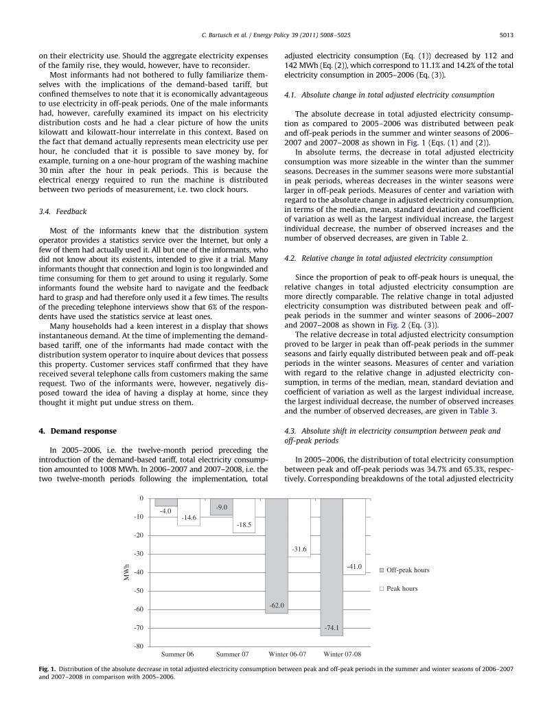
In 2005–2006, i.e. the twelve-month period preceding theintroduction of the demand-based tariff, total electricity consump-tion amounted to 1008 MWh. In 2006–2007 and 2007–2008, i.e. thetwo twelve-month periods following the implementation, total

-4.0 -9.0

-62.0

-14.6-18.5

-80

-70

-60

-50

-40

-30

-20

-10

0

Summer 06 Summer 07 Wint

MW

h

Fig. 1. Distribution of the absolute decrease in total adjusted electricity consumption be

and 2007–2008 in comparison with 2005–2006.

adjusted electricity consumption (Eq. (1)) decreased by 112 and142 MWh (Eq. (2)), which correspond to 11.1% and 14.2% of the totalelectricity consumption in 2005–2006 (Eq. (3)).

4.1. Absolute change in total adjusted electricity consumption

The absolute decrease in total adjusted electricity consump-tion as compared to 2005–2006 was distributed between peakand off-peak periods in the summer and winter seasons of 2006–2007 and 2007–2008 as shown in Fig. 1 (Eqs. (1) and (2)).

In absolute terms, the decrease in total adjusted electricityconsumption was more sizeable in the winter than the summerseasons. Decreases in the summer seasons were more substantialin peak periods, whereas decreases in the winter seasons werelarger in off-peak periods. Measures of center and variation withregard to the absolute change in adjusted electricity consumption,in terms of the median, mean, standard deviation and coefficientof variation as well as the largest individual increase, the largestindividual decrease, the number of observed increases and thenumber of observed decreases, are given in Table 2.

4.2. Relative change in total adjusted electricity consumption

Since the proportion of peak to off-peak hours is unequal, therelative changes in total adjusted electricity consumption aremore directly comparable. The relative change in total adjustedelectricity consumption was distributed between peak and off-peak periods in the summer and winter seasons of 2006–2007and 2007–2008 as shown in Fig. 2 (Eq. (3)).

The relative decrease in total adjusted electricity consumptionproved to be larger in peak than off-peak periods in the summerseasons and fairly equally distributed between peak and off-peakperiods in the winter seasons. Measures of center and variationwith regard to the relative change in adjusted electricity con-sumption, in terms of the median, mean, standard deviation andcoefficient of variation as well as the largest individual increase,the largest individual decrease, the number of observed increasesand the number of observed decreases, are given in Table 3.

4.3. Absolute shift in electricity consumption between peak and

off-peak periods

In 2005–2006, the distribution of total electricity consumptionbetween peak and off-peak periods was 34.7% and 65.3%, respec-tively. Corresponding breakdowns of the total adjusted electricity

-74.1

-31.6

-41.0

er 06-07 Winter 07-08

Off-peak hours

Peak hours

tween peak and off-peak periods in the summer and winter seasons of 2006–2007

-1.6% -3.6%

-15.1%

-18.1%

-10.7%

-13.6%-14.8%

-19.2%

-25%

-20%

-15%

-10%

-5%

0%

Summer 06 Summer 07 Winter 06-07 Winter 07-08

Off-peak hours

Peak hours

Fig. 2. Distribution of the relative decrease in total adjusted electricity consumption between peak and off-peak periods in the summer and winter seasons of 2006–2007

and 2007–2008 in comparison with 2005–2006.

Table 3Measures of center and variation with regard to the relative changes in adjusted electricity consumption in peak and off-peak periods in the summer and winter seasons of

2006–2007 and 2007–2008 in relation to 2005–2006 (%).

Period Median Mean sd (pp)a cvb Max.

increase

Max.

decrease

Increase Decrease

Summer 2006 off-peak 0.2 �0.7 15 �2113 34 �35 52 48

Summer 2006 peak �9.9 �10.1 16 �155 27 �40 24 76

Summer 2007 off-peak �3.8 �3.3 20 �598 56 �46 38 62

Summer 2007 peak �14.4 �13.5 20 �148 46 �62 24 76

Winter 2006–2007 off-peak �13.8 �14.0 13 �95 17 �48 12 88

Winter 2006–2007 peak �11.5 �13.1 15 �112 42 �46 14 86

Winter 2007–2008 off-peak �14.9 �16.2 18 �111 46 �50 12 88

Winter 2007–2008 peak �15.0 �16.6 20 �118 41 �47 14 86

a Standard deviation (percentage points).b Coefficient of variation.

Table 2Measures of center and variation with regard to the absolute change in adjusted electricity consumption in peak and off-peak periods in the summer and winter seasons of

2006–2007 and 2007–2008 in relation to 2005–2006 (MWh).

Period Median Mean sda cv (%)b Max. increase Max. decrease Increase (e) Decrease (e)

Summer 2006 off-peak 0.01 �0.08 0.85 �1051 1.81 �2.89 26 24

Summer 2006 peak �0.21 �0.29 0.52 �179 1.00 �2.07 12 38

Summer 2007 off-peak �0.14 �0.18 1.16 �643 3.65 �3.19 19 31

Summer 2007 peak �0.30 �0.37 0.72 �195 1.70 �2.40 12 38

Winter 2006–2007 off-peak �0.99 �1.24 1.21 �98 0.60 �4.81 6 44

Winter 2006–2007 peak �0.45 �0.63 0.70 �110 0.64 �2.79 7 43

Winter 2007–2008 off-peak �1.11 �1.48 1.59 �107 2.31 �4.98 6 44

Winter 2007–2008 peak �0.58 �0.82 0.96 �117 1.08 �3.05 7 43

a Standard deviation.b Coefficient of variation.


consumption in 2006–2007 and 2007–2008 show that there wasa shift from peak to off-peak hours by 0.8 and 1.2 percentagepoints (Eqs. (6) and (7)), respectively, which are the equivalent of7.2 and 10.0 MWh (Eqs. (4) and (5)). The absolute shift, in termsof total adjusted electricity use, from peak to off-peak periods andvice versa was distributed between the summer and the winterseasons of 2006–2007 and 2007–2008 as shown in Fig. 3 (Eqs.(4) and (5)).

In the summer seasons 2006 and 2007 there were evident,absolute shifts in total adjusted electricity consumption frompeak to off-peak periods, but in the winter seasons 2006–2007and 2007–2008 there were no obvious changes in this respect.Measures of center and variation with regard to the absolute shift

in total adjusted electricity consumption, in terms of the median,mean, standard deviation and coefficient of variation as well asthe largest individual increase, the largest individual decrease, thenumber of observed increases and the number of observeddecreases, are given in Table 4.

4.4. Relative shift in electricity consumption between peak and

off-peak periods

The relative shift, in terms of total adjusted electricity use,between peak and off-peak hours was distributed between thesummer and winter seasons of 2006–2007 and 2007–2008 asshown in Fig. 4 (Eqs. (6) and (7)).

8.08.7

-0.5

1.6

-8.0-8.7

0.5

-1.6

-10

-8

-6

-4

-2

0

2

4

6

8

10


MW

h Off-peak hours

Peak hours

Fig. 3. Distribution of the absolute shifts in total adjusted electricity consumption between peak and off-peak periods in the summer and winter seasons of 2006–2007 and

2007–2008 in comparison with 2005–2006.

Table 4Measures of center and variation with regard to the absolute shifts in total adjusted electricity consumption in peak and off-peak periods in the summer and winter

seasons of 2006–2007 and 2007–2008 in relation to 2005–2006 (MWh).

Period Median Mean sda cv (%)b Max. increase Max. decrease Increase (e) Decrease (e)

Summer 2006 off-peak 55 160 262 164 1016 �221 38 12

Summer 2006 peak �55 �160 262 �164 221 �1016 12 38

Summer 2007 off-peak 98 179 266 149 946 �241 38 12

Summer 2007 peak �98 �179 266 �149 241 �946 12 38

Winter 2006–2007 off-peak �3 �15 137 �907 321 �424 25 25

Winter 2006–2007 peak 3 15 137 907 424 �321 25 25

Winter 2007–2008 off-peak 51 35 196 567 431 �631 34 16

Winter 2007–2008 peak �51 �35 196 �567 631 �431 16 34


2.2%2.5%

-0.1%

0.3%

-2.2%-2.5%

0.1%

-0.3%

-3%

-2%

-1%

0%

1%

2%

3%


Off-peak hours

Peak hours

Fig. 4. Distribution of the relative shifts in total adjusted electricity consumption between peak and off-peak periods in the summer and winter seasons of 2006–2007 and

2007–2008 in comparison with 2005–2006.


In the summer seasons 2006 and 2007 there were evident,relative shifts in total adjusted electricity consumption from peakto off-peak periods, but in the winter seasons 2006–2007 and2007–2008 there were no obvious changes in this respect.Measures of center and variation with regard to the relative shiftin total adjusted electricity consumption, in terms of the median,mean, standard deviation and coefficient of variation as well asthe largest individual increase, the largest individual decrease, the

number of observed increases and the number of observeddecreases, are given in Table 5.

4.5. Absolute change in maximum diversified demand

The maximum diversified demand in 2005–2006 was 291 kWand occurred in off-peak periods of the winter season, while peakdiversified demand in the summer season 2005 reached its

Table 5Measures of center and variation with regard to the relative shift in total adjusted electricity consumption in peak and off-peak periods in the summer and winter seasons

of 2006–2007 and 2007–2008 in relation to 2005–2006 (%).

Period Median Mean sd (pp)a cvb Max. increase Max. decrease Increase Decrease

Summer 2006 off-peak 1.0 2.2 3.3 154 13.3 �2.3 76 24

Summer 2006 peak �1.0 �2.2 3.3 �154 2.3 �13.3 24 76

Summer 2007 off-peak 1.7 2.5 3.6 146 12.2 �3.6 76 24

Summer 2007 peak �1.7 �2.5 3.6 �146 3.6 �12.2 24 76

Winter 2006–2007 off-peak 0.0 �0.2 1.4 �682 2.5 �5.1 50 50

Winter 2006–2007 peak 0.0 0.2 1.4 682 5.1 �2.5 50 50

Winter 2007–2008 off-peak 0.5 0.2 2.4 1026 5.0 �9.8 68 32

Winter 2007–2008 peak �0.5 �0.2 2.4 �1026 9.8 �5.0 32 68


3.7

-20.9

-8.1

-41.5

-10.4

-47.2

-12.4

-59.8

-70

-60

-50

-40

-30

-20

-10

0

10


kW

Off-peak hours

Peak hours

Fig. 5. Absolute change in maximum diversified demand in peak and off-peak periods of the summer and winter seasons of 2006–2007 and 2007–2008 in comparison

with 2005–2006.

2.1%

-11.7%

-2.8%

-14.3%

-5.6%

-25.4%

-4.3%

-20.9%

-30%

-25%

-20%

-15%

-10%

-5%

0%

5%


Off-peak hours

Peak hours

Fig. 6. Relative change in maximum diversified demand in peak and off-peak periods of the summer and winter seasons of 2006–2007 and 2007–2008 in comparison with

2005–2006.


maximum of 186 kW in peak periods. The absolute changes inmaximum diversified demand in peak and off-peak periods of thesummer and winter seasons of 2006–2007 and 2007–2008 arepresented in Fig. 5 (Eq. (8)).

By comparison with 2005–2006, there was a decrease inabsolute, maximum diversified demand in all periods and seasonsof 2006–2007 and 2007–2008 but the off-peak period in thesummer season of 2006–2007, when there was a slight increase.

4.6. Relative change in maximum diversified demand

The relative change in maximum diversified demand inpeak and off-peak periods of the summer and winter seasons of2006–2007 and 2007–2008 are presented in Fig. 6 (Eq. (9)).

In relation to 2005–2006, there was a relative decreasein maximum diversified demand in all periods and seasonsof 2006–2007 and 2007–2008 but the off-peak period in


the summer season of 2006–2007, when there was a slightincrease.

4.7. Absolute change in mean maximum demand

Absolute change in mean maximum demand in peak and off-peak periods in the summer and winter seasons of 2006–2007and 2007–2008 is presented in Fig. 7 (Eq. (10)).

In absolute terms there was an increase in mean maximumdemand in peak as well as off-peak periods of the summer season06 and a slight decrease in the corresponding periods of thesubsequent winter season. In the second twelve-month periodfollowing the introduction of the demand-based tariff there was amarked decrease in mean maximum demand in the summer aswell as the winter season, which was significantly larger in peakperiods. Measures of center and variation with regard to theabsolute change in maximum demand, in terms of the median,mean, standard deviation and coefficient of variation as well asthe largest individual increase, the largest individual decrease, thenumber of observed increases and the number of observeddecreases, are given in Table 6.

4.8. Relative change in mean maximum demand

The relative change in mean maximum demand in peak andoff-peak periods of the summer and winter seasons of 2006–2007and 2007–2008 are presented in Fig. 8 (Eq. (11)).

In the first summer season following the implementation ofthe demand-based tariff there was a relative increase in meanmaximum demand and in the subsequent winter season there

0.69

-0.44

-0.10

0.66

-0.85

-1.0

-0.8

-0.6

-0.4

-0.2

0.0

0.2

0.4

0.6

0.8

Summer 06 Summer 07 Wint

kW

Fig. 7. Absolute change in mean maximum demand in peak and off-peak periods of th

2005–2006.

Table 6Measures of center and variation with regard to the absolute change in maximum dem

and 2007–2008 in relation to 2005–2006 (MWh).

Period Median Mean sda cv (%)b

Summer 2006 off-peak 0.26 0.69 2.72 395

Summer 2006 peak �0.12 0.66 3.41 517

Summer 2007 off-peak �0.19 �0.44 1.65 �377

Summer 2007 peak �0.87 �0.85 1.57 �186

Winter 2006–2007 off-peak �0.49 �0.10 2.13 �2073

Winter 2006–2007 peak �0.14 �0.13 2.28 �1794

Winter 2007–2008 off-peak �0.62 �0.59 2.01 �338

Winter 2007–2008 peak �0.81 �0.91 1.92 �211


was no obvious change in that respect. In 2007–2008 there weremarked percentage decreases in mean maximum demand in thesummer as well as the winter season, which were considerablylarger in peak than off-peak periods. Measures of center andvariation with regard to the relative changes in maximumdemand, in terms of the median, mean, standard deviation andcoefficient of variation as well as the largest individual increase,the largest individual decrease, the number of observed increasesand the number of observed decreases are given in Table 7.

As is evident from Tables 2–7, there is considerable variationwith regard to all parameters among the households. The coeffi-cients of variation reveal that the normalized standard deviationin most cases amount to several hundred percent of the estimatedmean and in a few instances as much as several thousand percent.Tables 6 and 7 also reveal that the households who had reducedtheir maximum demand in peak periods outnumbered the onesthat had increased it and that the number of households who hadreduced their maximum demand in peak periods was greater inthe second than the first summer and winter season following theimplementation of the demand-based tariff.

4.9. Demand curves representing weekends and weekdays

Demand curves representing weekends and weekdays inthe summer and winter seasons of analysis are presented inFig. 9a and b.

Fig. 9a and b support that there was a decrease in electricityconsumption in both summer and winter seasons following theintroduction of a demand charge. Decreases were slightly largerin the second than the first twelve-month period of analysis and

-0.59

-0.13

-0.91

er 06-07 Winter 07-08

Off-peak hours

Peak hours

e summer and winter seasons of 2006–2007 and 2007–2008 in comparison with

and in peak and off-peak periods in the summer and winter seasons of 2006–2007

Max. increase Max. decrease Increase (e) Decrease (e)

10.58 �4.66 30 20

13.66 �2.70 22 28

2.79 �5.40 23 27

4.08 �3.91 12 38

11.63 �3.16 20 30

11.11 �4.36 22 28

5.39 �7.66 15 35

5.57 �4.89 12 38

Table 7Measures of center and variation with regard to the relative change in maximum demand in peak and off-peak periods in the summer and winter seasons of 2006–2007

and 2007–2008 in relation to 2005–2006 (%).

Period Median Mean sd (pp)a cvb Max. increase Max. decrease Increase Decrease

Summer 2006 off-peak 4.5 11.7 0.39 330 166 �50 60 40

Summer 2006 peak �2.3 9.6 0.47 493 198 �35 44 56

Summer 2007 off-peak �2.4 �4.5 0.20 �445 27 �55 46 54

Summer 2007 peak �14.1 �11.7 0.23 �195 55 �50 24 76

Winter 2006–2007 off-peak �4.1 0.4 0.26 6671 155 �28 40 60

Winter 2006–2007 peak �2.6 �0.1 0.27 �48 963 144 �46 44 56

Winter 2007–2008 off-peak �6.6 �4.6 0.20 �441 67 �51 30 70

Winter 2007–2008 peak �11.3 �9.5 0.22 �230 69 �46 24 76


11.7%

-4.5%

0.4%

-4.6%

9.6%

-11.7%

-0.1%

-9.5%

-15%

-10%

-5%

0%

5%

10%

15%


Off-peak hours

Peak hours

Fig. 8. Relative change in mean maximum demand in peak and off-peak periods of the summer and winter seasons of 2006–2007 and 2007–2008 in comparison with

2005–2006.


more significant in the winter than the summer seasons. In thesummer seasons, decreases in electricity consumption seem to bemore pronounced on weekdays than on weekends, while there isno obvious difference in this respect in the winter seasons.Compared to the summer and winter season of reference, therewere no dramatic changes to the shape of the demand curvesrepresenting weekends, but there were striking changes in thepattern of use on weekday evenings. In the following, thesechanges are quantified.

4.10. Absolute change in demand curves representing weekends and

weekdays

Absolute changes in the shape of demand curves representingweekends and weekdays in the summer and winter seasons of2006–2007 and 2007–2008 as compared to the period of refer-ence are presented in Fig. 10a and b (Eq. (12)).

In absolute terms, the decreases in demand proved to besomewhat larger in the second than the first summer season,and considerably larger in the second than the first winter season,following the introduction of the demand-based tariff. The abso-lute decrease in demand proved, furthermore, to be fairly larger inpeak than off-peak hours in the summer seasons, while thereverse applies to the winter seasons. The most dramatic changesin the demand profiles are represented by the evident increases indemand between 8 and 10 p.m. on weekdays in the summerseasons of 2006 and 2007, which amount to 0.38 and 0.36 kW,

respectively. Between 7 and 8 p.m. there were similar changes inthe shape of the demand curves representing weekdays in thewinter seasons, but on account of comparatively low electricityconsumption levels, these changes represented a small increase indemand of only 0.11 kW in 2006–2007 and no change at all in2007–2008. In peak hours, the smallest decreases in demandoccurred between 6 and 7 p.m. in all seasons but the winter of2006–2007 when the smallest observed cut in demand took placebetween 11 and 12 in the morning.

4.11. Relative change in demand curves representing weekends and

weekdays

The relative changes in the shape of demand curves represent-ing weekends and weekdays in the summer and winter seasons of2006–2007 and 2007–2008 as compared to the period of refer-ence are presented in Fig. 11a and b (Eq. (13)).

The relative changes in the shape of demand curves represent-ing weekends and weekdays in the seasons of analysis were notappreciably different from the absolute changes. Again, the moststriking deviations from the reference demand curves are to befound between 8 and 10 p.m. in the summer seasons and between7 and 8 p.m. in the winter seasons, which represent increases indemand by 22% and 21% in the summer seasons, 3% in the winterseason of 2006–2007 and no change whatsoever in the winterseason of 2007–2008.

0

0.5

1

1.5

2

2.5

0 1 2 3 4 5 6 7 8 9 10 11 12 13 14 15 16 17 18 19 20 21 22 23

kW

hours

Weekends summer 05 Weekends summer 06 Weekends summer 07

Weekdays summer 05 Weekdays summer 06 Weekdays summer 07

0.0

0.5

1.0

1.5

2.0

2.5

3.0

3.5

4.0

4.5

0 1 2 3 4 5 6 7 8 9 10 11 12 13 14 15 16 17 18 19 20 21 22 23

kW

hours

Weekends winter 05-06 Weekends winter 06-07 Weekends winter 07-08

Weekdays winter 05-06 Weekdays winter 06-07 Weekdays winter 07-08

Fig. 9. (a) Demand curves representing weekends and weekdays in the summer seasons of 2005, 2006 and 2007. The light gray areas represent off-peak hours, whereas the

white area represents peak hours. (b) Demand curves representing weekends and weekdays in the winter seasons of 2005–2006, 2006–2007 and 2007–2008. The light

gray areas represent off-peak hours, whereas the white area represents peak hours.


5. Economic consequences

The households’ average electricity expenses in the seasons ofanalysis are shown in Fig. 12 (Eqs. (14) and (15)). It should benoted that the customers in question were charged according tothe conventional distribution tariff in the seasons of reference(summer 2005 and winter 2005–2006) and the demand-baseddistribution tariff in the remaining seasons.

It is evident from Fig. 12 that the customers as a whole havebenefited economically from being charged according to thedemand-based tariff as opposed to the conventional tariff. Onaverage, costs of the households were 39.3% and 40.6% lower inthe summer seasons and 14.8% and 19.1% lower in the winterseasons of 2006–2007 and 2007–2008 than they would have beenunder the conventional tariff.

To provide a full account of as to whether individual house-holds have economically benefited or suffered from being chargedaccording to the demand-based tariff in each and every one of themonths in the period of analysis would not be justifiable fromconsiderations of space. However, the economic outcome inDecember 2006, as shown in Fig. 13 (Eq. (16)), constitutes arepresentative example to that end. Each point of the graph inFig. 13 represents individual households’ electricity consumptionand peak demand, in this case the 5 highest instances of demandin peak hours. The lines correspond to the levels of peak demandand electricity use at which the distribution tariffs at handgenerate the same costs. Thus households in the top left area ofthe graph have suffered economically from being charged accord-ing to the demand-based tariff, whereas the opposite applies tothose in the bottom right area.

-0.45

-0.30

-0.15

0.00

0.15

0.30

0.45

0 1 2 3 4 5 6 7 8 9 10 11 12 13 14 15 16 17 18 19 20 21 22 23

kW

hours

Weekends summer 06 Weekends summer 07

Weekdays summer 06 Weekdays summer 07

-0.90

-0.75

-0.60

-0.45

-0.30

-0.15

0.00

0.15

0.30

0 1 2 3 4 5 6 7 8 9 10 11 12 13 14 15 16 17 18 19 20 21 22 23

kW

hoursWeekends winter 06-07 Weekends winter 07-08

Weekdays winter 06-07 Weekdays winter 07-08

Fig. 10. (a) Absolute changes in the shape of demand curves representing weekends and weekdays in the summer seasons of 2006 and 2007 in relation to the summer

season of 2005. The light gray areas represent off-peak hours, whereas the white area represents peak hours. (b) Absolute changes in the shape of demand curves

representing weekends and weekdays in the winter seasons of 2006–2007 and 2007–2008 in relation to the winter season of 2005–2006. The light gray areas represent

off-peak hours, whereas the white area represents peak hours.


As is apparent from the graph in Fig. 13, a majority of thehouseholds have benefited economically from the introduction ofthe demand-based tariff. The cost savings that most customershave enjoyed are, however, not lock, stock and barrel attributed tocuts in demand. The hypothetical costs, which customers wouldhave had if charged under the demand-based tariff in 2005, werecalculated by applying the tariff rates that were in force in 2006 tothe consumption data of 2005. The results of these estimationsshow that the hypothetical costs are 40.6% and 23.7% lower underthe demand-based than the conventional tariff in the summer andwinter season of 2005–2006.

Whether individual households would hypothetically havebenefited or suffered economically from being charged accord-ing to the demand-based tariff in 2005 appears in Fig. 14(Eq. (16)).

Although peak demand levels were considerably higher inDecember 2005 than 2006, practically the same number of

households as in December 2006 would still have benefitedfrom being charged according to the demand-based distributiontariff.

6. Discussions

Electricity consumption levels were for obvious reasons con-siderably higher in the winter than the summer seasons. TheNordic countries have a very cold winter climate and many ofthe households in the distribution area at hand use electricityfor heating. Furthermore, the winter months have quite fewhours of natural daylight, which means that comparativelylarge amounts of electricity are used for lighting. In fact, Swedesliving in houses on average have 55 light sources in theirhomes and on average use 1 240 kWh, which correspond to 20%of their total electricity consumption, per year for lighting(Zimmermann, 2009).

-20%

-10%

0%

10%

20%

30%

0 1 2 3 4 5 6 7 8 9 10 11 12 13 14 15 16 17 18 19 20 21 22 23

hours

Weekends summer 06 Weekends summer 07

Weekdays summer 06 Weekdays summer 07

-30%

-20%

-10%

0%

10%

0 1 2 3 4 5 6 7 8 9 10 11 12 13 14 15 16 17 18 19 20 21 22 23

hours

Weekends winter 06-07 Weekends winter 07-08

Weekdays winter 06-07 Weekdays winter 07-08

Fig. 11. (a) Relative changes in the shape of demand curves representing weekends and weekdays in the summer seasons of 2006 and 2007 in relation to the summer

season of 2005. The light gray areas represent off-peak hours, whereas the white area represents peak hours. (b) Relative changes in the shape of demand curves

representing weekends and weekdays in the winter seasons of 2006–2007 and 2007–2008 in relation to the winter season of 2005–2006. The light gray areas represent

off-peak hours, whereas the white area represents peak hours.


There are several possible, not mutually exclusive, explana-tions for the substantial decreases in overall adjusted electricityconsumption that took place in 2006–2007 and 2007–2008 ascompared to the period of reference. Three of the households hadswitched space heating system in the beginning of the first of thetwo twelve-month periods, which the analyses comprise. Two ofthese households had installed an air heat pump to supplementelectricity for space heating, one of which had decreased con-sumption by 24% and 29%, whereas the other had increased totaluse by 4% and 6% in the periods at hand. The third household hadreplaced its electric boiler with an air-water heat pump, thusreducing consumption by 30% and 37% in the same periods. Thereductions, which two of these households account for, only

amount to a fraction of the total decreases in electricity con-sumption and none of them represent the largest individualdecrease recorded. Taken together, the facts that only three ofthe households had changed space heating system and thatreductions at night in the winter season were just as large as, oreven larger than they were in the daytime, suggest that house-holds have taken steps such as lowering the indoor temperature,turning off night lighting and replacing old refrigerators andfreezers with new more energy-efficient ones. Another contribu-tory factor is most likely that the mean outdoor temperatures inthe winter seasons of 2006–2007 and 2007–2008 were 3.9 and1.4 1C higher than in the period of reference. However, factremains that there were sizeable decreases in the summer

220236 245

311

356 364

143 146

303 294

0

50

100

150

200

250

300

350

400

summer 05 summer 06 summer 07 winter 05-06 winter 06-07 winter 07-08

conventional distribution tariff demand-based distribution tariff

Fig. 12. Households’ mean electricity costs as generated by the conventional and the demand-based distribution tariffs.

0

2

4

6

8

10

12

14

0 500 1000 1500 2000 2500 3000 3500 4000 4500 5000

peak

dem

and

(kW

)

electricity use (kWh)

lower costs with demand-baseddistribution t

lower costs withdistributi

conventionalon tariff

ariff

levels of peak demand and electricity use at which total costs generated by the conventional and the demand-

based distribution tariff are the same for households with fuse size 16 A





peak demand and electricity use in households with fuse size 16 A



Fig. 13. Economic outcome in December 2006.


seasons too. In recent years, the distribution system operator hasengaged in a range of activities for the purpose of promotingawareness and encouraging energy efficiency among its custo-mers and the observed decreases in electricity consumption maywell be a sign that its efforts have paid off. Yet another explana-tory variable may be spill-over impacts of the demand charge onthe overall electricity use in general. US experience with demand

response programs has in fact shown that demand responseactivities may raise awareness about how to save energy byimproving energy efficiency (York and Kushler, 2005).

Analyzing households’ power consumption, in and of itself, hasnot been the primary purpose of the study. However, from reduc-tions in total electricity use, it inevitably follows that averagedemand also decreases. The collective cut in overall electricity

0

2

4

6

8

10

12

14

0 500 1000 1500 2000 2500 3000 3500 4000 4500 5000

peak

dem

and

(kW

)

electricity use (kWh)

lower costs with demand-based

lower costsconventional

with

levels of peak demand and electricity use at which total costs generated by the conventional and the demand-based distribution tariff are the same for households with fuse size 16 A






Fig. 14. Hypothetical economic outcome in December 2005.


consumption could, despite the fact that it has complicated the taskof assessing the extent of demand response, for the above reason notbe disregarded. The calculations have, by way of example, impliedthat there were practically no changes in demand between 7 and8 p.m. in the winter seasons as compared to the correspondingperiod of reference. It is nevertheless visually obvious from theFigs. 10b and 11b that there was a dramatic change to the shape ofthe demand curve in that time of day on weekdays. Seeing theimpact of a considerable cut in overall electricity use on averagedemand, the results of these estimations in point of fact representmajor upward shifts in the demand curve.

From the fact that downward shifts in the demand curve wererelatively small between 6 and 7 p.m., it has been reasonablyinferred that households are not prepared to hold off preparingtheir dinner until off-peak hours. Similarly, the correspondingobservation that was made on the hour between 11 and 12 a.m. inthe winter season of 2006–2007, is most likely a result of house-holds preparing lunch.

As noted, the results of the analyses suggest that a majority ofthe households have benefited economically from the introductionof the demand-based tariff and most of them would have done soeven though they had not decreased peak demand. In order for thedemand-based tariff to be a real incentive for households to cut peakdemand it should have the opposite effect. The starting point for anaccurate determination of the tariff rates must surely be that theconventional and the demand-based tariffs, on average, generate thesame costs and implementing the demand-based tariff should meanthat customers whose peak demand is already low would benefit,

whereas those whose peak demand is relatively high would suffer,from it economically. Against this background it has been concludedthat the rates of the demand-based tariff were set too low. However,customers were not paradoxically enough aware of this unsatisfac-tory state of affairs. The tariff rates were obviously known to them,but residential customers are, as revealed by the interviews,commonly not very familiar with the unit kilowatt and do generallyhave a poor sense of how much energy-related activities andelectrical appliances affect demand. The households had, strictlyspeaking, access to information about their electricity use over theInternet, but the user rate and the frequency of use were low andthe feedback was not available until the next day. The conclusionthat follows from these circumstances is that estimating the priceelasticity of demand would be questionable or even frivolous. Thispiece of information would have been very useful for the analyses,but this indicator has for the above reason not been explored.

Critique may be leveled at the study methodology in thatdemand has not been temperature corrected. It has, however, beenargued that the negative effects of doing so would be more far-reaching than the positive ones. Established methods of temperaturecorrections have primarily been developed for the purpose ofcorrecting consumption of electrical power for temperature on anannual basis, not by the hour. It is fair to say that applying thesemethods to hourly consumption data would result in the proportionof demand that is due to behavior, which is being excluded from theanalyses. In light of these circumstances and seeing that demandresponse actions take place on an hourly basis, temperature hasbeen regarded as a secondary consideration in this context. In fact,

Table 8Pearson’s correlation coefficient, r, in the winter

periods of analysis.

Season r

Winter 2005–2006 �0.825n

Winter 2006–2007 �0.817n

Winter 2007–2008 �0.660n

All winter seasons �0.798n

n Significant at the 0.01 level (two-tailed),

p¼0.000.


the minimum temperature did not coincide with maximum demandin any of the winter seasons at hand. That is, however, not to saythat the prevailing temperature does not affect demand. Fallingtemperatures to some extent correlate with increasing demand.Pearson’s correlation coefficient, r, in the winter seasons of analysishas been estimated at �0.798 and has proven to be significant atthe 0.01 level (p¼0.000). The corresponding coefficients of theindividual winter seasons are given in Table 8.

It is evident from Table 8 that the negative correlation betweentemperature and demand is somewhat weaker in the first winterseason following the period of reference and even more so in thesecond. One of several possible contributory explanations for thismay well be that households have responded to the demand-basedtariff by reducing the indoor temperature in peak hours when it iscold outside. The general cut in demand in peak periods might alsohave had some effect on the negative correlation between tempera-ture and demand.

7. Conclusions

This study has demonstrated that households are generallysympathetic to being charged according to a demand-based tariff,seeing as how the distribution system operator’s motive forintroducing it relates to environmental issues. Most householdsadjust their behavior to the tariff’s intrinsic means of controllingelectricity demand, the most common measures being to runvarious domestic appliances in off-peak periods. These actionshave turned out to result in a shift in total electricity consumptionfrom peak to off-peak periods and a decrease in maximumdiversified demand and mean maximum demand in peak periods.Many customers experience that they to some extent are ‘‘gropingin the dark’’ in their quest for lower electricity costs and call for adevice that displays the current power output.

The shift in total electricity consumption from peak to off-peakperiods has brought about a substantial peak in demand between8 and 9 p.m. in summer seasons and between 7 and 8 p.m. inwinter seasons. Seeing that these peaks occur in off-peak periods,they are however of no negative consequence to the distributionsystem operator in question. The maximum diversified demand inpeak periods, which from the viewpoint of the distributionsystem operator is more crucial than individual customers’ peakdemand, decreased substantially as a result of introducing ademand-based tariff. The actual decrease in maximum diversifieddemand in peak periods was greater in the winter periods,whereas the percentage decrease was larger in the summerperiods following the implementation and the magnitude of theseeffects proved to be amplified over time.

Acknowledgements

The research presented in this article was financed by theSwedish Energy Agency. The distribution system operator Sala-Heby

Energi Elnat AB assisted in the extraction of hourly meter readingsand provided information on the distribution tariff rates. TheSwedish Meteorological and Hydrological Institute supplied dataon the outdoor temperatures in the area at hand.

References

Badano, A., Fritz, P., Goransson, A., Linden, M., 2007. Timmatning for alla: Nytta,regelverk och ekonomi (Hourly metering for everyone: Utility, regulations andeconomy). Elforsk, Stockholm 07:62.

Bartusch, C., Porathe, T., 2011. Climate-smart information design: visualizingresidential electricity use over the Internet. Information Design Journal 19(1), 3–17. doi:10.1075/idj.19.1.02bar.

Bartusch, C., Larsson, M., Wallin, F., Wester, L., 2010. Potential of hourly settle-ments in the residential sector of the Swedish electricity market: estimationsof risk reduction and economic result. International Journal of Green Energy 7(3), 224–240.

Borenstein, S., Jaske, M., Rosenfeld, A., 2002. Dynamic pricing, advanced metering,and demand response in electricity markets. USEM, WP 105. University ofCalifornia Energy Institute, Berkeley.

Braithwait, S.D., Eakin, K., 2002. The Role of Demand Response in Electric PowerMarket Design. Edison Electric Institute, Washington.

Chardon, A., Almen, O., Lewis, P.E., Stromback, J., Chateau, B., 2008. Demandresponse: a decisive breakthrough for Europe. Capgemini Retrieved 12February 2011 from/http://storage.vuzit.com/public/1i1un/Demand_Response__a_decisive_breakthrough_for_Europe.pdfS.

COM/2008/0030 final, 2008. Communication from the Commission to the Eur-opean Parliament, the Council, the European Economic and Social Committeeand the Committee of the Regions: 2020 by 2020 Europe’s climate changeopportunity.

Damsgaard, N., Fritz, P., 2006. Affarsmodeller for okad efterfragerespons paelmarknaden (Business models for increased demand response on the elec-tricity market). Elforsk, Stockholm 06:16.

Directive 2006/32/EC, 2006. Directive 2006/32/EC of the European Parliament andof the Council of 5 April 2006 on energy end-use efficiency and energy servicesand repealing Council Directive 93/76/EEC.

Econ Poyry AS, 2008. Effects of Large Scale Wind Capacities in Sweden. Elforsk,Stockholm 09:102.

Ericson, T., 2007. Short-term Electricity Demand Response. Doctoral Thesis,Norwegian University of Science and Technology, Department of ElectricalPower Engineering.

Faruqui, A., Harris, D., Hledik, R., 2010. Unlocking the h53 billion savings fromsmart meters in the EU: how increasing the adoption of dynamic tariffs couldmake or break the EU’s smart grid investment. Energy Policy 38 (10),6222–6231. doi:10.1016/j.enpol.2010.06.10.

Forsberg, K., Fritz, P., 2001. Methods to Secure Peak Load Capacity on DeregulatedElectricity Markets. Elforsk, Stockholm 02:09.

Fritz, P., 2006. Market Design Project: Demand Response Resources in Sweden—ASummary. Elforsk, Stockholm 06:41.

Fritz, P., 2007. Effektkapacitet hos kunderna: En sammanfattning av IEA-projektet’’Demand Response Resources, task 13’’ (Demand response resources ofcustomers: A summary of the IEA project ’’Demand Response Resources, task13’’). Elforsk, Stockholm 07:08.

Fritz, P., Jorgensen, E., Lindskoug, S., 2009. Att folja elpriset battre: Prismodelleroch styrteknik i faltforsok (To Better Follow the Electricity Price: Price modelsand Control Technology in Field Trials). Elforsk. Elforsk, Stockholm 09:70.

IVA, 2009. Svenska folkets kunskap och attityd kring energifragor (The SwedishPeople’s Knowledge and Attitude on Energy Issues). Ingenjors VetenskapsAkademin (IVA), Kungl Retrieved 26 July 2010 from/http://www.iva.se/PageFiles/6088/200906-IVA-V%c3%a4gval-energi-opinionsunders%c3%b6kning-D.pdfS.

Lindskoug, S., 2006. Demonstration Project: Consumer Reactions to Peak Prices.Elforsk, Stockholm 06:40.

Lundgren, J., 2008. Elkunden som marknadsaktor: Atgarder for okadforbrukningsflexibilitet (The Electricity Customer as a Market Actor: Measuresfor Increased Consumption Flexibility)., 13. Energy Markets Inspectorate,Eskilstuna.

PLMA, 2002. Demand Response: Design Principles for Creating Customer andMarket Value Retrieved 26 July 2010 from/http://www.peaklma.com/files/public/CustomerPrinciples.pdfS.

Pyrko, J., Sernhed, K., Abaravicius, J., Perez Mies, V., 2003. Pay for demand:electricity pricing with demand component. In: Attali, S., Metreau, E., Prone,M., Tillerson, K. (Eds.), ECEEE Summer Study 2003 Proceedings: Time to TurnDown Energy Demand. International Consulting on Energy, Paris, pp. 987–999.

Pyrko, J., 2006. Demand pricing: case studies in residential buildings. In: P.Bertoldi, B. Kiss, B. Atanasiu (Eds.), Energy Efficiency in Domestic Appliancesand Lighting: Proceedings of the 4th International Conference EEDAL’06, Vol.1 Office for Official Publications of the European Communities, Luxembourg,pp. 199–206.

Rosenstock, S., 2004. Final Results of the EEI/PLMA 2003 Demand ResponseBenchmarking Survey. Peak Load Management Alliance Retrieved 26 July2010 from/http://www.peaklma.com/publications.aspxS.

dx.doi.org/doi:10.1075/idj.19.1.02bar

&lang;http://storage.vuzit.com/public/1i1un/Demand_Response__a_decisive_breakthrough_for_Europe.pdf&rang;

&lang;http://storage.vuzit.com/public/1i1un/Demand_Response__a_decisive_breakthrough_for_Europe.pdf&rang;

dx.doi.org/doi:10.1016/j.enpol.2010.06.10

&lang;http://www.iva.se/PageFiles/6088/200906-IVA-V%c3%a4gval-energi-opinionsunders%c3%b6kning-D.pdf&rang;



&lang;http://www.peaklma.com/files/public/CustomerPrinciples.pdf&rang;

&lang;http://www.peaklma.com/files/public/CustomerPrinciples.pdf&rang;

&lang;http://www.peaklma.com/publications.aspx&rang;


Swedish Energy Agency, 2010. Energilaget 2010 (The Energy Situation 2010), 45.Swedish Energy Agency., Eskilstuna Retrieved 11 February 2011 from/http://webbshop.cm.se/System/ViewResource.aspx?p=Energimyndigheten&rl=default:/Resources/Permanent/Static/6792e3736ce045c4a41f2c397b1eff97/ET2010_45.pdfS.

Swedish Parliament, 2010. Lag (2003:436) om effektreserv (Law on Load Reserve).Retrieved July 5, 2010, from /http://www.riksdagen.se/webbnav/?nid=3911&bet=2003%3A436S.

Svenska Kraftnat, 2010. Retrieved July 5, 2010, from /http://www.svk.se/Energimarknaden/El/Effektreserv/Upphandling-av-effektreserv/S.

Torriti, J., Hassan, M.G., Leach, M., 2010. Demand response experience in Europe:policies, programmes and implementation. Energy 35, 1575–1583.

Wallin, F., Bartusch, C., Thorin, E., Backstrom, T., Dahlquist E., 2005. The use ofautomatic meter readings for a demand-based tariff. In: Proceedings ofTransmission & Distribution Conference & Exposition: Asia and Pacific, IEEE/PES, August 2005.

York, C., Kushler, M., 2005. Exploring the Relationship Between Demand Res-ponse and Energy Efficiency: A Review of Experience and Discussion of KeyIssues. American Council for an Energy-Efficient Economy (ACEEE, U052),Washington.

Zimmermann, J.P., 2009. End-use metering campaign in 400 households inSweden: assessment of the potential electricity savings. Enertech Retrieved26 July from/http://www.energimyndigheten.se/Global/Energifakta/F%c3%b6rb%c3%a4ttrad%20energistatistik/Festis/Final_report.pdfS.

&lang;http://webbshop.cm.se/System/ViewResource.aspx?p=Energimyndigheten&rl=default:/Resources/Permanent/Static/6792e3736ce045c4a41f2c397b1eff97/ET2010_45.pdf&rang;





&lang;http://www.riksdagen.se/webbnav/?nid=3911&bet=2003%3A436&rang;



&lang;http://www.svk.se/Energimarknaden/El/Effektreserv/Upphandling-av-effektreserv/&rang;

&lang;http://www.svk.se/Energimarknaden/El/Effektreserv/Upphandling-av-effektreserv/&rang;

&lang;http://www.energimyndigheten.se/Global/Energifakta/F%c3%b6rb%c3%a4ttrad%20energistatistik/Festis/Final_report.pdf&rang;

&lang;http://www.energimyndigheten.se/Global/Energifakta/F%c3%b6rb%c3%a4ttrad%20energistatistik/Festis/Final_report.pdf&rang;

Documents

Introducing a demand-based electricity distribution tariff in the residential sector: Demand response and customer perception