1

Introduction to High Performance Computing

n Why HPCn Basic conceptsn How to programn Technological trends

2

Why HPC?

n Many problems require more resources than available on a single computer n “Grand Challenge" (en.wikipedia.org/wiki/Grand_Challenge)

problems requiring PetaFLOPS and PetaBytes of computing resources.

n Web search engines/databases processing millions of transactions per second

3

Uses of HPCn Historically "the high end of computing”

n Atmosphere, Earth, Environmentn Physics - applied, nuclear, particle,

condensed matter, high pressure, fusion, photonics

n Bioscience, Biotechnology, Genetics

n Chemistry, Molecular Sciencesn Geology, Seismologyn Mechanical Engineering - from

prosthetics to spacecraftn Electrical Engineering, Circuit Design,

Microelectronicsn Computer Science, Mathematics

4

Uses of HPCn Today, commercial applications provide an

equal or greater driving force; require processing of large amounts of data in sophisticated ways

n Databases, data miningn Oil explorationn Web search engines, web based business

services

n Medical imaging and diagnosisn Pharmaceutical designn Management of national and multi-national

corporationsn Financial and economic modelingn Advanced graphics and virtual reality,

particularly in the entertainment industryn Networked video and multi-media technologiesn Collaborative work environments

ETP4HPCSRA-3Kick-offmeetingIBMIOT,Munich,March20th2017 PeterBauer&ErwinLaure4CoE

Targetforaddressingkeysciencechallengesinweather&climateprediction:Global1-kmEarthsystemsimulations@~1year/dayrate

Example:WeatherPrediction

10km

1km

5

ETP4HPCSRA-3Kick-offmeetingIBMIOT,Munich,March20th2017 PeterBauer&ErwinLaure4CoE

Example:NOMADScienceandDataHandlingChallenges

Discoveringinterpretablepatternsandcorrelationsinthisdatawill• createknowledge• advancematerialsscience,• identifynewscientificphenomena,and• supportindustrialapplications.

TheNOMADArchive10.000

100

1

#Ge

ometrie

sperCom

position

1Mio

1.000

1

#Co

mpo

sitions

Transparentmetals

Photovoltaics

Superconductors

Thermal-barriermaterials

Descriptor AD

escr

ipto

r B

The NOMADchallenge:Buildamapandfilltheexistingwhitespots

NOMADsupportsall importantcodesincomputationalmaterialsscience.Thecode-independentArchivecontainsdatafrommany millioncalculations(billionsofCPUhours).

Dataistherawmaterialsofthe21stcentury

6

HPCSummit,Prague

ExaFLOW

ExaFLOW

TheAirbusChallenge,DavidHills,2008

7

AnAirbus310cruisingat250m/sat10000mTeraflops machine (1012 Flops):8·105 yearsResult inone week:4·1019 flopsmachine (40EFlops)(based onJohnKim’s estimate,TSFP-9,2015)

Predicting interactomes by docking… a dream?

Ø ~20’000humanproteins

Ø Interactome predictionwillrequire20’0002 dockingruns

Ø Whichwillrequire>10billionsCPUhoursandgenerateabout100exabytes ofdata

Ø Interestinsimulating/understandingtheimpactofdisease-relatedmutationsthataffect/altertheinteractionnetwork

8

bioexcel.eu

Partners Funding

Α

Α/Β*

Β

Β/Γ*

Γ

Γ/Δ*

Δ

Δ/Ε*

Ε

E183

E226

E236

D259

F233

R1R2R3R4K5

R6

Q

E183E226D259

E236

R0

R1

R2

R3

K4

R5

VSD

A

B

Molecular Dynamics on the exascale• Understanding proteins and

drugs• A 1 μs simulation: 10 exaflop• Many structural transition: many

simulations needed• Study effect of several bound

drugs• Study effect of mutations• All this multiplies to >> zettaflop• Question: how far can we

parallelize?

Example:ionchannelinanervecell.Opensandclosesduringsignalling.Affectedbye.g.alcoholanddrugs.200000atoms

9

FET:HumanBrainProject

FSchürmann,HMarkram (BlueBrain Project,EPFL)

11

What is Parallel Computing

n Traditionally, software has been written for serialcomputation:n To be run on a single computer having a single Central

Processing Unit (CPU);n A problem is broken into a discrete series of instructions.n Instructions are executed one after another.n Only one instruction may execute at any moment in time.

12

Parallel Computing

n In the simplest sense, parallel computing is the simultaneous use of multiple compute resources to solve a computational problem:n A problem is broken into discrete parts that can be solved

concurrentlyn Each part is further broken down to a series of instructions

13

Parallelism on different levels

n CPUn Instruction level parallelism, pipeliningn Vector unitn Multiple cores

• Multiple threads or processes

n Computern Multiple CPUsn Co-processors (GPUs, FPGAs, …)

n Networkn Tightly integrated network of computers (supercomputer)n Loosely integrated network of computers (distributed computing)

14

Flynn’s taxonomy (1966)

n {Single, Multiple} {Instructions, Data}

SISDSingle Instruction, Single Data

SIMDSingle Instruction, Multiple Data

MISDMultiple Instruction, Single Data

MIMDMultiple Instruction, Multiple Data

15

Single Instruction Single Data

n A serial (non-parallel) computern Single instruction: only one instruction stream

is being acted on by the CPU during any one clock cyclen Single data: only one data stream is being used as input

during any one clock cyclen Deterministic executionn This is the oldest and used to be the most common type

of computer (up to arrival of multicore CPUs)n Examples: older generation mainframes, minicomputers

and workstations; older generation PCs.

n Attention: single core CPUs exploit instruction level parallelism (pipelining, multiple issue, speculative execution) but are still classified SISD

16

Single Instruction Multiple Data

n “Vector” Computern Single instruction:

All processing units execute the same instruction at any given clock cycle

n Multiple data: Each processing unit can operate on a different data element

n Best suited for specialized problems characterized by a high degree of regularity, such as graphics/image processing.

n Synchronous (lockstep) and deterministic executionn Two varieties: Processor Arrays and Vector Pipelinesn Most modern computers,

particularly those with graphics processor units (GPUs) employ SIMD instructions and execution units.

17

Multiple Instruction, Multiple Datan Currently, the most common

type of parallel computer. Most modern computers fall into this category.

n Multiple Instruction: every processor may be executing a differentinstruction stream

n Multiple Data: every processor may be working with a different data stream

n Execution can be synchronous or asynchronous, deterministic or non-deterministic

n Examples: most current supercomputers, networked parallel computer clusters and "grids", multi-processor SMP computers, multi-core PCs.

n Note: many MIMD architectures also include SIMD execution sub-components

18

Multiple Instruction, Single Data

n No examples exist todayn Potential uses might be:

n Multiple cryptography algorithms attempting to crack a single coded message

n Multiple frequency filters operating on a single signal

19

Single Program Multiple Data (SPMD)

n MIMDs are typically programmed following the SPMD model

n A single program is executed by all tasks simultaneously. n At any moment in time, tasks can be executing the same

or different instructions within the same program. All tasks may use different data. (MIMD)

n SPMD programs usually have the necessary logic programmed into them to allow different tasks to branch or conditionally execute only those parts of the program they are designed to execute. That is, tasks do not necessarily have to execute the entire program - perhaps only a portion of it.

20

Multiple Program Multiple Data (MPMD)

n MPMD applications typically have multiple executable object files (programs). While the application is being run in parallel, each task can be executing the same or different program as other tasks.

n All tasks may use different datan Workflow applications, multidisciplinary optimization,

combination of different models

21

FLOPS

n FLoating Point Operations per Secondn Most commonly used performance indicator for parallel

computersn Typically measured using the Linpack benchmarkn Most useful for scientific applicationsn Other benchmarks include

SPEC, NAS, stream (memory)

Name FlopsYotta 1024

Zetta 1021

Exa 1018

Peta 1015

Tera 1012

Giga 109

Mega 106

22

Moore’s Lawn Gordon E. Moore, "Cramming more components onto integrated circuits", Electronics

Magazine 19 April 1965:

“The complexity for minimum component costs has increased at a rate of roughly a factor of two per year ... Certainly over the short term this rate can be expected to continue, if not to increase. Over the longer term, the rate of increase is a bit more uncertain, although there is no reason to believe it will not remain nearly constant for at least 10 years. That means by 1975, the number of components per integrated circuit for minimum cost will be 65,000. I believe that such a large circuit can be built on a single wafer.”

n With later alterations:Transistor density doubles every 18 months

n So far this law holds

n It has also been interpreted asdoubling performance every 18 monthsn A little inaccurate - see later

23

4 Years

4 Years

24

Top500 Nr 1: ”TaihuLight - Sunway”n National Supercomputing Center in Wuxi, Chinan Sunway SW26010 260 cores, 1.45 GHzn 10,649,600 cores n 93 PF Linpack (125.5 PF theoretical peak)n 15 MW

25

Communication Architecture

26

A parallel computer is

“a collection of processing elements that communicate and cooperateto solve large problems fast”

(Almasi and Gottlieb 1989)

27

Communication Architecture

n Defines basic communication and synchronization operations

n Addresses the organizational structures that realize these operations

n Communication: exchange of data between processing units

n Synchronization: coordinate parallel activities

28

Synchronization: Dining Philosophers

n Algorithm:n Thinkn Take left forkn Take right forkn Eatn Release right forkn Release left fork

n Synchronization Problems:n Dead lock:

• All have left forkn Starvation:

• One philosopher can never get hold of two forks

• Only in modified algorithm• Release fork if cannot get

hold of second fork

29

Common Synchronization Patterns

n BarrierHold activities until all processes have reached the same point

n SemaphoreFinite resourcesTwo operations: P - wait for free resource and lock it; V - release

resourcen Mutex

Only one process can access a shared resourcen Events

Process waits until notified by another process

30

Typical Communication Architectures

n Shared Memoryn Distributed Memory

31

Shared Memory

32

Shared Memory Multiprocessor

n Hardware provides single physical address space for all processors

n Global physical address space and symmetric access to all of main memory (symmetric multiprocessor - SMP)

n All processors and memory modules are attached to the same interconnect (bus or switched network)

33

Differences in Memory Access

n Uniform Memory Access (UMA)Memory access takes about the same time independent of data

location and requesting processor

n Nonuniform memory access (NUMA)Memory access can differ depending on where the data is located and

which processor requests the data

34

Cache coherence

n While main memory is shared, caches are local to individual processors

n Client B’s cache might have old data since updates in client A’s cache are not yet propagated

n Different cache coherency protocols to avoid this problemn Subject of subsequent lectures

35

Synchronization

n Access to shared data needs to be protectedn Mutual exclusion (mutex)n Point-to-point eventsn Global event synchronization (barrier)

36

SMP Pros and Cons

n Advantages:n Global address space provides a user-friendly programming

perspective to memoryn Data sharing between tasks is both fast and uniform due to the

proximity of memory to CPUs n Disadvantages:

n Primary disadvantage is the lack of scalability between memory and CPUs. Adding more CPUs can geometrically increases traffic on the shared memory-CPU path, and for cache coherent systems, geometrically increase traffic associated with cache/memory management.

n Programmer responsibility for synchronization constructs that insure "correct" access of global memory.

n Expense: it becomes increasingly difficult and expensive to design and produce shared memory machines with ever increasing numbers of processors.

37

Distributed Memory Multiprocessors

38

DMMPs

n Each processor has private physical address spacen No cache coherence problem

n Hardware sends/receives messages between processorsn Message passing

39

Synchronization

n Synchronization via exchange of messages

n Synchronous communicationn Sender/receiver wait until data has been sent/received

n Asynchronous communicationn Sender/receiver can proceed after sending/receiving has been

initiated

n Higher level concepts(barriers, semaphores, …)can be constructed usingsend/recv primitivesn Message passing libraries

typically provide them

P1 P2

send(x)recv(y)

e=isend(x) e=irecv(y)wait(e) wait(e)

40

DMMPs Pros and Cons

n Advantages:n Memory is scalable with number of processors. Increase the

number of processors and the size of memory increases proportionately.

n Each processor can rapidly access its own memory without interference and without the overhead incurred with trying to maintain cache coherency.

n Cost effectiveness: can use commodity, off-the-shelf processors and networking.

n Disadvantages:n The programmer is responsible for many of the details associated

with data communication between processors.n It may be difficult to map existing data structures, based on global

memory, to this memory organization.n Non-uniform memory access (NUMA) timesn Administration and software overhead (essentially N systems vs. 1

SMP)

41

Hybrid Approaches

42

Combining SMPs and DMMPsn Today, DMMPs are typically built with SMPs as building

blocksn E.g. Cray XC40 has two CPUs with 16 cores each per DMMP noden Soon systems with more CPUs and many more cores will appear

n Combine advantages and disadvantages from both categoriesn Programming is more complicated due to the combination of

several different memory organizations that require different treatment

43

Moore’s law revisited

n Doubling of transistor density every 18 monthsn Often paraphrased as doubling of performance every 18 months

44

Reinterpreting Moore’s lawn Moore’s law is holding, in the number of transistors

n Transistors on an ASIC still doubling every 18 months at constant costn 15 years of exponential clock rate growth has ended

n Moore’s Law reinterpretedn Performance improvements are now coming from the increase in the number of cores

on a processor (ASIC)n #cores per chip doubles every 18 months instead of clock

2020 2025 2030Year

Perf

orm

ance

Transistors

Thread Performance

Clock Frequency

Power (watts)# Cores

Figure courtesy of Kunle Olukotun, Lance Hammond, Herb Sutter, and Burton Smith

45

Computing Power Consumption

n Capacitive load per transistor is a function of both the number of transistors connected to an output and the technology, which determines the capacitance of both wires and transistors

n Frequency switched is a function of the clock rate

FrequencyVoltageload CapacitivePower 2 ××=

46

Hitting the Power Wall

FrequencyVoltageload CapacitivePower 2 ××=

×1000×30 5V → 1V

47

Multiple cores deliver more performance per watt

C1

C4

C2

C3

Smallcore

Big core

Cache

Cache

1

2

3

4

1

2

1 1

1

2

3

4

1

2

3

4

Power

Performance

Power = ¼

Performance = 1/2

Many core is more power efficient

Power ~ area

Single thread performance ~ area**.5

48

Multicore CPUs

n Intel Xenon 6 core processor

49

What does this mean?

n The easy times have gonen Updating to the next processor generation will not automatically

increase performance anymore

n Parallel computing techniques are needed to fully exploit new processor generation

n Parallel computing is going mainstream

GPUs

50

GPUsn GPU = Graphical Processing Unit =

specialized microcircuit to accelerate the creation and manipulation of images in video frame for display devices. n Excellent for processing of large blocks of

data done in parallel.n GPUs are used in game consoles,

embedded systems (like systems on cars for automatic driving), computersand supercomputers.n Since 2012, GPUs are the main workforce for

training deep-learning networks

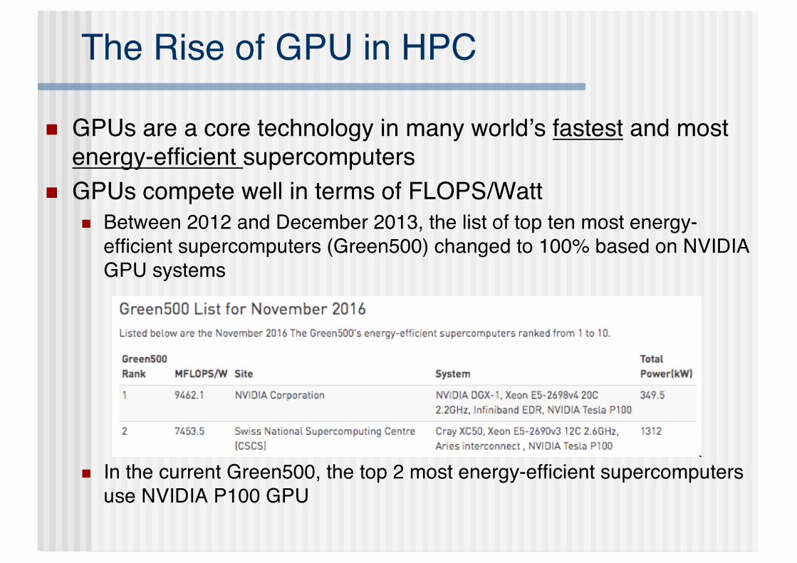
The Rise of GPU in HPC

n GPUs are a core technology in many world’s fastest and most energy-efficient supercomputers

n GPUs compete well in terms of FLOPS/Wattn Between 2012 and December 2013, the list of top ten most energy-

efficient supercomputers (Green500) changed to 100% based on NVIDIA GPU systems

n In the current Green500, the top 2 most energy-efficient supercomputers use NVIDIA P100 GPU

GPU Design Motivation: Process Pixels in Parallel

n Data paralleln In 1080i and 1080p videos, 1920 x

1080 pixels = 2M pixels per video frame à compute intensive

n Lots of parallelism at low clock speed à power efficient

n Computation on each pixel is independent from computation on other pixels.n No need for synchronization

n Large data-locality = access to data is regularn No need for large caches

CPU and GPU

n CPU has tens of massive cores, CPU excels at irregular control-intensive workn Lots of hardware for control, fewer ALUs

n GPU has thousands of small cores, GPU excels at regular math-intensive workn Lots of ALUs, little hardware for control

Weakness of GPU

GPU is very fast (huge parallelism) but getting data from/to GPU is slow

NVIDIA TESLA K40 = the most common GPU on supercomputers in Nov. 2016 top500 list

GPU CPU DRAM64GB

GDRAM

12GB

288 GB/s 32 GB/s 80 GB/s

Base clock:745 MHz

DDR4

PCIeGen3-12x

CPU vs GPU

n CPU are latency-optimizedn Reduce memory latency with big cachesn Hide memory latencies with other instructions (instruction

window, out-of-order)n Each thread runs as fast as possible but fewer threads

n GPU are throughput-optimizedn Each thread might take a long time but thousands of threads are

used

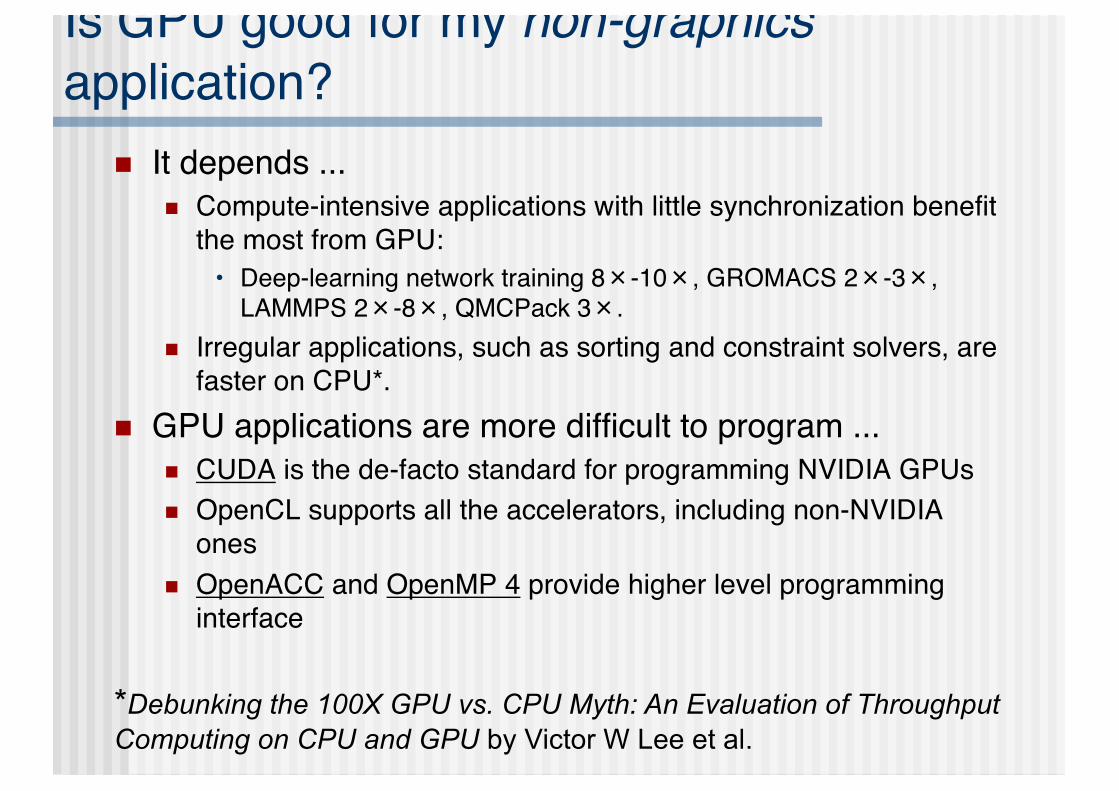
Is GPU good for my non-graphics application?

n It depends ...n Compute-intensive applications with little synchronization benefit

the most from GPU:• Deep-learning network training 8×-10×, GROMACS 2×-3×,

LAMMPS 2×-8×, QMCPack 3×. n Irregular applications, such as sorting and constraint solvers, are

faster on CPU*.n GPU applications are more difficult to program ...

n CUDA is the de-facto standard for programming NVIDIA GPUsn OpenCL supports all the accelerators, including non-NVIDIA

onesn OpenACC and OpenMP 4 provide higher level programming

interface

*Debunking the 100X GPU vs. CPU Myth: An Evaluation of Throughput Computing on CPU and GPU by Victor W Lee et al.

58

Network Topologies

59

The Role of the Network

n The overall performance of DMMPs depends critically on the performance of the network used to connect the individual nodesn How fast can messages be transmitted and how much data can

be exchangedn Also applies to networked SMPs

n Latency: time between start of packet transmission to the start of packet reception (but typically measured as round-trip of zero sized messages

n Bandwidth: how much data can be transmitted over the network (bit/s)

60

Different Technologies

n Ethernet

n Myrinet

n Infiniband

n Proprietary networksn Cray Ariesn IBM BlueGene

n Differ in bandwidth and latency but most notably in sustained performance through e.g. MPI

61

Network Topologies

n Networks can be arranged in a number of waysn Typical design goals is to balance performance and cost

n Factors in addition to latency and bandwidth:n Fault tolerancen Power consumptionn Number of switchesn Number of linksn Cable length

n Additional considerations:n Total Network Bandwidth

• Bandwidth of each link multiplied by the number of linksn Bisection Bandwidth

• Worst case bandwidth if nodes are divided into two disjoint sets

62

Common Topologies

n Busn Total bandwidth is bandwidth of the linkn Bisection bandwidth is bandwidth of the link

n Ringn TB: P times the bw of one linkn BS: 2 times the bw of one link

n Fully connected networkn TB: P x (P-1)/2n BS: (P/2)2

63

Common Topologies Cont’d

n Meshn Typically 2D or 3D

n N-cuben Hypercuben 2n nodes

n Fat treen Common in Infiniband based systems

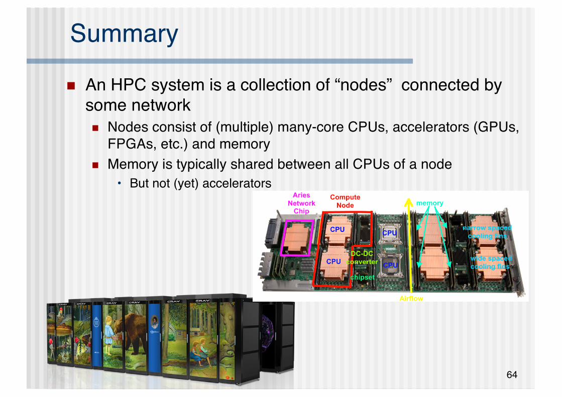
Summary

n An HPC system is a collection of “nodes” connected by some networkn Nodes consist of (multiple) many-core CPUs, accelerators (GPUs,

FPGAs, etc.) and memoryn Memory is typically shared between all CPUs of a node

• But not (yet) accelerators

64

65

Performance

66

Why worry about Performance?

n Compare different systemsn Select the most appropriate system for a given problem

n Make efficient use of available resources

n Scalingn Increase in resources should result in faster resultsn How does increase in resources effect overall runtime?n How does increase of problem size effect overall runtime?

67

Optimization Goals

n Execution timen Minimize the time between start and completion of a taskn Typical goal in HPC

n Throughputn Maximize the number of tasks completed in a given timen Typical goal of large data centers (HTC)

68

Performance Definitions

€

Performancex =1

Execution timex

€

Performancex > Performancey1

Execution timex>

1Execution timey

Execution timex > Execution timey

For two computers X and Y, if the performance of X is greater than the performance of Y, we have

69

Measuring Performancen Performance is measured in time units

n Different ways to measure timen Wall clock time or elapsed time

• Time taken from start to end• Measures everything, including other tasks performed on multitasking systems

n CPU time• Actual time the CPU spends computing for a specific task• Does not include time spent for other processes or I/O• CPU time < wall clock time

n User CPU time• CPU time spent for user program• User CPU time < CPU time < wall clock time

n System CPU time• CPU time spent on operating system tasks for user program• User/System CPU time difficult to measure

70

Factors of CPU performance

€

CPU execution time = CPU clock cyclesClock rate

CPU clock cycles = Instructions × Average clock cycles per instruction (CPI)

CPU time = Instruction count ×CPIClock rate

Components of performance Units of measureCPU execution time Seconds for the programInstruction count Instructions executed for the

programClock cycles per instruction (CPI)

Average number of clock cycles per instruction

Clock cycle time Seconds per clock cycle

71

Other Performance Factorsn Memory subsystem

n Cache missesn Amount and frequency of data to be moved

n I/O subsystemn Amount and frequency of data to be moved

n For parallel systemsn Synchronizationn Communicationn Load balancing

72

Amdahl’s Law

73

Amdahl’s law

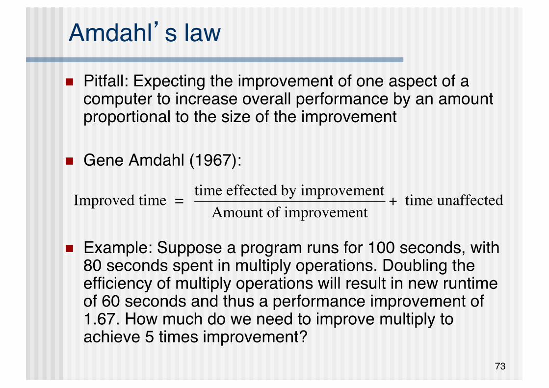
n Pitfall: Expecting the improvement of one aspect of a computer to increase overall performance by an amount proportional to the size of the improvement

n Gene Amdahl (1967):

n Example: Suppose a program runs for 100 seconds, with 80 seconds spent in multiply operations. Doubling the efficiency of multiply operations will result in new runtime of 60 seconds and thus a performance improvement of 1.67. How much do we need to improve multiply to achieve 5 times improvement?

€

Improved time = time effected by improvementAmount of improvement

+ time unaffected

74

Speedup

n Speedup (S) is defined as the improvement in execution time when increasing the amount of parallelism or sequential execution time (TS) over parallel execution time (TP)

Perfect Speedup

02468

1012141618

1 2 4 8 16

Number of CPUs

Sp

eed

up

€

S =TSTP

75

Efficiency

n Speedup as percentage of number of processors

n A speedup of 90 with 100 processors yields 90% efficiency.

€

E =1P×TSTP

=1PS

76

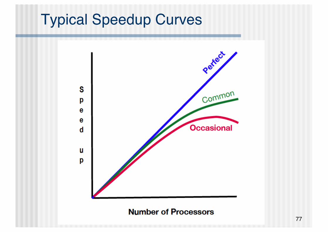
Superlinear Speedup

n Sometimes speedup is larger than number of processorsn Very rare

n Main reasons:n Different parallel and sequential algorithms

n Changes in memory behavior• Smaller problem size in parallel version fits main memory while

sequential one doesn’t• Changes in cache behavior

77

Typical Speedup Curves

78

Amdahl’s Law and Parallel Processing

n According to Amdahl’s law speedup is limited by the non-parallelizable fraction of a program

n Assume rp is the parallelizable fraction of a program and rsthe sequential one. rp+rs=1We can compute the maximum theoretical speedup achievable on n processors with

n If 20% of a program is sequential, the maximal achievable speedup is 5 for nÞ∞

€

Smax =1

rs +rpn

79

How to live with Amdahl’s law

n Many real-world problems have significant parallel portions

n Yet, to use 100,000 cores with 90% efficiency, the sequential part needs to be limited to 0,00001%!

n Conclusion: minimize rs and maximize rp

n Increase amount of work done in the parallel (typically compute intensive) parts

80

Scaling Examplen Workload: sum of 10 scalars, and 10 × 10 matrix sum

n Speed up from 10 to 100 processors

n Single processor: Time = (10 + 100) × tadd

n 10 processorsn Time = 10 × tadd + 100/10 × tadd = 20 × taddn Speedup = 110/20 = 5.5 (55% of potential)

n 100 processorsn Time = 10 × tadd + 100/100 × tadd = 11 × taddn Speedup = 110/11 = 10 (10% of potential)

n Assumes load can be balanced across processors

81

Scaling Example (cont)

n What if matrix size is 100 × 100?

n Single processor: Time = (10 + 10000) × tadd

n 10 processorsn Time = 10 × tadd + 10000/10 × tadd = 1010 × tadd

n Speedup = 10010/1010 = 9.9 (99% of potential)

n 100 processorsn Time = 10 × tadd + 10000/100 × tadd = 110 × taddn Speedup = 10010/110 = 91 (91% of potential)

n Assuming load balanced

82

Strong and Weak Scaling

n Strong scaling is the speedup achieved withoutincreasing the size of the problem

n Weak scaling is the speedup achieved while increasingthe size of the problem proportionally to the increase in number of processors

83

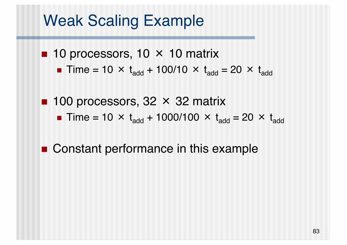
Weak Scaling Example

n 10 processors, 10 × 10 matrixn Time = 10 × tadd + 100/10 × tadd = 20 × tadd

n 100 processors, 32 × 32 matrixn Time = 10 × tadd + 1000/100 × tadd = 20 × tadd

n Constant performance in this example

84

Load Balancing

n Good speedup can only be achieved if the parallel workload is relatively equally spread over the available processors

n If workload is unevenly spread, overall performance is bound to the slowest processor (i.e. Processor with most workload)

85

Example Continued

n 100 processorsn Time = 10 × tadd + 10000/100 × tadd = 110 × taddn Speedup = 10010/110 = 91 (91% of potential)n Assumes each processor gets 1% of workload

n Assume one processor get 2% (i.e. 200 matrix elements) and the rest of 9800 elements is equally distributed over the remaining 99 processors.

n Speedup = 10010/210 = 47.6€

Time =Max 9800t99

,200t1

"

# $

%

& ' +10t = 210t

86

Load Balancing Examples

P0

P3

P2

P1

P2P0

P3P1

P0 P3P2P1

P0 P3P2P1 P0 P3P2P1 P0 P3P2 P0 P3P2P1 P1

87

Synchronization and Communication

n Parallel programs need synchronization and communication to ensure correct program behavior

n Synchronization and communication adds significant overhead and thus reduces parallel efficiency

€

S =TSTP

€

S =TS

TPC + synch wait time + communication time

can be refined as

with TPC symbolizing the net parallel computation time

88

Synchronization and Communication Cont’d

n Goal is to avoid synchronization and communication

n Not always possible

n Overlap communication with computation and optimize communicationn Communication overhead impacted by latency and bandwidth

• Block communication n Use more efficient communication patterns

n Profiling tools can help identifying synchronization and communication overhead

89

Example: Vampir traces

90

The Impact of Data

n Apart from communication, data is effecting performance at many levels

n Memory hierarchy

n I/O

Memory/Storage Hierarchies

91

Tomorrow

n How to program HPC systems

n Technological trends

92