Embed Size (px)
Citation preview
Warwick Research Software Engineering
Introduction to MPI
C.S. Brady and H. RatcliffeSenior Research Software Engineers
“The Angry Penguin”, used under creative commons licence
from Swantje Hess and Jannis Pohlmann.
December 18, 2018
Contents
Preface i0.1 About these Notes . . . . . . . . . . . . . . . . . . . . . . . . . . . . . i0.2 Example Programs . . . . . . . . . . . . . . . . . . . . . . . . . . . . . i
1 Principles of Parallel Programming 11.1 History . . . . . . . . . . . . . . . . . . . . . . . . . . . . . . . . . . . . 11.2 Kinds of Parallelism . . . . . . . . . . . . . . . . . . . . . . . . . . . . 21.3 Distributed Memory and MPI . . . . . . . . . . . . . . . . . . . . . . . 71.4 Alternatives to all of this . . . . . . . . . . . . . . . . . . . . . . . . . . 7
2 Starting with MPI 92.1 What is MPI? . . . . . . . . . . . . . . . . . . . . . . . . . . . . . . . . 92.2 The Parts of an MPI program . . . . . . . . . . . . . . . . . . . . . . . 102.3 A basic example program . . . . . . . . . . . . . . . . . . . . . . . . . . 13
3 Basics of Communication 193.1 Actually Communicating . . . . . . . . . . . . . . . . . . . . . . . . . . 193.2 Collective Communications . . . . . . . . . . . . . . . . . . . . . . . . . 193.3 MPI Barrier . . . . . . . . . . . . . . . . . . . . . . . . . . . . . . . . . 24
4 Point to Point Communication 264.1 Overview . . . . . . . . . . . . . . . . . . . . . . . . . . . . . . . . . . . 264.2 A simple example - the ring pass . . . . . . . . . . . . . . . . . . . . . 274.3 Sendrecv . . . . . . . . . . . . . . . . . . . . . . . . . . . . . . . . . . . 304.4 The Story So Far . . . . . . . . . . . . . . . . . . . . . . . . . . . . . . 30
5 Domain Decomposition Models 315.1 Motivation . . . . . . . . . . . . . . . . . . . . . . . . . . . . . . . . . . 315.2 What is Domain Decomposition . . . . . . . . . . . . . . . . . . . . . . 315.3 Basic Principle . . . . . . . . . . . . . . . . . . . . . . . . . . . . . . . 335.4 A “Simple” Example . . . . . . . . . . . . . . . . . . . . . . . . . . . . 335.5 Splitting the Domain . . . . . . . . . . . . . . . . . . . . . . . . . . . . 355.6 Arranging the Processors . . . . . . . . . . . . . . . . . . . . . . . . . . 385.7 Quick Recap . . . . . . . . . . . . . . . . . . . . . . . . . . . . . . . . . 435.8 Handling Boundary Exchanges . . . . . . . . . . . . . . . . . . . . . . . 44
CONTENTS
5.9 Putting it all Together . . . . . . . . . . . . . . . . . . . . . . . . . . . 45
6 Worker Controller Models 466.1 Motivation . . . . . . . . . . . . . . . . . . . . . . . . . . . . . . . . . . 466.2 Single Program Multiple Data (SPMD) . . . . . . . . . . . . . . . . . . 466.3 A Basic Arrangement . . . . . . . . . . . . . . . . . . . . . . . . . . . . 486.4 Pitfalls to Avoid . . . . . . . . . . . . . . . . . . . . . . . . . . . . . . 516.5 Non Blocking MPI . . . . . . . . . . . . . . . . . . . . . . . . . . . . . 52
7 Glossary of Terms 53Glossary . . . . . . . . . . . . . . . . . . . . . . . . . . . . . . . . . . . . . . 53
Preface
0.1 About these Notes
These notes were written by H Ratcliffe and C S Brady, both Senior Research SoftwareEngineers in the Scientific Computing Research Technology Platform at the Universityof Warwick for a Workshop first run in December 2018 at the University of Warwick.
This work, except where otherwise noted, is licensed under the CreativeCommons Attribution-NonCommercial-NoDerivatives 4.0 International Li-cense. To view a copy of this license, visit http://creativecommons.org/
licenses/by-nc-nd/4.0/.
The notes may redistributed freely with attribution, but may not be used for commercialpurposes nor altered or modified. The Angry Penguin and other reproduced material,is clearly marked in the text and is not included in this declaration.
The notes were typeset in LATEXby H Ratcliffe.Errors can be reported to [email protected]
0.2 Example Programs
Several sections of these notes benefit from hands-on practise with the concepts andtools involved. Test code is available on Github at https://github.com/WarwickRSE/IntroMPI
i
Chapter 1
Principles of Parallel Programming
1.1 History
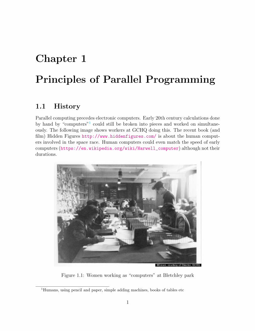
Parallel computing precedes electronic computers. Early 20th century calculations doneby hand by “computers”1 could still be broken into pieces and worked on simultane-ously. The following image shows workers at GCHQ doing this. The recent book (andfilm) Hidden Figures http://www.hiddenfigures.com/ is about the human comput-ers involved in the space race. Human computers could even match the speed of earlycomputers (https://en.wikipedia.org/wiki/Harwell_computer) although not theirdurations.
Figure 1.1: Women working as “computers” at Bletchley park
1Humans, using pencil and paper, simple adding machines, books of tables etc
1
2 CHAPTER 1. PRINCIPLES OF PARALLEL PROGRAMMING
1.2 Kinds of Parallelism
There are many levels at which computers can work on things in parallel. We’re onlygoing to discuss the MPI standards here, and not really any of the following:
• Bit level parallelism
Processors work on chunks of data at once rather than bit by bit
• Instruction level parallelism
Processors can operate on more than one variable at a time
NOT multicore
A large chunk of optimisation of code is trying to improve instruction levelparallelism
• Task level parallelism
Split up a “task” into separate bits that computer can work on separately
• Task Farming
Tasks that are unrelated to each other can easily just be handed off to differentprocessors
Exploring parameters
1.2.1 Embarrassing Parallelism
Embarrassing parallelism is a fairly special case that comes up a lot in practice. Here,you have a lot of unconnected, un-sequenced tasks. Since there’s no connections betweentasks, you can simply run multiple copies of your program. It is important not to runmore copies than you have physical processors. Modern computers use something called“Simultaneous Multithreading” or “Hyperthreading” which runs several things at once,swapping between them. This is great for normal computing loads, since generally a lotof time is spent waiting for user inputs, or for things to happen. For research computingloads, it doesn’t generally work well, with the threads contending for resources andtaking longer overall than running one then the other. Large or commercial machinesuse a scheduling system to run jobs only when there is a free processor.
1.2.2 Tightly coupled parallelism
The opposite of embarrassing parallelism is tightly coupled parallelism, where a problemsplits into chunks, but each chunk needs information from other chunks, whether this isonly some other chunks or all other chunks. Somehow the data has to be made availableto all chunks which need it.
This leads to two main concerns. To allow more than one processor to work on achunk of data you have to:
1.2. KINDS OF PARALLELISM 3
1. Make sure that the data is somewhere so that it can be used by a processor(communication)
2. Make sure that data transfer is synchronised so that you know you can use itwhen you need to
These two problems can be addressed in several ways, and different models of par-allelism use different approaches.
1.2.3 Shared Memory Paralellism
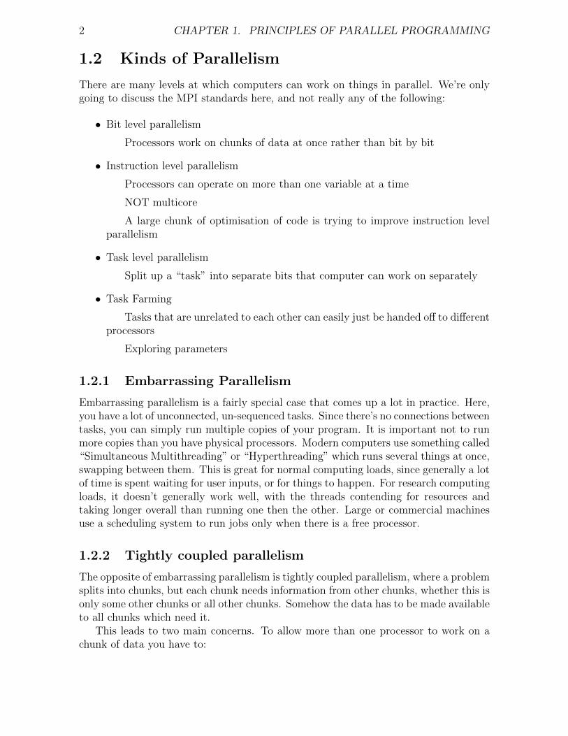
Figure 1.2: Schematic diagram of shared memory parallelism
Shared memory parallelism lets multiple tasks access the same data, i.e. they sharetheir data memory. Figure 1.2 shows this. Each processor has some designated workchunk, but the memory is shared. Communication is automatic, but synchronisationis a significant problem.
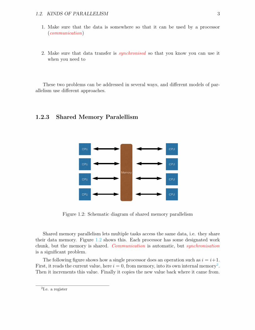
The following figure shows how a single processor does an operation such as i = i+1.First, it reads the current value, here i = 0, from memory, into its own internal memory2.Then it increments this value. Finally it copies the new value back where it came from.
2I.e. a register
4 CHAPTER 1. PRINCIPLES OF PARALLEL PROGRAMMING
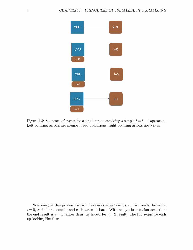
Figure 1.3: Sequence of events for a single processor doing a simple i = i+ 1 operation.Left-pointing arrows are memory read operations, right pointing arrows are writes.
Now imagine this process for two processors simultaneously. Each reads the value,i = 0, each increments it, and each writes it back. With no synchronisation occurring,the end result is i = 1 rather than the hoped for i = 2 result. The full sequence endsup looking like this:
1.2. KINDS OF PARALLELISM 5
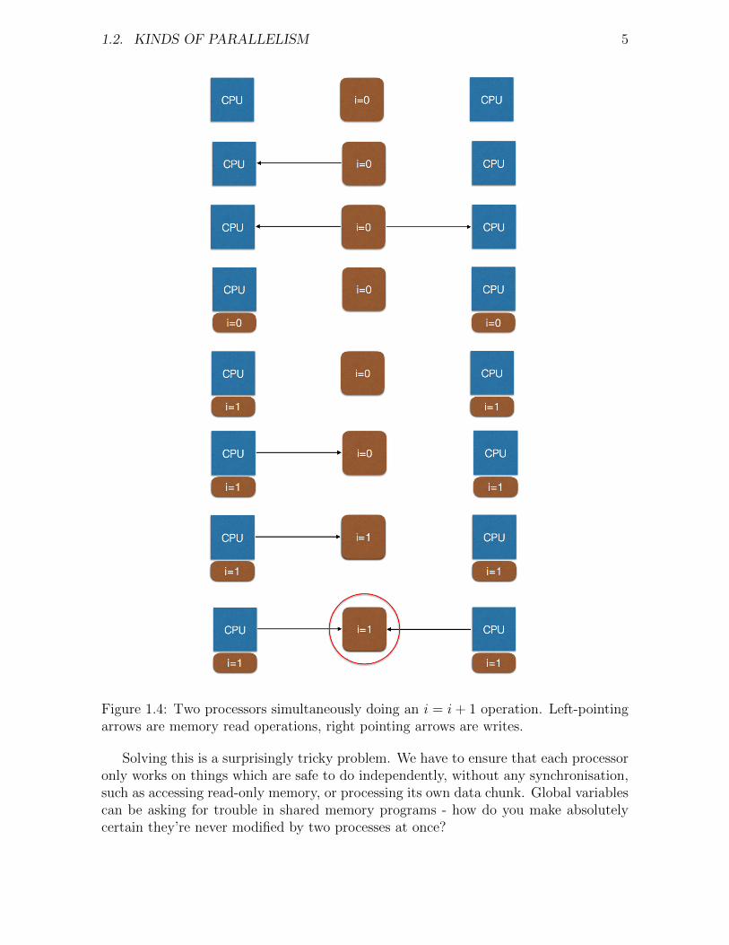
Figure 1.4: Two processors simultaneously doing an i = i+ 1 operation. Left-pointingarrows are memory read operations, right pointing arrows are writes.
Solving this is a surprisingly tricky problem. We have to ensure that each processoronly works on things which are safe to do independently, without any synchronisation,such as accessing read-only memory, or processing its own data chunk. Global variablescan be asking for trouble in shared memory programs - how do you make absolutelycertain they’re never modified by two processes at once?
6 CHAPTER 1. PRINCIPLES OF PARALLEL PROGRAMMING
The Read-Modify-Write sequence and Atomicity
The 2-processor sequence above is related to a very common problem called adata race. If instead of incrementing i, each processor was to set the value toits own rank, the end result would depend critically on the exact order of eachprocessor’s write operation, so the two are in a race to do their work. Theproblem comes because we are treating read, modify and write as separateoperations. What we wanted was for the complete sequence to be consideredone operation.This is very like a much deeper problem in multi-threaded computing, whereseveral operations might affect the same piece of data. Imagine if rather thana simple integer, we were writing a string, one letter at a time. Processor 1is trying to write the string “One”, while two is writing “Two”. Dependingon how the operations order, we might end up with nonsense like “Owe” or“Tno”.This can also happen to some variable types which are wider than the pro-cessors “load-store” width. This means the processor has to do more thanone write operation to write all the bytes of the variable, and you can, intheory, get two variables mashed together. Most systems allow you to usespecial operations which are guaranteed to happen all-at-once from the per-spective of other parts of the system. This is often called “atomicity” becausethe operation cannot be divided into parts. The term might be encounteredeverywhere from databases (you want a record to be modified completelyor not-at-all) at the largest scale, to interrupt programming (dealing withsignals from the operating system or devices) at the smallest scale.There is a fairly obvious answer to this problem, which is to use some sort offlag to “lock” a variable until you are done with it. But first you have to testwhether it is already locked: and imagine what happens if between your testand your set operation, another processor has already set the lock... Systemsimplement atomic versions of “test-and-set” and “read-modify-write” to getaround this. These can be used to implement locks, or “mutexes” (mutualexclusions).
In shared memory programming, critical sections are used to insist that operationsmust happen one after the other, and anything where this is important must be labelledcorrectly. In more complex cases it can be very tricky, but in many problems there areonly a few critical sections.
OpenMP
OpenMP is a system commonly used in research codes providing directives to tell thecompiler how to parallelise loops in code. This automates some of the synchronisation,although you still have to label critical sections, and it can’t do everything. It alsorequires a compatible compiler, although these are very common.
1.3. DISTRIBUTED MEMORY AND MPI 7
Threads
Threading libraries can be used to explicitly run parts of code in other threads. Theoperating system will try and balance the load across processors. This technique is verycommon in non-academic code, especially things with a user-interface, but less commonin academia. Mutual Exclusions (see aside box above) are used to force synchronisationand ensure only one processor works on data at once. A thread has to first get themutex, do its work, and then release it. Only one thread can hold it at a time, and allothers must wait. Obviously some care must be taken to avoid deadlocks, where thethreads are all depending on each other in a way that can’t be worked out.
1.3 Distributed Memory and MPI
In distributed memory systems all processors have their own memory, and data canonly flow between them via a fabric. Typically programs explicitly send and receivedata, i.e communication is done manually. Synchronisation is directly tied to this, andis usually guaranteed once a receive operation completes.
As a programmer, you have to manually work out the transfers of data and sendexplicit messages between processors which contain the data. There are a number ofcommon strategies to help with this, but in general it can be tricky, and in general thecomms fabric is quite slow compared with direct memory access, so we really need tominimise the amounts and frequency of data transfers.
1.3.1 MPI
The Message Passing Interface library is the most popular distributed memory library.It is just a library and needs no special compiler. It includes routines for sending andreceiving data, collective operations such as summing between processors, parallel fileI/O and many others.
MPI on a single computer performs nearly as well as shared memory, but is harderto program than OpenMP in simple cases. Programming is about as hard as writingthreaded code would be. Finally, while the library itself scales to the largest supercom-puters in the world, your algorithm may well not.
On shared memory architectures, MPI works fine. We program it as though it isdistributed, although there are some advanced features which are explicitly shared.If the algorithm is amenable to distributed memory we get comparable performanceto OpenMP or threading. On the other hand, some algorithms just map better ontoshared memory, so we can use a Hybrid approach combining MPI with OpenMP orpthreads (a common threading library) to get the best of all worlds.
1.4 Alternatives to all of this
There are some alternatives to avoid having to deal with any of this. These includeOpenSHMEM, a standard for writing shared-memory libraries. There are some exten-

8 CHAPTER 1. PRINCIPLES OF PARALLEL PROGRAMMING
sions to specific programming languages to tackle problems, such as Coarray Fortran, orUnified Parallel C. Some languages have built-in support for “concurrent” (simultane-ous) operations, including Chapel (a language developed by Cray) or X10 (from IBM).Support for these can be poor or patchy, and none have really obvious advantages overMPI or OpenMP.
Chapter 2
Starting with MPI
2.1 What is MPI?
At its core, MPI is a set of standards, set out by the MPI forum (http://mpi-forum.org). There are different versions of the MPI standard:
• MPI1 was the original standard from 1989. It still works, but much has beendeprecated and some bits don’t work well
• MPI2 was an updated standard from 1997. This added a broad variety of featuresand modernised lots of bits. The latest MPI2.2 standard is from 2009. We willbe teaching you this!
• MPI3 is a further update from 2012. Very useful and powerful additions, but notreally relevant for a beginning MPI course
• MPI4 further updates MPI3 and has not yet been formally ratified
There are many different implementations of the MPI standard, including
• OpenMPI
• MPICH
• MVAPICH
• Intel MPI
Valid MPI code will work with any of them, unless you manage to invoke one of themany interesting and strange bugs in implementations.
The MPI Application Programming Interface (API) changes according to the MPIversion you’re using, and the language binding you’re working with. For MPI there are3 official bindings, C, Fortran and Fortran-2008. The latter isn’t ready for general useyet, but is worth knowing about.
9
10 CHAPTER 2. STARTING WITH MPI
There used to be a C++ binding. Do not use it. It is formally deprecated, not upto date and will be removed in future. It also adds nothing over the C bindings for aC++ developer.
There are also unofficial bindings, including OpenMPI Java, which is an almostcompliant MPI 3.1 implementation, but this is only for OpenMPI. There is also MPI4Pywhich adds a Python layer onto any of the above MPI installations. This has a differentinterface to MPI proper and lacks some features. These, and the various others, areeither MPI vendor specific or not fully standards compliant1. This means you generallyhave to learn them separately, so we’re not going to cover them here.
2.2 The Parts of an MPI program
In general, any MPI program has the following parts:
• Initialisation
• Main program:
Compute
Communication
Output
• Finalisation
The main program part is often repeated in a loop.
Note that Compute and Communication are listed separately for a few reasons:
• Clarity - it’s harder to understand, debug and maintain code which mixes MPIcode in among general code
• Performance - you want to do as little comms as possible, using as few messagesas possible
1The MPI standards are available online. They’re a rather dry read but eventually you may needto be familiar with parts of them.
2.2. THE PARTS OF AN MPI PROGRAM 11
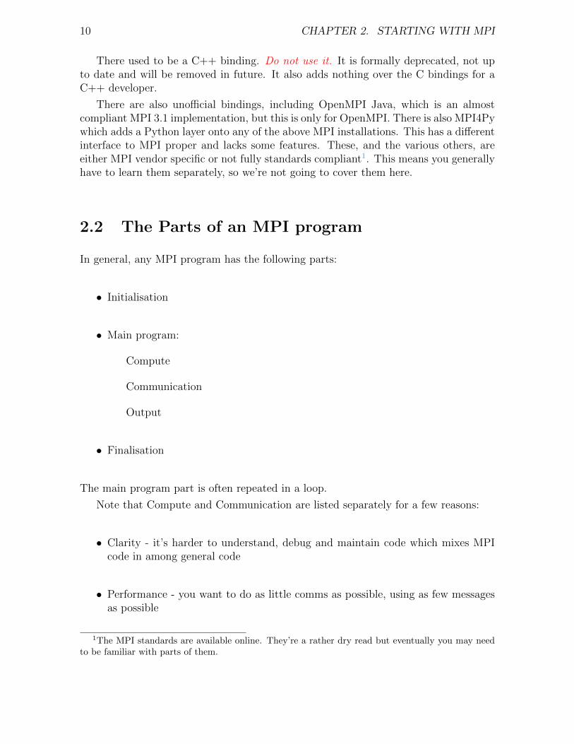
Figure 2.1: Data transferred over time for varying values of latency and bandwidth
12 CHAPTER 2. STARTING WITH MPI
Latency Bandwidth and Messaging
We just said “as little comms as possible, using as few messages as possible”.Each MPI message takes time to assemble, prepare for sending, arrange toreceive etc - this is latency. The time taken to move the data is limited bythe bandwidth - how much data can be moved per second. The image aboveshows how the two values change the overall time to move data.Imagine painting the centre line on a road. It takes you some time to getset up, open your paint can, and get going (latency). Once you’re started,the speed at which you proceed depends (mainly) on how much paint yourbrush will hold (bandwidth). Each time you have to stop and open a newpaint can you have a new chunk of latency.You may have heard the old joke - a {target of humorous excursion} istasked with painting the lines on a road. On the first day, they do brilliantly,painting 3 miles of new line. On the second day, they manage only 1.5 miles.By the third day they complete barely half a mile. “What is taking so long?”asks the supervisor. “Well,” they reply, “it just takes so long to keep goingback to the paint pot!”. Tiny messages are almost as bad as going back tothe paint pot if you have a lot of data to shift.As an example, on real HPC kit we have a latency of 0.5µ s per message anda bandwidth of 37 GB/s. So to send 100 messages of 1MB each, we have 50µs latency and 27 µ total sending time, a total of 77 µ s. Wheras to send asingle 100MB message, the total time is just 27.5 µ s.
2.2.1 Initialisation
The initialisation step uses a single routine, MPI Init, to initialise the MPI layer. Thismust be called before any other MPI routines. The signature is
1 MPI Init ( int ∗argc , char ∗∗∗ argv )
• argc Pointer to argc in main. Usually just &argc
• argv Pointer to argv in main. Usually just &argv
This is one of the few functions that is a bit different in Fortran. There, we don’thave the argc or argv arguments, but as usual we do have the final error parameter, sothe full signature is
1 MPI Init ( i e r r )
where ierr is an INTEGER.
2.3. A BASIC EXAMPLE PROGRAM 13
2.2.2 Finalisation
The finalisation step also uses just a single routine, MPI Finalize, to shut down theMPI layer. After calling this, you cannot call any other MPI routines, and you mustcall this on all ranks (processors) before the program ends. Warning : if you forget,your code will mostly work, but this is not guaranteed. The signature is
1 MPI Final ize ( )
with no parameters. Remember: in Fortran every MPI function has the extra parameterierr, including this one. So in Fortran this does have parameters
2.2.3 A very first MPI code
These two functions are enough to put together a very first MPI code:
1 #include <mpi . h>2 #include <s t d i o . h>3 int main ( int argc , char ∗∗ argv )4 {5 MPI Init(&argc , &argv ) ;6 p r i n t f (”Multiprocessor code\n”) ;7 MPI Final ize ( ) ;8 return 0 ;9 }
We now have to compile this using the MPI compiler, which supplies (links) all ofthe MPI functions. Usually the compiler will be mpicc (rather than gcc) or mpif90
(rather than gfortran), but if you’re using the Intel compiler suite or something likeCray, check the docs for the appropriate commands. To run the program, we have toget multiple copies going linked together by MPI - this uses the command mpiexec -n
<number of processors> <program name>.
This program is really not much use. If you compile and run it on more thanone processor you’ll see several lines all saying “Multiprocessor code”. Note that youdon’t see the letters jumbled together from different processors - while multiple printstatements will get mixed together, each one usually2 comes out in one piece. This isuseful for showing user messages - just remember to assemble the whole message intoa single print and keep it brief.
2.3 A basic example program
To demonstrate an actual use for MPI we need an example problem. We’ll use one thatmay be familiar from GCSE maths - calculating π using geometry.
In the following picture
2As far as we know this is almost always the case for simple, single prints, but isn’t guaranteed;sometimes you will get prints mixed into each other.
14 CHAPTER 2. STARTING WITH MPI
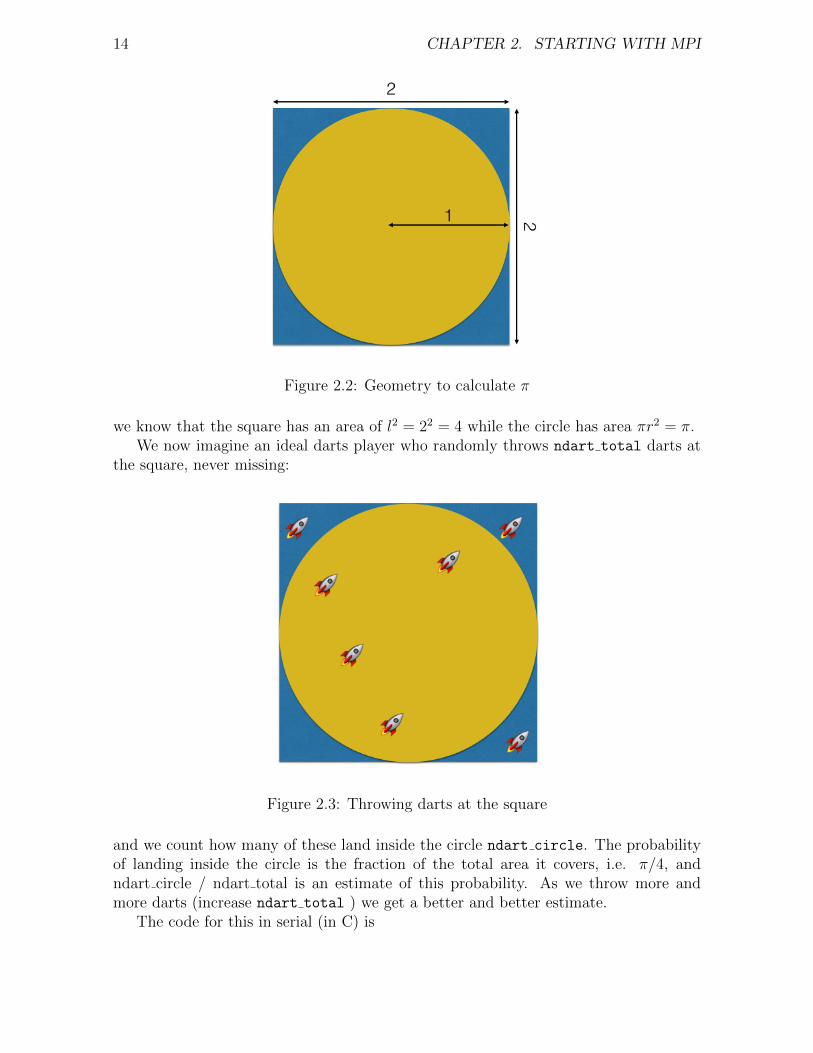
Figure 2.2: Geometry to calculate π
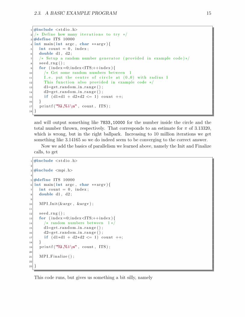
we know that the square has an area of l2 = 22 = 4 while the circle has area πr2 = π.We now imagine an ideal darts player who randomly throws ndart total darts at
the square, never missing:
Figure 2.3: Throwing darts at the square
and we count how many of these land inside the circle ndart circle. The probabilityof landing inside the circle is the fraction of the total area it covers, i.e. π/4, andndart circle / ndart total is an estimate of this probability. As we throw more andmore darts (increase ndart total ) we get a better and better estimate.
The code for this in serial (in C) is
2.3. A BASIC EXAMPLE PROGRAM 15
1 #include <s t d i o . h>2 /∗ Def ine how many i t e r a t i o n s to t ry ∗/3 #define ITS 100004 int main ( int argc , char ∗∗ argv ) {5 int count = 0 , index ;6 double d1 , d2 ;7 /∗ Setup a random number genera tor ( provided in example code ) ∗/8 s eed rng ( ) ;9 for ( index =0; index<ITS;++index ) {
10 /∗ Get some random numbers between 111 I . e . put the cent r e o f c i r c l e at (0 , 0 ) with rad iu s 112 This func t i on a l s o provided in example code ∗/13 d1=get random in range ( ) ;14 d2=get random in range ( ) ;15 i f ( d1∗d1 + d2∗d2 <= 1) count ++;16 }17 p r i n t f (”%i ,%i\n” , count , ITS ) ;18 }
and will output something like 7833,10000 for the number inside the circle and thetotal number thrown, respectively. That corresponds to an estimate for π of 3.13320,which is wrong, but in the right ballpark. Increasing to 10 million iterations we getsomething like 3.14165 so we do indeed seem to be converging to the correct answer.
Now we add the basics of parallelism we learned above, namely the Init and Finalizecalls, to get
1 #include <s t d i o . h>2
3 #include <mpi . h>4
5 #define ITS 100006 int main ( int argc , char ∗∗ argv ) {7 int count = 0 , index ;8 double d1 , d2 ;9
10 MPI Init(&argc , &argv ) ;11
12 s eed rng ( ) ;13 for ( index =0; index<ITS;++index ) {14 /∗ random numbers between 1 ∗/15 d1=get random in range ( ) ;16 d2=get random in range ( ) ;17 i f ( d1∗d1 + d2∗d2 <= 1) count ++;18 }19 p r i n t f (”%i ,%i\n” , count , ITS ) ;20
21 MPI Final ize ( ) ;22
23 }
This code runs, but gives us something a bit silly, namely
16 CHAPTER 2. STARTING WITH MPI
7805,10000
7805,10000
...
7805,10000
i.e. the exact same result on all processors.The reason is hidden away inside the bit we skipped over, because it was “irrelevant”.
Lots of things you don’t think of are different in parallel. Be very cautious callingsomething irrelevant based on experience in serial code. The problem is seeding (settingup) the random number generator. We used the usual standard approach, seeding withthe system clock to get a different answer run to run, as
1 #include <time . h>2 void s eed rng ( ) {3 t ime t t ;4 srand ( (unsigned ) time(&t ) ) ;5 }
But all of our processors share this clock, so we’ll generally get the same seed3 and sothe same random sequence.
We want to get something which is unique to each processor to ensure4 differentseeds. In MPI, each processor is assigned a rank, which is an integer value. The “first”processor is given a rank 0 and the rest are assigned in order up to the number ofprocessors. The function MPI Comm rank returns this value.
We also need the idea of an MPI communicator at this point. This is essentially alist of processors. Here we will always be using the default value MPI COMM WORLD whichmeans all the processors you’re running on. To get the rank value, we use (rememberingagain that in Fortran we have an extra, final ierr parameter)
1 MPI Comm rank(MPI Comm comm, int ∗ rank )
• comm - An MPI communicator. Generally just the constant MPI COMM WORLD
• rank - Pointer to integer to be filled with the unique rank value for this processorin communicator comm. If you have more than one communicator a processorcan have a different rank in each one.
Remember that Fortran is pass-by-reference, so where C requires a pointer, Fortran canuse a plain INTEGER So the Fortran signature is, instead
1 MPI Comm rank(INTEGER comm, INTEGER rank )
3Another place to be extra careful - because there can be tiny differences in timings betweenprocessors, especially processors on several compute nodes, you might in fact NOT get the same seedin your test runs, and never spot this potential bug.
4If you can spot why in rare cases in the code below we might still get the same seed, well done!Now fix it!
2.3. A BASIC EXAMPLE PROGRAM 17
• comm - An MPI communicator. Generally just the constant MPI COMM WORLD
• rank - Integer to be filled with the unique rank value for this processor in com-municator comm. If you have more than one communicator a processor can havea different rank in each one.
Using the rank, we seed the random number generator as
1 #include <time . h>2 #include <mpi . h>3 void s eed rng ( ) {4 t ime t t ;5 int rank ;6 MPI Comm rank(MPI COMM WORLD, &rank ) ;7 srand ( (unsigned ) time(&t ) + rank ) ;8 }
and compile and run this program. The results are something like
7860,10000
7814,10000
7856,10000
7850,10000
7814,10000
7889,10000
7839,10000
7934,10000
7803,10000
7855,10000
7869,10000
7820,10000
7771,10000
7829,10000
7869,10000
7812,10000
which is much better.Now in serial we parse and add up those results to get an estimate of π = 3.13710
just as if we’d run 16000 iterations on one processor.We know how to find the rank of our current processor, but how do we find out how
many there are in total? This uses the command MPI Comm size which again works ona communicator and returns an integer.
1 MPI Comm size (MPI Comm comm, int ∗ s i z e )
• comm - An MPI communicator. Generally just the constant MPI COMM WORLD
• size - Pointer to integer to be filled with the number of processors in comm.Since ranks start from 0, this will be 1 greater than the maximum rank
18 CHAPTER 2. STARTING WITH MPI
Once again, in Fortran both comm and size are plain INTEGER and we have a final,INTEGER parameter for the return code.
2.3.1 The Story So Far
So far, we’ve see how to do an embarassingly parallel (explained in a moment) prob-lem in MPI5. Every processor works independently on its own problem and then theresults can be synthesised into a single answer. We haven’t learned anything aboutcommunications yet at all. However this can already be useful.
This sort of divided work can be used to do “task-farming” - splitting work overmany processors with one in charge of dispatching. We talk about a simple model forthis in Chapter 6. Note that this is the main use of MPI in Python, via MPI4Py or asimilar library. MPI with communication is generally a bad idea in Python code, butthe dispatcher model is fairly useful. If you’d like some help with this sort of approach,let us know by email.
For general MPI programs though, we need to learn how to communicate, so readon!
5Well, mostly in parallel anyway
Chapter 3
Basics of Communication
3.1 Actually Communicating
MPI communications split into two general sets:
• Point to point communications
This processor talks to that processor
• Collective communications
Every processor communicates with every other 1 processor
Since these groups of functions, and the purposes they serve, are quite distinct, we treatthem separately over the next two chapters. We think collectives are a tiny bit easierto start with, so we start with them.
3.2 Collective Communications
The core set of collective communications are:
• Reduce - Combine data from all processors in specified way onto a single rootprocessor
Allreduce - Combine data from all processors in specified way and give resultto all processors
• Bcast - Broadcast same data from root processor to all others
• Scatter - Send different data from the root processor to all other processors
• Gather - Receive different data from each processor onto root processor
AllGather - Receive different data from each processor and put the result onall processors
1Every other processor in the communicator you’re using. But you can write many MPI programsand never use any communicator except MPI COMM WORLD, so don’t worry about the distinction for now.
19
20 CHAPTER 3. BASICS OF COMMUNICATION
• AllToAll - Send different data between every pair of processors at the same time.Don’t use this unless absolutely necessary. This is pretty much the slowest MPIcommunication routine there is.
At the low level, MPI communication is dumb: it just sends and receives bytes. Tosend useful messages, we need to be able to indicate that something is an integer, or afloating-point number etc.2 MPI has built in types for the basic types, and it is possibleto create custom ones representing e.g. a structure with multiple fields. For more onthis, see our Intermediate MPI (coming soon).
The basic types include:
• MPI INT - C Integer
• MPI INTEGER - Fortran Integer
• MPI FLOAT - C single precision
• MPI REAL - Fortran single precision
• MPI DOUBLE - C double precision
• MPI DOUBLE PRECISION - Fortran double precision
• MPI BYTE - Single byte value
• Many, many others
Do note that there are slightly different names in C and Fortran. If you use the wrongone things will probably compile and work, but there’s a risk of that changing over timeor on different computers (the sizes aren’t forced to be the same, for example, they justnearly always are).
The real power of MPI types is for reduction operations (taking several values andcombining them into one), where MPI not only sends the data, but does somethingwith it too. This means it needs to know details of the particular system’s data layoutetc. MPI can be used between computers that represent data differently, and MPI thenhas to take care of transforming the data types. Custom data types also allow fancythings like reshaping an array in flight (keeping the total number of elements the same).Once again, this is stuff you should know of, but shouldn’t need for a fair time, if ever.
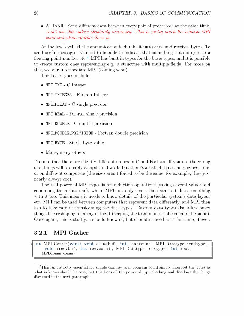
3.2.1 MPI Gather
1 int MPI Gather ( const void ∗ sendbuf , int sendcount , MPI Datatype sendtype ,void ∗ recvbuf , int recvcount , MPI Datatype recvtype , int root ,
MPI Comm comm)
2This isn’t strictly essential for simple comms- your program could simply interpret the bytes aswhat is knows should be sent, but this loses all the power of type checking and disallows the thingsdiscussed in the next paragraph.
3.2. COLLECTIVE COMMUNICATIONS 21
• sendbuf - Data to send to root
• sendcount - Number of elements in sendbuf
• sendtype - Type of data in sendbuf
• recvbuf - Array into which to receive data (should be recvcount * nproc elementslong)
• recvcount - Number of elements to receive from a single processor (unless usingcustom types for sendtype and/or recvtype should equal sendcount)
• recvtype - Type of data in recvbuf (generally same as sendtype)
• root - Rank of processor to receive data
• comm - MPI communicator (usually MPI COMM WORLD)
This looks a bit complicated, but in theory its pretty simple. Each processor sendssendcount elements to the processor whose rank equals root. On root you need toallocate an array of length sendcount * nproc elements to hold the results. Despitethis recvcount should be the number of elements received from each processor, not thetotal number. The results from rank 0 go into (0:sendcount-1). The results from rank1 go into (sendcount : 2 * sendcount -1) etc. etc. We use MPI Comm size to get thenumber of processors, nproc, so we can get this array ready to receive into.
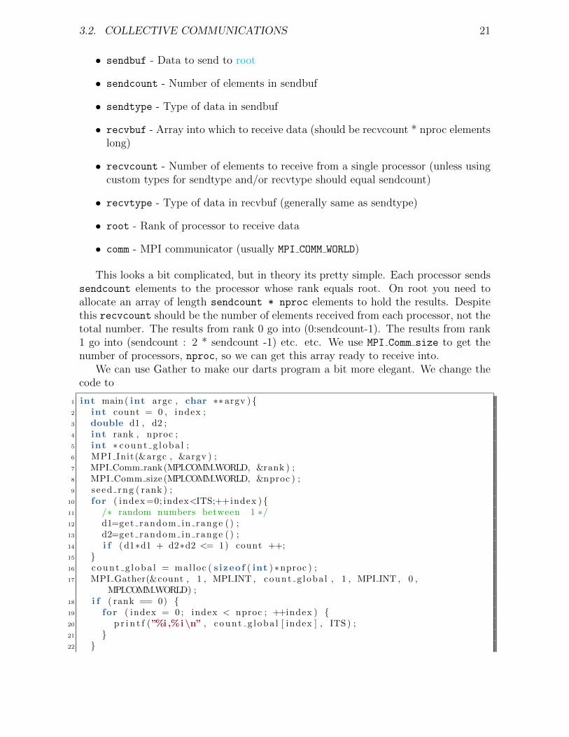
We can use Gather to make our darts program a bit more elegant. We change thecode to
1 int main ( int argc , char ∗∗ argv ) {2 int count = 0 , index ;3 double d1 , d2 ;4 int rank , nproc ;5 int ∗ count g l oba l ;6 MPI Init(&argc , &argv ) ;7 MPI Comm rank(MPI COMM WORLD, &rank ) ;8 MPI Comm size (MPI COMM WORLD, &nproc ) ;9 s eed rng ( rank ) ;
10 for ( index =0; index<ITS;++index ) {11 /∗ random numbers between 1 ∗/12 d1=get random in range ( ) ;13 d2=get random in range ( ) ;14 i f ( d1∗d1 + d2∗d2 <= 1) count ++;15 }16 count g l oba l = mal loc ( s izeof ( int ) ∗nproc ) ;17 MPI Gather(&count , 1 , MPI INT , count g loba l , 1 , MPI INT , 0 ,
MPI COMM WORLD) ;18 i f ( rank == 0) {19 for ( index = 0 ; index < nproc ; ++index ) {20 p r i n t f (”%i ,%i\n” , c oun t g l oba l [ index ] , ITS ) ;21 }22 }
22 CHAPTER 3. BASICS OF COMMUNICATION
23 MPI Final ize ( ) ;24 }
We’ve made a few changes to the code. We now get the rank inside main and passit to the seed function to avoid doing this twice. We get the number of processors usingMPI Comm size. We only print our answer on rank 0, which prints the values from eachprocessor, so we get the same output as before.
3.2.2 Reduction
We could add up the the numbers once we’ve collected them, and print one final result,but there’s a better way - we can add them all up as part of the collective operation,using reduction. The MPI layer combines data using the operation you specify, beforepassing it on. Here we want to use MPI SUM to sum values together.
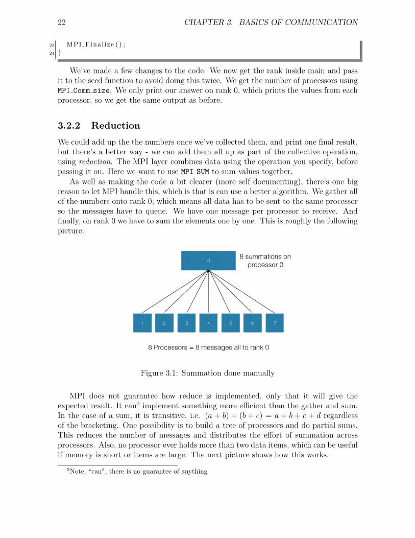
As well as making the code a bit clearer (more self documenting), there’s one bigreason to let MPI handle this, which is that is can use a better algorithm. We gather allof the numbers onto rank 0, which means all data has to be sent to the same processorso the messages have to queue. We have one message per processor to receive. Andfinally, on rank 0 we have to sum the elements one by one. This is roughly the followingpicture.
Figure 3.1: Summation done manually
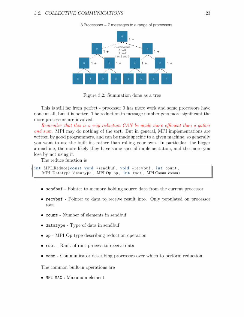
MPI does not guarantee how reduce is implemented, only that it will give theexpected result. It can3 implement something more efficient than the gather and sum.In the case of a sum, it is transitive, i.e. (a + b) + (b + c) = a + b + c + d regardlessof the bracketing. One possibility is to build a tree of processors and do partial sums.This reduces the number of messages and distributes the effort of summation acrossprocessors. Also, no processor ever holds more than two data items, which can be usefulif memory is short or items are large. The next picture shows how this works.
3Note, “can”, there is no guarantee of anything
3.2. COLLECTIVE COMMUNICATIONS 23
Figure 3.2: Summation done as a tree
This is still far from perfect - processor 0 has more work and some processors havenone at all, but it is better. The reduction in message number gets more significant themore processors are involved.
Remember that this is a way reduction CAN be made more efficient than a gatherand sum. MPI may do nothing of the sort. But in general, MPI implementations arewritten by good programmers, and can be made specific to a given machine, so generallyyou want to use the built-ins rather than rolling your own. In particular, the biggera machine, the more likely they have some special implementation, and the more youlose by not using it.
The reduce function is
1 int MPI Reduce ( const void ∗ sendbuf , void ∗ recvbuf , int count ,MPI Datatype datatype , MPI Op op , int root , MPI Comm comm)
• sendbuf - Pointer to memory holding source data from the current processor
• recvbuf - Pointer to data to receive result into. Only populated on processorroot
• count - Number of elements in sendbuf
• datatype - Type of data in sendbuf
• op - MPI Op type describing reduction operation
• root - Rank of root process to receive data
• comm - Communicator describing processors over which to perform reduction
The common built-in operations are
• MPI MAX : Maximum element
24 CHAPTER 3. BASICS OF COMMUNICATION
• MPI MIN : Minimum element
• MPI SUM : Sum all elements
• MPI PROD : Multiply all elements
• MPI LAND : Logical AND all elements
• MPI LOR : Logical OR all elements
• MPI BAND : Bitwise AND all elements
• MPI BOR : Bitwise OR all elements
It is also possible to create custom ones as well but that is unusual and a bit tricky.A closely related operation is the MPI Allreduce which is a reduce putting the result
onto all processors. This has a much higher comms requirement than plain reduce, soshould be used only when needed.
3.2.3 Dart program with a reduce
Using reduce, the program gets rather simpler, since we have to do less manually:
1 int main ( int argc , char ∗∗ argv ) {2 int count = 0 , index ;3 double d1 , d2 ;4
5 int rank , nproc , c oun t g l oba l ;6 MPI Init(&argc , &argv ) ;}7 MPI Comm rank(MPI COMM WORLD, &rank ) ;8 MPI Comm size (MPI COMM WORLD, &nproc ) ;9 s eed rng ( rank ) ;
10 for ( index =0; index<ITS;++index ) {11 /∗ random numbers between 1 ∗/12 d1=get random in range ( ) ;13 d2=get random in range ( ) ;14 i f ( d1∗d1 + d2∗d2 <= 1) count ++;15 }16 MPI Reduce(&count , &count g loba l , 1 , MPI INT , MPI SUM, 0 ,
MPI COMM WORLD) ;17 i f ( rank == 0) {18 p r i n t f (”%i ,%i\n” , count g loba l , ITS ∗ nproc ) ;19 }20 MPI Final ize ( ) ;21 }
3.3 MPI Barrier
The final really common collective operation seems to not really be communication atall - it is the MPI Barrier. This blocks (here meaning forces to wait) all processors in
3.3. MPI BARRIER 25
a communicator until they have all entered the barrier, after which the call returns andthe program can continue. This is useful to allow synchronisation of code, so that youknow all the processors are in the same place. The signature is
1 int MPI Barrier (MPI Comm comm)
• comm The communicator to block
where as usual in Fortran there is also the final error parameter.Barriers are often used after sections where only one processor (usually root) is
doing something special. That way, you can be sure the other processors aren’t racingoff and continuing their work, and you don’t need to worry as much about what mightgo wrong. It’s also really useful for debugging, where you don’t want errors from laterparts of the code to be appearing when the actual problem is with one stuck processearlier on.
Chapter 4
Point to Point Communication
4.1 Overview
The collectives we just discussed are very useful, but the most common form of MPIcomms is point-to-point. Here one processor, the source sends a message to another pro-cessor, the receiver. As well as the send command, the receiver must make a matchingreceive command. Matching will be discussed in a bit.
The most common problem you’ll likely encounter in MPI programming is deadlock-ing , where no commands can complete. This usually happens because a send occurswithout a matching receive, or a receive happens for a message that hasn’t been sent.This locks up because the default send and receive commands are blocking, so controldoesn’t return until the commands have “completed”1 We’ll show in a minute the usualproblem, where a send can’t complete until the receive line is reached, and the receiveline can’t be reached until the send completes, the programming analogue of opening acrate with the crowbar inside it.
The basic send command is
1 int MPI Send ( const void ∗buf , int count , MPI Datatype datatype , int dest ,int tag , MPI Comm comm)
• buf a buffer containing the data
• count number of elements to send
• datatype type of the elements to send
• dest which rank to send to
• tag integer code that identifies this message. Has to match in receive
• comm an MPI communicator
1We’ll come back to exactly what “completed” means, because it doesn’t quite mean that thesend-receive has finished
26
4.2. A SIMPLE EXAMPLE - THE RING PASS 27
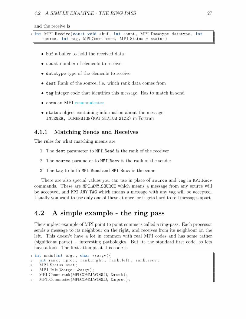
and the receive is
1 int MPI Receive ( const void ∗buf , int count , MPI Datatype datatype , intsource , int tag , MPI Comm comm, MPI Status ∗ s t a t u s )
• buf a buffer to hold the received data
• count number of elements to receive
• datatype type of the elements to receive
• dest Rank of the source, i.e. which rank data comes from
• tag integer code that identifies this message. Has to match in send
• comm an MPI communicator
• status object containing information about the message.INTEGER, DIMENSION(MPI STATUS SIZE) in Fortran
4.1.1 Matching Sends and Receives
The rules for what matching means are
1. The dest parameter to MPI Send is the rank of the receiver
2. The source parameter to MPI Recv is the rank of the sender
3. The tag to both MPI Send and MPI Recv is the same
There are also special values you can use in place of source and tag in MPI Recv
commands. These are MPI ANY SOURCE which means a message from any source willbe accepted, and MPI ANY TAG which means a message with any tag will be accepted.Usually you want to use only one of these at once, or it gets hard to tell messages apart.
4.2 A simple example - the ring pass
The simplest example of MPI point to point comms is called a ring-pass. Each processorsends a message to its neighbour on the right, and receives from its neighbour on theleft. This doesn’t have a lot in common with real MPI codes and has some rather(significant pause)... interesting pathologies. But its the standard first code, so letshave a look. The first attempt at this code is
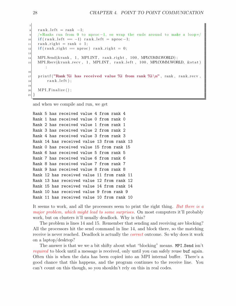
1 int main ( int argc , char ∗∗ argv ) {2 int rank , nproc , rank r i ght , r a n k l e f t , rank recv ;3 MPI Status s t a t ;4 MPI Init(&argc , &argv ) ;5 MPI Comm rank(MPI COMM WORLD, &rank ) ;6 MPI Comm size (MPI COMM WORLD, &nproc ) ;
28 CHAPTER 4. POINT TO POINT COMMUNICATION
7
8 r a n k l e f t = rank −1;9 /∗Ranks run from 0 to nproc−1, so wrap the ends around to make a loop ∗/
10 i f ( r a n k l e f t == −1) r a n k l e f t = nproc−1;11 r a n k r i g h t = rank + 1 ;12 i f ( r a n k r i g h t == nproc ) r a n k r i g h t = 0 ;13
14 MPI Send(&rank , 1 , MPI INT , rank r i ght , 100 , MPI COMM WORLD) ;15 MPI Recv(&rank recv , 1 , MPI INT , r a n k l e f t , 100 , MPI COMM WORLD, &s t a t )
;16
17 p r i n t f (”Rank %i has received value %i from rank %i\n” , rank , rank recv ,18 r a n k l e f t ) ;19
20 MPI Final ize ( ) ;21 }
and when we compile and run, we get
Rank 5 has received value 4 from rank 4
Rank 1 has received value 0 from rank 0
Rank 2 has received value 1 from rank 1
Rank 3 has received value 2 from rank 2
Rank 4 has received value 3 from rank 3
Rank 14 has received value 13 from rank 13
Rank 0 has received value 15 from rank 15
Rank 6 has received value 5 from rank 5
Rank 7 has received value 6 from rank 6
Rank 8 has received value 7 from rank 7
Rank 9 has received value 8 from rank 8
Rank 12 has received value 11 from rank 11
Rank 13 has received value 12 from rank 12
Rank 15 has received value 14 from rank 14
Rank 10 has received value 9 from rank 9
Rank 11 has received value 10 from rank 10
It seems to work, and all the processors seem to print the right thing. But there is amajor problem, which might lead to some surprises . On most computers it’ll probablywork, but on clusters it’ll usually deadlock. Why is this?
The problem is lines 14 and 15. Remember that sending and receiving are blocking?All the processors hit the send command in line 14, and block there, so the matchingreceive is never reached. Deadlock is actually the correct outcome. So why does it workon a laptop/desktop?
The answer is that we we a bit shifty about what “blocking” means. MPI Send isn’trequired to block until a message is received, only until you can safely reuse buf again.Often this is when the data has been copied into an MPI internal buffer. There’s agood chance that this happens, and the program continues to the receive line. Youcan’t count on this though, so you shouldn’t rely on this in real codes.
4.2. A SIMPLE EXAMPLE - THE RING PASS 29
There is a variant command, MPI Ssend which is guaranteed to block until themessage is received. Try this in the example - it should deadlock every time.
Similarly, MPI Recv only has to block until buf contains the correct received value.This isn’t quite the same as blocking until the receive has completed, which can happenonly once the send is completed. You can be sure that the send is complete once thematching receive has completed (remember, this doesn’t just mean the program hasmoved to the next line). Usually you don’t actually care when a send completes, justthat it has properly done so.
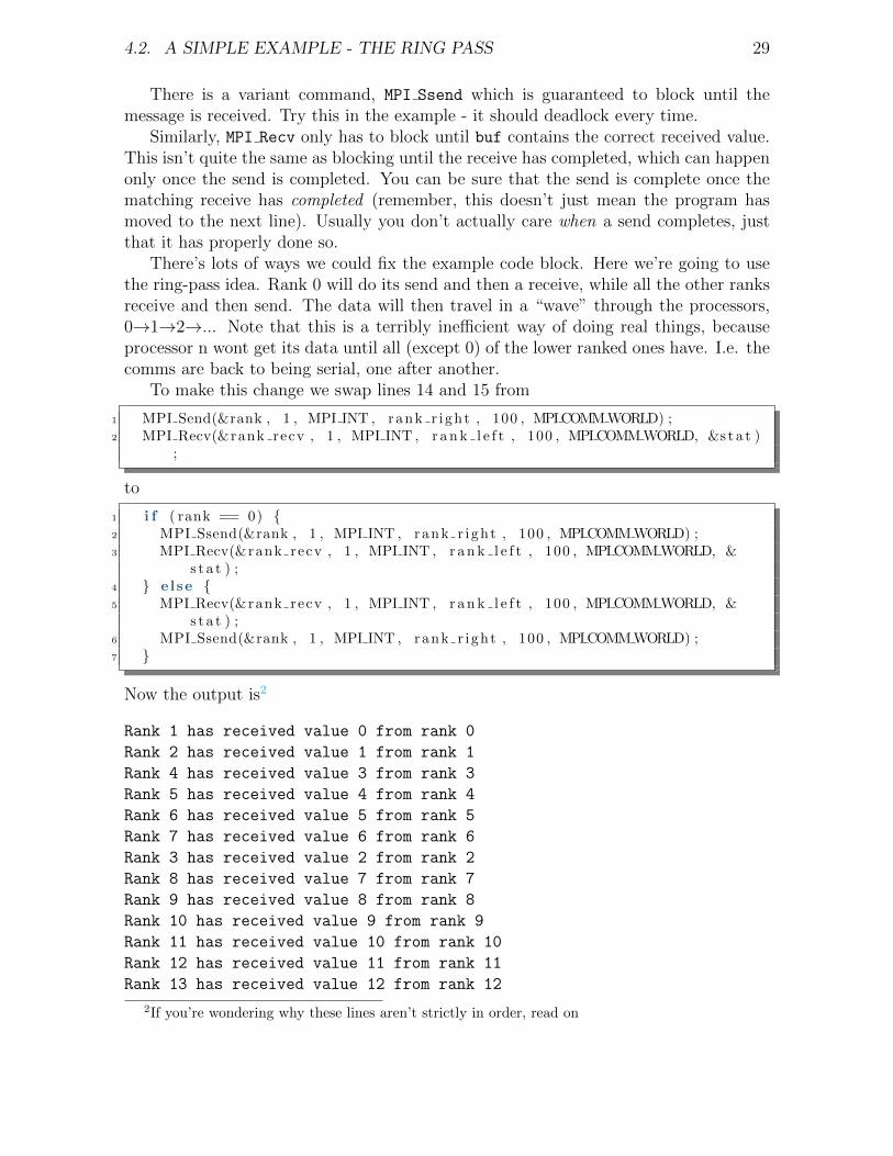
There’s lots of ways we could fix the example code block. Here we’re going to usethe ring-pass idea. Rank 0 will do its send and then a receive, while all the other ranksreceive and then send. The data will then travel in a “wave” through the processors,0→1→2→... Note that this is a terribly inefficient way of doing real things, becauseprocessor n wont get its data until all (except 0) of the lower ranked ones have. I.e. thecomms are back to being serial, one after another.
To make this change we swap lines 14 and 15 from
1 MPI Send(&rank , 1 , MPI INT , rank r i ght , 100 , MPI COMM WORLD) ;2 MPI Recv(&rank recv , 1 , MPI INT , r a n k l e f t , 100 , MPI COMM WORLD, &s t a t )
;
to
1 i f ( rank == 0) {2 MPI Ssend(&rank , 1 , MPI INT , rank r i ght , 100 , MPI COMM WORLD) ;3 MPI Recv(&rank recv , 1 , MPI INT , r a n k l e f t , 100 , MPI COMM WORLD, &
s t a t ) ;4 } else {5 MPI Recv(&rank recv , 1 , MPI INT , r a n k l e f t , 100 , MPI COMM WORLD, &
s t a t ) ;6 MPI Ssend(&rank , 1 , MPI INT , rank r i ght , 100 , MPI COMM WORLD) ;7 }
Now the output is2
Rank 1 has received value 0 from rank 0
Rank 2 has received value 1 from rank 1
Rank 4 has received value 3 from rank 3
Rank 5 has received value 4 from rank 4
Rank 6 has received value 5 from rank 5
Rank 7 has received value 6 from rank 6
Rank 3 has received value 2 from rank 2
Rank 8 has received value 7 from rank 7
Rank 9 has received value 8 from rank 8
Rank 10 has received value 9 from rank 9
Rank 11 has received value 10 from rank 10
Rank 12 has received value 11 from rank 11
Rank 13 has received value 12 from rank 12
2If you’re wondering why these lines aren’t strictly in order, read on
30 CHAPTER 4. POINT TO POINT COMMUNICATION
Rank 14 has received value 13 from rank 13
Rank 0 has received value 15 from rank 15
Rank 15 has received value 14 from rank 14
This code is working as expected, and we’ve used MPI Ssend so there’s no trickery here,this will work on any machine.
Note that the print statements are nearly in rank order, much more so than for the“simple” code. This is because of the wave propagating through the ranks. The orderisn’t perfect because print isn’t guaranteed to show in the order the processors try andprint. As we said above, this ordering really impacts performance though!
4.3 Sendrecv
Note though that this code doesn’t work on a single processor! Rank 0 has to send andreceive at the same time. This kind of both at once problem is fairly common in MPIcodes, and luckily there is a command to help!
MPI Sendrecv is a send and a receive glued together, so its signature is pretty long,but it really is just the two commands glued together:
1 int MPI Sendrecv ( const void ∗ sendbuf , int sendcount , MPI Datatypesendtype , int dest , int sendtag , void ∗ recvbuf , int recvcount ,MPI Datatype recvtype , int source , int recvtag , MPI Comm comm,MPI Status ∗ s t a t u s )
As long as both parts of the command can complete, the whole command will succeedand never deadlock.
Our example code gets much simpler using this, as we replace lines 14 and 15 withjust
1 MPI Sendrecv(&rank , 1 , MPI INT , rank r ight , 100 , &rank recv , 1 ,MPI INT , r a n k l e f t , 100 , MPI COMM WORLD, &s t a t ) ;
The output of this has all the ranks mixed up again, and we no longer have thepropagating wave of data. Performance is much better, the code works seamlessly onany number of processors and there’s no risk of deadlock. For all of these reasons, thiscommand is the preferred solution to this kind of problem.
4.4 The Story So Far
To recap, we now know how to
1. Combine data from all processors
2. Send data from one processor to another
3. Deal with the simplest class of deadlock for “send right-receive left” problems
This is plenty to get started, so on to some actual parallel code!
Chapter 5
Domain Decomposition Models
5.1 Motivation
In a working MPI program you effectively want to make your program act as thoughthere was one very powerful processor, and to ignore, as far as possible, that the work isbeing done by many processors. Remember “Embarrassing Parallelism”? That’s whereyou simply don’t care that there are many processors, because once you’ve assignedthem their tasks, they work alone, never needing to communicate with each other atall.
As we said though, that’s rarely the case in practice, and we usually need to find away to split up (decompose) our problem to make the tasks as independent as possible.We want to minimise the amount of MPI code we need to write, and minimise theamount of communication we need to do, so that most of the time our processors arehappily working away.
How we can, or should, do this depends very much on the problem at hand. In thischapter, we’re mainly going to focus on the most common situation, where we can splitup the problem so that each processor does the same tasks on different data. In thenext chapter, we’re going to talk about the other option, where one processor is special.
5.2 What is Domain Decomposition
Domain decomposition means splitting up the domain (“space”) of your problem intochunks, and working on each chunk separately (usually one per processor). Here,“space” often means physical space, dividing into regions, but it can also mean mo-mentum, energy or anything where you can work on different values independently.
When decomposing in space, you usually have a large array covering the entiredomain, and divide it into pieces, giving one to each processor, and use MPI messages tosend data that a processor needs from others around. In particular, you’re usually doingsomething to keep processors “in sync”, because ordinarily each must proceed one step(timestep, iteration etc) and can only go to the next step after some communications.
To work well, domain decomposition requires that your algorithm be local. This
31
32 CHAPTER 5. DOMAIN DECOMPOSITION MODELS
means the updates to one element depend only on those nearby.
5.2.1 Algorithms which Work Well
There are, happily, lots of algorithms like this. For instance, numerical derivativesrequire anything from one neighbouring cell (giving Euler’s method, https://en.
wikipedia.org/wiki/Euler_method) up to an arbitrary but fixed number (the en-tire family of Runge-Kutta methods https://en.wikipedia.org/wiki/Runge-Kutta_methods). All of these are examples of finite difference schemes, where a finite numberof grid cells give enough information to approximate a local derivative.
Finite-volume (roughly flux conservation) and finite-element methods are also amenable,as are many iterative matrix inversion schemes for certain inputs1, (Jacobi https:
//en.wikipedia.org/wiki/Jacobi_method , Gauss-Seidel https://en.wikipedia.
org/wiki/Gauss-Seidel_method (with extra care)).
5.2.2 Algorithms that Don’t Work Well
Any algorithm without locality wont work well. This doesn’t mean they wont workat all, but they can be very difficult to make work well. For instance, direct matrixinversion (e.g. Gaussian Elimination) or inversion of general matrices rely on all otherelements of the array. Fourier transforms also cannot be done piecewise, which meansspectral methods are mostly unpromising.
5.2.3 Nice Systems Without a Grid
Note that you don’t need to have a grid to be able to domain decompose. If you’recalculating pairwise interactions between particles you can consider only some numberof nearest neighbours, which is again a form of locality. Tree based schemes like Barnes-Hutt find ways to extend this by using less data from further away2. Some mesh freeschemes can work too (Mesh Free Galerkin etc.)
However all of these are generally messier and not as illuminating, so here we’refocusing on a simple grid based scheme.
Memory and Arrays
Behind the scenes, computer memory is one dimensional. Memory locationshave an address, which is a single number.a If your program uses a 2-Dor more array, this has to be somehow mapped into 1-D. C programmersmay already be familiar with this, as really flexible multi-dimensional arraysare usually created from a 1-D array and a function to work out the proper
1Strictly, Jacobi iteration depends on every other element in the array, but for e.g. a tri-diagonalmatrix only local elements are non-zero
2Roughly Barnes-Hutt averages far away particles together - more coarsely the further away youare
5.3. BASIC PRINCIPLE 33
location. For our purposes, what matters is that two elements that are besideeach other in the real array may not be beside each other (contiguous) inmemory.Programming languages differ by whether they keep the rows, or the columnscontiguous. In fact, C and Fortran take the opposite conventions on this!See https://en.wikipedia.org/wiki/Row-_and_column-major_order forsome details. For now, just bear in mind that taking a section of an arraywill not, in general, give you a single block of memory, and that this canmatter when you’re splitting up, or patching together, arrays.
aThis is greatly simplified, but if you know enough to know it is wrong, you shouldalready understand memory layouts.
5.3 Basic Principle
In practice domain decomposition for grid based schemes is rather simple. Ratherthan having one big array, dimensions (nx, ny) you have N arrays on N processors each(nx local, ny local). Remember that the big array doesn’t actually exist anywhere.Also, remember that the local sizes don’t have to be the same in general, but things aremuch easier if your sub-domains meet corner to corner (in 2-D think of dividing witha single line running all the way from one side of your domain to the other - you canvary the distance between the lines, but they always run straight all the way across).
Note that there are parallel schemes called Partitioned Global Address Space schemesthat do have the whole big array existing. These are less common than MPI and itsoften harder to write performant code that way.
5.4 A “Simple” Example
Imagine updating each element of your array using
temp [ i ] [ j ] = (u [ i +1] [ j ] + u [ i −1] [ j ] + u [ i ] [ j +1] + u [ i ] [ j −1 ] ) /4 . 0 ;
where once you’ve filled every element of temp you copy it back into u. This schemesimply smooths u in space over the 4 points immediately adjacent (notice u[i][j]
doesn’t appear). This uses only the current point and the points immediately adjacent,so it’s definitely local.
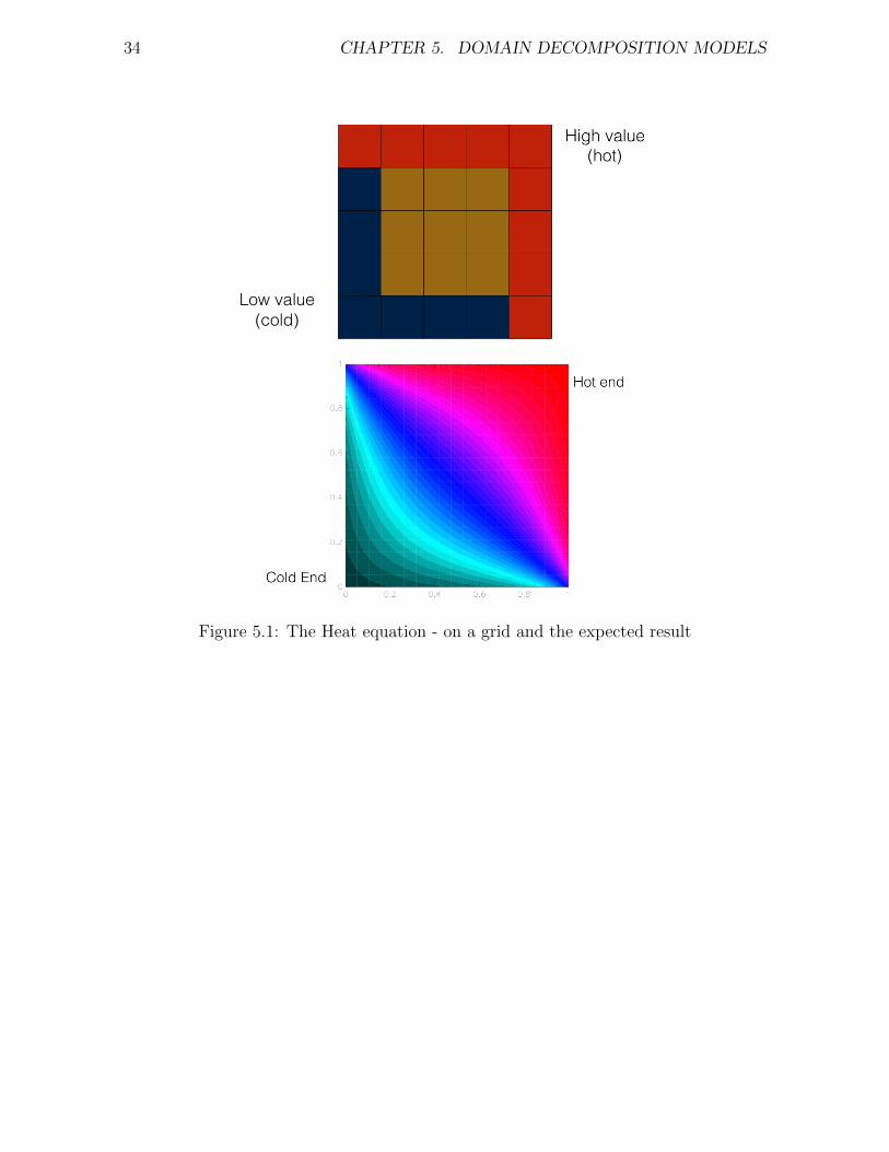
Actually, the scheme above can also be used to iteratively solve the heat equationusing the Jacobi method. This is a static problem (not changing in time) where we’reiterating towards the correct solution, not moving on in time. We’re going to use thisas an example. The following figure (5.1) shows the heat equation set up so that wehave a square of metal, with the bottom and left edges being held at a fixed, cold,temperature, and the top and right edges held at a fixed, higher temperature. Thesolution is a heat distribution as in the bottom panel of the figure, with smooth curvesshowing the lines of equal temperature, with pale blue coldest and red hottest.
34 CHAPTER 5. DOMAIN DECOMPOSITION MODELS
Figure 5.1: The Heat equation - on a grid and the expected result
5.5. SPLITTING THE DOMAIN 35
5.5 Splitting the Domain
5.5.1 Ghost or Guard Cells
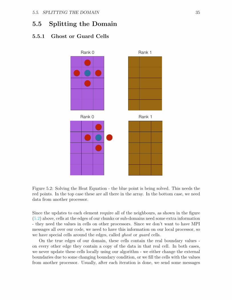
Figure 5.2: Solving the Heat Equation - the blue point is being solved. This needs thered points. In the top case these are all there in the array. In the bottom case, we needdata from another processor.
Since the updates to each element require all of the neighbours, as shown in the figure(5.2) above, cells at the edges of our chunks or sub-domains need some extra information- they need the values in cells on other processors. Since we don’t want to have MPImessages all over our code, we need to have this information on our local processor, sowe have special cells around the edges, called ghost or guard cells.
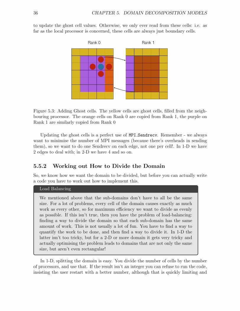
On the true edges of our domain, these cells contain the real boundary values -on every other edge they contain a copy of the data in that real cell. In both cases,we never update these cells locally using our algorithm - we either change the externalboundaries due to some changing boundary condition, or we fill the cells with the valuesfrom another processor. Usually, after each iteration is done, we send some messages
36 CHAPTER 5. DOMAIN DECOMPOSITION MODELS
to update the ghost cell values. Otherwise, we only ever read from these cells: i.e. asfar as the local processor is concerned, these cells are always just boundary cells.
Figure 5.3: Adding Ghost cells. The yellow cells are ghost cells, filled from the neigh-bouring processor. The orange cells on Rank 0 are copied from Rank 1, the purple onRank 1 are similarly copied from Rank 0
Updating the ghost cells is a perfect use of MPI Sendrecv. Remember - we alwayswant to minimise the number of MPI messages (because there’s overheads in sendingthem), so we want to do one Sendrecv on each edge, not one per cell!. In 1-D we have2 edges to deal with; in 2-D we have 4 and so on.
5.5.2 Working out How to Divide the Domain
So, we know how we want the domain to be divided, but before you can actually writea code you have to work out how to implement this.
Load Balancing
We mentioned above that the sub-domains don’t have to all be the samesize. For a lot of problems, every cell of the domain causes exactly as muchwork as every other, so for maximum efficiency we want to divide as evenlyas possible. If this isn’t true, then you have the problem of load-balancing:finding a way to divide the domain so that each sub-domain has the sameamount of work. This is not usually a lot of fun. You have to find a way toquantify the work to be done, and then find a way to divide it. In 1-D thelatter isn’t too tricky, but for a 2-D or more domain it gets very tricky andactually optimising the problem leads to domains that are not only the samesize, but aren’t even rectangular!
In 1-D, splitting the domain is easy. You divide the number of cells by the numberof processors, and use that. If the result isn’t an integer you can refuse to run the code,insisting the user restart with a better number, although that is quickly limiting and
5.5. SPLITTING THE DOMAIN 37
pretty annoying. A better option is to allow the size of domains to vary a bit so itfits (allow one more or less cell on some blocks). This can affect performance, but aslong as the domains aren’t very small it usually doesn’t matter much. If it really doesmatter, your only real option is to resize the domain to whatever you think is the mostsuitable size (largest divisible domain smaller than that asked for, or smallest possiblelarger than the one asked for).
In 2-D you have a trickier problem, since you have to decide how to arrange theprocessors into a grid. You can split in only one direction, but this often doesn’t performwell, and limits the maximum number of processors you can use (1 per cell in the splitdimension). We discuss why it doesn’t perform too well in the next section.
So, first we have to work out how to arrange N processors into a grid of (L , M), sothat L ∗M = N and L and M are somehow optimal. In 3-D we need one more split, soa grid of (K, L , M) with the same restrictions. You can calculate this yourself, butit’s easier not to worry about for now, unless your domain is oddly shaped.
5.5.3 MPI Dims create
MPI provides a function to do the splitting for the general case, where your wholeproblem is “pretty much square”, namely MPI Dims create. This has the signature
MPI Dims create ( i n t nnodes , i n t ndims , i n t dims [ ] )
• nnodes - Number of processors (from MPI Comm size)
• ndims - Number of dimensions that you want to decompose in (2D, 3D etc.)
• dims - Returned array containing numbers of processors in each dimension
Called with ndims = 2, MPI Dims create will give you an (L, M) decompositionof your N processors which is as close to square as possible i.e. both L and M are asclose as possible to SqrtN. This isn’t guaranteed to be optimal, but its one less thing toworry about. If your domain is really long and thin, this definitely isn’t optimal, butit will always work.
5.5.4 Domain Shapes
In any distributed system you want to spend as much time computing as possible andas little time communicating. Since you compute over the volume of a domain, andcommunicate along the edges, this means you want a lot of cells inside the domain, andas few as possible around the edges. Formally, you want to minimise the surface-areato volume ratio of your domains. This means keeping the subdomains as square aspossible.
38 CHAPTER 5. DOMAIN DECOMPOSITION MODELS
Surface Area to Volume Ratio
In 2-D, you might recall that a circle is the absolute best surface area tovolume ratio. Since we’re talking about rectangular grids, we’re restricted toonly horizontal and vertical lines (i.e. some sort of rectangle). Non rectan-gular grids do exist, but frankly they’re a nightmare.The surface area of a rectangle of size a by b is its circumference, namelyC = 2(a + b). Its volume is V = a ∗ b. If we start with a = b and fix Cit’s not hard to show that the volume can only decrease, so this definitelymaximises the ratio (let a→ a+ n then V → V − n2). So the best shape isas square as possible.
With that in mind, you can work out the optimal (L, M) split for your actualdomain, of size (x, y). You want the ratio of number of processors to number ofgrid cells to be as equal as possible in the two cases. Generally, this means minimisingx/L−y/M subject to L∗M = N AND x/L and y/M are both integers. That is... not soeasy. In the general case, any solution is impossible (imagine x and y both prime), andthe only possibility is to let the domains be different sizes. Even when exact division ispossible, minimising may require trying every combination of L and M. Once you allowdifferently sized domains,the problem changes to one of load-balancing and you mustquantify the load in a grid-cell and find some way of making a 1-D load curve out ofyour 1, 2 or 3 dimensional domain.
5.6 Arranging the Processors
So, one way or another, we now have a division of processors into an L x M grid. Nowwe need to divide our array(s) in a way consistent with that.
5.6.1 Matching Edges
At simplest level, what you’re worried about here is correctly matching the edges. Fig.. shows the entire array, and two ways we could distribute it across 4 processors.Processor 1 communicates its left-hand edge to the processor logically on its left, andits bottom edge to the processor logically below it. In the first case, this works perfectly.In the second case, processor 1 actually has the bottom left corner, so shouldn’t sendthe bottom or left edges anywhere, so we end up with nonsense.

5.6. ARRANGING THE PROCESSORS 39
Figure 5.4: Dividing a domain across processors. The middle panel shows how to giveeach processor a section so that things work. The bottom panel shows how to makenonsense.
40 CHAPTER 5. DOMAIN DECOMPOSITION MODELS
5.6.2 Real World Problems - Fabric Topology
In real MPI codes, we also have to think about how the actual computer works. Some-times, some processors are “nearer” (in some way) to your current processor than otherprocessors in the communication network.
Incidentally, being physically nearer is part of this - imagine a 3GHz processor.Each instruction takes 1 ns. This is the time taken for light in a vacuum to travelabout 33 cm. Electrical signal in cables, or light in optical cables is usually travellingat 0.3 to 0.8 light speed.3 So physical processors 1 m apart need between 4 and 10 nsjust for the light-travel time.
Since we’re only communicating with neighbouring processors, it makes sense toarrange processors so that communication is with processors nearby. MPI providessome functions to help with this, which may take account of all sorts of properties ofthe underlying computer fabric, such as which cores may be on the same node andwhich nodes are physically close. Note that this is all possible but not guaranteed.MPI implementations can do all sorts of optimisations, or they may not.
The helper functions fall into two families:
• MPI Cart * - Several routines for dealing with Cartesian topology (what I justdescribed)
• MPI Graph * - Several routines for dealing with arbitrary topologies described asgraphs
These are very useful, but add 3 or 4 new commands and quite a bit of complexity sowe’re going to ignore them here, except to tell you that they exist. They will be coveredin our (future) intermediate MPI workshops.
5.6.3 Manual Calculation
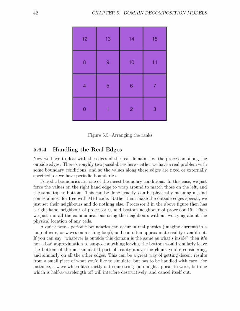
In these notes we’re just going to arrange our processors into a simple grid, and numberthem from bottom left to top right. We’re going to go through the first index we gotfrom MPI Dims create first, and call that x. Once we run out of processors in thisdirection, we’ll increment the second dimension, y.
Modulo Arithmetic
Doing the decomposition calculations yourself isn’t hard, it just requires a bitof modulo arithmetic. If this is unfamiliar, think of converting from Minutesinto Hours and Minutes. Every block of 60 minutes is an hour, so we needto know how many whole hours fit, and how many minutes are left over.The equations below do precisely this, but for rows and columns. Our y
3In fibre optics this is a combination of refractive index and longer path length, due to propagationin a wave guide.
5.6. ARRANGING THE PROCESSORS 41
co-ordinate is how many whole rows fit into our rank. The x co-ordinate ishow many cells are left over. So we calculate the whole rows (hours) first.Then we take this away, and see how many cells into that row (minutes) areleft.Say we’re looking at 164 minutes (processor with rank 164). We first workout FLOOR(164/60) = FLOOR(2.733...) I.e. the largest integer less than2.733..., which is 2. So this processor has y-coordinate of 2. Then we have164− 60 ∗ 2 = 164− 120 = 44 minutes left, i.e. x-coordinate of 44.
In full, the equations in 2-D are4
coords y = FLOOR( rank / nprocx )coords x = rank − coords y ∗ nprocx
Now you also need to find the ranks of your direct neighbours, since you’ll needthem to communicate. This is actually a bit easier. From the following image, we cantell that
• Processor to left has rank 1 lower
• Processor to right has rank 1 higher
• Processor upwards has rank nproc x higher
• Processor downwards has rank nproc x lower
4Floor means take the largest integer (whole number) which is less than the argument you give it.I.e. FLOOR(100/60) = FLOOR(1.66) = 1. For positive numbers, this means just dropping the decimalpart (truncating). For negative numbers, you still want the largest Integer less than the argument.I.e. -2 ¡ -1.66 ¡ -1, so FLOOR(-1.66) = 2. The opposite of FLOOR is CEIL or CEILING, the smallestInteger greater than the argument.
42 CHAPTER 5. DOMAIN DECOMPOSITION MODELS
Figure 5.5: Arranging the ranks
5.6.4 Handling the Real Edges
Now we have to deal with the edges of the real domain, i.e. the processors along theoutside edges. There’s roughly two possibilities here - either we have a real problem withsome boundary conditions, and so the values along these edges are fixed or externallyspecified, or we have periodic boundaries.
Periodic boundaries are one of the nicest boundary conditions. In this case, we justforce the values on the right hand edge to wrap around to match those on the left, andthe same top to bottom. This can be done exactly, can be physically meaningful, andcomes almost for free with MPI code. Rather than make the outside edges special, wejust set their neighbours and do nothing else. Processor 3 in the above figure then hasa right-hand neighbour of processor 0, and bottom neighbour of processor 15. Thenwe just run all the communications using the neighbours without worrying about thephysical location of any cells.
A quick note - periodic boundaries can occur in real physics (imagine currents in aloop of wire, or waves on a string loop), and can often approximate reality even if not.If you can say “whatever is outside this domain is the same as what’s inside” then it’snot a bad approximation to suppose anything leaving the bottom would similarly leavethe bottom of the not-simulated part of reality above the chunk you’re considering,and similarly on all the other edges. This can be a great way of getting decent resultsfrom a small piece of what you’d like to simulate, but has to be handled with care. Forinstance, a wave which fits exactly onto our string loop might appear to work, but onewhich is half-a-wavelength off will interfere destructively, and cancel itself out.
5.7. QUICK RECAP 43
MPI PROC NULL
For real (non-periodic) boundaries, we want to make sure the values they have for theirneighbours are special. MPI provides a special constant, a null (not simply the numberzero) rank. This is the value MPI PROC NULL. This lets us tell that those processors haveno neighbours, but actually is much more helpful. Passed to any MPI send or receivecommands, this value turns the operation into a null operation (no-op), so we don’teven need to test for it in these cases. The command is perfectly valid, but doesn’tsend or receive anything.
For the special Sendrecv command we can use this for either (or both) ranks (eitherrank recv, and/or rank send) and the relevant half of the command becomes a no-op.If given to only one half, then the other half works as normal.
Note that MPI PROC NULL is not valid as the rank of the root process in a gather,reduce etc commands and will cause runtime failure.
5.6.5 Calculating the Real Coordinates
The last step we need is to calculate which part of the “virtual” (not existing itselfanywhere in memory) global array a given processor has. That is, we need to divide upour co-ordinates. This is pretty easy since we’ve done most of the hard bits now.
We’re looking for the number of cells in each local bit of the array nx local, as wellas the local start and end part on each processor.
n x l o c a l = nx / nproc xx c e l l m i n l o c a l = n x l o c a l ∗ coords xx c e l l m a x l o c a l = n x l o c a l ∗ ( coords x + 1) − 1
Here coords x is the position we found earlier (Section 5.6.3). Note that these valuesare the offsets from the start of the array, so in Fortran where arrays start at 1 we haveto add 1 to both values to get the array index.
The calculation in y is identical, swapping all the x for y.Do note that you only need to know about this local position when you’re setting
up the initial values (initial conditions) or bringing your sections back together foroutput. Otherwise, all of the computation should work with local arrays (and anyaxes or physical coordinates required). Remember, (Section 5.1) as far as possible theprocessors shouldn’t know they’re part of a larger problem. They need to know whotheir neighbours are for the comms, but for the core calculation, they shouldn’t reallycare.
5.7 Quick Recap
To recap what we’ve worked out so far:
• The domain is decomposed onto the required number of processors
• We know how the “virtual global” array maps onto our original array
44 CHAPTER 5. DOMAIN DECOMPOSITION MODELS
• We know which processors are neighbours to our current processor
• We’ve set up some ghost or guard cells so each processor has all of the informationit needs
Now we need to actually do the sends and receives. The idea of this is pretty obvious.We’ve set up the ghost cells, so all we have to do is make sure they contain the correctdata, and then our calculations can proceed as usual.
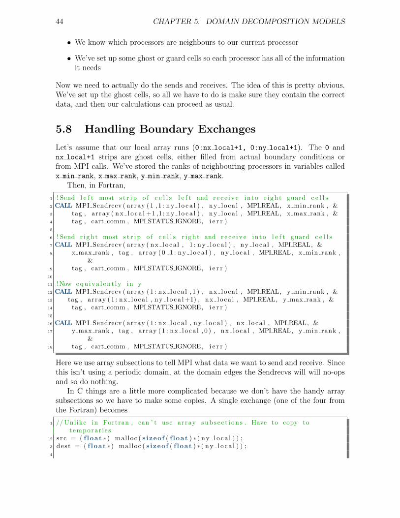
5.8 Handling Boundary Exchanges
Let’s assume that our local array runs (0:nx local+1, 0:ny local+1). The 0 andnx local+1 strips are ghost cells, either filled from actual boundary conditions orfrom MPI calls. We’ve stored the ranks of neighbouring processors in variables calledx min rank, x max rank, y min rank, y max rank.
Then, in Fortran,
1 ! Send l e f t most s t r i p o f c e l l s l e f t and r e c e i v e in to r i g h t guard c e l l s2 CALL MPI Sendrecv ( array ( 1 , 1 : n y l o c a l ) , ny l o ca l , MPI REAL, x min rank , &3 tag , array ( n x l o c a l +1 ,1: n y l o c a l ) , ny l o ca l , MPI REAL, x max rank , &4 tag , cart comm , MPI STATUS IGNORE, i e r r )5
6 ! Send r i g h t most s t r i p o f c e l l s r i g h t and r e c e i v e in to l e f t guard c e l l s7 CALL MPI Sendrecv ( array ( nx l o ca l , 1 : n y l o c a l ) , ny l o ca l , MPI REAL, &8 x max rank , tag , array ( 0 , 1 : n y l o c a l ) , ny l o ca l , MPI REAL, x min rank ,
&9 tag , cart comm , MPI STATUS IGNORE, i e r r )
10
11 !Now e q u i v a l e n t l y in y12 CALL MPI Sendrecv ( array ( 1 : nx l o ca l , 1 ) , nx l o ca l , MPI REAL, y min rank , &13 tag , array ( 1 : nx l o ca l , n y l o c a l +1) , nx l o ca l , MPI REAL, y max rank , &14 tag , cart comm , MPI STATUS IGNORE, i e r r )15
16 CALL MPI Sendrecv ( array ( 1 : nx l o ca l , n y l o c a l ) , nx l o ca l , MPI REAL, &17 y max rank , tag , array ( 1 : nx l o ca l , 0 ) , nx l o ca l , MPI REAL, y min rank ,
&18 tag , cart comm , MPI STATUS IGNORE, i e r r )
Here we use array subsections to tell MPI what data we want to send and receive. Sincethis isn’t using a periodic domain, at the domain edges the Sendrecvs will will no-opsand so do nothing.
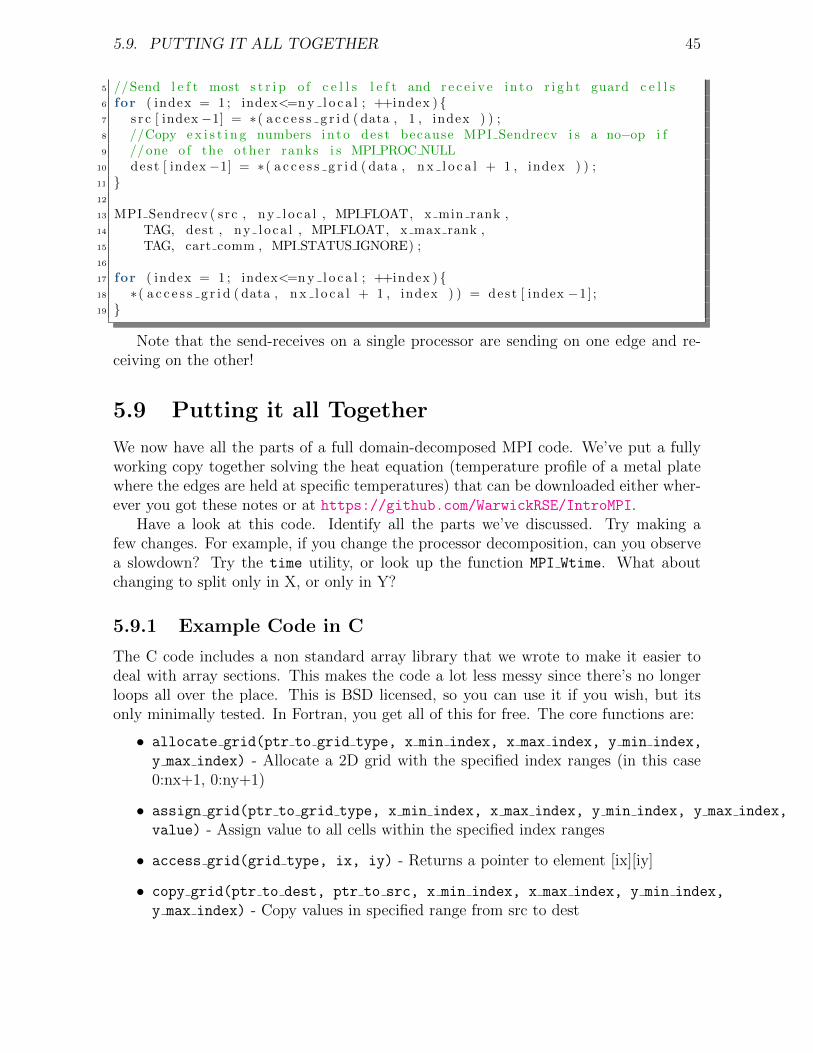
In C things are a little more complicated because we don’t have the handy arraysubsections so we have to make some copies. A single exchange (one of the four fromthe Fortran) becomes
1 // Unl ike in Fortran , can ’ t use array s u b s e c t i o n s . Have to copy totemporar i e s
2 s r c = ( f loat ∗) mal loc ( s izeof ( f loat ) ∗( n y l o c a l ) ) ;3 dest = ( f loat ∗) mal loc ( s izeof ( f loat ) ∗( n y l o c a l ) ) ;4
5.9. PUTTING IT ALL TOGETHER 45
5 //Send l e f t most s t r i p o f c e l l s l e f t and r e c e i v e in to r i g h t guard c e l l s6 for ( index = 1 ; index<=n y l o c a l ; ++index ) {7 s r c [ index −1] = ∗( a c c e s s g r i d ( data , 1 , index ) ) ;8 //Copy e x i s t i n g numbers in to des t because MPI Sendrecv i s a no−op i f9 // one o f the other ranks i s MPI PROC NULL
10 dest [ index −1] = ∗( a c c e s s g r i d ( data , n x l o c a l + 1 , index ) ) ;11 }12
13 MPI Sendrecv ( src , ny l o ca l , MPI FLOAT, x min rank ,14 TAG, dest , ny l o ca l , MPI FLOAT, x max rank ,15 TAG, cart comm , MPI STATUS IGNORE) ;16
17 for ( index = 1 ; index<=n y l o c a l ; ++index ) {18 ∗( a c c e s s g r i d ( data , n x l o c a l + 1 , index ) ) = dest [ index −1] ;19 }
Note that the send-receives on a single processor are sending on one edge and re-ceiving on the other!
5.9 Putting it all Together
We now have all the parts of a full domain-decomposed MPI code. We’ve put a fullyworking copy together solving the heat equation (temperature profile of a metal platewhere the edges are held at specific temperatures) that can be downloaded either wher-ever you got these notes or at https://github.com/WarwickRSE/IntroMPI.
Have a look at this code. Identify all the parts we’ve discussed. Try making afew changes. For example, if you change the processor decomposition, can you observea slowdown? Try the time utility, or look up the function MPI Wtime. What aboutchanging to split only in X, or only in Y?
5.9.1 Example Code in C
The C code includes a non standard array library that we wrote to make it easier todeal with array sections. This makes the code a lot less messy since there’s no longerloops all over the place. This is BSD licensed, so you can use it if you wish, but itsonly minimally tested. In Fortran, you get all of this for free. The core functions are:
• allocate grid(ptr to grid type, x min index, x max index, y min index,
y max index) - Allocate a 2D grid with the specified index ranges (in this case0:nx+1, 0:ny+1)
• assign grid(ptr to grid type, x min index, x max index, y min index, y max index,
value) - Assign value to all cells within the specified index ranges
• access grid(grid type, ix, iy) - Returns a pointer to element [ix][iy]
• copy grid(ptr to dest, ptr to src, x min index, x max index, y min index,
y max index) - Copy values in specified range from src to dest
Chapter 6
Worker Controller Models
6.1 Motivation
After Domain Decomposition, the next most common approach for MPI programs isthe worker-controller approach, also called master-slave. Here one processor is in chargeof handing out work packages to all of the others, which do their work and then eitherask for more, or finish.
It is possible to have the controller processor also be a worker, but this makes theMPI more complex. In particular, you have to make sure the controller is doling outthe work packages fast enough that the workers aren’t sitting idle, or you’ll lose morefrom this than you gain from the work done on the controller process. We’re not goingto consider this for the main part of this chapter, but we give a brief discussion of thefunctions you’d need in 6.5.
6.2 Single Program Multiple Data (SPMD)
A core question in parallelising workloads is whether a program has multiple entitiesall following the same steps on different data, or whether they can be doing completelydifferent tasks, either on the same data, or different sets. See https://en.wikipedia.
org/wiki/Flynn%27s_taxonomy for details.
Single-Program Multiple-Data is pretty much the model of MPI. You write oneprogram that runs the same steps on different sets of data. Obviously, in practiseyou often have e.g. rank-0 doing something a little bit “special” but this is frombranches within the code. As a counter, Multiple-Program Multiple-Data would besomething like a data-processing pipeline, where a different program carries out eachstep, transforming the data to be fed to the next step. This can be done in parallel(although with a little bit of startup latency). Alternately, a typical server-client modelis solidly MPMD.
Do note that Single-Program is a lot more general than Single-Instruction (if youhave ever heard of SIMD, or looked at the link above). Despite running the same code,different processes can be (and are) at different steps.
46
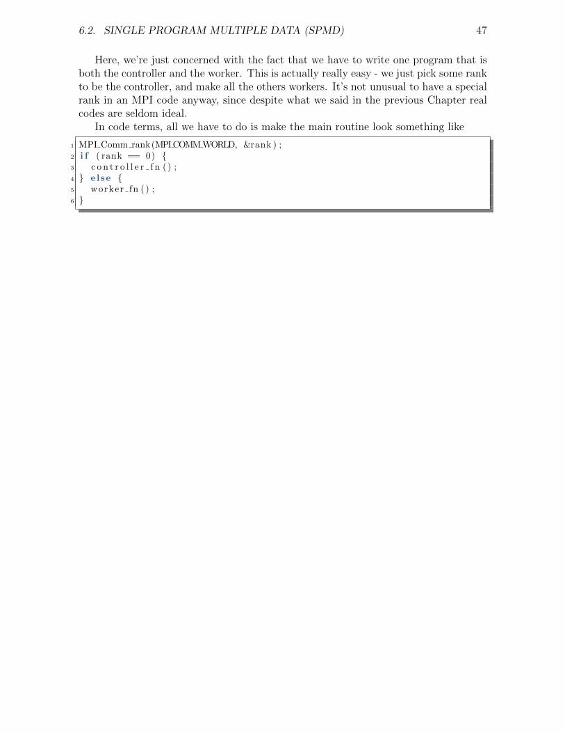
6.2. SINGLE PROGRAM MULTIPLE DATA (SPMD) 47
Here, we’re just concerned with the fact that we have to write one program that isboth the controller and the worker. This is actually really easy - we just pick some rankto be the controller, and make all the others workers. It’s not unusual to have a specialrank in an MPI code anyway, since despite what we said in the previous Chapter realcodes are seldom ideal.
In code terms, all we have to do is make the main routine look something like
1 MPI Comm rank(MPI COMM WORLD, &rank ) ;2 i f ( rank == 0) {3 c o n t r o l l e r f n ( ) ;4 } else {5 worker fn ( ) ;6 }
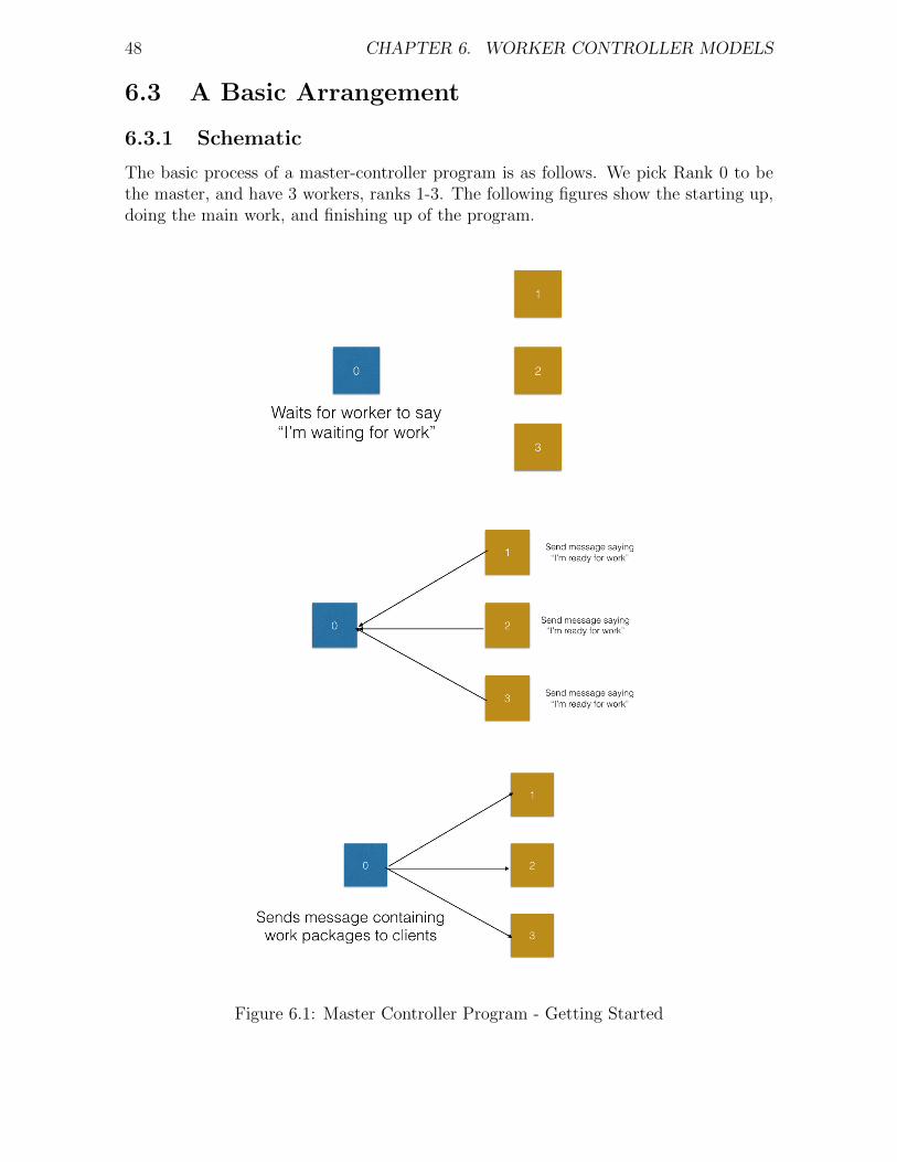
48 CHAPTER 6. WORKER CONTROLLER MODELS
6.3 A Basic Arrangement
6.3.1 Schematic
The basic process of a master-controller program is as follows. We pick Rank 0 to bethe master, and have 3 workers, ranks 1-3. The following figures show the starting up,doing the main work, and finishing up of the program.
Figure 6.1: Master Controller Program - Getting Started
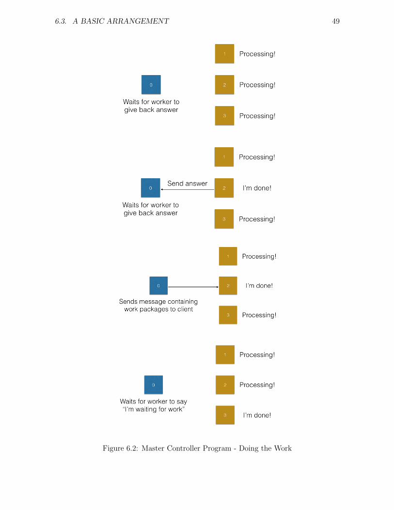
6.3. A BASIC ARRANGEMENT 49
Figure 6.2: Master Controller Program - Doing the Work
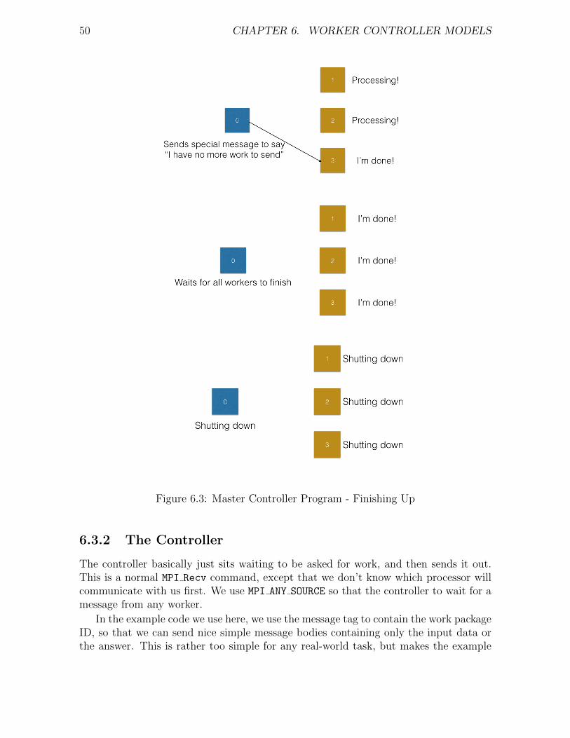
50 CHAPTER 6. WORKER CONTROLLER MODELS
Figure 6.3: Master Controller Program - Finishing Up
6.3.2 The Controller
The controller basically just sits waiting to be asked for work, and then sends it out.This is a normal MPI Recv command, except that we don’t know which processor willcommunicate with us first. We use MPI ANY SOURCE so that the controller to wait for amessage from any worker.
In the example code we use here, we use the message tag to contain the work packageID, so that we can send nice simple message bodies containing only the input data orthe answer. This is rather too simple for any real-world task, but makes the example
6.4. PITFALLS TO AVOID 51
code nice and easy. In general you would want to send a message containing somesort of data structure giving input parameters and any other information needed, andsimilarly send back a structure. However, dealing with sending these is a bit tricky -we intend to cover this in our Intermediate (or possibly Advanced) MPI course.
Since the Tag contains the ID of a work package, the controller wants to wait for amessage with any tag value, so we use the special MPI ANY TAG value in the tag field.The Receive call then looks like:
1 int data ;2 MPI Recv ( data , 1 , MPI INT , MPI ANY SOURCE, MPI ANY TAG, MPI COMM WORLD,
s t a t ) ;
6.3.3 Parsing MPI Status
In the previous chapter on domain decomposition we didn’t need to use the MPI statusobjects, since we already knew which receive came from which neighbour, and weren’tusing the tags to transmit any information. Here, we need to capture and interrogatethis to find out which processor sent the message and what the tag was. The code todo this is, in C and Fortran respectively:
1 MPI Status s ;2 p r i n t f (”source %i\n” , s .MPI SOURCE) ;3 p r i n t f (”tag %i\n” , s .MPI TAG) ;
1 INTEGER : : s (MPI STATUS SIZE)2 PRINT ∗ , ” Source ” , s (MPI SOURCE)3 PRINT ∗ , ”Tag” , s (MPI TAG)
Note that in the C code we are accessing a structure by named values, whereasin the Fortran the status is simply an array of integers, with some named constantsprovided telling us which field contains which value.1
The code in the workers is rather simpler. They simply do an MPI Send to rank0 to send results back to the controller, and an MPI Recv from rank 0 to get the nextwork package, or the message telling them there is no more data to send (via a sentinelvalue for the tag), and to shutdown.
6.4 Pitfalls to Avoid
The main pitfalls of this sort of Worker Controller code arise because it relies on allprocesses getting the messages they expect, when they expect them. This is particularlytrue of the workers, which must be told when to terminate. In particular, be careful tomake sure that your code will terminate correctly under all conditions.
The controller must send out proper messages if there aren’t any valid work packagesat all. It must keep listening even after the last work package is sent out, and only stop
1Newer MPI Fortran Bindings (2008 onwards) are extending the types to look more like the C. Thisis definitely outwith the scope of this Intro.
52 CHAPTER 6. WORKER CONTROLLER MODELS
when the last worker finishes. It must make sure to shut down all the workers beforeshutting down itself.
If you accidentally stop receiving on the controller before the last worker has sentback its result then your code won’t terminate properly. Usually, your code will thenbe killed by the wall-time limit on a cluster, but this can be up to 48 or 72 hours. Youcan easily waste a lot of core hours this way (and that can be expensive).
6.5 Non Blocking MPI
The worker-controller strategy here is a very simple one that you probably wont see inthe “real world”. Instead, you will probably see the MPI commands MPI Isend andMPI Irecv (those are capital-i’s if the font is unclear). These are special non-blockingMPI send and receive commands. They return you a MPI Request object which youcan interrogate to check on the status of the send or receive operation.
It is then up to you to make sure things have correctly happened. To do this, youneed the following commands:
• MPI Wait - Wait until a given MPI Request completes
• MPI Waitall - Wait until all of the MPI Requests in an array have completed
• MPI Waitany - Wait until any MPI Request in an array of MPI Requests hascompleted
These versions halt your code until the request is finished. As well as these, thereare the Test versions,(MPI Test, MPI Testall, MPI Testany) that return a logical flagabout the current state of an MPI Request (completed or not) rather than waiting forcompletion. These functions also all return MPI Status objects (just like MPI Recv)which allow you to check the tag, source etc of the message once it has been received.
The non-blocking commands give you a (relatively) easy way of letting rank-0 actas a worker as well as a controller. This process posts a non-blocking receive (usingMPI Irecv), does its work, and when convenient uses MPI Testany to check if any ofthe workers have completed.
Non-blocking MPI is quite a bit harder to use in general, so we aren’t going intodetails here. In particular, you have to be very careful using any temporary arrays, asthey mustn’t be changed or deallocated until the receive or send has completed. Fortranarray sections, which are effectively temporary arrays, are right out. Usually you wantto use special custom MPI types to make things more robust too.
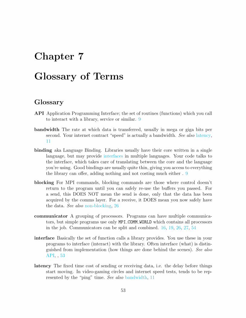
Chapter 7
Glossary of Terms
Glossary
API Application Programming Interface; the set of routines (functions) which you callto interact with a library, service or similar. 9
bandwidth The rate at which data is transferred, usually in mega or giga bits persecond. Your internet contract “speed” is actually a bandwidth. See also latency,11
binding aka Language Binding. Libraries usually have their core written in a singlelanguage, but may provide interfaces in multiple languages. Your code talks tothe interface, which takes care of translating between the core and the languageyou’re using. Good bindings are usually quite thin, giving you access to everythingthe library can offer, adding nothing and not costing much either . 9
blocking For MPI commands, blocking commands are those where control doesn’treturn to the program until you can safely re-use the buffers you passed. Fora send, this DOES NOT mean the send is done, only that the data has beenacquired by the comms layer. For a receive, it DOES mean you now safely havethe data. See also non-blocking, 26
communicator A grouping of processors. Programs can have multiple communica-tors, but simple programs use only MPI COMM WORLD which contains all processorsin the job. Communicators can be split and combined. 16, 19, 26, 27, 54
interface Basically the set of function calls a library provides. You use these in yourprograms to interface (interact) with the library. Often interface (what) is distin-guished from implementation (how things are done behind the scenes). See alsoAPI, , 53
latency The fixed time cost of sending or receiving data, i.e. the delay before thingsstart moving. In video-gaming circles and internet speed tests, tends to be rep-resented by the “ping” time. See also bandwidth, 11
53
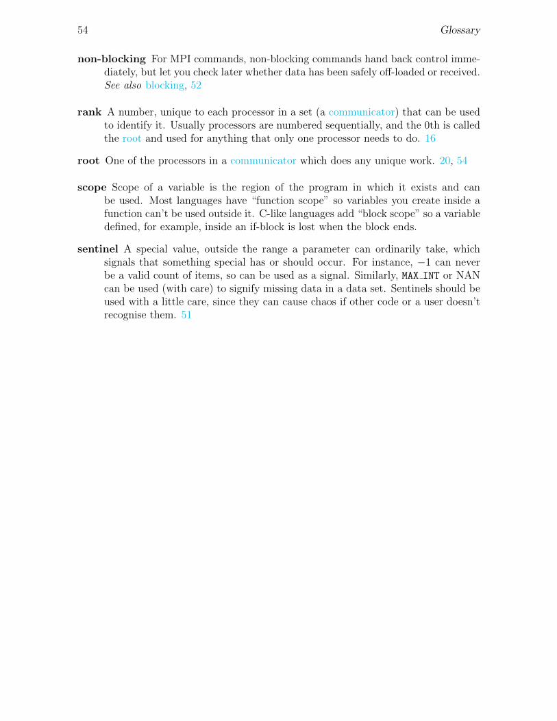
54 Glossary
non-blocking For MPI commands, non-blocking commands hand back control imme-diately, but let you check later whether data has been safely off-loaded or received.See also blocking, 52
rank A number, unique to each processor in a set (a communicator) that can be usedto identify it. Usually processors are numbered sequentially, and the 0th is calledthe root and used for anything that only one processor needs to do. 16
root One of the processors in a communicator which does any unique work. 20, 54
scope Scope of a variable is the region of the program in which it exists and canbe used. Most languages have “function scope” so variables you create inside afunction can’t be used outside it. C-like languages add “block scope” so a variabledefined, for example, inside an if-block is lost when the block ends.
sentinel A special value, outside the range a parameter can ordinarily take, whichsignals that something special has or should occur. For instance, −1 can neverbe a valid count of items, so can be used as a signal. Similarly, MAX INT or NANcan be used (with care) to signify missing data in a data set. Sentinels should beused with a little care, since they can cause chaos if other code or a user doesn’trecognise them. 51