Investigating Real-Time Sonar Performance Predictions Using

Old Dominion UniversityODU Digital Commons

Computer Science Theses & Dissertations Computer Science

Summer 2007

Investigating Real-Time Sonar PerformancePredictions Using Beowulf ClusteringCharles Lane CartledgeOld Dominion University

Follow this and additional works at: https://digitalcommons.odu.edu/computerscience_etds

Part of the Computer Sciences Commons

This Thesis is brought to you for free and open access by the Computer Science at ODU Digital Commons. It has been accepted for inclusion inComputer Science Theses & Dissertations by an authorized administrator of ODU Digital Commons. For more information, please [email protected].

Recommended CitationCartledge, Charles L.. "Investigating Real-Time Sonar Performance Predictions Using Beowulf Clustering" (2007). Master of Science(MS), thesis, Computer Science, Old Dominion University, DOI: 10.25777/w2ry-5163https://digitalcommons.odu.edu/computerscience_etds/50

https://digitalcommons.odu.edu?utm_source=digitalcommons.odu.edu%2Fcomputerscience_etds%2F50&utm_medium=PDF&utm_campaign=PDFCoverPages

https://digitalcommons.odu.edu/computerscience_etds?utm_source=digitalcommons.odu.edu%2Fcomputerscience_etds%2F50&utm_medium=PDF&utm_campaign=PDFCoverPages

https://digitalcommons.odu.edu/computerscience?utm_source=digitalcommons.odu.edu%2Fcomputerscience_etds%2F50&utm_medium=PDF&utm_campaign=PDFCoverPages

https://digitalcommons.odu.edu/computerscience_etds?utm_source=digitalcommons.odu.edu%2Fcomputerscience_etds%2F50&utm_medium=PDF&utm_campaign=PDFCoverPages

http://network.bepress.com/hgg/discipline/142?utm_source=digitalcommons.odu.edu%2Fcomputerscience_etds%2F50&utm_medium=PDF&utm_campaign=PDFCoverPages

https://digitalcommons.odu.edu/computerscience_etds/50?utm_source=digitalcommons.odu.edu%2Fcomputerscience_etds%2F50&utm_medium=PDF&utm_campaign=PDFCoverPages

mailto:[email protected]

INVESTIGATING REAL-TIME SONAR PERFORMANCE

PREDICTIONS USING BEOWULF CLUSTERING

Charles Lane Cartledge AEET June 1972, University of Alaska

BEET June 1974, Oregon Institute of Technology

A Thesis Submitted to the Faculty of Old Dominion University in Partial Fulfillment of the

Requirement for the Degree of

MASTER OF SCIENCE

COMPUTER SCIENCE

OLD DOMINION UNIVERSITY August 2007

by

Approved by:

Chester E. Grosch, Ph.D. (Director)

Alex Pothen, Ph.D. (Member)

Mohammad Zubair, Ph.D. (Member)

R eproduced with perm ission of the copyright owner. Further reproduction prohibited without perm ission.

UMI Number: 1449364

Copyright 2007 by

Cartledge, Charles Lane

All rights reserved.

INFORMATION TO USERS

The quality of this reproduction is dependent upon the quality of the copy

submitted. Broken or indistinct print, colored or poor quality illustrations and

photographs, print bleed-through, substandard margins, and improper

alignment can adversely affect reproduction.

In the unlikely event that the author did not send a complete manuscript

and there are missing pages, these will be noted. Also, if unauthorized

copyright material had to be removed, a note will indicate the deletion.

®

UMIUMI Microform 1449364

Copyright 2008 by ProQuest Information and Learning Company.

All rights reserved. This microform edition is protected against

unauthorized copying under Title 17, United States Code.

ProQuest Information and Learning Company 300 North Zeeb Road

P.O. Box 1346 Ann Arbor, Ml 48106-1346


ABSTRACT

INVESTIGATING REAL-TIME SONAR PERFORMANCE PREDICTIONS USING BEOWULF CLUSTERING

Charles Lane Cartledge Old Dominion University, 2007 Director: Dr. Chester E. Grosch

Predicting sonar performance, critical to using any sonar to its maximum effectiveness, is

computationally intensive and typically the results are based on data from the past and may not be

applicable to the current water conditions. This paper discusses how B eow ulf clustering techniques were

investigated and applied to achieve real-time sonar perform ance prediction capabilities based on

commercially off the shelf (COTS) hardware and software. A sonar system measures am bient noise in real

time. Based on the active sonar range scale, new am bient measurem ents can be available every 1 to 24

seconds. Traditional sonar performance prediction techniques operated serially and often took

approximately 120 seconds o f computing tim e per prediction. These predictions were outdated by

potentially several sonar measurements. Using B eow ulf clustering techniques, the same prediction now

takes approxim ately 2 seconds. Analysis o f measured data using a sonar hardw are suite reveals that there is

a set o f sonar system param eters where a serial approach to sonar performance prediction is more efficient

than B eowulf clustering. Using these param eters, a sonar engineer can make the best decision for system

prediction capability based on the num ber o f sonar beam s and the expected operational range. The paper

includes a discussion on the taxonom ies o f parallel com puting, the historical developm ents leading to

measuring the speed of light, and how those measurem ents enable acoustic paths to be com puted in ocean

environments.


Copyright 2007 by Charles Lane Cartledge. All rights reserved.


This thesis is dedicated to my wife and our son.


V

ACKNOWLEDGMENTS

I would like to acknowledge the support and encouragem ent o f two organizations and three individuals.

Old Dominion U niversity provided much o f the hardware and com puter software for the early investigation

into real-time sonar perform ance prediction capabilities. Along with these tangible assets, ODU created and

maintained an environm ent where ideas could be explored and where efforts that did not succeed were not

considered a failure, but rather a positive learning experience. At ODU, C om puter Science Lecturer Mr. Jay

Morris provided access to the hardware and software, acted as a sounding board and continually provided

encouragem ent in face o f seemingly overw helm ing obstacles. Also at ODU, CS student, Mr. Kenneth

Belkofer, “stood shoulder to shoulder in the trenches” to face and overcom e problem s with hardware

settings and specifications, software installation, errors in documentation, to create not one, but several

B eowulf clusters before and after the B eow ulf laboratories were moved across campus. EDO Corporation

provided access to hardware, software and engineering personnel. A crucial part to com puting a sonar’s

performance prediction is the algorithm and source code to compute the probability o f detection based on a

set o f assum ptions and measurem ents. EDO provided access to the detailed and com plex source code to

compute that probability. The code represents a significant investm ent in intellectual property and EDO

was willing to allow the code to be used to provide an authentic test environment. Mr. M ike Palmer, EDO

Corporation Hardware Engineer, worked diligently to establish a test environm ent that would mimic a

shipboard sonar system using hardware and software that is destined to be installed onboard a ship. This

hardware suite was instrum ental in defining the limits w ithin which serial sonar perform ance prediction

makes sense and beyond where B eowulf clustering was the only viable solution. This work would not have

been possible without the aid, assistance, encouragem ent and support o f these outstanding people, and I am

deeply indebted to each o f them.


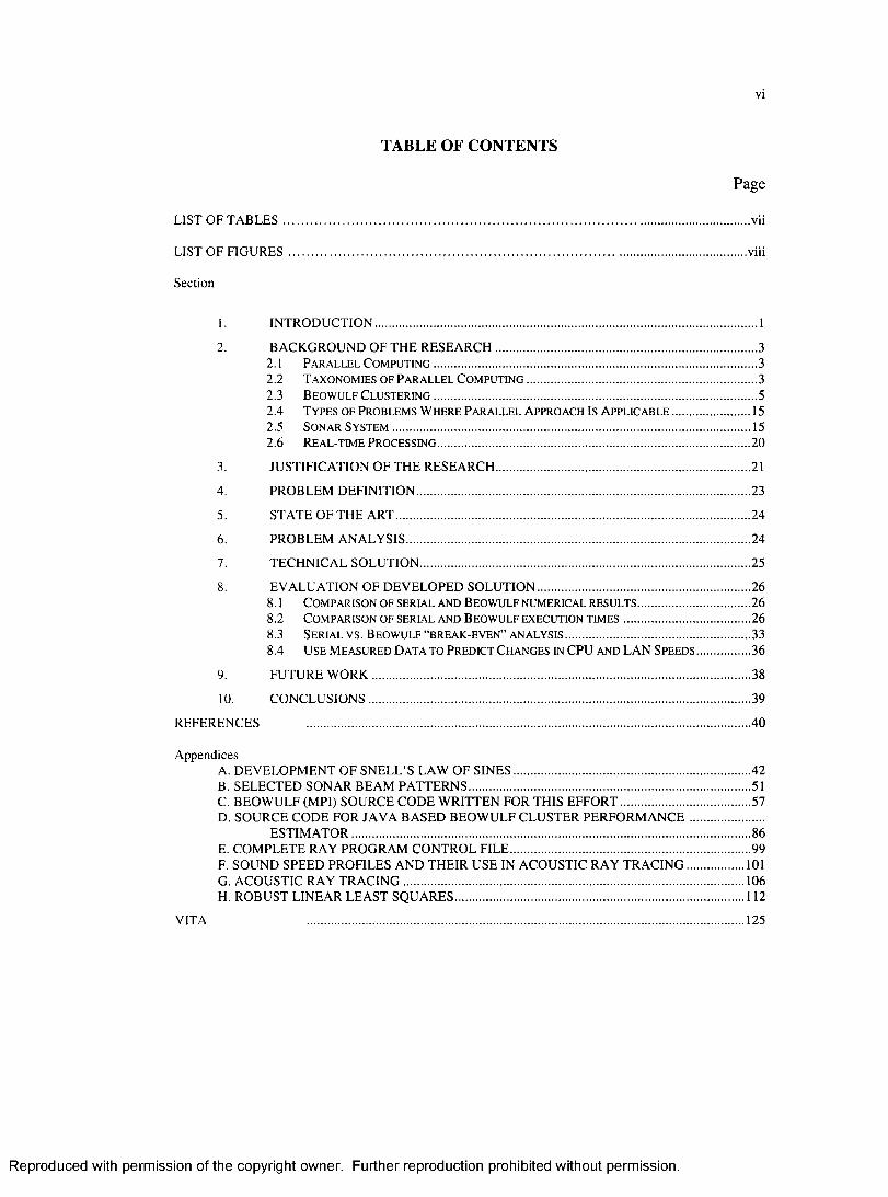
TABLE OF CONTENTS

Page

LIST OF T A B L E S ................................................................................................................................................................ vii

LIST OF FIGURES ............................................................................................................................................................. viii

Section

1. IN TRO D U C TIO N .....................................................................................................................................1

2. BACKGROUND OF THE R E S E A R C H ...........................................................................................32.1 P a r a l l e l C o m p u t i n g .................................................................................................................................32 .2 T a x o n o m ie s o f P a r a l l e l C o m p u t i n g ............................................................................................32 .3 B e o w u l f C l u s t e r i n g ................................................................................................................................ 52 .4 T y p e s o f P r o b l e m s W h e r e P a r a l l e l A p p r o a c h I s A p p l i c a b l e .................................152 .5 S o n a r S y s t e m ...............................................................................................................................................152 .6 R e a l -t im e P r o c e s s i n g ............................................................................................................................ 20

3. JUSTIFICATIO N OF THE R ESEA RC H ........................................................................................ 21

4. PROBLEM D EFIN ITIO N ................................................................................................................... 23

5. STATE OF THE A R T ...........................................................................................................................24

6. PROBLEM A NA LY SIS....................................................................................................................... 24

7. TECH NICA L SO LU TIO N .................................................................................................................. 25

8. EVALUATION OF DEV ELO PED SO LU T IO N .......................................................................... 268.1 C o m p a r is o n o f s e r ia l a n d B e o w u l f n u m e r ic a l r e s u l t s ..............................................268 .2 C o m p a r is o n o f s e r ia l a n d B e o w u l f e x e c u t io n t i m e s ................................................... 268 .3 S e r ia l v s . B e o w u l f “ b r e a k -e v e n ” a n a l y s i s ...........................................................................338 .4 U s e M e a s u r e d D a t a t o P r e d ic t C h a n g e s in C P U a n d L A N S p e e d s ....................... 36

9. FUTURE W O R K ...................................................................................................................................38

10. C O N C L U SIO N S ....................................................................................................................................39

REFERENCES 40

AppendicesA. D EV ELO PM ENT OF SN ELL’S LAW OF S IN E S ................................................................................. 42B. SELECTED SONAR BEAM PA TTERN S.................................................................................................51C. BEOW ULF (M PI) SOURCE CODE W RITTEN FOR THIS E FF O R T .............................................57D. SOURCE CODE FOR JAVA BASED BEO W U LF CLUSTER P E R F O R M A N C E .........................

E ST IM A T O R ......................................................................................................................................... 86E. COM PLETE RAY PROGRAM CONTROL FIL E ...................................................................................99F. SOUND SPEED PROFILES AND TH EIR USE IN ACOUSTIC RAY T R A C IN G .................... 101G. ACOUSTIC RAY T R A C IN G ..................................................................................................................... 106H. ROBUST LINEAR LEAST SQ U A RES....................................................................................................112

VITA 125


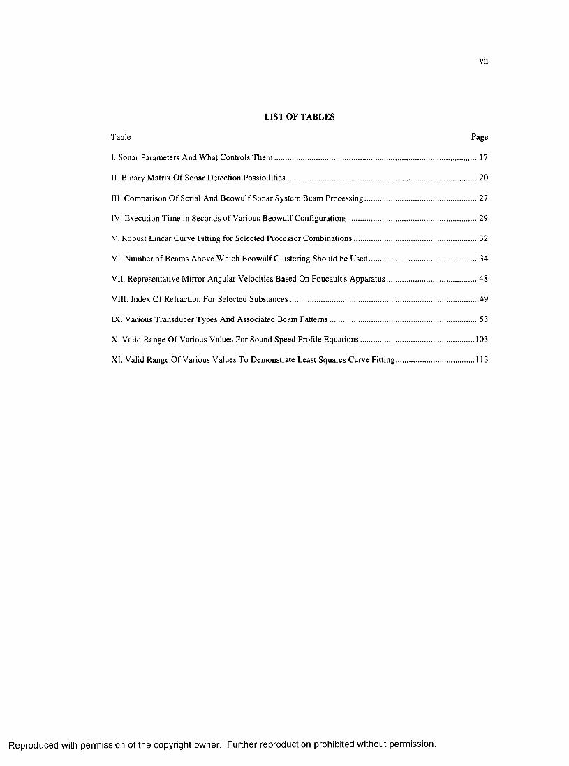
LIST OF TABLES

T able Page

I. Sonar Param eters And W hat Controls T h e m .............................................................................................................. 17

II. Binary M atrix O f Sonar D etection P ossib ilities.......................................................................................................20

III. Comparison O f Serial And B eow ulf Sonar System Beam Processing ............................................................. 27

IV. Execution Time in Seconds o f Various B eow ulf C onfigura tions......................................................................29

V. Robust Linear Curve Fitting for Selected Processor C om binations................................................................... 32

VI. Number o f Beam s Above W hich Beow ulf C lustering Should be U sed ...........................................................34

VII. Representative M irror Angular Velocities Based On Foucault's A pparatus................................................. 48

VIII. Index O f Refraction For Selected S ubstances..................................................................................................... 49

IX. Various Transducer Types And Associated Beam P atte rn s................................................................................ 53

X. Valid Range O f Various Values For Sound Speed Profile E quations..............................................................103

XI. Valid Range O f Various Values To Demonstrate Least Squares Curve F itting ...........................................113


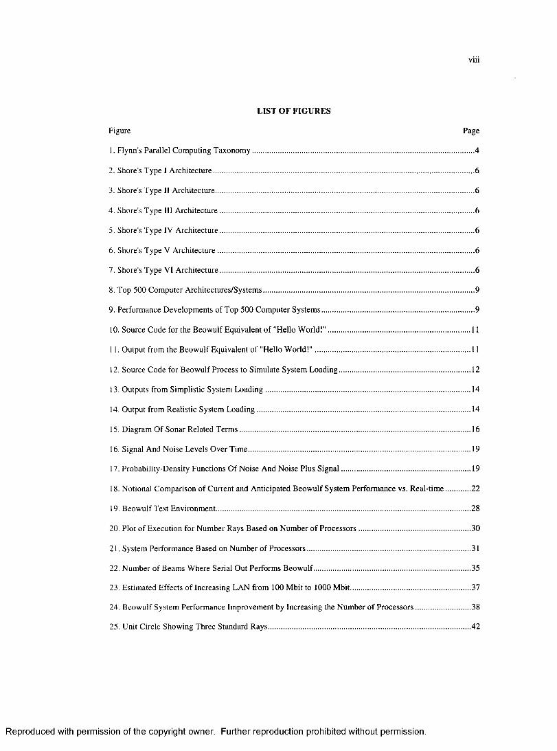
LIST OF FIGURES

Figure Page

1. Flynn's Parallel Com puting T axonom y......................................................................................................................... 4

2. Shore’s Type I A rchitecture............................................................................................................................................. 6

3. Shore's Type II A rchitecture............................................................................................................................................ 6

4. Shore's Type III A rch itecture ..........................................................................................................................................6

5. Shore's Type IV A rchitecture ..........................................................................................................................................6

6. Shore's Type V A rch itecture........................................................................................................................................... 6

7. Shore's Type VI A rchitecture..........................................................................................................................................6

8. Top 500 Com puter A rchitectures/System s....................................................................................................................9

9. Performance Developments o f Top 500 Com puter System s....................................................................................9

10. Source Code for the B eow ulf Equivalent o f "Hello W orld !" .............................................................................. 11

11. Output from the B eow ulf Equivalent o f "Hello W o rld !" ..................................................................................... 11

12. Source Code for B eow ulf Process to Simulate System L oading........................................................................ 12

13. Outputs from Simplistic System L o ad in g .................................................................................................................14

14. Output from Realistic System L oad ing ..................................................................................................................... 14

15. Diagram O f Sonar Related T e rm s...............................................................................................................................16

16. Signal And Noise Levels Over T im e.......................................................................................................................... 19

17. Probability-D ensity Functions O f Noise And Noise Plus S ig n a l....................................................................... 19

18. Notional Com parison o f Current and Anticipated B eow ulf System Perform ance vs. R eal-tim e..............22

19. B eow ulf Test Environm ent........................................................................................................................................... 28

20. Plot o f Execution for N um ber Rays Based on N um ber o f P rocesso rs............................................................. 30

21. System Perform ance Based on Number o f Processors..........................................................................................31

22. N um ber o f Beams W here Serial Out Performs B eow ulf...................................................................................... 35

23. Estimated Effects o f Increasing LAN from 100 M bit to 1000 M bit.................................................................. 37

24. B eowulf System Performance Im provement by Increasing the N um ber o f Processo rs.............................. 38

25. Unit Circle Showing Three Standard R ays...............................................................................................................42


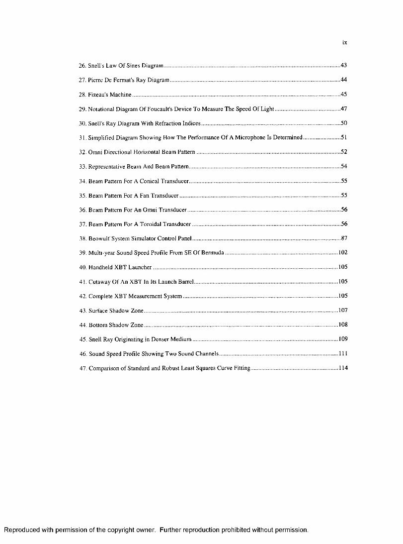
26. Snell's Law O f Sines D iagram ..................................................................................................................................... 43

27. Pierre De Fermat's Ray D iagram ................................................................................................................................ 44

28. Fizeau's M ach ine .............................................................................................................................................................45

29. Notational D iagram O f Foucault's Device To M easure The Speed O f L ig h t................................................. 47

30. Snell's Ray Diagram W ith Refraction Ind ices.........................................................................................................50

31. Simplified D iagram Showing How The Performance O f A M icrophone Is D eterm ined ............................51

32. Omni Directional Horizontal Beam P a tte rn .............................................................................................................52

33. Representative Beam And Beam Pattern.................................................................................................................. 54

34. Beam Pattern For A Conical T ransducer.................................................................................................................. 55

35. Beam Pattern For A Fan T ransducer..........................................................................................................................55

36. Beam Pattern For An Omni T ransducer....................................................................................................................56

37. Beam Pattern For A Toroidal T ransducer................................................................................................................ 56

38. B eowulf System Sim ulator Control P anel................................................................................................................ 87

39. M ulti-year Sound Speed Profile From SE O f B erm uda..................................................................................... 102

40. Handheld XBT L auncher............................................................................................................................................105

41. Cutaway O f An XBT In Its Launch B arrel.............................................................................................................105

42. Complete XBT M easurem ent S ystem ..................................................................................................................... 105

43. Surface Shadow Z one...................................................................................................................................................107

44. Bottom Shadow Z one ...................................................................................................................................................108

45. Snell Ray O riginating in Denser M ed ium .............................................................................................................. 109

46. Sound Speed Profile Showing Two Sound C hannels.......................................................................................... 111

47. Comparison o f Standard and Robust Least Squares Curve F itting.................................................................. 114


1

SECTION 1. INTRODUCTION

B eowulf com puter clustering is a technique used to have multiple low cost com puters w ork in parallel to

solve problem s that are typically solved in a linear manner. Currently B eow ulf clustering techniques are

used to construct networks whose aggregate computing pow er rival the most expensive supercomputers.

Acoustic ray tracing is at the heart o f most current sonar perform ance prediction systems. Ray-tracing

programs are used to predict the path that an acoustic wave would take from the sonar to an object (for

example: a target, torpedo, fish, etc.) and then back to the sonar where the detection takes place. Once this

predicted path is computed, mathematical terms are applied to com pute the probability o f detection o f the

assumed threat. These terms can be divided into three areas:

• Factors that rem ain relatively static (on the order o f at least small num bers o f tens o f minutes):

strength o f the sonar, signal absorption, the target’s acoustic reflectivity,

• Factors that change slowly (on the order o f every few seconds): relative bottom topography, the

direction in which the sonar is looking, the ocean sound speed profile, acoustic path, and

• Factors that change in real-time (on the order o f many hundreds o f times per second): ambient

noise.

In this paper 1 will provide:

• A discussion on the various taxonom ies o f parallel com puter systems,

• A B eow ulf im plem entation o f single board computers using the M essage Passing Interface (M PI)

protocol,

• A brief description o f computational problems that have to be solved in a serial m anner versus

those that can be solved with parallel programming techniques,

• An appendix containing historical inform ation relative to the origin o f the single equation (Snell’s

Law of Sines) that is at the heart o f all ray-tracing programs,

• A discussion on acoustic ray tracing in an aquatic environment,

• An introduction to the characteristics o f acoustic beam patterns based on the selected piezoelectric

The journa l m odel fo r this thesis is the IEEE/ACM Transactions on Networking.


2

shapes,

• A high level description o f sonar systems and how the probability o f detection for the system is

computed based on sonar beams,

• M easured B eow ulf sonar perform ance prediction times versus serial im plem entation for the same

data set, and

• An analysis o f the B eow ulf and serial measurem ents to identify system design “breakeven” points

where it make sense to chose one approach over another.

This paper discusses how B eow ulf clustering can be used to achieve real-time sonar perform ance

predictions and provides an analysis o f the trade-off in design betw een serial and parallel com putation

approaches.


3

SECTION 2. BACKGROUND OF THE RESEARCH

2 1 PARALLEL COMPUTING

Parallel computing is the application of multiple computing elem ents, possibly CPUs, working in concert to

solve a problem. In the general sense, if the problem lends itself to a parallel com puting approach, the more

computing elem ents that can be applied to a problem, the faster an answer will be com puted. In 1972 Flynn

developed a taxonom y o f parallel computing elem ent and data combinations that is now know n as F lynn’s

Taxonomy.

2 2 TAXONOMIES OF PARALLEL COMPUTING

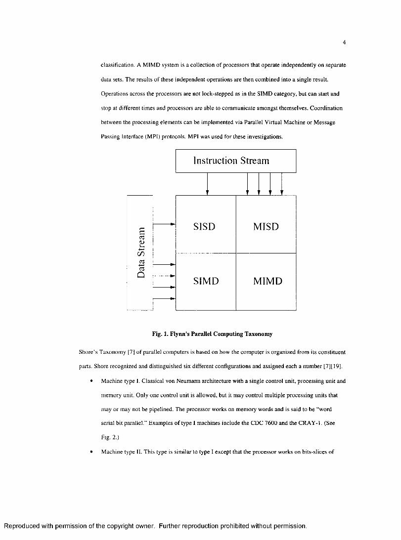
Flynn’s Taxonom y is based on the num ber o f distinct instructions and the num ber o f data elem ents the

instructions operate on. Fig. 1 [9] provides diagrams o f Flynn’s taxonomy. Flynn’s taxonom y is based on

the idea o f single or multiple numbers o f instructions or data elem ents processed sim ultaneously. These

possibilities are shown in the figure as a single or multiple arrow headed lines. Because there are two

options for the instructions and for the data, there are four possible combinations. The characteristics o f

each combination are:

• Single Instruction Single Data (SISD): This is a classic von Neumann machine. The processor

retrieves a single piece o f data and uses one instruction to operate on that data. M odem

im plem entations o f SISD processors have pipelining em bedded in the CPU, but there is only one

CPU. A single CPU is an SISD architecture.

• Single Instruction M ultiple Data (SIMD): A controlling elem ent “clocks” a parallel collection of

processors, each o f which has a different data set presented to it. Each processor executes the same

instruction on different data.

• M ultiple Instruction Single Data (M ISD): M ISD may have many processing elem ents working in

a serial manner, all o f which are executing independent instructions. W here the output data from

one processing elem ent serves as the input to the next elem ent, this is a m acro-pipelining

processor.

• M ultiple Instructions M ultiple Data (M IMD): M ost current multiprocessor systems are in this


4

classification. A M IM D system is a collection o f processors that operate independently on separate

data sets. The results o f these independent operations are then com bined into a single result.

Operations across the processors are not lock-stepped as in the SIM D category, but can start and

stop at different tim es and processors are able to com m unicate amongst them selves. Coordination

betw een the processing elem ents can be im plem ented via Parallel Virtual M achine or M essage

Passing Interface (M PI) protocols. M PI was used for these investigations.

ctJI4—»GOC3 ■*—> 03

Q

Instruction Stream

SISD M IS D

SIM D M IM D

Fig. 1. Flynn's Parallel Computing Taxonomy

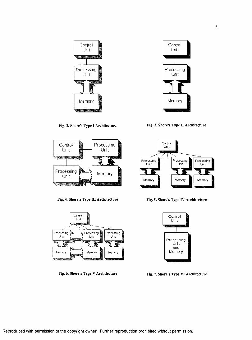
Shore’s Taxonom y [7] o f parallel computers is based on how the com puter is organized from its constituent

parts. Shore recognized and distinguished six different configurations and assigned each a num ber [7] [19].

• M achine type I. Classical von Neumann architecture with a single control unit, processing unit and

memory unit. Only one control unit is allowed, but it may control m ultiple processing units that

may or may not be pipelined. The processor works on m em ory words and is said to be “word

serial bit parallel.” Examples o f type I machines include the CDC 7600 and the CRAY-1. (See

Fig. 2.)

• M achine type II. This type is sim ilar to type I except that the processor works on bits-slices o f


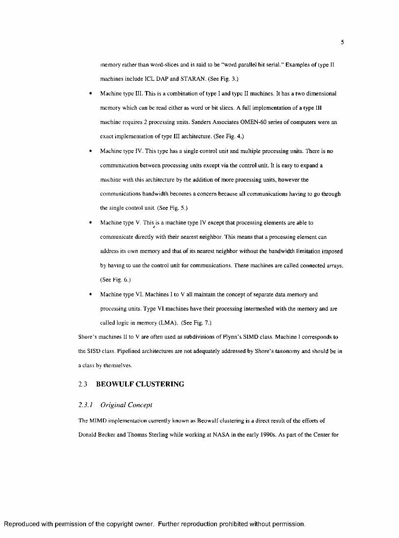
5

memory rather than w ord-slices and is said to be “word parallel bit serial.” Examples o f type II

machines include ICL DAP and STARAN. (See Fig. 3.)

• M achine type III. This is a combination o f type I and type II machines. It has a two dim ensional

memory which can be read either as word or bit slices. A full im plem entation o f a type III

machine requires 2 processing units. Sanders A ssociates O M EN-60 series o f com puters were an

exact im plem entation o f type III architecture. (See Fig. 4.)

• M achine type IV. This type has a single control unit and multiple processing units. There is no

com m unication betw een processing units except via the control unit. It is easy to expand a

machine with this architecture by the addition of more processing units, how ever the

com m unications bandwidth becom es a concern because all com m unications having to go through

the single control unit. (See Fig. 5.)

• M achine type V. This is a m achine type IV except that processing elem ents are able to

com m unicate directly with their nearest neighbor. This means that a processing elem ent can

address its own memory and that o f its nearest neighbor without the bandw idth lim itation imposed

by having to use the control unit for comm unications. These machines are called connected arrays.

(See Fig. 6.)

• M achine type VI. M achines I to V all maintain the concept o f separate data memory and

processing units. Type VI machines have their processing interm eshed with the m em ory and are

called logic in memory (LM A). (See Fig. 7.)

Shore’s machines II to V are often used as subdivisions o f Flynn’s SIM D class. M achine I corresponds to

the SISD class. Pipelined architectures are not adequately addressed by Shore’s taxonom y and should be in

a class by themselves.

2.3 BEOWULF CLUSTERING

2.3.1 Original Concept

The M IM D im plem entation currently known as Beow ulf clustering is a direct result o f the efforts o f

Donald Becker and Thom as Sterling while working at N ASA in the early 1990s. As part o f the Center for


ControlUnit

ProcessingUnit

Memory

Fig. 2. Shore's Type I Architecture

ProcessingUnit

ControlUnit

ProcessingUnit

M em ory

Fig. 4. Shore's Type III Architecture

P ro ces s in gUnit

P r o c e s s in g I Unit [

P ro ces s in gUnit

M emory M emory Mem ory

'Hi

Fig. 6. Shore's Type V Architecture

ControlUnit

ProcessingUnit

Memory

Fig. 3. Shore's Type II Architecture

ControlUnit

ProcessingUnit

ProcessingUnit

ProcessingUnit

Memory Memory Memory

Fig. 5. Shore's Type IV Architecture

ControlUnit

ProcessingUnitand

Memory

Fig. 7. Shore's Type VI Architecture


7

Excellence in Space Data and Information Services (CESDIS) (Goddard Space Flight Center) portion of

the Earth System Science (ESS) program, they were interested in finding a way to conduct parallel

computing without using the expensive custom hardw are that was the normal approach at the time.

The original Beow ulf cluster was constructed with comm odity o ff the shelf (CO TS) hardw are and had 16

DX4 com puters com m unicating over a bonded Ethernet network. It was designed to help ESS personnel

solve problems germ ane to their endeavors involving large amounts o f data. The intended cluster users

drove many of the initial cluster design decisions. These users were experienced parallel programming

professionals that were looking for a more cost-effective solution to their com puting needs than was being

provided elsewhere. The users were willing to program their applications them selves in order to optimize

the system ’s performance. This “do-it-yourself’ attitude was supported by the growth o f both the GNU and

Linux comm unities.

There has been a considerable amount o f folklore and rum or as to how the original COTS cluster o f

computers was named Beowulf; in some respects the truth is not as interesting as the lore. Dr. Thomas

Sterling wrote an article [14] in which he explained the origin:

" ... In truth, I'd been struggling to come up with some cutesy acronym and failing miserably. W ith

some small em barrassm ent, you can find exam ples o f this in our early papers, which included such

terms as "piles o f PCs" and even "PoPC." The first term was picked up by others at least briefly.

Thankfully, the second never was.

Then one afternoon, Lisa, Jim Fischer's accounts manager, called me and said, "I've got to file

paperw ork in 15 minutes and I need the name o f your project fast!" o r some w ords to that effect. I

was desperate. I looked around my office for inspiration, which had eluded me the entire previous

month, and my eyes happened on my old, hardbound copy o f Beowulf, which was lying on top of

a pile o f boxes in the com er. Honestly, I haven't a clue why it was there. As I said, I was

desperate. W ith the phone still in my hand and Lisa waiting not all that patiently on the other end,

I said, "W hat the hell, call it 'Beowulf.' No one will ever hear of it anyway. ..."

2.3.2 Current Concept

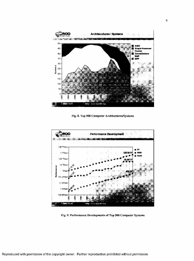
Fig. 8 and Fig. 9 [16] show the architectures and perform ance o f the top 500 computers in the world as o f

Novem ber 2003. Fig. 8 illustrates the trend o f basing more and more o f the top 500 systems on B eow ulf


clusters to achieve greater computational capacity. The constellation category is very sim ilar to Shore’s

type V machine. Fig. 9 shows that while the m aximum performance has rem ained constant for the past 3

years (as shown by the num ber 1 supercom puter having a performance o f 35.86 TF), the spread between

the perform ance of the top and the bottom systems has been reduced. In 1993, the least powerful o f the top

500 computers to make the list was rated at 0.42 GF. Over the past 3 years, the least powerful system has

increased from 100 G F to 403 GF.

2.3.3 Implementation

There are two basic im plem entations o f B eow ulf clustering. One im plem entation relies on the operating

system to provide the appearance o f shared memory betw een all processors, w hereby each processor

comm unicates with another through pseudo shared memory. The other technique, M essage Passing

Interface (M PI) relies on processes sending m essages to other processes. The sending and receiving

processes make explicit calls to message passing library routines to perform the sending and receiving of

messages. M essage sending was selected as the B eow ulf im plem entation o f choice for this investigation

because o f the minimal changes that would be required to the existing test environm ent. In a m essage

passing im plem entation, typically there is one process that is designated as the m aster and all other

processes are designated as slaves.

In the MPI universe o f available processors, each processor listens on “a well know n” port for

comm unications from other members o f the universe. A processor that initiates com m unication to the

universe attempts to contact universe members listed in a configuration file that is available at startup. Each

universe mem ber can have different configuration files.

2.3.3.1 Master

The m aster process is responsible for tasking the other processes to complete some allocated work unit

[11]. Often the master will have knowledge o f how to divide the total work required into portions that

slaves can work on and then consolidate their results in some manner.

2.3.3.2 Slave

A slave process waits to be tasked by the master process. W hen the slave com pletes some am ount o f work,

it notifies the m aster that the work has been done and then waits further tasking.


Architectures / Systems

■ SIMD■ Single Processor f | Cluster■ Constellations

SMP■ MW

Fig. 8. Top 500 Computer Architectures/Systems

Performance Development

I 00 P F lopss *1

529.60 TrI P F lo p s -

0 0 TFIops 35.86 TF

10 TFIops

£ 1 TFIops

i£ 1 00 GFIop3 -

I 0 G Flops

1 G F lops

I 0 0 M F lops

Fig. 9. Performance Developments of Top 500 Computer Systems


10

2.3.3.3 Communications between Master and Slave Processes

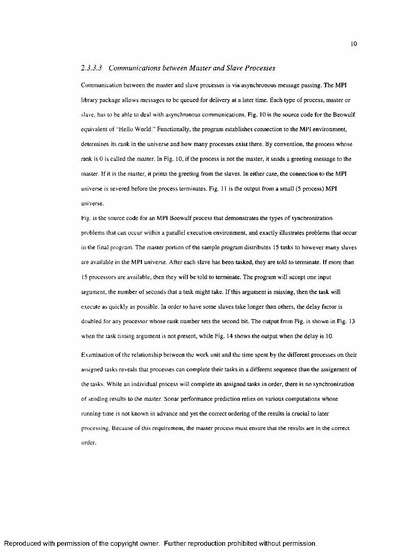
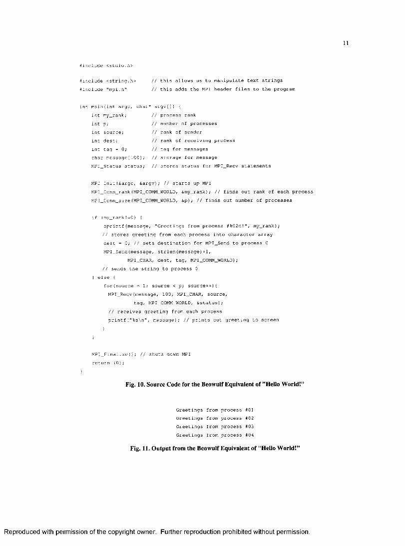
Comm unication betw een the master and slave processes is via asynchronous m essage passing. The M PI

library package allows m essages to be queued for delivery at a later time. Each type o f process, m aster or

slave, has to be able to deal with asynchronous comm unications. Fig. 10 is the source code for the B eow ulf

equivalent o f “Hello W orld.” Functionally, the program establishes connection to the M PI environment,

determines its rank in the universe and how many processes exist there. By convention, the process whose

rank is 0 is called the master. In Fig. 10, if the process is not the master, it sends a greeting m essage to the

master. If it is the master, it prints the greeting from the slaves. In either case, the connection to the MPI

universe is severed before the process terminates. Fig. 11 is the output from a sm all (5 process) M PI

universe.

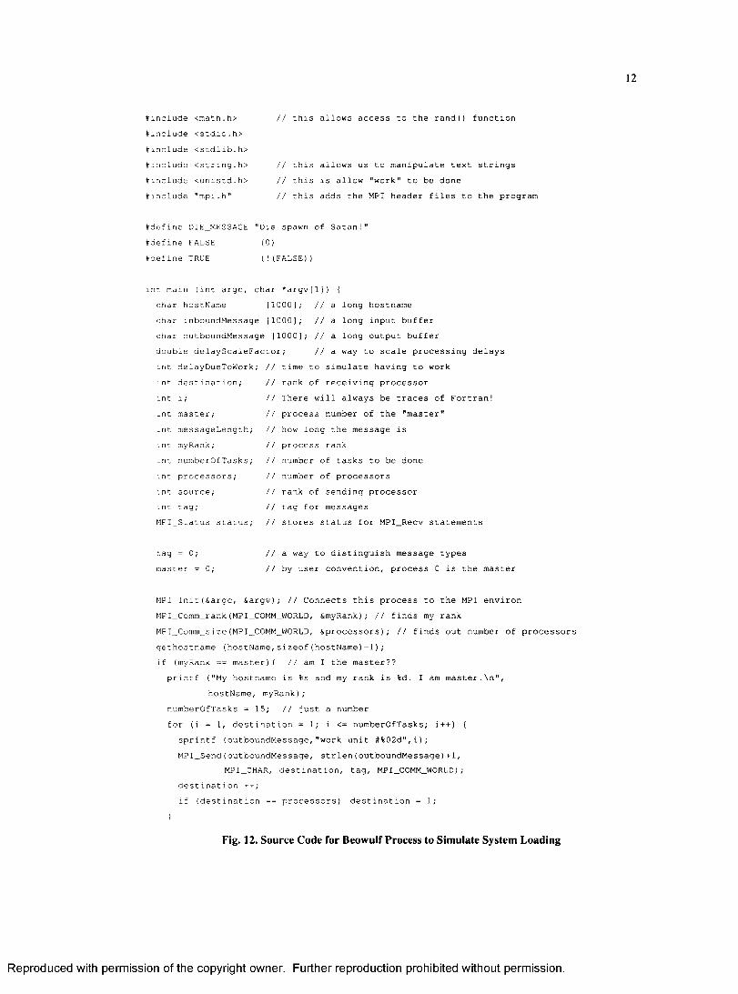
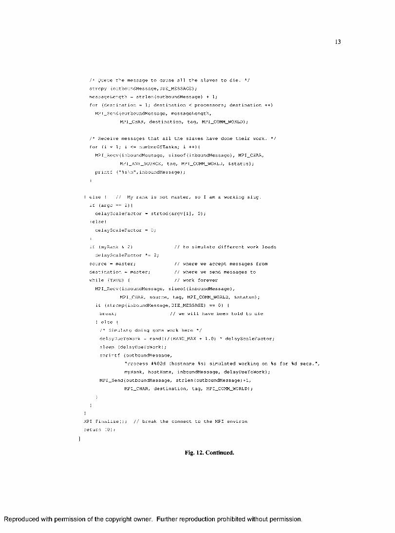
Fig. is the source code for an M PI B eowulf process that dem onstrates the types o f synchronization

problems that can occur within a parallel execution environment, and exactly illustrates problem s that occur

in the final program. The m aster portion o f the sample program distributes 15 tasks to how ever many slaves

are available in the M PI universe. A fter each slave has been tasked, they are told to terminate. If more than

15 processors are available, then they will be told to terminate. The program will accept one input

argument, the num ber o f seconds that a task might take. I f this argum ent is missing, then the task will

execute as quickly as possible. In order to have some slaves take longer than others, the delay factor is

doubled for any processor whose rank number sets the second bit. The output from Fig. is shown in Fig. 13

when the task tim ing argum ent is not present, while Fig. 14 shows the output when the delay is 10.

Examination o f the relationship between the work unit and the tim e spent by the different processes on their

assigned tasks reveals that processes can com plete their tasks in a different sequence than the assignm ent o f

the tasks. W hile an individual process will com plete its assigned tasks in order, there is no synchronization

of sending results to the master. Sonar performance prediction relies on various com putations whose

running tim e is not known in advance and yet the correct ordering o f the results is crucial to later

processing. Because o f this requirem ent, the master process must ensure that the results are in the correct

order.


11

#include <stdio.h>

#include <string.h> ftinclude "mpi.h"

// this allows us to manipulate text strings // this adds the MPI header files to the program

int main(int argc, char* argv[]) {int my_rank;int p;int source;

int tag = 0;int dest;

// process rank// number of processes// rank of sender// rank of receiving process// tag for messages

char message[100]; // storage for messageMPI_Status status; // stores status for MPI_Recv statements

MPI_Init(&argc, &argv); // starts up MPIMPI_Comm_rank(MPI_COMM_WORLD, &my_rank); // finds out rank of each process MPI_Comm_size(MPI_COMM_WORLD, &p); // finds out number of processes

i f (my_rank!=0) {sprintf(message, "Greetings from process #%02d!n, my_rank);// stores greeting from each process into character array dest = 0; // sets destination for MPI_Send to process 0 MPI_Send(message, strlen(message)+1,

MPI_CHAR, dest, tag, MPI_COMM_WORLD);// sends the string to process 0

} else {for (source = 1; source < p; source++){ MPI_Recv(message, 100, MPI_CHAR, source,

tag, MPI_C OMM_WORL D, &status);// receives greeting from each processprintf("%s\n", message); // prints out greeting to screen

MPl_Finalize(); // shuts down MPI return (0);

Fig. 10. Source Code for the Beowulf Equivalent of "Hello World!"

Greetings from process #01 Greetings from process #02 Greetings from process #03 Greetings from process #04

Fig. 11. Output from the Beowulf Equivalent o f "Hello World!"


12

#include <math.h>#include <stdio.h>#include <stdlib,h> #include <string.h> #mclude <unistd.h> # include "mpi.h"

// this allows access to the rand() function

// this allows us to manipulate text strings// this is allow "work" to be done// this adds the MPI header files to the program

#define DIE_MESSAGE "Die spawn of Satan!"ttdefine FALSE #define TRUE

( 0 )

(!(FALSE))

int main (int argc char hostName

char *argv[1]) {[1000]; // a long hostname

char inboundMessage [1000]; 11 a long input bufferchar outboundMessage [1000]; // a long output bufferdouble delayScaleFactor; // a way to scale processing delaysint delayDueToWork ; // time to simulate having to workint dest inat ion; // rank of receiving processorint i; If There will always be traces of Fortran!int ma s t e r; 11 process number of the "master"int messageLength; ii how long the message isint myRank; // process rankint numberOfTasks; // number of tasks to be doneint processors; I i number of processorsint source; 11 rank of sending processorint tag; 11 tag for messagesMPI,_Status status; // stores status for MPI_Recv statements

tag = 0; // a way to distinguish message typesmaster = 0; 11 by user convention, process 0 is the master

MPI._Init(&argc, &argv),; // Connects this process to the MPI environMPI._Comm_rank(MPI_COMM__WORLD, &myRank); // finds my rankMPI_Comm_size(MPI_COMM_WORLD, &processors); // finds out number of processors gethostname (hostName,sizeof(hostName)-1); if (myRank == master){ // am I the master??

printf ("My hostname is %s and my rank is %d. I am master.\n", hostName, myRank);

numberOfTasks = 15; // just a numberfor (i = 1, destination = 1; i <= numberOfTasks; i++) {

sprintf (outboundMessage,"work unit #%02d",i);MPl_Send(outboundMessage, strlen(outboundMessage)+1,

MPI_CHAR, destination, tag, MPI_COMM_WORLD); destination + +;if (destination == processors) destination = 1;

Fig. 12. Source Code for Beowulf Process to Simulate System Loading


13

/'* Queue the message to cause all the slaves to die. */ strcpy (outboundMessage,DIE_MESSAGE); messageLength = strlen(outboundMessage) + 1;for (destination = 1; destination < processors; destination ++)

MPl_Send(outboundMessage, messageLength,MPI_CHAR, destination, tag, MPI_COMM_WORLD);

/* Receive messages that all the slaves have done their work. */ for (i = 1; i <= numberOfTasks; i + + ){

MPI_Recv(inboundMessage, sizeof(inboundMessage), MPI_CHAR, MPI_ANY_SOURCE, tag, MPI_COMM_WORLD, &status);

printf ("%s\n",inboundMessage);}

else { / / M y rank is not master, so I am a working slug, if (argc == 2){

delayScaleFactor = strtod(argv[1], 0);) else{

delayScaleFactor = 0;

if (myRank & 2)delayScaleFactor *=

source = master; destination = master; while (TRUE) {

// to simulate different work loads

// where we accept messages from // where we send messages to // work forever

MPI_Recv{inboundMessage, sizeof(inboundMessage),MPI_CHAR, source, tag, MPI_COMM_WORLD, &status);

if (strcmp(inboundMessage,DIE_MESSAGE) == 0) {break; // we will have been told to die

} else (/* Simulate doing some work here */delayDueToWork = rand()/(RAND_MAX + 1.0) * delayScaleFactor; sleep (delayDueToWork); sprintf (outboundMessage,

"Process #%02d (hostname %s) simulated working on %s for %d secs. myRank, hostName, inboundMessage, delayDueToWork);

MPI_Send(outboundMessage, strlen(outboundMessage)+1,MPI_CHAR, destination, tag, MPI_COMM_WORLD);

MPI_Finalize(); // break the connect to the MPI environr e t u r n ( 0 ) ;

Fig. 12. Continued.


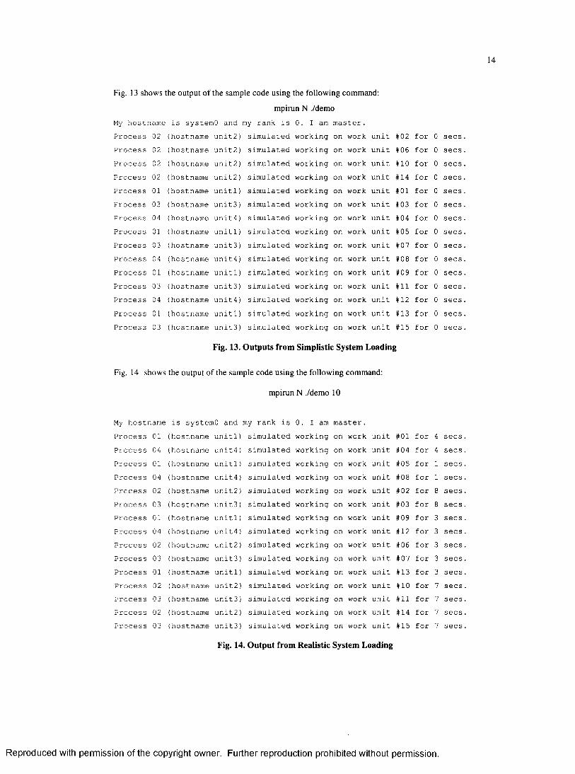
Fig. 13 shows the output o f the sample code using the following command:

mpirun N ./demo

My hostname is systemO and my rank is 0. I am master.Process 02 (hostname unit2) simulated working on work unit #02 for 0 secsProcess 02 (hostname unit2) simulated working on work unit #06 for 0 secsProcess 02 (hostname unit2) simulated working on work unit #10 for 0 secsProcess 02 (hostname unit2) simulated working on work unit #14 for 0 secsProcess 01 (hostname unitl) simulated working on work unit #01 for 0 secsProcess 03 (hostname unit3) simulated working on work unit #03 for 0 secsProces s 04 (hostname unit4) simulated working on work unit #04 for 0 secsProcess 01 (hostname unitl) simulated working on work unit #05 for 0 secsProcess 03 (hostname unit3) simulated working on work unit #07 for 0 secsProcess 04 (hostname unit4) simulated working on work unit #08 for 0 secsProcess 01 (hostname unitl) simulated working on work unit #09 for 0 secsProcess 03 (hostname unit3) simulated working on work unit #11 for 0 secsProcess 04 (hostname unit4) simulated working on work unit #12 for 0 secsProcess 01 (hostname unitl) simulated working on work unit #13 for 0 secsProcess 03 (hostname unit3) simulated working on work unit #15 for 0 secs

Fig. 13. Outputs from Simplistic System Loading

Fig. 14 shows the output o f the sample code using the following command:

mpirun N ./demo 10

My hostname is systemO and my rank is 0. I am master.Process 01 (hostname unitl) simulated working on work unit #01 for 4 secsProcess 04 (hostname unit4) simulated working on work unit #04 for 4 secsProcess 01 (hostname unitl) simulated working on work unit #05 for 1 secsProcess 04 (hostname unit4) simulated working on work unit #08 for 1 secsProcess 02 (hostname unit2) simulated working on work unit #02 for 8 secsProcess 03 (hostname unit3) simulated working on work unit #03 for 8 secsProcess 01 (hostname unitl) simulated working on work unit #09 for 3 secsProcess 04 (hostname unit4) simulated working on work unit #12 for 3 secsProcess 02 (hostname unit2) simulated working on work unit #06 for 3 secsProcess 03 (hostname unit3) simulated working on work unit #07 for 3 secsProcess 01 (hostname unitl) simulated working on work unit #13 for 3 secsProcess 02 (hostname unit2) simulated working on work unit #10 for 7 secsProcess 03 (hostname unit3) simulated working on work unit #11 for 7 secsProcess 02 (hostname unit2) simulated working on work unit #14 for 7 secsProcess 03 (hostname unit3) simulated working on work unit #15 for 7 secs

Fig. 14. Output from Realistic System Loading


15

2.4 TYPES OF PROBLEMS WHERE PARALLEL APPROACH IS

APPLICABLE

Parallel programming techniques are applicable to solving problems where the solution algorithm can be

decomposed into steps or blocks that can be executed independently o f data from other steps. The

following code snippet can be im plem ented in a parallel m anner because all data elem ents (a, b, and c) are

independent from each other and can be represented by Shore’s type IV abstraction where the computation

of the value “a” could be assigned to individual processors, each o f which would return their part o f the

total solution. The data in each step o f the program execution is independent o f data from any other step.

for (i = n; i < m; i++)

a(i) = b(i) + c(i)

By way of contrast, the next code snippet is an algorithm that is not perfectly paralizable. The computation

o f the value o f “a” depends on the value o f “a” from a different iteration. W hile it m ight be technically

possible to im plem ent the algorithm in a parallel environm ent, it would require reworking into a different

algorithmic structure.

for (i = n; i < m; i++)

a(i+k) = b(i) + a(i)

2 5 SONAR SYSTEM

The goal o f sonar is to “detect” an underwater object and provide an alert to either an operator or to another

electronic system onboard the ship. Active sonar puts acoustic energy into the w ater and then listens for an

echo. Passive sonar never puts energy into the water; it only listens for acoustic energy from the target. The

amount o f energy that a sonar has to receive for a detection to take place can be expressed as a sum of

several individual decibels values.

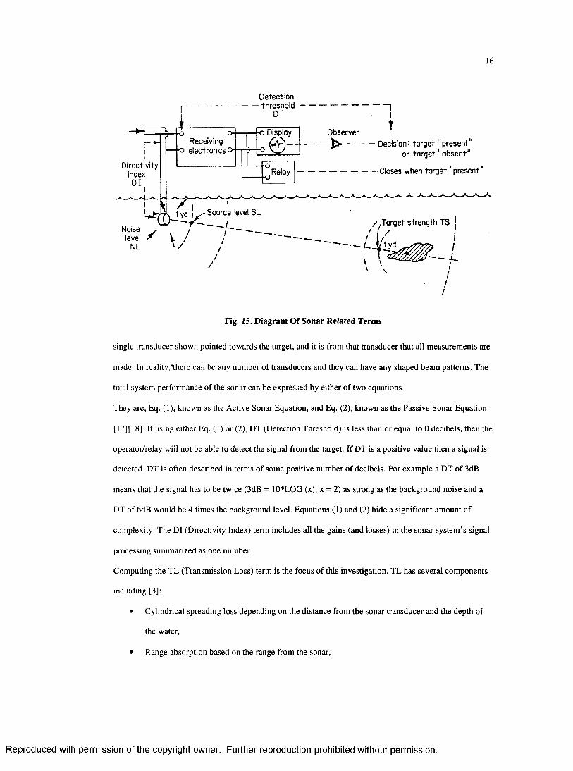
Fig. 15 shows the major com ponents o f a sonar system and serves as a framework for com puting the

sonar’s performance. TABLE I lists the various total sonar system com ponents and indicate which

parameters o f the sonar system perform ance equation(s) are attributable to each component. In Fig. 15, a


16

Detectionthreshold

-o Display Observer

0 - 4— ---------------------Receiving

■o electronics o— Decision: target "present"

or target “absent"

- — Closes when target “presentDirectivity

indexDI

Relay

Source level SL//T arget strengthTS

Noiselevel

NL

//

Fig. 15. Diagram O f Sonar Related Terms

single transducer shown pointed towards the target, and it is from that transducer that all measurem ents are

made. In reality,*there can be any num ber o f transducers and they can have any shaped beam patterns. The

total system perform ance o f the sonar can be expressed by either o f two equations.

They are, Eq. (1), known as the Active Sonar Equation, and Eq. (2), known as the Passive Sonar Equation

[ 17J[ 18]. If using either Eq. (1) or (2), DT (Detection Threshold) is less than or equal to 0 decibels, then the

operator/relay will not be able to detect the signal from the target. I f D T is a positive value then a signal is

detected. DT is often described in terms o f some positive num ber o f decibels. For exam ple a DT o f 3dB

means that the signal has to be twice (3dB = 10*LOG (x); x = 2) as strong as the background noise and a

DT of 6dB would be 4 times the background level. Equations (1) and (2) hide a significant am ount o f

complexity. The Dl (Directivity Index) term includes all the gains (and losses) in the sonar system ’s signal

processing sum marized as one number.

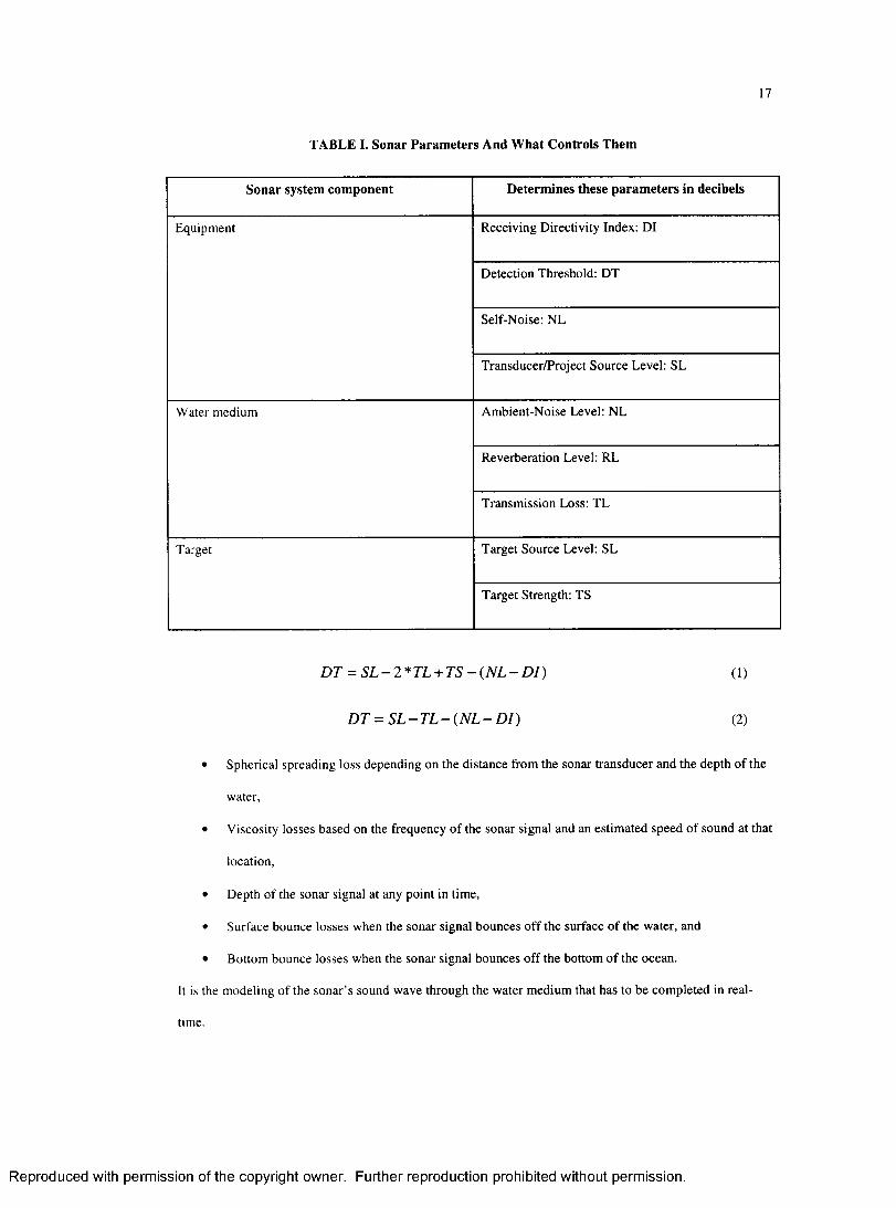
Computing the TL (Transm ission Loss) term is the focus o f this investigation. TL has several com ponents

including [3]:

• Cylindrical spreading loss depending on the distance from the sonar transducer and the depth of

the water,

• Range absorption based on the range from the sonar,


17

TABLE I. Sonar Parameters And What Controls Them

Sonar system component Determines these parameters in decibels

Equipment Receiving Directivity Index: DI

Detection Threshold: DT

Self-Noise: NL

Transducer/Project Source Level: SL

W ater medium A m bient-N oise Level: NL

Reverberation Level: RL

Transm ission Loss: TL

Target Target Source Level: SL

Target Strength: TS

DT = S L -2 * T L + TS -- ( N L - D I ) (1)

DT = S L - T L - (NL - DI) (2)

• Spherical spreading loss depending on the distance from the sonar transducer and the depth o f the

water,

• Viscosity losses based on the frequency o f the sonar signal and an estim ated speed o f sound at that

location,

• Depth of the sonar signal at any point in time,

• Surface bounce losses when the sonar signal bounces o ff the surface o f the water, and

• Bottom bounce losses when the sonar signal bounces o ff the bottom o f the ocean.

It is the modeling o f the sonar’s sound wave through the water m edium that has to be com pleted in real

time.


18

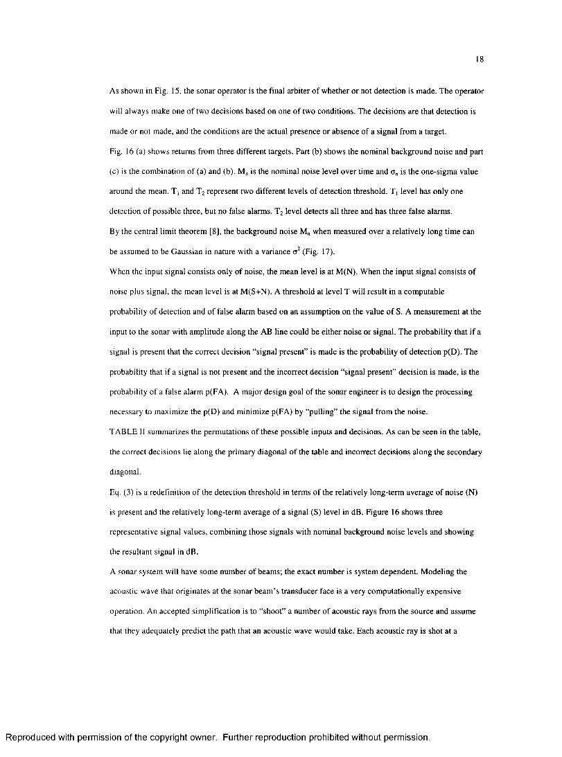
As shown in Fig. 15, the sonar operator is the final arbiter o f whether o r not detection is made. The operator

will always make one o f two decisions based on one o f two conditions. The decisions are that detection is

made or not made, and the conditions are the actual presence or absence o f a signal from a target.

Fig. 16 (a) shows returns from three different targets. Part (b) shows the nominal background noise and part

(c) is the combination o f (a) and (b). M n is the nominal noise level over tim e and a n is the one-sigm a value

around the mean. Ti and T 2 represent two different levels o f detection threshold. T! level has only one

detection o f possible three, but no false alarms. T 2 level detects all three and has three false alarms.

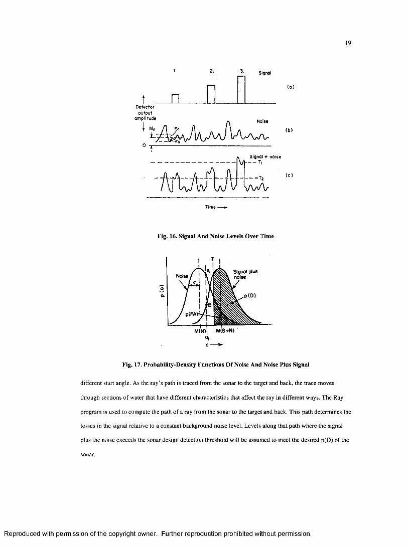
By the central limit theorem [8], the background noise M n when measured over a relatively long tim e can

be assumed to be G aussian in nature with a variance a 2 (Fig. 17).

When the input signal consists only o f noise, the mean level is at M (N). W hen the input signal consists o f

noise plus signal, the mean level is at M (S+N). A threshold at level T will result in a com putable

probability o f detection and o f false alarm based on an assum ption on the value o f S. A m easurem ent at the

input to the sonar with am plitude along the AB line could be either noise or signal. The probability that if a

signal is present that the correct decision “signal present” is made is the probability o f detection p(D). The

probability that if a signal is not present and the incorrect decision “signal present” decision is made, is the

probability o f a false alarm p(FA). A m ajor design goal o f the sonar engineer is to design the processing

necessary to maximize the p(D) and minimize p(FA) by “pulling” the signal from the noise.

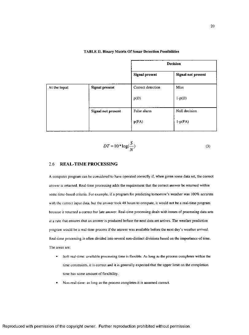
TABLE II summarizes the perm utations o f these possible inputs and decisions. As can be seen in the table,

the correct decisions lie along the prim ary diagonal o f the table and incorrect decisions along the secondary

diagonal.

Eq. (3) is a redefinition o f the detection threshold in terms o f the relatively long-term average o f noise (N)

is present and the relatively long-term average o f a signal (S) level in dB. Figure 16 shows three

representative signal values, combining those signals with nominal background noise levels and showing

the resultant signal in dB.

A sonar system will have some number o f beam s; the exact num ber is system dependent. M odeling the

acoustic wave that originates at the sonar beam ’s transducer face is a very com putationally expensive

operation. An accepted simplification is to “shoot” a num ber o f acoustic rays from the source and assume

that they adequately predict the path that an acoustic wave would take. Each acoustic ray is shot at a


19

2 . Signal

( o )

t _ aDetecto r

ou tpu tampli tude

1 £-A?” II

Noise

( b )

T* S ig n a l + n o is evn— t ,

-T z

vwv( c )

Time ■

Fig. 16. Signal And Noise Levels Over Time

Signal plus noiseNoise

o

p(D)a

p(FAV

M(N)j M(S+N) °i

Fig. 17. Probability-Density Functions O f Noise And Noise Plus Signal

different start angle. As the ray’s path is traced from the sonar to the target and back, the trace moves

through sections o f water that have different characteristics that affect the ray in different ways. The Ray

program is used to com pute the path o f a ray from the sonar to the target and back. This path determ ines the

losses in the signal relative to a constant background noise level. Levels along that path where the signal

plus the noise exceeds the sonar design detection threshold will be assumed to m eet the desired p(D) o f the

sonar.


20

TABLE II. Binary Matrix O f Sonar Detection Possibilities

Decision

Signal present Signal not present

At the input Signal present Correct detection Miss

P(D) l-p(D )

Signal not present False alarm Null decision

p(FA) l-p(FA )

£>r = io*iog(—) (3)N

2.6 REAL-TIME PROCESSING

A com puter program can be considered to have operated correctly if, when given some data set, the correct

answer is returned. Real-time processing adds the requirem ent that the correct answ er be returned within

some time-based criteria. For example, if a program for predicting tom orrow ’s weather was 100% accurate

with the correct input data, but the answer took 48 hours to compute, it would not be a real-tim e program

because it returned a correct but late answer. Real-tim e processing deals with issues o f processing data sets

at a rate that ensures that an answer is produced before the next data set arrives. The w eather prediction

program would be a real-time process if the answer was available before the next day’s weather arrived.

Real-time processing is often divided into several non-distinct divisions based on the im portance o f time.

The areas are:

• Soft real-time: available processing time is flexible. As long as the process com pletes w ithin the

time constraints, it is correct and it is generally expected that the upper lim it on the com pletion

time has some am ount o f flexibility.

• Non-real-time: as long as the process completes it is assum ed correct.


21

• Hard real-time: available processing time is a fixed determ inistic length o f time; all processing has

to be com pleted within that time, or the process fails.

Real-time processing does not relate directly to how fast a program processes data. The fundam ental

requirem ent is that the process be finished before the next data set arrives, or is needed. A process reading a

deck of cards on an old style com puter card deck driven com puter is a real-time process if the com puter can

be finished with the processing before the next deck o f cards is put in the card reader. A m odem CPU

operating at 3.1 GHz is a non real-time environm ent if new data arrives every m illisecond and it takes two

milliseconds to process.

A sonar system has sections that are hard real-time and others that are soft real-time. A t the front end o f the

sonar, there are a num ber o f analog to digital (A/D) converters that convert the acoustic energy from the

transducers to digital data. A/D converters sample the incom ing data at a fixed rate and define the hard real

time processing limit for the system. Digital Signal Processors (DSP) have to accept data from the A/D at

their output rate, process the data in some m anner and forward data to the later processes. DSPs often

reduce the am ount o f data from the A/D to some lesser, but more inform ationally rich format. As the

processing continues within the sonar from the DSP to the CRTs that display data, the real-tim e

requirements becom e less and less hard. At the A/D level, real-time is defined as a 32 KHz sample rate

(3.05 x 1 0 5 second) while at the CRT an update every 0.25-second is considered real-time. There is one

process, performance prediction, which will be the focus o f attention in the following paragraphs. Serial

performance prediction takes one sample o f data from the D SPs and processes that data for approximately

120 seconds. These serial operations are considered real-time.

SECTION 3. JUSTIFICATION OF THE RESEARCH

The normal operating environm ent for sonars o f the type under consideration for this paper is that of

searching for a target. One of the keys to best utilize the sonar is to be able to predict how the sonar will

perform against the target. The perform ance o f the sonar changes on a continuing basis due to changes in

the ocean environm ent that are undetectable onboard the ship (for example, changes in the sound speed

profile between the sonar and the target, fish and other aquatic life betw een the ship and the sonar,

unknown differences in the bottom that affect the sonar when the acoustic wave bounces o ff the bottom,


22

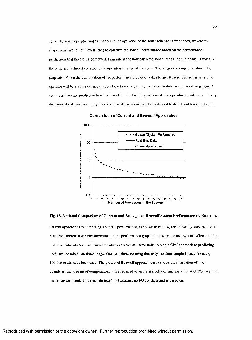
etc.). The sonar operator makes changes in the operation of the sonar (change in frequency, waveform

shape, ping rate, output levels, etc.) to optim ize the sonar’s perform ance based on the perform ance

predictions that have been computed. Ping rate is the how often the sonar “pings” per unit time. Typically

the ping rate is directly related to the operational range o f the sonar. The longer the range, the slower the

ping rate. W hen the com putation of the perform ance prediction takes longer then several sonar pings, the

operator will be making decisions about how to operate the sonar based on data from several pings ago. A

sonar performance prediction based on data from the last ping will enable the operator to make more timely

decisions about how to employ the sonar, thereby maximizing the likelihood to detect and track the target.

Comparison of Current and Beowulf Approaches

1000

100

10

1 -

0.1

- - - Beowulf System Performance

........... Real Time Data

1 Cuirent Approaches

Number of Processors In the System

Fig. 18. Notional Comparison of Current and Anticipated Beowulf System Performance vs. Real-time

Current approaches to computing a sonar’s perform ance, as shown in Fig. 18, are extrem ely slow relative to

real-time ambient noise m easurem ents. In the perform ance graph, all m easurem ents are “norm alized” to the

real-time data rate (i.e., real-time data always arrives at 1 tim e unit). A single CPU approach to predicting

performance takes 100 times longer than real-time, meaning that only one data sam ple is used for every

100 that could have been used. The predicted B eowulf approach curve shows the interaction o f two

quantities: the amount o f computational time required to arrive at a solution and the am ount o f I/O time that

the processors need. This estim ate Eq.(4) [4] assumes no I/O conflicts and is based on:


23

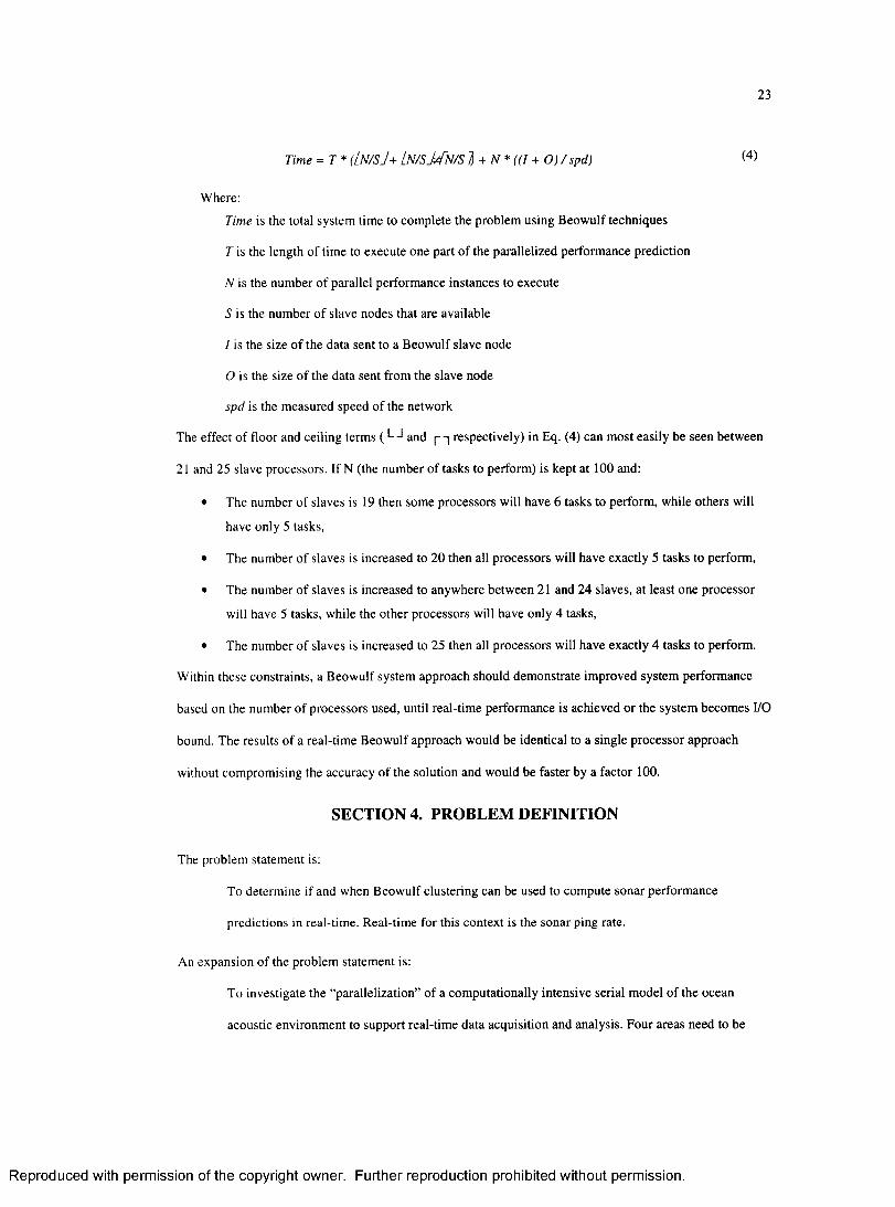
Time = T * (LN/SJ+ Ln / s J 4 n /S } + N * ( ( / + O) / spd) W

Where:

Time is the total system time to complete the problem using B eow ulf techniques

T is the length o f tim e to execute one part o f the parallelized performance prediction

N is the number o f parallel perform ance instances to execute

S is the number o f slave nodes that are available

I is the size o f the data sent to a B eow ulf slave node

O is the size o f the data sent from the slave node

spd is the measured speed o f the network

The effect o f floor and ceiling terms ( L -I and p -] respectively) in Eq. (4) can m ost easily be seen between

21 and 25 slave processors. If N (the num ber o f tasks to perform) is kept at 100 and:

• The number o f slaves is 19 then some processors will have 6 tasks to perform , while others will

have only 5 tasks,

• The number o f slaves is increased to 20 then all processors will have exactly 5 tasks to perform,

• The number o f slaves is increased to anywhere betw een 21 and 24 slaves, at least one processor

will have 5 tasks, while the other processors will have only 4 tasks,

• The number o f slaves is increased to 25 then all processors will have exactly 4 tasks to perform.

Within these constraints, a B eow ulf system approach should dem onstrate im proved system performance

based on the num ber o f processors used, until real-time performance is achieved or the system becom es I/O

bound. The results o f a real-tim e B eow ulf approach would be identical to a single processor approach

without com prom ising the accuracy o f the solution and would be faster by a factor 100.

SECTION 4. PROBLEM DEFINITION

The problem statem ent is:

To determine if and when B eowulf clustering can be used to compute sonar perform ance

predictions in real-time. Real-time for this context is the sonar ping rate.

An expansion o f the problem statem ent is:

To investigate the “parallelization” o f a com putationally intensive serial m odel o f the ocean

acoustic environm ent to support real-time data acquisition and analysis. Four areas need to be


24

investigated. They are [5]:

o Decomposition: analyzing the entire perform ance prediction algorithm to identify those

areas that can be parallelized,

o Assignm ent o f tasks: based on the results o f the decom position analysis, possible creation

o f parallel routines to replace serial routines,

o Scheduling: data access, com m unication, and synchronization betw een processes, and

o M apping o f processes to processors.

SECTION 5. STATE OF THE ART

Two parts o f this effort are worthy o f note. One part is paralyzing the application o f an acoustic ray-tracing

program. The other part is the use o f Beow ulf clustering in a sonar related environment.

Ray [2] is a state o f the art acoustic modeling program in wide use among oceanographers. The program is

used to predict the paths o f acoustic waves from seismic and man-made sources for short (tens o f feet) and

long (thousands o f kilom eters) ranges. Ray was developed by W oods Hole Oceanographic Institute, and is

fundamental to the com putation o f the sonar’s perform ance prediction.

B eowulf clustering is currently in use in some sonar related endeavors, primarily in three areas. The areas

are:

• Independent robotic operations where sonar is used as the “eyes” o f the robot and a cluster is used

to make sense o f the data,

• Image enhancem ents for side scan sonar systems, and

• References in the marketing literature o f some defense contractors to passive and active sonar

contact detection and classification.

No references were found that combined Ray and B eow ulf to achieve real-time sonar perform ance

prediction capability.

SECTION 6. PROBLEM ANALYSIS

A sonar system is com posed o f many different pieces o f hardw are and software. From a macro view, the


25

sonar system is composed of a num ber o f sonar beams that are processed by the sonar detection hardware.

The predicted performance capability o f a sonar system is a function o f the predicted perform ance o f each

beam. The performance of each beam is based on the path that the acoustic wave from each beam is

assumed to take. The acoustic path for each wave is assumed to be represented by the interaction o f the

individual rays “shot” from each beam. The path that an individual ray takes is independent o f all other rays

and is dependent only on its start angle and the defined environment. The mechanics o f com puting the

performance of a sonar system conforms very nicely to Shore’s Type V machine, or as a M IM D from

Flynn’s taxonomy.

SECTION 7. TECHNICAL SOLUTION

A sonar system will typically have more than one beam. An acoustic wave front in each beam is modeled

by some num ber o f acoustic rays. The relationship o f beam s and rays fits exactly into a nested loop control

structure. A serial approach uses a single processor for all computations. In the lim it, a B eow ulf approach

would use a slave processor for each ray for each beam.

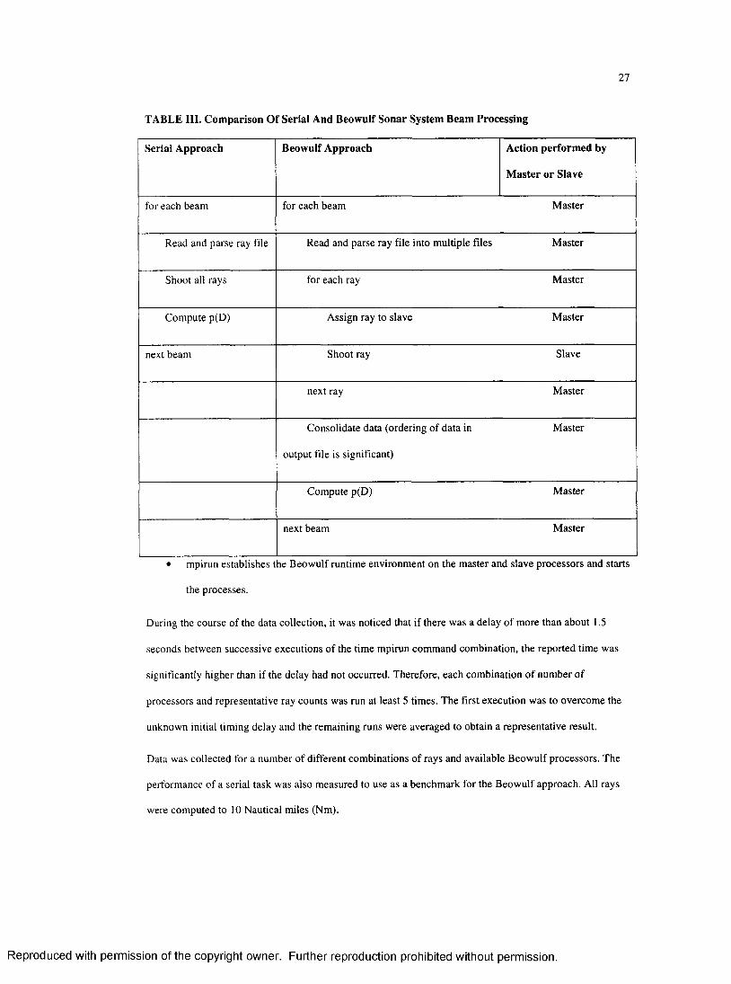
The Ray program reads a configuration file containing directives about which bottom topography and

which bathytherm ograph files to read, how many rays to shoot, how far to shoot them and other control

parameters. A fter the individual rays are shot, the resulting wave front is used to com pute p(D). T A B L E

III shows the processing that occurs in both serial and B eow ulf approaches. The serial approach uses a

single process to do all the work, whereas the B eow ulf approach partitions the original ray initialization file

into a set o f files, each o f which deals with a single ray. A fter the file is parsed, each reduced count ray file

is assigned to a processor. Each o f the reduced count files has a different initial start angle for its ray. Based

on the start angle and the bathygraphic data, processing tim e may be different, so the resulting data from

the individual processors have to be organized as if the entire operation was executed in a serial manner.

Appendix C is a complete program listing o f the code to read, parse, assign tasks and consolidate results.

The source code for the final step of computing p(D) is not included because it is part o f the intellectual

property o f EDO Corporation. EDO Corporation provided access to the final test and developm ent

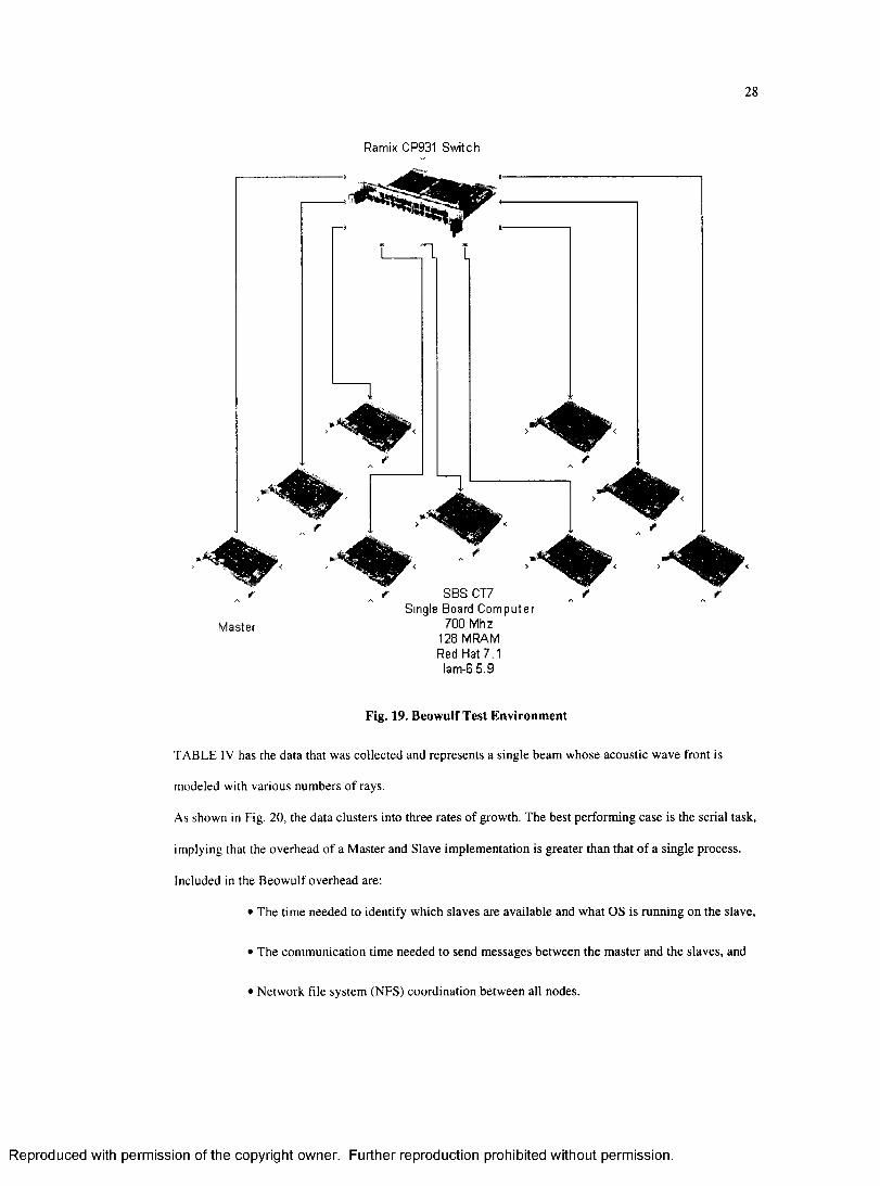
environment for this effort. Fig. 19 is a representation o f the test environment.

The processes used for computing the p(D) for a single beam are the same for all beams. Each beam is


26

looking/listening in a different direction, but the same algorithm is used to com pute p(D) for all beams. The

ability o f a hardware suite to compute p(D) in real-time for a single beam can be expanded to computing

the p(D) for the entire sonar system by the application o f additional hardware.

SECTION 8. EVALUATION OF DEVELOPED SOLUTION

Performance prediction o f a sonar system is a com posite o f the performance prediction for each sonar

beam. The time to serially compute the performance prediction is equal to the tim e required to com pute a

single beam times the num ber o f beams in the system. The time to compute the perform ance prediction for

the sonar system using a parallel approach is approximately the time to compute a single beam.

The proposed solution to real-time B eow ulf processing was rigorously com pared to the serial processing

approach. The B eow ulf solution was evaluated from three different perspectives: com parison o f the

Beowulf output to a serial output, com parison of serial and B eow ulf sonar perform ance prediction times,

determ ination o f a “break-even” point where one approach is faster than another and use m easured data to

predict the effects o f different CPU and LAN speeds. Each o f these perspectives is addressed in the

following sub-sections.

8 . 1 COMPARISON OF SERIAL AND BEOWULF NUMERICAL RESULTS

The output fde resulting from running a serial Ray program with the test input file was com pared using the

emacs compare buffer comm and to the reconstituted B eow ulf ray trace output file. There were no

differences. Appendix E contains the Ray runtim e file used to validate the B eow ulf im plem entation against

the serial execution.

8 2 COMPARISON OF SERIAL AND BEOWULF EXECUTION TIMES

Comparison o f serial and B eow ulf execution tim es with the same input data. Tw o Linux com m ands (time

and mpirun) were used to collect all data for this analysis:

• time reports, among other things, the user time that a user supplied com m and (in this case:

mpirun) takes to execute, and


27

TABLE III. Comparison Of Serial And Beowulf Sonar System Beam Processing

Serial Approach Beowulf Approach Action performed by

Master or Slave

for each beam for each beam M aster

Read and parse ray file Read and parse ray file into multiple files M aster

Shoot all rays for each ray M aster

Compute p(D) Assign ray to slave M aster

next beam Shoot ray Slave

next ray M aster

Consolidate data (ordering o f data in

output file is significant)

M aster

Com pute p(D) M aster

next beam M aster

• mpirun establishes the B eow ulf runtim e environm ent on the m aster and slave processors and starts

the processes.

During the course o f the data collection, it was noticed that if there was a delay o f more than about 1.5

seconds between successive executions o f the tim e mpirun com m and combination, the reported time was

significantly higher than if the delay had not occurred. Therefore, each com bination o f num ber o f

processors and representative ray counts was run at least 5 times. The first execution was to overcom e the

unknown initial tim ing delay and the rem aining runs were averaged to obtain a representative result.

Data was collected for a num ber of different combinations o f rays and available B eow ulf processors. The

performance o f a serial task was also measured to use as a benchm ark for the B eow ulf approach. All rays

were com puted to 10 Nautical miles (Nm).


28

Ramix CP931 Switch

M aster

SBS CT7 Single Board C om puter

700 Mhz 128 MRAM Red Hat 7.1

lam-6.5.9

Fig. 19. Beowulf Test Environment

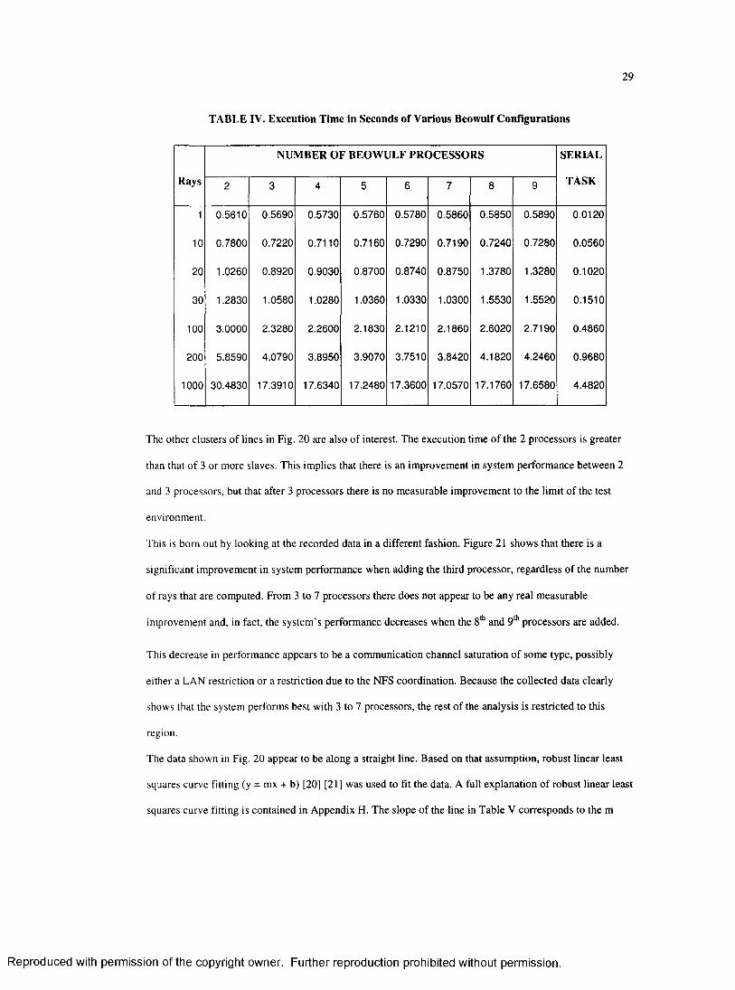
TABLE IV has the data that was collected and represents a single beam whose acoustic wave front is

modeled with various numbers o f rays.

As shown in Fig. 20, the data clusters into three rates o f growth. The best perform ing case is the serial task,

implying that the overhead o f a M aster and Slave im plem entation is greater than that o f a single process,

included in the B eow ulf overhead are:

• The time needed to identify which slaves are available and w hat OS is running on the slave,

• The com m unication time needed to send m essages betw een the m aster and the slaves, and

1 N etwork file system (NFS) coordination betw een all nodes.


29

TABLE IV. Execution Time in Seconds of Various Beowulf Configurations

NUMBER OF BEOWULF PROCESSORS SERIAL

Rays 2 3 4 5 6 7 8 9 TASK

1 0.5610 0.5690 0.5730 0.5760 0.5780 0.5860 0.5850 0.5890 0.0120

10 0.7800 0.7220 0.7110 0.7160 0.7290 0.7190 0.7240 0.7280 0.0560

20 1.0260 0.8920 0.9030 0.8700 0.8740 0.8750 1.3780 1.3280 0.1020

30 1.2830 1.0580 1.0280 1.0360 1.0330 1.0300 1.5530 1.5520 0.1510

100 3.0000 2.3280 2.2600 2.1830 2.1210 2.1860 2.6020 2.7190 0.4860

200 5.8590 4.0790 3.8950 3.9070 3.7510 3.8420 4.1820 4.2460 0.9680

1000 30.4830 17.3910 17.6340 17.2480 17.3600 17.0570 17.1760 17.6580 4.4820

The other clusters o f lines in Fig. 20 are also o f interest. The execution time o f the 2 processors is greater

than that o f 3 or more slaves. This implies that there is an im provem ent in system perform ance betw een 2

and 3 processors, but that after 3 processors there is no m easurable im provem ent to the lim it o f the test

environment.

This is bom out by looking at the recorded data in a different fashion. Figure 21 shows that there is a

significant im provem ent in system perform ance when adding the third processor, regardless o f the num ber

o f rays that are computed. From 3 to 7 processors there does not appear to be any real m easurable

im provem ent and, in fact, the system ’s perform ance decreases when the 8th and 9th processors are added.

This decrease in performance appears to be a com m unication channel saturation o f some type, possibly

either a LAN restriction or a restriction due to the NFS coordination. Because the collected data clearly

shows that the system performs best with 3 to 7 processors, the rest o f the analysis is restricted to this

region.

The data shown in Fig. 20 appear to be along a straight line. Based on that assum ption, robust linear least

squares curve fitting (y = mx + b) [20] [21] was used to fit the data. A full explanation o f robust linear least

squares curve fitting is contained in Appendix H. The slope o f the line in Table V corresponds to the m


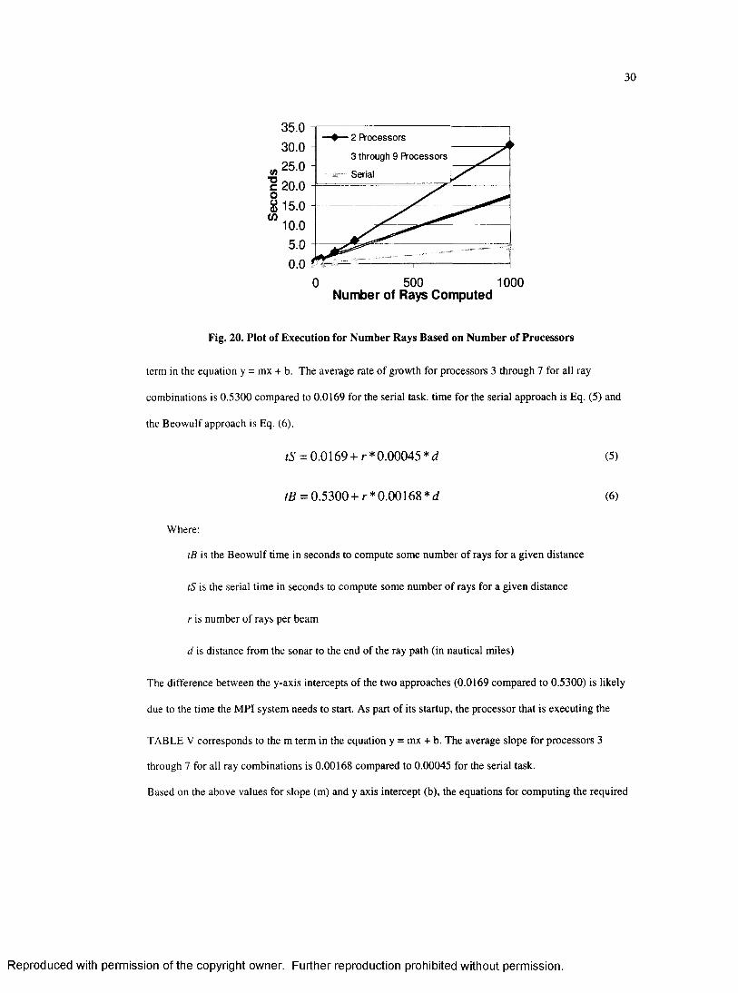
30

0 5 0 0Number of Rays Computed

1000

Fig. 20. Plot of Execution for Number Rays Based on Number of Processors

term in the equation y = mx + b. The average rate o f growth for processors 3 through 7 for all ray

combinations is 0.5300 compared to 0.0169 for the serial task, tim e for the serial approach is Eq. (5) and

the B eow ulf approach is Eq. (6).

Where:

tB is the B eow ulf time in seconds to com pute some num ber o f rays for a given distance

tS is the serial tim e in seconds to compute some num ber o f rays for a given distance

r is num ber o f rays per beam

d is distance from the sonar to the end of the ray path (in nautical miles)

The difference betw een the y-axis intercepts o f the two approaches (0.0169 com pared to 0.5300) is likely

due to the time the MP1 system needs to start. As part o f its startup, the processor that is executing the

TABLE V corresponds to the m term in the equation y = mx + b. The average slope for processors 3

through 7 for all ray combinations is 0.00168 compared to 0.00045 for the serial task.

Based on the above values for slope (m) and y axis intercept (b), the equations for com puting the required

tS = 0.0169 + r *0.00045 *d (5)

tB = 0.5300 + r *0.00168* d (6)


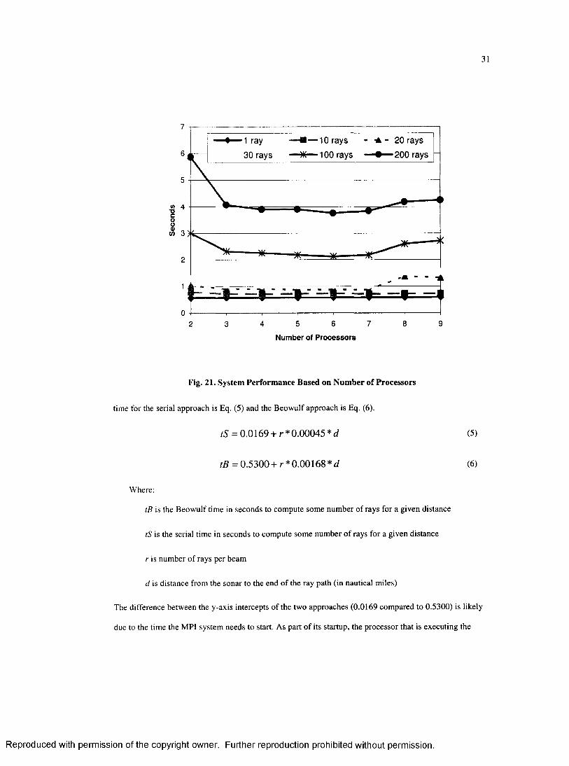
31

T3Coua)

7

1 ray

30 rays6 100 rays 200 rays

5

4

3

2

A- ~ ..** I t *w ~ —1

095 6 7 842 3

Number of Processors

Fig. 21. System Performance Based on Number of Processors

time for the serial approach is Eq. (5) and the Beow ulf approach is Eq. (6).

tS = 0.0169 + r *0.00045 *d (5)

tB = 0.5300+ r* 0.00168 * d (6)

Where:

tB is the B eow ulf time in seconds to compute some num ber o f rays for a given distance

tS is the serial time in seconds to compute some num ber o f rays for a given distance

r is num ber o f rays per beam

d is distance from the sonar to the end o f the ray path (in nautical miles)

The difference betw een the y-axis intercepts o f the two approaches (0.0169 com pared to 0.5300) is likely

due to the time the M PI system needs to start. As part o f its startup, the processor that is executing the


32

TABLE V. Robust Linear Curve Fitting for Selected Processor Combinations

Number of Slave processors Y axis intercept Slope of the line

3 0.553405 0.00168376

4 0.539091 0.00170894

5 0.541148 0.00167085

6 0.476149 0.00168633

7 0.540560 0.00165107

Totals 2.650353 0.00840095

Average coefficients for a

distance of 1 Nm

0.530070 0.00168019

Serial coefficients for a

distance of 1 Nm

0.0168646 0.000446658

mpirun comm and has to query the requested num ber o f other hosts (m aster and som e num ber o f slaves) to

see if they are available for use. Once this startup phase is completed, the differences in the slopes o f the

lines come into play. The B eowulf im plem entation has each process run a single instance o f the Ray

program, and it is reasonable to assume that the execution for that single instance and the serial execution

should be the same (0.00045 seconds). As the Ray program is executing, it is outputting data to a data file.

In the serial execution, new ray data is appended to an already opened file. In the B eow ulf im plem entation,

each slave outputs its data to its own file. The file is then closed and the m aster process has to examine the

data file to determine where the ray data begins and copy data from that point on to another file. This

copying o f data is the consolidation o f data into a serial look alike form. The m aster opening the slave’s file

and searching it for data is likely to be time consuming.


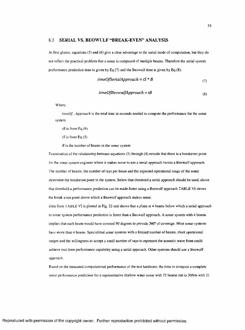
33

8.3 SERIAL VS. BEOWULF “BREAK-EVEN” ANALYSIS

At first glance, equations (5) and (6) give a clear advantage to the serial mode o f com putation, but they do

not reflect the practical problem that a sonar is composed o f m ultiple beams. Therefore the serial system

performance prediction time is given by Eq.(7) and the B eow ulf tim e is given by Eq.(8).

timeOfSerialApproach = tS* B ^

timeOfBeowulfApproach = tB ^

Where:

timeOf...Approach is the total time in seconds needed to compute the perform ance for the sonar

system

tB is from Eq.(6)

tS is from Eq.(5)

B is the num ber o f beams in the sonar system

Examination o f the relationship between equations (5) through (8) reveals that there is a breakeven point

for the sonar system engineer where it makes sense to use a serial approach versus a B eow ulf approach.

The number of beams, the num ber o f rays per beam and the expected operational range o f the sonar

determine the breakeven point in the system. Below that threshold a serial approach should be used, above

that threshold a perform ance prediction can be made faster using a B eow ulf approach TABLE VI shows

the break-even point above which a B eow ulf approach makes sense.

Data from TABLE VI is plotted in Fig. 22 and shows that a plane at 4 beams below w hich a serial approach

to sonar system perform ance prediction is faster than a B eow ulf approach. A sonar system with 4 beams

implies that each beam would have covered 90 degrees to provide 360° o f coverage. M ost sonar systems

have more than 4 beams. Specialized sonar systems with a lim ited num ber o f beams, short operational

ranges and the willingness to accept a small num ber o f rays to represent the acoustic wave front could

achieve real-time perform ance capability using a serial approach. O ther system s should use a B eow ulf

approach.

Based on the measured computational perform ance of the test hardware; the tim e to com pute a com plete

sonar performance prediction for a representative shallow water sonar with 72 beams out to 30Nm with 21


34

TABLE VI. Number of Beams Above Which Beowulf Clustering Should be Used

Nm

Number of Rays to be Computed per Beam

1 10 20 30 40 50 60 70 80 90 100 110 120

1 31 26 22 19 17 16 14 13 13 12 11 11 10

2 30 22 17 14 13 11 10 10 9 9 8 8 7

3 29 19 14 12 10 9 9 8 7 7 7 7 6

4 29 17 13 10 9 8 7 7 7 6 6 6 6

5 28 16 11 9 8 7 7 6 6 6 6 6 5

6 28 14 10 9 7 7 6 6 6 6 5 5 5

7 27 13 10 8 7 6 6 6 5 5 5 5 5

8 27 13 9 7 7 6 6 5 5 5 5 5 5

9 26 12 9 7 6 6 6 5 5 5 5 5 5

10 26 11 8 7 6 6 5 5 5 5 5 5 5

11 25 11 8 7 6 6 5 5 5 5 5 5 4

12 25 10 7 6 6 5 5 5 5 5 5 4 4

13 24 10 7 6 6 5 5 5 5 5 5 4 4

14 24 10 7 6 5 5 5 5 5 5 4 4 4

15 24 9 7 6 5 5 5 5 5 4 4 4 4

16 23 9 7 6 5 5 5 5 5 4 4 4 4

17 23 9 6 6 5 5 5 5 4 4 4 4 4

18 22 9 6 6 5 5 5 5 4 4 4 4 4

19 22 8 6 5 5 5 5 4 4 4 4 4 4

20 22 8 6 5 5 5 5 4 4 4 4 4 4


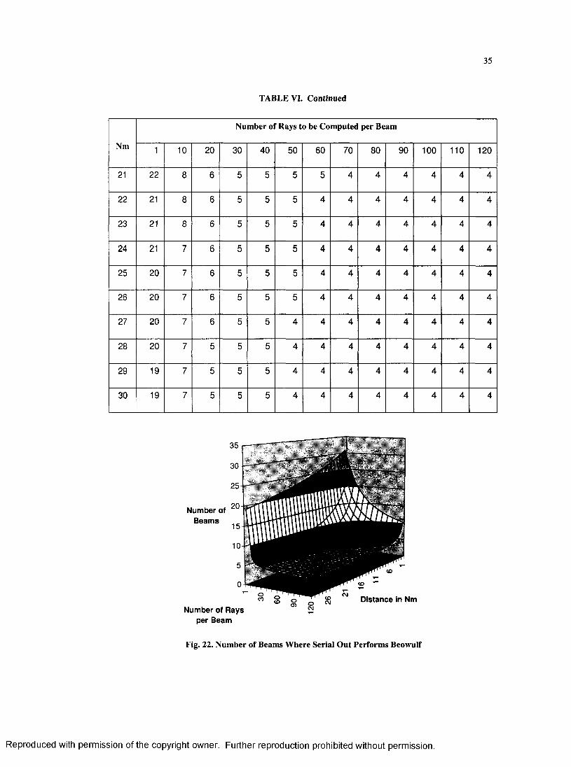
35

TABLE VI. Continued

Nm

Number of Rays to be Computed per Beam

1 10 20 30 40 50 60 70 80 90 100 110 120

21 22 8 6 5 5 5 5 4 4 4 4 4 4

22 21 8 6 5 5 5 4 4 4 4 4 4 4

23 21 8 6 5 5 5 4 4 4 4 4 4 4

24 21 7 6 5 5 5 4 4 4 4 4 4 4

25 20 7 6 5 5 5 4 4 4 4 4 4 4

26 20 7 6 5 5 5 4 4 4 4 4 4 4

27 20 7 6 5 5 4 4 4 4 4 4 4 4

28 20 7 5 5 5 4 4 4 4 4 4 4 4

29 19 7 5 5 5 4 4 4 4 4 4 4 4

30 19 7 5 5 5 4 4 4 4 4 4 4 4

Number of Beams

Distance in NmNumber of Rays

per Beam

Fig. 22. Number of Beams Where Serial Out Performs Beowulf


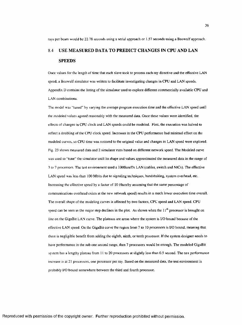
36

rays per beam would be 22.78 seconds using a serial approach or 1.57 seconds using a B eow ulf approach.

8.4 USE MEASURED DATA TO PREDICT CHANGES IN CPU AND LAN

SPEEDS

Once values for the length o f time that each slave took to process each ray directive and the effective LAN

speed, a Beow ulf sim ulator was written to facilitate investigating changes in CPU and LAN speeds.

Appendix D contains the listing o f the sim ulator used to explore different com m ercially available CPU and

LAN combinations.

The model was “tuned” by varying the average program execution tim e and the effective LAN speed until

the modeled values agreed reasonably with the measured data. Once these values were identified, the

effects o f changes in CPU clock and LAN speeds could be modeled. First, the execution was halved to

reflect a doubling o f the CPU clock speed. Increases in the CPU perform ance had minim al effect on the

modeled curves, so CPU time was restored to the original value and changes in LAN speed were explored.

Fig. 23 shows measured data and 2 sim ulator runs based on different network speed. The M odeled curve

was used to “tune” the sim ulator until its shape and values approximated the m easured data in the range of

3 to 7 processors. The test environm ent used a 100BaseTX LAN (cables, switch and NICs). The effective

LAN speed was less than 100 M bits due to signaling techniques, handshaking, system overhead, etc.

Increasing the effective speed by a factor o f 10 (thereby assum ing that the same percentage o f

comm unications overhead exists at the new network speed) results in a much low er execution tim e overall.

The overall shape o f the modeling curves is affected by two factors, CPU speed and LAN speed. CPU

speed can be seen in the m ajor step declines in the plot. As shown when the 11th processor is brought on

line on the G igaBit LAN curve. The plateaus are areas where the system is I/O bound because o f the

effective LAN speed. On the G igaBit curve the region from 7 to 10 processors is I/O bound, meaning that

there is negligible benefit from adding the eighth, ninth, o r tenth processor. If the system designer needs to

have perform ance in the sub one second range, then 7 processors would be enough. The modeled GigaBit

system has a lengthy plateau from 11 to 20 processors at slightly less than 0.5 second. The nex perform ance

increase is at 21 processors, one processor per ray. Based on the m easured data, the test environm ent is

probably I/O bound som ewhere between the third and fourth processor.


37

Performance of the Beowulf Cluster21 task s to perform and 21 procssesors

Input = 0.09 sec, processing = 0.18 sec. Output = 0.0 sec.

* — Modeled

— Actual

G igaB it LAN

3.0

« 2.5■acooa>

” 2.0 aEs=o

0.5

0.04 5 B 7 8 9 10 11 12 13 14 15 16 17 18 19 20 213

Total Number of Processors in the System

Fig. 23. Estimated Effects of Increasing LAN from 100 Mbit to 1000 Mbit

Another way to evaluate the system is to plot the effect on system performance by the addition o f each

processor. Figure 24 shows the effect o f increm entally adding processors to the system. Using the m easured

data, when the third processor is added, it improves overall perform ance by about 26%, while the fourth

adds little positive im provem ent, but the fifth and six each im prove the system som ewhat. The seventh and

eighth processors actually cause the system perform ance to degrade. W hile the m odeled perform ance for

the 100 M b LAN shows a continuous im provem ent for each additional processor until becom ing I/O bound

at 7 processors. The curves for a GigaBits LAN were not plotted because all data w ould have been based

on conjecture.

The current work investigated w hether or not it is theoretically possible to com pute a sonar performance

prediction in real-tim e using a B eow ulf clustering approach. That goal has been achieved. Several areas

deserve further study. They include:


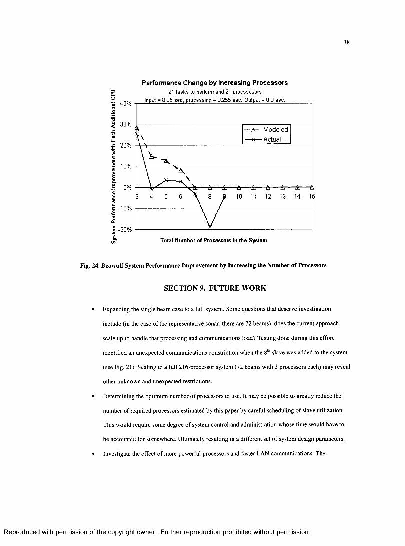
38

Performance Change by Increasing Processors21 tasks to perform and 21 procssesors

Input = Q.Q5 sec, processing = 0.255 sec. Output = 0.0 sec.75 40%S0

1 30%- A - Modeled

— * — ActualXO(OID

2 0 %XIsI 1 0 %03>0uQ.1 0%O)0 c5- - 10%ta>a1 -20%

Total Number of Processors in the System

Fig. 24. Beowulf System Performance Improvement by Increasing the Number of Processors

SECTION 9. FUTURE WORK

• Expanding the single beam case to a full system. Some questions that deserve investigation

include (in the case o f the representative sonar, there are 72 beams), does the current approach

scale up to handle that processing and com m unications load? Testing done during this effort

identified an unexpected com m unications constriction when the 8th slave was added to the system

(see Fig. 21). Scaling to a full 216-processor system (72 beam s with 3 processors each) may reveal

other unknown and unexpected restrictions.

• Determ ining the optimum num ber o f processors to use. It may be possible to greatly reduce the

number o f required processors estim ated by this paper by careful scheduling o f slave utilization.

This would require some degree o f system control and adm inistration whose tim e would have to

be accounted for somewhere. U ltimately resulting in a different set o f system design parameters.

• Investigate the effect o f more powerful processors and faster LAN com m unications. The


39

processors and network used in the test environm ent are not leading edge technology. Faster

processors would reduce execution tim e o f the Ray program on the individual processors, but if the

LAN cannot move the data fast enough, the system would probably degenerate very quickly into an

I/O bound condition.

SECTION 10. CONCLUSIONS

Real-time sonar perform ance prediction is possible using B eow ulf clustering techniques. There is a

breakeven point betw een serial and B eow ulf com putational approaches that is dependent on the num ber of

processors and the LAN that connects them. The time to com pute the total probability o f detection [p(D)]

for a representative shallow w ater sonar system is based on the following relationships:

• Serial approach = serial computation time for each beam tim es the num ber o f beams

• Beow ulf approach = serial com putation tim e per beam

Based on data collected from the test hardw are suite, the com putational times in seconds for the serial and

Beow ulf approaches can be computed using the following equations:

• Serial com putation tim e per beam = 0.0169 + num ber o f rays * 0.00045 * distance (in Nm)

• B eow ulf com putation tim e per beam = 0.5300 + number o f rays * 0.00168 * distance (in Nm)

For a representative shallow w ater sonar system with 72 beams, shooting 21 rays to em ulate an acoustic

wave front, to a range o f 30 Nm; the serial approach will take 21.5 seconds and the B eow ulf approach will

take 1.6 seconds. The coefficients in the serial and B eow ulf computation tim e equations show that there are

system breakeven points based on the num ber of rays, num ber o f beams and distance. A sonar system

designer can determine the least costly and m ost effective hardw are and softw are suite required to achieve

real-time sonar prediction capability by using the approaches and equations derived in this paper.


40

REFERENCES

[ 1 ] J. D. Bernal, “A History o f Classical Physics From A ntiquity to the Q uantum ,” Barnes & N oble Books, 1997.

[2] J. B. Bowlin, “Ocean Acoustic Ray-Tracing Software RAY W H OI-93-10,” W oods HoleO ceanographic Institute, 1992.

[3] C. Cartledge, “M odel 610E M od 1 Sonar System, Signal Excess Prediction Equations,” EDOCorporation Com bat Systems, report 990801, 1997.

[4] C. Cartledge, “Application o f an Adaptive B eow ulf Computational Approach to Reduce AcousticEnvironm ental M odeling Tim es,” U ndersea Defence Technology Europe Conference, 2003.

[5] D. E. Culler and J.P. Singh, “Parallel Com puter Architecture, A H ardware/Software A pproach,”M organ Kaufmann Publishers, Inc., 1999.

[6] C. D. Hodgman, “H andbook o f Chemistry and Physics,” Chemical R ubber Publishing Co., 1952.

[7] R. W. Hockney, and C. R. Jesshope, “Parallel Com puters,” Adam H ilger Ltd, Bristol, 1981.

[8] I. M iller and J. E. Freund, “Probability and Statistics for Engineers,” Prentice-Hall, Inc., 1977.

[9] A. M odi, “Real-tim e V isualization o f Aerospace Sim ulations Using Com putational Steering andB eow ulf C lusters,” 2002. Available: http://w w w .anirudh.net/phd/thesis.pdf.

[10]J. J. O ’Connor and E. F. Robertson, “Pierre de Ferm et.” Available: http://vvww-gap.dcs.st- im d.ac.uk/~history/M atheniaticians/Ferm at.html

[1 1]P. S. Pachecho, “Parallel Programming with M PI,” M organ Kaufmann Publishers, Inc., 1997.

[ 12] E. M. Podeszwa, “Sound Speed Profiles for the North A tlantic Ocean,” N aval U nderwater Systems Center, 1976.

[ 13] G. Snow, “Underwater A coustics and Sonar Transducers,” EDO W estern D ivision, report 17018, 1983.

[ 14]T. Sterling, “B eow ulf Breakthroughs,” Linux M agazine, June 2003. Available: http://www.lm ux-miig.com/2003-06/breakthroughs_01 .html

[15] A. S. Tanenbaum , “Com puter N etw orks,” Prentice-Hall, Inc., 1996.

[16] TOP-500, “Top 500 Computer Sites, N ovem ber 2003.” Available: http://w ww .top500.org/

[17] R. J. Urick, “Principles o f Underwater Sound for Engineers,” M cGraw-Hill, Inc., 1967.

[ 18] R. J. Urick, “Sound Propagation in the Sea,” Defense Advanced Research Projects Agency, 1979.

[19]C. Wasel, “Parallel C om puter Taxonom y,” A berystwyth University, 1994. Available: http://www .gigaflop.dem on.co.uk/com p/chapt7.htm

[20] “NIST H andbook 148,” N ational Institute o f Standards and Technology D ataplot ReferenceManual. Available: http://w w w .itl.nist.gov/div898/softw are/dataplot/refm anl/ch5/w eights.pdf


http://www.anirudh.net/phd/thesis.pdf

http://vvww-gap.dcs.st-

http://www.lmux-

http://www.top500.org/

http://www.gigaflop.demon.co.uk/comp/chapt7.htm

http://www.itl.nist.gov/div898/software/dataplot/refmanl/ch5/weights.pdf

[21 ] M athW orks, “Curve Fitting Toolbox.” Available:http://w ww .m athworks.eom /access/helpdesk/help/toolbox/curvefit/ch_fitt5.htm l#67660


http://www.mathworks.eom/access/helpdesk/help/toolbox/curvefit/ch_fitt5.html%2367660

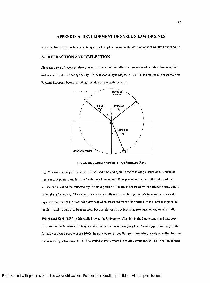
42

APPENDIX A. DEVELOPMENT OF SNELL’S LAW OF SINES

A perspective on the problems, techniques and people involved in the developm ent o f Snell’s Law o f Sines.

A .l REFRACTION AND REFLECTION

Since the dawn o f recorded history, man has known o f the reflective properties o f certain substances, for

instance still water reflecting the sky. Roger B acon’s Opus M ajus, in 1267 [1] is credited as one o f the first

W estern European books including a section on the study o f optics.

Normal to surface

Incident Reflectedray

Refracted t ray

denser medium

Fig. 25. Unit Circle Showing Three Standard Rays

Fig. 25 shows the m ajor terms that will be used time and again in the following discussions. A beam of

light starts at point A and hits a reflecting m edium at point B. A portion of the ray reflected off o f the

surface and is called the reflected ray. Another portion o f the ray is absorbed by the reflecting body and is

called the refracted ray. The angles a and r were easily m easured during B acon’s tim e and were exactly

equal (to the lim it o f the measuring devices) when measured from a line norm al to the surface at point B.

Angles a and p could also be measured, but the relationship between the two was not known until 1703.

W illeb ro rd Snell (1580-1626) studied law at the U niversity o f Leiden in the Netherlands, and was very

interested in mathematics. He taught m athematics even while studying law. As was typical o f many o f the

formally educated people o f the 1600s, he traveled to various European countries, m ostly attending lectures

and discussing astronomy. In 1602 he settled in Paris where his studies continued. In 1617 Snell published


43

Eratosthenes Batavus, which contains his methods for measuring the Earth, in w hich he proposed the

method of triangulation. This work is the foundation o f geodesy.

rarer medium

sin aIncident

RefractedV ray

densermedium

Fig. 26. Snell's Law O f Sines Diagram

sin a= k (9)sm p

Snell’s contribution to the topic o f ray tracing (Appendix G) is the law of sines that bears his name. Snell’s

Law of Sines, as shown in Figure 26, was the discovery that the ratio o f the sines o f a and p were constant

for any pair o f mediums. Eq. (9) is Snell’s Law o f Sines. He was not able to explain the basis o f the

constant, ju s t that it was a constant.

Pierre de Fermat (1601-1665) studied Law at the U niversity o f Orleans and had a prosperous and

professionally active career in law and the judiciary. Ferm at is known as a superb mathematician, even

though he did not publish often. His technique of getting others to follow his line o f thinking was to pose a

particularly difficult question along with the answer and challenge other mathem aticians to come up with

the same answer. Only afterwards would he reveal his technique, often pushing the bounds of math at the

time.

Fermat and Rene Descartes had a long running continuous professional and personal disagreem ent about

Snell’s Law o f Sines. N either would dispute that Snell’s approach matched the m easured data, what they


44

disagreed on was “why” there was a constant. Descartes took the position that light traveled faster through

the denser medium than it did in the rarer medium. Ferm at took the position that light was taking the least

time path to get from point A to point B. It is probable that Descartes based his position on the behavior o f

sound. D escartes’ reasoning was that sound travels faster in a denser medium com pared to a rarer medium,

so why shouldn’t light? Ferm at took the position that light traveled slower in the denser m edium but that

the time it took for light to travel, as shown in Fig. 27 from point A to point C via point B, was less than the

time from point A to C via D.

sin aIncident

Refracted t ray

denser medium

Fig. 27. Pierre De Fermat's Ray Diagram

I AB 1=1 B C I (10)

IA B I +1 BC l>l A C I (11)

(I AD I / vl+1 D C I / v2) > (I AB l / v l + l B C I / v2) (12)

Equations (10) through (12) show the basis for Ferm at’s argument. Eq. (10) is his first assum ption that the

distances are equal. Because o f the first assum ption then the second next assumption, Eq. (11) follows. The

only way that (10) and (11) could be true is if (12) was also true. Fermat could not assign values to the

speed o f light (v 1 and v2 in the equations), he could only theorize about their relationship. Another 200

years would pass before progress could be made.


45

A.2 WHAT IS THE SPEED OF LIGHT?

H ippoly te F izeau (1819 - 1896) in 1849 was the first person to use terrestrial based techniques to measure

the speed o f light. Danish astronom er Ole Rom er in 1676 had calculated the speed o f light using the motion

o f the earth and the moons of Jupiter as 212,000 km/s (an error o f 29%), but Fizeau is credited with the

calculating the speed as 313,000 km/s using a device like the one shown in Fig. 28 [10].

Fig. 28. F izeau 's M ach ine

Through a series o f reduction gears, the hand crank causes the wheel in front o f the eyepiece to rotate. The

wheel has 720 notches cut into its outer edge. In front o f the eyepiece is a partially reflecting m irror

mounted so that a light source can be placed to the left o f the eyepiece and focused on the mirror. The

mirror reflects the light through notches in the wheel and out to a reflecting m irror some distance away.

This reflected light is focused back through the eyepiece to the viewer.

In Fizeau’s experiment, the mechanical device was in M ountartre, France and the reflecting m irror was on

Mount V alerien in Suresnes, 8,633 m eters away. The basis for measuring the speed was to cause the wheel


46

to spin at just the right rate so that light passing through one notch would be able to return through the same

notch. Fizeau found that the right speed was 12.6 revolutions per second. Equations (13) through (18) are

similar to those that Fizeau used to compute the speed o f light. Eq. (13) is the definition o f the tim e that

light took to travel from F ixeau’s eyepiece and return. Eq. (14) expresses the size o f one o f the notches in

the wheel. Eq. (15) is the angular velocity o f the notch in wheel o f the apparatus. Eq. (16) is the tim e that

light would be visible through the notch. Eq. (17) sets the tim e for the light to transit the valley equal to the

time that the light could be visible through the notch. Finally, (18) reorders the term and solves for c.

2 * d 2 * 8 6 3 37 1 =

2 *7ta = -

2 * 7 2 0

v = 2* 7t *12.6

2 * n

(13)

(14)

(15)

T 2 - a - 2 * 7 2 0 _ 1 (16)v 2 * tt*12.6 2 * 7 2 0 * 1 2 .6

2 * d a 71 = 7 2 = — = -

c v(17)

2 * d * v 2 * 8 6 3 3 * 2 * 7 2 0 * 1 2 6 c = ^ - ^ = = 313,0 00km /s (18)

Fizeau's m easurem ents for the speed o f light is only 4.3% greater than the 21st century accepted speed of

300,00 km/s. The size o f the experim ental apparatus (8,633 meters) precluded it from being used to

measure the speed of light in anything other then air.

Leon F o u cau lt (1819-1868) in 1862 was able to measure the speed o f light in a laboratory. His device is

shown diagram m atically in Fig. 29.

A light is focused on a rotating mirror. The rotating m irror bounces the light to a stationary m irror that

reflects the light back to the rotating mirror. During this tim e, the mirror has rotated to a different angle,


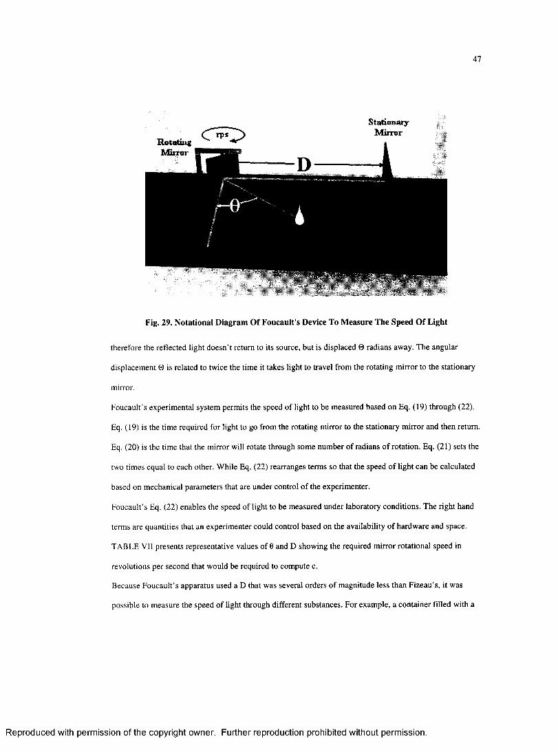
47

S t a t i o n a r yM irror

RotatingM inor

Fig. 29. Notational Diagram Of Foucault's Device To Measure The Speed Of Light

therefore the reflected light doesn’t return to its source, but is displaced 0 radians away. The angular

displacem ent 0 is related to twice the tim e it takes light to travel from the rotating m irror to the stationary

mirror.

Foucault’s experim ental system perm its the speed o f light to be measured based on Eq. (19) through (22).

Eq. (19) is the time required for light to go from the rotating mirror to the stationary m irror and then return.

Eq. (20) is the time that the m irror will rotate through some num ber o f radians o f rotation. Eq. (21) sets the

two times equal to each other. W hile Eq. (22) rearranges terms so that the speed o f light can be calculated

based on mechanical param eters that are under control o f the experimenter.

Foucault’s Eq. (22) enables the speed o f light to be measured under laboratory conditions. The right hand

terms are quantities that an experim enter could control based on the availability o f hardw are and space.

TABLE VII presents representative values of 6 and D showing the required m irror rotational speed in

revolutions per second that would be required to compute c.

Because Foucault’s apparatus used a D that was several orders o f m agnitude less than F izeau’s, it was

possible to measure the speed of light through different substances. For exam ple, a container filled with a


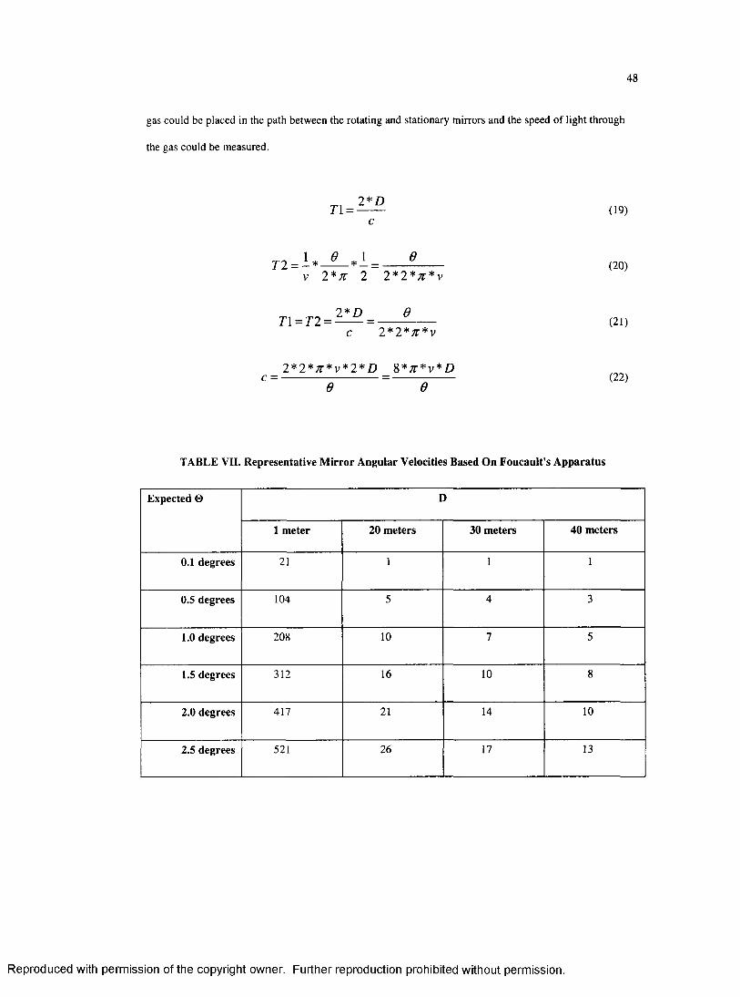
48

gas could be placed in the path between the rotating and stationary mirrors and the speed o f light through

the gas could be measured.

(19)

(20)

(21)

(22)

TABLE VII. Representative Mirror Angular Velocities Based On Foucault's Apparatus

71 =2 * D

ev 2 *7C 2 2 * 2 * n * v

71 = 7 2 =2 * D 6

2 * 2 * n * v

c =2*2* n * v * 2 * D 8* k * v * D

e e

Expected 0 D

1 meter 20 meters 30 meters 40 meters

0.1 degrees 21 1 1 1

0.5 degrees 104 5 4 3

1.0 degrees 208 10 7 5

1.5 degrees 312 16 10 8

2.0 degrees 417 21 14 10

2.5 degrees 521 26 17 13


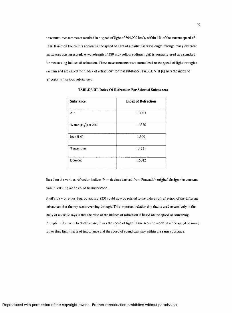
49

Foucault’s measurem ents resulted in a speed o f light o f 304,000 km/s, within 1% o f the current speed of

light. Based on Foucault’s apparatus, the speed o f light o f a particular wavelength through many different

substances was measured. A wavelength o f 589 m p (yellow sodium light) is norm ally used as a standard

for measureing indices o f refraction. These measurem ents were norm alized to the speed o f light through a

vacuum and are called the “index o f refraction” for that substance. TABLE VIII [6] lists the index o f

refraction o f various substances:

TABLE VIII. Index Of Refraction For Selected Substances

Substance Index of Refraction

Air 1.0003

W ater (H20) at 20C 1.3330

Ice (H20) 1.309

Turpentine 1.4721

Benzene 1.5012

Based on the various refraction indices from devices derived from Foucault’s original design, the constant

from Snell’s Equation could be understood.

Snell’s Law o f Sines, Fig. 30 and Eq. (23) could now be related to the indices o f refraction o f the different

substances that the ray was traversing through. This im portant relationship that is used extensively in the

study of acoustic rays is that the ratio o f the indices o f refraction is based on the speed o f som ething

through a substance. In Snell’s case, it was the speed o f light. In the acoustic world, it is the speed o f sound

rather than light that is o f im portance and the speed o f sound can vary within the sam e substance.


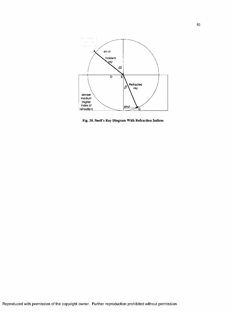
50

a / sin a f N Jncident

/ X V

/

AD B

denser \ medium \(higher index of

refraction)

A Refracted / P \ ray /

sin/S

Fig. 30. Snell's Ray Diagram With Refraction Indices


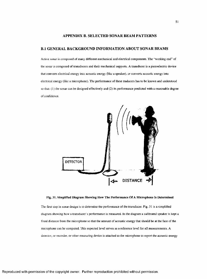
51

APPENDIX B. SELECTED SONAR BEAM PATTERNS

B .l GENERAL BACKGROUND INFORMATION ABOUT SONAR BEAMS

Active sonar is com posed o f many different m echanical and electrical components. The “working end” of

the sonar is composed of transducers and their m echanical supports. A transducer is a piezoelectric device

that converts electrical energy into acoustic energy (like a speaker), or converts acoustic energy into

electrical energy (like a microphone). The perform ance o f these traducers has to be known and understood

so that: ( 1) the sonar can be designed effectively and (2) its performance predicted with a reasonable degree

o f confidence.

DISTANCE

Fig. 31. Simplified Diagram Showing How The Performance Of A Microphone Is Determined

The first step in sonar design is to determine the perform ance o f the transducer. Fig. 31 is a simplified

diagram showing how a transducer’s performance is measured. In the diagram a calibrated speaker is kept a

fixed distance from the microphone so that the am ount o f acoustic energy that should be at the face o f the

m icrophone can be computed. This expected level serves as a reference level for all m easurem ents. A

detector, or recorder, or other m easuring device is attached to the microphone to report the acoustic energy


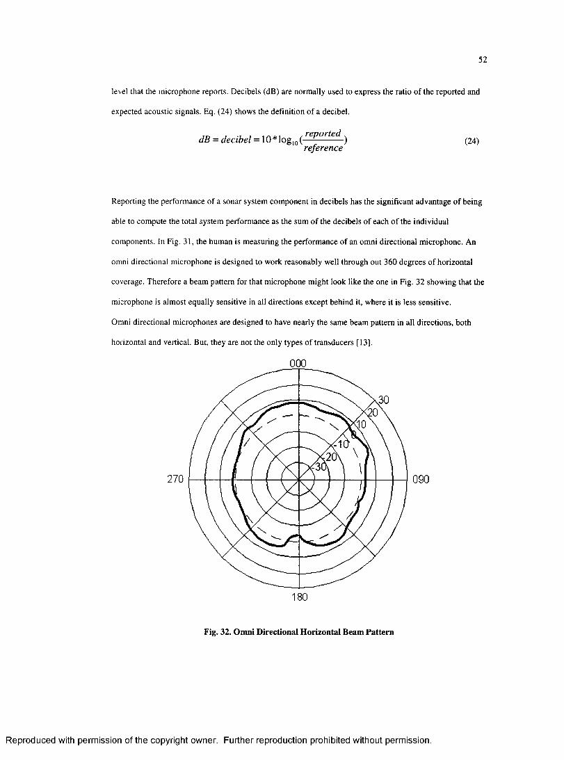
52

level that the microphone reports. Decibels (dB) are normally used to express the ratio o f the reported and

expected acoustic signals. Eq. (24) shows the definition o f a decibel.

Reporting the perform ance o f a sonar system com ponent in decibels has the significant advantage o f being

able to compute the total system perform ance as the sum o f the decibels o f each o f the individual

components. In Fig. 31, the hum an is measuring the perform ance o f an omni directional microphone. An

omni directional microphone is designed to work reasonably well through out 360 degrees o f horizontal

coverage. Therefore a beam pattern for that microphone might look like the one in Fig. 32 showing that the

microphone is alm ost equally sensitive in all directions except behind it, where it is less sensitive.

Omni directional microphones are designed to have nearly the same beam pattern in all directions, both

horizontal and vertical. But, they are not the only types o f transducers [13].

dB = decibel = 10* log10 (reportedreference

(24)

000

270 090

180

Fig. 32. Omni Directional Horizontal Beam Pattern


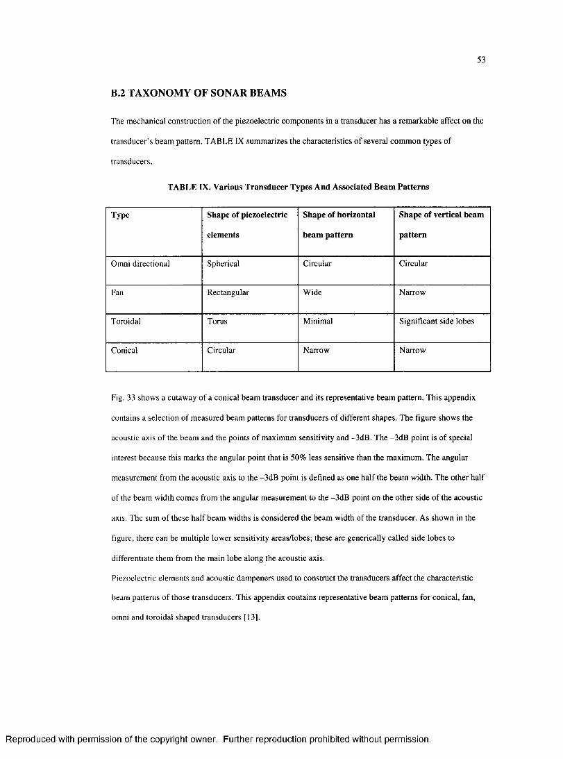
53

B.2 TAXONOMY OF SONAR BEAMS

The mechanical construction o f the piezoelectric com ponents in a transducer has a rem arkable affect on the

transducer’s beam pattern. TABLE IX sum marizes the characteristics o f several com m on types o f

transducers.

TABLE IX. Various Transducer Types And Associated Beam Patterns

Type Shape of piezoelectric

elements

Shape of horizontal

beam pattern

Shape of vertical beam

pattern

Omni directional Spherical C ircular Circular

Fan Rectangular W ide N arrow

Toroidal Torus M inimal Significant side lobes

Conical Circular Narrow Narrow

Fig. 33 shows a cutaw ay o f a conical beam transducer and its representative beam pattern. This appendix

contains a selection of measured beam patterns for transducers o f different shapes. The figure shows the

acoustic axis o f the beam and the points o f maximum sensitivity and -3dB . The -3 d B point is o f special

interest because this marks the angular point that is 50% less sensitive than the maximum . The angular

m easurem ent from the acoustic axis to the -3dB point is defined as one half the beam width. The other half

o f the beam width comes from the angular m easurem ent to the -3 d B point on the other side o f the acoustic

axis. The sum o f these half beam widths is considered the beam width of the transducer. As shown in the

figure, there can be multiple low er sensitivity areas/lobes; these are generically called side lobes to

differentiate them from the main lobe along the acoustic axis.

Piezoelectric elem ents and acoustic dam peners used to construct the transducers affect the characteristic

beam patterns o f those transducers. This appendix contains representative beam patterns for conical, fan,

omni and toroidal shaped transducers [13].


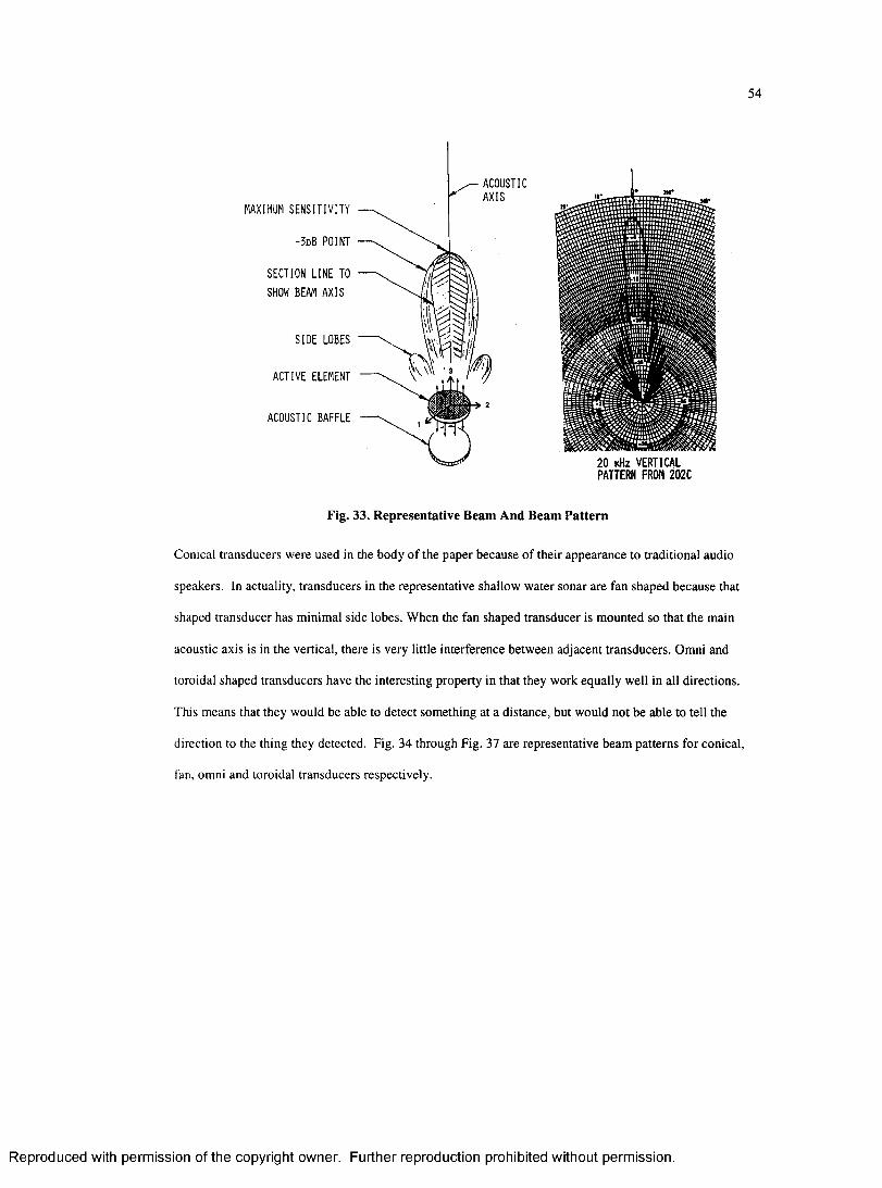
54

ACOUSTICMAXIMUM SENSITIVITY

-3d B POINT

SECTION LINE TO SHOW BEAM AXIS

SIDE LOBES

ACTIVE ELEMENT

ACOUSTIC BAFFLE

20 kHz VERTICAL PATTERN FROM 202C

Fig. 33. Representative Beam And Beam Pattern

Conical transducers were used in the body o f the paper because o f their appearance to traditional audio

speakers. In actuality, transducers in the representative shallow water sonar are fan shaped because that

shaped transducer has minimal side lobes. W hen the fan shaped transducer is m ounted so that the main

acoustic axis is in the vertical, there is very little interference between adjacent transducers. Omni and

toroidal shaped transducers have the interesting property in that they work equally well in all directions.

This means that they would be able to detect something at a distance, but would not be able to tell the

direction to the thing they detected. Fig. 34 through Fig. 37 are representative beam patterns for conical,

fan, omni and toroidal transducers respectively.


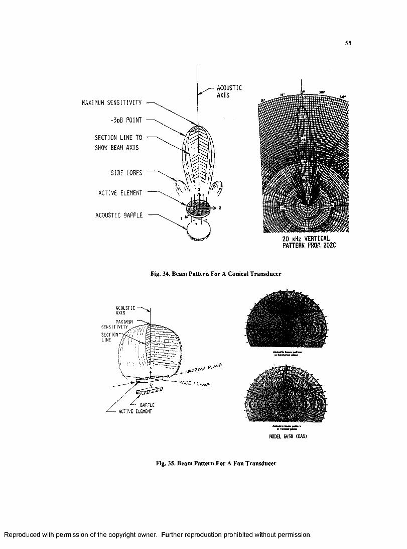
55

ACOUSTICAXIS

MAXIMUM SENSITIVITY

~3d B POINT

SECTION LINE TO SHOW BEAM AXIS

SIDE LOBES

ACTIVE ELEMENT

ACOUSTIC BAFFLE

20 kHz VERTICAL PATTERN FROM 202C

Fig. 34. Beam Pattern For A Conical Transducer

ACOUSTICAXISMAXIMUM

SENSITIVITYSECTION LINE

WIDE P t t w E

BAFFLE ACTIVE ELEMENT

MODEL 6N58 (OAS)

Fig. 35. Beam Pattern For A Fan Transducer


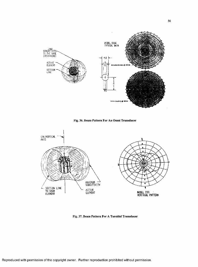
56

MODEL 6166 TYPICAL DATA

QhN I SENSITIVITY-is the: s a m eEVERYWHERE)

A C T I V EELEMENT RpriieM*! 4r»cthdy $ iMtHl

SECTIONLINE

tferiitu dit«rfi*il> 9 19 kta

Fig. 36. Beam Pattern For An Omni Transducer

C Y L I N D R I C A LAXIS

MAXIMUM SENSITIVITYt - SECTION LINE

TO SHOW ELEMENT

ACTIVEELEMENT MODEL 233

VERTICAL PATTERN

Fig. 37. Beam Pattern For A Toroidal Transducer


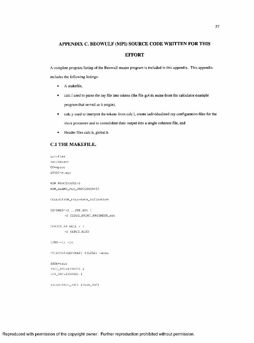
57

APPENDIX C. BEOWULF (MPI) SOURCE CODE W RITTEN FOR THIS

EFFORT

A complete program listing of the B eowulf m aster program is included in this appendix. This appendix

includes the following listings:

• A makefile,

• calc.l used to parse the ray file into tokens (the file got its name from the calculator exam ple

program that served as it origin),

• calc.y used to interpret the tokens from calc.l, create individualized ray configuration files for the

slave processes and to consolidate their output into a single coherent file, and

• Header files calc.h, global.h

C .l THE MAKEFILE.

LEX=f lex YACC=bison CC=mpicc ETAGS=etags

NUM_PROCESSORS=5NUM_BEAMS_PER_PROCESSOR=10

COLLECTION_FILE=data_collection

DEFINES = -D USE__GNU \-D DEBUG_PRINT_PROGRESS_not

DEBUGS_AS„WELL = \-D DEBUG_ALSO

LIBS=-11 -lm

CFLAGS=S(DEFINES) $(LIBS) -ansi

BASE-calcYACC_SRC=$(BASE).y LEX_SRC=$(BASE).1

SRC = $ (YACC_SRC) $ (LEX_SRC)


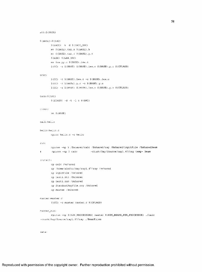
58

all:$(BASE)

$ (BASE):$(SRC)$(YACC) -v -d $(YACC_SRC) mv $ (BASE).tab.h $(BASE).h mv $(BASE).tab.c $(BASE).y.c $ ( LEX} $(LEX_SRC) mv lex.yy.c $(BASE).lex.c$(CC} -o $(BASE) $ (BASE).lex.c $(BASE).y.c S(CFLAGS)

or ig:$(CC) -c $ (BASE).lex.c -o $ (BASE).lex.o $(CC) -c $(BASE).y .c -o $(BASE).y.o$(CC) -o $(BASE) $ (BASE).lex.o $(BASE).y.o $(CFLAGS)

tags:$(SRC)5 (ETAGS) -d -t -1 c $ (SRC)

clean:rm $(BASE)

call:hello

hello:hello.cmpicc hello.c -o hello

run:mpirun -np 5 /Bshared/calc /Bshared/ray /Bshared/inputFile /BsharedBeam

# mpirun -np 5 calc ~chuck/Ray/Source/rayl.47/ray temp- Beam

install:cp calc /Bsharedcp /home/alofts/Ray/ray1.47/ray /Bsharedcp inputFile /Bsharedcp testl.bth /Bsharedcp testl.ssp /Bsharedcp StandardRayFile.ray /Bsharedcp master /Bshared

master:master.c$ (CC) -o master master.c $(CFLAGS)

master_run:mpirun -np $ (NUM_PROCESSORS) master $ (NUM_BEAMS_PER_PROCESSOR) ./calc

-chuck/Ray/Source/ray1.47/ray ./BeamFiles

data :


59

touch $(COLLECTION_FILE)./worker $ (NUM_PROCESSORS) $ (NUM_BEAMS_PER_PROCESSOR) >> $(COLLECTION_FILE)

temp:mpirun -np 2 /Bshared/calc /Bshared/ray /Bshared/inputFile /Bshared/beam

C.2 THE CALC.L FILE.

%f#include "global.h"#include "calc.h"

#include <stdlib.h>

%}

white [ \t ] +

signs [+-]?

digit [0-9]intege {digit}+exponant [ eE]{signs}?{intege}

eal {signs}{intege}("."{intege})?{exponant}?

text [a-zA-Z0-9_]+

%%

{white} { /* We ignore white space */ }

{eal} {yylval=atof(yytext); return(NUMBER);

}

return(PLUS); return(MINUS);

return(TIMES); return(DIVIDE);

return(POWER);

return(LEFT_PARENTHESIS); return(RIGHT_PARENTHESIS);


60

" \ n "

.. N ..

"add_extrema" "min_angle11 " iterations" "rnm_dz" "z_miss"

"angles""first""last""number" "specific" "degrees"" radi ans"

"eigenrays""geo_miss""search_max"

"fan"" d r "

"input""prof_file" "bath_file"" lcss_file" "units"

"model" "bathymetry""bath_smoothing "bottom_depth" "bottom_type" "earth_radius"" integrat ion""margins""max_angle" "max_bounces "" range_depend""z_tolerance"

return(END);

return(SEMICOLON); return(LEFT_CURLY_BRACE); return(RIGHT_CURLY_BRACE); return(QUOTE); return(EQUAL);

return(ADD_EXTREMA); return(MIN_ANGLE); return(ITERATIONS); return(MIN_DZ); return(Z_MISS);

return(ANGLE); return(FIRST); return(LAST); return(NUMBER); return(SPECIFIC);{strcpy (GlobalVars.temp.units, yytext); return(ANGLE_UNITS);} {strcpy (GlobalVars.temp.units, yytext) ; return(ANGLE_UNITS);}

return(EIGENRAYS); return(GEO_MISS); return(SEARCH_MAX);

return(FAN); return(DR);

return(INPUT); return(PROF_FILE); return(BATH_FILE); return(LOSS_FILE);(strcpy (GlobalVars.text, yytext); return(UNITS);}

return(MODEL); return(BATHYMETRY);" return(BATH_SMOOTHING); return(BOTTOM_DEPTH); return(BOTTOM_TYPE); return(EARTH_RADIUS); return(INTEGRATION); return(MARGINS); return(MAX_ANGLE); return(MAX_BOUNCES); return(RANGE_DEPEND) ; return(Z_TOLERANCE);


61

"output" return(OUTPUT);"ascii_file" return(ASCII_FILE);

"paths" return(PATHS);"min_range" return(MIN_RANGE);"max_range" return(MAX_RANGE);"fixed_dr" return(FIXED_DR);

"prof_smoothing" return(PROF_SMOOTHING);"levitus" (strcpy (GlobalVars.text, yytext); return(LEVITUS);}"auto_max" (strcpy (GlobalVars.text, yytext); return(AUTO_MAX);}

"source" "receiver" "range" "depth"

return(SOURCE); return(RECEIVER), return(RANGE); return(DEPTH);

"step_size" return(STEP_SIZE);"cos_factor" return(COS_FACTOR);"max" return(MAX);"min" return(MIN);"multiplier" return(MULTIPLIER);

m" {strcpy (GlobalVars.units, yytext) return(DISTANCE_UNITS)km" (strcpy (GlobalVars.units, yytext) return(DISTANCE_UNITS)Nmi " {strcpy (GlobalVars.units, yytext) return(DISTANCE_UNITS)ft" (strcpy (GlobalVars.units, yytext) return(DISTANCE_UNITS)furlong" (strcpy (GlobalVars.units, yytext) return(DISTANCE_UNITS)parsec" (strcpy (GlobalVars.units, yytext) return(DISTANCE_UNITS)cm" (strcpy (GlobalVars.units, yytext) return(DISTANCE_UNITS)mm" (strcpy (GlobalVars.units, yytext) return(DISTANCE_UNITS)Mm" (strcpy (GlobalVars.units, yytext); return(DISTANCE_UNITS)lightyear" (strcpy (GlobalVars.units, yytext) return(DISTANCE_UNITS)angstrom" (strcpy (GlobalVars.units, yytext); return(DISTANCE_UNITS)

(text) (strcpy (GlobalVars.text, yytext); return (TEXT);}

return(END_OF_FILE);

C.3 THE CALC.Y FILE.


62

#define YYDEBUG 1

#def ine BEGIN_FAN "begin_fan"#define BEGIN_WAVEFRONT "begin_wavefront"#define DEFAULT_LENGTH 1024#def ine DIE_MESSAGE "Be gone, spawn of#define END_FAN "end_fan\n"#def ine END_WAVEFRONT "end_wavefront"

#if DEBUGtfdefine PRINT(a ) printf(a);#else#define PRINT(a )#endi f

# i £def DEBUG_ALSO#define PRINT1(vl,f1} printf(#vl "=%"#fl "\n",vl)#define PRINT2 (vl,fl,v2,f2) printf(#vl "=%"#fl "\t",vl); PRINT1(v2,f2)#define PRINT3 (vl,fl,v2,f2,v3,f3) printf(#vl "=%"#fl "\t",vl); PRINT2 (v2,f2,v3,f3) #define PRINT4(vl,f1,v2,f2,v3,f3,v4, f4) printf(#vl "=%"#fl "\t",vl);PRINT3(v2,f2,v3,f3,v4,f 4}#else#define PRINT1(a,f)#define PRINT2(vl,f1,v2,f2)#define PRINT3(vl,fl,v2,f2/v3,f3)#define PRINT4 (vl,f1,v2,f2,v3,f3, v4,f4) ttendif

#include <signal.h>#include <stdio.h>#include <stdlib.h>#include <string.h> /* this allows us to manipulate text strings */#include <unistd.h>^include "global.h" /* this allows access to the global structures */#include "mpi.h" /* this adds the MPI header files to the program */

extern FILE *yyin, *yyout; extern char *yytext;

extern int yydebug;

extern int errno;

#define FALSE 0 taefine TRUE (! FALSE)

%)


63

%token NUMBER%token PLUS MINUS TIMES DIVIDE POWER%token LEFT_PARENTHESIS RIGHT_PARENTHESIS%token END

%token SPECIFIC RIGHT_CURLY_BRACE LEFT_CURLY_BRACE SEMICOLON EQUAL%token END_OF_FILE QUOTE TEXT DISTANCE_UNITS

%token ADD_EXTREMA MIN_ANGLE ITERATIONS MIN_DZ Z_MISS %token ANGLE FIRST LAST ANGLE_UNITS %token EIGENRAYS GEO_MISS SEARCH_MAX %token FAN DR%token INPUT PROF_FILE BATH_FILE LOSS_FILE UNITS%token MODEL BATHYMETRY INTEGRATION RANGE_DEPEND BATH_SMOOTHING BOTTOM_DEPTH EARTH_RADIUSZ_TOLERANCE%token MARGINS MAX_BOUNCES MAX_ANGLE BOTTOM_TYPE%token OUTPUT ASCII_FILE%token PATHS MIN_RANGE MAX_RANGE FIXED_DR %token PROF_SMOOTHING LEVITUS AUTO_MAX %token RECEIVER SOURCE RANGE DEPTH %token STEP_SIZE COS_FACTOR MAX MIN MULTIPLIER

%lef t PLUS MINUS%left TIMES DIVIDE%lef t NEG %right POWER

%start Input %%

Input:/* Empty */

I Input Line

Line:END

| END_OF_FILE I Expression END I AngleLine END

group.\n"); }I InputLine END

group.\n"); }I ModelsLine END

group.\n"); }

{return;} t printf("Result: %f\n",$l); }

{ PRINT ("Parsed something in the angles

{ PRINT ("Parsed something in the input

{ PRINT ("Parsed something in the models


t OutputLine END group An");}

I SourceLine END group.\n");)

( StepSizeLine END group.\n");}

I ReceiverLine END group.\n") ; }

j PathsLine END group An") ; }

I FanLine END I AddExtremaLine END

group An");)I EigenRaysLine END

group.\n");)I ProfSmoothingLine END

group.\n");)

{ PRINT ("Parsed something in the output

{ PRINT ("Parsed something in the source

{ PRINT ("Parsed something in the step size

( PRINT ("Parsed something in the receiver

{ PRINT ("Parsed something in the path

{ PRINT ("Parsed something in the fan group.\n{ PRINT ("Parsed something in the add extrema

{ PRINT ("Parsed something in the eigen

{ PRINT ("Parsed something in the prof smoothi

Expression:NUMBERExpression PLUS Expression { $$=$l+$3; }Expression MINUS Expression { $$=$l-$3; }Expression TIMES Expression { $$=$1*$3; }Expression DIVIDE Expression { $$=$l/$3; }MINUS Expression %prec NEG { $$=-$2; }Expression POWER Expression { $$=pow($1,$3); }LEFT_PARENTHESIS Expression RIGHT_PARENTHESIS { $$=$2 ; }

AddExtremaMinAngle:MIN_ANGLE AngleValue { ANGLE_VALUE(AddExtremaGroup.min_angle,"min_angle"); }

AddExtremalterations:ITERATIONS EQUAL Expression SEMICOLON {

NUMERIC_VALUE(AddExtremaGroup.iterations, "iterations", $3); }

AddExtremaMinDz:MIN_DZ DistanceValue { DISTANCE_VALUE(AddExtremaGroup.min_dz,"min_dz"); }

AddExtremaZMiss:Z_MISS DistanceValue { DISTANCE_VALUE(AddExtremaGroup.z_miss,"z_miss"); }


65

AddExtremaLine:ADD_EXTREMA AddExtremaMinAngle

I ADD_EXTREMA AddExtremalterations I ADD_EXTREMA AddExtremaMinDz I ADD_EXTREMA AddExtremaZMiss

AngleValue:EQUAL Expression AngleUnits SEMICOLON { GlobalVars.temp.value = $2; }

AngleUnits:LEFT_PARENTHESIS ANGLE_UNITS RIGHT_PARENTHESIS

AnglesFirst:FIRST AngleValue { ANGLE_VALUE(AnglesGroup.first,"first"); }

AnglesLast:LAST AngleValue { ANGLE_VALUE(AnglesGroup.last,"last"); }

AnglesNumber:NUMBER EQUAL Expression SEMICOLON {

NUMERIC_VALUE(AnglesGroup.number,"number", $3); }

AnglesSpecific:ANGLE SPECIFIC EQUAL LEFT_CURLY_BRACE Expression RIGHT_CURLY_BRACE AngleUnits

SEMICOLON { $ $ = $1; }

AngleLine:ANGLE AnglesFirst

I ANGLE AnglesLast I ANGLE AnglesNumberI ANGLE LEFT_CURLY_BRACE END AnglesFirst END AnglesLast END AnglesNumber END

RIGHT__CURLY_BRACE SEMICOLON END

DistanceUnits:LEFT_PARENTHESIS DISTANCE_UNITS RIGHT_PARENTHESIS (strcpy

(GlobalVars.temp.units, GlobalVars.units);}

DistanceValue:EQUAL Expression DistanceUnits SEMICOLON { GlobalVars.temp.value = $2; }


66

EigenRayGeoMiss:GEO_MISS DistanceValue { DISTANCE_VALUE(EigenRaysGroup.geo_miss,"geo_miss"); }

EigenSearchMax:SEARCH_MAX EQUAL Expression SEMICOLON { NUMERIC_VALUE(EigenRaysGroup.search_max,

"search_max", $3); }

EigenDr:DR DistanceValue { DISTANCE_VALUE(EigenRaysGroup.dr,"dr"); }

EigenRaysLine:EIGENRAYS EigenRayGeoMiss I EIGENRAYS EigenSearchMax I EIGENRAYS EigenDr

FanDr:DR DistanceValue { DISTANCE_VALUE(FanGroup.dr,"dr"); }

FanMaxRange:MAX_RANGE DistanceValue { DISTANCE_VALUE(FanGroup.max_range,"max_range"); }

FanMinRange:MIN_RANGE DistanceValue { DISTANCE_VALUE(FanGroup.min_range,"min_rangen); }

F anLine:FAN FanMaxRange

! FAN FanMinRange I FAN FanDr

InputBatn:BATH_FILE EQUAL QUOTE TEXT QUOTE SEMICOLON

{STRING_VALUE(InputGroup.bath_file,"bath_file");}

InputLoss :LOSS_FILE EQUAL QUOTE TEXT QUOTE SEMICOLON

{STRING_VALUE(InputGroup.loss_file,"loss_file");}


67

InputProfile:PROF_FILE EQUAL QUOTE TEXT QUOTE SEMICOLON

i STRING_VALUE(InputGroup.prof_file,"prof_file");}

InputUnits:UNITS EQUAL QUOTE TEXT QUOTE SEMICOLON

{STRING_VALUE(InputGroup.units, "units");}

InputLine:INPUT InputProfile

I INPUT InputBath | INPUT InputLoss I INPUT InputUnits

ModelsBathymetry:BATHYMETRY EQUAL TEXT SEMICOLON

{STRING_VALUE(ModelsGroup.bathymetry,"bathymetry");}

ModelBathSmoothing:BATH_SMOOTHING DistanceValue {

DISTANCE_VALUE(ModelsGroup.bath_smoothing,"bath_smoothing"); }

ModelBottomDepth:BOTTOM_DEPTH DistanceValue {

DISTANCE_VALUE(ModelsGroup.bottom_depth,"bottom_depth"); }

ModelBottomType:BOTTOM__TYPE EQUAL TEXT SEMICOLON

{STRING_VALUE(ModelsGroup.bottom_type,"bottom_type"); }

ModelEarthRadius:EARTH_RADIUS DistanceValue {

DISTANCE_VALUE(ModelsGroup.earth_radius, "earth_radius") ; }

Models Integration:INTEGRATION EQUAL TEXT SEMICOLON

(STRING_VALUE(ModelsGroup.integration,"integration");}

ModelMargins:


68

MARGINS EQUAL Expression SEMICOLON { NUMERIC_VALUE(ModelsGroup.margins, "margins", $3); }

ModelMaxAngle:MAX_ANGLE AngleValue { ANGLE_VALUE(ModelsGroup.max_angle,"max_angle"); }

ModelMaxBounces:MAX_BOUNCES EQUAL Expression SEMICOLON {

NUMERIC_VALUE(ModelsGroup.max_bounces, "max_bounces", $3); }

Mode 1sRange_depend:RANGE_DEPEND EQUAL TEXT SEMICOLON

(STRING_VALUE(ModelsGroup.range„depend,"range_depend");}

ModelZTolerance:Z_TOLERANCE DistanceValue {

DISTANCE_VALUE(ModelsGroup.z_tolerance,"z_tolerance"); }

ModelsLine:MODEL ModelsIntegrationMODEL ModelsRange_dependMODEL ModeIsBathymetryMODEL ModelBathSmoothingMODEL ModelBottomDepthMODEL ModelEarthRadiusMODEL ModelZToleranceMODEL ModelMarginsMODEL ModelMaxBouncesMODEL ModelMaxAngleMODEL ModelBottomType

OutputAscii:ASCII_FILE EQUAL QUOTE TEXT QUOTE SEMICOLON

(STRING_VALUE(OutputGroup.ascii_file,"ascii_file");}

OutputLine:OUTPUT OutputAscii

PathsLine:MIN_RANGE DistanceValue { DISTANCE_VALUE(PathsGroup.min_range,"min_range");


69

i MAX_RANGE DistanceValue { DISTANCE_VALUE(PathsGroup.max_range,"max_range");

I FIXED_DR DistanceValue { DISTANCE_VALUE(PathsGroup.fixed_dr/"fixed_dr"); }

ProfSmoothingStyle:LEVITUS SEMICOLON { STRING_VALUE(ProfSmoothingGroup.style,"style"); }I AUTO_MAX SEMICOLON { STRING_VALUE(ProfSmoothingGroup.style,"style"); }

ProfSmoochingSpecific:

ProfSmoochingLine:PROF_SMOOTHING ProfSmoothingStyle

SonarRange:RANGE DistanceValue

SonarDepth:DEPTH DistanceValue

ReceiverLine:RECEIVER SonarRange { DISTANCE_VALUE(ReceiverGroup.range, "range"); }

| RECEIVER SonarDepth { DISTANCE_VALUE(ReceiverGroup.depth,"depth”); }

SourceLine:SOURCE SonarRange { DISTANCE_VALUE(SourceGroup.range,"range"); }I SOURCE SonarDepth { DISTANCE_VALUE{SourceGroup.depth,"depth"); }

StepSizeCosFactor:COS_FACTOR EQUAL Expression SEMICOLON {

NUMERIC_VALUE(StepSizeGroup.cos_factor,"cos_factor", $3); }

StepSizeMax:MAX DistanceValue { DISTANCE_VALUE{StepSizeGroup.max, "max"); }

ScepS i zeMin:MIN DistanceValue { DISTANCE_VALUE(StepSizeGroup.min,"min"); }


70

StepSizeMultiplier:MULTIPLIER EQUAL Expression SEMICOLON {

NUMERIC_VALUE(StepSizeGroup.multiplier,"multiplier", $3); }

StepSizeLine:STEP_SIZE StepSizeMultiplier

I STEP_SIZE StepSizeCosEactor I STEP_SIZE StepSizeMax I STEP_SIZE StepSizeMin

void sigcatch(int sig){char hostName [DEFAULT_LENGTH]; gethostname (hostName,sizeof (hostName)-1); printf ("\n%s has caught signal %d and is exiting.\n\n",

hostName, sig); return (0);

}

void outputStringData (FILE *outputFile, char *group, LineData variable){ char tempString [DEFAULT_LENGTH]; if (variable.used) {

sprintf (tempString, "%s %s;\n", group, variable.text);

fwrite (tempString, 1, strlen(tempString), outputFile);}

}

void outputQuotedStringData (FILE *outputFile, char *group, LineData variable){ char tempString [DEFAULT_LENGTH]; if (variable.used) {

sprintf (tempString, "%s %s = %c%s%c;\n”, group, variable.name,34,variable.text,34);

fwrite (tempString, 1, strlen(tempString), outputFile);

)

}

void outputNumericData (FILE *outputFile, char *group, LineData variable){ char tempString [DEFAULT_LENGTH]; if (variable.used){

sprintf (tempString, "%s %s = %f", group, variable.name, variable.value, variable.units);

if (variable.units [ 0]){


71

strcat (tempString," ");strcat (tempString,"(");strcat (tempString,variable.units);strcat (tempString,")");

}strcat (tempString,";\n");fwrite (tempString, 1, strlen(tempString), outputFile);

})

void outputlntegerData (FILE *outputFile, char *group, LineData variable){ char tempString [ DEFA(JLT_LENGTH ]; if (variable.used){

sprintf (tempString, "%s %s = %d", group, variable.name,(int) variable.value);

if (variable.units [0)){ strcat (tempString," "); strcat (tempString,"("); strcat (tempString,variable.units); strcat (tempString,")");

}

strcat (tempString,";\n");fwrite (tempString, 1, strlen(tempString), outputFile);

})

void appendParameterizedData(FILE *outFile){ char tempString [DEFAULT_LENGTH]; sprintf (tempString,"angles first = $1$ (%s);\n",

GlobalVars.AnglesGroup.first.units); fwrite (tempString, 1, strlen(tempString), outFile);sprintf (tempString,"angles last = $1$ (%s);\n",

GlobalVars.AnglesGroup.first.units); fwrite (tempString, 1, strlen(tempString), outFile);sprintf (tempString, "angles number = l;\n"); fwrite (tempString, 1, strlen(tempString), outFile);

sprintf (tempString, "output ascii_file = \"$2$\";\n"); fwrite (tempString, 1, strlen(tempString), outFile);

)

void createOutputFile (FILE *outFile) { char tempString [DEFAULT_LENGTH];

strcpy (tempString,"input");outputQuotedStringData (outFile,tempString,GlobalVars.InputGroup.bath_file); outputQuotedStringData (outFile,tempString,GlobalVars.InputGroup.loss_file);


72

outputQuotedStringData (outFile,tempString,GlobalVars.InputGroup.prof_file); outputQuotedStringData (outFile,tempString,GlobalVars.InputGroup.units);

strcpy (tempString,"step_size");outputNumericData (outFile, tempString,GlobalVars.StepSizeGroup.max); outputNumericData (outFile,tempString,GlobalVars.StepSizeGroup.min); outputNumericData (outFile,tempString, GlobalVars.StepSizeGroup.multiplier); outputNumericData (outFile,tempString,GlobalVars.StepSizeGroup.cos_factor);

strcpy (tempString,"add_extrema");outputNumericData (outFile,tempString,GlobalVars.AddExtremaGroup.min_angle); outputNumericData (outFile,tempString,GlobalVars.AddExtremaGroup.min_dz); outputNumericData (outFile,tempString,GlobalVars.AddExtremaGroup.z_miss); output IntegerData (outFile,tempString,GlobalVars.AddExtremaGroup.iterations);

/* These lines are serviced in appendParameterizedData() strcpy (tempString, "output'1) ;outputQuotedStringData (outFile,tempString,GlobalVars.OutputGroup.mat_file); outputQuotedStringData (outFile,tempString,GlobalVars.OutputGroup.ascii_file);

strcpy (tempString,"angles");outputNumericData (outFile,tempString,GlobalVars.AnglesGroup.first); outputNumericData (outFile,tempString,GlobalVars.AnglesGroup.last); output IntegerData (outFile,tempString,GlobalVars.AnglesGroup.number);* /

strcpy (tempString,"eigenrays");outputNumericData (outFile,tempString,GlobalVars.EigenRaysGroup.geo_miss); outputNumericData (outFile,tempString,GlobalVars.EigenRaysGroup.dr); output IntegerData (outFile,tempString,GlobalVars.EigenRaysGroup.search_max);

strcpy (tempString,"fan");outputNumericData (outFile,tempString,GlobalVars.FanGroup.min_range); outputNumericData (outFile,tempString, GlobalVars.FanGroup.max_range); outputNumericData (outFile,tempString,GlobalVars.FanGroup.dr);

strcpy (tempString,"receiver");outputNumericData (outFile,tempString,GlobalVars.ReceiverGroup.range); outputNumericData (outFile,tempString,GlobalVars.ReceiverGroup.depth);

strcpy (tempString,"source");outputNumericData (outFile,tempString,GlobalVars.SourceGroup.range); outputNumericData (outFile,tempString,GlobalVars.SourceGroup.depth);

strcpy (tempString,"prof_smoothing");outputStringData (outFile,tempString,GlobalVars.ProfSmoothingGroup.style);

}

int yywrap(){


73

int ceaseProcessingAfterEOF = TRUE;/* printf ("made it to yywrap()\n"); */ return ceaseProcessingAfterEOF;

}

void initVars(){memset (&GlobalVars, sizeof(GlobalVars), 0);

}

void printVars(){int printAddExtremaGroup = TRUE;int printAnglesGroup = TRUE;int printEigenRaysGroup = TRUE;int printFanGroup = TRUE;int printlnputGroup = TRUE;int printModelsGroup = TRUE;int printfOutputGroup = TRUE;int printProfSmoothingGroup = TRUE;int printSourceGroup = TRUE;int printStepSizeGroup = TRUE;int printReceiverGroup = TRUE;

if (printAddExtremaGroup){printf ("AddExtremaGroup:\n");PRINT_NUMERIC_DATA(AddExtremaGroup.min_angle); PRINT_NUMERIC_DATA(AddExtremaGroup.min_dz); PRINT_NUMERIC_DATA(AddExtremaGroup.z_miss); PRINT_NUMERIC_DATA(AddExtremaGroup.iterations);

}

if (printAnglesGroup){printf ("AnglesGroup:\n");PRINT_NUMERIC_DATA(AnglesGroup.first); PRINT_NUMERIC_DATA(AnglesGroup.last); PRINT_NUMERIC_DATA(AnglesGroup.number) ;

}

if (printEigenRaysGroup){printf ("EigenRaysGroup:\n"); PRINT_NUMERIC_DATA(EigenRaysGroup.geo_miss); PRINT_NUMERIC_DATA(EigenRaysGroup.dr); PRINT_NUMERIC_DATA(EigenRaysGroup.search_max);

1

if (printFanGroup){printf("FanGroup:\n");PRINT_NUMERIC_DATA(FanGroup.max_range); PRINT_NUMERIC_DATA(FanGroup.min_range) ;


74

PRINT_NUMERIC_DATA(FanGroup. dr) ;)

if (printlnputGroup) {printf ("InputGroup:\n");PRINT„STRING_DATA(InputGroup.prof_file); PRINT_STRING_DATA(InputGroup.bath_file); PRINT_STRING_DATA(InputGroup.loss_file); PRINT_STRING_DATA(InputGroup.units);

I

if (printModelsGroup) {printf ("ModelsGroup:\n");PRINT_STRING_DATA(ModelsGroup.integration); PRINT_STRING_DATA(ModelsGroup.range_depend); PRINT_STRING_DATA(ModelsGroup.bathymetry); PRINT_STRING_DATA(ModelsGroup.bottom_type);

I

if (printfOutputGroup){printf ("OutputGroup:\n");PRINT_STRING_DATA(OutputGroup.asci i_file);

f

if (printProfSmoothingGroup){printf ("Profile Smoothing Group:\n"); PRINT_STRING_DATA(ProfSmoothingGroup.style);

)

if (printSourceGroup){printf {"SourceGroup:\n");PRINT_NUMERIC_DATA(SourceGroup.range); PR1NT_NUMERIC_DATA(SourceGroup.depth);

}

if (printStepSizeGroup){printf ("Step Size Group:\n"); PRINT_NUMERIC_DATA(StepSizeGroup.max);P RIN T_N UME RIC_DATA(StepSizeGroup.min); PRINT_NUMERIC_DATA(StepSizeGroup.multiplier); PRINT_NUMERIC_DATA(StepSizeGroup.cos_factor);

)

if (printReceiverGroup){printf ("ReceiverGroup:\n"); PRINT_NUMERIC_DATA(ReceiverGroup.range); PRINT_NUMERIC_DATA(ReceiverGroup.depth) ;

}


75

}

int yyerror (char *msg){if (strcmp(yytext,"END_OF_DATA") != 0){

printf (Myyerror() message =>%s<= yytext=>%s<=\n",msg,yytext);

}

return 0;

void postProcess(){}

void closeFile (FILE ‘file, char *fileName){ char tempString[DEFAULT_LENGTH]; if (fclose (file)) {

printf ("fclose() in closeFile() returned %d\n",errno);)

if (fileName) {sprintf (tempString,"rm %s", fileName); system (tempString);/* printf ("%s\n",tempString); */

int main (int argc, char *argv[]) {FILE *inFile;FILE ‘outFile;LineData firstAngle, lastAngle, number;double angle, angleStep;double ‘doublePtr;c h a r tempFile [DEFAULT_LENGTH];i n t i , j ;

int myRank; /* process rank */int processes; /* number of processes */int source; /* rank of sender */int dest; /* rank of receiving process */int tag = 0; /* tag for messages */char message[DEFAULT_LENGTH]; /* storage for message */MPl_Status status; /* stores status for MPI_Recv statements */int workToDo;int workUnitsDone;char outputFileName (DEFAULT_LENGTH];char “ outputFiles;c h a r lineFromFile [10000];c h a r tempString [DEFAULT_LENGTH];char ‘charPtr;int numberOfCharsRead;char tempRayOutputFile [DEFA(JLT_LENGTH] ;


76

int messageLength; char header [DEFAULT_LENGTH]; char hostName [DEFAULT_LENGTH]; int returnValue;

MPI_Init(&argc, &argv); /* make MPI connection */MPI_Comm_rank(MPI_COMM_WORLD, SmyRank); /* finds out rank of my process */ MPI_Comm_size(MPI_COMM_WORLD, &processes); /* finds out number of processes */

gethostname (hostName,sizeof(hostName)-1);

signal (SIGSEGV,sigcatch);

returnValue = 0; i f (myRank == 0) {

strcpy (header,"DEFAULT”); yydebug = 0;/ *

for (i = 0; i < argc; i++)printf ("argv[%d] =>%s<*\n",i,argv[i]);

* /

switch (argc){ case 4:

strcpy (header,argv[3]); case 3:

inFile = fopen(argv[2],"r");if ( inFile == 0){ returnValue = 1;printf ("%s: Unable to open %s for reading.\n\texit(%d)\n",

argv[0],argv[2], returnValue); goto returnExit;

}yyin = inFile; break;

default:returnValue = 3; printf (

"Usage: %s LocationOfRayProgram LocationOfRaylnitFile [Header]\n\texit(%d)\n",

argv(0],returnValue) ; goto returnExit;

}initVars(); yyparse();/* printVars(); */ closeFile (inFile, NULL);


77

firstAngle = GlobalVars.AnglesGroup.first; lastAngle = GlobalVars.AnglesGroup.last; number = GlobalVars.AnglesGroup.number;/* The units for the first and last angles must be made to match. */ if (strcmp(firstAngle.units, lastAngle.units) != 0){

if (strcmp(firstAngle.units, "degrees") == 0){/* If this is true, then last units must be radians. */ lastAngle.value = RADIANS_TO_DEG(lastAngle.value);

}else{/* Otherwise the last units are degrees. */ lastAngle.value = DEG_TO_RADIANS(lastAngle.value);

Istrcpy (lastAngle.units, firstAngle.units);

}if (number.value == 0)

number.value = 2;angleStep = (lastAngle.value - firstAngle.value)/ (number.value - 1); doublePtr = (double *)calloc (number.value, sizeof (double));

strcpy (GlobalVars.AnglesGroup.last.units, lastAngle.units);GlobalVars.AnglesGroup.number.value = 1; for (i = 1, angle = firstAngle.value;

i <= number.value; i + + , angle += angleStep){

* (doublePtr + (i — 1)) = angle;)

PRINTl ("Made it here #01.",s );sprintf (tempFile,"/Bshared/StandardRayFile.ray"); outFile = fopen(tempFile,"w+");if (outFile == 0){

returnValue = 2;printf ("%s: Unable to open %s for output.\n\texit(%d)\n",

argv[0],tempFile,returnValue); goto returnExit;

}

createOutputFile(outFile); appendParameterizedData(outFile);closeFile (outFile, NULL);PRINTl ("Made it here #02. ",s);outputFiles = (char **) calloc (number.value, sizeof(char *));

for (i = 1, dest = 1; i <= number.value; i++) {angle = * (doublePtr + (i-1));/* printf ("i = %d angle = %f %s\n",i,angle,GlobalVars.AnglesGroup.first.units); */ sprintf (outputFileName,"%s%0 5d",header,i);* (outputFiles + (i-1)) = (char *) calloc(sizeof(outputFileName),

sizeof(char));


strcpy (*(outputFiles + (i-1)), outputFileName);/* printf ("output filename =>%s<=\n",* (outputFiles + (i-1))); */MPI_Send(outputFileName, strlen(outputFileName)+1,

MPI_CHAR, dest, tag, MPI_COMM_WORLD); sprintf (message,"%s %s %f %s -q >/dev/null",

argv[l], tempFile, angle,outputFileName);MPI_Send(message, strlen(message)+1,

MPI_CHAR, dest, tag, MPI_COMM_WORLD);/* printf ("Sent =>%s<= to %d\n",message,dest); */ dest ++;if (dest == processes) dest - 1;

}

sprintf (message,"%s", DIE_MESSAGE); messageLength = strlen(message)+1;/* Cause all the slaves to die. */for (dest = 1; dest < processes; dest + + )

MPI_Send(message, messageLength,MPI_CHAR, dest, tag, MPI_COMM_WORLD);

source = 1;MPI_Recv(message, sizeof(message), MPI_CHAR,

source, tag, MPI_COMM_WORLD, &status);# i fdef DEBUG_PRINT_PROGRESS

printf ("Process %d has completed work on %s\n",source,message);#endif

/* Consolidate the various output files into one. */

outFile = fopen(GlobalVars.OutputGroup.ascii_file.text,"w+");/ *

printf ("opening %s for output, outFile = %x\n",GlobalVars.OutputGroup.ascii_f ile.text, outFile);

* /

sprintf (tempRayOutputFile,"%s.asc",*(outputFiles)); inFile = fopen(tempRayOutputFile,"r");/* printf ("opening %s for input, inFile - %x\n",tempRayOutputFile, inFile lineFromFile[0] = 0; strcpy (message,END_FAN); messageLength = strlen(message);

for(workToDo = TRUE; workToDo; ){getline (&charPtr, &numberOfCharsRead, inFile); workToDo = strncmp(charPtr,message,messageLength) ; i f (workToDo) { fwrite (charPtr, 1, strlen(charPtr), outFile);/* printf ("writing =>%s<= %d chars\n",charPtr,strlen(charPtr)); */

}


c l o s e F i l e (inFile, t e m p R a y O u t p u t F i l e ) ;

for (i = 2; i <= number.value; i++){ source ++;if (source == processes) source = 1;

MPI_Recv(message, sizeof(message), MPI_CHAR,source, tag, MPI_COMM_WORLD, &status);

/* Get past the top of file info */sprintf (tempRayOutputFile,"%s.asc",*(outputFiles + (i-1))); inFile = fopen(tempRayOutputFile, "r");/* printf ("opening %s for input, inFile = %x\n",tempRayOutputFile, inFile);lineFromFile[0] = 0;sprintf (tempString," %d\n",i+l);strcpy (message,BEGIN_FAN);messageLength = strlen(message);for(workToDo = TRUE; workToDo;

workToDo = strncmp(charPtr,message,messageLength)) getline (&charPtr, &numberOfCharsRead, inFile);

/* Get past the header line */getline (&charPtr, &numberOfCharsRead, inFile);/* printf ("We are past the header stuff, now to work!\n"); */workToDo = TRUE;strcpy (message,END_FAN);messageLength = strlen(message);while (workToDo){getline (&charPtr, &numberOfCharsRead, inFile); workToDo = strncmp(charPtr,message,messageLength); if (workToDo){

strcpy(lineFromFile,charPtr);/* printf ("processing =>%s<=",lineFromFile); */ for (j = strlen(lineFromFile); j; j— ){

if (lineFromFile[j] == ' '){lineFromFile[j] = 0; strcat (lineFromFile,tempString);fwrite (lineFromFile, 1, strlen(lineFromFile), outFile); break;

}

closeFile (inFile, tempRayOutputFile);)strcpy (message,END_FAN); messageLength = strlen(message); fwrite (message, 1, messageLength, outFile); closeFile (outFile, NULL);


80

postProcess();/* Clean up after ourselves. */ for (i = 0; i < number.value; i++)

free (*(outputFiles + i)); free (outputFiles); free (doublePtr);

} else { /* My rank is not 0, so I am a working slug. */workUnitsDone = 0; source = 0;dest = 0; /* sets destination for MPI_Send to process 0 */ while (TRUE) {

MPl_Recv(outputFileName, sizeof(outputFileName),MPI_CHAR, source, tag, MPI_COMM__WORLD, &status) ;

PRINT2("Received #01",s,outputFileName,s); if (strcmp(outputFileName,DIE_MESSAGE) == 0) {break;

} else {/* Do some work here */

ttifdef DEBUG_PRINT_PROGRESSprintf ("Process %d (on %s) is working on %s.\n",

myRank, hostName, outputFileName);#endif

MPI_Recv(message, sizeof(message), MPI_CHAR, source, tag, MPI_COMM__WORLD, &status);

PRINT2("Received #02",s,message,s); i = system (message);PRINT2("system() returned",s,i,d); MPI_Send(outputFileName, strlen(outputFileName)+1,

MPI_CHAR, dest, tag, MPI_COMM_WORLD); workUnitsDone ++;

}

}}

/* It is now time to die. */ returnExit:MPI_Finalize();PRINTS(myRank,d, "(", s, hostName, s, ") is dieing!) s);

#ifdef DEBUG_PRINT_PROGRESSprintf ("%s has completed its work and is dieing!\n",hostName);

#endifreturn returnValue;


81

C.4 THE CALC.H HEADER FILE.

Strictly speaking, this file is created by the yacc/lex processing and is included here only for completeness.

#i£ndef YYSTYPE frdefine YYSTYPE int #endif#defineNUMBER 257frdefine PLUS 258#define MINUS 259#define TIMES 260#def ine DIVIDE 261frdefine POWER 262frdefine LEFT_PARENTHESIS 263frdefine RIGHT_PARENTHESIS 264#def ine END 26 5#def ine SPECIFIC 266frdefine RIGHT_CURLY_BRACE 267frdefine LEFT_CURLY_BRACE 268frdefine SEMICOLON 269frdefineEQUAL 270frdefine END_OF_FILE 271frdefine QUOTE 272frdefine TEXT 273frdefine DISTANCE_UNITS 274frdefine ADD_EXTREMA 275frdefine MIN_ANGLE 276frdefine ITERATIONS 277frdef ine MIN_DZ 278frdefine Z__MISS 279frdefine ANGLE 280frdefine FIRST 281frdefine LAST 282fraef ine ANGLE_UNITS 283frdefine EIGENRAYS 284frdefine GEO_MISS 285frdefine SEARCH_MAX 286frdefine FAN 287frdefine DR 288frdefine INPUT 289frdefine PROF_FILE 290frdefine BATH_FILE 291frdefine LOSS_FILE 292frdefine UNITS 293frdefine MODEL 294fraef ine BATHYMETRY 295frdefine INTEGRATION 296frdefine RANGE_DEPEND 297


#define BATH_SMOOTHING 298#define BOTTOM_DEPTH 299#aefine EARTH_RADIUS 300Idefine 2_T0LERANCE 301#def ine MARGINS 302#define MAX_BOUNCES 303#def ine MAX_ANGLE 304#define BOTTOM_TYPE 305#define OUTPUT 306#define ASCII_FILE 307#define PATHS 308#define MIN_RANGE 309#def ine MAX_RANGE 310#define FIXED_DR 311#define PROF_SMOOTHING 312#def ine LEVITUS 313#aef ine AUTO_MAX 314#define RECEIVER 315#def ine SOURCE 316#def ine RANGE 317#define DEPTH 318

#def ine STEP__S I 2E 319#def ine COS_FACTOR 320#define MAX 3 21#define MIN 322tdefine MULTIPLIER 323#define NEG 324

extern YYSTYPE yylval;

C.5 THE GLOBAL.H HEADER FILE.

#define YYSTYPE double#define M_PI 3.1415926535897932384626433832795029L /* pi */

/* Be very carefull with the next few lines. There is magic in them. */#define DISTANCE_VALUE(a,b) {GlobalVars.a .value = GlobalVars.temp.value; \ strcpy (GlobalVars.a .units, GlobalVars.temp.units); \GlobalVars.a .used = TRUE; \ strcpy (GlobalVars.a .name, b);}

#def ine PRINT_NUMERIC_DATA(a) \printf ("\t%s = %f (%s) (%sset)\n", GlobalVars.a .name, \GlobalVars.a .value, GlobalVars.a .units, (GlobalVars.a .used ?"":"not "));


83

#define PRINT_STRING_DATA(a ) \printf ("\t%s = =>%s<= (%sset)\n", GlobalVars.a .name, \GlobalVars.a .text, (GlobalVars.a .used ?"":"not "));

^define NUMERIC_VALUE (a, b, c) \{strcpy(GlobalVars.a .name, b); GlobalVars.a .value = c;GlobalVars.a .used = TRUE;}

#def m e STRING_VALUE (a, b) \{strcpy(GlobalVars.a .name, b); strcpy(GlobalVars.a .text, GlobalVars.text);GlobalVars.a .used = TRUE;}

/* The magic has ended. Can you find it?? Have fun. C. Cartledge, July 2003 */

ffaefine ANGLE_VALUE(a,b) DISTANCE_VALUE (a, b) ;#define DEG_TO_RADIANS(a ) (M_PI/180. *(a))#define RADIANS_TO_DEG(a ) (180./M_PI * (a))

extern YYSTYPE yylval;

typedef struct lineData { double value; char units [100]; int used; char name[100]; char text [100] ;

) LineData;

struct {char units [100] ; char text [100] ;LineData temp;

struct {LineData min_angle, min_dz, z_miss, iterations;

} AddExtremaGroup;

struct {LineData first, last, number;

} AnglesGroup;

struct {LineData geo_miss, dr, search_max;

} EigenRaysGroup;

struct {LineData min_range, max_range, dr; int include_bounces;

) FanGroup;


84

struct {LineData bath_file, loss_file, prof_file, units;

I InputGroup;

struct {LineData integration;LineData range_depend;LineData bathymetry; struct {

LineData max, min;} range_step; struct {

LineData factor;LineData iteration;

} debias;LineData bath_smoothing;LineData bottom_depth;LineData earth_radius;LineData z_tolerance;LineData margins;LineData max_bounces;LineData max_angle;LineData bottom_type;

} ModelsGroup;

struct {LineData mat_file;LineData ascii_file;int initialization;int filenames;int sound_speeds;int bathymetry;int fan;int wavefront;int eigenrays;int everything;int environment_only;int turning_points;

} OutputGroup;

struct {LineData min_range, max_range, fixed_dr; struct {

int range; int depth; int time; int angle;


85

int speed; int grad; int top_bounces; int bot_bounces; int ray_number; int everything;

} columns;} PathsGroup;

struct {LineData style;

} ProfSmoothingGroup;

struct {LineData range;LineData depth;

} ReceiverGroup, SourceGroup;

struct {LineData max, min, multiplier, cos_factor;

} StepSizeGroup;

} GlobalVars;


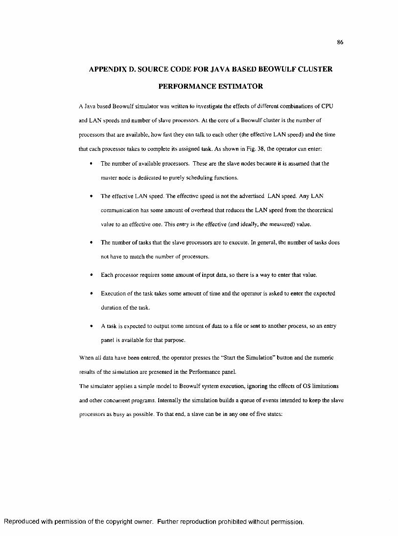
86

APPENDIX D. SOURCE CODE FOR JAVA BASED BEOW ULF CLUSTER

PERFORMANCE ESTIMATOR

A Java based B eow ulf sim ulator was written to investigate the effects o f different com binations o f CPU

and LAN speeds and num ber o f slave processors. At the core o f a B eow ulf cluster is the num ber of

processors that are available, how fast they can talk to each other (the effective LAN speed) and the time

that each processor takes to com plete its assigned task. As shown in Fig. 38, the operator can enter:

• The number o f available processors. These are the slave nodes because it is assumed that the

m aster node is dedicated to purely scheduling functions.

• The effective LAN speed. The effective speed is not the advertised LAN speed. Any LAN

com m unication has some amount o f overhead that reduces the LAN speed from the theoretical

value to an effective one. This entry is the effective (and ideally, the m easured) value.

• The num ber o f tasks that the slave processors are to execute. In general, the num ber o f tasks does

not have to match the number o f processors.

• Each processor requires some amount o f input data, so there is a way to enter that value.

• Execution o f the task takes some amount o f time and the operator is asked to enter the expected

duration o f the task.

• A task is expected to output some am ount o f data to a file or sent to another process, so an entry

panel is available for that purpose.

W hen all data have been entered, the operator presses the “Start the Sim ulation” button and the numeric

results o f the simulation are presented in the Perform ance panel.

The sim ulator applies a simple model to B eow ulf system execution, ignoring the effects o f OS lim itations

and other concurrent programs. Internally the simulation builds a queue o f events intended to keep the slave

processors as busy as possible. To that end, a slave can be in any one o f five states:


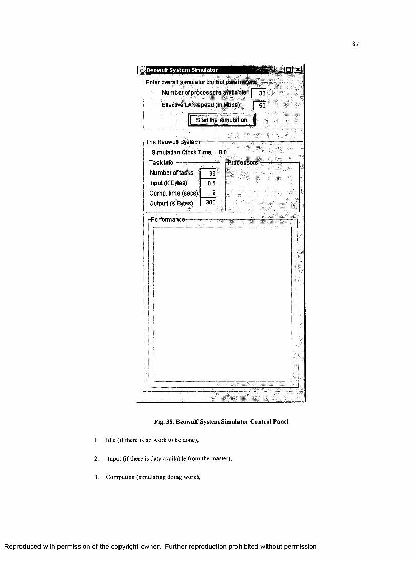
87

Beowulf System Simulator

Enter overall simulator control parameters:

Number of processors available: | 36

Effective LAN speed (in Mbps): | 50

! Start the simulation

The Beowulf System-

Simulation Clock Time: 0.0

1 Cl O f t I I M U .

Number of tasks

Input (K Bytes)

Comp, time (secs)

36

0.5

g

Output] (K Bytes) 300

(-Performance............ ............—

Processors -

. . . ^

Fig. 38. Beowulf System Simulator Control Panel

1. Idle (if there is no work to be done),

2. Input (if there is data available from the master),

3. Com puting (sim ulating doing work),


4. W aiting to output data, or

5. O utput (returning data to the master).

Because each o f these operations takes a finite amount o f tim e, as determ ined by the operator entered data,

a time line o f events can be constructed to mimic the expected B eow ulf system operation. The simulator

then models the system using a different num ber o f processors per iteration and returns the total run time

based on the num ber o f processors. Once the model has been “tuned” to reasonably m atch real data, the

computation time can to be changed to see the gross effects o f changing CPU clock speed. Or, the speed of

the LAN could be changed to see the effects o f different netw orking techniques. By seeing the effects o f

these changes, a system designer can focus in on the hardw are combination that will m eet the system

throughput requirem ents.

There are three files in this appendix:

1. BeowulfSystem .java - the main context for the sim ulator

2. Fram e2.java - the operator interface and associated GUI functions

3. BeowulfProcessor.java - the B eow ulf p rocesso rs)

D .l PACKAGE BEOWULFSIMULATOR;

import javax.swing.UIManager;

public class BeowulfSystem { boolean packFrame = false;

//Construct the application public BeowulfSystem() {

Frame2 frame = new Frame2();//Validate frames that have preset sizes//Pack frames that have useful preferred size info, e.g. from their layout if (packFrame) {

frame.pack();}

else {frame.validate();

}

frame.setVisible(true);


89

(

//Main methodpublic static void main{String[] args) {

try {UIManager.setLookAndFeel(UIManager.getSystemLookAndFeelClassName());

}

catch(Exception e) { e.printStackTrace();

}

new BeowulfSystem();

}

}

D.2 PACKAGE BEOWULFSIMULATOR;

import java.awt.*;import java.awt.e v e n t ;import javax.swing.*;import com.borland.jbcl.layout.*;import javax.swing.border.*;

public class Frame2 extends JFrame {JPanel contentPane;XYLayout xYLayoutl = new XYLayout();JPanel jPanell = new JPanel();JLabel jLabell = new JLabel();XYLayout xYLayout2 = new XYLayout();JTextField numberOfProcssors = new JTextField();JLabel jLabel2 = new JLabel();JTextField effectiveLANSpeed = new JTextField();JButton startButton = new JButtonO;Border border1;TitledBorder titledBorder1;JPanel systemPanel = new JPanel();XYLayout xYLayout3 = new XYLayout();Border border2;TitledBorder titledBorder2;JPanel tasklnfo = new JPanel();Border border3;TitledBorder titledBorder3;JPanel outputlnfo = new JPanel();Border border^;TitledBorder titledBorder4;static JPanel processors = new JPanel();Border border5;TitledBorder titledBorder5;


90

XYLayout xYLayout4 = new XYLayout();XYLayout xYLayout5 = new XYLayout();JLabel jLabel4 = new JLabel();JLabel jLabel5 = new JLabel();JLabel jLabe!6 = new JLabel();JLabel jLabel7 = new JLabel();JTextField numberTasks « new JTextField();JTextField inputKbytes = new JTextField{);JTextField compTime = new JTextField();JTextField outputKbytes = new JTextField();JScrollPane outputPanel = new JScrollPane();JTextArea output Area = new JTextAreaO;JLabel jLabel8 = new JLabel();JLabel simulationClockTimeLabel « new JLabel();XYLayout xYLayoutS = new XYLayout();

double clockTime = 0;

//Construct the frame public Frame2() {

enableEvents (AWTEvent. WINDOW_EVENT__MASK) ; try {

jblnit();

}

catch(Exception e) { e .printStackTrace();

}

}

//Component initializationprivate void jblnit() throws Exception {

contentPane = (JPanel) this.getContentPane(); border1 = BorderFactory.createEmptyBorder(); titledBorderl = new TitledBorder(new

EtchedBorder(EtchedBorder.RAISED,Color.white,new Color(142, 142, 142)),"Enter overall simulator control parameters:");

border2 = BorderFactory.createEmptyBorder(); titledBorder2 = new TitledBorder(new

EtchedBorder(EtchedBorder.RAISED,Color.white,new Color(142, 142, 142)),"The Beowulf System");

border3 = new EtchedBorder(EtchedBorder.RAISED,Color.white,new Color(142, 142,142));

titledBorder3 = new TitledBorder(new EtchedBorder(EtchedBorder.RAISED,Color.white,new Color(142, 142, 142)), "Task Info. ");

border4 = new EtchedBorder(EtchedBorder.RAISED,Color.white,new Color(142, 142,142));

titledBorder4 = new TitledBorder(border4,"Performance");


91

borders = new EtchedBorder(EtchedBorder.RAISED,Color.white,new Color(142, 142,142)) ;

titledBorder5 = new TitledBorder(border5,"Processors ");contentPane.setLayout(xYLayoutl);this.setSize(new Dimension(351, 700));this.setTitle("Beowulf System Simulator");jLabe11.setText("Number of processors available:");jPanel1.setLayout(xYLayout2);numberOfProcssors.setText("36");numberOfProcssors.setHorizontalAlignment(SwingConstants.RIGHT); jLabe!2.setText("Effective LAN speed (in Mbps):");effectiveLANSpeed.setText("50");ef fectiveLANSpeed.setHorizontalAlignment(SwingConstants.RIGHT); startButton.setText ("Start the simulation");startButton.addActionListener(new java.awt.event.ActionListener() {

public void actionPerformed(ActionEvent e) { startButton_actionPerformed(e);

}} ) ;

jPanell.setBorder(titledBorderl);systemPanel.setLayout(xYLayout3);systemPanel.setBorder(titledBorder2);systemPanel.setMinimumSize(new Dimension(800, 1000));contentPane.setMinimumSize(new Dimension(800, 1000));contentPane.setPreferredSize(new Dimension(800, 1000));taskInfo.setBorder(titledBorder3);taskInfo.setLayout{xYLayout4);output Info.setBorder(titledBorder4);output Info.setLayout(xYLayout5);processors.setBorder(titledBorder5);processors.setLayout(xYLayout6);jLabel4.setText("Number of tasks");jLabel5.setText("Input (K Bytes)");jLabel6.setText("Output] (K Bytes)");jLabel7.setText("Comp. time (secs)");numberTasks.setText("36");numberTasks.setHorizontalAlignment(SwingConstants.RIGHT);inputKbytes.setText{"0.5");inputKbytes.setHorizontalAlignment(SwingConstants.RIGHT); compTime.setText("9");compTime.setHori zontalAlignment(SwingConstants.RIGHT);outputKbytes.setText("300");outputKbytes.setHorizontalAlignment(SwingConstants.RIGHT); jLabel8.setText("Simulation Clock Time: ");simulationClockTimeLabel.setToolTipText(""); simulationClockTimeLabel.setText("0.0");contentPane.add(jPanell, new XYConstraints(8, 5, 339, 109));


92

jPanell.add(jLabell, new XYConstraints(36, 1, 190, -1));jPanell.add(numberOfProcssors, new XYConstraints(223, 1, 32, -1));jPanell.add(jLabel2, new XYConstraints(36, 26, -1, -1));jPanell.add(effectiveLANSpeed, new XYConstraints(227, 26, 28, -1));jPanell.add(startButton, new XYConstraints(91, 52, -1, -1));contentPane.add(systemPanel, new XYConstraints(8, 128, 339, 527));systemPanel.add(jLabel8, new XYConstraints(15, 1, -1, -1));systemPanel.add(simulationClockTimeLabel, new XYConstraints(154, 1, 95, -1));systemPanel.add(Casklnfo, new XYConstraints(1, 21, 160, 115));tasklnfo.add(jLabel5, new XYConstraints(3, 21, -1, -1));tasklnfo.add(jLabel7, new XYConstraints(3, 42, -1, -1));tasklnfo.add(jLabel6, new XYConstraints(3, 63, -1, -1));tasklnfo.add(numberTasks, new XYConstraints(107, 0, 37, -1));tasklnfo.add(compTime, new XYConstraints(107, 39, 37, -1));tasklnfo.add(outputKbytes, new XYConstraints(107, 59, 37, -1));tasklnfo.add(inputKbytes, new XYConstraints(107, 20, 37, -1));tasklnfo.add(jLabel4, new XYConstraints(4, 0, 98, -1));systemPanel.add(processors, new XYConstraints(164, 21, 160, 115));systemPanel.add(outputInfo, new XYConstraints(4, 138, 316, 359));outputlnfo.add(outputPanel, new XYConstraints(8, 4, 289, 320));outputPanel.getViewport().add(outputArea, null);

}

//Overridden so we can exit when window is closedprotected void processWindowEvent(WindowEvent e) (

super.processWindowEvent(e);if (e.getID() == WindowEvent.WINDOW_CLOSING) {

System.exit(0);}

}

void setClocktime(double newClockTime){ clockTime = newClockTime; displayClockTime();

}

void incrementClockTime(double increment){ double tempDouble = clockTime; setClocktime(tempDouble + increment);

i

void displayClockTime(){simulationClockTimeLabel.setText(new String(Double.toString(clockTime)));

}

void startButton_actionPerformed(ActionEvent e) { int xLocationStep = 30;


93

int yLocationStep = 30int xStartLocation = 0int yStartLocation = 0int xLocation;int yLocation;int processorNumber;int processorLimit;int i;int processor;int task;int taskLimit;double nextEventTime; boolean foundWork; double inputTimeDuration; double outputTimeDuration; double taskDuration;

processorLimit = Integer.parselnt(numberOfProcssors.getText()); taskLimit = Integer.parselnt(numberTasks.getText());

BeowulfProcessor processorArray!] = new BeowulfProcessor[processorLimit + 1];

// Create the processor display xLocation = xStartLocation; yLocation = yStartLocation;i = 0;for (processorNumber = 0; processorNumber < processorLimit; processorNumber + + ){

processorArray[processorNumber] =new BeowulfProcessor(processorNumber, xLocation, yLocation); processors.add(processorArray[processorNumber],

new XYConstraints(xLocation, yLocation, -1, -1));// this.setSize(15,10);

processorArray[processorNumber].SetProcessorDurations(i,0,0,0);

if (i == 3){xLocation = xStartLocation; yLocation += yLocationStep; i = 0;

} else{xLocation += xLocationStep; i + + ;

}}// Processor display now complete.

// Run complete tasks list against each possible processor combination

// Convert KBytes to seconds on a Mb rated network. inputTimeDuration = Double.parseDouble(inputKbytes.getText())


94

* 8. / 1000. / Double.parseDouble(effectiveLANSpeed.getText()); outputTimeDuration = Double.parseDouble(outputKbytes.getText())

* 8. / 1000. / Double.parseDouble(effectiveLANSpeed.getText()); taskDuration = Double.parseDouble(compTime.getText());outputArea.append(new String("Don11 Remove!! There are this many "+taskLimit+"

tasks.\n")) ;outputArea.append(new String("Don't Remove!! Processing takes this long: " +

taskDuration + " seconds A n " ) );outputArea.append(new String("Don't Remove!! Output takes this long: " +

outputTimeDuration + " seconds A n " ) );outputArea.append(new String("Don't Remove!! Input takes this long: " +

inputTimeDuration + " seconds.\n"));outputArea.append(new String("Don11 Remove!! There are barely, just " +

processorLimit + " processors\n"));outputArea.append(new String("Don't Remove!!\n")); for (processor=0; processor < processorLimit; processor++){

outputArea.append(new String((processor + 1)+" processors and " + taskLimit + " tasks "));

setClocktime(0); nextEventTime = 0; foundWork = true; task = 0;while (foundWork){

foundWork = false; displayClockTime();

/* Look for a processor that is (in priority order):1. Waiting to output data2. Available to accept data3. Last case, set the clock to the next event in the system

* /

// Check for someone waiting to output data for (i = 0; i <= processor; i++){

if ((processorArray[ij.GetProcessorNextEventTime() <= clockTime) && (processorArray[i].GetProcessorState() ««

BeowulfProcessor.WaitingOutput)){// Allow time for the output to occur

// outputArea.append(new String("processor #"+i+" waitingoutput\n")); incrementClockTime(outputTimeDuration); processorArray[i].SetProcessorClockTime(0);processorArray[i].SetProcessorState(BeowulfProcessor.AwaitingData); //foundWork = true; break;

}

}

// Check for someone waiting to accept data if (foundWork == false){

if (task < taskLimit){ for (i = 0; i <= processor; i + + H


95

if ((processorArray[i].GetProcessorNextEventTime() <= clockTime) && (processorArray[i].GetProcessorState() ==

BeowulfProcessor.AwaitingData)){// Allow time for the input to occur

processorArray[i].SetProcessorDurations(task,inputTimeDuration, taskDuration, outputTimeDuration);

processorArray[i].SetProcessorClockTime(clockTime);processorArray[i j .SetProcessorState(BeowulfProcessor.WaitingOutput); processorArray[i].ComputeNextEventTime(); incrementClockTime(inputTimeDuration); task ++;

/ *

outputArea.append(new String("processor #"+i+" inputTimeDuration " + inputTimeDuration +" NextEventTime » " +

processorArray[i].GetProcessorNextEventTime()+ " state = " + processorArray[i].GetProcessorState()+" clockTime = M + clockTime+ " \ n ") ) ;

* /

foundWork = true; break;

}}

}

}

// Check get the time of the next processor eventif (foundWork == false){

double timeNextProcessorEvent = Double.MAX_VALUE; double tempDouble;// Look for the next closest event in time for (i = 0; i <= processor; i++){

tempDouble = processorArray[i].GetProcessorNextEventTime(); if (tempDouble > 0) // There is work to be done

timeNextProcessorEvent = Math.min (tempDouble, timeNextProcessorEvent);

}

if (timeNextProcessorEvent != Double.MAX_VALUE){// Only happen if there is work to be done if (clockTime < timeNextProcessorEvent)

setClocktime(timeNextProcessorEvent); foundWork = true;

}f

// At the end of searching. If foundWork == false, at the all work}

outputArea.append("takes " + clockTime +" seconds.\n");


96

/ * *

* Title: <p>* Description: <p>* Copyright: Copyright (c) <p>* Company: <p>* Qauthor* Qversion 1.0 * /

D.3 PACKAGE BEOWULFSIMULATOR;

import java.awt.Color;

public class BeowulfProcessor extends javax.swing.JButton{

static int AwaitingData = 0; static int Recvinglnput = AwaitingData +1; static int Processing = AwaitingData + 2; static int WaitingOutput = AwaitingData + 3; static int OutputingData = AwaitingData + 4;

int ProcessorState; int ProcessorNumber; int taskNumber;

double clockTime = 0; double inputTimeDuration = 0; double processTimeDuration = 0; double outputTimeDuration = 0;

public BeowulfProcessor(int processorNumber, int x, int y) { ProcessorState = AwaitingData;ProcessorNumber = processorNumber;// Frame2.processors.add(this);// this.setLocation(x,y); this.setText(LableString());// this.setSize(15,10); this.setVisible(true);

}

void ComputeNextEventTime{){if (ProcessorState == AwaitingData){

clockTime = 0;


97

} else {if ((ProcessorState == Recvinglnput)I i (ProcessorState == Processing)I| (ProcessorState == WaitingOutput)){

clockTime += (inputTimeDuration + processTimeDuration);} else {

if (ProcessorState == OutputingData){/* do nothing */

}}

})

int GetProcessorState() {return ProcessorState;}

String LableString () {return (new String

(Integer.toString(ProcessorNumber)+"/"+Integer.toString(taskNumber)));}

void SetProcessorClockTime(double time) {clockTime = time;}

double GetProcessorNextEventTime() {return clockTime;}

void SetProcessorDurations(int task, double inputTime, double processTime, double outputTime){

taskNumber = task; inputTimeDuration = inputTime; processTimeDuration = processTime; outputTimeDuration = outputTime;}

void SetProcessorState(int state){ProcessorState = state;this.setBackground(StateColor());

try {Thread.sleep((long) (0*1000.));} catch (InterruptedException e){;} this.repaint();

}

String CurrentState(){ switch (ProcessorState){ case 0:return new String{"awaiting data"); case 1:return new String("receiving data"); case 2:return new String{"processing");


98

case 3:return new String("waiting to output"); case 4:return new String ("outputing data"); default:return new String ("UNKNOWN STATE");}}Color StateColor(){

int r = 127; int g = 127; int b = 127;if (ProcessorState == AwaitingData){

r = 0; g = 12 8; b = 0;} else

if (ProcessorState == Recvinglnput){ r = 255; g = 255; b = 102;

} elseif (ProcessorState == Processing){

r = 0; g = 255; b = 0;} else

if (ProcessorState == WaitingOutput){ r = 51; g = 255; b = 255;

} elseif (ProcessorState == OutputingData)(

r = 0; g = 0; b = 255;}

return new Color(r,g,b);}

}


99

APPENDIX E. COMPLETE RAY PROGRAM CONTROL FILE

This is a listing o f the control file read by the B eow ulf m aster program and then parsed into separate files

for the slave processes. The slave processes read their tailored file prior to beginning execution.

input prof_file = "testl"; input bath_file = "testl";

output ascii_file = "ascii";

source range = 0 (m); source depth = 10 (m);

receiver range = 10 (Nmi); receiver depth = 100 (m);

angles first = 10 (degrees); angles last = -11 (degrees); angles number = 21;

fan dr = 375 (m) ;fan min_range = 123 (m);fan max_range = 2345 (Nmi);

add_extrema min_angle = 123 (degrees); add_extrema iterations = 4; add_extrema min_dz = 45 (m);add_extrema z_miss = 67 (m);

model range_depend = full;model bottom_type reflecting;mode 1 bath_smoothing 10 (km);model bottom_depth = 6000 (m);model earth_radius = 6378.137 (km)model z_tolerance = le-06 (m);model margins 100;model max_bounces = 900;model max_angle 100 (degrees)

eigenrays geo_miss = 5 (m) ;eigenrays search_max = 10;eigenrays dr = 0 (m);

step_size multiplier = 1;


100

step_size max = 200 (m)jstep_size min = 5 (m);step_size cos_factor = 10;

prof_smoothing levitus;


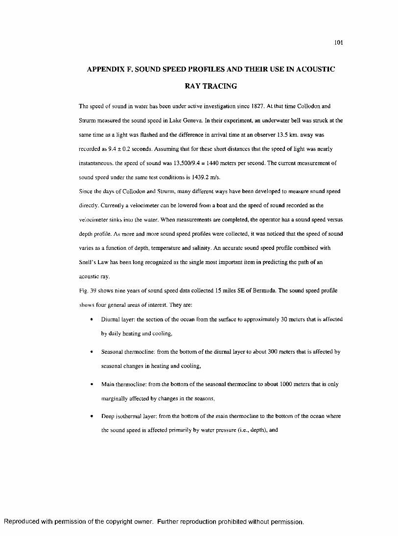
101

APPENDIX F. SOUND SPEED PROFILES AND THEIR USE IN ACOUSTIC

RAY TRACING

The speed o f sound in water has been under active investigation since 1827. A t that tim e Collodon and

Strurm m easured the sound speed in Lake Geneva. In their experiment, an underw ater bell was struck at the

same time as a light was flashed and the difference in arrival time at an observer 13.5 km. away was

recorded as 9.4 ± 0.2 seconds. Assuming that for these short distances that the speed o f light was nearly

instantaneous, the speed o f sound was 13,500/9.4 = 1440 meters per second. The current m easurem ent o f

sound speed under the same test conditions is 1439.2 m/s.

Since the days o f Collodon and Strurm, many different ways have been developed to measure sound speed

directly. Currently a velocim eter can be lowered from a boat and the speed o f sound recorded as the

velocimeter sinks into the water. W hen measurem ents are completed, the operator has a sound speed versus

depth profile. As more and more sound speed profiles were collected, it was noticed that the speed o f sound

varies as a function o f depth, tem perature and salinity. An accurate sound speed profile com bined with

Snell’s Law has been long recognized as the single m ost im portant item in predicting the path o f an

acoustic ray.

Fig. 39 shows nine years o f sound speed data collected 15 miles SE o f Bermuda. The sound speed profile

shows four general areas o f interest. They are:

• Diurnal layer: the section o f the ocean from the surface to approximately 30 meters that is affected

by daily heating and cooling,

• Seasonal thermocline: from the bottom o f the diurnal layer to about 300 meters that is affected by

seasonal changes in heating and cooling,

• M ain thermocline: from the bottom o f the seasonal therm ocline to about 1000 m eters that is only

marginally affected by changes in the seasons,

• Deep isothermal layer: from the bottom o f the main therm ocline to the bottom o f the ocean where

the sound speed is affected primarily by water pressure (i.e., depth), and


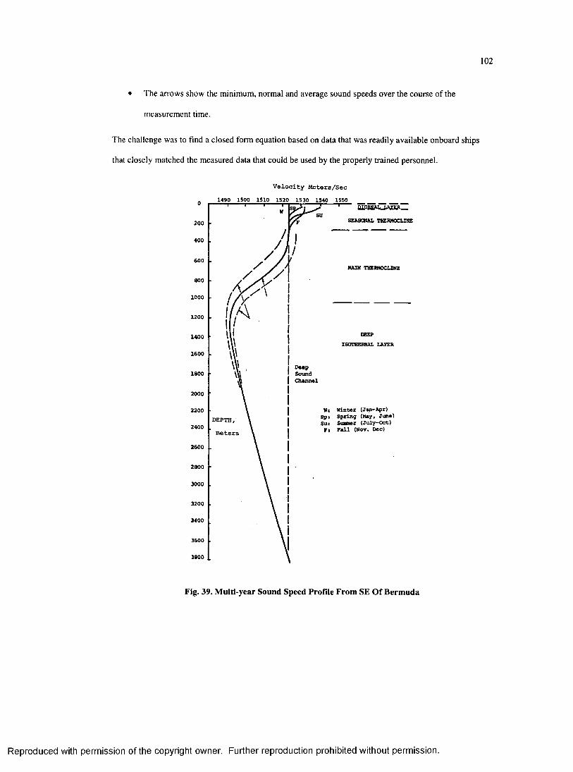
102

• The arrows show the minimum, normal and average sound speeds over the course o f the

measurem ent time.

The challenge was to find a closed form equation based on data that was readily available onboard ships

that closely matched the measured data that could be used by the properly trained personnel.

Velocity Meters/Sec1490 1S00 1510 1520 1530 1540 1550

DIURNAL LAYER

SEASONAL THERMOCLINE200

400

600MAIN THERMOCLINE

600

1000

1200

1400ISOTHERMAL LAYER

1600

DeepSoundChannel

1800

2000

Ws W inter (Jan-Apr) Spt Spring (May, June) Sut Susaner (Ju ly-O ct)

F i F a l l (Nov. Dec)

2200

DEPTH,2400

2600

2800

3000

3200

3400

3600

Fig. 39. Multi-year Sound Speed Profile From SE O f Bermuda


103

F .l DERIVATION

During the 1940s, 1950s, and 1960s the US Navy expended a considerable am ount o f tim e and effort trying

to find a single sound speed profile equation that fit most o f the data collected by that time. Equations (25)

through (28) are known respectively as K uw ahara’s, Del G rosso’s, W ilson’s and Leroy’s sound speed

equations. All equations are still in use.

c = 1445.5 +4.6647’ - 0 .0554r2 +1.307 * ( S - 35) +... (25)

c = 1448.6 + 4.618T - 0.0523T 2 +1.25 * (5 - 35) + ... (26)

c = 1449.2 + 4.623T - 0.054672 +1.391 * (S - 35) +... (27)

c = 1492.9 + 3*(7’-1 0 ) -6 * K T 3*(7’ -1 0 )2 - 4 * l( T 2*(7’-1 8 )2(28)

+ 1.2* (5 - 35)-1*10 * (T -1 8 )* (S -35 ) + Z/61

TABLE X shows the param eters, units and valid ranges o f the com ponents in the sound speed equations.

TABLE X. Valid Range Of Various Values For Sound Speed Profile Equations

Symbol Units Lower Limit Upper Limit

Temperature T Celsius -2 24.5

Salinity S Practical salinity units 30 42

Depth Z M eters 0 1,000

Speed of sound c M eters per second 1433.04 1557.78

Additionally, there are other sound speed equations besides those listed here. Leroy’s Equation (Eq. (28))

has the most wide spread use in current applications because it is relatively easy to program into digital


104

computers. Exam ination of Leroy’s Equation shows that eventually the depth o f the water (due to the

pressure at depth) will dominate all other terms.

F.2 BA TH Y TH ER M O G R A PH DATA

The use o f L eroy’s Equation in a shipboard environm ent is relatively easy. M ost o f the earth’s oceans have

a salinity o f about 35 parts per thousand, so it can alm ost be treated as a constant, only varying under

unusual circumstances. The temperature o f the w ater can be m easured via the use o f a reusable

bathytherm ograph or an expendable (XBT) probe. A handheld XBT launcher is shown in Fig. 40 and a

cutaway XBT is shown in Fig. 41. O f particular interest in the cutaway are the tw o spools o f wire, one in

the probe and the other in the canister. The wire is made of two copper strands thinner than a hum an hair

and therefore would not withstand any tension. W hen the X BT is launched/dropped, both spools start to

unwind. The spool on the probe unwinds to com pensate for the sinking of the probe, while the upper spool

unwinds to com pensate for the movem ent o f the ship. The net effect o f these unw indings is zero tension on

the wire. The XBT sinks at a constant rate, so timed tem perature measurem ents from the therm istor in the

nose o f the probe equate to the tem perature at an assumed depth. These data can be fed directly into a

computer. A complete system showing different types of XBT launchers is shown in Fig. 42. Armed with

the tem perature at depth, depth and salinity, shipboard personnel can use L eroy’s Equation to com pute a

sound speed profile.


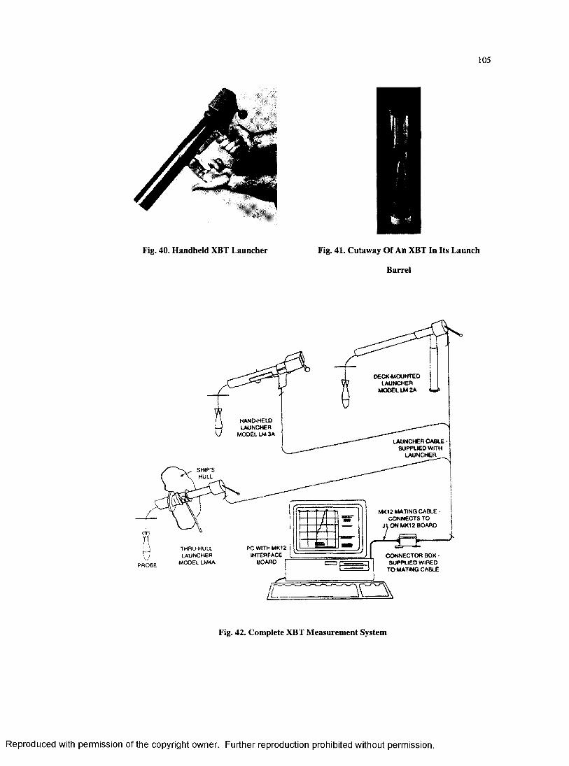
105

Fig. 40. Handheld XBT Launcher Fig. 41. Cutaway Of An XBT In Its Launch

Barrel

P6CK-MOUNTEO LAUNCHES

MODEL LM 2 A

LAUNCHER CABLE SUPPLIED WITH

LAUNCHER

SHIP'SHULL

MK12 MATING CABLE • CONNECTS TO

J t ON MK12 BOARD

PC WITH MK12 INTERFACE

BOARD fCONNECTOR BOX •

SUPPLIED WIRED TO MATING CABLE

PROBE

Fig. 42. Complete XBT Measurement System


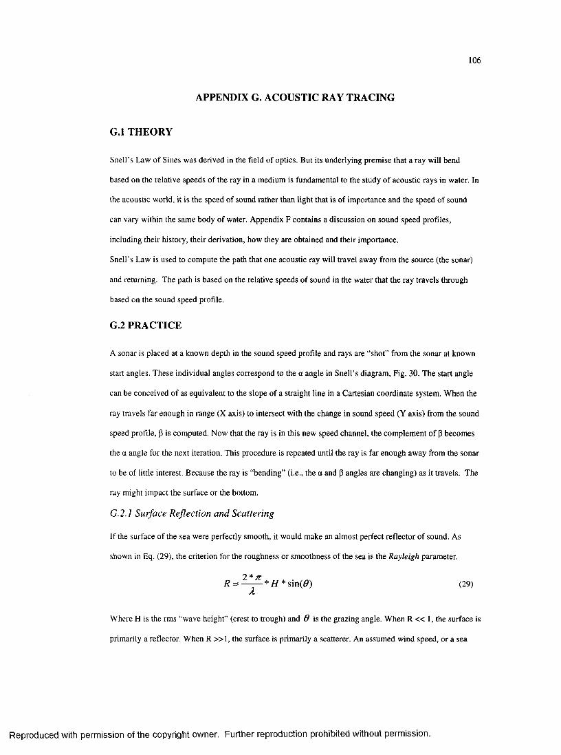
106

APPENDIX G. A CO U STIC RAY TR A CIN G

G .l TH EO R Y

Snell’s Law o f Sines was derived in the field o f optics. But its underlying prem ise that a ray will bend

based on the relative speeds o f the ray in a medium is fundam ental to the study o f acoustic rays in water. In

the acoustic world, it is the speed of sound rather than light that is o f im portance and the speed o f sound

can vary within the same body of water. Appendix F contains a discussion on sound speed profiles,

including their history, their derivation, how they are obtained and their importance.

Snell’s Law is used to com pute the path that one acoustic ray will travel away from the source (the sonar)

and returning. The path is based on the relative speeds o f sound in the water that the ray travels through

based on the sound speed profile.

G.2 PR A C T IC E

A sonar is placed at a known depth in the sound speed profile and rays are “shot” from the sonar at known

start angles. These individual angles correspond to the a angle in Snell’s diagram , Fig. 30. The start angle

can be conceived o f as equivalent to the slope o f a straight line in a Cartesian coordinate system. W hen the

ray travels far enough in range (X axis) to intersect w ith the change in sound speed (Y axis) from the sound

speed profile, (3 is computed. Now that the ray is in this new speed channel, the com plem ent o f P becom es

the a angle for the next iteration. This procedure is repeated until the ray is far enough away from the sonar

to be o f little interest. Because the ray is “bending” (i.e., the a and P angles are changing) as it travels. The

ray might im pact the surface or the bottom.

G.2.1 Surface Reflection and Scattering

If the surface o f the sea were perfectly smooth, it would make an alm ost perfect reflector o f sound. As

shown in Eq. (29), the criterion for the roughness or sm oothness o f the sea is the Rayleigh parameter.

R = ^ K * H * sin(#) (29)X

W here H is the rms “wave height” (crest to trough) and 6 is the grazing angle. W hen R « 1, the surface is

primarily a reflector. W hen R » 1 , the surface is prim arily a scatterer. An assum ed wind speed, or a sea


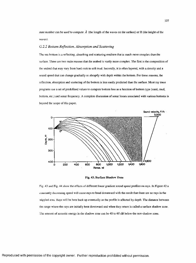
107

state num ber can be used to com pute X (the length o f the waves on the surface) o r H (the height o f the

waves).

G.2.2 Bottom Reflection, Absorption and Scattering

The sea bottom is a reflecting, absorbing and scattering m edium that is much m ore com plex than the

surface. There are two main reasons that the seabed is vastly more complex. The first is the composition o f

the seabed that may vary from hard rock to soft mud. Secondly, it is often layered, with a density and a

sound speed that can change gradually or abruptly with depth within the bottom. For these reasons, the

reflection, absorption and scattering o f the bottom is less easily predicted than the surface. M ost ray trace

programs use a set o f predefined values to com pute bottom loss as a function o f bottom type (sand, mud,

bottom, etc.) and sonar frequency. A complete discussion o f sonar losses associated with various bottom s is

beyond the scope o f this paper.

Sound velocity, ft/s ■ 5,000

v V /iV •\ *»%•*

Ronae. vd

Fig. 43. Surface Shadow Zone

Fig. 43 and Fig. 44 show the effects o f different linear gradient sound speed profiles on rays. In Figure 42 a

constantly decreasing speed will cause rays to bend dow nward with the result that there are no rays in the

stippled area. Rays will be bent back up eventually as the profile is affected by depth. The distance betw een

the range where the rays are initially bent downward and when they return is called a surface shadow zone.

The amount o f acoustic energy in the shadow zone can be 40 to 60 dB below the non-shadow zone.


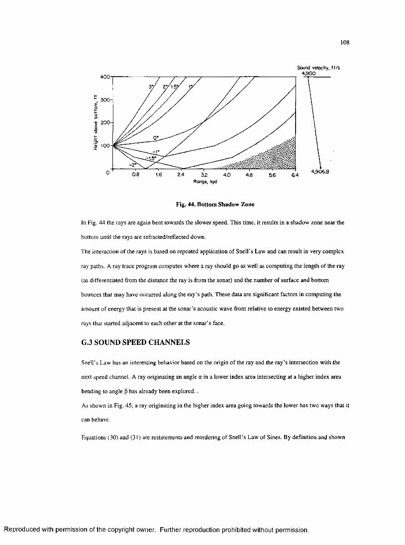
108

Sound velocity, t t / s4,900400-

300-

«. 200-

100- r

- 2*

4,906.80.8 1.6 2.4 3 2 Range, kyd

4.0 4.8 5.6 64

Fig. 44. Bottom Shadow Zone

In Fig. 44 the rays are again bent towards the slower speed. This time, it results in a shadow zone near the

bottom until the rays are refracted/reflected down.

The interaction of the rays is based on repeated application of Snell’s Law and can result in very com plex

ray paths. A ray trace program computes where a ray should go as well as com puting the length o f the ray

(as differentiated from the distance the ray is from the sonar) and the num ber o f surface and bottom

bounces that may have occurred along the ray ’s path. These data are significant factors in com puting the

amount o f energy that is present at the sonar’s acoustic wave front relative to energy existed betw een two

rays that started adjacent to each other at the sonar’s face.

G.3 SOUND SPEED CHANNELS

Snell’s Law has an interesting behavior based on the origin o f the ray and the ray ’s intersection with the

next speed channel. A ray originating an angle a in a low er index area intersecting at a higher index area

bending to angle p has already been ex p lo red ..

As shown in Fig. 45, a ray originating in the higher index area going towards the low er has two ways that it

can behave.

Equations (30) and (31) are restatements and reordering o f Snell’s Law o f Sines. By definition and shown


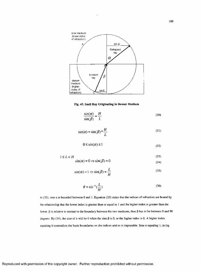
109

rarer medium(lower index of refraction)

sin aRefracted

ray >

Incidentray

denser medium (higher index of

refraction)

Fig. 45. Snell Ray Originating in Denser Medium

sin(a) Hsin (/?) L

(30)

sin(a) = sin(/?)*— ^L

0 < sin(or) < 1 3̂2)

1 < L < H (33)sin(a) = 0 => sin(/7) = 0 q 4)

sin(or) = 1 => sin(/?) = (35^

6 = sin"1 (— ) (36)H

in (32), sine a is bounded betw een 0 and 1. Equation (33) states that the indices o f refraction are bound by

the relationship that the low er index is greater than or equal to 1 and the higher index is greater than the

lower, p is relative to normal to the boundary betw een the two mediums, thus P has to be betw een 0 and 90

degrees. By (34), the sine o f a will be 0 when the sine P is 0, or the higher index is 0. A higher index

equaling 0 contradicts the basic boundaries on the indices and so is impossible. Sine a equaling 1, in Eq.


110

(35) is possible if sine p equals the ratio o f the low er index to the higher index. The ratio o f the low er to the

higher index defines a limit, known as the critical angle lim it for the p, as shown in Eq. (36). Any value of

P less than or equal to the critical angle will result in a correct value for a. Angle p greater than the critical

angle will cause the ray to be reflected back into the high index channel at an angle equal to the angle o f

incidence. The critical angle for a water to air interfaces is 48.6 degrees.

Fig. 46 shows two sound speed profiles from the area approximately 180 N m south o f N ova Scotia, Canada

with significant sound channels [12], A ray that is started in the sum m er upper sound channel

(approximately 300 feet from the surface) may be trapped forever in the channel depending on the angle

that the ray intersects the boundary at approxim ately 600 feet. A different ray in the deep sound channel

will be trapped between 600 feet and the bottom. For a ray to rem ain trapped, it m ust intercept the changes

in the sound speed profile at an angle less then the critical angle.

Snell’s Law, Eq. (23) is also at the heart o f the way m odem fiber optic cables operate [15]. A light ray is

“shot” down the fiber optic cable at an angle greater than the Snell’s critical angle (36). Snell’s critical

angle is computed based on the relative indices o f the mediums, in the case o f fiber optic cable, one

medium is the center conductor and the other is the outer sheathing. Light “shot” at an angle greater than

the critical angle, will not escape from the m edium with the higher index and will rem ain trapped in the

medium.


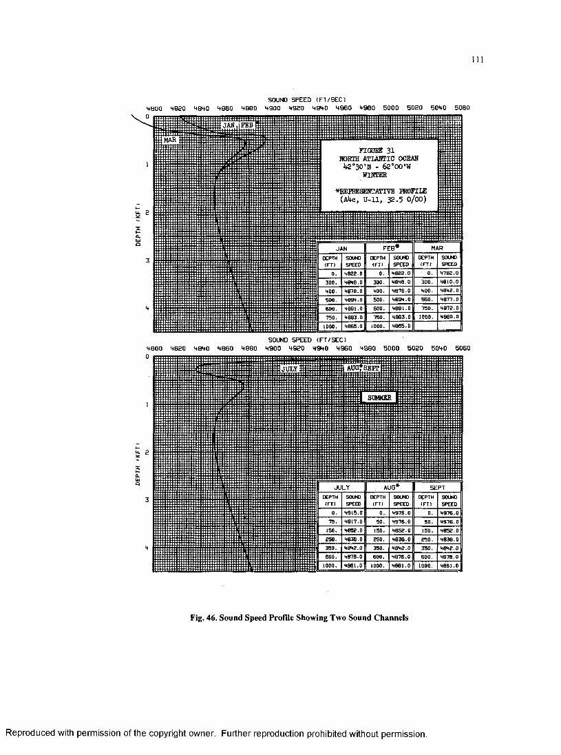
DEPTH

IKFTI

DEPTH

IKPT I

111

SOUND SPEED (F T /SE C )4QOO 4 8 2 0 4 8 4 0 4 8 6 0 4 8 8 0 4 9 0 0 4 9 2 0 4 9 4 0 4 9 6 0 4 9 8 0 5 0 0 0 . 5 0 2 0 5 0 4 0 506 0

JAM, FEB

FIGURE 31 NORTH ATLANTIC OCEAN

te ^ O ’N - 62°00'W WINTER

*EEIRESENTATIVE PROFILE (Atvc, U -ll , 32.5 0/00)

DEPTH(FT I

DEPTH(F T )

OEPTH(FT)

SOUNDSPEED

4 8 2 2 .0 4 7 8 2 .04 8 2 2 .04 8 1 0 .04 8 4 6 .04 8 4 2 .04870 .0

48 9 4 .0

4 0 0 .

4 8 7 7 .0

4 8 7 2 .048 9 1 .0BOO.

4 8 6 0 .04 8 8 3 .0

48 6 5 .01000

4 8 0 0 482 00

4 8 4 0SOUND SPEED (FT/SEC)

4 8 6 0 4 8 8 0 4 9 0 0 4 9 2 0 4 9 4 0 4 9 6 0 4 9 8 0 5 0 0 0 5 0 2 0 5 0 4 0 506 0

DEPTH(F T )

DEPTH(FT)

DEPTH(F T )

4 9 1 5 .0 4 9 7 6 .0 4 9 7 6 .0

4 9 1 7 .0 4 9 7 6 .0 49 7 6 .0

4 8 5 2 .0 4 8 5 2 .0 4 8 5 2 .0

4 8 3 6 .0 4 8 3 6 .0 4 8 3 6 .0

4 0 4 2 .0 4 8 4 2 .0 4 0 4 2 .0

4 8 7 6 .0 4 8 7 6 .0 4 8 7 6 .0

4 8 6 1 .0 4 8 6 1 .0 4 8 6 1 .0

Fig. 46. Sound Speed Profile Showing Two Sound Channels


112

APPENDIX H. ROBUST LINEAR LEAST SQUARES

During the data analysis phase o f the investigation, it appeared that there was a linear relationship betw een

the num ber o f processors and the execution tim e for a given num ber o f rays. This relationship was first

apparent by visual inspection o f the data. A linear relationship is defined as Eq. (37).

y — m x + b (37)

The com putation o f m and b as shown in Eq. (37) can be found in many introductory statistics books [8]

and is often included as part o f introductory com puter program m ing courses.

One o f the underlying assumptions in the com putation of m and b is that any errors in the data form a

Gaussian distribution on each data point. Standard least squares curve fitting assum es that all data is valid,

thereby treating each data point equally. This assumption causes any data points that are far outside the

Gaussian distribution to have an unwarranted effect on the solution.

Robust least squares makes no assumptions about the error distribution in the data. A n estim ate o f the

coefficients is com puted and than applied to all data points. The distance betw een the real data point and

the computed data point is used to “w eigh” the real data. Points that are far away from the com puted line,

are weighed less than points that are close to the line. Robust least squares continues to w ork on a data set

until the differences betw een consecutive iterations falls below some pre-set threshold, o r the solution fails

to converge after a pre-set num ber o f iterations.

Visual inspection o f the data clearly reveals that the (140,1.78) data point is grossly out o f bounds.

Standard least squares treated the data point as valid, while robust least squares arrived at a solution that

more closely matched the majority o f the data. Eq. (38) is the standard least squares fit to the data. Eq. (39)

is the robust least squares fit.

TABLE XI [8] has a series o f data points that are plotted in Fig. 47 along with standard and robust least

squares fits.

Visual inspection o f the data clearly reveals that the (140,1.78) data point is grossly out o f bounds.

Standard least squares treated the data point as valid, while robust least squares arrived at a solution that


113

more closely matched the majority o f the data. Eq. (38) is the standard least squares fit to the data. Eq. (39)

is the robust least squares fit.

TABLE XI. Valid Range Of Various Values To Demonstrate Least Squares Curve Fitting

Air velocity

(cm/sec)

Evaporation coefficient

(m m2/sec)

20 0.18

60 0.37

100 0.35

140 1.78

180 0.56

220 0.75

260 1.18

300 1.36

340 1.17

380 1.65

<= Changed from the original o f 0.78 for illustration

StdardLeastSquares = 0.0037400*x + 0.2601250

RobustLeastSquares = 0.0039284*x + 0.032286

(38)

(39)

The robust least squares fit arrived at its solution after 5 iterations.

The following pages contain the robust least squares program and make file that was used to analyze the

B eowulf perform ance data. The robust least squares program is based on newmatlOA. D ata for Fig. 47 was

produced using the comm and: ./testing 0 6.


114

4- I Mc0)•5 1.2

i -oc 0.8 o

0.6 o§• 0.4& 0.2

Raw Data

Standard LeastSquares Robust LeastSquares

0 100 200 300 400

Air velocity

Fig. 47. Comparison of Standard and Robust Least Squares Curve Fitting

H .l THE MAKE FILE:

CXX = g++

LIBRARIES=-lnewmat \

- lm

LIBDIR=-L../Lib

INCLUDES=-I ../Include

CXXFLAGS = -0 2 $(LffiDIR) $(LIBRARIES) $(INCLUDES)

all :testing

testing:../Src/testing.cc

$(CXX) -o ../testing ../Src/testing.cc $(CXXFLAGS)

run:

../testing

clean:

rm -f ../testing


115

H.2 THE SOURCE FILE TESTING.CC:

#include <iostream>

#include <list>

#include <math.h>

#include <stdlib.h>

#include <stdio.h>

#include ''newmat.h"

#define DEBUG_PRINT

#ifdef DEBUG_PR1NT

tdefine DEBUG_PRINT(...) (fprintf (stderr,"%s() in %s at %d; M,_ F U N C T IO N _ , _ F IL E _ _ , _ L I N E _ ) ;f p r in tf

(stderr, VA_ARGS ););

#define DEBUG_VARlABLE(v,fmt) (DEBUG_PRINT(#v ” =>% "#fmt "<=\n",v);};

#else

#define DEBUG_PR1NT(...)

#define DEBUG_VAR1ABLE(...)

# e n d i f

using namespace std;

void matrixFunction (ColumnVector *x, double (*func) (double value)){

for (int i = 1; i <= x->Nrows(); i++)

x->elem ent(i-l) = ((*func) ((double) x->elem ent(i-l)));

)

void matrixDump(char titled , char matrixName[J, M atrix x)l

DEB UG_PRlNT("%s\n",title);

for (int i= 1; i <=x.Nrows(); i++)(

for (int j = 1; j<=x.Ncols(); j++)

DEBUG_PRINT("%s [%d][%d] = %f\n", matrixName, i, j, x (ij));

void leastSquares (ColumnVector x, ColumnVector y, ColumnVector *yHat, ColumnVector *r, Colum nVector *b, M atrix w){

Matrix X (x.Nrows(),2);

for (int i = I ; i<= x.NrowsO; i++)|

X(i, 1) = x(i);

X (i,2 )= 1;

I

Matrix B = (X.t() * w * X).i() * (X.t() * w * y);


116

matrixDumpC'ln leastSquares

Matrix YHat = (X * B);

// matrixDump ("Least squares","YHat",YHat);

// Copy internal data to the outside

for (int i = 1; i <= YHat.Nrows(); i++)(

yHat->elem ent(i-l) = Y H at(i,l);

r->elem ent(i-1) = (y(i) - yHat->elem ent(i-1));

)

b->element(0) = B ( l , l) ; //T h e slope of the line.

b->elem ent(l) = B (2 ,l); //T h e y-intercept

1

double matrixM edian(ColumnVector r)(

list <double> values;

int size;

double returnValue;

for (int i = 1; i <= r.NrowsO; i++){

values. push_back(r(i));

)

values.sort();

size = values. size();

if (size & 1){ // an odd number of entries

for (int i = 1; i <= (int)(size/2); i++)

values.pop_front();

returnValue = values. front();

}else{ // an even number of entries

for (int i = 1; i <= (size/2); i++){

returnValue = values.front();

values.pop_front();

IreturnValue += values.front();

returnValue /= 2.;

)return returnValue;

1

int robustLeastSquares (ColumnVector x, ColumnVector y, ColumnVector *yHatOut, ColumnVector *rOut, ColumnVector *bOut)(

// Based on DataPlot manual .Weights section

ColumnVector delta(y.Nrows()), delta2(y.Nrows());

ColumnVector r(y.Nrows()), rOld(y.NrowsO);

ColumnVector temp(y.Nrows());

ColumnVector u(y.Nrows()), tag(y.Nrows());

ColumnVector yHat(y.NrowsQ), b(2);


117

ColumnVector yHatOld(y.NrowsO), bO!d(2);

double c = 4.685;

double denom;

double epsilon = 0.0001;

double mad;

double median;

double num;

double s;

int iterationCounter;

int m axlterations = 10;

int nanFlag = 0;

matrixDumpC'Original x values","x", x);

matrixDumpC’Original y values","y", y);

Matrix w (x.Nrows(),x.Nrows());

w = 0.0;

for (int i = 1; i <=x.Nrows(); i ++)

w(i,i) = 1;

// Initialize the residual vector

leastSquares (x, y, &yHat, &r, &b, w);

yHatOld = yHat;

bOld = b;

for (iterationCounter = I;

iterationCounter < maxlterations;

iterationCounter++) {

rOld = r;

median = matrixM edian(r);

temp = r - median;

// Apply the fabs function to all elements of the temp matrix

matrixFunction(&temp, fabs);

H matrixDump ("robustLeastSquares”,"temp",temp);

mad = matrixM edian(temp);

s = mad/0.6745;

u = r / s;

tag = u / c;

// matrixDump ("robustLeastSquares tag","tag",tag);

matrixFunction(&tag, fabs);


118

for (int i = I ; i <= x.Nrows(); i++)|

if(tag (i)> 1)

w(i,i) = 0;

else

{double locaiDouble = tag(i);

localDouble *= locaiDouble;

locaiDouble = 1 - localDouble;

w(i,i) = localDouble * localDouble;

11// Compute a weighted least squares fit with new weights


delta = (rOld - r);

for (int i = 1; i <= x.Nrows(); i++)

delta(i) = delta(i) * delta(i);

num = delta.Sum();

DEBUG_VARIABLE(num,f);

if (isnan(num) != 0){

nanFlag = 1;

break;

Inum = sqrt(num);

for (int i = I ; i <= x.Nrows(); i++)

delta2(i) = rOld(i) * rOld(i);

denom = delta2.Sum ();

DEBUG_VARIABLE(denom,f);

if (isnan(denom) != 0){

nanFlag = 1;

break;

)denom = sqrt (denom);

/*

If the difference between the last iteration and this

is less then the limit then we are finished

* /

if (denom == 0) { // Houston we have closure!

DEBUG_PRlNT("denom == 0, we have closure!!\n");

break;}

DEBUG_PRINT("iteration %d closeness % f\n”, iterationCounter, (num/denom));

if ((num/denom) < epsilon)

break;


119

// Save the old values

yHatOld = yHat;

bOld = b;

)

if (nanFlag)) // Something is a nan, so use old data

for (int i = 1 ; i <= yHat.NrowsO; i++){

yHat(i) = yHatOld(i);

b ( l) = bO ld(l);

b(2) = b01d(2);

1

// Copy internal data to the output matrices

for (int i = 1; i <= yHat.NrowsO; i++)(

yH atO ut->elem ent(i-l) = yHat(i);

rO ut->elem ent(i-l) = y(i) - yHat(i);

1

bOut->element(0) = b (l) ; // Also known as the slope o f the line

bO ut->elem ent(l) = b(2); // The y-intercept.

return (iterationCounter);

1

void matrixTester(ColumnVector x, ColumnVector y)(

Matrix w (x.Nrows(),x.Nrows());

ColumnVector yHat(y.NrowsO), r(y.Nrows()), b(2);

w = 0.0;

for (int i = 1; i <= x.Nrows(); i++)

w(i,i) = 1.0;


matrixDumpC'Tester funtion b (simple least squares function)","b", b);

// matrixDumpC'Function r","r",r);

// matrixDumpC’Function yHat","yHat",yHat);

cout « "robustLeastSquares iterations = " « robustLeastSquares (x, y, &yHat, &r, &b) « endl;

cout « "y = " « b .elem ent(l) « " + " « b.element(O) « "*x" « endl;

matrixDumpC'Funtion robustLeastSquares b","b", b);

// matrixDumpC'Function robustLeastSquares yHat","yHat",yHat);

1

void matrixTestM edian(char testName[J, ColumnVector x, double expectedValue)(


120

double m atrixRetum = matrixM edian(x);

c o u t« "matrixM edian()

if (matrixRetum == expectedValue)

c o u t« "passed";

else

c o u t« "failed";

cout « " " « testName « " test, returning " « matrixRetum « " when expecting " « expectedValue « endl;

}

int main(int argc, char *argv[J){

ColumnVector x;

ColumnVector y;

int categoryTest;

int subCategoryTest;

int returnValue = 0;

categoryTest = 0;

subCategoryTest = 5;

if (argc>l){

switch (argc){

case 3:

subCategoryTest = atoi(argv[2]);

case 2:

categoryTest = atoi(argv[lj);

break;

default:

printf ("Usage: %s IcategoryTest [subCategoryTestj]\n exit(-99)\n",argv[0]);

exit(-99);

switch (categoryTest){

case 0: // Data from "good" soruces

switch (subCategoryTest) {

case 0: // Data from Probability and Statistics for Engineers

x.ReSize (10);

y.ReSize (x.NrowsO);

x « 20 « 60 « 100 « 140 « 180 « 220 « 260 « 300 « 340 « 380;

y « 0.18 « 0.37 « 0.35 « 0.78 « 0.56 « 0.75 « 1.18 « 1.36 « 1.17 « 1.65;

break;

case 1: // Data from DataPlot Manual, W eights section

x.ReSize (10);


x « 1 « 2 « 3 « 4 « 5 « 6 « 7 « 8 « 9 « 10; y « 2 « 4 « 60 « 7 « 9 « 12 « 14 « 15 « 18 « 20;


121

break;

case 2:// Data from http://www.cs.bsu.edu/hom epages/fischer/m athl25/regression.pdf

x.ReSize (4);


x « 2 « 6 « 8 « 4;

y « 5 « 4 « 9 « 2;

break;

case 3:// Data from http://www.udayton.edu/-cps/csp353/lsqd/lsqd.htm l

x.ReSize (10);


x « 1 « 2 « 3 « 4 « 5 « 6 « 7 « 8 « 9 « 10;

y « 1.3 « 3.5 « 4.2 « 5 « 7 « 8.8 « 10.1 « 12.5 « 13 « 15.6;

break;

case 4: // Data from my mind

x.ReSize (30);


x ( l) = 0;

x (2 )= I;

for (int i = 3; i <= x.NrowsO; i++)

x(i) = x (i-l) + x(i-2); // Fibemaci series

for (int i = 1; i <= x.NrowsO; i++){

y(i) = (0.23456 * x(i) + 8.9) + 30 *( (double)rand()/(double)RAND_M AX);

if (i & 4)

y(i) += 100 *( (double)rand()/(double)RAND_M AX);

)break;


x.ReSize(5);

x « 15 « 14 « 2 « 27 « 13;

matrixTestM edian ("first",x,14);

x.ReSize(6);

x « 17 « 9 « 15 « 19 « 4 « 16;

matrixTestM edian ("second'',x,15.5);

matrixTestM edian ("second (intentional failure)",x, 15);

returnValue = -4;

break;


// with some GROSSLY wrong

x.ReSize (10);


x « 20 « 60 « 100 « 140 « 180 « 220 « 260 « 300 « 340 « 380;

y « 0.18 « 0.37 « 0.35 « 1.78 « 0 . 5 6 « 0.75 « 1.18 « 1.36 « 1.17 « 1.65;

break;

default:

returnValue = -1;


http://www.cs.bsu.edu/homepages/fischer/mathl25/regression.pdf

http://www.udayton.edu/-cps/csp353/lsqd/lsqd.html

break;

case 1: // Data from real time Beowulf paper

x.ReSize (7);

x « 1 « 20 « 20 « 30 « 100 « 200 « 1000;


switch (subCategoryTest))

case 1: // Serial execution times

y « 0.0120 « 0.0560 « 0.1020 « 0.1510 « 0.4860 « 0.9680 « 4.4820;

break;

case 3: // 3 slaves execution times

y « 0.5690 « 0.7220 « 0.8920 « 1.0580 « 2.3280 « 4.0790 « 17.3910;

break;


y « 0.5730 « 0.7110 « 0.9030 « 1.0280 « 2.2600 « 3.8950 « 17.6340;

break;


y « 0.5760 « 0.7160 « 0.8700 « 1.0360 « 2.1830 « 3.9070 « 17.2480;

break;

case 6: // 6 slaves exectuion times

y « 0.5780 « 0.7290 « 0.8740 « 1.0330 « 2.1210 « 3.7510 « 17.3600;

break;


y « 0.5860 « 0.7190 « 0.8750 « 1.0300 « 2.1860 « 3.84720 « 17.0570;

break;

default;

returnValue = -2;

Ibreak;

default:

returnValue = -3;

)

switch (returnValue))

case 0:)

// Where the work starts

matrixDumpC'Original x values","x", x);

matrixDumpC'Original y values","y”, y);

Matrix X (x.NrowsO,2);

for(int i = 1; i <=x.Nrows(); i++)(

X(i, 1) = x(i);

X (i,2 )= 1;

1


123

// Least squares as a series of explicit functions

Matrix b = (X.t() * X).i()* (X .t() * y);

Matrix yHat = (X * b);

Matrix r = (y - yHat);

// matrixDumpC'Explicit b","b", b);

// matrixDumpC'Computed y values","y", yHat);

// matrixDump("Resdiuals","r", r);

// W eighted least squares as a series of explicit calls

Matrix W (X.NrowsO,X.NrowsO);

W = 0.0:

// matrixDumpC'W eights before computation","W ", W);

for (int i = 1; i <= W.Nrows(); i ++)

W(i,i)= l/( r(i,l)* r(i,l));

// matrixDumpC'W eights","W ", W);

Matrix b2 = (X.t() * W * X).i() * (X.t() * W * y);

Matrix yHat2 = (X * b2);

M atnx r2 = (y - yHat2);

// matrixDump("W eighted b'',"b2", b2);

// matrixDumpC'W eighted y","yHat2", yHat2);

// matrixDumpC'W eighted Resdiuals",”r2", r2);

Matrix bD iff = (b - b2);

// matrixDumpC'b differences","bD iff', bDiff);

matrixTester(x.y);

)break;

case -3:

case -2:

case -1:

cout « "No action defined where categoryTest = " « categoryTest;

cout « " and subCategoryTest = " « subCategoryTest;

c o u t« endl;

cout « "exit (" « returnValue « " ) " « endl;

exit(retumValue);

break;

case -4: // Everything OK, just return from main()

returnValue = 0;

break;


124

default:

cout « "No action defined where returnValue = " « returnValue;

cout « ", main() returning." « endl;

}

return (returnValue);

}


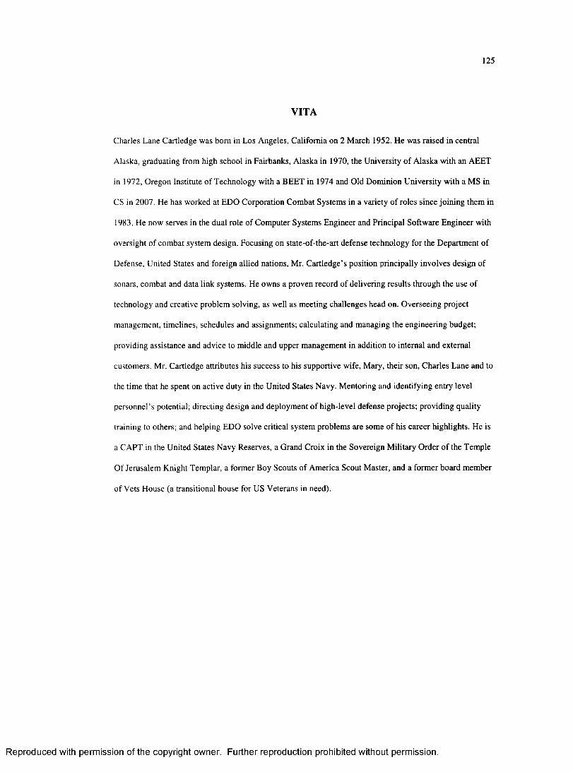
125

VITA

Charles Lane Cartledge was born in Los Angeles, California on 2 March 1952. He was raised in central

Alaska, graduating from high school in Fairbanks, A laska in 1970, the University o f Alaska with an AEET

in 1972, Oregon Institute o f Technology with a BEET in 1974 and Old Dominion University with a MS in

CS in 2007. He has worked at EDO Corporation Com bat Systems in a variety o f roles since jo in ing them in

1983. He now serves in the dual role o f Com puter Systems Engineer and Principal Software Engineer with

oversight o f com bat system design. Focusing on state-of-the-art defense technology for the D epartm ent o f

Defense, United States and foreign allied nations, Mr. C artledge’s position principally involves design of

sonars, combat and data link systems. He owns a proven record o f delivering results through the use of

technology and creative problem solving, as well as meeting challenges head on. O verseeing project

management, timelines, schedules and assignments; calculating and managing the engineering budget;

providing assistance and advice to middle and upper managem ent in addition to internal and external

customers. Mr. Cartledge attributes his success to his supportive wife, Mary, their son, Charles Lane and to

the tim e that he spent on active duty in the United States Navy. M entoring and identifying entry level

personnel’s potential; directing design and deploym ent o f high-level defense projects; providing quality

training to others; and helping EDO solve critical system problem s are some o f his career highlights. He is

a CAPT in the United States Navy Reserves, a Grand Croix in the Sovereign M ilitary O rder o f the Temple

O f Jerusalem Knight Templar, a form er Boy Scouts o f Am erica Scout Master, and a form er board mem ber

o f Vets House (a transitional house for US Veterans in need).


Documents

Investigating Real-Time Sonar Performance Predictions Using