Is face recognition really a Compressive Sensing problem?

Qinfeng Shi†, Anders Eriksson†, Anton van den Hengel†, Chunhua Shen† ‡

The Australian Centre for Visual Technologies, The university of Adelaide †National ICT Australia ‡

{javen.shi, anders.eriksson, anton.vandenhengel, chunhua.shen} @adelaide.edu.au

Abstract

Compressive Sensing has become one of the standardmethods of face recognition within the literature. We show,however, that the sparsity assumption which underpinsmuch of this work is not supported by the data. This lackof sparsity in the data means that compressive sensing ap-proach cannot be guaranteed to recover the exact signal,and therefore that sparse approximations may not deliverthe robustness or performance desired. In this vein we showthat a simple `2 approach to the face recognition problemis not only significantly more accurate than the state-of-the-art approach, it is also more robust, and much faster. Theseresults are demonstrated on the publicly available YaleBand AR face datasets but have implications for the appli-cation of Compressive Sensing more broadly.

1. Introduction

The application of Compressive Sensing (CS) to theproblem of face recognition has received significant recentattention in the literature (see [18, 19, 14] for example). Thegoal of many such methods has been to exploit the underly-ing sparsity in the problem in order to improve the robust-ness, speed, or accuracy with which classification might beperformed, or all three. As in many applications of CS,however, the sparsity of in the problem is assumed, ratherthan proven, or measured. We show here that the sparsityassumption is not supported by data, and that an `2-basedapproach out-performs the state-of-the-art in CS methods interms of speed, accuracy, and robustness. The implicationsare important for the application of CS to face recognitionbut also to other problems where sparsity is assumed ratherthan proven.

2. The space of all face images

Consider face recognition with n frontal training faceimages collected from K subjects. Let nk denote the num-ber of training images of subject k , thus n =

∑Kk=1 nk.

Without loss of generality, we assume that all the data havebeen sorted according to their labels and then we collectall the vectors in a single matrix A with m rows and ncolumns, given by

A = [x1, ...,xn] ∈ Rm×n. (1)

The assumption which underpins the application of CS toface recognition by Yang et al. [19], Wright et al. [18], andShi et al. [14] is as follows:

Assumption 1 Any test image1 lies in the subspacespanned by the training images belonging to the same per-son. That is for any test image x, without knowing its la-bel information, it’s assumed that there exists a η-sparse2

α = (α1, α2, ..., αn) such that

x = Aα. (2)

To seek a sparse solution, one could use

minα∈Rn

‖α‖`1 (3a)

s.t. x = Aα. (3b)

Solving this problem via linear programming becomescomputationally expensive when m is large, however.

In order to exploit the presumed sparsity in the problemthe authors in [19] and [18] generate a random matrix Φ ∈Rd×m (where d � m) and identify the vector α whichminimises the following `1 problem:

minα∈Rn

‖α‖`1 (4a)

s.t. Φx = ΦAα, (4b)

or the related problem:

minα∈Rn

‖α‖`1 (5a)

s.t. ‖Φx−ΦAα‖`2 ≤ ε, (5b)

1The image here can be either an original image, or a feature imageextracted from the original one, e.g. an eigenface. Often the dimensionalityof the feature has to be reduced due to the complexity of the recognitionalgorithm.

2A n-dimensional signal is said η-sparse if it has at most η non-zeroentries.

553

for a given error tolerance ε > 0. Introducing the matrixΦ significantly reduces the computational complexity (par-ticularly when d� m), yet the CS signal recovery theorem[5, 4, 11] shows that when d ≥ O(η log(n/η)) the signal αcan be exactly recovered (that is, it reaches the optimum ofthe original problem specified in Equation (3)) with over-whelming probability at least 1− eO(−d).

Shi et al. in [14] showed the connection between HashKernels [12, 13, 17] and CS. In doing so they showed thatit is possible to replace Φ with an implicit hash matrix Hin order to reduce storage requirements and speed up facerecognition with Orthogonal Matching Pursuit (OMP)[15].

2.1. Is the set of face images really sparse?

Despite the results of [19], [18] and [14], it is clearthat the validity of Assumption 1 depends on the particu-lar data set being used. What is not as immediately clearis that Assumption 1 does not hold for data of the formtypically used to evaluate face recognition algorithms. As-sumption 1 is sometimes justified on the basis of the resultin [2] that the images of a rigid Lambertian surface undervarying illumination lie close to a 9-dimensional linear sub-space. This presumes perfect registration of the images, noself-shadowing, occlusion, or specularities, and ignores thefact that faces are neither rigid nor Lambertian, however. Inorder to evaluate the validity of Assumption 1 directly weform the matrix A in the same manner as in [19] and [18].

The AR dataset, which is used in many face recogni-tion papers including those above, consists of 26 alignedimages of each subject in different lighting conditions andwith different facial expressions and disguises. We ran-domly selected 100 such subjects and cropped the imagesto 165× 120 pixels and converted to grayscale (as in [19]),and, using (1), formed the matrix A where m = 19800 andn = 2600. A plot of the log of the singular values of thismatrix is given in Figure 1.

Typically a subset (often half) of the database is usedfor training, and the remainder for testing. If Assumption 1holds then we would hope that 13 training images per sub-ject would suffice to span the space of all face images of thesubject, and thus that the remaining (testing) 13 were linearcombinations of the training set. This would lead to a ma-trix A with rank at most 1300 (rank 13 per subject for 100subjects). Figure 1 does not support this hypothesis, how-ever, as there is no obvious dip in the singular values of Aat 1300, or any at other point. Note that Figure 1 depicts thesingular values of the matrix of all face images in the ARdata set, rather than only those for a single subject. It thusshows not only that there is little redundancy in AR datasetface images for any single subject, but also that there is lit-tle redundancy in AR dataset face images for all subjectscollectively. The first few singular values are significantlyhigher than the remainder, which reflects the commonality

in the overall shape of the face, but there is little differenti-ation between the remaining components.

The fact that there is no significant dip in the singularvalues of A does not discount sparsity completely, as thereis inevitably noise in the training data, but it gives an indi-cation that there is no simple linear dependence in the dataset.

0 500 1000 1500 2000 2500-10

-5

0

5

10

15

Singular value number

Log

sing

ular

val

ue

AR Database MatrixGaussian Random Matrix

Figure 1. The log of the singular values of the data matrix A cal-culated using the AR data set, and for comparison, of a matrix ofthe same size with elements sampled from N(0, 1).

Having seen that the the training data are not linearly de-pendent we now show that the sparsity espoused in [19, 18]and [14] is not a feature of the problem, but of the solu-tion. In applying the matrix Φ ∈ Rd×m (where d � m)the methods proposed cause the problem to become sparse,with a degree proportional to the value of d selected. Fig-ure 2 shows the values of α estimated by solving equa-tion (4) directly when A is constructed as above, but from13 images each of 100 subjects, and x represents anotherimage from the AR dataset. Two matrices Φ have beenused, one with d = n − 1 and one with d = 300. Theplots show that the coefficients α are not sparse until theselection of a small d forces them to be so.

We show below that the CS methods for face recognitionlisted above achieve their state-of-the-art results on the ARand Yale B datasets only when the the number of features dis at least 300. This and Figure 2 imply that the coefficientsof α are not as sparse as may have been hoped, and thatat least 300 non-zero coefficients are required in order toachieve acceptable classification performance.

This analysis draws into question the theoretical supportfor all face recognition methods based on Assumption 1 andany method relying on the sparsity of the coefficients α.This does not mean that the `1 norm has no place in facerecognition, however, but rather that it needs to be appliedappropriately.

3. Robust vs. sparse `1

One argument with the analysis above might be that the`1 term is intended to achieve robustness, rather than indi-cating a belief in the sparsity of the coefficients. This isan important distinction. The `1 norm is used in CS as atractable alternative to the `0 norm [3]. Sparseness does not

554

0 200 400 600 800 1000 1200 1400−40

−30

−20

−10

0

10

20

30

40

50

(a)

0 200 400 600 800 1000 1200 14000

5

10

15

20

25

30

35

40

45

(b)

0 200 400 600 800 1000 1200 1400−0.1

−0.05

0

0.05

0.1

0.15

0.2

0.25

0.3

(c)

0 200 400 600 800 1000 1200 14000

0.05

0.1

0.15

0.2

0.25

0.3

0.35

(d)

Figure 2. Visualising the sparsity of α when recovered by solvingequation (4). (a) Plot of α when d = 1299. (b) Plot of sorted αwhen d = 1299. (c) Plot of α when d = 300. (d) Plot of sorted αwhen d = 300.

necessarily lead to robustness to the presence of outliers.To achieve robustness, one could use `1-Regression [16,

chap. 12.4] as follows:

minα∈Rn

‖x−Aα‖`1 , (6)

which avoids overly penalising gross outliers.The `1 norm in CS and `1 norm in `1-Regression are,

however, two unrelated uses of the same norm. The twoapplications differ in the quantities to which the `1 normis applied. Robustness cannot therefore be used to justifyapplying the `1-norm to the coefficients α without furtherexplanation. No such explanation is given, however.

The problem with (6) is that solving such a linear pro-gram can be computationally expensive as the data sizegrows. Rather than resort to approaches such as those in (4)and (5), however, we now show that faster, more accurate,and more robust methods may be achieved by modellingoutliers explicitly and using the `2 norm.

4. The orthonormal `2 norm methodIn contrast to the `1 case, it is possible to estimate α

using the `2 norm by solving

argminα∈Rn

‖x−Aα‖2`2 . (7)

Even when the system is overdetermined, the optimal solu-tion, (in the sense of the smallest reconstruction error) canbe recovered by α = (ATA)−1AT x.

Algorithm 1 Orthonormal `2 Face RecognitionInput: a training image matrix A for K subjects, a testimage matrix X.Compute QR = A.for x ∈ X doα = R−1QT xfind the identity of image x via (10).

end forOutput: identity for all test images.

Solving (7) efficiently requires re-formulating thepsuedo-inverse, however. By QR factorisation of A, wehave A = QR, where Q forms a orthonormal basis, and Ris an upper triangle matrix. Therefore,

(ATA)−1AT = R−1QT. (8)

Consequently, we can estimate α via

α = R−1QT x . (9)

Here R−1QT remains the same for all x. So we just needto compute R−1QT once and store it. If a set of test imagesis provided as X whose columns are test images, then Λ =R−1QT X.

Once the coefficients are estimated, one can find theidentity of image x via minimising the residuals

c∗(x) = argmink||x−Akαk||`2 (10)

for k = 1, . . . ,K, where αk is the nk dimensional subvec-tor consisting of components of α and Ak is a m-by-nksubmatrix of A, both corresponding to the basis of personk. A similar reformulation applies to the Nearest Subspacemethod [6].

It should also be noted that the distance measure used in(10) is different from that of the nearest subspace method.This difference becomes apparent when comparing the co-ordinates given by the respective approaches:

αk = Ik(ATA

)−1ATx (11)

αNSk =

(AT

k Ak

)−1AT

k x, (12)

where Ik =[

0 ... I ... 0]

is a matrix extractingthe coordinates corresponding to the k-th individual fromα. These differences are discussed in length in the supple-mentary material of [18].

5. Face recognition without corruptionThe above orthonormal `2 minimisation approach (Algo-

rithm 1), leads to a very efficient face recognition methodwhen faces are not corrupted by random noise or foreignobjects.

In order to compare to CS based face recognition, we usethe same datasets (Extended YaleB and AR) as [18, 19, 14].

555

(a) (b)

0 200 400 600 800 1000 1200 1400 1600−5

−4

−3

−2

−1

0

1

2

3

4

(c) (d)

(e) (f) (g) (h)

(i) (j)

0 200 400 600 800 1000 1200 1400 1600−0.3

−0.2

−0.1

0

0.1

0.2

0.3

0.4

(k) (l)

(m) (n) (o) (p)

Figure 3. Prediction on face wearing sunglasses. Top two rows:for `2 method. Bottom two rows: for `1 method. (a) and (i) arethe test faces. (b) and (j) are used to show the person’s identityby displaying the first training image from that person. (c) and (k)are the plots of the estimated α. (d) and (l) are the gross residualimages x − [A,B]α. (e) and (m) are the reconstructed imagesby α, i.e. Aα + Bβ. (f) and (n) are the reconstructed images bythe predicted person’s training images only, i.e. Aαc∗ . (g) and (o)are the reconstructed images by all subjects i.e. Aα. (h) and (p)are Bβ. For visualisation purpose, all residual images (d,h,l,p) arere-scaled such that the highest pixel value is 255.

Datasets The AR dataset consists of over 3, 000 frontalimages of 126 individuals. There are 26 images of each in-dividual, taken at two different occasions [10]. The facesin AR contain variations such as illumination change, ex-pressions and facial disguises (i.e. sun glasses or scarf). Werandomly selected 100 subjects (50 male and 50 female) forour experiments. For each subject, we randomly permutethe 26 images and then take the first half for training and therest for testing. This way, we have 1, 300 images for train-ing and 1, 300 images for testing. For statistical stability, we

generate 10 different training and test dataset pairs by ran-domly permuting 10 times. The extended YaleB dataset [7]consists of 2, 414 frontal face images of 38 subjects. Theyare captured under various lighting conditions and croppedand normalised to 192 × 168 pixels. For our experiment,we take 62 images per person thus in total we use 2, 356images. Again for each subject, we randomly permute the62 images and take the first half for training and the restfor testing. For statistical stability, we generate 10 differenttraining and test dataset pairs.

Performance comparisons We compare our fast `2 normmethod to the `1 norm method with a Gaussian random ma-trix [18], OMP on a Gaussian random matrix and OMP ona Hash matrix [14] and the Nearest Subspace method [6].Wright et al. in [18] use flattened raw pixel values as fea-tures after downsampling the images claiming that this isnecessary for computational tractability. However, we showour `2 norm method has no problem dealing with the orig-inal feature dimension. We thus simply flatten the original165× 120 images to feature vectors of length 19800.

All of the methods listed above need to estimate α, thencheck the test image’s identity by identifying the minimalresidual. There are also off-line processes (independent ofthe test images) which need to be carried out for each of themethods. For the `2 norm method, R−1QT must be com-puted, but this can happen before hand. For the `1 normmethod, the Gaussian random matrix Φ must be generatedand ΦA computed. For both OMP methods (Random OMPand Hash OMP), each column of A must be normalied tounit length (`2 distance). Random OMP requires a Gaussianrandom matrix Φ and that ΦA be computed. In principle,Hash OMP does not need to compute the Hash matrix H ex-plicitly. One can feed the data stream into the hash code andgenerate the HA on the fly. However, for ease of compar-ison, we generate it explicitly here and compute HA. Wesolve (4) using CVX, a package for specifying and solvingconvex programs [9, 8].

Results All algorithms are evaluated on the training andtest dataset pairs constructed as described above. The com-parison results for the AR dataset are reported in Table 1.As we can see, `2 has the highest average recognition rateat 95.89%, and the second best is the `1 with norm d = 300which acheives 93.12%. What is notable here is that `2takes only 2.71 seconds (in matlab) to estimate α for all1, 300 test images, which is over 2, 000 times faster than the`1 method with 2.77% higher recognition rate. The offlineprocess of the `2 norm method takes only 28.74 seconds,which is negligible for an offline process. The speed of theNearest Subspace method is comparable with that of the `2norm method, but it has it has worse average recognitionrate and significantly larger standard deviation. Likewise,

556

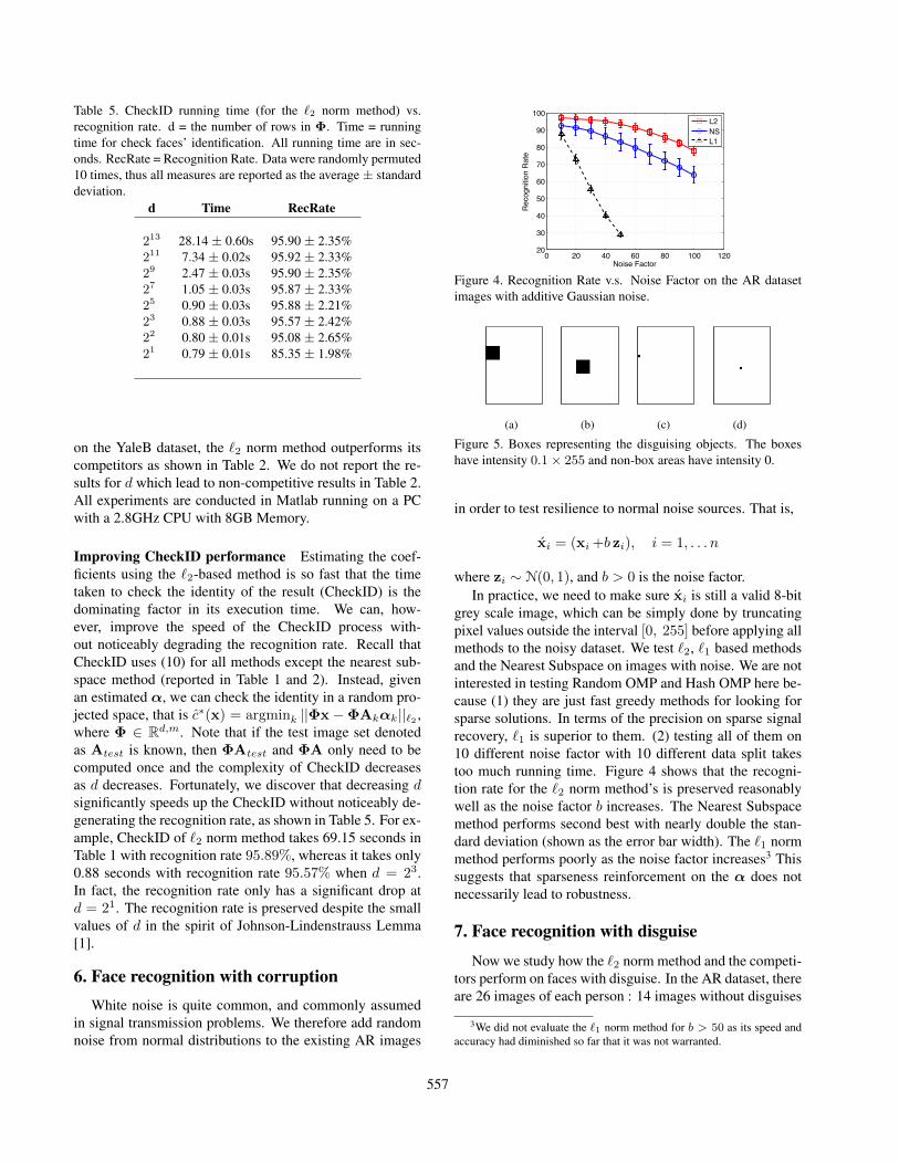
Table 5. CheckID running time (for the `2 norm method) vs.recognition rate. d = the number of rows in Φ. Time = runningtime for check faces’ identification. All running time are in sec-onds. RecRate = Recognition Rate. Data were randomly permuted10 times, thus all measures are reported as the average ± standarddeviation.

d Time RecRate

213 28.14 ± 0.60s 95.90 ± 2.35%211 7.34 ± 0.02s 95.92 ± 2.33%29 2.47 ± 0.03s 95.90 ± 2.35%27 1.05 ± 0.03s 95.87 ± 2.33%25 0.90 ± 0.03s 95.88 ± 2.21%23 0.88 ± 0.03s 95.57 ± 2.42%22 0.80 ± 0.01s 95.08 ± 2.65%21 0.79 ± 0.01s 85.35 ± 1.98%

on the YaleB dataset, the `2 norm method outperforms itscompetitors as shown in Table 2. We do not report the re-sults for d which lead to non-competitive results in Table 2.All experiments are conducted in Matlab running on a PCwith a 2.8GHz CPU with 8GB Memory.

Improving CheckID performance Estimating the coef-ficients using the `2-based method is so fast that the timetaken to check the identity of the result (CheckID) is thedominating factor in its execution time. We can, how-ever, improve the speed of the CheckID process with-out noticeably degrading the recognition rate. Recall thatCheckID uses (10) for all methods except the nearest sub-space method (reported in Table 1 and 2). Instead, givenan estimated α, we can check the identity in a random pro-jected space, that is c∗(x) = argmink ||Φx−ΦAkαk||`2 ,where Φ ∈ Rd,m. Note that if the test image set denotedas Atest is known, then ΦAtest and ΦA only need to becomputed once and the complexity of CheckID decreasesas d decreases. Fortunately, we discover that decreasing dsignificantly speeds up the CheckID without noticeably de-generating the recognition rate, as shown in Table 5. For ex-ample, CheckID of `2 norm method takes 69.15 seconds inTable 1 with recognition rate 95.89%, whereas it takes only0.88 seconds with recognition rate 95.57% when d = 23.In fact, the recognition rate only has a significant drop atd = 21. The recognition rate is preserved despite the smallvalues of d in the spirit of Johnson-Lindenstrauss Lemma[1].

6. Face recognition with corruptionWhite noise is quite common, and commonly assumed

in signal transmission problems. We therefore add randomnoise from normal distributions to the existing AR images

0 20 40 60 80 100 12020

30

40

50

60

70

80

90

100

Noise Factor

Rec

ogni

tion

Rat

e

L2NSL1

Figure 4. Recognition Rate v.s. Noise Factor on the AR datasetimages with additive Gaussian noise.

(a) (b) (c) (d)

Figure 5. Boxes representing the disguising objects. The boxeshave intensity 0.1× 255 and non-box areas have intensity 0.

in order to test resilience to normal noise sources. That is,

xi = (xi +b zi), i = 1, . . . n

where zi ∼ N(0, 1), and b > 0 is the noise factor.In practice, we need to make sure xi is still a valid 8-bit

grey scale image, which can be simply done by truncatingpixel values outside the interval [0, 255] before applying allmethods to the noisy dataset. We test `2, `1 based methodsand the Nearest Subspace on images with noise. We are notinterested in testing Random OMP and Hash OMP here be-cause (1) they are just fast greedy methods for looking forsparse solutions. In terms of the precision on sparse signalrecovery, `1 is superior to them. (2) testing all of them on10 different noise factor with 10 different data split takestoo much running time. Figure 4 shows that the recogni-tion rate for the `2 norm method’s is preserved reasonablywell as the noise factor b increases. The Nearest Subspacemethod performs second best with nearly double the stan-dard deviation (shown as the error bar width). The `1 normmethod performs poorly as the noise factor increases3 Thissuggests that sparseness reinforcement on the α does notnecessarily lead to robustness.

7. Face recognition with disguise

Now we study how the `2 norm method and the competi-tors perform on faces with disguise. In the AR dataset, thereare 26 images of each person : 14 images without disguises

3We did not evaluate the `1 norm method for b > 50 as its speed andaccuracy had diminished so far that it was not warranted.

557

Table 1. Recognition Rate and Running Time on AR dataset. Offline = running time for offline processing. Est = running time for estimatingcoefficients. CheckID = running time for checking face identification for all test images (not per image). All running time are in seconds.RecRate = Recognition Rate. Data were randomly permuted 10 times, thus all measures are reported as the average ± standard deviation.Lowest running time and highest recognition rate are in bold.

Algorithms Offline Est CheckID RecRate

`2 28.74 ± 0.37s 2.71 ± 0.02s 69.15 ± 0.32s 95.89 ± 2.35%`1(d = 300) 1.01 ± 0.01s 5519.01 ± 23.70s 91.20 ± 0.77s 93.12 ± 2.94%`1(d = 200) 0.68 ± 0.01s 2893.47 ± 67.41s 102.16 ± 1.79s 91.54 ± 3.15%`1(d = 100) 0.35 ± 0.00s 1068.20 ± 25.94s 102.13 ± 1.50s 86.13 ± 3.87%Random OMP(d = 300) 1.98 ± 0.01s 1177.52 ± 3.02s 91.90 ± 0.28s 84.85 ± 3.43%Random OMP(d = 200) 1.64 ± 0.02s 348.88 ± 1.24s 85.75 ± 0.15s 80.52 ± 4.12%Random OMP(d = 100) 1.31 ± 0.01s 44.85 ± 0.78s 60.95 ± 0.12s 64.68 ± 5.50%Hash OMP(d = 300) 4.51 ± 0.04s 153.08 ± 7.39s 63.90 ± 0.94s 86.92 ± 3.44%Hash OMP(d = 200) 4.21 ± 0.02s 38.37 ± 2.11s 59.90 ± 0.39s 82.99 ± 3.63%Hash OMP(d = 100) 3.93 ± 0.01s 7.05 ± 0.20s 58.33 ± 0.11s 64.49 ± 5.27%Nearest Subspace 1.06 ± 0.06s 3.07 ± 0.03s 0.07 ± 0.01s 92.32 ± 4.16%

Table 2. Recognition Rate and Running Time on YaleB dataset.Algorithms Offline Est CheckID RecRate

`2 29.02 ± 0.25s 3.55 ± 0.09s 70.60 ± 0.71s 98.91 ± 1.37%`1(d = 300) 1.52 ± 0.01s 4191.34 ± 14.16s 79.48 ± 0.03s 96.63 ± 3.03%Random OMP(d = 200) 2.43 ± 0.07s 12291.77 ± 87.31s 48.21 ± 0.19s 93.75 ± 4.40%Hash OMP (d = 300) 7.04 ± 0.09s 3246.28 ± 250.37s 51.09 ± 0.98s 94.92 ± 3.86%Nearest Subspace 2.74 ± 0.03s 3.83 ± 0.04s 0.02 ± 0.00s 96.87 ± 2.12%

but with various facial expressions and illumination condi-tions, 6 images with sunglasses and 6 images with scarves.We thus split the dataset into a training set (i.e. 1400 un-occluded faces only), a sunglasses test set ( 600 images ofsubjects wearing sunglasses) and a scarves test set (600 im-ages of subjects wearing scarves). This ensures that noneof the disguising objects (sunglasses or scarves) appears inthe training set. Note that in [18] only a subset (200 out of600 ) of disguised images are used for testing in each dis-guise case. When we apply all competitors to the full testsets, the results are very different from what was reportedthere, which will be discussed in detail later in this sectionafter we introduce a method for dealing with the disguisingobjects.

To represent the disguising objects Wright et al. in [18]expand the basis by a square identity matrix I, then seek αand β by the following `1 minimisation:

minα∈Rn,β∈Rm

‖[ αβ

]‖`1 (13a)

s.t. Φx = Φ[A, I][αβ

], (13b)

or alternatively

minα∈Rn,β∈Rm

‖[ αβ

]‖`1 (14a)

s.t. ‖Φx−Φ[A, I][αβ

]‖`2 ≤ ε. (14b)

Identity is again determined by identifying the minimalresiduals among all subjects. This is problematic, how-ever, since I can represent any possible face image withoutA. Alternatively, they construct more sophisticated features(e.g. partition features) to improve the performance of the`1 norm method. However, the features are not applied toother competitors in [18], thus it is not clear that whetherthe improvement comes from the `1 norm method or purelyfrom the new features.

We use a similar method (but with significantly feweradditional columns) to cope with the disguise. The key ideais to try to let β only represent non-face objects and let αonly represent faces. Clearly an identity I is not a goodchoice for it is able to represent any image with that size.Thus we generate a number of images with one grey box invarious locations to represent reasonable size objects. In theexperiment, we use 8 large (30 by 30) box images and 144small (5 by 5) box images4 shown in Figure 5. The face

4In fact, users can design other images as long as the images follow the“key idea” mentioned above.

558

Table 3. Performance comparison when subjects are disguised with sunglasses and scarves. Since we use all non-disguised faces as trainingset, we have one unique data split.

Wearing Sunglasses Wearing ScarvesAlgorithms Offline Est CheckID RecRate Offline Est CheckID RecRate

`2 48.22s 1.49s 35.01s 78.50% 47.52s 1.50s 34.89s 79.50%`1(d = 300) 0.87s 2917.69s 47.56s 40.17% 0.93s 2935.33s 47.37s 55.17%Random OMP(d = 300) 1.60s 426.05s 40.20s 43.00% 1.70s 3170.02s 39.75s 27.00%Hash OMP(d = 300) 4.12s 189.95s 38.66s 46.50% 4.20s 1660.65s 37.29s 32.50%

Table 4. `1 results on the downsampled AR dataset with disguise. Correct = the number of correct predictions of the test images. `1 = LPform uses (13). `1r = the reduced problem uses (14) . Both use d = 300. m is the size of images after downsampling.

Wearing Sunglasses Wearing ScarvesAlgorithms Offline Est CheckID Correct RecRate Offline Est CheckID Correct RecRate

`1(m = 540) 0.19s 3679.03s 2.78s 294 49.00% 0.20s 3738.69s 2.80s 378 63.00%`1(m = 130) 0.05s 2903.38s 0.97s 220 36.67% 0.05s 2853.37s 0.96s 179 29.83%`1r(m = 540) 0.19s 4828.12s 2.80s 291 48.50% 0.20s 4740.44s 2.78s 378 63.00%`1r(m = 130) 0.05s 4156.75s 0.98s 220 36.67% 0.06s 4148.06s 1.00s 180 30.00%

images and the box images can be downloaded from theauthors’ website. Stacking the box images as columns, we

get a matrix B. Let A = [A,B] and α = [αβ

], and then

input A (instead of A) to Algorithm 1 to estimate α (insteadofα). The person id is predicted via minimal residuals overall αk, while β can be ignored as it is shared by all subjectsto represent the disguising objects.

In order to ensure a fair comparison all competitors havebeen tested using the same A. Since we use all non-disguised faces as the training set, we have one unique datasplit. Table 3 shows that in the case of both sunglasses andscarves the `2 norm method outperforms its competitors bya very large margin in terms of recognition rate and estima-tion running time. In particular, `2 achieves 38.33% higherrecognition rate than `1 in sunglasses case and 24.33%higher recognition rate than `1 in scarves case with over2, 000 times speed up.

It is interesting to note that the image reconstructed bythe `1 coefficients is highly distorted (Figure 3(m)) whereasthat reconstructed by `2 (Figure3(e) ) is more faithful to theoriginal image. The `1 norm gives a sparse α whereas `2norm gives a dense one as expected (see Figure 3(k) and3(c)). However, a sparse α does not necessarily lead to amore robust estimation. In fact, from Table 3, the dense αvia the `2 norm outperforms the sparse one via `1 in recog-nition rate by a significant amount.

We also tested the Nearest Subspace method on thisdataset. Since the projection onto the additional B is notmeaningful we instead used A, and achieved a recognitionrate of 62.83% on the sunglasses test set and 13.83% recog-nition rate on the scarves test set. The result is not directly

(a) (b)

0 200 400 600 800 1000 1200 1400 1600−0.4

−0.3

−0.2

−0.1

0

0.1

0.2

0.3

0.4

0.5

(c)

0 200 400 600 800 1000 1200 1400 1600−4

−3

−2

−1

0

1

2

3

4x 10−4

(d)

Figure 6. Prediction on downsampled AR faces with size 13× 10.(a) test face. (b) predicted test face by `1 and `1r. (c) estimatedcoefficient α via `1. The coefficient achieved by `1r is very sim-ilar to (c), thus it is not presented here. (d) The difference ofthe estimated coefficients by `1 and `1r. The difference is onlyin O(10−4).

comparable to those in Table 3, but is still informative.

Performance comparison against Wright et al. [18] In[18] the downsampling of AR face images from 165× 120to 27 × 20 and 13 × 10 is justified as being necessary forcomputational tractability. They train on 799 unoccludedimages and test on two separate test sets (i.e. sunglasses andscarves) of 200 images. Since it is not stated which 799 ofthe 1400 unoccluded images or which 200 of the 600 sun-glasses(or scarves) images are used, we have selected all1, 400 unoccluded images as the training set, and 600 sun-glasses images and 600 scarf images as two separate testingsets. To better compare with their results, we downsam-ple AR images to 27 × 20 and 13 × 10 as well, though thedownsampling step itself is arguable: after downsampling ,the 13 × 10 images are hardly recognisable as faces and itis extremely difficult for a human to recognise the subjects’identities (see Figure 6 (a) and (b)). We use both (13) and(14) as in [18]. Here (13) is a linear program, hence it is

559

expected to be faster than (14), which is a convex problem(a second-order cone program) [5]. We solve both problemsusing CVX [9, 8]. For (14), we set ε = 0.05 as in [18]. Theresults are reported in Table 4. Both (13) and (14) producealmost identical recognition rates though (13) is faster as ex-pected. The difference between the estimated coefficients isvery small (in O(10−4) see Figure 6(d) ). Comparing toTable 3, downsampled `1 still produces results inferior to`2. Moreover, the recognition rate of downsampled `1 de-creases as the image size m decreases.

8. DiscussionIn this work we have compared Compressive Sensing

face recognition methods, such as [18] and [14], with stan-dard `2 approaches. The conclusion we have drawn asa result is that there is no theoretical or empirical reasonto expect that enforcing sparsity on the coefficients of (2)will improve robustness. The experiments carried out hereclearly demonstrate this. Not only does solving (4) lead toworse performance, it is also less robust and orders of mag-nitudes slower than least-squares type approaches.

We do not propose a novel robust method for face recog-nition, but rather show that well know least-squares ap-proaches out perform many of the existing more compli-cated algorithms. We also showed that if `1 minimisation isintended to improve the robustness of the method then thisshould be achieved by solving (6) as discussed in section3. This may be computationally expensive, however, as itrequires solving a linear program. Ways of efficiently solv-ing (6) and an investigation in to the performance of such aformulation is the topic of future work.

References[1] R.G. Baraniuk, M. Davenport, R. DeVore, and M.B. Wakin.

A simple proof of the restricted isometry principle for ran-dom matrices. Constructive Approximation, 2007.

[2] R. Basri and D.W. Jacobs. Lambertian reflectance and linearsubspaces. Pattern Analysis and Machine Intelligence, IEEETransactions on, 25(2):218 – 233, February 2003.

[3] E. Candes, J. Romberg, and T. Tao. Robust uncertainty prin-ciples: Exact signal reconstruction from highly incompletefrequency information. IEEE Trans. Information Theory,52(2):489–509, 2006.

[4] E. Candes and T. Tao. Decoding by linear programming.IEEE Trans. Information Theory, 51(12):4203–4215, 2005.

[5] E.J. Candes and M.B. Wakin. An introduction to compres-sive sensing. IEEE Signal Processing Magazine, pages 21–30, 2008.

[6] Kuang chih Lee, Jeffrey Ho, and David Kriegman. Acquiringlinear subspaces for face recognition under variable lighting.

IEEE Transactions on Pattern Analysis and Machine Intelli-gence, 27:684–698, 2005.

[7] A.S. Georghiades, P.N. Belhumeur, and D.J. Kriegman.From few to many: Illumination cone models for face recog-nition under variable lighting and pose. IEEE Trans. PatternAnal. Mach. Intelligence, 23(6):643–660, 2001.

[8] M. Grant and S. Boyd. Graph implementations for non-smooth convex programs. In V. Blondel, S. Boyd, andH. Kimura, editors, Recent Advances in Learning and Con-trol, Lecture Notes in Control and Information Sciences,pages 95–110. Springer-Verlag Limited, 2008. http://stanford.edu/˜boyd/graph_dcp.html.

[9] M. Grant and S. Boyd. CVX: Matlab software for disciplinedconvex programming, version 1.21. http://cvxr.com/cvx, October 2010.

[10] A. Martinez and R. Benavente. The ar face database. Tech-nical Report 24, CVC Tech. Report, 1998.

[11] M. Rudelson and R. Veshynin. Geometric approach to errorcorrecting codes and reconstruction of signals. Int. Math.Res. Notices, 64:4019–4041, 2005.

[12] Q. Shi, J. Petterson, G. Dror, J. Langford, A. Smola,A. Strehl, and S. V. N. Vishwanathan. Hash kernels. In Proc.Int. Workshop Artificial Intell. & Statistics, 2009.

[13] Q. Shi, J. Petterson, G. Dror, J. Langford, A. J. Smola, andS.V.N. Vishwanathan. Hash kernels for structured data. J.Mach. Learn. Res., 10:2615–2637, 2009.

[14] Qinfeng Shi, Hanxi Li, and Chunhua Shen. Rapid face recog-nition using hashing. In Proc. IEEE Conf. Computer Visionand Pattern Recognition, San Francisco, USA, 2010.

[15] J. A. Tropp and A. C. Gilbert. Signal recovery from randommeasurements via orthogonal matching pursuit. IEEE Trans.Information Theory, 53(12):4655–4666, 2007.

[16] Robert J. Vanderbei. Linear Programming: Foundations andExtensions. 2nd, edition, 2008.

[17] K. Weinberger, A. Dasgupta, J. Attenberg, J. Langford, andA.J. Smola. Feature hashing for large scale multitask learn-ing. In L. Bottou and M. Littman, editors, Proc. Int. Conf.Mach. Learn., 2009.

[18] J. Wright, A. Y. Yang, S. S. Sastry, and Y. Ma. Robust facerecognition via sparse representation. IEEE Trans. PatternAnal. Mach. Intelli., 2008.

[19] A. Y. Yang, J. Wright, Y. Ma, and S. S. Sastry. Feature selec-tion in face recognition: A sparse representation perspective.Tech. Report, 2007.

560