Embed Size (px)
Citation preview

European Journal of Scientific Research
ISSN: 1450-216X / 1450-202X Volume 103 Issue 2 June 2013 Editors-in-Chief Lillie Dewan, National Institute of Technology Co-Editors Chanduji Thakor, Gujarat Technological University Claudio Urrea Oñate, University of Santiago Editorial Board Maika Mitchell, Columbia University Medical Center Prabhat K. Mahanti, University of New Brunswick Parag Garhyan, Auburn University Morteza Shahbazi, Edinburgh University Jianfang Chai, University of Akron Sang-Eon Park, Inha University Said Elnashaie, Auburn University Subrata Chowdhury, University of Rhode Island Ghasem-Ali Omrani, Tehran University of Medical Sciences Ajay K. Ray, National University of Singapore Mutwakil Nafi, China University of Geosciences Felix Ayadi, Texas Southern University Bansi Sawhney, University of Baltimore David Wang, Hsuan Chuang University Cornelis A. Los, Kazakh-British Technical University Teresa Smith, University of South Carolina Ranjit Biswas, Philadelphia University Chiaku Chukwuogor-Ndu, Eastern Connecticut State University M. Femi Ayadi, University of Houston-Clear Lake Emmanuel Anoruo, Coppin State University H. Young Baek, Nova Southeastern University Dimitrios Mavridis, Technological Educational Institute of West Macedonia Jerry Kolo, Florida Atlantic University Mohamed Tariq Kahn, Cape Peninsula University of Technology Publication Ethics and Publication Malpractice Statement Duties of Editors
Confidentiality— Editors of the journal must treat received manuscripts for review as confidential documents. Editors and any editorial staff must not disclose any information about submitted manuscripts to anyone other than the corresponding author, reviewers, other editorial advisers, and the publisher.
Equal Treatment—Editors of the journal must evaluate manuscripts for their intellectual content and their contribution to specific disciplines, without regard to gender, race, sexual orientation, religious belief, ethnic origin, citizenship, or political philosophy of the authors.

Disclosure and Conflicts of Interest— Editors of the journal and any editorial staff must not use materials disclosed in a submitted manuscript (published or unpublished) for their own research without the author’s written authorization.
Integrity of Blind Reviews—Editors of the journal should ensure the integrity of the blind review process. As such, editors should not reveal either the identity of authors of manuscripts to the reviewers, or the identity of reviewers to authors.
Publication Decisions—Editors of the journal are responsible for deciding which of the manuscripts submitted to the journal should be reviewed or published. However, editors may consult other editors or reviewers in making such decisions.
Cooperative involvement in investigations—Editors of the journal should conduct a proper and fair investigation when an ethical complaint (concerning a submitted or published manuscript) is reported. Such process may include contacting the author(s) of the manuscript and the institution, giving due process of the respective complaint. If the complaint has merits, a proper action should be taken (publication correction, retraction, etc.). Besides, every reported action of unethical publishing behavior should be investigated even if it is discovered years after publication.
Duties of Reviewers
Confidentiality—Reviewers must consider all received manuscripts for review as confidential documents. Received manuscripts must not be seen by or discussed with others, except as authorized by the journal editors or authorized editorial staff.
Objectivity—Reviewers should conduct their reviews objectively. Criticism of the author’s personality or the topic is unprofessional and inappropriate. Reviewers should explain their recommendations clearly and explicitly and provide rational support and justification. Editors Recommendations could be one of the following:
• Accept the publication of the manuscript after compliance with the reviewers’ recommendations.
• Consider the publication of the manuscript after minor changes recommended by its reviewers.
• Consider the publication of the manuscript after major changes recommended by its reviewers.
• Reject the publication of the manuscript based on the reviewers’ recommendations
Fast-Track Reviews—Reviewers are requested to complete their reviews within a timeframe of 30 days. Reviewers also are free to decline reviews at their discretion. For instance, if the current work load and/or other commitments make it impossible for reviewers to complete fair reviews in a short timeframe (e.g., few days for fast-track review), reviewers should refuse such invitations for review and promptly inform the editor of the journal.
Qualifications—Reviewers who believe that they are not qualified to review a received manuscript should inform the journal editors promptly and decline the review process.
Disclosure—Information or ideas obtained through blind reviews must be kept confidential and must not be used by reviewers for personal benefits.
Conflict of Interest —Reviewers should refuse the review of manuscripts in which they have conflicts of interest emerging from competitive, collaborative, or other relationships and connections with any of the authors, companies, or institutions connected to the manuscripts.
Substantial Similarity—Reviewers should inform editors about significant resemblances or overlap between received manuscripts and any other published manuscripts that reviewers are aware of.

Proper and Accurate Citation —Reviewers should identify relevant published work that has not been cited by the authors. Statements that include observation, derivation, or argument (currently or previously reported) should be accompanied by a relevant and accurate citation.
Contribution to Editorial Decisions—Reviewers assist editors in making editorial publication decisions, and also assist authors in improving their submitted manuscripts, through the editorial communications with authors. Therefore, reviewers should always provide explicit and constructive feedback to assist authors in improving their work.
Duties of Authors
Originality—Authors submitting manuscript to the journal should ensure that this submission is original work and is neither currently under consideration for publication elsewhere, nor has been published as a copyrighted material before. If authors have used the ideas, and/or words of others researchers, they should acknowledge that through proper quotes or citations.
Plagiarism—Plagiarism appears into various types, such as claiming the authorship of work by others, copying and paraphrasing major parts of others research (without attribution), and using the results of research conducted by other researchers. However, any type of plagiarism is unacceptable and is considered unethical publishing behavior. Such manuscripts will be rejected.
Authorship of Manuscripts—Authorship of a manuscript should be limited to authors who have made significant contributions and the names of authors should be ranked by efforts. The corresponding author must ensure that all listed coauthors have seen and approved the final version of the manuscript (as it appeared in the proofreading copy) and agreed to its publication in the journal. Authors can permit others to replicate their work.
Multiple or Concurrent Publication— Authors should not publish manuscripts describing essentially the same research in more than one journal. Submitting the same manuscript to more than one journal concurrently constitutes unethical publishing behavior and is unacceptable. This action leads to the rejection of the submitted manuscripts.
Acknowledgement of the Work of Others—Authors should always properly and accurately acknowledge the work of others. Authors should cite publications that have significant contribution to their submitted manuscripts. Unacknowledged work of others contributing to manuscripts is unethical behavior and is unacceptable. Such manuscripts will be rejected.
Reported objectives, discussions, data, statistical analysis, and results should be accurate. Fraudulent or knowingly inaccurate results constitute unethical behavior and are unacceptable. Such manuscripts will be rejected.
Data Access and Retention— Authors may be asked to provide the raw data in connection with manuscripts for editorial review, and should be prepared to provide public access to such data if possible. However, such authors should be prepared to retain data for a reasonable time after publication.
Hazards and Human or Animal Subjects— If a research study involves chemicals, procedures or equipment that have any unusual hazards inherent in their use, the author(s) must clearly identify these in the submitted manuscript. Authors should also inform participating human subjects about the purpose of the study.
Conflicts of Interest— In their manuscript(s), authors should disclose any financial or other substantive conflict of interest that might influence the results or interpretation of their manuscript.

Copyright of Accepted Manuscripts—Authors of accepted manuscripts for publication in the journal agree that the copyright will be transferred to journal and all authors should sign copyright forms. However, those authors have the right to use of their published manuscripts fairly, such as teaching and nonprofit purposes.
Substantial errors in published Manuscripts—When authors discover substantial errors or inaccuracy in their own published manuscripts, it is the authors’ responsibility to promptly inform the journal editors or publisher, and cooperate with them to correct their manuscripts.
Acknowledgement of Indirect Contributors and Financial Supporters—Authors should acknowledge individuals whose contributions are indirect or marginal (e.g., colleagues or supervisors who have reviewed drafts of the work or provided proofreading assistance, and heads of research institutes, centers and labs should be named in an acknowledgement section at the end of the manuscript, immediately preceding the List of References). In addition, all sources of financial support for the research project should be disclosed.
Disclaimer Neither the editors nor the Editorial Board are responsible for authors’ expressed opinions, views, and the contents of the published manuscripts in the journal. The originality, proofreading of manuscripts and errors are the sole responsibility of the individual authors. All manuscripts submitted for review and publication in the journal go under double-blind reviews for authenticity, ethical issues, and useful contributions. Decisions of the reviewers are the only tool for publication in the journal and will be final.

European Journal of Scientific Research Volume 103 Issue 2, June 2013
Contents
Quelques Aspects de La Reproduction du Fuligule Nyroca Aytya Nyroca Dans le Lac Tonga (Site Ramsar Nord-Est Algerien) ................................................................................... 165-174
Badis Bakhouche, Khalil Draidi, Moussa Houhamdi and Zihad Bouslama A Comparative Look at the Spirituality in Higher Education University Students’ Search for Meaning and Purpose; Albania & USA .............................................................................. 175-184
Ahmet Ecirli Is the Application of Simple Trading Rules a Powerful Tool for Profitability Prediction?: The Case of the FTSE-20 of the Athens Exchange ................................................................... 185-206
Georgia S. Demiri, Apostolos G. Christopoulos, Ioannis G. Dokas and Konstantinos P. Vergos Brain Extracting Using a Simple Standard Deviation and Mathematical Morphology in Medical Images MRI .............................................................................................................. 207-217
Samir Bara, Mounir Ait Kerroum and Ahmed Hammouch Report on the Development of Standard Criteria of Environmental Education for School Under Tak Primary Educational Service Area Office 1 .......................................................... 218-226
Paisarn Pandan, Vinai Veeravatnanond and Raveevan Sananvorakiat A Critical Analysis of the Effectiveness of Human Resource Development Techniques in the Non-Government Organizations of Balochistan ...................................................................... 227-238
Saubia Ramzan and Uzma Mukhtar Dimensionality Reduction of High Dimensional Data Using Fractional Cuckoo Search Algorithm to Improve Clustering Process ................................................................................ 239-255
Golda George and Latha Parthiban Bioactivity of Injected Boric Acid on German Cockroaches: Lethality, Analysis of Residues and Acethylcholinesterase and Glutathione S-Transferase Activities ................................... 256-266
Dahbia Habes, Karim Bouazdia, Rouhia Messiad, Anissa Boussatha and Noureddine Soltani Cardiac Arrhythmia Classification Using Regularized Least Squares Classifier ................. 267-281
Hamza Baali, Momoh.J.E.Salami, Rini Akmeliawati, Aida Khorshidtalab Practical Proposal for Roundabouts Bypass Calculation ........................................................ 282-295
Raffaele Mauro and Marco Guerrieri Comprehensive Investigation on Harmonic Spreading Effects of SPWM and RPWM Methods .......................................................................................................................... 296-303
T.Jarin and P.Subburaj

An Analytical Approach to Pricing Discrete Barrier Options under Time-Dependent Models ............................................................................................................. 304-312
Mohammad H. Beheshti, Amir T. Payandeh Najafabadi and Rahman Farnoosh Tunable and Reconfigurable Spectrum Sliced Microwave Photonic Filter Using Parallel Fabry-Perot Filters with External Delay and Windowing ...................................................... 313-325
R. K. Jeyachitra and J. Martin Leo Manickam Mobility Issues in 4G Heterogeneous Wireless Networks ....................................................... 326-332
K.Komala and P.Indumathi Le Fuligule Nyroca (Aythya Nyroca) dans le Lac Tonga (Nord Est de l’Algérie): Dénombrement et Étude des Rythmes d’Activités ................................................................... 333-342
Khalil Draidi, Badis Bakhouche, Salah Tlailia, Moussa Houhamdi and Zihad Bouslama
European Journal of Scientific Research ISSN 1450-216X / 1450-202X Vol. 103 No 2 June, 2013, pp.165 - 174 http://www.europeanjournalofscientificresearch.com
Quelques Aspects de La Reproduction du Fuligule Nyroca Aytya
Nyroca Dans le Lac Tonga (Site Ramsar Nord-Est Algerien)
Badis Bakhouche EcoSTAq – Laboratoire d’Ecologie des Systèmes Terrestres et Aquatiques
Université Badji Mokhtar – Annaba – Algérie E-mail: [email protected]
Tel: +213-551-53-02-19
Khalil Draidi EcoSTAq – Laboratoire d’Ecologie des Systèmes Terrestres et Aquatiques
Université Badji Mokhtar – Annaba – Algérie
Moussa Houhamdi EcoSTAq – Laboratoire d’Ecologie des Systèmes Terrestres et Aquatiques
Université Badji Mokhtar – Annaba – Algérie
Zihad Bouslama EcoSTAq – Laboratoire d’Ecologie des Systèmes Terrestres et Aquatiques
Université Badji Mokhtar – Annaba – Algérie
Résumé
Le fuligule nyroca (Aythya nyroca), espèce nicheuse dans le Nord-Est Algérien fréquente le lac Tonga toute l’année avec une variation des effectifs atteignant son maximum à partir de la deuxième moitié du mois d’août jusqu’à la deuxième moitié du mois de septembre. Notre travail porte sur l’écologie de la reproduction de cette espèce dans le lac Tonga et a été réalisé pendant l’année 2012. Nous avons pu localiser 112 nids dont 55% d’entre eux ont été installés dans des petits ilots de végétation. La grandeur de ponte est de 9,46 œuf/nid et le succès de l’éclosion de 59%. La principale cause de l’échec d’éclosion des œufs est la prédation des nids. Motsclé : Fuligule nyroca, Aythya nyroca, lac Tonga, dénombrement, reproduction, taux
d’échec. 1. Introduction L’Algérie fait partie des Hotspot de la méditerranée en raison de sa très grande superficie (2400000km2) (Erol Véla et Benhouhou. 2007), de la grande diversité de climats (subtropicale, aride semi-aride, méditerranéen), et de son littoral (1350 km) lui permettant de jouir d’une large gamme de biotopes favorisant une faune et une flore remarquables (Stevenson et al. 1988 ; Samraoui et De Belair, 1997, 1998). D’autre part de par la grande diversité de ses habitats, elle jouit d’un potentiel en zones humides de grandes valeurs écologiques, culturelles et économiques (Quezel et Médail, 2003).
Les oiseaux d’eau, considérés comme chainon important des zones humides et très bons bio-indicateurs de l’état de santé des zones humides, sont très diversifiés et parmi eux nous retrouvons le

166 Badis Bakhouche, Khalil Draidi, Moussa Houhamdi and Zihad Bouslama
Fuligule nyroca (Aytya nyroca). Selon les dernières classifications de l’IUCN concernant la liste rouge des espèces animales menacées, cet Anatidé occupe le statut d’espèce peu menacée (Near Thretened) (IUCN 2006) suite à la destruction des zones humides causant ainsi un déclin dramatique de ces effectifs,
Les populations des Fuligules nyroca sont subdivisées en deux catégories une population eurasienne située dans la rive Nord, la seconde se concentre surtout dans le Maghreb et le Sahel (Green et al.,1998,1999,2001 ; Green et El Hamzaoui 2000, 2006 ; Robinson et Huges 2002). En Afrique du Nord malgré le statut de sédentarité de l’espèce, peu de travaux lui ont été consacrés ;(El Agbani 1997) au Maroc,(Boumezbeur 1993, Houhamdi et Samraoui 2008)en Algérie et (Azefzaf 2002) en Tunisie.
Notre travail porte sur l’étude de quelques aspects de l’écologie de la reproduction du Fuligule nyroca dans le lac Tonga, site Ramsar situé à l’extrême Nord est algérien qui représente l’un des plus importants sites d’hivernage à l’échelle du pays et de la région (Aissaoui et al 2009). 2. Matériel et Méthodes 2.1. Description du Site D’étude
Le lac Tonga (36°53 N, 08°31 E) s’étendant sur une superficie de 2500 ha (Belhadj et al,2007,Lazli et al 2011,2012) est l’un des sites ramsar le plus important des zones humides d’Afrique du Nord (Boumezbeur, 1993,Samraoui et De Belair, 1998). Il est situé à l’extrême Nord-Est de l’Algérie, fait partie du parc national d’El-Kala (PNEK) et classé parmi les aires protégées de la région méditerranéenne lui donnant la nomenclature de réserve de la biosphère. La végétation aquatique abondante de ce lac joue un rôle prépondérant dans la répartition des espèces d’oiseaux d’eau en leur offrant à la fois l’abri et l’aliment. Elle est principalement composée par des ilots de Typha angustifolia, Irispseudoacorus, Scirpus lacustris, S.maritimus Phragmites australis, Salix pedicellatt et Sparganium erectum. Au printemps, nous assistons à l’émergence et la floraison d’une hydrophyte très envahissante des espaces d’eau libres Nymphaea alba.
Sur le plan avifaunistique, cet écosystème limnique est un excellent quartier d’hivernage pour les populations du Paléarctique occidental, comme il peut servir de terrain de repos pour d’autres espèces d’oiseaux pendant les périodes de migration. Le lac Tonga est également un site de nidification utilisé par de nombreuses espèces telles que la Foulque macroule Fulca atra, le Fuligule nyroca Aythya nyroca, l’Erismature à tête blanche Oxyura leucocephala (Chalabi, 1990, Boumezbeur 1993), la Poule sultane Porphyrio porphyrio, la Poule d’eau Gallinula chloropus, le Canard colvert Anas platyrhyncos, le Grèbe castagneux Tachybaptus rufficollis, le Grèbe huppé Podiceps cristatus (Ledant et al., 1981, Samraoui et De Bélair 1998, Isenemann et Moali 2000), le Héron garde-bœuf Bubulcus ibis, le Héron pourpré Ardea purpurea, le Héron crabier Ardea ralloides, le Héron bihoreau Nycticorax nycticorax, le Blongios nain Ixobrychus minutus, l’Aigrette garzette Egretta garzetta et l’Ibis falcinelle Pellagadis falcinellus (Belhadj et al., 2007).

Quelques Aspects de La Reproduction du Fuligule Nyroca Aytya Nyroca Dans le Lac Tonga (Site Ramsar Nord-Est Algerien) 167
Figure 1: Localisation du lac Tonga dans le complex de zones humides d’el Kala
Algérie
Bouteldja
RN44
El-Aioun
Oum-Teboul
El-Kala
Ain-Assel
Sidi-Kassi
Ben M’hidi
Annaba
El-Hadjar
M e d i t e r r a n e n n s e a
RN16
RN21
RN44
CW110
CW3
Tunisia
Lac des Oiseaux
Marais de la Mekkhada
Lac Tonga
Lac Oubeira
Lac El-Mellah
Les Salines
RN16
N
Vers El-Kala
Commune Rmal Souk
Commune
Vers Oum Taboul
10 Km
El-Taref
Afin d’étudier la reproduction de notre modèle, certains paramètres décrits par la littérature scientifique (Schömwetter 1967 in Cramp & Simmons 1983, Goriup 1982, Géroudet 1982, Khorkov 1982, Seriot 1987,Maazi et al 2010 ) ont été pris en considération :
1. Comptage des effectifs des Fuligule nyroca pandant l’année 2012 en utilisant un télescope KONUS SPOT 20x60.
2. Le suivi des effectifs des couples nicheurs dès leur apparition dans le site jusqu'à la fin de la reproduction.
3. Recherche des nids dans la typha et les îlots de végétation , une fois détecté, nous mesurons toutes leurs caractéristiques (composition, diamètre interne, externe, leur densité (le nombre total des nids du site / la surface des îlots ou a eu la reproduction) ainsi que les mesures des distances entre les nids plus proche.
4. Le volume est calculé par la méthode Harris (1964) V= 0,476.L.B2/1000 où L=longueur (mm), B=largeur (mm) et V=volume (cm3).

168 Badis Bakhouche, Khalil Draidi, Moussa Houhamdi and Zihad Bouslama
Dès la fin de la construction du nid nous notons les dates, période et grandeur ou taille de ponte ainsi que le taux d’éclosion. Lorsqu’un nid n’a pas éclos, nous discuterons les causes de l’échec (prédation ou abandon). 2.2. Analyses Statistiques
Les analyses statistiques ont été déterminées grâce aux statistiques élémentaires en utilisant le Microsoft Excel(2007). 3. Résultats et Discussion 3.1. Statut et Structure
D’après la figure (2), nous remarquons que notre modèle est omniprésent dans notre site d’étude tout au long de l’année. Ces résultats confortent ceux de Aissaoui (2009).
L’évolution des effectifs suit une courbe fluctuante, divisée en quatre phases : 1. La première est ascendante (du 01 Janvier jusqu’au 10 mai) qui pourrait être expliqué par
l’arrivée des populations migratrices. 2. La seconde est descendante (à partir du mois de mai jusqu’à la mi-juillet)) qui serait due à la
reproduction. En effet, lors de cette période, les individus ne s’éloignent pas de leurs nids et ne seraient donc pas comptabilisés lors du dénombrement.
3. la troisième est ascendante (18 juillet au 30 Septembre) période au cours de laquelle les fuligules nyroca voient leurs effectifs très importants atteignant un pic entre le 18 août et le 30 septembre qui correspondrait à la l’arrivée des populations estivantes
4. La quatrième est descendante au cours de laquelle l’effectif diminue jusqu’à arriver à 90 qui correspondrait à la population sédentaire.
Figure 2 : Evolution de l’effectif du fuligule nyroca Aytya nyroca dans le lac Tonga en 2012
3.2. Ecologie de la Reproduction
3.2.1. Dynamique de Construction des Nids

Quelques Aspects de La Reproduction du Fuligule Nyroca Aytya Nyroca Dans le Lac Tonga (Site Ramsar Nord-Est Algerien) 169
Figure 3: Evolution de l’installation des nids du Fuligule nyroca (Aythya nyroca) au lac Tonga
Anciens nids Nouveaux nids
Les deux premiers nids ont été repérés le 19 Avril, vérifiant les données trouvées dans le même
site par Lazli en 2011 et ce au niveau de la station Oued el Hout. Par la suite nous observons une augmentation du nombre atteignant un maximum de 50 durant la période du 13 au 19 juin. On assiste après cette date, à une régression du nombre et ce jusqu’au 13 juillet où les deux derniers nids ont été observés (Figure3). Maizila et la vieille école présentent les endroits les plus importants pour l’installation des nids avec respectivement 25% et 23% de la totalité des nids (Figure 04).
Figure 4 : Distributions des nids dans les différents secteurs du lac Tonga

170 Badis Bakhouche, Khalil Draidi, Moussa Houhamdi and Zihad Bouslama
3.2.2. Caractéristiques des Nids Tableau 02 : Mensurations des nids (n=112) D : diamètre ; Prof : profondeur ; nid/nid : distance entre 02 nids
Nids D.ext (cm) D.int (cm) prof nid (cm) prof eau (cm) Elévation
(cm) nid/nid (m)
moyenne 25,79±4,21 16,82±2,55 8,66 ±3,43 78,81 ±33,40 2,82 ±8,77 2,4 ±1,49 Max 35 26 19 170 50 8 Min 14 11 1 20 0 0,2
Les nids ont un diamètre externe de 25,79 ±4,2cm et un interne de 16,82 cm±2,55. Leurs
profondeurs est de 8,66cm (min 1et max 19cm). La profondeur de l’eau ou se trouve les nids du fuligule nyroca est de 78,81 cm (min 20 cm et max 170cm) qui est différente de l’étude (Aissaoui ,2011) 172,10cm et 2,82 cm concernant leurs élévations par rapport à l’eau (min 0cm et max 50cm) et une distance entre les nids de 240cm (min20cm et max 800cm) différente par rapport à 96,93cm (Aissaoui 2012) . 3.2.3. Biométrie des Œufs Tableau 2: Mensurations des œufs (n=112)
Œuf Longueur (mm) Largeur (mm) Poids (g) Volume (cm3) moyenne 50,86 ±2,10 38,19 ±1,36 40,76 ±3,30 35,24 Max 56,2 40 47,5 55,00 Min 42 35,6 35 25,33
La longueur des œufs été égale 50,86 mm (le minimum est de 42 mm et le maximum 56,2 mm)
et pour la largeur 38,19 mm (le minimum 35,6 et le maximum 40) et avec un poids de 40,76g (le minimum 35 et le maximum 47,5) qui sont proche des résultats de l’étude de (Aissaoui, 2012) Grandeur de ponte
Sur notre échantillon de 112 nids la moyenne de la grandeur de ponte était de 9,46. 3.2.4. Succès et Échecs de L’éclosion
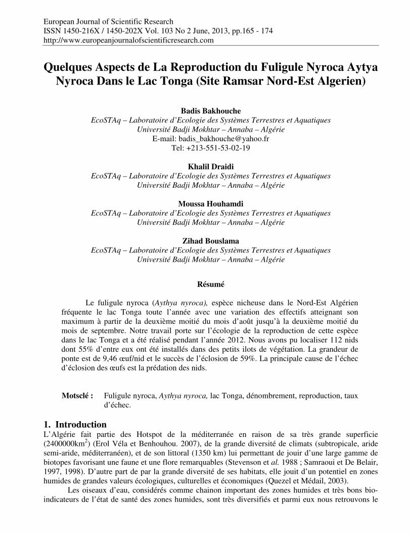
Figure 4: (A) Taux de réussite d’éclosion (B) principales causes de l’échec
(A) (B)
Les premières éclosions ont eu lieu à partir du 7 mai et les dernières ont été enregistrées le 13
juillet 2012. Ainsi sur les 112 nids suivis 68 ont réussi à éclore soit un taux de 59%, soit un taux plus bas que celui trouvé en 2010 (80%) dans le même site par Aissaoui (2012). La cause principale est la prédation qui a affecté 26 nids, soit 55% de causes d’échec. Ces nids ont été attaqués par différents prédateurs (oiseaux rapaces et reptiles aquatiques). Les autres nids ont été abandonnés suite à la mort
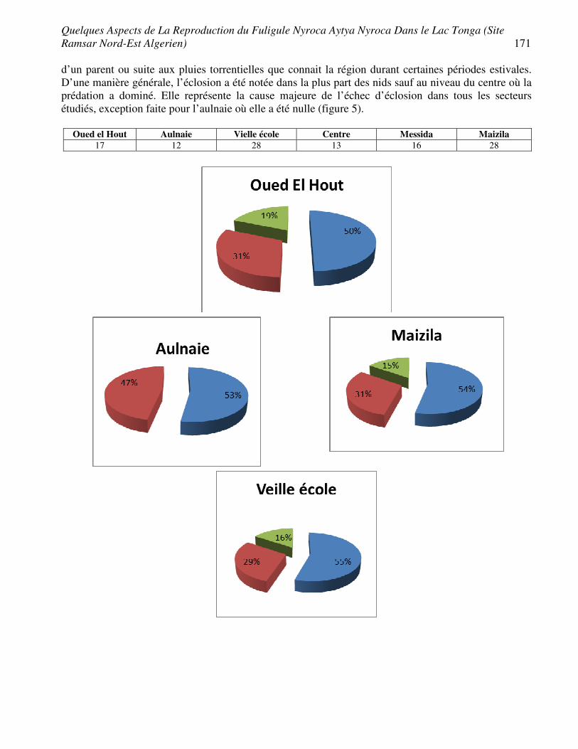
Quelques Aspects de La Reproduction du Fuligule Nyroca Aytya Nyroca Dans le Lac Tonga (Site Ramsar Nord-Est Algerien) 171 d’un parent ou suite aux pluies torrentielles que connait la région durant certaines périodes estivales. D’une manière générale, l’éclosion a été notée dans la plus part des nids sauf au niveau du centre où la prédation a dominé. Elle représente la cause majeure de l’échec d’éclosion dans tous les secteurs étudiés, exception faite pour l’aulnaie où elle a été nulle (figure 5).
Oued el Hout Aulnaie Vielle école Centre Messida Maizila 17 12 28 13 16 28
172 Badis Bakhouche, Khalil Draidi, Moussa Houhamdi and Zihad Bouslama
éclosion prédation abandon 5. Conclusion Le Fuligule nyroca Aythya nyroca est une espèce sédentaire nicheuse dans le lac Tonga. L’effectif observé est souvent composé d’une population hivernante, fréquentant principalement le centre du plan d’eau. La seconde population nicheuse dans le site ce qui corrobore avec les données de Aissaoui et al., (2009, 2011) et Lazli (2012). Ces Anatidés exploitent préférentiellement les régions méridionales du plan d’eau où ils installent leurs nids (Boumezbeur, 1993, Lazli 2012). Le lac Tonga peut être considéré comme le site de reproduction type pour cette espèce de canard plongeur en Algérie (Lazli, 2012). Nous avons recensé 112 nids et la plus part sont conçus dans des touffes de Typha angustifolia, Phragmites australis, Sciprus maritimus et sur des ilots composés principalement de Salix pedicelata. L’espace vital du couple nicheur est très petit. Les Foulques macroules Fulica atra et la poule d’eau Galunila chloropus sont les deux espèces qui nichent au voisinage de cet Anatidés.
La pression anthropique et la prédation sont assez importantes causant ainsi 55% de causes d’échec. Les nids installés en premier subissent souvent une prédation plus forte. Le succès biologique de reproduction chez ces nids est faible. Le taux d’éclosion est assez important mais la survie des poussins est faible. Les couleuvres vipérine Natrix maura , les rapaces diurnes (Busard des roseaux circus aeruginosus ) constituent les principaux prédateurs de nids et de poussins.
Il est important de signaler que malgré le statut Ramsar du site, le pillage des œufs de cette espèce et d’autres classées sur la liste rouge de l’UICN (Erismature à tête blanche Oxyura leucocephala, poule sultane Porphyrio porphyrio…) et le braconnage sont très observés par les riverains et par les passants. De plus, la proximité du plan d’eau de la Méditerranée fait en sorte que le site est souvent fréquenté par les estivants et ce dès le mois de mai provoquant des dérangements, surtout pendant la période d’installation des nids. Références Bibliographiques [1] Aissaoui R., Houhamdi M. and Samraoui B. (2009). Eco-Éthologie des Fuligules Nyroca
Aythya Nyroca dans le Lac Tonga (Site Ramsar, Parc Nationald’El-Kala, Nord-Est de l’Algérie). European Journal of Scientific Research :47-59.
[2] Aissaoui R., Tahar A., Saheb M., Guergueb L. and Houhamdi M. (2011). Diurnal behaviour of Ferruginous Duck Aythya nyroca wintering at the El-Kala wetlands (Northeast Algeria). Bulletin de l’Institut Scientifique, Rabat, section Sciences de la Vie, 2011, N°33 (2) : 67-75.

Quelques Aspects de La Reproduction du Fuligule Nyroca Aytya Nyroca Dans le Lac Tonga (Site Ramsar Nord-Est Algerien) 173 [3] Aissaoui R. (2012). Eco-éthologie des Anatidés dans la Numidie orientale cas de la fuligule
nyroca (Aythya nyroca) dans le lac Tonga. Thèse de doctorat en biologie animale et environnement. Université Badji Mokhtar d’Annaba. 176P
[4] Altmann J. (1974). Observational study of behaviour: Sampling methods. Behaviour 49:227-267.
[5] Azafzaf H. (2002). The Ferruginous duck in Tunisia, Ferruginous Duck: From research to conservation, 84-87. Conservation Series N°6. Birdlife International-BSPB-TWSG.
[6] Baldassarre G.A., Paulus S.L., Tamisier A. and Titman D.R.D. (1988).Workshop summary techniques for timing activity of wintering waterfowl. Waterfowl in winter. Univ. Minnesota press. Minneapolis. 23p.
[7] Belhadj G., Chalabi B., Chabi Y., Kayser Y. et Gauthier-Clerc M. (2007). Le retour de l’Ibis falcinelle (Plegadis falcinellus) nicheur en Algérie. Aves 44(1): 29-36.
[8] Boumezebeur A. (1993). Ecologie et biologie de la reproduction de l’Erismature à tête Blanche Oxyura leucocephala et du Fuligule nyroca Aythya nyroca sur le Lac Tonga et le Lac des oiseaux, Est algérien. Thèse de doctorat, Université Montpellier, 254 p.
[9] Benyacoub S. and Chabi Y. (2000). Diagnose écologique de l'avifaune du Parc National d'El Kala. Synthèse (N°7). 98p.
[10] Boumezebeur A., Moali A. et Isenmann P. (2005). Nidification du Fuligule nyroca Aythya nyroca et de l’échasse blanche Himantopus himantopus en zone saharienne (El Goléa, Algérie). Alauda 73 (2): 143-144.
[11] El Agbani M.A. (1997). L'Hivernage des Anatidés au Maroc. Principales espèces, zones humides d'importance majeure et propositions de mesures de protection. Thèse de doctorat d'Etat ès-Sciences, Faculté des Sciences, Rabat (Maroc). 186p.
[12] Green A. J. (1998). Habitat selection by the Marbled Teal Marmaronetta angustirostris, Ferruginous Duck Aythya nyroca and other ducks in the Göksu Delta, Turkey, in summer. Revue Ecologie (Terre and Vie), 53: 225-243.
[13] Green A. J., Fox, A. D., Hughes B. and Hilton G. M. (1999). Time-activity budgets and site selection of White-headed Ducks Oxyura leucocephala at Burdur Lake, Turkey in late winter. Bird Study, 46: 62-73.
[14] Green A.J. and El Hamzaoui M. (2000). Diuranal behavior and habitat use of Marbled teal Marmaronetta angustirostris Canadian journal of zoology, 78:2112-2118.
[15] Green A.J. and El Hamzaoui M. (2006). Interspecific associatins in habitat use between marbled and other waterbirds wintering at Sidi Boughaba Moroco. Ardeola 53: 99-106.
[16] Green A. J. and Hughes B. (2001). Oxyura leucocephala White-headed Duck. Pp 79-90 in : BWP Update. Vol.3, Number 2. Oxford University Press.
[17] Grenn A.J., El Hamzaoui M., El Agbani M-A. and Fanchimount J. (2002). The conservation status of morocan wetlands with particular reference to waterbirds and to changes since 1978. Biological conservation 104:71-82
[18] Houhamdi M. and Samraoui B. (2008). Diurnal and nocturnal behaviour of ferruginous duck Aythya nyroca at Lac des Oiseaux, northeast Algeria. Ardeola 55: 59-69.
[19] IUCN (2006). Red list of Threatened Species, Downloaded from www.redlist.org. [20] Jonsson L. (1994). Les oiseaux d’Europe, d’Afrique du Nord et du Moyen-Orient. Nathan.
414p. [21] Lazli A. (2011). Contribution à la connaissance de l’écologie et de la biologie de la
reprduction de l’érismature à tête blanche Oxyura leucocephala et le Fuligule nyroca Aythya nyroca au niveau du lac Tonga. Thèse de doctorat en Ecologie et Environnement. Université Abdelrahmane Mira de Bejaia.265
[22] Ledant J-P., Jacobs J-P., Malher F., Ochando B. et Roché J. (1982). Mise à jour de l’avifaune algérienne. Le Gerfaut 71: 295-398.

174 Badis Bakhouche, Khalil Draidi, Moussa Houhamdi and Zihad Bouslama
[23] Losito M.P., Mirarchi E. and Baldassarre G.A. (1989). New techniques for time activity studies of avian flocks in view-retricted habitats. J. Field. Ornithol. 60: 388-396.
[24] Maazi M-C., Saheb M., Bouzegag A., Seddik S., Nouijem Y., Bensaci E., Mayache B., Chefrour A. et Houhamdi M. (2010). Ecologie de la reproduction de l’Echasse blanche Himantopus himantopusdans la Garaet de Guellif (Hauts plateaux de l’Est algérien). Bulletin de l’Institut Scientifique, Rabat, Section Sciences de la Vie, 2010, N°32 (2), 101-109.
[25] Samraoui B. et De Belair G. (1998). Les zones humides de la Numidie orientale: bilan des connaissances et perspectives de gestion. Synthèse (Numéro spécial 4): 1-90.
[26] Vila E. et Benhouhou S. (2007). Evaluation d’un nouveau point chaud de biodiversité végétal dans le bassin méditerranéen (Afrique du Nord). Comptes Rendues Biologies 330 (2007) 589–605.

European Journal of Scientific Research ISSN 1450-216X / 1450-202X Vol. 103 No 2 June, 2013, pp.175 - 184 http://www.europeanjournalofscientificresearch.com
A Comparative Look at the Spirituality in Higher Education
University Students’ Search for Meaning and Purpose; Albania & USA
Ahmet Ecirli, PhD Dean. Lecturer, Faculty of Philology and Education
Hena e Plote Beder University, Tirana, Albania E-mail: [email protected]
Tel: +355673374134, Fax: +3554 24 19 333
Abstract
This paper mainly deals with a national study to find out the level of college students’ search for meaning and purpose carried out by HERI - Higher Education Research Institute Graduate School of Education & Information Studies at UCLA- University of California, Los Angeles. The findings as a result of the report involve 112,232 first-year students attending 236 various colleges and universities across the US between the years 2003 and 2007; help us to improve our understanding of the role that spirituality plays in students’ lives and to ascertain strategies that institutions can use to advance students’ spiritual growth. A similar study using the instruments of HERI has been carried out by our research team at Beder University to find out the similarities and differences for spirituality in higher education in Albania. The study was based on data collected in early fall and late summer 2012 from 2360 students attending a national sample of 18 colleges and universities in Albania. The research contributes to the understanding as to how higher education medium serve students considering their religious and spiritual identities. The notions surveyed include students’ search for “spiritual issues and questions such as the meaning of life and work”, their view for “spirituality and related qualities such as compassion, generosity, optimism, and kindness”, their “engagement in spiritual/religious commitment”, the effects of spiritualty on academic and personal development. The findings of this study show a current comparative look at the “Spirituality in Higher Education” in Albania and the USA. Keywords: Spirituality in higher education, spiritual commitment, spiritual issues and
qualities, academic and personal development, meaning of life and work 1. Introduction The survey SAHE; “Spirituality in Albanian Higher Education” provides a country-wide scheme to identify tendencies, patterns, and codes of spirituality and religiousness among university students in Albania. Some of the important findings are compared with those in the USA, by the data provided by HERI; Higher Education Research Institute Graduate School of Education & Information Studies at UCLA- University of California, Los Angeles. HERI conducted a similar multi-year research in the years 2003-2007. The findings as a result of the report deal with 112,232 first-year students attending 236 various colleges and universities across the US.

176 Ahmet Ecirli
SAHE aims to address the issues and questions such as the number of students actively searching and curious about spirituality, religion, compassion, generosity, optimism and kindness. It also concerns with the religious practices and their impacts on students’ academic and personal development. The connection between traditional religious practices and spiritual development has been studied as well. The research tried to look for an answer whether the undergraduate experience facilitates or hinders students’ spiritual/religious quest.
This study presents highlights of findings based on data collected in early Fall and late Summer 2012 from 2360 students attending a national sample of 18 colleges and universities in Albania. Students responded to a six-page survey questionnaire that addressed questions about their backgrounds, educational and occupational aspirations, and values and beliefs with respect to spiritual and religious matters.
The study revealed that today’s college students have very high levels of spiritual interest and involvement. Many are actively engaged in a spiritual quest and are exploring the meaning and purpose of life. They also display high levels of religious commitment and involvement.
As they begin their college experience, freshmen have high expectations for the role their institutions will play in their emotional and spiritual development. They place great value on their college enhancing their self-understanding, helping them develop personal values, and encouraging their expression of spirituality.
There are important similarities and distinctions between those students who are strongly religious and those who are highly spiritual. These qualities manifest themselves in a variety of ways related to students’ practices, feelings, self-conceptions, and worldviews. Varying degrees of spirituality and religiousness also translate into significant differences in students’ political and social attitudes. Some of these differences, however, do not correspond to what would be expected in the current national political discourse. Spiritual and religious beliefs and practices also play a role in a students’ psychological and physical well-being.
Finally, the survey looked at 19 different religious preferences, and this report provides some insights into the similarities and differences among students of different religious faiths.
This paper mainly deals with some of the important findings of the survey. 2. Theoretical Background and Previous Studies Evelyn L. Lehrer (1999) has documented from several sources that religion has vital roles in the behavior of American families in areas such as marriage, divorce, fertility and employment as well as on education, earnings and other processes of socioeconomic accomplishment.
Kim and Seidlitz (2000) found supported evidence about the beneficial health consequences related to religiousness and spirituality in their study examining the relationship between these values and physical adjustment to daily stress. They concluded that spirituality safeguarded the adverse effect of stress on adjustment confirmed with the findings which implied the necessity for developing prevention programs with emphasis on spirituality.
As a result of a study examining the effects of a spiritual care by nurses on patients Vlasblom and his colleagues (2011) concluded that such training for nurses may have positive effects on patient’s health experiences.
Eva Marie Garroutte and her colleagues (2003) examined the relations between the probability of suicidal attempt and spiritualty and concluded that among American Indians the tribal members with high levels of cultural spiritual practices tend to have relatively less inclination towards suicidal attempts.
Michelle L. Drerup, Thomas J. Johnson and Stephen Bindl (2011) studied the relationship between religiousness/spirituality and alcohol problems in an adult community. Their works showed that Religious and Spiritual association was intermediated by moral assumptions and commitments about alcohol.

A Comparative Look at the Spirituality in Higher Education University Students’ Search for Meaning and Purpose; Albania & USA 177
There are numerous other scientists studying religiousness and spirituality such as Adam Burke, Mickey Eliason, Juliana van Olphen, Religiosity, Spirituality, Alternative Health Practices, and Health Status among College Students (2009); Marc Galanter, Helen Dermatis, Gregory Bunt, Caroline Williams, Manuel Trujillo, Paul Steinke, Assessment of spirituality and its relevance to addiction treatment (2007); TeriSue Smith-Jackson, Justine J. Reel, Rosemary Thackeray, Coping with “Bad Body Image Days”: Strategies from first-year young adult college women (2011); Joseph A. Himle, Robert Joseph Taylor, Linda M. Chatters, Religious involvement and obsessive compulsive disorder among African Americans and Black Caribbeans (2012). 3. Methodology The survey “Spirituality in Albanian Higher Education” (SAHE) has been carried out in the year 2012 by Beder University research team. The instrument for the survey was mainly adapted from a similar study1 by Higher Education Research Institute, University of California, Los Angeles (HERI) which is an ongoing study started in the year 20032.
The initial idea of the survey, SAHE, was to make a comparative study with the findings in Albania and that of HERI in the United States.
The tool for determining “spiritualty” and “religiousness” was adapted and developed in order to take the social and religious structure of Albania in to account. Such considerations include:
• The people of Albania has just experienced an officially atheist form of government management several decades ago.
• There are still the impacts of historical experiences with Muslim world on Albanian people. New Albania is trying to be part of modern Europe rather than being an Eastern country.
4. Participants The sample for the current study was purposefully drawn from university students in Albania. A team of master students at Beder University carried out research in coordination of the author. The team members work as teachers in different regions of Albania. They were still in contact with their graduate students studying at universities in their regions, who could assist them to conduct the survey.
The participants in the sample met several criteria: (a) they were enrolled at a higher education institution in an Albanian state or private university; (b) they were entering freshman students; (c) they were selected from different regions of the country. One important purpose of the determining the criteria for selecting participants is to make it as similar as possible to the sample for HERI study, in order to be able to make a comparative analysis.
The total sample size was 953 (Female = 635) and 82% of the participants were between the ages of 17 and 21 while the rest were 22 or older. Participants were living in 36 different towns; however the majority of the participants were from five major cities in the country. Table 1 presents the hometown and the respective number of the participants.
1 http://spirituality.ucla.edu/findings/ 2 The development of the original tool and the scale is explained in the methodological report which can be found at the
Appendix, retrieved from: http://spirituality.ucla.edu/docs/results/freshman/Appendix_Methodology.pdf

178 Ahmet Ecirli
Table 1: Regional distribution of the participants
Hometown Number of Participants Female to Male Ratio Percentage of 22 or Older Tirana 370 3.87 17.34 Korce 140 0.92 17.26 Elbasan 61 1.10 31.15 Durres 55 1.30 18.18 Shkoder 52 6.43 7.69 Other locations (n = 31)
275 1.57 18.55
5. Instrument Data collection instrument used in the current study was an adaptation of the College Students' Beliefs and Values (CSBV) survey, developed by Higher Education Research Institute (HERI) at the University of California (HERI, 2007). The CSBV instrument was adapted for two reasons: (a) CSBV was originally designed to enable university students from all belief systems to respond in a meaningful way and (b) CSBV was user-friendly, excluding theological jargon (HERI, 2007). An expert on theology and another expert on Albanian culture provided evidence for content and face validities of our measure, warning against the possible cultural differences particularly in the definition of conservatism in the US (where the original questions were written for) and Albanian contexts. Construct validity evidence through a confirmatory factor analysis method was below an accepted level, indicating a poor fit of our model to data and the need to further develop the items in the instrument. Thus, modified version of the CSBV instrument in this exploratory study consisted of two sections: The first section included 5-scales 40 Likert-type questions (strongest disagreement = 1 and strongest agreement = 5), which were designed to measure students’ spiritual orientations in four dimensions (spirituality, religiousness, physical well-being, and conservativeness). The second section included 11 questions to enable students indicate their opinions on specific religious or spiritual matters.
Missing data was handled with regression imputation method by using Analysis of Moment Structures (AMOS) (Arbuckle & Wothke,1999). Data points, beyond the three standard deviation, around the mean in any four dimensions were treated as outliers and excluded from further analysis. The mean statistics for Religiousness and Physical Well-being variables were normalized with a natural logarithmic transformation. Score reliabilities were estimated for each dimension’s internal consistency with Cronbach’s alpha: Spirituality (6-items; alpha = .80), Religiousness (17 items; alpha = .95), Physical Well-being (5 items; alpha = .45), Conservativeness (10 items; alpha = .50). The overall reliability was alpha = .88. Appendix A includes the items used in the instrument. 6. Results Table 2 presents the mean and the standard deviations of the scores coming from four dimensions before data in our sample were transformed for normality. The averages of all males for Spirituality (Mean = 2.84, SD = 0.86), for Religiousness (Mean = 2.28, SD = 0.82), Physical Well-being (Mean = 3.84, SD = 0.58), Conservativeness (Mean = 2.16, SD = 0.46) and of females for Spirituality (Mean = 2.72, SD = 0.68), for Religiousness (Mean = 2.02, SD = 0.68), Physical Well-being (Mean = 4.10, SD = 0.54), Conservativeness (Mean = 2.09, SD = 0.44) dimensions indicated that Albanian youth were vigilant with their physical well-being, somehow spiritual but not religious while they were also quite liberal in their world views.

A Comparative Look at the Spirituality in Higher Education University Students’ Search for Meaning and Purpose; Albania & USA 179
Table 2: Descriptive Statistics from Original Sample
Age Gender Spirituality Religiousness
Physical Well-being
Conservativeness Sample
Size
X . SD X . SD X . SD X . SD N 17-19 Male 3.05 .84 2.38 .80 3.98 .53 2.17 .49 70 Female 2.71 .63 1.99 .68 4.15 .54 2.13 .42 198 Total 2.80 .71 2.09 0.73 4.10 0.54 2.14 0.44 268 20-21 Male 2.73 .88 2.23 .85 3.80 .55 2.15 .44 138 Female 2.70 .70 2.01 .64 4.10 .52 2.06 .42 342 Total 2.71 0.75 2.07 0.71 4.02 0.55 2.09 0.43 480 22-older Male 2.84 .82 2.27 .79 3.77 .66 2.18 .46 81 Female 2.83 .75 2.14 .79 4.01 .64 2.11 .53 83 Total 2.83 0.78 2.21 0.79 3.89 0.66 2.15 0.50 164 Total 2.76 0.75 2.10 0.73 4.02 0.57 2.11 0.45 921
Figure 1 estimates the confidence intervals around the mean for each category, showing that the
students on average indicated that they were more spiritual than they were religious.
Figure 1: .95% Confidence intervals for each category from input data
Legend: Spirituality; Religiousness; Conservativeness; Physical Well-being
Table 3 presents the correlations, estimated with Pearson’s correlation coefficient r, indicating that the strongest statistically significant correlation was between Albanian youth’s religiousness and spirituality levels (r = .56; p < .01). The statistically significant correlation between physical well-being and spirituality indicated that more spiritual Albanian youth tended to care more for their physical well-being (r = .13; p < .01). One of the most striking finding was that the negative correlation between conservativeness and physical well-being, showing that participants with a stronger conservative world-view cared less for their physical well-being (r = -.24; p < .01). Table 3: Bivariate Correlations between Spirituality, Religiousness, Physical Well-Being, and
Conservativeness
Spirituality Religiousness Physical Well-being Conservativeness Spirituality 1 .56** .13** -.08* Religiousness 1 .06 -.06 Physical Well-being 1 -.24** Conservativeness 1
Legend: * p < .05, 2-tailed. ** p < .01 , 2-tailed.
180 Ahmet Ecirli
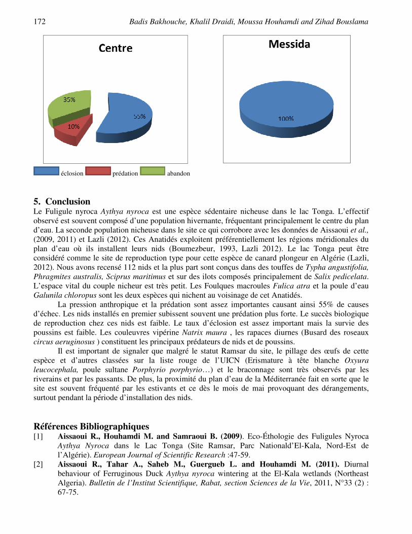
Multiple Analysis of Variance (MANOVA), investigating the main effects of age and gender independent variables on the religiousness and spirituality scores, indicated that there existed some statistically significant differences between groups. Figure 2 shows the effect of age variable (with three levels of 17-19, 20-21, or 22-older) and gender on Religiousness, providing evidence to believe that males were more religious than the females on average.
Figure 2: Estimated marginal means for Religiousness
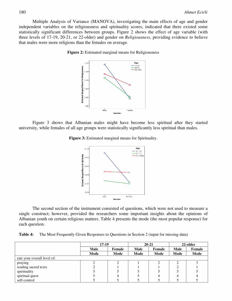
Figure 3 shows that Albanian males might have become less spiritual after they started university, while females of all age groups were statistically significantly less spiritual than males.
Figure 3: Estimated marginal means for Spirituality.
The second section of the instrument consisted of questions, which were not used to measure a single construct; however, provided the researchers some important insights about the opinions of Albanian youth on certain religious matters. Table 4 presents the mode (the most popular response) for each question. Table 4: The Most Frequently Given Responses to Questions in Section 2 (input for missing data)
17-19 20-21 22-older Male Female Male Female Male Female Mode Mode Mode Mode Mode Mode
rate your overall level of: praying 2 2 1 2 2 3 reading sacred texts 2 1 1 1 2 1 spirituality 5 5 5 5 5 5 spiritual quest 5 4 5 4 4 4 self-control 5 5 5 5 5 5

A Comparative Look at the Spirituality in Higher Education University Students’ Search for Meaning and Purpose; Albania & USA 181
Table 4: The Most Frequently Given Responses to Questions in Section 2 (input for missing data) (Continued)
17-19 20-21 22-older
Male Female Male Female Male Female Mode Mode Mode Mode Mode Mode
religious commitment 5 5 5 5 5 3 religious/social conservatism 5 5 5 5 5 5 religious skepticism 1 2 1 1 2 2 religious struggle 1 1 1 3 1 1 charitable involvement 5 5 5 4 4 4 compassion 5 5 5 5 5 5 caring others 5 5 5 5 5 5 understanding others and tolerance 5 5 5 5 5 5
Legend: 1 = "conflicted"; 2 = "doubting"; 3 = "not interested"; 4 = "seeking"; 5 = "feel secure".
Also presented, two of the most remarkable findings of the section 2 of the current study were students’ reading levels of sacred books and their attributes of compassion. Figure 4 and 5 specify the percentages for each question in pie charts.
Figure 4: Reading sacred texts (%) Figure 5: Compassion (%)
7. Comparative Data Data found as a result of SAHE is compared with the findings by HERI. Part of the comparative analysis will be given as follows.
Figure 6: Spirituality
Legend: *** = consider it very important, ** = agree strongly or somewhat, * = to some or a great extent

182 Ahmet Ecirli
Figure 6 demonstrates that about spiritual values such as “Seeking out opportunities to help one grow spiritually”, “one’s spirituality is a source of joy”, having discussions about the meaning of life with friends”, “searching for meaning/purpose in life”, “having an interest in spirituality”, “believing in the sacredness of life” responses of Albanian students are apparently lower in percentages than those respondent by HERI. Table 5: Religiousness
Religiousness UCLA - USA Albania Believe in God 79 63 to some or a great extent Pray 69 48 to some or a great extent Attended religious services 81 54 to some or a great extent Discussed religion/spirituality with friends 80 35 to some or a great extent Discussed religion/spirituality with family 76 32 agree strongly or somewhat Religious beliefs provide strength, support, and guidance 69 55 agree strongly or somewhat
The data seen in table 5 shows a considerable difference between Albanian and American
students about religiousness. The scales “ discussing religion and spirituality with friends / family members” relatively show 80/76 percent among American students and only 35/32 percent of the Albanian students who strongly agree on the fact.
Figure 7: Current Views about Spiritual/Religious Matters
Seeking rate of spiritulaity and religious matters (figure 7) is higher (22 %) among Americans. The data is supported by the fact that “not interested Albanian is higher ( 29%) than that of Ameicans (13%).
Figure 8: Social/Political Views of Students of Religious Engagement

A Comparative Look at the Spirituality in Higher Education University Students’ Search for Meaning and Purpose; Albania & USA 183
Legend: red= Albanian students who agree strongly; blue= American students who agree strongly The greatest difference in the compared data in figure 8 (44%) is given by the scale “Abortion
should be legal” which shows 77 % of the Albanian students agree strongly on the statement while that of American is 23 %. 8. Concluding Remarks The difference between the American and Albanian students in terms religiousness and spirituality can be attribute to social, antropologic and historical fact regarding the two nations. Some of these can be evaluated in terms of the impact of former political system for Albanians, Social satisfaction level of the American society, exterior and interior features of students’ development, the fact that the new generation expresses certain pledge to matching materialism and spirituality. The study shows that there is a risk of neglecting the student’s inner development while taking only material needs into account when developing policies about their education. References [1] Arbuckle, J. L. & Wothke, W., 1999, AMOS 4.0 user’s guide. Chicago: Small Waters. [2] Burke, A., et al., 2009, Religiosity, Spirituality, Alternative Health Practices, and Health Status
among College Students, EXPLORE: The Journal of Science and Healing, Volume 5, Issue 3, Page 164, ISSN 1550-8307, 10.1016/j.explore.2009.03.053. Retrieved from, http://www.sciencedirect.com/science/article/pii/S1550830709000986)
[3] Drerup, M. L., et al., 2011, Mediators of the relationship between religiousness/spirituality and alcohol problems in an adult community sample, Addictive Behaviors, Volume 36, Issue 12, Pages 1317-1320, ISSN 0306-4603, 10.1016/j.addbeh.2011.07.013. Retrieved from, http://www.sciencedirect.com/science/article/pii/S0306460311002231
[4] Galanter, M., et al., 2007, Assessment of spirituality and its relevance to addiction treatment, Journal of Substance Abuse Treatment, Volume 33, Issue 3, Pages 257-264, ISSN 0740-5472, 10.1016/j.jsat.2006.06.014. Retrieved from, http://www.sciencedirect.com/science/article/pii/S0740547206002066
[5] Garroutte, E. M., et al., 2003, the AI-SUPERPFP Team, Spirituality and attempted suicide among American Indians, Social Science & Medicine, Volume 56, Issue 7, Pages 1571-1579, ISSN 0277-9536, 10.1016/S0277-9536(02)00157-0. Retrieved from, http://www.sciencedirect.com/science/article/pii/S0277953602001570
[6] HERI, Higher Education Research Institute (2007). A National Study of Spirituality in Higher Education: Students’ Search for Meaning and Purpose. Retrieved from, http://spirituality.ucla.edu/
[7] Himle, J. A., et al., 2011, Religious involvement and obsessive compulsive disorder among African Americans and Black Caribbeans, Journal of Anxiety Disorders, Volume 26, Issue 4, Pages 502-510, ISSN 0887-6185, 10.1016/j.janxdis.2012.02.003. Retrieved from, http://www.sciencedirect.com/science/article/pii/S0887618512000266
[8] Kim, Y., Seidlitz, L., 2002, Spirituality moderates the effect of stress on emotional and physical adjustment, Personality and Individual Differences, Volume 32, Issue 8, Pages 1377-1390, ISSN 0191-8869, 10.1016/S0191-8869(01)00128-3. Retrieved from, http://www.sciencedirect.com/science/article/pii/S0191886901001283
[9] Lehrer, L. E., 1999, Religion as a Determinant of Educational Attainment: An Economic Perspective, Social Science Research, Volume 28, Issue 4, Pages 358-379, ISSN 0049-089X, 10.1006/ssre.1998.0642.Retrieved from, http://www.sciencedirect.com/science/article/pii/S0049089X98906421

184 Ahmet Ecirli
[10] Smith-Jackson,T., et al., 2011, Coping with “Bad Body Image Days”: Strategies from first-year young adult college women, Body Image, Volume 8, Issue 4, Pages 335-342, ISSN 1740-1445, 10.1016/j.bodyim.2011.05.002. Retrieved from, http://www.sciencedirect.com/science/article/pii/S1740144511000581
[11] Vlasblom, J. P., et al., 2011, Effects of a spiritual care training for nurses, Nurse Education Today, Volume 31, Issue 8, Pages 790-796, ISSN 0260-6917, 10.1016/j.nedt.2010.11.010. Retrieved from, http://www.sciencedirect.com/science/article/pii/S0260691710002364
European Journal of Scientific Research ISSN 1450-216X / 1450-202X Vol. 103 No 2 June, 2013, pp.185 - 206 http://www.europeanjournalofscientificresearch.com
Is the Application of Simple Trading Rules a Powerful Tool for
Profitability Prediction?: The Case of the FTSE-20 of the Athens Exchange
Georgia S. Demiri National Technical University of Athens
School of Applied Mathematics and Physics
Apostolos G. Christopoulos (Corresponding Author) University of Athens, Faculty of Economics
E-mail: [email protected] Tel: +(30) 210 3689397
Ioannis G. Dokas
University of Athens, Faculty of Economics
Konstantinos P. Vergos Portsmouth Business School
Abstract
The aim of this paper is to test the profitability predicting power of firms, by using Moving Average (MA), the simplest and most popular trading rule. The Index FTSE-20 of the Athens Exchange (ASE) is employed in order to compare the ability of this technique with the performance of a buy-and-hold strategy to earn excessive profits. The rules of the Moving Average are applied with bands of various periods and RSI Oscillator and SI Oscillator. In the empirical analysis daily stock values of the 20 largest capitalised firms of the ASE are elaborated for the period 2004-2012. The results are encouraging, particularly, for the effectiveness of simple moving averages, while for the efficiency of the oscillators the results are rather discouraging. The investment strategies are suited for short investment periods as long the excessive profits “evaporate” as the time passes and the transaction costs increase. The statistical significance of the results is controlled by the t-statistics, accepting the possibility of error due to non-normality of the data, while, the Granger Casualty test is also applied. Finally, linear and EGARCH models are estimated in order to predict the future price changes of the FTSE20 Index. It is concluded that the linear model is satisfactory in terms of interpretation and predictability while the estimated EGARCH model is more complicated and its predictability is lower than that of the linear model. Keywords: Technical Analysis, Trading Rules, Moving Average, Oscillators, Granger
test, Linear Regression, EGARCH.

186 Georgia S. Demiri, Apostolos G. Christopoulos, Ioannis G. Dokas and Konstantinos P. Vergos
1. Introduction and Literature Review Technical analysis consist a very valuable tool for brokers, gaining grounds against the fundamental theory, mainly due to the speediness in decision making, based on signals. It allows for faster response to unexpected events, based on fewer data and required knowledge, while it offers easier, more flexible and adaptable practices into different markets and commodities. In contrast, the fundamental analysis is based on more reliable financial indicators, and is more suitable for long-term investments, mainly for institutional investors. In addition a survey by Taylor and Allen (1992), suggest that results become more effective when the two methods are employed complementary rather than competitively. Although, in the past, technical analysis was considered theoretically unfounded, recently this opinion has been revised, primarily due to the results of various studies on the profitability of simple technical rules such as the moving averages. It seems that, overall, non-linear methods work better, which is not surprising, in the light of the non-linearity, found in the Markets, by Ammermanna and Patterson (2003), Barkoulas and Travlos (1998), Abhyankar, et. al. (1997), Brooks (1996), Hsieh and LeBaron (1991), Hsieh (1989), Scheinkman and LeBaron (1989), Frank and Stengos (1989)
Furthermore, Millionis and Papanagiotou (2011) investigated the variability of the returns of simple moving averages as a function of their duration on the New York Stock Exchange (NYSE), the Athens Stock Exchange (ASE) and the Vienna Stock Exchange (VSE) using daily data for the period 1993-2005. Without including any transaction costs, the results showed that the overall yield of technical rules for the ASE and VSE was statistically higher than that of the passive strategy. Thus, the case of efficient market hypothesis (EMH), in its weak form, discharged in these markets. On the contrary, the total yield, by technical rule, for NYSE was significantly lower than that of the passive strategy, confirming the weak efficiency form. When transaction costs are incorporated in the results, the profitability of the technical analysis for the ASE in some cases becomes significantly higher than that of a passive strategy, while others do not differ significantly, resulting in mixed results. Kenourgios, et. al. (2008) apply MAs in FTSE-20 of the ASE and find higher performance of technical rules compared with the passive strategy. Finally, Panagiotidis (2005), Milionis, et. al. (1998), Niarchos with Alexakis (1998) show that in most cases the efficiency market hypothesis (E.M.H) hypothesis is rejected in the case of ASE.
Early efforts in academia to assess the effectiveness of technical analysis were taking into consideration simple rules, namely the filter rules. Such rules involve the buying of a security when it has risen by %x in a given period or selling a security when its price has fallen by %x in a given period. However, Alexander (1964) and Fama with Blume (1966) showed that tests by such rules do not yield beneficial results. That is why more recent literature on technical analysis has considered MA as the main tool of technical analysis. The idea is that financial prices are volatile but they follow a specific trend. MAs are supposed to capture trends and leave aside the "noisy" part of the price. According to this rule, the buy or sell signals are generated by two MAs of the level of the index: A long period moving average and a short period moving average. The strategy involves buying the asset when the short average is above the long moving average and selling the asset when the short period MA is below the long period MA.
Various technical trading rules have been empirically tested in an attempt to investigate their effectiveness. Studies on technical trading rules have increased significantly during the 1990s, along with the methods which are used to test trading rules. Some of the most influential studies that supported the trading rules were introduced by Blume, et. al. (1994) and Jegadeesh with Titman, (1993) who showed that trading volumes provide information that cannot be deduced from the price. Further, Grundy and Martin, (2001), Rouwenhorst, (1998), Campbell et. al. (1997), Chan et. al. (1996), showed that traders by using information from the market statistics do better than traders who do not.
Moving averages are well defined by Neftci, (1991). Several technical indicators do provide incremental information and may provide practical value, by examining the effectiveness of technical analysis on the US stocks for the period 1962-1996. Brock et. al. (1992), Chang with Osler (1999), Osler with Chang (1995), Allen with Karjalainen (1999), Lo with MacKinlay (1999), Lo et. al. (2000).

Is the application of Simple Trading Rules a powerful tool for Profitability Prediction? : The case of the FTSE-20 of the Athens Exchange 187
Moreover, Gençay, (1998), and Weller with Neely (1999) concluded that genetic programming shows that technical trading rules can be profitable during US foreign exchange interventions. They noted that although technical analysis stresses when a buy or a sell decision is better, a composite one based on as many conducive signals as possible is even better: Volume of trade, convergence-divergence indicators, e.t.c. Quite often the MA rule, due to its generated signals, can be used as a stand-alone method, particularly in the automated trend following systems. In this way it becomes purely a “mechanical”, rather than a technical, trading rule. Pring (1991) argues that even in its “mechanical” use, the MA trading rule may have several versions, while more recently Rodriguez et al. (2003) research showed that other non-linear methods such as the nearest neighbor predictor, perform better on exchange rates than the MA trading rule in its mechanical form. 2. Data and Technical Trading Rules In the following analysis the applied data sample includes 2,119 observations of the FTSE-20 Index of ASE for the period 2 January 2004 - 22 June 2012. Until the late 1980s, ASE had low capitalization value, with a few listed companies, small daily volumes of trade and almost exclusively local investors. Kenourgios et al., (2008), Laopodis (2004) and Alexakis with Xanthakis, (1995) show that during 1990s, progress in harmonization with the standards of the more developed and mature financial markets, in terms of legislation and regulation was obvious, resulted in the increase of the total capitalisation value and the average volume of transactions.
The choice of the time frame is far from random. It covers a period during which Greece’s economy was in a phase of excessive and perhaps unjustified optimism and prosperity (2004-2008), beginning with the organisation of the 2004 Olympic Games and the boom in construction, which terminated at the end of 2009. On June 2012 after three years of recession the haircut of the public debt to the private sector (PSI) by 50% became inevitable.
Throughout this paper { }tx denotes the price series and { }ty the continuously compounded
returns, where: 1lnx lnxt t ty −= − .
i. Moving Average and Moving Averages with Bands
MA is a trend method which is frequently useful as the basis for more sophisticated schemes. The idea behind the MAs is to normalize an otherwise volatile series. Definition 1 MA is a linear transformation which can be written as a finite polynomial in the back shift operator iL with non-time varying parameters { }iϑ :
1
mi
ii
M Lϑ=
=∑ , where: 11t tL x x −= .
The series [ ]{ }tM x is smoother than { }tx and can be used as a primary estimate of the market
trend. In others words, the calculation of a MA is derived as follows: The closing price of the security is added for the corresponding period and this sum is divided by the number of time period in days. The definition of the technical trading rule ( )1 2, ,m m d determined by the band d and the two moving
averages 1M and 2M with lengths 2 1 1m m ≥≻ respectively, is given below. The generation of the
signals are based on the following definition:

188 Georgia S. Demiri, Apostolos G. Christopoulos, Ioannis G. Dokas and Konstantinos P. Vergos
Definition 2 Buy signals are generated sequentially at the times { }, 1B
i iτ ≥ , where:
[ ] [ ]{ }1 1 2 1inf : ,B Bi i t t tt t M x M x dxτ τ − −≡ −≻ ≻ , and Sell signals are generated sequentially at the times
{ }, 1Si iτ ≥ , where: [ ] [ ]{ }1 2 1 1inf : ,S S
i i t t tt t M x M x dxτ τ − −≡ −≻ ≻ .
The initials 0Bτ , 0
Sτ are defined as zero and the band d is no negative while the parameters { }iϑ
are taken to be 1
m
. The MA rule is tested between the band zero and one percent. As a result, days
are classified into three categories: buy / sell / no action. No signal is generated if the short moving average is within the band. The band d is designed to reduce the number of trades caused by frequent whipsaws in the price series during non-trending markets. In this case, the signal that gives the MA is not reliable and the investor prefers not to negotiate in the market but to keep a risk-free security. It is assumed that a risk free asset has a daily return of 0.05% based on the return of 10year government bond divided by 251, i.e. the trading days given by ASE. Therefore, a risk free asset is employed with daily return 0.05%. To calculate a moving average, the appropriate time span is selected. The ranges of the three parameters 1 2,m m and d can vary greatly in practice, depending primarily on market
volatility, investor’s horizon and previous results of the different rules. The most popular MA rule is 1:200, where the short period is one day and the long period is 200 days. While numerous variations of this rule are used in practice, the most popular ones are applied: (1:200:0), (1:100:0), (1:50:0), (1:30:0) and (1:5:0). And also: (1:200:1), (1:100:1), (1:50:1), (1:30:1) and (1:5:1). ii. RSI and SI Oscillators
Another aim of technical analysis is the prediction of trend reversal points. This is the main use of oscillators, which are complementary tools to MAs providing signals of neutralization (exit from the market), buying and selling. The oscillators can find out if a stock is overbought or oversold. According to Pring (1991) and Bechu with Bertrand (1998), the two most popular oscillators are the RSI and the Stochastic oscillator. In this paper both of them are investigated. The indicator of relative strength suggested by Welles Wilder (1978) and is defined as follows:
100100
1tt
RSIRS
= −+
where ( )
( )
1
1
max 0,
min 0,
t d
n nn t
t t d
n nn t
x xRS
x x
−
−==
−=
−
=
−
∑
∑,
where d is the number of days for which the RSI is calculated and the price nx is the closing price of day n . High ratio means that the number of periods that the price increases is greater than the number of periods that the price decreases. In this situation the stock is considered overbought, and vice versa. The index runs between 0 and 100. In this paper, we investigate the relative strength index of 21 days considering the level of neutralization 30/70.
The other popular oscillator is the Stochastic Oscillator (SI) which is defined as follows:
,
0 1, ,
1100
l yt l t l t l x
tt t t l x t l t l x
p LSI
y H L
−− − − −
= − − − − − −
−=
−∑ ,
where x y≻ , tp is the price at time t , and ,t l t l xL − − − is the lowest price between time t l− and t l x− −
while ,t l t l xH − − − is the highest price between time t l− and t x l− − . The SI is another way of depicting
overbought or oversold situations. Instead of focusing on a series of variations, the SI compares the distance between the last price of an asset and the lowest price in a period of x days before, with the distance between the highest and lowest price on the same period of x days. This ratio is then

Is the application of Simple Trading Rules a powerful tool for Profitability Prediction? : The case of the FTSE-20 of the Athens Exchange 189
recomputed for y preceding periods and averaged over time. This means that if the latest price is systematically close to the lowest observed price in a certain period, the asset is considered as oversold and the prices are expected to rise in the near future. On the other hand if the last price is systematically close to the highest price observed then SI indicates that the prices are going to drop. Respectively with RSI, we will present the results for 14 days and 90/10 neutralization level. 3. Methodology i. Measuring Profitability and Transaction Costs
The profitability of the trading rules is determined by comparing the returns generated by the trading signals to the buy-and-hold trading strategy returns. The returns from the buy-and-hold strategy are calculated by investing in the security at the beginning of the data set, and holding the security until the end of the data set. The trading rule is also calculated in a simple manner. When S LMA MA≻ , the
investor takes a long position and the returns will be calculated at the market rate. When S LMA MA≺ ,
the investor takes a short position and returns will be calculated at the opposite market rate, as the short selling is allowed in ASE and the derivates market is in operation for the whole period investigated. In the case of using a band of 1%, there are neutral periods, in which the trader is out of the market and follows an alternative scenario, investing the liquated capital at the free risk rate. Finally, the overall strategy returns, resulted from the returns given by the buy signals of the moving averages, plus the returns given by the investment at the risk free asset minus the returns of the sell signals of the moving averages. This sum is compared with buy-and-hold overall return.
The returns result from RSI and SI Oscillators though are calculated in a different way. As long as the price of the Oscillators waves between the neutralization zone 30/70 and 90/10 respectively, the trader makes no transactions gaining the market return and when the RSI gives a buy signal, he takes a buy position while it gives a sell signal, he takes a short position. The overall returns are given with the same way as described above. Similar to Gençay (1998), the returns generated from the trading rules are adjusted for transaction costs. It is also assumed a 0.16% fee per transaction as it is charged by commercial banks on the contracts and the risk-free asset return of 0.05%, in which the investor is placed when is out of the market. ii. Robustness Testing
Testing for robustness involves calculating the trading rule returns across different sub-periods of the data sets. Without testing for structural breaks, the most sensible breakdown of the eight year data set is into two sub-periods as:
a. Bubble: (02.01.2004 – 27.06.2008): 1,122 Observations, Average Daily Return: 0.0403%, Standard Deviation: 0.012171 and Average Annual Return of 10.06%
b. Post-Bubble: (30.06.2008 – 22.06.2012): 997 Observations, Average Daily Return: -0.2094%, Standard Deviation: 0.028332 and Average Annual Return of -52.35% In this division it is aimed to analyze the results of technical rules based on the trends and the
psychology that prevails in the market, as in recent years the Greek economy shows abrupt and large shifts which are accompanied by anxiety, panic or unwillingness to trade.
In line with Gençay (1998), the returns from the trading rules and the buy-and-hold strategy, along with the Sharpe ratio, are calculated and compared for each sub-period. If a trading strategy is robust, excess returns will be present in all sub-periods. Also, if the Sharpe ratios are of similar magnitude, the return/ risk ratios of the trading strategies would be considered robust and invariant of time.

190 Georgia S. Demiri, Apostolos G. Christopoulos, Ioannis G. Dokas and Konstantinos P. Vergos
iii. Statistical Significance
The t-statistics calculated using the following formula: 1
2 2 2
Z
ZN N
µ µ
σ σ
−
+
where Zµ is the average return of a
buy or a sell period and ZN the number of buy or sell signals in each period. The letter µ represents
the mean return and the letter N is the total number of days without restrictions. The 2σ shows the variance of the entire sample. The aggregate number of transactions of buying and selling periods is the total number of transactions resulting from each strategy. 4. Empirical Results Table 1 presents the summary statistics and Graph 1 the distribution of the examined series. As it can be seen, values and returns are leptokyrtic (fat tailed) and positively skewed. As Jarque-Bera probability is zero, the hypothesis of normality is rejected. Table 1: Descriptive Statistics
VALUES RETURNS MAUP (2/1/2004-
27/6/2008) MAD (20/6/2008-
22/6/2008) Mean 1445.838 -0.000772 0.000403 -0.002094 Median 1325.180 0.000157 0.001052 -0.002594 Maximum 2841.230 0.163741 0.078558 0.163741 Minimum 169.8800 -0.097963 -0.061862 -0.097963 Std. Dev. 730.2067 0.021388 0.012171 0.028332 Skewness 0.088632 0.246344 -0.260170 0.362853 Kurtosis 1.898146 7.575127 6.155422 5.054318 Jarque-Bera 109.9677 1869.535 478.1329 197.1930 Probability 0.000000 0.000000 0.000000 0.000000 Sum 3063731. -1.636336 0.451630 -2.087966 Sum Sq. Dev. 1.13E+09 0.968861 0.166055 0.799515 Observations 2,119 2,119 1,122 997
Graph 1: Distribution of Values and Returns
.0000
.0002
.0004
.0006
.0008
.0010
-1,000 0 1,000 2,000 3,000 4,000
Density
VALUES
0
4
8
12
16
20
24
28
-.2 -.1 .0 .1 .2
Histogram Normal
Density
RETURNS
Next, autocorrelation and the linear independence of time series are examined. It is observed that the values are characterized by strong autocorrelation, whilst the returns are characterizes by a serious weakening in linear autocorrelation structure but not in the non-linear autocorrelation structure, as measured by the autocorrelation coefficients of the squared returns (Table 2). This is an important finding as the presence of nonlinearity is a necessary condition for trading rules in order to have potential predictive power of.
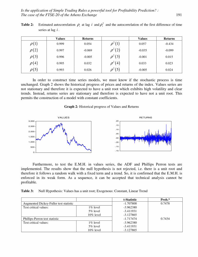
Is the application of Simple Trading Rules a powerful tool for Profitability Prediction? : The case of the FTSE-20 of the Athens Exchange 191
Table 2: Estimated autocorrelation iρ at lag i and 2iρ and the autocorrelation of the first difference of time
series at lag i .
Values Returns Values Returns
( )1ρ 0.999 0.054 ( )2 1ρ 0.057 -0.434
( )2ρ 0.997 -0.069 ( )2 2ρ -0.035 -0.099
( )3ρ 0.996 -0.005 ( )2 3ρ -0.001 0.015
( )4ρ 0.995 0.032 ( )2 4ρ 0.033 0.023
( )5ρ 0.993 0.026 ( )2 5ρ -0.005 0.024
In order to construct time series models, we must know if the stochastic process is time
unchanged. Graph 2 shows the historical progress of prices and returns of the index. Values series are not stationary and therefore it is expected to have a unit root which exhibits high volatility and clear trends. Instead, returns series are stationary and therefore is expected to have not a unit root. This permits the construction of a model with constant coefficients.
Graph 2: Historical progress of Values and Returns
0
500
1,000
1,500
2,000
2,500
3,000
VALUES
-.15
-.10
-.05
.00
.05
.10
.15
.20
RETURNS
Furthermore, to test the E.M.H. in values series, the ADF and Phillips Perron tests are
implemented. The results show that the null hypothesis is not rejected, i.e. there is a unit root and therefore it follows a random walk with a fixed term and a trend. So, it is confirmed that the E.M.H. is enforced in its weak form. As a sequence, it can be accepted that technical analysis cannot be profitable. Table 3: Null Hypothesis: Values has a unit root; Exogenous: Constant, Linear Trend
t-Statistic Prob.* Augmented Dickey-Fuller test statistic -1.707800 0.7478 Test critical values: 1% level -3.962380 5% level -3.411931 10% level -3.127865 Phillips-Perron test statistic -1.717474 0.7434 Test critical values: 1% level -3.962380 5% level -3.411931 10% level -3.127865

192 Georgia S. Demiri, Apostolos G. Christopoulos, Ioannis G. Dokas and Konstantinos P. Vergos
5. Profitability and Transaction Costs The profitability of trading rules without transaction fees is represented in Appendix 1. It is found that historical prices seem to add value in forecasting future prices. Without trading fees, all the indicators besides Stochastic Oscillator and Relative Strength Oscillator have positive performance. This means that Oscillators cannot have predictive ability when they are used independently from other trading rules. The average daily returns obtained with the use of the moving average rule is greater than the negative daily returns of -0.0772% or -19,46% on an annual basis (-0.0772% * 252 trading days) is accomplished by a passive strategy. Moreover, in most of the cases, the average returns are significantly different from the buy-and-hold strategy in a more than 80% confidence interval. As a result, it can be concluded that the results are significant.
As far as the Moving averages is concerned, the sell periods have surprisingly high average returns providing the downwards evolution of the index. Although, the returns achieved through the buy periods are not statistically significant. MA(1:30:0) is the most profitable one, yielding annually 39.19%.
The number of sell positions is superior to the number of buy positions. This is consistent with the downward-slopping trend. The signals are successful at a rate greater than 50% of the cases. It is also observed that buy signals are more accurate than sell signals as shown by the larger fraction of right signals obtained in buy periods. As expected, the number of trades increases as long moving averages decreases, because trading rules becomes sensitive to variation of the index.
In terms of volatility, the standard deviation of the buy periods is less than the sell periods, which is consistent with the well-known feature of asset returns called leverage effect, noted by Black (1976).
Higher returns yield the use of a band 1%. The band has removed days with poorer performance and it permits to sort out the most extreme returns. MA(1:30:1) yields 53.34% annually. The most significant finding is that the returns of the strategy are statistically significant at higher significance levels. This is due to the fact that the use of bands induces neutral positions which yield the risk-free rate while the market decreases.
In the face of trading costs, technical analysis is far less effective, as we see in Table 4. MA(1:200:0) is the most profitable with included trading costs while MA without bands seems more profitable in contrast to MA with bands. Table 4: Aggregate Results for MAs with and without bands after transaction costs
Trading rule N(trades) �(strategy)% N(trades) �(strategy)%
Moving Average with Bands Moving Averages [1,200] 79 29,90% 36 27,98% 17,26%** 22,22%* [1,100] 144 40,37%** 70 31,61%*** 17,33%** 20,41%* [1,50] 202 48,06%** 109 36,45%*** 15,74%*** 19,01%* [1,30] 293 53,34%* 143 39,19%** 6,46% 16,31%** [1,5] 771 64,95%* 457 19,78% -58,41% -53,34%
Except from a standard fee for each transaction, investors are charged with extra fees referred
to capital management, company’s debit policy and the Stock Exchange itself. Considering a total charge of 4% over returns after transaction costs, it is proved that the above rules are still profitable.

Is the application of Simple Trading Rules a powerful tool for Profitability Prediction? : The case of the FTSE-20 of the Athens Exchange 193
Graph 3: Trading rules and Transaction costs
The Graph 3 above shows the returns of trading rules as a function of transaction costs. The findings of this study are important. It can be seen that not only trading strategies yield less as the transaction costs rise but also the sole remaining profitable rule is the MA(1:200:0). 6.1. Statistical Significance
In order to evaluate the above performances, the statistical significance of technical signals shall be taken into account since it ensures the economic feasibility of the results.
Graph 4: Significance of Technical Signals
From the above Graph 4, it can be concluded that bands provide more reliable results without trading costs while MA has a greater statistical significance when such costs are included. Consequently, they are more suitable in real market conditions. Once again, oscillators proved inappropriate.

194 Georgia S. Demiri, Apostolos G. Christopoulos, Ioannis G. Dokas and Konstantinos P. Vergos
6.2. Sign Prediction Ability
Finally, as far as the evaluation of the correctness of the signals is concerned, the results sum up in the Graph 5.
Graph 5: Percentage of correct signals of each strategy
According to the Graph 5, MA(1:200:0) and MA(1:100:0) have the highest percentage of success for both signals, buy and sell, provided that RSI is not exercised alone, while MA(1:30:0) is equally effective. We can also mention that Moving Averages with Bands have noteworthy lower success percentage in sell signals, especially the MA(1:200:1), while the weakness of SI in effectiveness is obvious. 7. Robustness Another interesting question to be answered is whether these results hold on also in the case of sub periods. In Table 1 the summary descriptive statistics were presented for the sub- samples. In Appendix 2 and 3 the results for a bull and a bear market are shown for each of the four trading rules.
As far as Moving Averages is concerned, significant rates of success of signals in both the upward and downward markets are identified, which fully justify the assumption that technical analysis works most efficiently in markets with a trend. It is, also, observed that the number of signals to buy or sell is doubled, depending on whether the market is in the upward or downward phase respectively which can be justified by the market trend, which the moving averages generally follows.
The RSI does not lead to a great improvement of the results or it leads to great loses when the transaction costs are also included, although they presented high percentage of correct buy signals in all market periods in assuring their aim. The returns of buy strategy are extremely high and statistically significant at a 95% confidence level.
In Table 5 the performance of rules is shown comparatively between a bear and a bull market, both with and without trading costs. Table 5: Aggregate performance in trend markets
Trading rule Moving Averages with Bands Moving Averages
Bull Market Bear Market Bull Market Bear Market �(strategy)% �(strategy)% �(strategy)% �(strategy)%
[1:200] 18.55% 42.67% 16.15% 41.28% 10.71% 37.87%*** 12.47% 39.20%*** [1:100] 26.09% 56.43% 16.49% 48.63% 10.89% 48.59%* 10.89% 43.03%* [1:50] 35.71%** 61.95% 21.44% 53.33% 16.03%** 49.31%* 12.96% 44.37%*

Is the application of Simple Trading Rules a powerful tool for Profitability Prediction? : The case of the FTSE-20 of the Athens Exchange 195
Table 5: Aggregate performance in trend markets (continued)
[1:30] 39.89%** 68.48%*** 18.30% 62.70%*** 12.37%*** 49.12%* 5.66% 52.46%* [1:5] 79.25%* 48.46% 20.84% 18.60% 21.73% -7.94% -18.36% -15.32%
Precisely, in a bear market the actual yield is 10.14% and in a bull market -52.78%. It becomes
obvious that in both cases MA with bands is the most appropriate technical rule during bear markets, whilst in a bull market MA and MA with Bands are approximately equivalent.
Aiming to investigate the validity of the results in periods with different trends the Sharpe Ratio is applied, which is defined as follows:
p f
p
R RS
σ
−=
, where pR the return and pσ the standard deviation of each strategy. fR the return of the market.
From the Appendix 4 it can be derived that MA with bands except MA(1:5:1) are robust through sub-periods while MA(1:30:1) has the highest yield per unit of risk.
Lastly, in Table 6 the returns are segmented and then buy and sell signals throughout the entire period are portioned and compared with the sub-periods. The point is a great disparity in the distribution of returns. It is noticed though that moving averages do not produce statistically significant returns in the case of separate strategies while they did so in the case of a sole strategy. Thereby, the short-term investment horizon of technical analysis is confirmed as higher returns are produced for short-term periods. Table 6: Disparity of returns according to the market trend (Moving Averages without band)
Trading rule Overall Bull Market Bear Market
�(buy)% �(sell)% �(buy)% �(sell)% �(buy)% �(sell)% [1:200] 4.26% 23.72%* 13.15% 3.00% -5.75% 47.03%* [1:100] 6.08% 25.54%* 13.32% 3.18% -2.07% 50.70%* [1:50] 8.49%*** 27.95%* 15.79% 5.65% 0.28% 53.05%* [1:30] 9.87%*** 29.32%* 14.22% 4.08% 4.96% 57.74%* [1:5] 0.16% 19.62%* 15.49% 5.35% -17.09% 35.69%*
8.1. Feasibility Table 7: Alternative Strategy Outcomes
Tr. Rule
N(tr) N(b) N(s) �(b) �(b) % �(s) �(s) % �(str) �(str)
% [1:200] 36 1089 1030 0.00000810 2.03 0.0004728**** 11.82 0.000554 13.85 [54.91] [53.79] (0.01871) (0.0004962) (0.01871) [1:100] 70 1074 1045 0.000229 5.72 0.000584** 14.60 0.000813 20.32** [54.93] [53.68] (0.021517) (0.000621) (0.021519) [1:50] 109 1047 1072 0.000427*** 10.68 0.000643** 16.07 0.00107 26.75* [53.77] [52.61] (0.022568) (0.000671) (0.022566) [1:30] 143 1042 1077 0.000537*** 13.43 0.000633** 15.82 0.00117 29.25* [54.70] [53.48] (0.022801) (0.000664) (0.022796) [1:5] 457 1083 1036 -0.00024 -6.07 0.0005*** 12.50 0.000257 6.44 [51.06] [50.00] (0.026997) (0.00054) (0.027)

196 Georgia S. Demiri, Apostolos G. Christopoulos, Ioannis G. Dokas and Konstantinos P. Vergos
It can be argued that the results of Appendix 1 are not feasible on the ASE as short positions could be relatively difficult to build over the period. Another way to achieve similar results is to use the following strategy: When a buy signal is observed, the investor borrows and doubles the relevant investment on the index. This yields twice the market return less the risk-free rate. When the investor observes a sell signal, he/she sells the index and invests all his/her money on the risk-free asset. If there is an equal number of buy and sell signals and if the borrowing and lending rates are close, then such a strategy would yield similar results to the long-short strategy investigated. When this alternative strategy is applied on our data, we find that the results of such investment policy yields relevant results for separate periods but the overall return of the strategy is statistically significant which means that the results of Appendix 1 are possible, see Table 7. 8.2. Empirical Application
The purpose of this section is to reinforce the hypothesis of the predictive ability of technical analysis rules. The aim is to develop an effective model for predicting price index using statistics commonly used in technical analysis (charts, indicators, oscillators) and readily available to investors such as open price, high price, low price, trading volumes and the returns achieved by the investor implementing the technical rules discussed above.
Statistical tests which were performed in the previous section assumed that returns are normally distributed i.e. skewness of 0 and kyrtosis of 3, the observations are independent and the distribution does not change through the time. However, Table 1 shows that this is not the case and that the distribution of returns of FTSE-20 index has fatter tails than the normal and is asymmetric. Furthermore, the returns are not independent as is witnessed by the significant ( )1ρ , ( )2ρ , ( )4ρ ,
( )5ρ coefficients. As a result, the apparent predictability of the returns could simply be due to these
features. Providing that the t-tests and the Sharpe Ratio, as they were implemented above, did not take into account these deviations, it is possible that, the statistical significance of the trading strategies is derived from the data structure and the above features. In this paper, we use the Granger Casualty Test in order to identify causal relational between the series.
Resistance and Support levels are widely used in Technical Analysis because of their handiness and the clearness of their signals. Resistance and Support Values of the FTSE-20 Index computed on a monthly basis.
{ }Resistance max , 30tx t= =
{ }min , 30tSupport x t= =
Observing and testing all the series for stationary, the results are as follows: • Prices, Open, High, Low, Volume, Resistance and Support Series are non stationary, i.e.
have a unit root, in Levels according to ADF, PP, KPSS tests • The first differences of Prices, Open, High, Low, Volume, Resistance and Support Series
are stationary, i.e., have not a unit root, according to ADF, PP, KPSS tests • Returns, Ma(200), Ma(100), Ma(50), Ma(30), Ma(5), Ba(200), Ba(100), Ba(50), Ba(30),
Ba(5), RSI, SI Series are stationary, i.e. have a unit root, according to ADF, PP, KSPP tests and Volume Series has a unit according to ADF, PP.
• The first differences of the above Series are stationary. The second aim is to identify the Casualty between the series due to the distribution of the
Prices. For this, the Granger Casualty Test is applied for different lag periods in order to examine the power’s length of the phenomenon. The aggregate results are presented in Appendix 5:
1Lag = : The short period is examined for daily causality between the variables 4Lag = : The mid period is examined for weekly causality between the variables 10Lag = : The 15-daily causality is examined

Is the application of Simple Trading Rules a powerful tool for Profitability Prediction? : The case of the FTSE-20 of the Athens Exchange 197
20Lag = : The monthly causality is examined 8.3. Empirical Conclusions
Through Granger Causality Test the above analysis ends up to the followings Conclusions: • The difference of the index Prices and the returns using the trading rules are independent for
every lags used at statistical significance level 5% • ( )D prices cause , , ,Support, ResistanceOpen High Low
• ( )D prices do not cause Resistance and Support for short and mid periods, whilst Support for 10Lags ≻ causes ( )D prices
• Open series does not cause ( )D prices , while High and Low series do cause ( )D prices for 10Lags ≻
• As far as the Volume is concerned, there is a short term causality relation from ( )D prices to Volume and a vice versa long term causality from Volume to ( )D prices The above conclusions are consistent with the market theory and empirical ascertainments. From the empirical analysis the following linear model (Appendix 6) is estimated as follows:
( ) 0.0208366898324 662.483105176* Returns 0.428879566528* ( )
0.439071125426* ( ) 0.44872942862* D(Low) 100.163184873* MA100
34.0436204403* MA 30 273.802263674* BA 200
D prices D Open
D High
= + − +
+ − +
+
Because of the existence of a breakpoint, the sample is divided as above and the linear model (Appendix 7) is re-estimated as follows:
( ) ( )
( )
Prices 0.126920933226 1732.49520918* Re 0.140426345195*
0.12737194142* 0.16602727224* 80.887337455* 20
=
( ) 0
D turns D Open
D High D Low MA
− + − +
+ −
( ) ( )
( )
Prices 0.0235079474546 585.573462225* Re 0.365431727254 * D
0.376291461054* 0.387924257999* 64.6249936195* 100
205.772990407* 20
( )
0
D turns Open
D High D Low MA
BA
= + − +
+ − +
Evaluating the two models, it is shown that R2 and Adjusted R were increased while both AIC and SIC were decreased, resulting to higher percentage power for the estimation of the prices’ variance. Durbin–Watson statistic is lower, due to the reduction of Autocorrelation, while fixed term c is not statistically significant, a fact that reduces the possibility of bias of the applied model. Furthermore, Volumes, Resistance and Support are not statistically significant in any model. In the above models, MA(200), MA(100), MA(30) and BA(200) are the most important variables. These results are closed to the empirical results presented above. According to Jarque-Bera test, Breusch-Pagan-Goldfrey Heteroskedasticity test, Ramsey test, LM test: The null hypothesis is rejected. Last but not least, in Table 8, the predictability of the above models is compared. The results are satisfactory (Theil’s Inequality Coefficient closed to 0) and confirm the existence of a breaking point and the necessity of the two different models. Table 8: Predictability Analysis
Criteria One Period Bubble Period Post-Bubble Period Root Mean Error 8.591776 4.653625 8.447018 Mean Absolute Error 5.889734 3.392356 5.743721 Mean Absolute Percentage Error 0.642814 0.186347 0.94256 Theil Inequality Coefficient 0.002652 0.001139 0.004520

198 Georgia S. Demiri, Apostolos G. Christopoulos, Ioannis G. Dokas and Konstantinos P. Vergos
Table 8: Predictability Analysis (continued)
Bias Proportion 0.000000 0.000000 0.000000 Variance Proportion 0.000626 0.001762 0.004237 Covariance Proportion 0.999374 0.998238 0.995763
Similarly, a more elaborate model can be estimated which is chosen according to the Akaike
Criterion and the EGARCH model (Appendix 8) and its overall sample is divided into periods as in Appendix 9.
According to these results, it can be observed that R2 and Adjusted R2 are decreased for each period, compared to the linear model, while the Criteria AIC and SIC have lower prices. The model proved to face autocorrelation problems while according to ARCH-LM test, the null hypothesis was not rejected. Important Variables are not consistent with empirical results and the model is quite complicated. From the above, we can conclude that in spite of the improvement of the model, the predictive ability of EGARCH model is weaker than that of the linear one, see Table 9. The more practical and easy way to compute a linear least squared model combines with a satisfactory predictive ability. Table 9: Predictability Analysis
Criteria One Period Bubble Period Post-Bubble Period Root Mean Error 12.61335 5.352196 11.33726 Mean Absolute Error 7.107316 3.474433 5.62367 Mean Absolute Percentage Error 0.776963 0.180834 1.214118 Theil Inequality Coefficient 0.003893 0.001309 0.006044 Bias Proportion 0.000005 0.000071 0.000085 Variance Proportion 0.000421 0.000573 0.006655 Covariance Proportion 0.999574 0.999358 0.993260
9. Conclusions This paper tests whether technical analysis and its widest used trading rules can be profitable for ASE prices. Applying ADF and Phillips Perron tests it is concluded that the Efficient Market Hypothesis is forced in its weak form. As a sequence, it can be accepted that technical analysis is not to be profitable. However, our results belie.
Daily return of -0.0772% or -19.46% in annual basis (-0.0772% * 252 trading days) achieved through a passive strategy. Excluding costs per transaction (0.0016%) MA(1:30:0) yields 39.19% annually and MA(1:30:1) yields 53.34%. Including costs MA(1:200:0) yields 22.22% annualy. The results are statistically significant on a 10% significance level and Oscillators RSI and SI do not have essecive returns. The fact that quite many further charges are applied, cannot be ignored (S.A Expenses, Fixed Expenses, etc). To get closer to the real conditions in trading we proportionally reduced by 4% (aggregate extra fee) the results and we stil havel excessive returns.
An important finding is that the results of the trading strategies yield less as the transaction costs arise. This means that large investors who fulfill two conditions: pay transactions costs and trade the index at closing price can achieve greater returns. As small investors cannot achieve these conditions, they cannot get the same profits from these simple technical results. This could also explain why the profit opportunities associated with these strategies have not disappeared as a large fraction of market traders could not get any profit because of the presence of transactions costs. This also means that the hypothesis of weak form efficiency of the market cannot be rejected for that large part of participants.
In this paper, the trading rules were tested separately in bull and bear periods. The MA(1:30:0) is recommended for a bear trend with or without costs having essecive returns. On the other hand

Is the application of Simple Trading Rules a powerful tool for Profitability Prediction? : The case of the FTSE-20 of the Athens Exchange 199
MA(1:50:1) is recommended for a bull market. As a result, moving averages with bands are more profitable and reliable in trend markets.
Also, it was investigated whether the results are feasible from an investor’s point of view, as short positions could be relatively difficult to build over the period. Another way to achieve similar results is to use the following strategy: when a buy signal is observed, the investor borrows and doubles his investment in the index. When this alternative strategy was implemented found that the results of such an investment policy yield relevant results allowing believing the feasibility existence of the returns. Lastly, the short-term horizon and trend-relation of Moving averages is confirmed.
The Granger Causalty Test is performed in order to test whether previous results are not due to one of non-normal characteristics. It is found that the difference of the index Prices and the returns using the Trading rules are independent for every lags used at statistical significance level 5%. According to Granger, the ( )D prices cause , , , Open High Low Support and Resistance while
(Prices)D do not cause Resistance and Support for short and mid periods. There is a short term
casualty relation from ( ) D Prices to Volume and a vice versa long term casualty from
( ) Volume to D Prices .
In the econometric model the most commonly used statistics of technical analysis (charts, indicators, oscillators) are applied which is converged to a simple linear model rather than a more elaborating EGARCH model, evaluating Root Mean Square Error, Mean Square Error and Theil’ s Inequality Coefficient.
Last but not least, the existence of a break point is confirmed and accordingly more satisfactory linear models are provided respectively. The coefficients of the models are coincided with empirical results in many cases. References [1] Abhyankar, A., Copeland, L.S. and Wong, W. (1997). "Uncovering Nonlinear Structure in
Real-Time Stock-Market Indexes: The S&P 500, the DAX, the Nikkei 225, and the FTSE-100", Journal of Business & Economic Statistics, American Statistical Association, vol. 15(1), pp.1-14.
[2] Alexander S. (1961). “Price movements in speculative markets: Trends or random walks?”, Industrial Management Review, vol.2, pp.7-26.
[3] Alexander, S. (1964). “Price movements in speculative markets: trends or random walks”, Industrial Management Review, vol.5(2), pp.25-46.
[4] Allen, F. and Karjalainen, R. (1999). “Using genetic algorithms to find technical trading rules”, Journal of Financial Economics, vol.51, pp.245 – 271.
[5] Ammermann, P.A. and Patterson, D.M. (2003). “The Cross-Sectional and Cross-Temporal Universality of Nonlinear Serial Dependencies: Evidence from World Stock Indices and the Taiwan Stock Exchange”, Pacific-Basin Finance Journal, vol.11 pp.175–95.
[6] Barkoulas, J. and Travlos, N. (1998). “Chaos in an Emerging Capital Market? The Case of the Athens Stock Exchange”, Applied Financial Economics, vol.8, pp.231-243.
[7] Béchu T. and Bertrand, E. (1998). “L'Analyse Technique: Pratiques et Méthodes”, Economica, Paris 3rd ed.
[8] Bessembinder H., Chan K. (1998). “Market Efficiency and the Returns to Technical Analysis”, Financial Management, vol.27(2), pp.5-17.
[9] Black, F. (1976). “The pricing of commodity contracts”, Journal of Financial Economics, vol.3, Issues 1–2, pp. 167–179

200 Georgia S. Demiri, Apostolos G. Christopoulos, Ioannis G. Dokas and Konstantinos P. Vergos
[10] Blume L., Easley D., O’Hara M. (1994). “Market Statistics and Technical Analysis: The Role of Volume”, Journal of Finance, vol. XLIX(1), pp.153-181.
[11] Bollerslev T., Chou R. and Kroner, K. (1992). “ARCH modelling in finance: A review of the theory and empirical evidence”, Journal of Econometrics vol.52, pp.5-59.
[12] Brock W., Lakonishok J. and LeBaron, B. (1992). “Simple technical trading rules and the stochastic properties of stock returns”, Journal of Finance vol.47, pp.1731-1764.
[13] Brock, W.A., Hsieh, D.A. and Lebaron, B. (1991). “Nonlinear Dynamics, Chaos, and Instability: Statistical Theory and Economic Evidence”. Cambridge, MA: The MIT Press.
[14] Brooks, C. (1996). “Testing for Non-linearity in Daily Sterling Exchange Rates” Applied Financial Economics, vol.6, pp.307-17.
[15] Campbell, J. Y., Lo, A. W., & MacKinlay, A. C. (1997). “The econometrics of financial markets”. Princeton, N.J.: Princeton University Press.
[16] Chan, L. K. C., Jegadeesh, N. and Lakonishok, J. (1996). “Momentum Strategies”, The Journal of Finance, vol. LI(5).
[17] Chang, K.P.H. and Osler, C. (1999) "Methodical Madness: Technical Analysis and the Irrationality of Exchange-Rate Forecasts", Economic Journal vol.109(458), pp.636-61.
[18] Chang, P.H.K., and Osler, C. L. (1999). “Methodical Madness: Technical Analysis and the Irrationality of Exchange-rate Forecasts” The Economic Journal. vol.109(458), pp. 636–661.
[19] Fama, E., and Blume, M. (1966). "Filter rules and stock market trading profits", Journal of Business, vol.39, pp.226-241.
[20] Frank, M.Z. and Stengos, T. (1989). “Measuring the Strangeness of Gold and Silver Rates of Return”, Review of Economic Studies, vol.56(4), pp.553-67.
[21] Gençay, R. (1998). "The predictability of securities returns with simple technical rules", Journal of Empirical Finance, vol.5, pp. 347-359.
[22] Grundy, B. D., and Martin, J. S. (2001). “Understanding the Nature of the Risks and the Source of the Rewards to Momentum Investing”, Review of Financial Studies, vol.14, pp.29-78.
[23] Hsieh, D.A. (1988). “The statistical properties of daily foreign exchange rates: 1974-1983”, Journal of International Economics, vol.24, pp.129-145.
[24] Hsieh, D. A. (1989), “Modeling heteroskedasticity in daily foreign exchange rates”, Journal of Business and Economic Statistics, vol.7, pp.307-317.
[25] Hudson R., Dempsey M. and Keasey, K. (1996). “A note on the weak form efficiency of capital markets: The application of simple technical trading rules to UK stock prices – 1935 to 1994”, Journal of Banking and Finance, vol.20, pp.1121-1132.
[26] Irwin, S.H. and Park, Cheol-Ho. (2007). “What Do We Know About the Profitability of Technical Analysis?”, Journal of Economic Surveys, vol.21(4), pp. 786-826.
[27] Jegadeesh, N. and Titman, S. (1993). “Returns to Buying Winners and Selling Losers: Implications for Stock Market Efficiency”, The Journal of Finance, vol. XLVIII(1).
[28] Kenourgios, D., Papathanasiou, S. and Kouravelos, E. (2008). “Profitability of technical trading rules: the case of large capitalization firms in the Athens Stock Exchange”, Managerial Finance, vol.34.
[29] Lo, A.W. and Mackinlay, A.C. (1997). “Maximizing Predictability in the Stock and Bond Markets”, Macroeconomic Dynamics, Cambridge University Press, vol.1(01), p.p.102-134.
[30] Lo, A. and MacKinlay, C. (1999). “A Non-Random Walk Down Wall Street”. Princeton, NJ: Princeton University Press.
[31] Lo, A.W., Mamaysky, H. and Wang, J. (2000). “Foundations of Technical Analysis: Computational Algorithms, Statistical Inference, and Empirical Implementation”, The Journal of Finance, vol.LV(4).
[32] Milionis A. E., Moschos D., and Xanthakis M. (1998). “The Influence of Foreign Stock Markets on the Athens Stock Exchange”, Spoudai, vol.48, pp.140-149.

Is the application of Simple Trading Rules a powerful tool for Profitability Prediction? : The case of the FTSE-20 of the Athens Exchange 201
[33] Milionis, A.E. and Papanagiotou, E. (2011). “A test of significance of the predictive power of the moving average trading rule of technical analysis based on sensitivity analysis: application to the NYSE, the Athens Stock Exchange and the Vienna Stock Exchange. Implications for weak-form market efficiency testing”. Applied Financial Economics, vol.21(6), pp.421-436.
[34] Mills, T., C. (1997). “Technical Analysis and the London Stock Exchange: Testing Trading Rules Using the FT30”, Int. J. Fin. Econ. Vol.2, pp. 319-331.
[35] Mitra, S.K. (2011), “How rewarding is technical analysis in the Indian stock market?”, Quantitative Finance, vol.11(2), pp.287-297.
[36] Murphy, J. J. (1986). “Technical Analysis of the future markets: A comprehensive guide to trading methods and applications”, New York Institute of Finance, Prentice Hall, New York.
[37] Neftci, S. N. (1991). “Naïve trading rules in financial markets and Wiener-Kolmogorov prediction theory: a study of technical analysis”, Journal of Business, vol.64(4), pp.549-571.
[38] Ng, S. (1995). “Testing for Unit Roots in Flow Data Sampled at Different Frequencies”, Economics Letters, vol.47, pp.237-242.
[39] Niarchos, N.A. and Alexakis, C.A. (1998). “Stock market prices, ‘causality’ and efficiency: evidence from the Athens stock exchange”, Applied Financial Economics, vol.8, pp.167–74.
[40] Osler, C.L., and Chang, K.P.H. (1995). “Head and shoulders: Not just a flaky pattern”, Federal Reserve Bank of New York Staff Report No.4.
[41] Panagiotidis, T. (2005). “Market capitalization and efficiency. Does it matter? Evidence from the Athens stock exchange”, Applied Financial Economics, vol.15, pp.707–13.
[42] Pring, M. J. (1991). “Technical analysis explained”, 3rd edn, McGraw-Hill, New York. [43] Rodríguez, F.F. Rivero, S. S. & Félix, J. A. (1999). "Technical analysis in the Madrid stock
exchange", Working Papers 99-05, FEDEA. [44] Rodríguez, F.F., Martel, G Ch. and Rivero, S.S. (2000). "On the profitability of technical
trading rules based on artificial neural networks: Evidence from the Madrid stock market". Economics Letters vol.69, pp.89-94.
[45] Rodríguez, F. F., Rivero,S S. and González, M.J.M. (2003). "Credibility in the EMS: New evidence using nonlinear forecastability tests", The European Journal of Finance, vol.9, pp.194-197.
[46] Rouwenhorst, G. (1998). “International Momentum Strategies”, The Journal of Finance, Vol.LIII(1).
[47] Scheinkman, J.A. and LeBaron, B. (1989). "Nonlinear Dynamics and Stock Returns," The Journal of Business, University of Chicago Press, vol.62(3), pp.311-37.
[48] Vasiliou, D., Eriotis, N., and Papathanasiou, S. (2006). “How rewarding is Technical Analysis? Evidence from Athens Stock Exchange (ASE)”, Operational Research Journal, Vol 3(2), pp.85-102.
[49] Vasiliou D., Eriotis N., and Papathanasiou Sp. (2008). “Technical Trading Profitability in Greek Stock Market”, The Empirical Economics Letters, vol.7 pp.749-756.
[50] Weller. P. and Neely, C. (1999). "Intraday Technical Trading in the Foreign Exchange Market," Working Papers wp 99-02, Warwick Business School, Financial Econometrics Research Centre.
[51] Welles Wilder, J. (1978). “New concepts in technical Trading System”, Trend Research. [52] Zhu Y. and Zhou G. (2009). “Technical Analysis: An asset allocation perspective on the use of
moving averages”, Journal of Financial Economics, vol.92, pp.519-544.
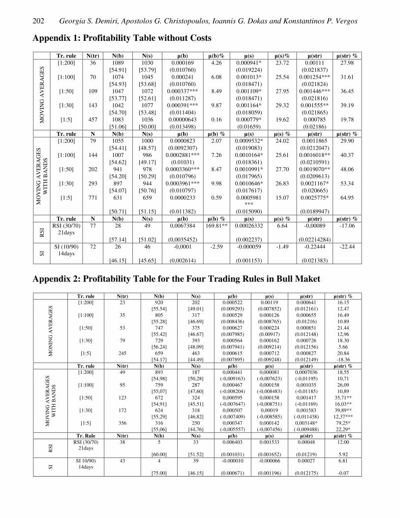
202 Georgia S. Demiri, Apostolos G. Christopoulos, Ioannis G. Dokas and Konstantinos P. Vergos
Appendix 1: Profitability Table without Costs
Tr. rule N(tr) N(b) N(s) �(b) �(b)% �(s) �(s)% �(str) �(str) %
MO
VIN
G A
VE
RA
GE
S [1:200] 36 1089 1030 0.000169 4.26 0.000941* 23.72 0.00111 27.98
[54.91] [53.79] (0.010760) (0.019224) (0.021837) [1:100] 70 1074 1045 0.000241 6.08 0.001013* 25.54 0.001254*** 31.61
[54.93] [53.68] (0.010760) (0.018471) (0.021824) [1:50] 109 1047 1072 0.000337*** 8.49 0.001109* 27.95 0.001446*** 36.45
[53.77] [52.61] (0.011287) (0.018471) (0.021816) [1:30] 143 1042 1077 0.000391*** 9.87 0.001164* 29.32 0.001555** 39.19
[54.70] [53.48] (0.011404) (0.018059) (0.021865) [1:5] 457 1083 1036 0.00000643 0.16 0.000779* 19.62 0.000785 19.78
[51.06] [50.00] (0.013498) (0.01659) (0.02186) Tr. rule N N(b) N(s) �(b) �(b) % �(s) �(s) % �(str) �(str) %
MO
VIN
G A
VE
RA
GE
S
WIT
H B
AN
DS
[1:200] 79 1055 1000 0.0000823 2.07 0.0009532* 24.02 0.0011865 29.90 [54.41] [48.57] (0.0092307) (0.019083) (0.0212047)
[1:100] 144 1007 986 0.0002881*** 7.26 0.0010164* 25.61 0.0016018** 40.37 [54.62] [49.17] (0.01031) (0.018361) (0.0210591)
[1:50] 202 941 978 0.0003360*** 8.47 0.0010991* 27.70 0.0019070** 48.06 [54.20] [50.29] (0.010796) (0.017965) (0.0209613)
[1:30] 293 897 944 0.0003961*** 9.98 0.0010646* 26.83 0.0021167* 53.34 [54.07] [50.76] (0.010797) (0.017617) (0.020665)
[1:5] 771 631 659 0.0000233 0.59 0.0005981 ***
15.07 0.0025775* 64.95
[50.71] [51.15] (0.011382) (0.015090) (0.0189947)
Tr. rule N N(b) N(s) �(b) �(b) % �(s) �(s) % �(str) �(str) %
RS
I RSI (30/70) 21days
77 28 49 0,0067384 169.81** 0.00026332 6.64 -0,00089 -17.06
[57.14] [51.02] (0,0035452) (0.002237) (0.02214284)
SI
SI (10/90) 14days
72 26 46 -0,0001 -2.59 -0.000059 -1.49 -0.22444 -22.44
[46.15] [45.65] (0,002614) (0.001153) (0.021383)
Appendix 2: Profitability Table for the Four Trading Rules in Bull Maket
Tr. rule N(tr) N(b) N(s) �(b) �(s) �(str) �(str) %
MO
NIN
G A
VE
RA
GE
S
[1:200] 23 920 202 0.000522 0.00119 0.000641 16.15 [55.54] [49.01] (0.009293) (0.007852) (0.012161) 12.47
[1:100] 35 805 317 0.000529 0.000126 0.000655 16.49 [55.28] [46.69] (0.008436) (0.008765) (0.01216) 10.89
[1:50] 53 747 375 0.000627 0.000224 0.000851 21.44 [55.42] [46.67] (0.007985) (0.00917) (0.012148) 12,96
[1:30] 79 729 393 0.000564 0.000162 0.000726 18.30 [56.24] [48.09] (0.007941) (0.009214) (0.012156) 5.66
[1:5] 245 659 463 0.000615 0.000712 0.000827 20.84 [54.17] [44.49] (0.007895) (0.009248) (0.012149) -18.36
Tr. rule N(tr) N(b) N(s) �(b) �(s) �(str) �(str) %
MO
VIN
G A
VE
RA
GE
S W
ITH
BA
ND
S
[1:200] 49 893 187 0,000441 0,000081 0,0007036 18,55 [54,98] [50,28] (-0,009163) (-0,007623) (-0,01195) 10,71
[1:100] 95 759 287 0,000467 0,000158 0,001035 26,09 [55,07] [47,60] (-0,008204) (-0,008483) (-0,01185) 10,89
[1:50] 123 672 324 0,000595 0,000158 0,001417 35,71** [54,91] [45,51] (-0,007647) (-0,008751) (-0,01169) 16,03**
[1:30] 172 624 318 0,000507 0,00019 0,001583 39,89** [55,29] [46,82] (-0,007409) (-0,008585) (-0,011438) 12,37***
[1:5] 356 316 250 0,000347 0,000142 0,003148* 79,25* [55,06] [44,76] (-0,005557) (-0,007456) (-0,009488) 22,29*
Tr. Rule N(tr) N(b) N(s) �(b) �(s) �(str) �(str) %
RSI
RSI (30/70) 21days
38 5 33 0.006403 0.001533 0.00048 12.00
[60.00] [51.52] (0.001031) (0.001652) (0.01219) 5.92
SI SI 10/90)
14days 43 4 39 -0.000010 -0.000066 0.00027 6.81
[75.00] [46.15] (0.000671) (0.001196) (0.012175) -0.07

Is the application of Simple Trading Rules a powerful tool for Profitability Prediction? : The case of the FTSE-20 of the Athens Exchange 203
Appendix 3: Profitability Table for the Four Trading Rules in Bear Market
Tr. Rule N(tr) N(b) N(s) �(b) �(s) �(str) �(str)%
MO
VIN
G A
VE
RA
GE
S [1:200] 13 169 828 -0.00023 0.001866* 0.001638 41.28
[51.48] [54.85] (0.009417) (0.02673) (0.028362) 39.20*** [1:100] 35 269 728 -0.000823 0.002012* 0.00193 48.63
[53.90] [56.73] (0.012888) (0.02524) (0.028344) 43.03* [1:50] 56 300 697 0.000111 0.002105* 0.002116 53.33
[49.67] [55.81] (0.014105) (0.024571) (0.028331) 43.37* [1:30] 64 313 684 0.0001968 0.002291* 0.002488*** 62.70***
[51.12] [56.58] (0.014336) (0.024419) (0.02843) 52.46* [1:5] 212 424 573 -0.000678 0.001416* 0.000738 18.60
[46.23] [54.45] (0.01778) (0.022092) (0.0284) -15.32
MO
VIN
G A
VE
RA
GE
S
WIT
H B
AN
DS
[1:200] 30 162 819 -0.00032 0.0001935* 0.001693 42.67 [51.23] [54.82] (0.009299) (0.0266) (0.028203) 37.87***
[1:100] 49 248 715 0.000087 0.001982* 0.002239 56.43 [53.23] [56.36] (0.01226) (0.02519) (0.028012) 48.59*
[1:50] 79 269 677 0.000044 0.002158* 0.002458 61.95 [52.42] [55.98] (0.013491) (0.024462) (0.027934) 49.31*
[1:30] 121 273 645 0.000272 0.002049* 0.002717*** 68.48*** [51.28] [55.81] (0.013645) (0.023991) (0.027579) 49.12*
[1:5] 355 315 449 -0.00034 0.001111* 0.001939 48.46 [46.35] [53.67] (0.015512) (0.020529) (0.025797) -7.94
Tr. Rule N(tr) N(b) N(s) �(b) �(s) �(str) �(str) %
RS
I RSI (30/70) 21days
49 23 16 0.006811 -0.00236 -0.00197492 -49.77
[56.52] [50.00] (0.005052) (0.00275) (0.02953449) -56.01
SI
SI (10/90) 14days
29 22 7 -0.00021 -0,000051 -0.55366 -55.37
[40.91] [42.86] (0.003742) (0,0011033) (0.028325) -59.05 Appendix 4: Sharpe Ratio Table
Without Costs With costs Trading Rule Bull Market Bear Market Bull Market Bear Market MA(1:200:0) 7.65368228 35.17851639 2.966956643 34.40058944 MA(1:100:0) 7.245598314 40.17230326 0.856857037 37.95373806 MA(1:50:0) 12.31892861 43.18553049 3.071742427 39.5388957 MA(1:30:0) 8.856190481 47.28696336 -4.862189858 43.0935097 MA(1:5:0) 11.56631525 32.29907953 -30.81898817 16.94837644 MA(1:200:1) 26.05879985 35.88272672 24.31823985 34.07818962 MA(1:100:1) 32.20240081 43.35106833 27.51627773 40.23874254 MA(1:50:1) 36.44040012 46.89926175 28.88078065 41.73200648 MA(1:30:1) 44.93880984 50.54082247 36.18218524 42.47107595 MA(1:5:1) 7.389240178 49.50745701 -22.26670932 21.83942175 RSI 1.522393472 1.018154812 -3.466466861 -1.094629266 SI -2.738413115 -0.914882219 -8.389532949 -2.21410535
Appentix 5: Granger Casualty Test
Null Hypothesis: Lag 1 Lag 4 Lag 10 Lag20 Prob. Prob. Prob. Prob.
OPEN does not Granger Cause D(PRICES) 0.9440 0.3445 0.0721 0.3131 D(PRICES) does not Granger Cause OPEN 0.0000 0.0000 0.0000 0.0000 HIGH does not Granger Cause D(PRICES) 0.9221 0.8695 0.0001 0.0002 D(PRICES) does not Granger Cause HIGH 4E-136 1E-202 8E-219 6E-215 LOW does not Granger Cause D(PRICES) 0.9654 0.3749 0.0439 0.0347 D(PRICES) does not Granger Cause LOW 2E-124 1E-184 1E-194 4E-189 VOLUME does not Granger Cause D(PRICES) 0.1443 0.1024 0.0072 0.0261 D(PRICES) does not Granger Cause VOLUME 0.0342 0.0370 0.6911 0.6112

204 Georgia S. Demiri, Apostolos G. Christopoulos, Ioannis G. Dokas and Konstantinos P. Vergos
Appentix 5: Granger Casualty Test (Continued)
MA200 does not Granger Cause D(PRICES) 0.1719 0.6307 0.3552 0.5057 D(PRICES) does not Granger Cause MA200 0.0764 0.4839 0.4987 0.5595 MA100 does not Granger Cause D(PRICES) 0.3420 0.7828 0.6444 0.7902 D(PRICES) does not Granger Cause MA100 0.1631 0.5190 0.8100 0.6263 MA50 does not Granger Cause D(PRICES) 0.2137 0.6071 0.1856 0.2929 D(PRICES) does not Granger Cause MA50 0.8921 0.9930 0.9838 0.6180 MA30 does not Granger Cause D(PRICES) 0.1626 0.2711 0.1540 0.4258 D(PRICES) does not Granger Cause MA30 0.6207 0.7665 0.9276 0.9691 MA5 does not Granger Cause D(PRICES) 0.1089 0.0183 0.0415 0.2745 D(PRICES) does not Granger Cause MA5 0.4479 0.6305 0.9139 0.0754 BA200 does not Granger Cause D(PRICES) 0.2326 0.6996 0.3287 0.6316 D(PRICES) does not Granger Cause BA200 0.1161 0.5933 0.5820 0.5514 BA100 does not Granger Cause D(PRICES) 0.2161 0.6719 0.5747 0.8008 D(PRICES) does not Granger Cause BA100 0.3228 0.7834 0.9318 0.6998 BA50 does not Granger Cause D(PRICES) 0.2050 0.6192 0.2937 0.4355 D(PRICES) does not Granger Cause BA50 0.8279 0.9841 0.9571 0.6310 BA30 does not Granger Cause D(PRICES) 0.0879 0.1978 0.1532 0.4591 D(PRICES) does not Granger Cause BA30 0.6580 0.8140 0.8820 0.9393 BA5 does not Granger Cause D(PRICES) 0.0909 0.0444 0.1157 0.4852 D(PRICES) does not Granger Cause BA5 0.4273 0.2065 0.7367 0.0217 RSI does not Granger Cause D(PRICES) 0.8635 0.1097 0.0850 0.2930 D(PRICES) does not Granger Cause RSI 0.9317 0.3353 0.2450 0.4075 SI does not Granger Cause D(PRICES) 0.9855 0.6549 0.6778 0.9063 D(PRICES) does not Granger Cause SI 0.7580 0.6462 0.3389 0.5131 RESISTANCE does not Granger Cause D(PRICES) 0.8034 0.3423 0.7630 0.8058 D(PRICES) does not Granger Cause RESISTANCE 2.E-14 4.E-13 4.E-13 5.E-16 SUPPORT does not Granger Cause D(PRICES) 0.9670 0.4713 0.0002 0.0098 D(PRICES) does not Granger Cause SUPPORT 5.E-76 2.E-91 6.E-96 1.E-96
Appendix 6: Linear Regression (Overall Sample)
Dependent Variable: D(PRICES) Included observations: 2118 after adjustments
Variable Coefficient Std. Error t-Statistic Prob. C 0.020837 0.187626 0.111055 0.9116 RETURNS 662.4831 16.89780 39.20529 0.0000 D(OPEN) -0.428880 0.013644 -31.43339 0.0000 D(HIGH) 0.439071 0.016662 26.35208 0.0000 D(LOW) 0.448729 0.014405 31.15095 0.0000 MA100 -100.1632 15.15483 -6.609323 0.0000 MA30 34.04362 12.10960 2.811291 0.0050 BA200 273.8023 14.86112 18.42406 0.0000
R-squared 0.885069 Mean dependent var -0.456303 Adjusted R-squared 0.884688 S.D. dependent var 25.34930 S.E. of regression 8.608023 Akaike info criterion 7.147036 Sum squared resid 156346.9 Schwarz criterion 7.168408
Log likelihood -7560.712 Hannan-Quinn criter. 7.154861 F-statistic 2321.266 Durbin-Watson stat 2.437367
Prob(F-statistic) 0.000000

Is the application of Simple Trading Rules a powerful tool for Profitability Prediction? : The case of the FTSE-20 of the Athens Exchange 205
Appendix 7: Linear Regression (Bubble Period Sample)/ (Post-Bubble Sample)
Dependent Variable: D(PRICES) Included observations: 1121 after adjustments Included observations: 997
Variable Coefficient Std. Error
t-Statistic Prob. Variable Coefficient
Std. Error
t-Statistic Prob.
C -0.126921 0.139616 -0.909072 0.3635 C 0.023508 0.270755 0.086824 0.9308 RETURNS 1732.495 25.47690 68.00258 0.0000 RETURNS 585.5735 19.88347 29.45026 0.0000 D(OPEN) -0.140426 0.013115 -10.70757 0.0000 D(OPEN) -0.365432 0.018440 -19.81694 0.0000 D(HIGH) 0.127372 0.015927 7.997213 0.0000 D(HIGH) 0.376291 0.021678 17.35832 0.0000 D(LOW) 0.166027 0.013214 12.56486 0.0000 D(LOW) 0.387924 0.019638 19.75344 0.0000 MA200 -80.88734 11.72861 -6.896584 0.0000 MA100 -64.62499 13.62041 -4.744716 0.0000 BA200 205.7730 17.74486 11.59620 0.0000 R-squared 0.966034 Mean dependent var 0.574139 R-square 0.888594 Mean dependent var -1.614905 Adjusted R-squared
0.965882 S.D. dependent var 25.26179 Adjusted R-squared
0.887919 S.D. dependent var 25.41010
S.E. of regression 4.666129 Akaike info criterion 5.923875 S.E. of regression
8.506935 Akaike info criterion 7.126637
Sum squared resid
24276.63 Schwarz criterion 5.950754 Sum squared resid
71644.26 Schwarz criterion 7.161073
Log likelihood -3314.332 Hannan-Quinn criter. 5.934034 Log likelihood -3545.628 Hannan-Quinn criter. 7.139727 F-statistic 6342.426 Durbin-Watson stat 1.992576 F-statistic 1316.067 Durbin-Watson stat 2.355630 Prob(F-statistic) 0.000000 Prob(F-statistic) 0.000000
Appendix 8: EGARCH Model (Overall Sample)
Dependent Variable: D(PRICES) LOG(GARCH) = C(17) + C(18)*ABS(RESID(-1)/@SQRT(GARCH(-1)) +
C(19)*RESID(-1)/@SQRT(GARCH(-1)) + C(20)*LOG(GARCH(-1)) Variable Coefficient Std. Error z-Statistic Prob. C 0.020181 0.015792 1.277878 0.2013 RETURNS 1047.757 12.99268 80.64210 0.0000 D(OPEN) -0.009804 0.002634 -3.722185 0.0002 D(LOW) 0.006678 0.002992 2.232045 0.0256 D(HIGH) 0.014210 0.001872 7.590688 0.0000 MA200 114.2480 10.24397 11.15271 0.0000 MA100 -5.465709 1.248085 -4.379277 0.0000 MA50 9.226196 3.237091 2.850150 0.0044 MA30 6.606956 1.496078 4.416185 0.0000 MA5 6.062361 1.023558 5.922832 0.0000 BA200 143.5298 10.36584 13.84641 0.0000 BA50 15.21316 3.432947 4.431515 0.0000 RSI -14.97275 4.094100 -3.657154 0.0003 SI -27.05788 12.62612 -2.143007 0.0321 AR(1) 0.665404 0.164052 4.056050 0.0000 MA(1) -0.656503 0.167167 -3.927217 0.0001
Variance Equation C(17) -0.351845 0.015897 -22.13240 0.0000 C(18) 0.507454 0.020290 25.01027 0.0000 C(19) 0.024625 0.011826 2.082294 0.0373 C(20) 0.994034 0.001764 563.5755 0.0000 R-squared 0.752354 Mean dependent var -0.464780 Adjusted R-squared 0.750110 S.D. dependent var 25.35228 S.E. of regression 12.67336 Akaike info criterion 6.134285 Sum squared resid 336807.5 Schwarz criterion 6.187736 Log likelihood -6473.141 Hannan-Quinn criter. 6.153854 F-statistic 335.3010 Durbin-Watson stat 1.972076 Prob(F-statistic) 0.000000 Inverted AR Roots .67 Inverted MA Roots .66

206 Georgia S. Demiri, Apostolos G. Christopoulos, Ioannis G. Dokas and Konstantinos P. Vergos
Appendix 9: EGARCH Model (Bubble Period Sample)/ (Post-Bubble Sample)
Dependent Variable: D(PRICES) LOG(GARCH) = C(13) + C(14)*ABS(RESID(-1)/@SQRT(GARCH(-
1)) + LOG(GARCH) = C(15) + C(16)*ABS(RESID(-1)/@SQRT(GARCH(-
1)) +
C(15)*RESID(-1)/@SQRT(GARCH(-1)) + C(16)*LOG(GARCH(-1)) C(17)*RESID(-1)/@SQRT(GARCH(-1)) + C(18)*LOG(GARCH(-1))
Variable Coefficient
Std. Error
z-Statistic
Prob. Variable Coefficient
Std. Error
z-Statistic
Prob.
C -0.042041 0.016555 -2.539503
0.0111 C 0.055584 0.039163 1.419314 0.1558
RETURNS 2022.133 9.198371 219.8360 0.0000 RETURNS 893.7117 7.724104 115.7043 0.0000 MA100 83.33581 2.569401 32.43395 0.0000 D(OPEN) -0.025560 0.004075 -6.272743 0.0000 MA30 6.344263 2.596896 2.443017 0.0146 D(HIGH) 0.027788 0.003847 7.222550 0.0000 MA5 4.213969 1.540630 2.735225 0.0062 D(LOW) 0.024378 0.005450 4.473445 0.0000 BA200 -255.6732 3.043812 -83.99767 0.0000 MA100 -14.14228 2.679145 -5.278653 0.0000 BA50 10.60446 2.196346 4.828225 0.0000 MA50 19.59739 2.538164 7.721088 0.0000 BA30 9.142458 2.746216 3.329111 0.0009 MA30 13.31861 3.721981 3.578366 0.0003 BA5 8.920437 2.590019 3.444159 0.0006 MA5 10.67321 1.362218 7.835167 0.0000 RSI -29.21403 8.855878 -3.298830 0.0010 BA200 205.4265 2.632736 78.02777 0.0000 AR(1) 0.706651 0.109231 6.469316 0.0000 BA30 10.60542 5.002419 2.120058 0.0340 MA(1) -0.685161 0.114573 -5.980111 0.0000 RSI 35.28107 7.556757 4.668811 0.0000 Variance Equation C(13) -0.315082 0.018290 -17.22701 0.0000 MA(1) -0.510523 0.403585 -1.264970 0.2059 C(14) 0.423979 0.026215 16.17321 0.0000 AR(1) 0.472011 0.423992 1.113255 0.2656 C(15) 0.093137 0.017108 5.444205 0.0000 Variance Equation C(16) 0.995864 0.002755 361.4632 0.0000 C(15) -0.359168 0.025992 -13.81850 0.0000 R-squared 0.955093 Mean dependent var 0.559036 C(16) 0.534879 0.033276 16.07403 0.0000 Adjusted R-squared 0.954483 S.D. dependent var 25.26802 C(17) 0.027040 0.016480 1.640726 0.1009 S.E. of regression 5.390840 Akaike info criterion 5.113146 C(18) 0.991082 0.003135 316.1768 0.0000 Sum squared resid 32083.52 Schwarz criterion 5.184876 R-squared 0.800731 Mean dependent var -1.614905 Log likelihood -2847.362 Hannan-Quinn criter. 5.140258 Adjusted R-squared 0.797271 S.D. dependent var 25.41010 F-statistic 1565.359 Durbin-Watson stat 1.830776 S.E. of regression 11.44101 Akaike info criterion 5.994898 Prob(F-statistic) 0.000000 Sum squared resid 128147.9 Schwarz criterion 6.083449 Inverted AR Roots .71 Log likelihood -2970.457 Hannan-Quinn criter. 6.028558 Inverted MA Roots .69 F-statistic 231.4094 Durbin-Watson stat 1.857144 Prob(F-statistic) 0.000000 Inverted AR Roots .47 Inverted MA Roots .51

European Journal of Scientific Research ISSN 1450-216X / 1450-202X Vol. 103 No 2 June, 2013, pp.207 - 217 http://www.europeanjournalofscientificresearch.com
Brain Extracting Using a Simple Standard Deviation and
Mathematical Morphology in Medical Images MRI
Samir Bara Laboratoir LRTT, Unité Associée au CNRST(URAC29)
Faculty of Sciences, Mohamed V-Agdal University B.P. 1014 Rabat, Morocco E-mail: bara−[email protected]; [email protected]
Mounir Ait Kerroum
Laboratoir LRTT, Unité Associée au CNRST(URAC29) Faculty of Sciences, Mohamed V-Agdal University B.P. 1014 Rabat, Morocco
Equipe Imagerie et Multimedia, Ibn Tofail University Laboratory LARIT, ENCG Kénitra, Maroc
Ahmed Hammouch
Laboratoir LRTT, Unité Associée au CNRST(URAC29) Faculty of Sciences, Mohamed V-Agdal University B.P. 1014 Rabat, Morocco
Laboratory LRGE, ENSET, Mohamed V-Souissi University B.P. 6207 Rabat, Morocco
Abstract
We have developed a new method for extracting the region of interest brain, from MRI brain. This new method called Brain extracting using a simple standard deviation and Mathematical Morphology in (BSDM), is a pre-segmentation of brain tissues; it is performed using hybrid techniques based on simple elementary operations of optimal mathematical morphology operators.
The performance of this method is validated on medical images. The results obtained show the good performance of this approach. Keywords: Edge detection, Image analysis, Mathematical morphology, Brain extracting,
MRI images. 1. Introduction The magnetic resonance imaging (MRI) is one of the most significant medical advances; it is derived from works on the magnetic properties of nuclei of atomsled by F. Bloch and E. Purcell [2] in 1946. Today, it is a privileged technique for the observation in vivo of brain anatomical structures and their pathologies. Note that this technique has been recognized through the 2003 Nobel Prize in Medicine awarded to P. Lauterbur and P. Mansfield on the origin of the use of the phenomenon of magnetic resonance imaging and through the Nobel Prize in Physics 2003 awarded to A. Abrikosov and V. Ginzburg for their work on superconductors.
The segmentation of cerebrovascular structures consists of extracting the relevant information contained in the angiographic images (i.e., vascular volume) allowingthe radiologist to focus effectively on the analysis of this information. Recent researches have demonstrated the relevance of a segmentation methodology based on discrete notions of processing and image analysis of this problem.

208 Samir Bara, Mounir Ait Kerroum and Ahmed Hammouch
This methodology relies ontheoretical concepts of mathematical morphology and discrete topology as well as incorporating elements of a high-level anatomical knowledge to guide tools built on these concepts. These applications of segmentation, recent but promising, needs to be developed and enhanced in order to reach applications used in clinical routine.
The anatomist has long been interested in sectional anatomy which is the study of cut surfaces of the human organs. The sectional anatomy is based on four imaginary planes, i.e., axial (horizontal), median (midsagittal), sagittal, and coronal planes that pass through the body. It is particularly important in the brain, where functional topography is of utmost interest. This sectional anatomy of brain becomes increasingly significant as a response to giant strides in neuroimaging technology.
Traditionally, three standard anatomical planes, namely axial, sagittal, and coronal have been practiced in the brain. All these planes are based on the median plane in most anatomy books (1-3). The sagittal plane has been defined as any vertical plane parallel to the median plane. And the coronal plane is a vertical plane perpendicular to the sagittal plane, whereas axial plane is a plane perpendicular to both sagittal and coronal planes. However, these are all imaginary planes without specific landmarks or reference points. Therefore, the cutting directions of the brain have been decided by the examiner's need and intention.
The images below show this cerebral segmentation:
The brain extraction of MRI images remains a delicate problem and influences strongly the corresponding analyses.The great variability of brains, the different methods of acquisition and the presence of artifacts are the main difficulties linked to the implementation of a robust and efficient algorithm.
Our objective is to develop a solid method of extracting MRI brain images. The problem here is more complex than for MRI images of an adult because maternal tissues surround the head. The proposed approach is founded on an analysis of intensities in MRI images and more particularly of the cerebrospinal fluid that surrounds the brain and appears highlighted in MRI images. Initialization can be done with the aid of a model form realigned on the MRI image. The surface of the brain is then refined (minimum cut of graph or deformable model). The algorithm developed during this work will be validated based on clinical images.
After a brief review of brain extraction, the brain extraction algorithm is described in detail.

Brain Extracting Using a Simple Standard Deviation and Mathematical Morphology in Medical Images MRI 209
The rest of this paper is organized as follows: In section (II) we will give a brief view about the formation of an MRI image, a discussion of the noises in medical images and the denoising approach. In section (III), we will survey, in some detail, a number of brain extraction segmentation methods that are well-suited to image analysis and will describe our proposed method for Brain Extraction .The complete results, comments and their comparison will be qualitatively presented in section (V), followed by a conclusion that gives some indications about future work in Section (VI). 2. Interactive Examination of an MRI Image 2.1. Noises in Medical Images
During the acquisition of medical images, we often found distributions of different sounds depending on the acquisition process, voluntary or involuntary, patient motion such as blood circulation, breathing, etc., The presence of noise gives a mottled image, grainy textured, or snowy appearance. Now we briefly discuss the best-known distributions of noise based on the medical imaging modalities. 2.1.1. Speckel Noise The main source of noise in MRI images is the thermal noise for patient [21]. The MRI image is commonly reconstructed by computing the inverse discrete fourier transform of the raw data [14,15].
Speckle noise affects all coherent imaging systems including medical images MRI. The only drawback of this modality is that it is usually affected by Speckle noise [21] that gives
a snowy appearance to the noisy image. This multiplicative noise is defined as shown in equation (1) where Y presents the noisy observation, R describes the real observation and n presents the noise.
Y(i;j)=R(i;j)n(i;j) (1)
2.1.2. Additive White Gaussien Noise (AWGN) AWGN is a channel model in which the only impairment to communication is a linear addition of wideband or white noise with a constant spectral density (expressed as watts per hertz of bandwidth) and a Gaussian distribution of amplitude.
Gaussian noise is commonly founded in medical image especially in tomography images (CT) [22]. The Gaussian noise follows the distribution given in equation (2) where R presents free-noise data, Y describes the noisy observation and n is the white Gaussian noise.
Y(i;j)=R(i;j)+n(i;j) (2)
2.1.3. Poisson Noise There are some medical modalities that are corrupted by non-Gaussian noise like Poisson noise, which affects the quality of scintigraphy images [23]. 2.1.4. Rician Noise (MRI) provides high spatial resolution but suffers from Rician noise that can be approximated to Gaussian noise under some conditions. 2.2. Denoising Approaches in Medical Images MRI
In digital image processing, image denoising is a procedure aiming at the removal of noise, which may corrupt an image during its acquisition or transmission, while retaining its quality [24].In this section we will describe the techniques for denoising MRI medical images and the existing algorithms for the restoration of medical images.

210 Samir Bara, Mounir Ait Kerroum and Ahmed Hammouch
2.2.1. Wavelet Coefficients Thresholding Decomposing the image using discreet wavelet transform (DWT) [24] is an efficient approach that demonstrates its capacity of providing a compromising between noises’ suppression and conserving the most important features of signal. The first denoising attemptusing wavelet was conducted by Weaver [25]. The denoising algorithm in this case follows three steps. In the first step, we choose the appropriate wavelet and the number of decomposition levels; in the second, we apply a soft or hard thresholding as need for each level; finally we reconstruct the image using the new coefficients. Generally, if we take a small value of Threshold it could leave many noisy coefficients. Therefore, the denoised image still contains noise when we apply a higher value for Thershold; the image may contain a lot of artifacts and blur. 2.2.2. Nl-Means This algorithm is based on the redundancy of information in the image. It looks for the pixel that their neighborhood looks like a pixel to be denoised then replaces the value of the noisy pixel by the non-local average of other pixels that are similar in order to remove noise. 2.2.3. Total Variation We consider R the free noise image, Y the image that we want to restore. Remove noise using Total Variation is based on the minimization of the function describes in equation (4).
ArgMinφ (x) = ∫||VR(x)dx|| + γ∫||Y(x) - R(x)dx|| * ||Y(x) - R(x)dx||dx (4)
2.2.4. Anisotropic Diffusion Unlike linear filters as Gaussian filtering that destroy the finer details in the image like edges, Anisotropic Diffusion removes noise progressively without suppressing images edges. This approach is based on Partial Differential Equations (PDE) (Equation (3)) and it has proved an efficient denoising method for MRI data.
U = div(g(|∇∇∇∇Y|)∇∇∇∇Y) (3) Where U represents a denoising image, ∇∇∇∇ the Gradient operator, g the function of the diffusion
that controls the smoothing, Y represents noisy image and div the divergence operator that is a linear differential operator. The only problem with this approach is that it’s based on Gradient operator to determine edges that is not enough for localizing edges when noise like Speckle is present in the image. 2.2.5. Pizurica and Philips’s Approach The authors in [9] have introduced a new denoising technique called Generalized Likelihood (GinLik), which can be applied to unknown noises distributions and also gives the medical expertthe ability of a balanced parameter to control the quality of denoised image. It is based on wavelets and it was applied with success for Ultrasound and MRI data denoising. 3. Brain Extraction via Mathematical Morphology Method 3.1. Overview of the Brain Extraction Method
Segmentation of brain/non-brain tissue is one of the most time-consuming preprocessing steps performed in neuro imaging laboratories, and numerous brain extraction algorithms (BEAs) have been developed to perform this step automatically [2]. To date, there have been four main methods proposed for achieving brain/non-brain segmentation. We briefly describe and compare these methods. 3.1.1. SPM2 SPM2 does not explicitly generate a strip mask; however, one can be created as the binarized sum of the grey matter (GM) and white matter (WM) compartments after segmentation (J. Ashburner,

Brain Extracting Using a Simple Standard Deviation and Mathematical Morphology in Medical Images MRI 211
personal communication, 2003). The Realign and Normalize routines were employed to transform the volumes into Talaraich space, and the Segment routine was employed to create GM, WM, and CSF compartments. Brain masks were then created using Interactive Data Language (IDL, Research Systems, Inc., Boulder, CO) as the binarized sum of the GM and WM compartments, and Normalize was employed to transform the masks back into native space for comparison against the manual masks. To maintain a constant volume size throughout this ‘‘stripping’’ process, bounding boxes employed by Normalize were customized for the two transforms, and voxel sizes were inputted. 3.1.2. Brain Extraction Tool(BET) BET makes an intensity-based estimation of the brain/non-brain threshold, which determines the center of gravity of the head, defines an initial sphere based on the center of gravity, and deforms the tessellated sphere outward towards the brain surface(Smith, 2002). Two parameters are user-adjustable: fractional intensity threshold and threshold gradient.
Histogram-based threshold estimation
Binarisation using t to find centre of gravity
Initialisation of surface
Final ROI
3.1.3. Brain Surface Extractor (BSE) BSE is an edge-based method that employs anisotropic diffusion filtering. Edge detection is implemented using a 2D Marr–Hildreth operator employing low-pass filtering with a Gaussian kernel and localization of zero crossings in the Laplacian of the filtered image; the final step is morphological processing of the edge map (Shattuck et al., 2001). Three parameters are user adjustable: anisotropic smoothing kernel, number of iterations, and edge detection
Input image
Filtering the image to remove
Detecting edges in the image.
Performing morphological erosions and brain
Performing surface cleanup and image masking
3.1.4. Minneapolis Consensus Stripping(McStrip) McStrip is an automatic hybrid algorithm implemented in IDL that incorporates BSE and requires no user intervention; it relies on warping to a template, intensity thresholding, and edge detection (Rehm et al., 2004).It should be noted that these four algorithms were not developed with the same design goals. BET, BSE, and McStrip algorithms are designed to remove muscle, fat, skin, bone, and dura to produce a cortical envelope for use in subsequent data analysis.

212 Samir Bara, Mounir Ait Kerroum and Ahmed Hammouch
In this first comparison based on quantitative boundary and volume metrics, reproducibility across repeated scans of a single subject, and assessments of performance consistency across datasets acquired different scanners at different institutions. McStrip, a hybrid method incorporating warping to a template, intensity thresholding, and edge detection, consistently outperformed SPM2, BET, and BSE, all of which rely on a single algorithmic strategy. 3.2. Brain Extraction Using a Simple Standard Deviation and Mathematical Morphology Method (Proposed Method) The goal of our method is to extract the brain from the acquired image: this will allow us to simplify the segmentation of the brain tissues. The region of interest is the brain. To extract this region we use the AND operator between the original filtered image and the binary mask obtained in last step. The non-brain tissues are obtained by applying AND operator between the initial image and the logical complement of the mask.
Our easy and effective method can be divided in seven steps: 3.2.1. Image Filtering Median filtering is a common nonlinear method for noise suppression that has unique characteristics. It does not use convolution to process the image with a kernel of coefficients. Rather, in each position of the kernel frame, a pixel of the input image contained in the frame is selected to become the output pixel located at the coordinates of the kernel center. The kernel frame is centered on each pixel (m,n) of the original image, and the median value of pixels within the kernel frame is computed. The pixel at the coordinates (m,n) of the output image is set to this median value. In general, median filters do not have the same smoothing characteristics as the mean filter [3]. 3.2.2. Binarisation using a Simple Standard Deviation Approach Binarisation methods can be categorized according to differences in the criteria used for thresholding. This step is based on global binary image thresholding using a new image binarisation method that uses a simple standard deviation approach and gives us very good results for MRI brain images.
The problem of binarisation of gray MRI images due to the black background and large intensity variation has been overcome by this method. In the proposed methods we use standard deviation to select the threshold intensity of the image.
Ultimate selection of threshold has been done by multiplying a constant value with the threshold intensity of the image using standard deviation. We use the threshold intensity as a global value i.e., the threshold intensity of the entire image is unique. This method is very useful to extract the objects of interest from an image and; hence, to distinguish the foreground (brain) from the background (black background).
The proposed algorithms are described below:

Brain Extracting Using a Simple Standard Deviation and Mathematical Morphology in Medical Images MRI 213
When different binarisation methods are being applied on MRI of brain database, most of the algorithms binarised whole images without properly detecting the region of interest and the black background, so some methods fail to give appropriate binarisation.
Our motivation to use this method is to produce very good results for all type of MRI brain images. We also proved that our proposed method produces better results visually as well as metric wise compared to the other established image binarisation. 3.2.3. Greatest Connected Component Extraction (Connected Components Labeling and Extraction) Connected Components Labeling and Extraction Method of segmentation and removal is extremely helpful when the unwanted object to be segmented and removed shares common intensity levels with the desired information where traditional threshold based procedures like adaptive thresholding will fail to accomplish precise segmentation results. Segmentation methods like Active Contours and Region Growing can only identify the ROI but will not remove the identified interphase cells. Initial placement of contour for active contours and initial placement of seed for region growing consumes a lot of time where the Connected Components Labeling and Extraction method can yield the most accurate results. 3.2.4. Filling the Holes To fill holes in our model of structure, we propose in this step a technique which automatically adjusts and clones large image patches that have similar structure, a user wanting to paint over a hole still faces threechallenges: (1) choosing the right constant offset to the source pixels, (2) choosing anappropriate brush size, and (3) finding source pixels featuring structure that is compatible with the destination. We propose that these tasks can be assisted with automation like recent works on texture synthesis [9]. 3.2.5. Dilatation Morphological operations are non-linear filters that can be applied to both binary images and those to grayscale.
The analysis via mathematical morphology aims at changing the structure and the form of image objects as to separate objects, discriminate them depending on their seize, fill holes, etc.
The effect of the expansion is to expand the first figure; the height and width of the expanded figure are respectively the height and width of the original figure and the structuring element. If the structuring element is off, the expansion will shift the figure in the same direction. Finally, the convex corners of the figure will be distorted depending on the structuring element.

214 Samir Bara, Mounir Ait Kerroum and Ahmed Hammouch
3.2.6. Mask(Mask Selection for Image Processing) There are many techniques for visual inspection. Four of them are (1) Image subtraction, (2) Dimensional verification, (3) Syntactic approach and, (4) Feature Matching [1]. In Feature Matching or Template Matchingmethod, in our method we use Image subtraction, the image to be inspected is scanned and compared to the original image, which has been stored before. The subtracted image is analyzed. 3.2.7. ROI Extracting Researchers have found out that most information is only from some key regions in an image. If these key regions are extracted and processed, the computational speed can be highly improved. Therefore, based on this idea, regions of interest are developed.A ROI or region of interest is used to select the important area of an image for processing. ROIs can be used to greatly reduce image-processing time. 4. Experimentale Results In this section, we turn to present results of numerical experiments which are performed on the MRI images.
Our method performed the best overall. In most cases, our algorithm was able to precisely determine the pial boundary of the brain, resulting in an accurate segmentation. Also, our method performed well independently of the data set, and proved to be more robust than others.
We have evaluated the performance of our algorithm tested real and simulated MRI images with and without noise. Robustness regarding scale, noise, contrast, and accuracy will be discussed.
Figures show the simulation results of two MRI provided by the website Brainweb [14,15]. The whole implementation (MatLab coding) is run on a PC with a 1.5GHz Intel(R) Pentium(R) CPU.
Table 1 summarizes the performance comparison of the brain extraction method in different circumstances, where in general our method is superior to the others in terms of location accuracy and computational time. The details follow. Figure 1: Brain Extraction steps on axial slice of number in simulated data volume [21] with 5% uniform
noise.
Figure 2: Brain Extraction steps on axial slice of number in simulated data volume [21] with 5% uniform
noise.

Brain Extracting Using a Simple Standard Deviation and Mathematical Morphology in Medical Images MRI 215
Discussion The criteria presented in this section are, for the most part, indicators traditionally used to evaluate segmentation in an unsupervised environment. The value of each criterion increases with the quality of the result of segmentation. These values were normalized to facilitate their comparisons.
• Visual criterion: This criterion allows you to plot the results of the selected algorithms on the image to compare them with the reference you have selected.
• Computation time. • Similarity criterion: Four similarity criteria can be computed between the result of the
algorithms and the reference: o Dice criterion: o Peak signal-to-noise ratio(PSNR) o Hausdor-distance
TABLE 1: Similarity indices calculated for different extraction techniques applied to brain
Algorithm Visual
Criterion Dice MSSD PSNR
Hausdor_ distance
Computation time
SPM2 0.6 54.64 10.63 21.35 3 mn BET [30] 0.7 153.35 8.86 31.98 3 mn BSE [31] 0.85 119.9 8.31 21.54 3 mn McStrip [28,29] 0.87 59.85 7.19 16.97 2 mn BSDM 0.88 155.64 11.01 20.10 3 mn
According to our tests, our method gives comparable results to SMP2, BSE and BET in term of
accuracy but with lowest time processing (creating mask in about 4 min). But when compared with McStrip technique it is faster. 5. Conclusions and Future Trends The magnetic resonance imaging is now a powerful tool for the in vivo observation of brain anatomy. Used in clinical routine, the multiplicity of weights acquisition allows physicians to access rich and abundant information, particularly for the diagnosis of brain tumors.
In this paper we propose an automated method of extracting data from MRI images into brain and non-brain, for several reasons such as the detection of brain tumors in the context of aid in the diagnosis of the latter.
The robustness of the method up on the different artefacts usually present in magnetic resonance images such as noise and intensity in homogeneity will be evaluated in future work. In other hand, we are extending this method for 3D brain MRI and comparing it with some well-known similar ones trough performance measure.
Finally, note that results from a brain extraction algorithm may improve if the image is pre-processedin certain ways, such as with intensity in homogeneity reduction algorithm. References [1] Roland, T.C. and Charles, A.H., “Automated visual inspection: A Survey”, IEEE Transac. On
Pattern Analysis and Machine Intelligence, Vol. PAMI-4, No.6., 1982. [2] F. Bloch. Nuclear induction. In Physical Review, pages 460–474, 1946 Handbook [3] "V. Caselles, R. Kimmel, and G. Sapiro.Geodesic active contours. International Journal
ofComputer Vision, volume 22, pp. 61-79, 1997."

216 Samir Bara, Mounir Ait Kerroum and Ahmed Hammouch
[4] "T. Chan and L. Vese. Active contours without edges. IEEE Transactions on Image Processing. volume10, pp. 266-277, February 2001."
[5] "S. Lankton, A. Tannenbaum. Localizing Region-Based Active Contours. In IEEE Transactions on Image Processing. volume 17, no. 11, pp. 2029-2039, 2008."
[6] "O. Bernard, D. Friboulet, P. Thevenaz, M.Unser. Variational B-Spline Level-Set: A Linear Filtering Approach for Fast Deformable Model Evolution. In IEEE Transactions on Image Processing. volume 18, no. 06, pp. 1179-1191, 2009."
[7] "C. Li, C.Y. Kao, J.C. Gore, Z. Ding. Minimization of Region-Scalable Fitting Energy for Image Segmentation. In IEEE Transactions on Image Processing. volume 17, no. 10, pp. 1940-1949, 2008."
[8] R. Malladi, J. A. Sethian. ”A Unified Approach to Noise Removal, Image Enhancement and Shape Recovery,” IEEE Transactions on Image Processing, 5, 11, 1154-1168, (1996).
[9] "Yonggang Shi, William Clem Karl. A Real-Time Algorithm for the Approximation of Level-Set-Based Curve Evolution. In IEEE Transactions on Image Processing. volume 17, no. 05, pp. 645-656, 2008."
[10] A. Yezzi, A. Tsai, and A.Willsky, “A fully global approach to image segmentation via coupled curve evolution equations,” J. Vis. Commun. Image Represent., vol. 13, no. 1, pp. 195–216, Mar. 2002.
[11] S. G. Vaidyanathan, CIHCI, vol. 1, no. 1, (2008), pp. 237-245. [12] O. Bernard, B. Touil, A. Gelas, R. Prost, and D. Friboulet, “A rbfbased multiphase level set
method for segmentation in echocardiography using the statistics of the radiofrequency signal,” in Proc. IEEE Int. Conf. Image Processing, San Antonio,TX, 2007, pp. 157–160.
[13] O. Bernard, J. Dhooge, and D. Friboulet,“Segmentation of echocardiographic images based on statistical modelling of the radio-frequency signal,” presented at the Eur. Signal Processing Conference (Eusipco), Florence, Italy, 2006, ID cr2205, 4 pages, unpublished.
[14] [GE System] http://www.gemedicalsystems.com [15] Brain MRI from http://www.itk.org/ [16] J Lie, M Lysaker and XC Tai, A binary level set model and some applications for Mumford-
Shah image segmentation, IEEE Transactions on Image Processing 15 (5) (2006), pp. 1171–1181
[17] Denoising of Magnetic Resonance Images using Wavelets- A Comparative Study [18] PiertoPerona and Jitendra Malik, “Scale-space and edge detection using anisotropic diffusion,”
IEEE Trans. vol. 12, July 1990. [19] AntoniBuades, BartoumColl “A non-local algorithm for image desnoising,” IEEE Trans. 2005. [20] Aleksandra Pizurica and Wilfried Philips “A versatile Weveltdomaine noise filtration technique
for medical imaging,” IEEE Trans. Vol. 22,pp. 323-331, March 2003. [21] Racine, René, Walker, Gordon and Daniel, “Speckle Noise and the Detection of Faint
Companions,” Publications of the Astronomical Society of the Pacific. Vol. 111, pp. 587-594, Mai 1999.
[22] PFAU Patrick R, SIVAK Michael V. and CHAK Amitabh, “Criteria for the diagnosis of dysplasia by endoscopic optical coherence tomography,” Gastrointestinal endoscopy. Vol. 58, pp.196-202, 2003.
[23] Michael V. Green, Harold G. Ostrow and Margaret, “High temporal Resolution Ecg-Gated ScintigraphicAngiocardiography”JNM. Vol. 16,pp 95-98, 1975.
[24] Mallat, S.G. “A theory for multiresolution signal decomposition: the wavelet representation” IEEE Trans. Vol. 1, pp. 674 – 693. Jul 1989.
[25] Weaver JB, XuYs, Healy DM Jr, Cromwell LD. “Filtring noise from images with wavelet transforms,” MagnReson Med. Vol. 21, pp. 288-95. Octobre 1991.
[26] Aleksandra Pizurica and AlleMejie Wink, “A review of weveltdenoising in MRI and Ultrasound brain imaging,” 2006.

Brain Extracting Using a Simple Standard Deviation and Mathematical Morphology in Medical Images MRI 217
[27] L.I. Rudin, S. Osher, and E. Fatemi. “Nonlinear total variation based noise removal algorithms.” Physica D, vol. 60, pp. 259–268, 1992
[28] R. E. Blanton, J. G. Levitt, J. R. Peterson, D. Fadale, M.L. Sporty, M. Lee, D. To, E. C. Mormino, P. M.Thompson, J. T. McCracken, and A. W. Toga, “Gender differences in the left inferior frontal gyrus in normal children”, NeuroImage, vol. 22, pp: 626-636, 2004.
[29] A.M. Dale AM, B. Fischl , and M. Sereno, “Cortical surface-based analysis. Segmentation and surface reconstruction”, Neuroimage, vol. 9, pp: 179-94, 1999.
[30] Shattuck, D.W., Sandor-Leahy, S.R., Shaper, K.A., Rottenberg, D.A., Leahy, R.M., Magnetic resonance image tissue classification using a partial volume model. NeuroImage. 13 (5), 856–876. 2001.
[31] S. M. Smith, “Fast robust automated brain extraction”, Human Brain Mapping, vol. 17, pp: 143-55, 2002.

European Journal of Scientific Research ISSN 1450-216X / 1450-202X Vol. 103 No 2 June, 2013, pp.218 - 226 http://www.europeanjournalofscientificresearch.com
Report on the Development of Standard Criteria of
Environmental Education for School Under Tak Primary Educational Service Area Office 1
Paisarn Pandan (Corresponding Author) Faculty of Environment and Resource Studies
Environmental Education Program, Valaya Alongkorn Rajabhat University Under The Royal Patronage Pathumthani, Thailand
E-mail: pai5656 @ gmail.com
Vinai Veeravatnanond Assoc.Prof., Advisors, Faculty of Environment and Resource Studies
Environmental Education Program, Valaya Alongkorn Rajabhat University Under The Royal Patronage Pathumthani, Thailand
Raveevan Sananvorakiat
Faculty of Environment and Resource Studies Environmental Education Program, Valaya Alongkorn Rajabhat University
Under The Royal Patronage Pathumthani, Thailand
Abstract
The purposes of this research were to 1) analyze the factors of and establish the standard criteria of environmental education for schools under Tak Primary Educational Service Area Office 1; and 2) carry out a confirmatory factors analysis for the standard criteria of environmental education. The sample used in the study was 350 educational administrators, school administrators and teachers under Tak Primary Educational Service Area Office 1 obtained by purposive selection and simple random sampling with the use of random number table. The research instruments were a questionnaire for the focus group, a questionnaire, and an evaluation form. The data were analyzed by using descriptive and inferential statistics including index of item-objective congruence (IOC), alpha coefficient (α ), percentage, mean ( Χ ), and standard deviation (S.D.).
The research results were as follows. 1) The standard criteria for schools under Tak Primary Educational Service Area Office 1 comprised 6 standards, 12 sub-standards, and 60 indicators. They were Standard 1 Management with 2 sub-standards and 10 indicators, Standard 2 Learning Management with 2 sub-standards and 10 indicators, Standard 3 Learner Quality with 2 sub-standards and 10 indicators, Standard 4 Environmental Management in Schools with 2 sub-standards and 10 indicators, Standard 5 Involvement with Community with 2 sub-standards and 10 indicators, and Standard 6 Assessment and Evaluation with 2 sub-standards and 10 indicators. 2) Regarding the confirmatory factors analysis with the sample of 350 people, it was found that the appropriateness of the standard criteria with the standard indicators of environmental education for schools under Tak Primary Educational Service Area Office 1 in general was at the high level ( Χ = 4.11).

219 Paisarn Pandan, Vinai Veeravatnanond and Raveevan Sananvorakiat
Keywords: Standard criteria of environmental education schools
1. Introduction The environment tends to be destroyed increasingly all the time. The destruction has then caused a lot of environmental problems which mostly come from humans. The major causes are from the lack of correct knowledge, understanding, attitude and value toward the environment. Therefore, for the sustainable solution of environmental problems, the quality of humans who are the cause of the problem needs to be developed by providing “education”. The main objective of the development is to promote people the appropriate attitude and belief toward the environment. When people have correct knowledge and understanding and appropriate attitude and belief about the environment, they will be able to make decision for their self practice correctly according to the situations. It has been accepted that education is a process to help humans to completely get into their potentials. Furthermore, education is also a factor for the promotion of sustainable development. The development in education is therefore necessary to be integrated with other contents under the same curriculum. Education is also a factor to help provide the learners achievement, conscious and awareness about the environment and morals; skills, and behaviors appropriate to the environmental conservation (Department of Environmental Quality Promotion, 2004). Similarly, the most important goal of environmental education aims at promoting awareness toward the problems and importance of the environment, and improving the behaviors and livings of humans in order to stop the environmental problems. This learning will help humans know how to make long term plans for their lives and to involve in the maintenance and the quality development of the environment (Veeravatnanond, 2003). The environmental education process will help achieve the operations to solve and prevent the environmental problems efficiently. The process is used to provide people with knowledge, awareness about environmental problems occurring, positive attitude, and motivation to involve in solving the environmental problems (Nilkham, 2011). Regarding the solution of problems about natural resources and the environment, the potential of humans who are the cause of the problem needs to be developed. The development will make changes of human behaviors seriously into the promotion and conservation of natural resources and the environment (Chankian, 2012). The integration of environmental contents with learning process according to the principles of environmental education will promote the intellectual development with broad, reasonable and systemic thinking; love and appreciation in value of the environment; and the self practice friendly to the environment (Veeravatnanond and Singseewo, 2010). To promote humans with awareness, love and needs of the environment including the involvement seriously and continuously in environmental protection should start from the children. It can be done by using school mechanism to promote the involvement (Piamphongsant, 2005). The primary education students are considered as the youths that need attention on their development. They will grow up to be adults with potentials and be part of the natural and environmental conservation. Therefore, they need to be promoted with knowledge and understanding about the importance and value of nature and the environment. These will help them grow up with responsibility for the environment (Singseewo, 2011). The basic education is therefore very important for promoting the learners with knowledge, ability, and especially awareness about making the best use of resources and the efficient conservation of the environment.
Schools are recognized as educational institutes where are important parts to promote students with knowledge and the desirable characteristics about the environment. This can be done because the schools are ready in all areas. They are academic sources that can efficiently educate and cultivate the students with characteristics needed. Activities of environmental education in school system that are appropriate and relevant to the school context and current situation of the environment will affect the promotion of conscious and involvement of students in the promotion of environmental quality (Supapongpichate, 2012). Importantly, the school should provide students the experience about the environment as follows. Firstly, the school has appropriate curriculum about the environment.

Report on the Development of Standard Criteria of Environmental Education for School Under Tak Primary Educational Service Area Office 1 220
Secondly, the school has appropriate personnel who are aware of the environment. Thirdly, the school creates atmosphere to facilitate the environmental conservation. Lastly, the school organizes activities about the environment in order to promote students the knowledge and behaviors and practice correctly and appropriately to the environment (Phra Dhammapitaka, 1999).
Regarding the management of environmental education in schools of basic education level, the school administrators, teachers, the community, and students’ parents are very important parts to encourage and motivate students to participate in planning for arranging learning activities about environmental education. The evaluation of these operations needs to be done continuously. According to the arrangement of environmental education in schools under Office of the Basic Education Commission in the past, it was found that various types of activity about environmental education were organized in schools. The major goal of these activities was to develop the learners with the behavior about the environmental conservation and development. However, the schools had a problem with the lack of framework and direction for clear operations, and shared criteria or indicators for the arrangement of activities about environmental education in schools. The schools need the models of these matters as guidelines into the same direction for their management of environmental education. This problem has caused the activities of environmental education in schools unsuccessful. From the above reasons and results of the study, the researcher was interested in the research to develop the environmental standard criteria for schools. The standard criteria with indicators were developed to determine the successful conditions for the arrangement of environmental education in schools. They were also used as framework and direction for the arrangement of learning activities about environmental education in schools. 2. Methodology The purposes of this research were to 1) analyze the factors of and establish the standard criteria of environmental education for schools under Tak Primary Educational Service Area Office 1; and 2) carry out a confirmatory factors analysis for the standard criteria of environmental education developed by the researcher.
The study group was 15 resource persons, academics in the area of environmental education, educational administrators, school administrators, and teachers who participated in the focus group.
The sample used in the research was 350 educational administrators, school administrators, and teachers under Tak Primary Educational Service Area Office 1 obtained by purposive selection and simple random sampling with the use of random number table.
The instruments used in the research were as follows: 1) A questionnaire was used for the focus group. 2) A 5 rating-scale questionnaire which followed Likert’s Scale was constructed and its content validity was tested. The index of item-objective congruence (IOC) of the whole paper was 0.09 while the IOC of all items was between 0.60-1.00. The discrimination of an individual item was examined. According to the Cronbach’s alpha coefficient, the alpha was .9732. 3) An evaluation form was constructed and its content validity was tested. The IOC of the whole paper was 1.00.
The data analysis, the analysis of general data and the confirmatory factor analysis were carried out by using descriptive statistics including percentage, mean ( Χ ) and standard deviation (S.D.). 3. Results and Discussion 3.1 The analysis of factors and the establishment of standard criteria for schools under Tak Primary Educational Service Area Office 1 were carried out in 2 steps of the developmental process. They were 1) the study and the synthesis of relevant concepts, theories, texts, and research; and 2) the focus group of resource persons, academics in the area of environmental education, educational administrators, school administrators, and teachers. The results revealed that the standard criteria for schools under

221 Paisarn Pandan, Vinai Veeravatnanond and Raveevan Sananvorakiat
Tak Primary Educational Service Area Office 1 comprised 6 standards, 12 sub-standards, and 60 indicators.
Standard 1 Management comprised 2 sub-standards: Sub-Standard 1 School has policy and management of environmental education, and Sub-Standard 2 School promotes teacher and personnel development about the environmental education; and 10 indicators. Standard 2 Learning Management comprised 2 sub-standards: Sub-Standard 1 School has learning plans relevant to the curriculum of environmental education, and Sub-Standard 2 School arranges learning relevant to the curriculum of environmental education: and 10 indicators. Standard 3 Learner Quality comprised 2 sub-standards: Sub-Standard 1 Learners have knowledge, understanding and skills, and apply the knowledge into practice in environmental conservation and development, and Sub-Standard 2 Learners have awareness toward and realized the value of sustainable conservation and development of the environment; and 10 indicators. Standard 4 Environmental Management in Schools comprised 2 sub-standards: Sub-Standard 1 School arranges its landscape to facilitate the learning, and Sub-Standard 2 School manages the environment systemically according to the principles of sanitation; and 10 indicators. 5) Standard for Involvement with Community comprised 2 sub-standards: Sub-Standard 1 School promotes the relationship with the community, and government and private sectors about the environmental conservation and development, and Sub-Standard 2 The community and parents network has a role to support the environmental activities in school; and 10 indicators. 6) Standard for Assessment and Evaluation comprised 2 sub-standards: Sub-Standard 1 School has the evaluation of plans/projects about environmental education, and Sub-Standard 2 School has the learning assessment of environmental education; and 10 indicators. Regarding the confirmatory factors analysis with the sample of 350 people, it was found that the appropriateness of the standard criteria with indicators of environmental education for schools under Tak Primary Educational Service Area Office 1 in general was at the high level ( Χ = 4.11). When considering in 6 individual standards, it was found that the appropriateness of Standard 4 Environmental Management in Schools ( Χ = 4.21), Standard 5 Involvement with Community ( Χ = 4.21), Standard 1 Management ( Χ = 4.12), Standard 3 Learner Quality ( Χ = 4.09), Standard 6 Assessment and Evaluation ( Χ = 4.06), and Standard 2 Learning Management ( Χ = 4.05) was at the high level respectively.
3.2 The study found that the standard criteria for schools under Tak Primary Educational Service Area Office 1 comprised 6 standards, 12 sub-standards, and 60 indicators. This might be because of the agencies involved at the policy level namely Ministry of Education and Office of the Basic Education Commission have paid their attention toward the environmental problems and then determined the policy for schools to arranged activities about environmental education. The activities have been organized in various forms and methods while the learning-teaching management has emphasized on providing learners the opportunity to learn from real natural experience linking with the groups of learning contents and to apply it into real practice in their daily lives. The activities help promote students with knowledge and correct understanding about the environment; conscious and good value toward the environment. They also teach the students about causes and effects, and how to improve and solve the problems of the environment in order to avoid the environmental problems and their impacts on humans.
The results of this research would be an important inspiration for educational administrators, school administrators, teachers and the community with the awareness toward the value of operations about environmental education in schools where are the places to educate and cultivate children and youths to grow up with good quality of life. This was consistent with the research of Sinrungtham (2004) who studied the future of environmental education curriculum at the level of basic education in the next decade (during 2004-2014). The study found that the management of environmental education curriculum of the agencies at policy level had to determine the policy of environmental education in different aspects. They were, for example, the learning management of environmental education, the development of environmental education, the management of environmental education curriculum, and the establishment of learning networks for environmental education. These matters should be clear,

Report on the Development of Standard Criteria of Environmental Education for School Under Tak Primary Educational Service Area Office 1 222
continuous, and able to apply concretely into practice at both levels of educational service area office and school. The features of environmental education curriculum at the level of basic education must be as follows. 1) The environmental education curriculum must be integrated with the process of conservation; and the development of natural resources, the environment and energy with all groups of learning content. 2) The management of learning activities for environmental education must be linked with the concept of sustainable development. 3) The development of ecological system of natural resources and energy must be integrated with the ways of life. 4) Government and private sectors and the community must get involved in the design of environmental education curriculum of the school. 5) The learners must have knowledge, attitude, awareness, skills, and involvement about the sustainable conservation, protection, and problem solution of natural resources, the environment, and energy. The findings matched with the research of Veeravatnanond (2002) who studied the development of environmental education schools. The study found that 1) the development of physical-biological environment was the essential factor for life and it directly affected humans. It was beneficial to teachers and students and it was a concrete learning source closest to the students. 2) The lesson plans about environmental education in all subjects of school could be integrated and liked with the contents of the environment. 3) Regarding the knowledge, understanding and attitude toward the environment of students after the use of lesson plans, it was found that the knowledge of students about the environment was at the good level. For the evaluation of attitude toward the environment of school, it was found that the attitude toward the environment of students in all levels was also at the good level. Moreover, the findings were consistent to the research of Kanchanasak (2002) who investigated the motivation affecting the intention to participate the activities of nature studies of upper secondary students. The study revealed that, with the regard of the curriculum development and teaching of environmental education, to achieve the goals and the principles of environmental education in promoting the learners with desirable characteristics, the schools should provide the learners with motivation to participate in activities about conservation, protection and problem solution of natural resources, the environment and energy. The activities were, for example, the management of learning for learners with direct experience from natural learning sources, the opportunity to survey and search for knowledge, the response of curiousness about natural resources and the environment, and the practice about the prevention and solution of problems about natural resources and the environment in order to improve the quality of life and the environment. Furthermore, the research findings agreed with the Standard 1 The Establishment of School Policy and Standard 4 The Management of School Environment for Health which were under the standard criteria of Ministry of Public Health to evaluate the health promotion schools. They also matched with the educational standards in Standard 3 Learners has conscious about the shared benefits, and environmental conservation and development; Standard 13 School has the structural management, and systemic and complete cycle of management to achieve the educational goals; Standard 14 School promotes the relationship and cooperation with the community for educational development; and Standard 15 School has the management of the environment to facilitate learning and promote health, sanitation, and safety of the learners. The Summary of Results of this Research
The standard criteria with indicators of environmental education for schools under Tak Primary Education Service Area Office 1 comprised 6 standards as sub-standards and 60 indicators as follows. Standard 1 Management Sub-Standard 1 School has policy and management of environmental education.
Indicator 1 School has plans/projects with participatory process. Indicator 2 School has goals and establishment of understanding with relevant people about the
environmental education.

223 Paisarn Pandan, Vinai Veeravatnanond and Raveevan Sananvorakiat
Indicator 3 School has operations according to the plans/projects and clear assignment of responsible persons.
Indicator 4 School has supervision and monitoring of operations according to the plans/projects. Indicator 5 School has systemic evaluation and reports at the end of the plans/projects.
Sub-Standard 2 School promotes teacher and personnel development about the environmental education.
Indicator 1 School has plans/projects for teacher development with knowledge about the environmental education.
Indicator 2 School organizes activities continuously for teacher and personnel development about the environment.
Indicator 3 School has a system of moral supports at work for teacher and personnel. Indicator 4 School has the development of model teachers and personnel in environmental
conservation. Indicator 5 School has the promotion of teacher and personnel for study visits outside school about
the environment. Standard 2 Learning Management Sub-Standard 1 School has learning plans relevant to the curriculum of environmental education.
Indicator 1 School has learning plans relevant to the curriculum of environmental education. Indicator 2 School has learning plans using local wisdom, learning sources, materials and
technology appropriate to the environment. Indicator 3 School has learning plans which can be used for learning management and truly
produce effective results toward the development of local environment. Indicator 4 School has the improvement of contents in the curriculum suitable for the needs of local
environment. Indicator 5 School uses various methods of learner assessment and evaluation.
Sub-Standard 2 School arranges learning relevant to the curriculum of environmental education Indicator 1 School has the development of environmental education curriculum in school. Indicator 2 School has the arrangement of learning activities about the environmental education. Indicator 3 School has the integration of learning activities about the environmental education with
all groups of learning content relevant to the environmental condition in school. Indicator 4 School arranges activities for learner development relevant to the environmental
education. Indicator 5 School organizes study visits for students about natural resources and the environment.
Standard 3 Learner Quality Sub-Standard 1 Learners have knowledge, understanding and skills, and apply the knowledge into practice in environmental conservation and development.
Indicator 1 Learners have knowledge, understanding, positive attitude and morals about the conservation and consumption of natural resources.
Indicator 2 Learners have skills and apply the knowledge into practice in environmental conservation and development.
Indicator 3 Learners study and search for knowledge to assist the environmental conservation and development.
Indicator 4 Learners can perform the knowledge about the environment. Indicator 5 Learners work for the public about the environment.
Sub-Standard 2 Learners have awareness toward and realize the value of sustainable conservation and development of the environment.
Indicator 1 Learners have awareness toward and realized the value of conservation.

Report on the Development of Standard Criteria of Environmental Education for School Under Tak Primary Educational Service Area Office 1 224
Indicator 2 Learners participate in activities for the environmental conservation and development of school.
Indicator 3 Learners participate in activities for the environmental conservation and development of the community.
Indicator 4 Learners are the leaders in the environmental conservation and development of school, the community, and the society.
Indicator 5 Learners are good models for the conservation and the problem solution of the environment.
Standard 4 Environmental Management in Schools Sub-Standard 1 School arranges its landscape to facilitate the learning.
Indicator 1 School arranges its environment to be tidy, clean, green, and beautiful. Indicator 2 School manages the buildings and classroom areas appropriate to facilitate the
learning. Indicator 3 School arranges flower gardens to facilitate the learning. Indicator 4 School grows vegetables and herbs as learning sources. Indicator 5 School has learning sources about energy saving within school.
Sub-Standard 2 School manages the environment systemically according to the principles of sanitation. Indicator 1 School has a system to collect and destroy the garbage according to the principles of
sanitation. Indicator 2 School has the maintenance of toilets and a system for waste water treatment
according to the principles of sanitation. Indicator 3 School has cafeterias and kitchens according to the principles of sanitation. Indicator 4 School arranges the lighting system suitable and sufficient for the classrooms. Indicator 5 School provides clean water sufficiently according to the standard.
Standard 5 Involvement with Community Sub-Standard 1 School promotes the relationship with the community, and government and private sectors about the environmental conservation and development.
Indicator 1 School arranges activities together with the community, and government and private sectors about the environmental conservation and development.
Indicator 2 School gets involved in the prevention and solution of the environmental problems of the community.
Indicator 3 School publicizes and has public relations about the environment. Indicator 4 School arranges learning sources or provides services about the environment to the
community or other agencies. Indicator 5 School establishes relationship and cooperation with the community or
organizations about the environmental conservation and development. Sub-Standard 2 The community and parents network has roles to support the environmental activities in school.
Indicator 1 The community and parents network gets involved in activities about the environment in school with continuous operations.
Indicator 2 School motivates the community and parents network to support activities about the environment in school continuously.
Indicator 3 School has information linkages and exchanges with learning sources and local wisdoms.
Indicator 4 School has public relations to provide knowledge and understanding about the environmental conservation.

225 Paisarn Pandan, Vinai Veeravatnanond and Raveevan Sananvorakiat
Indicator 5 School has various forms of public relations to allow the community and parents network to support activities about the environment in school.
Standard 6 Assessment and Evaluation Sub-Standard 1 School has the evaluation of plans/projects about environmental education.
Indicator 1 School has plans to monitor and evaluate the environmental education. Indicator 2 School has calendar to determine the periods for the evaluation of plans/projects
about environmental education. Indicator 3 School has personnel responsible for the evaluation of plans/projects about
environmental education. Indicator 4 School has instruments for evaluation and assessment. Indicator 5 School brings the results of evaluation for planning and monitoring.
Sub-Standard 2 School has the learning assessment of environmental education. Indicator 1 School has various instruments for the learning assessment of environmental
education. Indicator 2 School has personnel responsible for the learning assessment. Indicator 3 School brings the learning results of environmental education for learner
improvement and development. Indicator 4 School has the summary and progressive reports for learning management of
environmental education. Indicator 5 School publicizes the results of learning assessment of environmental education.
4. Suggestions 4.1 The standard criteria of environmental education for schools should be used as guidelines for
arranging learning activities about environmental education in schools with the similar context of resources and the environment. This will help manage the learning activities and student development more efficiently.
4.2 The evaluation criteria for the standard indicators of environmental education for schools should be studied appropriately to the context of school or educational service area.
References [1] Chankian, J. (2012). Science Curriculum Development on Environmental Conservation, with an
Emphasis on Promotion for Critical Thinking Skills for Mathayomsuksa 1 Students. European Journal of Scientific Research. 67(4): 512-520
[2] Department of Environmental Quality Promotion. (2004). The Green Bridge. Bangkok: Amarin Printing and Publishing.
[3] Joreskog, K. G. & Sorbom, D. (1993). LISREL 8: Structural Equation Modeling with the SIMPLIS Command Language. Hillsdale, NJ: Erlbaum.
[4] Kanchanasak, Phongsak. (2002). Motivation Affecting the Intention to Involve Nature Study Activity of Upper Secondary Students of Samroiyot Witthayakhom School, Prachuapkhirikhan Province. M.S. Thesis in Parks and Recreation, Kasetsart University.
[5] Ministry of Education. (2003). National Education Act B.E. 2542 and The Revision (2nd Issue) B.E. 2545. Bangkok: The Express Transportation Organization of Thailand.
[6] Nilkham,Thongchai. (2011). Educational and the Attribute Supported of Environmental Educator for Bachelor's Degree Graduated Students. European Journal of Social Sciences. 25(2): 233-243.
[7] Piamphongsant, Pasinee. (2005). Environmental Education: Teaching Guideline, Learning Contents and Learner-centered Activities. Bangkok: Thammada Press.

Report on the Development of Standard Criteria of Environmental Education for School Under Tak Primary Educational Service Area Office 1 226
[8] Phra Dhammapitaka (P.A.Payutto). (1999). Sustainable Development. Bangkok: Kheemthong Foundation.
[9] Singseewo, Adisak. (2011). Foundation of Environmental Education. Mahasarakham: Mahasarakham University.
[10] Sinrungtham, S. (2004). The Scenario of Environmental Education at the Basic Education Level in the Next Decade (During 2004-2014). Ph.D. Thesis, Graduate School of Srinakharinwirot University.
[11] Supapongpichate, Rachanont. (2012). Analyze the Environmental Education of Basic Education Schools in the Context of Thai Schools. AEE-T Journal of Environmental Education. 3(5) January–June: c1-c13.
[12] Veeravatnanond, Vinai. (2002). A Development of Environmental Education School. Songklanakharin Journal of Social Sciences and Humanities. 8(3) Sep – Dec: 333 - 342.
[13] Veeravatnanond, Vinai. (2003). Environmental Education. 3rd Edition. Bangkok: Odeon Store Ltd.
[14] Veeravatnanond, Vinai. and Singseewo, Adisak. (2010). A developed Model of Environmental Education School. European Journal of Social Sciences. 17(3) November : 391-403.

European Journal of Scientific Research ISSN 1450-216X / 1450-202X Vol. 103 No 2 June, 2013, pp.227 - 238 http://www.europeanjournalofscientificresearch.com
A Critical Analysis of the Effectiveness of Human Resource
Development Techniques in the Non-Government Organizations of Balochistan
Saubia Ramzan Institute of Management Sciences, University of Balochistan, Quetta
E-mail: [email protected] Tel: +92-3458341307
Uzma Mukhtar
Department of Computer Science, University of Balochistan, Quetta E-mail: [email protected]
Tel: +92-3228116569
Abstract
The development of human resource has been envisaged as organizational transformation in experience and knowledge which is deemed as vital for both individuals and organizations to fulfil the mandatory capability for organizational change and expansion. Contemporary approach towards the development of human resource has justified the compatibility of both organizational needs and individual’s objectives for the overall progression. This vividly discloses the separation of training process from the development as having longer term future for more tedious responsibilities. This activity is indispensible to tackle the additional and transformed responsibilities through enhanced experience or formal education. The development as an activity also extends to longer period of time in order to accept new horizons of growth and flourishing endurance for individuals and organizations.
This paper attempts to explore the development techniques for human resource in the NGOs of Balochistan as being least developed province of Pakistan. It emphasizes the effectiveness of development techniques categorized in two different types of traditional and innovative groups. The study also reveals information about the current use of these techniques for human resource development in the NGO sector in order to evaluate the level of awareness about both types of techniques. In the perspective of research study, the categorization has been performed to analyse the effectiveness of development techniques through different angles. Moreover, the use of information technology as an aid in the development process has also been analysed in the organizations in order to evaluate the effectiveness of innovative techniques.
The triangulation approach is adopted to study the variables and data collection which enables the researcher to critically analyze the problem through different aspects of conceptualization. This approach assists researcher to use a variety of sources and methods of information to verify and substantiate the data. Software-based analysis aids to achieve optimum accuracy in the research study while the analysis of semi-structured observations helps the qualitative data to verify and corroborate the information gained through interviews. Moreover, the secondary data has critically been analyzed that supports the investigated facts with evidences. In the end, the study presents a way forward as recommended framework for a development of human resource in the NGOs of Balochistan.

228 Saubia Ramzan and Uzma Mukhtar
Keywords: Development Techniques, NGOs, Human Resource, Effectiveness, Learning, Innovative Techniques.
1. Introduction The development of human resource is envisioned as strong organizational strategy for restructuring. The reform process in the organizations is conducted from time to time either by training or development. Development encompasses a range of transformation in experience and knowledge as vital ingredient for both individuals and organizations to fulfil the mandatory capability for change and expansion. As a point of fact, organizations develop self-reliance among their employees by persuading them for career development to improve professional growth. Alternatively, employees may start to show more loyalty to their career than to organizations. It has been established by HR research that failure to adopt success in the career may cause stress and feeling of despondency among human resource by deteriorating the psychological feeling of pride and achievement. Consequently, the culture of career planning may be promoted within organizations. The development techniques have been studies into the traditional and innovative perspectives. The underlying concept proves that innovative approach in terms of revolutionary technology along with the traditional techniques could have remarkable constructive results for both employees’ career development and organizational growth. On-line development techniques in the form of expert systems, repurposing, groupware and interactive voice technology can prove to be powerful tools for providing a constructive knowledge-base for trainees and trainers.
The core objective of the research paper is to analyze the scenario of development techniques for human resource in the NGOs of Balochistan in order to introduce globally prevailing technological trends for the effectiveness and efficiency of workforce. The study analyzes the scope, optimum utilization of information technology and sophisticated activity-based methodology of development in the NGOs of Balochistan. In this regard, pragmatic approach identifies that these NGOs are functioning under different legislations for secure conduct of their services and better utilization of funds to accomplish financial, administrative and professional tasks to achieve the desired targets. The analysis also suggested that carefully and intelligently designed techniques could aid in developing the problem solving skills, high intellect, great morale, decision making capability and cognitive abilities among human resource. The discussion from semi-structured observations of research reveals that NGOs are practicing several techniques of development in the organizations. Innovative techniques have been considered as effective and efficient but due to lack of awareness and funds, these organizations could not opt for such techniques. Another critically examined reason discloses that lack of proper knowledge to use these techniques is also one hindrance for not adopting these techniques in the NGOs of Balochistan.
Taking the above mentioned viewpoint into consideration that development symbolizes the enhancement of human resource capability to manage several changing assignments beyond the current job. For this underlying rationale, diverse approaches for techniques and methods can be adopted to develop the human resources. Although both on-the-job techniques and off-the-job methods are opted for development activity because development occurs either by change in experience or by formal education programs. In the perspective of research study, development techniques are categorized into two groups in order to collect and analyse the data. This categorization has been performed to analyse the effectiveness and efficiency of development techniques through different angles. They are known as traditional and innovative development techniques which are described in the following manner.
• Traditional Development Techniques Traditional techniques refer to old methods of human resource development. This involves
conventional approach of development usually lacking new ideas and latest trends. • Innovative Development Techniques
Innovative techniques are new ideas and modern approaches of human resource development. It involves latest trends and contemporary schemes for conducting development process.

A Critical Analysis of the Effectiveness of Human Resource Development Techniques in the Non-Government Organizations of Balochistan 229
Table 1 depicts the categorization of traditional and innovative development techniques for further analysis. This categorization has been used to explore effectiveness, efficiency and current use of development techniques in the NGOs of Balochistan. Table 1: Traditional and Innovative Design of Development Techniques for Human Resource
No. Categories of Development Techniques Sub-Techniques 1. Traditional Development Techniques 1. Coaching 2. Job Enlargement 3. Job Rotations 4. Job Enrichment 5. Transfers 6. Deputations 7. Promotions
2. Innovative Development Techniques 8. Committee – Assignments 9. Assistants-to-the Positions 10 Syndicate Technique 11. On-Line Development 12. Repurposing 13. Electronic Performance Support System-(EPSS) 14. Expert Systems 15. Interactive Voice Technology 16. Groupware 17. Corporate Universities for Formal Education 18. Development Centres 19. Internships 20. Sabbaticals (Leave of Absence) 21. Field Trips
2. Previous Research With the advent of new technology and increased worldwide competition among organizations, the training and development processes have been given a proper recognition for success of the ventures private or public. It has become indispensable for the organizations to align planned actions for human resource development with corporate strategies. The human resource development processes are actually assuming a proactive guidance role in response to training needs while the technological innovations have been integrated with the development process as an innovative approach of human resource development. In the present era, the development process embraces bold, inclusive and resourceful strategies for the overall development of organization. Useful publications have been contributed on the issues of computer-based instructional systems for human resource development. Burke & Day (1986) reported a cumulative study about the effectiveness of managerial training that latest techniques like behavioural modelling are effective for management development. Burke and Day’s meta-analysis of seventy studies of management development programs was commonly regarded as the principle empirical support for the evaluation of the effectiveness of managerial development. The analysis suggested the techniques that practitioners can attain substantial improvements in knowledge and skills if sufficient front-end analysis is conducted to assure the right development is offered to the right leaders.
A. Mumford (1987) has also provided helpful guidance on the uses and boundaries for action-learning designed for management development. This research study gained enthusiastic reviews as descriptive and qualitative study for activity-based techniques of human resource development. The study presented advice on how to make the best use of one’s learning style, how to improve each style and how to choose learning activities to suit one’s style. The research presents that action learning provides the opportunity to motivate participants to seek additional development of problem solving

230 Saubia Ramzan and Uzma Mukhtar
skills. Most of the writing about action-learning has been descriptive and anecdotal rather than empirical, presenting that action-learning is clearly a technique that is gaining wide use and enthusiastic reviews.
A. Rossett (1992:22) elaborated this concept that techniques and tools are used to fulfil purposes. Some techniques enrich our knowledge while others meet the needs about the gaps. The author clearly concluded that techniques and tools are the sources to supplement knowledge in order to enhance productivity. Boyatzis et al (1995) “Innovation in Professional Education: Steps on a Journey from teaching to learning” reported about the development programs. It explained that an evaluation study conducted over a two-year period showed evidence that the outcome-oriented, competency-based methods have a positive impact on individual’s ability. I. Roffe (1999:224-241) reviewed the contributions to the understanding of creativity and innovation in organizations and interpreted the implications for training and development. It implied the techniques for the development of innovation and enhancing creativity in individuals are well founded, there were relatively few reports on the practice of mainstreaming creativity in an organizational setting.
Moreover, the North Carolina Office of Day Care Services conducted a study concluding the cost effective methods of development via teleconferencing and satellite. In this reference, L. Stackel (1988) highlighted that National Technology University network (NTU) organized conferences on the benefits of telecommunication and technological training aids. Martin et al (2000) reported that in early 1990s, methods of staff development were initiated with a serious effort for enhancing innovation, customer focus and cost effectiveness. F. Kenneth (2001) analyzed different management development techniques reflecting intelligent ways of conducting development process. It also argues the e-learning techniques and their usefulness for the development process. Major contribution by S. Bhatia (2005) on “Emerging Developments Challenges and Strategies in HRD” discussed partially about the methods of training. These training methods were conceived in different headings, such as knowledge-based on-the-job training methods, simulation-based off-the-job methods and experiential-based off-the-job methods. This book focuses on the critical aspects of perspectives and developments, simulation and experimental methods, test-training instruments and training designs in specific fields. It also presents information on the online learning and model for systematic approach to training. Several research studies addressed to the problems relevant to the present research issue. The above mentioned research studies, books and conferences considered development techniques in different ways. Research in the relevant discipline analysed the techniques either for training or development, whereas, there is not enough evidence of research on the techniques of development and their efficacy. Moreover, the literature is lacking on the comparison of traditional and innovative techniques in the context of their effectiveness and efficiency.
It is deduced that information technology and innovative techniques can be used as an aid to development programs in order to enhance the effectiveness of program. The context of study proposes that effectiveness of development techniques relates with the adoption of technological trends in combination of traditional techniques. Furthermore, the literature presented that the implication of these techniques can have tremendous positive impact on the cognitive skills of human resources that would enhance the effectiveness and efficiency of development programs. 3. Hypotheses Following are the key hypotheses for study.
1. Innovative development techniques are more effective and efficient than traditional techniques for the performance of human resource.
2. Innovative techniques are more popularly used for development of human resource than traditional techniques

A Critical Analysis of the Effectiveness of Human Resource Development Techniques in the Non-Government Organizations of Balochistan 231
4. Research Method The procedural approach adopted to study the variables is triangulation (it provides the researcher to look at the issue through diverse perspectives of conceptualization, B. Mikkelsen (2005:97). This also assists researcher to internally validate the data through different observations collected during study. 4.1. Sample
The research study has been conducted under the consideration of legislative facet of NGOs in Balochistan in order to achieve the precision. Data about all NGOs in the province of Balochistan has been collected through the registration authorities. The research is based on the stratified random sampling technique with respect to different categories of areas of conduct under different registration legislations and international NGOs. The universe of the study extends to whole of Balochistan province. The data has been collected under the following strata in Balochistan NGOs. Table 2: Details of NGOs Working Under Different Legislative Provisions
No. Legislative Provisions No. of NGOs 1. The Societies Registration Act, 1860 339 2 The Voluntary Social Welfare Agencies (Registration and Control) Ordinance, 1961 1370 3 Cooperative Societies Act, 1861 888 4 The Companies Act, 1984 19 5. International Non-Governmental Organizations INGOs 67 Total 2.683
Figure A: NGOs Working Under Different Legislative Provisions
According to table 2, all the mentioned legislations provide security for the performance of NGOs and smooth operation of their conduct. Moreover, the legislation defines the path to work and categorizes the area of activities for the NGOs. The data has been collected in two phases for analysis of randomly selected NGOs’ head offices and regional offices working at national and international levels, located in the main city Quetta, Loralai, Sibi, Kuchlak and Panjgur. The survey is based on two phases which are described as follows. In the first phase of research, a detailed survey accompanied with semi-structured interviews has been conducted among the Registration Offices and Directorate of Social Welfare Organizations in order to analyze all the NGOs working in Balochistan under different legislations. These legislations are then studied and their scope has been analyzed to collect the valid information about the registered NGOs in Balochistan. According to the lists collected from different registration authorities, 2,683 NGOs are registered in Balochistan under the above mentioned legislations (fig A). In accordance with the available data, the registration authorities restrict the number of functional organizations to 123 only while 2,560 NGOs are considered dead or non-functional due to non-availability of funds or weak management control. In the second phase, the
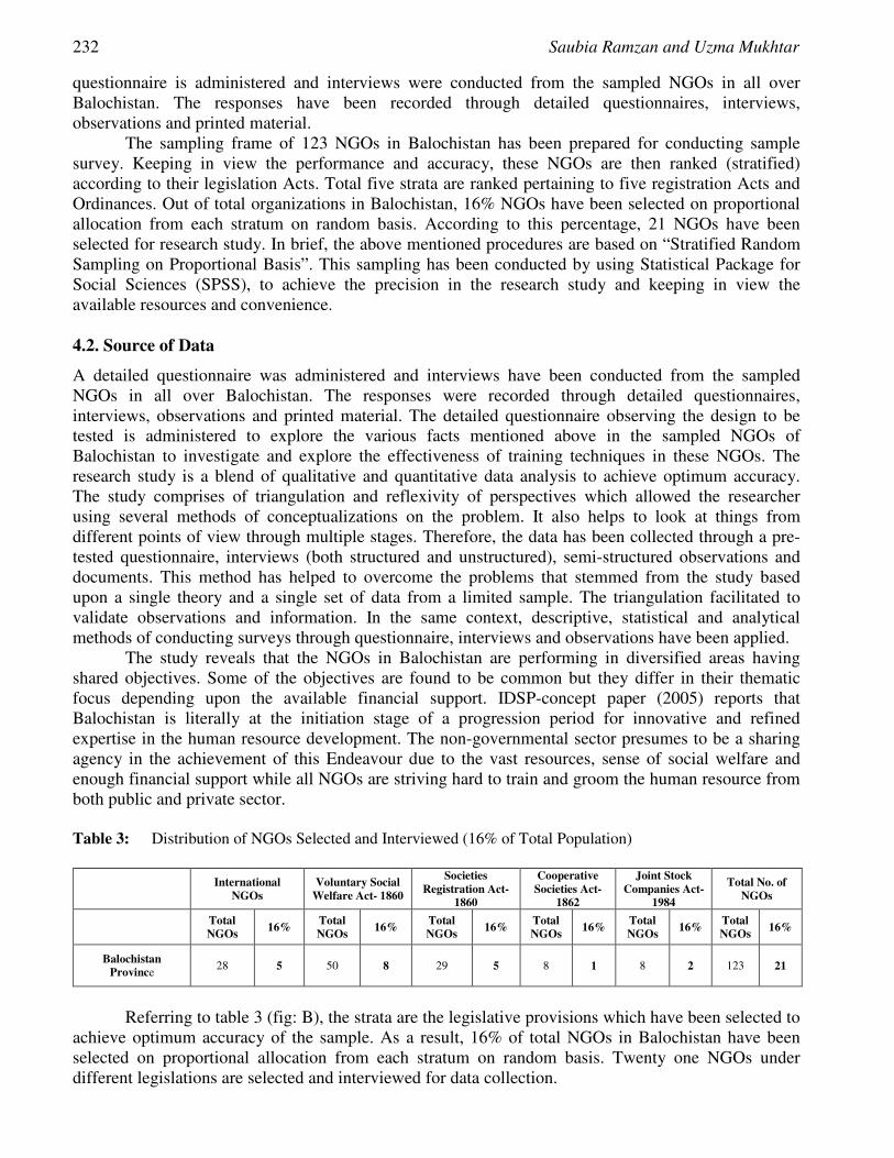
232 Saubia Ramzan and Uzma Mukhtar
questionnaire is administered and interviews were conducted from the sampled NGOs in all over Balochistan. The responses have been recorded through detailed questionnaires, interviews, observations and printed material.
The sampling frame of 123 NGOs in Balochistan has been prepared for conducting sample survey. Keeping in view the performance and accuracy, these NGOs are then ranked (stratified) according to their legislation Acts. Total five strata are ranked pertaining to five registration Acts and Ordinances. Out of total organizations in Balochistan, 16% NGOs have been selected on proportional allocation from each stratum on random basis. According to this percentage, 21 NGOs have been selected for research study. In brief, the above mentioned procedures are based on “Stratified Random Sampling on Proportional Basis”. This sampling has been conducted by using Statistical Package for Social Sciences (SPSS), to achieve the precision in the research study and keeping in view the available resources and convenience. 4.2. Source of Data
A detailed questionnaire was administered and interviews have been conducted from the sampled NGOs in all over Balochistan. The responses were recorded through detailed questionnaires, interviews, observations and printed material. The detailed questionnaire observing the design to be tested is administered to explore the various facts mentioned above in the sampled NGOs of Balochistan to investigate and explore the effectiveness of training techniques in these NGOs. The research study is a blend of qualitative and quantitative data analysis to achieve optimum accuracy. The study comprises of triangulation and reflexivity of perspectives which allowed the researcher using several methods of conceptualizations on the problem. It also helps to look at things from different points of view through multiple stages. Therefore, the data has been collected through a pre-tested questionnaire, interviews (both structured and unstructured), semi-structured observations and documents. This method has helped to overcome the problems that stemmed from the study based upon a single theory and a single set of data from a limited sample. The triangulation facilitated to validate observations and information. In the same context, descriptive, statistical and analytical methods of conducting surveys through questionnaire, interviews and observations have been applied.
The study reveals that the NGOs in Balochistan are performing in diversified areas having shared objectives. Some of the objectives are found to be common but they differ in their thematic focus depending upon the available financial support. IDSP-concept paper (2005) reports that Balochistan is literally at the initiation stage of a progression period for innovative and refined expertise in the human resource development. The non-governmental sector presumes to be a sharing agency in the achievement of this Endeavour due to the vast resources, sense of social welfare and enough financial support while all NGOs are striving hard to train and groom the human resource from both public and private sector. Table 3: Distribution of NGOs Selected and Interviewed (16% of Total Population)
International
NGOs Voluntary Social
Welfare Act- 1860
Societies Registration Act-
1860
Cooperative Societies Act-
1862
Joint Stock Companies Act-
1984
Total No. of NGOs
Total NGOs
16% Total NGOs
16% Total NGOs
16% Total NGOs
16% Total NGOs
16% Total NGOs
16%
Balochistan Province
28 5 50 8 29 5 8 1 8 2 123 21
Referring to table 3 (fig: B), the strata are the legislative provisions which have been selected to
achieve optimum accuracy of the sample. As a result, 16% of total NGOs in Balochistan have been selected on proportional allocation from each stratum on random basis. Twenty one NGOs under different legislations are selected and interviewed for data collection.

A Critical Analysis of the Effectiveness of Human Resource Development Techniques in the Non-Government Organizations of Balochistan 233
Figure B: Distribution of NGOs Selected and Intgerviewed (16% of Total Population)
In addition to the above context, the research exposed the core aspect of study which is concerned with the perception of human resource about traditional and innovative techniques, effectiveness, efficiency and current use. The following debate retrieves the facts about this theme. 4.3. Hypotheses Testing
4.3.1. Perceptions about Effectiveness, Efficiency and Current Use of Traditional and Innovative Development Techniques The selected sample analyzes two major aspects of research study in various dimensions. The aspects under examination are the development methodology of human resources in the NGOs of Balochistan. Therefore, the trainers have been selected randomly for separate perception in order to achieve accuracy of responses. The following version of table 4 presents a clear picture for the perception of trainers about effectiveness of development techniques further categorized into traditional and innovative methods. The following data has been obtained through the questionnaire for trainers about traditional and innovative techniques of development in the NGOs of Balochistan. During the data collection process, 21 itemized development techniques have been divided into two categories including 14 innovative development techniques and only 7 traditional development techniques. Table 4: Perceptions of Trainers about the Effectiveness, Efficiency & Current Use of Development
Techniques
Means of Development Techniques Innovative Traditional Effectiveness 3.9 3.3 Efficiency 3.5 3.4 Current Use 2.8 3.0
Figure C : Premption of Trainers about Effectiveness, Efficiency and Current Use of Development Techniques

234 Saubia Ramzan and Uzma Mukhtar
4.4. Scope of the Research
The research study has been conducted among the NGOs of Balochistan province existing under different legislative provision. The study is based on investigating efficiency and effectiveness of traditional and innovative techniques for development. It examines all enlisted categorised development techniques in the organizational setup to evaluate the effectiveness in terms of learning and innovation among trainees and trainers. Current use of both development techniques have been analysed to get the optimum accuracy in results. NGOs are main stakeholders that strive for capacity building and development of human resource having stable financial position supported by donors in the province. The study has been conducted in the year 2011-2012 pertaining to all information encompassing the development processes and techniques available in the running projects. 5. The Results of Hypotheses Testing In this section of paper we present analysis the results of research hypotheses. As mentioned before, for testing H2 and H4, we also use a sample of state companies. The following subsections provide analysis of results of hypotheses testing at total sample level, industrial group level, and year level. 5.1. Results of Hypothesis 1
According to the hypothesis, it is predicted that innovative development techniques can be more effective and efficient than traditional techniques for the performance of human resource. Table 4 clearly shows the mean scores of perceptions about effectiveness, efficiency and current use of development techniques in the NGOs of Balochistan. During the data collection process, 21 itemized development techniques have been divided into two categories including 7 traditional development techniques and 14 innovative development techniques. The above table shows that traditional development techniques are effective with the average of 3.3 while there are innovative with 3.9. The means of efficiency for the traditional techniques and innovative techniques appear as 3.4 and 3.5 respectively. Along these lines, traditional development techniques are being used with the average ratio of 3.0 while innovative techniques are currently being used with the average of 2.8, as illustrated in fig: C. Table 5: Results for Tests of Significance of Differences between Effectiveness & Efficiency Means of
Innovative & Traditional Development Techniques
Innovative Development Techniques
Traditional Development Techniques
t-test
Effectiveness n = 57 2d∑ = 21.357
X1 = 3.9
n = 57 2d∑ = 21.357
X2 = 3.3
D = 0.6 df = 56
tobt = 7.476 t.05 = 2.00
Efficiency n = 57 2d∑ = 19.344
X1 = 3.5
n = 57 2d∑ = 19.344
X2 = 3.4
D = 0.1 df = 56
tobt = 1.175 t.05 = 2.00
Table 5 shows that the mean perceptions of trainers about the effectiveness of innovative and
traditional development techniques are 3.9 and 3.3, respectively. Statistical analysis of the difference between the two means using t-test for paired sample revealed that for n=57, the observed difference is 7.476 between the means is significant α =.05. This establishes that trainers perceive innovative development techniques as more effective as compared to traditional techniques.

A Critical Analysis of the Effectiveness of Human Resource Development Techniques in the Non-Government Organizations of Balochistan 235
5.2. Results of Hypothesis 2
Table 5 also reveals the mean perceptions of trainers about the efficiency of innovative and traditional development techniques are 3.5 and 3.4 respectively. The difference between the two means is observed through statistical analysis by using t-test for paired sample. For n=57, the obtained value of t is 1.175 between the means is not significant at α =.05. The null hypothesis is not being rejected, therefore, the perceptions of trainers appear to be inconclusive about the efficiency of innovative development techniques as compared to traditional techniques. Table 6: Results for Tests of Significance of Differences between Current Use Means of Innovative &
Traditional Development Techniques
Innovative Development Techniques
Traditional Development Techniques
t-test
Current Use
n = 57 2d∑ = 23.760
X1 = 2.8
n = 57 2d∑ = 23.760
X2 = 3.0
D = -0.2 df = 56
tobt = -2.265 t.05 = 2.00
As predicted in hypothesis, innovative techniques are more popularly used for development of
human resource than traditional techniques in the NGOs of Balochistan. Table 6 shows that the mean perceptions of trainers about the current use of innovative and traditional development techniques are 2.8 and 3.0 respectively. Statistical analysis of the difference between the two means using t-test for paired sample reveals that for n=57, the observed difference is -2.265 between the means is significant at α= .05. Hence, it establishes that traditional techniques are more frequently being used than the innovative development techniques.
Additionally, based on the perceptions of trainers working in the NGOs of Balochistan, useful conclusions have been drawn about the innovative techniques of development. Biographic analysis of trainers shows that trainers in the NGOs are having diverse training experiences and IT capability. Almost the statistical analysis of data establishes that trainers perceive innovative development techniques as more effective and efficient as compared to traditional techniques. The study of means about the current use of development techniques elucidates that innovative development techniques are less frequently being used by trainers as compared to traditional techniques. This could be due to unawareness about latest trends or non-availability of resources. Similarly, statistical analysis deduced about the development techniques that trainers perceive innovative development techniques as more effective as compared to traditional techniques. However, the study reports inconclusiveness about the efficiency of innovative development techniques as compared to traditional techniques. It is assumed that innovation in development is considered effective but the efficiency of both traditional and innovative development techniques has been approved, although, the study of means assumed that innovative development techniques are not frequently being used as compared to traditional techniques. It is inferred that proper awareness and availability of resources are lacking for the adoption of innovative development techniques.94% of trainers are found to have basic IT expertise for applications. This can be assumed that majority of trainers have knowledge about the application of latest techniques into development programs.
Alternatively, the perceptions of trainees have been analysed in terms of means of responses on the set-scale. These responses also analyse the use of IT during training. It is estimated that almost 82.5% of trainees from the selected NGOs are having basic IT expertise for application. The inference indicates that according to trainees’ perceptions, IT can have tremendous positive effect on the professional skills of human resource. Moreover, it reflects that IT can be used as an aid for effective development programs. This specifies that IT can be used for assistance during development process,

236 Saubia Ramzan and Uzma Mukhtar
thereby enhancing the performance of human resource. Personnel’s professional skills and efficacy can be improved by using innovative techniques of development. It is also concluded that trainees are found uncertain about the perception that trainers are not using IT due to lack of knowledge. This can be presumed that lack of knowledge of trainers is not the reason for not using innovative techniques during development programs. 6. Summary and Concluding Remarks In conclusion, the above inferences indicate that traditional techniques for development have also been approved in terms of effectiveness and efficiency. The concept is well supported with relevant literature that traditional techniques could also enhance personnel’s professional skills for the organizations. Therefore, a mixed approach of innovative and traditional techniques can be adopted for the increased performance among human resource of NGOs in Balochistan.
NGOs are inclined to opt for trends of innovation for development of its human capital. Taking into account the drawn conclusions, following recommendations set a way forward for further research horizons.
The study reflects that the ratio of functional NGOs is only 4.6% which need to be checked by the registration authorities through strong accountability process. Strict measures are required by these authorities in order to reduce the increasing number of non-functional NGOs in Balochistan. It has been found out that awareness among trainers of NGOs for use of IT techniques is lacking, therefore, it seems appropriate to create awareness among trainers about the educational designs of IT for use in development of HR. Moreover, mixed practice of blending traditional and innovative development methods need to be introduced for achieving effectiveness in the processes. A mixed method strategy of traditional and innovative techniques for development needs to be promoted for maximum effectiveness and efficiency among human resource. There should be a common pool for training and development of human resource as an integrated effort from NGO network to achieve harmony and innovation in the HR development processes. In this study effectiveness, efficiency and current use of development techniques have been investigated by using triangulation approach. This research opens up various horizons for further investigations of development techniques by applying some other research models.
Theoretical questions such as; biographical characteristics of different age-groups, gender, academic qualifications, job experiences and IT-expertise can have any impact on the perceptions of trainers and trainees about the development techniques in order to explore other dimensions further research studies. The investigated cognitive paradigms of IT techniques for development raise questions for deeper analysis of innovative perspective of HR development in various research approaches. Present study presents a vivid picture about NGOs for human resource development. Other public and private sectors need to be explored for the application of innovation into development techniques for HR. References [1] Aksul Amal. IDSP- Institute for Development Studies and Practices, 2005. Islamabad: ESRA. [2] Albanese R. Competency-based Management Education, Journal of Management Development
1988. USA. [3] Amal- Human Development Network Youth Empowerment Skills – 2005. Pakistan: YES
Project Report. [4] Anthony WP, Perrewe PL and Kacmar KM, Human Resource Management-A Strategic
Approach, 3RD Edition, 1999. U.S.A: The Dryden Press. [5] Aswathappa K, Human Resource and Personnel Management, 4th Edition, 2005. India: Tata
McGraw-Hill.

A Critical Analysis of the Effectiveness of Human Resource Development Techniques in the Non-Government Organizations of Balochistan 237
[6] Bernadin HJ, Human Resource Management – An Experiential Approach, 3rd Edition, 2003. Delhi: McGraw-Hill.
[7] Bhatia SK, Training and Development, Concepts and Practices, Emerging Developments, Challenges and Strategies in HRD, 2005. New Delhi: Deep & Deep Publications.
[8] Blanchard RN and Thacker JW, Effective Training: Systems, Strategies, and Practices, NJ: 2005. Singapore: Pearson Prentice Hall.
[9] Brember I, Class hand-outs,1995. UK: University of Manchester. [10] Buckely R and Caple J, Handbook of Training and Coaching Skills, 2005. India: Kogan Page,
Crest Publishing House. [11] BOYATZIS, R.E., BAKER, A., LEONARD, D., RHEE, K. and THOMPSON, L. (1995), Will
It Make A Difference? Assessing a Value-added, Outcome-oriented, Competency-based Program, Jossey-Bass, San Francisco.
[12] Budd ML, Self-Instruction, In R.L. Craig Edition, Training and Development Handbook, 1987. New York: McGraw-Hill.
[13] BURKE, M.J. and Day, R.R. (1986), A Cumulative Study of the Effectiveness of Managerial Training, Journal of Applied Psychology, Southern Management Association.
[14] Campbell JP. Dunnette MD. Lawler,EE and Iiiweick,KEJR, Managerial Behavior: Performance and Effectiveness,1970. New York: McGraw-Hill.
[15] Chandra H, Human Resource Development- Theories and Practices, 2006. India, Akansha Publishing House.
[16] Collins Cobuild English Dictionary, 1995. UK: Harper Collins Publishers. [17] Connor O. Bronner M and Delaney C, Training for Organization, Cincinnati, 1999. Ohio,
South-Western Educational Publishing. [18] Department for education, Information Technology in Initial Teacher Training, 1989. London:
HMSO publications. [19] Desimone R L, Werner J M and Harris D M, Human Resource Development, 3rd Edition, 2005.
Singapore, Thomson South-Western. [20] Directory of Intermediary NGOs in Pakistan, 2000. Pakistan: NGORC, Karachi. [21] Directory of NGOs in Pakistan, NGO Resource center, 2005. Pakistan: Agha Khan Foundation. [22] Directory of Voluntary Social Welfare Agencies in Balochistan, Department of Social Welfare,
2005. Pakistan: Government of Balochistan. [23] Georce HC, Manager Development: Principles and Perspectives, 1961. Homewood: Richard
D. Irwin Inc. [24] Gutteridge TG, Lleibowitz ZB and Shore JE, Organizational Career Development:
Benchmarks for Building a World-class Workforce,1993. San Francisco: Jossey-Bass. [25] Hawkridge D. Jaworski J and Mcmahaon H, Computers and Education, 1990. UK. [26] Heery E and Noon M, A Dictionary of Human Resource Management, 2001. Great Britain:
Oxford University Press. [27] IDSP Concept Paper, Institute for Development Studies and Practices, 1997. Pakistan. [28] IDSP Pakistan Annual Report, Institute for Development Studies and Practices, 2005. Pakistan. [29] Igonor A, Success Factors for Development of Knowledge Management in E-Learning in Gulf
Region Institutions, 2002. Journal of Knowledge Management Practice. [30] James SG, Career Development and Job Training: A Manager’s Handbook, 2002. New York:
AMACOM. [31] Johnston JS JR and Associates, Educating Mangers: Executive Effectiveness Through Liberal
Learning, 1986. San Francisco: Jossey-Bass. [32] Kapenieks A. Zuga B. Buligina I. Gercane l. Kulitane I. Vucena A. Rudzite M and Trapenciere
I, Innovative E-Learning in Regional Development Projects in Latvia, Report prepared within

238 Saubia Ramzan and Uzma Mukhtar
EU, 5th Framework Programme Project Higher Education Reform Network (HERN), 2004. UK: Seminar in Glasgow.
[33] Keys B and Wolfe J, Management Education and Development: Current Issues and Emerging Trends, 1988. U.S.A: Journal of Management.
[34] Kirkpatrick D L, How to Improve Performance Through Appraisal and Coaching,1982. New York: AMACOM.
[35] Llgen D R and Pulakos E D, Adaptability in the workplace: Development of Adaptive Performance, 1999. USA: Journal of Applied Psychology.
[36] Malone S A. A to Z of Training & Development Tools & Techniques, 2005. India: Jaico Publishing House.
[37] Marliyn MA, Managing Career Development, Van Nostrand Reinhold Co, 1980. New York. [38] Martin B I and Briggs, L J, The Affective and Cognitive Domains: Integration for Instruction
and Research,1986. Englewood Cliffs: Educational Technology Publication. [39] MARTIN, B.L. and BRIGGS, L.J. (1986) The Affective and Cognitive Domains: Integration
for Instruction and Research, Educational Technology Publications, Englewood Cliffs, NJ. [40] Mathis R L and Jackson J H. Human Resource Management, 10th Edition, 2004. Ohio:
Thomson South Western. [41] Mikkelsen B. Methods For Development Work and Research – A New Guide For Practitioners,
2nd Edition, 2005. London: Sage Publication. [42] MUMFORD, A. (1987), Action Learning (Special Issue), Journal of Management
Development, New York. [43] ROFFE, I. Journal of European Industrial Training Year-1999, vol.23, No.4,5, Emerald. [44] Salzman M L and Sullivan D A. Inside Management Training: The Career Guide to Training
Programs for College Graduates, 1985. New York: New American Library. [45] STACKEL, L. (1988), Successful Training strategies, National Technological University, Lotto
& Associates, Jossey-Bass, San Francisco. [46] State of the Industry Report, ASTD- American Society for Training Directors, 2000.
Alexandria. [47] Transform, Issue on History Development Education and Culture, 2005. Islamabad: ESRA. [48] http://www.astd.org [49] www.cipd.co.uk/bookstore [50] http://www.dfes.gov.uk/learning strategy/elearning.stm [51] http://www.informationr.net/ir/2-1/paper12 html [52] www.ngorc.org.pk [53] www.pentagon-press.com [54] http://www.prenhall.com/gomez,(Gomez-Mejia, Balkin, and Cardy). [55] http://www.shrm.org/, Society for Human Resource Management (SHRM), (Home page of
SHRM; summarizes the latest developments in HRM on a daily basis). [56] http://www.shrm.org/docs/Hrmagazine.html, HR Magazine, (Articles from HR Magazine,
published monthly by the Society for Human Resource Management). [57] http://www.trainingnet.com/, Training Net, (An information resource for training
professionals).
European Journal of Scientific Research ISSN 1450-216X / 1450-202X Vol. 103 No 2 June, 2013, pp.239 - 255 http://www.europeanjournalofscientificresearch.com
Dimensionality Reduction of High Dimensional Data Using Fractional Cuckoo Search Algorithm to Improve Clustering
Process
Golda George Assistant Professor Department of Computer Science Engineering
Dr.MGR Educational & Research Institute, Chennai Research Scholar, Sathyabama University, Chennai
E-mail: [email protected]
Latha Parthiban Department of Computer Science; Pondicherry University Community College
Abstract
Dimensionality reduction is essential in multidimensional data mining since the dimensionality of real time data could easily reach higher dimensions. Most recent efforts on dimensionality reduction, however, are not adequate to multidimensional data due to lack of scalability. In this paper, we use the optimization algorithm for dimension reduction process. The optimization algorithm adopted for the proposed approach is the cuckoo search algorithm. The modifications on cuckoo search bring it as a dimensionality reduction algorithm to fit in the multidimensional clustering. The cuckoo search is selected for the dimensionality reduction process is because of the specific characteristics produced by the cuckoo search algorithm. Here, we introduce a modified cuckoo search algorithm called fractional cuckoo search (FCS) algorithm with levy space. We modified the cuckoo search algorithm to reduce the dimension and select the best dimension. Once the high dimensional data reduced in to low dimensional data, then the data is supplied to the clustering algorithm to make the partition easily. Finally, the experimentation is made with synthetic and real datasets (iris and wine) and we have proved the efficiency of the FCS algorithm 12.3% on iris, 35.1% on wine and synthetic dataset has 30.75% better than the FPSO in terms of accuracy. Keywords: Cuckoo search algorithm, levy flights, dimension reduction, high dimensional
database, fractional cuckoo search. 1. Introduction In discovering knowledge hidden in databases, data mining evolves as a promising solution. Data Mining has been properly defined as “the non-trivial extraction of implicit, previously unknown and potentially useful information from data in databases” [6], [7]. Both in the private and public sectors data mining has been utilized for multiple needs. market segmentation, fraud detection, direct marketing, interactive marketing, market basket analysis, trend analysis and more are included in the precise usage of data mining include [8]. Descriptive and predictive are the two general classes of data mining techniques. To discover patterns is the intention of descriptive data mining, e.g., product configurations produced in mass customization applications [9]. Clustering, Association rule mining
240 Golda George and Latha Parthiban
and sequential pattern mining are few examples of the descriptive data mining tasks [10]. The predictive data mining intends at building frameworks to resolve or predict an outcome, e.g., a stock level [9]. Classification, Regression and Deviation Detection are tasks encompassed in predictive data mining.
Clustering can be defined as the unsupervised classification of patterns into groups. It is the task of grouping a set of objects into different subsets such that objects belonging to the same cluster are highly similar to each other. For condensing and summarizing information clustering is a very important process, as it can give a synopsis of the stored data. In the field of data mining, multidimensional data clustering is one of the most discussed areas. The extensive computerization and affordable storage facilities resulted in copious amount of information to be available in databases belonging to various enterprises [5]. The decisive target of this huge data collection is the utilization of this information to achieve competitive remunerations, by identifying previously hidden patterns in data that can direct the process of decision making [11]. Lately, ABC algorithm [19] is used for data clustering. Later on, a general stochastic clustering method [21] is introduced as a generalization of nature-inspired ant-based clustering approach. It begins with a basic solution and then performs stochastic search to incrementally recover the solution until the fundamental clusters emerge, resulting in automatic cluster discovery in datasets.
The main problem in clustering the multidimensional is because of the higher dimensions of the data. In clustering high dimensional data, the clustering process strikes complexity. In mining high dimensional data, dimensionality reduction is among the keys. For many data mining tasks, with the rapid accumulation of high-dimensional data such as digital images, financial time series and gene expression microarrays, dimensionality reduction has been a fundamental tool. Existing dimensionality reduction methods can be roughly categorized into supervised ones and unsupervised ones, according to whether supervised information is available or not. Fisher Linear Discriminant (FLD) [12] is an example of supervised dimensionality reduction methods, which can extract the optimal discriminant vectors when class labels are available; while Principal Component Analysis (PCA) [13] is an example of unsupervised dimensionality reduction methods, which works through trying to conserve the global covariance structure of data when class labels are not available. In recent times, a number of researches are conducted based on the dimensionality reduction in order to progress the clustering of multidimensional data.
To exploit pair wise constraints or other prior information in dimensionality reduction, a number of recent works have attempted. Bar-Hillel et al. [14] proposed the constrained FLD (cFLD) for dimensionality reduction from equivalence constraints, as an interim-step for Relevant Component Analysis (RCA). Though, cFLD can only deal with the must link constraints. In addition, as in FLD, when constraints are limited cFLD has the singular problem. To guide dimensionality reduction, Tang and Zhong [15] used pair wise constraints, which can use both must-link constraints and cannot-link constraints but does not consider the value of abundant unlabelled data. Yang et al. [16] exploited prior information in the form of on-manifold coordinates of certain data samples for dimensionality reduction. It is evident that usually obtaining the pairwise constraints is much easier than obtaining the on-manifold coordinates of data samples. Recently, [1] have discussed a dimensionality reduction method through optimization algorithms, inspired from the research, I intent to propose a method for dimensionality reduction based optimization algorithms.
We modified the cuckoo search algorithm named as fractional cuckoo search algorithm (FBS) in this paper and to fit in the multidimensional clustering it brings a dimensionality reduction algorithm. At first, the FBS algorithm chooses number of nest then makes the dimension tables and nest tables then the FBS fills the eggs (solutions) randomly in the nest tables based on the dimension of the nest present in the dimension table. Based on the fitness value of the nest, FBS computes fitness value for each nest in the nest tables and arranged in descending order. FBS initialize the value of best nest by select the nest which placed in first on the nest table, from the arranged nest. If the fitness value of new best nest has less than existing fitness value, the best nest values may change at every iteration. The values (eggs) in the nest tables get updates based on the levy flights. At last, the best nest
Dimensionality Reduction of High Dimensional Data Using Fractional Cuckoo Search Algorithm to Improve Clustering Process 241
is selected with the best dimension (reduced dimension). The cluster algorithm makes the cluster easily based on the result of the FBS algorithm.
The rest of the paper is organized as follows: a brief review of some of the literature works in privacy preserving data mining is presented in Section 2. The problem formulation of proposed technique is given in Section 3. The proposed technique for dimensionality reduction of high dimensional data using fractional cuckoo search algorithm to improve clustering process is detailed in Section 4. The experimental results and the performance evaluation discussion are provided in Section 5. Finally, the conclusions are summed up in Section 6. 2. Literature Review In this section, plots of recent research are shown to discuss about the dimensionality reduction and different methods involving in solving the dimensionality reduction problem in clustering multidimensional data.
Serkan Kiranyaz et al. [1] have proposed two novel techniques in the field of particle swarm optimization (PSO), which successfully address several major problems and promise an important breakthrough over compound multimodal optimization problems at high dimensions. The first one, which is the so-called multidimensional (MD) PSO, with a dedicated dimensional PSO process re-forms the native structure of swarm particles in such a way that they can make interdimensional passes. Hence, swarm particles can seek both positional and dimensional optima in an MD search space, where the optimum dimension is unknown. For the family of swarm optimizers, this ultimately removes the inevitability of setting a fixed dimension a priori, which is a common drawback. Though, due to lack of divergence MD PSO is still liable to premature convergences. Among many PSO variants in the literature, none yields a healthy solution, mainly over multimodal complex problems at high dimensions. They proposed the fractional global best formation (FGBF) technique, which basically collects all the best dimensional components and fractionally creates an artificial global best (aGB) particle that has the possibility to be a better “guide” than the PSO’s native gbest particle to address the problem. At the true dimension regardless of the search space dimension, swarm size, and the difficulty of the problem, an wide set of experiments shows that in both application domains, MD PSO with FGBF exhibits a striking speed gain and converges to the global optima.
In mining high dimensional data, dimensionality reduction is among the keys. Daoqiang Zhang et al. [3] have studied semi-supervised dimensionality reduction. In the setting, besides abundant unlabelled examples, domain knowledge in the form of pairwise constraints are available, which specifies whether a pair of instances belong to the same class (must-link constraints) or different classes (cannot-link constraints). They proposed the SSDR algorithm, in the projected low-dimensional space which can protect the basic structure of the unlabelled data as well as both the must-link and cannot-link constraints defined on the labelled examples. To many recognized dimensionality reduction methods, the SSDR algorithm is capable and has a closed form solution. Experiments on a broad range of data sets show that SSDR is superior.
Min Soo Kim et al. [4] proposed a new type of simple but effective dimensionality reduction, called horizontal (dimensionality) reduction, for large document databases. Horizontal reduction converts each text document to a few bitmap vectors and provides tight lower bounds of inter-document distances using those bitmap vectors. For large and dynamic document databases, bitmap representation is very simple and enormously fast, and its instance-based nature makes it suitable. Using the proposed horizontal reduction, we develop an efficient k-nearest neighbour (k-NN) search algorithm for text mining such as classification and clustering, and we formally prove its correctness. The proposed algorithm decreases I/O and CPU overheads simultaneously since horizontal reduction (1) reduces the number of accesses to documents significantly by exploiting the bitmap-based lower bounds in filtering dissimilar documents at an early stage, and accordingly, (2) decreases the number of
242 Golda George and Latha Parthiban
CPU-intensive computations for obtaining a real distance between high-dimensional document vectors. Extensive experimental results show that horizontal reduction improves the performance of the reduction (pre-processing) process by one to two orders of magnitude compared with existing reduction techniques, and our k-NN search algorithm significantly outperforms the existing ones by one to three orders of magnitude.
Than the traditional K-means clustering algorithm, the Particle Swarm Optimization (PSO) clustering algorithm can produce more compact clustering results. Though when clustering high dimensional datasets, the PSO clustering algorithm is notoriously slows because its computation cost increases exponentially with the size of the dataset dimension. Dimensionality reduction techniques offer solutions that both considerably progress the computation time, and give up rationally accurate clustering results in high dimensional data analysis. Xiaohui Cui et al. [17] introduced research that combines different dimensionality reduction techniques in order to reduce the complexity of high dimensional datasets and speed up the PSO clustering process with the PSO clustering algorithm. We report noteworthy improvements in total runtime. Additionally, the clustering accuracy of the dimensionality reduction PSO clustering algorithm is comparable to the one that uses full dimension space.
Guanghui Yan [18] has given more attention for the interaction between dimensionality reduction and cluster evolution in the inconstant high dimensional stream data. And on this basis, they proposed the adaptive cluster evolution tracking algorithm which integrated the on-line fractal dimensionality reduction technique. Experimental results over a number of real and synthetic data sets shows that the method proposed are both effectiveness and efficiency. Detecting and tracking of cluster evolution has always been crucial to the stream data mining. As it is in high dimensional stream data environment, under the interaction between dimensionality reduction and cluster evolution condition it becomes more difficult. In the reduced dimensionality space, the past has been focus on cluster evolution occurred. Dimensionality reduction before the cluster evolution option, still, cannot cope with the unexpected changes which are common in stream data. During the process of the cluster evolution there is the demand of the dimensionality reduction, which is the most popular case.
Dervis Karaboga and CelalOzturk [19] have proposed an ABC algorithm used for data clustering on benchmark problems and the performance of ABC algorithm is compared with Particle Swarm Optimization (PSO) algorithm and other nine classification techniques from the literature. Thirteen of typical test data sets from the UCI Machine Learning Repository are used to demonstrate the outcomes of the methods. The simulation results specify that ABC algorithm can proficiently be used for multivariate data clustering. They selected the ABC algorithm, which is one of the most newly introduced optimization algorithms, since it simulates the intelligent foraging behavior of a honey bee swarm. Clustering analysis, used in many disciplines and applications, is an important tool and based on the values of their attributes a descriptive task seeking to identify homogeneous groups of objects
Bahriye Akay et.al [21] proposed an adapted version of the Artificial Bee Colony algorithm. For proficiently solving real-parameter optimization problems they have applied modified version. Swee Chuan Tan et.al [22] proposes a general stochastic clustering method that is a simplification of nature-inspired ant-based clustering approach. It begins with a basic solution and then performs stochastic search to incrementally progress the solution until the original clusters emerge, resulting in automatic cluster discovery in datasets. This method differs from a number of recent methods, in that it does not need users to input the number of clusters and it makes no clear assumption about the basic distribution of a dataset. In terms of clustering accuracy and effectiveness in majority of the datasets used in this study, our experimental results show that the proposed method performs better than quite a lot of existing methods. Our theoretical analysis shows that the proposed method has linear time and space complexities, and our empirical study shows that it can precisely and competently determine clusters in large datasets in which many accessible methods fail to run.
Fuhua Yu [20], allowing for the limited request and shortcoming of FCM (Fuzzy C-Means) clustering algorithm, proposed an enhanced automatic FCM clustering algorithm. Initially, the fuzzy equivalent matrix is achieved by fuzzier the standard uniform data sets; then, the objective function of the

Dimensionality Reduction of High Dimensional Data Using Fractional Cuckoo Search Algorithm to Improve Clustering Process 243
superior automatic FCM clustering algorithm is optimized by the adjustment of membership function and distance measuring function; To update iteration of membership degree and clustering center, the Lagrange multiplier optimization algorithm is calculated. To conclude, the automatic clustering is obtained by the degree of cohesion and separation. To apply the improved automatic FCM clustering algorithm, the traffic flow data of an extra-long highway tunnel in Shaanxi is taken as an actual example. The clustering result shows that the validity of clustering is enhanced using the better automatic FCM algorithm. 3. Problem Statement The high dimensional database has many fields { }1 2, . . . nDB A A A= where n is the total number of
fields (attributes). Clustering of the high dimensional data is very difficult process and the accuracy of the high dimensional data clustering is also poor. Dimension reduction is the technique to increase the accuracy of high dimensional clustering process. The selection of important attributes of the dimension is not an easy task and we modifying the cuckoo search algorithm to fit the dimension reduction process. Our paper gives solutions to solve the above problems. 4. Dimensionality Reduction of High Dimensional Data Using Fractional Cuckoo Search Algorithm to Improve Clustering Process The high dimensional database has many fields such as { }1 2, . . . nDB A A A= . The traditional clustering
of high dimensional database is very difficult and the clustering algorithm takes more computation time and less accuracy. To solve this problem, the researches plan to reduce the high dimensional dataset into low dimensional dataset to improve the accuracy and computation time of clustering by selecting the important attributes of the database. At the same time finding of important attribute of the high dimensional database is not an easy task. There are many dimension reduction algorithms are available [23]. From which optimization algorithms can gives the best solution for selecting the exact attributes. The particle swarm optimization algorithm (PSO) is mostly used optimization algorithm to solve many problems. In paper [1] introduced a method for dimensionality reduction based on fractional particle swarm optimization algorithm. The main drawback in the method based on PSO algorithm is the convergence performance. The convergence performance is not altered much by the PSO method, which intern reduces the efficiency of the dimensionality reduction. The use of cuckoo search can improve the convergence performance and increase the efficiency dimensionality reduction. In this paper, we modify the cuckoo search algorithm and we named the modified cuckoo search algorithm as fractional cuckoo search algorithm which helps to select the best dimension of the database.
Figure 1: Shows that the block diagram of the proposed algorithm

244 Golda George and Latha Parthiban
The above figure illustrates block diagram of this paper. Initially the high dimension data is given to the proposed fractional cuckoo search algorithm from which our proposed algorithm selects the best dimensions of the high dimension algorithm. Once the high dimensional data is reduced to low dimensional data by our proposed fractional cuckoo search algorithm, then the result data of the proposed algorithm is supplied to any of the clustering algorithm. The result of the clustering algorithm gives the efficient clustered data. 4.1. Fractional Cuckoo Search Algorithm
The fractional cuckoo search algorithm helps convert the high dimensional database to the low dimensional database through select the best attributes (fields) available in the high dimensional database. To select the important (best) attributes of the high dimensional data, the fractional cuckoo search algorithm maintains an additional table named as dimension table which helps to find the dimension of the nest.
The fractional cuckoo search algorithm has the following steps 1. Generation of nest and dimension tables 2. Calculation of fitness 3. Find best nest with best dimension 4. Updation of nest and dimension table with levy flights
4.1.1. Generation of Nest and Dimension Table 4.1.1.1. Dimension Table To select the best solution, initially the fractional cuckoo search algorithm chooses the number of nest
kN subsequently it assigns dimension to each nest ( )j iD N randomly named as dimension table ( )D T t
also it gets value of the number of clusters mC from the user. With the help of above three values kN ,
( )j iD N , mC , the proposed algorithm generates the nest table ( )N T t With possible eggs.
Table 1: Represents the dimension table
Nest Dimension
1N jD
2N jD
⋮ ⋮
1kN − jD
kN jD
Above table 1 represents the dimension table, which has the dimension of each nest. Each nest
has different dimension. The dimension value of the each nest must present in the range of 1 j n≤ ≥
where n is the maximum value of dimension. With the help of the minimum and maximum bound of
the dimension, initially the algorithm assigns the dimension to each nest ( )j iD N t randomly. Here, the
FCS algorithm makes the two dimension tables ( )j iD N t to find the perfect solution, the two dimension
tables are named as ( )j pD N t , ( )j qD N t
4.1.1.2. Nest Table

Dimensionality Reduction of High Dimensional Data Using Fractional Cuckoo Search Algorithm to Improve Clustering Process 245
To generate the nest table ( )N T t , the FCS algorithm needs one more value called number of clusters
mC which is get from the user. The value of cluster mC is same for the all nest iN but the value of
dimension jD is not same for every nest iN . The inner value of the nest table is filled by the solutions
(eggs). The following table 2 represents the nest table ( )N T t .
Table 2: Represents the nest table
Nest
Cluster 1C Cluster vC Cluster mC
1D 2D … 1nD −
nD 1D 2D …
1nD − nD 1D 2D … 1nD − nD
1N 111e 1
12e 11 je
11 1ne −
11ne 11
ve 12ve
1vje 1 1
vne −
vne1
me11 me12
mje1
mne 11 −
mne1
2N 121e
122e
12 je
1
12 −ne
12ne
ve21
ve22 v
je2 2 1vne − 2
vne
me21 me22
mje2
mne 12 −
mne2
⋮ 11ie
12ie
1ije
1
1−ine
1ine
vie 1
vie 2
vije
vine 1−
vine
mie 1
mie 2
mije
mine 1−
mine
1−kN
111−ke
121−ke
11 jke −
111 −− nke
11nke −
vke 11−
vke 12−
vjke 1−
vnke 11 −−
vnke 1−
mke 11−
mke 12−
mjke 1−
mnke 11 −−
mnke 1−
kN
11ke
1
2ke
1kje
1
1−kne
1kne
vke 1
vke 2
vkje
vkne 1−
vkne
mke 1
mke 2
mkje
mkne 1−
mkne
Here, the FCS algorithm makes the two dimension tables ( )j iD N t to find the perfect solution,
the two dimension tables are named as ( )j pD N t , ( )j qD N t for each dimension table, the algorithm
generates two nest tables namely ( )pN T t , ( )qN T t . The eggs (solutions) are filled in the each nest in
the nest table ( )N T t based on the value of cluster mC and values of dimension kD of the each nest
table from the high dimensional database. The eggs are filled in the each nest in the nest
table ( )pN T t from the high dimensional database based on the dimension values jD and cluster
values vC . The solution of the other nest table ( )qN T t is filled with random values based on the upper
bound and lower bound of the high dimensional database. Algorithm Procedure Input: high dimensional database Output: best nest value with best dimension Parameters
( )N T = nest table
kN = number of nest
mC = number of clusters
( )j iD N = dimension of nest
( )CS T t = column size of nest table
( )RS T t = row size of nest table

246 Golda George and Latha Parthiban
DB =database
iC =cluster centroid value
( )S DB =size of database
( )1 if N = initial fitness
F = fitness DM =distance matrix
( )RS T = random size table
Begin
Generate nest tables ( )pN T t , ( )qN T t
Get value of iN where ( )1 i K≤ ≥ , ( ) ( )p qK N T N T→ =
Generation of dimension table ( )pD T t , ( )qD T t
Get value of ( )j iD N t
Get value of CN
Column size of the ( )pN T t , ( )qN T t� ( ) ( ) ( )j iCS T t D N t N C= ×
Row size of the ( )pN T t , ( )qN T t� ( )RS T t = kN
Size of the nest ( )pN T t , ( )qN T t� ( ) ( )CS T t RS T t×
For each nest in ( )pN T t
For each cluster iC
Fill ( )tND ij number of eggs from DB
End for End for
For each nest ( )qN T t
For each cluster iC
Fill ( )j iD N t number eggs randomly
End for End for
Call fitness
Call p best and g best If G best (t+1) < G best (t)
Update g best and p best as G, P best (t+1) Else
Update p best as p (t+1) Call Updation Subroutine: Fitness For each nest
For each iC value
Calculate distance matrix DM with DB For each attribute in DM
Find min value
( )1 minf a=∑

Dimensionality Reduction of High Dimensional Data Using Fractional Cuckoo Search Algorithm to Improve Clustering Process 247
End for End for
Calculate fitness ( )
( )
( ) ( )( ) ( )( )( )( )
1
max 1
i
j j i
i
j i
f N
S DB D D NF N
D N
α × + − =
Subroutine: P best and g best For each nest
Arrange nest based on fitness
Select best 2kN nest
End for Concatenate those best values
Generate new nest table ( )rN T t
Arrange nest based on fitness Initialize p best (t) and g best (t)
Subroutine: Updation For each dimension table
Call levy flights End for
For each Nest table and Call levy function
End for Subroutine: Levy flights
Calculate ( )
( )11
2
*1 sin
2
1* * 2
2
ββ
π βγ β
σβ
γ β −
+
= +
For each nest Get value of ( )S T
Calculate U= ( )*RS T σ
Calculate V= ( )RS T
Calculate step = 1
~
U
V β
Calculate step size = ( )sbeststep*01.0
( )1iN t + = ( )( )iN t step size+ * ( )RS T
End for End 4.1.2. Calculation of Fitness The fitness value of the each nest helps to finds the best nest among the set of available nest.
In the nest table, there is K number of nest available from which to select the best nest FCS calculates the fitness value of each nest. Based on the fitness value of each nest FCS arranges the nest

248 Golda George and Latha Parthiban
in the nest table. To calculate fitness of each nest, initially the FCS algorithm computes the distance matrix for find the initial fitness of the nest. With the help of initial fitness, FCS algorithm computes the final fitness of each nest. The distance matrix is generated by compute the distance between the values of eggs in the each nest of each cluster v
ije and data label of the database idl .
4.1.2.1. Distance Matrix Each nest iN has the number of eggs v
ije where i represents the nest, j represents the dimension of the
eggs and value of j varies from1 j n≤ ≥ . The value of v represents the cluster of the eggs and the
value of vvary from1 v m≤ ≥ . The FCS algorithm computes the distance vijd between the eggs of the
nest iN in the nest table ( )N T t and the each data label idl in the database DB . Likewise the FCS
algorithm computes the distance matrix for every nest. The distance matrix for the nest iN is given the
following table 3. Table 3: Represents the distance matrix of nest iN with the DB
Data Base Cluster 1C Cluster vC
Cluster mC
1D
2D …
1−nD
nD 1D 2D
… 1−nD
nD
1D 2D …
1−nD
nD
1dl 111d
112d
11 jd
1
11 −nd
11nd
vd11
vd12 vjd1
vnd 11 −
vnd1
md11 md12
mjd1
mnd 11 −
mnd1
2dl 121d
122d
12 jd
1
12 −nd
12nd
vd 21
vd22 v
jd2 vnd 12 −
vnd2
md 21 md22
mjd2
mnd 12 −
mnd2
⋮ 11id
12id
1ijd
1
1−ind
1ind
vid 1
vid 2
vijd
vind 1−
vind
mid 1
mid 2
mijd
mind 1−
mind
1−Ndl
111−Nd
121−Nd
11 jNd −
11 −− nNd
11nNd −
vNd 11−
vNd 12−
vjNd 1−
vnNd 1 −−
vnNd 1−
mNd 11−
mNd 12−
mjNd 1−
mnNd 1 −−
mNd 1−
Ndl
11Nd
12Nd
1Njd
1
1−Nnd
1Nnd
vNd 1
vNd 2
vNjd
vNnd 1−
vNnd
mNd 1
mNd 2
mNjd
mNnd 1−
mNnd
4.1.2.2. Fitness The initial fitness of each nest is calculated from the distance matrix of that nest. With the aid of the initial fitness, the FBS algorithm can computes the final fitness of the nest ( )iF N . To find the initial
fitness of each nest ( )1 if N , the FBS takes the minimum distance vijd value of each dimension 1D where
1 j n≤ ≥ in each cluster vC where1 v m≤ ≥ . The addition of all minimum distance from each cluster in
the nest is the value of initial fitness. The following equation 1 helps to find the initial fitness of nest ( )1 if N . The equation 2 helps to find the final finest ( )iF N .
( ), ,
1, , 1
mini N j n v m
vi ij
i j v
f N d= = =
=
= ∑ (1)
( )
( )
( ) ( )( ) ( )( )( )( )
1
max 1
i
j j i
i
j i
f N
S DB D D NF N
D N
α × + − = (2)

Dimensionality Reduction of High Dimensional Data Using Fractional Cuckoo Search Algorithm to Improve Clustering Process 249
From the equation 2, ( )S DB represents the size of the database, ( )max jD represents
maximum value of the dimension of the database and ( )( )j iD N represents the dimension of the
nest iN and the value of α is the constant value. The order of the nest in the nest tables is changed in to
the descending order based on the fitness value of the nest tables ( )pN T t , ( )qN T t
4.1.3. Find Best Nest with Best Dimension
After change the position of the nest based on the fitness value of both nest table ( )pN T t , ( )qN T t the
FBS algorithm selects the first (best) 2kN values from each nest table denoted as ( ) 2k pN T and
( ) 2k qN T from the nest tables ( )pN T t , ( )qN T t respectively. The FCS generates new nest
table ( )rN T t by concatenate those ( ) 2k qN T , ( ) 2k pN T best values subsequently the nests are
arranged in descending order based on the fitness value of the nest table ( )rN T t consequently the FCS
algorithm initialize for “best nest” (centroid) by selects first value ( )1 rN T t as “best nest” from the nest
table ( )rN T t . At every iteration the value of g best become change if the following condition satisfied
which represents in the following equation (3).
( )( ) ( )( ) ( )( )
( )( )1 1 1
1
,
,
r r r
r
best nest N T t if F N T t F N T t TN T t T
F N T t T else
= < + + =
+ (3)
4.1.4. Updation In the first iteration, the FCS initializes value for best nest. To find the optimum value of best nest (best solution) algorithm changes value of nest at every iteration. Before Updation of nest table, FCS
updates the dimension tables first ( )j pD N t , ( )j qD N t . To find the best solution, every time (iteration)
the solution values vije (eggs) and dimension of the nest ( )( )j iD N must be change for both nest
table ( )pN T t , ( )qN T t . The levy flights technique which helps to change the value of vije and
( )( )j iD N of nest table ( )pN T t , ( )qN T t
4.1.4.1. Levy Flights For every nest in the nest table levy flights generates the random value U and V by consider the size of
the nest ( )( )j iD N andσ subsequently calculates step and step size with the aid of U and V. The levy
flights calculates step size value to generate a new value of nest by add the existing value of the nest. The old value of the nest ( )iN t is replaced by new value ( )1iN t + which is calculated with the help of
the following equation 4. The old value of the dimension of the nest is replaced by the new value
( )( ) 1j iD N t + which is calculated with the help of the following equation 5.
( ) ( )( ) ( )1 *i iN t N t step size RS T+ = + (4)
( )( ) ( )( )( ) ( )1 *j i j iD N t D N t step size RS T+ = + (5)
( )0.01*step size step sbest= (6)

250 Golda George and Latha Parthiban
1
~
Ustep
V β= (7)
( )*U RS T σ= (8)
( )V RS T= (9)
( )
( )11
2
*1 sin
2
1* * 2
2
β
β
π βγ β
σβ
γ β
−
+
= +
(10)
While replacing the existing value the algorithm confirm if the value of new solution must between the lower bound and upper bound of the database. After the Updation process, the dimension
table and nest tables are represented ( ) 1j pD N t + , ( ) 1j qD N t + , ( ) 1pN T t + , ( ) 1qN T t + respectively.
Every iterations the value of time ( )t gets increase.
5. Result and Discussion The experimental result of the proposed technique for dimensionality reduction of high dimensional data using fractional cuckoo search algorithm to improve clustering process is described in this section. The comparative analysis of the fractional cuckoo search algorithm with the FPSO algorithm [1] is presented for synthetic and real world datasets. 5.1. Experimental Design
The proposed approach of fractional cuckoo search algorithm is programmed using MATLAB 2011a (7.12.0). The experimentation has been carried out using the synthetic datasets as well as the real datasets with i3 processor PC machine with 4 GB main memory running a 32-bit version of Windows XP. Dataset 1: (synthetic data): We have generated the synthetic data that comprise of two attributes and 3000 numbers of instances. Dataset 2: (Real world data): We have taken the real world data, ‘iris’ and ‘wine’, from the UCI machine learning repository [24]. The iris data has 4 attributes and it has 150 numbers of instances. The wine dataset ha 13 attributes and it has 178 numbers of instances. The result of clustering of the synthetic dataset is given in the following figure 2.
Figure 2: Shows that the result of clustering of the synthetic dataset
5.2. Evaluation Metrics
We evaluate our proposed FCS algorithm based on the clustering accuracy. The output of the proposed FCS algorithm is the given to the clustering algorithm. The clustering algorithm considers the output of

Dimensionality Reduction of High Dimensional Data Using Fractional Cuckoo Search Algorithm to Improve Clustering Process 251
the FCS as centroid and makes the partitions based on the centroid. Now we compare the original classification data with our clustered result to evaluate the accuracy of the FCS algorithm. The following equation 10 helps to find the accuracy of the algorithm.
( )
( )1
.m
vv
N S PAccuracy
S DB==∑
(11)
( ). vN S P = number of same points between the manual group of the dataset with clustered
result ( )S DB = size of the dataset.
5.3. Performance Evaluation on the Iris Real World Dataset
Figure 3: Shows that the accuracy of iris dataset with 3 clusters
The figure 3 represents the accuracy of FPSO algorithm and Proposed FCS algorithm for various numbers of iterations on iris database for number of cluster 3. From figure 3, the accuracy of the FCS algorithm is increased gradually when the number of iteration increases. Initially accuracy of the FPSO algorithm is low and the accuracy get increased quickly up to reaches number of iteration 3. By comparing the both FCS and FPSO algorithm from the figure 3, our proposed FCS algorithm has more accuracy than the FPSO algorithm. From the initial stage itself our proposed FCS algorithm has more accuracy than the FPSO algorithm.
Figure 4: Shows that the accuracy of iris dataset with 4 clusters

252 Golda George and Latha Parthiban
The above figure 4 represents the accuracy of FPSO algorithm and Proposed FCS algorithm for various numbers of iterations on iris database for number of cluster 4. For the number of iteration 1, the accuracy of the proposed FCS algorithm is less than the FPSO algorithm. The accuracy of both algorithm FPSO and FCS is almost similar when the number of iteration reaches 2. For the number of iteration 3, 4 and 5, the accuracy of the FCS algorithm is high when compared with the FPSO algorithm. From the figure 3 and 4 we conclude, the accuracy of the proposed FCS algorithm of the iris dataset gets increase when the number of iterations get increased. 5.4. Performance Evaluation on the Wine Real World Dataset
The following figure 5 represents the accuracy of FPSO algorithm and proposed FCS algorithm for various numbers of iterations on wine database for number of cluster 3. The accuracy of the proposed FCS algorithm is less than the FPSO algorithm up to the number of iterations reaches 4. When the number of iteration reaches 5, the accuracy of the proposed FCS algorithm suddenly increase more than FPSO algorithm. When we increase the number of iterations, the accuracy of the proposed FCS algorithm also get increase.
Figure 5: Shows that the accuracy of wine dataset with 3 clusters
The following figure 6 represents the accuracy of FPSO algorithm and proposed FCS algorithm for various numbers of iterations on wine database for number of cluster 4. The accuracy of the proposed FCS algorithm is high when compared with the FPSO algorithm. By compare the figure 5 with the figure 6 we conclude, the accuracy of the proposed FCS algorithm get increase when the number of cluster increased. The number of iteration and number of cluster is not affecting the accuracy of the proposed FCS algorithm rather that they helps to increase the accuracy of the FCS algorithm.
Figure 6: Shows that the accuracy of wine dataset with 4 clusters
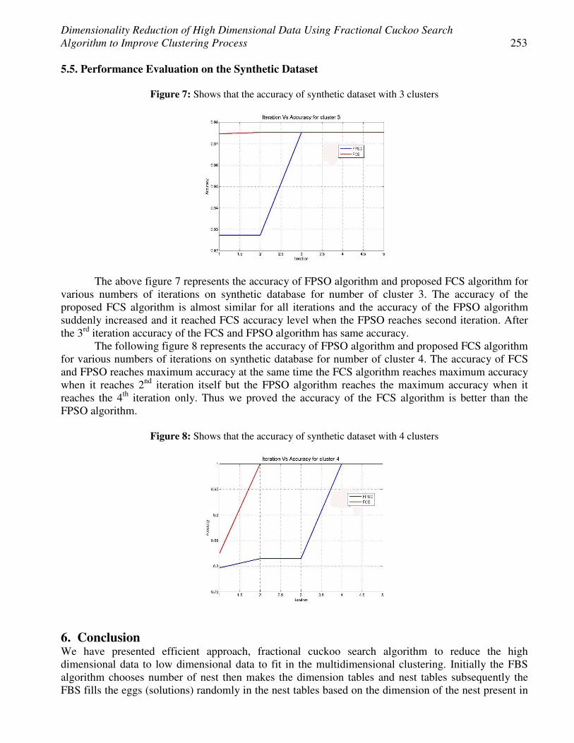
Dimensionality Reduction of High Dimensional Data Using Fractional Cuckoo Search Algorithm to Improve Clustering Process 253
5.5. Performance Evaluation on the Synthetic Dataset
Figure 7: Shows that the accuracy of synthetic dataset with 3 clusters
The above figure 7 represents the accuracy of FPSO algorithm and proposed FCS algorithm for various numbers of iterations on synthetic database for number of cluster 3. The accuracy of the proposed FCS algorithm is almost similar for all iterations and the accuracy of the FPSO algorithm suddenly increased and it reached FCS accuracy level when the FPSO reaches second iteration. After the 3rd iteration accuracy of the FCS and FPSO algorithm has same accuracy.
The following figure 8 represents the accuracy of FPSO algorithm and proposed FCS algorithm for various numbers of iterations on synthetic database for number of cluster 4. The accuracy of FCS and FPSO reaches maximum accuracy at the same time the FCS algorithm reaches maximum accuracy when it reaches 2nd iteration itself but the FPSO algorithm reaches the maximum accuracy when it reaches the 4th iteration only. Thus we proved the accuracy of the FCS algorithm is better than the FPSO algorithm.
Figure 8: Shows that the accuracy of synthetic dataset with 4 clusters
6. Conclusion We have presented efficient approach, fractional cuckoo search algorithm to reduce the high dimensional data to low dimensional data to fit in the multidimensional clustering. Initially the FBS algorithm chooses number of nest then makes the dimension tables and nest tables subsequently the FBS fills the eggs (solutions) randomly in the nest tables based on the dimension of the nest present in

254 Golda George and Latha Parthiban
the dimension table. FBS computes fitness value for each nest in the nest tables and arranged in descending order based on the fitness value of the nest. From the arranged nest, FBS initialize the value of best nest by select the nest which placed in first on the nest table. The best nest values may change at every iteration, if the fitness value of new best nest has less than existing fitness value. The values (eggs) in the nest tables get updates based on the levy flights. Once the high dimensional data is converted to the low dimensional data by the fractional cuckoo search (FCS) algorithm subsequently the reduced dimension data goes to the clustering algorithm to make the cluster efficiently. Finally, the experimentation is made with synthetic and real datasets and we have proved the efficiency the FCS algorithm 12.3% on iris, 35.1% on wine and synthetic dataset has 30.75% better than the FPSO in terms of accuracy. References [1] Serkan Kiranyaz, Turker Ince, Alper Yildirim, and Moncef Gabbouj, “Fractional Particle
Swarm Optimization in Multidimensional Search Space”, IEEE Transactions on Systems, Man, and Cybernetics, VOL. 40, NO. 2, pp: 298-319, 2010.
[2] X.-S. Yang, S. Deb, “Cuckoo search via L´evy flights”, in: Proc. Of World Congress on Nature & Biologically Inspired Computing (NaBIC 2009), December 2009, India. IEEE Publications, USA, pp. 210-214 (2009).
[3] Daoqiang Zhang, Zhi-Hua Zhou, Songcan Chen, “Semi-Supervised Dimensionality Reduction”, In: Proceedings of the 7th SIAM International Conference on Data Mining, pp: 11—393, 2007
[4] Min Soo Kim , Kyu-Young Whang ; Yang-Sae Moon, “Horizontal Reduction: Instance-Level Dimensionality Reduction for Similarity Search in Large Document Databases”, IEEE International Conference on Data Engineering, pp: 1061 – 1072, 2012.
[5] Vaibhav Kant Singh, Vijay Shah, Yogendra Kumar Jain, Anupam Shukla, A.S. Thoke, Vinay Kumar Singh, Chhaya Dule and Vivek Parganiha, "Proposing an Efficient Method for Frequent Pattern Mining", World Academy of Science, Engineering and Technology, vol.61, pp. 384-390, 2008.
[6] Osmar R. Z., “Introduction to Data Mining”, In: Principles of Knowledge Discovery in Databases. CMPUT690, University of Alberta, Canada, 1999.
[7] Kantardzic, Mehmed. “Data Mining: Concepts, Models, Methods, and Algorithms”, John Wiley and Sons, 2003.
[8] E. Wainright Martin, Carol V. Brown, Daniel W. DeHayes, Jeffrey A. Hoffer and William C. Perkins, “Managing information technology”, Pearson Prentice-Hall 2005.
[9] Andrew Kusiak and Matthew Smith, “Data mining in design of products and production systems”, in proceedings of Annual Reviews in control, vol. 31, no. 1, pp. 147- 156, 2007.
[10] Mahesh Motwani, J.L. Rana and R.C Jain, "Use of Domain Knowledge for Fast Mining of Association Rules", in Proceedings of the International Multi-Conference of Engineers and Computer Scientists, 2009.
[11] Satheesh, A. Mishra, D.K. and Patel, R. "Classification Rule Mining for Object Oriented Databases: A Brief Review", in proceedings of the First International Conference on Computational Intelligence, Communication Systems and Networks, pp. 259 - 263, Indore, July 2009.
[12] R. A. Fisher, The use of multiple measurements in taxonomic problems, Annals of Eugenics, 7 (1936), pp. 179–188.
[13] I. Joliffe, Principal Component Analysis, Springer, New York, NY, 1986. [14] A. Bar-Hillel, T. Hertz, N. Shental, D. Weinshall, Learning a mahalanobis metric from
equivalence constraints, Journal of Machine Learning Research, 6 (2005), pp. 937–965.

Dimensionality Reduction of High Dimensional Data Using Fractional Cuckoo Search Algorithm to Improve Clustering Process 255
[15] W. Tang and S. Zhong, Pairwise constraints-guided dimensinality reduction, in SDM’06 Workshop on Feature Selection for Data Mining, Bethesda, MD, 2006
[16] X. Yang, H. Fu, H. Zha, J. L. Barlow, Semisupervised nonlinear dimensionality reduction, in ICML’06, Pittsburgh, PA, 2006, pp. 1065–1072.
[17] Xiaohui Cui, Beaver, J.M.; St. Charles, J; Potok, T.E, “Dimensionality reduction particle swarm algorithm for high dimensional clustering”, Swarm Intelligence Symposium, pp:1-6, 2008.
[18] Guanghui Yan, "Integrating fractal dimensionality reduction with cluster evolution tracking", 2011 Eighth International Conference on Fuzzy Systems and Knowledge Discovery (FSKD), vol. 3, pp. 1668- 1672, 2011.
[19] DervisKaraboga, CelalOzturk, "A novel clustering approach: Artificial Bee Colony (ABC) algorithm", Applied soft computing, vol. 11, pp: 652-657, 2011
[20] Fuhua Yu, "An Improved Automatic FCM Clustering Algorithm", 2010 2nd International Workshop on Database Technology and Applications (DBTA), pp. 1- 4, 2010.
[21] BahriyeAkay, DervisKaraboga, “A modified ABC algorithm for real parameter optimization”, Information Sciences, vol. 192, June, 2012.
[22] SweeChuanTan, Kai Ming Ting, ShyhweiTeng, “A general Stochastic clustering method for automatic clustering Discovery”, Pattern Recognition, vol.44, October, 2011.
[23] Imola fodor, "A Survey of Dimension Reduction Techniques", 2002 [24] http://archive.ics.uci.edu/ml/datasets.html

European Journal of Scientific Research ISSN 1450-216X / 1450-202X Vol. 103 No 2 June, 2013, pp.256 - 266 http://www.europeanjournalofscientificresearch.com
Bioactivity of Injected Boric Acid on German Cockroaches:
Lethality, Analysis of Residues and Acethylcholinesterase and Glutathione S-Transferase Activities
Dahbia Habes Laboratory of Applied Animal Biology, Faculty of Sciences, Department of Biology
Badji-Mokhtar University of Annaba, 23000-Annaba, Algeria E-mail: dahbiahabes @ yahoo.fr; Fax: +38 87 54 00
Tel: +771 50 41 04
Karim Bouazdia Hadj-Lakhdar Université de Batna
E-mail: [email protected]; Tel: +770971143
Rouhia Messiad 8 Mai 45 Université de Guelma
E-mail: [email protected]; Tel: +561113867
Anissa Boussatha Faculty of Sciences, Department of Biology
Badji Mokhtar University of Annaba, 23000- Annaba, Algeria E-mail: [email protected], Tel: +697596115
Noureddine Soltani
Laboratory of Applied Animal Biology, Faculty of Sciences, Department of Biology Badji Mokhtar University of Annaba, 23000-Annaba, Algeria
E-mail: [email protected] Fax: + 38 87 54 00; Tel: + 773 38 76 33
Website: http:// www.lbaa-univ-annaba.org
Abstract
Conventional insecticides have been used widely to control cockroach which have developed resistance to these compounds. Thus, interest has again centred on lesser-used insecticides such as boric acid. Its mode of action on insects has not been satisfactorily established. In Algeria, Blattella germanica L. (Dictyoptera: Blattellidae) is a serious pest in the urban environment and their infestations were controlled for many years by organophosphate, carbamate, or pyrethroid insecticides. In order to obtain more information on the mode of action of boric acid, an inorganic insecticide, we first evaluated the toxicity of boric acid administered by injection on newly emerged male adults. The compound was been administered by injection at different doses ranging from 25, 50, 100 and 200µg/insect to newly emerged adults. Mortality was measured at different time’s treatment (1, 2, 3 and 6 days). Treatment resulted in a dose–dependent mortality since LD50 and DL90 recorded were 77,62 and 194,98 µg/insect at 6 day respectively, while the TL50 and TL90 were 2,99 and 7,63 days respectively. In a second series of experiments,

257 Dahbia Habes, Karim Bouazdia, Rouhia Messiad, Anissa Boussatha and Noureddine Soltani
the amount of residue was determined by a colorimetric method in several organs (hemolymph, gut, testes, fat body and body) by a colorimetric method. The compound was investigated on the activities of acethylcholinesterase (AChE) and glutathione S- transferases (GSTs). The analysis was made as function of the dose (LD50 and DL90) and the time following treatment (1 to 6 days). Results revealed that the amount of residues detected in these organs increased as function the time following of treatment. In addition, the amount was relatively important in fat body followed by testicles, midgut, posterior gut, foregut and hemolymph. Data showed that the compound induced GSTs and reduced the activity of AChE
Keywords: Cockroaches, Blattella germanica, Inorganic insecticide, Boric acid, Toxicity, Residues, Glutathione S-transferase, Acethylcholinesterase
1. Introduction Cockroaches are generally associated with grossly unsanitary conditions (Ebelling 1991) and are considered as the most important pests in the urban environment (Cloarec et al. 1992). Several species of cockroach are known to carry pathogenic or potentially pathogenic bacteria on or within their body (Leaderer et al., 2002) and are important for medical and public health points of view (Roberts, 1996; Mindykowski et al., 2010; Peden and Reed, 2010). In Algeria, the German cockroach, Blattella germanica L., is the most common domiciliary cockroach species and conventional insecticides such as organophosphate, carbamate and pyrethroid insecticides were used for many years to control their infestations. Because secondary effects of these conventional insecticides in environment alternative approaches were searched for controlling domestic cockroaches (Valles, 1999). Numerous studies have tested the efficacy of this compound on cockroaches (Strong et al., 1993; Habes et al., 2001; Appel, 2004; Habes et al., 2006). However, its mode of action on insects has not been satisfactorially established (Cochran, 1995). In a previous study, we reported that ingested boric acid to newly emerged adult of German cockroach caused death of insects perhaps ultimately by starvation via alterations of the midgut (Habes et al., 2006). In order to complete previous reports (Habes et al., 2001; Habes et al., 2006; Kilani-Morakchi et al.,2009) and to obtain more information on the mode of action of boric acid, the objectives of the present study were 1/ to test the toxicity of this compound by injection against male adults of B. germanica 2/ to determine the amounts of residues in several organs (insect body, hemolymph, testicles, midgut, foregut, posterior gut and fat body) as of the dose (LD50 and DL90) and the time following treatment (1 to 6 days) and 3/ to evaluate the activities of the detoxification enzyme, glutathione S-transferase (GST), and the target enzyme of neurotoxic insecticides, acethylcholinesterase (AChE). The latter results should help to obtain more information on its mode of action. 2. Materials and Methods 2.1. Animals
Colonies of B. germanica were reared in plastic containers (30x 30x 30 cm) and maintained at 27 ± 1°C, 80% RH under a photoperiod of 12:12h (L:D). The cockroaches were provided ad libitum with water and dry biscuit food (BIMO), which composition is (flour, grease, yeast, skim-milk, aroma, salt, syrup of glucose, Surbiton, Lecithin de soya). (SEMPAC)The age and number of insects tested in each bioassay are given with results. 2.2. Toxicity Tests
Boric acid (Merck) was injected at different dose ranging from 25 a 200 µg/insect. Control cockroaches were injected with 2 µl distilled water. Four replications each containing 13 newly

Bioactivity of Injected Boric Acid on German Cockroaches: Lethality, Analysis of Residues and Acethylcholinesterase and Glutathione S-Transferase Activities 258
emerged male (in our test we are choice the male than female because the female were use for breeding) adults per dose were tested. Mortality was recorded at 1, 2, 3 and 6 days following treatment, In a previous study, we are determined the toxicity of boric acid by ingestion to adult of German cockroach during a time following treatment (1 to 6 days) (Habes et al., 2006 ; and corrected (Abbott, 1925). Insecticidal data were subjected to probit analysis. The LD50 and LD90 values (i.e., the dose that is causing mortality in 50 and 90% of the treated insects, respectively) together with corresponding 95% confidence limits (95% CL) and the slope of the concentration-mortality lines were calculated (Finney, 1975). In a second bioassay, the TD50 and TD90 values (i.e., the time corresponding to mortality in 50 and 90% of the treated insects, respectively) were also determined. 2.3. Analysis of Residues
Quantity of boric acid accumulated in several organs (entire body, hemolymph, midgut, foregut, posterior gut, testicles, and fat body) was determined as function two tested dose (DL50= 77. 62 and DL90= 194. 98 µg/insect) and time following treatment (1 to 6 days).Insects were immobile by the cold for 3 mn then samples were grinded in ethanol 90° (500 µl/organ and 200 µl/ 2 µl hemolymph) and centrifuged at 4,000g, 15 min. The supernatant was removed and the boric acid contents in each sample were determined in aliquot of 100 µl according to method of Rodier (1975) as previously described (Kilani-Morakchi et al. 2009) using 300 µl of curcumin solution (curcumin 12.5 mg, acetic acid 10 ml), 300 µl acid reagent (acetic acid 50 ml, sulfphuric acid 50 ml) and 1 ml ammonium acetate buffer (ammonium acetate 25 g, acetic acid 30 ml, distilled water 100 ml). Absorbance was measured at 555 nm against standard solution (40 mg of boric acid/L). 2.4. Enzyme Assays
The LC50 =77.62 µg/insect was evaluated by injection on enzyme activities in adults newly emerged. The AChE activity was carried out following the method of Ellman et al., (1961) using acethylthiocholine as a substrate. Pooled heads (each containing 10 heads per series) were homogenized in the following solution containing 38.03 mg ethylene glycol tetraacetic acid (EGTA), 1ml Triton X-100 and 5.845 g Nacl, and 80 ml Tris buffer (10 Mm, pH 7). After centrifugation (5000g, 5min), the AChE activity was measured in aliquots (100µl) of resulting supernatants added to 100µl of 5-5’ dithiobis- (2-nitrobenzoic acid) (DTNB) in Tris buffer (0.01M, pH8) and 1ml Tris (0.1M, pH8). After 5min, 100µl acethylthiocholine was added. Measurements were conducted at a wavelength of 412 nm with a run time of 20 min. GSTactvities were determined with the soluble fraction as enzyme source.GST activities toward 1-cloro-2,4-dinitrobenzene (CDNB) were measured [Habig et al.,1974]. Adults were sampled from control and treated insects. Each decapitated body was homogenized in sodium phosphate buffer (0.1M, pH 6 ) and centrifuged (14000g, 30min).200 µl of the resulting supernatant was added to 1200 µl of reaction mixture containing 1Mm CDNB and 5mM reduced glutathione (GSH) in the homogenization buffer. Changes in absorbance were recorded at 340nm. Total protein content was determined according to Bradford (1976) using bovine serum albumin (Sigma) as a standard. Enzyme activities were expressed as µM/min/mg protein. 2.4. Statistical Analysis
Data are expressed by the mean ± standard deviation (SD) and subjected to a one-way analysis of variance (ANOVA). Comparison of two mean values was made by Student’s t-test. All statistical analyses were performed using MINITAB Software (SAS institute 1990) (Version 14, PA State College, USA) and p< 0.05 was considered to be a statistically significant difference.

259 Dahbia Habes, Karim Bouazdia, Rouhia Messiad, Anissa Boussatha and Noureddine Soltani
3. Results 3.1. Insecticidal Activity
Results showed that treated insects exhibited toxic symptoms with a dose-dependent mortality. Symptoms of boric acid poisoning were consistent with those described by Steinbring (1976). Paralysis normally started with the rear legs so that the thorax was dragged along the arena floor, but on a few occasions paralysis commenced with the forelegs. The cockroach movements were erratic and disorientated and may account for the large numbers that died outside harbourage. The percentage of corrected mortality of B. germanica was determined as function of the boric acid doses (25, 50,100 and 200 µg/insect) and the time of treatment (1, 2, 3 and 6 days). As illustrated in Fig. 1, data showed that the treatment is widely correlated to the dose of boric acid and the mortality is time dependent (χ2 = 6.4125; p <0. 001 at 5% level). LC50’s (µg/insect) calculate at selected times after injection application on newly emerged adults of B. germanica are 281.83 at 1 days, 208.92 at 2 days, 158.48 at 3 days and 77.62 at 6 days, respectively (Table 1) and TL50’s (days) are 43.63 for 25 µg/insect > 20. 88 for 50 µg/insect > 4. 67 for 100 µg/insect> 2.99 for 200 µg/insect (Table 2). These insecticidal data proved that the toxic effects of boric increase with the dose and the duration of treatment. The percentage of mortality is a 10% at the control cockroach Figure 1: Corrected mortality (%) as function of the dose of boric acid and the duration of treatment (days)
after injection application on newly emerged B. germanica : adults ( means ±SD established on four replicates each containing 13 cockroaches).
0 10
20
30
4050
60
70
8090
100
1 2 3 6
Time following treatment (days)
Co
rre
cte
d m
ort
ali
ty (
%)
25µg /insect
50µg/insect
100µg/insect
200µg/insect
Table 1: Toxicity of boric acid administered by injection to newly emerged adults of B. germanica: LC50’s
and LC90’s (µg/insect) with their fiducial limits (IC) at various times (days) following treatment.
Time (days) Linear regression Slope LC50 (IC) LC90 (IC) 1 Y = 3.83 X- 4.40 1.81 281.83 (195.5 -368.11) 602.55 (516.27-688.83) 2 Y = 4.33 X –5.07 1.69 208.92 (161.52-256.32) 416.86 (369.46–464.26) 3 Y = 4.83 X – 5.66 1.6 158.48 (106.19–210.77) 295.12 (242.83–347.41) 6 Y = 3.18 X – 1.03 2.04 77.62 (50.40–104.84) 194.98 (167.76–222.2)
Table 2: Toxicity of boric acid administered by injection to newly emerged adults of B.germanica: TL50’s
and TL90’s (days) with their fiducial limits (IC) at various doses (µg/insect).
Dose (µg/insect) Linear regression Slope LT50 (IC) LT90 (IC) 25 Y = 2.76X – 3.34 2.28 43.63 (42.17- 45.09) 125.83 (124.37–127.29) 50 Y = 4.4X – 6.88 1.67 20.88 (19.62- 22.14) 40.71 (39.45- 41.97)
100 Y = 2.37 X +0.13 2.63 4.67 (3.31- 6.03) 16.21 (14.85 – 17.57) 200 Y= 3.16 X– 0.87 2.06 2.99 (2.36 - 3.62) 7.63 (7.00 – 8.26)
3.2. Determination of Residue Amounts
Boric acid was administrated by injection to newly emerged adults of B. germanica (0 day) at two doses 77.62 and 194.98 µg/insect corresponding to LD50 and LD90, respectively. The treatment was

Bioactivity of Injected Boric Acid on German Cockroaches: Lethality, Analysis of Residues and Acethylcholinesterase and Glutathione S-Transferase Activities 260
realised for 6 days. The residues were extracted from different organs (insect body, gut, testicles, fat body and hemolymph) and quantified by a colorimetric method using a chromophoric compound, the curcumin. The result presented in figures 2-4, showed that the amounts of residues in insect body (Fig. 2), in hemolymph, testicle , fat body (Fig.3), and foregut, midgut , posterior gut (Fig. 4) increased significantly (p<0.001) according to the duration of treatment and the dose. The results show that amounts of residues detected are relatively important in fat body (7.02±1.01µg/mg) behind lesser one in hemolymph (0.08± 0.03 µg/µl (Table 3). Table 3: Amounts of residue (µg/mg fresh tissue, µg/µl) in different organs after 6 days of treatment by
injection at the LD50 and LD90 doses on newly emerged male adults of B. germanica (m ±SD).
Organs LD50 LD90 Fat body 7.02 ±1.01 a A 17.18 ±1.39 b A Testicles 4.03 ± 0.29 a B 8.89 ± 0.58 b B Midgut 3.26 ± 0.38 a B 8.65 ± 0.92 b B Posterior gut 2.69 ± 0.22 a C 8.82 ± 0.36 b B Foregut 2.32 ± 0.15 a C 8.54 ± 0.91 b B Hemolymph 0.08 ± 0.03 a D 3.27 ± 0.17 b C
For each organ or tissue, mean values followed by different letters in minuscule are significantly different, while for each lethal dose, mean values followed by different letters in majuscule are significantly different at p< 0.05. Figure 2: Boric acid residues (µg/mg tissue) insect body as function the dose (µg/insect) and the duration of
treatment (days) after injection application on newly emerged adults of B. germanica (mean ± SD each of 3-6 cockroaches).
Figure 3: Changes in boric acid residues ((µg/µl), µg/mg tissue) in hemolymph (A) testicle (B), fat body (C)
as function the dose (µg/insect) and the duration of treatment (days) after injection application on newly emerged adults of B. germanica (mean ± SD each of 3-6 cockroaches, for each age and dose, mean values followed by asterisks aresignificantly different (*: p<0.05; **:p<0.01; ***:p<0.001).
0
5
10 15
20
25
30
35
1 2 3 4 5 6
LD50 LD90
Re
sid
ue
s a
mo
un
ts (
µg
/µl)
***
*** ***
***
***
A
* **
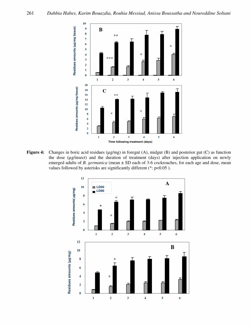
261 Dahbia Habes, Karim Bouazdia, Rouhia Messiad, Anissa Boussatha and Noureddine Soltani
0
1
2
3
4
5
6
7
8
9
10
1 2 3 4 5 6
*** *
*
**
B
Res
idu
es
am
ou
nts
(µ
g/m
g t
iss
ue)
0
2
4
6
8
10 12 14 16 18 20
1 2 3 4 5 6
Time following treatment (days)
C
* *
Resid
ues a
mo
un
ts (
µg
/mg
tis
su
e)
**
Figure 4: Changes in boric acid residues (µg/mg) in foregut (A), midgut (B) and posterior gut (C) as function
the dose (µg/insect) and the duration of treatment (days) after injection application on newly emerged adults of B. germanica (mean ± SD each of 3-6 cockroaches, for each age and dose, mean values followed by asterisks are significantly different (*: p<0.05 ).
0
2
4
6
8
10
12
1 2 3 4 5 6
Resid
ues a
mo
un
ts(
µg
/mg
) LD50 LD90
*
*
A
*
0
2
4
6
8
10
12
1 2 3 4 5 6
*
*
B
Re
sid
ue
s a
mo
un
ts (
µg
/mg
)
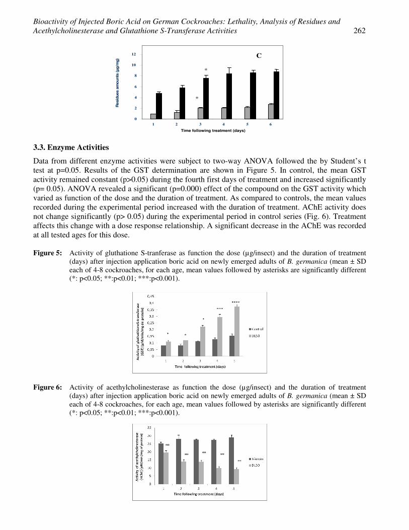
Bioactivity of Injected Boric Acid on German Cockroaches: Lethality, Analysis of Residues and Acethylcholinesterase and Glutathione S-Transferase Activities 262
0
2
4
6
8
10
12
1 2 3 4 5 6
Time following treatment (days)
Resid
ues a
mounts
(µg/m
g)
C
*
*
3.3. Enzyme Activities
Data from different enzyme activities were subject to two-way ANOVA followed the by Student’s t test at p=0.05. Results of the GST determination are shown in Figure 5. In control, the mean GST activity remained constant (p>0.05) during the fourth first days of treatment and increased significantly (p= 0.05). ANOVA revealed a significant (p=0.000) effect of the compound on the GST activity which varied as function of the dose and the duration of treatment. As compared to controls, the mean values recorded during the experimental period increased with the duration of treatment. AChE activity does not change significantly (p> 0.05) during the experimental period in control series (Fig. 6). Treatment affects this change with a dose response relationship. A significant decrease in the AChE was recorded at all tested ages for this dose. Figure 5: Activity of gluthatione S-tranferase as function the dose (µg/insect) and the duration of treatment
(days) after injection application boric acid on newly emerged adults of B. germanica (mean ± SD each of 4-8 cockroaches, for each age, mean values followed by asterisks are significantly different (*: p<0.05; **:p<0.01; ***:p<0.001).
Figure 6: Activity of acethylcholinesterase as function the dose (µg/insect) and the duration of treatment
(days) after injection application boric acid on newly emerged adults of B. germanica (mean ± SD each of 4-8 cockroaches, for each age, mean values followed by asterisks are significantly different (*: p<0.05; **:p<0.01; ***:p<0.001).

263 Dahbia Habes, Karim Bouazdia, Rouhia Messiad, Anissa Boussatha and Noureddine Soltani
4. Discussion The control of cockroaches includes crack, dusting, aerosol sprays and application of liquid insecticides. It involves the application of relatively large amounts of insecticides and deposit unprotected insecticidal residues. Use of baits insecticide results in less environmental contamination and greater ease of application than other insecticide products (Zurek et al., 2002). In the other hand, the combination of isolated populations and intense insecticide pressure often results in resistance (Zurek et al., 2003). Thus, interest has again centred on boric acid baits, but a more complete understanding of its properties is needed.
In this study, we have evaluated the toxicity of boric acid by injection on newly emerged adults of B. germanica. Our results show at 6 days after injection, the LD50 of boric acid was 77.62 µg/insect or (3.88 %) and the LD90 was 194.98µg/insect or (9.74%) and that treatment results in a dose and time-dependent mortality since the LD50’s and LD90’s (µg/insect) recorded decrease with the increase of duration of treatment. . LT50’s and LT’s90 correspond respectively of 2.99 and 7.63 days for a dose 200µg /insect. In a previous study (Zurek et al., 2002; Habes et al., 2006), the DL50 and DL90 of boric acid were 8.20%, 49.62% , a good correlation was observed between the increase concentration of boric acid and the decrease of duration of treatment. The comparison of the amounts shows that the LC50 and LC90 by injection are lower than those by ingestion (Zurek et al., 2002; Habes et al., 2006). Although the t mode of action of boric acid against insects remains unknown, destruction of the gut wall of B. germanica after boric acid ingestion has been suggested (Gore and Schal, 2004) .Based on a histological study of the digestive tract of B. germanica after ingestion of boric acid (Cochran, 1995) concluded that destruction of the foregut epithelium might result in death from starvation. This is unlikely, however, because cockroaches exposed to boric acid die much faster than starved cockroaches ((Zurek et al., 2002, 2003; Sumida et al., 2010) Boric acid is an inexpensive inorganic insecticide with a favourable safety tract record and no know cases of insect resistance in insects it was extensively used before the advent of fast-acting organic insecticides, including carbamates,organophosphates, and pyrethroids (Gore and Schal, 2004) and also it is thought to have little or no repellancy to cockroaches (Ebeling et al ., 1967)
Boric acid has been also reported to enhance the virulence of several pathogens including Bacillus thuringiensis (Berliner) subs, kurstaki against Mamestra configurata ( Walker) (Morris et al. 1995); nucleopolyedrosis virus against Lymantria dispar (L.) and Spodoptera frugiperda (Shapiro and Bell, 1982; Cisneros et al ., 2002) and Metarhizium anisopliae ( Metschnikoff) Sorokin against the German cockroach (Zurek et al., 2002) However, boric acid was the least toxic compound compared with conventional insecticides because the organic insecticides provide much faster kill. At 24 h after topical application on adults males of B. germanica , the LD50 of cypermethrin was 0. 90 µg/g (Vontas et al., 2000) after ingestion imidacloprid gel 2.15% and fipronil gel bait 0.05%, the cockroaches died more rapidly (Nasirian, 2007)
The bioaccumulation of boric acid in several organs shows that this insecticide is accumulated quickly (1 day) in the whole body, hemolymph, digestive tract, testicle and especially in the fat body. Thus acid boric diffuses in the various parts of the body of insect. Our results are in agreement with those (Habes et al., 2001, 2006; Kilani-Morakchi et al., 2009) which shows an important accumulation of this insecticide in the fat body in the female adults of B. germanica treated by application oral to two amounts 8.20% (DL50) and 49.62 (DL90). Boric acid residues were accumulated in insect body with a dose-response effect. However, despite the significant differences observed between the amounts of residues incorporated with the two doses at all tested days, the incorporation of residues in male treated LC90 was at most of 1.5 fold than the amounts of residues incorporated with the LC50 at 1day.Our results also agree with those of (Khebbeb et al., 1997) who demonstrated an important accumulation of diflurobenzuron (DFB), a benzoyl phenyl urea derivate in fat body after oral application at 5 to 10 mg/g on Tenebrio molitor .Other studies show that the fish collected in the Mississipi river basin and in the Amazon in Brazil were analysed for organochlorine chemical by gas chromatography with electron

Bioactivity of Injected Boric Acid on German Cockroaches: Lethality, Analysis of Residues and Acethylcholinesterase and Glutathione S-Transferase Activities 264
capture detection., residues of dichlorodiphenyltrichloroethane (DDT) were detected in about 95% of fish and 0.5mg/kg of total DDT respectively (Schmitt, 2002; Torres et al., 2002).
It is well recognized that biomarkers are useful tools for toxicologists and environmental scientists. They help to predict the toxicity and understand better the mode of action of chemicals and also to study environmental exposures and stress to potentially toxic compounds. Glutathione is considered one of the most important antioxidant agent involved in protection of cell membranes against free radicals damage (Lam, 2009; Ayodele et al., 2011). Glutathione-S-transferases are a family of dimeric multifunctional enzymes that have been shown to be involved in detoxication of xenobiotics, protection from oxidative damage, and the intracellular transport of hormones, endogenous metabolites and exogenous chemicals in diverse organisms (Zhou et al., 2009)
GSTs also play an important role in stress physiology, and have been implicated in intracellular transport and various biosynthetic pathways (Wilce and Parker 1994). Biochemical data revealed an induction in GST activities confirming previous report made in B. germanica (Habes et al., 2006) Acetylcholinesterase (AChE) has a key role in neurotransmission by hydrolyzing the neurotransmitter acetylcholine in cholinergic synapses of the nervous system and is inhibited by several neurotoxic insecticides ( Fernandez-Vega et al., 2002 , Van der Oost et al., 2003). The injection of the acid boric at the adults of B.germanica in a dose DL50 = 77,62µg / insect causes an increase of the GST and a decrease of the AChE according to the duration of treatment Our results are in agreement with those of Habes (2006) who shows that the ingestion of the acid boric at B. germanica affect an increase the GST and an decrease the AChE . Similar results were observed at the same species treated by the cypermethrine (Valles et al., 2000)
In conclusion, our results reveal that injection boric acid is a mode of application most efficacy, that ingestion in B. germanica. Thus acid boric diffuses in the various parts of the body of insect with an important accumulation in fat body. The assessment of biomarkers indicates a significant increase of glutathione S- transferase, highlighting the establishment of a mechanism of resistance. The decreased activity of acethylcholinesterase confirms the neurotoxicity of boric acid. This compound insecticide boric acid has the advantage over most conventional insecticides, and can be used as an adequate alternative to conventional organic insecticides for the management of cockroach infestations. Acknowledgements This work was supported by the Algerian Agency for Research Development in Health (Projet: CNEPRU F01120110038, PNR 18/U23/1466) References Cited [1] Abbott, W. B., 1925. A method for computing the effectiveness of an insecticide. J. Econ.
Entomol, 18, 265-267. [2] Appel, A.G., 2004. Contamination affects the performance of insecticidal baits against German
cockroaches (Dictyoptera: Blattellidae). J.Econ. Entomol. 97, 2035-2042. [3] Ayodele, O. Kolawole, Joshua O. Ajele, Ravi, Sirdeshmuhk. 2011. Studies on glutathione
transferase of cowpea storage bruchid,Callosobrochus maculatus F Pesticide Biochemistry and Physiology, Volume 100, Issue 3, July 2011, Pages 212-220
[4] Bradford, M.M., 1976. A rapid and sensitive method for the quantification of microgram quantities of protein utilizing the principle of protein dye binding. Anal. Biochem. 72-248
[5] Cloarec, A., Rivault, C., Fontaine, F. and Le Guyader, A., 1992.Cockroaches as carrier of bacteria in multi-family dwelling. Epidemiol. Infect 109, 483-490.
[6] Cochran, D.G., 1995. Toxic effects of boric acid on the German cockroach. Experientia. 51, 561-563.

265 Dahbia Habes, Karim Bouazdia, Rouhia Messiad, Anissa Boussatha and Noureddine Soltani
[7] Cisneros, J., J. A. Perz, D. I. penagos, J. Ruiz, D. Goulson, P. Cabellero, R. D. Cave, and T. Willams, 2002. formulation of a nucleopolyhedrovirus withboric acid for control of Spodoptera frugiperda ( Lepidoptera: Noctuidae) in maize. Biol. Control. 23, 87-95.
[8] Ebeling,W., Reierson, D.A.and Wagner, R. E., 1967. Influence of repellency on the efficacy of blatticides . II. Labortory experiments with German cockroach. J. Econ. Ent. 60, 1375-1390.
[9] Ebelling, W., 1991. Ecological and behavioural aspects of Cockroach management, pp 85- 113. MR. Gorham ed, Ecology and management of food- Industry pests. FA Technical Bulletin 4. Association of official Analytical chemist, Arlington.VA.
[10] Ebeling,W., 1995. Inorganic insecticides and dusts. In,*Understanding and controlling the German cockroach.* (M. K. Rust, J.M. Owens ,and D.A. Reierson, [eds.], pp. 193-230 Oxford University Press, New York
[11] Ellman, G.L.,Courtney, K.D,.Andres, V. ,Feather-stone, R.M., 1961. A new and rapid colorimetric determination of acethylcholinesterase activity. Biochem. Pharmacol. 7- 88.
[12] Fernandez-Vega, C, Sancho, E, Ferrando, M.D, Andreu, E., 2002. Thiobencarb induced changes acetylcholinesterase activity of the fish Anguilla anguilla. Pest. Biochem. Physio. 72, 55-6.
[13] Finney, D.J., 1971. Probit analysis (3rd ed).Cambrodge University.Press, London. 318p. [14] Gore, J.C, Zurek, L., Santangelo, R.G, Stringhan, S.M, Watson, D.W, Schal, C.,2004. Water
solutions of boric acid and sugur for management of German cockroach populations in livestock production systems. J.Econ. Entomol. 97 (2), 715-720.
[15] Gore, J. C, C. Schal., 2004. Laboratory evaluation of boric acid –sugar solutions as baits for management of German cockroach infestations. J. Econ. Entomol. 97(2), 581-587.
[16] Habes, D., Morakchi, S., Aribi, N., Farine, J.P., Soltani, N., 2001. Toxicity of boric acid to Blattella germanica (Dictyoptera: Blattellidae) and anlysis of residues in several organs. Med. Fac. Landbouww. Univ. Gent, 66/2a.
[17] Habes, D., Morakchi, S., Aribi, N., Farine, J.P., Soltani, N., 2006. Boric acid toxicity to the German cockroach, Blattella germanica: alterations in midgut structure, and acethylcholinesterase and glutathione Stransferase activity. Pestic. Biochem. Physiol. 84, 17-24
[18] Habig, W.H., Pabst, M.J., Jacoby, W. B., 1974.GluthtioneS-transferases, J. Biol. Chem. 249-71530
[19] Khebbeb, M.E. H., Delachambre, J., and Soltani, N., 1997. Lipid metabolism during the sexual maturation of the mealworm (Tenebrio molitor ): effect of ingestion diflubenzuron. Pesticide Biochem and Pysiol, 58, 209-217
[20] Kilani-Morakchi, S., Aribi,N., and Soltani, N., 2009. Activity of boric acid on German cockroaches: Analysis of residues and effects on reproduction African Journal of Biotechnology, 8(4), 703-70
[21] Lam, P.K.S., 2009. Use of biomarkers in environnmental monitoring. Ocean and Coastal Management 52, 348-354.
[22] Leaderer,B.P.,Kathleen,B.,Elizabeth,T.,andTheodore,H.,2002.Dust mites cockroaches, cat,Dog Allergen Concentration in Homes of asthmatic Children in the Northen United States : Impact of socioeconomic Factor and Population Density. Children’s Health Article Enviro. Health. Perspect, 110 (4) , 413-420.
[23] Mindykowski, B., Jaenicke, E., Tenzer, S., Cirak, S., Schweidardt, T., Schild, H., Decker, H., 2010. Cockroach allergens Per a 3 are oligomers. Dev Comp Immunol., 34(7) ,722-33.
[24] Morris, O.N., Converse, V.,and Kanagaratnam, P., 1995. Chemical additive effects on the efficacy of Bacillus thuringiensis Berliner subsp. Kurstaki against Marmestra configurata (Lepidoptera: Noctuidae). J. Econ. Entomol. 88, 815-824.
[25] Nasirian, H., 2007. Duration of fipronil and imidacloprid gel baits toxicity against Blattella germanica strains of Iran .Iranian. J. Arthropod-BorneDis. 1(2), 40-47

Bioactivity of Injected Boric Acid on German Cockroaches: Lethality, Analysis of Residues and Acethylcholinesterase and Glutathione S-Transferase Activities 266
[26] Peden, D., Reed, C.E., 2010. Environmental and occupational allergies. J Allergy clin immunol . 125, S 150-60
[27] Roberts, J., 1996. Cockroaches linked with asthma. Br.Med. J., 312 , 1630p. [28] Rodier, J., (1975). Analyse de l’eau. Eaux naturelles, eaux résiduaires, eaux de mer. Dunod and
Technique. Vol 1: 629 [29] SAS institute, 1990. SAS/STAT user’s guide, Vol.1 and 2. SAS Institue. Lary, Nil. [30] Shapiro, M., and Bell, R.A., 1982. Enhanced effectivness of Lymantria dispar (Lepidoptera:
Lymantriidae) nucleopolyhedrosis virus formulated with boric acid . Ann. Entoml. Soc. Am. 75, 346-349.
[31] Schmitt, C. J., 2002. Organochlorine chemical residues in fish from the Mississipi river basin, 1995.Arch. Environ. Contam. Toxicol. 43, 81-97.
[32] Steinbrink, H., 1976. Laborversuche zur Schabenbekämpfung mit Borpräparaten.-Z. .ges.Hyg. 22, 419-421.
[33] Strong, C. A., Koehler, P.G., and Patterson, R.S., 1993. Oral toxicity and repellency of borates to German Cockroach ( Dictyoptera: Blattellidae). J. Econ. Entomol. 86 (5), 1458-1463.
[34] Sumida,S.,Dasilva-Zacarin, E. C.M., Decio, P., Malaspina, O., Bueno, F.C.,Bueno., O. 2010. Toxicological and Histopathological Effects of Boric Acid on Atta sexdens rubropilosa (Hymenoptera: Formicidae) Workers .J. Econ. Entomol. 103(3): 676-690.
[35] Torres, J.P.M.., Pleiffer, W. C., Maekowitz, S., Pause, R., Malm, O., Janpaga, J., 2002. Diclorodiphenyltrichlroethane in soil, river sediment, and fish in the Amazon in Brazil. Environmental Research Section A 88, 134-139.
[36] Van der oost, R., Beyer, J., Vermeulent, N.P.E., 2003. Fish bioaccumulation and biomarkers in environmental risk assessment. Review. Environ. Toxicol. Pharmacol. 13, 57-149.
[37] Valles, S.M., Koehler, P.G., and Brenner, R.J., 1999. Comparative insecticide susceptibility and detoxification enzyme activities among pestiferous Blattodea, Comp. Biochem. Physiol. Part C 124, 227
[38] Vontas, J. G., Enayati, A. A., small, G. J., and Hemingway, J., 2000. A simple biochemical assay for Glutathion-S- tranferase activity and its possible field application for screening Glutathions-S- tranferase basedinsecticide resistance. Pest. Biochem. Physiol, 68:184-192.
[39] Yand, M.L., Zhang, J.Z., Zhu, K.Y., Xuan, T., Liu, X.J., Guo, Y.p, Ma, E.B., 2009. Mechanisms of organophosphate resistance in field population of oriental migratory locust, Locusta migratoria malensis(Meyen) Arch. Insect. Biochem. physiol., 71 (1), 3-15.
[40] Zhou, J., Wang, W.N., Wang, A.L., He, W-Y., Zhou, Q.T., Liu, Y., Xu, J., 2009. Glutathione S-transferase in the white shrimp Litopenaeus vannamei: characterization and regulation under pH stress. Comparative Biochemistry and Physiology (2009), doi: 10.1016/j.cbpc.2009.04.012
[41] Zurek, L., D. W., Watson, and C. Schal, 2002. Synergysm between Metarhizium anisopliae ‘ Deuteromycota: Hyphomycetes) and boric acid againstthe german cockroach (Dictyoptera: Blattellidae). Biol. Contr. 23, 296-302.
[42] Zurek, L.., J. C., Gore, M. S., Stringham, D. W., Watson, M.G Waldvogel Zurek, L., D. W. Watson, and C. Schal., 2003. Boric acid dust as a component of an integrated cockroach management program in confined swine production. J. Econ. Entomol. 96, 1362-1366.
European Journal of Scientific Research ISSN 1450-216X / 1450-202X Vol. 103 No 2 June, 2013, pp.267 - 281 http://www.europeanjournalofscientificresearch.com
Cardiac Arrhythmia Classification Using Regularized Least
Squares Classifier
Hamza Baali International Islamic University Malaysia (IIUM), Mechatronics Engineering Department
Jalan Gombak, 53100 Kuala Lumpur MALAYSIA E-mail: [email protected]
Momoh.J.E.Salami
International Islamic University Malaysia (IIUM), Mechatronics Engineering Department Jalan Gombak, 53100 Kuala Lumpur MALAYSIA
Rini Akmeliawati
International Islamic University Malaysia (IIUM), Mechatronics Engineering Department Jalan Gombak, 53100 Kuala Lumpur MALAYSIA
Aida Khorshidtalab
International Islamic University Malaysia (IIUM), Mechatronics Engineering Department Jalan Gombak, 53100 Kuala Lumpur MALAYSIA
Abstract
An algorithm for arrhythmia classification that conforms to the standard of the Association for the Advancement of Medical Instrumentation (AAMI) is examined in this paper. Three inter-patient classification scenarios are considered namely, detection of ventricular ectopic beats (VEBs), detection of supraventricular ectopic beats (SVEBs) and the multiclass recommended taxonomy. A new set of features extracted from the application of orthogonal decomposition of the ECG signal has been developed. These features in conjunction with some commonly used features are fed into the Regularized Least Squares Classifier (RLSC) with linear kernel. The proposed classification scheme shows good separation capability between the classes of ECG arrhythmias as it achieved a Balanced Classification Rate (BCR) of 83.9 % for the multiclass scenario which is comparable to the state-of-the-art performance of automatic arrhythmia classification. Keywords: Arrhythmia Classification, AAMI, ECG, RLSC, Orthogonal Transforms.
1. Introduction Cardiovascular diseases (CVDs) are the leading causes of death in the world, where more than 80% of these cases are found in the developing countries (Goldberger et al., 2000).This leading position will last for the next thirty years as forecasted by the World Health Organization (Organization, 2012). In numbers, CVDs claimed the lives of about 17.3 millions of the world population (i.e., 30% of the global deaths) in 2008. Moreover, the estimated economical cost of heart related diseases in the United States only was about 316.4 billions US $ in 2010. This cost covers health care services, medications and decrease in productivity (Frieden, 2010).

268 Hamza Baali, Momoh.J.E.Salami, Rini Akmeliawati and Aida Khorshidtalab
Electrocardiogram (ECG) is a crucial diagnostic tool for monitoring cardiac activities. Abnormalities in both electrical generation and conduction at different levels in the heart are reflected on the ECG as deviations from the normal heart rhythm. The term arrhythmia is used to refer to these deviations. Generally, the problem in the developing countries is due to an inadequate number of physicians who are able to read and analyze the ECG, particularly in rural areas. On the other hand, in the developed countries where the increase in the number of patients in intensive care units (ICU), the large amount of data recorded by the Holter monitor (~100,000 heartbeats in 24 hours ) make it almost unfeasible for the physicians to analyze all the acquired data.
In spite of many research efforts devoted to automatic arrhythmia monitoring, limited success has been achieved by researchers. The challenge is due to the variations in the morphology of ECG heartbeats that exhibit similar type of arrhythmias within and across patients, as shown in figure 1. These variations are referred to as intra-class variations. Besides, in many cases, heartbeats with different types of arrhythmias have similar waveform morphology and frequency content (Osowski and Linh, 2001). These similarities are referred to as inter-class similarities. These intra-class variations and inter-class similarities make it difficult to extract discriminative features from heartbeats. Consequently, in order to achieve accurate classification results, the set of input features as well as the classification algorithm are crucial.
Figure 1: Premature ventricular contractions (PVCs) with different shapes
In respect to the aforementioned issues, different approaches of feature extraction have been reported in the literature. Heuristic descriptors (such as ECG morphology and heartbeat intervals) are amongst the commonly used features (Chazal et al., 2004; Chazal and Reilly, 2006; Lannoy et al., 2011; Park et al., 2008). Others include, signal analysis and modeling techniques whereby the model parameters serve as features. Examples of these modeling techniques include Autoregressive (AR)(Ge et al., 2002; Ham and Han, 1996; Lin and Chang, 1989), Prony (Chen, 2000), Fourier analysis (Acır, 2005; Kutlu and Kuntalp, 2011; Minami et al., 1999), Wavelet transform (Khadra and Al-Nashash, 1997; Sternickel, 2002; Wiens and Guttag, 2010), and Hermite basis functions (HBF) (Jiang and Kong, 2007; Lagerholm et al., 2000; Osowski et al., 2004) . In addition, many statistical parameters have been considered for feature extraction such as high order statistics (HOS), Correlation and Shannon entropy (Chuang-Chien et al., 2005; Osowski and Linh, 2001; Tsipouras and Fotiadis, 2003).
Researchers have examined the use of a large variety of classifiers for arrhythmia classification including linear discriminants (LD)(Chazal et al., 2004; Chazal and Reilly, 2006), neural networks (Minami et al., 1999; Özbay and Tezel, 2010), self-organizing maps with learning vector quantization (Lagerholm et al., 2000), support vector machine (SVM)(Lannoy et al., 2011; Park et al., 2008), active learning (Wiens and Guttag, 2010) and combination of different classifiers (Castillo et al., 2011; Dokur and Olmez, 2001; Özbay et al., 2006).
The selection of the training and the test sets plays a key role in the practicality of the algorithm. The majority of published works apply “intra-patient” classification where a fraction of heartbeats from each record of each patient is used to train the algorithm .The remaining heartbeats are used for evaluation. The performances of these algorithms are optimistic on the selected records. However, the assessment of their performances in realistic scenarios is always missing (eg.,(Ge et al., 2002; Ham and Han, 1996; Osowski and Linh, 2001)). In other words, the accuracy can drop drastically when these algorithms are tested on data taken from new patients. To overcome this

Cardiac Arrhythmia Classification Using Regularized Least Squares Classifier 269
problem, many authors have proposed Patient-Adapting Heartbeat Classifiers, semi-automatic intra-patient approach, where a manual labelling of heartbeats from all new patients is needed and the classifier is adapted accordingly (eg., (Chazal and Reilly, 2006; Hu et al., 1997; Wiens and Guttag, 2010)). Although, this approach considerably improves the classifier performances, it does not seem practical due to the cost of acquiring trained physicians to label the data for each new patient. In addition, the practice in these studies is to label manually only the first five minutes of each record. This may not allow for the inclusion of all the morphologies present in the record during the training phase knowing that many abnormalities may occur as short episodes (few seconds) once in few days. This drawback makes it difficult for the classifier to correctly classify these abnormalities.
The second category of classifiers is referred to as “inter-patient” where the training and the test sets are taken from different patients. This approach is more practical; however, the reported performances are lower than those of “intra-patient” approach. Even though, most inter-patient classification techniques were tested on the MIT-BIH Arrhythmia database, it is inappropriate to benchmark these techniques as the types of arrhythmias classified vary from one published work to another.
Several recent works have established some general methodological guidelines to be followed in developing any arrhythmia classification algorithm namely, the class selection should follow the AAMI recommended practice, the validation should be on an open source database (MIT arrhythmia database is more suitable), and should be inter-patient based (Chazal et al., 2004).
Consequently, the endeavour in this research area should be on the development of automatic classifiers that perform well on unseen data without “assistance” from physicians. The fast development in data mining algorithms and the possibility of extraction of discriminative and stable features give rooms to achieve such objective.
This study investigates different scenarios of inter-patient classification based on the AAMI standard. The standard emphasizes on the discrimination of ventricular ectopic beats (VEBs) from the other three classes namely, normal beats (N), supraventricular ectopic beats (SVEBs) and fusion beats (F), and also the discrimination of SVEBs from the other classes ( N,VEBs and F). Each of the aforementioned categories contains different types of arrhythmias as shown in table 1. Table 1: Grouping of the MIT-BIH Arrhythmia Database Heartbeats Types Based on the AAMI Heartbeat
Classes
AAMI heartbeat
class
N S V F
beats originating in sinoatrial (SA)
node
MIT-BIH-label
supraventricular ectopic beats (SVEBs)
MIT-BIH-label
ventricular ectopic beats (VEBs)
MIT-BIH-label
Fusion beats MIT-BIH-label
Normal beats
(NOR) 1
Atrial premature beat (AP)
8
Premature ventricular contraction
(PVC)
5 Fusion of
ventricular and normal beats
6
Heartbeats types
Left bundle branch block
(LBBB) 3
Aberrated atrial premature beat (aAP)
4 Ventricular
escape beat (VE) 10
Right bundle branch block
(RBBB) 2
Nodal (junctional) premature beat (NP)
7
Atrial escape
beat (AE) 34
Supraventricular premature beat (SP)
9
Nodal
(junctional) escape beat (NE)
11
Unlike normal beats, which originate from the sinoatrial (SA) node, VEBs originate from the
ventricles. This class is dominated by premature ventricular contraction (PVC) beats. These heartbeats

270 Hamza Baali, Momoh.J.E.Salami, Rini Akmeliawati and Aida Khorshidtalab
are characterized by the absence of the P wave and a wide QRS complex, as illustrated in figure 1. Their presence in an ECG record becomes clinically significant only if their frequency of occurrence exceeds six beats per minute. Examples of these complex PVCs include, bigeminy (every other beat is a PVC), multifocal (varied shapes and forms of the PVCs) and couplet (two PVCs occur back to back). These complex PVCs could degenerate into serious ventricular arrhythmias such as ventricular tachycardia (Sigg et al., 2010). Therefore, many lives could be saved if these beats are detected early on and accurately. On the other hand, supraventricular ectopic beats (SVEBs) are non-life threatening arrhythmias which originate from the atria. Example of this class is atrial premature beats (APB), whereby additional heartbeats caused by electrical activation of an ectopic focus in the atria before the next sinus node impulse is established. Many healthy people may exhibit APB, especially elderly people. However, recent studies have demonstrated that frequent APB is a risk factor for stroke, heart failure, and atrial fibrillation (Engström et al., 2000; Rodríguez-Sotelo et al., 2009).
In this paper, a new set of features extracted from the impulse response matrix of the LPC filter and the transformed ECG signal is proposed. Using this approach, each ECG period is orthogonally transformed into a new domain where only few coefficients contain most of the signal information. The extracted features are fed into the classifier in conjunction with some commonly used features including the residual error energy, wavelet coefficients energy, RR intervals and high order statistics (Ham and Han, 1996; Lannoy et al., 2011; Lin and Chang, 1989).
Furthermore, this study investigates the use of the RLSC for classification of ECG arrhythmias. This algorithm has been shown to perform as accurately as SVM with some added advantages in terms of reduced computational complexity and memory requirements especially when applied with linear kernel (Rifkin, 2002; Rifkin and Lippert, 2007). To our knowledge, to date there is no study reported in literature that uses RLSC for classifying ECG arrhythmias with exception of some preliminary results for the detection of PVC beats reported in (Baali et al., 2013).
This paper is organized as follows, Section 2 presents the proposed method. In that section, ECG filtering, AR modeling of the ECG and feature extraction are analysed and discussed. Regularised least squares classifier is presented in Section 3. Results and discussion of the performances of the proposed algorithm for different classification scenarios are given in Section 4. Finally, Section 5 concludes the paper. 2. Methods This section includes a description of the de-noising stage employed on the raw ECG followed by a presentation of feature extraction process applied to the filtered signals. 2.1. ECG Filtering
The raw ECG signal is usually contaminated with different types of noise (eg., baseline wander, power line interference, and high-frequency noise). ECG filtering is aimed at improving the signal to noise ratio (SNR) by removing the noise.
In order to remove the power line interference, a second order notch-filter centred on
0 60 Hz f = with a bandwidth ∆F = 3Hz is first applied to the ECG signal. The transfer function of the
filter is given by:
( )( )
2 1 20 0
1 2 20
( 2cos ),
1 2 cosnotch
b z z zH
r z r z
ω
ω
− −
− −
− +=
− + (1).
Where ( )
( )
20 0
0 00
1 2 cos 2 �F ; ; 1 ; 360 .
2 1 2 cos ss s
r r fb r f Hz
f fr
ω π πω
ω
− += = = − =
−the parameter r controls the
spectral width and sharpness of the filter.
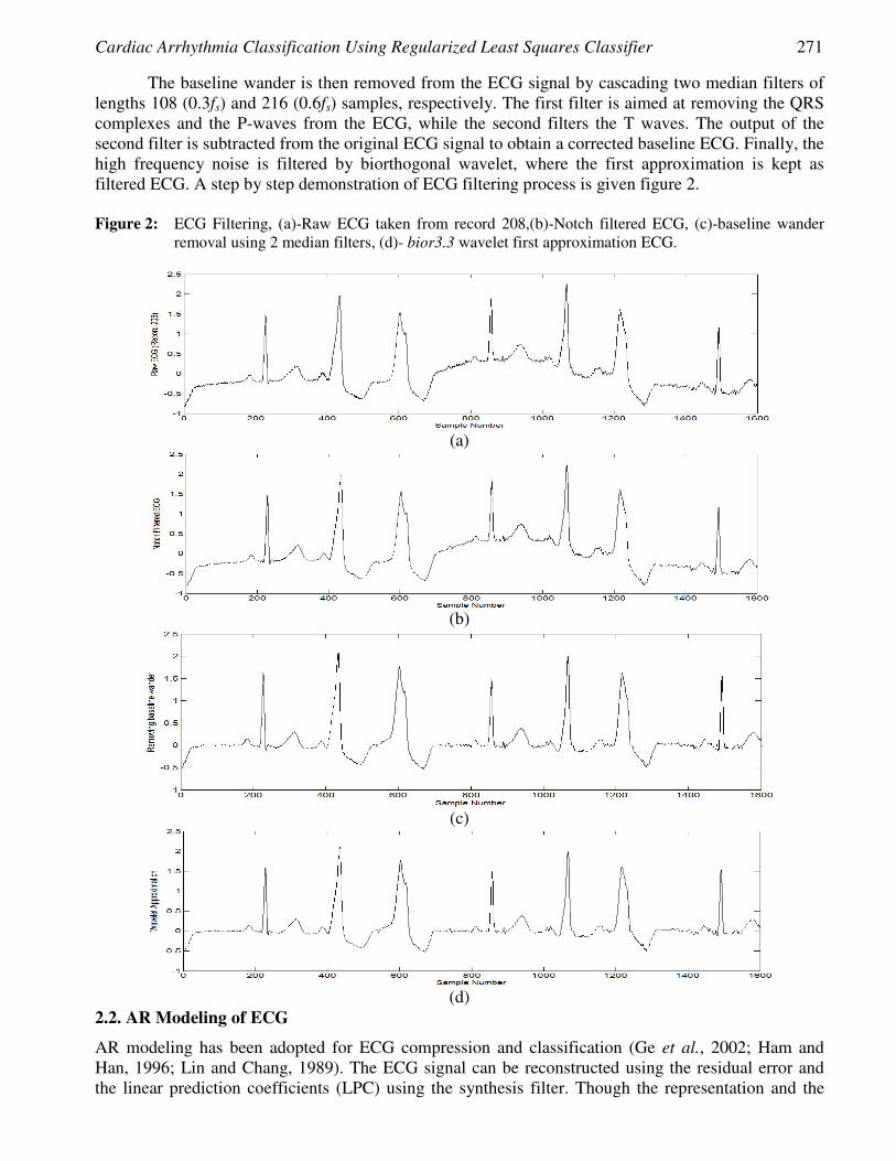
Cardiac Arrhythmia Classification Using Regularized Least Squares Classifier 271
The baseline wander is then removed from the ECG signal by cascading two median filters of lengths 108 (0.3fs) and 216 (0.6fs) samples, respectively. The first filter is aimed at removing the QRS complexes and the P-waves from the ECG, while the second filters the T waves. The output of the second filter is subtracted from the original ECG signal to obtain a corrected baseline ECG. Finally, the high frequency noise is filtered by biorthogonal wavelet, where the first approximation is kept as filtered ECG. A step by step demonstration of ECG filtering process is given figure 2. Figure 2: ECG Filtering, (a)-Raw ECG taken from record 208,(b)-Notch filtered ECG, (c)-baseline wander
removal using 2 median filters, (d)- bior3.3 wavelet first approximation ECG.
(a)
(b)
(c)
(d)
2.2. AR Modeling of ECG
AR modeling has been adopted for ECG compression and classification (Ge et al., 2002; Ham and Han, 1996; Lin and Chang, 1989). The ECG signal can be reconstructed using the residual error and the linear prediction coefficients (LPC) using the synthesis filter. Though the representation and the

272 Hamza Baali, Momoh.J.E.Salami, Rini Akmeliawati and Aida Khorshidtalab
use of the linear prediction filter coefficients as features have been well studied and understood, the extraction of relevant features from the residual error should equally receive much more emphasis as suggested in (Lin and Chang, 1989).
AR modeling consists of estimating the value of the current sample as a linear combination of previous P samples, that is,
( ) ( ) 1
, ˆP
ii
y n a y n i=
= − −∑ (2)
where ŷ(n) is the predicted signal, ai are the linear prediction coefficients (LPC ( ) y n i− ), is the i-th
previous sample of the ECG signal and P is the AR model order. The prediction coefficients may be found by minimizing the sum-of-squared error (SSE)
between the actual sample and the predicted one with respect to the LPCs according to:
( ) ( )2
2
1
( ) 0 P
in n ii i
e n y n a y n ia a =
∂ ∂= + − = ∂ ∂
∑ ∑ ∑ (3)
This equation leads to the autocorrelation or covariance method for estimating the LPCs. The autocorrelation method is computationally more efficient and the filter is guaranteed to be
stable, hence it is used in this study. The original signal can be reconstructed using the residual error and the LPCs using the synthesis filter, that is,
( ) ( ) ( )1
, 1
n
k
y n h n k e k n N=
= − ≤ ≤∑ (4)
where h (n) is the synthesis filter impulse response and N is the size of the ECG period. According to (Ge et al., 2002), a fourth-order LPC analysis is performed on each ECG
heartbeat belonging to one of the classes. Each heartbeat is considered to start from the midpoint between the R-peak of the given heartbeat and the R-peak of the previous heartbeat and ends on the midpoint between the R-peak of the current heartbeat and the R-peak of the following heartbeat. The heartbeat fiducial point times provided with the MIT-BIH arrhythmia database are used to locate the R-peaks (Goldberger et al., 2000). 2.3. ECG Features
As mentioned in Section 1, the set of features plays a vital role in achieving good classification results. To this end, each ECG heartbeat is transformed into a feature vector. In this section, a new set of features to explore more information from the ECG data is proposed. This new set of features is referred to as transform based features which will be discussed subsequently together with other commonly used features. a). RR-Interval Features The RR-interval is the interval between two consecutive R-peaks. Two RR-intervals are measured, namely the RR-interval between the actual heartbeat and the preceding heartbeat (Pre-RR interval) and the RR-interval between the actual heartbeat and the subsequent heartbeat (Post-RR interval) as shown in figure 3.

Cardiac Arrhythmia Classification Using Regularized Least Squares Classifier 273
Figure 3: Pre-RR and Post-RR intervals
b). Energy Based Features Residual error energy reE () is a time-domain measurement that characterises the performance of the
prediction, it is defined as: = T
reE ee (5)
In this study, Daubechies wavelet is used to decompose the signal ECG into approximation and detail coefficients. The total energy of the first level details coefficients is calculated and used as features. In previous studies the wavelet coefficients have been directly used as features (Sternickel, 2002; Wiens and Guttag, 2010). c). Transformation Based Features An interesting framework for an accurate representation of the excitation signal applied to speech signal was initiated in (Atal, 1989), and this was later investigated and further developed for ECG compression in (Baali et al., 2011a) and for ECG period normalization in (Baali et al., 2011b). This representation is subsequently briefly described and adopted for features extraction.
Equation (4) can be expressed in matrix form as: Y = He , (6)
whereY is N × 1 column vector in which its entries represent the time domain ECG samples and e is an N × 1 column vector of the residual error. H is the N × N impulse response matrix of the synthesis filter (also called LPC filter), its entries are completely determined by the linear prediction coefficients, H is a lower triangular and Toeplitz matrix.
( )
( ) ( )
1 0 . 0
1 1 . 0
.
. . . . .
1 2 . . 1
h
h N h N
= − −
⋯
⋱
⋮ ⋮ ⋱ ⋮H (7)
Applying the singular values decomposition (SVD) to H gives: = TY UDV e , (8)
where U and V are orthogonal N N× matrices, and D is a real valued N N× iagonal matrix containing the singular values of H .
The SVD domain representations of Y and e are given by θ and ζ respectively, where θ = UTY
and = VT e . Therefore,
=θ Dζ (9) From (9) each component of the residual signal (e) is projected onto the right singular vectors
of the matrix H and then weighted by the corresponding singular value. Since the singular values are always arranged in a descending order, one can expect that the transformed ECG signal (θ) decays as shown in figure 4.

274 Hamza Baali, Momoh.J.E.Salami, Rini Akmeliawati and Aida Khorshidtalab
Figure 4: Normal sinus beat and transformed ECG
From this transformation two features may be introduced: 1) The ratio between the number of elements containing 90% of the total energy of the
transformed ECG (θ) and the length of the ECG heartbeat (i.e., energy based ratio (EBR) .The energy of the ECG waveform and the transformed ECG is the same since the mapping UT
Y is isometric. Considering that the percentage of the total energy used (i.e., 90%) was selected empirically.
2) The two largest singular value of the impulse response matrix. For instance, figure 5 represents a two-dimensional feature space of normal (red ‘+’) and PVC
(black ‘o’) beats randomly taken from three different patients with identification numbers 116, 208 and 210. The first feature corresponds to the first principle component of the impulse response matrix H, while the second represents the EBR. The cluster plot shows that the newly introduced features have a good discrimination capability between the normal (NOR) and PVC beats.
Figure 5: Two-dimensional feature vectors of normal (red ‘+’) and PVC beats (black ‘o’) .
d). Higher Order Statistics Features Besides the aforementioned features, statistical approaches have been considered for feature extraction, namely the third and the fourth order cumulants (Manolakis and Ingle, 2011; Osowski and Linh, 2001).
The third-order central moment is known as the skewness. It characterizes the degree of asymmetry of a distribution around its mean. It is defined as a normalized third-order central moment, that is,

Cardiac Arrhythmia Classification Using Regularized Least Squares Classifier 275
{ }3
3
( ),
xE xskew
µ
σ
−= (8)
where E is the mathematical expectation operator, �x and σ are respectively the mean value and the second central moment (variance). The fourth-order central moment is known as kurtosis. It measures the relative peakedness, or flatness, of a distribution about its mean with respect to a normal distribution. The kurtosis is defined as:
{ }4
4
( )
xE xKurt
µ
σ
−= (9)
2.4. Feature Normalization
A linear method is used to normalize the features to zero mean and unit variance, such that:
, 1,2, ., ˆ ii
x xx i N
σ
−= = …… (10)
where ˆix is the normalised value, x and σ are respectively the mean value and standard deviation.
3. Regularized Least Squares Classification (RLSC) The use of Regularized least squares (RLS) is considered in this paper, where the aim is to build a function (i.e., a learning model) using a set of training points that accurately predicts the class to which the test points belong (i.e., unseen examples).
The RLS is a special case of the Tikhonov regularization problem which is mathematically stated as (Rifkin, 2002).
2K
1
1min ( , ( )) λ|| || ,i if
i
V y f f∈
=
+∑ xℓ
ℓH (11)
where V is the loss function, λ is the regularization parameter (λ R )+∈ . 2K|| ||f is the norm of f
measured in a Reproducing Hilbert space defined by the kernel K. The square loss function is given by :
( )( ) ( )( )2
, ,i i i iV y f y f= −x x (12)
where xi denotes the d-dim feature vector of the ith training point and { }1, 1iy ∈ − + gives the binary
outcome, for i = 1, …, ℓ (with ℓ is the number of training points). The Representer Theorem [34] states that for some xj the solution ƒ* of (11) has the form:
( )*
1
K( , ) j i j i ii
f c c=
= ∈∑x x xℓ
� (13)
There is a wide range of possible kernel functions that might be used, however, in this paper the linear kernel is chosen, that is,
( )K ,i j j=x x x xT
i . (14)
The kernel function measures the similarity between two feature vectors. The selection of the linear kernel is justified by the fact that it allows a lower computational complexity compared to other kernels (Rifkin and Lippert, 2007). The norm of ƒ is given by :
2K|| || . , ,f ×= ∈ ∈K ℓ ℓ ℓTc c c K� � (15)
where K is the square positive semidefinite training kernel matrix with elements :
( ) ( ), K , , for : 1, , and 1, ,i ji j i j= = … = …x x ℓ ℓK .
By using (12), (13) and (15), the Tikhonov regularization problem can be rewritten as:

276 Hamza Baali, Momoh.J.E.Salami, Rini Akmeliawati and Aida Khorshidtalab
( ) ( )1 λ
min , 2 2
T
∈− − +K K K
ℓℓ
T
cy c y c c c
�
(16)
y ∈ ℓ� with coordinates yi
The problem is brought forward to find the ℓ-dim weight vector c where the minimization of (16) with respect to c has the closed form solution:
1(C yλ −= K + I)ℓ (17) ×∈I ℓ ℓ
� is the identity matrix. Once the weight vector c is found, the determination of class membership of a test point xt is
possible. Thus,
( )*
1
K( , ). t j t jj
f c=
=∑x x xℓ
(18)
In binary classification, the label (or class) of xt is determined by the sign of ƒ*(xt) . 3.1. Tuning the Regularization Parameter λ
The weight vector c is a function of the regularization parameter λ. Rifkin et al [35] proposed an elegant way of tuning λ by rewriting (17) using the eigendecomposition of the kernel matrix. Let K = QΛQT and = QQT , then,
1( λ ) ,−= + TQ Λ I Qℓc Y (19)
where Λ = diag (λ1, … , λℓ). Writing c in the form given by (18) allows one to vary λ between the minimum and maximum eigenvalues of K efficiently. Note that the matrix (Λ + λℓI) is diagonal,
hence; 1 1( λ )
( λ )iiii
−+ =+
Λ IΛ I
.
3.2. Multiclass Classification
Many solutions have been proposed in the literature to tackle multiclass classification problem such as single machine approaches and error correcting approaches. Rifkin and Klautau, 2004 have shown that One-versus-all (OVA) strategy for multiclass classification is simpler and as accurate as any other approach (Rifkin and Klautau, 2004). Using this strategy, q different binary classifiers are trained, where q is the number of classes. Once the classifiers are trained the classification of a new test point is possible by using the winner-takes-all principle in which the classifier with the highest output is chosen.
( ) ( )argmax , 1,t i ti
f f i q= = …x x . (19)
In order to train each of the classifiers, the output y is considered to be equal to 1 if the training point belongs to class q and and -1 if the training point belongs to any other class. 4. Results and Discussion The MIT-BIH database is used to evaluate the performance of the algorithm (Goldberger et al., 2000). This database is a widely used benchmark database that consists of 48 half hour recordings of two-channel ambulatory ECG selected from 47 different patients. The first 23 records with identification numbers 100 to 124 were randomly taken from a pool of data containing 4000 records. Meanwhile, the remaining 25 records with identification numbers 200 to 234 (some numbers are missing) were carefully chosen as they contain unusual abnormalities that might not be represented in the database if all the records were randomly taken. The data is bandpass filtered at 1-100 Hz and sampled at 360 Hz to facilitate the elimination of the power line interference using notch filter. All the heartbeats (around

Cardiac Arrhythmia Classification Using Regularized Least Squares Classifier 277
109,000) in the database were manually annotated by cardiologists and made available for the users. In addition, fiducial point times are provided to locate the R-peaks.
The database is split into two independent datasets each contains 22 records .The first dataset is composed of patients records with identification numbers 101, 106, 108, 109, 112, 114, 115, 116, 118, 119,122, 124, 201, 203, 205, 207, 208, 209, 215, 220, 223 and 230. The second data set is composed of patient’s records 100,103, 105, 111, 113, 117, 121, 123, 200, 202, 210, 212, 213, 214, 219, 221, 222, 228, 231, 232, 233 and 234. The remaining 4 paced records are omitted as recommended by the AAMI. The first dataset was used to train the classifier while the second one was held out for testing. This data selection is the same as those used in (Chazal et al., 2004; Lannoy et al., 2011; Park et al., 2008). The details of the distribution of heartbeats in the two datasets and their frequencies are summarized in table 2. Table 2: Distribution of the extracted heartbeats in the two datasets.
N S V F Total Training 45807 943 3785 414 50949 89.90% 1.85% 7.42% 0.81% 100% Test 44197 1835 3219 388 49639 89.03% 3.69% 6.48% 0.78% 100%
Each of the extracted heartbeats is transformed into a thirteen-dimensional feature vector where
eleven of them are extracted from the first lead namely, the residual error energy, the two largest singular value of H, EBR , the two R-R intervals, the skewness and the kurtosis of the heartbeat and QRS complex and the skewness of the transformed ECG. The QRS complex is taken in a window of 91 samples centred at the QRS peak. The remaining two features are extracted from the second lead namely, the total energy of the first level details coefficient and the fourth linear prediction coefficient. The selection of features was done based on the following metrics
Five metrics are used to assess the performance of the proposed algorithm namely, sensitivity (Se), specificity (Sp), positive predictivity (+P), accuracy (ACC) and the (BCR). These metrics are mathematically expressed as:
TP TNSe , Sp
TP FN TN FPi i
i ii i i i
= =+ +
.
TP TP TNP , ACC
TP FP TP TN FP FNi i i
i ii i i i i i
++ = =
+ + + +.
where TP, FP, FN and TN refer respectively to “true positive", “false positive", “false negative" and “true negative".
Note that, the BCR gives unbiased accuracy for unbalanced datasets. It is defined as the mean value between sensitivity Se and the specificity Sp. For instance a trivial binary classifier would achieve 90% accuracy if the frequencies of the two classes are respectively 90% and 10%, respectively. The BCR for such classifier is only 50 %. In a multi-class problem, the BCR is equal to the average of class accuracies.
Three different tests are carried out. The first two scenarios performs the classification of VEB (V) versus (N, S and F) and the classification of SVEBs (S) versus (N,V and F). The results are shown in table 3. In the third test, the multiclass recommended taxonomy is investigated and the results are shown in the form of confusion matrix in table 4 and in the form of performance metrics in table 5.

278 Hamza Baali, Momoh.J.E.Salami, Rini Akmeliawati and Aida Khorshidtalab
Table 3: Performance of the proposed classification algorithm for the binary classification scenarios
Number of beats SVEB VEB Identification
number N S V F Acc Se +P Acc Se +P
100 2236 33 1 0 98.90 24.24 100.00 100.00 100.00 100.00 103 2079 2 0 0 99.38 0 0 100.00 - 0 105 2523 0 41 0 97.97 - 0 92.24 17.08 17.08 111 2120 0 1 0 100.00 - - 100.00 100.00 100.00 113 1786 6 0 0 98.83 16.67 05.88 99.94 - 0 117 1531 1 0 0 99.35 0 0 99.87 - 0 121 1858 1 1 0 99.89 0 0 100.00 100.00 100.00 123 1512 0 3 0 99.60 - 0 99.93 75.00 75.00 200 1741 30 825 2 95.42 13.33 04.12 98.96 96.74 99.75 202 2058 55 19 1 97.33 18.18 45.45 99.30 55.88 55.88 210 2420 22 195 10 98.87 68.18 39.47 99.02 87.13 96.17 212 2745 0 0 0 99.96 - 0 99.78 - 0 213 2638 28 220 362 99.63 96.43 71.05 94.15 53.55 53.68 214 2000 0 256 1 62.52 - 0 99.69 97.28 99.60 219 2079 7 64 1 63.09 100.00 00.87 99.07 75.90 76.83 221 2028 0 396 0 99.83 - 0 98.31 90.62 90.62 222 2271 209 0 0 99.72 97.61 99.03 99.11 - 0 228 1685 3 362 0 96.59 100.00 04.11 75.17 41.36 41.50 231 1565 1 2 0 97.70 100.00 02.70 49.17 00.25 00.25 232 397 1380 0 0 96.40 95.36 100.00 82.27 - 0 233 2228 7 830 11 78.58 42.86 00.46 86.61 66.48 67.19 234 2697 50 3 0 81.35 26.00 02.66 99.89 40.00 50.00
The first column in table 3 presents the identification number of the patients in the test data.
The subsequent four columns provide the number of beats in each class, followed by three columns which provide the binary classification results of VEB (V) versus (N, S and F) in terms of accuracy, sensitivity and positive predictive value. The classification results of SVEBs (S) versus (N,V and F) are given in the last three columns . The quasi-totality of accuracies achieved for each patient was above 96% for SVEBs (S) versus (N, V and F) problem. For the VEB (V) versus (N, S and F), the achieved accuracies were above 96% for the majority of patients while for four patients the achieved accuracy was 100%. The number of misclassified beats was above the average for record 231.
The overall multiclass classification performances of the RLSC are shown in table 5 along with some state-of-the-art of inter-patients classifiers that follow the AAMI recommended practice. Chazel et al., 2004 implemented a linear discriminant classifier for each lead using a diverse set of features including ECG morphology, heartbeat intervals, and RR-intervals. The classifiers outputs were combined to produce the final classification. However, Park et al., 2008 on the other hand, built a hierarchical model based on three SVM classifiers. Each classifier was fed by a different set of features, including R-R intervals, HBF and HOS. While Lannoy et al., 2011 used an exhaustive wrapper approach to select the most seven relevant features from a large variety of features reported in the literature. The selected features serve as input to a weighted-SVM classifier. The authors reported the results of raw SVM to emphasise the importance of weighting. It is worthy to mention that Chazel et al., 2004 have also taken into account the unbalanced data distribution problem across classes by taking around 400 training points from each class. In our experiment, the number of training points were 1548, 900, 560 and 400 for the N, S, V and F class, respectively. Table 4: Overall Confusion Matrix
Outcome Predicted Class N S V F
Actual Class
N 35324 4719 1138 3016 S 229 1575 4 27 V 461 75 2483 200 F 24 1 2 361
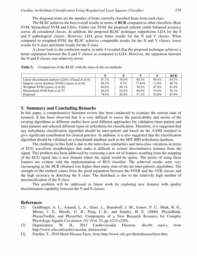
Cardiac Arrhythmia Classification Using Regularized Least Squares Classifier 279
The diagonal terms are the number of beats correctly classified beats from each class. The RLSC achieves the best overall results in terms of BCR compared to other classifiers (Raw
SVM, hierarchical SVM and LDA). Unlike raw SVM, the proposed scheme yields balanced accuracy across all considered classes. In addition, the proposed RLSC technique outperforms LDA for the S and F pathological classes. However, LDA gives better results for the N and V classes. When compared to weighted-SVM, the RLSC achieves comparable results for the N and V classes, lower results for S class and better results for the F class.
A closer look to the confusion matrix in table 4 revealed that the proposed technique achieves a better separation between the S and V classes as compared to LDA. However, the separation between the N and S classes was relatively lower. Table 5: Comparison of the RLSC with the state-of-the-art methods.
N S V F BCR Linear discriminant analysis (LDA ) Chazal et al [5] 87.1% 76.0% 80.3% 89.4% 83.2% Support vector machine (SVM) Lannoy et al [6] 96.5% 0.7% 77.84% 11.8% 46.7% Weighted-SVM Lannoy et al [6] 80.0% 88.1% 78.5% 87.6% 83.6% Hierarchical-SVM Park et al [7] 86.2% 82.6% 80.8% 54.9% 76.1% Proposed 79.9% 85.8% 77.1% 93.0% 83.9%
5. Summary and Concluding Remarks In this paper, a comprehensive literature review has been conducted to examine the current state of research. It has been observed that it is very difficult to assess the practicability and merits of the existing algorithms as different studies have used different approaches for validation (inter-patient and intra-patient) and selected different types of arrhythmia for classification. Therefore, it is suggested that any arrhythmia classification algorithm should be inter-patient and based on the AAMI standard to give significant contribution for clinical practice. In addition, it is also suggested that the classification algorithm should be validated on a benchmark database such as the MIT-BIH arrhythmia database.
The challenge in this field is due to the inter-class similarities and intra-class variations in terms of ECG waveform morphologies that make it difficult to extract discriminative features from the signal. This problem has been addressed by extracting a new set of features resulting from the mapping of the ECG signal into a new domain where the signal would be sparse. The merits of using these features are evident with the implementation of RLS classifier. The achieved results were very encouraging as the BCR obtained was higher than many state-of-the-art inter-patients algorithms. The strength of the method comes from the good separation between the SVEB and the VEB classes and the high accuracy in detecting the S class. The drawback is due to the relatively high number of misclassification of the N class.
This problem will be addressed in future work by exploring new features with quality discrimination capability between the N and S classes. References [1] Goldberger, A. L., Amaral, L. A., Glass, L., Hausdorff, J. M., Ivanov, P. C., Mark, R. G.,
Mietus, J. E., Moody, G. B., Peng, C.-K., and Stanley, H. E. (2000). PhysioBank, PhysioToolkit, and PhysioNet: Components of a New Research Resource for Complex Physiologic Signals Circulation 101 (Vol. 23, pp. e215-e220).
[2] Organization, W. H., 2012 Cardiovascular Diseases. Health topics, from http://www.who.int/cardiovascular_diseases/en/
[3] Frieden, T., 2010 Heart Disease Facts, from http://www.cdc.gov/heartdisease/facts.htm

280 Hamza Baali, Momoh.J.E.Salami, Rini Akmeliawati and Aida Khorshidtalab
[4] Osowski, S., and Linh, T. H., 2001," ECG Beat Recognition Using Fuzzy Hybrid Neural Network". Biomedical Engineering, IEEE Transactions, 48(11), pp. 1265-1271.
[5] Chazal, P. D., O'Dwyer, M., and Reilly, R. B., 2004," Automatic Classification of Heartbeats Using ECG Morphology and Heartbeat Interval Features". Biomedical Engineering, IEEE Transactions, 51(7), pp. 1196-1206.
[6] Chazal, P. d., and Reilly, R. B., 2006," A Patient-Adapting Heartbeat Classifier Using ECG Morphology and Heartbeat Interval Features". Biomedical Engineering, IEEE Transactions 53(12), pp. 2535-2543.
[7] Lannoy, G. d., Franc, D., Delbeke, J., and Verleysen, M., 2011," Weighted SVMs and Feature Relevance Assessment in Supervised Heart Beat Classification". Communications in Computer and Information Science 127(4), pp. 212-223.
[8] Park, K. S., Cho, B. H., Lee, D. H., Song, S. H., Lee, J. S., Chee, Y. J., Kim, I. Y., and Kim, S. I., 2008," Hierarchical Support Vector Machine Based Heartbeat Classification Using Higher Order Statistics and Hermite Basis Function". In Computers in Cardiology, IEEE, pp. 229-232
[9] Ge, D., Srinivasan, N., and Krishnan, S. M., 2002," Cardiac Arrhythmia Classification Using Autoregressive Modeling". BioMedical Engineering OnLine 1, 5(1).
[10] Ham, F. M., and Han, S., 1996," Classification of Cardiac Arrhythmias Using Fuzzy ARTMAP". Biomedical Engineering, IEEE Transactions, 43(4), pp. 425-429.
[11] Lin, K.-P., and Chang, W. H., 1989," QRS Feature Extraction Using Linear Prediction". Biomedical Engineering, IEEE Transactions, 36(10), pp. 1050-1055.
[12] Chen, S.-W., 2000," A Two-Stage Discrimination of Cardiac Arrhythmias Using a Total Least Squares-Based Prony Modeling Algorithm". Biomedical Engineering, IEEE Transactions 47(10), pp. 1317-1327.
[13] Acır, N., 2005," Classification of ECG Beats by Using a Fast Least Square Support Vector Machines with a Dynamic Programming Feature Selection Algorithm". Neural Computing & Applications, 14(4), pp. 299-309.
[14] Kutlu, Y., and Kuntalp, D., 2011," A Multi-Stage Automatic Arrhythmia Recognition and Classification System". Computers in Biology and Medicine 41(1), pp. 37-45.
[15] Minami, K.-i., Nakajima, H., and Toyoshima, T., 1999," Real-Time Discrimination of Ventricular Tachyarrhythmia with Fourier-Transform Neural Network". Biomedical Engineering, IEEE Transactions 46(2), pp. 179-185.
[16] Khadra, L. A. S. A.-F., and Al-Nashash, H., 1997," Detection of Life-Threatening Cardiac Arrhythmias Using the Wavelet Transformation". Medical and Biological Engineering and Computing, 35(6), pp. 626-632.
[17] Sternickel, K., 2002," Automatic Pattern Recognition in ECG Time Series". Computer Methods and Programs in Biomedicine, 68(2), pp. 109-115.
[18] Wiens, J., and Guttag, J. V., 2010," Active Learning Applied to Patient-Adaptive Heartbeat Classification". Advances in Neural Information Processing Systems, 23, pp. 2442-2450.
[19] Jiang, W., and Kong, G. S., 2007," Block-Based Neural Networks for Personalized ECG Signal Classification". Neural Networks, IEEE Transactions 18(6), pp. 1750-1761.
[20] Lagerholm, M., Peterson, a., Braccini, G., Edenbrandt, L., and S¨ornmo, L., 2000," Clustering ECG Complexes Using Hermite Functions and Self-Organizing Maps". Biomedical Engineering, IEEE Transactions, 47(7), pp. 838-848.
[21] Osowski, S., Hoai, L. T., and Markiewicz, T., 2004," Support Vector Machine-Based Expert System for Reliable Heartbeat Recognition". Biomedical Engineering, IEEE Transactions 51(4), pp. 582-589.
[22] Chuang-Chien, C. H. I. U., Tong-Hong, L. I. N., and Liau, B.-Y., 2005," Using Correlation Coefficient in ECG Waveform for Arrhythmia Detection". Biomedical Engineering: Applications, Basis and Communications 17(3), pp. 147-152.

Cardiac Arrhythmia Classification Using Regularized Least Squares Classifier 281
[23] Tsipouras, M. G., and Fotiadis, D. I., 2003," An Efficient System for the Detection of Arrhythmic Segments in ECG Recordings Based on Non-Linear Features of the RR Interval Signal". In Computers in Cardiology, IEEE, pp. 533-536.
[24] Özbay, Y., and Tezel, G., 2010," A New Method for Classification of ECG Arrhythmias Using Neural Network with Adaptive Activation Function". Digital Signal Processing 20(4), pp. 1040-1049.
[25] Castillo, O., Melin, P., Ramírez, E., and Soria, J., 2011," Hybrid Intelligent System for Cardiac Arrhythmia Classification with Fuzzy K-Nearest Neighbors and Neural Networks Combined with a fuzzy System". Expert Systems with Applications, 39, pp. 2947–2955.
[26] Dokur, Z., and Olmez, T., 2001," ECG Beat Classification by A Novel Hybrid Neural Network". Computer Methods and Programs in Biomedicine 66( 2-3 ), pp. 167-181.
[27] Özbay, Y., Ceylan, R., and Karlik, B., 2006," A Fuzzy Clustering Neural Network Architecture for Classification of ECG Arrhythmias". Computers in Biology and Medicine 36(4), pp. 376-388.
[28] Hu, Y. H., Palreddy, S., and Tompkins, W. J., 1997," A Patient-Adaptable ECG Beat Classifier Using A Mixture of Experts Approach". Biomedical Engineering, IEEE Transactions 44(9), pp. 891-900.
[29] Sigg, D. C., Iaizzo, P. A., Xiao, Y.-F., and He, B., 2010. Cardiac Electrophysiology Methods and Models: Springer.
[30] Engström, G., Hedblad, B., Juul-Möller, S., Tydén, P., and Janzon, L., 2000," Cardiac Arrhythmias and Stroke Increased Risk in Men with High Frequency of Atrial Ectopic Beats". Stroke, American Heart Association, 31(12), pp. 2925-2929.
[31] Rodríguez-Sotelo, J. L., Cuesta-Frau, D., and Castellanos-Dominguez., G., 2009," Unsupervised Classification of Atrial Heartbeats Using A Prematurity Index and Wave Morphology Features". Medical and Biological Engineering and Computing, 47(7), pp. 731-741.
[32] Rifkin, R. M. (2002). Everything Old is New Again: A Fresh Look at Historical Approaches in Machine Learning. PhD, MaSSachuSettS InStitute of Technology.
[33] Rifkin, R. M., and Lippert, R. A. (2007). Notes On Regularized Least Squares Computer Science and Artificial Intelligence Laboratory Technical Report: MIT.
[34] Baali, H., Akmeliawati, R., and Salami, M. J. E., 2013," Regularized Least Squares Applied to Heartbeat Classification using Transform-based and RR Intervals Features", BIOSTEC spain.
[35] Atal, B. S., 1989," A Model of LPC Excitation in Terms of Eigenvectors of the Autocorrelation of the Impulse Response of the LPC Filter", IEEE Conference on Acoustics, Speech, and Signal Processing, pp. 45-48.
[36] Baali, H., Akmeliawati, R., Salami, M. J. E., and Aibinu, M., 2011a," Analysis of the ECG Signal Using SVD-Based Parametric Modelling Technique", International Symposium on Electronic Design, Test and Application, Newzealand, pp. 180-184.
[37] Baali, H., Akmeliawati, R., Salami, M. J. E., Aibinu, M., and Gani, A., 2011b," Transform Based Approach for ECG period Normalization", Computing In Cardiology China, pp. 533-536.
[38] Manolakis, D. G., and Ingle, V. K., 2011. Applied Digital Signal Processing Theory and Practice Cambridge University Press.
[39] Rifkin, R., and Klautau, A., 2004," In Defense of One-VS-All Classification". The Journal of Machine Learning Research 5, pp. 101-141.
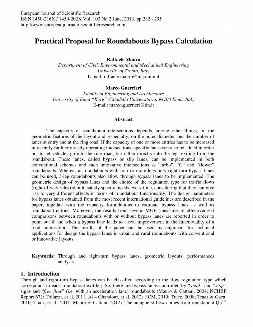
European Journal of Scientific Research ISSN 1450-216X / 1450-202X Vol. 103 No 2 June, 2013, pp.282 - 295 http://www.europeanjournalofscientificresearch.com
Practical Proposal for Roundabouts Bypass Calculation
Raffaele Mauro Department of Civil, Environmental and Mechanical Engineering
University of Trento, Italy E-mail: [email protected]
Marco Guerrieri
Faculty of Engineering and Architecture University of Enna “Kore” Cittadella Universitaria, 94100 Enna, Italy
E-mail: [email protected]
Abstract
The capacity of roundabout intersections depends, among other things, on the geometric features of the layout and, especially, on the outer diameter and the number of lanes at entry and at the ring road. If the capacity of one or more entries has to be increased in recently-built or already operating intersections, specific lanes can also be added in order not to let vehicles go into the ring road, but rather directly into the legs exiting from the roundabout. These lanes, called bypass or slip lanes, can be implemented in both conventional schemes and such innovative intersections as “turbo”, “C” and “flower” roundabouts. Whereas at roundabouts with four or more legs only right-turn bypass lanes can be used, 3-leg roundabouts also allow through bypass lanes to be implemented. The geometric design of bypass lanes and the choice of the regulation type for traffic flows (right-of-way rules) should satisfy specific needs every time, considering that they can give rise to very different effects in terms of roundabout functionality. The design parameters for bypass lanes obtained from the most recent international guidelines are described in the paper, together with the capacity formulations to estimate bypass lanes as well as roundabout entries. Moreover, the results from several MOE (measures of effectiveness) comparisons between roundabouts with or without bypass lanes are reported in order to point out if and when a bypass lane leads to a real improvement in the functionality of a road intersection. The results of the paper can be used by engineers for technical applications for design the bypass lanes in urban and rural roundabouts with conventional or innovative layouts. Keywords: Through and right-turn bypass lanes, geometric layouts, performances
analysis 1. Introduction Through and right-turn bypass lanes can be classified according to the flow regulation type which corresponds to each roundabout exit leg. So, there are bypass lanes controlled by “yield” and “stop” signs and “free flow” (i.e. with an acceleration lane) roundabouts (Mauro & Cattani, 2004; NCHRP Report 672; Tollazzi, et al, 2011, Al – Ghandour, et al. 2012; HCM, 2010; Tracz, 2008; Tracz & Gaca, 2010; Tracz, et al., 2011; Mauro & Cattani, 2012). The antagonist flow comes from roundabout QuTot

283 Raffaele Mauro and Marco Guerrieri
in bypass lanes, while it corresponds to the circulating flow on ring Qc in all the other entry lanes. As for the flow distribution in a roundabout, the following considerations should be taken into account:
1) Right-turn bypass lanes (see Fig. 1): in yield- or stop-controlled bypass lanes the right-turn flow into bypass (QE,R
bypass) must stop and give way to the flow coming from roundabout QuTot. On the contrary, in free-flow bypass lanes, the lane length must be so great as to allow at first the acceleration of the vehicles of bypass lane flow QE,R
bypass and then the entry into the main flow coming from roundabout QuTot (cf. Fig. 1). As for exit flow values, if we examine for instance leg No. 4 in Fig. 1, there is QuTot = Q1,4 + Q2,4 + QE,R
no-bypass; QE,R
no-bypass = Q3,4 - QE,Rbypass, where Qi,j denotes the flow originated from leg “i”, bound for
leg “J”. 2) Through bypass lanes (see Fig. 2): the above considerations for right-turn bypass lanes are
proper but here the traffic flow into the bypass lane is that one through the roundabout denoted with QE,T
bypass. The circulating flow opposing the latter one is that coming from roundabout QuTot = Qu + QE,T no-bypass. In Fig. 2, for instance, there is: QuTot = Q1,3 + QE,T no-
bypass; QE,T no-bypass=Q2,3 - QE,Tbypass.
Figure 1: Entry, circulating and exit flows at
roundabout with right-turn bypass lanes
Figure 2: Entry, circulating and exit flows at roundabout with through -turn bypass lanes
1.1. Yield- and Stop-Controlled Bypass Lanes
Stop-controlled through and right-turn bypass lanes are composed of the following basic sections: manoeuvering section of length Lm; deceleration section of length Ld; storage section of length Ls (see Fig. 3). Bypass lane capacity, estimated right at the stop line in the roundabout exit leg, is equal to the reciprocal of average service time b = E[s], where s denotes the general service time. Therefore, in the event of Poisson vehicle arrivals on the bypass lane, any service time s and vehicle headway τ (on the roundabout exit lane) distributed like a gamma random variable (Mauro & Branco, 2012) with a parameter K (K = 1 se 100 ≤ Q ≤ 300 veh/h; K = 2 if 400 ≤ Q ≤ 800 veh/h; K = 3 if 800 ≤ Q ≤ 1500 veh/h K = 4 if 1500 < Q ≤ 1800 veh/h), bypass lane capacity (be it right-turn or through) estimated just in correspondence to the stop line is equal to (Kendall, 1951; Mauro & Guerrieri, 2013a):
• Stop-controlled bypass lanes: 0,00121231,4
TotQubypassC e− ⋅= ⋅ (1)
• Yield -controlled bypass lanes [4]: 0,00111130
TotQubpassC e− ⋅= ⋅ (2)

Practical Proposal for Roundabouts Bypass Calculation 284
Figure 3: Layout of the Stop-controlled bypass lane
By denoting the circulating capacity with Q = QuTot and the service time variance with V[s], it is
possible to evaluate average queuing time E[w], average queued vehicle E[q] and average queue length Ls (average space between a vehicle and the subsequent c = 5,50 m), by means of the following expressions (Mauro & Guerrieri, 2013a) which are valid for right-turn bypass lanes:
1
bypass
bC
= (3)
1
0
12
0
( )( 1)
!( )
( )!
iKKQT
iiK
i
KQTK e
iV s
KQTKQ
i
+
=
−
=
+ ⋅ −
=∑
∑ (4)
2 2,
,,
( [ ])[ ]
2 (1 )
bypassbypass E R
E R bypassE R
Q b V sE w Q b
Q b
⋅ += ⋅ +
⋅ − ⋅ (5)
E[q] = QE;Rbypass E[w] (6)
Ls = c E[q] (7) The same expressions can be used for through bypass lanes, but in equations (5) and (6) flow
QE;tbypass needs obviously to be taken into account.
Graphs in Figures 4 and 5 illustrate the expected number of queued vehicles when the capacity varies at the stop-controlled bypass lane and at the roundabout exit lane (Qu = Qu
Tot) according to exit flow speed V1 = 30 km/h and V1 = 50 km/h. It is worth pointing out that when the exit flow speed increases - conditions being equal - the queue length increases more than proportionally. Since the vehicles in flow QuTot exiting from the roundabout tend to increase their speed to reach the planned road speed, it follows that it is necessary to verify the entry (stop- or yield line) just near the outer circumference of the ring.
Figure 4: Values of the queues (V1 = 30 km/h)
Figure 5: Values of the queues (V1 = 50 km/h)

285 Raffaele Mauro and Marco Guerrieri
1.2. Free-Flow Bypass Lanes
A reliable estimation of the free-flow bypass lane capacity (entry without a stop- or yield-sign) is given by the following equation obtained from (Tracz, 2008; Tracz & Gaca, 2010; Tracz, et al., 2011) and through tests on single-lane roundabouts.
0,0071250TotQu
bypassC e− ⋅= ⋅ (8)
Figure 6: Layout of the Free Flow bypass lane
(Polish Guidelines) Figure 7: Layout of the Free Flow bypass lane in the
case of pedestrian flow
Manual HCM 2010 does not provide free-flow bypass lanes with any formulation or capacity value but it reports that capacities can be expected, as a matter of fact, to be higher than those obtained from yield-controlled bypass lanes. With reference to the constituent parameters of free-flow bypass lanes the Polish guidelines (Wytyczne Projektowania Skrzyzowan drogowych, Czesc II, Warszawa, 2001) are extremely interesting, in that they identify the standard schemes in Figures 6 and 7 to be implemented respectively in absence and in presence of quite a significant pedestrian flow.The section length Lp (see Fig. 6) can be deduced from Table 2 and depends on the planned road speed, its grades and radius value R3 (cf. Fig. 6). Table 1: Lp length
Design Speed [km/h]
Grades [%] Lp [m] as function of R3 [m]
≤ 10 11 ÷ 15 16 ÷ 20 21 ÷ 30 >30
60
-4 40 35 30 - - -2 45 40 30 - - 0 50 45 35 25 - 2 60 55 45 30 - 4 75 65 55 40 25
Finally, the scheme in Fig. 8 concerning a free flow bypass lane is examined; it is composed of
the following basic sections: i) Acceleration section of length La; ii) Entry section of length Li; iii) Junction section of length Lr (see, in this regard, the parameters provided for in Italy by Ministerial Decree of 19 April 2006 entitled “Functional and geometric rules for building road intersections”).
Figure 8: Free Flow Bypass lane
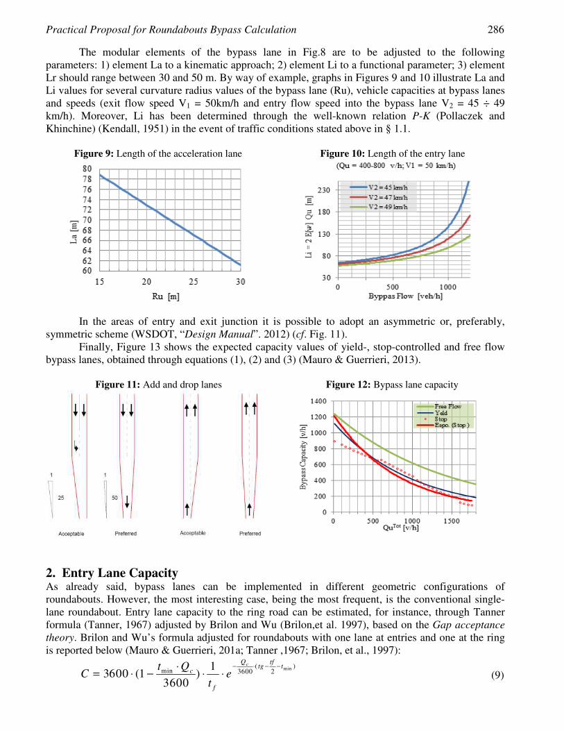
Practical Proposal for Roundabouts Bypass Calculation 286
The modular elements of the bypass lane in Fig.8 are to be adjusted to the following parameters: 1) element La to a kinematic approach; 2) element Li to a functional parameter; 3) element Lr should range between 30 and 50 m. By way of example, graphs in Figures 9 and 10 illustrate La and Li values for several curvature radius values of the bypass lane (Ru), vehicle capacities at bypass lanes and speeds (exit flow speed V1 = 50km/h and entry flow speed into the bypass lane V2 = 45 ÷ 49 km/h). Moreover, Li has been determined through the well-known relation P-K (Pollaczek and Khinchine) (Kendall, 1951) in the event of traffic conditions stated above in § 1.1.
Figure 9: Length of the acceleration lane Figure 10: Length of the entry lane
In the areas of entry and exit junction it is possible to adopt an asymmetric or, preferably, symmetric scheme (WSDOT, “Design Manual”. 2012) (cf. Fig. 11).
Finally, Figure 13 shows the expected capacity values of yield-, stop-controlled and free flow bypass lanes, obtained through equations (1), (2) and (3) (Mauro & Guerrieri, 2013).
Figure 11: Add and drop lanes Figure 12: Bypass lane capacity
2. Entry Lane Capacity As already said, bypass lanes can be implemented in different geometric configurations of roundabouts. However, the most interesting case, being the most frequent, is the conventional single-lane roundabout. Entry lane capacity to the ring road can be estimated, for instance, through Tanner formula (Tanner, 1967) adjusted by Brilon and Wu (Brilon,et al. 1997), based on the Gap acceptance theory. Brilon and Wu’s formula adjusted for roundabouts with one lane at entries and one at the ring is reported below (Mauro & Guerrieri, 201a; Tanner ,1967; Brilon, et al., 1997):
min( )min 3600 21
3600 (1 )3600
cQ tftg t
c
f
t QC e
t
− ⋅ − −⋅= ⋅ − ⋅ ⋅ (9)

287 Raffaele Mauro and Marco Guerrieri
where: • C = capacity of the entry lane [veh/h]; • Qc = circulating traffic flow in front of the entry E [veh/h]; • tg = critical gap, [s] • tf = follow – up tim [s]; • tmin = least headway between vehicles moving along the circulating lanes
The time intervals involved in relation (4) have recently been estimated and referred in (Brilon, 2011; Brilon, 2012) for small-sized compact roundabouts in function of the roundabout outer diameter (cf. Table 2). Table 2: Values of the behavioural parameters
Roundabout tc tf tmin Mini 13 m ≤ d ≤ 26 m
0,44,9
13tc d= − �
0,13,1
13tf d= − �
0,9 3,9
13tmin d= − �
Compact 13 m ≤ d ≤ 40 m
1(52,2 0,2 )
14tc d= +� �
1(51 0,4 )
14tf d= −� �
6 0,5·tmin d= −
The capacity values of an entry lane to the roundabout under varying circulating flow and outer
diameter are reported in Fig. 13. 3. Entry Capacity, Delays and Queues The estimation of the entry capacity to a single-lane roundabout must take into account the capacities of each single entry lane and vehicle flow distribution over both lanes. It is especially worth considering that in presence of bypass lanes, some manouvres can be performed through the latter lane or the entry lane at the ring.
For example, if users entering the intersection have to turn right into a 4-leg roundabout, they have two options: to use the bypass lane, or rather, the lane connected with the ring. If traffic conditions do not cause queues at the bypass lane, or if the queue length Lc is inferior to total bypass lane length Lbypass most users are supposed to utilize the bypass lane. On the contrary, if Lc tends to be equal to Lbypass a more or less substantial part of users will choose to utilize the adjacent lane, rather than queuing at the bypass lane: such users therefore will turn right by getting onto the ring road, as happens in roundabouts without bypass lanes.
For this reason, the entry capacity can be estimated through the following relations which are valid for right-turn and through bypass lanes, respectively (Mauro & Branco, 2010; Guerrieri, et al., 2012; Corriere & Guerrieri, 2012; Giuffrè, et al., 2012; Mauro & Guerrieri, 2013a; Mauro & Guerrieri, 2013b):
a) Right-turn bypass lanes: , ,
, , ,
, ,
( )
max[ , ]
E R E TLTE
E R E TLT E R
E R E TLT
Q QC
Q Q Q
C C
α β
+=
⋅ + ⋅ (10)
where: QE,R
bypass = α·QE,R ; QE,Rno-bypass = β·QE,R; 0 ≤ α≤ 1; 0 ≤ β≤ 1; α+β=1; QE,R denotes the total
right-turn flow. The capacity CE,TLT is given from equation (9), whereas CE,R is obtained through equations (1), (2) or (8) according to the regulation type scheduled for a bypass terminal.
b) Through bypass lanes:

Practical Proposal for Roundabouts Bypass Calculation 288
, ,
, , ,
, ,
( )
max[ , ]
E T E LE
E T E L E T
E T E L
Q QC
Q Q Q
C C
γ δ
+=
⋅ + ⋅ (11)
where: QE,T
bypass = γ ·QE,T ; QE,Rno-bypass = δ ·QE,T; 0 ≤ γ ≤ 1; 0 ≤ δ ≤ 1; γ +δ =1; QE,T denotes
the total through flow. The capacity CE,L is given form eq. (9), whereas CE,T R is obtained through equations (1), (2) o (8) according to the regulation type scheduled for a bypass terminal.
Figure 13: Entry capacity lane Figure 14: Sum of the Entry simple Capacity
Figure 14 shows the variation in the sum of the entry simple capacities of 4-leg roundabouts with right-turn bypass lanes (with a total length of 60 m) at each intersection leg under varying total entry flow and distribution coefficient for right-turn flow α. The roundabout capacity obviously tends to increase when the right-turn flow partly goes into the bypass lane (α ≠ 1). In order to determine the effects of pedestrian flow on the capacity of roundabout schemes with bypass lanes, see Mauro & Guerrieri, 2013, Corriere, et. al., 2013.
Delays Di and queues Ni95 for each entry lane can be worked out through the formulations in Capacity Manual HCM 2010, as follows:
2
3600( ) ( )3600
900 1 ( 1) 5 min[ ;1]450
QiQi Qi QiCi CiDi T
Ci Ci Ci T Ci
⋅
= + ⋅ ⋅ − + − + + ⋅ ⋅
(12)
295
3600( ) ( )
900 1 ( 1)150 3600
QiQi Qi CiCi CiN TCi Ci T
⋅
= ⋅ ⋅ − + − + + ⋅
(13)
where: Di is the Delay [sec/veh]; Q95 the 95th-percentile queu [veh]; Qi and Ci are the volume and the capacity of the subject lane; and T is the time period, h (T = 1 for a 1-h analysis, T = 0.25 for a 15-min analysis). 4. Functional Comparison 4.1. Roundabout with Four Legs and a Right-Turn Bypass Lane
In order to identify the traffic conditions which make roundabouts with a right-turn slip lane more advantageous than conventional roundabouts in terms of functionality, specific analyses have been

289 Raffaele Mauro and Marco Guerrieri
carried out for different O/D matrices. It is noteworthy to point out that if there is a right-turn slip lane at each leg, the functional geometric layout has the same behaviour as in flower roundabouts (see Figure 1c). The geometric layouts compared to one another are the following: a) Roundabouts with stop-controlled slip lanes (at each leg);b) Roundabouts with yield-controlled slip lanes (at each leg); c) Roundabouts with Free-flow slip lanes (at each leg); d) Conventional roundabouts with a single lane at entries and a single lane at the ring – layout (1+1); e) Conventional roundabouts with a single lane at entries and a double lane at the ring – layout (1+2); f) Conventional roundabouts with a double lane at entries and a double lane at the ring – layout (2+2).
In order to determine the capacities, the following formulations have been used: Equation (1) for roundabouts with a stop-controlled slip lane; Equation (2) for roundabouts with a yield-controlled slip lane; Equation (8) for roundabouts with a free-flow slip lane;
• The formula suggested by the HCM 2010 Manual for conventional roundabouts with a single lane at entries and 1 lane at the ring – layout (1+1): CE = 1130·e-0,0001·Qc (14)
• The formula suggested by the HCM 2010 Manual for conventional roundabouts with a single lane at entries and two lanes at the ring – layout (1+2): CE = 1130·e-0,007·Qc (15)
• The formulas suggested by the HCM 2010 Manual for conventional roundabouts with a double lane at entries and a double lane at the ring – layout (2+2). For the two lanes at entries the formulas are the following: CE,R = 1130·e-0,0007·Qc (16) CE,TLT = 1130·e-0,00075·Qc (17)
For each layout under study the mean control delays and the queues have been determined by employing Equations (12) and (13). The traffic conditions examined are the following:
• O/D Matrices - Origin/destination matrices of traffic flows in percentage terms - (the leg numeration is illustrated in Figure 1): ρ1 considers a majority of vehicles going ahead; the same occurs in ρ2 but left-turn percentages are 25%. Matrix ρ3 indicates a clear majority of crossings for flows 2 and 4 and very limited left-turns, ρ4 e ρ5 indicate two or one direction of preferential exit. Matrix 6 assumes that most users turn to the right (70% out of the total);
• Vehicular flow vectors. Q3 flows are basically the same on the four legs, Q2 flows especially move in direction 1-3; Q1 is an intermediate situation between Q3 and Q2; Q4 indicate very unbalanced flows.
• Pedestrian flow vectors: Qp1 and Qp2: pedestrian flows of average/high intensity; Qp3: very low pedestrian flows.
ρ =
0 0,15 0,74 0,11
ρ2 =
0 0,15 0,60 0,25 0,19 0 0,24 0,57 0,2 0 0,20 � ,55 0,63 0,15 0 0,22 0,60 0,25 0 0,15 0,19 0,74 0,07 0 0,30 0,50 0,20 0
ρ3 =
0 0,15 0,70 0,15
ρ4 =
0 0,125 0,75 0,125 0,02 0 0,18 0,80 0,375 0 0,375 0,25 0,70 0,15 0 0,15 0,75 0,125 0 0,125 0,18 0,80 0,02 0 0,375 0,25 0,375 0
ρ5=
0 0,25 0,75 0,125
ρ6 =
0 0,7 0,2 0,1 0,125 0 0,625 0,25 0,2 0 0,7 0,1 0,5 0,25 0 0, 25 0,1 0,3 0 0,6
0,125 0,25 0,625 0 0,7 0,2 0� 1 0
[Q1] = [300 200 500 400] [Q2] = [386 182 410 446]
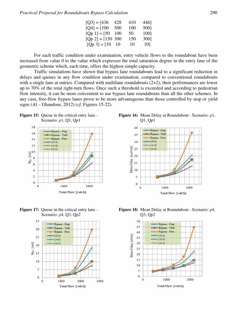
Practical Proposal for Roundabouts Bypass Calculation 290
[Q3] = [436 428 410 446] [Q4] = [100 500 100 500] [Qp 1] = [50 100 50 100] [Qp 2] = [150 300 150 300] [Qp 3] = [10 10 10 10]
For each traffic condition under examination, entry vehicle flows to the roundabout have been
increased from value 0 to the value which expresses the total saturation degree in the entry lane of the geometric scheme which, each time, offers the highest simple capacity.
Traffic simulations have shown that bypass lane roundabouts lead to a significant reduction in delays and queues in any flow condition under examination, compared to conventional roundabouts with a single lane at entries. Compared with multilane roundabouts (2+2), their performances are lower up to 70% of the total right-turn flows. Once such a threshold is exceeded and according to pedestrian flow intensity, it can be more convenient to use bypass lane roundabouts than all the other schemes. In any case, free-flow bypass lanes prove to be more advantageous than those controlled by stop or yield signs (Al – Ghandour, 2012) (cf. Figures 15-22). Figure 15: Queue in the critical entry lane -
Scenario: ρ1, Q1, Qp1 Figure 16: Mean Delay at Roundabout - Scenario: ρ1,
Q1, Qp1
Figure 17: Queue in the critical entry lane -
Scenario: ρ4, Q3, Qp2 Figure 18: Mean Delay at Roundabout - Scenario: ρ4,
Q3, Qp2
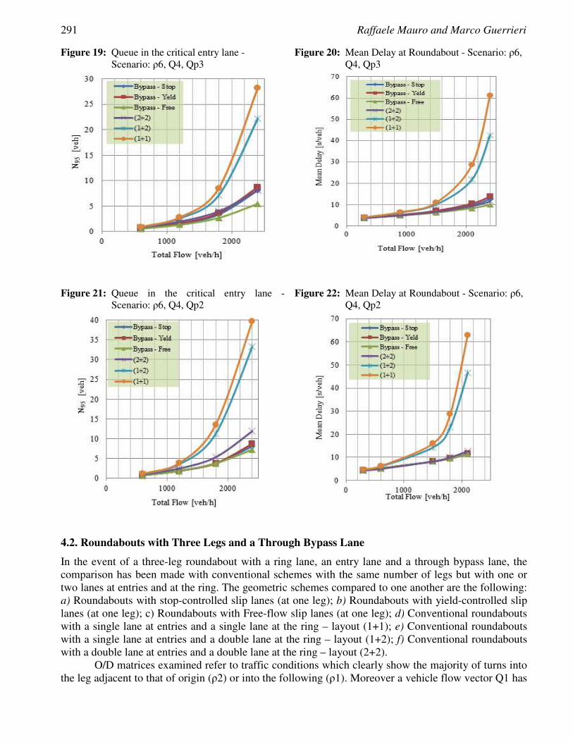
291 Raffaele Mauro and Marco Guerrieri
Figure 19: Queue in the critical entry lane - Scenario: ρ6, Q4, Qp3
Figure 20: Mean Delay at Roundabout - Scenario: ρ6, Q4, Qp3
Figure 21: Queue in the critical entry lane -
Scenario: ρ6, Q4, Qp2
Figure 22: Mean Delay at Roundabout - Scenario: ρ6, Q4, Qp2
4.2. Roundabouts with Three Legs and a Through Bypass Lane
In the event of a three-leg roundabout with a ring lane, an entry lane and a through bypass lane, the comparison has been made with conventional schemes with the same number of legs but with one or two lanes at entries and at the ring. The geometric schemes compared to one another are the following: a) Roundabouts with stop-controlled slip lanes (at one leg); b) Roundabouts with yield-controlled slip lanes (at one leg); c) Roundabouts with Free-flow slip lanes (at one leg); d) Conventional roundabouts with a single lane at entries and a single lane at the ring – layout (1+1); e) Conventional roundabouts with a single lane at entries and a double lane at the ring – layout (1+2); f) Conventional roundabouts with a double lane at entries and a double lane at the ring – layout (2+2).
O/D matrices examined refer to traffic conditions which clearly show the majority of turns into the leg adjacent to that of origin (ρ2) or into the following (ρ1). Moreover a vehicle flow vector Q1 has
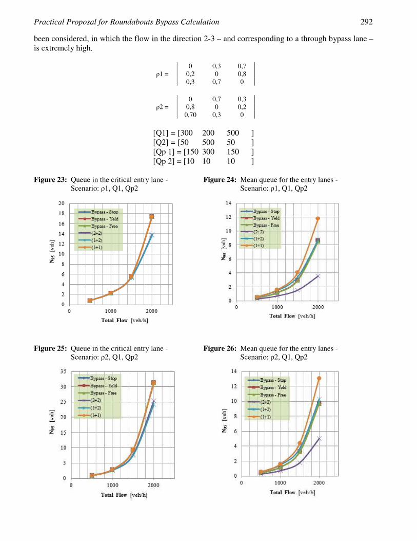
Practical Proposal for Roundabouts Bypass Calculation 292
been considered, in which the flow in the direction 2-3 – and corresponding to a through bypass lane – is extremely high.
0 0,3 0,7 ρ1 = 0,2 0 0,8 0,3 0,7 0
0 0,7 0,3 ρ2 = 0,8 0 0,2 0,70 0,3 0
[Q1] = [300 200 500 ] [Q2] = [50 500 50 ] [Qp 1] = [150 300 150 ] [Qp 2] = [10 10 10 ]
Figure 23: Queue in the critical entry lane -
Scenario: ρ1, Q1, Qp2 Figure 24: Mean queue for the entry lanes -
Scenario: ρ1, Q1, Qp2
Figure 25: Queue in the critical entry lane -
Scenario: ρ2, Q1, Qp2 Figure 26: Mean queue for the entry lanes -
Scenario: ρ2, Q1, Qp2
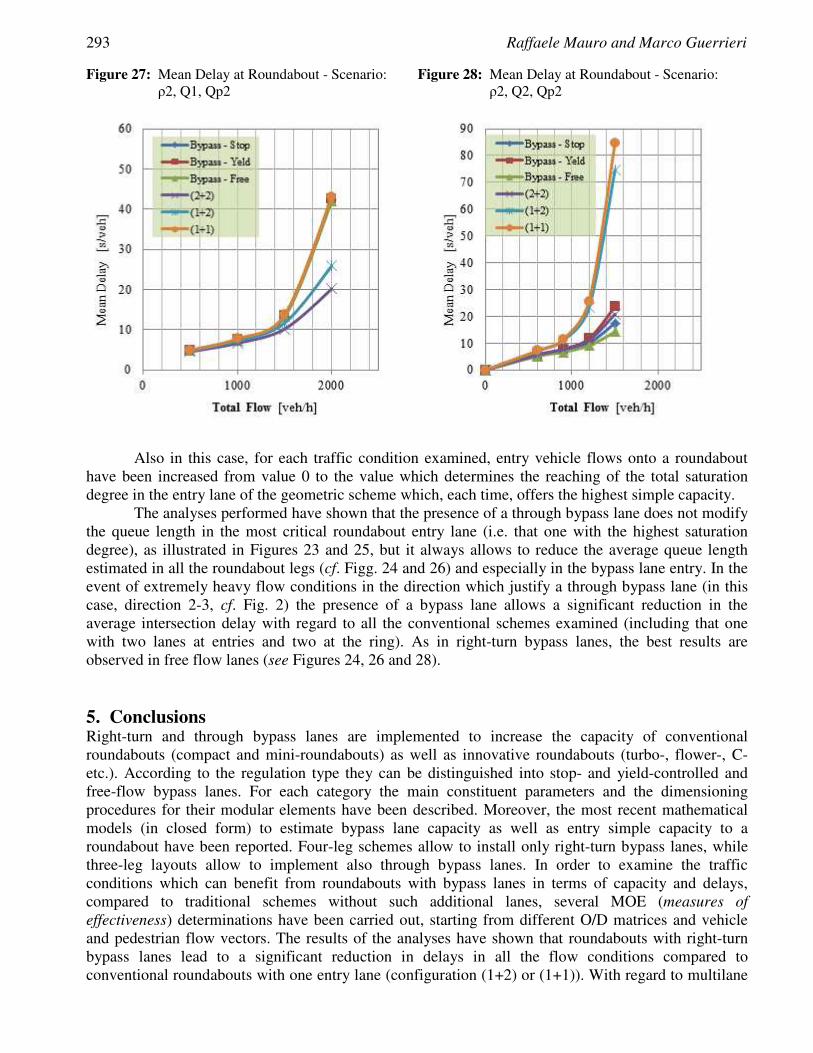
293 Raffaele Mauro and Marco Guerrieri
Figure 27: Mean Delay at Roundabout - Scenario: ρ2, Q1, Qp2
Figure 28: Mean Delay at Roundabout - Scenario: ρ2, Q2, Qp2
Also in this case, for each traffic condition examined, entry vehicle flows onto a roundabout have been increased from value 0 to the value which determines the reaching of the total saturation degree in the entry lane of the geometric scheme which, each time, offers the highest simple capacity.
The analyses performed have shown that the presence of a through bypass lane does not modify the queue length in the most critical roundabout entry lane (i.e. that one with the highest saturation degree), as illustrated in Figures 23 and 25, but it always allows to reduce the average queue length estimated in all the roundabout legs (cf. Figg. 24 and 26) and especially in the bypass lane entry. In the event of extremely heavy flow conditions in the direction which justify a through bypass lane (in this case, direction 2-3, cf. Fig. 2) the presence of a bypass lane allows a significant reduction in the average intersection delay with regard to all the conventional schemes examined (including that one with two lanes at entries and two at the ring). As in right-turn bypass lanes, the best results are observed in free flow lanes (see Figures 24, 26 and 28). 5. Conclusions Right-turn and through bypass lanes are implemented to increase the capacity of conventional roundabouts (compact and mini-roundabouts) as well as innovative roundabouts (turbo-, flower-, C- etc.). According to the regulation type they can be distinguished into stop- and yield-controlled and free-flow bypass lanes. For each category the main constituent parameters and the dimensioning procedures for their modular elements have been described. Moreover, the most recent mathematical models (in closed form) to estimate bypass lane capacity as well as entry simple capacity to a roundabout have been reported. Four-leg schemes allow to install only right-turn bypass lanes, while three-leg layouts allow to implement also through bypass lanes. In order to examine the traffic conditions which can benefit from roundabouts with bypass lanes in terms of capacity and delays, compared to traditional schemes without such additional lanes, several MOE (measures of effectiveness) determinations have been carried out, starting from different O/D matrices and vehicle and pedestrian flow vectors. The results of the analyses have shown that roundabouts with right-turn bypass lanes lead to a significant reduction in delays in all the flow conditions compared to conventional roundabouts with one entry lane (configuration (1+2) or (1+1)). With regard to multilane

Practical Proposal for Roundabouts Bypass Calculation 294
roundabouts (2 lanes at the ring + 2 lanes at entries) roundabouts with bypass lanes cause higher delays up to 70% of the total right-turn flows. Once such a threshold is exceeded, bypass lane roundabouts prove to be more convenient than the other schemes, in that, traffic conditions being equal, average vehicle delays decrease more and more markedly. Moreover, among the types, free flow bypass lanes prove to be more advantageous than those controlled by stop or yield signs, in that they offer higher and higher capacities (see curves Capacity – Exit Flow).In three-leg schemes, the presence of a through bypass lane leads to a significant reduction in the average number of queued vehicles although, obviously, it does not limit delays and queues in the most critical roundabout entry lane. Moreover, if the through flow proves to be extremely high, the presence of bypass lanes allows to reduce significantly the average delay at the intersection compared to all the other conventional schemes examined (and also compared to roundabouts with two lanes at entries and two at the ring). Moreover, similarly to right-turn bypass lanes, the best performances are given by free flow bypass lanes. References [1] Al - Ghandour, S., Rasdorf, W., (2012). Delay Analysis of Single-Lane Roundabout with a Slip
Lane under Varying Exit Types, Experimental Balanced Traffic Volumes, and Pedestrians: Using Microsimulation. TRB 2012 Annual Meeting.
[2] Brilon, W., Bondzio, L., Wu N. (1997). Unsignalized Intersection in Germany – a State of the Art . 2nd International Symposium for unsignalized Intersection, Portland/Oregon.
[3] Brilon, W. (2011). Studies on Roundabouts in Germany: Lessons Learned. 3rd International TRB roundabout Conference, Carmel, Indiana, May 2011.
[4] Brilon, W. (2012) “Studies on Roundabouts in Germany: Lessons Learned”. International TRB roundabout Conference, Carmel, Indiana, May 2012.
[5] Corriere, F., Guerrieri, M. (2012). Performance analysis of basic turbo-roundabout in urban context, Procedia - Social and Behavioral Sciences, Volume 53, 3 October 2012, Pages 622- 632, Elsevier, ISSN: 1877-0428. http://dx.doi.org/10.1016/j.sbspro.2012.09.912.
[6] Giuffrè. O., Guerrieri M., Granà A. (2012). Conversion of existing roundabouts into turbo-roundabouts: case studies from real world”, Journal of Civil Engineering and Architecture, ISSN 1934-7359, USA, Aug. 2012, Volume 6, No. 8 (Serial No. 57), pp. 953–962.
[7] Guerrieri M., Ticali D. and Corriere F. (2012). Turbo-roundabouts: a model to evaluate capacity, delays, queues and Level of Service, European Journal of Scientific Research, ISSN: 1450-216X/1450-202X , Volume 92 Issue 2, December 2012, pp. 267-282, EuroJournals Publishing, Inc. 2012.
[8] HCM 2010, Highway Capacity Manual. Transportation Research Board, edition 2010, TRB. [9] Kendall D.G. (1951). Some problem in theory of Queue. Journal of the Royal Statistical
Society, Val. XIII, n.2, 1951. [10] Mauro, R., Cattani, M. (2004). Model to Evaluate Potential Accident Rate at Roundabouts.
Journal of transportation engineering - ASCE, v. 130, n. 5, p. 602-609. DOI: 10.1061/(ASCE)0733-947X(2004)130:5(602).
[11] Mauro R. & Cattani M. (2012). Functional and Economic Evaluations for Choosing Road Intersection Layout. Promet–Traffic&Transportation, Vol 24, No 5 (pp. 441-448). DOI:v10.7307/ptt.v24i5.1180.
[12] Mauro, R., & Branco, F. (2012). Two Vehicular Headways Time Dichotomic Models. Modern Applied Science, 6(12), 1-12. http://dx.doi.org/10.5539/mas.v6n12p1.
[13] Mauro, R. and Branco, F. (2010). Comparative Analysis of Compact Multilane Roundabouts and Turbo-Roundabouts. Journal of Transportation Engineering – ASCE, 136(4), pp. 316–322. DOI: 10.1061/(ASCE)TE.1943-5436.0000106.
[14] R. Mauro, M. Guerrieri. (2013). Right-turn bypass lanes at roundabouts: geometric schemes and functional analysis. Modern Applied Science, ISSN 1913-1844 (Print) ISSN 1913-1852

295 Raffaele Mauro and Marco Guerrieri
(Online), Canadian Center of Science and Education, Vol. 7, No. 1, January 2013 (pp. 1-12). DOI: 10.5539/mas.v7n1p1.
[15] R. Mauro, M. Guerrieri. (2013). Flower roundabouts: performances analysis and comparison with conventional layouts. European Journal of Scientific Research, ISSN: 1450-216X/1450-202X , Volume 94 Issue 2, January 2013, pp. 242-252, EuroJournals Publishing, Inc. 2012.
[16] NCHRP Report 672 (2010). Roundabouts: An Informational Guide - Second Edition. TRB, 2010
[17] Tanner, J.C. (1967). “The capacity of an uncontrolled intersection”. Biometrica, 54 (3 and 4), pp. 657 – 658.
[18] Tracz, M. (2008). Analysis of Small Roundabouts’ Capacity. 2008 National roundabout conference, Kansas City, Missouri
[19] M. Tracz, J. Chodur, K. Ostrowsk. (2011). “Roundabouts Country report –Poland”, 6th International Symposium on Highway Capacity and Quality of Service, Stockholm, June 2011
[20] Tracz,M., Gaca, S. (2010). “Recent developments in highway geometric design in the reconstruction of the polish road network – country report”, 4th International Symposium on Highway Geometric Design June 2nd-5th 2010 Valencia, Spain
[21] Tollazzi, T., Renčelj, M., Turnšek, S. (2011). “New Type of Roundabout: Roundabout with “Depressed” Lanes for Right Turning – “Flower Roundabout”, Promet – Traffic&Transportation, Vol. 23, 2011, No. 5, 353-358
[22] Wytyczne Projektowania Skrzyzowan drogowych, Czesc II, Warszawa, 2001 [23] WSDOT, “Design Manual”. M 22-01.06 Page 1320-45, July 2012 [24] Corriere, F., Guerrieri, M., Ticali, D., Messineo, A. (2013). “Estimation of air pollutant
emissions in Flower roundabouts and in conventional roundabouts”, Archives of Civil Engineering, ISSN: 1230-2945, Issue 2, 2013.
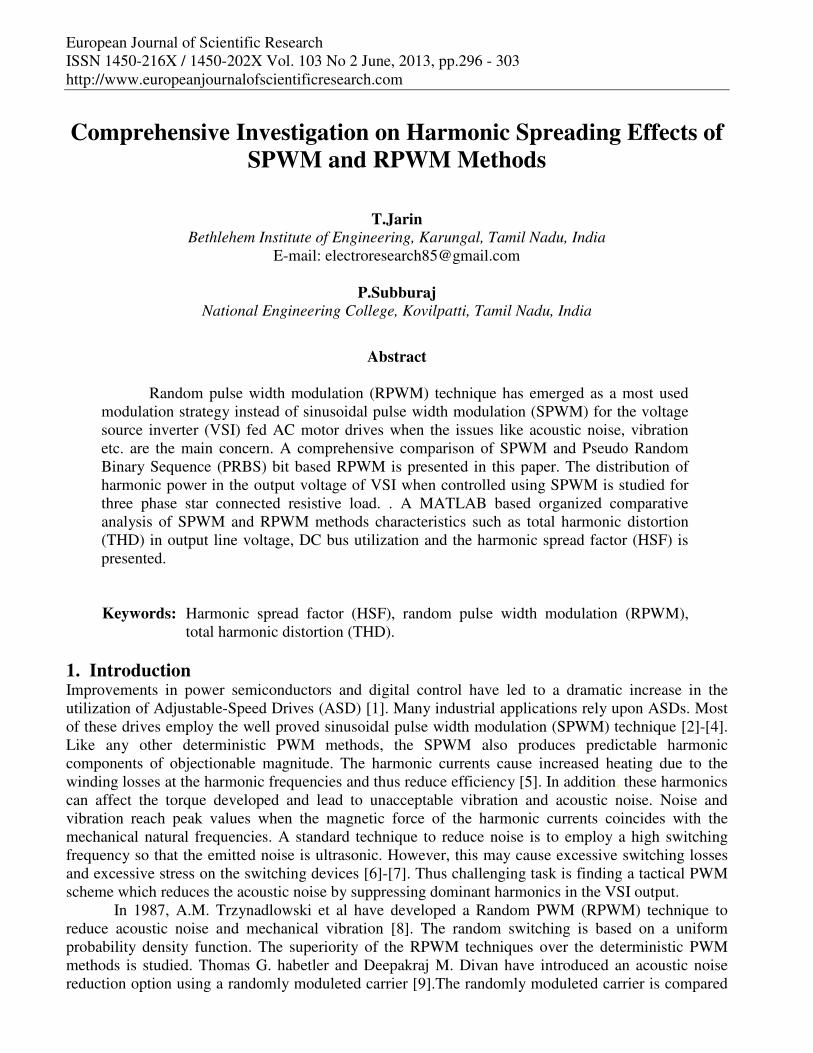
European Journal of Scientific Research ISSN 1450-216X / 1450-202X Vol. 103 No 2 June, 2013, pp.296 - 303 http://www.europeanjournalofscientificresearch.com
Comprehensive Investigation on Harmonic Spreading Effects of
SPWM and RPWM Methods
T.Jarin Bethlehem Institute of Engineering, Karungal, Tamil Nadu, India
E-mail: [email protected]
P.Subburaj National Engineering College, Kovilpatti, Tamil Nadu, India
Abstract
Random pulse width modulation (RPWM) technique has emerged as a most used modulation strategy instead of sinusoidal pulse width modulation (SPWM) for the voltage source inverter (VSI) fed AC motor drives when the issues like acoustic noise, vibration etc. are the main concern. A comprehensive comparison of SPWM and Pseudo Random Binary Sequence (PRBS) bit based RPWM is presented in this paper. The distribution of harmonic power in the output voltage of VSI when controlled using SPWM is studied for three phase star connected resistive load. . A MATLAB based organized comparative analysis of SPWM and RPWM methods characteristics such as total harmonic distortion (THD) in output line voltage, DC bus utilization and the harmonic spread factor (HSF) is presented. Keywords: Harmonic spread factor (HSF), random pulse width modulation (RPWM),
total harmonic distortion (THD). 1. Introduction Improvements in power semiconductors and digital control have led to a dramatic increase in the utilization of Adjustable-Speed Drives (ASD) [1]. Many industrial applications rely upon ASDs. Most of these drives employ the well proved sinusoidal pulse width modulation (SPWM) technique [2]-[4]. Like any other deterministic PWM methods, the SPWM also produces predictable harmonic components of objectionable magnitude. The harmonic currents cause increased heating due to the winding losses at the harmonic frequencies and thus reduce efficiency [5]. In addition, these harmonics can affect the torque developed and lead to unacceptable vibration and acoustic noise. Noise and vibration reach peak values when the magnetic force of the harmonic currents coincides with the mechanical natural frequencies. A standard technique to reduce noise is to employ a high switching frequency so that the emitted noise is ultrasonic. However, this may cause excessive switching losses and excessive stress on the switching devices [6]-[7]. Thus challenging task is finding a tactical PWM scheme which reduces the acoustic noise by suppressing dominant harmonics in the VSI output.
In 1987, A.M. Trzynadlowski et al have developed a Random PWM (RPWM) technique to reduce acoustic noise and mechanical vibration [8]. The random switching is based on a uniform probability density function. The superiority of the RPWM techniques over the deterministic PWM methods is studied. Thomas G. habetler and Deepakraj M. Divan have introduced an acoustic noise reduction option using a randomly moduleted carrier [9].The randomly moduleted carrier is compared

297 T.Jarin and P.Subburaj
with reference waveform to produce the RPWM pulses. In this technique random signal is used as the modulating function, the effects of its magnitude and varying speed (or bandwidth) on the inverter output harmonic distributed characteristics are analyzed. A RPWM scheme based on weighted switching decision has been developed by S.Y. R. (Ron) Hui et al. [10]. In this technique, the switching strategy can be applied to the entire range of the modulation index. In 2002, S.H Na et al. have reduced the audible switching noise in induction motor drives using random position space vector PWM [11]. In this technique the duty ratio of each pulse can be calculated and the pulse opposition is determined by the random number. Each range of pulse position is different according to the sector of the voltage vector. In this strategy, the angle step in the flux vectors and voltage vectors will vary randomly.Y.C.Lim et al havedetailed a pseudorandom carrier PWM scheme for reducing acoustic noise [12]. In this technique the pseudorandom carrier are produced through the random synthesis of the two triangular carrier each of the same switching frequency but of opposite phase. Multiplexer which are used as the random selecter of the two triangular carriers decided by Pseudo Random Binary Sequence (PRBS) is investigated.
The main objective of this paper is in two fold. The first one is performing thorough study on spectral study on SPWM fed VSI. Secondly, comparison of SPWM and PRBS based RPWM for the feature of harmonic spreading is presented in this paper. A MATLAB based simulation is presented for SPWM and RPWM methods when feeding three phase star connected resistive load. The indices such as total harmonic distortion (THD) in output line voltage, power density spectrum and the harmonic spread factor (HSF) are considered for discussion. The RPWM offers reduced HSF and THD, and improved fundamental component. For the modulation index (Ma) value of 0.8, the RPWM results in 37% reduction of HSF and 35% improvement in fundamental component. 2. Random PWM and Performance Indices The basic principle of RPWM is, if either the pulse position or switching frequency or duty ratio is varied in a random manner means, its output harmonic spectra are dispersed and continuously distributed. Hence acoustic noise, mechanical vibration and EMI can be greatly suppressed.RPWM techniques can be generally classified into four types, they are (i) Random switching PWM scheme, (ii) Random carrier frequency PWM scheme, (iii) Random pulse position PWM scheme and (iv)Hybrid Random PWM scheme.
Harmonic spread factor is an accurate evaluation index of any waveform for testing its harmonic spreading effects. The HSF quantifies the spread spectra effect of the random PWM scheme. For this purpose, the concept of statistical deviation can be employed and the HSF [13] is defined as follows:
20
0
1( )
N
jK
HSF H HN =
= −∑ (1)
01
( )N
jj
H H>
=∑ (2)
Where, ‘Hj’ is amplitude of jth harmonics, ‘H0’ is average value of all ‘N’ harmonics. Understanding how the strength of a signal is distributed in the frequency domain, power
spectral density graphs are used. 3. PRBS Based Random Carrier RPWM The pseudorandom carrier modulation PWM scheme are produced through the random synthesis of two triangular carrier, each of the same fixed frequency, but of opposite phase. The random selection of the two triangular carriers is decided by “0” or “1” states of the pseudorandom binary sequence (PRBS) random bits. Multiplexers, which are used as random selector of the PRBS random bits,
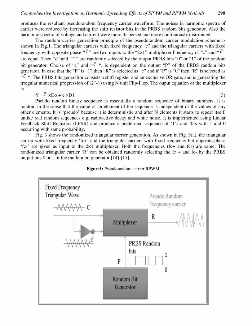
Comprehensive Investigation on Harmonic Spreading Effects of SPWM and RPWM Methods 298
produces the resultant pseudorandom frequency carrier waveform. The noises in harmonic spectra of carrier were reduced by increasing the shift resistor bits in the PRBS random bits generator. Also the harmonic spectra of voltage and current were more dispersed and more continuously distributed.
The random carrier generation principle of the pseudorandom carrier modulation scheme is shown in Fig.1. The triangular carriers with fixed frequency “c” and the triangular carriers with fixed frequency with opposite phase “ c ” are two inputs to the “2×1” multiplexer.Frequency of “c” and “ c ” are equal. Then “c” and “ c “ are randomly selected by the output PRBS bits “0” or “1” of the random bit generator. Choise of “c” and “ c “, is dependent on the output “P” of the PRBS random bits generator. In case that the "P” is “1” then “R” is selected as “c” and if “P” is “0” then “R” is selected as “ c “. The PRBS bits generatior consists a shift register and an exclusive OR gate, and is generating the irregular numerical progression of (2m-1) using N unit Flip-Flop. The ouput equation of the multiplexer is
Y= c ×Do + c ×D1 (3) Pseudo random binary sequence is essentially a random sequence of binary numbers. It is
random in the sense that the value of an element of the sequence is independent of the values of any other elements. It is ‘pseudo’ because it is deterministic and after N elements it starts to repeat itself, unlike real random sequences e.g. radioactive decay and white noise. It is implemented using Linear Feedback Shift Registers (LFSR) and produce a predefined sequence of ‘1’s and ‘0’s with 1 and 0 occurring with same probability.
Fig. 3 shows the randomized triangular carrier generation. As shown in Fig. 3(a), the triangular carrier with fixed frequency ‘fc+’ and the triangular carriers with fixed frequency but opposite phase ‘fc-’ are given as input to the 2×1 multiplexer. Both the frequencies (fc+ and fc-) are same. The randomized triangular carrier ‘R’ can be obtained randomly selecting the fc + and fc- by the PRBS output bits 0 or 1 of the random bit generator [14]-[15].
Figure1: Pseudorandom carrier RPWM
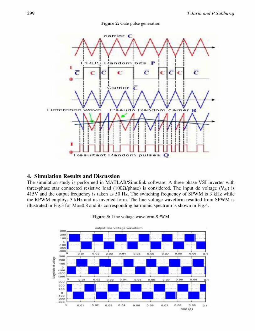
299 T.Jarin and P.Subburaj
Figure 2: Gate pulse generation
4. Simulation Results and Discussion The simulation study is performed in MATLAB/Simulink software. A three-phase VSI inverter with three-phase star connected resistive load (100�/phase) is considered. The input dc voltage (Vdc) is 415V and the output frequency is taken as 50 Hz. The switching frequency of SPWM is 3 kHz while the RPWM employs 3 kHz and its inverted form. The line voltage waveform resulted from SPWM is illustrated in Fig.3 for Ma=0.8 and its corresponding harmonic spectrum is shown in Fig.4.
Figure 3: Line voltage waveform-SPWM
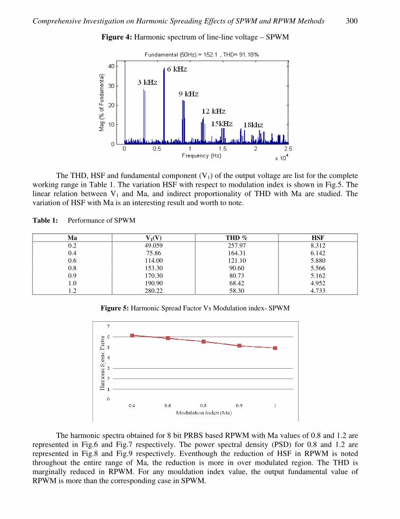
Comprehensive Investigation on Harmonic Spreading Effects of SPWM and RPWM Methods 300
Figure 4: Harmonic spectrum of line-line voltage – SPWM
The THD, HSF and fundamental component (V1) of the output voltage are list for the complete working range in Table 1. The variation HSF with respect to modulation index is shown in Fig.5. The linear relation between V1 and Ma, and indirect proportionality of THD with Ma are studied. The variation of HSF with Ma is an interesting result and worth to note. Table 1: Performance of SPWM
Ma V1(V) THD % HSF 0.2 49.059 257.97 8.312 0.4 75.86 164.31 6.142 0.6 114.00 121.10 5.880 0.8 153.30 90.60 5.566 0.9 170.30 80.73 5.162 1.0 190.90 68.42 4.952 1.2 280.22 58.30 4.733
Figure 5: Harmonic Spread Factor Vs Modulation index- SPWM
The harmonic spectra obtained for 8 bit PRBS based RPWM with Ma values of 0.8 and 1.2 are represented in Fig.6 and Fig.7 respectively. The power spectral density (PSD) for 0.8 and 1.2 are represented in Fig.8 and Fig.9 respectively. Eventhough the reduction of HSF in RPWM is noted throughout the entire range of Ma, the reduction is more in over modulated region. The THD is marginally reduced in RPWM. For any mouldation index value, the output fundamental value of RPWM is more than the corresponding case in SPWM.
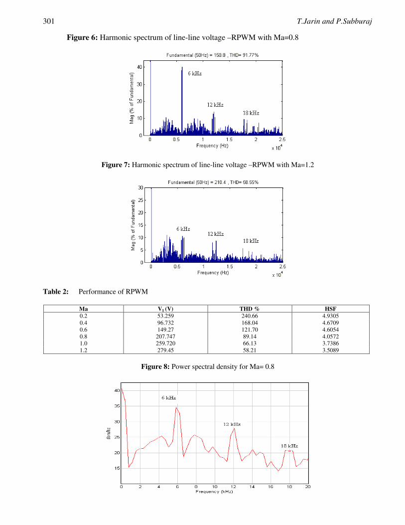
301 T.Jarin and P.Subburaj
Figure 6: Harmonic spectrum of line-line voltage –RPWM with Ma=0.8
Figure 7: Harmonic spectrum of line-line voltage –RPWM with Ma=1.2
Table 2: Performance of RPWM
Ma V1 (V) THD % HSF 0.2 53.259 240.66 4.9305 0.4 96.732 168.04 4.6709 0.6 149.27 121.70 4.6054 0.8 207.747 89.14 4.0572 1.0 259.720 66.13 3.7386 1.2 279.45 58.21 3.5089
Figure 8: Power spectral density for Ma= 0.8
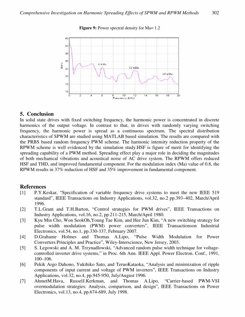
Comprehensive Investigation on Harmonic Spreading Effects of SPWM and RPWM Methods 302
Figure 9: Power spectral density for Ma= 1.2
5. Conclusion In solid state drives with fixed switching frequency, the harmonic power is concentrated in discrete harmonics of the output voltage. In contrast to that, in drives with randomly varying switching frequency, the harmonic power is spread as a continuous spectrum. The spectral distribution characteristics of SPWM are studied using MATLAB based simulation. The results are compared with the PRBS based random frequency PWM scheme. The harmonic intensity reduction property of the RPWM scheme is well evidenced by the simulation study.HSF is figure of merit for identifying the spreading capability of a PWM method. Spreading effect play a major role in deciding the magnitudes of both mechanical vibrations and acoustical noise of AC drive system. The RPWM offers reduced HSF and THD, and improved fundamental component. For the modulation index (Ma) value of 0.8, the RPWM results in 37% reduction of HSF and 35% improvement in fundamental component. References [1] P.Y.Keskar, “Specification of variable frequency drive systems to meet the new IEEE 519
standard”, IEEE Transactions on Industry Applications, vol.32, no.2 pp.393–402, March/April 1996.
[2] T.L.Grant and T.H.Barton, “Control strategies for PWM drives”, IEEE Transactions on Industry Applications, vol.16, no.2, pp.211-215, March/April 1980.
[3] Kyu Min Cho, Won SeokOh,Young Tae Kim, and Hee Jun Kim, “A new switching strategy for pulse width modulation (PWM) power converters”, IEEE Transactionson Industrial Electronics, vol.54, no.1, pp.330-337, February 2007.
[4] D.Grahame Holmes and Thomas A.Lipo, “Pulse Width Modulation for Power Converters:Principles and Practice”, Wiley-Interscience, New Jersey, 2003.
[5] S. Legowski and A. M. Trzynadlowski, “Advanced random pulse width technique for voltage- controlled inverter drive systems,” in Proc. 6th Ann. IEEE Appl. Power Electron. Conf., 1991, 100–106.
[6] Pekik Argo Dahono, Yukihiko Sato, and TeruoKataoka, “Analysis and minimization of ripple components of input current and voltage of PWM inverters”, IEEE Transactions on Industry Applications, vol.32, no.4, pp.945-950, July/August 1996.
[7] AhmetM.Hava, RusselJ.Kerkman, and Thomas A.Lipo, “Carrier-based PWM-VSI overmodulation strategies: Analysis, comparison, and design”, IEEE Transactions on Power Electronics, vol.13, no.4, pp.674-689, July 1998.

303 T.Jarin and P.Subburaj
[8] A.M. Trzynadlowski, S. Legowski, and R. L. Kirlin, “Random pulse width modulation technique for voltage controlled power inverters,” in Conf. Rec. IEEE— IAS Annu. Meeting, 1987, pp. 863–868.
[9] T. G. Habetler and D. M. Divian, “Acoustic noise reduction in sinusoidal PWM drives using a randomly modulated carrier,”IEEE Trans. PowerElectron., vol.6, no. 3, pp. 356–363, Jul. 1991.
[10] S. Y. R. (Ron) Hui, S. Sathiakumar, and Ki-Kwong Sung, “A Novel Random PWM Schemes with Weighted Switching Decision” IEEE Trans. Ind. Appl., vol.12, no.6, Nov. 1997.
[11] Y. G. Jung, S. H. Na, Y. C. Lim, and S. H. Yang, “Reduction of audible switching noise in induction motor drives using random position PWM,” IEEE Proc. Inst. Electr. Eng. Electr.Power Appl., vol. 149, no. 3, pp.195– 202, 2002.
[12] Young –cheol Lin, Young-gook Jung, Jong-namkim and Seog-oh Wi, “A pseudorandom carrier modulation Scheme”, IEEE Trans, vol 25, no.4, April 2010.
[13] Jiann-Fuh Chen, Juei-Lung Shyu, and Tsorng-Juu Liang, “A Multi-random PWM inverter with fixed switching frequency” Journal of the Chinese institute of Engineers, vol. 26, No. 3, pp.309-320, 2003.
[14] Young –cheol Lin, Young-gook jung, jong-namkim and seog-oh wi, “A pseudorandom carrier modulation Scheme”, IEEE Trans, vol 25, no.4, April 2010.
[15] Young-CheolLim,Seog-Oh Wi,jong-Nam Kim, and Young-Gook Jung, ”A Pseudo random Carrier Modulation Scheme”, IEEE Transactions on Power Electronics,Vol,no.4,April 2010,797.
European Journal of Scientific Research ISSN 1450-216X / 1450-202X Vol. 103 No 2 June, 2013, pp.304 - 312 http://www.europeanjournalofscientificresearch.com
An Analytical Approach to Pricing Discrete Barrier Options
under Time-Dependent Models
Mohammad H. Beheshti (Corresponding author) Department of Statistics, Science and Research Branch
Islamic Azad University, Tehran, Iran E-mail: [email protected]
Amir T. Payandeh Najafabadi
Faculty member of Department of Mathematical Sciences Shahid Beheshti University, G.C. Evin, 1983963113, Tehran, Iran
Rahman Farnoosh
School of Mathematics, Iran University of Science and Technology Narmak, 16846, Tehran, Iran
Abstract
Consider the problem of pricing a discrete barrier option under a time-dependent framework. This article provides an analytical solution for such an interesting problem in two steps . Namely, in the first step, the problem in hand restates a time invariant which has an exact solution. Secondly, the exact solution for the time-dependent model arrives by substituting such a solution in an integral equation. Applications to the Greeks of the contracts are given. Keywords: Barrier option, Black-Scholes framework, Discrete monitoring, Time-
dependent model. 1. Introduction The problem of pricing a discrete barrier option plays a role in the quantitative finance and financial industry. Barrier options are usually traded as the modification of simple European puts and call options. Barrier options activated (knock-ins) or terminated (knock-outs) if the sample path of the underlying asset has crossed a predetermined barrier prior to the exercise time. There are several pricing formulaes for barrier options in the Black-Scholes framework (see, Plesser 2000;Geman & Yor 1996; Rich 1994). In practice, barrier options differ from those studied in the academic literature in many respects. One of the most important is the monitoring frequency of the underlying assets. In the case of discrete monitoring, the sample path of the underlying asset is monitored at fixed times. Heynen & Kat (1995) were probably the scholars who issued an article noticing the discrepancy between option price under continuous and discrete monitoring. After seminal work of Heynen & Kat (1995), several authors proposed approximations based on a variety of different numerical approaches (see, Ait-sahlia & Lai, 1997; Bertoldi & Bianchetti, 2003; and Broadie & Glasserman, 1997). They used several methods such as: Recursive integration method, monte carlo simulation and trinomial tree. In the numerical approaches, computational cost increases whenever the number of monitoring increases. Moreover, the accuracy of the approximated solution decreases whenever asset price and the

305 Mohammad H. Beheshti, Amir T. Payandeh Najafabadi and Rahman Farnoosh
barrier are close to each other, in some sense. To overcome such difficulties, Fusai et al. (2006) provided an analytical method for the problem of pricing a discrete barrier option under time invariant framework.
For the problem of pricing a discrete barrier option under time-dependent framework (time-dependent parameters) the above findings are not valid anymore. More precisely, the problem of pricing a barrier option with time-dependent parameters is not a trivial extension of time invariant model. Roberts & Shorthland (1997) applied the hazard rate tangent approximation method to evaluate upper and lower bounds for price of such time-dependent barrier option. Unfortunately, their bounds cannot state in the closed form and consequently cannot be improved. Lo et al.(2003) presented a simple approach for computing upper and lower bounds (in the close form) for the price of barrier option.
This article considers the problem of pricing a down-and-out discrete barrier options on a divided paying equity whenever the risk-free rate and the dividend yield in the Black-Scholes partial differ- ential equation are deterministic functions of time. A method of reducing time-dependent partial differential equation to the heat equation is described in Wilmott et al. (1999). Also Marianito & Rogemar (2006) outlined a procedure that transforms the Black-Scholes partial differential equation with time-dependant parameters into the Black-Scholes equation with time-independent parameters. Our approach is to reduce the pricing problem to the time-independent case and the solution to the latter equation provided by Fusai et al. (2006).
Section 2 collects some useful elements for the other sections. Section 3 provides the price of discrete barrier option under the time-dependent parameters. The price of the Greeks of contract along with two examples are given in Section 3. 2. Preliminaries Now, we collect some essential elements for the next sections. Suppose 0 1 N0 = t < t < ... < t = T be the
monitoring dates that take at necessarily equally-spaced points in time, T the option maturity, L the constant lower barrier which is active at all times tn and K is the strick price of the option. The nth time interval is defined as n n+1t < t < t . We are interested in pricing a down-and-out call option, i.e., a
call option that expires worthless if a lower barrier has been hit at monitoring date. We denote V (S, t, n) is the price of a down and-out barrier option on a dividend-paying equity at time t in the nth
time interval and the asset price S . The asset price S satisfies the following stochastic differential equation
dS=(r(t)-d(t))+ dB
Sσ
with the constant volatility σ , the risk-free rate ( )r t and the dividend yield ( )d t ,then it is well known
(see, Merton (1973)) that V (S, t, n) satisfies following partial differential equation:
( ) ( ) ( )2 2
22
V (S, t, n) V (S, t, n) V (S, t, n)+ S r t - d t S r t V (S, t, n)=0
2t S S
σ∂ ∂ ∂+ − ∂ ∂ ∂
(1)
Given that the trigger condition is checked only at fixed times, it is needed to update the initial
condition at each of the monitoring dates nt :
n n (S L)V (S, t , n) = V (S, t , n - 1)I ,≥ (2)
0 (S max{K,L})V (S, t , 0) = (S - K)I .≥ (3)
Now, suppose V (S, t, n) denotes the price of a down-and-out barrier option on a non-
dividend-paying equity at time t and asset price S with the monitoring dates 0 1 N0 = t < t < ... < t = T

An Analytical Approach to Pricing Discrete Barrier Options under Time-Dependent Models 306
that take at necessarily equally-spaced points in time and option maturity T and the constant lower
barrier L and the strick price K . The asset price S satisfies the following geometric Brownian motion process
c
dS=r
S cdt dBσ+
with the constant volatility cσ and the constant risk-free rate cr , then V (S, t, n) satisfies Black-Scholes
partial differential equation: 22 2
2
V (S, t, n) V (S, t, n) S V (S, t, n)+ S V (S, t, n)
2c
c cr rt S S
σ∂ ∂ ∂− + =
∂ ∂ ∂ (4)
As before if the trigger conditions update at the monitoring dates, then, we have:
n n (S L)V (S, t , n) = V (S, t , n - 1)I
≥ (5)
0 (S max{K,L})V (S, t , 0) = (S - K)I
≥ (6)
Fusai et al.(2006) provided an analytical approach to evaluate nV (S, t , n) under the partial
differential Equation (4) with boundary conditions (5) and (6). The following provides definition of
some auxiliary functions that are used in the formulation of Fusai et al. (2006). For the asset price S
the function BSC (S) is defined as follows:
( ) ( ) [ ) ( ) ( ] ( )c c-r -rBS 1 2 0, ,0C (S)= S N d -Ke N d I k S -Ke I kn nt t
∞ −∞ + ,
in which 2
0
1 2 1 0
0
sln( ) ( )( ) k2kd = ;d d ; ln( ),
L
cc n
c n
c n
r t tt t k
t t
σ
σσ
+ + −− = − =
−
And the complex coefficients nµ is defined as below:
n ln 2 , ,q n i nµ π= + ∈ Ζ
in which q must satisfy the following condition:
( ) ( )( ){ }2 21 0
exp 1 ,q Iα γ
α γ− ≥
− −≺
where 2
1 022 ; ;
2
cc
cn
c
rt t
σσ τ
α τ γσ
+
−= − = − = .
Also the functions +L (u) and F(z,q)⌣
are respectively defined as follows:
( )2
+ 2 20
ln 1uL (u)=exp( ), ( ) 0,
zqedz u
i z uπ
−∞ −ℑ
−∫ ≻
(1- )k + +( 0)
n=- n=-
+( 0)
n=- + +
-iL L ( )e L ( )eF(z,q)= e
4 ( )( ( 1) ( ))
L L ( )e 1( .
2 L ( )( ) L ( ( 1) )( ( 1) )
n n
n
z zi i
n nk
n m m m m n
zi
kn
kn n n
Ii i
eI
i i i i
µ µγ γ
α
µγ
γ µ µ
µ µ µ αγ µ α γ µ µ
µ
µ αγ µ αγ α γ µ α γ
∞ ∞
≥∞ ∞
∞
∞
+ + − +
− −− − − −
∑ ∑
∑ ≺
⌣

307 Mohammad H. Beheshti, Amir T. Payandeh Najafabadi and Rahman Farnoosh
The general price of down-and-out discrete barrier option under the partial differential Equation(4) with boundary conditions ( 5) and (6) is stated in the following theorem.
Theorem 1. (Fusai et al., 2006): Consider partial differential Equation (4) with boundary condi-tions (5) and (6). Then,
(i) The price of down-and-out discrete barrier option at a monitoring date nt and asset price S is given by
ntn BS
S SV (S, t , n)=C (S)( ) (ln , ),
L Le f nα β⌣
(7)
where f⌣
and β is defined as follows 2
0
1( , ) ( , ) ,
2iu inu
nf z n F z e e du
π
ρπρ
= ∫⌣ ⌣
22
2c
cm rσ
β α α= + −
(ii) The Greeks of the contract, namely Delta, nV (S, t , n)
S
∂
∂ , and Gamma,
2n
2
V (S, t , n)
S
∂
∂, are
obtained as below
11 ( , )( ) ( ) ( , ) ,nt
BS
S f z nS e f z n
L zLβα α− ∂
∆ = ∆ + + ∂
⌣⌣
(8)
With z = ln( )S
Land where [ ) ( ]1 0, - ,0( )= N(d )I (k) + I (k)BS S
∞ ∞∆
22
2 2
1 ( , ) ( , )( ) ( ) ( 1) ( , ) (2 1)nt
BS
S f z n f z nS e f z n
z zLL
βα α α α− ∂ ∂Γ = Γ + − + − +
∂ ∂
⌣ ⌣⌣
(9)
where ( )BS SΓ is the Black-Scholes Gamma.
The corresponding down-and-in call option can be priced by subtracting from the price of standard call the price of the down-and-out call. Likewise, the barrier put option can be priced using the put call transformation given in Haug (1999).
Now consider, the problem of pricing the down-and-out discrete barrier option under the partial differential Equation (1), i.e., the problem of evaluating nV (S, t , n) under the partial differential
Equation (1) with conditions (2) and (3). The next section provides an analytic solution for such problem. 3. The Main Results This section provides an exact and analytic solution for the problem of pricing the down-and-out discrete barrier option under time-dependent framework. The following theorem provides the main result of this article.
Theorem 2. Suppose nV (S, t , n) represents the price of down-and-out barrier option at the
monitor-ing date nt and the asset price S which satisfies the partial differential Equation (1) and conditions(2) and (3). Then,
nt 2
nn 20
KV (S, t , n)= exp( ( ) ) V (S, t , n),
K cc
r r u duσ
σ
− ×
∫ (10)

An Analytical Approach to Pricing Discrete Barrier Options under Time-Dependent Models 308
where nV (S, t , n) is the price of discrete barrier option that is calculated based upon Theorem 1.The
above nV (S, t , n) with strick price K and lower barrier L and option maturity T that satisfy three following conditions
max ,1 max ,1L L
KK
=
(11)
nt 2
20
exp( ( ) ( ) )cc
L Lr u d u r du
KK
σ
σ
= − −
∫ (12)
2
2c
T Tσ
σ= (13)
Also, nt and S in the Equation (10) are calculated as follows: 2
n n 2t t
c
σ
σ= (14)
nt 2
20
exp( ( ) ( ) )cc
KS r u d u r du S
K
σ
σ
= − − ×
∫ (15)
Proof. In the first step, we transform the Black-Scholes equation with the time-varying parameters (1) into Black-Scholes equation (4) such that:
t 0= when t 0= (16) To observe this, we use the following transformations:
nV (S, t, n)=h(t)V (S, t , n) , S ( )S , t ( )tt tφ ψ= = (17) Using the chain rule, one may conclude that:
V V V=h(t) ( ) ( ) h (t)V
t S tt S tφ ψ
∂ ∂ ∂′ ′ ′+ +
∂ ∂ ∂
V V=h(t) ( ) ,
S Stφ
∂ ∂
∂ ∂
2 22
22
V V=h(t) ( ) ,
S Stφ
∂ ∂
∂ ∂
Substituting the above equations into (1) leads to: [ ] 2 2 2 2
2
( ) ( ) ( ) ( )V V ( ) V h (t)+r(t)h(t)+( ) +( ) ( )V 0
t ( ) 2 ( ) h(t) ( )S S
r t d t t S t S S t
t t t
φ φ σ φ
ψ ψ φ
′− − ′∂ ∂ ∂− − =
′ ′ ′∂ ∂ ∂
Comparing this with Equation (4) yields: 2 2 2 2
2 ( )=
2 2 ( )c c S t
St
σ σ φ
ψ ′ (18)
[ ]( ) ( ) ( ) ( )=
( )c
r t d t t S t Sr S
t
φ φ
ψ
′− −
′ (19)
( ) ( ) ( )=
( ) ( )c
h t r t h tr
h t tψ
′ +
′ (20)
From Equation (17) to (20), one may conclude that:
22
0
1( )= ( )
t
c
t d u Aψ σσ
+∫ (21)

309 Mohammad H. Beheshti, Amir T. Payandeh Najafabadi and Rahman Farnoosh
[ ]0
( )= exp ( ) ( ) ( ) ,t
ct r u d u r u duφ β ψ ′− −∫ (22)
[ ]0
( )= exp ( ) ( ) ,t
ch t C r u r u duψ ′ −∫ (23)
where A , B , and C are constant. Up to now, the Black-Scholes equation with time-varying parameters (1) is transformed into
Black-Scholes partial differential equation (4). As mentioned before, nV (S, t , n) with the two conditions (5), (6) can be evaluated based on Theorem 1. Therefore, the constants A , B , and C are
determinedand also some conditions on L , K are given simultaneously such that conditions (5), (6) equivalent to the (2) and (3).
Finally, nV (S, t , n) under the partial differential equations (1) with conditions (2) and (3) is evaluated with the first equation in (17).
From (3), (17) and (6) we have: +
[max{K,L}, ) 0
0 0
0 [max{K,L}, )
(S - K) I (S) = V (S, t , 0)
h(t )V (S, t , 0)
h(t )(S ) I (S).K
∞
+
∞
=
= −
But
0
+0 [max{K,L}, ) 0 0 0[max{K,L}, )
0 0 max{K,L}[ , )
0 (t )
h(t )(S - K) I (S) = h(t )( (t )S- ) I ( (t )S)
h(t ) (t ) (S- ) I (S)(t )
K
K
φ
φ φ
φφ
+
∞ ∞
+
∞
=
Therefore
0
0 0 [max{K,L}, ) max{K,L}[ , )
0 (t )
h(t ) (t ) =1 , , I (S) I (S)( )
KK
tφ
φφ
∞∞
= = (24)
Using Equations (16) to (24), one may conclude that:
0( ) 0;A tψ= = (25)
0( );K
B tK
φ= = (26)
0( );K
C h tK
= = (27)
max{K,L} max{K,L}
K K= (28)
Multiplying the both side of equation (5) by ( )nh t leads to
n n [L, )V (S, t , n) = V (S, t , n - 1)I (S)
∞ (29)
Equations (29) and (2) are equivalent, whenever the following conditions on L and K are exist.
[L, )[L, )I (S) =I (S) ∞∞
Therefore, L and K are chosen so that (S L)≥ equivalent (S L)≥ . Then, with equations (17) ,(22) and (25) it is sufficient to have
nt 2
20
exp ( ) ( ) cc
L Lr u d u r du
KK
σ
σ
= − −
∫ (30)

An Analytical Approach to Pricing Discrete Barrier Options under Time-Dependent Models 310
Also we must be aware of accuracy of the (S L)≥ , then L and K is chosen as following nt 2
20
exp ( ) ( ) cc
L Sr u d u r du
KK
σ
σ
≤ − −
∫ (31)
This observation complete the proof.
It would be worthwhile to mention: (i) two constant parameters cr and cσ , given in Theorem 2,respectively, are arbitrary risk-free and volatility in the Black-Scholes partial differential
Equation(4); (ii) There is a fixed period between the the monitoring dates nt that is driven in the theorem 2. If the volatility is non-constant function of time then the period between monitoring dates
nt may be not fixed and the Theorem 1 is unusable in this place. The following evaluates the Greeks of contract.
Corollary 1. The Greeks of the contract, namely Delta nV (S, t , n)
S
∂
∂ and Gamma,
2n
2
V (S, t , n)
S
∂
∂,under
the Black-Scholes equation with time-varying parameters (1) with conditions (2), (3) are obtained as follows:
n nt t2 2n
2 20 0
V (S, t , n)exp ( ) exp ( ) ( )c c
c c
r r u du r u d u r duS
σ σ
σ σ
∂∆ = − × − − ×
∂ ∫ ∫ (32)
n nt t2 2 2n2
22 20 0
V (S, t , n)exp ( ) (exp ( ) ( ) )c c
c c
Kr r u du r u d u r du
K S
σ σ
σ σ
∂Γ = − × − − ×
∂ ∫ ∫ (33)
where nV (S, t , n)
S
∂
∂and
nV (S, t , n)
S
∂
∂ are evaluated according to the Theorem 1(ii).
Proof. Desire proof arrives by derivation with respect to S from Equation (10) and (15). The following proves that the price of discrete barrier option and the Greeks of the contract are
invariant from choosing L and K in Theorem 2. Corollary 2. For the given lower barrier L and the stirk price K , there may exist many of the L and K such that satisfy conditions (11), (12). But the price of discrete barrier option and the Greeks of the contract that respectively evaluate based on (10), (32) and (33) are independent of different choices for
L and K . Proof. We just prove the corollary for the price of barrier option, the result for the Greeks consequent is immediate. Without less of generality suppose that L K≺ . By replacing the formulae with
nV (S, t , n) given by the Theorem 1 into Theorem 2, one may observe
n
1 2
V (S,t , n) ( ) ( ) (ln , )
( ) ( ) ( ) (ln , )
n
nc n
tBS
r t t
K S SC S e f n
K L L
S K S SK N d Ke N d e f n
K K L L
βα
βα−
∝ +
∝ − +
⌣
⌣
Now using Equation (15), the last expression can be restated as: *
* 1 * nn 1 2 n
1 1 (t )(t ) ( ) ( ) ( ) ( (t ) ) ( ) (ln ln , )nc nr t tK K
K SN d Ke N d S e f S nK KK L L
βα α α φφ φ− −− + +
⌣ (34)
where nt 2
*n 2
0
(t ) exp ( ) ( ) cc
r u d u r duσ
φσ
= − −
∫

311 Mohammad H. Beheshti, Amir T. Payandeh Najafabadi and Rahman Farnoosh
The function ( , )f z q⌣
that was defined previously has lower barrier L as coefficient. Then, the
last equation depend on L and K only from the proportion L
K . This fact completes the desire proof.
The following examples provide application of the above results to the problem of pricing a discrete barrier option and the Greeks of the contract for the different cases for r(t) and d(t) . Example 1. Suppose, we want to price down-and-out barrier option. Parameters used are S=100 , K=100 , r(t) = 0.1+0.05 exp(-t) , d(t) 0.05≡ , =0.2σ , T = 0.5 . Also the arbitrary parameters in the
transformed partial differential equation are cr 0.1= , =0.3cσ .The price of the barrier option and the
Greeks of the contract at the last monitoring date are evaluated for the different lower barriers L and the different monitoring numbers N . Results are summarized in Table 1. In this example for lower
barrier greater than (97) there are no L and K such that satisfy conditions (11) and (12).
Table 1: In this table for the different levels of the lower barrier, we chose L and K suitably, and then the price of discrete barrier options is evaluated based on Theorem 2
N L V ∆ Γ 5 88 7.6920 0.6515 0.0222 5 91 7.4905 0.6836 0.0188 5 94 7.0023 0.7375 0.0189 5 97 6.0966 0.7859 0.0403 15 88 7.6307 0.6622 0.0204 15 91 7.3110 0.7124 0.0132 15 94 6.5459 0.8121 0.0041 15 97 5.0815 0.9251 0.0266
Example 2. Consider the problem of pricing under S=100 , K=100 , r(t) = 0.075+0.05 t ,
d(t) 0.03+0.02t≡ , =0.3σ , T = 0.2 . Also the arbitrary parameters cr and cσ are given as previous
example. The price of the barrier option and the Greeks of the contract at the last monitoring date are evaluated for the different lower barriers L and the different monitoring numbers N . Results are summarized in Table 2.
Table 2: In this table for the different levels of the lower barrier, we chose L and K suitably and then the price of discrete barrier options are evaluated based on theorem 2
N L V ∆ Γ 5 87 5.7588 0.5562 0.0281 5 91 5.6456 0.5780 0.0249 5 95 5.1946 0.6315 0.0253 5 99 4.1134 0.8681 -0.7255
10 87 5.7489 0.5583 0.0277 10 91 5.5871 0.5896 0.0221 10 95 4.9358 0.6804 0.0175 10 99 3.4266 0.7254 -0.4748
4. Conclusion and Suggestions This article studies the pricing of discrete barrier options under a model where the risk-free rate, r(t) ,
and the dividend yield, d(t) ,are two given the functions of time. For non-constant volatility (t) σ , one may use the average volatility. Then, apply findings of this article to such problem. Also,if the problem

An Analytical Approach to Pricing Discrete Barrier Options under Time-Dependent Models 312
of option pricing can be solved when the monitoring dates take at not necessarily equally-spaced point, then the approach of the present paper is usable for the non-constant volatility too. Acknowledgements The author would like to thank professor Fussai and miss Hodoudi for their useful comments. References [1] Ait-Sahlia, F. & Lai, T. L. (1997). Valuation of discrete barrier and hindsight options.
J.Financial Eng. 6, 169–77. [2] Bertoldi, M . & Bianchetti, M . (2003). Monte Carlo simulation of discrete barrier options. In-
ternal Report, Financial Engineering-Derivatives Modelling, Caboto SIM S.p.a., Banca Intesa Group, Milan, Italy.
[3] Broadie, M. , Glasserman, P. & Kou. S. (1997). A continuity correction for discrete barrieroptions. Math Finance. 7, 325–349.
[4] Fusai, G. , Abrahams, I. D. & Sgarra, C. (2006). An exact analytical solution for barrier options, Financ Stochast. 10, 1–26.
[5] Geman. H. & Yor, M. (1996). Pricing & hedging double barrier options: a probabilistic approach. Math Finance.6, 365–378.
[6] Haug, E. G.(1999). Barrier put-call transformations, Tempus Financial Engineering Number 3–97, Norway, download at http://ssrn.com/abstract=150156.
[7] Heynen R. C. & Kat, H. M. (1995). Lookback options with discrete and partial monitoring of the underlying price. Appl. Math. Finance.2, 273–284.
[8] Lo, C. F. , Lee, H. C. & Hui, C. H. (2003). A simple approach for pricing barrier options with time-dependent parameters. Quantitative finance . 3, 98–107.
[9] Marianito, R.R. & Rogemar, S. M (2006). An alternative approach to solving the Black-Sholes equation with time-varing parameters. Applied Mathematics Letters. 19, 398–402.
[10] Merton, R. (1973). Theory of rational option pricing, Bell Journal of Management Sciences.4, 141–183.
[11] Pelsser, A. (2000). Pricing double barrier options using Laplace transforms. Finance Stochast. 4, 95–104.
[12] Rich, D. R. (1994). The mathematical foundations of barrier option pricing theory. Adv. Futures Options Res. 7 , 267–311.
[13] Roberts, G. O. & Hortland C. F.(1994).The hazard rate tangent approximation for boundary hitting times.Ann. Appl. Prob. 5, 446–60.
[14] Wilmott, P. Howison, S. & Dewynne, J. (1999). The Mathematics of Financial Derivatives,Cambridge, University Press.
European Journal of Scientific Research ISSN 1450-216X / 1450-202X Vol. 103 No 2 June, 2013, pp.313 - 325 http://www.europeanjournalofscientificresearch.com
Tunable and Reconfigurable Spectrum Sliced Microwave
Photonic Filter Using Parallel Fabry-Perot Filters with External Delay and Windowing
R. K. Jeyachitra (Corresponding Author) Assistant Professor, Department of ECE, National Institute of Technology, Trichy, India
Ph: +91 0431 2503320(Off.), +91 09443145540 (Mob) E-mail: [email protected], [email protected]
J. Martin Leo Manickam
Professor, Department of Electronics and Communication Engineering, St. Joseph’s College of Engineering, Chennai, Tamil Nadu, India
Abstract
A tunable and reconfigurable microwave photonic filter based on two Fabry-Perot filters connected in parallel and one filter with an external delay element (Fiber delay/Fiber Bragg Grating(FBG)) and high profiled windowing techniques is proposed. The architecture shows discrete filter tuning and reconfiguration capabilities using a spectrum slicing technique, realizes multi-tap, transversal RF filter with high frequency operation. Discrete tunability is achieved by changing delay time offered external delay in the filter configuration. The reconfigurable spectrum of the proposed filter is developed by employing different high profiled apodization techniques. The frequency responses of the filter by employing windows are tabulated and compared with that of filter without windowing. Simulation results show high FSR, sidelobe suppression and high Quality factor with this configuration using simple and cost effective filter architecture. Keywords: Apodization, Fabry-Perot (FP) filter, fiber delay, FBG, microwave photonics,
Quality factor (Q-factor), spectrum slicing, tunability, reconfigurability. 1. Introduction Microwave Photonics is a cross or inter-disciplinary area which combines microwave engineering and opto electronics. It uses photonic techniques for generation, transmission, processing and reception of signals having spectral components at microwave or millemeter-wave frequencies. It takes the distinctive advantages of both the fields: microwave and optical communication systems. The supplementary advantages are immunity to Electromagnetic Interference (EMI), tunability, and reconfigurability [1, 2]. One of the most important applications of microwave photonic technology is microwave photonic filters. It processes the filtering function of microwave signals directly in optical domain. It is one of the powerful techniques for implementing photonic signal processing of microwave signals. This technology offers wide range of benefits such as immunity to EMI, broad bandwidth, reduced size and weight and low and constant electrical loss [1, 2, 3]. Photonic filters for the processing of microwave signals brings several advantages, including the possibility of tuning and reconfiguring ( i.e., changing) the shape of their bandpass transfer functions, a feature which is not

314 R. K. Jeyachitra and J. Martin Leo Manickam
attainable with traditional microstrip or wave guide RF technologies [4]. With this advantage there is great scope for developing 40GHz to 60GHz band pico-cellular systems. However, there is the difficulty of attaining the reconfigured band pass transfer function of any filter with the traditional microstrip or waveguide Radio Frequency (RF) technologies. This difficulty can be overcome by external on-line measures in spectrum sliced microwave photonic filters [5, 6]. A simple, low cost solution to realize a multi-tap microwave photonic filter is based on spectrum slicing of broadband source [5, 7]. In recent years, the design of low cost photonic microwave filters with reconfiguration and tuning capabilities has been intense research interest, several structures have been proposed and results have been demonstrated [8, 9 ,10].
An automatic tunable and reconfigurable microwave photonic filter with limited taps based on uniform FBGs with broadband optical source was demonstrated [11]. A discrete tunable and reconfigurable filter with very low sidelobe suppression, limited number of taps and limited Q-factor are demonstrated in [10, 12]. A tunable and reconfigurable filter using a multiport programmable wavelength processor (PWP) based on two dimensional array of liquid crystal on Si pixels with limited tunable range of frequency is realized in [13]. Spectral slicing of a broadband spectrum by means of a tunable periodic filter (i.e., a fiber FP) can yield a potentially low-cost source with the desired properties [15]. A flexible tunable specrum sliced microwave photonic filter is proposed using FP filters and fibed delay[5]. A simple and compact spectrum sliced microwave photonic filter eliminating the practical difficulites in [5] is proposed in [6]. Only the tunable propoerty of the filter is presented in [5, 6].
The objective of this paper is to present the realization of spectrum sliced microwave photonic filter structure which can tune the filter centre frequency and also reconfigure the filter shape and exhibiting multiple-taps for high resolution. This work is the extension of the paper [5, 6], in order to design a tunable and reconfigurable filter. It is based on a spectrum slicing technique achieved using two Fabry-Perot filters connected in parallel and one filter with an external delay element (fiber delay/FBG) [5,6] and a high profiled windowing techniques. The filter tunability is achieved by changing the time delay offered by the external delay element (fiber delay/FBG) [5, 6] and the reconfiguration is obtained by weighting the power of the source using different windowing techniques. The performances of the proposed filter with windowing are tabulated and compared with that of without windowing. Simulation results demonstrate the feasibility of these filters in 40GHz to 60GHz applications.
This paper is organized as follows: The proposed filter architecture and its description are provided in Section II. The theoretical formulation for the evaluation of the proposed filter transfer function is provided in Section III. In Section IV, we present the simulation results that demonstrate the tunability and reconfigurability of our proposed filter for different time delays and various windowing techniques such as Gaussian, Kaiser, Hamming and Hanning windows. These results are compared with results of filter with unapodization technique in terms of FSR, MSSR and Quality factor. Finally, we present the conclusions of our work. 2. Filter Architecture and Description The general architecture of the filter is shown in Figure 1. The optical source is a low-cost, broadband Amplified Spontaneous Emission (ASE) spectrum which is obtained from a pumped Erbium Doped Fiber Amplifier (EDFA). The ASE signal level however is usually very small and requires further amplification in order to overcome the losses introduced by the remaining components of the filter. The optical power from the source is split and spectrally sliced by use of two multiwavelength FP filters connected in parallel, one with an adjustable delay implemented using optical fiber, to obtain the equivalent set of spectrally equispaced optical sources.

Tunable and Reconfigurable Spectrum Sliced Microwave Photonic Filter Using Parallel Fabry-Perot Filters with External Delay and Windowing 315
Figure 1: Proposed filter architecture
The output light from the parallel combination FP filters is combined and subsequently modulated by RF signal by means of an external modulator and fed to an optical dispersive element providing a linear group delay characteristic. The output signal from the dispersive element is fed to a photodetector and subsequent RF circuit. The filter tunability is obtained by using two FP filters of same incremental differential delay and by adjusting the delay times offered by fiber delay or FBG [5, 6]. The reconfigurability of the filter is obtained by changing the amplitude of the spectral carrier by means of windowing. 3. Theoretical Analysis When Single-Sideband (SSB) modulation is employed for the RF signal and a single FP filter is used, the RF transfer function of the filter [14] is given as
N-j[�(k-1)�τ]
RF kk=1
H (�) =R P e∑ (1)
where Pk represents the output power from the kth slice of the broadband source, R is the receiver responsivity, � is the RF frequency, and ∆τ represents the incremental differential delay experienced by two adjacent spectral slices of broadband source. It is given by �τ = D L �λwhere D (ps/km.nm) and L (m) are the dispersion and length of fiber respectively and ∆λ is wavelength spacing. The spectral response of a FIR filter is repesented in (1), where the number N of signal samples is equal to the number of significant spectral slices generated by the optical filter [5, 6].
When two FP filters are used in parallel, the overall transfer function is given as [5, 6]
overall 1 2H (�) = H (�)+H (�) (2)
1 2
N N-j[�(k-1)�τ ] -j[�(k-1)(�τ +τ)]
k kk=1 k=1
=R P e + P e∑ ∑ (3)
where Hoverall(�) is the overall transfer function of our proposed filter, where �τ1 and �τ2 are incremental differential delay of two FP filters and τ represents the time delay offered by the fiber/FBG. where τ represents the time delay offered by FBG
r g g t gT =D L λ =2nL /c∆ (4)

316 R. K. Jeyachitra and J. Martin Leo Manickam
where Tr is the round–trip time for a grating of length Lg, �λt is the total shift in bragg wavelength, Dg
is the dispersion parameter, n is the average refractive index and c is velocity of light in the fiber [6, 17]. 3.1. Design of Reconfigurable Filter
The shape of the transfer function of a discrete time transversal filter can be changed or reconfigured by changing the optical power of the different taps according to an apodization function. Therefore a decrease in the secondary sidelobes of the filter can be achieved [8, 11, 15]. It is also useful method for considerable reduction of secondary sidelobes [16].The different windowing profiles are described as follows:
The Gaussian window is described by 21
- 2 n-(N-1)/2
w(n)= e σ 0.5σ(N-1)/2
≤
(5)
The Kaiser window description is given by 2 1/2
0
0
I [β(1-[(n-α)/α)] ) ]0 n N
w(n)= I (β)
0 otherwise
≤ ≤
(6)
where N =number of taps, α=N/2 and I0(.) represents zeroth- order modified Bessel function of the first kind and the tapering parameter is β=1.9.
The Hamming window is described by 2πn
0.54 0.46 cos 0 n Nw(n) N 1
0 otherwise
− ≤ ≤= − (7)
The Hanning window is defined as 2πn
0.5 0.5 cos 0 n Nw(n) N 1
0 otherwise
− ≤ ≤= − (8)
Then the reconfigured transfer function of the proposed filter by employing apodization is obtained by
1 2
N N-j[�(k-1)�τ ] -j[�(k-1)(�τ +τ)]
withApod k k k kk-1 k-1
H (�) =R P w e + P w e∑ ∑ (9)
wk –weights calculated at the kth tap using (5-8). The filter tuning performance depends on the time delay offered by fiber/FBG and it is obtained
by changing the length of the fiber. Therefore, it possible to choose the fiber/FBG length allowing discrete tuning over the whole fiber spectral response margin. To shape the transfer function of the filter, the amplitude of each filter tap of transversal filter can be independently selected simply by changing the amplitude of spectral carriers [8]. 4. Results and Discussion The layout of the proposed configuration of spectrum sliced microwave photonic filter is shown in Figure 2. It uses two FP filters connected in parallel and one filter with an external delay element (Fiber delay/FBG). To obtain sharply apodized sliced spectrum with N = 34 taps, only a 9nm portion (centered at 1531.8nm, the wavelength corresponding to the ASE maximum of EDFA1) of the ASE
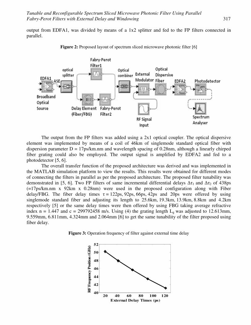
Tunable and Reconfigurable Spectrum Sliced Microwave Photonic Filter Using Parallel Fabry-Perot Filters with External Delay and Windowing 317
output from EDFA1, was divided by means of a 1x2 splitter and fed to the FP filters connected in parallel.
Figure 2: Proposed layout of spectrum sliced microwave photonic filter [6]
The output from the FP filters was added using a 2x1 optical coupler. The optical dispersive element was implemented by means of a coil of 46km of singlemode standard optical fiber with dispersion parameter D = 17ps/km.nm and wavelength spacing of 0.28nm, although a linearly chirped fiber grating could also be employed. The output signal is amplified by EDFA2 and fed to a photodetector [5, 6].
The overall transfer function of the proposed architecture was derived and was implemented in the MATLAB simulation platform to view the results. This results were obtained for different modes of connecting the filters in parallel as per the proposed architecture. The proposed filter tunability was demonstrated in [5, 6]. Two FP filters of same incremental differential delays �τ1 and �τ2 of 438ps (=17ps/km.nm x 92km x 0.28nm) were used in the proposed configuration along with Fiber delay/FBG. The fiber delay times τ = 122ps, 92ps, 66ps, 42ps and 20ps were offered by using singlemode standard fiber and adjusting its length to 25.6km, 19.3km, 13.9km, 8.8km and 4.2km respectively [5] or the same delay times were then offered by using FBG taking average refractive index n = 1.447 and c = 299792458 m/s. Using (4) the grating length Lg was adjusted to 12.613mm, 9.559mm, 6.811mm, 4.324mm and 2.064mm [6] to get the same tunability of the filter proposed using fiber delay.
Figure 3: Operation frequency of filter against external time delay
20 40 60 80 100 12040
42
44
46
48
50
52
External Delay Times (ps)
RF
Fre
quen
cy P
osit
ion
(GH
z)
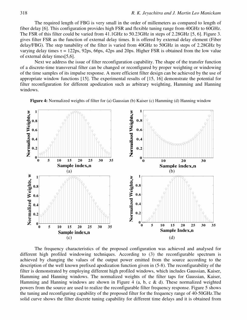
318 R. K. Jeyachitra and J. Martin Leo Manickam
The required length of FBG is very small in the order of millemeters as compared to length of fiber delay [6]. This configuration provides high FSR and flexible tuning range from 40GHz to 60GHz. The FSR of this filter could be varied from 41.1GHz to 50.23GHz in steps of 2.28GHz [5, 6]. Figure 3. gives filter FSR as the function of external delay times. It is offered by external delay element (Fiber delay/FBG). The step tunability of the filter is varied from 40GHz to 50GHz in steps of 2.28GHz by varying delay times τ = 122ps, 92ps, 66ps, 42ps and 20ps. Higher FSR is obtained from the low value of external delay times[5,6].
Next we address the issue of filter reconfiguration capability. The shape of the transfer function of a discrete-time transversal filter can be changed or reconfigured by proper weighting or windowing of the time samples of its impulse response. A more efficient filter design can be achieved by the use of appropriate window functions [15]. The experimental results of [15, 16] demonstrate the potential for filter reconfiguration for different apodization such as arbitrary weighting, Hamming and Hanning windows.
Figure 4: Normalized weights of filter for (a) Gaussian (b) Kaiser (c) Hamming (d) Hanning window
0 5 10 15 20 25 30 350
0.2
0.4
0.6
0.8
1
Sample index,n
Nor
mal
ized
Wei
ghts
,w
0 10 20 30
0
0.2
0.4
0.6
0.8
1
Sample index,n
Nor
mal
ized
Wei
ghts
,w
(a) (b)
0 5 10 15 20 25 30 350
0.2
0.4
0.6
0.8
1
Sample index,n
Nor
mal
ized
Wei
ghts
, w
0 5 10 15 20 25 30 350
0.2
0.4
0.6
0.8
1
Sample Index,n
Nor
mal
ized
Wei
ghts
,w
(c) (d)
The frequency characteristics of the proposed configuration was achieved and analysed for
different high profiled windowing techniques. According to (3) the reconfigurable spectrum is achieved by changing the values of the output power emitted from the source according to the description of the well known prefixed apodization function given in (5-8). The reconfigurability of the filter is demonstrated by employing different high profiled windows, which includes Gaussian, Kaiser, Hamming and Hanning windows. The normalized weights of the filter taps for Gaussian, Kaiser, Hamming and Hanning windows are shown in Figure 4 (a, b, c & d). These normalized weighted powers from the source are used to realize the reconfigurable filter frequency response. Figure 5 shows the tuning and reconfiguring capability of the proposed filter for the frequency range of 40-50GHz.The solid curve shows the filter discrete tuning capability for different time delays and it is obtained from
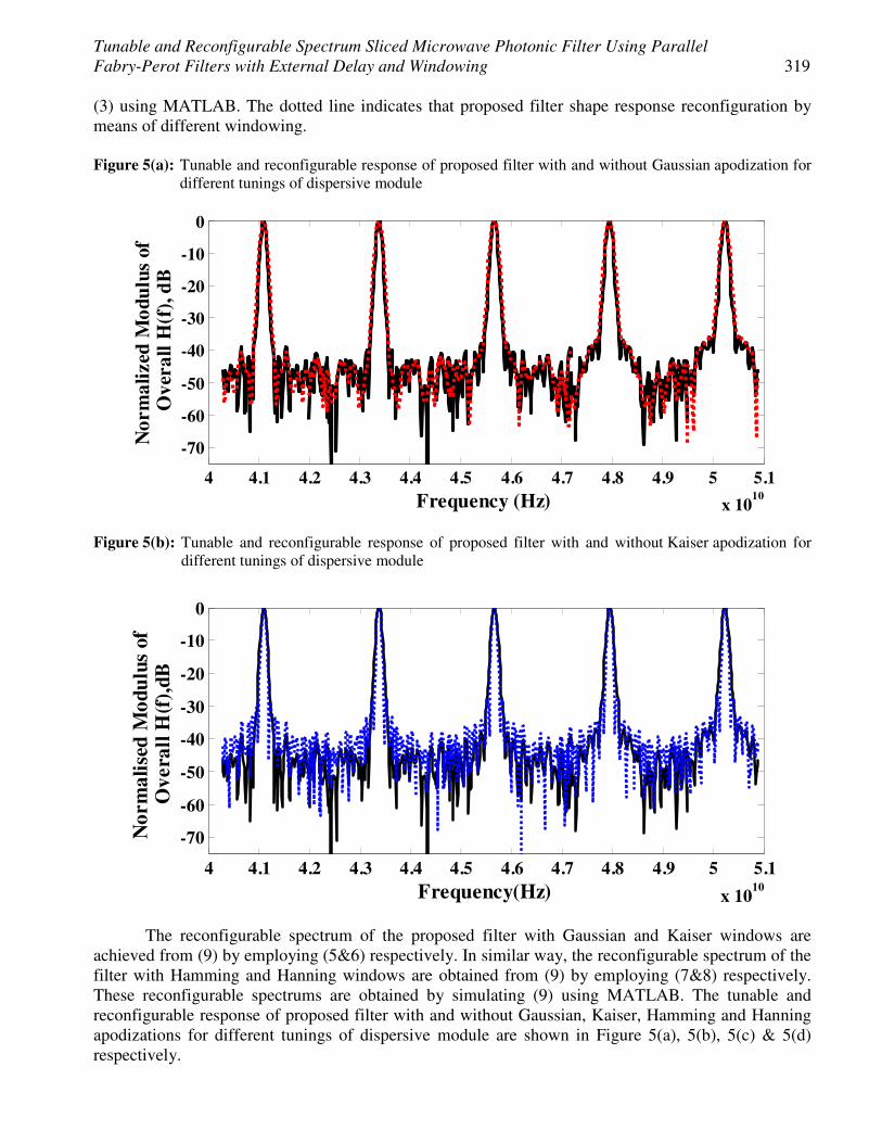
Tunable and Reconfigurable Spectrum Sliced Microwave Photonic Filter Using Parallel Fabry-Perot Filters with External Delay and Windowing 319
(3) using MATLAB. The dotted line indicates that proposed filter shape response reconfiguration by means of different windowing. Figure 5(a): Tunable and reconfigurable response of proposed filter with and without Gaussian apodization for
different tunings of dispersive module
4 4.1 4.2 4.3 4.4 4.5 4.6 4.7 4.8 4.9 5 5.1
x 1010
-70
-60
-50
-40
-30
-20
-10
0
Frequency (Hz)
Nor
mal
ized
Mod
ulus
of
Ove
rall
H(f
), dB
Figure 5(b): Tunable and reconfigurable response of proposed filter with and without Kaiser apodization for
different tunings of dispersive module
4 4.1 4.2 4.3 4.4 4.5 4.6 4.7 4.8 4.9 5 5.1
x 1010
-70
-60
-50
-40
-30
-20
-10
0
Frequency(Hz)
Nor
mal
ised
Mod
ulus
of
Ove
rall
H(f
),dB
The reconfigurable spectrum of the proposed filter with Gaussian and Kaiser windows are achieved from (9) by employing (5&6) respectively. In similar way, the reconfigurable spectrum of the filter with Hamming and Hanning windows are obtained from (9) by employing (7&8) respectively. These reconfigurable spectrums are obtained by simulating (9) using MATLAB. The tunable and reconfigurable response of proposed filter with and without Gaussian, Kaiser, Hamming and Hanning apodizations for different tunings of dispersive module are shown in Figure 5(a), 5(b), 5(c) & 5(d) respectively.
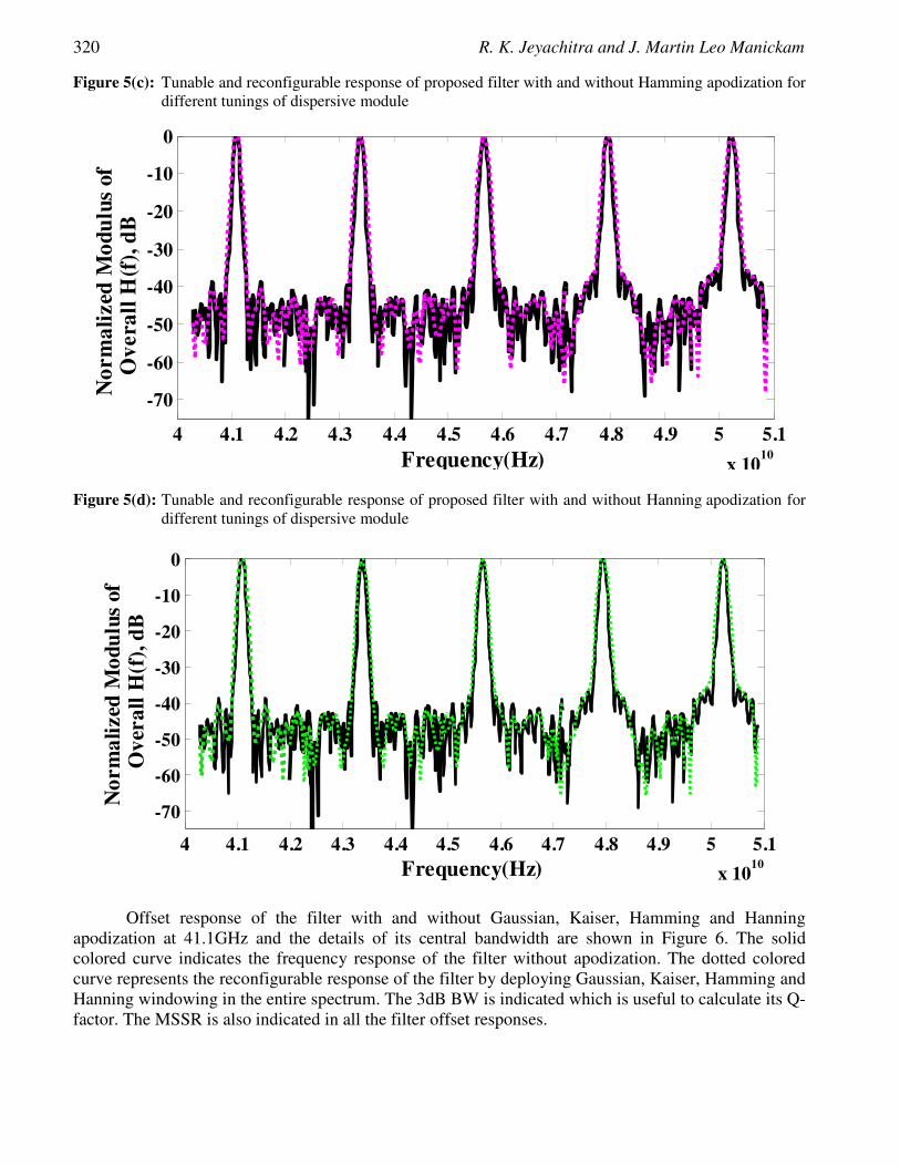
320 R. K. Jeyachitra and J. Martin Leo Manickam
Figure 5(c): Tunable and reconfigurable response of proposed filter with and without Hamming apodization for different tunings of dispersive module
4 4.1 4.2 4.3 4.4 4.5 4.6 4.7 4.8 4.9 5 5.1
x 1010
-70
-60
-50
-40
-30
-20
-10
0
Frequency(Hz)
Nor
mal
ized
Mod
ulu
s of
O
vera
ll H
(f),
dB
Figure 5(d): Tunable and reconfigurable response of proposed filter with and without Hanning apodization for
different tunings of dispersive module
4 4.1 4.2 4.3 4.4 4.5 4.6 4.7 4.8 4.9 5 5.1
x 1010
-70
-60
-50
-40
-30
-20
-10
0
Frequency(Hz)
Nor
mal
ized
Mod
ulu
s of
Ove
rall
H(f
), d
B
Offset response of the filter with and without Gaussian, Kaiser, Hamming and Hanning apodization at 41.1GHz and the details of its central bandwidth are shown in Figure 6. The solid colored curve indicates the frequency response of the filter without apodization. The dotted colored curve represents the reconfigurable response of the filter by deploying Gaussian, Kaiser, Hamming and Hanning windowing in the entire spectrum. The 3dB BW is indicated which is useful to calculate its Q-factor. The MSSR is also indicated in all the filter offset responses.
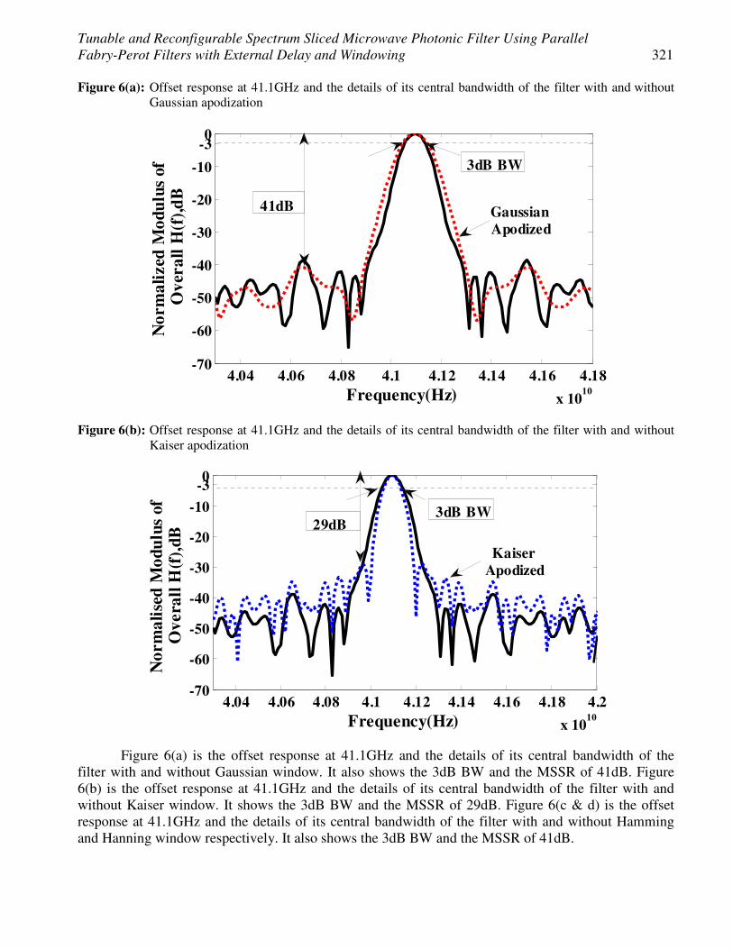
Tunable and Reconfigurable Spectrum Sliced Microwave Photonic Filter Using Parallel Fabry-Perot Filters with External Delay and Windowing 321
Figure 6(a): Offset response at 41.1GHz and the details of its central bandwidth of the filter with and without Gaussian apodization
4.04 4.06 4.08 4.1 4.12 4.14 4.16 4.18
x 1010
-70
-60
-50
-40
-30
-20
-10
-30
Frequency(Hz)
Nor
mal
ized
Mod
ulus
of
Ove
rall
H(f
),dB
3dB BW
Gaussian Apodized
41dB
Figure 6(b): Offset response at 41.1GHz and the details of its central bandwidth of the filter with and without
Kaiser apodization
4.04 4.06 4.08 4.1 4.12 4.14 4.16 4.18 4.2
x 1010
-70
-60
-50
-40
-30
-20
-10
-30
Frequency(Hz)
Nor
mal
ised
Mod
ulus
of
Ove
rall
H(f
),dB
29dB3dB BW
Kaiser Apodized
Figure 6(a) is the offset response at 41.1GHz and the details of its central bandwidth of the filter with and without Gaussian window. It also shows the 3dB BW and the MSSR of 41dB. Figure 6(b) is the offset response at 41.1GHz and the details of its central bandwidth of the filter with and without Kaiser window. It shows the 3dB BW and the MSSR of 29dB. Figure 6(c & d) is the offset response at 41.1GHz and the details of its central bandwidth of the filter with and without Hamming and Hanning window respectively. It also shows the 3dB BW and the MSSR of 41dB.
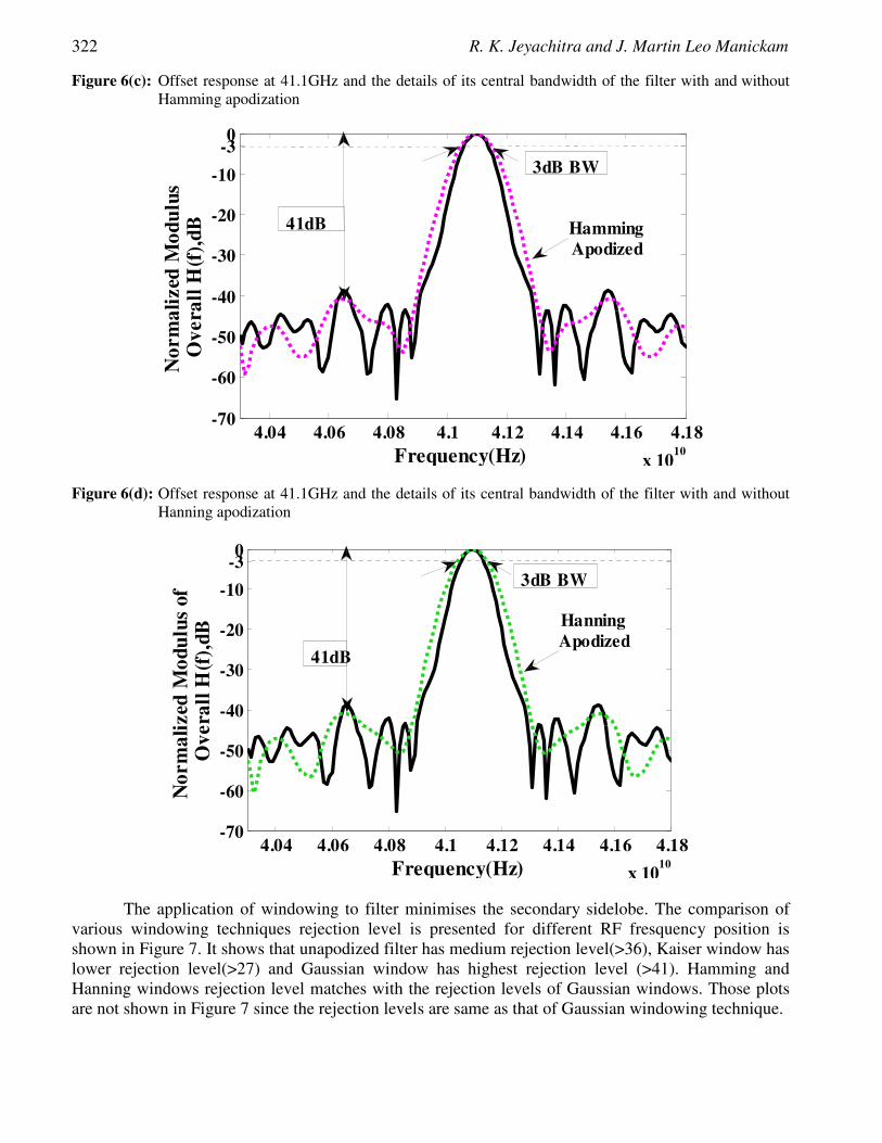
322 R. K. Jeyachitra and J. Martin Leo Manickam
Figure 6(c): Offset response at 41.1GHz and the details of its central bandwidth of the filter with and without Hamming apodization
4.04 4.06 4.08 4.1 4.12 4.14 4.16 4.18
x 1010
-70
-60
-50
-40
-30
-20
-10
-30
Frequency(Hz)
Nor
mal
ized
Mod
ulus
O
vera
ll H
(f),
dB
41dB
3dB BW
Hamming Apodized
Figure 6(d): Offset response at 41.1GHz and the details of its central bandwidth of the filter with and without
Hanning apodization
4.04 4.06 4.08 4.1 4.12 4.14 4.16 4.18
x 1010
-70
-60
-50
-40
-30
-20
-10
-30
Frequency(Hz)
Nor
mal
ized
Mod
ulus
of
Ove
rall
H(f
),dB
41dB
3dB BW
Hanning Apodized
The application of windowing to filter minimises the secondary sidelobe. The comparison of various windowing techniques rejection level is presented for different RF fresquency position is shown in Figure 7. It shows that unapodized filter has medium rejection level(>36), Kaiser window has lower rejection level(>27) and Gaussian window has highest rejection level (>41). Hamming and Hanning windows rejection level matches with the rejection levels of Gaussian windows. Those plots are not shown in Figure 7 since the rejection levels are same as that of Gaussian windowing technique.
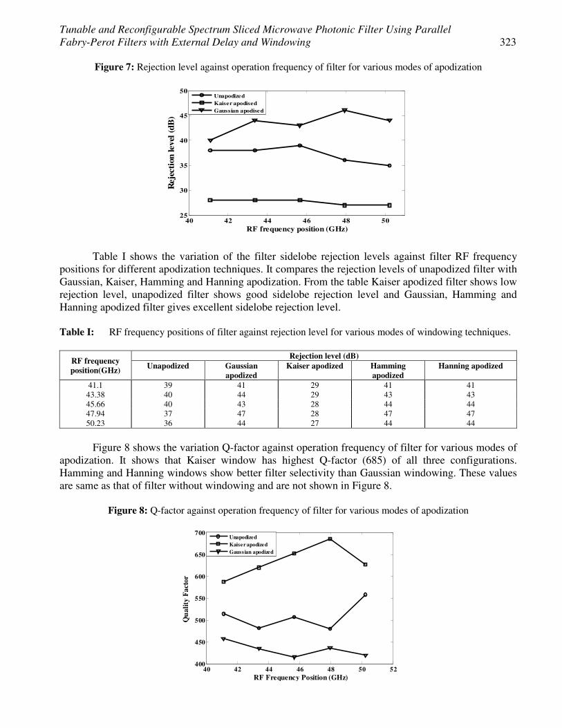
Tunable and Reconfigurable Spectrum Sliced Microwave Photonic Filter Using Parallel Fabry-Perot Filters with External Delay and Windowing 323
Figure 7: Rejection level against operation frequency of filter for various modes of apodization
40 42 44 46 48 5025
30
35
40
45
50
RF frequency position (GHz)
Rej
ecti
on le
vel
(dB
)
UnapodizedKaiser apodisedGaussian apodised
Table I shows the variation of the filter sidelobe rejection levels against filter RF frequency positions for different apodization techniques. It compares the rejection levels of unapodized filter with Gaussian, Kaiser, Hamming and Hanning apodization. From the table Kaiser apodized filter shows low rejection level, unapodized filter shows good sidelobe rejection level and Gaussian, Hamming and Hanning apodized filter gives excellent sidelobe rejection level. Table I: RF frequency positions of filter against rejection level for various modes of windowing techniques.
RF frequency position(GHz)
Rejection level (dB) Unapodized Gaussian
apodized Kaiser apodized Hamming
apodized Hanning apodized
41.1 39 41 29 41 41 43.38 40 44 29 43 43 45.66 40 43 28 44 44 47.94 37 47 28 47 47 50.23 36 44 27 44 44
Figure 8 shows the variation Q-factor against operation frequency of filter for various modes of
apodization. It shows that Kaiser window has highest Q-factor (685) of all three configurations. Hamming and Hanning windows show better filter selectivity than Gaussian windowing. These values are same as that of filter without windowing and are not shown in Figure 8.
Figure 8: Q-factor against operation frequency of filter for various modes of apodization
40 42 44 46 48 50 52400
450
500
550
600
650
700
RF Frequency Position (GHz)
Qu
alit
y F
acto
r
UnapodizedKaiser apodizedGaussian apodized
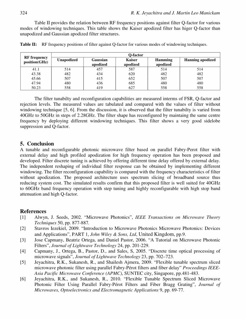
324 R. K. Jeyachitra and J. Martin Leo Manickam
Table II provides the relation between RF frequency positions against filter Q-factor for various modes of windowing techniques. This table shows the Kaiser apodized filter has higer Q-factor than unapodized and Gaussian apodized filter structures. Table II: RF frequency positions of filter against Q-factor for various modes of windowing techniques.
RF frequency position(GHz)
Q-factor Unapodized Gaussian
apodized Kaiser
apodized Hamming apodized
Hanning apodized
41.1 514 457 587 514 514 43.38 482 434 620 482 482 45.66 507 415 652 507 507 47.94 480 436 685 480 480 50.23 558 419 627 558 558
The filter tunabilty and reconfiguration capabilities are measured interms of FSR, Q-factor and
rejection levels. The measured values are tabulated and compared with the values of filter without windowing technique [5, 6]. From the discussion, it is observed that the filter tunabilty is varied from 40GHz to 50GHz in steps of 2.28GHz. The filter shape has reconfigured by maintaing the same centre frequency by deploying different windowing techniques. This filter shows a very good sidelobe suppression and Q-factor. 5. Conclusion A tunable and reconfigurable photonic microwave filter based on parallel Fabry-Perot filter with external delay and high profiled apodization for high frequency operation has been proposed and developed. Filter discrete tuning is achieved by offering different time delay offered by external delay. The independent reshaping of individual filter response can be obtained by implementing different windowing. The filter reconfiguration capability is compared with the frequency characteristics of filter without apodization. The proposed architecture uses spectrum slicing of broadband source thus reducing system cost. The simulated results confirm that this proposed filter is well suited for 40GHz to 60GHz band frequency operation with step tuning and highly reconfigurable with high stop band attenuation and high Q-factor. References [1] Alwyn, J. Seeds, 2002. “Microwave Photonics”, IEEE Transactions on Microwave Theory
Techniques 50, pp. 877-887. [2] Stavros Iezekiel, 2009. “Introduction to Microwave Photonics Microwave Photonics: Devices
and Applications”, PART 1, John Wiley & Sons, Ltd, United Kingdom, pp.9. [3] Jose Capmany, Beatriz Ortega, and Daniel Pastor, 2006. “A Tutorial on Microwave Photonic
Filters”, Journal of Lightwave Technology 24, pp. 201-229. [4] Capmany, J., Ortega, B., Pastor, D., and Sales, S, 2005. “Discrete time optical processing of
microwave signals”, Journal of Lightwave Technology 23, pp. 702–723. [5] Jeyachitra, R.K., Sukanesh, R., and Shailesh Ajmera, 2009. “Flexible tunable spectrum sliced
microwave photonic filter using parallel Fabry-Pérot filters and fiber delay” Proceedings IEEE-Asia Pacific Microwave Conference (APMC), SUNTEC city, Singapore, pp.481-483.
[6] Jeyachitra, R.K., and Sukanesh, R., 2010. “Flexible Tunable Spectrum Sliced Microwave Photonic Filter Using Parallel Fabry-Pérot Filters and Fiber Bragg Grating”, Journal of Microwaves, Optoelectronics and Electromagnetic Applications 9, pp. 69-77.

Tunable and Reconfigurable Spectrum Sliced Microwave Photonic Filter Using Parallel Fabry-Perot Filters with External Delay and Windowing 325
[7] Tong Chen, Xioake Yi, Thomas Huang and Minasian, R.A, 2009. “Spectrum sliced microwave photonic signal processor with tunability and reconfigurability”, IEEE 14th Opto Electronics and Communications Conference (OECC), Hong Kong, China, pp.243-244.
[8] Vidal, B., Polo, V., Corral, J.L., and Marti, J, 2003. “Photonic microwave filter with tuning and reconfiguration capabilities using optical switches and dispersive media”, Electronics Letters 39, pp. 547–549.
[9] Mora, J., Capmany, J., and Chen, L. R, 2007. “Tunable and reconfigurable single bandpass photonic microwave filter using a high birefringence sagnag loop and DWDM channel selector”, The 20th Annual Meeting of the IEEE Lasers and Electro-Optics Society, 2007. (LEOS 2007). FL, pp.192-193.
[10] Jose Capmany, Jose Mora, Beatriz Ortega and Daniel Pastor, 2005. “Microwave photonic filters using low-cost sources featuring tunability, reconfigurability and negative coefficients”, Optics Express13, pp. 1412-1417.
[11] Mora, J., Ortega, B., Capmany, J., Cruz, J., Andres, M.V., Pastor, D., and Sales, S, 2002. “Automatic tunable and reconfigurable fiber optic microwave filters based on a broadband optical source sliced by uniform fiber Bragg gratings”, Optics Express 10, pp. 1291-1298.
[12] John, D. Taylor, Lawrence, R. Chen, and Xijia Gu, 2007, “Simple Reconfigurable Photonic Microwave Filter Using an Arrayed Waveguide Grating and Fiber Bragg Gratings”, IEEE Photonics Technology Letters 19, pp. 510-512.
[13] Yi, X., Huang, T.X.H., and Minasian, R.A, 2009. “Microwave photonic filter with tunability, reconfigurability and bipolar taps”, Electronics Letters 45, pp. 840–841.
[14] Capmany, J., Pastor, D., and Ortega, B, 1999. “Fiber optic microwave and millimeter-wave filter with high density sampling and very high sidelobe suppression using subnanometer optical spectrum slicing”, Electronics Letters 35, pp. 494–496.
[15] Capmany, J., Pastor, D., and Ortega, B, 1999. “New and flexible fiber-optic delay-line filters using chirped Bragg gratings and laser arrays”, IEEE Transactions on Microwave Theory Techniques 47, pp. 1321-1326.
[16] Capmany, J., Pastor, D., and Ortega, B., 1999. “Efficient sidelobe suppression by source power apodization in fibre optic microwave filters composed of linearly chirped fibre grating by laser array”, Electronics Letters 35, pp. 640-642.
[17] Govind, P. Agarwal, 2006. “Applications of Nonlinear Fiber Optics”, Academic Press, Elsevier,USA, pp. 289.

European Journal of Scientific Research ISSN 1450-216X / 1450-202X Vol. 103 No 2 June, 2013, pp.326 - 332 http://www.europeanjournalofscientificresearch.com
Mobility Issues in 4G Heterogeneous Wireless Networks
K.Komala Professor, Dept of ECE, Valliammai Engg. College, Anna University, Chennai, India
E-mail: [email protected]
P.Indumathi Associate Professor, Dept of EE, M.I.T. Campus, Anna University, Chennai, India
E-mail: [email protected]
Abstract
A Heterogeneous Network is a network consisting of mix of macro cells, pico cells, femto cells, Remote Radio Heads (RRH) and relays. It is a 4G technology denoted as HetNet. A HetNet consists of infrastructure with different wireless access technologies, different network architectures and protocols for the various needs of the mobile users. There is a very tremendous traffic growth in broadband wireless networks. The major advantages of HetNets are improvement in the performances of the network, reducing the transmitter-to-receiver distance and providing a better spatial reuse of the spectrum. One of the research challenges of HetNets is the mobility management in order to achieve global roaming among the different access technologies. As the handover decisions play a major role in mobility management, the types of handover techniques are analyzed. The performance measures such as handoff delay and packet loss are analyzed with the help of the network simulator NS-2. Keywords: HetNets, Mobility Management, Handover, Handoff, Wireless LAN
1. Introduction The end users want to be Always Best Connected to the best resources available. Traditional 2G cellular networks used circuit switched techniques for voice transmission such as GSM. GPRS is a 2.5G technique which used circuit switching for voice and packet switching for data transmission. The 3G techniques like 3GPP and 3GPP2 were introduced for high speed and bandwidth capabilities. A 4th
generation network is an IP-based mobile system that deals with various radio interfaces. A 4G architecture introduces three basic areas of connectivity: Personal Area Networking (Bluetooth), Wireless LAN techniques (IEEE 802:11 and HIPERLAN) and cellular connectivity.
The characteristics of 4G networks are • High Speed • High Network Capacity • Fast/Seamless handover across multiple networks • Next-generation multimedia support. It is believed that the radio link quality can be improved by reducing the distance between
transmitter and the receiver. The larger number of cells are helpful in receiving larger data rates. The LTE Advanced (Long Term Evolution-Advanced) techniques are tried by the cellular operators and

327 K.Komala and P.Indumathi
HetNets are considered to be the major performance enhancement enablers of LTE-Advanced techniques.
The details of different elements of HetNets as dealt in [2] are shown in Table 1. Table 1: Specification of nodes in HETNET
Types of Nodes Transmit Power Coverage Backhaul Macro cell 46 dBM Few km S1 Interface Pico cell 23 – 30 dBm < 300 m X2 Interface Femto cell < 23 dBm < 50 m Internet IP Relay 30 dBm 300 m Wireless RRH 46 dBm Few km Fiber
2. Challenges of HetNets The key technical challenges of HetNets are Self organization, backhauling, handover and interference.
• Self Organization : The self organizing capability of HetNets are classified into three processes such as Self-Configuration, Self-Healing, and Self-Optimization.
• Backhauling : The design Backhauling NW is an issue due to the various types of coexisting cells. A HetNet backhaul is very essential in providing the most cost effective and QoS guaranteed solution.
• Handover : Handovers are very essential in the provision of a seamless uniform service to the users. The handovers are also efficient for traffic load balancing where the users at the borders of adjacent/overlapping cells are shifted to the less congested cells. This is considered as a system overhead.
• Interference : There are interference issues due to the following reasons. o The backhaul NW support different types of cells which may have different bandwidth and
delay constraints. o Due to the restricted access control with pico cells and femto cells, the users may not
handover to the nearest cells. This may lead to strong interference scenario in both uplink and downlink.
3. Literature Survey The various classifications of handoffs are thoroughly analyzed in [1]. Based on the network type, the handoff is classified as horizontal or vertical handoff. If the handoff process of a mobile terminal takes place between access points supporting the same network then the handoff is referred as horizontal handoff. It is also called as intra-domain handoff. If the handoff process takes place between different networks, then it is referred as vertical handoff. It is called as inter-domain handoff. There are two types of vertical handoffs. They are upward and downward vertical handoffs. An upward vertical handoff is roaming to an overlay with a larger cell size and a downward vertical handoff is roaming to an overlay with a smaller cell size.
The various technical challenges for HetNets are analyzed in [2]. The main focus of the research work is about the interference aspects of HetNets. The mobility management techniques in three distinct stages are explained in [3]. The focus is on the interaction between the functional entities involved in communication .
The various phases involved in the handoff process are clearly explained in [4]. The mobility management and handoff management issues of wireless networks and heterogeneous networks are analyzed in detail from [5] through [12].

Mobility Issues in 4G Heterogeneous Wireless Networks 328
4. Mobility Management Mobility Management consists of Location Management and Handoff Management. In a next generation networking scenario, there are two types of roaming for mobile terminals. They are intra-system and intersystem roaming. The movement between different cells of the same system is referred as intra-system roaming. The intersystem roaming refers to moving between different backhauls, protocol (or) service providers. 4.1. Location Management
Location Management helps to track the locations of the mobile terminals. It deals with two major tasks such as location update and call delivery. The mobile terminal updates the location database of the system with the up-to-date location information. During call delivery, the system determines the current location of the mobile terminal. 4.2. Handoff Management
Handoff Management is the process by which a mobile terminal keeps its connection achieve when it moves from one access point to another. There are two major types of handoff. They are intra-system (or) horizontal handoff and intersystem (or) vertical handoff. The horizontal handoff occurs when the signal strength of serving base station reduces below a threshold value. The vertical handoff occurs due to the following situations :
I. When a user moves out of the serving NW. II. When a user is connected to a particular network and chosen for handoff to another
network. III. When the overall network load is distributed among different systems for performance
optimization of networks. 5. Categories of Mobility Management The mobility management solutions of the heterogeneous wireless networks are classified into the following categories as in [6],
• Network Layer Solutions (L3 solutions) • Link Layer Solutions (L2 solutions) • Cross-Layer Solutions (L3 + L2 solutions)
5.1. Network Layer Solutions
Network Layer Mobility Management Solutions are classified into macro-mobility and micro-mobility management solutions. The movement of mobile users between two network domains is referred as macro-mobility. The movement of mobile users between two subnets within one domain is referred as micro-mobility. 5.2. Link Layer Solutions
Link Layer Mobility Management Solutions focuses on issues related to inter-system roaming between heterogeneous access networks. The two critical issues of the inte-rsystem roaming are air interface protocol and the mobile application part (MAP). Inter-system roaming requires the support of handoff between different types of networks.

329 K.Komala and P.Indumathi
5.3. Cross-Layer Solutions
The Cross-Layer Solutions are proposed mainly for handoff management techniques. Cross-Layer mobility management protocols reduce the movement detection delay. Mostly those mechanisms use link layer information to make an efficient network layer handoff. 5.3.1. Cross-Layer Handoff Mechanisms Four types of cross-layer handoff mechanisms are as follows,
• Link Layer-Assisted Fast Handoff • Seamless Handoff • Vertical Handoff • Media Independent Pre-Authentication Handoff.
6. Steps Involved in Mobility Control The mobility control in heterogeneous networks is divided into three steps as in [3]. They are
i. Monitoring and detecting available radio resources ii. Handover decisions-making and
iii. Handover execution. Radio Resource Management (RRM) monitors the active radio links. RRM interacts with
MRRM and produces the detected access set DAS. When DAS is available, handover decisions-making commences.
Handover decisions is made because of the following reasons [3]: i. Additions of new access to the DAS
ii. Change of radio signal strength iii. Change in the QoS requirements
During handover decision making, path selection calculates a rating metric and delivers a rating for each access in DAS. Based on this, MRRM calls upon HOLM for the execution of the handover.
During handover execution, the radio connectivity changes. The HOLM selects a handover protocol from the mobility tool box. HOLM interacts with path selection to make the final choice of path and locator. HOLM commends the MRRM to release and set up radio connectivity at the appropriate stage during the process of mobility management. 7. Proposed Architecture In the proposed architecture, an Automatic Neighbour Relations Handler (ANRH) is used to integrate different wireless networks belonging to different service providers. A mobile node, M-Node can move between different subnets belonging to one domain which is intra-domain mobility and between different access networks belonging to different domains, which is inter-domain mobility. The ANRH is used only during inter-domain mobility. In the proposed cross-layer algorithm, the necessity for inter-domain mobility is detected earlier and then authentication, authorization and registration of the M-Node in the next domain are carried out before the actual handoff. The necessary operations are carried out through the ANRH, which has separate service level agreement with both domains.
Mobility management architecture for NG-All IP based wireless systems is referred in [1]. A hetnet with a Wireless LAN Network and a WiMAX network is considered. A movement pattern is in said to be in one of the three patterns modes. They are
i. Linear ii. Stationary &
iii. Stochastic
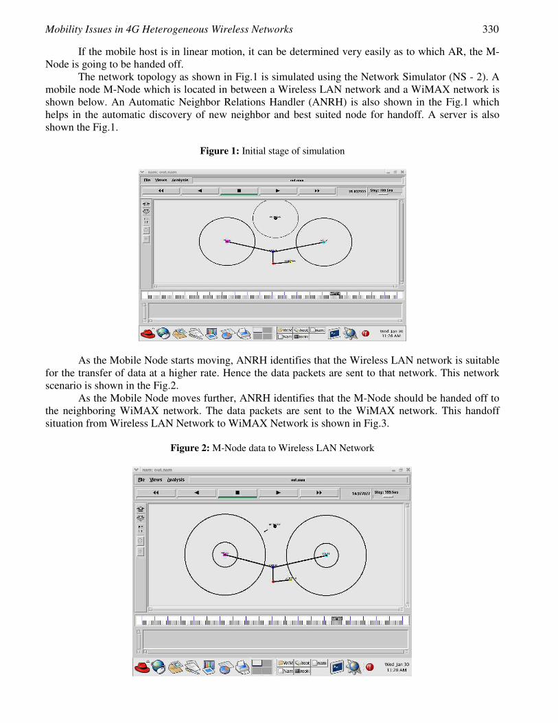
Mobility Issues in 4G Heterogeneous Wireless Networks 330
If the mobile host is in linear motion, it can be determined very easily as to which AR, the M-Node is going to be handed off.
The network topology as shown in Fig.1 is simulated using the Network Simulator (NS - 2). A mobile node M-Node which is located in between a Wireless LAN network and a WiMAX network is shown below. An Automatic Neighbor Relations Handler (ANRH) is also shown in the Fig.1 which helps in the automatic discovery of new neighbor and best suited node for handoff. A server is also shown the Fig.1.
Figure 1: Initial stage of simulation
As the Mobile Node starts moving, ANRH identifies that the Wireless LAN network is suitable for the transfer of data at a higher rate. Hence the data packets are sent to that network. This network scenario is shown in the Fig.2.
As the Mobile Node moves further, ANRH identifies that the M-Node should be handed off to the neighboring WiMAX network. The data packets are sent to the WiMAX network. This handoff situation from Wireless LAN Network to WiMAX Network is shown in Fig.3.
Figure 2: M-Node data to Wireless LAN Network
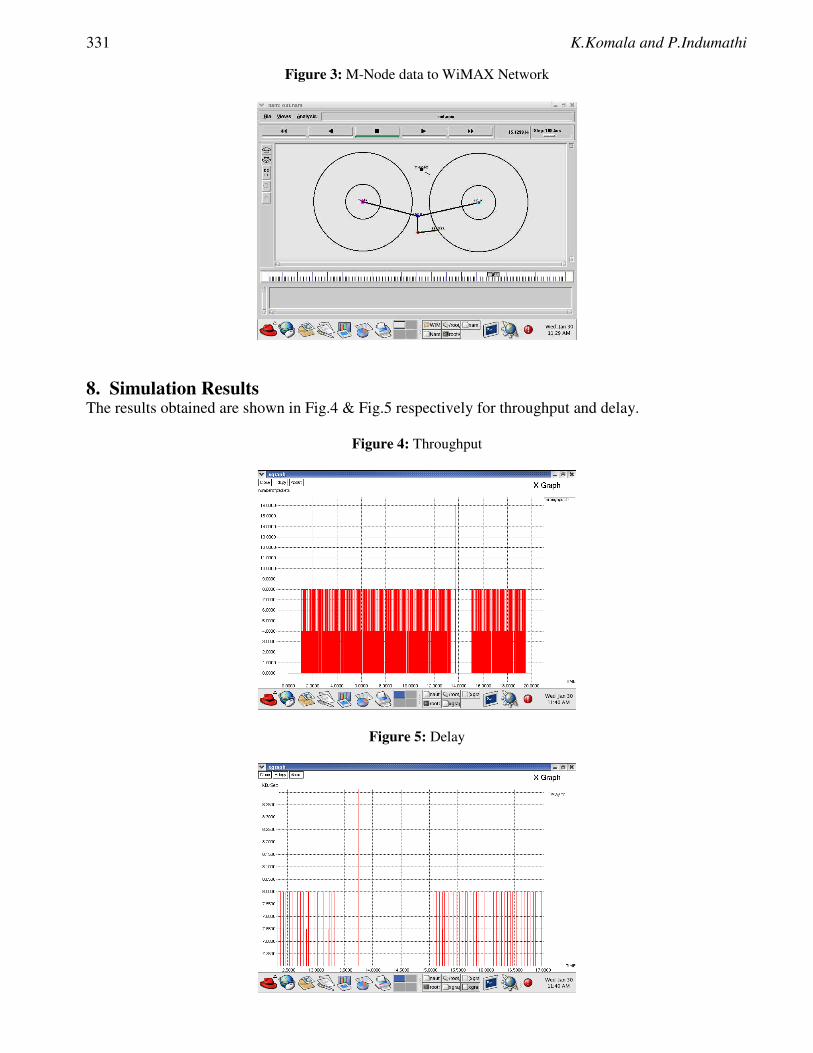
331 K.Komala and P.Indumathi
Figure 3: M-Node data to WiMAX Network
8. Simulation Results The results obtained are shown in Fig.4 & Fig.5 respectively for throughput and delay.
Figure 4: Throughput
Figure 5: Delay

Mobility Issues in 4G Heterogeneous Wireless Networks 332
9. Conclusion The mobility management issues of a heterogeneous network are analyzed in detail using Network Simulator (NS-2). A Wireless LAN Network and a WiMAX Network are considered for the various simulation scenarios. A Mobile Node is initially sending data to the Wireless LAN Network and then handsoff to the WiMAX network. The throughput and the delay are analyzed for the simulations performed. The results obtained are able to prove the efficiency of the mobility management of the node. There is no packet drop as seen in the results obtained and the delay is also minimum. This proves the efficiency of the proposed system of networking environment considered. This work can be extended for more number of Mobile Nodes and also for more number of networks. The directions for the future research may be the “Always Best Connected” and the self organizing issues of the HetNets. The various movement patterns of the M-Node can also be considered for further research work. References [1] Nidal Nasser, University of Guelph, Ahmed Hasswa and Hossam Hassanein, Queen’s
University, “ Handoffs in Fourth Generation Heterogeneous Networks”. [2] David Lopez-Perez, Ismail Guvenc, Guillaume de la Roche, Marios Kountouris, Tony
Q.S.Quek, Jie Zhang, “Enhanced Inter-Cell Interference Coordination Chellenges In Heterogeneous Networks”.
[3] Oliver Blume, Abigail Surtees, Ramon Aguero, ErangaPerera and Kostas Pentikousis, “A Generic Signaling Framework for Seamless Mobility in Heterogeneous Wireless Networks”.
[4] Ian.F.Akyilidz et al., “Mobility Management in Next Generation Wireless Systems”.Proc. IEEE, vol. 87, no. 8, Aug 1999, pp . 1347 – 84.
[5] Robert Hsieh, Zhe Guang Zhou, Aruna Seneviratne, “S-MIP: A Seamless Handoff Architecture for Mobile IP”, IEE INFOCOM 2003.
[6] Ian.F.Akyildiz, Jiang Xie, And Shantidev Mohanty, Georgia Institute Of Technology, “A Survey Of Mobility Management In Next-Generation All-IP-Baesd Wireless Systems”, IEE Wireless Communication, August 2004.
[7] Haoming Li, Javad Hajipour, Alireza Attar And Victor C.M.Leung, The University Of British Columbia, “Efficient HetNet Implementation Using Broadband Wireless Access With Fiber-Conneceted Massively Distributed Antennas Architecture”, IEE Wireless Communication, June 2011.
[8] Ashutosh Dutta, Subir Das, David Famolari, Telcordia Technologies, NJ Yoshihiro, Ohba, Kenchi Taniuchi, Toshikazu Kodama, Toshiba America Research Inc., NJ Henning Schulzrinne, Computer Science Department, Columbia University, NY. “Seamless Handover Across Hetrogeneous Networks – an IEEE 802.21 Centric Approach”.
[9] Jaydip Sen, Tata Consultancy Services, India, “Mobility And Handoff Management In Wireless Networks”.
[10] Justino Santos, Nuno Seneca, Susana Sargento And Rui Aguiar, Institudu de Telecomunicacoes, Universisade de Aveiro, “Mobility In Heterogeneous Networks : Integration Process”.
[11] Jianfeng Guan, Changqiao Xu, Hongke Zhang, Huachun Zhou, Huachun Zhou, “Mobility Challenges And Management In The Future Wireless Heterogeneous Networks”.
[12] Pablo Vidales, Leo Patanapongpibul, Glenford Mapp, Andy Hoper, Laboratory Of Communication Engineering, University Of Cambridge, “Experiences With Heterogeneous Wireless Networks, Unveiling the Challenges”.
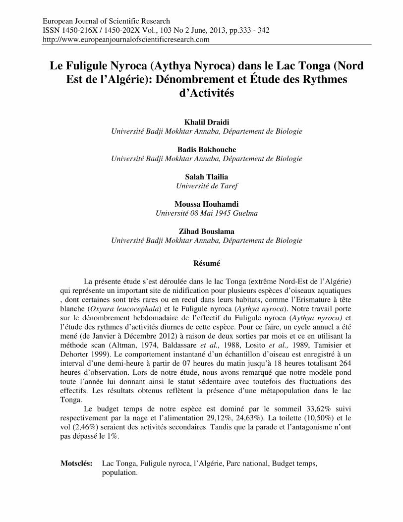
European Journal of Scientific Research ISSN 1450-216X / 1450-202X Vol., 103 No 2 June, 2013, pp.333 - 342 http://www.europeanjournalofscientificresearch.com
Le Fuligule Nyroca (Aythya Nyroca) dans le Lac Tonga (Nord
Est de l’Algérie): Dénombrement et Étude des Rythmes d’Activités
Khalil Draidi Université Badji Mokhtar Annaba, Département de Biologie
Badis Bakhouche
Université Badji Mokhtar Annaba, Département de Biologie
Salah Tlailia Université de Taref
Moussa Houhamdi
Université 08 Mai 1945 Guelma
Zihad Bouslama Université Badji Mokhtar Annaba, Département de Biologie
Résumé
La présente étude s’est déroulée dans le lac Tonga (extrême Nord-Est de l’Algérie) qui représente un important site de nidification pour plusieurs espèces d’oiseaux aquatiques , dont certaines sont très rares ou en recul dans leurs habitats, comme l’Erismature à tête blanche (Oxyura leucocephala) et le Fuligule nyroca (Aythya nyroca). Notre travail porte sur le dénombrement hebdomadaire de l’effectif du Fuligule nyroca (Aythya nyroca) et l’étude des rythmes d’activités diurnes de cette espèce. Pour ce faire, un cycle annuel a été mené (de Janvier à Décembre 2012) à raison de deux sorties par mois et ce en utilisant la méthode scan (Altman, 1974, Baldassare et al., 1988, Losito et al., 1989, Tamisier et Dehorter 1999). Le comportement instantané d’un échantillon d’oiseau est enregistré à un interval d’une demi-heure à partir de 07 heures du matin jusqu’à 18 heures totalisant 264 heures d’observation. Lors de notre étude, nous avons remarqué que notre modèle pond toute l’année lui donnant ainsi le statut sédentaire avec toutefois des fluctuations des effectifs. Les résultats obtenus reflètent la présence d’une métapopulation dans le lac Tonga.
Le budget temps de notre espèce est dominé par le sommeil 33,62% suivi respectivement par la nage et l’alimentation 29,12%, 24,63%). La toilette (10,50%) et le vol (2,46%) seraient des activités secondaires. Tandis que la parade et l’antagonisme n’ont pas dépassé le 1%. Motsclés: Lac Tonga, Fuligule nyroca, l’Algérie, Parc national, Budget temps,
population.

334 Khalil Draidi, Badis Bakhouche, Salah Tlailia, Moussa Houhamdi and Zihad Bouslama
1. Introduction L’Algérie compte 51 sites Ramsar (dont 4 nouveaux inscrits récemment, affirmant de plus en plus l’importance des zones humides algériennes tant au niveau national qu’international. Parmi ces réserves de la biosphère, le lac Tonga (Classé site Ramsar en 1983) est considéré comme étant l’une des plus importantes zones humides naturelles algériennes, voir même méditerranéennes (Ledant et al., 1982, Aissaoui et al., 2009 et 2011, Lazli et al., 2011) et ce par sa grande capacité d’accueil d’oiseaux aquatiques (plus de 25.000 anatidés et foulques) et par sa grande richesse faunistique et floristique (Lazli et al., 2011).
Cette avifaune aquatique tout comme les poissons et les végétaux, constituent une multiple ressource de ces milieux (Benyacoub et Chabi 2000). Ce patrimoine international subit un déclin dramatique des effectifs de l’avifaune suite à la destruction et à la fragmentation des zones humides. En effet, nous assistons de plus en plus à une réduction de la taille des populations de certaines espèces telles que le Fuligule nycoca (Aythya nyroca ) qui est notre modèle biologique et qui a le statut d’espèce peu menacée (IUNC 2006 Near Threatened), cet Anatidé est largement distribué en Europe, en Asie et en Afrique (Jonsson 1994). Néanmoins, ces effectifs ont connu ces dernières décennies des déclins et des changements de distribution nous permettant d’émettre l’hypothèse d’extinction de l’espèce considérée dans la nature durant les années à venir si des mesures sérieuses de conservation et de protection ne seraient pas adoptées dans les régions (Petkov et al., 2003).
La stratégie d’hivernage et le comportement diurne des canards plongeurs restent encore peu étudiés (Houhamdi et Samraoui, 2001, 2002, 2003, 2008). Il nous est impératif donc de combler les lacunes de nos connaissances par des études approfondies et indispensables consistant à réunir toutes les informations fondamentales à la compréhension du fonctionnement de nos écosystèmes (Houhamdi et Samraoui, 2008). Pour cela, dans le but de mettre un plan de gestion de cette espèce deux objectifs ont été visés : le dénombrement et l’étude de rythme d’activité. 2. Matériel et Méthodes 2.1.Description du Site d’étude
Notre étude à été réalisée à l’extrême Nord Est de l’Algérie, au niveau de site situé au parc national d’El-Kala : Le lac Tonga (Figure1) (36°53 N, 08°31 E) qui s’étend sur une superficie de 2500 ha (Belhadj et al., 2007) est l’un des sites Ramsar le plus important des zones humides d’Afrique du Nord (Boumezbeur, 1993, Samraoui et De Belair, 1998). Il est classé parmi les aires protégées de la région méditerranéenne ayant la nomenclature de réserve de la biosphère. C’est un lac de type palustre d’eau douce en communication avec la mer Méditerranée par un canal artificiel, le Canal Messida. Il se caractérise par une importante couverture végétale en mosaïque composée d’hélophytes (scirpes, phragmites et typhas). C’est un Site d’hivernage pour plus de 25.000 anatidés et foulques (Boumezbeur, 1993). Le lac Tonga et également un site de nidification important pour plusieurs espèces dont certaines sont très rares ou en recul dans leurs habitats, comme l’Erismature à tête blanche (Oxyura leucocephala) le Fuligule nyroca (Aythya nyroca) la poule Sultane (Porphyrio porphyrio), la Guifette moustac (Chlidonias hybridus) …etc. Ces deux bassins occupent une superficie de 15 km² chacun, mais le bassin versant nord ne semble plus alimenter le site depuis les tentatives d’assèchement entrepris durant la période coloniale (Aissaoui et al., 2011, Lazli, 2011). (Figure 1).

Le Fuligule Nyroca (Aythya Nyroca) dans le Lac Tonga (Nord Est de l’Algérie): Dénombrement et Étude des Rythmes d’Activités 335
Figure 1: Situation géographique du Lac Tonga
Algérie
Bouteldja
RN44
El-Aioun
Oum-Teboul
El-Kala
Ain-Assel
Sidi-Kassi
Ben M’hidi
Annaba
El-Hadjar
M e d i t e r r a n e n n s e a
RN16
RN21
RN44
CW110
CW37
Tunisia
Lac des Oiseaux
Marais de la Mekkhada
Lac Tonga
Lac Oubeira
Lac El-Mellah
Les Salines
RN16
N
Vers El-Kala
Commune Rmal Souk
Oued El-Hout
Commune Ain
Vers Oum Taboul
10 Km
El-Taref
2.2. Méthodologie du Travail
Notre étude s’est déroulée durant l’année 2012 (de Janvier à Décembre) à partir de laquelle nous avons effectué un suivi hebdomadaire de l’effectif à l’aide d’un télescope ornithologique SOLIGOR (25x60) et d’une paire de jumelle KONUSPOT (10x50). Un comptage individuel direct des Fuligules nyroca a été réalisé. Les données sont collectées à partir de plusieurs points d’observation (stations) préalablement choisis de manière à couvrir au maximum le pourtour du lac afin de déterminer le statut de ce dernier.
L’étude des rythmes d’activités diurnes a été menée sur un cycle annuel allant de Janvier à décembre 2012 à raison de deux sorties par mois. Pour ce faire, nous avons utilisé la méthode scan (Altman, 1974, Baldassare et al., 1988, Losito et al., 1989, Tamisier et Dehorter 1999). Cette méthode consiste à observer un groupe et d’enregistrer les activités instantanées de chaque individu; les résultats obtenus sont ensuite transformés selon des méthodes mathématiques afin de parvenir à un pourcentage de temps de chaque activité observée.
Le comportement instantané d’un échantillon d’oiseau est enregistré à un intervalle d’une demi-heure à partir de 07 heures du matin jusqu’à 18 heures totalisant 264 heures d’observations. Sept (07)
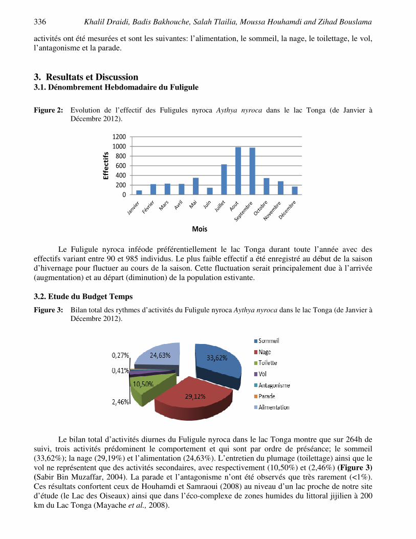
336 Khalil Draidi, Badis Bakhouche, Salah Tlailia, Moussa Houhamdi and Zihad Bouslama
activités ont été mesurées et sont les suivantes: l’alimentation, le sommeil, la nage, le toilettage, le vol, l’antagonisme et la parade. 3. Resultats et Discussion 3.1. Dénombrement Hebdomadaire du Fuligule
Figure 2: Evolution de l’effectif des Fuligules nyroca Aythya nyroca dans le lac Tonga (de Janvier à
Décembre 2012).
0
200
400
600
800
1000
1200
Effectifs
Mois
Le Fuligule nyroca inféode préférentiellement le lac Tonga durant toute l’année avec des effectifs variant entre 90 et 985 individus. Le plus faible effectif a été enregistré au début de la saison d’hivernage pour fluctuer au cours de la saison. Cette fluctuation serait principalement due à l’arrivée (augmentation) et au départ (diminution) de la population estivante. 3.2. Etude du Budget Temps
Figure 3: Bilan total des rythmes d’activités du Fuligule nyroca Aythya nyroca dans le lac Tonga (de Janvier à Décembre 2012).
Le bilan total d’activités diurnes du Fuligule nyroca dans le lac Tonga montre que sur 264h de suivi, trois activités prédominent le comportement et qui sont par ordre de préséance; le sommeil (33,62%); la nage (29,19%) et l’alimentation (24,63%). L’entretien du plumage (toilettage) ainsi que le vol ne représentent que des activités secondaires, avec respectivement (10,50%) et (2,46%) (Figure 3) (Sabir Bin Muzaffar, 2004). La parade et l’antagonisme n’ont été observés que très rarement (<1%). Ces résultats confortent ceux de Houhamdi et Samraoui (2008) au niveau d’un lac proche de notre site d’étude (le Lac des Oiseaux) ainsi que dans l’éco-complexe de zones humides du littoral jijilien à 200 km du Lac Tonga (Mayache et al., 2008).
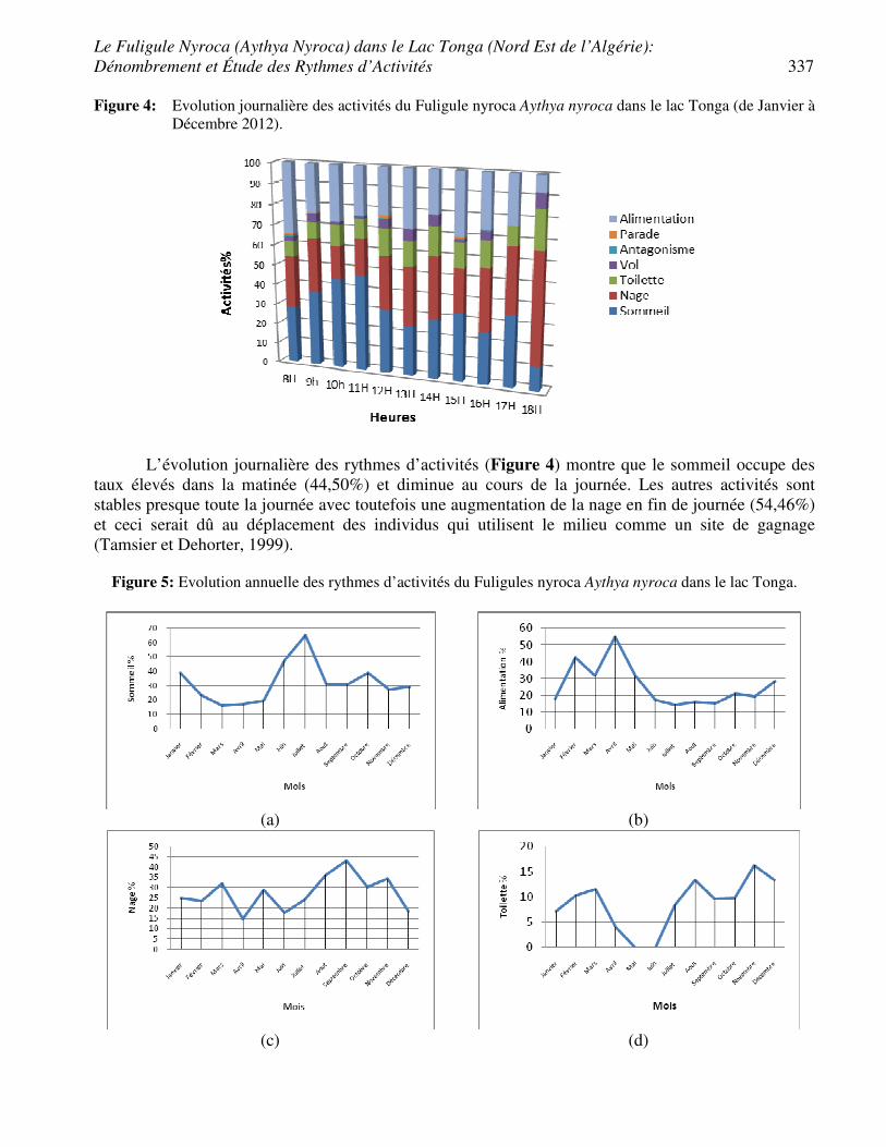
Le Fuligule Nyroca (Aythya Nyroca) dans le Lac Tonga (Nord Est de l’Algérie): Dénombrement et Étude des Rythmes d’Activités 337
Figure 4: Evolution journalière des activités du Fuligule nyroca Aythya nyroca dans le lac Tonga (de Janvier à Décembre 2012).
L’évolution journalière des rythmes d’activités (Figure 4) montre que le sommeil occupe des taux élevés dans la matinée (44,50%) et diminue au cours de la journée. Les autres activités sont stables presque toute la journée avec toutefois une augmentation de la nage en fin de journée (54,46%) et ceci serait dû au déplacement des individus qui utilisent le milieu comme un site de gagnage (Tamsier et Dehorter, 1999).
Figure 5: Evolution annuelle des rythmes d’activités du Fuligules nyroca Aythya nyroca dans le lac Tonga.
(a) (b)
(c) (d)
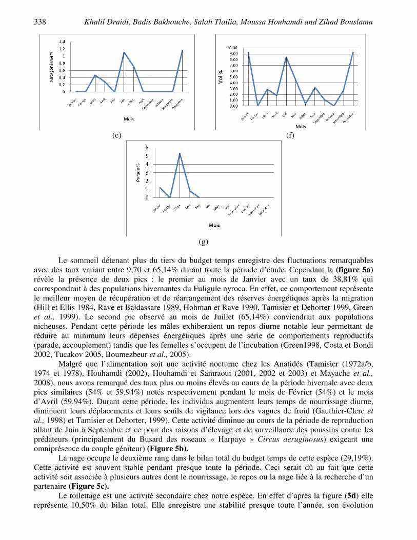
338 Khalil Draidi, Badis Bakhouche, Salah Tlailia, Moussa Houhamdi and Zihad Bouslama
(e) (f)
(g)
Le sommeil détenant plus du tiers du budget temps enregistre des fluctuations remarquables
avec des taux variant entre 9,70 et 65,14% durant toute la période d’étude. Cependant la (figure 5a) révèle la présence de deux pics : le premier au mois de Janvier avec un taux de 38,81% qui correspondrait à des populations hivernantes du Fuligule nyroca. En effet, ce comportement représente le meilleur moyen de récupération et de réarrangement des réserves énergétiques après la migration (Hill et Ellis 1984, Rave et Baldassare 1989, Hohman et Rave 1990, Tamisier et Dehorter 1999, Green et al., 1999). Le second pic observé au mois de Juillet (65,14%) conviendrait aux populations nicheuses. Pendant cette période les mâles exhiberaient un repos diurne notable leur permettant de réduire au minimum leurs dépenses énergétiques après une série de comportements reproductifs (parade, accouplement) tandis que les femelles s’occupent de l’incubation (Green1998, Costa et Bondi 2002, Tucakov 2005, Boumezbeur et al., 2005).
Malgré que l’alimentation soit une activité nocturne chez les Anatidés (Tamisier (1972a/b, 1974 et 1978), Houhamdi (2002), Houhamdi et Samraoui (2001, 2002 et 2003) et Mayache et al., 2008), nous avons remarqué des taux plus ou moins élevés au cours de la période hivernale avec deux pics similaires (54% et 59,94%) notés respectivement pendant le mois de Février (54%) et le mois d’Avril (59.94%). Durant cette période, les individus augmentent leurs temps de nourrissage diurne, diminuent leurs déplacements et leurs seuils de vigilance lors des vagues de froid (Gauthier-Clerc et al., 1998) et Tamisier et Dehorter, 1999). Cette activité diminue au cours de la période de reproduction allant de Juin à Septembre et ce pour des raisons d’élevage et de surveillance des poussins contre les prédateurs (principalement du Busard des roseaux « Harpaye » Circus aeruginosus) exigeant une omniprésence du couple géniteur) (Figure 5b).
La nage occupe le deuxième rang dans le bilan total du budget temps de cette espèce (29,19%). Cette activité est souvent stable pendant presque toute la période. Ceci serait dû au fait que cette activité soit associée à plusieurs autres dont le nourrissage, le repos ou la nage liée à la recherche d’un partenaire (Figure 5c).
Le toilettage est une activité secondaire chez notre espèce. En effet d’après la figure (5d) elle représente 10,50% du bilan total. Elle enregistre une stabilité presque toute l’année, son évolution
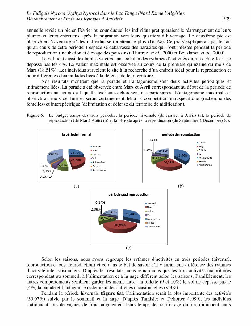
Le Fuligule Nyroca (Aythya Nyroca) dans le Lac Tonga (Nord Est de l’Algérie): Dénombrement et Étude des Rythmes d’Activités 339
annuelle révèle un pic en Février ou cour duquel les individus pratiqueraient le réarrangement de leurs plumes et leurs entretiens après la migration vers leurs quartiers d’hivernage. Le deuxième pic est observé en Novembre où les individus se toilettent le plus (16,3%). Ce pic s’expliquerait par le fait qu’au cours de cette période, l’espèce se débarrasse des parasites qui l’ont infestée pendant la période de reproduction (incubation et élevage des poussins) (Hurtrez, et al., 2000 et Bouslama, et al., 2000).
Le vol tient aussi des faibles valeurs dans ce bilan des rythmes d’activités diurnes. En effet il ne dépasse pas les 4%. La valeur maximale est observée au cours de la première quinzaine du mois de Mars (18,51%). Les individus survolent le site à la recherche d’un endroit idéal pour la reproduction et pour différentes chamaillades liées à la défense de leur territoire.
Nos résultats montrent que la parade et l’antagonisme sont deux activités périodiques et intimement liées. La parade a été observée entre Mars et Avril correspondant au début de la période de reproduction au cours de laquelle les jeunes cherchent des partenaires. L’antagonisme maximal est observé au mois de Juin et serait certainement lié à la compétition intraspécifique (recherche des femelles) et interspécifique (délimitation et défense du territoire de nidification). Figure 6: Le budget temps des trois périodes, la période hivernale (de Janvier à Avril) (a), la période de
reproduction (de Mai à Août) (b) et la période après la reproduction (de Septembre à Décembre) (c).
(a) (b)
(c)
Selon les saisons, nous avons regroupé les rythmes d’activités en trois periodes (hivernal,
reproduction et post reproduction) et ce dans le but de savoir s’il y aurait une différence des rythmes d’activité inter saisonniers. D’après les résultats, nous remarquons que les trois activités majoritaires correspondant au sommeil, à l’alimentation et à la nage diffèrent selon les saisons. Parallèlement, les autres comportements semblent garder les même taux : la toilette (9 et 10%) le vol ne dépasse pas le (4%) la parade et l’antagonise resteraient des activités occasionnelles (< 3%).
Pendant la période hivernale (figure 6a), l’alimentation serait la plus importante des activités (30,07%) suivie par le sommeil et la nage. D’après Tamisier et Dehorter (1999), les individus stationnant lors de vagues de froid augmentent leurs temps de nourrissage diurne, diminuent leurs

340 Khalil Draidi, Badis Bakhouche, Salah Tlailia, Moussa Houhamdi and Zihad Bouslama
déplacements et leurs seuils de vigilance (Gauthier-Clerc et al., 1998), tout en augmentant la durée de leurs activités de confort. D’autre part, le lac Tonga est connu pour être un excellent site d’hivernage des oiseaux aquatiques paléarctiques occidentaux. L’arrivée de l’avifaune hivernante qui exploite donc la même niche écologique, diminuerait les ressources alimentaires. Le Fuligule nyroca adopterait alors une stratégie alimentaire différente et ce en augmentant la durée du nourrissage.
En période de reproduction (Figure 6b) nous remarquons que le sommeil domine les trois activités (38,46%). Le taux élevé de cette activité serait expliqué par la récupération des réserves énergétiques des mâles après une série des comportements reproductifs (parade, incubation…). D’après Lebedeva (2001) ce sont les femelles qui se chargent de l’incubation des œufs. Après la reproduction (Figure 6c) la durée du sommeil diminue légèrement (31,48%) avec une augmentation de l’activité de nage (36,89%) due à l’élevage des poussins et la vigilance contre les prédateurs. 4. Conclusion Le Fuligule nyroca est ainsi présent pendant toute l’année dans le lac Tonga ce qui lui donnerait le statut d’espèce sédentaire. D’autre part, nous pourrions déduire l’existence de deux populations (une sédentaire et une autre estivante nicheuse) ce qui conforterait les travaux de Aissaoui et al., 2009). Le budget temps annuel de notre espèce subit une évolution fluctuante avec trois grands groupes répartis selon leur importance : activités principales (sommeil, alimentation et nage), secondaires (toilette et vol) et minimes (parade et antagonisme).
Le bilan saisonnier fait ressortir des variations au niveau des rythmes d’activités en rapport avec les conditions du milieu.
De part tous ces résultats concernant les rythmes d’activité (annuel, saisonnier et journalier), nous pourrions conclure au fait que d’une part le Fuligule nyroca serait peu actif pendant la journée et d’autre part qu’il utiliserait le lac Tonga comme un site de remise diurne. Références Bibliographiques [1] Altmann J. (1974). Observational study of behaviour: Sampling methods. Behaviour, 49:227-
267. [2] Aissaoui R. Houhamdi M., et Samraoui B. (2009). Eco-Éthologie des Fuligules Nyroca
Aythya Nyroca dans le Lac Tonga (Site Ramsar, Parc National d’El-Kala, Nord-Est de l’Algérie). European Journal of Scientific Research, N°1 47-59.
[3] AissaouiI R., Tahar A., Saheb M., Guergueb E., Houhamdi M. (2011). Diurnal behaviour of Ferruginous Duck Aythya nyroca wintering at the El-Kala wetlands (Northeast Algeria) Bulletin de l’Institut Scientifique, Rabat, section Sciences de la Vie, n°33 (2), p. 67-75.
[4] Baldassarre G.A., Paulus S.L., Tamisier A. and Titman D.R.D. (1988).Workshop summary techniques for timing activity of wintering waterfowl. Waterfowl in winter. Univ. Minnesota press. Minneapoli, 23p.
[5] Boumezebeur A. (1993). Ecologie et biologie de la reproduction de l’Erismature à tête Blanche Oxyura leucocephala et du Fuligule nyroca Aythya nyroca sur le Lac Tonga et le Lac des oiseaux, Est algérien. Thèse de doctorat, Université Montpellier, 254 p.
[6] Benyacoub S.et Chabi Y. (2000). Diagnose écologique de l'avifaune du Parc National d'El Kala. Synthèse, n°7.98p.
[7] Bouslama Z., Chabi Y., Lambrechts M. (2000). Chicks resist high parasite intensities in an Algerian population of blue tits. Ecoscience, 8 (3): 320 – 324.
[8] Boumezebeur A., Moali A. et Isenmann P. (2005). Nidification du Fuligule nyroca Aythya nyroca et de l’échasse blanche Himantopus himantopus en zone saharienne (El Goléa, Algérie). Alauda, 73 (2): 143-144.

Le Fuligule Nyroca (Aythya Nyroca) dans le Lac Tonga (Nord Est de l’Algérie): Dénombrement et Étude des Rythmes d’Activités 341
[9] Green A. J. (1998). Habitat selection by the Marbled Teal Marmaronetta angustirostris, Ferruginous Duck Aythya nyroca and other ducks in the Göksu Delta, Turkey, in summer.Revue Ecologie (Terre and Vie), 53: 225-243.
[10] Gauthier-Clerc M., Tamisier A. et Cézilly F. (1998). Sleep-vigilance trade-off in Green-winged Teal (Anas crecca crecca). Canadian Journal of Zoology, 76 (12): 2214-2218.
[11] Green A. J., Fox A. D., Hughes B. and Hilton G. M. (1999). Time-activity budgets and site selection of White-headed Ducks Oxyura leucocephala at Burdur Lake, Turkey in late winter. Bird Study, 46: 62-73.
[12] Belhadj G, Chalabi B, Chabi Y, Kayser Y, Gauthier-Clerc M. (2007). Le retour de l.Ibis falcinelle (Plegadis falcinellus) nicheur en Algérie Ibis, 44 1.qxp 14:26 Page 29.
[13] Hill D. A. and Ellis N. (1984). Survival and age related changes in the foraging behavior and time budget of Tufted Ducklings Aythya fuligula. Ibis, 126: 544-550.
[14] Hohman W. L. and Rave, D. P. (1990). Diurnal time activity budgets of wintering. Canvas backs in Louisiana. Wilson Bulletin, 102: 645-654.
[15] Hurtrez-Boussès S., Renaud F., Blondel J., Perret P. et Galan M. J. (2000). Effects of ectoparasites of young on parents’ behaviour in a Mediterranean population of blue tits. J. Avian Biol, 31: 266-269.
[16] Houhamdi M. and Samraoui B. (2001). Diurnal time budget of wintering Teal Anas crecca at Lac des Oiseaux, northeast Algeria. Wildfowl, 52: 87-96.
[17] Houhamdi M. (2002). Ecologie des peuplements aviens du Lac des Oiseaux (Numidie orientale). Thèse de Doctorat d’état. Université Badji Mokhtar, Annaba. 183p.
[18] Houhamdi M. et Samraoui B. (2002). Occupation spatio-temporelle par l’avifaune aquatique du Lac des oiseaux (Algérie). Alauda, 70: 301-310.
[19] Houhamdi M. and Samraoui B. (2003). Diurnal behaviour of wintering Wigeon Anas penelopeat Lac des Oiseaux, northeast Algeria. Wildfowl, 54: 51-62.
[20] Houhamdi M. and Samraoui B. (2008). Diurnal and nocturnal behaviour of ferruginous duck Aythya nyroca at Lac des Oiseaux, northeast Algeria. Ardeola, 55: 59-69.
[21] IUCN (2006). Red list of Threatened Species, Downloaded from www.redlist.org [22] Jonsson L. 1994. Les oiseaux d’Europe, d’Afrique du Nord et du Moyen-Orient. Nathan.558p [23] Ledant J-P., Jacobs J-P., Malher F., Ochando B. et Roché J. (1982). Mise à jour de
l’avifaune algérienne. Le Gerfaut, 71: 295-398. [24] Losito M.P., Mirarchi E. and Baldassarre G.A. (1989). New techniques for time activity
studies of avian flocks in view-retricted habitats. J. Field. Ornithol, 60: 388-396. [25] Lebedeva NV. and Markitan LV. (2001). Problems of population dynamics of the white-eyed
pochard (Aythya nyroca) in the eastern Sea of Azov region", Russ j Ecol, 32 (6). [26] Lazli A. (2011). Contribution à la connaissance de l’ecologie et de la biologie de la
reprduction de l’érismature à tête blanche oxyura leucocephala et le Fuligule nyroca Aythya nyroca au niveau du lac Tonga. Thèse doctorat. Université Abderahmane Mira de Béjaia, Algérie.136 p.
[27] Lazli A., Boumezbeur A., Moali-Grine N. et Moali A. (2011). Evolution de la population nicheuse de l’érismature à tête blanche oxyura leucocephala sur le lac Tonga (Algérie) Rev. Écol. (Terre Vie), vol. 66.
[28] Mayache B., Houhamdi M. et Samraoui B. (2008). Ecologie des Sarcelles d’hiver Anas crecca crecca L. hivernants dans l’éco-complexe de zones humides de Jijel (Nord-Est de l'Algérie). EJSR, 21 (1): 104-119.
[29] Petkov N., Hughes B. et Gallo-Orsi U. (2003). Ferruginous Duck : from research to conservation. Conservation Series N°6. Bird Life International / BSPB / TWSG,144 p.
[30] Rave D.P. and Baldassarre G.A. (1989). Activity budget of Green-Winged Teal wintering incostal wetlands of Louisiana. J.Wild. Manage, 53: 753-759.

342 Khalil Draidi, Badis Bakhouche, Salah Tlailia, Moussa Houhamdi and Zihad Bouslama
[31] Samraoui. et De Belair G. (1998). Les zones humides de la Numidie orientale: bilan des Connaissances et perspectives de gestion. Synthèse, (Numéro spécial 4): 1-90.
[32] Bin Muzaffar S. (2004). Diurnal time-activity budgets in wintering Ferruginous Pochard Aythya nyroca in Tanguar Haor, Bangladesh. Forktail, 20: 25–27.
[33] Tamisier A. (1972a). Rythmes nycthéméraux des Sarcelles d’hiver pendant leur hivernage en Camargue. Alauda, 2: 107-135.
[34] Tamisier A. (1972b). Rythmes nycthéméraux des Sarcelles d’hiver pendant leur hivernage en Camargue. Alauda, 2: 235-256.
[35] Tamisier A. (1974). Etho-écological studies of Teal wintering in the Camargue (Rhône delta, France). Wildfowl, 25: 122-133.
[36] Tamisier A. (1978). The functional units of wintering ducks: A spatial integration of theircomfort and feeding requirements. Verh. Orn. Ges. Bayern, 23: 229-238.
[37] Tamisier A. et Dehorter O. (1999). Camargue: Canard et Foulques. Fonctionnement d’un prestigieux quartier d’hiver. Centre Ornithologique du Gard. Nimes, 369 p.59.
[38] Tucakov M. (2005). Migration of common pochard Aythya ferina and ferruginous duck Aythya nyroca on Kolut Fishpond (Northern Serbia). Aquila, 112: 15-22.


