Is the inflation rate normally distributed? An empirical investigation

Birkbeck College, University of London

Department of Economics, Mathematics and

Statistics

André Bueno Rezende de Castro

Is the inflation rate normally distributed? An empirical investigation

Abstract: The purpose of this project is to determine whether the inflation rate of a specific set

of countries and regions can be described by a normal distribution and how their descriptive

statistics – such as mean, standard deviation, kurtosis, skewness – behave. A secondary

purpose of this project is to determine whether the consumer prices index (CPI) and the gross

domestic product (GDP) deflator differ in this regard. Finally this project will test both the CPI

and the GDP deflator for autocorrelation of order 1, using E-Views.

Word count: 3.004

London, UK – April, 2013

0.00

5.00

10.00

15.00

20.00

25.00

30.00

1 5 9 13172125293337414549

Latin America &

Caribbean CPI

Latin America &

Caribbean GDP

Deflator

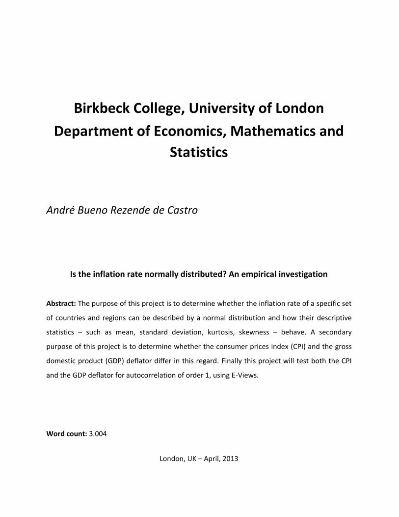
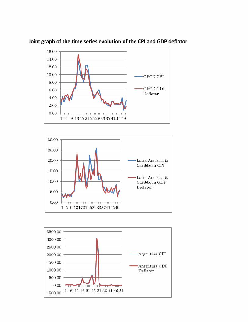
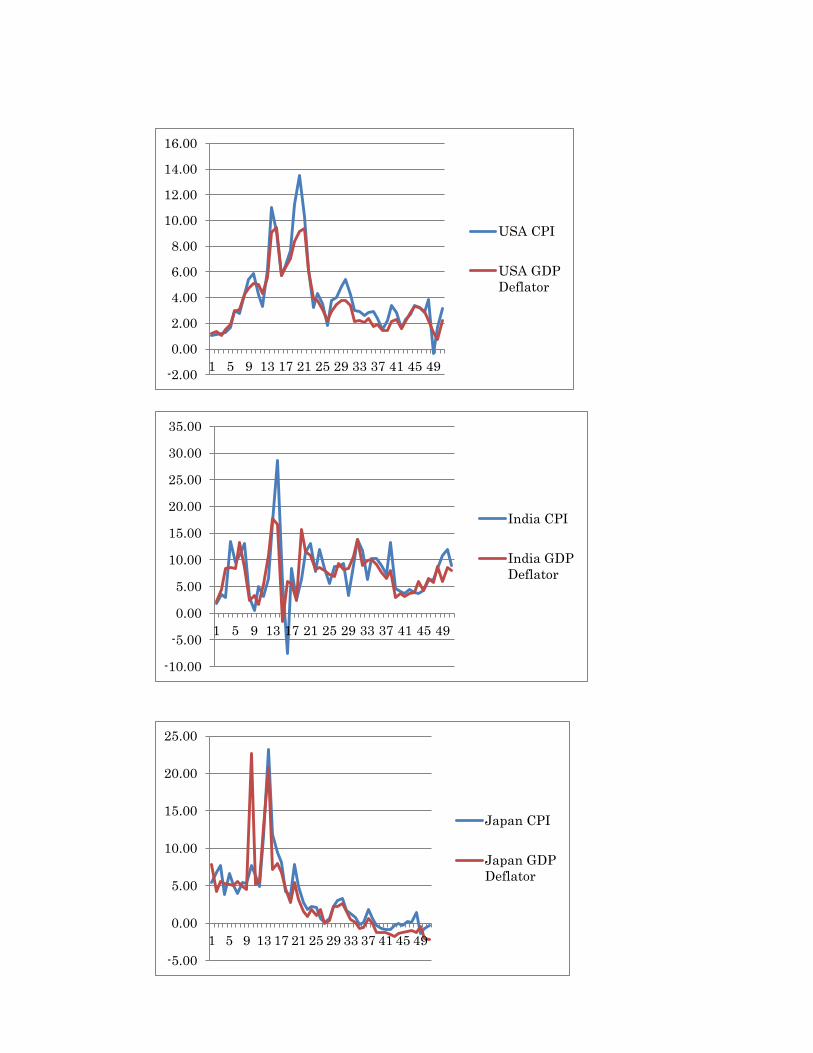
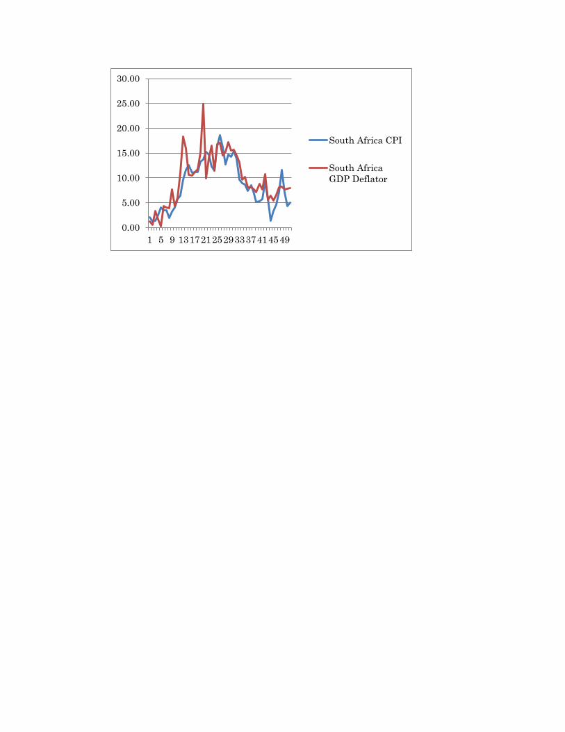
Joint graph of the time series evolution of the CPI and GDP deflator

0.00

2.00

4.00

6.00

8.00

10.00

12.00

14.00

16.00

1 5 9 13 17 21 25 29 33 37 41 45 49

OECD CPI

OECD GDP

Deflator

-500.00

0.00

500.00

1000.00

1500.00

2000.00

2500.00

3000.00

3500.00

1 6 11 16 21 26 31 36 41 46 51

Argentina CPI

Argentina GDP

Deflator

-10.00

-5.00

0.00

5.00

10.00

15.00

20.00

25.00

30.00

35.00

1 5 9 13 17 21 25 29 33 37 41 45 49

India CPI

India GDP

Deflator

-5.00

0.00

5.00

10.00

15.00

20.00

25.00

1 5 9 13 17 21 25 29 33 37 41 45 49

Japan CPI

Japan GDP

Deflator

-2.00

0.00

2.00

4.00

6.00

8.00

10.00

12.00

14.00

16.00

1 5 9 13 17 21 25 29 33 37 41 45 49

USA CPI

USA GDP

Deflator

0.00

5.00

10.00

15.00

20.00

25.00

30.00

1 5 9 13172125293337414549

South Africa CPI

South Africa

GDP Deflator

Behaviour of the descriptive statistics of the inflation rate indexes

Firstly and foremost, it is important to clarify that both the Consumers Price Index (CPI) and the

Gross Domestic Product (GDP) deflator have been computed in EViews in level, not in log,

simply because many of the countries and set of countries analysed had deflation during the

period. Since it is not possible to take logs of negative numbers, we treated the variables in

level.

The CPI is a weighted average of the price level of the main goods consumed in the economy

and the inflation rate reads as follows:

𝜋𝑡 = 100.(𝑃𝑡 − 𝑃𝑡−1)

𝑃𝑡−1

The GDP deflator is the implicit price deflator of the GDP, being a measure of prices of all final

and domestically produced goods and services in the economy. It doesn’t represent what a

typical family consumes, because it evaluates all the goods in the economy, contrary to the CPI.

The GDP deflator is as follows:

𝑃𝑡 = 100.𝑁𝑜𝑚𝑖𝑛𝑎𝑙 𝐺𝐷𝑃

𝑅𝑒𝑎𝑙 𝐺𝐷𝑃= 100.

∑ 𝑃𝑖𝑡 . 𝑄𝑖𝑡𝑁𝑖=1

∑ 𝑃𝑖0. 𝑄𝑖𝑡𝑁𝑖=1

Below follows an interpretation of the descriptive statistics estimated for the two indexes of

the inflation rate considered in this project: the CPI and the GDP deflator.

1. Mean (Average): obtained by adding all the observations of each country or series of

countries and dividing by the number of observations as in 𝜇 = ∑ 𝑋𝑖𝑖=𝑁

𝑖=1

𝑁. Since we are measuring

the mean from a sample, not from the population, the more appropriate formula is as follows:

�̅� = ∑ 𝑋

𝑁−1; (BARROW, 2009, p. 25)

2. Standard Deviation: the bigger the standard deviation is, the bigger the volatility of

inflation will be, bringing about unpredictability to the policy makers and to the consumers –

inflation expectations tend to be wrong. In arithmetical terms, the standard deviation, which is

a measure of dispersion, is the squared root of the variance. The purpose of taking the square

root of the variance is to yield a number in a definite measure, not in its squared form. The

formula is as follows: σ = √∑(𝑥− 𝜇)²

𝑁. Since we are measuring the standard deviation from a

sample, not from the population, the more appropriate formula is as follows: 𝑠 = √∑(𝑥−�̅�)²

𝑛−1;

(BARROW, 2009, p. 36)

3. Skewness: a certain distribution is generally skewed either to the left (negatively

skewed) or to the right (positively skewed), meaning that it has a long tail to the left(right)-hand

side of the distribution. The skewness measures the asymmetry of a distribution, whose

coefficient are a cubed deviation from the mean. A negatively skewed distribution would have a

negative coefficient for a left-skewed one and vice versa, yielding a zero coefficient for a

symmetric distribution, considering that it is normal. The formula of the coefficient is as

follows: 𝑆 = ∑ (𝑥𝑖−�̅�)³𝑛

𝑖=1

𝑁.σ³. (BARROW, 2009, p. 42) The importance of the skewness for the

inflation rate lies on the irregularity of rates lying too far away from the zero symmetric

standard, which could be interpreted as if the inflation has an irregular process, with many

variations. A positively or negatively skewed inflation rate indicates the following

3.1. A volatile business cycle which has so many fluctuations in the product affecting the

inflation through its impact on unemployment (the Okun’s Law inserted in a Phillips Curve). The

Phillips Curve being: πt = πte + �̅�. 𝑌�̃� + �̅�, with πt

e = πt-1 with adaptative expectations. The term

�̅�. 𝑌�̃� is the current state of the economy (aggregate demand), and �̅� being prices shocks to

inflation, affecting hence the aggregate supply. Then, to complete the model, the Okun’s Law

is: 𝑢 − �̅� = −1/2. 𝑌�̃�, in which the first two terms denote the unemployment gap, i.e., the

difference between current unemployment and the natural rate of unemployment, and the

second term being the effect of the unemployment gap to the GDP. A volatile business cycle

would have a sufficient number of price shocks and aggregate demand shocks impacting the

inflation rate, yielding an asymmetric distribution and a bigger standard deviation. It is

important to state that this volatility in the business cycle might be due to successive

government interventions or by disrupting market forces, which is not the object of analysis in

this project.

4. Kurtosis: as well as the skewness, the kurtosis measures the shape of a probability

distribution with the following formula: 𝐾 = ∑ (𝑥𝑖− �̅�)4𝑛

𝑖=1

𝑁.σ4, with the upper term being the fourth

moment of the mean. (DECARLO, 1997, p. 292) This coefficient can be standardised for a

normal distribution: by subtracting three from it, we obtain the excess kurtosis. It there is

excess kurtosis for either side, then the coefficient will deviate from nullity: a low kurtosis

distribution has shorter and thinner tails and a rounded peak whereas a high kurtosis

distribution has the opposite. For a symmetric distribution (as said, with zero skewness),

kurtosis evaluates how heavy the tails of the distribution are as well as how high the level of its

peaks can be. The implications of the kurtosis for the inflation rate are quite similar to those of

the skewness.

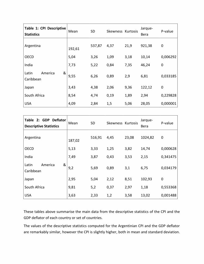
Table 1: CPI Descriptive

Statistics Mean SD Skewness Kurtosis

Jarque-

Bera P-value

Argentina

192,61 537,87 4,37 21,9 921,38 0

OECD 5,04 3,26 1,09 3,18 10,14 0,006292

India 7,73 5,22 0,84 7,35 46,24 0

Latin America &

Caribbean 9,55 6,26 0,89 2,9 6,81 0,033185

Japan 3,43 4,38 2,06 9,36 122,12 0

South Africa 8,54 4,74 0,19 1,89 2,94 0,229828

USA 4,09 2,84 1,5 5,06 28,05 0,000001

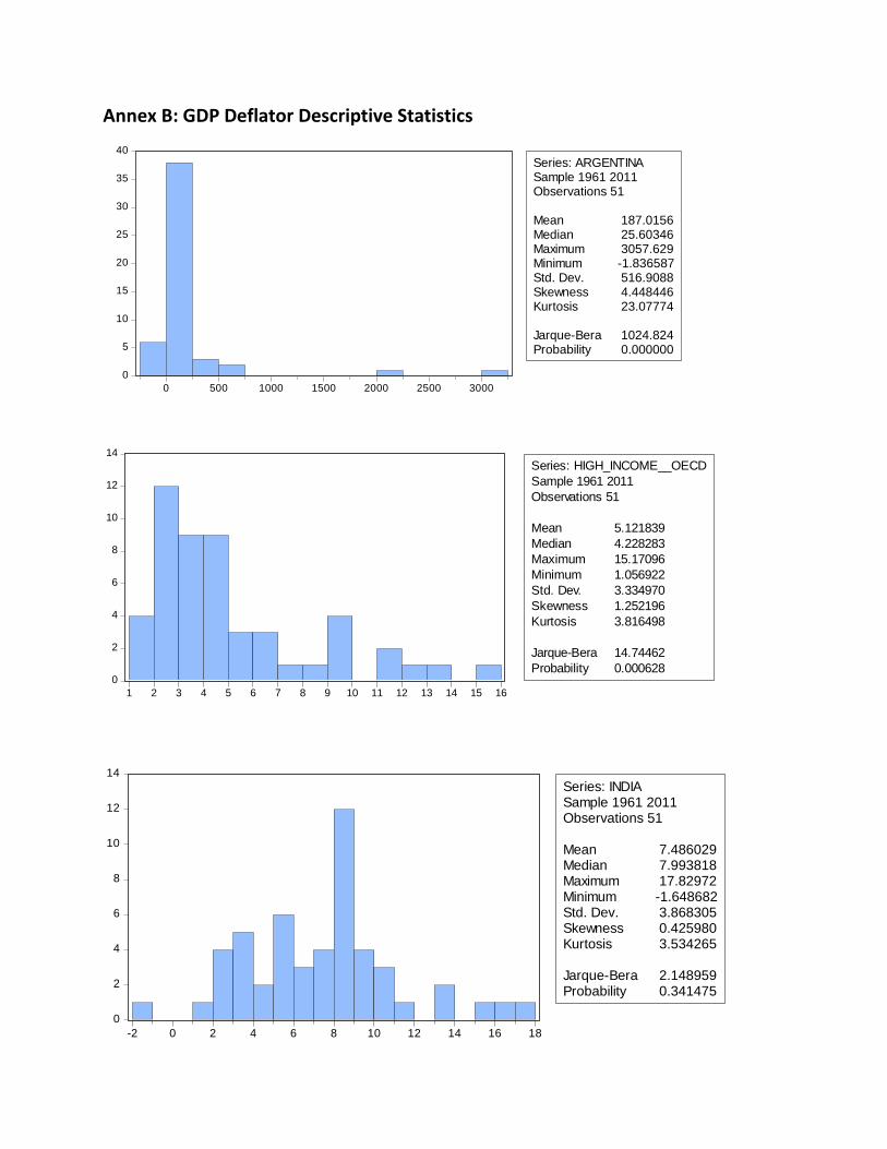
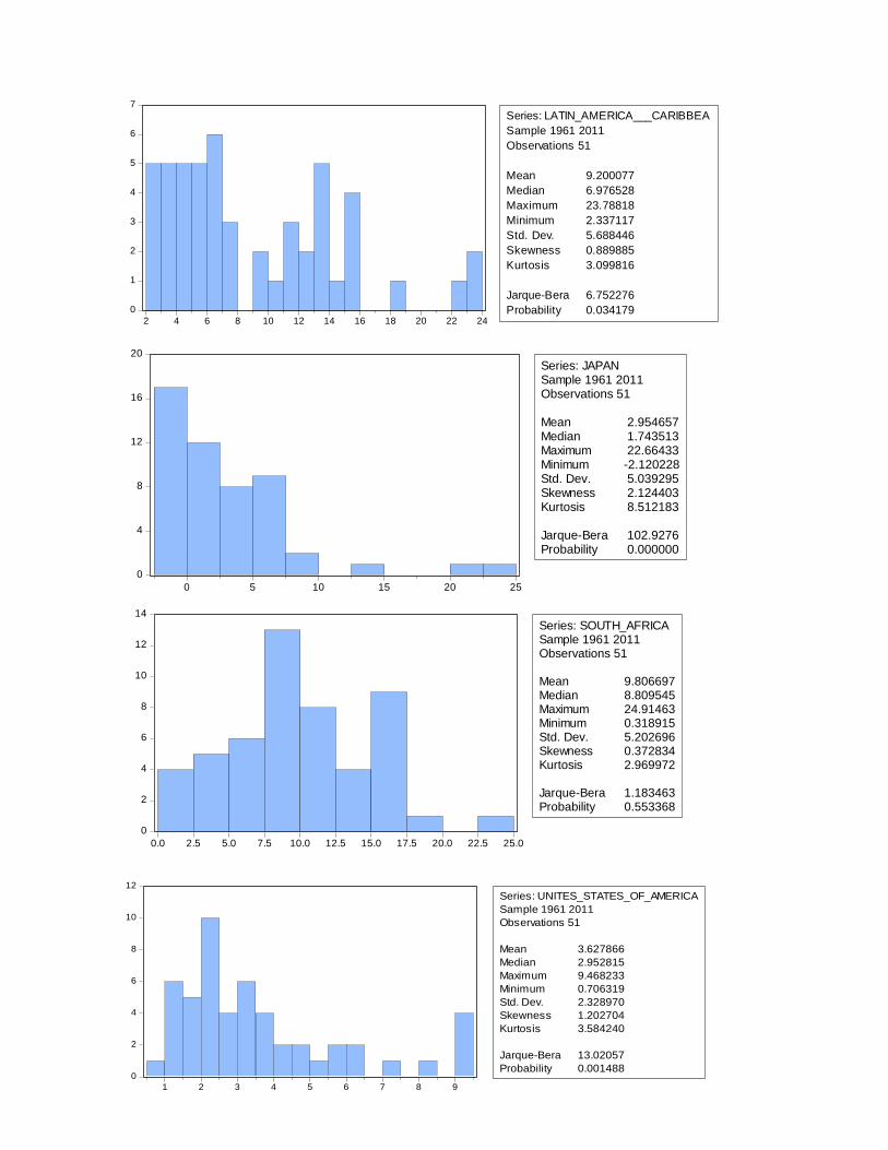
Table 2: GDP Deflator

Descriptive Statistics Mean SD Skewness Kurtosis

Jarque-

Bera P-value

Argentina

187,02 516,91 4,45 23,08 1024,82 0

OECD 5,13 3,33 1,25 3,82 14,74 0,000628

India 7,49 3,87 0,43 3,53 2,15 0,341475

Latin America &

Caribbean 9,2 5,69 0,89 3,1 6,75 0,034179

Japan 2,95 5,04 2,12 8,51 102,93 0

South Africa 9,81 5,2 0,37 2,97 1,18 0,553368

USA 3,63 2,33 1,2 3,58 13,02 0,001488

These tables above summarise the main data from the descriptive statistics of the CPI and the

GDP deflator of each country or set of countries.

The values of the descriptive statistics computed for the Argentinian CPI and the GDP deflator

are remarkably similar, however the CPI is slightly higher, both in mean and standard deviation.

For both, we reject H0, at the 5% significance level, that their distributions are normal.

The values of the descriptive statistics computed for the OECD CPI and the GDP deflator are

remarkably similar, however the CPI is slightly smaller, both in terms of mean and standard

deviation. Again, for both, we reject, at the 5% significance level, that their distributions are

normal.

The values of the descriptive statistics computed for the Indian CPI and the GDP deflator are

similar, however the CPI is slightly higher, both in mean and standard deviation. It is important

to notice that the difference of the standard deviations is more pronounced in the Indian case,

indicating a higher volatility of the inflation rate. We reject H0, at the 5% significance level, that

the CPI distribution is normal, however, we do not reject normality in the case of the GDP

deflator. It clearly bodes well for the GDP deflator as a more efficient inflation measure,

considering this discrepancy.

The values of the descriptive statistics computed for Latin America and Caribbean’s CPI and

GDP deflator are quite similar, however the CPI is slightly higher, both in mean and standard

deviation – again with a bigger difference in the latter statistic. For both, we reject H0, at the 5%

significance level, that their distributions are normal.

The values of the descriptive statistics computed for Japan’s CPI and GDP deflator are similar,

however the CPI has a slightly higher mean and has a smaller standard deviation. Again, for

both, we reject H0, at the 5% significance level, that their distributions are normal.

The values of the descriptive statistics computed for South Africa’s CPI and GDP deflator are

quite similar, however the CPI is slightly smaller, both in terms of mean and standard deviation.

For both, we do not reject H0, at the 5% significance level, that their distributions are normal.

The values of the descriptive statistics computed for the USA’s CPI and GDP deflator are very

much similar, however the CPI is slightly higher, both in mean and in standard deviation. For

both, we reject H0, at the 5% significance level, that their distributions are normal.

Normality Test of the Inflation Rate Indexes

The purpose of this project is to determine if the inflation rate (CPI and GDP deflator) can be

determined by a normal distribution. The question whether this is valid or not is important for

monetary policy, in the sense that the more “well behaved” the inflation is, the easier it is to

implement an inflation targeting macroeconomic programme and, as well, the less toll the

inflation tends to exact from the consumers, both in terms of inflation tax – defined by π.M/P,

or the inflation rate (the “tax rate”) times the monetary base (the “tax base”) –, and of

diminishing purchasing power.

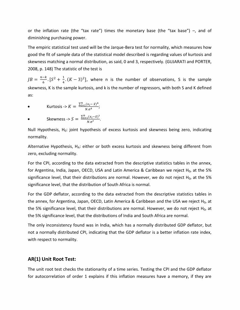
The empiric statistical test used will be the Jarque-Bera test for normality, which measures how

good the fit of sample data of the statistical model described is regarding values of kurtosis and

skewness matching a normal distribution, as said, 0 and 3, respectively. (GUJARATI and PORTER,

2008, p. 148) The statistic of the test is

𝐽𝐵 = 𝑛−𝑘

6. [𝑆2 +

1

4. (𝐾 − 3)2], where n is the number of observations, S is the sample

skewness, K is the sample kurtosis, and k is the number of regressors, with both S and K defined

as:

Kurtosis -> 𝐾 = ∑ (𝑥𝑖− �̅�)4𝑛

𝑖=1

𝑁.σ4 ;

Skewness -> 𝑆 = ∑ (𝑥𝑖−�̅�)³𝑛

𝑖=1

𝑁.σ³.

Null Hypothesis, H0: joint hypothesis of excess kurtosis and skewness being zero, indicating

normality.

Alternative Hypothesis, HA: either or both excess kurtosis and skewness being different from

zero, excluding normality.

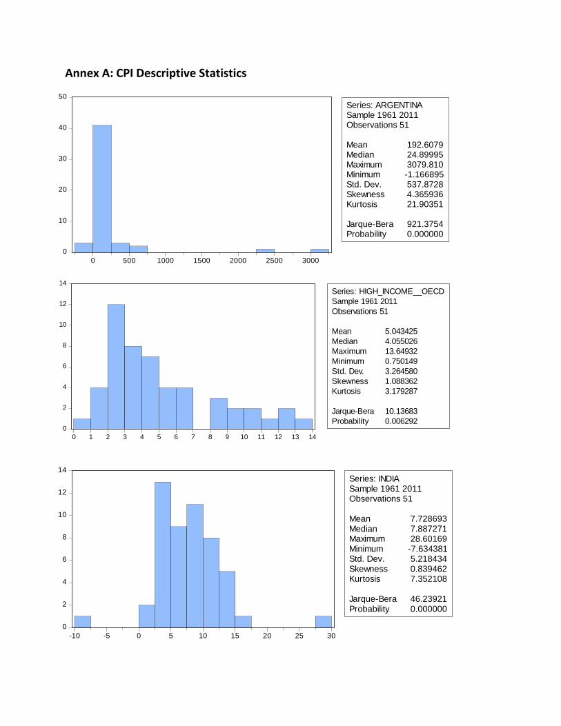
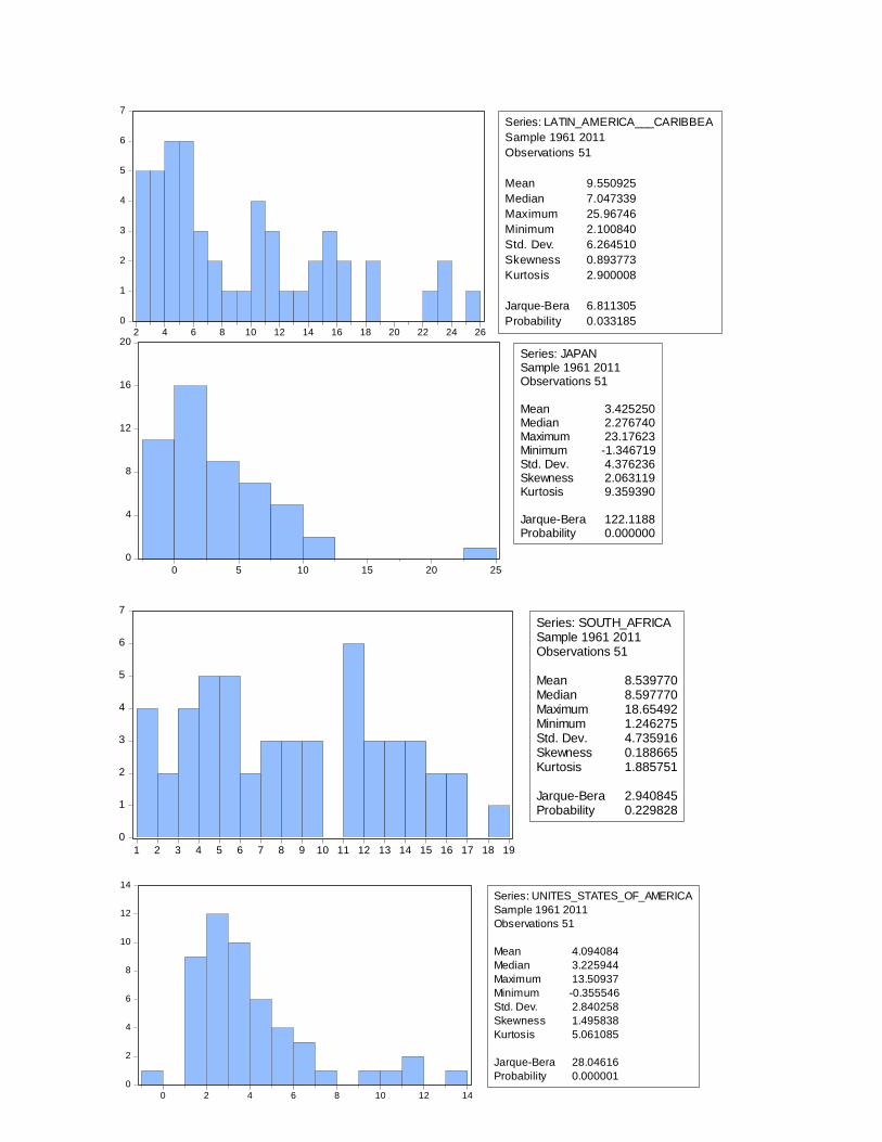
For the CPI, according to the data extracted from the descriptive statistics tables in the annex,

for Argentina, India, Japan, OECD, USA and Latin America & Caribbean we reject H0, at the 5%

significance level, that their distributions are normal. However, we do not reject H0, at the 5%

significance level, that the distribution of South Africa is normal.

For the GDP deflator, according to the data extracted from the descriptive statistics tables in

the annex, for Argentina, Japan, OECD, Latin America & Caribbean and the USA we reject H0, at

the 5% significance level, that their distributions are normal. However, we do not reject H0, at

the 5% significance level, that the distributions of India and South Africa are normal.

The only inconsistency found was in India, which has a normally distributed GDP deflator, but

not a normally distributed CPI, indicating that the GDP deflator is a better inflation rate index,

with respect to normality.

AR(1) Unit Root Test:

The unit root test checks the stationarity of a time series. Testing the CPI and the GDP deflator

for autocorrelation of order 1 explains if this inflation measures have a memory, if they are

correlated with themselves, i.e., past variables are carried on to future variables and explain

them in a certain amount – in this case, it is expected that it would explain less than 100%,

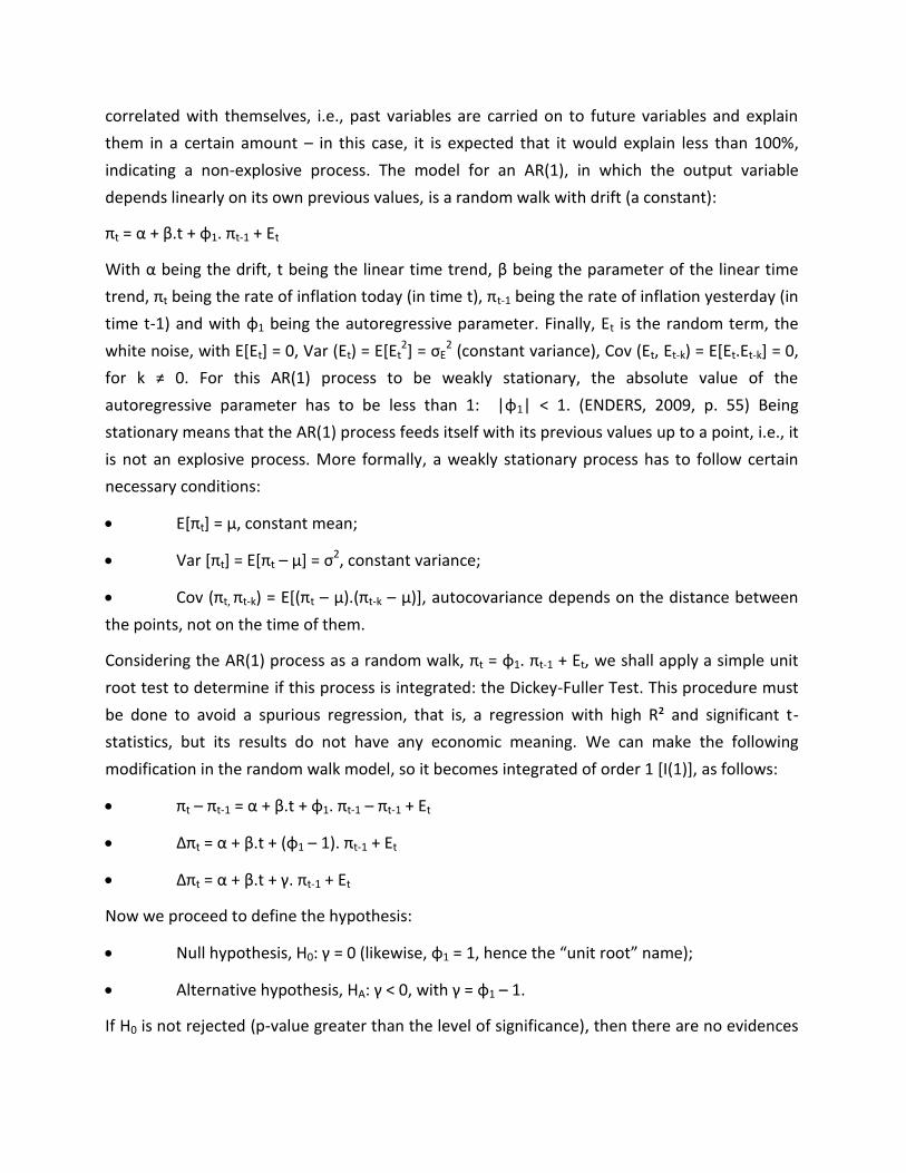
indicating a non-explosive process. The model for an AR(1), in which the output variable

depends linearly on its own previous values, is a random walk with drift (a constant):

πt = α + β.t + φ1. πt-1 + Et

With α being the drift, t being the linear time trend, β being the parameter of the linear time

trend, πt being the rate of inflation today (in time t), πt-1 being the rate of inflation yesterday (in

time t-1) and with φ1 being the autoregressive parameter. Finally, Et is the random term, the

white noise, with E[Et] = 0, Var (Et) = E[Et2] = σE

2 (constant variance), Cov (Et, Et-k) = E[Et.Et-k] = 0,

for k ≠ 0. For this AR(1) process to be weakly stationary, the absolute value of the

autoregressive parameter has to be less than 1: |φ1| < 1. (ENDERS, 2009, p. 55) Being

stationary means that the AR(1) process feeds itself with its previous values up to a point, i.e., it

is not an explosive process. More formally, a weakly stationary process has to follow certain

necessary conditions:

E[πt] = μ, constant mean;

Var [πt] = E[πt – μ] = σ2, constant variance;

Cov (πt, πt-k) = E[(πt – μ).(πt-k – μ)], autocovariance depends on the distance between

the points, not on the time of them.

Considering the AR(1) process as a random walk, πt = φ1. πt-1 + Et, we shall apply a simple unit

root test to determine if this process is integrated: the Dickey-Fuller Test. This procedure must

be done to avoid a spurious regression, that is, a regression with high R² and significant t-

statistics, but its results do not have any economic meaning. We can make the following

modification in the random walk model, so it becomes integrated of order 1 [I(1)], as follows:

πt – πt-1 = α + β.t + φ1. πt-1 – πt-1 + Et

Δπt = α + β.t + (φ1 – 1). πt-1 + Et

Δπt = α + β.t + γ. πt-1 + Et

Now we proceed to define the hypothesis:

Null hypothesis, H0: γ = 0 (likewise, φ1 = 1, hence the “unit root” name);

Alternative hypothesis, HA: γ < 0, with γ = φ1 – 1.

If H0 is not rejected (p-value greater than the level of significance), then there are no evidences

pointing to the fact that there is no unit root, therefore it is an integrated process. The critical

value does not have a t-Student distribution, under the null hypothesis, hence Dickey-Fuller and

MacKinnon derived asymptotic results whilst testing a group of critical values for different

sample sizes, resulting in the following modified critical value:

�̂� = γ̂

𝑠𝑒(𝛾)̂

where γ̂ is the estimate of γ, and se(γ)̂ is the coefficient standard error. (ENDERS, 2009, p. 206)

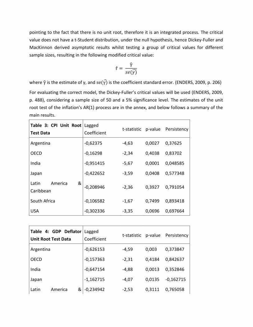
For evaluating the correct model, the Dickey-Fuller’s critical values will be used (ENDERS, 2009,

p. 488), considering a sample size of 50 and a 5% significance level. The estimates of the unit

root test of the inflation’s AR(1) process are in the annex, and below follows a summary of the

main results.

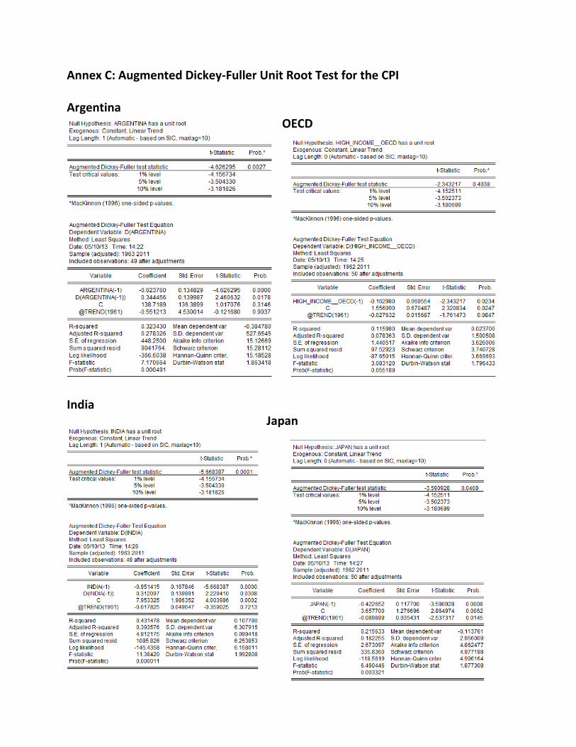
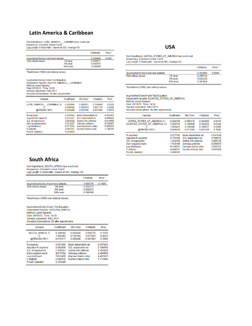
Table 3: CPI Unit Root

Test Data

Lagged

Coefficient t-statistic p-value Persistency

Argentina -0,62375 -4,63 0,0027 0,37625

OECD -0,16298 -2,34 0,4038 0,83702

India -0,951415 -5,67 0,0001 0,048585

Japan -0,422652 -3,59 0,0408 0,577348

Latin America &

Caribbean -0,208946 -2,36 0,3927 0,791054

South Africa -0,106582 -1,67 0,7499 0,893418

USA -0,302336 -3,35 0,0696 0,697664

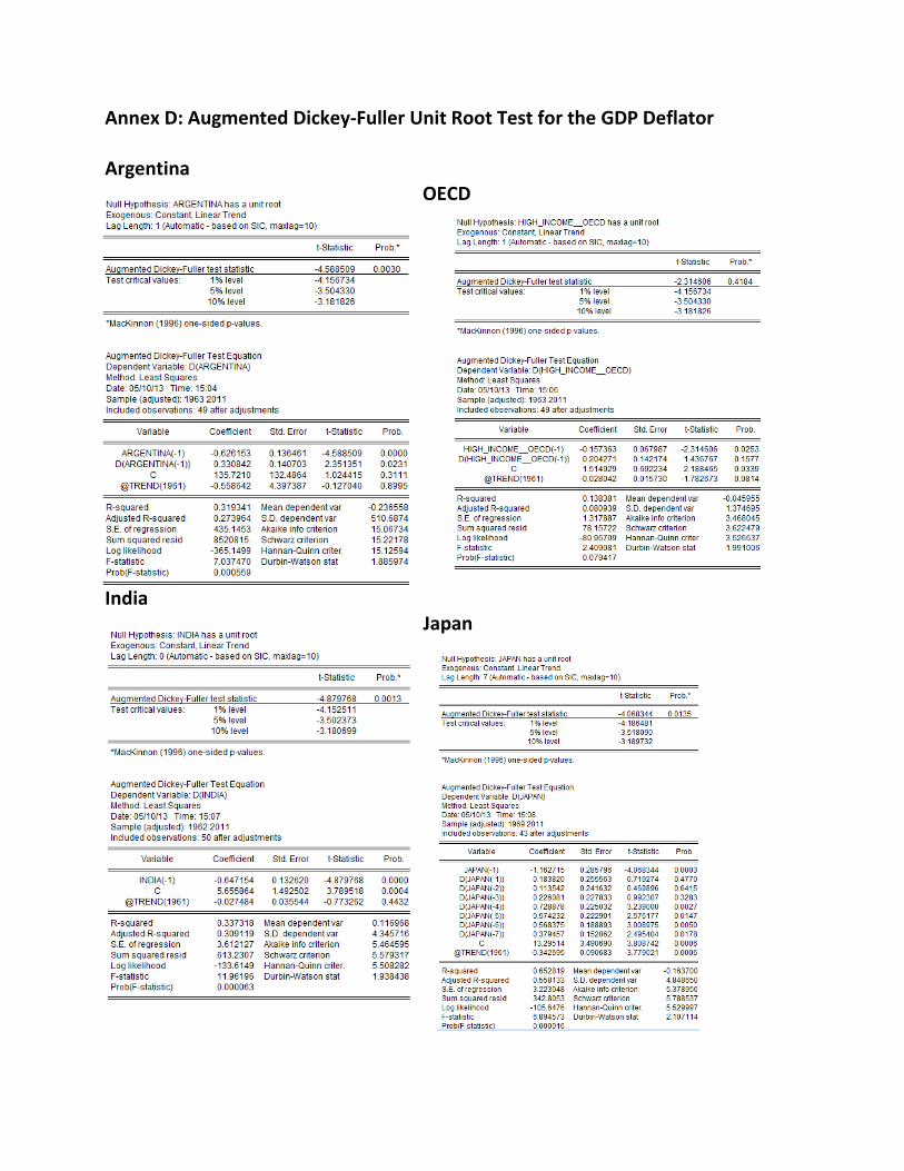
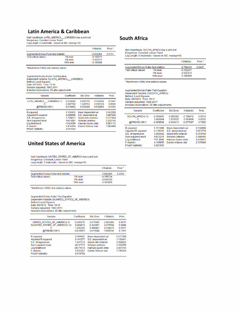
Table 4: GDP Deflator

Unit Root Test Data

Lagged

Coefficient t-statistic p-value Persistency

Argentina -0,626153 -4,59 0,003 0,373847

OECD -0,157363 -2,31 0,4184 0,842637

India -0,647154 -4,88 0,0013 0,352846

Japan -1,162715 -4,07 0,0135 -0,162715

Latin America & -0,234942 -2,53 0,3111 0,765058

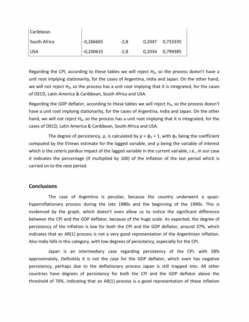
Caribbean

South Africa -0,266665 -2,8 0,2047 0,733335

USA -0,200615 -2,8 0,2034 0,799385

Regarding the CPI, according to these tables we will reject H0, so the process doesn’t have a

unit root implying stationarity, for the cases of Argentina, India and Japan. On the other hand,

we will not reject H0, so the process has a unit root implying that it is integrated, for the cases

of OECD, Latin America & Caribbean, South Africa and USA.

Regarding the GDP deflator, according to these tables we will reject H0, so the process doesn’t

have a unit root implying stationarity, for the cases of Argentina, India and Japan. On the other

hand, we will not reject H0, so the process has a unit root implying that it is integrated, for the

cases of OECD, Latin America & Caribbean, South Africa and USA.

The degree of persistency, ρ, is calculated by ρ = φ1 + 1, with φ1 being the coefficient

computed by the EViews estimate for the lagged variable, and ρ being the variable of interest

which is the ceteris paribus impact of the lagged variable in the current variable, i.e., in our case

it indicates the percentage (if multiplied by 100) of the inflation of the last period which is

carried on to the next period.

Conclusions

The case of Argentina is peculiar, because the country underwent a quasi-

hyperinflationary process during the late 1980s and the beginning of the 1990s. This is

evidenced by the graph, which doesn’t even allow us to notice the significant difference

between the CPI and the GDP deflator, because of the huge scale. As expected, the degree of

persistency of the inflation is low for both the CPI and the GDP deflator, around 37%, which

indicates that an AR(1) process is not a very good representation of the Argentinian inflation.

Also India falls in this category, with low degrees of persistency, especially for the CPI.

Japan is an intermediary case regarding persistency of the CPI, with 58%

approximately. Definitely it is not the case for the GDP deflator, which even has negative

persistency, perhaps due to the deflationary process Japan is still trapped into. All other

countries have degrees of persistency for both the CPI and the GDP deflator above the

threshold of 70%, indicating that an AR(1) process is a good representation of these inflation

indexes.

There aren’t significant differences in the descriptive statistics (majorly the mean and

the standard deviation) of the CPI and the GDP deflator for all countries. However, there is one

curiosity regarding India; it was the only country analysed whose results for normality of the CPI

and GDP deflator’s distributions were different. In the case of India, we rejected H0 in the

Jarque-Bera test for the CPI, indicating non-normality, but in the case of the GDP deflator, we

didn’t reject H0, indicating normality.

Considering the other countries analysed, we rejected H0 in the Jarque-Bera test for

the CPI and the GDP deflator, indicating non-normality, for Argentina, OECD, Latin America &

Caribbean, Japan and USA. Only for South Africa we didn’t reject H0 for both the indexes,

indicating normality.

Finally, the analysis of the joint graphs of the time series evolution of the CPI and the

GDP deflator allows us to notice a marked disconnection between these two indices mainly in

the mid-1970s and in the beginning of the 1990s, a gap which is wider in the case of the USA,

South Africa and India.

References

Barrow, Michael (2009). Statistics for Economics, Accounting and Business Studies. 5th Edition.

Pearson Education Ltd.

DeCarlo, Lawrence T. “On the Meaning and Use of Kurtosis” (1997). In: Psychological Methods,

v. 2, n. 3, p. 292-307.

Enders, Walter (2009). Applied Econometric Time Series. 3rd Edition. John Wiley & Sons.

Gujarati, Damodar N.; Porter, Dawn C. (2008). Basic Econometrics. 5th Edition. McGraw-Hill.

Jones, Charles I. (2011). Macroeconomics. 2nd Edition. W.W. Norton & Company.

Smith, Ron (2012). “Applied Statistics and Econometrics Notes and Exercises”. Birkbeck College,

University of London.

Wooldridge, Jeffrey M. (2008). Introductory Econometrics: a Modern Approach. 4th Edition.

South Western College.

0

10

20

30

40

50

0 500 1000 1500 2000 2500 3000

Series: ARGENTINASample 1961 2011Observations 51

Mean 192.6079Median 24.89995Maximum 3079.810Minimum -1.166895Std. Dev. 537.8728Skewness 4.365936Kurtosis 21.90351

Jarque-Bera 921.3754Probability 0.000000

0

2

4

6

8

10

12

14

0 1 2 3 4 5 6 7 8 9 10 11 12 13 14

Series: HIGH_INCOME__OECD

Sample 1961 2011

Observations 51

Mean 5.043425

Median 4.055026

Maximum 13.64932

Minimum 0.750149

Std. Dev. 3.264580

Skewness 1.088362

Kurtosis 3.179287

Jarque-Bera 10.13683

Probability 0.006292

0

2

4

6

8

10

12

14

-10 -5 0 5 10 15 20 25 30

Series: INDIASample 1961 2011Observations 51



Annex A: CPI Descriptive Statistics

0

1

2

3

4

5

6

7

2 4 6 8 10 12 14 16 18 20 22 24 26

Series: LATIN_AMERICA___CARIBBEA

Sample 1961 2011

Observations 51

Mean 9.550925

Median 7.047339

Maximum 25.96746

Minimum 2.100840

Std. Dev. 6.264510

Skewness 0.893773

Kurtosis 2.900008



0

4

8

12

16

20

0 5 10 15 20 25

Series: JAPANSample 1961 2011Observations 51



0

1

2

3

4

5

6

7

1 2 3 4 5 6 7 8 9 10 11 12 13 14 15 16 17 18 19

Series: SOUTH_AFRICASample 1961 2011Observations 51

Mean 8.539770Median 8.597770Maximum 18.65492Minimum 1.246275Std. Dev. 4.735916Skewness 0.188665Kurtosis 1.885751


0

2

4

6

8

10

12

14

0 2 4 6 8 10 12 14

Series: UNITES_STATES_OF_AMERICA

Sample 1961 2011

Observations 51

Mean 4.094084

Median 3.225944

Maximum 13.50937

Minimum -0.355546

Std. Dev. 2.840258

Skewness 1.495838

Kurtosis 5.061085



0

5

10

15

20

25

30

35

40

0 500 1000 1500 2000 2500 3000

Series: ARGENTINASample 1961 2011Observations 51



0

2

4

6

8

10

12

14

1 2 3 4 5 6 7 8 9 10 11 12 13 14 15 16

Series: HIGH_INCOME__OECD

Sample 1961 2011

Observations 51

Mean 5.121839

Median 4.228283

Maximum 15.17096

Minimum 1.056922

Std. Dev. 3.334970

Skewness 1.252196

Kurtosis 3.816498



0

2

4

6

8

10

12

14

-2 0 2 4 6 8 10 12 14 16 18

Series: INDIASample 1961 2011Observations 51



Annex B: GDP Deflator Descriptive Statistics

0

1

2

3

4

5

6

7

2 4 6 8 10 12 14 16 18 20 22 24

Series: LATIN_AMERICA___CARIBBEA

Sample 1961 2011

Observations 51

Mean 9.200077

Median 6.976528

Maximum 23.78818

Minimum 2.337117

Std. Dev. 5.688446

Skewness 0.889885

Kurtosis 3.099816



0

4

8

12

16

20

0 5 10 15 20 25

Series: JAPANSample 1961 2011Observations 51



0

2

4

6

8

10

12

14

0.0 2.5 5.0 7.5 10.0 12.5 15.0 17.5 20.0 22.5 25.0

Series: SOUTH_AFRICASample 1961 2011Observations 51

Mean 9.806697Median 8.809545Maximum 24.91463Minimum 0.318915Std. Dev. 5.202696Skewness 0.372834Kurtosis 2.969972


0

2

4

6

8

10

12

1 2 3 4 5 6 7 8 9

Series: UNITES_STATES_OF_AMERICA

Sample 1961 2011

Observations 51

Mean 3.627866

Median 2.952815

Maximum 9.468233

Minimum 0.706319

Std. Dev. 2.328970

Skewness 1.202704

Kurtosis 3.584240



Annex C: Augmented Dickey-Fuller Unit Root Test for the CPI Argentina

OECD

India

Japan

Latin America & Caribbean

USA

South Africa

Annex D: Augmented Dickey-Fuller Unit Root Test for the GDP Deflator Argentina

OECD

India Japan

Latin America & Caribbean South Africa

United States of America

Documents

Is the inflation rate normally distributed? An empirical investigation