Embed Size (px)
Citation preview

ISSN: 2249-6645
International Journal of Modern Engineering Research
(IJMER)
Volume 4 2014 Issue 6 June

Contents :
Finite Element Analysis of a Natural Fiber (Maize) Composite Beam 01-07T.Subramani, S.Vishnupriya
Solar Crop Drying-A Viable Tool for Agricultural Sustainability and Food Security 08-19J.T Liberty, W.I Okonkwo, S.A Ngabea
Effect of Dimensional Variation of Test Section on Performance of Portable Ultrasound 20-27Non-Destructive Digital Indicator Tester in Assessment of Status of ConcreteNV Mahure, Pankaj Sharma, US Vidyrthi, Sameer Vyas, Anil Rustagi, SL Gupta
Advanced Cable Stayed Bridge Construction Process Analysis with ANSYS 28-33T.Subramani, A.Kumaresan
Performance Evaluation of Push-To-Talk Group Communication 34-40Jong Min Lee
Modelling and Analysis of Hybrid Composite Joint Using Fem in ANSYS 41-46T.Subramani, R. Senthil Kumar
Automatic Image Segmentation Using Wavelet Transform Based On Normalized Graph Cut 74-50Prof. S.N. Dandare, Niraj N. Kant
Prediction of Deflection and Stresses of Laminated Composite Plate with Artificial Neural 51-58Network AidT.Subramani, S.Sharmila
Design of 8-Bit Comparator Using 45nm CMOS Technology 59-64Ranjeet Kumar, Prof. S. R. Hirekhan
MATLAB Simulink for single phase PWM inverter in an uninterrupted power supply 65-71V. K. Saxena, Abhishek Ranjan
Volume : 4 Issue : 6 (Version-1) June - 2014ISSN : 2249-6645
International Journal of Modern Engineering Research
(IJMER)

International
OPEN ACCESS Journal
Of Modern Engineering Research (IJMER)
| IJMER | ISSN: 2249–6645 | www.ijmer.com | Vol. 4 | Iss. 6| June. 2014 | 1|
Finite Element Analysis of a Natural Fiber (Maize) Composite
Beam
T.Subramani1, S.Vishnupriya
2
1Professor & Dean, Department of Civil Engineering, VMKV Engg. College, Vinayaka Missions University,
Salem, India 2PG Student of Structural Engineering, Department of Civil Engineering, VMKV Engg. College,Vinayaka
Missions University, Salem, India
I. Introduction
Natural fibres are subdivided based on their origins, coming from plants, animals or minerals. All plant
fibres are composed of cellulose while animal fibres consist of proteins (hair, silk, and wool). Plant fibres
include bast (or stem or soft sclerenchyma) fibres, leaf or hard fibres, seed, fruit, wood, cereal straw, and other
grass fibres. Over the last few years, a number of researchers have been involved in investigating the exploitation of natural fibres as load bearing constituents in composite materials.
The use of such materials in composites has increased due to their relative cheapness, their ability to
recycle and for the fact that they can compete well in terms of strength per weight of material. Natural fibres can
be considered as naturally occurring composites consisting mainly of cellulose fibrils embedded in lignin
matrix. The cellulose fibrils are aligned along the length of the fibre, which render maximum tensile and flexural
strengths, in addition to providing rigidity.
The reinforcing efficiency of natural fibre is related to the nature of cellulose and its crystallinity. The
main components of natural fibres are cellulose (a-cellulose), hemicellulose, lignin, pectins, and waxes.
Cellulose is a natural polymer consisting of D anhydroglucose (C6H11O5) repeating units joined by 1,4-b-D-
glycosidic linkages at C1 and C4 position (Nevell & Zeronian, 1985). The degree of polymerization (DP) is
around 10,000. Each repeating unit contains three hydroxyl groups. These hydroxyl groups and their ability to
hydrogen bond play a major role in directing the crystalline packing and also govern the physical properties of
cellulose. Solid cellulose forms a microcrystalline structure with regions of high order i.e. crystalline regions
and regions of low order i.e. amorphous regions. Cellulose is also formed of slender rod like crystalline
microfibrils. The crystal nature (monoclinic sphenodic) of naturally occurring cellulose is known as cellulose I.
Cellulose is resistant to strong alkali (17.5 wt%) but is easily hydrolyzed by acid to water-soluble sugars.
Cellulose is relatively resistant to oxidizing agents.
Reinforced concrete (RC) has become one of the most important building materials and is widely used
in many types of engineering structures. The economy, the efficiency, the strength and the stiffness of reinforced
concrete make it an attractive material for a wide range of structural applications. For its use as structural
material, concrete must satisfy the following conditions:
Abstract: Natural fiber composite are termed as biocomposites or green composites. These fibers are green, biogradable, and recyclable and have good properties such as low density and low cost when
compared to synthetic fibers.The present work is investigated on the finite element analysis of the
natural fiber (maize) composite beam, processed by means of hand lay-up method. Composite beam
material is composed of stalk-based fiber of maize and unsaturated polyester resin polymer resin
polymer as matrix with methyl ethyl ketone peroxide (MEKP) as a catalyst and cobalt octoate as a
promoter. The material was modeled and resembled as a structural beam using suitable assumption and
analyzed by means of finite element method using ANSYS software for determining the deflection and
stress properties. Morphological analysis and X-ray diffraction (XRD) analysis for the fiber were
examined by means of scanning electron microscope (SEM) and X-ray diffractometer. From the results, it has been found that the finite element values are acceptable with proper assumptions, and the prepared
natural fiber composite beam material can be used for structural engineering applications.
Keywords: Maize stalk beam, Morphology analysis, Biocomposites, X-ray diffraction, Finite element
analysis, Heat transfer.

Finite Element Analysis Of A Natural Fiber (Maize) Composite Beam
| IJMER | ISSN: 2249–6645 | www.ijmer.com | Vol. 4 | Iss. 6| June. 2014 | 2|
(1) The structure must be strong and safe. The proper application of the fundamental principles of
analysis, the laws of equilibrium and the consideration of the mechanical properties of the component materials
should result in a sufficient margin of safety against collapse under accidental overloads.
(2) The structure must be stiff and appear unblemished. Care must be taken to control deflections under
service loads and to limit the crack width to an acceptable level.
(3) The structure must be economical. Materials must be used efficiently, since the difference in unit
cost between concrete and steel is relatively large.
The ultimate objective of design is the creation of a safe and economical structure. Advanced analytical
tools can be an indispensable aid in the assessment of the safety and the serviceability of a proposed design.
II. Experimental Work
2.1 hand lay-up method Hand lay-up technique was employed for the preparation of the natural fiber-reinforced polymer
composite; mould made of steel was used with dimensions of 80 x 40 x 10 mm as shown in figure 2.1.
Figure 2.1 Schematic of hand lay up mold.
This method is the cheapest method of manufacturing, but it has some disadvantages such as long
curing time and low production rate, and further the quality of the composite depends on the skill of the worker.
The stalk fibers were placed in the mold evenly, and thermosetting resin is mixed with promoter and
catalyst. Mold release agent is applied all over the mold surface, and a brush or roller is used to wrap layering
process of the fibers. Layers of the fibers impregnated with the resin are used to build up the require thickness.
2.2 Materials
Maize stalk fibers are collected from a local farm field, davangere, india, and general purpose
unsaturated polyster resin , catalyst, and promoter were purchased from vinayaka chemicals, private limited,
Bangalore, india. Unsaturated polyster resins are commercial thermoset polymers which contain a number of
carbon, C=C double bonds.
Unsaturated means that the resin is capable of being cured from a liquid to a solid state. Typical unsaturated polyester may be prepared by reacting an unsaturated diabasic acid, maleic anhydride, with a glycol
and ethylene glycol. Matrix characteristics of unsaturated polyester resin are shown in table2.1.
.
Table 2.1 Matrix characteristics of unsaturated polyester resin
2.3 Alkali treatment
Alkali treatment is the simplest method of chemical treatment of fibers;it leads to the increase in the
amount of amorphous cellulose at the expense of crystalline cellulose. The important modification occurring

Finite Element Analysis Of A Natural Fiber (Maize) Composite Beam
| IJMER | ISSN: 2249–6645 | www.ijmer.com | Vol. 4 | Iss. 6| June. 2014 | 3|
here is the removal of hydrogen bonding in the network structure. The following reaction takes place as a result
of alkali treatment.
2.4 Preparation of maize stalk beam Maize stalk fibers are cleaned thoroughly and later chopped in tiny sizes, and the chemical composition
of maize stalk fibers are shown in table. These fibers are chemically treated by alkali method with 5% sodium
hydroxide (NaOH) and are thoroughly rinsed with distilled water for 2 to 3 times and placed in oven for 70
minutes at 60o C. the polymer matrix is mixed with catalyst and promoter.
The resins are thoroughly mixed at appropriate proportions and processed by hand lay-up technique to
produce a composite beam. The matrix must be liquid to ensure good wetting and impregnation of fibers during
formation. A small beam mould is prepared and made to consist of maize stalks fibers of approximate length of
80mm and placed in a unidirectional manner as shown in figures 2.2 and 2.3.
Figure 2.2 Maize fibers with unsaturated polyester resin placed in the mould
Figure 2.3 Specimen of maize fiber composite beam
III. Finite Element Model And Analysis
Fiber composites consist of fiber and matrix phases, and the mechanical behavior of the composites is
much determined by the fiber and matrix properties. Microstructures such as fiber shape, fiber array, and
volume fraction of fibers are also more important in determining the mechanical properties. Micromechanical
models have been used to predict the properties starting from the intrinsic properties and their constituents, and
these models show that the fibre strength is not being completely employed as a result of poor fibre matrix interfacial adhesion and fiber length.
The material is modeled using certain assumptions and analyzed for mechanical properties with finite
element method software (ANSYS).The composite material is assigned as unidirectional composite by assuming
some properties that are given below.
Some of the assumptions used for the analysis work have been gathered by the literature.
1) Fibers are not porous.
2) The material property for all the constituents are attributed as isotropic material for both volumes.
3) Fibers are uniform in properties with diameter.
4) Interphase bonding is maintained between fibers and matrix.

Finite Element Analysis Of A Natural Fiber (Maize) Composite Beam
| IJMER | ISSN: 2249–6645 | www.ijmer.com | Vol. 4 | Iss. 6| June. 2014 | 4|
5) Perfect bond between fiber and matrix and no slip-page.
6) Fibers are arranged in unidirectional manner and perfectly aligned.
7) Composite material is free of voids.
The interface between fiber and matrix is also an interface that serves to transfer externally applied
loads to the reinforcement via shear stress over the interface. Controlling the strength of the interface is
imperative. Clearly good bonding is essential if stresses are to be adequately transferred to the reinforcement
and hence provide a true reinforcing function. another important mechanical property is toughness or the ability of an engineering material to resist the propagation of cracks.
This occurs in composites by virture of their heterogeneous structure. It is important that under certain
circumstances interfacial adhesion breaks down so as to allow various toughening mechanisms to become
operative. These mechanisms include crack blunting as proposed by and various energy absorption processes
such as the frictional sliding of debonded fibre fragments within the matrix, fibre fracture, and the cration of
new crack surfaces.
The finite element method was used to model the behavior of a material on the basis of
micromechanical level. The model was assumed to be an isotropic material with a rectangular section of a beam.
This section is then modeled in detailed using volume elements to represent the composite. Each element will
have an isotropic property and will be positioned corresponding to the fibers, and the mesh regions are coarsely
meshed (converged solution).
Composite material with fibre and matrix
Figure3.1 Fibre and matrix region
The composite material consists of fibers aligned in unidirectional manner and modeled as a regular
uniform arrangement, as shown in figure. This model assumed that the fiber is a perfect cylinder of length L (80
mm) and diameter d (1mm) in a matrix as shown in figure.3.1
Figure 3.2 Fem model of the composite with fiber and matrix

Finite Element Analysis Of A Natural Fiber (Maize) Composite Beam
| IJMER | ISSN: 2249–6645 | www.ijmer.com | Vol. 4 | Iss. 6| June. 2014 | 5|
Figure 3. 3D model of the composite beam
The model is treated As a linear isotropic problem. The FEA model is constituted of SOLID 95
elements, used for fibre- matrix structure as shown in fig. the model included the fibre, matrix, and fibre- matrix
interface. Nine fibres were modelled to the surrounding matrix . the fibers with surrounding matrix were
selected for stress analysis in this model. These regions were modeled using the coarse mesh as shown in figure
3.2 and 3.3 and the load applied of I Kg at the top edge of the model.
3.1Morphology analysis of maize fiber composites
Morphological analysis of raw maize stalk fiber and alkali- treated maize fiber with unsaturated
polymeric resin was carried out by studying scanning electron microscope (SEM). Natural fiber samples were
coated with gold using a vacuum sputter coater and analyzed. The morphology changes were observed using
jeol JSM -5600LV electron microscopy with an accelerating voltage of 15 kV.
3.2 X-ray diffraction (XRD) analysis of maize fiber composites
The XRD analysis determined the crystallinity of the maize fiber and was used to indicate the dramatic
change in the crystallinity of the maize fiber as shown in table. All the fiber samples were scanned in 2θ range
varying from 10o to 50o. the spectrum corresponding to maize raw fibers shows the diffraction peaks of amorphous region and crystalline region at the following 2θ angles at 22.58o and a high peak nearly at
29.46o.For alkali-treated fibers, same peaks can be observed at 22.44o and 29.28 o. similarly for the chemically
treated fiber with unsaturated polymeric resin, the crystalline region peak at 28.12 o and the amorphous region at
20.36 o were observed. The position of the peak indicates an increase of interplanar distance in relation to fibre
treated. This occurs due to generations of disorder when fibre is treated and the patterns for the above materials
are similar.
IV. Ansys Analysis Results
The maize beam element is analysed using ANSYS and the ANSYS analysis results are shown
from figure 4.1 to4.7.
Figure 4.1 MESHED ELEMENT Figure 4.2 MAIZE BEAM DEFORM SHAPE

Finite Element Analysis Of A Natural Fiber (Maize) Composite Beam
| IJMER | ISSN: 2249–6645 | www.ijmer.com | Vol. 4 | Iss. 6| June. 2014 | 6|
Figure 4.3 MAIZE BEAM DOF Figure 4.4 MAIZE BEAM DOF1
Figure 4.5 MAIZE BEAM STRAIN Figure 4.6 MAIZE BEAM STRAIN INTENSITY
INTENSITY
Figure 4.7 MAIZE BEAM VON MISSES STRESS
V. Conclusion
From the above morphological results, it can be concluded that it is necessary need to get good adhesion between fibers and the matrix; hence the fibers must undergo some additional chemical treatment. In
order to get a good composite material, these fibers should change from hydrophilic to hydrophobic characters.
From the finite element method analysis, it is confirmed that there is possibility of reducing the stress
concentration in the matrix and at the fiber interface by increasing the fiber content to an optimum content.
More stress deviation in the fiber, matrix and interface regions of the composite leads to chances of
fiber debonding. Vacuum infusion method used in this study offers more benefits than hand lay-up method due
to better of fiber to resin ratio resulting in stronger and lighter laminates.
Thermo gravimetric analysis and differential scanning calorimetric tests were carried for maize fiber
and polyester resin coated maize fiber samples, they provide useful information on thermal degradation values
of composite. It is seen from thermal gravimetric analysis, the initial degradation temperature was around 200°C
but Tmax for raw fiber is around 330°C and for the polyester coated maize fiber, it was around 410°C, and thus increase in thermal stability could be seen. Also it can be concluded from DSC profiles, the endothermic peak is
noticed at around 97°C for raw fiber and 67°C for polyester coated fiber and are mostly due to adsorbed
moisture.

Finite Element Analysis Of A Natural Fiber (Maize) Composite Beam
| IJMER | ISSN: 2249–6645 | www.ijmer.com | Vol. 4 | Iss. 6| June. 2014 | 7|
The exothermic peaks are due to the degradation of the maize fiber noticeable above 300°C in case of
raw fiber. Certain amount of variations in comparison of numerical and experimental results is shown.
Limitations include a propensity to moisture uptake resulting in property degradation, and a large variation in
fiber properties. The geometry and properties of natural fibers depend on the species, growing conditions,
cambium age, harvesting, defibration and processing conditions. This variation makes it more difficult to
analyze the effects of the fibers and their interfaces on the thermal properties of the composite material. These
difficulties call for development of new strategies. From FEM analysis it is confirmed that there is a possibility of reducing the stress concentration in the matrix and at the fiber interface by increasing the fiber content to an
optimum content. More stress deviation in the fiber, matrix, and interface regions of the composite leads to
chances of fiber debonding. Finite element method software simulation (ANSYS) reveals that there is a need to
have certain assumptions for the perfect bonding and also to define interface properties. In the present method
the model is validated using some assumptions because natural fibers are anisotropy, porosity and the interphase
, whose volume will vary with different conditions and fiber arrangements. Hence, the obtained values are
predicted values.
REFERENCES [1]. K. Mohanty, M. Misra, L.T. Drzal and S. E. Selke, Natural Fibers, Biopolymers, and Biocomposites: An Introduction in
Natural Fibers, Biopolymers, and Biocomposites, A. K. Mohanty, M. Misra and L. T. Drzal Eds. 2005, Boca Raton, FL,
CRC Press.
[2]. V. S. Joshi, T. L Drzal, A. K. Mohanty and S. Arora , “Are Natural Fiber Composites Environmentally Superior to Glass
Fiber Reinforced Composites”, Compos A, Volume 35, 2004, pp. 371-376
[3]. G. Marsh, “Next Step for Automotive Materials”, Materials Today, 36-43, April 2003.
[4]. S. Kim, S. Lee, J. Kang, and K. Kang, “Thermal Conductivity of Thermoplastics Reinforced with Natural Fibers”, Intl J.
thermophysics, Vol. 27, No. 6, 2006, pp. 1873-1881.
[5]. R. Agarwal, N. S. Saxena, K. B. Sharma, S. Thomas and L. A. Pothan, “Thermal Conduction and diffusion through
polyester composites”, Indian J. Pure & Applied Physics, Vol.44, 2006, pp.746-750.
[6]. G. S. Springer, and S. W. Tsai, “Thermal conductivity of unidirectional materials”, J. Compos. Materials, Vol.1, No 2,
1967, pp.166-173.
[7]. M. Idicula, A. Boudenne, L. U. Devi, L.Ibos, Y. Candau and S. Thomas, “Thermophysical properties of natural fiber
reinforced polyester composites”, Compos. Sci. and Tech., Vol 66, No 15, 2006, pp.2719–2725.
[8]. G. C. M. Kumar, “A Study of Short Areca Fiber Reinforced PF Composites” Proc. of the World Congress on Engg., Vol II
WCE 2008, London, U.K.
[9]. K. Mohanty, M. Misra, and G. Hinrichsen, “Biofibers, biodegradable polymers and biocomposites: An overview”,
Macromol. Materials and Engg. 276–277, 2000, pp 1–24.
[10]. M. J. John and S. Thomas, “Biofibers and Bio composites,” Carbo. Polym. 71, 3, 2008, pp. 343-364.
[11]. K. Bledzki and J. Gassan. “Composites reinforced with cellulose based fibers,” Prog. Poly. Sci., 24, 1999, pp. 221-274.
[12]. R. A. Young and R. M. Rowell, Cellulose. Structure, modification and hydrolysis. 1986, John Wiley & Sons, New York,
USA.
[13]. J. Holbery and D. Houston, “Natural fiber reinforced polymer composites in automotive applications,” JOM, 58, 11, 2006,
pp 80-86.
[14]. L. A. O’Donnel., M. A. Dweib, and R. P .Wool, “Natural fiber composites with plant oil-based resin,” Compos. Sci. and
Tech., 64, 2004, pp.1135-1145.
[15]. U. Gayer and T. G. Schuh. “Automotive Application of Natural Fibers Composite”, First Intl.. Symp. on Ligno cellulosic
Compos., UNESP-Sao Paulo State University, 1996.
[16]. K .K. Chawla, Composite materials: Science and Engineering, 2nd Edition, Springer- Verlag, 1998.
[17]. P. Grady, Carbon Nanotube- Polymer Composites: Manufacture, Properties, and Applications, 2011, John Wiley & Sons,
Inc.
[18]. Mishra, A. Satapathy and A. Patnaik, “A simulation study on thermal conductivity of glass bead embedded polymeric
system,” Int. J Plastic Tech. 16(1), 2012, pp. 24-38.
[19]. K. K. Dewangan and A. Satapathy, “A numerical study on enhancement of thermal insulation capability of polyester by
reinforcement of micro-sized rice husk particles”, Intl. Conf. Advancements in Polym. Materials, APM 2012, CIPET
Ahmedabad, India.
[20]. J. F. Su, X. Y. Wang, Z. Huang, Y. H. Zhao and X. Y. Yuan, “Thermal conductivity of micro PCMs-filled epoxy matrix
composites,” Colloid Polym. Sci., 289, 2011, pp.1535-1542.
[21]. M. Karkri, “Effective thermal conductivity of composite: numerical and experimental study,” Proc. of the COMSOL
Conference, 2010, Paris.
[22]. R. A. Shanks, “Modelling of polymeric fibre-composites and finite element simulation of mechanical properties” in Finite
Element Analysis, D. Moratal, Ed., 2010, InTech Publisher.
[23]. S. Rao, K. Jayaraman and D. Bhattacharyya, “Micro and macro analysis of sisal composites hollow core sandwich panels,”
Compos B, 43, 2012, pp. 2738-2745.
[24]. J. M. Bayldon and I. M. Daniel, Flow modeling of the VARTM process including progressive saturation effects, Compos A,
40 (8), 2009, pp. 1044-1052.
International
OPEN ACCESS Journal Of Modern Engineering Research (IJMER)
| IJMER | ISSN: 2249–6645 | www.ijmer.com | Vol. 4 | Iss. 6| June. 2014 | 8|
Solar Crop Drying-A Viable Tool for Agricultural Sustainability
and Food Security
J.T Liberty1, W.I Okonkwo
2, S.A Ngabea
3
1, 2, 3 (Department of Agricultural and Bioresources Engineering, University of Nigeria, Nsukka, Enugu State,
Nigeria)
I. Introduction Preservation of fruits, vegetables, and food are essential for keeping them for a long time without
further deterioration in the quality of the product. Several process technologies have been employed on an
industrial scale to preserve food products; the major ones are canning, freezing, and dehydration. Among these,
drying is especially suited for developing countries with poorly established low-temperature and thermal
processing facilities. It offers a highly effective and practical means of preservation to reduce postharvest losses and offset the shortages in supply. Drying is a simple process of moisture removal from a product in order to
reach the desired moisture content and is an energy intensive operation. The prime objective of drying apart
from extended storage life can also be quality enhancement, ease of handling, further processing and sanitation
and is probably the oldest method of food preservation practiced by humankind [1]
Drying involves the application of heat to vaporize moisture and some means of removing water vapor
after its separation from the food products. It is thus a combined and simultaneous heat and mass transfer
operation for which energy must be supplied. The removal of moisture prevents the growth and reproduction of
microorganisms like bacteria, yeasts and molds causing decay and minimizes many of the moisture-mediated
deteriorative reactions. It brings about substantial reduction in weight and volume, minimizing packing, storage,
and transportation costs and enables storability of the product under ambient temperatures. These features are
especially important for developing countries [2].
The drying process takes place in two stages. The first stage happens at the surface of the drying material at constant drying rate and is similar to the vaporization of water into the ambient. The second stage
Abstract: One of the most important potential applications of solar energy is the solar drying of
agricultural products. Losses of fruits and vegetables during their drying in developing countries
are estimated to be 30–40% of production. The postharvest losses of agricultural products in the
rural areas of the developing countries can be reduced drastically by using well-designed solar
drying systems. Solar drying is becoming a popular option to replace mechanical thermal dryers
owing to the high cost of fossil fuels which is growing in demand but dwindling in supply. This
paper presents the viability of solar dryer for agricultural sustainability and food security. Detailed
description, fundamentals and preceding research work performed on solar dryers and solar air heaters, as the vital element for the indirect and mixed modes of solar dryers, were presented in the
present review paper. For sustainability and climate change, it is important to use renewable
sources of energy as much as possible. Solar energy applications were divided mainly into two
categories: the first is the direct conversion to electricity using solar cells (electrical applications).
The second is the thermal applications. The latter include solar heating, solar cooling, solar drying,
solar cooking, solar ponds, solar distillation, solar furnaces, solar thermal power generation, solar
water heating, solar air heating. Among the different types of solar dryers, the indirect mode forced
convection solar dryer has been demonstrate to be superior in the speed and quality of drying.
Incorporating of sensible and/or latent heat storage media within the solar drying systems
accelerate the drying process during the night time and low intensity solar radiation periods and
exclude the need for using auxiliary heat sources during low solar radiation seasons. The latent storage media is preferable compared to the sensible store media to achieve nearly constant drying
air temperature during the drying process. Since the solar air heater is the most important
component of the indirect solar drying system, improvement of the solar air heater would led to
better performance of the drying system.
Keywords: Solar crop dryer; mechanical thermal dryers; open sun-drying, sustainable; food
security.

Solar Crop Drying-A Viable Tool for Agricultural Sustainability and Food security
| IJMER | ISSN: 2249–6645 | www.ijmer.com | Vol. 4 | Iss. 6| June. 2014 | 9|
takes place with decreasing (falling) drying rate. The condition of the second stage determined by the properties
of the material being dried [3]. Open sun drying is the most commonly used method to preserve agricultural
products like grains, fruits and vegetables in most developing countries. Such drying under hostile climate conditions leads to severe losses in the quantity and quality of the dried product [4]. These losses related to
contamination by dirt, dust and infestation by insects, rodents and animals. Therefore, the introduction of solar
dryers in developing countries can reduce crop losses and improve the quality of the dried product significantly
when compared to the traditional methods of drying such as sun or shade drying [5]. Solar drying methods are
usually classified to four categories according to the mechanism by which the energy, used to remove moisture,
is transferred to the product [6]:
(1) Sun or natural dryers: The material to be dried is placed directly under hostile climate conditions like solar
radiation, ambient air temperature, relative humidity and wind speed to achieve drying.
(2) Direct solar dryers: In these dryers, the material to be dried is placed in an enclosure, with transparent covers
or side panels. Heat is generated by absorption of solar radiation on the product itself as well as the internal
surfaces of the drying chamber. This heat evaporates the moisture from the drying product and promotes the natural circulation of drying air.
(3) Indirect solar dryers: In these dryers, air is first heated in a solar air heater and then ducted to the drying
chamber.
(4) Mixed-type solar dryers: The combined action of the solar radiation incident directly on the material to be
dried and the air pre-heated in the solar air heater furnishes the energy required for the drying process.
II. Agricultural Products Drying Mechanism Almost all agricultural products can be preserved by drying. Products like fruits such as apple,
vegetable grains beverage crops, fish; meat, timber etc can be dried and preserved for years [7]. In most developing nations, agricultural products are dried by the convectional open-air drying, where
the product intended to be dried is exposed directly to sun allowing the solar radiation to be absorbed by the
product sprayed on mat, concrete or on clear soil. It was reported that this method of drying has many
shortcomings consisting of poor quality yield, soiling, and contamination etc [8].
The mechanized form of dryer is a container designed to house product to be dried which is powered
by electricity or fuel as a source of heat and/or air to dry the product. This form of drying is faster than open-air
drying but the equipment is very expensive and requires a substantial quantity of fuel to operate [9]. Table 1 and
2 present some of the benefits of solar dryer in comparison with other means of drying [9]. As such, the
evolution of solar dryer is opted to be the positive alternative technology to agricultural product drying. This is
large because of lower operating cost and it’s environmentally friendliness when compared with the mechanized
dryer. Other reasons are largely connected to fossil fuel limitation and cost, depleting of the resources and its
negative environmental effects such as air pollution, global warming etc [10].

Solar Crop Drying-A Viable Tool for Agricultural Sustainability and Food security
| IJMER | ISSN: 2249–6645 | www.ijmer.com | Vol. 4 | Iss. 6| June. 2014 | 10|
III. Preceding Research Done on Solar Dryers
3.1. Direct solar dryers
Drying of agricultural and marine products is one of the most attractive and cost-effective application
of solar energy. Numerous types of solar dryers had been designed and developed in various parts of the world,
yielding varying degrees of technical performance. The simplest of solar cabinet dryer was reported by Fudholi
et al. [12], it was very simple, and consists essentially of a small wooden hot box. Dimensions of this dryer was
2 m × 1 m where the sides and bottom were constructed from wood and metal sheets. A transparent
polyethylene sheet was used as cover at the upper surface. Air holes were located on the sides of the dryer for
circulation. Evaluation performance studies of solar cabinet dryers were reported by many investigators [13–15]. Okonkwo and Okoye [16] evaluated the performance of a passive solar energy crop drying system. The solar
crop dryer consists of an imbedded pebble bed solar heat storage unit/solar collector and crop drying chamber
measuring 67 cm x 110 cm x 21cm and 50 cm x 90 cm respectively. The crop-drying chamber was made of
drying trays of wire gauze while the roof was made of transparent glazing. Test performance evaluation of the
solar crop dryer indicates that maximum absorber temperature of 72 0C, heat storage bed temperature of 58 0C
and chamber temperature of 57 0C were obtained using the dryer when the maximum ambient temperature was
34 0C. Sharma et al. [13] found that the predicted plate temperature for no load reaches a maximum of 80–85 C
during the noon hours, while with a load of 20 kg of wheat, the maximum temperature was 45–50 C.
Gbaha et al. [17] designed and tested experimentally a direct type natural convection solar dryer for
drying cassava, bananas and mango slices. This dryer is a simple design and can be manufactured by farmers
from local materials. It has a relatively moderate cost and is easy to use. The thermal performance of the newly developed dryer was found to be higher compared to open sun drying for the selected food materials. Singh et
al. [18] investigated a small size domestic natural convection solar dryer. It is mainly consists of a hot box, base
frame, trays and shading plates. A transparent window glass (4 mm thick) was fixed as glazing. It was fixed to
the hot box with an aluminum angle. In order to provide air circulation in the dryer, 40 holes with total area of
0.002 m2 were drilled in the top and sides of the dryer. A flat sheet of 5 cm thick of thermocole was used as
insulator. Mursalim et al. [19] evaluated a modified cabinet dryer with natural convection system. The dryer had
a single transparent plastic cover and the sawdust was used as an insulating material. The drying chambers walls
were build of plywood painted black with dimensions 120 cm × 80 cm × 40 cm (long, width, and height). For
air flow, 12 holes were provided at the bottom.
3.2. Indirect solar dryers
The main disadvantages of the cabinet or direct solar dryers are: (i) small capacity of the crop; hence, they cannot used for commercial purposes, (ii) the required drying time is long, (iii) due to evaporation of
moisture and its condensation on the glass cover, the transmissivity of the glass cover is reduced, (iv)
overheating of the crop may take place due to direct exposure to sunlight; consequently, the quality of the
product may deteriorate, and (v) the efficiency is low because part of the solar energy input is used to induce air
flow, and the product itself acts as an absorber. In order to solve the above problems, various design of indirect
solar dryer had been developed and tested. These designs had been recommended for commercial purposes. The
indirect type solar dryers include the chamber-type dryers (tray and rack type dryer, bin type, and tunnel type),
chimney-type dryers and wind-ventilated dryers. Bolaji [20] investigated an indirect solar dryer using a box type
absorber collector. The dryer consists of an air heater, an opaque crop bin, and a chimney. The box-type
absorber collector, made of a glass cover and black absorber plate, was inclined at angle of 20 to the horizontal
to allow the heated air to rise up the unit with little resistance. He reported that the maximum efficiency obtained in the box-type absorber system was 60.5%. He found also that the maximum average temperatures
inside the collector and drying chamber were 64 and 57 C, respectively; while, the maximum observed ambient
temperature was 33.5 C.
Madhlopa et al. [21] developed a solar dryer which had composite absorber systems on the principles
of psychometry. The dryer consists of a flat plate collector, wire mesh absorber, glass cover, chimney and
drying chamber. The heater was integrated to a drying chamber for food dehydration. The performance of the
dryer was evaluated by drying fresh samples of mango. Results showed that the temperature rise of the drying
air was up to 40 C during noon hours. The thermal efficiency of the flat plate collector and wire mesh absorber
were approximately 17% and 21%, respectively, at flow rate 0.0083 kg/s. Pangavhane et al. [4] designed and
developed a multipurpose natural convection indirect solar dryer consisting of a solar air heater and drying
chamber. The solar air heater consists of a finned absorber (painted matte black), glass cover, insulation and
frame. The air duct beneath the absorber was made from an aluminum sheet through which air was passed. The U-shaped corrugations (11 in number) were placed in the absorber plate parallel to the direction of airflow.
Aluminum fins (a matrix foil 0.15 mm thick) were fitted to the back of the absorber. At the lower end of the
collector (air inlet), shutter Plates 4 mm thick and 0.08 m × 0.4 m in size, were also provided to stop the air

Solar Crop Drying-A Viable Tool for Agricultural Sustainability and Food security
| IJMER | ISSN: 2249–6645 | www.ijmer.com | Vol. 4 | Iss. 6| June. 2014 | 11|
flowing during the night. The air duct was made leak-proof with a good quality sealing material. The entire unit
was placed in a rectangular box made from a galvanized iron sheet of 0.9 mm thick. The gap between the
bottom of the air duct and the box was filled with glass wool insulation. This system can be used for drying various agricultural products like fruits and vegetables. Grapes were successfully dried in this solar dryer.
Sharma et al. [22] investigated a multistacked natural convection solar dryer. It is a simple solar dryer housed in
a single cubic wooden box. The box had been divided into two halves. The first half is a single glazed solar air
collector, whereas the drying unit is in the second half of the complete unit. A glazed solar air heater located at
the base of the drying chamber provides supplementary heat. Preheated air in the solar collector rises through
the second half of the system. A chimney was provided at the top of the drying unit. The hot air dehydrates the
product and gets exhausted through the chimney. The dried product was placed on the moveable trays kept on
the metallic frames. The system can be operated both in natural as well as in forced convection mode.
The indirect-mode forced convection solar dryer essentially consists of an air heater, drying chamber,
and a blower/fan to duct the heated air into the drying chamber. Al-Juamily et al. [23] constructed and tested an
indirect-mode forced convection dryer for drying fruits and vegetables in Iraq. The solar dryer consists of a solar collector, a blower, and a solar drying cabinet. Two identical air solar collectors having V-groove absorption
plates of two air passes and a single glass cover were used. The total area of the collectors was 2.4 m2. The
dimensions of the drying cabinet were 1 m × 0.33 m × 2 m (width, depth, and height). The cabinet was divided
into six divisions separated by five shelves. The distance between the shelves was 0.3 m except the upper one,
which was 0.5 m from the roof. Each shelf had dimensions of 0.95 m × 0.3 m and was made of a metallic mesh.
Two types of fruits and one type of vegetables were dried during this dryer. These were grapes, apricots, and
beans. The moisture content of apricot had been reduced from 80% to 13% within one day and a half of drying.
Moreover, the moisture content of grapes had been reduced from 80% to 18% in two and a half days of drying.
Finally, the beans moisture content had been reduced from 65% to 18% in 1 day only. They concluded that the
air temperature is the most effective factor on drying rate. The effect of variation of the speed of air inside the
drying cabinet was small and may be neglected. They also concluded that the relative humidity of air exits from
the cabinet was small (between 25% and 30%) and therefore there is no need for high velocity of air inside the cabinet. Solar drying system using V-groove solar collector was also developed and tested by Kadam and
Samuel [24] for drying cauliflower. Cauliflower was blanched for 3 min in boiling water and dipped in sodium
chloride, potassium metabisulphite and sodium benzoate for 15 min in 1% preservative concentration level
before drying cauliflower in solar dryer. The treatment was found to be significantly different for all
preservatives. They concluded that the potassium metabisulphite was the best among sodium chloride and
sodium benzoate. Karim and Hawlader [25] studied the V-groove, fins and flat-plate collectors for crop drying
applications. The results showed that the V-groove collector had 7–12% higher efficiency than flat-plate
collector. The double pass operation of the collector improved the efficiency of all three collectors. The
efficiency of all the air collectors is a strong function of airflow rate. The flow rate 0.035 (kg/m2 s) was
considered optimal for solar drying of agricultural product. Karsli [26] investigated the thermal performance of
four types of air heating flat plate solar collectors for drying application: a finned collector with an angle of 75, a finned collector with an angle of 70, a collector with tubes and a base collector. Banout et al. [27] introduced
a new design of double-pass solar dryer (DPSD). They compared the performances of the DPSD with those of a
typical cabinet dryer (CD) and a traditional open-air sun drying for drying of red chilli.
The energy and exergy analyses of the thin layer drying process of mulberry via forced solar dryer
were studied by Akbulut and Durmus [28]. El- Beltagi et al. [29] developed a mathematical model of a thin
layer drying for strawberry using an indirect forced convection solar dryer. The dryer consisted of a drying
chamber, and a solar collector with W-corrugated black aluminum sheet to absorb most of the available solar
radiation. Heat dissipation by convection was minimized by placing a flat transparent glass cover 4 mm thick on
the top of the corrugated sheet. The solar collector was tilted at an angle of 20 from the horizontal plane.
Ambient air was drawn in by a fan and heated up in the solar collector then enters the drying chamber through
the bottom and up through the samples and through the chimney. Dissa et al. [30] introduced mathematical
model and experimental validation of thin layer indirect solar drying of mango slices. Goyal and Tiwari [31,32] developed and analyzed a model using both a reverse flat-plate absorber as the heating medium and a cabinet
dryer as the drying chamber. The whole unit was termed as a reverse absorber cabinet dryer (RACD). The
absorber plate was horizontal and downward facing. A cylindrical reflector was placed under the absorber to
introduce solar radiation from below. The area of the aperture was the same as that of the absorber plate. The
cabinet dryer was mounted on the top of the absorber maintaining a gap of 0.03 m for air to flow above the
absorber plate. The incoming air was heated and entered the dryer from the bottom. The bottom area of the dryer
was equal to that of the absorber plate area. The inclination of the glass cover was taken as 45 from horizontal
to receive maximum radiation. The thermal performance of the new proposed dryer was analyzed by solving the
various energy balance equations using the finite difference technique. Mohanraj and Chandrasekar [33] were
design, fabricated and tested an indirect mode forced dryer for drying copra. The moisture content of copra

Solar Crop Drying-A Viable Tool for Agricultural Sustainability and Food security
| IJMER | ISSN: 2249–6645 | www.ijmer.com | Vol. 4 | Iss. 6| June. 2014 | 12|
reduced from 51.8% to 7.8% and 9.7% in 82 h for trays at the bottom and top, respectively. Sarsilmaz et al. [34]
conducted experiments on drying of apricots in a newly developed rotary column cylindrical dryer (RCCD)
equipped with a specially designed air solar collector to find the optimum drying air rate and rotation speed of dryer, to maintain uniform and hygienic drying conditions and to reduce drying times. The systems were
constituted of three parts: air blow region (fan), air heater region (solar collector) and drying region (rotary
chamber).
3.3. Solar dryers with heat storage media
Several workers have explored different techniques for accelerating the solar drying of various
agricultural products by considering the possible use of thermal storage materials, and developed drying models
to predict the drying curves of the dried materials [34–39]. A review article of the solar drying systems
incorporating with phase change materials (PCM) for drying agricultural food products was recently presented
by Bal et al. [39]. Tiwari et al. [34, 35] experimentally evaluated a crop dryer-cumwater heater and crop dryer
rock bed storage. They reported that the energy balance equations for each component of the system have been used to predict the analytical results. On the basis of the analytical results, it was observed that the drying time is
significantly reduced on using the water and the rock best as storage media. The system can be used to provide
hot water in case the drying system is not in operation. The water heater below the air heater systems will act as
a storage material for drying the crop during off-sunshine hour. Comparative performance of coriander dryer
coupled to solar air heater and solar air heater-cum rock bed storage was studied by Chauhan et al. [36]. They
concluded that the average moisture content of the grains in the grain bed can be reduced from 28.2% (db) to
11.4% (db) in 27 cumulative sunshine hours (i.e. 3 sunshine days) by using the solar air heater only; whereas, by
using the solar air heater during sunshine hours and the rock bed energy storage during off-sunshine hours the
same amount of moisture can be evaporated in 31 cumulative hours (18 sunshine and 13 off sunshine hours).
During sunshine drying, the effect of grain bed depths on drying performance of coriander was observed to be
remarkable, while the air mass velocity has no significant effect on the moisture content reduction rate.
However, off-sunshine drying time can be reduced by 1 h for each increment of 50 (kg/h m2) in air mass velocity. Hence, the heat stored in the rock bed can be used effectively for heating the inlet (ambient) air for off-
sunshine drying of agricultural products.
Jain and Jain [37] and Jain [38] modeled the system performance of multi-tray crop drying using an
inclined multi-pass solar air heater with built-in thermal storage. They concluded that the proposed
mathematical model is useful for evaluating the thermal performance of a flat plate solar air heater for the crop
drying in multiple trays. It is also useful for predicting the moisture content, crop temperature and drying rate in
the different drying trays. They also concluded that the grain temperature increase with the increase of collector
length, breadth and tilt angle up to typical value of these parameters. El-Sebaii et al. [40] designed an indirect
type natural convection solar dryer. It consists of a flat-plate solar air heater connected to a cabinet acting as a
drying chamber. Sand was used as the thermal storage material. The drying parameters such as drying
temperature, ambient temperature, relative humidity, solar irradiance and temperature distribution in different parts of the system during drying had been recorded. Grapes, figs, apples, green peas, tomatoes and onions were
dried successfully with and without using the storage material. They concluded that the equilibrium moisture
content Me for seedless grapes was reached after 60 and 72 h when the system was used with and without
storage the material, respectively. Therefore, the storage material reduced the drying time by 12 h. In order to
accelerate the drying process, the drying products are divided into pieces and then chemically treated by dipping
the samples into boiling water containing 0.4% olive oil and 0.3% NaOH for 60 s. The required time to achieve
Me for the chemically treated seedless grapes, when the system is used with sand as a storage material, was
drastically reduced to 8 h.
Moreover, they found that the storage and chemical pretreatment have caused significant decreases of
the drying time for all the investigated crops. Enibe [41] designed and evaluated a passive solar powered air
heating system, for the crop drying and poultry egg incubation, consisting of a single-glazed flat-plate solar
collector integrated with a PCM as a heat storage material. The PCM was prepared in modules, with the modules equispaced across the absorber plate. The spaces between the module pairs serve as the air heating
channels, the channels being connected to common air inlet and discharge headers. The system was tested
experimentally under daytime no-load conditions, over the ambient temperature range of 19–41 C, and a daily
global irradiation range of 4.9–19.9 MJ/m2. These results showed that the system can be operated successfully
for crop drying applications. Shanmugam and Natarajam [42] fabricated an indirect forced convection with
desiccant integrated solar dryer. The main parts were: a flat-plate solar air collector, a drying chamber, desiccant
bed and a centrifugal blower. The system was operated in two modes, sunshine hours and off sunshine hours.
During sunshine hours, the hot air from the flat plate collector was forced to the drying chamber for drying the
product and simultaneously the desiccant bed receives solar radiation directly and through the reflecting mirror.
During off sunshine hours, the dryer was operated by circulating the air inside the drying chamber through the

Solar Crop Drying-A Viable Tool for Agricultural Sustainability and Food security
| IJMER | ISSN: 2249–6645 | www.ijmer.com | Vol. 4 | Iss. 6| June. 2014 | 13|
desiccant bed by a reversible fan. The dryer was used to dry 20 kg of green peas and pineapple slices. Drying
experiments were conducted with and without the integration of desiccant unit. The effect of using a reflecting
mirror on the drying potential of the desiccant unit was also investigated. With the inclusion of reflecting mirror, the drying potential of the desiccant material was increased by 20%. Approximately, in all the drying
experiments 60% of moisture was removed by the air heated using solar energy and the remainder by the
desiccant. The inclusion of reflecting mirror on the desiccant bed caused faster regeneration of the desiccant
material.
3.4. Mixed-type solar dryers
In this type of solar dryers the material to be dried is heated by two ways, through the direct absorption
of solar radiation and the preheated air coming from the solar air heater. Bolaji and Olalusi [43] constructed a
mixed-mode solar dryer for food preservation. They reported that the temperature rise inside the drying cabinet
was up to 74% for about 3 h immediately after 12.00 h (noon). The drying rate and system efficiency were 0.62
kg/h and 57.5%, respectively. The rapid rate of drying in the dryer reveals its ability to dry food items reasonably rapidly to a safe moisture level. Results showed also that during the test period, the temperatures
inside the dryer and solar collector were much higher than ambient temperature during most hours of the day-
light. Tripathy and Kumar [44] constructed a laboratory scale mixed-mode solar dryer consisting of an inclined
flat plate solar collector connected in series to a drying chamber glazed at the top. They used the dryer to
perform natural convection drying of potato cylinders of length 0.05 m and diameter 0.01 m and slices of
diameter 0.05 m and thickness 0.01 m. Simate [45] designed, constructed and tested two different types of
natural convection solar dryers. For the mixed-mode, the drying chamber cover was transparent whereas for the
indirect mode it was opaque. Numerical calculations indicated that a shorter collector length should be used for
the mixed-mode solar dryer (1.8 m) compared to the indirect mode dryer (3.34 m) of the same capacity (90 kg).
The quantity of dry grain obtained from the mixed-mode for the whole year is about 2.81 tones and was less
than that from the indirect mode by 15%.
Forson et al. [46] designed a mixed-mode natural convection solar dryer. They proposed a methodology combining principles/concepts and rules of thumb that enable the design of a properly engineered
mixed-mode natural convection solar crop dryer. The resulting empirical model requires the crop physical
properties and the location ambient conditions as input data. Singh et al. [47] developed a natural convection
solar dryer. The dryer had a multi-shelf-design with intermediate heating, passive, integral, direct/indirect and
portable solar dryer. It had four main components, multi-tray rack, movable glazing, shading plate and trays.
The multi-rack was inclined depending upon the latitude of the
location. The movable glazing consisted of a movable frame and a stabilized plastics sheet. It was fixed on the
movable frame. The dryer could be used in cottage industries in remote places due to its low cost.
Numerous research works relating the mathematical modeling and kinetics of the drying process of agricultural
products for describing the thin layer drying characteristics, such as those concerning mint [48,49], figs
[40,50,51], grapes [4,22,42], strawberry [20], banana [52,53], pineapples [54], mango [16,20,29], potatoes and apples [55], red peppers [56], eggplants [16], green peas [38,40], okra [57], green beans [22,58], apricot [22],
red chilli [26], mulberry [27], prickly pear cactus cladodes [59], cauliflowers [23], pistachio [60], black tea [61],
olive pomace [62].
IV. Preceding Research Done on Solar Air Heaters To improve the thermal performance of the indirect solar dryers, the thermal performance of the solar
air heater connected to the drying chamber should be improved. The next sections review the methods that were
used to improve the thermal performance of the solar air heaters. Several designs for solar air heaters had been
proposed and discussed in the literature. The designer and potential user of these systems must consider a number of factors when comparing their merits. These can mainly be categorized as: (i) thermal performance,
(ii) cost and (iii) lifetime, durability, maintenance and ease of installation. Thermal performance of collectors
was compared by using the concept of thermal efficiency. It was generally believed that the thermal efficiency
of a solar air heater is the major requirement for the prediction of thermal performance of the complete solar
system of which the solar air heater is a part [63]. Ekechukwu and Norton [64] classified the solar air heaters
broadly into two types: bare plate and cover plate solar air heaters. The bare plate solar air heater consists of a
single channel design with single air flow between absorber and bottom plates with insulation.
Choudhury et al. [65] studied the thermal performance of this design. The thermal performance of this
air heater had been also predicted by Ong [66]. Njomo [67] and Njomo and Daguenet [68] investigated heat
transfer in this design. In the cover plate solar air heaters the heater was covered by a single or double glass
covers. The single cover solar air heater in which the air flow in a single channel between the cover and
absorber plate was investigated by [66,68–74]. Hegazy [75] investigated the effect of variation in the absorber width on both the thermal and hydraulic performances of the single cover solar air heater. Aboul-Enein et al.

Solar Crop Drying-A Viable Tool for Agricultural Sustainability and Food security
| IJMER | ISSN: 2249–6645 | www.ijmer.com | Vol. 4 | Iss. 6| June. 2014 | 14|
[76] analyzed a flat plate solar air heater with and without thermal storage material under the absorber plate. The
single duct double glass solar air heaters with air flowing between the lower glass cover and the absorber plate
had been studied by Njomo and Daguenet [68], Mohamad [71] and Naphon and Kongtragool [73]. Mohamad [71] investigated the heat transfer in this design under the steady state conditions. In the back-pass solar air
heater, the absorber plate was placed directly behind the transparent cover with a layer of static air separating it
from the cover. The air to be heated flows between the inner surface of the absorber plate and the layer of
insulation [64]. The heat transfer in this design had been investigated by Choudhury et al. [65], Ong [66], Garg
et al. [77], Choudhury et al. [78], Al-Kamil and Al-Ghareeb [79], Jannot and Coulibaly [80] and Hegazy
[75,81]. The double-pass solar air heater consists of one glass cover, double channels in which the air flows
between the glass cover and the absorber plate (upper channel) and between the absorber and bottom plates
(lower channel) with an insulation behind the back plate. The double-pass solar air heater was investigated by
many authors [66,72,74,75,82,83]. Yeh et al. [84] investigated the heat transfer of the double-pass solar air
heater with the presence of second glass cover. The double-pass double glass cover solar air heater with the air
firstly flows in the upper channel and then forced to circulate to the lower channel was presented by Choudhury et al. [78], Yeh et al. [85] and Ho et al. [92]. They found that, increasing the velocity of air enhances the heat
transfer coefficient, resulting in improved performance. In addition to increasing the fluid velocity, the recycling
of air also produces the effect of remixing the inlet fluid with the hot outgoing fluid. Naphon [87] studied
theoretically the heat transfer characteristics and performance of a double-pass flat solar air heater with recycle
with and without porous media.
The single pass solar air heater with single and double glass covers with the passage filled with packing
was studied by Choudhury and Garg [88]. Ramadan et al. [89] investigated the double-pass solar air heater with
packed bed in which; the air was firstly forced through the packed bed existing in the upper channel formed
between the lower cover and the absorber plate, and was then re-circulated to flow in the opposite direction
through the lower channel, formed between the absorber and back plates. The different heat transfer
mechanisms in terms of the various heat transfer coefficients were also studied. El-Sebaii et al. [90] proposed an
investigation of heat transfer on a double-pass solar air heater where the air was firstly forced through the upper channel, formed between the lower cover and the absorber plate, and then recirculated to flow in the opposite
direction through the packed bed that exists in the lower channel, formed between the absorber and back plates.
The thermal performances of single and double pass solar air heaters with steel wire mesh layers instead of the
flat absorber plate were experimentally investigated by Aldabbagh et al. [91]. Comparisons between the
performances of a packed bed collector with those of a conventional collector showed a substantial enhancement
in the thermal efficiency. Ho et al. [92] developed a theoretical formulation of the energy balance equations for
a multi-pass solar air heater with external recycle and investigated the recycle effect on collector efficiency.
The effect of channel depth ratio on the collector efficiency was also studied. Jain and Jain [37] and
Jain [38] investigated the heat transfer mechanisms in the multi-pass solar air heater with building thermal
storage. In this model, the solar radiation transmits from the glass covers and is absorbed by the absorber plate.
The air flows in between the covers, above the absorber plate and below the storage material, where it is heated along the path. The porous or matrix type solar air heater consists of single glazing at the top, matrix, back
metallic plate and insulation. In a design, the air flows upward through the matrix and in other design; it flows
downward through the matrix. These models had been investigated by Sharma et al. [93,94]. Due to the poor
thermal conductivity and small heat capacity of air, the convective heat transfer rate inside the air flow channel
where the air is heated is low. Big efforts had been made to increase this rate. One of the effective ways to
increase the convective heat transfer rate is to increase the heat transfer area or to increase turbulence inside the
flowing channel by using fins or corrugated surface [95–99]. El-Sebaii et al. [100,101] performed theoretical
and experimental investigations of forced convection double pass vcorrugated [100] and finned [101] solar air
heaters and compared their performances with those for a double pass flat plat solar air heater. They were
concluded that the double pass v-corrugated plate solar air heater is 9.3–11.9% and 11–14% more efficient than
the double pass finned plate solar air heater [101] and the conventional double pass flat plate solar air heater
[100], respectively. Performance evaluation of a natural convection solar air heater with a rectangular finned absorber plate was conducted by Pakdaman et al. [102]. It was indicted that the main parameter which
characterizes the thermal behavior of the system is the solar radiation. Besides, exergy analysis had been carried
out and the optimum conditions that achieved the highest performance had been determined. The influence of
recycle on the performance of baffled double-pass flat-plate solar air heaters with internal fins attached was
performed by Ho et al. [103]. Alta et al. [104] investigated experimentally three different types of solar air
heaters; two having fins and the other without fins. One of the heaters with fins had single glass cover and the
others had double glass covers. Based on the energy and exergy output rates they concluded that, the heater with
double glass covers and fins was more effective and the difference between the input and output air temperature
was higher than the others.

Solar Crop Drying-A Viable Tool for Agricultural Sustainability and Food security
| IJMER | ISSN: 2249–6645 | www.ijmer.com | Vol. 4 | Iss. 6| June. 2014 | 15|
The performance of single and double pass solar air heaters with fins and steel wire mesh as absorber
was investigated experimentally by Omojaro and Aldabbagh [105]. They found that, the efficiency increase with
increasing air mass flow rate and for the same mass flow rate, the efficiency of the double pass was found to be higher than the single pass by 7–9%. Karim and Hawlader [106] studied the thermal performance of flat plate,
v-corrugated and finned air collectors. They indicated that, the V-groove collector is the most efficient collector
and the flat-plate collector is the least efficient one. Optimum conditions of these three collectors were studied
to perform up to approximately 70% thermally efficiency at 0.031 (kg/m2 s) could be attained with the V-
groove. Nwosu [107] investigated the pin fins attached to the absorber of a solar air heater. A comparison
between flat plate, V-grooved and chevron pattern absorbers was presented by El-Sawi et al. [108]. They
concluded that, under the considered configurations and operating conditions, the chevron pattern absorber was
found to be the most efficient and the flat plate one was the least efficient. The chevron pattern was found to
have higher performance, reaching up to 20% improvement in thermal efficiency and an increase of 10 C in
outlet temperature at some ranges of mass flow rates. Performance analysis of a new flat-plate solar air heater
with several obstacles at different angles and without obstacles was experimentally studied by Akpinar and Kocyigit [109]. They found that the efficiency of the solar air collectors depends significantly on the solar
radiation, surface geometry of the collectors and the extension of the air flow line. They concluded also that, the
largest irreversibility was occurring at the solar air heater without obstacles for which the collector efficiency
was smallest.
A computational analysis of heat transfer augmentation and flow characteristic due to rib roughness
over the absorber plate of solar air heaters were presented by Chaube et al. [110]. Sahu and Bhagoria [111]
investigated experimentally the heat transfer coefficient by using 90 broken transverse ribs on the absorber
plate of a solar air heater. They concluded that the roughened absorber plates increase the heat transfer
coefficient 1.25–1.4 times as compared to smooth rectangular duct under similar operating conditions at higher
Reynolds number. The heat transfer and friction characteristics of rectangular solar air heater duct using rib-
grooved artificial roughness was studied by Jaurker et al. [112]. They inferred that as comparison to the smooth
duct, the presence of rib-grooved artificial roughness yields Nusselt number up to 2.7 times while the friction factor rises up to 3.6 times in the range of the parameters investigated. The performance of solar air heaters
having v-down discrete rib roughness on the absorber plate was investigated by Karwa and Chauhan [113].
Analysis of fluid flow and heat transfer in a rib grit roughened surface solar air heater was presented by Karmare
and Tikekar [114]. The previous studies on rib roughness over the absorber plate of the solar air heaters
indicated that the artificial roughness results in the desirable increase in the heat transfer rate with the penalty of
the undesirable increase in the pressure drop due to the increased friction.
V. Conclusions and Recommendations One of the most important potential applications of solar energy is the solar drying of agricultural
products. Losses of fruits and vegetables during their drying in developing countries are estimated to be 30–40%
of production [115]. The postharvest losses of agricultural products in the rural areas of the developing countries
can be reduced drastically by using well-designed solar drying systems. Among the different types of solar
dryers, the indirect mode forced convection solar dryer has been demonstrate to be superior in the speed and
quality of drying. Since the solar air heater is the most important component of the indirect solar drying system,
improvement of the solar air heater would led to better performance of the drying system. Therefore; more
studies to investigate and improve the thermal performance of double pass flat, v-corrugated and finned plate
solar air heaters is still of considerable interest. Incorporating of sensible and/or latent heat storage media within
the solar drying systems accelerate the drying process during the night time and low intensity solar radiation
periods and exclude the need for using auxiliary heat sources during low solar radiation seasons. The latent
storage media is preferable compared to the sensible store media to achieve nearly constant drying air temperature during the drying process. However, the phase change materials should be investigated in view of
their chemical stability and compatibility with the containing materials before their integration within the drying
system. Furthermore, before using the drying systems on large scale, computer simulation models must be
performed to simulate the short and long terms performance of the drying systems with and without the storage
media to estimate the solar drying curves of the dried products and investigate the cost benefits of the solar
drying of agricultural products.
REFERENCES [1] Mujumdar, A. S. 2007. An overview of innovation in industrial drying: Current status and R&D needs. Transport in
Porous Media, 66(1-2), 3-18. [2] Zhang, F., Zhang, M., Mujumdar, A.S. 2011.Drying characteristics and quality of restructured wild cabbage chips
processed using different drying methods. Drying Technology, 29(6), 682-688. [3] Can A. Drying kinetics of pumpkin seeds. 2000. International Journal of Energy Research;24:965–75.

Solar Crop Drying-A Viable Tool for Agricultural Sustainability and Food security
| IJMER | ISSN: 2249–6645 | www.ijmer.com | Vol. 4 | Iss. 6| June. 2014 | 16|
[4] Pangavhane DR, Sawheny RL, Sarsavadia PN. 2002. Design, development and performance testing of a new natural convection solar dryer. Energy;27:579–90.
[5] Yaldiz O, Erteken C, Uzun HI. 2001. Mathematical modeling of thin layer solar drying of sultana grapes. Energy;26:457–65.
[6] Furlan G, Mancini NA, Sayigh AAM. 1983. Non-conventional energy sources. Miramare-Triest, Italy;. [7] Azad E. 2008. Design and Experimental Study of Solar Agricultural Dryer for Rural Area, 9pgs.
www.irrd.org/irrd20/9/azad20134.htm. Accessed 7th July, 2009.
[8] Lorna S.W.H. 2010; Solar Drying and Vegetables, Agbiopubs.sdstate.edu/articles/EXEX14091.ptf-similar [9] Green, M.G. and D.Schwarz (2001); Solar Drying Technology for Food Preservation. Gate Technical Information
E015E GTZ-GATE. 5pages.http://www.gtz.de/gate/ accessed 18th July, 2009.
[10] Idiata D. J., S.Q. Olubodun and I.O. Ukponwmwan. 2008; The Chemistry of Environmentology Effects of Fossil Fuel Usage. Journal of Research in Engineering, 5(4):66-72
[11] Babagana Gutti, Silas Kiman and Ahmed M. Murtala, 2012. Solar Dryer - An Effective Tool for Agricultural Products Preservation. Journal of Applied Technology in Environmental Sanitation, 2 (1): 31-38.
[12] Fudholi A, Sopian K, Ruslan MH, Alghoul MA, Sulaiman MY. 2010. Review of solar dryers for agricultural and marine products. Renewable and Sustainable Energy Reviews;14:1–30.
[13] Mojola O.O. 1987. Solar crop drying in a low humidity environment. International Journal of Energy Research;11(3):333–42.
[14] Ampratwum DB, Dorvlo ASS. 1998. Evaluation of a solar cabinet dryer as an air heating system. Applied Energy;59(1):63–71.
[15] Sharma SJ, Sharma VK, Ranjana JHA, Ray RA. 1990. Evaluation of the performance of a cabinet type solar dryer. Energy Conversion & Management;30(2):75–80.
[16] W. I. Okonkwo and Okoye, E. C. 2005. Performance evaluation of a pebble bed solar crop dryer. Nigerian Journal of Technology
[17] Gbaha P, Andoh HY, Saraka JK, Koua BK, Toure S. 2007. Experimental investigation of a solar dryer with natural convective heat flow. Renewable Energy;32:1817–29.
[18] Singh P.P, Singh S, Dhaliwal S.S. 2006. Multi-shelf domestic solar dryer. Energy Conversion & Management;47:1799–815.
[19] Mursalim, Supratomo, Dewi Y.S. 2002. Drying of cashew nut in shell using solar dryer. Science & Technology;3(2):25–33.
[20] Bolaji B.O. 2005. Development and performance evaluation of box-type absorber solar air collector for crop drying. Journal of Food Technology;3(4):515–600.
[21] Madhlopa A, Jones SA, Saka J.D.K. 2002. A solar air heater with composite-absorber systems for food dehydration. Renewable Energy;27:27–37.
[22] Sharma VK, Colangelo A, Spagna G. 1995.Experimental investigation of different solar dryers suitable for fruit and
vegetable drying. Renewable Energy;6(4):413–24. [23] Al-Juamily KEJ, Khalifa AJN, Yassen TA. 2007. Testing of performance of fruit and vegetable solar drying system
in Iraq. Desalination;209: 163–70. [24] Kadam DM, Samuel DVK. Convective flat-plate solar heat collector for cauliflower drying. Biosystems
Engineering;93(2):189–98. [25] Karim MA, Hawlader MNA. 2006. Development of solar air collectors for drying applications. Energy Conversion
& Management 2004;45:329–44. [26] Karsli S. 2007. Performance analysis of new-design solar air collectors for drying applications. Renewable
Energy;32:1645–60. [27] Banout J, Ehl P, Havlik J, Lojka B, Polesny Z, Verner V. 2011. Design and performance evaluation of a double-pass
solar drier for drying of red chilli (Capsicum annum L.). Solar Energy;85:506–15. [28] Akbulut A, Durmus A. 2010. Energy and exergy analyses of thin layer drying of mulberry in a forced solar dryer.
Energy;35:1754–63. [29] El-Beltagi A, Gamea GR, Essa AHA. 2007. Solar drying characteristics of strawberry. Journal of Food
Engineering;78:456–64. [30] Dissa AO, Bathiebo J, Kam S, Savadogo PW, Desmorieux H, Koulidiati J. 2009. Modeling and experimental
validation of thin layer indirect solar drying of mango slices. Renewable Energy;34:1000–8. [31] Goyal RK, Tiwari GN. 1999. Performance of a reverse flat plate absorber cabinet dryer: a new concept. Energy
Conversion & Management;40:385–92. [32] Goyal RK, Tiwari GN. 1997. Parametric study of a reverse flat plate absorber cabinet dryer: a new concept. Solar
Energy;60(1):41–8. [33] Mohanraj M, Chandrasekar P. 2008. Drying of copra in forced convection solar drier. Biosystems
Engineering;99:604–7. [34] Sarsilmaz C, Yildiz C, Pehlivan D. 2000. Drying of apricots in a rotary column cylindrical dryer (RCCD) supported
with solar energy. Renewable Energy;21:117–27. [35] Tiwari GN, Bhatia PS, Singih AK, Goyal RK.. 1997. Analytical studies of crop drying cum water heating system.
Energy Conversion & Management;38(8):751–9. [36] Tiwari GN, Bhatia PS, Singh AK, Sutar RF. 1994. Design parameters of a shallow bed solar crop dryer with
reflector. Energy Conversion & Management;35(6):542–635.

Solar Crop Drying-A Viable Tool for Agricultural Sustainability and Food security
| IJMER | ISSN: 2249–6645 | www.ijmer.com | Vol. 4 | Iss. 6| June. 2014 | 17|
[37] Chauhan PM, Choudhury C, Garg HP. 1996. Comparative performance of coriander dryer coupled to solar air heater and solar air-heater-cum-rockbed storage. Applied Thermal Engineering;16(6):475–86.
[38] Jain D, Jain RK. 2004. Performance evaluation of an inclined multi-pass solar air heater within built thermal storage on deep-bed drying application. Journal of Food Engineering;65:497–509.
[39] Jain D. 2005. Modeling the system performance of multi-tray crop drying using an inclined multi-pass solar air heater with in-built thermal storage. Journal of Food Engineering.;71:44–54.
[40] Bal LM, Satya S, Naik SN. 2011. Review of solar dryers with latent heat storage systems for agricultural products.
Renewable and Sustainable Energy Reviews;15:876–80. [41] El-Sebaii AA, Aboul-Enein S, Ramadan MRI, El-Gohary HG. 2002.Experimental investigation of an indirect type
natural convection solar dryer. Energy Conversion & Management;43:2251–66. [42] Enibe S.O. 2002. Performance of natural circulation solar air heating system with phase change material energy
storage. Renewable Energy;27: 69–86. [43] Shanmugam V, Natarajam E. 2007.Experimental study of regenerative desiccant integrated solar dryer with and
without reflective mirror. Applied Thermal Engineering;27:1543–51. [44] Bolaji B.O, Olalusi A.P. 2008. Performance evaluation of a mixed-mode solar dryer. AU Journal of
Technology;11(4):225–31. [45] Tripathy PP, Kumar S. 2008. Determination of temperature dependent drying parameters for potato cylinders and
slices during solar drying. Energy Conversion and Management;49:2941–8. [46] Simate I.N. 2003 Optimization of mixed-mode and indirect-mode natural convection solar dryers. Renewable
Energy;28:435–53. [47] Forson FK, Nazha MAA, Akuffo FO, Rajakaruna H. 2007. Design of mixed-mode natural convection solar crop
dryers: application of principles and rules of thumb. Renewable Energy;32:2306–19. [48] Singh S, Singh P.P, Dhaliwal S.S. 2004. Multi-shelf portable solar dryer. Renewable Energy;29:753–65. [49] Akpinar E.K. 2010. Drying of mint leaves in a solar dryer and under open sun: modelling, performance analyses.
Energy Conversion and Management;51:2407–18. [50] Doymaz I. 2006. Thin layer drying behaviour of mint leaves. Journal of Food Engineering;74:370–5. [51] Xanthopoulos G, Yanniotis S, Lambrinos G. 2010.Study of the drying behavior in peeled and unpeeled whole figs.
Journal of Food Engineering;97:419–24. [52] Babalis SJ, Belessiotis V.G. 2004.Influence of the drying conditions on the drying constants and moisture
diffusivity during the thin-layer drying of figs. Journal of Food Engineering;65:449–58. [53] Amer B.M.A, Hossain M.A, Gottschalk K.. 2010. Design and performance evaluation of a new hybrid solar dryer
for banana. Energy Conversion and Management;51:813–20.
[54] Karim M.D.A, Hawlader M.N.A. 2005.Drying characteristics of banana: theoretical modeling and experimental validation. Journal of Food Engineering;70:35–45.
[55] Sreekumar A. 2010.Techno-economic analysis of a roof-integrated solar air heating system for drying fruit and vegetables. Energy Conversion and Management;51:2230–8.
[56] Akpinar E.K. 2005.Determination of suitable thin layer drying curve model for some vegetables and fruits. Journal of Food Engineering;73:75–84.
[57] Akpinar EK, Bicer Y, Yildiz C. 2003.Thin layer drying of red pepper. Journal of Food Engineering.;59:99–104. [58] Doymaz I. 2005. Drying characteristics and kinetics of okra. Journal of Food Engineering;69:75–279.
[59] Doymaz I. 2005 Drying behavior of green beans. Journal of Food Engineering;69:161–5. [60] Lopez R, Ita AD, Vaca M. 2009.Drying of prickly pear cactus cladodes (Opuntia ficus indica) in a forced
convection tunnel. Energy Conversion and Management;50:2119–26. [61] Midilli A, Kucuk H. 2003. Mathematical modelling of thin layer drying of pistachio by using solar energy. Energy
Conversion and Management;44:1111–22. [62] Panchariya PC, Popovic D, Sharma AL. 2002.Thin layer modeling of black tea drying process. Journal of Food
Engineering;52:349–57. [63] Montero I, Blanco J, Miranda T, Rojas S, Celma AR. 2010.Design, construction and performance testing of a solar
dryer for agroindustrial by-products. Energy Conversion and Management;51:1510–21. [64] Chandra R, Sodha MS. 1991.Testing procedures for solar air heaters: a review. Energy Conversion and
Management;32(1):11–33. [65] Ekechukwu OV, Norton B. 1999. Review of solar-energy drying systems III: low temperature air-heating solar
collectors for crop drying applications. Energy Conversion and Management;40:657–67. [66] Choudhury C, Chauhan P.M, Garg H.P. 1995. Design curves for conventional solar air heaters. Renewable
Energy;6(7):739–49. [67] Ong K.S. 1995. Thermal performance of solar air heaters: mathematical model and solution procedure. Solar
Energy;55(2):93–109.
[68] Njomo D. 2000. Unglazed selective absorber solar air collector: heat exchange analysis. Heat and Mass Transfer;36:313–7.
[69] Njomo D, Daguenet M. 2006.Sensitivity analysis of thermal performances of flat plate solar air heaters. Heat and Mass Transfer;42:1065–81.
[70] Garg HP, Chandra R, Rani U. 1981.Transient analysis of solar air heaters using finite differences technique. Energy Research;5:243–52.
[71] Njomo D. 1991.Modeling the heat exchanges in a solar air heater with a cover partially transparent to infrared radiation. Energy Conversion and Management;31(5):495–503.

Solar Crop Drying-A Viable Tool for Agricultural Sustainability and Food security
| IJMER | ISSN: 2249–6645 | www.ijmer.com | Vol. 4 | Iss. 6| June. 2014 | 18|
[72] Mohamad A.A. 1997. High efficiency solar air heater. Solar Energy;60(2):71–6. [73] Hegazy A.A. 2000.Performance of the flat solar air heaters with optimum channel geometry for constant/variable
flow operation. Energy Conversion and Management;41:401–17. [74] Naphon P, Kongtragool B. 2003.Theoretical study on heat transfer characteristics and performance of the flat-plate
solar air heaters. International Communications in Heat and Mass Transfer;30(8):1125–36. [75] Zhai XQ, Dai YJ, Wang RZ. 2005.Comparison of heating and natural ventilation in a solar house induced by two
roof solar collectors. Applied Thermal Engineering;25:741–57.
[76] Hegazy A.A. 2000.Thermohydraulic performance of heating solar collectors with variable width, flat absorber plates. Energy Conversion and Management;41:1361–78.
[77] Aboul-Enein S, El-Sebaii AA, Ramadan MRI, El-Gohary HG. 2000. Parametric study of a solar air heater with and without thermal storage for solar drying applications. Renewable Energy;21:505–22.
[78] Garg HP, Datta G, Bhargava K. 1984.Some studies on the flow passage dimension for solar air testing collector. Energy Conversion and Management;24(3):181–4.
[79] Choudhury C, Chauhan PM, Garg H.P. 1995. Performance and cost analysis of two pass solar air heaters. Heat Recovery Systems & CHP;15(8):755–73.
[80] Al-Kamil MT, Al-Ghareeb AA. Effect of thermal radiation inside solar air heaters. Energy Conversion and Management 1997;38(14):1451–8.
[81] Jannot Y, Coulibaly Y. 1997. Radiative heat transfer in a solar air heater covered with a plastic film. Solar Energy;60(1):35–40.
[82] Hegazy A.A. 1999. Optimum channel geometry for solar air heaters of conventional design and constant flow operation. Energy Conversion and Management;40:757–74.
[83] Ucar A, Inalli M. 2006.Thermal and exergy analysis of solar air collectors with passive augmentation technique. International Communication in Heat and Mass Transfer;33:1281–90.
[84] Forson FK, Nazha MAA, Rajakaruna H. 2003.Experimental and simulation studies on a single pass, double duct
solar air heater. Energy Conversion and Management;44:1209–27. [85] Yeh H-M, Ho C-D, Hou J-Z. 1999.The improvement of collector efficiency in solar air heaters by simultaneously
air flow over and under the absorbing plate. Energy;24:857–71. [86] Yeh H-M, Ho C-D, Sheu W.S. 2000.Double-pass heat or mass transfer through a parallel-plate channel with
recycle. International Journal of Heat and Mass Transfer;43:487–91. [87] Ho CD, Yeh HM, Wang RC. 2005. Heat-transfer enhancement in double-pass flat plate solar air heaters with
recycle. Energy;30:2796–817. [88] Naphon P. 2005.Effect of porous media on the performance of double-pass flat plate solar air heater. International
Communication of Heat and Mass Transfer;32:140–50. [89] Choudhury C, Garg H.P. 1993. Performance of air-heating collectors with packed airflow passage. Solar
Energy;30(3):205–21. [90] Ramadan MRI, El-Sebaii A.A, Aboul-Enein S, El-Bialy E. 2007.Thermal performance of a packed bed double-pass
solar air heater. Energy;32: 1524–35. [91] El-Sebaii AA, Abou-Enein S, Ramadan MRI, El-Bialy E. 2007.Year round performance of double pass solar air
heater with packed bed. Energy Conversion and management;48:990–1003. [92] Aldabbagh LBY, Egelioglu F, Ilkan M. 2010.Single and double pass solar air heaters with wire mesh as packing
bed. Energy;35:3783–7. [93] Ho CD, Yeh H.M, Hsieh S.M. 2005.Improvement in device performance of multi pass flat-plate solar air heaters
with external recycle. Renewable Energy;30:1601–21. [94] Sharma V.K, Sharma Sanjay, Mahajan R.B, Garg H.P. 1990.Evaluation of a matrix solar air heater. Energy
Conversion and Management;30(1):1–8. [95] Sharma VK, Rizzi G, Garg HP. 1991.Design and development of a matrix type solar air heater. Energy Conversion
and Management;31(4):379–88. [96] Naphon P. 2006.On the performance and entropy generation of the double pass solar air heater with longitudinal
fins. Renewable Energy;30: 1345–57. [97] Yeh H.M, Ho C.D, Hou J.Z. 2002.Collector efficiency of double-flow solar air heaters with fins attached.
Energy;27:715–27. [98] Yeh H.M, Ho C.D. 2009.Effect of external recycle on the performances of flat plate solar air heaters with internal
fins attached. Renewable Energy;34:1340–7. [99] Youcef-Ali S, Desmons J.Y. 2006. Numerical and experimental study of a solar equipped with offset rectangular
plate fin absorber plate. Renewable Energy;31:2063–75. [100] Wenxian L, Wenfeng G, Tao L. 2006.A parametric study on the thermal performance of cross-corrugated solar air
collectors. Applied Thermal Engineering;26:1043–53.
[101] El-Sebaii A.A, Aboul-Enein S, Ramadan M.R.I, Shalaby S, Moharram B.M. 2011. Investigation of thermal performance of-double pass-flat and v-corrugated plate solar air heater. Energy;36:1076–86.
[102] El-Sebaii AA, Aboul-Enein S, Ramadan MRI, Shalaby S, Moharram B.M. 2011.Thermal performance investigation of double pass-finned plate solar air heater. Applied Energy;88:1727–39.
[103] Pakdaman MF, Lashkair A, Tabrizi B, Hosseini. 2011.Performance evaluation of natural-convection solar air-heater with a rectangular-finned absorber plate. Energy Conversion and Management;52:1215–25.
[104] Ho CD, Yeh HM, Cheng TW, Chen TC, Wang RC. 2009.The influences of recycle on performance of baffled double-pass-plate solar air heater with internal fins attached. Applied Energy;86:1470–8.

Solar Crop Drying-A Viable Tool for Agricultural Sustainability and Food security
| IJMER | ISSN: 2249–6645 | www.ijmer.com | Vol. 4 | Iss. 6| June. 2014 | 19|
[105] Alta D, Bilgili E, Ertekin C, Yaldiz O. 2010.Experimental investigation of three different solar air heater: energy and exergy analyses. Applied Energy;87:2953–73.
[106] Omojaro AP, Aldabbagh LBY. 2010;.Experimental performance of single and double pass solar air heater with fins and steel wire mesh as absorber. Applied Energy 87:3759–65.
[107] Karim M.A, Hawlader M.N.A. 2006. Performance investigation of flat, v-corrugated and finned air collectors. Energy;31:452–70.
[108] Nwosu N.P. 2010.Employing exergy-optimized pin fins in the design of an absorber in a solar air heater.
Energy;35:571–5. [109] El-Sawi A.M, Wifi AS, Younan M.Y, Elsayed E.A, Basily B.B. 2010.Application of folded sheet metal in flat bed
solar air collectors. Applied Thermal Engineering;30:864–71. [110] Akpinar E.K, Kocyigit F. 2010.Energy and exergy analysis of a new flat-plate solar air heater having different
obstacles on absorber plates. Applied Energy;87:3438–50. [111] Chaube A, Sahoo P.K, Solanki S.C. 2006.Analysis of heat transfer augmentation and flow characteristics due to rib
roughness over absorber plate of a solar air heater. Renewable Energy;31:317–31. [112] Sahu M.M, Bhagoria J.L. 2005.Augmentation of heat transfer coefficient by using 90 broken transverse ribs on
absorber plate of solar air heater. Renewable Energy;30:2057–73. [113] Jaurker A.R, Saini J.S, Gandhi B.K. 2006. Heat transfer and friction characteristics of rectangular solar air heater
duct using rib-grooved artificial roughness. Solar Energy;80:895–907. [114] Karwa R, Chauhan K. 2010.Performance evaluation of solar air heaters having v-down discrete rib roughness on the
absorber plate. Energy;35: 398–409. [115] A.A. El-Sebaii and S.M. Shalaby. 2012. Solar drying of agricultural products: A review. Renewable and Sustainable
Energy Reviews 16.37– 43
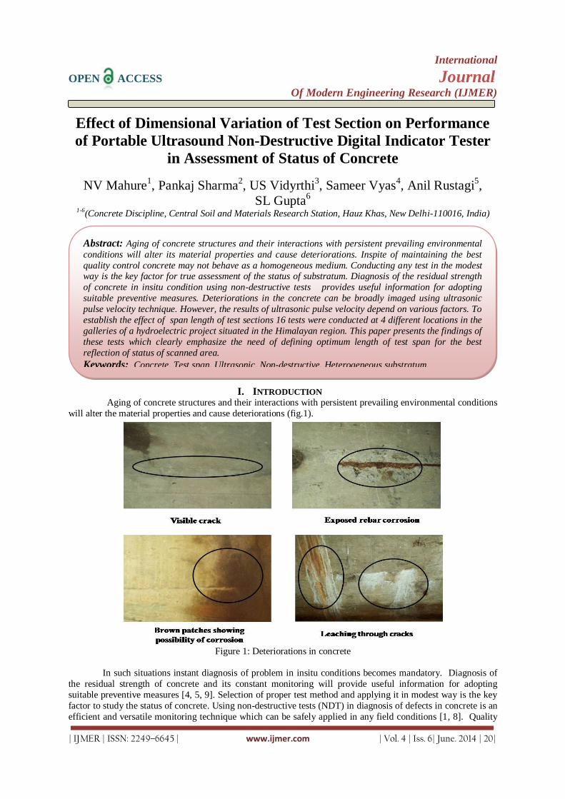
International
OPEN ACCESS Journal Of Modern Engineering Research (IJMER)
| IJMER | ISSN: 2249–6645 | www.ijmer.com | Vol. 4 | Iss. 6| June. 2014 | 20|
Effect of Dimensional Variation of Test Section on Performance
of Portable Ultrasound Non-Destructive Digital Indicator Tester
in Assessment of Status of Concrete
NV Mahure1, Pankaj Sharma
2, US Vidyrthi
3, Sameer Vyas
4, Anil Rustagi
5,
SL Gupta6
1-6(Concrete Discipline, Central Soil and Materials Research Station, Hauz Khas, New Delhi-110016, India)
I. INTRODUCTION Aging of concrete structures and their interactions with persistent prevailing environmental conditions
will alter the material properties and cause deteriorations (fig.1).
Figure 1: Deteriorations in concrete
In such situations instant diagnosis of problem in insitu conditions becomes mandatory. Diagnosis of
the residual strength of concrete and its constant monitoring will provide useful information for adopting
suitable preventive measures [4, 5, 9]. Selection of proper test method and applying it in modest way is the key
factor to study the status of concrete. Using non-destructive tests (NDT) in diagnosis of defects in concrete is an
efficient and versatile monitoring technique which can be safely applied in any field conditions [1, 8]. Quality
Abstract: Aging of concrete structures and their interactions with persistent prevailing environmental
conditions will alter its material properties and cause deteriorations. Inspite of maintaining the best
quality control concrete may not behave as a homogeneous medium. Conducting any test in the modest way is the key factor for true assessment of the status of substratum. Diagnosis of the residual strength
of concrete in insitu condition using non-destructive tests provides useful information for adopting
suitable preventive measures. Deteriorations in the concrete can be broadly imaged using ultrasonic
pulse velocity technique. However, the results of ultrasonic pulse velocity depend on various factors. To
establish the effect of span length of test sections 16 tests were conducted at 4 different locations in the
galleries of a hydroelectric project situated in the Himalayan region. This paper presents the findings of
these tests which clearly emphasize the need of defining optimum length of test span for the best
reflection of status of scanned area.
Keywords: Concrete, Test span, Ultrasonic, Non-destructive, Heterogeneous substratum.

Effect of Dimensional Variation of Test Section on Performance of Portable Ultrasound Non-…..
| IJMER | ISSN: 2249–6645 | www.ijmer.com | Vol. 4 | Iss. 6| June. 2014 | 21|
of concrete can be evaluated using ultrasonic pulse velocity technique which is a NDT method of testing [2]. For
assessing insitu deterioration indirect transmission of ultrasonic pulse velocity (UPV) is applied. In this method
ultrasonic stress waves are propagated between two points located on the same surface. It uses the basic
principle of determining time taken by an irrational pulse to travel a known distance through a concrete [3].
UPV is influenced by status of concrete [6, 7].
Inspite of best quality control concrete may not behave as a homogeneous medium so for any two
sections UPV may or may not be the same. It may differ if the length of test section is altered. So in order image the correct condition of test section an optimum length of test section needs to be defined. To study this
16 tests were carried out at 4 different locations in the galleries of a hydroelectric project situated in the
Himalayan region.
II. METHOD ADOPTED
Ultrasound Non destructive Test Through an indirect transmission mode, as illustrated in Fig. 2, ultrasonic pulse velocities were
measured by a commercially available Portable Ultrasound Non destructive Digital Indicator Tester (PUNDIT)
with an associated transducer pair. The nominal frequency of the transducers used for testing concrete sections
is 54 kHz. The principle of ultrasonic pulse velocity measurement involves sending a wave pulse into concrete
by an electro-acoustical transducer and measuring the travel time for the pulse to propagate through the concrete.
The pulse is generated by a transmitter and received by a similar type of receiver in contact with the other
surface. In the experimental studies, the transmitter and receiver were placed in two different manners
1. At a distance of 0.3 m horizontally
2. At a distance of 0.9 m horizontally
As a result, the traveling length of the ultrasonic pulse was 0.3 m and 0.9m horizontally. The concrete surface was prepared in advance for a proper acoustic coupling by applying grease. Light pressure was applied
to ensure firm contact of the transducers against the concrete surface. Knowing the path length (L), the
measured travel time between the transducers (T) can be used to calculate the pulse velocity (V) using the
formula V = L/T.
Figure 2: Indirect Transmission Mode (T: Transducer, R: Receiver)
III. Equipment Used
Portable Ultrasound Non destructive Digital Indicator Tester (PUNDIT)
PUNDIT (Fig. 3) was used to observe the time of travel of ultrasonic wave between two fixed point at a
specified distance. Waves are generated through one transducer and received by another transducer. Based on
the UPV the status of concrete is assessed
Figure 3: Portable Ultrasound Non destructive Digital Indicator Tester Equipment (PUNDIT)
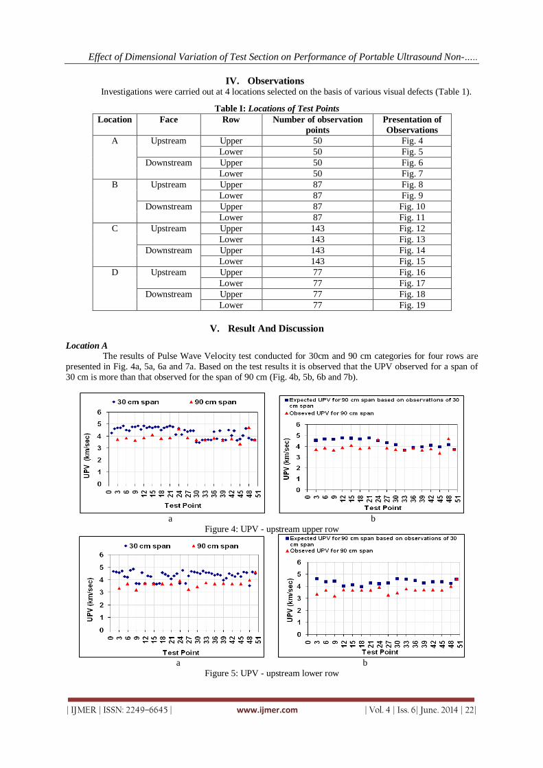
Effect of Dimensional Variation of Test Section on Performance of Portable Ultrasound Non-…..
| IJMER | ISSN: 2249–6645 | www.ijmer.com | Vol. 4 | Iss. 6| June. 2014 | 22|
IV. Observations Investigations were carried out at 4 locations selected on the basis of various visual defects (Table 1).
Table I: Locations of Test Points
Location Face Row Number of observation
points
Presentation of
Observations
A Upstream Upper 50 Fig. 4
Lower 50 Fig. 5
Downstream Upper 50 Fig. 6
Lower 50 Fig. 7
B Upstream Upper 87 Fig. 8
Lower 87 Fig. 9
Downstream Upper 87 Fig. 10
Lower 87 Fig. 11
C Upstream Upper 143 Fig. 12
Lower 143 Fig. 13
Downstream Upper 143 Fig. 14
Lower 143 Fig. 15
D Upstream Upper 77 Fig. 16
Lower 77 Fig. 17
Downstream Upper 77 Fig. 18
Lower 77 Fig. 19
V. Result And Discussion
Location A
The results of Pulse Wave Velocity test conducted for 30cm and 90 cm categories for four rows are
presented in Fig. 4a, 5a, 6a and 7a. Based on the test results it is observed that the UPV observed for a span of
30 cm is more than that observed for the span of 90 cm (Fig. 4b, 5b, 6b and 7b).
a b
Figure 4: UPV - upstream upper row
a b
Figure 5: UPV - upstream lower row
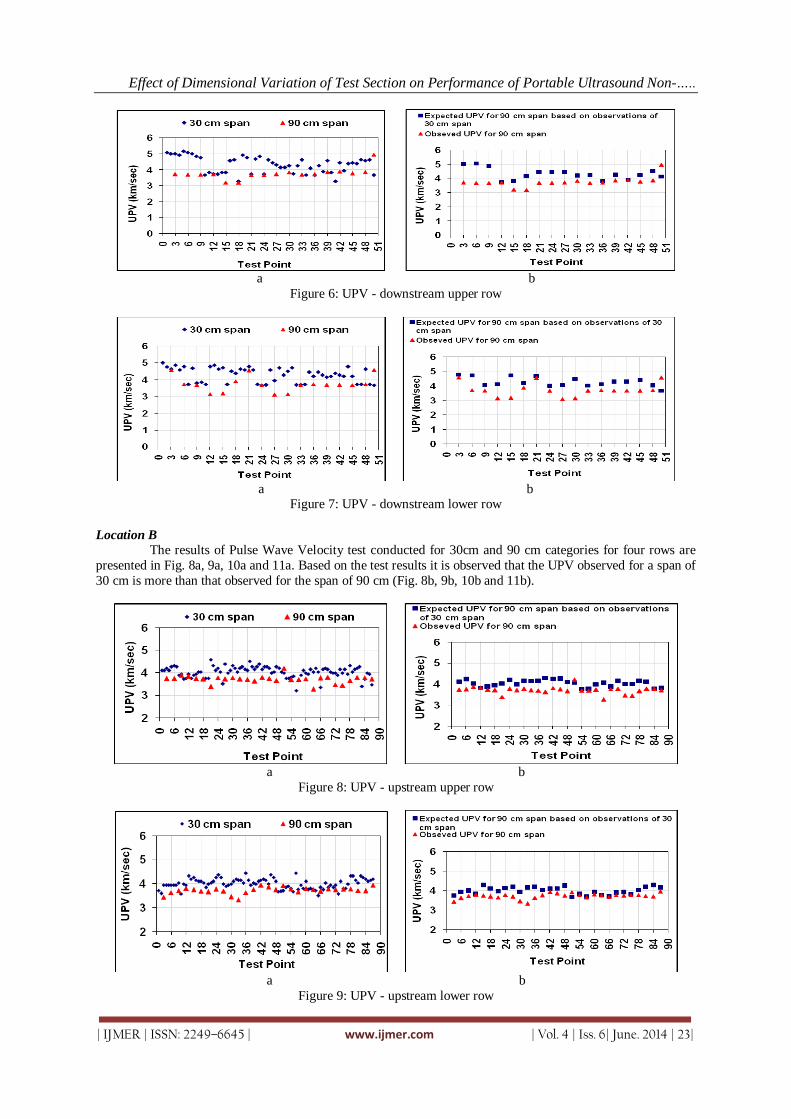
Effect of Dimensional Variation of Test Section on Performance of Portable Ultrasound Non-…..
| IJMER | ISSN: 2249–6645 | www.ijmer.com | Vol. 4 | Iss. 6| June. 2014 | 23|
a b
Figure 6: UPV - downstream upper row
a b
Figure 7: UPV - downstream lower row
Location B
The results of Pulse Wave Velocity test conducted for 30cm and 90 cm categories for four rows are
presented in Fig. 8a, 9a, 10a and 11a. Based on the test results it is observed that the UPV observed for a span of
30 cm is more than that observed for the span of 90 cm (Fig. 8b, 9b, 10b and 11b).
a b
Figure 8: UPV - upstream upper row
a b
Figure 9: UPV - upstream lower row
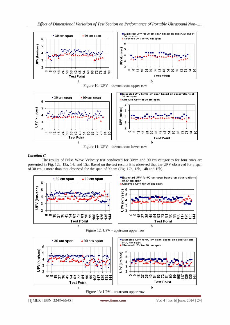
Effect of Dimensional Variation of Test Section on Performance of Portable Ultrasound Non-…..
| IJMER | ISSN: 2249–6645 | www.ijmer.com | Vol. 4 | Iss. 6| June. 2014 | 24|
a b
Figure 10: UPV - downstream upper row
a b
Figure 11: UPV - downstream lower row
Location C
The results of Pulse Wave Velocity test conducted for 30cm and 90 cm categories for four rows are
presented in Fig. 12a, 13a, 14a and 15a. Based on the test results it is observed that the UPV observed for a span
of 30 cm is more than that observed for the span of 90 cm (Fig. 12b, 13b, 14b and 15b).
a b
Figure 12: UPV - upstream upper row
a b
Figure 13: UPV - upstream upper row
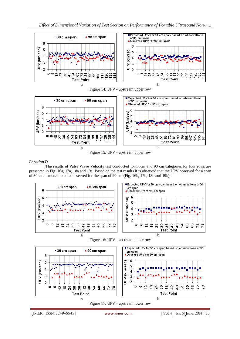
Effect of Dimensional Variation of Test Section on Performance of Portable Ultrasound Non-…..
| IJMER | ISSN: 2249–6645 | www.ijmer.com | Vol. 4 | Iss. 6| June. 2014 | 25|
a b
Figure 14: UPV - upstream upper row
a b
Figure 15: UPV - upstream upper row
Location D
The results of Pulse Wave Velocity test conducted for 30cm and 90 cm categories for four rows are
presented in Fig. 16a, 17a, 18a and 19a. Based on the test results it is observed that the UPV observed for a span
of 30 cm is more than that observed for the span of 90 cm (Fig. 16b, 17b, 18b and 19b).
a b
Figure 16: UPV - upstream upper row
a b
Figure 17: UPV - upstream lower row
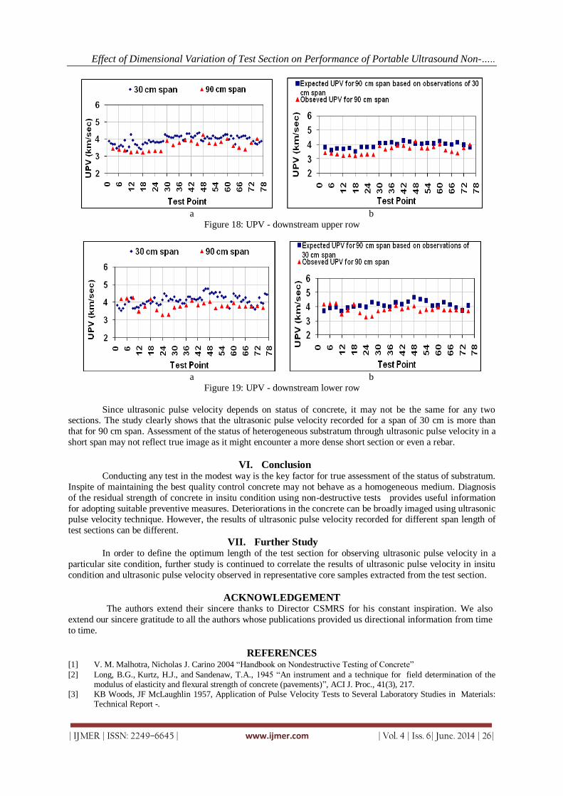
Effect of Dimensional Variation of Test Section on Performance of Portable Ultrasound Non-…..
| IJMER | ISSN: 2249–6645 | www.ijmer.com | Vol. 4 | Iss. 6| June. 2014 | 26|
a b
Figure 18: UPV - downstream upper row
a b
Figure 19: UPV - downstream lower row
Since ultrasonic pulse velocity depends on status of concrete, it may not be the same for any two sections. The study clearly shows that the ultrasonic pulse velocity recorded for a span of 30 cm is more than
that for 90 cm span. Assessment of the status of heterogeneous substratum through ultrasonic pulse velocity in a
short span may not reflect true image as it might encounter a more dense short section or even a rebar.
VI. Conclusion Conducting any test in the modest way is the key factor for true assessment of the status of substratum.
Inspite of maintaining the best quality control concrete may not behave as a homogeneous medium. Diagnosis
of the residual strength of concrete in insitu condition using non-destructive tests provides useful information
for adopting suitable preventive measures. Deteriorations in the concrete can be broadly imaged using ultrasonic pulse velocity technique. However, the results of ultrasonic pulse velocity recorded for different span length of
test sections can be different.
VII. Further Study In order to define the optimum length of the test section for observing ultrasonic pulse velocity in a
particular site condition, further study is continued to correlate the results of ultrasonic pulse velocity in insitu
condition and ultrasonic pulse velocity observed in representative core samples extracted from the test section.
ACKNOWLEDGEMENT The authors extend their sincere thanks to Director CSMRS for his constant inspiration. We also
extend our sincere gratitude to all the authors whose publications provided us directional information from time
to time.
REFERENCES [1] V. M. Malhotra, Nicholas J. Carino 2004 “Handbook on Nondestructive Testing of Concrete”
[2] Long, B.G., Kurtz, H.J., and Sandenaw, T.A., 1945 “An instrument and a technique for field determination of the modulus of elasticity and flexural strength of concrete (pavements)”, ACI J. Proc., 41(3), 217.
[3] KB Woods, JF McLaughlin 1957, Application of Pulse Velocity Tests to Several Laboratory Studies in Materials: Technical Report -.

Effect of Dimensional Variation of Test Section on Performance of Portable Ultrasound Non-…..
| IJMER | ISSN: 2249–6645 | www.ijmer.com | Vol. 4 | Iss. 6| June. 2014 | 27|
[4] Sturrup, V. R.; Vecchio, F. J.; and Caratin, H., 1984 "Pulse Velocity as a Measure of Concrete Compressive Strength," In-Situ/Nondestructive Testing of Concrete, SP-82, V. M. Malhotra, American Concrete Institute, Farmington Hills, Mich., pp. 201-227.
[5] Lin, Y.; Changfan, H.; and Hsiao, C., 1998 "Estimation of High- Performance Concrete Strength by Pulse Velocity,"
Journal of the Chinese Institute of Engineers, V. 20, No. 6, pp. 661-668. [6] Popovics, S.; Rose, L. J.; and Popovics, J. S., 1990, "The Behavior of Ultrasonic Pulses in Concrete," Cement and
Concrete Reaserch, V. 20, No. 2, pp. 259-270. [7] N.V. Mahure, G.K Vijh, Pankaj Sharma, 2011 “Correlation between Pulse Velocity and Compressive Strength of
Concrete” International Journal of Earth Sciences and Engineering, Volume 04, No 06 SPL, , pp 871-874 [8] Pankaj Sharma et al, 2013, “Corrosion Monitoring Of Reinforcement in Underground Galleries of Hydro Electric
Project” Int. Journal of Engineering Research and Applications, Vol. 3, Issue 5, pp.1087-1090.
[9] Diagnosis of Deterioration of Concrete Structures-Identification of Defects, valuation and Development of Remedial
Actions, Concrete Society Camberley, UK, Technical Report. 54,(2000)

International
OPEN ACCESS Journal Of Modern Engineering Research (IJMER)
| IJMER | ISSN: 2249–6645 | www.ijmer.com | Vol. 4 | Iss. 6| June. 2014 | 28|
Advanced Cable Stayed Bridge Construction Process Analysis
with ANSYS
T.Subramani1, A.Kumaresan
2
1Professor & Dean, Department of Civil Engineering, VMKV Engg. College, Vinayaka Missions University,
Salem, India 2PG Student of Structural Engineering, Department of Civil Engineering, VMKV Engg. College, Vinayaka
Missions University, Salem, India
I. Introduction
Civil FEM is a customization of the finite element analysis software ANSYS, which has the aim to
approach the Civil Engineering World with the general purpose tools of ANSYS. The structure of Civil FEM is
made up of a main program, called Civil FEM Intro, onto which several specific modules of Civil Engineering applications can be added: Bridges, Prestressed Concrete and
Abstract: This paper demonstrates how sophisticated computational techniques can help to
understand better the behaviour of cable-stayed bridges and what kind of tools are available for
bridge engineers to handle even the most extreme situations. Since one of the key elements in the
success of this structural system lies in its construction method, the main focus of this paper is on
the simulation of the free-cantilever construction process and the determination of cable forces during the phases of the erection in order to achieve the desired shape and internal force
distribution in the final state of the structure. The paper, using ANSYS/CivilFEM, a software
package developed for advanced civil engineering analyses, presents different numerical
techniques (based on both linear and non-linear analysis) to determine the final state of the
bridge and the backward process analysis to conduct a step-by-step analysis of the
construction.Finite Element Analysis can provide engineers with an overwhelming amount of
data therefore the efficient presentation of results (post processing) is of outmost importance
especially for such complex systems as cable-stayed bridges.The paper also demonstrates how the
flexibility of ANSYS/CivilFEM allows the users to find a sensible way to access all the necessary
data and produce both texts based and graphical outputs. A typical example of a cable-stayed
bridge is analyzed by the methods described in the paper and the results are presented using post processing techniques.Cable stayed bridges have good stability, optimum use of structural
materials, aesthetic, relatively low design and maintenance costs, and efficient structural
characteristics. Therefore, this type of bridges are becoming more and more popular and are
usually preferred for long span crossings compared to suspension bridges. A cable stayed bridge
consists of one or more towers with cables supporting the bridge deck.In terms of cable
arrangements, the most common type of cable stayed bridges are fan, harp, and semi fan bridges.
Because of their large size and nonlinear structural behaviour, the analysis of these types of
bridges is more complicated than conventional bridges. In these bridges, the cables are the main
source of nonlinearity. Obtaining the optimum distribution of post-tensioning cable forces is an
important task and plays a major role in optimizing the design of cable stayed bridges. An
optimum design of a cable-stayed bridge with minimum cost while achieving strength and
serviceability requirements is a challenging task.In this thesis, an advanced and comprehensive numerical model is used to obtain the post-tensioning forces and the optimum design of the three
types of cable-stayed bridge. The numerical method is based on finite element, B-spline curves,
and real coded genetic algorithm. The optimization accounts for all the variables that define the
geometry and cross-section of the bridge. Comparison between the three types, in terms of post-
tensioning forces and cost, is carried out in this thesis.
Keywords: Dynamic Mechanic Analysis, Stability Isolated Base, Non Linear Response Cable,
Pre-Stressing Load.

Advanced Cable Stayed Bridge Construction Process Analysis With Ansys
| IJMER | ISSN: 2249–6645 | www.ijmer.com | Vol. 4 | Iss. 6| June. 2014 | 29|
Geotechnics.
The first of these modules has utilities for modeling and analyze virtually any bridge types:
Metallic bridges.
Prestressed concrete bridges.
Mixed or composite bridges.
With different types of supports:
Simple supports. Suspension bridges.
Cable-Stayed bridges.
Arch bridges.
The history of cable stayed bridges dates back to 1595, found in a book by the Venetian inventor
(Bernard et al., 1988). Many suspension and cable-stayed bridges have been designed and developed since 1595
such as the Albert bridge and the Brooklyn bridge (Wilson and Gravelle, 1991), (Bernard et al., 1988). Cable-
stayed bridges have been later constructed all over the world. The Swedish Stromsund bridge, designed in 1955,
is known as the first modern cable-stayed bridge (Wilson and Gravelle, 1991).
The total length of the bridge is 332 m, and its main span length is 182 m. It was opened in 1956, and it
was the largest cable-stayed bridge of the world at that time. This bridge was constructed by Franz Dischinger,
from Germany, who was a pioneer in construction of cable-stayed bridges (Tori et al., 1968). The designers realized that cable stayed style requires less material for cables and deck and can be erected much easier than
suspension bridges (Bernard et al., 1988), (Tori et al., 1968), (Wilson and Gravelle, 1991), (Simoes and Negrao,
1994), (Ren and Peng, 2005), and (Nieto et al., 2009).
This is mainly due to advances in design and construction method and the availability of high strength
steel cables. The Theodor Heuss bridge was the second true cable-stayed bridge and was erected in 1957 across
the Rhine river at Dusseldrof. It had a main span of 260 m and side spans of 108 m which was larger than the
Stromsund.
It has a harp cable arrangement with parallel stays and a pylon composed of two free-standing posts
fixed to the deck. The reason for choosing the harp style was aesthetics appearance. The Severins Bridge in
Köln designed in 1961 was the first fan shape cable stayed bridge, which has a A-shape pylon.
In this bridge, the cross section of the deck was similar to the one used in Theodor Heuss bridge
(Bernard et al., 1988). The Flehe bridge was the first semi-fan type which was erected in 1979 in Dusseldrof, Germany over the Rhine river. The remarkable feature of this bridge was the reinforced concrete tower, which
has the shape of an inverted Y (Bernard et al., 1988). In what follows, the main types of long span bridges are
reviewed.
.
II. Study Area
2.1 Analysis Algorithm The purpose of the analysis is to study the stresses the cables must have during the construction phases,
to achieve at the end of the construction and for a specified load state, a certain deformed shape of the deck
(usually null movements). To obtain this, the following process calculates the structure at its final stage,
obtaining this way the final stresses in the cables and, step by step, removes the cables and deck elements in the
opposite order to the building procedure (backward analysis).
Apart from movements, forces and moments in towers and deck, at each step the forces in the cables
are also obtained. The prestressing load in each cable is equal to the force in the cable in the last calculation step
before the cable is “killed”, i.e. removed from the model. The calculation steps can be described as follows:
1. Cable forces are calculated for the final state of the bridge (all the cable elements are alive):
The deformations of the deck due to the self weight of the structure and additional dead load is
calculated using linear analysis. Every cable is prestressed by unit change in the length (-1 m) one by one (the other cables are assumed
to be stress free) and the deformations of the deck are calculated for each case using linear analysis.
A system of linear equations is assembled: K ⋅ f = u . The response of the structure – the “stiffness of
the structure” - to the unit cable shortening are the elements of the coefficient matrix (K). The
deformations (UY of the deck and UX of the tower top) are the elements of the vector on the right-hand
side (u).
The system of linear equations is solved and f is determined. The elements of the f vector are the actual
cable shortening required to achieve the desired shape of the structure.
The f vector is applied as cable shortening and the structure is solved again.
2. Nonlinear construction process analysis: backward analysis ('demolishing' the bridge step by step)
Remove additional dead load.
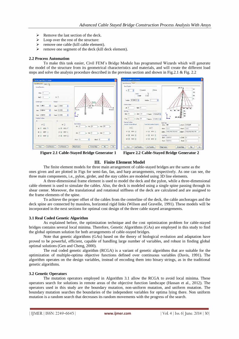
Advanced Cable Stayed Bridge Construction Process Analysis With Ansys
| IJMER | ISSN: 2249–6645 | www.ijmer.com | Vol. 4 | Iss. 6| June. 2014 | 30|
Remove the last section of the deck.
Loop over the rest of the structure:
remove one cable (kill cable element).
remove one segment of the deck (kill deck element).
2.2 Process Automation
To make this task easier, Civil FEM’s Bridge Module has programmed Wizards which will generate the model of the structure from its geometrical characteristics and materials, and will create the different load
steps and solve the analysis procedure described in the previous section and shown in Fig.2.1 & Fig. 2.2
Figure 2.1 Cable-Stayed Bridge Generator 1 Figure 2.2 Cable-Stayed Bridge Generator 2
III. Finite Element Model The finite element models for three main arrangement of cable-stayed bridges are the same as the
ones given and are plotted in Figs for semi-fan, fan, and harp arrangements, respectively. As one can see, the
three main components, i.e., pylon, girder, and the stay cables are modeled using 3D line elements.
A three-dimensional frame element is used to model the deck and the pylon, while a three-dimensional
cable element is used to simulate the cables. Also, the deck is modeled using a single spine passing through its
shear center. Moreover, the translational and rotational stiffness of the deck are calculated and are assigned to
the frame elements of the spine.
To achieve the proper offset of the cables from the centerline of the deck, the cable anchorages and the deck spine are connected by massless, horizontal rigid links (Wilson and Gravelle, 1991). These models will be
incorporated in the next sections for optimal cost design of the three cable stayed arrangements.
3.1 Real Coded Genetic Algorithm
As explained before, the optimization technique and the cost optimization problem for cable-stayed
bridges contains several local minima. Therefore, Genetic Algorithms (GAs) are employed in this study to find
the global optimum solution for both arrangements of cable-stayed bridges.
Note that genetic algorithms (GAs) based on the theory of biological evolution and adaptation have
proved to be powerful, efficient, capable of handling large number of variables, and robust in finding global
optimal solutions (Gen and Cheng, 2000).
The real coded genetic algorithm (RCGA) is a variant of genetic algorithms that are suitable for the
optimization of multiple-optima objective functions defined over continuous variables (Davis, 1991). The algorithm operates on the design variables, instead of encoding them into binary strings, as in the traditional
genetic algorithms.
3.2 Genetic Operators
The mutation operators employed in Algorithm 3.1 allow the RCGA to avoid local minima. These
operators search for solutions in remote areas of the objective function landscape (Hassan et al., 2012). The
operators used in this study are the boundary mutation, non-uniform mutation, and uniform mutation. The
boundary mutation searches the boundaries of the independent variables for optima lying there. Non uniform
mutation is a random search that decreases its random movements with the progress of the search.

Advanced Cable Stayed Bridge Construction Process Analysis With Ansys
| IJMER | ISSN: 2249–6645 | www.ijmer.com | Vol. 4 | Iss. 6| June. 2014 | 31|
The Uniform mutation is a random search element. The crossover operators produce new solutions
from parent solutions having good objective function values. In this study, it is used to produce new bridges
from pairs of low cost bridge. The crossover operators used are the arithmetic, uniform and heuristic crossovers.
The first produces new solutions in the functional landscape of the parent solutions.
Details of such operators are given by Michalewics and Fogel (2004) and recently employed in Hassan
et al. (2012). The above operators are applied on each population with the following values:
1) Population size = 100 solution instances 2) 4 instances undergo boundary mutation.
3) 4 instances undergo non-uniform mutation.
4) 4 instances undergo uniform mutation.
5) 2 instances undergo arithmetic crossover.
6) 2 instances undergo uniform crossover.
7) 2 instances undergo heuristic crossover.
3.3 Post-tensioning Cable Forces
In the previous chapter, a numerical method is employed to obtain the post-tensioning cable forces for
specific number of cables N, mid-span length M, and height of the pylon H. These forces are implemented in the
analysis/design scheme employed in this chapter. However, in the design optimization process, the variables N, M, and H, can be assigned some random values that do not match the values considered. To overcome this issue,
three-dimensional linear interpolation (N, M, and H) is conducted between the data points for the forces of post-
tensioning cable forces evaluated.
3.4 Load Considerations
Dead load, wind load, and live load are considered in this thesis based on Canadian Highway Bridge
Design Code (CAN/CSA-S6-06, 2006).
Dead Load
According to clause 3.6 of the CAN/CSA-S6-06 (2006), the dead load of the bridge contains the
structural weight of the bridge, a thickness of 0.09 m layer of asphalt, and two concrete traffic barriers having an
average thickness and height of 0.325 m and 0.85 m, respectively.
Live Load
To compute the live load acting on the bridge deck using clause 3.8.3.2 of the CAN/CSA-S6-06 (2006)
the following two cases are considered:
CL-W truck.
CL-W truck with each axle reduced to 80% and superimposed with a uniformly distributed load (qL =
9kN=m) lane.
In short and medium span cable-stayed bridges, the main effect always results due to a single axle, group of
axles, or single truck. For long span cable-stayed bridges, the critical force effect and largest deflection are due
to the distributed lane loads. Hence, the live load acting on the bridge deck in this study is given as:
Liveload = mFnLaneqL where mF is the modification factor used when more than one design lane is loaded according to clause
3.8.4.2, and Table 3.8.4.2, of CAN/CSA-S6-06 (2006), nLane, is the number of the lanes, and qL = 9kN=m is
the uniformly distributed load. The nine live load configurations applied to determine the optimum cost design
of three type of the cable-stayed bridge are shown in Fig.3.1 (Walther et al., 1988). The live load is calculated
using the equation. It has a magnitude equal to 16.2 kN=m and 25.2 kN=m for the case of two and four lanes,
respectively CAN/CSA-S6- 06 (2006).
Wind Load
Cable-stayed bridges are considered sensitive to wind load. Therefore, wind tunnel tests are required to
determine the lift (CN), torsional (CM), and drag (CD) shape coefficients of the deck.

Advanced Cable Stayed Bridge Construction Process Analysis With Ansys
| IJMER | ISSN: 2249–6645 | www.ijmer.com | Vol. 4 | Iss. 6| June. 2014 | 32|
Figure 3.1: Live load cases used in the numerical model
IV. Conclusion
The algorithm described provides an accurate method to obtain the needed prestressing forces in the
cables of a cable-stayed bridge, for each of the construction phases. This method allows to solve the bridge in a
very short time, which provides obvious benefits compared with other optimization methods, without having to
use approximations.
This accurate and rapid performance, in conjunction with the preprocessing utilities available, allows the engineer to spend more time in shape design optimization and allows to compare different solutions to
obtain the best suitable one.
The postprocessing of the bridge analysis provides a quick review of the structural behavior. It also
gives valuable information for the construction of the bridge by automatically exporting the prestressing forces
of each cable, at each construction step.
REFERENCES [1]. Abdel-Ghaffar, A.M., and Khalifa, M.A. (1991). “Importance of cable vibration in dynamics of cable-stayed
bridges.” Journal of Engineering Mechanics, ASCE, 117(11), 2571-2589. [2]. Gimsing, N.J. (1997). “Cable supported bridges: Concept and design.” Second Edition, John Wiley & Sons, Ltd,
Chichester, UK. [3]. Fujino, Y., Warnitchai, P., and Pacheco, B.M. (1993). “An experimental and analytical study of autoparametric
resonance in a 3DOF model of cable-stayed-beam.” Nonlinear Dynamics, 4(2), 111-138. [4]. Warnitchai, P., Fujino, Y., Pacheco, B.M., and Agret, R. (1993). “An experimental study on active tendon control of
cable-stayed bridges.” Earthquake Engineering and Structural Dynamics, 22(2), 93-111.
[5]. Warnitchai, P., Fujino, Y., and Susumpow, T. (1995). “A non-linear dynamic model for cables and its application to a cable-structure system.” Journal of Sound and Vibration, 187(4), 695-712.
[6]. Lilien, J.L., and Pinto da Costa, A. (1994). “Vibration amplitudes caused by parametric excitation of cable stayed structures.” Journal of Sound and Vibration, 174(1), 69-90.
[7]. Pinto da Costa, A., Martins, J.A.C., Branco, F., and Lilien, J.L. (1996). “Oscillations of bridge stay cables induced by periodic motions of deck and/or towers.” Journal of Engineering Mechanics, ASCE, 122(7), 613-622.
[8]. Gattulli, V., Morandini, M., and Paolone, A. (2002). “A parametric analytical model for non-linear dynamics in cable-stayed beam.” Earthquake Engineering and Structural Dynamics, 31(6), 1281-1300.
[9]. Gattulli, V., and Lepidi, M. (2003). “Nonlinear interactions in the planar dynamics of cable-stayed beam.” International Journal of Solids and Structures, 40(18), 4729-4748.
[10]. Gattulli, V., Lepidi, M., Macdonald, J.H.G., and Taylor, C.A. (2005). “One-to-two globallocal interaction in a cable-stayed beam observed through analytical, finite element and experimental models.” International Journal of Non-Linear Mechanics, 40(4), 571-588.
[11]. Gattulli, V., and Lepidi, M. (2007). “Localization and veering in the dynamics of cablestayed bridges.” Computers and Structures, 85(21-22), 1661-1678.
[12]. Tuladhar, R., Dilger, W.H., and Elbadry, M.M. (1995). “Influence of cable vibration on seismic response of cable-
stayed bridges.” Canadian Journal of Civil Engineering, 22(5), 1001-1020. [13]. Caetano, E., Cunha, A., and Taylor, C.A. (2000a). “Investigation of dynamic cable-deck interaction in a physical
model of a cable-stayed bridge. Part I: modal analysis.” Earthquake Engineering and Structural Dynamics, 29(4), 481-498.

Advanced Cable Stayed Bridge Construction Process Analysis With Ansys
| IJMER | ISSN: 2249–6645 | www.ijmer.com | Vol. 4 | Iss. 6| June. 2014 | 33|
[14]. Caetano, E., Cunha, A., and Taylor, C.A. (2000b). “Investigation of dynamic cable-deck interaction in a physical model of a cable-stayed bridge. Part II: seismic response.” Earthquake Engineering and Structural Dynamics, 29(4), 499-521.
[15]. Au, F.T.K., Cheng, Y.S., Cheung, Y.K., and Zheng, D.Y. (2001). “On the determination of natural frequencies and
mode shapes of cable-stayed bridges.” Applied Mathematical Modelling, 25(12), 1099-1115. [16]. Caetano, E., Cunha, A., Gattulli, V., and Lepidi, M. (2008). “Cable-deck dynamic interactions at the International
Guadiana Bridge: On-site measurements and finite element modelling.” Structural Control and Health Monitoring, 15(3), 237-264.
[17]. Liu, M.Y., Zuo, D., and Jones, N.P. (2005). “Deck-induced stay cable vibrations: Field observations and analytical model.” Proceedings of the Sixth International Symposium on Cable Dynamics, 175-182, Charleston, South Carolina, USA, September 19-22.
[18]. Wang, P.H., Tseng, T.C., and Yang, C.G. (1993). “Initial shape of cable-stayed bridges.” Computers and Structures, 46(6), 1095-1106.
[19]. Wang, P.H., and Yang, C.G. (1996). “Parametric studies on cable-stayed bridges.” Computers and Structures, 60(2), 243-260.
[20]. Wang, P.H., Lin, H.T., and Tang, T.Y. (2002). “Study on nonlinear analysis of a highly redundant cable-stayed bridge.” Computers and Structures, 80(2), 165-182.

International
OPEN ACCESS Journal
Of Modern Engineering Research (IJMER)
| IJMER | ISSN: 2249–6645 | www.ijmer.com | Vol. 4 | Iss. 6| June. 2014 | 34|
Performance Evaluation of Push-To-Talk Group Communication
Jong Min Lee1 1Department of Computer Software Engineering, Dong-Eui University, Republic of Korea
I. INTRODUCTION Recently many Internet applications have been used widely in our lives for the proliferation of smart
phones. Especially the concept of the VoIP has been used in many applications such as Skype, Viber, Voxer, TiKL
etc. Among applications which support VoIP, there are several VoIP applications such as Voxer, and TiKL which
support the group communication as well as one-to-one communication, which is also known as the push-to-talk
(PTT or P2T) [1, 2, 3]. This push-to-talk technology supports the half duplex communication among end-to-end
users like the trunked radio system (TRS). Nextel communications was the first company to provide the
push-to-talk service commercially using iDEN.
The problem of the group communication results from the asymmetry between the in-bound traffic and
the out-bound traffic in a VoIP server. As the out-bound traffic increases, the packet delay and the packet loss can
be occurred. There are no problem in terms of sending and receiving packets, but there can be the decrease of the
voice quality in terms of listeners due to the characteristic of voice traffic. In this paper, we analyze how these
parameters results in the voice quality. We use ns-2.34 [4] for the simulation study and ns2Voip++ package [5]
for the analysis of the voice quality.
In Section 2, we describe the media transfer in the group communication and ns2Voip++ package briefly.
In Section 3, we describe the VoIP server added to the legacy ns-2.34 code to simulate the group communication.
The performance study due to the packet delay and the packet loss is given in Section 4. Finally, we give a
conclusion in Section 5.
II. RELATED WORKS In this section, we describe the media transfer in the PoC architecture [6] briefly in order to explain the
flow of VoIP packets. Then we describe the ns2Voip++ Package [5] in short to explain the simulation
environment.
2.1 Media Transfer
Major communication and computer companies such as Nokia, Samsung Electronics, Qualcomm, Intel
and Microsoft have standardized the Push-to-talk over Cellular (PoC) to support group communication under the
Open Mobile Alliance (OMA) [7]. We use the PoC standard to explain the group communication. After the PoC
Session [8] is established, media packets including voice data are transferred between the PoC Server and PoC
Clients. These media packets are transported by RTP/UDP/IP [6]. The PoC Server forwards received RTP Media
packets towards all other PoC Clients that are not on hold [6], that is, the received packet is copied and forwarded
to other PoC Clients in a group. The basic RTP header of media packets is described in RFC 3550 [9] and
additional RTP payload formats for various audio/video codecs such as G.729A, GSM, EVRC and AMR are
described in several RFC documents [10, 11, 12]. From the SSRC field of the RTP header, the PoC Server and
PoC Clients can find who sends the RTP packet.
Abstract: Recently the VoIP technology has been used for the purpose of voice conversation through the
Internet since the proliferation of smart phones. In this paper, we are interested in the network performance
of the group communication a.k.a. the push-to-talk (PTT) service. As the media traffic to a VoIP server
increases, the VoIP server can be a bottleneck and the voice quality can be declined, which results from the
asymmetry between the in-bound traffic and the out-bound traffic in a VoIP server. To simulate the voice
packet transfer of the group communication, we use ns-2.34 and the ns2VoIP++ package to calculate the
end-to-end mean opinion score. Simulation results show that both the packet error rate and the packet delay
have a significant effect on the performance in terms of the mean opinion score.
Keywords: OMA PoC, User Plane, Group Communication, Push-To-Talk, MOS
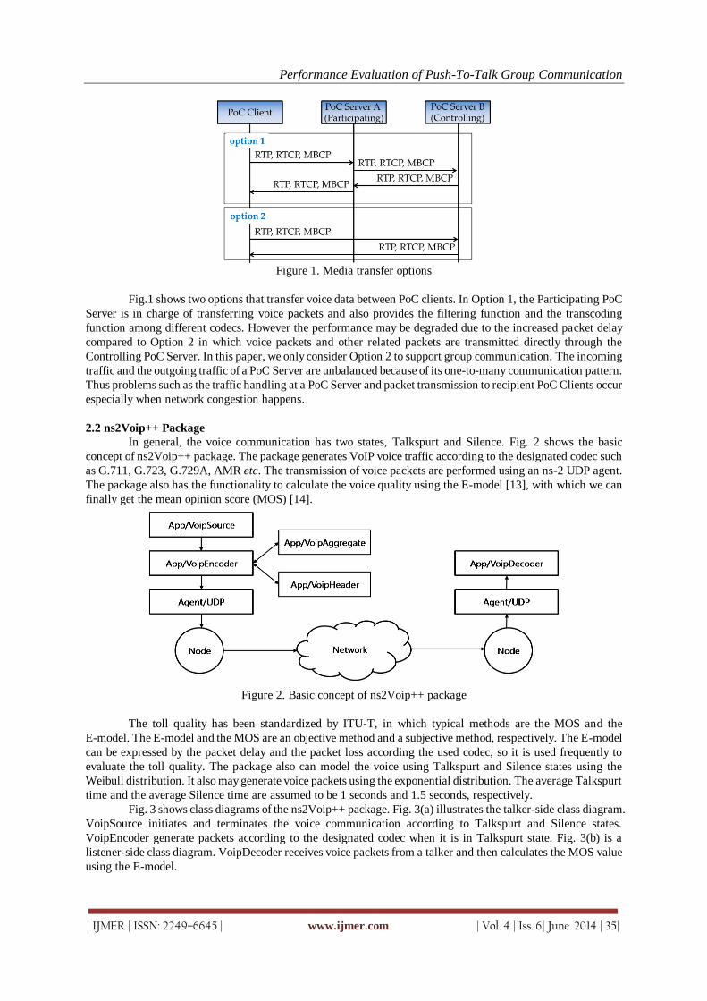
Performance Evaluation of Push-To-Talk Group Communication
| IJMER | ISSN: 2249–6645 | www.ijmer.com | Vol. 4 | Iss. 6| June. 2014 | 35|
Figure 1. Media transfer options
Fig.1 shows two options that transfer voice data between PoC clients. In Option 1, the Participating PoC
Server is in charge of transferring voice packets and also provides the filtering function and the transcoding
function among different codecs. However the performance may be degraded due to the increased packet delay
compared to Option 2 in which voice packets and other related packets are transmitted directly through the
Controlling PoC Server. In this paper, we only consider Option 2 to support group communication. The incoming
traffic and the outgoing traffic of a PoC Server are unbalanced because of its one-to-many communication pattern.
Thus problems such as the traffic handling at a PoC Server and packet transmission to recipient PoC Clients occur
especially when network congestion happens.
2.2 ns2Voip++ Package
In general, the voice communication has two states, Talkspurt and Silence. Fig. 2 shows the basic
concept of ns2Voip++ package. The package generates VoIP voice traffic according to the designated codec such
as G.711, G.723, G.729A, AMR etc. The transmission of voice packets are performed using an ns-2 UDP agent.
The package also has the functionality to calculate the voice quality using the E-model [13], with which we can
finally get the mean opinion score (MOS) [14].
Figure 2. Basic concept of ns2Voip++ package
The toll quality has been standardized by ITU-T, in which typical methods are the MOS and the
E-model. The E-model and the MOS are an objective method and a subjective method, respectively. The E-model
can be expressed by the packet delay and the packet loss according the used codec, so it is used frequently to
evaluate the toll quality. The package also can model the voice using Talkspurt and Silence states using the
Weibull distribution. It also may generate voice packets using the exponential distribution. The average Talkspurt
time and the average Silence time are assumed to be 1 seconds and 1.5 seconds, respectively.
Fig. 3 shows class diagrams of the ns2Voip++ package. Fig. 3(a) illustrates the talker-side class diagram.
VoipSource initiates and terminates the voice communication according to Talkspurt and Silence states.
VoipEncoder generate packets according to the designated codec when it is in Talkspurt state. Fig. 3(b) is a
listener-side class diagram. VoipDecoder receives voice packets from a talker and then calculates the MOS value
using the E-model.
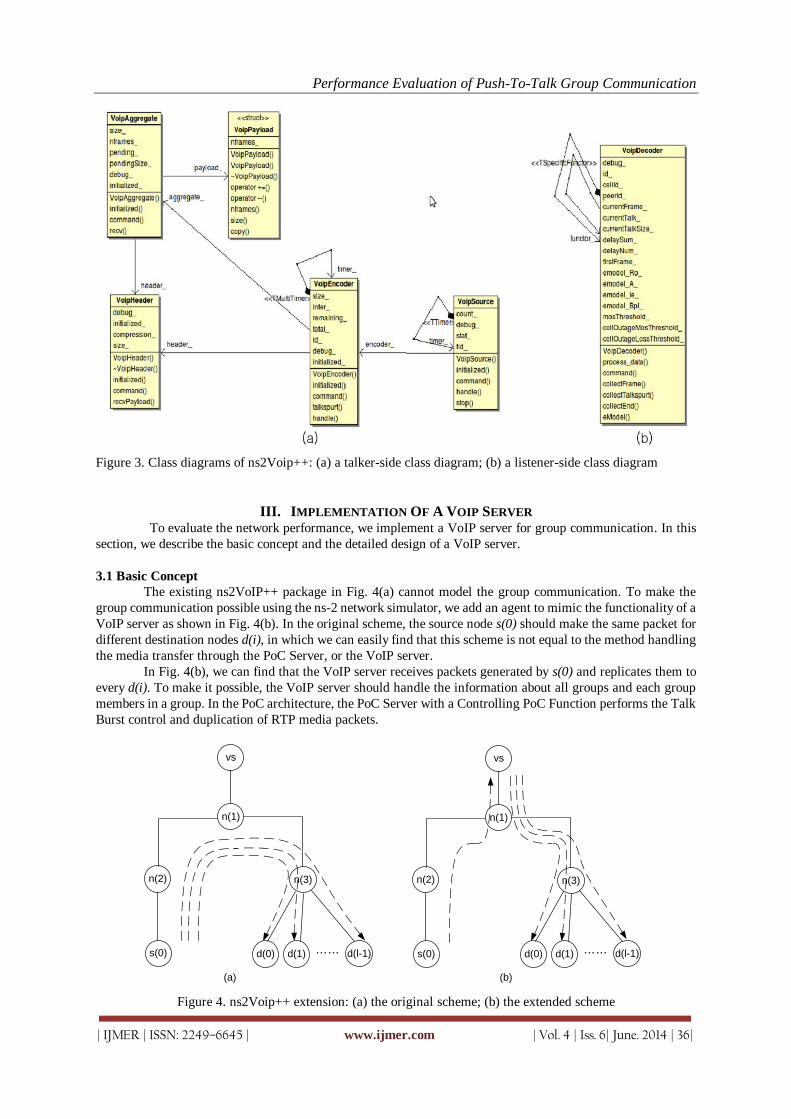
Performance Evaluation of Push-To-Talk Group Communication
| IJMER | ISSN: 2249–6645 | www.ijmer.com | Vol. 4 | Iss. 6| June. 2014 | 36|
Figure 3. Class diagrams of ns2Voip++: (a) a talker-side class diagram; (b) a listener-side class diagram
III. IMPLEMENTATION OF A VOIP SERVER To evaluate the network performance, we implement a VoIP server for group communication. In this
section, we describe the basic concept and the detailed design of a VoIP server.
3.1 Basic Concept
The existing ns2VoIP++ package in Fig. 4(a) cannot model the group communication. To make the
group communication possible using the ns-2 network simulator, we add an agent to mimic the functionality of a
VoIP server as shown in Fig. 4(b). In the original scheme, the source node s(0) should make the same packet for
different destination nodes d(i), in which we can easily find that this scheme is not equal to the method handling
the media transfer through the PoC Server, or the VoIP server.
In Fig. 4(b), we can find that the VoIP server receives packets generated by s(0) and replicates them to
every d(i). To make it possible, the VoIP server should handle the information about all groups and each group
members in a group. In the PoC architecture, the PoC Server with a Controlling PoC Function performs the Talk
Burst control and duplication of RTP media packets.
s(0)
n(2) n(3)
vs
n(1)
s(0) d(0)
n(2) n(3)
vs
n(1)
d(1)
(a) (b)
d(0) d(1) …… …… d(l-1) d(l-1)
Figure 4. ns2Voip++ extension: (a) the original scheme; (b) the extended scheme

Performance Evaluation of Push-To-Talk Group Communication
| IJMER | ISSN: 2249–6645 | www.ijmer.com | Vol. 4 | Iss. 6| June. 2014 | 37|
3.2 VoipServer Agent
The following functionalities of a VoIP server are required to simulate the group communication:
The function to set the maximum number of groups
The function to add a group member to a certain group
The function to duplicate packets from a source node and transfer them to group members
Figure 5. The VoipServer agent class
We add the VoipServer agent as shown in Fig. 5. The name of an ns-2 agent acting as a VoIP server is
definded as “Agent/VoipServer” and can be declared in the ns-2 script as follows:
set voipserver [$ns node]
set agtserver [new Agent/VoipServer]
$ns attach-agent $voipserver $agtserver
It is easy to implement the function to set the maximum number of groups, k. We implement it in
VoipServer::command() and it can be set as follows.
$agtserver set-ksize 10
We assume that the number of group members, l, for each group is the same for simplicity. The
information of group members, or destination nodes, for each group is managed using the C++ STL map class in
ns-2, which is shown in Fig. 6. In the Tcl script, we can set the value k and l for arbitrary number of destination
nodes.
0
1
.
.
.
k-1
d(0) d(1) …… d(l-1)
d(l) d(l+1) …… d(2l-1)
d((k-1)l)d((k-1)l
+1)…… d(kl-1)
group id list of destination nodes
Figure 6. Data structure for managing the list of destination nodes
To implement the function to duplicate packets from a source node and transfer them to group members,
we reflect the service time to make a packet for a group member and send it. The service time is fixed as 10-6
second. To change the service time freely without compilation, Tcl/C++ binding is used.
Except the VoipServer agent, the existing ns2Voip++ package is changed as follows:
The configuration of RNG (random number generator) for the class „VoipSource‟ to change the RNG
The singleton class „MosLogger‟ is added to record the final MOS value to get the average MOS
value
The class „VoipDecoderOptimal‟ is changed to use the class „MosLogger‟ to record the MOS value
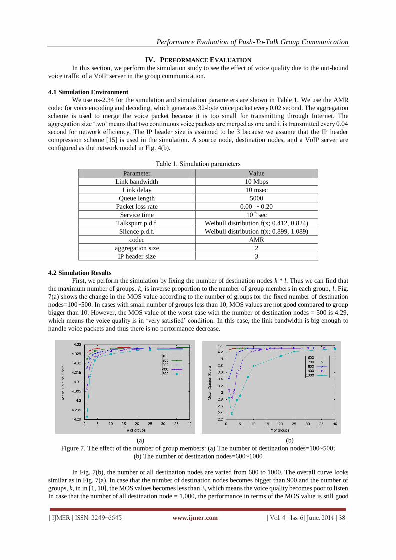
Performance Evaluation of Push-To-Talk Group Communication
| IJMER | ISSN: 2249–6645 | www.ijmer.com | Vol. 4 | Iss. 6| June. 2014 | 38|
IV. PERFORMANCE EVALUATION In this section, we perform the simulation study to see the effect of voice quality due to the out-bound
voice traffic of a VoIP server in the group communication.
4.1 Simulation Environment
We use ns-2.34 for the simulation and simulation parameters are shown in Table 1. We use the AMR
codec for voice encoding and decoding, which generates 32-byte voice packet every 0.02 second. The aggregation
scheme is used to merge the voice packet because it is too small for transmitting through Internet. The
aggregation size „two‟ means that two continuous voice packets are merged as one and it is transmitted every 0.04
second for network efficiency. The IP header size is assumed to be 3 because we assume that the IP header
compression scheme [15] is used in the simulation. A source node, destination nodes, and a VoIP server are
configured as the network model in Fig. 4(b).
Table 1. Simulation parameters
Parameter Value
Link bandwidth 10 Mbps
Link delay 10 msec
Queue length 5000
Packet loss rate 0.00 ~ 0.20
Service time 10-6 sec
Talkspurt p.d.f. Weibull distribution f(x; 0.412, 0.824)
Silence p.d.f. Weibull distribution f(x; 0.899, 1.089)
codec AMR
aggregation size 2
IP header size 3
4.2 Simulation Results
First, we perform the simulation by fixing the number of destination nodes k * l. Thus we can find that
the maximum number of groups, k, is inverse proportion to the number of group members in each group, l. Fig.
7(a) shows the change in the MOS value according to the number of groups for the fixed number of destination
nodes=100~500. In cases with small number of groups less than 10, MOS values are not good compared to group
bigger than 10. However, the MOS value of the worst case with the number of destination nodes = 500 is 4.29,
which means the voice quality is in „very satisfied‟ condition. In this case, the link bandwidth is big enough to
handle voice packets and thus there is no performance decrease.
(a) (b)
Figure 7. The effect of the number of group members: (a) The number of destination nodes=100~500;
(b) The number of destination nodes=600~1000
In Fig. 7(b), the number of all destination nodes are varied from 600 to 1000. The overall curve looks
similar as in Fig. 7(a). In case that the number of destination nodes becomes bigger than 900 and the number of
groups, k, in in [1, 10], the MOS values becomes less than 3, which means the voice quality becomes poor to listen.
In case that the number of all destination node = 1,000, the performance in terms of the MOS value is still good
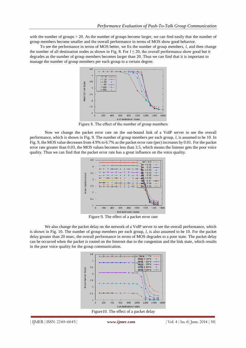
Performance Evaluation of Push-To-Talk Group Communication
| IJMER | ISSN: 2249–6645 | www.ijmer.com | Vol. 4 | Iss. 6| June. 2014 | 39|
with the number of groups > 20. As the number of groups become larger, we can find easily that the number of
group members become smaller and the overall performance in terms of MOS show good behavior.
To see the performance in terms of MOS better, we fix the number of group members, l, and then change
the number of all destination nodes as shown in Fig. 8. For l ≤ 20, the overall performance show good but it
degrades as the number of group members becomes larger than 20. Thus we can find that it is important to
manage the number of group members per each group to a certain degree.
Figure 8. The effect of the number of group members
Now we change the packet error rate on the out-bound link of a VoIP server to see the overall
performance, which is shown in Fig. 9. The number of group members per each group, l, is assumed to be 10. In
Fig. 9, the MOS value decreases from 4.9% to 6.7% as the packet error rate (per) increases by 0.01. For the packet
error rate greater than 0.03, the MOS values becomes less than 3.5, which means the listener gets the poor voice
quality. Thus we can find that the packet error rate has a great influence on the voice quality.
Figure 9. The effect of a packet error rate
We also change the packet delay on the network of a VoIP server to see the overall performance, which
is shown in Fig. 10. The number of group members per each group, l, is also assumed to be 10. For the packet
delay greater than 20 msec, the overall performance in terms of MOS degrades to a poor state. The packet delay
can be occurred when the packet is routed on the Internet due to the congestion and the link state, which results
in the poor voice quality for the group communication.
Figure10. The effect of a packet delay

Performance Evaluation of Push-To-Talk Group Communication
| IJMER | ISSN: 2249–6645 | www.ijmer.com | Vol. 4 | Iss. 6| June. 2014 | 40|
V. CONCLUSION In this paper, we have evaluated the overall performance of the group communication in terms of the
mean opinion score (MOS), that is the voice quality. We have used ns-2.34 for the simulation and the ns2VoIP++
package for the analysis of the voice quality. To simulate the group communication, we have added some
functionalities of the VoIP server. The large number of group members has a significant effect on the overall
performance, so we have found that it should be managed equal to or less than 20. We also have found that both
the packet error rate and the packet delay have a significant effect on the performance in terms of MOS. From the
simulation result, we can find that the efficient scheme to manage the voice quality for the group communication
is required to handle those situations.
ACKNOWLEDGEMENTS
This work was supported by Dong-Eui University Foundation Grant (2013).
REFERENCES [1] Open Mobile Alliance, Push to talk over cellular (PoC) – architecture: approved version 2.0 (Aug. 2011).
[2] R.S. Cruz, M. Serafim, G. Varatojo, and L. Reis, Push-to-talk in IMS mobile environment, Proc. 2009 fifth Int‟l Conf.
on Networking and Services, Valencia, Spain, 2009, 389-395.
[3] L.-H. Chang, C.-H. Sung, H.-C. Chu, and J.-J. Liaw, Design and implementation of the push-to-talk service in ad hoc
VoIP network, IET Communications, 3(5), 2009, 740-751.
[4] ns-2 homepage, http://nsnam.isi.edu/nsnam/index.php/Main_Page.
[5] M.M. Andreozzi, D. Miqliorini, G. Stea and C. Vallati, Ns2Voip++, and Enhanced Module for VoIP Simulations, Proc.
3rd Intl. ICST Conf. on Simulation Tools and Techniques, Brussels, Belgium, 2010.
[6] Open Mobile Alliance, PoC user plane: approved version 2.0 (Aug. 2011).
[7] Open Mobile Alliance Mobile Phone Standards and Specification, http://openmobilealliance.org/.
[8] Open Mobile Alliance, OMA PoC control plane: approved version 2.0 (Aug. 2011).
[9] H. Schulzrinne, S. Casner,R. Frederick and V. Jacobson, RTP: A Transport Protocol for Real-Time Applications,
RFC 3550, July 2003.
[10] H. Schulzrinne and S. Casner, RTP Profile for Audio and Video Conferences with Minimal Control, RFC 3551, July
2003.
[11] A. Li, RTP Payload Format for Enhanced Variable Rate Codecs (EVRC) and Selectable Mode Vocoders (SMV), RFC
3558, July 2003.
[12] J. Sjoberg , M. Westerlund, A. Lakaniemi and Q. Xie, RTP Payload Format and File Storage Format for the Adaptive
Multi-Rate (AMR) and Adaptive Multi-Rate Wideband (AMR-WB) Audio Codecs, RFC 4867, April 2007.
[13] ITU-T Recommendation G.107, “The E-Model, a Computational Model for Use in Transmission Planning,” March
2005.
[14] ITU-T Recommendation P.800, “Methods for Subjective Determination of Transmission Quality,” Aug. 1996.
[15] Bormann (Ed.), Robust Header Compression (ROHC): Framework and four profiles: RTP, UDP, ESP, and
uncompressed, RFC 3095, July 2001.
Jong Min Lee received the B.S. degree in computer engineering from Kyungpook National
University, Korea, in 1992, and the M.S. and the Ph.D. degrees in Computer Science from
Korea Advanced Institute of Science and Technology (KAIST) in 1994 and 2000,
respectively. From Sept. 1999 to Feb. 2002, he worked for Samsung Electronics as a senior
engineer. Since 2002, he has been a faculty member of the Department of Computer Software
Engineering, Dong-Eui University, Busan, Korea. From Feb. 2005 to Feb. 2006, he visited the
University of California, Santa Cruz as a research associate. From Feb. 2012 to Feb. 2013, he
was a visiting scholar of the Department of Computer Science at The University of Alabama,
Tuscaloosa, AL. His research interests include routing in ad hoc networks and sensor networks, mobile
computing, and parallel computing.

International
OPEN ACCESS Journal Of Modern Engineering Research (IJMER)
| IJMER | ISSN: 2249–6645 | www.ijmer.com | Vol. 4 | Iss. 6| June. 2014 | 41|
Modelling and Analysis of Hybrid Composite Joint Using Fem in
ANSYS
T.Subramani1, R. Senthil Kumar
2
1Professor & Dean, Department of Civil Engineering, VMKV Engg. College, Vinayaka Missions University,
Salem, India. 2PG Student of Structural Engineering, Department of Civil Engineering, VMKV Engg.College,Vinayaka
Missions University, Salem, India
I. Introduction
Nowadays the composite materials like plastics reinforced with carbon fibers (CFRP), glass fibers
(GFRP), and aramid fibers (AFRP) are widely used in various industries such as automotive, chemical,
electrical industry, aircraft and even in cryogenics. Due to its superior properties, composites have been one of
the materials used for repairing the existing structures in various applications and also for joining composite
parts together, using adhesives or mechanical fasteners nowadays, a new method called hybrid joint is also
being employed where a combination of both adhesive and mechanical fasteners are used.
In the present project ,an attempt is made to analyze the stress distribution in 3D models of three
configurations of double riveted single lap joint namely bonded, riveted, hybrid. A major advantage of adhesive bonds with fastener may be designed and made in such a way that they can be stronger than the ultimate
strength of many metals and it is broadly used in the aircrafts.
Hybrid joints are a combination of adhesive bonding and mechanical fastening and have previously
been considered in relation to repair and improvement in damage tolerance. Hart-Smith conducted a theoretical
investigation of hybrid (boned/bolted) stepped lap joints and found that there was no significant strength benefit
over perfectly bonded joints.
II. Hybrid Joints
The permanent assembly of individual manufactured components is an important aspect of fabrication and construction. There are many ways for accomplishing this including the use of fastenings such as bolts and
rivets, the use of adhesives, and by soldering, brazing and welding. Joint design is dependent upon the nature of
materials to be joined as well as the method of joining.
The first cast iron bridge, at Ironbridge, in Shropshire, England, was erected in 1777-1779 by casting
massive half-arches and assembling the mortise and tenon joints, with fit-on parts and tapered pegs.
Abstract: Composite materials are widely used in the various Fields. Due to the high strength they
arewidelyusedinthelowweightconstructionsandalsousedasasuitablealternativetometals.InvariousapplicationsAnd also for joining various composite parts together, they are fastened together using adhesives or
Mechanical fasteners. Modelling and static analysis of 3-D Models of joints such as bonded, riveted and
hybrid. The results were found in terms of von-mises stress, shear stress and normal stress for stress
distribution. ANSYS FEA tool has been used for stress distribution characteristics of various
configurations of double riveted single lap joint with three joining methods namely bonded, riveted and
hybrid the present study deals with the analysis of single lap joint subjected to the given tensile load and
the stress distribution in the members under various design conditions are found.
Keywords: compositematerials,FEA–Ansys, jointstrength,bonded,riveted,hybrid
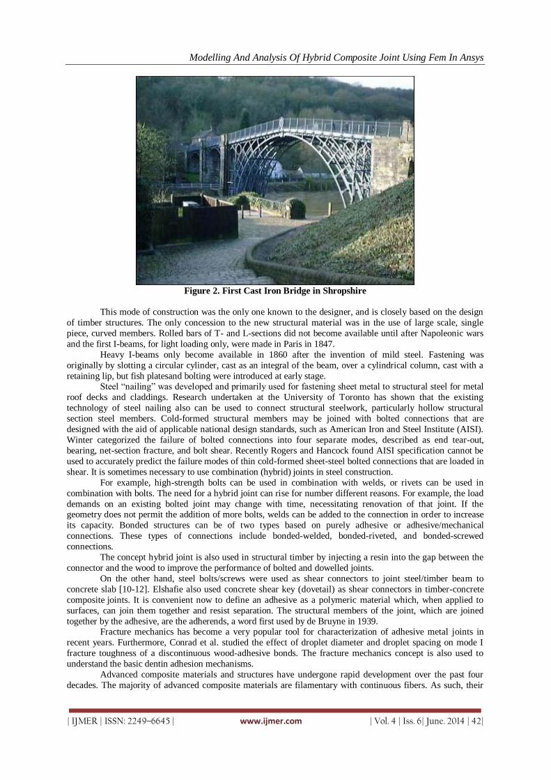
Modelling And Analysis Of Hybrid Composite Joint Using Fem In Ansys
| IJMER | ISSN: 2249–6645 | www.ijmer.com | Vol. 4 | Iss. 6| June. 2014 | 42|
Figure 2. First Cast Iron Bridge in Shropshire
This mode of construction was the only one known to the designer, and is closely based on the design
of timber structures. The only concession to the new structural material was in the use of large scale, single
piece, curved members. Rolled bars of T- and L-sections did not become available until after Napoleonic wars
and the first I-beams, for light loading only, were made in Paris in 1847.
Heavy I-beams only become available in 1860 after the invention of mild steel. Fastening was
originally by slotting a circular cylinder, cast as an integral of the beam, over a cylindrical column, cast with a
retaining lip, but fish platesand bolting were introduced at early stage. Steel “nailing” was developed and primarily used for fastening sheet metal to structural steel for metal
roof decks and claddings. Research undertaken at the University of Toronto has shown that the existing
technology of steel nailing also can be used to connect structural steelwork, particularly hollow structural
section steel members. Cold-formed structural members may be joined with bolted connections that are
designed with the aid of applicable national design standards, such as American Iron and Steel Institute (AISI).
Winter categorized the failure of bolted connections into four separate modes, described as end tear-out,
bearing, net-section fracture, and bolt shear. Recently Rogers and Hancock found AISI specification cannot be
used to accurately predict the failure modes of thin cold-formed sheet-steel bolted connections that are loaded in
shear. It is sometimes necessary to use combination (hybrid) joints in steel construction.
For example, high-strength bolts can be used in combination with welds, or rivets can be used in
combination with bolts. The need for a hybrid joint can rise for number different reasons. For example, the load
demands on an existing bolted joint may change with time, necessitating renovation of that joint. If the geometry does not permit the addition of more bolts, welds can be added to the connection in order to increase
its capacity. Bonded structures can be of two types based on purely adhesive or adhesive/mechanical
connections. These types of connections include bonded-welded, bonded-riveted, and bonded-screwed
connections.
The concept hybrid joint is also used in structural timber by injecting a resin into the gap between the
connector and the wood to improve the performance of bolted and dowelled joints.
On the other hand, steel bolts/screws were used as shear connectors to joint steel/timber beam to
concrete slab [10-12]. Elshafie also used concrete shear key (dovetail) as shear connectors in timber-concrete
composite joints. It is convenient now to define an adhesive as a polymeric material which, when applied to
surfaces, can join them together and resist separation. The structural members of the joint, which are joined
together by the adhesive, are the adherends, a word first used by de Bruyne in 1939. Fracture mechanics has become a very popular tool for characterization of adhesive metal joints in
recent years. Furthermore, Conrad et al. studied the effect of droplet diameter and droplet spacing on mode I
fracture toughness of a discontinuous wood-adhesive bonds. The fracture mechanics concept is also used to
understand the basic dentin adhesion mechanisms.
Advanced composite materials and structures have undergone rapid development over the past four
decades. The majority of advanced composite materials are filamentary with continuous fibers. As such, their

Modelling And Analysis Of Hybrid Composite Joint Using Fem In Ansys
| IJMER | ISSN: 2249–6645 | www.ijmer.com | Vol. 4 | Iss. 6| June. 2014 | 43|
behavior and the behavior of structures made from them are more complicated than that of monolithic materials
and their structures.
Advanced composite materials can be divided into classes in various manners. One simple
classification scheme is to separate them according to the reinforcement forms- particulate-reinforced, fiber-
reinforced, or laminarcomposites. Fiber-reinforced composites, can be further divided into those containing
discontinuous or continuous fibers. Polymers, ceramics, and metals are all used as matrix materials, depending
on the particular requirements. The matrix holds the fibers together in structural unit and protects them from external damage, transfers and distributes the applied loads to the fibers, and in many cases contributes some
needed property such as ductility, toughness, or electrical insulation.
The structure of polymers consists of long molecules with a backbone of carbon atoms linked by
covalent bonds. In non-crystalline or amorphous polymers the molecular chains have an entirely random
orientation and are cross-linked occasionally by a few strong covalent bonds and numerous but weaker van der
Waals bonds. These weaker bonds break as the temperature reaches a value known as the glass transition
temperature, Tg, characteristic for each polymer. Below T
gthe polymer behaves as a linear elastic solid.
Creep becomes increasingly significant as the temperature increases and, above Tg, the polymer
deforms in a viscous manner under load. In crystalline polymers the molecules are oriented along preferred
directions, bringing with them optical and mechanical anisotropy. Polymers are described as being either
thermosets (e.g., epoxy, polyester, SiC, SiN, ZrO), have a wide range of engineering applications. The strong ionic and covalent nature of the bonding in most ceramics leads to a stable crystal structure
with a high melting point and high stiffness. Many ceramic materials have very high elastic moduli and
strengths, but the advantages of these properties bestow are often outweighed by their highly brittle nature,
which leads to low and unpredictable failure stress resulting from the presence of flaws.
Metal matrix composites typically comprise a light metallic alloy matrix, usually based on aluminum,
magnesium or titanium alloys. The major reinforcing elements used in composites are glass, carbon/graphite,
organic, and ceramic.
Both metal and ceramic materials have properties closer to those of likely reinforcements and this
leads to a different choice of properties for which these composite systems are optimized.
With polymer matrix composites, it is almost true to say that the properties of the composite are
essentially those of the fibers, with little contribution from the properties of the matrix. phenolic) or
thermoplastics (e.g., polyimide, polysulfone, polyetheretherketone, polyphenylenesulfide). Ceramics, such as glasses, cement & concrete, and engineering ceramics(Al
2O
3).
FiberReinforced Polymer (FRP), earlier limited to aerospace structures, are gaining acceptance in civil
engineering applications also. FRP plates, sheets, rebar, and strands have been increasingly used in the
construction industry due to their superior properties.
One of the potential structural applications of FRP composites with concrete or steel structures is strengthening of RC or steel beams with unidirectional fiber-composite sheets/plates bonded on their tension
faces via the use of epoxy adhesives.
Growing maintenance and durability problems in transportation infrastructure have led researchers to
explore FRP box-girder, I-beam, or other shapes in bridges. There are numerous examples of completed all-
composite new bridges and several more are under construction.
Due to the relatively low weight and high strength of FRP girders and decks it has proven to be
efficient to replace old bridges that no longer meet today’s requirements with FRP alternatives. While design
concepts vary, several systems employ a modular system to build up the bridge deck, meaning that composite
profiles are transversely joined to form the required bridge span or occasionally width. Kumar et al. installed an
all-composite bridge deck made up of FRP.
. III. Snap Joint in Composite Structures
In the majority of the composite structural components, both bolted and/or adhesive bonded joint was
used. Most of the details are similar to those for metal joints. It was shown from extensive testing on bolted
composite joints that failure always occurs in a catastrophic manner due to high stress concentration developed
at the bolt locations.
Due to the inherent low bearing and interlaminar shear strengths of composites, these stress
concentrations threaten the downfall of every piece of the composite structure [86-87]. The optimum composite
joint design is the one capable of distributing stresses over a wide area rather than to concentrate them at a
point. Adhesively bonded joints can satisfy these requirements, however, most of the adhesives are brittle, and
brittle failure is unavoidable. This was the motivation of developing what is called the SNAP joint.

Modelling And Analysis Of Hybrid Composite Joint Using Fem In Ansys
| IJMER | ISSN: 2249–6645 | www.ijmer.com | Vol. 4 | Iss. 6| June. 2014 | 44|
Figure3.1 Snap Joint
The snap joint technology developed by W. Brandt Goldworthy& Associates, Inc. The concept is
based on similar joining technology used for connecting wooden parts. Also, this technique is very similar to
techniques which were used a decade or so again for plastic. Figure 4-1 shows a pultruded structural composite
member (A) with one end shaped as a fir-tree, and therefore has a large load bearing area.
In this figure, part (A) has been snapped into another structural shape (B). From Fig. 4-1 one can see
that, the later shape has been designed to combine its structural shape with functionality that allows or the
engagement of the load-bearing surface of member (A). It is possible to "snap" joint both parts together since
part (A) has been cut for a short distance along it length to provide enough lateral flexibility to move out of the
way when entering part (B). In order to make this joining concept successful, the fiber architecture of part (A)
must be designed in such a way that the load bearing surfaces have higher inter-laminar shear strength capacity.
Also, it can be noticed from the figure, that a circular hole was introduced at the end of the horizontal slot of
part (A) to inhibit the crack propagation along the length of the pultruded member. The applications of this technology in composite structures will have benefits as follow:
• The structures are easy to assembly.
• Installation of structure members become faster.
• Installation needs smaller number of labor and equipment.
• Since it use composite materials, its weight is less than traditional structures.
The first prototype or "Demonstration project" using this joining method was in designing and
construction of three Transmission Tower Structures, near Los Angeles by W. Brandt Goldworthy& Associates,
Inc. and Ebert Composites Corporation. Through California Department of Transportation, they have proposed
the design and the construction of a truss structure to carry highway singes. The snap joining technique is
considered to be one of the optimum techniques to join composite structural members. However, it has a major
limitation, and can only be used in specific applications. That is, this method can only be used to transmit axial loads, which make it ideal for truss-type structures.
However, in my opinion, this method should NOT be recommended when out-of-plane loads or any
shear loads are introduced since the connection is not design to carry any major bending moments. Under
flexural loads, it is expected that the joint will be very flexible, and the artificial cracks introduced to members
will propagate and a complete failure will occur even under moderate service flexural and/or shear loading.
Figure 3.2 Snap Joint Projects

Modelling And Analysis Of Hybrid Composite Joint Using Fem In Ansys
| IJMER | ISSN: 2249–6645 | www.ijmer.com | Vol. 4 | Iss. 6| June. 2014 | 45|
IV. Hybrid Joints
In an attempt to improve the joint strength of composite materials, a hybrid of adhesive and bolted
joints has also been explored [88], Fig. 5-1. Hybrid joints failed at a higher load than the bolted joints and with
the proper clamping torque reached the same failure load as the adhesive joints. Furthermore, unlike the adhesive joints, hybrid joints failed in two steps, first by initiation of fiber tear
(akin to delamination in laminated continuous fiber composites) at one of the lap ends and then by tensile
failure across the bolt hole. This led to a slightly higher overall elongation at failure for specimens with the
hybrid joints.
Failure in fatigue also started by fiber tear and when the fiber tear progressed to the bolted area, a
combination of half-net-tension failure and splitting (cleavage failure) occurred. In both static as well fatigue,
failure was initiated by fiber tear and the round washers with their edges located slightly away from the lap ends
were not effective in preventing fiber tear.
Hybrid joints give better static as well as fatigue performance than adhesive joints in composites when
fibertear, the primary failure mode in adhesive joints, is either prevented or delayed by the presence of
clamping. The presence of the lateral clamping pressure can significantly decrease the maximum peel stress at
the interface, which helps in achieving improved joint performance. The square washer representing full clamping to the edges of the overlap area gives a better performance compared to round washer, representing
partial clamping.
In an attempt to improve the joint strength of composite materials, a hybrid of adhesive and bolted
joints has also been explored, Fig. 5-1. Hybrid joints failed at a higher load than the bolted joints and with the
proper clamping torque reached the same failure load as the adhesive joints. Furthermore, unlike the adhesive
joints, hybrid joints failed in two steps, first by initiation of fiber tear (akin to delamination in laminated
continuous fiber composites) at one of the lap ends and then by tensile failure across the bolt hole.
This led to a slightly higher overall elongation at failure for specimens with the hybrid joints. Failure in
fatigue also started by fiber tear and when the fiber tear progressed to the bolted area, a combination of half-net-
tension failure and splitting (cleavage failure) occurred. In both static as well fatigue, failure was initiated by
fiber tear and the round washers with their edges located slightly away from the lap ends were not effective in preventing fiber tear.
Fu and Mallick found that, hybrid joints give better static as well as fatigue performance than adhesive
joints in structural reaction injection molded composites when fiber tear, the primary failure mode in adhesive
joints, is either prevented or delayed by the presence of clamping. Their finite element analyses proved that the
presence of the lateral clamping pressure can significantly decrease the maximum peel stress at the interface,
which helps in achieving improved joint performance.
Figure 4 Sketch of an Adhesive/Bolted (Hybrid) Joint
V. Conclusion
In this analysis, FEA for the prediction of stress distribute on in bonded, riveted and hybrid joints
have been carried out 3D models were created by using PROE (creoparametric) and analyzed using ANSYS
workbench FEA software .shear stress was used to compared the results with three joining methods. The shear
stress with hybrid joint has less value of stress and also the carbon Fiber reinforced plastic is more strength than
any other composite material. The stress induced by using ANSYS is less than the material ultimate stress and
ultimate limit. The total deformation for both the materials in hybrid joint is less. It was found that a well
designed hybrid joint is very efficient when compared to bonded, riveted joints in case of repair situation in
aircraft fuselage panels, structures etc.

Modelling And Analysis Of Hybrid Composite Joint Using Fem In Ansys
| IJMER | ISSN: 2249–6645 | www.ijmer.com | Vol. 4 | Iss. 6| June. 2014 | 46|
REFERENCES [1]. Noah M. Salih1, Mahesh J. Patil 2, Hybrid (Bonded/Bolted) Composite Single-Lap Joints And Its Load Transfer
Analysis, International Journal of Advanced Engineering Technology E-ISSN 0976-3945 IJAET/Vol.III/ Issue I/January-March, 2012/213-216.
[2]. Ch. Aswini Kumar1, G. Pattabhi2, S.Santosh3, I. Bhanu Latha4, Analysis of Adhesively Bonded Double Lap Joint in Laminated FRP Composites Subjected To Longitudinal Loading, international journal of engineering science & advanced technology volume-2, issue-2, 307 – 316 ijesat | Mar-Apr 2012.
[3]. Vincentcaccesse, Richard newer, until s. vel detection of bolt load loss in hybrid composite.metal bolted connections
elseiver engineering structures 26(2004) 895-906. [4]. W. Hufenbach a, L.A. Dobrzański b, M. Gude a, J. Konieczny b, A. Czulak a, Optimisation of the rivet joints of the
CFRP Composite material and aluminum alloy, Journal of Achievements in Materials and Manufacturing Engineering, volume 20 issues 1-2 January-February 2007.
[5]. M.A. McCarthy*, C.T. McCarthy, Finite Element Analysis Of The Effects Of clearance On Single-Shear, Composite Bolted Joints, Journal of Plastics, Rubber and Composites, The Institute of Materials, London, UK, Vol. 32, No. 2, in-press.
[6]. Proceedings of the “National Conference on Emerging Trends In Mechanical Engineering 2k13” 122 NCETIME –
2k13 Design Of Hybrid Composite Joints For Research Area S. Lokesha and H. Mohitaa Student, Refrigeration and Air Conditioning Division, Department of Mechanical Engineering, College of Engineering, Anna University, Chennai-28.

International
OPEN ACCESS Journal
Of Modern Engineering Research (IJMER)
| IJMER | ISSN: 2249–6645 | www.ijmer.com | Vol. 4 | Iss. 6| June. 2014 | 47|
Automatic Image Segmentation Using Wavelet Transform Based
On Normalized Graph Cut
Prof. S.N. Dandare1, Niraj N. Kant2 1, 2 (Associate Professor, Student, (Babasaheb Naik College of Engineering, Pusad (M.S.))
I. INTRODUCTION In image processing the input is an image and the output is either an image or parameters related to
the image is used to solve identification problems, such as forensic medicine or creating weather maps from
satellite pictures. Image segmentation is a process of extracting and representing information from an image in
order to group pixels together into regions of similarity. Image segmentation is classified into three categories
viz.
i) Manual i.e., supervised or interactive in which the pixels belonging to the same intensity range
pointed out manually and segmented, the disadvantage is that it consumes more time if the image is large.
ii) Automatic i.e., unsupervised which is more complex and algorithms need some priori information
such as probability of the objects having a special distribution to carry out the segmentation.
iii) Semi-automatic is the combination of manual and automatic segmentation [1]. The pixel intensity
based image segmentation is obtained using Histogram-Based method, Edge-Based method, Region-Based
method and Model-Based method. Model-Based segmentation algorithms are more efficient compared to other
methods as they are dependent on suitable probability distribution attributed to the pixel intensities in the
entire image[2]. To achieve close approximation to the realistic situations, the pixel intensities in each region
follow Generalized Gaussian Distribution (GGD). Some of the practical applications of image segmentation
are Medical Imaging to locate tumors and other pathologies, locate objects in satellite images viz., roads,
forests, etc., automated-recognition system to inspect the electronic assemblies, biometrics, automatic traffic
controlling systems, machine vision, separate and track regions appearing in consequent frames of an image
sequence and real time mobile robot applications employing vision systems [3][4].
Image segmentation plays an important role in biometrics as it is the first step in image processing
and pattern recognition. Model based algorithms are used for efficient segmentation of images where intensity
is the prime feature. The problem of random initialization is overcome by using Histogram based estimation
[2]. The Wavelet transform solves the problem of resolution which can indicate the signal without information
loss and reduces the complexity. The segmentation is faster since approximation band coefficients of DWT are
considered [1].
This paper, introduced Wavelet based on normalized graph cut method concept for image
segmentation which may easy way by considering approximation band of an image which is small in
dimensions and contains significant information of original image. The initial parameters and final parameters
are obtained by applying Histogram based algorithm and Expectation and Maximization algorithm respectively
[5]. GGD model is constructed and segmented by Maximum Likelihood estimation of each approximation
coefficient.
Abstract: Model-Based image segmentation plays an important role in image analysis and image
retrieval. To analyze the features of the image, model based segmentation algorithm will be more
efficient. This paper, proposed Automatic Image Segmentation using Wavelets (AISWT) based on
normalized graph cut method to make segmentation simpler. Discrete Wavelet Transform is considered
for segmentation which contains significant information of the input for the approximation band of image.
The Histogram based algorithm is used to obtain the number of regions and the initial parameters like
mean, variance and mixing factor.
Keywords: Discrete Wavelets, Image Segmentation, Histogram, Generalized Gaussian Distribution, EM
Algorithm, ML Estimation.

Automatic Image Segmentation using Wavelet Transform Based on Normalized Graph Cut
| IJMER | ISSN: 2249–6645 | www.ijmer.com | Vol. 4 | Iss. 6| June. 2014 | 48|
II. WAVELET TRANSFORM In this section the paper discussed definitions and AISWT model
A. Definitions:
i. Mean: The average intensity of a region is defined as the mean of the pixel intensities within that region.
The mean μz of the intensities over M pixels within a region K is given by Equation (1)
µz =
_
(1)
Alternatively, we can use formulation based on then normalized intensity histogram p(zi) where i=0,1,2,…,L-1
and L is the number of possible intensity values as given by Equation (2)
µ = p( ) (2)
ii. Variance: The variance of the intensities within a region K with M pixels is given by Equation (3).
=
(3)
Using histogram formulation the variance is given by Equation (4)
= p( ) (4)
iii. Probability Distribution Function (PDF) of the intensities: The PDF P(z), is the probability that an intensity
chosen from the region is less than or equal to a given intensity value z. As z increases from -∞ to +∞, P (z)
increases from 0 to 1. P(z) is monotonic, non-decreasing in z and thus dP/dz ≥ 0.
iv. Shaping parameter P: Shaping parameter defines the Preakness of the distribution which varies from 1 to
∞. The GGD becomes Laplacian Distribution if P = 1, Gaussian distribution if P=2 and Uniform Distribution if
P→ +∞.
v. Computational Time: Time required for the Execution of the algorithm.
III. BLOCK DIAGRAM OF AISWT The Figure 1 gives the block diagram of AISWT
1. Input image:
The input images are of different formats, sizes and types. The image pixel intensity in the entire
image is a Random Variable and follows a GGD.
2. DWT:
The Wavelet Transform is created by repeatedly filtering the image coefficients on a row by row and
column by column basis. A two-dimensional DWT decomposition of image contains various band information
such as low-low frequency approximation band, high-low frequency vertical detail band, low-high frequency
horizontal detail band and high-high frequency diagonal detail band. We assume each coefficient of
approximation band is a Random Variable z and also follow GGD. The approximation band is used for the
segmentation purpose, which is quarter the size and has significant information of the original image. Hence
the computation time required reduces.
3. Initial parameters Estimation:
Initial parameters like mean μ, variance σ and mixing parameter α are determined using Histogram
based initial estimation which is a clustering algorithm. The initial parameters are calculated in two steps:
i) Histogram is constructed by dividing approximation band coefficients into intervals and counting the
number of elements in each subspace, which is called as bin. The K highest density bins are selected and the
average of the observed elements belonging to the bins is calculated to derive a Centroid. If K centroids are not
obtained because of narrow intervals, the Histogram is rebuilt using wider intervals and the centroids are
recalculated.

Automatic Image Segmentation using Wavelet Transform Based on Normalized Graph Cut
| IJMER | ISSN: 2249–6645 | www.ijmer.com | Vol. 4 | Iss. 6| June. 2014 | 49|
ii) The minimum distance clustering is used to label all the observed elements by calculating the distance D
between each centroid and all the elements of the histogram as given in Equation (5)
Dj= min||Ci – Yj|| (5)
Where
Ci is ith centroid for i = 1 to K
Dj is minimum distance between Ci and jth element Yj for j= 1 to N.
The Histogram based initial estimation do not use random selection for initial parameters, thus the method is
stable and useful for unsupervised image segmentation applications. The obtained mean, variance and mixing
parameter for the k regions are considered as the initial parameters for EM algorithm.
IV. Shaping parameter P:
The Shaping parameter defines the peakness of the distribution. In GGD, the three parameters mean,
variance and shaping parameter determines the PDF. The optimal shaping parameter [22, 23] is determined
using initial parameters and the absolute mean value E [ ] . The absolute mean is given by Equation (6)
E [ ] = (6)
P is estimated using Equation (7)
P = M −1(ρ) (7)
Where ρ is given by
ρ =
M is the Generalized Gaussian ratio function given by Equation (8)
M(ρ) =
IV. BLOCK DIAGRAM OF AISWT

Automatic Image Segmentation using Wavelet Transform Based on Normalized Graph Cut
| IJMER | ISSN: 2249–6645 | www.ijmer.com | Vol. 4 | Iss. 6| June. 2014 | 50|
V. RESULTS Here we have used model based segmentation algorithm to increase the efficiency of the segmentation
process. Automatic Image Segmentation using Wavelet Transform (AISWT) based on normalized graph cut
method is applied on image having significant information of the input image & observed that larger images
can be easily segmented. Original image, preprocessed image with partitioned image is as shown below
Originals image with its Segmented parts
preprocessed image.
VI. CONCLUSION This paper gives easy segmentation algorithm AISWT using normalized graph cut method. The
approximation band of an image DWT is considered. The initial parameters are estimated using Histogram
based method. Through EM algorithm, the final parameters are obtained. The segmentation is done by ML
estimation. The AISWT algorithm is computationally efficient for segmentation of large images and performs
much superior to the earlier image.
REFERENCES [1] H C Sateesh Kumar, K B Raja, Venugopal K R, L M Patnaik, “Automatic Image Segmentation using Wavelets,”
IJCSNS International Journal of Computer Science and Network Security, VOL.9 No.2, February 2009
[2] Z. Shi and V. Govindaraju, “Historical Handwritten Document Image Segmentation using Background Light
Intensity Normalization,” SPIE Proceedings on Center of Excellence for Document Analysis and Recognition,
Document Recognition and Retrieval, vol. 5676, pp. 167-174, January 2005.
[3] J. A. D. Molina and R. M. R. Dagnino, “A Practical Procedure to Estimate the Shape Parameters in the
Generalized Gaussian Distribution,” IEEE Transactions on Image Processing, pp. 1-18, 2003.
[4] K. Sharifi and A. L. Garcia, “Estimation of Shape Parameter for Generalized Gaussian Distribution in Subband
Decomposition of video,” IEEE Transactions on Circuits and Systems for Video Technology, vol. 5, no.1, pp. 52-
56,1995.
[5] T. Yamazaki, “Introduction of EM Algorithm into Color Image Segmentation,” Proceedings of International
Conference on Intelligent Processing Systems, pp. 368-371,1998.
[6] E. Sharon, A. Brandt and R. Basri, “Fast Multi-Scale Image Segmentation,” Proceedings of the IEEE Conference
on Computer Vision and Pattern Recognition, vol. 1, pp. 70-77, 2000.
[7] P. V. G. D. Prasad Reddy, K. Srinivas Rao and S. Yarramalle, “Unsupervised Image Segmentation Method
Hungarian Joint Symposium on Applied Machine Intelligence and Informatics, pp. 313-317, Januar 2007.\
[8] P. F. Felzenswalb and D. P. Huttenlocher, “Efficient Graph- Based Image Segmentation,” Proceedings of
International Journal of Computer Vision, vol. 59, no. 2, pp. 167-181,2004.
[9] J. Shi and J. Malik, “Normalized Cuts and Image Segmentation,” IEEE Transactions on Pattern Analysis and
Machine Intelligence, vol. 22, no. 8, pp. 888-905, 2000.
[10] W. Cai, J. Wu and A. C. S. Chung, “Shape-Based Image Segmentation using Normalized Cuts,” proceedings
ofThirteenth International Conference on Image Processing,pp. 1101-1104, October 2006.
[11] T. Geraud, P. Y. Strub and J. Darbon, “Color Image Segmentation based on Automatic Morphological Clustering,”
Proceedings of IEEE International Conference on Image Processing, vol. 3, pp. 70-73, October 2001.
[12] M. Ozden and E. Polat, “Image Segmentation using Color and Texture Features,” Proceedings of Thirteenth
European Signal Processing Conference, September 2005.

International
OPEN ACCESS Journal Of Modern Engineering Research (IJMER)
| IJMER | ISSN: 2249–6645 | www.ijmer.com | Vol. 4 | Iss. 6| June. 2014 | 51|
Prediction of Deflection and Stresses of Laminated Composite
Plate with Artificial Neural Network Aid
T.Subramani1, S.Sharmila
2
1Professor & Dean, Department of Civil Engineering, VMKV Engg. College, Vinayaka Missions University,
Salem, India. 2PG Student of Structural Engineering, Department of Civil Engineering, VMKV Engg.College,Vinayaka
Missions University, Salem, India
I. Introduction
Composite materials are particularly attractive to aviation and aerospace applications because of their
exceptional strength and stiffness-to-density ratios and superior physical properties. The mechanical behavior of a laminate is strongly dependent on the fiber directions and because of that; the laminate should be designed to
meet the specific requirements of each particular application in order to obtain the maximum advantages of such
materials. Usually, laminated composite materials are fabricated from unidirectional plies of giving thickness
and with fiber orientations limited to a small set of angles, eg., 0o, 45o, -45o and 90o.
A true understanding of their structural behaviour is required, such as the deflections, buckling loads
and modal characteristics, the through thickness distributions of stresses and strains, the large deflection
behaviour and, of extreme importance for obtaining strong, reliable multi-layered structures, the failure
characteristics. In the past, the structural behaviour of plates and shells using the finite element method has been
studied by a variety of approaches. Choudhary and Tungikaranalyzed the geometrically nonlinear behavior of
laminated composite plates using the finite element analysis.
They studied the effect of number of layers, effect of degree of orthotropy (both symmetric and
antisymmetric) and different fibre orientations on central deflections. Ganapathiet al. presented an eight-node C0 membrane-plate quadrilateral finite element-based on the Reissner-Mindlin plate theory to analyse
moderately large deflection, static and dynamic problems of moderately thick laminates including buckling
analysis and membrane-plate coupling effects. Han et al. used the hierarchical finite element method to carry
out the geometrically nonlinear analysis of laminated composite rectangular plates. Based on the first-order
shear deformation theory and Timoshenko’s laminated composite beam functions, the current authors
developed a unified formulation of a simple displacement based 3-node, 18degree-of-freedom flat triangular
plate/shell element and two simple, accurate, shear-flexible displacement based 4-node quadrilateral elements
and for linear and geometrically nonlinear analysis of thin to moderately thick laminated composite plates.
The deflection and rotation functions of the element boundary were obtained from Timoshenko’s
laminated composite beam functions. Raja Sekhara Reddy et al. applied the artificial neural networks (ANN) in
predicting the natural frequency of laminated composite plates under clamped boundary condition. They used the D-optimal design in the design of experiments to carry out the finite element analysis. WEN etal.used the
finite element method to predict the damage level of the materials.
They studied the prediction of the elastic-plastic damage and creep damage using Gurson model and
creep damage model, which is based on the Kachanov-Rabothov continuum creep damage law. They also
studied the creep damage properties of thin film/substrate systems by bending creep tests and carried the
Simulation of the interface characterization of thin film/substrate systems.
Abstract: This paper discusses the use of D-optimal designs in the design of experiments (DOE) and
artificial neural networks (ANN) in predicting the deflection and stresses of carbon fibre reinforced plastic (CFRP) square laminated composite plate subjected to uniformly distributed load. For training
and testing of the ANN model, a number of finite element analyses have been carried out using D-
optimal designs by varying the fiber orientations and thickness of each lamina. The composite plate is
modeled using shell 99 elements. The ANN model has been developed using multilayer perceptron
(MLP) back propagation algorithm. The adequacy of the developed model is verified by root mean
square error and regression coefficient. The results showed that the training algorithm of back
propagation was sufficient enough in predicting the deflection and stresses.
Keywords: D-Optimal designs, Finite Element Method, Artificial neural network, Multilayer
perception.

Prediction Of Deflection And Stresses Of Laminated Composite Plate With Artificial Neural Network
| IJMER | ISSN: 2249–6645 | www.ijmer.com | Vol. 4 | Iss. 6| June. 2014 | 52|
Reddy et al employed a distance-based optimal design in the design of experimental techniques and
artificial neural networks to optimize the stacking sequence for a sixteen ply simply supported square laminated
composite plate under uniformly distributed load (UDL) for minimizing the deflections and stresses using finite
element method. Therefore the finite element method is especially versatile and efficient for the analysis of
complex structural behavior of the composite laminated structures.
The present study proposes a new experimental design method for selection of practical laminates and
thickness of each ply for a criterion of a response. This method employs D-optimality for selections from a set of feasible laminates. This method is applied to a 10 layer laminate to predict the deflection and stresses of a
composite plate subjected to a uniform distributed load under simply supported boundary condition and an
artificial neural network model has been developed to predict the same.
II. Material and Methods
The material used to model the physical structure of the laminated composite plate is carbon fibre
reinforced plastic (CFRP). The material properties are as follows:
E1=220GPa, E2=6.9GPa, E3=6.9GPa, G12=G23=G13=4.8GPa, v12=0.25, Vf=0.6.
The methodology adopted in predicting the deflections and stresses using the integrated approach.
2.1. Geometry of the shell 99 element
In this study to model the laminated composite plate the finite element analysis software ANSYS has
been used. In ANSYS software, there are many element types available to model layered composite materials.
In our FE analysis, the linear layered structural shell element (Shell 99) is used. It is designed to model thin to
moderately thick plate and shell structures with a side-to-thickness ratio of roughly 10 or greater.
The linear layered structural shell element allows a total of 250 uniform-thickness layers.
Alternatively, the element allows 125 layers with thicknesses that may vary bilinearly over the area of the layer.
An accurate representation of irregular domains (i.e. domains with curved boundaries) can be accomplished by
the use of refined meshes and/or irregularly shaped elements.
For example, a non-rectangular region cannot be represented using only rectangular elements; however, it can be represented by triangular and quadrilateral elements. Since, it is easy to derive the
interpolation functions for a rectangular element, and it is much easier to evaluate the integrals over rectangular
geometries than over irregular geometries, it is practical to use quadrilateral elements with straight or curved
side assuming you have a means to generate interpolation functions and evaluate their integrals over the
quadrilateral elements. The linear layered structural shell element is shown in Figure. 2.1 Nodes are represented
by I, J, K, L, M, N, O, and P.
Figure 2.1 Geometry of 8-node element with six degrees of freedom
2.2 Design of experiments
Design of Experiments (DOE) is a mathematical methodology that defines an optimal set of
experiments in the design space, in order to obtain the most relevant information possible with the highest accuracy at the lowest cost. This scientific exploration of the design space replaces a tedious, manual, trial-and-
error process, and is the fastest way to acquire the most relevant information with minimum computational
effort.
Traditional experimental designs (Full Factorial Designs, Fractional Factorial Designs, and Response
Surface Designs) are appropriate for calibrating linear models in experimental settings where factors are
relatively unconstrained in the region of interest. In some cases, however, models are necessarily nonlinear.
In other cases, certain treatments (combinations of factor levels) may be expensive or infeasible to
measure. D-optimal designs are model-specific designs that address these limitations of traditional designs. The
D-optimality criterion states that the best set of points in the experiment maximizes the determinant | X T X |.
"D" stands for the determinant of the X matrix associated with the model.

Prediction Of Deflection And Stresses Of Laminated Composite Plate With Artificial Neural Network
| IJMER | ISSN: 2249–6645 | www.ijmer.com | Vol. 4 | Iss. 6| June. 2014 | 53|
A D-optimal design is generated by an iterative search algorithm and seeks to minimize the covariance
of the parameter estimates for a specified model. This is equivalent to maximizing the determinant D=|XT X|,
where X is the design matrix of model terms (the columns) evaluated at specific treatments in the design space
(the rows).
Unlike traditional designs, D-optimal designs do not require orthogonal design matrices, and as a
result, parameter estimates may be correlated. Parameter estimates may also be locally, but not globally, D-
optimal. The D-optimal design uses the row-exchange and Co-ordinate exchange algorithms to generate the optimal designs [16]. A related measure of the moment matrix (X T X/k) is the D-efficiency and can be
calculated by using the following expression:
where
ND is the number of points in the design and p is the number of effects in the model including the
intercept. If all variables are normalized so that they vary from -1 to 1, then the maximum value of the Deffis 1. Furthermore, the quality of the set of points can then be measured by Deff..
2.3 Artificial neural networks
An Artificial Neural Network (ANN) is an information processing paradigm that is inspired b the way
biological nervous systems, such as the brain, process information. It resembles the human brain in two aspects:
the knowledge is acquired by the network through a learning process, and inter neuron connection strengths
known as synaptic weights are used to store the knowledge.
A typical biological neuron collects signals from others through a host of fine structures called
dendrites. The neuron sends out spikes of electrical activity through a long, thin stand known as an axon, which
splits into thousands of branches. At the end of each branch, a structure called a synapse converts the activity
from the axon into electrical effects that inhibit or excite activity from the axon into electrical effects that inhibit or excite activity in the connected neurons.
When a neuron receives excitatory input that is sufficiently large compared with its inhibitory input, it
sends a spike of electrical activity down its axon. Learning occurs by changing the effectiveness of the synapses
so that the influence of one neuron on other changes. A biological neuron and artificial neuron are shown in.
figure 2.3.1 and figure 2.3.2.
.
Figure2. 3.1 Simplified model of a biological Neuron Figure 2.3.2 artificial neuron model
III. Finite Element Analysis
3.1. Validation of linear layered structural shell element-a case study
In order to validate the usage of the linear layered structural shell element, a numerical example is
solved in static analysis. The boundary condition is simply supported and the geometry and material properties are as follows:
E1/E2=40, G12=G13=0.6E2, G23=0.5E2,V12= 0.25 , a/h=10, a=1, q=1.0.
The center deflection and stresses are presented here in non-dimensional form using the following:

Prediction Of Deflection And Stresses Of Laminated Composite Plate With Artificial Neural Network
| IJMER | ISSN: 2249–6645 | www.ijmer.com | Vol. 4 | Iss. 6| June. 2014 | 54|
Table 3.1 and Table3.2 represents the mesh convergence study and comparison of results of non-
dimensional displacement obtained from Reddy and the ANSYS computer program.The results using a free
mesh show an excellent correlation to the results given by Reddy.
Table 3.1 Nondimensional displacement of Table 3.2 Nondimensional displacement of
composite plates (cross- ply) composite plates (θ/- θ/ θ/- θ
IV. Results and Discussion
4.1. Development of ANN model
One of the key issues when designing a particular neural network is to calculate proper weights for
neuronal activities. These are obtained from the training process applied to the given neural network. To that
end, a training sample is provided, i.e. A sample of observations consisting of inputs and their respective
outputs. The observations are fed to the network. In the training process the algorithm is used to calculate neuronal weights, so that the root mean squared error between the calculated outputs and observed outputs from
the training set is minimized.
4.2. Neural network training
To calculate the connection weights, a set of desired network output values is needed. Desired output
values are called the training data set. The training data set in this study was selected based on a D-optimal
design in the design of experiments. In this study, 322 data sets were used for training, 80 data set were for
validation and 20data set were used for testing the network
respectively.
For calculation of weight variables, often referred to as network training. To get the best prediction by
the network, several architectures were evaluated and trained using the finite element analyses data. A network
with one hidden layer and 30 neurons provided to be an optimum ANN. The performance of the network (RMSE and Regression coefficient (R2)) with the number of neurons is shown in Figure.4.1.
Figure 4.1 Root-mean square vs. number of neurons for nondimensional displacement
V. Neural Network Validation
Once the weights are adjusted the performance of the trained network was validated and tested with the
finite element analyses which were never used in the training process. Validation set is a part of the data used to
tune the network topology or network parameters other than weights. It is used to define the number of hidden
units to detect the moment when the predictive ability of neural network started to deteriorate.
One method, k-fold cross validation, is used to determine the best model complexity, such as the depth
of a decision tree or the number of hidden units in a neural network. The method of k-fold cross validation
partitions the training set into k sets. For each model complexity, the learner trains k times, each time using one

Prediction Of Deflection And Stresses Of Laminated Composite Plate With Artificial Neural Network
| IJMER | ISSN: 2249–6645 | www.ijmer.com | Vol. 4 | Iss. 6| June. 2014 | 55|
of the sets as the validation set and the remaining sets as the training set. It then selects the model complexity
that has the smallest average error on the validation set (averaging over the k runs).
5.1 Neural network testing
The ANN predicted results are in very good agreement with experimental results and the network can
be used for testing. Hence the test data sets are applied to the network, which were never used in the training
process and is presented in Table. 5.1. The test set is a part of the input data set used only to test how well the neural network will predict on
new data. The results predicted by the network were compared with the finite element results and shown in
Figure. The regression coefficients for deflection and stresses (Sx, Sy, Sxy) were found to be 0.882, 0.983,
0.993 and 0.999 respectively.
Table. 5.1. ANN predicted results
VI. Ansys Analysis Report
The laminated plate is subjected to deflection and stresses and analysed using ANSYS. The ANSYS
analysis report are shown from figure 6.1 to6.7.
Figure 6.1 Meshed Element Figure 6.2 laminated plate deformed shape
Figure 6.3 laminated plate DOF Figure 6.4 laminated plate DOF 1

Prediction Of Deflection And Stresses Of Laminated Composite Plate With Artificial Neural Network
| IJMER | ISSN: 2249–6645 | www.ijmer.com | Vol. 4 | Iss. 6| June. 2014 | 56|
Figure 6.5 laminated plate strain intensity Figure 6.6 laminated plate stress intensity
Figure 6.7 laminated plate von misses stress intensity
STEEL PLATE
The steel plate is subjected to deflection and stresses and analysed using ANSYS. The ANSYS
analysis report are shown from figure 6.8 to 6.14 .
Figure 6.8 meshed element Figure 6.9 steel plate deform shape
Figure 6.10steel plate DOF Figure 6.11 steel plate DOF 1

Prediction Of Deflection And Stresses Of Laminated Composite Plate With Artificial Neural Network
| IJMER | ISSN: 2249–6645 | www.ijmer.com | Vol. 4 | Iss. 6| June. 2014 | 57|
Figure 6.12 steel plate strain intensity Figure 6.13 steel plate stress intensity
Figure 6.14 steel plate von misses stress
VII. Conclusion
This study presented a new D-optimal set of laminates to model the artificial neural networks for
predicting the deflection and stresses. The ANN predicted results are in very good agreement with the finite
element results. Hence, the D-optimal design of experiments can be applied to any structural analysis.
The D-optimal set of laminates is not limited to 10 ply laminates for changing the ply thickness. It is
applicable to laminates of any number of plies by changing the ply thickness. The effectiveness of the method is
shown with predicting capability to deflection and stresses of laminated composite plates subjected to uniformly
distributed load under simply supported boundary condition.
The two stage effort of obtaining the optimal stacking sequence by a new distance-based optimal
design in design of experiments and artificial neural networks has resulted in fairly useful method for laminated
composite plates. The following conclusions are drawn from the results for laminated composite material plates: The developed ANN model could predict the deflections and stresses (Sx, Sy, and Sxy) with an average
percentage deviation of 0.028875%, 1.587178%, 2.119705% and 3.018923% respectively from training
data set.
The ANN model could predict the deflections and stresses (Sx, Sy, and Sxy) with an average percentage
deviation of 6.132743%, 1.3096766%, 0.0945797% and 5.7492823% respectively from test data set.
The ANN predicted results are very good agreement with the finite element results.
For anti-symmetric laminated composite plates [45/-45]8, the non-dimensional deflection and transverse
shear stress are lower compared to the symmetrical one.
For anti-symmetric laminated composite plates [0/90]8, the Normal stress in x-direction is lower
compared to the symmetrical one.
REFERENCES [1]. Akira, T. and Ishikawa, T. 2004. Design of experiments for stacking sequence optimizations with genetic algorithm
using response surface approximation. Journal of CompositeStructures, 64: 349-357.

Prediction Of Deflection And Stresses Of Laminated Composite Plate With Artificial Neural Network
| IJMER | ISSN: 2249–6645 | www.ijmer.com | Vol. 4 | Iss. 6| June. 2014 | 58|
[2]. Cristovao, M., Soares, M., Carlos, A., Soares, M., Victor, M., and Correia, F. 1997. Optimization of multilaminated structures using higher order deformation models. Journalof Computational Methods in Applied Mechanical Engineering, 149:133-152.
[3]. Choudhary, S. S. and Tungikar, V. B. 2011. A simple finite element for nonlinear analysis of composite plates.
International Journal of Engineering Science and technology, 3(6): 4897-4907. [4]. Ganapathi, M., Polit, O., and Touratier, M. 1996. AC0 eight-node membrane shear-bending element for
geometrically non-linear (static and dynamic) analysis of laminates. International Journal of Numerical Method in Engineering, 39(20): 3453-3474.
[5]. Wanmin, H., Maurice, P., and Hsiao, Kuo-Mo. 1994. Investigation into a geometrically nonlinear analysis of rectangular laminated plates using the hierarchical finite element method. International Journal of Finite Element Analysis and Design, 18(1-3): 273-288.
[6]. Zhang, Y. X. and Kim, K. S. 2005. A simple displacement-based 3-node triangular element for linear and geometrically nonlinear analysis of laminated composite plates. InternationalJournal of Computational Methods in
Applied Mechanical Engineering, 194: 4607-4632. [7]. Zhang, Y. X. and Kim, K. S. 2004. Two simple and efficient displacement-based quadrilateral elements for the
analysis of composite laminated plates. International Journalof Numerical Methods in Engineering, 61: 1771-1796. [8]. Zhang, Y. X. and Kim, K. S. 2006. Geometrically nonlinear analysis of laminated composite plates by two new
displacement-based quadrilateral plate elements. Journal of CompositeStructures, 72(3): 301-310. [9]. Rajasekhara Reddy, M., Sidda Reddy, B., Nageswara Reddy, V., and Sreenivasulu, S. 2012. Prediction of Natural
Frequency of Laminated Composite Plates Using Artificial Neural Networks. Engineering, 4(6): 329-337. [10]. Shifeng, W., Wuzhu, Y., Jianxiong, K., Jun, L., and Zhufeng, Y. 2010. Simulation of the creep damage behavior of
thin film/substrate systems by bending creep tests. Journal ofMaterials & Design, 31(7): 3531-3536. [11]. Shifeng, W., Wuzhu, Y., Jianxiong, K., and Zhufeng, Y. 2010. Simulation of the interface characterization of thin
film/substrate systems using bending creep tests. Journal of AppliedSurface Science, 257(4): 1289-1294. [12]. Ramanjaneya Reddy, A., Sidda Reddy, B., and Vijaya Kumar Reddy, K. 2011. Application of design of experiments
and artificial neural networks for stacking sequence optimizations of laminated composite plates. International Journal on Engineering, Science andTechnology, 3(6): 295-310.
[13]. Baker, A., Dutton, S., and Kelly, D. 2004. “Composite Materials for Aircraft Structures”. 2nd Edition. American Institute of Aeronautics and Astronautics, Inc.1801, Chapter 8, pp. 240.
[14]. ANSYS, 2010. “Theory manual”. [15]. Reddy, J. N. 1997. “Mechanics of Laminated Composite plates”. CRC Press. Florida. [16]. Wang, P.H., Lin, H.T., and Tang, T.Y. (2002). “Study on nonlinear analysis of a highly redundant cable-stayed
bridge.” Computers and Structures, 80(2), 165-182.

International
OPEN ACCESS Journal Of Modern Engineering Research (IJMER)
| IJMER | ISSN: 2249–6645 | www.ijmer.com | Vol. 4 | Iss. 6| June. 2014 | 59|
Design of 8-Bit Comparator Using 45nm CMOS Technology
Ranjeet Kumar1, Prof. S. R. Hirekhan
2
1, 2 (Department of Electronics, Government College of Engineering Aurangabad, India)
I. Introduction Binary comparator is widely used in digital system to compare between two numbers. Binary
comparators are found in a wide variety of circuits, such as microprocessors, communications systems,
encryption devices, and many others. A faster, more power efficient, or more compact comparator would be an advantage in any of these circuits. A circuit that compares two binary numbers is called comparator. It also
decides whether both numbers are equal or not equal.
In this paper, we present two CMOS unsigned binary comparators. Our approaches is first to design 1-
bit comparator as one component and then generate its symbol to design 8-bit comparator.
Here we use Microwind3.1 to draw the layout of the CMOS circuit. Then we extract the spice file in
Microwind3.1 and run under PSPICE to get the simulation.
II. Previous Work
The current mode signal processing using CMOS technology has gained great interesting circuit designing. With the shrinkage of feature size and increasing demand of high speed and low power application,
the current-mode circuit has been considered to be an alternative to voltage-mode circuit. Current comparator is
fundamental component of analog system because of better accuracy, low noise and low power consumption. It
can be used in A/D converters, oscillators, current to frequency converters, VLSI neural network, sensor circuit
and portable wireless communication etc. H. Traff [1] proposed the first high speed, low input impedance
current comparator using a simple inverter. Tarff’s approach has been modified by a number of designs, A. T.
K. Tang et al. [2] and L. Ravezzi et al.[3], where speed increases have been attained at the cost of an increase in
power consumption.
Several previous high-speed comparator designs have been proposed. In all[6]precharged function
block is attached to several feedback transistors which add extra discharge paths, thus reducing the comparator's
delay. However, the precharge period is not utilized for any computation, so the design is not as fast as our high-
speed design, as we will show in the sequel. It is desirable that comparators must provide high speed and low power consumption. Here we need to
design such kind of a comparator which compares the value of two 8-bit numbers and output X becomes to 1
when the first number A is larger than the second number B, output Y becomes to 1 when the two numbers A
and B are equal and Z becomes 1 when both X and Y becomes zeros.
III. 1-Bit Comparator First of all we need to design a 1 bit comparator. We can easily make such a component, 2 bits for
input A and B, and 2 bits for output X and Y. X is one when A is larger than B which means only when A is one
and B is zero will set X to one. And for the Y, only when A and B both become one and zero will it be set. Here we can define.
X as X=A.B’
Y as Y = A.B +A’.B
Z as Z= (A+B)’
Second we draw the Karnaugh-map of 1-bit comparator and find the relationship between the input and the
output.
Abstract: In this paper design of 8- bit binary comparator using 45nm CMOS technology is discussed. This design needs less area and less number of transistors, also discussed about power and execution time. The circuit has three output X, Y and Z. X is active high, when A>B, Y is active high when A=B and Z is active high
when both X and Y are active low. Design 1- bit comparator with the help of precharge gate.The design of 1-bit
comparator has been extended to implement an 8-bit comparator by connecting in series with pass
transistor between them. The design has been implemented in Microwind3.1, is tested successfully and
has been validated using Pspice for different measurable parameter.
Keywords: Power, VLSI, 45nm CMOS technology, area, no of transistors, execution time.

Design Of 8-bit Comparator Using 45nm CMOS Technology
| IJMER | ISSN: 2249–6645 | www.ijmer.com | Vol. 4 | Iss. 6| June. 2014 | 60|
X =A.B’ (When A>B) Y =A.B +A’.B’ (When A=B)
Fig.3.1. Schematic of conventional 1-bit comparator
Fig.3.2. Schematic of 1-bit comparator (proposed)

Design Of 8-bit Comparator Using 45nm CMOS Technology
| IJMER | ISSN: 2249–6645 | www.ijmer.com | Vol. 4 | Iss. 6| June. 2014 | 61|
The layout of one bit comparator in Microwind3.1 isshown in fig.3.3
Fig.3.3. Layout of 1-bit conventional comparator
IV. 4-Bit Comparator
The implementation of 4- bit comparator is easy, byconnecting four 1-bit comparator in series. It
consist off four one bit comparator, one four input OR gate and one NOR gate. It has three outputs X, Y and Z.
Output X becomes high when input A is greater than B (Where A and B is the input), output Y becomes
highwhen both inputs are equal. When both X and Y output are low then in thatcase output Z becomes high.
Fig.4.1.Schematic of 4-bit conventional comparator
The layout of Four- bit comparator in Microwind3.1 isshown in fig.4.2.
Fig.4.2. Layout of 4-bit conventional comparator
In similar way we can design 8-bit comparatorwhich is shown in fig.4.3.

Design Of 8-bit Comparator Using 45nm CMOS Technology
| IJMER | ISSN: 2249–6645 | www.ijmer.com | Vol. 4 | Iss. 6| June. 2014 | 62|
Fig.4.3.Schematic of8-bit conventional comparator
Fig4.4.Layout of 8-bit comparator
V. Design Of 8-Bitcomparator (Proposed) The proposed comparator design consists of a precharged gate with 8pull-down stages connected to 7
intermediate pass-transistors, During the precharge period, (when the clock is low) each stage is precharged to
VDD. In the evaluate period, (when the clock is high) the ithpull-down stack in the circuit will form a discharge
path if Ai > Bi. The XNOR gates attached to the intermediate pass-transistors allow pull-down stack i - 1 to
discharge the output if Ai = Bi. The XNOR gate outputs are computed during the precharge period to avoid any
potential race condition caused by the pass transistors being in the wrong state. The result is that the output
discharges if and only if A > B. Therefore, the output is high if and only if A > B. To determine A = B, the
outputs of all the XNOR gates are ANDed together.
Fig.5.1. Schematic of 8-bit comparator (proposed)

Design Of 8-bit Comparator Using 45nm CMOS Technology
| IJMER | ISSN: 2249–6645 | www.ijmer.com | Vol. 4 | Iss. 6| June. 2014 | 63|
Fig.5.2. Layout of 8-bit comparator (proposed)
VI. Result And Discussion
At the precharged period (clock is deactivate i.e. low) each stage is precharged to VDD. But when clock is high
8th pull-down stack in the circuit will generate discharged path if Ai >Bi.The waveform of 8-bit comparator is
shown in fig.6.1.
Fig.6.1. Waveform of 8-bit comparator (proposed)
So we can say that the output is low (if and only ifA<=B).The output becomes high when input A
becomesgreater than input B.
Bits No of
transistors
Execution Time Power
Dissipation(watts) Are𝑎(𝜇𝑚)2
1 20 0.06 1.32E-12 10.21
4 90 0.16 2.61E-12 68.94
8 178 0.69 8.53E-12 165.16
Table: 6.1Simulation Result for conventional Comparator

Design Of 8-bit Comparator Using 45nm CMOS Technology
| IJMER | ISSN: 2249–6645 | www.ijmer.com | Vol. 4 | Iss. 6| June. 2014 | 64|
Bits No of
transistors
Execution Time Power
Dissipation(watts) Are𝑎(𝜇𝑚)2
1 14 0.08 1.15E-12 7.41
4 59 0.30 4.94E-12 45.14
8 111 0.55 9.54E-12 104.34
Table: 6.2 Simulation Result for 8-bit comparator (proposed)
VII. Conclusion
This paper has described different designs for CMOS binary comparator and show different parameter
like area, power, execution time and number of transistor. This design needs less area and less number of
gates.CMOS circuit is used to construct the comparator by using the logic relation between different
input and output. A Karnaugh map is used to minimize the representation of function..
REFERENCES [1]. H. Traff, “Noval approach to high speed CMOS current comparator,” Electron. Letter, vol. 28, no. 3, pp.
310- 312, Jan.1992.
[2]. A.T K. Tang and C. Toumazou, “High performance CMOS current comparator,” Electron. Letter, vol.
30, pp. 5-6, 1994.
[3]. L. Ravezzi, D. Stoppa and G. F. DallaBetta, “Simple High speed CMOS current comparator,” Electron.
Letter, vol.33, pp.1829-1830, 1997.
[4]. Current Comparator Design,” Electron.Letter, vol. 44, no.3, pp.171-172, Jan. 2008.
[5]. Ding Chengwei, NiuYuechao, “ 3-bit comparator design” Submicron Project, SoC 2005.
[6]. Eric R. Menendez, Dumezie K. Maduikez , Rajesh Garg, and Sunil P. Khatri, “CMOS Comparators for
High Speed and Low Power Applications” 1-4244-9707-X/06 ©2006 IEEE

International
OPEN ACCESS Journal Of Modern Engineering Research (IJMER)
| IJMER | ISSN: 2249–6645 | www.ijmer.com | Vol. 4 | Iss. 6| June. 2014 | 65|
MATLAB Simulink for single phase PWM inverter in an
uninterrupted power supply
V. K. Saxena1, Abhishek Ranjan
2
1Asst. Professor of EEE Department, R.V.S. College of Engineering & technology, Jamshedpur,
2Electrical Engg.Department, NIT Patna, India
I. Introduction In the last few decades, the traditional power generation methods of burning fossil fuels has affected
the environment, causing an increase in the greenhouse gas emissions that lead to global warming.
Consequently, thishas become the driving force for the growing interest in alternative energy [1, 2].However, a
battery inverter system is more preferable and more flexible to operate in stand-alone modeapplications. The
single-phase inverters in stationary battery cell power generation systems have been installedworldwide in case
of utility power failures and are widely used in delivering backup power to critical loads,such as for computers
and life-support systems in hospitals, hotels, office buildings, schools, utility powerplants, and even in airport terminals, as well as in communication systems [5]. Any UPS system has two operating modes: bypass mode
and backup mode. Ideally, a UPSshould be able to deliver a regulated sinusoidal output voltage with low total
harmonic distortion(THD) during the two modes, even when feeding nonlinear loads. The first step is to
generate 5V smooth DC so that microcontroller may be switched ON i.e. regulated DC power supply.
Figure 1: Regulated DC power supply.
This 5v switch ON microcontroller and output of rectifier is given as input to the inverter circuit when
main supply is there and when power is cut then inverter circuit is supplied through 12 v battery and power is
uninterruptedly provided to the user. Circuit diagram of single phase full wave PWM inverter is shown below:
Abstract: Now a day’s Uninterrupted power supply is very necessary for industry, and domestic purpose. This paper presents the design and implementation of UPS for using personal computer. Here solar
energy is used for charging the battery in sunny days and in absence of solar energy it will automatically
connect to main AC supply. Also MATLAB simulation work is done for PWM single phase inverter and
full bridge rectifier.. Here microcontroller is used for switching between solar plate and main AC supply
to Battery. By using this method we can save our electricity bill which is consumed in charging of battery.
Keywords: Single-phase Inverter, Battery cell, Sinusoidal pulse-width-modulation and microcontroller.
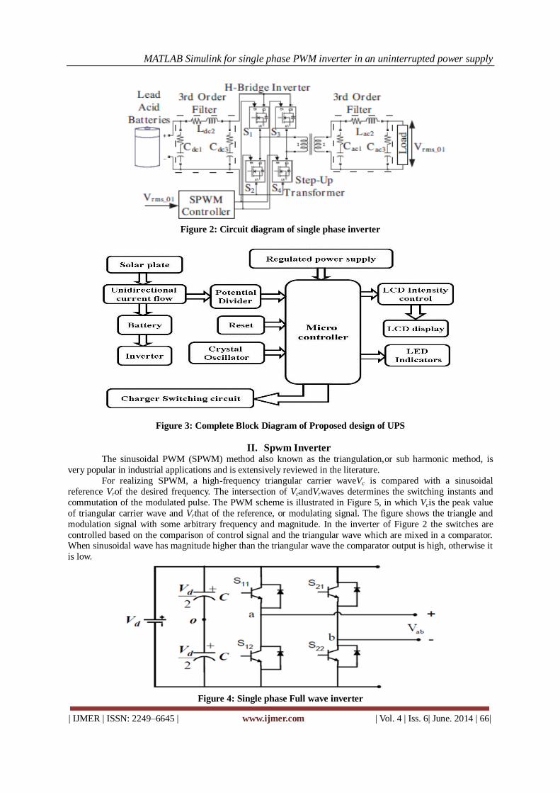
MATLAB Simulink for single phase PWM inverter in an uninterrupted power supply
| IJMER | ISSN: 2249–6645 | www.ijmer.com | Vol. 4 | Iss. 6| June. 2014 | 66|
Figure 2: Circuit diagram of single phase inverter
Figure 3: Complete Block Diagram of Proposed design of UPS
II. Spwm Inverter The sinusoidal PWM (SPWM) method also known as the triangulation,or sub harmonic method, is
very popular in industrial applications and is extensively reviewed in the literature.
For realizing SPWM, a high-frequency triangular carrier waveVc is compared with a sinusoidal
reference Vrof the desired frequency. The intersection of VcandVrwaves determines the switching instants and
commutation of the modulated pulse. The PWM scheme is illustrated in Figure 5, in which Vcis the peak value
of triangular carrier wave and Vrthat of the reference, or modulating signal. The figure shows the triangle and
modulation signal with some arbitrary frequency and magnitude. In the inverter of Figure 2 the switches are
controlled based on the comparison of control signal and the triangular wave which are mixed in a comparator. When sinusoidal wave has magnitude higher than the triangular wave the comparator output is high, otherwise it
is low.
Figure 4: Single phase Full wave inverter
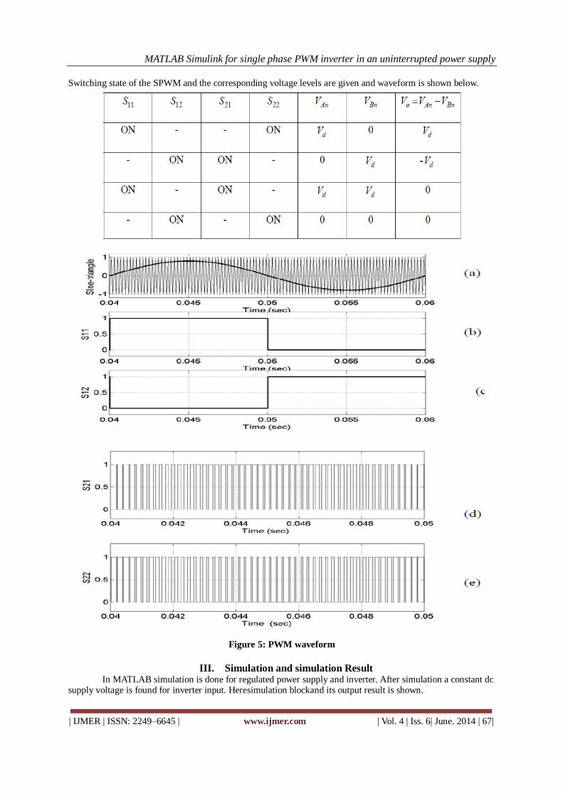
MATLAB Simulink for single phase PWM inverter in an uninterrupted power supply
| IJMER | ISSN: 2249–6645 | www.ijmer.com | Vol. 4 | Iss. 6| June. 2014 | 67|
Switching state of the SPWM and the corresponding voltage levels are given and waveform is shown below.
Figure 5: PWM waveform
III. Simulation and simulation Result In MATLAB simulation is done for regulated power supply and inverter. After simulation a constant dc
supply voltage is found for inverter input. Heresimulation blockand its output result is shown.
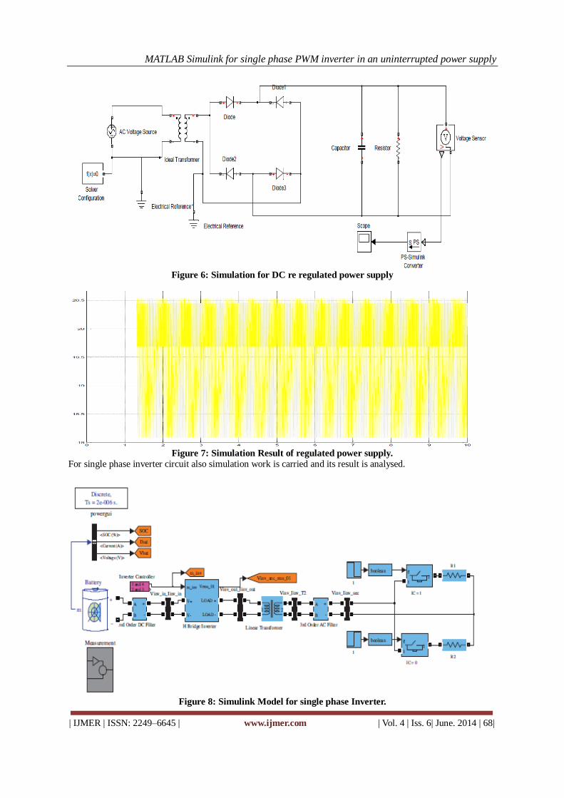
MATLAB Simulink for single phase PWM inverter in an uninterrupted power supply
| IJMER | ISSN: 2249–6645 | www.ijmer.com | Vol. 4 | Iss. 6| June. 2014 | 68|
Figure 6: Simulation for DC re regulated power supply
Figure 7: Simulation Result of regulated power supply.
For single phase inverter circuit also simulation work is carried and its result is analysed.
Figure 8: Simulink Model for single phase Inverter.

MATLAB Simulink for single phase PWM inverter in an uninterrupted power supply
| IJMER | ISSN: 2249–6645 | www.ijmer.com | Vol. 4 | Iss. 6| June. 2014 | 69|
Figure 9:(a) Terminal current of the battery when the loadchanges from a resistive load of 400 W to an
inductive loadof 500 W with 0.85 PF lagging.(b) Output voltage after the load changes from a resistive load of
400 W toan inductive load of 500 W with 0.85 PF lagging.
IV. Microcontroller In this project PIC microcontroller is used. Although in simulation microcontroller is not shown but in
hardware part microcontroller is used by which battery charging is done by solar energy whenever it is available
otherwise it is connected to main supply. The complete circuit diagram is shown below of this project in which
microcontroller plays as a brain of this UPS system.
Figure 10: Complete circuit diagram of project

MATLAB Simulink for single phase PWM inverter in an uninterrupted power supply
| IJMER | ISSN: 2249–6645 | www.ijmer.com | Vol. 4 | Iss. 6| June. 2014 | 70|
V. Conclusion The inverter unit consists of four, IGBTs connected as a bridge and drivewith a low cost driver. The
experimental result matched with simulation results. Although any parameters are adjusted for giving
fundamentalfrequency rms output voltage of 220V at 50 Hz. With this inverter unit, furtherresearch on single-phase inverters can becarried out such as soft switching inverters. By using this proposed UPS we can save
electricity bill and also can use better alternate renewable energy source. In this project there is future scope is
that during presence of solar energy we can use solar energy instead of main supply.
REFERENCES JOURNAL PAPERS:
[1] J.I. Itoh, F. Hayashi, \Ripple current reduction of a fuel cell for a single-phase isolated converter using a DC active
filter with a center tap", IEEE Transactions on Power Electronics, Vol. 25, pp. 550556, 2010. [2] `S.H. Lee, S.G. Song, S.J. Park, C.J. Moon, M.H. Lee, \Grid-connected photovoltaic system using current-source
inverter", Solar Energy, Vol. 82, pp. 411419, 2008. [3] M. Delshad, H. Farzanehfard, \A new soft switched push pull current fed converter for fuel cell applications", Energy
Conversion and Management, Vol. 52, pp. 917923, 2010. [4] H.M. Tao, J.L. Duarte, M.A.M. Hendrix, \Line-interactive UPS using a fuel cell as the primary source", IEEE
Transactions on Industrial Electronics, Vol. 55, pp. 30123021, 2008. [5] A. Kawamura, T. Haneyoshi, R.G. Hoft, \Deadbeat controlled PWM inverter with parameter estimation using only
voltage sensor", IEEE Transactions on Power Electronics, Vol. 3, pp. 118125, 1988. [6] X.Q. Guo, W.Y. Wu, H.R. Gu, \Modeling and simulation of direct output current control for LCL-interfaced grid-
connected inverters with parallel passive damping", Simulation Modelling Practice and Theory, Vol. 18, pp. 946956, 2010.
[7] A.F. Zobaa, \Voltage harmonic reduction for randomly time-varying source characteristics and voltage harmonics", IEEE Transactions on Power Delivery, Vol. 21, pp. 816822, 2006.
[8] A. Varschavsky, J. Dixon, M. Rotella, L. Moran, \Cascaded nine-level inverter for hybrid-series active power filter,
using industrial controller", IEEE Transactions on Industrial Electronics, Vol. 57, pp. 27612767, 2010. [9] F.P. Zeng, G.H. Tan, J.Z. Wang, Y.C. Ji, \Novel single-phase _ve-level voltage-source inverter for the shunt active
power filter", IET Power Electronics, Vol. 3, pp. 480489, 2010. [10] J.A. Pomilio, S.M. Deckmann, \Characterization and compensation of harmonics and reactive power of residential
and commercial loads", IEEE Transactions on Power Delivery, Vol. 22, pp. 10491055, 2007. [11] J. Dixon, L. Moran, \Multilevel inverter, based on multi-stage connection of three-level converters scaled in power of
three", IEEE 28th Annual Conference of the Industrial Electronics Society, pp. 886891, 2002. [12] O. • O. Mengi, _I.H. Alta_s, \Fuzzy logic control for a wind/battery renewable energy production system", Turkish
Journal of Electrical Engineering & Computer Sciences, Vol. 20, pp. 187206, 2012. [13] A. Khairy, M. Ibrahim, N. Abdel-Rahim, H. Elsherif, \Comparing proportional-resonant and fuzzy-logic controllers
for current controlled single-phase grid-connected PWM DC/AC inverters", IET Conference on Renewable Power Generation, pp. 16, 2011. [14]”Fundamentals of new diode clamped multi-level inverter“ byXiaming Yuan IroBarbi, Senior member IEEE
[15] A comparison of high power converter topologies for the implementation of FACTS controllers by Diego Soto, Member, IEEE, and Tim C. Green, Member, IEEE
[16] H. Rostami and D. A. Khaburi, "Voltage gain comparison of different control methods of the Z-source inverter," in
Electricaland Electronics Engineering, 2009. ELECO 2009.International Conference on, 2009, pp. I-268-I-272. [17] S. R. and L. Jayawickrama, "Steady-State Analysis and Designing Impedance Network of Z-Source Inverters," IEEE
Transactions on industrial electronics, vol. 57, p. 9, July 2010. [18] O. Ellabban, J. Van Mierlo, and P. Lataire, "Comparison between different PWM control methods for different Z-
sourceinverter topologies," in Power Electronics and Applications,2009. EPE '09. 13th European Conference on, 2009, pp. 1-11.
[19] P. C. Loh, D. M. Vilathgamuwa, C. J. Gajanayake, L. T. Wong, and C. P. Ang, "Z-source current-type inverters: digital modulation and logic implementation," in Industry Applications Conference, 2005. Fourtieth IAS Annual
Meeting.Conference Record of the 2005, 2005, pp. 940-947 Vol.
BOOKS:
[1.] Microcontroller Projects in C for the 8051 by Dogan Ibrahim
[2.] The 8051 Microcontroller by I. Scott Mackenzie 2nd Edition
[3.] The 8051 Microcontroller Architecture, Programming and application by Kenneth J. Ayala
[4.] E Balaguruswamy, „Programming in ANSI C‟, Tata McGraw Hill, 2004.
[5.] Power Electronics By KanchanDhani
[6.] The 8051 Microcontroller and Embedded Systems Using Assembly and C-2nd-ed by Mazidi

MATLAB Simulink for single phase PWM inverter in an uninterrupted power supply
| IJMER | ISSN: 2249–6645 | www.ijmer.com | Vol. 4 | Iss. 6| June. 2014 | 71|
[7.] Microcontroller-Based Temperature Monitoring and Control By Dogan Ibrahim
[8.] Microcontrollers: Architecture, Programming, Interfacing and System DesignBy Raj Kamal
[9.] Embedded Systems Design with 8051 Microcontrollers: Hardware and Software edited by
ZdravkoKarakehayov
[10.] Power Electronics: Circuits, Devices & Applications by Muhammad Rashid
[11.] Power Electronics by P. S. Bimbhra
[12.] Power Electronics And Motor Drives: Advances and Trends By Bimal K. Bose [13.] Electrical Drives And Control By U.A.Bakshi, M.V.Bakshi
[14.] Fundamentals of Electrical Drives By G. K. Dubey, Gopal K. Dubey

Contents :
Damping Of Composite Material Structures with Riveted Joints 01-05T. Subramani, K. Udhaya Kumar
Image compression using Hybrid wavelet Transform and their Performance Comparison 06-12Deepa T, Girisha H
Investigation of the Behaviour for Reinforced Concrete Beam Using Non Linear Three 13-18Dimensional Finite ElementsT. Subramani, S. Sundar, M. Senthilkumar
Analysis of Non Conventional Cross Section of Pipe Made Of Composite Material 19-27Suraj Bharadiya, Dr. R.J. Patil
Simulation and Analysis of a D-STATCOM for Load Compensation and Power 28-36Factor ImprovementGaurav Pundlik
Anaerobic Digestion of Vinasse cane alcohol: The influence of OLR by a UASB reactor 37-42Cinthya Alejandra Sosa-Villalobos, Elena Rustrián, Eric Houbron
Design of VGA Controller using VHDL for LCD Display using FPGA 43-49Khan Huma Aftab, Monauwer Alam
An Improved Single Phase Transformer less Inverter Topology for Cost Effective PV Systems 50-61Geethu Chacko, Riya Scaria
Mathematical Modelling of an 3 Phase Induction Motor Using MATLAB/Simulink 62-67Mr. Punit L. Ratnani, Dr. A. G. Thosar
Land Use/Land Cover Mapping Of Allahabad City by Using Remote Sensing & GIS 68-73Jamal Mohamed Salih Irhoumah, V. C. Agarwal, Deepak Lal
Volume : 4 Issue : 6 (Version-2) June - 2014ISSN : 2249-6645
International Journal of Modern Engineering Research
(IJMER)

International
OPEN ACCESS Journal
Of Modern Engineering Research (IJMER)
| IJMER | ISSN: 2249–6645 | www.ijmer.com | Vol. 4 | Iss. 6| June. 2014 | 1|
Damping Of Composite Material Structures with Riveted Joints
T. Subramani1, K. Udhaya Kumar
2
1Professor & Dean, Department of Civil Engineering, VMKV Engg. College, Vinayaka Missions University,
Salem, India. 2PG Student of Structural Engineering, Department of Civil Engineering,VMKV Engg.College,Vinayaka
Missions University, Salem, India
I. Introduction
Damping capacity is an extent of a material's ability to dissipate elastic-strain energy during mechanical vibration or wave propagation. Complications involving vibration arise in many regions of
mechanical, civil and aerospace engineering. The damping of a structural component or element is often a
significantly overlooked criterion for good mechanical design. Numerous mechanical failures over a seemingly
infinite multitude of structures occurred dueto lack of damping in structural elements.
For accounting the damping effects in a structural material, lots of researches and studies have been
done in the field to suppress the vibration and to minimize the mechanical failures. Since it was found that
damping materials can be utilised in treatment in passive damping technology to mechanical components and
structures to increase the damping performance, there had been a commotion on the on-going research and
studies over the last few periods to either alter the existing materials and components, or to develop an entirely
new type of material to improve the structural dynamics of components for which damping concept could be
applied. Composite structures are generally polymers, which give various ranges of different compositions
which result in different material properties as well as behaviour. Hence, composite damping structures and
materials can be developed and tailored quite efficiently for a specific purpose and application. Problems
involving vibration and damping occur in many regions of mechanical, civil and aerospace engineering.
Engineering composite structures and materials are generally fabricated using a variety of connections
which include bolted, riveted, welded and bonded joints etc. The dynamics of mechanical joints is a topic of
special importance due to their strong effect on the performance of the structural material. Moreover, the
inclusion of the above mentioned joints play a significant role in the overall system behaviour, particularly the
damping level of the components and structures. However, determining damping either by analysis or by
experiment is never easy and straightforward keeping in view of the complexity of the dynamic interaction of
components. The estimation of damping in beam-like structures using passive damping approach is very
essential in problem solving addressed by the present research
Abstract: Vibration and noise reduction are crucial in maintaining high performance level and prolonging the useful life of machinery, automobiles, aerodynamic and spacecraft structures. It is
observed that damping in materials occur due to energy release due to micro-slips along frictional
interfaces and due to varying strain regions and interaction between the metals. But it was found
that the damping effect in metals is quite small that it can be neglected. Damping in metals is due to
the micro-slips along frictional interfaces. Composites, however, have better damping properties
than structural metals and cannot be neglected. Typically, the range of composite damping begins
where the best damped metal stops.In the present work, theoretical analysis was done on various
polymer matrix composite (glass fibre polyesters) with riveted joints by varying initial conditions.
Strain energy loss was calculated to calculate the damping in composites. Using FEA model, load
variation w.r.t time was observed and the strain energy loss calculated was utilised in finding the material damping for Carbon fibre epoxy with riveted joints. Various simulations were performed in
ANSYS and these results were utilised to calculate the loss factor, Rayleigh‘s damping constants
and logarithmic decrement.
Keywords: Material damping, Energy balanced approach, Damping mechanism, Structural
damping factor.
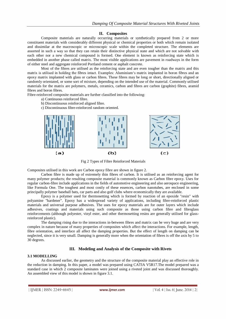
Damping Of Composite Material Structures With Riveted Joints
| IJMER | ISSN: 2249–6645 | www.ijmer.com | Vol. 4 | Iss. 6| June. 2014 | 2|
II. Composites
Composite materials are naturally occurring materials or synthetically prepared from 2 or more
constituent materials with considerably different physical or chemical properties or both which remain isolated
and dissimilar at the macroscopic or microscopic scale within the completed structure. The elements are assorted in such a way so that they can retain their distinctive physical state and which are not solvable with
each other nor a new chemical compound is formed. One element is known as reinforcing state which is
embedded in another phase called matrix. The most visible applications are pavement in roadways in the form
of either steel and aggregate reinforced Portland cement or asphalt concrete.
Most of the fibres are utilised as the reinforcing state and are even tougher than the matrix and this
matrix is utilised in holding the fibres intact. Examples: Aluminium‘s matrix implanted in boron fibres and an
epoxy matrix implanted with glass or carbon fibres. These fibres may be long or short, directionally aligned or
randomly orientated, or some sort of mixture, depending on the intended use of the material. Commonly utilised
materials for the matrix are polymers, metals, ceramics, carbon and fibres are carbon (graphite) fibres, aramid
fibres and boron fibres.
Fibre-reinforced composite materials are further classified into the following:
a) Continuous reinforced fibre. b) Discontinuous reinforced aligned fibre.
c) Discontinuous fibre-reinforced random oriented.
Fig 2 Types of Fibre Reinforced Materials
Composites utilised in this work are Carbon epoxy fibre are shown in figure 2.
Carbon fibre is made up of extremely thin fibres of carbon. It is utilised as an reinforcing agent for
many polymer products; the resulting composite material is commonly known as Carbon fibre epoxy. Uses for
regular carbon-fibre include applications in the fields of automotive engineering and also aerospace engineering,
like Formula One. The toughest and most costly of these essences, carbon nanotubes, are enclosed in some
principally polymer baseball bats, car parts and also golf clubs where economically they are available. Epoxy is a polymer used for thermosetting which is formed by reaction of an epoxide "resin" with
polyamine "hardener". Epoxy has a widespread variety of applications, including fibre-reinforced plastic
materials and universal purpose adhesives. The uses for epoxy materials are for outer layers which include
adhesives, coatings and materials using such composite as those using carbon fibre and fibreglass
reinforcements (although polyester, vinyl ester, and other thermosetting resins are generally utilised for glass-
reinforced plastic).
The damping rising due to the interactions in-between fibres and matrix can be very huge and are very
complex in nature because of many properties of composites which affect the interactions. For example, length,
fibre orientation, and interface all affect the damping properties. But the effect of length on damping can be
neglected, since it is very small. Damping is generally more when the orientation of fibres is off the axis by 5 to
30 degrees.
III. Modeling and Analysis of the Composite with Rivets
3.1 MODELLING As discussed earlier, the geometry and the structure of the composite material play an effective role in
the reduction in damping. In this paper, a model was prepared using CATIA V5R17.The model prepared was a
standard case in which 2 composite laminates were joined using a riveted joint and was discussed thoroughly. An assembled view of this model is shown in figure 3.1.

Damping Of Composite Material Structures With Riveted Joints
| IJMER | ISSN: 2249–6645 | www.ijmer.com | Vol. 4 | Iss. 6| June. 2014 | 3|
Figure 3.1: Model designed on CATIA V5R17
3.2 HARMONIC RESPONSE ANALYSIS
It is a technique utilised to determine the steady state response of a linear structure to loads that varies
sinusoidal with time. The mode superposition method calculations factored mode shapes (eigenvectors) from
modal analysis to calculate the structures response. Hence it is known as harmonic response analysis as shown
in figure 3.2
Figure 3.2: Harmonic response analysis of ANSYS model
IV. Modeling of Vibration Damping In Composite Structures
Composite damping or energy dissipation property of vibrating composite structures, refers to a
complex physical dynamic nature that is amenable to rheological modal analysis. In a broad class of composite
structures, the distinguishing characteristic of the damping mechanism is its strong dependence on the eigen
frequencies such that it exhibits little damping at high frequency level. In contrast to the dynamic nature of
isotropic materials, a further complication arises in composite domain due to the mutual effects of various
parameters, such as code number, degree of isotropism (volume fraction), boundary conditions as well as the
vibrating mode number on the damping and stiffness distributions.
As an example, the decreasing of volume fraction of the ber enhances energy dissipation by increasing
the loss associated with matrix composite. It might be expected that the natural frequencies of vibrating
composite structures and in sequence the damping capacity, can be altered by changing the layer's orientations
and stacking sequence, so that the damping nature as a function of frequencies of composites should be further studied. At the present time, it is still difficult to determine accurately the modal characteristics of composite
structures (particularly damping parameters) by an analytical approach.
The experimental confirmation prediction is therefore at very least desirable and can be used to form
analytically the mathematical model. In turn it can be used to more clearly understand the effect of parameters
controlling the dynamics of composite states. Recently, a mathematical model representing the damping
capacity of the composite was established. Based on the student distribution approximation of the measured

Damping Of Composite Material Structures With Riveted Joints
| IJMER | ISSN: 2249–6645 | www.ijmer.com | Vol. 4 | Iss. 6| June. 2014 | 4|
values of damping in the fundamental mode, the modal relationships between the fundamental frequencies and
the damping factors were developed in equivalence to the uniform mass damping of isotropic structures.
In the present work, an attempt has been made to improve the convergence characteristics of the model
within a wide range of frequencies for different code numbers at two levels of volume fraction. Basically, a
weight factor (a) has been introduced for correlating and updating the mathematical model to the experimental
data throughout the utilization of the curve fitting response function. This has resulted in generalized quasi-
rectangular hyperbolic relationships between the loss factors and the natural frequencies with the confidence level at 99.5%. These results permit the uncoupling of simultaneous equations of motion of composite structures
with the lowest residual errors.
In the experimental work, cantilever composite beams made from fiber reinforced plastic FRP are
considered as the object of the study for their simplicity and for extensive applications. Various specimens made
from three plies, Fig. 1, are utilized for two levels of volume fraction (a) a weakly composite 15% and (b) an
average composite 45%.
Fig. 4 layered beam model.
In order to evaluate accurately the influences of code number on the damping capacities and natural
frequencies, twelve specimens of unidirectional cross-ply and angle-ply laminate have been fabricated in the
laboratory by using hand lay up technique. Numerically the first four natural frequencies at the two levels of
volume fraction are computed by the use of the modified formula MFM and listed in the second column of
Tables 1 and 2. For the sake of verification, the experimental results of the natural frequencies and the loss
factors for the first four natural modes are listed in the third and fourth columns in these tables, respectively.
To highlight the unpredictable nature of the damping parameters, various curves representing mutual
relationships of modal parameters were plotted in Figs.. The close agreement of the results of the proposed
mathematical and experimental models proves the efficient applicability of the proposed models for deeply
understanding the dynamic nature of vibrating damping composite structures.
IV. Conclusion
From modal analysis reported modal frequency = 591.87 Hz
From harmonic response model, Maximum strain energy = 8.68 X 10⁻⁵ J.
In transient analysis, the directional deformation along z axis with an impulsive force of 100 N applied,
the values of maximum deformation fluctuate and tend to converges to 9.42X 10⁻¹⁰.
ω = 2πf = 3718.82 rad/sec.
logarithmic decrement, δ, as follows:
X1 and X2 are two consecutive displacements one cycle apart δ= ln(x1/x2) = 6.3 X 10⁻³, X1 and X2
are taken from the values of the table

Damping Of Composite Material Structures With Riveted Joints
| IJMER | ISSN: 2249–6645 | www.ijmer.com | Vol. 4 | Iss. 6| June. 2014 | 5|
ζ = 1.04X 10⁻³.
α = 2δω = 7.471 s-1 and β = 2δ/ω = 5.59 x 10⁻⁷ s
Energy released = πcωx2 =1.95 x 10⁻⁵ J.
Loss factor (ε) =1/2π (energy released per cycle / maximum strain energy) = 0.0358
REFERENCES [1]. Cochardt, A.W., 1954, A method for determining the internal damping of machine members, ASME, Journal of
Applied Mechanics, Vol. 76, No. 9, pp. 257-262. [2]. Goodman, L.E. and Klumpp, J.H., 1956, Analysis of slip damping with reference to turbine-blade vibration, ASME,
Journal of Applied Mechanics, Vol. 23, pp. 421–429.
[3]. Beards, C.F., 1992, Damping in structural joints, The Shock and Vibration Digest, Vol. 24, No. 7, pp. 3-7. [4]. Ruzicka, J. E., ―Structural Damping‖. ASME, New Jersey (1959). [5]. Lazan, B. J., ―Damping of Materials and Members in Structural Mechanics‖. Pergamon Press, London (1968) [6]. Nashif, A. D., Jones, D. I. G. and Henderson, J. P., ―Vibration Damping‖. John Wiley & Sons, Inc., New York
(1985). [7]. Jones, D. I. G., ―Handbook of Viscoelastic Vibration Damping‖. John Wiley & Sons, Inc., New York (2001). [8]. Sun, C. T., Lu, Y. P., ―Vibration Damping of Structural Elements‖. Prentice Hall PTR, Englewood Cliffs, NJ ,
(1995).
[9]. Beards, C. F., ―Structural Vibration Analysis: Modeling, Analysis, and Damping of Vibrating Structures‖. Halsted Press, Chichester (1983).
[10]. Ungar, E. E., "Structural Damping", Chapter 12 in Noise and Vibration Control Engineering: Principles and Applications, Leo. L. Beranek (Editor). John Wiley & Sons, Inc.,(1992).
[11]. Mead, D. J., ―Passive Vibration Control‖. John Wiley & Sons, New York (1999). [12]. Bert, C.W., ―Composite materials: A survey or the damping capacity of fibrereinforced composites in damping
applications for vibration control‖, AMD-Vol. 38. (1980). [13]. Nashif, A.D, Jones, D.I.G and Henderson, J.P. Vibration Damping, Wiley, New York, (1985).
[14]. Chandra, R., Singh S.P, and Gupta.K Damping studies in fibre-reinforced composites—a review. Composite Structs, 46(1), 41-51, (1999).
[15]. Gibson, R.F., Chaturvedi, S.K. and Sun, C.T., ―Complex moduli of aligned discontinuous fibre-reinforced polymer composites‖, J. Mater Sci., Vol. 17. pp. 3499-3509 (1982).
[16]. Gibson, R.F., Chaturvedi, S.K. and Sun, C.T., ―Internal damping of short-fibre reinforced polymer matrix composites‖, Comput. Struct 20, pp. 391—401, (1985).

International
OPEN ACCESS Journal Of Modern Engineering Research (IJMER)
| IJMER | ISSN: 2249–6645 | www.ijmer.com | Vol. 4 | Iss. 6| June. 2014 | 6|
Image compression using Hybrid wavelet Transform and their
Performance Comparison
Deepa T1
, Girisha H2
1, 2 (Computer Science and Engineering, Rao Bahadur Y. Mahabaleswarappa college of engineering, Bellary,
Affiliated to VTU Belgaum, Karnataka, India)
I. Introduction Images may be worth a thousand words, but they generally occupy much more space in hard disk, or
bandwidth in a transmission system, than their proverbial counterpart. Compressing an image is significantly
different than compressing raw binary data. Of course, general purpose compression programs can be used to
compress images, but the result is less than optimal. This is because images have certain statistical properties
which can be exploited by encoders specifically designed for them. Also, some of the finer details in the image
can be sacrificed for the sake of saving a little more bandwidth or storage space. Compression is the process of
representing information in a compact form. Compression is a necessary and essential method for creating
image files with manageable and transmittable sizes. The data compression schemes can be divided into
lossless and lossy compression. In lossless compression, reconstructed image is exactly same as compressed image. In lossy image compression, high compression ratio is achieved at the cost of some error in reconstructed
image. Lossy compression generally provides much higher compression than lossless compression.
Wavelets are used to characterize a complex pattern as a series of simple patterns and coefficients
that, when multiplied and summed, reproduce the original pattern. Wavelets transforms are now being adopted
for various applications like Industrial supervision of gear-wheel, Speech recognition, Computer graphics and
multifractal analysis. Wavelet transform of a function is the improved version of Fourier transform[1]. It is good
tool to replace the fourier transform. Fourier transform is a powerful tool for analyzing the components of a
stationary signal. But it is failed for analyzing the non-stationary signal. wavelet transform allows the
components of a non-stationary signal to be analyzed. Discrete Cosine Transform is widely used[2].It separates
an image into different frequency components. Low frequency components are located at top left corner giving
high energy compaction. High frequencies are located in bottom right corner. Elimination of these high
frequency elements gives transformed image with few low frequency components. If image is reconstructed from such lesser number of transformed, low frequency elements, it gives compressed image without losing
much data contents in original image. Hybrid transformation techniques combine properties of two different
transforms. It gives compressed image with visually perceptible image quality. Initially focus was on Haar
Wavelets. But in recent literature, wavelets of other orthogonal transforms have been introduced and studied.
These transform include Walsh, DCT, DKT, Hartley transform.
II. Related Work Image compression technique by using wavelet transform by v.v.sunil kumar [3] is concerned with a
certain type of compression technique by using wavelet transforms. There are a variety of wavelets for use in compression. Several methods are compared on their ability to compress standard images and the fidelity of the
Abstract: Image compression is a widely addressed researched area. Despite rapid progress in mass-
storage density, processor speeds, and digital communication system performance, demand for data
storage capacity and data-transmission bandwidth continues to outstrip the capabilities of available
technologies. Wavelet transform is generated from orthogonal transform .Image compression using
hybrid wavelet transform is proposed here by using two orthogonal transform. Hybrid wavelet transform are generated using orthogonal transforms alias DCT, DHT, DWT, DKT transform .Different color
images of size 256x256 are used for experimentation. Proposed hybrid wavelet transform is applied on
red, green and blue planes of image separately. Then in each plane transformed coefficients are sorted
in descending order of their energy and lowest energy coefficients are eliminated. Root mean square
error between original image and reconstructed image is calculated to check the performance at
different compression ratios. Hybrid of DCT and DKT gives the best results among the combination of
mentioned image transforms used for generating hybrid wavelet transforms.
Keyword: DCT, DHT ,DKT, DWT, Hybrid wavelet transform, RMSE, PSNR.

Image compression using Hybrid wavelet Transform and their Performance Comparison
| IJMER | ISSN: 2249–6645 | www.ijmer.com | Vol. 4 | Iss. 6| June. 2014 | 7|
reproduced image to the original image. A lossless image Compression using Approximate Matching and Run
Length [4] is proposed by Samir Kumar Bandyopadhyay, Tuhin Utsab Paul, Avishek
Raychoudhury.Performance is compared with available jpeg compression technique over a wide number of images. Performance Analysis of Image Compression Using Wavelets [5] by Sonja Grgic, Mislav Grgic,
Branka Zovko-Cihlar discusses important features of wavelet transform in compression of still images,
including the extent to which the quality of image is degraded by the process of wavelet compression and
decompression. In[6]-[7], Dr.H.B.kekre, Sudeep D. Thepade, Adib Parkardisucces the technique to store color
information within grayscale image can be used in effective for image compression as the matted grayscale
image alone can be used to reconstructed the original color image using haar and kekre wavelet transform. In[8],
Prabhakar Telagarapu etl. Proposed Image Compression using DCT and Wavelet Transformations, The JPEG
standard makes use of Discrete Cosine Transform (DCT) for compression. The analysis of compression using
DCT and Wavelet transform by selecting proper threshold method, better result for PSNR have been obtained.
In[9], wavelet transform is generated from orthogonal component transforms of different sizes and it is applied
on colour images. DCT, DST, Hartley and Real-DFT are used as component transforms to generate their respective wavelet transforms. Blocking effect is observed in all wavelets except DCT and it depends upon the
size of local component transform. Performance Comparison of Image Retrieval Techniques using Wavelet
Pyramids of Walsh, Haar and Kekre Transforms is explained in [10], Content Based Image Retrieval (CBIR) is
done using the image feature set extracted from Wavelets applied on the image at various levels of
decomposition.
III. Basic Theoritical Cosideration
3.1 Error Metrics
Two of the error metrics used to compare the various image compression techniques are the Mean
Square Error (MSE) and the Peak Signal to Noise Ratio (PSNR) to achieve desirable compression ratios. The
MSE is the cumulative squared error between the compressed and the original image, whereas PSNR is a
measure of the peak error. The mathematical formulae for the two are :
MSE =
PSNR = 20 * log10 (255 / sqrt(MSE)) _(2)
where I(x,y) is the original image, I'(x,y) is the approximated version (which is actually the decompressed image) and M,N are the dimensions of the images in (1). A lower value for MSE means lesser
error, and as seen from the inverse relation between the MSE and PSNR, this translates to a high value of PSNR.
Logically, a higher value of PSNR is good because it means that the ratio of Signal to Noise is higher. Here, the
'signal' is the original image, and the 'noise' is the error in reconstruction. So, if we find a compression scheme
having a lower MSE (and a high PSNR), we can recognise that it is a better one.
3.2 Wavelet Transform
Wavelet transform (WT) represents an image as a sum of wavelet functions (wavelets) with different
locations and scales. Any decomposition of an image into wavelets involves a pair of waveforms: one to
represent the high frequencies coresponding to the detailed parts of an image (wavelet function ) and one for the
low frequencies or smooth parts of an image (scaling function ).
3.2.1 Discrete Wavelet Transform
One of the big discoveries for wavelet analysis was that perfect reconstruction filter banks could be
formed using the coefficient sequences aL(k)and aH(k) (Fig.4). The input sequence is convolved with high-pass
(HPF) and low-pass (LPF) filters and aL(k) and aH(k) and each result is downsampled by two, yielding the transform signals xH and xL. The signal is reconstructed through upsampling and convolution with high and low
synthesis filters sH(k) and sL(k) . For properly designed filters, the signal is reconstructed exactly (y = x ).
Figure.1 Two-channel filter bank.

Image compression using Hybrid wavelet Transform and their Performance Comparison
| IJMER | ISSN: 2249–6645 | www.ijmer.com | Vol. 4 | Iss. 6| June. 2014 | 8|
The choice of filter not only determines whether perfect re-construction is possible, it also determines
the shape of wavelet we use to perform the analysis. By cascading the analysis filter bank with itself a number
of times, a digital signal decomposition with dyadic frequency scaling known as DWT can be formed. The mathematical manipulation that effects synthesis is called inverse DWT. The new twist that wavelets bring to
filter banks is connection between multiresolution analysis (that, in principle, can be performed on the original,
continuous signal) and digital signal processing performed on discrete, sampled signals. Four channel perfect
reconstruction filter bank is shown in fig.4
decompression.
Each filter is 2-D with the subscript indicating the type of filter (HPF or LPF) for separable horizontal and
vertical components. The resulting four transform components consist of all possible combinations of high- and low-pass filtering in the two directions. By using these filters in one stage, an image can be decomposed into
four bands. There are three types of detail images for each resolution: horizontal (HL), vertical (LH), and
diagonal (HH). The operations can be repeated on the low–low band using the second stage of identical filter
bank. Thus, a typical 2-D DWT, used in image compression, will generate the hierarchical pyramidal structure
shown in Fig.2(b).
3.2.2. Discrete Cosine Transform(DCT)
Figure.3 Image compression and decompression using DCT
The discrete cosine transform (DCT) is a technique for converting a signal into elementary frequency
components. Like other transforms, the Discrete Cosine Transform (DCT) attempts to de correlate the image
data. After de correlation each transform coefficient can be encoded independently without losing compression
efficiency.
Proposed DCT Algorithm
1. The image is broken into 8x8 blocks of pixels.
2. Working from left to right, top to bottom, the DCT is applied to each block. 3. Each block is compressed through quantization.
4. The array of compressed blocks that constitute the image is stored in a drastically reduced amount of
space.
5. When desired, the image is reconstructed through decompression, a process that uses the inverse
Discrete Cosine Transform (IDCT).
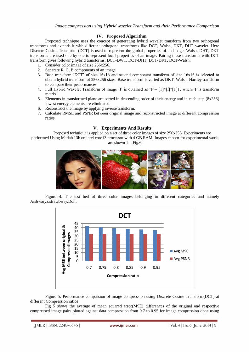
Image compression using Hybrid wavelet Transform and their Performance Comparison
| IJMER | ISSN: 2249–6645 | www.ijmer.com | Vol. 4 | Iss. 6| June. 2014 | 9|
IV. Proposed Algorithm Proposed technique uses the concept of generating hybrid wavelet transform from two orthogonal
transforms and extends it with different orthogonal transforms like DCT, Walsh, DKT, DHT wavelet. Here
Discrete Cosine Transform (DCT) is used to represent the global properties of an image. Walsh, DHT, DKT
transforms are used one by one to represent local properties of an image. Pairing these transforms with DCT
transform gives following hybrid transforms: DCT-DWT, DCT-DHT, DCT-DKT, DCT-Walsh.
1. Consider color image of size 256x256.
2. Separate R, G, B components of an image
3. Base transform „DCT‟ of size 16x16 and second component transform of size 16x16 is selected to
obtain hybrid transform of 256x256 sizes. Base transform is varied as DKT, Walsh, Hartley transform
to compare their performances.
4. Full Hybrid Wavelet Transform of image „f‟ is obtained as „F‟= [T]*[f]*[T]T. where T is transform matrix.
5. Elements in transformed plane are sorted in descending order of their energy and in each step (8x256)
lowest energy elements are eliminated.
6. Reconstruct the image by applying inverse transform.
7. Calculate RMSE and PSNR between original image and reconstructed image at different compression
ratios.
V. Experiments And Results Proposed technique is applied on a set of three color images of size 256x256. Experiments are
performed Using Matlab 13b on intel core i3 processor with 4 GB RAM. Images chosen for experimental work
are shown in Fig.6
Figure 4. The test bed of three color images belonging to different categories and namely Aishwarya,strawberry,Doll.
Figure 5: Performance comparsion of image compression using Discrete Cosine Transform(DCT) at
different Compression ratios
Fig 5 shows the average of mean squared error(MSE) differences of the original and respective
compressed image pairs plotted against data compression from 0.7 to 0.95 for image compression done using
05
1015202530354045
0.7 0.75 0.8 0.85 0.9 0.95
Avg
MSE
bet
wee
n o
rigi
nal
&
Co
mp
ress
ed im
ages
Compression ratio
DCT
Avg MSE
Avg PSNR

Image compression using Hybrid wavelet Transform and their Performance Comparison
| IJMER | ISSN: 2249–6645 | www.ijmer.com | Vol. 4 | Iss. 6| June. 2014 | 10|
Discrete Cosine Transform(DCT).Here the performance of DCT at compression ratio 0.95 is the best as
indicated by minimum MSE values over the other compression ratios.
Figure 6: Performance comparsion of image compression using Wavelet at different compression ratios
Fig 6 shows the average of mean squared error(MSE) differences of the original and respective compressed
image pairs plotted against data compression from 0.7 to 0.95 for image compression done using Walete
trasform.Here the performance of wavelet at compression ratio 0.95 is the best as indicated by minimum MSE
values over the other compression ratios.
Figure 7: Performance comparsion of image compression using Discrete Cosine Transform(DCT)-
Discrete Walsh transform at different compression ratios Fig 7 shows the average of mean squared error(MSE) differences of the original and respective compressed
image pairs plotted against data compression from 0.7 to 0.95 for image compression done using hybrid
Discrete Cosine Transform(DCT)- Discrete Walsh transform.Here the performance of wavelet at compression
ratio 0.95 is the best as indicated by minimum MSE values over the other compression ratios.
0
100
200
300
400
0.7 0.75 0.8 0.85 0.9 0.95
Avg
MSE
be
twe
en
o
rigi
nal
&co
mp
ress
ed
im
ages
compression ratio
WAVELET
Avg MSE
Avg PSNR
0
500
1000
1500
2000
2500
0.7 0.75 0.8 0.85 0.9 0.95
Avg
MSE
bet
wee
n o
rigi
nal
&
com
pre
ssed
imag
es
Compression ratio
DCT-Walsh
Avg MSE
Avg PSNR
0
20
40
60
80
0.7 0.75 0.8 0.85 0.9 0.95
MSE
be
twe
en
ori
gin
al &
co
mp
ress
ed
ima
ges
Compression ratio
DCT-DKT
Avg MSE
Avg PSNR
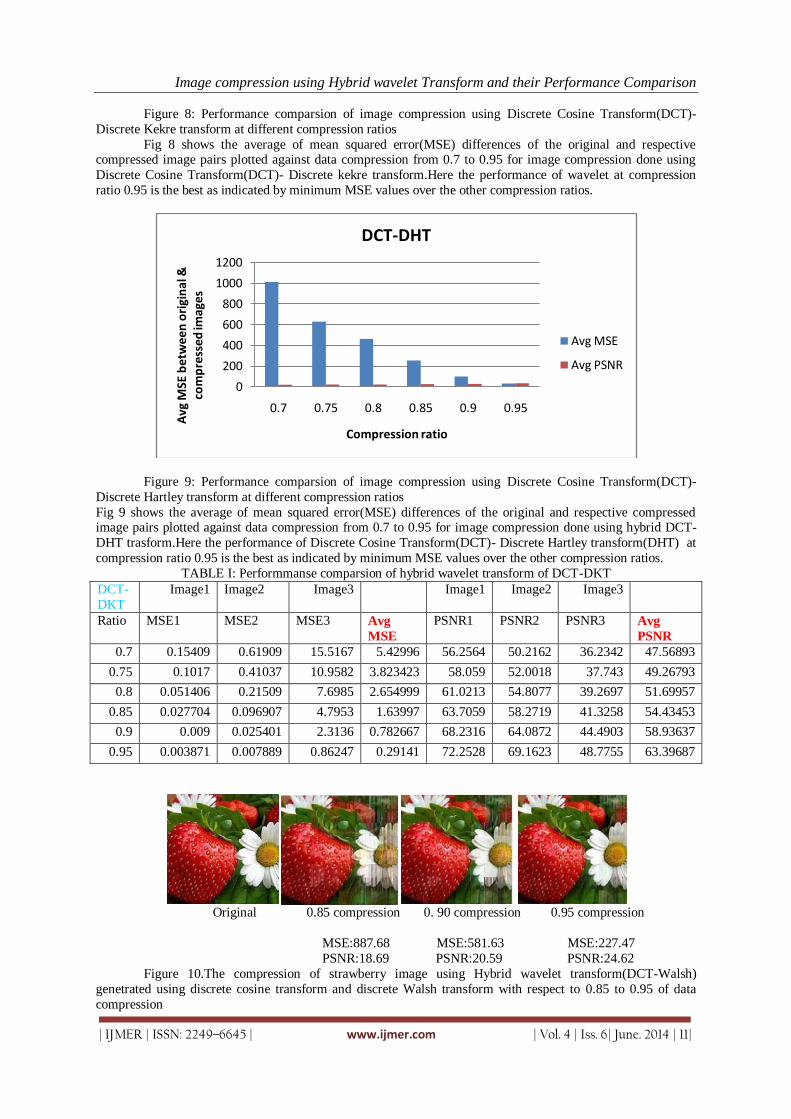
Image compression using Hybrid wavelet Transform and their Performance Comparison
| IJMER | ISSN: 2249–6645 | www.ijmer.com | Vol. 4 | Iss. 6| June. 2014 | 11|
Figure 8: Performance comparsion of image compression using Discrete Cosine Transform(DCT)-
Discrete Kekre transform at different compression ratios
Fig 8 shows the average of mean squared error(MSE) differences of the original and respective compressed image pairs plotted against data compression from 0.7 to 0.95 for image compression done using
Discrete Cosine Transform(DCT)- Discrete kekre transform.Here the performance of wavelet at compression
ratio 0.95 is the best as indicated by minimum MSE values over the other compression ratios.
Figure 9: Performance comparsion of image compression using Discrete Cosine Transform(DCT)-
Discrete Hartley transform at different compression ratios
Fig 9 shows the average of mean squared error(MSE) differences of the original and respective compressed image pairs plotted against data compression from 0.7 to 0.95 for image compression done using hybrid DCT-
DHT trasform.Here the performance of Discrete Cosine Transform(DCT)- Discrete Hartley transform(DHT) at
compression ratio 0.95 is the best as indicated by minimum MSE values over the other compression ratios.
TABLE I: Performmanse comparsion of hybrid wavelet transform of DCT-DKT
DCT-
DKT
Image1 Image2 Image3 Image1 Image2 Image3
Ratio MSE1 MSE2 MSE3 Avg
MSE
PSNR1 PSNR2 PSNR3 Avg
PSNR
0.7 0.15409 0.61909 15.5167 5.42996 56.2564 50.2162 36.2342 47.56893
0.75 0.1017 0.41037 10.9582 3.823423 58.059 52.0018 37.743 49.26793
0.8 0.051406 0.21509 7.6985 2.654999 61.0213 54.8077 39.2697 51.69957
0.85 0.027704 0.096907 4.7953 1.63997 63.7059 58.2719 41.3258 54.43453
0.9 0.009 0.025401 2.3136 0.782667 68.2316 64.0872 44.4903 58.93637
0.95 0.003871 0.007889 0.86247 0.29141 72.2528 69.1623 48.7755 63.39687
Original 0.85 compression 0. 90 compression 0.95 compression
MSE:887.68 MSE:581.63 MSE:227.47
PSNR:18.69 PSNR:20.59 PSNR:24.62
Figure 10.The compression of strawberry image using Hybrid wavelet transform(DCT-Walsh)
genetrated using discrete cosine transform and discrete Walsh transform with respect to 0.85 to 0.95 of data
compression
0
200
400
600
800
1000
1200
0.7 0.75 0.8 0.85 0.9 0.95
Avg
MSE
be
twe
en
ori
gin
al &
co
mp
ress
ed im
ages
Compression ratio
DCT-DHT
Avg MSE
Avg PSNR

Image compression using Hybrid wavelet Transform and their Performance Comparison
| IJMER | ISSN: 2249–6645 | www.ijmer.com | Vol. 4 | Iss. 6| June. 2014 | 12|
Original 0. 85compression 0. 90 compression 0.95 compression
MSE: 0.097 MSE: 0.025 MSE: 007 PSNR: 25.58 PSNR: 64.09 PSNR: 69.2
Figure 11. The compression of strawberry image using Hybrid wavelet transform(DCT-DKT)
genetrated using discrete cosine transform and discrete Kekre transform with respect to 0.85 to 0.95 of data
compression.
VI. Conclusion In this paper, experimental work is done to generate hybrid wavelet transform using two orthogonal
component transforms. Discrete Cosine Transform (DCT) is used as one component transforms which
contributes to global properties of an image. Second component transform that contributes to local properties of image is varied. For 256x256 size image, hybrid wavelet transform of size 256x256 is generated. Here the
hybrid wavelet transforms are generated using Discrete Walsh Transform (DWT), Discrete Kekre Transform
(DKT), Discrete Hartley Transform (DHT) and Discrete Cosine Transform (DCT) for image compression. The
various orthogonal transforms can be considered for crossbreeding to generate the hybrid wavelet transform
based on the expected behavior of the hybrid wavelet transform for particular application. The experimental
results have shown that hybrid of DCT with DKT gives best results of image quality among other hybrid
wavelet transform. DCT-DKT gives a minimum error of 0.2(MSE) and image quality upto 63.4(PSNR).
ACKNOWLEGEMENT I Deepa T would like to thank my guide Mr.Girisha.H, Assistant professor who supported me in
making this paper.
REFERENCES [1]. Strang G. "Wavelet Transforms Versus Fourier Transforms." Bull. Amer. Math. Soc. 28, 288-305, 1993. [2]. K. R. Rao and P. Yip, Discrete Cosine Transform: Algorithms, Advan- tages and Applications. San Diego, CA:
Academic, 1990. [3]. V.V. Sunil Kumar, M. IndraSen Reddy, “Image Compression Techniques by using Wavelet Transform”, Journal of
Information Engineering and Applications, Vol 2, No.5, 2012, pp. 235-239. [4]. Samir Kumar Bandyopadhyay, Tuhin Utsab Paul, Avishek Raychoudhury, “ Image Compression using Approximate
Matching and Run Length” International Journal of Advanced Computer Science and Applications, Vol. 2, No. 6, pp. 117-121, 2011.
[5]. Sonja Grgic, Mislav Grgic, Branka Zovko-Cihlar, “Performance Analysis of Image Compression Using Wavelets” IEEE TRANS. On Industrial Electronics, Vol. 48, No. 3, pp. 682-695, June 2001.
[6]. Dr. H.B.kekre, Sudeep D. Thepade, Adib Parkar, “A Comparison of Haar Wavelets and Kekre‟s Wavelets for Storing Colour Information in a Greyscale Image”, International Journal of Computer Applications (IJCA), Volume 1, Number 11, December 2010, pp 32- 38.
[7] Dr. H.B.kekre, Sudeep D. Thepade, Adib Parkar “Storage of Colour Information in a Greyscale Image using Haar
Wavelets and Various Colour Spaces”, International Journal of Computer Applications (IJCA), Volume 6, Number 7, pp.18-24, September 2010. [6] Dr.H.B.Kekre, Sudeep D. Thepade, Juhi Jain, Naman A.
[8]. Prabhakar Telagarapu etl. “Image Compression using DCT and Wavelet Transformations”, International Journal of Signal Processing, Image Processing and Pattern Recognition, Vol. 4, No. 3, September 2011, pp. 61- 74.
[9]. H.B.Kekre, Tanuja Sarode, Prachi Natu “Image Compression using Wavelet Transforms of DCT, DST, Hartley and Real-DFT with Variation in Size of Component Transforms”, International Journal of Scientific & Engineering Research(IJSER), Volume 4, Issue 10, October-2013
[10]. H.B.Kekre, Sudeep D. Thepade, Akshay Maloo, “Performance Comparison of Image Retrieval Techniques using
Wavelet Pyramids ofWalsh, Haar and Kekre Transforms”, International Journal of Computer Applications (IJCA)Volume 4, Number 10, August 2010, pp. 1-8.
International
OPEN ACCESS Journal Of Modern Engineering Research (IJMER)
| IJMER | ISSN: 2249–6645 | www.ijmer.com | Vol. 4 | Iss. 6| June. 2014 | 13|
Investigation of the Behaviour for Reinforced Concrete Beam
Using Non Linear Three Dimensional Finite Elements
T. Subramani1, S. Sundar
2, M. Senthilkumar
3
1Professor & Dean, Department of Civil Engineering, VMKV Engg. College, Vinayaka Missions University,
Salem, India. 2,3PG Students of Structural Engineering, Department of Civil Engineering, VMKV Engg. College,Vinayaka
Missions University, Salem, India
I. Introduction
The idea for a new form of construction emerged from two separate research investigations. One of
these on composite construction with deep haunches, the other was on the use of very high strength steels in
reinforced concrete. Both these separate modes of construction, although as yet little used in practice, will undoubtedly develop further in their own right. However, they have some disadvantages 2which will mitigate
against their development, but by altering slightly the form of the deep haunch, the disadvantages of both can be
largely overcome. The resulting form of construction is known as composite reinforced concrete.
The normal form of composite construction is shown. The main advantage of using deep haunches is
the considerable economy that can be affected in the amount of steelwork. This can be 40% of that used in
normal composite construction, even for the same overall depth. The deep haunch can be formed easily by
precast units or similar spanning between the steel beams and the problem of deep haunches composite beams
developed form the desirability to use this method of construction.
Concrete Problem of reinforced concrete beams on elastic foundations with both compressional and
frictional resistances are good examples to extend the applications to foundations. In these problems, the
compressional resistances of the elastic medium to the bottom face of the beams are determined by considering the linear relationships of the normal displacement to the compressional reactions (Winkler model).
The frictional restraints are modeled by considering the linear relation to the horizontal displacement
(Winkler model). Winkler (1867) proposed the first model of beam on an elastic foundation based on pure
bending beam theory, later Pasternak in 1954 proposed the shear model based on the assumption of pure
Abstract: This study presents theoretical investigation that reinforced concrete and composite
construction might be suitably combined to give a new structural material : composite reinforced
concrete. To study theoretically the composite beam, non-linear three-dimensional finite elements
have been used to analyze the tested beam.
The 8-node brick elements in (ANSYS) are used to represent the concrete, the steel bars are modelled
as discrete axial members connected with concrete elements at shared nodes assuming perfect bond
between the concrete and the steel. The results obtained by finite element solution showed good agreement with experimental results.
The main objective of the present investigation is to carry out a nonlinear analysis of reinforced
concrete beams resting on elastic foundation. Material nonlinearities due to cracking of concrete,
plastic flow, crushing of concrete and yielding of reinforcement are considered. Foundation
representation is assumed linear using Winkler model.
The reinforced concrete beam is modelled by using three dimensional finite elements with steel bars
as smeared layers. The examples have been chosen in order to demonstrate the applicability of the
modified computer program (Dynamic Analysis of Reinforced Concrete Beams on Elastic
Foundations DARCEF ) by comparing the predicted behaviour with that from other experimental and
analytical observations. The program modified in the present research work is capable of simulating
the behaviour of reinforced concrete beams resting of Winkler foundation and subjected to different types of loading. The program solutions obtained for different reinforced concrete beams resting on
elastic foundations are in good agreement with the available results. Maximum percentage difference
in deflection is 15 %
Keywords: Investigation, Behaviour, Reinforced Concrete Beam , Non Linear Three Dimensional
Finite Element

Investigation Of The Behaviour For Reinforced Concrete Beam Using Non Linear Three Dimensional
| IJMER | ISSN: 2249–6645 | www.ijmer.com | Vol. 4 | Iss. 6| June. 2014 | 14|
shear of the beam. Both of these two models take an extreme point of view on the deformation behavior of the
beam. Cheung and Nag (1968) studied the effects of separation of contact surfaces due to uplift forces. In
addition, they have enabled the prediction of the bending and torsion moments in the plate sections by adopting
three degrees of freedom per node. Bowles (1974) developed a computer program to carry out the analysis of
beams on elastic foundation by using the finite element method, in which Winkler model is adopted to represent
the elastic foundation. Selvadurai (1979) presented a theoretical analysis of the interaction between a rigid
circular foundation resting on elastic half space and a distributed external load of finite extent which acts at an exterior region of the half space. Yankelevsky et al. (1988) presented an iterative procedure for the analysis of
beams resting on nonlinear elastic foundation based on the exact solution for beams on a linear elastic
foundation. Yin (2000) derived the governing ordinary differential equation for a reinforced Timoshenko beam
on an elastic foundation. Guo and Wietsman (2002) made an analytical method, accompanied by a numerical
scheme, to evaluate the response of beams on the space-varying foundation modulus, which is called the
modulus of subgrade reaction (Kz=Kz(x)).
.
II. Study Area
2.1 COMPOSITE BEAMS
Many researchers studied the behavior of simply supported composite beams. Some of these models,
which are comprehensive and worth evaluating, are reviewed herein. In 1975, Johnson has derived a differential
equation for Newmark. The equilibrium and compatibility equations are reduced to a single
second order differential equation in terms of interface slip instead of axial forces. The solution of which lead to
slip values at the interface along the beam span, after satisfying the suitable boundary conditions. In 1985,
Roberts presented an elastic analysis for composite beams with partial interaction assuming a linear shear
connector behavior while the normal stiffness of the connectors was taken infinity. The basic equilibrium and
compatibility equations were expressed in terms of four independent displacements, which are the horizontal and vertical displacements in each component of the composite section. These equations were solved using
finite difference representation of various derivatives.
2.1.1 Nonlinear Finite Element (by using ANSYS program)
In 2006 Ali Hameed Aziz has investigated experimentally the strength, deflection and ductility of
reinforced concrete I-beams made ofnormal or hybrid reinforced concrete under two point monotonic loads. The
experimental work includes the following four main categories:
i- Flexural behaviour of I-beams cast monolithically.
ii- Flexural behaviour of I-beams cast in two-step procedure (with one construction joint).
iii- Flexural behaviour of I-beams cast in three-step procedure (with two construction joints).
iv- Shear behaviour of I-beams cast monolithically, but, the web is made with concrete different from the
concrete of compression and tension flanges. To implement a nonlinear finite element procedure to analyze all tested beams.
III. Material Modelling
3.1 Numerical modelling of concrete
The numerical modelling of concrete, which is used in the nonlinear finite element program, includes
the following:
A stress-strain model to represent the behaviour of concrete in compression.
Failure criteria to simulate cracking and crushing types of fracture.
A suitable crack representation model.
A post-cracking stress-strain relationship.
3.2 Stress-strain models for concrete in compression
Because of the complex behaviour of reinforcement and concrete under general load, a mathematical
description of the material properties of concrete is established by using suitable constitutive equations. Several
models have been proposed to define the complicate stress-strain behavior of concrete in compression under
various stress states (Chen 1982). These models can be generally classified into:
Elasticity based models.
Plasticity based models.
3.3 Modelling of concrete fracture
Fracture of concrete can be classified as crushing or cracking. The crushing type of fracture is defined
by progressive degradation of the material internal structure under compressive stresses. The cracking type of
fracture is characterized by a general growth of micro-cracks which join together to form a failure plane. In

Investigation Of The Behaviour For Reinforced Concrete Beam Using Non Linear Three Dimensional
| IJMER | ISSN: 2249–6645 | www.ijmer.com | Vol. 4 | Iss. 6| June. 2014 | 15|
general, two different methods were employed to represent the cracks in the finite element analysis of concrete
structures. These are the discrete crack representation and the smeared cracks representation. In the first model,
the cracks are simulated by physical separation or disconnection by the
displacements at nodal points for adjoining element. The major difficulty in this approach is that the location
and orientation of the cracks are not known in advance.
In the second approach, the cracked concrete is assumed to remain a continuum and implies an infinite
number of parallel fissures across that part of a finite element. The cracks are assumed to be distributed, or smeared, over the volume of the sampling point under consideration.
3.4 Post-cracking behaviour
Many experimental studies show that when the concrete cracks, the tensile stresses normal to the
cracked plane are gradually released as the crack width increases. This response can be generally modelled in
the finite element analysis using the tension-stiffening model. When the tensile stress reaches the limiting tensile
strength, primary cracks will be formed. The properties of cracks, and their number and extent, depend on the
size, position and orientation of the reinforcing bars with respect to the plane of cracks.
3.5 Yield criterion
As mentioned earlier, a yield criterion must be independent of the coordinates system in which the
stress state is defined. Therefore, it must be a function of stress invariants only. Under multiaxial state of
stresses, the yield criterion for concrete is assumed to depend on three stress invariants. However, a yield criterion, which depends on two stress invariants, has been proved to be
adequate for most practical situations. The yield criterion incorporated in the
present model is expressed as (Chen 1982):
The stress (σ0) is the equivalent effective stress at the onset of plastic deformation which can be
determined from uniaxial compression test as:
The coefficient (Cp) is the plasticity coefficient, which is used to mark the initiation of plasticity deformation.
The material parameters αand ßcan be determined from the uniaxial compression test and biaxial test under
equal compressive stresses. The parameters αand ßhave been found to be (0.35468) and (1.35468) respectively
and equation (1) can be rewritten as:
Equation (4) can be solved for (σ0) as:
The hardening rule is necessary to describe the motion of the loading surfaces during plastic
deformation. In the present study an isotropic hardening rule is adopted. Therefore, equation (6) can be
expressed for the subsequent loading functions as:
In the present model, the stress-strain curve is assumed to have a parabolic relationship for both normal
and high strength concrete. This parabolic curve represents the work-hardening stage of behavior, when the peak
compressive stress is reached, a perfectly plastic response is assumed to occur. The equivalent uniaxial stress-
strain curve in the various stages of behavior, which is given:
1. During the elastic stage, when
2. After the initial yield, and up to the peak concrete compressive strength, when

Investigation Of The Behaviour For Reinforced Concrete Beam Using Non Linear Three Dimensional
| IJMER | ISSN: 2249–6645 | www.ijmer.com | Vol. 4 | Iss. 6| June. 2014 | 16|
In the present study, values of 0.3 and 0.5 are assumed for plastic coefficient Cp for the normal and
high strength concrete respectively, and the plastic yielding begin at a stress level of Cp fc '(Al-Ani, 2000). If
Cp=1.0, then the elastic perfectly plastic behaviour is specified.
IV. Finite Element Method
4.1. Finite element representation
The finite element idealization of reinforced concrete is necessary for the application to reinforced
concrete beams under static loads. In the present study, concrete is simulated by brick elements, and
reinforcement bars are modeled as a smeared layer (Al-Obaidie 2005).
4.2 Concrete representation
The 20-node isoparametric quadratic brick element is used in the present study to represent the
concrete.
4.3 Displacement representation The displacement field within the element is defined in terms of the shape functions and displacement
values at the nodes. Each nodal point has three degrees of freedom u, v and w along the Cartesian coordinates x,
y and z, respectively. Therefore, for each element the displacement vector is:
The strains are given by :
or
where, [B] is the strain displacement matrix. The stresses are given by :
where, [D] is the stress-strain elastic relation matrix given by:
in which E is the Young’s modulus, vis the Poisson’s ratio and G is the shear modulus.
4.4 Reinforcement representation
There are three alternative representations, which have been widely used to simulate the reinforcement
in connection with the finite element formulation. These representations are (Scordelis 1971):
a- Discrete representation.
b- Distributed representation.
c-Embedded representation.

Investigation Of The Behaviour For Reinforced Concrete Beam Using Non Linear Three Dimensional
| IJMER | ISSN: 2249–6645 | www.ijmer.com | Vol. 4 | Iss. 6| June. 2014 | 17|
In the present study, the distributed representation is used. For this representation, the steel bars are
assumed to be distributed over the concrete element in any direction in a layer with uniaxial properties. A
composite concrete-reinforcement constitutive relation is used in this case. To derive such a relation, perfect
bond is assumed between concrete and steel.
Fig. 4.1 Distributed representation of reinforcement.
The element stiffness matrix of the beam-foundation system can be calculated from the following
expression:
A modified computer program (DARCEF) (Dynamic Analysis of Reinforced Concrete Beams on
Elastic Foundations) (Al-Obaidie 2005) of the original program (DARC3) (Dynamic Analysis of Reinforced
Concrete in 3D) (Hinton 1988) is developed for solving the problems of reinforced concrete beams resting on
elastic foundations. The Winkler model for compressional and frictional resistances is added to the original program to represent the foundation.
Figure 4.2 Three Dimensional 8-node Brick Element
V. Results
Fig. 4.3.Steel stress compared with previous study.

Investigation Of The Behaviour For Reinforced Concrete Beam Using Non Linear Three Dimensional
| IJMER | ISSN: 2249–6645 | www.ijmer.com | Vol. 4 | Iss. 6| June. 2014 | 18|
Table 4.4.Values of deflections at mid span for half of simply supported beam resting on an
elastic foundation in comparison with previous solutions.
VI. Conclusions
The Main conclusion to be drawn from this investigation is that composite reinforced concrete is a
viable structural form. Flexural cracks up to the working load stage remain very fine and the calculation of their
width is unlikely to be necessary in design. The arrangement of reinforcement and steel channel is ideally suited for the use of very high strength reinforcing steels, and reinforcement stresses over 120000 lb/sq. can be used at
the ultimate load while still satisfying the serviceability requirements at working load. There are no cracks at the
bottom of the beam because of the channel. There will be cracks in the concrete web, but these should remain
fine, and they will not be visible.
The (DARCEF) program used in the present research work is capable of simulating the behavior of
reinforced concrete beams resting on elastic foundations and subjected to different types of loading. The
program solutions obtained for different reinforced concrete beams resting on elastic foundations are in
good agreement with the available results. Maximum percentage difference in deflection is 15%.
The maximum deflection will decrease at a decreasing rate as the beam width is increased. It was found
that by increasing the width of the beam from (150 to 450 mm), the maximum deflection for the beam is
decreased by (31.25%).
The maximum steel stress will decrease at a decreasing rate as the beam width is increased. It was found
that by increasing the width of the beam from (150 to 450 mm), the maximum steel stress for the beam is
decreased by (21.21%).
The maximum steel stress will decrease at a decreasing rate as the beam depth is increased. It was found
that by increasing the depth of the beam from (300 to 900 mm), the maximum steel stress for the beam is
decreased by (12.12%).
The maximum deflection will decrease as the vertical subgrade reaction is increased. Also, the maximum
deflection will decrease as the horizontal subgrade reaction is increased. It was found that by increasing
the vertical and horizontal subgrade reactions for the beam from (0.128 N/mm3 to 1.024 N/mm3), the
maximum deflection is decreased by (51%) and (9%) respectively.
REFERENCES [1]. Al-Ani W.F.(2000). Nonlinear analysis of reinforced concrete corbels, M.Sc. Thesis, Nahrian University. [2]. Al-Jubory A. A. (1992). Deep beams and thick plates under generalized loadings, M.Sc. Thesis, Nahrian University. [3]. Al-Musawi A. N. (2005). Three dimensional finite element analysis of beams on elastic foundations, M.Sc. Thesis,
Nahrian University. [4]. Al-Obaidie A. M. (2005). Nonlinear analysis of reinforced concrete beams on elastic foundations, M.Sc. Thesis,
Nahrian University. [5]. Biot A. S. (1937). Bending of an infinite beam on an elastic foundation, Journal of Applied Mechanics, 59, A1-A7. [6]. Bowles J. E. (1974). Analytical and Computer Methods in Foundation Engineering, McGraw- Hill Book Company,
New York. [7]. Chen W.F. (1982). Plasticity in Reinforced Concrete, McGraw – Hill Book Company. [8]. Cheung Y. K., Nag D.K. (1968). Plates and beams on elastic foundations-linear and non-linear behavior,
Geotechnique, 18, 250-260. [9]. Guo Y., Wietsman Y. (2002). Solution methods for beams on nonuniform elastic foundations, Journal of Engineering
Mechanics, ASCE, 128, 592-594. [10]. Hetenyi M. (1949). Beams on Elastic Foundations, University of Michigan Press, Ann Arbor, Michigan. [11]. Hinton E. (1988). Numerical Methods and Software for Dynamic Analysis of Plate and Shell, Pineridge Press
limited. [12]. Levinson M. (1949). A new rectangular beam theory, McMaster University, Hamilton, CEEM Rpt. 4-79.

International
OPEN ACCESS Journal Of Modern Engineering Research (IJMER)
| IJMER | ISSN: 2249–6645 | www.ijmer.com | Vol. 4 | Iss. 6| June. 2014 | 19|
Analysis of Non Conventional Cross Section of Pipe Made Of
Composite Material
Suraj Bharadiya1, Dr. R.J. Patil
2
1 Student, Dr. D.Y. Patil Inst. Of Engg & Tech, Ambi India 2 Principal, Dr. D.Y. Patil Inst. Of Engg & Tech, Ambi. India
I. Introduction Our search for oil is sending us deep into the sea, however this has its own challenges. The salinity of
the sea, acts as an active corrosive agent, and it steadily weakens the structure to get around this, non-corrosive composite piping has been deployed in critical regions of the structure. However to enable pipe stacking,
sometimes to avail of space constraints, instead of circular c/s, the pipes are increasingly being made of
triangular or rectangular c/s. For such c/s theoretical calculations are not possible, hence we need FEA to help us
understand the behavior of such c/s.
II. Composite Materials Composite materials are formed by the combination of two or more materials to achieve properties
(physical, chemical, etc.) that are superior to those of its constituents. The main components of composite
materials, or composites, are fibers and matrix. The fibers provide most of the stiffness and strength. The matrix binds the fibers together thus providing load transfer between fibers and between the composite and the external
loads and supports. Also, it protects the fibers from environmental attack.
III. Result
3.1 Deflection & Stress Generation in Fixed Beam
A B C D Lengt
h
No.of
Layer
Meshin
g Size
DM
X SMN SMX
No.
of
Nodes
200
0
200
0
200
0
200
0 20000
5
200
76.53 6.57 695.89
12000
6 56.48 2.96
555.33
3
7 35.14 0.94
401.67
3
8 23.91 0.44
310.10
2
10 13.95 0.4
213.02
1
12 7.36 0.4 143
Abstract: Composite materials have been widely used in the ship-building, aerospace and construction
industries because of their distinct advantages of low weight, high stiffness, and high strength to weight
ratios. These properties are due to the low weight of the epoxy core matrix and high strengths of the
glass/carbon fibres. Composite pipes used in various applications are traditionally spherical in cross-
section. In this study, non-conventional cross-sectioned composite pipes [i.e. rectangular and triangular
cross-sections] have been proposed, fabricated, tested and analyzed because of their ability to be bundled without loss of space. The behaviors of these pipes under an internal pressure test have been
studied and its failure mechanisms have been investigated.
Keywords: Non Conventional, composite, FEA.
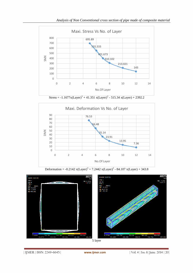
Analysis of Non Conventional cross section of pipe made of composite material
| IJMER | ISSN: 2249–6645 | www.ijmer.com | Vol. 4 | Iss. 6| June. 2014 | 20|
Stress = -1.1677x(Layer)3 + 41.351 x(Layer)2 - 515.34 x(Layer) + 2392.2
Deformation = -0.2142 x(Layer)3 + 7.2442 x(Layer)2 - 84.107 x(Layer) + 343.8
5 layer
695.89
555.333
401.673
310.102
213.021143
0
100
200
300
400
500
600
700
800
0 2 4 6 8 10 12 14
SMX
No.Of Layer
Maxi. Stress Vs No. of Layer
76.53
56.48
35.14
23.91
13.957.36
0
10
20
30
40
50
60
70
80
90
0 2 4 6 8 10 12 14
DM
X
No.Of Layer
Maxi. Deformation Vs No. of Layer
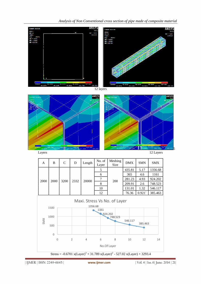
Analysis of Non Conventional cross section of pipe made of composite material
| IJMER | ISSN: 2249–6645 | www.ijmer.com | Vol. 4 | Iss. 6| June. 2014 | 21|
12 layers
5 Layers 12 Layers
A B C D Length No. of
Layer
Meshing
Size DMX SMN SMX
2000 2000 3200 2332 20000
5
200
435.81 5.17 1356.68
6 365 4.6 1161
7 281.23 4.93 924.202
8 209.91 2.6 748.523
10 131.01 1.32 546.117
12 76.36 0.921` 385.463
Stress = -0.6701 x(Layer)3 + 31.789 x(Layer)2 - 527.02 x(Layer) + 3293.4
1356.681161
924.202748.523
546.117385.463
0
500
1000
1500
0 2 4 6 8 10 12 14
SMX
No.Of Layer
Maxi. Stress Vs No. of Layer
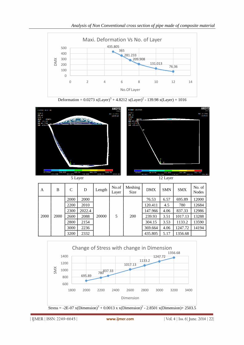
Analysis of Non Conventional cross section of pipe made of composite material
| IJMER | ISSN: 2249–6645 | www.ijmer.com | Vol. 4 | Iss. 6| June. 2014 | 22|
Deformation = 0.0273 x(Layer)3 + 4.8212 x(Layer)2 - 139.98 x(Layer) + 1016
5 Layer 12 Layer
A B C D Length No.of
Layer
Meshing
Size DMX SMN SMX
No. of
Nodes
2000 2000
2000 2000
20000 5 200
76.53 6.57 695.89 12000
2200 2010 120.411 4.5 780 12684
2300 2022.4 147.966 4.06 837.33 12986
2600 2088 239.93 3.51 1017.13 13288
2800 2154 304.15 3.53 1133.2 13590
3000 2236 369.664 4.06 1247.72 14194
3200 2332 435.805 5.17 1356.68
Stress = -2E-07 x(Dimension)3 + 0.0013 x x(Dimension)2 - 2.8501 x(Dimension)+ 2503.5
435.805365
281.233209.908
131.01376.36
0
100
200
300
400
500
0 2 4 6 8 10 12 14
DM
X
No.Of Layer
Maxi. Deformation Vs No. of Layer
695.89780
837.33
1017.131133.2
1247.721356.68
600
800
1000
1200
1400
1800 2000 2200 2400 2600 2800 3000 3200 3400
SMX
Dimension
Change of Stress with change in Dimension
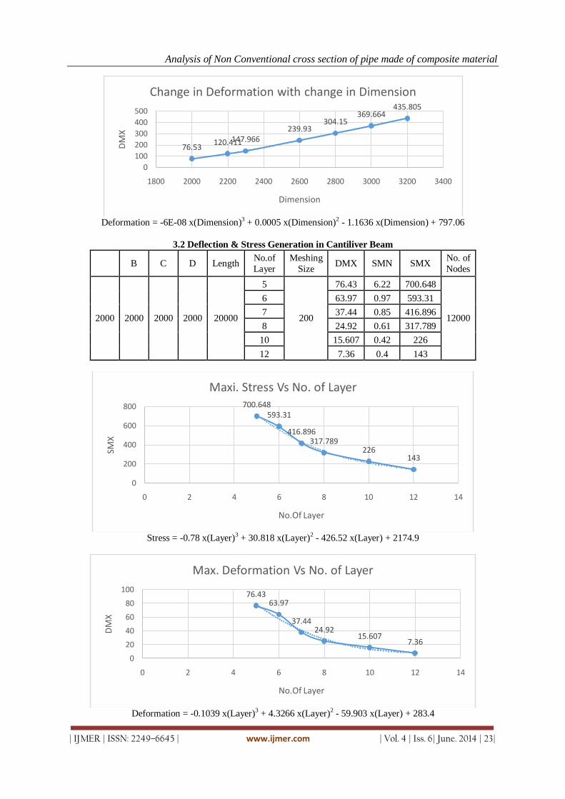
Analysis of Non Conventional cross section of pipe made of composite material
| IJMER | ISSN: 2249–6645 | www.ijmer.com | Vol. 4 | Iss. 6| June. 2014 | 23|
Deformation = -6E-08 x(Dimension)3 + 0.0005 x(Dimension)2 - 1.1636 x(Dimension) + 797.06
3.2 Deflection & Stress Generation in Cantiliver Beam
A B C D Length No.of
Layer
Meshing
Size DMX SMN SMX
No. of
Nodes
2000 2000 2000 2000 20000
5
200
76.43 6.22 700.648
12000
6 63.97 0.97 593.31
7 37.44 0.85 416.896
8 24.92 0.61 317.789
10 15.607 0.42 226
12 7.36 0.4 143
Stress = -0.78 x(Layer)3 + 30.818 x(Layer)2 - 426.52 x(Layer) + 2174.9
Deformation = -0.1039 x(Layer)3 + 4.3266 x(Layer)2 - 59.903 x(Layer) + 283.4
76.53120.411147.966
239.93304.15
369.664435.805
0
100
200
300
400
500
1800 2000 2200 2400 2600 2800 3000 3200 3400
DM
X
Dimension
Change in Deformation with change in Dimension
700.648593.31
416.896317.789
226143
0
200
400
600
800
0 2 4 6 8 10 12 14
SMX
No.Of Layer
Maxi. Stress Vs No. of Layer
76.4363.97
37.4424.92
15.6077.36
0
20
40
60
80
100
0 2 4 6 8 10 12 14
DM
X
No.Of Layer
Max. Deformation Vs No. of Layer
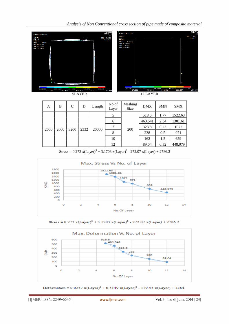
Analysis of Non Conventional cross section of pipe made of composite material
| IJMER | ISSN: 2249–6645 | www.ijmer.com | Vol. 4 | Iss. 6| June. 2014 | 24|
5LAYER 12 LAYER
Stress = 0.273 x(Layer)3 + 3.1703 x(Layer)2 - 272.07 x(Layer) + 2786.2
A B C D Length No.of
Layer
Meshing
Size DMX SMN SMX
2000 2000 3200 2332 20000
5
200
518.5 1.77 1522.63
6 463.541 2.34 1381.61
7 323.8 0.23 1072
8 238 0.5 971
10 162 1.5 659
12 89.04 0.52 448.079
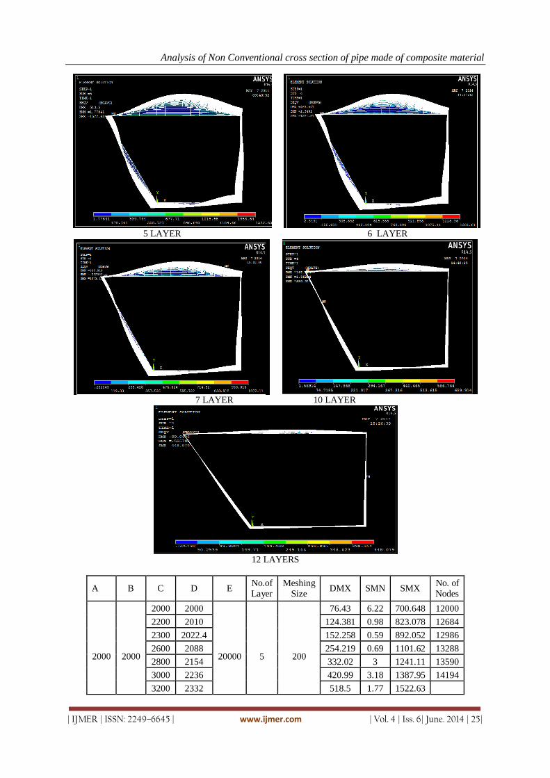
Analysis of Non Conventional cross section of pipe made of composite material
| IJMER | ISSN: 2249–6645 | www.ijmer.com | Vol. 4 | Iss. 6| June. 2014 | 25|
5 LAYER 6 LAYER
7 LAYER 10 LAYER
12 LAYERS
A B C D E No.of
Layer
Meshing
Size DMX SMN SMX
No. of
Nodes
2000
2000
2000 2000
20000
5
200
76.43 6.22 700.648 12000
2200 2010 124.381 0.98 823.078 12684
2300 2022.4 152.258 0.59 892.052 12986
2600 2088 254.219 0.69 1101.62 13288
2800 2154 332.02 3 1241.11 13590
3000 2236 420.99 3.18 1387.95 14194
3200 2332 518.5 1.77 1522.63
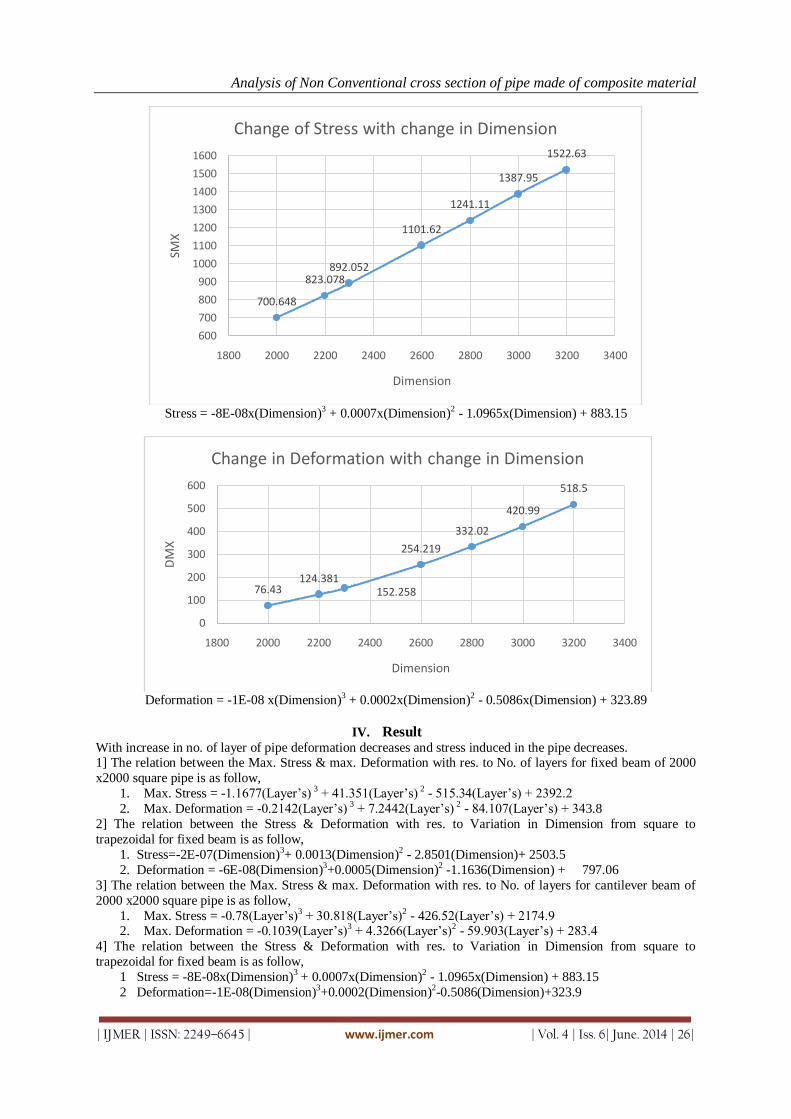
Analysis of Non Conventional cross section of pipe made of composite material
| IJMER | ISSN: 2249–6645 | www.ijmer.com | Vol. 4 | Iss. 6| June. 2014 | 26|
Stress = -8E-08x(Dimension)3 + 0.0007x(Dimension)2 - 1.0965x(Dimension) + 883.15
Deformation = -1E-08 x(Dimension)3 + 0.0002x(Dimension)2 - 0.5086x(Dimension) + 323.89
IV. Result With increase in no. of layer of pipe deformation decreases and stress induced in the pipe decreases. 1] The relation between the Max. Stress & max. Deformation with res. to No. of layers for fixed beam of 2000
x2000 square pipe is as follow,
1. Max. Stress = -1.1677(Layer’s) 3 + 41.351(Layer’s) 2 - 515.34(Layer’s) + 2392.2
2. Max. Deformation = -0.2142(Layer’s) 3 + 7.2442(Layer’s) 2 - 84.107(Layer’s) + 343.8
2] The relation between the Stress & Deformation with res. to Variation in Dimension from square to
trapezoidal for fixed beam is as follow,
1. Stress=-2E-07(Dimension)3+ 0.0013(Dimension)2 - 2.8501(Dimension)+ 2503.5
2. Deformation = -6E-08(Dimension)3+0.0005(Dimension)2 -1.1636(Dimension) + 797.06
3] The relation between the Max. Stress & max. Deformation with res. to No. of layers for cantilever beam of
2000 x2000 square pipe is as follow,
1. Max. Stress = -0.78(Layer’s)3 + 30.818(Layer’s)2 - 426.52(Layer’s) + 2174.9 2. Max. Deformation = -0.1039(Layer’s)3 + 4.3266(Layer’s)2 - 59.903(Layer’s) + 283.4
4] The relation between the Stress & Deformation with res. to Variation in Dimension from square to
trapezoidal for fixed beam is as follow,
1 Stress = -8E-08x(Dimension)3 + 0.0007x(Dimension)2 - 1.0965x(Dimension) + 883.15
2 Deformation=-1E-08(Dimension)3+0.0002(Dimension)
2-0.5086(Dimension)+323.9
700.648
823.078892.052
1101.62
1241.11
1387.95
1522.63
600
700
800
900
1000
1100
1200
1300
1400
1500
1600
1800 2000 2200 2400 2600 2800 3000 3200 3400
SMX
Dimension
Change of Stress with change in Dimension
76.43124.381
152.258
254.219
332.02
420.99
518.5
0
100
200
300
400
500
600
1800 2000 2200 2400 2600 2800 3000 3200 3400
DM
X
Dimension
Change in Deformation with change in Dimension

Analysis of Non Conventional cross section of pipe made of composite material
| IJMER | ISSN: 2249–6645 | www.ijmer.com | Vol. 4 | Iss. 6| June. 2014 | 27|
V. Conclusion 1. Analysis results are reliable as seen in Mesh Sensitivity convergence and actual Testing.
2. Concerned with FEA analysis more accurate results are achieved.
3. We conclude the point at which maximum stress occurs and the effect of stress and deformation with
change in dimensions and change in layers with change in orientation. Shape distortion i.e. change from
square shape to trapezoidal shape has an effect on the stress an deformation levels,, as the distortion
increases the stress start increasing with a cubic relation
4. Shape distortion also increases deformation with a cubic relation
5. No of layers, as we increase them we see an increase in stiffness with is rapid which reduces the
deformation and stresses also Shell 281 proves to be a good candidate for composite analysis, showing
good mesh convergence characteristics
6. Parametric program enables data collection and database management in an efficient manner
VI. Future Scope Further analysis can be done for different Non-conventional cross section components Pentagon,
Hexagon, Triangle etc for evaluating the results to improve efficiency and life of the composite pipe.
REFERENCES [1.] Experimental And Numerical Modeling Of Stresses In Non-Conventional Cross-Sectioned Composite Pipes”,
Prashanth Ramachandran; Louisiana State University; May 2009. [2.] Introduction to Composite Material Design”, Ever J. Barbero; CRC Press; Second Edition. New York. [3.] Finite Element Analysis of Composite Materials”, Ever J. Barbero; CRC Press; New York. [4.] Filament Winding the String & the Glue”, Scott W. Bechwith [5.] Composite Material Design & Application”, Daniel Gay, Suong V. Hoa, Stephen W. Tsai; CRC Press, New York.

International
OPEN ACCESS Journal Of Modern Engineering Research (IJMER)
| IJMER | ISSN: 2249–6645 | www.ijmer.com | Vol. 4 | Iss. 6| June. 2014 | 28|
Simulation and Analysis of a D-STATCOM for Load
Compensation and Power Factor Improvement
Gaurav Pundlik (B.Tech, Electrical Engineering department, Visvesvaraya National Institute of Technology (VNIT)
(NIT Nagpur) Nagpur
I. Introduction The power quality in the distribution system is contaminated due to high reactive power burden,
distorted and unbalance load currents .Due to excessive reactive power demand, there is an increase in
transmission & distribution losses, increased voltage sag, increase in the current on source side and reduction in
active power flow capability of the distribution system.
Further, the operation of transformers and generators are also affected due to unbalancing of currents
and it also increases the size of utility. Therefore, reactive power compensation of a distribution system is
mandatory. Poor power factor loads and load balancing is an important issue in the modern power distribution
system. The power indices are governed by various standards such as IEEE-519 standard hence it is extremely
essential to keep the power factor close to unity. For the above stated purpose a STATCOM is used in this paper
The primary requirements of any compensator are firstly ,to stay in synchronism with the ac system under all conditions and on occurrence of fault the compensator must regain synchronism immediately . Secondly to be
able to regulate the bus voltage for voltage support and improved transient stability .Thirdly to inject the
required amount of reactive current into the system when used for load compensation.
For load compensation, we need to generate the required amount of reactive power using some other
means. Various methods are available for reactive power generation like variable impedance type reactive
power generation. Here we have devices like Thyristor controlled reactor. thyristor switched capacitor , Fixed
capacitor and thyristor controlled reactor combination , Thyristor switched capacitor and Thyristor controlled
reactor . These devices are now not much in use because of their characteristics and losses. Now a days
STATCOM is widely used for reactive power compensation and source power factor improvement.
II. Statcom A STATCOM system is nothing but a three phase inverter connected to the grid through a reactor and
a connecting transformer. In the three phase inverter instead of a DC battery , a capacitor is used to provide the
DC link voltage . A controller is used to control the voltages ,phase and the frequency of the STATCOM to
maintain synchronism with the grid.
The active and reactive power transfer between the power system and the STATCOM is caused by the
voltage difference across this reactance. The STATCOM is connected in shunt with the power networks at
customer side, where the load compensation. All required voltages and currents are measured and are fed into
the controller to be compared with the commands. The controller then performs closed loop feedback control
Abstract: Power Generation and Transmission is a complex process, requiring the working of many
components of the power system in tandem to maximize the output. One of the main components to form
a major part is the reactive power in the system. It is required to maintain the voltage to deliver the
active power through the lines. Loads like motor loads and other loads require reactive power for their
operation. To improve the performance of ac power systems, we need to manage this reactive power in
an efficient way and this is known as reactive power compensation. In developing countries like India,
where the variation of power frequency and many such other determinants of power quality are
themselves a serious question, it is very vital to take positive steps in this direction.
The work presented here illustrates a method to compensate for the load reactive power using a DSTATCOM
A DSTATCOM injects a current into the system to provide for the reactive component of the load
current. The validity of proposed method and achievement of desired compensation are confirmed by
the results of the simulation in MATLAB/ Simulink.
Index Terms: DSTATCOM, Load compensation, Power factor correction, Reactive Power.

Simulation And Analysis Of A D-Statcom For Load Compensation And Power Factor Improvement
| IJMER | ISSN: 2249–6645 | www.ijmer.com | Vol. 4 | Iss. 6| June. 2014 | 29|
and outputs a set of switching signals to drive the main semiconductor switches (IGBT’s, which are used at the
distribution level) of the power converter accordingly.
By varying the amplitude of the output voltages produced, the reactive power exchange between the converter and the ac system can be controlled.
If the amplitude of the output voltage is increased above that of the ac system voltage, then the current
flows through the reactor from the STATCOM to the ac system, and the STATCOM generates reactive
(capacitive) power for the ac system. If the amplitude of the output voltage is decreased below that of the ac
system, then the reactive current flows from the ac system to the STATCOM, and the STATCOM absorbs
reactive (inductive) power. In a practical inverter, the semiconductor switches ( IGBT ) are not lossless, and
there for the energy stored in the dc capacitor would be used up by the internal losses. However, these losses
can be supplied from the ac system by making the output voltages of the converter lag the ac system voltages by
a small angle.
In this way the inverter absorbs a small amount of real power from the ac system to replenish its
internal losses and keep the capacitor voltage at the desired level. The mechanism of phase angle adjustment can also be used to control the var generation or absorption by increasing or decreasing the capacitor voltage, and
thereby the amplitude of the output voltage produced by the inverter. A STATCOM used in the distribution
system is generally called as a DSTATCOM.
The basic block diagram of the STATCOM is as shown in Fig (1).
Figure 1 .Block diagram of D STATCOM
The phasor diagram for reactive power flow from the STATCOM refer Fig (2).
Figure (2) : phasor diagram for reactive power flow from the DSTATCOM .
The phasor diagram for reactive power flow to the D STATCOM is as shown in Fig(3).
Figure(3) : phasor diagram for reactive power flow to the DSTATCOM
III. Statcom Controller The internal control is an integral part of the converter. Its main function is to operate the inverter
power switches so as to generate a fundamental output voltage waveform with the demanded magnitude and
phase angle in synchronism with the ac system. In this way the power inverter with the internal control can be
viewed as a sinusoidal, synchronous voltage source behind a reactor, the amplitude and phase angle of which are
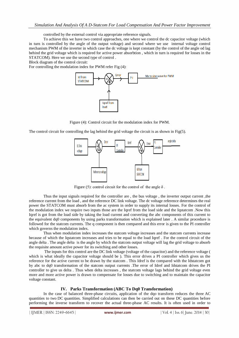
Simulation And Analysis Of A D-Statcom For Load Compensation And Power Factor Improvement
| IJMER | ISSN: 2249–6645 | www.ijmer.com | Vol. 4 | Iss. 6| June. 2014 | 30|
controlled by the external control via appropriate reference signals.
To achieve this we have two control approaches, one where we control the dc capacitor voltage (which
in turn is controlled by the angle of the output voltage) and second where we use internal voltage control mechanism PWM of the inverter in which case the dc voltage is kept constant (by the control of the angle od lag
behind the grid voltage which is required for active power absorbtion , which in turn is required for losses in the
STATCOM). Here we use the second type of control .
Block diagram of the control circuit:
For controlling the modulation index for PWM refer Fig (4):
Figure (4): Control circuit for the modulation index for PWM.
The control circuit for controlling the lag behind the grid voltage the circuit is as shown in Fig(5).
Figure (5): control circuit for the control of the angle δ .
Thus the input signals required for the controller are , the bus voltage , the inverter output current ,the
reference current from the load , and the reference DC link voltage. The dc voltage reference determines the real power the STATCOM must absorb from the ac system in order to supply its internal losses. For the control of
the modulation index we require two inputs those are the Iqref from the load side and the Iqstatcom .Now this
Iqref is got from the load side by taking the load current and converting the abc components of this current to
the equivalent dq0 components by using parks transformation which is explained later . A similar procedure is
followed for the statcom currents. The q component is then compared and this error is given to the PI controller
which governs the modulation index.
Thus when modulation index increases the statcom voltage increases and the statcom currents increase
because of which the Iqstatcom increases and tries to be equal to the load Iqref . For the control circuit of the
angle delta . The angle delta is the angle by which the statcom output voltage will lag the grid voltage to absorb
the requisite amount active power for its switching and other losses.
The inputs for this control are the DC link voltage (voltage of the capacitor) and the reference voltage (
which is what ideally the capacitor voltage should be ). This error drives a PI controller which gives us the reference for the active current to be drawn by the statcom . This Idref is the compared with the Idstatcom got
by abc to dq0 transformation of the statcom output currents .The error of Idref and Idstatcom drives the PI
controller to give us delta . Thus when delta increases , the statcom voltage lags behind the grid voltage even
more and more active power is drawn to compensate for losses due to switching and to maintain the capacitor
voltage constant.
IV. Parks Transformation (ABC To Dq0 Transformation) In the case of balanced three-phase circuits, application of the dqo transform reduces the three AC
quantities to two DC quantities. Simplified calculations can then be carried out on these DC quantities before performing the inverse transform to recover the actual three-phase AC results. It is often used in order to

Simulation And Analysis Of A D-Statcom For Load Compensation And Power Factor Improvement
| IJMER | ISSN: 2249–6645 | www.ijmer.com | Vol. 4 | Iss. 6| June. 2014 | 31|
simplify the analysis of three-phase synchronous machines or to simplify calculations for the control of three-
phase inverters and their gating pulses. For this transformation there are two aspects . One is the abc to α-β
transformation and the other is α-β to dq transformation. The matrix for abc to α-β transformation is:
The matrix for α-β to dq transformation is:
Where ɸ is the frequency at which we want to rotate the α-β frame ± the angle between the frames.
A sample output for this transformation is:- Input:
Figure (6) .Sample input for abc to dq0 transformation
Output:
Figure (7), Sample output from abc to ddq0 transformation
V. Three Phase Pll It is necessary for the power factor control to detect the accurate phase information of the utility
voltages. Therefore, the phase-locked loop (PLL) can be considered to be an important part of grid-connected
power generation systems. The block diagram for implementing the three phase PLL is as follows:

Simulation And Analysis Of A D-Statcom For Load Compensation And Power Factor Improvement
| IJMER | ISSN: 2249–6645 | www.ijmer.com | Vol. 4 | Iss. 6| June. 2014 | 32|
Figure (8) Implementation of three phase PLL
VI. Single Line Diagram Of The System
Figure (9) Single line diagram of the system
VII. Simulink Model Of The System The simulink model for the test system is as shown it consists of a source , a inductance between the
source and the point where the STATCOM is connected to the system to represent the transmission line
inductance , the three winding transformer and the load. The STATCOM consists of the DC link capacitor the
three phase inverter connected to the three winding transformer . It also consists of a three phase PLL connected
to the load side. It consists of two control circuits. One of that of the modulation index and the lower one of the angle δ.
The modulation indexis then multiplied with the sine waves of the gating pulses which are then
compared with the ramp wave to get us the gating pulses.
The waveforms are thus :
ma*sin(wt- δ) , ma*sin(wt-(2π/3)-δ) and ma*sin(wt+(2π/3)-δ).
The Simulink model is as shown in Fig(10)

Simulation And Analysis Of A D-Statcom For Load Compensation And Power Factor Improvement
| IJMER | ISSN: 2249–6645 | www.ijmer.com | Vol. 4 | Iss. 6| June. 2014 | 33|
Figure (10). Simulink model of the system
The plot of the power consumption of the load side is as follows:- Active power is shown in Fig (11)
Figure(11) : Active power consumed by the load .
Reactive power is shown in Fig (12)
Figure (12) : Reactive power consumed by the load
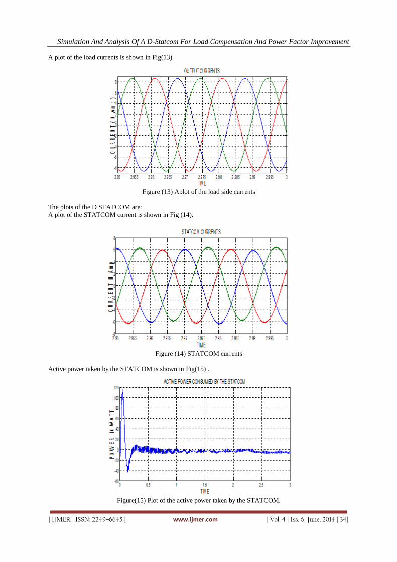
Simulation And Analysis Of A D-Statcom For Load Compensation And Power Factor Improvement
| IJMER | ISSN: 2249–6645 | www.ijmer.com | Vol. 4 | Iss. 6| June. 2014 | 34|
A plot of the load currents is shown in Fig(13)
Figure (13) Aplot of the load side currents
The plots of the D STATCOM are:
A plot of the STATCOM current is shown in Fig (14).
Figure (14) STATCOM currents
Active power taken by the STATCOM is shown in Fig(15) .
Figure(15) Plot of the active power taken by the STATCOM.
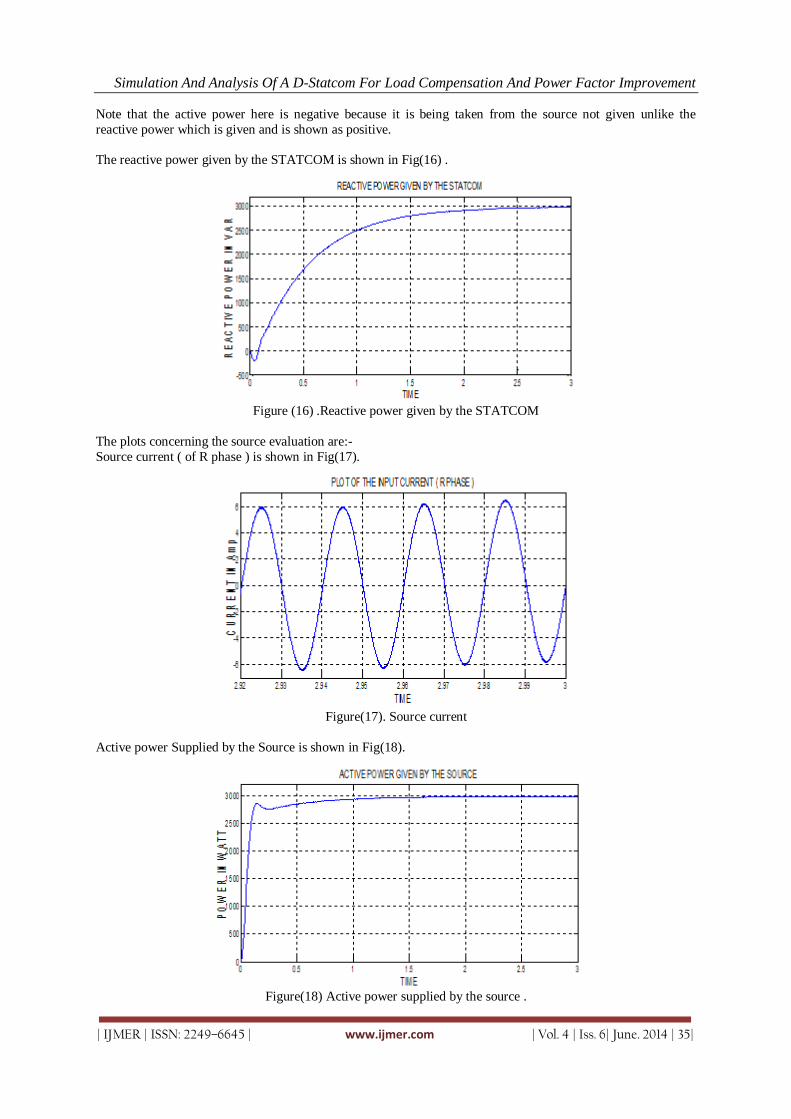
Simulation And Analysis Of A D-Statcom For Load Compensation And Power Factor Improvement
| IJMER | ISSN: 2249–6645 | www.ijmer.com | Vol. 4 | Iss. 6| June. 2014 | 35|
Note that the active power here is negative because it is being taken from the source not given unlike the
reactive power which is given and is shown as positive.
The reactive power given by the STATCOM is shown in Fig(16) .
Figure (16) .Reactive power given by the STATCOM
The plots concerning the source evaluation are:-
Source current ( of R phase ) is shown in Fig(17).
Figure(17). Source current
Active power Supplied by the Source is shown in Fig(18).
Figure(18) Active power supplied by the source .

Simulation And Analysis Of A D-Statcom For Load Compensation And Power Factor Improvement
| IJMER | ISSN: 2249–6645 | www.ijmer.com | Vol. 4 | Iss. 6| June. 2014 | 36|
The reactive power supplied by the source is shown in Fig (19).
Figure (19) Reactive power supplied by the source
Note that here some reactive power is still given by the source because of the reactance kept near the source to
represent the source inductance and the inductance of the transmission lines
VIII. Conclusion The comparison between load side current and the source side current gives us that the source side
current is lesser in magnitude than the load side current as the source does not have to supply reactive power.
This indicates that a higher amount of load can be supplied from the same transmission line on using a
STATCOM to compensate for the reactive power of the load . Thus power transfer capacity is increased.
The source active power is seen at 3000 W and the reactive power at 200 VAR. Thus the source power
factor is 0.9977 ( close to 1 ).Thus the source power factor correction is achieved.
The reactive power supplied by the STATCOM and that consumed by the load are equal .Thus the
reactive power of the load is given by the STATCOM .Thus load compensation by the STATCOM is achieved .
IX. Future Work The possibilities for the future work in the field of STATCOM and load compensation are many. A
multilevel inverter can be used. The control circuit can employ fuzzy controller PR controller or adaptive PI
fuzzy controller. The devices can be set to work on PV cells or wind power.
REFERENCES [1] N.G.Hingorani,”Flexible AC Transmission”, IEEE Spectrum, vol. 30, pp.40-44,1993. [2] K.K. Sen, “STATCOM: Theory, Modeling, Applications,”in IEEE PES 1999 Winter Meeting Proceedings, pp. 11
77-1183. [3] Mohan, T. M. Undeland, andW. P. Robbins, Power Electronics: Converter Applications and Design. New York:
Wiley. 1995. [4] Sangita Nandurkar, Design and Simulation of three phase Inverter for grid connected Photovoltic systems,
Proceedings of third biennial national conference NCNTE – 2012 Feb 24-24 [5] H. Rashid, “Power Electronics” 2nd edition, Elsevier, Inc, Publication, California, U.S.A 2007. [6] pierre Giroux , Modeling and Simulation of a Distribution STATCOM using Simulink’s Power System Blockset,
IEEE industrial electronics society [7] B.S.Krishna Varma , Simulated Control System Design of a Multilevel STATCOM for Reactive Power
Compensation , ICAESM- 2012 March 30,31 2012 . [8] Ravilla Madhusudan ,” Modeling and Simulation of a Distribution STATCOM (D-STATCOM) for Power Quality
Problems-Voltage Sag and Swell Based on Sinusoidal Pulse Width Modulation (SPWM) “, ICASEM- 2012 March30 ,31 2012
[9] Dr. P.Linga Reddy ,” A DSTATCOM-Control Scheme for Power Quality Improvement of Grid Connected Wind Energy System for Balanced and Unbalanced Non linear Loads “, IJMER vol 2 issue 3 may 2012 pp 661-666 .

International
OPEN ACCESS Journal
Of Modern Engineering Research (IJMER)
| IJMER | ISSN: 2249–6645 | www.ijmer.com | Vol. 4 | Iss. 6| June. 2014 | 37|
Anaerobic Digestion of Vinasse cane alcohol: The influence of
OLR by a UASB reactor
Cinthya Alejandra Sosa-Villalobos1, Elena Rustrián2, Eric Houbron3 1(Escuela Técnica Superior de Ingenieros de Caminos, Canales y Puertos/ Universidad Politécnica de
Madrid, España) 2, 3(Facultad de Ciencias Químicas/ Universidad Veracruzana, Orizaba, México)
I. INTRODUCTION
The sugar and distillery industries are the most important agro-industries for economic development
in Mexico and several countries for the production of sugar and alcohol. However, alcohol industry has been
proved as one of the industries, which consume large amount of water and energy, produce numerous organic
pollutants, and cause serious contamination [1]. All distilleries produce an effluent commonly known as
“vinasse,” an amount equal to 10–15 times that of the volume of alcohol [2]
According to the origin of the raw material and the fermentation / distillation used for obtaining
alcohol, is the high content of COD, total nitrogen, total phosphorus effluent among other parameters. The
vinasses disposal into the environment is hazardous and has high pollution potential. The highly colored
components of the vinasses reduce sunlight penetration in rivers, lakes or lagoons, which in turn decrease both
photosynthetic activity and dissolved oxygen concentration affecting aquatic life. In accordance Pant and
Adholeya [3] the brown colour is due to phenolics (tannic and humic acids) from the feedstock, melanoidins
from Maillard reaction of sugars (carbohydrates) with proteins (amino groups)
[2] Patel et al. reported that the dry vinasse or effluent contains about 38–40% inorganic salts of
potassium, sodium, magnesium, and calcium in the form of chlorides, sulfates, and phosphates, and about 60–
62% organic compounds. Besides a strong pungent smell and intense dark color, effluent has a large biological
oxygen demand (BOD) and chemical oxygen demand (COD) in the range of 45 and 100 g/L, respectively.
[4] Mohana et al. indicate that the unpleasant odor of the vinasse is due to the presence of skatole,
indole and other sulphur compounds, which are not effectively decomposed by yeast during distillation.
A number of technologies have been explored for reducing the pollution load of distillery effluent.
Biological treatment of distillery is either aerobic or anaerobic but in most cases a combination of both is used.
Various physicochemical methods such as adsorption, coagulation–flocculation, and oxidation processes have
also been practiced for the treatment of distillery effluent [3].
Among anaerobic technologies available, based clearly in the granular sludge blanket is the most
interesting. The UASB concept is one of the most notable developments in anaerobic treatment process
technology, conceived in the late 1970’s in the Netherlands by Professor Lettinga Gatze Wageningen.
Abstract: An Anaerobic Sludge Blanket (UASB) reactor was used to study the treatment of distillery
effluent. Vinasse was used to feed the reactor, although its Chemical Oxygen Demand (COD)
concentration varied during the experiment, the volume utilized to feed the reactor was adjusted to
maintain constant Organic Load Rate (OLR). The UASB reactor was operated with OLR 1, 2, 4 and 6
gCOD/Ld. Removal efficiencies of 76,64,63 and 51% respectively were observed. The reactor responded
with progressive decreases of efficiency with each increase of OLR, the total mass removed increased.
An average biogas production of 1.400, 1.872, 2.17 and 2.172 L to each OLR of 1, 2, 4 and 6 gCOD/Ld,
respectively was observed. The methane content in biogas was 63, 68, 86 and 89% each OLR tested.
Methane production is also followed with values of .892 L to OLR 1 gCOD/Ld, 1.264 L to OLR 2
gCOD/Ld, 1.876 L to OLR 4 gCOD/Ld and 2.900 L to OLR 6 gCOD/Ld.
The UASB reactor operating in continuous mode, it was necessary to evaluate the best conditions for
this type of waste. The treatment of distillery effluents using a UASB reactor is feasible and is an
alternative to treat these wastes in the alcohol industries
Keywords: Anaerobic digestion, organic load rate (OLR), UASB reactor, Vinasse, Biogas

Anaerobic Digestion of Vinasse cane alcohol: The influence of OLR by a UASB reactor
| IJMER | ISSN: 2249–6645 | www.ijmer.com | Vol. 4 | Iss. 6| June. 2014 | 38|
The key features of the UASB process that allow the use of high volumetric COD loadings compared
to other anaerobic processes. In this study the influence Organic Load Rate (OLR) with the removal efficiency
was evaluated.
II. MATERIALS AND METHODS 2.1 UASB reactor
The UASB reactor (Figure 1) consisted of a glass column 53 cm high, with 7.5 cm internal diameter
and six sampling points along its length, the reactor had a total volume of 2.3 L.
The reactor was fed with vinasse using a peristaltic pump and the vinasse was maintained at 20°C in a
container during the feeding to the reactor. The hydrodynamic conditions and upflow was maintained by
recycling using a Masterflex® peristaltic pump .An inverted conic gas-solid-liquid separator was installed in
the upper part of the reactor, after the biogas passed through a Mariotte Flask containing to (3N NaOH)
solution. The operation temperature was of 35±2°C using a Polystat® water bath heater circulator
1. Effluent
3.Vinassereservoir
4.Feedingpump
6.Recyclepump5.waterbath
heatercirculator
8.Thermometer
9.Mario e´sflaskdevice
2.Samplingports
7.Biogasoutput
Figure 1. UASB reactor
2.2 Experimental procedure
To inoculate the UASB reactor, there were used granular sludge from a Wastewater Treatment Plant
(WWTP), which is a mixture of urban wastewater (UW) and Industrial Wastewater (IW), from various local
industries such as; brewery, paper, production of drugs, chemicals, steel mills, petrochemical and others. In the
beginning of the experiment, an operation was performed in batches. 600 ml of concentrated sludge were used,
which represented an initial concentration of 10.63 g/L of VSS in the mixed liquor in the reactor. A solution of
inorganic medium adds (Table 1)
Table 1. Modified inorganic medium
Modified Kawahara Stock solution volume/100 ml of reactor
KH2PO4 4.05 g/l 15 ml Stock solution of KH2PO4
K2HPO4 8.385 g/l 4 ml Stock solution of K2HPO4
NH4Cl 7.95 g/l 4 ml Stock solution of NH4Cl
CaCl2 1.125 g/l 4 ml Stock solution of CaCl2
MgCl2.6H2O 1.0 g/l 4 ml Stock solution of MgCl2.6H2O
FeSO4.7H2O 5.6 g/l 4 ml Stock solution of FeSO4.7H2O
Note: Original Inorganic medium [5]

Anaerobic Digestion of Vinasse cane alcohol: The influence of OLR by a UASB reactor
| IJMER | ISSN: 2249–6645 | www.ijmer.com | Vol. 4 | Iss. 6| June. 2014 | 39|
2.3 Substratum
The vinasse used throughout the entire study, came from a family local distillery that processes about
20,000 liters of daily alcohol from molasses. The production of vinasse is about 20 L per liter of processed
alcohol, i.e. 200 m3 per day. This vinasse are downloaded and processed in an anaerobic lagoon system. The
vinasse was sampled monthly during the project; in the Table 2, the average characterization of the vinasse
used for the project is summarized. It was operated in continuous mode, feeding vinasses by a peristaltic pump.
The vinasse was neutralized before feeding the reactor, taking a pH of 4-7 with manual addition of 3N NaOH.
Initial OLR 1 gCOD/Ld was applied, with an average concentration of vinasse of 108.33 and 97.47 gCOD/L
total and soluble, respectively. OLR gradually increasing values were performed at 2, 4, up to a maximum
value of 6 gCOD/Ld observing the stabilization of the system in each condition. In Table 3, the UASB reactor
operations conditions are shown. Gradual increases were performed according to the recommended values by
Lettinga and Hulshoff [6]
Table 2. Characterization of the vinasse
Parameter Average Maximum Minimum
pH 4.14 4.44 4.03
Conductivity (µs/cm) 21.17 29.80 7.73
Tot-COD (g/L) 128.63 217.71 57.59
Sol-COD(g/L) 108.48 156.07 36.13
TTS (g/L) 80.12 113.98 17.85
VTS (g/L) 58.11 81.67 11.81
TSS (g/L) 6.83 15.24 1.08
VSS (g/L) 5.42 11.78 0.96
N-Organic(g/L) 0.25 0.65 0.08
TKN (g/L) 0.28 0.69 0.12
N-NH4 (g/L) 0.03 0.05 0.003
Total phosphate (g/L) 0.08 0.15 0.01
Sulfates (g/L) 9.36 14.64 5.03
Table 3. Average operating conditions of the UASB reactor with proved OLR
OLR (gCOD/L·d)
1 2 4 6
Upflow velocity (m/h) 2 2-3 2,5-3 2,5-3
HRT (days) 109 58 30 25
Flowrate (L/d) 0,022 0,042 0,108 0,099
Temperature (ºC) 36±2 36±2 36±2 36±2
2.4 Performed analyzes
To verify the stability of the system, the following parameters were analyzed daily, influent and
effluent: CODTotal, CODSoluble, sulfate (SO42-), total solids (TS), volatile total solids (VTS), total suspended
solids (TSS) and volatile suspended solids (VSS), pH, temperature, biogas and CH4 produced. For the
analytical determination of soluble compounds previously samples were centrifuged (6000 rpm for 30 min.).
The procedures correspond to those reported by Mexican standards, and standardized methods for the analysis
of drinking and Wastewater [7]

Anaerobic Digestion of Vinasse cane alcohol: The influence of OLR by a UASB reactor
| IJMER | ISSN: 2249–6645 | www.ijmer.com | Vol. 4 | Iss. 6| June. 2014 | 40|
III. RESULTS AND DISCUSSION
3.1 Process Performance
The percentage of CODsoluble removal function of time can be seen in Figure 1. At the beginning of the
experiment, was observed an upper 98% removal during the first 20 days. It is up to day 50 and up to a length
approximately equivalent to 1 HRT that is beginning to show a stable clearance values over 70%. Initially the
OLR of 2 gCOD/L·d values for removal of approximate 80% this is still observed for 72 days after the 1 OLR
gCOD/L·d, ie equivalent to the period of 1 HRT. The observed average value of COD removal percentage is
approximately 60%. By applying OLR of 4 gCOD/L·d due to a change in the concentration of our vinasse
during a period of approximately 50 days, we obtain data clearance 40 to 60%. Once stabilized feeding
conditions, a removal of CODsoluble average of 60% is reached.
During OLR of 6 gCOD/L·d is observed a greater variability in the percentage of COD
removal. Excluding the period in batch mode to recover the activity of the reactor, the average removal
efficiency of soluble COD was 51%. We can observe that while the reactor responds by a progressive reduction
to each increase efficiency OLR the total mass removed increases.
The response of the reactor and the biodegradability of the effluent is considered that further increases
OLR could irreversibly affect the operation of the reactor. However it is clear that the concentration of vinasse
and consequently, HRT plays an important role in the operation and efficiency of the UASB reactor. This
directly impacts the Hydraulic Retention Time (HRT), which has values of 118, 59, 41, 24 days for the OLR 1,
2, 4 and 6 gCOD/Ld respectively.
These facts still position the UASB technology in a suitable and appropriate process for the treatment
of sugar cane alcohol vinasses.
0
20
40
60
80
100
0 50 100 150 200 250 300 350 400 450 500 550 600 650
Rem
ov
al
%
Time, days
OLR=1 gCOD/L·d OLR=2 gCOD/L·d OLR=6 gCOD/L·d OLR=4 gCOD/L·d
Figure 2. COD soluble removal versus time
3.2 Biogas production
The biogas production, CH4 and CH4 percentage is illustrated in figure 3. To an OLR 1 gCOD/Ld
average and stable biogas production and methane with values of 1.4 L and 0.892 L respectively was observed.
The presented biogas contained 63% of methane. Biogas production and methane observed reflect a good
development of the granule and a good metabolism by this. Furthermore, the average theoretical production of
CH4 is 0,646 L, i.e. lower than actually occurred, this may have two explanations. First, the sensitivity of the
biogas production volumetric system. However, the measured values would be lower than the theoretical, in
this case. For this reason, a second alternative is required. According E. Houbron, et al [8] a solids residence
time of more than 20 days, promotes liquefaction of solid organic wastes. Indeed given the amount of solids in
the vinasse and HRT 118 days, the conditions for hydrolysis-solubilization of this organic matter are presented
and allow additional methane production. With respect to the OLR 2 gCOD/Ld, the average production of
biogas and methane had values of 1.87 L and 1.26 L respectively. The methane gas is 68%, which represents
an interesting quality of biogas from the energy standpoint. The theoretical value calculated methane is 1 L.
This value is still lower than what actually occurred. Under these operating conditions the HRT of 59 days is
still suitable to hydrolysis-solubilization of solid waste and the generation of an extra amount of methane. By
increasing OLR 4 gCOD/Ld proportional increases were observed in the production of biogas and methane.
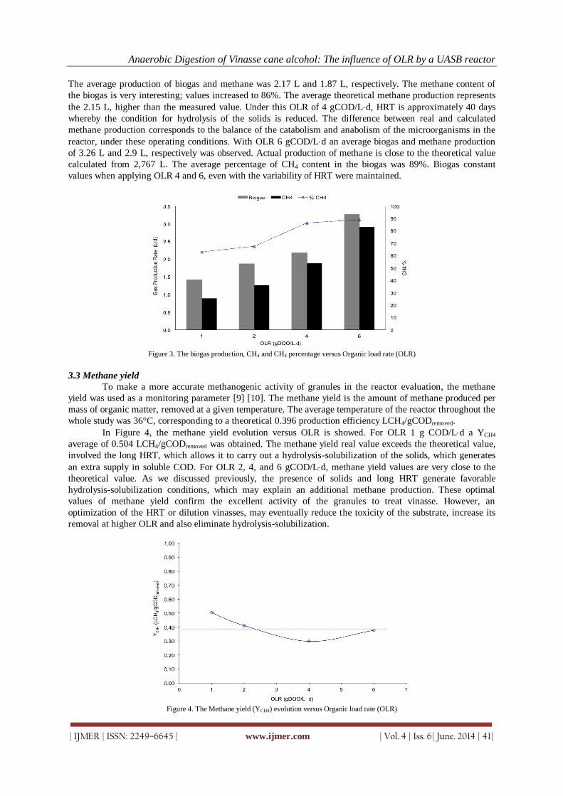
Anaerobic Digestion of Vinasse cane alcohol: The influence of OLR by a UASB reactor
| IJMER | ISSN: 2249–6645 | www.ijmer.com | Vol. 4 | Iss. 6| June. 2014 | 41|
The average production of biogas and methane was 2.17 L and 1.87 L, respectively. The methane content of
the biogas is very interesting; values increased to 86%. The average theoretical methane production represents
the 2.15 L, higher than the measured value. Under this OLR of 4 gCOD/Ld, HRT is approximately 40 days
whereby the condition for hydrolysis of the solids is reduced. The difference between real and calculated
methane production corresponds to the balance of the catabolism and anabolism of the microorganisms in the
reactor, under these operating conditions. With OLR 6 gCOD/Ld an average biogas and methane production
of 3.26 L and 2.9 L, respectively was observed. Actual production of methane is close to the theoretical value
calculated from 2,767 L. The average percentage of CH4 content in the biogas was 89%. Biogas constant
values when applying OLR 4 and 6, even with the variability of HRT were maintained.
Figure 3. The biogas production, CH4 and CH4 percentage versus Organic load rate (OLR)
3.3 Methane yield
To make a more accurate methanogenic activity of granules in the reactor evaluation, the methane
yield was used as a monitoring parameter [9] [10]. The methane yield is the amount of methane produced per
mass of organic matter, removed at a given temperature. The average temperature of the reactor throughout the
whole study was 36°C, corresponding to a theoretical 0.396 production efficiency LCH4/gCODremoved.
In Figure 4, the methane yield evolution versus OLR is showed. For OLR 1 g COD/Ld a YCH4
average of 0.504 LCH4/gCODremoved was obtained. The methane yield real value exceeds the theoretical value,
involved the long HRT, which allows it to carry out a hydrolysis-solubilization of the solids, which generates
an extra supply in soluble COD. For OLR 2, 4, and 6 gCOD/Ld, methane yield values are very close to the
theoretical value. As we discussed previously, the presence of solids and long HRT generate favorable
hydrolysis-solubilization conditions, which may explain an additional methane production. These optimal
values of methane yield confirm the excellent activity of the granules to treat vinasse. However, an
optimization of the HRT or dilution vinasses, may eventually reduce the toxicity of the substrate, increase its
removal at higher OLR and also eliminate hydrolysis-solubilization.
Figure 4. The Methane yield (YCH4) evolution versus Organic load rate (OLR)

Anaerobic Digestion of Vinasse cane alcohol: The influence of OLR by a UASB reactor
| IJMER | ISSN: 2249–6645 | www.ijmer.com | Vol. 4 | Iss. 6| June. 2014 | 42|
Several authors reported the operation of UASB reactors at higher loads of 10 gCOD/Ld [11] [12]
[13]. However all reported strong reduction removal efficiency by increasing the load. Moreover, it is reported
[14], that dilute effluent removal efficiencies increase. Now, while diluting a vinasse at laboratory does not
represent major problems, in situ requires a huge source of water. Given the laws in practice is unthinkable,
use clean water to dilute vinasse, so the only option would be to reuse the treated effluent. Another alternative
could be mixing the waters of vinasse with urban wastewater. But, as Toze [13] mentioned, there are a number
of risk factors to reuse. Certain factors are short term and vary in their degree of risk, depending human,
animal and environmental factors (pathogens, microbes), while others have a long term impact, which increase
with continued use of wastewater recycling (eg, saline effects on soil). Therefore, dilution of vinasse as charged
is not as viable in situ solution.
IV. CONCLUSION By operating the UASB reactor in continuous mode, it was possible to evaluate the best operating
conditions for this type of waste (vinasse). For a range of operation OLR 1-6 gCOD/Ld quite a favorable
response is observed with respect to the performance of UASB reactor, as presented soluble COD removal
percentages of 51 to 76%, similar efficiencies to those reported literature. The OLR 6 gCOD/Ld for the UASB
reactor fed with vinasse represents the limit of its capacity. However, with increasing OLR increased biogas
production and methane is generated. Elevated HRT applied, allowed hydrolysis-solubilization of solid,
generating an extra production of methane, which is reflected in the higher theoretical value YCH4. Once the
reactor stabilized, catabolism was the dominant biochemical process. Treating cane alcohol vinasse using an
UASB reactor is feasible, however the high concentration of organic matter imposes high HRT.
Acknowledgements This project was financially supported by Mexican FOMIX-CONACYT- Veracruz project Nº 41752.
REFERENCES [1] H.C. Guo, B. Chen, X.L. Yu, G.H. Huang, L. Liu and X.H. Nie (2006), Assessment of cleaner production options
for alcohol industry of China: a study in the Shouguang Alcohol Factory, Journal of Cleaner Production 14 (10),
2006, 94-103.
[2] N.M. Patel, P.J. Paul, H.S. Mukunda and S. Dasappa, (1996). Combustion studies on concentrated distillery
effluents. Twenty-Sixth Symposium (International) on Combustion/The Combustion Institute, Nápoles, Italia, 2479–
2485
[3] D. Pant, and A. Adholeya, Biological approaches for treatment of distillery wastewater: a review, Bioresource
Technology, 98(14), 2007, 2321–2334
[4] S. Mohana, B.K. Acharya and D. Madamwar, Review Distillery spent wash: Treatment technologies and potential
applications, Journal of Hazardous Materials, 163 (14), 2009, 12–25.
[5] K. Kawahara, Y. Yakabe, T. Ohide and Kenji Kida, Evaluation of laboratory-made sludge for an anaerobic
biodegradability test and its use for assessment of 13 chemicals, Chemosphere, 39(12), 1999, 2007-2018
[6] G. Lettinga and L.W. Hulshoff Pol, UASB process design for various types of wastewaters, Water Science and
Technology, 24 (20), 1991, 87-107.
[7] Standard Methods for the examination of water and wastewater, in American Public Health Association, American
Water Works Association, Water Environment Federation (Ed.), 19th edition (USA, 1995)
[8] E. Houbron, G.I. González-Lopez, V. Cano-Lozano, E. Rustrián, Hydraulic retention time impact of treated
recirculated leachate on the hydrolytic kinetic rate of coffee pulp in an acidogenic reactor, Water Science
Technology 58 (7), 2008 1415-21.
[9] S. Michaud, N. Bernet, P. Buffière, M. Roustan, R. Moletta, 2002), Technical note. Methane yield as a monitoring
parameter for the start-up of anaerobic fixed film reactors, Water Research (36), 2002, 1385–1391
[10] S. Michaud, N. Bernet, P. Buffière, M. Roustan, J.P. Delgenès, Use of the methane yield to indicate the metabolic
behaviour of methanogenic biofilms, Process Biochemistry (40),2005, 2751-2755.
[11] A.M. Jiménez, R. Borja, A. Martin, F. Raposo, Kinetic analysis of the anaerobic digestión of untreated vinasses
and vinasses previously treated with Penicillium decumbens, Journal of Environmental Management, 80, 2006,
303-310.
[12] S.V. Kalyuzhnyi, A. Gladchenko, V.I. Sklyar, and Y.S. Kizimenko, One-and Two-stage Upflow Anaerobic Sludge-
Bed Reactor Pretreatment of Winery Wastewater at 4-10°C, Applied Biochemistry and Biotechnology. 90, 2001,
107-124.
[13] H. Harada, S. Uemura, A.C. Chen, and J. Jayadevan, Anaerobic Treatment of a recalcitrant distillery wastewater by
a thermophilic UASB Reactor, Bioresource Technology 55, 1996, 215-221.
[14] W.J.B.M. Driessen, M.H. Tielbaard, and T.L.F.M. Vereijken, Experience on Anaerobic Treatment of Distillery
Effluent with the UASB Process, Water Science and Technology, 30(12), 1994, 193-201.
[15] S. Toze, Water reuse and health risks – real vs. perceived, Desalination 187, 2006, 41-51.

International
OPEN ACCESS Journal Of Modern Engineering Research (IJMER)
| IJMER | ISSN: 2249–6645 | www.ijmer.com | Vol. 4 | Iss. 6| June. 2014 | 43|
Design of VGA Controller using VHDL for LCD Display using
FPGA
Khan Huma Aftab1, Monauwer Alam
2
1, 2 (Department of ECE, Integral University, India)
I. INTRODUCTION The term VGA stands for Video Graphic Array. This VGA is a graphics display systems for PCs
developed by IBM. VGA has become one of the factor standards for PCs. In graphics, generally the resolution is either 640 by 480 within 16 colors or 320 by 200 within 256 colors. While this resolution has been superseded
in the personal computer market, it is becoming a popular resolution on mobile devices. Figure 1 shows
overview of VGA port connection to a monitor.
Fig 1: VGA port connection to a monitor
II. VGA PRINCIPAL A colorful image is generated when the electron beam from a cathode ray tube hits the fluorescent
screen. To generate an image, the screen will be scanned by the electron beam. The scan mode can be divided
into progressive scan and interlaced scan.
The progressive scan begins from the top left corner of the screen and it scans point by point from left
to the right of one line. After one line is scanned, the electron beam moves back to the left start point of the next
line and the beam is synchronized by horizontal synchronization signal. During this movement, the cathode ray
tube blanks the electron beam. The beam scans the screen line by line until it reaches to the bottom right corner
of the screen. After all lines scanned, the beam moves back to the top left corner of the screen and the beam is
synchronized by horizontal synchronization signal. During this movement also, the cathode ray tube blanks the electron beam. At this point, an image frame is generated. Figure 2 shows the progressive scan.
Abstract: Basically, here I have used VGA for implementing basic characters/Symbols that can be either
used in advertisements that deals with real-time application. So, I thought of using VGA as a standard for
this implementation as it is the basic graphics array and compatible with other graphical arrays. This project also describes about the design of VGA (Video Graphic Array) Controller using combination of
three bit input data to control eight differences colors to display text at monitor by using on board
pushbuttons for the input. Three color signal referred to collectively as R (red), G (green) and B (blue)
signal(i.e. RGB). The VGA monitor using resolution of 640 by 480 by mode to display
Characters/Text/Images in different colors. Here, we used VHDL language on Xilinx ISE software for
interfacing the required peripheral to the Xilinx FPGA Spartan Series. Where, I implementing the
application of VGA with the help of VHDL language on Xilinx FPGA, that will contain the logic part. For
Simulation part we are using Modelsim 10.2. Finally, the results that we obtained for VGA application
implementation.
Keywords: FPGA, Modelsim 10.2a, VGA, VHDL, Xilinx ISE 14.2.

Design of VGA Controller using VHDL for LCD Display using FPGA
| IJMER | ISSN: 2249–6645 | www.ijmer.com | Vol. 4 | Iss. 6| June. 2014 | 44|
The interlaced scanning scans every other line of the screen. After the screen is scanned once, the
electron beam returns to scan the rest lines.
Fig 2: Progressive Scan
2.1 VGA Controller:
Video Graphics Array (VGA) is mostly used for computer monitors, with a high-definition resolution
video standard. It has the ability the ability to transmit a sharp detailed image. VGA uses separate wires to
transmit the three color component signals, vertical and horizontal synchronization signals. Red, green and blue
are three signals that send color information to VGA monitor. There are four main components in VGA
controller which are VGA interface signals, VGA interface definition, VGA control signal, VGA timing Control
and VGA monitor.
2.1.1 VGA Interface Signals:
There are two types VGA interface signals to display which is data signal, and the other one is control
signal. Data signal have three parts which is Red, Green and Blue and for control signal have two parts which is
Horizontal Synchronization and Vertical Synchronization. There are different frequencies of the horizontal
synchronization signal and vertical synchronization signal for the changeable output resolution. Here is a table
to imply the range of
2.2 VGA Interface Definition:
VGA interface sends corresponding display signals to display through DB-15 linker which is directly
connected to Monitor or LCD by monitor cable. There are 15 pinholes which are asymmetrically divided into 3 lines, and there are 5 on each line. [3] Here is Figure 3 showing how these pinholes are arranged.
Fig 3: VGA display port

Design of VGA Controller using VHDL for LCD Display using FPGA
| IJMER | ISSN: 2249–6645 | www.ijmer.com | Vol. 4 | Iss. 6| June. 2014 | 45|
2.3 VGA Color Signal:
RGB Color Model is an additive color model. It generates various colors by adding three basic
colors—red, green and blue. A color can be represented by how much each of the three basic colors is included.
[4] Each of the three basic colors is one color component of the represented color. It can be concluded by the
following expression:
color = f (r, g,b)
They are just shown in Table 1. Table 1: 3-Bit Display Color Codes.
VGA_R VGA_G VGA_B Resulting Color
0 0 0 Black
0 0 1 Blue
0 1 0 Green
0 1 1 Cyan
1 0 0 Red
1 0 1 Pink
1 1 0 Yellow
1 1 1 White
2.4 VGA Monitor:
Since a VGA monitor is the output device in this thesis, an understanding of how it works is necessary.
This section describes the basics of the VGA technology, and how one goes about controlling it.
A VGA monitor is a complete video displaying system that provides a simple controlling interface, for
the displaying of video images. This interface is defined in a VGA standard. Video images can be defined as
images that consist of the 3 primary colors in various intensities; this creates a 2 dimensional image that is
lifelike in appearance. The VGA monitor interface consists of 5 controlling signals. These are the Red, Green
and Blue colour signals (RGB), the horizontal and vertical sync signals.
From Figure 3.2 below, it shows the VGA monitor with 640 columns by 480 rows. This VGA monitor is based
on 25MHz clock. A single dot of colour on a video monitor does not impact much information. A horizontal line of pixels carries a bit more information. However, a frame composed of multiple lines can present an image on
the monitor screen. A frame of VGA video typically has 480 lines and each line usually contains 640 pixels.
III. METHODOLOGY
3.1 The VGA Technology:
At the heart of the VGA monitor is the CRT described earlier. This time however, there are 3 electrons
guns for each of the primary colours. The electron beam is scanned across the display section, row by row,
starting from the top row. On the displaying end of the tube, there are 3 different phosphors, for each of the colours. The VGA monitor also contains the electronics that drive the horizontal and vertical deflection plates to
control this scanning process. The scanning process takes place at a constant rate, which is defined in the VGA
standard.
The viewing part of the monitor contains 480 x 640 picture elements, or pixels. The voltage levels on
the RGB control signals determine the colour of each pixel, when the electron beam scans across this pixel. In
order to provide motion in the image, the image needs to be refreshed at least 60 times per second as the human
eye can spot flicker at refresh rates less than about 30 times per seconds. For 480 x 640 pixels VGA monitor, at
a 60Hz refresh rate, approximately 40ns is needed per pixel. A 25 Mhz clock has a 40ns period
3.2 VGA Timing Control:
Pixels are updated in a serial fashion. The pixel clock runs at 25MHz. The electron beam starts at (0, 0) and goes horizontally through the first row, up to the last row, and last pixel at (479,639).
Timing of VGA signals are ruled by VESA. Here is a short introduction about how FPGA drive the
VGA display with 640×480@60Hz. In the standard of VGA industry, the output frequency of pixel is
25.175MHz, and the frequencies of horizontal scan and vertical scan are 31.496 KHz and 59.940 Hz. If display
receives this standard frequency, then the resolution will be 640×480, and refresh rate is 60Hz. [2]
The VGA vertical timing is basically the same as the VGA Horizontal Timing. The difference is that
vertical synchronization pulse represents the end of one image frame and the start of the next frame. The RGB
data during display interval includes all lines of the screen.

Design of VGA Controller using VHDL for LCD Display using FPGA
| IJMER | ISSN: 2249–6645 | www.ijmer.com | Vol. 4 | Iss. 6| June. 2014 | 46|
3.3 System Requirement Analysis:
Figure 4 shows the devices required in this project. We need Spartan 3E FPGA board which contain
VGA interface. The host PC is used to configure the hardware design and download the designed from FPGA
board. The display is controlled by the FPGA board interface and displayed on the LCD Monitor through VGA
interface. From these devices, the following components are required:
Spartan 3E FPGA board.
SDRAM Controller for Memory
VGA Controller Interface
Clocks for processor, SDRAM and VGA
Fig 4: Required Devices and Collections
Fig 5: Block Diagram of VGA Controller
IV. SIMULATION RESULTS In this paper i interface a VGA port available on FPGA board to generate the character(s) from ASCII
text characters. To display text on video controller is an important function. I made the Character generation
circuit that took the character from internal ROM to facilitate the display of text characters on a screen. To display text on my VGA display, I organized the 640x480 display area into "tiles" where each tile represents a
character location. In this project, the font size of each character is 16x8 (height & Width). This font will display
80 text characters in each line Mapped onto a 640x480 display (i.e., 640 pixels divided by 8 columns per
character) and 30 lines (480 / 16). Each of the 640x480 pixels in the display are associated with one of the
80x30 character locations fig 6 shows the simulation result of VGA controller for display color input 100,
display output color 100 and background color is 011.

Design of VGA Controller using VHDL for LCD Display using FPGA
| IJMER | ISSN: 2249–6645 | www.ijmer.com | Vol. 4 | Iss. 6| June. 2014 | 47|
Fig 6: Simulation Result for VGA
Fig 7 shows the simulation result of VGA controller for display color input 110, display output color 110 and
background color is 001.
Fig 7: Simulation Result for VGA
We have implemented our work on FPGA Spartan3E also and we get result for different display color
inputs by three DIP switches on FPGA board. DIP switches are responsible for the color of display character
and background color. We need a CRT monitor to visualize the effects (Results may be vary for different CRT
manufacturers) shows in fig 8.

Design of VGA Controller using VHDL for LCD Display using FPGA
| IJMER | ISSN: 2249–6645 | www.ijmer.com | Vol. 4 | Iss. 6| June. 2014 | 48|
(a)
(b)
Fig 8: Output display by FPGA kit.
We are using Xilinx tool for synthesis our code fig 9 shows the main RTL of our code.
Fig 9: Main RTL

Design of VGA Controller using VHDL for LCD Display using FPGA
| IJMER | ISSN: 2249–6645 | www.ijmer.com | Vol. 4 | Iss. 6| June. 2014 | 49|
V. CONCLUSION In this paper I interface a VGA port available on FPGA board to generate the character(s) from ASCII
text characters. To display text on video controller is an important function. I made the Character generation
circuit that took the character from internet ROM to facilitate the display of text characters on a screen. To display text on my VGA display, I organized the 640x480 display area into "tiles" where each tile represents a
character location. In this project, the font size of each character is 16x8(height & Width). This font will display
80 text characters in each line Mapped onto a 640x480 display (i.e., 640 pixels divided by 8 columns per
character) and 30 lines (480 / 16). Each of the 640x480 pixels in the display are associated with one of the
80x30 character locations.
VGA is an important output section for displaying the results. My work could be move further for
interfacing the keyboard (PS2/USB) for more interesting real world implementation to a complete gaming
device.
REFERENCES [1.] AvalonSwitchFabricAccessedmarch32014.www.ee.ryerson.ca/%7Ecourses/coe718/DataSheets/sopc/AVALONB
US_qii54003.pdf. [2.] VGA Timing. Accessed march 7 2014 martin.hinner.info/vga/timing.html [3.] VGA Interface and Pin out. Accessed march 7 2014http://www.allpinouts.org/index.php/VGA_15_Pin [4.] RGB Color Model. Accessed march 7 2014 http://en.wikipedia.org/wiki/RGB_color_model
[5.] Wisniewski, Remigiusz (2009). Synthesis of compositional microprogram control units for programmable devices.
Zielona Góra: University of Zielona Góra. p. 153. ISBN 978-83-7481-293-1.

International
OPEN ACCESS Journal Of Modern Engineering Research (IJMER)
| IJMER | ISSN: 2249–6645 | www.ijmer.com | Vol. 4 | Iss. 6| June. 2014 | 50|
An Improved Single Phase Transformer less Inverter Topology
for Cost Effective PV Systems
Geethu Chacko1, Riya Scaria
2
1,2 (M.Tech student, Assistant Professor, Department of Electrical and Electronics Engineering, Federal
Institute of Science and Technology/Mahatma Gandhi University ,Kerala, India)
I. INTRODUCTION Photovoltaic (PV) power supplied to the utility grid is gaining more and more visibility, while the
world’s power demand is increasing. . Photovoltaic inverters are widespread in both private and commercial
circles. These grid-connected inverters convert the available direct current supplied by the PV panels and feed it
into the utility grid.. The grid-connected photovoltaic (PV) systems, especially the low-power single-phase
systems, call for high efficiency, small size, light weight, and low-cost grid connected inverters. Most of the
commercial PV inverters employ either line-frequency or high-frequency isolation transformers.
However, line-frequency transformers are large and heavy, making the whole system bulky and hard to
install. Topologies with high-frequency transformers commonly include several power stages, which increases the system complexity and reduces the system efficiency. Consequently, the transformer less configuration for
PV systems is developed to offer the advantages of high efficiency, high power density and low cost.
Unfortunately, there are some safety issues. Without transformer, there is a path for leakage current
between PV array and the grid. High frequency common mode voltage generated by inverter appears across
stray capacitance formed between the ground and the array terminals. This causes flow of high leakage current
from the inverter to the ground. If the leakage current is not regulated within a reasonable margin, it can cause
electromagnetic interference, safety issues and grid current distortion. Therefore in order to minimize the
leakage current, high frequency common mode voltage must be avoided in transformer less grid connected PV
applications.
To avoid the common-mode leakage current, the conventional solution employs the half-bridge inverter
or the full-bridge inverter with bipolar sinusoidal pulse width modulation (SPWM), because no variable
common-mode voltage is generated. However, the half-bridge inverter requires a high input voltage which is greater than, approximately, 700V for 220-Vac applications. As a result, either large numbers of PV modules in
series are involved or a boost dc/dc converter with extremely high-voltage conversion ratio is required as the
first power processing stage. The full-bridge inverter just needs half of the input voltage demanded by the half-
bridge topology, which is about 350V for 220-Vac applications. But the main drawback is that the full bridge
inverter can only employ the bipolar SPWM strategy with two levels, which induces high current ripple, large
filter inductor, and low system efficiency. . The main goal of this project is to analyze and model transformer
less PV inverter systems with respect to the leakage current phenomenon that can damage the solar panels and
pose safety problems.
Abstract: In grid connected PV systems, the elimination of isolation transformer introduces common
mode leakage current due to the parasitic capacitance between PV panels and the ground. The common
mode leakage current reduces the efficiency of power conversion stage, affects the quality of grid
current, deteriorate the electric magnetic compatibility and give rise to various safety threats. In order
to eliminate the leakage current, an improved transformer less topology with virtual DC bus concept is
proposed here. By connecting the grid neutral line directly to the negative pole of the DC bus, the stray
capacitance between the PV panels and the ground is bypassed. The topology consists of only five power switches, two capacitors and the filter section. Therefore, the power electronics cost can be curtailed.
This advanced topology can be modulated with the sinusoidal pulse width modulation (SPWM) to reduce
the output current ripple. The simulation result of the proposed topology using MATLAB/SIMULINK is
presented.
Keywords: Common mode leakage current, Transformer less inverter, Unipolar SPWM, Virtual dc bus.

An Improved Single Phase Transformerless Inverter Topology For Cost Effective PV Systems
| IJMER | ISSN: 2249–6645 | www.ijmer.com | Vol. 4 | Iss. 6| June. 2014 | 51|
II. LITERATURE REVIEW Ideal transformer less inverter generates constant common mode voltage. However, if the voltage
varies with time, then a leakage current is produced. For the sake of minimizing this leakage current, different
topologies were studied in details.
2.1 Common Mode Current If the transformer is omitted, the common mode (CM) ground leakage current may appear on the
parasitic capacitor between the PV panels and the ground. The existence of the CM current may reduce the
power conversion efficiency, increase the grid current distortion, deteriorate the electric magnetic compatibility,
and more importantly, give rise to the safety threats. The CM current path in the grid-connected transformer less
PV inverter is illustrated in fig 2.1. It is formed by the power switches, filters, ground impedance ZG and the
parasitic capacitance CPV between the PV panels and the ground.
Fig 1. CM current path for the transformer less PV inverters
The simplified equivalent model of the common mode resonant circuit has been derived in as shown in
the Figure 2, where CPV is the parasitic capacitor, LA and LB are the filter inductors, icm is the common-mode
leakage current.
Fig.2 Simplified Equivalent Model of Common-mode Resonant Circuit
An equivalent common-mode voltage Vecm is defined by:
𝑉𝑒𝑐𝑚 = 𝑉𝑐𝑚 +𝑉𝑑𝑚
2
𝐿𝐵 − 𝐿𝐴
𝐿𝐴 + 𝐿𝐵
(1)
where 𝑉𝑐𝑚 is the common-mode voltage, 𝑉𝑑𝑚 is the differential mode voltage, 𝑉𝐴𝑁 and 𝑉𝐵𝑁 are the output
voltages of the inverter relative to the negative terminal N of the dc bus as the common reference.
𝑉𝑐𝑚 =𝑉𝐴𝑁 + 𝑉𝐵𝑁
2 2
𝑉𝑑𝑚 = 𝑉𝐴𝐵 = 𝑉𝐴𝑁 −𝑉𝐵𝑁 (3)
It is clear that the common-mode leakage current icm is excited by the defined equivalent common-
mode voltage Vecm.Therefore, the condition of eliminating common-mode leakage current is drawn that the
equivalent common-mode voltage Vecm must be kept a constant as follows:

An Improved Single Phase Transformerless Inverter Topology For Cost Effective PV Systems
| IJMER | ISSN: 2249–6645 | www.ijmer.com | Vol. 4 | Iss. 6| June. 2014 | 52|
𝑉𝑒𝑐𝑚 = 𝑉𝑐𝑚 +𝑉𝑑𝑚
2
𝐿𝐵 − 𝐿𝐴
𝐿𝐴 + 𝐿𝐵
=𝑉𝐴𝑁 +𝑉𝐵𝑁
2+
𝑉𝐴𝑁 −𝑉𝐵𝑁
2
𝐿𝐵−𝐿𝐴
𝐿𝐴+𝐿𝐵
=constant (4)
One of the filter inductors LA and LB is commonly zero.The condition of eliminating common-mode leakage current is accordingly met that
𝑉𝑒𝑐𝑚 =𝑉𝐴𝑁 + 𝑉𝐵𝑁
2+
𝑉𝐴𝑁 − 𝑉𝐵𝑁
2= 𝑉𝐴𝑁
=constant (𝐿𝐴 = 0) (5)
𝑉𝑒𝑐𝑚 =𝑉𝐴𝑁 + 𝑉𝐵𝑁
2−
𝑉𝐴𝑁 − 𝑉𝐵𝑁
2= 𝑉𝐵𝑁
=constant (𝐿𝐵 = 0) (6)
Thus the condition of eliminating leakage current is met such that
𝑉𝑒𝑐𝑚 = 𝑉𝑐𝑚 =𝑉𝐴𝑁 + 𝑉𝐵𝑁
2
=constant (𝐿𝐴 = 𝐿𝐵) (7)
2.2 Existing Topologies. 2.2.1 Full Bridge topologies
Many solutions have been proposed to realize CM voltage constant in the full-bridge transformerless
inverters . A traditional method is to apply the full-bridge inverter with the bipolar sinusoidal pulse width
modulation (SPWM). The CM voltage of this inverter is kept constant during all operating modes. Thus, it
features excellent leakage currents characteristic. However, the current ripples across the filter inductors and the
switching losses are likely to be large. The full-bridge inverters with unipolar SPWM control are attractive due
to the excellent differential-mode (DM) characteristics such as smaller inductor current ripple, and higher
conversion efficiency. However, the CM voltage of conventional unipolar SPWM full bridge inverter varies at
switching frequency, which leads to high leakage currents. The full-bridge inverter with bipolar PWM causes
high switching losses and large current ripples and does not eliminate the DC current injected into the grid that
has the tendency of saturating the transformer cores. Even though, this topology is being used in some
commercial transformerless inverters, it still presents quite low efficiency according to the European standards due to the losses caused by the double switching frequency.
For this reason, some state of the art topologies, such as the H5 inverter, the Heric inverter etc. have
been developed based on full bridge inverter, to keep Vcm constant when unipolar modulation is used.
H5 circuit
This topology is based on the full bridge with an extra switch on the DC side. In this topology, the
upper switches operate at grid frequency while the lower switches operate at high frequency . The extra switch
operates at high frequency and guarantees the disconnection of the DC source from the grid. This topology has
two main disadvantages. The first one is the high conduction losses due to the fact that three switches operate
simultaneously. The second one is that the reactive power flow is not possible due to the control strategy.
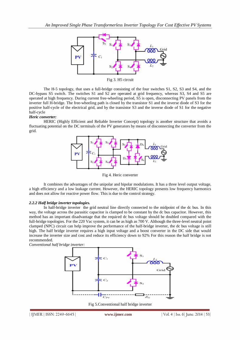
An Improved Single Phase Transformerless Inverter Topology For Cost Effective PV Systems
| IJMER | ISSN: 2249–6645 | www.ijmer.com | Vol. 4 | Iss. 6| June. 2014 | 53|
Fig 3. H5 circuit
The H-5 topology, that uses a full-bridge consisting of the four switches S1, S2, S3 and S4, and the DC-bypass S5 switch. The switches S1 and S2 are operated at grid frequency, whereas S3, S4 and S5 are
operated at high frequency. During current free-wheeling period, S5 is open, disconnecting PV panels from the
inverter full H-bridge. The free-wheeling path is closed by the transistor S1 and the inverse diode of S3 for the
positive half-cycle of the electrical grid, and by the transistor S3 and the inverse diode of S1 for the negative
half-cycle
Heric converter:
HERIC (Highly Efficient and Reliable Inverter Concept) topology is another structure that avoids a
fluctuating potential on the DC terminals of the PV generators by means of disconnecting the converter from the
grid.
Fig 4. Heric converter
It combines the advantages of the unipolar and bipolar modulations. It has a three level output voltage, a high efficiency and a low leakage current. However, the HERIC topology presents low frequency harmonics
and does not allow for reactive power flow. This is due to the control strategy.
2.2.2 Half bridge inverter topologies.
In half-bridge inverter the grid neutral line directly connected to the midpoint of the dc bus. In this
way, the voltage across the parasitic capacitor is clamped to be constant by the dc bus capacitor. However, this
method has an important disadvantage that the required dc bus voltage should be doubled compared with the
full-bridge topologies. For the 220 Vac system, it can be as high as 700 V. Although the three-level neutral point
clamped (NPC) circuit can help improve the performance of the half-bridge inverter, the dc bus voltage is still
high. The half bridge inverter requires a high input voltage and a boost converter in the DC side that would
increase the inverter size and cost and reduce its efficiency down to 92% For this reason the half bridge is not
recommended. Conventional half bridge inverter:
Fig 5.Conventional half bridge inverter
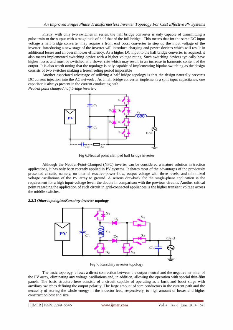
An Improved Single Phase Transformerless Inverter Topology For Cost Effective PV Systems
| IJMER | ISSN: 2249–6645 | www.ijmer.com | Vol. 4 | Iss. 6| June. 2014 | 54|
Firstly, with only two switches in series, the half bridge converter is only capable of transmitting a
pulse train to the output with a magnitude of half that of the full bridge . This means that for the same DC input
voltage a half bridge converter may require a front end boost converter to step up the input voltage of the
inverter. Introducing a new stage of the inverter will introduce charging and power devices which will result in
additional losses and an overall lower efficiency. As a higher DC input to the half bridge converter is required, it
also means implemented switching device with a higher voltage rating. Such switching devices typically have
higher losses and must be switched at a slower rate which may result in an increase in harmonic content of the output. It is also worth noting that the topology is only capable of implementing bipolar switching as the design
consists of two switches making a freewheeling period impossible
Another associated advantage of utilizing a half bridge topology is that the design naturally prevents
DC current injection into the AC network . As a half bridge converter implements a split input capacitance, one
capacitor is always present in the current conducting path.
Neutral point clamped half bridge inverter:
Fig 6.Neutral point clamped half bridge inverter
Although the Neutral-Point-Clamped (NPC) inverter can be considered a mature solution in traction
applications, it has only been recently applied in PV systems. It shares most of the advantages of the previously
presented circuits, namely, no internal reactive-power flow, output voltage with three levels, and minimized
voltage oscillations of the PV array to ground. A serious drawback for the single-phase application is the
requirement for a high input-voltage level; the double in comparison with the previous circuits. Another critical
point regarding the application of such circuit in grid-connected appliances is the higher transient voltage across
the middle switches.
2.2.3 Other topologies:Karschny inverter topology
Fig 7. Karschny inverter topology
The basic topology allows a direct connection between the output neutral and the negative terminal of the PV array, eliminating any voltage oscillations and, in addition, allowing the operation with special thin-film
panels. The basic structure here consists of a circuit capable of operating as a buck and boost stage with
auxiliary switches defining the output polarity. The large amount of semiconductors in the current path and the
necessity of storing the whole energy in the inductor lead, respectively, to high amount of losses and higher
construction cost and size.

An Improved Single Phase Transformerless Inverter Topology For Cost Effective PV Systems
| IJMER | ISSN: 2249–6645 | www.ijmer.com | Vol. 4 | Iss. 6| June. 2014 | 55|
III. PROPOSED TOPOLOGY Here ,a novel topology generation strategy called the virtual dc bus concept is proposed for the
transformer less grid connected pv inverter. In this solution, the grid neutral line is connected directly to the
negative pole of the dc bus, so that voltage across the parasitic capacitor is clamped to zero. As a result, the CM current is eliminated completely.Mean while,the virtual dc bus is created to help generate the negative output
voltage. The required dc bus voltage is still the same as the full bridge, and there is not any limitation on the
modulation strategy since the CM current is removed naturally by the circuit structure. In this way, the
advantage of the full bridge and half bridge based solutions are combined together.
3.1 Virtual DC Bus Concept
Fig 8.Virtual dc bus concept
By connecting the grid neutral line directly to the negative pole of the PV panel, the voltage across the
parasitic capacitance Cpv is clamped to zero. This prevents any leakage current flowing through it. With respect
to the ground point N, the voltage at midpoint B is either zero or +Vdc, according to the state of the switch bridge. The purpose of introducing virtual DC bus is to generate the negative output voltage, which is necessary
for the operation of the inverter. If a proper method is designed to transfer the energy between the real bus and
the virtual bus, the voltage across the virtual bus can be kept the same as the real one. The positive pole of the
virtual bus is connected to the ground point N, so that the voltage at the midpoint C is either zero or −Vdc.
The dotted line in the figure indicates that this connection may be realized directly by a wire or
indirectly by a power switch. With points B and C joined together by a smart selecting switch, the voltage at
point A can be of three different voltage levels, namely +Vdc, zero and –Vdc. Since the CM current is
eliminated naturally by the structure of the circuit, there’s not any limitation on the modulation strategy, which
means that the advanced modulation technologies such as the unipolar SPWM or the double frequency SPWM
can be used to satisfy various PV applications
3.2 Derived Topology And Modulation Strategy.
Fig 9. Proposed topology

An Improved Single Phase Transformerless Inverter Topology For Cost Effective PV Systems
| IJMER | ISSN: 2249–6645 | www.ijmer.com | Vol. 4 | Iss. 6| June. 2014 | 56|
Based on the negative voltage generation concept, an inverter topology is derived to show the clear
advantages of the proposed methodology. It consists of five power switches S1~S5 and only one single filter
inductor Lf. The PV panels and capacitor C1 form the real DC bus while the virtual DC bus is provided by C2.
With the switched capacitor technology, C2 is charged by the real DC bus through S1 and S3 to maintain a
constant voltage. This topology can be modulated with the unipolar SPWM and double frequency SPWM
3.3 Unipolar SPWM
Fig 7 Unipolar SPWM for proposed topology
The gate drive signals for the power switches are generated according to the relative value of the
modulation wave ug and the carrier wave uc. During the positive half grid cycle,ug> 0. S1 and S3 are turned on and S2 is turned off, while S4 and S5 commutate complementally with the carrier frequency. The capacitors C1
and C2 are in parallel and the circuit rotates between state 1 and state 2 . During the negative half cycle, ug< 0.
S5 is turned on and S4 is turned off. S1 and S3 commutate with the carrier frequency synchronously and S2
commutates in complement to them. The circuit rotates between state 3 and state 2. At state 3, S1 and S3 are
turned off while S2 is turned on. The negative voltage is generated by the virtual DC bus C2 and the inverter
output is at negative voltage level. At state 2, S1 and S3 are turned on while S2 is turned off. The inverter output
voltage VAN equals zero, meanwhile C2 is charged by the DC bus through S1 and S3.
3.4 Operating States for Proposed Topology
(a) State 1
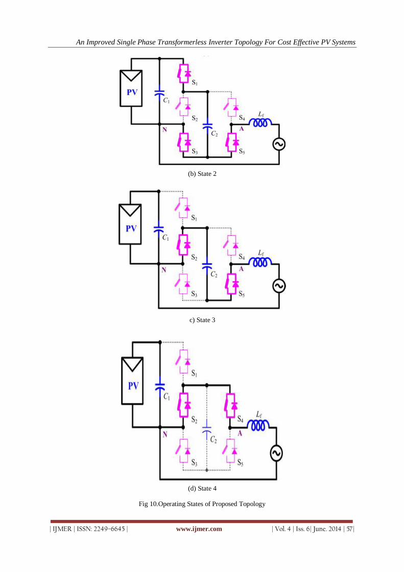
An Improved Single Phase Transformerless Inverter Topology For Cost Effective PV Systems
| IJMER | ISSN: 2249–6645 | www.ijmer.com | Vol. 4 | Iss. 6| June. 2014 | 57|
(b) State 2
c) State 3
(d) State 4
Fig 10.Operating States of Proposed Topology

An Improved Single Phase Transformerless Inverter Topology For Cost Effective PV Systems
| IJMER | ISSN: 2249–6645 | www.ijmer.com | Vol. 4 | Iss. 6| June. 2014 | 58|
For all of the four operation states, there is no limitation on the direction of the output current igrid,
since the power switches with anti parallel diodes can achieve bidirectional current flow. Therefore, the
proposed topology has the capability of feeding reactive power into the grid to help support the stability of the
power system.
The proposed topology is also immune against transient overvoltage of the grid. During the mains
positive voltage spikes, the voltage at point A is clamped at Vdc by C1 and the anti parallel diodes of S1 and S4
. Similarly, during the negative voltage spikes, the voltage at point A is clamped at −Vdc by C2 and the anti parallel diodes of S2 and S5 . Therefore, the mains transient overvoltage does not pose a safety threat for the
inverter.
IV. SYSTEM DESIGN CONSIDERATIONS A 500 W prototype is considered to verify the functionality of the proposed topology and the idea of
virtual dc bus concept. The terminal voltage for a 500 W PV panel is typically 40-60 V. Here a 400 V dc bus is
considered. The LCL filter is used to reduce the output current ripple. The grid voltage is 220Vac and frequency
is 50 Hz. MOSFET switches are employed as power switches. 4.1 Design Of LCL Filter
A LCL filter is often used to interconnect an inverter to the utility grid in order to filter the harmonics
produced by the inverter.The LCL filter achieves a higher attenuation along with cost savings, given the overall
weight and size reduction of the components.
𝐿1: inverter side inductor
𝐿2: grid side inductor
𝐶 𝑓 : filter capacitor.
𝑃𝑛 :be the rated active power.
𝑉𝑝 :phase voltage.
𝑉𝑑𝑐 :dc link voltage.
𝑓𝑔 :grid frequency.
𝑓𝑠𝑤 :switching frequency
𝐸𝑛 :rms grid voltage
𝑘𝑎 = 𝑎𝑡𝑡𝑒𝑛𝑢𝑎𝑡𝑖𝑜𝑛 𝑓𝑎𝑐𝑡𝑜𝑟
Assume 10% ripple in rated current
* ∆𝐼𝑙 max = 0.1 𝐼𝑚𝑎𝑥 …………………………………………………… (8)
* 𝐼𝑚𝑎𝑥 =𝑃𝑛 2
𝑉𝑝 ……………………………………………………….. (9)
𝐼𝑚𝑎𝑥 =500 ∗ 2
220= 3.214
From equation (1)
∆𝐼𝑙 max = 0.1 𝐼𝑚𝑎𝑥 =0.1*3.214 =0.3214
𝐿1 =𝑉𝑑𝑐
6𝑓𝑠𝑤 ∆𝐼𝑙𝑚𝑎𝑥 ……………………………………………………………… (10)

An Improved Single Phase Transformerless Inverter Topology For Cost Effective PV Systems
| IJMER | ISSN: 2249–6645 | www.ijmer.com | Vol. 4 | Iss. 6| June. 2014 | 59|
𝐿1 =400
6 ∗ 20000 ∗ 0.3214= 10.37 𝑚𝐻
The base impedance and base capacitance are defined by:
𝑍𝑏 =𝐸𝑛2
𝑃𝑛…………………………………………………………………….. (11)
=2202
500= 96.8
𝐶𝑏 =1
𝜔𝑔𝑍𝑏 ………………………………………………………………….. (12)
=1
2𝜋 ∗ 50 ∗ 96.8= 3.288 × 10⁻⁵
For the design of the filter capacitance, it is considered that the maximum power factor variation seen by the
grid is 5%,indicating that the base impedance of the system is adjusted as follows:
𝐶𝑓 = 0.05𝐶𝑏……………………………………………………………….. (13)
𝐶𝑓 =1.64×10⁻⁶ F.
Set desired attenuation factor 𝑘𝑎=20%=0.2
Switching frequency 𝑓𝑠𝑤 =20 kHz.
𝐿2 = (
1
𝑘𝑎2+1)
𝐶𝑓𝑓𝑠𝑤2 ……………………………………………………………… (14)
=7.77mH.
4.2 Design Of dc Capacitors
𝐶1 =𝑝
2.𝜔𝑔𝑟𝑖𝑑 𝑈𝑐∆𝑉𝑐1 ……………………………………………………………… (15)
𝑈𝑐 :mean voltage across capacitor
∆𝑉𝑐1 = 4.23 𝑉
𝐶1=470µF
∆𝑉𝑐2 = 2.11 𝑉
𝐶2 =𝑝
2.𝜔𝑔𝑟𝑖𝑑 𝑈𝑐∆𝑉𝑐2 …………………………………………………………….. (16)
𝐶2= 940µF.
V. EXPERIMENTAL RESULTS
5.1 Simulink model of proposed topology
powergui
Continuous
load
v+-
Total Harmonic
Distorsion
signal THD
Subsystem1
Out1
Out2
Out3
Out4
Out5
Scope 2
Scope 1
Scope
S5
g m
D S
S4
g m
D S
S3
g m
D S
S2
g m
D S
S1
g m
D S
Rs
LrLf
Display 1
462
1.003 e-012Display
0.003343
DC
i+ -
Cf
C2
Active & Reactive
Power
V
IPQ
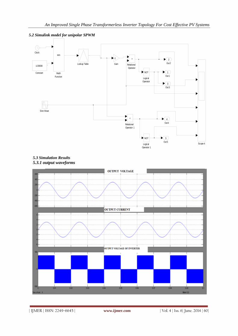
An Improved Single Phase Transformerless Inverter Topology For Cost Effective PV Systems
| IJMER | ISSN: 2249–6645 | www.ijmer.com | Vol. 4 | Iss. 6| June. 2014 | 60|
5.2 Simulink model for unipolar SPWM
5.3 Simulation Results
5.3.1 output waveforms
Out 5
5
Out4
4
Out 3
3
Out 2
2
Out 1
1
Sine Wave
Scope 4
Relational
Operator 1
<
Relational
Operator
>
Math
Function
rem
Lookup Table
Logical
Operator 1
NOT
Logical
Operator
NOT
Gain
-1
Constant
1/20000
Clock

An Improved Single Phase Transformerless Inverter Topology For Cost Effective PV Systems
| IJMER | ISSN: 2249–6645 | www.ijmer.com | Vol. 4 | Iss. 6| June. 2014 | 61|
5.3.2 switching pulses
VI. Conclusion The concept of the virtual DC bus is proposed to solve the CM current problem for the transformer less
grid-connected PV inverter. By connecting the negative pole of the DC bus directly to the grid neutral line, the
voltage on the stray PV capacitor is clamped to zero. This eliminates the CM current completely. Meanwhile, a
virtual DC bus is created to provide the negative voltage level. The required DC voltage is only half of the half
bridge solution, while the performance in eliminating the CM current is better than the full bridge based
inverters. Based on this idea, a novel inverter topology is proposed with the virtual DC bus concept by adopting
the switched capacitor technology. It consists of only five power switches and filter circuit. The proposed
topology is especially suitable for the small power single phase applications, where the output current is
relatively small so that the extra current stress caused by the switched capacitor does not cause serious reliability
problem for the power devices and capacitors. With excellent performance in eliminating the CM current, the virtual DC bus concept provides a promising solution for the transformer less grid-connected PV inverters. The
software tool used in this project is MATLAB 2007b.
REFERENCES [1.] Y. Gu, W. Li, Yi Zhao, Bo Yang, C. Li and X. He,” Transformerless Inverter With Virtual DC Bus Concept for Cost-
Effective Grid-Connected pv power Systems,” IEEE Transactions on Power Electronics, vol. 28, no. 2, Feb. 2013 [2.] B. Yang, W. Li, Y. Gu, W. Cui, and X. He, “Improved transformerless inverter with common-mode leakage current
elimination for a photovoltaic grid-connected power system,” IEEE Trans. Power Electron., vol. 27, no. 2, pp. 752–762, Feb. 2012.
[3.] H. Xiao and S. Xie, “Transformerless split-inductor neutral point clamped three-level PV grid-connected inverter,” IEEE Trans. Power Electron., vol. 27, no. 4, pp. 1799–1808, Apr. 2012
[4.] W. Cui, B. Yang, Y. Zhao, W. Li, and X. He, “A novel single-phase transformerless grid-connected inverter,” in Proc. 37th Annu. Conf. IEEE Ind. Electron. Soc., Nov. 7–10, 2011, pp. 1126–1130
[5.] T. Kerekes, R. Teodorescu, P. Rodr ıguez, G. V´azquez, and E. Aldabas, “A new high-efficiency single-phase transformerless PV inverter topology,” IEEE Trans. Ind. Electron., vol. 58, no. 1, pp. 184–191, Jan. 2011.
[6.] T. Kerekes, R. Teodorescu, P. Rodr ıguez, G. V´azquez, and E. Aldabas, “A new high-efficiency single-phase transformerless PV inverter topology,” IEEE Trans. Ind. Electron., vol. 58, no. 1, pp. 184–191, Jan. 2011
[7.] W. Yu, J.-S. Lai, H. Qian, C. Hutchens, J. Zhang, G. Lisi, A. Djabbari, G. Smith, and T. Hegarty, “High-efficiency
inverter with H6-type configuration for photovoltaic non-isolated ac module applications,” in Proc. 25th Annu. IEEE Appl. Power Electron. Conf. Expos., Feb. 21–25, 2010, pp. 1056–1061.

International
OPEN ACCESS Journal
Of Modern Engineering Research (IJMER)
| IJMER | ISSN: 2249–6645 | www.ijmer.com | Vol. 4 | Iss. 6| June. 2014 | 62|
Mathematical Modelling of an 3 Phase Induction Motor Using
MATLAB/Simulink
Mr. Punit L. Ratnani1, Dr. A. G. Thosar
2
1-2 (Department of Electrical Engineering, Govt. College of Engineering Aurangabad, India)
I. INTRODUCTION The dynamic simulation is one of the key steps in the validation of the design process of the motor-
drive system, which eliminates the designing mistakes and the resulting errors in the prototype construction and
testing. The dynamic model of the induction motor in direct, quadrature, and zero-sequence axes can be derived
from fundamental equations of transformation. The dynamic analysis of the symmetrical induction machines in
the arbitrary reference frame has been intensively used as a standard simulation approach from which any
particular mode of operation may then be developed. Matlab/Simulink has an advantage over other machine
simulators in modelling the induction machine using dq0 axis transformation. Generally modelling of these
equations is considered difficult so that in this paper they are presented in their simplified form. The
transformations used at various steps are based on simple trigonometric relationship obtained as projections on a
set of axes. The dynamic model is used to obtain transient responses, small signal equations, and a transfer
function of induction motor. Dynamic models (mathematical models) are employed in to better understand the
behaviour of induction motor in both transient and steady state.
The dynamic modelling sets all the mechanical equations for the inertia, torque and speed versus time.
It also models all the differential voltage, currents and flux linkages between the stationary stator as well as the
moving rotor. This mathematical model has been done by using MATLAB /Simulink which will represent the
three phase induction motor including a three phase to d-q axis transformations. The main benefit with
MATLAB Simulink is that in the electromechanical dynamic model can be accomplished in a simple way and it
can be simulated faster using function blocks.
II. THEORETICAL BACKGROUND
A. Assumptions
There are few assumptions are to be made while deriving mathematical model of a 3-phase Induction
Motor. They are listed below.
1. Uniform air gap.
2. Squirrel cage type construction.
3. Balanced stator and rotor windings, with sinusoidally distributed winding.
4. Saturation and parameter change are neglected.[1,2,3] The steady state model and equivalent circuit of the Induction Motor is useful for studying the
performance of the machine in steady state. This implies that all electrical transients are neglected during load
changes or stator frequency variations. Such variations arise in application involving variable-speed drives. The
variable-speed drives are converter fed from finite sources, unlike the utility sources, due to limitations of the
switch ratings and filter sizes. This results in their incapability to supply large transient power. Hence, we need
to evaluate the dynamics of converter-fed variable-speed drives to assess the adequacy of the converter switches
and the converters for a given number of motor and their interaction to determine the excursions of currents &
torque in the converter and motor.
Abstract: Mechanical energy is needed in the daily life use as well as in the industry. Induction motors
play a very important role in both worlds, because of low cost, reliable operation, robust operation and low
maintenance. To derive the mathematical model of a 3 phase Induction motor, the theory of reference
frames has been effectively used as an efficient approach. Dynamic models (mathematical models) are
employed in to better understand the behaviour of induction motor in both transient and steady state. The
dynamic modelling sets all the mechanical equations for the inertia, torque and speed versus time. It also
models all the differential voltage, currents and flux linkages between the stationary stator as well as the
moving rotor. This paper presents a step by step Matlab/Simulink implementation of an induction machine
using dq0 axis transformations of the stator and rotor variables in the arbitrary reference frame [1].
Keywords: Reference frames, Dynamic models, dq0 axis transformations, Matlab/Simulink.

Mathematical Modelling of an 3 Phase Induction Motor Using MATLAB/Simulink
| IJMER | ISSN: 2249–6645 | www.ijmer.com | Vol. 4 | Iss. 6| June. 2014 | 63|
B. Equivalent Circuit of an Induction Motor
The voltage and torque equations that describe the dynamic behaviour of an induction motor are time-
varying. It is successfully used to solve such differential equations and it may involve some complexity. A
change of variables can be used to reduce the complexity of these equations by eliminating all time-varying
inductances, due to electric circuits in relative motion, from the voltage equations of the machine [1, 2, 3, 4].
Fig. 1 A dq0 equivalent circuit of an Induction Motor
The above figure shows a dq0 equivalent circuit of an Induction motor. The circuit comprise of various
time varying inductances which are to be simulated to analyse the dynamic performance of the 3-phase
Induction motor.
III. INDUCTION MOTOR MODEL
A. Generalised Concept in an Arbitrary Reference Frame
Reference frame are very much like observer platforms, in that each of the platforms gives a unique
view of the system at hand as well as a dramatic simplification of the system equation. For example, for the
purpose of control, it is desirable to have the system variables as dc quantities, although the actual variables are
sinusoidal. This could be accomplished by having a reference frame revolving at the same angular speed as that
of the sinusoidal variable. As the reference frames are moving at an angular speed equal to the angular speed
equal to angular frequency of sinusoidal supply, so that differential speed between them is reduced to zero,
resulting in the sinusoid signal behaving as DC signal from the reference frames. So by moving that lane, it
becomes easier to develop a small-signal equation out of a nonlinear equations, as the operating point is
described only by DC values; this then leads to linearized system around operating point. Such advantages are
many from using reference frame s. instead of deriving the transformation for each and every particular
reference frame; it is advantageous to derive general transformation for an arbitrary rotating reference frame.
Then any particular reference frame model can be derived by substituting the appropriate frame speed and
position in the generalized reference model.
B. Three phase to Two phase Transformation
The dynamic model of induction motor can be derived if the equivalence between three-phase and two-
phase machine is studied. The equivalence is based on the quantity of MMF produced in two-phase and three-
phase windings along with equal current magnitudes. Assuming that each of the three-phase winding has Ns
turns per phase and equal currents magnitudes, the two-phase winding will have 3𝑁𝑠/2 turns per phase for
MMF equality. The d and q axes MMF are found by resolving MMF of the three-phase along d and q axes. The
common term, the number of turns is cancelled on both sides of equations leaving behind the current equalities.
The three-phase stator voltages of an induction machine under balanced conditions can be expressed as,[2,3,4]
𝑉𝑎 = 2𝑉𝑟𝑚𝑠 sin 𝜔𝑡 ;
𝑉𝑏 = 2𝑉𝑟𝑚𝑠 𝑠𝑖𝑛(𝜔𝑡 − 2𝜋 ⁄ 3);
𝑉𝑐 = 2𝑉𝑟𝑚𝑠 sin 𝜔𝑡 + 2𝜋3 ;
Here 𝑉𝑎 , 𝑉𝑏 & 𝑉𝑐 𝑎𝑟𝑒 𝑡ℎ𝑒 𝑡ℎ𝑟𝑒𝑒 𝑙𝑖𝑛𝑒 𝑣𝑜𝑙𝑡𝑎𝑔𝑒𝑠.
The relationship between αβ and abc is as follows.

Mathematical Modelling of an 3 Phase Induction Motor Using MATLAB/Simulink
| IJMER | ISSN: 2249–6645 | www.ijmer.com | Vol. 4 | Iss. 6| June. 2014 | 64|
𝑉𝛼𝑉𝛽
=2
3 1
1
2−
1
2
0 3
2−
3
2
𝑉𝑎𝑉𝑏
𝑉𝑐
Then, the direct and quadrature axes voltages are
𝑉𝑑
𝑉𝑞 =
cos 𝜃 sin 𝜃− sin 𝜃 cos 𝜃
𝑉𝛼𝑉𝛽
The instantaneous values of the stator and rotor currents in three-phase system are ultimately calculated using
the following transformation;
𝑖𝛼𝑖𝛽
= cos 𝜃 − sin 𝜃 sin 𝜃 cos 𝜃
𝑖𝑑𝑖𝑞
𝑖𝑎𝑖𝑏𝑖𝑐
=2
3
1 0
−1
2−
3
2
−1
2−
3
2
𝑖𝛼𝑖𝛽
C. Equations of Flux Linkages & Simulink Model
The dynamic model of induction motor in arbitrary reference frame can be represented by using flux
linkages as variables. This involves the reduction of a number of variables in dynamic equations, which greatly
facilitates their solution by using analogue and hybrid computers. Even when the voltages and currents are
discontinuous, the flux linkages are continuous. This gives the advantage of differentiating these variables with
numerical stability. In addition, the flux linkages representation is used in motor drives to highlight the process
of the decoupling of the flux and torque channels in the induction and synchronous machine.
The various flux linkage equations are expressed as [4],
𝑑𝛹𝑞𝑠
𝑑𝑡= 𝜔𝑏 𝑉𝑞𝑠 −
𝜔𝑒
𝜔𝑏
𝛹𝑑𝑠 − 𝑅𝑠
𝑋𝑙𝑠
𝛹𝑚𝑞 − 𝛹𝑞𝑠
𝑑𝛹𝑑𝑠
𝑑𝑡= 𝜔𝑏 𝑉𝑑𝑠 −
𝜔𝑒
𝜔𝑏
𝛹𝑞𝑠 − 𝑅𝑠
𝑋𝑙𝑠
𝛹𝑚𝑑 − 𝛹𝑑𝑠
𝑑𝛹𝑞𝑟
𝑑𝑡= 𝜔𝑏 𝑉𝑞𝑟 −
𝜔𝑒 − 𝜔𝑟
𝜔𝑏
𝛹𝑑𝑟 − 𝑅𝑟
𝑋𝑙𝑟
𝛹𝑚𝑞 − 𝛹𝑞𝑟
𝑑𝛹𝑑𝑟
𝑑𝑡= 𝜔𝑏 𝑉𝑑𝑟 −
𝜔𝑒 − 𝜔𝑟
𝜔𝑏
𝛹𝑞𝑟 − 𝑅𝑟
𝑋𝑙𝑟
𝛹𝑚𝑑 − 𝛹𝑑𝑟
Where
𝛹𝑚𝑞 = 𝑋𝑚𝑙 𝛹𝑞𝑠
𝑋𝑙𝑠
+𝛹𝑞𝑟
𝑋𝑙𝑟
𝛹𝑚𝑑 = 𝑋𝑚𝑙 𝛹𝑑𝑠
𝑋𝑙𝑠
+𝛹𝑑𝑟
𝑋𝑙𝑟
Then substituting the values of the flux linkages to find the currents,
𝑖𝑞𝑠 =1
𝑋𝑙𝑠
𝛹𝑞𝑠 − 𝛹𝑚𝑞 𝑋𝑚𝑙 = 1/ 1
𝑋𝑚
+1
𝑋𝑙𝑠
+1
𝑋𝑙𝑟

Mathematical Modelling of an 3 Phase Induction Motor Using MATLAB/Simulink
| IJMER | ISSN: 2249–6645 | www.ijmer.com | Vol. 4 | Iss. 6| June. 2014 | 65|
Fig. 2 Overview of the complete dynamic model in Matlab/Simulink environment
𝑖𝑞𝑟 =1
𝑋𝑙𝑟
𝛹𝑞𝑟 − 𝛹𝑚𝑞
𝑖𝑑𝑠 =1
𝑋𝑙𝑠
𝛹𝑑𝑠 − 𝛹𝑚𝑑
𝑖𝑑𝑟 =1
𝑋𝑙𝑟
𝛹𝑑𝑟 − 𝛹𝑚𝑑
Based on the above equations, the Electromagnetic torque and rotor speed can be determined as follows,
𝑇𝑒 = 3
2
𝑃
2
1
𝜔𝑏
𝛹𝑑𝑠 𝑖𝑞𝑠 − 𝛹𝑞𝑠 𝑖𝑑𝑠
𝜔𝑏 = 𝑃
2𝐽 𝑇𝑒 − 𝑇𝑙
With P = no of poles of Machine.
𝑇𝑒 = Electromagnetic torque developed
IV. MATLAB/SIMULINK RESULTS The induction motor of 3 hp was tested in this simulated model. The results of the simulation are given
for the first induction motor with the following specifications:
Input Parameters:[5]
1 Hp Rating 3
2 Vline 220 Volts
3 f 50
4 Rs & Rr 0.435 Ω
5 Xls 0.816 Ω
6 J 0.089
7 Xm 26.13 Ω
8 RPM 1500
The various performance parameters of an Induction motor ate the electromagnetic torque developed,
rotor speed, and stator and rotor currents in each of three phase windings.

Mathematical Modelling of an 3 Phase Induction Motor Using MATLAB/Simulink
| IJMER | ISSN: 2249–6645 | www.ijmer.com | Vol. 4 | Iss. 6| June. 2014 | 66|
A. Electromagnetic Torque Developed
Fig. 3 Electromagnetic Torque Developed
B. Stator Currents In A, B & C Phases
Fig. 4 Stator currents in A, B & C phases
C. Rotor Current in Each A, B & C Phases.
Fig. 5 Rotor currents in A, B & C phases

Mathematical Modelling of an 3 Phase Induction Motor Using MATLAB/Simulink
| IJMER | ISSN: 2249–6645 | www.ijmer.com | Vol. 4 | Iss. 6| June. 2014 | 67|
D. Speed of Rotor in Per Unit with Base Speed as 1500 Rpm.
Fig. 5 Speed of Rotor
V. Conclusion
In this paper, an implementation and dynamic modelling of a three-phase induction motor using
Matlab/Simulink is presented in a step-by-step manner. The model was tested by 3 hp induction motor.[5,6] The
simulated machine has given a satisfactory response in terms of the torque and speed characteristics. This
concludes that the Matlab/Simulink is a reliable and sophisticated way to analyse and predict the behaviour of
induction motors using the theory of reference frames.
REFERENCES [1] P. C. Krause, O. Wasynczuk, S. D. Sudhoff “Analysis of Electric Machinery and Drive Systems”, IEEE Press, A
John Wiley & Sons, Inc. Publication Second Edition, 2002.
[2] P.C. Krause and C. H. Thomas, “Simulation of Symmetrical Induction Machinery”, IEEE Transaction on Power
Apparatus and Systems, Vol. 84, November 1965, pp. 1038-1053.
[3] P. C. Krause, “Analysis of Electric Machinery”, McGraw-Hill Book Company, 1986.
[4] R. Krishnan, “Control, Modeling and Analysis of Electrical Drives”,
[5] Bimal K. Bose, “Modern power electronics and drives”.
[6] M. H. Rashid, “Power Electronics; circuits, devices, and applications”.
[7] M Ozaki, Y. Adachi, Y. Iwahori, and N. Ishii, Application of fuzzy theory to writer recognition of Chinese
characters, International Journal of Modelling and Simulation, 18(2), 1998, 112-116.
International
OPEN ACCESS Journal
Of Modern Engineering Research (IJMER)
| IJMER | ISSN: 2249–6645 | www.ijmer.com | Vol. 4 | Iss. 6| June. 2014 | 68|
Land Use/Land Cover Mapping Of Allahabad City by Using
Remote Sensing & GIS
Jamal Mohamed Salih Irhoumah1, V. C. Agarwal
2, Deepak Lal
3
1,2,3 (Department of Civil Engineering, (Survey), Department of Civil Engineering, Department of Soil Water,
Land Engineering and Management, Sam Higginbotom Institute of Agriculture Technology & Sciences)
I. INTRODUCTION
1. General Background Landuse and landcover exerts considerable influence on the various hydrologic phenomenons such as
interception, infiltration, evaporation and surface flow. Various aspects of hydrological problems (Vemu
Sreenivasulu et al. 2010). Land use and land cover is an important component in understanding the interactions
of the human activities with the environment and thus it is necessary to be able to simulate changes (Tiwari
Kuldeep, et al. 2011). Land-use and land-cover change has become a central component in current strategies in
managing natural resources and monitoring environmental changes. Urban expansion has increased the
exploitation of natural resources and has changed land use and land cover patterns. Rapid urbanization,
therefore, brings opportunities for new urban developments, however, it also has brought serious losses of arable
land, forest land and water bodies. Land cover change is a major concern of global environment change
(Bhagawat Rimal, 2011). Changes in Land use Land cover is a dynamic process taking place on the surface and
it become a central component in current strategies in managing natural resources and monitoring environmental
changes (Phukan P. et al. 2013). Change detection is the measure of the distinct data framework and thematic
change information that can guide to more tangible insights into underlying process involving land cover and
land use changes than the information obtained from continuous change (Ashutosh Singh, et al. 2013). In the
last three decades, the technologies and methods of remote sensing have evolved dramatically to include a suite
of sensors operating at a wide range of imaging scales with potential interest and importance to planners and
land managers. Coupled with the ready availability of historical remote sensing data, the reduction in data cost
and increased resolution from satellite platforms, remote sensing technology appears poised to make an even
greater impact on planning agencies and land management initiatives involved in monitoring land-cover and
land-use change at a variety of spatial scales. Current remote sensing technology offers collection and analysis of
data from ground-based, atmospheric, and Earth-orbiting platforms, with linkages to GPS data, GIS data layers
and functions, and emerging modeling capabilities (Franklin, 2001). This has made remote sensing a valuable
source of land-cover and land-use information. As the demand for increased amounts and quality of information
rises, and technology continues to improve, remote sensing will become increasingly critical in the future.
Therefore, the focus of this chapter is on the issues and challenges associated with monitoring land-cover and
land-use change. Urban growth leads to the change of land use and land cover many areas around the world;
especially in developing countries.Spatial distribution of land use land cover and its changes is desirable for any
planning management and monitoring programmers at local and national levels. Land use and land cover change
has become a central component in current strategies for managing natural resource and monitoring
environmental change. The rapid development of the concept studies of vegetation mapping has lead to increase
studies of land use and land cover change worldwide. Remote sensing information, in concert with available
enabling technologies such as GPS and GIS, can form the information base upon which sound planning
decisions can be made, while remaining cost-effective (Franklin et al., 2000). Clearly, however, the fast-paced
Abstract: The present study was carried out to produce and evaluate the land use/land cover maps by on
screen visual interpretation. The studies of land cover of Allahabad city (study area) consist of 87517.47 ha
out of which 5500.35 ha is build up land (Urban / Rural) Area. In this respect, the Build up land (Urban /
Rural) area scorers 6.28% of the total area. It has also been found that about 17155.001ha (19.60 %) of
area is covered by current fallow land. The double/triple crop land of 30178.44ha (34.84%). The area
covered by gullied / ravines is 1539.20 ha (1.75 %) and that of the kharif crop land is 2828.00 ha (3.23 %).
The area covered by other wasteland is 2551.05ha (2.91%). Table 4.1 shows the area distribution of the
various land use and land cover of Allahabad city. Keywords: Land use, Land caver, Remote Sensing, Geographic Information System.

Land Use/Land Cover Mapping Of Allahabad City By Using Remote Sensing & Gis
| IJMER | ISSN: 2249–6645 | www.ijmer.com | Vol. 4 | Iss. 6| June. 2014 | 69|
developmental nature of remote sensing technology often overlooks the needs of end-users as it ‘continues to
outpace the accumulation of experience and understanding’ (Franklin, 2001). In the near future, the field of
remote sensing will change dramatically with the projected increase in number of satellites of all types (Glackin,
1998). This will further compound the problems described above. In order to help create a better understanding
of the rapid advancements in remote sensing technology that has occurred over the last three decades, we review
the current state of remote sensing technology (i.e. sensors, data, analysis methods and applications) for
monitoring land cover and land use. Specifically, we provide a brief history of the advances in remote sensing
technology, and a review of the major technical considerations of land-cover and land-use monitoring using
remote Sensing data.
II. Materials and Method
2.1 Study Area Characteristics Geographical Location: Allahabad is located at 25
0 27’ N, 81
0 50’ E; 25.45
0 N, 81.84
0 E in the
southern part of the Uttar Pradesh at an elevation of 98 meters (322 f).The Indian longitude that is associated
with Jabalpur also passes through Allahabad, which is 343 km (213 mi) north to Jabalpur on the same longitude.
To its southwest, east and south west is the Bundelkhand region, to its north and north east is the Awadh region
and to its west is lower Doab of which it is a part. It is the last point of the Yamuna River and is the last frontier
of the Indian west.
Fig: 1 Location map of the study area
2.2 Data Used
2.2.1 Remote Sensing Data Landsat ETM
+ sensor data were used for this study. Since the study area was covered in many paths of
Landsat satellite data acquisition (each path is covered separately in a different day as per orbital calendar),
cloud free data was acquired in different time windows depending upon the overpass of satellite. Each scene was
ortho corrected; geo-referenced and suitable Image enhancements are applied to facilitate the delineation and
and interpretation of different thematic information. interpretation of different thematic information.
Characteristics of Land sat data is shown in Table 1.
Table.1 satellite remote sensing data specification
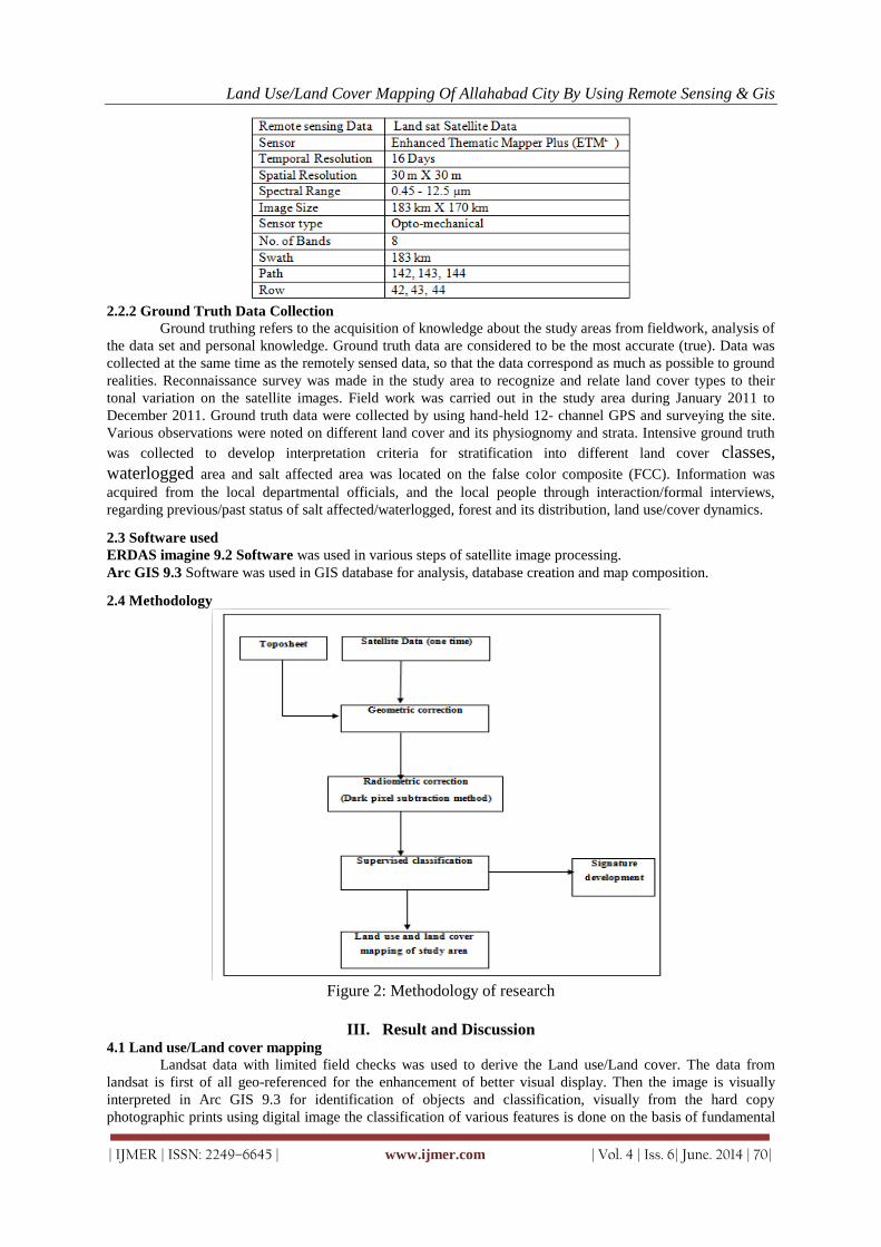
Land Use/Land Cover Mapping Of Allahabad City By Using Remote Sensing & Gis
| IJMER | ISSN: 2249–6645 | www.ijmer.com | Vol. 4 | Iss. 6| June. 2014 | 70|
2.2.2 Ground Truth Data Collection
Ground truthing refers to the acquisition of knowledge about the study areas from fieldwork, analysis of
the data set and personal knowledge. Ground truth data are considered to be the most accurate (true). Data was
collected at the same time as the remotely sensed data, so that the data correspond as much as possible to ground
realities. Reconnaissance survey was made in the study area to recognize and relate land cover types to their
tonal variation on the satellite images. Field work was carried out in the study area during January 2011 to
December 2011. Ground truth data were collected by using hand-held 12- channel GPS and surveying the site.
Various observations were noted on different land cover and its physiognomy and strata. Intensive ground truth
was collected to develop interpretation criteria for stratification into different land cover classes,
waterlogged area and salt affected area was located on the false color composite (FCC). Information was
acquired from the local departmental officials, and the local people through interaction/formal interviews,
regarding previous/past status of salt affected/waterlogged, forest and its distribution, land use/cover dynamics.
2.3 Software used
ERDAS imagine 9.2 Software was used in various steps of satellite image processing.
Arc GIS 9.3 Software was used in GIS database for analysis, database creation and map composition.
2.4 Methodology
Figure 2: Methodology of research
III. Result and Discussion 4.1 Land use/Land cover mapping
Landsat data with limited field checks was used to derive the Land use/Land cover. The data from
landsat is first of all geo-referenced for the enhancement of better visual display. Then the image is visually
interpreted in Arc GIS 9.3 for identification of objects and classification, visually from the hard copy
photographic prints using digital image the classification of various features is done on the basis of fundamental

Land Use/Land Cover Mapping Of Allahabad City By Using Remote Sensing & Gis
| IJMER | ISSN: 2249–6645 | www.ijmer.com | Vol. 4 | Iss. 6| June. 2014 | 71|
image characteristics depend on spectral spatial temporal and radiometric resolutions of sensor like tone, texture,
association shape, size, pattern, shadow, location. Topology is prepared and cleaning is done. Finally the
attributes are given to define the classes and thus LULC map is prepared.
3.2 Land use Land cover mapping
The satellite data was transformed into thematic land use land cover map using on screen visual
interpretation. The satellite data of 2011 was classified into various classes. The land Use land Cover map of the
study area is shown in figure 4. Statistics of study area has been calculated and shown in table 2.
3.3 Land use land covers statistics The modern techniques of satellite image processing have been applied to extract the different
information about land use land cover of Allahabad city. The land use /land cover categories such as Buitt up
land (Urban / Rural), Current follow, Double / Triple crop land, Gullied / Ravince, Kharif crop land, Other
wasteland, Plaution / Orchands Rabi crop land, Scru bland Water bodies and Zaid cropland.
Allahabad city (study area) consist of 87517.47 ha out of which 5500.35 ha is build up land (Urban /
Rural) Area. In this respect, the Build up land (Urban / Rural) area scorers 6.28% of the total area. It has also
been found that about 17155.001ha (19.60 %) of area is covered by current fallow land. The double/triple crop
land of 30178.44ha (34.84%). The area covered by gullied / ravines is 1539.20 ha (1.75 %) and that of the kharif
crop land is 2828.00 ha (3.23 %). The area covered by other wasteland is 2551.05ha (2.91%). Table 2 shows the
area distribution of the various land use and land cover of Allahabad city.
Different interpretation key like X, Y coordinate, shape, size, tone, site the texture, association, were
used to identify land use / land cover map.
Table 2. Area Statistics of Land use / Land Cover Map
Class Area(ha) Area (%)
Build up land (Urban / Rural) 5500.35 6.28
Current fellow land 17155.00 19.60
Double / Triple crop land 30178.44 43.84
Gullied / Ravines 1539.20 1.75
Kharif crop land 2828.00 3.23
Plantation / Orchards 152.39 0.17
Rabi crop land 11270.98 12.87
Scrubland 4310.24 4.92
Water bodies 8468.65 9.67
Zaid cropland 3563.17 4.07
Other wasteland 2551.05 2.91
Total 87517.47 100
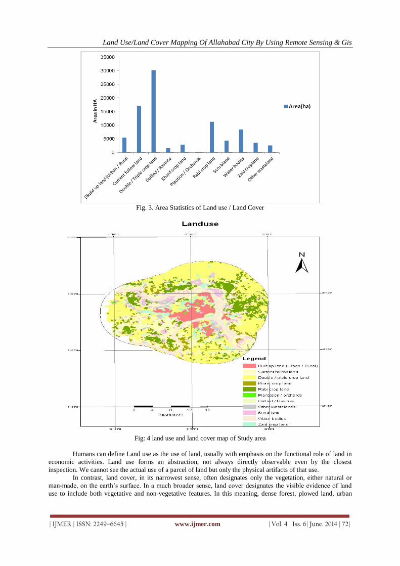
Land Use/Land Cover Mapping Of Allahabad City By Using Remote Sensing & Gis
| IJMER | ISSN: 2249–6645 | www.ijmer.com | Vol. 4 | Iss. 6| June. 2014 | 72|
Fig. 3. Area Statistics of Land use / Land Cover
Fig: 4 land use and land cover map of Study area
Humans can define Land use as the use of land, usually with emphasis on the functional role of land in
economic activities. Land use forms an abstraction, not always directly observable even by the closest
inspection. We cannot see the actual use of a parcel of land but only the physical artifacts of that use.
In contrast, land cover, in its narrowest sense, often designates only the vegetation, either natural or
man-made, on the earth’s surface. In a much broader sense, land cover designates the visible evidence of land
use to include both vegetative and non-vegetative features. In this meaning, dense forest, plowed land, urban

Land Use/Land Cover Mapping Of Allahabad City By Using Remote Sensing & Gis
| IJMER | ISSN: 2249–6645 | www.ijmer.com | Vol. 4 | Iss. 6| June. 2014 | 73|
structures, and paved parking lots all constitute land cover. Whereas land use is abstract, land cover is concrete
and therefore is subject to direct observation.
IV. Conclusion For this study remotely sensed data have been used for Land use/ Land cover mapping. The following
conclusion has been drawn from the result of study:
1. Study area consist of 87517.47 ha out of which 5500.35 ha is build up land (Urban / Rural) Area. In this
respect, the Build up land (Urban / Rural) area scorers 6.28% of the total area. It has also been found that
about 17155.001ha (19.60 %) of area is covered by current fallow land. The double/triple crop land of
30178.44ha (34.84%). The area covered by gullied / ravines is 1539.20 ha (1.75 %) and that of the kharif
crop land is 2828.00 ha (3.23 %). The area covered by other wasteland is 2551.05ha (2.91%).
2. Geo spatial techniques of Remote Sensing and GIS are useful in classifying the Land use/Land cover of any
specific area.
3. Remotely sensed data have been found to be effective, less time consuming, and accurate tool for Land use /
Land cover mapping.
4. Remotely sensed data of satellite image recognizes Land use/ Land cover spatially that open way for
management using other data towards sustainable agricultural development.
REFERENCES [1] Ashutosh Singh, Shalini Singh, Purushottam Kumar Garga, Kamlesh Khanduri, (2013). Land Use and Land Cover
Change Detection: A Comparative Approach Using Post Classification Change Matrix and Discriminate Function
Change Detection Methodology of Allahabad City, International Journal of Current Engineering and Technology,
Vol.3, No.1 (March 2013).
[2] Bhagawat Rimal, (2011). Application of remote sensing and gis, land use/land cover change in kathmandu
metropolitan city, nepal, Journal of Theoretical and Applied Information Technology, © 2005 - 2011 JATIT & LLS.
All rights reserved.
[3] Phukan P. Thakuriah G. and Saikia R. (2013). Land use Land Cover Change Detection Using Remote Sensing and
GIS Techniques - A Case Study of Golaghat District of Assam, India, International Research Journal of Earth
Science, Vol. 1(1), 11-15, April (2013).
[4] Tiwari Kuldeep 1 , Khanduri Kamlesh, (2010). Land Use / Land cover change detection in Doon valley (Dehradun
Tehsil), Uttarakhand: using GIS& Remote Sensing Technique, International Journal of Geomatics and Geosciences
Volume 2 Issue 1, 2011.
[5] Franklin, S.E., (2001). Remote Sensing for Sustainable Forest Management, Lewis Publishers, Boca Raton, FL, 407
pp.
[6] Franklin, J., Woodcock, C.E., Warbington, R., (2000). Digital vegetation maps of forest lands in California:
integrating satellite imagery, GIS modeling, and field data in support of resource management. Photogrammetric
Engineering and Remote Sensing 66, 1209 – 1217.
[7] Glackin, D.L. (1998). International space-based remote sensing overview: 1980 – 2007. Canadian Journal of Remote
Sensing 24, 307 – 314
[8] Vemu sreenivasulu, Pinnamaneni udaya bhaskar, (2010). Change Detection in Landuse and landcover using Remote
Sensing and GIS Techniques, International Journal of Engineering Science and Technology Vol. 2(12), 2010, 7758-
7762.

Contents :
Design of Multiplier Less 32 Tap FIR Filter using VHDL 01-05Abul Fazal Reyas Sarwar, Saifur Rahman
Design and Development of Gate Signal for 36 Volt 1000Hz Three Phase Inverter 06-11Devender Singh, Dr. Syed Hasan Saeed
Evaluation and Accuracy Assessment of Static GPS Technique in Monitoring of 12-18Horizontal Structural DeformationsProf. Dr. A.K. Abdel-Gawad, Dr. Y. M. Mogahed, Dr. Kh. M. Abdel Mageed, Eng. A.M. El-Maghraby
Redesign and Fabrication of Solar Power Tower using CAD and FEM Analysis 19-26Nilesh W. Nirwan, Ashish V. Shrirao
Enhanced Methodology for supporting approximate string search in Geospatial data 27-34Ashwina R., Mrs.T. Megala
An Overview of Distributed Generation 35-41Abhishek Chetty, Mohammed Shoaib, Dr. A. Sreedevi
A Realistic Cost Assessment for a Conventional Dwelling Unit (DU), Partially and 42-48Selectively Replaced With Engineered BambooChandra Sabnani, Mukesh Patel
High End Solution for Advanced Civil Engineering Projects 49-53T. Subramani, N. Kanthasamy
Heuristics for the Maximal Diversity Selection Problem 54-62S. R. Subramanya
FPGA implementation of universal modulator using CORDIC algorithm for 63-71communication applicationsM. Satheesh Kumar, S. Nagi Reddy
Volume : 4 Issue : 6 (Version-3) June - 2014ISSN : 2249-6645
International Journal of Modern Engineering Research
(IJMER)

International
OPEN ACCESS Journal
Of Modern Engineering Research (IJMER)
| IJMER | ISSN: 2249–6645 | www.ijmer.com | Vol. 4 | Iss. 6| June. 2014 | 1|
Design of Multiplier Less 32 Tap FIR Filter using VHDL
Abul Fazal Reyas Sarwar1, Saifur Rahman2 1(ECE, Integral University, India)
2 (Department of ECE, Integral University, India)
I. Introduction For many decades the aim of developing new hardware was to make devices smaller and faster. The
amount of power they consumed was hardly an issue, since the power wasn't the bottle neck. Today we face a
different situation, as the demand for real time application with a long battery lifetime is increasing.
Today, design of low power signal processing circuits is an important part of the electronics industry.
This is because portable computing and communication devices like cellular phones and laptop computers have
become very popular. The development seems to take a turn towards wireless communication and flexibility in
the sense that a stationary port is unnecessary. This challenges the industry to produce low power devices and
it challenges researchers to find new, less power consuming algorithms for the processes carried out by
portable devices. An important process is the digital signal processing (DSP). DSP is the transference of data
between devices, such as cellular phone communication, wireless Internet usage and digital TV transmission to
mention a few. Finite impulse response (FIR) filtering is a central task in DSP. By reducing the power needed
to process data through such a filter, power can be significantly reduced.
In signal processing, the function of a filter is to remove unwanted parts of the signal, such as random
noise, or to extract useful parts of the signal, such as the components lying within a certain frequency range
[2].
Fig 1: A block diagram of a basic filter.
A filter is an electrical network that alters the amplitude and/or phase characteristics of a signal with
respect to frequency. Ideally, a filter will not add new frequencies to the input signal, nor will it change the
component frequencies of that signal, but it will change the relative amplitudes of the various frequency
components and/or their phase relationships. Filters are often used in electronic systems to emphasize signals
in certain frequency ranges and reject signals in other frequency ranges.
Abstract: This Paper provide the principles of Distributed Arithmetic, and introduce it into the FIR
filters design, and then presents a 32-Tap FIR low-pass filter using Distributed Arithmetic, which save
considerable MAC blocks to decrease the circuit scale and pipeline structure is also used to increase the
system speed. The implementation of FIR filters on FPGA based on traditional method costs considerable
hardware resources, which goes against the decrease of circuit scale and the increase of system speed.
It is very well known that the FIR filter consists of Delay elements, Multipliers and Adders. Because of
usage of Multipliers in early design gives rise to 2 demerits that are:
(i) Increase in Area and
(ii) Increase in the Delay which ultimately results in low performance (Less speed).
So the Distributed Arithmetic for FIR Filter design and Implementation is provided in this work to solve
this problem. Distributed Arithmetic structure is used to increase the recourse usage and pipeline
structure is used to increase the system speed. Distributed Arithmetic can save considerable hardware
resources through using LUT to take the place of MAC units
Keywords: Distributed Algorithm, FIR Filter, Modelsim 10.2a, VHDL, Xilinx ISE 14.2.

Preparation of Papers for International Journal of Modern Engineering Research
| IJMER | ISSN: 2249–6645 | www.ijmer.com | Vol. 4 | Iss. 6| June. 2014 | 2|
There are two types of filter: analog and digital. FIR Filter is the kind of digital filter, which can be
used to perform all kinds of filtering.
II. Related Work A Ruan,A.W., Liao,Y.B., Li,P. , Li,J.X., (2009) [4] proposed and presented An ALU based universal
FIR filter where various FIR filters can be implemented just by programming instructions in the ROM with
identical hardware architecture. They presented Arithmetic Logic Unit (ALU) based universal FIR filter
suitable for implementation in Field Programmable Gate Arrays (FPGA) is proposed in this paper. Multiplier
and accumulator based architecture used in conventional FIR, the proposed ALU architecture implements FIR
functions by using accumulators and shift-registers controlled by the instructions of ROM.
Nekoei,F., Kavian,Y.S., Strobel,O., (2010) [5] presented realization of digital FIR filters on field
programmable gate array devices was proposed. Two common architectures called direct and transposed
architectures were employed for implementing FIR filters on a Xilinx SPARTAN2-XC2S50-5I-tq144 FPGA
using Verilog hardware description language codes.
X.Jiang, Y.Bao(2010) proposed a structure characteristics and the basic principles of the finite
impulse response (FIR) digital filter, and gives an efficient FIR filter design based on FPGA. Use MATLAB
FDATool to determine filter coefficients, and designed a 16-order constant coefficient FIR filter by VHDL
language, take use of Quartus-2 to simulate filters, the results meet performance requirements.
Li,J., Zhao,M., Wang,X., (2011) [6] They used distributed algorithm and its several structures, an
implementation method of 60-order FIR filter based on FPGA is presented, which converts multiplication to
look-up table structure, and implement multiplication operation. They used FPGA as the hardware platform.
This filter system has a good performance, the filter speed is higher and the resource occupation is fewer.
Beyrouthy,T., Fesquet,L., (2011) [3] presented an asynchronous FIR Filter architecture was presented,
along with an asynchronous Analog to digital converter(A-ADC). They designed FIR Filter architecture using
the micro-pipeline asynchronous style. They successfully implemented for the first time on a commercial
FPGA board (Altera-DE1). A specific library has also been designed for this purpose. It allows the synthesis of
asynchronous primitive blocks (the control path in this case) on the synchronous FPGA. Simulation results of
the FIR Filter after place and route validate the implementation. This work is still going on, in order to
optimize the implementation.
III. Methodology 3.1 Multiplierless FIR Filter:
It is widely accepted that the multiplication is the main source of complexity in a FIR filter. In other
words the multiplication consumes most area and is the main source of delaying the throughput, in addition to
its high consume of power. An array multiplier of length L consumes an area O(L2), whereas an adder spreads
over only O(L) area [1]. The multiplication by a constant can be represented behaviorally as in figure 2.
Fig 2: Multiplication using reduced additions
3.2 Distributed Arithmetic algorithms:
In multiplierless architectures the replacement of the multiplier with a series of additions and shifts is
on the cost of speed. The Distributed Arithmetic (DA) is a bit-serial computation process that offers speeds
approaching the original array multiplier's speed, and at the same time keeping the power consumption down
on the same level as the competing dedicated hardware and ASIC's power consumption. [7].

Preparation of Papers for International Journal of Modern Engineering Research
| IJMER | ISSN: 2249–6645 | www.ijmer.com | Vol. 4 | Iss. 6| June. 2014 | 3|
Fig 3: Distributed Arithmetic, the principle
The DA standard architecture is shown in figure 3. The variables are fed into the shift-registers. From there,
one by one they are fed into the Look Up Table (LUT). The LUT is the replacement of a multiplication, since it
consists of precomputed data.
3.3 Architecture implementation in VHDL:
The architectures implemented by the Distributed Arithmetic. The design grows in size according to the
number of taps used. An 8 tap implementation is illustrated in figure 4. We will design 32 tap multiplier less
Fir Filter.
Fig 4: 8 tap binary FIR Filter implementation
IV. Simulation Results In this paper we designed the low pass FIR filter for sampling frequency 48 KHz to meet the given
specification (i.e.: Pass band edge: 9.6 KHz, Stop band Edge:12KHz, Pass band Edge:1 dB and Stop band
Attenuation. : 90dB).The implementation of highly efficient serial DA algorithm was presented in this work.
Simulation results are shown below for different sample inputs in 16 bit hexadecimal values and the output is
shown in time domain. In fig 5 shows filtered output for sample value 1234h.

Preparation of Papers for International Journal of Modern Engineering Research
| IJMER | ISSN: 2249–6645 | www.ijmer.com | Vol. 4 | Iss. 6| June. 2014 | 4|
Fig 5: Simulation Result for 1234h.
In fig 6 shows filtered output for sample value 0123h.
Fig 6: Simulation Result 0123h.
We are using Xilinx tool for synthesis our code fig 7 shows the main RTL of our code and fig 8 shows the
internal RTL of our code.
Fig 7: Main RTL

Preparation of Papers for International Journal of Modern Engineering Research
| IJMER | ISSN: 2249–6645 | www.ijmer.com | Vol. 4 | Iss. 6| June. 2014 | 5|
Fig 8: Internal RTL
V. Conclusion We designed a double-precision low pass direct form FIR filter with Sampling Frequency 48KHZ to
meet the given specification(i.e.: Pass band edge: 9.6KHz, Stop band Edge:12KHz, Pass band Edge:1 dB and
Stop band Attenuation 90dB).The implementation of highly efficient serial DA algorithm was presented in
this work. The results were analyzed for 32-tap FIR filter using partitioned input based LUT on Xilinx 8.2 as a
target of SPARTAN-3E FPGA device .The speed performance of the Parallel DA FIR Filter was superior in
comparison to all other techniques . In 32 tap FIR filter, speed of parallel DA FIR design technique become 3
times faster than that of conventional FIR filter. The proposed algorithm for FIR filters is also area efficient
since approximately 50% of the area is saved with this technique as compared to conventional FIR filter
design. Area efficiency and high speed is achieved with parallel DA technique at very slight cost of power
consumption for large tap FIR filter. Since, distributed arithmetic FIR filters are area efficient and contained
less delay, so these filters can be used in various applications such as pulse shaping FIR filter in WCDMA
system, software design radio and signal processing system for high speed. In future the work to reduce the
power consumption in large tap DA FIR filters could be performed.
REFERENCES [1] H. Yoo and D. V. Anderson, “Hardware-Efficient Distributed Arithmetic Architecture for High-Order Digital
Filters” IEEE International Conference on Acoustics Speech and Signal Processing, ICASSP, pp. 125-128, 2005.
[2] Mitra,S. K., “Digital Signal Processing” 3rd Edition, Tata Mc. Graw Hill Publications.
[3] Beyrouthy,T., Fesquet,L., “An event-driven FIR filter: Design and implementation”, in proc. 22nd IEEE
International Symposium on Rapid System Prototyping (RSP), pp. 59 - 65, 2011.
[4] Ruan,A.W., Liao,Y.B., Li,P. , Li,J.X., “An ALU-Based Universal Architecture for FIR Filters” in proc.
International Conference on Communications, Circuits and Systems, IEEE, pp. 1070 – 1073, 2009.
[5] Nekoei,F., Kavian,Y.S., Strobel,O., “Some Schemes Of Realization Digital FIR Filter On FPGA For
Communication Application” in proc. 20th International Crimean Conference on Microwave and
Telecommunication Technology, pp. 616 – 619, 2010.
[6] Li,J., Zhao,M., Wang,X.,“Design and Simulation of 60-order Filter Based on FPGA” in proc. International
Conference on Intelligent Human-Machine Systems and Cybernetics (IHMSC), IEEE, pp. 113 - 115, Oct 2011.
[7] C. Shuyu, C. Yun, Z. Yang ,W. J. Zeng, X. Yang, Z. Dian, “VLSI Implementation of Reconfigurable SRRC Filters
With Automatic Code Generation,” 7th International Conference on ASIC , IEEE Proc. 1261-1264, 2007.

International
OPEN ACCESS Journal Of Modern Engineering Research (IJMER)
| IJMER | ISSN: 2249–6645 | www.ijmer.com | Vol. 4 | Iss. 6| June. 2014 | 6|
Design and Development of Gate Signal for 36 Volt 1000Hz Three
Phase Inverter
Devender Singh1, Dr. Syed Hasan Saeed
2
1PG Student, Integral University Lucknow,India, SSO-I, DGAQA, HAL-Lucknow, India 2HOD, Electronics And Communication Engineering, Integral University, Lucknow, India
I. INTRODUCTION Aerospace industry is a complex field of engineering, where all the branches of science and technology
have made their presence in general and specific in particular such as use of rectifier unit, rotary inverter, static
inverter in power system of fighter aircraft.Though the use of Sinusoidal pulse width modulation inverter is very
common in single and three phases of commercial inverters working on frequency 50 Hz/60Hz available in open market, but the article under question wherein the developed gating signal for 1000Hz,three phase for inverter of
36 volt is taken up in this paper. Other popular version of inverter in aircraft industry is 400Hz, 3 phase, 36 Volt;
which is used in older version of fighter aircraft to provide power supply to gyros. In high speed aerospace vehicle
such as missiles and aircraft with supersonic and hypersonic speed;inverter of 36volt, 3 phase, 1000 Hz can be
used. The rigidity and degree of precession of gyro is directly depend on frequency of rotation of gyro mass. In
modern aircraft, mechanical version of gyro is replaced by LRG (Laser Ring Gyro) or FOG (Fiber Optics Gyro)
[3]. The 1000 Hz, 3 phase, 36 Volt supply can be used to operate gyro and synchro in modern aircraft and missiles.
II. Literature Survey
The authors have surveyed various papers published in journals and studied the features of invertors, type
of SPWM method for generation and no evidence of work on 1000Hz, 3 phase, 36 Volt is found. However, for
commercial power supply i.e 230 Volt, 50Hz, single phase and 400 volt, 3 phase 50 Hz;a lot of papers are found.
The advantage of SPWM is clearly mentioned in [1]. Sinusoidal PWM results in lowest THD percentage as
compared with other techniques like square wave PWM, trapezoidal PWM and modified sinusoidal PWM [2].
Therefore, SPWM method is chosen for design.
III. SPWM The brief details of the SPWM are as follows:
(a) In SPWM sinusoidal signal frequency is compared with triangular carrier frequency.
(b) Sinusoidal signals V1 = A Sin ωt, V2 =A Sin (ωt-120), V3 = A sin (ωt+120) are fed to be positive inputs of
comparators and triangular signal (common to all three comparators) to the negative input of comparators.
(c) The pulse corresponding to the point whenever the instantaneous amplitude of sine signal is more than
triangular signal then a pulse is generated. The width of the pulse is function of sinusoidal angular position.
(d) The pulse width varies with sinusoidal manner so that the average fundamental component frequency is the same as sinusoidal signal.
(e) It is necessary to maintain carrier frequency (triangular wave) ofat least 15 times more than the frequency of
sinusoidal signal (1000 Hz). In practice, carrier frequency greater than 21 times are preferred; because, it reduces
sub harmonic contentin the output of inverter.
(f) The rms value of line voltage; Vl = √3 Vs. In present case, it will be approx110 volt DC to be applied at
MOSFET bridge to get 36 volts, phase to phase at inverter output. This is transformer-less design and output
voltage can easily be changed by changing MOSFET bridge supply.
Abstract: The sinusoidal PWM gating signals generation is most popular PWM method, which reduce
harmonic reduction in output. SPWM can be generated by FPGA, micro controller and micro processor but this kind of device needs programming and coding hence avoided in using power system of aircraft. This
paper present an experiment using SPWM method to generate 1000 Hz gating signals suitable for 36 Volt ,
1000 Hz, 3 phase, three wire supply. Discrete components design approach is chosen to provide noise
immunity at higher amplitude level of signal and a large flexibility to adjust and process various operating
parameters of signals. The circuit is proved with commercial components however MIL version of
components can be easily incorporated in design in later stage.
Keywords: aircraft, comparator,gyro, sine wave, triangular wave.

Design and Development of Gate Signal for 36 Volt 1000Hz Three Phase Inverter
| IJMER | ISSN: 2249–6645 | www.ijmer.com | Vol. 4 | Iss. 6| June. 2014 | 7|
(g) In case synchronous operation [3] when the initial point of triangular wave coincide with sine wave then
number of pulses per half cycle is N=(Fc/2Fs-1). Here design is asynchronous. (h) Modulation index MI = Vs / Vc .
IV. Experiment Setup For Generating Spwm
Figure 1. Block Diagram of Experiment setup
Experiment setup SPWM generation involves four blocks of circuits namely generation, feedback, comparator, driver, opto-coupler
gate driver. The brief of design and the voltage and frequency level are as follows:
(a) Each of the above levels of circuit is tested on bread board and then complete setup is assembled on PCB .
(b) Sine wave generation: Sine wave is generated through bipolar square wave of frequency 1000 Hz.
(i) Frequency = 1000 Hz ± 10 Hz
(ii) Voltage level: 1.8 to 2.5 Volts peak to peak at generation level and 8.2 to 13 Volt at comparator level selectable through potentiometer on PCB.
(c) Single phase to three phase conversion: This is obtained through three op-amp circuits and output are V1 = A
Sin ωt, V2 =A Sin (ωt-120), V3 = A sin (ωt+120). A is peak amplitude.
(d) Triangular wave generator: Triangular wave obtained through Op-amp circuits
(i) Frequency = 15KHZ to 25 KHZ adjustable by potentiometer.
(ii) Amplitude = 10 Volt to 13 Volt peak to peak adjustable by potentiometer.
(e) Comparator: One per phase precession comparators LM111 are used to get 3 phase PWM.
(f) Bipolar driver: One per phase bipolar driver IR 2108 is used to get normal and inverted signal
(g) Opto-couplar: Two per phase opto-couplar FOD 3120 are used to drive gate signal of normal and inverted
signal.
(h) Power Supply: The circuit is tested with following external power supply, however in aircraft it will be
supplied through Rectifier unit and through DC to DC convertor
(i) + 5 volt at 500 mA.
(j) – 12 volt , + 12 Volt at 500 mA.
(k) Bridge voltage supply as per voltage requirement of invertors in present case it is -55 Volt, +55 Volt and
ground.
(l) Feedback: Negative Feedback is externally provided at comparator through signal generator at frequency 1000
Hz sine wave to vary signal strength of input signal at the comparator by 1000 mV.
V. Parameters Studied Gernerally, for analysis of any wave form; shape of pulses, amplitude, rise time, fall time and duty cycle
are important parameters. But, in case of three phase inverter, 120 degree apart, three separate train of pulses with
their inverted form should be available on the output of gate signal circuit. Accordingly the following sets of
reading are taken in laboratory and results are analyzed.
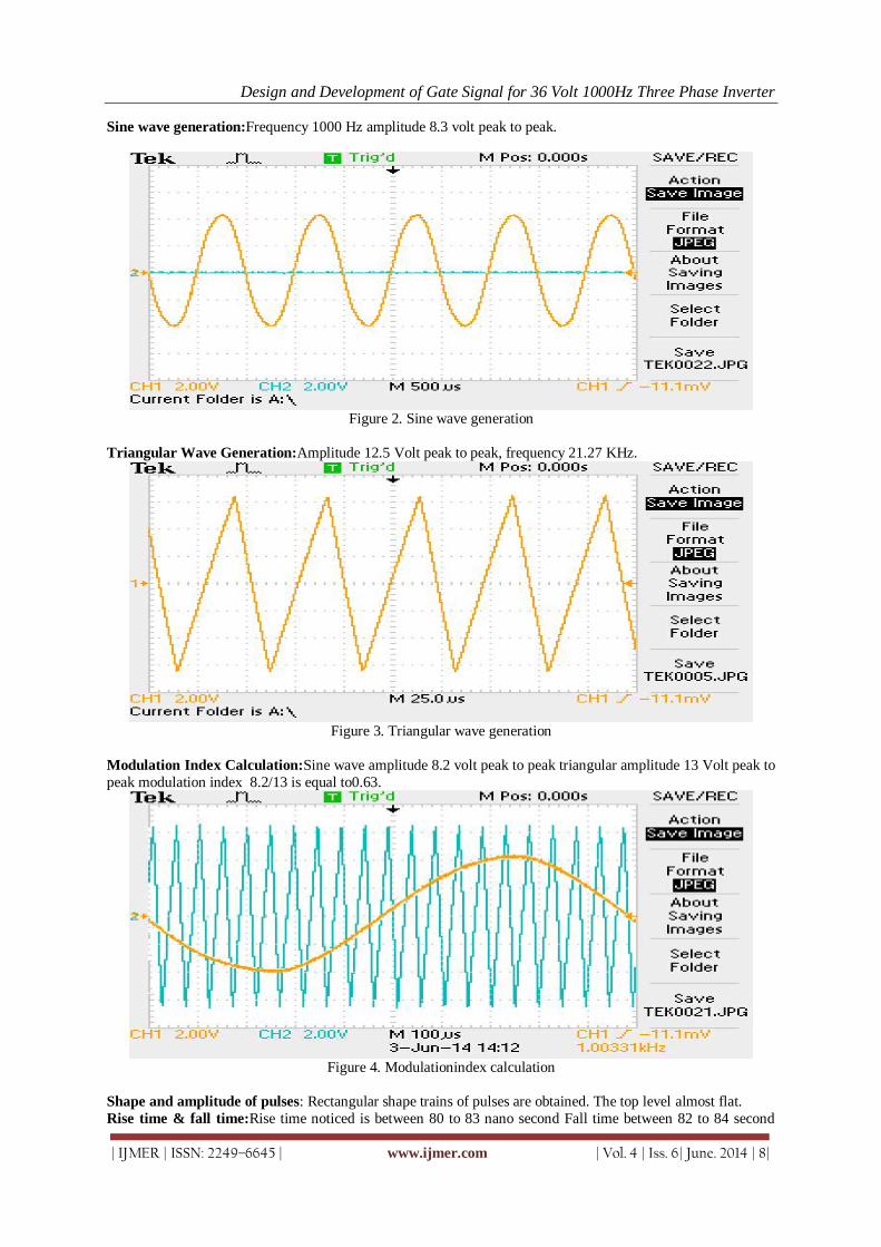
Design and Development of Gate Signal for 36 Volt 1000Hz Three Phase Inverter
| IJMER | ISSN: 2249–6645 | www.ijmer.com | Vol. 4 | Iss. 6| June. 2014 | 8|
Sine wave generation:Frequency 1000 Hz amplitude 8.3 volt peak to peak.
Figure 2. Sine wave generation
Triangular Wave Generation:Amplitude 12.5 Volt peak to peak, frequency 21.27 KHz.
Figure 3. Triangular wave generation
Modulation Index Calculation:Sine wave amplitude 8.2 volt peak to peak triangular amplitude 13 Volt peak to
peak modulation index 8.2/13 is equal to0.63.
Figure 4. Modulationindex calculation
Shape and amplitude of pulses: Rectangular shape trains of pulses are obtained. The top level almost flat.
Rise time & fall time:Rise time noticed is between 80 to 83 nano second Fall time between 82 to 84 second

Design and Development of Gate Signal for 36 Volt 1000Hz Three Phase Inverter
| IJMER | ISSN: 2249–6645 | www.ijmer.com | Vol. 4 | Iss. 6| June. 2014 | 9|
switching time 47 micro second so obtain rise time and fall time will suit the performance.
Duty cycle:Duty cycle cannot be calculated with certainty because SPWM is of asynchronous nature, accordingly inter space between pulses and width of pulse is varied continuously during the 500 microsecond (Half period
corresponding to 1000Hz) time period so switch ON time and OFF time recorded have no certainity to which
portion of wave it belong. Even for same voltage& frequency level of carrier and sinusoidal wave at different
instant of time wave recorded are found different,should be same but it is not. This is because at different instant of
time different portion of modulation is recorded in oscilloscope.Half period corresponding to 1000Hz is 500
micro second.
Number of pulses of PWM on various modulations index levels: Modulation index [4] is calculated on
different level of carrier frequency ans recorded below:-
Table 1
Sl. No.
Modulation Index MA
Number of pulses obtained
asynchronous
Carrier Frequency
fc (KHz)
Sinusoidal Frequency
fs (KHz)
No. of pulses calculated
N= (fc / 2 fs) - 1
synchronous
1. 0.63 7.27 15 1 6.5
2. 0.73 10.2 21 1 9.5
3. 0.84 12.1 25 1 11.5
As in present case of asynchronous design number of pulses obtained is more than synchronous pulses calculated.
Conformation of generation of normal & inverted signal for each phase:
Figure 5. Phase A and inverted phase A
Figure 6. Phase B and inverted phase B
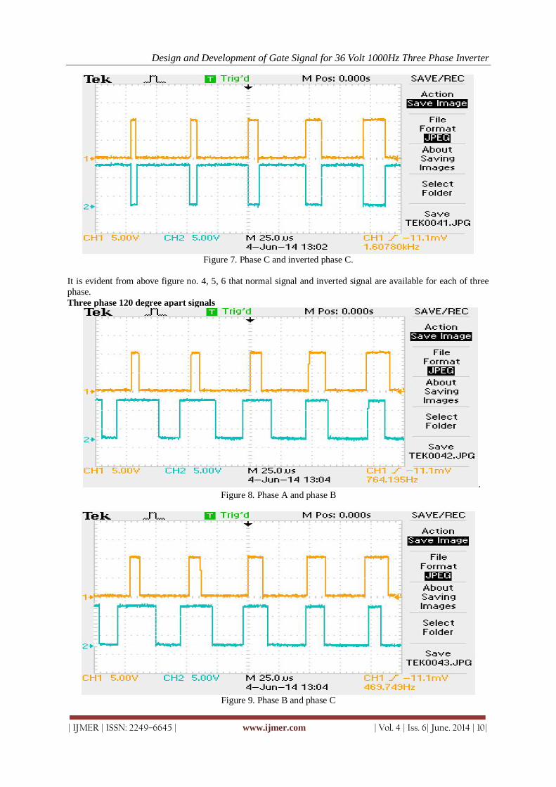
Design and Development of Gate Signal for 36 Volt 1000Hz Three Phase Inverter
| IJMER | ISSN: 2249–6645 | www.ijmer.com | Vol. 4 | Iss. 6| June. 2014 | 10|
Figure 7. Phase C and inverted phase C.
It is evident from above figure no. 4, 5, 6 that normal signal and inverted signal are available for each of three
phase.
Three phase 120 degree apart signals
.
Figure 8. Phase A and phase B
Figure 9. Phase B and phase C

Design and Development of Gate Signal for 36 Volt 1000Hz Three Phase Inverter
| IJMER | ISSN: 2249–6645 | www.ijmer.com | Vol. 4 | Iss. 6| June. 2014 | 11|
Figure 10. Phase C and phase A
VI. CONCLUSION Based on the actual measurement of different parameters on three phases,1000 Hz, 36 Volt gatting signal
setup; the following are concluded:
1. PWM signals and their inverted signals of 12 voltsmagnitude are available at the output of gate signal PCB.
The shape, amplitude, rise time, fall time, phase difference among three phases and their inverted signal are
found to be satisfactory. Hence, these arefit to be integrated with next stage of MOSFET bridge.
2. Limitation to calculate duty cycle from the recorded signal is noticed, however, it will not effect theoutput
performance of inverter.
3. In SPWM, switching losses are higher due to large switchingfrequency of MOSFET in bridge, but this disadvantage is not considered in comparison to the quality output obtained with low THD.
Acknowledgements
The authors are thankful to Mr. Kausar Mujtaba, Senior Manager, Shri Anurag Gupta, Manager,and shri
Shashank Gupta of Design Department H.A.L Lucknow for providing all the necessary cooperation during
conduction of experiment.
REFERENCES Journal Papers:
[1] Nazamul Islam Raju,Md SHhahium Islam, Ahmed Ashemuddin “Sinusodial PWM signal generationtechniques for three phase voltage source inverter with analog circuit and simulation of PWM inverter for stand alone load and microgrid system “ , International journal of Renewable Energy Research ( IJRER) Nizamul Islam Raju elal. Vol. 3 , No.3.
[2] Jagdish Chandra Pari, Jayanta Kumar Sahu “Harmonic analysis by using various PWM techniques & there comparision “Int,adv.res.sei ,technical vol. 1 , issue 1 October 201 pp , 35-44.
Whitepapers:
[3] KVH white paper on “An update on KVH fiber optic gyro and there benefit related to other
gyrotechnology2013-2014KVHindustries,Inc
Books: [4] Bimbra PS “A textbook of power electronics” Khanna publisher Pp 454-466.

International
OPEN ACCESS Journal
Of Modern Engineering Research (IJMER)
| IJMER | ISSN: 2249–6645 | www.ijmer.com | Vol. 4 | Iss. 6| June. 2014 | 12|
Evaluation and Accuracy Assessment of Static GPS Technique in
Monitoring of Horizontal Structural Deformations
Prof. Dr. A.K. Abdel-Gawad1, Dr. Y. M. Mogahed
2,
Dr. Kh. M. Abdel Mageed3, Eng. A.M. El-Maghraby
4
1 Civil Engineering Department, National Research Center, Egypt 2 Public Works Department, Faculty of Engineering, Ain Shams University, Egypt
3 Higher Technological Institute, Egypt 4 Enppi, engineering for the petroleum and process industries
I. Introduction It is well known that, deformation monitoring systems are considered, nowadays, to be the back bone
factor for human safety as well as preserving the ultimate economy of his achievements. In this context, there
has been always an increasing demand for precise deformation measurements in keeping up several industries,
like structure buildings for instance, as well as several engineering structures and historical monuments. Such
deformations constitute some problems from the structural point of view. Thus, it is necessary to measure and monitor such deformations before the repair stage; during the repair and after finishing the repair. This is
essential to avoid any undesirable consequences that may happen and cause disaster risks of any part of the
monument with time.
The deformation of any object can be defined as the variation of its position, size and shape with
respect to its original state or its designed shape. The purpose of measuring deformations is not the calculation
of the exact positions of the observed object but the variation of these positions with time. This is done to avoid
failure of the structures (monuments). The methods used for monitoring deformations may be generally
classified as surveying methods and non-surveying methods. The selection of the method of measurements
depends upon the accuracy requirements. This, in turn, is determined by the purpose of the measurements and
by the magnitude and direction of the expected deformations or movements [1], [2], [3], [4], [5], and [6].
Hence, many modern surveying techniques can be used in measuring and monitoring deformations [7]
and [8]. On the other hand, the main problem is the suitability of measuring according to the site obstacles as
well as the required accuracy. In terms of productivity and time saving, GPS could provide more than 75% time
saving [9] and [10]. The fact that GPS does not require inter-visibility between stations has also made it more
attractive to surveyors over the conventional methods.
Abstract: It is well known that, deformation monitoring systems are considered, nowadays, to be the
back bone factor for human safety as well as preserving the ultimate economy of his achievements. In
this context, there has been always an increasing demand for precise deformation measurements in
keeping up several engineering structures and historical monuments. Measuring and monitoring
monumental deformation is the sequence of operations that allows the finding of movements of points
or features in a specified coordinate system, during two different times for the same investigated
feature. The time interval sometimes is the main factor in measuring horizontal deformation, especially
in loading test of steel bridges. Hence, the present paper investigates the accuracy of the GPS in monitoring of horizontal deformation with respect to the time of observation. So, a practical
simulation test was made to assess the accuracy of GPS with time in measuring horizontal
deformation. The obtained results indicated that, the used methods and techniques presented in the
current research paper have possessed a very good accuracy, reliability and applicability in
monitoring horizontal deformations efficiently. The accuracy of measuring horizontal deformation of
points on structure using relative static technique of GPS is from (0.1mm) to (1.8mm) for time interval
from 30 minute to 5 minute and has R.M.S.E (0.3mm)
Key words: Deformation measurement – Horizontal Deformation – GPS - GPS accuracy – Static
GPS Positioning.

Evaluation and Accuracy Assessment of Static GPS Technique in Monitoring of Horizontal Structural
| IJMER | ISSN: 2249–6645 | www.ijmer.com | Vol. 4 | Iss. 6| June. 2014 | 13|
Other advantages of the GPS system, as mentioned by [11], are:
GPS can easily cover larger areas than classical surveying methods, with millimeter level precision.
The results between consecutive surveys are coherent - the procedures, data capture and computation are
always the same, regardless of the operator and the particular GPS equipment.
After a due training period, the equipment is easy to operate. The operator does not have to be an
experienced surveyor. Nonetheless, [12] listed additional advantages of the Global Positioning System versus the traditional surveying:
GPS is an all-weather navigating system, except in thunderstorm.
GPS is a day and night surveying tool.
With GPS, human mistakes are eliminated.
GPS serves many applications.
Unlimited base line length.
Un-necessity for visibility between points.
GPS doesn’t require huge man effort in measurements
Basically, the GPS observables are ranges which are deduced from measured time or phase differences
based on a comparison between received signals and generated signals. Unlike the terrestrial distance
measurements, GPS uses the so-called one-way concept, where, two clocks are used, namely one in the satellite,
and the other in the receiver. Thus, the ranges are affected by satellite and receiver clocks errors and,
consequently, they are denoted as pseudoranges [13]. Mainly, there are two types of GPS observables, namely the code pseudoranges and carrier phase
observables. In general, the pseudorange observations are used for coarse navigation, whereas the carrier phase
observations are used in high-precision surveying applications. That is due to the fact that the accuracy of the
carrier phase observations is much higher than the accuracy of code observations. Beside the two GPS
observables, the GPS satellite transmits a navigation message. The navigation message is a data stream added to
both L1 and L2 carriers as binary bi-phase modulation at a low rate of 50 Kbps. It consists of 25 frames of 1500
bits each, or 37500 bits in total. This means that, the transmition of the complete navigation message takes 750
seconds. The navigation message contains, along with other information, the coordinates of the GPS satellites as
a function of time, the satellite health status, the satellite clock correction, the satellite almanac, and atmospheric
data. Each satellite transmits its own navigation message with information on the other satellites, such as the
approximate location and health status [14]. There are different GPS relative positioning techniques. These techniques are static, stop and go,
kinematic, and real time kinematic RTK. Static GPS technique, is an accurate and reliable technique, however, it
is relatively slow in production. On the other hand, each one of other remaining techniques, is represented a
technological solution to the problem of obtaining high productivity, such as measuring many baselines in a
short period of time, or the ability to obtain results even while the receiver in motion, that is real time solution,
however, with a relatively less accuracy than the static case [15].
The biases that are affecting the GPS measurements fall into three categories which are: satellite biases,
receiver biases, and signal propagation biases [13]. Satellite biases consist of biases in satellite ephemeris,
satellite clock, and the effect of selective availability SA which is terminated in May 2000. Receiver biases
usually consist of receiver clock bias, receiver noise and antenna phase center variation. The signal propagation
biases appear due to tropospheric refraction, ionospheric refraction, and multipath. Beside the effect of these
biases, the accuracy of the computed GPS position is also affected by the geometric locations of the GPS satellites as seen by the receiver. Generally, the more spread out the satellites are in the sky, the better the
obtained accuracy, which is denoted as dilution of precision.
So, the main objective of the current research paper is to investigate the feasibility and applicability as
well as accuracy assessment of the GPS in measuring horizontal deformation of structures. To achieve this
objective, a simulation test was made to assess the accuracy of GPS in monitoring horizontal deformations of
structures. Hence, the purpose of this experiment is to determine the horizontal deformation of the bolts
positions relatively with each other by GPS technique compared with their position measured relatively by the
scaled vernier.

Evaluation and Accuracy Assessment of Static GPS Technique in Monitoring of Horizontal Structural
| IJMER | ISSN: 2249–6645 | www.ijmer.com | Vol. 4 | Iss. 6| June. 2014 | 14|
II. Methodology of Investigation To assess the accuracy of the GPS in monitoring horizontal deformation, a simulation was made
following the next steps:
1- Fixing of bolts at the roof of faculty of engineering, Ain Shams University.
2- Measuring the horizontal distances between bolts with scaled vernier with an accuracy of 0.05 mm.
3- Measuring the horizontal distances between bolts using three GPS receiver. Two receivers are fixed
and the third one is moving through the fixed bolts, using the slight movement of the legs.
4- Comparative study was done between the scale vernier measurements and the GPS measurements. The
first solution uses one GPS fixed point. The second solution uses two GPS fixed points.
III. The Used Instruments All instruments used in this test are tested and adjusted before using it. Such instruments are:
1-a vernier scale which model is (SOMET INOX) shown in figure (1) (divided scale as shown).
Figure (1) shows the distances between the bolts as well as the vernier scale.
2-Three GPS receivers (A,B&C)which are of model Trimble R3[16]. Figure (2) shows the GPS Receiver.
Figure (2) shows the GPS Receiver over the simulated bolts
specifications and measurements of the GPS receivers are:
- 12 Channels C/A Code, WAAS/EGNOS
- Trimble Maxwell GPS technology for robust satellite tracking - Trimble EVEREST™ multipath reduction technology
- Three tripod legs are available one for each receiver.
3-Rechargeable battery with electric cable to charge the GPS receivers in case of their battery is low.
4-A number of 6 bolts, 4 of them were used for the target points and 2 for static receivers.
5-A hammer used for fixing the bolts and markers for marking them.

Evaluation and Accuracy Assessment of Static GPS Technique in Monitoring of Horizontal Structural
| IJMER | ISSN: 2249–6645 | www.ijmer.com | Vol. 4 | Iss. 6| June. 2014 | 15|
IV. Description of the sight and fixing of control and monitored points This experiment has been carried out at the faculty of engineering, Ain Shams University at The public
works department building. The test was made on the roof of the building, this test was made to measure the
horizontal displacement of the positioning of the bolts relative to each other and comparing these relative
positioning using GPS with the positioning of them using vernier scale.
A net of 4 bolts (target points) are fixed on the roof of the building, and they were aligned on the same
edge of the slab by distance 1 cm apart exactly between each bolt of them (with accuracy of 1/20 mm) using the
(Vernier Marcasomethecho De AceroInoxiadble equipment) and the distance is measured 1 cm apart accurate
between them and marked on every bolt to ensure right and perpendicular verticality on them by the tripod of
the GPS. Figure (1) shows the position between the bolts where the distances were measured.
V. Observation procedure In this test, the observations of the horizontal distances between the bolts which initially taken by the
scale are then taken by GPS receiver. The first two receivers A&B where settled as static receivers and had a job
opened in each one , receiver A was opened at first which was far 300 meters approximately from C, then B had
job opened next ,which was away 50 meters approximately from C, then C was opened the last one.
The first receiver (A) was fixed on tripod and was horizontally adjusted and verticality adjusted by the
screws of the tripod and using the slight movement of the legs until the bubble was at the middle exactly, and
the antenna was placed on the tripod, then the height of the instrument was measured and entered until top of
notch height, after that the GPS receiver was opened and had a new job named by that date and was created by
the fast static technique job and occupied point named S1 and then the receiver began to search for a sufficient number of satellites and began to count working time.
The same procedures were done for the receiver (B) which was fixed on point named S2.
The same procedures were done for the receiver (C) which was fixed on bolts which are the
observation target; each one of them had a session of half hour then switched to the other bolt. Which means
that B1 had a job opened with a session half hour then after that switching to bolt B2 by movement of the tripod
with the antenna by using the screw bolts and taking on B2 another session with half hour and the same
switching to B3 with half hour then finally to B4 with half hour, all of that and the two static GPS receivers have
the constant observation time without stop in order to have an overlap time between the receivers to have a
process solution in the program after that in office work.
The precautions taken in consideration with the four sessions were necessary as taking care that the
battery of the three GPS receivers wasn’t consumed totally in order to have the three GPS receivers observing coordinates and working properly, also from the precautions that the number of satellites during the whole
observation time for each receiver wasn’t less than 4 in order to get coordinates for each point, also being sure
that the three tripods are fixed well on the roof to keep verticality and horizontality of the antenna was
considered during the experiment.
VI. Computations, Results and Analysis of Results The idea here is to compute the difference in results between the GPS receiver and that of the scale to
compare the accuracy and the applicability to use in deformation measuring projects.
6-1GPS obtained results and determining its accuracy with itself
To investigate the accuracy of GPS in monitoring the horizontal deformation according to every point
with itself with different time intervals, the results of positioning of every bolt is computed using GPS results
under conditions of cut off angle 15ᵒ and reference receiver S1 only, the results of positioning of each bolt is
compared in factor of different time intervals.
To investigate the GPS point positioning against itself, the difference of GPS results obtained for
positioning of points B1, B2, B3 and B4 from time interval (5mins) to (30mins) were computed. Figure (3)
shows the difference of GPS results obtained for positioning of point B1 from time interval (5mins) to (30mins)
and it shows that error of positioning is from (0.2 to 1.7mm) where 0.2 mm accuracy is for the difference
between the time intervals at 30 & 25 while the 1.7 mm error occurs at the difference between the time intervals
at 10&5 minutes.

Evaluation and Accuracy Assessment of Static GPS Technique in Monitoring of Horizontal Structural
| IJMER | ISSN: 2249–6645 | www.ijmer.com | Vol. 4 | Iss. 6| June. 2014 | 16|
Figure (3) difference of horizontal positioning of B1from a time interval with the next referenced to control
point S1 only in mm
6-2 GPS obtained results compared with that of vernier scale referenced to receiver A only
To investigate the accuracy of GPS in monitoring the horizontal deformation, the relative positions
(distances) between the lined bolts are computed using GPS results and the measured distances using vernier
scale each time interval which is 5 minutes under conditions of cut off angle 15ᵒ and referenced to receiver S1
only. For assessing the GPS results for each time interval, the RMS of error was computed for all points shown
in table (1).
Table 1: the RMS of horizontal displacement for all points at each time interval in mm
Diff.
RMS
(5 Min)
RMS
(10 Min)
RMS
(15 Min)
RMS
(20 Min)
RMS
(25 Min)
RMS
(30 Min)
b1-b2 0.40 -0.99 0.70 -0.30 -0.60 0.10
b2-b3 1.09 -0.08 0.40 -0.10 0.60 -0.10
b3-b4 1.81 1.22 1.10 -0.10 -0.50 -0.50
Tot. 2.15 1.58 1.36 0.35 0.98 0.51
Figure (4) shows the RMS of all points during the GPS time intervals.
The figure shows that the accuracy is increasing with the increase of time interval from 2mm at time interval of 5 minutes to 0.5 mm at time interval of 30 minutes and the RMS of time interval 20 minutes here is
an outlier result where it was possible that the GDOP of the satellites was the best at that time or there was less
GPS observation errors at that time interval.
Figure (4) shows the RMS of all points during the GPS time interval in mm

Evaluation and Accuracy Assessment of Static GPS Technique in Monitoring of Horizontal Structural
| IJMER | ISSN: 2249–6645 | www.ijmer.com | Vol. 4 | Iss. 6| June. 2014 | 17|
6-3 GPS obtained results compared with that of VERNIER scale referenced to A&B
To investigate the accuracy of GPS in monitoring the horizontal deformation, the relative positions
(distances) between the lined bolts are computed using GPS results and the measured distances using vernier scale each time interval which is 5 mins under conditions of cut off angle 15ᵒ and referenced to receivers A&B
and the software program solved the loop closure error adjustment. For assessing the GPS results for each time
interval, the RMS of error was computed for all points referenced to receiver a and b shown in table (2)
Table 2: the RMS of horizontal displacement for all points at each time interval in mm
Diff.
RMS
(5 Min)
RMS
(10 Min)
RMS
(15 Min)
RMS
(20 Min)
RMS
(25 Min)
RMS
(30 Min)
b1-b2 0.24 -1.00 -0.70 -0.20 -0.60 0.10
b2-b3 1.20 -0.10 -0.40 -0.10 0.60 -0.10
b3-b4 1.68 1.20 0.01 -0.10 0.50 0.50
Tot. 2.07 1.56 0.80 0.24 0.98 0.52
Figure (5) shows the RMS of all points during the GPS time intervals.
The figure shows that the accuracy is increasing with the increase of time interval from 2mm at time
interval of 5 minutes to 0.5 mm at time interval of 30 minutes and the RMS of time interval 20 minutes here is
an outlier result where it was possible that the GDOP of the satellites was the best at that time or there was less
GPS observation errors at that time interval.
Figure (5) shows the RMS of all points during the GPS time interval referenced to receiver A &B in mm
VII. Conclusions One of the main problems, facing the workers in structural or monuments repair, is the measuring and
monitoring of deformations before, during, and after repair. Some of this important task has been solved in the
present paper, through the evaluations of GPS accuracy in monitoring horizontal deformation. Based on the
results of our practical investigation contained here, the following important conclusions can be enumerated:
1- The accuracy of measuring the horizontal movement using relative static technique resulted from GPS
compared every point with itself is from about (0.2 to 2.7mm) and accuracy increases with the increase of
the time interval of the observation.
2- The accuracy of measuring horizontal deformation of points on structure using relative static technique of
GPS is from (0.1mm) to (1.8mm) and the best accuracy is for the 30 minutes time interval which reveals that moreover the time interval increase in the GPS, the accuracy increases.
3- The root mean square error decreases as the time interval increases as the 30 minutes gave the best accuracy
while the 5 minutes gave the least accuracy
4- No need to use two static receivers in measuring and monitoring of horizontal structural deformations as the
result of accuracy increase only by ratio 10% in the RMS of the points, where the cost of the project and
saving the cost of an additional receiver to use two static receiver is more valuable than 10% increase in
accuracy.

Evaluation and Accuracy Assessment of Static GPS Technique in Monitoring of Horizontal Structural
| IJMER | ISSN: 2249–6645 | www.ijmer.com | Vol. 4 | Iss. 6| June. 2014 | 18|
5- The applications of the horizontal deformation measurement and monitoring by GPS method can be used in
some old monuments and high rise buildings or concrete bridges deformations and monitoring with accuracy
about 3 millimeters.
REFERENCES [1] El-Maghraby, M.F. and A.K. Abdel-Gawad, 2004, “Evaluation of Non-Photogrammetric Precise Surveying
Techniques in Monitoring of Historical Monumental Deformations”, Scientific Bulletin of the Faculty of Engineering, Ain Shams University, Vol.39, No.2, June 2004, 327-347.
[2] Abdel-Gawad, A. K., 1994,“The Applications of Highly Precise Surveying Techniques in Measuring Deformations
of Structures”, M.Sc. Thesis, Faculty of Engineering, Ain Shams University. [3] Awad,M.I.1988, "Study of Geodetic and Other Techniques for Determination of Deformation of Tall Buildings in
Egypt", M.Sc. thesis, Ain Shams University, Cairo. [4] El-Tokhey, M. E., M. M. Awad, and A. K. Abdel-Gawad, 2001, “Theoretical Analysis and Experimental Field Test
for using Total Stations in Measuring Deflections of Steel Bridges" The Scientic Bulletin of Civil Engineering, Al-Azhar University, Vol. No., July, 2001.
[5] Tesky, W.F. and L. Gruendig, 1985, “Modern Methodology in Precise Engineering and Deformation Surveys”, PEDS Workshop, Division of Surveying Engineering, University of Calgary, Calgary, Canada.
[6] Stuart G., D. Lichti, M. Stewart and J. Franke, 2003, “Structural Deformation Measurement Usingterrestrial Laser Scanners”, Proceedings of 11th FIG Symposium on Deformation Measurements, Santorini, Greece.
[7] El-Maghraby, A. M., 2013,“ Assessment of new surveying techniques in measuring and monitoring of structural deformations”, M.Sc. Thesis, Faculty of Engineering, Ain Shams University.
[8] El-Tokhey, M. E., A.K. Abdel-Gawad, Y.M. Mogahed and A.M. El-Maghraby, 2013, “Accuracy Assessment of Laser Scanner in Measuring andMonitoring Deformations of Structures" World Applied Sciences Journal 26 (2): 144-151, 2013
[9] El-Rabbany, A., 2002, “Introduction to GPS: The Global Positioning System”, Artech House Mobile Communications Series, Boston, London.
[10] Berg, R.E., 1996, “Evaluation of Real-Time Kinematic GPS Versus Total Stations for Highway Engineering Surveys”, 8th Intl. Conf. Geomatics: Geomatics in the Era of RADARSAT, Ottawa, Canada, May 24.30, 1996.
[11] Gili, J.A.; Corominas, J. and Rius, J., 2000, “Using Global Positioning System techniques in landslide monitoring”, Engineering Geology, 55(3): 167-192.
[12] Blair, B.R., 1989, “Practical Applications of Global Positioning System”, Journal of Surveying, Vol. 115, No. 2, May 1989.
[13] Abdel Mageed Kh, 2006, “Towards improving the accuracy of GPS single point positioning”, Ph.D Thesis, Faculty of Engineering, Department of Public Works, Ain Shams University, Cairo, Egypt.
[14] Hofmann-Wellenhof B., H. Lichtenegger and J. Collins, 2001, “Global Positioning System, Theory and Practice”, 5th Revised Edition, Springer-Verlag, New York
[15] Leick A., 1995, “GPS Satellite Surveying”, A Willey Inter-Science Publications, John Willey & Sons, New York [16] Trimble Company, 2010, “Trimble GPS Receiver R3 datasheet, www.trimble.com.

International
OPEN ACCESS Journal Of Modern Engineering Research (IJMER)
| IJMER | ISSN: 2249–6645 | www.ijmer.com | Vol. 4 | Iss. 6| June. 2014 | 19|
Redesign and Fabrication of Solar Power Tower using CAD and
FEM Analysis
1 Nilesh W. Nirwan,
2Ashish V. Shrirao
1 (Department of Mechanical Engg., Wainganga College of Engineering and Management, Near Gumgaon
Railway Station, Wardha Road, Nagpur-441114) 2(M.Tech (CAD/CAM))
I. Introduction To date, the largest power towers ever built are the 10 MW Solar One and Solar Two plants. Assuming
success of the Solar Two project, the next plants could be scaled-up to between 30 and 100 MW in size for
utility grid connected applications in the Southwestern United States and/or international power markets. New
peaking and intermediate power sources are needed today in many areas of the developing world. India, Egypt,
and South Africa are locations that appear to be ideally suited for power tower development. As the technology
matures, plants with up to a 400 MW rating appear feasible.
As non-polluting energy sources become more favored, molten-salt power towers will have a high
value because the thermal energy storage allows the plant to be dispatch able. Consequently, the value of power is worth more because a power tower plant can deliver
energy during peak load times when it is more valuable. Energy storage also allows power tower plants to be
designed and built with a range of annual capacity factors (20 to 65%). Combining high capacity factors and the
fact that energy storage will allow power to be brought onto the grid in a controlled manner (i.e., by reducing
electrical transients thus increasing the stability of the overall utility grid); total market penetration should be
much higher than an intermittent solar technology without storage.
One possible concern with the technology is the relatively high amount of land and water usage. This
may become an important issue from a practical and environmental viewpoint since these plants are typically
deployed within desert areas that often lack water and have fragile landscapes. Water usage at power towers is
comparable to other Rankine cycle power technologies of similar size and annual performance. Land usage,
although significant, is typically much less than that required for hydro [3] and is generally less than that required for fossil (e.g., oil, coal, natural gas), when the mining and exploration of land are include
Abstract: The solar power tower (also known as 'Central Tower' power plants or 'Heliostat' power plants or power towers) is a type of solar furnace using a tower to receive the focused sunlight. It uses
an array of flat, moveable mirrors (called heliostats) to focus the sun's rays upon a collector tower (the
target). The high energy at this point of concentrated sunlight is transferred to a substance that can store
the heat for later use. The more recent heat transfer material that has been successfully demonstrated is
liquid sodium. Sodium is a metal with a high heat capacity, allowing that energy to be stored and drawn
off throughout the evening. That energy can, in turn, be used to boil water for use in steam turbines.
Water had originally been used as a heat transfer medium in earlier power tower versions (where the
resultant steam was used to power a turbine). This system did not allow for power generation during the
evening.
Keywords: Heliostats Attachment, Collector Tower, Liquid Sodium, Power a Turbine.
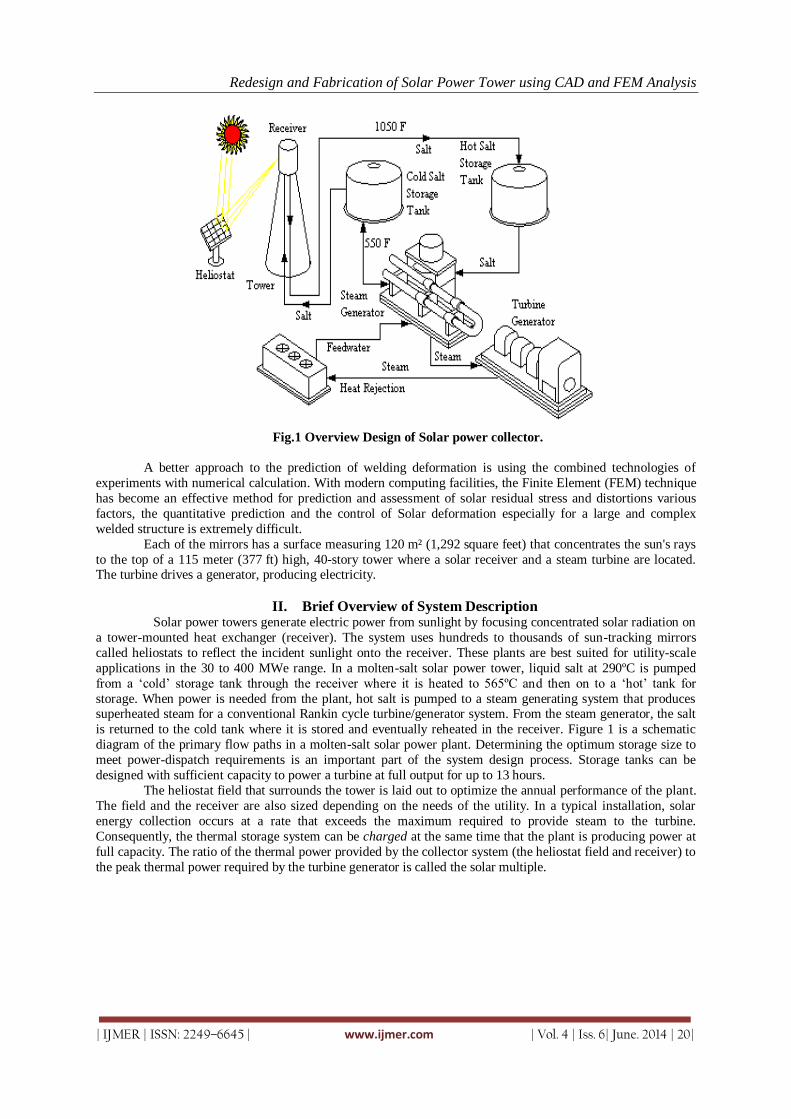
Redesign and Fabrication of Solar Power Tower using CAD and FEM Analysis
| IJMER | ISSN: 2249–6645 | www.ijmer.com | Vol. 4 | Iss. 6| June. 2014 | 20|
Fig.1 Overview Design of Solar power collector.
A better approach to the prediction of welding deformation is using the combined technologies of
experiments with numerical calculation. With modern computing facilities, the Finite Element (FEM) technique
has become an effective method for prediction and assessment of solar residual stress and distortions various
factors, the quantitative prediction and the control of Solar deformation especially for a large and complex
welded structure is extremely difficult.
Each of the mirrors has a surface measuring 120 m² (1,292 square feet) that concentrates the sun's rays
to the top of a 115 meter (377 ft) high, 40-story tower where a solar receiver and a steam turbine are located. The turbine drives a generator, producing electricity.
II. Brief Overview of System Description Solar power towers generate electric power from sunlight by focusing concentrated solar radiation on
a tower-mounted heat exchanger (receiver). The system uses hundreds to thousands of sun-tracking mirrors
called heliostats to reflect the incident sunlight onto the receiver. These plants are best suited for utility-scale
applications in the 30 to 400 MWe range. In a molten-salt solar power tower, liquid salt at 290ºC is pumped
from a „cold‟ storage tank through the receiver where it is heated to 565ºC and then on to a „hot‟ tank for
storage. When power is needed from the plant, hot salt is pumped to a steam generating system that produces superheated steam for a conventional Rankin cycle turbine/generator system. From the steam generator, the salt
is returned to the cold tank where it is stored and eventually reheated in the receiver. Figure 1 is a schematic
diagram of the primary flow paths in a molten-salt solar power plant. Determining the optimum storage size to
meet power-dispatch requirements is an important part of the system design process. Storage tanks can be
designed with sufficient capacity to power a turbine at full output for up to 13 hours.
The heliostat field that surrounds the tower is laid out to optimize the annual performance of the plant.
The field and the receiver are also sized depending on the needs of the utility. In a typical installation, solar
energy collection occurs at a rate that exceeds the maximum required to provide steam to the turbine.
Consequently, the thermal storage system can be charged at the same time that the plant is producing power at
full capacity. The ratio of the thermal power provided by the collector system (the heliostat field and receiver) to
the peak thermal power required by the turbine generator is called the solar multiple.

Redesign and Fabrication of Solar Power Tower using CAD and FEM Analysis
| IJMER | ISSN: 2249–6645 | www.ijmer.com | Vol. 4 | Iss. 6| June. 2014 | 21|
Fig.2 Overview Design of Solar power collector.
III. Rankine Cycle
There are four processes in the Rankine cycle, each changing the state of the working fluid. These
states are identified by number in the diagram above.
Process 4-1: First, the working fluid is pumped (ideally isentropic ally) from low to high pressure by a
pump. Pumping requires a power input (for example mechanical or electrical).
Process 1-2: The high pressure liquid enters a boiler where it is heated at constant pressure by an
external heat source to become a superheated vapor. Common heat sources for power plant systems are
coal, natural gas, or nuclear power.
Process 2-3: The superheated vapor expands through a turbine to generate power output. Ideally, this
expansion is isentropic. This decreases the temperature and pressure of the vapor.
Process 3-4: The vapor then enters a condenser where it is cooled to become a saturated liquid. This
liquid then re-enters the pump and the cycle repeats.
Rankine cycles describe the operation of steam heat engines commonly found in power generation
plants. In such vapor power plants, power is generated by alternately vaporizing and condensing a working fluid
(in many cases water, although refrigerants such as ammonia may also be used).
The working fluid in a Rankine cycle follows a closed loop and is re-used constantly. Water vapor seen
billowing from power plants is evaporating cooling water, not working fluid.
IV. Energy Storage The PS10 solar power tower stores heat in tanks as superheated and pressurized water at 50 bar and
285 °C. The water evaporates and flashes back to steam, releasing energy and reducing the pressure. Storage is for one hour. It is suggested that longer storage is possible, but that has not been proven yet in an existing power
plant. However, there are many considerations for using molten salt as an energy storage medium due to the
great capability of storing energy for long periods of time without substantial losses. Another possibility is to
use a phase-change material as thermal storage where latent heat is used to store energy.
V. Heliostat It comes from Helios, the Greek word for sun and stat, as in stationary. A Heliostat is a device that
tracks the movement of the sun. It is typically used to orient a mirror, throughout the day, to reflect sunlight in a
consistent direction. When coupled together in sufficient quantities, the reflected sunlight from the heliostats can generate an enormous amount of heat if all are oriented towards the same target. It was originally developed as
an instrument for use in surveying, allowing the accurate observation of a known point from a distance.
Heliostats have been used for sunlight-powered interior lighting, solar observatories, and solar power
generation. Mirrors and reflective surfaces used in solar power that do not track the sun are not heliostats.

Redesign and Fabrication of Solar Power Tower using CAD and FEM Analysis
| IJMER | ISSN: 2249–6645 | www.ijmer.com | Vol. 4 | Iss. 6| June. 2014 | 22|
The simplest heliostat devices use a clockwork mechanism to turn the mirror in synchronization with
the rotation of the Earth. More complex devices need to compensate for the changing elevation of the Sun
throughout a Solar year. Even more advanced heliostats track the sun directly by sensing its position throughout the day. The heliostat reflects the sunlight onto the transmission system. This is typically a set of mirrors that
direct the reflected sunlight into the building or, alternatively, a light tube. Fiber optic cabling has also been used
as a transfer mechanism. Various forms of commercial products have been designed for the point of termination
(the "light bulb").
Fig.3 Heliostat Device for Solar power collector
The heliograph had some great advantages. It allowed long distance communication without a fixed infrastructure, though it could also be linked to make a fixed network extending for hundreds of miles, as in the
fort-to-fort network used for the Geronimo campaign. It was very portable, did not require any power source,
and was relatively secure since it was invisible to those not near the axis of operation, and the beam was very
narrow, spreading only 50 feet per mile of range. However, anyone in the beam with the correct knowledge
could intercept signals without being detected. In the Boer war, where both sides used heliographs, tubes were
sometimes used to decrease the dispersion of the beam. Conversely, the narrow beam made it very difficult to stay aligned with a moving target, as when communicating from shore to a moving ship, and the British issued a
dispersing lens to broaden the heliograph beam from its natural diameter of 0.5 degrees to 15 degrees for that
purpose.
The distance that heliograph signals could be seen depended on the clarity of the sky and the size of the
mirrors used. A clear line of sight was required, and since the Earth's surface is curved, the highest convenient
points were used. Under ordinary conditions, a flash could be seen 30 miles (48 km) with the naked eye, and
much farther with a telescope. The maximum range was considered to be 10 miles for each inch of mirror
diameter. Mirrors ranged from 1.5 inches to 12 inches or more. The record distance was established by a
detachment of U.S. signal sergeants by the inter-operation of stations on Mount Ellen, Utah, and Mount
Uncompahgre, Colorado, 183 miles (295 km) apart on September 17, 1894, with Signal Corps heliographs
carrying mirrors only 8 inches square. A heliostat (from helios, the Greek word for sun, and stat, as in stationary) is a device that includes a mirror, usually a plane mirror, which turns so as to keep reflecting sunlight
toward a predetermined target, compensating for the sun's apparent motions in the sky. The target may be a
physical object, distant from the heliostat, or a direction in space. The alt-azimuth and polar-axis alignments are
two of the three orientations for two-axis mounts that are, or have been, commonly used for heliostat mirrors.

Redesign and Fabrication of Solar Power Tower using CAD and FEM Analysis
| IJMER | ISSN: 2249–6645 | www.ijmer.com | Vol. 4 | Iss. 6| June. 2014 | 23|
VI. Tracking Alternatives The movement of most modern heliostats employs a two-axis motorized system, controlled by
computer as outlined at the start of this article. Almost always, the primary rotation axis is vertical and the
secondary horizontal, so the mirror is on an alt-azimuth mount. One simple alternative is for the mirror to rotate
around a polar aligned primary axis, driven by a mechanical, often clockwork, mechanism at 15 degrees per
hour, compensating for the earth's rotation relative to the sun. The mirror is aligned to reflect sunlight along the
same polar axis in the direction of one of the celestial poles. There is a perpendicular secondary axis allowing
occasional manual adjustment of the mirror (daily or less often as necessary) to compensate for the shift in the
sun's declination with the seasons. The setting of the drive clock can also be occasionally adjusted to
compensate for changes in the Equation of Time. The target can be located on the same polar axis that is the
mirror's primary rotation axis, or a second, stationary mirror can be used to reflect light from the polar axis
toward the target, wherever that might be. This kind of mirror mount and drive is often used with solar cookers, such as Scheffler reflectors. For this application, the mirror can be concave, so as to concentrate sunlight onto
the cooking vessel.
VII. Land, Water, and Critical Materials Requirements The land and water use values provided in Table 4 apply to the solar portion of the power plant. Land
use in 1997 is taken from Solar Two design documents. Land use for years 2000 and beyond is based on
systems studies. The proper way to express land use for systems with storage is ha/MWh/yr. Expressing land
use in units of ha/MW is meaningless to a solar plant with energy storage because the effect of plant capacity
factor is lost. Water use measured at the SEGS VI and VII [20] trough plants form the basis of these estimates. Wet cooling towers are assumed. Water usage at Solar Two should be somewhat higher than at SEGS VI and
VII due to a lower power block efficiency at Solar Two (33% gross). However, starting in the year 2000, water
usage in a commercial power tower plant, with a high efficiency power block (42% gross), should be about 20%
less than SEGS VI and VII. If adequate water is not available at the power plant site, a dry condenser-cooling
system could possibly be used. Dry cooling can reduce water needs by as much as 90%. However, if dry cooling
is employed, cost and performance penalties are expected to raise level zed-energy costs by at least 10%.
Fig.4 Roof-mounted Close-Coupled Heliostats Receivers
VIII. Solar Power Applications Several kinds of very practical solar energy systems are in use today. The two most common are
passive solar heated homes (or small buildings), and small stand-alone photovoltaic (solar electric) systems.
These two applications of solar energy have proven themselves popular over a decade of use. They also
illustrate the two basic methods of harnessing solar energy: solar thermal systems, and solar electric systems.
The solar thermal systems convert the radiant energy of the sun into heat, and then use that heat energy as
desired. The solar electric systems convert the radiant energy of the sun directly into electrical energy, which can then be used as most electrical energy is used today.

Redesign and Fabrication of Solar Power Tower using CAD and FEM Analysis
| IJMER | ISSN: 2249–6645 | www.ijmer.com | Vol. 4 | Iss. 6| June. 2014 | 24|
Fig.5 The Solar Bowl above the ground in Auroville, India concentrates sunlight on a movable receiver to
produce heat for Electricity
Where temperatures below about 95 °C are sufficient, as for space heating, flat-plate collectors of the
non concentrating type are generally used. Because of the relatively high heat losses through the glazing, flat
plate collectors will not reach temperatures much above 200 °C even when the heat transfer fluid is stagnant.
Such temperatures are too low for efficient conversion to electricity. During the day the sun has different
positions. For low concentration systems (and low temperatures) tracking can be avoided (or limited to a few
positions per year) if nonimaging optics are used. For higher concentrations, however, if the mirrors or lenses do
not move, then the focus of the mirrors or lenses changes (but also in these cases nonimaging optics provides the widest acceptance angles for a given concentration). Therefore it seems unavoidable that there needs to be a
tracking system that follows the position of the sun (for solar photovoltaic a solar tracker is only optional). The
tracking system increases the cost and complexity. With this in mind, different designs can be distinguished in
how they concentrate the light and track the position of the sun.
Fig.6 Solar Panels of Collectors FEM Analysis
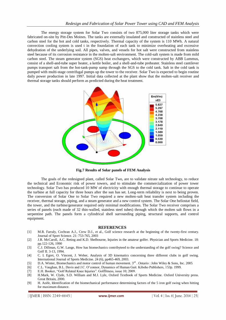
Redesign and Fabrication of Solar Power Tower using CAD and FEM Analysis
| IJMER | ISSN: 2249–6645 | www.ijmer.com | Vol. 4 | Iss. 6| June. 2014 | 25|
The energy storage system for Solar Two consists of two 875,000 liter storage tanks which were
fabricated on-site by Pitt-Des Moines. The tanks are externally insulated and constructed of stainless steel and
carbon steel for the hot and cold tanks, respectively. Thermal capacity of the system is 110 MWh. A natural convection cooling system is used t in the foundation of each tank to minimize overheating and excessive
dehydration of the underlying soil. All pipes, valves, and vessels for hot salt were constructed from stainless
steel because of its corrosion resistance in the molten-salt environment. The cold-salt system is made from mild
carbon steel. The steam generator system (SGS) heat exchangers, which were constructed by ABB Lummus,
consist of a shell-and-tube super heater, a kettle boiler, and a shell-and-tube preheater. Stainless steel cantilever
pumps transport salt from the hot-tank-pump sump through the SGS to the cold tank. Salt in the cold tank is
pumped with multi-stage centrifugal pumps up the tower to the receiver. Solar Two is expected to begin routine
daily power production in late 1997. Initial data collected at the plant show that the molten-salt receiver and
thermal storage tanks should perform as predicted during the heat treatment.
Fig.7 Results of Solar panels of FEM Analysis
The goals of the redesigned plant, called Solar Two, are to validate nitrate salt technology, to reduce
the technical and Economic risk of power towers, and to stimulate the commercialization of power tower
technology. Solar Two has produced 10 MW of electricity with enough thermal storage to continue to operate
the turbine at full capacity for three hours after the sun has set. Long-term reliability is next to being proven. The conversion of Solar One to Solar Two required a new molten-salt heat transfer system including the
receiver, thermal storage, piping, and a steam generator and a new control system. The Solar One heliostat field,
the tower, and the turbine/generator required only minimal modifications. The Solar Two receiver comprises a
series of panels (each made of 32 thin-walled, stainless steel tubes) through which the molten salt flows in a
serpentine path. The panels form a cylindrical shell surrounding piping, structural supports, and control
equipment.
REFERENCES [1] M.R. Farraly, Cochran A.J., Crew D.J., et al., Golf science research at the beginning of the twenty-first century.
Journal of Sport Science. 21: 753-765, 2003 [2] J.R. McCaroll, A.C. Reting and K.D. Shelbourne, Injuries in the amateur golfer. Physician and Sports Medicine. 18:
pp.122-126, 1990 [3] C.J. Dillman, G.W. Lange, How has biomechanics contribyteed to the understanding of the golf swing? Science and
Golf II. 3-13, 1994. [4] C. I. Egret, O. Vincent, J. Weber, Analysis of 3D kinematics concerning three different clubs in golf swing.
International Journal of Sports Medicine. 24 (6), pp465-469, 2003. [5] D.A. Winter, Biomechanics and motor control of human movement. 3rd . Ontario : John Wiley & Sons, Inc. 2005
[6] C.L. Vaughan, B.L. Davis and J.C. O‟connor, Dynamics of Human Gait. Kiboho Publishers, 153p. 1999. [7] E.H. Booker, “Golf Related Knee Injuries”. Golffitness, issue 10; 2009. [8] H.Mark, W. Clyde, S.D. William and M.J. Lyle, Oxford Textbook of Sports Medicine. Oxford University press.
Great Britain, 2000. [9] H. Aoife, Identification of the biomechanical performance determining factors of the 5 iron golf swing when hitting
for maximum distance.

Redesign and Fabrication of Solar Power Tower using CAD and FEM Analysis
| IJMER | ISSN: 2249–6645 | www.ijmer.com | Vol. 4 | Iss. 6| June. 2014 | 26|
[10] School of Health and Human Performance, Dublin City University. 2009 [11] C.A. Putnam, Sequential motions of body segment in striking and throwing skills: Descriptions and explanations.
Journal of Biomechanics, 26, 125-135, 1993. [12] E.H. Booker, Golf Related Knee Injuries. Golffitness. Issue 10, 2009. [13] Hardy PA, Recht MP, Piraino DW. Fat suppressed MRI of articular cartilage with a spatial-spectral excitation pulse.
J Magn Reson Image 1998;8:1279–1287. [14] Glaser C, Faber SC, Eckstein F, Springer V, Stammberger T, Englmeier K-H, Reiser M. Optimization. Magn Reson
Imag 2001;19:177–185. [15] Graichen H, Springer V, Flamann T, Stammberger T, Glaser C, Englmeier K-H, Reiser M, Cartilage 2000;8:106–
114. [16] Burgkart R, Glaser C, Hyhlik Du rr A, Englmeier K-H, Reiser M, Eckstein Rheum 2001;44:2072–2077. [17] Ateshian GA. A B-spline least-squares surface fitting method for articular surfaces of diarthrodial joints. J Biomech
Eng 1993;115:366–373. [18] Chung KL, Yan WM. Parallel b-spline surface fitting on mesh-connected computers. J Parall Distr Comput
1996;35:205–210.
[19] Kwak SD, Colman WW, Ateshian GA, Grelsamer cartilage: surface curvature analysis. J Orthop Res 1997;15:468–472.
International
OPEN ACCESS Journal Of Modern Engineering Research (IJMER)
| IJMER | ISSN: 2249–6645 | www.ijmer.com | Vol. 4 | Iss. 6| June. 2014 | 27|
Enhanced Methodology for supporting approximate string search
in Geospatial data
Ashwina.R1, Mrs.T.Megala
2
1, 2 (MCA-III year, MCA. Assistant professor, Sri Manakula Vinayagar Engineering College, Madagadipet,
Pondicherry, India)
I. INTRODUCTION Geospatial information is information that refers to the position of an entity on the Earth, and includes
information such as street, city, and national borders as well as longitude and latitude coordinates. There are
several local-search websites, such as Google Maps, Yahoo! Local, Bing Maps, Yellow Pages, and MapQuest
Maps. At such a website, a user might look for a restaurant called “Chaochi” close to San Jose in California. The
website returns the restaurants close to the city that match the keywords. Users often do not know the exact
spelling of keywords. For example, the user may mistype a query as (chochi restaurant) near (San Jose, CA) when looking for the restaurant Chaochi. Similarly, a user could mistype the word “restaurant” and submit a query:
(resturnt) near (San Jose). Approximate string search is necessary when users have a fuzzy search condition, or a
spelling error when submitting a query. It is important to find relevant answers to such mistyped queries.
Unfortunately, most existing location-based systems do not provide correct or approximate answers to a query
even with only a single typo.We conducted various experiments to show how several systems behaved for three
mistyped variations of the query “Chao chi restaurant” as of May 5, 2014.
In most cases, the search engines either returned an empty answer or gave irrelevant results. Both
Google and Yahoo returned “We could not find the desired results”. In this paper, we study how to solve this
problem by supporting approximate keyword search on spatial data. Given a query with keywords and a spatial
location, we want to find the location with those keywords, even if those keywords do not match exactly. Thus
we can find relevant objects for the user even in the presence of typos in the query or data.
TABLE I. RESULTS OF LOCAL-SEARCH ENGINES FOR MISTYPED QUERIES (AS OF MAY,5 2014)
Searc
h
Engi
ne
Results of mistyped queries
Chochi restaurant
Chooch
i
restaur
ant
Chauchi
restaura
nt
Yaho
o!
Could not find the desired
results
Word
misspelt misspelt
Googl
e Could not find the result
Misspel
t mispelt
Notice this approach is more powerful than the approach of suggesting an alternative query (the “Did
you mean” feature used by many systems). The latter can only suggest a new query, while the new approach can
find approximate answers, even if the answers’ keywords are only similar to those of the query.
Abstract: In recent years many websites have started providing keyword search services on maps. In these systems, users may experience difficulties finding the entities they are looking for if they do not
know their exact spelling, such as a name of a restaurant. In this paper, we present a novel index
structure and corresponding search algorithm for answering map based approximate-keyword in an
Euclidean space so that the users get their desired results even though they have typos in the keyword.
This work mainly focuses on investigating range queries in Euclidean space.
Keywords: Euclidean space, Approximate keyword, typos, LBAK.

Enhanced Methodology for supporting approximate string search in Geospatial data
| IJMER | ISSN: 2249–6645 | www.ijmer.com | Vol. 4 | Iss. 6| June. 2014 | 28|
BACKGROUND WORK
Euclidean plane or space is as a set of points satisfying certain relationships, expressible in terms of
distance and angle. It supports range queries. For example: It retrieves places within a particular range or
distance.
a. R TREE
R tree indexing is used for searching string queries in Euclidean space. They are actually data structures used for spatial access methods for indexing multi –dimensional information such as geographical co-ordinates.
But doesn’t exactly support for approximate string search.
Defining the similarity between 2 strings was a major issue since computing the edit distance between 2 strings
has a quadratic complexity (to the length of the string). Several string similarity comparisons lead to higher CPU
cost (overhead).
Suppose a query string that does not have any similar strings within its query range leads to minimum
query cost. But in R tree, it visits all the index nodes within query range leading to unnecessary IO overhead. R
tree solution could suffer from unnecessary node visits which lead to higher IO cost (overhead). The fundamental
issue here is that the possible pruning power from the string match predicate is completely ignored by the R tree
solution. Since the pruning power was completely ignored by the R tree a combined approach that prunes
simultaneously on string match predicate and spatial predicate was proposed.
b. MHR TREE
MHR tree is R tree augmented with the min- wise signature and the linear hashing technique. The min –
wise signature for an index node u keeps a concise representation of the union of q-grams from string under the
sub tree of u. The pruning functionality of such signatures was analyzed based on the set resemblance between
the query string and the q grams from the sub trees of index nodes.
In this structure similar strings are retrieved, points that do not satisfy the spatial predicate are pruned in
post processing.
But the size overhead of these signatures is very small. Less space so can’t increase query time. The
method misses query answers due to probabilistic nature of the signatures.
1. AK TREE
AK (Approximate Keyword) tree is used to return approximate results rather than exact results. It can answer queries such as find chochi restaurant near San Jose. Notice that chochi is misspelled but the AK-Tree
can still find useful answers. In short, the AK-Tree answers queries with a spatial component and a keyword
component, where the keywords don't need to match exactly but approximately. The main idea of the basic index
is to augment a tree-based spatial index with capabilities for approximate string search and keyword search. We
use approximate string search to identify for each keyword those strings that are similar. Once we have identified
similar keywords, we use the keyword-search capability to prune search paths. To support keyword search we
choose some nodes to store the union of keywords contained in objects of their sub tree. The indexing structure
used is R *tree which is an enhanced version of R tree.
1.2 PROBLEM FORMULATION
The problem of approximate keyword search on spatial data can be formulated as follows. Consider a collection of spatial objects obj1,...,ojbn, each having a textual description (a set of keywords) and a location. A
spatial approximate- keyword query Q = (Qs,Qt) consists of two conditions: a spatial condition Qs such as a
rectangle or a circle, and an approximate keyword condition Qt having a set of k pairs
(w1,δ1),(w2,δ2),...,(wk,δk), each representing a keyword wi with an associated similarity threshold δi. The
similarity thresholds refer to a similarity measure such as edit distance, Jaccard, etc., which could be different for
each keyword. Our goal is to find all objects in the collection that are within the spatial region Qs and satisfy the
approximate keyword condition Qt. We focus on conjunctive approximate keyword queries; thus, an object
satisfies the approximate keyword condition if for each keyword wi in Qt, the object has a keyword in its
description whose similarity to wi is within the corresponding threshold δi.
1.2.1 ALGORITHM We discuss the search procedure for answering spatial approximate-keyword queries. We classify the
AK- tree nodes into three categories:
S-Nodes
SA-Nodes
SK-Nodes
S-nodes: Do not store any textual information such as keywords or approximate indexes, and can only be
used for pruning based on the spatial condition.

Enhanced Methodology for supporting approximate string search in Geospatial data
| IJMER | ISSN: 2249–6645 | www.ijmer.com | Vol. 4 | Iss. 6| June. 2014 | 29|
SA-Nodes: Store the union of keywords of their sub tree, and an approximate index on those keywords. We
use SA-Nodes to find similar keywords, and to prune sub trees with the spatial and approximate keyword
conditions.
SK-Nodes: Store the union of keywords of their sub tree, and prune with the spatial condition and its
keywords. Note that we must have previously identified the relevant similar keywords once we reach an SK-
Node.
a. ALGORITHM OUTLINE
Let Q be a query with a spatial condition Qs and an approximate-keyword condition Qt with k
keywords. The algorithm traverses the tree top-down and performs the following actions at a tree node depending
on the node type. At an S-Node, the algorithm only relies on the spatial information of the node to decide which
children to traverse. Once the algorithm reaches an SA-Node, it uses the node’s approximate index to find similar
keywords. For each keyword wi in Qt, the algorithm maintains a set of key- words Ci that are similar to wi
according to its similarity threshold δi. Assuming we use the AND-semantics, a node is pruned if one of the
query’s Ci sets is empty. Otherwise, we propagate the list C = C1,...,Ck downward and use it for further pruning.
In particular, at each SK-Node n, for each keyword wi in Qt, the algorithm intersects its similar keywords Ci
propagated from the parent with the stored keywords of n. The node n can be pruned if one of the similar
keyword-sets Ci has an empty intersection with the node’s keywords. Otherwise, the algorithm passes those in- tersection sets of similar keywords to n’s children for further traversal. At a leaf node, the algorithm adds to the
answer set all the node’s objects that satisfy the condition Qs and have a non-empty intersection between their
keywords and each of the propagated similar-keyword sets from the query.
Pseudo-code: Let us examine the pseudo-code for AK- Search in Algorithm 1. Note that the algorithm
invokes several helper procedures, e.g. InitSimilarKeywordSets, Proc- SNode, etc., defined in Algorithms 2, 3, 4
and 5. The input of Algorithm 1 is a query Q = (Qs,Qt) and an AK-tree root r. We initialize a list C of k similar-
keyword sets (line 2), where k is the number of keywords in Qt. We maintain a stack S to traverse the tree.
Initially, we push the root r and the list C to the stack (line 4). We start traversing the tree by popping the pair (n,
C) from the stack (line 6). If n is not a leaf node, then all n’s children that satisfy the spatial condition will be
investigated (lines 7-9). Depending on the type of the node we invoke a helper procedure to process it (lines 10-
18): For an S-Node (lines 11-12), we only rely on the spa- tial condition to do pruning, and push the pair (ni, C) to
the stack S (within Algorithm 3). For an SA-Node (lines 13-14), we use its approximate index to find similar key- words for each query keyword as shown in Algorithm 4. We call GetSimKwds (wi, δi) to get wi’s similar
keywords, for i = 1,...,k, and store them in wi’s corresponding similar- keyword set Ci. If at least one similar
keyword is found for each keyword in Qt, then the pair (ni, C) is pushed to the stack S for future investigation.
For an SK-Node (lines 15- 16), we compute the intersection Gi between ni’s keywords and the similar-keyword
set Ci. If all the intersection sets are not empty, then the pair (ni, G) is pushed to S to be examined later
(Algorithm 5). Finally, when we reach a leaf node, we add its objects that satisfy the two conditions Qt and Qs to
the results.
Algorithm 1. Ak Search
Input: A query Q = hQs,Qti, with Qt having k pairs (w1,δ1),...,(wk,δk) associating a keyword wi with its similarity threshold δi;
An AK-tree root r;
Output: A set R of all objects satisfying Qs and Qt;
1 Result set R ← ∅;
2 C ← InitSimilarKeywordSets(r, Qt);
3 Initialize an empty stack S;
4 S.push (r,C);
5 while S = ∅ do
6 (n,C) ← S.pop();
7 if n is not a leaf node then 8 for each child ni of n do
9 if ni does not satisfy Qs then continue;
10 switch ni.type do
11 case S-Node:
12 S ← ProcSNode(ni, Qt, C, S);
13 case SA-Node:
14 S ← ProcSANode(ni, Qt, C, S);
15 case SK-Node:

Enhanced Methodology for supporting approximate string search in Geospatial data
| IJMER | ISSN: 2249–6645 | www.ijmer.com | Vol. 4 | Iss. 6| June. 2014 | 30|
16 S ← ProcSKNode(ni, Qt, C, S);
17 endsw
18 endsw
19 end
20 else // leaf node
21 foreach object oi of n do
22 if oi satisfies Qs and Qt then 23 R.add(oi);
24 end
25 end
26 end
27 end
28 return R
Algorithm 2. InitSimilarKeywordSets
Input: Root r of an LBAK-tree;
Qt = (w1,δ1),...,(wk,δk) Output: A list of similar-keyword sets
C = C1,...,Ck;
1 C ← ∅,∅,...,∅ // k empty sets
2 return C
Algorithm 3: ProcSnode
Input: S-Node n;
Qt = (w1,δ1),...,(wk,δk);
Similar-keyword sets C = C1,...,Ck;
Stack S; Output: Stack S;
1 S.push (n,C);
2 return S
Algorithm 4: ProcSANode
Input: SA-Node n;
Qt = (w1,δ1),...(wk,δk);
Similar-keyword sets C = C1,...,Ck;
Stack S;
Output: Stack S; 1 for i=1 to k do
2 Ci ← n.GetSimKwds(wi, δi);
3 end
4 if all Ci’s = ∅ then
5 S.push (n,C);
6 end
7 return S
Algorithm 5: ProcSKNode Input : SK-Node n;
Qt = (w1,δ1),...(wk,δk); Similar-keyword sets C = C1,...,Ck;
Stack S;
Output: Stack S;
1 for i=1 to k do
2 Gi ← n.keywords ∩ Ci;
3 end
4 if all Gi’s = ∅
then 5 G ← G1,G2,...,Gk;

Enhanced Methodology for supporting approximate string search in Geospatial data
| IJMER | ISSN: 2249–6645 | www.ijmer.com | Vol. 4 | Iss. 6| June. 2014 | 31|
6 S.push (n,G);
7 end
8 return S
II. Demonstration Description The system provides an interface similar to existing local-search on maps. The interface has a map and
two input boxes, one for textual keywords and one for a location. The map is using the Google Maps API, and
can display the search results for a query. We also use the Google Maps Geocoder API to obtain the latitude and
longitude of the entered location. When a user clicks the search button, the objects satisfying the query conditions
will be shown as red markers on the map. There are options to zoom in and out. The below screen shots are taken
from our project.
Fig.1 A screen shot of our system with a mistyped keyword “Calagaeri city”.
Fig. 2 Location displayed even though there were errors in the keyword for Chochi restaurant

Enhanced Methodology for supporting approximate string search in Geospatial data
| IJMER | ISSN: 2249–6645 | www.ijmer.com | Vol. 4 | Iss. 6| June. 2014 | 32|
Fig.3 A screen shot of our system with a mistyped keyword ”Lacoomeee city”.
FFig.4 A screen shot of our system with a mistyped keyword”Tibessa city”.
Fig.5 A screen shot of our system with a mistyped keyword ”Nunavote city”.

Enhanced Methodology for supporting approximate string search in Geospatial data
| IJMER | ISSN: 2249–6645 | www.ijmer.com | Vol. 4 | Iss. 6| June. 2014 | 33|
a. 3. Comparison Our system was compared with other several search engines. It is proved from the Figures 1,2,3,4 & 5
that the problem of approximate string search has been solved by 80 %. When other location based search engines
were unable to retrieve approximate results when a user entered a mis spelt keyword,our system retrieved accurate results even though the user entered a wrong keyword.
Fig.6 A screen shot of the search engine Google map retrieving with a mistyped keyword “Chochi restaurant near
san jose”.
Fig. 7. A screen shot of the search engine Yahoo map retrieving the keyword “Chochi Restaurant near San Jose”
The above screen shots show that still several search engines lack approximate string search. The figure 2. Shows the result of my system giving the exact result for the keyword “chochi restaurant san jose”. Thus it is
proved from the above results that our system provides approximate results even though the user has mistyped or
misspelt the keyword.This proves that our approach works better when compared to other systems.

Enhanced Methodology for supporting approximate string search in Geospatial data
| IJMER | ISSN: 2249–6645 | www.ijmer.com | Vol. 4 | Iss. 6| June. 2014 | 34|
Fig. 8. Comparison with various tree and their metric results
The above graph describes that R tree needs a higher IO and CPU cost whereas it has been proved to be
low in AK Tree. The edit distance metric for R tree and MHR tree is less when compared to AK tree and this
proves that AK tree supports better pruning than any other tree.
III. Conclusion
Thus the use of AK tree reduces the query time. Unnecessary CPU and IO overhead is completely
reduced with the use of R * tree. The usage of R * tree incurs a minimum query cost. A combined approach that
satisfies both string match predicate and spatial predicate solved the problem of pruning resulting in an accurate
string search. Comparisons from other system prove how efficient our system works.
REFERENCES [1] S. Acharya, V. Poosala, and S. Ramaswamy. Selectivity estimation in spatial databases. In SIGMOD, pages 13–24,
1999. [2] N. Beckmann, H. P. Kriegel, R. Schneider, and B. Seeger. The R∗- tree: an efficient and robust access method for
points and rectangles. In SIGMOD, pages 322–331, 1990. [3] A. Z. Broder, M. Charikar, A. M. Frieze, and M. Mitzenmacher. Min- wise independent permutations (extended
abstract). In STOC, pages 327–336, 1998. [4] G. Navarro. A guided tour to approximate string matching. ACM Comput. Surv., 33:31–88, 2001. [5] Hariharan, R., Hore, B., Li, C., Mehrotra, S.: Processing spatial-keyword (sk) queries in geographic information
retrieval (gir) systems. In: SSDBM, p. 16. (2007) [6] Li, C., Lu, J., Lu, Y.: Efficient merging and filtering algorithms for approximate string searches. In ICDE, pp. 257–
266. (2008)
[7] Felipe, I. D., Hristidis, V., Rishe, N.: Keyword search on spatial databases. In ICDE, pp. 656–665. (2008) [8] Yao, B., Li, F., Hadjieleftheriou, M., Hou, K.: Approximate string search in spatial databases. In ICDE. (2010) [9] A. Guttman. R-trees: A dynamic index structure for spatial searching. In B. Yormark, editor, SIGMOD’84,
Proceedings of Annual Meeting, Boston, Massachusetts, June 18-21, 1984, pp. 47–57. ACM Press, 1984. [10] K. S. McCurley. Geospatial mapping and navigation of the web. In WWW, pp. 221–229, 2001. [11] D. Zhang, Y. M. Chee, A. Mondal, A. K. H. Tung, and M. Kitsuregawa. Keyword search in spatial databases:
Towards searching by document. In ICDE, pp. 688–699, 2009. [12] D. Zhang, B. C. Ooi, and A. K. H. Tung. Locating mapped resources in web 2.0. In ICDE, pp. 521–532, 2010.
[13] J. Zobel and A. Moffat. Inverted files for text search engines. ACM Comput. Surv., 38(2):6, 2006. [14] E. Ukkonen. Approximate string-matching with q-grams and maximal matches. Theor. Comput. Sci., 92(1):191–211,
1992. [15] D. Zhang, Y. M. Chee, A. Mondal, A. K. H. Tung, and M. Kitsuregawa. Keyword search in spatial databases:
Towards searching by document. In ICDE, pages 688–699, 2009.

International
OPEN ACCESS Journal
Of Modern Engineering Research (IJMER)
| IJMER | ISSN: 2249–6645 | www.ijmer.com | Vol. 4 | Iss. 6| June. 2014 | 35|
An Overview of Distributed Generation
Abhishek Chetty1, Mohammed Shoaib
2, Dr. A .Sreedevi
3
1, 2, 3 (Student, Professor, Department of Electrical and Electronics Engineering, RVCE Bangalore, India)
I. INTRODUCTION Distributed Generation (DG) not an entirely new concept considering the manner in which the early
unit operating to produce and deliver the electricity. National grids were formed by large interconnected system
that made power system more economic and reliable. DG is a back-up electric power generating unit that is used in many facilities. Most of these back-up units are used primarily by customers to provide emergency power
during times when grid-connected power is unavailable and they are installed within the consumer premises
where the electric demand is needed. The installation of the back-up units close to the demand centre avoids the
cost of transmitting the power and any associated transmission losses. Back-up generating units are currently
defined as distributed generation to differentiate from the traditional centralized power generation model. With
the lack of significant increase in building new generating capacity or even in expanding existing ones to meet
the needs of today’s mega cities’ demand, the whole electrical power industry is facing serious challenges and is
looking for a solution. These issue decentralization of power system and liberalization of the electricity sector,
along with dramatically growing demand for electricity in many countries has made DG an attractive option.
The following are the general definition for DG
IEEE defines DG as: “A facility smaller then central plants/national grids, which is usually 10 MW or less, so that an interconnection can be allowed to any near point in the Grid, as Distributed resources”[1] .
US Department of energy (DOE) defines DG as: “Distributed power is modular electric generation or
storage located near the point of views. Distributed system include biomass-based generation, combustion
turbines, thermal solar power and Photo Voltaic (PV) system, fuel cells, wind turbines, micro turbines,
engines/generator sets storage and control technology. DG can either be grid connected or independent of
the grid. Those connected to the grids are typically interfaced at the distribution system.”[2].
General definition of DG is: “A generating plant connected directly to the grid at distribution level
voltage or customer side of the meter” [3].
The general DG technologies are such as solar power and PV, fuel cells, reciprocating engines. Wind
technology has been excluded, since it usually appears as wind farms and acts as centralized power plant. The
above definition does not specify any criteria or classification of DG capacity. Under different generating schemes diverse rating, behavior, regulation, purpose are being consider as DG in the power industry. Hence the
capacity specifications are not universally defined.
1.1 DG Energy Conversion Systems
A typical DG energy conversion system has two main energy converting stages. The first stage is the
prime fuel converting block in which the prime fuel internal energy is converted into mechanical energy, as in
the case of internal combustion engines. The second stage converts the mechanical energy into electrical power
using an electromechanical energy conversion device such asynchronous alternator or induction generator,
which produces AC power. Another way of obtaining electrical energy is through a chemical or photosynthesis
conversion process. Fuel cells and PV solar energy converter are good examples of this category and produce
Abstract: The Power Generated in Karnataka(INDIA) is 7445.91MW and Demand is 8500MWwhich
causes the problem of Load shedding, many states face this problem and are forced to buy the power from
other states which leads to the extra economical burden, this is where the Distributed Generation (DG)
plays a role to cut down the costs of the power purchased. This paper discusses the various aspects of DG
Opportunities, conversion system, technology interconnections and environmental performance. Also
some of the challenges DG system is confronting, an overview of connection between DG system and
Microgrid, the feature aspects of DG and benefits of DG system are also brought out.
Keywords: Distributed Generation (DG), Microgrid (MGR), Economic benefits and challenges, distributed generation technologies, environmental performance.

An Overview of Distributed Generation
| IJMER | ISSN: 2249–6645 | www.ijmer.com | Vol. 4 | Iss. 6| June. 2014 | 36|
DC power. The interfacing unit is essential to convert the produced DC source into harmonized constant voltage
and frequency AC power source.
DC to AC power electronic converter system is incorporated as interfacing unit. One important requirement for the inverter is to produce good quality AC power with supply frequency fluctuation limited to
1.2 Hz and with less than 5% THD of its voltage waveform at the coupling point in accordance with IEEE 519
standard [4].Islanding is a condition occurring when a generator or an inverter and a portion of the grid system
separates from the remainder of the large distribution system and continues to operate in an energized state.
Islanding may pose a safety threat or cause equipment problems; therefore, it cannot be permitted without full
coordination and planning between the parties [5–7].An additional requirement of the inverter is to have the
capability of preventing the DG from islanding (anti-islanding capability) on the hosting grid.
In the conversion types discussed above, the output produced must meet the hosting grid voltage and
frequency standards. A coupling transformer is needed to interface the DG generator with the grid to match the
distribution voltage level at the point of connection. Only when it is safe and exact paralleling conditions
(synchronization) exists, the DG is interconnected with the grid after obtaining the permission and full coordination from the grid operator.
Another configuration normally adopted for supplying power to sensitive electrical load demand is to
use DG armed with a UPS unit. The UPS system normally incorporates an energy storage medium such as
batteries to enable power supply continuity as well as improve power quality and reduce the influence of voltage
surges, spikes and swells which could cause loss of production. The DG/UPS can be configured in various
schemes to meet consumer demand and positively be part of the ancillary support to a hosting grid. In all the
systems described above, the DG output could ultimately be interconnected with the grid. The interconnection
takes place at the PCC at the grid side. Once the interconnection is established the hosting utility assumes
responsibility of DG operation and contribution and treats it as part of its generation system.
1.2 DG Opportunities
Energy investors and utility operators are attracted to the DG role and associated industry for the following foreseen opportunities. DG can be fuelled by locally available renewable and alternative mix of fuel
sources to meet today’s energy demand. Renewable sources are wind and solar, while alternative fuels are those
produced from waste products or biomass and can be in gas, liquid or solid form. Greater independency from
importing petroleum fuel can be achieved by incorporating DG that is powered by various fuel sources.
DG can support future increase in power demand without investment in the expansion of existing
distribution network as it can be installed very close to the new load center.
Installing DG within the industrial/commercial premises avoids negotiating land use and the need for
rights-of-way for electric transmission and distribution, thereby minimizing further capital investment.
DG can be used in reducing intermittent and peak supply burdens on utilities grid by injecting power as
and when required.
DG will have the capability to support the existing energy supply when needed and in a short time (black start) without incurring capital cost.
DG penetration in the energy market will create overall competitive pricing of energy. The current
generation rate ($/KWh) of DG is now competitive with the centralized generation system as efficient
fuel energy conversion units, such as fuel cells and micro turbines are continuously improved and
diversified.
DG could contribute to decreasing the vulnerability of the electric distribution system to external threats
and hidden undetected faults that may cause wide scale blackout by feeding power to the sensitive
infrastructure.
DG have a flexible feature in the capability to be configured to operate in a stand-by mode, isolated
mode, or sharing the load through integration with the existing nearby electric grid. For the general
public, using DG that is fuelled by various prime alternative fuel sources will be welcomed in order to reduce fossil fuel consumption.[4-7]
1.3 DG Classifications
DGs are classified according to their rated generation capacity, location, and size and by ownership.
DGs are also classified by their functionality in supporting the hosting grid, according to their interconnectivity,
power electronics interface or by the prime fuel source used.
DG equipment owned and operated by the power utilities are strategically located along the distribution
grid to support the power demand at specific locations for a specific time. The unit size is chosen to meet the
required forecasted secondary grid support. Its rated capacity can span from a few watts to hundreds of
kilowatts. Small rated units are normally designed to support residential and small industrial consumers and are
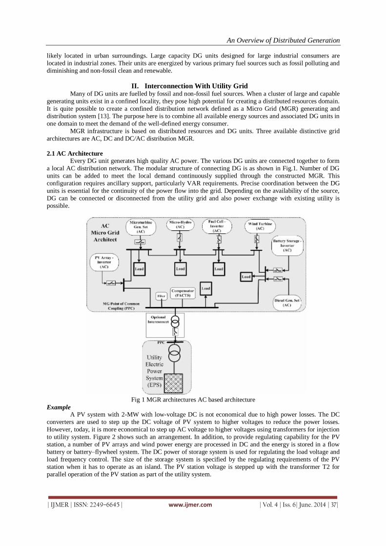
An Overview of Distributed Generation
| IJMER | ISSN: 2249–6645 | www.ijmer.com | Vol. 4 | Iss. 6| June. 2014 | 37|
likely located in urban surroundings. Large capacity DG units designed for large industrial consumers are
located in industrial zones. Their units are energized by various primary fuel sources such as fossil polluting and
diminishing and non-fossil clean and renewable.
II. Interconnection With Utility Grid Many of DG units are fuelled by fossil and non-fossil fuel sources. When a cluster of large and capable
generating units exist in a confined locality, they pose high potential for creating a distributed resources domain.
It is quite possible to create a confined distribution network defined as a Micro Grid (MGR) generating and
distribution system [13]. The purpose here is to combine all available energy sources and associated DG units in
one domain to meet the demand of the well-defined energy consumer.
MGR infrastructure is based on distributed resources and DG units. Three available distinctive grid
architectures are AC, DC and DC/AC distribution MGR.
2.1 AC Architecture
Every DG unit generates high quality AC power. The various DG units are connected together to form
a local AC distribution network. The modular structure of connecting DG is as shown in Fig.1. Number of DG
units can be added to meet the local demand continuously supplied through the constructed MGR. This
configuration requires ancillary support, particularly VAR requirements. Precise coordination between the DG
units is essential for the continuity of the power flow into the grid. Depending on the availability of the source,
DG can be connected or disconnected from the utility grid and also power exchange with existing utility is
possible.
Fig 1 MGR architectures AC based architecture
Example A PV system with 2-MW with low-voltage DC is not economical due to high power losses. The DC
converters are used to step up the DC voltage of PV system to higher voltages to reduce the power losses.
However, today, it is more economical to step up AC voltage to higher voltages using transformers for injection
to utility system. Figure 2 shows such an arrangement. In addition, to provide regulating capability for the PV
station, a number of PV arrays and wind power energy are processed in DC and the energy is stored in a flow
battery or battery–flywheel system. The DC power of storage system is used for regulating the load voltage and
load frequency control. The size of the storage system is specified by the regulating requirements of the PV
station when it has to operate as an island. The PV station voltage is stepped up with the transformer T2 for
parallel operation of the PV station as part of the utility system.
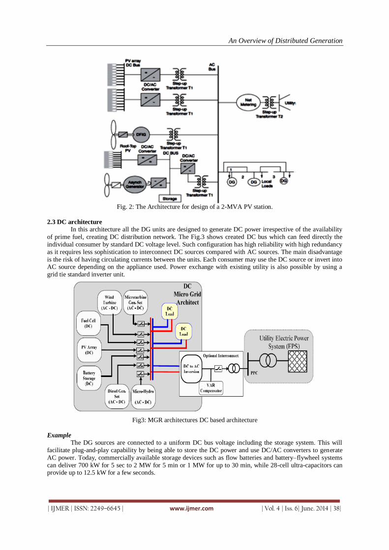
An Overview of Distributed Generation
| IJMER | ISSN: 2249–6645 | www.ijmer.com | Vol. 4 | Iss. 6| June. 2014 | 38|
Fig. 2: The Architecture for design of a 2-MVA PV station.
2.3 DC architecture
In this architecture all the DG units are designed to generate DC power irrespective of the availability
of prime fuel, creating DC distribution network. The Fig.3 shows created DC bus which can feed directly the
individual consumer by standard DC voltage level. Such configuration has high reliability with high redundancy
as it requires less sophistication to interconnect DC sources compared with AC sources. The main disadvantage
is the risk of having circulating currents between the units. Each consumer may use the DC source or invert into AC source depending on the appliance used. Power exchange with existing utility is also possible by using a
grid tie standard inverter unit.
Fig3: MGR architectures DC based architecture
Example
The DG sources are connected to a uniform DC bus voltage including the storage system. This will
facilitate plug-and-play capability by being able to store the DC power and use DC/AC converters to generate
AC power. Today, commercially available storage devices such as flow batteries and battery–flywheel systems
can deliver 700 kW for 5 sec to 2 MW for 5 min or 1 MW for up to 30 min, while 28-cell ultra-capacitors can provide up to 12.5 kW for a few seconds.
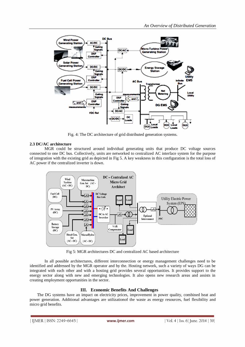
An Overview of Distributed Generation
| IJMER | ISSN: 2249–6645 | www.ijmer.com | Vol. 4 | Iss. 6| June. 2014 | 39|
Fig. 4: The DC architecture of grid distributed generation systems.
2.3 DC/AC architecture MGR could be structured around individual generating units that produce DC voltage sources
connected to one DC bus. Collectively, units are networked to centralized AC interface system for the purpose
of integration with the existing grid as depicted in Fig 5. A key weakness in this configuration is the total loss of
AC power if the centralized inverter is down.
Fig 5: MGR architectures DC and centralized AC based architecture
In all possible architectures, different interconnection or energy management challenges need to be identified and addressed by the MGR operator and by the. Hosting network, such a variety of ways DG can be
integrated with each other and with a hosting grid provides several opportunities. It provides support to the
energy sector along with new and emerging technologies. It also opens new research areas and assists in
creating employment opportunities in the sector.
III. Economic Benefits And Challenges The DG systems have an impact on electricity prices, improvement in power quality, combined heat and
power generation. Additional advantages are utilizationof the waste as energy resources, fuel flexibility and
micro grid benefits.

An Overview of Distributed Generation
| IJMER | ISSN: 2249–6645 | www.ijmer.com | Vol. 4 | Iss. 6| June. 2014 | 40|
1. Impact on electricity prices
In the electricity markets the independent system operator (ISO) charges the customers with an uplift
energy prices according to all services which are required to keep the system running in unrealizable manner. This uplift is the combination of transmission services, market administration, operating reserve, losses in
secondary auxiliary and it approximately amounts to 20% of the energy market prices. This additional cost adds
an extra tariff to the actual electricity market. Distribution companies and large consumers instead of buying
electricity directly from the market may consider implementing DG system to meet the increasing load demand.
This will reduce the cost and consumer can purchase less power from the gird.
2. Utilization of the waste as energy sources and fuel flexibility
DG technology use energy resources that are not economically or feasible to transport or convert. Some
oil fields have low quality gas that is not economical to transport and is ignited when disposed. Gas turbine and
micro turbine can utilize the bio-mass gas obtained from waste water treatment, landfills and farms. The most
commercialized DG technologies uses oil or natural gas, most part of the research has been only towards fuel cells and gas turbine which uses natural gas because of which advantage of DG system due fuel flexibility is
limited.
3. Combined heat and power (CHP) This technology can increase the overall efficiency of the production to more the 90% by combining
both heat and electricity usage efficiently. This technology is the better option, since the produced heat can be
used onsite.CHP usually a small increase in cost which is proportionalto the total capital cost of the unit (less
than 10% for industrial applications),hence economical also.
4. Microgrid
Microgrid is a new concept in which a cluster of loads and DG systems operate to improve the
reliability and quality of the power system in a controlled manner. For customers Microgrid provides the need for power and heat in a reliable way. For the whole system, Microgrid are dispatch able cells which can respond
to the signals from the system operator very fast. Information technology achievements along with new DG
systems with intelligent control systems allow system operators and Microgrid operators to interact in an
optimal manner [15].
5. Remote area electrification
The potential application of the DG is to provide electricity to the consumers who are located far from
the grid and usually do not have enough demand to justify for expanding the grid. The only possible way to
energize customer in remote communication site is though DG, mostly using PV system.
IV. Environmental Performance Of DG Systems The main environmental concern of electricity production is its effect on the local and regional air
quality by emission of NO and other greenhouse gases, in particular Carbon-did-oxide. This emission is largely
associated with non-renewable power generating technologies such as coal-fired generation.
Diesel-fired ICE has the highest NO emission and in most regions the diesel engines cannot be
operated for more than 150 hours (in USA). In regions with Coal fired generation, installation of low emission
DG units such as gas turbines, micro turbines and fuel cells can reduce the emission of NO in the region.
Carbon-di-oxide emission from non-renewable DG technologies has to be considered as well. All non-
renewable DG technologies without heat recovery have higher carbon-di-oxide emissions than combined-cycle
plants. So coal plants with CHP system can reduce carbon-di-oxide emission. Commercially available DG systems still have a long way to go to be significantly helpful in emission reduction programs [12].
V. Conclusions The potential applications for distribution generation (DG), decentralization of power system and the
trend to use renewable energies in most developed countries suggests that DG may have a large share in power
generation in the future. The DG opportunities, challenges and the economical benefits have been discussed,
examples of the grid architecture has been included. Nevertheless, more research and development is required to
overcome the barriers that DG systems are currently confronting. Higher efficiency, lower emissions and lower
capital costs are the main goals DG systems need to accomplish. The electricity market regulatory authorities and government policy makers should consider the worth of DG systems and modify the structure, operation
and pricing mechanisms of the open markets to help their viability and development.

An Overview of Distributed Generation
| IJMER | ISSN: 2249–6645 | www.ijmer.com | Vol. 4 | Iss. 6| June. 2014 | 41|
REFERENCES [1] “P1547 standard series for interconnecting distributed resources with electric power systems,” IEEE, 1547 Work
Group, Tech. Rep., 2003. [2] The US Department of Energy, Office of Distributed Energy Resources, online publications available at:
http://www.eere.energy.gov/der/, 2003. [3] Distributed Generation in Liberalised Electricity Markets. International EnergyAgency, 2002. [4] IEEE Standard 1547-2004, (2004) 1547 IEEE standard for interconnecting distributed resources with electric power
systems. Institute of Electrical and Electronics Engineers, Piscataway, New Jersey [5] Walling RA, Miller NW, (2002) Distribution generation islanding – implications on power system dynamic
performance. IEEE Conference Publications:92–96 [6] Kim JE, Hwang JS, (2001) Islanding detection method of distributed generation units connected to power distribution
system. Proceedings of the IEEE Summer Meeting:643–647 [7] Usta O, Redfem M, (2000) Protection of dispersed storage and generation units against islanding. IEEE PES Summer
Meeting 2000:976–979 [8] Lasseter R, (2002) Microgrid. Proceedings of the Power Engineering Society Winter Meeting, vol.1:27–31 [10] Khaled Nigim, Doon Campus Chapter06: “Integration of Distributed Generation with Electrical Power System”
Springer-Verlag London Limited in 2008 [11] Rashid MH, (2003) Flexible AC transmission. Chapter13: power electronics circuit devices and applications. Pearson
Prentice Hall, third edition
[12] H. Zareipour, K. Bhattacharya, and C.A. Canizares,” Distributed Generation: Current Status and Challenges “ NAPS 2004 in Feb. 2004
[13] Lasseter R, (2002) Microgrids. Proceedings of the Power Engineering Society Winter Meeting, vol.1:27–31 [14] A. Baueu, D. Hart, and A. Chase, “Fuel cells for distributed generation in developing countries- an analysis,”
International Journal of Hydrogen Energy, vol. 28, pp. 695–701, 2003. [15] T. Ackerman, G. Anderson, and L. Soder, “Distributed generation: a definition,” Electric Power System Research,
vol. 57, pp. 195–204, 2001. [16] G.pepermans, J. driesen, D. Haeseldonckx, R. Belmans, and W. D’haeseleer, “Distributed generation: Definition,
benefits and issues, Energy Policy, vol. 33, pp. 787–798, 2005.

International
OPEN ACCESS Journal
Of Modern Engineering Research (IJMER)
| IJMER | ISSN: 2249–6645 | www.ijmer.com | Vol. 4 | Iss. 6| June. 2014 | 42|
A Realistic Cost Assessment for a Conventional Dwelling Unit
(DU), Partially and Selectively Replaced With Engineered
Bamboo
Chandra Sabnani1, Mukesh Patel
2
1(Department of Architecture and Planning, VNIT, Nagpur, India) 2(Mukesh Patel Architects and Planners, Nairobi, Kenya)
I. Introduction To make realistic assessments, a convergence of the general understanding of the Govt. definition of
BPL and the simulated results that reveal what is possible in these incomes and what incomes are required for
what can be termed as acceptable.
For the purposes of a realistic understanding of affordability a modest conventional DU with minimum
requirements was designed as a framed structure. A ground floor structure with an area of 450 sq ft. G+1 being
900 sq ft. Care was however taken in ensuring that no compromises were made in the non negotiable or semi-
negotiable parameters.
The simulations to begin with, make use of all the RCC items with Steel Reinforced Concrete (SRC), except roof slab of first floor. Unit cost @ Rs. 659/Sq.Ft., Area = 450 Sq.Ft. per household, in a G+1
structure.While BPL latest definition places a household monthly income at Rs. < / =5000, the simulation
exercise establishes that even the cream layer of BPL cannot afford a house as per these norms that have been
framed.
II. What Is BPL? Defined as a category of households having 5 members, whose household monthly income is less than
or equal to Rs 5000/- these households are those who in reality are usually homeless or those that live in
shanties, or houses that are unfit for human habitation. They are found living on unauthorized land and are non tax payers. Their informal economic status and
uncertain source of livelihood, most often excludes them from the mainstream benefits. Hence the Govt. issues
them a BPL card, so that small benefits can be made provisions for, in the wake of their situation.
Abstract: The BPL (Below Poverty Line) definition has recently been revised. Now a larger number of
households fall under this category as the income bar was raised to Rs 5000 per HH of 5 members. It
has therefore been realised that unaffordability starts at a much higher income group level. A
conventional Dwelling Unit is unaffordable by most households that are Below Poverty Line (BPL). A
study shows that bamboo can replace steel in columns, Slabs and beams. It can replace bricks for inner
walls; The DU thus designed can bring down costs without compromising on quality, safety and
durability. However, even this DU is unaffordable by the BPL households in India. The urgency
therefore increases, for realistic cost assessments. The research on cost estimates for a partially bamboo
substituted house design has been conducted, for different built-up areas. The recommended size has been taken as the datum for assessment purposes.
Keywords: Below poverty line, Unit Cost of Construction, House Hold Income, affordable housing,
Realistic Estimates.

A Realistic Cost Assessment for a Conventional Dwelling Unit (DU), Partially and Selectively
| IJMER | ISSN: 2249–6645 | www.ijmer.com | Vol. 4 | Iss. 6| June. 2014 | 43|
Table I: Affordability Estimates in relation to HH income
Table II: Affordability Estimates in Absolute Figures (Govt. Data)
III. Arriving At Realistic Estimates Conventional Housing: The cheapest house that could be designed in a conventional way is a 450 sq ft
DU with the following description: A modest conventional DU with minimum requirements designed as a
framed structure. With a footprint of 450 sq ft, the structure with an area of 900 sq ft. is G+1 meant for two
households. All the RCC elements are out of SRC, Unit cost @ Rs. 659/Sq.Ft., the DU would cost
Rs.2,96,550/- Conversely, if a DU were to be constructed with the existing BPL definition, then the area of a
conventional DU cannot exceed 182 Sq.Ft.
Alternative Housing: The cheapest DU After rigorous cost cutting, a drop in the cost is seen. A 13.8%
reduction in cost with the unit cost of Rs. 568/- making the cost Rs. 2,55,600/-Conversely, if a DU were to be constructed with the existing BPL definition, then the area of an alternative DU would be 211 Sq.Ft.
Table III: Affordability test for Steel Reinforced Concrete, (SRC)
Income Group Monthly Household
(5 members)
Income
Rs.
Cost
As a Multiple of
Household Gross
Annual Income (x)
EMI/Rent
As a Percentage of Gross
Monthly Income
BPL < / =5000 </= 2x 5%
Annual < / = 60,000
Income Group Income
Monthly
Rs.
Affordable Cost of the
House (in Rs)
In Absolute Terms
Affordable EMI/Rent per
Month (in Rs)
In Absolute Terms
BPL <=5000 < /= 1,20,000 </ = 250
Income Group Monthly Household
(5 members)
Income
Required Rs.
Cost
of the cheapest DU
Designed out of
conventional materials
EMI/Rent
As a Percentage of Gross
Monthly Income
BPL < / =12,356
</= 2x= Rs.2,96,550/-
5%=618
Annual < / = 1,48,275

A Realistic Cost Assessment for a Conventional Dwelling Unit (DU), Partially and Selectively
| IJMER | ISSN: 2249–6645 | www.ijmer.com | Vol. 4 | Iss. 6| June. 2014 | 44|
Table IV: Affordability test for Bamboo Reinforced Concrete (BRC)
It is clear that to be able to afford the cheapest designed house (Bamboo or SRC) the HH must have a
minimum monthly income of Rs. 10,650/- which is more than twice the envisaged monthly HH income. Houses of the sizes 182 Sq.Ft. and 211 Sq.Ft. for a family size of 5 is unfit for human habitation.
Hence most houses either designed conventionally or through alternative materials are rendered unaffordable by
all HHs belonging to the BPL category and also those that have incomes more than double of those below
poverty line.
IV. Realistic Estimates Through Simulation
Realistic assessment of affordability needs to be made In the name of lawfulness, a large majority of the lawless cannot be excluded from benefits of
urbanism. It is only when the assessment affordability and /or un-affordability is unrealistic that laws get
violated. [1]
A small but dignified DU was designed as a simulative exercise, for the purpose of arriving at realistic
estimates for an affordable house by the combined incomes of a BPL HH. Initially the focus remained on
architectural design measures for cost cutting. Ref. Figs. 1 & 2. The outcome was a G+1 structure for 2
households, each with an area (Built-up) of 450 Sq.Ft. It has been designed with built – in storage and is out of conventional RCC, a framed structure. It has all fixtures, fittings, and is structurally safe and durable. No
compromises have been made on services, or its stability. Any further cost cutting would amount to
compromises leading to the inclusion of non negotiable parameters, transforming it into a non-habitable house.
The House to be designed for minimum 30 years of life span, and a structural design that offers a minimum
factor of safety = 3. It must have all toilet and electrical fixtures, fittings, built-in storage units, doors windows
grills, hard ware items like latches, stays, door locks, al-drops and general specifications like terrazzo tiles,
glazed tiles wherever appropriate. Water, sanitation and plumbing, is to be fixed at basic level.
On closer analysis of the National Policies it is clear that what gets promised is what is “Possible to be
built in a small budget while keeping the technology constant” and certainly not what is “desirable” or
“acceptable” in terms of size and number of rooms. A unilateral decision on compromise of standards is being
made uniformly across the country, thereby reducing the area, size of rooms, and number of rooms. Any constraints in exploring possibilities about material, design, technology or creative financial options will affect
affordability [2]
Step by Step Material Substitution
In step 1- replacing steel with bamboo reinforced in most structural elements except in foundation, first floor
slab, canopy and staircase Step 2 - all other material substitutions remaining the same as in step 1, replace bricks in all internal walls on
both floors with bamboo wall panels as per design.
Step 3- use of bamboo wall panels as a substitute for brick walls in all external walls on both floors above plinth
level.
Step 4- Use of fly ash brickwork external wall 1:4 cement plaster, bamboo wall panels as a substitute for brick
walls in all internal walls on both floors above plinth level
Step 5- Flushed doors shutters (wooden frame sandwiched between 4mm ply on both sides) to be substituted
with bamboo ply flush doors. This 5 step substitution brought down the cost of the DU by 13.8%. Refer Table 5
Figure 1. Section
Income Group Monthly Household
(5 members)
Income
Required Rs.
Cost
of the cheapest DU
Designed out of bamboo
EMI/Rent
As a Percentage of Gross
Monthly Income
BPL < / =10,650 </= 2x= 2,55,600/-
5%=533
Annual < / = 1,27,800

A Realistic Cost Assessment for a Conventional Dwelling Unit (DU), Partially and Selectively
| IJMER | ISSN: 2249–6645 | www.ijmer.com | Vol. 4 | Iss. 6| June. 2014 | 45|
Figure 1. Section
Figure 2. Plan

A Realistic Cost Assessment for a Conventional Dwelling Unit (DU), Partially and Selectively
| IJMER | ISSN: 2249–6645 | www.ijmer.com | Vol. 4 | Iss. 6| June. 2014 | 46|
Table V. Summary of cost cutting
Table VI: Reverse Iteration SRC
Final results at Rs.659 per Sq.Ft, for a DU of 450 Sq.Ft

A Realistic Cost Assessment for a Conventional Dwelling Unit (DU), Partially and Selectively
| IJMER | ISSN: 2249–6645 | www.ijmer.com | Vol. 4 | Iss. 6| June. 2014 | 47|
Table VII: Recommended Affordability model for a BPL HH
Conventional SRC DU of 450Sq.Ft
Tables 6 and 7 reveal that even in the case of steel reinforced concrete (SRC) other costs get added for
loans, fees etc. these make the proposal of taking loan for a house, seem un attractive to the BPL house hold.
Even through a subsidized loan channel it amounts to an increase of 23 % in the EMI (Equitable monthly
installment). There is no respite for this income group unless there are waivers and subsidies integrated into the
system.
Table VIII: Reverse Iteration BRC
Final results at Rs.568 per Sq.Ft, for a DU of 450 Sq.Ft
Table IX: Recommended Affordability model for a BPL HH
Recommended BRC DU of 450sq.ft
Income
Group
Monthly Household
(5 members)
Income
Rs.
Cost
As a Multiple of Household Gross
Annual Income (x)
EMI/Rent
As a Percentage of Gross
Monthly Income
BPL 10,650 </= 2x= Rs.2,55,600 23%= Rs. 2,450
Annual < / = 1,27,800

A Realistic Cost Assessment for a Conventional Dwelling Unit (DU), Partially and Selectively
| IJMER | ISSN: 2249–6645 | www.ijmer.com | Vol. 4 | Iss. 6| June. 2014 | 48|
Similarly, a rise in monthly outgoings is seen (Ref tables 8 & 9) in the monthly outgoings which
increase the cost burden on the beneficiary. These amount to 28 % more than the regular EMI that is expected to
be paid, as EMI.
V. Conclusion It is therefore concluded that unless the term “EMI” is replaced by “monthly outgoings” and subsides
waivers and grants are built into the housing finance system for the BPL category, no housing can be made
available to the urban poor leave alone bamboo housing.
Acknowledgment The Author thanks her Co- Author Ar. Mukesh Patel, Mukesh Patel Architects and Planners, Nairobi
Kenya, for his valuable contribution and unstinted guidance from time to time. She would specially like to
thank the Members of the Research and Consultancy cell of the Visvesvaraya National Institute of Technology
REFERENCES [1] Angel, Shlomo and Stanley Benjamin "Seventeen Reasons Why the Squatter Problem Can't Be Solved", Ekistics,
Vol. 41, No. 242, January, 1976, pp. 20 [2] Sabnani Chandra “Investigating the prevalence, relevance and appropriateness of bamboo technology for housing in
India” unpublished PhD thesis work [3] Presentation of the report of the task force (Deepak Parekh Report - DPC) on affordable housing for all documents
Members of the committee: Public Document [4] Cover Story-Feb09.qxp 24/01/2009 CMYK 86 CONSTRUCTION WORLD FEBRUARY 2009 Affordable Housing
needs a Revolution www.ConstructionWorld.in Public Document.
AUTHORS
Chandra Sabnani (Author1) is an Associate Professor and a PhD scholar (inter
disciplinary Board) with the Department of Architecture and Planning,
Visveswaraya National Institute of Technology, Bajaj Nagar, Nagpur. India, Phone: +91-9890253994; E-mail: [email protected]
Mukesh Patel is the principal architect and a planning consultant, at Mukesh Patel,
Architects and Planners, Nairobi, Kenya. Phone: +254-733848377;
Email:[email protected]

International
OPEN ACCESS Journal Of Modern Engineering Research (IJMER)
| IJMER | ISSN: 2249–6645 | www.ijmer.com | Vol. 4 | Iss. 6| June. 2014 | 49|
High End Solution for Advanced Civil Engineering Projects
T. Subramani1, N. Kanthasamy
2
1Professor & Dean, Department of Civil Engineering, VMKV Engg. College, Vinayaka Missions University,
Salem, India 2PG Student of Structural Engineering, Department of Civil Engineering, VMKV Engg. College, Vinayaka
Missions University, Salem, India
I. Introduction Civil FEM is at the present time one of the most advanced tools that engineers can embrace, a project
that is committed with a time and with a permanent vocation of investigation and development. Civil FEM
capabilities include a unique and extensive materials and sections library for concrete and steel structures. In
addition, the user may introduce any shape or material into the corresponding CivilFEM libraries.
A user-friendly beam and shell postprocessor includes listing and plotting section geometry, reinforcements, beam results or stresses and strains inside the cross-section. The skilled combination module, selects loads and
coefficients for logic code combinations. Results embrace concomitance at element and global level as well as
worst load arrangements in beam, shell and solid elements.
In the field of Seismic Analysis, the designer is provided with an automatic seismic design module
according to Eurocode No.8, UBC, NCSE-94 (Spanish Code) and others to make the seismic spectrum analysis
faster and easier. CivilFEM also performs concrete and steel code checking and design according to Eurocodes
(EC2 and EC3), American (ACI318 and AISC-LRFD), British (BS8110 and BS5950-1995 and 2001), Spanish
codes (EHE and EA), Model Code (CEB-FIP) and other main codes. With regards to serviceability, CivilFEM
conducts for the aforementioned codes cracking analysis. CivilFEM specialized add-on modules include non-
linear concrete, soil mechanics, prestressed concrete, bridges and dams features. The non-linear concrete module
supports large deflection buckling, non linear deformations, moment-curvature diagrams, cracking and transient effects.
For soil mechanics, slope stability analysis, libraries of soils and rocks properties, screens analysis and
design, nonlinear behaviour analysis and ballast module computation, will allow the user to carry out advanced
geotechnical problems.
The features and prestige of ANSYS in the finite element world, combined with CivilFEM's
capabilities and specialized modules, translates into a fully integrated state of the art Civil Engineering working
tool. This advantageous and unique bundle product represents the possibility of applying the analysis with finite
elements to a wide range of problems according to the hardships and requirements of this field.
II. CivilFEM Integration with ANSYS CivilFEM works inside Ansys program. That is, all Ansys tools may be used with CivilFEM (APDL,
UIDL, optimization, graphical output, ...), the CivilFEM menus are integrated inside the Ansys Main Menu,
CivilFEM Help is managed as Ansys Help System, CivilFEM commands are generated by CivilFEM menus and
written to the Ansys log file, and so on.
Ansys results are stored in CivilFEM results file in addition to data related to the cross section. You
may switch between Ansys and CivilFEM processors at any time, and mix commands from both to generate,
solve and postprocess your model easily. CivilFEM implementation is based in the use of dynamic link libraries
(DLLs). These libraries contain the CivilFEM code and are incorporated into Ansys executable file in execution
Abstract: Civil FEM performs the best customization of the well-known Finite Element Program ANSYS. The combination of both programs, totally integrated, provides the Construction and Civil Engineering
fields with the possibility of applying high-end technology to a wide range of projects. Using the same
windows graphic user interface and sharing input data and results, makes it very easy for the user to
apply them for solving difficult Civil Engineering problems. The ability to generate finite element models
of any complex three-dimensional civil structure with non-linear behaviour and construction process
simulation means a new and efficient approach to run advanced analysis on PC’s.
Keywords: Section library, load combination, Beam and shell utilises, Resource Scheduling,

High End Solution for Advanced Civil Engineering Projects
| IJMER | ISSN: 2249–6645 | www.ijmer.com | Vol. 4 | Iss. 6| June. 2014 | 50|
time, working as if they were part of Ansys. This structure allows to connect with the DLLs by means of
ANSYS external commands. These commands are declared in file ans_ext.tbl CivilFEM menus are elaborated
using Ansys UIDL features. All CivilFEM windows are written in Visual C++ and Dll’s in Fortran. Like Ansys,
CivilFEM may work in any system of units. However, the user must specify the units system before any
CivilFEM calculation is done, since specific code formulations and CivilFEM tools depend on units. A library
with the most usual (American and European) units in Civil Engineering is available. Furthermore you may also
define any other unit system (not available in the library) by selecting the "User Defined Units".
III. Civil Material Library CivilFEM defines the mechanical properties required by Ansys and the specific properties needed for
code checking of usual civil materials, in accordance with code specifications. This library includes materials
from most usual standards.
Nevertheless, the user is provided with the necessary tools to add materials into this library. Using this tool,
modified materials or new materials from any code may be included. CivilFEM material's library has five
classes of properties for all CivilFEM materials:
General properties: Common to all the materials. Structural analysis diagram: stress-strain diagram used when solving the model.
Design diagram: stress-strain diagram used when checking or designing a cross section.
Specific properties depending on the material: steel, concrete, soils, rocks.
Specific properties depending on codes: EC2, EC3, ACI, BS8110, BS5950-2001, LRFD,...
Moreover, user materials may be saved in CivilFEM’s material library. Material properties in
CivilFEM are time dependent which means that the user can solved the same model at different ages.
For each one of these scenarios, materials used in the model will be active or not, depending upon the age of the
material. The program will calculate the material age by subtracting from the age solicited the birth time of the
material.
With this capability, the user can simulate construction processes, not only at element level but inside
the cross section as well. For the non linear structural behaviour, a graphical control of stress-strain curves enables the user to select the graph that best represents the different types of loading of the structural analysis.
The user may also add or delete points, or simply create his/her own curve (See Figure 4). Different
relationships between stresses and strains are also provided for sections design, with the same possibilities as for
the structural stress-strain curve.
IV. Section Library All cross sections in CivilFEM are divided automatically into points and tessellas. A tesella is a
subdivision of the cross section and each tesella’s vertex is a point. This particular characteristic of CivilFEM’s
cross sections, allows the program to analyze and provide results inside the cross section. Cross sections in CivilFEM can be defined using eight different procedures:
1) The library of hot rolled shapes:
This library contains the most international sections libraries, such as hot rolled shapes distributed in
Europe by ARBED, as well as all the hot rolled shapes included in the AISC LRFD (over 4000 hot rolled steel
shapes are included). These last two series include all shapes groups in metric and U.S. units.
2) User library of hot rolled shapes:
CivilFEM enables the user to add more hot rolled shapes into the existing library. This capability is two
folded. The user may either read mechanical or geometric properties from a file or introduce the geometry
corresponding to the selected hot rolled section using a specific CivilFEM window. In the latter case, CivilFEM
will automatically calculate the mechanical properties for the section entered by the user. Using this tool, shapes
from any country may be added.
3) Definition of sections by dimensions: The most usual welded steel sections as well as the most usual concrete sections may be defined by
dimensions. In the case of reinforced concrete, a preliminary reinforcement may be defined using the predefined
options offered. Nevertheless user reinforcement layout for bending, shear or torsion is also available in
CivilFEM.
4) Definition of sections by plates:
Each plate adopts the active material. This feature allows defining a generic steel section built up with
2 to 100 plates with the possibility of having different materials. For each plate the ends coordinates, thickness
and restraint conditions need to be specified.

High End Solution for Advanced Civil Engineering Projects
| IJMER | ISSN: 2249–6645 | www.ijmer.com | Vol. 4 | Iss. 6| June. 2014 | 51|
5) Definition of sections starting from a 2D mesh of virtual elements MESH200:
This feature allows the definition of sections with any shape and even with mixed materials (different
concrete strengths or concrete with structural steel) using Ansys elements MESH200. Each teselum (subdivision
of the cross section) will adopt the material assigned to the corresponding element once the cross section is
captured by CivilFEM. Export of CivilFEM sections into Ansys are also possible.
6) Definition of beam cross section inside a 3D solid model of finite elements:
Each teselum adopts the material from the finite element to which is associated. The SOLID SECTION (cross section coming from a 3D ANSYS model) and the CROSS SECTION (transverse section as commonly
understood in engineering) are defined simultaneously and their numbers coincide.
This capability allows to build and solve a complete 3D solid model of the structure, and then select sections
inside this model to be processed by CivilFEM. This feature allows code checking and design of all user defined
sections of 3D
7) Composition of sections:
Any section defined by any of the above means can be combined with any other concrete or steel
section and form a new section
8) User data base of sections:
Any section defined by any of the above means can be stored in a user data base for later use.
CivilFEM uses its Beam & Shell property window to easily select the section for element ends i and j. The corresponding element type must also be entered in this window, and the real constants will automatically be
calculated by CivilFEM and sent to ANSYS.
V. Incentive Programs The following ideas and strategies were provided regarding incentive programs:
Include incentives for efficiency and for achieving milestones.
Consider bonus incentives at the trade, foreman and management levels.
Bonus schemes must be competitive across work groups.
Some bonus/incentive system must filters right down to the worker. This means if a group working on installing lighting finishes on or under budget time, they should be rewarded.
Performance based incentives targeting not just management, but more so on direct/trades persons.
Recognition programs for work: quality, quantity, HSE, milestones. Awards/rewards for no lost time
accidents.
Negotiate with crews and provide incentives to complete work packages (WP) on time and quality
without rework. As many WPs as they finish sooner directly relates to as much money as they
make.
Promote a healthy competition between crews in terms of safety and results by posting performance
by crew in selected locations across the site (safety and performance by crew).
Accountability of scope, time and cost. Maybe even a little bit of friendly competition.
Care for employees is an incentive. This means the flexibility to meet workers needs, consistent with project needs.
Monitor worker moral and watch for early warning for problems.
Full access to comprehensive employee and family assistance programs. Reduce distractions of
many kinds.
Aggressively address undesired behaviour. Harassment is less of a human rights and safety concern,
more of a performance killer. The Respect In The Workplace program is a good start.
Implement incentive programs for construction contractors and engineering firm.
Trades people, labour and all other associated workers should have bonus incentive clauses (today as in
the past they try to make the project last as long as possible).
Engage foremen with management and support them.
VI. Fire Protection By Taking Precautions I n Building Construction A building may be made more fire resistant by minimizing use of combustible materials,
protecting steel by fire resistant paints and providing stairs at suitable positions and protecting them from
fire. Various members of buildings can be made fire resistant as follows:
Walls:
Brick walls with cement plaster gives better fire resistance.
Roof:
R.C.C. flat roofs have good fire resistance. Hence they should be preferred.

High End Solution for Advanced Civil Engineering Projects
| IJMER | ISSN: 2249–6645 | www.ijmer.com | Vol. 4 | Iss. 6| June. 2014 | 52|
Ceiling:
Ceilings should be made up of cement plaster, asbestos cement board or fibre boards.
Floors:
R.C.C. floor is very good fire resisting floor.
Doors and Window Openings:
All these openings should be protected against fire by taking the following precautions:
(a) The thickness of shutters should not be less than 40 mm. (b) Instead of wooden, aluminium or steel shutters should be preferred. (c) They should be provided with fire
proof paints.
Stairs:
Wood should be avoided in the stair cases. To minimize fire hazard, stairs should be centrally placed in the
buildings so that people can approach them quickly. More than one stair case is always preferable. Emergency
ladder should be provided in the building.
Structural Design:
It should be such that under worst situation, even if part of the structure collapses, it should be localised and
alternate routes are available for escape.
VII. Conclusions
The findings of this pilot study conducted within the Alberta construction industry in the oil and
gas sector is another example of the great need for the development of efficient and effective best practices to
improve construction productivity. The prioritization of the 10 areas for improvement as assessed by industry
professionals provides a framework and a guideline for productivity improvement on future projects.
Future improvements as suggested by industry professionals can be summarized to include: Incentive and
recognition program
Transportation systems for people and large modules to remote sites
Job-site access to workers
Labour management and relations including working with unions
Overtime and work schedule
Training for supervisors and field personnel
Front-end planning
Workface planning
Proper management of tools, equipment, health, scaffolding, safety, management of change, and rework,
minimization, material management, quality management, contract administration, progress
measurement.
80% engineering completion, 100% IFC drawings before construction.
Supervision and leadership
Communication
Contractual strategy
Constructability in engineering
Pacing of projects
Modularization, prefabrication, pre-build in shops
Incentive and recognition program
Transportation systems for people and large modules to remote sites
Job-site access to workers
Labour management and relations including working with unions
Overtime and work schedule
Training for supervisors and field personnel
Front-end planning
Workface planning
Proper management of tools, equipment, health, scaffolding, safety, management of change, and rework,
minimization, material management, quality management, contract administration,
progress measurement.
80% engineering completion, 100% IFC drawings before construction.
Supervision and leadership
Communication
Contractual strategy
Constructability in engineering

High End Solution for Advanced Civil Engineering Projects
| IJMER | ISSN: 2249–6645 | www.ijmer.com | Vol. 4 | Iss. 6| June. 2014 | 53|
Pacing of projects
Modularization, prefabrication, pre-build in shops
Our analysis of the industry survey findings shows that each of the stakeholders be they, the Owner, the
EPC firm or Labour, has a role to play to achieve better productivity and to do a good job in performing
their duties.
Owner’s role may include doing a good job in leadership, engineering, scope, specifications, project requirements, staffing, managing change, contract and contractual arrangements, and communication. EPC
firm role includes doing a good job in leadership, organization, communication, cost management, time
management, safety management, material management, tools management, equipment management, access
management, scaffold management, design management and setting priorities. EPC role also includes doing a
good job in supervision and labour relations, subcontract work vs direct hire, work week, large job experience,
work density, summer work vs. winter construction, skill of engineering, training, morale, bussing, camp,
overtime, shift-work, turnover, rework, progress measurement, contingency plans and work face planning.
For labour on the other hand, their role is basically doing a good job in dealing with availability,
absenteeism, continuity, skills and competence, supervision skill, supervision training, and supervision
availability, jurisdiction, size of crew, waiting time, walking time, rework, weather, start, quit and break and
communication. How good are we as stakeholders in fulfilling our roles and doing our jobs? This question
must be answered by industry, because to improve construction productivity we must improve stakeholder performance in achieving their respective responsibilities. Improving construction productivity is not
impossible and can be done. It takes commitment of stakeholders to overcome barriers to implementing the
suggested ideas and lessons learned.
REFERENCES [1]. Singhal, Shaleen and Suneel Pandey. “ Solid waste management in India: status and future directions”, TERI
Information Monitor on Environmental Science, The Energy Research Institute, New Delhi, 2001 [2]. Viju, B and Sharad Vyas. “Clock’s ticking as Mumbai struggles to dispose of waste”, The Times of India, Mumbai, 5
June 2011 [3]. Pradhan, Kunal and Chandrima Pal. “Binned there, dumped that”, Mumbai Mirror, Mumbai, 28 August 2010 [4]. Vyas, Sharad. “BMC dreams of huge carbon credits from Deonar in the dumps”, The Times of India, Mumbai, 27
December 2010 [5]. Department of Environment, Food and Rural Affairs, UK. “Review of environmental and health effects of waste
management : municipal solid waste and similar wastes, UK (early 2000s). http://www.defra.gov.uk [6]. Lee, Fred G. and Anne Jones-Lee. “Flawed technology of Subtitle D. Landfilling of municipal solid waste”, G.
Fred Lee and Associates, USA, 2008 [7]. Ratnam, Dhamini. “Trying not to spill the bins”, The Hindustan Times, Mumbai, 5 June 2010
[8]. Mhapsekar, Jyoti. “Environmental entrepreneurship programme for urban poor women”, Urdhva Mela, vol. 5, no.1, Mumbai, 2008.

International
OPEN ACCESS Journal
Of Modern Engineering Research (IJMER)
| IJMER | ISSN: 2249–6645 | www.ijmer.com | Vol. 4 | Iss. 6| June. 2014 | 54|
Heuristics for the Maximal Diversity Selection Problem
S.R. Subramanya 1(School of Engineering and Computing, National University, San Diego, USA)
I. INTRODUCTION The problem of selecting a subset of elements from a given set, so that the “diversity” among the
selected elements is the maximum possible, has been well studied. It arises in numerous applications across
highly diverse areas such as in public administration, bio diversity measures, plant breeding, social problems,
economics, experimental design, pollution control, ecological preservation, capital investment, curriculum
design, the design of VLSI circuits etc. Some representative examples are, the selection of a governing body of
an organization from among a given set of nominations, the selection of jury to hear a case in a city, the
selection of people from a population to take part in a survey, the selection of persons for testing a product, the
selection of companies stocks to invest for a diverse investment portfolio, etc. This is a computationally hard
problem, and the optimum solution is practically impossible. Numerous approximation algorithms, probabilistic
algorithms, and heuristics have been proposed. We present two heuristics for this problem as applied to an
application using a part of the census data, and the experimental results of their implementation.
1.1 Problem statement
Informally, given a set of N elements, and a set of attributes and corresponding values for each of the
elements, the problem is to select a subset M (M < N) such that the selected elements are as diverse as possible
under a given diversity measure. The diversity measure between any two elements is usually a measure of
distance defined over the set of attributes of the two elements.
Note that the total number of all possible selections of K items from among N items (which is the
number of possible K -element subsets of N elements) is given by:
For each selection, the diversity of the elements needs to be computed, and the best subset (with the
maximum diversity) is to be selected. Using the naïve exhaustive search and determining the optimal solution
is not practical. Even for relatively moderate sizes of N, the time complexity is enormous. Therefore
approximation algorithms, probabilistic algorithms, and heuristics are possible recourses which yield good
enough solutions fairly quickly.
First, we will give the terminology and definitions used in the formal problem statement and in the
Pseudocode used in the heuristics.
S: Original Set
D: Set of maximally diverse elements selected
N: Number of elements in the set = |S|
K: Number of elements to be selected = |D|
R: Number of relevant attributes of interest of each element
Sik: State or value of attribute k of element i
dij: Diversity measure between elements i and j
δmi : Sum of the distances between the median of cluster i and the medians of all the other clusters.
Abstract: The problem of selecting k items from among a given set of N items such that the ‘diversity’
among the k items is maximum, is a classical problem with applications in many diverse areas such as
forming committees, jury selection, product testing, surveys, plant breeding, ecological preservation,
capital investment, etc. A suitably defined distance metric is used to determine the diversity. However,
this is a hard problem, and the optimal solution is computationally intractable. In this paper we present
the experimental evaluation of two approximation algorithms (heuristics) for the maximal diversity
selection problem.
Keywords: Maximum diversity selection, Selection problem, Diverse subset, Heuristics

Heuristics for the Maximal Diversity Selection Problem
| IJMER | ISSN: 2249–6645 | www.ijmer.com | Vol. 4 | Iss. 6| June. 2014 | 55|
δik : Sum of the distances between point i of cluster k and the medians of all the other clusters.
∆ : Sum of the pairwise distances between all pairs of the medians of the clusters
The diversity between two elements may be defined to be a normalized distance between them. There
have been several distance measures defined, and the choice of a distance measure depends on the application.
One of the most commonly used distance measure is the Euclidean distance. For any two elements i and j, with
vectors of attribute states (Si1, Si2, …… SiR) and (Sj1, Sj2, …… SjR), respectively, the Euclidean distance
between them dij is given by:
A measure of the diversity of a set of N elements could be the sum of the Euclidean distances between each
distinct pair of elements, which is:
Letting xi = 1 if element i is selected and 0 otherwise, the maximum diversity problem can then be formulated
as the following quadratic zero–one integer program.
Maximize
subject to
The general maximum diversity problem is intractable [1]. Thus, the optimal solution for the problem,
even for moderate problem sizes, is beyond reach, and it is unlikely to find an algorithm for the optimal
solution computation in reasonable (polynomial) time. Therefore, numerous heuristics and approximation
algorithms have been proposed in the literature.
In the next section we present some background and work related to maximum diversity selection
problem. Section 3 presents the two proposed heuristics. Section 4 describes the results of the implementation
of the heuristics and their performance. This is followed by conclusions.
II. BACKGROUND AND RELATED WORK The maximal diversity problem (MDP) was introduced by [2]. Considerable work has been done in
the solution of the maximum diversity selection (MDS) and related problems, many of them being
approximation algorithms and heuristics. We give below a few representative ones.
The formulation of the maximum diversity selection problem as a quadratic zero-one model is given
in [3]. It also presents situations and their handling where some attributes take precedence over others in the
measurement of diversity. Five heuristics to find groups of students with the most diverse characteristics such
as nationality, age, and graduation level, their implementation and testing on real data is presented in [4].
An iterative technique, called a greedy, randomized, adaptive search procedure (GRASP) has been
proposed in [5]. Each iteration in the process consists of two phases namely, construction and local search. A
feasible solution is built in the construction phase, and exploration of the neighborhood is performed by the
local search. The application of this technique to the maximal diversity selection problem has been the subject
of numerous studies, with implementations, and some examples are [6, 7, 8]. A Tabu search-based solution to
the MDP is presented in [9].
Conceptual issues such as qualitative versus quantitative diversity and choice of an index suitable for
describing the degree of inhomogeneity or diversity in a group of people or computer agents is discussed in
[10]. It also addresses an inverse problem, namely, given a pre–specified degree of inhomogeneity, to
determine the set of numbers having the desired degree of inhomogeneity.
A practical application in the manufacturing domain occurs where the number of different
configurations of a given part far exceeds the acceptable number on the assembly line. In these situations, an
optimal number of configurations is to be selected for manufacturing such that any required non-produced
configuration can be replaced by the cheapest produced one that is compatible with it. This is referred to as the

Heuristics for the Maximal Diversity Selection Problem
| IJMER | ISSN: 2249–6645 | www.ijmer.com | Vol. 4 | Iss. 6| June. 2014 | 56|
Optimal Diversity Management Problem (ODMP) which is given in [11]. In [12], the use of Lagrangean
relaxation to reduce the size of the problem is presented in order to be able to solve it to optimality via classical
integer optimization.
An exact algorithm using a network flow approach for the maximum diversity selection problem as
applied to finding diverse working groups for a graduate course is presented in [13]. A variant called Reactive
GRASP, for which a parameter used in the construction phase is self-adjusted for each iteration is proposed in
[14], where its application to TDMA traffic assignment is presented.
A review of all the heuristics and metaheuristics for finding near-optimal solutions for the maximum
diversity problem (MDP) is given in [15]. It also gives a new benchmark library MDPLIB, which includes
most instances previously used for this problem, as well as new ones. It presents comparison of extensive
computational experiments of 10 heuristics and 20 metaheuristics for the MDP. Non-parametric statistical tests
are reported in their study to draw significant conclusions.
Location of facilities according to distance, accessibility or impacts is given in [16]. Diversity
maximization which is crucial for establishing viable ecological systems is presented in [17]. A metaheuristic
framework called scatter search that explores solution spaces by evolving a set of reference points is presented
in [18]. It is shown to outperform the best approximation procedures reported in [8, 9].
For ambiguous or broad queries over large data sets, it is desirable to achieve “diversification” of
query results. The queries might have different contexts, domains, and applications, and without diversification
of results, results that could be of use might be missed out. The diversification also reduces redundancy by
showing more information, thus increasing both the effectiveness of the query as well as user satisfaction
across a wide variety of users. In this context, the several approximation algorithms have been impractical on
large data sets. A streaming-based approach which processes items incrementally, maintaining a near-optimal
diverse set at any point in time is proposed in [19]. This approach has been shown to have linear computation
and constant memory complexity with respect to input set size, and effective for streaming applications. A
general machine learning approach to predicting diverse subsets, which is shown to make predictions in linear
time and training time that scales linearly in the number of queries is presented in [20].
In drug discovery process, a subset selection scheme that minimizes the overall compound similarity
which ensures a wider coverage in terms of compound diversity has been used. A subset can be selected on the
basis of target-specific, gene family specific or chemical diversity for wider coverage of chemical series. A
metric that can be used as a measure of the diversity of subsets in the drug discovery domain is defined in [21].
It also presents a combinatorial optimization algorithm for selecting or partitioning the collections of subsets.
Algorithms for the diversity problem in the design-variable space of a multi-objective problem
(maximum design diversity) are presented in [22]. It is applicable in product design, where it is competitively
advantageous to develop a comprehensive list of the most diverse architectures spanning the design space, and
to be able to evaluate them to find those with the greatest real value. It also presents a real-world mixed-integer
non-linear programming model with two objectives, dozens of variables and hundreds of constraints taken
from the domain of aircraft-engine design.
A generic formulation of the core problem of optimal biodiversity preservation under a budget
constraint, called the Noah‟s Ark Problem is presented in [23]. It addresses the main question of how to
determine basic priorities for maintaining or increasing diversity. It develops a cost-effectiveness criterion
which can be used to rank priorities among biodiversity-preserving projects. Two restricted, but realistic
scenarios of the Noah‟s Ark Problem (allowing for variable conservation costs and uncertain survival of the
taxa) for which a greedy algorithm is guaranteed to produce optimal solutions are presented in [24].
III. PROPOSED HEURISTICS In this section, we present a description of the two heuristics, the Pseudocodes, and the time
complexity analyses. Both of the heuristics are based on iterative improvement of the solution. In the
descriptions, the terms “elements” and “points” are used synonymously. In the first heuristic, an initial set of K
elements which are (approximately) farthest from one another is derived from the original set. Then, the
elements of the set are iteratively improved. The improvement continues until no more significant
improvement is reported by the heuristic. In the second heuristic, the well–known K–means algorithm is
applied to the initial set of points (elements) to derive K clusters. It then proceeds to find iteratively an element
in each of the K clusters such that the sum of the distances between those elements is as large as possible.
When no more improvement is possible, the K elements are taken as the diverse set of elements (points).

Heuristics for the Maximal Diversity Selection Problem
| IJMER | ISSN: 2249–6645 | www.ijmer.com | Vol. 4 | Iss. 6| June. 2014 | 57|
3.1 Heuristics-I
In this heuristic, an initial set of K (approximately) farthest elements from out of the initial set S of N
elements is derived, and the process is shown in the flowchart in Fig. 1. First, the element which is farthest
from all of the remaining (N – 1) elements of S is determined. It is then removed and placed in the set D, the
set of maximally diverse elements (which is initially empty). Subsequently, the element in S whose total
distance from the elements of D is the maximum, is removed from S and placed in D. This process continues
until the number of elements in D reaches K. This is taken as the initial set of the most diverse K elements.
Figure 1. Deriving the initial set of K (approximately) farthest elements
The next stage of the heuristic iteratively improves the elements in the set D. The outline of this
iterative improvement process is shown in Fig. 2. The iterative improvement is necessary since the initial set D
is may not contain the maximally diverse elements. This is because, while selecting the element in S to be
included in D, the element with the largest of the sum of its distances to the elements in D is selected. Thus, it
is not considering the it‟s sum of the distances to other elements of S, and there are possibilities that points
which are farther apart in S than are points in D may be missed out to be selected for inclusion in D.
The iterative improvement process starts by computing DC, the sum of the pairwise distances of the K
points in D. Then, each point j in S is selected, and it is substituted for a point m selected in D. Its sum of the
pairwise distances with (K – 1) points in D (all the original points in D except point m replaced by point j from
S) is computed. This is done in K times, going round all the points in D. The maximum sum of the “new”
pairwise distances obtained by replacing each point of D with the given point of S is compared with DC. If it is
greater than DC, then the points m in D and j in S are swapped. Thus after this iteration, the sum of pairwise
distances of the elements of D would be greater than before the iteration, and thus there is improvement. This
is repeated for all points in S, keeping track of whether there has been a swap of points in D and S. If there has
been no swap, then there has been no improvement and the set D is taken to be the maximally diverse set of
elements.

Heuristics for the Maximal Diversity Selection Problem
| IJMER | ISSN: 2249–6645 | www.ijmer.com | Vol. 4 | Iss. 6| June. 2014 | 58|
Figure 2. The iterative process of heuristics-I to improve the distances (diversity) of the elements of set D
3.1.1 Pseudocode
The Pseudocode for the derivation of the initial set D is given below. The starting point is the given
set S of N elements and their pairwise distances, and the output is the initial set D of K (approximate) diverse
elements.
Algorithm InitDiversitySet
(Input: S (set of N elements); output: D (max. diversity subset of K elements of S))
begin
1. Find the sum of distances of every element (point) of S from every other element of S.
2. Determine the element which is farthest from all the others (one with the largest sum of the distances).
Add this element into the Diversity Set D, and remove it from S.
3. Identify the next element of D by calculating the element in S whose sum of the distances from the points
currently in D is the greatest. Add this point into Diversity Set D and remove it from S.
4. Repeat step 2 until the size of D reaches K elements.
end
Algorithm IterativeImprovement
(Input: S (set of N – K elements), D(initial diversity subset of K elements); output: D (improved diversity subset
of K elements))
begin
1. Compute DC, the pairwise distances among the K elements of D. distances of every element (point) of S
from every other element of S.
2. For i = 1 to (N – K) over the elements of S do steps 3 – 6.
2.1. For j = 1 to K over the elements of D do step 2.1.1.
2.1.1. Compute the sum of the distances from i to all the elements of D, excluding j. Let this be DCi,j‟.
2.2. Find the maximum of DCi,j‟ for all j. Let this be DCi,m‟, occurring when point m is excluded.
2.3 If DCi,m‟ > DC, swap i (in S) and m (in D). Replace DC by DCi,m‟.
3. Check if there was no swap done at all in the (N – K) iterations in step 2. If not go to step 2. Otherwise go
to step 4.
4. There has been convergence. Return D as the diversity set.
end

Heuristics for the Maximal Diversity Selection Problem
| IJMER | ISSN: 2249–6645 | www.ijmer.com | Vol. 4 | Iss. 6| June. 2014 | 59|
3.1.2 Analysis
Consider first the derivation of the initial set given in the algorithm InitDiversitySet. It is easy
to see that step 1 takes N(N – 1)/2 = O(N2) time. Step 2 is essentially finding the maximum among N values,
which takes O(N) time. In steps 3 and 4, at any step i, the sum of the distances of each of the (N – i) elements
of S with the i elements of D is computed. Steps 3 and 4 are performed (K – 1) times. Thus, the time taken by
steps 3 and 4 is: (N – 1) + 2(N – 2) + 3(N – 3) + … … (K – 1) (N – K + 1)
= [N + 2N + 3N + … … (K – 1) N] – [1 + 22 + 32 + … … + (K – 1)2]
= N [1 + 2 + 3 + … … + (K – 1)] – [1 + 22 + 32 + … … + (K – 1)2]
= N K(K – 1)/2 – K(K – 1) (2K – 1)/6
which is O(NK2 – K3).
Thus, the complexity of InitDiversitySet is O(N2) + O(N) + O(NK2 – K3). Assuming that the
pairwise distances of the N elements are given, the O(N2) computations are not necessary, and the overall
complexity would be O(NK2 – K3).
For the IterativeImprovement, step 1 takes K(K – 1)/2 = O(K2) time. Step 2 is essentially a
loop going over (N – K) times. The inner loop at step 2.1 goes over K times, and step 2.1.1 within the inner
loop takes time (K – 1). Thus the steps 2 – 2.1.1 take (N – K) K (K – 1) = O(NK2) time. Step 2.2 takes K units
of time. Thus the overall complexity of one iteration of the IterativeImprovement is O(K2) + O(NK2) +
O(K) = O(NK2). Suppose there are I iterations. Therefore, the complexity of IterativeImprovement is
O(NK2I).
3.2 Heuristics-II
An outline of this heuristics is shown in Fig. 3. In this heuristics, the well–known K–means clustering
algorithm is applied on the initial set S of N elements to derive an initial set of K clusters. Then, the elements
of the set are iteratively improved. The improvement continues until no more significant improvement is
reported by the heuristic.
Figure 3. Outline of heuristics-II and iterative improvement based on K-means clustering
The iterative improvement consists of the following steps. The medians (centroids) of the clusters are
determined, and the sum of the pairwise distances among the medians Dk is computed. Then, for each cluster
i, a point Pj which is sufficiently away from the median (beyond a threshold), is chosen, and the sum of the
pairwise distances between all the other medians and the selected point is computed. If this distance is more
than the sum of the pairwise distances of the current median Mi with the rest of the medians, then the median
Mi is replaced with the point Pj. This is repeated for all clusters. Then the sum of the pairwise distances of the
(possibly) new set of medians of the clusters D’k is computed. If D’k is greater than Dk, it indicates that there has
been an improvement. The above process is repeated. When D’k is no longer greater than Dk, it indicates further

Heuristics for the Maximal Diversity Selection Problem
| IJMER | ISSN: 2249–6645 | www.ijmer.com | Vol. 4 | Iss. 6| June. 2014 | 60|
improvements are highly unlikely. The heuristic stops and returns the medians of the K clusters as the diverse
set of K elements.
3.2.1 Pseudocode
The Pseudocode for the heuristics using the K–means clustering algorithm is given below. At the start
the K–means clustering algorithm is applied to the given set S of N elements (points) to derive K clusters. Then
an iterative improvement process is applied on the K clusters to derive one element from each cluster such that
the collection of the K elements is expected to be as diverse as possible.
Algorithm K-Means-Based-Diversity-Set
(Input: S (set of N elements); output: D (max. diversity subset of K elements of S))
begin
1. Apply the K–means clustering algorithm on the given set S of N elements.
2. Determine the median element (point) Mi for each of the clusters 1 ≤ I ≤ K.
3. Compute ∆, the sum of pairwise distances between the medians of the K clusters.
4. For each cluster i = 1 to K do the following:
4.1. Determine a point Pr which has not already been considered and away from the current median
beyond a threshold.
4.2. Compute δri, the total distance between Pr (of cluster i) and the other (K–1) medians Mj,1 ≤ j ≤ K, i ≠
j.
4.3. If δri > δmi, then replace the median of cluster i with the point Pr.
5. Compute ∆’, the sum of pairwise distances between the „new‟ medians of the K clusters.
6. If ∆’ > ∆ (there has been improvement), go to step 4. Otherwise, stop.
end
3.2.2 Analysis
The K-means clustering takes O(NKID) time, where N is the number of points, K is the number of
clusters, I is the number of iterations, and D is the number of attributes. Step 2 works on each of the K clusters.
Assuming that on the average, each cluster has N/K elements, finding the median element takes (N/K)2.
Therefore, step 2 requires O(K (N/K)2) = O(N2/K) time. Step 3 takes K(K – 1)/2 = O(K2) time. The loop in step
4 is done K times. Step 4.1 takes O(1) time, 4.2 takes (K – 1) time, and 4.3 takes O(1) time. Thus steps 4 – 4.3
take O(K2) time. Step 5 takes K(K – 1)/2 = O(K2) time. Thus, the complexity of steps 2–5 is O(N2/K + K2) time.
Assuming I iterations of improvement, the overall complexity of K-Means-Based-Diversity-Set
O(I(N2/K + K2)).
IV. IMPLEMENTATION AND EXPERIMENTAL RESULTS The proposed heuristics I and II given Sections 3.1 and 3.2 have been implemented in Python, and
leveraged two core Python modules for mathematics and scientific calculations: Numpy and Scipy.
Specifically, the initial clustering for the K–means algorithm was done using the kmeans2 algorithm provided
by the Scipy.cluster.vq module.
The data used in the experiments is a publicly available dataset from census.gov describing 2012
average poverty percentage rates and median incomes of 3141 US Counties. The objective was to determine 50
counties with the most diverse (a) median incomes and (b) average poverty percentages. The experiment used
scipy.cluster.vq.kmeans2 to identify 50 cluster centroids for Heuristic–II, and then analyzed each cluster to
locate the data point closest to this centroid.
4.1 Experimental results
The results of improvements in the diversity measures starting from an initial set and using the
iterative improvements of the proposed heuristics on the census data of (a) median incomes (left) and (b)
average poverty percentages (right) are shown in Fig. 4. It is seen that in both cases, the heuristics give
improvements in the diversity values. The improvements are around 10% of the initial set of values, where the
initial values themselves are derived using certain algorithms (as outlined in sections 3.1 and 3.2).
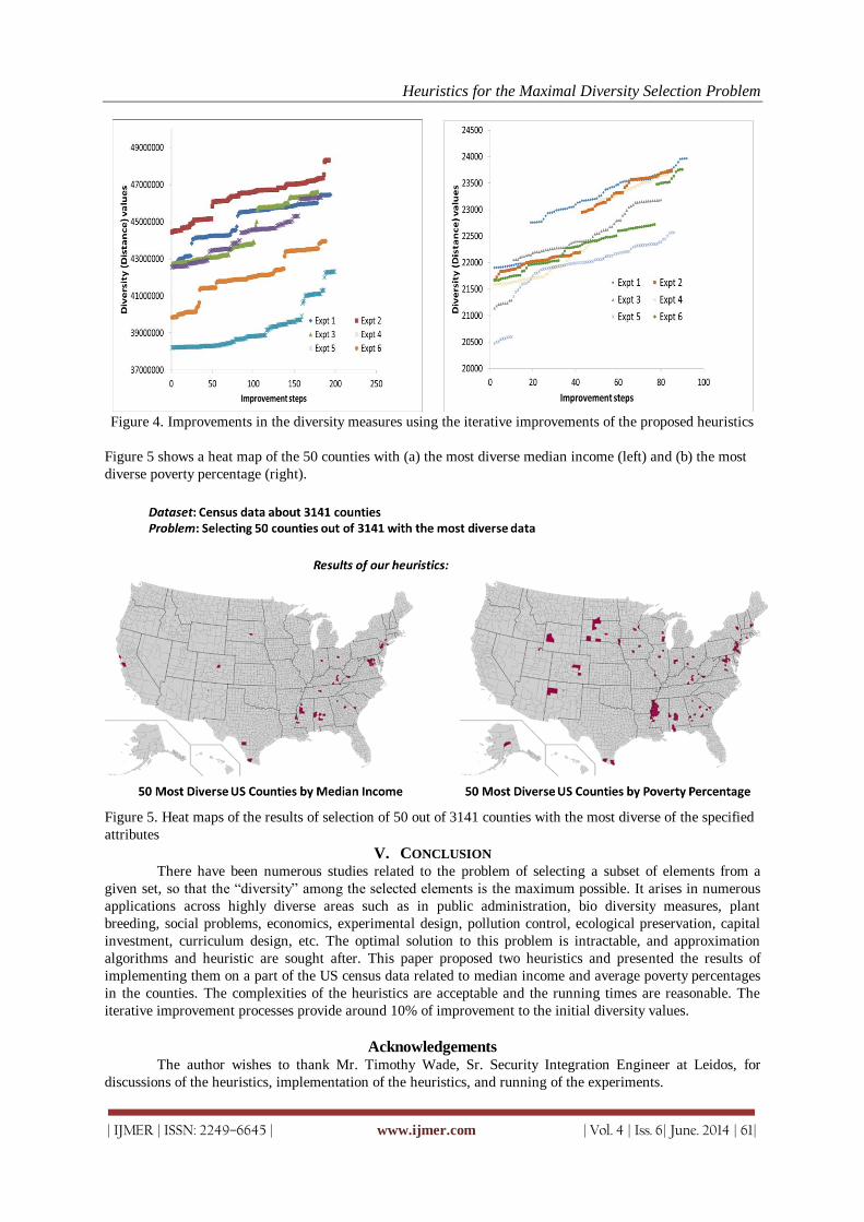
Heuristics for the Maximal Diversity Selection Problem
| IJMER | ISSN: 2249–6645 | www.ijmer.com | Vol. 4 | Iss. 6| June. 2014 | 61|
Figure 4. Improvements in the diversity measures using the iterative improvements of the proposed heuristics
Figure 5 shows a heat map of the 50 counties with (a) the most diverse median income (left) and (b) the most
diverse poverty percentage (right).
Figure 5. Heat maps of the results of selection of 50 out of 3141 counties with the most diverse of the specified
attributes
V. CONCLUSION There have been numerous studies related to the problem of selecting a subset of elements from a
given set, so that the “diversity” among the selected elements is the maximum possible. It arises in numerous
applications across highly diverse areas such as in public administration, bio diversity measures, plant
breeding, social problems, economics, experimental design, pollution control, ecological preservation, capital
investment, curriculum design, etc. The optimal solution to this problem is intractable, and approximation
algorithms and heuristic are sought after. This paper proposed two heuristics and presented the results of
implementing them on a part of the US census data related to median income and average poverty percentages
in the counties. The complexities of the heuristics are acceptable and the running times are reasonable. The
iterative improvement processes provide around 10% of improvement to the initial diversity values.
Acknowledgements The author wishes to thank Mr. Timothy Wade, Sr. Security Integration Engineer at Leidos, for
discussions of the heuristics, implementation of the heuristics, and running of the experiments.

Heuristics for the Maximal Diversity Selection Problem
| IJMER | ISSN: 2249–6645 | www.ijmer.com | Vol. 4 | Iss. 6| June. 2014 | 62|
REFERENCES
[1] M.R. Garey and D.S. Johnson, Computers and Intractability: A Guide to the Theory of NP–Completeness, W.H.
Freeman, 1979.
[2] F. Glover, G. Hersh, and C. McMillan, Selecting Subsets of Maximum Diversity, MS/IS Report No. 77–9,
University of Colorado–Boulder, 1977.
[3] C-C. Kuo, F. Glover, and K.S. Dhir, Analyzing and Modeling the Maximum Diversity Problem by Zero-One
Programming, Decision Sciences, Vol. 24, No. 6, (1993), 1171–1185.
[4] R. Weitz and S. Lakshminarayanan, An Empirical Comparison of Heuristic Methods for Creating Maximal
Diversity Groups, J. Operational Research Society, Vol. 49 (1998), 635–646.
[5] T.A. Feo and M.G.C. Resende, Greedy Randomized Adaptive Search Procedures, J. Global Optimization, Vol. 6,
(1995), 109–133.
[6] P. M. D. Andrade, A. Plastino, L. S. Ochi, and S. L. Martins, GRASP for the Maximum Diversity Problem,
Proceedings of the Fifth Metaheuristics International Conference, 2003.
[7] J.B. Ghosh, Computational aspects of the maximum diversity problem, Operations Research Letters archive, Vol.
19, Issue 4, October, 1996, 175–181.
[8] G. C. Silva, L. S. Ochi, and S. L. Martins. Experimental Comparison of Greedy Randomized Adaptive Search
Procedures for the Maximum Diversity Problem, Lectures Notes on Computer Science, Vol. 3059, Springer, 2004,
498–512.
[9] A. Duarte and R. Martí, Tabu Search and GRASP for the Maximum Diversity Problem, European Journal of
Operational Research, 178, (2007), 71–84.
[10] R. Warren, Designing Maximally, or Otherwise, Diverse Teams: Group-Diversity Indexes for Testing
Computational Models of Cultural and Other Social-Group Dynamics, Association for the Advancement of
Artificial Intelligence, 2009, 78–85.
[11] U. W. Thonemann and M. L. Brandeau, Optimal commonality in component design, Operations Research, Vol. 48,
(2000), 1–19.
[12] O. Brient and E. Naddef, The Optimal Diversity Management Problem, Operations Research, Vol. 52, No. 4, July–
August 2004, 515–526.
[13] J. Bhadury, E. Joy Mighty, and H. Damar, Maximizing Workforce Diversity in Project Teams: a Network Flow
Approach, Omega, Vol. 28 (2000), 143–153.
[14] M. Prais and C.C. Ribeiro, Reactive GRASP: an application to a matrix decomposition problem in TDMA traffic
assignment, INFORMS Journal on Computing, Vol. 12 (2000), 164–176.
[15] R. Marti, et. al., Heuristics and Metaheuristics for the Maximum Diversity Problem, Journal of Heuristics, Vol. 19,
Issue 4, (August 2013), 591–615.
[16] E. Erkut and S. Neuman, Comparison of four models for dispersing facilities, Canadian Journal of Operational
Research and Information Processing 29 (1991), 68–86.
[17] D. Pearce, Economics and genetic diversity”. Future 19(6), (1987) 710–712.
[18] M. Gallego, A. Duarte, M. Laguna, and R. Martí, Hybrid Heuristics for the Maximum Diversity Problem,
Computational Optimization and Applications, vol. 44, Springer (2009), 411–426.
[19] E. Minack, W. Siberski, and W. Nejdl, Incremental Diversification for Very Large Sets: a Streaming-based
Approach, SIGIR‟11, July 24–28, 2011, Beijing, China, 585–594.
[20] Y. Yue and T. Joachims, Predicting Diverse Subsets Using Structural SVMs, Proceedings of the 25th International
Conference on Machine Learning, Helsinki, Finland, 2008.
[21] H. Zhu, J. Klug-McLeod, and G. A. Bakken, A Heuristic Algorithm for Plate Selection That Maximizes Compound
Diversity, Croat. Chem. Acta 86 (4) (2013) 435–441.
[22] A. Zadorojniya, et.al., Algorithms for Finding Maximum Diversity of Design Variables in Multi-Objective
Optimization, Procedia Computer Science 8 (2012) 171–176.
[23] M. L. Weitzman, The Noah's Ark Problem, Econometrica, Vol. 66, No. 6 (Nov. 1998), 1279–1298.
[24] K. Hartmann and M. Steel, Maximizing Phylogenetic Diversity in Biodiversity Conservation: Greedy Solutions to
the Noah‟s Ark Problem, Systematic Biology 55(4), 2006, 644–651.
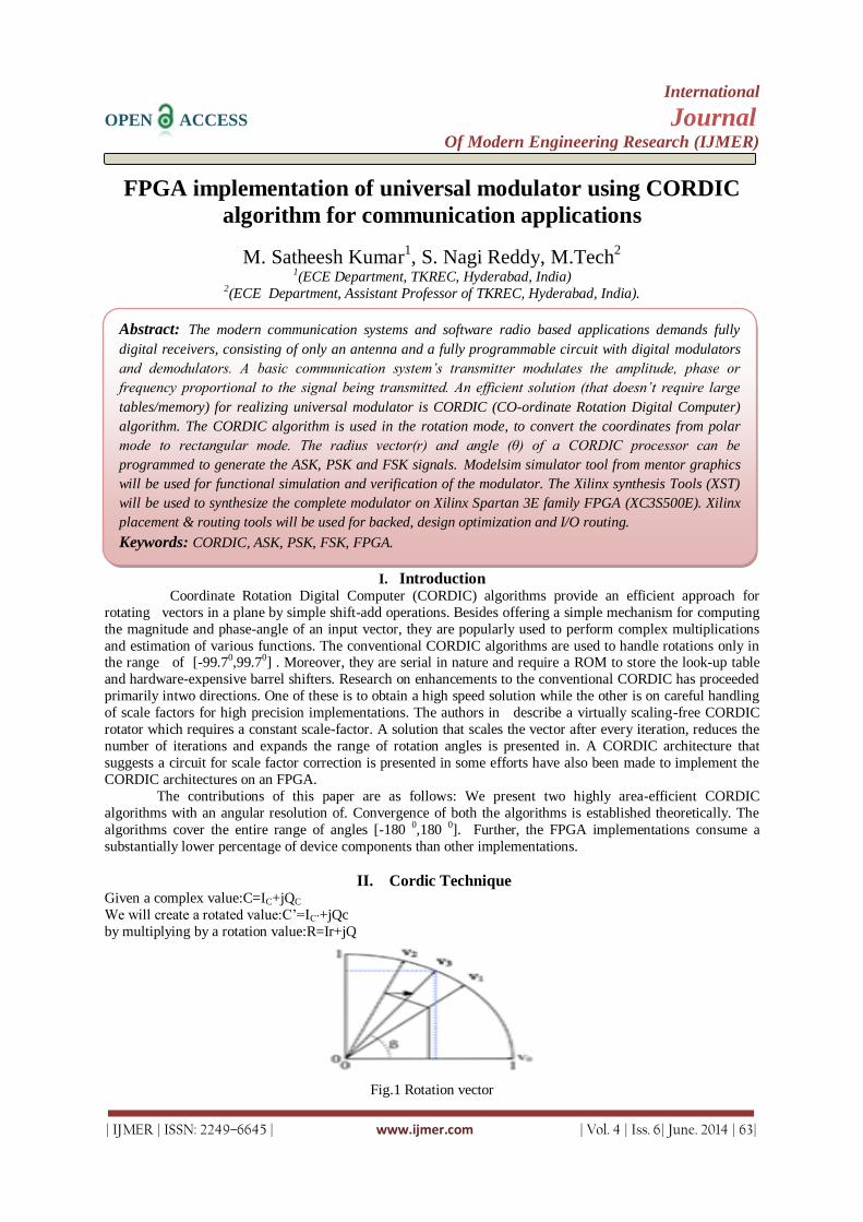
International
OPEN ACCESS Journal Of Modern Engineering Research (IJMER)
| IJMER | ISSN: 2249–6645 | www.ijmer.com | Vol. 4 | Iss. 6| June. 2014 | 63|
FPGA implementation of universal modulator using CORDIC
algorithm for communication applications
M. Satheesh Kumar1, S. Nagi Reddy, M.Tech
2
1(ECE Department, TKREC, Hyderabad, India) 2(ECE Department, Assistant Professor of TKREC, Hyderabad, India).
I. Introduction
Coordinate Rotation Digital Computer (CORDIC) algorithms provide an efficient approach for
rotating vectors in a plane by simple shift-add operations. Besides offering a simple mechanism for computing
the magnitude and phase-angle of an input vector, they are popularly used to perform complex multiplications
and estimation of various functions. The conventional CORDIC algorithms are used to handle rotations only in the range of [-99.70,99.70] . Moreover, they are serial in nature and require a ROM to store the look-up table
and hardware-expensive barrel shifters. Research on enhancements to the conventional CORDIC has proceeded
primarily intwo directions. One of these is to obtain a high speed solution while the other is on careful handling
of scale factors for high precision implementations. The authors in describe a virtually scaling-free CORDIC
rotator which requires a constant scale-factor. A solution that scales the vector after every iteration, reduces the
number of iterations and expands the range of rotation angles is presented in. A CORDIC architecture that
suggests a circuit for scale factor correction is presented in some efforts have also been made to implement the
CORDIC architectures on an FPGA.
The contributions of this paper are as follows: We present two highly area-efficient CORDIC
algorithms with an angular resolution of. Convergence of both the algorithms is established theoretically. The
algorithms cover the entire range of angles [-180 0,180
0]. Further, the FPGA implementations consume a
substantially lower percentage of device components than other implementations.
II. Cordic Technique
Given a complex value:C=IC+jQC
We will create a rotated value:C’=IC’+jQc
by multiplying by a rotation value:R=Ir+jQ
Fig.1 Rotation vector
Abstract: The modern communication systems and software radio based applications demands fully
digital receivers, consisting of only an antenna and a fully programmable circuit with digital modulators
and demodulators. A basic communication system’s transmitter modulates the amplitude, phase or
frequency proportional to the signal being transmitted. An efficient solution (that doesn’t require large
tables/memory) for realizing universal modulator is CORDIC (CO-ordinate Rotation Digital Computer)
algorithm. The CORDIC algorithm is used in the rotation mode, to convert the coordinates from polar
mode to rectangular mode. The radius vector(r) and angle (θ) of a CORDIC processor can be
programmed to generate the ASK, PSK and FSK signals. Modelsim simulator tool from mentor graphics
will be used for functional simulation and verification of the modulator. The Xilinx synthesis Tools (XST)
will be used to synthesize the complete modulator on Xilinx Spartan 3E family FPGA (XC3S500E). Xilinx
placement & routing tools will be used for backed, design optimization and I/O routing.
Keywords: CORDIC, ASK, PSK, FSK, FPGA.

FPGA implementation of universal modulator using CORDIC algorithm for communication
| IJMER | ISSN: 2249–6645 | www.ijmer.com | Vol. 4 | Iss. 6| June. 2014 | 64|
How multiplier less:
1. Recall that when you multiply a pair of complex numbers, their phases (angles) add and their magnitudes multiply. Similarly, when you multiply one complex number by the conjugate of the other, the phase of the
conjugated one is subtracted (though the magnitudes still multiply).
Therefore:
To add R’s phase to C: To subtract phase from C:
C' = C·R
Ic' = Ic·Ir-Qc·Qr
Qc' = Qc·Ir+Ic·Qr
2. To rotate by +90 degrees, multiply by R = 0 + j1. Similarly, to rotate by -90 degrees, multiply by R = 0 - j1.
If you go through the Algebra above, the net effect is:
To add 90 degrees Multiply by R=0+j1 To Subtract 90 degrees multiply by R=0-j1
3. To rotate by phases of less than 90 degrees, we will be multiplying by numbers of the form "R = 1 +/- jK". K
will be decreasing powers of two, starting with 2^0 = 1.0. Therefore, K = 1.0, 0.5, 0.25, etc. (We use the symbol
"L" to designate the power of two itself: 0, -1,-2,etc.) Since the phase of a complex number "I + jQ" isatan(Q/I),
the phase of "1 + jK" is atan(K). Likewise, the phase of "1 - jK" = atan(-K) = -atan(K).To add phases we use
"R = 1 + jK"; to subtract phases we use "R = 1 - jK". Since the real part of this, Ir, is equal to 1, we can simplify
our table of equations to add and subtract phases for the special case of CORDIC multiplications to:
To add a phaseMultiply by R=1+Jk To add a phaseMultiply by R=1+Jk
Table1 Table1. For an accumulator of 3 bits (j=3) controlled with an input of P = 3 and P =2
4. Each rotation has a magnitude greater than 1.0. That isn't desirable, but it's the price we pay for using
rotations of the form "1 + jK". The "CORDIC Gain" column in the table is simply a "cumulative magnitude"
calculated by multiplying the current magnitude by the previous magnitude. Notice that it converges to about
1.647; however, the actual CORDIC Gain depends on how many iterations we do. (It doesn't depend on whether
we add or subtract phases, because the magnitudes multiply either way).
C' = C·R*
Ic' = Ic·Ir+Qc·Qr
Qc' = Qc·Ir-Ic·Qr
IC’ = QC
QC’ =-IC
(negate I, then swap) IC’ = -QC
QC’ =IC
(negate Q,then swap)
Ic'=Ic+K·Qc=Ic + (2^-L)·Qc
Qc'=Qc-K·Ic = Qc- (2^-L)·Ic
Ic' = Ic-K·Qc =Ic(2^L)·Qc
Qc'=Qc+K·Ic=Qc+(2^-L)·Ic
L K=2^-L R=1+jK Phase of R in
degrees=atan(k)
Magnitude of R CORDIC Gain
0
1.0 1 + j1.0 45.00000 1.41421356 1.414213562
1 0.5 1+j0.5 26.56505 1.11803399 1.581138830
2 0.25 1 + j0.25 14.03624 1.03077641 1.629800601
3 0.125 1 + j0.125 7.12502 1.00778222 1.642484066
4 0.625 1 + j0.0625 3.57633 1.00195122 1.645688916
5 0.03125 1 + j0.031250 1.78991 1.00048816 1.646492279
6 0.015625 1 + j0.015625 0.89517 1.00012206 1.646693254
7 0.007813 1 + j0.007813 0.44761 1.00003052 1.646743507
….. ………. ………….. ……………... ……………… ………………..

FPGA implementation of universal modulator using CORDIC algorithm for communication
| IJMER | ISSN: 2249–6645 | www.ijmer.com | Vol. 4 | Iss. 6| June. 2014 | 65|
III. Cordic Basic Issues
Since we're using powers of two for the K values, we can just shift and add our binary numbers. That's
why the CORDIC algorithm doesn't need any multiplies.
The sum of the phases in the table up to L = 3 exceeds 92 degrees, so we can rotate a complex number by
+/- 90 degrees as long as we do four or more "R = 1 +/- jK" rotations. Put that together with the ability to
rotate +/-90 degrees using "R = 0 +/- j1", and you can rotate a full +/-180 degrees.
You can see that starting with a phase of 45 degrees, the phase of each successive R multiplier is a little
over half of the phase of the previous R. That's the key to understanding CORDIC: we will be doing a
"binary search" on phase by adding or subtracting successively smaller phases to reach some "target"
phase.
Each rotation has a magnitude greater than 1.0. That isn't desirable, but it's the price we pay for using rotations of the form "1 + jK". The "CORDIC Gain" column in the table is simply a "cumulative
magnitude" calculated by multiplying the current magnitude by the previous magnitude. Notice that it
converges to about 1.647; however, the actual CORDIC Gain depends on how many iterations we do. (It
doesn't depend on whether we add or subtract phases, because the magnitudes multiply either way.)
Modes of operation:
Basic mode: I and Q carrier signals for a chosen freq value
Modulator mode: producing ASK, FSK and PSK signals.
11-bit Control word format
M M F F F F F F F K K
MM --- Mode of operation 00 – Basic mode 01 – Binary Modulator mode 10 – Mary modulator mode
FFFFFFF – 7-bit Freq word KK (in Binary modulation mode) 00 – Amplitude shift keying 01 –Phase shift
keying 10 – Freq shift keying KK(in M-ary modulation mode) 00 – 4 level QAM 01 – QPSK 10– OQPSK
11-8psk.
IV. Block Diagram of Cordic Based Universal Modulator Realization
Fig.2 block diagram of CORDIC

FPGA implementation of universal modulator using CORDIC algorithm for communication
| IJMER | ISSN: 2249–6645 | www.ijmer.com | Vol. 4 | Iss. 6| June. 2014 | 66|
IV (i) Basic Blocks of Universal Modulator
All the blocks are connected with common clock and reset signals. The delta phase value decides the
phase increment for each clock pulse. Hence decides the resulting signal frequency. The Frequency modulating instantaneous value is added to the delta phase value which causes instant-aneous change in frequency. Due to
the digital nature of the modulator only at each clock tick the modulating signal value shall affect the resulting
frequency.The outputs of the Look Up Tables are given to the input lines a 4 to 1 Multiplexer.This multiplexer
connects one of the inputs to the output depending on the select lines. The output of Multiplexer consists the 8
amplitude bits which is the final output in case required modulation schemes are FM or PM. In case of
Amplitude modulation, the output of multiplexer is multiplied with instaneous modulating signals. CORDIC
engine isused for phase to amplitude conversion required for the generation of cosine and sin functions.
In three modulation schemes if modulating signal is analog in nature then anappropriate Analog
toDigital converter is required to convert into 8 bitdigital output. From the figure the basic blocks in DDFS can
be identified as PIPO registers, adders, look Up Tables, CORDIC engine and other combinational circuits.
IV (ii) DDFS Basic Principle: Direct Digital Frequency Synthesizer is a technique to produce desired output wave-forms with full
digital control. Direct digital synthesis (DDS) is becoming increasingly popular as a technique for fre-quency
synthesis, especially if high frequency resolution and fast switching between frequencies over a large bandwidth
are required.
The direct digital frequency synthesizer is shown in a simplified form in figure 4. The DDFS has the following
basic blocks:
(1) Frequency register
(2) adder and phase register
(3) phase to amplitude converter (conventionally a sine ROM)
(4) digital to analog converter and low pass filter
The phase value is generated using the modulo 2j overflowing property of a j-bit phase accumulator. The rate of the overflows is the output frequency
𝑓𝑜𝑢𝑡 =∆𝑃 𝑓𝑐𝑙𝑘
2𝑗 ∀ 𝑓𝑐𝑙𝑘 ≤
𝑓𝑐𝑙𝑘
2 -- (1.1)
Where ∆P is the phase increment word, j is the number of phase accumulator bits, fclkis the clock frequency and foutis the output frequency. The constraint for maximum value of fout in the above equation comes from the
sampling theorem.
The phase increment word in (1.1) is an integer, therefore the frequency resolution is found by setting ∆P = 1.
∆ 𝑓 = (𝑓𝑐𝑙𝑘 )/2𝑗 --- (1.2)
Fig.3: block diagram of DDFS
In the ideal case with no phase and amplitude quantization, the output sequence of the table is given by
sin(2π𝑃(𝑛)
2𝑗)--- --(1.3)
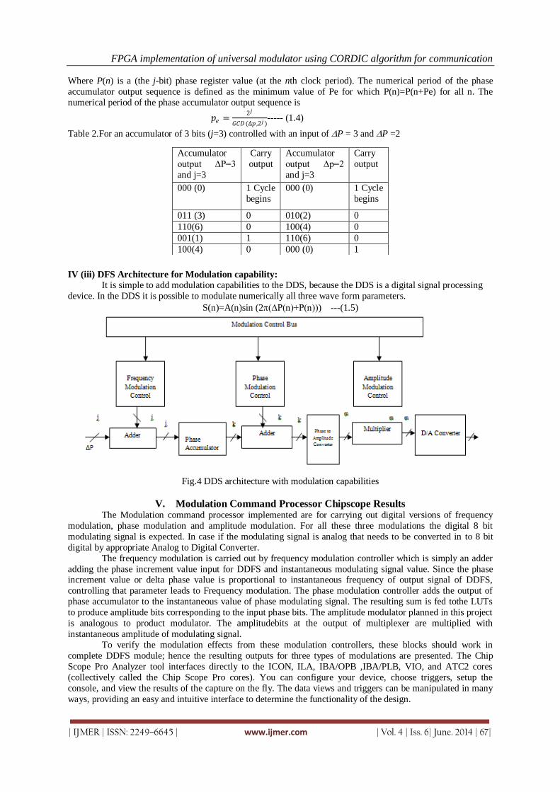
FPGA implementation of universal modulator using CORDIC algorithm for communication
| IJMER | ISSN: 2249–6645 | www.ijmer.com | Vol. 4 | Iss. 6| June. 2014 | 67|
Where P(n) is a (the j-bit) phase register value (at the nth clock period). The numerical period of the phase
accumulator output sequence is defined as the minimum value of Pe for which P(n)=P(n+Pe) for all n. The
numerical period of the phase accumulator output sequence is
𝑝𝑒 =2𝑗
𝐺𝐶𝐷 (∆𝑝 ,2𝑗 )----- (1.4)
Table 2.For an accumulator of 3 bits (j=3) controlled with an input of P = 3 and P =2
IV (iii) DFS Architecture for Modulation capability:
It is simple to add modulation capabilities to the DDS, because the DDS is a digital signal processing
device. In the DDS it is possible to modulate numerically all three wave form parameters.
S(n)=A(n)sin (2(∆P(n)+P(n))) ---(1.5)
Fig.4 DDS architecture with modulation capabilities
V. Modulation Command Processor Chipscope Results
The Modulation command processor implemented are for carrying out digital versions of frequency
modulation, phase modulation and amplitude modulation. For all these three modulations the digital 8 bit
modulating signal is expected. In case if the modulating signal is analog that needs to be converted in to 8 bit
digital by appropriate Analog to Digital Converter.
The frequency modulation is carried out by frequency modulation controller which is simply an adder
adding the phase increment value input for DDFS and instantaneous modulating signal value. Since the phase increment value or delta phase value is proportional to instantaneous frequency of output signal of DDFS,
controlling that parameter leads to Frequency modulation. The phase modulation controller adds the output of
phase accumulator to the instantaneous value of phase modulating signal. The resulting sum is fed tothe LUTs
to produce amplitude bits corresponding to the input phase bits. The amplitude modulator planned in this project
is analogous to product modulator. The amplitudebits at the output of multiplexer are multiplied with
instantaneous amplitude of modulating signal.
To verify the modulation effects from these modulation controllers, these blocks should work in
complete DDFS module; hence the resulting outputs for three types of modulations are presented. The Chip
Scope Pro Analyzer tool interfaces directly to the ICON, ILA, IBA/OPB ,IBA/PLB, VIO, and ATC2 cores
(collectively called the Chip Scope Pro cores). You can configure your device, choose triggers, setup the
console, and view the results of the capture on the fly. The data views and triggers can be manipulated in many
ways, providing an easy and intuitive interface to determine the functionality of the design.
Accumulator
output ∆P=3
and j=3
Carry
output
Accumulator
output ∆p=2
and j=3
Carry
output
000 (0) 1 Cycle
begins
000 (0) 1 Cycle
begins
011 (3) 0 010(2) 0
110(6) 0 100(4) 0
001(1) 1 110(6) 0
100(4) 0 000 (0) 1

FPGA implementation of universal modulator using CORDIC algorithm for communication
| IJMER | ISSN: 2249–6645 | www.ijmer.com | Vol. 4 | Iss. 6| June. 2014 | 68|
The waveforms obtained by the Chip Scope Pro Analyzer are shown in the figures
Put the slide switches in 0100 position (MM=01 and KK=00) to get ASK
Modulating signal (1 bit data) Fig: 5 ASK CHIPSCOPE RESULT
Put the slide switches in 0101 position (MM=01 and KK=01) to get PSK
Modulating signal (1 bit data) Fig: 6 PSK CHIPSCOPE RESULT

FPGA implementation of universal modulator using CORDIC algorithm for communication
| IJMER | ISSN: 2249–6645 | www.ijmer.com | Vol. 4 | Iss. 6| June. 2014 | 69|
Put the slide switches in 0110 position (MM=01 and KK=10) to get FSK
Modulating signal (1 bit data ) Fig: 7 FSK CHIPSCOPE RESULT
Put the slide switches in 1001 position (MM=10 and KK=01) to get QPSK (change the samples size to 2048)
Modulating signal (1 bit data ) Fig: 8 QPSK CHIPSCOPE RESULT
VI. Applications
Universal modulator is highly preferred option in instrumentation for signal generation and frequency
sweep etc.
Universal modulator can be efficiently used in several digital modulation schemes suchas FSK, PSK,
ASK, QPSK, OPQPSK, PI/QPSK, QAM and 8-bitPSK.
Universal modulator has been used in universal HAM radio/generator. Universal modulator is capable
of well controlled, rapid changes in frequency.
ADVANTAGE AND DISADVANTAGES
High frequency resolution and accuracy.
Fast switching between frequencies over a large bandwidth.
Compared to LUT method, it takes less area.
FPGA hardware can give high speed solution in comparison with software approach but not in
comparison with ASIC.

FPGA implementation of universal modulator using CORDIC algorithm for communication
| IJMER | ISSN: 2249–6645 | www.ijmer.com | Vol. 4 | Iss. 6| June. 2014 | 70|
TOOLS AND HARD WARE
Simulation software -Modelsim Xilinx Edition (MXE)
Synthesis, P&R - Xilinx ISE
On chip verification - Xilinx Chip scope
Hardware– Xilinx Spartan 3 Family FPGA board
VII. FPGA Design and Programming
To define the behavior of the FPGA, the user provides a hardware description language (HDL) or
a schematic design. The HDL form is more suited to work with large structures because it's possible to just
specify them numerically rather than having to draw every piece by hand. However, schematic entry can allow
for easier visualization of a design.Once the design and validation process is complete, the binary file generated (also using the FPGA company's proprietary software) is used to (re)configure the FPGA.
VIII. Conclusion
Our CORDIC Algorithm implementation has efficient area utilization as compared to LUT based
methods. But, it is slower than LUT based implementation.FPGA based DDFS is highly useful in semi-custom
VLSI chips, FPGA based VLSI solutions, signal processing cards, Instrumentation and Digital communications.
The present work shows basic DDFS implementation proving the design by synthesis on FPGA. The timing
analysis shows that high values of output frequencies can be achieved with FPGA based design. If higher end
FPGAs is used then very high bandwidth DDFS can be implemented efficiently. CORDIC Algorithm is
successfully implemented in VHDL, which helped to generate ASK, PSK, FSK&QAM signals. Utilizing 378flip flops/latches,432 four input LUTs,17 Bonded IOBs ,94 Shift registers ,17 Block RAMs,2 MUXS in
resource of XC3S500E320. Our project on CORDIC algorithm works with frequency 25.475MHz.it is
minimum input arrival time before clock 4.808ns, maximum output required time after clock 14.719ns and
maximum combinational path delay 1.975ns with minimum power dissipation of 87.66 mWatts.
.REFERENCES
[1.] J. Volder, The CORDIC trigonometric computing technique, IRE Transactions on
[2.] Electronic Computers, Vol. EC-8, 1959, pp. 330-334.
[3.] J.S. Walther, A unified algorithm for elementary functions, Proceedings of 38th Spring Joint Computer
Conference, 1971,pp. 379-385.
[4.] A Novel CRODIC Based Unified Architecture for DCT and IDCT international conference paper 2012.
[5.] A VLSI Implementation of Logarithmic and Exponential Functons Using a Novel Parabolic synthesis
methodology Compared To The CORDIC Algorithm Conference Paper 2011.
[6.] R. Andraka, A survey of CORDIC algorithms for FPGA-based computers, Proceedings of ACM/SIGDA Sixth
International Symposium on Field Programmable Gate Arrays, 1998, pp.191-200.
[7.] Efficient CORDIC Algorithms and Architectures for Low Area and High Throughput Implementation IEEE
paper2009.
[8.] A VLSI Implementation of Logarithmic and Exponential Functions Using a Novel Parboil Synthesis Methodology Compared to the CORDIC Algorithms IEEE paper2011.
[9.] M.G.B. Sumumanasena, ”Ascale factor correction scheme for the CORDIC Algorithm,”IEEE paoer 2008.
[10.] A direct digital frequency synthesis system for Low Power Communications by Alistair Mcewen,sunay shah and
steve Collin, department of engineering science University Of Oxford Parks Road Oxford UK.

FPGA implementation of universal modulator using CORDIC algorithm for communication
| IJMER | ISSN: 2249–6645 | www.ijmer.com | Vol. 4 | Iss. 6| June. 2014 | 71|
M.SATHEESH KUMAR S. NAGI REDDY, M. Tech
Dept of ECE, TKREC, Hyderabad Asst.Prof & in charge polytechnic
College, TKREC,Hyderabad.

Contents :
Performance and Analysis of OFDM Signal Using Matlab Simulink 01-07Anil Kumar, Ankit Mayur, Arvind Kr. Jaiswal
Experimental Investigation on Heat Transfer Analysis in a Cross flow Heat Exchanger with 08-14Waved Baffle Plates by using FLOEFDV. Chandrikha, D. Santha Rao, P. Sriivasa Rao
Electric Load Forecasting Using Genetic Algorithm – A Review 15-20Arun Kumar Gangwar , Farheen Chishti
MIMO System Performance Evaluation for High Data Rate Wireless Networks using 21-27Space Time Block Codes with Orthogonal StructureSandeep Narain, Dr. Syed Hasan Saeed
Analysis of Admixtures and Their Effects of Silica Fumes, Metakaolin and PFA on the 28-36Air ContentT. Subramani, T. Senthilkumar, J. Jayalakshmi
Ultra-Wide Bandpass filter using isosceles triangular microstrip patch resonator 37-41Rahul Kumar Shishodia, Sarvodaya Tyagi, Sawan Kumar, Pradeep Kumar
GIS based Road Network Assessment using Open source Technology 42-45Paru Thakkar, Krunal Patel, Movva Lakshmi Mounica
Vibration control of newly designed Tool and Tool-Holder for internal treading of 46-57Hydraulic Steering Gear NutD. R Kotkar, Wakchaure V. D
Suitability of Composite Material for Flywheel Analysis 58-61Nagaraj.r.m
Synthesis and characterization of Cu doped NiO nanoparticles 62-66B. Ramasubba Reddy, G. S. Harish, Ch. Seshendra Reddy, P. Sreedhara Reddy
Volume : 4 Issue : 6 (Version-4) June - 2014ISSN : 2249-6645
International Journal of Modern Engineering Research
(IJMER)

International
OPEN ACCESS Journal Of Modern Engineering Research (IJMER)
| IJMER | ISSN: 2249–6645 | www.ijmer.com | Vol. 4 | Iss. 6| June. 2014 | 1|
Performance and Analysis of OFDM Signal Using Matlab
Simulink
Anil Kumar1, Ankit Mayur
2, Arvind Kr. Jaiswal
3
1, 2 3(Faculty ECE, PG student, H.O.D, ECE Department, SHIATS-DU Allahabad India 211007)
I. INTRODUCTION Orthogonal frequency division multiplexing (OFDM) has been recently seen rising popularity in
wireless application. OFDM properties like high spectral efficiency, robustness to channel fading, immunity to impulse interference, uniform average spectral density, and capacity to handle very strong echoes and less non-
linear distortion, immunity to inter-symbol interference. The main disadvantages of OFDM systems is that it
exhibits a high peak to average power ratio, namely the peak value of some of the transmitted signal could be
much larger than the typical values. To reduce PAPR, many techniques have been proposed, such as clipping,
partial time sequence, interleaving, nonlinear companding transforms, hadamard transforms, SLM technique etc.
The selected mapping method (SLM) provides good performance for PAPR reduction, and this requirement
usually results in high computational complexity. Several techniques have been proposed based on low-
complexity selected mapping schemes for Peak-to-Average Power Ratio reduction in OFDM Systems.
In recent years OFDM is employed in Digital Television Broadcasting (such as the digital ATV
Terrestrial Broadcasting), European Digital Audio Broadcasting (DAB) and Digital Video Broadcasting
Terrestrial (DVB-T), and numerous Wireless Local Area Networks (e.g. IEEE 802.11a operating at 5 GHz) and European Telecommunications Standard Institute (ETSI) Broadband Radio Access Networks (BRAN)’s High
Performance Radio Local Area Network (HIPERLAN) Type-2 standard.
The organization of this paper is as follows. Section II presents OFDM signal model and formulae,
Section III presents the problem of PAPR and algorithm of least PAPR. Section IV presents the figure and table
of simulation results. Section V presents conclusion of simulation results.
II. ORTHOGONAL FREQUENCY DIVISION MULTIPLEXING (OFDM) Orthogonal Frequency Division Multiplexing is a frequency–division multiplexing (FDM) scheme
utilized as a digital multi–carrier modulation method. A large number of closely spaced orthogonal sub–carriers is used to carry data. The data is divided into several parallel streams of channels, one for each sub–carriers.
Each sub– carrier is modulated with a conventional modulation scheme (i.e. QPSK) at a low symbol rate,
maintaining total data rates similar to the conventional single carrier modulation schemes in the same
bandwidth. Orthogonal Frequency Division Multiplexing is a special form of multicarrier modulation which is
particularly suited for transmission over a dispersive channel. Here the different carriers are orthogonal to each
other that is they are totally independent of one another. This is achieved by placing the carrier exactly at null in
modulation spectra of each other.
Two periodic signals are orthogonal when the integral of their product over one period is equal to zero.
For the case of continuous time:
𝑐𝑜𝑠𝑇
𝑂(2πnf0t) cos (2πmf0t) dt = 0 (1)
For the case of discrete time:
𝑐𝑜𝑠𝑁−1𝐾=0
2𝜋𝑘𝑛
𝑁 cos
2𝜋𝑘𝑚
𝑁 dt = 0 (2)
Where, m ≠ n in both cases.
Abstract: Multi-carrier modulation is an attractive technique for fourth generation .OFDM is based on
multicarrier modulation technique. In OFDM system the bit stream is divided into many different sub
channels. An efficient and distortionless scheme for peak power reduction in OFDM is proposed. In this
paper, a set of mapping where the actual transmit signal is selected. From this set of signal reduced
PAPR. Simulation results are shown. The lowest PAPR is compared with conventional work. It is also
compared BER to SNR and best result is achieved.
Keywords: BER, IFFT, OFDM, PAPR, Phase Rotation, QAM, QPSK, SLM etc.

Performance and Analysis of OFDM Signal Using Matlab Simulink
| IJMER | ISSN: 2249–6645 | www.ijmer.com | Vol. 4 | Iss. 6| June. 2014 | 2|
Fig. 1: The area under a sine and a cosine wave over one period is always zero.
Fig 2: The area under a sine wave multiplied by its own harmonic is always zero.
The main concept in OFDM is orthogonality of the sub-carriers. Since the carriers are all sine/cosine wave, we
know that area under one time period of a sine or a cosine wave is zero.
Let's take a sine wave of frequency m and multiply it by a sinusoid (sine or a cosine) of a frequency n, where both m and n are integers. The integral or the area under this product is given by
F (t) = sin (mwt)* sin (nwt) (3)
By the simple trigonometric relationship, this is equal to a sum of two cosine of frequencies (m-n) and (m+n).
= 1
2cos 𝑚 − 𝑛 −
1
2 cos(𝑚 + 𝑛)
= 1
2cos 𝑚 − 𝑛 𝑤𝑡 −
2∏
0
1
2cos 𝑚 + 𝑛 𝑤𝑡
2∏
0
= 0 - 0
= 0
These two components are each a sinusoid/cosine, so the integral is equal to zero over one period.
Fig.3: OFDM Transmitter System
In figure 3, IFFT is performed on the modulated signal which is further processed by passing through a
parallel– to–serial converter. In order to avoid ISI we provide a cyclic prefix to the signal. The Cyclic Prefix or
Guard Interval is a periodic extension of the last part of an OFDM symbol that is added to the front of the
symbol in the transmitter, and is removed at the receiver before demodulation.
The cyclic prefix has to two important benefits –
1 .The cyclic prefix acts as a guard interval. It eliminates the inter – symbol interference from the previous
symbol.
2 .It acts as a repetition of the end of the symbol thus allowing the linear convolution of a frequency –selective
multipath channel to be modeled as circular convolution which in turn may be transform to the frequency
domain using a discrete fourier transform. This approach allow a simple frequency domain processing such as
channel estimation and quality.

Performance and Analysis of OFDM Signal Using Matlab Simulink
| IJMER | ISSN: 2249–6645 | www.ijmer.com | Vol. 4 | Iss. 6| June. 2014 | 3|
the received data is first made to pass through a low pass filter and the cyclic prefix is removed. FFT of the
signal is done after it is made to pass through a serial – to – parallel converter. A demodulator is used, to get
back the original signal.
III. THE PAPR OF OFDM SYSTEM The PAPR of OFDM is defined as the ratio between the maximum power and the average power, The
PAPR of the OFDM signal X (t) is defined as
PAPR = ppeak
paverage =
𝑥(𝑡) 20≤𝑡<𝑀𝑇𝑚𝑎𝑥
1
𝑀𝑇 𝑥(𝑡) 2𝑀𝑇
0
(4)
Presence of large number of independently modulated sub-carriers in an OFDM system the peak value
of the system can be very high as compared to the average of the whole system. This ratio of the peak to average
power value is termed as Peak-to-Average Power Ratio. Coherent addition of N signals of same phase produces
a peak which is N times the average signal.
The major disadvantages of a high PAPR are-
* Increased complexity in the analog to digital and digital to analog converter.
* Reduction is efficiency of RF amplifiers.
The main objective of this technique is to generate a set of data blocks at the transmitter end which represent the original information and then to choose the most favorable block among them for transmission. Let us consider
an OFDM system with N orthogonal sub–carriers. A data block is a vector composed of N complex symbols ,
each of them representing modulation symbol transmitted over a sub–carrier. X is multiplied element by
element with U vector composed of N complex numbers, defined so that , where |.| denotes the modulus
operator. Each resulting vector which, produced after IDFT, a corresponding OFDM signal is given by
Su(t) = 1
𝑁 𝑥𝑢 ,𝑛𝑒
𝑗2𝜋𝑛∆𝑓𝑡 0 ≤ 𝑡 ≤ 𝑇𝑁−1𝑛=0
(5)
Where T is the OFDM signal duration and f = 1/T is the sub-carrier spacing. Among the modified data blocks, the one with the lowest PAPR is selected for transmission. The amount of
PAPR reduction for SLM depends on the number of phase sequences U and the design of the phase sequences. In SLM technique, firstly the input information is divided into OFDM data block X, which consists of M
symbols, by the serial-to parallel (S/P) conversion and then data block X is multiplied carrier wise with each one
of the w different phase sequences 𝐵(𝑤), resulting in a set of w different OFDM data block
𝑋(𝑤 ) = [𝑋0(𝑤),𝑋1
(𝑤 ) −− −−,𝑋𝑀−1(𝑤)]^T (6)
Where, 𝑋𝑚𝑤 =𝑋𝑚𝐵𝑚
𝑤 , m = 0, 1, · ·, M − 1, w = 1, 2, · ·, w.
𝑋𝑚𝑤 =𝑋𝑚𝐵𝑚
𝑤 (7)
𝐵𝑤 = [𝑋0(𝑤),𝑋1
(𝑤) −−− −,𝑋𝑀−1(𝑤) ]^T (8)
Then all w alternative data blocks are transformed into time domain to get transmit OFDM symbol 𝑥𝑤=IFFT
𝑋(𝑤).
The transmit sequence 𝑥 =𝑥(𝑤) , where 𝑤 = arg 𝑚𝑖𝑛𝑤 max |x (w)|, is selected. The information on the
selected phase sequence must be transmitted to the receiver. Where m = 0,1,2,3 ……….M-1 .w = 0, 1, 2 …W,
to make w phase rotated OFDM data blocks. All w phase rotated OFDM data blocks represented the same
information as the unmodified OFDM data block Provided that the phase sequence is known. After applying the
SLM technique, the complex envelope of the transmitted OFDM signal becomes
X (t) = 1
𝑀 𝑋𝑚
𝑀−1𝑚=0 𝑒𝑗2𝜋𝑡𝑓𝑚 , 0 ≤ t ≤ M T -------------5
Here, MT is the duration of an OFDM data block. Output data of the lowest PAPR is selected to transmit.
Algorithm for least PAPR:
1) Firstly 16 sinusoidal subcarriers are taken. These are available subcarriers (QPSK Modulation)
assuming all one positive.
X1 =sin ((2*180*100*t) +w)
X2 =sin ((2*180*200*t) +w)

Performance and Analysis of OFDM Signal Using Matlab Simulink
| IJMER | ISSN: 2249–6645 | www.ijmer.com | Vol. 4 | Iss. 6| June. 2014 | 4|
X3 =sin ((2*180*300*t) +w)
.
.
.
X16= sin ((2*180*1600*t) +w)
These subcarriers are orthogonal to each other because in general for all integers’ m and n, sinmx, sinny,
cosmx, cosmy are orthogonal to each other. These frequencies are called harmonics. 2) Giving these entire subcarrier phase shift(w) 0 to 90.
3) Now sum of all these entire subcarriers sum = x1+x2+x3+x4+…………+x15+x16. (9)
4) Calculate the PAPR according to the formula given in equation (6)
For comparison of BER and SNR :
1) No. of Carriers: 64
2) coding used: Convolutional coding
3) Single frame size: 96 bits
4) Total no. of Frames: 100
5) Modulation: 16-QAM 6) No. of Pilots: 4
7) Cylic Extension: 25%(16)
IV. SIMULATION RESULT Simulation is carried with MATLAB 7.8 to evaluate the performance of the different phase rotation on
OFDM Signal, for reducing PAPR, BER and SNR
Fig 4: PAPR against different phase shift
From the simulation result we see that if we give all these 16 orthogonal subcarriers with phase rotation (w) of 0 to 90 we get the minimum PAPR at phase rotation 11 as shown in figure 4.The PAPR value at 11 degree and 55
degree is 4.5292dB and 4.9379 dB respectively are least PAPR.
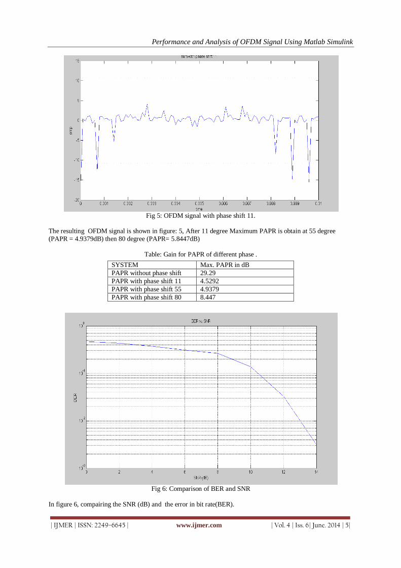
Performance and Analysis of OFDM Signal Using Matlab Simulink
| IJMER | ISSN: 2249–6645 | www.ijmer.com | Vol. 4 | Iss. 6| June. 2014 | 5|
Fig 5: OFDM signal with phase shift 11.
The resulting OFDM signal is shown in figure: 5, After 11 degree Maximum PAPR is obtain at 55 degree
(PAPR = 4.9379dB) then 80 degree (PAPR= 5.8447dB)
Table: Gain for PAPR of different phase .
Fig 6: Comparison of BER and SNR
In figure 6, compairing the SNR (dB) and the error in bit rate(BER).
SYSTEM Max. PAPR in dB
PAPR without phase shift 29.29
PAPR with phase shift 11 4.5292
PAPR with phase shift 55 4.9379
PAPR with phase shift 80 8.447

Performance and Analysis of OFDM Signal Using Matlab Simulink
| IJMER | ISSN: 2249–6645 | www.ijmer.com | Vol. 4 | Iss. 6| June. 2014 | 6|
Table SNR and BER
SNR BER
0 0.4672
2 0.4321
6 0.3231
10 0.1505
14 0.003958
From the table above, as the SNR increases the BER decreases
V. CONCLUSION
It is concluded that for improving efficiency of the Equipment (communication system) reducing
PAPR value of OFDM signal. So, in this paper we obtain a particular phase rotation value at which least PAPR
is obtain with the rising demand for more number of users on limited frequency spectrum in radio Mobile
communication, OFDM prove invaluable to fourth generation communication system and compare BER and
SNR for better future technologies and also prove invaluable to fourth generation communication system.
Acknowledgements It is our sincere obligation to thank our well-wishers Dr. Anil Kumar, faculty of Electronics and
Communication Engineering. and Dr. A. K. Jaiswal, H.O.D. ,Electronics and Communication Engineering,
SHIATS-DU, Allahabad(U.P.) India.
REFERENCES [1] R.W Chang, “Orthogonal Frequency Division Multiplexing,” U.S Patent 3388455, Jan 6, 1970, Filed Nov.4.1966. [2] L.J.Cimini, Jr, “Analysis and Simulation of a Digital Mobile Channel using OFDM”, IEEE Trans. On
Communications, vol.Com-33, no.7, pp.665-675, July 1985 [3] R.V.Paiement, “Evaluation of Single Carrier and Multicarrier Modulation Techniques for Digital ATV Terrestrial
Broadcasting CRC Rep”, Ottawa, ON, Canada, CRC-RP-004, 1994. [4] T.de. Couasnon, et al, “OFDM for Digital TV Broadcasting”, Signal Processing, vol.39, pp.1-32, 1994 [5] A. E. Jones, T. A. Wilkinson and S. K. Barton,”Block coding scheme for reduction of peak to mean envelope power
ratio of multicarrier transmission schemes,” Electronic Letters, pp. 2098-2099, Dec. 1994.
[6] “Broadband Radio Access Networks (BRAN); High Performance Radio Local Area Network (HIPERLAN) Type 2; Requirements and Architecture for Wireless Broadband Access”, TR 101 031, 1999.
[7] “Broadband Radio Access Networks (BRAN); High Performance Radio Local Area Network (HIPERLAN) Type 2; Requirements and Architecture for Wireless Broadband Access”, TR 101 031, 1999.
[8] Yang Chan Cho, Seung Hee Han, and Jae Hong Lee,” Selected Mapping Technique with Novel Phase Sequences for PAPR Reduction of an OFDM Signal,” Vehicular Technology conference,2004.VTC 2004-Fall,2004 IEEE vol. 7, pp. 4781-4787, Sep 2004.
[9] chin-liang wang, senior member, ieee, and yuan ouyang , student member, ieee “ low-complexity selected mapping schemes for peak-to-average power ratio reduction in ofdm systems ” ieee transactions on signal processing, vol. 53,
no. 12,december 2005. [10] V. Vijayarangan, DR. (MRS) R. Sukanesh, “An overview of techniques for reducing peak to average power ratio and
its selection criteria for orthogonal frequency division multiplexing radio systems”, Journal of Theoretical and Applied Information Technology, © 2005 - 2009 JATIT.
[11] Alireza Zolgha drasli, M.H. Ghamat,”Papr Reduction in OFDM System by using Hadamard Transform in BSLM Techniques” ©2007 IEEE
[12] Yang Jie, Chen Lei, Liu Quan and Chan De, .A Modified selected mapping technique to reduce the Peak to Average Power Ratio of OFDM signal. IEEE Transaction on consumer Electronics, Vol53, No.3, pp. 846-851, August 2007.
[13] N.V. Irukulapati, V.K. Chakka and A. Jain “SLM based PAPR reduction of OFDM signal using new phase sequence” ELECTRONICS LETTERS 19th November 2009 Vol. 45 No. 24.
[14] Anil Singh Rathore and Dr. Neelam Srivastava “Analysis of Selected Mapping and Partial Transmit Sequence for PAPR Reduction” Journal of Telecommunications, Volume 5, Issue 1, October 2010.
[15] S. p. vimal, K. r. Shankar kumar,” A new slm technique for papr reduction in ofdm systems”, European journal of scientific research, ISSN 1450-216x vol.65 no.2, pp. 221-230, 2011.
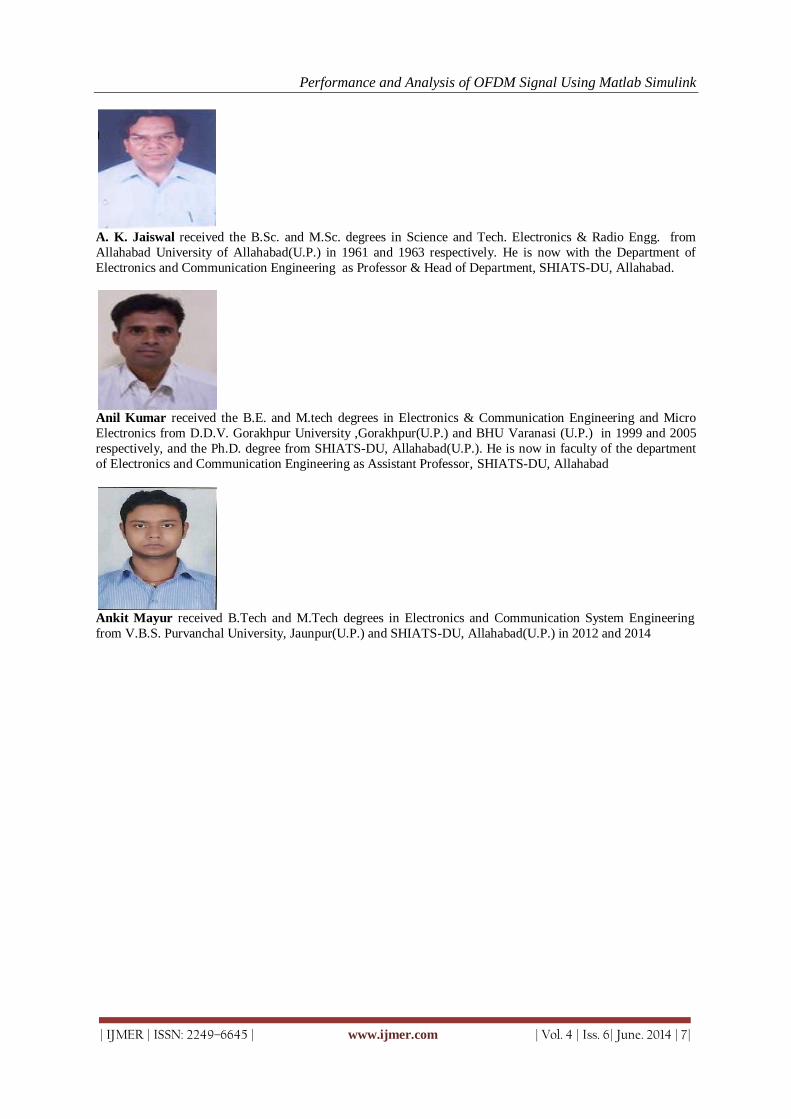
Performance and Analysis of OFDM Signal Using Matlab Simulink
| IJMER | ISSN: 2249–6645 | www.ijmer.com | Vol. 4 | Iss. 6| June. 2014 | 7|
A. K. Jaiswal received the B.Sc. and M.Sc. degrees in Science and Tech. Electronics & Radio Engg. from
Allahabad University of Allahabad(U.P.) in 1961 and 1963 respectively. He is now with the Department of
Electronics and Communication Engineering as Professor & Head of Department, SHIATS-DU, Allahabad.
Anil Kumar received the B.E. and M.tech degrees in Electronics & Communication Engineering and Micro
Electronics from D.D.V. Gorakhpur University ,Gorakhpur(U.P.) and BHU Varanasi (U.P.) in 1999 and 2005
respectively, and the Ph.D. degree from SHIATS-DU, Allahabad(U.P.). He is now in faculty of the department
of Electronics and Communication Engineering as Assistant Professor, SHIATS-DU, Allahabad
Ankit Mayur received B.Tech and M.Tech degrees in Electronics and Communication System Engineering
from V.B.S. Purvanchal University, Jaunpur(U.P.) and SHIATS-DU, Allahabad(U.P.) in 2012 and 2014

International
OPEN ACCESS Journal Of Modern Engineering Research (IJMER)
| IJMER | ISSN: 2249–6645 | www.ijmer.com | Vol. 4 | Iss. 6| June. 2014 | 8|
Experimental Investigation on Heat Transfer Analysis in a Cross
flow Heat Exchanger with Waved Baffle Plates by using FLOEFD
V. Chandrikha1, D. Santha Rao
2, P. Sriivasa Rao
3
1 (M.Tech Student, Mech. Dept. BVC Engineering College, Odalarevu) 2 (Associate Professor, Mechanical Department, BVC Engineering College, Odalarevu)
3 (Assistant Professor, Mechanical Department, Sai Spurthi Inst. of Tech, B. Gangaram)
I. Introduction
A heat exchanger is a device that is used for transfer of thermal energy between two or more fluids, between a solid surface and a fluid, or between solid particulates and a fluid, at differing temperatures and in
thermal contact, usually without external heat and work interactions. The fluids may be single compounds or
mixtures. Typical applications involve heating or cooling of a fluid stream of concern, evaporation or
condensation of a single or multi component fluid stream, and heat recovery or heat rejection from a system. In
other applications, the objective may be to sterilize, pasteurize, fractionate, distill, concentrate, crystallize, or
control process fluid. In some heat exchangers, the fluids exchanging heat are in direct contact. In other heat
exchangers, heat transfer between fluids takes place through a separating wall or into and out of a wall in a
transient manner.
In most heat exchangers, the fluids are separated by a heat transfer surface, and really they do not mix.
Such exchangers are referred to as the direct transfer type, or simply recuperate. In contrast, exchangers in
which there is an intermittent heat exchange between the hot and cold fluids via thermal energy storage and rejection through the exchanger surface or matrix are referred to as the indirect transfer type or storage type, or
simply regenerators. Such exchangers usually have leakage and fluid carryover from one stream to the other.
Many types of heat exchangers have been developed to meet the widely varying applications. Bank of tubes are
found in many industrial processes and in the nuclear industry, being the most common geometry used in heat
exchanger. The heat is transferred from the fluid inside the tubes to the flow outside them.
In the shell and tube heat exchanger, the cross flow through the banks is obtained by means of baffle
plates, responsible for changing the direction of the flow and for increasing the heat exchange time between
fluid and the heated surfaces. Numerical analysis of the laminar flow with heat transfer between parallel plates
with baffles was performed by Kelkar and Patankar [2]. Results show that the flow is characterized by strong
deformations and large recirculation regions. In general, Nusselt number and friction coefficient (FR) increase
with the Reynolds number. Measurement using LDA technique in the turbulent flow in a duct with several
baffle plates were performed by Berner et al. [3], with the purpose of determining the number of baffles
Abstract: Heat exchanger is devices used to exchange the heat between two liquids that are at different
temperature .These are used as a reheated in many industries and auto mobile sector and power
plants. The main aim of our project is thermal analysis of heat exchanger with waved baffles for
different types of materials at different mass flow rates and different tube diameters using FLOEFD software and comparing the results that are obtained. The work is a simplified model for the study of
thermal analysis of shell-and-tubes heat exchangers having water as cold and hot fluid. Shell and
Tube heat exchangers are having special importance in boilers, oil coolers, condensers, pre-heaters.
They are also widely used in process applications as well as the refrigeration and air conditioning
industry. The robustness and medium weighted shape of Shell and Tube heat exchangers make them
well suited for high pressure operations. The project shows the best material, best boundary conditions
and parameters of materials we have to use for better heat conduction. For this we are chosen a
practical problem of counter flow shell and tube heat exchanger having water, by using the data that
come from cfd analysis. A design of sample model of shell and tube heat exchanger with waved baffles
is using Pro-e and done the thermal analysis by using FLOEFD software by assigning different
materials to tubes with different diameters having different mass flow rates and comparing the result
that obtained from FLOEFD software.
Keywords: Heat Exchanger, Creo Design, Materials (Al-6061, Copper and Steel), FLOEFD Analysis,
Mass flow rates, dimensions of Materials, heat transfer rate.

Experimental Investigation on Heat Transfer Analysis in a Cross flow Heat Exchanger with Waved
| IJMER | ISSN: 2249–6645 | www.ijmer.com | Vol. 4 | Iss. 6| June. 2014 | 9|
necessary for obtaining a periodic boundary condition and the dependence on Reynolds number and the
geometry. Results showed that with a Reynolds number of 5.17×10³, four baffles are necessary for obtaining a
periodic boundary condition. By increasing the Reynolds number to 1.02×10⁴, a periodic boundary condition is obtained with three baffles. A significant amount of research has focused both on channels with internal
obstructions and tortuous channels, to determine the configurations that lead to the most vigorous mixing and
highest rate of heat transfer. Popiel and Van Der Merwe [4] and Popiel and Wojkowiak [5] who studied
experimental pressure drops for geometries with an undulating sinusoidal or U-bend configuration. In these
papers, the effects of Reynolds number, curvature, wavelength and amplitude on the friction factor were
investigated in laminar and low Reynolds number turbulent flow. An interesting observation made by these
authors is that when the friction factor is plotted against the Reynolds number, there is either no definite
transition from laminar to turbulent flow, or a delayed transition relative to that of a straight pipe. It is
hypothesized by Popiel and Van der Merwe [4] that a smooth transition to turbulence occurs due to the
secondary flows produced within the complex geometry. Dean [6] originally observed that the mixing effects of
these secondary flows are steadily replaced by the development of turbulent secondary flow. A method to study fully developed flow and heat transfer in channels with periodically varying shape was first developed by
Patankar et al. [7] for the analysis of an offset-plate fin heat exchanger.
Their method takes advantage of the repeating nature of the flow field to minimize the extent of the
computational domain. The method of Parankar et al. [7] assumes that for a periodic geometry, the flow is
periodic with a prescribed linear pressure gradient being applied to drive the flow. The outlet velocity field and
its gradient are wrapped to the inlet to produce periodic boundary conditions. Flow velocities within the
geometry are then calculated using momentum and mass conservation equations, assuming constant fluid
properties.Webb and Ramadhyani [8] and Park et al.[9] analyzed fully developed flow and heat transfer in
periodic geometries following the method of Patankar. Webb and Ramadhyani [8] studied parallel plate
channels with transverse ribs; they presented a comparison with the performance of a straight channel, and
reported an increase in both the heat transfer rate and pressure drop as the Reynolds number is increased. Park et
al. [9] incorporated optimization of the heat transfer rate and pressure drop into their study of the flow and thermal field of plate heat exchangers with staggered pin arrays. N.R. Rosaguti, D.F. Fletcher, and B.S. Haynes
[10] analyzed fully developed flow and Heat Transfer in geometries that are periodic in the flow direction. They
have studied laminar flow in serpentine duct of circular cross section with a constant heat flux applied at the
walls, they measured the performance of serpentine channel by comparing pressure drop and rate of heat
transfer in these channels to that achieved by fully developed flow in a straight pipe equal path length. Flow
characteristics within such channels are complex, leading to high rates of heat transfer, whilst low pressure loss
is maintained. Dean vortices act to suppress the onset of recirculation around each bend and are the main
contributing factor to these high levels of heat transfer performance, and low normalized friction factor. For
L/d=4.5, Rc/d=1 and Pr=6.13 two of vortices are observed at Reynolds Number above 150. This flow structure
occurs immediately after bends that turn in an opposite direction to the one previous. The influence of L/d on
Heat Transfer and pressure drop has been shown for a fixed Reynolds Number. Increasing L/d increases the rate of heat transfer and decreases the pressure drop relative to that of fully developed flow in a straight pipe.L.C.
Demartini, H.A. Vielmo, and S.V. Moller [11] investigated the numerical and experimental analysis of the
turbulent flow of air inside a channel of rectangular section, containing two rectangular baffle plates, where the
two plates were placed in opposite walls.
The scope of the problem is to identify the characteristics of the flow, pressure distribution as well as
the existence and extension of possible recirculation in Heat Exchanger. The geometry of the problem is a
simplification of the geometry baffle plate found in Shell- and- tube Heat Exchanger. The most important
features observed are the high pressure regions formed upstream of both baffle plates and the extension of the
low pressure regions on the downstream region. The latter are strongly associated with the boundary layer
separation on the tip of the baffle plates, which is also influenced by the thickness of the baffle plates. Low and
high pressure regions are associated to recirculation regions. The most intense is that occurring downstream of
the second baffle plate, responsible for the high flow velocities observed at the outlet of the test section, creating a negative velocity profiles which introduces mass inside the test section through the outlet. Numerical studies
of unsteady laminar flow heat transfer in grooved channel flows of especial relevance to electronic system was
performed by Y.M. Chung & P.G. Tucker [12]. The validity of a commonly used periodic flow assumption is
explored. Predictions for Re=500 show the flow typically can become periodic by around the fifth groove.
Hence, when modeling IC rows on circuit boards the popular periodic flow assumption might not be valid for
significant area. (13).Present work attempts to investigate the heat transfer performance of shell and tube heat
exchanger designed by Creo in FLOEFD.

Experimental Investigation on Heat Transfer Analysis in a Cross flow Heat Exchanger with Waved
| IJMER | ISSN: 2249–6645 | www.ijmer.com | Vol. 4 | Iss. 6| June. 2014 | 10|
II. Experimental set up and procedure
2.1 Experimental set up
Shell and Tube heat exchanger is designed by Creo software, actually PTC Creo Parametric is the
standard in 3D CAD, featuring state-of-the-art productivity tools that promote best practices in design while
ensuring compliance with your industry and company standards. PTC Creo Parametric provides the broadest
range of powerful yet flexible 3D CAD capabilities to help you address your most pressing design challenges
including accommodating late stage changes, working with multi-CAD data and electromechanical design A
scalable offering of integrated, parametric, 3D CAD, CAID, CAM, and CAE solutions allows you to design
faster than ever, while maximizing innovation and quality to ultimately create exceptional products. The following figure shows the assembly of shell and tube heat exchanger model in Creo software.
Fig. 1: assembly of shell and tube heat exchanger in creo
Heat transfer analysis predicted by using FLOEFD. Actually FLOEFD is a fluid flow and heat transfer analysis software that is fully integrated in Creo Elements/ProE and is based on the proved computational fluid
dynamics (CFD) technology. Unlike other CFD software, FLOEFD works directly with native Creo
Elements/Pro geometry in order to keep pace with on-going design changes. It has the same “look and feel” as
Creo Elements/Pro itself, so you can focus on solving the problem instead of learning a new software
environment. FLOEFD can reduce simulation time by as much as 65 to 75 percent in comparison to traditional
CFD tools due to its adoption of Concurrent CFD technology and enables users to optimize product
performance and reliability while reducing physical prototyping and development costs without time or material
penalties.
Designed by engineers for engineers, FLOEFD is widely used in many industries and for various
applications, where design optimization and performance analysis are extremely important, such as valves and
regulators, hydraulic and pneumatic components, heat exchangers, automotive parts, electronics and many others.
To perform an analysis, you just need to open your model and go through the following steps:
1) Create a FLOEFD project describing the most important features and parameters of the Problem. You can
use the Wizard to create the project in a simple step-by-step process.
2) Specify all necessary Input Data for the project.
3) Run the calculation. During this process, you can view the calculation progress on the Solver Monitor.
4) Analyze the obtained Results with powerful results processing tools available in FLOEFD.
The following figures show the assembly of shell and tube heat exchanger 3-D model with waved
baffle plates in FLOEFD software.

Experimental Investigation on Heat Transfer Analysis in a Cross flow Heat Exchanger with Waved
| IJMER | ISSN: 2249–6645 | www.ijmer.com | Vol. 4 | Iss. 6| June. 2014 | 11|
Fig.2: 3-d model of tube-shell heat exchanger with waved baffles.
The following figures show the thermal analysis of heat exchanger in FLOEFD.
Fig. 3: thermal analysis in floefd
Table1. Specifications of the Heat Exchanger
Specifications of the Heat Exchanger
S.I No Shell dimensions(mm) )
Tube dimensions(mm)
Length
300 300
Diameter 300 10,12,14
Thickness
1 1

Experimental Investigation on Heat Transfer Analysis in a Cross flow Heat Exchanger with Waved
| IJMER | ISSN: 2249–6645 | www.ijmer.com | Vol. 4 | Iss. 6| June. 2014 | 12|
Fig.4. shell and tube heat exchanger
2.2 Experimental Procedure by using FLOEFD.
Shell and Tube heat exchanger Experimental working analysis in FLOEFD is summarized as the
following steps.
1) First of all open the 3d model in floefd. 2) Open the flow analysis tab
3) Before opening wizard create lids at all open conditions. Otherwise the error note will appeared.
4) After creating lids, click on new wizard. A small window is appeared then enters the project title and set the
dimensions as per requirement.
6) Click on internal analysis type. Because of the fluid is flowing inside the shell. And click on box as per
requirement. Then selects the analysis medium
7) Selecting water as medium enters the wall conditions and specifies the environment conditions, set the mesh
type as per requirement. Click finish.
8) After creating wizard, assign the material and boundary conditions And RUN the project.
After complete running of the project in FLOEFD, load the results in the tabular form. Finally the results are shown in the graphical presentation is as follows.
Fig 6: variation of mass flow rate with effectiveness (d=10mm)
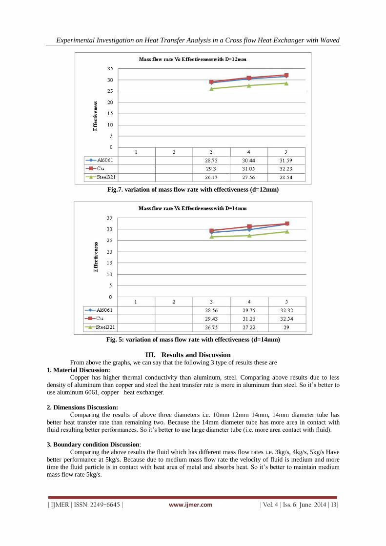
Experimental Investigation on Heat Transfer Analysis in a Cross flow Heat Exchanger with Waved
| IJMER | ISSN: 2249–6645 | www.ijmer.com | Vol. 4 | Iss. 6| June. 2014 | 13|
Fig.7. variation of mass flow rate with effectiveness (d=12mm)
Fig. 5: variation of mass flow rate with effectiveness (d=14mm)
III. Results and Discussion From above the graphs, we can say that the following 3 type of results these are
1. Material Discussion:
Copper has higher thermal conductivity than aluminum, steel. Comparing above results due to less
density of aluminum than copper and steel the heat transfer rate is more in aluminum than steel. So it’s better to
use aluminum 6061, copper heat exchanger.
2. Dimensions Discussion:
Comparing the results of above three diameters i.e. 10mm 12mm 14mm, 14mm diameter tube has
better heat transfer rate than remaining two. Because the 14mm diameter tube has more area in contact with
fluid resulting better performances. So it’s better to use large diameter tube (i.e. more area contact with fluid).
3. Boundary condition Discussion:
Comparing the above results the fluid which has different mass flow rates i.e. 3kg/s, 4kg/s, 5kg/s Have
better performance at 5kg/s. Because due to medium mass flow rate the velocity of fluid is medium and more
time the fluid particle is in contact with heat area of metal and absorbs heat. So it’s better to maintain medium
mass flow rate 5kg/s.

Experimental Investigation on Heat Transfer Analysis in a Cross flow Heat Exchanger with Waved
| IJMER | ISSN: 2249–6645 | www.ijmer.com | Vol. 4 | Iss. 6| June. 2014 | 14|
IV. Conclusions The conclusions deriving from present experimental investigation to evaluate the After completing the
analysis of counter flow heat exchanger of different materials, at different mass flow rates with different
diameter of tubes by using FLOEFD software. We can conclude that, Aluminum 6061, copper heat exchanger
with medium mass flow rate (5kg/s) and the tubes with more area in contact with hot fluid (14mm) has better
heat transfer performance compared to other materials, mass flow rates and diameters.
Acknowledgement The Authors also would like to thank the Sanya Technology Pvt. Limited, Hyderabad, A.P. and India.
For supporting this research, and also thank to our guides, they are given valuable suggestions to completion of
this project.
REFERENCES [1] Patankar, S.V. and spalding. D.B. (1974), “ A calculation for the transient and steady state behaviour of shell- and-
tube Heat Exchanger”. Heat transfer design and theory sourcebook. Afgan A.A. and Schluner E.U.. Washington. Pp. 155-176.
[2] KelKar, K.M and Patankar, S. V., 1987” Numerical prediction of flow and Heat transfer in a parallel plate channel with staggered fins”, Journal of Heat Transfer, vol. 109, pp 25-30.
[3] Berner, C., Durst, F. And McEligot, D.M., “Flow around Baffles”, Journal of Heat Transfer, vol. 106 pp 743-749. [4] Popiel, C.o & Vander Merwe, D.F., “Friction factor in sine-pipe flow, Journal of fluids Engineering”, 118, 1996,
341-345. [5] Popiel, C.O & Wojkowiak, J., “friction factor in U-type undulated pipe flow, Journal of fluids Engineering”, 122,
2000, 260-263. [6] Dean, W. R., Note on the motion of fluid in a curved pipe, The London, Edinburgh and Dublin philosophical
Magazine, 7 (14), 1927, 208-223. [7] Patankar, S.V., Liu, C.H & Sparrow, E.M., “Fully developed flow and Heat Transfer in ducts having streamwise
periodic variation in cross-sectional area”, Journal of Heat Transfer, 99, 1977, 180-186. [8] Webb, B.W & Ramdhyani, S., “Conjugate Heat Transfer in an channel with staggered Ribs” Int. Journal of Heat and
Mass Transfer 28(9), 1985,1679-1687. [9] Park, K., Choi, D-H & Lee, K-s., “design optimization of plate heat exchanger with staggered pins”, 14th Int.
Symp.on Transport phenomena, Bali, Indonesia, 6-9 July 2003. [10] N.R. Rosaguti, D.F. Fletcher & B.S. Haynes “Laminar flow in a periodic serpentine”. 15th Australasian fluid
mechanics conference. The University of Sydney, Sydney, Australia 13-17 December 2004.
Books
[1] Textbook Heat and Mass transfer by RAJPUT [2] Textbook Heat &Mass transfer by S.DOMAKUNDWAR & S.C. ARORA
International
OPEN ACCESS Journal
Of Modern Engineering Research (IJMER)
| IJMER | ISSN: 2249–6645 | www.ijmer.com | Vol. 4 | Iss. 6| June. 2014 | 15|
Electric Load Forecasting Using Genetic Algorithm – A Review
Arun Kumar Gangwar 1, Farheen Chishti 2 1(Department of Electrical Engineering, Assistant Professor, Invertis University, India)
2 (Department of Electrical Engineering, Assistant Professor, Shri Ram Murti Smarak Women College of
Engg. & Tech, Bareilly, India)
I. INTRODUCTION Load forecasting plays an important role in power system planning, operation and control.
Forecasting is the study to estimate active loads ahead of actual load occurrence. Planning and operational
applications of load forecasting requires a certain „lead time‟ also called forecasting intervals. Accurate models
for electric power load forecasting are essential to the operation and planning of a utility company. Load
forecasting helps an electric utility to make important decisions including decisions on purchasing and
generating electric power, load switching, and infrastructure development [1]. Load forecasts are extremely
important for energy suppliers, and other participants in electric energy generation, transmission, distribution,
and markets. The forecasts for different time horizons are important for different operations within a utility
company.
The standard back propagation training-based rules can be used to solve a variety of load forecasting
problems. However, as problem complexity increases, their performance falls rapidly. Other drawbacks include
issues like: long training period, single point search, scaling, initial parameters dependence etc. However,
genetic algorithm (GA) is regarded as an alternative approach. This technique was initially discovered in the
mid-1970s at University of Michigan by John Holland. The main idea was to design artificial systems retaining
the robustness and adoption properties of natural systems[2]. Since the inception, these methodologies were
then further improved by other researchers and are now widely used in various fields (business, science,
engineering etc) to solve a variety of optimization problems that lie outside the scope of the standard
optimization toolbox.
GA mimics the biological processes to perform a random search in a defined N-dimensional possible
set of solutions. For an optimization problem, one needs to search and find the best solution in a given search
space. The idea behind the GA‟s principle is inspired by Darwin‟s theory of evolution (survival of the fittest).
II. CONVENTIONAL OPTIMIZATION VERSUS GA GA differs considerably from conventional search and optimization techniques. The most notable and
important differences are (Goldberg, 1989 and Maifeld et al., 1994):
1. GAs do not require derivative information or other auxiliary knowledge but use an objective function
instead.
2. GAs implement a parallel search in a population, not single point [3]
3. GA use probabilistic transition rules, not deterministic ones.
Abstract: Many real-world problems from operations research and management science are very
complex in nature and quite hard to solve by conventional optimization techniques. So, intelligent
solutions based on genetic algorithm (GA), to solve these complicated practical problems in various
sectors are becoming more and more widespread nowadays. GAs are being developed and deployed
worldwide in myriad applications, mainly because of their symbolic reasoning, flexibility and
explanation capabilities. This paper provides an overview of GAs, as well as their current use in the field of electric load
forecasting. The types of GA are outlined, leading to a discussion of the various types and parameters of
load forecasting. The paper concludes by sharing thoughts and estimations on GA for load forecasting
for future prospects in this area. This review reveals that although still regarded as a novel
methodology, GA technologies are shown to have matured to the point of offering real practical benefits
in many of their applications.
Keywords: Load Forecasting, GA, Types of Load Forecasting.

Electric Load Forecasting Using Genetic Algorithm – A Review
| IJMER | ISSN: 2249–6645 | www.ijmer.com | Vol. 4 | Iss. 6| June. 2014 | 16|
4. Except in real-value representations, GAs work on encoding of the parameter set rather than parameters
themselves.
III. FACTORS AFFECTING LOAD FORECASTING Generally, the load of an electric utility is composed of very different consumption units. A large part
of the electricity is consumed by industrial activities and another part is used by private people in forms of
heating, lighting, cooking, laundry, etc. Also many services offered by society demand electricity, for example
street lighting, railway traffic etc. Factors affecting the load depend on the particular consumption unit[4]. The industrial load is usually
mostly determined by the level of the production. The load is often quite steady, and it is possible to estimate
its dependency on different production levels. However, from the point of view of the utility selling electricity,
the industrial units usually add uncertainty in the forecasts. The problem is the possibility of unexpected
events, like machine breakdowns or strikes, which can cause large unpredictable disturbances in the load level.
In the case of private people, the factors determining the load are much more difficult to define. Each
person behaves in his own individual way, and human psychology is involved in each consumption decision.
Many social and behavioral factors can be found. For example, big events, holidays, even TV-programs, affect
the load. The weather is the most important individual factor, the reason largely being the electric heating of
houses, which becomes more intensive as the temperature drops.
As a large part of the consumption is due to private people and other small electricity customers, the
usual approach in load forecasting is to concentrate on the aggregate load of the whole utility. This reduces the
number of factors that can be taken into account, the most important being:
In the short run, the meteorological conditions cause large variation in this aggregated load. In addition to
the temperature, also wind speed, cloud cover, and humidity have an influence [5].
In the long run, the economic and demographic factors play the most important role in determining the
evolution of the electricity demand.
From the point of view of forecasting, the time factors are essential. By these, various seasonal effects and
cyclical behaviors (daily and weekly rhythms) as well as occurrences of legal and religious holidays are
meant.
The other factors causing disturbances can be classified as random factors. These are usually small in
the case of individual consumers, although large social events and popular TV-programs add uncertainty in the
forecasts. Industrial units, on the other hand, can cause relatively large disturbances.
IV. CLASSIFICATION OF LOAD FORECASTING METHODS In terms of lead time, load forecasting methods are divided into four main categories as listed below:
4.1 Very short-term load forecasting (VSTLF)
It is used for lead time from few seconds to few minutes. In VSTLF instead of modeling relationships
between load, time, weather conditions and other load affecting factors we have to focus on extrapolating the
recently observed load pattern to the nearest future. Methods for very short-term load forecasting are not so
numerous. Some reported techniques include first or second order polynomial extrapolation, autoregressive and
autoregressive moving average models, and artificial neural networks. VSTLF is used in prediction of
generation, distribution schedules, contingency analysis for system security etc.
4.2 Short-term load forecasting (STLF)
It is used for lead time from few minutes to few hours. For short-term load forecasting several factors
should be considered, such as time factors, weather data, and possible customers‟ classes. Short-term load
forecasting plays a vital role in system operations and is the main source of information for all daily and
weekly operations concerning generation commitment and scheduling. STLF is also important for the
economic and reliable operation of the power system. In order to achieve high forecasting accuracy and speed,
it is required to know the factors that affect the load. Some of these factors are: the type and time of day, the
weather conditions of the forecasting area, the season, etc. Since most days have different load profiles, it is
necessary to have a day type. Time of the day is an important factor in short term load forecasting. It is
required to know the forecasting time of the day because the level of demand at any time of the day is different.
Therefore, the relationships between these factors and the load demand need to be determined so that the

Electric Load Forecasting Using Genetic Algorithm – A Review
| IJMER | ISSN: 2249–6645 | www.ijmer.com | Vol. 4 | Iss. 6| June. 2014 | 17|
forecasts may be as accurate as possible. STLF is generally used for allocation of spinning reserve, operational
planning and unit commitment, maintenance scheduling [6].
4.3 Mid-term load forecasting (MTLF)
It is used for lead time from a few days to a few weeks. MTLF is used for prediction load in for
seasonal changes such as peak-summer, winter.
4.4 Long-term load forecasting (LTLF)
It is used for lead time from a few months to few years. The medium and long-term forecasts take
into account the historical load and weather data, the number of customers in different categories, the
appliances in the area and their characteristics including age, the economic and demographic data and their
forecasts, the appliance sales data, and other factors. LTLF is used for planning generation growth.
Table 1.Different Types of Load Forecasting
V. HOW DOES GA WORKS? The algorithm is commenced with a search space containing set of solutions (or chromosomes) called
population. Like its counterpart in nature, Chromosomes from one population are chosen based on fitness and
then combined to form new generation. The best fit individuals are more likely to be selected and subsequently
reproduce in the next generation. This approach is encouraged by a hope that the new population will be better
than the old one. These procedures are carried out repeatedly until some pre-determined stopping conditions
(such as generation, time limits) are met. Like its counterpart in biology, this process requires some genetic
operators such recombination, crossover, and mutation [7]. To implement a genetic based search, one
needs to define the objective function to be optimized. Strictly speaking, the objective function
can be viewed as the input to the algorithm. This function is primarily intended to provide a
measure of how individuals have performed in the problem domain. Depending on the
optimization goal, most fit elements in case of a maximization problem would ideally have the
largest numerical values. The process of a GA is shown by following flowchart:
Fig. 1 Flow Chart of GA Process

Electric Load Forecasting Using Genetic Algorithm – A Review
| IJMER | ISSN: 2249–6645 | www.ijmer.com | Vol. 4 | Iss. 6| June. 2014 | 18|
5.1 Selection:
There are many different types of selection, this paper covers the most common type - roulette wheel
selection. In roulette wheel selection, individuals are given a probability of being selected that is directly
proportionate to their fitness. Two individuals are then chosen randomly based on these probabilities and
produce offspring.
5.2 Crossover:
After selecting individuals, how these individuals produce offspring with them? The most common
solution is something called crossover, and while there are many different kinds of crossover, the most
common type is single point crossover. In single point crossover, choose a locus at which you swap the
remaining alleles from on parent to the other. This is complex and is best understood visually.
As the figure shows, the children take one section of the chromosome from each parent. The point at
which the chromosome is broken depends on the randomly selected crossover point. This particular method is
called single point crossover because only one crossover point exists. Sometimes only child 1 or child 2 is
created, but oftentimes both offspring are created and put into the new population. Crossover does not always
occur, however. Sometimes, based on a set probability, no crossover occurs and the parents are copied directly
to the new population. The probability of crossover occurring is usually 60% to 70% [8].
5.3 Mutation:
After selection and crossover, we have a new population full of individuals. Some are directly copied,
and others are produced by crossover. In order to ensure that the individuals are not all exactly the same,
system allow for a small chance of mutation. The system loop through all the alleles of all the individuals, and
if that allele is selected for mutation, system can either change it by a small amount or replace it with a new
value. The probability of mutation is usually between 1 and 2 tenths of a percent. A view of mutation is shown
below.
Before: 1101101001101110
After: 1101100001101110
As we see that, mutation is fairly simple. It just changes the selected alleles based on what you feel is necessary
and move on. Mutation is, however, vital to ensuring genetic diversity within the population [9].
VI. DIFFERENT ALGORITHMS OF GA
6.1 Greedy Strategy Algorithm:
The greedy algorithm, always takes the best immediate, or local, solution while finding an answer.
Greedy algorithms find the overall, or globally, optimal solution for some optimization problems, but may find
less-than-optimal solutions for some instances of other problems. In general, we use greedy algorithms for
optimization problems [10].
Optimization problems, by their very nature, always require an overall solution that is
globally optimal. The best solution is necessary. Imagine the following decision tree scenario:
Greedy walks through the following tree, beginning from the root node, and at each node
looks around and picks the local optimum. As you can see in figure below, there are always
two routes to take; it picks the one that currently looks best.

Electric Load Forecasting Using Genetic Algorithm – A Review
| IJMER | ISSN: 2249–6645 | www.ijmer.com | Vol. 4 | Iss. 6| June. 2014 | 19|
Fig. 2. Greedy Decision Based on Local Optimum Algorithm
However, walking through the tree using the aforementioned mentality does not guarantee that you
end up with a globally optimal solution despite the fact that you have always picked the “local best” route on
each level. You cannot be absolutely sure that this leads to the overall best solution. This is why greedy often
gives the optimal solution, but not always.
6.2 Dynamic Programming:
By its very nature, is the most appropriate algorithm for those problems that have the aforementioned
complex structure. As we know that, the greedy algorithm wouldn't suffice because its approach works only
until the second type of tree comes in. But this combination is the specialty of dynamic programming. The
dynamic programming technique can be approached in two distinctive ways: top-down and bottom-up. The
former is an advanced recursion combined with memorization, since it means breaking the problem into all of
its sub-problems, solved them, and storing the solutions, assuming we're going to re-use them. The latter
predicts the sub-problems that might be required and solves them in advance; this is the way it tries to build
the final solution from the sub-problems' solutions. This approach requires more resources (stack space).
All in all, the dynamic programming technique is based on the optimality principle. It starts from the
trivial but optimal solutions of the sub-problems; moving further, it builds the final solution. However, it's
really important that the algorithm stores the solution of each sub-problem; we use an array for this purpose.
The array can be multi-dimensional depending on how many parameters describe the solution(s).
Branch and Bound: It is an algorithm technique that is often implemented for finding the optimal solutions in
case of optimization problems; it is mainly used for combinatorial and discrete global optimizations of
problems. In a nutshell, we opt for this technique when the domain of possible candidates is way too large and
all of the other algorithms fail. This technique is based on the en masse elimination of the candidates [11].
Greedy and Dynamic Programming are methods for solving optimization problems. Greedy algorithms are
usually more efficient than Dynamic Programming solutions. However, often you need to use dynamic
programming since the optimal solution cannot be guaranteed by a greedy algorithm. Dynamic Programming
provides efficient solutions for some problems for which a brute force approach would be very slow. To use
Dynamic Programming we need only show that the principle of optimality applies to the problem.
VII. CONCLUSION Load forecasting plays a dominant part in the economic optimization and secure operation of electric
power systems. Load forecasting represents the future generation, transmission and distribution facilities. Any
substantial deviation in the forecast will result in either overbuilding of supply facilities, or curtailment of
customer demand. The confidence levels associated with classical forecasting techniques, when applied to
forecasting problem in mature and stable utilities are likely to be similar to those of dynamic and fast growing
utilities. Different methods of load forecasting are defined in this paper. All of these methods can forecast the
load of the power system, but the amount of previous data and such variable which they need to forecast, make
them different in accuracy from area to area. Finally, for load forecasting, we should know the power system in
details, and after that we can select the best method for the specified power system. Traditional methods, such as time series, regression models etc. are used in most of the countries,
because of their reliable result.
Neural networks can solve nonlinear problems, and because of nonlinear behavior of load, so they can
be useful for load forecasting.

Electric Load Forecasting Using Genetic Algorithm – A Review
| IJMER | ISSN: 2249–6645 | www.ijmer.com | Vol. 4 | Iss. 6| June. 2014 | 20|
Genetic algorithm can forecast the load, when we have a lot amount of different variables and we
want to find the best solution to follow the future load. In this paper different techniques of genetic algorithm
are defined and we can use these techniques depending on the variable and efficiency of the technique.
REFERENCES [1]. Sandeep Sachdeva, Maninder Singh, U. P. Singh and Ajat Shatru Arora, “Efficient Load Forecasting Optimized by
Fuzzy Programming and OFDM Transmission”, in Hindawi Publishing Corporation Advances in Fuzzy Systems,
Vol. 2011, Article ID 326763, pp. 6, April 2011.
[2]. Sandeep Sachdeva, Maninder Singh and A. S. Arora, “Reduction of Error for Load Forecasting using Fuzzy
Programming and OFDM Transmission”, in International Journal of Science Technology & Management, ISSN
0976-2140, Vol. 2, Issue 2, pp. 78-83, December 2010.
[3]. Sachdeva S.,Verma C.M., “Load Forecasting using Fuzzy Methods,” in Proc. 2008 IEEE Power System Technology
and Power INDIA Conference, pp. 1–4.
[4]. S. Phimphachan, K. Chamnongthai, P. Kumhom, N. Jittiwarangkul and A. Sangswang, "Energy and Peak Load
Forecast Models using Neural Network for Fast Developing Area," in Proc. 2004 IEEE Communications and
Information Technologies Conf., pp. 389-393.
[5]. Irfan Mulyawan Malik and Dipti Srinivasan, “Optimum Power Flow using Flexible Genetic Algorithm Model in
Practical Power System”, in Proc. 2010 IPEC, pp. 1146-1151.
[6]. Yan Wang, Vesna Ojleska and Yuanwei Jing, “Short Term Load Forecasting: A Dynamic Neural Network Based
Genetic Algorithm Optimization”, 14th International Power Electronics and Motion Control Conference, EPE-
PEMC-2010, PP. 157-161.
[7]. Yan Wang, Yuanwei Jing and Weilun Zhao, “Dynamic Neural Network Based Genetic Algorithm Optimizing for
Short Term Load Forecasting”, Chinese Control and Decision Conference 2010, pp. 2701-2704.
[8]. Wei Sun, “A Novel Hybrid GA Based SVM Short Term Load Forecasting Model”, 2nd International Symposium on
Knowledge Acquistion and Modeling 2009, pp. 227-229.
[9]. Shouchun Wang and Xiucheng Dong, “Predicting China‟s Energy Consumption Using Artificial Neural Networks
and Genetic Algorithm”, International Conference on Business Intelligence and Financial Engineering 2009, pp. 8-
11.
[10]. Sanjib Mishra and Sarat Kumar Patra, “Short Term Load Forecasting using Neural Network trained with Genetic
Algorithm & Particle Swarm Optimization”, 1st International Conference on Emerging Trends in Engineering and
Technology 2008, pp. 606-609.
[11]. Ladan Ghods and Mohsen Kalantar, “Methods for Long Term Electric Load Demand Forecasting; A comprehensive
Investigation”, IEEE International Conference on Industrial Technology 2008, pp. 1-4.
International
OPEN ACCESS Journal
Of Modern Engineering Research (IJMER)
| IJMER | ISSN: 2249–6645 | www.ijmer.com | Vol. 4 | Iss. 6| June. 2014 | 21|
MIMO System Performance Evaluation for High Data Rate
Wireless Networks using Space Time Block Codes with
Orthogonal Structure
Sandeep Narain1, Dr. Syed Hasan Saeed2 1, 2 (Department of ECE, Integral University, India)
I. INTRODUCTION Due to fading in a multipath wireless channels makes it becomes very tough for the receiver antenna
to differentiate the transmitted signal if the receiver is adjusted with some specific type of diversity having
some less-faded replica of the signal transmitted by sending end antenna. In today’s many applications one of
the popular practical way of achieving diversity is multiplication of number of the antenna at the transmitter
and may also be on the receiver additionally. But there is a desired need that receivers should be of small size.
Hence under this consideration it may not be practical to use multiple receiving side antennas at the mobile
remote station. This justifies the consideration of mainly transmit side diversity.
Transmit diversity is treated as a method of removing data errors in wireless fading channels [2]. It is
very popular due to its simplicity of design and the reliability of multiple antennas at the base station. In terms
of the cost of multiple transmit chains at the base can be applied over numerous users. Space–time trellis
coding [10] is a new coding scheme that combines signal processing at the receiver with coding techniques
appropriate to multiple transmit antennas. Specific space–time trellis codes designed for 2–4 transmit antennas
perform extremely well in slow-fading environments (typical of indoor transmission) and come close to the
outage capacity computed by Telatar [3] and independently by Foschini and Gans [4]. However, when the
number of transmit antennas is fixed, the decoding complexity of space–time trellis codes (measured by the
number of trellis states in the decoder) increases exponentially with transmission rate. In reference to the
matter of the complexity in decoding recently a remarkable scheme is proposed for transmission using only two
transmit antennas. This scheme is simplicity on compared with the space–time trellis coding for two transmit
antennas but a loss in performance is found as compared to space–time trellis codes. Despite this loss of
performance, Alamouti’s scheme [1] is applying in many places due to its simplicity and performance and it
motivated researchers of all the world for discovering similar schemes using more than or equal to two
transmit antennas based communication systems.
Abstract: Space–time block coding is used for data communication in fading channels by multiple
transmit antennas. Message data is encoded by applying a space–time block code and after the encoding
the data is break into ‘n’ streams of simultaneously transmitted strings through n transmit antennas. The
received signal at the receiver end is the superposition of the n transmitted signals distorted due to noise
.For data recovery maximum likelihood decoding scheme is applied through decoupling of the signals
transmitted from different antennas instead of joint detection. The maximum likelihood decoding scheme
applies the orthogonal structure of the space–time block code (OSTBC) and gives a maximum-likelihood
decoding algorithm based on linear processing at the receiver. In this paper orthogonal space–time
block codes based model is developed using Matlab/Simulink to get the maximum diversity order for a
given number of transmit and receive antennas subject with a simple decoding algorithm.
The simulink block of orthogonal space coding block with space–time block codes is applied with and
without gray coding. The OSTBC codes gives the maximum possible transmission rate for any number of
transmit antennas using any arbitrary real constellation such of M-PSK array. For different complex
constellation of M- PSK space–time block codes are applied that achieve 1/2 and 3/4 of the maximum
possible transmission rate for MIMO transmit antennas using different complex constellations.
Keywords: Transmit diversity, Multipath channels, Multiple input multiple output, Wireless
communication and OSTBC.

MIMO System Performance Evaluation for High Data Rate Wireless Networks using Space Time
| IJMER | ISSN: 2249–6645 | www.ijmer.com | Vol. 4 | Iss. 6| June. 2014 | 22|
II. RELATED WORK In this paper we have applied the theory of orthogonal designs to create simulation model of Alamouti
scheme, of space–time block coding for more than or equal to two transmit antennas. The study of orthogonal
designs is a field of mathematics which has been investigated by several great number researchers including
Radon and Hurwitz. The work of Geramita and Seberry [5] is an excellent document to understand the
significance of orthogonal designs. A classical result in this area is provided by Radon. In his work they
determined the set of required dimensions for which an orthogonal design exists [8].
Their analysis results only considers with real square orthogonal designs. In this work, we have
applied an extended form of nonsquare and complex orthogonal designs related to the theory of generalized
orthogonal designs. Using this concept, we have used orthogonal structure space–time block codes for multiple
transmit antennas. Since our approach is related to the theory of orthogonal designs from a communications
perspective hence our simulated design model corresponds to combined coding and linear processing at the
transmitter.
We have simulated the concept of the orthogonal designs and develop a model based on of generalized
orthogonal designs. Using this mathematical theory, we applied a coding schemes for multiple number of
transmit antennas. These schemes is providing a full diversity order that can be utilized by the transmitting
and receiving antennas. In most of the works very simple maximum likelihood decoding algorithms based only
on linear processing at the receiver are applied. It provides a maximum possible transmission rate using totally
real constellations as established in the theory of space–time coding [7]. We have also considered the complex
orthogonal designs and their properties. Our model restores the scheme given by Alamouti [1], though it is
found that generalization to more than two transmit antennas is not possible. We then develop our model
related to theory of complex generalized orthogonal designs. These designs exist multiple transmit antennas
and again have remarkably simple maximum-likelihood decoding algorithms based only on linear processing
at the receiver. In many works full spatial diversity and of the maximum possible rate (as established
previously in the theory of space–time coding) using complex constellations are also provided. For complex
constellations and for the specific cases of two, three, and four transmit antennas, these diversity schemes are
improved to provide, respectively all and of maximum possible transmission rate.
III. SPACE-TIME (MIMO) SYSTEMS Digital communication using multiple-input-multiple output (MIMO) wireless link is now a day’s
emerged as one of the most popular technical application in modern communications. This method focuses
mainly on the list of recent technical advances with a chance of solving the problems of traffic capacity for
future Internet related wireless networks. In a starting years of invention of this technology it seems that it is
has entered in large-scale standards-driven commercial wireless products and networks like broadband wireless
systems, wireless LAN, third-generation networks and beyond.
MIMO systems can be defined simply as an arbitrary wireless communication system having a link
for which the transmitting side and also the receiving side is equipped with multiple antenna devices (Fig.
1).In the MIMO the signals on the transmit (TX) antennas at one end and the receive (RX) antennas at the
other end are “combined” in such a way that the quality (bit-error rate or BER) or the data rate (bits/sec) of the
communication for each MIMO user are enhanced. Such benefits are used to improve both the network’s
quality of service and the operator’s revenues significantly. The main process in MIMO systems is space–time
signal processing in which time (the natural dimension of digital communication data) is complemented with
the spatial dimension inherent in the use of multiple spatially distributed antennas. In this way the MIMO
systems can be considered as an extension of the new terminology called as smart antennas, a popular
technology using antenna arrays for improving wireless transmission dating back several decades.
We have developed our simulation model by considering the multiple antenna system (Fig. 1). A
digital source data in the form of a binary stream is provided to a transmitting block containing the functions
of error control coding and (possibly joined with) mapping to complex modulation symbols (M phase-shift
keying (MPSK), M-QAM, etc.). This produces multiple separate symbol streams which range from
independent to partially redundant to fully redundant. Each symbol stream is then mapped onto one of the
multiple TX antennas. Mapping includes either linear spatial weighting of the antenna elements or linear
antenna space–time pre coding. After upward frequency conversion, filtering and amplification, the signals are
launched into the wireless channel. At the receiver, the signals are captured by possibly multiple antennas and
demodulation and demapping operations are performed to recover the message. The level of intelligence,
complexity, and a priori channel knowledge used in selecting the coding and antenna mapping algorithms can
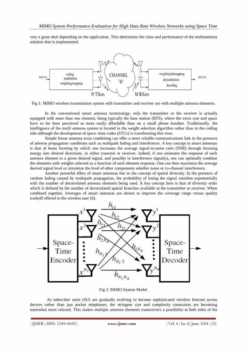
MIMO System Performance Evaluation for High Data Rate Wireless Networks using Space Time
| IJMER | ISSN: 2249–6645 | www.ijmer.com | Vol. 4 | Iss. 6| June. 2014 | 23|
vary a great deal depending on the application. This determines the class and performance of the multiantenna
solution that is implemented.
Fig 1: MIMO wireless transmission system with transmitter and receiver are with multiple antenna elements.
In the conventional smart antenna terminology, only the transmitter or the receiver is actually
equipped with more than one element, being typically the base station (BTS), where the extra cost and space
have so far been perceived as more easily affordable than on a small phone handset. Traditionally, the
intelligence of the multi antenna system is located in the weight selection algorithm rather than in the coding
side although the development of space–time codes (STCs) is transforming this view.
Simple linear antenna array combining can offer a more reliable communications link in the presence
of adverse propagation conditions such as multipath fading and interference. A key concept in smart antennas
is that of beam forming by which one increases the average signal-to-noise ratio (SNR) through focusing
energy into desired directions, in either transmit or receiver. Indeed, if one estimates the response of each
antenna element to a given desired signal, and possibly to interference signal(s), one can optimally combine
the elements with weights selected as a function of each element response. One can then maximize the average
desired signal level or minimize the level of other components whether noise or co-channel interference.
Another powerful effect of smart antennas lies in the concept of spatial diversity. In the presence of
random fading caused by multipath propagation, the probability of losing the signal vanishes exponentially
with the number of decorrelated antenna elements being used. A key concept here is that of diversity order
which is defined by the number of decorrelated spatial branches available at the transmitter or receiver. When
combined together, leverages of smart antennas are shown to improve the coverage range versus quality
tradeoff offered to the wireless user [6].
Fig 2: MIMO System Model.
As subscriber units (SU) are gradually evolving to become sophisticated wireless Internet access
devices rather than just pocket telephones, the stringent size and complexity constraints are becoming
somewhat more relaxed. This makes multiple antenna elements transceivers a possibility at both sides of the
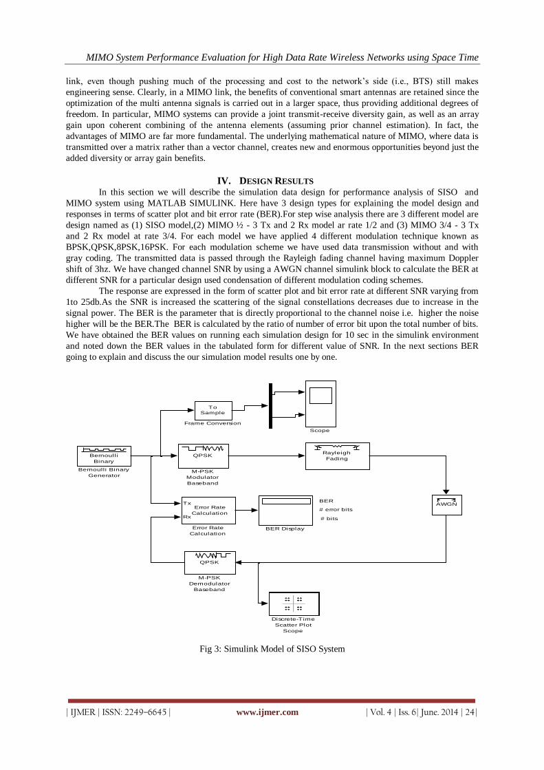
MIMO System Performance Evaluation for High Data Rate Wireless Networks using Space Time
| IJMER | ISSN: 2249–6645 | www.ijmer.com | Vol. 4 | Iss. 6| June. 2014 | 24|
link, even though pushing much of the processing and cost to the network’s side (i.e., BTS) still makes
engineering sense. Clearly, in a MIMO link, the benefits of conventional smart antennas are retained since the
optimization of the multi antenna signals is carried out in a larger space, thus providing additional degrees of
freedom. In particular, MIMO systems can provide a joint transmit-receive diversity gain, as well as an array
gain upon coherent combining of the antenna elements (assuming prior channel estimation). In fact, the
advantages of MIMO are far more fundamental. The underlying mathematical nature of MIMO, where data is
transmitted over a matrix rather than a vector channel, creates new and enormous opportunities beyond just the
added diversity or array gain benefits.
IV. DESIGN RESULTS In this section we will describe the simulation data design for performance analysis of SISO and
MIMO system using MATLAB SIMULINK. Here have 3 design types for explaining the model design and
responses in terms of scatter plot and bit error rate (BER).For step wise analysis there are 3 different model are
design named as (1) SISO model,(2) MIMO ½ - 3 Tx and 2 Rx model ar rate 1/2 and (3) MIMO 3/4 - 3 Tx
and 2 Rx model at rate 3/4. For each model we have applied 4 different modulation technique known as
BPSK,QPSK,8PSK,16PSK. For each modulation scheme we have used data transmission without and with
gray coding. The transmitted data is passed through the Rayleigh fading channel having maximum Doppler
shift of 3hz. We have changed channel SNR by using a AWGN channel simulink block to calculate the BER at
different SNR for a particular design used condensation of different modulation coding schemes.
The response are expressed in the form of scatter plot and bit error rate at different SNR varying from
1to 25db.As the SNR is increased the scattering of the signal constellations decreases due to increase in the
signal power. The BER is the parameter that is directly proportional to the channel noise i.e. higher the noise
higher will be the BER.The BER is calculated by the ratio of number of error bit upon the total number of bits.
We have obtained the BER values on running each simulation design for 10 sec in the simulink environment
and noted down the BER values in the tabulated form for different value of SNR. In the next sections BER
going to explain and discuss the our simulation model results one by one.
# bits
# error bits
BER
Scope
AWGN
Rayleigh
FadingQPSK
M-PSK
Modulator
Baseband
QPSK
M-PSK
Demodulator
Baseband
To
Sample
Frame Conversion
Error Rate
Calculation
Tx
Rx
Error Rate
Calculation
Discrete-Time
Scatter Plot
Scope
Bernoulli
Binary
Bernoulli Binary
Generator
BER Display
Fig 3: Simulink Model of SISO System

MIMO System Performance Evaluation for High Data Rate Wireless Networks using Space Time
| IJMER | ISSN: 2249–6645 | www.ijmer.com | Vol. 4 | Iss. 6| June. 2014 | 25|
BER
# error bits
# bits
vvv
U Y
Selector2
U Y
Selector1
U Y
Selector
Scope
AWGN
3 TxRate 1/2
OSTBC Encoder
3 Tx, 2 RxRate 1/2
Rx
cEst
OSTBC Combiner
RayleighFadingGain
RayleighFading
Gain
RayleighFading Gain
RayleighFading
Gain
RayleighFading
Gain
RayleighFading Gain
3
2
2
2
16-PSK
M-PSKModulatorBaseband
16-PSK
M-PSKDemodulator
Baseband
ToSample
ToSample
ToSample
Frame Conversion
Error Rate Calculation
Tx
Rx
Error RateCalculation
Discrete-TimeScatter Plot
Scope
BernoulliBinary
Bernoulli BinaryGenerator
BER Display
Fig 4: Simulink Model of MIMO1/2 System
Table 1: Performance results of SISO model design. SNR 1 5 10 15 20 25
Bpsk(B) 0.505 0.4994 0.498 0.501 0.5004 0.5005
BPSK(G) 0.505 0.4994 0.4983 0.501 0.5004 0.5005
Qpsk(B) 0.493 0.4853 0.472 0.4602 0.4575 0.4562
Qpsk(G) 0.4958 0.4953 0.4903 0.4846 0.4862 0.4875
8psk(B) 0.4956 0.4861 0.4879 0.4893 0.4884 0.485
8psk(G) 0.4947 0.4877 0.4781 0.4747 0.4736 0.4742
16psk(B) 0.4964 0.4962 0.4926 0.4857 0.4869 0.4827
16psk(G) 0.4917 0.4927 0.489 0.4892 0.4886 0.488
Table 1,2 And 3 represents the BER values of our SISO model (figure 3), MIMO1/2 (figure 4) and
MIMO3/4 design where B indicate binary coding and G indicate gray coding for each row in the table used
under different modulation. Each columns shows the bit error rate for different SNR varying in db. It can be
observed that in table 1 BER value are varying in between 0.48 to 0.505 under different coding and modulation
schemes. Hence this table indicates that there is no variation of BER in the SISO model by using different
coding and modulation schemes.

MIMO System Performance Evaluation for High Data Rate Wireless Networks using Space Time
| IJMER | ISSN: 2249–6645 | www.ijmer.com | Vol. 4 | Iss. 6| June. 2014 | 26|
BER
# error bits
# bits
U Y
Selector2
U Y
Selector1
U Y
Selector
Scope
AWGN
QPSK
QPSK
Modulator
Baseband
3 Tx
Rate 3/4
OSTBC Encoder
3 Tx, 2 Rx
Rate 3/4
Rx
cEst
OSTBC Combiner
Rayleigh
FadingGain
Rayleigh
FadingGain
Rayleigh
FadingGain
Rayleigh
FadingGain
Rayleigh
FadingGain
Rayleigh
FadingGain
3
2
2
2
16-PSK
M-PSK
Modulator
Baseband
16-PSK
M-PSK
Demodulator
Baseband
To
Sample
To
Sample
To
Sample
Frame Conversion
Error Rate
Calculation
Tx
Rx
Error Rate
Calculation
Discrete-Time
Scatter Plot
Scope
Bernoulli
Binary
Bernoulli Binary
Generator
BER Display
Fig 5: Simulink Model of MIMO3/4 System.
Table 2: Mimo Model ¾ Design Result SNR 1 5 10 15 20 25
Bpsk(B) 0.01075 0.0002 0 0 0 0
BPSK(G) 0.01075 0.0002 0 0 0 0
Qpsk(B) 0.5165 0.01011 0 0 0 0
Qpsk(G) 0.04464 0.006198 0 0 0 0
8psk(B) 0.1809 0.7153 0.006899 0 0 0
8psk(G) 0.1126 0.04468 0.004599 0 0 0
16psk(B) 0.3607 0.2778 0.09028 0.0112 0.0003997 0
16psk(G) 0.2155 0.1168 0.03788 0.006095 0.0001998 0
Table 3: MIMO Model 1/2 Design Result SNR 1 5 10 15 20 25
Bpsk(B) 0.01191 0.000799 0 0 0 0
BPSK(G) 0.01191 0.0007998 0 0 0 0
Qpsk(B) 0.04337 0.008258 0.0003332 0 0 0
Qpsk(G) 0.03754 0.005998 0.000288 0 0 0
8psk(B) 0.1916 0.00535 0.007164 0.0003999 0 0
8psk(G) 0.1111 0.03667 0.005199 0.0003333 0 0
16psk(B) 0.2551 0.1977 0.0546 0.01562 0.001132 0.0001332
16psk(G) 0.2315 0.11ter26 0.03791 0.007985 0.0007327 0

MIMO System Performance Evaluation for High Data Rate Wireless Networks using Space Time
| IJMER | ISSN: 2249–6645 | www.ijmer.com | Vol. 4 | Iss. 6| June. 2014 | 27|
V. CONCLUSION We Multiple input multiple output (MIMO) technology proves itself that it can need the demands by
increasing spectral efficiency using spatial multiple path gain and its also improves the reability by considering
antenna diversity gain in our design algorithm.We have investigated an analyzed various problem in the area
of MIMO wireless communication related to the literature describing theoretical perspective and hard ward
implementation perspective. It has been observed that MIMO technology has reached the level where we can
used it for practical system. In this paper we have investigated the problem that exist to it MIMO system i.e.
high bit error rate due to channel fadings. We have designed to different MIMO model based on1/2 and ¾
MIMO transmitter receiver antenna and included the effect of gray coding in the effect of gray coding in the
signal trial to the modulation. It has been observed that in the SISO system mode BER is very large for any
kind modulation scheme even at the small noise power mirror. Due to fading channel BER is never reduced
below 0.4. But in the case of ½ and ¾ designing results BER has reached to zero level at SNR over than 25
for any type of modulation scheme. In the case of MIMO ½ design BER for BPSK modulation are negeable an
almost same for binary and gray coding. In the case of BPSK, QPSK, 8PSK and 16PSK the BER after gray
coding is found lower than the BER due to binary coding. Similarly in the case of MIMO ¾ model BER is
reduced for due the modulation scheme on using gray coding. In this way we can conclude that gray coding
helps in improving data transmission efficiency for both ½ and ¾ MIMO systems.
We have also compared our MIMO ½ and ¾ system and it has been found that for BPSK modulation
½ model is giving lower BER at all the SNR. For the case of QPSK ¾ MIMO design is better than ½ MIMO
design but for the case of 8 and 16PSK schemes our MIMO ½ design is lower bit error rate as compared to
MIMO ¾ specially at the SNR above or equal to 10db. In this way in maximum cases that we have considered
MIMO ½ channel design has performed better than MIMO ¾ channel design.
REFERENCES [1] S. M. Alamouti, “A simple transmitter diversity scheme for wireless communications,” IEEE J. Select. Areas
Commun., vol. 16, pp. 1451–1458, Oct. 1998.
[2] N. Balaban and J. Salz, “Dual diversity combining and equalization in digital cellular mobile radio,” IEEE Trans.
Veh. Technol., vol. 40, pp. 342–354, May 1991.
[3] E. Telatar, “Capacity of multi-antenna Gaussian channels,” AT&T-Bell Laboratories Internal Tech. Memo., June
1995.
[4] G. J. Foschini Jr. and M. J. Gans, “On limits of wireless communication in a fading environment when using
multiple antennas,” Wireless Personal Commun., Mar. 1998.
[5] A. V. Geramita and J. Seberry, Orthogonal Designs, Quadratic Forms and Hadamard Matrices, Lecture Notes in
Pure and Applied Mathematics, vol. 43. New York and Basel: Marcel Dekker, 1979.
[6] A. Paulraj and C. B. Papadias, “Space–time processing for wireless communications,” IEEE Signal Processing
Mag., vol. 14, pp. 49–83, Nov. 1997.
[7] V. Tarokh, N. Seshadri, and A. R. Calderbank, “Space–time codes for high data rate wireless communication:
Performance analysis and code construction,” IEEE Trans. Inform. Theory, vol. 44, pp. 744–765, Mar. 1998.
[8] J. Radon, “Lineare scharen orthogonaler matrizen,” in Abhandlungen aus dem Mathematischen Seminar der
Hamburgishen Universit¨at, vol. I. pp. 1–14, 1922.

International
OPEN ACCESS Journal Of Modern Engineering Research (IJMER)
| IJMER | ISSN: 2249–6645 | www.ijmer.com | Vol. 4 | Iss. 6| June. 2014 | 28|
Analysis of Admixtures and Their Effects of Silica Fumes,
Metakaolin and PFA on the Air Content
T. Subramani1, T. Senthilkumar
2, J. Jayalakshmi
3
1 Professor & Dean, Department of Civil Engineering, VMKV Engineering College, Vinayaka Missions
University, Salem, India. 2,3PG Students of Structural Engineering, Department of Civil Engineering, VMKV Engineering College,
Vinayaka Missions University, Salem,
1. Introduction The raw materials needed for the manufacture of Portland cement (PC) are available in most parts of
the world, and the energy requirements for its production may be considered to be relatively modest.
Nevertheless the use of alternative binders or cement replacement materials, has become a necessity for the
construction industry because of the economic, environmental and technological benefits derived from
their use. Furthermore recent years have seen increased concerns regarding the depletion of raw
materials, energy demands and the consequent environmental damage. These concerns have led to
wider utilization of existing cement replacement materials and further search for other less energy intensive
materials. Many of these mineral admixtures are industrial by-products, and are considered as waste. When
used as a partial cement replacement material, typically in the range of 20 to 60% by mass, the energy and
cost savings are substantial. From an environmental point of view mineral admixtures are playing an undisputed
role. They are responsible for substantial “environmental unloading” because their disposal can be hazardous to the environment and higher utilisation of them can result in reduction of greenhouse gas emissions
attributed to the cement industry. Two of the revolutionary developments in concrete technology in the last
century have been produced by air entraining agents (AEAs) and superplasticizers. Superplasticizers or
high range water reducing admixtures (HRWRAs) are concrete admixtures which can be mainly used either to
increase the workability of fresh concrete at a given mix composition or to reduce the amount of mixing
water and water/cement (w/c) ratio for a given workability in order to increase strength and durability. For
instance to compensate for the loss of workability in mixes like those containing pozzolanic materials such as
condensed silica fume (CSF) and metakaolin (MK) or even increase the water reduction effect of pulverized
fuel ash (PFA) and ground granulated blast furnace slag (GGBS) we normally use superplasticizers. Due to
addition of superplasticizers the slump increase at a given mix composition can be 150-200 mm and the
reduction of mixing water at a given slump can be up to 30%, both depending on the method of addition, dosage and type of admixture used. Presently the most important HRWRAs available are based on condensed
melamine sulfonated formaldehyde (MSF) or naphtalene sulfonated formaldehyde (NSF) in the form of 40%
aqueous solution to facilitate an accurate, reliable and automatic dispensing at the batching plant. The optimum
dosage of commercial superplasticizers is in general in the range 1- 2% by mass of cement. The main action
of the molecules of such superpalsticizers is to wrap themselves around the cement particles and give them a
Abstract: This paper presents a review of the properties of fresh concrete including workability, heat
of hydration, setting time, bleeding, and reactivity by using mineral admixtures fly ash (FA), silica
fume (SF), ground granulated blast furnace slag (GGBS), metakaolin (MK), and rice husk ash (RHA).
Comparison of normal and high strength concrete in which cement has been partially supplemented
by mineral admixture has been considered. It has been concluded that mineral admixtures may be
categorized into two groups: chemically active mineral admixtures and microfiller mineral
admixtures. Chemically active mineral admixtures decrease workability and setting time of concrete
but increase the heat of hydration and reactivity. On the other hand, micro filler mineral admixtures increase workability and setting time of concrete but decrease the heat of hydration and reactivity. In
general, small particle size and higher specific surface area of mineral admixture are favourable to
produce highly dense and impermeable concrete; however, they cause low workability and demand
more water which may be offset by adding effective super plasticizer.
Keywords: Silica Fume (SF), Metakaolin (MK), Fly Ash (FA), Ground Granulated Blast Furnace Slag
(GGBS),

Analysis of Admixtures and Their Effects of Silica Fumes, Metakaolin and Pfa on the Air Content
| IJMER | ISSN: 2249–6645 | www.ijmer.com | Vol. 4 | Iss. 6| June. 2014 | 29|
highly negative charge so that they repel each other. This results in deflocculation and dispersion of cement
particles with the resulting improvement in workability.
Air entraining agents are admixtures which are capable of forming air bubbles dispersed
throughout the cement matrix that binds the aggregates. After compaction, normal concrete is likely to
contain about 1-2% air by volume, this accidentally entrapped air being unevenly distributed and
consisting of bubbles of irregular size and shape. Air entraining agents introduce a controlled amount of air
in the form of millions of bubbles of uniform size and uniformly distributed throughout the concrete
mix. There is another distinctive difference between air voids accidentally entrapped in concrete and the
deliberately entrained air bubbles. The latter are very much smaller, typically 50 m in diameter whereas
the former can be as large as the familiar, albeit undesirable, pockmarks on the formed surface of concrete. Numerous types of air entraining agents are commercially available with the vinsol resin based
products being the most common ones. The optimum dosage for AEAs is usually below 1% by mass of
cement.
The presence of entrained air in fresh concrete has a pronounced effect on its properties. One of
these is workability, which is improved. For adequate workability, the aggregate particles must be spaced in
a way that they can move past one another with relative ease during mixing and placing. In this
respect, the entrained air voids are often thought of as millions of tiny ball bearings in the concrete,
making the mix more workable. Entrained air also eliminates or minimises segregation and subsequent
bleeding. Although there are also other advantages to be realised, the principal reason behind the use of
air entrainment agents is the improvement that they impart to the concrete’s resistance to frost action and
to its deterioration due to repeated freezing and thawing. A given volume of air and an appropriate
spacing factor are required to produce an adequate air bubbles system to protect concrete from freezing and thawing. Because the damaging action of freezing and thawing involves expansion of water on
freezing and associated osmotic processes, it is logical to expect that, if excess water can readily escape
into adjacent air-filled voids, damage to the concrete will not occur. This is the underlying principle of
improved frost resistance by air entrainment.
II. Admixture
2.1 CHEMICAL ADMIXTURES FOR CONCRETE
Definition: what are chemical admixtures?
The definition of RILEM (International Union of Testing and Research Laboratories for Materials and
Structures) is:
Admixtures for concrete, mortar or paste are inorganic or organic materials
These are added to the normal components of a mix not normally exceeding 5% by mass of cement or
cementitious materials
Why admixtures? The need.
If we are pouring a low grade concrete, say M20, If we are not unduly concerned about its water
content nor its water-cement ratio,
If the cost of materials and labour are paid entirely by the owner (or some one else) at whatever rates
we have quoted, then, Admixtures will make the concrete more expensive. But then our concrete will be an
indifferent one,
How do they act?
The chemical, physical or physio-chemical actions of admixtures in cement concrete are quite complex.
In fact, cement itself is an extremely complex compound with major compounds such as calcium
silicates, calcium aluminates, gypsum.
Besides it contains many alkali and other calcium salts.
The action of admixtures can, however, be simplified for the sake of Understanding, as:
(i) adsorption
(ii) De-flocculation or dispersion
(iii)Chemical absorption or interaction

Analysis of Admixtures and Their Effects of Silica Fumes, Metakaolin and Pfa on the Air Content
| IJMER | ISSN: 2249–6645 | www.ijmer.com | Vol. 4 | Iss. 6| June. 2014 | 30|
Often, all the three take place. We should know a little about these so that we can choose admixtures for our job
more correctly
2.2 PHYSICO-CHEMICAL ACTIONS OF ADMIXTURES
The most important compounds of cement that react very early when water is added are:
Tricalcium silicate (C3S), and
Tricalcium Aluminate (C3A)
III. Silica fume, Metakaolin,
PULVERISED FUEL ASH (PFA)
3.1 SILICA FUME
Silica fume (SF) is a byproduct of the smelting process in the silicon and ferrosilicon industry. The
reduction of high-purity quartz to silicon at temperatures up to 2,000_C produces SiO2 vapours, which oxidizes
and condense in the low temperature zone to tiny particles consisting of non-crystalline silica. (Fig.3.1)
Fig. 3.1 Silica fume
Properties of Silica Fume
Physical Properties
Silica fume particles are extremely small, with more than 95% of the particles finer than 1 lm. Its
typical physical properties are given in Table.3.1 & Fig.3.2. Silica fume colour is either premium white or grey.
Chemical Composition
Silica fume is composed primarily of pure silica in non-crystalline form. X-ray diffraction analysis of
different silica fumes reveals that material is essentially vitreous silica, mainly of cristobalite form. Silica fume
has a very high content of amorphous silicon dioxide and consists of very fine spherical particles.
Fig. 3.2 Schematic diagram of silica fume production

Analysis of Admixtures and Their Effects of Silica Fumes, Metakaolin and Pfa on the Air Content
| IJMER | ISSN: 2249–6645 | www.ijmer.com | Vol. 4 | Iss. 6| June. 2014 | 31|
Table 3.1 Typical physical properties of silica fume
3.2 METAKAOLIN
What is metakaolin?
Metakaolin is refined kaolin clay that is fired (calcined) under carefully controlled conditions to create
an amorphous aluminosilicate that is reactive in concrete. Like other pozzolans (fly ash and silica fume are two
common pozzolans), metakaolin reacts with the calcium hydroxide (lime) byproducts produced during cement
hydration.(Fig.3.3)
3.3 PULVERISED FUEL ASH (PFA)
The Lands and Works Branch Practice Note on Concrete Technology No. 4, The Use of Pulverised
Fuel Ash in Structural Concrete, was issued in 1983. It was stated therein that the Note would be reviewed when
more information on the local use of PFA was available. There is more information available now, but there is
nothing which requires the Note to be amended. There are, however, other factors which make the issue of this
Addendum desirable.(Fig.3.4)
IV. Result and Discussion
Fig 4.1 comparison of the effect of CSF and MK on the dosage of air entraining agent to obtain
7±1 % air content in the fresh concrete
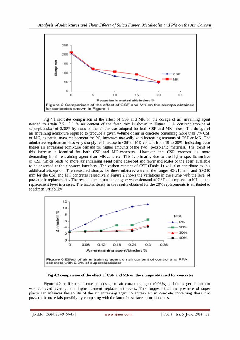
Analysis of Admixtures and Their Effects of Silica Fumes, Metakaolin and Pfa on the Air Content
| IJMER | ISSN: 2249–6645 | www.ijmer.com | Vol. 4 | Iss. 6| June. 2014 | 32|
Fig 4.1 indicates comparison of the effect of CSF and MK on the dosage of air entraining agent
needed to attain 7.5 0.6 % air content of the fresh mix is shown in Figure 1. A constant amount of superplastisizer of 0.35% by mass of the binder was adopted for both CSF and MK mixes. The dosage of
air entraining admixture required to produce a given volume of air in concrete containing more than 5% CSF
or MK, as partial mass replacement for PC, increases markedly with increasing amounts of CSF or MK. The
admixture requirement rises very sharply for increase in CSF or MK content from 15 to 20%, indicating even
higher air entraining admixture demand for higher amounts of the two pozzolanic materials. The trend of
this increase is identical for both CSF and MK concretes. However the CSF concrete is more
demanding in air entraining agent than MK concrete. This is primarily due to the higher specific surface
of CSF which leads to more air entraining agent being adsorbed and fewer molecules of the agent available
to be adsorbed at the air-water interfaces. The carbon content of CSF (Table 1) will also contribute to this
additional adsorption. The measured slumps for these mixtures were in the ranges 45-210 mm and 50-210
mm for the CSF and MK concretes respectively. Figure 2 shows the variations in the slump with the level of pozzolanic replacements. The results demonstrate the higher water demand of CSF as compared to MK, as the
replacement level increases. The inconsistency in the results obtained for the 20% replacements is attributed to
specimen variability.
Fig 4.2 comparison of the effect of CSF and MF on the slumps obtained for concretes
Figure 4.2 indi cat es a constant dosage of air entraining agent (0.06%) and the target air content
was achieved even at the higher cement replacement levels. This suggests that the presence of super
plasticizer enhances the ability of the air entraining agent to entrain air in concrete containing these two
pozzolanic materials possibly by competing with the latter for surface adsorption sites.
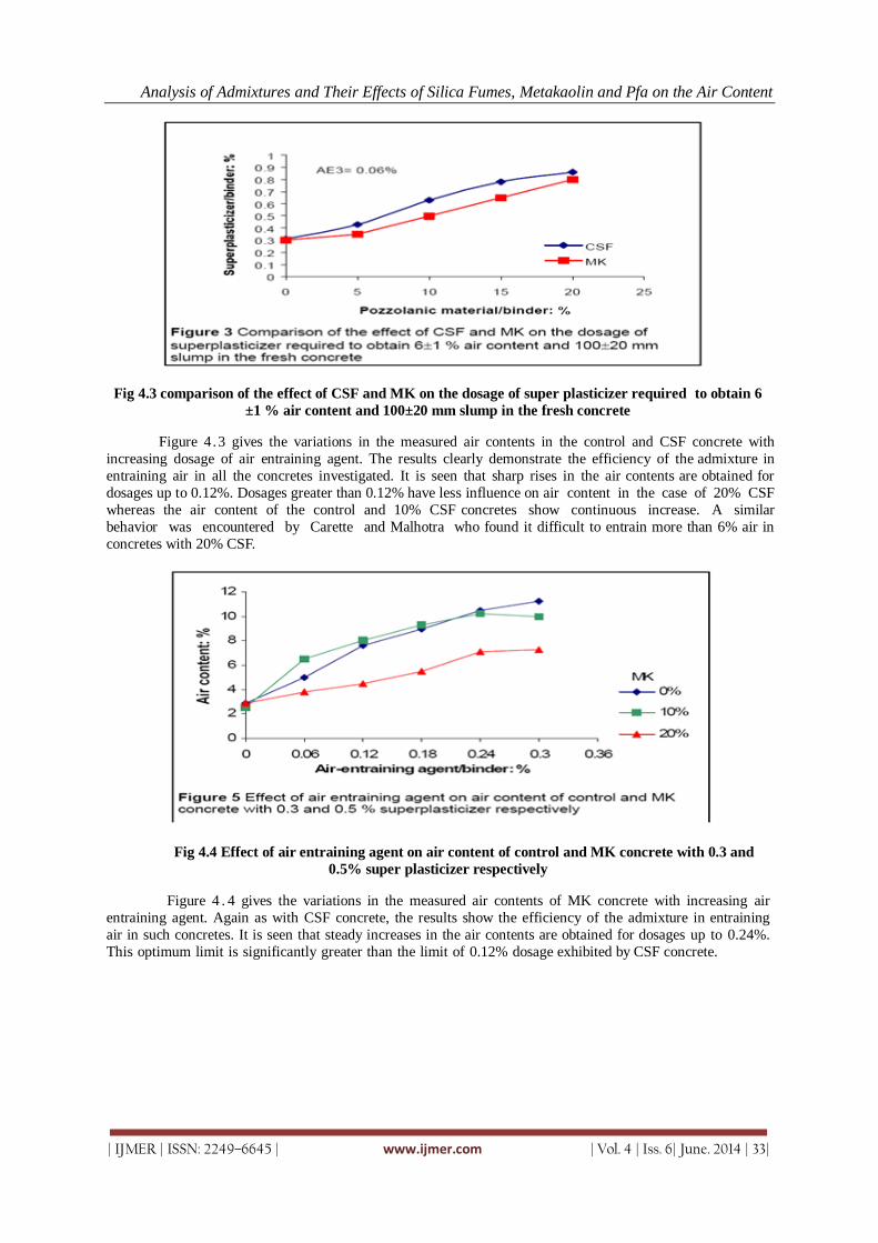
Analysis of Admixtures and Their Effects of Silica Fumes, Metakaolin and Pfa on the Air Content
| IJMER | ISSN: 2249–6645 | www.ijmer.com | Vol. 4 | Iss. 6| June. 2014 | 33|
Fig 4.3 comparison of the effect of CSF and MK on the dosage of super plasticizer required to obtain 6
±1 % air content and 100±20 mm slump in the fresh concrete
Figure 4.3 gives the variations in the measured air contents in the control and CSF concrete with
increasing dosage of air entraining agent. The results clearly demonstrate the efficiency of the admixture in
entraining air in all the concretes investigated. It is seen that sharp rises in the air contents are obtained for
dosages up to 0.12%. Dosages greater than 0.12% have less influence on air content in the case of 20% CSF
whereas the air content of the control and 10% CSF concretes show continuous increase. A similar
behavior was encountered by Carette and Malhotra who found it difficult to entrain more than 6% air in
concretes with 20% CSF.
Fig 4.4 Effect of air entraining agent on air content of control and MK concrete with 0.3 and
0.5% super plasticizer respectively
Figure 4 . 4 gives the variations in the measured air contents of MK concrete with increasing air
entraining agent. Again as with CSF concrete, the results show the efficiency of the admixture in entraining
air in such concretes. It is seen that steady increases in the air contents are obtained for dosages up to 0.24%.
This optimum limit is significantly greater than the limit of 0.12% dosage exhibited by CSF concrete.
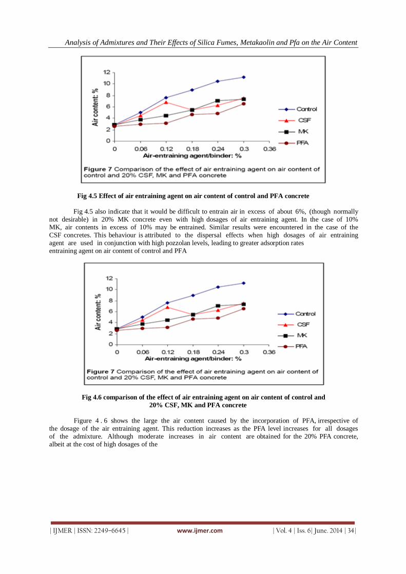
Analysis of Admixtures and Their Effects of Silica Fumes, Metakaolin and Pfa on the Air Content
| IJMER | ISSN: 2249–6645 | www.ijmer.com | Vol. 4 | Iss. 6| June. 2014 | 34|
Fig 4.5 Effect of air entraining agent on air content of control and PFA concrete
Fig 4.5 also indicate that it would be difficult to entrain air in excess of about 6%, (though normally
not desirable) in 20% MK concrete even with high dosages of air entraining agent. In the case of 10%
MK, air contents in excess of 10% may be entrained. Similar results were encountered in the case of the
CSF concretes. This behaviour is attributed to the dispersal effects when high dosages of air entraining
agent are used in conjunction with high pozzolan levels, leading to greater adsorption rates
entraining agent on air content of control and PFA
Fig 4.6 comparison of the effect of air entraining agent on air content of control and
20% CSF, MK and PFA concrete
Figure 4 . 6 shows the large the air content caused by the incorporation of PFA, irrespective of
the dosage of the air entraining agent. This reduction increases as the PFA level increases for all dosages
of the admixture. Although moderate increases in air content are obtained for the 20% PFA concrete,
albeit at the cost of high dosages of the

Analysis of Admixtures and Their Effects of Silica Fumes, Metakaolin and Pfa on the Air Content
| IJMER | ISSN: 2249–6645 | www.ijmer.com | Vol. 4 | Iss. 6| June. 2014 | 35|
Fig 4.7 percentage strength reduction versus percentage air content increase for concretes under
investigation at different curing ages
Figure4.7 gives a plot of the percentage reductions in strength with percentage increases in the
air content of concretes incorporating CSF, MK or PFA. It can be seen that the relationship between
the percentage reductions in strength and the percentage increases in strength is almost linear with the
exception of those reductions corresponding to small increases in the air content of the fresh concrete.
Table 4.1 summarises the results for the compressive strength reductions at each of the ages
of 7, 14, 28 and 90 days corresponding to increases in the air contents for concretes incorporating CSF,
MK or PFA & Effect of increase in air content on reduction in compressive strength.
Table 4.1 Results for the compressive strength reductions
For example when the air content in 10% CSF concrete increases by 304% i.e. from 2.6 to 10.5%
there is a reduction in the 28-day compressive strength of 41%. The reduction in the 28-day strength of
the 10% MK concrete corresponding to an increase in the air content of 300%, i.e. from 2.5 to 10% is 33%. Similar effects are produced in the PFA concretes. For example an increase in air content of 150%,
i.e. from 2.6 to 6.5% in 20% PFA concrete gives a reduction in the 28 day strength of 24%. The results show
that irrespective of the curing time, the percentage reductions in strength due the increase in air content are
more or less the same for all concretes considered in the present study.

Analysis of Admixtures and Their Effects of Silica Fumes, Metakaolin and Pfa on the Air Content
| IJMER | ISSN: 2249–6645 | www.ijmer.com | Vol. 4 | Iss. 6| June. 2014 | 36|
V. Conclusions The following conclusions may be drawn from the work reported in this paper:
For a given slump and air content CSF has more demand for superplasticiser and air entraining admixtures than
MK. The superplasticiser enhances the performance of the air entraining admixture and/or itself plays a
secondary role in entraining air to the fresh concrete. A three fold increase in slump is produced in control
and 10% CSF concretes by adding 0.12% of air entraining admixture.
Although further additions of the admixture lead to increased slump in the control, little
benefit in workability is exhibited by the CSF concrete. This is attributed to the greater diffusion of the air
entrain inggent and consequent adsorption of the admixture by the very fine CSF particles. Up to 0.12% air
entraining admixture results in steep rises in the air content of superplasticised CSF concrete.
The benefits of higher levels of the admixture diminish, particularly in the concretes with high CSF contents (20%). The superplasticiser plays an important role in increasing the air content of
low level CSF concrete. Up to 0.24% air entraining admixture results in a steady increase in the air content
of MK concrete. This is compared to a limit of 0.12% for CSF concrete. Non-air entrained control, CSF and
MK concretes all have the same volume of naturally entrapped air (approximately 2%).
This is attributed to the role played by the additional superplasticiser used in the CSF and MK
concretes. PFA causes large reductions in the air content of fresh concrete, irrespective of the dosage of the
air entraining admixture. The compressive strength of all concretes show systematic and more or less linear
reductions with increasing air contents (2 to 10%) of the fresh concrete. Further analysis is done with software
for extra accuracy in result.
REFERENCES [1.] Collepardi M. “Superplasticizers and Air Entraining Agents: state of the art and future needs”, Concrete
Technology Past Present and Future, Proceedings of V. Mohan Malhotra Symposium, 1994, ACI SP-144, pp.399-
416. [2.] Dodson V. “Concrete Admixtures”, Ed. Van Nostrand Reinhold, 1990. [3.] “Pozzolanic and Cementitious materials”, Ed.V.M. Malhotra and P.K Mehta, Gordon and Preach Publishers,
1996. [4.] Dhir R.K. McCarthy M.J., Limbachiya M.C., El Sayad H.I. and Zhang D.S. “Pulverized fuel ash
concrete: air entrainment and freeze/thaw durability”, Magazine of Concrete Research, Vol.51, No.1, Feb. 1999, pp.53-64.
[5.] Kostuch J.A., Walters G.V. and Jones T.R. “High performance concrete incorporating metakaolin-a review”, Concrete 2000, 1993, 2, pp.1799-1811.
[6.] Wild S., Khatib J and Jones A. “Relative strength, pozzolanic activity and cement hydration in superplasticized metakaolin concrete” Cement and Concrete Research, 1996, 26, No.10, pp.1537-1544.
[7.] Khatib J and Wild S. “Sulfate resistance of metakaolin mortar” Cement and Concrete Research, 1998, 28,
No.1, pp.38-92. [8.] Jones T.R., Walters G.V. and Kostuch J.A. “Role of metakaolin in suppressing ASR in concrete containing reactive
aggregate and exposed to saturated NaCl solution” Proceedings of the 9th International Conference on Alkali-
Aggregate Reaction in Concrete, 1992, 1, pp.485-496. [9.] Sabir B.B, Wild S. and Khatib J. “On the workability and strength development of metakaolin concrete” In
International Congress on Concrete in the service of Mankind, Concrete for Environment Enhancement and Protection, Theme 6, Waste Materials and Alternative Products, University of Dundee (eds R.K Dhir and D.T. Dyer) Spon, London, 1996, pp.651-662.
[10.] Sturrup V.R., Hooton R.D. and Clendenning T.G. “Durability of Fly Ash Concrete”, ACI SP-79, Vol.I, Aug. 1983,
pp.47-69.
International
OPEN ACCESS Journal
Of Modern Engineering Research (IJMER)
| IJMER | ISSN: 2249–6645 | www.ijmer.com | Vol. 4 | Iss. 6 | June. 2014 | 37|
Ultra-Wide Bandpass filter using isosceles triangular microstrip
patch resonator
Rahul Kumar Shishodia1, Sarvodaya Tyagi2, Sawan Kumar3, Pradeep Kumar4 1, 2, 3 (Electronics and Communication Engineering, ABES Institute of Technology, India)
4(Department of Electrical and Electronics Engineering, ABES Institute of Technology, India)
I. INTRODUCTION Ultra-Wide Band (UWB) technology has found many applications in high speed wireless
communication. UWB radio systems are very promising, because data transmission rates greater than those of
other wireless LAN systems can be obtained with low power dissipation. In this area, various studies are under
progress [1–6]. Ultra-Wide bandpass filters are characterized by wide bandwidth, low insertion loss, good band
rejection and flat group delay properties. The filter is designed using microstrip planar technology due to its
high power handling capability, low insertion loss, low cost and easy fabrication. The patch resonators are an
obvious choice for bandpass filter applications where low insertion loss and high power handling are primary
concern [7–10]. Microstrip circuits suffer from radiation losses, dispersion, unwanted coupling and
discontinuity effects. These problems can be greatly reduced by using thinner substrate which allows operation
at millimeter-waves with reduced dispersion and radiation losses [11].
Many kind of microstrip patch resonator filter configurations such as square patch [12], circular patch
[13-14], trapezoidal patch [15] and ring patches have been reported, but they suffer from high conductor losses
and low power handling capability. Triangular resonator was first studied by Ogasawara and Noguchi [16] in
1974, later Helszajn and James in 1978 [17] studied the microstrip one and confirmed that two orthogonal split
modes could be excited. Moreover, they also demonstrated that the radiation loss was lower than that of a disk-
shaped microstrip resonator. In 2004 Hong and Li [11] reported dual mode microstrip filters using equilateral
triangular patch resonator. With the rapid development of modern communication systems, more and more
miniature planar filters [18-22] with excellent performances are required.
In this paper, we propose an ultra-wide bandpass filter using isosceles triangular microstrip patch
resonator. The filter is designed on a 1.27mm thick dielectric substrate with relative dielectric constant 10.8
and loss tangent of 0.002. A 10 µm thick copper patch is used with corners cut and etched slits. The simulated
results show that it has insertion loss of 0.224 dB, return loss of more than 58 dB at central frequency 8.47
GHz, multiple transmission zeroes, passband in C-X band, wider bandwidth and it can be fabricated on 8 mm
x 12 mm board.
II. THEORETICAL FORMULATIONS Helszajn and James [16] reported a theoretical and experimental investigation for the resonant
frequency of electromagnetic filed patterns of TM modes of an equilateral triangular microstrip planar
resonator. The electromagnetic field pattern has no variation along the thickness of resonator and the wave
equation can be written as:
Abstract: In this paper, Ultra-Wide bandpass filter using isosceles triangular patch resonator (ITPR) is
proposed. The reported design has wide bandwidth, low insertion loss, high return loss and flat group
delay properties. The filter characteristics, which are influenced by the height of the triangular structure,
are studied. The proposed design has been prepared in two steps: First, cutting the corners of the
triangular structure to make filter size more compact and avoid line coupling losses, Second, Etching slits
to improve filter performance. Simulation of proposed filter has been carried out with Agilent Advanced
Design System (ADS) and it shows good agreement with theoretical results.
Keywords: microstrip filters, s-parameters, bandpass filter, microstrip patch resonators

Ultra-Wide Bandpass filter using isosceles triangular microstrip patch resonator
| IJMER | ISSN: 2249–6645 | www.ijmer.com | Vol. 4 | Iss. 6 | June. 2014 | 38|
),( yxEz =
b
ymin
b
x
b
yinm
b
x
b
ynmi
b
x
A inm
3
)(2cos
3
2
3
2cos
3
)(2cos
3
2
3
2cos
3
)(2cos
3
2
3
2cos
,,
(1)
xH = y
Ej z
r
0
(2)
yH = x
Ej z
r
0
(3)
zH = xE = yE = 0 (4)
Where Am,n,i is a constant representing the mode amplitude, b is the effective length of the triangle, Ω is the
angular frequency and m, n and i are indexes under condition m+n+i=0, which determine the resonant mode
of the triangular resonator and must satisfy the wave equation below:
zinm Ekyx
2
,,2
2
2
2
= 0 (5)
Where km,n,i is the resonance wave-number, it can be written as:
22
,,
4nmnm
bk inm
(6)
Resonance frequency corresponding to different modes can be written as:
22,,
),,(3
2
2nmnm
b
cckf
rr
inm
inmr
(7)
Where c is the velocity of light in free space and ϵr is the relative dielectric constant of the substrate. According
to equation (7) there are an infinite number of resonant frequencies corresponding to different modes.
III. CHARACTERIZATION OF PROPOSED FILTER The dimensions of proposed filter are shown in Figure 1, the design is developed using 10µm thick
copper patch on a 1.27 mm thick RT Duroid dielectric with a relative dielectric constant of 10.8 and loss
tangent 0.002.
Fig.1 dimensions of the proposed filter
I/O feed lines have characteristic impedance of 50Ω so that maximum power transfer from source to
resonator can be ensured. Cutting the corners of the triangular structure will result in reduction of the filter
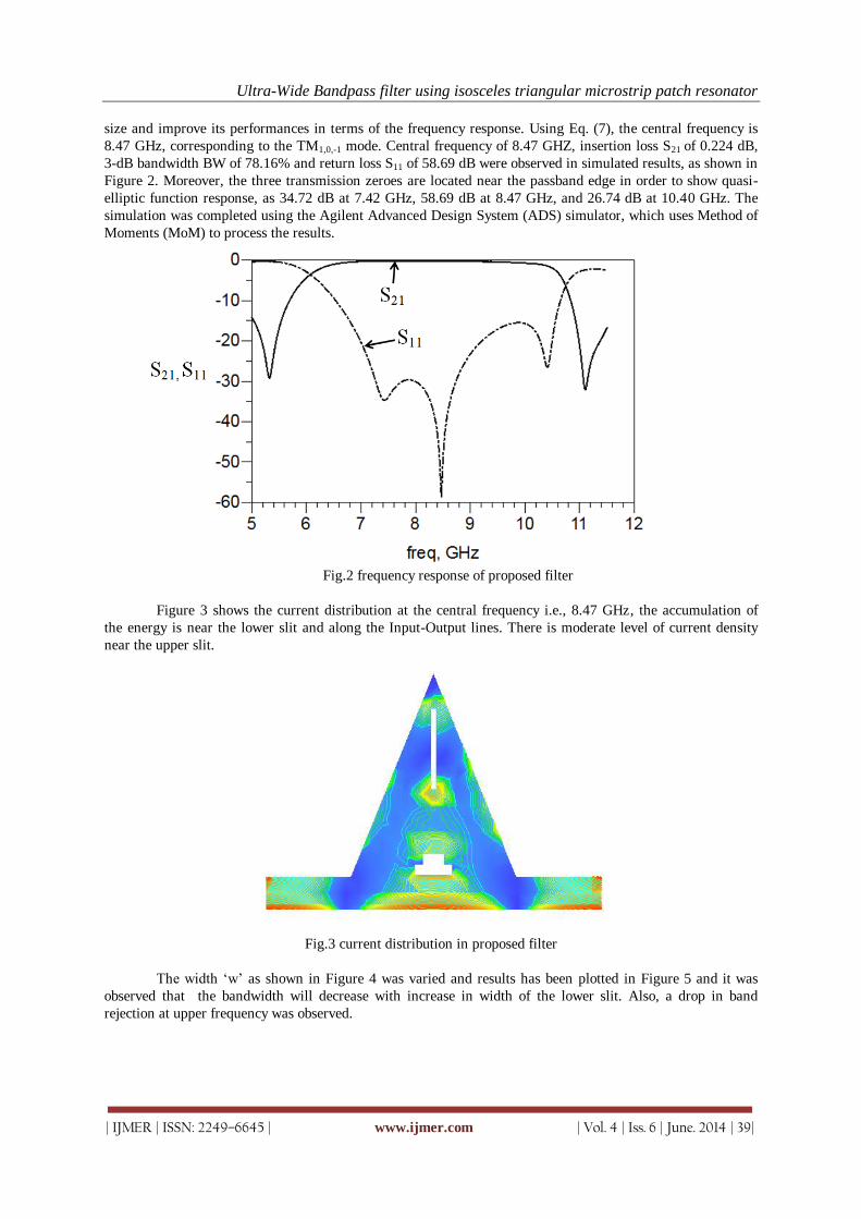
Ultra-Wide Bandpass filter using isosceles triangular microstrip patch resonator
| IJMER | ISSN: 2249–6645 | www.ijmer.com | Vol. 4 | Iss. 6 | June. 2014 | 39|
size and improve its performances in terms of the frequency response. Using Eq. (7), the central frequency is
8.47 GHz, corresponding to the TM1,0,-1 mode. Central frequency of 8.47 GHZ, insertion loss S21 of 0.224 dB,
3-dB bandwidth BW of 78.16% and return loss S11 of 58.69 dB were observed in simulated results, as shown in
Figure 2. Moreover, the three transmission zeroes are located near the passband edge in order to show quasi-
elliptic function response, as 34.72 dB at 7.42 GHz, 58.69 dB at 8.47 GHz, and 26.74 dB at 10.40 GHz. The
simulation was completed using the Agilent Advanced Design System (ADS) simulator, which uses Method of
Moments (MoM) to process the results.
Fig.2 frequency response of proposed filter
Figure 3 shows the current distribution at the central frequency i.e., 8.47 GHz, the accumulation of
the energy is near the lower slit and along the Input-Output lines. There is moderate level of current density
near the upper slit.
Fig.3 current distribution in proposed filter
The width „w‟ as shown in Figure 4 was varied and results has been plotted in Figure 5 and it was
observed that the bandwidth will decrease with increase in width of the lower slit. Also, a drop in band
rejection at upper frequency was observed.
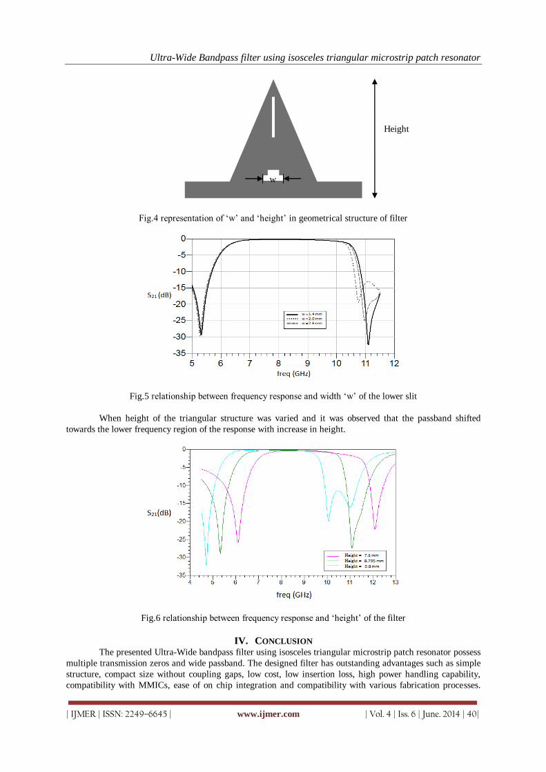
Ultra-Wide Bandpass filter using isosceles triangular microstrip patch resonator
| IJMER | ISSN: 2249–6645 | www.ijmer.com | Vol. 4 | Iss. 6 | June. 2014 | 40|
Fig.4 representation of „w‟ and „height‟ in geometrical structure of filter
Fig.5 relationship between frequency response and width „w‟ of the lower slit
When height of the triangular structure was varied and it was observed that the passband shifted
towards the lower frequency region of the response with increase in height.
Fig.6 relationship between frequency response and „height‟ of the filter
IV. CONCLUSION The presented Ultra-Wide bandpass filter using isosceles triangular microstrip patch resonator possess
multiple transmission zeros and wide passband. The designed filter has outstanding advantages such as simple
structure, compact size without coupling gaps, low cost, low insertion loss, high power handling capability,
compatibility with MMICs, ease of on chip integration and compatibility with various fabrication processes.
w
Height

Ultra-Wide Bandpass filter using isosceles triangular microstrip patch resonator
| IJMER | ISSN: 2249–6645 | www.ijmer.com | Vol. 4 | Iss. 6 | June. 2014 | 41|
Also, it can be realized on variety of substrates depending on the specific need. The proposed filter can be
easily integrated in UWB wireless communication systems. It may also find applications in RFID, vehicular
RADARs, military RADARs, indoor and handheld devices.
REFERENCES [1] F. Geran, G. Dadashzadeh, M. Fardis, N. Hojjat, and A. Ahmadi, “Rectangular slot with a novel triangle ring
microstrip feed for UWB applications,” Journal of Electromagnetic Waves and Applications, Vol. 21, No. 3, 387–
396, 2007.
[2] Z. G. Fan, L. X. Ran, and J. A. Kong, “Source pulse optimizations for UWB radio systems,” Journal of
Electromagnetic Waves and Applications, Vol. 20, No. 11, 1535–1550, 2006.
[3] S. Sadat, M. Houshmand, and M. Roshandel, “Design of a microstrip square-ring slot antenna filled by an H-shape
slot for UWB applications,” Progress In Electromagnetics Research, PIER 70, 191–198, 2007.
[4] F. G. Kharakhili, M. Fardis, G. Dadashzadeh, A. A. K. Ahmad, and N. Hojjat, “Circular slot with a novel circular
microstrip open ended microstrip feed for UWB applications,” Progress In Electromagnetics Research, PIER 68,
161–167, 2007.
[5] S. Sadat, M. Fardis, F. G. Kharakhili, and G. Dadashzadeh, “A compact microstrip square-ring slot antenna for
UWB applications,” Progress In Electromagnetics Research, PIER 67, 173–179, 2007.
[6] M. Klemm, and G. Troester, “EM energy absorption in the human body tissues due to UWB antennas,” Progress In
Electromagnetics Research, PIER 62, 261–280, 2006.
[7] R. R. Mansour, B. Jolley, S. Ye, F. S. Thomson, and V. Dokas, “On the power handling capability of high
temperature superconductive filters,” IEEE Trans. Microwave Theory Tech., vol. 44, pp. 1322–1338, July 1996.
[8] Z. Y. Shen, C. Wilker, P. Pang, and C. Carter, “High-power HTS planar filters with novel back-side coupling,”
IEEE Trans. Microwave Theory Tech., vol. 44, pp. 984–986, June 1996.
[9] M. A. Hein et al., “High-power high-Q YB C O disk resonator filter,” Proc. EUCAS Applied Superconductivity,
1997, pp. 319–322.
[10] J. S. Hong and M. J. Lancaster, “Microstrip triangular patch resonators filters,” IEEE MTT-S Int. Microwave
Symp. Dig., 2000, pp. 331–334.
[11] J. S. Hong and Shuzhou Li, “Theory and Experiment of Dual-Mode Microstrip Triangular Patch Resonators and
Filters,” IEEE transactions on microwave theory and techniques, VOL. 52, NO. 4, APRIL 2004.
[12] J. Xiao, S. Li, and Y. Li, “Novel planar bandpass filters using single patch resonators with corner cuts,” Journal of
Electromagnetic Waves and Applications, Vol. 20, No. 11, 1481–1493, 2006.
[13] J. L. Li, J. X. Chen, J. P. Wang, et al., “Dual-mode microstrip bandpass filter using circular patch resonator with
two transmission zeros,” Microwave and Optical Technology Letters, Vol. 46, No. 1, 28–30, 2005.
[14] M. H. Weng and H.-D. Hsueh, “A novel compact dual-mode circular-patch bandpass filter with improved second
spurious response,” Microwave and Optical Technology Letters, Vol. 47, No. 3, 203–206, 2005.
[15] J. Xiao and Y. Li, “Novel trapezoidal planar dual-mode bandpass filter using one single patch resonator,”
Microwave and Optical Technology Letters, Vol. 48, No. 11, 2142–2145, 2006.
[16] N. Ogasawara and T. Noguchi, “Modal analysis of dielectric resonator of the normal triangular cross section,” 1974
Annual National Convention of IEEE, Japan, 1974.
[17] J. Helszajn and D. S. James, “Planar triangular resonators with magnetic walls,” IEEE Trans. Microwave Theory
and Techniques, Vol. 26, No. 2, 95–100, 1978.
[18] L.P. Zhao, X. Zhai, B. Wu, T. Su, W. Xue, and C.-H. Liang, “Novel design of dual-mode bandpass filter using
rectangle structure,” Progress In Electromagnetics Research B, Vol. 3, 131–141, 2008.
[19] J. K. Xiao,, S.P. Li, and Y. Li, “Novel planar bandpass filters using one single patch resonators with corner cuts,”
Journal of Electromagnetic Waves and Applications, Vol. 20, No. 11, 1481–1493, 2006.
[20] J. K. Xiao and Y. Li, “Novel compact microstrip square ring bandpass filters,” Journal of Electromagnetic Waves
and Applications, Vol. 20, No. 13, 1817–1826, 2006.
[21] Y. X. Wang, B.-Z. Wang, and J. P. Wang, “A compact square loop dual-mode bandpass filter with wide stop-
band,” Progress In Electromagnetics Research, PIER 77, 67–73, 2007.
[22] Z. X. Chen, X. W. Dai, and C.-H. Liang, “Novel dual-mode dual band bandpass filter using double square-loop
structure,” Progress In Electromagnetics Research, PIER 77, 409–416, 2007.

International
OPEN ACCESS Journal
Of Modern Engineering Research (IJMER)
| IJMER | ISSN: 2249–6645 | www.ijmer.com | Vol. 4 | Iss. 6| June. 2014 | 42|
GIS based Road Network Assessment using Open source
Technology
Paru Thakkar1, Krunal Patel2, Movva Lakshmi Mounica3 1, 2 Bhaskaracharya Institute for Space Applications and Geo-informatics(BISAG),Department of Science &
Technology, Government of Gujarat 3Department of Computer Science, GITAM University, Visakhapatnam, India
I. INTRODUCTION In Developing countries an extensive and well-maintained network of primary, secondary, and feeder
roads is critical for economic growth and poverty alleviation. Because of their high and diverse functionality
and wide range of beneficiaries, roads have become an essential component of all national transport systems,
usually consuming the greatest proportion of public and private investment resources in both infrastructure and
services. Road Agencies in turn are required to deliver high quality road projects in time and according to the
budgetary allocations. Use of obsolete methods and technology must be avoided. Proper steps should be taken
by considering into account, the recent survey reports and analyze the loop holes in this system and try to bring
in a change. This calls for the need to develop a strong and well developed road transportation system.
This app helps one to visit any site/road and get a detailed report about the condition and maintenance
of that particular road based on the user‟s current GPS location. One can easily avoid duplication in the
process of resurfacing of bad roads, as the app provides clear information of the dates, when a particular road
was modified last. There is also a provision to retrieve data about all the roads in a particular city that are
either in good or bad condition so that necessary action can be taken accordingly, thus building a healthy road
transportation system to ensure easy and safe flow of men and material around the world.
The GPS (Global Positioning System) a space-based satellite navigation system that provides location
and time information in all weather conditions, anywhere on or near the Earth where there is an unobstructed
line of sight to four or more GPS satellites. The system provides critical capabilities to military, civil and
commercial users around the world. It is maintained by the United States government and is freely accessible
to anyone with a GPS receiver.
This feature, used in the app helps user to retrieve his current location and displays the details of the
road that he is presently at. This helps him to analyze and develop a detailed report about when the road was
last resurfaced and how many times were it reconstructed in the past decade. Based on this report the
concerned authorities can make a decision whether to include this particular road in their next development
plan or not.
Abstract: Finding one’s way with a map is a relatively recent phenomenon. In pre-modern times, maps
were used, if at all, mainly for planning journeys in advance, not for guiding travelers on the road.
The app “Road Factor”, build to run on any android platform, provides the condition of the roads in a
selected city or area by tracking your GPS location. It provides data that would help our government to
know the conditions of the roads in a particular area and take necessary measures accordingly. One can
easily know when and how many times a particular road was modified in the past ten years. This app also
facilitates easy governance and monitoring of the roads in an area. The app has a user friendly interface
that allows an individual to select his state ,city and the road whose condition is to be viewed.
the content of the paper. Try to keep the abstract below 200 words. Do not make references nor display
equations in the abstract. The journal will be printed from the same-sized copy prepared by you. Your
manuscript should be printed on A4 paper (21.0 cm x 29.7 cm). It is imperative that the margins and style
described below be adhered to carefully. This will enable us to keep uniformity in the final printed copies
of the Journal. Please keep in mind that the manuscript you prepare will be photographed and printed as
it is received. Readability of copy is of paramount importance. (10 Italic)
Keywords (11Bold): About five key words in alphabetical order, separated by comma (10 Italic)
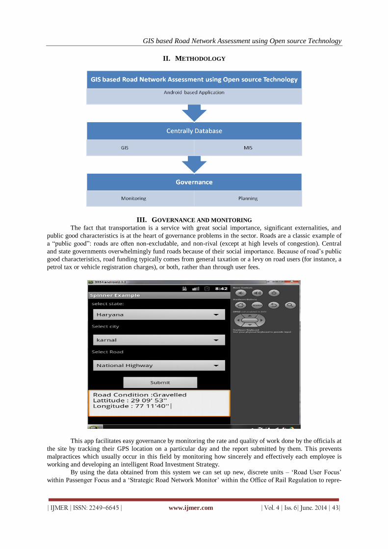
GIS based Road Network Assessment using Open source Technology
| IJMER | ISSN: 2249–6645 | www.ijmer.com | Vol. 4 | Iss. 6| June. 2014 | 43|
II. METHODOLOGY
III. GOVERNANCE AND MONITORING The fact that transportation is a service with great social importance, significant externalities, and
public good characteristics is at the heart of governance problems in the sector. Roads are a classic example of
a “public good”: roads are often non-excludable, and non-rival (except at high levels of congestion). Central
and state governments overwhelmingly fund roads because of their social importance. Because of road‟s public
good characteristics, road funding typically comes from general taxation or a levy on road users (for instance, a
petrol tax or vehicle registration charges), or both, rather than through user fees.
This app facilitates easy governance by monitoring the rate and quality of work done by the officials at
the site by tracking their GPS location on a particular day and the report submitted by them. This prevents
malpractices which usually occur in this field by monitoring how sincerely and effectively each employee is
working and developing an intelligent Road Investment Strategy.
By using the data obtained from this system we can set up new, discrete units – „Road User Focus‟
within Passenger Focus and a „Strategic Road Network Monitor‟ within the Office of Rail Regulation to repre-

GIS based Road Network Assessment using Open source Technology
| IJMER | ISSN: 2249–6645 | www.ijmer.com | Vol. 4 | Iss. 6| June. 2014 | 44|
sent the interests of all those who use and rely upon the strategic road network, and to monitor the efficiency
and performance of the workers.
During emergencies, it is critical for the road management authorities to be able to collect and report
current road status and damage assessments in a consistent and timely manner. Use of this application would
enable the corresponding supervisors and managers to deploy limited department resources most effectively. In
addition this app provides current road status information and report on the progress of response activities.
The major goal of the project is to minimize the lag time between obtaining a report in the field and
providing that report to decision makers in the command centers. The development team accomplishes this by
providing communication between the Road Status/Damage Assessment (RSDA) field tool and a multiuser geo
database. When a PWD network connection is available (through a field office or secure VPN), RSDA will
transfer new and revised reports to the enterprise geo database using the Upload tool. This capability greatly
improves reporting speed.
Thus it helps to put in place a robust system of governance for road surveillance, giving the road oper-
ator the flexibility needed to operate, manage and enhance the strategic road network effectively, while ensur-
ing clear accountability to the Secretary of State, Parliament and road users.
IV. THE MANAGEMENT INFORMATION SYSTEM (MIS) This Application is link to centrally database server. From this database server we can generate serval
MIS as well as GIS reports. Management information system, or MIS, broadly refers to a computer-based
system that provides managers with the tools to organize, evaluate and efficiently manage departments within
an organization. In order to provide past, present and prediction information, the management information
system here includes software that helps in decision making, data resources such as centralized database,
the hardware resources of a system, decision support systems, people management and project management
applications, and any computerized processes that enable the department to run efficiently.
The centralized database provides data integrity. With all the information centralized, it is much
easier to develop reports that show the details of the work done on a particular road in the past . With multiple
databases, records need to be matched, de-duping needs to occur, and the opportunity for duplicate records is
greatly increased. Here the MIS manager with the help of centralized database can typically analyze the report
and take controlled decisions thereby avoiding duplication in the process of resurfacing of roads. Thus MIS
brings coordination and makes control easier.
This app makes use of the SQL Server as the centralized database containing information about the
road conditions in various cities of different states in India. Thus a user can view with ease all the data
corresponding to a road in particular location with a simple tap of his finger. The user can retrieve information
such as when the road was last resurfaced and how many times was it resurfaced in the past 10 years. The user
can also view the list of all roads that are presently in poor condition in a particular city and need to be
resurfaced.

GIS based Road Network Assessment using Open source Technology
| IJMER | ISSN: 2249–6645 | www.ijmer.com | Vol. 4 | Iss. 6| June. 2014 | 45|
V. POSSIBLE FUTURE IMPROVEMENTS PWD emergency operations centers can be set up in every state that use information collected by
RSDA to prioritize repair and cleanup work. The map-based view of damage assessments can provide crews
with a view of problems nearby, allowing more work to be accomplished on a single trip. The RSDA Viewer
could be provided and thus by using the same operational picture at both locations, the state and county can
coordinate their response activities better.
This application can be used for assessment of the hazardous materials transport risk in a multi-
commodity, multiple origin – destination setting. The risk assessment methodology can be integrated with a
Geographical Information System (GIS), which can make large-scale implementation possible. A GIS-based
model of the shipments of dangerous goods via the highway network can be developed. Based on the origin
and destination of each shipment, the risk associated with the routes that minimize (1) the transport distance,
(2) the population exposure, (3) the expected number of people to be evacuated in case of an incident, and (4)
the probability of an incident during transportation can be evaluated. Using these assessments, a government
agency can estimate the impact of alternative policies that could alter the carriers‟ route choices. A related
issue is the spatial distribution of transport risk, because an unfair distribution is likely to cause public concern.
Thus, an analysis of transport risk equity in every state can be provided.
VI. CONCLUSION A proper implementation of this app would be useful to a large section of people in different ways.
Common people can use it as a reference while travelling in order to decide which road to take. The GPS
feature used in this app helps track the current user location and provide details based on it. This app provides
the PWD department with the necessary data about the condition of the roads which helps them to take
necessary actions for the development of an efficient transportation system in the city. With proper centralized
road network assessment data in hand the PWD department can plan the budget accordingly and allocate
money for the same. At the same time ensuring that the same road is not resurfaced repeatedly irrespective of
its condition.
Thus implementing an e-Governance of roads through mobile apps and various other software ensures
improvements in planning, implementation and operation of the road sector through provision of timely,
reliable, sufficient and accurate detailed data which will facilitate the decision making activities.
ACKNOWLEDGEMENTS The authors like to express their sincere thanks to Shri T.P. Singh, Director, Bhaskarcharya Institute
for Space Applications and Geo-informatics (BISAG), Department of Science & Technology, Government of
Gujarat, Gandhinagar-382 007 for his constant encouragement, guidance and kind permission to carry out this
project.
REFERENCES
Books: [1] Shane Conder and Lauren Darcey, Android Wireless Application Development (Addisen-Wesely, Boston,2010).
[2] GIS Fundamentals, 4th Edition. Softcover available for $39, from Atlas Books, www.atlasbooks.com, 800-247-
6553. ISBN 978-0-9717647-3-6
[3] www.gislounge.com/free-gis-books/
Internet: [4] http://www.w3schools.com
[5] http://www.javacodegeekss.com
[6] http://youtube.com –video tutorials
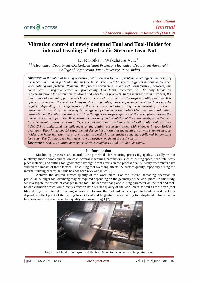
International
OPEN ACCESS Journal
Of Modern Engineering Research (IJMER)
| IJMER | ISSN: 2249–6645 | www.ijmer.com | Vol. 4 | Iss. 6| June. 2014 | 46|
Vibration control of newly designed Tool and Tool-Holder for
internal treading of Hydraulic Steering Gear Nut
D. R Kotkar1, Wakchaure V. D2
1, 2 (Mechanical Department (Design),
Assistant Professor Mechanical Department Amrutvahini
College of Engineering, Pune University, Pune, India)
I. Introduction Machining processes are manufacturing methods for ensuring processing quality, usually within
relatively short periods and at low cost. Several machining parameters, such as cutting speed, feed rate, work
piece material, and cutting tool geometry have significant effects on the process quality. Many researchers have
studied the impact of these factors. The cutting tool overhang affects the surface quality, especially during the
internal turning process, but this has not been reviewed much [9].
Achieve the desired surface quality of the work piece. For the internal threading operation in
particular, a longer tool overhang may be required depending on the geometry of the work piece. In this study,
we investigate the effects of changes in the tool –holder over hang and cutting parameter on the tool and tool-
holder vibration which will directly effect on both surface quality of the work piece as well as tool wear (tool
life), during the internal threading operation. Because the tool holder is subject to bending and buckling
depend on effect point of the cutting force (Axial and tangential force), cutting tool displaced. This situation
has negative effects on the surface quality as shown in Fig.1 [2]
Fig 1: Tool holder undergoing deflection, δ due to the Axial and tangential force
Abstract: In the internal turning operation, vibration is a frequent problem, which affects the result of
the machining and in particular the surface finish. There will be several different actions to consider
when solving this problem. Reducing the process parameters is one such consideration; however, this
could have a negative effect on productivity. Our focus, therefore, will be easy hands on
recommendations for productive solutions and easy to use products. In the internal turning process, the
importance of machining parameter choice is increased, as it controls the surface quality required. It is
appropriate to keep the tool overhang as short as possible; however, a longer tool overhang may be
required depending on the geometry of the work piece and when using the hole-turning process in
particular. In this study, we investigate the effects of changes in the tool–holder over hang and cutting
parameter on the vibration which will directly effect on surface quality of the work piece, during the
internal threading operation. To increase the buoyancy and reliability of the experiments, a full Taguchi
L9 experimental design was used. Experimental data controlled were tested with analysis of variance
(ANOVA) to understand the influences of the cutting parameter along with changes in tool-Holder
overhang. Taguchi method L9 experimental design has shown that the depth of cut with changes in tool-
holder overhang has significant role to play in producing the surface roughness followed by constant
feed rate. The Cutting speed has lesser role on surface roughness from the tests.
Keywords: ANOVA, Cutting parameter, Surface roughness, Tool- Holder Overhang.

Vibration control of newly designed Tool and Tool-Holder for internal treading of Hydraulic
| IJMER | ISSN: 2249–6645 | www.ijmer.com | Vol. 4 | Iss. 6| June. 2014 | 47|
The determination of optimal cutting condition and tool-holder overhang for specified surface
roughness and accuracy of product are the key factors in the selection of machining process. Internal threading
operations are associated with serious vibration-related problems. To reduce the problem of vibration and
ensure that the desired shape and tolerance are achieved, extra care must be taken with production planning
and in the preparations for the machining of a work-piece. A thorough investigation of the vibrations involved
is therefore an important step toward solving the problem. In internal threading operation, the performances of
cutting tools are depending on a few cutting conditions and parameters. The proper selection of depth of cut
has direct effect to the product surface roughness. Internal turning process by maximizing cutting speed and
depth of cut will optimize the cutting process and minimize the production cost. The tool life, machined
surface integrity and cutting forces are directly dependent on cutting parameters and will determine the cutting
tool performances. The study of surface roughness form will resolve the characteristic and phenomena
happening during the machining process. The questions to be answered at the end of the study are how the tool
overhangs length and diameter influences the surface roughness during internal threading operation. The study
was carried out to investigate the effects of cutting tool overhang and cutting parameter on the surface quality
in internal threading processes. Because the tool holder is subject to bending and buckling depend on effect
point of the cutting force (Axial and tangential force), cutting tool displaced.(1) To evaluate the effects of
different process parameter on internal threading operation.(2) To develop a mathematical model for
predicting surface roughness for internal threading operation by using design of experiment approach.(3)
Study the microstructure of the work piece internal threading operation. Machining operations tend to leave
characteristic evidence on the machined surface [10].
The Taguchi process helps to select or to determine the optimum cutting conditions with proper tool-
holder overhang for internal threading operation. Many researchers developed many mathematical models to
optimize the cutting parameters to get lowest surface roughness by internal turning process. The variation in
the material hardness, alloying elements present in the work piece material and other factors affecting surface
finish and tool wear [4].
II. System Description And Design
2.1. MATERIAL SELECTION
2.1.1 Tool holder: - 20MnCr
Table 2.1.1.a):-Chemical Composition of Tool Holder 20MnCr5.
Fig 2.1.1.a) Drawing of Tool Holder
2.1.2 TOOL: - High speed steel (HSS)
Grade
C
%
Si
%
Mn% Cr% S% Other
20MnCr5 0.20 0.25 1.25 1.15 0.035 Pb
Grade C
%
Vanadium
%
Tungsten
%
Cr%
HSS 0.7 1.00 18.00 4.00

Vibration control of newly designed Tool and Tool-Holder for internal treading of Hydraulic
| IJMER | ISSN: 2249–6645 | www.ijmer.com | Vol. 4 | Iss. 6| June. 2014 | 48|
Fig 2.1.2.a) Drawing of HSS Tool
2.1.3 WORK PIECE: - 17CrNimo6
Mechanical Properties of 17CrNiMo6:-
Fig 2.1.3.a) Drawing of Work piece
2.2. DESIGN OF EXPERIMENT
It is methodology based on statistics and other discipline for arriving at an efficient and effective
planning of experiments with a view to obtain valid conclusion from the analysis of experimental data. Design
of experiments determines the pattern of observations to be made with a minimum of experimental efforts. To
be specific Design of experiments (DOE) offers a systematic approach to study the effects of multiple variables
/ factors on products / process performance by providing a structural set of analysis in a design matrix. More
specifically, the use of orthogonal Arrays (OA) for DOE provides an efficient and effective method for
determining the most significant factors and interactions in a given design problem. [11]
Table No.2.2: Level of Experimental Parameters
2.3 EXPERIMENTAL SETUP
The experimental setup and layout diagram for this project are as shown in figure 8 and8.1
respectively. It includes a MKU-8 CNC turning lathe.
Grade C% Cr Mn% Si% P% S% Ni
17CrNiM06 0.15-0.21 1.50-1.8 0.50-0.90 0.4 0.025 0.015 1.40-1.7
Parameter Level I Level II Level III
Cutting speed 250 300 350
D.O.C 0.16 0.18 0.20
Tool holder Overhang 3.54 3.95 4.37

Vibration control of newly designed Tool and Tool-Holder for internal treading of Hydraulic
| IJMER | ISSN: 2249–6645 | www.ijmer.com | Vol. 4 | Iss. 6| June. 2014 | 49|
Fig 2.3 EXPERIMENTAL SETUP
In this study, I selected the Speed, DOCs and tool overhang as variable experimental parameters and
keeping feed rate constant and measured the surface roughness of the work piece. Our experimental studies
were carried using a CNC turning Lathe. As the cutting tool, we used HSS and Tool-Holder. The work pieces
used in the experiments were 40 mm (External) and 32 (internal) in diameter and Length 45mm. The
Company provided information about selection of the work piece material which is 17CrNiMo6, The tool
overhang lengths were 85, 95 and 105 mm. The DOCs we selected were 0.16, 0.18and 0.20 mm. The cutting
speed was selected as 250, 300 and 350 rpm and constant feed rate 14±0.01 mm/rev (for internal Threading
pitch is the feed rate). The external turning processes were carried out using the anticipated parameters. The
processes can be seen Fig 8.1.
A Carl Zeiss Surface Roughness measuring instrument show in Figure 3.4 was used to process the
measured profile data. The Carl Zeiss Surface Roughness measuring instrument is capable of evaluating
surface textures including waviness with the variety of parameters according to various digitally/graphically on
the touch panel and output to built-in printer. The stylus of the Carl Zeiss Surface Roughness measuring
instrument detector unit traces the minute irregularities of the work piece surface. Surface roughness is
determined from the vertical stylus displacement produced during the detector traversing over the surface
irregularities and the measuring setup shows in Fig 4. The Lathe Tool VM=82 Vibrometer has been designed
so that sensor can be directly fixed on to the tool- Holder. The dynamometer can measure 2 forces in mutually
perpendicular directions, i.e. Axial and Tangential. Cutting condition need to setup in this experiment, to
make sure all the experiment run follow according the data given. A fractional factorial is selected so that all
intersection between the independent variables could be investigated. The dependent variable is the resulting
first 28 cut surface roughness. The level was selected to cover the normal cutting operation [6]
2.4 FINAL EXPERIMENTATION
Design of Experiment (DOE) approach is selected for investigation effect of varying controllable
parameter and Overhang of Tool-Holder on acceleration at three levels, since Taguchi design of 9 runs is
efficient to study the effect of two or more factors these three levels of factor are referred as low, intermediate
& high level. In this experiment amplitude of vibration and surface roughness are measured with and without
damping pad.

Vibration control of newly designed Tool and Tool-Holder for internal treading of Hydraulic
| IJMER | ISSN: 2249–6645 | www.ijmer.com | Vol. 4 | Iss. 6| June. 2014 | 50|
Table 2.4.1 Observation Table
III. Results And Discussion
3.1 EFFECT AND COMPARISONS OFWITH & WITHOUT SLEEVE.
The vibration phenomenon for various cutting condition has been analyzed using Lab VIEW software.
The plan of the experiment was developed not only to assess the effect of cutting speed, depth of the cut and
overhang but also to study the effect of damping pad (sleeve) on the cutting tool vibration, surface roughness.
Table 8.3 illustrates the experimental result of vibration in both tangential and axial cutting direction. After
analysis of the vibration, sleeve is provided to tool-Holder for fitting into the turret of the CNC Lathe. Now the
same experiment was carried out for various cutting condition and with and without sleeve, also corresponding
cutting tool vibration and surface roughness are measured.
1 2 3 4 5 6 7 8 9
Series 1 1.51 1.74 2.55 1.94 2.85 2.09 2.55 2.31 2.4
Series 2 1.24 1.55 2.27 1.64 2.1 1.77 2.05 1.95 1.97
1.511.74
2.55
1.94
2.85
2.09
2.552.31 2.4
1.241.55
2.27
1.64
2.11.77
2.05 1.95 1.97
0
0.5
1
1.5
2
2.5
3
RM
S V
alu
e
Readings
Graph 3.1.1 Comparison of with sleeve & without sleeve Base on Axial Vibration
From Graph 3.1.1 it is observed that after using sleeve as damping pad, axial acceleration of machine
tool is get reduced.
Sr.No C.S D.O.C L/D Amplitude of Acceleration of Tool-Holder
in m/s2
Surface Roughness
Ra in µm
Axial
direction(R.M.S))
Tangential
direction (R.M.S)
Without
sleeve
With
Sleeve
Without
sleeve
With
sleeve
Without
sleeve
With
sleeve
1 250 0.16 3.54 1.51 1.24 0.34 0.26 3.19 3.08
2 250 0.18 3.95 1.74 1.55 0.37 0.28 3.22 3.12
3 250 0.20 4.37 2.55 2.27 0.44 0.31 3.88 3.35
4 300 0.16 3.95 1.94 1.64 0.33 0.27 3.46 3.32
5 300 0.18 4.37 2.85 2.10 0.54 0.36 4.56 3.39
6 300 0.20 3.54 2.09 1.77 0.49 0.29 3.37 3.27
7 350 0.16 4.37 2.55 2.05 0.55 0.39 4.77 3.92
8 350 0.18 3.54 2.31 1.95 0.51 0.32 3.86 3.76
9 350 0.20 3.95 2.40 1.97 0.48 0.31 4.02 3.89
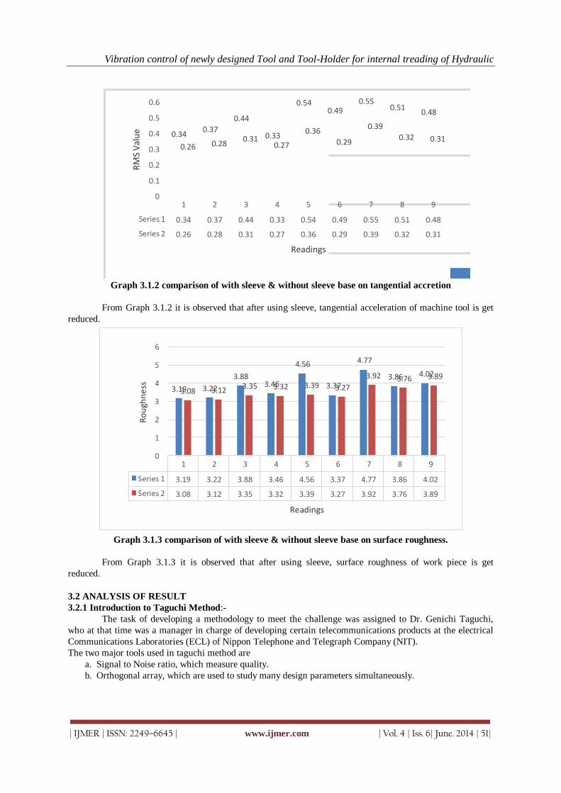
Vibration control of newly designed Tool and Tool-Holder for internal treading of Hydraulic
| IJMER | ISSN: 2249–6645 | www.ijmer.com | Vol. 4 | Iss. 6| June. 2014 | 51|
1 2 3 4 5 6 7 8 9
Series 1 0.34 0.37 0.44 0.33 0.54 0.49 0.55 0.51 0.48
Series 2 0.26 0.28 0.31 0.27 0.36 0.29 0.39 0.32 0.31
0.340.37
0.44
0.33
0.540.49
0.550.51
0.48
0.26 0.280.31
0.27
0.36
0.29
0.39
0.32 0.31
0
0.1
0.2
0.3
0.4
0.5
0.6
RM
S V
alu
e
Readings
Graph 3.1.2 comparison of with sleeve & without sleeve base on tangential accretion
From Graph 3.1.2 it is observed that after using sleeve, tangential acceleration of machine tool is get
reduced.
1 2 3 4 5 6 7 8 9
Series 1 3.19 3.22 3.88 3.46 4.56 3.37 4.77 3.86 4.02
Series 2 3.08 3.12 3.35 3.32 3.39 3.27 3.92 3.76 3.89
3.19 3.22
3.883.46
4.56
3.37
4.77
3.86 4.02
3.08 3.12 3.35 3.32 3.39 3.27
3.92 3.76 3.89
0
1
2
3
4
5
6
Ro
ugh
ne
ss
Readings
Graph 3.1.3 comparison of with sleeve & without sleeve base on surface roughness.
From Graph 3.1.3 it is observed that after using sleeve, surface roughness of work piece is get
reduced.
3.2 ANALYSIS OF RESULT
3.2.1 Introduction to Taguchi Method:-
The task of developing a methodology to meet the challenge was assigned to Dr. Genichi Taguchi,
who at that time was a manager in charge of developing certain telecommunications products at the electrical
Communications Laboratories (ECL) of Nippon Telephone and Telegraph Company (NIT).
The two major tools used in taguchi method are
a. Signal to Noise ratio, which measure quality.
b. Orthogonal array, which are used to study many design parameters simultaneously.

Vibration control of newly designed Tool and Tool-Holder for internal treading of Hydraulic
| IJMER | ISSN: 2249–6645 | www.ijmer.com | Vol. 4 | Iss. 6| June. 2014 | 52|
3.2.2 Classification of Parameters
In the basic design process, a number of parameters can influence the quality characteristic or
response of the product. These can be classified into the following three classes and shown below in the block
diagram of a product/process design.
Fig 3.2.2: Design block diagram of product/process
The response for the purpose of optimization in the robust design is called the quality characteristic.
The different parameters, which can influence this response, are described below.
1. Signal Factors: These are parameters set by the user to express the intended value for the response of
the product. Example- Speed setting of a fan is a signal factor for specifying the amount of breeze.
Steering wheel angle – to specify the turning radius of a car.
2. Noise Factors: Parameters which cannot be controlled by the designer or parameters whose settings are
difficult to control in the field or whose levels are expensive to control are considered as Noise factors.
The noise factors cause the response to deviate from the target specified by the signal factor and lead to
quality loss.
3. Control Factors: Parameters that can be specified freely by the designer. Designers have to determine
best values for these parameters to result in the least sensitivity of the response to the effect of noise
factors.
The levels of noise factors change from unit to unit, one environment to another and from time to
time. Only the statistical characteristics (mean & variance) can be known or specified. The noise factors cause
the response to deviate from the target specified by the signal factor and lead to quality loss.
3.2.3 Orthogonal array
Orthogonal array is an important technique in robust design. It gives more reliable estimates of factor
effects with fewer experiments when compared to the traditional methods such as one factor at a time
experiments. Consequently more factors can be studies leading to more robust and less expensive products.
The columns of an orthogonal array are pair wise orthogonal that is for every pair of columns, all combinations
of factor levels occur an equal number of times. The columns of an orthogonal array represent factors to be
studied and rows represent individual experiments. Orthogonal array used for variety of purposes in robust
design they are used to study the effects of control factors, noise factors, Evaluation of S/N ratio etc.
3.2.4 Signal to Noise ratio
In Taguchi method, the signal to noise ratio is used to measure the quality characteristics deviating
from the desired value. S/N ratio developed by Genichi Taguchi, is a predictor of quality loss after making
certain simple adjustments to the product’s function. It isolates the sensitivity of the product’s function to
noise factors. The signal to noise ratios (S/N) are log functions of desired output, serve as the objective
functions for optimization, help in data analysis and the prediction of the optimum results.
Depending upon the objective of the robust parameter design experiment, Taguchi defined three different
statistics called signal to noise ratios. These ratios were defined as the means to measure the variation of the
Product/Process Response
Signal factors
Noise factors
Control factors

Vibration control of newly designed Tool and Tool-Holder for internal treading of Hydraulic
| IJMER | ISSN: 2249–6645 | www.ijmer.com | Vol. 4 | Iss. 6| June. 2014 | 53|
response with respect to the noise factors .There are three forms of signal to noise (S/N) ratio that are common
interest for optimization of static problems.
Smaller-the-better expressed as
η = -10Log [mean of sum of squares of measured data]
This is usually the chosen S/N ratio for all the undesirable characteristics like defects for which the ideal value
is zero. When an ideal value is finite and its maximum or minimum value is then the difference between the
measured data and the ideal value is expected to be as small as possible. Thus, the generic form of S/N ratio
becomes,
η = -10Log [mean of sum of squares of measured-ideal]
Larger-the-better expressed as
η = -10Log [mean of sum of squares of reciprocal of measured data]
Nominal-the-better expressed as
η = -10 Log [square of mean/variance]
3.3 Analysis of variance
The purpose of analysis of variance (ANOVA) is to investigate which design parameters significantly
affect the quality characteristic. This is accomplished by separating the total variability of the signal to noise
ratios, which is measured by the sum of the squared deviations from the total mean S/N ratio, into
contributions by each of the design parameters and error. [9]
The S/N ratio is evaluated using the equation.
S/N ratio = -10Log (MSD)
The effect of parameter level is defined as the deviation it causes from the overall mean. Hence as a first step,
calculating the overall mean value of S/N ratio for the experimental region defined by the factor levels in Table
6.3.
Mean= = ( + +….. )
The signal to noise ratios nine set of experiments shown in Table 6.The mean and the S/N ratios are.
*S/N Ratio= -10Log(n)²
*Sum of square due to parameter A=
[(number of experiments at level A1)x (mA1-m)]+
[(number of experiments at level A2)x (mA2-m)]
+[(number of experiments at level A3)x (mA3-m)]. Where m= medium of S/N Ratio
3.3.A) Average S/N for different parameter levels for axial acceleration
Table 3.3.A.1: Average S/N for different parameter levels Optimum setting A1 B1 C1
Table 3.3.A.2: ANOVA for S/N ratio of axial acceleration
Symbol DOF Parameters Sum of squares Mean square F Contribution (%)
A. 2 CS 4.4121 2.206
29.21
B. 2 DOC 5.3341 2.66 1.20 35.31
C. 2 L/D 5.3578 2.67 1.21 35.47
Error 2 4.4121
Total 6 15.1040
Error 2 4.4121 2.205
Parameters Levels
1 2 3
A CS -4.264* -5.233 -5.974
B DOC -4.133* -5.350 -5.989
C L/D -4.209* -4.663 -5.959
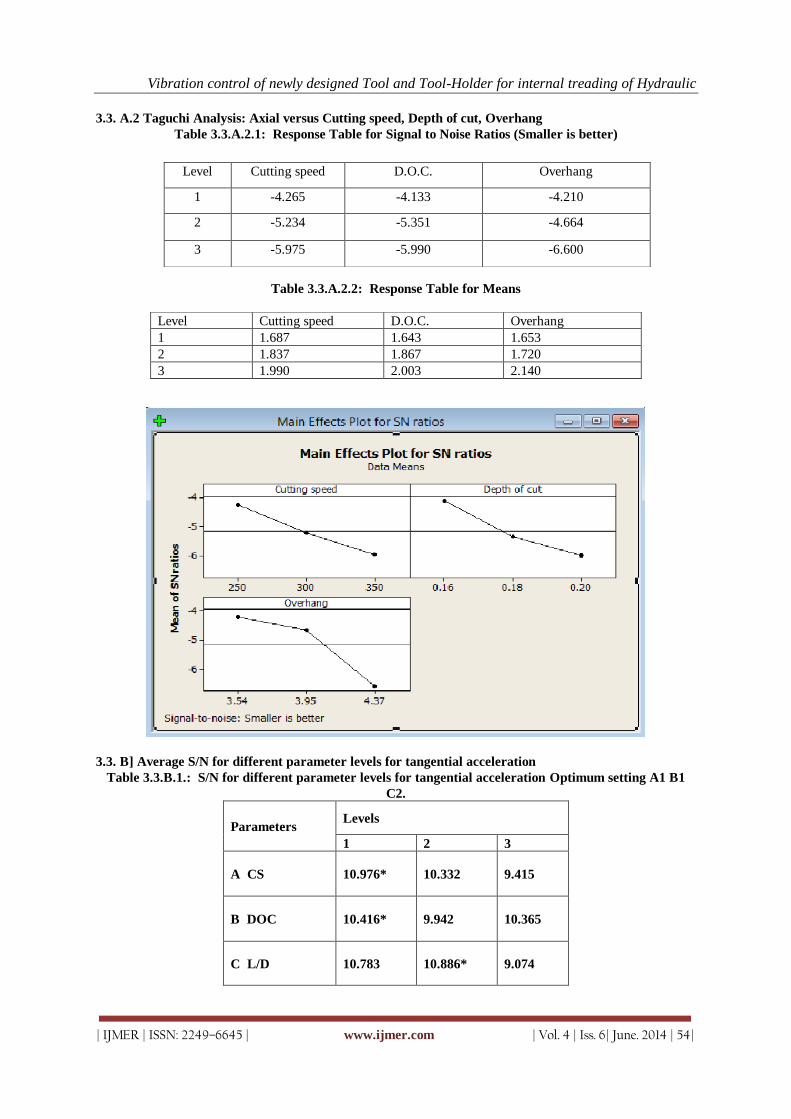
Vibration control of newly designed Tool and Tool-Holder for internal treading of Hydraulic
| IJMER | ISSN: 2249–6645 | www.ijmer.com | Vol. 4 | Iss. 6| June. 2014 | 54|
3.3. A.2 Taguchi Analysis: Axial versus Cutting speed, Depth of cut, Overhang
Table 3.3.A.2.1: Response Table for Signal to Noise Ratios (Smaller is better)
Table 3.3.A.2.2: Response Table for Means
3.3. B] Average S/N for different parameter levels for tangential acceleration
Table 3.3.B.1.: S/N for different parameter levels for tangential acceleration Optimum setting A1 B1
C2.
Parameters Levels
1 2 3
A CS 10.976* 10.332 9.415
B DOC 10.416* 9.942 10.365
C L/D 10.783 10.886* 9.074
Level Cutting speed D.O.C. Overhang
1 -4.265 -4.133 -4.210
2 -5.234 -5.351 -4.664
3 -5.975 -5.990 -6.600
Level Cutting speed D.O.C. Overhang
1 1.687 1.643 1.653
2 1.837 1.867 1.720
3 1.990 2.003 2.140

Vibration control of newly designed Tool and Tool-Holder for internal treading of Hydraulic
| IJMER | ISSN: 2249–6645 | www.ijmer.com | Vol. 4 | Iss. 6| June. 2014 | 55|
Table 3.3.B.2: ANOVA for S/N ratio Of Tangential acceleration
Symbol DOF Parameters Sum of
squares
Mean
square F
Contribution
(%)
A. 2 CS 3.6923 1.8461 9.0896 39.35
B. 2 DOC 0.4058 0.2031
4.32
C. 2 L/D 5.2838 2.6419 13.00 56.31
Total 6 9.3819
Error 2 0.4058 0.2031
3.3. B.3 Taguchi Analysis: Tangential versus Cutting speed, Depth of cut, Overhang
Table 3.3.B.3: Response Table for Signal to Noise Ratios Smaller is better
Table 3.3.B.4: Response Table for Means
3.3. C] Average S/N for different parameter levels for surface roughness. Table 3.3.C.1 Average S/N for different parameter levels for surface roughness Optimum setting A1 B2
C1
Parameters Levels
1 2 3
A CS -10.051* -10.438 -11.722
B DOC -10.686 -10.663* -10.862
C L/D -10.521* -10.701 -10.989
Table 3.3.C.2: ANOVA for S/N ratio of surface roughness
Level Cutting speed D.O.C. Overhang
1 10.977 10.417 10.783
2 10.333 9.943 10.867
3 9.416 10.366 9.075
Level Cutting speed D.O.C. Overhang
1 0.2833 0.3067 0.2900
2 0.3067 0.3200 0.2867
3 0.3400 0.3033 0.3533
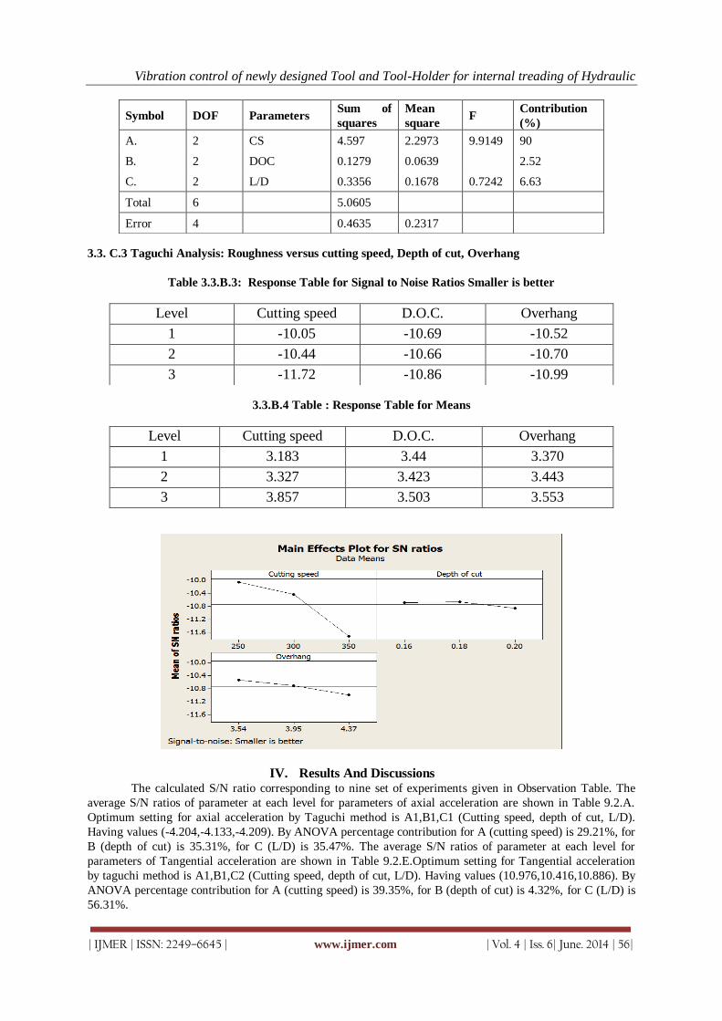
Vibration control of newly designed Tool and Tool-Holder for internal treading of Hydraulic
| IJMER | ISSN: 2249–6645 | www.ijmer.com | Vol. 4 | Iss. 6| June. 2014 | 56|
3.3. C.3 Taguchi Analysis: Roughness versus cutting speed, Depth of cut, Overhang
Table 3.3.B.3: Response Table for Signal to Noise Ratios Smaller is better
3.3.B.4 Table : Response Table for Means
IV. Results And Discussions The calculated S/N ratio corresponding to nine set of experiments given in Observation Table. The
average S/N ratios of parameter at each level for parameters of axial acceleration are shown in Table 9.2.A.
Optimum setting for axial acceleration by Taguchi method is A1,B1,C1 (Cutting speed, depth of cut, L/D).
Having values (-4.204,-4.133,-4.209). By ANOVA percentage contribution for A (cutting speed) is 29.21%, for
B (depth of cut) is 35.31%, for C (L/D) is 35.47%. The average S/N ratios of parameter at each level for
parameters of Tangential acceleration are shown in Table 9.2.E.Optimum setting for Tangential acceleration
by taguchi method is A1,B1,C2 (Cutting speed, depth of cut, L/D). Having values (10.976,10.416,10.886). By
ANOVA percentage contribution for A (cutting speed) is 39.35%, for B (depth of cut) is 4.32%, for C (L/D) is
56.31%.
Symbol DOF Parameters Sum of
squares
Mean
square F
Contribution
(%)
A. 2 CS 4.597 2.2973 9.9149 90
B. 2 DOC 0.1279 0.0639
2.52
C. 2 L/D 0.3356 0.1678 0.7242 6.63
Total 6 5.0605
Error 4 0.4635 0.2317
Level Cutting speed D.O.C. Overhang
1 -10.05 -10.69 -10.52
2 -10.44 -10.66 -10.70
3 -11.72 -10.86 -10.99
Level Cutting speed D.O.C. Overhang
1 3.183 3.44 3.370
2 3.327 3.423 3.443
3 3.857 3.503 3.553

Vibration control of newly designed Tool and Tool-Holder for internal treading of Hydraulic
| IJMER | ISSN: 2249–6645 | www.ijmer.com | Vol. 4 | Iss. 6| June. 2014 | 57|
The average S/N ratios of parameter at each level for parameters of surface Roughness are shown in
Table 9.2.I.Optimum setting for Roughness by taguchi method is A1,B2,C1 (Cutting speed, depth of cut, L/D).
Having values (-10.051,-10.663,-10.521). By ANOVA percentage contribution for A (cutting speed) is 90%,
for B (depth of cut) is 2.52%, for C (L/D) is 6.63%.
As we know that tangential acceleration is much lesser than axial acceleration. Hence it can be
neglected for overall optimum selection of parameters. Value of cutting speed is same for all above which is
250 rpm. Value of D.O.C. has large contribution in axial acceleration than others. Hence D.O.C. is selected for
axial acceleration, which is (B1) 0.16mm. Value for L/D Ratio has large contribution in axial acceleration as
tangential acceleration has been neglected. Hence the value of L/D ratio is 3.54.
4.1 Conclusion of Taguchi Method In this study, the optimum parameter for high percentage yield was selected by varying parameters
through Taguchi method. With an orthogonal array (L-9) a total set of nine experiments having three
parameters each at three levels indicated that the Taguchi method was an efficient method of determining the
optimum parameters for internal threading of hydraulic steering gear nut. ANOVA helped to estimate the
contribution of each parameter in Axial, Tangential Acceleration & Roughness values.
4.2 Conclusions & Recommendations for Future
4.2.1 Conclusions From Analytical Calculations, Graphs, and Taguchi Analysis conclusions Interpreted are as follows:
By using passive Damping (sleeve) machine tool vibration is minimize.
Sleeve having good damping capacity which results into less vibration, less average tool temperature
and good surface finish
Overhang is major influencing parameter for combine axial acceleration and surface roughness.
Cutting speed and depth of cut are closely correlated to axial acceleration and surface roughness.
4.2.2 Recommendations for Future In many machining process vibration is one of the harmful factor which is minimize by controlling
cause parameter and using damper.
Passive damping:
Passive damping is use for present work, but damping capacity of passive damper is always constant
due to constant strength value .In machining processes intensity of vibration is varying but due to limitation of
vibration absorbing capacity proper damping is not possible. To achieve proper damping, needs a proper
damper which having varying damping capacity, this can be achieved by using active damping. For active
damping damper of MR fluid can be use, of which strength will change with single send by controller.
Controller takes signal from sensor which mounts on machine tool.
Tool-Holder Overhang:
The design and dimensions of the component decide the diameter and length of the Tool-Holder for
internal machining operation. Internal turning is very sensitive to vibration. Minimize the tool overhang and
select the largest possible tool size in order to obtain the best possible stability and accuracy.
REFERENCES [1] “E.J.A. Armarego, R.H. Brown, The Machining of Metals, Prentice-.Hall, Englewood Cliffs, (1969), PP 122-134.
[2] “Zhang, Bonifacio, A.E. Diniz, Correlating tool wear, tool life, surface.roughness, and vibration in finish urning
with coated carbide tools,Wear (1994),PP 137–144.
[3] “Industrial management &engineering” by A. K. Bewoor, PP. 50-26.
[4] “Adams Tooling structure: interface between cutting edge and machine tool Annals of the …..CIRP (2000), PP
591–634.
[5] M.B. Cai, et al., Crack initiation in relation to the tool edge radius and cutting conditions .in nanoscale cutting of
silicon, International Journal of Machine Tools and Manufacture …. (2007),PP 562–569.
[6] D. Zhang, D. Chen, Optimization of cutting parameters in vibration tapping of titanium ….alloys, Acta Aeronautica
et Astronautica Sinica 13 (10) (1992).PP (B571-B573), PP. 6-8.
[7] “Metal cutting machine tool’s” by G.Thirupati Reddy, 3rd edition.v, PP. 1-15.
[8] “Metal cutting machine tool’s” by G.Thirupati Reddy, 3rd edition, PP. 25-45.
[9] Sandvik Silent tools - user´s guide.
[10] Sandvik internal threading - user´s guide.

International
OPEN ACCESS Journal Of Modern Engineering Research (IJMER)
| IJMER | ISSN: 2249–6645 | www.ijmer.com | Vol. 4 | Iss. 6| June. 2014 | 58|
Suitability of Composite Material for Flywheel Analysis
Nagaraj.r.m PG Scholar, The oxford college of engineering Bangalore, India
I. Introduction In today’s society energy storage plays a vital role, where almost all the things we use for our day –to-
day life needs energy to work. Sometimes energy can be supplied directly or taken it from some kind of local
energy storage. Flywheel technology is a very bright future for storing energy. As Flywheels are very “green”
technology they have been widely used for a long time as mechanical energy storage devices.
It has rotating disk that stores energy as kinetic energy, spinning of flywheel decides how much amount
of energy it stores. S.M.Choudhary1, D.Y.Shahare [1] has proposed the creation of various profiles of flywheel according to the geometry and calculation of stored kinetic energy with respective flywheel profile. Xingjian
DAI, Kai ZHANG and Xiao-zhang[2] has given information regarding proper design of a flywheel energy
storage prototype to get high energy density and low bearing loss. Mainly finite element analysis is subjected to
analyse the different modes of the rim -hub- shaft system by using some tools. The testing of flywheel system is
carried out where complex non-synchronous vibration was observed, analysed and suppressed. O.J. Fiske, M.R.
Ricci[3] Figure out the comparison between materials used for flywheel as earlier days steel was widely used for
its strength but less energy storage density .Akshay P. Punde[4], has proposed the design and analysis of
flywheel which is a major part of an I.C.engine to bring the requirement for smoothing out the large
asynchronous oscillations in velocity during a process. Some flywheels possess poor energy storage in their own
therefore selection of material plays very important role. For energy storage we need low density materials so
the best option is composite materials so here we are using aluminium metal matrix composite for flywheel Here
we are using the test material properties for analysis purpose.
II. Evolution Of Tools CATIA (Computer Aided Three-dimensional Interactive Application):
Is one of the world’s most developing key solutions for product design and innovation which is
developed by dassault system. Mainly for advance structures it provides a better way to improve our ability to
accomplish the design to manufacture process. The way it approaches to the market is based on 3D experience
platform by providing a singular digital product experience as compared to the traditional 3D CAD software
Abstract: The paper deals with analysis of flywheel in which comparison of flywheel existing material
and test material are done. There must be proper design and analysis of flywheel in order to meet the
necessity to smooth out enormous oscillations in velocity that occur during a cycle of i.c.engine in a
flywheel. So here some finite element analysis tools are used for design and analysis purpose. Then results
are compared with existing material. Keywords:Arm type flywheel, material properties, FE analysis.

Suitability Of Composite Material For Flywheel Analysis
| IJMER | ISSN: 2249–6645 | www.ijmer.com | Vol. 4 | Iss. 6| June. 2014 | 59|
tools.Catia is back up for various stages of product development which includes computer aided design,
manufacturing, engineering etc. and also denoted to 3D product lifecycle management software suite. It
provides all kinds of positive facilities in the fields like plant design, automotive, defence, aerospace and in
some management areas. In catia we are creating 3D parts from sketches with respect to given dimensions.
ABAQUS:
Abaqus is a one of the most controlling engineering program which is centred by the finite element method, that have capability to solve all kind of problems ranging from modest linear analyses to the most interesting
nonlinear analyses occurring in engineering field. It is combination of three main stages and they are pre-
processing, simulation and post processing. Abaqus is able to model any geometry as well as can simulate the
behaviour of any engineering materials. It is widely used to find solutions in the areas like structural, fluid
dynamics, soil mechanics, heat transfer and thermal components etc. The role of abaqus in linear and non-linear
analysis is very important especially in non-linear analysis it chooses an appropriate values of load and tolerance
very neatly and automatically.
III. Modelling Of Flywheel Modelling plays very important role in design and it’s a first step to move to the analysis. Model of a
flywheel is created based on geometry assigned and it is shown below. Mainly two types of models are used for
analysis and they are 2-D modelling and 3-D modelling. These 2-D modelling and 3-D modelling are differ by
memory they consume and accuracy. For the accurate results flywheel is given in 3-D model which is shown
below.
Fig 2: Geometry of flywheel Fig 3: Flywheel 3-D model
IV. Flywheel Analysis
4.1. Material Properties The properties of two materials are given below.
Material Young’s
modulus€
Density Poisons ratio
Grey cast iron 101e3 7.5 0.23
Aluminium MMC’s(test material) 80.23e3 2.56 0.33
Table 1: Material properties
4.2. Element Type It is pertaining to the element solid 72, a 3dimension 8-noded tetrahedral structural solid with rotation
is used for meshing, depends upon the attention for rotational deformations in the flywheel. Mainly the element
is defined by 8 Nodes with 6 DOFs at each node which will be well proper solution to produce uneven meshes.
Abaqus programme controls the problem occurring with elements.
Element type (# elements)
C3D8R : (57120),
Table 2: Element type

Suitability Of Composite Material For Flywheel Analysis
| IJMER | ISSN: 2249–6645 | www.ijmer.com | Vol. 4 | Iss. 6| June. 2014 | 60|
4.3. Meshing Method Mainly in finite element methods there is a reduction of degrees of freedom from infinite to finite
which is called as meshing. For structural analysis quad and hex are preferred over tetras, pentas. Here
geometry size and shape have more values for meshing purpose. The meshing related diagrams are given below as per the nodes and elements chosen. Mesh is defined as a discrete representation of some spatial domain. We
have structural, unstructural, conformal mesh and hanging nodes.
Fig 4: Top view Fig 5: Isoview
Fig 6: Front view
4.4. Boundary Conditions and Loads In boundary condition all the six degrees of freedom are taken into account as region of a part selected
is based on angle and boundary condition type is displacement/rotation . As per the load consideration here
rotational body force is selected with angular velocity.
V. Results And Discussions A static analysis is performed on flywheel and determining stress and deformation. The below table
shows the discretisation of Flywheel into 57120 elements and 68214 nodes.
Instance
Name # Elements
#
Nodes
FLYWHEEL 57120 68214
Table 3: discretisation of Flywheel
Fig 7: total deformation fig 8: normal stress

Suitability Of Composite Material For Flywheel Analysis
| IJMER | ISSN: 2249–6645 | www.ijmer.com | Vol. 4 | Iss. 6| June. 2014 | 61|
5.1. Comparison of Results by Abaqus
Material used
Normal stress (Mpa)
Total deformation (m)
Test material 4.58e-01 8.29e-05
Grey cast iron 44.07 5.3399*e-04
Table 4: result comparisons
VI. Conclusion Thus we can conclude based on the work we carried out for a flywheel and the results what we got
from design and analysis methods that for energy storage low density and high strength is required in turns
stress and deformation should be low. So it is clear that, the existing grey cast iron flywheels are having more
Stress and deformation whereas the test material is comparatively low. Therefore the test material (aluminium
MMC’s) can be used in flywheel for high energy storing purpose with low density and less mass.
REFERANCES [1.] S.M.Choudhar “ Design Optimization of Flywheel of Thresher Using FEM” International Journal of Emerging
Technology and Advanced Engineering Website: www.ijetae.com (ISSN 2250-2459, ISO 9001:2008 Certified Journal, Volume 3, Issue 2, February 2013)
[2.] P.A.Hatwalne “ FLYWHEEL MOTOR-AN UPDATE” International Journal of Advanced Technology &
Engineering Research (IJATER) ISSN No: 2250-3536 Volume 2, Issue 6, Nov. 2012 [3.] O.J. Fiske, M.R. Ricci “Third Generation Flywheels For High Power Electricity Storage” Launch Point
Technologies, Inc., Goleta, California, USA [4.] Xingjian DAI, Kai ZHANG “Design and test of a 300Wh composites flywheel energy storage prototype with active
magnetic bearing”. [5.] Akshay P. Punde, 1 G.K.Gattani2 “analysis of flywheel” International Journal of Modern Engineering Research
(IJMER) www.ijmer.com Vol.3, Issue.2, March-April. 2013

International
OPEN ACCESS Journal Of Modern Engineering Research (IJMER)
| IJMER | ISSN: 2249–6645 | www.ijmer.com | Vol. 4 | Iss. 6| June. 2014 | 62|
Synthesis and characterization of Cu doped NiO nanoparticles
B. Ramasubba Reddy1, G. S. Harish
2, Ch. Seshendra Reddy
3,
P. Sreedhara Reddy4
1, 2, 3, 4 Department of Physics, Sri Venkateswara University, Tirupati, 517502, India
I. Introduction At present, nano-sized materials have attracted much attention because of their unusual properties
based on size-quantization effect and large surface area [1 - 3]. Nanosized nickel -oxide (NiO) is of great
interest because it exhibits particular catalytic [4, 5], anomalous electronic [6- 8], and magnetic [9– 12]
properties. NiO, as one of the relatively few metal oxides which exhibits p-type conductivity. It is a stable wide
band gap material and can be used as a transparent p-type semiconducting layer. Among transition metal oxides,
nickel oxide (NiO) has been received considerable attention due to their wide range of applications in various
fields, including catalysis [4, 5], electrochromic windows [13], and sensors [14]. The characteristic properties of
nanosized NiO particles also enable to tailor the properties for a variety of applications. In the present study, pure and copper doped NiO nanoparticles were synthesized using chemical co-precipitation method and studied
various properties like structural, compositional, morphological, luminescence and Raman studies.
II. Experimental details All chemicals were of analytical reagent grade and were used without further purification. Pure and Cu
doped NiO nanoparticles were prepared by chemical precipitation method. The reactants were NiCl2. 6H2O and
CuSO4.5H2O. Ultrapure de-ionized water was used as the reaction medium in all the synthesis steps. In a typical
synthesis, desired molar proportions of NiCl2. 6H2O and CuSO4.5H2O (0, 2, 4 and 6 at.%) each in 100 ml were
dissolved in ultrapure de-ionized water and stirred for 30 minutes, NaOH solution was drop wisely added to the solution to adjust the pH value to 10. Stirring was continued for four hours to get fine precipitation. The
obtained precipitate was washed with de-ionized water for several times. Finally, the powders were vacuum
dried for 3 hours at 80 0C to obtain pure and Cu doped NiO nanoparticles.
III. Characterization The X-ray diffraction patterns of the samples were collected on a Rigaku D X-ray diffractometer with
the Cu-Kα radiation (λ=1.5406A°). Morphology and elemental composition of the prepared samples were
analyzed through EDAX using Oxford Inca Penta FeTX3 EDS instrument attached to Carl Zeiss EVO MA 15
scanning electron microscope. Photoluminescence spectra were recorded in the wavelength range of 400–600 nm using PTI (Photon Technology International) Fluorimeter with a Xe-arc lamp of power 60 W and an
excitation wavelength of 320 nm was used. Raman Spectroscopic studies of the as prepared samples were
carried out using LabRam HR800 Raman Spectrometer.
IV. Results and discussion
4.1. Structural analysis by X-ray diffraction (XRD) The X-ray diffraction patterns for the Pure NiO and Cu doped nanoparticles are shown in Fig. 1. From
the figure it is obvious that the peaks are indexed as (111), (200), (220), (311) and (222) planes at 2θ values
37.39o, 43.45
o, 62.98
o, 75.5
o and 79.49
o that correspond to face centered cubic structure of NiO nanoparticles
which are in consistent with the JCPDS (No. 47-1049) data.
Abstract: Copper doped NiO nanoparticles were synthesized by chemical precipitation method and
studied the structural, compositional, morphological, luminescence and optical properties using X-ray
diffraction (XRD), Energy dispersive analysis of X-rays (EDAX), Scanning electron microscopy (SEM),
PL Fluorimeter and High Resolution Raman spectroscopy. XRD studies confirm the fcc structure of the
prepared samples. EDAX showed the effective doping of copper into NiO. For pure NiO, PL peak was
observed at 434 nm and an enhancement in the PL intensity was observed with increasing dopant
concentration. The Raman peak observed at 518 cm-1 confirms the Ni-O bonds and no impurity peaks
were observed due to dopant.
Keywords: Cu-doped NiO, XRD, RAMAN, EDAX

Synthesis and characterization of Cu doped NiO nanoparticles
| IJMER | ISSN: 2249–6645 | www.ijmer.com | Vol. 4 | Iss. 6| June. 2014 | 63|
Fig.1. XRD patterns of Pure and Cu doped NiO nanoparticles
The average particle size of Pure and Cu doped NiO nanoparticles was calculated using Debye–
Scherrer’s equation [a] by determining the width of the (200) Bragg’s reflection.
------------------ [a]
Where, D is the average particle size and βhkl is full width at half maximum of XRD peak expressed in
radians and θ is the position of the diffraction peak.
The average sizes of the particles prepared at different concentration of Pure NiO and Cu ( 2, 4 and 6 at.%) doped NiO nanoparticles were of 76, 64, 52 and 60 nm, respectively hence the decrease in particle size
with increasing doping concentration has predicted. Increase in particle size of Cu (6%) doped NiO
nanoparicles, may be due to interactions between neighboring Cu-Cu ions.
4.2. Compositional analysis
The EDAX profile of prepared Pure and Cu (2, 4 and 6 at %) doped NiO nanoparticles are shown in
Fig.2. It is evident from the EDAX Spectra, no other elemental peaks other than Ni, O and Cu are observed
except that only the elemental carbon arises due to adhesion of carbon tape on to the stud used in the analysis.
The results confirm the effective doping of Cu into NiO.

Synthesis and characterization of Cu doped NiO nanoparticles
| IJMER | ISSN: 2249–6645 | www.ijmer.com | Vol. 4 | Iss. 6| June. 2014 | 64|
Fig. 2. Representative EDS spectrum of prepared nanoparticles (a) Pure NiO, (b) Cu (2 at.%),
(c) Cu (4 at.%) and (d) Cu (6 at.%)
4.3. Morphological studies
The size and morphology of the Pure and Cu doped NiO nanoparticles were observed by SEM
measurements. The SEM images of Pure and Cu(2, 4 and 6 at.%) doped NiO nanoparticles were shown in Fig.
3(a), 3(b), 3(c) and 3(d) respectively.
Fig. 3. SEM images of (a) Pure NiO and (b) Cu( 2 at. %), (c) Cu(4 at.%) and (d) Cu( 6 at.%)
doped NiO nanoparticles
(a) (b)
(c) (d)
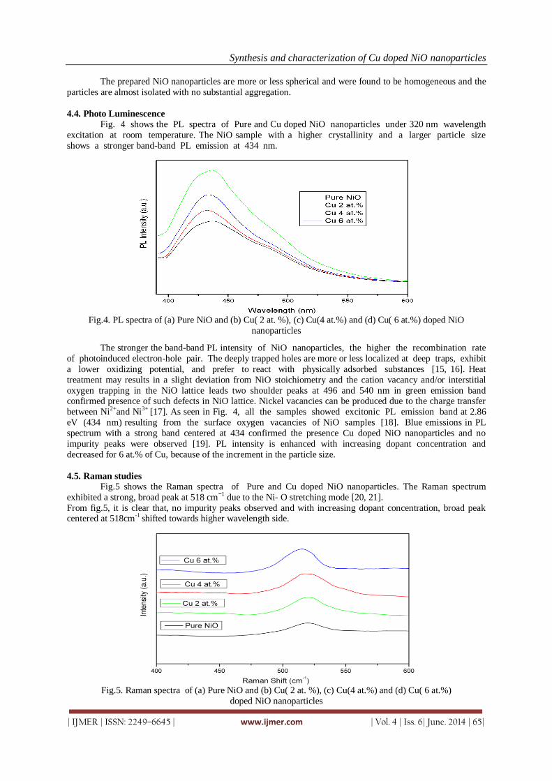
Synthesis and characterization of Cu doped NiO nanoparticles
| IJMER | ISSN: 2249–6645 | www.ijmer.com | Vol. 4 | Iss. 6| June. 2014 | 65|
The prepared NiO nanoparticles are more or less spherical and were found to be homogeneous and the
particles are almost isolated with no substantial aggregation.
4.4. Photo Luminescence
Fig. 4 shows the PL spectra of Pure and Cu doped NiO nanoparticles under 320 nm wavelength
excitation at room temperature. The NiO sample with a higher crystallinity and a larger particle size
shows a stronger band-band PL emission at 434 nm.
Fig.4. PL spectra of (a) Pure NiO and (b) Cu( 2 at. %), (c) Cu(4 at.%) and (d) Cu( 6 at.%) doped NiO
nanoparticles
The stronger the band-band PL intensity of NiO nanoparticles, the higher the recombination rate
of photoinduced electron-hole pair. The deeply trapped holes are more or less localized at deep traps, exhibit
a lower oxidizing potential, and prefer to react with physically adsorbed substances [15, 16]. Heat
treatment may results in a slight deviation from NiO stoichiometry and the cation vacancy and/or interstitial
oxygen trapping in the NiO lattice leads two shoulder peaks at 496 and 540 nm in green emission band confirmed presence of such defects in NiO lattice. Nickel vacancies can be produced due to the charge transfer
between Ni2+and Ni3+ [17]. As seen in Fig. 4, all the samples showed excitonic PL emission band at 2.86
eV (434 nm) resulting from the surface oxygen vacancies of NiO samples [18]. Blue emissions in PL
spectrum with a strong band centered at 434 confirmed the presence Cu doped NiO nanoparticles and no
impurity peaks were observed [19]. PL intensity is enhanced with increasing dopant concentration and
decreased for 6 at.% of Cu, because of the increment in the particle size.
4.5. Raman studies
Fig.5 shows the Raman spectra of Pure and Cu doped NiO nanoparticles. The Raman spectrum
exhibited a strong, broad peak at 518 cm−1 due to the Ni- O stretching mode [20, 21].
From fig.5, it is clear that, no impurity peaks observed and with increasing dopant concentration, broad peak centered at 518cm-1 shifted towards higher wavelength side.
Fig.5. Raman spectra of (a) Pure NiO and (b) Cu( 2 at. %), (c) Cu(4 at.%) and (d) Cu( 6 at.%)
doped NiO nanoparticles

Synthesis and characterization of Cu doped NiO nanoparticles
| IJMER | ISSN: 2249–6645 | www.ijmer.com | Vol. 4 | Iss. 6| June. 2014 | 66|
V. Conclusions Pure and Cu doped NiO nanoparticles were prepared by chemical precipitation method using NiCl2.
6H2O and CuSO4.5H2O as reactants. Structural, compositional, morphological, Luminescence and optical
properties of the prepared samples were studied using X-ray diffraction, Energy dispersive spectroscopy, scanning electron microscopy (SEM), PTI Fluorimeter and High Resolution Raman spectroscopy. XRD studies
confirmed the fcc structure of the prepared samples. EDAX spectra showed the effective doping of copper into
NiO. For pure NiO, PL peak was observed at 434 nm and an enhancement in the PL intensity was observed
with increasing Copper concentration. The Raman peak observed at 518 cm-1 confirms the Ni-O bonds and no
impurity peaks were observed due to dopant incorporation.
REFERENCES [1.] K.J. Klabunde, J. Stark, O. Koper, C. Mohs, G.P. Dong, S. Decker, Y. Jiang, I. Lagadic, D. Zhang, J. Phys. Chem.
100 (1996) 12142–12153. [2.] P.V. Kamat, Chem. Rev. 93 (1993) 267–300. [3.] B.G. Ershov, E. Janata, A. Henglein, J. Phys.Chem. 97 (1993) 339–343. [4.] A. Alejandre, F. Medina, P. Salagre, A. Fabregat, J.E. Sueiras, Appl. Catal. B: Environ. 18 (1998) 307–315. [5.] C.L. Carnes, K.J. Klabunde, J. Mol. Catal. A: Chem. 194 (2003) 227–236. [6.] L. Soriano, M. Abbate, J. Vogel, J.C. Fuggle Chem. Phys. Lett. 208 (1993) 460–464.
[7.] D. Alders, F.C. Voogt, T. Hibma, G.A. Sawatzky, Phys. Rev. B 54 (1996) 7716–7719. [8.] V. Biju, M.A. Khadar, Mater. Sci. Eng. A 304–306 (2001) 814–817. [9.] S.A. Makhlouf, F.T. Parker, F.E. Spada, A.E. Berkowitz, J. Appl. Phys. 81 (1997) 5561–5563.
[10.] R.H. Kodama, S.A. Makhlouf, A.E. Berkowitz Phys. Rev. Lett. 79 (1997) 1393–1396. [11.] R.H. Kodama, J. Magn. Magn. Mater. 200 (1999) 359–372. [12.] F. Bodker, M.F. Hansen, C.B. Koch, S.J. Morup, J. Magn. Magn. Mater. 221 (2000) 32–36. [13.] D. Das, M. Pal, E.D. Bartolomeo, E. Traversa, D. Chakravorty, J. Appl. Phys. 88 (2000) 6856–6860. [14.] Y. Wang, J. Zhu, X. Yang, L. Lu, X. Wang, Thermochim. Acta 437 (2005) 106–109. [15.] D.W. Bahnemann, M. Hilgendorff, R. Memming, J. Phys. Chem. B, 101 (1997) 4265–4275.
[16.] Y. Tamaki, A. Furube, M. Murai, K. Hara, R. Katoh, M. Tachiya, J. Amer. Chem. Soc. 128 (2006) 416–417.
[17.] S. Mochizuki, T. Saito Physica B 404 (2009) 4850–4853. [18.] M.H. Zhou, J.G. Yu, S.W. Liu, P.C. Zhai, L. Jiang, J. Hazard. Mater. 154 (2008) 1141–1148. [19.] S. Mohseni Meybodi, S.A. Hosseini, M. Rezaee, S.K. Sadrnezhaad, D. Mohammadyan, Ultrason. Sonochem. 19
(2012) 841–845. [20.] S.I. Cordoba-Torresi, A. Hugot-Le Goff, S. Joiret, J. Electrochem. Soc. 138 (1991) 1554. [21.] N. Dharmaraj, P. Prabu, S. Nagarajan, C.H. Kim, J.H. Park, H.Y. Kim, Mater. Sci. Eng., B 128 (2006) 111–114.

Contents :
Impact of Hybrid Pass-Transistor Logic (HPTL) on Power, Delay and Area in VLSI Design 01-06G. Sivaiah, T. Kishore, K. Vijay Kumar
An Application of Energy and Exergy Analysis of Transport Sector of India 07-15Dr. Soupayan Mitra, Devashish Gautam
Evalouation of Expansive Soil Properties by Electrical Resistivity 16-22Mahmoud M. Abu zeid, Ahmed M. Hassan, Ahmed M. Abu Bakr, Fayek A. Hassouna
Investigation for Spatial and Physical Factors of Open Areas in Residential Complex of 23-29Apadana Regarding the Relationship Improvement between Internal and External Residential AreasHadiseh Baghi, Mohammad Reza Namdari
Exploring the Potentials of blacksmithing for Rural Industrialization in Bauchi State 30-40D. M. D. Ningi, M. H. Muhammad, M. E. Ibrahim, L. G. Abubakar
Prediction of groundwater quality in Selected Locations in Imo State 41-49Okoro, Ekeleme
Flow Analysis of Butterfly Valve Using CFD 50-56Arun Azad, Deepak Baranwal, Rajeev Arya, Nilesh Diwakar
Behavioural Modelling Outcomes prediction using Casual Factors 57-69J. Vamsinath , I. Madhumathi
Review on Implementation of Fir Adaptive Filter Using Distributed Arithmatic and Block 70-74Lms AlgorithmMiss. Rima P. Deshmukh, Prof. S. A. Koti, Prof. V. B. Baru
An Hybrid Learning Approach using Particle Intelligence Dynamics and Bacterial Foraging 75-79Behavior for Optimized PID Parameters Evolutionary Computation of Control System Transfer FunctionsAstha Singh, Saifur Rahman
Volume : 4 Issue : 6 (Version-5) June - 2014ISSN : 2249-6645
International Journal of Modern Engineering Research
(IJMER)

International
OPEN ACCESS Journal Of Modern Engineering Research (IJMER)
| IJMER | ISSN: 2249–6645 | www.ijmer.com | Vol. 4 | Iss. 6| June. 2014 | 1|
Impact of Hybrid Pass-Transistor Logic (HPTL) on Power, Delay
and Area in VLSI Design
G. Sivaiah1, T. Kishore
2, K. Vijay Kumar
3
1, 2, 3 (Assistant Professor, M.Tech, Dept. of ECE, Ravindra College Of Engineering For Women, Kurnool)
I. Introduction The power consumption in a circuit can be decreased by reducing:
• Switching activity in the circuit
• Switching capacitance of each node
• Supply voltage
• Short-Circuit Current
Let’s look at a PTL design:
Fig 1 shows the PTL design
This kind of PTL design is called the Single-Rail Pass-Transistor Logic (also called LEAP). Here, a
basic AND/NAND function is implemented. The PMOS transistor which is connected opposite to the output
inverter is called a bleeder transistor, which is used to pull the weak „1‟ arriving at the input of the inverter.
Now, the advantage of PTL comes from the fact that it is best suitable to implement all the above
power reduction techniques:
1. Switching activity in the circuit can be reduced by eliminating the glitches. This can be done by controlling
the delays of each pass transistor (controlling the widths and lengths). 2. Switching capacitance of a node in the PTL will be less when compared to a node in the CMOS design.
Due to the smaller size of the transistors in PTL implementation.
• The lengths of the transistors should be as small as possible, because increased lengths result in more
IRdrop
across the transistor.
• The widths of transistors also should be small. It‟s because the improvement seen in the switching of that
transistor will be subdued by the delay caused in the input, which is driving that wider gate.
3. Like the CMOS technologies, the supply voltage can be reduced at the cost of some increase in delay of the
circuit.
4. There are fewer ground connections (only at the inverters) means fewer VDD
to GND connections during
switching. So theoretically PTL implementation should draw least amount of short circuit power.
Abstract: Power reduction is a serious concern now days. As the MOS devices are wide spread, there is high need for circuits which consume less power, mainly for portable devices which run on batteries, like
Laptops and hand-held computers. The Pass-Transistor Logic (PTL) is a better way to implement circuits
designed for low power applications.
Keywords: Pass-Transistor Logic (PTL), MOS devices, low power applications.

Impact of Hybrid Pass-Transistor Logic (HPTL) on Power, Delay and Area in VLSI Design
| IJMER | ISSN: 2249–6645 | www.ijmer.com | Vol. 4 | Iss. 6| June. 2014 | 2|
II. The Present Project
Fig 2 shows the Present Project Array & Cells structure
Steps followed to create the final 32x32 bit CMOS design:
1. A full adder is designed at the behavioral level in VHDL.
2. A multi_cell is implemented using the full adder and “and” gate. 3. The 32x32 bit multiplier is designed at the structural level using the „multi_cell‟ in VHDL.
4. The generated 32x32 bit multiplier code is simulated in ModelSim to verify its functionality.
5. Then the 32x32 bit multiplier is synthesized using Leonardo for TSMC025 technology.
6. The synthesized model is imported into Design Architect.
The critical path given by Leonardo for my design is:
“Eldo” simulator which is a part of the Anacad&Mentor package is used for simulations at the transistor level.
III. Implementations There are basically 3 implementations I have manually designed transistor by transistor:
1. Normal PTL single rail design.
2. Transmission gate based design show in fig 3
3. A new PTL design based on special XOR/XNOR gates )
Fig 3 shows the implementation design pattern

Impact of Hybrid Pass-Transistor Logic (HPTL) on Power, Delay and Area in VLSI Design
| IJMER | ISSN: 2249–6645 | www.ijmer.com | Vol. 4 | Iss. 6| June. 2014 | 3|
All the implementations are working properly. Actually, I have implemented and simulated a full 4x4
multiplier using the above transmission gate based design. The above design is robust w.r.t loads (has good
Delay Vs Load characteristics). The waveforms are looking robust like the CMOS based design with reasonable delays. But, the Eldo is having problems with this implementation (not reporting the static power correctly).
IV. Power Consumption And Delay
Fig 4 shows the Power Consumption and Delay table
Only 15 transistors are needed. The XOR design implemented in here will not produce a complete
transition for 0, 0 inputs. It is considered that having smaller voltage swing will save dynamic power.
Given below are the previously obtained results for a 0.35μm 4x4 multiplier based on the new PTL cell
operating at 3.3V and 500 MHz. [2]
(compared with other designs)
V. Area Overhead
Considering for each cell, the area consumed by CMOS is at least 4 times the area consumed by the
PTL design. So if we consider a 32x32 bit multiplier a much higher saving in area can be expected from the
PTL design.
VI. Proposed Model There are two measures employed to overcome the draw backs in the conventional designs. Due to the
presence of the large number of transistors in the discharge path the delay is high and also large power is
consumed in power-up of the transistors. So, the number of nMOS transistors in the discharging path should be
reduced. Also there is a need to increase the pull down strength when the input data=1. So there is a need to
conditionally enhance the pull down strength when input data is “1.” This design inherits the upper part of the
SCCER design. Transistor stacking design of ip-DCO in Figure 4.4 and SCCER in Figure 4.6, is replaced by
removing the transistor N2 from the discharging path. Transistor N2 and N3 are connected in parallel to form a two-input pass transistor logic (PTL)-based AND. It controls the discharge of transistor N1.
The input to the AND logic is always complementary to each other. As a result, the output node is kept
at zero most of the time. There is a floating node when both input signals equal to “0”. But it doesn‟t provide
any harm to the circuit performance. The critical circumstance occurs only when there is rising edges at the
clock pulse. Transistors N2 and N3 are turned ON together in this case to pass a weak logic high to node. This
weak pulse strength is enhanced by switching ON the transistor N1 by a time span equal to the delay provided
by inverter I1. The switching power at node can be reduced due to a diminished voltage swing. Unlike the
MHLLF design, where the discharge control signal is driven by a single transistor, parallel conduction of two
nMOS transistors (N2 and N3) speeds up the operations of pulse generation. On designing the flip-flop in this
way, the number of transistors in the discharging path can be reduced. This speeds up the pulse generation and
hence delay is reduced. The area overhead is also reduced.The flip-flop using the conditional enhancement scheme is given in the Figure 3.
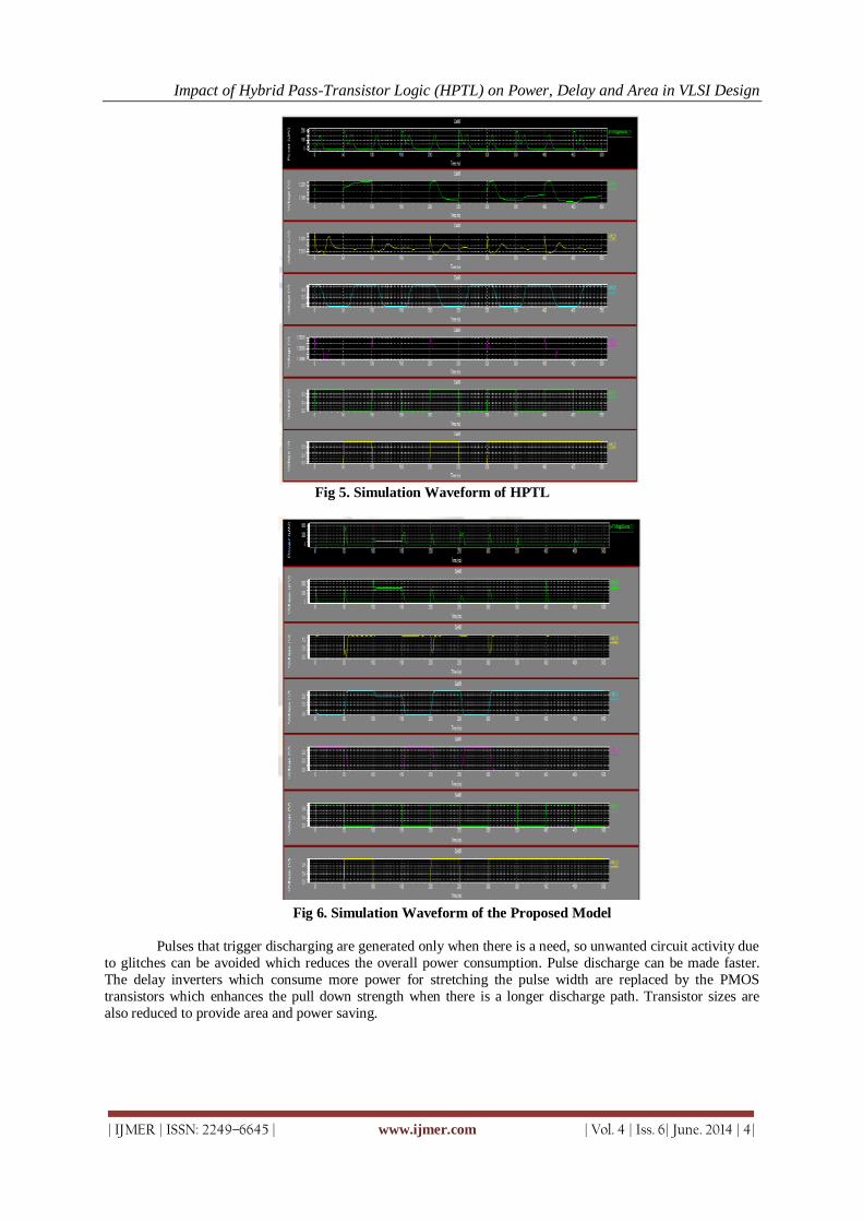
Impact of Hybrid Pass-Transistor Logic (HPTL) on Power, Delay and Area in VLSI Design
| IJMER | ISSN: 2249–6645 | www.ijmer.com | Vol. 4 | Iss. 6| June. 2014 | 4|
Fig 5. Simulation Waveform of HPTL
Fig 6. Simulation Waveform of the Proposed Model
Pulses that trigger discharging are generated only when there is a need, so unwanted circuit activity due
to glitches can be avoided which reduces the overall power consumption. Pulse discharge can be made faster.
The delay inverters which consume more power for stretching the pulse width are replaced by the PMOS
transistors which enhances the pull down strength when there is a longer discharge path. Transistor sizes are
also reduced to provide area and power saving.

Impact of Hybrid Pass-Transistor Logic (HPTL) on Power, Delay and Area in VLSI Design
| IJMER | ISSN: 2249–6645 | www.ijmer.com | Vol. 4 | Iss. 6| June. 2014 | 5|
The Waveforms
VII. Lessons Learnt As there are no particular cell libraries for PTL designs. I had to manually create my own designs. The
mistake I have done is instead of creating a single logic gate and fully optimizing it; I aggressively designed the
entire multi_cell and tried to optimize the widths and lengths of that complex cell.
So whenever we want to create a complex cell, first we should start with a basic gate, try to get the best
optimized design and then go for the bigger one.
VIII. Conclusion The area overhead of CMOS is at least 4 times more than the PTL. The power consumption is less in
case of PTL compared to CMOS. A good PTL design needs a lot of astute trade-offs. In clock generation
circuitry an AND function is removed and is replaced with a Pass Transistor logic based AND gate. Since in the
PTL style AND gate the n-mos transistors are in parallel they consume less power and provide a faster discharge
of the pulse. A software package called the TANNER EDA tools utilizing MOSIS 90nm technology is used for
the study. The comparison of the Number of transistors used and the Average power consumed for 100%
activity, 50% activity and 0% activity are done. The power consumed is for five cycles of operation. The power
consumption shows a decreasing trend as the switching activities are reduced. From the above results it is clear that this type of design approach can be implemented in real space systems to increase the efficiency as well as
to minimize the power consumption
REFERENCE [1] Dr. V D Agrawal‟s Project assignment. [2] Fayed, A.A and Bayoumi, M.A., "A Low Power 10 Transistor Full Adder Cell for Embedded Architectures," in
Proc. IEEE Int/. Symp. Circuits and Systems, vol. 4, pp. 226-229, Sydney, Australia, May 2001. [3] J. M. Rabaey, A. Chandrakasan, B Nikolic, Digital Integrated Circuits-A Design Perspective. Prentice Hall, 2004. [4] R. Zimmermann and Wolfgang Fichtner, “Low-power Logic Styles: CMOS Versus Pass-Transistor Logic,” IEEE J.
Solid-State Circuits, vol.32, pp. 1079-1090, Jul. 1997. [5] Geun Rae Cho, Tom Chen. "On The Impact of Technology Scaling On Mixed PTL/Static Circuits," 2002 IEEE
International Conference on Computer Design (ICCD'02),p. 322, 2002. [6] Jyh-Ming Wang, Sung-Chuan Fang, Wu-Shiung Feng,“New Efficient Designs for XOR and XNOR Functions on the
Transistor Level,” IEEE J. of Solid-state Circuits, Vol. 29, pp. 780-786, July 1994. [7] H. T. Bui, Y. Wang, and Y. Jiang, "Design and analysis of low-power IO-transistor full adders using novel XOR-
XNOR gates," IEEE Trans. on Circuits and Systems-I/: Analog and digital signal processing, vol. 49, no. 1, pp. 25-30, Jan 2002.
[8] H. Lee and G.E. Sobelman, “A new low-voltage adder circuit,” in Proc. 7th Great Lakes Symp. VLSI, Urbana, IL,
1997. [9] A. Shams and M. Bayoumi, “A new full adder cell for low-power applications,” in Proc. of the 1998 Great Lakes
Symposium ,1997.

Impact of Hybrid Pass-Transistor Logic (HPTL) on Power, Delay and Area in VLSI Design
| IJMER | ISSN: 2249–6645 | www.ijmer.com | Vol. 4 | Iss. 6| June. 2014 | 6|
[10] K. Taki, “A Survey for Pass-Transistor Logic Technologies”, Proc. Asia South-Pacific Design Automation Conference , pp. 223-226, February 1998.
Author Biographies
Mr. G. SIVAIAH completed his M.tech in VLSI System Design (V.L.S.I) in
Annamacharya Institute of Technology & Science, Rajampet. His area of interest is in the
field of VLSI. Now presently working as Assistant Professor in Ravindra College of
Engineering For Women Kurnool.
Mr. T.Kishore finished his M.tech in VLSI System Design (V.L.S.I) in St.Johns College
Engineering & Technology. His area of interest is in the field of VLSI. Now presently
working as Assistant Professor in Ravindra College of Engineering For Women Kurnool.
Mr. K.Vijay Kumar finished his M.tech in Communication Signal Processing (C.S.P) in G.Pulla Reddy Engineering College, Kurnool. His area of interest is in the field of Digital
Signal Processing and Communications. Now presently working as Assistant Professor in
Ravindra College of Engineering For Women Kurnool.

International
OPEN ACCESS Journal
Of Modern Engineering Research (IJMER)
| IJMER | ISSN: 2249–6645 | www.ijmer.com | Vol. 4 | Iss. 6| June. 2014 | 7|
An Application of Energy and Exergy Analysis of Transport
Sector of India
Dr. Soupayan Mitra1, Devashish Gautam2 1(Associate Professor, Dept. of Mechanical Engineering, Jalpaiguri Govt. Engineering College/WBUT, India
2 (P.G. Scholar, Dept. of Mechanical Engineering, Jalpaiguri Govt. Engineering College/WBUT, India
I. INTRODUCTION India’s transport sector is large and diverse; it caters to the needs of 1.2 billion people. In 2007, the
sector contributed about 5.5 percent to the nation’s GDP, with road transportation contributing the lion’s
share. Good physical connectivity in the urban and rural areas is essential for economic growth. Since the early
1990s, India's growing economy has witnessed a rise in demand for transport infrastructure and services.
However, the sector has not been able to keep pace with rising demand and is proving to be a drag on the
economy. Major improvements in the sector are required to support the country's continued economic growth
and to reduce poverty. [1]
This work represents a brief critical and analytical account of the development of the concept of
exergy and of its applications to the society. It is based on a careful and consultation of a very large
number of published references taken from archival journals, technical reports, lecture series etc.,
considered first of its kind in India since there is no such study on energy and exergy utilizations for the
transportation sub-sector of India. Furthermore, comparison of obtained results of energy and exergy
efficiencies with other countries around the world is carried out. The results obtained are expected to yield
useful data in developing ‘energy-security’ policy targeting towards sustainable development in the hands of
energy policy makers of the country.
II. THEORETICAL AND MATHEMATICAL FORMULATION OF EXERGY ANALYSIS
2.1 The concept of exergy
Exergy can be defined as a measure of maximum capacity of an energy system to perform useful work
as it proceeds to a specified final state in equilibrium within the surroundings. In simple words, we can
describe exergy as the ability to produce work. The available work that can be extracted from an energy source
depends on the state of its surroundings. The greater the temperature differences between an energy source and
its surroundings, the greater the capacity to extract work from the system.
Exergy analysis permits many of the shortcomings of energy analysis to be overcome. Exergy analysis
is based on the second law of thermodynamics, and is useful in identifying the causes, locations and
magnitudes of process inefficiencies which are not revealed by energy analysis alone based on first law of
thermodynamics. The exergy associated with an energy quantity is a quantitative assessment of its usefulness
or quality. Exergy analysis acknowledges that, although energy cannot be created or destroyed, it can be
degraded in quality, eventually reaching a state in which it is in complete equilibrium with the surroundings
and hence of no further use for performing tasks.
Abstract: The present article is dedicated for evaluating the transportation sector of India in terms of
energetic and exergetic aspects. In this regard, energy and exergy utilization efficiencies during the
period 2005-2011 are assessed based on real data obtained from Energy statistics of India. Sectoral
energy and exergy analyses are conducted to study the variations of energy and exergy efficiencies,
overall energy and exergy efficiencies for the entire sub-sector are found to be in the range of 21.30 to
30.03%. When compared with other neighbouring countries, such as Saudi Arabia, Malaysia and Turkey,
the Indian transport sector is the least efficient. Such difference is inevitable due to dissimilar transport
structure in these countries. It is expected that that the results of this study will be helpful in developing
highly useful and productive planning for future energy policies, especially for the transportation sector. This, in turn, will help achieve the ‘energy-security’ goal of the country. Keywords: Energy, Exergy, Efficiency, Sectoral energy use, Transport sector of India.

An Application of Energy and Exergy Analysis of Transport Sector of India
| IJMER | ISSN: 2249–6645 | www.ijmer.com | Vol. 4 | Iss. 6| June. 2014 | 8|
2.2 Energy and exergy values for commodities in macrosystems
The exergy of an energy resource can for simplicity often be expressed as the product of its energy
content and a quality factor (the exergy-to-energy ratio) for the energy resource. This value relates to the price
of the material or resource, which is also partly defined by the environment through, for instance, demand. In
assessments of regions and nations, the most common material flows often are hydrocarbon fuels at near
ambient conditions. The physical exergy for such material flows is approximately zero, and the specific exergy
reduces to the fuel specific chemical exergy exf, which can be written as:
exf = γfHf (1)
where γf denotes the exergy grade function for the fuel, defined as the ratio of fuel chemical exergy to fuel
higher heating value Hf . [2,3]
Table-1 lists typical values of Hf , exf and γf for fuels typically encountered in regional and national
assessments. The specific chemical exergy of a fuel at T0 and P0 is usually approximately equal to its higher
heating value Hf.
Table-1: Properties of selected fuels.*
Fuel Hf
(kJ/kg)
Chemical exergy (kJ/kg) γf
Gasoline 47.849 47.394 0.99
Natural gas 55,448 51,702 0.93
Fuel oil 47,405 47,101 0.99
Diesel 39,500 42,265 1.07
Kerosene 46,117 45,897 0.99
* For a reference-environment temperature of 25C, pressure of 1 atm and chemical composition as defined in
the text. Source: Reistad (1975). [4]
2.3 The reference environment for macrosystems
The reference environment used in many assessments of macrosystems is based on the model of
Gaggioli and Petit (1977), which has a temperature T0=25C, pressureP0=1 atm and a chemical composition
consisting of air saturated with water vapor, and the following condensed phases at 25C and 1 atm: water
(H2O), gypsum (CaSO4·2H2O) and limestone (CaCO3). This reference-environment model is used in this
chapter, but with a temperature of 10C. [3, 5]
2.4 Efficiencies for devices in macrosystems
Energy η and exergy ψ efficiencies for the principal processes in macrosystems are usually based on
standard definitions:
η = (Energy in products) / (Total energy input)
(2)
ψ = (Exergy in products) / (Total exergy input)
(3)
Exergy efficiencies can often be written as a function of the corresponding energy efficiencies by assuming the
energy grade function γf to be unity, which is commonly valid for typically encountered fuels (kerosene,
gasoline, diesel and natural gas).
Heating
Electric and fossil fuel heating processes are taken to generate product heat Qp at a constant temperature Tp,
either from electrical energy We or fuel mass mf . The efficiencies for electrical heating are
ηh,e = Qp/We
(4)
and
ψh,e = ExQp/Ex
We = (1 − T0/Tp)Qp/We

An Application of Energy and Exergy Analysis of Transport Sector of India
| IJMER | ISSN: 2249–6645 | www.ijmer.com | Vol. 4 | Iss. 6| June. 2014 | 9|
Combining these expressions yields
ψh,e = (1 − T0/Tp)ηh,e
(5)
For fuel heating, these efficiencies are
ηh,f = Qp/mfHf
(6)
and
ψh,f = ExQp/mf exf
or
ψh,f = (1 − T0/Tp)Qp / (mfγfHf ) ≈ (1 − T0/Tp)ηh,f
(7)
where double subscripts indicate processes in which the quantity represented by the first subscript is produced
by the quantity represented by the second, e.g., the double subscript h,e means heating with electricity.
Cooling
The efficiencies for electric cooling are
ηc,e = Qp / We
(8)
ψc,e = ExQp / ExWe = (1 − T0 / Tp) Qp / We
(9)
or
ψc,e = (1 − T0 / Tp) ηc,e
(10)
Work production
Electric and fossil fuel work production processes produce shaft work W. The efficiencies for shaft work
production from electricity are
ηm,e = W / We
(11)
ψm,e = ExW / ExWe = W / We = ηm,e
(12)
For fuel-based work production, these efficiencies are
ηm,f = W / mf Hf
(13)
ψm,f = ExW / mf exf = W/mf γf Hf ≈ ηm,f
(14)
Electricity generation
The efficiencies for electricity generation from fuel are

An Application of Energy and Exergy Analysis of Transport Sector of India
| IJMER | ISSN: 2249–6645 | www.ijmer.com | Vol. 4 | Iss. 6| June. 2014 | 10|
ηe,f = We / mfHf
(15)
ψe,f = ExWe
/mf exf = We/mf γf Hf ≈ ηe,f
(16)
Kinetic energy production
The efficiencies for the fossil fuel-driven kinetic energy production processes, which occur in some devices in
the transportation sector (e.g., turbojet engines and rockets) and which produce a change in kinetic energy Δke
in a stream of matter ms, are as follows:
ηke,f = ms Δkes / mfHf
(17)
ψke,f = ms Δkes / mf exf = ms Δkes / mf γf Hf ≈ ηke,f
(18)
III. METHODOLOGY AND DATA SOURCES
3.1 Analysis of the Transportation Sector
Energy and exergy utilization in the transportation sector is evaluated and analyzed. The
transportation sector in India is composed of mainly International aviation, Domestic aviation, Pipeline
transport, Roadways and Railways which uses mainly 3 types of fuels, viz. High speed diesel oil (HSDO), Light
diesel oil (LDO) and Furnace oil (FO). Another type of fuel that is used is Low sulphur heavy stock oil,
however this fuel has not been considered as it has no contribution in the transportation sector.
Mean energy and exergy efficiencies are calculated by multiplying the energy used in each mode by
the corresponding efficiency. Then, these values are added to obtain the overall efficiency of the transportation
sector.
3.2 Energy efficiencies for the transportation sector Table-2 provides energy efficiencies for the various types of fuels in the modes of transportation.
These values are based on average U.S devices. They seem to represent the general nature of the devices and
are assumed to represent the Indian devices in absence of any other more accurate data. Since, vehicles
generally are not operated at full load; a distinction is made between rated load (full load) efficiencies and
estimated operating load (part load) efficiencies. [4]
Table-2: Efficiencies for the Transport Sector (Process and operating data) [2]
Fuel/Petroleum product Rated Load/Efficiency
(%)
Estimated Operating
Load/Efficiency (%)
High speed diesel oil 28 22
Light diesel oil 28 22
Fuel oil - 15
3.3 Data sources
Amount of fuel consumption by different machineries used in the transportation activities are
collected from Energy statistics of India 2013 and presented in Table-3.
Table-3: Energy consumption data for Transport Sector in India for 2005-2011. [1]
Year Petroleum Product Consumption
(‘000 tonnes)
2005 High speed diesel oil 4264
Light diesel oil 52
Fuel oil 478

An Application of Energy and Exergy Analysis of Transport Sector of India
| IJMER | ISSN: 2249–6645 | www.ijmer.com | Vol. 4 | Iss. 6| June. 2014 | 11|
2006 High speed diesel oil 4316
Light diesel oil 53
Fuel oil 502
2007 High speed diesel oil 5003
Light diesel oil 35
Fuel oil 315
2008 High speed diesel oil 5292
Light diesel oil 15
Fuel oil 469
2009 High speed diesel oil 5365
Light diesel oil 6
Fuel oil 560
2010 High speed diesel oil 5416
Light diesel oil 5
Fuel oil 780
2011 High speed diesel oil 5528
Light diesel oil 3
Fuel oil 371
3.4 Steps and procedures for energy and exergy analysis
Energy and exergy efficiencies were determined using (2) and (3) considering grade function as unity.
The overall energy efficiency can be easily found by dividing total energy produced by total input energy. [3]
The overall weighted mean was obtained for the energy and exergy efficiencies for the fossil fuel processes as
well. Weighing factors are the ratio of energy input of each of the fuels to the total input energy of this sector.
The device exergy efficiencies are evaluated using data for the years 2005– 2011. Energy and exergy
efficiencies were then used to calculate the overall energy and exergy efficiencies of this sector.
Table-4: Energy consumption data for Transport Sector in India for 2005-2011. [1, 2]
Year
Petroleum
Product
Consumption
(‘000 tonnes)
Energy Consumption Energy Efficiency
PJ % Rated
Load Estimated
Operating
Load
2005 High speed
diesel oil 4264 178.53 88.67 28 22
Light diesel
oil 52 2.81 1.4 28 22
Fuel oil 478 20 9.93 - 15
2006 High speed
diesel oil 4316 180.71 88.61 28 22
Light diesel
oil 53 2.22 1.09 28 22

An Application of Energy and Exergy Analysis of Transport Sector of India
| IJMER | ISSN: 2249–6645 | www.ijmer.com | Vol. 4 | Iss. 6| June. 2014 | 12|
Fuel oil 502 21 10.3 - 15
2007 High speed
diesel oil 5003 209.47 93.46 28 22
Light diesel
oil 35 1.46 0.64 28 22
Fuel oil 315 13.19 5.9 - 15
2008 High speed
diesel oil 5292 221.58 91.61 28 22
Light diesel
oil 15 0.63 0.26 28 22
Fuel oil 469 19.64 8.13 - 15
2009 High speed
diesel oil 5365 224.63 90.45 28 22
Light diesel
oil 6 0.25 0.11 28 22
Fuel oil 560 23.45 9.44 - 15
2010 High speed
diesel oil 5416 226.77 87.34 28 22
Light diesel
oil 5 0.21 0.08 28 22
Fuel oil 780 32.66 12.58 - 15
2011 High speed
diesel oil 5528 231.46 93.66 28 22
Light diesel
oil 3 0.125 0.06 28 22
Fuel oil 371 15.53 6.28 - 15
IV. Data Analysis, Results And Discussions
4.1 Mean and overall energy efficiencies
Generally, the overall or mean weighted energy efficiency is determined by dividing the total energy
produced by the total energy output. In this problem, all the fuels have the same part loads. Using the part load
efficiency, weighted mean energy efficiency of every fuel can be found. Based on the data listed in Table-4, the
weighted mean energy efficiency for the transport sector in the year 2010, e.g., is calculated using equation: η0
= η HSDO +
η LDO+ η FO.
η0 = (0.8734 x 22) + (0.0008 x 22) + (0.1258 x 15) = 21.119% ≈ 21.12%
4.2 Mean and overall exergy efficiencies
Before evaluating the overall mean exergy efficiencies for the transportation sector, it is noted that the
outputs of transportation devices are in the form of kinetic energy (shaft work). The exergy associated with
shaft work (W) is by definition equal to the energy.
i.e: ExW = W
Thus, for electrical shaft work production, the energy and exergy efficiencies of transportation devices can be
shown to be identical.
ηm,e = W / We
ψm,e = Exw / ExWe = W / We = ηm,e

An Application of Energy and Exergy Analysis of Transport Sector of India
| IJMER | ISSN: 2249–6645 | www.ijmer.com | Vol. 4 | Iss. 6| June. 2014 | 13|
ψm,e = ηm,e
For fossil fueled shaft work production in transportation devices, the exergy efficiency can be shown to be
similar to the energy efficiency:
ηm,f = W/mf.Hf
ψm,f = Exw/ mf.Hf.γf
When γf is unity (as is often assumed for most fuels). [Rosen, 1992]. [6]
ψm,f = ηm,f
Hence, η0 = ψ0
Thus, the overall mean exergy efficiencies for the transportation sector are equal to the overall mean energy
efficiencies.
Based on the data listed in Table-4, the weighted mean energy efficiency for the transport sector in the year
2010, e.g., is calculated using equation: ψ0 = ψ HSDO + ψ LDO+ ψ FO.
Ψ0 = (0.8734 x 22) + (0.0008 x 22) + (0.1258 x 15) = 21.119% ≈ 21.12%
Fig. 1 Overall mean energy and exergy efficiencies for the transport sector for 2005-2011
4.3 Comparison with other countries
Sector and overall energy and exergy efficiencies for India, Saudi Arabia, Malaysia and Turkey are
compared. The comparison is based on previous studies, and the data used is for the year 1993 for Saudi
Arabia and Turkey and 2005 for India and Malaysia. The efficiencies differ slightly, but the main trends
described earlier in this section regarding the differences between energy and exergy efficiencies are exhibited
by each country.

An Application of Energy and Exergy Analysis of Transport Sector of India
| IJMER | ISSN: 2249–6645 | www.ijmer.com | Vol. 4 | Iss. 6| June. 2014 | 14|
Fig. 2: Comparison of overall energy and exergy efficiencies for the industrial sector of India, Saudi Arabia,
Malaysia and Turkey. [1, 2]
When compared with other neighboring countries, such as Saudi Arabia and Malaysia, the transport
sector is less efficient. Such difference is inevitable due to dissimilar structure of the modes of transportation
in these countries. It is expected that that the results of this study will be helpful in developing highly
applicable and productive planning for future energy policies, especially for the Residential, Agricultural ,
Public and private and Utility sectors.
V. CONCLUSION In summary, it can be said that the potential usefulness of exergy analysis in sectoral energy
utilization is substantial and that the role of exergy in energy policy making activities is crucial. The results of
exergy analyses of processes and systems have direct implications on application decisions and on research and
development (R&D) directions. Further, exergy analyses more than energy analyses provide insights into the
best directions for R&D effort. The overall mean energy efficiency and the overall mean exergy efficiency in
the Indian transportation sector for the period 2005-2011 is 22.55%. This study also shows that airway
transportation contribution should be increased to improve the overall energy and exergy efficiencies of the
Indian transport sector. It is very necessary in the light of the results of this work that Indian policy makers
review the issue of mass importation of used vehicles into the country. All efforts should also be made to ease
air transportation and make it affordable for Indians. The Indian railway system should also be resuscitated for
cheap and affordable transportation of goods and passengers.
Acknowledgements The authors wish to acknowledge the support provided by Jalpaiguri Government Engineering
College, Jalpaiguri, West Bengal-735101 and West Bengal University of Technology (WBUT).
REFERENCES Books: [1] Energy Statistics. 2013, Central Statistics Office, National Statistical Organization, (Ministry of Statistics and
Programme Implementation, Government of India, 2013).
[2] Ibrahim Dincer and Marc A. Rosen. June 2007. Exergy, energy, environment and sustainable development.
(Elsevier, 2007).
Journal Papers: [3] Dincer, I., Hussain, M.M., Al-Zaharnah, I., 2004. Energy and exergy utilization in transportation sector of Saudi
Arabia. Applied Thermal Engineering 24, pp. 525–538.

An Application of Energy and Exergy Analysis of Transport Sector of India
| IJMER | ISSN: 2249–6645 | www.ijmer.com | Vol. 4 | Iss. 6| June. 2014 | 15|
[4] Reistad GM. 1975. Available energy conversion and utilization in the United States. J.Eng. Power 97, pp. 429–434.
[5] Gaggioli R.A., Petit PJ. 1977. Use the second law first. Chemtech7, pp. 496–506.
[6] Rosen MA. 1992. Evaluation of energy utilization efficiency in Canada using energy and exergy analyses. Energy-
The International Journal 17:pp.339–350.
[7] Gaggioli, R.A., 1998. Available energy and exergy. International Journal of Applied Thermodynamics 1, pp. 1–8.
[8] Rosen MA. 1992b. Appropriate thermodynamic performance measures for closed systems for thermal energy
storage. ASME Journal of Solar Energy Engineering 114:pp.100–105.
[9] Wall G. 1990. Exergy conversion in the Japanese society. Energy-The International Journal 15: pp. 435–444.
[10] Wall G. 1991. Exergy conversions in the Finnish, Japanese and Swedish societies. OPUSCULA Exergy Papers, pp.
1–11.
[11] van Gool W. 1997. Energy policy: fairly tales and factualities. Innovation and Technology-Strategies and Policies,
pp. 93– 105.
[12] Wall G. 1993. Exergy, ecology and democracy-concepts of a vital society. ENSEC’93: International Conference on
Energy Systems and Ecology, July 5–9, Cracow, Poland, pp.111–121.
[13] Rosen MA, Le MN. 1995. Efficiency measures for processes integrating combined heat and power and district
cooling. Thermodynamics and the Design, Analysis and Improvement of Energy Systems, AES-Vol. 35, American
Society of Mechanical Engineers: New York, pp.423–434.

International
OPEN ACCESS Journal Of Modern Engineering Research (IJMER)
| IJMER | ISSN: 2249–6645 | www.ijmer.com | Vol. 4 | Iss. 6| June. 2014 | 16|
Evalouation of Expansive Soil Properties by Electrical Resistivity
Mahmoud M. Abu zeid1 , Ahmed M. Hassan
2, Ahmed M. Abu Bakr
3,
Fayek A. Hassouna4
1 Civil Engineering Department, South Valley University, Qena, Egypt, 2, 3, 4 Civil Engineering Department, Faculty of Engineering, Minia University, Minia, Egypt
I. INTRODUCTION The problem of expansive soils is one of the most well known geotechnical problems that was studied
and researched by a lot of geotechnical researchers. This problem was not recognized by soil engineers until
1930, the increasingly extensive use of concrete slab on ground construction after 1940, has further increased
the damage to structures caused by expansive soils. Since the last six decades there was a world wide interest in
expansive clay and shale's. The application of electrical measurements to evaluate engineering properties of
soils has gained a wide, promising field of research in recent years. Conductivity of direct current was the first
attempt used to characterize the pore structure of electrically non-conducting particles. In the last decades there
is a great demand towards using special techniques and apparatuses for measuring the soil properties in situ. The
electrical geophysical methods is one of these techniques which allow rapid measurement of soil electrical
properties , such as resistivity , electrical conductivity and potential directly from soil surface to any depth without soil disturbance . Some in-situ electrical geophysical methods were used to evaluate temperature, water
content and structure of soils. These methods are not commonly applied in soil studies mainly due to three
reasons. Firstly, the equipment for geophysical methods of vertical four-electrode profiling, electrical sounding,
ground-penetrating radar, etc. manufactured is suited only for exploration of deep geological profiles.
Therefore, the distributions of electrical properties in shallow (0 – 5 m) soil profiles usually cannot be measured
with such equipment. The methods need to be modified for soil investigations. Secondly, the theory about nature
of development and distribution of soil electric field, which parameters is measured with the electrical
geophysical methods, is still being developed. Finally, the in-situ measurements of electrical parameters need a
specific calibration in every study to be reliable to evaluate different soil properties. Nowadays only the
methodologies of four-electrode probe and electromagnetic induction method for application on saline soils are
well developed. This dissertation includes broad material on applications of methodologies of four-electrode probe in soil studies.
Abstract: Expansive soil creates problems for structures built on it due to its high swelling and
shrinkage characteristics. Easy and quick methods instead of using traditional methods such as
drilling and taking probes which are difficult to carry out, For long time, there is a great demand on
using the geophysical methods and small, easy, and modern apparatus as to measure the soil
characteristics in the field. The electrical resistivity method is considered one of these methods which
measure directly soil properties from the ground surface level to any depth. In this investigation a
resistivity field survey for a site using an electrical resistivity apparatus with eleven holes logs was
performed. Research program has been conducted on specimens obtained by mixing commercial
bentonite was added to clayey soil to produce sample with different swelling potential. Many
correlations between electrical resistivity were determines with each of the following properties of soil: optimum moisture content, maximum dry density, Attreberge limits, swelling pressure, and
swelling potential. Linear correlations between different bentonite ratios with electrical resistivity
were made. Correlations between different bentonite ratios and the soil properties previously
mentioned were conducted, finally, linear correlations between different soil properties at different
bentonite ratios.
Keywords: Expansive soil, electrical resistivity, bentonite, electrode.

Evalouation Of Expansive Soil Properties By Electrical Resistivity
| IJMER | ISSN: 2249–6645 | www.ijmer.com | Vol. 4 | Iss. 6| June. 2014 | 17|
II. EXPERIMENTAL WORK
2.1. Sample Preparation
Clay-bentonite mixture was prepared using clayey soil from a site, commercial bentonite (Betomid O C
M a Brand D.F.C.P.4 produced by Egypt Mining & Drilling Chemical Company). Undisturbed sample from site
were coated with wax and delivered directly to the laboratory. Natural soil was oven dried for 24 hours at 100
to 1050C. It was sieved on sieve No.4, then different bentonite ratios (10%-100%) were added and mixed in the dry condition using an electric mixer for at least 15 minutes to ensure that the soil mixture becomes
homogeneous and of uniform in color. Different soil laboratory tests were then performed on that mixture.
Prepared clay-bentonite mixture was then put into transparent plastic box as shown in Fig. (1). the transparent
plastic was tested in the field, therefore was chosen to bear the sample and to keep its contents. In addition, it
doesn't obstruct the sent wave from the apparatus or affect on the current.
2.2. Electrical Resistivity Apparatus
Eleven vertical electrical sounding were conducted in location by using wenner configuration
techniques. Earth resistivity meter called TELLUROHM C. A2, Was used in this work. The TELLUROHM C.
A2 is a work site instrument designed for earth resistance and soil resistivity measurements. Especially since it
suited to measurements in difficult conditions such as when there are stray voltages present, high telluric
currents and high value of auxiliary plate resistances. Steel electrodes (40 cm long and 1.2 cm diameter each) were used for transmitting current and potential
into the ground. To provide good electrical contact with the ground, it was necessary to use water around the
electrodes. The electrodes were inserted into the ground to a depth which ensured a true contact between the
electrode and the surface medium. Single conductor and low electrical resistance, 0.75mm2 wirers mounts on
plastic reels were used. For the potential lines, two reels were used each of which has about 50 meters of wires.
For the current lines, other two reels, each has 100 meters of wires been utilized. The field instruments and
equipment are shown in Fig (2),
To enable these measurements, a wenner array of point electrodes was applied. The wenner array
configuration applied to this survey is the most commonly used point – electrode surveying system. This method
allows lateral and vertical sampling of apparent resistivity to be taken within the array. The lateral sampling
collects measurements from a point mid array, which is at a depth of half that of the electrode spacing (a). In this technique four electrodes are fixed in the earth, two for the potential and the others for the current. The
distances between each one of them (a) are equal. The measurements at each station were carried in successive
rate and increased continuously depends on the desired depth.
1.3 Procedure
At first, a hole was made in the ground by 1m width, 1.5m length and 90cm depth. The depth and the
length were chosen according to the distance between the electrodes (a). This distance equals the required depth.
To allow to the sent waves from the apparatus to the model, the model should be in the center of the hole. The
model shouldn't be less than 80cm height, the length and the width of the model shouldn’t be less than 20cm. the
model with dimension 80 x 20 x 20 cm was chosen, the width of the hole shouldn’t be less than the width of the
model. Therefore, it was chose to be 1m in this research to facilitate the digging process. After that, the model
with specimen was put inside in the center of the hole. To flatten the hole to the ground surface, the model axes was had by string to the hole to guarantee passing the sent waves from the apparatus to the specimen. After
flatting the ground, the two electrodes (C and D) was put one on the left 25cm away from the center, the other
on the right 25cm away from the center as shown in Fig (3). The sent wave from the electrode (C and D) passes
15cm below the top of the model because we had left 10cm between the ground surface and the top of the
model. This distance (10 + 15 ) represents the whole depth of the wave between electrode ( C and D ).after that,
the electrodes (A and B ) was put, to get the required depth of the average wave (50cm ), the electrode (C ) was
put at 50 cm away from electrode (A ) and the same went the electrode (B ) and ( D ).The sent wave from
electrode (A) and (B) passes 15cm above the bottom of the model. As result, the distance between the two sent
waves is 50cm which equals the required depth. However, the obtained reading (R) from the apparatus is the
bisection wave to the two waves from electrodes (C to D and A to B). The bisection wave passes through the
center of the model, 50cm away from the ground surface, and the sent wave is measured from the point of connection between the electrode and the ground surface and not from the end of the electrode underground.
Next, the electrodes was connect to the apparatus by gave along press-on power button. Then the same method
was applied on all the other specimens which were mentioned before. This formula was applied to get the
electrical resistivity value:
ρ = 2πR a

Evalouation Of Expansive Soil Properties By Electrical Resistivity
| IJMER | ISSN: 2249–6645 | www.ijmer.com | Vol. 4 | Iss. 6| June. 2014 | 18|
Where:
ρ = electrical resistivity , R = reading from apparatus , a = required depth
Finally, correlations were mad between the electrical resistivity with some soil properties determined in the
laboratory.
Fig (1): Transparent Plastic Box

Evalouation Of Expansive Soil Properties By Electrical Resistivity
| IJMER | ISSN: 2249–6645 | www.ijmer.com | Vol. 4 | Iss. 6| June. 2014 | 19|
Fig (2): Parts of Apparatus Used in Field Survey
Fig (3): Configuration Array in the Field
III. RESULTS AND ANALYSIS In this section experimental results of to all testes carried out in this investigation are presented.
Discussion and analysis of these results is also given. Correlation between the measured electrical resistivity
value and its corresponding measured laboratory soil properties at different bentonite ratios are presented. This
linear correlation may be used to determine different soil parameters on site as shown in the following.
3.1 Liquid Limit
Fig (4): Correlation between Electrical Resistivity and Liquid Limit at Different Bentonite Ratios
Fig (4) shows the relationship between laboratory measured liquid limit, L.L and field measured
electrical resistivity, ρ. Regression analysis of this relationship provided a linear correlation between electrical
resistivity and liquid limit as follows:
ρ = - 0.0159 L.L + 7.893 (2)
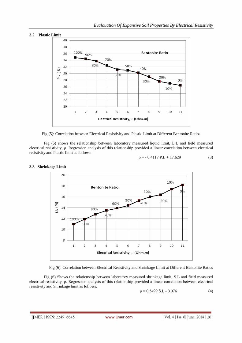
Evalouation Of Expansive Soil Properties By Electrical Resistivity
| IJMER | ISSN: 2249–6645 | www.ijmer.com | Vol. 4 | Iss. 6| June. 2014 | 20|
3.2 Plastic Limit
Fig (5): Correlation between Electrical Resistivity and Plastic Limit at Different Bentonite Ratios
Fig (5) shows the relationship between laboratory measured liquid limit, L.L and field measured
electrical resistivity, ρ. Regression analysis of this relationship provided a linear correlation between electrical
resistivity and Plastic limit as follows:
ρ = - 0.4117 P.L + 17.629 (3)
3.3. Shrinkage Limit
Fig (6): Correlation between Electrical Resistivity and Shrinkage Limit at Different Bentonite Ratios
Fig (6) Shows the relationship between laboratory measured shrinkage limit, S.L and field measured
electrical resistivity, ρ. Regression analysis of this relationship provided a linear correlation between electrical
resistivity and Shrinkage limit as follows:
ρ = 0.5499 S.L - 3.076 (4)
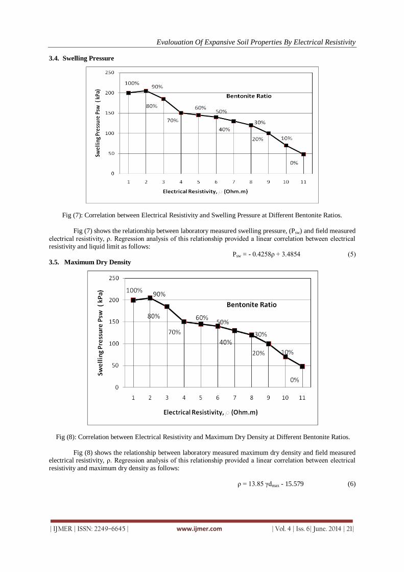
Evalouation Of Expansive Soil Properties By Electrical Resistivity
| IJMER | ISSN: 2249–6645 | www.ijmer.com | Vol. 4 | Iss. 6| June. 2014 | 21|
3.4. Swelling Pressure
Fig (7): Correlation between Electrical Resistivity and Swelling Pressure at Different Bentonite Ratios.
Fig (7) shows the relationship between laboratory measured swelling pressure, (Psw) and field measured
electrical resistivity, ρ. Regression analysis of this relationship provided a linear correlation between electrical
resistivity and liquid limit as follows: = - 0.4258ρ + 3.4854 (5) Psw
3.5. Maximum Dry Density
Fig (8): Correlation between Electrical Resistivity and Maximum Dry Density at Different Bentonite Ratios.
Fig (8) shows the relationship between laboratory measured maximum dry density and field measured electrical resistivity, ρ. Regression analysis of this relationship provided a linear correlation between electrical
resistivity and maximum dry density as follows:
ρ = 13.85 γdmax - 15.579 (6)

Evalouation Of Expansive Soil Properties By Electrical Resistivity
| IJMER | ISSN: 2249–6645 | www.ijmer.com | Vol. 4 | Iss. 6| June. 2014 | 22|
IV. CONCLUSIONS Different properties of clay-bentonite mixture were estimated using an electrical resistivity apparatus.
With eleven holes logs were performed. Many correlations between electrical resistivity were determines with
the results showed that for the soil used linear correlation between electrical resistivity and different soil
properties. This may provide a direct method of estimating these properties on site. However further
investigation on a wide variety of soil is needed to verify the included correlation.
REFERENCES [1] Abu-Hassanein, Zeyad S., (1996), “Electrical Resistivity of Compacted Clays”. Journal of Geotechnical Engineering,
Vol. 122, No. 5,p.p.397-406. [2] Abu zeid, M. M., (2009),”Evaluation of Expansive Soil Properties by Electrical Resistivity”, A Thesis Submitted
for the Degree of Master of Science in Civil Engineering, Minia University, Egypt, [3] Amgad. E. S, (2005). “Correlations between the Electrical Resistivity and Some Properties of Clayey Soil” Thesis
submitted for the degree of Master of Science in Civil Engineering, faculty of Engineering, Minia University. [4] Bertin J., (1976). “Experimental and Theoretical Aspects of IP”. Vol.1.Presentation and Application of the IP
Method-Case Histories. Gebruder Borntraeger, Berlin, P.P.250.
[5] Campanella R.G. and Weemees I.(1990),“ Development and Use of an Electrical Resistivity Cone for Groundwater Contamination Studies ”. Canadian Geotechnical Journal, Vol. 27, p.p. 557-590.
[6] Jeffery J. Roberts and Wildenschild, D., (2004), ”Electrical Properties of Sand–Clay Mixtures Containing Trichloroethylene and Ethanol”, Journal of Envioronmental & Engineering Geophysics , March, Volume 9, Issue 1.
[7] Wildenschild, D., Roberts, J.J., and Carlberg, E.D., (1999), ”Influence of microstructural properties on geophysical measurements in sand–clay mixtures”, Symposium on the Application of Geophysics to Engineering and Environmental Problems..
[8] Wildenschild, D., Roberts, J.J., and Carlberg, E.D., (2000), ”Electrical properties of sand–clay mixtures: The effect
of microstructure”, Geophys. Res. Lett., 27, 3085–3089. 2000 [9] Kalinski R.J. and Kelly w.e., (1994),“Electrical Resistivity Measurements For Evaluating Compacted soil Liners”.
Journal of Geotechnical Engineering, Vol. 120, No. 2,Feb., p.p. 451-457.

International
OPEN ACCESS Journal Of Modern Engineering Research (IJMER)
| IJMER | ISSN: 2249–6645 | www.ijmer.com | Vol. 4 | Iss. 6| June. 2014 | 23|
Investigation for Spatial and Physical Factors of Open Areas in
Residential Complex of Apadana Regarding the Relationship
Improvement between Internal and External Residential Areas
Hadiseh Baghi1, Mohammad Reza Namdari
2
1 M.Sc. Student , Department of Environmental Design Engineering, College of Environment and Energy,
Tehran Science and Research Branch, Islamic Azad University, Tehran, Iran 2Department of Architecture, Faculty of Art &Architecture, University of Science & Culture, Tehran, Iran
I. Introduction It’s perhaps can’t clearly be expressed that RC is a function emerged in 20th century within cities, but
obviously this function has changed during that era such that resulted in creation of new and different concept
within architectural functions field (Lai, 2011; Glaeser et al, 2006). Undoubtedly, life quality in bulky,
overpopulated and monotonous complexesnot only accompanied sense of alienationfor Eastern people (who
used to live in houses with a yard, vast balconies, and luminous area)but also for all residents of cities
habituating for the first time in these complexes (Smith, 2014; Gkartzios& Scott, 2013).They are products of living in 20th century based cities. They basically have been unimaginable prior to fast overpopulation, industrial
revolution, rural migrations to urban areas, increasing prices of lands and dwellings,mass production and
prefabrication. They were inevitable to live inside after world war particularly during mid- decades of 20th
century (renovations after World War II) (Hong et al, 2014). For this, what is considered as superiority criterion
for complex design compared to others is nothing more than accomplishment rate of each design to decrease this
sense of alienation and increase ownership feeling and restoration of individual characteristic of each residential
unit.Since residential open areas are parts of artifact environment occupying the volume between constructed
framework and can be composed of natural and artificial elements with beautiful, fascinating and desirable view
(Anderson, 2013; Hennessy &Patterson, 2012). They make fixation drawing the attention of people and
environment vivacity. Open areas of RCs are can meet users’ demands and play a role creating a desirable
residential area (Atkinson-Palombo, 2010). Thus, here we practice to evaluate open areas spatial and Physical factors within RCs (Mortensen et al, 2014).
II. Residential open area (ROA) and its Physical and Spatial elements Residential open areas (ROAs) are referred to one or more organized, ordered and arrayed areas located
among constructed residential surfaces and make a basis for human activities and behaviors. Open area
designing is the art of combining open area to behavioral mass, human memorials, and citizens’ impression out
of their living environment (Cerón-Palma et al, 2013). ROA within urban elements hierarchal is a barrier
between private (house) and public (urban open area) areas and form separation line between these two as a
Abstract: Residential open area provides light, internal spaces brightness and natural ventilation as
well as is considered as an opportunity of more relation with nature and a place for social interactions.
It’s an opportunity to promote performance of internal space and relationship to external one
regarding limitations of internal space of residential units. Therefore, revision and recognition of status
quo of open area predisposes more conscious design for open areas and landscapes of residential
areas. Since open areas in residential complexes (RCs) can respond crucial demands of users and play
a major role creating desirable residential area. Therefore, we practiced here to evaluate spatial and Physical factors for open areas in ApadanaRCin order to improve life quality within RCs. The method
for this paper is survey and is of explanatory- analysis kind. 325 resident household were randomly
sampled. Results were analyzed using descriptive and perceptive statistics. SPSS 18.0 was applied to all
analyses. Data analyses indicated that 50% of studied units evaluated the quality of open area as
moderate, 48.8% desirable and 0.6% undesirable in Apadana RCs. Finally, certain suggestions have
been offered in order to expand these areas qualitatively and quantitatively emphasizing spatial and
Physical factors and relationship between internal and external areas.
Keyword: Residential Complex, Open Space, Physical and Spatial Factors, Apadana.

Investigation for Spatial and Physical Factors of Open Areas in Residential Complex of……
| IJMER | ISSN: 2249–6645 | www.ijmer.com | Vol. 4 | Iss. 6| June. 2014 | 24|
transmission and middle area. It also allows for both physical and psychological movement through public and
private areas (Chaskin et al, 2013).Spatial and Physical elements of these areas are including sidewalks, motor
ways, landscape, playgrounds and etc. whose design and array should be performed observing stability
principles and ecological planning in addition to general design of the area (Temelová & Slezáková, 2014;
Mattingly, 2012).
III. Necessity and significance of within RCs Dimensions of residential units internal areas in general and especially for certain classes of the society
tends to incline. Most of current life needs aren’t met within limited private space of residential units and
naturally overflows out of this space (Ibem & Amole, 2013). Then the semiprivate, semipublic and public
spaces become significant and seriously applied. Since activities are performed within open areas, diverse
activities may be allowed to emerge creating desirable spaces resulting in residential areas vivacity (Sengupta,
2010). Certain advantages of application of residential open areas are:
1. Securing them via bodies by creating sanctum, hierarchal and climatic circumstances preservation
2. Increasing social interactions and recent constructions mixed to traditional identity and stable pattern
3. Enjoying reasonable level of leisure time facilities, traffic and other urban services fit to RC
4. Establishing Physical relationship through domiciles and their surrounding contexts and their direct effects
on RCs view
Examples of applying patterns of internal and external areas combined to each other within RCs
1. Karow residential complex in north eastern Berlin
Design for RC of North Karow by Charles Moor and his colleagues contain 500 residential
units(Dutton,2000). Open areas of RCs created by building bodies are significant ones that are being included in
a series of vacant and occupied spaces forming whole city. Open areas have been created with identity and
correspond to its performance when combining closed and open areas. It’s clear that private sanctum for
residential units are being created through combination of building masses and open areas. Private pen areas
and/ or public paths have been constructed using building bodies within this design (Fig. 1).
Figure 1. The pattern mix of open and closed spaces, a residential town of Karow in the northeast of Berlin
(Dutton, 2000)
2. RCs onLos Angles, Playavistain of US
Moor and his colleagues have provided another plan related to Playavista of LA including 11750
residential units within which business, administrative, education and open areas are placed in residential
context so that residents have access to them easily (Fig. 2). Designer had noticed hierarchy of open areas
formed by building constructions from one hand, constructions visual highlight to signify open areas on the
other hand(Ojeda,2004).

Investigation for Spatial and Physical Factors of Open Areas in Residential Complex of……
| IJMER | ISSN: 2249–6645 | www.ijmer.com | Vol. 4 | Iss. 6| June. 2014 | 25|
Figure 2. The pattern mix of open and closed spaces and residential complexes in the city of Los Angeles,
Playavysta
3. RCs of Savigney Le Tempel in Senart of France
As a medium heighted and high density project, AlianSrafti has designed 88 residential units for low
income classes on the corner of Pairsurban and suburb areas. The street has been changed to a public element
that exhibits residents’ diversity through highly diverse visual experiences (Fig. 3). It also provides an
opportunity to show personal interests in public places leading to collective identity expansion (Goodman,
2003).
Figure 3. Residential of Savigney Le Tempel in Senart of France
IV. Case study Apadana complex located at west of Tehran, region 5. The area is 304.407 m. It’s bounded to Sheykh
Fazllolah highway on the north, Ekbatan 3rd phase on the northwest, 1st Bime lane on the southwest, and from
south to south west to barren lands of Fakoori and Apadana (belonging to ministry of defence). All buildings of
the complex include 2901 residential unit having 2 or 3 bedrooms and divided to 6 phases (Table 1).

Investigation for Spatial and Physical Factors of Open Areas in Residential Complex of……
| IJMER | ISSN: 2249–6645 | www.ijmer.com | Vol. 4 | Iss. 6| June. 2014 | 26|
Table 1.The town units based on phase, block and entrance
Phase Block Entrance Units
1 2
3
4
5
6
8 8
7
8
8
7
28 30
27
30
30
24
488 510
459
512
512
420
Sum 46 169 2901
Apadana complex is one of the wealthiest districts of Tehran regarding landscapes. An area
approximately 8 m width along with concrete walls has been tree planted all around the complex. Inside the
complex, the space between blocks and cement pavements is decorated with lawn, flowers, trees and shrubs.
Therefore, the area can be as a big park for residents.
V. Research Method
This research is of explanatory- analysis survey kind. 328 households of Apadana complex were
sampled based on Kukran formulation. Questionnaire and interviews containing closed items and checklist were applied to collect observations. Field and physical observations, taking photos and pictures of different areas
includeother sections of data collection system. Data analysis was performed using explanatory and perceptive
statistics. The relationship between certain demographic qualities and respondents scores was investigated
applying X2 test. SPSS 18.0 software was applied to all statistical analysis. The relationship among ranked data
was evaluated via Friedman and Wilcoxon test. Study samples were households whose habitation exceeds one
year. Questionnaires consist of two sections: social- personal characteristics and evaluation of quality of open
areas in Apadana RCs. Respondents answered the items using five point Likert scale with (5) “I completely
agree”; (4) “I agree; (3) “I have no idea”; (2)“I disagree”; and (1); I completely disagree”. The consistency of
data collection instruments was obtained 0/86 using internal consistency method. A questionnaire wasfirst
devised through library studies, reviewing sources related to research subject including book, performed papers
and researches and then 12 experts and specialists investigated and valuated items.
VI. Results and Findings The quality of open areas in Apadana RCs can be divided in to three categories:
1. Undesirable (1-106 score)
2. Moderate (107-213 score)
3. Desirable (214-320 score)
The majority of respondents (50%) evaluated it as moderate while the minority (0.6%) as undesirable.
Average and standard deviation of studied units here were 2.496 and 0.512, respectively. Findings related to
research primary goal (quality of spatial and Physical organization of open areas in Apadana RCs) suggested that majority of respondents (56.1%) and minority (1.82%) of them have evaluatedresearched units as desirable
and undesirable, respectively.The average score and standard deviation were respectively 2.54 and 0.53
forquality of spatial and Physical organization of open areas in Apadana RCs. Findings in case of second goal
(the facilities and equipment quality of open areas in Apadana RCs) indicated that majority of
participants(59.7%) have evaluated this quality as moderate while minority of them (8.5%) as undesirable.
Findings related to the third goal of the research (quality of traffic and access to open areas in RCs)
showed that majority of respondents (65.3%) have rated this quality as moderate while minority of them (0.6%)
rating as desirable. The average and standard deviation in this case were 2.65 and 0.476, respectively (Table 2).
Friedman test was also used to study the difference of average scores of studied units regarding the quality of
open areas in Apadana RCs which was significant based on this test (P<0.05) (Table 3). wilkokxon ranks test
was used to paired comparison of average scores for studied units regarding special goals in case of the quality of open areas in Apadana RCs.According to Wilcoxon test results, paired comparisons of average scores for
studied units to first &second; first & third; and finally second & third goals are significant (Table 4).
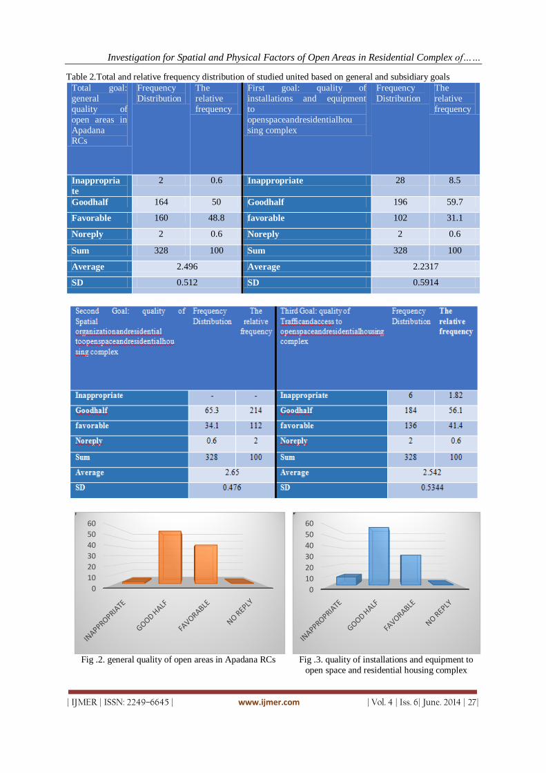
Investigation for Spatial and Physical Factors of Open Areas in Residential Complex of……
| IJMER | ISSN: 2249–6645 | www.ijmer.com | Vol. 4 | Iss. 6| June. 2014 | 27|
Table 2.Total and relative frequency distribution of studied united based on general and subsidiary goals
Total goal:
general
quality of
open areas in
Apadana
RCs
Frequency
Distribution
The
relative
frequency
First goal: quality of
installations and equipment
to
openspaceandresidentialhou
sing complex
Frequency
Distribution
The
relative
frequency
Inappropria
te
2 0.6 Inappropriate 28 8.5
Goodhalf 164 50 Goodhalf 196 59.7
Favorable 160 48.8 favorable 102 31.1
Noreply 2 0.6 Noreply 2 0.6
Sum 328 100 Sum 328 100
Average 2.496 Average 2.2317
SD 0.512 SD 0.5914
Fig .2. general quality of open areas in Apadana RCs Fig .3. quality of installations and equipment to
open space and residential housing complex
0
10
20
30
40
50
60
0
10
20
30
40
50
60

Investigation for Spatial and Physical Factors of Open Areas in Residential Complex of……
| IJMER | ISSN: 2249–6645 | www.ijmer.com | Vol. 4 | Iss. 6| June. 2014 | 28|
Fig .4. quality of Spatial organization and residential to
open space and residential housing complex
Fig .5. quality of Traffic and access to open space
and residential housing complex
Table 3.A comparison of average scores for studied units regarding determination of general quality of open
areas in Apadana RCs according to special goals
Number Average Standard
deviation Min Max
Chi-
Square
installations and equipment to
openspaceandresidentialhousing
complex
2901 2.2270 0.59018 1.00 2.00
df= 6
Chi-
Square=
293.757
sig= 0.000
Spatial
organizationandresidential
toopenspaceandresidentialhousing
complex
2901 2.5399 0.53488 1.00 2.00
Trafficandaccess to
openspaceandresidentialhousing
complex
2901 2.6503 0.47761 2.00 3.00
Table 4.Pairwise comparisonof average scores for studied units regarding determination of special goals quality
of open areas of according to the Wilcoxon test in Apadana RCs according to
Test First and secondtest First and Third test secondand Third test
Z -9.3889 (a) -3.838 (b) -11.106 (b)
P. Value 0.000 0.000 0.000
Certain demographic characteristics of habitants regarding the quality of open areas in Apadana RCs
suggested that age groups of 15-25 (76%), 26-45 (52.4%), and +65 (84.4%) have considered this quality as
desirable. Regarding gender, majority of males (52.5%) ad females (51.5%) have evaluated the quality of areas
as moderate and desirable, respectively. Majority of singles (63.2%) and married ones (51.1%) have considered
it as moderate and desirable, respectively. Most of households with 5-3 member (50.5%) have considered it as
desirable. Majority of illiterate and low literate (85.5%) have evaluated the quality as moderate while 61.6% of
literates put it as desirable. Regarding the profession, majority of unemployed ones (83.4), housewives (56.8%), and laborers (56.2%) have considered the quality as desirable while office clerks (52.2%) and freelancers
(58.4%) put it as moderate. Test result of K2 suggested that there is a significant relationship between age,
income, gender, marital status, household aspect, education, number of kids younger than 18 and profession
variable and the quality of open areas in Apadana RCs (P<0.01).
VII. Conclusion This research attempted to investigate the quality of open areas in Apadana RCs located in Tehran
region. This research is significant due to the fact that this complex attracts certain part of Tehran and
surrounding districts population overflow. Therefore, expanding open and public areas within RCs and integrating internal and external areas of residential constructions may in turn be helpful to population attract
and fixation as well as more attracted Apadana RCs. The analysis of results indicated 50% of samples
0
10
20
30
40
50
60
0
10
20
30
40
50
60

Investigation for Spatial and Physical Factors of Open Areas in Residential Complex of……
| IJMER | ISSN: 2249–6645 | www.ijmer.com | Vol. 4 | Iss. 6| June. 2014 | 29|
considered the quality of open areas as moderate; 48.8% desirable; and 0.6% as undesirablein Apadana RCs.
Therefore, open areas should be expanded qualitatively and quantitatively corresponding to social groups in line
with physical expansion of the city. Naturally, in addition to employment and production variables, noticing
vivacity, eagerness and life and creating fresh areas can serve this objective.
REFERENCE [1.] Anderson, J. R. (2013). The architecture of cognition. Psychology Press. [2.] Atkinson-Palombo, C. (2010). New housing construction in Phoenix: Evidence of “new suburbanism”?. Cities,
27(2), 77-86. [3.] Cerón-Palma, I., Sanyé-Mengual, E., Oliver-Solà, J., Montero, J. I., Ponce-Caballero, C., & Rieradevall, J. (2013).
Towards a green sustainable strategy for social neighbourhoods in Latin America: Case from social housing in Merida, Yucatan, Mexico. Habitat International, 38, 47-56.
[4.] Chaskin, R. J., Sichling, F., & Joseph, M. L. (2013). Youth in mixed-income communities replacing public housing complexes: Context, dynamics and response. Cities, 35, 423-431.
[5.] Dutton, J., 2000. "New American Urbanism". (Reforming the suburban Metropolis), Skira Palazzo casati Stampa, Italy.
[6.] Gkartzios, M., & Scott, M. (2013). Attitudes to housing and planning policy in rural localities: Disparities between long-term and mobile rural populations in Ireland. Land Use Policy, 31, 347-357.
[7.] Glaeser, E. L., Gyourko, J., & Saks, R. E. (2006). Urban growth and housing supply. Journal of Economic Geography, 6(1), 71-89.
[8.] Goodman, Elizabeth R., 2003. Blurring the Lines Between Public & Private Sp. [9.] Hennessy, J. L., & Patterson, D. A. (2012). Computer architecture: a quantitative approach. Elsevier.
[10.] Hong, T., Koo, C., Kim, H., & Seon Park, H. (2014). Decision support model for establishing the optimal energy retrofit strategy for existing multi-family housing complexes. Energy Policy, 66, 157-169.
[11.] Ibem, E. O., & Amole, D. (2013). Subjective life satisfaction in public housing in urban areas of Ogun State, Nigeria. Cities, 35, 51-61.
[12.] Lai, J. H. (2011). Comparative evaluation of facility management services for housing estates. Habitat International, 35(2), 391-397.
[13.] Mattingly, K. S. (2012). Housing and Transport Expenditure: Socio-spatial Indicators of Affordability in Auckland: a Thesis Submitted in Partial Fulfilment for the Degree of Master of Planning at the University of
Otago, Dunedin, New Zealand (Doctoral dissertation, University of Otago.). [14.] Mortensen, A., Heiselberg, P., & Knudstrup, M. (2014). Economy controls energy retrofits of Danish single-family
houses Comfort, indoor environment and architecture increase the budget. Energy and Buildings. [15.] Ojeda, O.2004. "Moor Ruble yodel (Houses & Housing)", Rockpost Publishers, Massachusetts, USA. [16.] Sengupta, U. (2010). The hindered self-help: Housing policies, politics and poverty in Kolkata, India. Habitat
International, 34(3), 323-331. [17.] Smith, S. J. (2014). Safe as Houses?: The Uneven Integration of Housing, Mortgage, and Financial Markets. OUP
Catalogue.
[18.] Temelová, J., & Slezáková, A. (2014). The changing environment and neighbourhood satisfaction in socialist high-rise panel housing estates: The time-comparative perceptions of elderly residents in Prague. Cities, 37, 82-91.

International
OPEN ACCESS Journal Of Modern Engineering Research (IJMER)
| IJMER | ISSN: 2249–6645 | www.ijmer.com | Vol. 4 | Iss. 6| June. 2014 | 30|
Exploring the Potentials of blacksmithing for Rural
Industrialization in Bauchi State
D. M. D. Ningi1, M. H. Muhammad
2, M. E. Ibrahim
3, L. G. Abubakar
4
1 (Department of Mechanical Engineering, Federal Polytechnic Bauchi, Nigeria) 2 (Mechanical Engineering Programme, A.T.B.U Bauchi, Nigeria)
3 (Mechanical Engineering Programme, F.U.T Yola, Nigeria) 4 (Agricultural Engineering Programme, A.T.B.U.Bauchi, Nigeria)
I. Introduction The contributions of indigenous manufacturing tools and processes to the technological advancement
of Nigeria cannot be overemphasized. In Nigeria, prior to the arrival of colonial masters, these tools and
processes contributed to the development of the then Nigeria‟s civilization and resulted in the evolution of most
of the present day or the modern tools and processes. As time goes, the tools and processes become incapable of
meeting various demands. This may be due to their inability to produce high precision components, inability to
achieve mass production within the minimum production time as required by demand, absence of ergonomic
and anthropometric considerations in design, thus subjecting the operator or worker to undue stress which
lowers productivity as well as subjecting the operator to risks of accidents. Despite the above shortcomings and
considering the low level of technological development of Nigeria and Africa in general, there is no indication
that these tools and processes will be replaced with modern ones in the near future. Indigenous tools and processes of manufacture are gradually disappearing as they have become
obsolete and can no longer meet increasing consumer needs, new service conditions and material requirements.
However, in view of the important roles which they play to the economic well-being of the people, especially
the rural populace, they will continue to be relevant in the lives of many Africans, most especially Nigerians.
Therefore, there is the need to identify areas of further development and improvement of these methods as well
as preserving them, as it is anticipated that in the very near future most of the traditional tools and processes
may disappear (Ezeadichie, 2002). Currently, these tools and processes are being applied in various ways by the
rural populace. A study on the use of tools and implements by women in agricultural production up to and
including harvest was carried out by International Fund for Agricultural Development (IFAD) in five Sub-
Saharan countries, i.e. Burkina Faso, Zambia, Uganda, Senegal and Zimbabwe (FAO, 2000). It was found that
more than 70% of food production work (planting, weeding and harvesting) was being done by women in Africa
and when attempts had been made to introduce new tools for cultivation or other operations, they had often been rejected by the rural people (IFAD, 2001).This is a clear indication that introduction of new tools and methods
may not necessarily have immediate acceptance or impact on the lives of the rural populace and hence
improvement of existing ones may be a better option.
Abstract: Nigeria like any other developing country is being faced by a number of developmental
challenges, such as social, economic and technological. The country is blessed with numerous resource
potentials one of which is the human resource, where in 1996 it was estimated to have a population of
nearly 170 million people. This abundant human resource could effectively be harnessed for the technological advancement of the country through the utilization of indigenous technologies for the
adaptation and imitation of technologies of advanced countries. This paper presents the status of
indigenous technology and the role of blacksmithing on technological development in Bauchi State. The
paper explores the available skills of the existing blacksmiths of Bauchi State for rural
industrialization. Results show that production of agricultural tools is more prominent in the Northern
zone of the state, while the Southern zone specializes in the production of industrial tools. It is
recommended that if the enabling environment is provided this human resource potential could be
adopted for rural industrialization through the establishment of specialized small scale industries for
the production of high quality tools and products for use in various sectors of the economy. This will
provide employment opportunities for the people of the state as well as contributing to industrial
development of Nigeria.
Key words: Blacksmithing, Indigenization, Rural Industrialization, Tools.

Exploring the Potentials of blacksmithing for Rural Industrialization in Bauchi State
| IJMER | ISSN: 2249–6645 | www.ijmer.com | Vol. 4 | Iss. 6| June. 2014 | 31|
The large quantity of discarded machinery, which litters maintenance yards all over Africa and the
huge array of inefficiently operated plants in factories and workshops, imported from advanced countries,
cannot solve all or even most of our technological problems. Even the scarcity of foreign exchange to import technologies, now poses a critical problem (Okon, 1991). If the fundamental philosophical underpinnings of our
development efforts since the attainment of independence have not advanced our cause, it ought to be changed.
That is why the Federal Ministry of Science and Technology and all stakeholders in the Nigerian project
particularly, must now place emphasis on the promotion of indigenous or traditional technologies for industries,
for health services as well as for agricultural practices. Efforts should therefore be directed at upgrading such
indigenous technologies in such a way that they represent true Nigerian home -grown technologies and capable
of meeting the requirements of modern living. Okon (1991) further contended that for a long time foreign
structures have continuously been imported without developing the skills necessary to ensure the sustainable
production of similar and even better ones. Nigeria cannot continue to support the visible aspects of foreign
technology without developing the capacity to understand and apply the associated underlying processes. An
option open to Africa especially Nigeria, is to turn to our cultural and traditional capabilities as our evolutionary base for our economic development. In this direction, there are vast array of traditional skills and technologies,
for which Nigeria is well known in history, that are still waiting to be upgraded and modernized. These include
Benin Bronze Arts, Abuja Pottery arts, Yoruba “Aso-Oke” production technique and “Agatu Dane Gun”
production to mention but a few (Akpomuvie, 2011). Akpomuvie (2011) further argued that there is the need to
revert to very simple technologies, which depend upon a variety of local conditions for their success as a basic
foundation for advancement. Tristram (1977) described this as “barefoot technology” which is based on the
practical improvement of local materials and the simplification of imported technology from the more
technologically advanced nations. This internally oriented and small-scale option has its merits. It requires
modest investment and the ability to generate considerable capital formation through small private investors
which form the majority of the Africa‟s productive population. These tools and processes will therefore,
continue to play important roles to the development of the country as well as economic well-being of the
common man, hence the need to study them further. In general, the indigenous tools and processes are characterized by a number of problems capable of
lowering the standard of the technology, such as low quality of the products, low productivity of the processes.
It is as result of these that the tools and processes become incapable of meeting various demands with time, such
as their inability to produce high precision components, inability to achieve mass production within the
minimum production time as required by demand. Absence of ergonomic and anthropometric considerations in
the design of the workstation is another problem, as most of the processes are carried out in a sitting position
thus subjecting the artisan to undue stress as well as subjecting him to risks of accidents (Dhimmar et al, 2011).
Other major problems being faced by the indigenous technology were lack of standardization and codification
(NACETEM, 2008) which makes both knowledge transfer and preservation of its integrity over time difficult.
On the other hand, due to the background of the local fabricators, as majority of them are not trained
professionally, their products do not reflect adequate engineering considerations in design, material selection and proficiency in the use of tools.(RMRDC, 2002).
A typical application of indigenous technology is seen in blacksmithing, which has made a reasonable
contribution to the economic well-being of the rural populace in Bauchi State. The contributions of Blacksmiths
and other indigenous crafts dated as far back as 1905 during the British colonial rule. A report on Bauchi as
quoted from Colonial Report-Annual (1907) reads thus: “The old taxes on smiths, weavers, cloth-beaters, and
dyers amount respectively to £115 10s, £55 9s, £18 and £255”.
Presently, blacksmithing has received wide acceptability and is practiced in almost all the 20 local
government areas of Bauchi State. The greater impact is seen in the area of agriculture where most of the
implements are fabricated by the blacksmiths. Investigation also revealed that spare parts of imported machinery
are re-constructed by the Blacksmiths to meet the needs of the State. Implements and spare parts produced
locally by the blacksmiths also include: Pistons, head-pans, Ox-ridger, Ox-plough, Ox-cultivator as well as
tractor spare parts such as: mould board, disc plough, steering box, rotary spikes and shears (pers. discussion, BASAC, 25/02/2013). In terms of job creation, nearly 2000 people are currently employed under over fifty
registered cooperative blacksmithing societies across the twenty Local Government Areas of Bauchi State
(BASAC, 2013).
1.1 Statement of the problem
In a survey conducted in 2007, Nigeria was ranked the 2nd poorest country in the world whereas Bauchi
State was ranked 22 poorest State out of the 36 States of the country (Wikipedia, 2012). Of course, this situation
has manifested itself in the various crises being faced throughout the country, particularly the North East Sub-
region which could be attributed to poverty and unemployment. Therefore, any attempt to improve the living
conditions of the people by enhancing the tools and processes used in their various trades will translate into

Exploring the Potentials of blacksmithing for Rural Industrialization in Bauchi State
| IJMER | ISSN: 2249–6645 | www.ijmer.com | Vol. 4 | Iss. 6| June. 2014 | 32|
economic growth and social stability. This paper is part of a research work aimed at studying the indigenous
tools and processes on a more scientific basis with the aim of identifying areas of improving them for enhanced
quality and productivity. It presents the potentials of Bauchi State in terms of human resource engaged in applying blacksmithing for the production of various tools and products. A lot of work has been done in the
field of indigenous tools, mostly by archeologist (Olaoye, 1992) and anthropologist (Micheal and Baba, 2009)
and scientific explanations were scanty. The purpose is to explore the individual skills in the various parts of
the Bauchi State that specialize in the production of specific tools or products for the purpose of rural
industrialization.
II. Methodology
2.1 Study scope
Bauchi State occupies a total land area of 49,119 km² representing about 5.3% of Nigeria‟s total land
mass and is located between latitudes 9° 3' and 12° 3' north and longitudes 8° 50' and 11° east (Min. of
Commerce Bauchi, 2007). According to the 2006 census, the state has a population of 4,653,066 (NPC, 2006).
It consists of 20 Local Government Areas (LGAs) divided into three senatorial zones, i.e:
i. Central Senatorial Zone consisting of Dambam, Darazo, Ganjuwa, Misau, Ningi, and Warji Local
Government Areas.
ii. North Senatorial Zone consisting of Gamawa, Giade, Itas-Gadau, Jama,are, Katagum, Shira, and Zaki
Local Government Areas,
iii. South Senatorial Zone consisting of Alkaleri, Bauchi, Bogoro, Dass, Tafawa Balewa, Kirfi, and Toro Local Government areas (Fig.1).
Blacksmith in the study area is contributing immensely to the socio-economic factors of the entire
populace due to economic influx of people in search of agricultural tools, local weapons and kitchen utensils
from the adjoining communities as well as sourcing raw materials to local manufacturers.
2.2 Sampling procedure and data collection
Descriptive research design was used for the study. There were two categories of data: Primary data
and secondary data. Primary data was obtained through administration of questionnaires, interviews and
observations of processes in the workshops. The secondary data were obtained from relevant agencies such as
the Bauchi State Agricultural Development Project (BSADP) and literatures from RMRDC and Federal Bureau
of Statistics. A total of 210 questionnaires were administered equally to a LGA selected from each of the three
senatorial zones of the State using the quota non-probability sampling technique (Kumar, 2008; Khotari, 2004). The blacksmiths were selected from Katagum, Ganjuwa and Toro LGAs representing Northern, Central and
Southern senatorial zones respectively of the State.
Figure.1Map of Bauchi State showing the 20 LGAs making up the three Senatorial Zones
(Source: http://www.ncocusa.com/images/map.bauchi1.gif)

Exploring the Potentials of blacksmithing for Rural Industrialization in Bauchi State
| IJMER | ISSN: 2249–6645 | www.ijmer.com | Vol. 4 | Iss. 6| June. 2014 | 33|
III. Results And Discussion The results of the study are as shown in Figs.2 to 17.
Number of blacksmiths by age in Bauchi State
Fig.2. number of blacksmiths by age in Bauchi State
In Fig.2 is shown the age of blacksmiths where 74% were above 40 years old and were almost equally
distributed between the zones. None was less than 18 years old, while only 26% lies between the ages of 18 and
40 years old and 50% of this category were from the Northern zone.
This result implies that the blacksmithing is practiced by the aged members of the community while the youths
within the age bracket of 18 and 40 years which constitute the labour force are the fewest (26%) and mostly
from the Northern zone (50%).
Number of blacksmiths assistance by age in Bauchi State
Fig.3 number of blacksmiths assistance by age in Bauchi State
In Fig.3, 37% of the assistants were within the age bracket of 18 and 40 years old while 54% were
those below 18 years old. Only 9% were above 40 years old. There was no significant difference in the number
of assistants within the three zones, though 61% of the assistants over 40 years were found in the Northern zone.
Educational qualifications of blacksmiths in Bauchi State
Fig. 4 educational qualifications of blacksmiths in Bauchi State
The result shows that 54% of the black smiths in Bauchi State attended only non-formal education.
20% attended only primary school as shown in Fig.4, whereas only 15% had not attended any school at all. The
10% that had Secondary education and 1% that had tertiary education were all found in the Northern Zone.
0%
26%
74%
Less than 18 years
Between 18 and 40 yearsAbove 40 years
54%37%
9%Less than 18 years
Between 18 and 40 yearsAbove 40 years
54%20%
10%
1%15%
Non-formal
Primary
Secondary
Tertiary
None

Exploring the Potentials of blacksmithing for Rural Industrialization in Bauchi State
| IJMER | ISSN: 2249–6645 | www.ijmer.com | Vol. 4 | Iss. 6| June. 2014 | 34|
Products of the blacksmiths in Bauchi State
Fig.5 category of blacksmith products in Bauchi State
Fig.5 shows that 50% of the Blacksmith produce Agricultural tools and implements such as hoes, ox
plough, hand plough, hoes, etc while only 8% produce Industrial products such as spanners, chisels, hammers,
etc. It also shows that 37% produce domestic products such as knives, local stoves, spoons, chairs and only 5%
produce traditional products used by local barbers such as scissors and knives. Among the 50% that produce the
agricultural tools and implements, the highest number was found in the Northern zone followed by the Southern
zone and the Central zone. The Southern zone produces more of industrial and traditional products.
Local tools used by blacksmiths in Bauchi State
Fig.6 category of local tools used by blacksmiths in Bauchi State
Fig.6 indicates that 58% of blacksmiths in Bauchi State produce their own tools and 36% purchase
tools that were produced locally. 4% of the blacksmiths improvised their tools through adaptation of spare parts
to serve as tools, such as the conversion of automobile stem valve to serves as an anvil by the shoe cobbler and a
broken crankshaft by some blacksmiths. 2% inherited the tools while none used imported tools.
Category of production processes used by blacksmiths in Bauchi State
Fig.7 category of production processes by blacksmiths in Bauchi State
Fig.7 shows the application of production methods to produce the various tools and implements by the
blacksmiths. It has been found that 56% of the blacksmiths employ heating followed by hand forging to produce
their products. While 27% apply bending in addition to heating and hand forging, whereas 15% employ heating
and bending and 2% use bending alone to produce their products.
50%
37%
8%5%
Agricultural
Domestic
Industrial
Traditional
58%
36%
0% 4% 2% Self-improvised
Locally purchased
Imported
Self-improvised and
locally purchased
Inherited
56%
15%
2%
27%
Heat &Forge
Heat &Bend
Bending
Heat, Forge &Bend
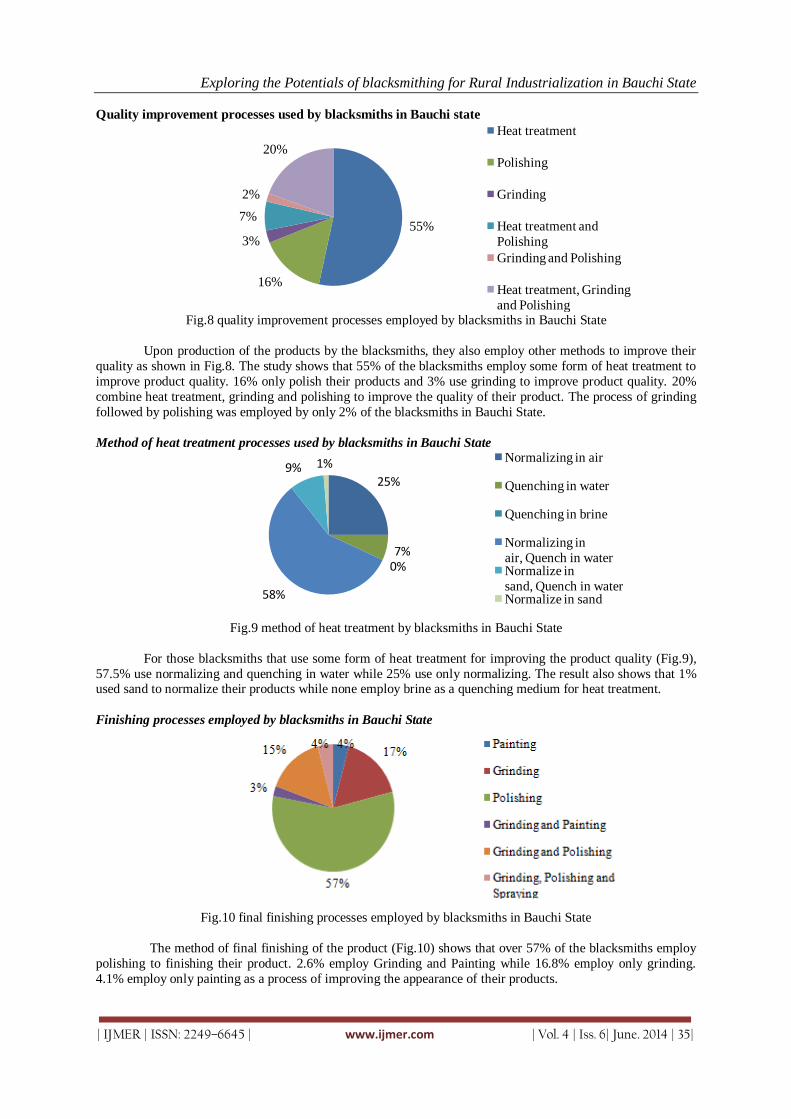
Exploring the Potentials of blacksmithing for Rural Industrialization in Bauchi State
| IJMER | ISSN: 2249–6645 | www.ijmer.com | Vol. 4 | Iss. 6| June. 2014 | 35|
Quality improvement processes used by blacksmiths in Bauchi state
Fig.8 quality improvement processes employed by blacksmiths in Bauchi State
Upon production of the products by the blacksmiths, they also employ other methods to improve their
quality as shown in Fig.8. The study shows that 55% of the blacksmiths employ some form of heat treatment to
improve product quality. 16% only polish their products and 3% use grinding to improve product quality. 20%
combine heat treatment, grinding and polishing to improve the quality of their product. The process of grinding
followed by polishing was employed by only 2% of the blacksmiths in Bauchi State.
Method of heat treatment processes used by blacksmiths in Bauchi State
Fig.9 method of heat treatment by blacksmiths in Bauchi State
For those blacksmiths that use some form of heat treatment for improving the product quality (Fig.9),
57.5% use normalizing and quenching in water while 25% use only normalizing. The result also shows that 1% used sand to normalize their products while none employ brine as a quenching medium for heat treatment.
Finishing processes employed by blacksmiths in Bauchi State
Fig.10 final finishing processes employed by blacksmiths in Bauchi State
The method of final finishing of the product (Fig.10) shows that over 57% of the blacksmiths employ
polishing to finishing their product. 2.6% employ Grinding and Painting while 16.8% employ only grinding.
4.1% employ only painting as a process of improving the appearance of their products.
55%
16%
3%
7%
2%
20%
Heat treatment
Polishing
Grinding
Heat treatment and
Polishing
Grinding and Polishing
Heat treatment, Grinding
and Polishing
25%
7%0%
58%
9% 1% Normalizing in air
Quenching in water
Quenching in brine
Normalizing in
air, Quench in waterNormalize in
sand, Quench in waterNormalize in sand

Exploring the Potentials of blacksmithing for Rural Industrialization in Bauchi State
| IJMER | ISSN: 2249–6645 | www.ijmer.com | Vol. 4 | Iss. 6| June. 2014 | 36|
Source of raw materials by blacksmiths in Bauchi State
Fig.11 source of raw materials by blacksmiths in Bauchi State
Fig.11 indicates that majority of the blacksmiths (49.7%) used a combination of automobile scrap and
standard metal stocks as their source of raw material while 33.5% used scrap of domestic equipment and
standard metal stocks bought from the market. 16.8% used only automobile scrap as a source of raw material.
None of the blacksmiths uses standard metal stocks only as a source of raw material. Automobile scraps mostly
used include failed crankshafts, leaf and coiled springs and push rods. While domestic equipment used mostly
include gas cookers, washing machines and fans. Standard metal stocks include rods, pipes, sheet metals, plates
and angle sections.
Method of identifying raw materials by blacksmiths in Bauchi State
Fig.12 method of identifying raw materials by blacksmiths in Bauchi State
The blacksmiths employ various methods to identify the raw material as shown in Fig.12. In this study
31.2% apply the use of sound while 14.1% use colour. It was found that 22.1 % use the weight to identify the raw material. However, only 1.5% used both sound and colour to identify the raw material.
Annual demand of raw material by blacksmiths in Bauchi State
Fig.13 annual demand of raw material by blacksmiths in Bauchi State
31%
14%22%
1%
15%
17%Sound
Colour
Weight
Sound and Colour
Colour and Weight
Sound and Weight
6%
28%
66%
Less than 15kg (5.6)
Between 15kg and 30kg
(28.2)
Above 30kg (66.2)

Exploring the Potentials of blacksmithing for Rural Industrialization in Bauchi State
| IJMER | ISSN: 2249–6645 | www.ijmer.com | Vol. 4 | Iss. 6| June. 2014 | 37|
In Fig.13 is shown the percentage of blacksmiths demanding various quantities of raw material
annually. 66.2% demand over 30kg of raw material annually while only 5.6% demand less than 15kg annually.
28.2% of the blacksmiths demand between 15kg and 30kg of raw material annually.
Annual production capacity of blacksmiths in Bauchi State
Fig.14 annual production capacity of Blacksmiths in Bauchi State
Fig.14 shows the annual production capacity of blacksmiths in Bauchi State. 32.4% produce over
1000units of the product annually, 32.8% produce between 500units and 1000units annually whereas 34.8%
produce less than 500units annually.
Application of safety measures in the workshop by blacksmiths in Bauchi State
Fig.15 application of safety measures in the workshop by blacksmiths in Bauchi State
The result in Fig.15 shows that a total number of 51.8% of the blacksmiths used water as a safety
measure. 26.5% used sand while 20.5% used both sand and water and none used fire extinguisher for safety
purpose. However, a negligible number of 1.2% of the blacksmiths used first aid box for safety purpose.
Major consumers of products of blacksmiths in Bauchi State
Fig.16 major consumers of products of blacksmiths in Bauchi State
Fig.16 shows that 90% of the consumers of products of blacksmiths are farmers while 7.5% and 2.5%
are other artisans such as barbers, butchers, cobblers and households respectively. It also shows that industries rarely (0%) patronize the products of blacksmiths.
35%
33%
32%Less than 500units
Between 500units and 1000units
Above 1000units
0%
26%
52%
1%
21%Fire Extinguisher (0)
Sand (26.5)
Water (51.8)
First Aid Box (1.2)
Sand and Water (20.5)
90%
7%0%3%
Farmers
Other Artisans
Industries
Households

Exploring the Potentials of blacksmithing for Rural Industrialization in Bauchi State
| IJMER | ISSN: 2249–6645 | www.ijmer.com | Vol. 4 | Iss. 6| June. 2014 | 38|
Source of initial capital by blacksmiths in Bauchi State
Fig.17 source of initial capital by blacksmiths in Bauchi State
The results of Fig.17 shows that majority of the blacksmiths (64%) inherited their tools initial capital
after the demise of their parents, whereas only 2% sourced their tools from a loan taken from the bank. This
reveals that the low quality of their products and low productivity could be attributed to lack of access to
sufficient funds to procure modern equipment. 28% of the blacksmiths sourced their initial capital from personal
savings.
Major developmental challenges of blacksmithing operations
Fig.18 major developmental challenges of blacksmithing operations in Bauchi State
Fig. 18 reveals that 61% of the blacksmiths considered lack of market as a major challenge against the
development of blacksmithing activities in Bauchi State, while 16% considered lack of market and financial support as major challenges. 14% considered lack of financial support as a challenge and only 3% each
considered lack of market and high cost of scrap, high cost of scrap, lack of technical support as major
challenges. This implies that lack of market is the most serious challenge being faced by the blacksmiths while
lack of technical supports and high cost of scrap are considered as less challenging.
IV. Conclusions From the above results, it could be concluded that:
The elderly people in each of the three zones are those that mostly practice blacksmithing, while
greater percentage of the assistants was within the productive age of 40years and below. This implies that the
technology has good prospects of being sustainable for rural industrialization. This is what was expected such
that the skills possessed by the elderly could be easily transmitted to the youths for sustainability. This debunked
the fear of extinction of the technology in due course.
Greater percentage of the blacksmiths attended non-formal education and the few that had tertiary
education were found in the Northern zone only, whereas a certain significant number had not attended any
school at all.
Agricultural tools and implements were the most produced products then followed by domestic,
industrial and lastly traditional tools and implements. This is in line with the findings of Oke (2007) and
Oladimeji (2013). Northern zone mostly engage in the production of agricultural tools and implements. The finding that Southern zone produce more of industrial and traditional tools could be attributed to their proximity
to Jos Plateau were a lot of solid mineral activity had been going on. This is an indication that if blacksmith
2%
64%
28%
6%
Bank Loan
Inheritance
Personal Savings
Assistance from Relatives
61%14%
3%
3%16%
3% Lack of Market
Lack of Financial Support
Lack of Technical Support
High Cost of Scrap
Lack of Market and Financial SupportLack of Market and High Cost of Scrap

Exploring the Potentials of blacksmithing for Rural Industrialization in Bauchi State
| IJMER | ISSN: 2249–6645 | www.ijmer.com | Vol. 4 | Iss. 6| June. 2014 | 39|
shop is developed its contribution will be felt by all areas of human endeavors therefore improving the economy
of the country.
Majority of the blacksmiths produced their own tools while a significant number by tools that were produced by either their colleagues or other local artisans such as the welders or wood carvers. None used
imported tools. The Northern zone has greater number of those that only improvised their tools (47%) as well as
only purchase locally produced tools (74%), whereas the Central zone has the highest number of those that
combine improvised as well as purchase locally produced tools (56%) more than other zones in the State.
This shows the capability of the blacksmiths to be self sufficient in terms of tools production. Such
skill could be explored in the production of high quality tools for use in other sectors. The major operations used
by the blacksmiths are heating and forging, this could be automated using simple designs of furnaces and forges
to reduce the manual effort for enhanced quality and quantity. Majority of the blacksmiths have the skills to
conduct heat treatment in order to improve the quality of their products. Grinding and polishing are also used by
the blacksmiths to improve the quality of their products.
Greater percentage of the blacksmiths population possesses the knowledge of heat treating their products using normalizing. Whereas none had the knowledge that brine could equally be used to heat treat
products. Polishing process used by the blacksmiths is employed to improve the quality of the product so as to
make it more aesthetic and qualitative.Sand and water are the most used materials for observing safety measures
in the workshop of the blacksmiths.
Majority of the consumers of blacksmith products are farmers while industrial products are rarely
produced. The skills of the blacksmith could be diversified for the production of industrial products such as
tools like spanners, hammers, pliers, jacks, clamps, etc. Households in the Southern zone patronize products of
blacksmiths more than any other zone in the Bauchi State.
The blacksmiths lack access to bank loan or fail to utilize the facility provided by the banks and
majority of their tools were inherited, which is responsible for the low quality and low productivity as the tools
or processes were not upgraded to modern ones. Majority of the blacksmiths in the Northern zone raise their
initial capital through personal savings, which agrees with the findings of Oladimeji (2013). The blacksmiths consider lack of market as a major challenge, which implies that they do not have
problem with the sale of their products and could be able to manufacture any product but that they are unable to
meet the demand of their customers in terms of quality and quantity. This is in agreement with the findings of
Oke (2007).It is only the Northern zone that considered lack of financial support as a major challenge while the
Central zone considered lack of technical support as a major challenge.
V. Recommendations Considering the skills possessed by blacksmiths in the different zones of Bauchi State, it is evident that
with necessary support from the government rural industrialization can be achieved. The study reveals that there
are specific products that are commonly produced in each zone. Government should support each zone
financially and technically so as to further strengthen them for specialization in the production of high quality
products.
For example, the Northern can be encouraged to specialize in the production of agricultural tools and
implements while Southern zone to specialize in the production of industrial tools and implements.
Furthermore considering the low educational level of the blacksmiths in Bauchi State, training could
commence by introduction of technical courses such as „Introduction to Technology‟ from the primary school
level.
REFERENCES [1.] Akpomuvie, O.H. (2011). The role of traditional skills and techniques in the development of modern Science and
technology in Africa. International Journal of Humanities and Social Science, Vol.1 (13), special Issue. [2.] Bauchi State Agricultural Supply Company, BSADP (2013). Monitoring unit committee report Colonial Reports -
annual of Northern Nigeria, No. 516 (1905-1906) on Bauchi, (1907).An annual report presented to both houses of parliament by command of his majesty. Printed for his majesty‟s stationary office. Darling and Sons ltd, London.
[3.] Dhimmar, V., Sheth, S. & Shah, S. (2011). Proposed workstation for rural blacksmiths. National Conference on Recent Trends in Engineering and Technology. Gujurat India: B.M.V. Engineering College.
[4.] Ezeadichie, U.E. (2002). External influence on nation building in Nigeria. A Critic Paper for conference on Externalist Vs Internalist Influence on African History and Culture organized by SOREC at Montclair State University, New Jersey, U.S.A.
[5.] IFAD. (2001). Rural poverty report 2001: The challenge of ending rural poverty. Oxford: OUP for IFAD. [6.] Kothari, C.R. (2004). Research methodology- methods and techniques, New Age International (P) Publishers,
Daryaganj, New Delhi India. [7.] Kumar, R.C. (2008). Researcfh methodology: non-probability sampling design in quantitative research, APH
Publishing Company, New Delhi, India.

Exploring the Potentials of blacksmithing for Rural Industrialization in Bauchi State
| IJMER | ISSN: 2249–6645 | www.ijmer.com | Vol. 4 | Iss. 6| June. 2014 | 40|
[8.] Micheal, B. & Baba, A.T. (2009). Construction of a furnace among the guddirawa: Description and linguistic remarks. A joint research project SFB 268, Johann Wolfgang Goethe-University, Frankfurt and the University of Maiduguri.
[9.] Ministry of Commerce Bauchi. (2007). Information bulletin. [10.] National Centre for Technology Management (NACETEM). (2008).Indigenous technology mapping and analysis
of skills acquisition methodologies in the aluminium and bronze casting industry in Nigeria. Policy research project funded by the Federal Government of Nigeria.
[11.] National Population Commision (2006). Census report [12.] Oke, P.K.(2007).An evaluation of improved local blacksmith Process. Journal of Engineering and Applied
Sciences, Vol.2, NO.8. [13.] Okon, E.E. (1991). Traditional skills and techniques as primary assets for the development of modern sciences and
technology. In: Culture, economy and national development. Bello, S. and Nasidi, Y. (eds). Tolalu and Associates, Lagos, (1991).
[14.] Personal Discussion (2013), Manager (Engineering), Bauchi State Agricultural Supply Company (BASAC) held on 25-02-2013.
[15.] Raw Materials Research and Development Council (RMRDC),(2002).RMRDC Report of the Technical Committee for the Upgrade of Directory of Equipment/Machinery Fabricators in Nigeria, Abuja..
[16.] Tristram, U. (1997). Barefoot technology. The Courier. 42.
International
OPEN ACCESS Journal Of Modern Engineering Research (IJMER)
| IJMER | ISSN: 2249–6645 | www.ijmer.com | Vol. 4 | Iss. 6| June. 2014 | 41|
Prediction of groundwater quality in Selected Locations in
Imo State
Okoro1, Boniface C., Ekeleme
2, Anthony C.
1, 2 Department of Civil Engineering, School of Engineering , Federal University of Technology, P.M.B 1526,
Owerri, Imo State, Nigeria.
I. Introduction Water is required by man in various activities such as washing, general cleaning, laundry and in
agricultural activities. Water is a necessity, a resource and at the same time a major contributory factor in the
contamination/pollution problems (Sabo et al.,2013). Water has been an indispensable commodity to man,
hence there has been extensive research and effort for its proper conservation and distribution for use. Safe
drinking water remains inaccessible for about 1.1 billion people in the world (Mintz et al., 2001). About 52% of
Nigerians do not have access to improved drinking water supply (Orebiyi et al., 2010). The use of water is
limited by its quality and this attribute of water also defines its general purpose.
For most communities the most secure source of safe drinking water is pipe-borne water from
municipal water treatment plants. Often, most of water treatment facilities do not deliver or fail to meet the
water requirements of the community due to corruption, lack of maintenance or increased population. The
scarcity of pipe borne water has made communities to find alternative sources of water - ground water sources
being a ready source. Wells are a common ground water source readily explored to meet community water requirement or
make up the short fall (Adekunle, 2008). The source of water also contributes to its quality and the chief source
of water for various domestic and agricultural uses is groundwater.
Groundwater is increasingly gaining significance as the main solution to the water supply problems in
Nigeria, especially in the sub-urban and rural areas (Akoteyon,2013). Groundwater quality comprises of
physical, chemical and biological properties. Temperature, turbidity, colour, taste and odour make up the list of
physical water quality parameters. The mineral ions which are divided into major, minor and trace constituent’s
make up the chemical properties. These parameters mentioned determine the extent of contamination of
groundwater whether or not the water is fit and of what purpose it can find use.
The rate of urbanization in Nigeria is alarming and the major cities areas are growing at rates between
10-15% per annum (Yusuf, 2007) and thus, human activities including soil fertility remediation, indiscriminate refuse and waste disposal, and the use of septic tanks, soak-away pits and pit latrines are on the increase.
Most inhabitants of Owerri West rely on borehole water as their chief supply of portable water supply,
therefore it becomes imperative that not only the quality of these water sources be studied but also, their
vulnerability to contamination be assessed and recommendation on efficient and effective protection strategy be
given to the appropriate regulatory bodies to forestall the negative consequences of negligence to this obvious
fact. In Nigeria, there is the challenge of lack of supply of pipe borne water hence many homes have borehole
wells sited around the house at a distance from the septic tank.
Abstract: The prediction of groundwater quality in selected locations was carried out in Owerri-West
L.G.A. of Imo State. The Physical, chemical and biological parameters of groundwater samples from
Nekede (Ward A), Ihiagwa (Ward B), Eziobodo (Ward C), Obinze (Ward D) and Avu (Ward E) were
analysed using the Atomic Absorption Spectrophotometer (AAS). A total of three replicates of fifteen
different borehole water samples were collected based on distances from closest potential sources of
contamination. All parameters were detected up to 61m from pollution source and most of them
increased in concentration during the periods, pointing to infiltrations from storm water. The results for Iron, pH and TVC decreased as distance increases while for nitrate and BOD increased as distance
increases. Results also showed that most of the boreholes were polluted and not suitable for human
consumption without adequate treatment, Regular monitoring of groundwater quality, abolishment of
unhealthy waste disposal practices and introduction of modern techniques are recommended.
Keywords: Groundwater, Pollution, distance, Physical, Chemical, Biological.

Prediction of groundwater quality in Selected Locations in Imo State
| IJMER | ISSN: 2249–6645 | www.ijmer.com | Vol. 4 | Iss. 6| June. 2014 | 42|
1.1 Description of Study Area
Owerri is a rapidly growing urban centre. It became the capital of Imo State in 1976. The Imo state
capital has three Local Government Areas - Owerri Municipal, Owerri North and Owerri West. The study area
is Owerri West L.G.A in Imo State is in the South Eastern part of Nigeria. It is bounded by latitudes 5o34 and 5
o34’ N and longitude 6 o52’ and 7o05’E.
II. Materials And Methods Five wards namely Nekede, Ihiagwa, Eziobodo, Obinze and Avu in Owerri Metropolis were chosen
for the purpose of this investigation. The locations from which the samples were taken are given in Table 1.
Distance from the borehole to a potential source of contamination which includes landfills, septic tank (sewers)
and pit toilet (latrines) was measured with a standard meter rule and recorded. The distance is also included in
Table 1. For convenience, the water samples from the 15 different boreholes were labeled W1 – W15. Replicate
of three samples in each of the areas were collected but from different boreholes.
The water samples were collected in the early morning hours when freshly pumped from the ground in
compliance with the Nigerian Standard for Drinking Water Quality (NSDQW) best practices for Water Quality
Analysis in October, 2011. Prior to collection as part of quality control measures all the bottles used for the sample collection were washed and rinsed with distilled water. The bottles were rinsed three times with the
sample water at the point of collection before the final water sampling was done. The bottles were held at the
bottom while filling, to avoid contamination of water from the hands or fingers (Oparaocha, et al., 2011). All the
sample containers were kept in ice boxes and brought to the laboratory for analysis. The bottles were labeled
with masking tapes and the identification details were written on them according to sampling location as shown
in Table 1.
The closest sources of pollution to these boreholes sampled were noted as shown in Table1. The
qualitative analysis was carried out at the Central Laboratories of National Root Crops Research Institute
Umudike (NRCRI), Umuahia, Abia State.
Table 1. Selected location areas within Owerri West L.G.A and their distances from sources of contamination
Ward
Area
Sample
Depth to static water
level (m)
Distance From closest
potential
Sources
contamination
(meters)
NAFDAC
Closest contamination
source
30m Septic tank
A Nekede W1
W2
W3
47 3.0
12.6
14.9
Septic tank
Septic tank
Septic tank
B Eziobodo W4
W5
W6
46 11.0
30.2
20.5
Septic tank
Landfill
Open site
C Ihiagwa W7
W8
W9
47 26.4
13.6
13.9
Pit latrine
Septic tank
Septic tank
D Obinze W10 W11
W12
46 48.6 13.3
60.4
Septic tank Septic
Septic tank
E Avu W13
W14
W15
46 50.4
61.3
13.4
Septic tank
Pit latrine
Pit latrine

Prediction of groundwater quality in Selected Locations in Imo State
| IJMER | ISSN: 2249–6645 | www.ijmer.com | Vol. 4 | Iss. 6| June. 2014 | 43|
2.1. Test for Biological Parameters The samples collected from the various boreholes were analyzed for the following biological
parameters; Biochemical Oxygen Demand (BOD), Total Viable Count (TVC) and coliform test. The membrane
filter (MF) technique was used for the analysis.
2.2 Test for Chemical Parameters
The samples were analyzed for the following chemical parameters: Nitrate (NO3-), Zinc (Zn),
Manganese (Mn), Lead (Pb), and Iron (Fe), according to the procedures described by APHA (2005).
2.3 Test for Physical Parameters
The samples were examined physically to determine the taste, colour, odour and temperature. Other
physical parameters examined included the PH ,concentration of suspended and dissolved solids.
2.4 Quadratic Regression Model
The quadratic regression model was used to predict the biochemical parameters with respect to the
distances from the source of contamination.
Considering a polynomial of the form
Y = ao - a1 x + a2 + x2 (1) where x= distance from the borehole to a potential source of contamination
Y= experimental value obtained from the laboratory
The sum of squared deviations of the observed values of y from the predicted values is given by
S = (y –ao – a1 x – a2x2)2 (2)
Minimizing Eq 3.2 by setting its partial derivatives with respect to ao, a1, a2 equal to zero, we have
y = aon + a1 x + a2 x2
Xy = aox + a1 x2 + a2 x3 (3)
x2y = aox2 + a1 x3 + a2 x4
Solving the above equations give solutions to the values of ao, a1, a2
For instance, considering a 3 x 3 matrix
X Y Z ao I
C D E a1 J
F G H a2 k
Solving for the unknown coefficient of ao, a1, a2, we have
a2 = 𝐾
𝐻 (4)
a1 = 𝐸𝐾 − 𝐽 (5)
ao = 𝐼 − 𝑦(𝑎₁) − 𝑍(𝑎₂) (6)
The Quadratic Regression Model equations 3, 4, 5, and 6 respectively were used to predict the biological, chemical and physical parameters against distances from the sources of contamination.
III. Results And Discussion The predicted equations and values of physico-chemical and biological parameters of the water
samples obtained from boreholes in selected locations Owerri West are presented in Table 3 to Table 9. Also the
graphs of predicted parameters are shown from Fig. 1 to Fig.5.
Figure 1.0 showed the graph of TVC against measured distances. The TVC values starts to decrease
from at 6.4 Cfu/ml at a distance of 3 meters. At a distance of 40m, the TVC value recorded the minimum value of 3.6 Cfu/ml. After this distance, the TVC values increased with distances from the source of contamination.
This implies that siting a borehole at about 40m from any source of contamination would be most appropriate
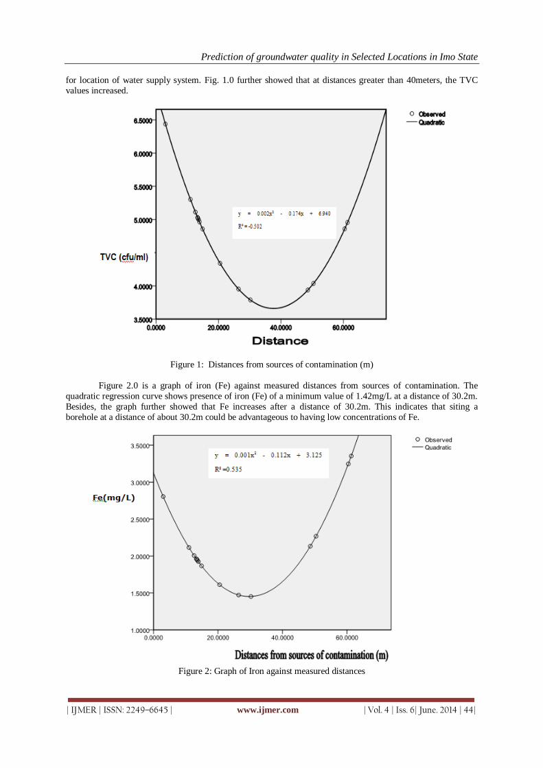
Prediction of groundwater quality in Selected Locations in Imo State
| IJMER | ISSN: 2249–6645 | www.ijmer.com | Vol. 4 | Iss. 6| June. 2014 | 44|
for location of water supply system. Fig. 1.0 further showed that at distances greater than 40meters, the TVC
values increased.
Figure 1: Distances from sources of contamination (m)
Figure 2.0 is a graph of iron (Fe) against measured distances from sources of contamination. The
quadratic regression curve shows presence of iron (Fe) of a minimum value of 1.42mg/L at a distance of 30.2m.
Besides, the graph further showed that Fe increases after a distance of 30.2m. This indicates that siting a
borehole at a distance of about 30.2m could be advantageous to having low concentrations of Fe.
Figure 2: Graph of Iron against measured distances
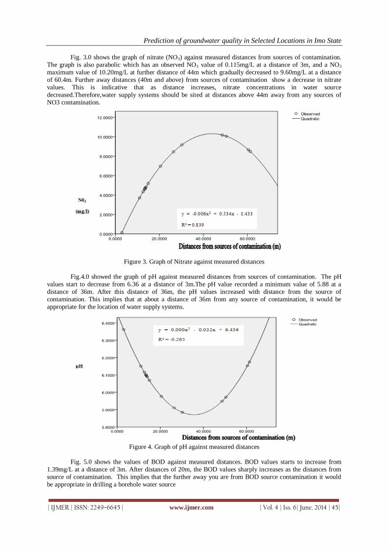
Prediction of groundwater quality in Selected Locations in Imo State
| IJMER | ISSN: 2249–6645 | www.ijmer.com | Vol. 4 | Iss. 6| June. 2014 | 45|
Fig. 3.0 shows the graph of nitrate (NO3) against measured distances from sources of contamination.
The graph is also parabolic which has an observed NO3 value of 0.115mg/L at a distance of 3m, and a NO3
maximum value of 10.20mg/L at further distance of 44m which gradually decreased to 9.60mg/L at a distance
of 60.4m. Further away distances (40m and above) from sources of contamination show a decrease in nitrate
values. This is indicative that as distance increases, nitrate concentrations in water source
decreased.Therefore,water supply systems should be sited at distances above 44m away from any sources of
NO3 contamination.
Figure 3. Graph of Nitrate against measured distances
Fig.4.0 showed the graph of pH against measured distances from sources of contamination. The pH
values start to decrease from 6.36 at a distance of 3m.The pH value recorded a minimum value of 5.88 at a
distance of 36m. After this distance of 36m, the pH values increased with distance from the source of
contamination. This implies that at about a distance of 36m from any source of contamination, it would be
appropriate for the location of water supply systems.
Figure 4. Graph of pH against measured distances
Fig. 5.0 shows the values of BOD against measured distances. BOD values starts to increase from
1.39mg/L at a distance of 3m. After distances of 20m, the BOD values sharply increases as the distances from
source of contamination. This implies that the further away you are from BOD source contamination it would
be appropriate in drilling a borehole water source

Prediction of groundwater quality in Selected Locations in Imo State
| IJMER | ISSN: 2249–6645 | www.ijmer.com | Vol. 4 | Iss. 6| June. 2014 | 46|
Figure 5. Graph of BOD against measured distances
Table 3: The various Physical ,Bio-chemical Parameters, Equation of Curves and Regression Parameters
Parameters Model Equation curves for Determination of
distances
Regression parameters
TVC (cfu/mL) YTvc = 0.002x2 – 0.174 x + 6.940 GF = -0.502
CC = -0.708
Fe3+(mg/L) YFe3+ = 0.001X2 – 0.112X + 3.125 GF = 0.535
CC = 0.731
NO3- (mg/L) YNO3
- = -0.006x2 + 0.534x – 1.433 GF = 0.839
CC =0.916
Ph YpH = 0.00x2 – 0.032x + 6.456 GF = -0.265
CC = -0.515
BOD(mg/L) YBOD = 𝑒 - 04x2 – 0.001x + 1.401 GF = 0.965
CC = 0.982
Regression parameters:
GF = Goodness of fit CC = correlation coefficient, 𝑒 = starndard error.
Table 4: Total viable Count (TVC) values with measured distances from all sources of contamination
Distance
X
(m)
(TVCe)y
X2 X3 X4 Xy X2y TVCp = a0 +
a1x + a2x2
3 7.3 9 27 81 21.9 65.7 6.438234
12.6 3.0 158.76 2000.376 25204.74 37.8 476.28 5.11184
14.9 5.0 222.01 3307.949 49288.44 74.5 1110.05 4.85742
11 4.7 121 1331 14641 51.7 568.7 5.303274
30.2 3.3 912.04 27543.61 831817 99.66 3009.732 3.788356
20.5 5.3 420.25 8615.125 176610.1 108.65 2227.325 4.340378
26.4 5.0 696.96 18399.74 485753.2 132 3484.8 3.952709
13.6 3.7 184.96 2515.456 34210.2 50.32 684.352 4.998213
13.9 4.7 193.21 2685.619 37330.1 65.33 908.087 4.965028
48.6 4.3 2361.96 114791.3 5578855 208.98 10156.43 3.938168
13.3 6.0 176.89 2352.637 31290.07 79.8 1061.34 5.031815
60.4 5.3 3648.16 220348.9 13309071 320.12 19335.25 4.859217
50.4 3.3 2540.16 128024.1 6452413 166.32 8382.528 4.036997
61.3 4.7 3757.69 230346.4 14120234 288.11 17661.14 4.955927
13.4 6.0 179.56 2406.104 32241.79 80.4 1077.36 5.020568
393.5 71.6 15582.61 764695.2 41179041 1785.59 70209.07
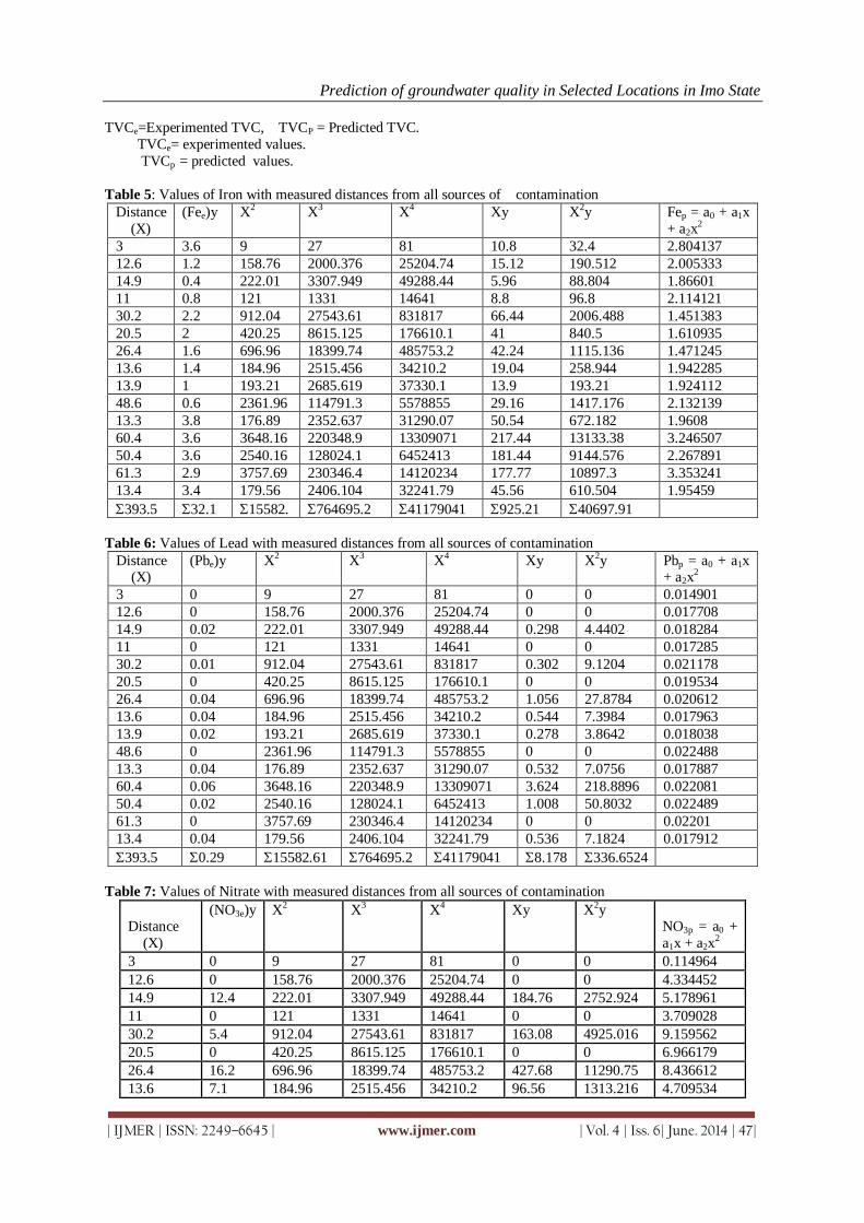
Prediction of groundwater quality in Selected Locations in Imo State
| IJMER | ISSN: 2249–6645 | www.ijmer.com | Vol. 4 | Iss. 6| June. 2014 | 47|
TVCe=Experimented TVC, TVCP = Predicted TVC.
TVCe= experimented values.
TVCp = predicted values.
Table 5: Values of Iron with measured distances from all sources of contamination
Distance
(X)
(Fee)y
X2 X3 X4 Xy X2y Fep = a0 + a1x
+ a2x2
3 3.6 9 27 81 10.8 32.4 2.804137
12.6 1.2 158.76 2000.376 25204.74 15.12 190.512 2.005333
14.9 0.4 222.01 3307.949 49288.44 5.96 88.804 1.86601
11 0.8 121 1331 14641 8.8 96.8 2.114121
30.2 2.2 912.04 27543.61 831817 66.44 2006.488 1.451383
20.5 2 420.25 8615.125 176610.1 41 840.5 1.610935
26.4 1.6 696.96 18399.74 485753.2 42.24 1115.136 1.471245
13.6 1.4 184.96 2515.456 34210.2 19.04 258.944 1.942285
13.9 1 193.21 2685.619 37330.1 13.9 193.21 1.924112
48.6 0.6 2361.96 114791.3 5578855 29.16 1417.176 2.132139
13.3 3.8 176.89 2352.637 31290.07 50.54 672.182 1.9608
60.4 3.6 3648.16 220348.9 13309071 217.44 13133.38 3.246507
50.4 3.6 2540.16 128024.1 6452413 181.44 9144.576 2.267891
61.3 2.9 3757.69 230346.4 14120234 177.77 10897.3 3.353241
13.4 3.4 179.56 2406.104 32241.79 45.56 610.504 1.95459
393.5 32.1 15582. 764695.2 41179041 925.21 40697.91
Table 6: Values of Lead with measured distances from all sources of contamination
Distance (X)
(Pbe)y
X2 X3 X4 Xy X2y Pbp = a0 + a1x + a2x
2
3 0 9 27 81 0 0 0.014901
12.6 0 158.76 2000.376 25204.74 0 0 0.017708
14.9 0.02 222.01 3307.949 49288.44 0.298 4.4402 0.018284
11 0 121 1331 14641 0 0 0.017285
30.2 0.01 912.04 27543.61 831817 0.302 9.1204 0.021178
20.5 0 420.25 8615.125 176610.1 0 0 0.019534
26.4 0.04 696.96 18399.74 485753.2 1.056 27.8784 0.020612
13.6 0.04 184.96 2515.456 34210.2 0.544 7.3984 0.017963
13.9 0.02 193.21 2685.619 37330.1 0.278 3.8642 0.018038
48.6 0 2361.96 114791.3 5578855 0 0 0.022488
13.3 0.04 176.89 2352.637 31290.07 0.532 7.0756 0.017887
60.4 0.06 3648.16 220348.9 13309071 3.624 218.8896 0.022081
50.4 0.02 2540.16 128024.1 6452413 1.008 50.8032 0.022489
61.3 0 3757.69 230346.4 14120234 0 0 0.02201
13.4 0.04 179.56 2406.104 32241.79 0.536 7.1824 0.017912
393.5 0.29 15582.61 764695.2 41179041 8.178 336.6524
Table 7: Values of Nitrate with measured distances from all sources of contamination
Distance
(X)
(NO3e)y
X2 X3 X4 Xy X2y NO3p = a0 +
a1x + a2x2
3 0 9 27 81 0 0 0.114964
12.6 0 158.76 2000.376 25204.74 0 0 4.334452
14.9 12.4 222.01 3307.949 49288.44 184.76 2752.924 5.178961
11 0 121 1331 14641 0 0 3.709028
30.2 5.4 912.04 27543.61 831817 163.08 4925.016 9.159562
20.5 0 420.25 8615.125 176610.1 0 0 6.966179
26.4 16.2 696.96 18399.74 485753.2 427.68 11290.75 8.436612
13.6 7.1 184.96 2515.456 34210.2 96.56 1313.216 4.709534

Prediction of groundwater quality in Selected Locations in Imo State
| IJMER | ISSN: 2249–6645 | www.ijmer.com | Vol. 4 | Iss. 6| June. 2014 | 48|
13.9 0 193.21 2685.619 37330.1 0 0 4.819687
48.6 6.3 2361.96 114791.3 5578855 306.18 14880.35 10.1766
13.3 0 176.89 2352.637 31290.07 0 0 4.598286
60.4 5.8 3648.16 220348.9 13309071 350.32 21159.33 8.662168
50.4 13 2540.16 128024.1 6452413 655.2 33022.08 10.05503
61.3 11.6 3757.69 230346.4 14120234 711.08 43589.2 8.477166
13.4 16.2 179.56 2406.104 32241.79 217.08 2908.872 4.63549
393.5 94 15582.61 764695.2 41179041 3111.94 135841.7
Table 8: Values of pH with measured distances from all sources of contamination
Distance
(X)
(pHe)y
X2 X3 X4 XY X2Y pHp= a0 +
a1x + a2x2
3 6.4 9 27 81 19.2 57.6 6.361927
12.6 6.2 158.76 2000.376 25204.74 78.12 984.312 6.11551
14.9 5.9 222.01 3307.949 49288.44 87.91 1309.859 6.069091
11 6.1 121 1331 14641 67.1 738.1 6.150679
30.2 5.8 912.04 27543.61 831817 175.16 5289.832 5.884436
20.5 6.3 420.25 8615.125 176610.1 129.15 2647.575 5.976463
26.4 5.6 696.96 18399.74 485753.2 147.84 3902.976 5.910153
13.6 6 184.96 2515.456 34210.2 81.6 1109.76 6.094729
13.9 6.1 193.21 2685.619 37330.1 84.79 1178.581 6.088674
48.6 6.1 2361.96 114791.3 5578855 296.46 14407.96 5.948226
13.3 6.5 176.89 2352.637 31290.07 86.45 1149.785 6.100866
60.4 6.3 3648.16 220348.9 13309071 380.52 22983.41 6.153416
50.4 6.1 2540.16 128024.1 6452413 307.44 15494.98 5.971228
61.3 5.9 3757.69 230346.4 14120234 361.67 22170.37 6.174335
13.4 5.8 179.56 2406.104 32241.79 77.72 1041.448 6.098811
393.5 91.1 15582.61 764695.2 41179041 2381.13 94466.54
Table 9. Values of BOD with measured distances from all sources of contamination
Distance
(X)
(BODe)
y
X2 X3 X4 XY X2y
BODp = a0 +
a1x + a2x2
3 1.3 9 27 81 3.9 11.7 1.39658
12.6 1.4 158.76 2000.376 25204.74 17.64 222.264 1.393016
14.9 1.4 222.01 3307.949 49288.44 20.86 310.814 1.394845
11 1.2 121 1331 14641 13.2 145.2 1.392356
30.2 1.6 912.04 2754.61 831817 48.32 1459.264 1.433398
20.5 1.6 420.25 8615.125 176610.1 32.8 672.4 1.403633
26.4 1.5 696.96 18399.74 485753.2 39.6 1045.44 1.41954
13.6 1.4 184.96 2515.456 34210.2 19.04 258.944 1.393684
13.9 1.3 193.21 2685.619 37330.1 18.07 251.173 1.393923
48.6 1.1 2361.96 114791.3 5578855 53.46 2598.156 1.54053
13.3 1.2 176.89 2352.637 31290.07 15.96 212.268 1.393463
60.4 1.6 3648.16 220348.9 13309071 96.64 5837.056 1.644158
50.4 1.4 2540.16 128024.1 6452413 70.56 3556.224 1.554574
61.3 2 3757.69 230346.4 14120234 122.6 7515.38 1.653182
13.4 1.8 179.56 2406.104 32241.79 24.12 323.208 1.393535
393.5 21.8 15582.61 764695.2 41179041 596.77 24419.49

Prediction of groundwater quality in Selected Locations in Imo State
| IJMER | ISSN: 2249–6645 | www.ijmer.com | Vol. 4 | Iss. 6| June. 2014 | 49|
IV. Conclusion And Recommendations The prediction of groundwater quality in selected locations evaluated using standard analytical methods
for testing physico-chemical and biological parameters was moderately high. The land-use activities in these
locations which include poorly constructed pit latrines, septic tanks, landfills and open dump sites all aid in the vulnerability of the region to groundwater pollution.
Based on the result obtained from the quadratic regression in the selected locations, the following
conclusion can be made. The quadratic regression model gives a goodness of fit and correlation coefficient in
most of the predicted parameters. The predicted parameters give best fit curves to regretted data this is evident
from the very high positive values of goodness of fit of the curve as stated in Table 3.Most of the graph of
Predicted parameters increased with increase in distance from the borehole well source. As a preventive
measure to reduce the health threat associated with consumption of the nitrate, Magnesium and iron
contaminated water as contained in the ground water in the selected locations, There is need for proper
treatment of water before consumption. Government through the various water resource management bodies
should create massive public awareness programmes on the television and other mass media agencies to educate
the populace of the health implications of groundwater pollution.
REFERENCES [1] Adekunle, A. S. (2008). Impacts of industrial effluent on quality of well water within Asa Dam Industrial Estate,
Ilorin, Nigeria. Nature and Science 6(3): 1-5. [2] APHA. (2005). Standard Methods for the Examination of Water and Waste Water, 21st ed. American Public Health Association, Washington, DC. Pp 1-252.
[3] Mintz, E., Bartram, J., Lochery, P. and Wegelin M. (2001). Not just a drop in the bucket: Expanding access to point of use water treatment systems. American Journal of Public Health 91:1565-1570.
[4] NSDQW, (2007). Nigerian Standard for Drinking Water Quality, Nigerian Industrial Standard (NIS) 554. Standard Organization of Nigeria. Pp. 30-45.
[5] Oparaocha, E.T., Iroegbu, O.C. and Obi, R.K. (2011). Assessment of quality of drinking water sources in the Federal University of Technology, Owerri, Imo state, Nigeria. Journal of Applied Biosciences. 32: 1964 – 1976.
[6] Orebiyi, E.O., Awomeso, J. A., Idowu, O.A., Martins, O., Oguntoke, O. and Taiwo, A. M. (2010). Assessment of pollution hazards of shallow well water in Abeokuta and Environs, Southwest, Nigeria. American Journal of
Environmental Sciences 6(1): 50-56 [7] Sabo,A., Adamu, H. and Yuguda,A.U. (2013). Assessment of Wash-Borehole Water Quality in Gombe Metropolis,
Gombe State, Nigeria. Journal of Environment and Earth Science. Vol. 3(1): 65-71. [8] Yusuf, K. A. (2007). Evaluation of groundwater quality characteristics in Lagos-City. Journal of Applied Sciences
7(13): 1780-1784.

International
OPEN ACCESS Journal Of Modern Engineering Research (IJMER)
| IJMER | ISSN: 2249–6645 | www.ijmer.com | Vol. 4 | Iss. 6| June. 2014 | 50|
Flow Analysis of Butterfly Valve Using CFD
Arun Azad1, Deepak Baranwal
2, Rajeev Arya
3, Nilesh Diwakar
4
1 PG Research scholar Department of Mechanical Engineering TIEIT, Bhopal 2 Research scholar Department of Civil Engineering MANIT, Bhopal
3 Professor & Dean PG Department of Mechanical Engineering TIEIT, Bhopal 4 Professor & HOD Department of Mechanical Engineering TIEIT Bhopal
I. Introduction Butterfly valve is very versatile component for use both as shut off and throttling valve in water
system. Butterfly valve has simple mechanical assembly, and a small flow resistance in a fully open position,
butterfly valves provide a relatively high flow capacity. They are the best suited for relatively low pressure flow.
Generally, the fluid friction coefficient is low and also the build up is usually minimum because of the Butterfly
valve is operated with a quarter turn (like the ball valve). Manual Operation may be through lever or gear. The
position of the disc is noted by an indicator on the gearbox or from the position of the handle. The first attempt at collecting and collating the published data concerning butterfly valves was probably made by Cohn in 1951.
Experimental studies on butterfly valve flow characteristics have been conducted by Addy et al in 1985.The
results of numerical simulation of flow characteristics including both velocity and pressure calculations are
presented in literature. Study on hydrodynamic torque of the butterfly valve has been conducted by Morris and
Dutton in 1989.
II. Technical Requirements Of Butterfly Valve Main purpose of the valves installed ahead of turbine is to close the penstock while the turbine is not in
operating condition. Valve must possess high degree of reliability and durable strength at closed position so that trouble free operation can take place. It should also ensure the possibility of carrying out repair works, revisions
of turbines, pumps, pressure penstock and at the same time to create lowest resistance to flow. Valve must close
at velocity of water occurring during emergency cases (rupture of penstock or runway speed of
turbine).Maximum time for closure of the valve when it is installed before the turbine pump is 1‐3 minutes and
depends upon the permissible time of operation of generator at run way speed and motor of the pump in
generator regime. If the valve is installed at the beginning of the penstock, then its closure time will be in the
range of 30‐120 seconds. Time of closing of valve on sluice and irrigation schemes is determined from the
operational conditions of these constructions. Minimum time of emergency closure is determined as per
permissible value of hydraulic impact on penstock. Operation of spherical and b.f. valve is depend upon the
extreme positions of the rotating part while in case of cylindrical valve it is accomplished at any position including extreme positions for regulating discharge of liquid through them is zero to maximum possible
discharge. Servomotors of various designs are used to rotate the rotating element, by mechanical or electro
mechanical drive.
Abstract: Butterfly valves are widely used in hydro power plants to regulate and control the flow through hydraulic turbines. That’s why it is important to design the valve in such a way that it can give
best performance so that optimum efficiency can be achieved in hydraulic power plants. Conventionally
that the models of large size valves are straight in the laboratory to determine their performance
characteristics. This is a time consuming and costly process. High computing facility along with the use
of numerical techniques can give the solution to any fluid flow problem in a lesser time. In this research
work flow analysis through butterfly valve with aspect ratio 1/3 has been performed using
computational software. For modelling the valve ICEM CFD 12 has been used. Valve characteristics
such as flow coefficient and head loss coefficient has been determined using CFX 12 for different valve
opening angle as 30°,60°,75°, and 90° (taking 90°as full opening of the valve) for incompressible fluid.
Value of head loss coefficient obtained from numerical analysis has been compared with the
experimental results.
Key Words: Butterfly valve, CFD flow analysis, simulation, valve opening.

Flow Analysis Of Butterfly Valve Using Cfd
| IJMER | ISSN: 2249–6645 | www.ijmer.com | Vol. 4 | Iss. 6| June. 2014 | 51|
III. Objective Butterfly valves are required to have high performance characteristics and better precision as they are
used as shut off valves. The characteristics of a valve i.e. head loss characteristic, torque characteristics and
force characteristics of butterfly valve is determined conventionally through tests. If the test valve is of large
size, scale model of valve is tested to determine its characteristics. Analysis of flow characteristic
experimentally is a hectic and not very precise work. Exact theoretical analysis of flow through complex
geometry is very difficult with the use of high speed computers, and the numerical techniques, the flow analysis
can be made using CFD.That’s why flow analysis is to be performed using simulation software. Objective of
this research work is to determine head loss coefficient and flow coefficient, for different valve opening and
discharge value. At present almost every industry is using software for analysis, Butterfly valves are used in
various power plants, so it has wide scope, this research work will be beneficial for all those industries that are
using butterfly valve. Computational fluid dynamics is a tool to carry out numerical flow simulation for predicting the flow behaviour within a specific domain by numerical solution of governing equations to
acceptable accuracy. Computational fluid dynamics is becoming very useful approach for engineering design
and analysis because of improved numerical method and at the same time, it saves time and energy of
experimental work. In this thesis, flow simulation has been carried out for double disc butterfly valve using
Ansys ICEM CFD and CFX. The geometric modelling is done for four angular position of valve disk to assess
the head loss and discharge coefficients Characteristics of valve.
IV. Computational Fluid Dynamics CFD is a computational technology that enables to study the dynamics of matters that flows. CFD is
predicting what will happen, quantitatively, when fluids flow even with the complications of simultaneous flow
of heat, mass transfer, phase change, chemical reaction, mechanical movement, stresses in and displacement of
immersed or surrounding solids. CFD include expressions for the conservation of mass, momentum, pressure,
species and turbulence. Navier‐Stokes equation given by Claude Louis Marie Henry Navier and the George
Gabriel Stokes. Which defines any single‐phase fluid flow, is the fundamental bases of all CFD problems.CFD
software is based on sets of very complex non‐linear mathematical expressions that define the fundamental
equations of fluid flow, heat andmaterials transport? These equations are solved iteratively using complex
computer algorithms embedded within CFD software. Outputs from CFD software can be viewed graphically in
colour plots of velocity vectors, contours of pressure, lines of constant flow field properties, or as "hard"
numerical data and X‐Y plots. In CFD it is possible to directly solve the Navier‐Stokes equations for laminar
flows and for turbulent flows when all the relevant length scales can be resolved by the grid (a direct numerical
simulation). In general however, the range of length scales appropriate to the problem is larger than even today's
massively parallel computers can model. In these cases, turbulent flow simulations require the introduction of a
turbulence model. Large eddy simulations (LES) and the Reynolds‐averaged Navier‐Stokes equations (RANS)
formulation, with the k‐ε model or the Reynolds stress model, are two techniques for dealing with these scales.
V. Boundary Conditions
Here inlet, outlet and other boundary conditions are defined. In this analysis in pipe domain inlet and
outlet boundaries has been created and subjected to various Conditions.
1. Inlet boundary condition In this location is selected as inlet of the pipe, flow is subsonic, mass flow rate has been set different for
different opening angles. Flow direction is normal to the boundary and turbulence is set at medium (intensity
=5%)
2. Outlet boundary condition In this location is selected as outlet of the pipe, flow is subsonic, average static pressure has been taken as 1 atm.
VI. Velocity Distribution
Fig.1 streamlines of flow through butterfly valve at 30°opening.
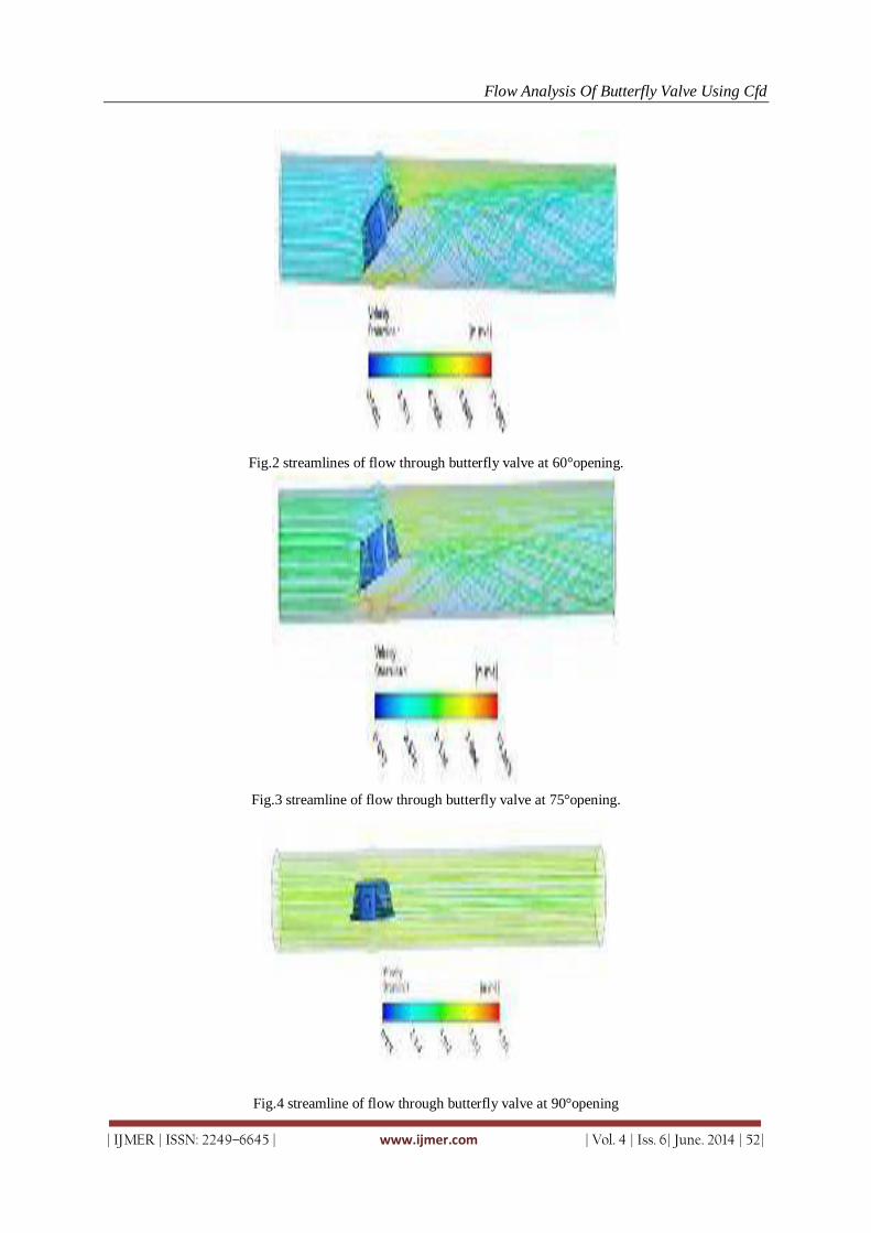
Flow Analysis Of Butterfly Valve Using Cfd
| IJMER | ISSN: 2249–6645 | www.ijmer.com | Vol. 4 | Iss. 6| June. 2014 | 52|
Fig.2 streamlines of flow through butterfly valve at 60°opening.
Fig.3 streamline of flow through butterfly valve at 75°opening.
Fig.4 streamline of flow through butterfly valve at 90°opening
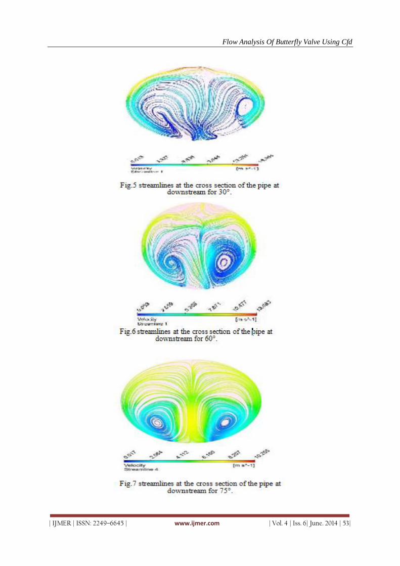
Flow Analysis Of Butterfly Valve Using Cfd
| IJMER | ISSN: 2249–6645 | www.ijmer.com | Vol. 4 | Iss. 6| June. 2014 | 53|
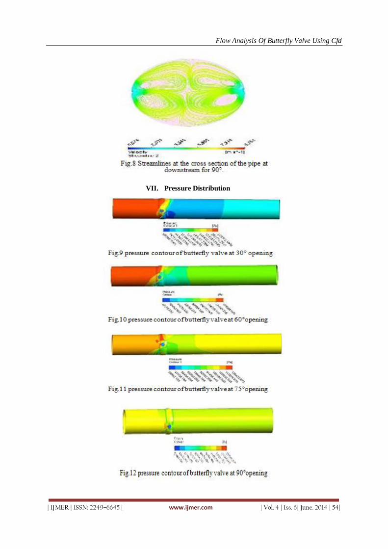
Flow Analysis Of Butterfly Valve Using Cfd
| IJMER | ISSN: 2249–6645 | www.ijmer.com | Vol. 4 | Iss. 6| June. 2014 | 54|
VII. Pressure Distribution

Flow Analysis Of Butterfly Valve Using Cfd
| IJMER | ISSN: 2249–6645 | www.ijmer.com | Vol. 4 | Iss. 6| June. 2014 | 55|
VIII. Result
IX. Conclusion During this research work, analysis of flow through Butterfly valve has been done to determine the
performance characteristics by CFD analysis and based on the simulation results, following conclusions are
drawn:
• Velocity at upstream as well as downstream is increasing with the increase in opening angle.
• Streamlines at the downstream side of the door is becoming uniform with the increase in opening angle.
This indicates that the disturbances are reduced for higher valve opening angle.
• Total pressure at upstream is decreasing while at downstream side of the door it is increasing with the
opening angle. This indicates that the pressure imbalance is reducing on the two sides of the door with
increase in angle of opening.
• Streamlines at the cross section of the pipe shows that vortices are shifting towards downward direction and becoming clearly visible with increase in opening angle.
• At small angle of opening, there are vortices formed behind the door. The turbulence in the flow is also
high. These are causing large form drag and a high amount of total loss. Relative loss coefficient is
decreasing, that’s why head loss coefficient is increasing with the increase in valve opening angle. It
shows that head loss coefficient is a strong function of opening angle .
• Flow coefficient is increasing with the valve opening and having maximum value 0.1630 for fully open
condition .
• Numerical results are matching with the experimental results very closely, thus conforming the present
CFD analysis .
REFERENCES [1]. A. D. Henderson, J. E. Sargison, G. J. Walker and J. Haynes, ”A numerical study of the flow through a safety
butterfly valve in a hydro electric power scheme”,16th Australasian fluid mechanics conference, December 2007.
[2]. Fangbiao Lin and Gerold A. schohl,:‐“A CFD prediction &validation of butterfly valve hydrodynamic forces”, ASCE Conf. Proc. doi:10.1061/40737(2004)232 Critical Transitions in Water and Environmental
Resources Management, World Water and Environmental Resources Congress, 2004 [3]. Gerhart Penninger, Helmut Benigni” New design of butterfly valves for modern pump‐storage power plants” Voith
Siemens Hydro Power GenerationGmb H&Co. KG and Institute for Hydraulic Fluid machinery, Engineering &Design – TUK Technical University of Graz.
[4]. Hui‐xiong Wan.Jun Fang and Hui Huang “Numerical simulation on a throttle governing system with hydraulic
butterfly valves in a marine environment”Harbin engineering university & spriger‐verlay Berlin hedelberg, 2010.
[5]. Janusz WOJTKOWIAK, Czeslaw oleskowkz‐popiel investigation of butterfly valve flow characteristics”
[6]. Jeon S Y, Yoon J Y, Shin M S.”Flow characteristics and performance evaluation of butterfly valves using numerical analysis”, 25th IAHR Symposium on Hydraulic Machinery and system.
[7]. M. S. Kalsi, B. Eldiwany, Vinod Sharma, Aaron Richie ”Effect of butterfly valve disc shape variations on Torque Requirements for power plant application”, Eight NRC/ASME Symposium on valve and pump testing,
Washington, D.C, July 2004

Flow Analysis Of Butterfly Valve Using Cfd
| IJMER | ISSN: 2249–6645 | www.ijmer.com | Vol. 4 | Iss. 6| June. 2014 | 56|
[8]. Kim S. W., Kim J. H., Choi Y. D., Lee Y. H. ,”Flow characteristics of Butterfly valve and CFD” Fifth international conference on fluid mechanics, Aug 2007,shanghai,Chaina.
[9]. Lin Wang, Xueguan Song, Youngchul Park, “The improvement of large butterfly valve by using numerical analysis method” 6th WSEAS international conference on fluid mechanics, 2009.
[10]. Park Youngchul and Song Xueguan “Numerical Analysis of Large Diameter Butterfly valve” springer science business Media, 2009.
[11]. V.Caille, J. Laumonier,”Effect of periodic aerodynamic pulsation on flow over aconfined butterfly valve”, journal
from spriger‐verlog, 1998
[12]. Weerachai Chaicorapuek: ‐“The engineering investigation of the water flow past the butterfly valve” June 2007, [13]. Xue Gguan Song, Young Chul Park, “Numerical Analysis of butterfly valve prediction of flow coefficient and
hydrodynamic torque coefficient”, world congress on engineering and computer science, October 2007, San Francisco, USA.
[14]. Zachary Leutwyler, Dalton Charls”A computational study of torque and force due to compressible flow on a butterfly valve disc in mid stroke position” September‐2006,J fluid engg, volume 128,issue 5,1074
[15]. Zachary Leutwyler, Charls Dalton ”A CFD study of flow field, resultant forced aerodynamic torque on a symmetric disc butterfly valve in a compressible Fluid” may‐2008, j.pressure vessel techno l volume 130, issue 2012-13 02
[16]. A Thesis submitted by Mukesh Kumar Meena,”Constructional and operational aspects of main inlet valve of hydro power plants”, civil engineering Department, MANIT Bhopal, February 2005.
[17]. Ashok Kumar, Jsv Sharma, “Site Experience of spherical and Butterfly valve “National seminar on Gates and Valves, July 1984.
[18]. http://forum.bulk‐online.com/showthread.php?7088‐How‐amp‐Why‐Are‐Butterfly‐Valves‐Used
[19]. http://www.1butterflyvalve.com/technology‐1.html (history)
[20]. http://scholar.google.co.in/
[21]. www.cfd‐online.com
CFX‐12.0, User Manual from http: //www.ansys.com. [22]. Jun-Oh Kim, Seol-Min Yang, Seok-Heum Baek, Sangmo Kang” Structural Design Strategy of Double-Eccentric
Butterfly Valve using Topology Optimization Techniques” World Academy of Science, Engineering and Technology 66 2012.
[23]. Abhijeet T. Bhosale , A.S.Dhekane “Finite Element Analysis of based Optimization Butterfly valve disc” International Journal of Engineering Research & Technology (IJERT) Vol. 2 Issue 10, October - 2013

International
OPEN ACCESS Journal Of Modern Engineering Research (IJMER)
| IJMER | ISSN: 2249–6645 | www.ijmer.com | Vol. 4 | Iss. 6| June. 2014 | 57|
Behavioural Modelling Outcomes prediction using Casual
Factors
J. Vamsinath 1, I. Madhumathi
2
1 Assoc. Professor, Dept. of CSE, PBR Visvodaya Inst. of Tech. & Sci., Kavali, AP, INDIA 2 M. Tech Student, Dept. of CSE, PBR Visvodaya Inst. of Tech. & Sci., Kavali, AP, INDIA.
I. Introduction There are many problems in which one seeks to develop predictive models to map between a set of
predictor variables and an outcome. Statistical tools such as multiple regression or neural networks provide
mature methods for computing model parameters when the set of predictive covariates and the model structure
are pre-specified. Furthermore, recent res earch is providing new tools for inferring the structural form of non-
linear predictive models, given good input and output data [1]. However, the task of choosing which potentially
predictive variables to study is largely a qualitative task that requires substantial domain expertise. For example,
a survey designer must have domain expertise to choose questions that will identify predictive covariates. An
engineer must develop substantial familiarity with a design in order to determine which variables can be
systematically adjusted in order to optimize performance.
The need for the involvement of domain experts can become a bottleneck to new insights. However, if
the wisdom of crowds could be harnessed to produce insight into difficult problems, one might see exponential
rises in the discovery of the causal factors of behavioral outcomes, mirroring the exponential growth on other online collaborative
communities. Thus, the goal of this research was to test an alternative approach to modeling in which the
wisdom of crowds is harnessed to both propose potentially predictive variables to study by asking questions, and
respond to those questions, in order to develop a predictive model.
Machine science
Machine science [2] is a growing trend that attempts to automate as many aspects of the scientific
method as possible. Automated generation of models from data has a long history, but recently robot scientists
have been demonstrated that can physically carry out experiments [3], [4] as well as algorithms that cycle
through hypothesis generation, experimental design, experiment execution, and hypothesis refutation [5], [1].
How-ever one aspect of the scientific method that has not yet yielded to automation is the selection of variables for which data should be collected to evaluate hypotheses. In the case of a prediction problem, machine science
is not yet able to select the independent variables that might predict an outcome of interest, and for which data
collection is required.
This paper introduces, for the first time, a method by which non domain experts can be motivated to
Abstract: Generating models from large data sets—and deter-mining which subsets of data to
mine—is becoming increasingly automated. However choosing what data to collect in the first place
requires human intuition or experience, usually supplied by a domain expert. This paper describes a
new approach to machine science which demonstrates for the first time that non-domain experts can collectively formulate features, and provide values for those features such that they are predictive of
some behavioral outcome of interest. This was accomplished by building a web platform in which
human groups interact to both respond to questions likely to help predict a behavioral outcome and
pose new questions to their peers. This results in a dynamically-growing online survey, but the result
of this cooperative behavior also leads to models that can predict user's outcomes based on their
responses to the user-generated survey questions. Here we describe two web-based experiments that
instantiate this approach: the first site led to models that can predict users' monthly electric energy
consumption; the other led to models that can predict users' body mass index. As exponential
increases in content are often observed in successful online collaborative communities, the proposed
methodology may, in the future, lead to similar exponential rises in discovery and insight into the
causal factors of behavioral outcomes.
Index Terms: Crowdsourcing, machine science, surveys, social media, human behavior modeling

Behavioural Modelling Outcomes prediction using Casual Factors
| IJMER | ISSN: 2249–6645 | www.ijmer.com | Vol. 4 | Iss. 6| June. 2014 | 58|
formulate independent variables as well as populate enough of these variables for successful modeling. In short,
this is accomplished as follows. Users arrive at a website in which a behavioural outcome (such as household
electricity usage or body mass index, BMI) is to be modeled. Users provide their own outcome (such as their own BMI) and then answer questions that may be predictive of that outcome (such as `how often per week do
you exercise'). Periodically, models are constructed against the growing dataset that predict each user's
behavioral outcome. Users may also pose their own questions that, when answered by other users, become new
independent variables in the modeling process. In essence, the task of discovering and populating predictive
independent variables is outsourced to the user community.
Crowdsourcing
The rapid growth in user-generated content on the Internet is an example of how bottom-up interactions
can, under some circumstances, effectively solve problems that previously required explicit management by
teams of experts [6]. Harnessing the experience and effort of large numbers of individuals is frequently known
as ―crowdsourcing‖ and has been used effectively in a number of research and commercial applications [7]. For an example of how crowdsourcing can be useful, consider Amazon's Mechanical Turk. In this crowd-sourcing
tool a human describes a ―Human Intelligence Task‖ such as characterizing data [8], transcribing spoken
language2. [9], or creating data visualizations [10]. By involving large groups of humans in many locations it
is possible to complete tasks that are difficult to accomplish with computers alone, and would be prohibitively
expensive to accomplish through traditional expert-driven processes [11].
Although arguably not strictly a crowdsourced system, the rapid rise of Wikipedia illustrates how
online collaboration can be used to solve difficult problems (the creation of an encyclopedia) without financial
incentives. Ref. [12] reviews several crowdsourcing tools and argues that direct motivation tasks (tasks in
which users are motivated to perform the task because they find it useful, rather than for financial motivation)
can produce results that are superior to financially motivated tasks. Similarly, ref. [12] reports that competition
is useful in improving performance on a task with either direct or indirect motivation. This paper reports on two
tasks with direct motivation: for the household energy usage task, users are motivated to understand their home energy usage as a means to improve their energy efficiency; for the body mass index task, users are motivated to
understand their lifestyle choices in order to approach a healthy body weight. Both instantiations include an
element of competition by allowing participants to see how they compare with other participants and by ranking
the predictive quality of questions that participants provide.
There is substantial evidence in the literature and commer-cial applications that laypersons are more
willing to respond to surveys and queries from peers than from authority figures or organizations. For example
within the largest online collaborative project, Wikipedia, article writers often broadcast a call for specialists
to fill in details on a particular article. The response rates to such peer-generated requests are enormous, and
have led to the overwhelming success of this particular project. In the open source community, open source
software that crashes automatically generates a debug request from the user. Microsoft adopted this practice but
has found that users tend not to respond to these requests, while responses to open source crashes are substantially higher [13], [14]. Medpedia, a Wikipedia-styled crowdsourced system, increasingly hosts queries
from users as to what combinations of medications work well for users on similar medication cocktails. The
com-binatorial explosion of such cocktails is making it increasingly difficult for health providers to locate such
similar patients for comparison without recourse to these online tools.
Collaborative systems are generally more scalable than top-down systems. Wikipedia is now orders-of-
magnitude larger than Encyclopedia Britannica. The climateprediction.net project has produced over 124
million hours of climate simulation, which compares favourably with the amount of simulation time produced
by supercomputer simulations. User-generated news content sites often host as many or more readers than
conventional news outlets [15]. Finally, many of the most recent and most successful crowdsourced systems
derive their success from their viral [16], [17] nature: they are designed such that selective forces exerted by
users lead to an exponential increase in content, automated elimination of inferior content, and automated
propagation of quality content [18]. Citizen science [19], [20], [21] platforms are a class of crowdsourcing systems that include non-scientists
in the scientific process. The hope is that participants in such systems are motivated ideologically, as their
contributions forward what they perceive as a worthy cause. In most citizen science platforms user contributions
are `passive': they contribute computational but not cognitive resources [19], [22]. Some platforms allow users
to actively participate by searching for items of interest [23] or solve problems through a game interface [24].
The system proposed here falls into this latter category: users are challenged to pose new questions that, when
answered by enough of their peers, can be used by a model to predict the outcome of interest.
Finally, problem solving through crowdsourcing can produce novel, creative solutions that are
substantially different from those produced by experts. An iterative, crowdsourced poem translation task
produced translations that were both surprising and preferable to expert translations [25]. We conjecture that
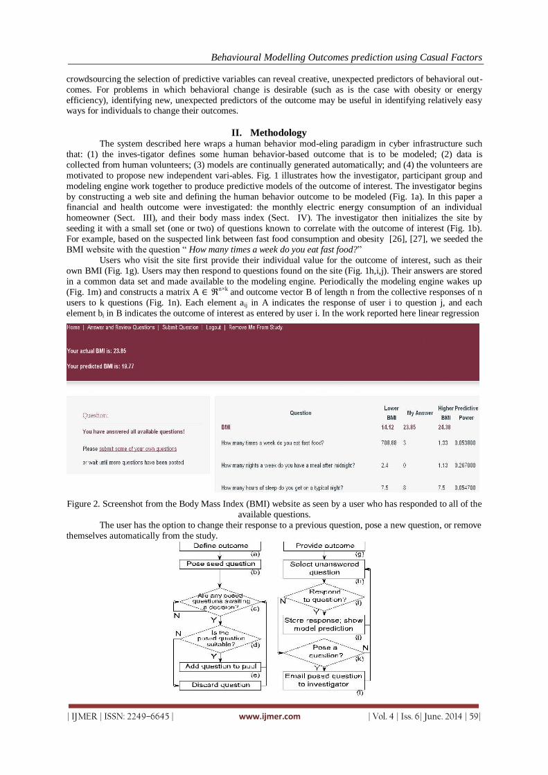
Behavioural Modelling Outcomes prediction using Casual Factors
| IJMER | ISSN: 2249–6645 | www.ijmer.com | Vol. 4 | Iss. 6| June. 2014 | 59|
crowdsourcing the selection of predictive variables can reveal creative, unexpected predictors of behavioral out-
comes. For problems in which behavioral change is desirable (such as is the case with obesity or energy
efficiency), identifying new, unexpected predictors of the outcome may be useful in identifying relatively easy ways for individuals to change their outcomes.
II. Methodology The system described here wraps a human behavior mod-eling paradigm in cyber infrastructure such
that: (1) the inves-tigator defines some human behavior-based outcome that is to be modeled; (2) data is
collected from human volunteers; (3) models are continually generated automatically; and (4) the volunteers are
motivated to propose new independent vari-ables. Fig. 1 illustrates how the investigator, participant group and
modeling engine work together to produce predictive models of the outcome of interest. The investigator begins
by constructing a web site and defining the human behavior outcome to be modeled (Fig. 1a). In this paper a financial and health outcome were investigated: the monthly electric energy consumption of an individual
homeowner (Sect. III), and their body mass index (Sect. IV). The investigator then initializes the site by
seeding it with a small set (one or two) of questions known to correlate with the outcome of interest (Fig. 1b).
For example, based on the suspected link between fast food consumption and obesity [26], [27], we seeded the
BMI website with the question ― How many times a week do you eat fast food?‖
Users who visit the site first provide their individual value for the outcome of interest, such as their
own BMI (Fig. 1g). Users may then respond to questions found on the site (Fig. 1h,i,j). Their answers are stored
in a common data set and made available to the modeling engine. Periodically the modeling engine wakes up
(Fig. 1m) and constructs a matrix A ∈ ℜn×k and outcome vector B of length n from the collective responses of n
users to k questions (Fig. 1n). Each element aij in A indicates the response of user i to question j, and each
element bi in B indicates the outcome of interest as entered by user i. In the work reported here linear regression
Figure 2. Screenshot from the Body Mass Index (BMI) website as seen by a user who has responded to all of the
available questions.
The user has the option to change their response to a previous question, pose a new question, or remove
themselves automatically from the study.

Behavioural Modelling Outcomes prediction using Casual Factors
| IJMER | ISSN: 2249–6645 | www.ijmer.com | Vol. 4 | Iss. 6| June. 2014 | 60|
Figure 1. Overview of the system
The investigator (a-f) is responsible for initially creating the web platform, and seeding it with a starting question. Then, as the experiment runs they filter new survey questions generated by the users. Users (g-
l) may elect to answer as-yet unanswered survey questions or pose some of their own. The modeling engine (m-
p) continually generates predictive models using the survey questions as candidate predictors of the outcome
and users' responses as the training data. was used to construct models of the outcome (Fig. 1o), but any model
form could be employed. The modeling process outputs a vector C of length k + 1 that contains the model
parameters. It also outputs a vector D of length k that stores the predictive power of each question: dj stores the
r2 value obtained by regressing only on column j of A against the response vector B. These two outputs are then
placed in the data store (Fig. 1p).
At any time a user may elect to pose a question of their own devising (Fig. 1k,l). Users could pose
questions that required a yes/no response, a five-level Liker rating, or a number. Users were not constrained in
what kinds of questions to pose. However, once posed, the question was filtered by the investigator as to its
suitability (Fig. 1d). A question was deemed unsuitable if any of the following conditions were met: (1) the question revealed the identity of its author (e.g. ― Hi, I am John Doe. I would like to know if...‖) thereby
contravening the Institutional Review Board approval for these experiments;
(2) the question contained profanity or hateful text; (3) the question was inappropriately correlated with the
outcome (e.g. ― What is your BMI?‖). If the question was deemed suitable it was added to the pool of questions
available on the site (Fig. 1e); otherwise the question was discarded (Fig. 1f).
Each time a user responded to a question, they were shown a new, unanswered question as well as
additional data devised to maintain interest in the site and increase their participation in the experiment. Once a
user had answered all available questions, they were shown a listing of the questions, their responses, and
contextual information to indicate how their responses compared to those of their peers. Fig. 2 shows the listing
that was shown to those users who participated in the BMI site; the individual elements are explained in more
detail in Sect. IV. The most important datum shown to each user after respond-ing to each question was the value of their
actual outcome as they entered it (bi) as well as their outcome as predicted by the current model (ˆi). Fig. 2
illustrates that visitors to the b BMI site were shown their actual BMI (as entered by them) and their predicted
BMI. The models were able to predict each user's outcome before they had responded to every question by
substituting in missing values. Thus after each response from a user
+ c1ai1 + c2ai2 + ... + ckaik + ǫ i (1)
bi = c0
where aij = 0 if user i has not yet responded to question j and aij is set to the user's response otherwise.
III. Energy Efficiency Instantiation And Results In the first instantiation of this concept, we developed a web-based social network to model residential
electric energy consumption. Because of policy efforts to increase energy efficiency, many are working to
provide consumers with better information about their energy consumption. Research on consumer perception of energy efficiency indicates that electricity customers often misjudge the relative importance of various
activities and devices to reducing energy consumption [28]. To provide customers with better information,
numerous expert-driven web-based tools have been deployed [29], [30], [31]. In some cases these tools use
social pressure as a means of improving energy efficiency [32], [33], however the feedback provided to
customers typically comes from a central authority (i.e., top-down feedback) and research on risk perception
[34] indicates that the public is often skeptical of expert opinions. A recent industry study [35] indicates that
customers are notably skeptical of large online service providers (e.g., Google, Microsoft) and (to a lesser
extent) electric utilities as providers of unbiased information about energy conservation. Therefore, information
generated largely by energy consumers themselves, in a bottom-up fashion, may have value in terms of
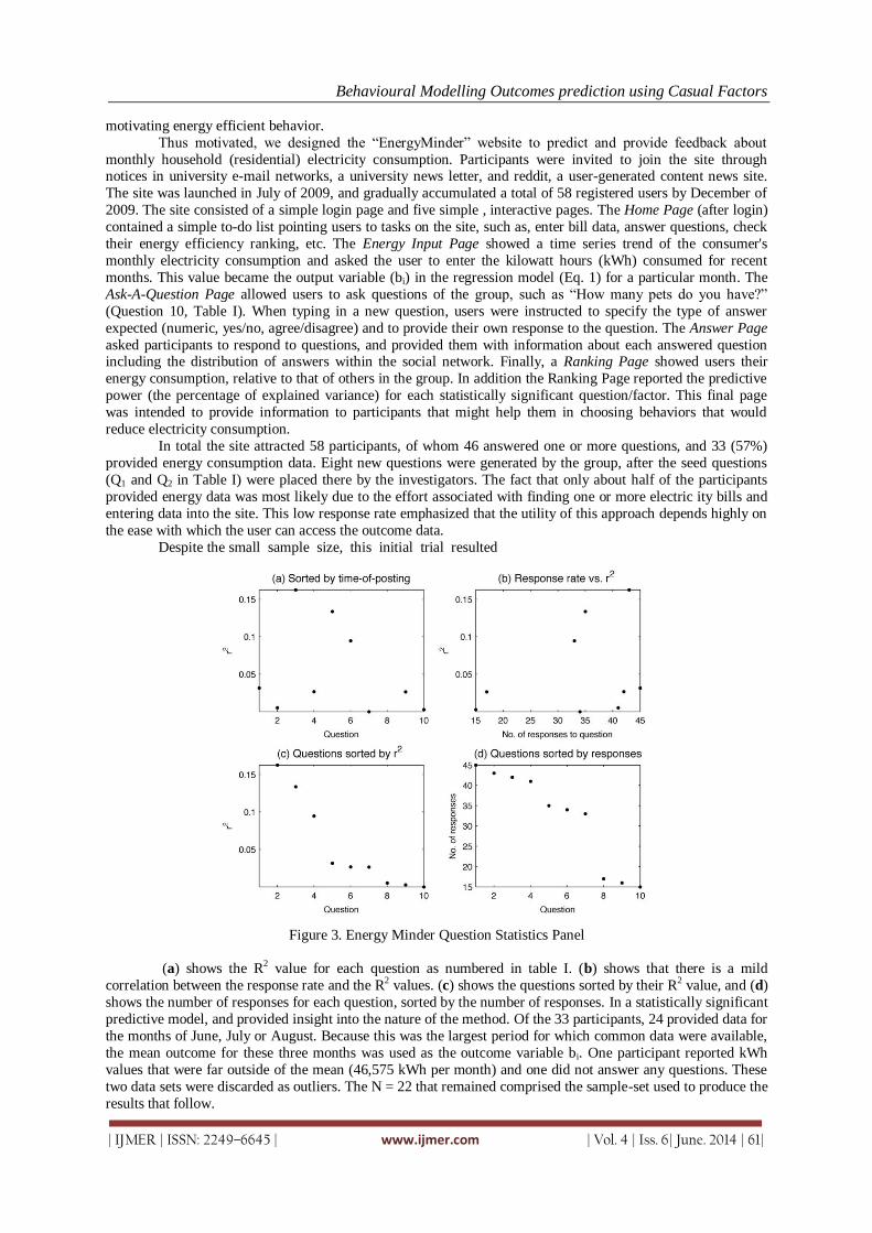
Behavioural Modelling Outcomes prediction using Casual Factors
| IJMER | ISSN: 2249–6645 | www.ijmer.com | Vol. 4 | Iss. 6| June. 2014 | 61|
motivating energy efficient behavior.
Thus motivated, we designed the ―EnergyMinder‖ website to predict and provide feedback about
monthly household (residential) electricity consumption. Participants were invited to join the site through notices in university e-mail networks, a university news letter, and reddit, a user-generated content news site.
The site was launched in July of 2009, and gradually accumulated a total of 58 registered users by December of
2009. The site consisted of a simple login page and five simple , interactive pages. The Home Page (after login)
contained a simple to-do list pointing users to tasks on the site, such as, enter bill data, answer questions, check
their energy efficiency ranking, etc. The Energy Input Page showed a time series trend of the consumer's
monthly electricity consumption and asked the user to enter the kilowatt hours (kWh) consumed for recent
months. This value became the output variable (bi) in the regression model (Eq. 1) for a particular month. The
Ask-A-Question Page allowed users to ask questions of the group, such as ―How many pets do you have?‖
(Question 10, Table I). When typing in a new question, users were instructed to specify the type of answer
expected (numeric, yes/no, agree/disagree) and to provide their own response to the question. The Answer Page
asked participants to respond to questions, and provided them with information about each answered question including the distribution of answers within the social network. Finally, a Ranking Page showed users their
energy consumption, relative to that of others in the group. In addition the Ranking Page reported the predictive
power (the percentage of explained variance) for each statistically significant question/factor. This final page
was intended to provide information to participants that might help them in choosing behaviors that would
reduce electricity consumption.
In total the site attracted 58 participants, of whom 46 answered one or more questions, and 33 (57%)
provided energy consumption data. Eight new questions were generated by the group, after the seed questions
(Q1 and Q2 in Table I) were placed there by the investigators. The fact that only about half of the participants
provided energy data was most likely due to the effort associated with finding one or more electric ity bills and
entering data into the site. This low response rate emphasized that the utility of this approach depends highly on
the ease with which the user can access the outcome data.
Despite the small sample size, this initial trial resulted
Figure 3. Energy Minder Question Statistics Panel
(a) shows the R2 value for each question as numbered in table I. (b) shows that there is a mild
correlation between the response rate and the R2 values. (c) shows the questions sorted by their R2 value, and (d)
shows the number of responses for each question, sorted by the number of responses. In a statistically significant
predictive model, and provided insight into the nature of the method. Of the 33 participants, 24 provided data for
the months of June, July or August. Because this was the largest period for which common data were available,
the mean outcome for these three months was used as the outcome variable bi. One participant reported kWh
values that were far outside of the mean (46,575 kWh per month) and one did not answer any questions. These
two data sets were discarded as outliers. The N = 22 that remained comprised the sample-set used to produce the
results that follow.

Behavioural Modelling Outcomes prediction using Casual Factors
| IJMER | ISSN: 2249–6645 | www.ijmer.com | Vol. 4 | Iss. 6| June. 2014 | 62|
Table I shows results from two predictive models. Model 1 included all questions that had 18 or more
answers (Q1-Q7). The total explained variance for Model 1 was r2 = 0.63. Model 1 indicated that the number of
adults in the home (Q3) significantly increased monthly electricity consumption ( P < 0.05) and the ownership of a natural gas hot water heater (Q6) significantly decreased electricity consumption ( P < 0.05). Note that this
second result is not consistent with the fact that owning an electric hot water heater increases electricity
consumption. It appears either that this correlation was due to chance, or that ownership of a gas hot water
heater correlates to some other factor, such as (for example) home ownership. Model 2 tested the removal of the
least significant predictor s, and included only Q3, Q5, and Q6. Model 2 showed the same pair of statistically
significant predictors ( Q3 and Q6).
Figure 3 shows the relative predictive power of the 10 questions. The results show that the most highly
correlated factors (Q3, Q5, and Q6) were posed after the initial two seed questions (Fig. 3a) and a weak
correlation between the response rate and the r2 values, indicating that more answers to questions would have
likely produced improved results. Panels (c) and (d) show the distributions of r2 values and the number of
responses, to facilitate comparison with the BMI Table I
QUESTIONS ENTERED INTO THE ENERGYMINDER WEB SITE.
While the small sample size in this study limits the generality of these results, this initial trial provided
useful information about the crowdsourced modeling approach. Firstly, we found that participants were reluctant
or unable to provide accurate outcome data due to the challenge of finding one's electric bills. Our second
experiment corrects this problem by focusing on an outcome that is readily accessible to the general public.
Secondly, we found that participants were quite willing to answer questions posed by others in the group. Questions 1-4 were answered by over 70% of participants. This indicated that it is possible to produce user-
generated questions and answers, and that a trial with a larger sample size might provide more valuable insight.
Finally, questions that were posed early in the trial gained a higher response rate, largely because many users
did not return to the site after one or two visits. This emphasizes the importance of attracting users back to the
site to answer questions in order to produce a statistically useful model.
IV. Body Mass Index Instantiation And Results In order to test this approach with an outcome that was more readily available to participants a second
website was deployed in which models attempted to predict the body mass index of each participant. Body mass
index (BMI) is calculated as mass (kg) / (height(m))2 and, although it is known to have several limitations [36],
is still the most common measure for determining a patient's level of obesity. Each user's BMI could readily be
calculated as all users know and are thus able to immediately enter their height and weight. A second motivator
for investigating this behavioral outcome is that obesity has been cited [37] as one of the major global public
health challenges to date, it is known to have myriad causes [38], [39], and people with extreme BMI values
are likely to have intuitions as to why they deviate so far from the norm.
Participants arriving for the first time at the BMI site were asked to enter their height and weight in
feet, inches and pounds respectively, as most of the visitors to the site resided in the U.S. Participants were then
free to respond to and pose new questions.

Behavioural Modelling Outcomes prediction using Casual Factors
| IJMER | ISSN: 2249–6645 | www.ijmer.com | Vol. 4 | Iss. 6| June. 2014 | 63|
In order to further motivate the participants, in addition to displaying their predicted outcome, users
were also shown how their responses compared to two peer groups. For each user the peer groups were
constructed as follows. The first peer group was composed of 10 other users who had BMI values as close to but below that of the user; the second group was composed of 10 other users who had BMI values as close to but
above that of the user. If N < 10 users could be found the peer group was composed of those N users. The
average BMI for each of the two peer groups, as well as the user's own BMI, were displayed (see Fig. 2). Also,
the responses to each question, within each peer group, were averaged and shown alongside the user's response
to that question. Finally, the `predictive power' of each question was shown. Predictive power was set equal to
the r2 obtained when the responses to that question alone were regressed against the outcome.
The peer group data were meant to help users compare how their lifestyle choices measured up to their
most similar peers who were slightly more healthy than themselves, and slightly less healthy than themselves.
This approach in effect provides individualized suggestions to each user as to how slight changes in lifestyle
choices may lead to improvements in the health indicator being measured. Presenting the user with the
predictive power of each question was designed to help them learn what questions tend to be predictive, and thus motivate them to formulate new or better questions that might be even more predictive. For example one
user posed the question ― How many, if any, of your parents are obese?‖. Another user may realize that the
`predictive power' of this question (which achieved an r2 in the actual experiment of 0.23 and became the sixth-
most predictive question out of a total of 57) may be due to it serving as an indirect measure of the hereditary
component of obesity. This may cause the user to pose a new question better tailored to eliciting this
information, such as ― How many, if any, of your biological parents are obese?‖ (a question of this form was not
posed during the actual experiment).
The BMI site went live at 3:00pm EST on Friday, November 12, 2010, stayed live for slightly less than
a week, and was discontinued at 10:20am EST on Thursday, November 18, 2010. During that time it attracted
64 users who supplied at least one response. Those users proposed 56 questions (in addition to the original seed
question), and together provided 2021 responses to those questions.
Table II
LISTING OF THE 20 MOST PREDICTIVE QUESTIONS FROM THE BMI SITE.
Index Question R2 Responses
1 Do you think of yourself as overweight? 0.5524 43 2 How often do you masturbate a month? 0.3887 32
3 What percentage of your job involves sitting? 0.3369 57
4 How many nights a week do you have a meal after midnight? 0.2670 67
5
You would consider your partner/boyfriend/girlfriend/spouse etc to be
overweight? 0.2655 24
6 How many, if any, of your parents are obese? 0.2311 57
7 Are you male? 0.2212 32
8 I am happy with my life 0.2062 31
9 How many times do you cook dinner in an average week? 0.2005 44
10 How many miles do you run a week? 0.1865 28
11 Do you have a college degree? 0.1699 12 12 Do you have a Ph.D. 0.1699 12
13 Would you describe yourself as an emotional person? 0.1648 30
14 How often do you eat (meals + snacks) during a day 0.1491 33
15 How many hours do you work per week? 0.1478 46
16 Do you practice a martial art? 0.1450 31
17 What is your income? 0.1419 55
18 I was popular in high school 0.1386 31
19 Do you ride a bike to work? 0.1383 64
20
What hour expressed in 1-24 on average do you eat your last meal before
going to bed? 0.1364 30
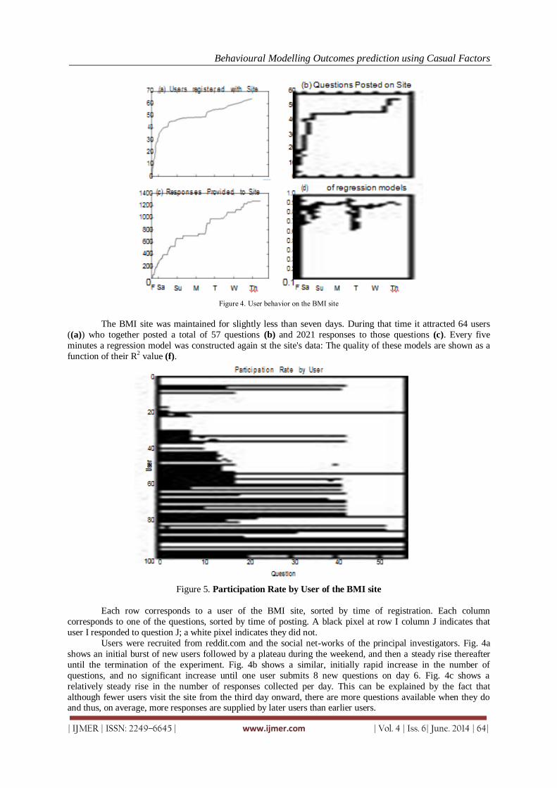
Behavioural Modelling Outcomes prediction using Casual Factors
| IJMER | ISSN: 2249–6645 | www.ijmer.com | Vol. 4 | Iss. 6| June. 2014 | 64|
Figure 4. User behavior on the BMI site
The BMI site was maintained for slightly less than seven days. During that time it attracted 64 users
((a)) who together posted a total of 57 questions (b) and 2021 responses to those questions (c). Every five
minutes a regression model was constructed again st the site's data: The quality of these models are shown as a
function of their R2 value (f).
Figure 5. Participation Rate by User of the BMI site
Each row corresponds to a user of the BMI site, sorted by time of registration. Each column
corresponds to one of the questions, sorted by time of posting. A black pixel at row I column J indicates that
user I responded to question J; a white pixel indicates they did not.
Users were recruited from reddit.com and the social net-works of the principal investigators. Fig. 4a
shows an initial burst of new users followed by a plateau during the weekend, and then a steady rise thereafter
until the termination of the experiment. Fig. 4b shows a similar, initially rapid increase in the number of
questions, and no significant increase until one user submits 8 new questions on day 6. Fig. 4c shows a
relatively steady rise in the number of responses collected per day. This can be explained by the fact that
although fewer users visit the site from the third day onward, there are more questions available when they do and thus, on average, more responses are supplied by later users than earlier users.
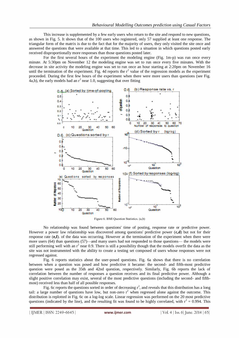
Behavioural Modelling Outcomes prediction using Casual Factors
| IJMER | ISSN: 2249–6645 | www.ijmer.com | Vol. 4 | Iss. 6| June. 2014 | 65|
This increase is supplemented by a few early users who return to the site and respond to new questions,
as shown in Fig. 5. It shows that of the 100 users who registered, only 57 supplied at least one response. The
triangular form of the matrix is due to the fact that for the majority of users, they only visited the site once and answered the questions that were available at that time. This led to a situation in which questions posted early
received disproportionally more responses than those questions posted later.
For the first several hours of the experiment the modeling engine (Fig. 1m-p) was run once every
minute. At 5:30pm on November 12 the modeling engine was set to run once every five minutes. With the
decrease in site activity the modeling engine was set to run once an hour starting at 2:20pm on November 16
until the termination of the experiment. Fig. 4d reports the r2 value of the regression models as the experiment
proceeded. During the first few hours of the experiment when there were more users than questions (see Fig.
4a,b), the early models had an r2 near 1.0, suggesting that over fitting
Figure 6. BMI Question Statistics. (a,b)
No relationship was found between questions' time of posting, response rate or predictive power.
However a power law relationship was discovered among questions' predictive power (c,d) but not for their
response rate (e,f). of the data was occurring. However at the termination of the experiment when there were
more users (64) than questions (57)—and many users had not responded to those questions— the models were
still performing well with an r2 near 0.9. There is still a possibility though that the models overfit the data as the
site was not instrumented with the ability to create a testing set composed of users whose responses were not
regressed against.
Fig. 6 reports statistics about the user-posed questions. Fig. 6a shows that there is no correlation
between when a question was posed and how predictive it became: the second- and fifth-most predictive
question were posed as the 35th and 42nd question, respectively. Similarly, Fig. 6b reports the lack of correlation between the number of responses a question receives and its final predictive power. Although a
slight positive correlation may exist, several of the most predictive questions (including the second- and fifth-
most) received less than half of all possible responses.
Fig. 6c reports the questions sorted in order of decreasing r2, and reveals that this distribution has a long
tail: a large number of questions have low, but non-zero r2 when regressed alone against the outcome. This
distribution is replotted in Fig. 6c on a log-log scale. Linear regression was performed on the 20 most predictive
questions (indicated by the line), and the resulting fit was found to be highly correlated, with r2 = 0.994. This

Behavioural Modelling Outcomes prediction using Casual Factors
| IJMER | ISSN: 2249–6645 | www.ijmer.com | Vol. 4 | Iss. 6| June. 2014 | 66|
finding suggests that a power law relationship is highly likely that it correlates with the outcome: people who
perceive themselves as overweight are likely to be overweight. However, it is known that for those suffering
from body image disorders the opposite is often the case: those that perceive themselves incorrectly as overweight can become extremely underweight [47]. Separating the auto- and anti-correlated components of
this broad question could be accomplished by supplementing it with more targeted questions (eg., ― Do you
think you are overweight but everyone else tells you the
opposite?‖).
Despite the lack of filtering on the site there were only a few cases of clearly dishonest responses. Fig.
2 indicates that at least one member of this user's peer group answered the fast food question dishonestly. It is
interesting to note that this dishonest answer (or answers) was supplied for the seed question, and this
question—despite collecting the most responses (70)—had nearly no individual correlation (r2 = 0.054) and thus
contributed negligibly to the predictions of the models. Questions 3, 4, 6, 9, 15, and 20 as shown in Table II
have maximum possible values (qs. 3 max=100; qs. 4 and 9 max=7; qs. 6 max=2; qs. 15 max=168; qs. 20
max=24), and together collected 301 responses. Of those responses, none were above the maximum or below the minimum (min=0 for all qs.) indicating that all responses were not theoretically impossible. This suggests
that clear dishonesty (defined as supplying a response below or above the theoretical minimum or maximum,
respectively) was quite rare for this experiment. Conversely, unlike the popular yet corrupted seed question,
these questions became significantly predictive as the experiment progressed. Further investigation into whether
or how the
The close linear fit for these questions does not guarantee th at a power law exists among these
questions, however [40]. Subsequent work and a larger data set will be required to confirm if power law
relationship s do indeed exist among user-generated questions predictive of a behavioral outcome. Rare cases of
clear dishonesty (and the possibly larger amount of hidden dishonesty) affect modeling in such systems remains
to be investigated.
V. Discussion/Conclusions This paper introduced a new approach to social science modeling in which the participants themselves
are motivated to uncover the correlates of some human behavior outcome, such as homeowner electricity usage
or body mass index. In both cases participants successfully uncovered at least one statistically significant
predictor of the outcome variable. For the body mass index outcome, the participants successfully formulated
many of the correlates known to predict BMI, and provided sufficiently honest values for those correlates to
become predictive during the experiment. While, our instantiations focus on energy and BMI, the proposed
method is general, and might, as the method improves, be useful to answer many difficult questions regarding
why some outcomes are different than others. For example, future instantiations might provide new insight into
difficult questions like: "Why do grade point averages or test scores differ so greatly among students?", "Why do certain drugs work with some populations, but not others?", "Why do some people with similar skills and
experience, and doing similar work, earn more than others?"
Despite this initial success, much work remains to be done to improve the functioning of the system,
and to validate its performance. The first major challenge is that the number of questions approached the
number of participants on the BMI website. This raises the possibility that the models may have over fit the data
as can occur when the number of observable features approaches the number of observations of those features.
Nevertheless the main goal of this paper was to demonstrate a system that enables non domain experts to
collectively formulate many of the known (and possibly unknown) predictors of a behavioral outcome, and that
this system is independent of the outcome of interest. One method to combat overfitting in future instantiations
of the method would be to dynamically filter the number of questions a user may respond to: as the number of
questions approaches the number of users this filter would be strengthened such that a new user is only exposed on a small subset of the possible questions.
A. User Fatigue
Another challenge for this approach is user fatigue: Fig. 5 indicates that many of the later users only
answered a small fraction of the available questions. Thus it is imperative that users be presented with questions
that most require additional responses first. This raises the issue of how to order the presentation of questions. In
the two instantiations presented here, questions were simply presented to all users in the same order: the order in
which they were posted to the site. It was possible that this ordering could have caused a `winner take all'
problem in that questions that accrue more responses compared to other questions would achieve a higher
predictive power, and users would thus be attracted to respond 8 to these more predictive questions more than
the less predictive questions. However, the observed lack of correlation between response rate and predictive
power (Fig. 6b) dispelled this concern. In future instantiations of the method, question ordering will be approached in a principled way.

Behavioural Modelling Outcomes prediction using Casual Factors
| IJMER | ISSN: 2249–6645 | www.ijmer.com | Vol. 4 | Iss. 6| June. 2014 | 67|
Instead of training a single model m, an ensemble of methods m1, ..., mk will be trained on different subsets of
the data [48], [49]. Then, query by committee [50] will be employed to determine question order: The question
that induces maximal disagreement among the k models as to its predictive power will be presented first, followed by the question that induces the second largest amount of disagreement, and so on. In this way
questions that may be predictive would be validated more rapidly than if question ordering is fixed, or random.
B. User Motivation
Typically, human subjects play a passive role in social science studies, regardless of whether that study
is conducted offline (pen-and-paper questionnaire) or online (web-base d survey): They contribute responses to
survey questions, but play no role in crafting the questions. This work demonstrates that users can also
contribute to the hypothesis-generation component of the discovery process: Users can collectively contribute—
and populate—predictors of a behavioral out-come.
It has been shown here that users can be motivated to do this without requiring an explicit reward: The
subjects were unpaid for both studies. Much work remains to be done to clarify under what conditions subjects will be willing and able to contribute predictors.
We hypothesize that willingness to generate candidate predictors of a behavioral outcome may be
stimulated under several conditions. First, if subjects are incurring a health or financial cost as a result of the
outcome under study, they may be motivated to contribute. For example a user that has an above average
electricity bill or body mass index, yet has similar lifestyle attributes as his fellow users, may wish to generate
additional attributes to explain the discrepancy. Conversely, a user that posts a superior outcome (i.e. a low
electricity bill or very healthy body mass index) may wish to uncover the predictor that contributes to their
superior outcome (i.e. a well-insulated house or good exercise regimen) and thus advertise it to their peers. This
may act as a form of online `boasting', a well known motivator among online communities.
In the current studies, some participants may have been motivated to contribute because they were part
of the authors' social networks. However, a substantial number of users were recruited from online communities
outside of the authors' social networks, indicating that some online users are motivated to contribute to such studies even if they do not know those responsible for the study. The exact number of users in these two groups
is not clear on account of the anonymity requirements stipulated for these human subject studies. Similarly, a
non domain expert's ability to contribute a previously unknown yet explanatory predictor of a behavioural
outcome may rely on them suffering or benefiting from a far-from-average outcome. For example consider
someone who is extremely underweight yet their outcome is not predicted by the common predictors of diet and
exercise: this user has a high caloric intake and does not exercise. This user may be able to generate a predictor
that a domain expert may not have thought of, yet is predictive for a certain underweight demographic: this user
may ask her peers: ―Are you in an abusive relationship?‖
Users may also be motivated to contribute to such studies because it provides entertainment value:
users may view the website as a competitive game in which the `goal' is to propose the best questions. In a
future version we plan to create a dynamically sorted list of user-generated questions: questions bubble up to the top of the list if (1) it is a question that many other users wish to respond to, (2) it is orthogonal to the other
questions, and (3) it is found to be predictive of the outcome under study. Users may then compete by
generating questions that climb the leader board and thus advertise the user's understanding of the outcome
under study.
C. Rare Outcomes
Obesity and electricity usage are well-studied behavioral outcomes. It remains to be seen though how
the proposed methodology would work for outcomes that affect a small minority of online users, or for which
predictors are not well known.
We hypothesize that for rare outcomes, online users who have experience with this outcome, could be
encouraged to participate, and would be intrinsically motivated to contribute. For example if the outcome to be
studied were a rare disease, users who suffer from the disease would be attracted to the site. Once there, they may be in a unique position to suggest and collectively discover previously unknown predictors of that disease.
Moreover, a user who suffers from the disease is likely to know more people who suffer from that disease and
would be motivated to advertise the site to them. Finally, even if a user discovers the site and does not suffer
from the disease, he may know someone who does and thus introduce the site to that person. Such a person may
serve as a caregiver for someone suffering from the disease, such as a family member. A caregiver may be able
to contribute novel predictors that are different from those proposed by the sufferer himself.
Thus, a website that hosts such a rare outcome may serve as a `magnet' for people who exhibit the
outcome or know people that do. In future we will study the 'attractive force' of such websites: if such a website
experiences increased user traffic as the study goes forward, and the average outcome of users on the site drifts
away from the global population's mean value for this outcome, that would indicate that a growing number of

Behavioural Modelling Outcomes prediction using Casual Factors
| IJMER | ISSN: 2249–6645 | www.ijmer.com | Vol. 4 | Iss. 6| June. 2014 | 68|
people with such an outcome are being attracted to the site. In closing, this paper has presented a novel
contribution to the growing field of machine science in which the formulation of observables for a modeling
task—and the populating of those observables with values—can be offloaded to the human group being modeled.
Acknowledgement The authors acknowledge valuable contributions from three anonymous reviewers, and useful
discussions with collabora-tors in the UVM Complex Systems center.
REFERENCES [1.] J. Bongard and H. Lipson, ―Automated reverse engineerin g of nonlinear dynamical systems,‖ Proceedings of the
National Academy of Sciences, vol. 104, no. 24, pp. 9943–9948, 2007. [2.] J. Evans and A. Rzhetsky, ―Machine science,‖ Science, vol. 329, no. 5990, p. 399, 2010. R. D. King, K. E.
Whelan, F. M. Jones, P. G. K. Reiser, C. H. Bryant, H. Muggleton, D. B. Kell, and S. G. Oliver, ―Functional genomic hypothesis generation and experimentation by a robot scientist,‖ Nature, vol. 427, pp. 247–252, 2004.
[3.] R. King, J. Rowland, S. Oliver, M. Young, W. Aubrey, E. Byrne, Liakata, M. Markham, P. Pir, L. Soldatova et al., ―The automation of science,‖ Science, vol. 324, no. 5923, p. 85, 2009.
[4.] J. Bongard, V. Zykov, and H. Lipson, ―Resilient machines through continuous self-modeling,‖ Science, vol. 314, pp. 1118–1121, 2006.
[5.] J. Giles, ―Internet encyclopedias go head to head,‖ Nature, vol. 438, no. 15, pp. 900–901, 2005. [6.] D. C. Brabham, ―Crowdsourcing as a model for problem solv ing,‖ Convergence, vol. 14, pp. 75–90, 2008.
Sorokin and D. Forsyth, ―Utility data annotation with amazon me-chanical turk,‖ in Proc. IEEE Computer Society Conference on Computer Vision and Pattern Recognition Workshops, 2008.
[7.] M. Marge, S. Banerjee, and A. Rudnicky, ―Using the amazon mechanical turk for transcription of spoken language,‖ in Proc. IEEE International Conference on Acoustics Speech and Signal Processing, 2010.
[8.] N. Kong, J. Heer, and M. Agrawala, ―Perceptual guidelin es for creating rectangular treemaps,‖ IEEE Transactions on Visualization and Com-puter Graphics, vol. 16, no. 6, 2010. Kittur, E. Chi, and B. Suh, ―Crowdsourcing user studi es with mechanical turk,‖ in Proc.Twenty-sixth annual SIGCHI conference on human factors in computing
systems, 2008. [9.] D. Wightman, ―Crowdsourcing human-based computation ,‖ in Proceed-ings of the 6th Nordic Conference on
Human-Computer Interaction: Extending Boundaries, 2010. [10.] B. Fitzgerald, ―The transformation of open source soft ware,‖ Manage-ment Information Systems Quarterly, vol.
30, no. 3, pp. 587–598, 2006. [11.] J. Howe, Crowdsourcing: Why the Power of the Crowd is Driving the Future of Business. Crown Business, 2009. [12.] N. Thurman, ―Forums for citizen journalists? adoption of user generated content initiatives by online news media,‖
New Media and Society, vol. 10, no. 1, 2008.
[13.] C. DiBona, M. Stone, and D. Cooper, Open Source 2.0: The Continuing Evolution. O'Reilly Media, 2005. [14.] J. Leskovec, L. Adamic, and B. Huberman, The Dynamics of Viral Marketing. New York: ACM Press, 2007. [15.] K. Lerman, ―Social networks and social information filt ering on digg,‖ arXiv: cs/0612046v1, 2006. [16.] D. Anderson, J. Cobb, E. Korpela, M. Lebofsky, and D. Werthimer, ―Seti@home: an experiment in public-
resource computing,‖ Communi-cations of the ACM, vol. 45, no. 11, pp. 56–61, 2002. [17.] J. Cohn, ―Citizen science: Can volunteers do real resea rch?‖ BioScience, vol. 58, no. 3, pp. 192–197, 2008. [18.] J. Silvertown, ―A new dawn for citizen science,‖ Trends in Ecology & Evolution, vol. 24, no. 9, pp. 467–471,
2009. Beberg, D. Ensign, G. Jayachandran, S. Khaliq, and V. Pande, ―Folding@home: Lessons from eight years of
volunteer distr ibuted computing,‖ in IEEE International Symposium on Parallel Distributed Processing, May 2009, pp. 1–8. Lintott, K. Schawinski, A. Slosar, K. Land, S. Bamford, D. Thomas, Raddick, R. Nichol, A. Szalay, D. Andreescu et al., ―Galaxy zoo: morphologies derived from visual inspection of galaxies from the sloan digital sky survey?‖ Monthly Notices of the Royal Astronomical Society, vol. 389, no. 3, pp. 1179–1189, 2008.
[19.] S. Cooper, F. Khatib, A. Treuille, J. Barbero, J. Lee, M. Beenen, Leaver-Fay, D. Baker, Z. Popovic et al., ―Predicting protein structures with a multiplayer online game,‖ Nature, vol. 466, no. 7307, pp. 756– 760, 2010. Kittur, ―Crowdsourcing, collaboration and creativ ity,‖ XRDS, vol. 17, no. 2, pp. 22–26, 2010.
[20.] S. Bowman, S. Gortmaker, C. Ebbeling, M. Pereira, and D. Ludwig, ―Effects of fast-food consumption on energy
intake and diet quality among children in a national household survey,‖ Pediatrics, vol. 113, [21.] no. 1, p. 112, 2004. [22.] [27] J. Currie, S. DellaVigna, E. Moretti, and V. Pathania, ― The effect of fast food restaurants on obesity and
weight gain,‖ American Economic Journal: Economic Policy, vol. 2, no. 3, pp. 32–63, 2010. [23.] S. Z. Attari, M. L. DeKay, C. I. Davidson, and W. B. de Bruinc, ―Public perceptions of energy consumption and
savings,‖ Proceedings of the National Academy of Sciences, Aug. 16 2010. [24.] Microsoft. (2011) Microsoft hohm. [Online]. Available: http://www.microsoft-hohm.com/ [25.] E. Mills, ―The home energy saver: Documentation of calc ulation methodology, input data, and infrastructure,‖
Lawrence Be rkeley Na-tional Laboratory, Tech. Rep. LBNL-51938, 2008.
[26.] H. Allcott, ―Social norms and energy conservation,‖ Journal of Public Economics, 2011. [27.] J. E. Petersen, V. Shunturov, K. Janda, G. Platt, and K. Weinberger, [28.] ―Dormitory residents reduce electricity consumption when exposed to real-time visual feedback and incentives,‖

Behavioural Modelling Outcomes prediction using Casual Factors
| IJMER | ISSN: 2249–6645 | www.ijmer.com | Vol. 4 | Iss. 6| June. 2014 | 69|
International Journal of Sustainability in Higher Education, vol. 8, no. 1, pp. 16–33, 2007. [29.] L. Kaufman, ―Utilities turn their customers green, wit h envy,‖ The New York Times, Jan. 30 2009. [30.] P. Slovic, ―Trust, emotion, sex, politics, and science : Surveying the risk-assessment battlefield,‖ Risk Analysis,
vol. 19, no. 4, 1999. [31.] G. S. Guthridge, ―Understanding consumer preferences in energy ef-ficiency: Accenture end-consumer
observatory on electrici ty manage-ment,‖ Accenture, Tech. Rep. ACC10-0229, 2010. [32.] [36] A. Romero-Corral, V. Somers, J. Sierra-Johnson, R. Thomas,Collazo-Clavell, J. Korinek, T. Allison,
J. Batsis, F. Sert-Kuniyoshi, and F. Lopez-Jimenez, ―Accuracy of body mass index in diagno sing obe-sity in the adult general population,‖ International Journal of Obesity, vol. 32, no. 6, pp. 959–966, 2008.
[33.] L. Barness, J. Opitz, and E. Gilbert-Barness, ―Obesity : genetic, molecu-lar, and environmental aspects,‖ American Journal of Medical Genetics Part A, vol. 143, no. 24, pp. 3016–3034, 2007.
[34.] T. Parsons, C. Power, S. Logan, and C. Summerbell, ―Chil dhood predictors of adult obesity: a systematic review.‖ International journal of obesity and related metabolic disorders: journal of the International Association for the Study of Obesity, vol. 23, p. S1, 1999.
[35.] Y. Wang and M. Beydoun, ―The obesity epidemic in the Unit ed States— gender, age, socioeconomic,
racial/ethnic, and geographic characteris-tics: a systematic review and meta-regression analysis,‖ Epidemiologic reviews, vol. 29, no. 1, p. 6, 2007. Clauset, C. Rohilla Shalizi, and M. Newman, ―Power-l aw distribu-tions in empirical data,‖ SIAM review, vol. 51, no. 4, pp. 661–703, 2009.
[36.] P. Boumtje, C. Huang, J. Lee, and B. Lin, ―Dietary habits , demographics, and the development of overweight and obesity among children in the United States,‖ Food Policy, vol. 30, no. 2, pp. 115–128, 2005. Herbert, N. Gerry, M. McQueen, I. Heid, A. Pfeufer, T. Illig, Wichmann, T. Meitinger, D. Hunter, F. Hu et al., ―A common genetic variant is associated with adult and childhood obesity,‖ Science, vol. 312, no. 5771, p. 279, 2006.
[37.] M. Friedman and K. Brownell, ―Psychological correlate s of obesity: Moving to the next research generation.‖ Psychological Bulletin, vol. 117, no. 1, p. 3, 1995.
[38.] M. Van der Merwe, ―Psychological correlates of obesity in women,‖ [39.] International Journal of Obesity, vol. 31, pp. S14–S18, 2007. [40.] [45] R. Bonow and R. Eckel, ―Diet, obesity, and cardiovascul ar risk,‖ N Engl J Med, vol. 348, no. 21, pp.
2057–2058, 2003. [41.] R. Ewing, T. Schmid, R. Killingsworth, A. Zlot, and S. Raudenbush, ―Relationship between urban sprawl and
physical activity, obesity, and morbidity,‖ Urban Ecology, pp. 567–582, 2008. [42.] S. Grogan, Body image: Understanding body dissatisfaction in men, women, and children. Taylor & Francis, 2008. [43.] M. Skurichina and R. Duin, ―Bagging, boosting and the ra ndom sub-space method for linear classifiers,‖ Pattern
Analysis & Applications, vol. 5, no. 2, pp. 121–135, 2002. [44.] Z. Lu, X. Wu, and J. Bongard, ―Active learning with adapt ive het-erogeneous ensembles,‖ in Data Mining, 2009.
ICDM'09. Ninth IEEE International Conference on. IEEE, 2009, pp. 327–336. [45.] H. Seung, M. Opper, and H. Sompolinsky, ―Query by commit tee,‖ in
[46.] Proceedings of the fifth annual workshop on Computational le arning theory. ACM, 1992, pp. 287–294.
International
OPEN ACCESS Journal
Of Modern Engineering Research (IJMER)
| IJMER | ISSN: 2249–6645 | www.ijmer.com | Vol. 4 | Iss. 6| June. 2014 | 70|
Review on Implementation of Fir Adaptive Filter Using
Distributed Arithmatic and Block Lms Algorithm
Miss. Rima P. Deshmukh1, Prof. S. A. Koti2, Prof. V. B. Baru3
1, 2, 3(Department of Electronics and Telecommunication, Sinhgad College of Engineering Vadgaon, Pune,
India)
I. INTRODUCTION Adaptive filters are the core contributor in the digital signal processing applications. The most
popular adaptive algorithms are Least Mean Square (LMS) and Recursive Least Square (RLS) algorithm.
Because of simplicity of LMS algorithm it has been productively applied in many areas. Least mean square
(LMS) based finite impulse response (FIR) adaptive filter is the most prevalent because it is simple and
provides satisfactory convergence performance. FIR filters have many advantages such as FIR filters are linear
in phase, coefficients are easy and simple to calculate, the design methods are generally linear, are always
stable, and can be realized efficiently in hardware. The adaptive algorithm for FIR filters is broadly used in
different applications such as biomedical, communication and control. Because of its simplicity it has been
used in many applications where to minimize computational requirements is essential. It is rational to choose
the adaptive algorithm in the design of adaptive filter and LMS algorithm can be selected for the designing
purpose. Least mean squares algorithms are a class of adaptive filter that find the filter coefficients and relate
that coefficients to produce the least mean squares of the error signal to provide the desired filter.
In Recursive least squares algorithm filter coefficients are found recursively. The filter coefficients
minimize a weighted linear least squares cost function involving the input signals. The LMS algorithm aims to
reduce the mean square error. In the beginning of RLS algorithm, the input signals are considered
deterministic. In LMS the input signals are considered stochastic. As compared to other algorithms RLS
exhibits faster convergence performance. However the fast convergence is achieved by giving high
computational complexity. A distributed arithmetic (DA) can be formed for the application of block least mean
square (BLMS) algorithm. DA forms an inner product or dot product of a pair of vectors in a one step by bit
serial computation operation. Efficiency of mechanization is the main advantage of DA. DA based techniques
uses look up table (LUT) sharing method for the for the calculation of filter outputs and weight-increment
terms in BLMS algorithm. Using this technique significant saving of adders is achieved which constitute a
main component of DA based structures. DA based BLMS algorithm performs convolution and correlation
operation using same LUT. This will reduce the number of LUT words required to be updated per output.
Hence saves power consumption and the external logic required.
II. Literature Review Adaptive digital filters have tremendous applications in signal processing. According to the LMS
algorithm, there is a delay in the feedback error for updating the weights which does not favor the pipeline
implementation, when the sampling rate is high. [2] have proposed the delayed LMS algorithm for pipeline
application of LMS based ADF. In LMS algorithm, the adaptation step can be performed after a fixed delay
only, in some practical situations. In such a cases the implemented algorithm is a modified version of LMS
Abstract: Adaptive filters play very important role in signal processing application. There are several
algorithms for implementation of filters such as Least mean square (LMS), Recursive least square (RLS),
etc. The LMS algorithm is the most efficient algorithm for implementation of FIR adaptive filters. RLS
algorithm gives faster convergence as compared to LMS but the computational complexity is high in case
of RLS. An effective distributed arithmetic can be used to implement the block least mean square
algorithm (BLMS). The DA based structure uses a LUT sharing scheme to calculate the filter output and
weight increment terms of BLMS algorithm. The structure can save a number of adders. This paper
presents a literature review on the different algorithms used for implementation of FIR adaptive filters
and implementation of filters using distributed arithmetic and block LMS algorithm.
Keywords: LMS, BLMS, DA, RLS, ADF.

Review On Implementation Of Fir Adaptive Filter Using Distributed Arithmatic And Block Lms
| IJMER | ISSN: 2249–6645 | www.ijmer.com | Vol. 4 | Iss. 6| June. 2014 | 71|
algorithm known as the delayed LMS (DLMS) algorithm. In DLMS the coefficient adaptation is performed
after a delay. The work shows the conditions for convergence and estimates of convergence rate, both for the
mean of the DLMS filter coefficients and for its excess mean square error. The only difference between the
LMS and DLMS algorithm is that the correction term for updating the filter weights of the current iteration are
computed from error corresponding to the past iteration. Many methods have been proposed to implement
BLMS based adaptive digital filters efficiently in systolic VLSI with minimum adaptation delay [2] [17] [11]
[12]. In order to avoid adaptation delay [3] has proposed a modified DLMS algorithm. In some of the
applications of the adaptive finite impulse response filtering, the adaptation algorithm can be applied with a
delay only in the coefficient update. This has a dissimilar effect on the convergence behavior of the algorithm.
In this work it is shown how the delayed LMS algorithm can be converted into the typical LMS algorithm at
simply slight increase in the computational expense. The modified DLMS is used by [4] to derive a systolic
architecture but it requires large amount of hardware resources as compared to the earlier one. BLMS is useful
for fast and computationally-efficient implementation of adaptive digital filters. The convergence performance
of BLMS ADFs and LMS ADFs are similar, but for block length L BLMS ADFs offers L fold higher
throughput. Considering this , many BLMS algorithms like time and frequency domain block filtered-X LMS
(BFXLMS) has been proposed by [19] for specific applications. Computationally more efficient BFXLMS
using FFT and fast Hartley transform (FHT). A delayed block LMS algorithm and a concurrent multiplier-
based design for high throughput pipeline execution of BLMS ADFs have been proposed [13].
In [13] a block LMS algorithm with delayed weight adaptation for hardware execution of FIR
adaptive filters has been proposed. The delayed block least mean square algorithm take a block of L input
samples and produces block of L output, in every training cycle. The simulation result in [13] shows that the
DBLMS algorithm has convergence performance same as that of the DLMS algorithm. A highly synchronized
systolic architecture for FIR adaptive filters has been derived. The suggested architecture can support L time
higher sampling rate when compared with the other pipelined designs and hence include less samples of
adaptation delays and would provide a more effective execution of LMS-based adaptive filters. [9], [10] have
suggested structure for FPGA implementation of BLMS ADFs based on distributed arithmetic. [9] derived a
design and implement a high throughput ADF using Fast Block Least Mean Squares (FBLMS) adaptive
algorithm. The structure of filter is built on Distributed Arithmetic. The structure calculate the inner product
as: (i) shifting (ii) accumulating (iii) storing in look-up table. The desired adaptive digital filter obtained will
be multiplier less. Hence a DA based execution of adaptive filter is area efficient. FPGA implementation
results imitates that the proposed DA based adaptive filter in [9] can implement with meaningfully smaller
area usage, (about 45%) less than that of the remaining FBLMS algorithm based adaptive filter. The structure
in [10] replaces multiply-and accumulates operations with a series of look-up-tables (LUT). FPGA
implementation results in [10] conforms that the suggested DA based adaptive filter can implement with
expressively smaller area usage about 52% less than that of the existing FBLMS algorithm based adaptive
filter applications. The structure in [8] for block LMS ADFs supports a very low sampling rate because it uses
single multiply-accumulate cell for the computation of filter output and the weight increment term.
DA in [18] uses bit-serial operations and LUTs to implement high throughput filters which uses
simply about one cycle per bit of resolution irrespective of filter length. Though, building adaptive DA filters
requires recalculation of the LUTs for every adaptation which can deny any performance advantages of DA
filtering. With the help of an auxiliary LUT with distinctive addressing, the efficiency and throughput of DA
adaptive filters can be made as same order as fixed DA filters. In this paper, a new hardware adaptive filter
structure has been suggested for very high throughput LMS adaptive filters. [18] have described the
development of DA adaptive filters and showed that practical executions of DA adaptive filters have very high
throughput comparative to multiply and accumulate architectures. [18] also showed that DA adaptive filters
have a potential area. The power consumption advantage over digital signal processing microprocessor
architectures is also achieved.
III. Review On Fir Filters Implementation Using BLMS And DA
3. 1. THE LMS ALGORITHM
The least-mean-square (LMS) is a search algorithm in which a generalization of the gradient vector
calculation is made possible by properly modifying the objective function. in order to establish a range for the
convergence factor that will guarantee stability, the convergence characteristics of the LMS algorithm are
inspected.

Review On Implementation Of Fir Adaptive Filter Using Distributed Arithmatic And Block Lms
| IJMER | ISSN: 2249–6645 | www.ijmer.com | Vol. 4 | Iss. 6| June. 2014 | 72|
The LMS algorithm can be calculated as:
w (k + 1) = w(k) + μe(k)x(k) (1)
e(n) = d(n)-y(n) (2)
y(n) = wT(n)x(n) (3)
x(n) and w(n) can be defined as
x(n)=[x(n), x(n-1), . . . . , x(n-M+1)]T (4)
w(n)=[w(0), w(1), . . . . , w(M-1)]T (5)
where,
x(n) is input vector.
w(n) is the weight vector .
y(n) is the filter output.
d(n) is the desired response.
µ is the convergence factor.
3. 2. Block LMS algorithm
It uses block processing technique in which block of output is calculated from a block of input samples
during each iteration. The processing of the LMS ADFs can be increased L fold using BLMS algorithm, where
L is the block size. For (k+1)-th input block, BLMS algorithm for updating the filter weights can be given by:
wk+1(n) = wk(n)+µ (6)
y(kL+l)=wkT(n)xk(n+l) (7)
wk(n)=[wk(0), wk(1), . . . . , wk(N-1)]T (8)
input vector xk(n+l) consists of N input samples
xk(n+l)=[x(kL+l), x(kL+l-1), . . . . x(kL+l-N+1)]T (9)
The k-th block of errors can be calculated using the relation
ek(l)=dk(l)-yk(l) (10)
where
yk(l)=[y(kL), y(kL+1), . . . . . , y((k+1)L-1)]T (11)
ek(l)=[e(kL), e(kL+1), . . . . . , e((k+1)L-1)]T (12)
dk(l)=[d(kL), d(kL+1), . . . . . , d((k+1)L-1)]T (13)
for l = 0, 1, . . . . . ,L-1 and n = 0, 1, . . . . . ,N-1
3.3. Distributed Arithmetic (DA):
Distributed arithmetic plays key role in digital signal processing functions. DA is an efficient
technique for calculation of sum of product or vector dot product or multiply and accumulate. The basic DA
technique is bit serial in nature. It is basically a bit level rearrangement of MAC operation. It efficiently
implements MAC using basic building blocks i.e. look up tables in FPGA. Area saving by using DA is 50-
80%. DA can be applied to BLMS and also to the other algorithms to reduce computations and also the area
usage.
The DA-BLMS structure consist of one error bit-slice generator (EBSG), one DA-module and one
weight-update cum bit-slice generator (WBSG). WBSG updates the filter weights and produces the essential
bit-vectors in accordance with the DA-formulation. EBSG computes the error block according to (10) and
generates its bit-vectors. The DA-module updates the LUTs and makes use of the bit-vectors created by WBSG
and EBSG to compute the filter output and weight-increment terms according to (19) and (20).
Let Xk is the input matrix having size (LxN), L is input block size, N is a filter length and it is decayed into M
square matrices Sjk having size (LxL). The weight vector is decomposed into M short weight vectors Cj
k. the
output yk can be written as
yk = jk.C
jk (14)
Let ckj(r) and ek(r), be the (r + 1)-th components of the L-point vectors ck
j and ek, and assumed to be B-bit
numbers in 2’s complement representation:
ckj(r) = ( ck
j(r) )0 + kj
l (15)
ek (r) = ( ek (r) )0 + k l (16)
(ckj(r))l and (ek(r))l are the l-th bit of ck
j(r) and ek(r). Substituting (15) in (14), we have

Review On Implementation Of Fir Adaptive Filter Using Distributed Arithmatic And Block Lms
| IJMER | ISSN: 2249–6645 | www.ijmer.com | Vol. 4 | Iss. 6| June. 2014 | 73|
u( i , j )= ( ckj(r) )l] + x(Lj’ – i - r)( ck
j(r) )0] (17)
Reorganizing the order of summation, (13) may otherwise be expressed as:
u( i , j ) = (ckj(r )l] (18)
where j’ = k - j, signl = 1 for 1 ≤ l ≤ B-1 , and signl = -1 for l = 0. where j’ = k - j, signl = 1 for 1 ≤ l ≤ B-1 , and
signl = -1 for l = 0. Every term in (17) represents the inner-product of skij. All possible inner-products are pre-
computed and stored in an LUT and when the l-th bit-vector of weight vector (ckj)l=[wk(jL)l wk(jL + 1)l ..
wk(jL+L-1)l] for l= 0, 1, …., B-1, is fed to the LUT as address, its inner-product is read from the LUT with skij.
The computation of inner sum of (18) in the form of memory read operation could be expressed as:
u(i, j) = l [ F (( ckj )l)] 2
-l (19)
where F(.) is a memory-read operation, (ckj)l for l = 0,1, …..,B - 1, is used as LUT-address. The inner-product
may be expressed in the form of memory-read operation as
v (i, j) = l [ F (( ek)l)] 2-l (20)
where ek is the l-th bit-vector of error-vector ek defined as:( ek)l = [e(kL), e(kL-1), ……, e(kL-L-1)l], which is
used as address of an LUT to read its inner-products with skij. LUT contents for the computation of u(i , j) and
v(i, j) are just the same. When the bit-vector (ckj)l is used as address, the partial results of u(i , j) are read from
the LUT, and when (ek)l is used as address, then partial results of v(i , j) are read from the same LUT.
Therefore, by using the suggested scheme, a common set of LUTs could be used for the calculation weight-
increment terms and filter output. Since, a block of input samples changes after each iteration, the LUTs are
necessary to be updated to accommodate the new input-block in each iteration.
Fig. 2. DA based structure for implementation of BLMS adaptive FIR filters for N = 16 and L = 4. The
subscript l varies from 0 to B-1 in B cycles.
IV. Conclusion In this paper, the review of FIR Adaptive Filter Using Distributed Arithmetic and Block LMS
Algorithm is presented. In this, the different algorithms and the use of distributed arithmetic is discussed. In
section II, the work done by different researcher in implementation of adaptive filters is summarized. In section
III, the LMS algorithm, BLMS algorithm and FIR filter implementation with the help of BLMS and
distributed arithmetic is discussed in brief.
Acknowledgement I wish to express my sincere thanks and deep sense of gratitude to respected mentor and guide
Prof.S.A. Koti, Assistant professor and Prof. V.B. Baru, Associate Professor in Department of Electronics and
Telecommunication Engineering of Sinhgad college of Engineering, Vadgaon (BK), Pune 41, for the technical
advice, encouragement and constructive criticism, which motivated to strive harder for excellence.

Review On Implementation Of Fir Adaptive Filter Using Distributed Arithmatic And Block Lms
| IJMER | ISSN: 2249–6645 | www.ijmer.com | Vol. 4 | Iss. 6| June. 2014 | 74|
REFERENCES [1] S.Haykin and B.Widrow, Least-Mean-Square Adaptive Filters. Hoboken, NJ: Wiley- Interscience, 2003.
[2] R.Haimi-Cohen, H.Herzberg, and Y.Beery, “Delayed adaptive LMS filtering: Current results,” in Proc.IEEE Int.
Conf. Acoust., Speech, Signal Process, Albuquerque, NM, Apr. 1990, pp. 1273–1276.
[3] R.D.Poltmann, “Conversion of the delayed LMS algorithm into the LMS algorithm,” IEEE Signal Process. Lett.,
vol. 2, p. 223, Dec. 1995.
[4] S.C.Douglas, Q. Zhu, and K. F. Smith, “A pipelined LMS adaptive FIR filter architecture without adaptive delay,”
IEEE Trans. Signal Process, vol. 46, pp. 775–779, Mar. 1998.
[5] S.A.White, “Applications of distributed arithmetic to digital signal processing: A tutorial review,” IEEE ASSP
Mag., vol. 6, pp. 4–19, Jul. 1989.
[6] D.J.Allred, H. Yoo, V. Krishnan, W. Huang, and D. V. Anderson, “LMS adaptive filters using distributed
arithmetic for high throughput,” IEEE Trans. Circuits Syst., vol. 52, no. 7, pp. 1327–1337, Jul. 2005.
[7] R.Guo and L.S.DeBrunner, “Two high performance adaptive filter implementation schemes using distributed
arithmetic,” IEEE Trans. Circuits Syst. II, Exp. Briefs, vol. 58, no. 9, pp. 600–604, Sep. 2011.S.
[8] R.Jayashri, H.Chitra, H.Kusuma, A. V. Pavitra, and V. Chandrakanth, “Memory based architecture to implement
simplified block LMS algorithm on FPGA,” in Proc. Int. Conf. Commun. Signal Process. (ICCSP), Feb. 10–12,
2011, pp. 179–183.
[9] S.Baghel and R.Shaik, “FPGA implementation of fast block LMS adaptive filter using distributed arithmetic for
high-throughput,” in Proc. Int. Conf. Commun. Signal Process. (ICCSP), Feb. 10–12, 2011, pp. 443–447.
[10] S.Baghel and R.Shaik, “Low power and less complex implementation of fast block LMS adaptive filter using
distributed arithmetic,” in Proc. IEEE Students Technol. Symp., Jan. 14–16, 2011, pp. 214–219.
[11] L.D.Van and W.S.Feng, “Efficient systolic Architectures for 1-D and 2-D DLMS adaptive digital filters,” in Proc.
IEEE Asia Pacific Conf. Circuits Syst., Tianjin, China, Dec. 2000, pp. 399–402.
[12] L.D.Van and W.S. Feng, “An efficient architecture for the DLMS adaptive filters and its applications,” IEEE Trans.
Circuits Syst. II, Analog Digit. Signal Process., vol. 48, no. 4, pp. 359–366, Apr. 2001.
[13] B.K.Mohanty and P.K.Meher, “Delayed block LMS algorithm and concurrent architecture for high-speed
implementation of adaptive FIR filters,” presented at the IEEE Region 10 TENCON2008 Conf., Hyderabad, India,
Nov. 2008.
[14] D.P.Das, G.Panda, and S.M.Kuo, “New block filtered-X LMS algorithms for active noise control systems,” IEE
Signal Procesd., vol. 1, no. 2, pp. 73–81, Jun. 2007.
[15] D.J.Allred, H.Yoo,V. Krishnan, W. Huang, and D.V.Anderson, “A novel high performance distributed arithmetic
adaptive filter implementation on an FPGA,” in Proc. IEEE Int. Conf. Acoust., Speech, Signal Process. (ICASSP),
2004, vol. 5, p. V-161-4.
[16] Basant K. Mohanty, “A High-Performance Energy-Efficient Architecture for FIR Adaptive Filter Based on New
Distributed Arithmetic Formulation of Block LMS Algorithm” IEEE Transactions On Signal Processing, Vol. 61,
No. 4, February 15, 6–2013.
[17] V.Visvnathan and S.Ramanathan, “A modular systolic architecture for delayed least mean square adaptive
filtering,” in Proc. IEEE Int. Conf. VLSI Des., Bangalore, 1995, pp. 332–337.
[18] D. J. Allred, H. Yoo, V. Krishnan, W. Huang, and D. V. Anderson, “LMS adaptive filters using distributed
arithmetic for high throughput,” IEEE Trans. Circuits Syst., vol. 52, no. 7, pp. 1327–1337, Jul. 2005.
[19] Q.Shen and A.S.Spanias, “Time and frequency domain X block LMS algorithm for single channel active noise
control,” Control Eng. J., vol. 44, no. 6, pp. 281–293, 1996.
International
OPEN ACCESS Journal
Of Modern Engineering Research (IJMER)
| IJMER | ISSN: 2249–6645 | www.ijmer.com | Vol. 4 | Iss. 6| June. 2014 | 75|
An Hybrid Learning Approach using Particle Intelligence
Dynamics and Bacterial Foraging Behavior for Optimized PID
Parameters Evolutionary Computation of Control System
Transfer Functions
Astha Singh1, Saifur Rahman2 1(ECE, Integral University, India)
2(Department of ECE, Integral University, India
I. INTRODUCTION In the recent time optimization methods using on PSO have received great interest from the
researchers and design engineers for dealing with problems objectives that have been shown to be
unaccomplished by using conventional solving techniques. Some researchers have used hybrid optimization
algorithm approaches [1] are also proposed for many design problems. In this method combined reasoning
takes place by use of fuzzy aggregation functions, capable of combining information by compensatory
connectives that replicates the human reasoning process, employed in traditional set theories. The optimum
value of parameters of the connectives is evaluated by genetic algorithms.
Similarly the use of different methods from the fuzzy logic for classification was proposed [3] with the
potential of their application in providing better classification results. This method considered the integration
of techniques with an initial rule generation step and a following rule tuning approach using different
evolutionary algorithms. Lee and Lee [4] introduced a hybrid search algorithm combining the genetic
algorithms and ant colony optimization (ACO) that can help in exploring the search space and exploit the best
solutions.
The methodology related to natural selection works with the eliminations of animals with poor
foraging strategies through methods of locating, handling, and ingesting food, and supports the propagation of
genes in animals that have successful foraging strategies, because they have more likely to obtain reproductive
success [7, 8]. In this way after many generations, poor foraging strategies are either eliminated or converted
into better strategies. Since a foraging organism/animal takes actions to maximize the energy utilized per unit
time spent foraging, considering all the constraints presented by its own physiology, such as sensing and
cognitive capabilities and environmental parameters (e.g., density of prey, risks from predators, physical
characteristics of the search area), natural evolution could lead to optimization. This is the main theory idea
that are applied in the complex optimization problems. The optimization problem search space could be
modeled as a social foraging environment where groups of parameters communicate cooperatively for finding
solutions to difficult engineering problems [9].
Abstract: The foraging behavior of E. Coli is used for optimization problems. This paper is based on a
hybrid method that combines particle swarm optimization and bacterial foraging (BF) algorithm for
solution of optimization results. We applied this proposed algorithm on different closed loop transfer
functions and the performance of the system using time response for the optimum value of PID
parameters is studied with incorporating PSO method on mutation, crossover, step sizes, and chemotactic
of the bacteria during the foraging. The bacterial foraging particle swarm optimization (BFPSO)
algorithm is applied to tune the PID controller of type 2, 3 and 4 systems with consideration of minimum
peak overshoot and steady state error objective function. The performance of the time response is
evaluated for the designed PID controller as the integral of time weighted squared error. The results
illustrate that the proposed approach is more efficient and provides better results as compared to the
conventional PSO algorithm.
Keywords: PSO, Bacterial foraging, PID tuning, Evolutionary Algorithm, Optimum Control.

An Hybrid Learning Approach using Particle Intelligence Dynamics and Bacterial Foraging
| IJMER | ISSN: 2249–6645 | www.ijmer.com | Vol. 4 | Iss. 6| June. 2014 | 76|
II. RELATED WORK As a result of extensive investigation to devise methods of choosing optimum controller setting for the
PID controller, Ziegler and Niclhols showed how they could be estimated using open and closed loop tests on
the plants. The method is referred to as ZN rules. The ZN setting usually experiences excessive overshoot of
the plant response. With the ease of computation, numerical optimization methods become significant in
devising formula for PI and PID controller parameter tuning. The squared error integral criteria are the most
common for such optimization.
Several optimization techniques using the swarming principle have been adopted to solve a variety of
engineering problems in the past decade. Ant Colony Optimization (ACO) was introduced around 1991-1992
by M. Dorigo and colleagues as a novel nature-inspired metaheuristic for the solution of hard combinatorial
optimization problems. Farooq et al developed a bee inspired algorithm for routing in telecommunication
network. The work is inspired by the way these insects communicate. Swarming strategies in bird flocking and
fish schooling are used in the Particle Swarm Optimization (PSO) introduced by Eberhart and Kennedy [5]. A
relatively newer evolutionary computation algorithm, called Bacterial Foraging scheme has been proposed and
introduced recently by K.M.Passino [2]. In this paper, the use of both PSO and (E coli) based optimization for
PID parameter tuning is investigated. A new algorithm bacterial foraging oriented by particle swarm
optimization (BF-PSO) is proposed that combine the above mentioned optimization algorithms.
III. METHODOLOGY
3.1Bacterial foraging algorithm:
Recently, search and optimal foraging of bacteria have been used for solving optimization problems
[6].To perform social foraging, an animal needs communication capabilities and over a period of time it gains
advantages that can exploit the sensing capabilities of the group. This helps the group to predate on a larger
prey, or alternatively, individuals could obtain better protection from predators while in a group.
Overview of chemo tactic behavior of Escherichia coli: In our research, we considered the foraging
behavior of E. coli, which is a common type of bacteria.
Its behavior and movement comes from a set of six rigid spinning (100–200 r.p.s) flagella, each
driven as a biological motor. An E. coli bacterium alternates through running and tumbling. Running speed is
10–20 lm/s, but they cannot swim straight. The chemo tactic actions of the bacteria are modeled as follows:
In a neutral medium, if the bacterium alternatively tumbles and runs, its action could be similar to
search.
If swimming up a nutrient gradient (or out of noxious substances) or if the bacterium swims longer
(climb
up nutrient gradient or down noxious gradient), its behavior seeks increasingly favorable
environments.
If swimming down a nutrient gradient (or up noxious substance gradient), then search action is like
avoiding unfavorable environments.
Therefore, it follows that the bacterium can climb up nutrient hills and at the same time avoids
noxious substances. The sensors it needs for optimal resolution are receptor proteins which are very sensitive
and possess high gain. That is, a small change in the concentration of nutrients can cause a significant change
in behavior. This is probably the best-understood sensory and decision-making system in biology [6].
Mutations in E. coli affect the reproductive efficiency at different temperatures, and occur at a rate of
about 10_7 per gene per generation. E. coli occasionally engages in a conjugation that affects the
characteristics of the population. There are many types of taxis that are used in bacteria such as, aerotaxis
(attracted to oxygen), phototaxis (light), thermotaxis (temperature), magnetotaxis (magnetic lines of flux) and
some bacteria can change their shape and number of flagella (based on the medium) to reconfigure in order to
ensure efficient foraging in a variety of media. Bacteria could form intricate stable spatio-temporal patterns in
certain semisolid nutrient substances and they can survive through a medium if placed together initially at its
center.
Moreover, under certain conditions, they will secrete cell-to-cell attractant signals so that they will
group and protect each other.

An Hybrid Learning Approach using Particle Intelligence Dynamics and Bacterial Foraging
| IJMER | ISSN: 2249–6645 | www.ijmer.com | Vol. 4 | Iss. 6| June. 2014 | 77|
3.2Particle swarm optimization (PSO):
The Particle Swarm Optimization (PSO) model [5] consists of a swarm of particles, which are
initialized with a population of random candidate solutions. They move iteratively through the d-dimension
problem space to search the new solutions. Each particle has a position represented by a position-vector Xik
where (i is the index of the particle), and a velocity represented by a velocity-vector V Ik . Each particle
remembers its own best position PiLbest. The best position vector among the swarm then stored in a vector
PiGlobal. During the iteration time k, the update of the velocity from the previous velocity to the new velocity
is determined by.
V ik+1 = V ik +C1R1(PiLbest −Xik)+C2R2(PiGlobal −Xik) (1)
The new position is then determined by the sum of the previous position and the new velocity.
Xik+1 = Xik+ V ik+1 (2)
Where R1 and R2 are random numbers. A particle decides where to move next, considering its own
experience, which is the memory of its best past position, and the experience of the most successful particle in
the swarm .
Double click here to initialize plant data and optimization parameters.
Tunable Variables are PID gains, Kp, Ki, and Kd.
1
Out1
e2
StepScope
u y
Plant & Actuator
u2
1/s
optsiminit
PID
Controller
Fig 1: Block Diagram of Tunable closed loop PID controller system.
IV. RESULTS AND DISCUSSION In this section we will discuss the results of our developed hybrid Bacterial Foraging and PSO
optimization algorithm for determining optimize solution of tuned values of the PID controller parameters.
The results consist of time response of the system having tuned PID values at which we get minimum steady
state error and peak over shoot in the step response for a plant. We have drive the values of PID parameters
using PSO and Bacterial Swarm Optimization hybrid method (BSO) on a systems of different types and order
system as a plant transfer function. The cost function is considered as the sum of peak over shoot and squared
of the integral error. Each iteration algorithm selected the parameter which gives minimum cost. The Block
diagram of our control system is designed by simulink model as shown in fig 1 for different transfer functions
of plant. Results are calculated using PSO and Hybrid BFO-PSO algorithm implemented in MATLAB 10. The
optimization alogorithm is written that runs the close loop control system (fig 1) design iteratively under the
formulation of respective optimization technique.
The transfer functions considered for the plants are given are:
Table 1: List of Transfer Function Considered for PID Tunning
S.No.
Transfer Function
Name
Equation
(a) TF1
(b) TF2
(c) TF3
(d) TF4

An Hybrid Learning Approach using Particle Intelligence Dynamics and Bacterial Foraging
| IJMER | ISSN: 2249–6645 | www.ijmer.com | Vol. 4 | Iss. 6| June. 2014 | 78|
0 5 10 15 20 25 30 35 400
0.2
0.4
0.6
0.8
1
PSO
BSO
0 5 10 15 20 25 30 35 40
0
0.1
0.2
0.3
0.4
0.5
0.6
0.7
0.8
0.9
1
PSO
BSO
0 10 20 30 40 50 60 70 80 90 1000
0.2
0.4
0.6
0.8
1
1.2
1.4
PSO
BSO
0 10 20 30 40 50 60 70 80 90 1000
0.2
0.4
0.6
0.8
1
1.2
1.4
PSO
BSO
Fig 2 shows the best response out of responses obtained by the BSO algorithm(dashed line) with the
step response having minimum steady state error and error in the peak overshoot for all the transfer functions
TF1 to TF4. In same figures in fig 2 we demonstrate the step response obtained by running PSO
algorithm(solid line) for best optimum values of PID gain with minimum steady state error and peak over
shoot out of these five responses from both PSO and BSO. Below the figures we have also given the peak over
shoot (MPBSO and MPPSO)of all the four cases of both algorithms for TF1 to TF4 in the table .It is giving a
clear idea about the variation in peak values from steady state response that cannot be easily observed from the
fig 2 plots. From the tabulated values we can conclude that BSO is giving minimum peak over shoot.
MPBSO
MPPSO
0.024897113162271
0.020736526713352
0.823320191 x10 -4
0.210999901082420 x10⁻⁴
(a)TF1 step response for BSO and PSO. (b) TF2 step response for BSO and PSO.
MPBSO
MPPSO
0.1256
-0.0494
0.351458065311533
0.014747796747556
(c) TF3 step response for BSO and
PSO.
(d) TF4 step response for BSO and PSO.
Fig 2 : Time Response of Different Transfer functions.
V. CONCLUSION In this article a new hybdrib optimization approach is proposed by combining benefits of Particle
swarm and Bacterial Foraging technique in order to get better optimization valueswith higher accuracy and in
less time. The proposed hybrid optimization BSO method is utilized to the problem of tuning of PID controller
at the minimum cost of peak over shoot and steady state error and is compared with conveniently Particle
swarm optimization.

An Hybrid Learning Approach using Particle Intelligence Dynamics and Bacterial Foraging
| IJMER | ISSN: 2249–6645 | www.ijmer.com | Vol. 4 | Iss. 6| June. 2014 | 79|
The cost function here is the square of integral error. The closed loop PID controller cascaded with
the process is tuned for values Kp, Ki and Kd. Results obtained by using (BSO) algorithm are presented in
terms of step response and peak overshoot values. Figure 2 presents the tuning results using PSO and BSO.
The parametric value of Kp,Ki and Kd are randomly initialized in the same range for all methods.The result
founded by the both algorithms nearly gives the the same conclusion i.e in each algorithm peak overshoot in
case of BSO is less than PSO.
REFERENCES [1] A. Abraham, EvoNF: A framework for optimization of fuzzy inference systems using neural network learning and
evolutionary computation, in: The 17th IEEE International Symposium on Intelligent Control, ISIC’02, IEEE Press,
ISBN 0780376218, 2002, pp. 327–332.
[2] K.M.Passino, “Biomimicry of Bacterial Foraging for Distributed Optimization and Control,” IEEE Control Systems
Magazine, vol. 22, no. 3, pp. 52–67, June 2002.
[3] P. Angelov, A fuzzy controller with evolving structure, Information Sciences 161 (1–2) (2004) 21–35.
[4] J. Arabas, Z. Michalewicz, J. Mulawka, GAVaPS – A genetic algorithm with varying population size, in:
Proceedings IEEE International Conference on Evolutionary Computation, Orlando, 1994, pp. 73–78.
[5] J. Kennedy and R. C. Eberhart, “Particle Swarm Optimization,” in Proc. of the IEEE Int. Conf. on Neural
Networks. Piscataway, NJ: IEEE Service Center, 1995, pp. 1942–1948.
[6]. Xu JX, Liu C, and Hang CC (1996), Tuning of Fuzzy PI Controllers Based on Gain/Phase Margin Specifications
and ITAE Index, ISA Transactions, Volume 35, pp. 79–91.
[7] A.L. Buczak, R.E. Uhrig, Hybrid fuzzy – genetic technique for multisensor fusion, Information Sciences 93 (3–4)
(1996) 265–281.
[8] D.R. Carvalho, A.A. Freitas, A hybrid decision tree/genetic algorithm method for data mining, Information
Sciences 163 (1–3) (2004) 13–35.
[9] P. Chootinan, A. Chen, Constraint handling in genetic algorithms using a gradient-based repair method, Computers
and Operations Research 33 (8) (2006) 2263–2281.

Contents :
Impact of Climate Change on Eye Health in Visakhapatnam District Of Andhra Pradesh – 01-06A Case Study
Investigation of the Role of Bulkhead and Crack Stopper Strap in the Fail-Safe Design 07-14of a Wide Bodied Transport Aircraft
Modeling and simulation for PV, Fuel cell Based MICROGRID under Unbalanced 15-28Loading Conditions
Fuzzy Rule Based Model for Optimal Reservoir Releases 29-32
Design and Development of Double Offset Butterfly Valve 33-39
Synthesis of nano materials by sputtering 40-44
Optimization of Cutting Parameters Using Genetic Algorithm and Particle Swarm Optimization 45-51
Optimization of Factors Affecting Glucuronic Acid Production in Yogurt Fermentation 52-58
Optimal Location and Sizing of DG using Fuzzy logic 59-64 Design of Model based controller for Two Conical Tank Interacting Level systems 65-71 A Review on Sentimental Analysis of Application Reviews 72-76
Theoretical heat conduction model development of a Cold storage using Taguchi Methodology 77-82
Load balancing in Content Delivery Networks in Novel Distributed Equilibrium 83-90
In Multi-Hop Routing identifying trusted paths through TARF in Wireless sensor networks 91-96
Volume : 4 Issue : 6 (Version-6) June - 2014ISSN : 2249-6645
International Journal of Modern Engineering Research
(IJMER)

International
OPEN ACCESS Journal Of Modern Engineering Research (IJMER)
| IJMER | ISSN: 2249–6645 | www.ijmer.com | Vol. 4 | Iss. 6| June. 2014 | 1|
Impact of Climate Change on Eye Health in Visakhapatnam
District Of Andhra Pradesh – A Case Study
Dr. Viswamithra P.1, Hema Malini B
2
1, Associate Professor, Department of Ophthalmology, Andhra Medical College, Visakhapatnam,
2 Professor Emeritus, Department of Geography, Andhra University, Visakhapatnam
I. Introduction
Earth is the only planet in this entire universe, to have a suitable atmosphere to support life. It would
not be an exaggeration to say that Earth’s climate has shaped the history of mankind biologically, socially, culturally and geographically. Climate of the Earth and mankind are in a dynamic interrelationship. Earth
receives energy from the sun and it emits back the same to the space. Any variation in this balance results in
variations in climate. In the past also climatic variability occurred due to natural processes but it was gradual. At
present, climate change become rapid due to the twin of activities of man namely urbanization and
industrialization. The gases such as carbon dioxide, methane, nitrous oxide and Chloro Fluro Carbons emitted
into the atmosphere in larger quantities by human activities and trapping the outgoing energy like glass panels of
a greenhouse and responsible for global warming. Hence, these gases are known as greenhouse gases. The
Concentration of these gases have increased in the atmosphere since 19th century (subhodh Sarma et al, 2006).
This increase is by 29 percent, 150 percent and 29 percent of carbon dioxide, methane and nitrous oxide
respectively (Intergovernmental Panel on Climate Change, 2001). Initially, the annual average concentration of
CO2 measured at Mauna Loa of 315 ppm in 1958 has increased to 338 ppm in 1980 (Jager,1983). By 2006 the
CO2 concentration is ~ 380 ppm (Sarma and Rama Krishna, 2007). As a result, mean surface temperature globally risen by 0.4 to 0.8 °C (Oliver and Hidore, 2002). IPCC report (2001) s indicated that, the global
average temperatures increased by 0.6 ± 0.2 ˚C since 1900. Some predictive models suggested that there will be
increase of temperature of about 4 °C by 2100 (Dash and Hunt, 2007; Oliver and Hidore, 2002). In addition,
concentration of Chloro Fluro Carbons gases is responsible for the depletion of ozone which enable the free
entry of the UV radiation directly to reach the surface of the Earth. With the thinning of protective ozone layer,
more UV radiation reaches the earth (Orval et al, 2007).
Exposure to high temperatures and intense Ultraviolet radiation together may responsible for the
increase in the incidence of acute and chronic health effects on the skin, eye, and immune system of the body.
The eye diseases include age-related cataract, Pterygium, ocular surface squamous neoplasia (OSSN),
photokeratitis, corneal degenerative changes, dry eyes and photo conjunctivitis (which manifests as redness ,
grittiness, foreign body sensation of the eyes). Sometimes these eye diseases lead to blindness. The three diseases namely cataract, pterygium and ocular surface squamous neoplasia (OSSN) are directly attributed to
the exposure to UV radiation. Solar radiation exposes the eye to UV radiation-B rays, UV- A radiation and
visible rays. UV – B induces the formation cataracts in the eyes (Joan, 2011). Cataract is one of the major
causes of blindness in the world. Pterygium is another eye related disease and its prevalence is attributed to
Abstract: Eyes are the utmost significant organs in human life. Ocular deterioration is mainly caused by three elements namely oxygen, heat and solar radiation. Out of which, exposure to heat and radiation
are more dangerous. Incidences of ocular diseases are on increase due to global warming and ozone
depletion all over the world. The major causes for global warming and ozone depletion are
concentration of greenhouse gases and Chloro Fluro Carbons in the atmosphere as a result of urban
and industrial activities of man. These gases have a tendency to trap the outgoing radiation creating
green house effect and destruct ozone molecules. As a consequence, harmful ultraviolet solar radiation
(UVR) which is supposed to be filtered out by the ozone layer directly reaches the earth surface in
larger quantities. Though, smaller amounts of UV radiation are essential for gaining Vitamin D, longer
exposure to larger quantities of UV radiation harmful and cause health risks of skin, eye and immune
system. In the present study, an attempt has been made to understand the trends in the incidence of eye
related diseases i.e. cataracts, extra growths on the surface of the eye and carcinomas of the surface of
the eye in the scenario of warming and high incidence of UV radiation that taking place in Visakhapatnam district. The study revealed a significant increase in the occurrence of these disorders
in recent years, in all the age groups.

Impact Of Climate Change On Eye Health In Visakhapatnam District Of Andhra Pradesh – A Case
| IJMER | ISSN: 2249–6645 | www.ijmer.com | Vol. 4 | Iss. 6| June. 2014 | 2|
exposure to UV radiation and suspended particulate matter. Ocular surface squamous neoplasia (OSSN) also
results from excess exposure to UV radiation particularly in the regions closer to equator. For the present study,
the trends in the incidence of these three diseases in Visakhapatnam district were considered.
II. Study Area Visakhapatnam district is one of the north coastal districts of Andhra Pradesh located and lies between
17° 1’18.16”N latitudes and 83°13’07.53”E longitudes. The district is bound in the northwest by Odisha State,
in the northeast by Vizianagaram district, in the southwest by East Godavari district and in the east by Bay of
Bengal. The district covers an area of 11,161 km2 and exhibits heterogeneity in its physiographic characteristics.
Based on the nature of physiography, the district can be broadly recognized as eastern coastal plains and western
hilly area. The total population of the district is 3.83 million as per the 2001 Census out of about 3.25 million
(~85%) people live in the Coastal plain while the Hilly area accounts for the remaining 0.58 million. Half of the district’s population lives in rural and tribal areas and most of their earning is based on outdoor activities like
farming, gathering and fishing, thus are exposing themselves to excessive sun. The district experiences semi arid
climatic conditions in the coastal plains and dry sub humid climates in the hilly tract. The temperature of the
district ranges from 18°C to 34°C throughout the year. In view of the above facts, a study was undertaken to
assess the prevalence of eye related in the district of Visakhapatnam.
III. Data Collection And Analysis
Data on the incidence of ocular diseases namely cataract, pterygium and OSSN of Visakhapatnam
district were collected from the records maintained by the Government Regional eye hospital, Department of Ophthalmology, Andhra medical College, Visakhapatnam, for a period of ten years ( 2002 to 2012). The data
were analyzed and results discussed and represented in the form of graphs.
IV. Results And Discussion The human eye is constantly exposed to sunlight and artificial lighting. However, exposure to the
intense ambient solar radiation can pose a hazard particularly if the recipient is over 40 years of age (Joan,
2011). This radiation exposure can lead to impaired vision and transient or permanent blindness.
Cataract is “opacification or cloudiness of the lens inside the eye which obstructs the light rays and
causing decrease in vision (Fig.1). Cataract is mostly responsible for visual impairment and blindness worldwide especially in middle age. Approximately 12 to 15 million people are becoming blind annually around
the world, of which around 20 % may be due to exposure to sun (http://www.who.int/uv/health/en) induced
cataract formation. Higher prevalence of cataract in India was observed among females (Sharma,1962).
Epidemiological studies revealed that many workers including doctors are known to have developed premature
cataracts while exposed to X-rays, Ultraviolet-A and Ultraviolet-B radiation and heat waves (Park and Park,
1977). But more incidence is due to UV-B radiation. Absorption of UV-B radiation leads to damage of tissues
of cornea and lens of the eye (American optometric Association, 1993). Data on the incidence of cataracts in
Visakhapatnam district were analyzed and graphically represented for the period between 2002 and 2012.
(Fig.2). There were about 37 cases per 100 hospital based population, reported in the Regional eye hospital in
Visakhapatnam in the year 2002-2003. Since then the cases were increased each year without any decline. By
2011-2012, the incidences reported were 51 per 100 population i.e. (51%). Pterygium is another ocular disease with the manifestation of triangular growth of the bulbar conjunctival tissue on white part of the eye that may
extend onto the clear cornea where it can block the vision (Fig.3). Incidence of Pterygium has its geographical
extent and occurs in between 37° N and 37° S latitudes (Fig.4). In these latitudes the prevalence rate of
Pterygium is 2 percent to 29 percent. In India, its prevalence rate is 9.5 to 10.8 percent. It mostly occurs in the
population who work in the sun and windy outdoors. And its prevalence is attributed to exposure to UV
radiation and suspended particulate matter. This disorder can be cured surgically but sometime recurs. If not
treated, it may lead to blindness. Incidence of Pterygium is increasing at alarming rates in Visakhapatnam
district (Fig. 5). The analysis of data indicated that in the year 2002-2003 around 46 cases per 1000 hospital
based population, were reported. Since then there is continuous rise in the incidence in each year. By 2011-2012
the cases of incidence were increased almost 5 times more than that of 2002-2003.
Ocular surface squamous neoplasia (OSSN) represents a rare spectrum of disease involving the
conjunctiva and the cornea. Ocular surface squamous neoplasia (OSSN) comprises a wide spectrum of dysplastic changes in surface of the eye, e.g. the cornea and the conjunctiva causing “precancerous” lesions or
invasive carcinoma of the ocular surface (Fig.6). World prevalence of OSSN varies between 0.03 and 1.9 per
million population. OSSN incidence is high in the countries of located in the lower latitudes where excessive
exposure to UV radiation is more common. UV-B radiation has shown to cause p53 gene mutation, which is
associated with the incidence of OSSN (Mohamed, 2002). The rate of risk depends up on the type of UV rays,
the intensity of exposure, total cumulative exposure and the amount of light absorption by the protective mantle

Impact Of Climate Change On Eye Health In Visakhapatnam District Of Andhra Pradesh – A Case
| IJMER | ISSN: 2249–6645 | www.ijmer.com | Vol. 4 | Iss. 6| June. 2014 | 3|
of the melanin. Out of UVA (320–400 nm), UVB (280–320 nm) and UVC (200– 280 nm), Ultraviolet- B (UVB)
radiation is believed to be responsible for the incidence of various cutaneous and ocular surface cancers (Ng J et
al, 2008). Histological evidence of solar injury, which is identified as a major contributory factor for conjunctival OSSN, has been reported in 50-100% cases of OSSN (Noopur et al, 2010). Apart from the
exposure to UV radiation incidence of OSSN disease is associated with advanced age, male gender, fair skin,
smoking, infection with human papilloma infection (HPV), immunosuppression and infection with human
immunodeficiency virus (HIV) ( Ruchi Mittal et al, 2013). The incidence of OSSN indicated changing trends
with the upsurge of HIV infection (Karcioglu, 2009).
Figure 7 shows the increasing occurrence of Ocular Surface Squamous Neoplasia in the population of
Visakhapatnam district. In Visakhapatnam district OSSN ocular diseases was a rare disease in the past, but at
present its rate of incidence is increasing year by year in the study area. During 2002-2003 only one case
recorded. However, since 2008-2009 the number of incidences has increased. During 2011-2012 around 22
cases per 10,000 hospital based population were reported.
V. Conclusions The study of three eye diseases, the incidence of which are directly related with exposure to sun’s
radiation intensity are on increase on par with the warming of temperatures in Visakhapatnam district.
Research on ocular hazards of sunlight is essential as it helpful for the improvement of visual health through
implementing preventive medicine strategies.
REFERENCES [1.] American Optometric association, 1993: Statement on Ocular Ultraviolet Radiation Hazards In Sunlight A Cooperative
Initiative of: The National Society to Prevent Blindness, The American Academy of Ophthalmology, Zpp.1-3
[2.] Basti A,Macsai A MS 2003 : Ocular surface squamous neoplasia, a review. Cornea;22:687-704
[3.] Dar, William D., 2007: Climate Change: Adding Uncertainty to Risk Prone Rain fed Agriculture in Africa and Asia. In
Bahadur,Bir and Satyanarayana, B., eds Op.cit. PP. 315-228.
[4.] Dash S.K., and J. C. R. Hunt J.C.R., 2007: Variability of climate change in India, Current Science, VOL. 93, NO. 6, Pp.
782-788
[5.] Hansen J, Sato M, Ruedy R et al , 2006 : Global temperature change.Proc Natl Acad Sci USA 103:14288–14293
doi:10.1073/ pnas.0606291103
[6.] Intergovernmental Panel on Climate Change (IPCC), 2001: The Scientific Basis, ontribution of Working Group I to the
Third Assessment Report of the Cambridge University Press, Cambridge, 2001a.
[7.] Intergovernmental Panel on Climate Change (IPCC), 2007: Issues warning on Global warming, The Hindu news paper,
P.13.
[8.] Jager J., 1983: Climate and Energy Systems-A review of their interactions, John Wiley & Sons, New York, pp. 215-220.
[9.] Joan E. Roberts, 2011: Ultraviolet Radiation as a Risk Factor for Cataract and Macular Degeneration, , Eye & Contact
Lens Volume 37, Number 4, July 2011, DOI: 10.1097/ICL.0b013e31821cbcc9
[10.] Karcioglu Z.A., Wagoner, M.D. , 2009: Demographics, etiology, and behavior of conjunctival squamous cell carcinoma
in the 21st century.Ophthalmology;116:2045–6.
[11.] Lee G.A., HirstL.W., Sheehan, 1994: Knowledge of sunlight effects on the eyes and protective behaviours in the general
community. Ophthalmic Epidemiology, Vol 1(2):67-84.
[12.] Mahomed A., Chetty R., 2002: Human immunodeficiency virus infection, Bci-2, p53 protein, and Ki-67 analysis in.
OSSN. Arch Ophthalmol., 120:554-8
[13.] Ng J, Coroneo M.T., Wakefield D., and Di Girolamo N., 2008: Ultraviolet radiation and the role of matrix
metalloproteinases in the pathogenesis of ocular surface squamous neoplasia. Invest Ophthalmol Vis Sci., 49:5295–306.
[14.] Noopur Gupta , Shibal Bhartiya , Rajesh Sinha , Namrata Sharma,2010: Ocular Surface Squamous Neoplasia : Major
Review, Kerala Journal of Ophthalmology, Vol. XXII, No.2, Pp. 133-140
[15.] Oliver, J.E., and Hidore J.J., 2002: Climatology: An Atmospheric Science, Pearson Education (Singapore) Pvt. Ltd.
Indian Branch, Delhi, pp.1-410. P.297
[16.] Orval M., Cullen A.P., De Gruijl F.R., 2007: The effects on human health from stratospheric ozone depletion and its
interactions with climate change.Photochem Photobiol Sci 6:232–251
[17.] Ruchi Mittal, Suryasnata Rath, and Geeta Kashyap Vemuganti, 2013: Ocular surface squamous neoplasia – Review of
etio-pathogenesis and an update on clinico-pathological diagnosis, Saudi Journal of Ophthalmology, Volume 27, Issue 3 ,
Pp 177-186
[19.] Sarma N.S., Sri Rama Krishna M. 2007: Green house warming by Carbon dioxide and its capture, storage and
sequestration: An overview; in Proc of National conference on Global temperature rise : An Indian effort towards
mitigation of CO2 emissions, Andhra university, Visakhapatnam, pp.2-11.
[20.] Schein O and Manoj B., 1997: Prevalence of dry eyes in the elderly, American journal of Ophthalmology, ;124:773-774
[21.] Srinivasan J., 2006: Hottest decade: Early warning or false alarm? Current Science, Vol. 90, No. 3, 10 February 2006,
Pp.273-274
[22.] Subodh Sharma, Sumana Bhattacharya and Amit Garg 2006: Greenhouse gas emissions from India A perspective,
Current Science, Vol. 90, No. 3, 10 February P. 326
[23.] WHO – “Magnitude and causes of visual impairement”. WHO.int.2012-06-21.Retrived 2012-07-18
Young, 1992 : J Natl Med Assoc. Apr 1992; 84(4): 353–358.

Impact Of Climate Change On Eye Health In Visakhapatnam District Of Andhra Pradesh – A Case
| IJMER | ISSN: 2249–6645 | www.ijmer.com | Vol. 4 | Iss. 6| June. 2014 | 4|
Fig. 1. Showing eye affected with cataract
Fig.2. Trends in cataract incidence in Visakhapatnam district during 2002-2012
Fig.3. Eye affected with Pterygium disorder

Impact Of Climate Change On Eye Health In Visakhapatnam District Of Andhra Pradesh – A Case
| IJMER | ISSN: 2249–6645 | www.ijmer.com | Vol. 4 | Iss. 6| June. 2014 | 5|
Fig.4. Geographic areas mostly affected with Pterygium in the world
Figure 5.Trends in the incidence of Pterygium in Visakhapatnam district.
Fig. 6. Eye showing Ocular surface squamous neoplasia disorder

Impact Of Climate Change On Eye Health In Visakhapatnam District Of Andhra Pradesh – A Case
| IJMER | ISSN: 2249–6645 | www.ijmer.com | Vol. 4 | Iss. 6| June. 2014 | 6|
Fig.7. Trends in the incidence of OSSN in Visakhapatnam District
International
OPEN ACCESS Journal Of Modern Engineering Research (IJMER)
| IJMER | ISSN: 2249–6645 | www.ijmer.com | Vol. 4 | Iss. 6| June. 2014 | 7|
Investigation of the Role of Bulkhead and Crack Stopper Strap in
the Fail-Safe Design of a Wide Bodied Transport Aircraft
Shadrak Babu.Katta1, Dr M.V.Mallikharjuna
2
1, 2 PG Student, Professor, Department of Mechanical Engineering , QIS College Of Engineering &Technology,
Ongole
I. Introduction The basic functions of an aircraft’s structure are to transmit and resist the applied loads; to provide an
aerodynamic shape and to protect passengers, payload systems, etc., from the environmental conditions encountered in flight. These requirements, in most aircraft, result in thin shell structures where the outer surface
or skin of the shell is usually supported by longitudinal stiffening members and transverse frames to enable it to
resist bending, compressive and torsional loads without buckling. Such structures are known as semi-
monocoque, while thin shells which rely entirely on their skins for their capacity to resist loads are referred to as
monocoque.
The load-bearing members of these main sections, those subjected to major forces, are called the
airframe. The airframe is what remains if all equipment and systems are stripped away. In most modern aircrafts,
the skin plays an important role in carrying loads. Sheet metals can usually only support tension. But if the sheet
is folded, it suddenly does have the ability to carry compressive loads. Stiffeners are used for that. A section of
skin, combined with stiffeners, called stringers, is termed a thin-walled structure.
The main body structure is the fuselage to which all other components are attached. The fuselage
contains the cockpit or flight deck, passenger compartment and cargo compartment. While wings produce most of the lift, the fuselage also produces a little lift.
A bulky fuselage can also produce a lot of drag. For this reason, a fuselage is streamlined to decrease
the drag. We usually think of a streamlined car as being sleek and compact - it does not present a bulky obstacle
to the oncoming wind. A streamlined fuselage has the same attributes. It has a sharp or rounded nose with sleek,
tapered body so that the air can flow smoothly around it.
As a result of the investigations into the accidents in the 1950’s, aircraft manufacturers began to
incorporate into their fuselage designs features which would increase the ability of the aircraft to sustain damage
caused by fatigue cracking; i.e., a damage tolerant design philosophy. A reinforced doubler on the inside of the
fuselage skin, termed tear strap, crack stopper strap, or fail-safe strap, is commonly employed. Tear straps are
simply strips of material attached circumferentially to the skin of the fuselage which capitalize on the advantage
of flapping. A tear strap locally reduces the hoop stress thus causing the bulge stress to become greater than the hoop stress for an axial crack length that is less than the axial crack length for flapping the un-stiffened cylinder.
Properly designed tear straps are able to induce flapping and contain the damage between two tear straps.
These tear straps are made up of aluminum alloy and are placed between the bulkhead and skin and
they run below the bulkhead as shown in the figure1
Abstract: One of the fail-safe design features is the two-bay crack arrest capability of the airframe. In
particular two-bay longitudinal and two-bay circumferential crack arrest feature is the main aspect of
design for damage tolerance of the pressurized fuselage cabin. Under fuselage pressurization load cycles
fatigue cracks develop at location of maximum tensile stress. There are locations on the airframe which
are favorable for the initiation of longitudinal cracks and other locations for circumferential cracks.This
investigation identifies one such location from where a longitudinal crack can initiate and studies the fast
fracture and crack arrest features under the action of uni-axial hoop stress. The main crack arresting
features are the bulkheads and crack stopper straps.A finite element modeling and analysis approach will
be used for a realistic consideration of bulkheads and crack stopper straps and their role in the two-bay crack arrest capability of the aircraft.In particular through a stress analysis at a hoop stress
corresponding to the design limit load, the load carrying ability of the bulkheads and the crack stopper
straps will be assessed.For a realistic representation of two-bay cracking scenario it will be examined
under what condition a two-bay crack can be arrested.
Keywords: Damage tolerance, circumferential crack, fracture, bulkhead, tear strap, Finite element
analysis, fail-safe design.

Investigation Of The Role Of Bulkhead and Crack Stopper Strap In The Fail-Safe Design Of A Wide
| IJMER | ISSN: 2249–6645 | www.ijmer.com | Vol. 4 | Iss. 6| June. 2014 | 8|
ref: H. Vlieger,
Figure.1 (a) Frame with Crack stopper
(b) Frame without Crack stopper
1.1 The problem
Stiffened panels are the most generic structural elements in an airframe. Currently large transport airplanes are being developed with “Large damage tolerance capability” as a design goal. An important concept
in the design of the pressurized fuselage of large transport aircraft is the provision of crack stopper straps to
arrest the fast fracturing of a crack.
1.2 Objective of the present work
In this project the role of the crack stopper strap in the fail-safe design of the fuselage is investigated. As
a first approximation a stiffened flat panel with a center longitudinal crack is considered. The strength of this
cracked panel is investigated as a function of crack length in the absence of crack stopper straps. Crack stopper
straps is then introduced at the locations of stiffeners perpendicular to the crack line and strength of the cracked
flat panel is investigated as a function of crack length in the presence of crack stopper straps.
The failure criteria that is used in this study are
The skin crack will have a fast fracture when the maximum stress intensity factor becomes equal to the fracture toughness of the skin material at that thickness
1. There is no rivet failure
2. There is no failure of the stiffener normal to the crack Line
A Finite element analysis approach is followed in this investigation. Industry relevant data is used in
this investigation .Geometrical dimensions representative of actual aircraft in service is considered. The material
is taken as 2024-T3 sheet aluminum alloy.
A panel strength diagram is derived from the stress analysis of this cracked stiffened panel. This
diagram illustrates the strength of the skin and the stiffener as function of crack length
SKIN
STRINGER
R
BULKH
EAD

Investigation Of The Role Of Bulkhead and Crack Stopper Strap In The Fail-Safe Design Of A Wide
| IJMER | ISSN: 2249–6645 | www.ijmer.com | Vol. 4 | Iss. 6| June. 2014 | 9|
II. Material Properties The material considered for the structure is Aluminum Alloy – 2024-T351, with the following
properties.
Young’s Modulus, E = 70,000 N/mm2 Poison's Ratio, μ = 0.3
Ultimate Tensile Strength, σu = 420 N/mm2
Yield Stress, σy = 350 N/mm2
The following table shows the composition of the material considered.
Table.1 Chemical composition of AA 2024-T351 aluminum alloy
M Wt. % M Wt. %
Al 90.7-94.7 Mn 0.3-0.9
Cr max. 0.1 Si max. 0.5
Cu 3.8-4.9 Ti max. 0.15
Fe max. 0.5 Zn max. 0.25
Mg 5.2-5.8 Others max. 0.15 A small part of fuselage is taken, which is rectangular stiffened panel as shown in the Figure 2 and relevant loads
and boundary conditions are applied and analyzed. The stiffened panel consists of, Skin, Bulkhead, Crack
stopper strap (tear strap), Longerons (stringer) Fasteners (rivets).
Figure.2 Detailed view of fuselage part
All the components of the stiffened panel are assembled together by riveting with the rivet pitch 25mm
and diameter of the rivet is 5mm.
The following Figure.4 show the details about the finite element mesh generated on each part of the
structure using MSC PATRAN.
Fig 3: Close up view of stiffened panel
Figure.4Complete finite element mesh on stiffened panel
Figure.5 Geometric dimensions of tear strap (crack stopper)
In the Finite element meshing of tear strap nodes are placed at calculated distance so that the riveting
could be carried out in a proper way. The tear straps are placed on the skin and the rivet nodes are aligned so that
the riveting could be carried out once the rest of the components are ready. These tear straps are placed in
between the skin and bulkhead and runs below the bulkhead in the circumferential direction and perpendicular to
the longitudinal crack. The close up view of the meshed tear strap is shown in
TEAR STRAP

Investigation Of The Role Of Bulkhead and Crack Stopper Strap In The Fail-Safe Design Of A Wide
| IJMER | ISSN: 2249–6645 | www.ijmer.com | Vol. 4 | Iss. 6| June. 2014 | 10|
Figure.6 Finite element mesh on Tear strap
Loads and boundary conditions
A differential pressure of 9 psi (0.062066MPa) is considered for the current load case. Due to this
internal pressurization of fuselage (passenger cabin) the hoop stress will be developed in the fuselage structure.
The tensile loads at the edge of the panel corresponding to pressurization will be considered for the linear static analysis of the panel.
Hoop stress is given by
σ hoop =
Where
Wh Cabin pressure (p) = 9 psi= 0.062066MPa
Radius of fuselage(r) = 1500 mm
Thickness of skin (t) = 1.5mm
After substitution of these values in (Eq6.1) we will get
σ hoop =6.327 N/mm2 We know that
σ hoop =
Above equation can be written as
P = σ hoop *A ------ Eq.1
Load on Tear strap
Here
Pts=Load on skin
σ hoop =6.327 Kg/mm2
A=Cross sectional area of each Tear strap in mm2
i.e. Width *Thickness(30*1.5)
Substituting these values in the Eq.1
we get
Pts=1423Kg On each Tear strap
Uniformly distributed load on Tear strap will be
Pts =9.4905Kg/mm
Fig 7.Stress counter for tear strap

Investigation Of The Role Of Bulkhead and Crack Stopper Strap In The Fail-Safe Design Of A Wide
| IJMER | ISSN: 2249–6645 | www.ijmer.com | Vol. 4 | Iss. 6| June. 2014 | 11|
Figure shows the stress contour on the tear strap from global analysis results. It is clear that the
maximum stress on tear strap is at the rivet location where the rivets are used to fasten tear strap, bulkhead and
longeron on skin.
Stress intensity factor (SIF) approach
There are different methods used in the numerical fracture mechanics to calculate stress intensity factors
(SIF). The Virtual Crack Closure Technique (VCCT) originally proposed in 1977 by Rybicki and Kanninen, is a very attractive SIF extraction technique because of its good accuracy, a relatively easy algorithm of application
capability to calculate SIF for all three fracture modes. The VCCT has a significant advantage over other
methods, it has not yet been implemented into most of the large commercial general-purpose finite element
codes.
The detail calculation of the energy release rate is,
G= ------Eq.2
Where
G=Strain energy release rate
F=Forces at the crack tip in kg or N
𝜟c=change in virtual crack length in mm t= thickness of skin in mm
Then the SIF is calculated by FEM method by substituting Eq.2 in below Eq.3
KI= --MPa -----Eq.3
Where,
KI= stress intensity factor (SIF)
E =young’s modulus =7000Kg/mm2
= 68670 Mpa G=Strain energy release rate
Theoretically SIF value is calculated by
KI = * f ( ---MPa --- (Eq.4)
And
f ( = ---(Eq.5)
Where
= Crack length in mm
f ( =Correction factor b=Width of the plate (1500mm)
SIF (stress intensity factor) has been calculated by FEM (by using VCCT technique). SIF values are
obtained analytically(FEM) by using EQUATIONS 2 AND 3 for un-stiffened panel having same dimension as
skin in stiffened panel by applying boundary conditions which are discussed earlier. SIF values are also obtained
for stiffened panel using FEM.

Investigation Of The Role Of Bulkhead and Crack Stopper Strap In The Fail-Safe Design Of A Wide
| IJMER | ISSN: 2249–6645 | www.ijmer.com | Vol. 4 | Iss. 6| June. 2014 | 12|
Crack
length mm
SIF by Theoretical in
MPa√m
SIF by FEM
Analytical in
MPa√m
50 26.1 26.53
100 36.92 37.59
150 45.25 46.13
200 52.30 53.39
250 58.54 59.85
300 64.23 65.75
350 69.50 71.25
400 74.46 76.45
450 79.16 81.39
500 83.68 86.16
550 88.04 90.78
600 92.28 95.28
Table 2. comparison between theoritical and fem
From the table 2 it is clear that SIF values obtained by using FEM (by using VCCT technique) for un-
stiffened panel agrees with the SIF values calculated theoretically.Therefore FEM (by using VCCT method) for
finding SIF value is valid. For the evaluation of effect of tear strap (crack stopper strap) for crack arrest capability, as a first approximation a stiffened flat panel with a center longitudinal crack is considered. The SIF
value of this cracked panel is investigated as a function of crack length in the absence of crack stopper straps.
Crack stopper straps are then introduced at the locations of stiffeners perpendicular to the crack line. The SIF
Values of the cracked flat panel is investigated as a function of crack length in the presence of crack stopper
straps. In the parametric study the thickness is varied. The SIF values obtained for stiffened panel without tear
strap and stiffened panel with tear strap are compared with the critical stress intensity factor KIc (Fracture
toughness of the material) If SIF (K) at the crack tip approaches or exceeds an upper limit of stress intensity
factor (KIc), then the crack will zip through leading to catastrophic failure of the structure. The upper limit is
known as critical stress intensity factor (Fracture toughness of the material) which is the material property and is
usually denoted by KIc. Graph 1. sif vs cracklength
The stress intensity factor is a parameter to measure severity of stress at the crack tip but critical stress intensity factor is the limit on SIF such that if SIF exceeds beyond the critical stress intensity factor, the crack
will grow rapidly leading to the final failure.
When the crack stress intensity factor due to remote loading reduces below the fracture toughness of the
material then a crack will get arrested. We know that aluminum maximum yield strength is 35 kg/mm2. The
structure is normally designed in such a way that the maximum stress developed at design limit load will be
equal to the yield strength of the material. By using incremental ratio, which is ratio of aluminum yield strength
to the obtained maximum stress.
= = 1.35
So we can increase the stress to 1.35 times the originally obtained values. Those values are calculated and
tabulated below.
Crack
length
(a) in mm
KI FEA
without Tear
strap
(MPa√m)
KI FEA with
Tear strap
(MPa√m)
100 56.06 82.35
200 68.58 69.57
300 78.92 79.21
400 88.74 88.12
500 96.43 95.40
600 103.63 101.97
700 108.37 104.71
800 102.80 94.44
Table 3. Comparison of KI FEA values with tear strap and without tear strap of stiffened panel for actual loads
and boundary conditions

Investigation Of The Role Of Bulkhead and Crack Stopper Strap In The Fail-Safe Design Of A Wide
| IJMER | ISSN: 2249–6645 | www.ijmer.com | Vol. 4 | Iss. 6| June. 2014 | 13|
S.I.F as a function of crack length without tear strap
Graph 2. S.I.F as a function of crack length with tear strap
From the results it is clear that the SIF value increases as crack length increases, as the crack approaches
near to the stiffening member (bulkhead and tear strap) SIF decreases because near the stiffener region the load
gets transferred from skin to the stiffener. Therefore the SIF in the skin reduces. When the crack is propagated
beyond the bulkhead position, there will be an increase in SIF because the load shared by the skin increases
gradually. The increasing trend in the curve is observed as the crack moves away from the bulkhead position. So
by using the tear strap we can control the crack growth rate (kI) within the two-bay structure.
III. Conclusion 1. A stiffened panel which is generic structural element of the fuselage structure is evaluated analytically for its
crack arrest capability.
2. Finite element analysis (FEA) approach is used for structural analysis of the stiffened panel.
3. Stress analysis is carried out to identify the maximum tensile stress location in the stiffened panel. The
magnitude of maximum tensile stress in loading direction is 23.3 Kg/mm2 (228.59 MPa) which is in the
bulkhead at the stringer cut-out. The maximum stress locations are the probable locations for crack
initiation. Invariably these locations will be at stringer cut-out locations in the bulkhead.
4. There are other possibilities of crack initiation at different locations in the stiffened panel due to discrete
source of damage. It may be due to bird hit, foreign object hit. For the analysis centre cracked stiffened
panel with central broken bulkhead and tear strap is considered which is due to discrete source of damage.
5. Modified virtual crack closure technique (VCCT) along with FEA analysis results are used for calculation of
stress intensity factor (SIF). The effect of tear strap in arresting two-bay crack is studied.
6. Tear straps (crack stopper straps) with thickness 1.5 mm shows that a two bay crack is arrested it the stiffened panel.
7. These results were obtained for the rivet pitch of 25mm in the bulkheads by varying the pitch of the rivet
may alter the crack arrest capability of the stiffened panel.
REFERENCES [1.] F. Erdogan and M. Ratwani, International journal of fracture mechanics, Vol. 6, No.4, December 1970. [2.] H. Vlieger, 1973, “The residual strength characteristics of stiffened panels containing fatigue crakes”, engineering
fracture mechanics, Vol. 5pp447-477, Pergamon press. [3.] H. Vlieger, 1979, “Application of fracture mechanics of built up structures”, NLR MP79044U. [4.] Thomas P. Rich, Mansoor M. Ghassem, David J. Cartwright, “Fracture diagram for crack stiffened panel”,
Engineering Fracture Mechanics, Volume 21, Issue 5, 1985, Pages 1005-1017
[5.] Pir M. Toor “On damage tolerance design of fuselage structure (longitudinal cracks)”, Engineering Fracture Mechanics, Volume 24, Issue 6, 1986, Pages 915-927
[6.] Pir M. Toor “On damage tolerance design of fuselage structure (circumferential cracks) Engineering fracture mechanics, Volume 26, Issue 5, 1987, Pages 771-782
[7.] Federal Aviation Administration technical center “Damage tolerance handbook” Vol. 1 and 2. 1993. [8.] T. Swift “Damage tolerance capability”, international journal of fatigue, Volume 16, Issue 1, January 1994, Pages
75-94 [9.] J. Schijve “Multiple –site damage in aircraft fuselage structure” In 10 November 1994
[10.] T. Swift, 1997, “Damage tolerances analysis of redundant structure”, AGARD- fracture mechanics design
methodology LS-97,pp 5-1:5-34.

Investigation Of The Role Of Bulkhead and Crack Stopper Strap In The Fail-Safe Design Of A Wide
| IJMER | ISSN: 2249–6645 | www.ijmer.com | Vol. 4 | Iss. 6| June. 2014 | 14|
[11.] E.F. Rybicki and M.F. Kanninen, 1997, “A finite element calculation of stress intensity factor by a modified crack closure integral.”, Engineering fracture mechanics, vol. 9, pp. 931-938.
[12.] Amy L. Cowan “Crack path bifurcation at a tear strap in a pressurized stiffened cylindrical Shell” in August 24, 1999
[13.] Andrzej Leski, 2006, “Implementation of the virtual crack closure technique in engineering FE calculations”. Finite element analysis and design 43, 2003,261-268.
[14.] Jaap Schijve, “Fatigue damage in aircraft structures, not wanted, but tolerated?” international journal of fatigue, Volume 31, Issue 6, June 2009, Pages 998-1011
[15.] X Zhang “Fail-safe design of integral metallic aircraft structures reinforced by bonded crack retarders”. Departments of Aerospace Engineering and Materials, Cranfield University Bedfordshire, in 3 rd may 2008
[16.] Michael F. Ashby and David R. H. Jones “Engineering materials and an introduction to their properties and applications”, Department of Engineering, University of Ambridge, UK
[17.] D.P Rokke and D.J.Cartwright “Compendium of stress intensity factor”, Royal Aircraft Establishment Farnborough
and University of Southampton. [18.] Michael Chun-Yung Niu “Airframe stress analysis and sizing” Second edition-1999

International
OPEN ACCESS Journal
Of Modern Engineering Research (IJMER)
| IJMER | ISSN: 2249–6645 | www.ijmer.com | Vol. 4 | Iss. 6| June. 2014 | 15|
Modeling and simulation for PV, Fuel cell Based MICROGRID
under Unbalanced Loading Conditions
T. Venugopal1, B. Bhavsingh
2, D. Vani
3
1 (Electrical And Electronics Engineering, Vaagdevi College Of Engineering,Jntuh,Ap)
2(Electrical And Electronics Engineering, Jayamukhi Institute Of Technological Sciences,Jntuh,Ap)
3 (Electrical And Electronics Engineering, Vaagdevi College Of Engineering,Jntuh,Ap)
I. Introduction MEDIUM voltage (MV) microgrids will play a major role in controlling of distribution network in the
future smart grids. The role of MV microgrids is more important when considering the environmental issues and
economical, social, and political interests. The recently presented concept of multi-microgrids is a motivation
for proposing the concept of the higher voltage level structure of microgrids, e.g., MV level A multi-microgrid
consists of low voltage (LV) microgrids and distributed generation (DG) units connected to several adjacent MV
feeders. Many innovative control techniques have been used for power quality enhanced operation as well as for
load sharing. A microgrid that supplies to a rural area is widely spread and connected to many loads and DGs at
different locations. In general, a DG may have local loads that are very close to it. There may be loads that are
not near to any of the DGs and they must be shared by the DGs and the utility. These are termed as common
load in this paper. The most common method of local load sharing is the droop characteristics. Parallel
converters have been controlled to deliver desired real and reactive power to the system. Local signals are used
as feedback to control the converters, since in a real system, the distance between the converters may make an
inter-communication impractical. The real and reactive power sharing can be achieved by controlling two
independent quantities – the power angle and the fundamental voltage magnitude This paper presents a new
control strategy for an islanded microgrid consisting of several dispatchable electronically-interfaced three-wire
DG units. The microgrid consists of several buses and operates in an MV level. Each DG unit supplies the local
and nonlocal loads which can be unbalanced. The overall microgrid is controlled based on the decentralized
control strategy, i.e., each DG unit is considered as a subsystem equipped with the proposed control strategy.
However, it is assumed that each nonlocal bus (feeder) is equipped with a phase measurement unit (PMU)
which transmits the phasor information of the feeder to the adjacent DG units. The proposed control strategy of
each DG comprises a voltage control loop, a droop controller and a negative-sequence output impedance
controller. The voltage controller adaptively regulates the load voltage using a PR controller. The average power
sharing between the DG units is carried out by the droop controller. However, the droop controller is not able to
share the negative-sequence current resulting from the unbalanced loads. Thus, a new control strategy is
proposed in this paper to efficiently share the negative-sequence current among the DG units. The proposed
Abstract: Distributed generation has attracted great attention in recent years, thanks to the progress
in new-generation technologies and advanced power electronics. The Microgrid has been a successful
example by integrating various generation sources with the existing power distribution network
through power electronic converters. This paper proposes a PV, Fuel cell based microgrid and a new
control strategy for the islanded operation of a multi-bus medium voltage (MV) microgrid. The
proposed control strategy of each DG comprises a proportional resonance (PR) controller with an
adjustable resonance frequency, a droop control strategy, and a negative-sequence impedance
controller (NSIC). The PR and droop controllers are, respectively, used to regulate the load voltage
and share the average power components among the DG units. The NSIC is used to effectively
compensate the negative-sequence currents of the unbalanced loads and to improve the performance
of the overall microgrid system. Moreover, the NSIC minimizes the negative-sequence currents in the
MV lines and thus, improving the power quality of the microgrid. The performance of the proposed
control strategy is verified with PV, Fuel cell inputs by using digital time-domain simulation studies in
the MATLAB/SIMULINK software environment
Key words: Distributed generation, medium voltage (MV) microgrid, negative-sequence current,
power sharing, unbalance load, voltage control.

Modeling And simulation for PV, Fuel cell Based Microgrid Under Unbalanced Loading Conditions
| IJMER | ISSN: 2249–6645 | www.ijmer.com | Vol. 4 | Iss. 6| June. 2014 | 16|
negative-sequence current controller adjusts the negative-sequence output impedance of its own DG such that
the negative-sequence currents of the MV lines will be minimized.
II. Modeling of PV and Fuel Cell System
The strategy of modeling a PV module is no different from modeling a PV cell. It uses the same PV
cell model (Odeh I, et al., 2006). The parameters are the all same, but only a voltage parameter (such as the
open circuit voltage) is different and must be divided by the number of cells. The model consists of a current
source (IPh), a diode (D), and a series resistance (Rse). The effect of parallel resistance (RPa) is very small in a
single module, thus the model does not include it. To make a better model, it also includes temperature effects
on the short-circuit current (Isc) and the reverse saturation current of diode (Mezghanni D, et al., 2007). It uses a
single diode with the diode ideality factor (n) set to achieve the best I-V curve match.
FIG 2.1Equivalent circuit of PV cell
The below figure shows the I-V characteristics for the PV cell modeled in MATLAB. The curves are
ploted with different radiations of sun from 0.25 to 1
Fig.2.2 I-V characteristics of PV cell
The below figure shows the characteristics of PV module at different temperatures ranging from 25oto
100oc.These curves match the practical characteristics of PV cells which shows that simulated model is truly
working.
Fig.2.3 I-V characteristics with varying temperature

Modeling And simulation for PV, Fuel cell Based Microgrid Under Unbalanced Loading Conditions
| IJMER | ISSN: 2249–6645 | www.ijmer.com | Vol. 4 | Iss. 6| June. 2014 | 17|
III. Multi-Bus MV Microgrid Structure
Fig. 1 shows a single-line diagram of a multi-bus MV microgrid which is composed of a 20-kV three-
feeder distribution system and two electronically-coupled three-wire DG units. A combination of balanced and
unbalanced loads are supplied through three radial
Fig.1. MV multi-bus microgrid consisting of two DG Unit
Feeders,F1,F2,F3. The DG units are connected to feeders F1,F2 through step-up transformers and are
assumed to be dispatchable. Thus, each DG unit can supply any amount of the real/reactive power within the
pre-specified limits. Moreover, each DG must control its own power in a decentralized control manner. The
loads are connected to the MV feeders via Y/Δ transformers, and therefore, the loads do not absorb any zero-
sequence current from the MV feeders. Nevertheless, the load current can assume the negative-sequence
component. In this paper, it is assumed that the microgrid system operates in the islanded mode. Therefore, the
DG units are responsible for compensating the negative-sequence current of the unbalanced loads. The
microgrid parameters are given in Table I.
IV. Dynamic Model of a Three-Wire Dg Unit Each DG unit including its series and capacitive (LC) filters can be considered as a subsystem of the
microgird. To control the microgrid using the a decentralized control strategy, it is required that the dynamic
model of each subsystem be derived first. Thus, in this section, the dynamic model of a three-wire DG unit, as a
subsystem of the overall microgrid, is presented. Fig. 2 shows the circuit diagram of a three-wire DG subsystem.
The objective is to design a feedback control system to robustly regulate the load voltages in the presence of
disturbances. It should be noted that since the microgrid system is a three-phase three-wire system, the zero-
sequence of the currents become zero. Thus, using the Clarke transformation, the state space equation of the
system in the stationary reference frame is obtained as follows [16]:
TABLE I
Microgrid System Parameters

Modeling And simulation for PV, Fuel cell Based Microgrid Under Unbalanced Loading Conditions
| IJMER | ISSN: 2249–6645 | www.ijmer.com | Vol. 4 | Iss. 6| June. 2014 | 18|
Fig. 2. Circuit diagram of a three-phase, three-wire DG unit.
The (1) in the Laplace domain is
Equation (4) shows that the matrix transfer function of the DG subsystem is diagonal (completely
decoupled) and can be viewed as two SISO control systems.
V. Operation Principles of the Proposed Control Strategy
The proposed control strategy comprises 1) a voltage control, 2) a power sharing control loop, and 3) a
negative-sequence current controller. The purpose of the voltage control loop is to keep the voltage of each bus
of the microgrid within the acceptable limits. To eliminate the impact of the unknown dynamics (load
dynamics), a feed forward controller is incorporated in the voltage control loop. In the αβ -frame, the reference
signals are sinusoidal, and therefore, a PR controller is designed to ensure the excellent reference tracking [17],
[18]. Moreover, since the frequency is determined by the droop control strategy and may deviate from its rated
value, the proposed PR controller should adaptively adjust its parameters.
When the load is unbalanced, its power components will b oscillatory [19]. In this case, the
conventional droop controller is used for sharing the average power components of the loads and a negative-
sequence output impedance control strategy is proposed to effectively share the oscillatory portions of the load
power. It should be noted that each DG unit mainly compensates the oscillatory power of its local load.
However, the oscillatory power components of the nonlocal loads are shared among all DG units. Therefore, the
proposed control strategy improves the power quality of the overall microgrid. In the following sections, the
control design procedure is explained in detail.

Modeling And simulation for PV, Fuel cell Based Microgrid Under Unbalanced Loading Conditions
| IJMER | ISSN: 2249–6645 | www.ijmer.com | Vol. 4 | Iss. 6| June. 2014 | 19|
A .Proportional Resonance Controller with Non-Fixed Resonance Frequency
Since the matrix transfer function of the DG subsystem in the αβ- frame is diagonal, two identical SISO
controllers can be independently designed for the quadrature axes and. Fig. 3 shows the block diagram of the
voltage controller for α or β which is used to increase the internal stability and to protect the voltage source
converter (VSC) of the DG unit. The gain of the proportional controller is set such that the damping factor of the
dominant poles of the inner loop system becomes 0.7. In this case, the gain is set to 2.9. The reference signal for
the inner Loop is generated by the PR controller as shown in Fig. 3.The PR controller is designed using the
SISO tools of MATLAB software. The designed controller provides goo robust stability margins for the overall
closed loop system, i.e., the phase and gain margins are 46 and 8 dB. The PR controller can be considered as a
series connection of a fixed part C(s) and a parameter dependent part CAD(s) as
Based on the internal model control (IMC) theory, zero steady State tracking error for a sinusoidal
reference signal is achieved if the parameter equals the frequency of the reference signal Vref. The frequency of
the reference signal is determined by the droop controller and may slightly drift from its nominal value Thus, the
transfer function CAD(s) is implemented such that the parameter can adaptively be adjusted, as shown in Fig. 4.
Fig. 3. Voltage controller structure in the or axis.
Fig. 4. Block diagram of the proposed PR controller.
Fig. 5. Output impedance of the closed-loop DG system

Modeling And simulation for PV, Fuel cell Based Microgrid Under Unbalanced Loading Conditions
| IJMER | ISSN: 2249–6645 | www.ijmer.com | Vol. 4 | Iss. 6| June. 2014 | 20|
Fig. 6. Structure of the proposed control system
In this case, an excellent tracking is achieved even if the frequency of the reference signal deviates
from its rated value. The damping factor ωcut > 0 is a very small number whose role will be explained in Section
V-D. The output impedance of the DG is defined as
Where Iout and Vout are the terminal current and output voltage of the DG, respectively. Fig. 5 shows
the frequency response of Zout for the frequency interval [49 Hz, 51 Hz]. Note that the output impedance is
computed for the closed-loop system according to Fig. 3 and (6). As shown in Fig. 5, the variation of Zout is
significant around 50 Hz. Thus, if the conventional PR controller with a fixed central frequency ω is used, the
output impedance will be increased due to the frequency drift imposed by the droop controller. However, the
proposed PR controller with an adjustable resonance frequency dynamically sets its central frequency to keep
the output impedance at its minimum value.
B . Proposed Control System
Fig. 6 shows the block diagram of the proposed control system. The voltage controllers consist of two
identical PR controllers whose reference signals are The averaged power components are then applied to the
droop controller to calculate frequency and voltage magnitude of the reference signals. The reference generator
unit generates the reference signals for the PR controller. The outputs of the voltage controllers are considered
as the reference signals for the current controllers. These signals are compared with the Currents of the series
filter and are added with the feed forward signals ioα and ioβ the resultant signals are then applied to the current
controllers to generate the control signals Uα and Uβ. To share the negative-sequence currents among the DG
units, the signals Uα and Uβ are are decomposed into the symmetrical Components using the unified three-
phase signal processor (UTSP) proposed in [21]. The instantaneous negative-sequence components of the
control signals are multiplied by a DC gain Kn which is generated by the NSIC. In this case, the negative-
sequence output impedance of each DG is adjusted by manipulating the gain Kn. The positive- and negative-
sequence components of the control signals are finally summed up to generate the control signals for the gating
signal generator of the VSC.
C. Positive- and Negative-Sequence Models of Microgrid
To obtain the positive- and negative-sequence models of the overall microgrid, the dynamic model of
each DG unit is obtained in the positive- and negative-sequence frames using Fig. 6. The positive-sequence
voltages of the closed-loop system in the αβ-frame can be expressed as
The negative-sequence voltages of the closed-loop system is expressed as

Modeling And simulation for PV, Fuel cell Based Microgrid Under Unbalanced Loading Conditions
| IJMER | ISSN: 2249–6645 | www.ijmer.com | Vol. 4 | Iss. 6| June. 2014 | 21|
Fig. 7. (a) Positive- and (b) negative-sequence models of the two DG microgrid of Fig. 1.
Based on (7) and (8), the positive- and negative sequenc models of the DG units of Fig. 1 are obtained,
as shown in Fig. 7 The line and transformer parameters of both positive- and negative-sequence models are
identical, and each load is modeled by a current source.
C. Negative-Sequence Current Sharing Strategy
To optimally share the negative-sequence currents between the DG units, the negative-sequence output
impedance of each DG is adjusted by the parameter Kn [Figs. 6 and 7(b)]. The studies show that the
negative-sequence output impedance is inversely proportional to Kn and increases as ωcut is increased (Fig. 8).
The magnitude of the negative-sequence output impedance at the system frequency. With respect to the
parameter Kn for three values of ωcut is shown in Fig. 8. The maximum value of the parameter Kn is determined
such that the stability margins of the closed-loop system are not degraded. The maximum value for Zout(s) , or
equivalently, the minimum permissible value for Kn can be calculated based on the IEEE standards [3], [4], i.e.,
Moreover, the capability of a VSC in injecting the negativesequence current is a limiting factor which, together
with (9),
Fig. 8. Effect of Kn the negative-sequence output impedance of the inverter.
Fig. 9. NSIC structure
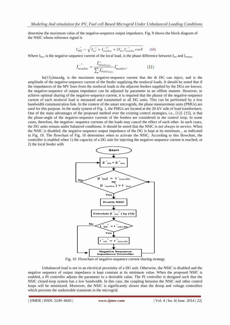
Modeling And simulation for PV, Fuel cell Based Microgrid Under Unbalanced Loading Conditions
| IJMER | ISSN: 2249–6645 | www.ijmer.com | Vol. 4 | Iss. 6| June. 2014 | 22|
determine the maximum value of the negative-sequence output impedance. Fig. 9 shows the block diagram of
the NSIC whose reference signal is
Where Iloc, is the negative-sequence current of the local load, is the phase difference between Iloc and Inonioc:
In(11),Imaxdg, is the maximum negative-sequence current that the th DG can inject, and is the
amplitude of the negative-sequence current of the feeder supplying the nonlocal loads. It should be noted that if
the impedances of the MV lines from the nonlocal loads to the adjacent feeders supplied by the DGs are known,
the negative-sequence of output impedance can be adjusted by parameter in an offline manner. However, to
achieve optimal sharing of the negative-sequence current, it is required that the phasor of the negative-sequence
current of each nonlocal load is measured and transmitted to all DG units. This can be performed by a low
bandwidth communication link. In the context of the smart microgrids, the phase measurement units (PMUs) are
used for this purpose. In the study system of Fig. 1, the PMUs are located at the 20-kV side of load transformers.
One of the main advantages of the proposed method over the existing control strategies, i.e., [12]–[15], is that
the phase-angle of the negative-sequence currents of the feeders are considered in the control loop. In some
cases, therefore, the negative- sequence currents of the loads may cancel the effect of each other. In such cases,
the DG units remain under balanced conditions. It should be noted that the NSIC is not always in service. When
the NSIC is disabled, the negative-sequence output impedance of the DG is kept at its minimum, , as indicated
in Fig. 10. The flowchart of Fig. 10 determines when to activate the NSIC. According to this flowchart, the
controller is enabled when 1) the capacity of a DG unit for injecting the negative-sequence current is reached, or
2) the local feeder with
Fig. 10. Flowchart of negative-sequence current sharing strategy
Unbalanced load is not in an electrical proximity of a DG unit. Otherwise, the NSIC is disabled and the
negative sequence of output impedance is kept constant at its minimum value. When the proposed NSIC is
enabled, a PI controller adjusts the parameter to a desirable value. The PI controller is designed such that the
NSIC closed-loop system has a low bandwidth. In this case, the coupling between the NSIC and other control
loops will be minimized. Moreover, the NSIC is significantly slower than the droop and voltage controllers
which prevents the undesirable transients in the microgrid.

Modeling And simulation for PV, Fuel cell Based Microgrid Under Unbalanced Loading Conditions
| IJMER | ISSN: 2249–6645 | www.ijmer.com | Vol. 4 | Iss. 6| June. 2014 | 23|
VI. Simulation Results
Fig :-MATLAB/SIMULINK MODEL OF FEEDER 1
Fig :-MATLAB/SIMULINK MODEL OF FEEDER 2
The real and reactive power of the three feeders for these changes are shown in the below figure. Since
feeder becomes unbalanced, a double-frequency ripple is appeared in the instantaneous power components of
this feeder. As it is observed, the double-frequency ripple is increased at due to the inclusion of the unbalanced
three-phase load. The figure below shows: Wave form for the Instantaneous Active power For Unbalanced Load
Changes at Feeder F1
(a) Fig:- Wave form for the 3-phase instantaneous Active power For Unbalanced Load changes at feeder f1.
The figure below shows: Wave form for the Instantaneous Reactive power For Unbalanced Load
Changes at Feeder F1
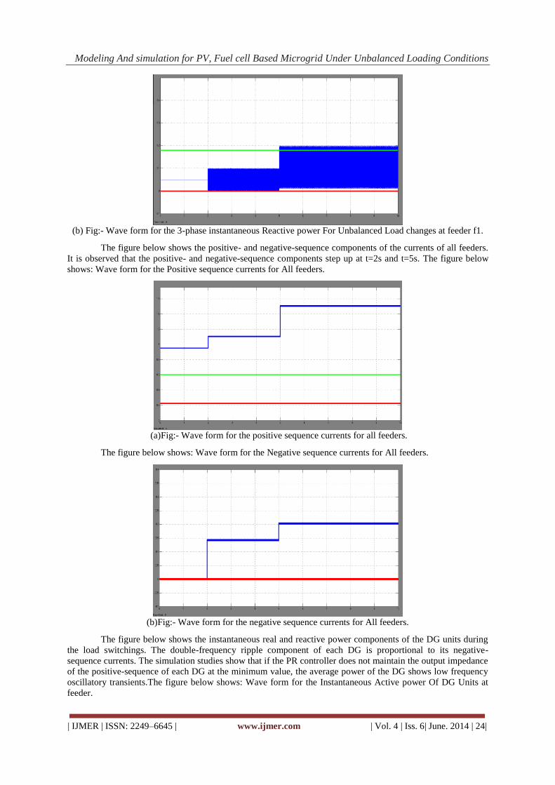
Modeling And simulation for PV, Fuel cell Based Microgrid Under Unbalanced Loading Conditions
| IJMER | ISSN: 2249–6645 | www.ijmer.com | Vol. 4 | Iss. 6| June. 2014 | 24|
(b) Fig:- Wave form for the 3-phase instantaneous Reactive power For Unbalanced Load changes at feeder f1.
The figure below shows the positive- and negative-sequence components of the currents of all feeders.
It is observed that the positive- and negative-sequence components step up at t=2s and t=5s. The figure below
shows: Wave form for the Positive sequence currents for All feeders.
(a)Fig:- Wave form for the positive sequence currents for all feeders.
The figure below shows: Wave form for the Negative sequence currents for All feeders.
(b)Fig:- Wave form for the negative sequence currents for All feeders.
The figure below shows the instantaneous real and reactive power components of the DG units during
the load switchings. The double-frequency ripple component of each DG is proportional to its negative-
sequence currents. The simulation studies show that if the PR controller does not maintain the output impedance
of the positive-sequence of each DG at the minimum value, the average power of the DG shows low frequency
oscillatory transients.The figure below shows: Wave form for the Instantaneous Active power Of DG Units at
feeder.

Modeling And simulation for PV, Fuel cell Based Microgrid Under Unbalanced Loading Conditions
| IJMER | ISSN: 2249–6645 | www.ijmer.com | Vol. 4 | Iss. 6| June. 2014 | 25|
(a)Fig:- 3-phase Instantaneous Active Powers of DG Units at feeder f1.
The figure below shows: Wave form for the Instantaneous Reactive powers Of DG Units at feeder f1.
(b)Fig:- Wave form for the 3-phase Instantaneous Reactive Power Of DG Units at feeder f1.
Figs. 3(a&b) and 4(a&b) shows the instantaneous power components and the positive- and negative-
sequence current components of the three feeders, respectively. Subsequent to the load switching event at
t=2s,theDG units activate their NSICs to share the demanded negative-sequence current by feeder f3 after 0.9 s.
In this case, the phasor f3 is measured by a PMU and transmitted to the adjacent DG units. The reference signal
of the NSIC of each DG unit is calculated.The figure below shows: Wave form for the Instantaneous Active
power at feeder f1,f2 and f3.
Fig 3(a):- Wave form for the 3-phase instantaneous Active power at f1,f2 and f3.
The figure below shows: Wave form for the Instantaneous Reactive power at feeder f1,f2 and f3.
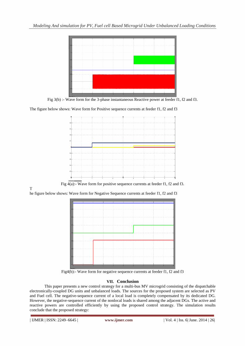
Modeling And simulation for PV, Fuel cell Based Microgrid Under Unbalanced Loading Conditions
| IJMER | ISSN: 2249–6645 | www.ijmer.com | Vol. 4 | Iss. 6| June. 2014 | 26|
Fig 3(b) :- Wave form for the 3-phase instantaneous Reactive power at feeder f1, f2 and f3.
The figure below shows: Wave form for Positive sequence currents at feeder f1, f2 and f3
Fig 4(a):- Wave form for positive sequence currents at feeder f1, f2 and f3.
T
he figure below shows: Wave form for Negative Sequence currents at feeder f1, f2 and f3
Fig4(b):- Wave form for negative sequence currents at feeder f1, f2 and f3
VII. Conclusion
This paper presents a new control strategy for a multi-bus MV microgrid consisting of the dispatchable
electronically-coupled DG units and unbalanced loads. The sources for the proposed system are selected as PV
and Fuel cell. The negative-sequence current of a local load is completely compensated by its dedicated DG.
However, the negative-sequence current of the nonlocal loads is shared among the adjacent DGs. The active and
reactive powers are controlled efficiently by using the proposed control strategy. The simulation results
conclude that the proposed strategy:

Modeling And simulation for PV, Fuel cell Based Microgrid Under Unbalanced Loading Conditions
| IJMER | ISSN: 2249–6645 | www.ijmer.com | Vol. 4 | Iss. 6| June. 2014 | 27|
• robustly regulates voltage and frequency of the microgrid;
• is able to share the average power among the DGs;
• effectively compensates the negative-sequence currents of local loads; and
• shares the negative-sequence current of the nonlocal loads such that the power quality of the overall
microgrid is not degraded.
REFERENCES [1] N. Hatziargyriou, H. Asano, R. Iravani, and C. Marnay, “Microgrids,” IEEE Power Energy Mag., vol. 5, pp. 78–94,
Jul.–Aug. 2007.
[2] A. G. Madureira and J. A. P. Lopes, “Coordinated voltage support in distribution networks with distributed
generation and microgrids,” IET Renew. Power Gener., vol. 3, pp. 439–454, Sep. 2009.
[3] IEEE Recommended Practice for Monitoring Electric Power Quality, IEEE Std. 1159, 2009.
[4] IEEE Recommended Practice for Electric Power Distribution for Industrial Plants, ANSI/IEEE Std. 141, 1993.
[5] R. Lasseter, “Microgrids,” in Proc. IEEE Power Eng. Soc. Winter Meeting, 2002, pp. 305–308.
[6] M. H. J. Bollen and A. Sannino, “Voltage control with inverter-based distributed generation,” IEEE Trans. Power
Del., vol. 20, no. 1, pp. 519–520, Jan. 2005.
[7] M. C. Chandrokar, D. M. Divan, and B. Banerjee, “Control of distributed ups systems,” in Proc. 25th Annu. IEEE
PESC, 1994, pp. 197–204.
[8] E. A. A. Coelho, P. C. Cortizo, and P. F. D. Garcia, “Small signal stability for parallel-connected inverters in stand-
alone ac supply systems,” IEEE Trans. Ind. Appl., vol. 38, pp. 33–542, Mar./Apr. 2002.
[9] N. L. Soultanis, A. I. Tsouchnikas, N. D. Hatziargyriou, and J. Mahseredjian, “Dynamic analysis of inverter
dominated unbalanced lv micro-grids,” IEEE Trans. Power Syst., vol. 22, no. 1, pp. 294–304, Feb. 2007.
[10] Y. Li, D. M. Vilathgamuwa, and P. C. Loh, “Design, analysis, and realtime testing of a controller for multibus
microgrid system,” IEEE Trans. Power Electron., vol. 19, pp. 1195–1204, Sep. 2004.
[11] T. L. Lee and P. T. Cheng, “Design of a new cooperative harmonic filtering strategy for distributed generation
interface converters in an islanding network,” IEEE Trans. Power Electron., vol. 22, pp. 1919–1927, Sep. 2007.
[12] P. Cheng, C. Chen, T. Lee, and S. Kuo, “A cooperative imbalance compensation method for distributed-generation
interface converters,”
[13] M. B. Delghavi and A. Yazdani, “Islanded-mode control of electronically coupled distributed-resource units under
unbalanced and nonlinear load conditions,” IEEE Trans. Power Del., vol. 26, no. 2, pp. 661–673, Apr. 2011.
[14] D. De and V. Ramanarayanan, “Decentralized parallel operation of inverters sharing unbalanced and non-linear
loads,” IEEE Trans. Power Electron., vol. 25, pp. 3015–3025, Aug. 2010.
[15] R. Majumder, A. Ghosh, G. Ledwich, and F. Zare, “Load sharing and power quality enhanced operation of a
distributed microgrid,” IET Renew. Power Gener., vol. 3, no. 2, pp. 109–119, 2009.
[16] M. N. Marwali and A. Keyhani, “Control of distributed generation systems- part i: Voltages and currents control,”
IEEE Trans. Power Electron., vol. 19, pp. 1541–1550, Nov. 2004.
[17] A. Timbus, M. Liserre, R. Teodorescu, P. Rodriguez, and F. Blaabjerg, “Evaluation of current controllers for
distributed power generation systems,” IEEE Trans. Power Electron., vol. 24, pp. 654–664, Mar. 2009.
[18] H. Karimi, A. Yazdani, and R. Iravani, “Robust control of an autonomous four-wire electronically-coupled
distributed generation unit,” IEEE Trans. Power Del., vol. 26, no. 1, pp. 455–466, Jan. 2011.
[19] H. Akagi, E. H. Watanabe, and M. Aredes, Instantaneous Power Theory and Applications to Power Conditioning.
New York: Wiley, 2007.
[20] M. C. Chandorkar, D. M. Divan, and R. Adapa, “Control of parallel connected inverters in standalone ac supply
systems,” IEEE Trans. Ind. Appl., vol. 29, no. 1, pp. 136–143, Jan.–Feb. 1993.
[21] M. Karimi-Ghartemani and H. Karimi, “Processing of symmetrical components in time-domain,” IEEE Trans. Power
Syst., vol. 22, no. 2, pp. 572–579, May 2007.
Mr.T.Venugopal iscurrently Associate Professor in the Department of Electrical
and Electronics Engineering,Vaagdevi college of engineering ,warangal, India.
He graduated and also persued M.Tech from JNTUH his area of intrests include
Energy management , Distributed Generation, power electronics in
volvemachine drives and power systems etc,
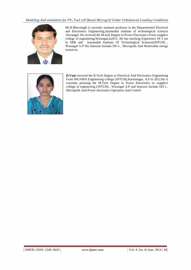
Modeling And simulation for PV, Fuel cell Based Microgrid Under Unbalanced Loading Conditions
| IJMER | ISSN: 2249–6645 | www.ijmer.com | Vol. 4 | Iss. 6| June. 2014 | 28|
Mr.B.Bhavsingh is currently assistant professor in the Departmentof Electrical
and Electronics Engineering,Jayamukhi institute of technological sciences
,Warangal. He received the M.tech Degree in Power Electronics From vaagdevi
college of engineering,Warangal,in2012. He has teaching Experience Of 3 yrs
in SRR and Jayamukhi Institute Of Technological Sciences(JNTUH) ,
Warangal A.P His Interests Include DG’s , Microgrids And Renewable energy
resources.
D.Vani received the B.Tech Degree in Electrical And Electronics Engineering
From NIGAMA Engineering college (JNTUH),Karimnagar, A.P in 2012.He is
currently perusing the M.Tech Degree in Power Electronics in vaagdevi
college of engineering (JNTUH) , Warangal A.P and Interests Include DG’s ,
Microgrids And Power electronics Operation And Control

International
OPEN ACCESS Journal
Of Modern Engineering Research (IJMER)
| IJMER | ISSN: 2249–6645 | www.ijmer.com | Vol. 4 | Iss. 6| June. 2014 | 29|
Fuzzy Rule Based Model for Optimal Reservoir Releases
Dr. T. M. V. Suryanarayana1, Mihir Kemkar
2
1 (Associate professor, Water Resources Engineering and Management Institute, Faculty of Technology and
Engineering, The Maharaja Sayajirao University of Baroda, Samiala-391410, Vadodara, Gujarat, India 2 (P.G. Student, Water Resources Engineering and Management Institute, Faculty of Technology and
Engineering, The Maharaja Sayajirao University of Baroda, Samiala-391410, Vadodara, Gujarat, India
I. INTRODUCTION Risk and uncertainty always remain as one of important issues due to lack of future knowledge
information that leads to achieve the planning goals precisely, therefore, recognizing future uncertainty helps to
decrease the risks and increase the benefits, however, even with development of mathematical and
computational techniques, finding an exact deterministic solutions still skeptical. Reservoir operation is not
exception, hence any reservoir operation problem contains some degree of uncertainty and ambiguity due to
several involved components, Reservoirs are built usually to serve multiple purposes for example irrigation,
municipal and industrial water supply, hydro-power and flood control. Fuzzy systems are an alternative to
traditional notions of set membership and logic that has its origins in ancient Greek philosophy, and applications
at the leading edge of Artificial Intelligence. Optimal operation of reservoir has been an active area of research
for many years The fuzzy logic approach may provide a promising alternative to the methods used for reservoir
operation modeling, The uncertainty of water resources systems due to parameters inputs randomness can be
handled adequately using probability theory in case of sufficient data availability, while the uncertainty that
attributed to imprecision can be solved appropriately using the capability of fuzzy set theory that allowing to
translate the human experience in mathematical forms taking the shape of memberships functions. Panigrahi and
Majumdar [1] developed a fuzzy rule based model for the operation of a single purpose reservoir. The model
operates on an „if – then‟ principle, where the „if‟ is a vector of fuzzy premises and the „then‟ is a vector of
fuzzy consequences. Mousavi et al. [2] developed a dynamic programming fuzzy rule–based (DPFRB) model
for optimal operation of reservoirs system. This method results in deriving the operating policies, which are
robust against the uncertainty of inflows. These policies are derived by using long-term synthetic inflows and an
objective function that minimizes its variance. The DPFRB performance is tested and compared to a model,
which uses the commonly used, multiple regression–based operating rules. Results show that the DPFRB
performs well in terms of satisfying the system target performances and computational requirements. Bai and
Tamjis [3] developed a fuzzy logic model for deriving optimal operational rules at the macro level for better
performance and control of hydro-power generation. Mohan and Sivakumar [4] developed a heuristic Dynamic
Programming based Neuro-Fuzzy Model (DPNF to optimize the operation of a multi-reservoir using dynamic
programming and Adaptive Neuro Fuzzy Inference Systems (ANFIS) techniques. The demonstrations of
developed models are carried out through application of Parambikulam AliyarProject (PAP) systems in India.
Abdullah and Stamm [5] developed a Fuzzy Rule Based (FRB) membership functions depending on statistical
parameters of time series analysis accompanied with different future climate change perspectives for inflow
Abstract: The aim of this paper is to develop a Fuzzy Rule Based(FRB) model for obtaining the
optimal reservoir releases. The area considered for the study is ukai reservoir project. The data
considered are for the months of July, August, September and October for the years 2007 and 2011.
The inputs considered are inflow (MCM), Storage (MCM), Demand (MCM) and the Release (MCM) is
considered as output. Fuzzy logic, analysis is based on designing of if and then rules. Fuzzy logic
model can handle with various kinds of data regulations implication and defuzzification. The steps
involved in the development of the model include the construction of membership functions, creating
the Fuzzy rules, implication and deffuzification. The results obtained shows that the releases obtained
from the FRB model are satisfying the demand completely in all the four months, i.e. July, August,
September and October for the year 2007 and the same is observed for the year 2011. Also, a
significant amount of water is being saved, when the actual releases are compared with the releases
obtained from the FRB model.
Keywords: Fuzzy rules, Membership functions, Optimal release, Optimization, Reservoir operation,
Ukai reservoir project.

Fuzzy Rule Based Model for Optimal Reservoir Releases
| IJMER | ISSN: 2249–6645 | www.ijmer.com | Vol. 4 | Iss. 6| June. 2014 | 30|
scenarios at the Eastern Nile region, while a statistical analysis and expert opinions have been used to shape the
different storage, releases, and demands membership functions in order to obtain the optimum release.
II. MODEL FORMULATION Fuzzy logic starts with the concept of a fuzzy set. A fuzzy set is a set without crisp or clearly defined
boundary. It can contain elements with only a partial degree of membership. The fuzzy inference process
known as Mamdani‟s fuzzy inference method is used in this study. It‟s the most commonly seen fuzzy
methodology. All output membership functions are singleton spikes, and the implication and aggregation
method are fixed and cannot be edited.
A fuzzy rule based model operates on “IF-THEN” principle, where “IF” represents the vector of fuzzy
explanatory variable, and “THEN” the fuzzy consequences, to apply this principles efficiently, a Fuzzy
Inference System (FIS) is a control system built using fuzzy set theory based on combining the fuzzy sets from
each rule through aggregation operator to get a fuzzy set result, then defuzzify the fuzzy set for each output
variable. Two types of (FIS) can be applied in fuzzy logic, the most commonly and widely used Mamdani type
(1977) and Takagi Sugeno type (1985); both methods are similar in many aspects; however the main difference
between them is the output membership functions (MF) in Sugeno type are linear or constant. Since the output
membership functions in this paper (namely reservoir release) are not necessarily linear, the FIS Mamdani has
been adopted as it represents the output (release) more realistically.
1. Input and output variables fuzzification using convenient linguistics subsets such as high, medium, low, etc.
2. Based on expert knowledge and available information, IF-Then rules constructed to combine the linguistic
inputs subsets to the output fuzzy sets using the logical conjunction such as “and”.
3. The implication part of fuzzy system is defined as the shape of the consequent based on the premise
(antecedent) part.
4. Finally, to have a crisp value, the resulted fuzzy set is defuzzified using the appropriate defuzzification
method such as centroid.
The inputs to the fuzzy system are inflow (MCM), storage (MCM) and demand (MCM) for the
reservoir. The output is the optimal release from the reservoir. The model is developed in the MATLAB.
The main objective of the study is to compute the quantity of the water that should be released to meet the
monthly irrigation demand and also an attempt has been made in developing the model that obtained optimal
releases from the FRB model should be less than actual releases of the reservoir while satisfying the demand
completely.
To apply Fuzzy Rules to the above formulated model, the data used are inflow, demand, actual release,
and storage in MCM. In modeling of reservoir operation with fuzzy logic, the following distinct steps are
followed: (a) Fuzzification of inputs, where the crisp inputs such as the inflow, reservoir storage and release, are
transformed into fuzzy variables, (b) Formulation of the fuzzy rule set, based on an expert knowledge base, (c)
Application of a fuzzy operator, to obtain one number representing the premise of each rule, (d) Shaping of the
consequence of the rule by implication, and (e) Defuzzification. The study area considered for developing the
FRB model is ukai Reservoir project, Gujarat, India. The data comprises for the months of July, August,
September and October for the years 2007 and 2011.
III. Results and Discussion
The developed Fuzzy Rule Based (FRB) model gives the optimal releases for the data considered for
the study.
Table 1: Actual release, Demand and Releases from FRB 2007
Year Month Actual Release
(MCM)
Demand
(MCM) Releases from
FRB model
2007
July 3135.12 2508.09 2510
August 2912.65 1336.84 1500
September 1696.92 1720.84 1790
October 499.46 505.79 529
Table 1 shows the obtained optimal releases from FRB model for the months of July, August, September and
October respectively for the year 2007, it is also given in Fig.1.

Fuzzy Rule Based Model for Optimal Reservoir Releases
| IJMER | ISSN: 2249–6645 | www.ijmer.com | Vol. 4 | Iss. 6| June. 2014 | 31|
Fig. 1: Actual release, Demand and Releases from the FRB model for the year 2007
From Fig. 1, it is observed that releases obtained from FRB model are satisfying 100% demand in all
the four months i.eJuly, August, September and October for the year 2007. Also a significant amount of water is
being saved when actual releases are compared with the releases from the FRB model. In case of September and
October although releases obtained from the FRB model are greater than the actual releases, but the actual
releases were not satisfying demand for those two months.
The results obtained for the year 2011 are shown in Table 2
Table 2: Actual release, Demand and Release from FRB 2011
Year Month Actual Release
(MCM)
Demand
(MCM) Releases from
FRB model
2011
July 151.93 335.69 340
August 1754.43 1403.54 1500
September 1770.86 1530.89 1540
October 353.00 200.7 293
Table 2 shows the obtained optimal releases from FRB model for the months of July, August, September and
October respectively for the year 2011, it is also given in Fig. 2.
Fig. 1: Actual release, Demand and Releases from the FRB model for the year 2007

Fuzzy Rule Based Model for Optimal Reservoir Releases
| IJMER | ISSN: 2249–6645 | www.ijmer.com | Vol. 4 | Iss. 6| June. 2014 | 32|
From Fig. 2, it is observed that releases obtained from FRB model are satisfying 100% demand in all
the four months i.e. July, August, September and October for the year 2011. Even though in the month of July
releases from FRB model are greater than actual releases, but actual releases were not satisfying demand. Also it
is observed that in all four months model developed is saving significant amount of water and at the same time
care has been taken for satisfying the demand completely.
IV. CONCLUSION
It can be concluded that the FRB model yields the optimal releases for all the four months considered
for the study i.e. July, August, September and October for the years 2007 and 2011. It has been found out that
the obtained optimal release from the FRB model for the year 2007, in case of September and October and for
the year 2011, in case of July FRB releases are greater than the actual releases but the care has been taken to
satisfy the demand and in some cases, a significant amount of water is being saved when the actual releases are
compared to the FRB releases.
REFERENCES Journal Papers: [1] D.P. Panigrahi and P.P. Majumdar, Reservoir operation modeling with Fuzzy Logic, Water Resources Management, 14, 2000, 89–
109.
[2] S.J. Mousavi, K .Ponaabalam and F. Karray, Reservoir Operation Using a Dynamic Programming Fuzzy Rule–Based Approach,
Water Resources Management, 19, 2005, 655–672.
[3] V. Ramani Bai and M. Rom Tamjis, Fuzzy Logic Model on Operation and Control of Hydro- Power dams in Malaysia, ICCES,
4(1), 2007, 31-39.
[4] S. Mohan and S. Sivakumar, Development of multi reservoir system using dp based neuro-Fuzzy model: a case study in Pap System, India, INWEPF Steering Meeting and Symposium, 4, 2007, 1-11.
[5] M. Abdullah. and Jurgen Stamm, Developing an Optimum Multipurpose Reservoir Operation Policy under Uncertain Conditions,
Nile Basin Water Science & Engineering Journal, 5(2), 2012,36-48.

International
OPEN ACCESS Journal
Of Modern Engineering Research (IJMER)
| IJMER | ISSN: 2249–6645 | www.ijmer.com | Vol. 4 | Iss. 6| June. 2014 | 33|
Design and Development of Double Offset Butterfly Valve
Piyush P. Nagpurkar1, Prof. R. S.Tajane
2
1( CAD/CAM Production Department, A.V.C.O.E. Sangamner, Maharashtra, India)
2 (Production Department, A.V.C.O.E. Sangamner, Maharashtra, India)
I. INTRODUCTION A valve is a mechanical device that controls the flow of fluid and pressure within a system or process.
A valve controls system or process fluid flow and pressure by performing any of the following functions:
- Stopping and starting fluid flow
- Varying (throttling) the amount of fluid flow
- Controlling the direction of fluid flow
- Regulating downstream system or process pressure
There are many valve designs and types that satisfy one or more of the functions identified above. A
multitude of valve types and designs safely accommodate a wide variety of industrial applications. Regardless of
type, all valves have the following basic parts: the body, bonnet, trim (internal elements), actuator and packing.
II. OBJECTIVE OF PROJECT Design and development for the 4’’ X 150# Butterfly Valve with Double Eccentricity
TABLE I. DESIGN INPUT DATA SHEET Sr. No. Input Details
1 Product Butterfly Valve
2 Size 4”
3 Pressure Rating/ Class 150 #
4 Maximum Operating Pressure 20 Bar
TABLE II. ALLOWABLE DESIGN STRESS VALUE
Allowable design stress value for various materials as per ASME Boiler and Pressure Vessel code Section VII
division I is as below,
Sr. No. 1 2 3 4 5
Material WCB WC6 WC9 CF3 CF8
Ref. Table UCS-23 UCS-23 UCS-23 UHA-23 UHA-23
Ref. Page 286 294 294 400 400
Min. Yield Strength ksi 36 40 40 30 30
Spec. Min. Yield Strength ksi 70 70 70 70 70
Allowable Stress ksi 17.5 17.5 20.5 17.5 17.5
Maximum ksi 14 14 16.4 14 14
Abstract: Valves are mechanical devices specially designed to direct, start, stop, mix or regulating the
flow, pressure of a process fluid. A butterfly valve typically consists of a metal disk formed around a
central shaft, which acts as its axis of rotation. As the valve's opening angle is increased from 0 degrees
(fully closed) to 90 degrees (fully open), fluid is able to more readily flow past the valve. These valves are
commonly used to control fluid flow inside of piping systems. The main objective of this study is to find out
stresses developed in butterfly valve Shell and Disk.
This report contains the information about design and development for the 4’’ X 150# Butterfly
Valve with Double Eccentricity using ANSYS. It comprises the calculations which are required for design
of Butterfly Valve such as Shell Thickness, Disc Thickness, Stem Diameter and Calculation of Torque using
ASME, IBR. Also includes the modeling and assembly of butterfly valve using Pro-E.
During project, we will discuss Finite Element Analysis of Butterfly valve Shell, Disc stem and
their assembly. The solid model will discretized into finite elements and logical constrains will applied in
boundary conditions. The stress results obtained in finite element analysis will have to check whether, is
there a chance for optimization of design.
Keywords: Valves, Butterfly Valve, Double offset Butterfly Valve, ASME, IBR.

Design and Development of Double Offset Butterfly Valve
| IJMER | ISSN: 2249–6645 | www.ijmer.com | Vol. 4 | Iss. 6| June. 2014 | 34|
Sr. No. 1 2 3 4 5
Material WCB WC6 WC9 CF3 CF8
Allowable
Stress MPa 96.5 96.5 113 96.5 96.5
Kg/ cm2 984 984 1153 984 984
III. DESIGN CALCULATIONS 3.1 Calculation for Shell Thickness of Valve Body
3.1.1 Thick Cylinder (As per IBR 290(d))
Where,
WP = Maximum Working Pressure, Kgf/mm2
D = External Diameter of Chest, mm
F = Allowable Stress, Kg/mm2
Lower of the two expression i.e. &
C = Minimum Positive Tolerance, mm
(5 mm for Carbon Steel and 2.5 mm for Stainless Steel)
3.1.2 Thin Cylinder
Where,
t = Shell thickness mm
P = Maximum Working Pressure, MPa
D = Maximum Internal Diameter of Body, mm
S = Maximum Allowable Working Stress. MPa
3.1.3 From Valve Design Book by Pearson [7]
Where,
P = Working Pressure, MPa
D = Inside Diameter or Port Opening, mm
f = Maximum Allowable Working Stress, MPa
t = Shell Thickness, mm
C = Constant (8 mm for CI and 6.5 mm for Carbon Steel)
3.1.4 By Formula ASME see VIII Div-1
Where,
P = Design Pressure, Kg/cm2 R = Inside Radius of Shell, cm
S = Maximum Allowable Stress Value Kg/cm2
E = Joint Efficiency = 1
TABLE III. SHELL THICKNESS ACCORDING TO DIFFERENT FORMULAE
Sr. No. As per Formulae Shell Thickness
(mm)
1 Thick Cylinder (As per IBR 290 (d)) 5.24
2 Thin Cylinder 1.04
3 Valve Design Book by Pearson 6.72
4 ASME (VIII Div. 1) 1.04
Provided Shell Thickness 9.0

Design and Development of Double Offset Butterfly Valve
| IJMER | ISSN: 2249–6645 | www.ijmer.com | Vol. 4 | Iss. 6| June. 2014 | 35|
3.2 Calculation of Disc Thickness
By using following formula, we can calculate the thickness of Disc. In this calculation, we consider a
disc as a simply supported flat plate with a uniform distributed load.
Where, w = Total Load acting on Disc
M = Reciprocal of Poisson’s ratio = 3.4
f = Maximum Allowable Working Stress
r = Distance at which thickness to be determine
After putting the values for all variable used in the above formulae, we got thickness value of Disc at
various distance from center of Disc which are noted in following table.
TABLE IV. DISC THICKNESS AT VARIOUS DISTANCE FROM CENTER OF DISC
Sr. No. Radius (mm) from center Thickness
(mm)
1 0 (at center) 8.92
2 14.25 8.64
3 28.5 7.89
4 42.75 6.24
Provided Disc Thickness at
Center 9.00
IV. D MODELING 4.1 Body
4.2 Disc
4.3 Assembly

Design and Development of Double Offset Butterfly Valve
| IJMER | ISSN: 2249–6645 | www.ijmer.com | Vol. 4 | Iss. 6| June. 2014 | 36|
V. STRESS ANALYSIS USING ANSYS R10 5.1 Introduction
The stress analysis can be linear/elastic or nonlinear/plastic depending on the addressed failure mode
and on the applied code rule. In this analysis, the scope is concerned with the calculation of Displacement and
Von Mises Stress using FEA numerical solver. Finite element analysis is carried out on the various parts of
butterfly valve.
The parts are listed as given below,
1) Body
2) Disc
3) Assembly
Finite element analysis is carried out using different material Grade in Carbon Steel and Stainless Steel
such as WCB and CF8 for Body and Disc. For Stem material, we considered ASTM A276-Type 410.
5.2 Material Properties
The elements are attributed with the material properties as shown in the table below,
TABLE V. MATERIAL PROPERTIES OF DIFFERENT MATERIALS Sr. No. 1 2 3
MATERIAL NAME ASTM A216 Gr WCB ASTM A351 Gr CF8 ASTM A276 Type 410
YOUNG’S MODULUS 210 GPa 194 GPa 199.982 GPa
POISSION’S RATIO 0.3 0.265 0.285
YIELD STRENGTH 249.2 MPa 206 MPa 275.76 MPa
ULTIMATE STRENGTH 482.6 MPa 483 MPa 483 MPa
5.3 Result of Analysis
5.3.1 Body
5.3.1.1 Von Mises Stress
Fig 5.3.1.1 Von Mises Stress for WCB Material (Max. Value 5.594 MPa)
5.3.1.2. Displacement Sum

Design and Development of Double Offset Butterfly Valve
| IJMER | ISSN: 2249–6645 | www.ijmer.com | Vol. 4 | Iss. 6| June. 2014 | 37|
Fig 5.3.1.2 Displacement Vector Sum for WCB Material (Max. Value 0.000258 mm)
TABLE VI. SUMMARY OF VON MISES STRESS AND DISPLACEMENT VECTOR SUM OF BODY
Material Maximum Von Mises Stress (MPa) Maximum Displacement (mm)
ASTM A216 Gr WCB 5.594 0.000258
ASTM A351Gr CF8 5.728 0.000276
5.3.2 DISC
5.3.2.1 Von Mises Stress
Fig 5.3.2.1 Von Mises Stress for CF8 Material (Max. Value 58.928 MPa)
5.3.2.2. Displacement Sum

Design and Development of Double Offset Butterfly Valve
| IJMER | ISSN: 2249–6645 | www.ijmer.com | Vol. 4 | Iss. 6| June. 2014 | 38|
Fig 5.3.2.2 Displacement Vector Sum for CF8 Material (Max. Value 0.011143mm)
TABLE VII. SUMMARY OF VON MISES STRESS AND DISPLACEMENT VECTOR SUM OF DISC
Material Maximum Von Mises Stress (MPa) Maximum Displacement (mm)
ASTM A351Gr CF8 58.928 0.011143
5.3.3 Assembly
5.3.3.1 Von Mises Stress
Fig 5.3.3.1 Von Mises Stress for WCB Material (Max. Value 83.877 MPa)

Design and Development of Double Offset Butterfly Valve
| IJMER | ISSN: 2249–6645 | www.ijmer.com | Vol. 4 | Iss. 6| June. 2014 | 39|
5.3.3.2. Displacement Sum
Fig 5.3.3.2 Displacement Vector Sum for WCB Material (Max. Value 0.015521mm)
TABLE VIII. SUMMARY OF VON MISES STRESS AND DISPLACEMENT VECTOR SUM OF ASSEMBLY
Material Maximum Von Mises Stress (MPa) Maximum Displacement (mm)
ASTM A216 Gr WCB 83.877 0.015521
ASTM A351Gr CF8 85.896 0.015514
5.4 Summary of Result TABLE IX. SUMMARY OF ANSYS ANALYSIS
Part /
Material (Yield
Strength)
Body Disc Assembly
VM
(MPa)
DISP
(mm)
VM
(MPa)
DISP
(mm)
VM
(MPa)
DISP
(mm)
WCB
(249.2 MPa)
5.594
0.000258
NA
NA
83.877
0.01552
CF8
(206 MPa)
5.728
0.000276
58.928
0.011143
85.896
0.01551
VI. CONCLUSION As from the summary of the result, we see that, the Von Mises Stress induced in the parts of Butterfly
Valve because of applied pressure of 20 bars, are less than the yield strength of the material. Hence we conclude
that, Design of Butterfly Valve for Chosen Material is safe.
REFERENCES [1] Naseradinmousavi, P., & Nataraj, C. (2011), Nonlinear mathematical modeling of butterfly valves driven by solenoid
actuators, Applied Mathematical Modeling, 35(5), pp. 2324-2335.
[2] Kwuimy, C. K., & Nataraj, C. (2012), Modeling and dynamic analysis of a butterfly valve, 70(1), pp. 435-451.
[3] Song, X. G., Wang, L., Baek, S. H., & Park, Y. C. (2009), Multidisciplinary optimization of a butterfly valve. ISA
transactions, 48(3), pp. 370-377.
[4] Kim, S. W., Kim, J. H., Choi, Y. D., & Lee, Y. H. (2009), New Trends in Fluid Mechanics Research Springer Berlin
Heidelberg, pp. 463-466.
[5] Kimura T, Tanaka T, Fujimoto K and Ogawa K (1995), Hydrodynamic Characteristics of a Butterfly - Prediction of
Torque Characteristics ISA Transactions pp. 327-333.
[6] Boesch, B. E., A. S. Humpherys, and D. A. Young. 1981. How scheduling fits in the irrigation program in the Grand
Valley of Colorado. Proc. Am. Soc. Agric. Engr. Irrig. Scheduling Conf., (Dec. 1981), pp. 159-165.
[7] Pearson G. H., “Valve Design”, Mechanical Engineering Publication Ltd, London.

International
OPEN ACCESS Journal Of Modern Engineering Research (IJMER)
| IJMER | ISSN: 2249–6645 | www.ijmer.com | Vol. 4 | Iss. 5| June. 2014 | 40|
Synthesis of nano materials by sputtering
Zaheer Ahamed1, Jeevan H.P
2, A. R. Anwar Khan
3
1(Associate Professor, Department of Mechanical Engg, Al-Habeeb college of Engg, Hyderabad, India 2(PG student, Department of mechanical engineering,Ghousia college of engineering, VTU, Ramanagara,
Karnataka, India 3 (Professor and Head, Department of Mechanical Engg, Ghousia College of Engg, Ramanagara, India
I. INTRODUCTION A Nanomaterial is a material where some controllable relevant dimension is of the order of 100nm or
less. The simple presence of nanoscale structure alone is not sufficient to define a nanomaterial, since most if
not all materials have structure in this range. The ability to control the structure at this scale is essential. One
could argue, in this sense, that many of the classical alloys and structural materials that contained nanoscale
components by design could be called nanomaterials. In modern usage, nanomaterials are newly developed
materials where the nanoscale structure that is being controlled has a dominant effect on the desired behavior of
the material or device. There are three different classes of nanomaterials: discrete nanomaterials, nanoscale device materials, and bulk nanomaterials. In a broad sense, the approaches used to make materials can be put
into two categories: top-down approaches, in which one begins with a bulk material that is then processed to
make a nanomaterial, and bottom-up approaches, in which the nanomaterial is built up from finer scales (in the
limit, building the nanomaterial up one atom at a time).
It is evident that bottom-up approaches require control of processes at very fine scales, but this is not
as difficult as it sounds, since chemical reactions essentially occur molecule by molecule. Depend upon the
application one has to select the appropriate approach for the production of nano materials. The electron beam
lithography is the one of the best top down approach for the synthesis of nano materials. EBL is well known for
its maskless lithography for a better control over line width i.e less than 5 nm. Only one disadvantage of using
this technique is it takes too much time for writing the pattern onto the resist material. After transferring the
pattern onto the PMMA resist, the desired material can be synthesized with the help of sputtering (electron beam evaporation or thermal evaporation). Sputtering means ejecting material from a target and depositing it on a
substrate such as a silicon wafer. The target is the source material.
II. Experimental Procedure
2.1 Materials used
Alumina (Al2O3) is very hard material and its hardness is exceeded only by diamond and a few
synthetic substances such as carborundum, and silicon carbide. This property of alumina lends itself for use as
an abrasive material. Another useful property of the material is its high melting point, i.e., above 2000°C
(3632°F), which makes it useful as a refractory and as linings of special furnaces.
Abstract: Nanoscience and nanotechnology primarily deal with the synthesis, characterization,
exploration, and exploitation of nanostructures materials. These materials are characterized by at least
one dimension in the nanometer (1nm = 10−9 m) range. In this research project nano materials are
synthesized or deposited by sputtering process. Prior to this sputtering process, the desired specimen and
its pattern is prepared with one of the mask less lithographic techniques such as electron beam
lithography (EBL). In this process, EBL machine is used with 220 KV of power and it is used to write the
pattern with raster scan method. After co-deposition of Al2O3 and SiO2 with the help of sputtering then finally characterization has taken place. In this characterization, Scanning electron microscope (SEM)
images are taken and then finally atomic force microscope (AFM) images are taken in order to know the
deflection error, adhesiveness, and DMT modulus
Keywords: About five key words in alphabetical order, separated by comma.

Synthesis of nano materials by sputtering
| IJMER | ISSN: 2249–6645 | www.ijmer.com | Vol. 4 | Iss. 5| June. 2014 | 41|
Property* Value
General
Chemical Formula Al2O3
Mechanical
Density 3.88 gm/cc
Hardness 2000 Knoop
Tensile Strength 35 kpsi
Modulus of Elasticity 48 - 54 x 106 psi
Flexural Strength 57 kpsi
Compressive Strength 368 kpsi
Poisson's Ratio 0.23 - 0.26
Fracture Toughness 4.3 MPa m½
Electrical
Dielectric Strength 210 - 220 ac V/mil
Dielectric Constant 9.7 (@ 1 MHz)
Volume Resistivity > 1014 ohm-cm
Thermal
Coefficient of Thermal Expansion
5.1 - 7.2 x 10⁻⁶/°C
Thermal Conductivity 30.3 - 35.0 W/mK
Specific Heat 0.20 cal/g °C
Maximum Working Temperature
1750 °C
Shock Resistance 200 °C Diff.
The pure form of Silica (SiO2) is Quartz and the impure form is sand. Mainly it is used with aluminium
in car manufacturing industries. Used in waterproofing treatments, moulding compounds and mould-release
agents, mechanical seals, high temperature greases and waxes, caulking compounds and even in applications as
diverse as breast implants and explosives.
Material Quartz Fused silica
Density (g/cm3) 2.65 2.2
Thermal conductivity (Wm-1
K) 1.3 1.4
Thermal expansion coeff. (10-6
K-1
) 12.3 0.4
Tensile strength (MPa) 55 110
Compressive strength (MPa) 2070 690-1380
Fracture toughness (MPa) - 0.79
Melting point (C) 1830 1830
Modulus of elasticity (GPa) 70 73
Thermal shock resistance Excellent Excellent
2.2 Process flow
The first step in the first stage is sample preparation where SiN wafer is cleaned with Piranha solution.
After cleaning of this substrate it is dipped into dil. HF. Then dehydration process will takes place with a
prebake temperature of 150 0C for about 5 minutes. Then Spin the PMMA resist at 6000 rpm in order to get 200
nm thickness for 60 seconds.

Synthesis of nano materials by sputtering
| IJMER | ISSN: 2249–6645 | www.ijmer.com | Vol. 4 | Iss. 5| June. 2014 | 42|
Figure 1: process Flow diagram
The spin off stage takes place for approximately 10 seconds after spin up. After obtaining 200 nm
thickness of PMMA resist then it is used for soft bake at 95 0C for 45 seconds.
Figure 2: Raith EBL at IISc, Bangalore
In this experiment Raith EBL equipment (shown in above figure) is used to produce the desired pattern
and the wafer along with PMMA deposition is kept in the sample loading unit of EBL. Raith uses NPGS (Nano
pattern Generation System) software to design the layout of the pattern and the generated pattern is as shown in
figure 3. Each cube consists of 30 nm x 30 nm x 30 nm.
Fig 3: Pattern of an EBL (side view)
In this process, it is proposed to synthesis 50nm cubes of 7*7 matrix. The diameter of the wafer is 4
inch and whereas the thickness is 525 µm. The film of resist are exposed to line dose of 1-2 nC/cm and area
dose of 200 mC/cm2 at 30 kV of energy beam depending on the pattern. Then finally allow the electrons from
the electron gun from electron source towards PMMA resist in order to deposit the desired pattern which was
designed. It took 7 hours of time to deposit the desired pattern. Then finally lift-off process is conducted on the
specimen in order to remove the unwanted PMMA resist and to get the final desired pattern which will be ready
for next process i.e, sputtering process. In this process the material to be deposited is taken for co-deposition and
is kept in sample holder. Then allow high voltage current in order to evaporate from the sample holder and
allow it to deposit on to the silicon nitride wafer i.e on to the holes as well as on the PMMA resist. Then allow it for solidification. The lift-off process is used in order to chip-off or remove the unwanted PMMA resist as well
as to remove the unwanted deposited material with the help of sputtering process. The final specimen will look
like as shown in the figure 4. This specimen is further is used for characterization for SEM and AFM.

Synthesis of nano materials by sputtering
| IJMER | ISSN: 2249–6645 | www.ijmer.com | Vol. 4 | Iss. 5| June. 2014 | 43|
III. Results And Discussions
3.1 SEM Analysis
Fig 4: 1 µm level at a magnification of 25 KX
The above figure shows the SEM image of nano sillimanite cubes. It is seen at 1 µm level at a
magnification of 25 KX. From this it is clearly visible that the presence of nano sillimanite is available. The
white dots indicate the co-deposition of alumina and silica materials. Whereas the remaining dark area indicates
the silicon nitride wafer.
3.2 AFM Analysis 3.2.1 3D image analysis
Figure 5: 3D image of nano sillimanite
The figure 7 shows the 3D image of sillimanite cube. The golden yellowish color shows the presence
of silicon dioxide and whereas the white color indicates the presence of aluminium dioxide. The valleys present
in the image indicate the presence of any voids.
3.2.2 Adhesiveness
Fig 6: Adhesive property of nano sillimanite cube
The above figure shows the adhesive property and from the figure it is very clear that this image is taken from 0 – 5 µm range. There are various colors on the plot. The yellowish color indicates that the material
have more adhesive towards the tip of the cantilever beam. That means there is a frictional force behind this
phenomenon. Whereas the dark brown color indicates that there is a less adhesiveness when we move from
center of the material towards the edge of the material. And this value again very less when we move towards
the edges of the specimen.
3.2.3 Deflection error
Fig 7: deflection error of cantilever beam

Synthesis of nano materials by sputtering
| IJMER | ISSN: 2249–6645 | www.ijmer.com | Vol. 4 | Iss. 5| June. 2014 | 44|
The above figure is plotted between deflection error (nm) and height sensor (nm). When the tip of the
cantilever beam is far away from the surface of the material then the deflection error is more and is as shown in
figure. When the cantilever beam is started to bring near to the surface of the material then the deflection error is
gradually reducing. This zero deflection can also be considered as adhesiveness of the material.
3.2.5 DMT modulus
Fig 8: DMT modulus of the scanned area
The above figure shows the DMT (Derjaguin, Muller and Toporov) modulus values across the scanned
area. Usually the tip of the cantilever beam is of spherical shape. The radius of curvature of spherical tip will be
in contact with the surface of the material. The surface energy or adhesive force will have impact on outer side
of the radius of the tip. This adhesive force or DMT modulus (dark brown color) at the contact area will be very
less because of the presence of porosity at contact area. The yellowish color shows that DMT modulus value is
more and this is because of more adhesive force present over there. And it is average at the rest of the scanned area.
IV. CONCLUSION 1) It seen from the SEM images that the distribution of the nano sillimanite tiles of 50 nm is uniform
throughout the scanned surface area.
2) It is seen from the image that 50nm cubes are clearly visible.
3) The white spotted areas indicate that the presence of nano sillimanite tiles whereas the dark area indicate
silicon nitride wafer.
4) From the AFM images it is seen almost a flat surface except with some valleys. 5) It has very good adhesiveness property with the tip of the cantilever beam of the atomic force microscope
and this is because of the surface roughness present between the surface of the material and the tip of the
cantilever beam.
6) The combination and presence of two ceramic materials will give almost zero surface roughness i.e 1.21 nm
which is almost negligible. The maximum surface roughness at ever be peaks and valleys is 12.4 n
REFERENCES [1.] Chang L. L. Y., “Mullite, silimanite, andalusite and kyanite in industrial mineralogy”, Prentice-Hall, Upper Saddle
River, NY, 2002, PP. 373-385.
[2.] Richard C. B., Joaquin A. S. and Heberto B. R., “Nano-milling of the Sillimanite mineral, Kyanite, and its reaction with alumina to form mullite”, J. of Ceram. Proc. Res., Vol. 6, No. 4, 2005, P. 271-275.
[3.] Tripathi H. S. and Banerjee J., “Synthesis and mechanical properties of mullite from beach sand silimanite: Effect of TiO2”, J. of European Cera. Soc., Vol. 18, 1998, P. 2081-2087.
[4.] E- beam tool specifications by Center for Nanoscience Engineering, IISc, Bangalore. [5.] Electron Beam Lithography by Hans-Georg Braun, Sep 22, 2008. [6.] Handbook of Microlithography, Micromachining and Microfabrication, Editor P.R. Choudhury, SPIE Press
Monograph PM 39.
[7.] General introduction to lithography, IISc, Bangalore. [8.] Electron Beam Lithography in Nanoscale Fabrication: Recent Development by Ampere A. Tseng, Kuan Chen,
Chii D. Chen, and Kung J. Ma, IEEE transactions on electronics packaging manufacturing, vol. 26, no. 2, april 2003.

International
OPEN ACCESS Journal
Of Modern Engineering Research (IJMER)
| IJMER | ISSN: 2249–6645 | www.ijmer.com | Vol. 4 | Iss. 6| June. 2014 | 45|
Optimization of Cutting Parameters Using Genetic Algorithm
and Particle Swarm Optimization
G. Bala Subramanyam1, P. Punna Rao
2
M.Tech (Student) Mechanical Engineering, NIMRA College of Engineering & technology
M.Tech Asst Professor of Mechanical Engineering Department, NIMRA College of Engineering & Technology,
Jupudi, Vijayawada. A.P
I. Introduction Surface roughness has received serious attention for many years. It has formulated an important design
feature in many situations such as parts subject to fatigue loads, precision fits, fastener holes, and aesthetic
requirements. In addition to tolerances, surface roughness imposes one of the most critical constraints for the
selection of machines and cutting parameters in process planning. A considerable number of studies have
investigated the general effects of the speed, feed, and depth of cut on the surface roughness.
To improve the efficiency of these turning processes, it is necessary to have a complete process
understanding and model. To this end, a great deal of research has been performed in order to quantify the effect
of various hard turning process parameters to surface quality. These factors can be divided into a) setup
variables, b) tool variables, and c) work piece variables. In order to gain a greater understanding of the turning
process it is necessary to understand the impact of the each of the variables, but also the interactions between
them. It is impossible to find all the variables that impact surface roughness in turning operations. In addition, it
is costly and time consuming to discern the effect of the every variable on the output. In order to simplify the
problem, one needs to eliminate or select specific variables that correspond to practical applications.
II. Literature SurveyParametric Analysis and Optimization of Cutting Parameters for Turning Operations based on Taguchi
Method by Dr. S.S.Mahapatra Amar Patnaik Prabina Ku. Patnaik (1) in this paper they have conducted
experiment work and done on Genetic Algorithm to optimization the experimental values. On-line optimization
of the turning using an inverse process neurocontroller, Transactions of ASME, Journal of Manufacturing
Science and Engineering by R. Azouzi, M. Guillot,(2) Process modeling and optimization are the two important
issues in manufacturing products. The manufacturing processes are characterized by a multiplicity of
dynamically interacting process variables
Surface roughness prediction models for fine turning; International Journal of Production Research by
A. Mital, M. Mehta (3) a greater attention is given to accuracy and surface roughness of product by the
Abstract: In machining operations, achieving desired surface quality features of the machined product,
is really a challenging job. Because, these quality features are highly correlated and are expected to be
influenced directly or indirectly by the direct effect of process parameters or their interactive effects
(i.e. on process environment). However, the extents of significant influence of the process parameters
are different for different responses. Therefore, optimization of surface roughness is a multi-factor,
multi-objective optimization problem. Therefore, to solve such a multi-objective optimization problem, it
is felt necessary to identify the optimal parametric combination, following which all objectives could be
optimized simultaneously. In this context, it is essential to convert all the objective functions into an
equivalent single objective function or overall representative function to meet desired multi-quality
features of the machined surface. The required multi-quality features may or may not be conflicting in
nature. The representative single objective function, thus calculated, would be optimized finally. In the
present work, Design of Experiment (DOE) with Design of Expect software, Mini Tab & optimized
using genetic algorithm by MAT Lab and Particle Swarm Optimization (PSO) by “C” program in
straight turning operation. Collected data related to surface roughness have been utilized for
optimization. Due to complexity of this machining optimization problem, a genetic algorithm (GA) and
Particle Swarm Optimization (PSO) are applied to resolve the problem and the results obtained from
GA and PSO are compared.
Keywords: Turning Operation; Surface Roughness; Genetic Algorithm; Particle Swarm Optimization.

Optimization of Cutting Parameters Using Genetic Algorithm and Particle Swarm Optimization
| IJMER | ISSN: 2249–6645 | www.ijmer.com | Vol. 4 | Iss. 6| June. 2014 | 46|
industry these days. Surface finish has been one of the most important considerations in determining the
machinability of materials. Surface roughness and dimensional accuracy are the important factors required to
predict machining performances of any machining operations.
Present situation and future trends in modeling of machining operations. Progress Report of the CIRP
working group on ‗Modeling of machining operations by C.A. Van Luttervelt, T.H.C. Childs, I.S. Jawahir,
F. Klocke, P.K.Venuvinod.(4) The predictive modeling of machining operations requires detailed prediction of
the boundary conditions for stable machining. The number of surface roughness prediction models available in
literature is very limited. Most surface roughness prediction models are empirical and are generally based on
experiments in the laboratory. In addition it is very difficult in practice, to keep all factors under control as
required to obtain reproducible results. Generally these models have a complex relationship between surface
roughness and operational parameters, work materials and chip-breaker types.
Multi machining output—multi independent variable turning research by response surface
methodology, International Journal of Production Research by K.Taraman(5) used Response Surface
Methodology (RSM) for predicting surface roughness of different materials. A family of mathematical models
for tool life, surface roughness and cutting forces were developed in terms of cutting speed, feed, and depth of
cut. Comparison of a full factorial experiment to fractional and taguchi designs in a lathe dry turning operation
by Youssef a. Youssef, yves beauchamp and marc Thomas(6) F~cole de technologie superieure 4750, ave
henri-julien, montr6al, Canada . This paper presents a comparison of three different Experimental designs aimed
at studying the effects of cutting Parameters variations on surface finish. The results revealed That the effects
obtained by analyzing both fractional and Taguchi designs (16 trials each) were comparable to the main Effects
and tow-level interactions obtained by the full factorial Design (288 trials). Thus, we conclude that screening
designs Appear to be reliable and more economical since they permit to Reduce by a factor 18 the amount of
time and effort required to Conduct the experimental design without losing valuable Information.
Investigation Of Cutting Parameter Effects On Surface Roughness In Lathe* Boring Operation By Use
Of A Full Factorial Design Yves Beauchamp,ext (7) The main objective of this study is to investigate cutting
parameter effects of surface roughness in a lathe dry boring operation. A full factorial design was used to
evaluate the effect of six (6) independent variables (cutting speed, feed rate, depth of cut, tool nose radius, tool
length and type of boring bar) and their corresponding two-level interactions. In this experiment, the dependant
variable was the resulting first cut surface roughness (Ra).
Determination of optimal cutting conditions using design of experiments and optimization Techniques
M. S. CHUAT (8) In process planning or NC part programming, optimal cutting conditions are to be
determined using reliable mathematical models representing the machining conditions of a particular work-tool
combination. The development of such mathematical models requires detailed planning and proper analysis of
experiments. In this paper, the mathematical models for TiN-coated carbide tools and RSchling T4
mediumcarbon steel were developed based on the design and analysis of machining experiments. The models
developed were then used in the formulation of objective and constraint functions for the optimization of a
multipass turning operation with such work-tool combinations
III. Problem Description To find the optimum machining parameters in order to get the minimum surface roughness. Particle
Swarm Optimization (PSO) and Genetic Algorithm (GA) are used to do this and the results are compared.
We have taken 14 samples of turning operation in finishing cut the values of the speed, feed and depth
of cut and their respective surface roughness. The value obtained in this by varying three parameter are taken in
design of expect V-8 software to obtain an equation. In the response surface methodology the linear and second
order polynomials were fitted to the experimental data for obtaining regression equations.
And then using Particle Swarm Optimization (PSO) algorithm we can obtain the optimization value by
using C-program and similarly optimized using genetic algorithm by MAT Lab
In this paper the optimal machining parameters for continuous profile machining are determined with
respect to the minimum production time, subject to a set of practical constraints, cutting force, power and
dimensional accuracy and surface finish. Due to complexity of this machining optimization problem, a genetic
algorithm (GA) and Particle Swarm Optimization (PSO) are applied to resolve the problem and the results
obtained from GA and PSO are compared.
3.1Objective Function:
The full development of machining process planning is based on optimization of the economic criteria
subject to technical and managerial constraints. The economic criteria are the objectives of machining
operations in terms of quality.
The objectives considered in this paper are surface roughness to be minimized

Optimization of Cutting Parameters Using Genetic Algorithm and Particle Swarm Optimization
| IJMER | ISSN: 2249–6645 | www.ijmer.com | Vol. 4 | Iss. 6| June. 2014 | 47|
IV. Experimental Part The present study has been done through the following plan of experiment.
a) Checking and preparing the Centre Lathe ready for performing the machining operation.
b) Cutting S45C bars by power saw and performing initial turning operation in Lathe to get desired dimension
(of diameter 59 mm and length 100mm) of the work pieces.
c) Performing straight turning operation on specimens in various cutting environments involving various
combinations of process control parameters like: spindle speed, feed and depth of cut.
d) Measuring surface roughness and surface profile with the help of a portable stylus-type profilometer,
Talysurf (Taylor Hobson, Surtronic 3+, UK)
Experimental Details
Turning is one of the most common of metal cutting operations. In turning, a work piece is rotated
about its axis as single-point cutting tools are fed into it, shearing away unwanted material and creating the
desired part. Turning can occur on both external and internal surfaces to produce an axially-symmetrical
contoured part.
Parts ranging from pocket watch components to large diameter marine propeller shafts can be turned on
a lathe. The capacity of a lathe is expressed in two dimensions. The maximum part diameter, or "swing," and the
maximum part length, or "distance between centers."
The general-purpose engine lathe is the most basic turning machine tool. As with all lathes, the two
basic requirements for turning are a means of holding the work while it rotates and a means of holding cutting
tools and moving them to the work. The work may be held on one or by both its ends. Holding the work by one
end involves gripping the work in one of several types of chucks or collets. Chucks are mounted on the spindle
nose of the lathe, while collets usually seat in the spindle. The spindle is mounted in the lathe's "headstock,"
which contains the motor and gear train that makes rotation possible. Directly across from the headstock on the
lathe is the "tailstock." The tailstock can hold the work by either alive or dead center. Work that is held at both
ends is said to be "between centers." Additionally, longer work pieces may have a "steady rest" mounted
between the headstock and tailstock to support the work. Typically work pieces are cylindrical, but square and
odd shaped stock can also be turned using special chucks or fixtures. Lathe cutting tools brought to the work
may move in one or more directions. Tool movement on the engine lathe is accomplished using a combination
of the lathe's "carriage", "cross slide", and "compound rest".
The carriage travels along the machine‘s bed ways, parallel to the work piece axis. This axis is known
as the "Z" axis. Motion perpendicular to the work is called the "X" axis. On an engine lathe this motion is
provided by the cross slide mounted on the carriage.
Atop the cross slide is the "compound rest," which can be rotated to any angle and secured. The
compound rest also holds the "tool post," where tools are mounted. Tools may also be mounted in the tailstock
for end-working operations.
Cutting Tool Tungsten carbide with the grade of P-10 Tungsten carbide also called cemented carbide, hard metal. There are 2
compounds of tungsten and carbon, WC and tungsten semi carbide.
Work piece Material
S45C OR Equivalent Alloy (1045)
COMPOSITION:
Typical Applications:
Axles, bolts, connecting rods, studs, rams, pins, rolls, spindles, ratchets, crankshafts, torsion bars,
sockets, worms, light gears, guide rods etc.
The working ranges of the parameters for subsequent design of experiment, based on Taguchi‘s L27
Orthogonal Array (OA) design have been selected. In the present experimental study, spindle speed, feed rate
METALS COMPOSITION
MIN MAX
Carbon 0.42 0.48
Silicon 0.15 0.35
Manganese 0.60 0.90
Phosphorus max0.03
Sulphur max0.035
IRON REMAINING

Optimization of Cutting Parameters Using Genetic Algorithm and Particle Swarm Optimization
| IJMER | ISSN: 2249–6645 | www.ijmer.com | Vol. 4 | Iss. 6| June. 2014 | 48|
and depth of cut have been considered as process variables. The process variables with their units (and
notations) are listed in Table 4.1
Table 4.1: Process variables and their limits
Variables Values of different levels
Designation Description Low
( -1 )
Medium
(0)
High
( +1 )
D Depth of
cut (mm) 0.6 1.00 1.60
F Feed rate
(mm/rev) .08 0.2 0.32
V
Cutting
speed
(m/min ) 135 210 285
Measuring Surface Roughness:-
Roughness measurement has been done using a portable stylus-type profilometer, Talysurf (Taylor
Hobson, Surtronic 3+, UK).
Experiments have been carried out using Taguchi‘s L27 Orthogonal Array (OA) experimental design
which consists of 27 combinations of spindle speed, longitudinal feed rate and depth of cut. According to the
design catalogue prepared by Taguchi, L 27 Orthogonal Array design of experiment has been found suitable in
the present work. It considers three process parameters (without interaction) to be varied in three discrete levels.
The experimental design has been shown in Table 4 (all factors are in coded form). The coded number for
variables used in Table 4.3 and 4.4 are obtained from the following transformation equations:
By obtain Taguchi‘s L27 Orthogonal Array the experiment have be conducted and the value of the
particular feed, speed and depth of cut are given below
Std Cutting
speed
Feed
rate
Depth
of cut
Surface
Roughness
m/min mm/rev mm µm
1 135 .08 0.6 2.086
2 135 .08 1 2.338
3 135 .08 1.6 2.522
4 135 .2 0.6 4.326
5 135 .2 1 4.714
6 135 .2 1.6 5.044
7 135 .32 0.6 6.887
8 135 .32 1 7.2362
9 135 .32 1.6 7.788
10 210 .08 0.6 3.414
11 210 .08 1 3.618
12 210 .08 1.6 3.773
13 210 .2 0.6 5.966
14 210 .2 1 6.1983
15 210 .2 1.6 6.363
16 210 .32 0.6 8.041
17 210 .32 1 8.197
18 210 .32 1.6 8.303
19 285 .08 0.6 4.391
20 285 .08 1 4.521
21 285 .08 1.6 4.608
22 285 .2 0.6 6.868
23 285 .2 1 6.994
24 285 .2 1.6 7.071
25 285 .32 0.6 8.536
26 285 .32 1 8.304
27 285 .32 1.6 8.653

Optimization of Cutting Parameters Using Genetic Algorithm and Particle Swarm Optimization
| IJMER | ISSN: 2249–6645 | www.ijmer.com | Vol. 4 | Iss. 6| June. 2014 | 49|
V. Experimental Results And Analysis The experimental results are presented in Table given below For the purpose of developing the
mathematical model; both the data for the machining responses and factors were logarithmically transformed.
Using these sets of data, the parameters for the mathematical models were determined using the multiple
regression method and the significance of the models and the parameters were then analyses using analysis of
variance. In this work, a commercially available statistical software package DOE was used for the computation
of regression and statistical analysis of the constants and parameters. The procedure PROC REG from this
package was used to compute values of the mathematical models and to carry out the analysis of variance for the
models developed. In the following sections, the significance of each model developed will be discussed. The
experimental value were obtain form the experiment is given the following table 5.1 and 5.2 and by using above
software‘s the mathematical equation is obtain in term of speed, feed and depth of cut for the surface roughness.
Using Design-Expect Software
SURFACE ROUGHNESS (Ra)
TABLE 5.1 ANOVA for Response Surface Quadratic Model
Analysis of variance table [Partial sum of squares - Type III]
Sum of
Squares DoF Mean
F p-value
Source Value Prob > F
Model 110.4894389 9 12.2766 561.2594 < 0.0001 Significant
A-A 15.68472238 1 15.68472 717.0711 < 0.0001
B-B 18.69230265 1 18.6923 854.571 < 0.0001
C-C 0.724005556 1 0.724006 33.09994 < 0.0001
AB 0.889549653 1 0.88955 40.66826 < 0.0001
AC 0.182698201 1 0.182698 8.352561 0.0102
BC 4.18E-05 1 4.18E-05 0.001911 0.9656
A^2 0.437292007 1 0.437292 19.99203 0.0003
B^2 73.37755104 1 73.37755 3354.661 < 0.0001
C^2 0.001906597 1 0.001907 0.087165 0.7714
Residual 0.37184638 17 0.021873
Cor Total 110.8612852 26
TABLE 5.2 Analysis of variance (ANOVA) for Surface Roughness
Actor
Coefficient
Df
Standard 95% CI
95%
CI
Estimate Error Low High VIF
Intercept 3.6806 1 0.077 3.518111 3.84
A-A 0.9365 1 0.035 0.862751 1.01 1.007
B-B -1.0224 1 0.035 -1.09618 -0.9 1.007
C-C 0.2006 1 0.035 0.127008 0.27 1.013
AB 0.2723 1 0.043 0.18219 0.36 1
AC -0.1226 1 0.042 -0.21206 -0 1.007
BC -0.0019 1 0.042 -0.09134 0.09 1.007
A^2 -0.27 1 0.06 -0.39735 -0.1 1
B^2 3.4971 1 0.06 3.369696 3.62 1
C^2 -0.0187 1 0.063 -0.15227 0.11 1.013

Optimization of Cutting Parameters Using Genetic Algorithm and Particle Swarm Optimization
| IJMER | ISSN: 2249–6645 | www.ijmer.com | Vol. 4 | Iss. 6| June. 2014 | 50|
Final Equation in Terms of Coded Factors: Ra =+ 6.184 + 0.9711* A + 2.2593* B + 0.1811* C- 0.1991* A * B - 0.0989 * A * C -
0.0018* B * C - 0.2677 * A2 - 0.21277 * B2- 0.06667* C2
Final Equation in Terms of Actual Factors: Ra = -5.257 + 0.0402 * A + 29.4195 * B + 1.50896 * C - 0.0221* A * B - 0.0016637 *
A * C - 0.0311 * B * C 4.8 e -5
* A2 - 14.776 * B2 - 0.266666* C2
VI. Optimization Of Cutting Parameters
6.1 Particle Swarm Optimization (PSO)
In recent years, the collective behavior of large numbers of moving cooperative agents, frequently
called particles, has proven to be useful in the fields of optimization and control. The collection of these
particles is called a swarm and its application is referred to as swarm intelligence. The power of swarm
intelligence is that simple behavior on the local level can result in useful, often more complex, and behavior on
the global level. Even if the individual agents are too simple for the label ‗intelligent‘, the swarm often does
manifest intelligent behavior. The global behavior of the swarm is difficult to predict based on the local
dynamics of the particles.
6.2 Genetic Algorithm
Machining optimization problem requires a robust search method (Robustness means numerical
stability and ability to find a solution for a wide range of algorithmic parameters), which runs well in complex
situations. The genetic algorithm (GA) approach has been selected firstly because their behavior is robust and so
far efficient and secondly more and more attention is being is drawn to GA in a variety of disciplines. Evolution
program started in the sixties when a group of biologists used digital computers to simulate genetic systems
6.3 Procedure for Genetic Algorithm
1. The sample values given below are taken and these values are used to train the network.
2. Then the network is exported to the Matlab workspace and this network is selected and tested by using the
same values as input and the layers and numbers of neurons per layer are varied in order to get the best network.
3. Then this network works as Regression equation and it is used in the genetic algorithm program in order to
get the optimum result.
4. Here we are using minimization problem and the objective is minimized and the optimum parameters to get
the minimized objective is found
Procedure of Single Objective Optimization
1. At first random strings are generated such that the string is divided into the inputs such as speed, feed and
depth of cut.
2. Then the strings are sent into a fitness function, we know that genetic algorithm is based on survival of the
fittest.
3. Then the minimum fitness function is generated, generally GA is used for maximization problems, so the
minimum fitness function is converted in maximum fitness function
4. Then find the cumulative fitness function
5. By using the cumulative fitness function find the normalized fitness function.
6. By using the normalized fitness function find the minimum
7. Then give string numbers to each string.
8. Then generate a matpool based on the string numbers.
9. Then apply the genetic operators on the matpool such as crossover mutation etc so that a new population is
generated. This population is used as an input for the next generation.
10. Then find the optimum values for finding the minimum fitness function
VII. Conclusions Genetic Algorithm
A neural network is created based on experimental values is used instead of mathematical models and
optimized machining parameters are found using Genetic algorithm.
By training the network using single objective function and using genetic algorithm optimum speed, feed and
depth of cut are evaluated and the corresponding values of objective functions for corresponding speed feed and
depth of cut are found and the results are as follows.
1. By optimization of surface Roughness

Optimization of Cutting Parameters Using Genetic Algorithm and Particle Swarm Optimization
| IJMER | ISSN: 2249–6645 | www.ijmer.com | Vol. 4 | Iss. 6| June. 2014 | 51|
Optimum speed = 145.405 m/min
Optimum feed = 0.0876 mm/rev
Optimum depth = 0.6057 mm
Minimized surface roughness =2.494 µm
Particle Swarm Optimization By obtained equation form the design of expect software and written particle swarm optimization in c-
language the program obtain the corresponding value of objective function for corresponding speed feed and
depth of cut are found and the results are as follows.
2. By optimization of surface Roughness
Optimum speed = 145m/min
Optimum feed = 0 .08 mm/rev
Optimum depth = 0.6 mm
Minimized surface roughness =3.199 µm
Based on the conducted experiments and accomplished analysis, the following conclusions can be made
1. The speed and feed rate are the most significant factors in surface roughness model.
2. All types of lathe machines have been used to produce continuous finished profiles. A continuous finished
profile has many types of operations such as turning. To model the machining process, several important
operational constraints have been considered. These constraints were taken to account in order to make the
model more realistic. A model of the process has been formulated with non-traditional algorithms; GA and
PSO have been employed to find the optimal machining parameters for the continuous profile. GA produces
better results.
Future Scope 1. The neural network, single objective genetic algorithm and multi objective genetic algorithm and RSM
provide a very good process modeling. In addition, the single objective genetic algorithm next multi
objective genetic algorithm and next RSM provide the better data coverage value has to be conducted
further.
2. In the present work, the cutting conditions such as feed and speed are optimized based on the total
production cost, total production time and combined of these two, as objective functions by taking into
consideration the various constraints such as feed, cutting speed, power, cutting force, temperature, and
surface roughness. Whereas, there are other constraints also such as dimensional accuracy, rigidity and
reliability of the system etc. that could also be considered.
REFERENCES [1.] Dr. S.S.Mahapatra Amar Patnaik Prabina Ku. Patnaik, Parametric Analysis and Optimization of Cutting
Parameters for Turning Operations based on Taguchi Method. Proceedings of the International Conference on
Global Manufacturing and Innovation - July 27-29, 2006
[2.] R. Azouzi, M. Guillot. On-line optimization of the turning using an inverse process neurocontroller, Transactions
of ASME, Journal of Manufacturing Science and Engineering.
[3.] A. Mital, M. Mehta Surface roughness prediction models for fine turning; International Journal of Production
Research.
[4.] V. S. R. K. Prasad et al., ―Optimal selection of process parameters for turning operations in a CAPP system‖,
International Journal of Production Research, 35, pp.1495–1522, 1997.
[5.] G. C. Onwubolu et al., ―Multi-pass turning operations optimization based on genetic algorithms‖, Proceedings of
Institution of Mechanical Engineers, 215, pp. 117–124, 2001.
[6.] R. Gupta et al., ―Determination of optimal subdivision of depth of cut in multi-pass turning with constraints‖,
International Journal of Production Research, 33(9), pp.2555–2565, 1995.
[7.] C.A. Van Luttervelt, T.H.C. Childs, I.S. Jawahir, F. Klocke, P.K.Venuvinod Present situation and future trends in
modeling of machining operations. Progress Report of the CIRP working group on ‗Modeling of machining
operations.
[8.] K.Taraman Multi machining output—multi independent variable turning research by response surface
methodology, International Journal of Production Research.
[9.] Yves Beauchamp, Marc Thomas, Youssef A. Youssef & Jacques Masounave Investigation Of Cutting Parameter
Effects On Surface Roughness In Lathe* Boring Operation By Use Of A Full Factorial Design in Computers ind.
Engn S, VoL 31, No. 3/4, pp. 645 -651,1996 Copyright O 1995 China Mach~ Press Published by Elsevier Science
Ltd. Printed in great Britain.
International
OPEN ACCESS Journal Of Modern Engineering Research (IJMER)
| IJMER | ISSN: 2249–6645 | www.ijmer.com | Vol. 4 | Iss. 6| June. 2014 | 52|
Optimization of Factors Affecting Glucuronic Acid Production in
Yogurt Fermentation
Huong H. L. Ly1, Huong T. Nguyen
2
1,2(Department of Biotechnology – Ho Chi Minh City University of Technology)
I. Introduction
Glucuronic acid (C6H10O7) was a carbohydrate compound that condensed formula
HCO(CHOH)4COOH. It was formed by the oxidation of sixth carbon of glucose [1]. Glucuronic acid was found
in Glycyrrhiza and some studies also mentioned that Kombucha contained glucuronic acid. It has been known as
an anti-oxidation factor because it’s combination with free radicals to form harmful component to enhance
human immune system [2]. Additionally, glucuronic acid could be combined with fucose sulfate and manose
sulfate in U-fucoidan which led to apotosis of cancer cells in gastrointestinal system. Microbial synthesis of glucuronic acid has been concerned recently. In 2008, Khan et al enhanced the
glucuronic acid production in tea fungus fermentation [3]. Yang et al (2010) proved that glucuronic acid
concentration in Kombucha tea could be increased by combination of acetic acid bacteria and lactic acid
bacteria. Optimization of glucuronic acid synthesis in Kombucha was mentioned in 2010 and 2011 by Yavari
[5,6]. In 2014, Nguyen et al combined acetic acid bacteria and lactic acid bacteria in Kombucha for increasing
glucuronic acid formation [7].
Study on glucuronic acid formation in the combination of lactic acid bacteria and acetic acid bacteria in
yogurt is a new research that has supported for researches of bioactive components in probiotic yogurt
fermentation. In this research, the screening with Plackett-Burman matrix design and the response surface
methodology with central composite design were used to optimize affecting factors that influent to glucuronic
acid production.
II. Materials And Methods 2.1. Starters
Microorganism used in this study was two identified strains: high probiotic activity Lactobacillus
acidophilus and high capacity of glucuronic acid formation Gluconacetobacter nataicola that were 16S rDNA
sequenced by Nam Khoa Biotek Company. The nucleotide sequencing was analyzed by free BLAST Search
software.
2.2. Culture media
In this research, sterilized fresh milk was used for culturing and fermenting. L. acidophilus was
reserved in Man Rogosa Sharpe agar (MRS) and G. nataicola was reserved in Heschin-Schramm agar (HS)
medium.
2.3. Experimental planning methods
2.3.1. Determination of factors affecting the glucuronic acid production
Glucuronic acid production in yogurt fermentation was influenced by many factors. There were seven factors were selected including G. nataicola initial density, L. acidophilus initial density, sucrose concentration,
fermentation temperature, initial pH, fermentation time, and shaking speed. The antecedent factors were
properly selected for carrying out next experiments. Table I showed the ranges of each factor.
Abstract: Drinking yogurt fermentation with two bacteria strains Lactobacillus acidophilus and
Gluconacetobacter nataicola was optimized to get maximal glucuronic acid concentration. A Blackett –
Burman matrix was designed to screen the effect of seven factors to glucuronic acid concentration in
yogurt. The design in Response surface methodology (RSM) with Central composite design (CCD) was
applied to get maximum value of glucuronic acid concentration was 59.81mg/L in fermentation at 4.43
log CFU/mL of G. nataicola density, 5.1 log CFU/mL of L. acidophilus density, 9.96% sucrose, initial
pH 5 and incubation time 32°C. Keywords: Glucuronic acid, Lactobacillus acidophilus, Gluconacetobacter nataicola, Plackett-Burman,
RSM-CCD.

Optimization of Factors Affecting Glucuronic Acid Production in Yogurt Fermentation
| IJMER | ISSN: 2249–6645 | www.ijmer.com | Vol. 4 | Iss. 6| June. 2014 | 53|
Table I. Experimental range of factors
Factor
Density of
G. nataicola
(log CFU/mL)
Density of
L. acidophilus
(log CFU/mL)
Sucrose
(%)
Temperature
(°C) pH
Time
(hours)
Shaking
speed
(rpm)
Range
3 4 5 25 4 12 60
4 5 7.5 30 4.5 24 90
5 6 10 35 5 36 120
6 7 12.5 40 5.5 48 150
15 45 6 180
2.3.2. Plackett-Burman matrix design for screening factors affecting the glucuronic acid production
Plackett-Burman matrix was designed base on the results of affecting factors that effected to glucuronic
acid formation in yogurt fermentation in order to determine strong factors affecting glucuronic acid concentration and their influences [8].
In Plackett-Burman matrix, there were seven factors included G. nataicola initial density, L.
acidophilus initial density, sucrose concentration, fermentation temperature, initial pH, fermentation time, and
shaking speed. Base on experimental range of optimzed single factor in table I, these factors were studied with
the highest (1) and the lowest level (-1), respectively. Important factors were examined base on 12 experimental
design matrix (table II). Selected factors with p value lower than 0.05 were applied to response surface method
with central composite design (RSM-CCD).
2.3.3. Response surface method with central composite design (RSM-CCD)
Factors with high statistical significance (p < 0.05) were selected by Plackett-Burman matrix has been
carried out RSM-CCD for glucuronic acid concentration optimization. These selected factors were examined in five levels (-2, -1, 0, +1, +2) of CCD 28 experiments [9] (table III). Data was analyzed by Stagraphics
Centurion XV.I. The most effective level of each factor for maximum glucuronic acid concentraion were
determined base on the analyzation.
2.4. Glucuronic acid quantified method
Glucuronic acid concentration was determined by K-Uronic acid kits and measured absorption at
340nm by UV-Vis spectro 6000 spectrophotometer.
III. Results And Discussion
3.1. Optimization of single factors affecting glucuronic acid concentration
Glucuronic acid was produced in the growth and development of G. nataicola in yogurt fermentation.
This process was mainly affected by objective factors.
In this study, initial density of G. nataicola for fermentation media was firstly concerned because G.
nataicola played the main role in the production of glucuronic acid. After 24 hours, highest glucuronic acid was
33.96 mg/L at 4 log CFU/mL of initial density. Increasing of density to 6 log CFU/mL, the concentration of acid
dropped down to 29.84 mg/L. High population of G. Nataicola led to the decrease of glucuronic acid formation;
because the bacteria competed for nutrition for growth and development. Therefore, suitable density of G.
nataicola for fermentation was 4 log CFU/mL. L. acidophilus played the main role in yogurt fermentation and also effectively stimulated glucuronic
acid formation of G. nataicola [4]. L. acidophilus initial density for highest glucuronic acid was 5 log CFU/mL
(34.33 mg/L); it was not significant with concentration of glucuronic acid at 6 log CFU/mL of L. acidophilus
density (33.14 mg/L). The increasing of glucuronic acid followed L. acidophilus density had been mentioned by
Yang (2010) in the rearch on the symbiosis of acetic acid bacteria and lactic acid bacteria in Kombucha [4]. The
increase of glucuronic acid in the symbiosis of L. acidophilus and G. nataicola was importantly meaning to the
biological activity enhancing in yogurt fermentation.
The effective level of each factor was found by measuring the maximal concentration of glucuronic
acid by following step by step experimental factors. Glucuronic acid was 34.46 mg/L at 10% sucrose, highest in
this experiment. This concentration was go up to 41.28 mg/L at 35°C and 44.14 mg/L at pH 5. Glucuronic acid
concentration was double increase from 21.69 to 43.99mg/L in 12 and 24 hours. After 24 hours, the concentration remained around 44mg/L and was not significant in increasing. Jonas (1998) stated that efficient
temperature of acetic acid bacteria was 30 - 35°C [14], and a study of Pederson (1995) also confirmed
Gluconacetobacter can successfully develop at low pH. Therefore, this study once again confirmed

Optimization of Factors Affecting Glucuronic Acid Production in Yogurt Fermentation
| IJMER | ISSN: 2249–6645 | www.ijmer.com | Vol. 4 | Iss. 6| June. 2014 | 54|
Gluconacetobacter fermentation condition [10]. Because after 24 hours the level of glucuronic acid had not
significant, 24 hours was chosen as suitable time for high bio-activity yogurt fermentation. So, single affecting
factors with 10% sucrose, pH 5, 35°C of incubation and 24 hours were selected for fementation.
Heath et al (2012) indicated that shaking speed affected cellulose formation of acetic acid bacteria [11];
also Khan et al (2008) stated there was a companion between cellulose formation and acid production of
Gluconacetobacter xylinus, but there was not significant of acid concentration in different shaking speed for
fermentation [3]. However, drinking yogurt would not be clumped with shaking speed at 120rpm was higher than other levels. Therefore, 120rpm was chosen for optimization.
Glucuronic acid formation was affected by experimental factors based on the level of glucuronic acid
concentration after fermentation. As a result, these selected factors were used for screening by Blackett-Burman
matrix and then optimization by RSM-CCD method (model) to find optimal conditions for glucuronic acid
formation in yogurt fermentation.
3.2. Plackett-Burman design for sreening factors affecting glucuronic acid production Screening was a very important step in experimental planning when there were several factors affected
to experimental samples. This process helped to determine real affecting factors and removed non or less
affecting factors in order to simplified the study process.
The results of seven factors affecting the glucuronic acid was screenced by Plackett-Burman matrix
based on glucuronic acid formation in fermentation were shown in table II. The results were analyzed variance
(ANOVA) to determine affecting levels and p value (table III).
Table II. Plackett-Burman matrix in screening factors affecting glucuronic acid production
Expt
G. nataicola
initial density
(log CFU/mL)
L.
acidophilus
initial
density
(log
CFU/mL)
Sucrose
(%)
Temperature
(°C) pH
Time
(hours)
Shaking
speed
(rpm)
Glucuronic
acid
concentration
(mg/L)
1 2 3 15 45 6 12 180 7.79
2 6 3 15 25 4 12 180 37.42
3 2 7 15 25 6 12 60 20.53
4 6 7 5 45 6 12 180 17.6
5 6 3 15 45 4 36 60 30.62
6 6 7 15 25 6 36 60 36.85
7 2 3 5 25 4 12 60 24.87
8 2 7 5 25 4 36 180 29.11
9 6 3 5 25 6 36 180 17.42
10 2 7 15 45 4 36 180 30.15
11 2 3 5 45 6 36 60 6.28
12 6 7 5 45 4 12 60 36.19
Table III. The influence levels and p value of factors
Factor Influence level p value
G. nataicola initial density 9.5617 0.0051
L. acidophilus initial density 7.6717 0.0112
Sucrose 5.315 0.0366
Temperature -6.262 0.0219
pH -13.65 0.0014
Time 1.005 0.5903
Shaking speed -2.642 0.1993
ANOVA results showed that seven factors affected to the glucuronic acid formation in yogurt
fermentation. There were 5 factors had p value lower than 0.05 that really affected to the glucuronic acid
production included G. nataicola initial density, L. acidophilus initial density, sucrose concentration,
fermentation temperature, and initial pH. Therefore, these 5 factors were applied in RSM-CCD model to determine optimal points for maximal glucuronic acid.
There were 5 factors were selected to apply in RSM-CCD model included G. nataicola initial density,
L. acidophilus initial density, sucrose concentration, fermentation temperature, and initial pH. In the
optimization model, these were signed as X1, X2, X3, X4, X5, respectively.

Optimization of Factors Affecting Glucuronic Acid Production in Yogurt Fermentation
| IJMER | ISSN: 2249–6645 | www.ijmer.com | Vol. 4 | Iss. 6| June. 2014 | 55|
3.3. The RSM-CCD modeling for optimization of glucuronic acid production in yogurt fermentation
RSM-CCD was used as design for modeling glucuronic acid formation in fermentation process. From
this model, the optimal points for maximal glucuronic acid formation were pointed out. Glucuronic acid
concentration when applied RSM-CCD model (table IV) was analyzed and evaluated affecting level and p value
(table V) to determine regression equation.
Table IV. The RSM-CCD modeling in glucuronic acid optimization
Experiment Factor Yaxit glucuronic (mg/L)
Reality
Yaxit glucuronic (mg/L)
Model X1 X2 X3 X4 X5
1 5 6 12.5 30 4.5 37.87 38.3756
2 4 5 10 25 5 35.02 36.9926
3 3 4 7.5 30 5.5 36.72 35.3364
4 4 5 10 35 6 10.57 15.3543
5 5 4 7.5 30 4.5 42.79 43.6714
6 5 4 12.5 30 5.5 40.85 38.5939
7 3 6 12.5 40 4.5 24.51 26.3456
8 5 4 7.5 40 5.5 19.07 18.5456
9 3 6 7.5 40 5.5 16.06 16.0322
10 3 4 7.5 40 4.5 21.32 23.5314
11 4 3 10 35 5 48.02 48.3259
12 4 7 10 35 5 48.08 47.3409
13 2 5 10 35 5 47.64 46.9526
14 3 6 7.5 30 4.5 30.15 31.5281
15 3 4 12.5 40 5.5 22.09 21.1639
16 3 4 12.5 30 4.5 30.43 30.9097
17 4 5 15 35 5 41.74 42.7976
18 5 6 7.5 30 5.5 42.25 40.8922
19 4 5 10 45 5 9.75 7.34427
20 5 4 12.5 40 4.5 27.19 28.5289
21 5 6 7.5 40 4.5 22.34 24.5772
22 6 5 10 35 5 54.28 54.5343
23 4 5 5 35 5 42.19 40.6993
24 4 5 10 35 4 25.15 19.9326
25 5 6 12.5 40 5.5 21.19 20.2897
26 3 6 12.5 30 5.5 40.06 38.3006
27 4 5 10 35 5 60.08 60.9816
28 4 5 10 35 5 59.45 60.9816
Table V. The influence levels and p value of factors
Factor Influence level p value Factor Affecting level p value
X1 3.79083 0.042 X2 X2 6.19906 0.0065
X2 -0.4925 0.7563 X2 X3 1.52125 0.4425
X3 1.04917 0.5139 X2 X4 -0.63875 0.7426
X4 -14.8242 0.0000 X2 X5 0.96125 0.6229
X5 -2.28917 0.1773 X3 X3 -9.24156 0.0007
X1 X1 -4.74406 0.0220 X3 X4 2.36125 0.2469
X1 X2 -0.80875 0.6783 X3 X5 0.83625 0.6681
X1 X3 -1.52375 0.4418 X4 X4 -19.0316 0.0000
X1 X4 -2.57375 0.2109 X4 X5 -4.44875 0.0489
X1 X5 -1.91875 0.3388 X5 X5 -21.2941 0.0000
ANOVA results indicated independent variables of regression equation in reality model included
factors in table IV that had p < 0.05 (table V). Regression equation was Y= -1777.9 + 44.5429X1 + 30.0419X3 -
2.37203X12 + 3.09953X2
2 – 0.73933X32 – 0.38063X4
2 – 0.88975X4X5 – 42.5881X52

Optimization of Factors Affecting Glucuronic Acid Production in Yogurt Fermentation
| IJMER | ISSN: 2249–6645 | www.ijmer.com | Vol. 4 | Iss. 6| June. 2014 | 56|
Regression coefficient (R2) was 0.981279 showed that 98.1279% experimental data fitted with
expected data in model. According to Castillo (2007), R2 > 0.75 had meaning that designed model fitted with
reality [6]. So, there was a strong compatibility between studied factors and glucuronic acid formation, it
indicated the accuracy of model and the exist of effective points.
The regression equation that showed all the factors are positively affected on the formation of
glucuronic acid. The initial pH factor had the strongest influence level, and the results show that the lower the
pH, the amount of glucuronic acid produced higher. High pH inhibited the biosynthesis of glucuronic acid in yogurt fermentation. This result is consistent with the conclusions of Hestrin (1954) about limitation in activity
of acetic acid bacteria [12], and this result was again determined the study of Hwang et al (1999). In the study
of cellulose acetic acid bacteria, Hwang et al found that this microbial strain grew effectively in low pH
condition, the higher the pH the growth and development of them decreased.
Yoghurt fermentation temperature also had a huge impact on glucuronic acid production of G.
nataicola. In the range of temperature from 25 to 45°C, when the yogurt fermentation temperature rose, the
growth of bacteria was inhibited, and led to the decrease of glucuronic acid. This issue was also explained based
on the conditions for microbial adaptation. Different microbial strains have different adaptation of temperature.
Research the growth of Gluconacetobacter had shown that the proper temperatures for the growth of
Gluconacetobacter were 12-35°C, while the optimal temperatures were 28-35°C [14]. G. nataicola was a
bacteria of the genus Gluconacetobacter, so they fitted with this temperature range. Therefore, when temperatures rose too high (40-45°C), the growth and development of G. nataicola were inhibited, and they
formed spores to protect themselves that led to the limitation of metabolic processes and glucuronic acid
production was reduced.
During the fermentation process that enhance glucuronic acid production, G. nataicola was very
important because it directly generated glucuronic acid. In this study, we found that when there were effects of
other factors in the study, the concentration of acid produced depends greatly on the initial density of G.
nataicola. As the density increased, the amount of glucuronic acid greatly generated. This was also been
mentioned in the study of Khan (2008) [3], glucuronic acid content increased along with the increase of
cellulose fibers of Gluconacetobacter. Earlier in 1992, Arie and colleagues found a correlation between the
formation of cellulose and the density of acetic acid bacteria. Therefore, the results showed that initial density
of G. nataicola had a positive impact on the formation of glucuronic acid in yogurt fermentation. However, if
the density was too high, it led to nutritional competitiveness, also led to the limitation of glucuronic acid biosynthesis.
The regression equation also showed that the greater of L. acidophilus initial density, the higher of
glucuronic acid production from G. nataicola. This result also coincided with experimental results of Yang et al
in 2010 [4]. In research on the symbiosis of acetic acid bacteria and lactic acid bacteria in Kombucha, Yang
found that the addition of lactic acid bacteria in the fermentation of acetic acid bacteria; greater glucuronic acid
concentration was produced. Based on the growth and metabolic characteristics of Gluconacetobacter and lactic
acid bacteria, the mechanism could be explained by the growth of lactic acid bacteria faster than the growth of
Gluconacetobacter, so lactic acid bacteria fermented carbohydrates into simple carbon sources which
Gluconacetobacter used as a nutrient source. Therefore, acetic acid bacteria did not need to use cellular
enzymes to process glycolysis, they produced enzymes for pentose phosphate pathway; so, glucuronic acid
greater generated. However, when applied a great number of density of L. acidophilus, led to the decrease of nutrient and nutrient competitiveness; also decreased the glucuronic acid biosynthesis of G. nataicola.
Sucrose concentration also affected the formation of glucuronic acid in yogurt fermentation because
this is the nutrient source for microorganisms that involved in the fermentation were L. acidophilus and G.
nataicola. Optimized results showed that when sucrose concentration rose up, the glucuronic acid concentration
also increased, but until a certain limitation; the continued increase in nutrition could inhibit glucuronic acid
generation. This was explained by the term about nutritional needs of microorganisms. Microorganisms require
an adequate level of nutrition in the development process. So, when increasing the nutrient content that exceeds
a certain limit, the enzyme activity is reduced due to substrate pressure on the biosynthesis of enzymes.
Substrates increased while the maximum of enzymatical capacity remains constant, led to the decrease of
glucuronic acid production.
Thus, the experimental results showed that all the examined factors in the optimization model had a strong influence on the formation of glucuronic acid in yogurt fermentation with varying degrees depending on
each specific factor. Response surface plots (Figure 1a, 1b, 1c, 1d) showed the interaction of factorial pairs and
the optimal value of each factor for maximum response function could be determined from the diagrams. The
regression equation was found to reflect the degree of influence of each factor to glucuronic acid production.
This confirmed the existence of the optimal point in the RSM-CCD modeling.
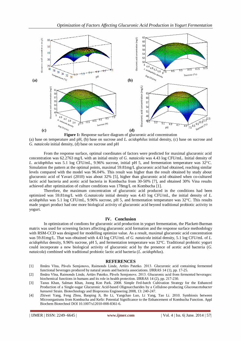
Optimization of Factors Affecting Glucuronic Acid Production in Yogurt Fermentation
| IJMER | ISSN: 2249–6645 | www.ijmer.com | Vol. 4 | Iss. 6| June. 2014 | 57|
(a) (b)
Estimated Response SurfaceMat do G nataicola=4.0,Nhiet do=35.0,pH=5.0
44.4
4.85.2
5.66Mat do L acidophilus 7.5 8.5 9.5 10.5 11.5 12.5
Sucrose
50
52
54
56
58
60
62
Ha
m lu
on
g a
cid
glu
cu
ron
ic
Ham luong acid glucuronic
52.0
53.0
54.0
55.0
56.0
57.0
58.0
59.0
60.0
61.0
62.0
63.0
Glu
curo
nic
acid
con
cent
rati
on (m
g/L)
(c)
Glu
curo
nic
aci
d c
on
cen
trat
ion
(m
g/L)
Estimated Response SurfaceMat do L acidophilus=5.0,Nhiet do=35.0,pH=5.0
33.4
3.84.2
4.65
Mat do G nataicola
7.58.5
9.510.5
11.512.5
Sucrose
49
51
53
55
57
59
61
Ha
m lu
on
g a
cid
glu
cu
ron
ic
Ham luong acid glucuronic
52.0
53.0
54.0
55.0
56.0
57.0
58.0
59.0
60.0
61.0
62.0
63.0
(d)
Glu
curo
nic
aci
d c
on
cen
trat
ion
(m
g/L)
Estimated Response SurfaceVi khuan acetic=15.0,Vi khuan probiotic=10.0,Nhiet do=35.0
7.58.5
9.510.5
11.512.5
Sucrose4.54.74.95.15.35.5
pH
45
48
51
54
57
60
63
Glu
cu
ron
ic a
cid
Glucuronic acid
51.0
52.2
53.4
54.6
55.8
57.0
58.2
59.4
60.6
61.8
63.0
64.2 Figure 1: Response surface diagram of glucuronic acid concentration
(a) base on temperature and pH, (b) base on sucrose and L. acidophilus initial density, (c) base on sucrose and
G. nataicola initial density, (d) base on sucrose and pH
From the response surface, optimal coordinates of factors were predicted for maximal glucuronic acid
concentration was 62.2763 mg/L with an initial ensity of G. nataicola was 4.43 log CFU/mL. Initial density of
L. acidophilus was 5.1 log CFU/mL, 9.96% sucrose, initial pH 5, and fermentation temperature was 32°C.
Simulation the pattern at the optimal points, maximal 59.81mg/L glucuronic acid had obtained, reaching similar
levels compared with the model was 96.04%. This result was higher than the result obtained by study about glucuronic acid of Yavari (2010) was about 32% [5], higher than glucuronic acid obtained when co-cultured
lactic acid bacteria and acetic acid bacteria in Kombucha from 30-50% [7], and obtained 30% Vina results
achieved after optimization of culture conditions was 178mg/L on Kombucha [1].
Therefore, the maximum concentration of glucuronic acid produced in the conditions had been
optimized was 59.81mg/L with G.nataicola initial density was 4.43 log CFU/mL, the initial density of L.
acidophilus was 5.1 log CFU/mL, 9.96% sucrose, pH 5, and fermentation temperature was 32°C. This results
made yogurt product had one more biological activity of glucuronic acid beyond traditional probiotic activity in
yogurt.
IV. Conclusion In optimization of condions for glucuronic acid production in yogurt fermentation, the Plackett-Burman
matrix was used for screening factors affecting glucuronic acid formation and the response surface methodology
with RSM-CCD was designed for modelling optimize value. As a result, maximal glucuronic acid concentration
was 59.81mg/L. That was obtained with 4.43 log CFU/mL of G. nataicola initial density, 5.1 log CFU/mL of L.
acidophilus density, 9.96% sucrose, pH 5, and fermentation temperature was 32°C. Traditional probiotic yogurt
could incorporate a new biological activity of glucuronic acid by the presence of acetic acid bacteria (G.
nataicola) combined with traditional probiotic lactic acid bacteria (L. acidophilus).
REFERENCES [1] Ilmāra Vīna, Pāvels Semjonovs, Raimonds Linde, Artūrs Patetko. 2013. Glucuronic acid containing fermented
functional beverages produced by natural yeasts and bacteria associations. IJRRAS 14 (1), pp. 17-25.
[2] Ilmāra Vīna, Raimonds Linde, Artūrs Patetko, Pāvels Semjonovs. 2013. Glucuronic acid from fermented beverages: biochemical functions in humans and its role in health protection. IJRRAS 14 (2), pp. 217-230.
[3] Taous Khan, Salman Khan, Joong Kon Park. 2008. Simple Fed-batch Cultivation Strategy for the Enhanced Production of a Single-sugar Glucuronic Acid-based Oligosaccharides by a Cellulose-producing Gluconacetobacter hansenii Strain. Biotechnology and Bioprocess Engineering 2008, 13: 240-247.
[4] Zhiwei Yang, Feng Zhou, Baoping Ji, Bo Li, Yangchao Luo, Li Yang, Tao Li. 2010. Symbiosis between Microorganisms from Kombucha and Kefir: Potential Significance to the Enhancement of Kombucha Function. Appl Biochem Biotechnol DOI 10.1007/s12010-008-8361-6.

Optimization of Factors Affecting Glucuronic Acid Production in Yogurt Fermentation
| IJMER | ISSN: 2249–6645 | www.ijmer.com | Vol. 4 | Iss. 6| June. 2014 | 58|
[5] Nafiseh Yavari, Mahnaz Mazaheri Assadi, Kambiz Larijani, Mohammad Bamani Moghadam. 2010. Response Surface Methodology for Optimization of Glucuronic Acid Production Using Kombucha Layer on Sour Cherry Juice. Australian Journal of Basic and Applied Sciences, 4(8): 3250-3256, ISSN 1991-8178.
[6] Nafiseh Yavari, Mahnaz Mazaheri Assadi, Mohammad Bamani Moghadam, Kambiz Larijani. 2011. Optimizing
Glucuronic Acid Production Using Tea Fungus on Grape Juice by Response Surface Methodology. Australian Journal of Basic and Applied Sciences, 5(11): 1788-1794, ISSN 1991-8178.
[7] Nguyen K. Nguyen, Ngan T.N. Dong, Phu H. Le, Huong T. Nguyen. 2014. Evaluation of the Glucuronic Acid Production and Other Biological Activities of Fermented Sweeten-Black Tea by KBC Layer and the Co-Culture with Different Lactobacillus sp. Strains. International Journal Of Modern Engineering Research (IJMER), vol.4, iss.5, ISSN: 2249–6645.
[8] Plackett R. L., Burman J.P., 1946. The design of optimum multifactorial experiments. Biometrika 37: 305-325. [9] Castillo E Del. 2007. Process Optimization A Statistical Approach. Springer Science. New York, USA: 118-122. [10] Pederson C. S., 1995. Microbiology of food fermentation. AVI Publishers, USA.
[11] Heath P. B. et al., 2012. Personal cleansing compositions comprising a bacterial cellulose netwoek and cationic polymer. US 8097574B2, USA Patent.
[12] Hestrin S., Schramm M. 1954. Factor affecting production of cellulose at the air liquid interface of a culture of Acetobacter xylinum. Journal of General Microbiology, 11: 123-129.
[13] Hwang, J.W., Hwang, J.K., Pvun, Y. R., Kim, Y.s. (1999) Effects of pH and dissolved oxygen on cellulose production by Acetobacter xylimim BRC5 in agitated culture. J Ferment Bioeng, 88: 183-188.
[14] Jonas R. R., Luiz. 1998. Production and application of microbial cellulose. Polymer degradation and stability, 59: 101-106
International
OPEN ACCESS Journal
Of Modern Engineering Research (IJMER)
| IJMER | ISSN: 2249–6645 | www.ijmer.com | Vol. 4 | Iss. 6| June. 2014 | 59|
Optimal Location and Sizing of DG using Fuzzy logic
Sujata Huddar1, B. Kantharaj
2, K. R. Mohan
3, S. B. Patil
4, Rudresh Magadum
5
1(PG scholar Department of Electrical & Electronics Engg A.I.T Chikmagalur, Karnataka,India)
2, 3 (Associate professor Department of Electrical & Electronics Engg A.I.T Chikmagalur, Karnataka,India) 4(Assistan professor Department of Electrical & Electronics Engg H.I.T Nidasoshi, karnataka, India)
5(Assistant professor Department of Electrical & Electronice Engg G.I.T belgaum, Karnataka,India)
I. INTRODUCTION Distributed generation is defined as small scale generation which is not directly connected to the bulk
transmission system & it is not centrally dispatched. Distributed generation is connected at the distribution level
which leads to the many changes in the characteristics of distribution network. The proper location of DG plays
a very important role to upgrade the system reliability and stability, to reduce the system losses, to improve the
system voltage profile [1].At present the number of scholars are carry the work on placement of DG here the
reference [2] considers the case of single radial feeder with the three load conditions namely uniform load,
concentrated load, increasing load for which the optimal location of DG is found with the analytical approaches
to minimize the losses in the single radial feeder. The optimal location of DG is needed to increase the
distributed generation potential benefits in the power system. There are many methods for the proper location
and sizing DG, some of the methods are explained in reference [3]. Such as Evolutionary computational method
[including genetic algorithm, fuzzy logic, & tabu search], 2/3 Rule, optimal power flow. Reference [4] shows the
consideration of Fuzzy rules for the proper location of capacitor. In case of Fuzzy logic a set of Fuzzy rules are
considered for the proper placement of DG by considering the VSI and PLI as a input to the system and output
as DGSI. The mathematical equations are used to calculate the sizing of DG [5].
The reference [6] shows the optimal placement of DG units using Fuzzy & real coded Genetic
algorithm, Any how the research work is continuous to upgrade the network losses, improve the voltage stability
and reliability of the power system. In this paper we have considered the fuzzy logic method for the optimal
location and sizing of DG. Proposed method is tested by considering the IEEE33 bus system data, before
obtaining location and sizing, the load flow analysis is performed by considering the NR method.
II. INTRODUCTION TO FUZZY LOGIC First consider the given system data then conduct the load flow analysis, from which we get the PLI
(power loss indices) & VSI (voltage sensitivity indices). The PLI & VSI are used as the inputs to the Fuzzy
interfacing system after Fuzzification & defuzzification we get the output DGSI (distributed generator sensitivity
index). The ranges of VLI, PLI, and DGSI are considered from the load flow analysis. For example let us
consider the range of PLI is 0 to 1, The VLI ranges from 0.9 to 1.1and the output DGSI varies from 0 to 1. The
variables for these ranges are described with the help of five membership functions they are high, high medium,
medium, and low medium, low. The membership functions of PLI & DGSI are triangular in shape & where as
Abstract: Introduction of distributed generation modifies the structure of power system network. High
levels of penetration of distributed generation (DG) are new challenges for traditional electric power
systems. A power injection from DG units modifies network power flows, changes energy losses and
improves voltage profile of the system. Proper locations of DG units in power systems are very important
in order to obtain maximum potential advantages. There are some of the most popular DG placement
methods, such as Optimal Power Flow, 2/3Rule and Evolutionary Computational Methods. The
Evolutionary computational method includes Genetic Algorithm, Fuzzy Systems and Tabu Search. In this
paper we have considered the Fuzzy logic method for the optimal location and sizing of DG.
The optimal placement of DG is necessary to improve the reliability and stability. Proposed method is
tested by considering IEEE 33bus system data. The Fuzzy logic method includes a fuzzy inference system
(FIS) containing a set of rules which are considered to determine the DG placement suitability index of
each node in the distribution system. The optimal sizing of DG unit is obtained with the help of
mathematical expressions.
Keywords: Distributed Generation (DG); Fuzzy logic; Fuzzy rule; Optimal Location; Optimal Power flow.

Optimal Location and Sizing of DG using Fuzzy logic
| IJMER | ISSN: 2249–6645 | www.ijmer.com | Vol. 4 | Iss. 6| June. 2014 | 60|
the VSI membership functions are combination of both triangular & trapezoidal in shape, these are graphically
shown as fallows.
Fig 1 Power loss index membership function
Fig 2 Voltage membership function
Fig 3 Distributed generator suitability index membership function
To determine the best DG placement problems certain rules are defined in order to determine the
suitability index of bus. For DG installation the rules are summarized in the fuzzy decision matrix as shown
below.
AND
VSI
L LN N HN H
PLI
L LM LM L L L
LM M LM LM L L
M HM M LM L L
HM HM HM M LM L
H H HM M LM LM
Table1 matrix to determine the DG suitability index
III. DETERMINATION OF SENSITIVE BUSES FOR THE OPTIMAL
IV. LOCATION OF DG FOR 33BUS SYSTEM Bus no VSI PLI DGSI
1 1.00 0 0.49
2 0.9952 0.0198 0.5
3 0.9725 0.0839 0.471

Optimal Location and Sizing of DG using Fuzzy logic
| IJMER | ISSN: 2249–6645 | www.ijmer.com | Vol. 4 | Iss. 6| June. 2014 | 61|
4 0.9601 0.0342 0.425
5 0.9479 0.0322 0.404
6 0.9317 0.0152 0.366
7 0.9259 0.0033 0.376
8 0.9178 0.0084 0.382
9 0.9074 0.0073 0.402
10 0.8976 0.0062 0.404
11 0.8962 0.0010 0.4
12 0.8937 0.0015 0.4
13 0.8835 0.0047 0.395
14 0.8797 0.0013 0.39
15 0.8773 0.0006 0.387
16 0.8750 0.0005 0.384
17 0.8716 0.0004 0.381
18 0.8706 0.0001 0.38
19 0.9944 0.0003 0.498
20 0.9886 0.0013 0.491
21 0.9875 0.0002 0.49
22 0.9864 0.0001 0.442
23 0.9667 0.0053 0.462
24 0.9558 0.0086 0.415
25 0.9504 0.0021 0.403
26 0.9285 0.0045 0.374
27 0.9242 0.0058 0.375
28 0.9051 0.0136 0.421
29 0.8914 0.0068 0.403
30 0.8855 0.0028 0.396
31 0.8785 0.0004 0.388
32 0.8770 0.0001 0.386
33 0.8755 0.0196 0.432
Table 2 DGSI output from the Fuzzy system
Result: The above table shows that maximum value of Distributed generation sensitivity index is at bus 2 with
DGSI= 0.5, Therefore the best location of DG is at bus 2.
Improvement Of Voltage Profile With DG
Bus
No
Without DG With DG
Voltage in P.U Voltage in P.U
1 1.0000 1.0000
2 0.9952 0.9968
3 0.9725 0.9826
4 0.9601 0.9714
5 0.9479 0.9604
6 0.9317 0.9461
7 0.9259 0.9409
8 0.9178 0.9337
9 0.9074 0.9244
10 0.8976 0.9159
11 0.8962 0.9146
12 0.8937 0.9124
13 0.8835 0.9034

Optimal Location and Sizing of DG using Fuzzy logic
| IJMER | ISSN: 2249–6645 | www.ijmer.com | Vol. 4 | Iss. 6| June. 2014 | 62|
14 0.8797 0.9001
15 0.8773 0.8980
16 0.8750 0.8960
17 0.8716 0.8931
18 0.8706 0.8922
19 0.9944 0.9959
20 0.9886 0.9903
21 0.9875 0.9891
22 0.9864 0.9881
23 0.9667 0.9844
24 0.9558 0.9866
25 0.9504 1.000
26 0.9285 0.9432
27 0.9242 0.9394
28 0.9051 0.9226
29 0.8914 0.9104
30 0.8855 0.9052
31 0.8785 0.8991
32 0.8770 0.8977
33 0.8755 0.8964
Table3 Bus voltages with & without DG
Bus no
Fig 4 Bus voltages with & without DG
V. PROCEDURE TO CALCULATE THE OPTIMAL SIZE OF DG First let us consider the drawn system diagram in which the DG is placed at the bus i, which produces
the current of IDG. In a radial distribution system the current IDG changes for the current branches which are
connected to bus i, where as the current of other branches are unchanged.
Therefore new current Ik’ of the kth
branch is given by
Ik’=Ik+AkIDG (1)
Where AK=1 if Kth
branch which is connected to bus i otherwise Ak=0
The value of current IDG can be calculated with the help of fallowing equation
IDG=- (2)
Now the size of DG is calculated by considering the fallowing equation
SDG=ViIDG (3)
Where Vi=Voltage at the ith
bus

Optimal Location and Sizing of DG using Fuzzy logic
| IJMER | ISSN: 2249–6645 | www.ijmer.com | Vol. 4 | Iss. 6| June. 2014 | 63|
VI. CONCLUSION In this paper we have considered optimal location & sizing of DG using Fuzzy logic. Optimal location
of DG is optained using Fuzzy logic and optimal size of DG is calculated by analytical method which are helpful
to upgrade the loss minimization and improvement of voltage profile. Finally we can conclude that proper
location & sizing of DG is better to improve the voltage profile, reduction in the losses and helps to improve the
overall system stability.
REFERENCES [1] Hussein.A.Attia, M.EI-shibini, Z.H.Osman and Ahmed A Moftah “An assessment of a global performance index for
distributed generation impacts on distribution system” Electrical power and Machines Department ,carlo University.
2010.
[2] Zhang jun-fang, Dingsi-min, Hang yin-li and Hu guang “Research on distributed generation source placement” 2009.
[3] K.Abookazemi, M.Y.Hassan, and M.S.Majid “A review on optimal placement methods of distribution generation
sources” 2010 IEEE interational conference on power and energy.
[4] Optimal capacitor placement using fuzzy logic
[5] Optimal distributed generator placement using fuzzy logic
[6] Ramalingaiah Varikuti, Dr. M.Damodar Reddy “optimal placement of dg units using fuzzy and real coded genetic
algorithm” Journal of Theoretical and Applied Information Technology © 2005 - 2009 JATIT. All rights reserved.
APPENDIX
IEEE 33 Bus system
A. Line data for IEEE 33 Bus system
BASE: 12.66 kV, 100MVA
Sending bus Receiving bus R (in ohm) X (in ohm)
1 2 0.09220 0.04700
2 3 0.49300 0.25110
3 4 0.36600 0.18640
4 5 0.38110 0.19410
5 6 0.81900 0.70700
6 7 0.01872 0.61880
7 8 0.71140 0.23510
8 9 1.03000 0.74000
9 10 1.04400 0.74000
10 11 0.19660 0.06500
11 12 0.37440 0.12380
12 13 1.46800 1.15500
13 14 0.54160 0.71290
14 15 0.59100 0.52600
15 16 0.74630 0.54500
16 17 1.28900 1.72100
17 18 0.73200 0.57400
2 19 0.16400 0.15650
19 20 1.50420 1.35540
20 21 0.40950 0.48740
21 22 0.70890 0.93730
3 23 0.45120 0.30830
23 24 0.89800 0.70910
24 25 0.89600 0.70110
6 26 0.20300 0.10340
26 27 0.20420 0.14470
27 28 1.05900 0.93370
28 29 0.80420 0.70060

Optimal Location and Sizing of DG using Fuzzy logic
| IJMER | ISSN: 2249–6645 | www.ijmer.com | Vol. 4 | Iss. 6| June. 2014 | 64|
29 30 0.50750 0.25850
30 31 0.97440 0.96300
31 32 0.31050 0.36190
32 33 0.34100 0.53020
B. Load data for IEEE 33Bus system
Bus No
Bus code
Load Data
K
W KVAR
1 1 - -
2 0 100 60
3 0 90 40
4 0 120 80
5 0 60 30
6 0 60 20
7 0 200 100
8 0 200 100
9 0 60 20
10 0 60 20
11 0 45 30
12 0 60 35
13 0 60 35
14 0 120 80
15 0 60 10
16 0 60 20
17 0 60 20
18 0 90 40
19 0 90 40
20 0 90 40
21 0 90 40
22 0 90 40
23 0 90 50
24 0 420 200
25 0 420 200
26 0 60 25
27 0 60 25
28 0 60 20
29 0 120 70
30 0 200 600
31 0 150 70
32 0 210 100
33 0 60 40

International
OPEN ACCESS Journal
Of Modern Engineering Research (IJMER)
| IJMER | ISSN: 2249–6645 | www.ijmer.com | Vol. 4 | Iss. 6| June. 2014 | 65|
Design of Model based controller for Two Conical Tank
Interacting Level systems
S. Vadivazhagi1, Dr. N. Jaya
2
1(Department of Electronics and Communication Engineering, MRK Institute of Technology, India)
2 (Department of Electronics & Instrumentaion Engineering, Annamalai University, India
I. INTRODUCTION The control of liquid level is mandatory in all process industries. Most of the process industries need
the usage of conical tanks as its structure contributes to better drainage of solid mixtures, slurries and viscous
liquids. Food processing industries, Concrete Mixing industries, Hydrometallurgical industries and waste water
treatment industries are some examples which makes effective usage of conical tanks.
To achieve a satisfactory performance using conical tanks, its controller design becomes a challenging
task because of its non-linearity. A very important task of a controller is to maintain the process at desired set
point and to achieve optimum performance even in the presence of disturbances. Many Industries use
Proportional Integral Controller (PI) and Proportional Integral Derivative controller (PID) because of its simple
structure and easy tuning.
An alternative to this controller is the usage of Internal Model controller (IMC) which gives satisfactory
performance for Conical Tank Interacting Level systems [1]. In this paper an Internal Model Controller is
designed and implemented to Conical Interacting systems [2]. This controller uses the model of the process to
run in parallel with the actual process [3]. The IMC design procedure is exactly same as the open loop control
design procedure. Unlike the open loop control the IMC structure compensates for disturbances and model
uncertainty.
Paper is organized as follows. Section II describes the Mathematical modelling of Two Tank Conical
Interacting Systems and its operating parameters. Piecewise linearization is carried out around four operating
regions.The implementation of IMC controller is discussed in Section III. Section IV presents experimental
results showing four different simulations for four regions. Finally Section V presents Conclusion.
II. MATHEMATICAL MODELLING OF TWO TANK CONICAL INTERACTING SYSTEM The two tank conical interacting system consists of two identical conical tanks (Tank 1 and Tank 2),
two identical pumps that deliver the liquid flows Fin1 and Fin2 to Tank 1 and Tank 2 through the two control
valves CV1 and CV2 respectively. These two tanks are interconnected at the bottom through a manually controlled
valve, MV12 with a valve coefficient 12. Fout1 and Fout 2 are the two output flows from Tank 1 and Tank 2 through
manual control values MV1 andMV2 with valve coefficients 1 and 2 respectively. The non linear equations
describing the open loop dynamics of the Two Tank Conical Interacting Systems is derived using the Mass
balance equation and Energy balance equation principle [4].
Abstract: This paper presents the modelling and control of Two Tank Conical Interacting systems which
is highly a non linear process. A Model based controller is designed for the process at different operating
regions and its performance is studied with and without disturbance. The aim is to control the liquid level
of tank. Piecewise linearization technique is applied for linearising the non linear system output. An
Internal Model control is designed for each region. The controller will be simulated using MATLAB
SIMULINK software.
Keywords: Conical Tank Interacting Level systems, IMC Controller, Mathematical Modelling, MATLAB
software, Non linear process.

Design of Model based controller for Two Conical Tank Interacting Level systems
| IJMER | ISSN: 2249–6645 | www.ijmer.com | Vol. 4 | Iss. 6| June. 2014 | 66|
Fig. 1 Schematic diagram of two tanks Conical Interacting System
The Mathematical model of two tank conical interacting system is given by equations 1 and 2. [5]:
(1)
(2)
Where
A(h1) = Area of Tank 1 at h1(cm2)
A(h2) = Area of Tank 2 at h2(cm2)
h1= Liquid level in Tank 1 (cm)
h2= Liquid level in Tank 2 (cm)
TABLE I
Operating Parameters Of Two Tank Conical Interacting System
Parameter Description Value
R Top radius of conical tank 19.25cm
H Maximum height of
Tank1&Tank2
73cm
Fin1 & Fin2 Maximum inflow to
Tank1&Tank2
252cm3/sec
1 Valve coefficient of MV1 35 cm2/sec
12 Valve coefficient of MV12 78.28 cm2/sec
2 Valve coefficient of MV2 19.69 cm2/secs
The open loop responses of h1 and h2 are shown in fig.2 as shown below.
Fig. 2 Open loop response of h1 and h2
The process considered here has non linear characteristics and can be represented as piecewise
linearized regions around four operating regions[6]. Transfer function for every region is obtained by
substituting the values of time constant and gain using Process reaction curve method as shown in Table III.[7].
2
2
12
211221111
11
3
1
)(1
H
hR
hhhhsignhdt
hdAhF
dt
dhin
2
2
22
2221122122
2
3
1
)(2
H
hR
dt
hAdhhhhhsignhF
dt
dhin

Design of Model based controller for Two Conical Tank Interacting Level systems
| IJMER | ISSN: 2249–6645 | www.ijmer.com | Vol. 4 | Iss. 6| June. 2014 | 67|
TABLE III Model Parameters Of Two Tank Conical Interacting System
Region Inflow
(cm3/s)
Height
h2
(cms)
Steady
State
Gain
Time
constant
(secs)
Transfer
Function
model
I 0-66 1.374 0.0208 0.002 0.0208
0.002s+1
II 66-120 4.19 0.0349 0.03 0.0349
0.03s+1
III 120-186 8.447 0.0454 0.146 0.0454
0.146s+1
IV 186-252 12.56 0.0498 0.338 0.0498
0.338s+1
III. IMPLEMENTATION OF INTERNAL MODEL CONTROLLER (IMC) A more comprehensive model based design method, Internal Model Control was developed by Morari
and co-workers. The IMC method is based on the simplified block diagram as shown in Fig. 3[8].
Fig. 3 Internal Model Control (IMC)
Internal Model Control is designed in two steps.
Step 1: The process model is factored as :
G = G + G - (3)
Where G + contains any time delays and right half plane zeros.In addition G + is required to have a steady state
gain equal to one in order to ensure that the two factors in equation 3 are unique.
Step 2: The controller is specified as:
Gc* = (1/ G -) f (4)
Where f is a low pass filter with a steady state gain of one.
Thus the Internal Model Controller is designed as inverse of the Process model which is in series with the low
pass filter.
Fig.4 represents the MATLAB simulink diagram of Internal Model controller for region 1.
Fig. 4 Simulink diagram for region 1 using Internal Model Control (IMC)
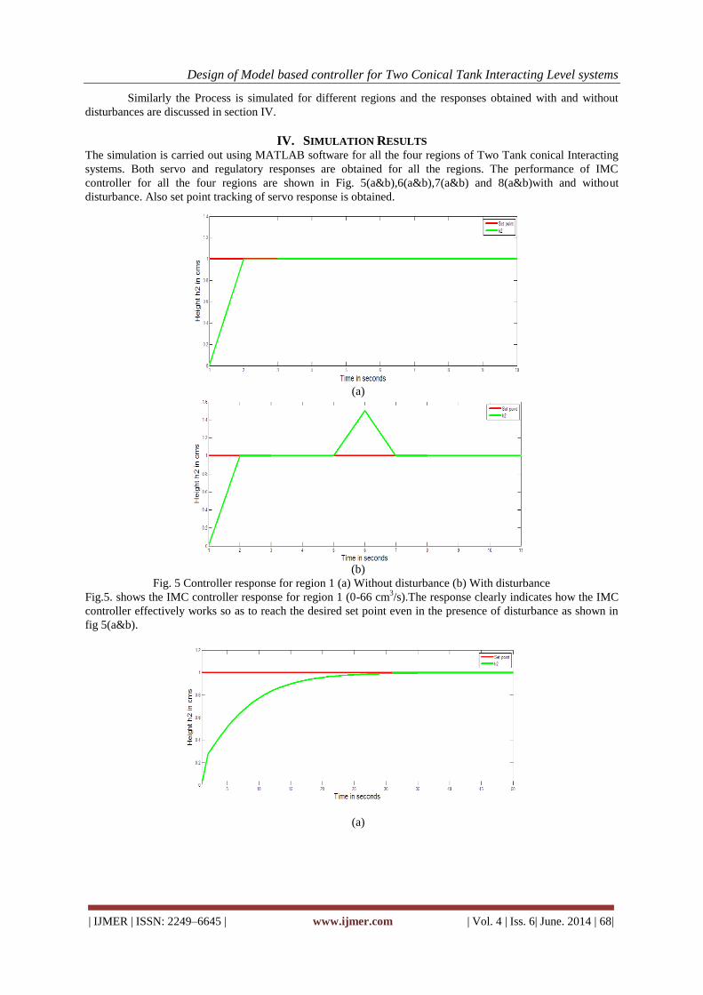
Design of Model based controller for Two Conical Tank Interacting Level systems
| IJMER | ISSN: 2249–6645 | www.ijmer.com | Vol. 4 | Iss. 6| June. 2014 | 68|
Similarly the Process is simulated for different regions and the responses obtained with and without
disturbances are discussed in section IV.
IV. SIMULATION RESULTS The simulation is carried out using MATLAB software for all the four regions of Two Tank conical Interacting
systems. Both servo and regulatory responses are obtained for all the regions. The performance of IMC
controller for all the four regions are shown in Fig. 5(a&b),6(a&b),7(a&b) and 8(a&b)with and without
disturbance. Also set point tracking of servo response is obtained.
(a)
(b)
Fig. 5 Controller response for region 1 (a) Without disturbance (b) With disturbance
Fig.5. shows the IMC controller response for region 1 (0-66 cm3/s).The response clearly indicates how the IMC
controller effectively works so as to reach the desired set point even in the presence of disturbance as shown in
fig 5(a&b).
(a)
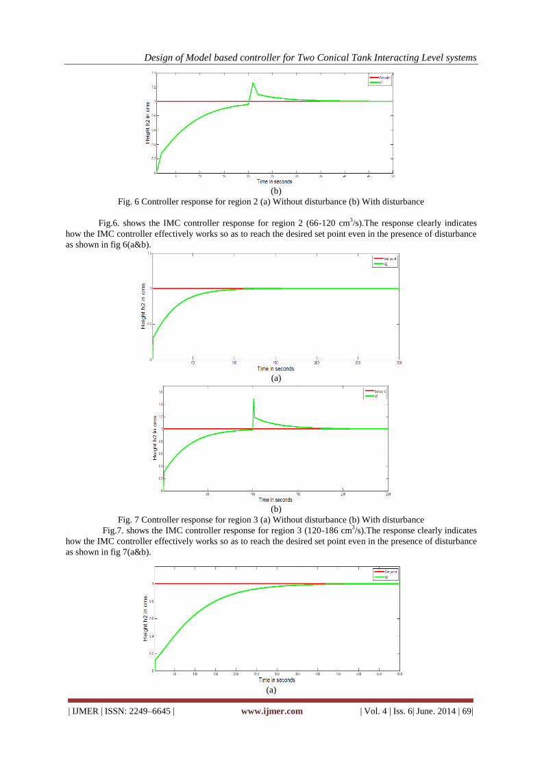
Design of Model based controller for Two Conical Tank Interacting Level systems
| IJMER | ISSN: 2249–6645 | www.ijmer.com | Vol. 4 | Iss. 6| June. 2014 | 69|
(b)
Fig. 6 Controller response for region 2 (a) Without disturbance (b) With disturbance
Fig.6. shows the IMC controller response for region 2 (66-120 cm3/s).The response clearly indicates
how the IMC controller effectively works so as to reach the desired set point even in the presence of disturbance
as shown in fig 6(a&b).
(a)
(b)
Fig. 7 Controller response for region 3 (a) Without disturbance (b) With disturbance
Fig.7. shows the IMC controller response for region 3 (120-186 cm3/s).The response clearly indicates
how the IMC controller effectively works so as to reach the desired set point even in the presence of disturbance
as shown in fig 7(a&b).
(a)

Design of Model based controller for Two Conical Tank Interacting Level systems
| IJMER | ISSN: 2249–6645 | www.ijmer.com | Vol. 4 | Iss. 6| June. 2014 | 70|
(b)
Fig. 8 Controller response for region 4 (a) Without disturbance (b) With disturbance
Fig.8. shows the IMC controller response for region 4 (186-252 cm3/s).The response clearly indicates
how the IMC controller effectively works so as to reach the desired set point even in the presence of disturbance
as shown in fig 8(a&b).
Fig. 9 Set point tracking
Fig.9. shows the set point tracking response using IMC controller.
V. CONCLUSION Design of Internal Model based controller has given good and acceptable performance without
oscillation as well as fast settling response. Besides, it also shows good result for disturbance rejection with fast
settling response. The Model based controller is designed in such a way that the system is robust and physically
realizable. This concludes that the Internal model control is applicable for nonlinear interacting conical tank
systems.
REFERENCES [1] Anna Joseph and Samson Isaac. J,Real time implementation of Modern Reference Adaptive Controller for a Conical
Tank,Proceeding of International Journal on Theoretical and Applied Research in Mechanical Engineering,Vol.2,No
1,pp.57-62,2013.
[2] Y. Christy, D. Dinesh Kumar, Modeling and Design of Controllers for Interacting Two Tank Hybrid System,
International Journal of Engineering and Innovative Technology,Vol.3,Issue 7,2014.
[3] D.Angeline Vijula,K.Vivetha,K.Gandhimathi,T.Praveena, Model based Design for Conical Tank system,
International journal of Computer Application,Vol.85,No.12,2014.
[4] George Stephanapoulos, Chemical Process control(Prentice Hall of India,New Delhi,1990).
[5] Ravi.V.R and Thyagarajan.T, A decentralized PID controller for interacting non linear systems ,Proceedings of
Emerging trends in Electrical and Computer Technology,pp. 297-302,2008.
[6] S.Vadivazhagi,Dr.N.Jaya, Modelling and Simulation of Interacting Conical Tank Systems, International Journal of
Innovative Research in Science,Engineering and Technology,Vol.3,Issue 6,2014.
[7] B.Wayne Bequette, Process control Modeling,Design and Simulation(Prentice Hall,USA,2003).
[8] Daniel E. Rivera, Manfred Morari, and Sigurd Skogestad, Internal Model Control. 4. PID Controller Design, Ind.
Eng. Chem. Process Des. Dev,Vol 25, pp.252-265,1986.
[9] S.Nithya, N.Sivakumaran, T.Balasubramanian and N.Anantharaman, Model based controller design for a Spherical
Tank Process in real time ,Proceedings of International journal of Simulation,System,Science and
Technology,Vol.9,No.A4,pp.247-252,2008.

Design of Model based controller for Two Conical Tank Interacting Level systems
| IJMER | ISSN: 2249–6645 | www.ijmer.com | Vol. 4 | Iss. 6| June. 2014 | 71|
BIOGRAPHY
S. Vadivazhagi is presently working as an Assistant Professor in the Department of
ECE at MRK Institute of Technology,Kattumannarkoil,Tamilnadu,India. She received
her B.E degree in 2001 and M.E degree in 2006 in the Department of Instrumentation
Engineering from Annamalai University,Chidambaram,Currently she is persuing her
Ph.D degree in the area of Process Control at Annamalai University.
Dr.N.Jaya is presently working as an Associate Professor in the Department of
Instrumentation Engineering at Annamalai University, Chidambaram, India. She
received her BE, ME and PhD degrees from Annamalai University, India in 1996,1998
and 2010 respectively. Her main research includes process control, fuzzy logic control,
control systems and adaptive control.

International
OPEN ACCESS Journal Of Modern Engineering Research (IJMER)
| IJMER | ISSN: 2249–6645 | www.ijmer.com | Vol. 4 | Iss. 6| June. 2014 | 72|
A Review on Sentimental Analysis of Application Reviews
Amandeep Kaur1, Er. Nidhi Gumber
2
1 Research Scholar, CSE Dept. CGC Group of Colleges, Gharuan, Mohali, India 2 Assistant Professor, CSE Dept. CGC Group of Colleges, Gharuan, Mohali, India
I. Introduction
Sentimental analysis is a data mining technique that systematically evaluates textual content using
machine learning techniques. Sentiment analysis is a type of natural language processing for tracking the mood
of the public about a particular product or topic. Here sentimental analysis is used to collect and examine textual
reviews on different applications. As textual reviews on applications are available in very unstructured form on
web. Sentimental analysis identify these expressions of writers and a simple algorithm used to classify a
document as „positive‟ and „negative‟. As in different papers different techniques are approached. There are
broadly three types of approaches for sentiment classification of texts: (a) using a machine learning based text
classifier -such as Naïve Bayes, SVM or kNN- with suitable feature selection scheme; (b) using the
unsupervised semantic orientation scheme of extracting relevant n-grams of the text and then labeling them either as positive or negative and consequentially the document; and (c) using the SentiWordNet based publicly
available library that provides positive and negative scores for words[1]. There are two major approaches for
performing sentiment analysis; statistical model based approaches and Natural Language Processing (NLP)
based approaches to create rules. In this study, we first apply text mining to summarize user‟s reviews of Apps
and extract features of the apps mentioned in the reviews. Then NLP approach for writing rules is used. Android
App Store. SAS® Enterprise Miner TM 7.1 is used for summarizing reviews and pulling out features, and
SAS® Sentiment Analysis Studio 12.1 is used for performing sentiment analysis. Results shows that carefully
designed NLP rule-based models outperform the default statistical models in SAS® Sentiment Analysis Studio
12.1 for predicting sentiments in test data. NLP rule based models also provide deeper insights than statistical
models in understanding consumers‟ sentiments[2].In another one paper a techniques is used for extracting
keywords from online documents which could be further very used for sentimental analysis this novel
approach is used for semiautomatic question generation to support academic writing. First extract key phases are extracted using JWPL .Using content of matched content conceptual graph structure representations for each
key phrase. Then question generated and question should be specific. To evaluate quality bystander turing test is
done. Here is some basic steps are explained which can be used for sentimental analysis of application reviews.
We will take all the inputs throughout the globe and collect it in a intelligent data base. All the data collected
will be processed using verbal algorithms of the Natural processing and converting it into useful information
and collecting it in an new data base. Making graphical and analytical charts for comparison and performance of
the application.
Abstract: As with rapid evolution of computer technology and smart phones mobile applications
become very important part of our life. It is very difficult for customers to keep track of different
applications reviews so sentimental analysis is used. Sentimental analysis is effective and efficient
evolution of customer’s opinion in real time. Sentimental analysis for applications review is performed
two approaches statistical model based approaches and Natural Language Processing (NLP) based
approaches to create rules. Two schemes used for analyzing the textual comments- aspect level
sentimental analysis analyses the text and provide a label on each aspect then scores on multiple
aspects are aggregated and result for reviews shown in graphs. Second scheme is document level
analyses which comprising of adjectives, adverbs and verbs and n-gram feature extraction. I have also
used our SentiWordNet scheme to compute the document-level sentiment for each movie reviewed
and compared the results with results obtained using Alchemy API. The sentiment profile of a movie is also compared with the document-level sentiment result. The results obtained show that my scheme
produces a more accurate and focused sentiment profile than the simple document-level sentiment
analysis.

A Review On Sentimental Analysis Of Application Reviews
| IJMER | ISSN: 2249–6645 | www.ijmer.com | Vol. 4 | Iss. 6| June. 2014 | 73|
Fig 1.1: Basic steps for sentimental analysis
Here are some applications of sentimental analysis are Voting Advise Applications, Automated content
analysis and Argument mapping software. These are the some of applications but sentimental analysis can be
further used for movie reviews and applications reviews. Input for sentimental analysis system is textual reviews
of customers or consumers given for particular application. Rest of paper is organized as follow second section
explain input , third section will explain data mining techniques techniques, forth section contains different
techniques for algorithmic formulation and 5th is about applications and tools used for sentimental analysis.
II. Input User‟s opinion is a major criterion for the Improvement of the quality of services rendered and
Enhancement of the deliverables. Blogs, review sites, data and micro blogs provide a good understanding of
there caption level of the products and services.
2.1. Blogs With an increasing usage of the internet, blogging and blog pages are growing rapidly. Blog page shave
become the most popular means to express one‟s personal opinions. Bloggers record the daily events in their
lives and express their opinions, feelings, and emotions in a blog (Chau & Xu, 2007). Many of these blogs
contain reviews on many products, issues, etc. Blogs are used as a source of opinion in many of the studies
related to sentiment analysis (Martin, 2005;Murphy, 2006; Tang et al., 2009).
2.2. Review sites For any user in making a purchasing decision, the opinions of others can be an important factor. A
large and growing body of user-generated reviews is available on the Internet. The reviews for products or
services are usually based on opinions expressed in much unstructured format. The review‟s data used in most
of the sentiment classification studies are collected from the e-commerce websites like www.amazon.com
(product reviews), www.yelp.com (restaurant reviews),www.CNET download.com (product reviews) and
www.reviewcentre.com, which hosts millions of product reviews by consumers. Other than these the available
are professional review sites such as www.dpreview.com , www.zdnet.com and consumer opinion sites on
broad topics and products such as www .consumerreview.com, www.epinions.com, www.bizrate.com
(Popescu& Etzioni ,2005 ; Hu,B.Liu ,2006 ; Qinliang Mia, 2009; Gamgaran Somprasertsi ,2010).
2.3. Data Set Most of the work in the field uses application reviews data for classification. Application review
datasets are available as dataset Other dataset which is available online is multi-domain sentiment (MDS)
dataset. The MDS dataset contains four different types of product reviews extracted from Amazon.com
including Books, DVDs, Electronics and Kitchen appliances, with 1000 positive and 1000 negative reviews for
each domain. Another review dataset available is This dataset consists of reviews of five electronics products
downloaded from Amazon and Cnet (Hu and Liu ,2006; Konig & Brill ,2006 ; Long Sheng ,2011; Zhu Jian
,2010 ; Pang and Lee ,2004; Bai et al. ,2005;
2.4. Micro-blogging Twitter is a popular micro blogging service where users create status messages called "tweets". These
tweets sometimes express opinions about different topics. Twitter messages are also used as data source for classifying sentiment.

A Review On Sentimental Analysis Of Application Reviews
| IJMER | ISSN: 2249–6645 | www.ijmer.com | Vol. 4 | Iss. 6| June. 2014 | 74|
III. Data Mining There are different techniques used for data mining in different papers which are explained below.
Document level and aspect level approach based on sentiwordnet can be used. The document-level sentiment
classification attempts to classify the entire document (such as one review) into „positive‟ or „negative‟ class.
The document-level classification involves use of different linguistic features(ranging from Adverb+Adjective
combination to Adverb+Adjective+Verb combination). We have also devised a new domain specific heuristic
for aspect-level sentiment classification of movie reviews. This scheme locates the opinionated text around the
desired aspect/ feature in a review and computes its sentiment orientation. For a movie, this is done for all the
reviews. The sentiment scores on a particular aspect from all the reviews are then aggregated. There are broadly
three types of approaches for sentiment classification of texts: (a) using a machine learning based text classifier
-such as Naïve Bayes, SVM or kNN- with suitable feature selection scheme; (b) using the unsupervised
semantic orientation scheme of extracting relevant n-grams of the text and then labeling them either as positive or negative and consequentially the document; and (c) using the SentiWordNet based publicly available library
that provides positive and negative scores for words[1].
Fig 2.1 data mining technique
In second technique S AS® Enterprise MinerTM 7.1 is used for text mining . It starts with text parsing
node. In parsing node, each comment is divided into tokens (terms). The identified tokens are listed in a “term
by frequency” matrix. Inthis node, we ignored abbr, aux, conj, det, interj, num, part, prep, pron, and prop in the
part-of-speech. Those are listed as selected. In the text clustering node, we used SVD dimensions (k) of 40).
Singular Value Decomposition (SVD) is used to reduce dimensionality by converting the term frequency matrix
into allow dimensional form Smaller values of k (2 to 50) are thought to generate better results for text
clustering using sort textual comments [4].another techniques can be used in sentimental analysis is key phrase
extraction technique. First extract key phases are extracted using JWPL .Using content of matched content
conceptual graph structure representations for each key phrase. Here two approaches are studied supervised
technique required labeled data to train system. It is more simple but more restricted. On other hand
unsupervised techniques do not require any training dataset and mostly applicable to wider knowledge domains , but they are also less accurate. Turney[1] introduce key phrase extraction system called GenEx, which is based
on heuristic rules tuned by genetic algorithms. both GenEx and naïve bayes classifier are examples of
supervised approaches for key phrase extraction. Barker and cornacchia are used for unstructured key phrase
extraction. Another technique studied in natural language processing to extract semantic information from
textual descriptors of web services :linguistics patterns and extraction rules. Linguist patterns characterize the
behavior of texts of domain; there for they are dependent of domain and are used to extract relevant information
from corpus. As these patterns are dependent of the domain we need to choose are to characterize it then choose
financial domain. Extraction rules are used to identify a set of words in corpus. To obtain these rules we make
an analysis about characteristics of sublanguage that is used to describe web services.
IV. Methodologies The Sent i Word Net approach involves obtaining sentimentscore for each selected opinion containing
term of the text by a lookup in its library. In this lexical resource each term t occurring in WordNet is associated
to three numerical scores obj(t), pos(t) and neg(t), describing the objective, positive and negative polarities of
the term, respectively. These three scores are computed by combining the results produced by eight ternary
classifiers. To make use of SentiWordNet we need to first extract relevant opinionated terms and then lookup
for their scores in the SentiWordNet. Use of SentiWordNet requires a lot of decisions to be taken regarding the
linguistic features to be used, deciding how much weight is to be given to each linguistic feature, and the
aggregation method for consolidating sentiment scores. We have implemented the SentiWordNet based
algorithmic formulation for both document-level and aspect-level sentiment classification.
A. Document-level Sentiment Classification
The document-level sentiment classification attempts to classify the entire document (such as one
review) into „positive‟ or „negative‟ class. The approaches based on SentiWordNet targets the term profile of the
review document and extract terms having desired POS label (such as adjectives, adverbs or verbs). This clearly
DATASET
TEXT PARSING
TEXT FILTER TEXT CLUSTER

A Review On Sentimental Analysis Of Application Reviews
| IJMER | ISSN: 2249–6645 | www.ijmer.com | Vol. 4 | Iss. 6| June. 2014 | 75|
shows that before applying the SentiWordNet based formulation; the review text should be applied to a POS
tagger which tags each term occurring in the review text. Then some selected terms (with desired POS tag) are
extracted and the sentiment score of each extracted term is obtained from the SentiWordNet library. The scores for all extracted terms in a review are then aggregated using some weightage and aggregation scheme. Thus two
key issues are to decide (a) which POS tags should be extracted, and (b) how to decide the weightage of scores
of different POS tags extracted while computing the aggregate score.
We have explored with different linguistic features and scoring schemes. Computational Linguists
suggest that adjectives are good markers of opinions. For example, if a review sentence says “The movie was
excellent”, then use of adjective „excellent‟ tells us that the movie was liked by the reviewer and possibly he had
a wonderful experience watching it. Sometimes, Adverbs further modify the opinion expressed in review
sentences. For example, the sentence “The movie was extremely good expresses a more positive opinion about
the movie than the sentence “the movie was good”. A related previous work [6] has also concluded that
„Adverb+Adjective‟ combine produces better results than using adjectives alone. Hence we preferred the
„adverb+adjective‟ combine over extracting „adjective‟ alone. The adverb sare usually used as complements or modifiers. Few more examples of adverb usage are: he ran quickly, only adults, very dangerous trip, very nicely,
rarely bad, rarely good etc. In all these examples adverbs modify the adjectives. Though adverbs are of various
kinds, but for sentiment classification only adjectives of degree seem useful.
B. Aspect-level Sentiment Analysis
The document-level sentiment classification is a reasonable measure of positivity or negativity
expressed in a review. However, in selected domains it may be a good idea to explore the sentiment of the
reviewer about various aspects of the item in that domain, expressed in that review. Moreover, practically most
of the reviews have mixture of positive and negative sentiment about different aspects of the item and it may be
difficult and inappropriate to insist on an overall document-level sentiment polarity expressed in a review for the
item. Thus, the document-level sentiment classification is not a complete, suitable and comprehensive measure
for detailed analysis of positive and negative aspects of the item under review. The aspect-level sentiment analysis allows us to analyze the positive and negative aspects of an item. However, this kind of analysis is often
domain specific. The aspect-level sentiment analysis involves the following: (a) identifying which aspects are to
be analyzed, (b) locating the opinionated content about that aspect in the review, and (c) determining the
sentiment polarity of views expressed about an aspect. Second algorithm to collect data from Google Play
Android App Store. Google Play Android App Store has a large and varied collection of Android Apps with
rankings and user reviews. We extracted textual reviews having rich content from the App Store site. Rich
content refers to a textual review that says more than just cursory comments such as “I love this app” or “I hate
this app” which do not convey or uncover any information about app features. An example of a rich content is,
“The game is good. I love its graphics design and I can play it for hours.” This review tells us that graphics and
design of the app are great and he/she is addicted to this game. SAS® Enterprise Miner 7.1 is used for
summarizing reviews and pulling out features, and SAS® Sentiment Analysis Studio 12.1 is used for performing sentiment analysis. Our results show that for both apps, carefully designed NLP rule-based models
outperform the default statistical models in SAS® Sentiment Analysis Studio 12.1 for predicting sentiments in
test data. NLP rule based models also provide deeper insights than statistical models in understanding
consumers‟ sentiments. Last I have studied is that The first step is to establish the ground truth of citation
sentiment by manually annotating a corpus. The unit of analysis is a citation statement, defined as a block of
context that involves a particular citation. A citation statement can be as short as a sentence, or span across
multiple sentences or even paragraphs. Citation sentiment is annotated for each statement. Table 1 sampled five
citation statements that hold conflicting opinions. By common understanding of polarity, #1 is clearly negative,
questioning the test data‟s representativeness. This citation statement not only spans three sentences, but also
contains another nested statement - the positive citation toward (Yang, 1999). #2 also criticized the data
representativeness, but the negative comment was mitigated by starting with praise. #3 seems neutral since no
linguistic cues indicated positivity or negativity; however, it is also reasonable to infer that #3 is implicitly positive, since it trusted the cited work by using it as a benchmark system. #4 is clearly positive, praising
CONSTRUE as one of the successful text categorization systems. #5 also seems neutral without explicit cues of
polarity. However, it may also be considered as undefined as in (Shafer & Spurk, 2010) because the citation
statement did not explicitly explain the relationship between the citing and cited papers, making thejudgment
difficult.
V. Applications And Tools Some of the applications of sentiment analysis includes online advertising, hotspot detection in forums
etc. Online advertising has become one of the major revenue sources of today‟s Internet ecosystem. Sentiment analysis find its recent application in Dissatisfaction oriented online advertising Guang Qiu(2010) andBlogger-

A Review On Sentimental Analysis Of Application Reviews
| IJMER | ISSN: 2249–6645 | www.ijmer.com | Vol. 4 | Iss. 6| June. 2014 | 76|
Centric Contextual Advertising (Teng-Kai Fan,Chia-Hui Chang ,2011), which refers to the assignment of
personal ads to any blog page, chosen in according to bloggers interests [6]. Some other applications of
sentimental analysis are Voting Advise Applications, Automated content analysis and Argument mapping software.
VI. Conclusion Sentiment detection has a wide variety of applications in information systems, including classifying
reviews, summarizing review and other real time applications. For sentimental analysis system aspect level
scheme and linguistic patterns approaches are very useful as these gives accuracy result 98.9%[3]. These
methods contains result about a applications and product reviews based on different criteria‟s. There are likely
to be many other applications that is not discussed. It is found that sentiment classifiers are severely dependent
on domains or topics. From the above work it is evident that neither classification model consistently outperforms the other, different types of features have distinct distributions. It is also found that different types
of features and classification algorithms are combined in an efficient way in order to overcome their individual
drawbacks and benefit from each other‟s merits, and finally enhance the sentiment classification performance.
In future, more work is needed on further improving the performance measures. Sentiment analysis can be
applied for new applications. Although the techniques and algorithms used for sentiment analysis are advancing
fast, however, a lot of problems in this field of study remain unsolved. The main challenging aspects exist in use
of other languages, dealing with negation expressions; produce a summary of opinions based on product
features/attributes, complexity of sentence/ document , handling of implicit product features , etc. More future
research could be dedicated to these challenges.
REFERENCES [1] V.K Singh, R.Pirayani, A. Uddin & P. Walia “Sentiment Analysis of Movie Reviews”IEEE,978-1-4673-5090-7/13,
2013.
[2] Meena Rambocas , João Gam, “Marketing Research : The Role of Sentimental”, FEP research papers, ISSN: 0870-8541, n. 489, April 2013.
[3] Rudy Prabowo1, Mike Thelwall Sentiment Aalysis: A CombinedApproach, 2012 [4] Jiawen Liu,Mantosh Kumar Sarkar & Goutam Chakraborty,“Feature-based Sentiment Analysis on Android App
Reviews Using SAS® Text Miner and SAS® Sentiment Analysis Studio”, SAS Globol Forum,2013. [5] Ming Liu, Rafael A. Calvo & Luiz Augusto Pizzato“Using Wikipedia and Conceptual Graph Structures to generate
Questions for academic writing support”, IEEE tractions on learning technologies, VOL. 5, NO. 3, july-september 2012.
[6] Maricela bravo, alejandro Reyes, “Natural Language Processing Techniques for Extraction of Semantic Information
in Web Services”, IEEE,987-0-7695-3441-1/08, 2008. [7] P. Waila, Marisha, V.K. Singh & M.K. Singh, “Evaluating Machine Learning and Unsupervised Semantic
Orientation Approaches for Sentiment Analysis of Textual Reviews”, Proceedings of International Conference on Computational Intelligence and Computing Research, Coimbatore, India, Dec. 2012.
[8] V. K. Singh, P. Waila, Marisha, R. Piryani & A. Uddin, “Sentiment Analysis of Textual Reviews: Evaluating Machine Learning, Unsupervised and SentiWordNet Approaches”, In Proceedings of 5th International Conference of Knowledge and Smart Technologies, Burapha University, Thailand, Jan. 2013.
[9] Yi and Niblack, “Sentiment Mining in Web Fountain”,Proceedings of 21st international Conference on Data
Engineering, pp. 1073-1083, Washington DC,2005 [10] Yongyong Zhail, Yanxiang Chenl, Xuegang Hu, “Extracting Opinion Features in Sentiment Patterns” , International
Conference on Information, Networking and Automation (ICINA),2010. [11] Pang, B. & Lee, L. Seeing stars: exploiting class relationships for sentiment categorization with respect to rating
scales. In Proceedings of the 43rd annual meeting of the Association for ComputationalLinguistics (ACL), June 25–30 (pp. 115–124). University ofMichigan, USA, 2005.
International
OPEN ACCESS Journal Of Modern Engineering Research (IJMER)
| IJMER | ISSN: 2249–6645 | www.ijmer.com | Vol. 4 | Iss. 6| June. 2014 | 77|
Theoretical heat conduction model development of a Cold storage
using Taguchi Methodology
Prof. N. Mukhopadhaya1, Raju Das
2
1(Asst. Professor, Department of Mechanical Engineering , Jalpaiguri Govt.Engg College, India 2(P.G. Scholar, Department of Mechanical Engineering, Jalpaiguri Govt.Engg. College, India
I. Introduction A major use of refrigeration is in the preservation, storage and distribution of perishable foods. Cold
storage plays an important role in the preservation of perishables especially fruits and vegetables. It helps in
scientific preservation of perishables, stabilizes prices by regulating marketing period and supplies. It also helps the primary producer from distress sale and encourages farmers to produce more. In view of the fall in prices of
fruits and vegetables immediately after harvest and to avoid spoilage of fruits and vegetables worth crores of
rupees, it has become necessary to create cold storage facility in the producing as well as consuming centers to
take care of the existing and projected production of fruits and vegetables.
A cold storage is a building or a group of buildings with thermal insulation and a refrigerating system
in which perishable food products can be stored for various lengths of times in set conditions of temperature and
humidity. Such storage under controlled conditions slows the deterioration and spoilage that would naturally
occur in an uncontrolled natural environment. Thus, cold storage warehouses play an important role in the
storage of food products in the food delivery chain throughout the year under conditions specially suited to
prevent their degradation. This function makes seasonal products available all year round. So it is very
important to make cold storage energy efficient or in the other words reduce its energy consumption. The energy consumption of the cold storage can be reduced, by minimizing the heat flow from high temperature ambience
to low temperature cold room. By setting optimum values of different control parameters the heat gain in the
cold room can be reduced.
M.S. Soeylemez et al (1997)[1] has suggested A thermo economic optimization analysis is presented
yielding a simple algebraic formula for estimating optimum insulation thickness for refrigeration applications.
The effects of design parameters on the optimum insulation thickness are investigated for three test cities using
an interactive computer code written in Fortran 77. The equivalent full load hour’s method is used to estimate
the energy requirements. N.Yusoff et al (2010)[2] has suggested that study presents a procedure for selecting
optimization variables in a Refrigerated Gas Plant(RGP) using Taguchi method with L27(39) orthogonal arrays.
Patel Amit M., Patel R. I., (2012)[3] has also studied effect of various control parameters on cold storage energy
consumption with the help of L9(33) orthogonal array.
In this present study Taguchi L27 orthogonal array[4] have been used as a design of experiments
(D.O.E) method. It is a 3factor 3 level design involving 27 test runs. With the help of the array and multiple
regression analysis[5] a theoretical heat conduction model of a cold storage is proposed. After generating a
computer program various data sets have been generated to see the variations of the response variable i.e. heat
gain(Q) in the cold room with predictor variables. In this present study predictor variables are- insulation
thickness of the side walls(TW), area of the side walls(AW), and the insulation thickness of the roof(TR). After
graphical analysis critical values of the predictor variables have been identified for minimum heat transfer from
the outside ambience to the inside of the cold room.
Abstract: In this project work a mathematical heat conduction model of a cold storage (with the help of
computer program; and multiple regression analysis) has been proposed which can be used for further
development of cold storages in the upcoming future. Taguchi L27 orthogonal array (OA) has been used as
a design of experiments (D.O.E). Heat gain (Q) in the cold room taken as the output variable of the study.
With the help of a computer program several data sets have been generated on the basis of the proposed
model. From the graphical interpretation, the critical values of the predictor variables also proposed so
as the heat flow from the outside ambience to the inside of the cold room will be minimum. Insulation
thickness of the side walls (TW), area of the wall (AW), and insulation thickness of the roof(TR) have been chosen as predictor variables of the study.
Keywords: Cold storage refrigeration plant, Design of experiments(D.O.E),Orthogonal array(OA),
regression analysis.

Theoretical heat conduction model development of a Cold storage using Taguchi Methodology
| IJMER | ISSN: 2249–6645 | www.ijmer.com | Vol. 4 | Iss. 6| June. 2014 | 78|
II. Methodology
D.O.E [6] techniques enable designers to determine simultaneously the individual and interactive
effects of many control factors that could affect the output parameter. Simply put, DOE helps to pin point the
sensitive parts and sensitive areas in designs that cause problems in Yield. It helps turn any design into robust
one.
There are several D.O.E are available like factorial design, response surface methodology (RSM), Taguchi
orthogonal array. The advantage of Taguchi methodology over other design of experiments is that it requires
less number of test runs than the other methods. Thus saves the time and resource for data handling. This
method uses a special set of arrays called orthogonal array. While there are many standard orthogonal arrays
available, each of arrays is meant for a specific number of independent control variables and levels.
III. Theoretical Model development Three control parameters, viz. insulation thickness of the side walls (TW), area of the walls (AW),
insulation thickness of the roof (TR) taken as predictor variables and heat flow(Q) from outside to inside of the
cold room taken as response variable.
The insulating material taken as PUF (Polly urethane foam) Panel for analysis. The available Panel
Thicknesses are [7]- 40mm, 50mm, 60mm, 80mm, 100mm, 150mm, 200mm.out of the available insulation
thicknesses only three values are taken for analysis. The cold storage building taken for the study is Penguin
Cold Storage situated in the region of Khed Shivapur of Pune city. The overall dimensions of cold storage plant
are 17m x 22m x 12m [6]. It consist four cold chambers. They are called cold rooms. The dimension of the cold
rooms are 8m x 5m. The height of the cold chamber is 4m. Only one chamber is considered for this study. The
levels of the AW are obtained by only varying the height of the chamber. TABLE 1 shows the control parameters and their levels.
Table 1 control parameters and their levels
The following equation is used for calculating the values Q:
Q= 𝑘×𝐴×𝑇𝐷
𝑋 (1)
Where,
K= thermal conductivity of insulating material =.023 W/mk
A= area
TD= temperature difference.
X= insulation thickness.
The temperature inside the cold room is taken as 2 and assume that it is constant throughout the cold
room. With the help of equation(1) Q values are computed.
Multiple regression analysis has been used to set up the relationship between the predictor variables and the
response variable. The proposed model analyses the influence of predictor variables on response variable. The
general polynomial regression equation can be expressed as-
Y= 𝛽0+ 𝛽𝑚𝑖=1 iXi+ 𝛽𝑚
𝑖=1 iiXi2+ 𝛽𝑚
𝑖 ,𝑗=1𝑗>1
i jXiXj+𝜀 (2)
Where Y= response variable, X=predictor variables, m= number of variables, 𝛽=regression coefficients, and 𝜀=
error.
In this present work, response variable is Q, & the predictor variables are TW (insulation thickness of the side walls), AW (area of the side walls), & TR (insulation thickness of the side walls). So that m=3. After
expanding the equation no (2) the general form of the polynomial equation becomes-
Q= 𝛽0+ 𝛽1(TW)+ 𝛽2(AW)+ 𝛽3(TR)+ 𝛽4(TW2)+ 𝛽5(AW2)+ 𝛽6(TR2)+ 𝛽7(TW*AW)+ 𝛽8(TW*TR)
+ 𝛽9(AW*TR) (3)
Notation Factors Unit Levels
1 2 3
TW Insulation thickness
of the side wall m 0.100 0.150 0.200
AW Area of the side
wall m2 78 104 130
TR Insulation thickness
of the roof m 0.080 0.100 0.150

Theoretical heat conduction model development of a Cold storage using Taguchi Methodology
| IJMER | ISSN: 2249–6645 | www.ijmer.com | Vol. 4 | Iss. 6| June. 2014 | 79|
To establish the prediction model, a software package MiniTab has used to determine the regression
coefficients.
The present work is a three factor three level problem, the available Taguchi orthogonal array is L9 &
L27.In order to determine which one is suitable, degrees of freedom (D.O.F) in both cases have to be determined.
D.O.F tells about the minimum number of test runs required for a particular problem. The following formula is
used to determined D.O.F-
D.O.F=m(l-1)+n(l-1)(l-1)+1 [8] (4)
Where m= number of variables, l= number of levels, n=number of interaction terms. From equation (3)
it can be seen that number of interaction terms n=3(TW*AW, TW*TR, AW*TR). So m=3, l=3, n=3. After
putting these values in equation (4) D.O.F becomes=19. So the minimum number of test runs required for this
problem is 19. But L9 orthogonal array only provides 9 test runs, which is less than 19. So the appropriate
orthogonal array is L27 which provides 27 test runs. The following table shows L27 OA with the response
variable. The values of response variable calculated by using equation (1)
Table 2 Observation table
Obs No- TW AW TR Q
1 0.1 78 0.08 706.56
2 0.1 78 0.1 651.36
3 0.1 78 0.15 577.76
4 0.1 104 0.08 850.08
5 0.1 104 0.1 794.88
6 0.1 104 0.15 721.28
7 0.1 130 0.08 993.6
8 0.1 130 0.1 938.4
9 0.1 130 0.15 864.8
10 0.15 78 0.08 563.04
11 0.15 78 0.1 507.84
12 0.15 78 0.15 434.24
13 0.15 104 0.08 658.72
14 0.15 104 0.1 603.52
15 0.15 104 0.15 529.92
16 0.15 130 0.08 754.4
17 0.15 130 0.1 699.2
18 0.15 130 0.15 625.6
19 0.2 78 0.08 491.28
20 0.2 78 0.1 436.08
21 0.2 78 0.15 362.48
22 0.2 104 0.08 563.04
23 0.2 104 0.1 507.84
24 0.2 104 0.15 434.24
25 0.2 130 0.08 634.8
26 0.2 130 0.1 579.6
27 0.2 130 0.15 506
IV. Result and Discussion By using statistical software package MiniTab and with the help of Table 2 the proposed multiple
regression equation becomes-
Q = 1043 - 5741 TW + 8.13 AW - 6072 TR + 19136 TW*TW - 0.00000 AW*AW + 18400 TR*TR -
27.6 TW*AW – 0.00 TW*TR - 0.00 AW*TR (5)
It represents the relationship between the response variable and predictor variables involving the linear, quadric, and interaction terms. On the basis of the above proposed equation a computer program has been
generated. With the help of the computer program various data sets have been generated. These data sets depict
the variation of the response variable with the proctor variables. These data sets also used for graphical
interpretation. The following Table shows one of the data stes generated by the computer program-
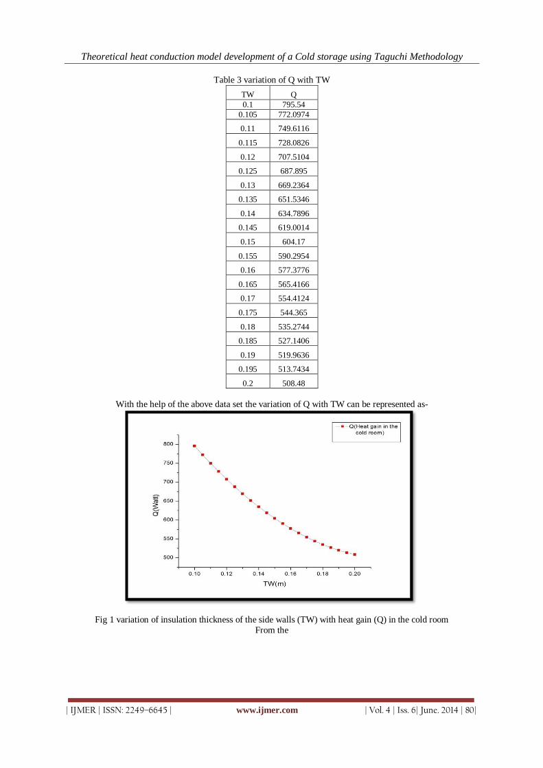
Theoretical heat conduction model development of a Cold storage using Taguchi Methodology
| IJMER | ISSN: 2249–6645 | www.ijmer.com | Vol. 4 | Iss. 6| June. 2014 | 80|
Table 3 variation of Q with TW
TW Q
0.1 795.54
0.105 772.0974
0.11 749.6116
0.115 728.0826
0.12 707.5104
0.125 687.895
0.13 669.2364
0.135 651.5346
0.14 634.7896
0.145 619.0014
0.15 604.17
0.155 590.2954
0.16 577.3776
0.165 565.4166
0.17 554.4124
0.175 544.365
0.18 535.2744
0.185 527.1406
0.19 519.9636
0.195 513.7434
0.2 508.48
With the help of the above data set the variation of Q with TW can be represented as-
Fig 1 variation of insulation thickness of the side walls (TW) with heat gain (Q) in the cold room
From the
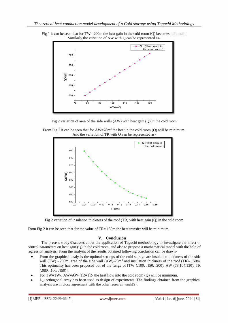
Theoretical heat conduction model development of a Cold storage using Taguchi Methodology
| IJMER | ISSN: 2249–6645 | www.ijmer.com | Vol. 4 | Iss. 6| June. 2014 | 81|
Fig 1 it can be seen that for TW=.200m the heat gain in the cold room (Q) becomes minimum.
Similarly the variation of AW with Q can be represented as-
Fig 2 variation of area of the side walls (AW) with heat gain (Q) in the cold room
From Fig 2 it can be seen that for AW=78m2 the heat in the cold room (Q) will be minimum.
And the variation of TR with Q can be represented as-
Fig 2 variation of insulation thickness of the roof (TR) with heat gain (Q) in the cold room
From Fig 2 it can be seen that for the value of TR=.150m the heat transfer will be minimum.
V. Conclusion The present study discusses about the application of Taguchi methodology to investigate the effect of
control parameters on heat gain (Q) in the cold room, and also to propose a mathematical model with the help of
regression analysis. From the analysis of the results obtained following conclusion can be drawn-
From the graphical analysis the optimal settings of the cold storage are insulation thickness of the side wall (TW) -.200m; area of the side wall (AW)-78m2 and insulation thickness of the roof (TR)-.150m.
This optimality has been proposed out of the range of [TW (.100, .150, .200), AW (78,104,130), TR
(.080, .100, .150)]. For TW=TW3, AW=AW1,TR=TR3 the heat flow into the cold room (Q) will be minimum.
L27 orthogonal array has been used as design of experiments. The findings obtained from the graphical
analysis are in close agreement with the other research work[9].

Theoretical heat conduction model development of a Cold storage using Taguchi Methodology
| IJMER | ISSN: 2249–6645 | www.ijmer.com | Vol. 4 | Iss. 6| June. 2014 | 82|
REFERENCE [1] M.S.Soylemez, M.Unsal(1997), Optimum Insulation Thickness for Refrigerant applications, Energy Conservation
and Management, 40(1999) 13-21.
[2] N.Yusoff and M.Ramasamy(2010), Selection of RGP Optimization variables using Taguchi Method, Journal of
Applied Science 10(24) 3313-3318,2010 ISSN 1812-5654 [3] Patel Amit M., Patel R. I., Optimization of different parameter of cold storage for energy conservation, International
Journal of Modern Engineering Research, Vol.2, Issue.3, May-June 2012 pp-1001-1005.
[4] M. S. Phadke, “Quality engineering using robust design” (2nd edition, Pearson, 2009). [5] D. C. Montgomery, E. A. Peck and G. G. Vining, “Introduction to linear regression analysis”,4th edition, John wiley
and sons, 2006.
[6] D. C. Montgomery, “Design and analysis of experiments”(3rd edition, John wiley and sons, 1991) [7] Ashish .S. Utage, K. V. Mali, A. D. Kadam, Performance simulation of cold storage using energyplus, International
Journal of Engineering Science and Technology, Vol. 5 No.02, February 2013 ISSN : 0975-5462. [8] Dale.H.Besterfield,Carol Besterfield ,”Total quality management”(Pearson). [9] Raju.Das, Development of theoretical heat conduction model of a cold storage and its optimization using Taguchi
Methodology, Master degree thesis., Jalpaiguri Govt.Engg.College, Jalpaiguri, W.B,India, 2014.

International
OPEN ACCESS Journal Of Modern Engineering Research (IJMER)
| IJMER | ISSN: 2249–6645 | www.ijmer.com | Vol. 4 | Iss. 6| June. 2014 | 83|
Load balancing in Content Delivery Networks in Novel
Distributed Equilibrium
V. Kamakshamma1, D. Anil
2
1Department of CSE, VEC, Kavali, 2Asst.Profesor, Department of CSE, VEC, Kavali,
I. Introduction The average size of web objects has grown over the years. Today Internet users regularly download
rented films (e.g.,from iTunes and NetFlix), TV programmes (e.g., using BBC iPlayer), large security updates,
virtual machine images and entire operating system distributions. File sizes for this content can range from a
few megabytes (security patches) to several gigabytes (rented high-definition films). Content providers
usecontent delivery networks (CDNs), such as Akamai [16], Limelight, CoralCDN [3] and CoDeeN [17], to
provide files to millions of Internet users through a distributed network of content servers.
To achieve a scalable and reliable service, a CDN should have two desirable properties. First, load
awareness should partition requests across a group of servers with replicated content, balancing computational
load and network congestion. This increases the number of users that can be served requesting the same content.
The degree of replication may be chosen dynamically to handle surges of incoming requests (flash crowds)
when content suddenly becomes popular (known as the Slashdot effect) [2]. Second, locality awareness should exploit proximity relationships in the network, such as geographic distance, round-trip latency
or topological distance, when assigning client requests to con tent servers.
Intuitively, by keeping network paths short, a CDN can provide better quality-of-service (QoS) to
clients. It is challenging to design a CDN that makes a trade-of between load- and locality-awareness. Simple
CDNs that always redirect clients to geographically-closest content servers lack load-balancing and suffer from
overload when local content popularity increases. More advanced CDNs that are based on distributed hash
tables (DHTs) [15] primarily focus on load-balancing. They use network locality only as a tie breaker between
multiple servers, leading to sub-optimal decisions about network locality. State-of-the-art CDNs such as Akamai
[16] are proprietary, with little public knowledge on the types of complex optimizations that they perform.
In this paper, we describe a new type of CDN that uses load-aware network coordinates (LANCs) to
capture naturally the tension between load and locality awareness. LANCs are synthetic coordinates (calculated using a metric embedding [10] of application-level delay measurements) that incorporate network location and
load of content servers. Our CDN uses LANCs to map clients dynamically to the most appropriate server in a
decentralised fashion. Popular content is replicated among nearby content servers with low load. By combining
locality and load using the unified mechanism of LANCs, we simplify the design of the CDN and discard the
need for ad-hoc solutions.The main contributions of this work are: (1) the introduction of LANCs, showing how
they react to CPU load and network congestion; (2) the design and implementation of a CDN that uses LANCs
to route client requests to content servers and replicate content; (3) a preliminary evaluation of our LANC-based
CDN on PlanetLab, demonstrating its benefits in comparison to other approaches.
Our result shows that, with a locality-heavy workload, our approach achieves almost an order of
magnitude lower request times compared to direct retrieval of content. The rest of the paper is structured as
follows. In Section 2,we discuss the requirements for CDNs in more detail and,in Section 3, we describe
LANCs. We present our CDN design in Section 4, focusing on request mapping and request redirection. In Section 5, we evaluate LANCs on a local network and also present results from a large-scale PlanetLab
deployment. Section 6 describes related work and Section 7 concludes with an outlook on future work.
Abstract: In today’s world’s to provide service to netizen’s with good availability of data, content delivery networks (CDNs) must balance requests between servers while assigning clients to closet
servers. In this paper, we describe a new CDN design that associates artificial load-aware coordinates
with clients and data servers and uses them to direct content requests to cached data. This approach
helps achieve good accuracy and service when request workloads and resource availability in the CDN
are dynamic. A deployment and evaluation of our system on Planet Lab demonstrates how it achieves low
request times with high cache hit ratios when compared to other CDN approaches.

Load balancing in Content Delivery Networks in Novel Distributed Equilibrium
| IJMER | ISSN: 2249–6645 | www.ijmer.com | Vol. 4 | Iss. 6| June. 2014 | 84|
II. Content Delivery Networks Global CDNs are typically implemented as a distributed network of servers hosting replicated content.
Servers may be located at geographically-diverse data centres, providing content to users in a given region. Web
clients issue requests to fetch content from the CDN, which are satisfied by content servers according to a particular mapping strategy. A goal of the CDN is to minimize total request time, i.e., the time until a client has
successfully retrieved desired content. Load awareness.For a CDN to be load-aware, there must be a mechanism
that balances load between content servers. This may be the done by, for example, distributing requests
uniformly across all content servers or redirecting requests to the least-loaded server. If content requests go to
overloaded servers, clients experience poor performance.In our model, we distinguish between load balancing
for computational load and network congestion. (1) Computational load at a content server is caused by the
processing associated with content requests. This involves request parsing, retrieval of cached content if there is
a cache hit and content delivery to the client. (2) Network congestion is caused by the limited capacity of
network paths to carry traffic.This creates bottleneck links that determine the throughput at which content can be
delivered to clients. Considering the Internet path from client to server, the bottleneck may be: (a) at the client’s
access link, in which case only the performance of this client is aff ected and the CDN cannot provide any
remedy; (b) at the client’s upstream ISP or Internet backbone, affecting a larger number of clients. Here,the choice of a diff erent content server may lead to improved performance; (c) at the content servers’ access link,
aff ecting all client requests to this server. In this case, the CDN should redirect requests away from the
congested server.Locality awareness.
A CDN is locality-aware if network paths are kept short. For example, a CDN can take request origins
into account and return content from nearby servers with low load. Proximity may be defined in terms of
geographic distance, latency, number of routing hops or overlap between address prefixes. By minimising
network path lengths, clients are more likely to experience better QoS [11]. Intuitively, this is because: (1) short
paths offer low latencies. This helps TCP obtain high throughput quickly therefore reducing transmission times
for small content; (2) short paths are less likely to encounter congestion hot-spots, resulting in improved
throughput; (3) short paths tend to be more reliable as they involve fewer network links and routers; (4) short
paths decrease overall network saturation, leaving more spare network capacity for other traffic.
III. Load Aware Network Coordinates Overlay networks can use network coordinates (NCs) [10] to become locality-aware [13]. In a NC
system, each node maintains a synthetic n-dimensional coordinate (of low dimensionality, typically 2 ≤ n ≤ 5)
based on round-trip latency measurements between nodes. The NCs of nodes are calculated by embedding the
graph of latency measurements into a metric space. Euclidean distances between NCs then predict the actual
communication latencies. NCs are updated dynamically to reflect changes in Internet latencies. A benefit of NCs
is that they estimate missing measurements. They allow Internet nodes to reason about their relative proximities
without having to collect all measurements. However, triangle inequality violations found in Internet latencies make it impossible to embed measurements without error [9], resulting in less accurate latency prediction. There
is also a constant measurement overhead when maintaining NCs in the background. Vivaldi. Our CDN
uses the Pyxida library [14] to maintain NCs according to the Vivaldi [1] algorithm. Vivaldi is a decentralized
algorithm that computes NCs using a spring relaxation technique. Nodes are modeled as point masses and
latencies as springs between nodes. The NCs of nodes change as nodes attract and repel each other.
E =XX(Lij − kxi − xjk)
2(1)
Let xibe the NC assigned to node i and xjto j. Lijis the actual latency between nodes i and j. Vivaldi
characterizes the errors in the NCs using the squared-error function in Eq. 1, where kxi− xjk is the Euclidean
distance between the NCs of nodes i and j. Since Eq. 1 corresponds to energy in a physical mass-spring system,
Vivaldi minimises prediction errors by finding a low-energy state of the spring network.NCs are computed by
each node in a decentralised fashion:When node I receives a new latency measurementLijto node j, it compares
the true latency Lij to the predicted latency kxi− xjk. It then adjusts its NC xito minimize the prediction error
according to Eq. 1. Measurements are filtered to remove outliers [7]. The above process converges quickly in
practice and leads to stable and accurate NCs [6]. Load-awareness It is easy to see how a CDN could benefit from NCs to achieve locality-awareness.
Assuming that clients and servers have known NCs, clients could direct requests to the server with the closest
NC. Also, servers could use their neighbours to replicate popular content, keeping content replication local
while reducing total request times. The lower accuracy of NCs for latency prediction compared to direct
measurements [18] is less important for a CDN. A small latency reduction by choosing a slightly closer server
will only have a marginal impact on the total request time for large content. The goal for locality-awareness in a
CDN is to select a content server with good performance, as opposed to finding the single closest one.
However, regular NCs do not provide load-balancing between content servers. Servers in densely-populated
areas are likely to become overloaded, whereas servers in sparse regions will have spare capacity. To address
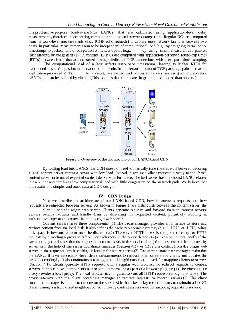
Load balancing in Content Delivery Networks in Novel Distributed Equilibrium
| IJMER | ISSN: 2249–6645 | www.ijmer.com | Vol. 4 | Iss. 6| June. 2014 | 85|
this problem,we propose load-aware NCs (LANCs) that are calculated using application-level delay
measurements, therefore incorporating computational load and network congestion. Regular NCs are computed
from network-level measurements (e.g., ICMP echo requests) to capture pure network latencies between two
hosts. In particular, measurements aim to be independent of computational load (e.g., by assigning kernel-space
timestamps to packets) and of congestion on network paths (e.g., by using small measurement packets
least affected by congestion) [5].In contrast, LANCs are computed with application-perceived round-trip times
(RTTs) between hosts that are measured through dedicated TCP connections with user-space time stamping. The computational load of a host affects user-space timestamps, leading to higher RTTs for
overloaded hosts. Congestion on network paths results in the retransmission of TCP packets, again increasing
application perceived RTTs. As a result, overloaded and congested servers are assigned more distant
LANCs and can be avoided by clients. (This assumes that clients are, in general, less loaded than servers.)
Figure 1: Overview of the architecture of our LANC-based CDN.
By folding load into LANCs, the CDN does not need to manually tune the trade-off between choosing a local content server versus a server with low load. Instead, it can map client requests directly to the “best”
content server in terms of expected content delivery performance. The best server has the closest LANC relative
to the client and combines low computational load with little congestion on the network path. We believe that
this results in a simpler and more natural CDN design.
IV. CDN Design Next we describe the architecture of our LANC-based CDN, how it processes requests, and how
requests are redirected between servers. As shown in Figure 1, we distinguish between the content server, the
client and the origin web server. Clients generate requests and forward them to content servers. Servers receive requests and handle them by delivering the requested content, potentially fetching an
authoritative copy of the content from the origin web server.
Content servers have three components: (1) The cache manager provides an interface to store and
retrieve content from the local disk. It also defines the cache replacement strategy (e.g., LRU or LFU) when
disk space is low and content must be discarded.(2) The server HTTP proxy is the point of entry for HTTP
requests by providing a proxy interface. For each request, the proxy decides to (a) retrieve content locally if the
cache manager indicates that the requested content exists in the local cache; (b) request content from a nearby
server with the help of the server coordinate manager (Section 4.2); or (c) return content from the origin web
server to the requester, while caching it locally for future access.(3) The server coordinate manager maintains
the LANC. It takes application-level delay measurements to random other servers and clients and updates the
LANC accordingly. It also maintains a routing table of neighbours that is used for mapping clients to servers (Section 4.1). Clients generate HTTP requests with a regular web browser. To redirect requests to content
servers, clients run two components as a separate process (or as part of a browser plugin): (1) The client HTTP
proxyprovides a local proxy. The local browser is configured to send all HTTP requests through this proxy. The
proxy interacts with the client coordinate manager to redirect requests to content servers.(2) The client
coordinate manager is similar to the one on the server-side. It makes delay measurements to maintain a LANC.
It also manages a fixed-sized neighbour set with nearby content servers used for mapping requests to servers.
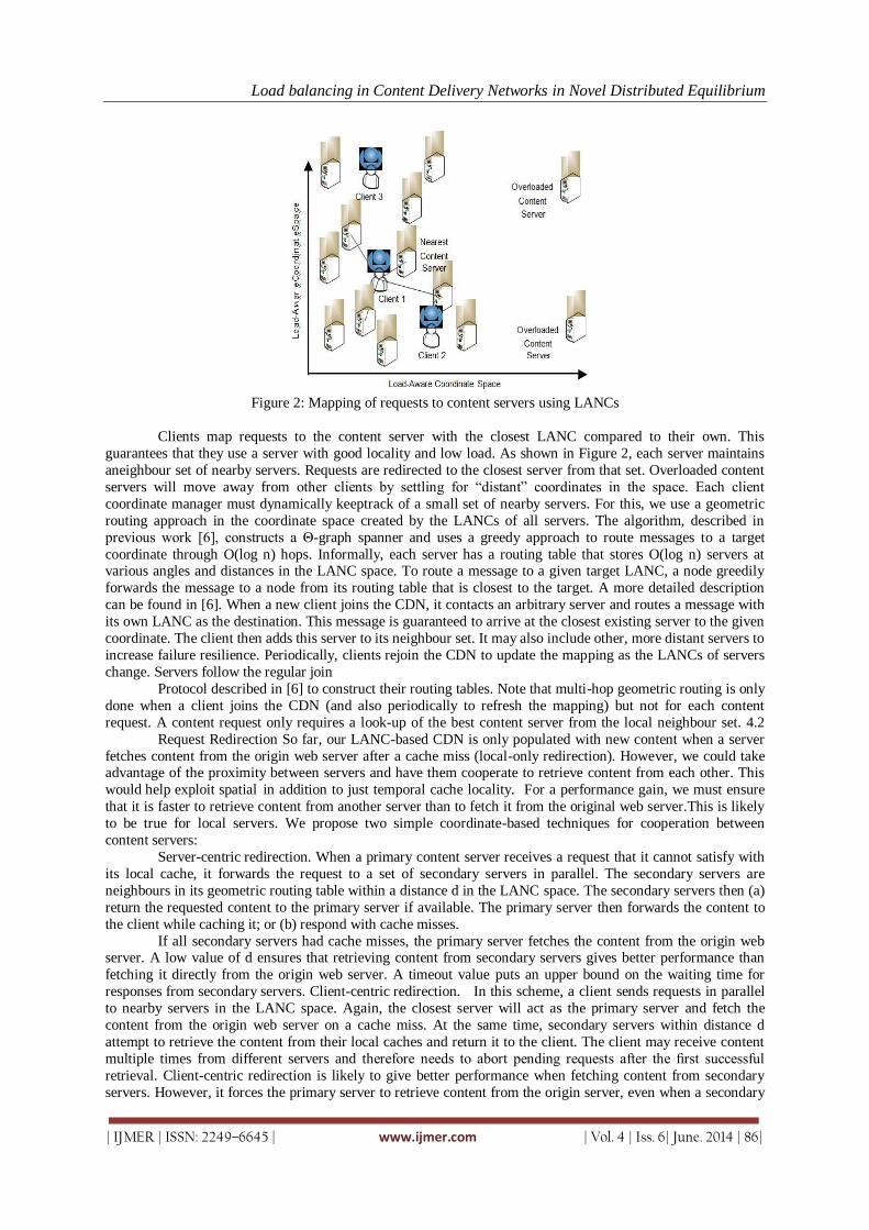
Load balancing in Content Delivery Networks in Novel Distributed Equilibrium
| IJMER | ISSN: 2249–6645 | www.ijmer.com | Vol. 4 | Iss. 6| June. 2014 | 86|
Figure 2: Mapping of requests to content servers using LANCs
Clients map requests to the content server with the closest LANC compared to their own. This
guarantees that they use a server with good locality and low load. As shown in Figure 2, each server maintains
aneighbour set of nearby servers. Requests are redirected to the closest server from that set. Overloaded content
servers will move away from other clients by settling for “distant” coordinates in the space. Each client
coordinate manager must dynamically keeptrack of a small set of nearby servers. For this, we use a geometric
routing approach in the coordinate space created by the LANCs of all servers. The algorithm, described in
previous work [6], constructs a Θ-graph spanner and uses a greedy approach to route messages to a target
coordinate through O(log n) hops. Informally, each server has a routing table that stores O(log n) servers at various angles and distances in the LANC space. To route a message to a given target LANC, a node greedily
forwards the message to a node from its routing table that is closest to the target. A more detailed description
can be found in [6]. When a new client joins the CDN, it contacts an arbitrary server and routes a message with
its own LANC as the destination. This message is guaranteed to arrive at the closest existing server to the given
coordinate. The client then adds this server to its neighbour set. It may also include other, more distant servers to
increase failure resilience. Periodically, clients rejoin the CDN to update the mapping as the LANCs of servers
change. Servers follow the regular join
Protocol described in [6] to construct their routing tables. Note that multi-hop geometric routing is only
done when a client joins the CDN (and also periodically to refresh the mapping) but not for each content
request. A content request only requires a look-up of the best content server from the local neighbour set. 4.2
Request Redirection So far, our LANC-based CDN is only populated with new content when a server
fetches content from the origin web server after a cache miss (local-only redirection). However, we could take advantage of the proximity between servers and have them cooperate to retrieve content from each other. This
would help exploit spatial in addition to just temporal cache locality. For a performance gain, we must ensure
that it is faster to retrieve content from another server than to fetch it from the original web server.This is likely
to be true for local servers. We propose two simple coordinate-based techniques for cooperation between
content servers:
Server-centric redirection. When a primary content server receives a request that it cannot satisfy with
its local cache, it forwards the request to a set of secondary servers in parallel. The secondary servers are
neighbours in its geometric routing table within a distance d in the LANC space. The secondary servers then (a)
return the requested content to the primary server if available. The primary server then forwards the content to
the client while caching it; or (b) respond with cache misses.
If all secondary servers had cache misses, the primary server fetches the content from the origin web server. A low value of d ensures that retrieving content from secondary servers gives better performance than
fetching it directly from the origin web server. A timeout value puts an upper bound on the waiting time for
responses from secondary servers. Client-centric redirection. In this scheme, a client sends requests in parallel
to nearby servers in the LANC space. Again, the closest server will act as the primary server and fetch the
content from the origin web server on a cache miss. At the same time, secondary servers within distance d
attempt to retrieve the content from their local caches and return it to the client. The client may receive content
multiple times from different servers and therefore needs to abort pending requests after the first successful
retrieval. Client-centric redirection is likely to give better performance when fetching content from secondary
servers. However, it forces the primary server to retrieve content from the origin server, even when a secondary
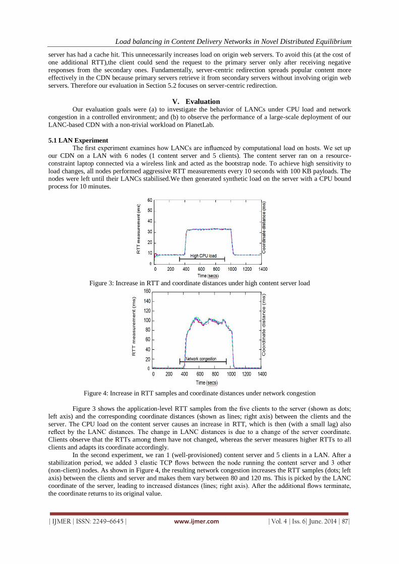
Load balancing in Content Delivery Networks in Novel Distributed Equilibrium
| IJMER | ISSN: 2249–6645 | www.ijmer.com | Vol. 4 | Iss. 6| June. 2014 | 87|
server has had a cache hit. This unnecessarily increases load on origin web servers. To avoid this (at the cost of
one additional RTT),the client could send the request to the primary server only after receiving negative
responses from the secondary ones. Fundamentally, server-centric redirection spreads popular content more
effectively in the CDN because primary servers retrieve it from secondary servers without involving origin web
servers. Therefore our evaluation in Section 5.2 focuses on server-centric redirection.
V. Evaluation Our evaluation goals were (a) to investigate the behavior of LANCs under CPU load and network
congestion in a controlled environment; and (b) to observe the performance of a large-scale deployment of our
LANC-based CDN with a non-trivial workload on PlanetLab.
5.1 LAN Experiment
The first experiment examines how LANCs are influenced by computational load on hosts. We set up
our CDN on a LAN with 6 nodes (1 content server and 5 clients). The content server ran on a resource-
constraint laptop connected via a wireless link and acted as the bootstrap node. To achieve high sensitivity to
load changes, all nodes performed aggressive RTT measurements every 10 seconds with 100 KB payloads. The nodes were left until their LANCs stabilised.We then generated synthetic load on the server with a CPU bound
process for 10 minutes.
Figure 3: Increase in RTT and coordinate distances under high content server load
Figure 4: Increase in RTT samples and coordinate distances under network congestion
Figure 3 shows the application-level RTT samples from the five clients to the server (shown as dots;
left axis) and the corresponding coordinate distances (shown as lines; right axis) between the clients and the
server. The CPU load on the content server causes an increase in RTT, which is then (with a small lag) also
reflect by the LANC distances. The change in LANC distances is due to a change of the server coordinate.
Clients observe that the RTTs among them have not changed, whereas the server measures higher RTTs to all
clients and adapts its coordinate accordingly.
In the second experiment, we ran 1 (well-provisioned) content server and 5 clients in a LAN. After a
stabilization period, we added 3 elastic TCP flows between the node running the content server and 3 other (non-client) nodes. As shown in Figure 4, the resulting network congestion increases the RTT samples (dots; left
axis) between the clients and server and makes them vary between 80 and 120 ms. This is picked by the LANC
coordinate of the server, leading to increased distances (lines; right axis). After the additional flows terminate,
the coordinate returns to its original value.
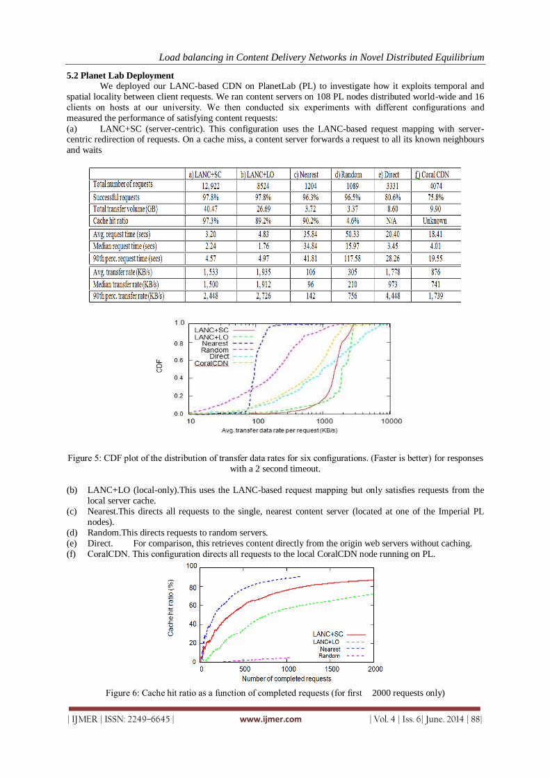
Load balancing in Content Delivery Networks in Novel Distributed Equilibrium
| IJMER | ISSN: 2249–6645 | www.ijmer.com | Vol. 4 | Iss. 6| June. 2014 | 88|
5.2 Planet Lab Deployment
We deployed our LANC-based CDN on PlanetLab (PL) to investigate how it exploits temporal and
spatial locality between client requests. We ran content servers on 108 PL nodes distributed world-wide and 16
clients on hosts at our university. We then conducted six experiments with different configurations and
measured the performance of satisfying content requests:
(a) LANC+SC (server-centric). This configuration uses the LANC-based request mapping with server-centric redirection of requests. On a cache miss, a content server forwards a request to all its known neighbours
and waits
Figure 5: CDF plot of the distribution of transfer data rates for six configurations. (Faster is better) for responses
with a 2 second timeout.
(b) LANC+LO (local-only).This uses the LANC-based request mapping but only satisfies requests from the
local server cache.
(c) Nearest.This directs all requests to the single, nearest content server (located at one of the Imperial PL
nodes).
(d) Random.This directs requests to random servers.
(e) Direct. For comparison, this retrieves content directly from the origin web servers without caching.
(f) CoralCDN. This configuration directs all requests to the local CoralCDN node running on PL.
Figure 6: Cache hit ratio as a function of completed requests (for first 2000 requests only)

Load balancing in Content Delivery Networks in Novel Distributed Equilibrium
| IJMER | ISSN: 2249–6645 | www.ijmer.com | Vol. 4 | Iss. 6| June. 2014 | 89|
Each experiment was set up in the same way. The first content server acted as the bootstrap node for all
other nodes. After starting the servers, we added the client nodes and let coordinates stabilise for one hour. RTT
measurements between nodes were taken with 4 KB payloads exchanged through TCP connections every
minute. All content servers started with cold caches. We generated a synthetic request workload on the 16
clients. Each client continuously requested a Gentoo Linux distribution file with a size of 3.28 MB from a list of
100 web servers distributed world-wide [4]. (Since the URLs were different, all CDNs assumed these to be
different files, with no caching between URLs.) This request load provided spatial locality (all requests came from clients at our university) and temporal locality (clients eventually requested the same URL repeatedly).
The high load on PL nodes exercised our load balancing mechanism. We deliberately chose a relatively small
file size to stay below per-slice transmission limits on PL. Each configuration ran for one hour.
The results are summarized in Table 1. Figure 5 shows the distribution of average transfer data rates
per request across all clients on a logarithmic scale. LANC+SC manages to satisfy the most requests (12, 922) in
one hour. The low value for the 90th percentile of request times (4.57 seconds) is due to its good choice of
content servers (with nearby LANCs), which results in high transfer rates, and its aggressive fetching of cached
content from other servers, which means a high cache hit ratio of 97.3%.During the experiment, we observed
that most clients requested content from a small set of servers running on PL nodes with low load at Imperial, in
France and in Germany.
LANC+LO satisfies fewer requests compared to LANC+SC. As seen in Figure 5, its performance suffers from a small fraction of requests with low transfer rates. We observed that these were mostly cache
misses that forced the retrieval of content from slow web servers. At the same time, the 90th percentile of its
transfer rate is slightly higher than for LANC+SC because servers do not have the overhead of relaying content
when fetching it from neighbours. Since LANC+LO only considers a single content server for satisfying
requests, it has a lower cache hit ratio (89.2%).
Nearest gives poor performance because the single content server becomes a bottleneck and can only
satisfy requests with a consistently low transfer rate. It has a high cache hit ratio (90.2%) because all requests
are directed to the same server (but not the highest because clients do not manage to submit all requests twice
within one hour).Random balances requests across many servers but fails to exploit spatial or temporal locality,
leading to a low cache hit ratio (4.6%). Selected servers often take a long time to retrieve content due to high
load on PL nodes and/or low available bandwidth.
Direct illustrates the benefit of caching with a CDN compared to retrieving content directly from hosting web servers. Finally, we used Coral CDN on PL to retrieve content. Although this is not a fair
comparison because, as a public service, Coral CDN handles a higher work-load than just the requests we
directed at it, we believe that it illustrates the potential of our approach. As expected, Coral CDN showed a
substantially higher average request time (18.41 seconds) than our LANC-based CDN. As shown in Figure 5, its
average transfer rates were lower than fetching content directly (while presumably significantly reducing load
on the origin web servers). For now, we can only speculate whether this is due to Coral CDN’s high workload or
less optimal choice of content servers. In future work, we plan to repeat this experiment in a controlled setting.
Figure 6 illustrates the difference between LANC+SC and LANC+LO in more detail. It shows the change in
cache hit ratio as a function of completed requests. The cache hit ratio of LANC+SC grows faster because it
considers nearby servers for requested content. This means that LANC+SC reduces the load on the origin web
servers by retrieving more content from the CDN. With our workload, eventually all requests can be satisfied by the CDN and the cache hit ratio asymptotically approaches unity.
VI. Related Work CoralCDN [3] is a peer-to-peer CDN built to help web servers handle huge demands of flash crowds.
With cooperating cache nodes, CoralCDN minimises the load on the original web server and avoids the creation
of hot spots. It builds a load-balanced, latency-optimised hierarchical indexing infrastructure based on a weakly-
consistent DHT and achieves locality-awareness by making nodes members of multiple DHTs called clusters.
Clusters are specified by a maximum RTT and can reduce request latencies by prioritizing nearby nodes. Our
work shares many of the design goals of CoralCDN in terms of locality- and load-awareness. However our approach of using a unified scheme based on LANCs is different, aiming for good request
mappings in environments with dynamic load and network congestion.
CoDeeN [17] is a network of open proxy servers running on PL. The system leaves it up to the user to
choose a suitable proxy server for browser requests. If the local proxy cannot satisfy a request, it selects another
proxy based on locality, load and reliability. Our LANC-based CDN automates the initial mapping step at the
cost of running a client component on user machines.
Globule [12] is a collaborative CDN that exploit client resources for caching using a browser plug-in.
Because Globule runs on client hosts, it must make diff erent assumption about churn and security. It uses
landmark-based NCs for locality-awareness. Replicated content is placed according to the locations of clients in

Load balancing in Content Delivery Networks in Novel Distributed Equilibrium
| IJMER | ISSN: 2249–6645 | www.ijmer.com | Vol. 4 | Iss. 6| June. 2014 | 90|
a coordinate space. Since it leverages many client machines for caching, balancing computational load is less
important.
Meridian [18] builds an overlay network for locality-aware node selection with on-demand probing to
estimate node distances. To find the nearest node to a client, Meridian uses a set of ICMP echo requests to move
logarithmically closer to the target. Similar to our geometric routing tables, each nodes maintains a fixed number
of links to other nodes with exponentially increasing distances. Meridian aims to return the closest existing node
to a client. We argue that such accuracy is not necessary when selecting content servers, as other factors such as load will be equally important.
VII. Conclusions We have described a novel CDN that uses a coordinate space with application-level latency
measurements between clients and content servers for the mapping and redirection of requests. We
demonstrated how our LANC-based CDN reacts to computational load and network congestion. A large-scale
deployment on PL with a locality-heavy workload highlights the benefits of our approach. As future work, we
plan to study the stability and load awareness of LANCs under dynamic workloads (e.g., flash crowds) and
varying resource availability. We also plan a more extensive comparison against other CDNs. Finally, we want to investigate how proxy NCs [8] can relieve the burden from maintaining LANCs
from client nodes.
REFERENCES [1] F. Dabek, R. Cox, F. Kaashoek, and R. Morris.Vivaldi: A Decentralized Network Coordinate System.In Proc. of
SIGCOMM, Aug. 2004. [2] J. Elson and J. Howell. Handling Flash Crowds from Your Garage. In Proc. of USENIX, 2008. [3] M. J. Freedman, E. Freudenthal, and D. Mazi`eres.Democratizing Content Publication with Coral. In Proc. of NSDI,
2004. [4] Gentoo. Gentoo Mirror List.www.gentoo.org/main/en/mirrors2.xml, Aug. 2008.
[5] J. Ledlie, P. Gardner, and M. Seltzer. Network Coordinates in the Wild. In Proc. of NSDI, 2007. [6] J. Ledlie, M. Mitzenmacher, M. Seltzer, and P. Pietzuch. Wired Geometric Routing. In Proc. Of IPTPS, Bellevue,
WA, USA, Feb. 2007. [7] J. Ledlie, P. Pietzuch, and M. Seltzer. Stable and Accurate Network Coordinates. In ICDCS, July 2006. [8] J. Ledlie, M. Seltzer, and P. Pietzuch. Proxy Network Coordinates. TR 2008/4, Imperial College, Feb. 2008. [9] E. K. Lua, T. Griffin, et al. On the Accuracy of Embeddings for Internet Coord. Sys. In IMC, 2005. [10] T. E. Ng and H. Zhang. Predicting Internet Network Distance with Coordinates-Based Approaches. In Proc. of
INFOCOM’02, New York, NY, June 2002.
[11] D. Oppenheimer, J. Albrecht, D. Patterson, and A. Vahdat. Distributed Resource Discovery on PlanetLab with SWORD. In WORLDS, Dec. 2004.
[12] G. Pierre and M. van Steen. Globule: a Collaborative CDN. IEEE Comms. Magazine, 44(8), Aug. 2006. [13] P. Pietzuch, J. Ledlie, M. Mitzenmacher, and M. Seltzer. Network-Aware Overlays with Network Coordinates. In
Proc. of IWDDS, July 2006. [14] Pyxida Project. pyxida.sourceforge.net, 2006. [15] I. Stoica, R. Morris, D. Karger, et al. Chord: A Scalable Peer-to-
peer Lookup Service for Internet Applications. In Proc. SIGCOMM, Aug. 2001. [16] A.-J. Su, D. Choff nes, A. Kuzmanovic, et al. Drafting Behind Akamai. In SIGCOMM, 2006.[17] L. Wang, K. Park,
R. Pang, V. S. Pai, and [17] L. Wang, K. Park, R. Pang, V. S. Pai, and L. Peterson. Reliability and Security in the CoDeeN Content Distribution
Network. In USENIX, 2004. [18] B. Wong et al. Meridian: A Lightweight Network Loc.Service without Virtual Coords. In SIGCOMM, 2005.

International
OPEN ACCESS Journal
Of Modern Engineering Research (IJMER)
| IJMER | ISSN: 2249–6645 | www.ijmer.com | Vol. 4 | Iss. 6| June. 2014 | 91|
In Multi-Hop Routing identifying trusted paths through TARF in
Wireless sensor networks
P.Esswaraiah1, Ch.Srilakshmi
2
1 Assoc.Prof , Department of CSE , PBR VITS, 2 Department of CSE, PBR VITS, Kavali,
I. Introduction Wireless sensor networks (WSNs) are ideal candidates for applications to report detected events of
interest, such as military surveillance and forest fire monitoring. A WSN comprises battery-powered
senor nodes with extremely limited processing capabilities. With a narrow radio communication range, a
sensor node wirelessly sends messages to a base station via a multi-hop path. However, the multi-hop
routing of WSNs often becomes the target of malicious attacks. An attacker may tamper nodes
physically, create traffic collision with seemingly valid transmission, drop or misdirect messages in routes,
or jam the communication channel by creating radio interference. This paper focuses on the kind of attacks in which adversaries misdirect network traffic by identity deception through replaying routing information.
Based on identity deception, the adversary is capable of launching harmful and hard-to-detect attacks
against routing, such as selective forwarding, wormhole attacks, sinkhole attacks and Sybil attacks. As a
harmful and easy-to-implement type of attack, a malicious node simply replays all the outgoing routing
packets from a valid node to forge the latter node’s identity; the malicious node then uses this forged
identity to participate in the network routing, thus disrupting the network traffic. Those routing packets,
including their original headers are replayed without any modification. Even if this malicious node
cannot directly overhear the valid node’s wireless transmission, it can collude with Other malicious
nodes to receive those routing packets and replay them somewhere far away from the original valid
node, which is known as a wormhole attack. Since a node in a WSN usually relies solely on the packets
received to know about the sender’s identity, replaying routing packets allows the malicious node to forge the identity of this valid node. After ―stealing‖ that valid identity, this malicious node is able to
misdirect the network traffic. For instance, it may drop packets received, forward packets to another node
not supposed to be in the routing path, or even form a transmission loop through which packets are passed
among a few malicious nodes infinitely. It is often difficult to know whether a node forwards received
packets correctly even with overhearing techniques. Sinkhole attacks are another kind of attacks that can be
launched after stealing a valid identity. In a sinkhole attack, a malicious node may claim itself to be a base
station through replaying all the packets from a real base station. Such a fake base station could lure
Abstract: The multi-hop routing in wireless sensor networks (WSNs) highly vulnerable against identity cheating through replaying routing data. An attacker can uses this drawback to launch
various serious or even disturbing attacks against the routing protocols, like sinkhole attacks,
wormhole attacks and Sybil attacks. The situation is further forced by mobile and unkind
network conditions. old cryptographic techniques or efforts at developing trust-aware routing
protocols do not effectively address this serious problem. To secure the WSNs against attackers
misdirecting the multi-hop routing, we have designed and implemented TARF, a robust trust-aware
routing framework for dynamic WSNs. Without tight time synchronization or known geographic
information, TARF provides trustworthy and energy-efficient route. Most importantly, TARF proves
effective against those dangerous attacks developed out of identity cheat; the flexibility of TARF is verified through extensive evaluation with both simulation and empirical experiments on
large-scale WSNs under various scenarios including mobile and RF-shielding network conditions.
Further, we have implemented allow-overhead TARF module in TinyOS; as demonstrated, this
implementation can be included into existing routing protocols with the little effort. Based on
TARF, we also demonstrated a proof-of-concept mobile target detection application that functions
well against an anti-detection mechanism.

In Multi-Hop Routing identifying trusted paths through TARF in Wireless sensor networks
| IJMER | ISSN: 2249–6645 | www.ijmer.com | Vol. 4 | Iss. 6| June. 2014 | 92|
more than half the traffic, creating a ―black hole‖. This same technique can be employed to conduct
another strong form of attack - Sybil attack: through eplaying the routing information of multiple legitimate
nodes, an attacker may present multiple identities to the network. A valid node, if compromised, can also launch all these attacks. a poor network connection causes much difficulty in distinguishing between an
attacker and a honest node with transient failure. Without proper protection, WSNs with existing routing
protocols can be completely devastated under certain circumstances. In an emergent sensing application
through WSNs, saving the network from being devastated becomes crucial to the success of the
application.
Unfortunately, most existing routing protocols for WSNs both assume the honesty of nodes and
focus on energy efficiency, or attempt to exclude unauthorized participation by encrypting data and
authenticating packets. Examples of these encryption and authentication schemes for WSNs include TinySec,
Spins, TinyPK, and TinyECC. Admittedly, it is important to consider efficient energy use or battery
powered sensor nodes and the robustness of routing under topological changes as well as common
faults in a wild environment. However, it is also critical to incorporate security as one of the most important goals; meanwhile, even with perfect encryption and authentication, by replaying routing
information, a malicious node can still participate in the network using another valid node’s identity.
The gossiping-based routing protocols offer certain protection against attackers by selecting random
neighbors to forward packets, but at a price of considerable overhead in propagation time and energy
use. In addition to the cryptographic methods, trust and reputation management has been employed in
generic ad hoc networks and WSNs to secure routing protocols.
Basically, a system of trust and reputation management assigns each node a trust value
according to its past performance in routing. Then such trust values are used to help decide a secure and
efficient route. However, the proposed trust and reputation management systems for generic ad hoc
networks target only relatively powerful hardware platforms such as laptops and smart phones. Those
systems cannot be applied to WSNs due to the excessive overhead for resource-constrained sensor nodes
powered by batteries. As far as WSNs are concerned, secure routing solutions based on trust and reputation
management rarely address the identity deception through replaying routing information .The countermeasures
proposed so far strongly depends on either tight time synchronization or known geographic information
while their effectiveness against attacks exploiting the replay of routing information has not been
examined yet. At this point, to protect WSNs from the harmful attacks exploiting the replay of routing
information, we have designed and implemented a robust trust-aware routing framework, TARF, to
secure routing solutions in wireless sensor networks. Based on the unique characteristics of resource-
constrained WSNs, the design of TARF centers on trustworthiness and energy efficiency. Though TARF
can be developed into a complete and independent routing protocol, the purpose is to allow existing
routing protocols to incorporate our implementation of TARF with the least effort and thus producing a
secure and efficient fully-functional protocol. Unlike other security measures, TARF requires neither tight time synchronization nor known geographic information. Most importantly, TARF proves
resilient under various attacks exploiting the replay of routing information, which is not achieved by previous
security protocols. Even under strong attacks such as sinkhole attacks, wormhole attacks as well as Sybil
attacks, and hostile mobile network condition, TARF demonstrates steady improvement in network
performance. The effectiveness of TARF is verified through extensive evaluation with simulation and
empirical experiments on large-scale WSNs.
II. Design Considerations In a data collection task, a sensor node sends its sampled data to a remote base station with the aid
of other intermediate nodes, as shown in Figure 1. Though there could be more than one base station, our
routing approach is not affected by the number of base stations; to simplify our discussion, we assume that
there is only one base station. An adversary may forge the identity of any legal node through replaying
that node’s outgoing routing packets and spoofing the acknowledgement packets, even remotely through a
wormhole.
Nonetheless, our approach can still be applied to cluster based WSNs with static clusters,
where data are aggregated by clusters before being relayed. Cluster-based WSNs allows for the great
savings of energy and bandwidth through aggregating data from children nodes and performing routing
and transmission for children nodes. In a cluster-based WSN, the cluster headers themselves form a sub-
network; after certain data reach a cluster header, the aggregated data will be routed to a base station only
through such a sub-network consisting of the cluster headers. Our framework can then be applied to this
sub-network to achieve secure routing for cluster based WSNs. TARF may run on cluster headers only and cluster headers communicate with their children nodes directly since a static cluster has known

In Multi-Hop Routing identifying trusted paths through TARF in Wireless sensor networks
| IJMER | ISSN: 2249–6645 | www.ijmer.com | Vol. 4 | Iss. 6| June. 2014 | 93|
relationship between a cluster header and its children nodes, though any link-level security features may be
further employed.
Finally, we assume a data packet has at least the following fields: the sender id, the sender sequence number, the next-hop node id (the receiver in this one hop transmission), the source id (the node
that initiates the data), and the source’s sequence number. We insist that
the source node’s information should be included for the following reasons because that allows the
base station to track whether a data packet is delivered. It would cause too much overhead to transmit all
the one hop information to the base station. Also, we assume the routing packet is sequenced.
2.1 Authentication Requirements
Though a specific application may determine whether data encryption is needed, TARF requires
that the packets are properly authenticated, especially the broadcast packets from the base station. The
broadcast from the base station is asymmetrically authenticated so as to guarantee that an adversary is
not able to manipulate or forge a broadcast message from the base station at will. Importantly, with authenticated broadcast, even with the existence of attackers, TARF may use Trust Manager and the received
broadcast packets about delivery information to choose trustworthy path by circumventing compromised nodes.
Without being able to physically capturing the base station, it is generally very difficult for the adversary to
manipulate the base station broadcast packets which are asymmetrically authenticated. The asymmetric
authentication of those broadcast packets from the base station is crucial to any successful secure
routing protocol. It can be achieved through existing asymmetrically authenticated broadcast schemes that
may require loose time synchronization. As an example, µTESLA achieves asymmetric authenticated
broadcast through a symmetric cryptographic algorithm and a loose delay schedule to disclose the keys from
a key chain. Other examples of asymmetric authenticated broadcast schemes requiring either loose or no
time synchronization are found. Considering the great computation cost incurred by a strong asymmetric
authentication scheme and the difficulty in key management, a regular packet other than a base station
broadcast packet may only be moderately authenticated through existing symmetric schemes with a limited set of keys, such as the message authentication code provided by TinySec. It is possible that an
adversary physically captures a non-base legal node and reveals its key for the symmetric authentication.
With that key, the adversary can forge the identity of that non-base legal node and joins the network
―legally‖. However, when the adversary uses its fake identity to falsely attract a great amount of traffic,
after receiving broadcast packets about delivery information, other legal nodes that directly or indirectly
forwards packets through it will start to select a more trustworthy path through Trust Manager.
2.2 Goals
TARF mainly guards a WSN against the attacks misdirecting the multi-hop routing, especially
those based on identity theft through replaying the routing information. This paper does not address the
denial-of-service (DoS) attacks, where an attacker intends to damage the network by exhausting its resource. For instance, we do not address the DoS attack of congesting the network by replaying numerous
packets or physically jamming the network. TARF aims to achieve the following desirable properties:
High Throughput— Throughput is defined as the ratio of the number of all data packets delivered
to the base station to the number of all sampled data packets. Through put reflects how efficiently the
network is collecting and delivering data. Here we regard high throughput as one of our most important
goals. Energy Efficiency— Data transmission accounts for a major Portion of the energy consumption.
We evaluate energy efficiency by the average energy cost to successfully deliver a unit-sized data packet
from a source node to the base station. be given enough attention when considering energy cost since each re-
transmission causes a noticeable increase in energy consumption. If every node in a WSN consumes
approximately the same energy to transmit a unit-sized data packet, we can use another metric hop-per-
delivery to evaluate energy efficiency. Under that assumption, the energy consumption depends on the
number of hops, i.e. the number of one-hop transmissions occurring. To evaluate how efficiently energy is used, we can measure the average hops that each delivery of a data packet takes, abbreviated as
hop-per-delivery. Scalability & Adaptability— TARF should work well with WSNs of large magnitude
under highly dynamic contexts. We will evaluate the scalability and adaptability of TARF through
experiments with large-scale WSNs and under mobile and hash network conditions.
III. Design Of TARF TARF secures the multi-hop routing in WSNs against intruders misdirecting the multi-hop routing
by evaluating the trustworthiness of neighboring nodes. It identifies such intruders by their low
trustworthiness and routes data through paths circumventing those intruders to achieve satisfactory throughput. TARF is also energy efficient, highly scalable, and well adaptable. Before introducing the
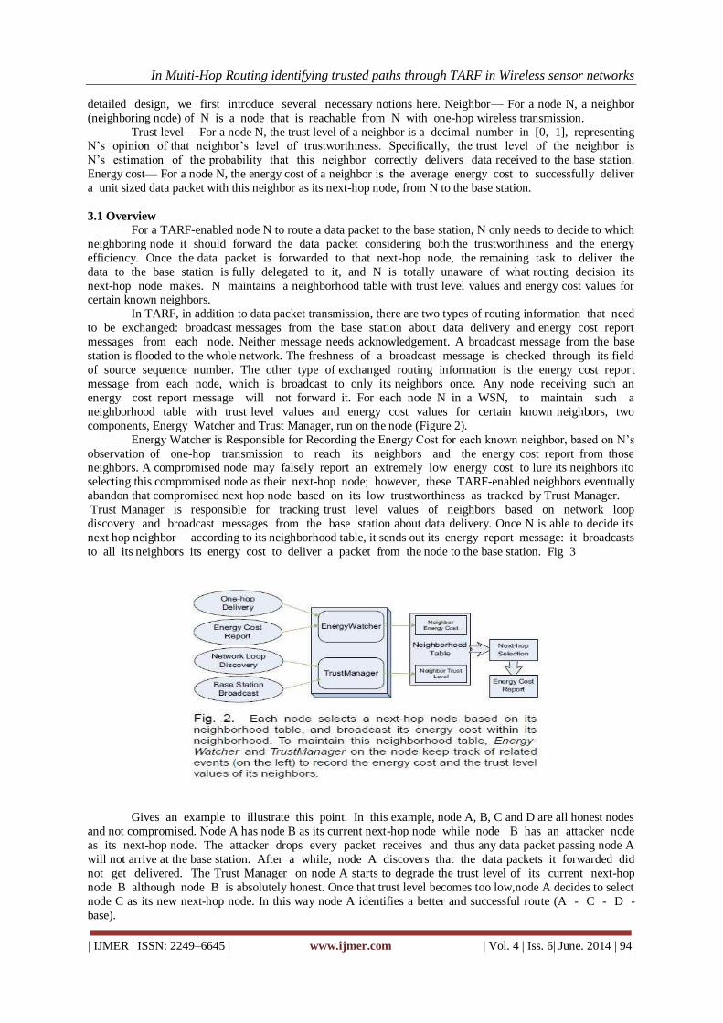
In Multi-Hop Routing identifying trusted paths through TARF in Wireless sensor networks
| IJMER | ISSN: 2249–6645 | www.ijmer.com | Vol. 4 | Iss. 6| June. 2014 | 94|
detailed design, we first introduce several necessary notions here. Neighbor— For a node N, a neighbor
(neighboring node) of N is a node that is reachable from N with one-hop wireless transmission.
Trust level— For a node N, the trust level of a neighbor is a decimal number in [0, 1], representing N’s opinion of that neighbor’s level of trustworthiness. Specifically, the trust level of the neighbor is
N’s estimation of the probability that this neighbor correctly delivers data received to the base station.
Energy cost— For a node N, the energy cost of a neighbor is the average energy cost to successfully deliver
a unit sized data packet with this neighbor as its next-hop node, from N to the base station.
3.1 Overview
For a TARF-enabled node N to route a data packet to the base station, N only needs to decide to which
neighboring node it should forward the data packet considering both the trustworthiness and the energy
efficiency. Once the data packet is forwarded to that next-hop node, the remaining task to deliver the
data to the base station is fully delegated to it, and N is totally unaware of what routing decision its
next-hop node makes. N maintains a neighborhood table with trust level values and energy cost values for certain known neighbors.
In TARF, in addition to data packet transmission, there are two types of routing information that need
to be exchanged: broadcast messages from the base station about data delivery and energy cost report
messages from each node. Neither message needs acknowledgement. A broadcast message from the base
station is flooded to the whole network. The freshness of a broadcast message is checked through its field
of source sequence number. The other type of exchanged routing information is the energy cost report
message from each node, which is broadcast to only its neighbors once. Any node receiving such an
energy cost report message will not forward it. For each node N in a WSN, to maintain such a
neighborhood table with trust level values and energy cost values for certain known neighbors, two
components, Energy Watcher and Trust Manager, run on the node (Figure 2).
Energy Watcher is Responsible for Recording the Energy Cost for each known neighbor, based on N’s
observation of one-hop transmission to reach its neighbors and the energy cost report from those neighbors. A compromised node may falsely report an extremely low energy cost to lure its neighbors ito
selecting this compromised node as their next-hop node; however, these TARF-enabled neighbors eventually
abandon that compromised next hop node based on its low trustworthiness as tracked by Trust Manager.
Trust Manager is responsible for tracking trust level values of neighbors based on network loop
discovery and broadcast messages from the base station about data delivery. Once N is able to decide its
next hop neighbor according to its neighborhood table, it sends out its energy report message: it broadcasts
to all its neighbors its energy cost to deliver a packet from the node to the base station. Fig 3
Gives an example to illustrate this point. In this example, node A, B, C and D are all honest nodes
and not compromised. Node A has node B as its current next-hop node while node B has an attacker node
as its next-hop node. The attacker drops every packet receives and thus any data packet passing node A
will not arrive at the base station. After a while, node A discovers that the data packets it forwarded did
not get delivered. The Trust Manager on node A starts to degrade the trust level of its current next-hop
node B although node B is absolutely honest. Once that trust level becomes too low,node A decides to select
node C as its new next-hop node. In this way node A identifies a better and successful route (A - C - D -
base).

In Multi-Hop Routing identifying trusted paths through TARF in Wireless sensor networks
| IJMER | ISSN: 2249–6645 | www.ijmer.com | Vol. 4 | Iss. 6| June. 2014 | 95|
In spite of the sacrifice of Node B’s trust level, the network performs once a valid node
identifies a trustworthy honest neighbor as its next-hop node; it tends to keep that next-hop selection
without considering other seemingly attractive nodes such as a fake base station. That tendency is
caused by both the preference to maintain stable routes and the preference to highly trustable nodes
IV. Implementation And Empirical Evaluation In order to evaluate TARF in a real-world setting, we implemented the Trust Manager
component on TinyOS 2.x, which can be integrated into the existing routing protocols for WSNs with
the least effort. Originally, we had implemented TARF as a self-contained routing protocol on TinyOS
1.x before this second implementation. However, we decided to re-design the implementation considering
the following factors. First, the first implementation only supports TinyOS 1.x, which was replaced by
TinyOS 2.x; the porting procedure from TinyOS 1.x to TinyOS 2.x tends to frustrate the developers.
Second, rather than developing a self-contained routing protocol, the second implementation only
provides a Trust Manager component that can be easily incorporated into the existing protocols for routing
decisions. The detection of routing loops and the corresponding reaction are excluded from the
implementation of Trust Manager since many existing protocols, such as Collection Tree Protocol and the link connectivity-based protocol, already provide that feature. As we worked on the first implementation, we
noted that the existing protocols provide many nice features, such as the analysis of link quality, the loop
detection and the routing decision mainly considering the communication cost. Instead of providing those
features, our implementation focuses on the trust evaluation based on the base broadcast of the data
delivery, and such trust information can be easily reused by other protocols. Finally, instead of using
TinySec exclusively for encryption and authentication as in the first implementation on TinyOS 1.x, this re-
implementation let the developers decide which encryption or authentication techniques to employ; the
encryption and authentication techniques of TARF may be different than that of the existing protocol.
4.1 Trust manager Implementation Details
The Trust Manager component in TARF is wrapped into an independent TinyOS configuration
named TrustManage rC. TrustManager C uses a dedicated logic channel for communication and runs as a periodic service with a configurable period, thus not interfering with the application code.
Though it is possible to implement TARF with a period always synchronized with the routing protocol’s
period that would cause much intrusion into the source code of the routing protocol. The current Trust
Manager C uses a period of 30 seconds; for specific applications, by modifying a certain header file,
the period length may be re-configured to reflect the sensing frequency, the energy efficiency and
trustworthiness requirement. TrustManager C provides two interfaces, Trust Control and Record, which
are implemented in other modules. The Trust Control interface provides the commands to enable and
disable the trust evaluation, while the Record interface provides the commands for a root, i.e., a base
station, to add delivered message record, for a non-root node to add forwarded message record, and for a node
to retrieve the trust level of any neighboring node. The implementation on a root node differs from that on a
non-root node: a root node stores the information of messages received (delivered) during the current period into a record table and broadcast delivery failure record; a non-root node stores the information of
forwarded messages during the current period also in a record table and compute the trust of its neighbors
based on that and the broadcast information. Noting that much implementation overhead for a root can
always be transferred to a more powerful device connected to the root, it is reasonable to assume that
the root would have great capability of processing and storage.

In Multi-Hop Routing identifying trusted paths through TARF in Wireless sensor networks
| IJMER | ISSN: 2249–6645 | www.ijmer.com | Vol. 4 | Iss. 6| June. 2014 | 96|
V. Conclusions We have designed and implemented TARF, a robust trust-aware routing framework for WSNs, to secure
multi-hop routing in dynamic WSNs against harmful attackers exploiting the replay of routing
information. TARF focuses on trustworthiness and energy efficiency, which are vital to the survival of a
WSN in a hostile environment. With the idea of trust management, TARF enables a node to keep track
of the trustworthiness of its neighbors and thus to select a reliable route. Unlike previous efforts at secure
routing for WSNs, TARF effectively protects WSNs from severe attacks through replaying routing
information; it requires neither tight time synchronization nor known geographic information. The
resilience and scalability of TARF is proved through both extensive simulation and empirical evaluation
with large-scaleWSNs; the evaluation involves static and mobile settings, hostile network conditions, as
well as strong attacks such as wormhole attacks and Sybil attacks.
REFERENCES [1] G. Zhan, W. Shi, and J. Deng, ―TARF: A trust-aware routing framework for wireless sensor networks,‖ in
Proceeding of the 7th European Conference on Wireless Sensor Networks (EWSN’10), 2010. [2] F. Zhao and L. Guibas, Wireless Sensor Networks: An Information Processing Approach. Morgan Kaufmann
Publishers, 2004. [3] A. Wood and J. Stankovic, ―Denial of service in sensor networks,‖ Computer, vol. 35, no. 10, pp. 54–62, Oct 2002. [4] C. Karlof and D. Wagner, ―Secure routing in wireless sensor networks: attacks and countermeasures,‖ in
Proceedings of the 1st IEEE International Workshop on Sensor Network Protocols and Applications, 2003. [5] M. Jain and H. Kandwal, ―A survey on complex wormhole attack in wireless ad hoc networks,‖ in
Proceedings of International Conference on Advances in Computing, Control, and Telecommunication Technologies (ACT ’09), 28-29 2009, pp. 555 –558.
[6] I. Krontiris, T. Giannetsos, and T. Dimitriou, ―Launching a sinkhole attack in wireless sensor networks; the
intruder side,‖ in Proceedings of IEEE International Conference on Wireless and Mobile Computing, Network

Contents :
Resolution of human arm redundancy in point tasks by synthesizing two criteria 01-12
Earthquake Resistance Design-Impact On Cost Of Reinforced Concrete Builidings 13-25
Investigation of Effects of impact loads on Framed Structures 26-33
Between α-closed Sets and Semi α-closed Sets 34-41
Microstructure Degradation after Prolonged Exploitation of Heatresistant Steel 14mov6-3 42-46
Receiver Module of Smart power monitoring and metering distribution system using 47-56Domestic power line data transfer
Application of Taguchi Parametric Technique for the Decrease in Productivity Loss 57-61(In Percentage) In an Industry
Evaluation of Mechanical Properties of Sintered Hot Upset Forged Square Cross Section 62-72Bars of Chromium-Molybdenum Low Alloy Steels
Vibration Analysis of Multiple Cracked Shaft Earthquake Resistant Design of Low-Rise Open Ground Storey Framed Building 79-85 Experimental Analysis of Emission Parameters for Various Blends of Gasohol on 86-91Multi-Cylinder and Single Cylinder Petrol Engine
Erosive Wear Behavior of Nanoclay Filled Basalt - Epoxy Hybrid Composite
73-78
92-97
Volume : 4 Issue : 6 (Version-7) June - 2014ISSN : 2249-6645
International Journal of Modern Engineering Research
(IJMER)
International
OPEN ACCESS Journal Of Modern Engineering Research (IJMER)
| IJMER | ISSN: 2249–6645 | www.ijmer.com | Vol. 4 | Iss. 6| June. 2014 | 1|
Resolution of human arm redundancy in point tasks by
synthesizing two criteria
Kashi Barak1, Li Zhi
2, Rosen Jacob
3, Avrahami Idit
4, Brand Moshe
5
1(School of Mechanical Engineering, Tel-Aviv University, Israel) 2,3(Department of Computer Engineering, University of CaliforniaSanta Cruz,USA)
4,5(Department of Mechanical Engineering and Mechatronics, Ariel University, Israel)
I. INTRODUCTION Pointing with the fingertip to a preselected point in space is a task that involves three degrees of
freedom (DOF), which arethe X,Y and Z coordinates of the point in space.The human arm includes seven DOF
excluding scapular motion. When the wrist joint is fixed, four DOF ( ,,, - Fig. 1a) remain active. Since
the number of DOF of the arm is greater than the number of DOF required for the pointing task, the arm is
considered a redundant manipulator. As such, a specific pointing task can be accomplished by infinite arm
configurations. As a result, there is not a unique solution for the inverse kinematics (IK) problem involved in
defining the joint angles of the human arm given a pointing task.
Despite the human arm redundancy, it has been shown experimentally that a small range of unique
solutions for the joint angles are selected by human subjects in pointing tasks, a result consistent within and
across multiple participants[1-5]. It has also been shown experimentally that the final arm configuration depends
on its initial posture [2-5]. One approach for solving the under-determined IK problem of the redundant human
arm is by adding additional kinematics, dynamics, or energy-based criteria, formulated as a cost functions. As
part of the solution, the cost function is either minimized or maximized to provide a unique solution to the IK
problem when applied to intermediate points along the trajectory of the human arm end effector (i.e. the finger
tip for a point task)[3-10].
Optimization criteria may be divided into two classes: (1) biomechanical (kinematics and dynamics of
the human body) criteria and (2) anatomical based criteria. The first class includes the minimal angular
displacement (MAD) model[3,4], the minimal work model [3,5], the minimal peak kinetic energy model[4],
the minimal torque change model[5,6] and the minimal potential energy change model [8]. Physical quantities
such as energy, torque or displacement form the cost function which is further minimized or maximized as part
of the solution. The second class is based on anatomical models such as the joint range availability (JRA)
criterion (also called Dexterity) [7] and the minimum discomfort criterion[9]. The cost functions in this class are
based on anthropometric data of joint motion ranges, the intension of which is to quantify psychophysical
discomfort related to the proximity to joint limits or nominal arm configuration.
The majority of these models, when studied individually, and validated experimentally, have
demonstrated limited capabilities for solving the IK problem of a redundant human arm and predicting arm
Abstract: The human arm is kinematically redundant in the task of pointing. As a result, multiple arm configurations can be used to complete a pointing task in which the tip of the index finger is brought to a
preselected point in a 3D space. The authors have developed a four degrees of freedom (DOF)model of the
human arm with synthesis of two redundancy resolution criteria that were developed as an analytical tool
for studying the positioning tasks. The two criteria were: (1) minimizing the angular joint displacement
(Minimal Angular Displacement - MAD) and (2) averaging the limits of the shoulder joint range (Joint
Range Availability - JRA). As part of the experimental protocol conducted with ten subjects, the kinematics
of the human arm was acquired with a motion capturing system in a 3D space. The redundant joint angles
predicted by a equally weighted model synthesizing the MAD and JRA criteria resulted with a linear
correlation with the experimental data (slope=0.88; offset=1⁰; r2=0.52). Given the experiment protocol,
individual criterion showed weaker correlation with experimental data (MAD slope=0.57, offset=14⁰, r2=0.36 or JRA slope=0.84, offset=-1⁰, r2=0.45). Solving the inverse kinematics problem of articulated
redundant serials mechanism such as a human or a robotic arm has applications in fields of human-robot
interaction and wearable robotics, ergonomics, and computer graphics animation.
Keywords: human arm, redundancy, pointing task, kinematics, optimization.
Keywords(11Bold):About five key words in alphabetical order, separated by comma(10 Italic)

Resolution of human arm redundancy in point tasks by synthesizing two criteria
| IJMER | ISSN: 2249–6645 | www.ijmer.com | Vol. 4 | Iss. 6| June. 2014 | 2|
onfiguration. In order to overcome the limited capabilities of individual criteria, it was suggested that two or
more criteria should be synthesized with weighted factors [3-5], [12-14].
II. MATERIALS AND METHODS
2.1 Kinematic Arm Model
The human arm may be modeled as aserial kinematic chain. For the purposes of this study it is modeled
as a four DOF kinematic linkage, consisting of two links (upper arm and forearm along with the hand) and two
joints (shoulder joint and elbow joint, wherethe wrist joint is fixed). The shoulder joint is simplified as a ball and
socket joint with three DOFs, and the elbow is simplified as a revolute joint with a single DOF. This model implies that the forearmand hand are aligned with a fixed wrist jointangle during a reach and point movement.
While the position of the hand in Cartesian space is defined by three coordinates (x,y,z), the posture of
the arm requires four angles to fully and uniquely specify its configuration.As a result the human arm model
may be treated as a kinematically redundant mechanism with respect toa pointing task[15].
2.1.1 Forward Kinematics
The forward kinematics equations of a 4 DOF human arm model (see Fig. 1a and Fig. 1b) are defined
by (1) - (4) for whichθis the pitch angle, ηis the yaw angle, ζis the upper arm torsion angle (shoulder joint), and
ϕis the flexion/exertion angle of the elbow joint.
0 se e0
s1 1
P PT
0 ef f0 s
s e1 1
P PT T
where Tffff
0 ,, zyxP and Teeee
0 ,, zyxP are the elbow and fingertip position vectors in a shoulder fixed
frame, T2f
e ,0,0 LP is the fingertip position vector in an elbow frame, f
eP is the elbow's position in a shoulder
frame, L2 is the distance from the elbow to the fingertip, s
0T and
e
sT are the 4x4 homogenous transformation
matrices for the shoulder and elbow joints, respectively, as defined by (3) and (4):
1000
0100
00CS
00SC
1000
0CS0
0SC0
0001
1000
0100
00CS-
00SC
zxzs
0
TTTT (3)
1000
1100
0010
0001
1000
0CS0
0SC0
0001
2xe
s ,0,0
L
L
TTT
where Tx and Tz are 4x4 Homogeneous transformation matrices (pure rotations), T is a 4x4 coordinate
translation matrix, and L1 is the distance from the shoulder to the elbow.
Once the position of the hand is fixed at a specific target in space, the elbow joint may swivel around a
virtual line connecting the shoulder joint and the location of the hand with an angle defined as the swivel angle
αwhich constitutes the redundancy of the human arm (see Fig. 1c). Given the physiological joint limits, the elbow joint may only follow a limited arc out of the full circle depicted in Fig. 1b.

Resolution of human arm redundancy in point tasks by synthesizing two criteria
| IJMER | ISSN: 2249–6645 | www.ijmer.com | Vol. 4 | Iss. 6| June. 2014 | 3|
Figure 1:A 4 DOF model of the human arm: (a) Shoulder and elbow joints coordinate systems.(b) The swivel
angle α. (c) Definition of arm parameters – shoulder joint pitch angle θ, yaw angle η, torsion angle ζ and elbow
joint flexion/extension angle ϕ.
By solving (1) for 0fP , we obtain:
SinSinCosCosSinCosSinCosSin-SinSin 221f LLLx (5)
SinSinCosSinSinCosSinCosSinSinC 221f LLosLy (6)
CosCSinCosSinCos 21f osLLz (7)
2.1.2Inverse Kinematics (IK)
One may note that the FK defines the fingertip position (x,y,z) as a function of the four angles of the arm θ,
η, ζ and ϕ. For solving the IK, given the fingertip position and the redundancy of the mechanism, the problem is
underdetermined. There are 4 unknowns (θ, η, ζ and ϕ ) and only 3 equations (5-7). To obtain a closed form
solution one of the unknowns must be specified. Alternatively, the IK problem can be formulated by using the
swivel angle (8) or by defining the elbow joint position (9). These two alternative approaches were used to
solve the IK namely the arm configuration Θ=(θ,η,ζ,ϕ)T:
f ,Θ P
f e,Θ P P
where Teeee ,, zyxP.
Figure 2: Definition of a local coordinate system at the center of the swivel circle, the point Q and the angle γ.
In order to find the arm's posture, given a swivel angle, first, the elbow's position is defined first. A virtual line is defined connecting the center of the shoulder joint and the fingertip. This line is depicted in Fig. 2
as the swivel axis OF . A plane perpendicular to this line intersects with the line a point C and with the center of
the elbow joint at point E. The swivel circle is formed at this plane with a center at point C with a radius r. A
local coordinate system is define with the origin at the center of the circle at point C and three unit vectors u,v,
and n such that uis pointing down along the vector of gravity, v is located at the same plane but perpendicular to
u, and n is perpendicular to the plane. The three unit vectors are defined in mathematically as :
f
f
=P
nP
- +( )=
- +( )
z z n nu
z z n n
v u n
where z is a unit vector with the direction of the z axis as defined in Fig. 1a. We also define the angle FOE
and calculate it as in:
21
2
2
2
11-
2
OFCos
LL
LL
The center of the swivel circle is defined by:
CosOC 1Ln
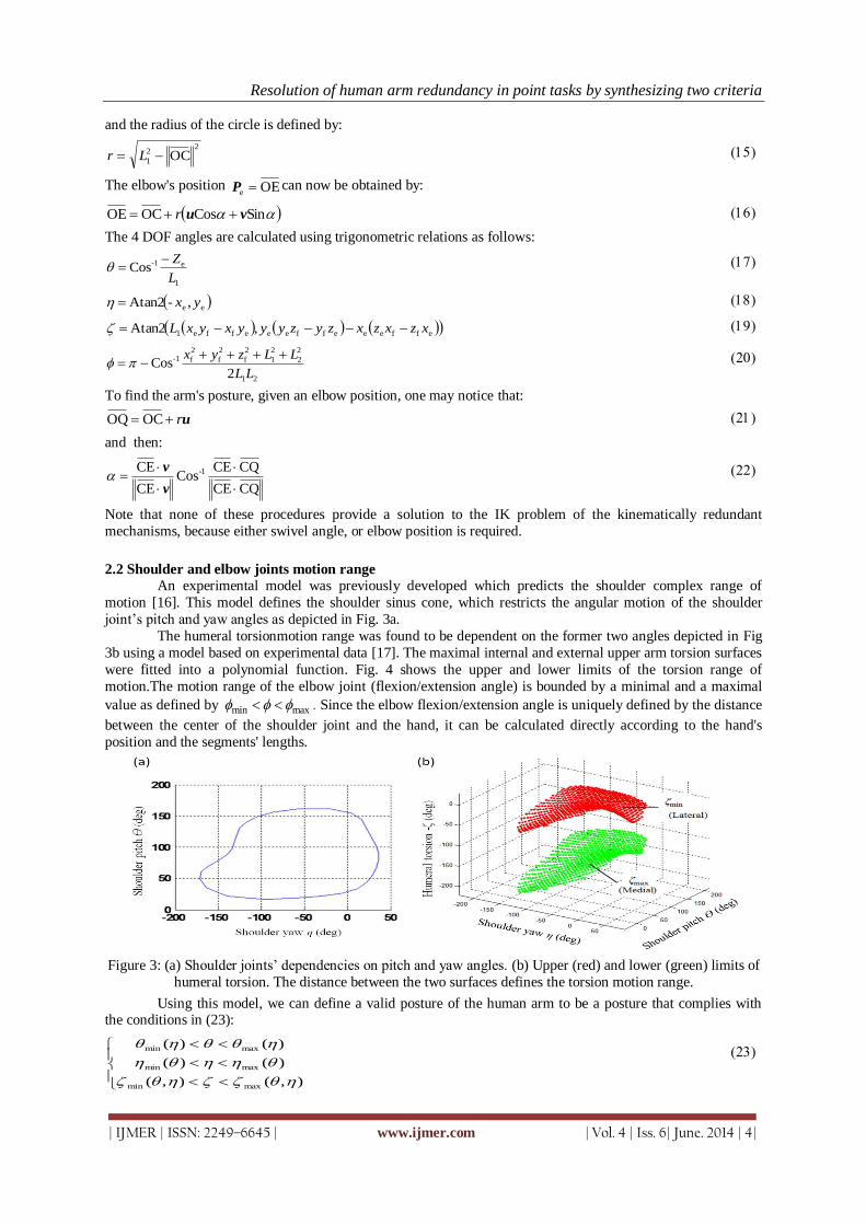
Resolution of human arm redundancy in point tasks by synthesizing two criteria
| IJMER | ISSN: 2249–6645 | www.ijmer.com | Vol. 4 | Iss. 6| June. 2014 | 4|
and the radius of the circle is defined by:
22
1 OC Lr
The elbow's position OEe P can now be obtained by:
SinCosOCOE vu r
The 4 DOF angles are calculated using trigonometric relations as follows:
1
e1-CosL
Z
ee ,-Atan2 yx
effeeeffeeeffe1 ,Atan2 xzxzxzyzyyyxyxL
21
2
2
2
1
2
f
2
f
2
f1-
2Cos
LL
LLzyx
To find the arm's posture, given an elbow position, one may notice that:
ur OCOQ
and then:
CQCE
CQCECos
CE
CE 1-
v
v
Note that none of these procedures provide a solution to the IK problem of the kinematically redundant
mechanisms, because either swivel angle, or elbow position is required.
2.2 Shoulder and elbow joints motion range
An experimental model was previously developed which predicts the shoulder complex range of
motion [16]. This model defines the shoulder sinus cone, which restricts the angular motion of the shoulder
joint’s pitch and yaw angles as depicted in Fig. 3a.
The humeral torsionmotion range was found to be dependent on the former two angles depicted in Fig
3b using a model based on experimental data [17]. The maximal internal and external upper arm torsion surfaces
were fitted into a polynomial function. Fig. 4 shows the upper and lower limits of the torsion range of
motion.The motion range of the elbow joint (flexion/extension angle) is bounded by a minimal and a maximal
value as defined by min max . Since the elbow flexion/extension angle is uniquely defined by the distance
between the center of the shoulder joint and the hand, it can be calculated directly according to the hand's
position and the segments' lengths.
Figure 3: (a) Shoulder joints’ dependencies on pitch and yaw angles. (b) Upper (red) and lower (green) limits of
humeral torsion. The distance between the two surfaces defines the torsion motion range.
Using this model, we can define a valid posture of the human arm to be a posture that complies with the conditions in (23):
),(),(
)()(
)()(
maxmin
maxmin
maxmin

Resolution of human arm redundancy in point tasks by synthesizing two criteria
| IJMER | ISSN: 2249–6645 | www.ijmer.com | Vol. 4 | Iss. 6| June. 2014 | 5|
An alternative and simpler approach to the shoulder's joint motion range is given by constant ranges to each
DOF, independent on each other. Values for joint limits can be found in anthropometric data sources [18] as in
(24):
0 180
134 48
34 97
Both approaches are used in this study, in order to compare their effect on the solution of the kinematic redundancy problem of the human arm.
2.3 Joint Range Availability (JRA) Criterion
The JRA criterion is based on the assumption that the human arm tends to adopt postures with joint
angles that are as close as possible to their mid-range values and as far as possible from their joint limits. As the
elbow joint swivels, and (theoretically) provides an infinite number of possible arm postures (solutions to the IK problem), the pitch, yaw and torsion angles of the shoulder joint are adjusted appropriately to maintain the hand
position. A valid anatomical posture is achieved if all three angles of the shoulder joint are within their
anatomical ranges of motion either according to (23) or according to (24).There is a continuous subset of valid
arm postures with a swivel angle in the range of maxmin . Based on the JRA criterion, the optimal posture
is achieved by a mean value of the swivel angle limits defined by:
2
maxminmean
Figure 4 illustrates the swivel angle limits and the optimal posture at some handposition in space.
Figure 4: Swivel angle limits and optimal posture. The solid arc denotes valid postures domain. Dashed arc
denotes invalid postures domain.
2.4Minimal Angular Displacement Criterion (MAD)
The minimal angular displacement (MAD) criterion minimizes the sum of the differences of the
various joint angles, between their initial and final values. In other words, the final arm posture defined by this
criterion yields the shortest distance between the initial and the final value of the joint angles in joint space. This
criterion can be formulated as an optimization problem using the following cost function:
2 2 2
f i f i f iMADf
where i denotes initial value and f denotes final value for the pitch, yaw, and torsion angles. However, it has
been shown experimentally that the shoulder joint velocities vary simultaneously [4]. Therefore, the shoulder
shifts directly from its initial pitch and yaw angles to its final pitch and yaw angles (see Fig. 5), and not by two
separate rotations as implied by (26). This rotation occurs about an axis that is normal to the plane formed by the shoulder (O), the initial elbow position (P1), and the elbow final position (P2). The direct rotation of the
shoulder, and the direct rotation angle are illustrated in the following figure:

Resolution of human arm redundancy in point tasks by synthesizing two criteria
| IJMER | ISSN: 2249–6645 | www.ijmer.com | Vol. 4 | Iss. 6| June. 2014 | 6|
Figure 5: The direct rotation angle δ. P1 and P2 are two elbow positions, and m is a vector normal to the plane
defined by points O, P1 and P2.
The direct rotation angle is calculated by:
21
211-CosPP
PP
and:
2 2
2 f i f i
Therefore, the cost function of MAD criterion in this study is formulated as follows:
2
2 f iMADf
Since a 4 DOF arm model is redundant by only one DOF, this optimization problem can be solved by a one degree step grid search where solving for the swivel angle that minimizes the cost function under the given
constraint, using (29).During the brute force search, the initial posture of the arm remains constant, while the
final posture varies with the value of the swivel angle, and the cost function's value changes accordingly.
2.5 Bi-Criterion Model The JRA and MAD criteria are used independently, as previously explained, to calculate the swivel
angles αJRA and αMAD,respectively. The synthesized criterion model then merges the two results by calculating
the weighted average of the swivel angle optimal as defined by:
JRAMADoptimal 1 kk
where kis a weight factor. Its value is later optimized to match experimental results with the model prediction,
and to explore its effect on the correlation with the experimental results.
2.6 Pointing Experiment
2.6.1 Subjects Definition
Ten right handed volunteer (ages 22 years to 28 years, heights 1.65 m to 1.93 m, weights 52 Kg to 94
Kg) performed unconstrained point to point movements. None of the participants reported having any clinical
symptoms or any history of motor, sensory, or neurological disorders. The subjects were naive as to the purpose
the experiment, and were only instructed to perform point to point reaching movement in a natural self-paced
way. The experimental protocol was approved by the UCSC IRB committee.
2.6.2 Experimental Setup
Subjects sat on a chair with back rest and adjustable height. They were positioned in front of a
spherical target array (see Fig. 6a and Fig. 6b) with a radius of 750 mm, such that the right shoulder was in line
with the center of the sphere.The distance between the chair and the target was adjusted for each subject so that
his/her elbow flexion angle was approximately 90⁰.
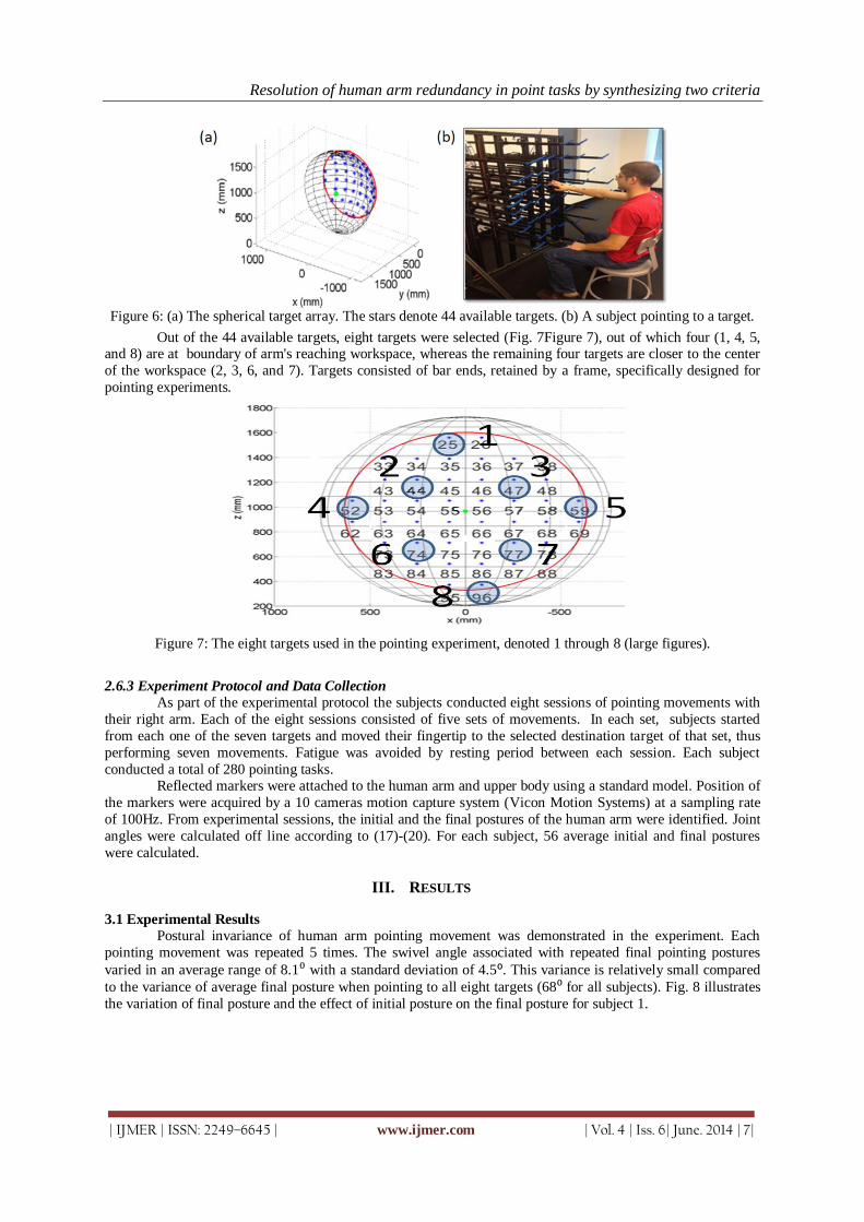
Resolution of human arm redundancy in point tasks by synthesizing two criteria
| IJMER | ISSN: 2249–6645 | www.ijmer.com | Vol. 4 | Iss. 6| June. 2014 | 7|
Figure 6: (a) The spherical target array. The stars denote 44 available targets. (b) A subject pointing to a target.
Out of the 44 available targets, eight targets were selected (Fig. 7Figure 7), out of which four (1, 4, 5, and 8) are at boundary of arm's reaching workspace, whereas the remaining four targets are closer to the center
of the workspace (2, 3, 6, and 7). Targets consisted of bar ends, retained by a frame, specifically designed for
pointing experiments.
Figure 7: The eight targets used in the pointing experiment, denoted 1 through 8 (large figures).
2.6.3 Experiment Protocol and Data Collection
As part of the experimental protocol the subjects conducted eight sessions of pointing movements with
their right arm. Each of the eight sessions consisted of five sets of movements. In each set, subjects started
from each one of the seven targets and moved their fingertip to the selected destination target of that set, thus
performing seven movements. Fatigue was avoided by resting period between each session. Each subject
conducted a total of 280 pointing tasks. Reflected markers were attached to the human arm and upper body using a standard model. Position of
the markers were acquired by a 10 cameras motion capture system (Vicon Motion Systems) at a sampling rate
of 100Hz. From experimental sessions, the initial and the final postures of the human arm were identified. Joint
angles were calculated off line according to (17)-(20). For each subject, 56 average initial and final postures
were calculated.
III. RESULTS
3.1 Experimental Results
Postural invariance of human arm pointing movement was demonstrated in the experiment. Each
pointing movement was repeated 5 times. The swivel angle associated with repeated final pointing postures
varied in an average range of 8.1⁰ with a standard deviation of 4.5⁰. This variance is relatively small compared
to the variance of average final posture when pointing to all eight targets (68⁰ for all subjects). Fig. 8 illustrates
the variation of final posture and the effect of initial posture on the final posture for subject 1.
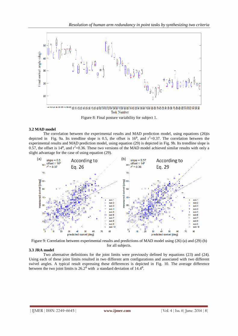
Resolution of human arm redundancy in point tasks by synthesizing two criteria
| IJMER | ISSN: 2249–6645 | www.ijmer.com | Vol. 4 | Iss. 6| June. 2014 | 8|
Figure 8: Final posture variability for subject 1.
3.2 MAD model The correlation between the experimental results and MAD prediction model, using equations (26)is
depicted in Fig. 9a. Its trendline slope is 0.5, the offset is 16⁰, and r2=0.37. The correlation between the
experimental results and MAD prediction model, using equation (29) is depicted in Fig. 9b. Its trendline slope is
0.57, the offset is 14⁰, and r2=0.36. These two versions of the MAD model achieved similar results with only a
slight advantage for the case of using equation (29).
Figure 9: Correlation between experimental results and predictions of MAD model using (26) (a) and (29) (b)
for all subjects.
3.3 JRA model
Two alternative definitions for the joint limits were previously defined by equations (23) and (24).
Using each of these joint limits resulted in two different arm configurations and associated with two different
swivel angles. A typical result expressing these differences is depicted in Fig. 10. The average difference
between the two joint limits is 26.2⁰ with a standard deviation of 14.4⁰.
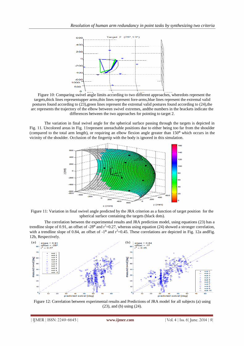
Resolution of human arm redundancy in point tasks by synthesizing two criteria
| IJMER | ISSN: 2249–6645 | www.ijmer.com | Vol. 4 | Iss. 6| June. 2014 | 9|
Figure 10: Comparing swivel angle limits according to two different approaches, wheredots represent the
targets,thick lines representupper arms,thin lines represent fore-arms,blue lines represent the extremal valid
postures found according to (23),green lines represent the extremal valid postures found according to (24),the arc represents the trajectory of the elbow between swivel extremes, andthe numbers in the brackets indicate the
differences between the two approaches for pointing to target 2.
The variation in final swivel angle for the spherical surface passing through the targets is depicted in
Fig. 11. Uncolored areas in Fig. 11represent unreachable positions due to either being too far from the shoulder
(compared to the total arm length), or requiring an elbow flexion angle greater than 150⁰ which occurs in the
vicinity of the shoulder. Occlusion of the fingertip with the body is ignored in this simulation.
Figure 11: Variation in final swivel angle predicted by the JRA criterion as a function of target position for the
spherical surface containing the targets (black dots).
The correlation between the experimental results and JRA prediction model, using equations (23) has a
trendline slope of 0.91, an offset of -28⁰ and r2=0.27, whereas using equation (24) showed a stronger correlation,
with a trendline slope of 0.84, an offset of -1⁰ and r2=0.45. These correlations are depicted in Fig. 12a andFig.
12b, Respectively.
Figure 12: Correlation between experimental results and Predictions of JRA model for all subjects (a) using
(23), and (b) using (24).
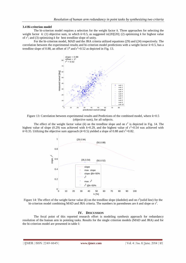
Resolution of human arm redundancy in point tasks by synthesizing two criteria
| IJMER | ISSN: 2249–6645 | www.ijmer.com | Vol. 4 | Iss. 6| June. 2014 | 10|
3.4 Bi-criterion model
The bi-criterion model requires a selection for the weight factor k. Three approaches for selecting the
weight factor k: (1) objective sum, in which k=0.5, as suggested in[20][20]; (2) optimizing k for highest value
of r2; and (3) optimizing k for best trendline slope of unity.
For the bi-criterion model, MAD and the JRA criteria utilized equations (29) and (24) respectively. The
correlation between the experimental results and bi-criterion model predictions with a weight factor k=0.5, has a
trendline slope of 0.88, an offset of 1⁰ and r2=0.52 as depicted in Fig. 13.
Figure 13: Correlation between experimental results and Predictions of the combined model, where k=0.5
(objective sum), for all subjects.
The effect of the weight factor value (k) on the trendline slope and on r2 is depicted in Fig. 14. The highest value of slope (0.29) was achieved with k=0.29, and the highest value of r2=0.54 was achieved with
k=0.35. Utilizing the objective sum approach (k=0.5) yielded a slope of 0.88 and r2=0.82.
Figure 14: The effect of the weight factor value (k) on the trendline slope (dashdot) and on r2(solid line) for the
bi-criterion model combining MAD and JRA criteria. The numbers in parentheses are k and slope or r2.
IV. DISCUSSION The focal point of this reported research effort is modeling synthesis approach for redundancy
resolution of the human arm in pointing tasks. Results for the single criterion models (MAD and JRA) and for
the bi-criterion model are presented in table I:
0 10 20 30 40 50 60 70 800
10
20
30
40
50
60
70
80
predicted swivel [deg]
me
asu
red
sw
ive
l [d
eg
]
slope = 0.88offset = 1º
r2 = 0.52
sub 1
sub 2
sub 3
sub 4
sub 5
sub 6
sub 7
sub 8
sub 9
sub 10
0 10 20 30 40 50 60 70 80 90 1000
0.2
0.4
0.6
0.8
1 (29,0.94)
(50,0.88)
(35,0.54) (50,0.52)
MAD2+JRAC
k [%]
slo
pe,
r2
slope
max. slope
slope @k=50%
r2
max. r2
r2 @k=50%
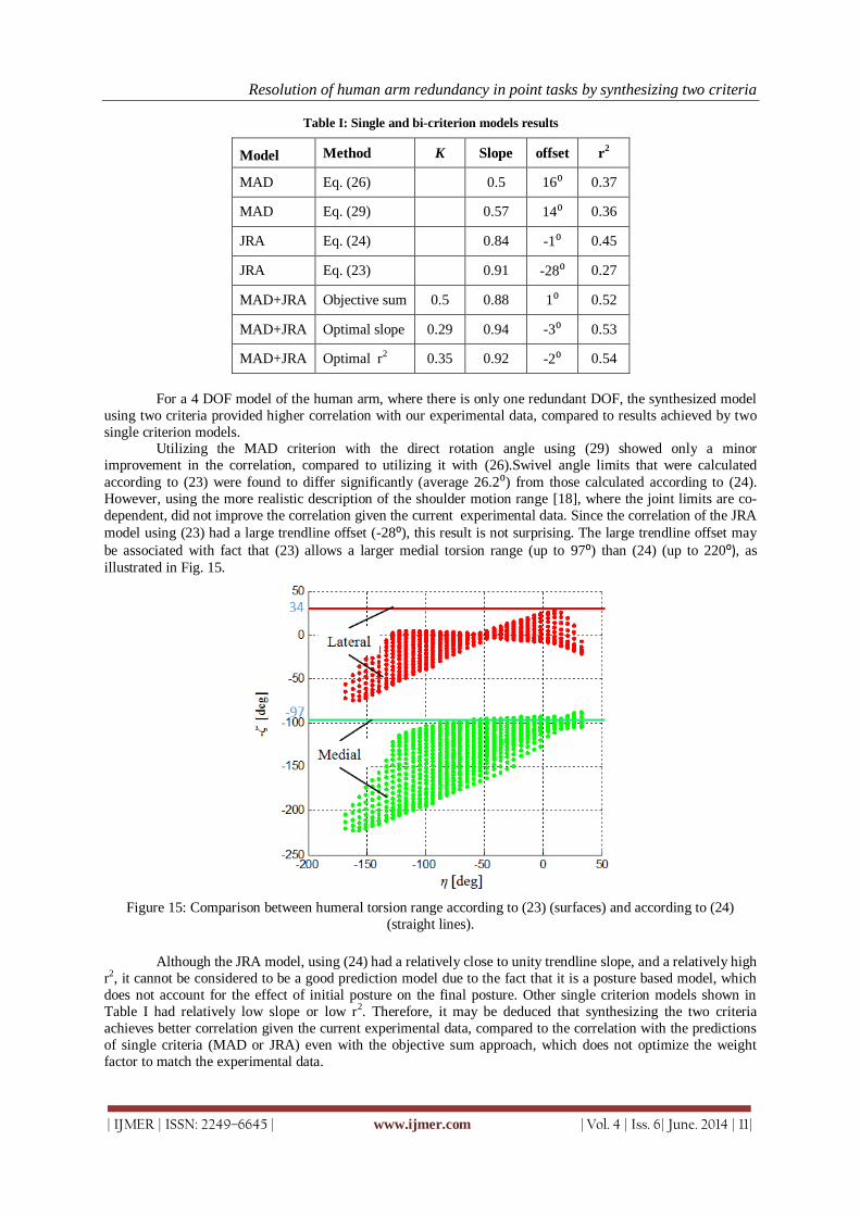
Resolution of human arm redundancy in point tasks by synthesizing two criteria
| IJMER | ISSN: 2249–6645 | www.ijmer.com | Vol. 4 | Iss. 6| June. 2014 | 11|
Table I: Single and bi-criterion models results
Model Method K Slope offset r2
MAD Eq. (26) 0.5 16⁰ 0.37
MAD Eq. (29) 0.57 14⁰ 0.36
JRA Eq. (24) 0.84 -1⁰ 0.45
JRA Eq. (23) 0.91 -28⁰ 0.27
MAD+JRA Objective sum 0.5 0.88 1⁰ 0.52
MAD+JRA Optimal slope 0.29 0.94 -3⁰ 0.53
MAD+JRA Optimal r2 0.35 0.92 -2⁰ 0.54
For a 4 DOF model of the human arm, where there is only one redundant DOF, the synthesized model
using two criteria provided higher correlation with our experimental data, compared to results achieved by two
single criterion models. Utilizing the MAD criterion with the direct rotation angle using (29) showed only a minor
improvement in the correlation, compared to utilizing it with (26).Swivel angle limits that were calculated
according to (23) were found to differ significantly (average 26.2⁰) from those calculated according to (24).
However, using the more realistic description of the shoulder motion range [18], where the joint limits are co-
dependent, did not improve the correlation given the current experimental data. Since the correlation of the JRA
model using (23) had a large trendline offset (-28⁰), this result is not surprising. The large trendline offset may
be associated with fact that (23) allows a larger medial torsion range (up to 97⁰) than (24) (up to 220⁰), as
illustrated in Fig. 15.
Figure 15: Comparison between humeral torsion range according to (23) (surfaces) and according to (24)
(straight lines).
Although the JRA model, using (24) had a relatively close to unity trendline slope, and a relatively high
r2, it cannot be considered to be a good prediction model due to the fact that it is a posture based model, which
does not account for the effect of initial posture on the final posture. Other single criterion models shown in
Table I had relatively low slope or low r2. Therefore, it may be deduced that synthesizing the two criteria
achieves better correlation given the current experimental data, compared to the correlation with the predictions
of single criteria (MAD or JRA) even with the objective sum approach, which does not optimize the weight
factor to match the experimental data.

Resolution of human arm redundancy in point tasks by synthesizing two criteria
| IJMER | ISSN: 2249–6645 | www.ijmer.com | Vol. 4 | Iss. 6| June. 2014 | 12|
Previous research efforts indicated that correlation of alternative criteria such as the minimal work and
minimal torque change were associated with a slope of 0.3 and r2=0.56 for both criteria [5]. Using the minimum
peak kinetic energy criterion[4] led to correlation with slope of approximately 1 and r2 in the range of 0.522 to 0.915 using a database of four subjects.
Future work will focus on examining the various approaches for integrating criteria (objective sum,
min-max, and global sum), and on finding an optimal combination of several criteria to achieve good correlation
with experimental data.
Redundancy resolution of articulated serial mechanism such as human or robotic arm has applications
in the field of wearable robotics [21,22], where the robot and human body are physically coupled and the need
to implement a redundancy resolution algorithm into the control system of the robot is essential to guarantee
natural integration between the two systems. Additional application that may benefit for a solution the problem
under study might be simulations in ergonomics and computer graphics.
REFERENCES [1] A.P. Georgopoulos, J.F. Kalaska, and J.T. Massey, Spatial Trajectories and Reaction-Times of Timed Movements –
Effects of Practice, Uncertainty, and Change in Target Location, Journal of Neurophysiology, 46, 1981, 725–743. [2] J.F. Soechting and F. Lacquaniti, Invariant Characteristics of a Pointing Movement in Man, Journal of Neuroscience,
1, 1981, 710–720.
[3] J.F. Soechting, C.A. Buneo, U. Herrmann and M. Flanders, Moving Effortlessly in 3-Dimensions – Does Donders-Law Apply to Arm Movement, Journal of Neuroscience, 15, 1995, 6271–6280.
[4] A. Biess, D.G. Liebermann and T. Flash, A Computational Model for Redundant Human Three-Dimensional Pointing Movements: Integration of Independent Spatial and Temporal Motor Plans Simplifies Movement Dynamics, The Journal of Neuroscience, 27, 2007, 13045-13064.
[5] M.A. Admiraal, M.J. Kuster and S. Gielen, Modeling Kinematics and Dynamics of Human Arm Movements, Motor Control, 8, 2007, 312-338.
[6] Y. Uno, M. Kawato, and R. Suzuki, Formation and Control of Optimal Trajectory in Human Multijoint Arm Movement – Minimum Torque-Change Model, Biological Cybernetics, 61, 1989, 89-101.
[7] E.S. Jung, D. Kee and M.K. Chung, Upper Body Reach Posture Prediction for Ergonomic Evaluation Models, International Journal of Industrial Ergonomics, 16, 1995, 95-107.
[8] Z. Mi, J. Yang and K. Abdel-Malek, Optimization-Based Posture Prediction for Human Upper Body, Robotica, 27, 2008, 607–620.
[9] E.S. Jung, J. Choe and S.H. Kim, Psychophysical Cost Function of Joint Movement for Arm Reach Posture Prediction, Proc. of the Human Factors and Ergonomics Society 38th Annual Meeting, 636-640, 1994.
[10] D.E. Whitney, Resolved Motion Rate Control of Manipulators and Human Prostheses, IEEE Transactions on Man-Machine Systems, 10, 1969, 47-53.
[11] R.T. Marler, J. Yang, J.S. Arora, and K. Abdel-Malek,Study of Bi-Criterion Upper Body Posture Prediction using Pareto Optimal Sets, Proc. of the Fifth IASTED International Conference, 229-234, 2005.
[12] P. Vetter, T. Flash, D.M. Wolpert, Planning Movements in a Simple Redundant Task,Curr. Biol., 12, 2002, 488–491.
[13] T. Okadome, and M. Honda, Kinematic Construction of the Trajectory of Sequential Arm Movements, Biol. Cybern., 80, 1999, 157-169.
[14] F. Hermens, and S. Gielen, Posture-Based or Trajectory-Based Movement Planning: a Comparison of Direct and Indirect Pointing Movements, Exp. Brain Res., 159, 2004, 340–348.
[15] D. Tolani, A. Goswami, and N. I. Badler, Real-Time Inverse Kinematics Techniques for Anthropomorphic Limbs, Graphical Models, 62, 2000, 353-388.
[16] Engin, A.E. and Chen S.M., Statistical Data Base for the Biomechanical Properties of the Human Shoulder Complex—I: Kinematics of the Shoulder Complex, Journal of Biomechanical Eng., 1986.
[17] X. Wang, M. Maurin, F. Mazet, N.D.C. Maia, K. Voinot, J.P. Verriest, and M. Fayet, Three-Dimensional Modeling of the Motion Range of Axial Rotation of the Upper Arm, Journal of Biomechanics, 31, 1998, 899-908.
[18] Chaffin, Andersson, and Martin, Occupational Biomechanics, Wiley, 1984.
[19] J. Rosen and J.C. Perry, Upper Limb Powered Exoskeleton,Journal of Humanoid Robotics, 4, 2007, 1–20.
[20] J. Yang, T. Marler, and S. Rahmatalla, Multi-objective optimization-based method for kinematic posture prediction:development and validation, Robotica, 29, 2011, 245-253.
[21] J. C. Perry, J. Rosen, and S. Burns, Upper-Limb Powered Exoskeleton Design, IEEE Transactions on Mechatronics, 12(4), 2007, 408-417.
[22] H. Kim, L. M. Miller, A. Al-Refai, M. Brand, and J. Rosen, Redundancy Resolution of a Human Arm for Controlling a Seven DOF wearable Robotic System,33rd Annual International Conference of the IEEE Engineering in Medicine and Biology Society (EMBC), Boston MA, 2011.

International
OPEN ACCESS Journal Of Modern Engineering Research (IJMER)
| IJMER | ISSN: 2249–6645 | www.ijmer.com | Vol. 4 | Iss. 6| June. 2014 | 13|
Earthquake Resistance Design-Impact On Cost Of Reinforced
Concrete Builidings
T. Anusha1, S. V. Narsi Reddy
2, T. Sandeep
3
1Student, Department of Civil Engineering (M.Tech Structures), Malla Reddy Engineering college,
Hyderabad, Telangana State, India 2Associate Professor, Department of Civil Engineering, Malla Reddy Engineering college, Hyderabad,
Telangana State, India 3Assistant Professr,Department of Civil Engineering,Malla Reddy Engineering College,
Hyderabad,Telagana State,India
I. INTRODUCTION Vibrations of the earth‟ s surface caused by waves coming from a source ofdisturbances inside the
earth are described as earthquake. By far the most important earthquake from an engineering standpoint is of tectonic origin, that is,those associated with large scale strains in the crust of the earth. Almost any building can
be designed it be earthquake resistant provided its site is suitable.Buildings suffer during an earthquake
primarily because horizontal forces are exerted on a structure that often meant to contend only with vertical
stresses. The important point to be highlighted is that accurate prediction will help save lives,but structures have
to be engineered to withstand appropriate forces depending on the seismiczone where they are located.If the
building material is week in tension such as brick or stone masonry cracking occurs which reduces the effective
area for resisting bending moment. It follows that the strength in tension and shear is importantfor earthquake
resistance.
The extent of damage to a building depend much on the strength, ductility, and integrity of a building
and the stiffness of ground beneath it in a given intensity of the earthquakes motions. The following properties
and parameters are most important from the point of view of
the seismic design. (i) Building material properties
Strength in compression, tension and shear, including dynamic effects
Unit weight
Modulus of elasticity
(ii) Dynamic characteristics of building components.
II. ANALYSIS SIGNIFICANCE Seismic analysis or earthquake analysis is a subset of structural analysis and is the calculation of the
response of a structure to the earthquakes. A structure has the potential to waveback and forth during an earthquake this is called the fundamental mode and is the lowes tfrequency of the structure response. However,
buildings also have higher modes of response,which are uniquely activated during an earthquake.
The analysis process can be categorized on the basis of three factors, the type of externally applied
loads, the behaviour of the structure or the structural material and the type of structural modal selected.
Importance of seismic analysis:
Abstract: Earthquakes strike suddenly, violently and without warning at any time of the day or night.It is highly impossible to prevent an earthquake from occuring, but the damage to the builiding can be
controlled through proper design and detailing. Hence it is mandatory to do the sesmic analysis and
design to structure against collapse. This study addresses the performance and variation of precentage
steel and concrete quantity of R.C framed structure in different seismic zones and influence on overall
cost of construction. This study mainly focuses on the comparision of percentage steel and concrete
quantities when the builiding is designed for gravity loads as per IS 456:2000 and when the builiding is
designed for earthquake forces in different seismic zones as per IS 1893:2002. A five storied R.C.C
framed structure has been analyse and designed using STAAD ProV8i. Ductile detailing has been done
in conformation with IS:13920
Keywords: Earthquake, seismic analysis, seismic zones, overall cost.

Earthquake Resistance Design-Impact On Cost Of Reinforced Concrete Builidings
| IJMER | ISSN: 2249–6645 | www.ijmer.com | Vol. 4 | Iss. 6| June. 2014 | 14|
1. Resist minor level of earthquake ground motion without damage
2. Resist moderate level of earthquake motion without structural damage, possible experience non-structural
damage. 3. Resist severe earthquake ground motion having intensity equal to the strongest shaking experienced at the
site, without collapse of structure as well known as non-structural damage.
III. OBJECTIVE OF THE STUDY 1. To prevent loos of life, serious injury and to prevent buildings from collapse and dangerous damage
under maximum intensity earthquakes.
2. To ensure buildings against irreparable damage under moderate to heavy earthquake. The strength built
into the structure alone cannot create and earthquake resistant design, it also requires absorption, which
means that structure should have predictable ductility as wellas strength. 3. The damping characteristics of a structure have a major effect on its response to ground motion because
small amount of damping significantly reduces the maximum deflection to resonant response of the
structure.
IV. METHODOLOGY Seismic analysis of the structures is carried out on the basis of lateral force assumed to act along with
the gravity loads. In this study, a five (G+4) storied RC building has been analyzed using the equivalent static
method in STAAD-Pro V8i.In the earthquake analysis along with earthquake loads, vert ical loads are also
applied. For the earthquake analysis, IS 1893-2002 code was used.
4.1 Preliminary Data for the problem taken:
Type of the structure : RCC Framed structure
Number of stories : G+4
floor to floor height : 3.6 m
Plinth height : 0.6 m
Walls thickness : 230 mm
Grade of concrete : M 25
Grade of steel : Fe 415
Earthquake load : As per IS1893 (Part 1) : 2002
Size of the columns : 0.4mx0.4m and 0.45mx0.45m
Size of the beams : 0.23mx0.4m
Slab thickness : 0.13m
SBC of soil taken : 200kN/m²
Live load : 3kN/m²
Floor finishes : 1kN/m²
Seismic zones considered : II,III,IV,V
4.2 Loading Data:
Dead Load (DL)
1. Self weight of slab = 0.13x25 = 3.25kN/m2
2. Floor finishes = 1.00kN/m2
Total DL = 4.25kN/m2
(Assume 130mm total depth of slab)
3. Weight of walls = 0.23x19x 3.6 = 15.73kN/m
Live Load (LL)
Live Load on each slab = 3.00kN/m2
Earthquake Load (EL)
As per IS-1893 (Part 1): 2002.

Earthquake Resistance Design-Impact On Cost Of Reinforced Concrete Builidings
| IJMER | ISSN: 2249–6645 | www.ijmer.com | Vol. 4 | Iss. 6| June. 2014 | 15|
4.3 Loading combinations:
The following load combinations are used in the seismic analysis, as mentioned in the code IS
1893(Part-1): 2002.
1. 1.5(DL+LL)
2. 1.2(DL+LL+EQX)
3. 1.2(DL+LL- EQX)
4. 1.2(DL+LL+ EQZ)
5. 1.2(DL+LL- EQZ)
6. 1.5(DL+ EQX)
7. 1.5(DL- EQX)
8. 1.5(DL+ EQZ)
9. 1.5(DL-EQZ)
10. 0.9DL+ 1.5EQX
11. 0.9DL- 1.5EQX
12. 0.9DL+ 1.5EQZ
13. 0.9DL-1.5EQZ
Earthquake load was considered in +X,-X, +Z and –Z directions. Thus a total of 13 load combinations
are taken for analysis. Since large amount of data is difficult to handle manually all the load combinations are
analyzed using software STAAD Pro. All the load combinations are mentioned above.
Fig.1 Plan of the building
Fig.2: Nomenclature of columns
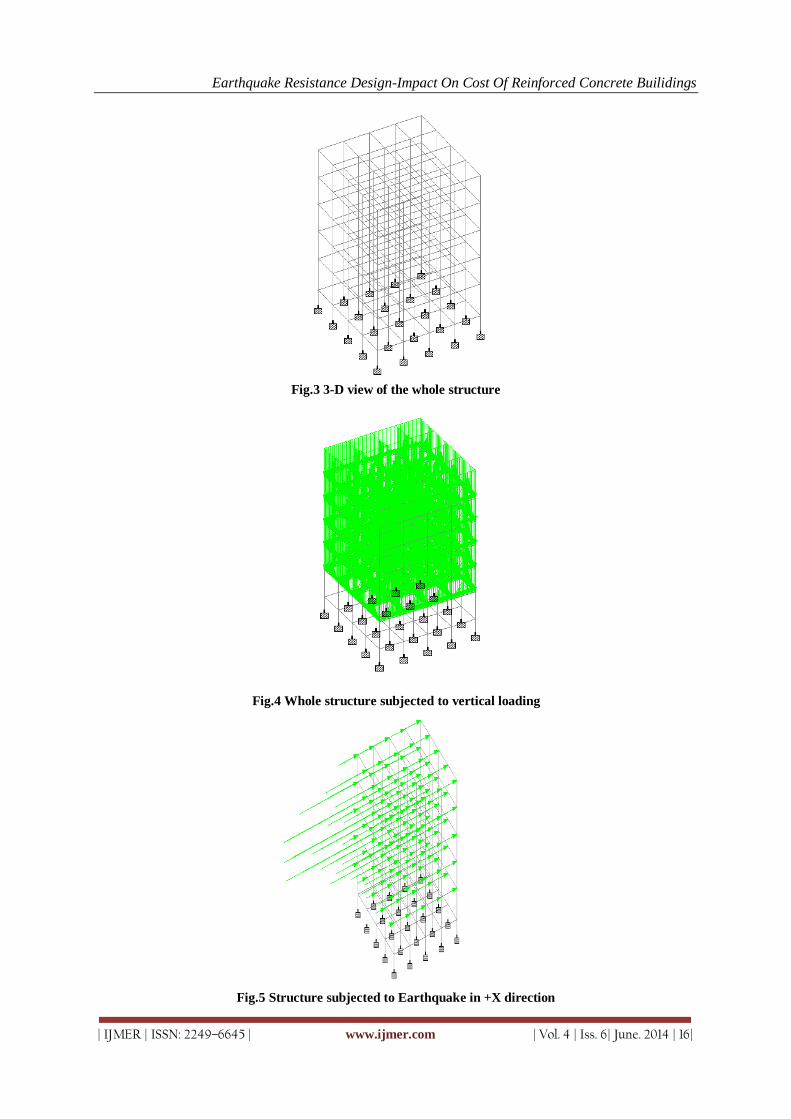
Earthquake Resistance Design-Impact On Cost Of Reinforced Concrete Builidings
| IJMER | ISSN: 2249–6645 | www.ijmer.com | Vol. 4 | Iss. 6| June. 2014 | 16|
Fig.3 3-D view of the whole structure
Fig.4 Whole structure subjected to vertical loading
Fig.5 Structure subjected to Earthquake in +X direction
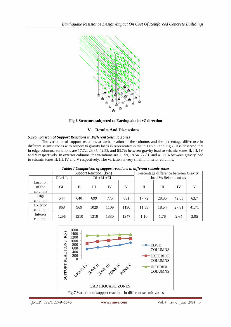
Earthquake Resistance Design-Impact On Cost Of Reinforced Concrete Builidings
| IJMER | ISSN: 2249–6645 | www.ijmer.com | Vol. 4 | Iss. 6| June. 2014 | 17|
Fig.6 Structure subjected to Earthquake in +Z direction
V. Results And Discussions
5.1comparison of Support Reactions in Different Seismic Zones The variation of support reactions at each location of the columns and the percentage difference in
different seismic zones with respect to gravity loads is represented in the in Table I and Fig.7. It is observed that
in edge columns, variations are 17.72, 28.35, 42.53, and 63.7% between gravity load to seismic zones II, III, IV
and V respectively. In exterior columns, the variations are 11.59, 18.54, 27.81, and 41.71% between gravity load
to seismic zones II, III, IV and V respectively. The variation is very small in interior columns.
Table: I Comparison of support reactions in different seismic zones
Support Reaction (ken) Percentage difference between Gravity
load Vs Seismic zones DL+LL DL+LL+EL
Location
of the
columns
GL II III IV V II III IV V
Edge
columns 544 640 699 775 891 17.72 28.35 42.53 63.7
Exterior
columns 868 969 1029 1109 1130 11.59 18.54 27.81 41.71
Interior
columns 1296 1310 1319 1330 1347 1.10 1.76 2.64 3.95
Fig.7 Variation of support reactions in different seismic zones
0200400600800
1000120014001600
SU
PP
OR
T R
EA
CT
ION
S (
KN
)
EARTHQUAKE ZONES
EDGE
COLUMNS
EXTERIOR
COLUMNS
INTERIOR
COLUMNS

Earthquake Resistance Design-Impact On Cost Of Reinforced Concrete Builidings
| IJMER | ISSN: 2249–6645 | www.ijmer.com | Vol. 4 | Iss. 6| June. 2014 | 18|
5.2 Comparison of Volume of Concrete in Footings in Different Seismic Zones
The variation of volume of concrete at each location of the column footing and the increase in
percentage difference in different seismic zones with respect to gravity loads is represented in the in Table II and Fig.8. It is observed that in edge column footings, variations are 17.75, 17.75, 27.17 and 42.0% between
gravity load to seismic zones II, III, IV and V respectively. In exterior column footings, the variations are 21.51,
21.51, 45.15 and 57.77% between gravity load to seismic zones II, III, IV and V respectively. Therefore, the
volume of concrete in footings is increasing in seismic zones III, IV and V due to increase of support reactions
due to lateral forces. However the variation is very small in interior column footings.
Table II Comparison of volume of concrete in footings in different seismic zones
Volume of concrete in footings (cu m) Percentage difference between
Gravity load Vs Seismic zones DL+LL DL+LL+EL
Location of
the columns
footings
GL II III IV V II III IV V
Edge 2.18 2.57 2.57 2.78 3.10 17.75 17.75 27.17 42.0
Exterior 1.50 1.83 1.83 2.186 2.376 21.51 21.51 45.15 57.77
Interior 3.29 3.29 3.29 3.40 3.40 0.0 0.0 3.51 3.51
Fig.8 Variation of volume of concrete in footings in different seismic zones
5.3 Comparison of Weight of the Steel in Footings in Different Seismic Zones
The variation of weight of steel at each location of the column footing and the percentage difference in
different seismic zones with respect to gravity loads is represented in the in Table III and Fig.9. It is observed that in edge column footings, variations are 0.0, 23.61, 47.92, and 98.96% between gravity load to seismic zones
II, III, IV and V respectively. In exterior column footings, the variations are 38.17, 54.88, 70.79 and 91.04%
between gravity loads to seismic zones II, III, IV and V respectively. In the interior columns footings, the
variations are 22.07, 42.44, 56.03 and 67.91% between gravity loads to seismic zones II, III, IV and V
respectively
Table III Comparison of weight of the steel in footings in different seismic zones
Weight of the steel in footings (kg) Percentage difference between Gravity
load Vs Seismic zones DL+LL DL+LL+EL
Location of
the column
footings
GL II III IV V II III IV V
Edge 28.80 28.80 35.60 42.60 57.30 0.00 23.61 47.92 98.96
Exterior 46.90 64.8 72.64 80.10 89.60 38.17 54.88 70.79 91.04
Interior 58.90 71.9 83.9 91.9 98.9 22.07 42.44 56.03 67.91
0
0.5
1
1.5
2
2.5
3
3.5
4
CO
NC
RE
TE
IN
(C
U M
)
EDGE
FOOTINGS
EXTERIOR
FOOTINGS
INTERIOR
FOOTINGS

Earthquake Resistance Design-Impact On Cost Of Reinforced Concrete Builidings
| IJMER | ISSN: 2249–6645 | www.ijmer.com | Vol. 4 | Iss. 6| June. 2014 | 19|
Fig. 9 Variation of weight of steel in footings in different seismic zones
5.4 Comparison of Percentage of the Steel in Columns in Different Seismic Zones
The variation of percentage of steel at each location of the column in different seismic zones with
respect to gravity loads is represented in the in Table IV and Fig 10. The variation of percentage of steel in edge
columns vary from 0.8% to 3%, exterior columns varying from 0.8% to 3.9% and interior columns varying
from 1.1% to 3.7% between gravity loads to zone V. For the comparison purpose at each location, the cross
sectional dimension of column was kept same in all the zones.
Table IV Comparison of percentage of the steel in columns in different seismic zones
Percentage of the steel reinforcement in the columns
DL+LL DL+LL+EL
Location of the
columns GL II III IV V
Edge 0.8 0.9 1 1.5 3
Exterior 0.8 0.9 1.5 2.3 3.9
Interior 1.1 1.3 1.8 2.4 3.7
Note: for the comparison purpose at each location , the cross section of columns was kept in all the
zones
Fig. 10 Variation of percentage of steel in columns in different seismic zones
0.00
20.00
40.00
60.00
80.00
100.00
120.00
WE
IGH
T O
F S
TE
EL
IN
( K
G'S
)
TYPE OF LOADING
EDGE
FOOTINGS
EXTERIOR
FOOTINGS
0
0.5
1
1.5
2
2.5
3
3.5
4
4.5
PE
RC
EN
TA
GE
OF
ST
EE
L
TYPE OF LOADING
EDGE COLUMNS
EXTERIOR
COLUMNS
INTERIOR
COUMNS

Earthquake Resistance Design-Impact On Cost Of Reinforced Concrete Builidings
| IJMER | ISSN: 2249–6645 | www.ijmer.com | Vol. 4 | Iss. 6| June. 2014 | 20|
5.5 Comparison of Percentage of the Steel in Beams in Different Seismic Zones
The variation of percentage of steel in beams in different seismic zones with respect to gravity loads is
represented in the in Table V and Fig.11. The variation of percentage of steel at supports, in external beams 0.54% to 1.23% and in internal beams 0.78% to 1.4% varying from gravity loads to zone V. At mid span
locations of external and internal beams, the percentage of reinforcement is same in all the zones.
Table V Comparison of percentage of the steel in beams in different seismic zones
Percentage of the steel reinforcement in the beams
DL+LL DL+LL+EL
Location of the
columns
Beams GL II III IV V
At supports External 0.54 0.64 0.75 0.93 1.23
Internal 0.78 0.83 0.97 1.18 1.4
At mid span External 0.32 0.32 0.32 0.32 0.32
Internal 0.42 0.42 0.42 0.42 0.42
Note: for the comparison purpose at each location , the cross section of beams was kept in all the zones
Fig11 Percentage of steel in beams in different seismic zones
5.6 Comparison of Weight of the Steel in Beams in Different Seismic Zones:
The variation of weight of steel at each location of the beams and the percentage difference in different
seismic zones with respect to gravity loads is represented in the in Table VI and Fig.12. It is observed that in
external beams, variations are 4.38, 13.8, 31.3, and 49.6% between gravity loads to seismic zones II, III, IV and
V respectively. In the internal beams, the variations are 3.07, 15.3, 20.2 and 53.3% between gravity loads to
seismic zones II, III, IV and V respectively.
Table VI Comparison of weight of the steel in beams in different seismic zones
Weight of the steel (kg) Percentage difference between
Gravity load Vs Seismic zones DL+LL DL+LL+EL
Beams GL II III IV V II III IV V
External 137 143 156 180 205 4.38 13.8 31.3 49.6
Internal 163 168 188 196 250 3.07 15.3 20.2 53.3
Note: For the comparison purpose at each location, the cross sectional dimension of beams was kept
same in all the zones.
00.20.40.60.8
11.21.41.6
PE
RC
EN
TA
GE
OF
ST
EE
L
TYPE OF LOADING
AT SUPPORTS
EXTERNAL
BEAMSAT SUPPORTS
INTERNAL
BEAMSAT MID SPAN
INTERNAL
BEAMS

Earthquake Resistance Design-Impact On Cost Of Reinforced Concrete Builidings
| IJMER | ISSN: 2249–6645 | www.ijmer.com | Vol. 4 | Iss. 6| June. 2014 | 21|
Fig. 12 Variation of weight of steel in beams in different seismic zones
5.7 Volume of Concrete for the Total Building and Percentage Variation of Concrete Non Earthquake
Design Vs Earthquake Design
The total quantity of the concrete for the building has shown in table VII, for the entire earthquake and
non earthquake zone and the percentage variation of the concrete for earthquake vs. non earthquake zones
shown in table 8.
Table VII Volume of concrete for the total building
Type of loading Volume of concrete (Culm)
Gravity loads [DL+LL] 406.8
Zone II [DL+LL+EL] 412.82
Zone III [DL+LL+EL] 414.7
Zone IV [DL+LL+EL] 417.75
Zone V [DL+LL+EL] 422.36
Fig. 13 Volume of concrete in all the earthquake and non earthquake zones
Table VIII Percentage variation the volume of concrete for earthquake design Vs non earthquake design
Type of loading Percentage difference
Gravity loads Vs Zone II 1.479
Gravity loads Vs Zone III 1.94
Gravity loads Vs Zone IV 2.69
Gravity loads Vs Zone V 3.824
0
50
100
150
200
250
300
WE
IGH
T O
F S
TE
EL
IN
(K
G'S
)
TYPE OF LOADING
EXTERNAL
BEAMS
395
400
405
410
415
420
425
Gravity Zone II Zone III Zone IV Zone V
VO
LU
ME
OF
CO
NC
RE
TE
(CU
.M)
TYPE OF LOADING

Earthquake Resistance Design-Impact On Cost Of Reinforced Concrete Builidings
| IJMER | ISSN: 2249–6645 | www.ijmer.com | Vol. 4 | Iss. 6| June. 2014 | 22|
Fig. 13.1 Percentage variation of the concrete quantity in different zones
5.8 Quantity of Steel for the Total Building and Percentage Variation of Steel Non-Earthquake Design Vs Earthquake Design:
The total quantity of the steel for the building has shown in Table IX, for the entire earthquake and non
earthquake zones, and the percentage variation of the weight of the steel for earthquake vs. non- earthquake
designs shown in Table 10.
Table IX Weight of the steel for the total building in different seismic zones
Type of loading Weight of steel
(Tonnes)
Gravity loads [DL+LL] 20.92
Zone II [DL+LL+EL] 23.62
Zone III [DL+LL+EL] 24.76
Zone IV [DL+LL+EL] 29.58
Zone V [DL+LL+EL] 39.55
Fig. 14 Quantity of the steel in all the earthquake and non earthquake zones
Table X Percentage variation of the quantity of steel for earthquake and non earthquake designs
Type of loading Percentage difference
Gravity loads Vs Zone II 12.96
Gravity loads Vs Zone III 18.35
Gravity loads Vs Zone IV 41.395
Gravity loads Vs Zone V 89.10
0
0.5
1
1.5
2
2.5
3
3.5
4
4.5
GL vs
ZONE II
GL vs
ZONE III
GL vs
ZONE IV
GL vs
ZONE V
PE
RC
EN
TA
GE
VA
RIA
TIO
N
COMPARISON OF ZONES
PERCENTAGE
VARIATION OF …
0
5
10
15
20
25
30
35
40
45
WE
IGH
T O
F S
TE
EL
IN
(TO
NN
ES
)
TYPE OF LOADING

Earthquake Resistance Design-Impact On Cost Of Reinforced Concrete Builidings
| IJMER | ISSN: 2249–6645 | www.ijmer.com | Vol. 4 | Iss. 6| June. 2014 | 23|
Fig14.1 Percentage variation of the steel quantity in different zones
5.9 Total Cost of the Building for All the Seismic Zones:
The total cost of the building for the design with respect to gravity loads and all the seismic zones as
shown Table XI, and the variation of percentage of cost for non-earthquake vs. earthquake designs shown in
Table 12.
Table XI Cost of the building for all the earthquake and non earthquake zones
Type of the loading Cost of the building Cost of the building
Per (sft)
Cost of the building
Per (sq m)
Gravity loads [DL+LL] 1,16,68,472 834/- 9115.99/-
Zone II [DL+LL+EL] 1,19,64,319 854/- 9347.12/-
Zone III [DL+LL+EL] 1,20,57,329 862/- 9419.78/-
Zone IV [DL+LL+EL] 1,25,00,188 892/- 9765.77/-
Zone V [DL+LL+EL] 1,33,71,609 995/- 10446.56/-
Fig. 15 Cost of the building in all the zones
Table XII Comparison of percentage variation of the cost for the building in earthquake and non earthquake
designs
Type of the loading % difference
Gravity loads Vs Zone II 2.53
Gravity loads Vs Zone III 3.33
Gravity loads Vs Zone IV 7.12
Gravity loads Vs Zone V 14.59
12.90618.355
41.395
89.053
0
10
20
30
40
50
60
70
80
90
100
GL vs II GL vs III GL vs IV GL vs V
COST
VARIATION
TYPE OF LOADING
PE
RC
EN
TA
GE
DIF
FE
NC
E
10500000
11000000
11500000
12000000
12500000
13000000
13500000
CO
ST
O
F T
HE
B
UIL
DIN
G
TYPE OF LOADING
cost of the building

Earthquake Resistance Design-Impact On Cost Of Reinforced Concrete Builidings
| IJMER | ISSN: 2249–6645 | www.ijmer.com | Vol. 4 | Iss. 6| June. 2014 | 24|
Fig. 15.1 Percentage of the cost variation for the building with earthquake and without earthquake
5.10 Cost Comparison Of Ductile Detailing Vs Non Ductile Detailng Of The Building:
The cost comparison for the ductile detailing and non ductile detailing as shown in the Table 13. Hear
the cost variation only due to the increasing of steel in ductile detailing. The variation of cost in ductile detailing
vs. non ductile detailing is nearly 4 percent.
Table XIII Steel quantity and cost difference for the building with ductile and without ductile detailing
Ductile Non ductile % difference
Weight of steel 46.2 T 39.6 T 16.66
Cost of the building 1,39,15,086.14/- 1,33,71,608.81/- 4.06
VI. Conclusions 1. The variation of support reactions in exterior columns increasing from 11.59% to 41.71% and in edge
columns increasing from 17.72% to 63.7% in seismic Zones II to V. However the variations of support
reactions are very small in interior columns.
2. The volume of concrete in exterior and edge column footings is increasing in seismic zones III, IV and V
due to increase of support reactions with the effect of lateral forces. However the variation is very small
in interior column footings.
3. It is observed that the weight of steel in edge column footings between gravity loads to zone II, III, IV
and V varies as 0, 23.6, 47.9 and 98.9 % respectively.
4. It is observed that the weight of steel in exterior column footings between gravity loads to zone II, III, IV
and V varies as 38.1, 54.8, 70.7 and 91.04 % respectively.
5. It is observed that the weight of steel in interior column footings between gravity loads to zone II, III, IV and V varies as 22.07, 42.4, 56.03, and 67.9% respectively.
6. The percentage variation of steel in edge, exterior and interior columns varies from 0.8-3%, 0.8-3.9% and
1.1-3.7% between gravity loads to seismic zone V respectively.
7. The variation of percentage of steel at support sections in external beams is 0.54% to 1.23% and in
internal beams is 0.78% to 1.4%.
8. In the external and internal beams, the percentage of bottom middle reinforcement is almost same for
both earthquake and non earthquake designs.
9. Percentage variation of total concrete quantity for the whole structure, between gravity load and seismic
zones II, III, IV and V varies as 1.4, 1.94, 2.69 and 3.8 respectively.
10. Percentage variation of total steel quantity for the whole structure, between gravity load and seismic
zones II, III, IV and V varies as 12.96, 18.35, 41.39 and 89.05 respectively.
11. It is observed that the percentage variation of cost for the whole structure, between gravity load and seismic zones II, III, IV and V varies as 2.53, 3.33, 7.17 and 14.59 respectively.
12. It is observed that the cost of the building per SFT with the design for
13. Gravity loads -----------834 /-
14. Zone II-------------------854 /-
15. Zone III------------------862/-
16. Zone IV-----------------892/-
2.543.33
7.13
14.60
0
2
4
6
8
10
12
14
16
GL&II GL&III GL&IV GL&V
% DIFFRENCE
PE
RC
EN
TA
GE
DIF
FR
EN
CE
TYPE OF LOADING

Earthquake Resistance Design-Impact On Cost Of Reinforced Concrete Builidings
| IJMER | ISSN: 2249–6645 | www.ijmer.com | Vol. 4 | Iss. 6| June. 2014 | 25|
17. Zone V------------------995/-
18. It is observed that the cost of the building per Sq m with the design for
19. Gravity loads ------------9115.9/- 20. Zone II-------------------9347.12 /-
21. Zone III------------------9419.78/-
22. Zone IV------------------9765.77/-
23. Zone V------------------10446.56/-
24. The percentage increase of steel for the whole structure with ductile detailing compared to non ductile
detailing is 16%.
25. The percentage increase in cost for the whole structure with ductile detailing compared to non ductile
detailing is 4.06%
REFERENCES [1.] Andreas J. Kappos, Alireza Manafpour (2001), “Seismic Design of R.C Buildings with the Aid of Advanced
Analytical Techniques”, Engineering Structures, Elsevier, 23, 319-332.
[2.] B. Suresh, P.M.B raj kiran Nanduri(2012) “earthquake analysis and design vs. non earth quake analysis and design using Staad pro” , international journal of advanced engineering and technology, vol III/IssueIV/oct-Dec,2012/104-106.
[3.] Design Aids for Reinforced concrete to IS: 456-1978(SP-16), Bureau of Indian standards, New Delhi. [4.] Durgesh C. Rai (2005) “The guidelines for seismic evaluation and strengthening of buildings” Department of Civil
Engineering, IIT Kanpur. [5.] Government of Andhra Pradesh [Standard schedule rates for 2012-13(SSR)]. [6.] H.J. Shah and Sudhir K. Jain (2008), “Final Report: A -Earthquake Codes IITK-GSDMA Project on Building
Codes (Design Example of a Six Storey Building)”, IITK-GSDMA-EQ26-V3.0 [7.] H. M. Salem, A. K. El-Fouly, H.S. Tagel-Din (2011), “Toward an Economic Design of Reinforced Concrete
Structures against Collapse”, Engineering Structures, Elsevier, 33, 3341-3350. [8.] IS: 875 part II-1987 Indian Standard Code of Practice for Design Loads (Other Than Earthquake) for Buildings
and Structures Part 2 Imposed Loads. [9.] IS: 1893 (PART 1)-2002 “Criteria For Earthquake Design Of Structures: General provisions and buildings”(Fifth
revision), Bureau of Indian Standards , New Delhi. [10.] IS: 456(2000), “Plain and Reinforced Concrete- Code of Practice”, Bureau of Indian standards, New Delhi.

International
OPEN ACCESS Journal Of Modern Engineering Research (IJMER)
| IJMER | ISSN: 2249–6645 | www.ijmer.com | Vol. 4 | Iss. 6| June. 2014 | 26|
Investigation of Effects of impact loads on Framed Structures
Dhiraj R. Patil1, U. R. Awari
2
1(PG student AISSMSCOE, Pune (India) 2(Assistant professor, AISSMSCOE, Pune (India)
I. Introduction This paper presents method of analysis for the framed structures of steel. The framed structure has the
function of protecting important equipments, structures or specific areas from the damage of projectile impact.
The affected structural member will undergo large deformation to absorb the energy brought by the projectile,
without loss of its own integrity. The effect of an impact force on structure depends on the shape, mass, and
velocity of the impacting body; the contact area; the structure’s dynamic response; and the material type, etc. A
significant analysis effort is required to evaluate the behavior of a structure under impact loading. To simplify
the design, a methodology has been developed using an equivalent static load for a framed structure under impact load. This method has been used in structural design and has demonstrated satisfactory results in meeting
design criteria. [1]
This paper work deals with behavior of framed structure under impact loading. In beginning there is
over all study of Dynamic behavior of frame under Impact load. After that study, by using the analytical
methods there is examination of the framed structure. Later by casting the model of frame structure there is
experimental study by applying impact loads on it. Here impact load is created by dropping mass from desired
height. In this work, impact load is applied on framed structure from certain height and observations are
recorded by using FFT Analyzer and accelometer. Such successive readingsrecorded by gradually increasing
height and the mass so that, impact will increases. Follow the same work as above for all readings. Finally,
experimental and analytical readings are compared to draw conclusion.
1.1 Fast Fourier Transform (FFT) The Fast Fourier Transform (FFT) is the powerful tool for analyzing and measuring signals from plug-
in data acquisition devices. By using FFT, you can build a lower cost measurement system and avoid the
communication overhead of working with a stand-alone instrument. Plus, you have the flexibility of configuring
your measurement processing to meet your needs.
To perform FFT-based measurement, however, you must understand the fundamental issues and computations
involved. This application note serves the following purposes.
1. Describes some of the basic signal analysis computations.
2. Discusses antialiasing and acquisition front ends for FFT based signal analysis.
3. Explains how to use windows correctly.
4. Explains some computations performed on the spectrum.
5. Shows you how to use FFT-based functions for network measurement.
The basic functions for FFT-based signal analysis are the FFT, the Power Spectrum, and the Cross
Power Spectrum. Using these functions as building blocks, you can create additional measurement functions
such as frequency response, impulse response, coherence, amplitude spectrum, and phase spectrum. [2]
1.2 The Finite Element Method
The finite element method (FEM) is the dominant discretization technique in structural mechanics. The
basic concept in the physical FEM is the subdivision of the mathematical model into disjoint (non-overlapping)
Abstract: This research work consists of a general overview of numerical analysis and dynamic
response of framed structures under impact loading. The purpose of the work is to introduce the Finite Element Method which is difficult while analyzing dynamic response to framed structures. Also to
introduce the Ansys software and it will also explain and discuss particular model cases subjected to
various impact loadings. With these models there will be understanding of the behavior of framed
structures showing the clear results of stress, strain and deformation developed throughout the
structures.
Keywords: Ansys, Deformation, Dynamic Response, Impact Loading, Numerical analysis.

Investigation of Effects of impact loads on Framed Structures
| IJMER | ISSN: 2249–6645 | www.ijmer.com | Vol. 4 | Iss. 6| June. 2014 | 27|
components of simple geometry called finite elements or elements for short. The response of each element is
expressed in terms of a finite number of degrees of freedom characterized as the value of an unknown function,
or functions, at a set of nodal points. The response of the mathematical model is then considered to be approximated by that of the discrete model obtained by connecting or assembling the collection of all elements.
A general procedure for finite element analysis comprises of certain steps which are common to all such
analyses, whether fluid flow, structural, heat transfer or some other problem. These steps are sometimes
embodied in the software packages used for commercial purposes. The steps can be described as follows:
i) Preprocessing:
This step in general includes:
1. Defining the geometric domain of any problem.
2. Defining the type of element or elements to be used.
3. Defining the elemental material properties.
4. Defining the geometrical properties of elements such as length, area etc.
5. Defining the connectivities of elements. 6. Defining the boundary conditions.
7. Defining the conditions of loading.
This step sometimes also referred as model definition step is critical. It can be said that a finite element
problem which is perfectly computed is of no value if it corresponds to a wrong problem.
ii) Solution:
While solving the problem, FEM assembles the governing algebraic equations in matrix form and
computes the unknown values of the primary dependent variables or field variables. These primary dependent
variables can then be used by back substitution to compute additional, derived variables such as heat flow,
element stresses, reaction forces etc.
iii) Post processing: It comprises of the analysis and evaluation of the solution results. It contains sophisticated routines to
print, sort and plot the selected results from a finite element solution. Operations that can be done include:
1. Checking equilibrium.
2. Animating the dynamic model behavior.
3. Plotting the deformed structural shape.
4. Calculating the factors of safety.
5. Sorting the element stresses in order of their magnitude. [3]
II. Experimental Analysis
2.1 Numerical Analysis
Finite element analysis/method (FEM) is very widely used method to assess the behavior of a variety
of structural systems. FEM views the solution region built up of many small, interconnected sub regions or
elements. It is designed to contain the structural properties and the material which specifies how the structure
will react under specific loading conditions. ANSYS is a suite of powerful engineering simulation programs,
based on the finite element method that can solve problems ranging from relatively simple linear analyses to the
most challenging nonlinear simulations.[4]-[5]
2.2 Modeling of the framed structure
To study this work, Ansys has been used to analyze the dynamic behavior of the Frame under the
impact loadings. Thus the report successfully shows how a Frame Structure will resist impact loads or blast
loads and bypasses the need to perform a physical experiment which is too costly and exceeds the factors of
safety. In this experimental and analytical analysis steel frame with dimension of 0.3X0.3X0.3m and
0.3X0.3X0.6m are used. The same work can be done by varying dimensions of the model or by increasing
number of storey or bays. Here, the results are shown only for the model of dimensions 0.3X0.3X0.3m. The
Density used will be set as 1800 kg/m3, also specified from the journal above and is a value used in normal test
data. An impact loading of certain amount is to be dropped on the framed structures from some height and as
soon as it will fall on the structure, at the same instant observe FFT analyzer and record the reading. Then by
varying height of drop and later mass of drop, numbers of observations are to be recorded. The intensity of
falling amount of mass (force) applied on the top of the framed structure is considered as impact load.
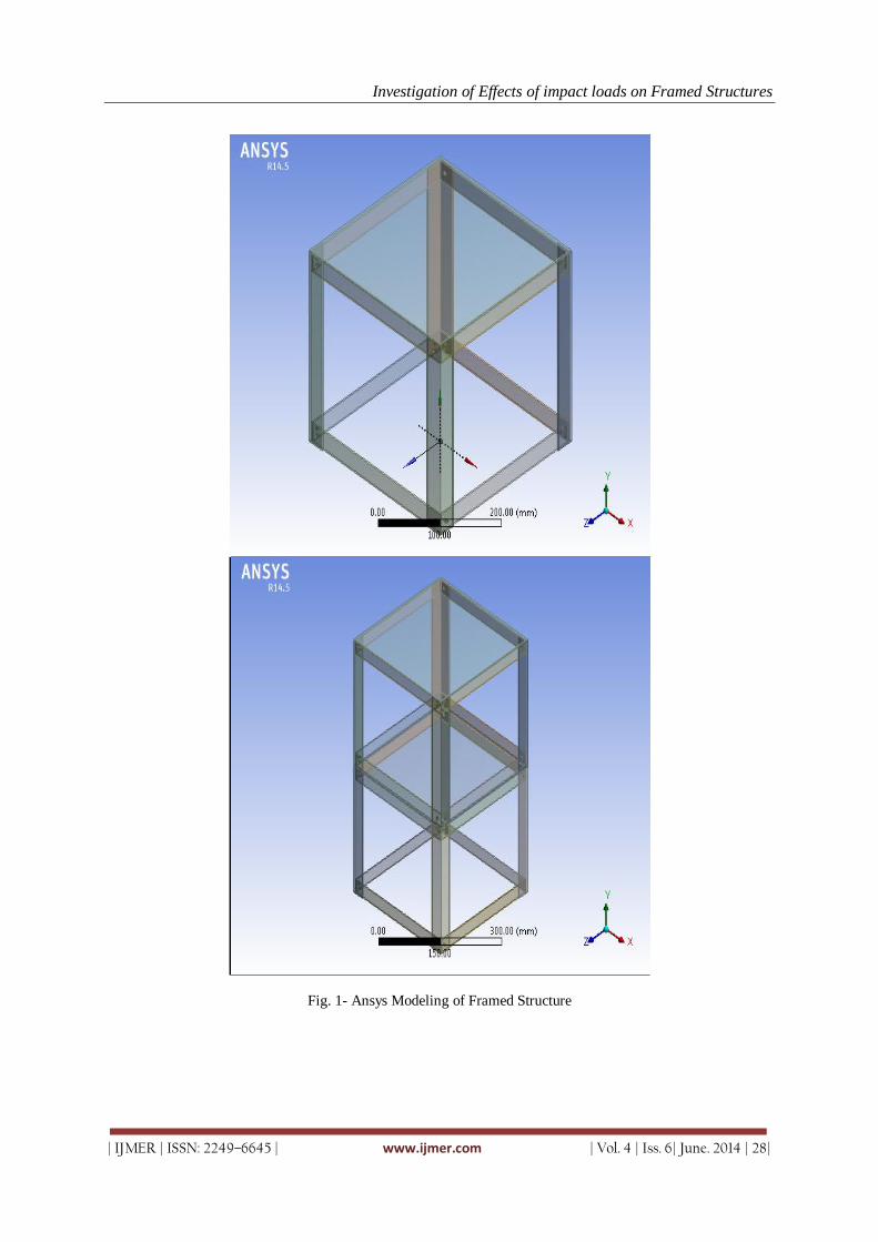
Investigation of Effects of impact loads on Framed Structures
| IJMER | ISSN: 2249–6645 | www.ijmer.com | Vol. 4 | Iss. 6| June. 2014 | 28|
Fig. 1- Ansys Modeling of Framed Structure
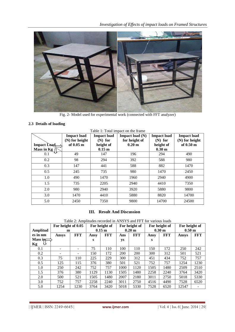
Investigation of Effects of impact loads on Framed Structures
| IJMER | ISSN: 2249–6645 | www.ijmer.com | Vol. 4 | Iss. 6| June. 2014 | 29|
Fig. 2- Model used for experimental work (connected with FFT analyzer)
2.3 Details of loading
Table 1: Total impact on the frame
Impact Load
Mass in Kg
Impact load
(N) for height
of 0.05 m
Impact load
(N) for
height of
0.15 m
Impact load (N)
for height of
0.20 m
Impact load
(N) for
height of
0.30 m
Impact load
(N) for height
of 0.50 m
0.1 49 147 196 294 490
0.2 98 294 392 588 980
0.3 147 441 588 882 1470
0.5 245 735 980 1470 2450
1.0 490 1470 1960 2940 4900
1.5 735 2205 2940 4410 7350
2.0 980 2940 3920 5880 9800
3.0 1470 4410 5880 8820 14700
5.0 2450 7350 9800 14700 24500
III. Result And Discussion
Table 2: Amplitudes recorded in ANSYS and FFT for various loads
Amplitud
es in nm
Mass in
Kg
For height of 0.05
m
For height of
0.15 m
For height of
0.20 m
For height of
0.30 m
For height of
0.50 m
Ansys FFT Ansy
s
FFT Ans
ys
FFT Ansy
s
FFT Ansys FFT
0.1 - - 75 110 100 110 150 172 250 242
0.2 - - 150 172 200 200 300 312 501 521
0.3 75 110 225 229 300 312 451 434 752 757
0.5 125 115 376 380 501 521 752 757 1254 1230
1.0 250 242 752 757 1000 1120 1505 1480 2509 2510
1.5 376 380 1129 1130 1505 1480 2258 2240 3764 3420
2.0 500 521 1505 1480 2007 2180 3011 2750 5018 5330
3.0 752 757 2258 2240 3011 2750 4516 4490 7528 6520
5.0 1254 1230 3764 3420 5018 5330 7528 6520 12547 -
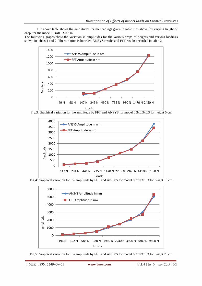
Investigation of Effects of impact loads on Framed Structures
| IJMER | ISSN: 2249–6645 | www.ijmer.com | Vol. 4 | Iss. 6| June. 2014 | 30|
The above table shows the amplitudes for the loadings given in table 1 as above, by varying height of
drop, for the model 0.3X0.3X0.3 m.
The following graphs show the variation in amplitudes for the various drops of heights and various loadings shown in tables 1 and 2. The variation is between ANSYS results and FFT results recorded in table 2.
Fig.3: Graphical variation for the amplitude by FFT and ANSYS for model 0.3x0.3x0.3 for height 5 cm
Fig.4: Graphical variation for the amplitude by FFT and ANSYS for model 0.3x0.3x0.3 for height 15 cm
Fig.5: Graphical variation for the amplitude by FFT and ANSYS for model 0.3x0.3x0.3 for height 20 cm
0
200
400
600
800
1000
1200
1400
49 N 98 N 147 N 245 N 490 N 735 N 980 N 1470 N 2450 N
ANSYS Amplitude In nm
FFT Amplitude In nm
0
500
1000
1500
2000
2500
3000
3500
4000
147 N 294 N 441 N 735 N 1470 N 2205 N 2940 N 4410 N 7350 N
ANSYS Amplitude In nm
FFT Amplitude In nm
0
1000
2000
3000
4000
5000
6000
196 N 392 N 588 N 980 N 1960 N 2940 N 3920 N 5880 N 9800 N
ANSYS Amplitude In nm
FFT Amplitude In nm
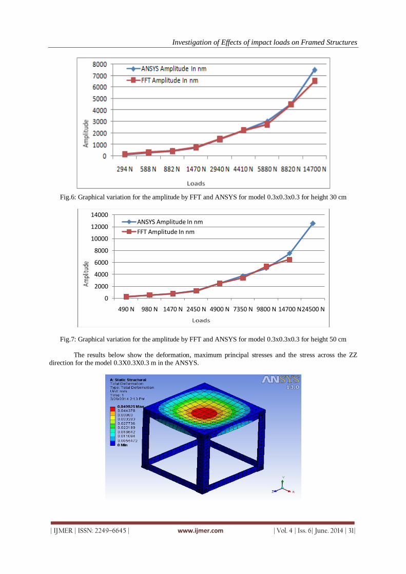
Investigation of Effects of impact loads on Framed Structures
| IJMER | ISSN: 2249–6645 | www.ijmer.com | Vol. 4 | Iss. 6| June. 2014 | 31|
Fig.6: Graphical variation for the amplitude by FFT and ANSYS for model 0.3x0.3x0.3 for height 30 cm
Fig.7: Graphical variation for the amplitude by FFT and ANSYS for model 0.3x0.3x0.3 for height 50 cm
The results below show the deformation, maximum principal stresses and the stress across the ZZ
direction for the model 0.3X0.3X0.3 m in the ANSYS.
0
2000
4000
6000
8000
10000
12000
14000
490 N 980 N 1470 N 2450 N 4900 N 7350 N 9800 N 14700 N24500 N
ANSYS Amplitude In nm
FFT Amplitude In nm
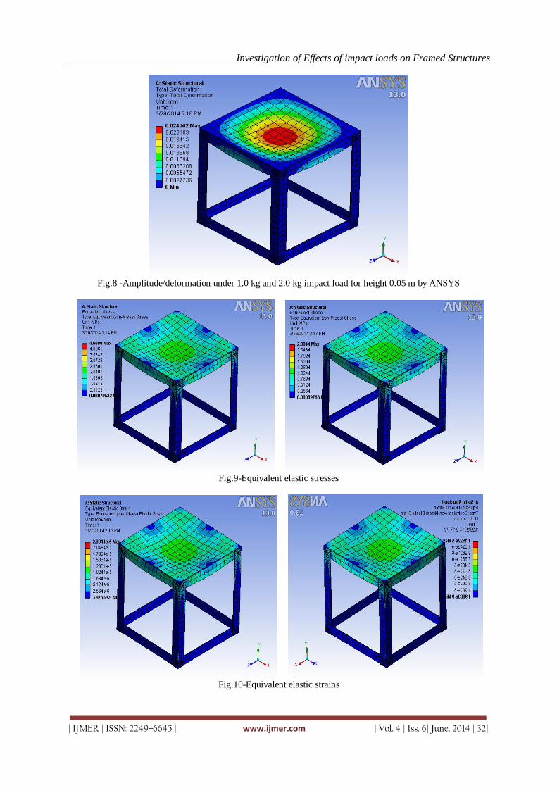
Investigation of Effects of impact loads on Framed Structures
| IJMER | ISSN: 2249–6645 | www.ijmer.com | Vol. 4 | Iss. 6| June. 2014 | 32|
Fig.8 -Amplitude/deformation under 1.0 kg and 2.0 kg impact load for height 0.05 m by ANSYS
Fig.9-Equivalent elastic stresses
Fig.10-Equivalent elastic strains

Investigation of Effects of impact loads on Framed Structures
| IJMER | ISSN: 2249–6645 | www.ijmer.com | Vol. 4 | Iss. 6| June. 2014 | 33|
IV. Conclusion 1. The impact pressure develops larger kinetic energy in the structure which ultimately produces large amount
of displacement in the structure.
2. The duration of the impact load, the maximum amount of impact and the maximum midspan deflection are
directly proportional to the height of drop of load.
3. The flexural rigidity of the structure affects the duration of the impact load, the maximum amount of impact
and the maximum midspan deflection.
4. The results produced by using Ansys software are too closed to the experimental results.
5. Finite element method by using Ansys software is capable of investigating the possible damage modes of
RC frame subjected to impact loading.
V. Future Scope There is a scope of carrying out same project work for the frame made up of different material. The
drop of height and the number of bays and storeys may also vary. One can apply the lateral loading to the
structure as it may suppose to expose earthquake loading, wind loading etc.
REFERENCES Journal Papers:
[1] Yimin Zhu,Engineering Method Design Ductile Structure under Impact Load, Beijing, China, August 7-12, 4896P; pp. 267-273.
Books: [2] John G. Proakis and Dimitris G. Manolakis, Digital signal processing (3rd edition, Pearson Prentice Hall publication)
Thesis: [3] Eshan Verma and G. Ashish, Vibrational analysis of framed structures, National Institute of Technology, Rourkela,
India. May 2011.
Proceeding Papers:
[4] Wahid Arif, Numerical Analysis of the Dynamic Response of Masonry Structures Subjected to Impact Loading, School of Civil Engineering, Faculty of Engineering.
[5] Norman Jones, The Response of Structures Subjected to Large Impact Loads, Ship structures symposium, Arlington, Virginia,Nov.1993.

International
OPEN ACCESS Journal
Of Modern Engineering Research (IJMER)
| IJMER | ISSN: 2249–6645 | www.ijmer.com | Vol. 4 | Iss. 6| June. 2014 | 34|
Between α-closed Sets and Semi α-closed Sets
A. Robert1, S. Pious Missier2
1Deparment of Mathematics, Aditanar College, Tiruchendur, India 2P.G Department of Mathematics, V.O.Chidambaram College, Thoothukudi, India
I. INTRODUCTION In 1963 Levine [1] introduced the concepts of semi-open sets and semi-continuity in topological
spaces. Levine [2] also defined and studied generalized closed sets as a generalization of closed sets. Dunham
[3] introduced the concept of generalized closure using Levine's generalized closed sets and defined a new
topology τ* and studied its properties. Njastad [4] introduced the concept of α-open sets in 1965. In 2000
Navalagi [5] introduced the concept of semi α-open sets by considering α-open set instead of open set in the
definition of semi-open set. Hakeem A. Othman [6] introduced and studied various concepts concerning semi
α-open sets. Since then, various notions of semi α-open sets have been studied. Pasunkili Pandian [7] defined
and studied semi*-preclosed sets and investigated its properties. The authors [8] have recently introduced the
concept of semi*α-open sets and investigated its properties in the light of already existing concepts and results
in topology. The semi*α-interior of a subset has also been defined and its properties studied.
In this paper, we define a new class of sets, namely semi*α-closed sets, as the complement of semi*α-
open sets. We further show that the class of semi*α-closed sets is placed between the class of α-closed sets and
the class of semi α-closed sets. We find characterizations of semi*α-closed sets. We investigate fundamental
properties of semi*α-closed sets. We also define the semi*α-closure of a subset. We also study some basic
properties of semi*α-closure. Further we define the semi*α-derived set of a subset and investigate its
properties.
II. Preliminaries Throughout this paper (X, τ) will always denote a topological space on which no separation axioms
are assumed, unless explicitly stated. If A is a subset of the space (X, τ), Cl(A) and Int(A) denote the closure
and the interior of A respectively. Also 𝓕 denotes the class of all closed sets in the space (X, τ).
Definition 2.1: A subset A of a space X is
(i) generalized closed (briefly g-closed) [2] if Cl(A)⊆U whenever A⊆U and U is open in X.
(ii) generalized open (briefly g-open) [2] if X\A is g-closed in X.
Definition 2.2: If A is a subset of X,
(i) the generalized closure [3] of A is defined as the intersection of all g-closed sets in X containing A and is
denoted by Cl*(A).
(ii) the generalized interior of A is defined as the union of all g-open subsets of A and is denoted by Int*(A).
Definition 2.3: A subset A of a topological space (X, τ) is
(i) semi-open [1] (resp. semi*-open [9] ) if there is an open set U in X such that U⊆A⊆Cl(U) (resp.
U⊆A⊆Cl*(U)) or equivalently if A⊆Cl(Int(A)) (resp. A⊆Cl*(Int(A))).
(ii) α-open[4] (resp. preopen [10]) if A⊆Int(Cl(Int(A)) ( resp. A⊆Int(Cl(A)) ).
Abstract: In general topology many strong and weak forms of open and closed sets have been defined
and studied. Govindappa Navalagi introduced the concept of semi α-open sets which is a weaker form of
α-open sets. Semi*α-open set is defined analogously by replacing the closure operator by the
generalized closure operator due to Dunham in the definition of semi α-open sets. In this paper we
introduce a new class of sets, namely semi*α-closed sets, as the complement of semi*α-open sets. We
find characterizations of semi*α-closed sets. We also define the semi*α-closure of a subset. Further we
investigate fundamental properties of the semi*α-closure. We define the semi*α-derived set of a subset
and study its properties.
Keywords: semi α-open set, semi α-closed set, semi*α-open set, semi*α-interior, semi*α-closed set,
semi*α-closure.

Between α-closed Sets and Semi α-closed Sets
| IJMER | ISSN: 2249–6645 | www.ijmer.com | Vol. 4 | Iss. 6| June. 2014 | 35|
(iii) semi α-open [5] (resp. semi*α-open [8] )if there is an α-open set U in X such that U⊆A⊆Cl(U) (resp.
U⊆A⊆Cl*(U) or equivalently if ACl(Int(Cl(Int(A))))(resp. ACl*(αInt(A).)
(iv) semi-preopen [11](resp. semi*-preopen [7] ) if A⊆Cl(Int(Cl(A))) (resp. A⊆Cl*(pInt(A)) ).
(v) semi-closed [12](resp. semi*-closed[13], preclosed [10], -closed [4] , semi α-closed [6] and
semi*preclosed[7] ) if Int(Cl(A))⊆A (resp. Int*(Cl(A))⊆A, Cl(Int(A)⊆A, Cl(Int(Cl(A)))⊆A ,
Int(Cl(Int(Cl(A))))A and Int*(pCl(A))⊆A).
The class of all semi-open (resp. α-open, semi-closed, preclosed, semi-preclosed, semi*-preclosed, semi*-open
and semi*-closed) sets is denoted by SO(X, τ) (resp. αO(X,) or α, SC(X, τ), PC(X, τ), SPC(X, τ), S*PC(X, τ),
S*O(X, τ) and S*C(X, τ)).
Definition 2.4.[13] Let A⊆X. An element x∈X is called a semi*-limit point of A if every semi*-open set in X
containing x intersects A \x.
Definition 2.5.[13] The set of all semi*-limit points of A is called the semi*-derived set of A and it is denoted
by Ds*(A).
The other forms of derived sets are similarly defined. The derived set, semi-derived set, pre-derived set, α-
derived set, semi α-derived set, semi*α-derived set, semi*pre-derived set and semi-pre-derived set of A are
respectively denoted by D[A], sD[A], pD[A], αD[A], sαD[A], s*αD[A], s*pD[A], and spD[A].
Definition 2.6: [2] A topological space X is T1/2 if every g-closed set in X is closed.
Definition 2.7: A topological space (X, α) is called an α-structure if αO(X,)=.
Definition 2.8: [3] If (X, τ) is a topological space, let τ* be the topology on X defined by the Kuratowski
closure operator Cl*. That is, τ*=U⊆X : Cl*(X\U)=X\U.
Theorem 2.9: [3] If (X, τ) is a topological space, then (X, τ*) is T1/2. Definition 2.10: [14] A space X is locally indiscrete if every open set in X is closed.
Definition 2.9: [14] A space X is extremally disconnected if the closure of every open set in X is open.
Definition 2.11: [15] The topology on the set of integers generated by the set S of all triplets of the form 2n-1,
2n, 2n+1 as sub base is called the Khalimsky topology and it is denoted by κ. The digital line equipped with
the Khalimsky topology is called the Khalimsky line. The topological product of two Khalimsky lines (ℤ, κ) is
called the Khalimsky plane (ℤ2, κ2).
Theorem 2.12: [8] In any topological space,
(i) Every α-open set is semi*α-open.
(ii) Every open set is semi*α-open.
(iii) Every semi*-open set is semi*α-open.
(iv) Every semi*α-open set is semi α-open.
(v) Every semi*α-open set is semi*-preopen.
(vi) Every semi*α-open set is semi-preopen.
(vii) Every semi*α-open set is semi-open.
Theorem 2.13: [8] If A is a subset of a topological space, then the following statements are equivalent:
(i) A is semi*α-open.
(ii) ACl*(αInt(A)).
(iii) Cl*(A)=Cl*(αInt(A)).
Theorem 2.14: [8] In any topological space, arbitrary union semi*α-open sets is semi*α-open.
Theorem 2.15: [8] If A is semi*α-open in X and B is open in X, then A∩B is semi*α-open in X.
Theorem 2.16: [8] If A is semi*α-open in X and BX is such that αInt(A)BCl*(A). Then B is semi*α-open.
Theorem 2.17:[8]If A is any subset of a topological space X, then s*αInt(A) is precisely the set of all semi*α-
interior points of A.
Remark 2.18:[8] : (i)If (X, τ) is a locally indiscrete space,
τ =αO(X, τ)= S*αO(X, τ) = SαO(X, τ)=S*O(X,)=SO(X, τ).
(ii) In an α-structure semi*α-open sets and semi*-preopen sets coincide.
(iii) In an extremally disconnected space, the semi*α-open sets and the semi*-preopen sets coincide.
III. Semi*α-Closed Sets
Definition 3.1. The complement of a semi*α-open set is called semi*α-closed. The class of all semi*α-closed
sets in (X, τ) is denoted by S*αC(X, τ) or simply S*αC(X).
Definition 3.2. A subset A of X is called semi*α-regular if it is both semi*α-open and semi*α-closed.
Theorem 3.3. For a subset A of a topological space X, the following statements are equivalent:
(i) A is semi*α-closed.

Between α-closed Sets and Semi α-closed Sets
| IJMER | ISSN: 2249–6645 | www.ijmer.com | Vol. 4 | Iss. 6| June. 2014 | 36|
(ii) There is an α-closed set F in X such that Int*(F)⊆A⊆F.
(iii) Int*(αCl(A))⊆A.
(iv) Int*(αCl(A))=Int*(A).
(v) Int*(A∪Cl(Int(Cl(A))))=Int*(A).
Proof: (i)⟹(ii): Suppose A is semi*α-closed. Then X\A is semi*α-open. Then by Definition 2.3(iii), there is an
α-open set U in X such that U⊆X\A⊆Cl*(U). Taking the complements we get, X\U⊇A⊇X\Cl*(U). Since for
any subset U in the space X, we have Int*(X\U)=X\Cl*(U). Therefore F⊇A⊇Int*(F) where F=X\U is α-closed
in X.
(ii)⟹(iii): By assumption, there is an α-closed set F such that Int*(F)⊆A⊆F. Since AF and F is α-closed,
we have αCl(A)F. Hence Int*(αCl(A)) Int*(F)⊆A.
(iii)⟹(iv): By assumption, Int*(αCl(A))⊆A. This implies that Int*(αCl(A))⊆Int*(A). Since it is true that
A⊆αCl(A), we have Int*(A)⊆Int*(αCl(A)). Therefore Int*(αCl(A))=Int*(A).
(iv)⟹(i): If Int*(αCl(A))=Int*(A), then taking the complements, we get X\Int*(αCl(A))=X\Int*(A). Hence
Cl*(αInt(X\A))=Cl*(X\A). Therefore by Theorem 2.13., X\A is semi*α-open and hence A is semi*α-closed.
(iv)⟺(v): Follows from the fact that for any subset A, αCl(A)=A∪Cl(Int(Cl(A)))
Theorem 3.4. If a subset A of a topological space X is semi*α-closed, then the following statements hold:
(i) There is a closed set H in X such that Int*(Cl(Int(H)))⊆A⊆H.
(ii) There is a closed set H in X such that Int*(sInt(H))⊆A⊆H.
(iii) There is a closed set H in X such that Int*(H∩Cl(Int(H)))⊆A⊆H.
(iv) Int*(Cl(Int(Cl(A))))⊆A.
Proof:(i) Since A is semi*α-closed, from Theorem 3.3 there is an α- closed set F such that Int*(F)⊆A⊆F.
Since F is α-closed, there is a closed set H such that Cl(Int(H)))⊆A⊆H. This proves (i)
(ii) follows from (i) and from the fact that for any closed set H, sInt(H)=Cl(Int(H))
(iii) follows from (ii) since for any set H, sInt(H)=H∩Cl(Int(H))
(iv) Follows from (i) since H is closed.
Remark 3.5. (i) In any topological space (X, τ), ϕ and X are semi*α-closed sets.
(ii) In a T1/2 space, the semi*α-closed sets and the semi-α-closed sets coincide. In particular, in the Khalimsky
line and in the real line with usual topology the semi*α-closed sets and the semi-α-closed sets coincide.
Theorem 3.6. Arbitrary intersection of semi*α-closed sets is also semi*α-closed.
Proof: Let Ai be a collection of semi*α-closed sets in X. Since each Ai is semi*α-closed, X\Ai is semi*α-
open. By Theorem 2.14, X\(∩Ai)= ∪(X\Ai) is semi*α-open. Hence ∩Ai is semi*α-closed.
Corollary 3.7. If A is semi*α-closed and U is semi*α-open in X, then A\U is semi*α-closed.
Proof: Since U is semi*α-open, X\U is semi*α-closed. Hence by Theorem 3.6, A\U=A∩(X\U) is semi*α-closed.
Remark 3.8. Union of two semi*α-closed sets need not be semi*α-closed as seen from the following examples.
Example 3.9: In the space (X, τ), where X = a, b, c, d and τ =, a, b, a, b, a, b, c , X, the subsets
a, c, e and b, c, e are semi*α-closed but their union a, b, c, e is not semi*α-closed.
Example 3.10: Let X= 1, 2×1, 2, 3 be given the subspace topology of the digital plane. In X, the subsets
A=(1, 1), (1, 2), (2, 1), (2, 3) and B=(1, 2), (1, 3), (2, 1), (2, 3) are semi*α-closed but A∪B is not semi*α-
closed.
Theorem 3.11. If A is semi*α-closed in X and B is closed in X, then A∪B is semi*α-closed.
Proof: Since A is semi*α-closed, X\A is semi*α-open in X. Also X\B is open. By Theorem 2.15,
(X\A)∩(X\B)=X\(A∪B) is semi*α-open in X. Hence A∪B is semi*α-closed in X.
Theorem 3.12. In any topological space,
(i) Every α-closed set is semi*α-closed.
(ii) Every closed set is semi*α-closed.
(iii) Every semi*-closed set is semi*α-closed.
(iv) Every semi*α-closed set is semi-α-closed.
(v) Every semi*α-closed set is semi*-preclosed.
(vi) Every semi*α-closed set is semi-preclosed.
(vii) Every semi*α-closed set is semi-closed.
Proof: (i) Let A be α-closed. Then X\A is α-open. By Theorem 2.12(i), X\A is semi*α-open. Hence A is semi*α-
closed. (ii) follows from (i) and the fact that every closed set is α-closed. To prove (iii) let A be a semi*-closed
set in X. Then X\A is semi*-open in X. By Theorem 2.12(iii) X\A is semi*α-open. Hence A is semi*α-closed in
X. To prove (iv) let A be semi*α-closed, then X\A is semi*α-open. By Theorem 2.12(iv), X\A is semi-α-open.

Between α-closed Sets and Semi α-closed Sets
| IJMER | ISSN: 2249–6645 | www.ijmer.com | Vol. 4 | Iss. 6| June. 2014 | 37|
Hence A is semi-α-closed. Let A be a semi*α-closed set in X. Then X\A is semi*α-open in X. By Theorem
2.12(v) X\A is semi*-preopen. Hence A is semi*-preclosed in X. This proves (v). The statement (vi) follows
from (v) and the fact that every semi*-preclosed set is semi-preclosed. (vii) follows from Theorem 2.12(vii).
Remark 3.13: The converse of each of the statements in Theorem 3.12 is not true.
Remark 3.14. From the discussions above we have the following diagram
semi*-closed semi-closed
g-closed
Closed α-closed semi*α-closed semi-α-closed semi-preclosed
pre-closed semi*-preclosed
Relationship Diagram for Semi*α-Closed Sets
Corollary 3.15. (i)If A is semi*α-closed and F is α-closed in X, then A∩F is semi*α-closed in X.
(ii) If A is semi*α-closed and F is closed in X, then A∩F is semi*α-closed in X.
(iii)If A is semi*α-closed and U is open in X, then A\U is semi*α-closed in X.
Proof: (i) Since F is α-closed, by Theorem 3.12(i) F is semi*α-closed. Then by Theorem 3.6, A∩F is semi*α-
closed.
(ii)Since F is closed, by Theorem 3.11(ii), F is semi*α-closed. Then by Theorem 3.6, A∩F is semi*α-closed.
(iii)Since U is open in X, its complement X\U is closed in X. From (i), A\U=A∩(X\U) is semi*α-closed .
Theorem 3.16. In any topological space (X, τ),
(i) 𝓕 αC(X, τ)S*αC(X, τ) SαC(X, τ)SPC(X, τ)
(ii) 𝓕 αC(X, τ) S*αC(X, τ) S*PC(X, τ) SPC(X, τ)
(iii) 𝓕 αC(X, τ) S*αC(X, τ) SC(X, τ) SPC(X, τ) and
(iv) 𝓕 S*C(X, τ) S*αC(X, τ) SαC(X, τ) SPC(X, τ).
Proof: Follows from Theorem 3.11 and from the facts that every closed set is α-closed, every semi-closed set is
semi-preclosed, every closed set is semi*-closed, every semi α-closed set is semi-preclosed and every semi*-
preclosed set is semi-preclosed.
Remark 3.17. (i) If (X, τ) is a locally indiscrete space, then 𝓕=αC(X, τ)= S*αC(X, τ) = SαC(X, τ)=S*C(X,)=
SC(X, τ).
(ii) In the Sierpinski space (X, τ), where X=a, b and τ=, a, X, 𝓕=αC(X, τ)=S*C(X, τ)=SC(X, τ)=
S*αC(X, τ)=SαC(X, τ)=PC(X, τ)=S*PC(X, τ)=SPC(X, τ) .
(iii) If (X, τ) is extremally disconnected, S*αC(X, τ)=S*PC(X, τ).
(iv) If (X, τ) is an α-structure, S*αC(X, τ) = S*C(X,)
(v) The inclusions in Theorem 3.16 involving S*α(X,) may be strict and equality may also hold. This can be
seen from the following examples.
Remark 3.18. The concept of semi*α-closed set is independent of each of the concepts of g-closed sets and
pre-closed sets.
Theorem 3.19. If A is semi*α-closed in X and B be a subset of X such that Int*(A)⊆B⊆αCl(A), then B is
semi*α-closed in X.
Proof: Since A is semi*α-closed, X\A is semi*α-open. Now Int*(A)⊆B⊆αCl(A) which implies
X\Int*(A)⊇X\B⊇
X\ αCl(A). That is, Cl*(X\A)⊇X\B⊇αInt(X\A). Therefore by Theorem 2.16, X\B is semi*α-open. Hence B is
semi*α-closed.
Theorem 3.20. Let C be a collection of subsets in X satisfying (i) αC(X) ⊆C (ii) If AC and D⊆X is such
that Int*(A)⊆D⊆αCl(A) imply that DC. Then S*αC(X)⊆C. Thus S*αC(X) is the smallest collection of
subsets of X satisfying the conditions (i) and (ii).
Proof: By Theorem 3.16(i), S*αC(X) satisfies (i) and by Theorem 3.19, S*αC(X) satisfies (ii). Further if
AS*αC(X), then by Theorem 3.3, there is an α-closed set F in X such that Int*(F)⊆A⊆F. By (i), FC.
Since F is α-closed, αCl(F)=F . Therefore Int*(F)⊆A⊆αCl(F). Hence by (ii), AC. Thus S*αC(X)⊆C. This
shows that S*αC(X) is the smallest collection of subsets of X satisfying (i) and (ii).

Between α-closed Sets and Semi α-closed Sets
| IJMER | ISSN: 2249–6645 | www.ijmer.com | Vol. 4 | Iss. 6| June. 2014 | 38|
IV. Semi*α-Closure Of A Set
Definition 4.1. If A is a subset of a topological space X, the semi*α-closure of A is defined as the intersection
of all semi*α-closed sets in X containing A. It is denoted by s*αCl(A).
Theorem 4.2. If A is any subset of a topological space (X, τ), then s*αCl(A) is semi*α-closed. In fact s*αCl(A)
is the smallest semi*α-closed set in X containing A.
Proof: Since s*αCl(A) is the intersection of all semi*α-closed supersets of A, by Theorem 3.6, it is semi*α-
closed and is contained in every semi*α-closed set containing A and hence it is the smallest semi*α-closed set
in X containing A.
Theorem 4.3. Let A be a subset of a topological space (X, τ). Then A is semi*α-closed if and only if
s*αCl(A)=A.
Proof: If A is semi*α-closed, then s*αCl(A)=A is obvious. Conversely, let s*αCl(A)=A. By Theorem 4.2,
s*αCl(A) is semi*α-closed and hence A is semi*α-closed.
Theorem 4.4. (Properties of Semi*α-Closure)
In any topological space (X, τ), the following results hold:
(i) s*αCl()=.
(ii) s*αCl(X)=X.
If A and B are subsets of X,
(iii) A⊆s*αCl(A).
(iv) A⊆B⟹s*αCl(A)⊆s*αCl(B).
(v) s*αCl(s*αCl(A))=s*αCl(A).
(vi) A⊆spCl(A)⊆sαCl(A)⊆s*αCl(A)⊆αCl(A)⊆Cl(A).
(vii) A⊆spCl(A)⊆sαCl(A)⊆s*αCl(A)⊆s*Cl(A)⊆Cl(A).
(viii) A⊆spCl(A)⊆sCl(A)⊆s*αCl(A)⊆αCl(A)⊆Cl(A).
(ix) A⊆spCl(A)⊆s*pCl(A)⊆s*αCl(A)⊆αCl(A)⊆Cl(A).
(x) s*αCl(A∪B)⊇s*αCl(A)∪s*αCl(B).
(xi) s*αCl(A∩B)⊆s*αCl(A)∩s*αCl(B).
(xii) Cl(s*αCl(A))=Cl(A).
(xiii) s*αCl(Cl(A))=Cl(A).
(xiv) If (X, τ) is an α-structure and A⊆X, then s*Cl(A)=s*αCl(A).
(xv) If (X, τ) is extremally disconnected and A⊆X, then s*pCl(A)=s*αCl(A).
(xvi) If (X, τ) is a locally indiscrete space and A⊆X, then Cl(A)=αCl(A)=s*Cl(A)=s*αCl(A)=sαCl(A)=
sCl(A)
Proof: (i), (ii), (iii) and (iv) follow from Definition 4.1. From Theorem 4.2 s*αCl(A) is semi*α-closed and
from Theorem 4.3 s*αCl(s*αCl(A))=s*αCl(A).This proves (v). Clearly (vi), (vii), (viii) and (ix) follow from
Theorem 3.12. Now (x) and (xi) follow from (iv) and set theoretic properties. From (iii), we have A⊆s*αCl(A)
and hence Cl(A)⊆Cl(s*αCl(A)). Also from (vi), we have Cl(A)⊇s*αCl (A) and hence Cl(A)⊇Cl(s*αCl(A)).
Therefore Cl(s*αCl(A))=Cl(A). This proves (xii). Now statement (xiii) follows from the fact that Cl(A) is
closed and hence by Theorem 3.12(ii), Cl(A) is semi*α-closed and by Theorem 4.3, s*αCl(Cl(A))=Cl(A).
Remark 4.5. In Theorem 4.4, the inclusions may be strict and equality may also hold.
Theorem 4.6. Let A⊆X and let xX. Then xs*αCl(A) if and only if every semi*α-open set in X containing x
intersects A.
Proof: Let us prove the contra positive of the theorem. Suppose xs*αCl(A). Then xX\s*αCl(A)=X\∩F:
A⊆F and F is semi*α-closed in X=∪X\F: A⊆F and F is semi*α-closed in X and so xX\F for some
semi*α-closed set F containing A. Hence X\F is a semi*α-open set containing x that does not intersect A. On
the other hand, suppose there is a semi*α-open set U containing x that is disjoint from A. Then X\U is a
semi*α-closed set containing A. Therefore by Definition 4.1 s*αCl(A)⊆X\U. Hence xs*αCl(A). Thus
xs*αCl(A) if and only if there is a semi*α-open set containing x that does not intersect A. This proves the
theorem.
Theorem 4.7. If A is a subset of X, then
(i) s*αCl(X\A)=X\s*αInt(A).
(ii) s*αInt(X\A)=X\s*αCl(A).
Proof: (i) Let xX\s*αInt(A).Then xs*αInt(A).This implies that x does not belong to any

Between α-closed Sets and Semi α-closed Sets
| IJMER | ISSN: 2249–6645 | www.ijmer.com | Vol. 4 | Iss. 6| June. 2014 | 39|
semi*α-open subset of A. Let F be a semi*α-closed set containing X\A. Then X\F is a semi*α-open set
contained in A. Therefore xX\F and so xF. Thus x belongs to every semi*α-closed set containing X\A.
Hence xs*αCl(X\A). Therefore X\s*αInt(A)⊆s*αCl(X\A). On the other hand, let xs*αCl(X\A). Then x does
not belong to any semi*α-open subset of A. On the contrary, suppose there exists a semi*α-open subset U of A
containing x. Then X\U is a semi*α-closed set that contains X\A but not x. This contradiction proves that
xs*αInt(A). Thatis, xX\s*αInt(A). Hence s*αCl(X\A)⊆ X\s*αInt(A). This proves (i). Clearly statement (ii)
can be proved from (i) by replacing A by X\A and taking the complements on both sides.
Theorem 4.8. Let D be a subset of a topological space (X,). Then the following statements are equivalent:
i) D is dense in (X, α).
ii) s*αCl(D)=X.
iii) If F is a semi*α-closed subset of X containing D, then F=X
iv) For each xX, every semi*α-open set containing x intersects D.
v) s*αInt(X\D)=.
Proof: (i)⟹(ii): Let D be dense in (X, α) and let xX. Let A be a semi*α-open set in X containing x. Then by
Definition 2.3, there exists an α-open set U such that U⊆A⊆Cl*(U). Since D is dense in (X, α), U∩D≠ and
hence A∩D≠. Thus every semi*α-open set in X containing x intersects D. Therefore by Theorem 4.6,
xs*αCl(D). Hence s*αCl(D)=X.
(ii)⟹(i): Suppose s*αCl(D)=X. Then by Theorem 4.4(vi), X=s*αCl(D)⊆αCl(D)⊆X. Hence αCl(D)=X. That
is, D is dense in (X, α).
(ii)⟹(iii): Let F be a semi*α-closed subset of X containing D. Then X=s*αCl(D)⊆s*αCl(F)=F which implies
F=X.
(iii)⟹(ii): Since s*αCl(D) is a semi*α-closed set containing D, by (iii)s*αCl(D)=X.
(ii)⟹(iv): Let xX. Then xs*αCl(D). By Theorem 4.6, every semi*α-open set containing x intersects D.
(iv)⟹(ii): Let xX. Then every semi*α-open set containing x intersects D. By Theorem 4.6, xs*αCl(D).
Hence s*αCl(D)=X.
(iv)⟹(v): If possible, let xs*αInt(X\D). Then s*αInt(X\D) is a nonempty s*α-open set containing x. From
(iv), D∩(X\D)≠. This contradiction proves (v).
(v)⟹(ii):Suppose s*αInt(X\D)=. By Theorem 4.7(ii), X\s*αCl(D)=. Hence s*αCl(D)=X.
Remark 4.9: If (X, τ) is an α-structure, then D is dense in X if and only if s*αCl(D)=X .
Theorem 4.10. If A is a subset of a topological space X,
(i) s*αCl(A)=A∪Int*(αCl(A)).
(ii) s*αInt(A)=A∩Cl*(αInt(A)).
Proof:(i) Now Int*(αCl(A∪Int*(αCl(A))))=Int*(αCl(A)∪αCl(Int*(αCl(A))))=Int*(αCl(A))⊆A∪Int*(αCl(A)).
Then by Theorem 3.3, A∪Int*(αCl(A)) is a semi*α-closed set containing A. Hence by Theorem 4.2, s*αCl(A)⊆
A∪Int*(αCl(A)). Since s*αCl(A) is semi*α-closed , by invoking Theorem 3.3, we get Int*(αCl(A))⊆
Int*(αCl(s*αCl(A)))⊆ s*αCl(A).Therefore A∪Int*(αCl(A))⊆s*αCl(A). This proves (i). Clearly (ii) follows
from (i) by replacing A by X\A and taking the complements on both sides and applying Theorem 4.7.
V. Semi*α-Derived Set
Definition 5.1. Let A⊆X. An element x∈X is called a semi*α-limit point of A if every semi*α-open set in X
containing x intersects A \x.
Definition 5.2. The set of all semi*α-limit points of A is called the semi*α-Derived set of A.
It is denoted by Ds*α(A).
Lemma 5.3. If A⊆X, then Ds*α(A)⊆s*αCl(A).
Proof: Follows from Definition 5.1 and Theorem 4.6
Theorem 5.4. If A⊆X, then s*αCl(A)=A∪Ds*α(A).
Proof: By definition, A⊆s*αCl(A). By Lemma 5.2, we have Ds*α(A)⊆s*αCl(A). Thus A∪Ds*α(A)⊆s*αCl(A).
On the other hand, let xs*αCl(A). If xA, then xA∪Ds*α(A). Suppose xA. We claim that x is a semi*α-limit
point of A. Let U be a semi*α-open set containing x. Then by Theorem U intersects A. Since xA, U intersects
A\x and hence xDs*α(A). Therefore s*αCl(A)⊆A∪Ds*α(A). This proves the theorem.
Corollary 5.5. A subset A of X is semi*α-closed if and only if A contains all its semi*α-limit points. That is, A
is semi*α-closed if and only if Ds*α(A)⊆A.

Between α-closed Sets and Semi α-closed Sets
| IJMER | ISSN: 2249–6645 | www.ijmer.com | Vol. 4 | Iss. 6| June. 2014 | 40|
Proof: By Theorem 5.4, s*αCl(A)=A∪Ds*α(A) and by Theorem 4.3, A is semi*α-closed if and only if
s*αCl(A)=A. Hence A is semi*α-closed if and only if Ds*α(A)⊆A.
Theorem 5.6. (Properties of Semi*α-Derived Set)
In any topological space (X, τ) the following statements hold.
If A and B are subsets of X,
(i) A⊆B⟹Ds*α(A)⊆Ds*α(B).
(ii) Dsp(A)⊆Dsα(A)⊆Ds*α(A)⊆Dα(A)⊆D(A).
(iii) Dsp(A)⊆Ds*p(A)⊆Ds*α(A)⊆Dα(A)⊆D(A).
(iv) Dsp(A)⊆Dsα(A)⊆Ds*α(A)⊆Ds*(A)⊆D(A).
(v) Dsp(A)⊆Ds(A)⊆Ds*α(A)⊆Dα(A)⊆D(A).
(vi) Ds*α(Ds*α(A))\A⊆Ds*α(A).
(vii) Ds*α(A∪B)⊇Ds*α(A)∪Ds*α(B).
(viii) Ds*α(A⋂B)⊆Ds*α(A)⋂Ds*α(B).
(ix) Ds*α(A∪Ds*α(A))⊆A∪Ds*α(A).
(x) s*αInt(A)=A\Ds*α(X\A).
(xi) If (X, τ) is an α-structure, then Ds*α(A)=Ds*(A).
(xii) If (X, τ) is an extremally disconnected space, then Ds*α(A)=Ds*p(A).
(xiii) If (X, τ) is a locally indiscrete space and A⊆X, then D[A]=αD[A]=s*D[A]=s*αD[A]=sαD[A]= sD[A]
Proof: (i) follows from the definition.
(ii), (iii), (iv) and (v) follow from Theorem 2.12 and from definitions.
(vi) Let xDs*α(Ds*α(A))\A and U be a semi*α-open set containing x. Then U∩(Ds*α(A)\x)≠. Let
yU∩(Ds*α(A)\x). Then x≠yU and yDs*α(A). Hence U∩(A\y)≠. If z U∩(A\y), then z≠x and
U∩(A\x)≠ which shows that xDs*α(A). This proves (vi).
(vii) Since A⊆A∪B, by (i), Ds*α(A)⊆Ds*α(A∪B). Similarly Ds*α(B)⊆Ds*α(A∪B). Hence
Ds*α(A)∪Ds*α(B)⊆Ds*α(A∪B). This proves (vii).The proof for (viii) is similar.
By Theorem 5.4, A∪Ds*α(A)=s*αCl(A) which is semi*α-closed by Theorem 4.3. From Corollary 5.5, we have
Ds*α(A∪Ds*α(A))⊆A∪Ds*α(A).This proves (ix). Let xA\Ds*α(X\A). Then xDs*α(X\A) which implies there is a
semi*α-open set U containing x such that U∩((X\A)\x)=. Since x∈A, U∩(X\A)= which implies U⊆A.
Then xU⊆A and hence xs*αInt(A). On the other hand if xs*αInt(A) then s*αInt(A) is a semi*α-open set
containing x and contained in A. Hence s*αInt(A)∩(X\A)= which implies xDs*α(X\A). Thus
s*αInt(A)⊆A\Ds*α(X\A). This proves (x). The statements (xi), (xii) and (xiii) follow from Remark 2.18.
Remark 5.7. It can be seen that the inclusions in Theorem 5.6 may be strict and equality may hold as well.
VI. Conclusion The newly defined concept of semi*α-closed sets is shown to be weaker than the concepts of α-closed
sets and semi*-closed sets but stronger than the concepts of semi α-closed sets, semi-closed sets and semi*-
preclosed sets. Explict expressions for semi*α-closure and semi*α-interior of a subset have been found. The
properties of semi*α-border, semi*α-frontier and semi*α-exterior have been investigated.
REFERENCES [1] N. Levine, "Semi-open sets and Semi-continuity in topological spaces", American Mathematical Monthly, 70
(1)(1963), 36-41.
[2] N. Levine, "Generalized Closed Sets in Topology", Rend. Circ. Mat. Palermo, 19(2) (1970), 89-96.
[3] W. Dunham, "A new closure operator for Non-T1 topologies", Kyungpook Math. J., 22(1) (1982), 55-60.
[4] O. Njastad, "Some Classes of Nearly Open Sets", Pacific J. Math., 15 (3) (1965), 961-970.
[5] G.B. Navalagi, Definition Bank in General Topology, Topology Atlas (2000)
[6] H.A. Othman, "New types of α-continuous mapping", Master Degree Thesis, Al-Mustansiriya University, IRAQ
(2004).
[7] S. Pasunkili Pandian, "A Study on Semi Star-Preopen Sets in Topological Spaces", Ph.D Thesis, Manonmaniam
Sundaranar University, Tirunelveli, India, 2013.
[8] A. Robert and S. Pious Missier, "A New Class of sets weaker than α-open sets" ( submitted for publication)
[9] A. Robert and S. Pious Missier, "A New Class of Nearly Open Sets", International Journal of Mathematical
Archive, 3(7), 2012, 1-8.

Between α-closed Sets and Semi α-closed Sets
| IJMER | ISSN: 2249–6645 | www.ijmer.com | Vol. 4 | Iss. 6| June. 2014 | 41|
[10] A.S, Mashhour, M.E. Abd El-Monsef and S.N. El-Deeb, "On Precontinuous and Weak Precontinuous mappings",
Proc. Math. Phys. Soc. Egypt 53(1982) 47-53.
[11] D. Andrijevic, "Semi-Preopen Sets", Mat. Vesnik, 38(1986), 24-32.
[12] P. Das, "Note on some applications of semiopen sets", Progre. Math. Soc., Allahabad, 7 (1973), 33- 44.
[13] A. Robert and S. Pious Missier, "On Semi*-closed sets", Asian Journal Of Current Engineering And Maths., 1 (4)
(2012), 173-176.
[14] S. Willard, General Topology, Addison–Wesley Publishing Company, Inc, 1970.
[15] E.D. Khalimsky, "Applications of Connected Ordered Topological spaces in Topology", Conference of Math.
Departments of Povolsia, 1970.

International
OPEN ACCESS Journal Of Modern Engineering Research (IJMER)
| IJMER | ISSN: 2249–6645 | www.ijmer.com | Vol. 4 | Iss. 6| June. 2014 | 42|
Microstructure Degradation after Prolonged Exploitation of
Heatresistant Steel 14mov6-3
Pradeep Suman1, Shekhar pal
2
1 (Thermal Engineering, Career Point University, Kota) Dharmendra Kumar Jain 2 (Guide , Department of Mechanical Engineering ,Govt. Polytechnic college Kota)
I. Introduction Components of power plant boiler are exposed to elevated temperatures, aggressive environment,
creep, fatigue, and other damage mechanisms that can cause degradation, deformation or cracking of
components. Under such conditions microstructure and mechanical properties of metallic materials degrade,
causing sometimes significant reduction of high-temperature components life. The steel 14MoV6-3 concept
goes back to the dawn of creep resistant steels. Experiments with single alloy molybdenum-vanadium steel go
back to the time prior to World War II and this steel appears to have stood the test already during the war. The
difficult post-war supply situation contributed essentially to the evolution of this low-alloy, but cheap steel of
the West German Edelstahl and Roehren werke. Creep rupture strength of steel 14MoV6-3 was clearly superior
to that of the higher alloyed steel 10CrMoV9-10 which was adopted in West Germany, [1]. Because of microstructure evolution and degradation of properties of this steel in exploitation the inspection measures
should be planned and started depending on evaluation of the exhaustion degree. According to the German
Codes VGB-R 509L and TRD 508 the start or extended material inspection is required after about 70.000 h for
steel 14MoV6-3 and about 100.000 h of exploitation for the other heat-resistant steels, [2]. Investigated material
14MoV6-3 is taken from the Unit 5 main steamline (ø245×28mm) that was in exploitation 156194.207 hours at
steam temperature 540 °C and steam pressure 13,5MPa, in thermal power plant in india. Samples of streamline
exploited material 14MoV6-3 were cut in 2008 because of residual life estimation and microstructure inspection
was a just part of overall investigation conducted on this material. Virgin material used for comparing of
investigated properties was also cut from the same steam line material 14MoV6-3 (ø245×28mm).
II. Microstructure Evolution According To Technical Norms Metallographic methods have been developed that can correlate either cavitations evolution or changes
in carbide spacing with creep-life expenditure. It has been observed that, in many structural applications,
cavitation is the principal damage mechanism in brittle zones, and high-stress regions in the base metal. In other
cases, carbide coarsening can provide a better indication of life consumption, [3]. The determination of the
structural condition and materials exhaustion of creep exposed power plant components is increasingly carried
out by field metallographic, examining the relevant components. VGB-TW 507 represents guideline for the
assessment of microstructure and damage development of creep exposed materials for pipes and boiler
components. The microstructure is primarily dependent on the operating temperature, while the damage is
mainly controlled by stress or strain. This guideline is therefore restricted to creep exposed components. Depending upon the provision of materials it was anticipated to present microstructures of pipes, bends, fittings
Abstract: Metallographic testing of material microstructure represents important method for characterization of material behavior. In case of heat resistant steels that are used for steam lines and
boiler components of thermal power plants for a long period of service time, under the influence of
mechanical and thermal loads their microstructure will be changed. As a result, it will have significant
influence on mechanical properties of such material. Metallographic testing can be used for following
of microstructure evolution
and estimation of components further safe service time, but at the same time knowing of changes in
material microstructure is necessary for better understanding of mechanical properties degradation
mechanism. Microstructure as indicator of material degradation of heat resistant streamline steel
14MoV6-3 after almost 200.000 hours of exploitation at steam temperature 540 °C and pressure 13,5MPa has been investigated in this paper. It is necessary to emphasize that this streamline has been
designed for service life time of 100.000 hours for mentioned steam parameters.
Keywords: Microstructure evolution, prolonged exploitation, 14MoV6-3,

MICROSTRUCTURE DEGRADATION AFTER PROLONGED EXPLOITATION OF EATRESISTANT
| IJMER | ISSN: 2249–6645 | www.ijmer.com | Vol. 4 | Iss. 6| June. 2014 | 43|
and headers. The assessment of the structure was performed on selected components, with heat treatments in
accordance with the respective standard. The structures often stabilize and unify after prolonged thermal
exposure. For this reason service exposed materials exceeding 100.000h were selected in VGB-TW 507 guideline, [4].
III. CHEMICAL COMPOSITION OF 14mov6-3 Chemical composition of investigated material 14MoV6-3 (virgin and exploited) was accomplished in
order to confirm that all delivered specimens of steam line are made from the same material, so the results of
predicted investigation on virgin and exploited material could be comparable. Method for determination of
chemical composition was spectral analysis. Chemical composition of material 14MoV6-3 according to
normative DIN 17175/79, [5], is presented in Table 1, and for virgin and exploited material in Table 2 and Table
3, respectively. From the results of chemical composition analysis it is obvious that investigated steam line specimens (virgin and exploited) are made of the same material 14MoV6-3.
Table 1. Chemical composition of steel 14MoV6-3, according to DIN 17175, [5]
grade C % Si % Mn % P % Cr % Mo % V %
14MoV6-3 0.10-0.18 0.10-.35 .40-.70 Max. 0.035 Max. 0.035 0.50-0.70 0.22-0.32
Table 2. Chemical composition of virgin material 14MoV6-3, [6]
grade C % Si % Mn % P % Cr % Mo % V %
14MoV6-3 0.149 0.30 0.57 0.013 0.015 0.475 0.28
Table 3. Chemical composition of exploited material 14MoV6-3, [6]
grade C % Si % Mn % P % Cr % Mo % V %
14MoV6-3 0.319 0.32 0.56 0.013 0.013 0.47 0.28
IV. Results Of Metallographic Testing
In order to investigate microstructure of exploited steamline material, metallographic testing was
accomplished. This was done in laboratory at IWS Institute TU Graz (Institute for materials and welding at
Technical University Graz), Austria, by testing and comparison of microstructure of virgin material and exploited material 14MoV6-3 after 194.207 hours of exploitation.
One specimen per material condition (virgin and exploited) was used and metallographic testing of
material microstructure by optical microscope was done with different magnifications of 200x, 500x 157 and
1000x. Figures 1, 2, 3, 4, 5 and 6 shows microstructure of investigated material 14MoV6-3 at transversal cross
section of steamline pipe with different magnifications.
Figure 1. Microstructure of virgin steam line material 14MoV6-3, magnification 200x, [6]

MICROSTRUCTURE DEGRADATION AFTER PROLONGED EXPLOITATION OF EATRESISTANT
| IJMER | ISSN: 2249–6645 | www.ijmer.com | Vol. 4 | Iss. 6| June. 2014 | 44|
Figure 2. Microstructure of exploited steam line material 14MoV6-3, magnification 200x, [6]
Figure 3. Microstructure of virgin steam line material 14MoV6-3, magnification 500x, [6]
Figure 4. Microstructure of exploited steam line material 14MoV6-3, magnification 500x, [6]

MICROSTRUCTURE DEGRADATION AFTER PROLONGED EXPLOITATION OF EATRESISTANT
| IJMER | ISSN: 2249–6645 | www.ijmer.com | Vol. 4 | Iss. 6| June. 2014 | 45|
Figure 5. Microstructure of virgin steamline material 14MoV6-3, magnification 1000x, [6]
Figure 6. Microstructure of exploited steamline material 14MoV6-3, magnification 1000x, [6]
V. Final Remarks
Long-term operation of thermal power plant main steamline material at elevated temperature causes
decrease of strength, greater in the case of yield strength than in the case of tensile strength, but also significant
decrease of impact toughness. Deterioration in functional properties is caused by changes in the steel
microstructure due to long-lasting operation. Microstructure changes under the influence of temperature, stress
and environment in exploitation cause the substantial degradation of mechanical properties.
According to previous investigations of this material with similar service conditions, that are published
in scientific journals, the initial microstructure of the 14MoV6-3 low-alloyed steel features the mixture of
bainite with ferrite, sometimes with a small amount of pearlite. Occurrences of the significant amount of the M3C carbides and numerous, very fine MC type ones, are identified in such material.
The final structure image after prolonged exploitation is ferrite with rather homogeneously distributed
precipitations inside grains and chains of the significant amount of precipitations on their boundaries, [7].
Results of microstructure investigation that are presented in this paper mainly can confirm previous facts, but in
addition to mentioned microstructure evolution, there is also a significant growth of ferrite grain size after long-
term operation at elevated temperature.
Among the different aspects that can be observed the evaluation of microcavitation presence and creep
damage evolution seems to be, for the widely applied ferritic low alloyed steels, the most consolidated approach
and the evolution of Neubauer classification with subclassification in particular of grade 2 and 3 (that

MICROSTRUCTURE DEGRADATION AFTER PROLONGED EXPLOITATION OF EATRESISTANT
| IJMER | ISSN: 2249–6645 | www.ijmer.com | Vol. 4 | Iss. 6| June. 2014 | 46|
corresponds to the longest part of a component life) should be continued and encouraged, [8]. Revision of
Neubauer classification is presented in the German VGB-TW 507 “Guidelines for the assessment of
microstructure and damage development of creep exposed materials for pipes and boiler components” that is considered as one of the most updated reference document in European countries. For every other
microstructural aspect (except microcavities), whatever is the monitored one it is very important that the
evaluation is made by comparison with the original (virgin material) status.Major limitation of the
metallographic testing is the necessity to reduce the examined area to a very limited extension if compared to
actual component dimension. The preliminary correct identification of the position in component that should be
investigated is thus a very critical phase, in order to be sure that the examined sample of material is
representative of the most probabilistic damaged area. Evaluation of microstructural evolution in exposed to
service materials is a key tool for a correct
evaluation of material status and allowable service extension. The knowledge of the structure and
degree of damage could be essential for the assessment of residual service life and damage analysis respectively.
It should however be pointed out that the above mentioned knowledge alone does not allow a prediction of the residual service life. A reliable life assessment should be made not only bymeans of microstructural inspection
but it’s preferable that together with other inspections the same is included.
REFERENCES [1] H.R. Kautz, H.E.D. Zuern: Damage Examples and Lessons from Power Plant Engineering, VGB Kraftwerkstechnik,
Vol. 65, N o. 3, VGB, 1985 [2] ECCC Recommendations – Volume 9, Part II: High Temperature Component Analysis Overview of Assessment &
Design Procedures, ECCC, 2005 [3] Gordon J.R.: Fitness for Service Assessment of Welded Structures, High-Temperature Creep, Vol. 6, ASM
Handbook, ASM International, 1993 [4] VGB-TW 507 - Guidelines for the Assessment of Microstructure and Damage Development of Creep Exposed
Materials for Pipes and Boiler Components, VGB Technical Association of Large Power Plant Operators, 1992 [5] Normative DIN 17175/79: Seamless steel tubes for elevated temperatures, DIN, 1979 [6] D. Hodzic: PhD Dissertation “Contribution to integrity assessment of power plant steam pipeline constructed of
14MoV6-3 material”, Faculty of Mechanical Engineering Sarajevo, 2010 [7] J. Dobrzanski, A. Zielinski, H.Krtzon: Mechanical Properties and Structure of the Cr-Mo-V Low-alloyed Steel After
Long-term Service in Creep Condition, Journal of Achievements in Materials and Manufacturing Engineering, Vol. 23, International OSCO World Press, 2007
[8] Residual Life Assessment and Microstructure, ECCC Recommendations, Vol. 6, 2005
International
OPEN ACCESS Journal
Of Modern Engineering Research (IJMER)
| IJMER | ISSN: 2249–6645 | www.ijmer.com | Vol. 4 | Iss. 6| June. 2014 | 47|
Receiver Module of Smart power monitoring and metering
distribution system using Domestic power line data transfer
Jeneeth Subashini. S1, Dr. D. Dhanasekaran2, Priya3, Madhumitha4 1 Assistant Professor, Department of ECE, Saveetha School of Engineering, Saveetha University 2 Associate Professor, Department of CSE, Saveetha School of Engineering, Saveetha University
3, 4 UG Students, Department of ECE, Saveetha School of Engineering, Saveetha University)
I. INTRODUCTION
In this system of power , operation communication is a very critical and vital area. For good
operation of the grid, communication between sub-stations and the load dispatch center is a must. Similarly
for better operation the load dispatcher shall get real time data of various generating stations and the sub-
stations for which good communication links is very important. As the generating stations such as hydro and
sub-stations is generally located in the remote areas, to have normal P&T telecommunication systems will be
very difficult, costly and not much reliability. This resulted in the development of a new concept called PLCC
using the high voltage and extra high voltage transmission lines such as 110 kV, 220 kV, 400 kV is acting as a
medium for sending the carrier signals by super imposing on the Electrical power signals and transmitting on
the power line with necessary equipment‟s. The power lines are originally intended for transmission of AC
power in conventional use. But these power lines are used for sending and receiving information between two
sub stations (or) two subscribers etc.
This project is done in an electricity mine which is located in Tamilnadu. Neyveli is situated in the Cuddalore
District of Tamilnadu about 200 Kms. South of Chennai. The Existence of Lignite in this area is known since
1870. However during 1934, the existence of Lignite was first encountered while drilling a bore well for
agricultural purpose at Jambulinga Mudaliar‟s land. While drilling, lignite gushed out what appeared as
“Black clay” from the bore well and later it was identified as lignite.
Later Neyveli, home of Neyveli Lignite Corporation limited is today India Energy Bridge to the 21st
century & fulfillment of Pandit Nehru‟s launched the mining operation in May 1957. NLC has achieved the
objectives it has set for itself, fulfilling its corporate mission to be the leader in the industry, with 2 mines& 2
thermal power stations. NLC contributes a total power about 2490MW to national grid.
NlC Telecommunication Division
Abstract: In the current situation all the communication is very much important and faster range but
the usage of the power should be less in order to reduce the power and the usage of the sources we are
going for this data transmission through the power lines which is common and much feasible since
power line is used at all homes. In this paper we have concentrated much in the receiver module where
the receiver receives the data through the power lines through which we can know the readings of
amount of usage of power at each homes and also the power theft if it occurs anywhere.by this way we
no need to generate any particular infrastructure for transmitting an d receiving instead we can use the
power line itself.This is the work done in NLC,TAMILNADU india which is very less explained in this
paper.
Keywords: Receiver Module, Data Transformation, Power monitoring distribution system, power line
carrier communication (PLCC), SCADA, Power Theft.

Receiver Module of Smart power monitoring and metering distribution system using Domestic power
| IJMER | ISSN: 2249–6645 | www.ijmer.com | Vol. 4 | Iss. 6| June. 2014 | 48|
NLC Telecommunication division was established during 1986 to provide effective communications
facility within NLC complex. Earlier all communications was provided through telephones operated by
erstwhile P&T department (Now BSNL) using old type electromechanical exchanges. With the expansion of
NLC operations with new Thermal stations and Mine, BSNL was unable to satisfy the growing communication
requirements. Hence a new telecommunication division was established under the control of GM/Electrical
Services. The unit was renamed as Electrical Services & Communication (ES&C).
Under consultation with M/s TCIL (Telecommunication Consultant of India Ltd. ) a new telecom
system was established. Accordingly 4 analog exchanges were installed in Township and 6 Exchanges in
various production units. Later more exchanges were introduced in accordance with the growing demands.
The analog EPABX-200 exchanges of the initial project were supplied by M/s ITI Ltd. These
exchanges were having ultimate capacity of 200 lines. In accordance with the communication requirements
during the initial project, exchanges were installed in 10 locations later 3 more locations were added to the
network to meet additional requirements in township (Block 21) and new projects like TPS-I Expansion and
Mine-IA. The latest addition to this network is TPS-II Expansion.
The NLC telecom network is spread over a wide area across NLC campus and exchanges are located
in the following places.
1. TPS-I 8. Corporate Office
2. TPS-I Expn. 9. New Service Unit
3. TPS-II 10. Block-26
4. TPS-II Expn. 11. Block-16
5. Mine- I 12. General Hospital
6. Mine- IA 13. Block-21
7. Mine- II 14. TA Exchange
With the growth of new ISDN and VOIP technologies and in order to meet the ever growing
requirement of telephone connections new IP enabled ISDN exchanges were installed in all locations one by
one.
Networking Of Exchanges:
The exchanges located at these 13 sites are interconnected throughout the Tandem exchanges at Block
26. Alternatively the exchanges are interconnected two nearby exchanges on both sites so as to have alternate
connectivity during failure of main link.
Normally a call from one exchange to the other is routed through Tandem exchange. In case of failure
of the link between the exchange and Tandem exchange, available alternate route is chosen automatically and
call is routed through the neighbor exchange. Number of connectivity between any two exchanges is
established based on the capacity of the exchange and practical call flow as per studies conducted. The links
are established through latest ISDN technology called PRI. Each PRI provides 30 voice links. For small
exchanges one PRI to the Tandem exchange and one PRI each to the adjacent exchange is provided. For high
capacity exchanges the Tandem exchange connectivity is increased to 2 or more PRI as per the call flow study.
Telecom Cable Network:
NLC Telecom Network was a combination of state of the art of technologies at that time and
commissioned at the fag end of 1986 to fulfill the communication requirements of the vast NLC Complex. We
were one of the first in India to introduce Polythene Insulated Jelly Filled (PIJF) cables in our complex.
We have been using underground PIJF cables right from the exchanges to the subscriber‟s ends
without going for overhead lines in any section. This ensures reliability of the communication network. As
these cables are jelly filled, they are moisture resistant and working satisfactorily throughout the year including
rainy seasons.So far, 600Kms of different sizes of distribution and junction cables have been laid and are in
service. This network also consists of 230Kms of internal wiring, 4200Nos distribution points (DPs) for
providing the total of around 5500Nos Telephone connections.
Every year around 150-200 new connections are being provided in addition to the maintenance and operation
of existing Telecom Network using annual maintenance contracts for about 10Kms trenching and 5Kms of
wiring.

Receiver Module of Smart power monitoring and metering distribution system using Domestic power
| IJMER | ISSN: 2249–6645 | www.ijmer.com | Vol. 4 | Iss. 6| June. 2014 | 49|
Telephone Instruments Lab:
In Telephone instruments lab at Block-26 Tandem Exchange, all the repairing and testing of various
makes and various types of telephone instruments like pushbutton, Main and Extension, Cordless telephones,
Executive Secretary plan 1+1 telephones and Eliminators are carried out. Around 6000Nos of various make
telephone instruments, 150Nos of mini exchanges connected in residential, plants and office areas connected
through satellite Exchanges are maintained.
Any fault occurs in telephone connected in sites are replaced by good working telephones through
satellite Exchanges. The faulty telephones removed from sites are transported to telephone instruments lab for
repair. The repairing of telephones by replacing the faulty parts by spare parts and testing are carried out in
telephones instruments lab. Daily, around 25Nos of telephone instruments are repaired, tested and transported
to the satellite exchanges for replacing faulty telephone instruments.
The parameters being measured in our project are as follows:
1) Voltage
2) Current
3) Power supply
4) Real power
5) Active power
6) Reactive power
7) Power factor
Fault detection
There are many cases were fault are very frequent in any distribution system, so theses also can cause loss in
distribution system and these faults can be easily located and isolated.
Power theft
Power theft is also very common in distribution system culprits are there many in number who gets illegal
connections to them. These also easily determined and punished.
SPECIAL FACILITIES:
I. NlC Automated Complaint Registration System
1. Features available:
Complaint registration NLC Automated Complaint Registration System
Complaint status enquiry
2. To access the facility dial 198 from any telephone and follow the „voice guidance‟ provided from the
system.
Note: Remember the „complaint number‟ allotted by the system for complaint status enquiry.
II. Voice Mail System
1. Leaving a „Voice Mail Message‟
When you make a call, the call is automatically forwarded to the voice mail system after
approximately 10-13 rings (only if the called party telephone is provided with voice mail
facility)
To record your message follow the voice guidance provided by system.
2. Message retrieving:
2.1 Block-26 and Block-16 Exchanges.
From own Telephone
Dial 1222 from your own telephone and follow the instructions provided by voice
guidance.
From any NLC phone
Dial 3900 for Bl-26 Exchange
Dial 7600 for Bl-16 Exchange
and follow the instructions of voice guidance system.
2.2 GH, Block-21 and Chemical unit exchanges.
From own Telephone
Dial 1222 from your own telephone and follow the instructions provided by voice
guidance.
From any NLC phone
Dial 2800 for GH Exchange
Dial 8600 for Bl-21 Exchange

Receiver Module of Smart power monitoring and metering distribution system using Domestic power
| IJMER | ISSN: 2249–6645 | www.ijmer.com | Vol. 4 | Iss. 6| June. 2014 | 50|
Dial 6200 for Chemical Units Exchange and follow the instructions of voice guidance
system.
III. Other Facilities
In Block-26, Block-16 and CO Exchanges
Automatic call back of busy telephones.
When called phones is busy, dial flash & 9 and replace handset, exchange gives ring when both
phones become free.
Call transfer
Dial flash and phone number to which call is to be transferred and replace your handset.
Reminder call
Dial 9211 & time in 12 hour format & AM/PM code (AM-2, PM-7) and replace handset (eg. For
reminder call at 5.40 AM dial 921105402). The phone gives you a ring at the registered time.
In Block-21 & Chemical Unit Exchange
Automatic call back of busy telephones.
When called phones is busy, dial 91 and replace handset gives ring when both phones become free.
Call transfer
Dial flash and phone number to which call is to be transferred and replace your handset.
Reminder call
Dial 92 & time in 24 hour format and replace handset (eg. For reminder call at 5.40 PM dial 921740).
The phone gives you a ring at the registered time.
TELE-FACILITIES
I. MPLS Voice Connectivity Between Regional Projects:
1.0 The Regional office Chennai, Barsingsar project and Neyveli are connected with MPLS (Multi Protocol
Label Switching) connectivity for voice connectivity between the exchanges at these sites.
2.0 By dialing the following access codes, the voice connectivity can be established between the above sites.
STATION NAME OLD CODE NEW CODE
From Barsingsar to Neyveli 02 81
From Chennai to Neyveli - 81
From Neyveli to Barsingsar 02 82
From Chennai to Barsingsar - 82
3.0 For Example:
1. To contact Chennai Regional Office from Barsingsar and Neyveli
Dial 84 + 3 digit intercom number. ( eg : 84 100)
2. To contact Barsingsar from Chennai Regional Office and Neyveli
Dial 82 + 4 digit number. ( eg : 82 6200)
3. To contact Neyveli from Barsingsar and Chennai Regional Office
Dial 81 + 5 digit number. ( eg ; 81 73200)
II. NLC Automated complaint registration system:
1. Features available:
Complaint registration
Complaint status enquiry
2. To access the facility dial 198 from any telephone and follow the „voice guidance‟ provided from the
system.
Note: Remember the „complaint number‟ allotted by the system for complaint status enquiry.
III. Voice Mail System
1. Leaving a „Voice Mail Message‟
When you make a call, the call is automatically forwarded to the voice mail system after
approximately 10-13 rings (only if the called party telephone is provided with voice mail
facility)
To record your message follow the voice guidance provided by system.
2. Message retrieving:
2.1 Block-26 and Block-16 Exchanges.

Receiver Module of Smart power monitoring and metering distribution system using Domestic power
| IJMER | ISSN: 2249–6645 | www.ijmer.com | Vol. 4 | Iss. 6| June. 2014 | 51|
From own Telephone
Dial 1222 from your own telephone and follow the instructions provided by voice
guidance.
From any NLC phone
Dial 3900 for Bl-26 Exchange
Dial 7600 for Bl-16 Exchange
and follow the instructions of voice guidance system.
2.2 GH, Block-21 and Chemical unit exchanges.
From own Telephone
Dial 1222 from your own telephone and follow the instructions provided by voice
guidance.
From any NLC phone
Dial 2800 for GH Exchange
Dial 8600 for Bl-21 Exchange
Dial 6200 for Chemical Units Exchange
and follow the instructions of voice guidance system.
IV Other facilities
In Block-26, Block-16 and CO Exchanges
Automatic call back of busy telephones.
When called phones is busy, dial flash & 9 and replace handset, exchange gives ring when both
phones become free.
Call transfer
Dial flash and phone number to which call is to be transferred and replace your handset.
Reminder call
Dial 9211 & time in 12 hour format & AM/PM code (AM-2, PM-7) and replace handset (eg. For
reminder call at 5.40 AM dial 921105402). The phone gives you a ring at the registered time.
Automatic call back of busy telephones.
When called phones is busy, dial 91 and replace handset gives ring when both phones become free.
Call transfer
Dial flash and phone number to which call is to be transferred and replace your handset.
Reminder call
Dial 92 & time in 24 hour format and replace handset (eg. For reminder call at 5.40 PM dial 921740). The
phone gives you a ring at the registered time.
I. PLCC MODEM FOR TRANSFERRING DATA
The PLC Modem is a device which is used for transferring data over low voltage power line. The
PLC modems are used in the power line cable as communication medium. It is very efficient as it eliminates
the need to lay additional cables.. At the receiving end, the modem recovers the data from the power line
carrier signal by demodulation and sends the data to data terminals through RS-232 interface.
The basic process involves three steps
• It Modulate the data so that it can be sent over transmission medium.
• It Transmit the signal in such a manner to reduce signal distortion.
• Also receive and demodulate the signal to extract the data.
The reliability of transmission lines in terms of availability and mechanical strength is much higher than
the telecommunication lines. The PLCC channels are solely used by the Electric utilities and not by general
public, so the availability factor will be much higher. The capital cost of the PLCC equipment is
considerably less compared to the VHF or Microwave equipment and also maintenance is very less.
Disadvantages of PLCC:
As the medium used for communication is High Voltage the cost of insulation of the equipment is high.
Because of corona noise level will be high. High-speed data transmission is not possible

Receiver Module of Smart power monitoring and metering distribution system using Domestic power
| IJMER | ISSN: 2249–6645 | www.ijmer.com | Vol. 4 | Iss. 6| June. 2014 | 52|
Real time Data transmission
For transmission of real time data such as MW, MVAR, Frequency, Voltage and currents etc. of
power system RTUs are employed. All parameters are converted to voltage form and this will be fed to RTUs
(Remote Terminal Unit). In that all the parameters converted in to digital form and stored. Whenever request
come from the servers which are located at load dispatch center's the RTU will send its stored data to the
modem. In modem the digital data transferred as frequency and transmit to the carrier set. The frequency
change will be reproduced in the receiver end and digital pulses are sent to a COM port of the computer and
can be displayed on the screen.
The reliability of transmission lines in terms of availability and mechanical strength is much higher
than the telecommunication lines. The PLCC channels are solely used by the Electric utilities and not by
general public, so the availability factor will be much higher. The capital cost of the PLCC equipment is
considerably less compared to the VHF or Microwave equipment and also maintenance is very less.
There are some reasons why the existing system is inefficient
1. The technology is outdated in energy meter
2. There are some Social obligations
3. Some Human errors
4. There are some Times consuming
5. Few Errors in the meter
Proposed System
Though we produce large amount of power, at a very high cost, we do not have effective technology to
control and monitor the losses .The losses pose a major threat in the development of power sector. Power
Thefts have a greater share in the losses and it takes place in each and every sector of distribution and
consumption such as industrial, domestic and commercial. This is because of improper monitoring of power
consumption.
The existing system is modified with microcontroller based system through power lines with a proper
isolation system. The need of the ours technology in which would enable the electricity board to monitor the
MW and MVAR consumption of any particular industrial or agricultural, domestic and or commercial concern
at any desired time, accurately. A technology which would enable to monitor the MW and MVAR
consumption through telemetry would remove the human intervention.

Receiver Module of Smart power monitoring and metering distribution system using Domestic power
| IJMER | ISSN: 2249–6645 | www.ijmer.com | Vol. 4 | Iss. 6| June. 2014 | 53|
DATA TRANSFER THROUGH DOMESTIC POWER LINES is one such technology which would
revolutionize the smart power monitoring and metering distribution system and it is used to find out the power
theft.
MAX 232- RECEIVER
FEATURES:
Operate With Single 5-V Power Supply
Operate Up to 120 kbit/s
Two Drivers and Two Receivers
±30-V Input Levels
Low Supply Current . . . 8 mA Typical
Designed to be Interchangeable With Maxim MAX232
ESD Protection Exceeds JESD 22
2000-V Human-Body Model (A114-A)
System Architecture.
The following figure shows the system architecture of SCADA for DAS that is used PLC modem as
the communication media. The Embedded Ethernet RTU and computer are connected directly to the PLC
modems. The PLC modems use spread spectrum (SS) technology – CE bus. The SS technology is referred as
the method of signal modulation where the transmitted signal occupies a bandwidth which is greater than the
minimum necessary to send the information. The PLC modems use spread spectrum (SS) technology - CEbus.
The SS technology is referred as the method of signal modulation where the transmitted signal occupies a
bandwidth which is greater than the minimum. The spread spectrum techniques that have been applied to the
PLC systems use chirping method. Figure shows the carrier chirp waveform measured from the PLC systems.
In the CE bus standard the frequency range of the chirping method is to send the information.

Receiver Module of Smart power monitoring and metering distribution system using Domestic power
| IJMER | ISSN: 2249–6645 | www.ijmer.com | Vol. 4 | Iss. 6| June. 2014 | 54|
II. ARCHITECTURE The following figure shows the system architecture of SCADA for DAS that is used PLC modem as
the communication media. The Embedded Ethernet RTU and computer are connected directly to the PLC
modems. The system architecture using PLC is given as follows:
The PLC modems use spread spectrum (SS) technology - CEbus. The SS technology is referred as the
method of signal modulation where the transmitted signal occupies a bandwidth which is greater than the
minimum necessary to send the information. The spread spectrum techniques that have been applied to the
PLC systems use chirping method. Figure shows the carrier chirp waveform measured from the PLC systems.
In the CEbus standard the frequency range of the chirping method is from 100 kHz to 400 kHz over a 100_s
meaning a Unity Symbol Time (UST). In CEbus protocol, the data is transmitted in short frame as shown in
figure. The PLC target modem will answer back to the source PLC modem when it receives a request.
III. SCADA SYSTEM There are many parts of a working SCADA system. A SCADA system usually includes signal
hardware (input and output), controllers, networks, user interface (HMI), communications equipment and
software. All together, the term SCADA refers to the entire central system. The central system usually
monitors data from various sensors that are either in close proximity or off site (sometimes miles away).
For the most part, the brains of a SCADA system are performed by the Remote Terminal Units
(sometimes referred to as the RTU). The Remote Terminal Units consists of a programmable logic converter.
The RTU are usually set to specific requirements, however, most RTU allow human intervention, for instance,
in a factory setting, the RTU might control the setting of a conveyer belt, and the speed can be changed or
overridden at any time by human intervention.
One of key processes of SCADA is the ability to monitor an entire system in real time. This is
facilitated by data acquisitions including meter reading, checking statuses of sensors, etc that are
communicated at regular intervals depending on the system. Besides the data being used by the RTU, it is also
displayed to a human that is able to interface with the system to override settings or make changes when
necessary.
IV. VISUAL BASIC FRONT END Visual Basic (VB) is the third-generation event-driven programming language and integrated
development environment (IDE) from Microsoft for its COM programming model. VB is also considered a
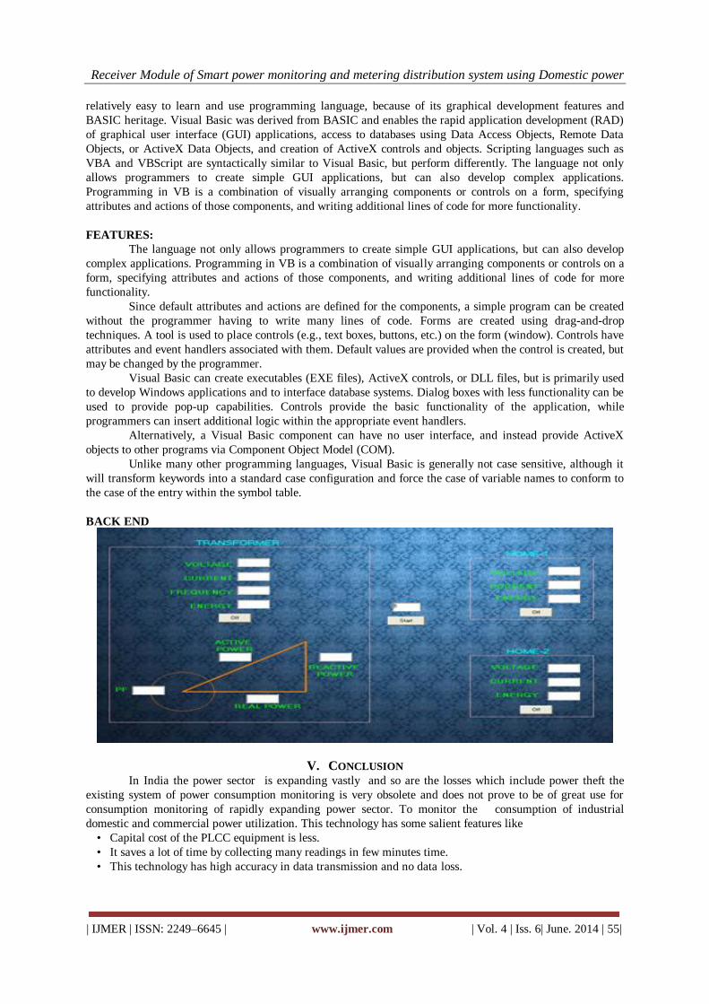
Receiver Module of Smart power monitoring and metering distribution system using Domestic power
| IJMER | ISSN: 2249–6645 | www.ijmer.com | Vol. 4 | Iss. 6| June. 2014 | 55|
relatively easy to learn and use programming language, because of its graphical development features and
BASIC heritage. Visual Basic was derived from BASIC and enables the rapid application development (RAD)
of graphical user interface (GUI) applications, access to databases using Data Access Objects, Remote Data
Objects, or ActiveX Data Objects, and creation of ActiveX controls and objects. Scripting languages such as
VBA and VBScript are syntactically similar to Visual Basic, but perform differently. The language not only
allows programmers to create simple GUI applications, but can also develop complex applications.
Programming in VB is a combination of visually arranging components or controls on a form, specifying
attributes and actions of those components, and writing additional lines of code for more functionality.
FEATURES:
The language not only allows programmers to create simple GUI applications, but can also develop
complex applications. Programming in VB is a combination of visually arranging components or controls on a
form, specifying attributes and actions of those components, and writing additional lines of code for more
functionality.
Since default attributes and actions are defined for the components, a simple program can be created
without the programmer having to write many lines of code. Forms are created using drag-and-drop
techniques. A tool is used to place controls (e.g., text boxes, buttons, etc.) on the form (window). Controls have
attributes and event handlers associated with them. Default values are provided when the control is created, but
may be changed by the programmer.
Visual Basic can create executables (EXE files), ActiveX controls, or DLL files, but is primarily used
to develop Windows applications and to interface database systems. Dialog boxes with less functionality can be
used to provide pop-up capabilities. Controls provide the basic functionality of the application, while
programmers can insert additional logic within the appropriate event handlers.
Alternatively, a Visual Basic component can have no user interface, and instead provide ActiveX
objects to other programs via Component Object Model (COM).
Unlike many other programming languages, Visual Basic is generally not case sensitive, although it
will transform keywords into a standard case configuration and force the case of variable names to conform to
the case of the entry within the symbol table.
BACK END
V. CONCLUSION In India the power sector is expanding vastly and so are the losses which include power theft the
existing system of power consumption monitoring is very obsolete and does not prove to be of great use for
consumption monitoring of rapidly expanding power sector. To monitor the consumption of industrial
domestic and commercial power utilization. This technology has some salient features like
• Capital cost of the PLCC equipment is less.
• It saves a lot of time by collecting many readings in few minutes time.
• This technology has high accuracy in data transmission and no data loss.

Receiver Module of Smart power monitoring and metering distribution system using Domestic power
| IJMER | ISSN: 2249–6645 | www.ijmer.com | Vol. 4 | Iss. 6| June. 2014 | 56|
Data transfer through medium (or) low voltage power line helps in monitoring the load pattern,
MVAR consumption, voltage variation, power theft, distribution losses etc. This project is an important tool
for detecting theft and maintaining power consumption discipline. This technology would save the power
sector from crumbling clutches of losses and theft. This project paves a way for a new trend in peak demand
and load management in distribution system.
VI. FUTURE ASSESMENT At present we concentrate only on the power usage of homes category all the other high voltage
usage of the power in industries tanneries and other vast areas we can implement in the future projects so that
it will be very efficient in finding the limitations of the power and the theft if any.
REFERENCES [1]. Archnet, “Embedded Power Line Carrier Modem”, available online
http//www.archnetco.com/english/product/ATL90.htm.
[2]. CIRED, “Distribution Utility Telecommunication Interfaces, Protocols and Architectures”, Final Report of the
CIRED Working Group WG06, September 2003. pp.52
[3] Customized Non-interruptible Distribution Automation System, Short Term Project No. PJP/2006/FKE (1), UTeM,
2005-2006
[4] K Dostert, 1997, Telecommunications over the Power Distribution Grid- Possibilities and Limitations Proc 1997
Internet. Symp. On Power Line Comms and its Applications pp1-9
[5] Intelligent Distribution Automation System Customized SCADA Based Rtu for Distribution Automation System,
M.Sc. Research Project, UTeM, 2005-2007.
[6] K.W. Louie, A. Wang, Wilson, and Buchanan, “Discussion on Power Line Carrier Applications”, Manitoba HVDC
Research Centre, IEEE, 2006, pp.655
[7] K.W. Louie, A. Wang, Wilson, and Buchanan, “Discussion on Power Line Carrier Applications”, Manitoba HVDC
Research Centre, IEEE, 2006, pp.656
[8] Miriam P. Sanders and Roger E. Ray, “Power Line Carrier Channel & Application Considerations for Transmission
Line Relaying”, Pulsar Document Number C045-P05967, 2000.
International
OPEN ACCESS Journal Of Modern Engineering Research (IJMER)
| IJMER | ISSN: 2249–6645 | www.ijmer.com | Vol. 4 | Iss. 6| June. 2014 | 57|
Application of Taguchi Parametric Technique for the Decrease in
Productivity Loss (In Percentage) In an Industry
Ramji Mishra1, Prof. R. P. Kori
2
1 M.Tech. (Production Student) MITS Gwalior 2Assistant Professor, (Mechanical Engineering) Department of Mechanical Engineering, MITS Gwalior
I. Introduction All the industries are suffering from the tremendous problem of not achieving 100% productivity.
Many researchers have been done to short out the problems, even they got success. This problem kept in mind
that some workers are not utilizing their capacity or potential of doing work completely. The workers who are
dealing with job more than its capacity is suffering from physical problems like body pain, mental harassment,
boredom and monotony, he has to work over its capacity. The work done by visiting industry GAJRA GEARS Pvt. Ltd. Dewas (M.P.) to increase productivity by the worker.
II. Present Study For attending goal of the work, it is find out the main factors responsible for loss in production and
among causes designed in fish bone diagram and necessary data collection.
Identification For Causes In % Loss In Production
By Fish Bone Diagram
Abstract: Now a day, working in industry is not as comfortable as in earlier times. The man power is decreasing day by day and new recruitment is not in same ratio as the persons leaving industries. This is
turn increase the work load on employees which causes physical problems to employees and also
decreases the productivity of worker. The purpose is to determine the optimum combination of three
parameters like Worker weight, component weight and worker age for achieving minimum loss (in
percentage) in productivity of worker. In order to meet the purpose in terms of productivity study will
utilize Taguchi parameter optimization methodology. The study includes selection of parameters
utilizing an orthogonal array, conducting experimental runs, data analysis, determining the optimum
combination, verification finally the modeling of input parameters (worker weight, component weight
and worker age), for a particular job work, for particular machine to minimize fatigue of worker and loss (in percentage) of productivity in industry.
Keywords: Taguchi techniques, Optimization Orthogonal Array.

Application Of Taguchi Parametric Technique For The Decrease In Productivity Loss (In
| IJMER | ISSN: 2249–6645 | www.ijmer.com | Vol. 4 | Iss. 6| June. 2014 | 58|
Material handling includes following activities lifting, holding, pulling, carrying or moving of load. Manual
material handling includes pushing, pulling, carrying, lifting and lowering. It includes lifting boxes at packaging
lines.
Negative Health Effects of Manual Material Handling
Cuts, brushes, fractures due to sudden, unexpected events such as accident.
Damage to musculoskeletal system of body as a consequence of gradual and cumulative wear and tear
through repetitive manual handling.
Advantages Of Well Designed MMHS –
(1) Improve efficiency of production by ensuring right quantity of materials at right place at right time.
(2) Cut down indirect labor cost.
(3) Reduce damage of materials during storage and movement.
(4) Improve customer service for a manner convenient for handling.
Contribution of Organization
Study of process in turning department in GAJRA GEAR.
Identification of Taguchi methodology, for method refer to parameter design, design of experiments using orthogonal array and to evaluate measuring system.
Implementation of procedure and steps of Taguchi parameter design.
Analyzing the results and determining the combination of selected parameters.
III. Research Methodology
Taguchi Technique
“The Father of Quality Engineering” introduced the concept of offline quality control techniques
known as Taguchi parameter design. It is reported that thousand of engineers have performed tens of thousands
of experiment based on teaching Taguchi method is statistical tool, adopted experimentally to investigate
influence of product such as weight of worker, weight of component and age. Thus it helps to determine right
person on right machine by optimizing the available factors. Thus Taguchi design is used to optimize design for performance quality and cost. Taguchi method is efficient method for designing process that operates and over a
variety of conditions. Taguchi approach is easy to adopt and may be applied with limited knowledge of
statistics, the engineering and scientific community.
Taguchi Philosophy –
(a) Achieving high system quality levels requires quality to be designed to the product.
(b) Quality losses defined as deviation from target not conformance to arbitrary specification.
(c) Quality is best achieved by minimizing deviation from a target.
Signal to Noise Ratios (S/N Ratios)
Taguchi recommends the use of the criterion he calls, “Signal to noise ratio” as performance statistic. The change in quality characteristic of a product under investigations in response to factor induced in the
experimental design is the signal of the desired effect. The effect of external affairs (Uncontrollable factors) on
the outcome of the quality characteristic under test is termed the noise.
The signal to noise ratio measures the sensitivity of the quality characteristic being investigated in
controlled manner, to those external influencing factors not under control. The S/N ratio is basically a
transformed figure of merit, created from the loss function. To use the loss function as figure of merit an
appropriate loss function with its constant value must first be established which is not always cost effective and
easy. Taguchi recognizes that dilemma early in the development of his methodologies and created the transform
of the loss function, which is named S/N ratio.
From the quality point of view, there are three possible categories of quality characteristic. They are:
1. Smaller the better.
2. Nominal is the best. 3. Larger is better.

Application Of Taguchi Parametric Technique For The Decrease In Productivity Loss (In
| IJMER | ISSN: 2249–6645 | www.ijmer.com | Vol. 4 | Iss. 6| June. 2014 | 59|
The S/N ratio is computed from the mean sqaure deviation (MSD) by the equations:
S/N=-10log10 (MSD) -------- (i)
For the S/N ratio to be large, MSD must have a value that is small. If smaller is the best quality characteristic;
MSD=-[(Y12+Y2
2+ ------------- +Yn
2)]/N -------- (ii)
Where, Y1, Y2 --------------- Yn are the quality characteristic.
If nominal is the best quality characteristic;
MSD=-[(Y1-Y0)2+(Y
2-Y
0)
2 ------- (Yn-Y0)
2]/N ------(iii)
Where, Y0= Target or nominal value
If larger is the best quality characteristic;
MSD=-[(1/Y12+1/Y2
2 +------- +1/Yn
2)]/N ------(iv)
The S/N ratio analysis is designed to measure quality characteristic. This is Taguchi‟s solution to Robust
Product or Process Design.
Taguchi Design And Analysis
As to process design stage, the analysis of processing sequences, the selections of production
equipment, tentative process parameter values, etc. are involved. Since system design is an initial functional
design, it may be far from optimization in term of quality and cost. Following on from system design is
parameter design. The objective of parameter design is to optimize the setting of the process parameter value for
improving quality characteristics and to indentify the product parameter values under the optimal process
parameter values. In addition, it is expected that the optimal process parameter values obtained from parameter
design are insensitive to variation in the environmental conditions and other noise factors. Finally, tolerance
design is used to determine and analyze tolerance around the optimal settings recommended by the parameter
design.
Steps of Taguchi Parameter Design
Step-1: Selection of the quality characteristic
There are three types of quality characteristic in the Taguchi methodology, such as smaller-the-better,
larger the-better, and nominal-the-best.
Step-2: Selection of noise factors and control factors
In this step, the controllable factors are Weight of worker (A), Weight of component (B) and age (C),
which were selected because they can potentially affect the productivity. Since these factors are controllable in
the production process, they are considered as controllable factors in the study.
Step-3: Selection of Orthogonal Array
There are 9 basic types of standard Orthogonal Arrays (OA) in the Taguchi parameter design (Genichi Taguchi And Yu-in Wu, 1979). An L9 Orthogonal Array is selected from Appendix B, 2nd edition, 2005, Taguchi
Techniques for quality Engineering, Philip J Ross 20, Tata McGraw-Hill Publishing Company limited, for this
study.
Step-4: Conducting the experiments
After the data were collected and recorded, signal-to-noise ratios of each experimental run were
calculated based on the following equation, which are listed below
S/N RATIO (Hi) = - 10 Log10 [MSD] ------------- (v)
Where, MSD=[Y12+Y2
2+ -----------------Yn2]; n=3
The average response values were also calculated and recorded
Step-5: Analyzing the results and determining the optimum cutting conditions (a) Analysis of Raw Data and S/N Ratios
(b) Determination of the Optimum Factor-Level Combination
Step-6: Predicting Optimum Performance
Using the aforementioned data, one could predict the optimum combination of Worker weight,
component weight, and age using the different worker, component, age combination. With this prediction, one
could conclude that which combination will creates the minimum loss in target achievement within the range of
specified combinations of the variables.

Application Of Taguchi Parametric Technique For The Decrease In Productivity Loss (In
| IJMER | ISSN: 2249–6645 | www.ijmer.com | Vol. 4 | Iss. 6| June. 2014 | 60|
Step-7: Establishing the design by using a confirmation experiment
The confirmation experiment is very important in parameter design, particularly when screening or
small fractional factorial experiments are utilized. The purpose of the confirmation experiment in this study was to validate the optimum welding conditions.
Advantages
(i) Consistency in experimental design and analysis.
(ii) Measurement of quality in terms of deviation from the target (loss functions).
(iii) Up-front improvement of quality by design and process development.
(iv) Reduction of time and cost of experiments.
Limitations
(i) The technique can only be effective when applied early in the design of the product/process.
(ii) The technique needs knowledge and training. Most severe limitations of the technique are the need for timing with respect to product/process
development.
IV. Experimental Setup
Selection of Ranges & Levels of Process Variables
The experimental setup is constructed for the various factors and their levels are chosen, which are dependent on
Weight of Worker
Weight of job/component
Age of the workers.
Weight of the worker
Different persons have different weight. So they can be arranged in intervals. Selection of Ranges for
Weight is as follows:
L = (40-55) Kg
M = (55-70) Kg
H = (70-85) Kg
Weight of Components
The second parameter is Weight of Components and it has three levels. The three levels are low,
medium and high. L = Lower Level = (2-6) Kg
M = Medium Level = (6-10) Kg
H = High Level = (10-15) Kg
Age of Workers
Different persons have different ages but we use here three levels called three age parameters such as
L, M and H. L type of person are lower age persons and having high strength. M type of person is of middle age
and middle strength category and the other belongs to higher age person and having lower strength.
L = Lower Age = (30-40)
M = Middle Age = (40-50)
H = Higher Age = (50-onwards)
V. Conclusion And Future Scope By the application of Taguchi Methodology and Mathematical Regression Modeling the researcher has
find out a formula in order to find out that for a fixed percentage loss in productivity, which operator has to
assign in which machine so that the maximum utilization of an operator could be possible.
Summary of the Work
The researcher has first visited to the company i.e., GAJRA GEAR, DEWAS, M.P., there in the
company the researcher found that a critical phase is there that an appropriate worker is not appoint to the proper machine, due to which the operator has to suffer from many physical problems such as low back pain, monotony
etc.,

Application Of Taguchi Parametric Technique For The Decrease In Productivity Loss (In
| IJMER | ISSN: 2249–6645 | www.ijmer.com | Vol. 4 | Iss. 6| June. 2014 | 61|
This gives the researcher a motivation to compute a formula so, that an operator can be appointed to a
proper machine where the person gives maximum efficiency and low productivity loss.
The Mathematical Regression Modeling has been implemented to find out the formula for the percentage loss of an operator if all his physical attributes and component weight are known. So, that it is
concluded whether the operator is assigned to a proposed machine or not. The formula obtained is
Here, Y= the percentage loss in productivity
Ww= Weight of Worker,
Wc = Weight of component.
VI. Contribution After finding out the problem of % loss in productivity. The researcher go through the optimization
technique of Taguchi Method of optimizing parameters in order to overcome the problem of % loss in
productivity. A mathematical regression modeling has been done to obtain a formula by which it can be
suggested that which operator should appoint to which machine so, as to get maximum productivity by
minimizing the losses.
VII. Future Scope Presently the researcher has applied the technique of Taguchi in a single Department i.e., Turning
Deptt. In the company. In future the work can be extended for all over the company.
REFERENCES [1.] U.S. Department of Labor, Bureau of Labor Standards, “Safety in Industry, Mechanical and Physical Hazards
Series: Teach Them to Lift,” Bulletin 110, Revised 1965. [2.] National Safety council, “Lifting, Carrying, Lowering Inanimate Objects,” Safety Education Data Sheet No.7
(Rev.), 1964 [3.] International Labor Office, “Maximum Permissible Weight to be carried by one worker,” Geneva, 1964. [4.] ASTM International, F-1166-88 (and rev. 2007), Standard Practice for Human Engineering for Marine Systems,
Equipments and Facilities. [5.] Snook , Stover H., and Vincent M. Ciriello, “The Design of Manual Handling Tasks: Revised Tables of Maximum
Acceptable Weights and Forces,” Ergonomics, Volume 34, No. 9, 1991. [6.] Kackar N. Raghu, (1985), “Off-line Quality Control Parameter Design & Taguchi Method” Journal of Quality
Technology, Vol. 17, No. 4, pp. 176-188. [7.] Mitchell. J.P., (June 1987), “Reliability of Isolated Clearance Defects on Printed Circuit Boards.” Proceedings of
Printed Circuit World Convention IV, Tokyo, Japan, pp. 50.1-50.16 [8.] Phillip J Ross, (2005), „Taguchi Techniques for Quality Engineering” Tata Mc Graw Hill 2nd edition.
[9.] Sathiya, P & Abdul Jaleel, May (2010), “Grey based Taguchi method for optimization Bead geometry in Laser Bead-on-Plate Welding”, Advances in Production Engineering & Management, 5(2010) 4 4,225-234, ISSN 1854-6250.
[10.] Dr. Saurav Datta, Prof. Siba Sankar Mahapatra & Prof. Asish Bandyopadhyay. (2010), “Elimination Joining Processes: Challenges for Quality, Design and Development, March 5-6, 2010 National Institute of Technology, Agartala, Tripura.
Y=(Ww)C1*(Wc)C
2* (Strength)C3

International
OPEN ACCESS Journal
Of Modern Engineering Research (IJMER)
| IJMER | ISSN: 2249–6645 | www.ijmer.com | Vol. 4 | Iss. 3 | Mar. 2014 | 62 |
Evaluation of Mechanical Properties of Sintered Hot Upset
Forged Square Cross Section Bars of Chromium-Molybdenum
Low Alloy Steels
1Hemlata Nayak,
2C. M. Agrawal,
3K. S. Pandey
1, 2PhD. Research Scholar, Ex. Professor,Department of Mechanical Engineering, MANIT, BHOPAL, M. P.,
India 3Professor, Department of Metallurgical and Materials Engineering,National Institute of Technology,
Tiruchirapalli-620015 Tamilnadu, India
I. Introduction Past seventy years have witnessed a tremendous growth in the area of powder perform forging/
extrusion/rolling either cold/warm or hot to produce components to near net shape with almost one hundred per
cent density. Further it has been believed over the past several decades that higher is the density, improved are
the mechanical properties, but, the last remaining residual porosity becomes very vital to all related properties of
the product .However, the reports also indicate that merely attaining the high density is not an index of improved mechanical properties. This very aspect can be referred elsewhere[1-3].The conventional P/M route
has been to consolidate the metal or blended powders in a suitable die, punch and bottom insert assembly at
enhanced pressures and sintering them under the protective or the reducing atmospheres for a given length of
time and same were employed directly in service. However, the demands raised by the automobile, nuclear and
space industries were that the parts produced must serve the requirements of structural applications and, hence,
one of the deformation processes were thought to be essential to be employed even though an open option of
liquid phase sintering or liquid phase infiltration processes were available to enhance sound metallurgical bonds.
But, the period beyond seventies saw a sea change in producing forged P/M parts for direct applications with
improved efficiency. In majority of the cases, P/M forged parts exhibited higher range of mechanical properties
which were isotropic in nature then the conventionally produced ingot metallurgy (I/M) parts.
Abstract: Present investigation pertains to evaluate the tensile properties of sintered hot forged and oil quenched and also homogenized, but furnace cooled specimens which were machined from
square cross section bars of approximate dimensions of ~13mm x ~13mm x~100±5mm of Fe-
0.16%C, Fe-0.16%C-0.7%Mn, Fe-0.16%C-1.0%Cr-0.55%Mo and Fe-0.16%C-2.25Cr-1.05%Mo
P/M steels prepared from elemental powders. Green compacts of homogeneously blended powders
of all compositions were prepared with initial aspects ratio of 1.34 with diameter being 27.5mm
using suitable compaction die set assembly on 1.0MN capacity UTM to a density level of 0.85±0.01
of theoretical employing controlled pressures in the range of 490±10MPa and taking pre – weighed
powder blends. All green compacts were protected during sintering by applying thin film of
indigenously developed ceramic coating on the entire surfaces. Ceramic coated compacts were
sintered in an electric muffle furnace at 1373±10K for a period of 120 minutes. All sintered
preforms of each com position were hot forged on a 1.0MN capacity friction screw press to square cross section bars of afore mentioned dimensions. Once the forging operation was completed 10-12
bars were quenched in linseed oil and nearly 12 bars were homogenized at sintering temperature
for one hour and then cooled inside the furnace itself. Standard tensile specimens were machined
and tested on Hounsfield Tensometer for evaluating tensile properties which were appreciably close
to the properties reported in literature for the above steels. Microstructure of specimens containing
chromium and molybdenum exhibited few un-dissolved particles along with the presence of fine
pores. SEM Fractography revealed mixed mode failure mostly ductile and partly brittle. These
steels also exhibited adequate ductility as is exhibited by conventionally produced steels. Thus, this
investigation shows the way how to produce high density P/M steels which can be used in structural
applications.
Key Words: applications, bars, composition, density, dissolved, ductility, failure, furnace cooled,
fractography, hot forged, microstructures, sintered, structural, tensile.

Evaluation of Mechanical Properties of Sintered Hot Upset Forged Square Cross Section Bars of....
| IJMER | ISSN: 2249–6645 | www.ijmer.com | Vol. 4 | Iss. 3 | Mar. 2014 | 63 |
P/M parts are practically well suited for fast high volume production of countless parts in the
automotive, various appliances, agricultural equipment, business machines, electrical and electronic, power
tools ordnance and machine tools industries. However, they also find extensive applications in the aerospace,
nuclear and other industries [4]. Thus, powder metallurgy offers the engineers and scientists, a means of
conserving materials, minimizing machining and by securing a uniform product at reasonable costs [5]. In
industries, the forming of structural components from porous materials, either directly from atomized powders
or from blended powders, but, sintered preforms is becoming a popular route. This is due to the fact that P/M forming processes result in savings in energy and materials in addition to quality improvement. In automotive
industries, the weight reduction results in favourable operating conditions of the engine in terms of reduced
exhaust gas emissions and vibrations. Thus, lowering down the fuel consumptions .Connecting rod is the bulk
component, i.e., required in automobiles, and, hence, the P/M forming route is in strong competition with the
conventional processes such as casting and forgings routes [6].
In powder preform forging or hot isostatic pressing, the density and the mechanical properties of
components and parts is raised to values to those of wrought products [7]. Plastic deformation of sintered
powder materials are similar to that of conventionally fully dense materials, but, there are additional
complications due to the substantial volume fraction of voids in the perform materials. In particular, the voids
must be eliminated during deforming operation so that a sound metallurgical structure is obtained [8]. The
forging of sintered powder performs has been shown to be a process capable of producing higher density P/M parts for high stress applications where porosity must be minimized or completely eliminated. Mechanical
properties of powder forged parts depend upon the processing parameters, the composition, the sintering time
and forging operations [9]. Pores present in a P/M parts act as stress raisers and also provide initiation sites for
corrosion, especially in an environment containing chloride ions. However, industrial use of stainless P/M
products has increased in the recent years due to their improved corrosion properties and at relatively low cost.
Porosity in P/M parts makes them highly susceptible to crevice corrosion [10]. However, the probability of
fracture is mainly dependent upon the volume fraction of pores and only to a small extent depends on pore size
[11]. However, the fatigue properties in P/M parts can be referred elsewhere [12-16]. But, the fatigue strength of
hot forged and shot pinned P/M parts are detailed elsewhere [17, 18] and other stressed P/M parts can be further
referred in literature [19-23]. Apart from these, the mechanical properties of differently produced ferrous based
P/M steels of challenging in nature can be referred elsewhere [24-29].
Systems selected to be produced through elemental powders were (A) Fe-0.16%C, (B) Fe-0.16%C-0.70%Mn, (C) Fe-0.16%C-1.0%Cr-0.55%Mo, and (D) Fe-0.16%C-2.25%Cr-1.05%Mo steels. Applications of
(A) category of steels i.e., Fe-0.16%C steels are that they are used for rivets, wires, nails, chains, stampings,
seam welded pipes, hot and cold rolled strips, sheets and plates for general purposes, ship plates, boiler plates,
cams and shafts, stay bolts, wheel hubs, brake housings and brake pedal levers. Since, B grades of steels, i.e.,
Fe-0.16%C-0.7%Mn steels contain 0.7%Mn which neutralizes the harmful effects of sulphur by forming MnS
which melts at higher temperatures. Further manganese enhances the tensile strengths, imparts freedom from
blow holes, deoxidizes the steel and produces fine grained steel and improves surface quality. Manganese can be
used as structural materials as well. However, (C) grade of steels, i. e., Fe-0.16%C-1.0%Cr-0.55%Mo, and (D)
grade of steels, i. e., Fe-0.16%C-2.25%Cr-1.05%Mo containing chromium and molybdenum as alloying
elements which are known to induce beneficial effects to these steels. Chromium is added in steels as it is
comparatively less expensive and imparts many useful characteristics to the steel. Readily combines with carbon in preference to iron. Cr offers resistance to oxidation. However, the addition of molybdenum in steels refines
grains, enhances harden ability and improves high temperature properties. Thus, Cr-Mo steels possess good
mechanical properties and sufficiently adequate machinability as molybdenum enhances the beneficial effects of
chromium in chromium molybdenum steels and find applications as low alloy structural steels. These steels
have good resistance to corrosion and oxidation and offer high creep resistance. Therefore, the above four steels
have been selected for the present investigation. Basically, Cr and Mo are strong carbide formers. Cr raises
tensile strengths, hardness, wears resistance and hardenability and makes the steel stainless when added beyond
12%. These steels find applications in general purpose structural applications such as ball bearing steels, spring
steels, hard magnetic steels, and, stainless steels. Since, molybdenum is a strong carbide former, imparts high
temperature strengths, enhances resistance to creep, minimizes temper embrittlement, and increases the
resistance to corrosion of high chromium steels, and, therefore, molybdenum assists in case hardening steels, Hot work steels, High speed steels, and, Non magnetic steels.
Aim of the present investigation is to produce and evaluate the tensile properties of hot forged square
cross section (~13mm x ~13mm) bars with an approximate lengths of 100±05mm of Fe-0.16%C, Fe-0.16%C-
0.7%Mn, Fe-0.16%C-1.0%Cr-0.55%Mo,and, Fe-0.16%C-2.25%Cr 1.05%Mo steels prepared from elemental
powders which were suitably mixed, homogeneously blended, compacted, sintered, hot forged to square cross-
section bare and heat treated differently. Mechanical properties are suitably related to microstructure and SEM
fractographs.

Evaluation of Mechanical Properties of Sintered Hot Upset Forged Square Cross Section Bars of....
| IJMER | ISSN: 2249–6645 | www.ijmer.com | Vol. 4 | Iss. 3 | Mar. 2014 | 64 |
II. Experimental Details 2.1 Materials Required
Atomized iron powder of -180 um was procured from M/s. Sundaram Fasteners Pvt. Limited,
Hyderabad, and Andhra Pradesh, India. Manganese, chromium and molybdenum powders of -37 um were obtained from M/s. The Ghrishma Speciality Powders Limited, Mumbai, Maharashtra, India. However, the
graphite powder of less than 5 micron was supplied by the M/s. Ashbury Graphite Inc., New Jersey, U.S.A.
2.2 Tooling and Equipment
High-Carbon High-Chromium die steel was required to fabricate the mother die, punch, and the bottom
insert for compaction of powder blends. Molybdenum-di-sulphide paste was needed to be used during
compaction as a die wall lubricant. In house designed, fabricated die, punch and bottom insert were suitably heat
treated and tempered. However, hot forging die set was fabricated from molybdenum hot die steel. These were
suitably heat treated and tempered.
2.3 Powder and Powder Blend Characteristics
Basically, the ability of a metal powder blends to be effectively compacted and the resulting properties of the compacts before and after sintering are influenced to a substantial degree by the characteristics of the
starting powdered material. The basic powder characteristics required to be assessed include, sieve size analysis,
apparent density, flow rate and compressibility. Sieve size analysis of basic iron powder is given in Table 1,
and, Table 2 shows the flow rates, apparent densities and the compressibility for iron powder and other powder
blends to yield the final composition of Fe-0.16%C, Fe-0.16%C-0.7%Mn, Fe-0.16%C-1.0%Cr-0.55%Mo, Fe-
0.16%C-2.25%Cr-1.05%Mo steels after sintering. Manganese, chromium and molybdenum powders taken in
the present investigation were of -37 microns.
Table 1 Sieve Size Analysis of Iron Powder
Sieve size, µm Powder Size Distributio
Wt %
retained
-180
+ 150
-150
+125
-125
+106
-106
+90
-90
+75
-75
+63
-63
+53
-53
+37 -37
Wt% powder
retained 1.52 1.83 23.12 1.11 21.86 2.21 18.60 13.62 16.11
Cum, Wt%
powder Ret. 1.52 3.35 26.47 27.58 49.44 51.65 70.25 83.87 99.98
2.4 Powder Blend Preparation
Powder mixes of Fe-0.16%C, Fe-0.16%C-0.7%Mn, Fe-0.16%C-1.0%Cr-0.55%Mo and Fe-0.16%C-
2.25%Cr-1.05%Mo were separately kept in a standard stainless steel pots with a powder mix to porcelain balls
of 10 - 15mm diameter in the weight ratio of 1.1:1. Pot lids were securely tightened, and, the pots were fixed on
the pot mill and the mill was switched on. The blending operation was carried out for a period of 32 hours which
yielded homogeneous powder blends. Homogeneity of powder blends were ascertained by taking nearly 120±10
g of each of the powder mixes from each pot and were used for measuring the flow rates, and apparent densities.
Immediately, after the completion of measurements of flow rates and apparent densities, the powder mixes were
returned back to their respective pots, and, the pot lids were tightened once again and were placed back on the potmill and securely fixed and then the mill was switched on again, This operation was repeatedly carried out
till the last thee consecutive readings of flow rates and apparent densities were almost constant independently.
This ensured the homogeneity of the powder blends. Thus, the time of blending was experimentally found to be
32 hours and the same was fixed.
Table 2 Basic Properties of Iron, Fe-0.16%C, Fe-0.16%C-0.7%Mn, Fe-0.16%C-1.0%Cr-0.55%Mo and Fe-
0.16%C-2.25%Cr-1.05%Mo Powder Blends.
Sl.
No. Systems
Apparent
density, g/cc
Flow rate by Hall
Flow Meter, S/100g. Remarks
1 Iron 2.973 51.52 6.594g/cc at 400±10MPa
2 Fe-0.16%C 2.934 48.67 6.751g/cc at 450±10MPa
3 Fe-0.16%C-0.7%Mn 2.990 50.93 6.756g/cc at 375±10MPa
4 Fe-0.16%C- 1.0%Cr-0.55%Mo 3.010 47.01 6.74g/cc at 450±10MPa
5 Fe-0.16%C-2.25Cr -1.05%Mo 3.090 46.77 6.732g/cc at 375±10MPa

Evaluation of Mechanical Properties of Sintered Hot Upset Forged Square Cross Section Bars of....
| IJMER | ISSN: 2249–6645 | www.ijmer.com | Vol. 4 | Iss. 3 | Mar. 2014 | 65 |
2.5 Compact Preparation from Iron powder and the Powder Blends
Green compacts of iron powder and the above prepared powder blends were prepared on a 1.0 MN
capacity Universal Testing Machine. Compacts of initial aspect ratios of 1.34 with the diameter being 27.75mm
were prepared by applying pressures in the range of 540±10 M Pa in the relative density range of 0.85±0.01of
theoretical by taking accurately pre-weighed iron powder and powder blends respectively. In all, twenty four
compacts of each composition were prepared. A schematic diagram shown in fig.1 depicts the compaction
assembly for the compaction of iron powder and powder blends.
Figure 1 Complete Compaction Assembly - Schematic Diagram
2.6 Application of Indigenously Developed Ceramic Coating and Drying
Entire surfaces of all compacts of all compositions were coated with a thin film of indigenously
developed ceramic coating [30] and the same was allowed to dry for a period of 12 hours under an ambient
conditions. A second coat of the same coating was now applied on the entire surfaces of all the compacts once
again, but, this time 900 to the previous coating. This second coating was also allowed to dry under the
aforementioned conditions for a further period of 12 hours.
2.7 Sintering and Hot Forging To Square Cross-Section Bars
The ceramic coated compacts of all compositions were separately sintered in an electric muffle furnace in
the temperature range of 1373±10K for a period of 120 minutes. The sintered compacts of H/D ratio of 1.34 with a diameter of 27.75mm were hot forged to square cross-section (13mmx~13mm) bars of approximate
lengths of 100±5mm. Twelve forged bars of each compositions were kept inside the furnace chamber and
homogenized for a period of sixty minutes at the sintering temperature itself, and, subsequently cooled to room
temperature inside the furnace chamber by switching off the furnace. Apart from the above, other sets of twelve
sintered compacts of each composition were also forged to similar types of bars and then quenched in linseed oil
kept at room temperature separately.
III. Results and Discussions
3.1 Dimensional Measurements and Tensile Properties
Standard tensile specimens as per specifications given elsewhere [27] were machined from the Fe-
0.16%C, Fe-0.16%C-0.7%Mn, Fe-0.16%C-1.0%Cr-0.55%Mo and Fe-0.16%C-2,25%Cr-1.05%Mo sintered
powder metallurgy steels hot forged to square cross-section bars under two different conditons of heat
treatments, namely, sintered hot forged and oil quenched (SFOQ) and sintered hot forged, but, homogenized at
1373±10K for sixty minutes and furnace cooled (SFHFC). Prior to conducting the tensile tests, the dimensional
measurements such as initial gauge length (L0), initial diameter (D0) within the guage length were under taken and recorded. During and after fracture, the final gauge length (Lf) and final diameter (Df) at the point of
fracture were also measured and recorded. Further peak load (Ppl, Kg) qand fracture load (Ffl, Kg) were also
recrded during and after carrying out the tensile tests respectively. All tension test experiments were carried out
on a 0.02 MN capacity bench type Haunsfield Tensometer. Original area of cross-section (A0, mm2) for all
specimens were calculated and all experimental and measured parameters are provided in Table 3. Perusal of
this table very clearle reflects that the area of cross-section at the fracture point has decreased irrespective of the
heat treatments meted out to the specimens and their compositions. Further the area of reduction in tension
tested specimens were observed to be more when the
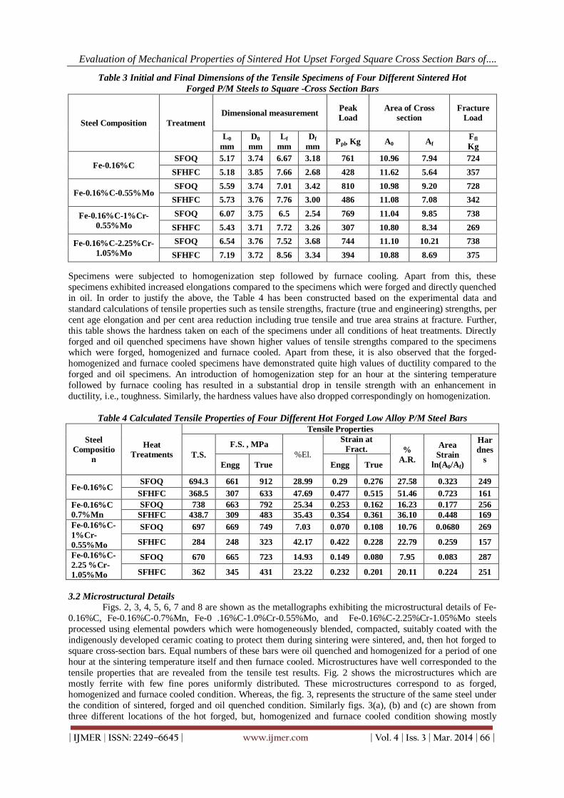
Evaluation of Mechanical Properties of Sintered Hot Upset Forged Square Cross Section Bars of....
| IJMER | ISSN: 2249–6645 | www.ijmer.com | Vol. 4 | Iss. 3 | Mar. 2014 | 66 |
Table 3 Initial and Final Dimensions of the Tensile Specimens of Four Different Sintered Hot
Forged P/M Steels to Square -Cross Section Bars
Steel Composition Treatment
Dimensional measurement Peak
Load
Area of Cross
section
Fracture
Load
L0
mm
D0
mm
Lf
mm
Df
mm Ppl, Kg A0 Af
Ffl
Kg
Fe-0.16%C SFOQ 5.17 3.74 6.67 3.18 761 10.96 7.94 724
SFHFC 5.18 3.85 7.66 2.68 428 11.62 5.64 357
Fe-0.16%C-0.55%Mo SFOQ 5.59 3.74 7.01 3.42 810 10.98 9.20 728
SFHFC 5.73 3.76 7.76 3.00 486 11.08 7.08 342
Fe-0.16%C-1%Cr-
0.55%Mo
SFOQ 6.07 3.75 6.5 2.54 769 11.04 9.85 738
SFHFC 5.43 3.71 7.72 3.26 307 10.80 8.34 269
Fe-0.16%C-2.25%Cr-
1.05%Mo
SFOQ 6.54 3.76 7.52 3.68 744 11.10 10.21 738
SFHFC 7.19 3.72 8.56 3.34 394 10.88 8.69 375
Specimens were subjected to homogenization step followed by furnace cooling. Apart from this, these
specimens exhibited increased elongations compared to the specimens which were forged and directly quenched
in oil. In order to justify the above, the Table 4 has been constructed based on the experimental data and
standard calculations of tensile properties such as tensile strengths, fracture (true and engineering) strengths, per
cent age elongation and per cent area reduction including true tensile and true area strains at fracture. Further,
this table shows the hardness taken on each of the specimens under all conditions of heat treatments. Directly
forged and oil quenched specimens have shown higher values of tensile strengths compared to the specimens which were forged, homogenized and furnace cooled. Apart from these, it is also observed that the forged-
homogenized and furnace cooled specimens have demonstrated quite high values of ductility compared to the
forged and oil specimens. An introduction of homogenization step for an hour at the sintering temperature
followed by furnace cooling has resulted in a substantial drop in tensile strength with an enhancement in
ductility, i.e., toughness. Similarly, the hardness values have also dropped correspondingly on homogenization.
Table 4 Calculated Tensile Properties of Four Different Hot Forged Low Alloy P/M Steel Bars
Steel
Compositio
n
Heat
Treatments
Tensile Properties
T.S.
F.S. , MPa
%El.
Strain at
Fract. %
A.R.
Area
Strain
ln(A0/Af)
Har
dnes
s
Engg True Engg True
Fe-0.16%C SFOQ 694.3 661 912 28.99 0.29 0.276 27.58 0.323 249
SFHFC 368.5 307 633 47.69 0.477 0.515 51.46 0.723 161
Fe-0.16%C
0.7%Mn
SFOQ 738 663 792 25.34 0.253 0.162 16.23 0.177 256
SFHFC 438.7 309 483 35.43 0.354 0.361 36.10 0.448 169
Fe-0.16%C-
1%Cr-
0.55%Mo
SFOQ 697 669 749 7.03 0.070 0.108 10.76 0.0680 269
SFHFC 284 248 323 42.17 0.422 0.228 22.79 0.259 157
Fe-0.16%C-
2.25 %Cr-
1.05%Mo
SFOQ 670 665 723 14.93 0.149 0.080 7.95 0.083 287
SFHFC 362 345 431 23.22 0.232 0.201 20.11 0.224 251
3.2 Microstructural Details Figs. 2, 3, 4, 5, 6, 7 and 8 are shown as the metallographs exhibiting the microstructural details of Fe-
0.16%C, Fe-0.16%C-0.7%Mn, Fe-0 .16%C-1.0%Cr-0.55%Mo, and Fe-0.16%C-2.25%Cr-1.05%Mo steels
processed using elemental powders which were homogeneously blended, compacted, suitably coated with the
indigenously developed ceramic coating to protect them during sintering were sintered, and, then hot forged to
square cross-section bars. Equal numbers of these bars were oil quenched and homogenized for a period of one
hour at the sintering temperature itself and then furnace cooled. Microstructures have well corresponded to the
tensile properties that are revealed from the tensile test results. Fig. 2 shows the microstructures which are
mostly ferrite with few fine pores uniformly distributed. These microstructures correspond to as forged, homogenized and furnace cooled condition. Whereas, the fig. 3, represents the structure of the same steel under
the condition of sintered, forged and oil quenched condition. Similarly figs. 3(a), (b) and (c) are shown from
three different locations of the hot forged, but, homogenized and furnace cooled condition showing mostly

Evaluation of Mechanical Properties of Sintered Hot Upset Forged Square Cross Section Bars of....
| IJMER | ISSN: 2249–6645 | www.ijmer.com | Vol. 4 | Iss. 3 | Mar. 2014 | 67 |
ferrite and few scattered but rounded pores well within the structure itself. However, fig. 4 represents the same
steel under the as forged and oil quenched condition. Similarly figs. 5 and 6 correspond to Fe-0.16%C-1.0%Cr-
0.55%Mo steel under two above mentioned conditions. Likewise figs. 7(a), 7(b) and 7(c) and fig.8 correspond to
the P/M steel of composition Fe-0.16%C-2.25%Cr-1.05%Mo under the above conditions, i.e., under the forged,
homogenized and the furnace cooled condition. and also under the forged and oil quenched condition. The
general observations of these micro-structures reveal that the homogenization step has introduced grain growth
and structural modification. These structures clearly show that they are under the completely stress relieved condition. These structures very closely corresponded to the tensile properties as well as the respective hardness
values. Further observation reveals that the microstructure of forged and homogenized specimens contain
rounded and evenly distributed pores, but, they are very few in numbers whereas, the microstructure
corresponding to forged and oil quenched conditions did exhibit the presence of rounded pores but unevenly
distributed in the microstructure. Apart from these, the steels containing chromium and molybdenum have
shown carbide formation and also at few places un-dissolved chromium and molybdenum particulate structures
are evidently seen. Such particulate structures are seen in both types of heat treated specimens.
(a) SFHFC CONDITION(2% Nital) Mag. 250X (b)SFOQ CONDITION (2% Nital) Mag. 250X
Figure 2 Microstructures of Sintered Forged Fe-0.16%C Steel Under Two different Heat Treated
Condition (etchant; 2% Nital)
(a) Centre(100X)
(b ) Middle of centre and edge(100X) (c) Edge(100X)
Figure 3 Microstructures shown at Three Different Locations of the Cross-section Bars of
Fe-0.16%C-0.7%Mn P/M Steel SFHFC Condition (etchant; 2% Nital)
Figure 4 Microstructures shown at the Centre Locations of the Cross-section Bar of Fe-0.16%C-0.7%Mn
P/M Steel SFOQ Condition at 250X; (etchant; 2% Nital).

Evaluation of Mechanical Properties of Sintered Hot Upset Forged Square Cross Section Bars of....
| IJMER | ISSN: 2249–6645 | www.ijmer.com | Vol. 4 | Iss. 3 | Mar. 2014 | 68 |
(a) Centre(250 X) (b) Edge(250 X)
Figure 5 Microstructures shown at the Centre and at the Edge Locations of the Cross-section Bar of Fe-
0.16%C-1.0%Cr-0.55%Mo P/M Steel SFHFC Condition (etchant; 2% Nital)
Magnification = 100X
Figure 6 Microstructures shown at the Centre Locations of the Cross-section Bar of Fe-0.16%C-1.0%Cr-
0.55%Mo P/M Steel SFOQ Condition (etchant; 2% Nital).
(a) Centre(100 X) (b) Edge(100 X)
Figure 7 Microstructures shown at the Centre d at the Edge Locations of the Cross-section Bar of Fe-
0.16%C-2,25%Cr-1.05%Mo P/M Steel SFHFC Condition (etchant; 2% Nital)
(a) Centre(400X) (b) Middle of centre and edge(400X) (c) Edge(400X)
Figure 8 Microstructures shown at the Three DifferentLocations of the Cross-section Bar of Fe-0.16%C-
2.25%Cr-1.05%Mo P/M Steel Under SFOQ Condition (etchant; 2% Nital).

Evaluation of Mechanical Properties of Sintered Hot Upset Forged Square Cross Section Bars of....
| IJMER | ISSN: 2249–6645 | www.ijmer.com | Vol. 4 | Iss. 3 | Mar. 2014 | 69 |
3.3 SEM Fractography Fractured Surfaces of Tensile Tested Specimens all four Steels Investigated Fractographs shown through figs. 9 to 12 reveal the exact nature of the fractured surfaces of the tensile
tested specimens under various conditions. Fig. 9 (a) shows the fractographs corresponding to Fe-0.16%C P/M
steel which has been homogenized and furnace cooled. This structure clearly shows large number of dimples
indicating the failure mode to be highly ductile and the same is very well supported by the tensile properties that
are fairly high, which is an index of high ductility (~48%elongation and ~52% area reduction). Similarly the
fractographs represented through fig. 9 (b) also depicts fairly large number of dimples and at places fine, but, rounded porosities in good numbers are also visible. Fractured pieces of this specimen when visually examined
have exhibited cup and cone type separation of the two corresponding counter parts. High level of ductility
(29% elongation and 28% area reduction) is recorded. Similarly the steel corresponding to Fe-0.16%C-0.7%Mn
composition exhibited quite ductile mode of failures under both the conditions of heat treatments.However,
under the homogenized and furnace cooled condition the failure has advanced through the coalescence of
residual pores, but, the failure remained ductile only (fig.10(a). Once again the similar situation existed when
the steel has been forged and oil quenched. Even though, the steel exhibited high strength values, the ductility
remained fairly high indicating that the steel under this condition also remained fairly tough and thus the failure
remained quite ductile as is evident through the fig.10(b).
(a) SFHFC (b) SFOQ Figure 9 SEM Fractographs of Tensile Tested Specimen fractured Surfaces of Fe-0.16%C P/M Steel
Figs. 11 and 12 showing the SEM fractographs corresponding to the steel composition of Fe-0.16%C-1.0%Cr-
0.55%Mo. This steel SEM fractographs under the forged, homogenized and furnace cooled condition shows
large number of dimples an index of ductile mode of failure (fig. 11(a)) which is ably supported by the tensile
test results exhibiting high percentage of elongation (~42%) and per cent area reduction (~23%).SEM
fractographs shown in fig. 11(b) corresponds to the same steel, but, under sintered, forged and oil quenched
condition. Even though dimples
(a)
SFHFC (b)SFOQ
Figure 10 SEM Fractographs of Tensile Tested Specimen fractured Surfaces of Fe-0.16%C-0.7%Mn P/M
Steel Under Two conditions of Heat Treatments.

Evaluation of Mechanical Properties of Sintered Hot Upset Forged Square Cross Section Bars of....
| IJMER | ISSN: 2249–6645 | www.ijmer.com | Vol. 4 | Iss. 3 | Mar. 2014 | 70 |
(a) SFHFC (b) SFOQ
Figure 11 SEM Fractographs of Tensile Tested Specimen fractured Surfaces of Fe-0.16%C-1.0%Cr-
0.55%Mo P/M Steel Under Two conditions of Heat Treatments.
(a) SFHFC
(b) SFOQ
Figure 12 SEM Fractographs of Tensile Tested Specimen fractured Surfaces of Fe-0.16%C-2.25%Cr-
1.05%Mo P/M Steel Under Two conditions of Heat Treatments.
IV. Conclusions Based on the experimental data on tensile properties of four different low alloy steels produced through powder metallurgical routes using elemental powders via homogeneous blending, compacting, sintering and hot
forging to square cross-section bars and heat treating them under two distinct conditions such as sintering,
forging and oil quenching (SFOQ) and sintering, forging and homogenizing at the sintering temperature for a
period of an hour followed by cooling them inside the furnace itself and after analyzing the data critically, the
following main conclusions have emerged:
1. Four P/M steels investigated in the present investigation produced from the elemental powders which were
sintered, forged and oil quenched have shown improved strengths, but, reduced ductility compared to the
steels which were sintered, forged, homogenized and furnace cooled which have shown high degree of
ductility,
2. Microstructures of all the four steels have clearly shown the presence of porosities which were mostly
rounded in the event of homogenized for a period of one hour at the sintering temperature and cooling inside the furnace itself. However, at places in the microstructures corresponding to steels containing chromium
and molybdenum, few un-dissolved particles of these elements are also present,
3. Tensile tested specimens fractured in a cup and cone type in all the steels except for the steel Fe-0.16%C
which was highly cup and cone type when they were homogenized and furnace cooled. However, the forged
and oil quenched specimens have exhibited mixed mode of failures,

Evaluation of Mechanical Properties of Sintered Hot Upset Forged Square Cross Section Bars of....
| IJMER | ISSN: 2249–6645 | www.ijmer.com | Vol. 4 | Iss. 3 | Mar. 2014 | 71 |
4. SEM fractographs corresponding to steels which were produced by sintering, forging, homogenizing
and furnace cooling have exhibited mostly ductile failures as it contained large number of dimples which are an
index of ductile failures, but, the quenched steels in their corresponding fractographs have shown fairly good
amount of dimples as well as presence of particle de-lamination which is an index of mixed mode of failures,
Finally summarizing the outcome of the present investigation, it is, established that there exists a
certainty of producing the quality P/M products by using elemental powders and their homogeneously blended
mixes to required compositions of the given steel/s. The higher mechanical properties such as strength and sound metallurgical structures along with the enhanced toughness under the sintered forged and oil quenched
condition. However, under sintered, forged, homogenized and furnace cooled condition, the strength and
toughness attained are suitable for producing quality structural parts. Thus, the present investigation opens up a
new area of research to produce structural components using elemental powders.
REFERENCES [1] K. S. Pandey, "Salient Characteristics of High Temperature Forging of Ferrous Preforms", Key Engineering
Materials, Vol. 29-31, pp.465-486, 1989, Trans. Tech. Publications, Switzerland. [2] K. S. Pandey, "Some Characteristics of SINTA-FORGING of Iron and Hyper Eutectoid Steel Through a Partially
Open Step Down Cylindrical Die Cavity at 1400K", Quarterly International Journal of Powder Metallurgy Science and Technology, Vol. 4, No. 1, pp.25-34, 1992.
[3] K. S. Pandey, "Hot Forging of Sintered Iron and Fe-0.35 Per cent Carbon Steel Through a Partially Open Step Down Cylindrical Die Cavity at 11200C", Quarterly International Journal of Powder Metallurgy Science and Technology,
Vol. 5, No. 1, pp.23-32, 1993. [4] R. L. McGee, J. E. Campbells, L. R. Carlson and G. K. Manning," The Mechanical Properties of Certain Aircraft
Structural Metals at Very Low Temperatures ", WADCTR 58-386, Wright Air Development Centre, 1958. [5] S. F. Moustafa, S. A. El-Bandry and A. M. Sanad, "Effect of Graphite With and Without Copper Coating on
Consolidation Behaviour and Sintering of Copper- Graphite Composites", Powder Metallurgy, Vol. 40, No. 3, pp.210-225, 1997.
[6] Ashok G. K. Jinka and Michel Bellet, "Hot Forging of a P/M Connecting Rod - A Three Dimensional Computer Model", The International Journal of Powder Metallurgy, Vol. 33, No. 3, pp.37-43, 1996.
[7] Wang Junha, Qi Ji Azhong, Yan Fuyanand Wang Enka,"Effect of Hot Repressing on the Mechanical Properties of Sintered Steels", Modern Developments in powder Metallurgy, Proceedings of 1984 P/M Conference, Canada, Edited by N. Aqua and Charles I. Whitman, Vol. 15, pp. 639-653.
[8] Howard A. Kuhn and Alan Lawley, "Powder Metallurgy Processing", Academic Press, Inc., pp.99-138, 1978. [9] M. C. Wang, "Properties of High Density Powder Forged Iron Based Alloy", Powder Metallurgy, Vol. 37, No. 3, pp,
201-205, 1994. [10] Dah-Weiyan, Joseph R.Spirko and Howard I. Sanderow, "Colorimetric Corrosion Testing on P/M Stainless Steel",
The International Journal of Powder Metallurgy, Vol. 33, No. 2, pp.41-49, 1997. [11] A. Nordgren and A. Malandar, "Influence of Porosity on Strength of WC - 10%Co Cemented Carbide," Powder
Metallurgy, Vol. 32, No. 3, pp,189--200, 1988. [12] F. H. Usmani and T. J. Davies, "Effect of Surface Treatment on Fatigue of Powder Forged Steels", Powder
Metallurgy, Vol. 24, No. 1, pp.23-30, 1980. [13] J. Holmes and R. A. Queeney,"Fatigue Crack Initiation in Porous Steels", Powder Metallurgy, Vol. 28, No.4, pp.231-
235, 1980. [14] N. Douib, I. J. Mellanby and J. R. Moon, "Fatigue of Inhomogeneous Low Alloy P/M steels", Powder Metallurgy,
Vol. 32, No. 3, pp.209-214, 1989. [15] Erhard Klar, David F. Berry, Prasan K. Samal, John J. Le Wandowski and Joseph D. Rigneys, "Fracture Toughness
and Fatigue Crack Growth Response of Copper Infiltrated Steel", The International Journal of Powder Metallurgy, Vol. 31, No. 4, pp.317-323, 1995.
[16] C. M. Sonsino, "Fatigue Design for P/M", Powder Metallurgy, Vol. 33, No. 3, pp.317-323, 1990. [17] R. A. Chemenkaff, S. Mocarski and D. A. Yeager, "Increased Fatigue Strength of Powder Forged Connecting Rods
by Optimized Shot Peening", Powder Metallurgy, Vol. 38, No. 3, pp.190-200, 1995. [18] S. Saritas, C. Dogan and R. Varol, "Improvement of Fatigue Properties of P/M Steels by Shot Peening", Powder
Metallurgy, Vol. 42, No. 2, pp.126-130, 1999. [19] S. Saritas and T. J. Davies, "Fracture Behaviour of Powder forged Steels", Modern Developments in powder
Metallurgy, Proceedings of 1984 P/M Conference, Canada, Edited by N. Aqua and Charles I. Whitman, Vol. 15, Principles and Processes, pp. 599-609.
[20] I. Bertilsson and B. Carlsson, "Dynamic Properties of Sintered Steels", Powder Metallurgy, Vol. 30, No. 3, pp.183-188,
[21] J. S. 1987. Santner, "Effect of Notch Acuity on the Fatigue Behaviour of X7091 Aluminium Alloy", The International Journal of Powder Metallurgy and Powder Technology, Vol. 18, No. 8, pp.225-231, 1999.
[22] D. D. Poland, R. J. Stephens and T. Prucher, "Influence of Density and Sintering Temperature on Smooth Notched Behaviour of F 14405 High Strength P/M Steel", Powder Metallurgy, Vol. 41, No. 4, pp.274-280,1998.
[23] Lars Arn berg, Anita Karlsson and Helene Hrandrup Wognsen, Influence of Slag Particles on the Mechanical Properties and Corrosion Resistance of a P/M Stainless Steel", The International Journal of Powder Metallurgy, Vol. 24, No. 3, pp.215-223, 1999.

Evaluation of Mechanical Properties of Sintered Hot Upset Forged Square Cross Section Bars of....
| IJMER | ISSN: 2249–6645 | www.ijmer.com | Vol. 4 | Iss. 3 | Mar. 2014 | 72 |
[24] N. Nokita, T. Kawamura and Y. Kondo, "New Low Alloy Steel Powders Provide Improved Mechanical Properties for P/M Forgings", The International Journal of Powder Metallurgy and Powder Technology, Vol. 14, No. 3, pp.203-211, 1978.
[25] W. F. Wang and Y. L. Su, "Mechanical Properties, Corrosion Resistance and High Temperature Oxidation of
Sintered Duplex Stainless Steels", Powder Metallurgy, Vol. 29, No. 3, pp.177-182, 1986. [26] G. I. Zhou and J. V. Wood, "Influence of Alloying Elements on Mechanical Properties Sintered High Speed Steel
Powders", Powder Metallurgy, Vol. 38, No. 3, pp.230-236,195. [27] Manucla Oliveria and John D. Bolton, "Effect of Ceramic Particles on the Mechanical Properties of M3/2 High
Speed Steel", The International Journal of Powder Metallurgy, Vol. 32, No. 1, pp.37-49, 1996. [28] A. Salak, "Improvement of Steel Properties Using Fine Grain Structure Hameag Iron Powder", The International
Journal of Powder Metallurgy and Powder Technology, Vol. 18, No. 1, pp.11-23, 1982. [29] M. V. Veidis, "Mechanical Properties of Copper Infiltrated Low Alloy Steel Powders", The International Journal of
Powder Metallurgy and Powder Technology, Vol. 12, No.2 pp.127-130, 1982, 1976.
[30] K. S. Pandey,"Indigenously Developed Ceramic Coating", Department of metallurgical and Materials Engineering, National Institute of Technology, Tiruchirappalli-620015, Tamil Nadu, India.

International
OPEN ACCESS Journal
Of Modern Engineering Research (IJMER)
| IJMER | ISSN: 2249–6645 | www.ijmer.com | Vol. 4 | Iss. 6| June. 2014 | 73|
Vibration Analysis of Multiple Cracked Shaft
Dinesh R. Satpute1, Milind S. Mhaske2, Prof. S. B. Belkar3
1( PG Scholar, Pravara Rural College of Engineering, Ahmednagar, India) 2 (Department of Mechanical Engineering, Pravara Rural College of Engineering, Ahmednagar, India )
3(Head and associate professor, Mechanical Engineering Department, PREC LONI, Ahmednagar)
I. INTRODUCTION There are number of methods of crack detection in the beam has been presented by many authors. The
problem of crack detection is simple whenever dealt with single crack but as number of cracks to handle are
more than one then the problem becomes relatively complex. D. P. Patil and S. K. Maiti [1] propose method to
detect multiple cracks in the beam using frequency measurement. Their results give linear relationship between
damage parameters and natural frequency of vibration of beam. A. K. Darpe et al. [2] studied dynamics of a
bowed rotor with a transverse surface crack. They concluded that amplitude and directional nature of higher
harmonic components of bowed rotor remains unaltered, however rotating frequency component changes in
magnitude. In another research Athanasios C. Chasalevris and Chris A. Papadopoulos [3] studied
identification of multiple cracks in beams under bending. They formulate compliance matrix of two DOF as a
function of both crack depth and angle of rotation of the shaft. Their stated method gives not only depth and
size of the crack but also angular position of the crack. Ashish K. Darpe [4] proposes a novel way to detect
transverse surface crack in a rotating shaft. He studied the behavior of the simply supported shaft with
transverse crack subjected to both bending and torsional vibration. K.M. Saridakis et al. [5] propose the
application of neural networks, genetic algorithm and fuzzy logic for the identification of cracks in shafts. In
another research of Ashish K. Darpe [6] he present coupled vibrations of a rotor with slant crack. He
established stiffness matrix for Timoshenko beam on concepts of fracture mechanics the behavior of the shaft
slant crack was compared with transverse crack. Sachin S. Naik and Surjya K. Maiti [7] studied triply coupled
bending–torsion vibration of Timoshenko and Euler–Bernoulli shaft beams with arbitrarily oriented open
crack. The variation of compliance coefficients with angular position of the crack was illustrated. The study
shows that the frequency of vibration decreases as the distance of the crack from free end increases. Ashish K.
Darpe [8] studied dynamics of a Jeffcott rotor with slant crack. Stiffness coefficients based on flexibility
coefficients was used to form equation of motion. His study shows that the lateral and longitudinal stiffness is
more for slant crack as compared to transverse crack. The trend of 3 x frequency component can be used to
detect as well as to identify the type of crack. Tejas H. Patel, Ashish K. Darpe [9] studied influence of crack
breathing model on nonlinear dynamics of a cracked rotor. Their study shows that for the rotor with deeper
crack, the switching crack model displays chaotic, quasi-periodic and sub harmonic motion. A.S. Sekhar [10]
presented a review on multiple cracks effects and identification. He summaries different methods of single and
double crack detection. S.K. Georgantzinos, N.K. Anifantis [11] presented the study of breathing mechanism
of a crack in a rotating shaft. He studied the behavior of the transverse crack in cantilever shaft beam with two
Abstract: Crack in component if undetected may lead to catastrophic failure of the component. The
cracked rotor problem received the first attention in 1970 and after that the interest among the
researchers started. The vibration behavior of cracked structures, in particular cracked rotors, is
important to study as the introduction of the crack alters the vibration characteristics of the structure.
The problem of damage and crack detection in structural components has acquired important role in past
few years. However, cracked rotor studies are mainly deals with single crack. For multiple cracked
structures the problem of crack sizing and location becomes more complex. Only few authors have
pointed out the multiple crack assessment in the rotor. The proposed work is on vibration analysis of
multiple cracked shaft beam. An Euler Bernoulli beam fixed at one end with two transverse cracks is
considered. The vibration characteristics of the shaft are studied using Experimental Modal Analysis and
Finite Element Analysis. The mode shapes and natural frequencies of the beams are studied and their
variation with change in position and depth of the crack is also studied. The study shows good agreement
of the results obtained using Finite Element Analysis and Experimental Modal Analysis.
Keywords: vibration analysis, crack detection, modal analysis, damage, condition monitoring.

Vibration Analysis of Multiple Cracked Shaft
| IJMER | ISSN: 2249–6645 | www.ijmer.com | Vol. 4 | Iss. 6| June. 2014 | 74|
different cases of straight and curved front of the shaft. Flexibility coefficients were calculated based on energy
principle. He concludes that the breathing behavior depends on depth and shape of the crack front. In the
present work the Experimental modal analysis of the shaft beam was done and the results are compared with
results of Finite Element Analysis performed in ANSYS 14.5.
II. FEA ANALYSIS OF SHAFT BEAM The 3-D modeling of the shaft with diameter 0.03m and length 0.360m is done in ANSYS 14.5. The
3-D model of the shaft is meshed with element 20node186. The material used for the shaft has following
properties,
1) Modulus of Elasticity= 2x10¹¹N/m2,
2) Poisons ratio= 0.3 and
3) Mass Density 7850 kg/m2.
Boundary Conditions as cantilever beam is applied by making all degrees of freedom zero at one end
of the shaft. A Block Lanczos method was used for extraction of natural frequency of free vibration. The first
three modes of transverse vibration are extracted. Also the mode shapes of the first three modes of transverse
vibration are plotted.
Fig.1. 1st Mode of Vibration (e1=0.25, a1/d=0.1, e2=0.55, a2/d=0.1)
Fig.2 2nd Mode of Vibration (e1=0.25, a1/d=0.1, e2=0.55, a2/d=0.1)

Vibration Analysis of Multiple Cracked Shaft
| IJMER | ISSN: 2249–6645 | www.ijmer.com | Vol. 4 | Iss. 6| June. 2014 | 75|
Fig.3 3
rd Mode of Vibration (e1=0.25, a1/d=0.1, e2=0.55, a2/d=0.1)
III. EXPERIMENTAL MODAL ANALYSIS
Fig.4 Test rig for Experimental Modal Analysis
The fig. 4 shows the test rig used for experimental modal analysis of the shaft beam. The instruments
used for experimental modal analysis are Fast Fourier Transform analyzer, accelerometer, impact hammer and
related accessories. The FFT analyzer used is 4 channel Bruel and Kjaer make with measuring range 10-200
dB, amplitude stability + 0.1 dB. RT-PROTM software, compatible with the FFT analyzer is used. The
piezoelectric, miniature type unidirectional accelerometer is used to sense the frequency response functions.
The accelerometer is mounted on the beam using wax. The accelerometer is mounted just near the crack to
capture the correct signals. The impact hammer is used to excite the beam whose frequency response function
is to be captured. The beam is tapped gently using impact hammer. Impact hammer has the range of excitation
1-4000 Hz.
IV. RESULTS 4.1 Experimental and FEA Results
Table 1. Experimental and FEA results
Sr. no. e1 a1/d e2 a2/d ω1 FEA,
HZ
ω1 Exp.,
HZ
ω2 FEA,
HZ
ω2 Exp.,
HZ
1 Healthy beam 163.65 167.98 1002.6 1008
2 0.25 0.1 0.55 0.1 162.97 160.33 998.32 982.54
3 0.25 0.2 0.55 0.2 160.49 162.34 983.46 964.69
4 0.25 0.3 0.55 0.3 155.43 159.86 953.26 942.31
5 0.25 0.4 0.55 0.4 147.48 145.17 906.99 898.78
6 0.25 0.5 0.55 0.5 135.41 136.64 838.66 829.85
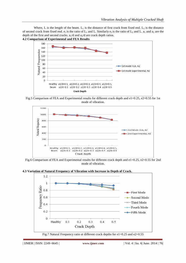
Vibration Analysis of Multiple Cracked Shaft
| IJMER | ISSN: 2249–6645 | www.ijmer.com | Vol. 4 | Iss. 6| June. 2014 | 76|
Where, L is the length of the beam. L1 is the distance of first crack from fixed end. L2 is the distance
of second crack from fixed end. e1 is the ratio of L1 and L. Similarly e2 is the ratio of L2 and L. a1 and a2 are the
depth of the first and second cracks. a1/d and a2/d are crack depth ratios.
4.2 Comparison of Experimental and FEA Results
Fig.5 Comparison of FEA and Experimental results for different crack depth and e1=0.25, e2=0.55 for 1st
mode of vibration.
Fig.6 Comparison of FEA and Experimental results for different crack depth and e1=0.25, e2=0.55 for 2nd
mode of vibration.
4.3 Variation of Natural Frequency of Vibration with Increase in Depth of Crack.
Fig.7 Natural Frequency ratio at different crack depths for e1=0.25 and e2=0.55
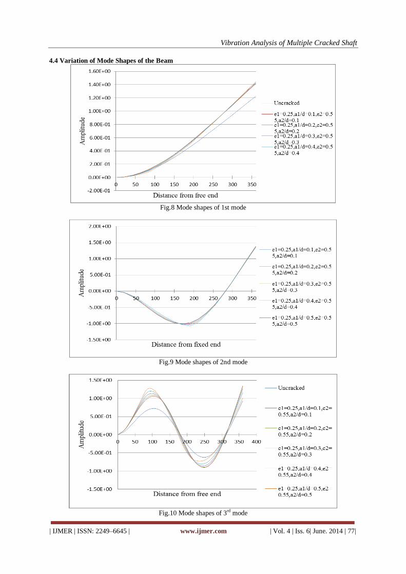
Vibration Analysis of Multiple Cracked Shaft
| IJMER | ISSN: 2249–6645 | www.ijmer.com | Vol. 4 | Iss. 6| June. 2014 | 77|
4.4 Variation of Mode Shapes of the Beam
Fig.8 Mode shapes of 1st mode
Fig.9 Mode shapes of 2nd mode
Fig.10 Mode shapes of 3rd mode

Vibration Analysis of Multiple Cracked Shaft
| IJMER | ISSN: 2249–6645 | www.ijmer.com | Vol. 4 | Iss. 6| June. 2014 | 78|
V. DISCUSSION The Natural Frequency of the beam for first three modes of transverse vibration is extracted from
ANSYS. The results obtained using Finite Element Analysis for the first three modes are compared with the
results obtained using Experimental Modal Analysis of the beam. The results obtained by FEA and
Experimental Modal Analysis show good agreement as shown in the figure 5 and figure 6. Also the variation
of the Natural Frequencies of first three transverse modes with increase in crack depth is studied. The
orientation of the crack in the structure caused the local flexibility. As shown in the figure 7 the Natural
Frequency of vibration decreases with increase in depth of the crack. The mode shapes of the first, second and
third modes of transverse vibration are extracted and plotted as shown in figures 8 to 10. It has been observed
that the mode shapes of the healthy beam and the cracked beam has different shapes. This is because of
increase in flexibility causes increase in amplitude of vibration.
VI. CONCLUSION In this study the Finite Element Analysis of a shaft beam with two transverse cracks was done in
ANSYS and its validation is done using Experimental Modal Analysis. Mode shapes of first three modes of
transverse vibration are plotted and comparison of mode shapes of healthy and cracked shaft was done. Also
the comparison of the values of natural frequency obtained by Finite Element Analysis is compared with the
results of Experimental Modal Analysis. The study shows good agreement between Experimental modal
analysis and Finite Element Analysis results. It is observed that the natural frequency of vibration of all three
transverse vibrations decreases with increase in depth of the crack as the presence of crack in structural
member introduces local flexibilities. The mode shapes of the first three modes of vibration are plotted on the
graph and it can be seen that the introduction of the crack changes the shape of mode shapes.
Acknowledgements The authors wish to thank Prof. S. B. Belkar, Head of Mechanical department, PREC Loni and Prof.
P. R. Baviskar, Mechanical Department, RSCOE Pune for their advice and supports during experimental
testing.
REFERENCES [1] D.P. Patil, S.K. Maiti [2002], “Detection of multiple cracks using frequency measurements”, Engineering Fracture
Mechanics 70, pp1553–1572.
[2] A.K. Darpe, K. Gupta, A. Chawla [2006], “Dynamics of a bowed rotor with a transverse surface crack”, Journal of
Sound and Vibration 296, pp888–907.
[3] Athanasios C. Chasalevris, Chris A. Papadopoulos [2006], “Identification of multiple cracks in beams under
bending”, Mechanical Systems and Signal Processing 20, pp1631–1673.
[4] Ashish K. Darpe [2007], “A novel way to detect transverse surface crack in a rotating shaft”, Journal of Sound and
Vibration 305, pp151–171.
[5] K.M. Saridakis, A.C. Chasalevris, C.A. Papadopoulos , A.J. Dentsoras [2007], “Applying neural networks, genetic
algorithms and fuzzy logicfor the identification of cracks in shafts by using coupled response measurements”,
Computers and Structures 86 pp1318–1338
[6] Ashish K. Darpe [2007], “Coupled vibrations of a rotor with slant crack”, Journal of Sound and Vibration 305,
pp172–193
[7] Sachin S. Naik, Surjya K. Maiti [2009], “Triply coupled bending–torsion vibration of Timoshenko and Euler–
Bernoulli shaft beams with arbitrarily oriented open crack”, Journal of Sound and Vibration 324 , pp1067–1085.
[8] Ashish K. Darpe [2007], “Dynamics of a Jeffcott rotor with slant crack”, Journal of Sound and Vibration 303, pp1–
28
[9] Tejas H. Patel, Ashish K. Darpe [2007], “Influence of crack breathing model on nonlinear dynamics of a cracked
rotor”, Journal of Sound and Vibration 311, pp953–972.
[10] A.S. Sekhar [2007], “Multiple cracks effects and identification”, Mechanical Systems and Signal Processing 22,
pp845–878
[11] S.K. Georgantzinos, N.K. Anifantis [2008], “An insight into the breathing mechanism of a crack in a rotating
shaft”, Journal of Sound and Vibration 318, pp279–295.

International
OPEN ACCESS Journal
Of Modern Engineering Research (IJMER)
| IJMER | ISSN: 2249–6645 | www.ijmer.com | Vol. 4 | Iss.6| June. 2014 | 79|
Earthquake Resistant Design of Low-Rise Open Ground Storey
Framed Building
Bhagavathula Lohitha 1, S.V.Narsi Reddy2 1Student, Department of Civil Engineering (M.Tech Structures), Malla Reddy Engineering college,
Secunderabad, Telangana State, India
2Asst.Professor, Department of Civil Engineering, Malla Reddy Engineering college, Secunderabad,
Telangana State, India
I. INTRODUCTION Due to increasing population since the past few years car parking space for residential apartments in
populated cities is a matter of major concern. Hence the trend has been to utilize the ground storey of the
building itself for parking. These types of buildings having no infill masonry walls in ground storey, but
infilled in all upper storeys, are called Open Ground Storey (OGS) buildings. They are also known as ‘open
first storey building’ (when the storey numbering starts with one from the ground storey itself), ‘pilotis’, or
‘stilted buildings’. There is significant advantage of these category of buildings functionally but from a seismic
performance point of view such buildings are considered to have increased vulnerability. From the past
earthquakes it was evident that the major type of failure that 2 occurred in OGS buildings included snapping of
lateral ties, crushing of core concrete, buckling of longitudinal reinforcement bars etc. Due to the presence of
infill walls in the entire upper storey except for the ground storey makes the upper storeys much stiffer than the
open ground storey. Thus, the upper storeys move almost together as a single block, and most of the horizontal
displacement of the building occurs in the soft ground storey itself. In other words, this type of buildings sway
back and forth like inverted pendulum during earthquake shaking, and hence the columns in the ground storey
columns and beams are heavily stressed. Therefore it is required that the ground storey columns must have
sufficient strength and adequate ductility. The vulnerability of this type of building is attributed to the sudden
lowering of lateral stiffness and strength in ground storey, compared to upper storeys with infill walls.
II. OBJECTIVE OF THE STUDY The salient objectives of the present study have been identified as follows:
i) To study the effect of infill strength and stiffness in the seismic analysis of OGS buildings.
ii) To check the applicability of the multiplication factor of 2.5 as given in the Indian Standard IS 1893:2002
for design of low rise open ground storey building.
iii) To assess the effect of support condition on the seismic behaviour of OGS buildings.
Abstract: Presence of infill walls in the frames alters the behavior of the building under lateral loads.
However, it is common industry practice to ignore the stiffness of infill wall for analysis of framed
building. Engineers believe that analysis without considering infill stiffness leads to a conservative
design. An existing RC framed building (G+3) with open ground storey located in Seismic Zone-V is
considered for this study. This building is analyzed for two different cases: (a) considering both infill
mass and infill stiffness and (b) considering infill mass but without considering infill stiffness. Two
separate models were generated using commercial software SAP2000. Infill weights were modelled
through applying static dead load and corresponding masses considered from this dead load for
dynamic analyses. Infill stiffness was modelled using a diagonal strut approach. Two different support
conditions, namely fixed end support condition and pinned end support condition, are considered to
check the effect of support conditions in the multiplication factors. Linear and non-linear analyses were
carried out for the models and the results were compared.
Keywords: infill walls, diagonal strut, open ground storey, equivalent static analysis, response
spectrum analysis, pushover analysis, low rise building .

Earthquake Resistant design of Low-rise open ground storey framed building
| IJMER | ISSN: 2249–6645 | www.ijmer.com | Vol. 4 | Iss.6| June. 2014 | 80|
III. Modeling The methodology worked out to achieve the above-mentioned objectives is as follows:
(i) Review the existing literature and Indian design code provision for designing the OGS building
(ii) Select an existing building model for the case study.
(iii)Model the selected building with and without considering infill strength/ stiffness. Models need to consider
two types of end support conditions as mentioned above.
(iv) Linear analysis of the selected building model and a comparative study on the results obtained from the
analyses.
(v) Nonlinear analysis of the selected building model and a comparative study on the results obtained from the
analyses.
(vi) Observations of results and discussions.
Structural Modeling
3.1 Overview
It is very important to develop a computational model on which linear / non-linear, static/ dynamic
analysis is performed. The first part of this chapter presents a summary of various parameters defining the
computational models, the basic assumptions and the geometry of the selected building considered for this
study. Accurate modelling of the nonlinear properties of various structural elements is very important in
nonlinear analysis. In the present study, frame elements were modelled with inelastic flexural hinges using
point plastic model. A detailed description on the nonlinear modelling of RC frames is presented in this
chapter. Infill walls are modelled as equivalent diagonal strut elements. The last part of the chapter deals with
the computational model of the equivalent strut including modelling nonlinearity.
3.2 Building Description
An existing OGS framed building located at Guwahati, India (Seismic Zone V) is selected for the
present study. The building is fairly symmetric in plan and in elevation. This building is a G+3 storey building
(12m high) and is made of Reinforced Concrete (RC) Ordinary Moment Resisting Frames (OMRF). The
concrete slab is 150mm thick at each floor level. The brick wall thicknesses are 230 mm for external walls and
120 mm 24 for internal walls. Imposed load is taken as 2 kN/ m2 for all floors. Fig. 3.1 presents typical floor
plans showing different column and beam locations. The cross sections of the structural members (columns
and beams 300 mm×600 mm) are equal in all frames and all stories. Storey masses to 295 and 237 tonnes in
the bottom storyes and at the roof level, respectively. The design base shear was equal to 0.15 times the total
weight.

Earthquake Resistant design of Low-rise open ground storey framed building
| IJMER | ISSN: 2249–6645 | www.ijmer.com | Vol. 4 | Iss.6| June. 2014 | 81|
The amount of longitudinal reinforcement in the columns and beams is given in Table 3.2. Although
the columns have equal reinforcement in all storey levels beam reinforcement in floor and roof are different.
Refer Fig. 3.1 (a) and (b) for column and beam identification (ID).
3.3 Structural Modelling
Modelling a building involves the modelling and assemblage of its various load-carrying elements.
The model must ideally represent the mass distribution, strength, stiffness and deformability. Modelling of the
material properties and structural elements used in the present study is discussed below.
3.3.1 Material Properties
M-20 grade of concrete and Fe-415 grade of reinforcing steel are used for all the frame models used in
this study. Elastic material properties of these materials are taken as per Indian Standard IS 456: 2000. The
short-term modulus of elasticity (Ec) of concrete is taken as:
Ec=5000√𝑓𝑐k𝑀
fck
is the characteristic compressive strength of concrete cube in MPa at 28-day (20 MPa in this case). For the
steel rebar, yield stress (fy) and modulus of elasticity (E
s) is taken as per IS 456:2000. The material chosen for
the infill walls was masonry whose compressive strength (fm’) from the literature was found out to be 1.5 MPa
and the modulus of elasticity was stated as:
Em
= 350 to 800 MPa for table moulded brick
= 2500 to 5000 MPa for wire cut brick
According to FEMA 356:2000 elasticity of modulus of brick is taken as Em
= 750 fm’. For the present study the
modulus of elasticity of the masonry is taken as given in literature by Asokan (2006).
3.3.2 Structural Elements
Beams and columns are modelled by 3D frame elements. The beam-column joints are modelled by
giving end-offsets to the frame elements, to obtain the bending moments and forces at the beam and column
faces. The beam-column joints are assumed to be rigid. Beams and columns in the present study were modelled
as frame elements with the centrelines joined at nodes using commercial software SAP2000NL. The rigid
beam-column joints were modelled by using end offsets at the joints (Fig. 3.2). The floor slabs were assumed to
act as diaphragms, which ensure integral action of all the vertical lateral load-resisting elements. The weight of
the slab was distributed as triangular and trapezoidal load to the surrounding beams.
The structural effect of slabs due to their in-plane stiffness is taken into account by assigning ‘diaphragm’
action at each floor level. The mass/weight contribution of slab is modelled separately on the supporting
beams.
3.3.3 Modelling of Column Ends at the Foundation
The selected building is supported on a raft foundation. Therefore, the column ends are modelled as
fixed at the top of the raft and analysed. To study how the response of the building changes with the support
conditions, the same building model also analysed by providing a hinge in place of fixity.
3.3.4 Modelling Infill Walls
Infill walls are two dimensional elements that can be modelled with orthotropic plate element for
linear analysis of buildings with infill wall. But the nonlinear modelling of a two dimensional plate element is
not understood well. Therefore infill wall has to be modelled with a one-dimensional line element for
nonlinear analysis of the buildings. Same building model with infill walls modelled as one-dimensional line
element is used in the present study for both linear and nonlinear analyses. Infill walls are modelled here as
equivalent diagonal strut elements. Section 3.5 explains the modelling of infill was as diagonal strut in detail.
Fig. 3.3 presents a three-dimensional computer model of building without and with considering infill stiffness.

Earthquake Resistant design of Low-rise open ground storey framed building
| IJMER | ISSN: 2249–6645 | www.ijmer.com | Vol. 4 | Iss.6| June. 2014 | 82|
(a)Without infill (b) With infill
Fig. 3.3: 3D Computer model of building without and with considering infill stiffness respectively.
IV. Result & Discussions As mentioned earlier the selected OGS building is analyzed for following two different cases and two
end support conditions (fixed and pinned end support) (a) Considering infill strength and stiffness (with
infill/infilled frame) (b) Without considering infill strength and stiffness (without infill/bare frame). Therefore
there are a total of four building models: (a) building modelled without infill and fixed end support, (b)
building modelled with infill and fixed end support, (c) building modelled without infill and pinned end
support and (d) building modelled with infill and pinned end support. Equivalent static and response spectrum
analyses of these four building models are carried out to evaluate the effect of infill on the seismic behaviour of
OGS building for two different support conditions. Following sections presents the results obtained from these
analyses.
4.1 Calculation of Time Period and Base Shear
The design base shear (VB) was calculated as per IS 1893: 2002 corresponding to the fundamental
period for moment-resisting framed buildings with brick infill panels as follows
𝑉𝐵=𝐴𝑊
𝐴=𝑍/2.𝐼/𝑅.𝑆𝑎/𝑔
where W ≡ seismic weight of the building, Z ≡ zone factor, I ≡ importance factor, R ≡ response reduction
factor, Sa
/g ≡ spectral acceleration coefficient corresponding to an approximate time period (Ta) which is given
by: 𝑇𝑎=0.09/√𝑑 for RC frame with masonry infill
Table 4.1: Comparison of fundamental time periods for with and without infill for pinned and fixed end
support condition
4.2 Shift in Period
Table 4.2 (a): Shift in period for fixed end Table 4.2 (b): Shift in period for pinned end
support condition support condition.

Earthquake Resistant design of Low-rise open ground storey framed building
| IJMER | ISSN: 2249–6645 | www.ijmer.com | Vol. 4 | Iss.6| June. 2014 | 83|
From Table 4.2(a) and 4.2(b) we can see that there is not much considerable difference in the time
periods of the building irrespective of the directions considered according to the empirical formula. From the
computational value we can see that there is a considerable shift of period for buildings modelled with fixed
end support conditions. But the period shift is found to be very little in case of buildings modelled with pinned
end support conditions Hence it can be said that the IS 1893:2002 (Part-1) does not take into account the
support conditions for the calculation of fundamental period. It always gives a lower bound solution to be
conservative for force calculation.
4.3 Column Interaction Ratios
This table clearly shows that for a low rise OGS building model with fixed-end support the ground
storey column forces actually reduced when infill stiffness is considered in Equivalent Static Analysis. It
marginally increases (less than 10%) in the case of response spectrum analysis. This is because the forces
applied to building model with infill stiffness is little more compared to that applied to building model without
infill stiffness in Response Spectrum Analysis. But the applied forces to these two buildings are same in case of
Equivalent Static Analyses. Therefore using a multiplication factor of 2.5 for ground floor columns of low rise
OGS buildings as per Indian Standard IS 1893:2002 (Part-1) is not justified.
4.4 Beam Demand-to-Capacity Ratios

Earthquake Resistant design of Low-rise open ground storey framed building
| IJMER | ISSN: 2249–6645 | www.ijmer.com | Vol. 4 | Iss.6| June. 2014 | 84|
Table 4.4 presents results from both equivalent static analyses (ESA) and response spectrum analyses
(RSA). The table presented above shows that the conclusion drawn for the columns hold good for beams also.
Force demands in all first floor beams are found to be lower when infill stiffness modelled in OGS building. It
can be concluded from this results that it is conservative to analyse low-rise OGS building without considering
infill stiffness.
V. CONCLUSION Followings are the salient conclusions obtained from the present study:
i) IS code gives a value of 2.5 to be multiplied to the ground storey beam and column forces when a building
has to be designed as open ground storey building or stilt building. The ratio of IR values for columns and
DCR values of beams for both the support conditions and building models were found out using ESA and RSA
and both the analyses supports that a factor of 2.5 is too high to be multiplied to the beam and column forces of
the ground storey. This is particularly true for low-rise OGS buildings.
ii) Problem of OGS buildings cannot be identified properly through elastic analysis as the stiffness of OGS
building and Bare-frame building are almost same.
iii) Nonlinear analysis reveals that OGS building fails through a ground storey mechanism at a comparatively
low base shear and displacement. And the mode of failure is found to be brittle.
iv) Both elastic and inelastic analyses show that the beams forces at the ground storey reduce drastically for the
presence of infill stiffness in the adjacent storey. And design force amplification factor need not be applied to
ground storey beams.
v) The linear (static/dynamic) analyses show that Column forces at the ground storey increases for the presence
of infill wall in the upper storeys. But design force amplification factor found to be much lesser than 2.5.
vi) From the literature available it was found that the support condition for the buildings was not given much
importance. Linear and nonlinear analyses show that support condition influences the response considerably
and can be an important parameter to decide the force amplification factor.
REFERENCES [1.] A. Asokan, (2006) Modelling of Masonry Infill Walls for Nonlinear Static Analysis of Buildings under Seismic
Loads. M. S. Thesis, Indian Institute of Technology Madras, Chennai. 2.Agarwal P. and Shrikhande M. (2006)
Earthquakeresistant design of structures, PHI Learning Pvt. Ltd., New Delhi.
[2.] Al-Chaar, G. (2002) Evaluating strength and stiffness of unreinforced masonry infill structures. U.S. Army
Corps of Engineers. Technical Report NO. ERDC/CERL TR-02-1. Construction Engineering Research
Laboratory. Campaign. USA
[3.] Al-Chaar, G., M. Issa and S. Sweeney (2002) Behaviour of masonry infilled non-ductile RC frames. Journal of
Structural Engineering. American society of Civil Engineers. 128(8). 1055-1063
[4.] Arlekar, J.N.; S. K. Jain and C.V.R Murty (1997) Seismic response of RC frame buildings with soft first
storeys. Proceedings of CBRI golden jubilee conference on natural hazards in urban habitat. New Delhi
[5.] Asteris P. G. (2003) Lateral stiffness of brick masonry infilled plane frames. Journal of Structural Engineering.
129(8). 1071-1079
[6.] Chopra A. K. (1973) Earthquake resistance of buildings with a soft first storey. Earthquake and Structural
Dynamics. 1. 347-355
[7.] Chug, R. (2004) Studies on RC Beams. Columns and Joints for Earthquake Resistant Design. M. Tech Project
Report. Indian Institute of Technology Madras, Chennai. India

Earthquake Resistant design of Low-rise open ground storey framed building
| IJMER | ISSN: 2249–6645 | www.ijmer.com | Vol. 4 | Iss.6| June. 2014 | 85|
[8.] Crisafulli F. J. (1999) Seismic Behaviour of reinforced concrete structures with masonry infills. Ph.D. Thesis.
University of Canterbury. New Zealand. 10. Das, S. (2000) Seismic design of vertically irregular reinforced
concrete structures. Ph.D. Thesis. North Carolina State University. Raleigh. NC
[9.] Das, S. and J. M. Nau (2003) Seismic design aspects of vertically irregular reinforced concrete buildings.
Earthquake Spectra. 19. 455-477
[10.] Deodhar, S. V. and A. N. Patel (1998) Ultimate strength of masonry infilled steel frames under horizontal load.
Journal of Structural Engineering. Structural Engineering Research Centre. 24. 237-241 13. Dhansekar, M. and
A.W. Page (1986) the influence of brick masonry infill properties on the behaviour of infilled frames.
Proceedings of Institution of Civil Engineers. Part 2. 81. 593-605
[11.] Dolsek M and P. Fajfar (2001) Soft storey effects in uniformly infilled reinforced concrete frames. Journal of
Earthquake Engineering. 5(1). 1-12
[12.] Dolsek M and P. Fajfar (2000) On the seismic behaviour and mathematical modelling of RC framed structures.
12th
World Conference on Earthquake Engineering. Auckland. New Zealand. 296-305
[13.] Fardis, M.N. and T. B. Panagiotakos (1997) Seismic design and response of bare and masonry-infilled concrete
buildings. Part II: Infilled structures. Journal of Earthquake Engineering. 1. 475-503
[14.] Govindan, P. and D. Vivekanandan(1990 Effect of Opening in Brick Infilled Square Panel, Indian Concrete
Journal. 64. 298-303
[15.] Hashmi, A. K. and A. Madan (2008) Damage forecast for masonry infilled

International
OPEN ACCESS Journal Of Modern Engineering Research (IJMER)
| IJMER | ISSN: 2249–6645 | www.ijmer.com | Vol. 4 | Iss. 6| June. 2014 | 86|
Experimental Analysis of Emission Parameters for Various
Blends of Gasohol on Multi-Cylinder and Single Cylinder Petrol
Engine
Nevil Panchal1, Chirag Tarsadia
2, Jaynil Parikh
3, Ravishankar Agrawal
4,
Parth Rathod5
1, 2, 3, 4, 5 Mechanical Department, SNPIT & RC, Gujarat technological University, Gujarat, India
I. Introduction
Petrol engines are widely used for various applications in automobiles. Spark Ignition Engine has the
advantages of low specific weight, compactness and simplicity in the design, low production cost and low
maintenance cost. However this type of engine has serious drawback of High pollutant emission.
With increasing concerns on environmental pollution and the steadily inflation in demand for liquid fuels and downtrend in supply of petroleum crude oil, researchers have been forced to look to substitute fuels in
order to fulfill the future demands for liquid fuels. Recent events throughout the world, including the inadequacy
of petroleum crude oil, the sharp rising in the cost of oil and gasoline motor fuels, and the political instability of
some crude oil producing countries, have demonstrated the vulnerability of the current sources for liquid fuel.
Nevertheless, even if these supply and economic risks were acceptable, it is clear that worldwide product of
petroleum products at projected levels can neither keep pace with the increasing demand nor continue
indefinitely. It is becoming increasingly evident that the time will soon come when there will have to be a
transition to resources which are more plentiful and preferably renewable.
Alternative fuels, as defined by the Energy Policy Act of 1992 (EPACT, US), include ethanol, natural
gas, hydrogen, biodiesel, electricity, methanol and so on. These fuels are being used worldwide in a variety of
vehicle applications. They are a major force in the effort to reduce petroleum consumption, harmful pollutants and exhaust emissions in the transportation sectors.
Among alternative fuels, ethanol is one of fuels employed most widely. The reasons are in the
followings. First, it is technically feasible to make ethanol from a wide variety of available feed-stocks. Fuel
ethanol could be made from crops which contain starch such as feed grains, food grains, and tubers, such as
potatoes and sweet potatoes. Crops containing sugar, such as sugar beets, sugarcane, and sweet sorghum also
could be used for the production of ethanol. In addition, food processing byproducts, such as molasses, cheese
whey, and cellulosic materials including grass and wood, as well as agricultural and forestry residues could be
processed to ethanol. Thus it is renewable source of energy. Secondly, ethanol (CH3CH2OH) is made up of a
group of chemical compounds whose molecules contain a hydroxyl group,-OH, bonded to a carbon atom; so, the
oxygen content of this fuel favors the further combustion of gasoline. Besides, ethanol is most commonly used
to increase gasoline’s octane number [1-3]. It can be concluded that using ethanol–gasoline blended fuels can ease off the air pollution and the depletion of petroleum fuels simultaneously. As a result, study of the effect of
ethanol fuel on the pollutant emissions of an engine gain more attention.
1.1 Literature Related Review
C. Ananda Srinivasan et al. [4] tested the properties of ethanol-gasoline blended fuels with various
blends. Results show that using ethanol–gasoline blend with additives causes improvement in engine performance and exhaust emissions. Ethanol addition results in the increase in brake thermal efficiency. Using
ethanol blended gasoline leads to a significant reduction in exhaust emissions. For all engine speeds, the values
Abstract: In India, Ethanol is generally produced as a by-product of sugar is blended with petrol and was
tested for their use as a substitute fuel, based on their emissions. The main aim of this experiment is to
study the effect of various blends on the exhaust of the engine. The 99.96% pure ethanol was blended with gasoline, solutions of gasohol (ethanol blended gasoline) with 5%, 10%, 15%, 20% and 25% ethanol
blended in gasoline, volume per volume were prepared and tested on a 1000cc four stroke four cylinder
inline engine by a digital analyzer and on a 100cc four stroke single cylinder engine by standard PUC
norms followed in India. It was observed that E20 had the optimum readings of emission.
Keywords: Engine, Ethanol, Exhaust Emission, Gasohol, Substitute Fuel.

Experimental Analysis of Emission Parameters for Various Blends of Gasohol on Multi-Cylinder and
| IJMER | ISSN: 2249–6645 | www.ijmer.com | Vol. 4 | Iss. 6| June. 2014 | 87|
of CO, CO2, HC, and NOX have been reduced. On the other hand, O2 emissions have been increased
significantly. The E60 gives the best result for the engine performance and exhaust emissions: The brake
thermal efficiency is 23.24% at 2,800 rpm. The CO emission is reduced to 0.08% by volume at 2,600 rpm and
3,000 rpm. The CO2 emission is reduced to 7.9% by volume at 2,800 rpm. The HC emission is reduced to 15
ppm at 2,800 rpm and 3,000 rpm. The NOX emission is reduced to 224 ppm at 3,000 rpm. The O2 emission is
increased to 9.5% by volume at 2,800 rpm. The study of He et al. [5] pointed out that the fuel containing 30%
ethanol by volume can drastically reduce engine-out HC, CO and NOX emissions at idle speed, but unburned ethanol and acetaldehyde emissions increase. Hasan [6] investigated that using an ethanol–unleaded gasoline
blend leads to a significant reduction in exhaust emissions by about 46.5 and 24.3% of the mean average values
of CO and HC emissions, respectively, for all engine speeds. On the other hand, CO2 emission increases by
about 7.5%. The research of Ajava et al. [7] showed that the exhaust gas temperature, lubricating oil temperature
and exhaust emissions (CO and NOX) are lower with operations on ethanol–diesel blends as compared to
operation on diesel.
II. Objectives of the Study
Hygroscopic nature of ethanol may produce corrosion effect on metallurgies of engine. Since corrosion effect is negligible for proportion of ethanol up to 25, hence ethanol up to 25% can be readily used in existing
engine without any modification. So the objective of present study is to gain insight into the effect of ethanol-
gasoline blended fuel with various blended rates (0, 5, 10, 15, 20, 25 %) by volume on exhaust emission of
Spark Ignition Engine.
III. Experimental Apparatus and Method
3.1 Engine Setup
The experiments were carried out on four stroke four cylinder engine having cylinder of 65mm bore
and stroke of 72 mm and swept volume of engine is 1000 cm3 with compression ratio 8.8:1.The engine having
rated power is 44 BHP at 3000 rpm. This engine is attached with electrical dynamometer in order to measure
torque produce by engine at output shaft. Fuel consumption was measured by burette and stopwatch. The
emission of NOXand SOX were measured by digital gas analyzer. The single cylinder four stroke engine having
100 cc displacement was used and maximum power developed by engine was 7.2 BHP at 8000 rpm. Using this
engine PUC report for HC was generated.
1. The Engine
2. Dynamometer
3. Digital Display
4. Fuel Burette
5. Gas Analyzer
6. Drive Shaft
Figure 1: The schematic diagram of the engine and its instrumentation

Experimental Analysis of Emission Parameters for Various Blends of Gasohol on Multi-Cylinder and
| IJMER | ISSN: 2249–6645 | www.ijmer.com | Vol. 4 | Iss. 6| June. 2014 | 88|
Figure 2: Experimental Setup
3.2 Fuel Used In this experiment two types of fuel were used, ethanol and unleaded gasoline. Using these two fuel
different blends were made in which ethanol contain vary from 0% to25% with increment of 5%.The fuel are
represented by E5,E10,E15,E20 and E25.Here E5 stands for 5% ethanol in one liter blend with 95% gasoline.
Properties comparison of both the fuels is given in table.
Table 1: Properties Comparison of Ethanol and Gasoline
Properties Gasoline Ethanol
Formula (Liquid) C8H18 C2H6O
Molecular weight (kg kmol-1) 114.15 46.07
Density (kg m-3) 765 785
Heat of vaporization (kJ kg-1) 305 840
Specific heat (kJ kg-1 K-1)
(Liquid) 2.4 1.7
(Vapor) 2.5 1.93
LHV (kJ kg-1) 44000 26900
Stoichiometric air-fuel ratio 15.13 9.00
From above tables it can be seen that there is minor difference in density of ethanol and gasoline so
they can be easily blended. Calorific value of blended fuel decreases from E0 to E25 as low heat value (LHV) of
ethanol is lower than gasoline.
3.3Procedure
The engine was made to run at constant 3000 rpm and 99.96% pure Ethanol blended with regular gasoline in various compositions was used as fuel. A four cylinder four stroke, inline S.I. engine of 1000cc and a
single cylinder four stroke S.I. engine of 100cc was used in this analysis. The 1000cc engine is directly attached
to an electric dynamometer which was used for analysis and its SOX, NOX and HC emission was checked by gas
analyzer. PUC reports of various blends on 100cc bike engine were generated.

Experimental Analysis of Emission Parameters for Various Blends of Gasohol on Multi-Cylinder and
| IJMER | ISSN: 2249–6645 | www.ijmer.com | Vol. 4 | Iss. 6| June. 2014 | 89|
IV. Results and Discussions
4.1 SOX Emission
Table 2: SOX Emission for Various Blends
BLENDS E0 E5 E10 E15 E20 E25
SOX 0.96 0.78 0.60 0.57 0.54 0.50
Figure 3: Emission of SOX for Various Blends
The results of SOX from the gas analyzer suggest that the amount of SOX emission decreases with
increase in percentage of ethanol in the fuel, which makes it a better and a greener fuel in compare of only
gasoline (E0). Analysis shows that E25 has the least SOX emission and is optimum fuel, based on SOX
emission.SOX emission depends upon amount of sulphur contain in gasoline,since the amount of sulphur will
reduce in ethanol blended gasoline as quantity of gasoline reduces in gasohol compare to pure gasoline, emission of SOX reduces in case of gasohol.
4.2 NOX Emission
Table 3: NOX Emission for Various Blends
BLENDS E0 E5 E10 E15 E20 E25
NOX 1.98 1.94 1.64 1.62 1.60 1.58
Figure 3: Emission of SOX for Various Blends
0
0.2
0.4
0.6
0.8
1
1.2
E0 E5 E10 E15 E20 E25
SO
X(
pp
m )
SOX
SOX
0
0.5
1
1.5
2
2.5
E0 E5 E10 E15 E20 E25
NO
X(p
pm
)
NOX
NO X

Experimental Analysis of Emission Parameters for Various Blends of Gasohol on Multi-Cylinder and
| IJMER | ISSN: 2249–6645 | www.ijmer.com | Vol. 4 | Iss. 6| June. 2014 | 90|
Above NOX emission graph represents that emission of NOX reduces with increase in proportion of
ethanol in gasoline and in our experiment NOX emission is optimum in case of E25.The reason behind reduction
in NOX emission is that the reaction rate between nitrogen and oxygen will be high at higher temperature, since
calorific value of ethanol is lower than gasoline so temperature of combustion product will be less than that of
gasoline which reduces the emission of NOX.
4.3 HC Emission
Table 2: HC Emission for Various Blends
BLENDS E0 E5 E10 E15 E20 E25
HC (ppm) 3140 1868 1123 1049 605 967
Figure 3: Emission of HC for Various Blends
The emission of Hydro-Carbon (HC), decreases from E0 to E20 and then again increases from E25,
suggesting that the combustion efficiency of the fuel increases with increase in amount of ethanol, till E20 and
then decreases at E25. Thus, suggesting that E20 is the optimum fuel.The cause behind reduction of HC in
emission is that extra O2 present in the ethanol helps in combustion and it will take combustion process towards
complete combustion hence reduction in HC emission take place.
V. Conclusions
In the present study, the effect of ethanol blended gasoline on pollutant emission of commercial engine
has been investigated. The results of research indicated that the amount of SOXand NOXemission decreases with
increase in percentage of ethanol blended with gasoline and E25 has highest i.e. 48% and 20 % reduction in
SOXand NOXemissionrespectively when compared with pure gasoline (E0). It is also found that increasing the
ethanol content, amount of HC emission decreases drastically and reduction is highest for E20 i.e. 81% when
compared with pure gasoline(E0).Thus the use of ethanol reduces adverse effect on health of living creature
caused by SOXand NOXand further lead to cleaner environment by reducing HC emission. It can be concluded
that using ethanol–gasoline blended fuels can ease off the air pollution and the depletion of petroleum fuels
simultaneously.
Acknowledgement The authors like to express their thanks to all the faculties of mechanical department of S.N.Patel
Institute of Technology and Research Center, Umrakh for their support and encouragement during this work.
0
500
1000
1500
2000
2500
3000
3500
E0 E5 E10 E15 E20 E25
HC
(p
pm
)
HC
HC

Experimental Analysis of Emission Parameters for Various Blends of Gasohol on Multi-Cylinder and
| IJMER | ISSN: 2249–6645 | www.ijmer.com | Vol. 4 | Iss. 6| June. 2014 | 91|
REFERENCES [1] M. Roger, N. Calle, A. Barbro, Emissions of aldehydes and ketones from a two-stroke engine using ethanol and
ethanol–blended gasoline as fuel, Environ. Sci. Technol. 36 (2002) 1656–1664. [2] S.G. Poulopoulos, D.P. Samaras, C.J. Philippopoulos, Regulated and unregulated emissions from an internal
combustion engine operating on ethanol–containing fuels, Atmos. Environ. 35 (2001) 4399–4406. [3] E. Zerves, X. Montagne, J. Lahaye, Emission of alcohols and carbonyl compounds from a spark ignition engine:
influence of fuel and air/fuel equivalence ratio, Environ. Sci. Technol. 36 (2002) 2414–2421. [4] C. Ananda Srinivasan & C. G. Saravanan (2013) Emission Reduction on Ethanol–Gasoline Blend Using Fuel
Additives for an SI Engine, Energy Sources, Part A: Recovery, Utilization, and Environmental Effects, 35:12, 1093-1101, DOI: 10.1080/15567036.2011.584114
[5] B.Q. He, J.X. Wang, J.M. Hao, X.G. Yan, J.H. Xiao, A study on emission characteristics of an EFI engine with ethanol blended gasoline fuels, Atmos. Environ. 37 (2003) 949–957.
[6] M.A. Hasan, Effect of ethanol–unleaded gasoline blends on engine performance and exhaust emission, Energy Convers. Manage.24 (2003) 1547–1561.
[7] E.A. Ajava, B. Singhb, T.K. Bhattacharya, Experimental study ofsome performance parameters of a constant speed stationary dieselengine using ethanol–diesel blends as fuel, Biomass. Bioenergy 17(1999) 357–365.
International
OPEN ACCESS Journal Of Modern Engineering Research (IJMER)
| IJMER | ISSN: 2249–6645 | www.ijmer.com | Vol. 4 | Iss. 6| June. 2014 | 92|
Erosive Wear Behavior of Nanoclay Filled Basalt - Epoxy Hybrid
Composite
C R Mahesha 1, Shivarudraiah
2, N Mohan
3, Suprabha R
4
1, 3, 4 Department of Industrial Engg. & Management, Dr. Ambedkar Institute of Technology, Bangalore 2 Department of Mechanical Engineering, University Visvesvaraya College of Engineering, Bangalore
I. INTRODUCTION
In the fast growing field of nanotechnology, polymer nanocomposites have become a prominent area of
current research and developments. Considerable interest is being shown in the use of composite for high
technology engineering components in such applications as wind mill blade, pipelines carrying sand slurries,
petroleum refining, aircraft gas turbine compressor blades, radomes etc. All these applications may involve
impingement by solid particles. Knowledge of impact and erosion behavior is necessary before composite can
be used with confidence in these systems. It has been shown that dramatic improvements in mechanical
properties can be achieved by incorporation of a few weight percentages (wt %) of inorganic exfoliated clay
minerals consisting of layered silicates in polymer matrices.[1-3] Three main types of structures can be obtained
when layered clay is associated with a polymer: (i) a phase-separated structure, (ii) an intercalated structure and
(iii) an exfoliated or delaminated structure.[4-5] When the polymer is unable to intercalate (or penetrate)
between the silicate sheets, a phase-separated composite is obtained and the properties stay in the same range as
those for traditional microcomposites. In an intercalated structure, where a single extended polymer chain can penetrate between the silicate layers, a well-ordered multilayer morphology results with alternating polymeric
and inorganic layers. An exfoliated or delaminated structure is obtained when the silicate layers are completely
and uniformly dispersed in a continuous polymer matrix. When the filler has nanometer thickness and high
aspect ratio (30–1000) plate-like structure, it is classified as layered nanomaterial (such as organo-silicate) [6].
In general, nanomaterials provide reinforcing efficiency because of their high aspect ratios [7]. Epoxy resins
have played a vital role in polymer matrix materials because of their superior mechanical and adhesive
properties. They have been used widely as a matrix to hold the high-performance fiber reinforcement together in
composite materials, as well as structural adhesives. Nanocomposites are named when the dispersed phase
particle size is less than 100 nm, and the reinforcement of polymeric resin with nanoclay as fillers has resulted
in light-weight materials with increased modulus and strength, decreased permeability, less shrinkage and
increased heat resistance even at low friction loading. But in recent times epoxy resin added with modified MMT clay as filler finds major applications. Visualizing the importance of polymer composites lot of work has
been done by various researchers [8-9] to evaluate the erosion resistance of various types of polymers and their
composites to solid particle erosion. Most of these workers have carried out wide range of thermo sets and
thermoplastics polymer composite with synthetic fibers like glass, carbon, graphite and Kevlar. However there
is no information available on erosive wear behavior of basalt fiber reinforced composite. The goal of this
study is to improve the wear properties of Basalt-epoxy composites by incorporation of nanoclay. For this
Abstract: Developments of nano clay particle reinforced plastics are of growing interest towards the
emergence of new materials which enhance optimal utilization of natural resources and particularly of
renewable resources. The effects of nano clay as filler in Basalt–epoxy composite systems on the
tribological properties have been discussed in this article. Basalt fiber reinforced epoxy (BE) composite finds widespread application in erosive environment due to its several advantages like high wear
resistance, high strength-to-weight ratio and low cost. Experiments were carried out to study the effects
of impingement angle, particle velocity and filler material on the solid particle erosive wear behavior of
BE composite. The erosive wear is evaluated at different impingement angles from 30° to 90° at three
different velocities of 23, 42, & 60 m/s. The erodent used is silica sand with the size range (150 – 280 µm)
of irregular shape. The result shows semi-ductile behavior with maximum erosion rate at 60°
impingement angle. It is observed that wear rate increases with increasing particle velocity and
decreases with increases of filler percentage. The morphology of the eroded surfaces was examined by
using Scanning electron microscopy (SEM).
Keywords: Erosive wear, Basalt Fabric, Nanoclay, Vacuum Assisted Resin Infusion Technique, Wear Mechanism.

Erosive Wear Behavior of Nanoclay Filled Basalt - Epoxy Hybrid Composite
| IJMER | ISSN: 2249–6645 | www.ijmer.com | Vol. 4 | Iss. 6| June. 2014 | 93|
purpose, Basalt-epoxy composites containing various loading of clay was produced by VARI technique
followed by thermal curing. In order to improve the dispersion and exfoliation of the Clay in the epoxy matrix,
both sonication and mechanical stirring techniques were used together. It is believed that Nanoclay can improve
the modulus, strength and impact properties of the Basalt-epoxy composites profoundly, provided that well
exfoliated structure and good interfacial bonding can be achieved. In this study, erosive wear behavior of the
Basalt-epoxy composites were characterized and discussed.
II. EXPERIMENTAL DETAILS
2.1 Material Used Basalt woven fabric 360 g/m2 obtained from M/s. APS Austria. The basalt fabric diameters 18 μm was
used as reinforcement. Multifunctional epoxy-Bisphenol A-epichlorohydrin (MY 740) and cyclo aliphaticamine
(HY 951) (room temperature cure system) were obtained from M/s. S& S POLYMERS, Bangalore, India. The
resin is a clear liquid, its viscosity at 250C is 10000– 14500 mPa s and density is 1.15-1.20 gm/cc. The hardener
is a liquid and its viscosity is 50–80 mPa s and specific gravity is 1.59. The commercially available Nano clay
powder was procured from M/s Sigma Aldrich, Bangalore, India.
2.2 Fabrication of Composite Specimen Material The composite fabrication consist of mixing of the epoxy resin and filler using a mechanical stirrer,
mixing of the curing agent with the filled epoxy resin, fiber impregnation and consolidation and curing of
fabricated composites. In the first step a known quantity of filler was mixed with epoxy resin using a high speed
mechanical stirrer to ensure the proper dispersion of filler in the epoxy resin and the hardener was mixed into
the filled epoxy resin using a mechanical stirrer and then an ultrasonic mixing was used to distribute various content of nanofillers in epoxy resin. The ratio of epoxy resin to hardener was 100:30 on weight basis. The
composites were fabricated using the VARI process as described elsewhere [10]. Fig1. shows schematic
representation of VARI. Basalt fabrics were cut into required dimensions. A granite mold was used for the
fabrication. Granite mold was cleaned by using an acetone and it is pre-coated with a releasing agent (suitable
wax) to facilitate easier removal of the part from the mold. The basalt fabrics are placed on a granite mold. On
the top layer of the basalt fabrics, a peel ply (porous teflon film) and breather were placed. This peel ply enables
separation of the part from the vacuum bag and breather ensures uniform distribution of vacuum. A two sided
insulated tape (acts as a sealant) was placed all around the fabrics at a distance of about 75 mm around the
perimeter of the mold, an open spiral tubes were attached and connecting to a vacuum pump, which acts as a air
channel from inside the mold when vacuum is applied. Air is evacuated by a vacuum pump and maintained at
0.0965Mpa of pressure, and a low viscosity epoxy resin is infused into the lay-up to impregnate the fabrics. once the layers were wet with resin system, the vacuum bagging was removed. The entire assembly was again
covered with vacuum bag with a new peel ply and breather and allowed to cure under vacuum at 0.0965Mpa of
pressure at room temperature up to 24 h. To improve the consolidation and reduces the voids and dry spots, the
epoxy resin was injected into the mould before going into VARI. Finally the panels were post cured at 1000C for
3 h in a controlled oven.
The details of the composites are provided in Table 1.The laminate of dimensions 300 mm x 300 mm x
2.6 ± 0.2 mm was fabricated. The specimens for the required dimensions of 30mm X 30mm were cut using a
diamond tipped cutter. Density of the composite specimens was determined using a high precision digital
electronic weighing balance of 0.1 mg accuracy.
2.3 Testing The method used is the one involving dry and compressed air accelerating the solid particles to strike
the surface of specimens. (as in Fig. 2) which was designed for the tests consists of main reservoir, pressured
particle tank, universal valves, pressure indicator, flow control and pressure regulators, nozzle, specimen holder,
recycling box and a compressor. The particles impact velocities used in the tests (23, 42 and ≈60 m/s) were
adjusted by using the double disc method in which two discs were connected to a common shaft from a driving
prime mover [11]. The impingement angle, one of the most important parameters affecting solid particle erosive
wear was varied by turning the test specimen holder around its own axis, in addition, moving the specimen
holder up and down to adjust the standup distance. (Between the nozzle and the test specimen).

Erosive Wear Behavior of Nanoclay Filled Basalt - Epoxy Hybrid Composite
| IJMER | ISSN: 2249–6645 | www.ijmer.com | Vol. 4 | Iss. 6| June. 2014 | 94|
Fig. 1 Schematic of VARTM setup (a) Granite molding tool, (b) Dry Basalt fabrics, (c) peel ply and breather
material (d) distribution medium, (e) Vacuum bag (f) resin inlet (g) vacuum outlet.
Table1. Formulation of composite specimen with measured density
Materials Sample code Matrix
( Wt.%)
Filler
(Wt.%)
Density
(gm/cc)
Basaltfibre-Epoxy composite BE 40 - 1.987
1% clay filled Basalt -Epoxy Composite 1CL-BE 39 1 1.976
2% Clay filled Basalt -Epoxy Composite 2CL-BE 38 2 1.947
3% Clay filled Basalt -Epoxy Composite 3CL-BE 37 3 1.914
The solid particle erosion experiments were carried out as per ASTM-G76 standard on the erosion test
rig. The silica sand of size 150–280 μm is used as erodent. The normalized erosion rate (Ws) was expressed in
terms of equation (1):
gmgmErW
WcWS /
(1) Where Wc is the loss in weight of the composite material and WEr is the total weight of erodent used
for erosion of each specimen. Wc is determined by weighing the sample before and after the erosive wear test
using a digital electronic balance, 0.1 mg accuracy. Each erosive wear test was performed twice and average
values for wear loss were calculated. The experimental details are presented in TABLE 2.
The graphical plots of erosion rate versus impingement angles at two different velocities of filled and
unfilled composite systems are shown in Fig. 3.
Fig.2 Details of erosion test rig. (1) Erodent pipe from hopper (2) Conveyor belt system for sand flow (3)
Particle -air mixing chamber (4) Pressure transducer (5) Nozzle (6) X-Y and axes assembly (7) Sample
holder.
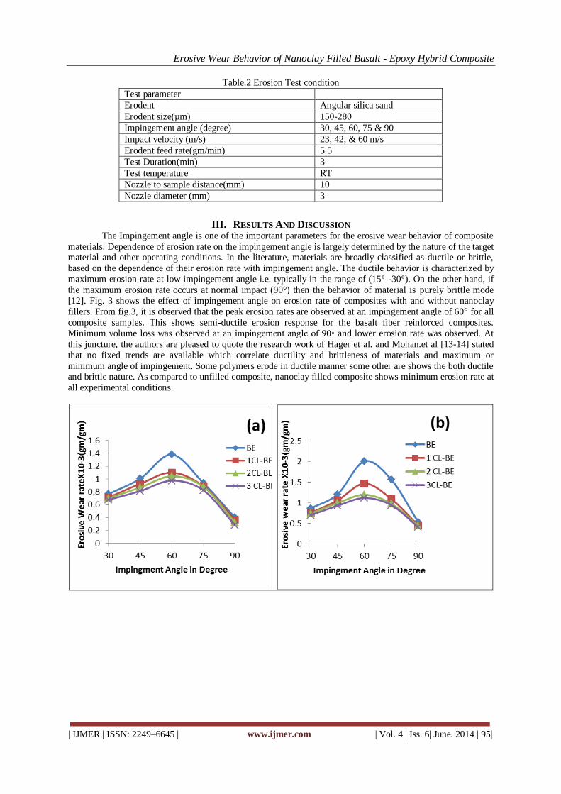
Erosive Wear Behavior of Nanoclay Filled Basalt - Epoxy Hybrid Composite
| IJMER | ISSN: 2249–6645 | www.ijmer.com | Vol. 4 | Iss. 6| June. 2014 | 95|
Table.2 Erosion Test condition
III. RESULTS AND DISCUSSION The Impingement angle is one of the important parameters for the erosive wear behavior of composite
materials. Dependence of erosion rate on the impingement angle is largely determined by the nature of the target material and other operating conditions. In the literature, materials are broadly classified as ductile or brittle,
based on the dependence of their erosion rate with impingement angle. The ductile behavior is characterized by
maximum erosion rate at low impingement angle i.e. typically in the range of (15° -30°). On the other hand, if
the maximum erosion rate occurs at normal impact (90°) then the behavior of material is purely brittle mode
[12]. Fig. 3 shows the effect of impingement angle on erosion rate of composites with and without nanoclay
fillers. From fig.3, it is observed that the peak erosion rates are observed at an impingement angle of 60° for all
composite samples. This shows semi-ductile erosion response for the basalt fiber reinforced composites.
Minimum volume loss was observed at an impingement angle of 90 and lower erosion rate was observed. At
this juncture, the authors are pleased to quote the research work of Hager et al. and Mohan.et al [13-14] stated
that no fixed trends are available which correlate ductility and brittleness of materials and maximum or
minimum angle of impingement. Some polymers erode in ductile manner some other are shows the both ductile and brittle nature. As compared to unfilled composite, nanoclay filled composite shows minimum erosion rate at
all experimental conditions.
Test parameter
Erodent Angular silica sand
Erodent size(µm) 150-280
Impingement angle (degree) 30, 45, 60, 75 & 90
Impact velocity (m/s) 23, 42, & 60 m/s
Erodent feed rate(gm/min) 5.5
Test Duration(min) 3
Test temperature RT
Nozzle to sample distance(mm) 10
Nozzle diameter (mm) 3

Erosive Wear Behavior of Nanoclay Filled Basalt - Epoxy Hybrid Composite
| IJMER | ISSN: 2249–6645 | www.ijmer.com | Vol. 4 | Iss. 6| June. 2014 | 96|
Fig.3: Erosion Rate versus Angle of Impingement for the composite at (a) 23 m/s, (b) 42 m/s (c) 60 m/s and
(d) Variation of Erosion Rate as a function of Impact Velocity at 60° Impingement Angle.
Worn Surface Morphology
To identify the mode of material removal, the morphologies of eroded surface are studied under
scanning electron microscope. Fig. 4(a) shows a portion of the composite after erosion occurred. It shows good
bonding of nanoclay particulate with epoxy and basalt fiber. At a velocity of 23m/s and at an impingement angle
of 60°, matrix removal was observed.
Fig. 4(b) shows the worn surface of BE composite, it can be seen from the micrograph that, when
impacting at angles, the hard erodent particles can penetrate the surfaces of the samples and cause material
removal by fiber cutting and removal of fibers are seen. It indicates plastic deformation and micro cracking as
the dominant wear mechanisms. Repeated impact of the erodent caused roughening of the surface of the
material and cutting with chip formation is reflected in Fig. 5(b). Erosion along the fibres and clean removal of the matrix to expose glass fibers and breakage is also seen, the matrix shows multiple fractures and material
removal. The exposed fibres are broken into fragments at some points along with some amount of cavitations
and thus can be easily removed from the worn surfaces
(a) Filled (b) Unfilled
Fig. 4: SEM Images of Eroded Surfaces at a velocity of 23 m/s at 60° Impingement angle.
Fig.5(a) shows the removal of matrix material is observed with greater degree of severity as compared
to Fig.4(a). Fiber breakage is more in this case because of the higher magnitude of the impact velocity. Fig.5(a) shows the good bonding of matrix and fibre because the nano clay restricts the debonding of materials even at
higher velocity.

Erosive Wear Behavior of Nanoclay Filled Basalt - Epoxy Hybrid Composite
| IJMER | ISSN: 2249–6645 | www.ijmer.com | Vol. 4 | Iss. 6| June. 2014 | 97|
(a) Filled (b) Unfilled
Fig. 5: SEM Images of Eroded Surfaces at a velocity of 60 m/s at 60° Impingement angle.
IV. CONCLUSION Addition of nanoclay in B-E composite shows minimum erosion rate as it restricts the fiber–matrix
deboning, without any filler shows highest erosion rate due to weak bonding strength and has adequate
potential for tribological applications.
Influence of the impingement angle on erosive wear of all composites under consideration exhibits semi-
ductile behavior with maximum erosion at 60° impingement angle.
SEM studies of worn surfaces support the wear mechanisms involved and indicated pulverization of wear
debris, exposure of fibers, micro-cutting, crushing of fibre and cavities due to detachment of broken
fibers from the resin matrix and cracks at higher particle velocity.
REFERENCES [1] Ray SS, Okamoto M, Polymer/layered silicate nanocomposites: a review from preparation to processing, Progress in
Polymer Science 2003; 28: 1539 – 641. [2] Kim MH, Park CI, Choi WM, Lee JW, Lim JG, Park OO. Synthesis and material properties of syndiotactic
polystyrene/ organophilic clay nanocomposites. J Applied Polymer Science 2004; 92 : 2144–50. [3] Zhang YH, Wu JT, Fu SY, Yang SY, Li Y, Fan L, et al, Studies on characterization and cryogenic mechanical
properties of polyimide-layered silicate nanocomposite films, Polymer 2004; 45(22) : 7579–87 [4] S. S. Ray, P. Maiti, M. Okamoto, K. Yamada, K. Ueda, "New Polylactide/Layered Silicate Nanocomposites. 1.
Preparation, Characterization, and Properties" Macromolecules, 35(8), 3104-3110 (2002).
[5] Ray S S, Yamada K, Okamoto M and Ueda K, Polylactide-Layered Silicate Nanocomposite: A Novel Biodegradable Material, Nano Letters, 2002 Vol. 2, No. 10, 1093-1096
[6] Michael Alexandre, Philippe Dubois “Polymer-layered silicate nanocomposites: preparation, properties and uses of a new class of materials”, Materials Science and Engineering, 28 (2000), 1-63
[7] J. J. Luo, I. M. Daniel, "Characterization and Modeling of Mechanical Behavior of Polymer/Clay Nanocomposites," Composites Science and Technology, Vol. 63, 2003, pp. 1607-1616.
[8] Harsh et al Investigation on solid particle erosion behavior of polyetherimide and its composites” Wear, vol. 262, No. 7-8, (2007), 807-818
[9] Tewari et al.,” Solid particle erosion of carbon fibre – and glass fibre-epoxy Composites”, Composite Science and Technology, Vo. 63, No. 3-4 (2003) pp 549-557
[10] Chisholm N, Mahfuzi H, Rangari V, Rodgers R, Jeelani S. Synthesis and mechanical characterization of carbon/epoxy composites reinforced with SiC nano particles. NSTI Nanotech, 2004; Vol. 3: 302–307
[11] V. K. Srivastava and A. G. Pawar. “Solid particle erosion of glass fibre reinforced flyash filled epoxy resin composites”, Composites Science and Technology, vol. 66, no. 15, pp. 3021–3028, 2006
[12] N.M. Barkoula and J. Karger-Kocsis, “Solid particle erosion of unidirectional GF reinforced EP composites with different fiber/matrix adhesion”, Journal of Reinforced Plastics and Composites, vol. 21, No. 15, pp. 1377–1388,
2002 [13] Hager, A., Friedrich, K., Dzenis, Y. A., and Paipetis, S. A. (1995), “Study of Erosion Wear of Advanced Polymer
Composites,” ICCM-10 Conference Proceedings , Street, K. (Ed.), Woodhead Publishing L Cambridge,UK, pp 155–162
[14] Mohan et. al. “Studies on Erosive wear behavior of UHMWPE filled Aramide – Epoxy Hybrid Composite”, Materials and Manufacturing Processes, Vol. 27, 2012, pp. 430 – 435