Embed Size (px)
Citation preview

İstanbul University-Cerrahpaşa, Engineering Faculty Avcılar-İSTANBUL
07 October 2018 Ali Rıza Berkem Hall (Engineering Faculty) Opening Session 09:00-10:00 Registration 10:00-12:00 Opening Ceremony
Prof. Dr. Ferhat ÖZÇEP ( Welcome Speech , Co-Chairman of NTGE 2018)
Opening Speeches: Prof. Dr. Nuri AYDIN
(Rector of Istanbul University - Cerrahpaşa)
Prof. Dr. Mehmet BİLGİN (Dean of Faculty of Engineering , Istanbul University - Cerrahpaşa)
Prof. Dr. Mümtaz HİSARLI (Chair of Department of Geophysical Engineering , Istanbul University –
Cerrahpaşa)
11:00-12:00 Opening Lecture:
“Review: New Developments in 2D/3D Modeling and Inversion of Geophysical Electrical Methods”
by Prof. Dr. Emin Candansayar and Dr. N Yıldırım Gündoğdu
12:00-13:00 Lunch
07 November 2018 Ali Rıza Berkem , Conference Hall Afternoon Session 1 Chairpersons: A. Elmas and A. Muhittin Albora 13.00-13.15
13:15- 13:30
Determination of The Tectonic Lines of The Map of Gravity Anomaly of The Western Anatolian Region by The Cellular Neural Network (Cnn) Method
M.A. ÜgeA.M. Albora
13:30-13:45 13:45 14:00
High Resolution Aeromagnetic (Hram) Basement Imaging of Off-Shore Gulf of Suez Prospect, Egypt.
S.M. Sharafeldin,H. Karslı
14:00 14:15
Coffee Break
07 November 2018 Ali Rıza Berkem , Conference Hall Afternoon Session 2 Chairpersons: Emin Candansayar and Ali İsmet Kanlı 14.15-14.30
Application of Filtering Technqiues To Enhance Magnetic Data From Egyptain Archaeological Sites
T. F. Abdallatif
14.30-14.45
The Magnetic Survey In Some Archaeological Sites In Iran
B. Aminpour
14.45-15.00
Site Characterization of Ras Al Khaimah National Museum Using Geophysical Techniques, Ras Al Khaimah, UAE
T. F. Abdallatif A.H. Ghandour M.S. Tantawi
15:00-15:15
Geoelectrical Structure of The Avcilar Landslide Using Vlf-Em Method
G. Karcıoğlu
15:15-15:30
Coffee Break
07 November 2018 Ali Rıza Berkem , Conference Hall Afternoon Session 3 Chairpersons: Hakan Karslı and Hakan Alp 15.30-15.45
Extending Spectral Band of Seismic Data by The Cepstral Short Time Fourier Transform
H. Karslı
15.45-16.00
Importance of Filtering Without Surgical Mute In Seismic Data Processing
H. KarslıD. Dondurur
16.00-16.15
Two Different Processing Methods For Chirp Seismic Data
M.A. ÜgeH. Alp
16:15-16:30
Comparison of methods used for suppression of multiple reflections
S. CerenH. Alp
NTGE 2018
Organisation Committee
Prof.Dr. Ali Muhittin ALBORA
Prof. Dr. Ferhat ÖZÇEP
Assoc. Prof. Dr. Hakan ALP
*The total time allotted to each speaker is 15 minutes. You should plan to speak for 12minutes and leave 3 minutes for questions.*All presentations must be made using the English language and all presentationmaterials must be created in English
Determination of Rock Mass Quality Using The Amplitude Attenuation Tomography: A Case Study From The Trabzon, Turkey
A.E. Babacan K. GelişliD. Tweeton
Seismotectonic Implications of the July 20th, 2017 Bodrum Earthquake
S.Över,S.Özden A.Pınar

08 November 2018 Ali Rıza Berkem , Conference Hall Morning Session 1 Chairpersons: Ergin Ulutaş and Ethem Görgün 09.30- 09.45
Seismotectonic Investigation of Biga Peninsula in SW Marmara Region Using Steerable Filter Technique, Potential Field Data and Recent Seismicity
E. GörgünA.M. Albora
09.45-10.00
Modelling The Tsunami Generation of The September 28, 2018 Minahasa Peninsula, Sulawesi Island, Indonesia Earthquake
E. Ulutaş
10.00-10.15
An Assessment On Current Seismicity Rate Changes In Erzurum Province of Turkey: Implication For Earthquake Hazard
S. ÖztürkM. Sarı
10.15-10.30
Crust and Upper Mantle Structure Beneath The KTUT (Trabzon) and ERZN (Erzincan) Stations From Joint Inversion of P and S Receiver Functions
H. AlkanH. CınarS. OreshinL. Vinnik
10.30-10.45
Coffee Break
08 November 2018 Ali Rıza Berkem , Conference Hall Morning Session 2 Chairpersons: Nilgün Sayıl and Ferhat Özçep 10.45-11:00
Evaluation of Soil Liquefaction Potential by Using Microtremor Measurements In Trabzon, Turkey
S. Ceylan,A.E. BabacanÖ. Akin
11.00-11.15
Study On The Applicability of The Ambient Noise Hvsr Method In Bağlarbaşi (Gümüşhane), Ne Turkey
Y. BekerN. Sayıl
11.15-11.45
Description of Subsoil Types From Microtremor H/V Spectral Ratio Method In Kelkit District of Gümüşhane Province, Turkey
S. ÖztürkY. BekerL. PehlivanM. Sarı
11:45-12:00
Analysis of Soil-Structure and Resonance Effects of Gümüşhane University Campus Area In Turkey With HVSR and FSR Methods
Y. BekerN. Sayıl
08 November 2018 Ali Rıza Berkem , Conference Hall Afternoon Session 1 Chairpersons: Serkan Öztürk and Onur Tan13.00-13.15
An Appraisal of Future Seismic Potential For Erzurum Province of Turkey: Analyses of Basic Size-Scaling Parameters
S. Öztürk
13:15- 13:30
Application of Slip Predictable Model to Earthquake In Anatolia
N. Sayıl
13:30-13:45
Bayesian Probabilities of Earthquake Occurrences In The East Anatolian and Surroundings (Eastern Turkey)
T. Türker,Y. Bayrak
13:45 14:00
Applicability of Time-Dependent Seismicity Model For Earthquake Occurrence Along The North Anatolian Fault Zone
N. Sayıl
14:00 14:15
Coffee Break
08 November 2018 Ali Rıza Berkem , Conference Hall Afternoon Session 2 Chairpersons: Tolga Bekler and Mümtaz Hisarlı 14.15-14.30
14.30-14.45
Investigation of Vulnerability Index by Single Station Microtremor Method: A Case Study of KTÜ Campus
Y. BekerN. SayilÖ. AkinK.H. Çoban
Availability of Artificial Neural Network (Ann) In Strong Ground Motion Prediction
K.H. Çoban N. Sayıl
15:15-15:30
Coffee Break
08 November 2018 Ali Rıza Berkem , Conference Hall Afternoon Session 3 Chairpersons: Gökhan Karcıoğlu and Mehmet Ali Üge 15.30-15.45
Biga-Çan Gravity Data, Comparison of 3d Euler Deconvolution and 3d Modeling Results
G. KarcıoğluO. Tarhan BalA. B.Tekkeli
15.45-16.00
An Analysis of The Magnetic Anomaly Map of The Black Sea Region by The Cellular Neural Network (CNN) Method
M.A. ÜgeA.M. Albora
16.00-16.15
Smooth 3d Modeling of Gravity Data Using Particle Swarm Optimization
G. KarcıoğluO. Tarhan BalA. B.Tekkeli
16:15-16:30
Differences between Time and Depth Migration Multi Processes of the Multi-Channel Seismic Reflection Data from BabaBurnu Shelf, Canakkale
M.A. ÜgeE. Demirbağ
16:30-16:45
Estimation of Velocity Distribution by 2d Travel Time Reflection Tomography In The Gulf of Izmir (Western Turkey)
Z.Altan N.OcakoğluG. Böhm
*The total time allotted to each speaker is 15 minutes. You should plan to speak for 12minutes and leave 3 minutes for questions.*All presentations must be made using the English language and all presentationmaterials must be created in English
14.45-15.00
Shallow Engineering Seismic Parameters At Landslide-Prone Areas and Its Evaluations: A Case Study From Çanakkale
T. Bekler,A.Demirci
15:00-15:15 Definition of The Crust Structure of Anatolia by Surface
Wave Data N. Sayıl
09 November 2018 Ali Rıza Berkem , Conference Hall Morning Session 1 Chairpersons: Bülent Oruç and Mualla Çinku 09.30: 09.45
09.45-10.00
Uppermost Crustal Structure of SW Bıga Penınsula by Local Earthquake Tomography
T. BeklerA. Demirci
10.00-10.15
Orientation of The Maximum Horizontal Comprehensive Stress Directions In Central Anatolia.
E. UlutaşB. OruçM.B. Doğan
10.15-10.30
Anisotropy of Magnetic Susceptibity Measurements On Predicting Flow Direction of Eastern Anatolian Volcanic Erruption
H. UçarM.C. Çinku
10.30-10.45
Coffee Break
09 November 2018 Ali Rıza Berkem , Conference Hall Morning Session 2 Chairpersons: Serkan Üner and Okan Tezel
10.45-11:00
Mining Search Examination With Time Domain Ip Methodat Giresun, Turkey
O. TezelM.A. Üge
11.00-11.15
Tracing The Hisarcık Fault With 2D VES Inversion and Numerical Fluid Flow and Temperature Simulations
S. ÜnerG.Ö.AğaçgözgüD.D. Doğan
11.15-11.45
Time Domain Induced Polarization Method Study of Metalic Ore (Antimony) At Gumushane, Turkey
O. TezelM.A. Üge
POSTER SESSION
P1 The Importance of Geophysical Methods In Soil Problems G. ErdanA.M.Albora
P2 The Investigation of The Central Anatolian Faults by Using Satellite Gravity Data
F. DoğruO.Pamukçu D.Altan
P3 Comparison of Marchenko Redatuming and Imaging With Conventional VSP Processing Applied To The Frio Carbon Sequestration Experiment
M.S.KirazR.L.Nowack
P4 Recent Fault detection using steerable filters: A case Study Gulf of Saros / NW TURKEY
H. AlpE. GörgünA.M. Albora
P5 Possible Mutuyama-Brunhes Boundary In Cave Sediment of The Czech Republic
H.UcarG.KletetschkaJ. KadlecT.KamenikovaE.B. Herrero
P6 A Close Look at Crustal Structure of Lake-Van Region from Inter-Station Rayleigh Wave Phase Velocities
H. AlkanH.Çınar
P7 Seismicity of the Erzurum City and the Surrounding Area from Maximum Likelihood Method
E.BayrakY.BayrakH.Alkan
P8
P9 Geophysical Methods for Near Surface Explorations M.HurbenA.M.Albora
P10 Seismotectonic Investigation of Gökova Gulf Using Seismic Reflection and Seismological Data Set
E.GörgünA. Azizov
P11 Applications of Post-stack migration types in seismic data Y.RahimovH.Alp
P12 Seismic Multiple Removal with Surface Related Multiple Attenuation (SRMA) Technique
Y. İşcan Alp,N. Ocakoğlu,O. Özel
P13 EU Liquefact Project Studies in Çanakkale Pilot Site F. ÖzçepS. ÖztoprakN. Aysalİ. BozbeyO. TezelC. ÖserS. SargınM. ÇinkuK. Özdemir
Determination of the low velocity crustal structures in Marmara Region
11.45-12.00
İ.H.Demirsıkan, Ş.Şahin
12.00-12.15
A.G.NovruzovThe Results Of Direct Search Of Oil And Gas Deposits By Refraction Waves Method Of Seismic Exploration In Complex With Gravity Exploration In Middle Kura Depression Conditions Of Azerbaijan
Forecasting the oil and gas saturation by seismic and gravimetrical survey in the boyuk palantokan-kollug Area of the middle kura depression
A.G.Novruzov
*The total time allotted to each speaker is 15 minutes. You should plan to speakfor 12 minutes and leave 3 minutes for questions.*All presentations must be made using the English language and all presentationmaterials must be created in English
The size of the poster boards will be 1 meter wide X 2 meters high; This means that your poster should be maximum 90 cm wide X 180 cm high (Portrait format).
Identification Of Pulse Shape Signals On Near Fault Stations With Convolutıional Neural Network Algorithms: Preliminary Results
P14 D. ErtuncayG. Costa
Paleomagnetic Results Along The Bitlis-Zağros Suture Zone In Se Anatolia, Turkey
B.BakkalM.C. ÇinkuF.Heller

Istanbul University - Cerrahpasa Engineering Faculty
Department of Geophysical Engineering

INDEXName SURNAME University/Company Page
Tareq Fahmy ABDALLATIFNational Research Institute of Astronomy and Geophysics 49,72
Gülçin Özürlan AGAÇGOZGUİstanbul Technical University 94
Özgenç AKINKaradeniz Technical University 79,154
A.Muhittin ALBORAIstanbul Üniversity-Cerrahpaşa 1,22,26,30,75,170
Hamdi ALKANVan Yüzüncü Yıl University 34,98
Hakan ALPIstanbul University-Cerrahpaşa 14,170,182,186
Dilan ALTANDokuz Eylul University 52
Zehra ALTANİstanbul Technical University 134
Namık AYSALIstanbul University-Cerrahpaşa
Azer AZIZOVIstanbul Üniversity-Cerrahpaşa 193
Ali Erden BABACANKaradeniz Technical University 45,154
Beyza BAKKALIstanbul Üniversity-Cerrahpaşa 189
Oya Tarhan BALIstanbul University-Cerrahpaşa 56,64
Erdem BAYRAKKaradeniz Technical University

Yusuf BAYRAKKaradeniz Technical University 166
Yasemin BEKERGümüşhane University 79,83,87,118
Tolga BEKLERCanakkale Onsekiz Mart University 158,162
İlknur BOZBEYIstanbul University-Cerrahpaşa
Gualtiero BÖHMOGS-Istituto Nazionale di Oceanografia e 134
Emin CANDANSAYARAnkara University 18
Selin CERENIstanbul University-Cerrahpaşa 182
Sinem CEYLANKaradeniz Technical University 154
Giovanni COSTAUniversity of Trieste 178
Hakan ÇINARKaradeniz Technical University 34,98
Mualla ÇINKUIstanbul University-Cerrahpaşa 122,189
Hakan ÇOBANKaradeniz Technical University 79,114
Emin DEMIRBAĞIstanbul Technical University 42
Alper DEMIRCICanakkale Onsekiz Mart University 158,162
İbrahim Hakan DEMIRSIKANSüleyman Demirel University 68
Mustafa Berkay DOĞANKocaeli University 130

Fatih DOĞRUAtaturk University 52
Derman DONDURURDokuz Eylul University 110
Doğa DÜŞÜNÜR DOĞANİstanbul Technical University 94
Göksu ERDANIstanbul University-Cerrahpaşa 30
Deniz ERTUNCAYUniversity of Trieste 178
Kenan GELİŞLİKaradeniz Technical University 45
A.H. GHANDOURAin Shams University 72
Ethem GÖRGÜNIstanbul University-Cerrahpaşa 22,170,193
N.Yıldırım GÜNDOĞDUAnkara University 18
Friedrich HELLER ETH Zürich 189
Emillio Bervera HERREROUniversity of Hawaii 126
Z. Mümtaz HİSARLIIstanbul University-Cerrahpaşa
Mustafa HÜRBENTurkish Republic of Northern Cyprus 75
Yeliz İŞCAN ALPIstanbul University-Cerrahpaşa 174
Jaroslav KADLECAcademy of Sciences of the Czech Republic 126
Tereza KAMENIKOVACharles University 126

Gökhan KARCIOĞLUIstanbul University-Cerrahpaşa 56,60,64
Hakan KARSLIKaradeniz Technical University 91,106,110
Mert Sinan KIRAZPurdue University
Gunther KLETETSCHKACharles University 126
Robert L. NOWACKPurdue University
Neslihan OCAKOĞLUİstanbul Technical University 134,174
Sergey ORESHINInstitute of physics of the Earth, Bolshaya Grouzinskaya 34
Bülent ORUÇKocaeli University 130
Cihan ÖSERIstanbul Üniversity-Cerrahpaşa
Kağan OZDEMIRIstanbul Üniversity-Cerrahpaşa
Ferhat ÖZÇEPIstanbul University-Cerrahpaşa
Oğuz ÖZELIstanbul University-Cerrahpaşa 174
Sadık ÖZTOPRAKIstanbul Üniversity-Cerrahpaşa
Serkan ÖZTÜRKGümüşhane University 38,118,138
Oya PAMUKCUDokuz Eylul University 52
Levent PEHLIVANGümüşhane University 118
Yusuf RAHIMOVIstanbul University-Cerrahpaşa 186
Sinan SARGINIstanbul University-Cerrahpaşa
Mahmut SARIGümüşhane University 118,138
Nilgün SAYILKaradeniz Technical University 79,83,87,114,142,146,150
S.M. SHARAFELDINCairo University 91
Şakir ŞAHINSüleyman Demirel University 68
M.S. TANTAWIGeoscience Geophysical Consulting, Abu Dhabi 72
Anisya B. TEKELLİIstanbul Üniversity-Cerrahpaşa 56,64
Okan TEZELIstanbul University-Cerrahpaşa 5,10
Tuğba TÜRKERKaradeniz Technical University 166
Darly TWEETONGeoTom 45
Hakan UÇARIstanbul Üniversity-Cerrahpaşa 122,126
Ergin ULUTAŞKocaeli University 102,130
Mehmet Ali ÜGEIstanbul University-Cerrahpaşa 1,5,10,14,26,42
Serkan ÜNERİstanbul Technical University 94
Denizhan VARDARIstanbul University 14

Lev VINNIKInstitute of physics of the Earth, Bolshaya Grouzinskaya 34

EXTENDED ABSTRACTS
New Trends in Geophysics and Engineering (International Semposium) 2018 7-9 November 2018, Istanbul , Turkey
An Analysis of the Magnetic Anomaly Map of the Black Sea Region by the Cellular Neural Network (CNN) Method
Mehmet Ali ÜGE1 and Ali Muhittin ALBORA1
Istanbul University , Engineering Faculty, Geophysical Department, 34320, Avcilar, Istanbul, Turkey
Email: [email protected], [email protected]
Presentation Type
All accepted proceedings will be published on the webpage of the symposium (ntge2018.istanbul.edu.tr)
ORAL POSTER
Abstracts
In this study, Cellular Neural Network (CNN) method was applied to the magnetic anomaly map of the Black Sea. It is compared with the structure boundaries with tectonic structure of the Black Sea and surrounding region. Thus, the tectonic structure of the zone was tried to be clarify by the tectonic information with the CNN output of the magnetic anomaly map.
Keywords: Maximum 5 items for indexing purposes (separated with commas)
Introduction
Cellular Neural Networks (CNN), special kind of artificial neural networks, were first introduced in 1988 by Leon Chua and Lin Yang (Chua and Yang 1998). The CNN method was first applied to the magnetic anomaly map measured at the archaeological sites, and the boundaries of the structures were found to be very similar to those of the CNN method (Matsumoto et al., 1990; Suzuki et al., 1992, Slot 1992, Sziranyi and Csapodi, 1994; (Özmen et al., 1999a; 1999b). The CNN method has yielded far more successful results than classical methods in separating regional and residual anomalies of potential field anomalies (Albora et al., 2001a) In this study, CNN method, which is frequently used in image processing, is applied to determine the structure boundaries of the Magnetic anomaly map obtained in Black Sea. Since the Black Sea has a complex structure in terms of tectonics, it took attention of many scientists (Çiftçi et al 2002, Çiftçi et al 2003, Ocakoğlu et al 2018).
Method and/or Theory
It is a dynamic artificial neural network that is connected to each other and mostly comes from two-dimensional cells. The most important feature distinguishing CNN from artificial neural networks in the sense that we know is that the connection weight coefficients form an unchanging connection network on the working plane. This puts CNN in a very advantageous position compared to artificial neural networks in the conventional sense. In addition to carrying some basic features of known artificial neural networks, they find a lot of applications in image processing and image recognition due to their two dimensional structure. The differential equations that characterize the cellular Neural Network can be written as
X
11
New Trends in Geophysics and Engineering (International Semposium) 2018
7-9 November 2018, Istanbul , Turkey
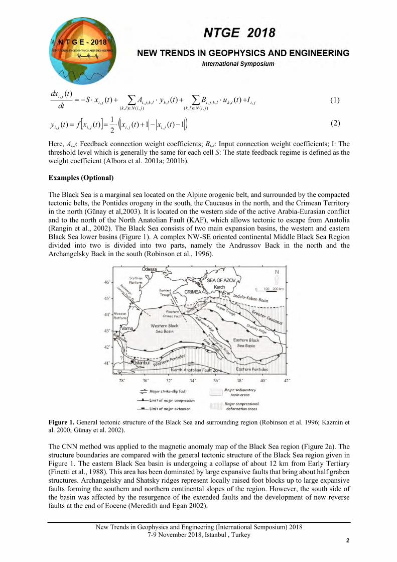
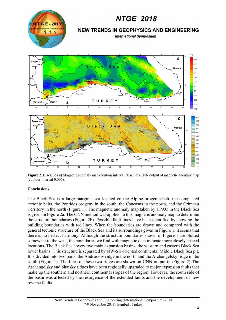
Here, Ai,J: Feedback connection weight coefficients; Bi,J: Input connection weight coefficients; I: The threshold level which is generally the same for each cell S: The state feedback regime is defined as the weight coefficient (Albora et al. 2001a; 2001b). Examples (Optional) The Black Sea is a marginal sea located on the Alpine orogenic belt, and surrounded by the compacted tectonic belts, the Pontides orogeny in the south, the Caucasus in the north, and the Crimean Territory in the north (Günay et al,2003). It is located on the western side of the active Arabia-Eurasian conflict and to the north of the North Anatolian Fault (KAF), which allows tectonic to escape from Anatolia (Rangin et al., 2002). The Black Sea consists of two main expansion basins, the western and eastern Black Sea lower basins (Figure 1). A complex NW-SE oriented continental Middle Black Sea Region divided into two is divided into two parts, namely the Andrussov Back in the north and the Archangelsky Back in the south (Robinson et al., 1996). Figure 1. General tectonic structure of the Black Sea and surrounding region (Robinson et al. 1996; Kazmin et al. 2000; Günay et al. 2002). The CNN method was applied to the magnetic anomaly map of the Black Sea region (Figure 2a). The structure boundaries are compared with the general tectonic structure of the Black Sea region given in Figure 1. The eastern Black Sea basin is undergoing a collapse of about 12 km from Early Tertiary (Finetti et al., 1988). This area has been dominated by large expansive faults that bring about half graben structures. Archangelsky and Shatsky ridges represent locally raised foot blocks up to large expansive faults forming the southern and northern continental slopes of the region. However, the south side of the basin was affected by the resurgence of the extended faults and the development of new reverse faults at the end of Eocene (Meredith and Egan 2002).
ji
jiNlklklkji
jiNlklklkjiji
ji ItuBtyAtxSdt
tdx,
),(),(,,;,
),(),(,,;,,
, )()()()(
ååÎÎ
+×+×+×-=
[ ] ( )1)(1)(
21)()( ,,,, --+×== txtxtxfty jijijiji
(1)
(2)
22
New Trends in Geophysics and Engineering (International Semposium) 2018
7-9 November 2018, Istanbul , Turkey
Figure 2. Black Sea a) Magnetic anomaly map (contour interval 50 nT) b) CNN output of magnetic anomaly map (contour interval 0.006). Conclusions The Black Sea is a large marginal sea located on the Alpine orogenic belt, the compacted tectonic belts, the Pontides orogeny in the south, the Caucasus in the north, and the Crimean Territory in the north (Figure 1). The magnetic anomaly map taken by TPAO in the Black Sea is given in Figure 2a. The CNN method was applied to this magnetic anomaly map to determine the structure boundaries (Figure 2b). Possible fault lines have been identified by showing the building boundaries with red lines. When the boundaries are drawn and compared with the general tectonic structure of the Black Sea and its surroundings given in Figure 1, it seems that there is no perfect harmony. Although the structure boundaries shown in Figure 1 are plotted somewhat to the west, the boundaries we find with magnetic data indicate more closely spaced locations. The Black Sea covers two main expansion basins, the western and eastern Black Sea lower basins. This structure is separated by NW-SE oriented continental Middle Black Sea pit. It is divided into two parts, the Andrussov ridge in the north and the Archangelsky ridge in the south (Figure 1). The lines of these two ridges are shown on CNN output in /Figure 2) The Archangelsky and Shatsky ridges have been regionally upgraded to major expansion faults that make up the southern and northern continental slopes of the region. However, the south side of the basin was affected by the resurgence of the extended faults and the development of new reverse faults.
33
New Trends in Geophysics and Engineering (International Semposium) 2018
7-9 November 2018, Istanbul , Turkey
References Albora A.M., Özmen A. ve Uçan O.N., 2001a. Residual Separation of Magnetic Fields Using a Cellular Neural Network Approach. Pure and Applied Geophysics, 158, 1797-1818. Albora A.M., Uçan O.N., Özmen A. and Özkan T., 2001b. Separation of Bouguer anomaly map using cellular neural network, Journal of Applied Geophysics, 46, 129-142. Chua L.O. and Yang L., 1998. Cellular Neural Networks: Theory, IEEE Transactions on Circuits and Systems, 35 (10), 1257 – 1272. Çifci G., Dondurur D. and Ergün E., 2002. Sonar and High Resolution Seismic Studies in the Eastern Black Sea, Turkish Journal of Earth Sciences, 11, 61-81. Çifci G., Dondurur D. and Ergün E., 2003. Deep and shallow structures of large pockmarks in the Turkish shelf, Eastern Black Sea, Geo-Marine Letters, 23, 311–322. Kazmin V.G., Schreider A.A. and Bulychev, A.A., 2000. Early stages of evolution of the Black Sea. In: Bozkurt, E., Winchester, J.A. and Piper, J.D.A. (eds) Tectonics and Magmatism in Turkey and the Surrounding Area. Geological Society, London, Special Publications 173, 235-249. Matsumoto T., Chua L.O. and Yokohama T., 1990. Image Thinning with a Cellular Neural Network, IEEE Transactions on Circuits and Systems, 37 (5), 638–640. Ocakoğlu N., İşcan Y., Kılıç Y., and Özel O., 2018. Morphologic and seismic evidence of rapid submergence offshore Cide-Sinop in the southern Black Sea shelf, Geomorphology, 311, 76-89. Özmen A., Uçan O.N. and Albora A.M., 1999. Arkeolojik Sahalarda Ölçülen Cisimlerin Hücresel Yapay Sinir Ağları Kullanılarak Görüntülenmesi, TMMOB Jeofizik Mühendisleri Odası İzmir Şubesi-İZMİR, 24. Özmen A., Albora A.M. and Uçan O.N. 1999. Hücresel Yapay Sinir Ağları (HYSA) Kullanarak Sivas Bölgesi Gürün ilçesi Kötüyurttepe mevkiinin modellenmesi, 11.Mühendislik Haftası Yerbilimleri Sempozyumu-ISPARTA, 373-381. Rangin C., Bader A.G, Pascal G., Ecevitoglu B., Görür N., 2002. Deep structure of the Mid Black Sea High (offshore Turkey) imaged by multi-channel seismic survey (BLACKSIS Cruise), Mar Geol 182, 265–278. Robinson A.G., Rudat J.H., Banks C.J. and Wiles R.L.F., 1996. Petroleum geology of the Black Sea. Mar Petrol Geol 13,195–223. Schultz A., 1998. Spatio Temporal CNN Algorithm for Object Segmentation and Object Recognition, Fifth IEEE International Workshop on Cellular Neural Networks and Their Applications Proceedings, South Bank University, London, UK, 347-352. Slot K., 1992. Cellular Neural Network Design for Solving Specific Image-Processing Problems, Internatinal Journal of Circuit Theory and Applications. 20, 629-637. Suzuki H., Matsimoto T. and Chua L.O., “A CNN Handwritten Character Recognizer”, International Journal of Circuit Theory and Applications, 20: 601-612, 1992. Sziranyi T. and Csapodi M., “Texture Classification and Segmentation by Cellular Neural Network using Genetic Learning”, Research Report, Computer and Automation Institute Hungarian Academy of Sciences, Budapest, Hungary, Kasım 1994.
44
New Trends in Geophysics and Engineering (International Semposium) 2018
7-9 November 2018, Istanbul , Turkey
MINING SEARCH EXAMINATION WITH TIME-ENVIRONMENTAL IP METHOD AT GIRESUN, TURKEY
Okan TEZEL1, Mehmet Ali ÜGE1
1İstanbul Üniversitesi Mühendislik Fakültesi Jeofizik Mühendisliği Bölümü Avcılar-İstanbul, e-mail : [email protected], e-mail : [email protected]
Presentation Type All accepted proceedings will be published on the webpage of the symposium (ntge2018.istanbul.edu.tr)
ORAL POSTER
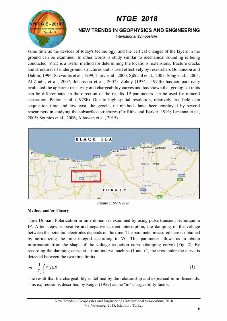
Abstracts This study, Giresun (Turkey) Kirazören in the Central Black Sea region of the vein type Pb-Zn ± Cu deposits, were studied to determine the location and depth using geophysical research. In this context, geophysical electricity methods; Inductive Polarization, Electrical Resistivity and Natural Potential methods are applied together. Chargeability, resistivity-depth and natural potential data were obtained with the measurements taken in the direction of geological information. Evaluation of these data has shown that high value of chargeability, low value resistivity and natural potential data are stimulating on the ore. It was also found that these impressions were in harmony with the data obtained from the existing galleries and geology. Keywords: Pb, Zn, Cu, Inductive Polarization, Chargeability, Resistivity, Natural Potential. Introduction In this study, Giresun (Turkey) Kirazören metallic sulphide ores (Zn-Pb ± C) the measures taken to investigate the feasibility evaluated (Fig.1). The vascular type Zn-Pb ± Cu deposits of the Middle Black Sea region have an important place in the Pontide metallogenesis. The vein mineralization in the region is a frequent and scattered feature. The fact that the beds are covered with high slope morphology and vegetation is causing difficulties for detailed research and mining studies. In the electrical methods, the electric current is transmitted through the solid part of the rock (electronic conductivity), and at the same time, it is also transported with the ions present in the groundwater filling the pores of the rock (ionic conductivity). Induction Polarization (IP) can be caused by sulphides that are scattered within a unit volume and are present in very small quantities (eg 0.5%). Therefore, metallic minerals in clusters in the rocks give a very good IP sign. The magnitude of the indication in IP increases with the value of mineralization (Sumner, 1976). Johnson (1984) has calculated the damping curve containing the time domain IP (TDIP) response. Time changes of overvoltages in the time domain have been studied by Tezel (1992). Vertical Electric Drilling (VED) is carried out with the IP at the
X
55
New Trends in Geophysics and Engineering (International Semposium) 2018
7-9 November 2018, Istanbul , Turkey
same time as the devices of today's technology, and the vertical changes of the layers in the ground can be examined. In other words, a study similar to mechanical sounding is being conducted. VED is a useful method for determining the locations, extensions, fracture cracks and structures of underground structures and is used effectively by researchers (Johansson and Dahlin, 1996; Savvaidis et al., 1999; Titov et al., 2000; Sjödahl et al., 2005; Song et al. , 2005; Al-Zoubi, et al., 2007; Johansson et al., 2007). Zohdy (1974a, 1974b) has comparatively evaluated the apparent resistivity and chargeability curves and has shown that geological units can be differentiated in the direction of the results. IP parameters can be used for mineral separation, Pelton et al. (1978b). Due to high spatial resolution, relatively fast field data acquisition time and low cost, the geoelectric methods have been employed by several researchers in studying the subsurface structures (Griffiths and Barker, 1993; Lapenna et al., 2005; Soupios et al., 2006; Alhassan et al., 2015).
Figure 1. Study area.
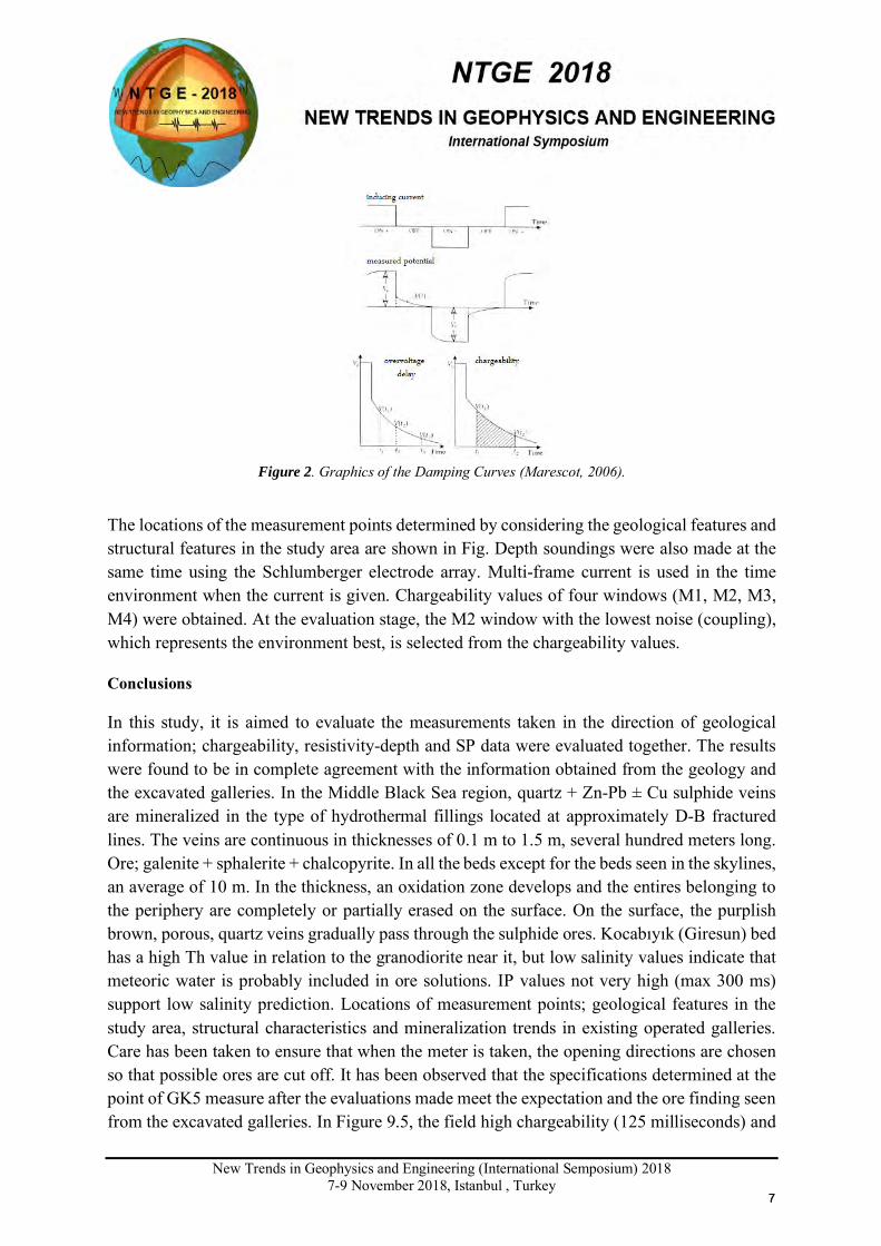
Method and/or Theory Time Domain Polarization in time domain is examined by using pulse transient technique in IP. After stepwise positive and negative current interruption, the damping of the voltage between the potential electrodes depends on the time. The parameter measured here is obtained by normalizing the time integral according to V0. This parameter allows us to obtain information from the shape of the voltage reduction curve (damping curve) (Fig. 2). By recording the damping curve at a time interval such as t1 and t2, the area under the curve is detected between the two time limits.
(1)
The result that the chargeability is defined by the relationship and expressed in milliseconds. This expression is described by Seigel (1959) as the "m" chargeability factor.
ò=2
1
)(1
0
t
t
dttVV
m
66
New Trends in Geophysics and Engineering (International Semposium) 2018
7-9 November 2018, Istanbul , Turkey
Figure 2. Graphics of the Damping Curves (Marescot, 2006).
The locations of the measurement points determined by considering the geological features and structural features in the study area are shown in Fig. Depth soundings were also made at the same time using the Schlumberger electrode array. Multi-frame current is used in the time environment when the current is given. Chargeability values of four windows (M1, M2, M3, M4) were obtained. At the evaluation stage, the M2 window with the lowest noise (coupling), which represents the environment best, is selected from the chargeability values. Conclusions In this study, it is aimed to evaluate the measurements taken in the direction of geological information; chargeability, resistivity-depth and SP data were evaluated together. The results were found to be in complete agreement with the information obtained from the geology and the excavated galleries. In the Middle Black Sea region, quartz + Zn-Pb ± Cu sulphide veins are mineralized in the type of hydrothermal fillings located at approximately D-B fractured lines. The veins are continuous in thicknesses of 0.1 m to 1.5 m, several hundred meters long. Ore; galenite + sphalerite + chalcopyrite. In all the beds except for the beds seen in the skylines, an average of 10 m. In the thickness, an oxidation zone develops and the entires belonging to the periphery are completely or partially erased on the surface. On the surface, the purplish brown, porous, quartz veins gradually pass through the sulphide ores. Kocabıyık (Giresun) bed has a high Th value in relation to the granodiorite near it, but low salinity values indicate that meteoric water is probably included in ore solutions. IP values not very high (max 300 ms) support low salinity prediction. Locations of measurement points; geological features in the study area, structural characteristics and mineralization trends in existing operated galleries. Care has been taken to ensure that when the meter is taken, the opening directions are chosen so that possible ores are cut off. It has been observed that the specifications determined at the point of GK5 measure after the evaluations made meet the expectation and the ore finding seen from the excavated galleries. In Figure 9.5, the field high chargeability (125 milliseconds) and
77
New Trends in Geophysics and Engineering (International Semposium) 2018
7-9 November 2018, Istanbul , Turkey
low resistivity (287 ohm) values are shown as ORE in the AB / 2 = 30-60 m opening interval. Again, the high-negative (-100 mV) SP data obtained at the same interval indicate that the ore is here. As a matter of fact, the 2-D resistivity model section shown in Fig. 12 also supported the possibility of ore at GK5 at about 30-40 m levels. Low resistance and high cohesion values are observed at 60 m in GK1, 180 m in GK2, and 120 m in GK3, but these signs are observed in the environment after galleys excavated here and are not very dense sulphide, chalcopyrite etc. . Low SP values have not been monitored at these points. There was no evidence to give an anomaly at GK4 measurement point. Acknowledgements This project was supported by Istanbul University Scientific Research Projects Coordination Unit “Project Number : YADOP-23190”. References Alhassan, UD., Obiora, DN., Okeke, FN. (2015) The assessement of aquifer potentials and
aquifer vulnerability of southern Paiko, North central Nigeria, using geoelectric method. Glob.
J. Pure Appl. Sci. 21:51-70.
Griffiths, D.H. and Barker, R.D. (1993) Two-dimensional resistivity imaging and modelling
in areas of complex geology. Journal of Applied Geophysics, 29, 211-226
Johnson, M.I. (1984) Spectral Induced Polarization parameters as determined trough time-
domain measurements, Geophysics, 49, 1993-2003.
Johansson, S. and Dahlin, T. (1996) Seepage Monitoring in an Earth Embankment Dam by
Repeated Resistivity Measurements, European Journal of Engineering of Environmental
Geophysics 1(3), 229-247.
Johansson, S., Jones, S. and Flyhammar, F. (2007) Comparisons of 2D- and 3D-Inverted
Resistivity Data As Well As of Resistivityand IP-Surveys on a Landfill, Near Surface, 13th
European Meeting of Environmental and Engineering Geophysics, Istanbul, Turkey, 3–5
September 2007, p. 42.
Lapenna, V., Lorenzo, P., Perrone, A., Piscitelli, S., Rizzo, E., Sdao, F. (2005) 2D electrical
resistivity imaging of some complex landslides in Lucanian Apennine chain, southern Italy.
Geophysics 70(3):B11-B18.
Pelton, W.H., Ward, S.H., Hallof, P.G., Sill, W.R. and Nelson, P.H. (1978b) Mineral
discirimination and removal of inductive coupling with multi frequency IP. Geophysics, 43,
588-609.
88
New Trends in Geophysics and Engineering (International Semposium) 2018
7-9 November 2018, Istanbul , Turkey
Savvaidis, A. S., Tsokas, G. N., Soupios, P. and Vargemezis, G. (1999) Geophysical
prospecting in the Krousovitis dam (N. Greece) by seismic and resistivity methods, Journal Of
The Balkan Geophysıcal Socıety 2(4), 128-138.
Seigel, H. (1959) Mathematical formulation and theoretical curves for IP. Geophysics, 24,
547-561.
Soupios P, Papazachos CB, Vargemezis G, Savvaidis A (2006). In situ geophysical
investigation to evaluate dynamic soil properties at theIlarionas Dam, Northern Greece. Proc.
2nd Int. Conf. Advances in Mineral Resources Management and Environmental
Geotechnology (Hania, Crete, Greece, 25-27) (Heliotopos Conferences). pp. 149-156.
Song, S., Song, Y. and Kwon, Y. (2005) Application of hydrogeological and geophysical
methods to delineate leakage pathways in an earth fill dam, Exploration Geophysics 36, 92-96.
Sumner, J.S. (1976) Principles of Induced Polarization for Geophysical Exploration, Elsevier,
London.
Tezel, O. (1992) Zaman Ortamı IP Yanıtlarının Araştırılması, Yüksek Lisans Tezi, İ.Ü. Fen
Bilimleri Enstitüsü.
Titov, K., Loukhmanov, V. and Potapov, A. (2000) Monitoring of water seepage from a
reservoir using resistivity and self polarization methods, case history of the Petergoph
foundation water supply system. Frist Break Technical Article, 431-435.
Zohdy, A. (1974a) A Computer Program for the Calculation of Schlumberger Sounding Curve
by Convolution. U.S. Geological Survey Open File Report No. USGS-GD-74-010.
Zohdy, A. (1974b) Electrical Methods in US Geological Survey, Tech Water Resources
Investigation, Book 2, Chap. D1.
99
New Trends in Geophysics and Engineering (International Semposium) 2018
7-9 November 2018, Istanbul , Turkey
TIME DOMAIN INDUCED POLARIZATION METHOD STUDY OF METALIC
ORE (ANTIMONY) AT GUMUSHANE, TURKEY
Okan TEZEL1 and Mehmet Ali UGE1
1 Istanbul University Faculty of Engineering Department of Geophysical Engineering
Avcilar-ISTANBUL. e-mail: [email protected], aliuge@İstanbul.edu.tr
Presentation Type
All accepted proceedings will be published on the webpage of the symposium (ntge2018.istanbul.edu.tr)
ORAL POSTER
Abstracts
In this study, Time Domain Induced Polarization methods of applying the results of Gumushane Turkey antimony ore exploration conducted in Torul is presented. A gallery has been placed at a previously determined point in the study area, from which approximately one ton of antimony ore has been removed. With this work, it was researched whether there is ore continuation in or near the ore taken place. First of all, measurements taken at points determined in the direction of geological information, chargebility and resistivity parameters were determined. In comparison of these parameters; high-value chargebility and low-value resistivity indications were observed to be warped at the same site (on the ore) as expected. These impressions were found to be in complete agreement with the information obtained from geological finds and galleries. Keywords: Geophysics, antimony, time domain IP, chargebility, resistivity.
Introduction
Most of the extruded mineral deposits are found nowadays. Therefore, studies for mining searches are carried out for deep deposits with no surface sign. Antimony, is found in the form of veins like ores in faults, fractures and movements in the natüre, in the deeper sides of the surface. The dominant ore mineral is antimony (Sb2S3). The most suitable geophysical method that can be applied in antimony searches is Induced Polarization (IP) because the environment where the mineral is present will be sulfur. At the same time, the current is also transmitted by the ions present in the groundwater filling the pores of the rock (ionic conductivity) while the electric current is transmitted through the solid part of the rock (electronic conductivity) in the rocks. The IP sign may be due to sulfites present in the unit volume and scattered in very small quantities (eg 0.5%). Therefore, metallic minerals in clusters in the rocks give a very good IP sign. The magnitude of the indication in IP increases with the value of mineralization (Sumner, 1976). Johnson (1984) has calculated the decay curve containing the time domain IP (TDIP) response. Time changes of overvoltages in the time domain have been studied by Tezel (1992).
X
1010
New Trends in Geophysics and Engineering (International Semposium) 2018
7-9 November 2018, Istanbul , Turkey
Vertical Electric Drilling (VES) is performed at the same time as the devices of today's technology, and the vertical changes of the layers in the ground can be examined. In other words, a study similar to mechanical sounding is being conducted. VES is a useful method for determining the locations, extensions, fracture cracks and structures of underground structures and is used effectively by researchers (Johansson and Dahlin, 1996; Savvaidis et al., 1999; Titov et al., 2000; Sjödahl et al., 2005; Song et al. , 2005; Al-Zoubi, et al., 2007; Johansson et al., 2007). Zohdy (1974a, 1974b) have comparatively evaluated the apparent resistivity and chargeability curves, and has shown that geological units can be differentiated in the direction of the results they found. IP parameters can be used for mineral separation, Pelton et al. (1978b). Method and/or Theory
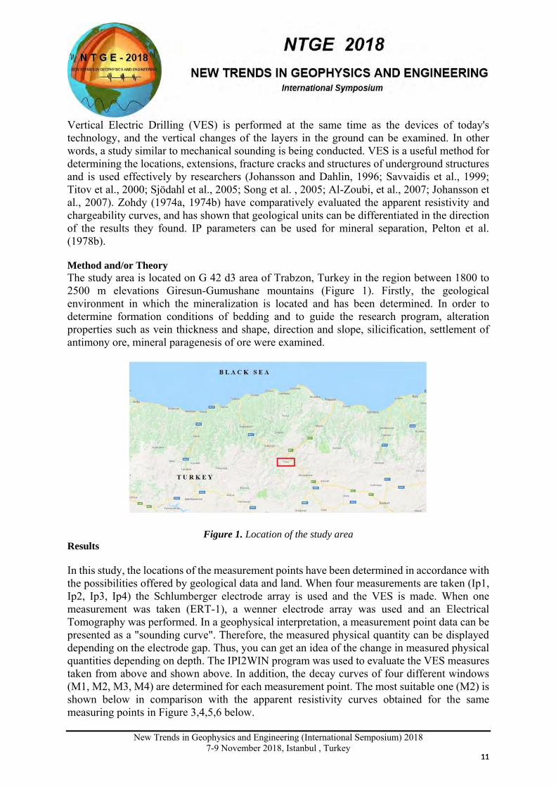
The study area is located on G 42 d3 area of Trabzon, Turkey in the region between 1800 to 2500 m elevations Giresun-Gumushane mountains (Figure 1). Firstly, the geological environment in which the mineralization is located and has been determined. In order to determine formation conditions of bedding and to guide the research program, alteration properties such as vein thickness and shape, direction and slope, silicification, settlement of antimony ore, mineral paragenesis of ore were examined.
Figure 1. Location of the study area
Results
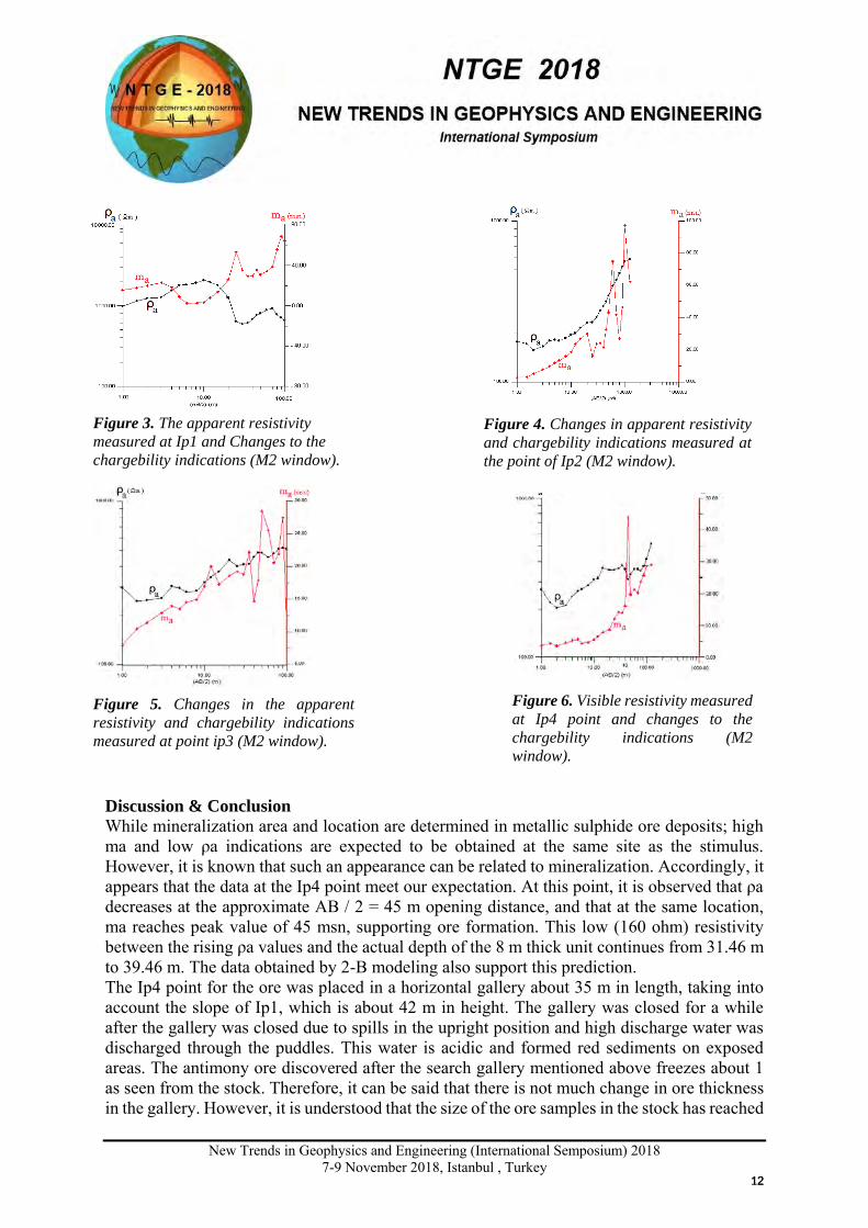
In this study, the locations of the measurement points have been determined in accordance with the possibilities offered by geological data and land. When four measurements are taken (Ip1, Ip2, Ip3, Ip4) the Schlumberger electrode array is used and the VES is made. When one measurement was taken (ERT-1), a wenner electrode array was used and an Electrical Tomography was performed. In a geophysical interpretation, a measurement point data can be presented as a "sounding curve". Therefore, the measured physical quantity can be displayed depending on the electrode gap. Thus, you can get an idea of the change in measured physical quantities depending on depth. The IPI2WIN program was used to evaluate the VES measures taken from above and shown above. In addition, the decay curves of four different windows (M1, M2, M3, M4) are determined for each measurement point. The most suitable one (M2) is shown below in comparison with the apparent resistivity curves obtained for the same measuring points in Figure 3,4,5,6 below.
1111
New Trends in Geophysics and Engineering (International Semposium) 2018
7-9 November 2018, Istanbul , Turkey
Discussion & Conclusion
While mineralization area and location are determined in metallic sulphide ore deposits; high ma and low ρa indications are expected to be obtained at the same site as the stimulus. However, it is known that such an appearance can be related to mineralization. Accordingly, it appears that the data at the Ip4 point meet our expectation. At this point, it is observed that ρa decreases at the approximate AB / 2 = 45 m opening distance, and that at the same location, ma reaches peak value of 45 msn, supporting ore formation. This low (160 ohm) resistivity between the rising ρa values and the actual depth of the 8 m thick unit continues from 31.46 m to 39.46 m. The data obtained by 2-B modeling also support this prediction. The Ip4 point for the ore was placed in a horizontal gallery about 35 m in length, taking into account the slope of Ip1, which is about 42 m in height. The gallery was closed for a while after the gallery was closed due to spills in the upright position and high discharge water was discharged through the puddles. This water is acidic and formed red sediments on exposed areas. The antimony ore discovered after the search gallery mentioned above freezes about 1 as seen from the stock. Therefore, it can be said that there is not much change in ore thickness in the gallery. However, it is understood that the size of the ore samples in the stock has reached
Figure 6. Visible resistivity measured
at Ip4 point and changes to the
chargebility indications (M2
window).
Figure 5. Changes in the apparent
resistivity and chargebility indications
measured at point ip3 (M2 window).
Figure 3. The apparent resistivity
measured at Ip1 and Changes to the
chargebility indications (M2 window).
Figure 4. Changes in apparent resistivity
and chargebility indications measured at
the point of Ip2 (M2 window).
1212
New Trends in Geophysics and Engineering (International Semposium) 2018
7-9 November 2018, Istanbul , Turkey
the 20 cm thickness of the mineralization in the place. Another material extracted from the gallery is pyritic quartz, which is not seen on the surface. However, it is estimated that the low resistivity values observed in the vicinity of the ore at the depths of 0-30 m between the openings of 170-190 m due to these pyrites. As a result; The antimony mineralization in the study area was developed due to the fracture system in the direction of K60-70D. The mineralization consists of antimony in an average thickness of 8 cm. Antimonite (stibnite) shows a genetic relationship with pyritic quartz veins. There are pyrite and antimonitic hydrothermal mineralizations, total 20 m thick lacerated zones. This observation supported a conductive zone evaluation of approximately 8 m thickness given in geophysical results.
Acknowledgements (Optional)
Author “Okan TEZEL” was supported by the Research Fund of Istanbul University, project number YADOP-23190.
References Al-Zoubi, A.S. 2007, Use of Multi Electrodes Resistivity Imagining for Sinkholes Hazard Assessment along the
Eastern Part of the Dead Sea, Jordan, American Journal of Environmental Sciences 3(4), 229-233.
Johnson, M.I., 1984. Spectral Induced Polarization parameters as determined trough time- domain measurements,
Geophysics, 49, 1993-2003.
Johansson, S. and Dahlin, T. 1996, Seepage Monitoring in an Earth Embankment Dam by Repeated Resistivity
Measurements, European Journal of Engineering of Environmental Geophysics 1(3), 229-247.
Johansson, S., Jones, S. and Flyhammar, F. 2007, Comparisons of 2D- and 3D-Inverted Resistivity Data As Well
As of Resistivityand IP-Surveys on a Landfill, Near Surface, 13th European Meeting of Environmental and
Engineering Geophysics, Istanbul, Turkey, 3–5 September 2007, p. 42.
Pelton, W.H., Rijo, L. and Swift, Jr. C.M. 1978b. Inversion of twodimensional resistivity and induced-
polarizatıon data. Geophysics, 43 (4), 788-803.
Savvaidis, A. S., Tsokas, G. N., Soupios, P. and Vargemezis, G. 1999, Geophysical prospecting in the Krousovitis
dam (N. Greece) by seismic and resistivity methods, Journal Of The Balkan Geophysıcal Socıety 2(4), 128-138.
Sjödahl, P., Dahlin, T. and Johansson, P. 2005, Using resistivity measurements for dam safety evaluation at
Enemossen tailings dam in southern Sweden, Environmental Geology 49, 267-273.
Song, S., Song, Y. and Kwon, Y. 2005, Application of hydrogeological and geophysical methods to delineate
leakage pathways in an earth fill dam, Exploration Geophysics 36, 92-96.
Sumner, J.S., 1976. Principles of Induced Polarization for Geophysical Exploration, Elsevier, London.
Tezel, O., Zaman Ortamı IP Yanıtlarının Araştırılması, Yüksek Lisans Tezi, İ.Ü.Fen Bilimleri Enstitüsü, 1992.
Titov, K., Loukhmanov, V. and Potapov, A. 2000, Monitoring of water seepage from a reservoir using resistivity
and self polarization methods, case history of the Petergoph foundation water supply system. Frist Break Technical
Article, 431-435.
Zohdy, A., 1974a. A Computer Program for the Calculation of Schlumberger Sounding Curves by Convolution.
Al-Zoubi, A.S. 2007, Use of Multi Electrodes Resistivity Imagining for Sinkholes Hazard Assessment along the
Eastern Part of the Dead Sea, Jordan, American Journal of Environmental Sciences 3(4), 229-233.
1313
New Trends in Geophysics and Engineering (International Semposium) 2018
7-9 November 2018, Istanbul , Turkey
TWO DIFFERENT PROCESSING METHODS FOR CHIRP SEISMIC DATA
Mehmet Ali Üge1 , Hakan Alp1 and Denizhan VARDAR2
1 Geophysical Eng. Department, Istanbul University-Cerrahpasa, Istanbul 2 Institute of Marine Sciences and Management, Istanbul University
Email: [email protected]
Presentation Type All accepted proceedings will be published on the webpage of the symposium (ntge2018.istanbul.edu.tr)
ORAL POSTER
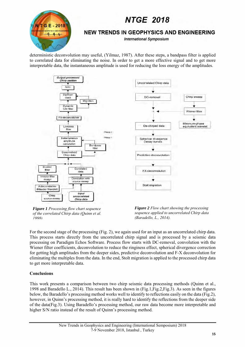
Abstracts The aim of the study is to improve the chirp seismic data quality by using two processing methods, to get more interpretable chirp data. For this purpose, we used for Chirp (2–8 kHz) seismic data. These were collected from the northern Marmara Sea. We also compare two processing methods (Quinn et al., 1998 and Baradello L., 2014) on our chirp data. These two techniques can be particularly useful for engineering- geotechnical surveys and archaeological investigations and imaging of the uppermost meters of the sub-seafloor. Keywords: Chirp, Seismic, Data Processing, Near Surface Introduction Chirp sub-bottom profile systems are generally used to investigate the 30–40 m of the marine sedimentary sequence in unconsolidated or poorly consolidated deposits. Generally, Chirp systems used for geological studies (Quinn et al. 1997; Fusi et al. 2006) and geohazard identifications (Dyer, 2011), well-site evaluation and pipe-line laying (Tian 2008), marine archaeological investigation (Bull et al. 1998; Plets et al. 2008). Chirp systems are collecting high-resolution data sets and it is very useful for stratigraphic correlations and reflectivity. The main advantage of Chirp systems is known of the signature, amplitude and frequency modulated sweep. Sweep source can be generated within a range from Hertz to kilohertz. Method and/or Theory For the first stage of the processing, uncorrelated chirp is used as an input. This process type divides into two steps (Fig. 1). For the first phase of the process stage is, correlation of the raw chirp data and applying deconvolution on it and for the 2nd phase of the process stage is to apply the band-pass filter on the data. These two phases of the first stage are effective processing steps for the uncorrelated chirp data. Using as an input of uncorrelated chirp data and correlating it with source sweep which we generate it at the beginning of the processing step. Thus we will have correlated data. Due to known, length, and frequency of the sweep signal, we have created the Klauder wavelet by taking the sweep signal autocorrelation. After taking autocorrelation of the signal and using the inverse filter method, we have obtained filter coefficients. To convolve between these coefficients and the correlated chirp data, we have a ringiness problem on the data. For reducing the ringiness problem of the data, the
X
1414
New Trends in Geophysics and Engineering (International Semposium) 2018
7-9 November 2018, Istanbul , Turkey
deterministic deconvolution may useful, (Yilmaz, 1987). After these steps, a bandpass filter is applied to correlated data for eliminating the noise. In order to get a more effective signal and to get more interpretable data, the instantaneous amplitude is used for reducing the loss energy of the amplitudes.
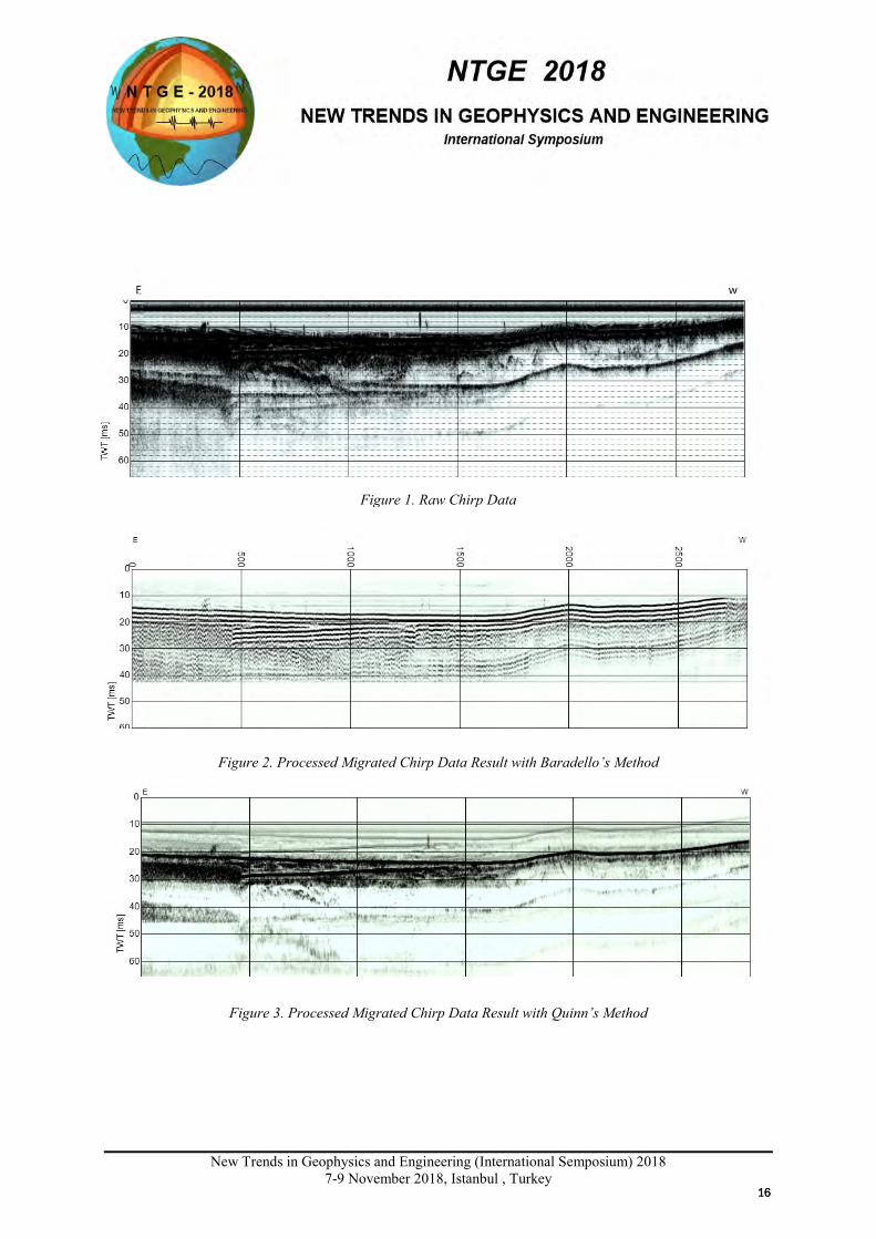
For the second stage of the processing (Fig. 2), we again used for an input as an uncorrelated chirp data. This process starts directly from the uncorrelated chirp signal and is processed by a seismic data processing on Paradigm Echos Software. Process flow starts with DC-removal, convolution with the Wiener filter coefficients, deconvolution to reduce the ringiness effect, spherical divergence correction for getting high amplitudes from the deeper sides, predictive deconvolution and F-X deconvolution for eliminating the multiples from the data. In the end, Stolt migration is applied to the processed chirp data to get more interpretable data.
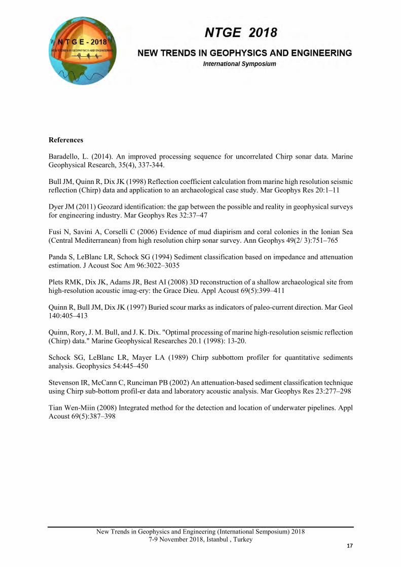
Conclusions This work presents a comparison between two chirp seismic data processing methods (Quinn et al., 1998 and Baradello L., 2014). This result has been shown in (Fig.1,Fig.2,Fig.3). As seen in the figures below, the Baradello’s processing method works well to identify to reflections easily on the data (Fig.2), however, in Quinn’s processing method, it is really hard to identify the reflections from the deeper side of the data(Fig.3). Using Baradello’s processing method, our raw data become more interpretable and higher S/N ratio instead of the result of Quinn’s processing method.
Figure 1 Processing flow chart sequence of the correlated Chirp data (Quinn et al. 1998).
Figure 2 Flow chart showing the processing sequence applied to uncorrelated Chirp data (Baradello, L., 2014).
1515
New Trends in Geophysics and Engineering (International Semposium) 2018
7-9 November 2018, Istanbul , Turkey
Figure 3. Processed Migrated Chirp Data Result with Quinn’s Method
Figure 2. Processed Migrated Chirp Data Result with Baradello’s Method
Figure 1. Raw Chirp Data
1616
New Trends in Geophysics and Engineering (International Semposium) 2018
7-9 November 2018, Istanbul , Turkey
References
Baradello, L. (2014). An improved processing sequence for uncorrelated Chirp sonar data. Marine Geophysical Research, 35(4), 337-344.
Bull JM, Quinn R, Dix JK (1998) Reflection coefficient calculation from marine high resolution seismic reflection (Chirp) data and application to an archaeological case study. Mar Geophys Res 20:1–11
Dyer JM (2011) Geozard identification: the gap between the possible and reality in geophysical surveys for engineering industry. Mar Geophys Res 32:37–47
Fusi N, Savini A, Corselli C (2006) Evidence of mud diapirism and coral colonies in the Ionian Sea (Central Mediterranean) from high resolution chirp sonar survey. Ann Geophys 49(2/ 3):751–765
Panda S, LeBlanc LR, Schock SG (1994) Sediment classification based on impedance and attenuation estimation. J Acoust Soc Am 96:3022–3035
Plets RMK, Dix JK, Adams JR, Best AI (2008) 3D reconstruction of a shallow archaeological site from high-resolution acoustic imag-ery: the Grace Dieu. Appl Acoust 69(5):399–411
Quinn R, Bull JM, Dix JK (1997) Buried scour marks as indicators of paleo-current direction. Mar Geol 140:405–413
Quinn, Rory, J. M. Bull, and J. K. Dix. "Optimal processing of marine high-resolution seismic reflection (Chirp) data." Marine Geophysical Researches 20.1 (1998): 13-20.
Schock SG, LeBlanc LR, Mayer LA (1989) Chirp subbottom profiler for quantitative sediments analysis. Geophysics 54:445–450
Stevenson IR, McCann C, Runciman PB (2002) An attenuation-based sediment classification technique using Chirp sub-bottom profil-er data and laboratory acoustic analysis. Mar Geophys Res 23:277–298
Tian Wen-Miin (2008) Integrated method for the detection and location of underwater pipelines. Appl Acoust 69(5):387–398
1717
New Trends in Geophysics and Engineering (International Semposium) 2018
7-9 November 2018, Istanbul , Turkey
REVIEW: NEW DEVELOPEMENTS IN 2D/3D MODELING AND INVERSION OF
GEOPHYSICAL ELECTRICAL METHODS
M. Emin CANDANSAYAR1 ve N. Yıldırım GÜNDOĞDU1
1 Ankara Üniversitesi, Mühendislik Fakültesi, Jeofizik Mühendisliği Bölümü, Jeofizik Modelleme Grubu (GMG), Gölbaşı, Ankara, Türkiye
E-posta: [email protected] Presentation Type All accepted proceedings will be published on the webpage of the symposium (ntge2018.istanbul.edu.tr)
ORAL POSTER
Abstracts In this study, we review studies about modeling and inversion of geophysical electrical methods. In this review, development of two dimensional and three dimensional modeling and inversion in electrical methods in last two decades and current popular research subjects are explained. We discuss this studies with respect to the used numerical forward solution and inversion techniques, and used solvers. We predict new research trends about geophysical electrical methods in the following years.
Keywords: applied geophysics, dc resistivity, 2D, 3D, modeling, inversion Introduction “Doğal Uçlaşma (DU) (Self Potential-SP), Doğru Akım Özdirenç (DAÖ) (direct current resistivity-DCR), ve “Yapay Uçlaşma (YU) (Induced Polarization-IP) yöntemleri, uyuglamalı jeofizikte kullanılan Jeofizik elektrik yöntemler olarak bilinmektedir. SP yöntemi 1830’ lu yıllarda Robert Fox tarafından önerilmiş ve 1920’ li yıllardan günümüze en çok metalik maden aramalarında ikincil yöntem olarak kullanılmaktadır (Telford vd. 1990). DAÖ yöntemi ile ilgili ilk uygulama ise 1912 yılında Conrad Schlumberger tarafından yapılmıştır (Telford vd. 1990; Dahlin 2001). YU yöntemi ise jeofizik yöntem olarak 1950’ li yıllarda kullanılmaya başlanmıştır (Telford vd. 1990). Günümüzde DAÖ ve YU ölçüleri çok-elektrodlu ve çok kanallı özdirenç aletleri sayesinde çok hızlı şekilde toplanmaktadır. Dolayısıyla, bu DAÖ ve YU verileri son 20 yılda daha çok iki boyutlu (2B) üç boyutlu (3B) ters çözüm algoritmaları ile yorumlanmaktadır. DAÖ ve YU yöntemlerinde kullanılan yeni nesil ölçü sistemlerinde en büyük avantaj binlerce verinin birkaç saat içinde ölçülebilmesidir. Bu ise 2B ve 3B yeraltı özdirenç modellerinin elde edilmesine uygun veri toplanmasını kolaylaştırmaktadır. Ancak, çok-elektrodlu ve çok-kanallı ölçü sistemlerinin dezavantajı, araştırma derinliğinin, kablo boyuna bağlı olmasıdır.Geliştirilen ölçü sistemleri ile birkaç metre ile birkaç yüz metre derinlikler için modeller incelenebilmektedir. Jeotermal aramalar gibi araştırma derinliğinin en az 1-2 km olması durumunda, çok elektrodlu aletler ile veri toplayabilmek için harici vericilerin kullanılması gerekmektedir. Ancak bu durumda da mevcut vericiler ile kullanılan çoklu kabloların fiyatları çok yüksektir.
x
1818
New Trends in Geophysics and Engineering (International Semposium) 2018
7-9 November 2018, Istanbul , Turkey
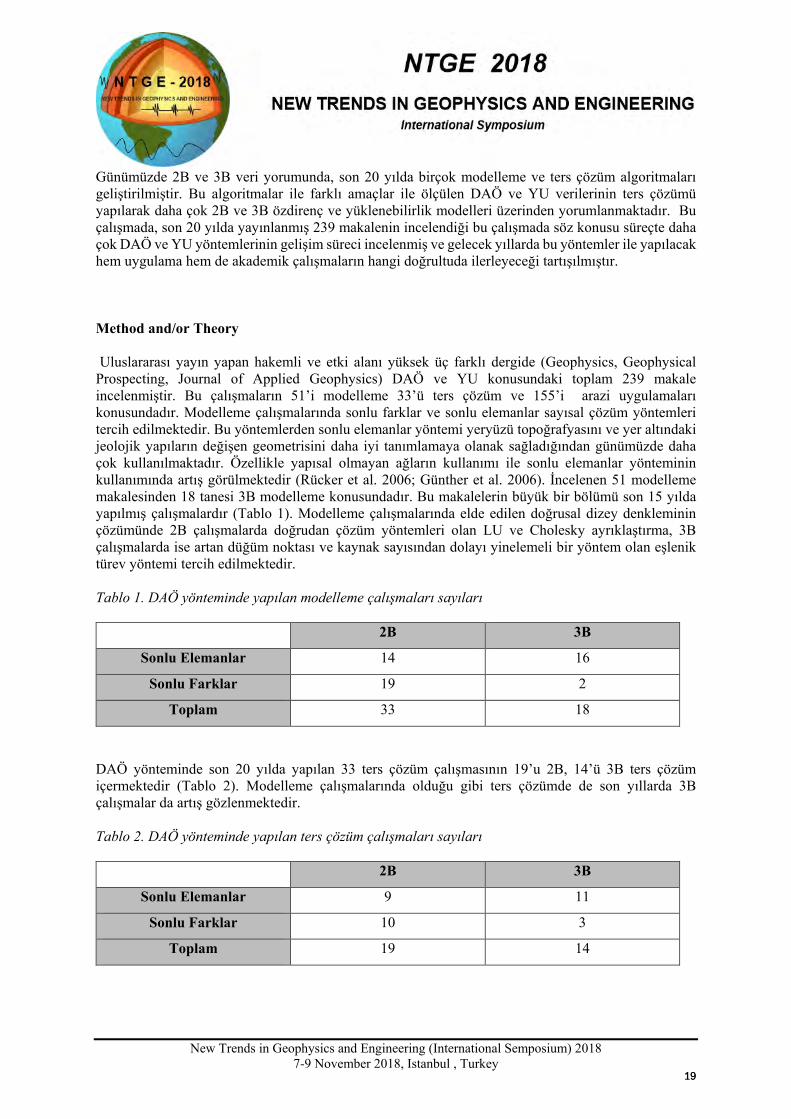
Günümüzde 2B ve 3B veri yorumunda, son 20 yılda birçok modelleme ve ters çözüm algoritmaları geliştirilmiştir. Bu algoritmalar ile farklı amaçlar ile ölçülen DAÖ ve YU verilerinin ters çözümü yapılarak daha çok 2B ve 3B özdirenç ve yüklenebilirlik modelleri üzerinden yorumlanmaktadır. Bu çalışmada, son 20 yılda yayınlanmış 239 makalenin incelendiği bu çalışmada söz konusu süreçte daha çok DAÖ ve YU yöntemlerinin gelişim süreci incelenmiş ve gelecek yıllarda bu yöntemler ile yapılacak hem uygulama hem de akademik çalışmaların hangi doğrultuda ilerleyeceği tartışılmıştır. Method and/or Theory Uluslararası yayın yapan hakemli ve etki alanı yüksek üç farklı dergide (Geophysics, Geophysical Prospecting, Journal of Applied Geophysics) DAÖ ve YU konusundaki toplam 239 makale incelenmiştir. Bu çalışmaların 51’i modelleme 33’ü ters çözüm ve 155’i arazi uygulamaları konusundadır. Modelleme çalışmalarında sonlu farklar ve sonlu elemanlar sayısal çözüm yöntemleri tercih edilmektedir. Bu yöntemlerden sonlu elemanlar yöntemi yeryüzü topoğrafyasını ve yer altındaki jeolojik yapıların değişen geometrisini daha iyi tanımlamaya olanak sağladığından günümüzde daha çok kullanılmaktadır. Özellikle yapısal olmayan ağların kullanımı ile sonlu elemanlar yönteminin kullanımında artış görülmektedir (Rücker et al. 2006; Günther et al. 2006). İncelenen 51 modelleme makalesinden 18 tanesi 3B modelleme konusundadır. Bu makalelerin büyük bir bölümü son 15 yılda yapılmış çalışmalardır (Tablo 1). Modelleme çalışmalarında elde edilen doğrusal dizey denkleminin çözümünde 2B çalışmalarda doğrudan çözüm yöntemleri olan LU ve Cholesky ayrıklaştırma, 3B çalışmalarda ise artan düğüm noktası ve kaynak sayısından dolayı yinelemeli bir yöntem olan eşlenik türev yöntemi tercih edilmektedir. Tablo 1. DAÖ yönteminde yapılan modelleme çalışmaları sayıları
2B 3B
Sonlu Elemanlar 14 16
Sonlu Farklar 19 2
Toplam 33 18
DAÖ yönteminde son 20 yılda yapılan 33 ters çözüm çalışmasının 19’u 2B, 14’ü 3B ters çözüm içermektedir (Tablo 2). Modelleme çalışmalarında olduğu gibi ters çözümde de son yıllarda 3B çalışmalar da artış gözlenmektedir. Tablo 2. DAÖ yönteminde yapılan ters çözüm çalışmaları sayıları
2B 3B
Sonlu Elemanlar 9 11
Sonlu Farklar 10 3
Toplam 19 14
1919
New Trends in Geophysics and Engineering (International Semposium) 2018
7-9 November 2018, Istanbul , Turkey
Çalışmaların büyük bir çoğunluğunda türev tabanlı yöntemler tercih edilirken, global ters çözüm tekniği sadece 2 adet 2B çalışmada kullanılmıştır (Akca ve Başokur 2010;Singh et al. 2017). Global ters çözüm tekniğinin 3B çalışmalarda uygulaması şu ana kadar yapılmamıştır. 3B çalışmalarda toplanan veri sayısı ve ters çözümde çözülen parametre sayısı düşünüldüğünde bu beklenen bir sonuçtur. Türev tabanlı ters çözüm yöntemlerinden en çok tercih edilen yöntemler Gauss-Newton (GN) (% 51) ve sönümlü en-küçük karelerdir (SEKK) (%40). Son adımda elde edilen dizey denkleminin çözümünde ise QR ayrıklaştırma ve eşlenik-türev (CG) yöntemleri tercih edilmektedir. Çok fazla sayıda verinin toplandığı ve parametre sayısının çok olduğu (özellikle 3B) çalışmalarda, dizey tersleme işlemine gerek duyulmayan doğrusal olmayan eşlenik-türev yöntemi de 4 çalışmada tercih edilmiştir. 3B çalışmalarda bir engel olarak görünen hafıza ve zaman probleminin aşılması için uygulanacak farklı yöntemler (paralel hesaplama, GPU tabanlı ters çözüm vb.) ilerleyen yıllarda araştırma konusu olabilir. Ters çözüm çalışmalarında dikkat çeken diğer bir nokta, yapılan çalışmaların hemen hemen tamamında durağanlaştırıcı olarak model parametrelerinin L2-normu olan yuvarlatıcılı durağanlaştırıcı kullanılmasıdır (% 95). Diğer durağanlaştırıcıların kullanıldığı çalışma sayısı ikidir (Gündoğdu and Candansayar, 2018). Conclusions Çalışmada 2000 yılından günümüze DAÖ modelleme ve ters çözüm çalışmalarına bakıldığında 2B çalışmaların belirli bir düzeye geldiği, araştırma konularının azaldığı açıkça görülmektedir. 2B çalışmaların özellikle uygulama alanlarına yönelik olarak devam edeceği açıktır. 3B çalışmalarda ise araştırma konularının beklenildiği gibi hafıza ve süre bakımından kısıtlayıcı engellerin azaltılmasına yönelik olacağı görülmektedir. GPU tabanlı ters çözüm, paralel hesaplama teknikleri vb. konular önümüzdeki dönemlerin çalışma konuları olarak görülmektedir. Ayrıca çalışma amacına yönelik farklı durağanlaştırıcı kullanımlarının (odaklanmış ters çözüm vb.) araştırma konusu olacağı düşünülmektedir. 3B çalışmalarda ters çözüm algoritmalarına erişimin zorluğu, bu konuda kullanıma ücretsiz açık yazılımın bulunmaması çalışma çeşitliliğini etkilemektedir. Belirli bir süre sonunda 2B ters çözümün gelişimine benzer olarak 3B ters çözüm algoritmalarının da kullanımı yaygınlaştıkça, 3B yer altı yapısını ortaya koyacak uygulama çalışmalarının artacağı düşünülmektedir. Günümüzde popüler olan kuyu içi ölçümlerle beraber deniz yüzeyi ve tabanında yapılan DAÖ ölçümleri önümüzdeki yıllarda yaygınlaşacaktır. Özellikle zamana bağlı 2B ve 3B ters çözüm algoritmaları, heyelan gibi doğal afetlerin erken uyarı sistemleri için kullanılabilir. Bu konularda ülkemizdeki çalışmalar hala yetersizdir. Acknowledgements (Optional) Kongre katılım desteğinden dolayı Ankara Üniversitesi, Mühendisilik Fakültesi dekanlığına teşekkür ederiz. References Akça, I., & Basokur, A. T. (2010). Extraction of structure-based geoelectric models by hybrid genetic
algorithms. Geophysics, 75(1), F15-F22.
2020
New Trends in Geophysics and Engineering (International Semposium) 2018
7-9 November 2018, Istanbul , Turkey
Dahlin, T. (2001). The development of DC resistivity imaging techniques. Computers & Geosciences, 27(9), 1019-1029.
Gündoğdu Y. And Candansayar, M.E., 2018, Three Dimensional Regularized Inversion Of Dc Resistivity Data with Different Stabilizing Functional. Geophysics (accepted manuscript)
Günther, T., Rücker, C., & Spitzer, K. (2006). Three-dimensional modelling and inversion of DC resistivity data incorporating topography—II. Inversion. Geophysical Journal International, 166(2), 506-517.
Rücker, C., Günther, T., & Spitzer, K. (2006). Three-dimensional modelling and inversion of DC resistivity data incorporating topography—I. Modelling. Geophysical Journal International, 166(2), 495-505.
Singh, A., Sharma, S. P., Akca, İ., & Baranwal, V. C. (2017). Fuzzy constrained Lp-norm inversion of direct current resistivity data. Geophysics, 83(1), 1-56.
Telford, W. M., Telford, W. M., Geldart, L. P., & Sheriff, R. E. (1990). Applied geophysics (Vol. 1). Cambridge university press.
2121
New Trends in Geophysics and Engineering (International Semposium) 2018
7-9 November 2018, Istanbul , Turkey
SEISMOTECTONIC INVESTIGATION OF BIGA PENINSULA IN SW MARMARA REGION USING STEERABLE FILTER TECHNIQUE, POTENTIAL FIELD DATA
AND RECENT SEISMICITY
Ethem Görgün , A. Muhittin Albora
Department of Geophysical Eng., Istanbul University-Cerrahpasa, Istanbul E-mail: [email protected]
Presentation Type All accepted proceedings will be published on the webpage of the symposium (ntge2018.istanbul.edu.tr)
ORAL POSTER
Abstract We examine seismotectonic setting of Biga Peninsula in western Anatolia (Çanakkale region) using the steerable filter technique and recent seismicity. One of the most important issue in geophysics is to observe borders or margins of tectonic/geologic discontinues. For this purpose, we apply this filter technique to gravity anomaly map of Biga Peninsula. We observe undetected/buried faults in Biga Peninsula using the steerable technique where they have never been seen in the geological maps before. These buried faults comply with recent seismicity for this region. Focal mechanisms of past earthquakes (M≥3.5) are in good agreement with fault orientations. This observation shows that we have to take into account these fault locations and consider for preparing future seismic hazard maps. The geometry of fault segments reveals mostly strike-slip faulting regime with NE-SW trending direction of T-axis in the entire study region. According to high-resolution hypocenter relocation of the Biga earthquake sequences in the observation period between 5 January 2005 and 14 November 2015 extends from N to S direction. The stress tensor inversion results indicate a predominant normal stress regime with a NW-SE oriented maximum horizontal compressive stress (SH). According to strong discrepancy of density in the Biga Peninsula is characterized by numerous small segmented secondary faults. These buried or undetected fault locations indicate that these segments are large enough to increase earthquake stress failure towards NW-SE and N-S directions, respectively. Seismotectonic setting of Biga Peninsula is divided into sub-regions by NE-SW trending secondary faults with normal and major strike-slip components. This output is verified by steerable filter and local/regional seismotectonic analysis. We propose a new seismotectonic model for Biga Peninsula and update the orientation of active fault segments. According to our model, North Anatolian Fault Zone cross-cuts the southern Marmara basins as a narrow fault segment and continues towards Aegean Sea.
Keywords: Biga Peninsula; Focal Mechanism; Marmara Region; Seismicity; Steerable Filter
2222
New Trends in Geophysics and Engineering (International Semposium) 2018 7-9 November 2018, Istanbul , Turkey
Introduction
One of the main goals in geophysics is to detect the edges of underground structures. These edges are generally estimated by evaluation of the points where the curvature changes. Different filtering techniques can be applied to anomaly maps obtained by geophysical methods to detect the borders of geological structures. There are various filters that can be used for border detection problems in potential anomaly maps. The steerable filter technique has advantages over the classical methods mainly in two aspects. Firstly, there is no need for time consuming pre-processes (e.g. wavenumber filtering, reduction to the pole, upward continuation) for separating residual-regional anomalies before application. Secondly, it is free from the direction, i.e. it can be applied in any selected direction while classical methods generally work in either one of x, y directions or both. Steerable filters, first defined by Freeman and Adelson (1991), emphasize the properties of the input data for a desired arbitrary direction, while minimizing effects in other directions. This steering feature is achieved by using band pass filters in certain directions. This kind of filtering is capable of evaluation of complex problems (Albora et al., 2006). In this study, we performed a steerable filter technique for gravity anomaly maps from General Directorate of Mineral Research and Exploration (MTA) to obtain more accurate picture of BP active fault structures. For this purpose, gravity anomaly maps at regional scale were used to compute borders of fault locations using the steerable filter technique (Freeman and Adelson, 1991). This provides additional information on a more accurate fault location map that is able to improve kinematic models for BP and thus develop the understanding of the local and regional tectonics. Furthermore, the double-difference relocation algorithm (Waldhauser and Ellsworth, 2000) and the stress tensor analysis (Vavryčuk, 2014) were applied to determine the expanded spatial distribution of the BP earthquake sequences. Determination of accurate fault orientations and locations using data from gravity maps and regional seismic networks are crucial for investigations of the seismotectonics in and around southern Marmara Sea.
The steerable filter technique
Steerable filter is a kind of bandpass filter with a specific direction. Margins of an image with different directions are separated using steerable filters which characterize margin determination, image squeezing and improving, also tissue analysis. These filters display special features as a bandpass filter with specific directions. Steerable filters allow us to find buried faults that we compare our results with geological and seismological maps. If there is a buried fault in a region, a strong discrepancy of density for geological structure is detected. Moreover, this diversity causes discontinuity in gravity anomaly maps. An oriented filter often needs to rotate different angles under adaptive control or wishes to calculate the filter response at various orientations. Freeman and Adelson (1991) presented an efficient architecture to synthesize filters of arbitrary orientations from linear combinations of basis filters. It is allowed us to use adaptively “steer” a filter to any orientation and to determine analytically the filter output as a function of orientation. Steerable filters can be designed in quadrature pairs to allow adaptive control over phase as well as orientation.
Stress tensor inversion
The stress tensor has six unknown, either three principal stresses and orientations, or three normal and three shear stress components (e.g., Zang and Stephansson, 2010). Four of the unknowns are resolved by the inversion of the stress tensor, the fifth unknown is calculated by the assumption that slip occurs in the direction of maximum shear stress (Wallace, 1951) and the sixth unknown is usually resolved using the assumption that the stress tensor is homogeneous and constant in the binning region throughout the time interval of interest.
2323
New Trends in Geophysics and Engineering (International Semposium) 2018
7-9 November 2018, Istanbul , Turkey
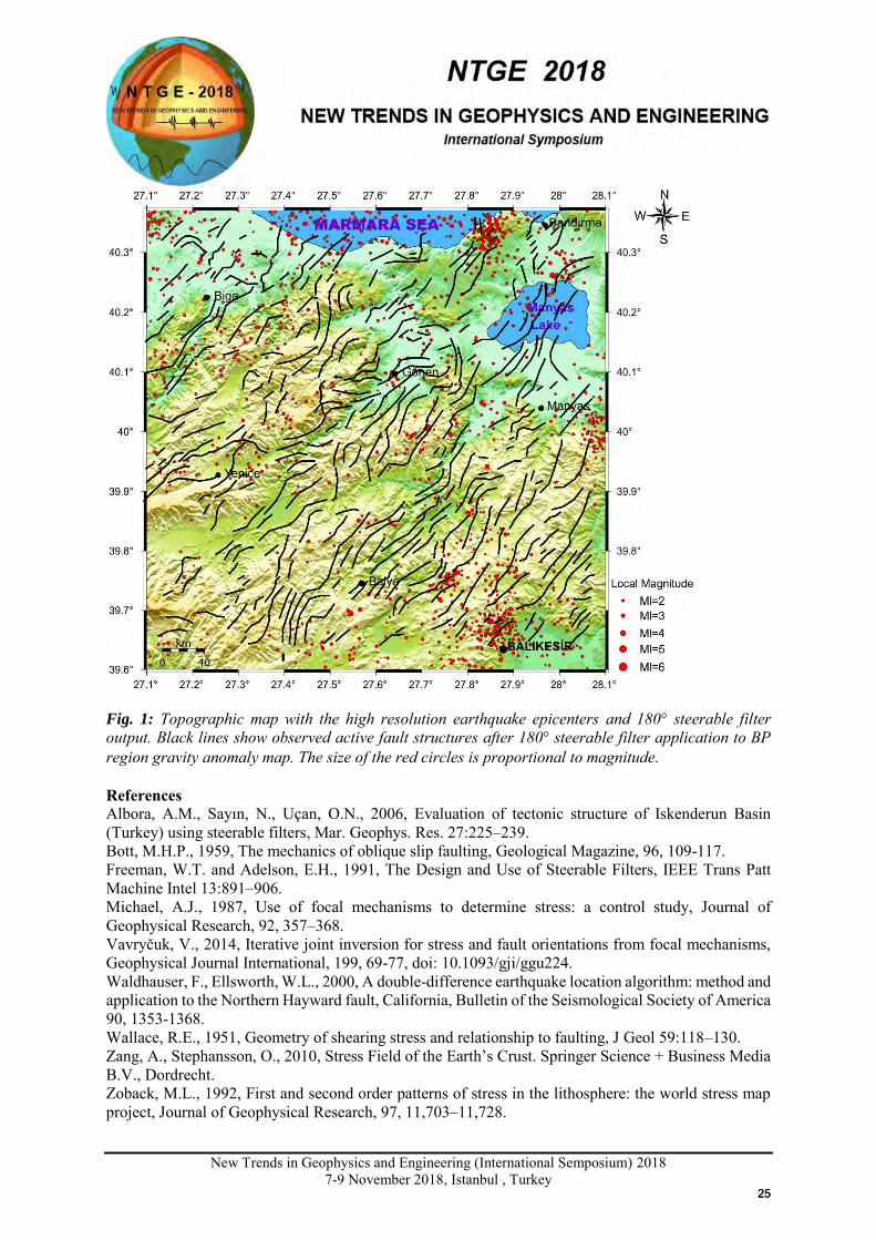
In this study, the technique of Michael (1987) is applied to the selected 27 events (Table 1) with magnitude (M) ≥ 3.5 from focal mechanism catalogue of Kandilli Observatory and Earthquake Research Institute (http://www.koeri.boun.edu.tr). The algorithm uses the statistical method of bootstrap re-sampling and allows determining the orientation of the three principal stresses (σ1 = maximum principal compressive stress, σ2 = intermediate and σ3 = minimum) as well as the stress ratio R = (σ2- σ3)/ (σ1- σ3), also called relative stress magnitude (Bott, 1959). The R is defined using the standard geologic/geophysical notation with compressive stress positive and σ1> σ2> σ3 (e.g. Zoback, 1992). The stress ratio (R) ranges from 0 to 1. Values of R < 0.5 and R > 0.5 indicate a transpressional and transtensional regime, respectively. All parameters are determined by finding the best fitting stress tensor to the observed focal mechanisms. Assumptions that must be fulfilled by the input data are: (1) stress is uniform in the area of interest during the observed time interval, however this assumption cannot be entirely valid given the diversity and complexity of the structures, (2) earthquakes are shear-dislocations on pre-existing faults, (3) similar shear stress magnitude are present on each fault and (4) slip occurs in the direction of the resolved shear stress on the fault plane. Conclusions In this study, the location of active faults in Biga Peninsula (BP) is determined by the steerable filters to the Bouguer gravity anomaly map in different directions. Our method is one of the first application to a synthetically produced gravity anomaly map by establishing prisms perpendicular to each other. Then the algorithm is evaluated for a gravity anomaly map of Biga Peninsula and used to estimate the locations of different secondary fault segments. A new fault map of the Biga Peninsula is produced using outputs of steerable filter applications to a gravity anomaly map with local/regional seismicity data (Fig. 1). We find that NE–SW trending right lateral strike-slip and normal faults in terms of discontinuities along southwestern Marmara region from outcomes of the steerable filters. 18 March 1953 M 7.2 Gönen earthquake fault rupture is determined as an extension of North Anatolian Fault Zone in southwestern Marmara Sea. We deduce that the main fault segments in Biga Peninsula, i.e. Yenice-Gönen and Biga-Çan faults, continue offshore southwest of Edremit Gulf and compose a southern margin of the North Anatolian Fault zone. Biga Peninsula earthquake focal mechanisms are clearly indicated that active NE-SW trending normal faulting systems with right-lateral strike-slip component are wide-spread along the southern Marmara region. These tectonic structures impose a threat to the nearby big districts and provinces (e.g. Istanbul, Bursa and Yalova) along the Marmara Sea region. Additionally, the high-resolution aftershock locations suggest that we interpret their orientation and spatial distribution in terms of the major strike-slip fault strands (e.g. NAFZ) and the basin boundaries (for the normal faults). The westernmost part of the BP region exhibits not only normal faulting mechanisms but also some strike-slip motions. These strike-slip mechanisms may occur due to the local/regional stress change in the BP region, resulting from the transform of the Anatolian and Eurasian plate interaction. Moreover, events in westernmost part of the BP region indicate that several small fault segments exist in this area. These small secondary faults may have different faulting mechanisms compared to the NAFZ.
2424
New Trends in Geophysics and Engineering (International Semposium) 2018
7-9 November 2018, Istanbul , Turkey
Fig. 1: Topographic map with the high resolution earthquake epicenters and 180° steerable filter output. Black lines show observed active fault structures after 180° steerable filter application to BP region gravity anomaly map. The size of the red circles is proportional to magnitude. References Albora, A.M., Sayın, N., Uçan, O.N., 2006, Evaluation of tectonic structure of Iskenderun Basin (Turkey) using steerable filters, Mar. Geophys. Res. 27:225–239. Bott, M.H.P., 1959, The mechanics of oblique slip faulting, Geological Magazine, 96, 109-117. Freeman, W.T. and Adelson, E.H., 1991, The Design and Use of Steerable Filters, IEEE Trans Patt Machine Intel 13:891–906. Michael, A.J., 1987, Use of focal mechanisms to determine stress: a control study, Journal of Geophysical Research, 92, 357–368. Vavryčuk, V., 2014, Iterative joint inversion for stress and fault orientations from focal mechanisms, Geophysical Journal International, 199, 69-77, doi: 10.1093/gji/ggu224. Waldhauser, F., Ellsworth, W.L., 2000, A double-difference earthquake location algorithm: method and application to the Northern Hayward fault, California, Bulletin of the Seismological Society of America 90, 1353-1368. Wallace, R.E., 1951, Geometry of shearing stress and relationship to faulting, J Geol 59:118–130. Zang, A., Stephansson, O., 2010, Stress Field of the Earth’s Crust. Springer Science + Business Media B.V., Dordrecht. Zoback, M.L., 1992, First and second order patterns of stress in the lithosphere: the world stress map project, Journal of Geophysical Research, 97, 11,703–11,728.
2525
New Trends in Geophysics and Engineering (International Semposium) 2018
7-9 November 2018, Istanbul , Turkey
DETERMINATION OF THE TECTONIC LINES OF THE MAP OF GRAVITY ANOMALY OF THE WESTERN ANATOLIAN REGION BY THE CELLULAR
NEURAL NETWORK (CNN) METHOD
Mehmet Ali ÜGE1 and Ali Muhittin ALBORA1
1Istanbul University-Cerrahpaşa, Engineering Faculty, Geophysical Department, 34320, Avcilar, Istanbul, Turkey
Presentation Type All accepted proceedings will be published on the webpage of the symposium (ntge2018.istanbul.edu.tr)
ORAL POSTER
Abstracts In this study, it is aimed to determine the boundaries of the fault lines of the graben structures in the region by applying Cellular Neural Network (CNN) method to the Bouguer anomaly map of Western Anatolia region. The Western Anatolian region has many active fault lines and these fault lines produce earthquakes up to 7 magnitudes. For this reason, the location of the fault lines is important both for seismologically and for revealing geothermal energy close to these fault lines. Keywords: CNN, Bouguer anomaly map, Western Anatolia Introduction Western Anatolia is a very active region in terms of earthquake risk. The region has a very complex tectonic structure. There is an active fault with high potential for earthquake generation in the region. The north of the zone is the North Anatolian fault zone (KAFZ) with a right lateral strike in the north and the Helen-West Cypriot arc in the south. For this reason the region is under the influence of compression tectonics. For this reason it can be characterized by intra-continental expansion regime. The area is sloped and normal faults are found on large scale and in large numbers. For this reason, grabens have come to the region in different shapes and sizes. Their interior is filled with neogene and quaternary rocks. The most important grabens are Gediz, Büyük Menderes and Küçük Menderes. Along the Cyprus and Hellenic springs, the oceanic lithosphere on the northern edge of the African continent has been swallowed under Anatolia and the Aegean (Kissel et al., 1993; Frizon et al., 1995). Cellular Neural Network (CNN) method has been applied to determine the structural boundaries of the gravity anomaly map of Western Anatolia. The CNN method was first proposed by Leon Chua and Lin Yang in 1988. The first applications of the CNN method to geophysical engineering were made (Özmen et al 1999; Albora et al 2001a; Albora et al 2001b).
X
2626
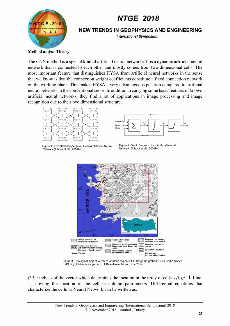
New Trends in Geophysics and Engineering (International Semposium) 2018
7-9 November 2018, Istanbul , Turkey
Method and/or Theory The CNN method is a special kind of artificial neural networks. It is a dynamic artificial neural network that is connected to each other and mostly comes from two-dimensional cells. The most important feature that distinguishes HYSA from artificial neural networks in the sense that we know is that the connection weight coefficients constitute a fixed connection network on the working plane. This makes HYSA a very advantageous position compared to artificial neural networks in the conventional sense. In addition to carrying some basic features of known artificial neural networks, they find a lot of applications in image processing and image recognition due to their two dimensional structure.
(i,J) : indices of the vector which determines the location in the array of cells c(i,J): : İ. Line, J. showing the location of the cell in column para-meters. Differential equations that characterize the cellular Neural Network can be written as:
Figure 1: Two Dimensional (4x4) Cellular Artificial Neural Network (Albora et all., 2001b).
Figure 2: Block Diagram of an Artificial Neural Network (Albora et all., 2001b).
Figure 3. Geological map of Western Anatolia region (BEG Bergama graben; GDG Gediz graben, BMG Büyük Menderes graben; KT Kale-Tavas basin (Oruç 2014).
2727
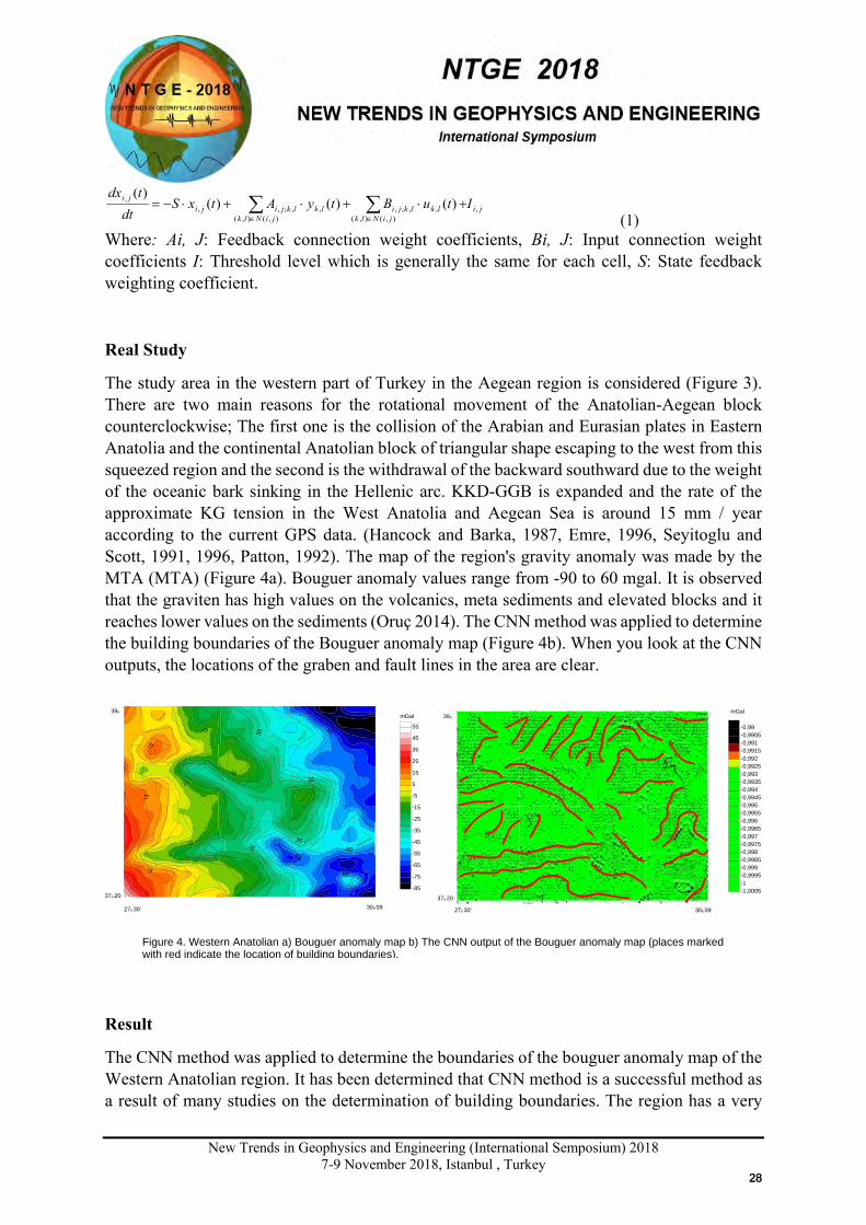
New Trends in Geophysics and Engineering (International Semposium) 2018
7-9 November 2018, Istanbul , Turkey
jijiNlk
lklkjijiNlk
lklkjijiji ItuBtyAtxS
dttdx
,),(),(
,,;,),(),(
,,;,,, )()()(
)(∑∑∈∈
+⋅+⋅+⋅−= (1)
Where: Ai, J: Feedback connection weight coefficients, Bi, J: Input connection weight coefficients I: Threshold level which is generally the same for each cell, S: State feedback weighting coefficient.
Real Study
The study area in the western part of Turkey in the Aegean region is considered (Figure 3). There are two main reasons for the rotational movement of the Anatolian-Aegean block counterclockwise; The first one is the collision of the Arabian and Eurasian plates in Eastern Anatolia and the continental Anatolian block of triangular shape escaping to the west from this squeezed region and the second is the withdrawal of the backward southward due to the weight of the oceanic bark sinking in the Hellenic arc. KKD-GGB is expanded and the rate of the approximate KG tension in the West Anatolia and Aegean Sea is around 15 mm / year according to the current GPS data. (Hancock and Barka, 1987, Emre, 1996, Seyitoglu and Scott, 1991, 1996, Patton, 1992). The map of the region's gravity anomaly was made by the MTA (MTA) (Figure 4a). Bouguer anomaly values range from -90 to 60 mgal. It is observed that the graviten has high values on the volcanics, meta sediments and elevated blocks and it reaches lower values on the sediments (Oruç 2014). The CNN method was applied to determine the building boundaries of the Bouguer anomaly map (Figure 4b). When you look at the CNN outputs, the locations of the graben and fault lines in the area are clear.
Result
The CNN method was applied to determine the boundaries of the bouguer anomaly map of the Western Anatolian region. It has been determined that CNN method is a successful method as a result of many studies on the determination of building boundaries. The region has a very
-60
-85
-75
-65
-55
-45
-35
-25
-15
-5
5
15
25
35
45
55
-1,0005-1-0,9995-0,999-0,9985-0,998-0,9975-0,997-0,9965-0,996-0,9955-0,995-0,9945-0,994-0,9935-0,993-0,9925-0,992-0,9915-0,991-0,9905-0,99
270 30' 300 09'
370 20'
390
300 09'270 30'
370 20'
390mGalmGal
Figure 4. Western Anatolian a) Bouguer anomaly map b) The CNN output of the Bouguer anomaly map (places marked with red indicate the location of building boundaries).
2828
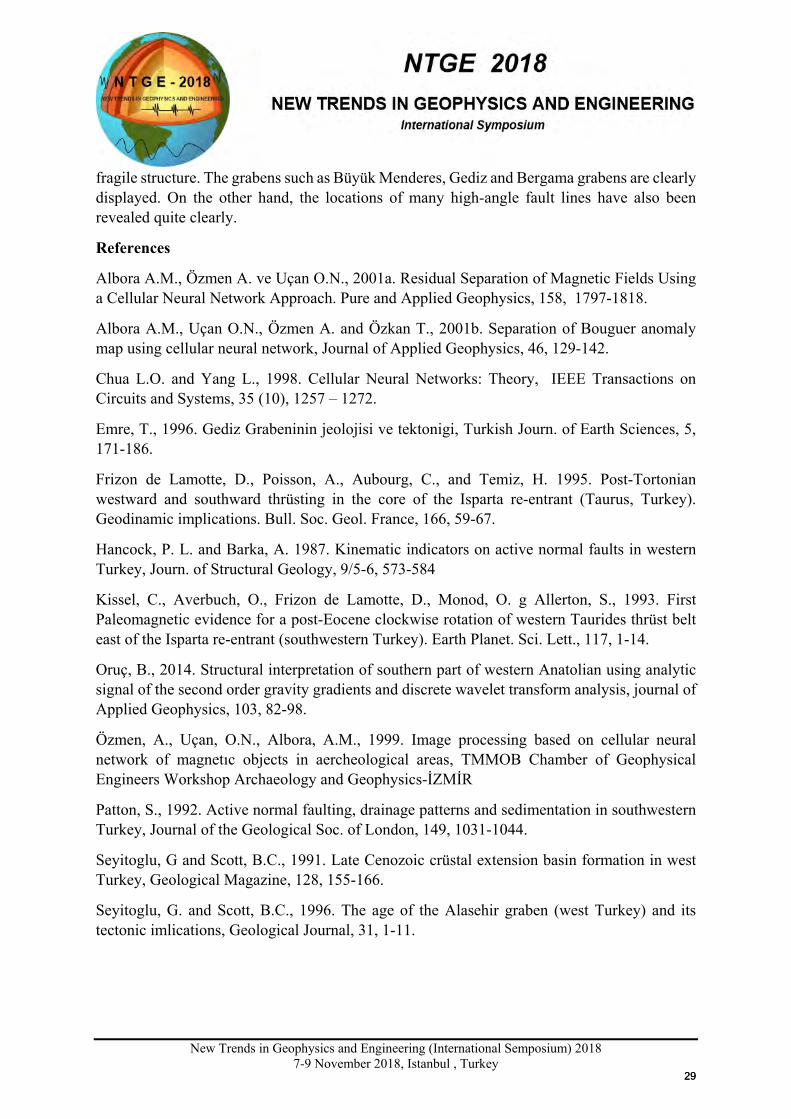
New Trends in Geophysics and Engineering (International Semposium) 2018
7-9 November 2018, Istanbul , Turkey
fragile structure. The grabens such as Büyük Menderes, Gediz and Bergama grabens are clearly displayed. On the other hand, the locations of many high-angle fault lines have also been revealed quite clearly.
References
Albora A.M., Özmen A. ve Uçan O.N., 2001a. Residual Separation of Magnetic Fields Using a Cellular Neural Network Approach. Pure and Applied Geophysics, 158, 1797-1818.
Albora A.M., Uçan O.N., Özmen A. and Özkan T., 2001b. Separation of Bouguer anomaly map using cellular neural network, Journal of Applied Geophysics, 46, 129-142.
Chua L.O. and Yang L., 1998. Cellular Neural Networks: Theory, IEEE Transactions on Circuits and Systems, 35 (10), 1257 – 1272.
Emre, T., 1996. Gediz Grabeninin jeolojisi ve tektonigi, Turkish Journ. of Earth Sciences, 5, 171-186.
Frizon de Lamotte, D., Poisson, A., Aubourg, C., and Temiz, H. 1995. Post-Tortonian westward and southward thrüsting in the core of the Isparta re-entrant (Taurus, Turkey). Geodinamic implications. Bull. Soc. Geol. France, 166, 59-67.
Hancock, P. L. and Barka, A. 1987. Kinematic indicators on active normal faults in western Turkey, Journ. of Structural Geology, 9/5-6, 573-584
Kissel, C., Averbuch, O., Frizon de Lamotte, D., Monod, O. g Allerton, S., 1993. First Paleomagnetic evidence for a post-Eocene clockwise rotation of western Taurides thrüst belt east of the Isparta re-entrant (southwestern Turkey). Earth Planet. Sci. Lett., 117, 1-14.
Oruç, B., 2014. Structural interpretation of southern part of western Anatolian using analytic signal of the second order gravity gradients and discrete wavelet transform analysis, journal of Applied Geophysics, 103, 82-98.
Özmen, A., Uçan, O.N., Albora, A.M., 1999. Image processing based on cellular neural network of magnetıc objects in aercheological areas, TMMOB Chamber of Geophysical Engineers Workshop Archaeology and Geophysics-İZMİR
Patton, S., 1992. Active normal faulting, drainage patterns and sedimentation in southwestern Turkey, Journal of the Geological Soc. of London, 149, 1031-1044.
Seyitoglu, G and Scott, B.C., 1991. Late Cenozoic crüstal extension basin formation in west Turkey, Geological Magazine, 128, 155-166.
Seyitoglu, G. and Scott, B.C., 1996. The age of the Alasehir graben (west Turkey) and its tectonic imlications, Geological Journal, 31, 1-11.
2929
New Trends in Geophysics and Engineering (International Semposium) 2018
7-9 November 2018, Istanbul , Turkey
THE IMPORTANCE OF GEOPHYSICAL METHODS IN SOIL PROBLEMS
Göksu ERDAN1 and Ali Muhittin ALBORA1
1 1Istanbul University-Cerrahpaşa, Engineering Faculty, Geophysical Department, 34320,
Avcilar, Istanbul, Turkey Presentation Type All accepted proceedings will be published on the webpage of the symposium (ntge2018.istanbul.edu.tr)
ORAL POSTER
Abstracts This study was carried out in order to find out the ground parameters in Istanbul-Esenyurt province and to determine the inequality. The methods used in the study are the MAW, micro tremor and laboratory experiments. Later on, drillings were made where necessary to obtain information about the soil parameters.
Keywords: MAW, micro tremor, laboratory experiments, Esenyurt-Turkey
Introduction In the case of earthquakes, residential areas may exhibit different behaviors in spite of the same ground, the same building materials, even the same people. In these settlements, the buildings are heavily damaged or moderately damaged, and there is no damage to the buildings next to or around the buildings. Geologic, geological and geophysical investigations have been carried out by many researchers in order to reduce the damage of structures in earthquakes due to the random distribution of earthquake heavy damages. In the 1985 earthquake in Mexico City, the earthquake struck the very center of the city, 350 km from the center. The great damage in the area can be explained by geophysical methods including deep investigations that it is a deep canyon below the city center (Alverez 1990). have used geophysical methods to investigate geological structures and to calculate the physical parameters of rocks (Klimis et al., 1999). In addition to geophysical methods, engineering parameters are taken into account in studying the soil structure in geotechnical studies. Severe damage zones in the Kobe earthquake of 1995 were explained by the fact that the folds of the seabed which can be detected by seismic measurements are caused by earthquake focusses on the propagation path of earthquake waves (Motosaka et al., 1997). It has been found that the mechanical properties of the rocks are closely related to the ultrasonic velocity and rock properties (D'Andrea et al., 1965; Chary, 2006; Özcep et al., 2007; Vasconcelos, 2008; Keceli 2009). For this reason, experimental or theoretical conformity is used between various physical and mechanical properties of rocks to obtain special design parameters of rock mass.
.
X
3030
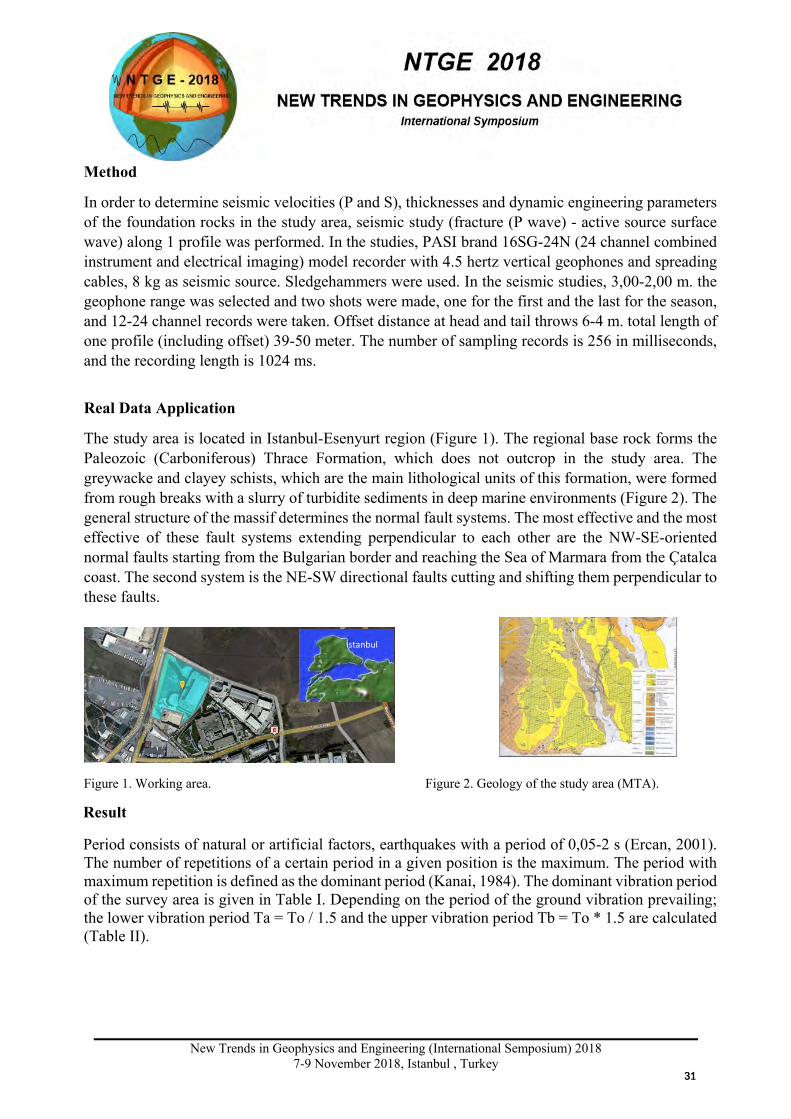
New Trends in Geophysics and Engineering (International Semposium) 2018
7-9 November 2018, Istanbul , Turkey
Method
In order to determine seismic velocities (P and S), thicknesses and dynamic engineering parameters of the foundation rocks in the study area, seismic study (fracture (P wave) - active source surface wave) along 1 profile was performed. In the studies, PASI brand 16SG-24N (24 channel combined instrument and electrical imaging) model recorder with 4.5 hertz vertical geophones and spreading cables, 8 kg as seismic source. Sledgehammers were used. In the seismic studies, 3,00-2,00 m. the geophone range was selected and two shots were made, one for the first and the last for the season, and 12-24 channel records were taken. Offset distance at head and tail throws 6-4 m. total length of one profile (including offset) 39-50 meter. The number of sampling records is 256 in milliseconds, and the recording length is 1024 ms.
Real Data Application
The study area is located in Istanbul-Esenyurt region (Figure 1). The regional base rock forms the Paleozoic (Carboniferous) Thrace Formation, which does not outcrop in the study area. The greywacke and clayey schists, which are the main lithological units of this formation, were formed from rough breaks with a slurry of turbidite sediments in deep marine environments (Figure 2). The general structure of the massif determines the normal fault systems. The most effective and the most effective of these fault systems extending perpendicular to each other are the NW-SE-oriented normal faults starting from the Bulgarian border and reaching the Sea of Marmara from the Çatalca coast. The second system is the NE-SW directional faults cutting and shifting them perpendicular to these faults.
Figure 1. Working area. Figure 2. Geology of the study area (MTA).
Result
Period consists of natural or artificial factors, earthquakes with a period of 0,05-2 s (Ercan, 2001). The number of repetitions of a certain period in a given position is the maximum. The period with maximum repetition is defined as the dominant period (Kanai, 1984). The dominant vibration period of the survey area is given in Table I. Depending on the period of the ground vibration prevailing; the lower vibration period Ta = To / 1.5 and the upper vibration period Tb = To * 1.5 are calculated (Table II).
İstanbul
3131
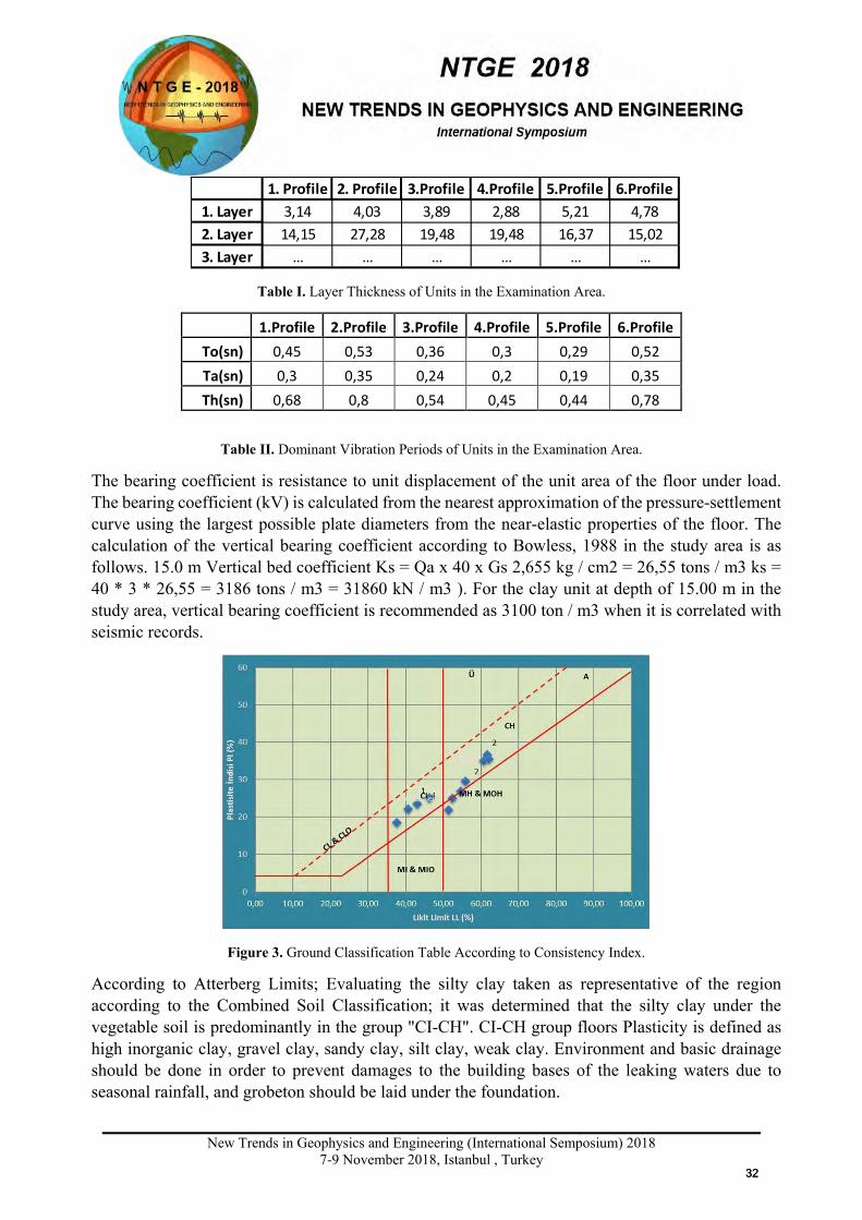
New Trends in Geophysics and Engineering (International Semposium) 2018
7-9 November 2018, Istanbul , Turkey
Table I. Layer Thickness of Units in the Examination Area.
1.Profile 2.Profile 3.Profile 4.Profile 5.Profile 6.Profile To(sn) 0,45 0,53 0,36 0,3 0,29 0,52 Ta(sn) 0,3 0,35 0,24 0,2 0,19 0,35 Th(sn) 0,68 0,8 0,54 0,45 0,44 0,78
Table II. Dominant Vibration Periods of Units in the Examination Area.
The bearing coefficient is resistance to unit displacement of the unit area of the floor under load. The bearing coefficient (kV) is calculated from the nearest approximation of the pressure-settlement curve using the largest possible plate diameters from the near-elastic properties of the floor. The calculation of the vertical bearing coefficient according to Bowless, 1988 in the study area is as follows. 15.0 m Vertical bed coefficient Ks = Qa x 40 x Gs 2,655 kg / cm2 = 26,55 tons / m3 ks = 40 * 3 * 26,55 = 3186 tons / m3 = 31860 kN / m3 ). For the clay unit at depth of 15.00 m in the study area, vertical bearing coefficient is recommended as 3100 ton / m3 when it is correlated with seismic records.
Figure 3. Ground Classification Table According to Consistency Index.
According to Atterberg Limits; Evaluating the silty clay taken as representative of the region according to the Combined Soil Classification; it was determined that the silty clay under the vegetable soil is predominantly in the group "CI-CH". CI-CH group floors Plasticity is defined as high inorganic clay, gravel clay, sandy clay, silt clay, weak clay. Environment and basic drainage should be done in order to prevent damages to the building bases of the leaking waters due to seasonal rainfall, and grobeton should be laid under the foundation.
1. Profile 2. Profile 3.Profile 4.Profile 5.Profile 6.Profile1. Layer 3,14 4,03 3,89 2,88 5,21 4,782. Layer 14,15 27,28 19,48 19,48 16,37 15,023. Layer … … … … … …
3232
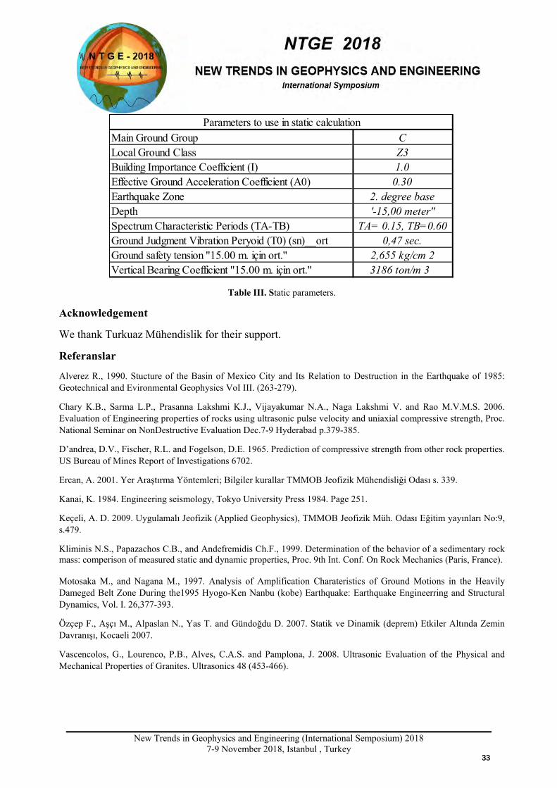
New Trends in Geophysics and Engineering (International Semposium) 2018
7-9 November 2018, Istanbul , Turkey
Table III. Static parameters.
Acknowledgement
We thank Turkuaz Mühendislik for their support.
Referanslar
Alverez R., 1990. Stucture of the Basin of Mexico City and Its Relation to Destruction in the Earthquake of 1985: Geotechnical and Evironmental Geophysics VoI III. (263-279).
Chary K.B., Sarma L.P., Prasanna Lakshmi K.J., Vijayakumar N.A., Naga Lakshmi V. and Rao M.V.M.S. 2006. Evaluation of Engineering properties of rocks using ultrasonic pulse velocity and uniaxial compressive strength, Proc. National Seminar on NonDestructive Evaluation Dec.7-9 Hyderabad p.379-385.
D’andrea, D.V., Fischer, R.L. and Fogelson, D.E. 1965. Prediction of compressive strength from other rock properties. US Bureau of Mines Report of Investigations 6702.
Ercan, A. 2001. Yer Araştırma Yöntemleri; Bilgiler kurallar TMMOB Jeofizik Mühendisliği Odası s. 339.
Kanai, K. 1984. Engineering seismology, Tokyo University Press 1984. Page 251.
Keçeli, A. D. 2009. Uygulamalı Jeofizik (Applied Geophysics), TMMOB Jeofizik Müh. Odası Eğitim yayınları No:9, s.479.
Kliminis N.S., Papazachos C.B., and Andefremidis Ch.F., 1999. Determination of the behavior of a sedimentary rock mass: comperison of measured static and dynamic properties, Proc. 9th Int. Conf. On Rock Mechanics (Paris, France). Motosaka M., and Nagana M., 1997. Analysis of Amplification Charateristics of Ground Motions in the Heavily Dameged Belt Zone During the1995 Hyogo-Ken Nanbu (kobe) Earthquake: Earthquake Engineerring and Structural Dynamics, Vol. I. 26,377-393.
Özçep F., Aşçı M., Alpaslan N., Yas T. and Gündoğdu D. 2007. Statik ve Dinamik (deprem) Etkiler Altında Zemin Davranışı, Kocaeli 2007.
Vascencolos, G., Lourenco, P.B., Alves, C.A.S. and Pamplona, J. 2008. Ultrasonic Evaluation of the Physical and Mechanical Properties of Granites. Ultrasonics 48 (453-466).
Main Ground Group CLocal Ground Class Z3Building Importance Coefficient (I) 1.0Effective Ground Acceleration Coefficient (A0) 0.30Earthquake Zone 2. degree baseDepth '-15,00 meter''Spectrum Characteristic Periods (TA-TB) TA= 0.15, TB=0.60Ground Judgment Vibration Peryoid (T0) (sn)__ort 0,47 sec.Ground safety tension ''15.00 m. için ort.'' 2,655 kg/cm 2Vertical Bearing Coefficient ''15.00 m. için ort.'' 3186 ton/m 3
Parameters to use in static calculation
3333
New Trends in Geophysics and Engineering (International Semposium) 2018
7-9 November 2018, Istanbul , Turkey
Crust and Upper Mantle Structure beneath the KTUT (Trabzon) and ERZN (Erzincan)
Stations from Joint Inversion of P and S Receiver Functions
Hamdi Alkan1*, Hakan Çınar2, Sergey Oreshin3, Lev Vinnik3
1 Department of Geophysics, Faculty of Eng.,Van Yüzüncü Yıl University, Van 2 Department of Geophysics, Faculty of Eng.,Karadeniz Technical University, Trabzon
3 Institute of physics of the Earth, Bolshaya Grouzinskaya, Moscow, Russia Email: [email protected]
Presentation Type All accepted proceedings will be published on the webpage of the symposium (ntge2018.istanbul.edu.tr)
ORAL POSTER
Abstracts P and S Receiver function technique is very suitable for studying the crust and upper mantle structures beneath the seismic stations using teleseismic events. This technique uses Ps or Sp converted phases to determine Earth discontinuities such as moho, 410 km and 660 km. In this study, we have applied joint inversion of the PRFs and SRFs with teleseismic residuals (dTs ve dTp) to investigate variations inner structure under KTUT (Trabzon) and ERZN (ERZN) broad-band seismic station, located Eastern Pontides Orogenic Belt (NE Turkey). The results reveal that depth to the moho boundary varies from 33 km to 42 km in our P and S-histograms from KTUT to ERZN, which agrees with the conclusions of previos studies in the region. The Vp/Vs values for the stations are generally consistent with the regional geology. We have found very low P and S-wave velocities (Vs=2.85 km/s, Vp=4.71 km/s) in the inversion results of KTUT station in the uppermost crust (about 4 km) and these velocities are interpreted as sedimentary layers. We have also clearly observed the low velocity layer under the ERZN station to depth of around 30 km. This layer may correspond to the North Anatolian Fault Zone. Beneath the KTUT and ERZN stations, an upper-mantle lid with an S velocity of about 4.5 km/s are underlain at a depth of about 79 and 85 km by a low-velocity zone, respectively. Keywords: Crust, Upper Mantle, Receiver Functions, Joint Inversion, KTUT and ERZN station. Introduction The P-Receiver Functions (PRFs) and S-Receiver Functions (SRFs) present a response of the Earth’s medium in the vicinity of the seismograph station to excitation by teleseismic P and S waves (Kiselev et al., 2008). Using these wave responses, the crust and upper mantle structure are investigated with simultaneous inversion with teleseismic P and S traveltime residuals. Through this approach, the aim of this study is to demonstrate the structure of the crust and upper mantle beneath the KTUT and ERZN seismic stations, located on the Eastern Pontides Orogenic Belt, NE Turkey (Fig. 1).
3434
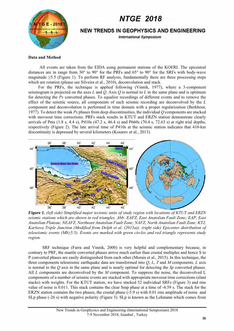
New Trends in Geophysics and Engineering (International Semposium) 2018
7-9 November 2018, Istanbul , Turkey
Data and Method
All events are taken from the EIDA using permanent stations of the KOERI. The epicentral distances are in range from 30° to 90° for the PRFs and 65° to 90° for the SRFs with body-wave magnitude ≥5.5 (Figure 1). To perform RF analysis, fundamentally there are three processing steps which are rotation (please see Silveira et al., 2010), deconvolution and stack. For the PRFs, the technique is applied following (Vinnik, 1977), where a 3-component seismogram is projected on the axes L and Q. Axis Q is normal to L in the same plane and is optimum for detecting the Ps converted phases. To equalize recordings of different events and to remove the effect of the seismic source, all components of each seismic recording are deconvolved by the L component and deconvolution is performed in time domain with a proper regularization (Berkhout, 1977). To detect the weak Ps phases from deep discontinuities, the individual Q components are stacked with moveout time corrections. PRFs stack results in KTUT and ERZN station demonstrate clearly arrivals of Pms (1.8 s, 4.4 s), P410s (47.2 s, 46.4 s) and P660s (70.4 s, 72.63 s) at right trial depths, respectively (Figure 2). The late arrival time of P410s at the seismic station indicates that 410-km discontinuity is depressed by several kilometers (Kosarev et al., 2013).
Figure 1. (left side) Simplified major tectonic units of study region with locations of KTUT and ERZN seismic stations which are shown in red triangles. Abb: EAFZ, East Anatolian Fault Zone; EAP, East Anatolian Plateau; NEAFZ, Northeast Anatolian Fault Zone; NAFZ, North Anatolian Fault Zone; KTJ, Karlıova Triple Junction (Modified from Delph et al. (2015a)). (right side) Epicenter distribution of teleseismic events (Mb≥5.5). Events are marked with green circles and red triangle represents study region. SRF technique (Farra and Vinnik, 2000) is very helpful and complementary because, in contrary to PRF, the mantle converted phases arrive much earlier than crustal multiples and hence S to P converted phases are easily distinguished from each other (Morais et al., 2015). In this technique, the three components teleseismic earthquake data are transformed into Q, L, T and M components. L axis is normal to the Q axis in the same plane and is nearly optimal for detecting the Sp converted phases. All L components are deconvolved by the M component. To suppress the noise, the deconvolved L components of a number of seismic events are stacked with appropriate moveout time corrections (slant stacks) with weights. For the KTUT station, we have stacked 52 individual SRFs (Figure 3) and rms value of noise is 0.011. This stack contains the clear Smp phase at a time of -4.59 s. The stack for the ERZN station contains the two phases, the crustal phase (-5.9 s) with 0.01 rms amplitude of noise and SLp phase (-26 s) with negative polarity (Figure 3). SLp is known as the Lehmann which comes from
3535
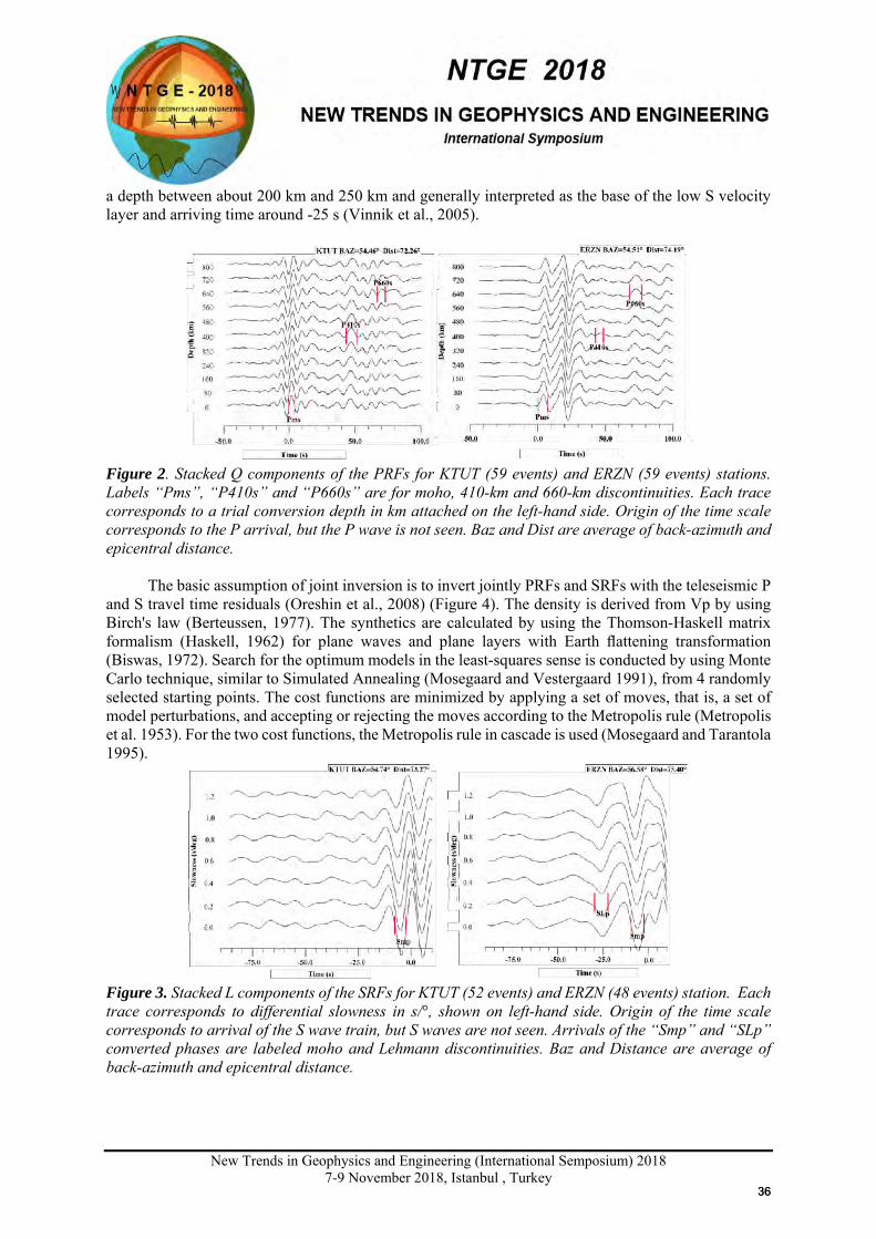
New Trends in Geophysics and Engineering (International Semposium) 2018
7-9 November 2018, Istanbul , Turkey
a depth between about 200 km and 250 km and generally interpreted as the base of the low S velocity layer and arriving time around -25 s (Vinnik et al., 2005).
Figure 2. Stacked Q components of the PRFs for KTUT (59 events) and ERZN (59 events) stations. Labels “Pms”, “P410s” and “P660s” are for moho, 410-km and 660-km discontinuities. Each trace corresponds to a trial conversion depth in km attached on the left-hand side. Origin of the time scale corresponds to the P arrival, but the P wave is not seen. Baz and Dist are average of back-azimuth and epicentral distance.
The basic assumption of joint inversion is to invert jointly PRFs and SRFs with the teleseismic P and S travel time residuals (Oreshin et al., 2008) (Figure 4). The density is derived from Vp by using Birch's law (Berteussen, 1977). The synthetics are calculated by using the Thomson-Haskell matrix formalism (Haskell, 1962) for plane waves and plane layers with Earth flattening transformation (Biswas, 1972). Search for the optimum models in the least-squares sense is conducted by using Monte Carlo technique, similar to Simulated Annealing (Mosegaard and Vestergaard 1991), from 4 randomly selected starting points. The cost functions are minimized by applying a set of moves, that is, a set of model perturbations, and accepting or rejecting the moves according to the Metropolis rule (Metropolis et al. 1953). For the two cost functions, the Metropolis rule in cascade is used (Mosegaard and Tarantola 1995).
Figure 3. Stacked L components of the SRFs for KTUT (52 events) and ERZN (48 events) station. Each trace corresponds to differential slowness in s/°, shown on left-hand side. Origin of the time scale corresponds to arrival of the S wave train, but S waves are not seen. Arrivals of the “Smp” and “SLp” converted phases are labeled moho and Lehmann discontinuities. Baz and Distance are average of back-azimuth and epicentral distance.
3636
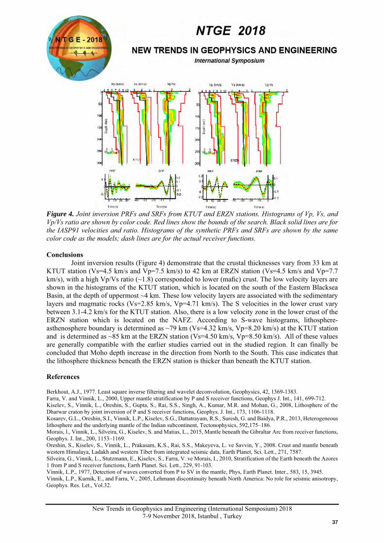
New Trends in Geophysics and Engineering (International Semposium) 2018
7-9 November 2018, Istanbul , Turkey
Figure 4. Joint inversion PRFs and SRFs from KTUT and ERZN stations. Histograms of Vp, Vs, and Vp/Vs ratio are shown by color code. Red lines show the bounds of the search. Black solid lines are for the IASP91 velocities and ratio. Histograms of the synthetic PRFs and SRFs are shown by the same color code as the models; dash lines are for the actual receiver functions. Conclusions Joint inversion results (Figure 4) demonstrate that the crustal thicknesses vary from 33 km at KTUT station (Vs=4.5 km/s and Vp=7.5 km/s) to 42 km at ERZN station (Vs=4.5 km/s and Vp=7.7 km/s), with a high Vp/Vs ratio (~1.8) corresponded to lower (mafic) crust. The low velocity layers are shown in the histograms of the KTUT station, which is located on the south of the Eastern Blacksea Basin, at the depth of uppermost ~4 km. These low velocity layers are associated with the sedimentary layers and magmatic rocks (Vs=2.85 km/s, Vp=4.71 km/s). The S velocities in the lower crust vary between 3.1-4.2 km/s for the KTUT station. Also, there is a low velocity zone in the lower crust of the ERZN station which is located on the NAFZ. According to S-wave histograms, lithosphere-asthenosphere boundary is determined as ~79 km (Vs=4.32 km/s, Vp=8.20 km/s) at the KTUT station and is determined as ~85 km at the ERZN station (Vs=4.50 km/s, Vp=8.50 km/s). All of these values are generally compatible with the earlier studies carried out in the studied region. It can finally be concluded that Moho depth increase in the direction from North to the South. This case indicates that the lithosphere thickness beneath the ERZN station is thicker than beneath the KTUT station.
References
Berkhout, A.J., 1977. Least square inverse filtering and wavelet deconvolution, Geophysics, 42, 1369-1383. Farra, V. and Vinnik, L., 2000, Upper mantle stratification by P and S receiver functions, Geophys J. Int., 141, 699-712. Kiselev, S., Vinnik, L., Oreshin, S., Gupta, S., Rai, S.S., Singh, A., Kumar, M.R. and Mohan, G., 2008, Lithosphere of the Dharwar craton by joint inversion of P and S receiver functions, Geophys. J. Int., 173, 1106-1118. Kosarev, G.L., Oreshin, S.I., Vinnik, L.P., Kiselev, S.G., Dattatrayam, R.S., Suresh, G. and Baidya, P.R., 2013, Heterogeneous lithosphere and the underlying mantle of the Indian subcontinent, Tectonophysics, 592,175–186. Morais, l., Vinnik, L., Silveira, G., Kiselev, S. and Matias, L., 2015, Mantle beneath the Gibraltar Arc from receiver functions, Geophys. J. Int., 200, 1153–1169. Oreshin, S., Kiselev, S., Vinnik, L., Prakasam, K.S., Rai, S.S., Makeyeva, L. ve Savvin, Y., 2008. Crust and mantle beneath western Himalaya, Ladakh and western Tibet from integrated seismic data, Earth Planet, Sci. Lett., 271, 7587. Silveira, G., Vinnik, L., Stutzmann, E., Kiselev, S., Farra, V. ve Morais, I., 2010, Stratification of the Earth beneath the Azores 1 from P and S receiver functions, Earth Planet. Sci. Lett., 229, 91-103. Vinnik, L.P., 1977, Detection of waves converted from P to SV in the mantle, Phys, Earth Planet. Inter., 583, 15, 3945. Vinnik, L.P., Kurnik, E., and Farra, V., 2005, Lehmann discontinuity beneath North America: No role for seismic anisotropy, Geophys. Res. Let., Vol.32.
3737
New Trends in Geophysics and Engineering (International Semposium) 2018
7-9 November 2018, Istanbul , Turkey
AN APPRAISAL OF FUTURE SEISMIC POTENTIAL FOR ERZURUM PROVINCE
OF TURKEY: ANALYSES OF BASIC SIZE-SCALING PARAMETERS
Serkan Öztürk
Department of Geophysics, Gümüşhane University, Gümüşhane Email: [email protected]
Presentation Type All accepted proceedings will be published on the webpage of the symposium (ntge2018.istanbul.edu.tr)
ORAL POSTER
Abstracts In this study, a comprehensive appraisal for future potential of earthquake occurrences in Erzurum province of Turkey was achieved by using Gutenberg-Richter b-value, fractal dimension Dc-value, magnitude completeness Mc-value, annual probability and recurrence time of earthquakes. Mc-value is calculated as 2.8 and b-value is estimated as 1.05±0.05 with this completeness level. This b-value is very close the average value of b=1.0 and this result shows that magnitude-frequency distribution of earthquakes in Erzurum is well represented by Gutenberg-Richter law with a b-value typically close to 1.0. Fractal dimension Dc-value is obtained as 1.60±0.02 with 95% confidence limits. This large Dc-value shows that seismicity in Erzurum is more clustered at larger scales or in smaller areas. Annual probability of the earthquakes for magnitude levels between 4.0 and 5.0 exhibits a value between 1 and 5. Recurrence time of the earthquakes for magnitude levels between 5.0 and 6.0 has a value between 2 and 20 years, relatively short, and a value between 20 and 50 years for magnitude levels between 6.0 and 6.5. These results suggest that Erzurum has a considerable seismic potential for strong earthquake occurrences in the intermediate term.
Keywords: Erzurum, b-value, Dc-value, annual probability, recurrence time Introduction Many statistical approaches have been applied to earthquake distributions to provide a quantitative size-scaling analyses and several parameters such as b-value, Dc-value, annual probability, recurrence time, moment and energy releases have been used by different researchers to evaluate the seismic potential for different parts of Turkey (eg., Öncel and Wilson, 2002; Polat et al., 2008; Öztürk, 2018). Since these types of studies are relatively rare for Erzurum, it is aimed to provide a comprehensive apraisal for the evaluation of future seismic potential in this part of Turkey and statistical analyses of b-value, Dc-value, annual probability and recurrence time of the earthquakes are presented in detailed. Data Catalog and Brief Explanation of Size-Scaling Laws Earthquake database is taken from Boğaziçi University, Kandilli Observatory and Earthquake Research Institute (KOERI). Earthquake catalog is homogeneous for duration magnitude, MD, and includes 7769 events for the time interval of April 21, 1970 and December 30, 2017. Tectonic structures are modified
X
3838
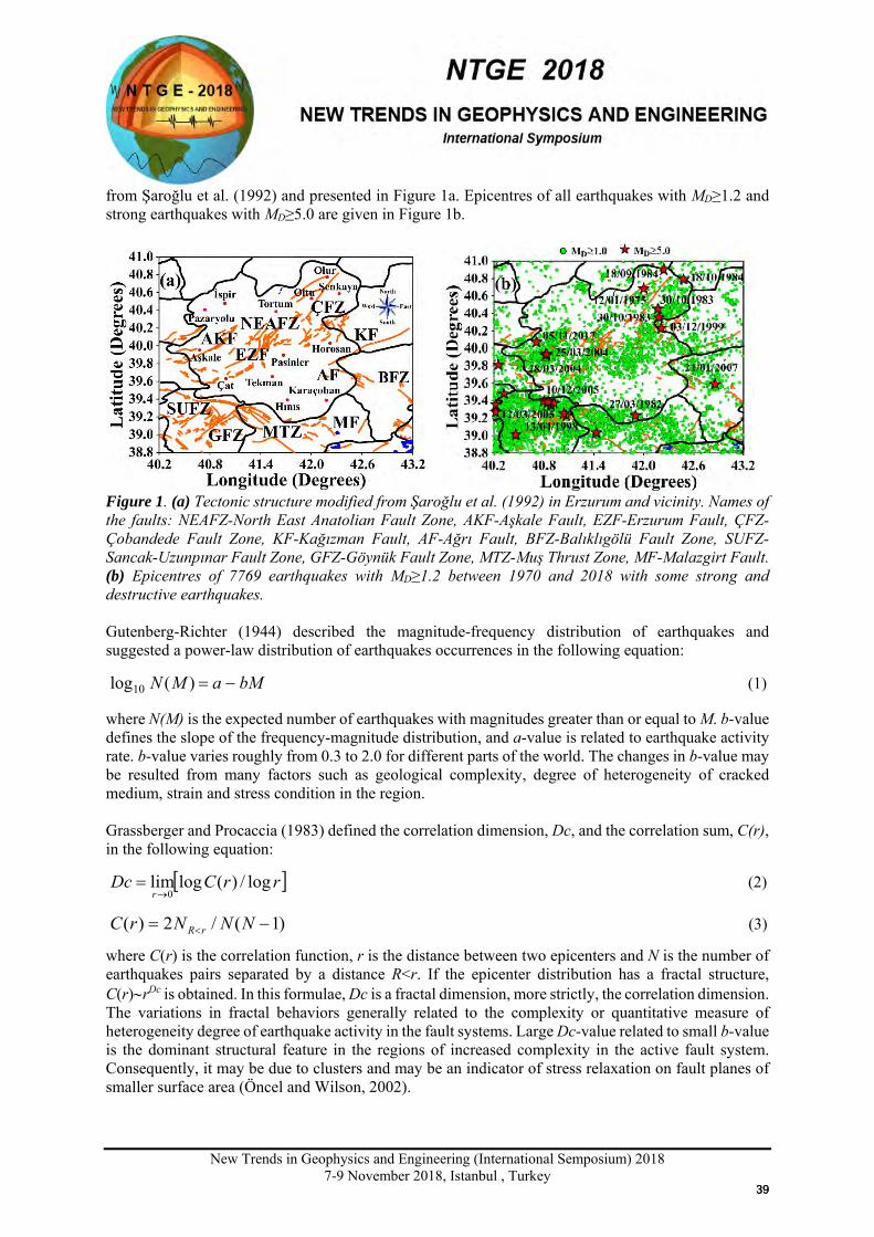
New Trends in Geophysics and Engineering (International Semposium) 2018
7-9 November 2018, Istanbul , Turkey
from Şaroğlu et al. (1992) and presented in Figure 1a. Epicentres of all earthquakes with MD≥1.2 and strong earthquakes with MD≥5.0 are given in Figure 1b.
Figure 1. (a) Tectonic structure modified from Şaroğlu et al. (1992) in Erzurum and vicinity. Names of the faults: NEAFZ-North East Anatolian Fault Zone, AKF-Aşkale Fault, EZF-Erzurum Fault, ÇFZ-Çobandede Fault Zone, KF-Kağızman Fault, AF-Ağrı Fault, BFZ-Balıklıgölü Fault Zone, SUFZ-Sancak-Uzunpınar Fault Zone, GFZ-Göynük Fault Zone, MTZ-Muş Thrust Zone, MF-Malazgirt Fault. (b) Epicentres of 7769 earthquakes with MD≥1.2 between 1970 and 2018 with some strong and destructive earthquakes. Gutenberg-Richter (1944) described the magnitude-frequency distribution of earthquakes and suggested a power-law distribution of earthquakes occurrences in the following equation:
bMaMN −=)(log10 (1)
where N(M) is the expected number of earthquakes with magnitudes greater than or equal to M. b-value defines the slope of the frequency-magnitude distribution, and a-value is related to earthquake activity rate. b-value varies roughly from 0.3 to 2.0 for different parts of the world. The changes in b-value may be resulted from many factors such as geological complexity, degree of heterogeneity of cracked medium, strain and stress condition in the region. Grassberger and Procaccia (1983) defined the correlation dimension, Dc, and the correlation sum, C(r), in the following equation:
[ ]rrCDcr
log/)(loglim0→
= (2)
)1(/2)( −= < NNNrC rR (3)
where C(r) is the correlation function, r is the distance between two epicenters and N is the number of earthquakes pairs separated by a distance R<r. If the epicenter distribution has a fractal structure, C(r)∼rDc is obtained. In this formulae, Dc is a fractal dimension, more strictly, the correlation dimension. The variations in fractal behaviors generally related to the complexity or quantitative measure of heterogeneity degree of earthquake activity in the fault systems. Large Dc-value related to small b-value is the dominant structural feature in the regions of increased complexity in the active fault system. Consequently, it may be due to clusters and may be an indicator of stress relaxation on fault planes of smaller surface area (Öncel and Wilson, 2002).
3939
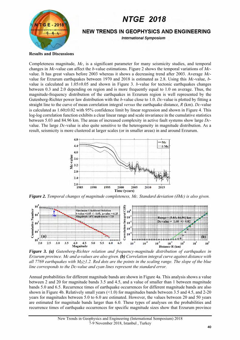
New Trends in Geophysics and Engineering (International Semposium) 2018
7-9 November 2018, Istanbul , Turkey
Results and Discussions
Completeness magnitude, Mc, is a significant parameter for many seismicity studies, and temporal changes in Mc-value can affect the b-value estimations. Figure 2 shows the temporal variations of Mc-value. It has great values before 2003 whereas it shows a decreasing trend after 2003. Average Mc-value for Erzurum earthquakes between 1970 and 2018 is estimated as 2.8. Using this Mc-value, b-value is calculated as 1.05±0.05 and shown in Figure 3. b-value for tectonic earthquakes changes between 0.3 and 2.0 depending on region and is more frequently equal to 1.0 on average. Thus, the magnitude-frequency distribution of the earthquakes in Erzurum region is well represented by the Gutenberg-Richter power law distribution with the b-value close to 1.0. Dc-value is plotted by fitting a straight line to the curve of mean correlation integral versus the earthquake distance, R (km). Dc-value is calculated as 1.60±0.02 with 95% confidence limit by linear regression and shown in Figure 4. This log-log correlation function exhibits a clear linear range and scale invariance in the cumulative statistics between 5.03 and 84.96 km. The areas of increased complexity in active fault systems show large Dc-value. The large Dc-value is also quite sensitive to the heterogeneity in magnitude distribution. As a result, seismicity is more clustered at larger scales (or in smaller areas) in and around Erzurum.
Figure 2. Temporal changes of magnitude completeness, Mc. Standard deviation (δMc) is also given.
Figure 3. (a) Gutenberg-Richter relation and frequency-magnitude distribution of earthquakes in Erzurum province. Mc and a-values are also given. (b) Correlation integral curve against distance with all 7769 earthquakes with MD≥1.2. Red dots are the points in the scaling range. The slope of the blue line corresponds to the Dc-value and cyan lines represent the standard error.
Annual probabilities for different magnitude bands are shown in Figure 4a. This analysis shows a value between 2 and 20 for magnitude bands 3.5 and 4.5, and a value of smaller than 1 between magnitude bands 5.0 and 6.5. Recurrence times of earthquake occurrences for different magnitude bands are also shown in Figure 4b. Relatively small years (<1.0) for magnitudes bands between 3.5 and 4.5, and 2-20 years for magnitudes between 5.0 to 6.0 are estimated. However, the values between 20 and 50 years are estimated for magnitude bands larger than 6.0. These types of analyses on the probabilities and recurrence times of earthquake occurrences for specific magnitude sizes show that Erzurum province
4040
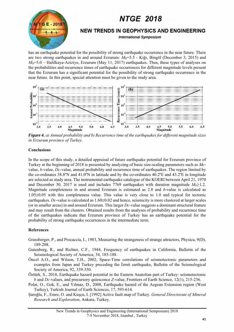
New Trends in Geophysics and Engineering (International Semposium) 2018
7-9 November 2018, Istanbul , Turkey
has an earthquake potential for the possibility of strong earthquake occurrence in the near future. There are two strong earthquakes in and around Erzurum: MD=5.5 - Kiğı, Bingöl (December 3, 2015) and MD=5.0 – Halilkaya-Aziziye, Erzurum (May 11, 2017) earthquakes. Thus, these types of analyses on the probabilities and recurrence times of earthquake occurrences for different magnitude levels present that the Erzurum has a significant potential for the possibility of strong earthquake occurrence in the near future. In this point, special attention must be given to the study area.
Figure 4. a) Annual probability and b) Recurrence time of the earthquakes for different magnitude sizes in Erzurum province of Turkey.
Conclusions
In the scope of this study, a detailed appraisal of future earthquake potential for Erzurum province of Turkey at the beginning of 2018 is presented by analyzing of basic size-scaling parameters such as Mc-value, b-value, Dc-value, annual probability and recurrence time of earthquakes. The region limited by the co-ordinates 38.8ºN and 41.0ºN in latitude and by the co-ordinates 40.2ºE and 43.2ºE in longitude are selected as study area. The instrumental earthquake catalogue of the KOERI between April 21, 1970 and December 30, 2017 is used and includes 7769 earthquakes with duration magnitude MD≥1.2. Magnitude completeness in and around Erzurum is estimated as 2.8 and b-value is calculated as 1.05±0.05 with this completeness value. This value is very close to 1.0 and typical for tectonic earthquakes. Dc-value is calculated as 1.60±0.02 and hence, seismicity is more clustered at larger scales (or in smaller areas) in and around Erzurum. This larger Dc-value suggests a dominant structural feature and may result from the clusters. Obtained results from the analyses of probability and recurrence time of the earthquakes indicate that Erzurum province of Turkey has an earthquake potential for the probability of strong earthquake occurrences in the intermediate term.
References
Grassberger, P., and Procaccia, I., 1983, Measuring the strangeness of strange attractors, Physica, 9(D), 189-208.
Gutenberg, R., and Richter, C.F., 1944, Frequency of earthquakes in California, Bulletin of the Seismological Society of America, 34, 185-188.
Öncel A.O., and Wilson, T.H., 2002, Space-Time correlations of seismotectonic parameters and examples from Japan and Turkey preceding the İzmit earthquake, Bulletin of the Seismological Society of America, 92, 339-350.
Öztürk, S., 2018, Earthquake hazard potential in the Eastern Anatolian part of Turkey: seismotectonic b and Dc-values, and precursory quiescence Z-value, Frontiers of Earth Science, 12(1), 215-236.
Polat, O., Gok, E., and Yılmaz, D., 2008, Earthquake hazard of the Aegean Extension region (West Turkey), Turkish Journal of Earth Sciences, 17, 593-614.
Şaroğlu, F., Emre, O. and Kuşçu, I. [1992] Active fault map of Turkey. General Directorate of Mineral Research and Exploration, Ankara, Turkey.
4141
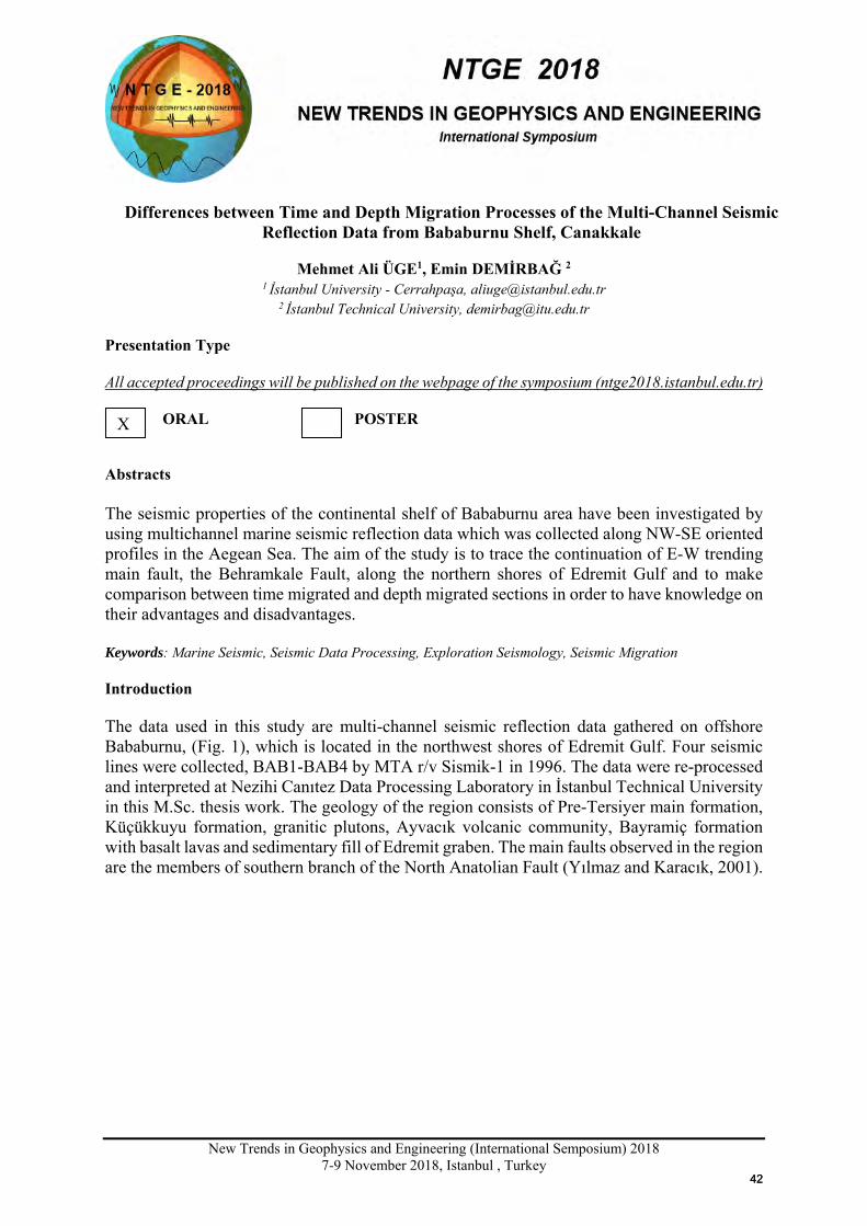
New Trends in Geophysics and Engineering (International Semposium) 2018
7-9 November 2018, Istanbul , Turkey
Differences between Time and Depth Migration Processes of the Multi-Channel Seismic Reflection Data from Bababurnu Shelf, Canakkale
Mehmet Ali ÜGE1, Emin DEMİRBAĞ 2 1 İstanbul University - Cerrahpaşa, [email protected]
2 İstanbul Technical University, [email protected] Presentation Type All accepted proceedings will be published on the webpage of the symposium (ntge2018.istanbul.edu.tr)
ORAL POSTER
Abstracts The seismic properties of the continental shelf of Bababurnu area have been investigated by using multichannel marine seismic reflection data which was collected along NW-SE oriented profiles in the Aegean Sea. The aim of the study is to trace the continuation of E-W trending main fault, the Behramkale Fault, along the northern shores of Edremit Gulf and to make comparison between time migrated and depth migrated sections in order to have knowledge on their advantages and disadvantages. Keywords: Marine Seismic, Seismic Data Processing, Exploration Seismology, Seismic Migration Introduction The data used in this study are multi-channel seismic reflection data gathered on offshore Bababurnu, (Fig. 1), which is located in the northwest shores of Edremit Gulf. Four seismic lines were collected, BAB1-BAB4 by MTA r/v Sismik-1 in 1996. The data were re-processed and interpreted at Nezihi Canıtez Data Processing Laboratory in İstanbul Technical University in this M.Sc. thesis work. The geology of the region consists of Pre-Tersiyer main formation, Küçükkuyu formation, granitic plutons, Ayvacık volcanic community, Bayramiç formation with basalt lavas and sedimentary fill of Edremit graben. The main faults observed in the region are the members of southern branch of the North Anatolian Fault (Yılmaz and Karacık, 2001).
X
4242
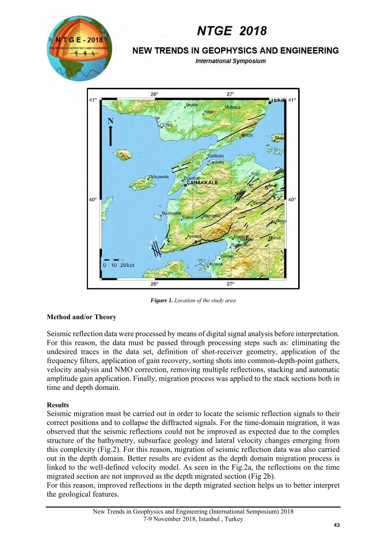
New Trends in Geophysics and Engineering (International Semposium) 2018
7-9 November 2018, Istanbul , Turkey
Figure 1. Location of the study area Method and/or Theory Seismic reflection data were processed by means of digital signal analysis before interpretation. For this reason, the data must be passed through processing steps such as: eliminating the undesired traces in the data set, definition of shot-receiver geometry, application of the frequency filters, application of gain recovery, sorting shots into common-depth-point gathers, velocity analysis and NMO correction, removing multiple reflections, stacking and automatic amplitude gain application. Finally, migration process was applied to the stack sections both in time and depth domain. Results Seismic migration must be carried out in order to locate the seismic reflection signals to their correct positions and to collapse the diffracted signals. For the time-domain migration, it was observed that the seismic reflections could not be improved as expected due to the complex structure of the bathymetry, subsurface geology and lateral velocity changes emerging from this complexity (Fig.2). For this reason, migration of seismic reflection data was also carried out in the depth domain. Better results are evident as the depth domain migration process is linked to the well-defined velocity model. As seen in the Fig.2a, the reflections on the time migrated section are not improved as the depth migrated section (Fig 2b). For this reason, improved reflections in the depth migrated section helps us to better interpret the geological features.
4343
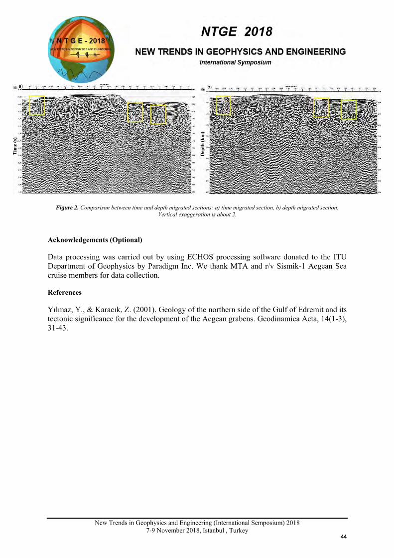
New Trends in Geophysics and Engineering (International Semposium) 2018
7-9 November 2018, Istanbul , Turkey
Figure 2. Comparison between time and depth migrated sections: a) time migrated section, b) depth migrated section.
Vertical exaggeration is about 2. Acknowledgements (Optional) Data processing was carried out by using ECHOS processing software donated to the ITU Department of Geophysics by Paradigm Inc. We thank MTA and r/v Sismik-1 Aegean Sea cruise members for data collection. References Yılmaz, Y., & Karacık, Z. (2001). Geology of the northern side of the Gulf of Edremit and its tectonic significance for the development of the Aegean grabens. Geodinamica Acta, 14(1-3), 31-43.
4444
New Trends in Geophysics and Engineering (International Semposium) 2018
7-9 November 2018, Istanbul , Turkey
X
DETERMINATION OF ROCK MASS QUALITY USING THE AMPLITUDE ATTENUATION TOMOGRAPHY: A CASE STUDY FROM THE TRABZON, TURKEY
Ali Erden Babacan1, Kenan Gelişli1, Daryl Tweeton2
1 Geophysical Eng. Department, Karadeniz Technical University, Trabzon
2 GeoTom, LLC,13785 Diamond Path, Apple Valley, MN 55124, USA Email: [email protected]
Presentation Type
ORAL POSTER
Abstracts The goal of this study was to determine the underground structure and rock quality of Eocene-Neogene aged volcanic rocks in the province of Trabzon, Turkey by seismic attenuation tomography. There is a wide volcanic rock area in Trabzon province and they are the foundation rocks for many buildings. Amplitudes of first-arrival times can be utilized to reconstruct attenuation coefficient for a rock mass structure. In attenuation tomography, measured amplitudes are first corrected for the spreading of the seismic wave. The corrected amplitudes are then inverted to obtain the distribution of attenuation coefficients α that provides the best fit to the data. In three areas selected for this study, shallow seismic refraction data were collected in 19 profiles. Amplitude inversions were performed with curved raypaths from velocity tomography. 3D α maps were generated from parallel lines of 2D refraction data. 1/ α values range from 1 to 23 for the studied areas. The foundation rocks in the studied areas generally consist of weathered and massive parts. The areas where the rock quality is good are clearly visible on the mappings.
Keywords: Seismic refraction, Amplitude attenuation tomography, Rock quality Introduction Trabzon, one of the most important cities of the Eastern Black Sea region (NE Turkey) has experienced a significant population increase in recent years. The increase in population and other development required the construction of new buildings. Thus, in rapidly developing cities, the site selection has become an important issue. Moreover, the suitable area for construction is very restricted in the region, and the settlement area is mountainous and covered with heavy vegetation. The characterization of rock mass structure using seismic surveys is significant for site selection. Seismic velocities and quality factor, Q are important parameters used to describe internal structures of rock masses. Many researchers have determined the engineering properties of rock mass with these parameters calculated from in situ seismic studies (Watanabe and Sassa, 1996; Tran and Hiltunen, 2012, Anbazhagan, 2009, Babacan et.al. 2014). Seismic wave attenuation is represented by the attenuation coefficient (α) or Q value (Xu et.al. 2000). The information of seismic wave attenuation is efficaciously a factor to define rock mass (Watanabe and Sassa, 1996). Attenuation is more sensitive in determining the variation of the physical properties of the rocks with regard to seismic wave velocity (Kaneko et.al, 1979; Krauß et.al. 2014). However, the estimate of the Q-values requires a
4545
New Trends in Geophysics and Engineering (International Semposium) 2018
7-9 November 2018, Istanbul , Turkey
higher signal quality than the determination of the seismic first arrival times (Krauß et.al. 2014). It is much more difficult to reliably obtain attenuation images. Therefore, high quality data set is needed to determine attenuation coefficients. Q or α is commonly calculated in the frequency or time domain using pulse broadening, amplitude decay, frequency shift method or spectral ratio method. The Amplitude decay method was used to determine the attenuation coefficients in this study. This method requires raypath information for the inversion and this information was obtained from the velocity tomography. Thus, when the rock mass structure is defined, velocity information was utilized besides the attenuation. In this paper application of tomographic seismic measurements are presented to characterize Tertiary volcanic rocks. Buildings or constructions in Trabzon city are usually built on volcanic rocks. There is intense construction on the selected studied areas. A lot of buildings in selected areas are under construction or in the planning phase. The rock mass structure and quality was revealed by the calculated 2D and 3D seismic velocities and α. Study area and Geological setting Trabzon province which is located in the northeast of Turkey was chosen as the study area. Seismic refraction data were collected in three different areas as Çukurçayır, Aydınlıkevler and Pelitli in Trabzon. Turkey is located on the Alpine-Himalayan orogenic belt. There are many dangerous active fault systems, such as The North and East Anatolian Fault Zone in Turkey. Trabzon province is situated to the North Anatolian fault zone at about 110 km. The Eastern Pontide Oragenic Belt is a major metallogenetic province in the Eastern Blacksea coastal region and forms a mountain chain, which are 500 km long and 100 km wide along the southeastern coast of the Blacksea. As a paleo-island arc setting, the eastern Pontides (NE Turkey) are characterized by varying episodes of volcanic activity from the Liassic to Tertiary times (Arslan et al., 1997). The eastern Pontides is commonly subdivided into Northern and Eastern Zones on the basis of structural and lithological differences (Gedikoğlu et.al. 1979; Bektaş et.al. 1995). Around Trabzon city, the studied area consists of the Eocene-Neogene aged volcano-sedimentary rocks, related to Plio-Quaternary regolith and Pliocene deposits containing sandstones, claystones, conglomerates, and agglomerates. The dominant lithologies in the Eocene-Neogene aged unit are basalt, andesite and pyroclastic rock. Soundings and field observations made in the region indicate that the main units are basalt and agglomerate-basalt in the studied areas. Field Example A total of nineteen seismic refraction measurements in three different areas (Çukurçayır, Aydınlıkevler and Pelitli) were performed to obtain the attenuation coefficients, P wave velocities (Vp), the depths to the bedrock in the studied areas. The refraction data were taken in parallel lines to each of the three areas to obtain 3D Vp and α sections. The refraction data were acquired on 5 profiles in the first field, 4 profiles in the second field and 10 profiles in the last field respectively. The profiles length which is 45, 41 and 39 meters, respectively and distance between profiles were selected according to field conditions. Seismic data were collected by with Geometrics 12-channel seismograph. A sledgehammer weighting 10 kg and a striker plate were utilized as a source. Sources and receivers were arranged in line. Raypath information is needed for the solution of the amplitude attenuation tomography. First of all, velocity tomography was applied to the refraction data. Thus, the Vp distribution and raypath information of the underground were calculated. The 3D Vp image obtained for Çukurçayır area was shown in Fig 1. The processing of the amplitude attenuation tomography was performed with GeoTomCG (GeoTomCG, 2011). The program is based on inversion with the simultaneous iterative reconstruction technique (SIRT) (Lehman, 2007). The raw amplitudes, obtained from refraction data, are used to determine the distributions of attenuation in amplitude attenuation tomography. Amplitude attenuation inversions can be done with curved raypaths. The data
4646
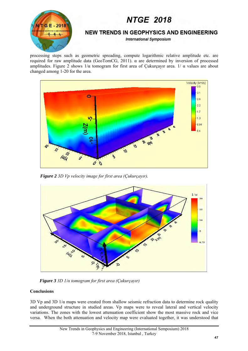
New Trends in Geophysics and Engineering (International Semposium) 2018
7-9 November 2018, Istanbul , Turkey
processing steps such as geometric spreading, compute logarithmic relative amplitude etc. are required for raw amplitude data (GeoTomCG, 2011). α are determined by inversion of processed amplitudes. Figure 2 shows 1/α tomogram for first area of Çukurçayır area. 1/ α values are about changed among 1-20 for the area.
Figure 2 3D Vp velocity image for first area (Çukurçayır).
Figure 3 3D 1/α tomogram for first area (Çukurçayır) Conclusions 3D Vp and 3D 1/α maps were created from shallow seismic refraction data to determine rock quality and underground structure in studied areas. Vp maps were to reveal lateral and vertical velocity variations. The zones with the lowest attenuation coefficient show the most massive rock and vice versa. When the both attenuation and velocity map were evaluated together, it was understood that
4747
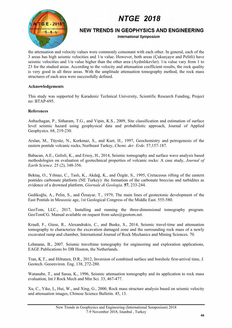
New Trends in Geophysics and Engineering (International Semposium) 2018
7-9 November 2018, Istanbul , Turkey
the attenuation and velocity values were commonly consonant with each other. In general, each of the 3 areas has high seismic velocities and 1/α value. However, both areas (Çukurçayır and Pelitli) have seismic velocities and 1/α value higher than the other area (Aydınlıkevler). 1/α value vary from 1 to 23 for the studied areas. According to the velocity and attenuation coefficient results, the rock quality is very good in all three areas. With the amplitude attenuation tomography method, the rock mass structures of each area were successfully defined. Acknowledgements This study was supported by Karadeniz Technical University, Scientific Research Funding, Project no: BTAP-695. References Anbazhagan, P., Sitharam, T.G., and Vipin, K.S., 2009, Site classification and estimation of surface level seismic hazard using geophysical data and probabilistic approach, Journal of Applied Geophysics. 68, 219-230. Arslan, M., Tüysüz, N., Korkmaz, S., and Kurt, H., 1997, Geochemistry and petrogenesis of the eastern pontide volcanic rocks, Northeast Turkey, Chemi. der. Erde. 57,157-187. Babacan, A.E., Gelisli, K., and Ersoy, H., 2014, Seismic tomography and surface wave analysis based methodologies on evaluation of geotechnical properties of volcanic rocks: A case study, Journal of Earth Science. 25 (2), 348-356. Bektaş, O., Yılmaz, C., Taslı, K., Akdağ, K., and Özgür, S., 1995, Cretaceous rifting of the eastern pontides carbonate platform (NE Turkey): the formation of the carbonate breccias and turbidites as evidence of a drowned platform, Giornale di Geologia. 57, 233-244. Gedikoğlu, A., Pelin, S., and Özsayar, T., 1979, The main lines of geotectonic development of the East Pontids in Mesozoic age, 1st Geological Congress of the Middle East. 555-580. GeoTom, LLC., 2017, Installing and running the three-dimensional tomography program. GeoTomCG. Manual available on request from [email protected]. Krauß, F., Giese, R., Alexandrakis, C., and Buske, S., 2014, Seismic travel‐time and attenuation tomography to characterize the excavation damaged zone and the surrounding rock mass of a newly excavated ramp and chamber, International Journal of Rock Mechanics and Mining Sciences. 70. Lehmann, B., 2007. Seismic traveltime tomography for engineering and exploration applications, EAGE Publications bv DB Houton, the Netherlands. Tran, K.T., and Hiltunen, D.R., 2012, Inversion of combined surface and borehole first-arrival time, J. Geotech. Geoenviron. Eng. 138, 272-280. Watanabe, T., and Sassa, K., 1996, Seismic attenuation tomography and its application to rock mass evaluation, Int J Rock Mech and Min Sci. 33, 467-477. Xu, C., Yike, L, Hui, W., and Xing, G., 2000, Rock mass structure analysis based on seismic velocity and attenuation images, Chinese Science Bulletin. 45, 13.
4848
New Trends in Geophysics and Engineering (International Semposium) 2018
7-9 November 2018, Istanbul , Turkey
Application of Filtering Technqiues to Enhance Magnetic Data from Egyptain Archaeological Sites
Tareq Fahmy Abdallatif
Prof. Dr. Tareq Fahmy Abdallatif: Department of Geomagnetism and Geoelectricity, National Research Institute
of Astronomy and Geophysics (NRIAG), Cairo, Egypt.
Presenter Email: [email protected] Presentation Type All accepted proceedings will be published on the webpage of the symposium (ntge2018.istanbul.edu.tr)
ORAL POSTER
Abstracts Filtering techniques are commonly used for smoothing geophysical data in order to remove the undesired noises as well as to enhance the obtained results and produce high quality presentation. The softwares of Geoplot and Geosoft have been used for applying low and high pass filtering techniques with respect to smoothing and enhancement of magnetic data obtained from gradiometer survey. Two case studies have been chosen for this purpose; the first one is located at the southeastern side of Shunet El Zebib, Sohag, Egypt, while the second one is located at the western side of Zoser pyramid. The measurements were done by the fluxgate gradiometer (FM36) with 0.5/0.5 m grid. The obtained data of each case was processed using Geoplot program to eliminate the field errors and noises, and then filtered using low and high pass filters. The obtained results show the efficiency of both programs in enhancing the selected gradiometer data. It has been found that the application of a low pass filter of Geoplot program is preferable with window size of X and Y = 2, while that of Geosoft program is preferable at cutoff frequencies ≥ 0.5 m-1 . Moreover, the application of a high pass filter of Geoplot program is preferable with window size of X and Y ≥ 5, while that of Geosoft program is preferable at cutoff frequencies ≤ 0.2 m-1 . Delineated archaeological features were ultimately interpreted more clearly after the application of filtering techniques. They belong to very old Dynasties of ancient Egyptians.
Keywords: Magnetic, Filtering, Geoplot, Geosoft, Archaeological sites, Egypt. Introduction The application of filtering techniques to geophysical data or any other data have nearly a similar physical meaning. However, the interpretation meaning is different in each case, even with respect to some geophysical data. The term filter is used to characterize a system, which can perform an effective prescribed separation of the desired information carried by the signal from the unwanted portion commonly called noise. The separation may be carried out e.g. on the basis of frequency, velocity, or polarization discrimination by frequency, velocity, or polarization filters, respectively (Kulhanek, 1976). In many geophysical problems, it is required to separate the observed field into low frequency
√
4949
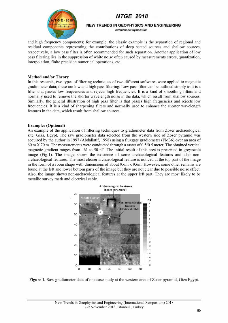
New Trends in Geophysics and Engineering (International Semposium) 2018
7-9 November 2018, Istanbul , Turkey
and high frequency components; for example, the classic example is the separation of regional and residual components representing the contributions of deep seated sources and shallow sources, respectively, a low pass filter is often recommended for such separation. Another application of low pass filtering lies in the suppression of white noise often caused by measurements errors, quantization, interpolation, finite precision numerical operations, etc.
Method and/or Theory In this research, two types of filtering techniques of two different softwares were applied to magnetic gradiometer data; these are low and high pass filtering. Low pass filter can be outlined simply as it is a filter that passes low frequencies and rejects high frequencies. It is a kind of smoothing filters and normally used to remove the shorter wavelength noise in the data, which result from shallow sources. Similarly, the general illustration of high pass filter is that passes high frequencies and rejects low frequencies. It is a kind of sharpening filters and normally used to enhance the shorter wavelength features in the data, which result from shallow sources. Examples (Optional) An example of the application of filtering techniques to gradiometer data from Zoser archaeological site, Giza, Egypt. The raw gradiometer data selected from the western side of Zoser pyramid was acquired by the author in 1997 (Abdallatif, 1998) using a fluxgate gradiometer (FM36) over an area of 60 m X 70 m. The measurements were conducted through a raster of 0.5/0.5 meter. The obtained vertical magnetic gradient ranges from –61 to 50 nT. The initial result of this area is presented in grey/scale image (Fig.1). The image shows the existence of some archaeological features and also non-archaeological features. The most clearer archaeological feature is noticed at the top part of the image in the form of a room shape with dimensions of about 9.6m x 9.6m. However, some other remains are found at the left and lower bottom parts of the image but they are not clear due to possible noise effect. Also, the image shows non-archaeological features at the upper left part. They are most likely to be metallic survey mark and electrical cable.
Figure 1. Raw gradiometer data of one case study at the western area of Zoser pyramid, Giza Egypt.
T
0 10 20 30 40 50 600
10
20
30
40
50
60
70
-8
-7
-6
-5
-4
-3
-2
-1
0
1
2
3
4
5
6
7
8nT
Archaeological Features (room structure)
Non-archaeological features Electrical cable
Metallic survey mark
5050
New Trends in Geophysics and Engineering (International Semposium) 2018
7-9 November 2018, Istanbul , Turkey
Conclusions The application of filtering techniques to gradiometer data has been clearly enhanced the quality of the results in both selected case studies (A & B). Moreover, the applied softwares, which help the selection of cut-off frequency, are recommended for smoothing the data using low pass filter. Meanwhile, we consider that the application of both low and high pass filtering by using two different softwares is valuable and recommended, but under certain circumstances. Finally, we recommend the following points for any similar cases: 1- In case of applying a low pass filtering of Geoplot program, it is preferable to use small window
sizes, while in case of applying a low pass filtering of Geosoft program, it is preferable to use from moderate to large cutoff frequencies.
2- In case of applying a high pass filtering of Geoplot program, it is preferable to use large window sizes, while in case of applying a high pass filtering of Geosoft program, it is preferable to use small values of cutoff frequencies.
References [1] Abdallatif, T.F. (1998). Magnetic prospection for some archaeological sites in Egypt. Ph.D. Thesis, Department of Geophysics, Faculty of Science, Ain Shams University. [2] Kulhanek, O. (1976). Introduction to digital filtering in geophysics. Elsevier, New York.
5151
New Trends in Geophysics and Engineering (International Semposium) 2018
7-9 November 2018, Istanbul , Turkey
THE INVESTIGATION OF THE CENTRAL ANATOLIAN FAULTS BY USING SATELLITE GRAVITY DATA
Fikret Doğru1, Oya Pamukçu2, Dilan Altan2
1 Ataturk University, Oltu Earth Sciences Faculty, Geophysical Engineering, Oltu, Erzurum
2 Dokuz Eylul University, Engineering Faculty, Geophysical Engineering, Buca, Izmir Email: [email protected]
Presentation Type
ORAL POSTER
Abstracts An Anatolian plate located between Eurasia, Africa and the Arabian plates. The Arabian and African plates move to the north and compress the Anatolian plate. The changing faster displacement of the Arabian plate causes the rise compressed eastern region of Turkey between the Arabian and stable Eurasian plates. This led to the formation of East-West stretching normal fault systems connected to the North-South opening regime in Western Anatolia. This northward relative movement causes the Anatolian plate to move in a counterclockwise direction along to left lateral direction North Anatolian Fault Zone and the right lateral direction East Anatolian Fault Zone. There are also secondary fault systems and fault zones that divide Anatolia into smaller blocks and contribute to the neotectonic development of the Anatolian block. The main ones are the left lateral Middle Anatolian Fault System, the characteristic oblique-slip Tuz Lake Fault Zone. In this study, it has been tried to determine the locations of Tuz Lake Fay Zone, Ecemis and Erciyes Faults by satellite gravity data. For this purpose, the Free-air anomaly of EGM2008 from satellite gravity models is calculated. In addition, Free-air anomaly was calculated using dV_ELL_Earth2014_plusGRS80 topographic model and Bouguer gravity anomaly was obtained by extracting these values from EGM2008 Free-air anomalies. Afterwards, terrain correction was performed using Earth Residual Terrain Model data and Complete Bouguer Gravity Anomaly was obtained. Finally, the tensor analysis was applied to Complete Bouguer Gravity Anomaly and tensor results were analysed together with the locations of Tuz Lake Fay Zone, Ecemis and Erciyes Faults in the region. Keywords: Anatolian Plate, Ecemis Fault, Tuz Lake Fault Zone, satellite gravity, terrain. Introduction In the Central Anatolian region, the basins of stress origin, limited to non-parallel strike-slip faults, are defined as "Plain" and this area is named as "Central Anatolian Plain Region" (Şengör, 1980). This area is an increasingly weakening continuation of the Western Anatolian expansion system to the east (Şengör, 1980). The Central Anatolian Plain Region also forms the transition zone between the other three neotectonic regions (Dirik and Göncüoğlu, 1996). There are also secondary fault systems and fault zones that divide Anatolia into smaller blocks and contribute to the neotectonic development of the Anatolian block and these are the left lateral Middle Anatolian Fault System, the characteristic oblique-slip Tuz Lake Fault Zone (Dirik and Göncüoğlu, 1996). The Salt Lake Fault Zone (SLFZ) is one of the most important intra-continental active fault zones of the Central Anatolian Region (Kürçer and Gökten, 2012). TGFZ is a normal fault zone
5252
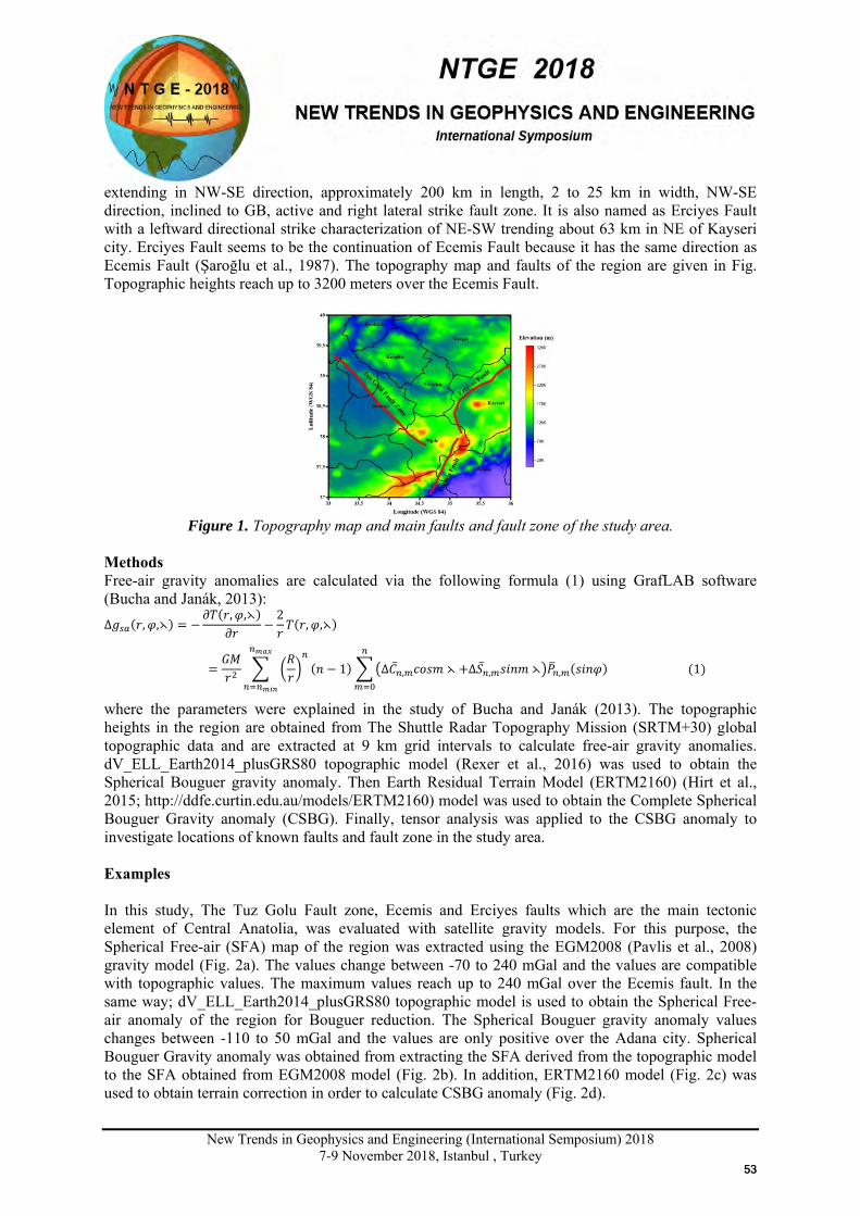
New Trends in Geophysics and Engineering (International Semposium) 2018
7-9 November 2018, Istanbul , Turkey
extending in NW-SE direction, approximately 200 km in length, 2 to 25 km in width, NW-SE direction, inclined to GB, active and right lateral strike fault zone. It is also named as Erciyes Fault with a leftward directional strike characterization of NE-SW trending about 63 km in NE of Kayseri city. Erciyes Fault seems to be the continuation of Ecemis Fault because it has the same direction as Ecemis Fault (Şaroğlu et al., 1987). The topography map and faults of the region are given in Fig. Topographic heights reach up to 3200 meters over the Ecemis Fault.
Figure 1. Topography map and main faults and fault zone of the study area.
Methods Free-air gravity anomalies are calculated via the following formula (1) using GrafLAB software (Bucha and Janák, 2013): ∆𝑔𝑔𝑠𝑠𝑠𝑠(𝑟𝑟,𝜑𝜑,⋋) = −
𝜕𝜕𝜕𝜕(𝑟𝑟,𝜑𝜑,⋋)𝜕𝜕𝑟𝑟
−2𝑟𝑟 𝜕𝜕
(𝑟𝑟,𝜑𝜑,⋋)
=𝐺𝐺𝐺𝐺𝑟𝑟2
𝑅𝑅𝑟𝑟
𝑛𝑛(𝑛𝑛 − 1)
𝑛𝑛𝑚𝑚𝑚𝑚𝑚𝑚
𝑛𝑛=𝑛𝑛𝑚𝑚𝑚𝑚𝑚𝑚
∆𝐶𝑛𝑛,𝑚𝑚𝑐𝑐𝑐𝑐𝑐𝑐𝑐𝑐 ⋋ +∆𝑆𝑆𝑛,𝑚𝑚𝑐𝑐𝑠𝑠𝑛𝑛𝑐𝑐 ⋋𝑃𝑃𝑛𝑛,𝑚𝑚(𝑐𝑐𝑠𝑠𝑛𝑛𝜑𝜑) (1)𝑛𝑛
𝑚𝑚=0
where the parameters were explained in the study of Bucha and Janák (2013). The topographic heights in the region are obtained from The Shuttle Radar Topography Mission (SRTM+30) global topographic data and are extracted at 9 km grid intervals to calculate free-air gravity anomalies. dV_ELL_Earth2014_plusGRS80 topographic model (Rexer et al., 2016) was used to obtain the Spherical Bouguer gravity anomaly. Then Earth Residual Terrain Model (ERTM2160) (Hirt et al., 2015; http://ddfe.curtin.edu.au/models/ERTM2160) model was used to obtain the Complete Spherical Bouguer Gravity anomaly (CSBG). Finally, tensor analysis was applied to the CSBG anomaly to investigate locations of known faults and fault zone in the study area. Examples In this study, The Tuz Golu Fault zone, Ecemis and Erciyes faults which are the main tectonic element of Central Anatolia, was evaluated with satellite gravity models. For this purpose, the Spherical Free-air (SFA) map of the region was extracted using the EGM2008 (Pavlis et al., 2008) gravity model (Fig. 2a). The values change between -70 to 240 mGal and the values are compatible with topographic values. The maximum values reach up to 240 mGal over the Ecemis fault. In the same way; dV_ELL_Earth2014_plusGRS80 topographic model is used to obtain the Spherical Free-air anomaly of the region for Bouguer reduction. The Spherical Bouguer gravity anomaly values changes between -110 to 50 mGal and the values are only positive over the Adana city. Spherical Bouguer Gravity anomaly was obtained from extracting the SFA derived from the topographic model to the SFA obtained from EGM2008 model (Fig. 2b). In addition, ERTM2160 model (Fig. 2c) was used to obtain terrain correction in order to calculate CSBG anomaly (Fig. 2d).
5353
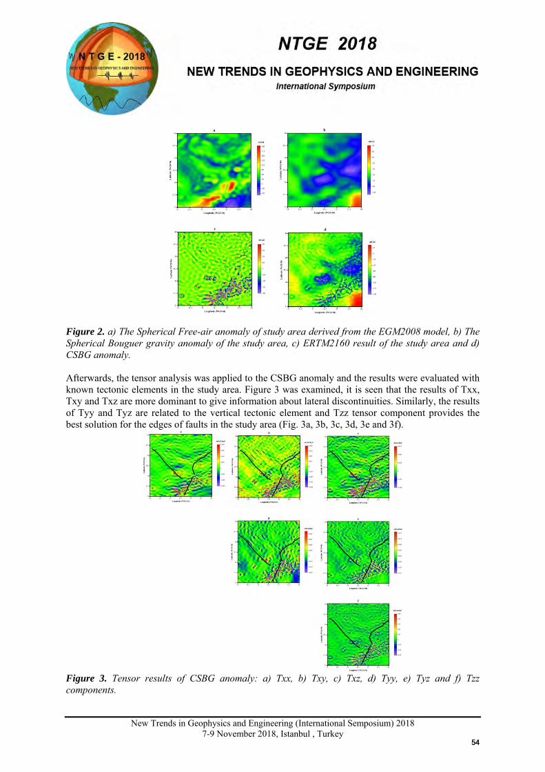
New Trends in Geophysics and Engineering (International Semposium) 2018
7-9 November 2018, Istanbul , Turkey
Figure 2. a) The Spherical Free-air anomaly of study area derived from the EGM2008 model, b) The Spherical Bouguer gravity anomaly of the study area, c) ERTM2160 result of the study area and d) CSBG anomaly. Afterwards, the tensor analysis was applied to the CSBG anomaly and the results were evaluated with known tectonic elements in the study area. Figure 3 was examined, it is seen that the results of Txx, Txy and Txz are more dominant to give information about lateral discontinuities. Similarly, the results of Tyy and Tyz are related to the vertical tectonic element and Tzz tensor component provides the best solution for the edges of faults in the study area (Fig. 3a, 3b, 3c, 3d, 3e and 3f).
Figure 3. Tensor results of CSBG anomaly: a) Txx, b) Txy, c) Txz, d) Tyy, e) Tyz and f) Tzz components.
5454
New Trends in Geophysics and Engineering (International Semposium) 2018
7-9 November 2018, Istanbul , Turkey
Conclusions
In this study, firstly, SFA gravity anomaly was obtained using the EGM2008 model in the study are in which the area consists of Salt Lake Fault Zone, Erciyes and Ecemis Faults. Then, CSBG anomaly was obtained using ERTM2160 model to apply tensor analysis. Finally, the tensor analysis was applied to CSBG anomaly data and the locations of mentioned faults and zone were evaluated with tensor results. The Tzz component gives the best compatible result in the whole tensor components.
References
Bucha, B., Janák, J., 2013, A MATLAB-based graphical user interface program for computing functionals of the geopotential up to ultra-high degrees and orders. Computers & Geosciences 56, 186–196, http://dx.doi.org/10.1016/j.cageo.2013.03. 012.
Dirik, K., Göncüoğlu, M.C., 1996, Neotectonic characteristics of Central Anatolia, Int. Geology Review 38, 807-817.
Hirt, C., Rexer, M., 2015, Earth2014: 1 arc-min shape, topography, bedrock and ice-sheet models–Available as gridded data and degree-10,800 spherical harmonics. International Journal of Applied Earth Observation and Geoinformation, 39, pp.103-112.
Kürçer, A, Gökten, Y.E., 2012, A New Photography Method for Paleoseismological Trenching: “Paleoseismological Three Dimensional Virtual Photography Method”, A Case Study: Tuzgölü Fault Zone, Central Anatolia, Turkey, Tectonics-Recent Advances, Evgenii Sharkov (Ed.), ISBN: 978-953-51-0675-3.
Pavlis, N.K., Holmes, S.A., Kenyon, S.C., and Factor, J.K., 2008, An earth gravitational model to degree 2160: EGM2008. EGU General Assembly, 2008(4), 4-2.
Rexer, M., C. Hirt, S. Claessens, and R. Tenzer, 2016: Layer-Based Modelling of the Earth’s Gravitational Potential up to 10-km Scale in Spherical Harmonics in Spherical and Ellipsoidal Approximation. Surv in Geophy, DOI:10.1007/s10712-016-9382-2.
Şaroğlu, F., Boray, A., Emre, Ö., 1987, Türkiye’nin Aktif fayları. Maden Tetkik ve Arama Genel Müdürlüğü Rapor No. 8643. 394 s., Ankara, (yayımlanmamış)
Şengör, A.M.C., 1980, Türkiye‟nin Neotektoniği’nin Esasları, Türkiye Jeoloji Kurumu Konferans Serisi 2.
5555
New Trends in Geophysics and Engineering (International Semposium) 2018
7-9 November 2018, Istanbul , Turkey
X
SMOOTH 3D MODELING OF GRAVITY DATA USING PARTICLE SWARM OPTIMIZATION
Gökhan Karcıoğlu1 , Anisya B.Tekkeli1 , Oya Tarhan Bal1
1 Geophysical Eng. Department, Istanbul University-Cerrahpaşa, Istanbul
Email: [email protected] Presentation Type All accepted proceedings will be published on the webpage of the symposium (ntge2018.istanbul.edu.tr)
ORAL POSTER
Abstract In this study, the ability of the Global Optimization methods to solve geophysical modeling problems with large parameter counts is investigated. For this purpose, a Particle Swarm Optimization algorithm is developed and implemented to realize 3D modeling of gravity data.
The developed algorithm uses several approaches to cope with large amount of model parameters, generally encountered during 3D modeling. The algorithm employs a starting model and starts the search for the smoothest possible model iteratively. The algorithm decreases the smoothness as the iterations increase. In order to prevent artefacts and to avoid problems arising from the randomness of the method the minimum gradient support is added as penalty to the function to be optimized.
The developed algorithm is tested on a synthetic data using a model mesh with 32.000 cells. The algorithm is found to be able to model both datasets with the given model meshes.
Keywords: Gravity data, 3D modelling, Particle Swarm Optimization, Global Optimization Introduction Global Optimization (GO) methods are mostly random search algorithms doesn’t need the calculation of the jacobian matrix, hence these methods needs significantly less memory on large problems. However, as the dimension of the given problem increase, the solution quality tends to decrease, limiting the use of these methods.
Due to the mentioned limitations of these methods, the implementation of the global optimization algorithms are rather limited. The studies are generally applied on 1D problems with limited model parameters (eg. Moorkamp et al.2007; Akpan et al. 2014) while 2D and 3D modeling studies are oriented on recovering structural models, constrained to reduce model parameters to be recovered (eg. Akça and Başokur 2010; Jie and Tao, 2015) or constrained using the jacobian matrix (eg. Liu et al. 2012).
5656
New Trends in Geophysics and Engineering (International Semposium) 2018
7-9 November 2018, Istanbul , Turkey
The modeling approach implemented in this study is aimed to solve large problems without implementing constraints to decrease the model parameters using Particle Swarm Optimization (PSO) method.
Traditional smooth inversion approaches (eg. Occam) requires the calculation of the Jacobian matrix and adds model smoothness to the penalty function to be minimized, realizing a multi-objective optimization. Calculation of the Jacobian is not necessary for GO algorithms. Besides, PSO (and other GO methods) often underperforms when trying to minimize (or maximize) multiple objective functions (misfit and smoothness). In order to prevent the method to solve a multi-objective optimization problem the model smoothness is forced on the model parameters by a simple smoothing operator. The amount of smoothness is decreased as the iterations increase and rougher models are obtained.
As the smoothness decrease, artefacts are found to be emerging in the models due to the randomness of the method. To prevent artefacts, minimum gradient support is added to the function to be minimized, acting as a threshold value to introduce structures.
Using the mentioned approaches, the developed PSO algorithm is successfully realized 3D modeling of the provided datasets. Even though, the mentioned approaches are tested only using the PSO method, these approaches are independent of the PSO method and can be implemented in other GO methods.
Method Particle Swarm Optimization (PSO) is population based random search method. Accordingly, at each iteration a number of models are generated and their fitness are evaluated by the algorithm. After the evaluation of models are completed, each model is updated according to the formula given below (Clerc and Kennedy, 2002). Vi(t+1)= χ(Vi(t) +c1ϕ1(Pi,best-xi) +c2ϕ2(Pg,best-xi) ) (1) χ=2k/|2-c- (c2-4c)1/2| (2) c=c1+c2 , c≥4 (3) Where, t is the iteration number, and Vi is the parameter change vector for the i.th model in the given iteration, Pi,best is the best model parameters generated for the i.th model until the current iteration, Pg,best is the best model parameters obtained by the algorithm until the current iteration. χ is the stabilizing coefficient, and c1 and c2 are positive invariables controlling the contribution of the Pi,best and Pg,best. ϕ1 and ϕ2 are random parameters employed to ensure to search a larger area in the model space. After each iteration, model parameters are updated according to the formula given below. xi(t+1)=xi(t)+vi(t+1) (4) Multi-objective optimization is known to be difficult to solve using GO methods. Due to this, in order to ensure obtaining smooth models, model smoothness is forced on the model parameters by the
5757
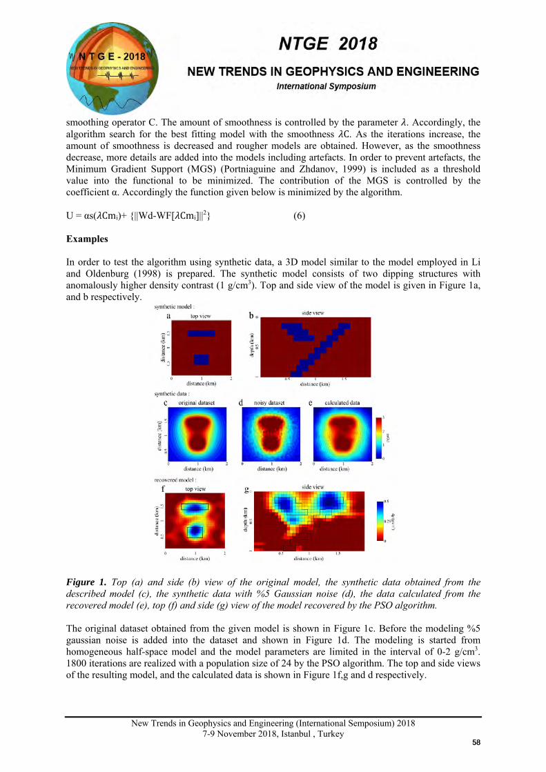
New Trends in Geophysics and Engineering (International Semposium) 2018
7-9 November 2018, Istanbul , Turkey
smoothing operator C. The amount of smoothness is controlled by the parameter 𝜆𝜆. Accordingly, the algorithm search for the best fitting model with the smoothness 𝜆𝜆C. As the iterations increase, the amount of smoothness is decreased and rougher models are obtained. However, as the smoothness decrease, more details are added into the models including artefacts. In order to prevent artefacts, the Minimum Gradient Support (MGS) (Portniaguine and Zhdanov, 1999) is included as a threshold value into the functional to be minimized. The contribution of the MGS is controlled by the coefficient α. Accordingly the function given below is minimized by the algorithm. U = αs(𝜆𝜆Cmi)+ ||Wd-WF[𝜆𝜆Cmi]||2 (6) Examples In order to test the algorithm using synthetic data, a 3D model similar to the model employed in Li and Oldenburg (1998) is prepared. The synthetic model consists of two dipping structures with anomalously higher density contrast (1 g/cm3). Top and side view of the model is given in Figure 1a, and b respectively.
Figure 1. Top (a) and side (b) view of the original model, the synthetic data obtained from the described model (c), the synthetic data with %5 Gaussian noise (d), the data calculated from the recovered model (e), top (f) and side (g) view of the model recovered by the PSO algorithm. The original dataset obtained from the given model is shown in Figure 1c. Before the modeling %5 gaussian noise is added into the dataset and shown in Figure 1d. The modeling is started from homogeneous half-space model and the model parameters are limited in the interval of 0-2 g/cm3. 1800 iterations are realized with a population size of 24 by the PSO algorithm. The top and side views of the resulting model, and the calculated data is shown in Figure 1f,g and d respectively.
5858
New Trends in Geophysics and Engineering (International Semposium) 2018
7-9 November 2018, Istanbul , Turkey
In the recovered model (Figure 1f,g), places and dips of the structures are obtained very similar to the real model (Figure 1a,b). Even though, there is some difference in the dipping part of the structure on the right, it’s in acceptable levels. Conclusions In this study, a Particle Swarm Optimization algorithm is developed and implemented in order to investigate the ability of the Global Optimization methods to recover 3D gravity models. Several approaches are implemented to avoid well known problems of the PSO: Model smoothness is forced on the model parameters using a simple smoothing operator. With this approach realizing multi-objective optimization is avoided, since the trade-off between the model fitness and smoothing is not searched by the algorithm. To obtain more detailed and rough models, model smoothness is decreased with iterations. To prevent artefacts Minimum Gradient Support is employed as a threshold value. The algorithm is tested on a synthetic model with 32000 model parameters. Even though, the high amount of model parameters to be recovered, the algorithm has minimized the model misfit successfully. Some difference in the boundaries of the recovered structures is determined. These differences are associated with the non-uniqueness of the model, and can be eliminated with better depth weighting. References Akça I. and Başokur A.T. , 2010, Extraction of structure-based geoelectric models by hybrid genetic algorithms, Geophysics, 75(1), F15-F22. Akpan A.E., Narayanan M., Harinarayana T., 2014, Estimation of subsurface temperatures in the Tattapani geothermal field, central India from limited volume of magnetotelluric data and borehole thermograms using a constructive back-propagation neural network, Earth Interact. Vol 18, pp. 1-26, Clerc M. and Kennedy J., 2002, The particle swarm–explosion, stability, and convergence in a multidimensional complex space, IEEE Transactions on Evolutionary Computation, 6(1):58–73. Jie X. and Tao Z., 2015, Multiobjective particle swarm inversion algorithm for two-dimensional magnetic data, Applied Geophysıcs, Vol.12, No.2, P.127-136 Li, Y., Oldenburg, D. W., 1998, 3-D inversion of gravity data. Geophysics, 63(1), 109-119. Liu B., Li S.C., Nie L.C., Wang J., L X., Zhang Q.S., 2012, 3D resistivity inversion using an improved Genetic Algorithm based on control method of mutation direction, J Appl. Geophys 87:1–8. Moorkamp M., JonesA. G., Eaton D. W., 2007, Joint inversion of teleseismic receiver functions and magnetotelluric data using a genetic algorithm: Are seismic velocities and electrical conductivities compatible? Geophys. Res. Lett., 34, L16311 Portniaguine O., Zhdanov M.S., 1999, Focusing Geophysical Inversion Images, Geophysics, Vol.64, No.3, P.874-887
5959
New Trends in Geophysics and Engineering (International Semposium) 2018
7-9 November 2018, Istanbul , Turkey
X
GEOELECTRİCAL STRUCTURE OF THE AVCILAR LANDSLIDE USING VLF-EM METHOD
Gökhan Karcıoğlu1
1 Geophysical Eng. Department, Istanbul University-Cerrahpaşa, Istanbul Email: [email protected]
Presentation Type All accepted proceedings will be published on the webpage of the symposium (ntge2018.istanbul.edu.tr)
ORAL POSTER
Abstract The western part of the Küçükçekmece Lake in the Avcılar region is generally described with N-NW oriented faults, conductive tertiary formations and landslides creating distinctive conductivity anomalies.
The conductivity distribution in the study area is previously investigated only using 1D interpretation techniques by several researchers. In this study, near surface conductivity structure within the Avcilar landslide down to 25 m is investigated through VLF-EM and VLF-R methods in order to image Avcilar landslide in 2D.
The VLF data is collected along two overlapping SW-NE profiles. The first traverse is collected with 6.5m intervals and the data on the second traverse is collected with 3m intervals to obtain more information about the anomalous area determined in the first profile. Inıtial interpretations are realized using Karous-Hjelt filtering technique. Subsequently, the data is modeled using a 2D inversion algorithm with smoothing constraint.
Inversion results suggests, the clayey formations consisting the base of the landslide at ~20-25 depth, and a fluid rich water accumulation zone at the toe area of the landslide. Besides, the recovered geo-electrical models in this study are considerably different from the results of the previous studies that employed 1D interpretation methods.
Keywords: Landslide, VLF, 2D inversion Introduction The study area is mainly defined with tertiary clayey formations. The surface of the study area is covered by the Güngören formation. Güngören formation consists of clays, silts and sands. The low durability of the clays within this formation is known to be causing landslides (Türkoğlu, 2003). The Güngören formation is underlied by the Çukurçeşme formation. The Çukurçeşme formation with its sand and clay content is very similar to the Güngören formation. These formations are underlied by the Gürpınar formation, which consists of claystones and siltstones. The main cause of the Avcılar
6060
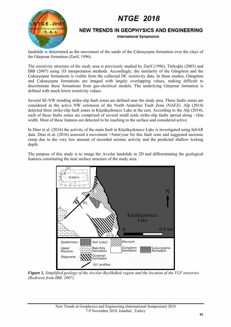
New Trends in Geophysics and Engineering (International Semposium) 2018
7-9 November 2018, Istanbul , Turkey
landslide is determined as the movement of the sands of the Çukurçeşme formation over the clays of the Gürpınar formation (Zarif, 1996).
The resistivity structure of the study area is previously studied by Zarif (1996), Türkoğlu (2003) and İBB (2007) using 1D interpretation methods. Accordingly, the similarity of the Güngören and the Çukurçeşme formations is visible from the collected DC resistivity data. In these studies, Güngören and Çukurçeşme formations are imaged with largely overlapping values, making difficult to discriminate these formations from geo-electrical models. The underlying Gürpınar formation is defined with much lower resistivity values.
Several SE-NW trending strike-slip fault zones are defined near the study area. These faults zones are considered as the active NW extension of the North Anatoliaz Fault Zone (NAFZ). Alp (2014) detected three strike-slip fault zones in Küçükçekmece Lake at the east. According to the Alp (2014), each of these faults zones are comprised of several small scale strike-slip faults spread along ~1km width. Most of these features are detected to be reaching to the surface and considered active.
In Diao et al. (2016) the activity of the main fault in Küçükçekmece Lake is investigated using InSAR data. Diao et al. (2016) assessed a movement >5mm/year for this fault zone and suggested aseismic creep due to the very low amount of recorded seismic activity and the predicted shallow locking depth.
The purpose of this study is to image the Avcılar landslide in 2D and differentiating the geological features constituting the near surface structure of the study area.
Figure 1. Simplified geology of the Avcılar-Beylikdüzü region and the location of the VLF traverses (Redrawn from İBB, 2007).
6161
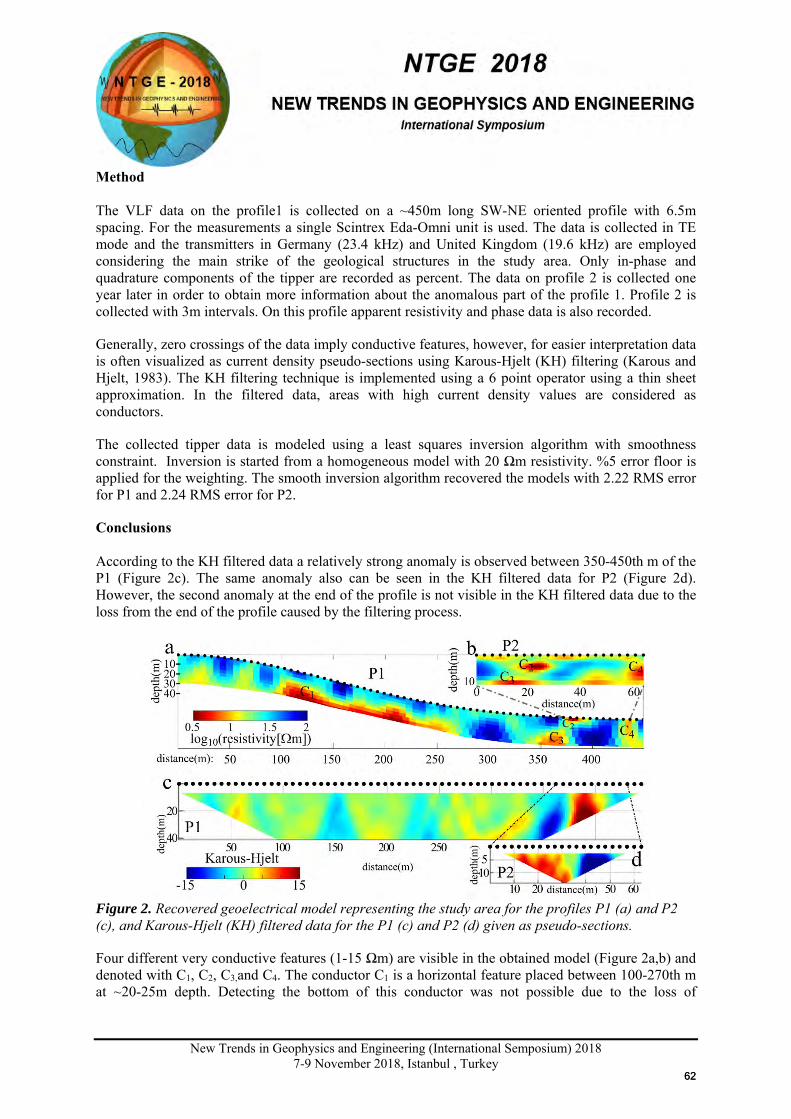
New Trends in Geophysics and Engineering (International Semposium) 2018
7-9 November 2018, Istanbul , Turkey
Method The VLF data on the profile1 is collected on a ~450m long SW-NE oriented profile with 6.5m spacing. For the measurements a single Scintrex Eda-Omni unit is used. The data is collected in TE mode and the transmitters in Germany (23.4 kHz) and United Kingdom (19.6 kHz) are employed considering the main strike of the geological structures in the study area. Only in-phase and quadrature components of the tipper are recorded as percent. The data on profile 2 is collected one year later in order to obtain more information about the anomalous part of the profile 1. Profile 2 is collected with 3m intervals. On this profile apparent resistivity and phase data is also recorded.
Generally, zero crossings of the data imply conductive features, however, for easier interpretation data is often visualized as current density pseudo-sections using Karous-Hjelt (KH) filtering (Karous and Hjelt, 1983). The KH filtering technique is implemented using a 6 point operator using a thin sheet approximation. In the filtered data, areas with high current density values are considered as conductors.
The collected tipper data is modeled using a least squares inversion algorithm with smoothness constraint. Inversion is started from a homogeneous model with 20 Ωm resistivity. %5 error floor is applied for the weighting. The smooth inversion algorithm recovered the models with 2.22 RMS error for P1 and 2.24 RMS error for P2.
Conclusions According to the KH filtered data a relatively strong anomaly is observed between 350-450th m of the P1 (Figure 2c). The same anomaly also can be seen in the KH filtered data for P2 (Figure 2d). However, the second anomaly at the end of the profile is not visible in the KH filtered data due to the loss from the end of the profile caused by the filtering process.
Figure 2. Recovered geoelectrical model representing the study area for the profiles P1 (a) and P2 (c), and Karous-Hjelt (KH) filtered data for the P1 (c) and P2 (d) given as pseudo-sections.
Four different very conductive features (1-15 Ωm) are visible in the obtained model (Figure 2a,b) and denoted with C1, C2, C3,and C4. The conductor C1 is a horizontal feature placed between 100-270th m at ~20-25m depth. Detecting the bottom of this conductor was not possible due to the loss of
6262
New Trends in Geophysics and Engineering (International Semposium) 2018
7-9 November 2018, Istanbul , Turkey
sensitivity under conductive areas. The conductors C2, C3 ,and C4 are obtained in the both models (Figure 2 a,b) as separate conductors.
The recovered geo-electrical model (Figure 3a) is considerably different from the results of the previous studies of Zarif (1996) and İBB (2007) which are obtained using 1D interpretation methods. Relatively high resistivity values (12-100 Ωm) previously associated with the Bakırköy formation is observed throughout the whole profile covering the surface. However, the absence of the Bakırköy formation in the study area is known from the previous studies incorporating detailed studies of the surficial distribution of the formations (Zarif, 1996; İBB, 2007). Hence, these resistivity values are considered as the Güngören and the underlying Çukurçeşme formations. Due to the geologically and electrically similar properties of these formations, these formations are considered undifferentiated. Lower resistivity values (5-20 Ωm) previously attributed to these formations are considered as the result of the 1D interpretation or the difference of the seasonal conditions and water content.
The clayey rocks of the Gürpınar formation is detected between 100-250th m at ~20-25m depth with 1-10 Ωm resistivity. The depth and the resistivity of this formation is coherent with the previous studies. The Gürpınar formation is known to be constituting the base of the Avcılar landslide (Zarif, 1996). The depth of this formation is also coherent with the depth prediction given in Lenti et al. (2016).
At the easternmost part of the profile Three separate conductors (1-15 Ωm) are detected exposed to the surface, partially overlying Güngören and Çukurçeşme formations. This conductive zone is interpreted as the water accumulation zone of the Avcilar landslide.
References Alp, H., 2014, Evidence for active faults in Küçükçekmece lagoon (Marmara Sea, Turkey), inferred
from high-resolution seismic data. Geo-Marine Letters. 34(5), 447-455.
Diao, F., Walter, T. R., Minati, F., Wang, R., Costantini, M., Ergintav, S., Xiong, X., Prats-Iraola, P., 2016, Secondary fault activity of the North Anatolian Fault near Avcilar, southwest of Istanbul: Evidence from SAR interferometry observations. Remote Sensing. 8(10), 846.
İBB, 2007, İstanbul Mikrobölgeleme Projesi Avrupa Yakası. İstanbul Büyükşehir Belediyesi (İBB), İstanbul. [Project Report in Turkish]
Karous, M., Hjelt, S.E., 1983, Linear filtering of VLF dip angle measurements. Geophysical Prospecting. 31, 782-794.
Lenti, L., Martino, S., & Musolino, G., 2016, Considering seismic coefficient distributions within slopes to calculate landslide reactivation probability. Bulletin of Engineering Geology and the Environment. 1-18.
Türkoğlu, E., 2003, Geçici elektromanyetik ve doğru akım elektrik özdirenç verilerinin ortak ters çözümü: Avcılar örneği. Master’s Thesis, İstanbul Technical University, Turkey, 76p. [In Turkish]
Zarif, H., 1996, Küçükçekmece-Büyükçekmece arasındaki alanın yamaç stabilitesi. PHD Dissertation, İstanbul University, Turkey, 141p. [In Turkish]
6363
New Trends in Geophysics and Engineering (International Semposium) 2018
7-9 November 2018, Istanbul , Turkey
X
BIGA-ÇAN GRAVITY DATA, COMPARISON OF 3D EULER DECONVOLUTION
AND 3D MODELING RESULTS
Gökhan Karcıoğlu1 , Oya Tarhan Bal1 , Anisya B.Tekkeli1
1 Geophysical Eng. Department, Istanbul University-Cerrahpaşa, Istanbul Email: [email protected]
Presentation Type All accepted proceedings will be published on the webpage of the symposium (ntge2018.istanbul.edu.tr)
ORAL POSTER
Abstract The Biga-Çan area in the NW Turkey is described with strike-slip and extensional features. The study area also contains features interpreted as the marks of the Intra-Pontide suture, consisting the boundary between the Sakarya Zone and the Strandja-Rhodope massifs.
In this study to extract more information about the area, 3D Euler deconvolution is applied on the gravity data collected by the Turkish Petroleum Co. (TPAO) with 1km inter-station spacing. The index parameter is selected as n=0 and n=1, corresponding to thin sheet edges and thin bed faults respectively. The selection of the index parameter and its meaning is usually ambiguous as in many studies fractional index parameters are used. Thus, 3D models are created using traditional smooth inversion and using a Global Optimization algorithm and the results of the 3D Euler deconvolution is compared to modeling results.
The results shows that a structural index parameter near n=0 marks the boundary between the sedimentary units and the crystalline basement. The agreement between 3D Euler deconvolution and 3D modeling results suggests that the 3D Euler deconvolution may be employed for mapping the approximate sedimentary thickness in the area.
Keywords: 3D gravity modelling, 3D Euler deconvolution Introduction The study area is located in the NW Turkey at the south of the Marmara Sea. The basement in the region is consists of granitic and metamorphic rocks (Çağlar, 2001). Majority of the study area is covered by Neogene deposits and Karakaya complex (Figure 1), consisting of pyroclastic rocks, shale and limestone (Çağlar, 2001). The igneous rocks in the study area is generally associated with mineral and geothermal resources (Ekinci and Yiğitbaş, 2012). There are also several active faults in the study area related with the extensional and strike-slip regimes.
6464
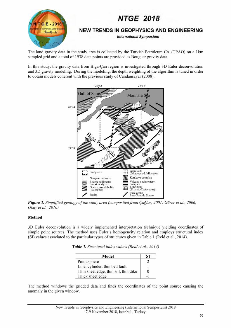
New Trends in Geophysics and Engineering (International Semposium) 2018
7-9 November 2018, Istanbul , Turkey
The land gravity data in the study area is collected by the Turkish Petroleum Co. (TPAO) on a 1km sampled grid and a total of 1938 data points are provided as Bouguer gravity data.
In this study, the gravity data from Biga-Çan region is investigated through 3D Euler deconvolution and 3D gravity modeling. During the modeling, the depth weighting of the algorithm is tuned in order to obtain models coherent with the previous study of Candansayar (2008).
Figure 1. Simplified geology of the study area (composited from Çağlar, 2001; Gürer et al., 2006; Okay et al., 2010) Method 3D Euler deconvolution is a widely implemented interpretation technique yielding coordinates of simple point sources. The method uses Euler’s homogeneity relation and employs structural index (SI) values associated to the particular types of structures given in Table 1 (Reid et al., 2014).
Table 1. Structural index values (Reid et al., 2014)
Model SI Point,sphere 2 Line, cylinder, thin bed fault 1 Thin sheet edge, thin sill, thin dike 0 Thick sheet edge -1
The method windows the gridded data and finds the coordinates of the point source causing the anomaly in the given window.
6565
New Trends in Geophysics and Engineering (International Semposium) 2018
7-9 November 2018, Istanbul , Turkey
Accordingly, Euler’s 3D equation can be given as (Silva and Barbosa, 2003),
(𝑥𝑥 − 𝑥𝑥0) 𝑑𝑑𝑑𝑑𝑑𝑑ℎ(𝑥𝑥,𝑦𝑦, 𝑧𝑧) + (𝑦𝑦 − 𝑦𝑦0) 𝑑𝑑
𝑑𝑑𝑑𝑑ℎ(𝑥𝑥,𝑦𝑦, 𝑧𝑧) + (𝑧𝑧 − 𝑧𝑧0) 𝑑𝑑
𝑑𝑑𝑑𝑑ℎ(𝑥𝑥,𝑦𝑦, 𝑧𝑧) = −𝑛𝑛ℎ(𝑥𝑥,𝑦𝑦, 𝑧𝑧) (1)
Where, h(x,y,z) is the total field anomaly in the current window, and n is the structural index. The coordinates of the point source (𝑥𝑥0,𝑦𝑦0, 𝑧𝑧0) with the structural index n can be obtained by solving the above equation using least squares method.
For better interpretation through 3D Euler deconvolution the window size and the SI parameter must be chosen carefully. A window size>5 is generally suggested (Reid et al., 2014), and in this study it’s chosen to be 7. Selection of the SI is often ambiguous and fractional values are widely used. In these studies different SI values are tried and chosen to obtain better fittings with the known geology or other geophysical data with depth resolution (eg. Tedla et al., 2011). In this study 3D Euler deconvolution results with different structural indexes are compared and interpreted with 3D gravity modeling results of the same dataset.
For the 3D modeling of the gravity data a Particle Swarm Optimization (PSO) algorithm is employed. PSO is a population based Global Optimization method recovers the model parameters by trial and errors. Since the PSO method usually suffers from large parameter counts and multi-objective optimization, additional measures are taken.
To avoid multi-objective optimization, the desired model smoothness is forced on the parameters by a simple smoothing operator. By this approach, searching a trade-off between smoothness and model misfit is prevented. Rougher models are obtained by decreasing the smoothness gradually during the iterations. As the model becomes rougher more details are added by the algorithm, generally causing artefacts (especially in the zones of low sensitivity) due to the random nature of the algorithm. To prevent artefacts Minimum Gradient Support (Portniaguine and Zhdanov, 1999) is added as a threshold value to introduce any changes. The contribution from the MGS is controlled by a small coefficient.
For the 3D modeling of the gravity data a model mesh with 466231 cells is prepared and the desired misfit is achieved after 4500 iterations using the developed PSO algorithm. During the modeling, depth weighting is implemented in order to recovered model to be in agreement with previous 2D magnetotelluric modeling study of Candansayar (2008). The E-W oriented MT profile modeled in Candansayar (2008) coincides with the southernmost part of the study area.
Conclusions The obtained 3D gravity model after 4500 iterations with the PSO algorithm is found to be coherent with previous studies and the general geology of the study area. The major faults and their locations are also coherent with the 3D Euler deconvolution results.
In figure 2, a S-N oriented depth slice from the central part of the study area is provided. In the model, sediments with negative density contrast are visible and the underlying basement with positive density contrast is clear. When the depth slice is compared to the 3D Euler deconvolution, it’s clear that the Euler solutions with n=0 marks the boundary between the sedimentary layers and the basement rocks. Solutions for the structural index n=1 is found to be related to the deeper boundaries and known faults as expected.
6666
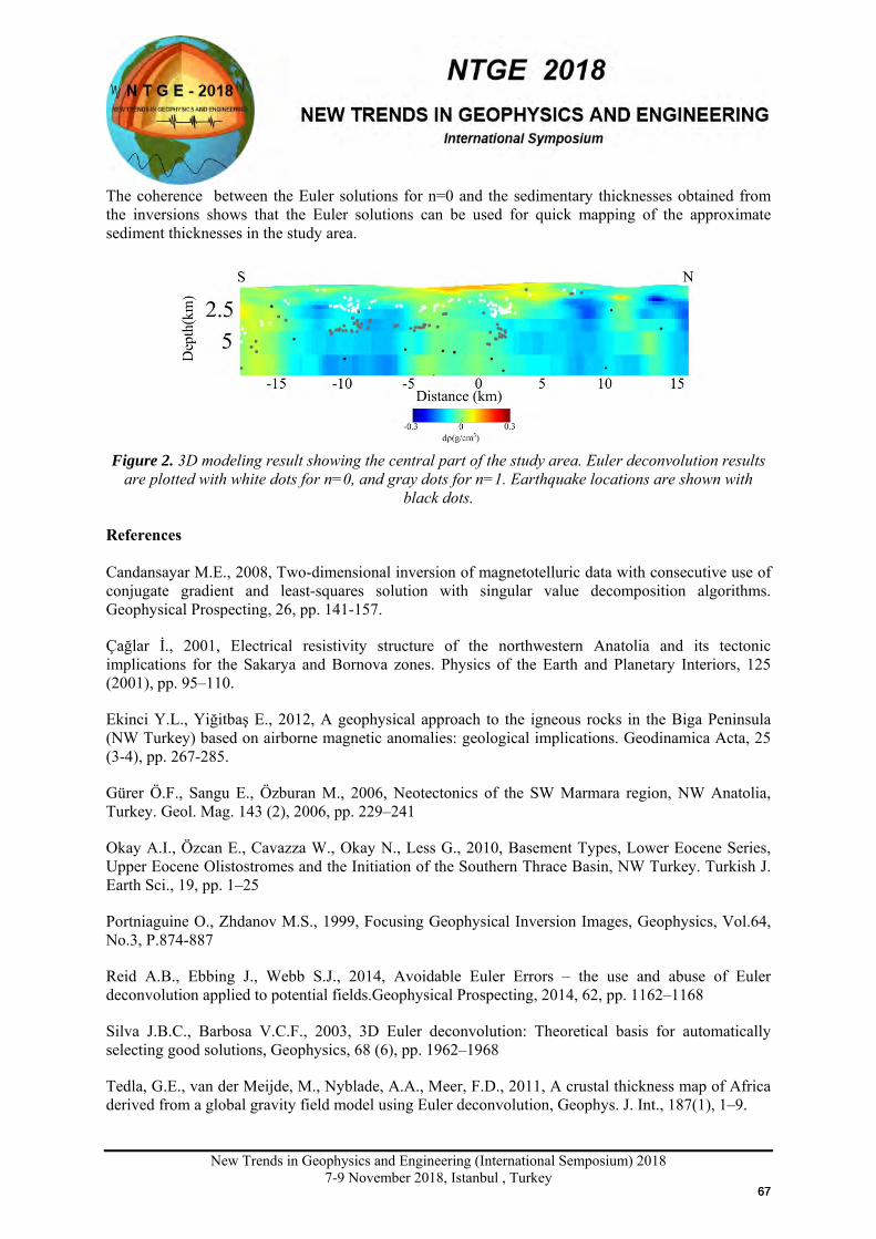
New Trends in Geophysics and Engineering (International Semposium) 2018
7-9 November 2018, Istanbul , Turkey
The coherence between the Euler solutions for n=0 and the sedimentary thicknesses obtained from the inversions shows that the Euler solutions can be used for quick mapping of the approximate sediment thicknesses in the study area.
Figure 2. 3D modeling result showing the central part of the study area. Euler deconvolution results
are plotted with white dots for n=0, and gray dots for n=1. Earthquake locations are shown with black dots.
References Candansayar M.E., 2008, Two-dimensional inversion of magnetotelluric data with consecutive use of conjugate gradient and least-squares solution with singular value decomposition algorithms. Geophysical Prospecting, 26, pp. 141-157.
Çağlar İ., 2001, Electrical resistivity structure of the northwestern Anatolia and its tectonic implications for the Sakarya and Bornova zones. Physics of the Earth and Planetary Interiors, 125 (2001), pp. 95–110.
Ekinci Y.L., Yiğitbaş E., 2012, A geophysical approach to the igneous rocks in the Biga Peninsula (NW Turkey) based on airborne magnetic anomalies: geological implications. Geodinamica Acta, 25 (3-4), pp. 267-285.
Gürer Ö.F., Sangu E., Özburan M., 2006, Neotectonics of the SW Marmara region, NW Anatolia, Turkey. Geol. Mag. 143 (2), 2006, pp. 229–241
Okay A.I., Özcan E., Cavazza W., Okay N., Less G., 2010, Basement Types, Lower Eocene Series, Upper Eocene Olistostromes and the Initiation of the Southern Thrace Basin, NW Turkey. Turkish J. Earth Sci., 19, pp. 1–25
Portniaguine O., Zhdanov M.S., 1999, Focusing Geophysical Inversion Images, Geophysics, Vol.64, No.3, P.874-887
Reid A.B., Ebbing J., Webb S.J., 2014, Avoidable Euler Errors – the use and abuse of Euler deconvolution applied to potential fields.Geophysical Prospecting, 2014, 62, pp. 1162–1168
Silva J.B.C., Barbosa V.C.F., 2003, 3D Euler deconvolution: Theoretical basis for automatically selecting good solutions, Geophysics, 68 (6), pp. 1962–1968
Tedla, G.E., van der Meijde, M., Nyblade, A.A., Meer, F.D., 2011, A crustal thickness map of Africa derived from a global gravity field model using Euler deconvolution, Geophys. J. Int., 187(1), 1–9.
6767
New Trends in Geophysics and Engineering (International Semposium) 2018
7-9 November 2018, Istanbul , Turkey
Determination of the low velocity crustal structures in Marmara Region
İbrahim Hakan Demirsıkan1 , Şakir Şahin1
1 Geophysical Eng. Department, Süleyman Demirel University, Isparta Email: [email protected]
Presentation Type All accepted proceedings will be published on the webpage of the symposium (ntge2018.istanbul.edu.tr)
ORAL POSTER
Abstracts In this study, We used Poisson Tomography method developed by Zhao et al. (1992) and we determine three dimensional P wave tomographic images of crustal structures under Marmara region and Marmara sea. We found the existence of a seismic low P velocity zone starting from the southern part of the Marmara to the İstanbul City. This low velocity zone is located at a depth of 15 km on biga karacabey and bursa line in the South Marmara region. This low velocity layer cuts the north anatolian fault line which is divided into three branches in the marmara sea and continues the existence to the İstanbul city. The one of this transform fault block which is under the biga karacabey and bursa line may caused this low velocity zone. The depth of the low velocity zone is around 15 km. This low velocity structures which we found are may be occured by the recent earthquakes on the northern Anatolian fault line. Due to the mixed stratigraphy of the Marmara region, these low velocity fields in crustal structures are capable of producing large earthquakes. This makes it important to reveal the crustal structure of the marmara region and it is important to figure out the active three dimensional tectonic map of the marmara region. Keywords: Marmara Region, Low velocity, Crustal Structures, Active Tectonic, Seismic Tomography.
Özet Bu çalışmada Zhao vd., 1992, tarafından geliştirilen Poisson Oranı Tomografi yöntemi kullanılmıştır. Marmara bölgesi ve Marmara denizi altındaki kabuk yapılarının üç boyutlu olarak P dalgası tomografisi kesitlerini belirledik. Marmara'nın güneyinden başlayıp İstanbul'a kadar olan bölgede düşük sismik hız tabakası varlığını keşfettik. Bu düşük hız bölgesi, Güney Marmara bölgesindeki Biga Karacabey ve Bursa hattında 15 km derinlikte yer almakta ve bu hattan itibaren düşük hız tabakası iki kol halinde Kuzey Anadolu Fay Hattını dik olarak keserek Marmara denizinin içinden geçerek İstanbul Boğazına kadar uzanmaktadır. Biga Karacabey ve Bursa hattının altından Kuzey Anadolu Fay hattının kollarından birinin geçmesi bu düşük hız zonunun varlığının nedenlerinden biri olabilir. Düşük hız zonu tabakalarının derinliği 15 km civarındadır. Bulduğumuz bu düşük hız yapıları, Kuzey Anadolu Fay Hattı ve üreteceği son depremler açısından önemli hale gelmiştir. Marmara bölgesinin karışık stratigrafisi nedeniyle, bu bölgedeki kabuk yapısını tanımlamak, bu düşük hız alanlarını belirlemek ve bölgenin aktif üç boyutlu tektonik haritasının belirlenmesi önem taşımaktadır.
Anahtar Kelimeler: Marmara bölgesi, düşük hız, kabuk yapıları, aktif tektonik, sismik tomografi.
X
6868
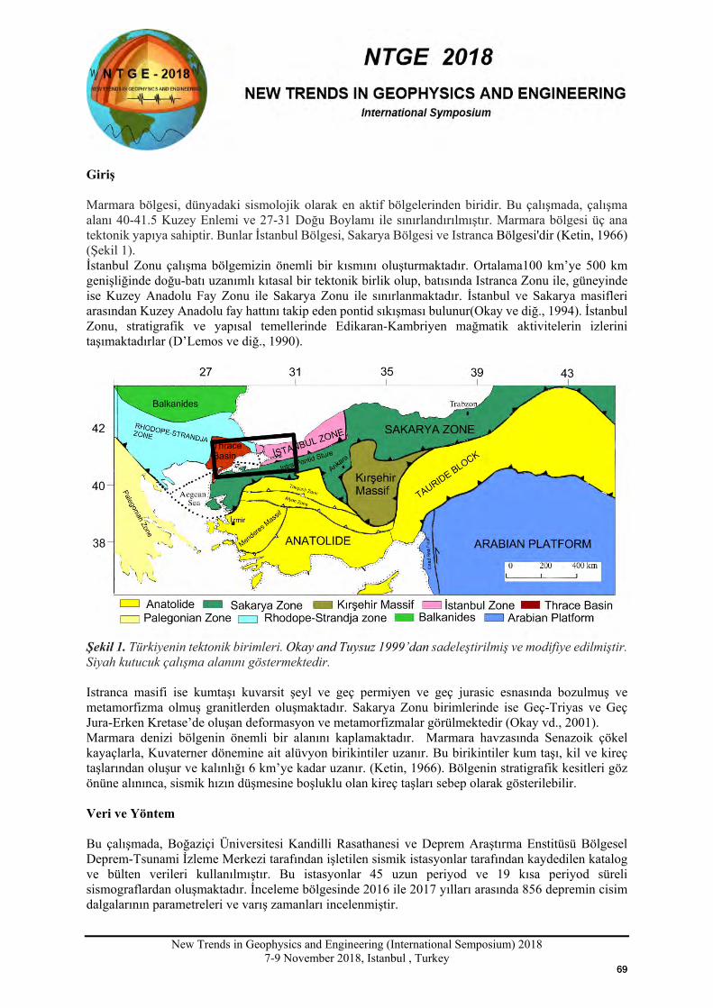
New Trends in Geophysics and Engineering (International Semposium) 2018
7-9 November 2018, Istanbul , Turkey
Giriş Marmara bölgesi, dünyadaki sismolojik olarak en aktif bölgelerinden biridir. Bu çalışmada, çalışma alanı 40-41.5 Kuzey Enlemi ve 27-31 Doğu Boylamı ile sınırlandırılmıştır. Marmara bölgesi üç ana tektonik yapıya sahiptir. Bunlar İstanbul Bölgesi, Sakarya Bölgesi ve Istranca Bölgesi'dir (Ketin, 1966) (Şekil 1). İstanbul Zonu çalışma bölgemizin önemli bir kısmını oluşturmaktadır. Ortalama100 km’ye 500 km genişliğinde doğu-batı uzanımlı kıtasal bir tektonik birlik olup, batısında Istranca Zonu ile, güneyinde ise Kuzey Anadolu Fay Zonu ile Sakarya Zonu ile sınırlanmaktadır. İstanbul ve Sakarya masifleri arasından Kuzey Anadolu fay hattını takip eden pontid sıkışması bulunur(Okay ve diğ., 1994). İstanbul Zonu, stratigrafik ve yapısal temellerinde Edikaran-Kambriyen mağmatik aktivitelerin izlerini taşımaktadırlar (D’Lemos ve diğ., 1990).
Şekil 1. Türkiyenin tektonik birimleri. Okay and Tuysuz 1999’dan sadeleştirilmiş ve modifiye edilmiştir. Siyah kutucuk çalışma alanını göstermektedir. Istranca masifi ise kumtaşı kuvarsit şeyl ve geç permiyen ve geç jurasic esnasında bozulmuş ve metamorfizma olmuş granitlerden oluşmaktadır. Sakarya Zonu birimlerinde ise Geç-Triyas ve Geç Jura-Erken Kretase’de oluşan deformasyon ve metamorfizmalar görülmektedir (Okay vd., 2001). Marmara denizi bölgenin önemli bir alanını kaplamaktadır. Marmara havzasında Senazoik çökel kayaçlarla, Kuvaterner dönemine ait alüvyon birikintiler uzanır. Bu birikintiler kum taşı, kil ve kireç taşlarından oluşur ve kalınlığı 6 km’ye kadar uzanır. (Ketin, 1966). Bölgenin stratigrafik kesitleri göz önüne alınınca, sismik hızın düşmesine boşluklu olan kireç taşları sebep olarak gösterilebilir. Veri ve Yöntem Bu çalışmada, Boğaziçi Üniversitesi Kandilli Rasathanesi ve Deprem Araştırma Enstitüsü Bölgesel Deprem-Tsunami İzleme Merkezi tarafından işletilen sismik istasyonlar tarafından kaydedilen katalog ve bülten verileri kullanılmıştır. Bu istasyonlar 45 uzun periyod ve 19 kısa periyod süreli sismograflardan oluşmaktadır. İnceleme bölgesinde 2016 ile 2017 yılları arasında 856 depremin cisim dalgalarının parametreleri ve varış zamanları incelenmiştir.
6969
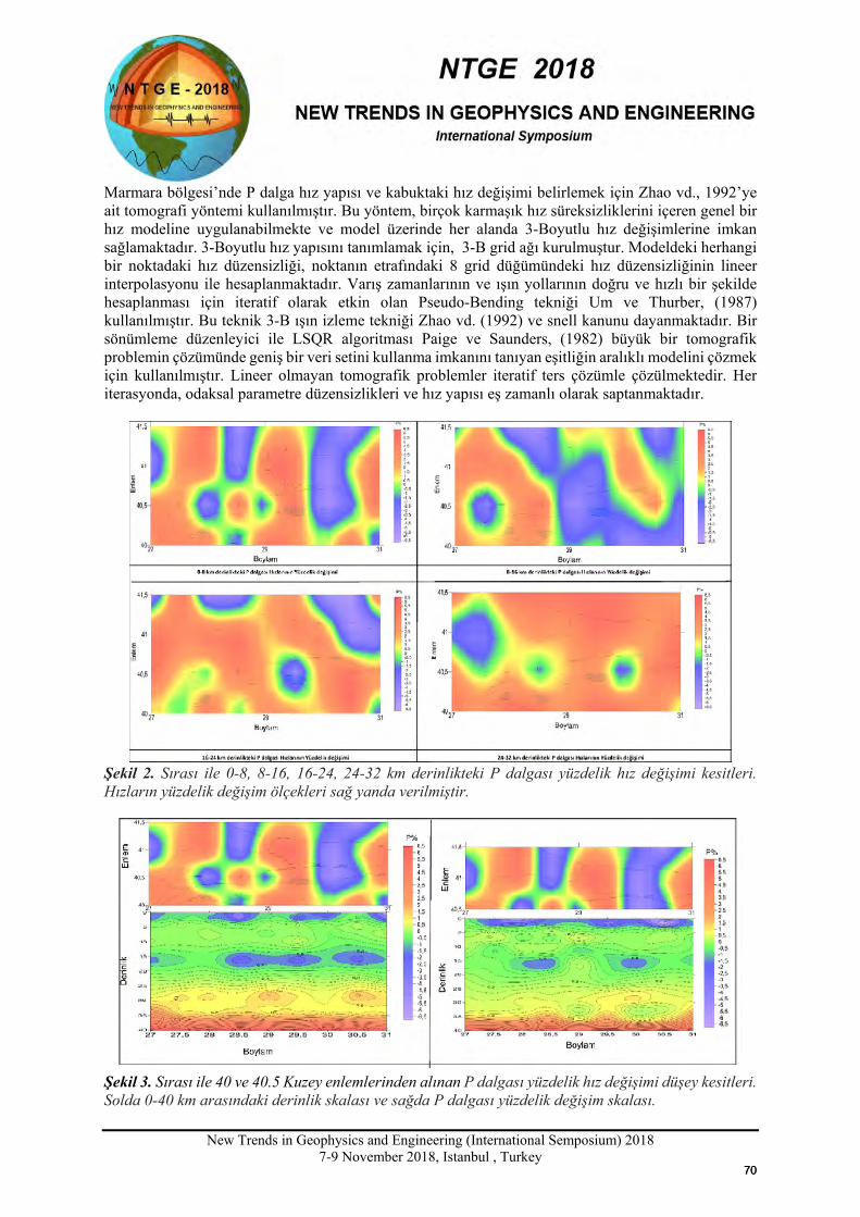
New Trends in Geophysics and Engineering (International Semposium) 2018
7-9 November 2018, Istanbul , Turkey
Marmara bölgesi’nde P dalga hız yapısı ve kabuktaki hız değişimi belirlemek için Zhao vd., 1992’ye ait tomografi yöntemi kullanılmıştır. Bu yöntem, birçok karmaşık hız süreksizliklerini içeren genel bir hız modeline uygulanabilmekte ve model üzerinde her alanda 3-Boyutlu hız değişimlerine imkan sağlamaktadır. 3-Boyutlu hız yapısını tanımlamak için, 3-B grid ağı kurulmuştur. Modeldeki herhangi bir noktadaki hız düzensizliği, noktanın etrafındaki 8 grid düğümündeki hız düzensizliğinin lineer interpolasyonu ile hesaplanmaktadır. Varış zamanlarının ve ışın yollarının doğru ve hızlı bir şekilde hesaplanması için iteratif olarak etkin olan Pseudo-Bending tekniği Um ve Thurber, (1987) kullanılmıştır. Bu teknik 3-B ışın izleme tekniği Zhao vd. (1992) ve snell kanunu dayanmaktadır. Bir sönümleme düzenleyici ile LSQR algoritması Paige ve Saunders, (1982) büyük bir tomografik problemin çözümünde geniş bir veri setini kullanma imkanını tanıyan eşitliğin aralıklı modelini çözmek için kullanılmıştır. Lineer olmayan tomografik problemler iteratif ters çözümle çözülmektedir. Her iterasyonda, odaksal parametre düzensizlikleri ve hız yapısı eş zamanlı olarak saptanmaktadır.
Şekil 2. Sırası ile 0-8, 8-16, 16-24, 24-32 km derinlikteki P dalgası yüzdelik hız değişimi kesitleri. Hızların yüzdelik değişim ölçekleri sağ yanda verilmiştir.
Şekil 3. Sırası ile 40 ve 40.5 Kuzey enlemlerinden alınan P dalgası yüzdelik hız değişimi düşey kesitleri. Solda 0-40 km arasındaki derinlik skalası ve sağda P dalgası yüzdelik değişim skalası.
7070
New Trends in Geophysics and Engineering (International Semposium) 2018
7-9 November 2018, Istanbul , Turkey
Sonuçlar Marmara'nın güneyinden başlayıp İstanbul'a kadar olan bölgede düşük sismik hız tabakası varlığı Şekil 2 ve 3 ‘te görülmektedir. Bu düşük hız bölgesi, Güney Marmara bölgesindeki Biga Karacabey ve Bursa hattında 15 km derinlikte yer almaktadır. Bu düşük hız tabakası iki kol halinde Kuzey Anadolu Fay Hattını dik olarak keserek Marmara denizinin içinden geçerek İstanbul Boğazına kadar uzandığı görülmektedir. Bu düşük hız tabakasının oluşmasında bölgeyi üç ana kola ayrılarak geçen Kuzey Anadolu Fay Hattının olması ve bölgenin stratigrafisi göz önüne alındığında Sakarya formasyonunun kireç taşlarının yoğun olarak bulundurması sebebiyle bu düşük hız tabakaları oluşmuş olabilir. Kaynaklar D’Lemos, R.S., Strachan, R.A., Topley, C.G., 1990, The Cadomian Orogeny in the North Armorican Massif: A Brief Review. Geol Soc. Lond. Spec. Publ., 51, 3-12.
Ketin, İ., 1966, Anadolunun Tektonik Birlikleri. Maden Tetkik Arama Enstitüsü Dergisi, Ankara, No. 66, 20-34.
Paige, C.C., M. A. Saunders, 1982, Sparse linear equations and least squares problems, ACM Trans: Math. Software 8, 43-71.
Okay, A.I., Şengör, A.M.C., Görür, N., 1994, Kinematic History of the Opening of the Black Sea and Its Effect on the Surrounding Regions. Geol Soc Am Bull, 22, 267-270.
Okay, A.I. and Tüysüz, O., 1999, Tethyan Sutures of Northern Turkey. In: Durand, B., Jolivet, L., Horváth, F. & Séranne, M. (Eds), The Mediterranean Basins: Tertiary Extension Within the Alpine Orogen. Geological Society, London, Special Publications,156, 475-515.
Okay, A.I., Satır, M., Tüysüz, O., Akyüz, S., Chen, F., 2001, The Tectonics of the Strandja Massif: Variscan and Mid-Mesozoic Deformation and Metamorphism in the Northern Aegean. Geol Rundsch., 90,217-233.
Um J., and C. Thurber, 1987, A fast algorithm for two-point seismic ray tracing: Bull Seismol Soc Am 77: 972-986.
Zhao D., A. Hasegawa, and S. Horiuchi, 1992, Tomographic imaging of P- and S-wave velocity structure beneath northeastern Japan: J Geophys Res 97: 19909-19928.
7171
New Trends in Geophysics and Engineering (International Semposium) 2018
7-9 November 2018, Istanbul , Turkey
Site Characterization of Ras Al Khaimah National Museum Using Geophysical Techniques, Ras Al Khaimah, UAE
Tareq F. Abdallatif1, A.H. Ghandour2 and M.S. Tantawi3
1- Prof. Dr. Tareq Fahmy Abdallatif: Department of Geomagnetism and Geoelectricity, National Research
Institute of Astronomy and Geophysics (NRIAG), Cairo, Egypt. 2- Dr. Ahmed Hamed El-Ghandour: Department of Geology, Faculty of Science, Ain Shams University,
Cairo, Egypt. 3- Eng. Mohamed Sayed Tantawi: Geoscience Geophysical Consulting, Abu Dhabi, United Arab Emirates.
Presenter Email: [email protected]
Presentation Type All accepted proceedings will be published on the webpage of the symposium (ntge2018.istanbul.edu.tr)
ORAL POSTER
Abstracts For the restoration of the existing historic Fort and the construction of new additional buildings, high resolution geophysical techniques are being carried within the premises of Ras Al-Khaimah National Museum to effectively characterize the subsurface site conditions and local geological stratigraphy, with a particular attention devoted to the relationship between the ancient masonry and the foundation. This has been achieved by determining the physical properties of the soil, observing the level of the water table, estimating the depth to the bedrock, detecting potential zones of weaknesses or cavities as well as recommending the type of foundations to be used. A total of 29 lines were measured inside and outside Ras Al-Khaimah National Museum using GPR and ERT geophysical methods. Correlation of GPR and ERT geophysical data proved a good matching of the obtained results, indicating the absence of remarkable hazardous geologic features within the investigation depth of the studied areas.
Keywords: GPR, ERT, Site Characterization, RAK Museum, UAE. Introduction
Assessment of the risk arising from near surface natural hazard is a crucial step in overcoming foundation problems commonly encountered in engineering projects. Geophysical investigation methods are best suited in site risk assessment (i.e. cavity detection) due to their capability to delineated near-surface cavities and overcome the limitations of traditional probing techniques. This of course helps engineers to develop the appropriate plans of hazard mitigation and implement accordingly the suitable engineering design. Several studies reported in literatures have utilized geophysical techniques for site characterization of karstic regions (Dunscomb and Rehwoldt, 1999; Kaufmann and Quinif, 2001; Roth and Nyquist, 2003; Butler, 2005). Although these techniques (e.g. resistivity, GPR…etc.) are disparate in their application and efficiency, they have proven good satisfactory results in different geological situations.
√
7272
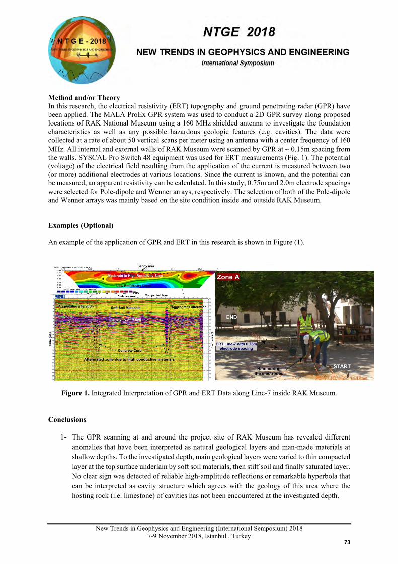
New Trends in Geophysics and Engineering (International Semposium) 2018
7-9 November 2018, Istanbul , Turkey
Method and/or Theory In this research, the electrical resistivity (ERT) topography and ground penetrating radar (GPR) have been applied. The MALÅ ProEx GPR system was used to conduct a 2D GPR survey along proposed locations of RAK National Museum using a 160 MHz shielded antenna to investigate the foundation characteristics as well as any possible hazardous geologic features (e.g. cavities). The data were collected at a rate of about 50 vertical scans per meter using an antenna with a center frequency of 160 MHz. All internal and external walls of RAK Museum were scanned by GPR at ∼ 0.15m spacing from the walls. SYSCAL Pro Switch 48 equipment was used for ERT measurements (Fig. 1). The potential (voltage) of the electrical field resulting from the application of the current is measured between two (or more) additional electrodes at various locations. Since the current is known, and the potential can be measured, an apparent resistivity can be calculated. In this study, 0.75m and 2.0m electrode spacings were selected for Pole-dipole and Wenner arrays, respectively. The selection of both of the Pole-dipole and Wenner arrays was mainly based on the site condition inside and outside RAK Museum. Examples (Optional) An example of the application of GPR and ERT in this research is shown in Figure (1).
Figure 1. Integrated Interpretation of GPR and ERT Data along Line-7 inside RAK Museum.
Conclusions
1- The GPR scanning at and around the project site of RAK Museum has revealed different anomalies that have been interpreted as natural geological layers and man-made materials at shallow depths. To the investigated depth, main geological layers were varied to thin compacted layer at the top surface underlain by soft soil materials, then stiff soil and finally saturated layer. No clear sign was detected of reliable high-amplitude reflections or remarkable hyperbola that can be interpreted as cavity structure which agrees with the geology of this area where the hosting rock (i.e. limestone) of cavities has not been encountered at the investigated depth.
7373
New Trends in Geophysics and Engineering (International Semposium) 2018
7-9 November 2018, Istanbul , Turkey
2- The ground water table detected by ERT method is largely fluctuated from area to another inside and outside RAK Museum. It was qualitatively estimated to be shallower (∼5.07-5.53m) inside RAK Museum, and deeper (∼12.5-13.0m) outside RAK Museum which explain the variation of the subsurface geological nature, surface topography, physical properties of the subsurface layers, proximity of the project site from Arabian Gul Sea.
3- Potential weak zones have been detected by the ERT method at some locations. Boreholes were proposed at these locations to be further investigated by geotechnical drilling and testing methods.
4- Remarkable variation of the depth of foundation layer at the internal (∼0.25-0.7m) and external walls (∼1.5-2.8m) suggests that this foundation was built at different stages with ancient traditional methods using irregular medium size boulders and stones transported from Jebel Jais. The external walls might be newly built, and this interpret why the depth of foundation at which is different (deeper ∼1.5-2.8m). However, the change in depth at the internal walls might be due uneven topography on which the walls were built, or possible settlement caused by the continuous use of irrigation system for the existing garden and tree, taking into account that this foundation is old and continuously exposed to shallow undergrounds water of saline nature.
5- Encountering the underground water table at shallow depth inside RAK Museum as delineated by ERT method might be a reason for the cracks observed at some walls, in particular this water is mostly saline. Potential leakage of water pipes used for Museum toilets is suggested to be another reason for the observed wall cracks.
References [1] A.C. Waltham, and P.G. Fookes “Engineering classification of karst ground conditions,” Quarterly Journal of Engineering Geology and Hydrogeology, vol. 36, pp. 101-118, 2003. [2] D. K. Butler “Near-Surface Geophysics,” SEG, Tulsa, p. 723, 2005. [3] M. H. Dunscomb, and E. Rehwoldt “Two-Dimensional Profiling; Geophysical Weapon of Choice in Karstic Terrain for Engineering Applications, Hydrogeology and Engineering Geology of Sinkholes and Karst,” Proceedings of the Seventh Multidisciplinary Conference on Sinkholes and the Engineering and Environmental Impacts of Karst, Hershey, Pennsylvania, pp. 219- 224, 1999. [4] O. Kaufmann, and Y. Quinif “An Application of Cone Penetration Tests and Combined Array 2D Electrical Resistivity Tomography to Delineate Cover-Collapse Sinkhole Prone Areas, Geotechnical and Environmental Applications of Karst Geology and Hydrology,” Proceedings of the Eighth Multidisciplinary Conference on Sinkholes and the Engineering and Environmental Impacts of Karst, Louisville, Kentucky, pp. 359-364, 2001.
7474
New Trends in Geophysics and Engineering (International Semposium) 2018
7-9 November 2018, Istanbul , Turkey
GEOPHYSICAL METHODS FOR NEAR SURFACE EXPLORATIONS
Mustafa HÜRBEN1 and Ali Muhittin ALBORA2
1Fehmi Ercan Caddesi Girne-Kıbrıs 2 1Istanbul University-Cerrahpaşa, Engineering Faculty, Geophysical Department, 34320,
Avcilar, Istanbul, Turkey Email: [email protected] Presentation Type All accepted proceedings will be published on the webpage of the symposium (ntge2018.istanbul.edu.tr)
ORAL POSTER
Abstracts This study covers ground surveys at Istanbul-Arnavutköy to find the ground parameters. Seismic refraction, MASW, vertical electrical sounding and microtremor methods have been applied out. As a result ground parameters, resistivity values and ground classifications have been found.
Keywords: MASW, microtremor , ground survey
Introduction As we always say, what is dangerous is not the earthquake but the building that is not built resistant to earthquakes. Earthquakes have existed and they will continue to exist. What we need to do is to take necessary precautions and elude the earthquakes with minimum damage. One of the things can be done is to examine how the ground to be built responses to earthquake waves. As a result of the examinations, it is necessary to reinforce the ground or take into consideration these ground features in the construction of the building. The earth is constantly on the move. This movement creates vibrations. These vibrations vary according to their amplitude. If these vibrations can be felt on the earth and cause damage, these vibrations can be called earthquakes. There are also constant oscillations that are not perceived by people on earth. These oscillations are called microtrotremor (Tokgöz, 2002). The soil contain substances in different phases, such as solid, liquid gas, and are therefore difficult to understand. These different phases also have a great effect on how the geophysical properties in the soil structure will be (Alpaslan and Özçep, p: 2). Thanks to geophysical researches, there have been many developments that can facilitate the understanding of soils from past to present. Coates started to use the longitudinal wave velocity in 1970 to determine ground free strength and took an important step in the solution of geotechnical problems. Hardin and Black (1968), later Hardin and Drnevich (1972), as a result of their
X
7575
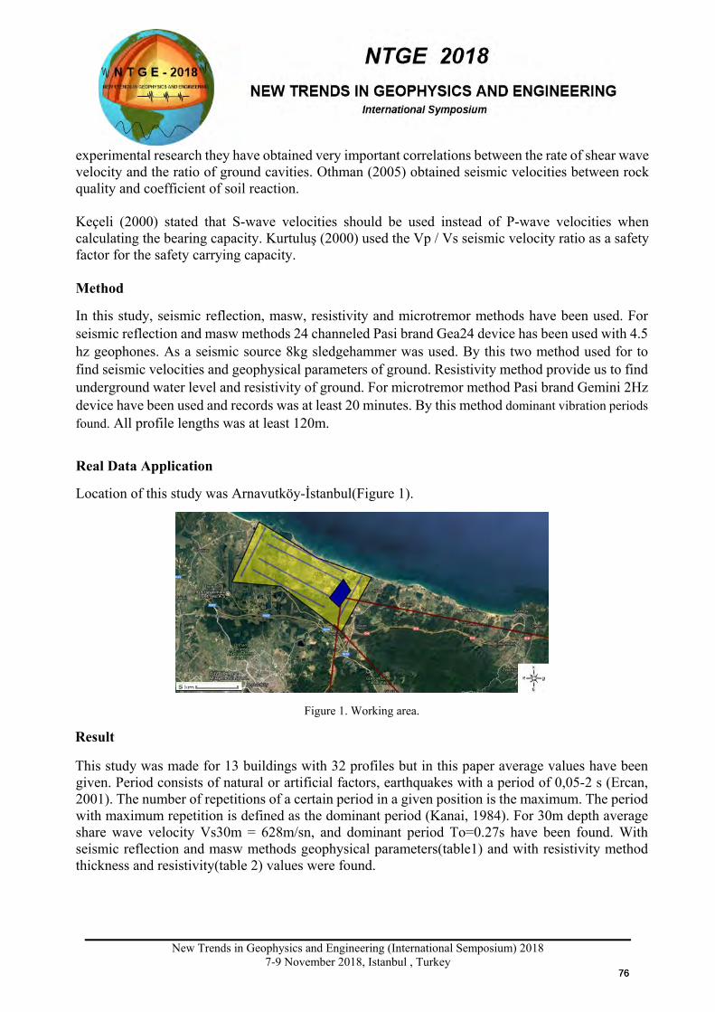
New Trends in Geophysics and Engineering (International Semposium) 2018
7-9 November 2018, Istanbul , Turkey
experimental research they have obtained very important correlations between the rate of shear wave velocity and the ratio of ground cavities. Othman (2005) obtained seismic velocities between rock quality and coefficient of soil reaction. Keçeli (2000) stated that S-wave velocities should be used instead of P-wave velocities when calculating the bearing capacity. Kurtuluş (2000) used the Vp / Vs seismic velocity ratio as a safety factor for the safety carrying capacity. Method
In this study, seismic reflection, masw, resistivity and microtremor methods have been used. For seismic reflection and masw methods 24 channeled Pasi brand Gea24 device has been used with 4.5 hz geophones. As a seismic source 8kg sledgehammer was used. By this two method used for to find seismic velocities and geophysical parameters of ground. Resistivity method provide us to find underground water level and resistivity of ground. For microtremor method Pasi brand Gemini 2Hz device have been used and records was at least 20 minutes. By this method dominant vibration periods found. All profile lengths was at least 120m.
Real Data Application
Location of this study was Arnavutköy-İstanbul(Figure 1).
Figure 1. Working area.
Result
This study was made for 13 buildings with 32 profiles but in this paper average values have been given. Period consists of natural or artificial factors, earthquakes with a period of 0,05-2 s (Ercan, 2001). The number of repetitions of a certain period in a given position is the maximum. The period with maximum repetition is defined as the dominant period (Kanai, 1984). For 30m depth average share wave velocity Vs30m = 628m/sn, and dominant period To=0.27s have been found. With seismic reflection and masw methods geophysical parameters(table1) and with resistivity method thickness and resistivity(table 2) values were found.
7676
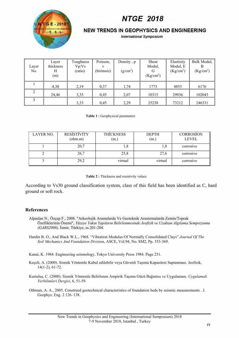
New Trends in Geophysics and Engineering (International Semposium) 2018
7-9 November 2018, Istanbul , Turkey
Layer No.
Layer thickness
H (m)
Toughness Vp/Vs (ratio)
Poisson, v
(birimsiz)
Density , p
(g/cm3)
Shear Modul,
G (Kg/cm2)
Elastisity Modul, E (Kg/cm2)
Bulk Modul, B
(Kg/cm2)
1 4,30 2,19 0,37 1,74 1773 4853 6176 2
24,46 3,35 0,45 2,07 10315 29936 102043 3
3,33 0,45 2,29 25238 73212 246331
Table 1 : Geophysical parameters
LAYER NO. RESİSTİVİTY (ohm.m)
THİCKNESS (m.)
DEPTH (m.)
CORROSİON LEVEL
1 20,7 1,8 1,8 corrosive
2 26,7 25,8 27,6 corrosive
3 29,2 virtual virtual corrosive
Table 2 : Thickness and resistivity values
According to Vs30 ground classification system, class of this field has been identified as C, hard ground or soft rock.
References
Alpaslan N., Özçep F., 2008. "Arkeolojik Aramalarda Ve Geoteknik Arastırmalarda Zemin/Toprak Özelliklerinin Önemi", Yüzeye Yakın Yapıların Belirlenmesinde Jeofizik ve Uzaktan Algılama Sempozyumu (GARS2008), İzmir, Türkiye, ss.201-204.
Hardin B. O., And Black W.L., 1968. “Vibration Modulus Of Normally Consolidated Clays”.Journal Of The
Soil Mechanics And Foundation Division, ASCE, Vol.94, No. SM2, Pp. 353-369.
Kanai, K. 1984. Engineering seismology, Tokyo University Press 1984. Page 251.
Keçeli, A. (2000). Sismik Yöntemle Kabul edilebilir veya Güvenli Taşıma Kapasitesi Saptanması. Jeofizik, 14(1-2), 61-72.
Kurtuluş, C. (2000). Sismik Yöntemle Belirlenen Ampirik Taşıma Gücü Bağıntısı ve Uygulaması. Uygulamalı
Yerbilimleri Dergisi, 6, 51-59. Othman, A. A., 2005. Construed geotechnical characteristics of foundation beds by seismic measurements . J.
Geophys. Eng. 2 126–138.
7777

New Trends in Geophysics and Engineering (International Semposium) 2018
7-9 November 2018, Istanbul , Turkey
Tokgöz, O. E. 2002. Bolu ve Yakın Çevresinin Mikrotremor Verileri ile Yer Etkisinin İncelenmesi, Ankara Üniversitesi Fen Bilimleri Enstitüsü Yüksek Lisans Tezi
7878
New Trends in Geophysics and Engineering (International Semposium) 2018
7-9 November 2018, Istanbul , Turkey
X
INVESTIGATION OF VULNERABILITY INDEX BY SINGLE STATION MICROTREMOR METHOD: A CASE STUDY OF KTU CAMPUS
Yasemin BEKER1, Nilgün SAYIL2, Özgenç AKIN2, Kaan Hakan ÇOBAN2
1Gümüşhane University, Geophysical Eng. Department, Gümüşhane 2Karadeniz Technical University, Geophysical Eng. Department, Trabzon
Email: [email protected] Presentation Type All accepted proceedings will be published on the webpage of the symposium (ntge2018.istanbul.edu.tr)
ORAL POSTER
Abstracts
Single station microtremor recordings are useful for determination of ground characteristics. By using this method predominant period (predominant frequency), H/V ratio, sediment thickness and vulnerability index can be obtained. Also the method has been using to specify building resonance risk during earthquakes in the last decades. In this study the aim is estimate ground parameters and their relationship with selected buildings at The Karadeniz Technical University (KTU) campus area in order to define how to response against earthquakes. The H/V ratio and predominant frequency values in the campus area have been calculated by Nakamura Method from the microtremor recordings. By using these data vulnerability index have been obtained for the 6 buildings located in the campus area. As result, the predominant periods change between 0.17-0.49 s. The predominant frequencies point out that the resonance risk is low for these buildings. The H/V ratios of the ground change between 1-3 and they are lower than the buildings ratios which change between 5.0-8.5. According to the results, vulnerability index of the northeastern part of the campus area is higher the other parts.
Keywords: Microtremor, Nakamura, Predominant frequency, Damping Introduction
Trabzon province is located very near to the North Anatolian Fault Zone (approximately 110 km) which is known the most active fault zone in Turkey. It is thought that the big earthquakes that have occurred on this fault zone have also affected this region. Because of that investigation of ground parameters and building characteristics is very important for take precautions against to the damage of earthquakes. Primarily ground parameter should be well calculated for building. Microtremor, is one of the non-destructive geophysical measurement techniques in order to investigate dynamic behavior of buildings and their soil. Microtremor measurement obtained by ground vibrations is one of the useful methods for determination of ground amplification and predominant frequency. Also the method has been using to specify building resonance risk during earthquakes in the last decades. In this study the aim is estimate ground parameters and buildings characteristics how to response against earthquakes at The Karadeniz Technical University (KTU) campus area. The H/V ratio and predominant frequency values in the campus area have been calculated by Nakamura Method from the microtremor recordings. By using these data vulnerability index have been obtained for the 6 buildings located in the campus area.
7979
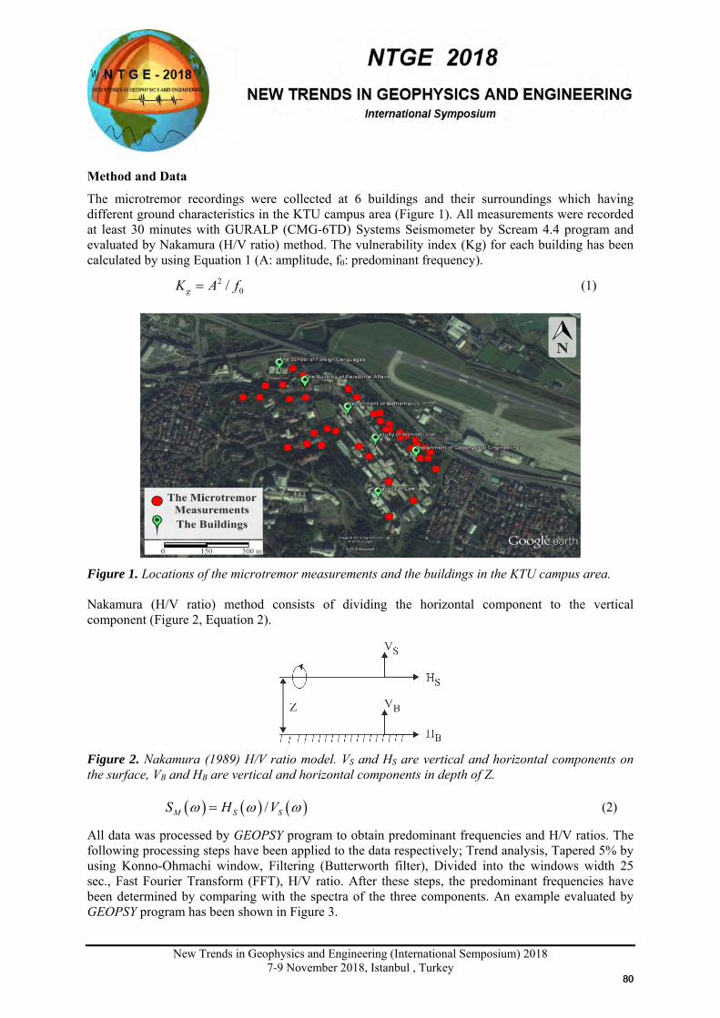
New Trends in Geophysics and Engineering (International Semposium) 2018
7-9 November 2018, Istanbul , Turkey
Method and Data
The microtremor recordings were collected at 6 buildings and their surroundings which having different ground characteristics in the KTU campus area (Figure 1). All measurements were recorded at least 30 minutes with GURALP (CMG-6TD) Systems Seismometer by Scream 4.4 program and evaluated by Nakamura (H/V ratio) method. The vulnerability index (Kg) for each building has been calculated by using Equation 1 (A: amplitude, f0: predominant frequency).
20/gK A f= (1)
Figure 1. Locations of the microtremor measurements and the buildings in the KTU campus area. Nakamura (H/V ratio) method consists of dividing the horizontal component to the vertical component (Figure 2, Equation 2).
Figure 2. Nakamura (1989) H/V ratio model. VS and HS are vertical and horizontal components on the surface, VB and HB are vertical and horizontal components in depth of Z.
( ) ( ) ( )/M S SS H Vω ω ω= (2)
All data was processed by GEOPSY program to obtain predominant frequencies and H/V ratios. The following processing steps have been applied to the data respectively; Trend analysis, Tapered 5% by using Konno-Ohmachi window, Filtering (Butterworth filter), Divided into the windows width 25 sec., Fast Fourier Transform (FFT), H/V ratio. After these steps, the predominant frequencies have been determined by comparing with the spectra of the three components. An example evaluated by GEOPSY program has been shown in Figure 3.
8080
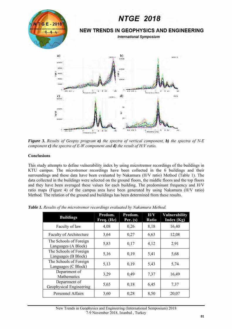
New Trends in Geophysics and Engineering (International Semposium) 2018
7-9 November 2018, Istanbul , Turkey
Figure 3. Results of Geopsy program a) the spectra of vertical component, b) the spectra of N-E component c) the spectra of E-W component and d) the result of H/V ratio. Conclusions
This study attempts to define vulnerability index by using microtremor recordings of the buildings in KTU campus. The microtremor recordings have been collected in the 6 buildings and their surroundings and these data have been evaluated by Nakamura (H/V ratio) Method (Table 1). The data collected in the buildings were selected on the ground floors, the middle floors and the top floors and they have been averaged these values for each building. The predominant frequency and H/V ratio maps (Figure 4) of the campus area have been generated by using Nakamura (H/V ratio) Method. The relation of the ground and buildings has been determined from these results.
Table 1. Results of the microtremor recordings evaluated by Nakamura Method.
Buildings Predom. Freq. (Hz)
Predom. Per. (s)
H/V Ratio
Vulnerability Index (Kg)
Faculty of law 4,08 0,26 8,18 16,40
Faculty of Architecture 3,64 0,27 6,63 12,08 The Schools of Foreign Languages (A Block) 5,83 0,17 4,12 2,91
The Schools of Foreign Languages (B Block) 5,16 0,19 5,41 5,68
The Schools of Foreign Languages (C Block) 5,13 0,19 5,43 5,74
Department of Mathematics 3,29 0,49 7,37 16,49
Department of Geophysical Engineering 5,65 0,18 6,45 7,37
Personnel Affairs 3,60 0,28 8,50 20,07
8181
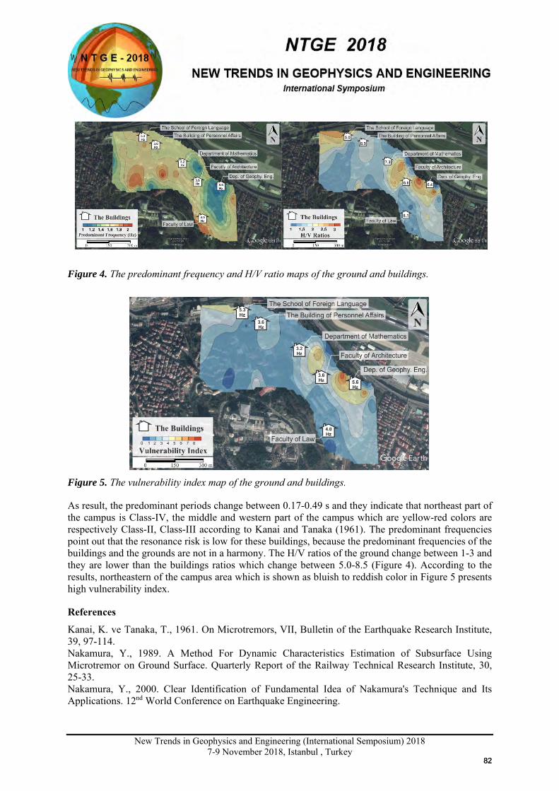
New Trends in Geophysics and Engineering (International Semposium) 2018
7-9 November 2018, Istanbul , Turkey
Figure 4. The predominant frequency and H/V ratio maps of the ground and buildings.
Figure 5. The vulnerability index map of the ground and buildings.
As result, the predominant periods change between 0.17-0.49 s and they indicate that northeast part of the campus is Class-IV, the middle and western part of the campus which are yellow-red colors are respectively Class-II, Class-III according to Kanai and Tanaka (1961). The predominant frequencies point out that the resonance risk is low for these buildings, because the predominant frequencies of the buildings and the grounds are not in a harmony. The H/V ratios of the ground change between 1-3 and they are lower than the buildings ratios which change between 5.0-8.5 (Figure 4). According to the results, northeastern of the campus area which is shown as bluish to reddish color in Figure 5 presents high vulnerability index.
References
Kanai, K. ve Tanaka, T., 1961. On Microtremors, VII, Bulletin of the Earthquake Research Institute, 39, 97-114. Nakamura, Y., 1989. A Method For Dynamic Characteristics Estimation of Subsurface Using Microtremor on Ground Surface. Quarterly Report of the Railway Technical Research Institute, 30, 25-33. Nakamura, Y., 2000. Clear Identification of Fundamental Idea of Nakamura's Technique and Its Applications. 12nd World Conference on Earthquake Engineering.
8282
New Trends in Geophysics and Engineering (International Semposium) 2018
7-9 November 2018, Istanbul , Turkey
X
Analysis of Soil-Structure and Resonance Effects of Gümüşhane University
Campus Area in Turkey with HVSR and FSR Methods
Yasemin Beker1 , Nilgün Sayıl2
1 Geophysical Eng. Department, Gumushane University, Gumushane Email: [email protected]
2 Geophysical Eng. Department, Karadeniz Technical University, Trabzon Email: [email protected]
Presentation Type All accepted proceedings will be published on the webpage of the symposium (ntge2018.istanbul.edu.tr)
ORAL POSTER
Abstracts Horizontal to Vertical Spectral Ratio (HVSR) method used for engineering seismology is very important for determining of dynamic ground parameters and its variations. In this study, HVSR method was applied to determine the seismic ground response of Gümüşhane university campus area. The ambient noise measurements were taken in the building of Faculty of Engineering and Natural Science (6 floors) and in the free-field using the Floor Spectral Ratio method (FSR) and the HVSR method. The amplification and fundamental frequency values obtained from the free-field measurements are 1.89-9.79 and 0.53-9.17 Hz, respectively. The natural frequency and period of faculty building is around 3.0 Hz and 0.314 s, respectively. The risk of soil-structure resonance was determined by comparing these methods. The risk is medium level. The HVSR of ambient noise can be used for estimated natural building frequency, resonance risk and site effect. Keywords: Ambient noise, Horizontal to Vertical Spectral Ratio, Fundamental frequency, soil-structure resonance, Gümüşhane. Introduction Ambient noise (microtremor) is generally defined as low amplitude vibrations of the Earth’s surface that is caused by various sources (such as wind, rain, sea currents, traffic, urban activity, etc.). The microtremor horizontal-to-vertical-spectral-ratio (HVSR) technique has received great attention from all over the world with its simplicity together with quick information about dynamic characteristics of ground and structures. The HVSR of microtremors gives a good estimation of natural building frequency. The response of the ground is strongly influenced by the proximity of structures. In this study, the potential danger of the soil-structure resonance was estimated by comparison of the ambient noise measurements in building of Faculty of Engineering and Natural Science (6 floors) and nearby free-field locations (20 measurement points) at Gümüşhane University, in NE Turkey (Figure 1). The geological map of study area is given in figure 1.
8383
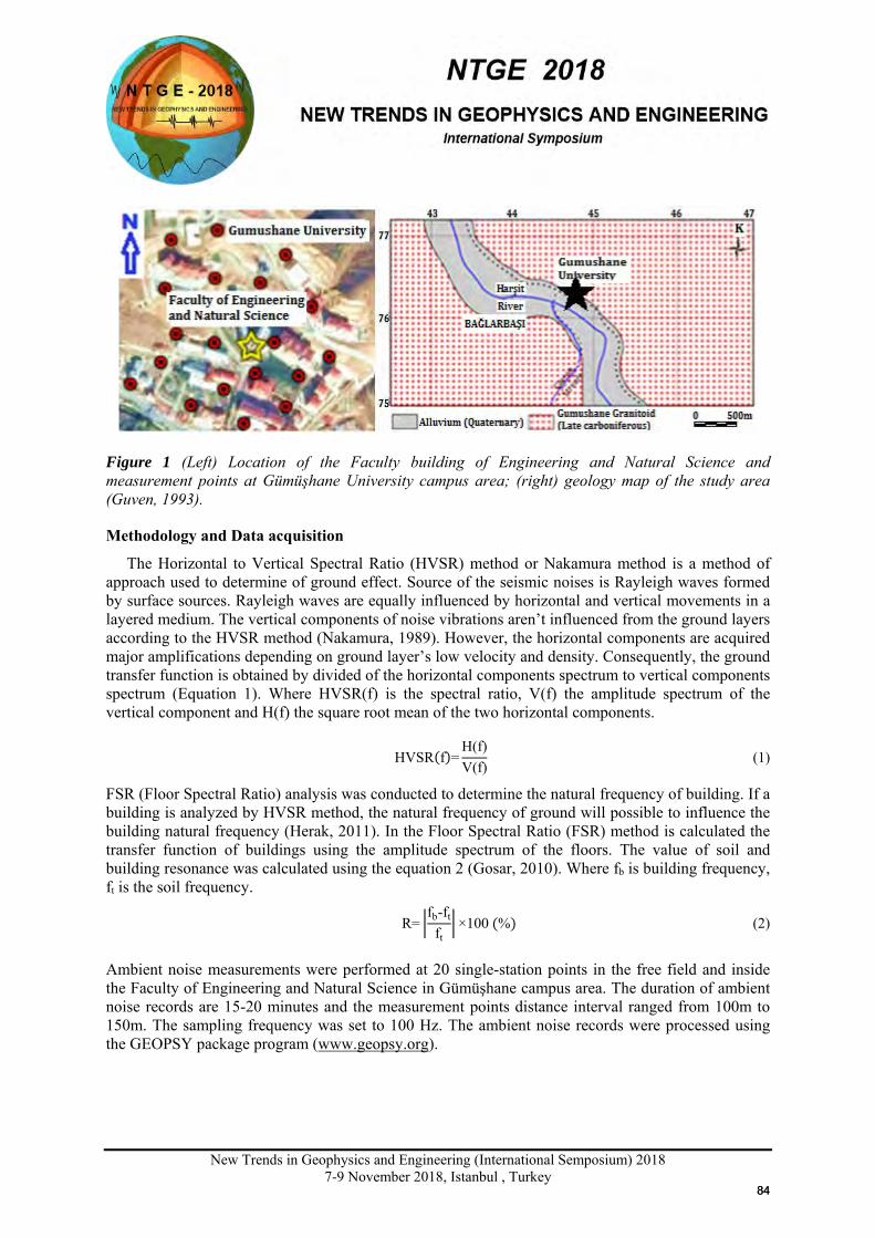
New Trends in Geophysics and Engineering (International Semposium) 2018
7-9 November 2018, Istanbul , Turkey
Figure 1 (Left) Location of the Faculty building of Engineering and Natural Science and measurement points at Gümüşhane University campus area; (right) geology map of the study area (Guven, 1993).
Methodology and Data acquisition
The Horizontal to Vertical Spectral Ratio (HVSR) method or Nakamura method is a method of approach used to determine of ground effect. Source of the seismic noises is Rayleigh waves formed by surface sources. Rayleigh waves are equally influenced by horizontal and vertical movements in a layered medium. The vertical components of noise vibrations aren’t influenced from the ground layers according to the HVSR method (Nakamura, 1989). However, the horizontal components are acquired major amplifications depending on ground layer’s low velocity and density. Consequently, the ground transfer function is obtained by divided of the horizontal components spectrum to vertical components spectrum (Equation 1). Where HVSR(f) is the spectral ratio, V(f) the amplitude spectrum of the vertical component and H(f) the square root mean of the two horizontal components.
HVSR(f)=H(f)V(f)
(1)
FSR (Floor Spectral Ratio) analysis was conducted to determine the natural frequency of building. If a building is analyzed by HVSR method, the natural frequency of ground will possible to influence the building natural frequency (Herak, 2011). In the Floor Spectral Ratio (FSR) method is calculated the transfer function of buildings using the amplitude spectrum of the floors. The value of soil and building resonance was calculated using the equation 2 (Gosar, 2010). Where fb is building frequency, ft is the soil frequency.
R= fb-ft
ft×100 (%) (2)
Ambient noise measurements were performed at 20 single-station points in the free field and inside the Faculty of Engineering and Natural Science in Gümüşhane campus area. The duration of ambient noise records are 15-20 minutes and the measurement points distance interval ranged from 100m to 150m. The sampling frequency was set to 100 Hz. The ambient noise records were processed using the GEOPSY package program (www.geopsy.org).
8484
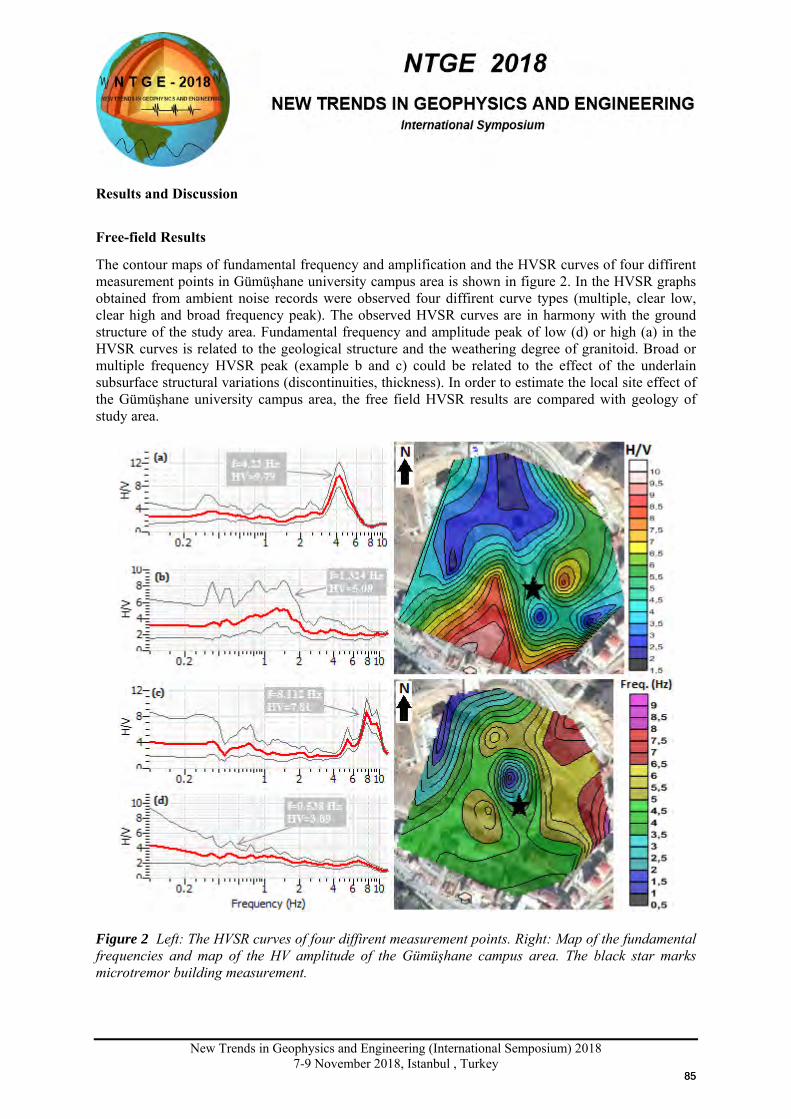
New Trends in Geophysics and Engineering (International Semposium) 2018
7-9 November 2018, Istanbul , Turkey
Results and Discussion
Free-field Results
The contour maps of fundamental frequency and amplification and the HVSR curves of four diffirent measurement points in Gümüşhane university campus area is shown in figure 2. In the HVSR graphs obtained from ambient noise records were observed four diffirent curve types (multiple, clear low, clear high and broad frequency peak). The observed HVSR curves are in harmony with the ground structure of the study area. Fundamental frequency and amplitude peak of low (d) or high (a) in the HVSR curves is related to the geological structure and the weathering degree of granitoid. Broad or multiple frequency HVSR peak (example b and c) could be related to the effect of the underlain subsurface structural variations (discontinuities, thickness). In order to estimate the local site effect of the Gümüşhane university campus area, the free field HVSR results are compared with geology of study area.
Figure 2 Left: The HVSR curves of four diffirent measurement points. Right: Map of the fundamental frequencies and map of the HV amplitude of the Gümüşhane campus area. The black star marks microtremor building measurement.
8585
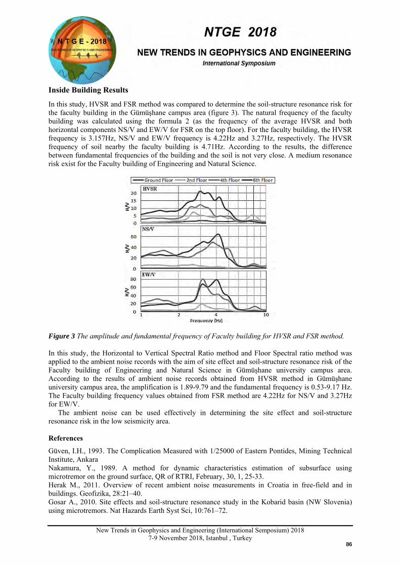
New Trends in Geophysics and Engineering (International Semposium) 2018
7-9 November 2018, Istanbul , Turkey
Inside Building Results
In this study, HVSR and FSR method was compared to determine the soil-structure resonance risk for the faculty building in the Gümüşhane campus area (figure 3). The natural frequency of the faculty building was calculated using the formula 2 (as the frequency of the average HVSR and both horizontal components NS/V and EW/V for FSR on the top floor). For the faculty building, the HVSR frequency is 3.157Hz, NS/V and EW/V frequency is 4.22Hz and 3.27Hz, respectively. The HVSR frequency of soil nearby the faculty building is 4.71Hz. According to the results, the difference between fundamental frequencies of the building and the soil is not very close. A medium resonance risk exist for the Faculty building of Engineering and Natural Science.
Figure 3 The amplitude and fundamental frequency of Faculty building for HVSR and FSR method.
In this study, the Horizontal to Vertical Spectral Ratio method and Floor Spectral ratio method was applied to the ambient noise records with the aim of site effect and soil-structure resonance risk of the Faculty building of Engineering and Natural Science in Gümüşhane university campus area. According to the results of ambient noise records obtained from HVSR method in Gümüşhane university campus area, the amplification is 1.89-9.79 and the fundamental frequency is 0.53-9.17 Hz. The Faculty building frequency values obtained from FSR method are 4.22Hz for NS/V and 3.27Hz for EW/V.
The ambient noise can be used effectively in determining the site effect and soil-structure resonance risk in the low seismicity area. References Güven, I.H., 1993. The Complication Measured with 1/25000 of Eastern Pontides, Mining Technical Institute, Ankara Nakamura, Y., 1989. A method for dynamic characteristics estimation of subsurface using microtremor on the ground surface, QR of RTRI, February, 30, 1, 25-33. Herak M., 2011. Overview of recent ambient noise measurements in Croatia in free-field and in buildings. Geofizika, 28:21–40. Gosar A., 2010. Site effects and soil-structure resonance study in the Kobarid basin (NW Slovenia) using microtremors. Nat Hazards Earth Syst Sci, 10:761–72.
8686
New Trends in Geophysics and Engineering (International Semposium) 2018
7-9 November 2018, Istanbul , Turkey
X
STUDY ON THE APPLICABILITY OF THE AMBIENT NOISE HVSR METHOD IN
BAĞLARBAŞI (GÜMÜŞHANE), NE TURKEY
Yasemin Beker1 , Nilgün Sayıl2
1 Geophysical Eng. Department, Gumushane University, Gumushane Email: [email protected]
2 Geophysical Eng. Department, Karadeniz Technical University, Trabzon Email: [email protected]
Presentation Type All accepted proceedings will be published on the webpage of the symposium (ntge2018.istanbul.edu.tr)
ORAL POSTER
Abstracts Horizontal to Vertical Spectral Ratio (HVSR) method is a very convenient tool to estimate the effect of surface geology on seismic motion without other geological information. HVSR method used for engineering seismology is very important for determining of dynamic ground parameters and its variations. The method based on frequency of horizontal and vertical component microtremor records provides to quick and economical estimation of dynamic ground parameters. In this study, HVSR method has been applied to ambient noise records taken with CMG-6TD three component broad band velocity seismometers in 12 points were laid out along two profiles with the aim of determining the fundamental frequency at the points and its variation with azimuth of the Bağlarbaşı (Gümüşhane), Turkey. The HVSR curve for each points and the variation of the HVSR ratio with azimuth was obtained from ambient noise records. The profiles cross two different geological formations (alluvium and granitoid) in the study area. Results showed that the HVSR ratio is sensitive to the change in geology. Keywords: Ambient noise, HVSR, Fundamental frequency, Gümüşhane. Introduction Ambient noise is generally defined as low amplitude vibrations of the Earth’s surface that is caused by various sources (such as wind, rain, sea currents, traffic, urban activity, etc.). The Horizontal to Vertical Spectral Ratio (HVSR) method is used to estimate the fundamental frequency, usually, for sedimentary layers in a basin. Recently, HVSR method used for engineering seismology provides the quick and economic results for estimating of dynamic ground parameters. Amplitude and frequency contents of the nature vibration of the ground are influenced by the factors as lithology and geometry of the ground (Kanai and Tanaka, 1954, 1961). In this study, ambient noise records were evaluated using HVSR method in Bağlarbaşı (Gümüşhane), NE, Turkey (Figure 1). The HVSR method has been applied to calculate the fundamental frequency at the measurement points and its variation with azimuth.
8787
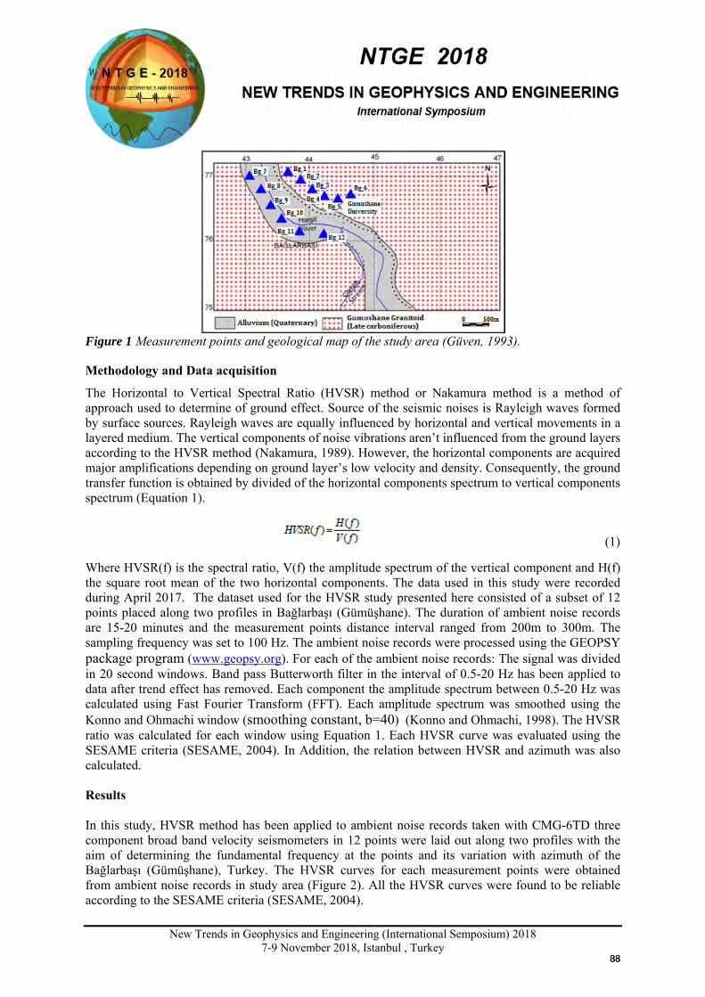
New Trends in Geophysics and Engineering (International Semposium) 2018
7-9 November 2018, Istanbul , Turkey
Figure 1 Measurement points and geological map of the study area (Güven, 1993).
Methodology and Data acquisition
The Horizontal to Vertical Spectral Ratio (HVSR) method or Nakamura method is a method of approach used to determine of ground effect. Source of the seismic noises is Rayleigh waves formed by surface sources. Rayleigh waves are equally influenced by horizontal and vertical movements in a layered medium. The vertical components of noise vibrations aren’t influenced from the ground layers according to the HVSR method (Nakamura, 1989). However, the horizontal components are acquired major amplifications depending on ground layer’s low velocity and density. Consequently, the ground transfer function is obtained by divided of the horizontal components spectrum to vertical components spectrum (Equation 1).
(1)
Where HVSR(f) is the spectral ratio, V(f) the amplitude spectrum of the vertical component and H(f) the square root mean of the two horizontal components. The data used in this study were recorded during April 2017. The dataset used for the HVSR study presented here consisted of a subset of 12 points placed along two profiles in Bağlarbaşı (Gümüşhane). The duration of ambient noise records are 15-20 minutes and the measurement points distance interval ranged from 200m to 300m. The sampling frequency was set to 100 Hz. The ambient noise records were processed using the GEOPSY package program (www.geopsy.org). For each of the ambient noise records: The signal was divided in 20 second windows. Band pass Butterworth filter in the interval of 0.5-20 Hz has been applied to data after trend effect has removed. Each component the amplitude spectrum between 0.5-20 Hz was calculated using Fast Fourier Transform (FFT). Each amplitude spectrum was smoothed using the Konno and Ohmachi window (smoothing constant, b=40) (Konno and Ohmachi, 1998). The HVSR ratio was calculated for each window using Equation 1. Each HVSR curve was evaluated using the SESAME criteria (SESAME, 2004). In Addition, the relation between HVSR and azimuth was also calculated. Results In this study, HVSR method has been applied to ambient noise records taken with CMG-6TD three component broad band velocity seismometers in 12 points were laid out along two profiles with the aim of determining the fundamental frequency at the points and its variation with azimuth of the Bağlarbaşı (Gümüşhane), Turkey. The HVSR curves for each measurement points were obtained from ambient noise records in study area (Figure 2). All the HVSR curves were found to be reliable according to the SESAME criteria (SESAME, 2004).
8888
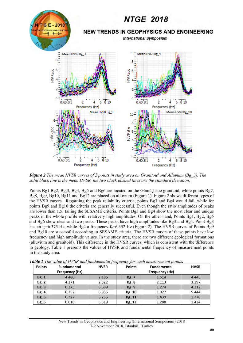
New Trends in Geophysics and Engineering (International Semposium) 2018
7-9 November 2018, Istanbul , Turkey
Figure 2 The mean HVSR curves of 2 points in study area on Granitoid and Alluvium (Bg_3). The solid black line is the mean HVSR, the two black dashed lines are the standard deviation. Points Bg1,Bg2, Bg,3, Bg4, Bg5 and Bg6 are located on the Gümüşhane granitoid, while points Bg7, Bg8, Bg9, Bg10, Bg11 and Bg12 are placed on alluvium (Figure 1). Figure 2 shows different types of the HVSR curves. Regarding the peak reliability criteria, points Bg3 and Bg4 would fail, while for points Bg9 and Bg10 the criteria are generally successful. Even though the ratio amplitudes of peaks are lower than 1.5, failing the SESAME criteria. Points Bg3 and Bg4 show the most clear and unique peaks in the whole profile with relatively high amplitudes. On the other hand, Points Bg1, Bg2, Bg5 and Bg6 show clear and two peaks. These peaks have high amplitudes like Bg3 and Bg4. Point Bg3 has an f0=6.375 Hz, while Bg4 a frequency f0=6.352 Hz (Figure 2). The HVSR curves of Points Bg9 and Bg10 are successful according to SESAME criteria. The HVSR curves of these points have low frequency and high amplitude values. In the study area, there are two different geological formations (alluvium and granitoid). This difference in the HVSR curves, which is consistent with the difference in geology. Table 1 presents the values of HVSR and fundamental frequency of measurement points in the study area. Table 1 The value of HVSR and fundamental frequency for each measurement points.
Points Fundamental Frequency (Hz)
HVSR Points Fundamental Frequency (Hz)
HVSR
Bg_1 4.480 2.186 Bg_7 1.614 4.443 Bg_2 4.271 2.322 Bg_8 2.113 3.397 Bg_3 6.375 6.689 Bg_9 1.274 4.212 Bg_4 6.352 6.855 Bg_10 1.027 5.444 Bg_5 6.327 6.255 Bg_11 1.439 1.376 Bg_6 6.618 5.319 Bg_12 1.288 1.424
8989
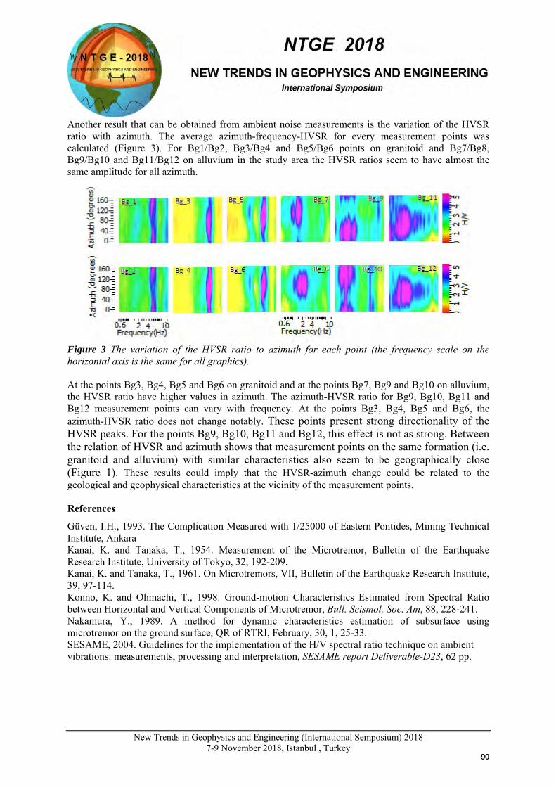
New Trends in Geophysics and Engineering (International Semposium) 2018
7-9 November 2018, Istanbul , Turkey
Another result that can be obtained from ambient noise measurements is the variation of the HVSR ratio with azimuth. The average azimuth-frequency-HVSR for every measurement points was calculated (Figure 3). For Bg1/Bg2, Bg3/Bg4 and Bg5/Bg6 points on granitoid and Bg7/Bg8, Bg9/Bg10 and Bg11/Bg12 on alluvium in the study area the HVSR ratios seem to have almost the same amplitude for all azimuth.
Figure 3 The variation of the HVSR ratio to azimuth for each point (the frequency scale on the horizontal axis is the same for all graphics). At the points Bg3, Bg4, Bg5 and Bg6 on granitoid and at the points Bg7, Bg9 and Bg10 on alluvium, the HVSR ratio have higher values in azimuth. The azimuth-HVSR ratio for Bg9, Bg10, Bg11 and Bg12 measurement points can vary with frequency. At the points Bg3, Bg4, Bg5 and Bg6, the azimuth-HVSR ratio does not change notably. These points present strong directionality of the HVSR peaks. For the points Bg9, Bg10, Bg11 and Bg12, this effect is not as strong. Between the relation of HVSR and azimuth shows that measurement points on the same formation (i.e. granitoid and alluvium) with similar characteristics also seem to be geographically close (Figure 1). These results could imply that the HVSR-azimuth change could be related to the geological and geophysical characteristics at the vicinity of the measurement points. References Güven, I.H., 1993. The Complication Measured with 1/25000 of Eastern Pontides, Mining Technical Institute, Ankara Kanai, K. and Tanaka, T., 1954. Measurement of the Microtremor, Bulletin of the Earthquake Research Institute, University of Tokyo, 32, 192-209. Kanai, K. and Tanaka, T., 1961. On Microtremors, VII, Bulletin of the Earthquake Research Institute, 39, 97-114. Konno, K. and Ohmachi, T., 1998. Ground-motion Characteristics Estimated from Spectral Ratio between Horizontal and Vertical Components of Microtremor, Bull. Seismol. Soc. Am, 88, 228-241. Nakamura, Y., 1989. A method for dynamic characteristics estimation of subsurface using microtremor on the ground surface, QR of RTRI, February, 30, 1, 25-33. SESAME, 2004. Guidelines for the implementation of the H/V spectral ratio technique on ambient vibrations: measurements, processing and interpretation, SESAME report Deliverable-D23, 62 pp.
9090
New Trends in Geophysics and Engineering (International Semposium) 2018
7-9 November 2018, Istanbul , Turkey
X
HIGH RESOLUTION AEROMAGNETIC (HRAM) BASEMENT IMAGING OF OFF-SHORE
GULF OF SUEZ PROSPECT, EGYPT.
S. M. Sharafeldin1,2, H. Karslı1
1 Geophysical Eng. Department, Karadeniz Technical University (KTÜ), Turkey. 2 Geophysics Department, Cairo University, Egypt.
Email: [email protected] Presentation Type
ORAL POSTER
Abstracts High Resolution Aeromagnetic (HRAM) surveys were interpreted to image the basement configuration of a producing off-shore oil field, Gulf of Suez in Egypt. A comprehensive scheme of data processing implemented producing maps that enhance the anomalies related to basement structures. The basement depth inverted using SPI method, and adjusted with 13 modelled profiles controlled by well data. Two sets of faults revealed in in the study area, the NW-SE trend that are bounding the main producing tilted uplifted block. Another set of cross Gulf trend revealed, some of them show a strike slip sense of movement. Two basins located along the northern and western borders of area that might be the sourcing of the oil field.
Keywords: Gulf of Suez, Aeromagnetic, Basement Imaging, Edge detection Introduction Aeromagnetic data have long been used by the petroleum industry to map structure and to estimate depth to magnetic basement. Most flown aeromagnetic surveys were intended to map magnetic crystalline rocks and to define the sedimentary cover thickness. The surveys were flown at an altitude and line spacing equal to one-half the depth to the sources to sample any deep source adequately (Reid, 1980). However, HRAM surveys conducted at tight flight line spacing, low altitude and small sampling interval that provides valuable data to enhance delineation of both subtle basement features and intra-sedimentary sources encountered in petroleum exploration target (Peirce et al., 1998). The study area is off-shore oil field in the Southern Gulf of Suez. Geologically, the Southern Gulf of Suez rift is characterized by rotated tilted faulted blocks of southwest dip direction (Meshref, 1990). The main exploration problems in the Gulf of Suez are the complexity of the rifted structures and the Pre-Miocene salt formation that reduce the quality of acquired seismic data. Method The HRAM survey was collected at a flight line spacing of 250 m, tie line spacing of 400 m, 150 m barometric altitude and sampling 7-9 meters along the flight lines and 0.01 nT accuracy sampling. The final grids were created for the survey area with cell size of 75m. The Total Magnetic Intensity (TMI) data transformed to Reduced to Pole (RTP) magnetic map as shown in (Fig.1). HRAM data were processed using suitable filtering process to separate the different frequency anomaly components, vertical, total horizontal, and source edge detection. Source Parameter Imaging method (SPI) applied for depth inversion of the data calibrated with the 2-D modeling and available well data. The above
9191
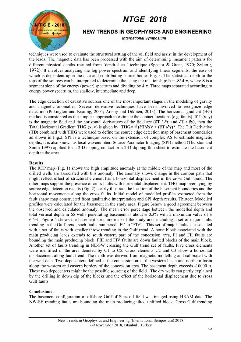
New Trends in Geophysics and Engineering (International Semposium) 2018
7-9 November 2018, Istanbul , Turkey
techniques were used to evaluate the structural setting of the oil field and assist in the development of the leads. The magnetic data has been processed with the aim of determining lineament patterns for different physical depths resulted from ‘depth-slices’ technique (Spector & Grant, 1970; Syberg, 1972). It involves analyzing the log power spectrum and identifying linear segments, the ease of which is dependent upon the data and contributing source bodies Fig. 3. The statistical depth to the tops of the sources can be interpreted to determine the using the relationship: h = -S/ 4 π, where S is a segment slope of the energy (power) spectrum and dividing by 4 π. Three maps separated according to energy power spectrum, the shallow, intermediate and deep. The edge detection of causative sources one of the most important stages in the modeling of gravity and magnetic anomalies. Several derivative techniques have been involved to recognize edge detection (Pilkington and Keating, 2004; Arisoy and Dikmen, 2013). The horizontal gradient (HG) method is considered as the simplest approach to estimate the contact locations (e.g. faults). If T (x, y) is the magnetic field and the horizontal derivatives of the field are (∂T / ∂x and ∂T / ∂y), then the Total Horizontal Gradient THG (x, y) is given by: THG= √ (∂T/∂x)2 + (∂T /∂y) 2. The Tilt Derivative (TD) combined with THG were used to define the source edge detection map of basement boundaries as shown in Fig.2. SPI is a technique based on the extension of complex AS to estimate magnetic depths; it is also known as local wavenumber. Source Parameter Imaging (SPI) method (Thurston and Smith 1997) applied for a 2-D sloping contact or a 2-D dipping thin sheet to estimate the basement depth in the area. Results The RTP map (Fig. 1) shows the high amplitude anomaly at the middle of the map and most of the drilled wells are associated with this anomaly. The anomaly shows change in the contour path that might reflect effect of structural element has a horizontal displacement in the cross Gulf trend. The other maps support the presence of cross faults with horizontal displacement. THG map overlaying by source edge detection results (Fig. 2) clearly illustrate the location of the basement boundaries and the horizontal movements along the cross faults. Initial model of modelled profiles extracted from the fault shape map constructed from qualitative interpretation and SPI depth results. Thirteen Modelled profiles were calculated for the basement in the study area. Figure 3show a good agreement between the observed and calculated anomaly. The mean error percentage between the modelled depth and total vertical depth in 65 wells penetrating basement is about ± 0.3% with a maximum value of ± 6.5%. Figure 4 shows the basement structure map of the study area including a set of major faults trending in the Gulf trend, such faults numbered “FI’ to “FIV”. This set of major faults is associated with a set of faults with smaller throw trending in the Gulf trend. A horst block associated with the main producing leads extends to south eastern part of the concession area, FI and FII faults are bounding the main producing block. FIII and FIV faults are down faulted blocks of the main block. Another set of faults trending in NE-SW crossing the Gulf trend set of faults. Five cross elements were identified in the area denoted by C1 to C5. Cross elements C2 and C3 show a horizontal displacement along fault trend. The depth was derived from magnetic modelling and calibrated with the well data. Two depocenters defined at the concession area, the western basin and northern basin along the western and eastern borders of the concession area. The basement depth exceeds -10000 ft. These two depocenters might be the possible sourcing of the field. The dry wells can partly explained by the drilling in down dip of the blocks and the effect of the horizontal displacement due to cross Gulf faults. Conclusions The basement configuration of offshore Gulf of Suez oil field was imaged using HRAM data. The NW-SE trending faults are bounding the main producing tilted uplifted block. Cross Gulf trending
9292
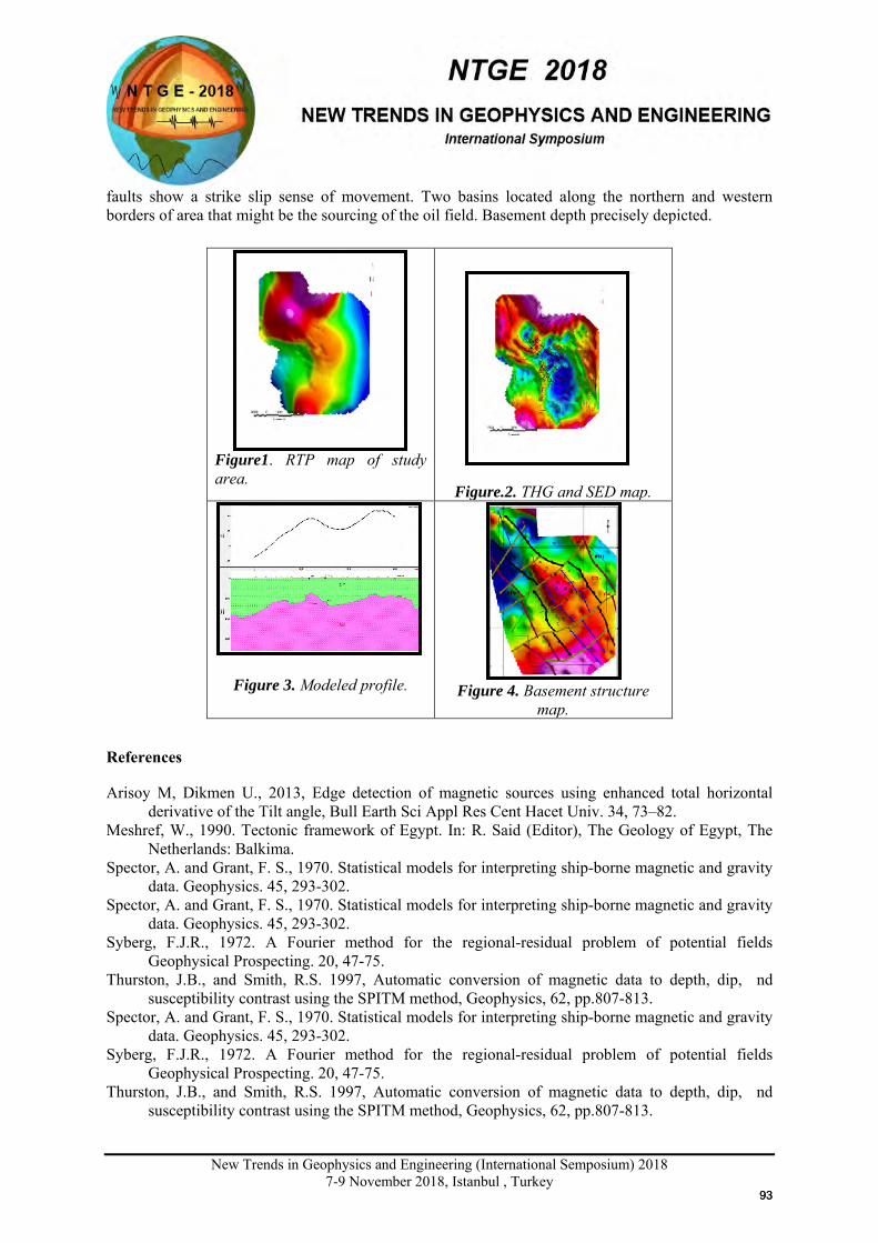
New Trends in Geophysics and Engineering (International Semposium) 2018
7-9 November 2018, Istanbul , Turkey
faults show a strike slip sense of movement. Two basins located along the northern and western borders of area that might be the sourcing of the oil field. Basement depth precisely depicted. References Arisoy M, Dikmen U., 2013, Edge detection of magnetic sources using enhanced total horizontal
derivative of the Tilt angle, Bull Earth Sci Appl Res Cent Hacet Univ. 34, 73–82. Meshref, W., 1990. Tectonic framework of Egypt. In: R. Said (Editor), The Geology of Egypt, The
Netherlands: Balkima. Spector, A. and Grant, F. S., 1970. Statistical models for interpreting ship-borne magnetic and gravity
data. Geophysics. 45, 293-302. Spector, A. and Grant, F. S., 1970. Statistical models for interpreting ship-borne magnetic and gravity
data. Geophysics. 45, 293-302. Syberg, F.J.R., 1972. A Fourier method for the regional-residual problem of potential fields
Geophysical Prospecting. 20, 47-75. Thurston, J.B., and Smith, R.S. 1997, Automatic conversion of magnetic data to depth, dip, nd
susceptibility contrast using the SPITM method, Geophysics, 62, pp.807-813. Spector, A. and Grant, F. S., 1970. Statistical models for interpreting ship-borne magnetic and gravity
data. Geophysics. 45, 293-302. Syberg, F.J.R., 1972. A Fourier method for the regional-residual problem of potential fields
Geophysical Prospecting. 20, 47-75. Thurston, J.B., and Smith, R.S. 1997, Automatic conversion of magnetic data to depth, dip, nd
susceptibility contrast using the SPITM method, Geophysics, 62, pp.807-813.
Figure1. RTP map of study area.
Figure.2. THG and SED map.
Figure 3. Modeled profile. Figure 4. Basement structure
map.
9393
New Trends in Geophysics and Engineering (International Semposium) 2018
7-9 November 2018, Istanbul, Turkey
Tracing the Hisarcık Fault with 2D VES Inversion and Numerical Fluid Flow and Temperature Simulations
Serkan Üner1 , Gülçin Özürlan Ağaçgözgü1, Doğa Düşünür Doğan1
1 Istanbul Technical University, Faculty of Mines, Geophysical Engineering Department
Presentation Type All accepted proceedings will be published on the webpage of the symposium (ntge2018.istanbul.edu.tr)
ORAL POSTER
Abstracts Under effect of extensive tectonism, Western Anatolia hosts many geothermal sources with low-moderate and high temperatures. Even though it is known that active faults play a dominant role to control recharge and discharge of the hot fluid, their effects are not fully understood. For this purpose, we have obtained the 2D geoelectrical structure of Hisarcık, Kütahya geothermal field to map possible conduits for the geothermal fluid and conducted numerical simulations to investigate fluid flow and temperature pattern of the area. Numerical simulation results suggest that Hisarcık fault predominantly control the transport of hot fluid from depth. Furthermore, predicted outflow vents match well with the location and temperature of the hot springs in the area.
Keywords: Resistivity, Inversion, Numerical simulation, Fluid flow, Temperature Introduction There are number of studies that investigate the geothermal potential of the Western Anatolia by means of resistivity and seismic surveys (e.g. Özürlan et al. 2006; Çifçti and Bozkurt, 2010; Erdoğan and Candansayar, 2017). Resistivity measurements are widely used and well suited for the investigations of the geothermal resources due to the sensitivity for the physical property changes occurred by hydrothermal processes. (e.g. Özürlan et al., 2006; Erdoğan and Candansayar, 2017). In geothermal areas, presence of hot water in the thermal springs seep through the faults with increased permeability and produce vertical electrical conductors, which can be imaged using electrical methods. Numerical simulations are powerful tools predict the fluid flow and temperature distribution in a geothermal area to estimate the geothermal potential (e.g. McKenna and Blackwell, 2004; Magri et al. 2010, 2012; Düşünür-Doğan 2014). Integrating stratigraphy, faults and topography in numerical models is important to investigate the possible pathways of the geothermal fluid and resulting temperature pattern. These integration is increasingly used in the exploration of fractured environments of hydrothermal systems (e.g., McKenna & Blackwell 2004; Simms and Garven 2004). One of the vital outcome of these studies is the understanding of importance of the faults as they control recharge and discharge of the geothermal system.
X
9494
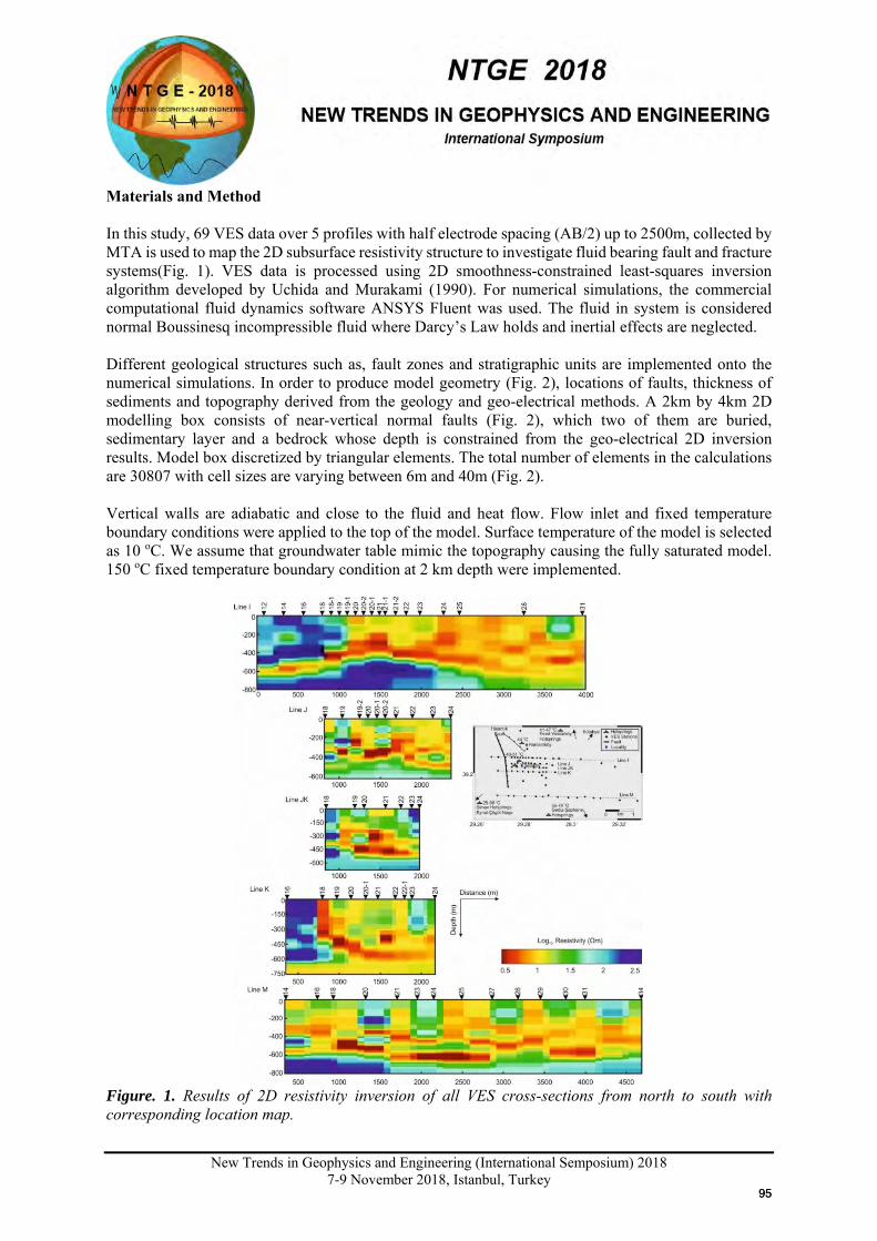
New Trends in Geophysics and Engineering (International Semposium) 2018
7-9 November 2018, Istanbul, Turkey
Materials and Method In this study, 69 VES data over 5 profiles with half electrode spacing (AB/2) up to 2500m, collected by MTA is used to map the 2D subsurface resistivity structure to investigate fluid bearing fault and fracture systems(Fig. 1). VES data is processed using 2D smoothness-constrained least-squares inversion algorithm developed by Uchida and Murakami (1990). For numerical simulations, the commercial computational fluid dynamics software ANSYS Fluent was used. The fluid in system is considered normal Boussinesq incompressible fluid where Darcy’s Law holds and inertial effects are neglected. Different geological structures such as, fault zones and stratigraphic units are implemented onto the numerical simulations. In order to produce model geometry (Fig. 2), locations of faults, thickness of sediments and topography derived from the geology and geo-electrical methods. A 2km by 4km 2D modelling box consists of near-vertical normal faults (Fig. 2), which two of them are buried, sedimentary layer and a bedrock whose depth is constrained from the geo-electrical 2D inversion results. Model box discretized by triangular elements. The total number of elements in the calculations are 30807 with cell sizes are varying between 6m and 40m (Fig. 2). Vertical walls are adiabatic and close to the fluid and heat flow. Flow inlet and fixed temperature boundary conditions were applied to the top of the model. Surface temperature of the model is selected as 10 oC. We assume that groundwater table mimic the topography causing the fully saturated model. 150 oC fixed temperature boundary condition at 2 km depth were implemented.
Figure. 1. Results of 2D resistivity inversion of all VES cross-sections from north to south with corresponding location map.
9595
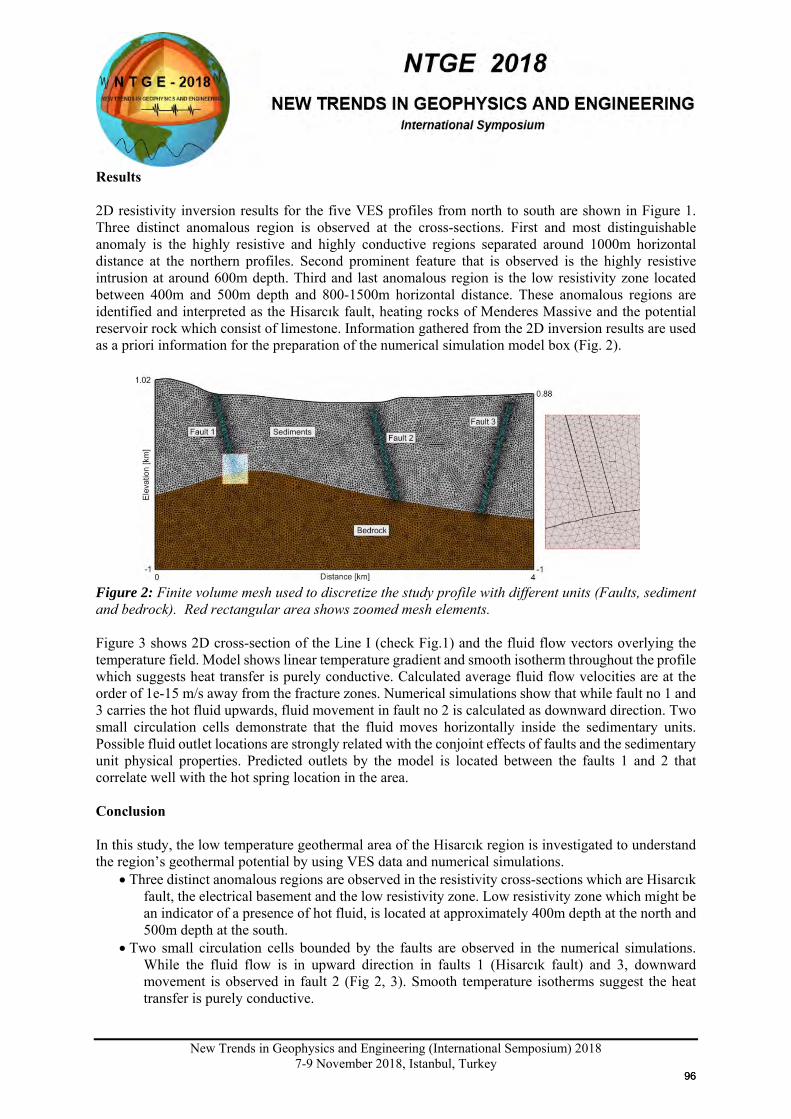
New Trends in Geophysics and Engineering (International Semposium) 2018
7-9 November 2018, Istanbul, Turkey
Results 2D resistivity inversion results for the five VES profiles from north to south are shown in Figure 1. Three distinct anomalous region is observed at the cross-sections. First and most distinguishable anomaly is the highly resistive and highly conductive regions separated around 1000m horizontal distance at the northern profiles. Second prominent feature that is observed is the highly resistive intrusion at around 600m depth. Third and last anomalous region is the low resistivity zone located between 400m and 500m depth and 800-1500m horizontal distance. These anomalous regions are identified and interpreted as the Hisarcık fault, heating rocks of Menderes Massive and the potential reservoir rock which consist of limestone. Information gathered from the 2D inversion results are used as a priori information for the preparation of the numerical simulation model box (Fig. 2).
Figure 2: Finite volume mesh used to discretize the study profile with different units (Faults, sediment and bedrock). Red rectangular area shows zoomed mesh elements. Figure 3 shows 2D cross-section of the Line I (check Fig.1) and the fluid flow vectors overlying the temperature field. Model shows linear temperature gradient and smooth isotherm throughout the profile which suggests heat transfer is purely conductive. Calculated average fluid flow velocities are at the order of 1e-15 m/s away from the fracture zones. Numerical simulations show that while fault no 1 and 3 carries the hot fluid upwards, fluid movement in fault no 2 is calculated as downward direction. Two small circulation cells demonstrate that the fluid moves horizontally inside the sedimentary units. Possible fluid outlet locations are strongly related with the conjoint effects of faults and the sedimentary unit physical properties. Predicted outlets by the model is located between the faults 1 and 2 that correlate well with the hot spring location in the area. Conclusion In this study, the low temperature geothermal area of the Hisarcık region is investigated to understand the region’s geothermal potential by using VES data and numerical simulations.
• Three distinct anomalous regions are observed in the resistivity cross-sections which are Hisarcık fault, the electrical basement and the low resistivity zone. Low resistivity zone which might be an indicator of a presence of hot fluid, is located at approximately 400m depth at the north and 500m depth at the south.
• Two small circulation cells bounded by the faults are observed in the numerical simulations. While the fluid flow is in upward direction in faults 1 (Hisarcık fault) and 3, downward movement is observed in fault 2 (Fig 2, 3). Smooth temperature isotherms suggest the heat transfer is purely conductive.
9696
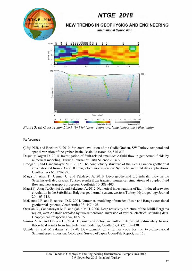
New Trends in Geophysics and Engineering (International Semposium) 2018
7-9 November 2018, Istanbul, Turkey
Figure 3: (a) Cross-section Line I, (b) Fluid flow vectors overlying temperature distribution. References Çiftçi N.B. and Bozkurt E. 2010. Structural evolution of the Gediz Graben, SW Turkey: temporal and
spatial variation of the graben basin. Basin Research 22, 846-873. Düşünür Doğan D. 2014. Investigation of fault-related small-scale fluid flow in geothermal fields by
numerical modeling. Turkish Journal of Earth Science 23, 67-79. Erdoğan E and Candansayar M.E. 2017. The conductivity structure of the Gediz Graben geothermal
area extracted from 2D and 3D magnetotelluric inversion: Synthetic and field data applications. Geothermics 65, 170-179.
Magri F., Akar T., Gemici U. and Pekdeger A. 2010. Deep geothermal groundwater flow in the Seferihisar–Balçova area, Turkey: results from transient numerical simulations of coupled fluid flow and heat transport processes. Geofluids 10, 388–405.
Magri F., Akar T., Gemici U. and Pekdeger A. 2012. Numerical investigations of fault-induced seawater circulation in the Seferihisar-Balçova geothermal system, western Turkey. Hydrogeology Journal 20, 103-118.
McKenna J.R, and Blackwell D.D. 2004. Numerical modeling of transient Basin and Range extensional geothermal systems. Geothermics 33, 457-476.
Özürlan G., Candansayar M.E. and Şahin M.H. 2006. Deep resistivity structure of the Dikili-Bergama region, west Anatolia revealed by two-dimensional inversion of vertical electrical sounding data. Geophysical Prospecting 54, 187-197.
Simms M.A. and Garven G. 2004. Thermal convection in faulted extensional sedimentary basins: theoretical results from finite-element modeling, Geofluids, 4, (2), 109-130.
Uchida T. and Murakami Y. 1990. Development of a fortran code for the two-dimensional Schlumberger inversion. Geological Survey of Japan Open-File Report, no. 150.
9797
New Trends in Geophysics and Engineering (International Semposium) 2018
7-9 November 2018, Istanbul , Turkey
A Close Look at Crustal Structure of Lake-Van Region from Inter-Station Rayleigh Wave Phase Velocities
Hamdi Alkan1*, Hakan Çınar2
1 Department of Geophysics, Faculty of Eng.,Van Yüzüncü Yıl University, Van
2 Department of Geophysics, Faculty of Eng.,Karadeniz Technical University, Trabzon Email: [email protected]
Presentation Type All accepted proceedings will be published on the webpage of the symposium (ntge2018.istanbul.edu.tr)
ORAL POSTER
Abstracts In this study, we have determined the average crustal and the uppermost mantle shear velocities around the Lake Van Region (Eastern Turkey). For this purpose, we have used to the fundamental mode interstation Rayleigh wave phase velocities. The phase velocities were calculated from the regional earthquakes recorded by Kandilli Observatory and Earthquake Research Institute stations. The earthquakes were downloaded by using European Integrated Data Archive. Considering back azimuth differences of each source and station path, three different broadband station pairs (GURO-VANB, AGRB-VANB and MLAZ-VANB) and a few earthquakes were selected to determine the 1-D S-wave structures by using an interstation method (slant stacking technique). The linearized least squares algorithm was helped to define the shear-velocity model, which is the best fit the observed phase velocity dispersion curve. The normalized statistical resolution matrix was calculated to measure the reliability of the solution. Inversion results show that the solution quality of the upper crust is not good because of the high resolution lengths. The average shear-wave velocities of the lower crust are nearly 3.5 km/s. It is concluded that the low-velocity zone shown in the lower crust may be associated with widespread volcanism. According to the last 2-D S-wave velocity models, the moho discontinuity is ~42 km, and shear velocities range between 3.6 to 4.2 km/s. In addition, the uppermost mantle (~45–70 km) velocities are slower than globally earth models, and it is probably connected with hot asthenospheric material. Keywords: Crustal Structure, Lake Van Basin, Inter-Station, Rayleigh Wave, Inversion Introduction Eastern Anatolian Plateau is livingly part of an active tectonic region, which is about the Arabian Plate collides with the Eurasian Plate. This system brings about to a westward escape and counter-clockwise rotation of the Anatolian Plate along the dextral North Anatolian Fault Zone (NAFZ) and sinistral East Anatolian Fault Zone (EAFZ). The tectonic structure of the Lake Van region, which is located in the south of the Bitlis-Zagros Thrust Zone, is related to this regional tectonic structure (Figure 1). The effects between the Arabian and Eurasian Plates naturally created several strike-slip and thrust faults such as Van Fault and Gevaş Fault in the study region (Utkucu et al., 2013; Çukur et al., 2017).
9898
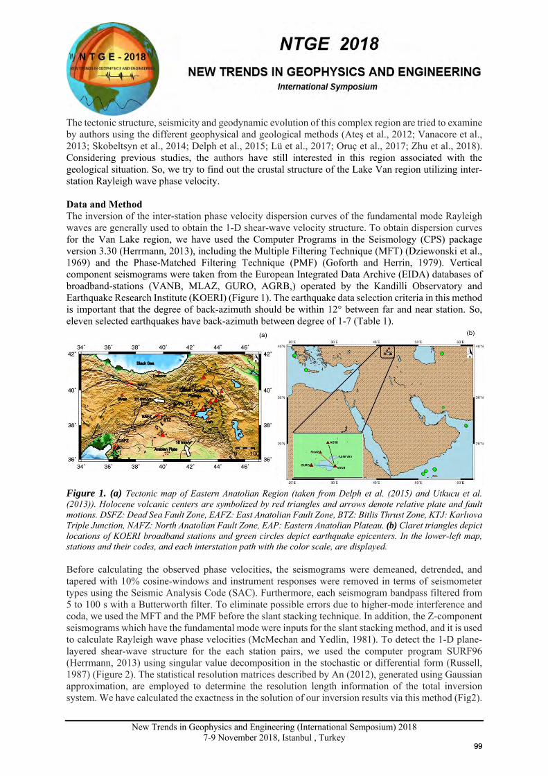
New Trends in Geophysics and Engineering (International Semposium) 2018
7-9 November 2018, Istanbul , Turkey
The tectonic structure, seismicity and geodynamic evolution of this complex region are tried to examine by authors using the different geophysical and geological methods (Ateş et al., 2012; Vanacore et al., 2013; Skobeltsyn et al., 2014; Delph et al., 2015; Lü et al., 2017; Oruç et al., 2017; Zhu et al., 2018). Considering previous studies, the authors have still interested in this region associated with the geological situation. So, we try to find out the crustal structure of the Lake Van region utilizing inter-station Rayleigh wave phase velocity. Data and Method The inversion of the inter-station phase velocity dispersion curves of the fundamental mode Rayleigh waves are generally used to obtain the 1-D shear-wave velocity structure. To obtain dispersion curves for the Van Lake region, we have used the Computer Programs in the Seismology (CPS) package version 3.30 (Herrmann, 2013), including the Multiple Filtering Technique (MFT) (Dziewonski et al., 1969) and the Phase-Matched Filtering Technique (PMF) (Goforth and Herrin, 1979). Vertical component seismograms were taken from the European Integrated Data Archive (EIDA) databases of broadband-stations (VANB, MLAZ, GURO, AGRB,) operated by the Kandilli Observatory and Earthquake Research Institute (KOERI) (Figure 1). The earthquake data selection criteria in this method is important that the degree of back-azimuth should be within 12° between far and near station. So, eleven selected earthquakes have back-azimuth between degree of 1-7 (Table 1).
Figure 1. (a) Tectonic map of Eastern Anatolian Region (taken from Delph et al. (2015) and Utkucu et al. (2013)). Holocene volcanic centers are symbolized by red triangles and arrows denote relative plate and fault motions. DSFZ: Dead Sea Fault Zone, EAFZ: East Anatolian Fault Zone, BTZ: Bitlis Thrust Zone, KTJ: Karlıova Triple Junction, NAFZ: North Anatolian Fault Zone, EAP: Eastern Anatolian Plateau. (b) Claret triangles depict locations of KOERI broadband stations and green circles depict earthquake epicenters. In the lower-left map, stations and their codes, and each interstation path with the color scale, are displayed. Before calculating the observed phase velocities, the seismograms were demeaned, detrended, and tapered with 10% cosine-windows and instrument responses were removed in terms of seismometer types using the Seismic Analysis Code (SAC). Furthermore, each seismogram bandpass filtered from 5 to 100 s with a Butterworth filter. To eliminate possible errors due to higher-mode interference and coda, we used the MFT and the PMF before the slant stacking technique. In addition, the Z-component seismograms which have the fundamental mode were inputs for the slant stacking method, and it is used to calculate Rayleigh wave phase velocities (McMechan and Yedlin, 1981). To detect the 1-D plane-layered shear-wave structure for the each station pairs, we used the computer program SURF96 (Herrmann, 2013) using singular value decomposition in the stochastic or differential form (Russell, 1987) (Figure 2). The statistical resolution matrices described by An (2012), generated using Gaussian approximation, are employed to determine the resolution length information of the total inversion system. We have calculated the exactness in the solution of our inversion results via this method (Fig2).
9999
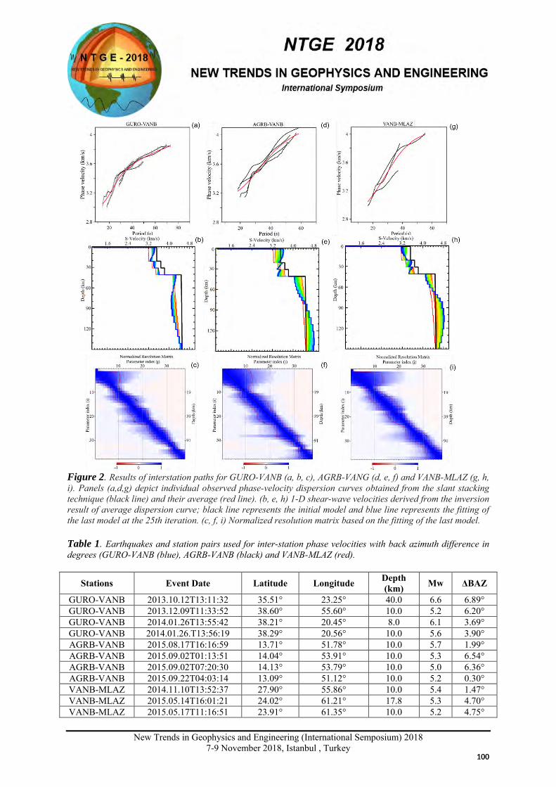
New Trends in Geophysics and Engineering (International Semposium) 2018
7-9 November 2018, Istanbul , Turkey
Figure 2. Results of interstation paths for GURO-VANB (a, b, c), AGRB-VANG (d, e, f) and VANB-MLAZ (g, h, i). Panels (a,d,g) depict individual observed phase-velocity dispersion curves obtained from the slant stacking technique (black line) and their average (red line). (b, e, h) 1-D shear-wave velocities derived from the inversion result of average dispersion curve; black line represents the initial model and blue line represents the fitting of the last model at the 25th iteration. (c, f, i) Normalized resolution matrix based on the fitting of the last model. Table 1. Earthquakes and station pairs used for inter-station phase velocities with back azimuth difference in degrees (GURO-VANB (blue), AGRB-VANB (black) and VANB-MLAZ (red).
Stations Event Date Latitude Longitude Depth (km) Mw ΔBAZ
GURO-VANB 2013.10.12T13:11:32 35.51° 23.25° 40.0 6.6 6.89° GURO-VANB 2013.12.09T11:33:52 38.60° 55.60° 10.0 5.2 6.20° GURO-VANB 2014.01.26T13:55:42 38.21° 20.45° 8.0 6.1 3.69° GURO-VANB 2014.01.26.T13:56:19 38.29° 20.56° 10.0 5.6 3.90° AGRB-VANB 2015.08.17T16:16:59 13.71° 51.78° 10.0 5.7 1.99° AGRB-VANB 2015.09.02T01:13:51 14.04° 53.91° 10.0 5.3 6.54° AGRB-VANB 2015.09.02T07:20:30 14.13° 53.79° 10.0 5.0 6.36° AGRB-VANB 2015.09.22T04:03:14 13.09° 51.12° 10.0 5.2 0.30° VANB-MLAZ 2014.11.10T13:52:37 27.90° 55.86° 10.0 5.4 1.47° VANB-MLAZ 2015.05.14T16:01:21 24.02° 61.21° 17.8 5.3 4.70° VANB-MLAZ 2015.05.17T11:16:51 23.91° 61.35° 10.0 5.2 4.75°
100100
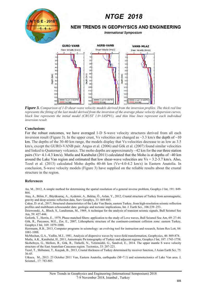
New Trends in Geophysics and Engineering (International Semposium) 2018
7-9 November 2018, Istanbul , Turkey
Figure 3. Comparison of 1-D shear-wave velocity models derived from the inversion profiles. The thick red line represents the fitting of the last model derived from the inversion of the average phase velocity dispersion curves, black line represents the initial model (CRUST 1.0+IASP91), and thin blue lines represent each individual inversion result. Conclusions For the robust outcomes, we have averaged 1-D S-wave velocity structures derived from all each inversion result (Figure 3). In the upper crust, Vs velocities are changed as ~3.3 km/s the depth of ~10 km. The depths of the 30-40 km range, the models display that Vs-velocities decrease to as low as 3.5 km/s, except the GURO-VANB pair. Angus et al. (2006) and Gök et al. (2007) found similar velocities and linked to Quaternary volcanics. The moho depths are approximately ~42 km for the our three station pairs (Vs= 4.1-4.3 km/s). Mutlu and Karabulut (2011) calculated that the Moho is at depths of ~40 km around the Lake Van region and estimated that low shear-wave velocities are Vs = 3.2-3.7 km/s. Also, Tezel et al. (2013) calculated Moho depths 40-46 km (Vs=4.0-4.2 km/s) in Eastern Anatolia. In conclusion, S-wave velocity models (Figure 3) have supplied on the reliable results about the crustal structure in the region.
References
An, M., 2012, A simple method for determining the spatial resolution of a general inverse problem, Geophys J Int, 191: 849-864. Ateş, A., Bilim, F., Büyüksaraç, A., Aydemir, A., Bektaş, Ö., Aslan, Y., 2012, Crustal structure of Turkey from aeromagnetic, gravity and deep seismic reflection data, Surv Geophys, 33: 869-885. Çukur, D. et al., 2017, Structural characteristics of the Lake Van Basin, eastern Turkey, from high-resolution seismic reflection profiles and multibeam echosounder data: geologic and tectonic implications, Int. J. Earth Sci., 106:239–253. Dziewonski, A., Bloch, S., Landisman, M., 1969, A technique for the analysis of transient seismic signals, Bull Seismol Soc Am, 59: 427-444. Goforth, T., Herrin, E., 1979, Phase-matched filters: application to the study of Love waves, Bull Seismol Soc Am, 69: 27-44. Gök, R., Pasyanos, M.E., Zor, E., 2007, Lithospheric structure of the continent-continent collision zone: eastern Turkey, Geophys J Int, 169: 1079-1088. Herrmann, R.B., 2013, Computer programs in seismology: an evolving tool for instruction and research, Seism Res Lett, 84: 1081-1088. McMechan, G.A., Yedlin, M.J., 1981, Analysis of dispersive waves by wave-field transformation, Geophysics, 46: 869-874. Mutlu, A.K., Karabulut, H., 2011, Anisotropic Pn tomography of Turkey and adjacent regions, Geophys J Int, 187: 1743-1758. Skobeltsyn, G., Mellors, R., Gök, R., Türkelli, N., Yetirmishli, G., Sandvol, E., 2014. The upper mantle S wave velocity structure of the East Anatolian-Caucasus region. Tectonics, 33: 207-221. Tezel, T., Shibutani, T., Kaypak, B., 2013, Crustal thickness of Turkey determined by receiver function, J Asian Earth Sci, 75: 36-45. Utkucu, M., 2013. 23 October 2011 Van, Eastern Anatolia, earthquake (M=7.1) and seismotectonics of Lake Van area. J, Seismol., 17: 783-805.
101101
New Trends in Geophysics and Engineering (International Semposium) 2018
7-9November 2018, Istanbul ,Turkey
MODELLING THE TSUNAMI GENERATION OF THE SEPTEMBER 28, 2018 MINAHASA PENINSULA, SULAWESI ISLAND, INDONESIA EARTHQUAKE
Ergin Ulutaş1
1 Geophysical Eng. Department, Kocaeli University, Kocaeli, Turkey Email: [email protected]
Abstract This study presents the preliminary results of the simulated tsunami generated from the Minahasa Peninsula, Sulawesi Island, Indonesia. The epicenter of the earthquake located in the mountainous Donggala Regency, in the neck of the Minahasa Peninsula. The earthquake occurred as a result of strike-slip faulting at shallow depths within the interior of the Molucca Sea microplate. Source rupture model from focal mechanism solution given by USGS (United State Geological Survey) was carried out to explain the tsunami propagation in Minahasa Peninsula and Palu Bay. The initial source model calculated in this study was used to model the deformation on sea bottom which is translated directly to the water surface. The vertical deformation on the sea floor was based on the elastic dislocation theory and empirical scaling laws for a uniform fault. The maximum subsidence and maximum uplift are found as -0.25 m and 0.10 m respectively. Based on the uniform sea floor deformation source model, arrival times and maximum wave heights were presented here for the coastal areas of Palu and Donggala. The results show that the earthquake could not generate 6 meters tsunamis contrary to the experienced larger tsunami heights and reported news in the region. This suggests that there may be a secondary effect, such as a sea landslide to generate larger tsunamis in the region.
Keywords: Focal mechanism solution, vertical deformation, initial height, tsunami simulation, bathymetry. Introduction A major earthquake occurred on September 28, 2018 at :10:02:43 UTC (05:02 Western Indonesia Local Time) in Minahasa Peninsula, Sulawesi Island, Indonesia. The earthquake was located 77 km away from the provincial capital Palu and was felt as far away as Samarinda on the East Kalimantan and also in Tawau, Malaysia. This event was preceded by a sequence of foreshocks, the largest of which was a magnitude 6.1 tremor that occurred earlier in the same day at 07:00:01 UTC. The earthquake struck just off the central island of Sulawesi, setting off a tsunami that destroyed mostly the coastal city of Palu. Thousands of homes, as well as an eight-storey hotel, hospital and a large department store were damaged in the city (https://www.theguardian.com). The death toll from the earthquake and tsunami was reported by the authorities as 1200 by Indonesia’s deadliest such disaster in more than a decade as of 4 October 2018 (https://www.bloomberg.com/news). Almost 800 people were seriously injured and 99 were missing show that this number will increase. Most tsunamis generating from earthquakes around Indonesia emerge from movement on the Sunda mega-thrust fault where the Indo-Australian plate dives down underneath the Eurasian plate. There are many tsunamis in the Sunda mega-thrust fault system. Most of these caused damage and death was the December 26, 2004 Indian ocean earthquake with an epicenter off the west coast of northern Sumatra and a magnitude of 9.3 from a mega-thrust faulting. Tsunamis are often the result of so-called megathrust earthquakes, when huge sections of the Earth’s crust are deformed, moving vertically along a fault. Violent vertical motion caused by mega-thrust earthquakes displace a huge volume of
102102
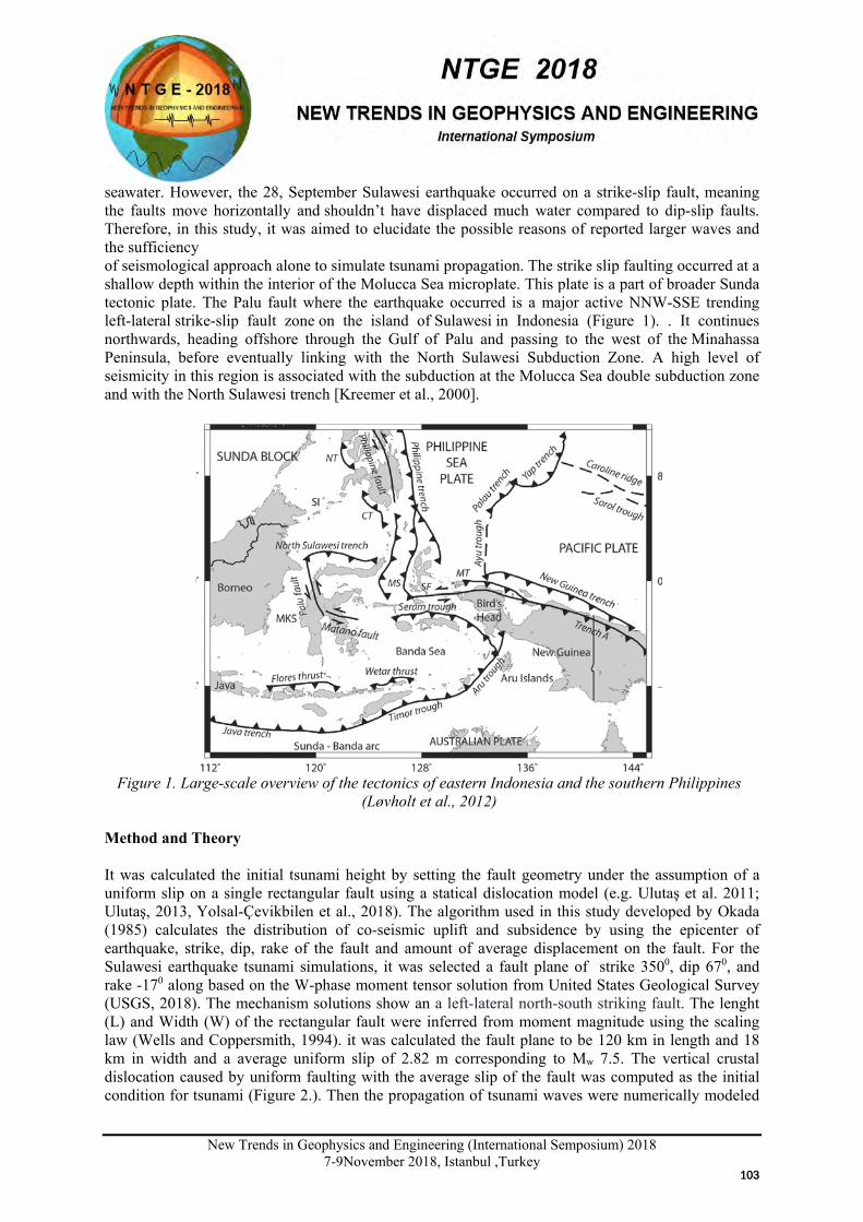
New Trends in Geophysics and Engineering (International Semposium) 2018
7-9November 2018, Istanbul ,Turkey
seawater. However, the 28, September Sulawesi earthquake occurred on a strike-slip fault, meaning the faults move horizontally and shouldn’t have displaced much water compared to dip-slip faults. Therefore, in this study, it was aimed to elucidate the possible reasons of reported larger waves and the sufficiency of seismological approach alone to simulate tsunami propagation. The strike slip faulting occurred at a shallow depth within the interior of the Molucca Sea microplate. This plate is a part of broader Sunda tectonic plate. The Palu fault where the earthquake occurred is a major active NNW-SSE trending left-lateral strike-slip fault zone on the island of Sulawesi in Indonesia (Figure 1). . It continues northwards, heading offshore through the Gulf of Palu and passing to the west of the Minahassa Peninsula, before eventually linking with the North Sulawesi Subduction Zone. A high level of seismicity in this region is associated with the subduction at the Molucca Sea double subduction zone and with the North Sulawesi trench [Kreemer et al., 2000].
Figure 1. Large-scale overview of the tectonics of eastern Indonesia and the southern Philippines
(Løvholt et al., 2012) Method and Theory It was calculated the initial tsunami height by setting the fault geometry under the assumption of a uniform slip on a single rectangular fault using a statical dislocation model (e.g. Ulutaş et al. 2011; Ulutaş, 2013, Yolsal-Çevikbilen et al., 2018). The algorithm used in this study developed by Okada (1985) calculates the distribution of co-seismic uplift and subsidence by using the epicenter of earthquake, strike, dip, rake of the fault and amount of average displacement on the fault. For the Sulawesi earthquake tsunami simulations, it was selected a fault plane of strike 3500, dip 670, and rake -170 along based on the W-phase moment tensor solution from United States Geological Survey (USGS, 2018). The mechanism solutions show an a left-lateral north-south striking fault. The lenght (L) and Width (W) of the rectangular fault were inferred from moment magnitude using the scaling law (Wells and Coppersmith, 1994). it was calculated the fault plane to be 120 km in length and 18 km in width and a average uniform slip of 2.82 m corresponding to Mw 7.5. The vertical crustal dislocation caused by uniform faulting with the average slip of the fault was computed as the initial condition for tsunami (Figure 2.). Then the propagation of tsunami waves were numerically modeled
103103
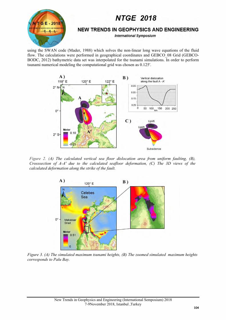
New Trends in Geophysics and Engineering (International Semposium) 2018
7-9November 2018, Istanbul ,Turkey
using the SWAN code (Mader, 1988) which solves the non-linear long wave equations of the fluid flow. The calculations were performed in geographical coordinates and GEBCO_08 Grid (GEBCO-BODC, 2012) bathymetric data set was interpolated for the tsunami simulations. In order to perform tsunami numerical modeling the computational grid was chosen as 0.125′.
Figure 2. (A) The calculated vertical sea floor dislocation area from uniform faulting, (B), Crosssection of A-A' due to the calculated seafloor deformation, (C) The 3D views of the calculated deformation along the strike of the fault.
Figure 3. (A) The simulated maximum tsunami heights, (B) The zoomed simulated maximum heights corresponds to Palu Bay.
104104
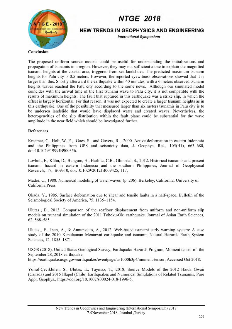
New Trends in Geophysics and Engineering (International Semposium) 2018
7-9November 2018, Istanbul ,Turkey
Conclusion The proposed uniform source models could be useful for understanding the initializations and propagation of tsunamis in a region. However, they may not sufficient alone to explain the magnified tsunami heights at the coastal area, triggered from sea landslides. The predicted maximum tsunami heights for Palu city is 0.5 meters. However, the reported eyewitness observations showed that it is larger than this. Shortly afterward the earthquake within 40 minutes, with a 6 meters observed tsunami heights waves reached the Palu city according to the some news. Although our simulated model coincides with the arrival time of the first tsunami wave to Palu city, it is not compatible with the results of maximum heights. The fault that ruptured in this earthquake was a strike slip, in which the offset is largely horizontal. For that reason, it was not expected to create a larger tsunami heights as in this earthquake. One of the possibility that measured larger than six meters tsunamis in Palu city is to be undersea landslide that would have displaced water and created waves. Nevertheless, the heterogeneities of the slip distribution within the fault plane could be substantial for the wave amplitude in the near field which should be investigated further. References Kreemer, C., Holt, W. E., Goes, S. and Govers, R., 2000. Active deformation in eastern Indonesia and the Philippines from GPS and seismicity data, J. Geophys. Res., 105(B1), 663–680, doi:10.1029/1999JB900356. Løvholt, F., Kühn, D., Bungum, H., Harbitz, C.B., Glimsdal, S., 2012. Historical tsunamis and present tsunami hazard in eastern Indonesia and the southern Philippines, Journal of Geophysical Research,117, B09310, doi:10.1029/2012JB009425, 117, Mader, C., 1988. Numerical modeling of water waves (p. 206). Berkeley, California: University of California Press. Okada, Y., 1985. Surface deformation due to shear and tensile faults in a half-space. Bulletin of the Seismological Society of America, 75, 1135–1154. Ulutas¸, E., 2013. Comparison of the seafloor displacement from uniform and non-uniform slip models on tsunami simulation of the 2011 Tohoku-Oki earthquake. Journal of Asian Earth Sciences, 62, 568–585. Ulutas¸, E., Inan, A., & Annunziato, A., 2012. Web-based tsunami early warning system: A case study of the 2010 Kepulaunan Mentawai earthquake and tsunami. Natural Hazards Earth System Sciences, 12, 1855–1871. USGS (2018). United States Geological Survey, Earthquake Hazards Program, Moment tensor of the September 28, 2018 earthquake. https://earthquake.usgs.gov/earthquakes/eventpage/us1000h3p4/moment-tensor, Accessed Oct 2018. Yolsal-Çevikbilen, S., Ulutaş, E., Taymaz, T., 2018. Source Models of the 2012 Haida Gwaii (Canada) and 2015 Illapel (Chile) Earthquakes and Numerical Simulations of Related Tsunamis, Pure Appl. Geophys., https://doi.org/10.1007/s00024-018-1996-5.
105105
New Trends in Geophysics and Engineering (International Semposium) 2018
7-9 November 2018, Istanbul , Turkey
X
EXTENDING SPECTRAL BAND OF SEISMIC DATA BY THE CEPSTRAL SHORT
TIME FOURIER TRANSFORM
Hakan Karslı1 1 Geophysical Eng. Department, Karadeniz Technical University, Trabzon
Email: [email protected] Presentation Type
ORAL POSTER
Abstracts The numerical processes to improve the vertical resolution of seismic reflection data are still on going because seismic data have generally poor available spectral bandwidth. Interpretations need to have more resolution seismic stack section to identify stratigraphic and structural fine features. Because the vertical resolution is a function of frequency content of a signal, if the available spectral band is first extended to both low and high frequencies parts by a processing technique, the side lobes of reflection wavelet reduce and its main lobe also narrows. Simultaneously, to achieve this, it can be combined the short time Fourier transform (STFT) and cepstrum analysis within a work flow which is named as cepstral STFT (C-STFT) and doesn’t require any user-defined parameter. In practice the cepstrum is defined as an inverse Fourier transform of logarithm of Fourier amplitude spectrum of signal. Therefore, lower frequencies are powering which leads to decrease the side lobes of reflection wavelet. On the other hand, the method amplifies the high frequencies without greatly boosting the random noise. Applications with synthetic and field data show that the method can improve the vertical resolution which is very useful to interpret the seismic data from thin layered sedimentary medium.
Keywords: Cepstrum, Short Time Fourier Transform, Seismic Data, Vertical Resolution Introduction The vertical resolution of seismic data is highly important to separate features and so define thinner stratigraphic units, smaller details, lateral changes in rock properties and sand-lens bearing hydrocarbon. Since the vertical resolution is directly related with extending the useful spectral band of seismic data to both sides (low and high frequencies), the spectral bandwidth needs to extend by post-processing methods which leads to reduce amplitude of side lobes and to narrow the main lobe of a reflection wavelet. For this reason, although the deconvolution processing is the popular method to broaden the bandwidth of seismic data, because of its inadequacy, new and more effective processes methods such as time variant spectral whitening (Yılmaz, 2001), inverse Q-filtering (Wang, 2008), Gabor deconvolution (Margrave et al., 2011), autoregressive extrapolation (Karslı, 2006) have been applied to seismic data during the data processing to achieve desirable vertical resolution before and after stacking and these developments are still going on. Each of them has their advantages and disadvantages because of the assumptions and theories governing their issues. Because the resolution improves as the signal dominant frequency is increased and as its bandwidth is widened, the processes mentioned above are generally designed and applied in frequency domain which is provided by
106106
New Trends in Geophysics and Engineering (International Semposium) 2018
7-9 November 2018, Istanbul , Turkey
Fourier transform (FT). However, because of nonstationary character of the wavelet which means the spectral content of it changes mostly with time, conventional FT, which is very useful and powerful for stationary signals, is not sufficient to analyze and so obtain desirable resolution. Because of this, the short time Fourier Transform (STFT) (Chakraborty and Okaya, 1995) that decomposes a signal into time-frequency (t, f) domain has recently been used for purposes of noise filtering, improving resolution and attribute analysis by several researchers (Sajid and Ghosh, 2014; Shang and Caldwell, 2003; Zhou et al., 2014). The STFT generally provides more frequency resolution with increasing spectral analysis window but decreasing time resolution. The lack of the STFT is also fulfilled by using cepstral analysis which is generally defined as the inverse Fourier transform of logarithm of Fourier amplitude spectrum (Oppenheim et al., 1997). The cepstrum analysis either provides amplifying the lower frequencies leading to diminish the side lobe of wavelet or handles time resolution limitation. In this paper, it is aimed to combine the STFT and cepstrum analysis, named as C-STFT, in an algorithm for reasonably widening the spectral bandwidth to increase the vertical resolution of seismic data. Applications with synthetic and field data show that the proposed method can effectively enhance the resolution of the seismic data. Methods and Examples The work flow and the mathematical formulas of the method are given in Figure 1. Other, what parameter and function mean is celarly indicated. However, a few points must be noted; (1) In formulations, p(t) shows the spectral decomposing window (gaussian, hann, hamming, etc.) function and τ is a time instant along time axis. In practice, by using a window function appropriately, the frequency content of the signal is mapped versus time instant, so the STFT of a signal is obtained in 2D. (2) Since the length of p(t) was optimally taken as one-fourth the length of the signal. (3) During the processing, taking logarithm of the amplitude spectrum provides the amplifying the low frequencies, but there exists negative amplitude values because of logarithm. To avoid this issue, the minimum of the logarithmic amplitude is subtracted from itself and thus all amplitude values are now purely positive and the amplitude normalization also provides an amplitude balance. Finally, the high resolution seismic trace, hrs(t) is obtained by inverse STFT transform. Note that the phase spectrum has to remain unchanged until the end of the process. It is observed that narrowing in time while widening in frequency is clearly observed when comparing the time and t-f images of the input, s(t) and output, hrs(t). The proposed method was applied on a 1D model seismic trace including very close reflection coefficient series (Fig. 2a, upper) with different polarity. The time intervals between pairs of other reflections, except for the first single reflection at 6.25ms, are respectively 7, 8, 10, 12 and 14ms. The synthetic trace (Fig. 2a, middle) as an input data was calculated by convolving a Ricker wavelet (f0=35Hz, dt=2ms) with the reflectivity series. The output from proposed method is shown in Fig. 2a (bottom). The t-f images of input and output and Fourier amplitude spectra are respectively given in Fig. 2b,c, d. When comparing the all spectral results, it is seen that the spectral band of input trace in Fig. 1a (middle) was quietly extended to both low and high frequencies. Thus, the extension gives rise to reduce side lobes and narrow the main lobe of wavelets, which leads to improve the temporal resolution of the input trace as seen in Fig. 2a (bottom). Especially, very close reflections especially at 0.12sec and 0.2sec, and a small amplitude reflection at 0.43sec could easily be defined as to define individual reflections. An application was done on a stacked field data with 4ms time interval that has many thin layers. Some selected results are presented here for making a comparison between input (Fig. 3a,d,g) and output (Fig. 3b,e,h) sections as shown in Figure 3. It can clearly be seen that the method considerably provides either more vertical resolution or horizontal reflection traceability and thus many subtle features are marked by arrows and ellipse on the sections.
107107
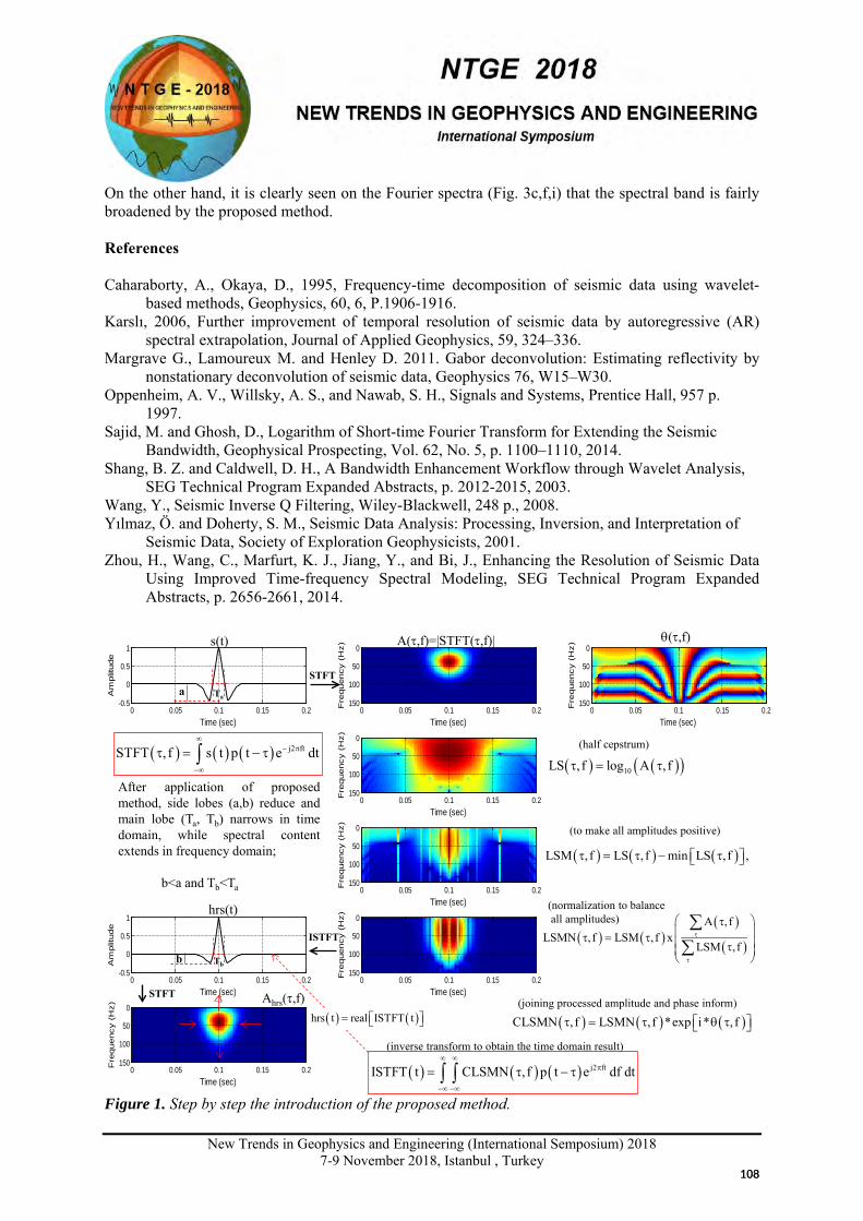
New Trends in Geophysics and Engineering (International Semposium) 2018
7-9 November 2018, Istanbul , Turkey
On the other hand, it is clearly seen on the Fourier spectra (Fig. 3c,f,i) that the spectral band is fairly broadened by the proposed method. References Caharaborty, A., Okaya, D., 1995, Frequency-time decomposition of seismic data using wavelet-
based methods, Geophysics, 60, 6, P.1906-1916. Karslı, 2006, Further improvement of temporal resolution of seismic data by autoregressive (AR)
spectral extrapolation, Journal of Applied Geophysics, 59, 324–336. Margrave G., Lamoureux M. and Henley D. 2011. Gabor deconvolution: Estimating reflectivity by
nonstationary deconvolution of seismic data, Geophysics 76, W15–W30. Oppenheim, A. V., Willsky, A. S., and Nawab, S. H., Signals and Systems, Prentice Hall, 957 p.
1997. Sajid, M. and Ghosh, D., Logarithm of Short-time Fourier Transform for Extending the Seismic
Bandwidth, Geophysical Prospecting, Vol. 62, No. 5, p. 1100–1110, 2014. Shang, B. Z. and Caldwell, D. H., A Bandwidth Enhancement Workflow through Wavelet Analysis,
SEG Technical Program Expanded Abstracts, p. 2012-2015, 2003. Wang, Y., Seismic Inverse Q Filtering, Wiley-Blackwell, 248 p., 2008. Yılmaz, Ö. and Doherty, S. M., Seismic Data Analysis: Processing, Inversion, and Interpretation of
Seismic Data, Society of Exploration Geophysicists, 2001. Zhou, H., Wang, C., Marfurt, K. J., Jiang, Y., and Bi, J., Enhancing the Resolution of Seismic Data
Using Improved Time-frequency Spectral Modeling, SEG Technical Program Expanded Abstracts, p. 2656-2661, 2014.
Figure 1. Step by step the introduction of the proposed method.
After application of proposedmethod, side lobes (a,b) reduce andmain lobe (Ta, Tb) narrows in timedomain, while spectral contentextends in frequency domain;
b<a and Tb<Ta
0 0.05 0.1 0.15 0.2-0.5
0
0.5
1
Time (sec)
Am
plitu
de
Time (sec)
Fre
quen
cy (
Hz)
0 0.05 0.1 0.15 0.2
0
50
100
150
Time (sec)
Fre
quen
cy (
Hz)
0 0.05 0.1 0.15 0.2
0
50
100
150
Time (sec)
Fre
quen
cy (
Hz)
0 0.05 0.1 0.15 0.2
0
50
100
150
Time (sec)
Fre
quen
cy (
Hz)
0 0.05 0.1 0.15 0.2
0
50
100
150
Time (sec)
Fre
quen
cy (
Hz)
0 0.05 0.1 0.15 0.2
0
50
100
1500 0.05 0.1 0.15 0.2
-0.5
0
0.5
1
Time (sec)
Am
plitu
de
Time (sec)
Fre
quen
cy (
Hz)
0 0.05 0.1 0.15 0.2
0
50
100
150
s(t) θ(τ,f)A(τ,f)=|STFT(τ,f)|
( ) ( )( )10LS , f log A ,fτ = τ
( ) ( ) ( )LSM ,f LS , f min LS ,f ,τ = τ − τ
( ) ( )( )
( )
A ,fLSMN ,f LSM ,f x
LSM ,fτ
τ
τ τ = τ τ
∑∑
hrs(t)
Ahrs(τ,f)
STFT
ISTFT
STFT
a
b
(half cepstrum)
Ta
Tb
( ) ( ) ( ) j2 ftSTFT ,f s t p t e dt∞
− π
−∞
τ = − τ∫
(to make all amplitudes positive)
(normalization to balanceall amplitudes)
(inverse transform to obtain the time domain result)
( ) ( ) ( )CLSMN ,f LSMN ,f *exp i* , fτ = τ θ τ
( ) ( ) ( ) j2 ftISTFT t CLSMN ,f p t e df dt∞ ∞
π
−∞ −∞
= τ − τ∫ ∫
(joining processed amplitude and phase inform)( ) ( )hrs t real ISTFT t=
108108
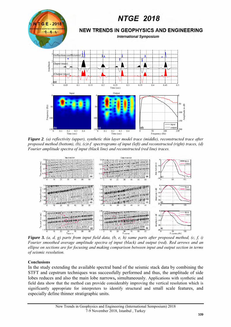
New Trends in Geophysics and Engineering (International Semposium) 2018
7-9 November 2018, Istanbul , Turkey
Figure 2. (a) reflectivity (upper), synthetic thin layer model trace (middle), reconstructed trace after proposed method (bottom), (b), (c)t-f spectrograms of input (left) and reconstructed (right) traces, (d) Fourier amplitude spectra of input (black line) and reconstructed (red line) traces.
Figure 3. (a, d, g) parts from input field data, (b, e, h) same parts after proposed method, (c, f, i) Fourier smoothed average amplitude spectra of input (black) and output (red). Red arrows and an ellipse on sections are for focusing and making comparison between input and output section in terms of seismic resolution. Conclusions In the study extending the available spectral band of the seismic stack data by combining the STFT and cepstrum techniques was successfully performed and thus, the amplitude of side lobes reduces and also the main lobe narrows, simultaneously. Applications with synthetic and field data show that the method can provide considerably improving the vertical resolution which is significantly appropriate for interpreters to identify structural and small scale features, and especially define thinner stratigraphic units.
0 0.05 0.1 0.15 0.2 0.25 0.3 0.35 0.4 0.45 0.5-1
0
1
2
3
Time (sec)
Am
plitu
de
Time (sec)
Freq
uenc
y (H
z)
Input
0 0.1 0.2 0.3 0.4
0
50
100
150
Time (sec)
Output
0 0.1 0.2 0.3 0.4
0
50
100
1500 50 100 150
-200
-150
-100
-50
0
Frequency (Hz)
Am
plitu
de in
dB
inputoutput
(reflection coefficients)
(Input trace)
(Output trace)
(a)
(b) (c) (d)
109109
New Trends in Geophysics and Engineering (International Semposium) 2018
7-9 November 2018, Istanbul , Turkey
X
IMPORTANCE OF FILTERING WITHOUT SURGICAL MUTE IN SEISMIC DATA
PROCESSING
Hakan Karslı1 , Derman Dondurur2
1 Geophysical Eng. Department, Karadeniz Technical University, Trabzon 2 Marine Science and Technology Institute, Dokuz Eylül University, İzmir
Email: [email protected] Presentation Type
ORAL POSTER
Abstracts In this study, two filtering techniques, Wiener-estimation and LITTM, to filter coherent noises such as ground-roll or swell and power line noises which distort and make them invisible contaminating seismic data are presented. The Wiener filter is designed to find the filter coefficients which are used to estimate the coherent noise embedded in seismic data. Therefore, the noise estimate has been adaptively subtracted from the data to perform attenuation process. LITTM filter is a simple and fast filtering procedure which is locally applied in spectral domain by iteratively trimmed and truncated principles to cancel power line noise with 50/60Hz. The procedure doesn’t require any reference signal or an estimate accurately the fundamental frequency of the harmonic noise. The applications of the methods to both land and marine datasets show encouraging results and also show that these kinds of filters are effective in preserving available signal band while greatly attenuating coherent amplitude noises which mostly damage the reflection signals. Especially, through the methods, it has been avoided from cut-off effects and waveform distortions encountering in conventional surgical muting filters. We expect these techniques may be a useful tool to recover the signal masked by other coherent noises in other geophysical data.
Keywords: Coherent noises, LITTM filtering, Wiener filtering Introduction Seismic data includes many types of noise that distorts the valuable primary reflections. The noises are generally grouped into coherent and non-coherent. The amplitudes of coherent noise are generally superimposed with that of the amplitude of reflection events at the specific frequencies, especially at low frequencies. These type of noises include ground roll in land and swell noise in marine data. The main characteristics of the noises are that they have high amplitude, low frequencies and lower propagation velocity. They are mostly filtered by using band-pass and transform based filters such as f-k (frequency-wavenumber), tau-p (tau-slowness), t-f (time-frequency) and etc. All these filters are mute-based filters depending on predetermined frequencies and velocities, that is, firstly the cut-off frequencies or velocities are defined and the amplitudes between them are eliminated by zeroing out or multiplying with a small numerical value. Another coherent but single frequency noise is power line harmonic noise with 50/60 Hz that often contaminates in land and marine seismic data and is caused by electric and magnetic fields at the fundamental frequency of power transmission and its
110110
New Trends in Geophysics and Engineering (International Semposium) 2018
7-9 November 2018, Istanbul , Turkey
harmonics, and it may be recorded directly during the acquisition of seismic data. In spectral domain the noise appears as a spike at 50/60Hz within available spectral band of the data, while in time domain its amplitude is relatively constant with recorded time, whereas the amplitude of the seismic data decreases with time. The noise is also generally filtered by classical notch filter which is a specific type of band-stop filter in spectral domain. The filtering of coherent noises by using frequency selective surgical mute is mostly practical and faster, but the available amplitudes within the spectral band and around the notch frequency are also filtered or distorted unnecessarily, and therefore, the signal to noise ratio of the data is reduced. Nowadays, it is mostly preferred the estimation and statistical-based filtering instead of surgical mute-based filtering to prevent the available spectral information of seismic data. One of the estimation-based filtering is the Wiener filter which is widely used for the purpose of deconvolution in the seismic processing (Yılmaz, 2001). The most important feature of Wiener filters is that they convert an input signal into any desired signal. Thus, this provides us to adjust the amplitude and phase of the coherent noises in the data with a reference noise signal. If a noise model is determined, the Wiener filter successfully converts it to real noise including the seismic data. A statistical-based filter to cancel the power line harmonic noise in any signal is a mean filter which is originally developed by Jiang (2012) and is firstly used by Karslı and Dondurur (2015) for attenuating it in land and marine seismic data. The proposed filter is designed in frequency domain and applied by iteratively trimmed and truncated principles within the local window including the noise. So, the filter was called as LITTM (Local Iterative Trimmed and Truncated Mean) filter. The main idea behind both filters is to determine the noise component from data and then to attenuate it by arithmetical subtraction. In this study, the importance and contribution of Wiener and LITTM filtering techniques in filtering of coherent noises without surgical muting the available spectral information was introduced and some real examples obtained from the application with mute and without surgical mute-based techniques are presented comparatively. Methods and Examples Since two filtering methods will be presented that have the same filtering logic but different mathematical background, here only the basic implementation of the methods will be briefly given. The idea of coherent noise filtering by Wiener estimation filter depends on the estimation of the embedded noise component from seismic data. When we consider a seismic data model as D(t)=S(t)+N(t) (S(t) is signal without noise), we need to know or estimate the noise N(t). The noise model N(t) can be conveniently estimated from the data itself by a simple filtering or calculated as a sinusoidal such as sweep signal according to frequency characteristics of the noise. In order to estimate the coherent noise from observed seismic data, it must be calculated an estimation filter coefficient f(t), which converts the input data D(t) into the coherent noise presented in the raw seismic data as NE(t)=f(t)*D(t) (* shows convolution). NE(t) is the noise estimate or called “actual output” embedded in raw . Using the Wiener filter mathematics, we can develop an error function E between the noise model and actual noise outputs by means of the least squares approach and by setting the partial derivative of E with respect to f(t) to zero in order to minimize the error and rearranging the equations, we obtain “normal equations” as the form of Toeplitz matrix. The inverse solution of the normal equations gives filter coefficients, f(t) and therefore the actual noise, NE(t), is obtained by convolving the filter coefficients f with the seismic data D(t). Finally, the output trace S(t), is obtained by simple subtraction of the estimated coherent noise NE(t) from the seismic data D as S(t)=D(t)-NE(t). More implementation details of the method can be found Dondurur and Karslı (2012). The main idea of the LITTM filter is to employ a simple trimming and truncating algorithm to iteratively remove extreme samples. Here, trimming a sample means removing it and truncating a sample is to replace its value by a threshold. Although this filter works like median filter, it is more effective
111111
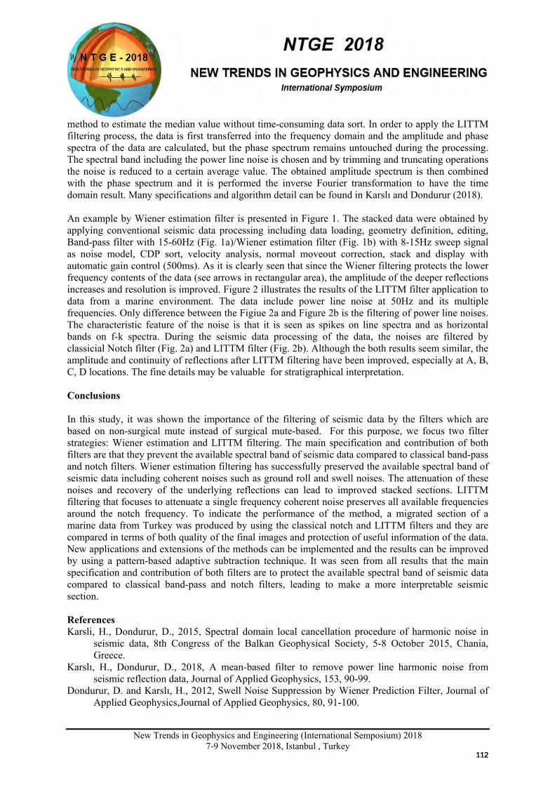
New Trends in Geophysics and Engineering (International Semposium) 2018
7-9 November 2018, Istanbul , Turkey
method to estimate the median value without time-consuming data sort. In order to apply the LITTM filtering process, the data is first transferred into the frequency domain and the amplitude and phase spectra of the data are calculated, but the phase spectrum remains untouched during the processing. The spectral band including the power line noise is chosen and by trimming and truncating operations the noise is reduced to a certain average value. The obtained amplitude spectrum is then combined with the phase spectrum and it is performed the inverse Fourier transformation to have the time domain result. Many specifications and algorithm detail can be found in Karslı and Dondurur (2018). An example by Wiener estimation filter is presented in Figure 1. The stacked data were obtained by applying conventional seismic data processing including data loading, geometry definition, editing, Band-pass filter with 15-60Hz (Fig. 1a)/Wiener estimation filter (Fig. 1b) with 8-15Hz sweep signal as noise model, CDP sort, velocity analysis, normal moveout correction, stack and display with automatic gain control (500ms). As it is clearly seen that since the Wiener filtering protects the lower frequency contents of the data (see arrows in rectangular area), the amplitude of the deeper reflections increases and resolution is improved. Figure 2 illustrates the results of the LITTM filter application to data from a marine environment. The data include power line noise at 50Hz and its multiple frequencies. Only difference between the Figiue 2a and Figure 2b is the filtering of power line noises. The characteristic feature of the noise is that it is seen as spikes on line spectra and as horizontal bands on f-k spectra. During the seismic data processing of the data, the noises are filtered by classicial Notch filter (Fig. 2a) and LITTM filter (Fig. 2b). Although the both results seem similar, the amplitude and continuity of reflections after LITTM filtering have been improved, especially at A, B, C, D locations. The fine details may be valuable for stratigraphical interpretation. Conclusions In this study, it was shown the importance of the filtering of seismic data by the filters which are based on non-surgical mute instead of surgical mute-based. For this purpose, we focus two filter strategies: Wiener estimation and LITTM filtering. The main specification and contribution of both filters are that they prevent the available spectral band of seismic data compared to classical band-pass and notch filters. Wiener estimation filtering has successfully preserved the available spectral band of seismic data including coherent noises such as ground roll and swell noises. The attenuation of these noises and recovery of the underlying reflections can lead to improved stacked sections. LITTM filtering that focuses to attenuate a single frequency coherent noise preserves all available frequencies around the notch frequency. To indicate the performance of the method, a migrated section of a marine data from Turkey was produced by using the classical notch and LITTM filters and they are compared in terms of both quality of the final images and protection of useful information of the data. New applications and extensions of the methods can be implemented and the results can be improved by using a pattern-based adaptive subtraction technique. It was seen from all results that the main specification and contribution of both filters are to protect the available spectral band of seismic data compared to classical band-pass and notch filters, leading to make a more interpretable seismic section. References Karsli, H., Dondurur, D., 2015, Spectral domain local cancellation procedure of harmonic noise in
seismic data, 8th Congress of the Balkan Geophysical Society, 5-8 October 2015, Chania, Greece.
Karslı, H., Dondurur, D., 2018, A mean-based filter to remove power line harmonic noise from seismic reflection data, Journal of Applied Geophysics, 153, 90-99.
Dondurur, D. and Karslı, H., 2012, Swell Noise Suppression by Wiener Prediction Filter, Journal of Applied Geophysics,Journal of Applied Geophysics, 80, 91-100.
112112
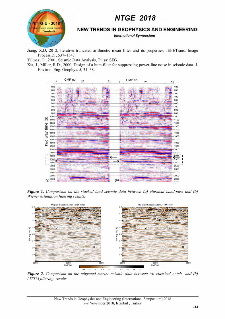
New Trends in Geophysics and Engineering (International Semposium) 2018
7-9 November 2018, Istanbul , Turkey
Jiang, X.D, 2012, Iterative truncated arithmetic mean filter and its properties, IEEETrans. Image Process.21, 537–1547.
Yılmaz, O., 2001. Seismic Data Analysis, Tulsa: SEG. Xia, J., Miller, R.D., 2000, Design of a hum filter for suppressing power-line noise in seismic data. J.
Environ. Eng. Geophys. 5, 31–38.
Figure 1. Comparison on the stacked land seismic data between (a) classical band-pass and (b) Wiener estimation filtering results.
Figure 2. Comparison on the migrated marine seismic data between (a) classical notch and (b) LITTM filtering results.
Two
way
time
(s)
1 25 51 1 25 51
(a) (b)
CMP no CMP no
CMP No
Two
way t
ime
(s)
Migrated Section After Notch Filter
2500 3000 3500
1.2
1.3
1.4
1.5
1.6
1.7
1.8
1.9
2
CMP No
Two
way t
ime
(s)
Migrated Section After LITTM Filter
2500 3000 3500
1.2
1.3
1.4
1.5
1.6
1.7
1.8
1.9
2
-0.4 -0.3 -0.2 -0.1 0 0.1 0.2 0.3 0.4 0.5
A
B
C
D
B
C
D
A
113113
New Trends in Geophysics and Engineering (International Semposium) 2018
7-9 November 2018, Istanbul , Turkey
AVAILABILITY OF ARTIFICIAL NEURAL NETWORK (ANN) IN STRONG
GROUND MOTION PREDICTION
Kaan Hakan Coban1, Nilgün Sayıl1
1 Department of Geophysical Engineering, Karadeniz Technical University, Trabzon Email: [email protected], [email protected]
Presentation Type All accepted proceedings will be published on the webpage of the symposium (ntge2018.istanbul.edu.tr)
ORAL POSTER
Abstracts The estimation of Peak Ground Acceleration (PGA) value is a significant factor for the building design and the damages of earthquakes. The PGA value has calculated with empirical attenuation relations in the literature. Many attenuation relations have been developed according to different earthquake parameter from strong motion data. Recently, advanced non-parametric models artificial neural network (ANN), found its application in geophysics. Also, The ANN have used for the prediction of PGA. In this study, we aim to predict PGA value with ANN algorithms and compare with the calculated empirical attenuation relationships for Turkey. Therefore, 27 earthquakes (5.0 ≤M) were selected in Turkey between 1990 – 2017. The magnıtude, epicenter distance and horizontal strong ground motion components of these earthquakes were used for training ANN according to different neuron number. The test data, which included the only magnitude and epicenter distance, were shown ANN and predicted the PGA value. The ANN obtained consistent results with measured values. Also, the results compared with empirical PGA results. Also, It has achieved better results than some empirical formulas. We will test and improve the prediction of PGA with ANN according to different parameters, such as soil structure, seismic velocity.
Keywords: Artificial Neural Network (ANN), Peak Ground Acceleration (PGA), Strong Ground Motion, Earthquakes Introduction The peak ground acceleration (PGA) forms the essential component in earthquake hazard studies and in the design of structures. The ground motion prediction can be performed based on mechanistic model or using empirical methods like attenuation relations, stochastic models, etc. Over the years there are numerous ground motion prediction equations (GMPE) developed across the world for both global and regional basis (Douglas, 2016). The absence of such recorded data, GMPEs could be build based on the synthetic databases generated using different empirical, numerical, analytical or hybrid techniques. The empirical attenuation relationships based on Turkish strong ground motion data were proposed by (Aydan et al., 1996; Inan et al., 1996; Gulkan and Kalkan, 2002; Beyaz, 2004 and Ulusay et al., 2004). Recently, advanced non-parametric models such as machine learning algorithms, artificial neural networks (ANNs), fuzzy logic, etc., found its application in geophysics. ANNs, however, are not
114114
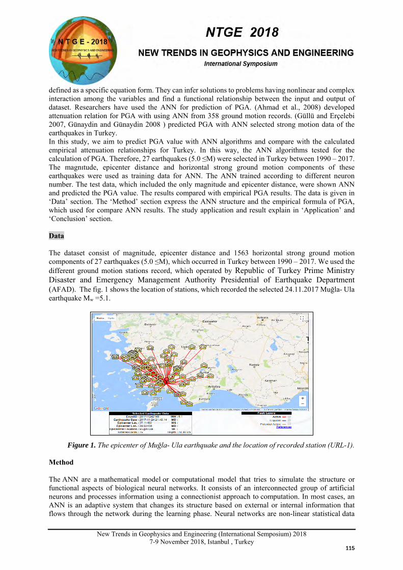
New Trends in Geophysics and Engineering (International Semposium) 2018
7-9 November 2018, Istanbul , Turkey
defined as a specific equation form. They can infer solutions to problems having nonlinear and complex interaction among the variables and find a functional relationship between the input and output of dataset. Researchers have used the ANN for prediction of PGA. (Ahmad et al., 2008) developed attenuation relation for PGA with using ANN from 358 ground motion records. (Güllü and Erçelebi 2007, Günaydin and Günaydin 2008 ) predicted PGA with ANN selected strong motion data of the earthquakes in Turkey. In this study, we aim to predict PGA value with ANN algorithms and compare with the calculated empirical attenuation relationships for Turkey. In this way, the ANN algorithms tested for the calculation of PGA. Therefore, 27 earthquakes (5.0 ≤M) were selected in Turkey between 1990 – 2017. The magnıtude, epicenter distance and horizontal strong ground motion components of these earthquakes were used as training data for ANN. The ANN trained according to different neuron number. The test data, which included the only magnitude and epicenter distance, were shown ANN and predicted the PGA value. The results compared with empirical PGA results. The data is given in ‘Data’ section. The ‘Method’ section express the ANN structure and the empirical formula of PGA, which used for compare ANN results. The study application and result explain in ‘Application’ and ‘Conclusion’ section. Data The dataset consist of magnitude, epicenter distance and 1563 horizontal strong ground motion components of 27 earthquakes (5.0 ≤M), which occurred in Turkey between 1990 – 2017. We used the different ground motion stations record, which operated by Republic of Turkey Prime Ministry Disaster and Emergency Management Authority Presidential of Earthquake Department (AFAD). The fig. 1 shows the location of stations, which recorded the selected 24.11.2017 Muğla- Ula earthquake Mw =5.1.
Figure 1. The epicenter of Muğla- Ula earthquake and the location of recorded station (URL-1). Method The ANN are a mathematical model or computational model that tries to simulate the structure or functional aspects of biological neural networks. It consists of an interconnected group of artificial neurons and processes information using a connectionist approach to computation. In most cases, an ANN is an adaptive system that changes its structure based on external or internal information that flows through the network during the learning phase. Neural networks are non-linear statistical data
115115
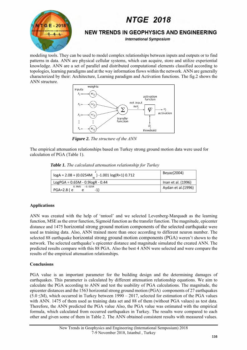
New Trends in Geophysics and Engineering (International Semposium) 2018
7-9 November 2018, Istanbul , Turkey
modeling tools. They can be used to model complex relationships between inputs and outputs or to find patterns in data. ANN are physical cellular systems, which can acquire, store and utilize experiential knowledge. ANN are a set of parallel and distributed computational elements classified according to topologies, learning paradigms and at the way information flows within the network. ANN are generally characterized by their: Architecture, Learning paradigm and Activation functions. The fig.2 shows the ANN structure.
Figure 2. The structure of the ANN The empirical attenuation relationships based on Turkey strong ground motion data were used for calculation of PGA (Table 1). Table 1. The calculated attenuation relationship for Turkey
logA = 2.08 + (0.0254MW
2) -1.001 log(R+1) 0.712 Beyaz(2004)
LogPGA = 0.65M - 0.9logR - 0.44 Inan et al. (1996)
PGA=2.8 ( e
0. 9MS e
- 0. 025R -1) Aydan et al.(1996)
Applications ANN was created with the help of ‘nntool’ and we selected Levenberg-Marquadt as the learning function, MSE as the error function, Sigmoid function as the transfer function. The magnitude, epicenter distance and 1475 horizontal strong ground motion components of the selected earthquake were used as training data. Also, ANN trained more than once according to different neuron number. The selected 88 earthquake horizontal strong ground motion components (PGA) weren’t shown to the network. The selected earthquake’s epicenter distance and magnitude simulated the created ANN. The predicted results compare with this 88 PGA. Also the best 4 ANN were selected and were compare the results of the empirical attenuation relationships. Conclusions PGA value is an important parameter for the building design and the determining damages of earthquakes. This parameter is calculated by different attenuation relationship equations. We aim to calculate the PGA according to ANN and test the usability of PGA calculations. The magnitude, the epicenter distances and the 1563 horizontal strong ground motion (PGA) components of 27 earthquakes (5.0 ≤M), which occurred in Turkey between 1990 – 2017, selected for estimation of the PGA values with ANN. 1475 of them used as training data set and 88 of them (without PGA values) as test data. Therefore, the ANN predicted the PGA value Also, the PGA value was estimated with the empirical formula, which calculated from occurred earthquakes in Turkey. The results were compared to each other and given some of them in Table 2. The ANN obtained consistent results with measured values.
116116
New Trends in Geophysics and Engineering (International Semposium) 2018
7-9 November 2018, Istanbul , Turkey
Also, It has achieved better results than some empirical formulas. We will test the prediction of PGA with ANN according to different parameters, such as soil structure, seismic velocity. We will improve our ANN structure for prediction of PGA.
Table 2. The comparison results (some of 88 results) PGA NET1 NET2 NET3 NET4 İnan Aydan Beyaz 1 9,66 21,21 8,66 9,63 5,77 16,45 54,86 8,61 2 6,13 6,65 5,16 6,66 8,13 17,88 43,48 7,66 3 39 34,46 62,79 29,79 36,33 96,21 158,72 18,29 4 3,03 3,18 4,83 9,13 24,58 25,03 56,92 9,03
References Ahmad, I., El Naggar, M. H., and Khan, A. N., 2008, Neural network based attenuation of strong motion peaks in Europe, Journal of Earthquake Engineering, 12(5), 663–680. Aydan, Ö., Sedak, M. and Yarar, R., 1996, The seismic characteristics of Turkish earthquakes, Eleventh World Conference on Earthquake Engineering, June 23-28, Acapulco, Mexico. Beyaz, T., 2004, Development of a new earthquake energy attenuation relation to Turkey by the recording earthquakes, Institute of Science Technology, Ankara University, Turkey Douglas, J., 2016, Ground motion prediction equations,1964–2016, http://www.gmpe.org.uk. Gülkan, P. And Kalkan, E., 2002, Attenuation modeling of recent earthquakes in Turkey, Journal of Seismology, 6, 397-409. Güllü , H., and Erçelebi, E., 2007, A neural network approach for attenuation relationships: An application using strong ground motion data from Turkey, Engineering Geology, 93(3–4), 65–81. Günaydın, K., and Günaydın, A., 2008, Peak ground acceleration prediction by artificial neural networks for northwestern Turkey, Mathematical Problems in Engineering, https://doi.org/10.1155/ 2008/919420. Inan, E., Çolakoglu, Z., Koç, N., Bayülke, N. Ve Çoruh, E., 1996, 1976-1996 Earthquake catalogue with acceleration records. T. C. Ministry of Public Works and Settlement General Directorate of Disaster Affairs, Department of Earthquake Research, 98 s, Ankara. Ulusay, R., Tuncay, E., Sonmez, H. and Gokceoglu, C., 2004, An Attenuation relationship based on Turkish strong motion data and iso-acceleration map of Turkey.Engineering Geology, 74, 265-291. URL-1 http://kyhdata.deprem.gov.tr/2K/kyhdata_v4.php
117117
New Trends in Geophysics and Engineering (International Semposium) 2018
7-9 November 2018, Istanbul , Turkey
DESCRIPTION OF SUBSOIL TYPES FROM MICROTREMOR H/V SPECTRAL
RATIO METHOD IN KELKIT DISTRICT OF GÜMÜŞHANE PROVINCE, TURKEY
Serkan Öztürk1, Yasemin Beker2, Levent Pehlivan3, Mahmut Sarı4
1,2,3,4Department of Geophysics, Gümüşhane University, Gümüşhane Email: [email protected]
Presentation Type All accepted proceedings will be published on the webpage of the symposium (ntge2018.istanbul.edu.tr)
ORAL POSTER
Abstracts Site effect classification studies based on the microtremor data analysis are very useful tool for engineers to measure the dominant frequency of soil sites and to describe the ground motion characteristics. In this study, we aimed to describe the subsoil types of Kelkit district of Gümüşhane province, Turkey. We used the ratio of horizontal to vertical components of Fourier amplitude spectra, designated as H/V spectral ratio model of Nakamura method based on the single station microtremor data analysis. Predominant frequency, H/V spectral ratio and predominant period were determined for 48 points with CMG-6TD three component broad band velocity seismometer. Predominant frequency changes between 1.2684 and 9.5374 Hz, H/V spectral ratio varies from 1.006 to 5.177, and predominant period was estimated between 0.104 and 0.715. Subsoil classification was made considering the predominant periods. According to the obtained results, three transient zones can be suggested as Z1, Z2 and Z3 between different surface geology in different parts of Kelkit district of Gümüşhane province. Keywords: Gümüşhane, microtremor, Nakamura method, predominant period, subsoil types Introduction The terms of microseisms and microtremors are used to describe the ambient vibrations of the ground caused by ambient or natural disturbances such as traffic, wind, industrial machinery, sea waves, etc. The use of measured microtremors in the description of subsoil types is based on the principle that microtremors spread in the ground and are amplified at periods which are synchronous with the predominant period of the site (Kanai, 1983; Haile et al. 1987). Microtremor is also an efficient and low-cost technique in seismic hazard microzonation. Thus, horizontal to vertical (H/V) ratio microtremor method has become popular worldwide since it was proposed by Nakamura (1989), and its advantages and limitations have been discussed in detailed in the literature. In this study, the single station H/V spectral ratio method was applied to describe the subsoil types considering the predominant period for Kelkit district of Gümüşhane province of Turkey. Microtremor Data and Brief Description of H/V Spectral Ratio Method To investigate the subsoil characteristics of Kelkit, a total of 48 single station microtremor measurements were taken with a CMG-6TD three component broad band velocity seismometer. Microtremor data (H/V) was processed with the GEOPSY software and all results are given in Table 1.
X
118118
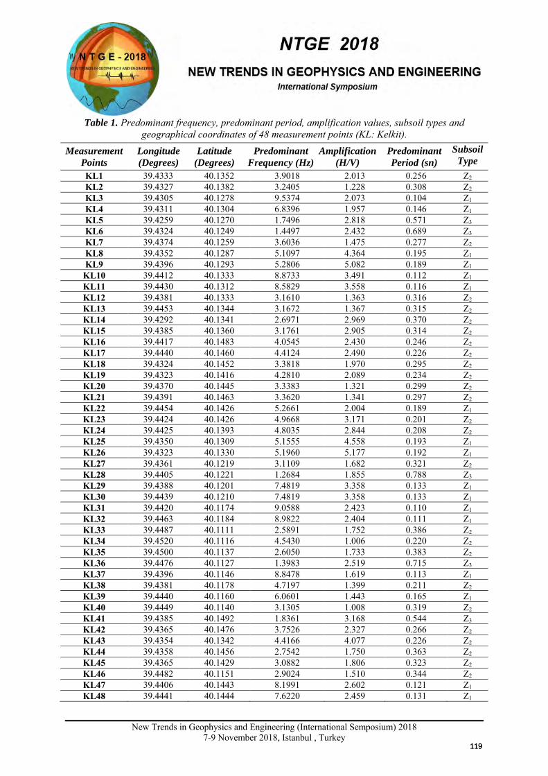
New Trends in Geophysics and Engineering (International Semposium) 2018
7-9 November 2018, Istanbul , Turkey
Table 1. Predominant frequency, predominant period, amplification values, subsoil types and geographical coordinates of 48 measurement points (KL: Kelkit).
Measurement Points
Longitude (Degrees)
Latitude (Degrees)
Predominant Frequency (Hz)
Amplification (H/V)
Predominant Period (sn)
Subsoil Type
KL1 39.4333 40.1352 3.9018 2.013 0.256 Z2 KL2 39.4327 40.1382 3.2405 1.228 0.308 Z2 KL3 39.4305 40.1278 9.5374 2.073 0.104 Z1 KL4 39.4311 40.1304 6.8396 1.957 0.146 Z1 KL5 39.4259 40.1270 1.7496 2.818 0.571 Z3 KL6 39.4324 40.1249 1.4497 2.432 0.689 Z3 KL7 39.4374 40.1259 3.6036 1.475 0.277 Z2 KL8 39.4352 40.1287 5.1097 4.364 0.195 Z1 KL9 39.4396 40.1293 5.2806 5.082 0.189 Z1
KL10 39.4412 40.1333 8.8733 3.491 0.112 Z1 KL11 39.4430 40.1312 8.5829 3.558 0.116 Z1 KL12 39.4381 40.1333 3.1610 1.363 0.316 Z2 KL13 39.4453 40.1344 3.1672 1.367 0.315 Z2 KL14 39.4292 40.1341 2.6971 2.969 0.370 Z2 KL15 39.4385 40.1360 3.1761 2.905 0.314 Z2 KL16 39.4417 40.1483 4.0545 2.430 0.246 Z2 KL17 39.4440 40.1460 4.4124 2.490 0.226 Z2 KL18 39.4324 40.1452 3.3818 1.970 0.295 Z2 KL19 39.4323 40.1416 4.2810 2.089 0.234 Z2 KL20 39.4370 40.1445 3.3383 1.321 0.299 Z2 KL21 39.4391 40.1463 3.3620 1.341 0.297 Z2 KL22 39.4454 40.1426 5.2661 2.004 0.189 Z1 KL23 39.4424 40.1426 4.9668 3.171 0.201 Z2 KL24 39.4425 40.1393 4.8035 2.844 0.208 Z2 KL25 39.4350 40.1309 5.1555 4.558 0.193 Z1 KL26 39.4323 40.1330 5.1960 5.177 0.192 Z1 KL27 39.4361 40.1219 3.1109 1.682 0.321 Z2 KL28 39.4405 40.1221 1.2684 1.855 0.788 Z3 KL29 39.4388 40.1201 7.4819 3.358 0.133 Z1 KL30 39.4439 40.1210 7.4819 3.358 0.133 Z1 KL31 39.4420 40.1174 9.0588 2.423 0.110 Z1 KL32 39.4463 40.1184 8.9822 2.404 0.111 Z1 KL33 39.4487 40.1111 2.5891 1.752 0.386 Z2 KL34 39.4520 40.1116 4.5430 1.006 0.220 Z2 KL35 39.4500 40.1137 2.6050 1.733 0.383 Z2 KL36 39.4476 40.1127 1.3983 2.519 0.715 Z3 KL37 39.4396 40.1146 8.8478 1.619 0.113 Z1 KL38 39.4381 40.1178 4.7197 1.399 0.211 Z2 KL39 39.4440 40.1160 6.0601 1.443 0.165 Z1 KL40 39.4449 40.1140 3.1305 1.008 0.319 Z2 KL41 39.4385 40.1492 1.8361 3.168 0.544 Z3 KL42 39.4365 40.1476 3.7526 2.327 0.266 Z2 KL43 39.4354 40.1342 4.4166 4.077 0.226 Z2 KL44 39.4358 40.1456 2.7542 1.750 0.363 Z2 KL45 39.4365 40.1429 3.0882 1.806 0.323 Z2 KL46 39.4482 40.1151 2.9024 1.510 0.344 Z2 KL47 39.4406 40.1443 8.1991 2.602 0.121 Z1 KL48 39.4441 40.1444 7.6220 2.459 0.131 Z1
119119
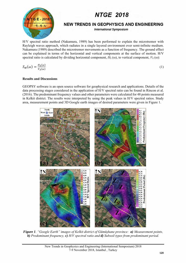
New Trends in Geophysics and Engineering (International Semposium) 2018
7-9 November 2018, Istanbul , Turkey
H/V spectral ratio method (Nakamura, 1989) has been performed to explain the microtremor with Rayleigh waves approach, which radiates in a single layered environment over semi-infinite medium. Nakamura (1989) described the microtremor movements as a function of frequency. The ground effect can be explained in terms of the horizontal and vertical components at the surface of motion. H/V spectral ratio is calculated by dividing horizontal component, HS (ω), to vertical component, VS (ω): 𝑆𝑆𝑀𝑀(𝜔𝜔) = 𝐻𝐻𝑆𝑆(𝜔𝜔)
𝑉𝑉𝑆𝑆(𝜔𝜔) (1)
Results and Discussions
GEOPSY software is an open source software for geophysical research and applications. Details of the data processing stages considered in the application of H/V spectral ratio can be found in Rincon et al. (2016). The predominant frequency values and other parameters were calculated for 48 points measured in Kelkit district. The results were interpreted by using the peak values in H/V spectral ratios. Study area, measurement points and 3D Google earth images of desired parameters were given in Figure 1.
Figure 1. “Google Earth” images of Kelkit district of Gümüşhane province: a) Measurement points,
b) Predominant frequency, c) H/V spectral ratio and d) Subsoil types from predominant period.
120120
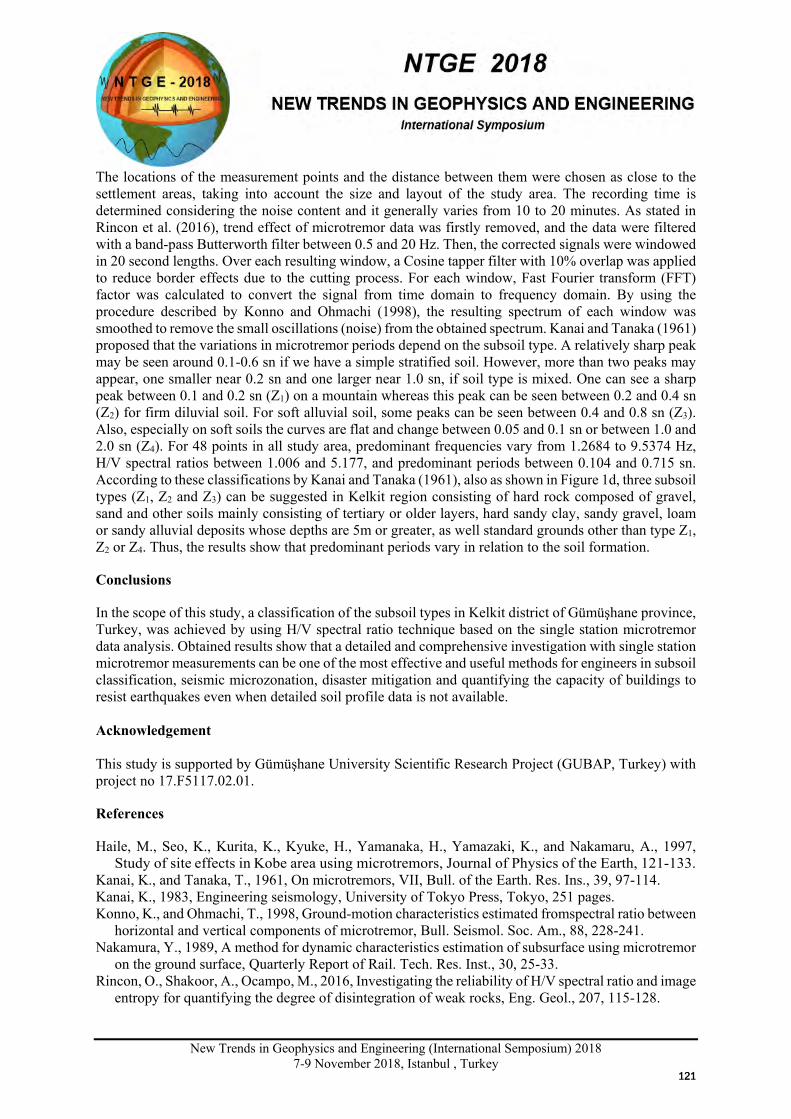
New Trends in Geophysics and Engineering (International Semposium) 2018
7-9 November 2018, Istanbul , Turkey
The locations of the measurement points and the distance between them were chosen as close to the settlement areas, taking into account the size and layout of the study area. The recording time is determined considering the noise content and it generally varies from 10 to 20 minutes. As stated in Rincon et al. (2016), trend effect of microtremor data was firstly removed, and the data were filtered with a band-pass Butterworth filter between 0.5 and 20 Hz. Then, the corrected signals were windowed in 20 second lengths. Over each resulting window, a Cosine tapper filter with 10% overlap was applied to reduce border effects due to the cutting process. For each window, Fast Fourier transform (FFT) factor was calculated to convert the signal from time domain to frequency domain. By using the procedure described by Konno and Ohmachi (1998), the resulting spectrum of each window was smoothed to remove the small oscillations (noise) from the obtained spectrum. Kanai and Tanaka (1961) proposed that the variations in microtremor periods depend on the subsoil type. A relatively sharp peak may be seen around 0.1-0.6 sn if we have a simple stratified soil. However, more than two peaks may appear, one smaller near 0.2 sn and one larger near 1.0 sn, if soil type is mixed. One can see a sharp peak between 0.1 and 0.2 sn (Z1) on a mountain whereas this peak can be seen between 0.2 and 0.4 sn (Z2) for firm diluvial soil. For soft alluvial soil, some peaks can be seen between 0.4 and 0.8 sn (Z3). Also, especially on soft soils the curves are flat and change between 0.05 and 0.1 sn or between 1.0 and 2.0 sn (Z4). For 48 points in all study area, predominant frequencies vary from 1.2684 to 9.5374 Hz, H/V spectral ratios between 1.006 and 5.177, and predominant periods between 0.104 and 0.715 sn. According to these classifications by Kanai and Tanaka (1961), also as shown in Figure 1d, three subsoil types (Z1, Z2 and Z3) can be suggested in Kelkit region consisting of hard rock composed of gravel, sand and other soils mainly consisting of tertiary or older layers, hard sandy clay, sandy gravel, loam or sandy alluvial deposits whose depths are 5m or greater, as well standard grounds other than type Z1, Z2 or Z4. Thus, the results show that predominant periods vary in relation to the soil formation.
Conclusions
In the scope of this study, a classification of the subsoil types in Kelkit district of Gümüşhane province, Turkey, was achieved by using H/V spectral ratio technique based on the single station microtremor data analysis. Obtained results show that a detailed and comprehensive investigation with single station microtremor measurements can be one of the most effective and useful methods for engineers in subsoil classification, seismic microzonation, disaster mitigation and quantifying the capacity of buildings to resist earthquakes even when detailed soil profile data is not available. Acknowledgement This study is supported by Gümüşhane University Scientific Research Project (GUBAP, Turkey) with project no 17.F5117.02.01.
References
Haile, M., Seo, K., Kurita, K., Kyuke, H., Yamanaka, H., Yamazaki, K., and Nakamaru, A., 1997, Study of site effects in Kobe area using microtremors, Journal of Physics of the Earth, 121-133.
Kanai, K., and Tanaka, T., 1961, On microtremors, VII, Bull. of the Earth. Res. Ins., 39, 97-114. Kanai, K., 1983, Engineering seismology, University of Tokyo Press, Tokyo, 251 pages. Konno, K., and Ohmachi, T., 1998, Ground-motion characteristics estimated fromspectral ratio between
horizontal and vertical components of microtremor, Bull. Seismol. Soc. Am., 88, 228-241. Nakamura, Y., 1989, A method for dynamic characteristics estimation of subsurface using microtremor
on the ground surface, Quarterly Report of Rail. Tech. Res. Inst., 30, 25-33. Rincon, O., Shakoor, A., Ocampo, M., 2016, Investigating the reliability of H/V spectral ratio and image
entropy for quantifying the degree of disintegration of weak rocks, Eng. Geol., 207, 115-128.
121121
New Trends in Geophysics and Engineering (International Semposium) 2018 7-9 November 2018, Istanbul , Turkey
ANISOTROPY OF MAGNETIC SUSCEPTIBITY MEASUREMENTS ON PREDICTING FLOW DIRECTION OF EASTERN ANATOLIAN VOLCANIC
ERRUPTION
Hakan Uçar1 , Mualla Cengiz Çinku1
1 Geophysical Eng. Department, Istanbul University, Istanbul Email: [email protected]
Presentation Type
All accepted proceedings will be published on the webpage of the symposium (ntge2018.istanbul.edu.tr)
ORAL POSTER
Abstracts
Eastern Anatolia comprises one of the high plateaus of the Alpine-Himalaya mountain belt with an average elevation of 2 km above the sea level. Available geochronologic data indicate that the volcanism started in the south of the region around the north of Lake Van and continued towards the norths in a age interval of 15.0 Ma to 0.4 Ma. The products are exposed as stratovolcanoes like Agri, Tendurek, Suphan and Girekol with the eruption of andesitic to rhyolitic lavas, ignimbrites and basaltic lava flows. In this study, anisotropy of magnetic susceptibility measurements were carried out on different lava flows (Tendurek, Girekol and Suphan) to determine the flow direction of lavas. It has been shown that the direction of maximum susceptibility is associated with magma flow direction in the vertical direction, while a horizontal flow direction is predicted for the volcano structure of Suphan. Anisotropy of magnetic measurements show a trend of lineation towards the center of the projection and shallow-dipping foliations which are largely scattered.
Keywords: anisotropy, susceptibility, magnetism, eastern, turkey
Introduction
In this study, anisotropy of magnetic susceptibility measurements were carried out on 21 different sites from the Eastern Anatolian Region to determine the determine the flow direction of lavas. In total, 133 volcanic samples from Pliocene-Quaternary ages were measured on 18 different measurement position by using Bartington MS2B susceptibility device and AMS-BAR software. As a result of the AMS measurements, magnetic lineations associated with a magma flow in horizontal direction have been determined. The magma flow directions are generally towards the volcano vent. Detailed rock magnetic experiments, including thermomagnetic measurements, acquisition of isothermal remanent magnetization (IRM), and thermal demagnetization of three-axes composite IRM, were conducted on each pilot sample. Thermomagnetic experiments were performed on representative samples by heating in air, using an Bartington MS2 susceptibility bridge fitted with an oven unit. IRMs were acquired using an ASC pulse magnetizer (Model IM-10-30). Steps of 1, 0.4, and 0.12 T were imparted along the Z-, Y-, and X-axis, respectively. Subsequently, samples were thermally
x
122122

New Trends in Geophysics and Engineering (International Semposium) 2018
7-9 November 2018, Istanbul , Turkey
demagnetized to identify the magnetic carriers based on their coercivity and unblocking behaviour. As a result of this measurements, most of the samples are characterized by titanomagnetite. Sampling Area
Figure 1: a) Plate motions of Turkey and its environment. According to GPS measurements, Arabian Plate moves towards Northwest at a rate of 18±2 mm every year. As a result of this movement, Anatolian block moves towards West at a rate of 24±2 mm across North Anatolian Fault(NAF) and 9±2 mm across East Anatolian Fault(EAF) every year. Also, West Anatolian Region moves towards Southwest at a rate of 30±1 mm every year(Okay and Tüysüz, 1999). b) Tectonic units, distribution of collisionrelated volcanic products and volcanic centers across Eastern Anatolia. E-K-P: the Erzurum-Kars Plateau; NATF and EATF: North and East Anatolian Transform Faults. I : The Pontide unit which is represented basically by a magmatic arc, II : Northwestern Iran Unit, III : The Eastern Anatolian Accretionary Complex (EAAC), IV : The BitlisPoturge Massif (BPM) and V : Arabian Plate. Green areas : Ophiolitic melange, Pink and red areas : Volcanic units which is related to the collision, White areas : Young units (Keskin et al., 2003)
Rock Magnetism Measurements
Figure 7: The results of the thermomagnetic analysis reveal three different types of behaviour (Fig. 7a, d, g). Most samples with minor alteration are characterized by a single ferromagnetic phase and Curie temperatures between 550 and 580 °C, indicating the presence of Tipoor titanomagnetites (Fig. 7a). In
123123
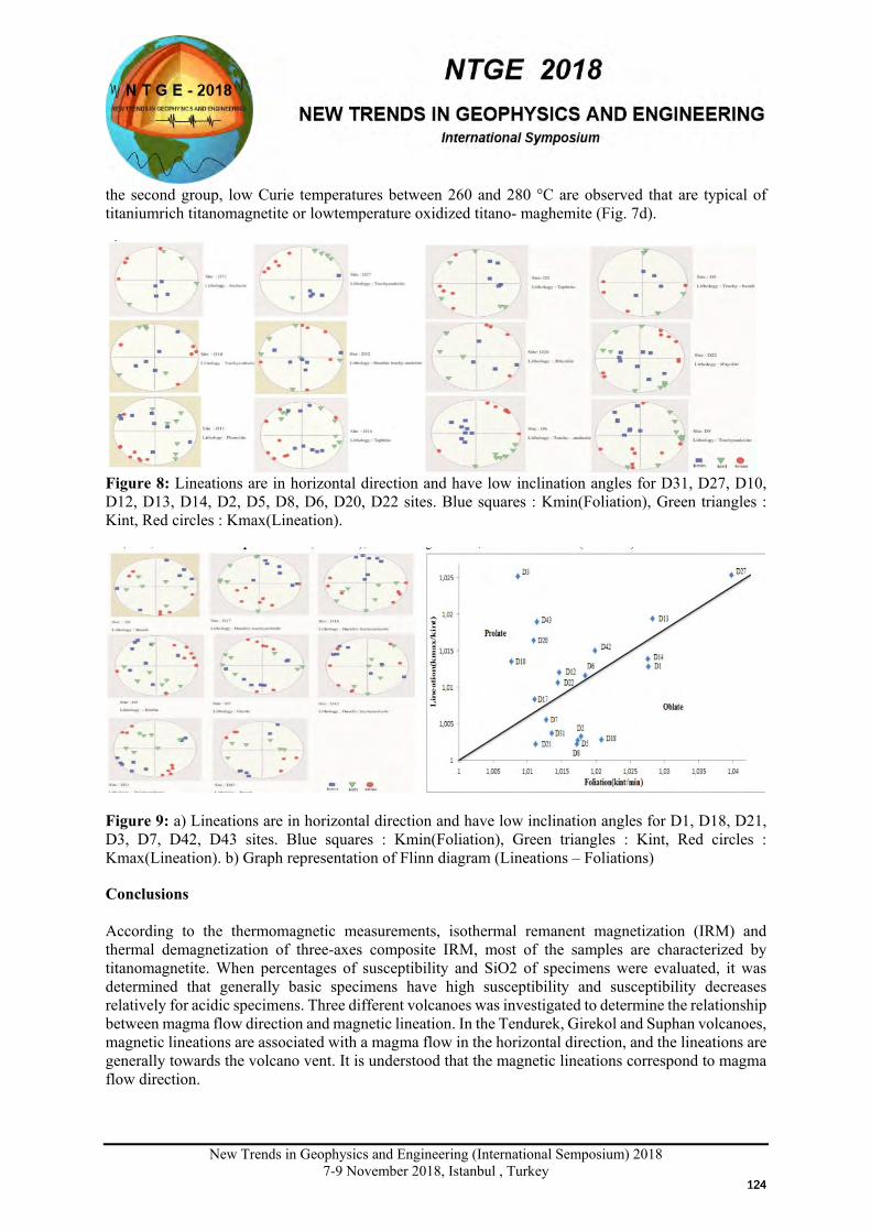
New Trends in Geophysics and Engineering (International Semposium) 2018
7-9 November 2018, Istanbul , Turkey
the second group, low Curie temperatures between 260 and 280 °C are observed that are typical of titaniumrich titanomagnetite or lowtemperature oxidized titano- maghemite (Fig. 7d).
Figure 8: Lineations are in horizontal direction and have low inclination angles for D31, D27, D10, D12, D13, D14, D2, D5, D8, D6, D20, D22 sites. Blue squares : Kmin(Foliation), Green triangles : Kint, Red circles : Kmax(Lineation).
Figure 9: a) Lineations are in horizontal direction and have low inclination angles for D1, D18, D21, D3, D7, D42, D43 sites. Blue squares : Kmin(Foliation), Green triangles : Kint, Red circles : Kmax(Lineation). b) Graph representation of Flinn diagram (Lineations – Foliations)
Conclusions According to the thermomagnetic measurements, isothermal remanent magnetization (IRM) and thermal demagnetization of three-axes composite IRM, most of the samples are characterized by titanomagnetite. When percentages of susceptibility and SiO2 of specimens were evaluated, it was determined that generally basic specimens have high susceptibility and susceptibility decreases relatively for acidic specimens. Three different volcanoes was investigated to determine the relationship between magma flow direction and magnetic lineation. In the Tendurek, Girekol and Suphan volcanoes, magnetic lineations are associated with a magma flow in the horizontal direction, and the lineations are generally towards the volcano vent. It is understood that the magnetic lineations correspond to magma flow direction.
124124
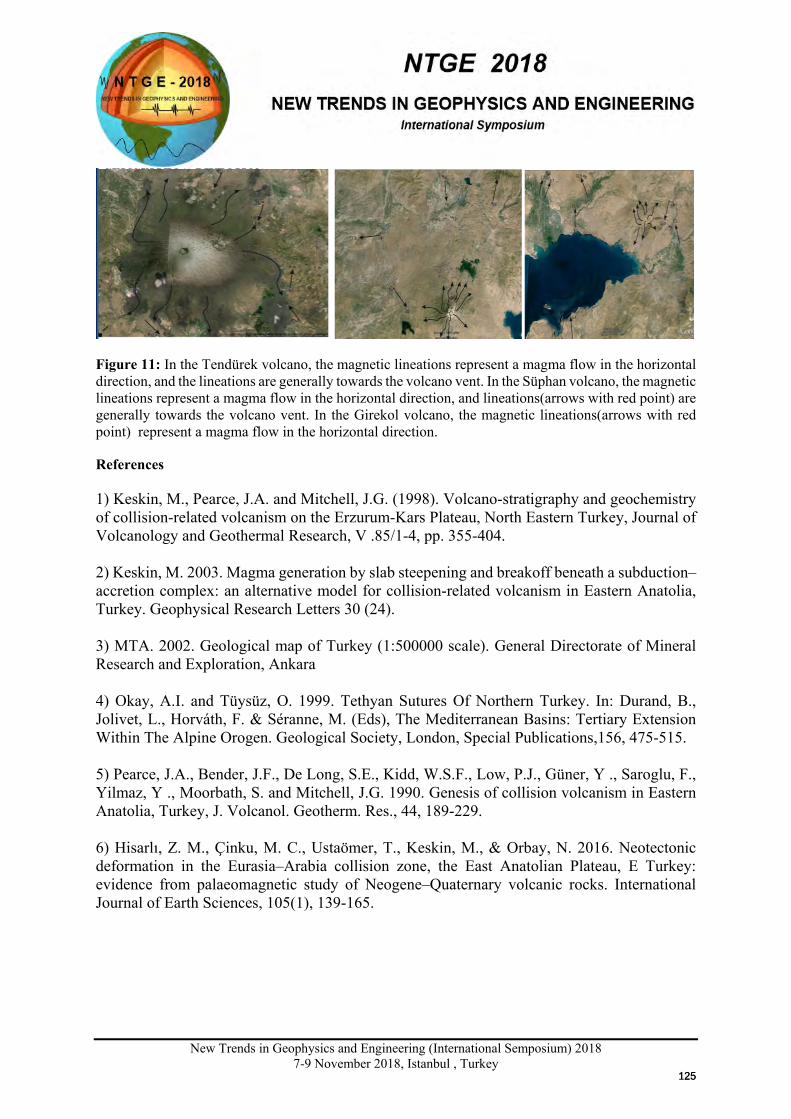
New Trends in Geophysics and Engineering (International Semposium) 2018
7-9 November 2018, Istanbul , Turkey
Figure 11: In the Tendürek volcano, the magnetic lineations represent a magma flow in the horizontal direction, and the lineations are generally towards the volcano vent. In the Süphan volcano, the magnetic lineations represent a magma flow in the horizontal direction, and lineations(arrows with red point) are generally towards the volcano vent. In the Girekol volcano, the magnetic lineations(arrows with red point) represent a magma flow in the horizontal direction.
References 1) Keskin, M., Pearce, J.A. and Mitchell, J.G. (1998). Volcano-stratigraphy and geochemistry of collision-related volcanism on the Erzurum-Kars Plateau, North Eastern Turkey, Journal of Volcanology and Geothermal Research, V .85/1-4, pp. 355-404. 2) Keskin, M. 2003. Magma generation by slab steepening and breakoff beneath a subduction–accretion complex: an alternative model for collision-related volcanism in Eastern Anatolia, Turkey. Geophysical Research Letters 30 (24). 3) MTA. 2002. Geological map of Turkey (1:500000 scale). General Directorate of Mineral Research and Exploration, Ankara 4) Okay, A.I. and Tüysüz, O. 1999. Tethyan Sutures Of Northern Turkey. In: Durand, B., Jolivet, L., Horváth, F. & Séranne, M. (Eds), The Mediterranean Basins: Tertiary Extension Within The Alpine Orogen. Geological Society, London, Special Publications,156, 475-515. 5) Pearce, J.A., Bender, J.F., De Long, S.E., Kidd, W.S.F., Low, P.J., Güner, Y ., Saroglu, F., Yilmaz, Y ., Moorbath, S. and Mitchell, J.G. 1990. Genesis of collision volcanism in Eastern Anatolia, Turkey, J. Volcanol. Geotherm. Res., 44, 189-229. 6) Hisarlı, Z. M., Çinku, M. C., Ustaömer, T., Keskin, M., & Orbay, N. 2016. Neotectonic deformation in the Eurasia–Arabia collision zone, the East Anatolian Plateau, E Turkey: evidence from palaeomagnetic study of Neogene–Quaternary volcanic rocks. International Journal of Earth Sciences, 105(1), 139-165.
125125
New Trends in Geophysics and Engineering (International Semposium) 2018
7-9 November 2018, Istanbul , Turkey
x
POSSIBLE MUTUYAMA-BRUNHES BOUNDARY IN CAVE SEDIMENT OF THE CZECH REPUBLIC
Hakan Ucar1, Gunther Kletetschka1,2,3, Jaroslav Kadlec4, Tereza Kamenikova2, and
Emilio Bervera Herrero5 1 Institute of Geology, Academy of Sciences of the Czech Republic, Czech Republic 2 Faculty of Science, Charles University, Czech Republic 3 Department of Geology and Geophysics, University of Alaska Fairbanks, USA 4 Geophysical Institute, Academy of Sciences of the Czech Republic, Czech Republic 5 Hawaii Institute of Geophysics and Planetology, University of Hawaii at Manoa, Honolulu, Hawaii, USA [email protected], [email protected] Presentation Type All accepted proceedings will be published on the webpage of the symposium (ntge2018.istanbul.edu.tr)
ORAL POSTER
Abstracts In this study, it was carried out a Matuyama-Brunhes transition research to understand the features of this transition. Matuyama-Brunhes transition occurred approximately 781,000 years ago. To carry out this study, we collected discrete samples from the homogeneous sedimentary profile in the cave Za Hajovnoulocated in the eastern part of the Czech Republic. Discrete sedimentary samples were taken from a layer having 35.5 cm a thickness. In addition to discrete samples we have collected across the same sedimentary profile 1 m long cores. We used step-wised demagnetization by alternating magnetic field of 2mT, 5 mT, 10 mT, 15 mT and 20 mT on both cores. Similar alternating magnetic field magnitudes (and more) were used on the discrete samples. Cores were measured in cryogenic magnetometer in Honolulu, while discrete samples magnetization were measured in Pruhonice laboratory in the Czech Republic. Both instruments were cryogenic 2G magnetometers. We used Remasoft software to interpret magnetic directional and intensity data. We identified viscous remanent magnetization in most of the samples. We identified natural remanent magnetization cleaned for the viscous component. We compared both core and discrete sample datasets and then compared these results with IODP magnetic measurements of the Matuyama-Brunhes transition. We discuss if the cave sediment might be this transition. For this discussion, we utilized Google Earth application where we illustrate the samples’ pole locations on the globe. Keywords: matuyama, brunhes, magnetism, transition Introduction Matuyama-Brunhes geomagnetic transition (781,000 years ago) could be present in Czech cave sediments. We collected sediments that could be of this age from Za Hajovnou Cave (Fig. 1). Both discrete samples and U-channel cores were collected from the homogeneous sedimentary profile in the cave Za Hajovnou located in the eastern part of the Czech Republic. Discrete samples were taken from a layer having 35.5 cm a thickness, while u-channel was a 1 m long section overlapping the depth from which discrete samples were taken.
126126
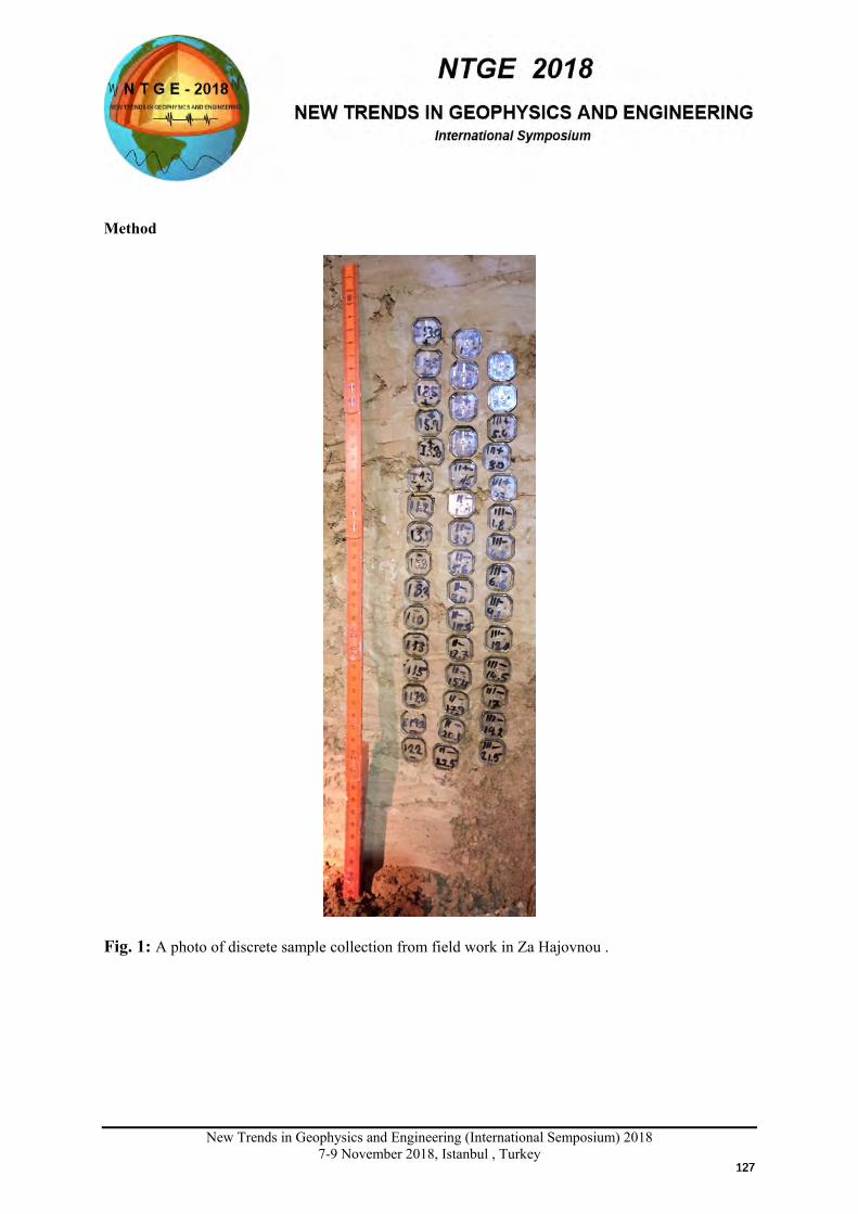
New Trends in Geophysics and Engineering (International Semposium) 2018
7-9 November 2018, Istanbul , Turkey
Method
Fig. 1: A photo of discrete sample collection from field work in Za Hajovnou .
127127
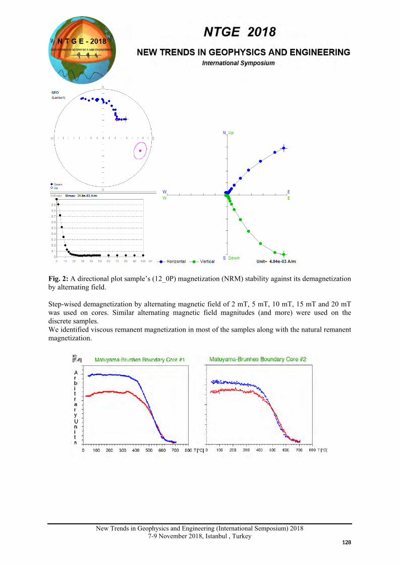
New Trends in Geophysics and Engineering (International Semposium) 2018
7-9 November 2018, Istanbul , Turkey
Fig. 2: A directional plot sample’s (12_0P) magnetization (NRM) stability against its demagnetization by alternating field. Step-wised demagnetization by alternating magnetic field of 2 mT, 5 mT, 10 mT, 15 mT and 20 mT was used on cores. Similar alternating magnetic field magnitudes (and more) were used on the discrete samples. We identified viscous remanent magnetization in most of the samples along with the natural remanent magnetization.
128128
New Trends in Geophysics and Engineering (International Semposium) 2018
7-9 November 2018, Istanbul , Turkey
Fig. 3: Curie measurements and pole positions from the datasets. Conclusions It was compared both core and discrete sample datasets if the cave sediment might be this transition. For this, inclination, declination and intensity data were compared. In the light of these data, the Matuyama-Brunhes transition appears to be about 40 cm deep of the cave sediment.
Fig. 5: Matuyama-Brunhes polarity transition VGPs.
Fig. 4: Comparison of different kind of datasets. Aknowledgements We would like thank to Petr Pruner and Petr Schnabl from the Paleomagnetic laboratory of Academy of Sciences for their contribution to the project.
129129
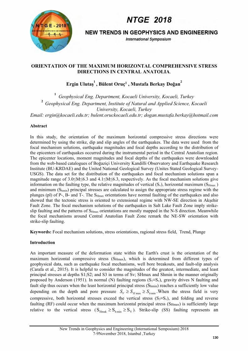
New Trends in Geophysics and Engineering (International Semposium) 2018
7-9November 2018, Istanbul ,Turkey
ORIENTATION OF THE MAXIMUM HORIZONTAL COMPREHENSIVE STRESS
DIRECTIONS IN CENTRAL ANATOLIA.
Ergin Ulutaş1 , Bülent Oruç1 , Mustafa Berkay Doğan2
1 Geophysical Eng. Department, Kocaeli University, Kocaeli, Turkey 2 Geophysical Eng. Department, Institute of Natural and Applied Science, Kocaeli
University, Kocaeli, Turkey Email: [email protected]; bulent.oruckocaeli.edu.tr; [email protected] Abstract In this study, the orientation of the maximum horizontal compressive stress directions were determined by using the strike, dip and slip angles of the earthquakes. The data were used from the focal mechanism solutions, earthquake magnitudes and focal depths according to the distribution of the epicenters of earthquakes occurred during the instrumental period in the Central Anatolian region. The epicenter locations, moment magnitudes and focal depths of the earthquakes were downloaded from the web-based catalogues of Boğaziçi University Kandilli Observatory and Earthquake Research Institute (BU-KRDAE) and the United National Geological Survey (Unites Stated Geological Survey-USGS). The data set for the distribution of the earthquakes and focal mechanism solutions span a magnitude range of 3.0≤M≤6.3 and 4.1≤M≤6.3, respectively. As the focal mechanism solutions give information on the faulting type, the relative magnitudes of vertical (Sv), horizontal maximum (SHmax ) and minimum (Shmin) principal stresses are calculated to assign the appropriate stress regime with the plunges (pl) of P-, B- and T-. The SHmax orientations have normal faulting of the earthquakes and also showed that the tectonic stress is oriented to extensional regime with NW-SE direction in Akşehir Fault Zone. The focal mechanism solutions of the earthquakes in Salt Lake Fault Zone imply strike-slip faulting and the patterns of SHmax orientations are mostly mapped in the N-S direction. Meanwhile the focal mechanisms around Central Anatolian Fault Zone remark the NE-SW orientation with strike-slip faulting.
Keywords: Focal mechanism solutions, stress orientations, ragional stress field, Trend, Plunge Introduction An important measure of the deformation state within the Earth's crust is the orientation of the maximum horizontal compressive stress (SHmax), which is determined from different types of geophysical data, such as earthquake focal mechanisms, well bore breakouts, and fault-slip analysis (Carafa et al., 2015). It is helpful to consider the magnitudes of the greatest, intermediate, and least principal stresses at depths S1;S2; and S3 in terms of Sv; SHmax and Shmin in the manner originally proposed by Anderson (1951). In normal (N) faulting regions (S1≡Sv), gravity drives N faulting and fault slip thus occurs when the least horizontal principal stress (Shmin) reaches a sufficiently low value depending on the depth and pore pressure minmax hHV SSS ≥≥ .When the stress field is very compressive, both horizontal stresses exceed the vertical stress (S3≡Sv), and folding and reverse faulting (RF) could occur when the maximum horizontal principal stress (SHmax) is sufficiently large relative to the vertical stress ( VminhHmak SSS ≥≥ ). Strike-slip (SS) faulting represents an
130130
New Trends in Geophysics and Engineering (International Semposium) 2018
7-9November 2018, Istanbul ,Turkey
intermediate stress state (S2≡Sv) in which minhVmaxH SSS ≥≥ . In this case, faulting occurs when the difference between SHmax and Shmin is sufficiently large (Zoback et al., 2003). As the focal mechanism allows us to define the faulting type, if the relative magnitudes of Sv, SHmax and Shmin are known. Thus, the pl of P-, B-, and T- are used to assign the appropriate stress regime to the data record (Table 1).
Table 1: Tectonic regime assignment (Zoback, 1992).
Plunges of Axes P/S1 B/S2 T/S3 Regime SHmax Azimutha
pl > 52 pl < 35
NF azim. of B-axis
40 < pl < 52 pl < 20
NS azim. of T-axis + 90°
pl < 40
pl > 45
pl < 20
SS azim. of T-axis + 90°
pl < 20
pl > 45
pl < 40
SS azim. of P-axis
pl < 20 40 < pl < 52
TS azim. of P-axis
pl < 35 pl > 52
TF azim. of P-axis
aFor some overcoring and hydraulic testing of preexisting fractures m measurements, the magnitudes of the full stress tensor are determined and the SHmax azimuth can be calculated directly from the eigenvectoors of the tensor. However, the stress regime characterizatioin in these cases is still based on the plunges of the principal axes.
Methodology Focal mechanisms are constructed from the radiation pattern of seismic waves, which defines a set of two possible orthogonal fault planes and slip vectors. It is not possible to determine solely from a focal mechanism based on the orthogonal right- and left-lateral fault planes. The relative magnitudes of the principal stresses can be obtained from the solutions of the focal mechanisms. However, P and T axes correspond to the maximum shortening and extensional strain directions for shear faults (Zoback et al., 1989). The principal stress orientations and relative magnitudes from focal mechanisms may be carried out in this context. Our approaches were based on the focal mechanism data that provides information on relative magnitudes of the principal stress. As described above; SHmax could be defined on a set of criteria proposed by Zoback (1992) using the plunge of P (S1), B(S2) and T(S3) axes. These axes could be also defined by using the available strike, dip, and rake of the earthquakes. The representations of the tectonic regimes which can be determined according to the stress axes of the above-mentioned criteria are given in three dimensions, with a plan view, cross-section and focal mechanism beach ball form (Figure 1). The focal mechanism solutions needed to calculate the plunges and trends of the axes are from the Global Focal Mechanism Project (GCMT-Harvard Seismology Group), the United States Geological Surve (NEIC-USGS) and Regional Moment Tensor Catalogues-RCMT (Pondrelli et al., 2002; Pondrelli et al., 2004).
131131
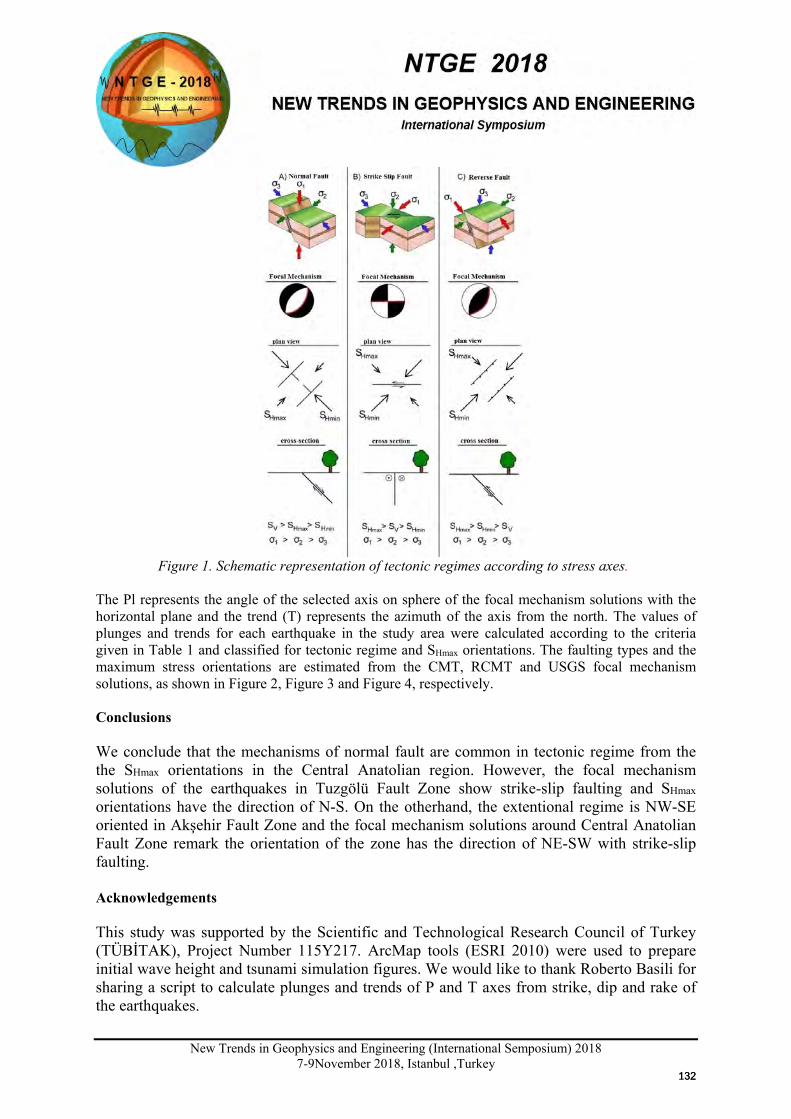
New Trends in Geophysics and Engineering (International Semposium) 2018
7-9November 2018, Istanbul ,Turkey
Figure 1. Schematic representation of tectonic regimes according to stress axes.
The Pl represents the angle of the selected axis on sphere of the focal mechanism solutions with the horizontal plane and the trend (T) represents the azimuth of the axis from the north. The values of plunges and trends for each earthquake in the study area were calculated according to the criteria given in Table 1 and classified for tectonic regime and SHmax orientations. The faulting types and the maximum stress orientations are estimated from the CMT, RCMT and USGS focal mechanism solutions, as shown in Figure 2, Figure 3 and Figure 4, respectively. Conclusions We conclude that the mechanisms of normal fault are common in tectonic regime from the the SHmax orientations in the Central Anatolian region. However, the focal mechanism solutions of the earthquakes in Tuzgölü Fault Zone show strike-slip faulting and SHmax orientations have the direction of N-S. On the otherhand, the extentional regime is NW-SE oriented in Akşehir Fault Zone and the focal mechanism solutions around Central Anatolian Fault Zone remark the orientation of the zone has the direction of NE-SW with strike-slip faulting. Acknowledgements This study was supported by the Scientific and Technological Research Council of Turkey (TÜBİTAK), Project Number 115Y217. ArcMap tools (ESRI 2010) were used to prepare initial wave height and tsunami simulation figures. We would like to thank Roberto Basili for sharing a script to calculate plunges and trends of P and T axes from strike, dip and rake of the earthquakes.
132132
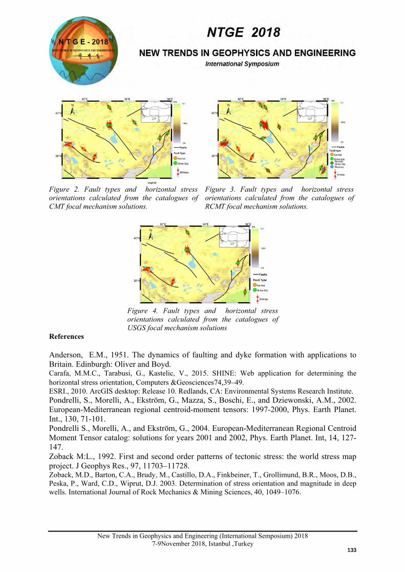
New Trends in Geophysics and Engineering (International Semposium) 2018
7-9November 2018, Istanbul ,Turkey
Figure 2. Fault types and horizontal stress orientations calculated from the catalogues of CMT focal mechanism solutions.
Figure 3. Fault types and horizontal stress orientations calculated from the catalogues of RCMT focal mechanism solutions.
Figure 4. Fault types and horizontal stress orientations calculated from the catalogues of USGS focal mechanism solutions
References Anderson, E.M., 1951. The dynamics of faulting and dyke formation with applications to Britain. Edinburgh: Oliver and Boyd. Carafa, M.M.C., Tarabusi, G., Kastelic, V., 2015. SHINE: Web application for determining the horizontal stress orientation, Computers &Geosciences74,39–49. ESRI., 2010. ArcGIS desktop: Release 10. Redlands, CA: Environmental Systems Research Institute. Pondrelli, S., Morelli, A., Ekström, G., Mazza, S., Boschi, E., and Dziewonski, A.M., 2002. European-Mediterranean regional centroid-moment tensors: 1997-2000, Phys. Earth Planet. Int., 130, 71-101. Pondrelli S., Morelli, A., and Ekström, G., 2004. European-Mediterranean Regional Centroid Moment Tensor catalog: solutions for years 2001 and 2002, Phys. Earth Planet. Int, 14, 127-147. Zoback M:L., 1992. First and second order patterns of tectonic stress: the world stress map project. J Geophys Res., 97, 11703–11728. Zoback, M.D., Barton, C.A., Brudy, M., Castillo, D.A., Finkbeiner, T., Grollimund, B.R., Moos, D.B., Peska, P., Ward, C.D., Wiprut, D.J. 2003. Determination of stress orientation and magnitude in deep wells. International Journal of Rock Mechanics & Mining Sciences, 40, 1049–1076.
133133
New Trends in Geophysics and Engineering (International Semposium) 2018 7-9 November 2018, Istanbul, Turkey
ESTIMATION OF VELOCITY DISTRIBUTION BY 2D TRAVEL TIME REFLECTION TOMOGRAPHY IN THE GULF OF IZMIR (WESTERN TURKEY)
Zehra Altan1, Neslihan Ocakoğlu1, Gualtiero Böhm2
1 Geophysical Engineering Department, Istanbul Technical University, Istanbul, Turkey 2 OGS-Istituto Nazionale di Oceanografia e di Geofisica Sperimentale, Trieste, Italy
Email: [email protected]
Presentation Type
ORAL POSTER
Abstracts
The data processing of a square grid of 250 km high-resolution multi-channel seismic reflection data in the İzmir Gulf by using seismic tomography has been carried out within the framework of a scientific cooperation agreement between ITU and OGS. Seismic tomography is a key for estimating the seismic velocity in depth for any source and receiver position/combination. The aim of this investigation is to define the velocity model down to 1 km below the seafloor, and to identify the shape and depth of reflective horizons in the investigated area. For this purpose, a 2D seismic line from the square grid has chosen to show the inversion procedure for the reflected arrivals. Five horizons were selected by the re-interpretation of the seismic section. The tomographic procedure started from the identification of main reflected events on common shot gathers. The related travel times were used in a process that follows the principle of the minimum time by using the analytical solution of the Snell’s law through an iterative procedure to calculate the ray path between source and receiver. Travel time inversion allows to estimate the local seismic velocities in the area crossed by ray paths by adopting SIRT (Simultaneous Iterative Reconstruction Technique) algorithm. The algorithm for estimating depth and shape of interfaces relies on the principle of minimum dispersion of the estimated reflection points. The investigation provided an accurate velocity model of the water column and sediments below in addition to depths of the interfaces. The geometry and the upper surface morphology of seismic units indicate that the acoustic basement deepens from S to N and the basin sediments above get thicker up to 1 km through the outer gulf.
Keywords: seismic tomography, travel-time inversion, SIRT algorithm, minimum dispersion, İzmir Gulf
Introduction
Seismic traveltime tomography has become an important tool for determining wave velocities particularly in the presence of lateral velocity variation (Bishop et al. 1985). Velocities derived from direct well measurements cannot be compared in accuracy and resolution by other methods. However, in the absence of wells in the study area, velocities obtained from conventional velocity analysis or tomography is the main source of velocity information. The conventional velocity analysis where interval velocities of the nth layer were averaged by the root mean square, is valid for a flat-layered earth
X
134134
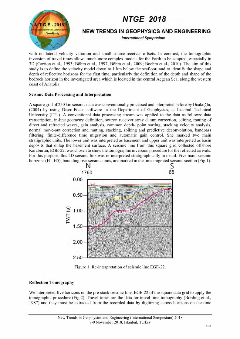
New Trends in Geophysics and Engineering (International Semposium) 2018
7-9 November 2018, Istanbul, Turkey
with no lateral velocity variation and small source-receiver offsets. In contrast, the tomographic inversion of travel times allows much more complex models for the Earth to be adopted, especially in 3D (Carrion et al., 1993; Böhm et al., 1997; Böhm et al., 2009; Boehm et al., 2010). The aim of this study is to define the velocity model down to 1 km below the seafloor, and to identify the shape and depth of reflective horizons for the first time, particularly the definition of the depth and shape of the bedrock horizon in the investigated area which is located in the central Aegean Sea, along the western coast of Anatolia. Seismic Data Processing and Interpretation A square grid of 250 km seismic data was conventionally processed and interpreted before by Ocakoğlu, (2004) by using Disco-Focus software in the Department of Geophysics, at Istanbul Technical University (ITU). A conventional data processing stream was applied to the data as follows: data transcription, in-line geometry definition, source–receiver array datum correction, editing, muting of direct and refracted waves, gain analysis, common depth- point sorting, stacking velocity analysis, normal move-out correction and muting, stacking, spiking and predictive deconvolution, bandpass filtering, finite-difference time migration and automatic gain control. She marked two main stratigraphic units. The lower unit was interpreted as basement and upper unit was interpreted as basin deposits that onlap the basement surface. A seismic line from this square grid collected offshore Karaburun, EGE-22, was chosen to show the tomographic inversion procedure for the reflected arrivals. For this purpose, this 2D seismic line was re-interpreted stratigraphically in detail. Five main seismic horizons (H1-H5), bounding five seismic units, are marked in the time migrated seismic section (Fig.1).
Figure 1: Re-interpretation of seismic line EGE-22. Reflection Tomography We interpreted five horizons on the pre-stack seismic line, EGE-22 of the square data grid to apply the tomographic procedure (Fig.2). Travel times are the data for travel time tomography (Bording et al., 1987) and they must be extracted from the recorded data by digitizing across horizons on the time
135135
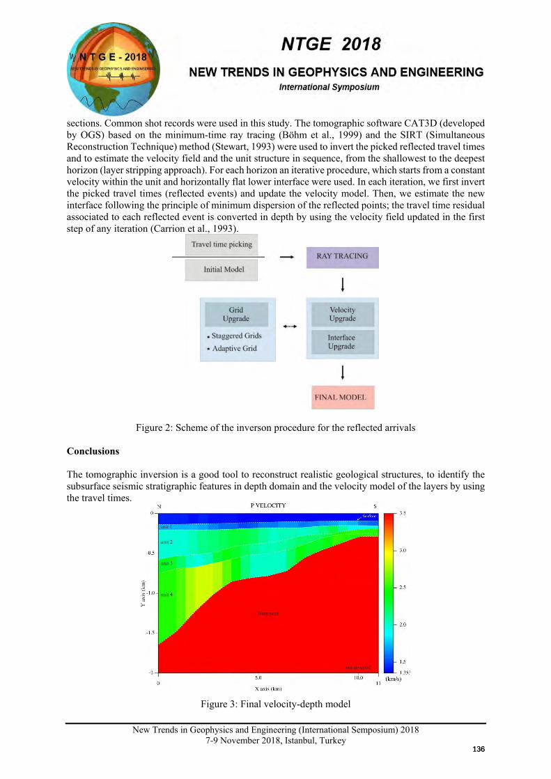
New Trends in Geophysics and Engineering (International Semposium) 2018
7-9 November 2018, Istanbul, Turkey
sections. Common shot records were used in this study. The tomographic software CAT3D (developed by OGS) based on the minimum-time ray tracing (Böhm et al., 1999) and the SIRT (Simultaneous Reconstruction Technique) method (Stewart, 1993) were used to invert the picked reflected travel times and to estimate the velocity field and the unit structure in sequence, from the shallowest to the deepest horizon (layer stripping approach). For each horizon an iterative procedure, which starts from a constant velocity within the unit and horizontally flat lower interface were used. In each iteration, we first invert the picked travel times (reflected events) and update the velocity model. Then, we estimate the new interface following the principle of minimum dispersion of the reflected points; the travel time residual associated to each reflected event is converted in depth by using the velocity field updated in the first step of any iteration (Carrion et al., 1993).
Figure 2: Scheme of the inverson procedure for the reflected arrivals Conclusions The tomographic inversion is a good tool to reconstruct realistic geological structures, to identify the subsurface seismic stratigraphic features in depth domain and the velocity model of the layers by using the travel times.
Figure 3: Final velocity-depth model
136136
New Trends in Geophysics and Engineering (International Semposium) 2018
7-9 November 2018, Istanbul, Turkey
This work illustrates the results of a 2D reflection tomography executed in the İzmir Gulf (Western Turkey) in order to define the velocity model down to 1.5 km below the topographic surface and identify shape and depth of interpreted reflective horizons. The produced 2D depth-velocity model has indicated an accurate velocity model with depth and the final model (Figures 3b) shows a few main aspects: Velocity of water column approx. 140 m thick is between 1410-1500 m/s (Fig. 3). Below it, the sediments (Unit-1) in a shallow layer approx. 60 m thick, Vp values increase to values of 1530-1740 m/s. Vp velocity of third layer (Unit-2) is between 1850-2000 m/s likewise fourth layer has velocity of 2000-2200 m/s (Unit-3). Lastly, fifth layer has the velocity of 2100-2500 m/s (Unit-4). The geometry and the upper surface morphology of seismic units indicate that the acoustic basement deepens from S to N and the basin sediments above it get thicker up to 1 km from S to N direction through the outer gulf.
Acknowledgements This study is part of Ph.D. thesis by Zehra Altan, which is supported by Istanbul Technical University Research Fund (İTÜ-FBE-BAP-Project No: 39685). It is further partly supported by TRILL Fellowship program of ICTP (visiting scholarship during May-August 2016, OGS Trieste, Italy) and Tinçel Kültür Vakfı (visiting scholarship during July 2017-January 2018, OGS Trieste, Italy). We gratefully acknowledge support by the Istituto Nazionale di Oceanografia e di Geofisica Sperimentale (OGS) for allowing us to use the CAT3D software. References Bording, R.P., Gersztenkorn, A., Lines, L. R., Scales J. A., Treitel, S., 1987, Applications of seismic travel-rime tomography. Geophys. J. R. astr. Soc. 90, 285-303. Böhm, G., Rossi, G., Vesnaver, A., 1997, Adaptive regridding in 3D reflection tomography, Annali di Geofisica. 40, 69–83. Böhm, G., Rossi, G., Vesnaver, A., 1999, Minimum time ray tracing for 3D irregular grids, J. Seism. Explor. 8, 117–131. Böhm, G., Ocakoğlu, N., Picotti, S., Santis, L.D., 2009, West Antarctic Ice Sheet evolution: New insights from a seismic tomographic 3D depth model in the Eastern Ross Sea (Antarctica), Marine Geology, 266, 109-128. Boehm, G., Francese R., Giorgi, M., 2010, Bedrock Detection from an Integrated Procedure of Refraction Analysis and Tomographic Inversion of the First Arrivals, 16th European Meeting of Environmental and Engineering Geophysics, Extended Abstracts, P41. Carrion, P., Böhm, G., Marchetti, A., Pettenati, F., Vesnaver, A., 1993, Reconstruction of lateral gradients from reflection tomography. J. Seism. Explor. 2, 55–67. Stewart, R., 1993, In: Domenico, S.N. (Ed.), Exploration Seismic Tomography: Fundamentals. Course note series, vol. 3. SEG-Society of Exploration Geophysicists.
137137
New Trends in Geophysics and Engineering (International Semposium) 2018
7-9 November 2018, Istanbul , Turkey
AN ASSESSMENT ON CURRENT SEISMICITY RATE CHANGES IN ERZURUM PROVINCE OF TURKEY: IMPLICATION FOR EARTHQUAKE HAZARD
Serkan Öztürk1, Mahmut Sarı2
1,2Department of Geophysics, Gümüşhane University, Gümüşhane
Email: [email protected] Presentation Type All accepted proceedings will be published on the webpage of the symposium (ntge2018.istanbul.edu.tr)
ORAL POSTER
Abstracts The current seismicity rate changes for Erzurum province of Turkey were statistically evaluated by using standard normal deviate Z-value and space-time characteristics of the earthquake occurrences at the beginning of 2018 were presented. Significant seismicity rate changes are observed in three regions at the beginning of 2018 and they centered at (i) 41.98ºN-40.48ºE (in and around Oltu and Çobandede Fault Zone), (ii) 40.88ºN-39.78ºE (between Çat and Aşkale, including Aşkale and Erzurum faults) and (iii) 41.87ºN-39.14ºE (the south of Hınıs, Erzurum-Muş borderline). The beginning times of these quiescence anomalies change between 2013 and 2016. The seismic quiescence regions may be the possible regions for the next earthquakes and for this reason, special attention should be given to these anomaly regions. Thus, both the observing the earthquake activity rate and determining the precursory seismic quiescence may present an important point of view in the implication of earthquake hazard.
Keywords: Erzurum, Seismicity rate changes, Decluster, Z-value, Earthquake hazard Introduction Space-time analyses of precursory seismic quiescence is very important but controversial topic. The analyses on the precursors of past events suggest that specific space-time earthquake occurrences include the seismic quiescence phenomenon and may be related to the seismic and tectonic process. Precursory seismic quiescence before some strong or destructive earthquakes has been reported by many authors for different parts of the world and Turkey (e.g., Huang et al. 2001; Polat et al. 2008; Öztürk, 2017). Arabsz and Wyss (1996) stated that expected time interval of precursory quiescence before large earthquakes in global scale has a value of 4.5±3 years and Öztürk (2009) suggested this time interval as 4.9±1.5 years before the occurrences of earthquakes in the eastern part of Turkey. Earthquake Data and Brief Description of Standard Normal Deviate Z-test Earthquake catalog is collected from Boğaziçi University, Kandilli Observatory and Earthquake Research Institute (KOERI). The catalog includes 7769 earthquakes between April 21, 1970 and December 30, 2017 with duration magnitude MD≥1.2. Magnitude completeness value (Mc) for Erzurum region earthquakes is estimated as 2.8. Main tectonics in and around Erzurum are modified from Şaroğlu
X
138138
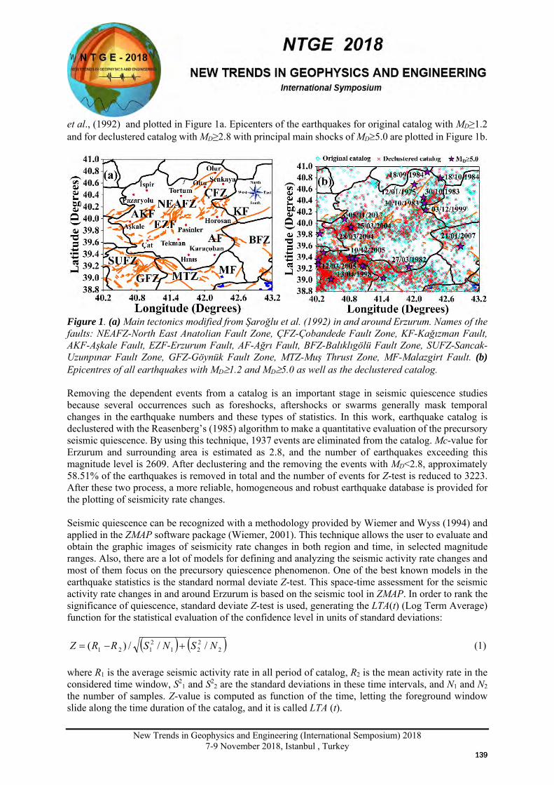
New Trends in Geophysics and Engineering (International Semposium) 2018
7-9 November 2018, Istanbul , Turkey
et al., (1992) and plotted in Figure 1a. Epicenters of the earthquakes for original catalog with MD≥1.2 and for declustered catalog with MD≥2.8 with principal main shocks of MD≥5.0 are plotted in Figure 1b.
Figure 1. (a) Main tectonics modified from Şaroğlu et al. (1992) in and around Erzurum. Names of the faults: NEAFZ-North East Anatolian Fault Zone, ÇFZ-Çobandede Fault Zone, KF-Kağızman Fault, AKF-Aşkale Fault, EZF-Erzurum Fault, AF-Ağrı Fault, BFZ-Balıklıgölü Fault Zone, SUFZ-Sancak-Uzunpınar Fault Zone, GFZ-Göynük Fault Zone, MTZ-Muş Thrust Zone, MF-Malazgirt Fault. (b) Epicentres of all earthquakes with MD≥1.2 and MD≥5.0 as well as the declustered catalog. Removing the dependent events from a catalog is an important stage in seismic quiescence studies because several occurrences such as foreshocks, aftershocks or swarms generally mask temporal changes in the earthquake numbers and these types of statistics. In this work, earthquake catalog is declustered with the Reasenberg’s (1985) algorithm to make a quantitative evaluation of the precursory seismic quiescence. By using this technique, 1937 events are eliminated from the catalog. Mc-value for Erzurum and surrounding area is estimated as 2.8, and the number of earthquakes exceeding this magnitude level is 2609. After declustering and the removing the events with MD<2.8, approximately 58.51% of the earthquakes is removed in total and the number of events for Z-test is reduced to 3223. After these two process, a more reliable, homogeneous and robust earthquake database is provided for the plotting of seismicity rate changes. Seismic quiescence can be recognized with a methodology provided by Wiemer and Wyss (1994) and applied in the ZMAP software package (Wiemer, 2001). This technique allows the user to evaluate and obtain the graphic images of seismicity rate changes in both region and time, in selected magnitude ranges. Also, there are a lot of models for defining and analyzing the seismic activity rate changes and most of them focus on the precursory quiescence phenomenon. One of the best known models in the earthquake statistics is the standard normal deviate Z-test. This space-time assessment for the seismic activity rate changes in and around Erzurum is based on the seismic tool in ZMAP. In order to rank the significance of quiescence, standard deviate Z-test is used, generating the LTA(t) (Log Term Average) function for the statistical evaluation of the confidence level in units of standard deviations:
( ) ( )2221
2121 ///)( NSNSRRZ +−= (1)
where R1 is the average seismic activity rate in all period of catalog, R2 is the mean activity rate in the considered time window, S2
1 and S22 are the standard deviations in these time intervals, and N1 and N2
the number of samples. Z-value is computed as function of the time, letting the foreground window slide along the time duration of the catalog, and it is called LTA (t).
139139
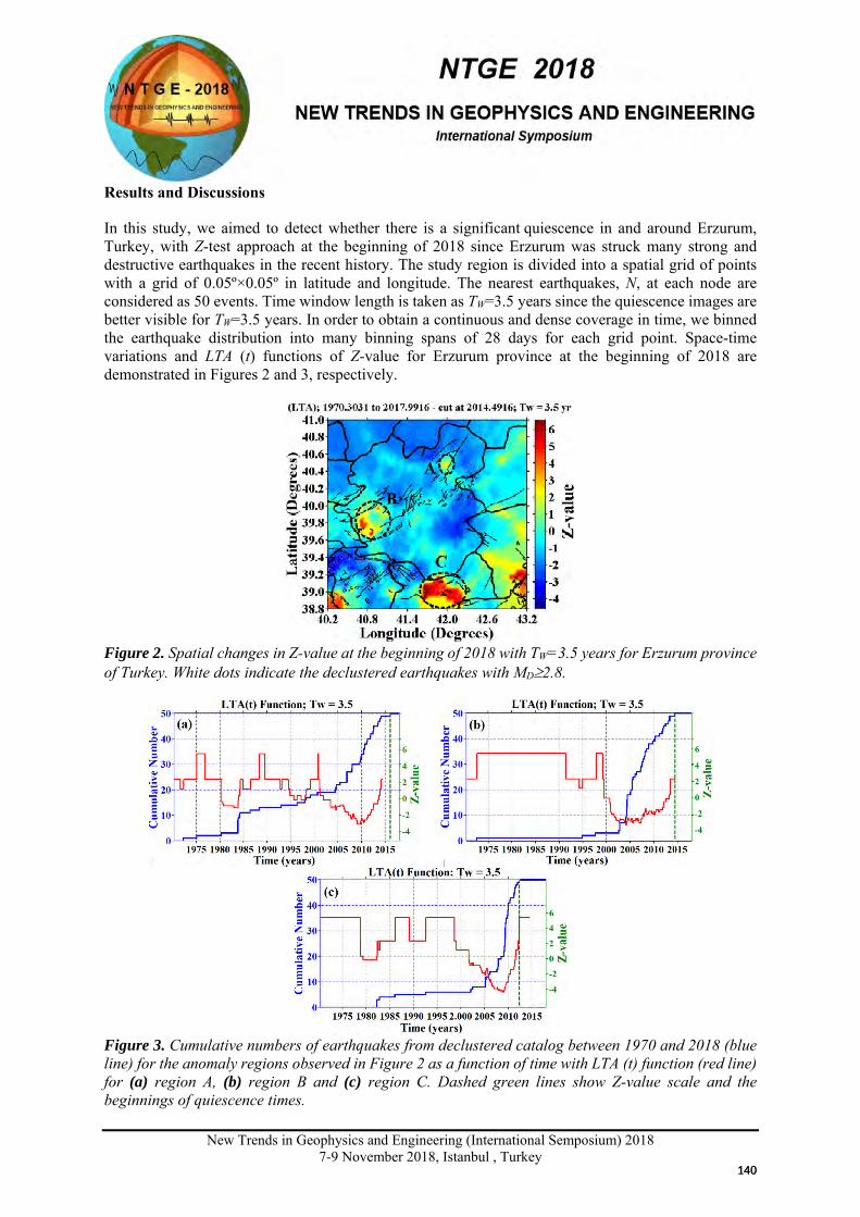
New Trends in Geophysics and Engineering (International Semposium) 2018
7-9 November 2018, Istanbul , Turkey
Results and Discussions
In this study, we aimed to detect whether there is a significant quiescence in and around Erzurum, Turkey, with Z-test approach at the beginning of 2018 since Erzurum was struck many strong and destructive earthquakes in the recent history. The study region is divided into a spatial grid of points with a grid of 0.05º×0.05º in latitude and longitude. The nearest earthquakes, N, at each node are considered as 50 events. Time window length is taken as TW=3.5 years since the quiescence images are better visible for TW=3.5 years. In order to obtain a continuous and dense coverage in time, we binned the earthquake distribution into many binning spans of 28 days for each grid point. Space-time variations and LTA (t) functions of Z-value for Erzurum province at the beginning of 2018 are demonstrated in Figures 2 and 3, respectively.
Figure 2. Spatial changes in Z-value at the beginning of 2018 with TW=3.5 years for Erzurum province of Turkey. White dots indicate the declustered earthquakes with MD≥2.8.
Figure 3. Cumulative numbers of earthquakes from declustered catalog between 1970 and 2018 (blue line) for the anomaly regions observed in Figure 2 as a function of time with LTA (t) function (red line) for (a) region A, (b) region B and (c) region C. Dashed green lines show Z-value scale and the beginnings of quiescence times.
140140
New Trends in Geophysics and Engineering (International Semposium) 2018
7-9 November 2018, Istanbul , Turkey
We observed three regions (A, B and C) exhibiting seismic quiescence anomalies. The first quiescence anomaly is centered at 41.98ºN-40.48ºE (region A, in and around Oltu and Çobandede Fault Zone), the second one is centered at 40.88ºN-39.78ºE (region B, between Çat and Aşkale, including Aşkale and Erzurum faults) and the third one is centered at 41.87ºN-39.14ºE (region C, the south of Hınıs, Erzurum-Muş borderline). Another aim in this study is also to estimate the beginning times of seismic quiescence. To estimate these beginnings, cumulative number of earthquakes are plotted in a circular area including defined three regions. Figure 3 show the cumulative number curves versus time and the correspondent LTA (t) function for three anomaly regions. The Z-value peaked with in 2016.14 for a circle of 23.42 km radius centered at region A, in 2014.50 for a circle of 21.59 km radius centered at region B and in 2012.80 for a circle of 13.92 km radius centered at region C. Thus, these seismic quiescence regions may be considered as the possible regions for the next earthquake occurrences in and around Erzurum.
Conclusions
A statistical assessment on current seismicity rate changes for Erzurum province of Turkey is achieved by using the standard normal deviate Z-test and seismic quiescence variation at the beginning of 2018 is mapped. The instrumental catalog of the KOERI including 7769 events with magnitude equal to and larger than 1.2 from 1970 until 2018 is used. Magnitude completeness for region is estimated as 2.8 and earthquake data set is declustered for Z-test. These processes removed 1937 events and nearly 58.51% of total earthquakes were eliminated from the catalog. Consequently, the final catalog contains 3223 earthquakes for Z-value analysis. At the beginning of 2018, three areas exhibiting seismic quiescence are detected for Erzurum province of Turkey. These anomalies are centered at (i) 41.98ºN-40.48ºE (in and around Oltu and Çobandede Fault Zone), (ii) 40.88ºN-39.78ºE (between Çat and Aşkale, including Aşkale and Erzurum faults) and (iii) 41.87ºN-39.14ºE (the south of Hınıs, Erzurum-Muş borderline). The beginning times of seismic quiescence coincides with recent years and changes between 2012.80 and 2016.14. Consequently, seismic quiescence areas in Erzurum province may be significant and reliable precursor for the next earthquake occurrences and implication for earthquake hazard.
References
Arabasz, W.J., and Wyss, M., 1996, Significant precursory seismic quiescences in the extensional Wasatch front region Utah. EOS, Trans. Am. Geophys. Un. 77, F455.
Huang, Q., Sobolev, G.A., and Nagao, T., 2001, Characteristics of the seismic quiescence and activation patterns before the M=7.2 Kobe earthquake, January 17, 1995, Tectonophysics, 337, 99-116.
Öztürk, S., 2009, An application of the earthquake hazard and aftershock probability evaluation methods to Turkey earthquakes. Ph.D. Thesis, Karadeniz Technical University, Trabzon, 346 pp (in Turkish with English abstract).
Öztürk, S., 2017, Space-time assessing of the earthquake potential in recent years in the Eastern Anatolia region of Turkey, Earth Sciences Research Journal, 21 (2), 67-75.
Polat, O., Gok, E., and Yılmaz, D., 2008, Earthquake hazard of the Aegean Extension region (West Turkey), Turkish Journal of Earth Sciences, 17, 593-614.
Reasenberg, P.A., 1985, Second-order moment of Central California Seismicity, 1969-1982, Journal of Geophysical Research, 90 (B7), 5479-5495.
Şaroğlu, F., Emre, O., and Kuşçu, I., 1992, Active fault map of Turkey, General Directorate of Mineral Research and Exploration, Ankara, Turkey.
Wiemer, S., and Wyss, M., 1994, Seismic quiescence before the Landers (M=7.5) and Big Bear (6.5) 1992 earthquakes, Bulletin of the Seismological Society of America, 84, 900-916.
Wiemer, S., 2001, A software package to analyze seismicity: ZMAP, Seismological Research Letters, 72(2), 373-382.
141141
New Trends in Geophysics and Engineering (International Semposium) 2018
7-9 November 2018, Istanbul , Turkey
X
Applicability of time-dependent seismicity model for earthquake
occurrence along the North Anatolian Fault Zone
Nilgün Sayıl
Geophysical Eng. Department, Karadeniz Technical University, Trabzon Email: [email protected]
Presentation Type All accepted proceedings will be published on the webpage of the symposium (ntge2018.istanbul.edu.tr)
ORAL POSTER
Abstracts North Anatolian Fault Zone has been separated into thirteen seismogenic zones on the basis of certain seismological and geomorphological criteria, and RTIMAP (regional time and magnitude predictable) model has been applied for these zones. The data belonging to both instrumental period (MS ≥ 5.5) and historical period (I0 ≥ 9.0 corresponding to MS ≥ 7.0) have been used in the analysis. Interevent times of mainshocks generated in each zone have predictive properties expressed by the RTIMAP. For the region considered, the positive correlation between the time interval of the events and the magnitude of the preceding earthquake shows that this model is suitable. On the basis of these relations and using the occurrence time and magnitude of the last main shocks in each seismogenic zone, occurrence probabilities to the next main shocks during the next 50 years and the magnitude of the expected main shocks were determined. Keywords: North Anatolian Fault Zone, Time-dependent Seismicity, RTIMAP, Earthquake Occurrence Probability Introduction In the time-predictable model, the time interval between two large earthquakes is proportional to the slip amount of the preceding earthquake and a large earthquake occurs when the stress has reached a limit value. The magnitude-predictable model gives the relation between the magnitudes of the preceding and the following earthquake and indicates that the larger the magnitude of the preceding mainshock, the smaller the magnitude of the following mainshock. Therefore, the time-predictable and magnitude-predictable models were combined to a single one called the RTIMAP (regional time and magnitude predictable) model, which applies to seismogenic zones including the main fault and other smaller faults. In this study, the validity of the time-dependent seismicity model was tested for earthquake generation along the North Anatolian Fault Zone (NAFZ) bounded by 38.5º-41.5º N and 26.0º-43.5º E (Figure 1).
142142
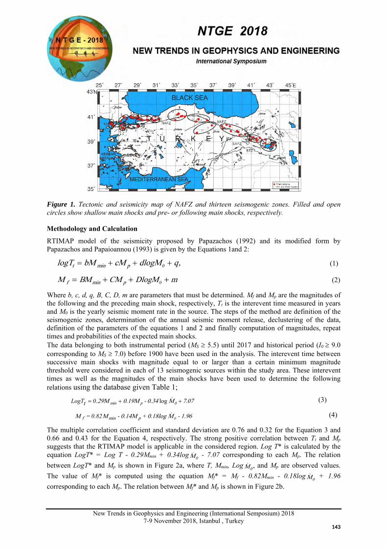
New Trends in Geophysics and Engineering (International Semposium) 2018
7-9 November 2018, Istanbul , Turkey
Figure 1. Tectonic and seismicity map of NAFZ and thirteen seismogenic zones. Filled and open circles show shallow main shocks and pre- or following main shocks, respectively.
Methodology and Calculation
RTIMAP model of the seismicity proposed by Papazachos (1992) and its modified form by Papazachos and Papaioannou (1993) is given by the Equations 1and 2:
,qMlogdcM bMTlog pmint +++= 0 (1)
mMlogDCMBMM pminf +++= 0 (2)
Where b, c, d, q, B, C, D, m are parameters that must be determined. Mf and Mp are the magnitudes of the following and the preceding main shock, respectively, Tt is the interevent time measured in years and M0 is the yearly seismic moment rate in the source. The steps of the method are definition of the seismogenic zones, determination of the annual seismic moment release, declustering of the data, definition of the parameters of the equations 1 and 2 and finally computation of magnitudes, repeat times and probabilities of the expected main shocks. The data belonging to both instrumental period (MS ≥ 5.5) until 2017 and historical period (I0 ≥ 9.0 corresponding to MS ≥ 7.0) before 1900 have been used in the analysis. The interevent time between successive main shocks with magnitude equal to or larger than a certain minimum magnitude threshold were considered in each of 13 seismogenic sources within the study area. These interevent times as well as the magnitudes of the main shocks have been used to determine the following relations using the database given Table 1;
7.07M 0.340.19M.29M 0pmin ++= log -0tLogT (3)
1.96M 0.18log0.14MMM 0pminf -+-= 0.82 (4)
The multiple correlation coefficient and standard deviation are 0.76 and 0.32 for the Equation 3 and 0.66 and 0.43 for the Equation 4, respectively. The strong positive correlation between Tt and Mp suggests that the RTIMAP model is applicable in the considered region. Log T* is calculated by the equation LogT* = Log T - 0.29Mmin + 0.34log 0M - 7.07 corresponding to each Mp. The relation between LogT* and Mp is shown in Figure 2a, where T, Mmin, Log 0M , and Mp are observed values. The value of Mf* is computed using the equation Mf* = Mf - 0.82Mmin - 0.18log 0M + 1.96 corresponding to each Mp. The relation between Mf* and Mp is shown in Figure 2b.
143143
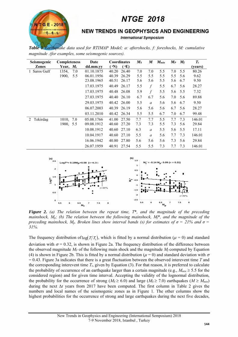
New Trends in Geophysics and Engineering (International Semposium) 2018
7-9 November 2018, Istanbul , Turkey
5.5 6 6.5 7 7.5 8Mp
0
0.5
1
1.5
2
2.5
LogT
*
LogT*= 0.19MP+0.08 (σ=0.21)
s
s
σ=21%
(a)
5.5 6 6.5 7 7.5 8
Mp
-2.5
-2
-1.5
-1
-0.5
0
0.5
1
1.5
M f*
s
s
Mf* = -0.14 Mp- 0.09 (σ = 0.31)
σ=31%
(b)
Figure 2. (a) The relation between the repeat time, T*, and the magnitude of the preceding mainshock, Mp; (b) The relation between the following mainshock, Mf*, and the magnitude of the preceding mainshock, Mp. Broken lines show interval bands (s) for estimates of σ = 21% and σ = 31%. The frequency distribution of ( )tTTlog , which is fitted by a normal distribution (µ = 0) and standard deviation with σ = 0.32, is shown in Figure 2a. The frequency distribution of the difference between the observed magnitude MF of the following main shock and the magnitude Mf computed by Equation (4) is shown in Figure 2b. This is fitted by a normal distribution (µ = 0) and standard deviation with σ = 0.43. Figure 3a indicates that there is a great fluctuation between the observed interevent time T and the corresponding interevent time Tt, given by Equation (3). For that reason, it is preferred to calculate the probability of occurrence of an earthquake larger than a certain magnitude (e.g., Mmin ≥ 5.5 for the considered region) and for given time interval. Accepting the validity of the lognormal distribution, the probability for the occurrence of strong (MS ≥ 6.0) and large (MS ≥ 7.0) earthquakes (M ≥ Mmin) during the next ∆t years from 2017 have been computed. The first column in Table 2 gives the numbers and local names of the seismogenic zones as in Figure 1. The other columns show the highest probabilities for the occurrence of strong and large earthquakes during the next five decades,
Table 1 Earthquake data used for RTIMAP Model; a: aftershocks, f: foreshocks, M: cumulative magnitude .(for examples, some seismogenic sources).
Seismogenic Zones
Completeness Year, Mc
Date dd.mm.yy
Coordinates ( N) ( E)
MS M Mmin MP Mf Tt (years)
1 Saros Gulf 1354, 7.0 01.10.1875 40.20 26.40 7.0 7.0 5.5 7.0 5.5 80.26 1900, 5.5 06.01.1956 40.39 26.29 5.5 5.5 5.5 5.5 5.6 9.62 23.08.1965 40.51 26.17 5.6 5.6 5.5 5.6 6.7 9.50 17.03.1975 40.49 26.17 5.5 f 5.5 6.7 5.6 28.27 17.03.1975 40.48 26.08 5.9 f 5.5 5.6 5.5 7.32 27.03.1975 40.40 26.10 6.7 6.7 5.6 7.0 5.6 89.88 29.03.1975 40.42 26.00 5.5 a 5.6 5.6 6.7 9.50 06.07.2003 40.39 26.19 5.6 5.6 5.6 6.7 5.6 28.27 03.11.2010 40.42 26.34 5.5 5.5 6.7 7.0 6.7 99.48
2 Tekirdag 1010, 7.0 05.08.1766 41.00 27.50 7.7 7.7 5.5 7.7 7.3 146.01 1900, 5.5 09.08.1912 40.60 27.20 7.3 7.3 5.5 7.3 5.6 29.84 10.08.1912 40.60 27.10 6.3 a 5.5 5.6 5.5 17.11 10.04.1917 40.60 27.10 5.5 a 5.6 7.7 7.3 146.01 16.06.1942 40.80 27.80 5.6 5.6 5.6 7.3 5.6 29.84 26.07.1959 40.91 27.54 5.5 5.5 7.3 7.7 7.3 146.01
144144
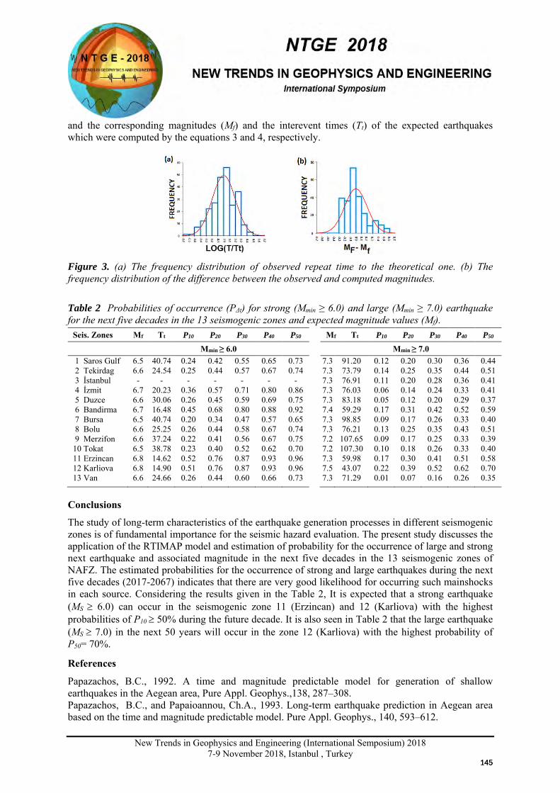
New Trends in Geophysics and Engineering (International Semposium) 2018
7-9 November 2018, Istanbul , Turkey
and the corresponding magnitudes (Mf) and the interevent times (Tt) of the expected earthquakes which were computed by the equations 3 and 4, respectively.
Figure 3. (a) The frequency distribution of observed repeat time to the theoretical one. (b) The frequency distribution of the difference between the observed and computed magnitudes.
Table 2 Probabilities of occurrence (PΔt) for strong (Mmin ≥ 6.0) and large (Mmin ≥ 7.0) earthquake for the next five decades in the 13 seismogenic zones and expected magnitude values (Mf).
Seis. Zones Mf Tt P10 P20 P30 P40 P50 Mf Tt P10 P20 P30 P40 P50
Mmin ≥ 6.0 Mmin ≥ 7.0 1 Saros Gulf 2 Tekirdag 3 İstanbul 4 İzmit 5 Duzce 6 Bandirma 7 Bursa 8 Bolu 9 Merzifon 10 Tokat 11 Erzincan 12 Karliova 13 Van
6.5 6.6 -
6.7 6.6 6.7 6.5 6.6 6.6 6.5 6.8 6.8 6.6
40.74 24.54
- 20.23 30.06 16.48 40.74 25.25 37.24 38.78 14.62 14.90 24.66
0.24 0.25
- 0.36 0.26 0.45 0.20 0.26 0.22 0.23 0.52 0.51 0.26
0.42 0.44
- 0.57 0.45 0.68 0.34 0.44 0.41 0.40 0.76 0.76 0.44
0.55 0.57
- 0.71 0.59 0.80 0.47 0.58 0.56 0.52 0.87 0.87 0.60
0.65 0.67
- 0.80 0.69 0.88 0.57 0.67 0.67 0.62 0.93 0.93 0.66
0.73 0.74
- 0.86 0.75 0.92 0.65 0.74 0.75 0.70 0.96 0.96 0.73
7.3 7.3 7.3 7.3 7.3 7.4 7.3 7.3 7.2 7.2 7.3 7.5 7.3
91.20 73.79 76.91 76.03 83.18 59.29 98.85 76.21
107.65 107.30 59.98 43.07 71.29
0.12 0.14 0.11 0.06 0.05 0.17 0.09 0.13 0.09 0.10 0.17 0.22 0.01
0.20 0.25 0.20 0.14 0.12 0.31 0.17 0.25 0.17 0.18 0.30 0.39 0.07
0.30 0.35 0.28 0.24 0.20 0.42 0.26 0.35 0.25 0.26 0.41 0.52 0.16
0.36 0.44 0.36 0.33 0.29 0.52 0.33 0.43 0.33 0.33 0.51 0.62 0.26
0.44 0.51 0.41 0.41 0.37 0.59 0.40 0.51 0.39 0.40 0.58 0.70 0.35
Conclusions
The study of long-term characteristics of the earthquake generation processes in different seismogenic zones is of fundamental importance for the seismic hazard evaluation. The present study discusses the application of the RTIMAP model and estimation of probability for the occurrence of large and strong next earthquake and associated magnitude in the next five decades in the 13 seismogenic zones of NAFZ. The estimated probabilities for the occurrence of strong and large earthquakes during the next five decades (2017-2067) indicates that there are very good likelihood for occurring such mainshocks in each source. Considering the results given in the Table 2, It is expected that a strong earthquake (MS ≥ 6.0) can occur in the seismogenic zone 11 (Erzincan) and 12 (Karliova) with the highest probabilities of P10 ≥ 50% during the future decade. It is also seen in Table 2 that the large earthquake (MS ≥ 7.0) in the next 50 years will occur in the zone 12 (Karliova) with the highest probability of P50= 70%.
References Papazachos, B.C., 1992. A time and magnitude predictable model for generation of shallow earthquakes in the Aegean area, Pure Appl. Geophys.,138, 287–308. Papazachos, B.C., and Papaioannou, Ch.A., 1993. Long-term earthquake prediction in Aegean area based on the time and magnitude predictable model. Pure Appl. Geophys., 140, 593–612.
145145
New Trends in Geophysics and Engineering (International Semposium) 2018
7-9 November 2018, Istanbul , Turkey
X
Definition of the crust structure of Anatolia by surface wave data
Nilgün Sayıl
Geophysical Eng. Department, Karadeniz Technical University, Trabzon
Email: [email protected] Presentation Type All accepted proceedings will be published on the webpage of the symposium (ntge2018.istanbul.edu.tr)
ORAL POSTER
Abstracts Dispersion property of surface waves has been used to investigate the Earth crust and upper mantle structure. In this study, the crust structure of Anatolia has been investigated by measuring the group velocity dispersion data of discriminated seismic surface waves. In the scope of the study, it has selected the profiles between six stations located in western Anatolia of Boğaziçi University Kandilli Observatory Earthquake Research Institute (KOERI), national network of Turkey, and records of an earthquake (having about 10˚ epicentral distance) occurred in the eastern of Anatolia have been used. Firstly, surface wave discrimination filter based on the polarization properties has been applied to three-component records and emphasized to surface waves. Then the group velocities have been calculated by multiple filter technique. A five-layered crustal model having total thickness of 38km - 40km and Pn-wave velocity of 8.00km/sec in the upper-mantle has been determined through inversion of surface wave group velocity dispersion data in the period range of 10 sec to 60 sec. Keywords: Dispersion, Surface Waves, Discrimination Filter, Anatolia Introduction Surface wave data have been used to define the earth structure on different propagating paths. The parameters as group arrival times, phase angles and amplitude values of surface waves are used to research elastic properties of the earth. In order to determine parameters as particle motion, phase and group velocity, single-station, two-station, and three- or more station methods can be used. The simplest one is a single-station method (Ewing et al., 1957; Pilant, 1979). Source effect is large on phase delays. And it also decreases while period increases. Therefore, the source functions are not considered for group velocity solutions for about 10˚ epicenter records on which periods are large enough (Panza et al., 1973, 1975). In this study, the crust and upper mantle structure of Anatolia have been investigated by measuring the group velocity dispersion data of discriminated seismic surface waves. Earthquakes occurred in eastern and western of Anatolia have good locations to construct the profiles across Anatolia. Long-period three-component seismograms at KOERI stations (YLVX, MLSB, MRMX, ISP, ISK, EDRB) located in western Anatolia of an earthquake (EZM) occurred in eastern Anatolia have been used (Figure 1).
146146
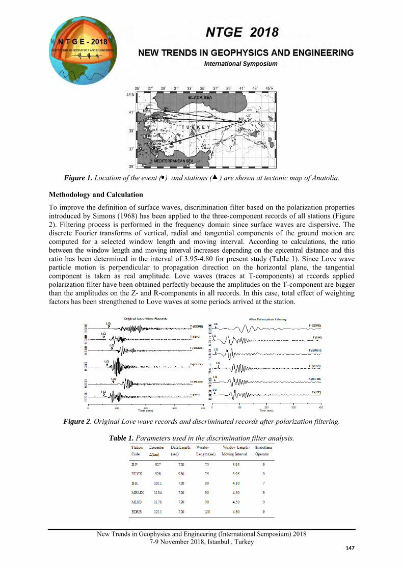
New Trends in Geophysics and Engineering (International Semposium) 2018
7-9 November 2018, Istanbul , Turkey
Figure 1. Location of the event ( ) and stations ( ) are shown at tectonic map of Anatolia.
Methodology and Calculation
To improve the definition of surface waves, discrimination filter based on the polarization properties introduced by Simons (1968) has been applied to the three-component records of all stations (Figure 2). Filtering process is performed in the frequency domain since surface waves are dispersive. The discrete Fourier transforms of vertical, radial and tangential components of the ground motion are computed for a selected window length and moving interval. According to calculations, the ratio between the window length and moving interval increases depending on the epicentral distance and this ratio has been determined in the interval of 3.95-4.80 for present study (Table 1). Since Love wave particle motion is perpendicular to propagation direction on the horizontal plane, the tangential component is taken as real amplitude. Love waves (traces at T-components) at records applied polarization filter have been obtained perfectly because the amplitudes on the T-component are bigger than the amplitudes on the Z- and R-components in all records. In this case, total effect of weighting factors has been strengthened to Love waves at some periods arrived at the station.
Figure 2. Original Love wave records and discriminated records after polarization filtering.
Table 1. Parameters used in the discrimination filter analysis.
147147
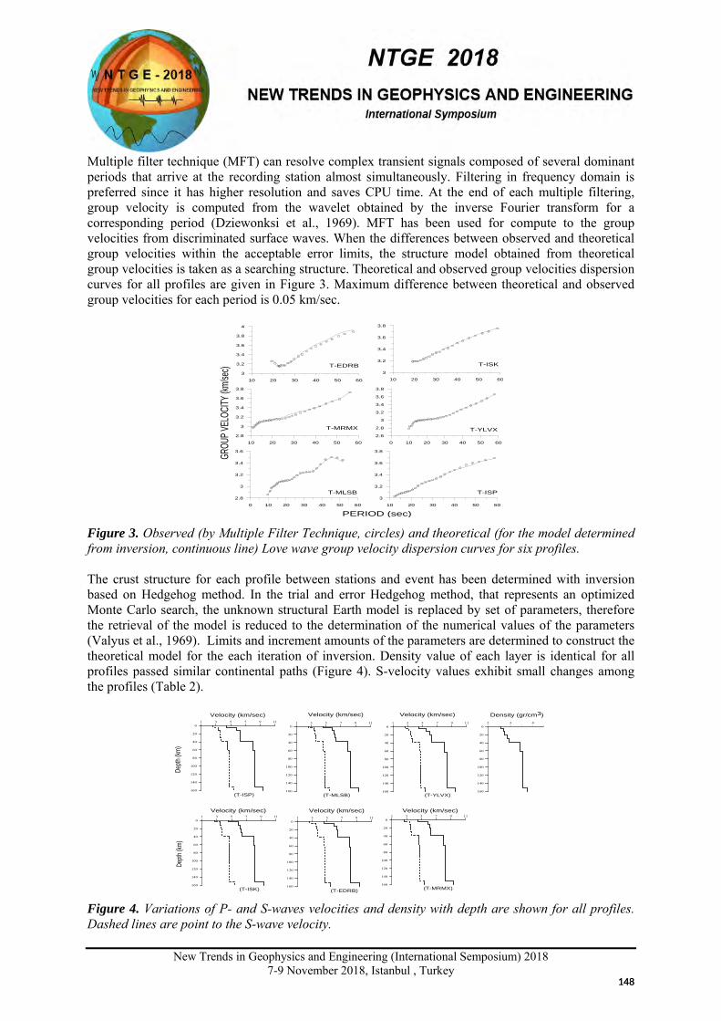
New Trends in Geophysics and Engineering (International Semposium) 2018
7-9 November 2018, Istanbul , Turkey
Multiple filter technique (MFT) can resolve complex transient signals composed of several dominant periods that arrive at the recording station almost simultaneously. Filtering in frequency domain is preferred since it has higher resolution and saves CPU time. At the end of each multiple filtering, group velocity is computed from the wavelet obtained by the inverse Fourier transform for a corresponding period (Dziewonksi et al., 1969). MFT has been used for compute to the group velocities from discriminated surface waves. When the differences between observed and theoretical group velocities within the acceptable error limits, the structure model obtained from theoretical group velocities is taken as a searching structure. Theoretical and observed group velocities dispersion curves for all profiles are given in Figure 3. Maximum difference between theoretical and observed group velocities for each period is 0.05 km/sec.
10 20 30 40 50 60
3
3.2
3.4
3.6
3.8
4
T-EDRB
10 20 30 40 50 60
3
3.2
3.4
3.6
3.8
T-ISK
10 20 30 40 50 60
2.8
3
3.2
3.4
3.6
3.8
T-MRMX
0 10 20 30 40 50 60
2.6
2.8
3
3.2
3.4
3.6
3.8
T-YLVX
0 10 20 30 40 50 60
2.8
3
3.2
3.4
3.6
T-MLSB
10 20 30 40 50 60
3
3.2
3.4
3.6
3.8
T-ISP
GROU
P VEL
OCITY
(km/
sec)
PERIOD (sec) Figure 3. Observed (by Multiple Filter Technique, circles) and theoretical (for the model determined from inversion, continuous line) Love wave group velocity dispersion curves for six profiles. The crust structure for each profile between stations and event has been determined with inversion based on Hedgehog method. In the trial and error Hedgehog method, that represents an optimized Monte Carlo search, the unknown structural Earth model is replaced by set of parameters, therefore the retrieval of the model is reduced to the determination of the numerical values of the parameters (Valyus et al., 1969). Limits and increment amounts of the parameters are determined to construct the theoretical model for the each iteration of inversion. Density value of each layer is identical for all profiles passed similar continental paths (Figure 4). S-velocity values exhibit small changes among the profiles (Table 2).
1 3 5 7 9 11
160
140
120
100
80
60
40
20
0
(T-ISP)
1 3 5 7 9 11
160
140
120
100
80
60
40
20
0
(T-MLSB)
1 3 5 7 9 11
160
140
120
100
80
60
40
20
0
(T-YLVX)
1 3 5 7 9 11
160
140
120
100
80
60
40
20
0
(T-MRMX)
1 3 5 7 9 11
160
140
120
100
80
60
40
20
0
(T-ISK)
1 3 5 7 9 11
160
140
120
100
80
60
40
20
0
(T-EDRB)
2 3 4
160
140
120
100
80
60
40
20
0
Density (gr/cm3)
Depth
(km)
Depth
(km)
Velocity (km/sec) Velocity (km/sec) Velocity (km/sec)
Velocity (km/sec) Velocity (km/sec) Velocity (km/sec)
Figure 4. Variations of P- and S-waves velocities and density with depth are shown for all profiles. Dashed lines are point to the S-wave velocity.
148148
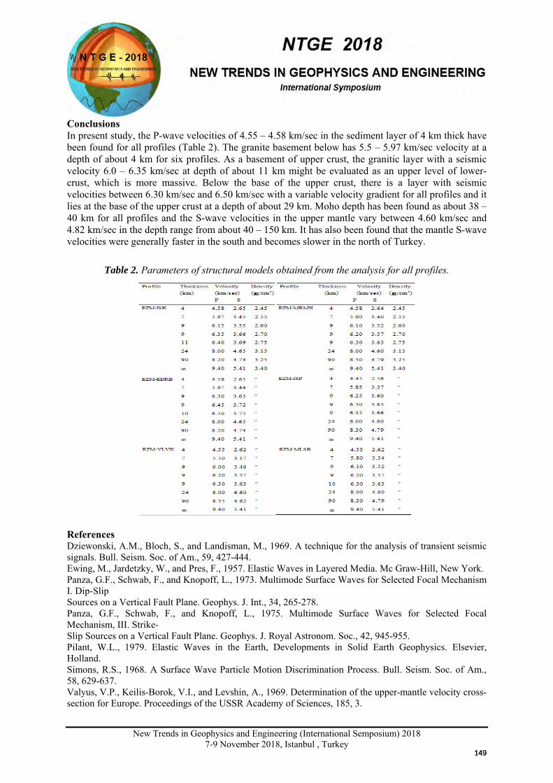
New Trends in Geophysics and Engineering (International Semposium) 2018
7-9 November 2018, Istanbul , Turkey
Conclusions In present study, the P-wave velocities of 4.55 – 4.58 km/sec in the sediment layer of 4 km thick have been found for all profiles (Table 2). The granite basement below has 5.5 – 5.97 km/sec velocity at a depth of about 4 km for six profiles. As a basement of upper crust, the granitic layer with a seismic velocity 6.0 – 6.35 km/sec at depth of about 11 km might be evaluated as an upper level of lower-crust, which is more massive. Below the base of the upper crust, there is a layer with seismic velocities between 6.30 km/sec and 6.50 km/sec with a variable velocity gradient for all profiles and it lies at the base of the upper crust at a depth of about 29 km. Moho depth has been found as about 38 – 40 km for all profiles and the S-wave velocities in the upper mantle vary between 4.60 km/sec and 4.82 km/sec in the depth range from about 40 – 150 km. It has also been found that the mantle S-wave velocities were generally faster in the south and becomes slower in the north of Turkey.
Table 2. Parameters of structural models obtained from the analysis for all profiles.
References Dziewonski, A.M., Bloch, S., and Landisman, M., 1969. A technique for the analysis of transient seismic signals. Bull. Seism. Soc. of Am., 59, 427-444. Ewing, M., Jardetzky, W., and Pres, F., 1957. Elastic Waves in Layered Media. Mc Graw-Hill, New York. Panza, G.F., Schwab, F., and Knopoff, L., 1973. Multimode Surface Waves for Selected Focal Mechanism I. Dip-Slip Sources on a Vertical Fault Plane. Geophys. J. Int., 34, 265-278. Panza, G.F., Schwab, F., and Knopoff, L., 1975. Multimode Surface Waves for Selected Focal Mechanism, III. Strike- Slip Sources on a Vertical Fault Plane. Geophys. J. Royal Astronom. Soc., 42, 945-955. Pilant, W.L., 1979. Elastic Waves in the Earth, Developments in Solid Earth Geophysics. Elsevier, Holland. Simons, R.S., 1968. A Surface Wave Particle Motion Discrimination Process. Bull. Seism. Soc. of Am., 58, 629-637. Valyus, V.P., Keilis-Borok, V.I., and Levshin, A., 1969. Determination of the upper-mantle velocity cross-section for Europe. Proceedings of the USSR Academy of Sciences, 185, 3.
149149
New Trends in Geophysics and Engineering (International Semposium) 2018
7-9 November 2018, Istanbul , Turkey
X
Application of Slip Predictable Model to Earthquake in Anatolia
Nilgün Sayıl
Geophysical Eng. Department, Karadeniz Technical University, Trabzon Email: [email protected]
Presentation Type All accepted proceedings will be published on the webpage of the symposium (ntge2018.istanbul.edu.tr)
ORAL POSTER
Abstracts Anatolia has been considered for an earthquake generation model using earthquake data in the historical and instrumental period earthquake catalogues. In this region, 33 seismogenic sources were identified on the basis of certain seismological and geomorphological criteria and time and slip predictable model has been applied for these sources. It is observed that the time interval between the two consecutive mainshocks depends upon the preceding mainshock magnitude. A linear relation between the logarithm of repeat time (T) of two successive events and the magnitude of the preceding mainshock (Mp) is established in the form “LogT = cMp + a”, where “c” is a positive slope of line and “a” is function of minimum magnitude of the earthquake considered. The values of the parameters “c” and “a” are estimated to be 0.19 and 0.68 in Turkey. Also, it is observed that the repeat time (T) between the two consecutive mainshocks depends upon the following mainshock (Mf). A linear regression with positive slope (0.05) between the logarithm of repeat time of two consecutive events (LogT) and the magnitude of the following mainshock (Mf) was obtained. For the region considered, the positive correlation between the time interval of the events and the magnitude of the preceding earthquake shows that the time-predictable model is suitable. Also, the negative slope (-0.01) was obtained between Mp and Mf and it indicates that a large mainshock is followed by a small one and vice versa, which is accordance with slip-predictable model.
Keywords: Slip-Predictable Model, Earthquake Occurrence Model, Anatolia Introduction
The earthquake recurrence models were proposed based on Reid’s concept of the elastic rebound theory, i.e. that successive earthquakes occur when stress reaches a critical value in a fault of seismogenic sources (Shimazaki and Nakata, 1980). Figure 1 shows the two levels of stresses, τ1 and τ2, upper and lower level, respectively. These stresses are responsible for controlling the behavior of a fault in the earthquake generation process. When τ1 is constant, the model is said to be time predictable (Fig. 1a). In this case, stress drop changes to different shocks. When τ2 constant, the model is said to be slip predictable. In this case, earthquakes start at variable states of stress (Fig. 1b). In the case of the slip-predictable model, the time interval between two successive, large earthquakes is proportional to the slip amount of the next large earthquake. In general, only the size of a future
150150
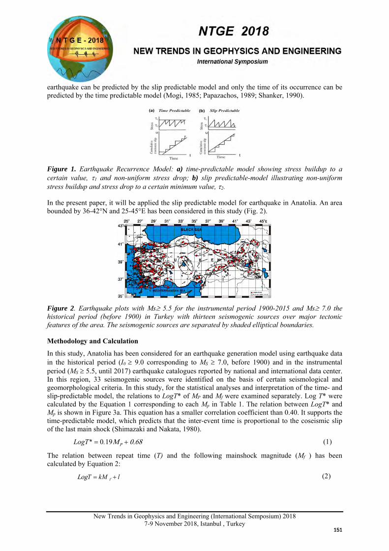
New Trends in Geophysics and Engineering (International Semposium) 2018
7-9 November 2018, Istanbul , Turkey
earthquake can be predicted by the slip predictable model and only the time of its occurrence can be predicted by the time predictable model (Mogi, 1985; Papazachos, 1989; Shanker, 1990).
Figure 1. Earthquake Recurrence Model: a) time-predictable model showing stress buildup to a certain value, τ1 and non-uniform stress drop; b) slip predictable-model illustrating non-uniform stress buildup and stress drop to a certain minimum value, τ2.
In the present paper, it will be applied the slip predictable model for earthquake in Anatolia. An area bounded by 36-42°N and 25-45°E has been considered in this study (Fig. 2).
Figure 2. Earthquake plots with Ms≥ 5.5 for the instrumental period 1900-2015 and Ms≥ 7.0 the historical period (before 1900) in Turkey with thirteen seismogenic sources over major tectonic features of the area. The seismogenic sources are separated by shaded elliptical boundaries.
Methodology and Calculation
In this study, Anatolia has been considered for an earthquake generation model using earthquake data in the historical period (I0 ≥ 9.0 corresponding to MS ≥ 7.0, before 1900) and in the instrumental period (MS ≥ 5.5, until 2017) earthquake catalogues reported by national and international data center. In this region, 33 seismogenic sources were identified on the basis of certain seismological and geomorphological criteria. In this study, for the statistical analyses and interpretation of the time- and slip-predictable model, the relations to LogT* of MP and Mf were examined separately. Log T* were calculated by the Equation 1 corresponding to each Mp in Table 1. The relation between LogT* and Mp is shown in Figure 3a. This equation has a smaller correlation coefficient than 0.40. It supports the time-predictable model, which predicts that the inter-event time is proportional to the coseismic slip of the last main shock (Shimazaki and Nakata, 1980).
0.68MP += 190.LogT* (1)
The relation between repeat time (T) and the following mainshock magnitude (Mf ) has been calculated by Equation 2:
lkMT += fLog (2)
151151
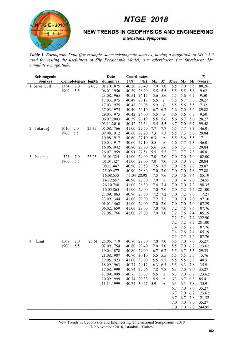
New Trends in Geophysics and Engineering (International Semposium) 2018
7-9 November 2018, Istanbul , Turkey
Table 1. Earthquake Data (for example, some seismogenic sources) having a magnitude of Ms ≥ 5.5 used for testing the usefulness of Slip Predictable Model; a = aftershocks, f = foreshocks, M= cumulative magnitude.
Seismogenic Sources
Completeness
logṀ0
Date dd.mm.yy
Coordinates ( N) ( E)
MS
M
Mmin
MP
Mf
Tt (years)
1 Saros Gulf 1354, 7.0 24.73 01.10.1875 40.20 26.40 7.0 7.0 5.5 7.0 5.5 80.26 1900, 5.5 06.01.1956 40.39 26.29 5.5 5.5 5.5 5.5 5.6 9.62 23.08.1965 40.51 26.17 5.6 5.6 5.5 5.6 6.7 9.50 17.03.1975 40.49 26.17 5.5 f 5.5 6.7 5.6 28.27 17.03.1975 40.48 26.08 5.9 f 5.5 5.6 5.5 7.32 27.03.1975 40.40 26.10 6.7 6.7 5.6 7.0 5.6 89.88 29.03.1975 40.42 26.00 5.5 a 5.6 5.6 6.7 9.50 06.07.2003 40.39 26.19 5.6 5.6 5.6 6.7 5.6 28.27 03.11.2010 40.42 26.34 5.5 5.5 6.7 7.0 6.7 99.48
2 Tekirdağ 1010, 7.0 25.37 05.08.1766 41.00 27.50 7.7 7.7 5.5 7.7 7.3 146.01 1900, 5.5 09.08.1912 40.60 27.20 7.3 7.3 5.5 7.3 5.6 29.84 10.08.1912 40.60 27.10 6.3 a 5.5 5.6 5.5 17.11 10.04.1917 40.60 27.10 5.5 a 5.6 7.7 7.3 146.01 16.06.1942 40.80 27.80 5.6 5.6 5.6 7.3 5.6 29.84 26.07.1959 40.91 27.54 5.5 5.5 7.3 7.7 7.3 146.01
3 Istanbul 325, 7.0 25.23 01.01.325 41.00 29.00 7.0 7.0 7.0 7.0 7.0 102.00 1900, 5.5 01.01.427 41.00 29.00 7.0 7.0 7.0 7.0 7.5 20.84 08.11.447 40.90 28.50 7.5 7.5 7.0 7.5 7.0 29.87 25.09.477 40.90 28.80 7.0 7.0 7.0 7.0 7.6 77.88 16.08.555 41.04 28.98 7.5 7.6 7.0 7.6 7.4 185.19 14.12.557 40.90 28.80 7.0 a 7.0 7.4 7.0 124.55 26.10.740 41.00 28.30 7.4 7.4 7.0 7.0 7.2 198.35 16.05.865 41.00 29.00 7.0 7.0 7.0 7.2 7.2 281.00
23.09.1063 40.90 28.30 7.2 7.2 7.0 7.2 7.0 117.27 23.09.1344 41.00 29.00 7.2 7.2 7.0 7.0 7.0 197.10 01.01.1462 41.00 29.00 7.0 7.0 7.0 7.0 7.0 107.29 06.02.1659 41.00 29.00 7.0 7.0 7.2 7.5 7.6 107.76 22.05.1766 41.00 29.00 7.0 7.0 7.2 7.6 7.4 185.19 7.2 7.4 7.2 322.90 7.2 7.2 7.2 281.00 7.4 7.5 7.6 107.76 7.4 7.6 7.4 185.19 7.5 7.5 7.6 107.76 4 İzmit 1509, 7.0 25.61 25.05.1719 40.70 29.50 7.0 7.0 5.5 7.0 7.0 35.27 1900, 5.5 02.09.1754 40.80 29.40 7.0 7.0 5.5 7.0 6.7 123.62 19.04.1878 40.80 29.00 6.7 6.7 5.5 6.7 5.5 29.33 21.08.1907 40.70 30.10 5.5 5.5 5.5 5.5 5.5 15.76 29.05.1923 41.00 30.00 5.5 5.5 5.5 5.5 6.3 40.3 18.09.1963 40.77 29.12 6.3 6.3 5.5 6.3 7.8 35.9 17.08.1999 40.74 29.96 7.8 7.8 6.3 7.0 7.0 35.27 13.09.1999 40.75 30.08 5.5 a 6.3 7.0 6.7 123.62 20.09.1999 40.74 29.33 5.5 a 6.3 6.7 6.3 85.41 11.11.1999 40.74 30.27 5.9 a 6.3 6.3 7.8 35.9 6.7 7.0 7.0 35.27 6.7 7.0 6.7 123.62 6.7 6.7 7.8 121.32 7.0 7.0 7.0 35.27 7.0 7.0 7.8 244.95
152152
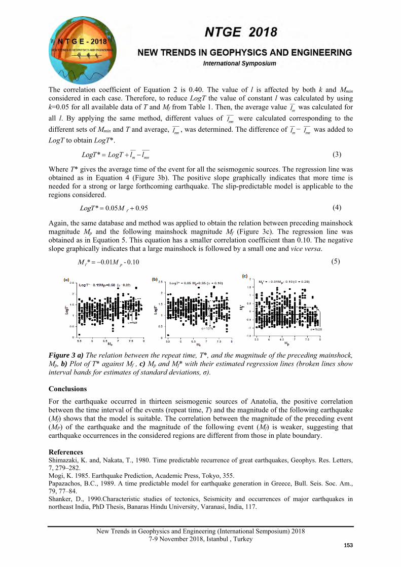
New Trends in Geophysics and Engineering (International Semposium) 2018
7-9 November 2018, Istanbul , Turkey
The correlation coefficient of Equation 2 is 0.40. The value of l is affected by both k and Mmin considered in each case. Therefore, to reduce LogT the value of constant l was calculated by using k=0.05 for all available data of T and Mf from Table 1. Then, the average value ml was calculated for all l. By applying the same method, different values of mnl were calculated corresponding to the different sets of Mmin and T and average, mnl , was determined. The difference of ml − mnl was added to LogT to obtain LogT*.
mnm llLogTT −+=*Log (3)
Where T* gives the average time of the event for all the seismogenic sources. The regression line was obtained as in Equation 4 (Figure 3b). The positive slope graphically indicates that more time is needed for a strong or large forthcoming earthquake. The slip-predictable model is applicable to the regions considered.
.950 05.0* += fLog MT (4)
Again, the same database and method was applied to obtain the relation between preceding mainshock magnitude Mp and the following mainshock magnitude Mf (Figure 3c). The regression line was obtained as in Equation 5. This equation has a smaller correlation coefficient than 0.10. The negative slope graphically indicates that a large mainshock is followed by a small one and vice versa.
.100 - 01.0* pfM M−= (5)
Figure 3 a) The relation between the repeat time, T*, and the magnitude of the preceding mainshock, Mp, b) Plot of T* against Mf , c) Mp and Mf* with their estimated regression lines (broken lines show interval bands for estimates of standard deviations, σ).
Conclusions
For the earthquake occurred in thirteen seismogenic sources of Anatolia, the positive correlation between the time interval of the events (repeat time, T) and the magnitude of the following earthquake (Mf) shows that the model is suitable. The correlation between the magnitude of the preceding event (MP) of the earthquake and the magnitude of the following event (Mf) is weaker, suggesting that earthquake occurrences in the considered regions are different from those in plate boundary.
References Shimazaki, K. and, Nakata, T., 1980. Time predictable recurrence of great earthquakes, Geophys. Res. Letters, 7, 279–282. Mogi, K. 1985. Earthquake Prediction, Academic Press, Tokyo, 355. Papazachos, B.C., 1989. A time predictable model for earthquake generation in Greece, Bull. Seis. Soc. Am., 79, 77–84. Shanker, D., 1990.Characteristic studies of tectonics, Seismicity and occurrences of major earthquakes in northeast India, PhD Thesis, Banaras Hindu University, Varanasi, India, 117.
153153
New Trends in Geophysics and Engineering (International Semposium) 2018
7-9 November 2018, Istanbul, Turkey
X
EVALUATION OF SOIL LIQUEFACTION POTENTIAL BY USING
MICROTREMOR MEASUREMENTS IN TRABZON, TURKEY
Sinem CEYLAN1, Ali Erden BABACAN1, Özgenç AKIN1
1Geophysical Eng. Department, Karadeniz Technical University, Trabzon
Email:[email protected] Presentation Type
ORAL POSTER
Abstracts Determination of the characteristics of the soils on which constructions will be built before earthquakes or similar disasters are among the most important topics of geotechnical engineering. One of the most important soil problems that cause damage to buildings during an earthquake is liquefaction. Liquefaction is a usually viscous liquid behavior instead of solid losing the strength of saturated sandy soils under dynamic loads such as earthquakes. In recent years, researchers have begun to use the microtremor method, which is one of the fast, easy to apply and low cost geophysical methods, especially in large scale studies. In this study, the liquefaction potential in Araklı district of Trabzon province was evaluated by using microtremor measurement results. For this purpose, measurements were taken at 14 points by single station microtremor method and data were analyzed using Nakamura method. Vulnerability index (Kg) values were calculated by using the amplitudes of the H/V ratio and the dominant frequency values and the liquefaction potential of the study area was evaluated by considering the threshold values given by Nakamura (1997). As a result, it has been determined that there is a high risk of liquefaction in a significant part of the study area according to the calculated Kg values.
Keywords: Liquefaction, Microtremor, Vulnerability index. Introduction Earthquakes are the most devastating natural disaster threatening both human life and structures.One of the most important physical events that occur in the soil due to earthquakes is liquefaction.Waterlogged, loose, low plasticity and the cohessionless soils lose their sliding resistance temporarily due to the increase of pore water pressure under dynamic or static loads and hence the effective stress is reset. This is called liquefaction of soil (Tezcan, 2004). Liquefaction is caused serious damage such as collapse, tipping, sinking or lying down in engineering structures. These damages cause too much loss of life and property. The best example for these events is the earthquake on August 17, in the Marmara region (Ansal et.al.1999). Along with the earthquake that caused liquefaction, the influence of local soil conditions is sizable. Therefore, it is important that defined the local soil conditions. The best approach for determining of the local soil conditions is direct observation of seismic ground motion. However, soil liquefaction can be calculated by geophysical, geological and geotechnical methods in many cases.Microtremor which is one of the geophysics methods identifies the local ground conditions quickly, cheaply and reliably for many years (Nakamura, 1997; Bindivd et.al.2000; Poovarodom and Plalinyot, 2013). Microtremor is a practical
154154
New Trends in Geophysics and Engineering (International Semposium) 2018
7-9 November 2018, Istanbul, Turkey
device to estimate the effect of surface geology on seismic motion irrespective of other geological knowledge (Nakamura, 2000). Using the microtremor method, soil amplification and dominant vibration frequency can be determined and then soil classification can be done using this data. In recent years, evaluation of soil liquefaction potential has been made using data obtained from microtremor measurements (Huang and Tseng, 2002; Beroyaet.al.2009;Rezaei and Choobbasti, 2014; Choobbasti et.al.2015; Fergany and Omar, 2017). For this purpose, the soil liquefaction potential was assessed using the microtremor records taken in the Araklı, Trabzon. According to the results obtained from microtremor data, it has been determined that there is a serious risk of liquefaction, especially in the eastern parts of the studied area. Examples It is very important to determine local soil conditions and building characteristics in order to be able to take precautions against earthquakes. For this purpose, microtremor measurements have been widely applied in both soils and buildings in recent years. Microtremors are soil vibrations caused by natural or artificial phenomena such as waves, winds and vibrations which are created by vehicles. The frequency and amplitude content of the natural soil vibration is influenced from the lithology and geometry of the soil. The soil amplification and the dominant vibration frequency are determined directly using microtremor measurements. The data obtained from microtremor measurements can be evaluated by several methods. At the head of these are the Nakamura (H/V) spectral ratio methods, in which the fast, economic and dominant frequency can be precisely determined(Nakamura, 1989).
In this study, Araklı district of Trabzon was chosen as the studied area. Araklı district is about 30 km from the city center.Moreover, the North Anatolian fault, one of the most active faults in the world, is approximately 110 km away.The coastal section of Araklı is composed of Quaternary alluvium (block, gravel, sand, silt, clay) and it is determined from the drilling works made around the study area that it consists of materials with a sand size of 15 m depth.It was also founded from drilling works that the average groundwater level was about 3 meters.Microtremor measurements were collected at 14 points from west to east along the coast in order to determine local soil conditions and evaluate the liquefaction potential in the study area (Fig. 1). Recordings were assessed using the GEOPSY program (www.geopsy.org). By using the amplitude spectrum of three components, H/V ratio and dominant vibration frequency were calculated according to Nakamura method. Figure 2 shows the spectra and H/V ratio obtained for measurement point 6.In order to evaluate potential soil liquefaction from microtremor measurements,Kg vulnerability index which is given by Nakamura in 1996 and 1997 were calculated by using H/V ratio values and dominant frequencies (Formula 1).
Kg = Ag2
Fg (1)
Ag :amplification factor, Fg : dominant frequency If the Kg value is greater than 20, the soil is exposed to high deformation (Nakamura, 1997). Huang and Tseng (2002) have used Kg values to estimate the soil liquefaction potential and the locations where Kg values are over 10 are risky areas for liquefaction. Rezaei and Choobbasti conducted a liquefaction assessment with traditional methods, artificial neural Networks and microtremor measurements in the Iran region in 2014 and compared the results. They calculated Kg values from microtremor data and concluded that there is the liquefaction potential when Kg is 5 or more for threshold value. In this study, Kg values were calculated by the help of formula 1 using H/V ratio and dominant frequency values obtained from microtremor measurements collected at 14 points.H/V ratio, frequency, period and Kg values calculated for 14 microtremor measurement points were given Table 1.
155155
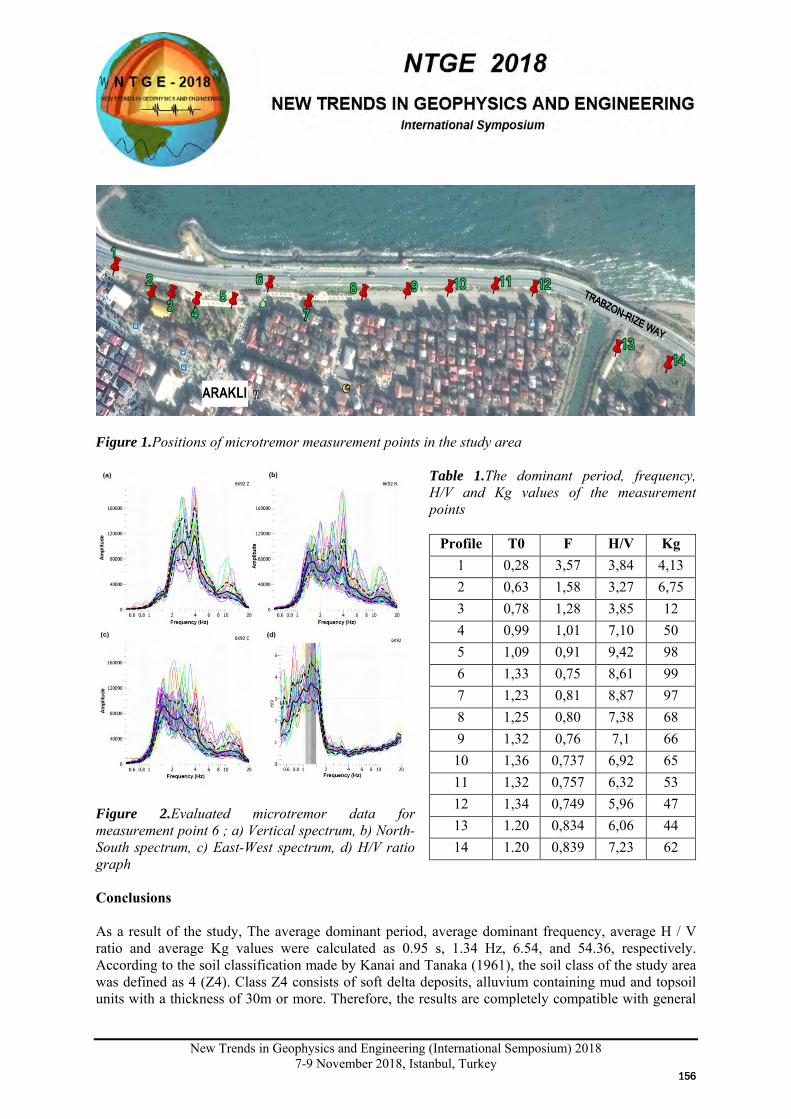
New Trends in Geophysics and Engineering (International Semposium) 2018
7-9 November 2018, Istanbul, Turkey
Figure 1.Positions of microtremor measurement points in the study area
Figure 2.Evaluated microtremor data for measurement point 6 ; a) Vertical spectrum, b) North-South spectrum, c) East-West spectrum, d) H/V ratio graph
Table 1.The dominant period, frequency, H/V and Kg values of the measurement points
Profile T0 F H/V Kg 1 0,28 3,57 3,84 4,13 2 0,63 1,58 3,27 6,75 3 0,78 1,28 3,85 12 4 0,99 1,01 7,10 50 5 1,09 0,91 9,42 98 6 1,33 0,75 8,61 99 7 1,23 0,81 8,87 97 8 1,25 0,80 7,38 68 9 1,32 0,76 7,1 66 10 1,36 0,737 6,92 65 11 1,32 0,757 6,32 53 12 1,34 0,749 5,96 47 13 1.20 0,834 6,06 44 14 1.20 0,839 7,23 62
Conclusions As a result of the study, The average dominant period, average dominant frequency, average H / V ratio and average Kg values were calculated as 0.95 s, 1.34 Hz, 6.54, and 54.36, respectively. According to the soil classification made by Kanai and Tanaka (1961), the soil class of the study area was defined as 4 (Z4). Class Z4 consists of soft delta deposits, alluvium containing mud and topsoil units with a thickness of 30m or more. Therefore, the results are completely compatible with general
156156
New Trends in Geophysics and Engineering (International Semposium) 2018
7-9 November 2018, Istanbul, Turkey
geology. According to average Kg values, the study area has a high risk of liquefaction. The Microtremor method can be used as a preliminary evaluation tool in terms of producing cheap, fast, easy and reliable results in the calculation of potential liquefaction. References Ansal, A., Bardet, J.P., Bray, J., Cetin, K.O., Durgunoglu, T., Erdik, M., Kaya, A., Ural, D., Yilmaz, T. and Youd, L., 1999, Initial geotechnical observations of the August 17, 1999 Izmit Earthquake, Earthquake Engineering Research Center. Beroya, M.A.A., Aydin, A., Tiglao, R., and Lasala, M., 2009, Use of microtremor in liquefaction hazard mapping,EngineeringGeology. 107, 140–153. Bindi, D., Parolai, S., Spallarossa, D., and Cattaneo, M., 2000, Site effects by H/V ratio: comparison of two different procedures,J.Earthq.Eng. 4:97–113. Choobbasti, A.J., Naghizadehrokni, M.,and Rezaei, S., 2015,Liquefaction assessment by microtremor measurements in Babol city.Fifth International Conference on Geotechnique, Construction Materials and Environment, Osaka, Japan. 16-18, ISBN: 978-4-9905958-4-5 C3051. Fergany, E., and Omar, K., 2017,Liquefaction potential of Nile delta, Egypt, NRIAG Journal of Astronomy and Geophysics. 6, 60–67. Huang, H.C., and Tseng, Y.S., 2002, Characteristics of soil liquefaction using H/V of microtremors in Yuan-Lin area, Taiwan, TAO. 13(3): 325–338. Kanai, K., and Tanaka, T., 1961, On Microtremors, VIII.Bulletin of Earthquakes Research Institute. 39, 97-114. Nakamura, Y., 1989,A method for dynamic characteristics estimation of subsurface using microtremor on the ground surface, Quarterly Report of RTRI. 30, 1, 25-33. Nakamura, Y., 1996, Real-Time Information Systems for Hazards Mitigation, Eleventh World Conference on Earthquake Engineering, Paper No. 2134. Nakamura, Y., 1997, Seismic Vulnerability Indices for Ground and Structures Using Microtremor, World Congress on Railway Research, Florence.3-4. Nakamura, Y., 2000, Clear Identification of Fundamental Idea of Nakamura’s Technique and its Applications, 12WCEE. 2656. Poovarodom, N., and Plalinyot, N., 2013, Site Characterization in the Greater Bangkok Area by Microtremor Observations, Journal of Earthquake Engineering. 17:209–226. Rezaei, S., and Choobbasti, A.J., 2014, Liquefaction assessment using microtremor measurement, conventional method and artificial neural network (Case study: Babol, Iran), Front. Struct. Civ. Eng. 8(3): 292–307. Tezcan, S.S., and Özdemir Z., 2004.Liquefaction Risk Analysis and Mapping Techniques, YüksekÖğrenimEğitimveAraştırmaVakfıYayınları, ISBH: 975-93005-1-6, Istanbul.
157157
New Trends in Geophysics and Engineering (International Semposium) 2018
7-9 November 2018, Istanbul , Turkey
SHALLOW ENGINEERING SEISMIC PARAMETERS AT LANDSLIDE-PRONE
AREAS AND ITS EVALUATIONS: A CASE STUDY FROM ÇANAKKALE.
Tolga Bekler1 , Alper Demirci1 1 Geophysical Eng. Department, Canakkale Onsekiz Mart University, Canakkale
Email: [email protected] Presentation Type All accepted proceedings will be published on the webpage of the symposium (ntge2018.istanbul.edu.tr)
ORAL POSTER
Abstract Geological structure and discontinuity distributions increase the presence of landslide hazards and risk factors in urban areas including dynamic routes such as highways in Çanakkale and its vicinity. The remarkable one of these landslides occurred in Güzelyalı central village. It is known to be considerable risk of landslide in these areas. The potential landslide in Güzelyalı that located on SW of the Çanakkale City, slip movements started in November 2001 and accelerated in January 2004. It is evident that although Güzelyalı landslide is not so big in size they pose a risk for the close settlements and vehicular traffic along the active highway in near future. Thus determining the slipping material features and landslide mechanism would yield to take early precautions for the possible risks that can be formed in near future. Landslide geometries were rapidly determined using geophysical measurements performed in landslide areas. It was seen that slipping surfaces developed between the layers, extension and thickness of slipping material and water content of the medium can be successfully determined by joint application and interpretation of seismic refraction methods.
Keywords: Landslide, Canakkale, Geophysics Introduction Landslides are generally defined as natural or slope down and lateral movement of alluvial material such as sedimentation (Varnes, 1958). The main factor of many landslides is the intense clay content in a high and inclined morphology, together with numerous triggering factors (Yalçın, 2007). These triggering factors may be of anthropogenic origin as well as natural origin (earthquakes and heavy rainfall). Geophysical methods offer important opportunities in revealing the physical dimensions of slip geometry and the underlying structure (Bogolosky and Ogilvy, 1977). In recent years, applications of geophysical imaging techniques for engineering and environmental research have been widely preferred. Therefore, high resolution geophysical imaging techniques as seismic refraction tomography exploring the shallow underground model are now routinely used to solve such problems (Bichler et.al.2004; Göktürkler et.al.2008). In this study, geophysical model results of the active landslides in Güzelyalı village, NW section settlement area, which has a very heavy traffic flow, are presented.
158158
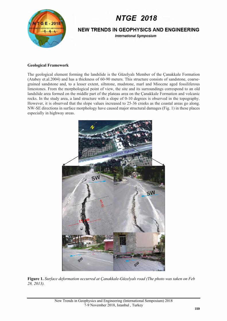
New Trends in Geophysics and Engineering (International Semposium) 2018
7-9 November 2018, Istanbul , Turkey
Geological Framework The geological element forming the landslide is the Güzelyalı Member of the Çanakkale Formation (Atabey et.al.2004) and has a thickness of 60-90 meters. This structure consists of sandstone, coarse-grained sandstone and, to a lesser extent, siltstone, mudstone, marl and Miocene aged fossiliferous limestones. From the morphological point of view, the site and its surroundings correspond to an old landslide area formed on the middle part of the plateau area on the Çanakkale Formation and volcanic rocks. In the study area, a land structure with a slope of 0-10 degrees is observed in the topography. However, it is observed that the slope values increased to 25-36 creeks as the coastal areas go along. NW-SE directions in surface morphology have caused major structural damages (Fig. 1) in these places especially in highway areas.
Figure 1. Surface deformation occurred at Çanakkale-Güzelyalı road (The photo was taken on Feb 28, 2013).
159159
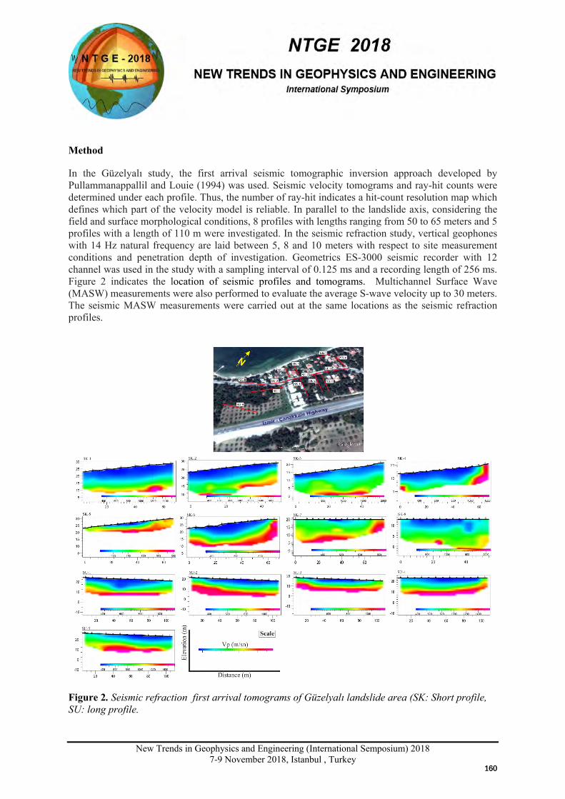
New Trends in Geophysics and Engineering (International Semposium) 2018
7-9 November 2018, Istanbul , Turkey
Method In the Güzelyalı study, the first arrival seismic tomographic inversion approach developed by Pullammanappallil and Louie (1994) was used. Seismic velocity tomograms and ray-hit counts were determined under each profile. Thus, the number of ray-hit indicates a hit-count resolution map which defines which part of the velocity model is reliable. In parallel to the landslide axis, considering the field and surface morphological conditions, 8 profiles with lengths ranging from 50 to 65 meters and 5 profiles with a length of 110 m were investigated. In the seismic refraction study, vertical geophones with 14 Hz natural frequency are laid between 5, 8 and 10 meters with respect to site measurement conditions and penetration depth of investigation. Geometrics ES-3000 seismic recorder with 12 channel was used in the study with a sampling interval of 0.125 ms and a recording length of 256 ms. Figure 2 indicates the location of seismic profiles and tomograms. Multichannel Surface Wave (MASW) measurements were also performed to evaluate the average S-wave velocity up to 30 meters. The seismic MASW measurements were carried out at the same locations as the seismic refraction profiles.
Figure 2. Seismic refraction first arrival tomograms of Güzelyalı landslide area (SK: Short profile, SU: long profile.
160160
New Trends in Geophysics and Engineering (International Semposium) 2018
7-9 November 2018, Istanbul , Turkey
Conclusions The weak zones in the sections with seismic tomograms of short profiles were self-depressed and the appearance of a heterogeneous structure with the effect of radial loads. Non-stationary shallow structures are thought to cause such heterogeneity. Seismic refraction method does not give a reliable model to detect if the alluvial thickness is thicker than 30 meters due to the length of the profiles. It is advantageous to use surface wave in residential areas in order to avoid such problems. The first layer velocity under the profiles is very low and the average is 190 m / s. Considering the Vp/Vs ratios, the increase in the Poisson Ratio as it goes deeper requires the presence of high water content in the environment. Based on these velocities, local site almost consists of sandy, silty and clayey. As the average S-wave velocities in 30 meters are very low, it is necessary to take precautions by considering the structural loads in these areas. Acknowledgements The Güzelyalı landslide project was carried out under the protocol signed between Çanakkale Municipality and Çanakkale Onsekiz Mart University on October 2013. Authors thank to the geophysical engineering students who helped during the field studies. References Atabey, E., Ilgar, A., And Sakıtaş, A., 2004, Çanakkale Havzasının Orta-Üst Miosen Stratigrafisi, Çanakkale, KB Türkiye. MTA Dergisi, 128: 79-97. Bichler, A., Bobrowsky, P., Best, M., Douma, M., Hunter, J., Calvert, T., And Burns, R., 2004, Three-dimensional mapping of a landslide using a multi-geophysical approach: the Quesnel Forks landslide, Landslides. 1, 29-40. Bogoslovsky, V.A., And Ogilvy, A.A., 1977, Geophysical methods for the investigation of landslides, Geophysics. 42, 562-571. Göktürkler, G., Balkaya, Ç ., And Erhan, Z., 2008, Geophysical investigation of a landslide: The Altındağ landslide site, İzmir (Western Turkey), Journal of Applied Geophysics. 65, 84-96. Pullammanappallil, S.K., And Louie, J.N., 1994, A generalized simulated-annealing optimization for inversion of first arrival times, Bulletin of the Seismological Society of America. 84, 1397-1409. Varnes, D.J., 1958, Landslide types and processes: Landslides and Engineering Practice by the Committee on Landslide Investigations. in Eckel, E.B. (ed.), Highway Research Board Special Report 29, Washington D.C. Yalcın, A., 2007, The effects of clay on landslides: A case study, Applied Clay Sciences. 38, 77-85.
161161
New Trends in Geophysics and Engineering (International Semposium) 2018
7-9 November 2018, Istanbul , Turkey
UPPERMOST CRUSTAL STRUCTURE OF SW BIGA PENINSULA BY LOCAL
EARTHQUAKE TOMOGRAPHY.
Tolga Bekler1 , Alper Demirci1 1 Geophysical Eng. Department, Canakkale Onsekiz Mart University, Canakkale
Email: [email protected] Presentation Type All accepted proceedings will be published on the webpage of the symposium (ntge2018.istanbul.edu.tr)
ORAL POSTER
Abstract An Mw5.4 earthquake which occurred February 6, 2017 and the following seismic activity around geothermally active Tuzla region of Ayvacık which lies at the Southwest tip of Biga Peninsula, revealed the necessity for studying the seismotectonics of the region in more detail. In order to monitor high seismic activity following the earthquake, 10 three-component broadband seismometers have been installed in region, particularly near Ayvacık. The preliminary results of the work show that the local earthquake activity is much higher than reported by national agencies. The number of seismic events detected during the first 12 months is more than 22,000. The source mechanism solutions of the moderate-sized earthquakes are obtained from the merged database and indicate dominant normal fault characters, mainly in NW-SE directions. The temporary stations installed at close distances improved not only the detection level but also and significantly increased the accuracy of the locations. The longevity of seismic activity and generation of multiple Mw>5 earthquakes show that there are multiple faults in the region which interact with each other. Based on these observations it becomes clear that there is a unique opportunity to image the complex structure and explore its interactions with fluids, heat and seismicity. For the local earthquake tomography, it was aimed to reveal the upper crust structure due to regional tectonism by using the P and S phase arrival times. Keywords: Ayvacık, Earthquakes, Tomography Introduction The Saroz-Gaziköy Fault strikes northeast-southwest with nearly 60 kilometer length. This right-lateral strike-slip fault caused the 7.3 magnitude Şarköy earthquake in 1912. With nearly 15 length within the provincial boundaries of Çanakkale, the Sarıköy Fault has nearly 60 kilometer length. Known to have caused the historical 1953 Yenice-Gönen earthquake with 7.2 magnitude, the Yenice – Gönen Fault Zone can be traced at the surface for nearly 50 kilometers (Herece, 1990). The seismicity in the region may be said to be the result of two basic tectonic elements; faults with dominantly strike-slip character representing the south branch of the North Anatolian Fault Zone passing through the Biga Peninsula and faults with dominantly vertical slip character representing the Western Anatolian extensional regime. When records from the instrumental period in the last hundred years are examined, the 1912
162162
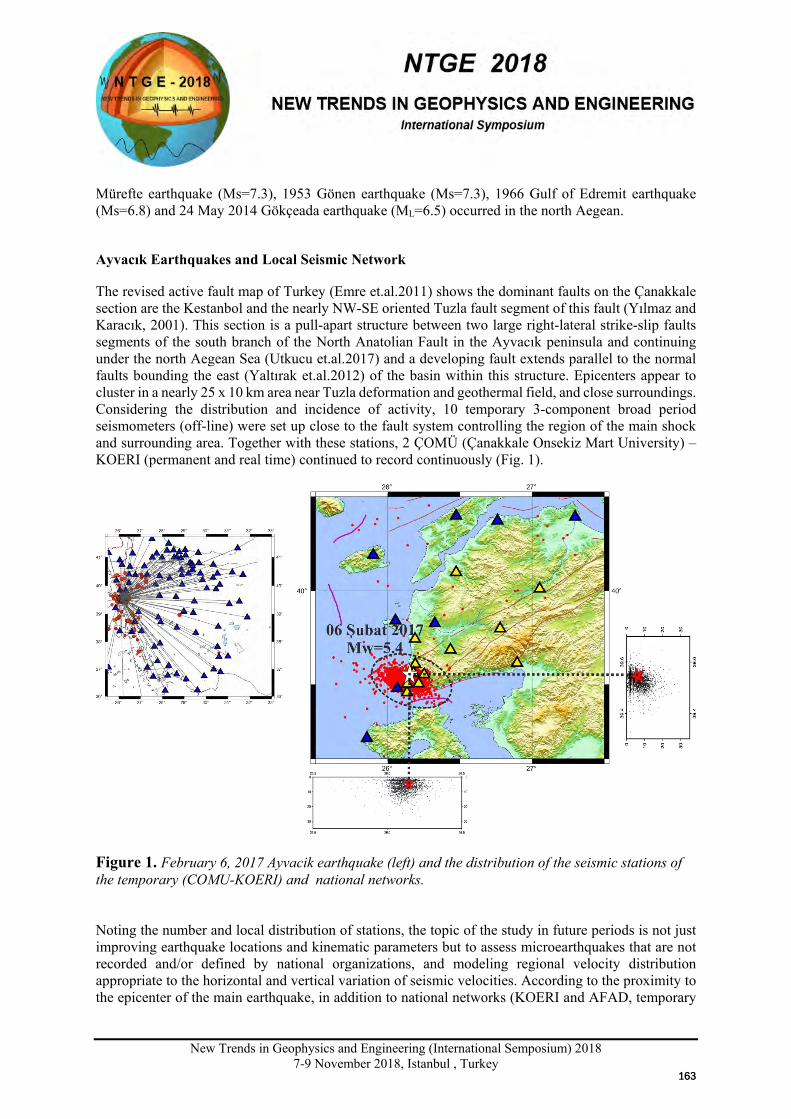
New Trends in Geophysics and Engineering (International Semposium) 2018
7-9 November 2018, Istanbul , Turkey
Mürefte earthquake (Ms=7.3), 1953 Gönen earthquake (Ms=7.3), 1966 Gulf of Edremit earthquake (Ms=6.8) and 24 May 2014 Gökçeada earthquake (ML=6.5) occurred in the north Aegean. Ayvacık Earthquakes and Local Seismic Network The revised active fault map of Turkey (Emre et.al.2011) shows the dominant faults on the Çanakkale section are the Kestanbol and the nearly NW-SE oriented Tuzla fault segment of this fault (Yılmaz and Karacık, 2001). This section is a pull-apart structure between two large right-lateral strike-slip faults segments of the south branch of the North Anatolian Fault in the Ayvacık peninsula and continuing under the north Aegean Sea (Utkucu et.al.2017) and a developing fault extends parallel to the normal faults bounding the east (Yaltırak et.al.2012) of the basin within this structure. Epicenters appear to cluster in a nearly 25 x 10 km area near Tuzla deformation and geothermal field, and close surroundings. Considering the distribution and incidence of activity, 10 temporary 3-component broad period seismometers (off-line) were set up close to the fault system controlling the region of the main shock and surrounding area. Together with these stations, 2 ÇOMÜ (Çanakkale Onsekiz Mart University) – KOERI (permanent and real time) continued to record continuously (Fig. 1).
Figure 1. February 6, 2017 Ayvacik earthquake (left) and the distribution of the seismic stations of the temporary (COMU-KOERI) and national networks. Noting the number and local distribution of stations, the topic of the study in future periods is not just improving earthquake locations and kinematic parameters but to assess microearthquakes that are not recorded and/or defined by national organizations, and modeling regional velocity distribution appropriate to the horizontal and vertical variation of seismic velocities. According to the proximity to the epicenter of the main earthquake, in addition to national networks (KOERI and AFAD, temporary
163163
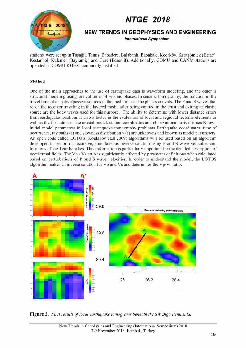
New Trends in Geophysics and Engineering (International Semposium) 2018
7-9 November 2018, Istanbul , Turkey
stations were set up in Taşağıl, Tamış, Babadere, Balabanlı, Babakale, Kocaköy, Karagömlek (Ezine), Kestanbol, Külcüler (Bayramiç) and Güre (Edremit). Additionally, ÇOMÜ and CANM stations are operated as ÇOMÜ-KOERI commonly installed. Method One of the main approaches to the use of earthquake data is waveform modeling, and the other is structural modeling using arrival times of seismic phases. In seismic tomography, the function of the travel time of an active/passive sources in the medium uses the phases arrivals. The P and S waves that reach the receiver traveling in the layered media after being emitted in the crust and exiting an elastic source are the body waves used for this purpose. The ability to determine with lower distance errors from earthquake locations is also a factor in the evaluation of local and regional tectonic elements as well as the formation of the crustal model. station coordinates and observational arrival times Known initial model parameters in local earthquake tomography problems Earthquake coordinates, time of occurrence, ray paths (s) and slowness distribution v (s) are unknowns and known as model parameters. An open code called LOTOS (Koulakov et.al.2009) algorithms will be used based on an algorithm developed to perform a recursive, simultaneous inverse solution using P and S wave velocities and locations of local earthquakes. This information is particularly important for the detailed description of geothermal fields. The Vp / Vs ratio is significantly affected by parameter definitions when calculated based on perturbations of P and S wave velocities. In order to understand the model, the LOTOS algorithm makes an inverse solution for Vp and Vs and determines the Vp/Vs ratio.
Figure 2. First results of local earthquake tomograms beneath the SW Biga Peninsula.
164164
New Trends in Geophysics and Engineering (International Semposium) 2018
7-9 November 2018, Istanbul , Turkey
Conclusions After the February 6, 2017 (03:51 UT) Mw=5.4 magnitude earthquake many researchers began studies revealing the character of the earthquake and its aftershocks. These studies were mainly seismologic studies based on field observations and databases offered by national seismic networks. This study partly uses these databases and began due to the very close proximity of fault segments in the region and the excessive earthquake production potential of these faults with very similar kinematic and involved setting up new earthquake stations to observe microearthquakes and more local scale seismological studies. The investigation of Tuzla Fault (Ayvacık) and its surroundings by local earthquake tomography shows the importance of tectonism and geothermal potential of this seismically active region. The variation of high and low velocities also corresponds to the heat sources in the SW Biga peninsula. The most prominent example is the Kestanbol geothermal area. Very low Vp velocity and Vp/Vs of 10-18 km are supported by this argument. Acknowledgements This study was supported by Çanakkale Onsekiz Mart Scientific Research Projects, with project code FBA-2017-1361 and FHD-2017-2704. References
Herece, E. And Akay, E., 2003, Kuzey Anadolu Fay (KAF) Atlası. Maden Tetkik Arama Genel Müdürlüğü. Ankara (In Turkish).
Emre Ö., Doğan A., Özalp S., And Yıldırım C. 2011, 1:250.000 Ölçekli Diri Fay Haritası Bandırma (NK 35-11b) Paftası, MTA 1:250.000 Ölçekli Diri Fay Haritaları Serisi.3: 55 (In Turkish). Kissling, E., Ellswoth, W.L., Eberhart-Phılıps, D., And Kradolfer, U., 1994, Initial reference models in seismic tomography. J. Geophys. Res. 99:19635-19646. Koulakov, I., 2009, LOTOS Code for local earthquake tomographic inversiyon. Benchmarks for testing tomographic algorithms, Bull. Seismol. Soc. Am. 99:194-214. Utkucu M., Budakoğlu E., And Kızılbuğa S., 2017, Şubat 2017 Ayvacık (Çanakkale) Deprem Silsilesinin Sismolojik Ön Değerlendirme Rapor. T.C. Sakarya Üniversitesi Rektörlüğü Afet Yönetim Uygulama Ve Araştırma Merkezi (In Turkish). Yaltırak, C., İşler, E.B., Aksu, A.E., And Hiscott, R.N,. 2012, Evolution of the Bababurnu basin and shelf of the Biga Peninsula: Western extension of the middle strand of the North Anatolian Fault Zone, Northeast Aegean Sea, Turkey. Journal of Asian Earth Sciences. 57:103-119. Yılmaz Y., And Karacık, Z. 2001, Geology of the northern side of the Gulf of Edremit and its tectonic significance for the development of the Aegean grabens. Geodinamica Acta. 14(1-3):31-43.
165165
New Trends in Geophysics and Engineering (International Semposium) 2018
7-9 November 2018, Istanbul , Turkey
BAYESIAN PROBABILITIES OF EARTHQUAKE OCCURRENCES IN THE EAST ANATOLIAN AND SURROUNDINGS (EASTERN TURKEY)
Tuğba Türker1 , Yusuf Bayrak2
1Geophysical Eng. Department, Karadeniz Technical University, Trabzon
2Geophysical Eng. Department, Karadeniz Technical University, Trabzon Email: [email protected]
Presentation Type All accepted proceedings will be published on the webpage of the symposium (ntge2018.istanbul.edu.tr)
ORAL POSTER
Abstracts The aim of this work, we determined to prediction the earthquake hazard of earthquake occurrence using the Bayesian extreme value distribution method for 12 different seismogenic zones in the East Anatolian and surroundings. We used Ms≥3 earthquakes for both instrumental and historical periods. We considered the several basic parameters for calculation the Bayesian prior estimates of the seismicity. It was the seismic moment, slip rate, earthquake recurrence rate, and magnitude, respectively. After that, the prior estimations got updated (posterior) parameters using the Bayesian theory and historical predicts of the seismicity in the East Anatolian. We estimated probabilities for return periods and the next 5, 10, 25, 50 and 100 years. As a result of the Van fault (zone 8) determined as the most dangerous zone and this zone can be occurred an earthquake in 8.0, 7.5 and 7.0 magnitudes with % 17, % 47, % 89 probabilities for the v=0.1 coefficient of variation in the next 100 years, respectively. The high probabilities (% 12, % 10, % 7, respectively) estimated for 8.0 magnitude of the other zones (the Dumlu fault zone (zone 1), Ağrı fault, Tutak fault, Karayazı fault zone (zone 7), Başkale fault (zone 9)) in the next 100 years. Addition to, this study will be used in earthquake hazard works in Turkey.
Keywords: The Bayesian extreme value distribution, in the East Anatolian and surroundings
1. Introduction Turkey had a long historical relationship occurred earthquakes. The East Anatolian and surroundings observed a lot of strong earthquakes in the East Anatolian Fault Zone (EAFZ) in the past years. Bayrak and Türker (2016, 2017) estimated the hazard parameters using the Bayesian method in Turkey. Türker et. al. (2017) investigated the Bayesian probabilities in the EAFZ. Also, Türker and Bayrak (2017) investigated the probabilities of the earthquake occurrences for the earthquake hazard in the Marmara Sea. We plotted the epicenter distribution and 12 different seismogenic zones on the tectonic map (Fig. 1). We written programs, all figures plotted and all parameters estimated for the Bayesian extreme value distribution method in the Matlab computer program.
166166
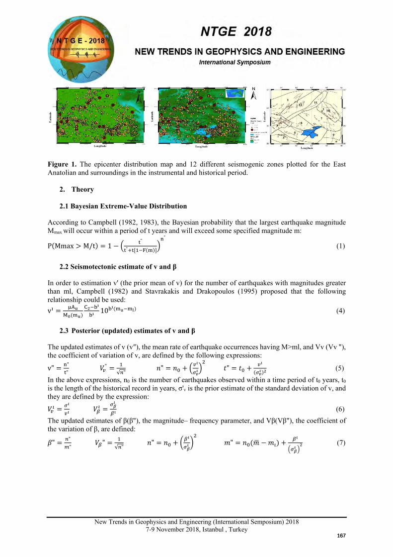
New Trends in Geophysics and Engineering (International Semposium) 2018
7-9 November 2018, Istanbul , Turkey
Figure 1. The epicenter distribution map and 12 different seismogenic zones plotted for the East Anatolian and surroundings in the instrumental and historical period.
2. Theory
2.1 Bayesian Extreme-Value Distribution
According to Campbell (1982, 1983), the Bayesian probability that the largest earthquake magnitude Mmax will occur within a period of t years and will exceed some specified magnitude m:
P(Mmax > M/t) = 1 − t"
t"+t[1−F(m)]n"
(1)
2.2 Seismotectonic estimate of v and β
In order to estimation v' (the prior mean of v) for the number of earthquakes with magnitudes greater than ml, Campbell (1982) and Stavrakakis and Drakopoulos (1995) proposed that the following relationship could be used: vı = µAu
M0(mu)C2−bı
bı10bı(mu−ml) (4)
2.3 Posterior (updated) estimates of v and β
The updated estimates of v (v″), the mean rate of earthquake occurrences having M>ml, and Vv (Vv "), the coefficient of variation of v, are defined by the following expressions:
v" = n"t"
𝑉𝑉𝑣𝑣" = 1√𝑛𝑛"
𝑛𝑛" = 𝑛𝑛0 + 𝑣𝑣𝚤𝚤
𝜎𝜎𝑣𝑣𝚤𝚤2 𝑡𝑡" = 𝑡𝑡0 + 𝑣𝑣𝚤𝚤
(𝜎𝜎𝑣𝑣𝚤𝚤)2 (5) In the above expressions, n0 is the number of earthquakes observed within a time period of t0 years, t0 is the length of the historical record in years, σ'v is the prior estimate of the standard deviation of v, and they are defined by the expression:
𝑉𝑉𝑣𝑣𝚤𝚤 = 𝜎𝜎𝚤𝚤
𝑣𝑣𝚤𝚤 𝑉𝑉𝛽𝛽
𝚤𝚤 =𝜎𝜎𝛽𝛽𝚤𝚤
𝛽𝛽𝚤𝚤 (6)
The updated estimates of β(β"), the magnitude– frequency parameter, and Vβ(Vβ"), the coefficient of the variation of β, are defined:
𝛽𝛽" = 𝑛𝑛"𝑚𝑚"
𝑉𝑉𝛽𝛽" = 1√𝑛𝑛"
𝑛𝑛" = 𝑛𝑛0 + 𝛽𝛽𝚤𝚤
𝜎𝜎𝛽𝛽𝚤𝚤 2 𝑚𝑚" = 𝑛𝑛0(𝑚𝑚 −𝑚𝑚𝚤𝚤) + 𝛽𝛽𝚤𝚤
𝜎𝜎𝛽𝛽𝚤𝚤
2 (7)
167167
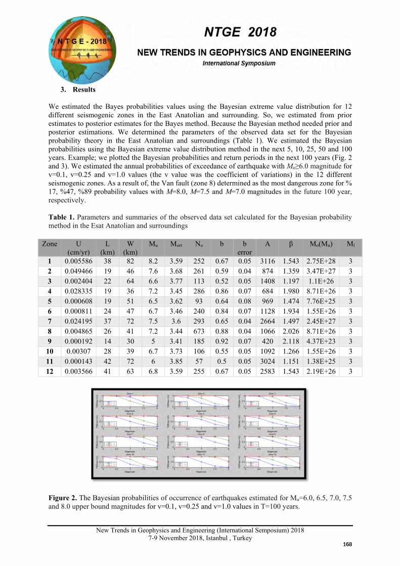
New Trends in Geophysics and Engineering (International Semposium) 2018
7-9 November 2018, Istanbul , Turkey
3. Results We estimated the Bayes probabilities values using the Bayesian extreme value distribution for 12 different seismogenic zones in the East Anatolian and surrounding. So, we estimated from prior estimates to posterior estimates for the Bayes method. Because the Bayesian method needed prior and posterior estimations. We determined the parameters of the observed data set for the Bayesian probability theory in the East Anatolian and surroundings (Table 1). We estimated the Bayesian probabilities using the Bayesian extreme value distribution method in the next 5, 10, 25, 50 and 100 years. Example; we plotted the Bayesian probabilities and return periods in the next 100 years (Fig. 2 and 3). We estimated the annual probabilities of exceedance of earthquake with Mu≥6.0 magnitude for v=0.1, v=0.25 and v=1.0 values (the v value was the coefficient of variations) in the 12 different seismogenic zones. As a result of, the Van fault (zone 8) determined as the most dangerous zone for % 17, %47, %89 probability values with M=8.0, M=7.5 and M=7.0 magnitudes in the future 100 year, respectively. Table 1. Parameters and summaries of the observed data set calculated for the Bayesian probability method in the Esat Anatolian and surroundings
Figure 2. The Bayesian probabilities of occurrence of earthquakes estimated for Mu=6.0, 6.5, 7.0, 7.5 and 8.0 upper bound magnitudes for v=0.1, v=0.25 and v=1.0 values in T=100 years.
Zone U (cm/yr)
L (km)
W (km)
Mu Mort No b b error
A β Mo(Mu) Ml
1 0.005586 38 82 8.2 3.59 252 0.67 0.05 3116 1.543 2.75E+28 3 2 0.049466 19 46 7.6 3.68 261 0.59 0.04 874 1.359 3.47E+27 3 3 0.002404 22 64 6.6 3.77 113 0.52 0.05 1408 1.197 1.1E+26 3 4 0.028335 19 36 7.2 3.45 286 0.86 0.07 684 1.980 8.71E+26 3 5 0.000608 19 51 6.5 3.62 93 0.64 0.08 969 1.474 7.76E+25 3 6 0.000811 24 47 6.7 3.46 240 0.84 0.07 1128 1.934 1.55E+26 3 7 0.024195 37 72 7.5 3.6 293 0.65 0.04 2664 1.497 2.45E+27 3 8 0.004865 26 41 7.2 3.44 673 0.88 0.04 1066 2.026 8.71E+26 3 9 0.000192 14 30 5 3.41 185 0.92 0.07 420 2.118 4.37E+23 3 10 0.00307 28 39 6.7 3.73 106 0.55 0.05 1092 1.266 1.55E+26 3 11 0.000143 42 72 6 3.85 57 0.5 0.05 3024 1.151 1.38E+25 3 12 0.003566 41 63 6.8 3.59 255 0.67 0.05 2583 1.543 2.19E+26 3
168168
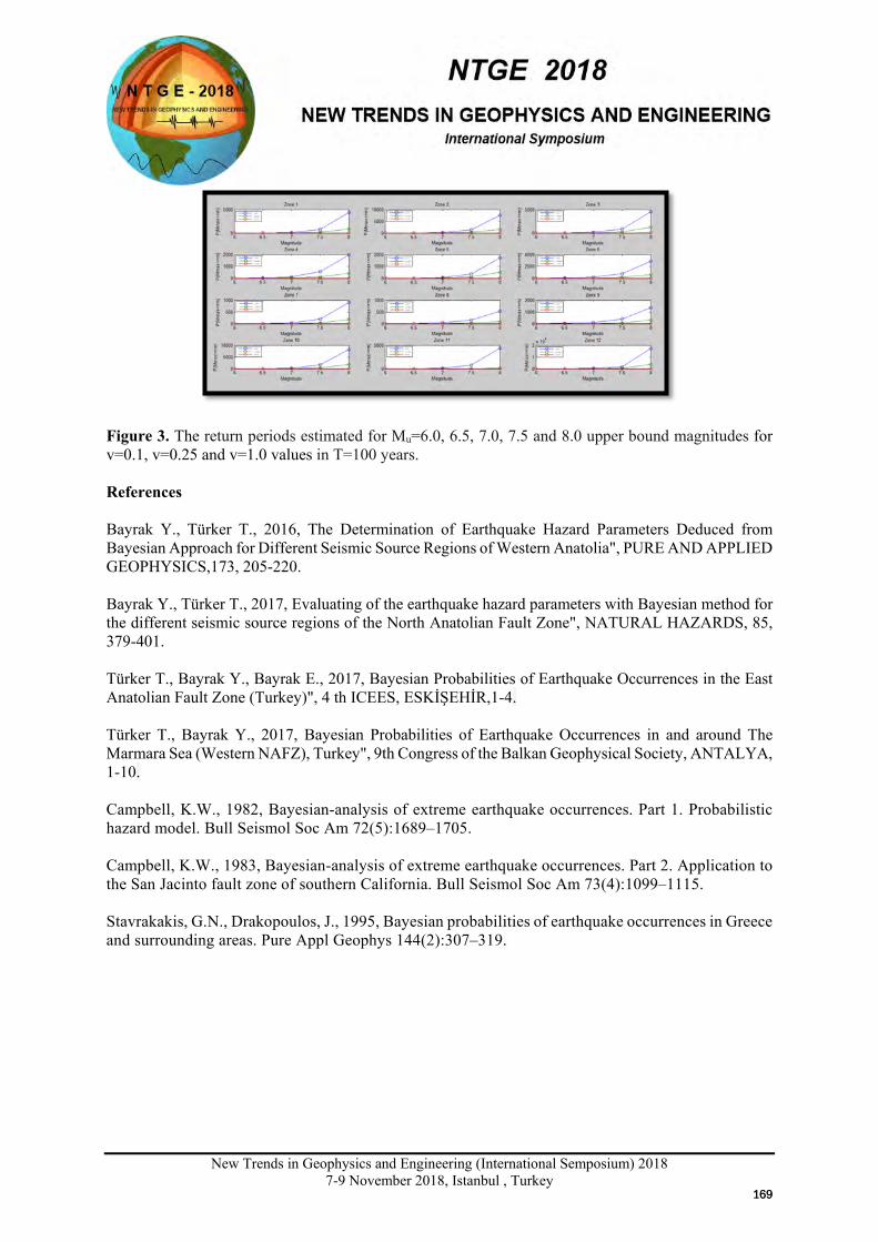
New Trends in Geophysics and Engineering (International Semposium) 2018
7-9 November 2018, Istanbul , Turkey
Figure 3. The return periods estimated for Mu=6.0, 6.5, 7.0, 7.5 and 8.0 upper bound magnitudes for v=0.1, v=0.25 and v=1.0 values in T=100 years. References Bayrak Y., Türker T., 2016, The Determination of Earthquake Hazard Parameters Deduced from Bayesian Approach for Different Seismic Source Regions of Western Anatolia", PURE AND APPLIED GEOPHYSICS,173, 205-220. Bayrak Y., Türker T., 2017, Evaluating of the earthquake hazard parameters with Bayesian method for the different seismic source regions of the North Anatolian Fault Zone", NATURAL HAZARDS, 85, 379-401. Türker T., Bayrak Y., Bayrak E., 2017, Bayesian Probabilities of Earthquake Occurrences in the East Anatolian Fault Zone (Turkey)", 4 th ICEES, ESKİŞEHİR,1-4. Türker T., Bayrak Y., 2017, Bayesian Probabilities of Earthquake Occurrences in and around The Marmara Sea (Western NAFZ), Turkey", 9th Congress of the Balkan Geophysical Society, ANTALYA, 1-10. Campbell, K.W., 1982, Bayesian-analysis of extreme earthquake occurrences. Part 1. Probabilistic hazard model. Bull Seismol Soc Am 72(5):1689–1705. Campbell, K.W., 1983, Bayesian-analysis of extreme earthquake occurrences. Part 2. Application to the San Jacinto fault zone of southern California. Bull Seismol Soc Am 73(4):1099–1115. Stavrakakis, G.N., Drakopoulos, J., 1995, Bayesian probabilities of earthquake occurrences in Greece and surrounding areas. Pure Appl Geophys 144(2):307–319.
169169
New Trends in Geophysics and Engineering (International Semposium) 2018
7-9November 2018, Istanbul ,Turkey
Recent Fault detection using steerable filters: A case Study Gulf of Saros / NW Turkey
Hakan Alp1 Ethem Görgün1 and A. Muhittin Albora1
1Istanbul University-Cerrahpaşa, Department of Geophysical Engineering, 34320 Avcılar-İstanbul E-mail: [email protected]
Presentation Type All accepted proceedings will be published on the webpage of the symposium (ntge2018.istanbul.edu.tr)
ORAL POSTER
Abstract Steerable filters behave as if band-pass filters exclusively have direction property. In extraction of directional properties, input data is passed through various directed band pass filters and then grouped into sub-bands. Here, to present the performance of steerable filters, we have chosen synthetic examples having various direction properties and tried to find out the borders of these samples. In this study we have first applied steerable filters to synthetic data and after satisfactory results, we have evaluated the tectonic setting of the Gulf of Saros in the NW region of Turkey by using application of steerable filters on potential fields. The gravity map of Gulf of Saros is obtained from Mineral Research and Exploration (MTA). Our filters result shows that the recent dextral shearing is accommodated by two fault zones bordering the Gulf. The faults are represented by en-echelon synthetic Riedel faults. The results are compared with seismic data which is published before. Steerable Filters results from this study suggests Ustaömer et al. 2008 hypothesis is accurate. Keywords: Predictive deconvolution, F-K filtering, Multichannel Seismic Data Introduction Steerable filters were first introduced by Freeman and Adelson in 1991 and since then used widely by many researchers for edge detection, image enhancement and pattern recognition. The term steerable filter is used to describe a class of filters in which a filter of arbitrary orientation is synthesized as a linear combination of a set of basis filters. In addition to linear features, these basis filters are designed to detect curvilinear or circular features represented. This method in geophysical applications was used by (Ucan et al., 2003) for evaluating for tectonic setting Gelibolu (Turkey). It was applied for delineating the boundaries of Iskenderun Bay (Albora et al., 2006) In this paper, we use steerable filters in edge detection of the faults and their directions using gravity anomaly maps as input. We demonstrate the procedure on both synthetic and real data. We apply steerable filter for Saros Bay region of Turkey. We model the region regarding steerable filter outputs. The results are compared to results interred from seismic data and geological studies. The comparison shows that a good agreement exists between various approaches.
Methods Steerable filters, having mainly properties of band pass filters in certain directions, are used in image processing, such as boundary determination, image compressing and improvement and texture analysis. Edges oriented in different directions can be obtained from the separation of directional sub-bands
X
170
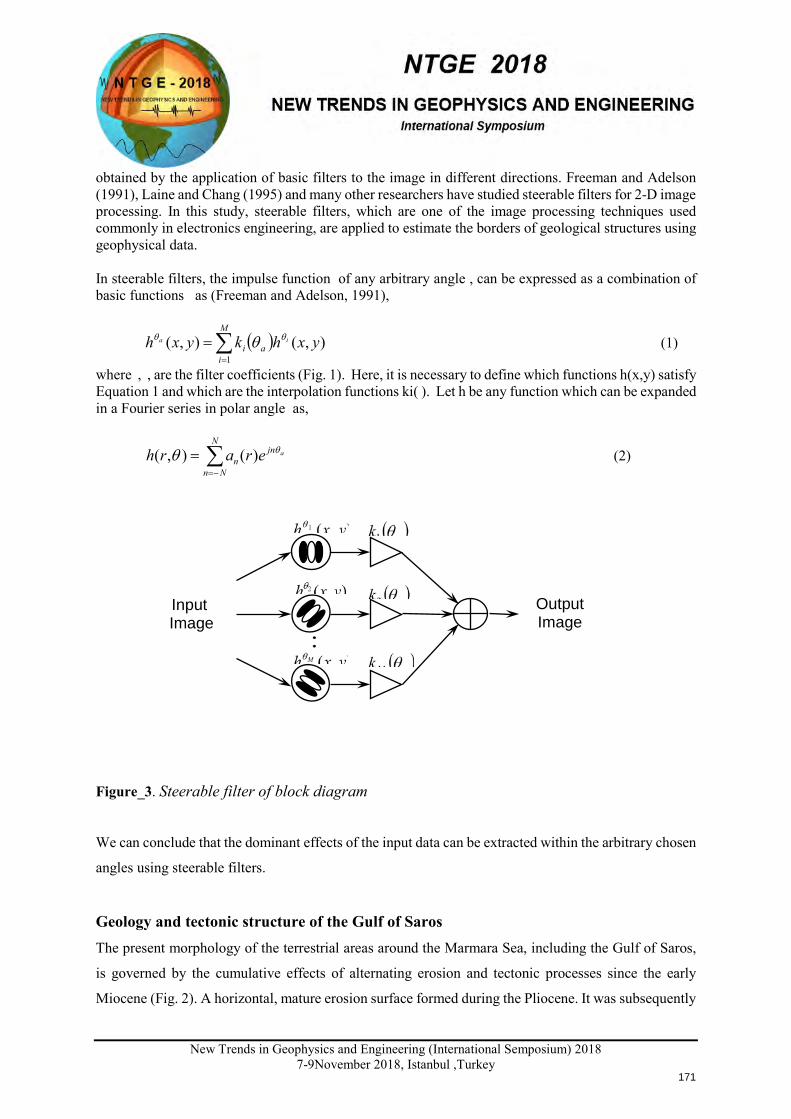
New Trends in Geophysics and Engineering (International Semposium) 2018
7-9November 2018, Istanbul ,Turkey
obtained by the application of basic filters to the image in different directions. Freeman and Adelson (1991), Laine and Chang (1995) and many other researchers have studied steerable filters for 2-D image processing. In this study, steerable filters, which are one of the image processing techniques used commonly in electronics engineering, are applied to estimate the borders of geological structures using geophysical data. In steerable filters, the impulse function of any arbitrary angle , can be expressed as a combination of basic functions as (Freeman and Adelson, 1991),
( )∑=
=M
iai yxhkyxh ia
1),(),( θθ θ (1)
where , , are the filter coefficients (Fig. 1). Here, it is necessary to define which functions h(x,y) satisfy Equation 1 and which are the interpolation functions ki( ). Let h be any function which can be expanded in a Fourier series in polar angle as,
∑−=
=N
Nn
jnn
aerarh θθ )(),( (2)
Figure_3. Steerable filter of block diagram
We can conclude that the dominant effects of the input data can be extracted within the arbitrary chosen
angles using steerable filters.
Geology and tectonic structure of the Gulf of Saros The present morphology of the terrestrial areas around the Marmara Sea, including the Gulf of Saros,
is governed by the cumulative effects of alternating erosion and tectonic processes since the early
Miocene (Fig. 2). A horizontal, mature erosion surface formed during the Pliocene. It was subsequently
Input Image
Output Image
171
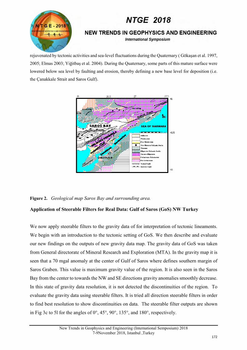
New Trends in Geophysics and Engineering (International Semposium) 2018
7-9November 2018, Istanbul ,Turkey
rejuvenated by tectonic activities and sea-level fluctuations during the Quaternary ( Gökaşan et al. 1997,
2005; Elmas 2003; Yiğitbaş et al. 2004). During the Quaternary, some parts of this mature surface were
lowered below sea level by faulting and erosion, thereby defining a new base level for deposition (i.e.
the Çanakkale Strait and Saros Gulf).
Figure 2. Geological map Saros Bay and surrounding area. Application of Steerable Filters for Real Data: Gulf of Saros (GoS) NW Turkey
We now apply steerable filters to the gravity data of for interpretation of tectonic lineaments.
We begin with an introduction to the tectonic setting of GoS. We then describe and evaluate
our new findings on the outputs of new gravity data map. The gravity data of GoS was taken
from General directorate of Mineral Research and Exploration (MTA). In the gravity map it is
seen that a 70 mgal anomaly at the center of Gulf of Saros where defines southern margin of
Saros Graben. This value is maximum gravity value of the region. It is also seen in the Saros
Bay from the center to towards the NW and SE directions gravity anomalies smoothly decrease.
In this state of gravity data resolution, it is not detected the discontinuities of the region. To
evaluate the gravity data using steerable filters. It is tried all direction steerable filters in order
to find best resolution to show discontinuities on data. The steerable filter outputs are shown
in Fig 3c to 5l for the angles of 0°, 45°, 90°, 135°, and 180°, respectively.
172
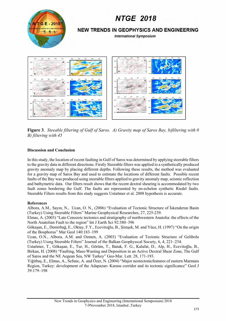
New Trends in Geophysics and Engineering (International Semposium) 2018
7-9November 2018, Istanbul ,Turkey
Figure 3. Steeable filtering of Gulf of Saros. A) Gravity map of Saros Bay, b)filtering with 0 B) filtering with 45 Discussion and Conclusion
In this study, the location of recent faulting in Gulf of Saros was determined by applying steerable filters to the gravity data in different directions. Firstly Steerable filters was applied to a synthetically produced gravity anomaly map by placing different depths. Following these results, the method was evaluated for a gravity map of Saros Bay and used to estimate the locations of different faults. Possible recent faults of the Bay was produced using steerable filters applied to gravity anomaly map, seismic reflection and bathymetric data. Our filters result shows that the recent dextral shearing is accommodated by two fault zones bordering the Gulf. The faults are represented by en-echelon synthetic Riedel faults. Steerable Filters results from this study suggests Ustaömer et al. 2008 hypothesis is accurate. References Albora, A.M., Sayın, N., Ucan, O. N., (2006) “Evaluation of Tectonic Structure of İskenderun Basin (Turkey) Using Steerable Filters” Marine Geophysical Researches, 27, 225-239. Elmas, A. (2003) “Late Cenozoic tectonics and stratigraphy of northwestern Anatolia: the effects of the North Anatolian Fault to the region” Int J Earth Sci 92:380–396 Gökaşan, E., Demirbağ, E., Oktay, F.Y., Ecevitoğlu, B., Şimşek, M. and Yüce, H. (1997) “On the origin of the Bosphorus” Mar Geol 140:183–199 Ucan, O.N., Albora, A.M. and Ozmen, A. (2003) “Evaluation of Tectonic Structure of Gelibolu (Turkey) Usıng Steerable Fılters” Journal of the Balkan Geophysıcal Socıety, 6, 4, 221–234. Ustaömer, T., Gökaşan, E., Tur, H., Görüm, T., Batuk, F. G., Kalafat, D., Alp, H., Ecevitoğlu, B., Birkan, H. (2008) “Faulting, Mass-Wasting and Deposition in an Active Dextral Shear Zone, The Gulf of Saros and the NE Aegean Sea, NW Turkey” Geo-Mar. Lett. 28, 171-193. Yiğitbaş, E., Elmas, A., Sefunc, A. and Özer, N. (2004) “Major neotectonicfeatures of eastern Marmara Region, Turkey: development of the Adapazarı–Karasu corridor and its tectonic significance” Geol J 39:179–198
40.0
40.4
40.8
27.226.425.6 26.826.0
40.0
40.4
40.8
27.226.425.6 26.826.0
40.0
40.4
40.8
27.226.8
40.0
40.4
40.8
27.226.425.6 26.826.0
40.0
40.4
40.8
27.226.425.6 26.826.0
40.0
40.4
40.8
27.226.425.6 26.826.0
40.0
40.4
40.8
27.226.425.6 26.826.0
40.4
40.8
27.226.8
40.4
40.8
27.226.8
A B
C D
E F
40.0
40.4
40.8
27.226.8
0 0
0
0 8
65 6 6 86 0
0 0
0
0 8
65 6 6 86 0
0 0
0
40.0
40.4
40.8
27.226.425.6 26.826.0
40.0
40.4
40.8
27.226.8
40.0
40.4
40.8
27.226.425.6 26.826.0
40.0
40.4
40.8
27.226.8
G
L
H
I J
K
173
New Trends in Geophysics and Engineering (International Semposium) 2018
7-9 November 2018, Istanbul, Turkey
SEISMIC MULTIPLE REMOVAL WITH SURFACE RELATED MULTIPLE ATTENUATION (SRMA) TECHNIQUE
Yeliz İşcan1, Neslihan Ocakoğlu2, Oğuz Özel1
1 Geophysical Engineering Department, Istanbul University, Istanbul, Turkey
2 Geophysical Engineering Department, Istanbul Technical University, Istanbul, Turkey
Email: [email protected] Presentation Type
ORAL POSTER
Abstracts Surface-related multiple attenuation (SRMA) as a multiple removal method had been considered as one of the great advancement in the removal of the seismic noise. Using this approach, it allows the prediction of all possible types of multiples without the need of any subsurface information. In this study two stages were performed for the SRMA application. Firstly, multiple reflections were modelled by predicting from the CDP data. Then, predicted multiples are adaptively subtracted from the data. Thus, the resolution of the data has been improved by increasing the S/N ratio. A key area from the Southern Black Sea shelf has been chosen for SRMA technique where a complex geology masked by strong multiples. The application of this method gave an improved results in multiple attenuation, especially where the primaries become more prominent and their continuity has been followed better with depth in the inclined layers. Keywords: Seismic data processing, seafloor multiples, SRMA technique Introduction Multiple reflection removal is one of the most important topic in seismic reflection processing, especially in the marine seismic data, where seabed multiple reflections can often severely mask the primary events. It is thus necessary to remove or to attenuate them prior to stack the data. In recent years, surface related multiple attenuation (SRMA) technique is undoubtedly one of the most popular method to remove multiple reflection from data. The historical development of this method starts with Anstey and Newman (1967), who observed that with autoconvolution of a trace, primary events were transformed into multiples. Berkhout (1982) redefined the multiple problem for laterally varying media by using a wave theory-based matrix formulation. An adaptive version has been shown with examples in Verschuur et al (1989), Wapenaar et al. (1990) and Verschuur (1991), (1992).
X
174
New Trends in Geophysics and Engineering (International Semposium) 2018
7-9 November 2018, Istanbul, Turkey
In SRMA method, the wavefield is extrapolated one round trip through the water layer, so that each event is transformed into a water-layer-related multiple of one order higher than it is. These predicted multiples are then adaptively subtracted from the data. In this study, SRMA technique has been tested to remove the multiples on a seismic reflection data in the southern Black Sea Shelf which has dominant multiple reflections due to the sea floor and sediments just below it. Application of SRMA technique to data Surface-related multiples are typically the strongest multiple events present in the seismic data and therefore need to be removed from prestack gathers prior to any further process. They are classified into different orders depending on how many times they are reflected back from the free surface. A multiple event is called first-order surface multiple if it is reflected only one at the free surface; while second-order multiple is reflected twice at the free surface. In general, an N-th order multiple gets reflected N times at the free surface. The SRMA technology is design to attenuate these multiples in a two-step fashion. During the first step, surface related multiples are predicted kinematically. The predicted multiples have about the same travel times as the multiples recorded in seismic data but different amplitudes and wavelet shapes. In the second step, the surface-related multiples present in the seismic data are attenuated using predicted multiples. The method assumes the sources and receivers have the same spatial sampling interval and they are located at the same locations at the free surface. This method does not require distinctive moveout differences between the primaries and multiples, and does not require any prior knowledge of the subsurface structure, such as velocities. The seismic data itself can be used to predict the surface-related multiples. According to the theory by Verschuur (1991), the multiple prediction operator can be expanded into a Taylor series. In the frequency domain, the Taylor expression can be expressed as,
Where matrix P is the input seismic data and the matrix P0 represents multiple-free data. R is the reflection coefficient at the free surface. S(w) is the source wavelet and is a function of frequency. In Taylor expansion, the terms T0, T1, T2 and T3 are corresponding to Taylor terms. Each item in the Taylor series contains multiples starting from a certain order. The zero order Taylor term T0=P in the expansion is the input seismic data itself containing both the primaries and multiples of various order. The first order Taylor term T1 corresponds first seafloor multiple while higher terms represent the higher order multiples. The input seismic data, when convolved with itself, predicts the first order Taylor term, which contain multiples only. Before applying SRMA to data pre-processing steps must be performed to improve the data. In this study, the pre-processing steps such as editing, geometry definition, muting, filtering were applied to the data. These steps and SRMA applications have been performed on Paradigm Echos software in ‘Nezihi Canıtez Data Processing Laboratory’ in Istanbul Technical University. In practice, the SRMA method consists of two stages. In the first stage, multiple reflections were modelled by predicting from the CDP data. The arrival times of the seafloor were considered to model the multiples. The amplitude and waveform of the first predicted multiple reflection is different from the primary reflection. While the amplitudes of multiples decrease systematically with the number of
175
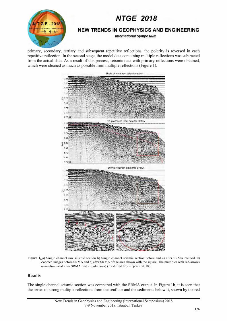
New Trends in Geophysics and Engineering (International Semposium) 2018
7-9 November 2018, Istanbul, Turkey
primary, secondary, tertiary and subsequent repetitive reflections, the polarity is reversed in each repetitive reflection. In the second stage, the model data containing multiple reflections was subtracted from the actual data. As a result of this process, seismic data with primary reflections were obtained, which were cleaned as much as possible from multiple reflections (Figure 1).
Figure 1. a) Single channel raw seismic section b) Single channel seismic section before and c) after SRMA method. d) Zoomed images before SRMA and e) after SRMA of the area shown with the square. The multiples with red-arrows were eliminated after SRMA (red circular area) (modified from İşcan, 2018).
Results The single channel seismic section was compared with the SRMA output. In Figure 1b, it is seen that the series of strong multiple reflections from the seafloor and the sediments below it, shown by the red
176
New Trends in Geophysics and Engineering (International Semposium) 2018
7-9 November 2018, Istanbul, Turkey
dashed line, were successfully attenuated after the SRMA method in Figure 1c. The resolution of the data has been improved by increasing the S/N ratio after the SRMA application. Especially, the primaries become more prominent and their continuity has been followed better with depth in the inclined layers (Figure 1d and 1e). On the other hand, the inclined primary reflections covered with multiple reflections in shallow waters where the seafloor is horizontal, could not be revealed as expected (Figure 1c). Because in the shallow water the period of the multiples is shorter and they dominantly mask the primaries. Acknowledgements This study was supported by The Scientific and Technological Research Council of Turkey, Project no. TUBITAK-ÇAYDAG-114Y057 and Istanbul University Graduate Studies Research Funds, Project no. 54445. The authors would like to thank ITU, TUBITAK and TPAO Corporation, coordinators and researchers for the realization of this project. References Anstey, N.A. and Newman, P., 1967, Part 1: The sectional auto-correlogram and Part II: The sectional retro-correlogram: Geophs. Prosp., 14, 391-426. Berkhout, A.J., 1982, Seismic migration: Imaging of acoustic energy by wavefield extrapolation. A theoretical aspects, second edition: Elsevier Science Publ. Co. Inc., 211-218. İşcan, Y., 2018, Investigation of Cide-Sinop offshore, Southern Black Sea shelf by bathymetry and seismic reflection data. PhD Thesis, pp. 185 Istanbul University, Istanbul Verschuur, D.J., Berkhout, A.J. and Wapenaar, C.P.A., 1989, Wavelet estimation by prestack multiple elimination: 59th Ann. Internal. Mtg., Soc. Expo,. Geophs., Expanded Abstracts, 1129-1132. Verchuur, D.J., 1991, Surface-related multiple elimination: an inversion approach, PhD Thesis, Delft Technical University, Holland. Verchuur, D.J., 1992, Adaptive surface-related multiple elimination, Geophysics, 57:1166-1177. Wapenaar, C.P.A., Hermann. P., Verschuur, D.J. and Berkhout, A.J., 1989, Decomposition of multi-component seismic data: Elsevier Science Publ. Co., Inc.
177
New Trends in Geophysics and Engineering (International Semposium) 2018
7-9 November 2018, Istanbul , Turkey
IDENTIFICATION OF PULSE SHAPE SIGNALS ON NEAR FAULT STATIONS WITH CONVOLUTIONAL NEURAL NETWORK ALGORITHMS: PRELIMINARY
RESULTS
Deniz Ertuncay1 , Giovanni Costa1
1 University of Trieste, Department of Mathematics and Earth Sciences, SeisRaM working group, 34127, Trieste, Italy
Email: [email protected] Presentation Type
ORAL POSTER
Abstracts Pulse shape ground motions have been identified as imposing extreme demands on structures and they are of interest in the fields of seismology and earthquake engineering. Algorithms are established to distinguish pulse shape signals from ordinary earthquake signal such as Shahi and Baker (2014) and Chang et al. (2016). These algorithms use wavelet analysis and least square methods to fit a pulse fro a given earthquake signal, respectively. Furthermore, Chang et al. (2016) can give the starting and the ending points of the impulse part of the signal. We used these algorithms to identify the pulse shape signals in our database. Our database contain near fault waveform of significant crustal earthquakes in hazardous seismic zones. Then, TensorFlow and Scikit-learn are used in order to detect possible pulse shaped signals. Convolutional neural networks are used in order to process the data. Signals are examined as velocity waveform. Not only the waveform but also the spectrogram of the waveforms are investigated. Pulse shape signals are determined with ~80% of accuracy rate.
Keywords: near-fault ground motion, pulse-like ground motion, velocity pulse, wavelet analysis, pulse shaped signal extraction Introduction Increasing number of seismic stations that are located near the active faults make it possible to investigate near-fault behavior of the seismic signals. Occasionally, these stations recorded earthquakes with peculiar seismic pattern at various major earthquakes. Such signals, called henceforward pulse-shape signals, can be seen at the early stages of the earthquake signal in velocity records. There are various algorithms to detect pulse-shape signals in earthquake waveform. Mavroeidis and Papageorgiou (2003) proposed a wavelet analysis to construct a mathematical representation of the pulse, which depends on amplitude, period, duration and phase shift. Shahi and Baker (2014) used a 4th-order Daubechies wavelet to determine pulse-shape signals. The method has some constraints such as a minimum PGV amplitude, a pulse arrival located at the beginning of the signal and arbitrary thresholds for the energy function. Mena and Mai (2011) used windowed Fourier transform analysis for the pulse shape signal and its position with certain energy thresholds. Chang et al. (2016) used the energy function with certain thresholds to determine the pulse-shape signal position and period.
X
178
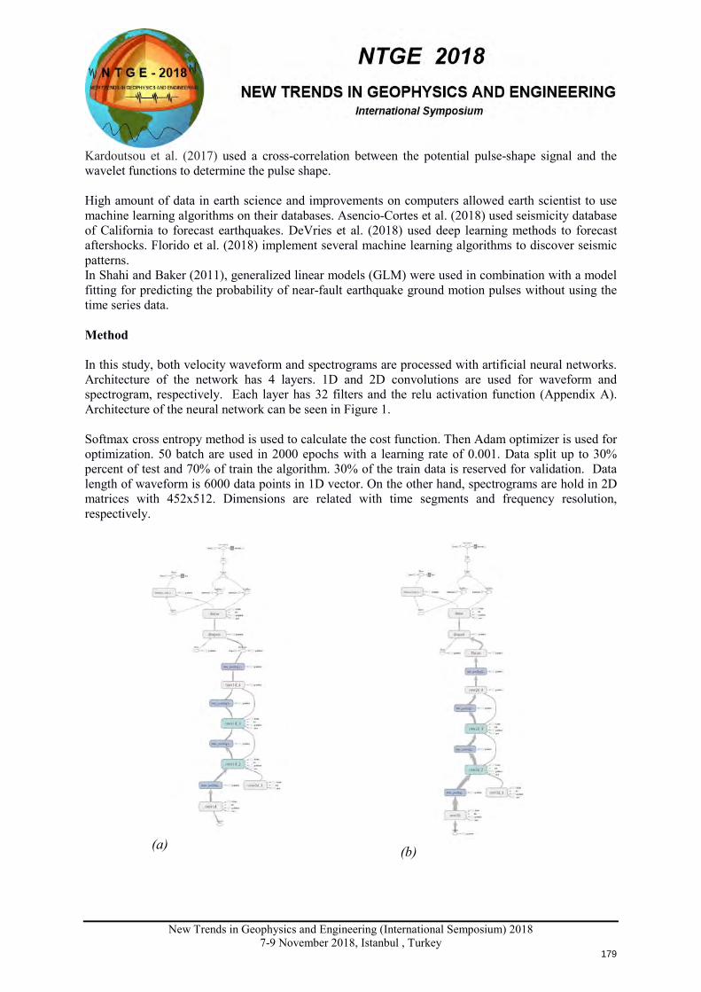
New Trends in Geophysics and Engineering (International Semposium) 2018
7-9 November 2018, Istanbul , Turkey
Kardoutsou et al. (2017) used a cross-correlation between the potential pulse-shape signal and the wavelet functions to determine the pulse shape. High amount of data in earth science and improvements on computers allowed earth scientist to use machine learning algorithms on their databases. Asencio-Cortes et al. (2018) used seismicity database of California to forecast earthquakes. DeVries et al. (2018) used deep learning methods to forecast aftershocks. Florido et al. (2018) implement several machine learning algorithms to discover seismic patterns. In Shahi and Baker (2011), generalized linear models (GLM) were used in combination with a model fitting for predicting the probability of near-fault earthquake ground motion pulses without using the time series data. Method In this study, both velocity waveform and spectrograms are processed with artificial neural networks. Architecture of the network has 4 layers. 1D and 2D convolutions are used for waveform and spectrogram, respectively. Each layer has 32 filters and the relu activation function (Appendix A). Architecture of the neural network can be seen in Figure 1. Softmax cross entropy method is used to calculate the cost function. Then Adam optimizer is used for optimization. 50 batch are used in 2000 epochs with a learning rate of 0.001. Data split up to 30% percent of test and 70% of train the algorithm. 30% of the train data is reserved for validation. Data length of waveform is 6000 data points in 1D vector. On the other hand, spectrograms are hold in 2D matrices with 452x512. Dimensions are related with time segments and frequency resolution, respectively.
(a) (b)
179
New Trends in Geophysics and Engineering (International Semposium) 2018
7-9 November 2018, Istanbul , Turkey
Figure 1. Structures of the neural network. Structure is the same for both waveform and spectrogram analysis except that in waveform analysis 1D convolution is used (a), whereas in spectrogram analysis 2D convolution is used (b).
Data
The analysed ground motions are selected from NGA-West2 (Ancheta et al. 2012), GeoNet, Itaca (Pacor et al. 2011, Luzi et al. 2016) and K-Net databases, which contain data from crustal earthquakes. Earthquake signals that are recorded due to M w ≥ 5.5 earthquakes with a maximum distance range of 115 km from the epicenter, are selected. In order to study pulse-shape signals, East and North components are rotated to radial and transverse components. In total, our database contains 2785 waveforms.
Conclusions
1. Both waveform and spectrogram analysis have promising accuracy rates, which are 84% and 81%, respectively.
2. Other architectures should be tested in order to find an optimal model. 3. More indicators of the signal should be analysed e.g. FFT, maximum and mean values of the
time segments. Acknowledgements We would like to thank to Assistant Prof. Dr. Zhiwang Chang from School of Civil Engineering, Southwest Jiaotong University for sharing his algorithm with us and Dr. Emine Kucukbenli from Department of Condensed Matter Theory, International School for Advanced Studies (SISSA) and Dr. Eric Medvet from Universtiy of Trieste, Machine Learning Lab. for their advices about machine learning algorithms. We also would like to thank the National Research Institute for Earth Science and Disaster Resilience (NIED) for their websitef or K-NET and KiK-net (http://www.kyoshin.bosai.go.jp/, last accessed September, 2018) that makes it possible to access strong-motion seismographs in Japan, and GeoNet (www.geonet.org.nz/, last accessed September, 2018) for providing New Zealand strong-motion data. References Ancheta, T.D., Bozorgnia, Y., Darragh, R., Silva, W.J., Chiou, B., Stewart, J.P., Boore, D.M., Graves, R., Abrahamson, N.A., Campbell, K.W. and Idriss, I.M., 2012. PEER NGA-West2 database: A database of ground motions recorded in shallow crustal earthquakes in active tectonic regions. In Proceedings, 15th World Conference on Earthquake Engineering. Asencio–Cortés, G., Morales–Esteban, A., Shang, X. and Martínez–Álvarez, F., 2018. Earthquake prediction in California using regression algorithms and cloud-based big data infrastructure. Computers & Geosciences, 115, pp.198-210. Chang, Z., Sun, X., Zhai, C., Zhao, J.X. and Xie, L., 2016. An improved energy‐based approach for selecting pulse‐l ike ground motions. Earthquake Engineering & Structural Dynamics, 45(14), pp.2405-2411.
180
New Trends in Geophysics and Engineering (International Semposium) 2018
7-9 November 2018, Istanbul , Turkey
DeVries, P.M., Viégas, F., Wattenberg, M. and Meade, B.J., 2018. Deep learning of aftershock patterns following large earthquakes. Nature, 560(7720), p.632. Florido, E., Asencio–Cortés, G., Aznarte, J.L., Rubio-Escudero, C. and Martínez–Álvarez, F., 2018. A novel tree-based algorithm to discover seismic patterns in earthquake catalogs. Computers & Geosciences, 115, pp.96-104. Kardoutsou, V., Taflampas, I. and Psycharis, I.N., 2017. A new pulse indicator for the classification of ground motions. Bulletin of the Seismological Society of America, 107(3), pp.1356-1364. Luzi, L., Puglia, R., Russo, E., D'Amico, M., Felicetta, C., Pacor, F., Lanzano, G., Çeken, U., Clinton, J., Costa, G. and Duni, L., 2016. The engineering strong‐motion database: A platform to access pan‐European accelerometric data. Seismological Research Letters, 87(4), pp.987-997. Maas, A.L., Hannun, A.Y. and Ng, A.Y., 2013, June. Rectifier nonlinearities improve neural network acoustic models. In Proc. icml (Vol. 30, No. 1, p. 3). Mavroeidis, G.P. and Papageorgiou, A.S., 2003. A mathematical representation of near-fault ground motions. Bulletin of the seismological society of America, 93(3), pp.1099-1131. Mena, B. and Mai, P.M., 2011. Selection and quantification of near-fault velocity pulses owing to source directivity. Georisk, 5(1), pp.25-43. Pacor, F., Paolucci, R., Luzi, L., Sabetta, F., Spinelli, A., Gorini, A., Nicoletti, M., Marcucci, S., Filippi, L. and Dolce, M., 2011. Overview of the Italian strong motion database ITACA 1.0. Bulletin of Earthquake Engineering, 9(6), pp.1723-1739. Shahi, S.K. and Baker, J.W., 2011. Regression models for predicting the probability of near‐fault earthquake ground motion pulses, and their period. Applications of Statistics and Probability in Civil Engineering, 30(4), p.459. Shahi, S.K. and Baker, J.W., 2014. An efficient algorithm to identify strong‐velocity pulses in multicomponent ground motions. Bulletin of the Seismological Society of America, 104(5), pp.2456-2466.
Appendix A: ReLU Function
Rectified linear unit (ReLU) function is an activation function that is used in artificial neural networks. Function gets positive values when the input is positive. Function has a mathematical formula as below:
𝑓𝑓(𝑥𝑥) = 𝑥𝑥+𝑚𝑚𝑚𝑚𝑥𝑥(0, 𝑥𝑥) (1)
ReLU functions have applications in speech recognition using deep neural networks (Maas et al. 2013).
181
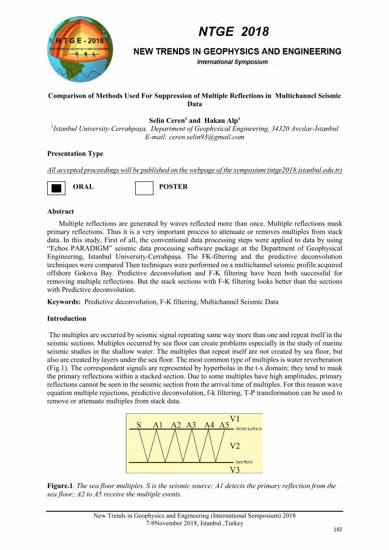
New Trends in Geophysics and Engineering (International Semposium) 2018
7-9November 2018, Istanbul ,Turkey
Comparison of Methods Used For Suppression of Multiple Reflections in Multichannel Seismic
Data
Selin Ceren1 and Hakan Alp1
1Istanbul University-Cerrahpaşa, Department of Geophysical Engineering, 34320 Avcılar-İstanbul E-mail: [email protected]
Presentation Type All accepted proceedings will be published on the webpage of the symposium (ntge2018.istanbul.edu.tr)
ORAL POSTER
Abstract
Multiple reflections are generated by waves reflected more than once. Multiple reflections mask primary reflections. Thus it is a very important process to attenuate or removes multiples from stack data. In this study, First of all, the conventional data processing steps were applied to data by using “Echos PARADIGM” seismic data processing software package at the Department of Geophysical Engineering, Istanbul University-Cerrahpaşa. The FK-filtering and the predictive deconvolution techniques were compared Then techniques were performed on a multichannel seismic profile acquired offshore Gokova Bay. Predictive deconvolution and F-K filtering have been both successful for removing multiple reflections. But the stack sections with F-K filtering looks better than the sections with Predictive deconvolution.
Keywords: Predictive deconvolution, F-K filtering, Multichannel Seismic Data Introduction The multiples are occurred by seismic signal repeating same way more than one and repeat itself in the seismic sections. Multiples occurred by sea floor can create problems especially in the study of marine seismic studies in the shallow water. The multiples that repeat itself are not created by sea floor, but also are created by layers under the sea floor. The most common type of multiples is water reverberation (Fig.1). The correspondent signals are represented by hyperbolas in the t-x domain; they tend to mask the primary reflections within a stacked section. Due to some multiples have high amplitudes, primary reflections cannot be seen in the seismic section from the arrival time of multiples. For this reason wave equation multiple rejections, predictive deconvolution, f-k filtering, T-P transformation can be used to remove or attenuate multiples from stack data.
Figure.1. The sea floor multiples. S is the seismic source; A1 detects the primary reflection from the sea floor; A2 to A5 receive the multiple events.
182
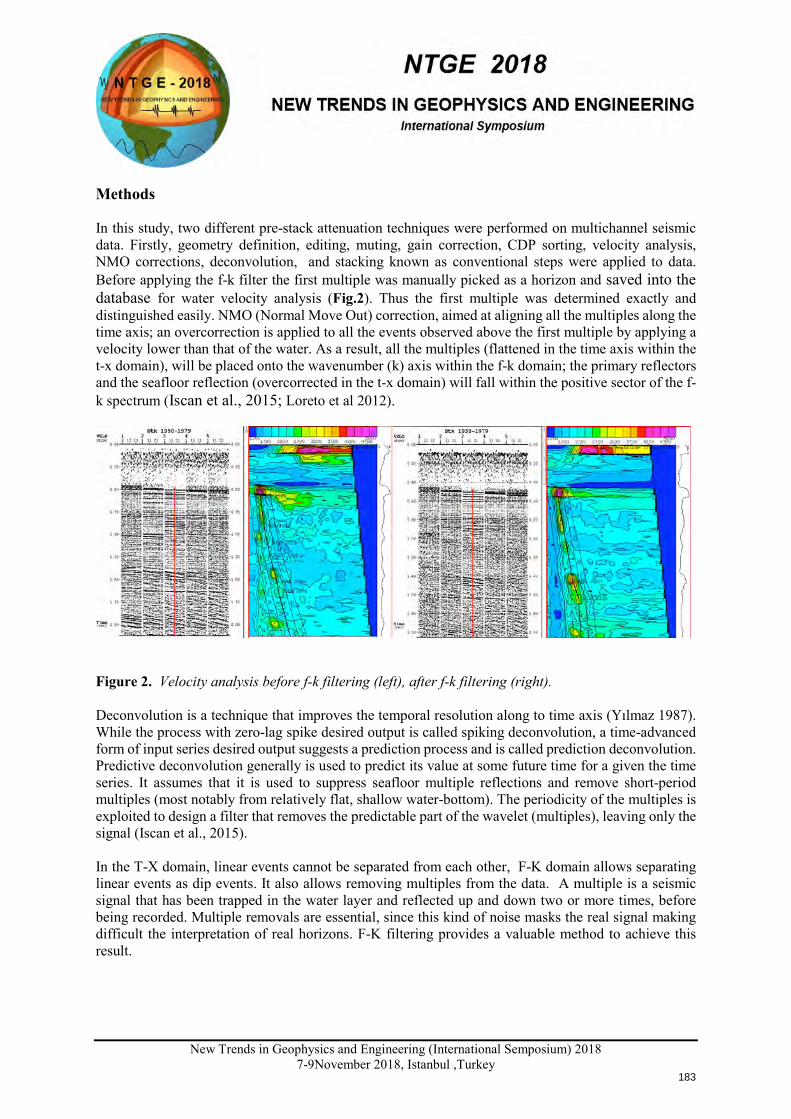
New Trends in Geophysics and Engineering (International Semposium) 2018
7-9November 2018, Istanbul ,Turkey
Methods In this study, two different pre-stack attenuation techniques were performed on multichannel seismic data. Firstly, geometry definition, editing, muting, gain correction, CDP sorting, velocity analysis, NMO corrections, deconvolution, and stacking known as conventional steps were applied to data. Before applying the f-k filter the first multiple was manually picked as a horizon and saved into the database for water velocity analysis (Fig.2). Thus the first multiple was determined exactly and distinguished easily. NMO (Normal Move Out) correction, aimed at aligning all the multiples along the time axis; an overcorrection is applied to all the events observed above the first multiple by applying a velocity lower than that of the water. As a result, all the multiples (flattened in the time axis within the t-x domain), will be placed onto the wavenumber (k) axis within the f-k domain; the primary reflectors and the seafloor reflection (overcorrected in the t-x domain) will fall within the positive sector of the f-k spectrum (Iscan et al., 2015; Loreto et al 2012).
Figure 2. Velocity analysis before f-k filtering (left), after f-k filtering (right). Deconvolution is a technique that improves the temporal resolution along to time axis (Yılmaz 1987). While the process with zero-lag spike desired output is called spiking deconvolution, a time-advanced form of input series desired output suggests a prediction process and is called prediction deconvolution. Predictive deconvolution generally is used to predict its value at some future time for a given the time series. It assumes that it is used to suppress seafloor multiple reflections and remove short-period multiples (most notably from relatively flat, shallow water-bottom). The periodicity of the multiples is exploited to design a filter that removes the predictable part of the wavelet (multiples), leaving only the signal (Iscan et al., 2015). In the T-X domain, linear events cannot be separated from each other, F-K domain allows separating linear events as dip events. It also allows removing multiples from the data. A multiple is a seismic signal that has been trapped in the water layer and reflected up and down two or more times, before being recorded. Multiple removals are essential, since this kind of noise masks the real signal making difficult the interpretation of real horizons. F-K filtering provides a valuable method to achieve this result.
183
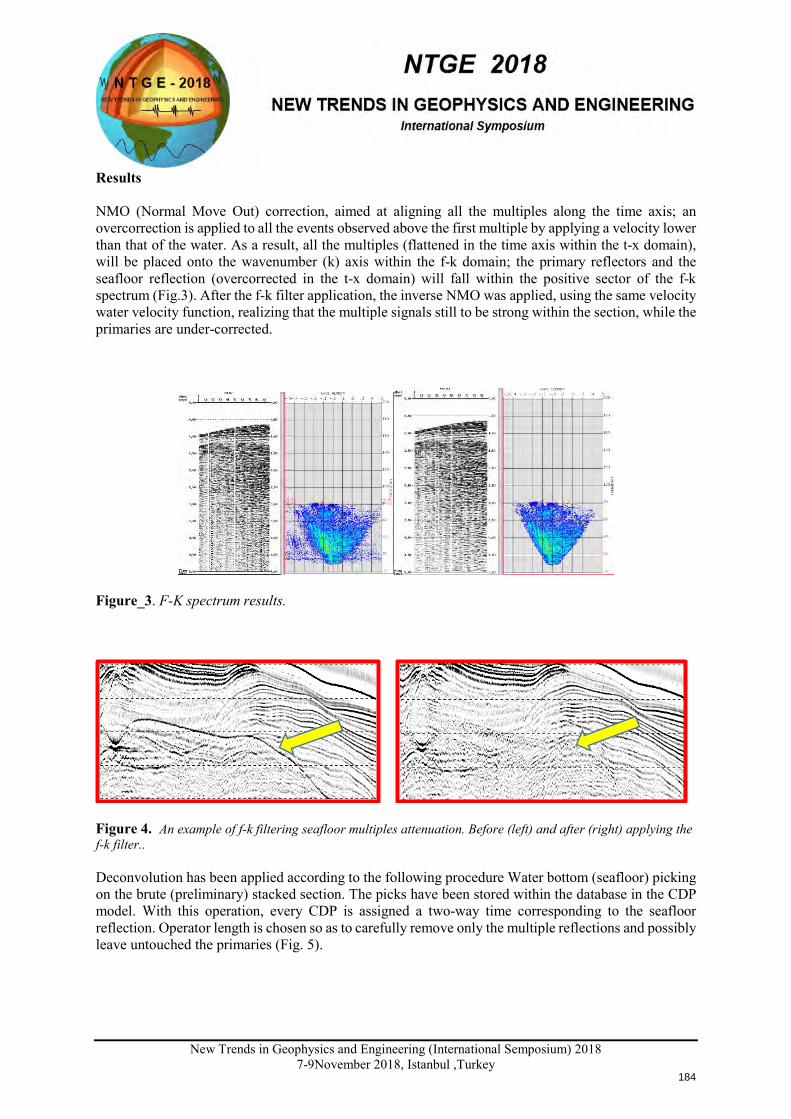
New Trends in Geophysics and Engineering (International Semposium) 2018
7-9November 2018, Istanbul ,Turkey
Results NMO (Normal Move Out) correction, aimed at aligning all the multiples along the time axis; an overcorrection is applied to all the events observed above the first multiple by applying a velocity lower than that of the water. As a result, all the multiples (flattened in the time axis within the t-x domain), will be placed onto the wavenumber (k) axis within the f-k domain; the primary reflectors and the seafloor reflection (overcorrected in the t-x domain) will fall within the positive sector of the f-k spectrum (Fig.3). After the f-k filter application, the inverse NMO was applied, using the same velocity water velocity function, realizing that the multiple signals still to be strong within the section, while the primaries are under-corrected.
Figure_3. F-K spectrum results.
Figure 4. An example of f-k filtering seafloor multiples attenuation. Before (left) and after (right) applying the f-k filter.. Deconvolution has been applied according to the following procedure Water bottom (seafloor) picking on the brute (preliminary) stacked section. The picks have been stored within the database in the CDP model. With this operation, every CDP is assigned a two-way time corresponding to the seafloor reflection. Operator length is chosen so as to carefully remove only the multiple reflections and possibly leave untouched the primaries (Fig. 5).
184
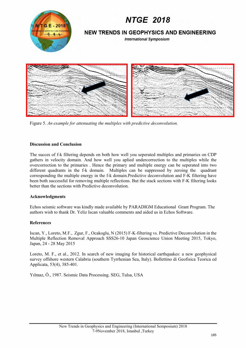
New Trends in Geophysics and Engineering (International Semposium) 2018
7-9November 2018, Istanbul ,Turkey
Figure 5. An example for attenuating the multiples with predictive deconvolution. Discussion and Conclusion
The succes of f-k filtering depends on both how well you seperated multiples and primaries on CDP gathers in velocity domain. And how well you aplied undercorrection to the multiples while the overcorrection to the primaries . Hence the primary and multiple energy can be seperated into two different quadrants in the f-k domain. Multiples can be suppressed by zeroing the quadrant corresponding the multiple energy in the f-k domain.Predictive deconvolution and F-K filtering have been both successful for removing multiple reflections. But the stack sections with F-K filtering looks better than the sections with Predictive deconvolution. Acknowledgments Echos seismic software was kindly made available by PARADIGM Educational Grant Program. The authors wish to thank Dr. Yeliz Iscan valuable comments and aided us in Echos Software. References Iscan, Y., Loreto, M.F., Zgur, F., Ocakoglu, N (2015) F-K-filtering vs. Predictive Deconvolution in the Multiple Reflection Removal Approach SSS26-10 Japan Geoscience Union Meeting 2015, Tokyo, Japan, 24 - 28 May 2015 Loreto, M. F., et al., 2012. In search of new imaging for historical earthquakes: a new geophysical survey offshore western Calabria (southern Tyrrhenian Sea, Italy). Bollettino di Geofisica Teorica ed Applicata, 53(4), 385-401. Yılmaz, Ö., 1987. Seismic Data Processing. SEG, Tulsa, USA
185
New Trends in Geophysics and Engineering (International Semposium) 2018
7-9 November 2018, Istanbul , Turkey
APPLICATIONS OF POST-STACK MIGRATION TYPES IN SEISMIC DATA Yusif Rahimov1, Hakan Alp1
1 Geophysical Eng. Department, Istanbul University, Istanbul [email protected]
Presentation Type All accepted proceedings will be published on the webpage of the symposium (ntge2018.istanbul.edu.tr)
ORAL POSTER
Abstracts Seismic reflection results obtained from seismic reflection studies, which are used mainly in petroleum and natural gas exploration, must pass through a number of complex data-processing stages in order to obtain the image of the sea bottom gold. These operations, which consist of a series of sequential mathematical operations, are called a seismic data processing Ard. The main objective is to remove the noise in the data and increase the signal-to-noise ratio. Seismic migration is one of the most important data-processing steps. Migration is the theory of the wave equation that carries the sloped reflections in the section to its real places and destroys the energy of scattering. The aim of the migration is to make the masonry section along the seismic line similar to the geological section. The positive and negative aspects, difficulties and convenience, advantages and disadvantages of these different types of migration (Kirchhoff, Finite differences and f-k) were examined and compared with each other. Keywords: Migration, Kirchhoff Migration, f-k Migration Introduction If the reflective surface is flat in the seismic reflection seismicity, the reflection point is considered to be the exact center of the shot-receiver distance. In the seismic sections formed by the seismic reflection traces from the inclined reflective surfaces, the observed structures show shifts from their actual locations (shot-receiver midpoint). Seismic migration is the theory of the wave equation that carries the sloped reflections in the section to its real places and destroys the energy of scattering. The main aim in migration is to reveal the real underground image of the seismic section obtained from the shot groups, taking into account the inclined surfaces. Migration is achieved in the time environment or in the depth environment. In case of sufficient accuracy of the speed information, the depth migration is ensured with a more precise view of the underground. However, in general, time migration is generally preferred because of the lack of accurate information in the lateral and vertical directions. There are basically different types of migration types developed according to the purposes and requirements. Pre-stacking migration is preferred in structurally complex areas and time and depth migrations are used in the regions where lateral velocity variations are present. There are different types of migration applications related to different migration algorithms. It is the depth migration that uses the RMS velocities and takes into consideration the beam twists and the intermediate velocities while not considering the beam twist at the layer boundaries.
X
186
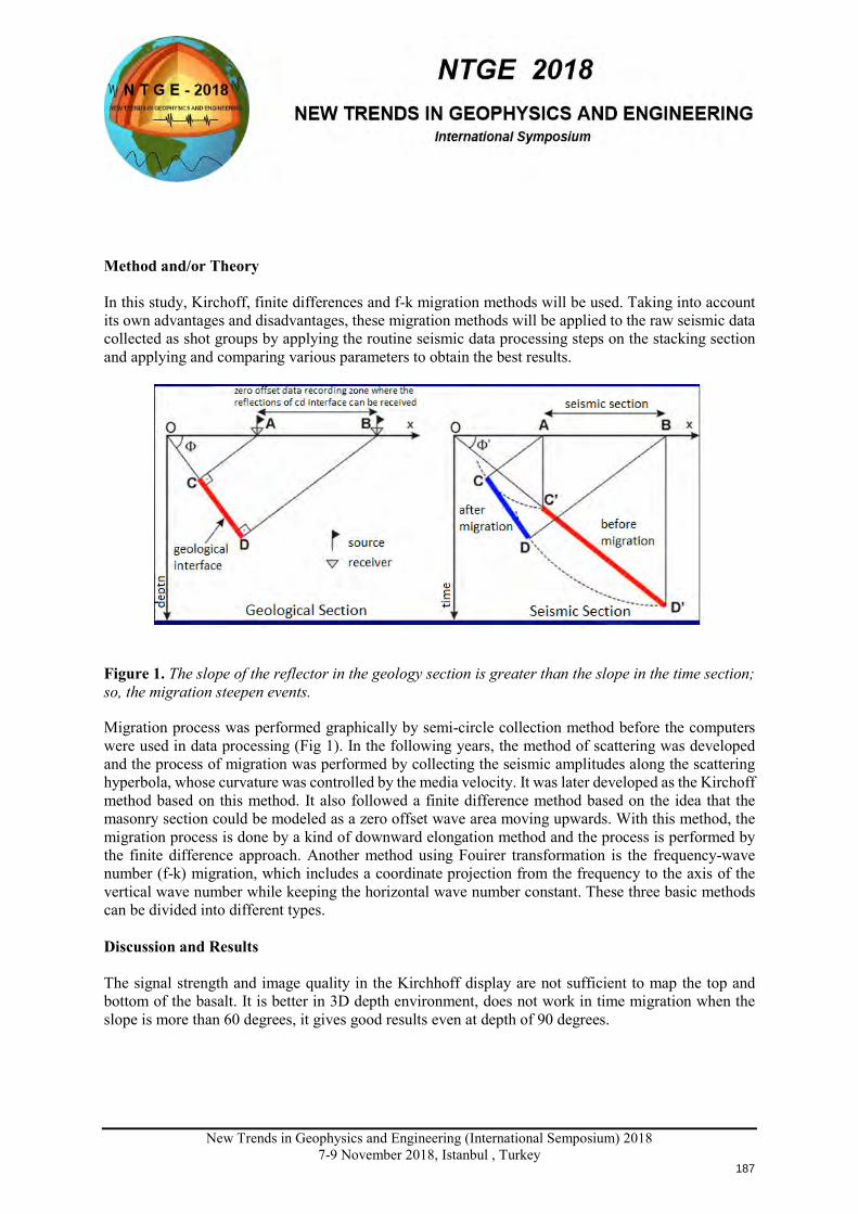
New Trends in Geophysics and Engineering (International Semposium) 2018
7-9 November 2018, Istanbul , Turkey
Method and/or Theory In this study, Kirchoff, finite differences and f-k migration methods will be used. Taking into account its own advantages and disadvantages, these migration methods will be applied to the raw seismic data collected as shot groups by applying the routine seismic data processing steps on the stacking section and applying and comparing various parameters to obtain the best results.
Figure 1. The slope of the reflector in the geology section is greater than the slope in the time section; so, the migration steepen events.
Migration process was performed graphically by semi-circle collection method before the computers were used in data processing (Fig 1). In the following years, the method of scattering was developed and the process of migration was performed by collecting the seismic amplitudes along the scattering hyperbola, whose curvature was controlled by the media velocity. It was later developed as the Kirchoff method based on this method. It also followed a finite difference method based on the idea that the masonry section could be modeled as a zero offset wave area moving upwards. With this method, the migration process is done by a kind of downward elongation method and the process is performed by the finite difference approach. Another method using Fouirer transformation is the frequency-wave number (f-k) migration, which includes a coordinate projection from the frequency to the axis of the vertical wave number while keeping the horizontal wave number constant. These three basic methods can be divided into different types. Discussion and Results The signal strength and image quality in the Kirchhoff display are not sufficient to map the top and bottom of the basalt. It is better in 3D depth environment, does not work in time migration when the slope is more than 60 degrees, it gives good results even at depth of 90 degrees.
187
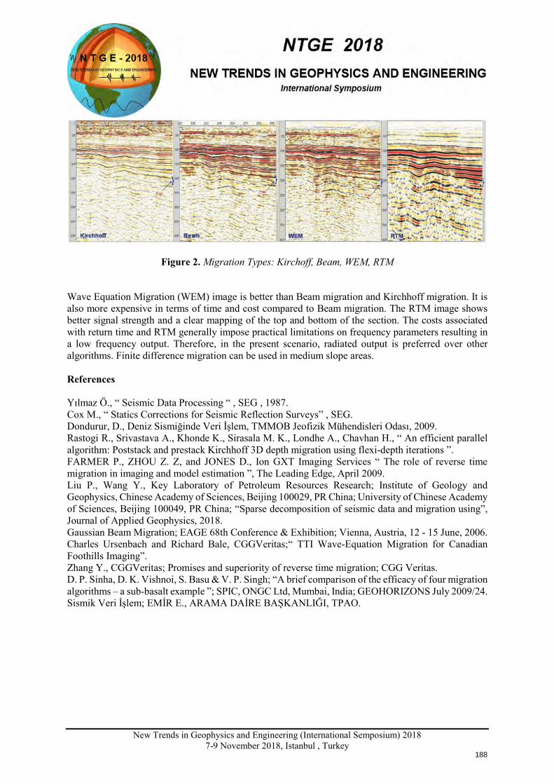
New Trends in Geophysics and Engineering (International Semposium) 2018
7-9 November 2018, Istanbul , Turkey
Figure 2. Migration Types: Kirchoff, Beam, WEM, RTM
Wave Equation Migration (WEM) image is better than Beam migration and Kirchhoff migration. It is also more expensive in terms of time and cost compared to Beam migration. The RTM image shows better signal strength and a clear mapping of the top and bottom of the section. The costs associated with return time and RTM generally impose practical limitations on frequency parameters resulting in a low frequency output. Therefore, in the present scenario, radiated output is preferred over other algorithms. Finite difference migration can be used in medium slope areas. References Yılmaz Ö., “ Seismic Data Processing “ , SEG , 1987. Cox M., “ Statics Corrections for Seismic Reflection Surveys” , SEG. Dondurur, D., Deniz Sismiğinde Veri İşlem, TMMOB Jeofizik Mühendisleri Odası, 2009. Rastogi R., Srivastava A., Khonde K., Sirasala M. K., Londhe A., Chavhan H., “ An efficient parallel algorithm: Poststack and prestack Kirchhoff 3D depth migration using flexi-depth iterations ”. FARMER P., ZHOU Z. Z, and JONES D., Ion GXT Imaging Services “ The role of reverse time migration in imaging and model estimation ”, The Leading Edge, April 2009. Liu P., Wang Y., Key Laboratory of Petroleum Resources Research; Institute of Geology and Geophysics, Chinese Academy of Sciences, Beijing 100029, PR China; University of Chinese Academy of Sciences, Beijing 100049, PR China; “Sparse decomposition of seismic data and migration using”, Journal of Applied Geophysics, 2018. Gaussian Beam Migration; EAGE 68th Conference & Exhibition; Vienna, Austria, 12 - 15 June, 2006. Charles Ursenbach and Richard Bale, CGGVeritas;“ TTI Wave-Equation Migration for Canadian Foothills Imaging”. Zhang Y., CGGVeritas; Promises and superiority of reverse time migration; CGG Veritas. D. P. Sinha, D. K. Vishnoi, S. Basu & V. P. Singh; “A brief comparison of the efficacy of four migration algorithms – a sub-basalt example ”; SPIC, ONGC Ltd, Mumbai, India; GEOHORIZONS July 2009/24. Sismik Veri İşlem; EMİR E., ARAMA DAİRE BAŞKANLIĞI, TPAO.
188
New Trends in Geophysics and Engineering (International Semposium) 2018
7-9 November 2018, Istanbul , Turkey
x
PALEOMAGNETIC RESULTS ALONG THE BITLIS-ZAĞROS SUTURE ZONE IN SE ANATOLIA, TURKEY
Beyza Bakkal1 , Mualla Cengiz Çinku1 , Friedrich Heller2
1 Department of Geophysical Engineering, Istanbul University, Istanbul
2 Institut für Geophysik, ETH Zürich, Switzerland Email: [email protected]
Presentation Type All accepted proceedings will be published on the webpage of the symposium (ntge2018.istanbul.edu.tr)
ORAL POSTER
Abstracts A paleomagnetic study has been carried out at Mesozoic and Cenozoic rocks at 34 localities along the Bitlis-Zağros suture zone in SE Anatolia located in the boundary region between the Taurides and the Arabian platform and delimited by the Dead Sea Fault. Paleomagnetic results from the area show clockwise rotations of 35.6°±14.1° and 26.7°±8.0° with respect to the African plate from upper Jurassic-lower Cretaceous and upper Cretaceous limestones, respectively. The paleomagnetic results indicate also an earlier deformation/opening due to the Dead Sea Fault Zone (DSFZ). Farther north on the Tauride Block, counterclockwise rotation of -34.5°±12.5° is recorded by upper Cretaceous limestones. In the SE of the study area on the northern margin of Arabia, counterclockwise rotations of -12.3°±8.3° and -2.5°±10.0°, in late Cretaceous and -12.7°±13.6° in middle Eocene rocks show relative tectonic stability. Middle Miocene rocks close to the suture zone suggest counterclockwise rotation by about -39.4°±10.9°, while farther away from the suture zone counterclockwise rotations of -21.9°±9.9° and -7.5°±5.8° are observed.
Keywords: Maximum 5 items for indexing purposes (separated with commas) Introduction The tectonic evolution of SE Anatolia is associated with the collision between the Taurides and the Arabian Platform in the early Cenozoic, after the final closure of the southern branch of the Neotethys ocean during Late Cretaceous to Early Eocene times. The ongoing deformation was characterized by northward movement of Arabia, followed by westward extrusion of Anatolia, having been displaced along the northern and eastern Anatolian transform faults. The neotectonic deformation history between the Anatolian Plate and the Arabian platform since the closure of the southern Neotethyan oceanic basin from Late Cretaceous to present has not been studied in detail paleomagnetically. Therefore we carried out a paleomagnetic study of Mesozoic and Cenozoic rocks at 34 localities along
189
New Trends in Geophysics and Engineering (International Semposium) 2018
7-9 November 2018, Istanbul , Turkey
the Bitlis-Zağros suture zone in SE Anatolia located in the boundary region between the Taurides and the Arabian platform and delimited by the Dead Sea Fault. Geology and Paleomagnetic Sampling The SE Anatolian region is constituted by three main tectonic features. The SE Anatolian orogenic belt to the north, the Arabian Platform to the south and a wide imbrication zone with major thrusts and faults in E-W direction divided from each other by major thrusts towards the north between these structures (Yılmaz et al., 1993; Robertson et al., 2006). The Arabian Platform consists of Pan-African crystalline basement which is overlain by autochthonous Palaeozoic to Tertiary sedimentary successions. Late Cretaceous and Tertiary ophiolitic units were emplaced on the platform, while younger deposits of late Miocene age crop out in a wide range of area (Yılmaz et al., 1993). In this study we sampled Upper Jurassic - Lower Cretaceous to middle Miocene limestones, sandstones and marls at 34 sites which are described below . The Upper Jurassic-Lower Cretaceous limestones were sampled (BZ 23–27, 31–34) in the NW of the study area, from platform carbonate rocks of the Amanos group, which are the equivalents of those on the Tauride platform. This sequence rests tectonically on the Late Cretaceous Kızıldağ ophiolite (Dubertret, 1953). Carbonate rocks of the Mardin group of Aptian and Campanian age (Görür et al., 1991) pass upwards into limestones, shales, marls and sandstones, which were deposited along the passive margin of the Arabian Plate (Sungurlu, 1973). They were sampled at several locations in the north of Osmaniye (BZ 1, 3, 4, 5, 7–11, 13–16). The Cenozoic sequence is composed of various clastic rocks including limestones, conglomerates, sandstones and mudstones of the Midyat group (Wilson and Krummenacher, 1957). The middle Eocene sequence was sampled in limestones (BZ12) and marls (BZ 19–22) at Kahramanmaraş and Adıyaman, respectively. The middle Miocene Fırat formation is composed of chalky limestones, tuff layers and turbidites of the Lice formation unconformably overly the uppermost part of the Eocene sedimentary rocks. The limestones, marls and sandstones were sampled at three different sites (BZ 2, 6, 18) around Adıyaman and Kahramanmaraş. Paleomagnetic rotations The paleomagnetic mean directions of each group were compared with expected mean directions derived from the coeval paleomagnetic poles for stable Eurasia and Africa of Besse and Courtillot (2002) using Enkin’s (unpublished data, 2004) PMGSC (version 4.2) software . Clockwise rotation of 35.6° ± 14.3° with respect to Africa is obtained for the Upper Jurassic - Lower Cretaceous sedimentary rocks along the Dead Sea Fault of the westernmost part of the Arabian Plate. The magnitude of rotation is 15.6° ± 12.9° if the reference pole for Eurasia is considered. The Late Cretaceous group mean declinations (G-K1 - G-K3) on rocks situated on the Arabian Plate suggest that G-K1, located to the south of Urfa, has been rotated counterclockwise by −12.3° ± 8.3°, while farther northwest, small counterclockwise rotation of −2.5° ± 10.1° is obtained with respect to Africa. When considering the Eurasian reference pole, rotations increase to the west of the study area. Between Osmaniye and Kahramanmaraş along the DSFZ, clockwise rotation of 26.7° ± 8° (G-K3) is observed with respect to Africa and less rotation when considering the Eurasian reference frame . The area around Osmaniye which tectonically belongs to the Anatolian Plate, is rotated counterclockwise by − 34.5° ± 12.5° (G-K4) with respect to Africa, but smaller rotation results with respect to Eurasia. The Middle Eocene sedimentary rocks on the Arabian Plate show a rotation of −12.7° ± 13.6° with respect to Africa and an increase when considering the Eurasian reference pole (−23.8° ± 12.2°). Individual tectonic rotations are obtained from single sites in Miocene sedimentary rocks in the Kahramanmaraş area along the East Anatolian Fault, showing counterclockwise rotation of −39.4° ± 10.9°. When moving farther to the south, then a decrease in rotation is observed from −21.9° ± 29.9° to −7.5° ± 5.8°.
190
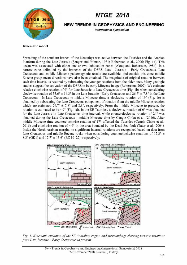
New Trends in Geophysics and Engineering (International Semposium) 2018
7-9 November 2018, Istanbul , Turkey
Kinematic model
Spreading of the southern branch of the Neotethys was active between the Taurides and the Arabian Platform during the Late Jurassic (Şengör and Yılmaz, 1981; Robertson et al., 2006; Fig. 1a). This ocean was associated with either one or two subduction zones (Aktaş and Robertson, 1984). In a narrow zone delimited by the branches of the DSFZ, Late Jurassic - Early Cretaceous, Late Cretaceous and middle Miocene paleomagnetic results are available, and outside this zone middle Eocene group mean directions have also been obtained. The magnitude of original rotation between each time interval is restored by subtracting the younger rotations from the older ones. Many geologic studies suggest the activation of the DSFZ to be early Miocene in age (Robertson, 2002). We estimate relative clockwise rotation of 9° for Late Jurassic to Late Cretaceous time (Fig. 1b) when considering clockwise rotation of 35.6° ± 14.3° in the Late Jurassic - Early Cretaceous and 26.7° ± 7.8° in the Late Cretaceous . In Late Cretaceous to middle Miocene time, a clockwise rotation of 19° (Fig. 1c) is obtained by subtracting the Late Cretaceous component of rotation from the middle Miocene rotation which are estimated 26.7° ± 7.8° and 8.8°, respectively. From the middle Miocene to present, the rotation is estimated to be ∼9° (Fig. 1d). In the SE Taurides, a clockwise rotation of 6° was obtained for the Late Jurassic to Late Cretaceous time interval, while counterclockwise rotation of 24° was obtained during the Late Cretaceous – middle Miocene time by Cengiz Çinku et al. (2016). After middle Miocene time counterclockwise rotation of 17° affected the Taurides (Cengiz Çinku et al., 2016) and clockwise rotation of ∼9° in the area bounded by the Dead Sea fault (Tatar et al., 2004). Inside the North Arabian margin, no significant internal rotations are recognized based on data from Late Cretaceous and middle Eocene rocks when considering counterclockwise rotations of 12.3° ± 8.3° (GK1) and 12.7° ± 13.6° (BZ 19–22), respectively.
Fig. 1. Kinematic evolution of the SE Anatolian region and surroundings showing tectonic rotations from Late Jurassic – Early Cretaceous to present.
191
New Trends in Geophysics and Engineering (International Semposium) 2018
7-9 November 2018, Istanbul , Turkey
Conclusions
Reliable paleomagnetic directions have been obtained and are interpreted to document two major tectonic phases, the closure of the southern Neotethys in the Late Cretaceous and the collision between the Arabian platform and Anatolia at the beginning of the Eocene. Deformation of Upper Jurassic to Miocene rocks in the Bitlis-Zağros Suture Zone is due to the closure of the southern Neotethys ocean and the collision between Arabia and Anatolia. In the area delimited by the Dead Sea Fault, clockwise rotation by 19° of Late Jurassic – Late Cretaceous to Miocene sedimentary rocks indicates an earlier deformation of this fault zone, while middle Eocene lavas of the SE Taurides reveal counterclockwise rotation of −24° in association with the closure of the southern Neotethys ocean during Late Cretaceous to Early Eocene time (Cengiz Çinku et al., 2016).
Acknowledgements (Optional)
This research was supported by the Scientific Research Projects Coordination Unit of Istanbul University, project number 23607.
References Besse, J., Courtillot, V., 2002. Apparent and true polar wander and the geometry of the geomagnetic field over the last 200 Myr. J. Geophys. Res.: Solid Earth 107. Cengiz Çinku, M., Hisarli, Z.M., Yılmaz, Y., Ülker, B., Kaya, N., Öksüm, E., Orbay, N., Özbey, Z.Ü., 2016. The tectonic history of the Niğde-Kırşehir Massif and the Taurides since the Late Mesozoic: Paleomagnetic evidence for two-phase orogenic curvature in Central Anatolia. Tectonics 35, 772–811. https://doi.org/10.1002/2015TC003956. Dubertret, L., 1953. Géologie des roches vertes du nord-ouest de la Syrie et du Hatay (Turquie). Notes et Mémoires sur le Moyen Orient 6, 5–227. Görür, N., Çelikdemir, E., Dülger, S., 1991. Carbonate platforms developed on passive continental margins: Cretaceous margin carbonates in southeast Anatolia as an example. Bull. Tech. Univ. Istanbul 33, 301–324. Robertson, A.H.F., 2002, Overview of the genesis and emplacement of Mesozoic ophiolites in the eastern Mediterranean Tethyan region, Lithos, 65 (1), 1-67. Robertson, A.H.F., Ustaömer, T., Parlak, O., Ünlügenç, U.C., Taslı, K., İnan, N., 2006, The Berit transect of the Tauride thrust belt, S. Turkey: Late Cretaceous-Early Cenozoic accretionary/collisional processes related to closure of the southern Neotethys, Journal of Asian Earth Sciences, 27, 108-145. Şengör, A.M.C., Yılmaz, Y., 1981, Tethyan evolution of Turkey: A plate tectonic approach, Tectonophysics, 75, 181-241. Tatar, O., Piper, J.D.A., Gürsoy, H., Heimann, A., Koçbulut, F., 2004. Neotectonic deformation in the transition zone between the Dead Sea transform and the East Anatolian fault zone Southern Turkey: a palaeomagnetic study of the Karasu rift volcanism. Tectonophysics 385, 17–43. Wilson, H.H. & Krummenacher, R., 1957, Geology and oil prospects of the Gaziantep Region SE Turkey. Petrol Dai. Bşk. Teknik arşivi, Ankara (yayımlanmamış). Yılmaz, Y., Yiğitbas¸ E., Genç, C., 1993, Ophiolitic and metamorphic assemblages of southeast Anatolia and their significance in the geological evolution of the orogenic belt, Tectonics, 12, 1280-1297.
192

New Trends in Geophysics and Engineering (International Semposium) 2018
7-9November 2018, Istanbul ,Turkey
x
Seismotectonic Investigation of Gökova Gulf Using Seismic Reflection and
Seismological Data Set
AzerAzizov,Ethem Görgün
Geophysical Eng. Department, Istanbul University-Cerrahpaşa, Istanbul Email: [email protected]
[email protected] Presentation Type All accepted proceedings will be published on the webpage of the symposium (ntge2018.istanbul.edu.tr)
ORAL POSTER
Abstracts 21 July 2017 Mw 6.6 Gökova Gulf earthquake and its aftershock sequence in Aegean Sea are examined. Centroid moment tensors (CMT) for 50 earthquakes with moment magnitudes (Mw) between 3.5 and 6.6 are determined by applying a waveform inversion method. The mainshock is shallow focus normal faulting event at a depth of 11 km. The seismic moment(Mo) of the mainshock is estimated as 8.45×10¹⁸ Nm and rupture eduration of the mainshock is 5s. The focal mechanisms of aftershocks are mainly normal faulting with a strike-slip component. The geometry of the moment tensors (Mw≥3.5) reveals a normal faulting regime with N- S trending direction of T-axis in the entire activated region. According to variance of the stress tensor inversion, to first order, the Gökova Gulf regions characterized by a homogeneous intraplate stress field. Keywords: Gökova Gulf, earthquake, mainshock
193
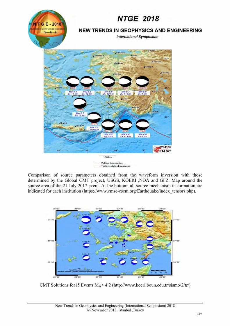
New Trends in Geophysics and Engineering (International Semposium) 2018
7-9November 2018, Istanbul ,Turkey
Comparison of source parameters obtained from the waveform inversion with those determined by the Global CMT project, USGS, KOERI ,NOA and GFZ. Map around the source area of the 21 July 2017 event. At the bottom, all source mechanism in formation are indicated for each institution (https://www.emsc-csem.org/Earthquake/index_tensors.php).
CMT Solutions for15 Events Mw> 4.2 (http://www.koeri.boun.edu.tr/sismo/2/tr/)
194
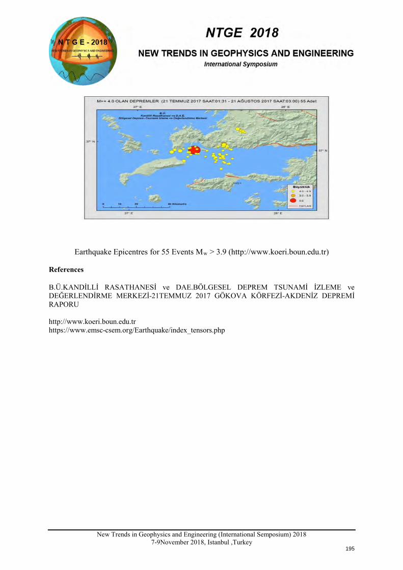
New Trends in Geophysics and Engineering (International Semposium) 2018
7-9November 2018, Istanbul ,Turkey
Earthquake Epicentres for 55 Events Mw > 3.9 (http://www.koeri.boun.edu.tr) References B.Ü.KANDİLLİ RASATHANESİ ve DAE.BÖLGESEL DEPREM TSUNAMİ İZLEME ve DEĞERLENDİRME MERKEZİ-21TEMMUZ 2017 GÖKOVA KÖRFEZİ-AKDENİZ DEPREMİ RAPORU http://www.koeri.boun.edu.tr https://www.emsc-csem.org/Earthquake/index_tensors.php
195


