Italian mortgage markets and their dynamics

Accepted Manuscript

Title: Italian mortgage markets and their dynamics

Author: Simone Landini Mariacristina Uberti SimoneCasellina

PII: S0378-4754(14)00107-4DOI: http://dx.doi.org/doi:10.1016/j.matcom.2014.04.005Reference: MATCOM 4061

To appear in: Mathematics and Computers in Simulation

Received date: 4-3-2013Revised date: 12-4-2014Accepted date: 20-4-2014

Please cite this article as: Simone Landini, Mariacristina Uberti, Simone Casellina,Italian mortgage markets and their dynamics, Mathematics and Computers inSimulation (2014), http://dx.doi.org/10.1016/j.matcom.2014.04.005

This is a PDF file of an unedited manuscript that has been accepted for publication.As a service to our customers we are providing this early version of the manuscript.The manuscript will undergo copyediting, typesetting, and review of the resulting proofbefore it is published in its final form. Please note that during the production processerrors may be discovered which could affect the content, and all legal disclaimers thatapply to the journal pertain.

http://dx.doi.org/doi:10.1016/j.matcom.2014.04.005

http://dx.doi.org/10.1016/j.matcom.2014.04.005

Page 1 of 24

Accep

ted

Man

uscr

ipt

Italian mortgage markets and their dynamics

Simone Landinia,∗, Mariacristina Ubertib, Simone Casellinac

aI.R.E.S. Piemonte, Via Nizza 18, 10125, Turin, ItalybUniversita degli Studi di Torino, Turin, Italy

cBanca d’Italia, Rome, Italy

Abstract

This paper deepens previous studies on the analysis of the fixed (FRMs)and adjustable rate mortgages (ARMs) dynamics and the interconnectionsbetween FRMs and ARMs markets. In particular, an econometric analysison the Italian mortgage markets series from 1997 : q1 to 2012 : q3 is setup by involving the VAR estimation technique. Very interesting results areachieve to point out how the effects of the European Central Bank control onthe Euribor transmit (i) to the behavior of interest rates term structure aswell as (ii) to interest rates of contracts involved in different technical formsoffered in the Italian mortgage markets.

Keywords: mortgage market, price fluctuations, market interactions,adjustable and fixed rate mortgage, Italian markets

1. Introduction and motivation

The interconnections between the markets of fixed (FRMs) and adjustablerate mortgages (ARMs) are an interesting phenomenon to analyse under dif-ferent profiles. In particular, with regard to Italy, this phenomenon has beenable to get the effects of the economic crisis triggered in 2008, to deflagrateto the same moment of the Lehman Brothers failure (cfr, for details, [10]).

If, more generally and for purposes of comparison, the market for housingfinance in the industrial countries is taken into account, it is well-known thatover the past 25 years this market has changed and developed greatly andthe literature concentrates primarily on two countries: the US and UK. An

∗Corresponding authorEmail address: [email protected] (Simone Landini)

Preprint submitted to Mathematics and Computers in Simulation April 12, 2014

http://ees.elsevier.com/matcom/viewRCResults.aspx?pdf=1&docID=6225&rev=1&fileID=169119&msid=8D279DDE-3648-480D-B130-00B14247FE92

Page 2 of 24

Accep

ted

Man

uscr

iptEURIBOR EURO LEHEMAN

1999:1−2001:4 2002:1−2004:4 2005:1−2008:2 2008:2−2012:30

,51

1,5

22,

53

3,5

44,

55

1999

q1

2000

q1

2001

q1

2002

q1

2003

q1

2004

q1

2005

q1

2006

q1

2007

q1

2008

q1

2009

q1

2010

q1

2011

q1

2012

q1

2013

q1

EURIBOR Fix−Adj spreadFix share Adj share

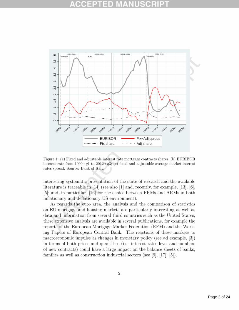
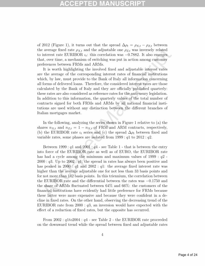
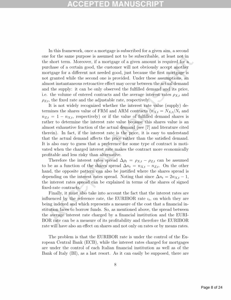
Figure 1: (a) Fixed and adjustable interest rate mortgage contracts shares; (b) EURIBORinterest rate from 1999 : q1 to 2012 : q3; (c) fixed and adjustable average market interestrates spread. Source: Bank of Italy.

interesting systematic presentation of the state of research and the availableliterature is traceable in [14] (see also [1] and, recently, for example, [13]; [6],[5]; and, in particular, [16] for the choice between FRMs and ARMs in bothinflationary and deflationary US environment).

As regards the euro area, the analysis and the comparison of statisticson EU mortgage and housing markets are particularly interesting as well asdata and information from several third countries such as the United States;these extensive analysis are available in several publications, for example thereports of the European Mortgage Market Federation (EFM) and the Work-ing Papers of European Central Bank. The reactions of these markets tomacroeconomic impulse as changes in monetary policy (see ad example, [3])in terms of both prices and quantities (i.e. interest rates level and numbersof new contracts) could have a large impact on the balance sheets of banks,families as well as construction industrial sectors (see [9], [17], [5]).

2

Page 3 of 24

Accep

ted

Man

uscr

ipt

In [4] and [20] some of the dynamics of the Italian markets of FRMs andARMs are analysed: the switching mechanism between these two marketsis pointed out by historical data on the universe of mortgages in Italy since1999 (the year of entry into force of EURIBOR rates) to 2011 and an originalmodel is proposed to grasp these peculiar interconnection behaviours.One of the fundamental assumptions of these studies is that the interest ratesfor mortgages are also indexed to the EURIBOR rate, among other factors.More precisely, since a mortgage is a form of funding that the financial in-stitutions deliver to customers, part of the funds granted in the mortgagesare thought coming from the EURIBOR interbank market. So, from the fi-nancial institution’s viewpoint, the spread between the charged interest rateto the mortgage contract and the interbank interest rate can be consideredas an indicator of contract’s profitability. The values of the quarterly EURI-BOR rates are calculated as the average of the monthly EURIBOR rates atthree months for those following its entry into force.

The time series of Italian mortgage markets (see Figure 1; source Bank ofItaly) used by [4] and [20] have become attractive not only, as stressed above,to look back at some phases of the recent past, but also for further aspects:(i) the interconnection between the two markets has become more evidentby evaluating the series of th k-th market values Vk,t = ρk,tNk,t, where theaverage rate ρk,t of the k-th type of market is defined as a price and theabsolute number of contracts Nk,t evaluates the demanded and, at the sametime, the supplied quantities for the k-th type of contract, (ii) the volatilityof market values and, finally, (iii) the effect that could induce a shock to thereference rate for mortgages, the EURIBOR rate ιt.

In order to study the dynamics of market shares, according to cobweb phe-nomenology, a mathematical model is developed in [4] and applied becauseit turned out able to easily see the switching mechanisms observed betweenFRMs and ARMs markets. Then, from this initial mathematical model, aneconometric model is derived and estimated in [20]. Although this derivedeconometric model reveals a good capacity to replicate the time series, it alsohighlights several questions that remained unanswered, including the effectsof monetary policy on mortgage markets. From here, the necessity to resumethe historical series and update them to set an econometric analysis aimedto explain the effect of a shock to the EURIBOR on interest rates for FRMsand ARMs.

Therefore, updating the data reported in [4] and [20] to the third quarter

3

Page 4 of 24

Accep

ted

Man

uscr

ipt

of 2012 (Figure 1), it turns out that the spread ∆ρt = ρX,t − ρZ,t betweenthe average fixed rate ρX,t and the adjustable one ρZ,t was inversely relatedto interest rate EURIBOR ιt: this correlation was −0.7882. It also emergesthat, over time, a mechanism of switching was put in action among customerpreferences between FRMs and ARMs.

It is worth highlighting the involved fixed and adjustable interest ratesare the average of the corresponding interest rates of financial institutionswhich, by law, must provide to the Bank of Italy all information concerningall forms of delivered loans. Therefore, the considered interest rates are thosecalculated by the Bank of Italy and they are officially published quarterly:these rates are also considered as reference rates for the anti-usury legislation.In addition to this information, the quarterly values of the total number ofcontracts signed for both FRMs and ARMs by all national financial insti-tutions are used without any distinction between the different branches ofItalian mortgages market.

In the following, analyzing the series shown in Figure 1 relative to (a) theshares nX,t and nZ,t = 1 − nX,t of FRM and ARM contracts, respectively,(b) the EURIBOR rate ιt series and (c) the spread ∆ρt between fixed andvariable rates, some phases are isolated from 1999 : q1 to 2012 : q2.

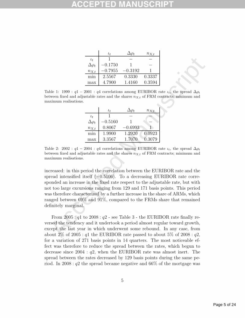
Between 1999 : q1 and 2001 : q4 - see Table 1 - that is between the entryinto force of the EURIBOR rate as well as of EURO, the EURIBOR ratehas had a cycle among the minimum and maximum values of 1999 : q2 -2000 : q3. Up to 2002 : q1, the spread in rates has always been positive andhas peaked in 2000 : q1 and 2002 : q1: the average fixed interest rate washigher than the average adjustable one for not less than 33 basis points andfor not more than 142 basis points. In this triennium, the correlation betweenthe EURIBOR rate and the differential between the rates was −0.1750 andthe share of ARMs fluctuated between 64% and 66%: the customers of thefinancial institutions have evidently had little preference for FRMs becausethese latter were more expensive and because they were confident in a de-cline in fixed rates. On the other hand, observing the decreasing trend of theEURIBOR rate from 2000 : q3, an inversion would have expected with theeffect of a reduction of fixed rates, but the opposite has occurred.

From 2002 : q1to2004 : q4 - see Table 2 - the EURIBOR rate proceededon the downward trend while the spread between fixed and adjustable rates

4

Page 5 of 24

Accep

ted

Man

uscr

ipt

ιt ∆ρt nX,t

ιt 1 − −∆ρt −0.1750 1 −nX,t −0.7955 −0.3192 1min 2.5567 0.3330 0.3337max 4.7900 1.4160 0.3594

Table 1: 1999 : q1 − 2001 : q4 correlations among EURIBOR rate ιt, the spread ∆ρtbetween fixed and adjustable rates and the shares nX,t of FRM contracts; minimum andmaximum realisations.

ιt ∆ρt nX,t

ιt 1 − −∆ρt −0.5160 1 −nX,t 0.8067 −0.6993 1min 1.9900 1.2920 0.0923max 3.3567 1.7070 0.3079


increased: in this period the correlation between the EURIBOR rate and thespread intensified itself (−0.5106). To a decreasing EURIBOR rate corre-sponded an increase in the fixed rate respect to the adjustable rate, but withnot too large excursions ranging from 129 and 171 basis points. This periodwas therefore characterized by a further increase in the share of ARMs, whichranged between 69% and 91%, compared to the FRMs share that remaineddefinitely marginal.

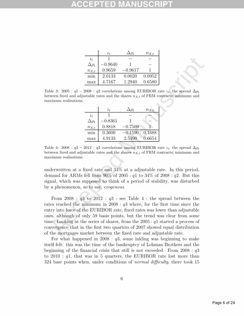
From 2005 : q1 to 2008 : q2 - see Table 3 - the EURIBOR rate finally re-versed the tendency and it undertook a period almost regular toward growth,except the last year in which underwent some rebound. In any case, fromabout 2% of 2005 : q1 the EURIBOR rate passed to about 5% of 2008 : q2,for a variation of 271 basis points in 14 quarters. The most noticeable ef-fect was therefore to reduce the spread between the rates, which begun todecrease since 2004 : q2, when the EURIBOR rate was almost inert. Thespread between the rates decreased by 129 basis points during the same pe-riod. In 2008 : q2 the spread became negative and 66% of the mortgage was

5

Page 6 of 24

Accep

ted

Man

uscr

ipt

ιt ∆ρt nX,t

ιt 1 − −∆ρt −0.9640 1 −nX,t 0.9659 −0.9617 1min 2.0133 0.0020 0.0952max 4.7167 1.2940 0.6580


ιt ∆ρt nX,t

ιt 1 − −∆ρt −0.8361 1 −nX,t 0.8818 −0.7509 1min 0.3600 −0.1590 0.1688max 4.9133 2.5390 0.6654


underwritten at a fixed rate and 34% at a adjustable rate. In this period,demand for ARMs fell from 90% of 2005 : q1 to 34% of 2008 : q2. But thissignal, which was supposed to think of a period of stability, was disturbedby a phenomenon, so to say, exogenous.

From 2008 : q3 to 2012 : q3 - see Table 4 - the spread between therates reached the minimum in 2008 : q3 where, for the first time since theentry into force of the EURIBOR rate, fixed rates was lower than adjustableones, although of only 59 basis points, but the trend was clear from sometime. Looking at the series of shares, from the 2005 : q1 started a process ofconvergence that in the first two quarters of 2007 showed equal distributionof the mortgages market between the fixed rate and adjustable rate.

For what happened in 2008 : q3, some inkling was beginning to makeitself felt: this was the time of the bankruptcy of Lehman Brothers and thebeginning of the financial crisis that still is not exceeded. From 2008 : q3to 2010 : q1, that was in 5 quarters, the EURIBOR rate lost more than324 base points when, under conditions of normal difficulty, there took 15

6

Page 7 of 24

Accep

ted

Man

uscr

ipt

quarters for a growth of approximately 300 base points. The EURIBORrate decreased exponentially because no one lent more money to someone,there was a climate of enormous distrust because financial institutions didnot know if what retained in their portfolios was toxic or not and, above all,they were worried about the recovery of claims.

The effect was not long to be seen: the spread between the interest ratesgrew symmetrically to the decrease of the EURIBOR rate and it reached itsmaximum in the 2009 : q2 − 2010 : q1 with an increase of 259 basis pointsfrom 2008 : q3. The fixed rates grew and the adjustable ones decreased: itwent back to a market that focused the demand for ARMs between 37% and82%, as in the mid-2000s, and so it remained until the end of 2012.

From 2010 : q1 on, various events occurred in both the financial settingand the real economy but, above all, in the second half of 2011 a heated de-bate was generated on the spread between Italian bonds and German Bundsyields. This gap - in some moments definitely worrying - had an impact ondomestic interest rates and, therefore, also on the mortgage rates. In thesame period, the EURIBOR rate backed to decreasing and this gave the de-creasing trend to the fixed-adjustable spread.

The paper is organized as follows. In Section 2, the research questionis posed. In Section 3, a phenomenological description of the underlin-ing dynamics is introduced. Section 4 specifies and estimates a suitableVector-auto-Regression (VAR) model to gather the associate Impulse Re-sponse Function (IRF) in order to analyse the effect of a monetary shock tothe EURIBOR rate on spreads of both interest rates and shares. Section 5concludes.

2. Research question

Since in the mortgage market there can not be excess-supply, the marketis assumed to be demand driven. Then, from the viewpoint of demand, thenumber of entered contracts NX,t or NZ,t for FRMs or ARMs, respectively,can be considered as the volume of the quantities purchased, i.e. the satisfieddemand: Nt = NX,t+NZ,t. However, the fulfilled demand can be less than theamount actually demanded Nt when, for example, there is credit rationing;in this case, the spread between the actual demand and the fulfilled onegenerates an excess of demand dt = Nt −Nt ≥ 0.

7

Page 8 of 24

Accep

ted

Man

uscr

ipt

In this framework, once a mortgage is subscribed for a given aim, a secondone for the same purpose is assumed not to be subscribable, at least not inthe short term. Moreover, if a mortgage of a given amount is required for apurchase of a certain good, the customer will not obviously accept anothermortgage for a different not needed good, just because the first mortgage isnot granted while the second one is provided. Under these assumptions, analmost instantaneous retroactive effect may occur between the actual demandand the supply: it can be only observed the fulfilled demand and its price,i.e. the volume of entered contracts and the average interest rates ρX,t andρZ,t, the fixed rate and the adjustable rate, respectively.

It is not widely recognized whether the interest rate value (supply) de-termines the shares value of FRM and ARM contracts (nX,t = NX,t/Nt andnZ,t = 1 − nX,t, respectively) or if the value of fulfilled demand shares israther to determine the interest rate value because this shares value is analmost exhaustive fraction of the actual demand (see [7] and literature citedtherein). In fact, if the interest rate is the price, it is easy to understandthat the actual demand affects the price rather than the satisfied demand.It is also easy to guess that a preference for some type of contract is moti-vated when the charged interest rate makes the contract more economicallyprofitable and less risky than alternative.

Therefore the interest rates spread ∆ρt = ρX,t − ρZ,t can be assumedto be as a function of the shares spread ∆nt = nX,t − nZ,t. On the otherhand, the opposite pattern can also be justified where the shares spread isdepending on the interest rates spread. Noting that since ∆nt = 2nX,t − 1,the interest rates spread can be explained in terms of the shares of signedfixed-rate contracts.

Finally, it must also take into account the fact that the interest rates areinfluenced by the reference rate, the EURIBOR rate ιt, on which they arebeing indexed and which represents a measure of the cost that a financial in-stitution faces to borrow funds. So, as mentioned above, the spread betweenthe average interest rate charged by a financial institution and the EURI-BOR rate can be a measure of its profitability and therefore the EURIBORrate will have also an effect on shares and not only on rates or by means rates.

The problem is that the EURIBOR rate is under the control of the Eu-ropean Central Bank (ECB), while the interest rates charged for mortgagesare under the control of each Italian financial institution as well as of theBank of Italy (BI), as a last resort. As it can easily be supposed, there are

8

Page 9 of 24

Accep

ted

Man

uscr

ipt

at least three main sources of interference on interest rates for mortgagesconsidered here: (i) the actual demand, (ii) the real interest rate and (iii)the EURIBOR rate.

The question is then the following: what is and how to explain the pos-sible effect of a monetary policy shock to the EURIBOR rate on the Italianmarkets of FRMs and ARMs?

To study some possible feedbacks and highlighted interconnections - atleast at the level of interactions between the respective interest rates with thereference rate - and to answer to the formulated research question, it is foundappropriate to specify a family of VAR models to assess the reaction to anexogenous shock of monetary policy resulting in the change of the EURIBORrate.

3. A phenomenological description of dynamics

The assumptions underlying the model follow a phenomenologically ra-tional description. Given the demand for mortgages as the supply driver,interest rates (price) on mortgages are directly influenced by the EURIBORrate, which is an index of the unit cost for a loan from a financial institu-tion, but the reaction speed is necessarily different: the adjustable rate reactsbefore the fixed one

ρX,t = aX + bXιt−kX + ǫX,t

ρZ,t = aZ + bZιt−kZ + ǫZ,t: kX > kZ (1)

Between the two rates some important differences can be highlighted. Asregards their determination on the market, there is not only a difference ofreaction to EURIBOR rate but also a different level of risk inherent in thecontracts. ARMs are contracts with a lower interest rate for the subscriberbecause the risk is higher whereas for FRMs the subscriber is willing to paymore just because the contract is riskless respect to financial fluctuations.

Furthermore, for FRMs a shock to the EURIBOR rate is completely irrel-evant while this last one exerts effects not only in the process of underwritingcontracts but also, and above all, on those already signed at floating rates.

The composition of demand Nt = NX,t +NZ,t can be described by sharesnX,t = 1 − nZ,t, where nX,t = Nk,t/Nt. Therefore, for a complete description

9

Page 10 of 24

Accep

ted

Man

uscr

ipt

of the demand composition, it is sufficient to consider the FRMs share sincethe ARMs share is the one’s complement.

The preference for one of the two branches of demand depends on thespread between the interest rates in a way not precisely determined becausethe demand is influenced by several conjunctural factors, by factors specifi-cally related to the signed contract and by the characteristics of the customeras well as the seller in terms of risk classification and default probabilities:

nX,t = fX(∆ρt) + ǫt∆ρt = ρX,t − ρZ,t

(2)

where fX(.) is a not determined function.

The mechanism of switching in various concentrations of demand betweenFRMs and ARMs can therefore be reasonably assumed to be explained ac-cording to the following phenomenology.

In response to an exogenous positive (negative) shock of monetary policyon EURIBOR rate, the adjustable rate reacts with a delay kZ in the same di-rection of the received pulse. This variation of the adjustable rate approachesthe fixed rate, the more inert, leading to a decrease (increase) of the spreadbetween the two rates, for the benefit of a higher concentration of demandin the market of FRMs.

With a longer delay kX > kZ , also the fixed rate increases (decreases) andthen the spread between the interest rates goes back up such that the fixedrate moves away from the reached level by the variable rate which curtailslittle by little the response to the received pulse.

Under normal conditions, i.e. in the absence of conjunctural upheavals orturbulence in the financial markets, when the spread between interest ratesreaches the level preceding the shock, albeit on levels now different, there isno more reason to prefer the fixed rate (more expensive but less risky) withrespect to adjustable rate (less expensive but more risky).

4. The model

The phenomenological description of section 3 constitutes the basic hy-pothesis to test to explain the observed dynamics on interest rates spread

10

Page 11 of 24

Accep

ted

Man

uscr

ipt

and demand composition in the Italian mortgage market. Due to the lack ofa model for (2), estimation of (1) is useless to identify specific delays kX andkZ for an EURIBOR’s shock effect on demand composition. Nevertheless,the hypothesis can be tested by means of a VAR model and by analysing theIRF outcomes of the specified model.

The state variable for the dynamic analysis is the vector

xt = (ιt,∆ρt, nX,t)′ ∈ M(3,1)(R) (3)

where the variables are put in a descendent order of exogeneity as sug-gested by [11]. The VAR(p) structure is

xt −

(

m0 +

p∑

h=1

Mhxt−h

)

= ǫt → WN(0,Σ) (4)

where m0 is a vector of intercepts with the same dimension of xt andMh ∈ M(3,3)(R) is a matrix of coefficients linking each observable in the(t− h)-lagged state vector to all the observables in xt. The last term ǫt is arandom vector of residuals assumed to follow a White-Noise process, that iswith null expected value E[ǫt] = 0 and a non-singular, constant and positive-definite covariance matrix E[ǫtǫ

′t] = Σ.

4.1. Lag-order selection

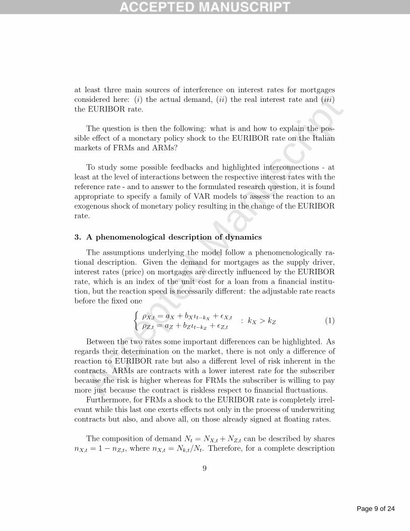
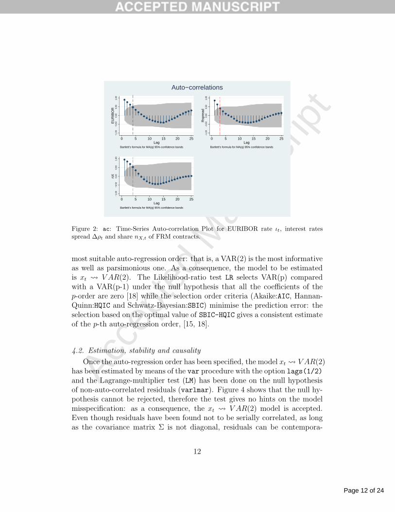
The auto-correlation functions in Figure 2 suggest that the a-priori lag-order to start with the specification of the VAR(p) is p = 4, that is the rel-evant data for the present are the same data one year-before on a quarterlytime series. With the exception of the interest rate spread, which involves alag of order 3, the confidence bands show that the auto-correlations becomenot significantly different from zero for p > 4. Confidence bands are definedby the Bartlet’s approximated formula for the auto-correlation standard er-ror (see [2], formula (6.2.2) p. 177 and formula (2.1.13) p. 35).

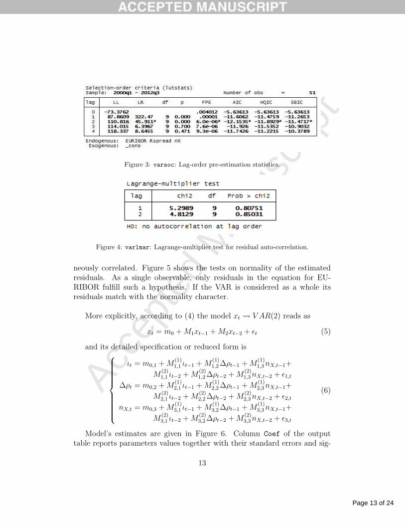
Figure 3 is obtained with the procedure varsoc of STATA1, and it showsthat all the selection-order criteria2 identify p = 2, see the symbol ′∗′, as the

1All the data processing have been developed with STATA-Release 10, [19].2These are IC (information criteria) in the Lutkepol [15] interpretation, see also [18]

on the varsoc command.

11

Page 12 of 24

Accep

ted

Man

uscr

ipt

−1,

00−

0,50

0,00

0,50

1,00

EU

RIB

OR

0 5 10 15 20 25Lag

Bartlett’s formula for MA(q) 95% confidence bands

−1,

00−

0,50

0,00

0,50

1,00

Rsp

read

0 5 10 15 20 25Lag


−1,

00−

0,50

0,00

0,50

1,00

nX

0 5 10 15 20 25Lag


Auto−correlations

Figure 2: ac: Time-Series Auto-correlation Plot for EURIBOR rate ιt, interest ratesspread ∆ρt and share nX,t of FRM contracts.

most suitable auto-regression order: that is, a VAR(2) is the most informativeas well as parsimonious one. As a consequence, the model to be estimatedis xt V AR(2). The Likelihood-ratio test LR selects VAR(p) comparedwith a VAR(p-1) under the null hypothesis that all the coefficients of thep-order are zero [18] while the selection order criteria (Akaike:AIC, Hannan-Quinn:HQIC and Schwatz-Bayesian:SBIC) minimise the prediction error: theselection based on the optimal value of SBIC-HQIC gives a consistent estimateof the p-th auto-regression order, [15, 18].

4.2. Estimation, stability and causality

Once the auto-regression order has been specified, the model xt V AR(2)has been estimated by means of the var procedure with the option lags(1/2)and the Lagrange-multiplier test (LM) has been done on the null hypothesisof non-auto-correlated residuals (varlmar). Figure 4 shows that the null hy-pothesis cannot be rejected, therefore the test gives no hints on the modelmisspecification: as a consequence, the xt V AR(2) model is accepted.Even though residuals have been found not to be serially correlated, as longas the covariance matrix Σ is not diagonal, residuals can be contempora-

12

Page 13 of 24

Accep

ted

Man

uscr

ipt

Figure 3: varsoc: Lag-order pre-estimation statistics.

Figure 4: varlmar: Lagrange-multiplier test for residual auto-correlation.

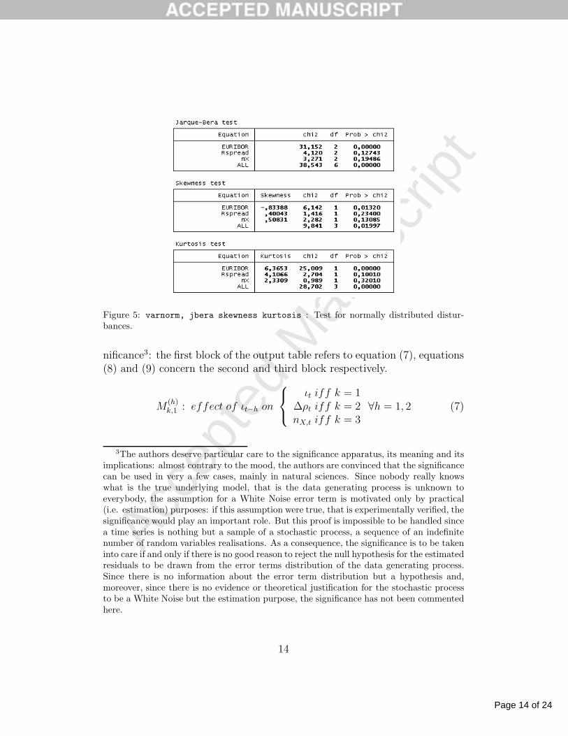
neously correlated. Figure 5 shows the tests on normality of the estimatedresiduals. As a single observable, only residuals in the equation for EU-RIBOR fulfill such a hypothesis. If the VAR is considered as a whole itsresiduals match with the normality character.

More explicitly, according to (4) the model xt V AR(2) reads as

xt = m0 +M1xt−1 +M2xt−2 + ǫt (5)

and its detailed specification or reduced form is

ιt = m0,1 +M(1)1,1 ιt−1 +M

(1)1,2∆ρt−1 +M

(1)1,3nX,t−1+

M(2)1,1 ιt−2 +M

(2)1,2∆ρt−2 +M

(2)1,3nX,t−2 + ǫ1,t

∆ρt = m0,2 +M(1)2,1 ιt−1 +M

(1)2,2∆ρt−1 +M

(1)2,3nX,t−1+

M(2)2,1 ιt−2 +M

(2)2,2∆ρt−2 +M

(2)2,3nX,t−2 + ǫ2,t

nX,t = m0,3 +M(1)3,1 ιt−1 +M

(1)3,2∆ρt−1 +M

(1)3,3nX,t−1+

M(2)3,1 ιt−2 +M

(2)3,2∆ρt−2 +M

(2)3,3nX,t−2 + ǫ3,t

(6)

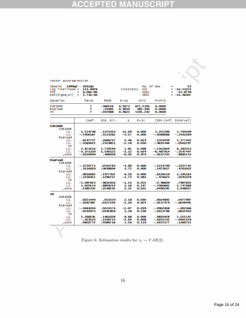
Model’s estimates are given in Figure 6. Column Coef of the outputtable reports parameters values together with their standard errors and sig-

13

Page 14 of 24

Accep

ted

Man

uscr

ipt

Figure 5: varnorm, jbera skewness kurtosis : Test for normally distributed distur-bances.

nificance3: the first block of the output table refers to equation (7), equations(8) and (9) concern the second and third block respectively.

M(h)k,1 : effect of ιt−h on

ιt iff k = 1∆ρt iff k = 2nX,t iff k = 3

∀h = 1, 2 (7)

3The authors deserve particular care to the significance apparatus, its meaning and itsimplications: almost contrary to the mood, the authors are convinced that the significancecan be used in very a few cases, mainly in natural sciences. Since nobody really knowswhat is the true underlying model, that is the data generating process is unknown toeverybody, the assumption for a White Noise error term is motivated only by practical(i.e. estimation) purposes: if this assumption were true, that is experimentally verified, thesignificance would play an important role. But this proof is impossible to be handled sincea time series is nothing but a sample of a stochastic process, a sequence of an indefinitenumber of random variables realisations. As a consequence, the significance is to be takeninto care if and only if there is no good reason to reject the null hypothesis for the estimatedresiduals to be drawn from the error terms distribution of the data generating process.Since there is no information about the error term distribution but a hypothesis and,moreover, since there is no evidence or theoretical justification for the stochastic processto be a White Noise but the estimation purpose, the significance has not been commentedhere.

14

Page 15 of 24

Accep

ted

Man

uscr

iptM

(h)k,2 : effect of ∆ρt−h on


∀h = 1, 2 (8)

M(h)k,3 : effect of nX,t−h on


∀h = 1, 2 (9)

At a first sight it can be seen that the specified model shows a high fittingperformance: all the R2s are above the 90% of the explained variance, whichis almost common in VAR estimation.

Before proceeding further, stationarity of xt is to be discussed togetherwith the stability of its VAR(2) representation. The expression (4) withp = 2 gives (5). By using the lag operator Lxt = xt−1 it then follows that

xt V AR(2) ⇒

G2(L)xt = m0 + ǫt → WN(m0,Σ)G2(L) = I −M1L−M2L

2 (10)

being I the identity matrix. The multi-variate stochastic process xt is saidto be mean-covariance stationary if the absolute value roots of its polynomialdetG2(L) = 0 are outside the unit circle. Its VAR(2) representation is saidto be stable if the matrix M in the companion matrix representation

(I −ML)yt = νt :

yt−h = (xt−h, xt−h−1)′

νt = (m0 + ǫt, 0)′

M =

[

M1 M2

I 0

] (11)

is found to be non-singular and that its eigenvalues in absolute value arenot outside the unit circle

det(I −Mλ) 6= 0 : |λ| ≤ 1 (12)

A fundamental result, shown in [11, 15] as regarding multivariate timeseries analysis, is that the stability of the VAR(p) representation is sufficientfor the mean-variance stationarity of the multi-variate stochastic process xt.Therefore, the easiest4 way to test for stationarity of xt is to test for stability

4Mean-variance stationarity could also be tested by solving the polynomial detG2(L) =

15

Page 16 of 24

Accep

ted

Man

uscr

ipt

Figure 6: Estimation results for xt V AR(2).

16

Page 17 of 24

Accep

ted

Man

uscr

ipt

−1

−,5

0,5

1Im

agin

ary

−1 −,5 0 ,5 1Real

Roots of the companion matrix

Figure 7: varstable, graph: Check stability condition of VAR estimates.

of VAR(2) by using the varstable procedure. Figure 7 clearly shows thatthe estimated model is stable, therefore xt is found to be stationary; as aconsequence, the residuals ǫt are reasonably found to follow a WN processwith null expected value and non-singular constant positive-definite covari-ance matrix.

According to (6-9) some comments can be made about estimates in Fig-ure 6, keeping in minds that the goal of VAR analysis is to determine the

interrelationships among the variables, ’not’ the parameter estimates [8]. Itthen turns out that the effects of the Italian demand nX,t−h on the EURI-BOR ιt is greater than the effects of the EURIBOR ιt−h on nX,t, while thecontrary would be more reasonable. To be true, there is no good reason forboth. Indeed, the EURIBOR contains several European interest rates, whichare influenced by either the national mortgage demands and other exogenousfacts, such as the real interest rate in the national economies. Perhaps as re-garding a different European country, these estimates would be different withrespect to the Italian ones, either in magnitude and sign. Indeed, the firstequation in (6) concerns the impact of past Italian interest rates spread anddemand on the EURIBOR, plus an auto-regressive EURIBOR component.

There is a second matter of fact: EURIBOR and demand are positivelyrelated on one period lag but negatively on a two period lag. The effect of the

0 in the variable L. If all its roots were found to be outside the unit circle, then stationaritywould be met. Unfortunately, this methodology does not allow for a closed form solutionif the polynomial degree is greater than five. Individual stationarity and unit root testshave been run for the observables in the vector xt = (ιt,∆ρt, nX,t)

′: with the exception ofthe spread between the interest rates, which could be I(1), the variables are not integratedof the first order. Moreover, it has also been tested that there is no co-integration.

17

Page 18 of 24

Accep

ted

Man

uscr

ipt

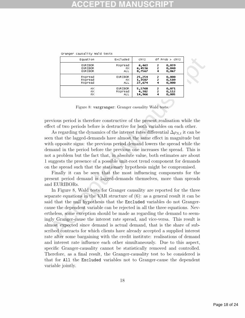
Figure 8: vargranger: Granger casuality Wald tests.

previous period is therefore constructive of the present realisation while theeffect of two periods before is destructive for both variables on each other.

As regarding the dynamics of the interest rates differential ∆ρX,t it can beseen that the lagged-demands have almost the same effect in magnitude butwith opposite signs: the previous period demand lowers the spread while thedemand in the period before the previous one increases the spread. This isnot a problem but the fact that, in absolute value, both estimates are about1 suggests the presence of a possible unit-root trend component for demandson the spread such that the stationary hypothesis might be compromised.

Finally it can be seen that the most influencing components for thepresent period demand is lagged-demands themselves, more than spreadsand EURIBORs.

In Figure 8, Wald tests for Granger causality are reported for the threeseparate equations in the VAR structure of (6): as a general result it can besaid that the null hypothesis that the Excluded variables do not Granger-cause the dependent variable can be rejected in all the three equations. Nev-ertheless, some exception should be made as regarding the demand to seem-ingly Granger-cause the interest rate spread, and vice-versa. This result isalmost expected since demand is actual demand, that is the share of sub-scribed contracts for which clients have already accepted a supplied interestrate after some bargaining with the credit institute: realisations of demandand interest rate influence each other simultaneously. Due to this aspect,specific Granger-causality cannot be statistically removed and controlled.Therefore, as a final result, the Granger-causality test to be considered isthat for All the Excluded variables not to Granger-cause the dependentvariable jointly.

18

Page 19 of 24

Accep

ted

Man

uscr

ipt

4.3. Impulse-response analysis

If xt V AR(p) is found to be stationary-stable, the Wold theorem (see[11, 15]) applies to get the following vector-moving-average (VMA) represen-tation

xt − x = H(L)ǫt : ǫt → WN(0,Σ) (13)

where H(L) is a matrix polynomial in L with an indefinite number ofterms and x = E[xt]. In real time series analysis, this means that samplext of n realisations has a representation based on past innovations since thebeginning ǫt−n up to the present ǫt.

Due to this representation of xt the so called innovation accounting canbe developed to answer the following questions: (i) what happens if oneexogenous shock or innovation hits a given component of xt, let’s say theEURIBOR ιt? (ii) how does the system dynamics change after such a shockrealises? (iii) how many periods it takes for the shock diffusion effect to van-ish? if no other shock contaminated the innovation ǫj,t−r, what would be theresponse xt+s? This topic is developed in [12] and it seems either computa-tionally easy and theoretically promising in its interpretation, unfortunatelythe innovation accounting method does not provide a unique result whenestimating the reactions to innovations.

Luckily enough, there is another way to understand how the system re-acts to some exogenous shock, it consists in deriving the Impulse-Response-Function (IRF) from the VMA(∞) representation in (13). Given a VAR(p)the VMA(∞) is

xt = x+∞∑

s=0

Hsǫt−s : Hs = H(Ls) , H0 = I (14)

from which∂xt+s

∂ǫ′t=

∂xt

∂ǫ′t−s

= Hs (15)

is a matrix of coefficients5: the (i, j) entry Hs(i, j) measures either theresponse of the i-th component xi,t to j-th impulse component ǫj,t−s received

5As suggested by [11], this matrix can be obtained by simulations; in the following itis described the methodology to estimate the IRF, for futher details see mainly [11] and[12, 15].

19

Page 20 of 24

Accep

ted

Man

uscr

ipt

s periods before and the response of the i-th component xi,t+s s periods aheadgiven the present period j-th impulse component ǫj,t.

All in all, the sequence IRFi =

∂xi,t+s

∂ǫj,t= Hs(i, j) : ∀j

s≤Sestimates the

response of the i-th component s periods ahead, xi,t+s, to all the present im-pulses received through the unanticipated innovations. The sequence IRFi,j =

∂xi,t+s

∂ǫj,t= Hs(i, j) : s ≤ S

is the i-th response to the j-th impulse through

S periods.

The implicit assumption in these representations of the IRF is that the i-th response is measured to the j-th impulse ǫj,t in xj,t when all the other xa,τ ,with a 6= j and τ ≤ t, are constant. Moreover, it might be considered thatif the covariance matrix E[ǫtǫ

′t] = Σ is not diagonal, although constant and

positive-definite, the innovations are contemporaneously correlated: as a con-sequence, the IRF in (15) does not separate the effect of contemporaneouslycorrelated innovations. To overcome this problem it might be considered anorthogonalisation procedure for the IRF6.Briefly, the covariance matrix Σ is symmetric and positive definite, thereforeΣ = UDU ′ is always a feasible description where D is diagonal and U islower-triangular with 1s on the main-diagonal. Therefore new uncorrelatedand orthogonal innovations can be constructed by et = U−1ǫt which can besubstituted into (13) to get

xt − x = H(L)Uet : et → WN(0, D) (16)

A sample estimate of the orthogonalised IRF (OIRF) from the VMA(∞)is found to be given by the product of the s-th matrix of the VMA and thej-th column vector of U

∂Ej,t[xt+s]

∂xj,t

= HsUj (17)

where s ≤ S is the time horizon of the sample estimate∂Ej,t[xt+s]

∂xj,t=

∂E[xt+s|xj,t,xj−1,t,...,x1,t,Xs−1]

∂xj,tand Xs−1 = (x′

s−1, . . . , x′s−p) according to [11].

6STATA irf procedure allows for five kinds of IRF: simple, orthogonalised, cumulative,cumulative orthogonalised and structural. See [18] for technical details.

20

Page 21 of 24

Accep

ted

Man

uscr

ipt

−1

0

1

2

0 1 2 3 4 5 6 7 8 9 10 11 12 13 14 15 16 17 18 19 20 21 22 23 24 25 26 27 28 29 30

IRFs, EURIBOR, EURIBOR

95% CI for irf 95% CI for oirf impulse response function (irf) orthogonalized irf

−,1

0

,1

,2

0 1 2 3 4 5 6 7 8 9 10 11 12 13 14 15 16 17 18 19 20 21 22 23 24 25 26 27 28 29 30

IRFs, EURIBOR, nX


−1

−,5

0

,5

0 1 2 3 4 5 6 7 8 9 10 11 12 13 14 15 16 17 18 19 20 21 22 23 24 25 26 27 28 29 30

IRFs, EURIBOR, Rspread


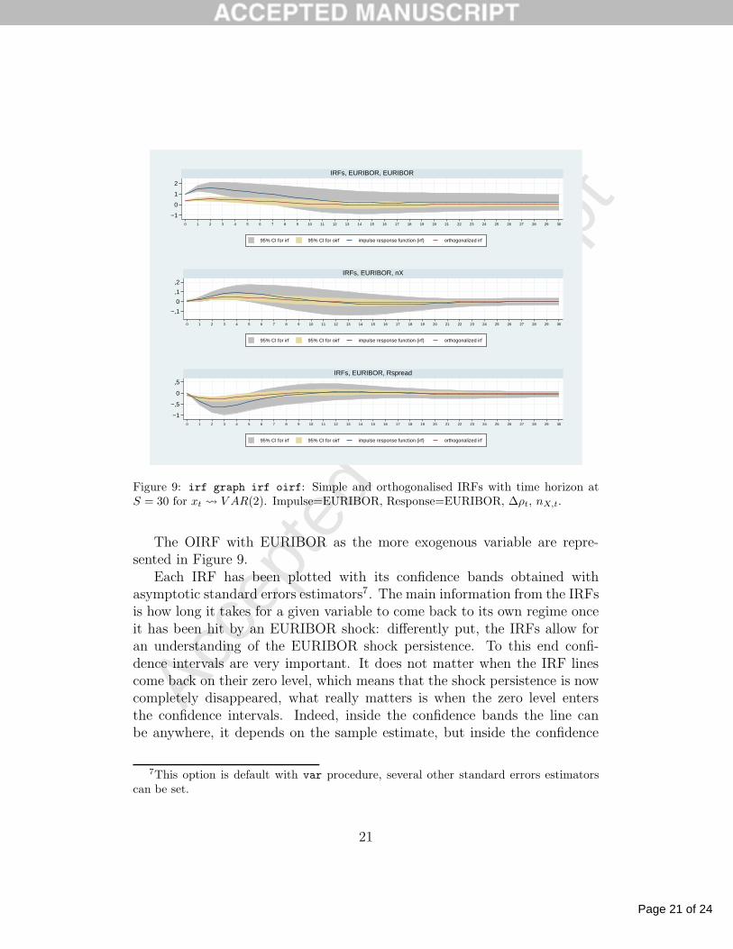
Figure 9: irf graph irf oirf: Simple and orthogonalised IRFs with time horizon atS = 30 for xt V AR(2). Impulse=EURIBOR, Response=EURIBOR, ∆ρt, nX,t.

The OIRF with EURIBOR as the more exogenous variable are repre-sented in Figure 9.

Each IRF has been plotted with its confidence bands obtained withasymptotic standard errors estimators7. The main information from the IRFsis how long it takes for a given variable to come back to its own regime onceit has been hit by an EURIBOR shock: differently put, the IRFs allow foran understanding of the EURIBOR shock persistence. To this end confi-dence intervals are very important. It does not matter when the IRF linescome back on their zero level, which means that the shock persistence is nowcompletely disappeared, what really matters is when the zero level entersthe confidence intervals. Indeed, inside the confidence bands the line canbe anywhere, it depends on the sample estimate, but inside the confidence

7This option is default with var procedure, several other standard errors estimatorscan be set.

21

Page 22 of 24

Accep

ted

Man

uscr

ipt

bands there is a 95% confidence that the IRF is not significantly differentfrom zero. Therefore, it might be considered that the EURIBOR shock ex-erts some effect until the confidence interval includes the zero level.

As it can be seen from the first panel of Figure 9, the EURIBOR shocktakes 7 periods before becoming significantly ineffective while, from the sec-ond and third panels, it takes 5 periods for demand and interest rate spreadto come to their original growth path.A shock on the EURIBOR gives an impulse to the demand in the same di-rection while the interest rate spread is hit in the opposite direction: thismakes sense since an increase in the EURIBOR implies an increase in theadjustable interest rate first and this shifts the demand on the fixed interestrate market. After three periods the spread keeps on growing since the fixedinterest rate is reacting with seemingly two periods of delay: this makes thespread decreasing although both interest rates might have been growing. Asa consequence, even though on higher level, the spread decreases because thefixed interest rate has grown enough to converge to the adjustable interestrate. As a consequence, the fixed interest rate becomes no more profitable,even though less risky, if compared to the adjustable one. This makes thedemand to switch again towards the adjustable interest rate market. Thisaction-reaction mechanism wears within 5 periods which means one year anda quarter.

5. Conclusions

Recently, a meaningful dataset had been arranged by the Bank of Italyon volumes and average interest rates for FRM and ARM on the Italianmortgage market from 1997 : q1 to 2011 : q4. Together with a brief discussionof the phases of the observed dynamics, [20] showed how the original model[4] for interdependent markets fitted to data at a good level and, moreover,they pointed out the capability of model to capture the switching mechanismbetween FRM and ARM markets, that remains significative also in presenceof breaks.

The present paper deepens the previous studies of the FRM and ARMdynamics involving also an econometric analysis of real data by means of theVAR estimation technique. This paper shows results in a fairly new researchstream which aims to understand how the effects of the European Central

22

Page 23 of 24

Accep

ted

Man

uscr

ipt

Bank control on the Euribor transmit to different technical form interestrates contracts in the Italian mortgage market, as well as to the behavior ofinterest rates term structure.

Acknowledgements

Authors are grateful to two anonymous referees for comments which haveimproved the paper and led to this final version. This research was partiallysupported by MIUR (Ministero dell’Istruzione, dell’Universita e della Ricercascientifica), Italy. The views and opinions expressed by the authors are theirown and do not involve the responsibility of the institutions to which theybelong.

References

[1] M. Bachofner, T. Lutzkendorf, Research trends in the mortgage market,Building Research and Information 4 (2005) 376–381.

[2] G. Box, G. Jenkins, Time Series Analysis. Forecasting and Control,Holden-Day, 1970.

[3] A. Calza, T. Monacelli, L. Stracca, Housing finance and monetary pol-icy, Working Paper Series 1069, European Central Bank, EurosystemFrankfurt, 2009.

[4] S. Casellina, S. Landini, M. Uberti, Credit market dynamics: a cobwebmodel, Computational Economics (2011) 221–239.

[5] A. Coles, J. Hardt, Mortgage markets: Why us and eu markets are sodifferent, Housing Studies 15 (2000).

[6] B. Coulibaly, G. Li, Choice of mortgage contracts:evidence from thesurvey of consumer finances, Real Estate Economics 37 (2009) 659–673.

[7] P. Del Giovane, G. Eramo, A. Nobili, Disentangling demand and supplyin credit developments: A survey-based analysis for italy, Journal ofBanking and Finance 35 (2011) 2719–2712.

[8] W. Enders, Applied Econometric Times Series, Wiley, 2009.

23

Page 24 of 24

Accep

ted

Man

uscr

ipt

[9] H. European Mortgage Federation, Review of Europe’s mortgage andhousing markets, Technical Report, 2012.

[10] R. Felici, E. Manzoli, R. Pico, La crisi e le famiglie italiane: un’analisimicroeconomica dei contratti di mutuo, Questioni di Economia e Fi-nanza (Occasional Paper) 125, Banca d’Italia, 2012.

[11] J. Hamilton, Time Series Analysis, Princeton University Press, Prince-ton, 1994.

[12] G. Judge, R. Hill, W. Griffiths, H. Lutkepol, T.C. Lee, Introduction tothe Theory and Practice of Econometrics, Wiley, New York, 1998.

[13] R. Koijen, O. Van Hemert, S. Van Nieuwerburgh, Mortgage timing,Journal of Financial Economics 93 (2009) 292–324.

[14] D. Leece, Economics of the mortgage market:perspectives on householddecision making, Wiley-Blackwell, Oxford, 2004.

[15] H. Lutkepol, New Introduction to Multiple Time Series Analysis,Springer, New York, 2005.

[16] D. MacDonald, K. Winson-Geideman, Residential mortgage selection,inflation uncertainty, and real payment tilt, Journal of Real Estate Re-search 34 (2012) 51–71.

[17] M. Mori, J. Diaz III, A.J. Ziobrowski, N.B. Rottke, Psychological andcultural factors in the choice of mortgage products: A behavioral inves-tigation, The Journal of Behavioral Finance 11 (2010) 82–91.

[18] StataCorp, Stata 10, Time Series, College Station, TX: StataCorp LP,2007.

[19] StataCorp, Stata Statistical Software: Release 10, College Station, TX:StataCorp LP, 2007.

[20] M. Uberti, S. Landini, S. Casellina, Adjustable and fixed interest ratesmortgage markets modelling. evidences from italy over the last fourteenyears, Central European Journal of Operations Research 22 (2013). 2014in press; doi:10.1007/s10100-013-0297-4.

24

Documents

Italian mortgage markets and their dynamics