ARTICLE IN PRESS

0165-1684/$ - se

doi:10.1016/j.si

$This resear

Academic Res

(DAAD, Accio

and the resear

TEC2005-24046

a MEC-FPU a�CorrespondE-mail addr

Signal Processing 87 (2007) 2503–2515

www.elsevier.com/locate/sigpro

Iterated tensor voting and curvature improvement$

Sylvain Fischera,�, Pierre Bayerlb, Heiko Neumannb,Rafael Redondoa, Gabriel Cristobala

aInstituto de Optica (CSIC), Serrano 121, 28006 Madrid, SpainbDepartment of Neural Information Processing, University of Ulm, D-89069 Ulm, Germany

Received 20 June 2006; received in revised form 25 January 2007; accepted 30 March 2007

Available online 14 April 2007

Abstract

Tensor voting (TV) methods have been developed in a series of papers by Medioni and coworkers during the last years.

The method has been proved efficient for feature extraction and grouping and has been applied successfully in a diversity

of applications such as contour and surface inferences, motion analysis, etc. We present here two studies on improvements

of the method. The first one consists in iterating the TV process, and the second one integrates curvature information. In

contrast to other grouping methods, TV claims the advantage to be non-iterative. Although non-iterative TV methods

provide good results in many cases, the algorithm can be iterated to deal with more complex or more ambiguous data

configurations. We present experiments that demonstrate that iterations substantially improve the process of feature

extraction and help to overcome limitations of the original algorithm. As a further contribution, we propose a curvature

improvement for TV. Unlike the curvature-augmented TV proposed by Tang and Medioni, our method evaluates the full

curvature, sign and amplitude in the 2D case. Another advantage of the method is that it uses part of the curvature

calculation already performed by the classical TV, limiting the computational costs. Curvature-modified voting fields are

also proposed. Results show smoother curves, a lower degree of artifacts and a high tolerance against scale variations of

the input. The methods are finally tested under noisy conditions showing that the proposed improvements preserve the

noise robustness of the TV method.

r 2007 Elsevier B.V. All rights reserved.

Keywords: Tensor voting; Contour extraction; Contour completion; Curvature compatibility

e front matter r 2007 Elsevier B.V. All rights reserved

gpro.2007.03.019

ch is supported in part by the German–Spanish

earch Collaboration Program HA 2001-0087

nes integradas Hispano-Alemanas 2002/2003)

ch Grants TEC2004-00834; TEC2005-24739-E;

-E and PI040765. S.F. and R.R. are supported by

nd a CSIC-I3P fellowship, respectively.

ing author.

ess: sylvain@optica.csic.es (S. Fischer).

1. Introduction

Perceptual contour extraction methods aim atdrawing or completing contours similarly as ahuman would do. For such purpose a variety ofalgorithms that simulate visual cortex neural net-works have been proposed [1–9]. They are generallybased on psychophysical experiments [10–12] or onphysiological studies of the visual cortex [13–15].Other methods such as the tensor voting (TV)[16–18] implement the Gestalt psychology laws [19].

.

ARTICLE IN PRESSS. Fischer et al. / Signal Processing 87 (2007) 2503–25152504

Alternatively there exist also algorithms based oncurves of least energy [20] or stochastic motion [21].

TV algorithms have been developed by Medioniand coworkers as an efficient method for contourextraction and grouping. Full descriptions of thealgorithms can be found e.g. in [16–18], and acomparison of TV with other algorithms can befound in [21]. TV is a non-iterative procedure, in thesense that the original scheme implements only twosteps of voting, claiming that no further iterativecycles are needed. One important earlier modelcalled relaxation labeling (RL) was proposed byZucker and colleagues [1,2,23] as an iterativeprocess. It incorporates probabilistic interactionsbetween labels which represents the orientationsand curvatures of the curves and the presence/abscence of a curve in each point. Many othermethods for perceptual grouping, e.g. [3–7], alsorefine the curve orientation through iterative loops.Thus, the first aim of this study is to investigate howthe incorporation of iterations in the votingmechanism can improve the results of TV. Somebasic examples are analyzed and a statistical studyon the influence of iterations is set up in a simplecase.

A curvature improvement (CI) has already beenproposed by Tang and Medioni [22] for 3D images. Itcomputes the sign of curvature to modify the votingfields. For the 2D case, we propose a moresophisticated calculation of the curvature informationfor a low computational cost. Instead of the sign ofcurvature, the proposed method evaluates the fullcurvature information using part of the calculationspreviously performed by the classical TV method. Weadopt the curvature compatibility approach that wasdescribed by Parent and Zucker [23], and which has arelevance as a vision model [2,13]. A statisticalevaluation is presented and the methods are finallytested with complex data and in the presence of noise.The present work builds upon and further extends thepreliminary investigations presented in [24]. Newresults have been included here for a more completeevaluation. They include additional comparisonsbetween the different methods, in particular anevaluation of the noise robustness has been set up.Note also that, recently Tong and Tang [25] proposedtensors of curvature, showing the increasing interest ofcurvature evaluation for TV. Also, Loss et al. [26]recently showed the interest of iterations for TV in thecontext of noise elimination.

The present implementations are efficient princi-pally for curves and crossing. They are less adequate

for certain particular junctions or endpointslike corners which would require extensions ofthe TV framework [17] or specific junction de-tectors [27]. Unlike Medioni and coworkers whousually apply TV to volumetric data (3D images)or even N-dimensional features [28,29], we pre-ferred to restrict the present work to 2D imagesfor the following reasons: (1) 2D examples are easierto visualize, which facilitates the study and evalua-tion of the different approaches. (2) Contourextraction in 2D images still remains a verycommon and nevertheless unsolved problem, whichmakes the presented approach an interesting alter-native to state-of-the-art algorithms. (3) 2D appli-cations have lower computational cost, which isimportant since TV methods are computationallyexpensive.

Section 2 briefly introduces the TV method.Section 3 presents a study on iterated TV andSection 4 describes improvements that can beachieved when both curvature information anditerations are used. Section 5 evaluates the robust-ness of the methods in the presence of noise. Finallysome concluding remarks are drawn in Section 6.

2. A brief introduction to TV

The tensor voting algorithm (referred to as TV inthe following) encodes a local description of thecurves at each point of the image by means of asymmetric positive 2� 2 tensor. Each tensor en-codes an evaluation of the tangential orientation, ofthe uncertainty on that tangential orientation and ofthe possible presence of a junction in a point.Tensors can be diagonalized, their eigenvalues aredenoted by l1, l2 with l1Xl2X0. The correspond-ing eigenvectors are denoted by e1, e2. Tensors aredecomposed as follows:

T ¼ ðl1 � l2Þe1eT1 þ l2I, (1)

where I is the identity matrix. The first term is calledthe stick component, where e1 corresponds to anevaluation of the tangential orientation of the curvesegment. The stick saliency l1 � l2 gives a con-fidence measure for the presence of a curve. Thesecond term is called the ball component, and itssaliency l2 measures the confidence to have ajunction. Note that the ball components can alsodenote an uncertainty on the tangential orientation.For binary images, tensors can be initialized as ball

ARTICLE IN PRESS

Fig. 1. (a) The classical tensor voting method is composed of

four steps. (1) Tensor initialization, (2) sparse voting, (3) dense

voting, and (4) feature extraction. (b) Example of a data set

containing endpoints (corners). (c) Corners are generally not

accurately extracted by the classical TV framework since the

voting fields extend out of the endpoints yielding an inappropri-

ate prolongation of the segments. Extensions of the method for

dealing with endpoints have been proposed in [17].

Fig. 2. The new contributions (in boldface characters) consist in

iterating the sparse voting step, evaluating the local curvature and

incorporating that curvature information into the voting fields.

S. Fischer et al. / Signal Processing 87 (2007) 2503–2515 2505

tensors, i.e. as the identity matrix I at locations thatcontain data points and null tensors at otherlocations.

The classical TV algorithm proceeds by twovoting steps in which each tensor propagates to itsneighborhood. Stick tensors propagate mostly inthe direction of e1. The region of propagation isdefined by the stick voting field which decays as afunction of the distance and curvature (the exactdefinition of the voting shape will be detailed inSection 4). Stick voting fields are built by followingthe Gestalt laws in perception. These establishcriteria for grouping points that lie on a curve.These criteria are ‘‘good continuation’’, proximity,to favor low curvatures over larger ones andconsistency of the curvature [16]. Ball tensors, onthe other hand, isotropically propagate in alldirections with a decay as a function of the distance.After the tensor propagation, all contributions aresummed up to define new tensors that will be usedfor the next step. That summation can be consideredas averaging or voting. The first voting step isreferred to as sparse vote because the vote isperformed only on points where tensors are notnull. The second voting step is called dense vote

because the vote is accomplished at every location.After all voting steps are completed, curves areextracted at local maxima of stick saliency along thenormal direction to stick components. Note that athreshold t is necessary to eliminate low-saliencylocal maxima. Fig. 1a summarizes the different stepsof the algorithm.

This classical TV framework is able to groupsparse points and extract the underlying curves inmost situations. Nevertheless some features, such asendpoints, corner, etc., are not accurately extractedusing this framework (see for instance the exampleproposed in Fig. 1b, c). For extracting accuratelysuch features, the method can been extended asproposed in [17]. The study of this extension staysout of the scope of the present paper. Thus, themethods proposed here aim at dealing accuratelywith curve extraction but do not pretend to offer anoptimal behavior at endpoints.

The TV algorithms will not be described more indetail here. For a more in-depth study the readercan refer to [16–18,22]. The novel contributionsdescribed in the following are represented in Fig. 2in boldface characters. They consist in iterating thesparse voting step (Section 3) and integratingcurvature information for using curved voting fields(Section 4).

3. Iterated TV

3.1. Example

The original TV approach [16] is particularlyefficient for grouping sparse data points that areseparated by gaps of comparable size. A freeparameter ss, called the scale factor, has to becoarsely adjusted to the inter-distance between

ARTICLE IN PRESSS. Fischer et al. / Signal Processing 87 (2007) 2503–25152506

points. If ss is miss-adjusted, extraction results loseaccuracy: if ss is too small points will not begrouped; if ss is too large the grouping is lessselective. Fig. 3a shows an example where points are

Fig. 3. Example tested for different values of the scale factor sswith the non-iterative method (TV) and with 12 iterations (IT

method). (a) Data points are located along a spiral. (b, e, h)

Contours of the voting field for ss ¼ 5; 8 and 11 are drawn at

50% (solid line) and 5% (dash-dot line) of the maximum value

(voting fields are defined by the Eq. (3). (c, f, i) Extraction results

with TV; (d, g, j) with IT.

situated along a spiral. Because the distancebetween two following points is smaller than thedistance between two successive arcs and assumingthe curvature is low, the Gestalt rules predict thatthe points have to be circularly grouped along thespiral, but not radially. Because the gaps betweenpoints vary along the spiral, it is not possible toadjust ss for proper extraction of the whole spiral.As it is shown in Fig. 3c, ss needs to be small, i.e.around 5, for grouping the central part of the spiral.But only a large ss, around 11, is able to group theexternal part of the spiral (Fig. 3i). Between thesevalues (e.g. ss around 8, Fig. 3f) neither the centralpart nor the external one are grouped properly.

3.2. Iterative tensor voting (IT) method

One objective of the sparse voting step is toevaluate the orientation (tangent) of the curve ineach data point, while the dense voting step linksthese points (fills the gaps) by propagating thetensors according to the voting fields. In principleboth sparse and dense voting steps could be iterated,nevertheless it has been chosen not to iterate thedense voting step for the following reasons: (1) thedense voting step has a much higher computationalcomplexity, and its iteration could be extremelycostly. (2) The dense voting step frequently pro-duces some irrelevant votes which themselves wouldpropagate through iterations, yielding divergent andunrealistic results. (3) In contrast the sparse votingstep only modifies the eigenvalues and eigenvectorsof the existing data points. It refines them throughmutual voting, but it does not add any tensor in theother points. No outlier points appear which isimportant for the stability of the iterative process.

A divergence of the eigenvalue amplitudes couldnevertheless occur by iterating the sparse vote. Thiscan be counteracted by a normalization stagekeeping constant the sum of eigenvalues of eachtensor. This normalization is applied after eachiteration of the sparse voting step (no normalizationis done after the dense voting step). Therefore, as itis shown in Fig. 2, the sparse voting stage is the onlystep to be iterated. For n iterations, n� 1 sparsevotes and one dense vote are realized.

The present algorithm is then inspired in partfrom the RL methodology [1,2,23] in particular forusing iterations to refine the descriptors of orienta-tion. Nevertheless it still follows the TV frameworkso as to take advantage of its useful improvements.In particular the tensor representation provides

ARTICLE IN PRESSS. Fischer et al. / Signal Processing 87 (2007) 2503–2515 2507

elegant and continuous descriptors for contourorientation (while RL generally requires the dis-cretization of the orientation and curvature descrip-tors). A second advantage is the use of the sparsevoting step for iterations: only the original datapoints are iterated which strongly limits thepropagation of errors through iterations.

Fig. 3d, g, j shows the results for 12 iterationswith ss ¼ 5, 8, and 11, respectively. Iterations donot fill the gaps between points where ss is toosmall, that is, as previously commented, iterationsdo not increment the range of propagation (Fig. 3d,g). On the contrary, iterations refine tensor orienta-tion so that the central part of the spiral isaccurately extracted even for large values of ss(compare the central parts of the Fig. 3g, j to theones in Fig. 3f, i). Iterations thus allow to extractthe entire spiral for ss ¼ 11 (Fig. 3j) while non-iterative TV fails.

The accuracy of voted tensors can be checkedcomparing their orientation with the one of the idealspiral defined by its mathematical equations. Wewill consider a tensor as misoriented if the angularerror exceeds p=10. For the TV method with ss ¼5,8 and 11, respectively 5, 5 and 16 tensors aremisoriented (over the 57 tensors situated in the datapoints). In contrast, for the IT method, all tensorsare accurately oriented for all ss ¼ 5, 8 and 11.

3.3. Statistics on the influence of iterations

For evaluating the effect of iterations on TV, asimplified version of Fig. 3a is proposed in Fig. 4a.It is inspired from classical psychophysical experi-ments for studying the competition between direc-tions of grouping [30]. It is composed by an array of

Fig. 4. Systematic evaluation of the influence of iterations using a 3� 3

Dy ¼ 9. (b) Contours extracted with TV: central points are not grou

moreover some artifacts appear (Q1 ¼ 0:40, i.e. the extraction is con

iterations): points are grouped in vertical lines (Q1 ¼ 2:38). This example

t is the same for both insets b and c.) The failure of the TV method can

and Dy. Thus, ss is too large to discriminate adequately between horiz

points (3� 3 points here). Vertical and horizontaldistances between points are denoted by Dx and Dy,respectively. In the following Dx will be chosensmaller than Dy. In such case, following the Gestaltrule of proximity, points have to be groupedvertically (in opposition if Dx4Dy, points wouldhave to be grouped horizontally. It is to note thatthe points could also be grouped in a region;nevertheless this kind of grouping will not beconsidered here.) A quality measure of good tensororientation can be defined as

Q1 ¼ �log101

9

X9i¼1

1�Tið1; 1Þ

Si

� �" #, (2)

where i indexes the 9 points of the array. Ti is thetensor of the point i, Si is the sum of eigenvalues ofTi, and Tið1; 1Þ the vertical component of the tensorTi.

As vertical lines have to be extracted, tensors arecorrectly oriented if they have a form close toTi ¼ Si

1000

� �. In such case

P9i¼1ð1� Tið1; 1Þ=SiÞ is

close to zero, providing a high value for Q1. It canbe considered that tensors are misoriented and thatthe extraction has failed when Q1o1 (in such case itcan be derived from Eq. (2) that the mean error oforientation for stick tensors is larger than p=10).Also when Q142, tensors can be considered as wellorientated and the structure as correctly extracted(the mean error of orientation is then smaller thanp=30).

3.4. Results

Fig. 6 presents the results obtained for differentparameters Dx, Dy, and n (number of iterations).For all cases the scale factor ss is fixed to 10. Again,

array of points. (a) Original array of points separated by Dx ¼ 4,

ped, lateral points are grouped but not in strictly vertical lines,

sidered as failed). (c) The structure is well extracted by IT (10

corresponds to the case 1 described in the following. (ss ¼ 10 and

be explained because of the ss value which is larger than both Dx

ontal and vertical grouping in just one sparse voting iteration.

ARTICLE IN PRESSS. Fischer et al. / Signal Processing 87 (2007) 2503–25152508

it is necessary to remark that in this study we areonly considering cases where DxoDy.

Case 1. If Dy ’ ss (that is if 8oDyo12) TV failsto extract the curves. In contrast, iterations pro-gressively improve the extraction quality to obtainthe correct structure. This can be observed in Fig. 6ain the center part, Fig. 6b in the left part and alsoFig. 4a–c.

Case 2. Similarly if Dx ’ Dy TV fails. Thereis conflict between horizontal and vertical group-ing, yielding to extracted curves of differentorientations. The use of iterations permits togroup them adequately (see Figs. 5 and 6c leftpart). Note that, for the most difficult cases,a high number of iterations can be necessary (50iterations for the configuration with Dx ¼ 13,Dy ¼ 14).

Case 3. If DxoDy5ss it is impossible to extractthe structure even if more iterations are deployed(see Fig. 6a left part), the scale factor is indeed toolarge to be selective enough between horizontal andvertical grouping.

Case 4. TV is accurate in the cases where ss5Dy:Dy is sufficiently large in comparison to ss (suchthat the algorithm is able to segregate betweenvertical and horizontal grouping) and where there isno intrinsic conflict between vertical and horizontalgrouping (that is where Dy and Dx are sufficientlydifferent, i.e. Dx5Dy). Even in those cases themeasurement Q1 shows an improvement on theextraction for any increase of the number ofiterations which shows the tensor orientation isrefined through iterations.

In conclusion, only if the features to be extractedare sufficiently simple, such that no conflict betweendifferent orientations of grouping appear, the non-iterative algorithm would suffice for correctly

Fig. 5. (a) Array with Dx ¼ 13, Dy ¼ 15. (b) Results for TV. (c) Resu

details are given in the text.

extracting image features (see also [31] for ananalysis in the RL case). For more complicatedcases, when some conflict between grouping orien-tations is present or when the scale factor ss is notprecisely adjusted, more than two iterations arerequired. Moreover, it has been shown that itera-tions do not impair the quality of the results. Ratheriterations refine the orientation of tensors and theextracted final structures.

3.5. Further remarks on the use of iterations

The number of iterations can be considered as anadditional parameter of the algorithm. A procedurecould also be implemented for stopping the itera-tions when the results do not differ much from oneiteration to the next, see [1]. For all examplespresented here a fixed number of iterations havebeen used. Generally, if data do not contain specialdifficulties (e.g. competition between directions ofgrouping or scale parameter dis-adjustment), asmall number of iterations, i.e. between 6 and 10iterations, have been shown to be sufficient. It isremarked also that the problem of scale para-meter adjustment could alternatively be solvedby multiscale analysis as recently described by Tonget al. [17].

The number of extra operations induced by theiteration of the sparse voting step depends of thedensity of data points. In general the density of datapoints is relatively small, consequently the sparsevoting step is considerably less costly than the densevoting step. Thus the computational cost ofdeploying additional iterations is small in compar-ison to the total cost. Moreover the order ofcomplexity does not increase with the iterative TV.

lts for IT (10 iterations). Those results correspond to the case 2,

ARTICLE IN PRESS

Fig. 6. Extraction quality of the Fig. 4 for different parameters Dx

and Dy. The number of iterations n is indicated by different gray

shades in the bars (two iterations bar corresponds to TV which uses

two voting steps). ss ¼ 10 and the threshold t are held constant for

the entire experiment. Q1o1 indicates the extraction has failed and

Q142 that it is accurate. (a) Dx fixed to 4 and 5pDyp13.

(b) Dx ¼ 8 and 9pDyp15. (c) Dx ¼ 13 and 14pDyp19.

S. Fischer et al. / Signal Processing 87 (2007) 2503–2515 2509

4. Curvature improvement

4.1. Method

In addition to the iterative improvement we alsopropose a novel mechanism for extracting andincorporating curvature information. This lastimprovement introduces a curvature calculationand modified stick voting fields. As proposed byParent and Zucker [23], we propose voting fieldsthat incorporate the curvature information to favorcurves having consistent curvature.

The curvature is evaluated in each voting point byaveraging over all receiver points the curvaturecalculation r already computed by the classical TV.In the classical TV, a voter A votes by adding in anypoint B a tensor of an amplitude described by thefollowing stick voting field:

V ðA;BÞ ¼ exp �sðA;BÞ2

s2s�

yðA;BÞ2

s2y

� �, (3)

where sðA;BÞ is the length of the circular arc AB

which is tangent to e1ðAÞ in A (see Fig. 7a). y is the

angle between the vectors e1ðAÞ and AB�!

. The scalefactors ss and sy are constants. This type of votingfield has been described e.g. in [18]. Fig. 3b, e, hshows the contours of those voting fields fordifferent values of ss.

Eq. (4) expresses the geometric relation betweenthe curvature rðA;BÞ, the length sðA;BÞ of the arcAB and the angle y (see Fig. 7a):

sðA;BÞ ¼2yðA;BÞrðA;BÞ

. (4)

Thanks to Eq. (4), Eq. (3) can be expressed as afunction of rðA;BÞ:

V ðA;BÞ ¼ exp �sðA;BÞ21

s2sþ

rðA;BÞ2

4s2y

� �� �. (5)

Another field described by Eq. (6) and Fig. 7c isalso frequently used by Medioni and coworkers [16]:

V ðA;BÞ ¼ exp �sðA;BÞ2 þ crðA;BÞ2

s2s

� �. (6)

Nevertheless it is not employed in this study. Oneadvantage of the former field of Eq. (3) is that theangular range sy does not require to be adjustedwhen ss is changed, whereas the value of c in Eq. (6)varies depending on ss value.

To permit inflexion points and changes ofcurvature, the curvature of any voter A is calculated

ARTICLE IN PRESS

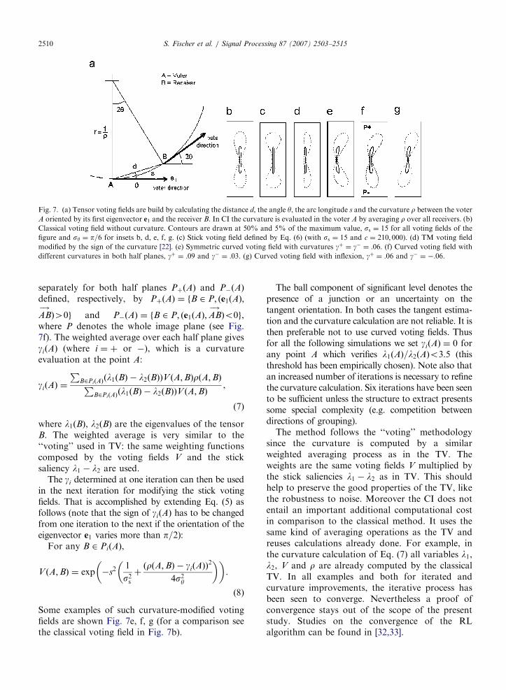
Fig. 7. (a) Tensor voting fields are build by calculating the distance d, the angle y, the arc longitude s and the curvature r between the voter

A oriented by its first eigenvector e1 and the receiver B. In CI the curvature is evaluated in the voter A by averaging r over all receivers. (b)

Classical voting field without curvature. Contours are drawn at 50% and 5% of the maximum value, ss ¼ 15 for all voting fields of the

figure and sy ¼ p=6 for insets b, d, e, f, g. (c) Stick voting field defined by Eq. (6) (with ss ¼ 15 and c ¼ 210; 000). (d) TM voting field

modified by the sign of the curvature [22]. (e) Symmetric curved voting field with curvatures gþ ¼ g� ¼ :06. (f) Curved voting field with

different curvatures in both half planes, gþ ¼ :09 and g� ¼ :03. (g) Curved voting field with inflexion, gþ ¼ :06 and g� ¼ �:06.

S. Fischer et al. / Signal Processing 87 (2007) 2503–25152510

separately for both half planes PþðAÞ and P�ðAÞ

defined, respectively, by PþðAÞ ¼ fB 2 P; ðe1ðAÞ;

AB�!

Þ40g and P�ðAÞ ¼ fB 2 P; ðe1ðAÞ;AB�!

Þo0g,where P denotes the whole image plane (see Fig.7f). The weighted average over each half plane givesgiðAÞ (where i ¼ þ or �), which is a curvatureevaluation at the point A:

giðAÞ ¼

PB2PiðAÞ

ðl1ðBÞ � l2ðBÞÞV ðA;BÞrðA;BÞPB2PiðAÞ

ðl1ðBÞ � l2ðBÞÞV ðA;BÞ,

(7)

where l1ðBÞ, l2ðBÞ are the eigenvalues of the tensorB. The weighted average is very similar to the‘‘voting’’ used in TV: the same weighting functionscomposed by the voting fields V and the sticksaliency l1 � l2 are used.

The gi determined at one iteration can then be usedin the next iteration for modifying the stick votingfields. That is accomplished by extending Eq. (5) asfollows (note that the sign of giðAÞ has to be changedfrom one iteration to the next if the orientation of theeigenvector e1 varies more than p=2):

For any B 2 PiðAÞ,

V ðA;BÞ ¼ exp �s21

s2sþðrðA;BÞ � giðAÞÞ

2

4s2y

� �� �.

(8)

Some examples of such curvature-modified votingfields are shown Fig. 7e, f, g (for a comparison seethe classical voting field in Fig. 7b).

The ball component of significant level denotes thepresence of a junction or an uncertainty on thetangent orientation. In both cases the tangent estima-tion and the curvature calculation are not reliable. It isthen preferable not to use curved voting fields. Thusfor all the following simulations we set giðAÞ ¼ 0 forany point A which verifies l1ðAÞ=l2ðAÞo3:5 (thisthreshold has been empirically chosen). Note also thatan increased number of iterations is necessary to refinethe curvature calculation. Six iterations have been seento be sufficient unless the structure to extract presentssome special complexity (e.g. competition betweendirections of grouping).

The method follows the ‘‘voting’’ methodologysince the curvature is computed by a similarweighted averaging process as in the TV. Theweights are the same voting fields V multiplied bythe stick saliencies l1 � l2 as in TV. This shouldhelp to preserve the good properties of the TV, likethe robustness to noise. Moreover the CI does notentail an important additional computational costin comparison to the classical method. It uses thesame kind of averaging operations as the TV andreuses calculations already done. For example, inthe curvature calculation of Eq. (7) all variables l1,l2, V and r are already computed by the classicalTV. In all examples and both for iterated andcurvature improvements, the iterative process hasbeen seen to converge. Nevertheless a proof ofconvergence stays out of the scope of the presentstudy. Studies on the convergence of the RLalgorithm can be found in [32,33].

ARTICLE IN PRESS

10 20 30 40 50 60

0

0.2

0.4

0.6

0.8

1

scale factor (sigma)

extr

action q

ualit

y (

Q2)

TV

TM

CI

Original image TV

TM CI

Fig. 8. Comparison between methods. (a) The input image is

composed by a sparse set of dots dispersed along a curve defined

by Eq. (9). (b, c, d) Extraction results with, respectively, TV, TM

[22], and CI (6 iterations). In insets b, c and d ss ¼ 20 and t is

adjusted for obtaining the best result following the Q2 calcula-

tion. In all cases the curve is extracted, but TV and TM produces

artifacts. CI produces the best result according to Q2. In

particular it avoids the appearance of outliers and yields smooth

curves. (e) Results for ss varying between 1 and 60. TM improves

on TV, while CI importantly improves on both TV and TM

methods

S. Fischer et al. / Signal Processing 87 (2007) 2503–2515 2511

In the following, the CI will be compared with thenon-iterative TV and with Tang and Medioni’smethod taking into account the sign of curvature(TM) [22]. In this last method that has beendeveloped for 3D images, the sign of curvature isemployed to decide if the entire voting field or onlyhalf of it should be used (see Fig. 7d for an exampleof a half voting field). Note that one more sparsevoting step has to be implemented to make thecurvature calculation possible. (Results of the Tangand Medioni’s method presented here are obtainedby our own implementation adapted for 2Dimages.)

4.2. Statistical study

Fig. 8a shows an image composed by sparsepoints randomly chosen along an eight-shape curvedefined by the following equation:

x ¼ aðtÞ cos2ðtÞ

y ¼ aðtÞ cos2ðtÞ sinðtÞ

(; t 2 �

p2;3p2

� �

with aðtÞ ¼

75 if t 2 �p2;p2

hh;

�41 if t 2p2;3p2

� �:

8>><>>:

(9)

The width in pixels of the right and the left loops ofthe curve are 75 and 41, respectively.

In Fig. 8a the gap between points vary between 2and 26 pixels. This example is used for comparingthe three versions of the algorithm. For differentvalues of the scale factor ss, the extraction qualityQ2 is measured as following:

Q2 ¼TP� FP

NP, (10)

where TP (true positive) is the number of pointscorrectly extracted along the curve tolerating adeviation of one pixel from the ideal curve definedby Eq. (9), FP (false positive) is the number ofpoints erroneously extracted outside the curve (i.e.artifacts, outliers), and NP (number of positive) isthe total number of points along the ideal curve (Eq.(9)). If Q2 ¼ 1 the extraction is exact and if Q2p0the extraction is considered as failed since itcontains more outliers than points on the curve.For each experiment the threshold t is automati-cally adjusted in order to obtain the best resultsfor each measurement (i.e. the highest Q2 value).Fig. 8b–d shows results for the three methodswith ss ¼ 20.

All versions of the algorithm require a ss valuehigher than a minimum threshold for extracting thecurve, i.e. ssX3. A smaller value of ss does notgroup the points together. On the other hand, thenumber of outliers increases for large values of ss.For TV, the number of misplaced points increasessignificantly (Q2o0:7) when ss420. Similar level ofoutliers appear with TM when ss430, whereas forCI the quality does not fall off before ss450. As a

ARTICLE IN PRESS

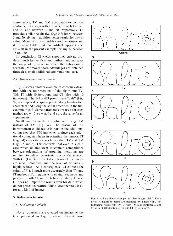
Fig. 9. A hand-drawn example. (a) Test image ‘‘Salt’’. For a

better visualization points are magnified by a factor of 3; (b)

Extraction results with TV; (c) with TM (our implementation);

(d) with IT (10 iterations); (e) with CI (10 iterations).

S. Fischer et al. / Signal Processing 87 (2007) 2503–25152512

consequence, TV and TM adequately extract thecontours, but always with artifacts, for ss between 3and 20 and between 3 and 30, respectively. CIprovides similar results (i.e. Q240.7) for ss between3 and 50, giving in addition better results for any ssvalue. Moreover it also yields smoother slopes andit is remarkable that no artifact appears (i.e.FP ¼ 0) in the present example for any ss between15 and 30.

In conclusion, CI yields smoother curves, pro-duces much less artifacts and outliers, and increasesthe range of ss value in which the extraction isaccurate. Moreover those advantages are obtainedthrough a small additional computational cost.

4.3. Handwritten text example

Fig. 9 shows another example of contour extrac-tion with the four versions of the algorithm: TV,TM, IT with 10 iterations and CI (also with 10iterations). The 147� 439 pixel image ‘‘Salt’’ (Fig.9a) is composed of sparse points along handwrittencharacters and along the spiral described in the firstexample Fig. 3. Same parameters are used for eachmethod (ss ¼ 15, sy ¼ p=6 and t are the same for allexperiments).

Small improvements are observed using TMinstead of TV (Fig. 9c). The reason of thisimprovement could reside in part in the additionalvoting step that TM implements, since each addi-tional voting step helps in orienting the tensors. IT(Fig. 9d) closes the curves better than TV and TM(Fig. 9b and c). This confirms that even in such acase which do not seem to contain competitionsbetween orientations of grouping, iterations arerequired to refine the orientations of the tensors.With CI (Fig. 9e) extracted contours of the curvesare much smoother, and the level of artifacts ishighly reduced. As a consequence, CI extracts thespiral of Fig. 3 much more accurately than TV andIT methods. For regions with straight segments andjunctions, both CI and IT behave similarly. Hence,CI does not impair the results even for data whichdo not present curvature. This allows then to use CIfor any kind of images.

5. Robustness to noise

5.1. Evaluation methods

Noise robustness is evaluated on images of thetype presented in Fig. 8 where different noise

ARTICLE IN PRESS

g=4; M=3.5; M ′=0.52

g=4; M=2; M ′=0.56 g=10; M=0.5; M ′=0.44

Fig. 10. Ratio of noise supported by the different methods of

tensor voting (ss ¼ 20). (a) Image with 2 pixel gaps between data

points ðg ¼ 2Þ and M ¼ 3:5 noise points for each data point. (b)

g ¼ 4 and M ¼ 2. (c) g ¼ 10 and M ¼ 0:5. Images a, b and c

contain the maximum quantity of noise for which algorithms are

able to extract the structure. (d) Results showing the ratio of

noise points (M) supported for each method. (e) Ratio of the

average gaps (M 0) supported by each method.

S. Fischer et al. / Signal Processing 87 (2007) 2503–2515 2513

densities are added. Moreover the average gap g

between data points varies between 2 and 20 pixels(see Fig. 10a–c). ss is fixed to 20 for all experiments.For each value of g, the number of noise points RðgÞ

supported by the methods is evaluated through thequality measurement Q2 of Eq. (10). R is defined asthe number of noise points for which Q2 ¼

12in the

mean. For each value of g, 250 successive experi-ments with a different number of noise points R0 arerealized. Results are plotted as points in the spaceðQ2;R

0Þ, then the line Q2 ¼ aR0 þ b best fitting theexperimental points is extracted by linear regressionand R is finally determined at half the height, that isat Q2 ¼

12. R is then determined as R ¼ ðð1

2� bÞ=aÞ.

Following the usual notation of Medioni andcoworkers papers, the noise robustness will be firstexpressed as the ratio M between the number ofsupported noise points R over the number of datapoints D (that is expressed as a percentage of noisepoints):

M ¼R

D. (11)

5.2. Measurement based on average gaps

The M measurement is not totally satisfactory fortwo reasons. First because it has been shown byKovacs and coworkers [34] that the critical factorfor humans in detecting a contour embedded innoise is the relative gap (or distance) between datapoints compared to the gap between noise points.Secondly because data points are concentratedalong a 1D curve while noise points are dispersedthroughout the whole 2D plane. In some cases thenoise points can be several times more numerousthan the data points, at the same time, while, themean gap between data points stays smaller thanthe one between noise points. The noise robustnessshould then be better expressed in relation to M 0,the ratio of average gap between data points andbetween noise points. The calculation of M 0 is givenas follows:

Let P be the image plane and S the number ofpoints of P. Let us consider for each noise point Bi

the region Pi defined as the set of points that arecloser to Bi than to any other noise point Bj (i.e.the Voronoi cell [35]). The mean area v of the Pi

regions is

v ¼S

R. (12)

ARTICLE IN PRESSS. Fischer et al. / Signal Processing 87 (2007) 2503–25152514

Approximating Pi as a disk of area s, we obtain h,the mean gap between two noise points as thediameter of such disk:

v ¼ ph

2

� �2

. (13)

From Eqs. (12) and (13) we deduce

h ¼ 2

ffiffiffiffiffiffiffiS

pR

r. (14)

Let l be the length of the curve to be extracted (innumber of points). The mean gap g between datapoints is directly defined by

g ¼l

D. (15)

The average gap between data points over theaverage gap between noise points is then

M 0 ¼g

h¼

l

2

ffiffiffiffipS

r ffiffiffiffiRp

D. (16)

If l is unknown M 0 should be expressed proportion-ally to

ffiffiffiffiRp

=D:

M 0 /

ffiffiffiffiRp

D. (17)

Note that M 0 is a function offfiffiffiffiRp

=D whereas M is afunction of R=D. The square root is suited toappropriately take into account the 2D distributionof noise points in relation with the 1D distributionof data points.

5.3. Results on noise robustness

Results presenting M versus g are shown in Fig.10d. Note first that the measurement of M

dramatically depends of the average gap betweenpoints (g): it falls off from 300% for g ¼ 2 to 20%for g ¼ 12. M 0 plotted in Fig. 10e shows moreconsistent results under variation of the averagedata gap g. Moreover, Kovacs et al. [34] have shownthat humans are able to extract the contour formedby unoriented elements only if the gap between dataelements is smaller than the gap between noiseelements (that is M 0p1). The M 0 measurementpermits then a comparison with human perfor-mances. The best rate is 0.55 for the classical TVand 0.65 for the CI to be compared with 1 forhumans.

M 0 2 ½0:28; :65� for all methods and for anyg 2 ½2; 12�. This means that the methods are ableto extract the curves if the noise gap h is from 1.5 to

3 times larger than the data gap g. It is notsurprising that results provided by all methodsdecay when gaps increase because there are lesspoints for ‘‘voting’’ (the noise robustness is based onthe ‘‘voting’’ process which is similar to anaveraging). Results also decrease for small valuesof g (i.e. smaller than 4–7, depending on themethod) which is probably due to the discrete grid:for highest data densities, the rounding off of thecoordinates of the data points makes the extractionof tangents less accurate.

Finally, the experiments show that IT and CI yieldbetter results than TV and TM methods under noisyconditions, particularly when the average gap betweendata points is larger. Even for low density of data(g ¼ 20) CI is still able to deal with a noise gap 2.5times larger than the data gap, whereas TV fails toextract the curve for any gX15. As a conclusion, thedescribed improvements do not impair the noiserobustness nor the ability to discard outliers of theTV method but even improve them.

6. Conclusion

The present study proposes new contributions forthe tensor voting (TV) framework with the aim ofimproving its performances in extracting curves in 2D.The scheme does neither implement extensions of theTV framework nor dedicated junctions extractor, andit is then less adequate for extracting endpoints suchas e.g. corners. The first part of this study shows thatiterations are useful for TV, particularly for accuratelyextracting contours in difficult or ambiguous situa-tions like competition between grouping orientation,scale parameter misadjustment or in presence ofdetails of different scales. The iterations refine andimprove the extraction quality yielding more accurateresults. Further experiments extending the method bythe incorporation of curvature information showbetter results especially for curved features. Thisextension provides smooth curves and reduces thelevel of artifacts, besides the fact that it also increasesthe robustness of the method to scale parametermisadjustment. The proposed improvements have lowcomputational cost, and they preserve and enhancethe good robustness to noise of the original method.

References

[1] S.W. Zucker, R.A. Hummel, A. Rosenfeld, An application

of relaxation labeling to line and curve enhancement, IEEE

Trans. Comput. 26 (1977) 394–403.

ARTICLE IN PRESSS. Fischer et al. / Signal Processing 87 (2007) 2503–2515 2515

[2] S.W. Zucker, A. Dobbins, L. Iverson, Two stages of curve

detection suggest two styles of visual computation, Neural

computation 1 (1) (1990) 68–81.

[3] S.-C. Yen, L.H. Finkel, Extraction of perceptually salient

contours by striate cortical networks, Vision Res. 38 (5)

(1998) 719–741.

[4] Z. Li, A neural model of contour integration in the primary

visual cortex, Neural Computation 10 (1998) 903–940.

[5] E. Mingolla, W. Ross, S. Grossberg, A neural network for

enhancing boundaries and surfaces in synthetic aperture

radar images, Neural Networks 12 (3) (1999) 499–511.

[6] T. Hansen, W. Sepp, H. Neumann, Recurrent long-range

interactions in early vision, in: S. Wermter, J. Austin, D.

Willshaw (Eds.), Emergent Neural Computational Archi-

tectures based on Neuroscience, vol. 2036, Springer,

Germany, 2001, pp. 127–138.

[7] H. Neumann, E. Mingolla, Computational neural models of

spatial integration in perceptual grouping, in: T. Shipley, P.

Kellman (Eds.), From Fragments to Objects—Segmentation

and Grouping in Vision, Elsevier Science, 2001, pp. 353–400.

[8] S. Fischer, R. Redondo, L. Perrinet, G. Cristobal, Sparse

approximation of images inspired from the functional

architecture of the primary visual areas, EURASIP Journal

on Advances in Signal Processing, in press, doi:10.1155/

2007/90727.

[9] R. VanRullen, A. Delorme, S. Thorpe, Feed-forward

contour integration in primary visual cortex based on

asynchronous spike propagation, Neurocomputing 38–40

(1–4) (2001) 1003–1009.

[10] D. Field, A. Hayes, R. Hess, Contour integration by the

human visual system: evidence for a local ‘‘association

field,’’ Vision Res. 33 (2) (1993) 173–193.

[11] R. Hess, A. Hayes, D. Field, Contour integration and

cortical processing, J. Physiol. Paris 97 (2–3) (2003) 105–119.

[12] S. Mandon, A. Kreiter, Rapid contour integration in

macaque monkeys, Vision Res. 45 (3) (2005) 291–300.

[13] A. Dobbins, S.W. Zucker, M.S. Cynader, Endstopped

neurons in the visual cortex as a substrate for calculating

curvature, Nature 329 (6138) (1987) 438–441.

[14] M. Kapadia, G. Westheimer, C. Gilbert, Spatial distribution

of contextual interactions in primary visual cortex and in

visual perception, J. Neurophysiol. 84 (4) (2000) 2048–2062.

[15] A. Pasupathy, C.E. Connor, Responses to contour features in

macaque area V4, J. Neurophysiol. 82 (5) (1999) 2490–2502.

[16] G. Medioni, M.-S. Lee, C.-K. Tang, A Computational

Framework for Feature Extraction and Segmentation,

Elsevier Science, March 2000.

[17] W.-S. Tong, C.-K. Tang, P. Mordohai, G. Medioni, First

order augmentation to tensor voting for boundary inference

and multiscale analysis in 3D, IEEE Trans. Pattern Anal.

Machine Intell. 26 (5) (2004) 594–611.

[18] G. Guy, G. Medioni, Inference of surfaces, 3D curves, and

junctions from sparse, noisy, 3D data, IEEE Trans. Pattern

Anal. Machine Intell. 19 (11) (1997) 1265–1277.

[19] I. Kovacs, Gestalten of today: early processing of visual

contours and surfaces, Behav. Brain Res. 82 (1) (1996) 1–11.

[20] E. Sharon, A. Brandt, R. Basri, Completion energies and

scale, IEEE Trans. Pattern Anal. Machine Intell. 22 (10)

(2000) 1117–1131.

[21] L. Williams, K. Thornber, A comparison of measures for

detecting natural shapes in cluttered backgrounds, Internat.

J. Comput. Vision 34 (2/3) (2000) 81–96.

[22] C.-K. Tang, G. Medioni, Curvature-augmented tensor

voting for shape inference from noisy 3D data, IEEE Trans.

Pattern Anal. Machine Intell. 24 (6) (June 2002) 858–864.

[23] P. Parent, S. Zucker, Trace inference, curvature consistency,

and curve detection, IEEE Trans. Pattern Anal. Machine

Intell. 11 (1989) 823–839.

[24] S. Fischer, P. Bayerl, H. Neumann, G. Cristobal, R.

Redondo, Are iterations and curvature useful for tensor

voting?, in: T. Pajda, J. Matas (Eds.), Proceedings of the

European Conference on Computer Vision, Lecture Notes in

Computer Science, vol. 3023, 2004, pp. 158–169.

[25] W.-S. Tong, C.-K. Tang, Robust estimation of adaptive

tensors of curvature by TV, IEEE Trans. Pattern Anal.

Machine Intell. 27 (3) (2005) 434–449.

[26] L. Loss, G. Bebis, M. Nicolescu, A. Skourikhine, Perceptual

grouping based on iterative multi-scale tensor voting, in: 2nd

International Symposium on Visual Computing ISCV, vol.

2, November 2006, pp. 870–881.

[27] T. Hansen, H. Neumann, Neural mechanisms for the robust

representation of junctions, Neural Computation 16 (5)

(2004) 1013–1037.

[28] C.-K. Tang, G. Medioni, M. Lee, N-dimensional tensor

voting and application to epipolar geometry estimation,

IEEE Trans. Pattern Anal. Machine Intell. 23 (8) (2001)

829–844.

[29] M. Nicolescu, G. Medioni, Layered 4D representation and

voting for grouping from motion, IEEE Trans. Pattern

Anal. Machine Intell. 25 (4) (2003) 492–501.

[30] D. Kandle, R.H. Wurtz, Constructing the visual image, in:

E.R. Kandle, J.H. Schwartz, T.M. Jessell (Eds.), Principles

of Neural Science, fourth ed., McGraw-Hill, New York,

2000, pp. 492–506.

[31] S.W. Zucker, Y.G. Leclerc, J.L. Mohammed, Continuous

relaxation and local maxima selection: conditions for

equivalence, IEEE Trans. Pattern Anal. Machine Intell. 3

(2) (1981) 117–128.

[32] R.A. Hummel, S.W. Zucker, On the foundations of

relaxation labeling processes, IEEE Trans. Pattern Anal.

Machine Intell. 5 (3) (1983) 267–287.

[33] M. Pelillo, The dynamics of nonlinear relaxation labeling

processes, J. Math. Imaging Vision 7 (4) (1997) 309–323.

[34] I. Kovacs, U. Polat, A.M. Norcia, Breakdown of binding

mechanisms in amblyopia, Invest. Ophthalmol Visual Sci. 37

(3) (1996) 670.

[35] R.O. Duda, P.E. Hart, D.G. Stork, Pattern Classification,

second ed., Wiley Interscience, 2000.