Tampereen teknillinen yliopisto. Julkaisu 1101 Tampere University of Technology. Publication 1101

Artem Migukin

Iterative Phase Retrieval from Multiple Noisy Observations: Variational and Sparse Object Approximation Techniques Thesis for the degree of Doctor of Science in Technology to be presented with due permission for public examination and criticism in Tietotalo Building, Auditorium TB222, at Tampere University of Technology, on the 20th of December 2012, at 12 noon.

Tampereen teknillinen yliopisto - Tampere University of Technology Tampere 2012

Suomen Yliopistopaino Oy Juvenes Print TTY 2012 Tampere ISBN 978-952-15-2974-0 ISSN 1459-2045

Abstract

A light field, considered with regard to the scalar diffraction theory, being monochro-matic and linearly polarized, may be completely described by its amplitude/intensi-ty and phase. The conventional digital imaging sensors detect only the light inten-sity. The phase of the radiation scattered from or transmitted through an objectcarries, however, a lot of important information about the object (e.g., its shape orthickness), which is of importance in many application areas such as microscopy,astronomy, material analysis, deformation detection, etc. The problem of recover-ing the phase from multiple (noisy) intensity observations of diffraction patternsrecorded at different measurement planes is referred to as phase retrieval. Thisthesis is devoted to the development of novel iterative phase-retrieval methodsand algorithms. The choice of the iterative phase-retrieval approach is due to itsrelatively simpler experimental arrangement and a lower sensitivity to noise andsetting errors of the optical system comparing with interferomentic methods ordeterministic phase-retrieval techniques.

In contrast to the conventional phase-retrieval methods focused mainly on wavefields at the sensor planes, the phase recovering discussed in this thesis is concen-trated on the object wave field, which produces the diffraction patterns at the mea-surement planes. For the accurate discrete-to-discrete modeling of the free spacediffraction propagation of the transverse object wave field to the sensor planes(dictated by the use of digital devices) a novel discrete diffraction transform isconstructed and analysed. The backward wave field propagation and therefore theobject estimation are represented by inverse imaging, via the regularized inverseof the forward propagation operator.

The complex-valued object wave field reconstruction is formulated in terms ofthe variational constrained maximum likelihood approach, targeting on the op-timal object amplitude and phase reconstruction from noisy measurement data,and a good imaging. The developed parallel multi-plane phase-retrieval algorithmsenable an efficient aggregation and processing a number of object estimates. Pro-vided the given prior knowledge about the modulation type of the object (for theamplitude- or phase-only object to be reconstructed) a significant enhancementof phase retrieval is obtained by the corresponding modifications of the parallelalgorithms. In addition, the incorporated object sparse modeling results in a veryeffective separate regularization (filtering) of noisy object amplitude and phase.

In this thesis we also consider the conventional 4f configuration with a phasemodulating spatial light modulator as an optical mask to imitate the lenslessmulti-plane optical setup. Various disturbances arising in a real optical system

iii

iv Abstract

due to dirt/dust, misfocusing, aberrations, misalignment are suggested to be com-pensated by an introduced cumulative equivalent at the entrance of the opticalsystem. Such a compensation of cumulative distortions is shown to essentially in-crease the reconstruction quality: a state-of-the-art filtering and a sharp imagingof the object are achieved from both synthetic and experimental data.

Preface

The research work presented in this thesis has been carried out at the Departmentof Signal Processing at Tampere University of Technology during the years 2008–2012. This thesis was financially supported by the Tampere Graduate School inInformation Science and Engineering (TISE), and by the Academy of Finlandfunded projects 213462 (2006–2011) and 138207 (2011–2014).

I am deeply thankful to my supervisor Prof. Jaakko Astola for the possibil-ity to work in a friendly international research environment and support duringthese years. I would like to express my sincere thanks and appreciation to myco-supervisor, Prof. Vladimir Katkovnik, for his excellent professional guidance,fruitful discussion, help and endless patience. My great gratitude goes to Prof.Karen Egiazarian for his valuable practical advices and support. I gratefully thankProf. Galina Malykhina from the Department of Information and MeasurementTechnologies at St. Petersburg State Polytechnical University for introducing meto the world of science from the very basics to the accomplishment of my firstscientific publishing.

I express my acknowledgements to Mostafa Agour from Bremer Institut furangewandte Strahltechnik (BIAS) for his help with experimental data.

I am indebted to the reviewers of my thesis, Prof. Jose Bioucas-Dias and Dr.Claas Falldorf, for their helpful and constructive comments.

I thank Virve Larmila, Marjo Elojoki, Pirkko Ruotsalainen, Ulla Siltaloppi andElina Orava for their assistance and support in many practical matters.

Many thanks to all my colleges for creating a nice and friendly atmosphere. Es-pecially, I would like to mention Sergey Smirnov, Mihail Georgiev, Alessandro Foi,Atanas Gotchev, Susanna Minasyan, Atanas Boev, Stanislav Stankovic, RobertBregovic and many others. I wish to acknowledge Kostadin Dabov and AramDanielyan for their skillful C/C++ implementation of the BM3D and BM3D-framefilters, which permitted the rapid development of the phase-retrieval algorithms.

Last but not least, my warmest appreciation to my family: my mother Olga,father Sergey, grandmother Zinaida, and my brother Maxim. I am grateful tothem for their love, moral support and continuous belief in me.

Tampere, November 2012 Artem Migukin

v

Contents

Abstract iii

Preface v

Contents vii

Introduction to the thesis xiOutline of the thesis . . . . . . . . . . . . . . . . . . . . . . . . . . . . . xiiList of publications . . . . . . . . . . . . . . . . . . . . . . . . . . . . . . xivNotation and conventions . . . . . . . . . . . . . . . . . . . . . . . . . . xvList of abbreviations . . . . . . . . . . . . . . . . . . . . . . . . . . . . . xixList of symbols . . . . . . . . . . . . . . . . . . . . . . . . . . . . . . . . xx

1 Preliminaries 11.1 Historical overview . . . . . . . . . . . . . . . . . . . . . . . . . . . 31.2 Foundations for description of light field . . . . . . . . . . . . . . . 6

1.2.1 Light intensity . . . . . . . . . . . . . . . . . . . . . . . . . 61.2.2 Phase of light wave field . . . . . . . . . . . . . . . . . . . . 71.2.3 Polarization of light . . . . . . . . . . . . . . . . . . . . . . 81.2.4 Diffraction and interference of light waves . . . . . . . . . . 91.2.5 Coherence of light waves . . . . . . . . . . . . . . . . . . . . 111.2.6 Holography and holograms . . . . . . . . . . . . . . . . . . 12

1.3 Principles of scalar diffraction theory . . . . . . . . . . . . . . . . . 131.3.1 Maxwell’s wave equation . . . . . . . . . . . . . . . . . . . . 131.3.2 Helmholtz wave equations . . . . . . . . . . . . . . . . . . . 141.3.3 Paraxial approximation and angular spectrum . . . . . . . 171.3.4 Plane wave decomposition . . . . . . . . . . . . . . . . . . . 181.3.5 Rayleigh–Sommerfeld diffraction integral . . . . . . . . . . . 201.3.6 Fresnel approximation . . . . . . . . . . . . . . . . . . . . . 211.3.7 Fraunhofer approximation . . . . . . . . . . . . . . . . . . . 26

1.4 Interferometric methods of light field reconstruction . . . . . . . . 261.4.1 Phase shifting method . . . . . . . . . . . . . . . . . . . . . 281.4.2 Digital holography . . . . . . . . . . . . . . . . . . . . . . . 301.4.3 Shearography . . . . . . . . . . . . . . . . . . . . . . . . . . 321.4.4 Limitation of interferometric techniques . . . . . . . . . . . 34

1.5 Diffractive optical elements (DOEs) . . . . . . . . . . . . . . . . . 34

vii

viii Contents

1.5.1 DOEs with fixed profiles . . . . . . . . . . . . . . . . . . . . 351.5.2 Reconfigurable DOEs: spatial light modulators (SLMs) . . 35

2 Introduction to phase retrieval 372.1 Plane-to-plane propagation modeling . . . . . . . . . . . . . . . . . 372.2 Free space diffraction propagation models . . . . . . . . . . . . . . 392.3 Inverse problem of phase retrieval . . . . . . . . . . . . . . . . . . . 402.4 Overview of phase-retrieval techniques and our contribution . . . . 41

2.4.1 Deterministic phase retrieval . . . . . . . . . . . . . . . . . 412.4.2 Iterative phase retrieval . . . . . . . . . . . . . . . . . . . . 422.4.3 Successive iterative multi-plane phase retrieval . . . . . . . 452.4.4 Parallel iterative multi-plane phase retrieval . . . . . . . . . 46

3 Discrete diffraction transform (DDT) 493.1 Discrete modeling of diffraction propagation . . . . . . . . . . . . . 503.2 Forward DDT with averaging . . . . . . . . . . . . . . . . . . . . . 51

3.2.1 Two-matrix DDT (M–DDT) . . . . . . . . . . . . . . . . . 533.2.2 Simplification of M–DDT . . . . . . . . . . . . . . . . . . . 533.2.3 Double size frequency domain DDT (F–DDT) . . . . . . . . 55

3.3 Sampling conditions . . . . . . . . . . . . . . . . . . . . . . . . . . 563.4 Numerical implementation . . . . . . . . . . . . . . . . . . . . . . . 573.5 Inverse of M–DDT . . . . . . . . . . . . . . . . . . . . . . . . . . . 59

3.5.1 Ill-posedness in M–DDT . . . . . . . . . . . . . . . . . . . . 603.5.2 Conditioning of M–DDT and inverse reconstruction accuracy 623.5.3 Regularization of inverse M–DDT . . . . . . . . . . . . . . 66

3.6 Actual results and accuracy prediction . . . . . . . . . . . . . . . . 703.7 Choosing the Tikhonov regularization parameter . . . . . . . . . . 743.8 Conclusions . . . . . . . . . . . . . . . . . . . . . . . . . . . . . . . 78

4 Multi-plane iterative phase retrieval 814.1 Propagation models . . . . . . . . . . . . . . . . . . . . . . . . . . 81

4.1.1 Free space propagation . . . . . . . . . . . . . . . . . . . . . 824.1.2 Observation model . . . . . . . . . . . . . . . . . . . . . . . 83

4.2 Multiple plane Frequency DDT (MF–DDT) . . . . . . . . . . . . . 834.3 Conditioning and reconstruction accuracy . . . . . . . . . . . . . . 854.4 Augmented Lagrangian technique . . . . . . . . . . . . . . . . . . . 88

4.4.1 Variational formulation of phase retrieval . . . . . . . . . . 894.4.2 Augmented Lagrangian algorithm (AL) . . . . . . . . . . . 904.4.3 AL for amplitude object (AL–A) . . . . . . . . . . . . . . . 924.4.4 AL for phase object (AL–Ph): gradient descent algorithm . 954.4.5 AL for phase object (AL–Ph): Gauss–Newton algorithm . . 96

4.5 Conclusions . . . . . . . . . . . . . . . . . . . . . . . . . . . . . . . 102

5 Phase retrieval with sparse object regularization 1035.1 Observation models . . . . . . . . . . . . . . . . . . . . . . . . . . . 103

5.1.1 4f configuration in phase-retrieval scenario . . . . . . . . . . 1045.1.2 Discrete modeling of 4f configuration . . . . . . . . . . . . . 105

5.2 Sparse modeling and BM3D filtering . . . . . . . . . . . . . . . . . 105

ix

5.2.1 Multi-objective optimization . . . . . . . . . . . . . . . . . 1075.2.2 Decoupled augmented Lagrangian (D–AL) algorithm . . . . 110

5.3 Sparse reconstruction with background compensation in 4f config-uration . . . . . . . . . . . . . . . . . . . . . . . . . . . . . . . . . . 1115.3.1 Cumulative disturbance model in imaging system . . . . . . 1125.3.2 SPAR–BC algorithm . . . . . . . . . . . . . . . . . . . . . . 1135.3.3 SPAR–BC for binary amplitude object . . . . . . . . . . . . 116

5.4 Discussion and further work . . . . . . . . . . . . . . . . . . . . . . 1185.4.1 Synthetic background in SPAR–BC: object “restoration” . 1195.4.2 Exploitation of parallel AL based algorithms . . . . . . . . 122

Appendix A: Derivations of AL algorithms 123A.1 Minimization of JAL on ur . . . . . . . . . . . . . . . . . . . . . . 123A.2 Minimization of JAL on u0 . . . . . . . . . . . . . . . . . . . . . . 124

A.2.1 Analytical solution: update of the object amplitude . . . . 124A.2.2 Analytical solution: update of the object phase . . . . . . . 125

A.3 Approximate solution: Gauss–Newton AL–Ph algorithm . . . . . . 126

Appendix B: 4f configuration for phase retrieval 129B.1 4f optical system . . . . . . . . . . . . . . . . . . . . . . . . . . . . 129B.2 Phase modulation by LC-SLM . . . . . . . . . . . . . . . . . . . . 130

References 133

Introduction to the thesis

A stationary monochromatic wave field, propagating in an isotropic, homogeneous,nondispersive and nonmagnetic medium, is commonly described at any point ofspace by its so-called complex amplitude, which contains the amplitude and phase.While the intensity of the scalar light wave field (amplitude is the square root of theintensity) is detected by eyes or measured using commodity digital cameras, thephase can not be directly recorded by an imaging sensor. However, the phase car-ries a lot of important information on the object, which the light wave is reflectedfrom or passed through. It can be shown that the phase significantly determinesimaging of objects. This phase information allows representing the volumetricobject, i.e its shape, thickness, small surface distortions and so on. It is veryessential for microscopy, material analysis, deformation detection, astronomy toname a few. In order to recover the complex amplitude of a light wave field onerequires computational techniques recovering the phase.

The conventional approaches of the complex-valued wave field reconstructioncan be divided into three groups according to the physical implementation:

• interferometric (holographic) techniques with an auxiliary reference beam;

• techniques based on the principle of the Shack–Hartmann sensor (microlensesarray);

• phase-retrieval techniques with no reference beam.

The interferometric methods are based on the superposition of the coherentobject and reference waves at the sensor plane. The phase information is ex-tracted from a number of intensity measurements of the resulting interferometricpatterns obtained by temporal or spatial phase shifting (see phase shifting holog-raphy and shearography). Despite a potentially high reconstruction accuracy andlateral resolution (high quality imaging), the requirement of an additional refer-ence beam leads to a considerable efforts of adjustment, a more complex opticalsetup, and high demands regarding the temporal/spatial coherence of the lightand mechanical stability of the optical system.

The Shack–Hartmann sensor based methods recover the phase (piecewise) fromthe measurement of the slops generated by a wavefront. An array of microlensesproduces a number of spots on a sensor corresponding to portions of the incidentwavefront. The phase is recalculated by measuring the displacement of the result-ing spots with respect to the reference positions of the focal points of the usedmicrolenses. No reference beam is required. However, the crucial disadvantage of

xi

xii Introduction to the thesis

this method is the low spatial resolution related to the size of microlenses: evi-dently the smaller lenses are, the more accurate representation of the phase canbe achieved. Thus, the arrangement of these sensors is relatively complex andexpensive.

Phase retrieval is an approach of phase reconstruction using a number of inten-sity observations of diffraction patterns from different measurement planes. Ex-perimental arrangements for phase-retrieval methods are often technically simplerand cheaper competing with the previous methods, because one detects only theresult of the diffraction propagation with no reference waves. This latter approachhas lower demands with respect to the coherence of the light and the mechani-cal stability of the setup, it is more reliable and robust to various disturbancessuch as vibration. Typically, these are two different phase-retrieval approaches:deterministic one based on the so-called transport-of-intensity and transport-of-phase equations, and iterative approach, which consists of periodic replacementof the estimated amplitude of the diffraction wave field at the observation planesby measured or a priori information. The deterministic methods are relativelyfast but have high demands regarding to the setting accuracy of the optical sys-tem, and as the result they are very sensitive to noise, misfocusing, misalignment,etc. We consider iterative phase-retrieval techniques while we try to reduce theserequirements to the accuracy of the experimental data.

In this thesis we propose iterative multi-plane phase-retrieval algorithms de-veloped in terms of variational constrained optimization problem, and based onthe maximum likelihood approach targeting on the optimal amplitude and phasereconstruction from noisy data. The phase recovering is focused on the objectwave field: its good reconstruction quality and imaging. The developed parallelscheme of phase retrieval enables an efficient aggregation and processing a num-ber of object estimates. Moreover, the use of a priori information on the object(in certain modifications of the phase-retrieval algorithms for the amplitude- andphase-only objects) significantly enhances the reconstruction accuracy. In addi-tion, the incorporated object sparse modeling is employed for effective separatefiltering of noisy object amplitudes and phases.

Outline of the thesis

This thesis can be roughly divided into three parts. The first part is devoted topreliminaries on the thesis topic. In Chapter 1 we firstly demonstrate the role ofthe phase information on object imaging: the phase significantly determines theresulting light wave field distribution. Section 1.1 provides a historical overview ofphilosophy of light and development of imaging devices. In Section 1.2 main usedcharacteristics of light, its amplitude/intensity and phase, as well as light wavephenomena, namely: polarization, interference and diffraction, are discussed. InSection 1.3 we consider principles of the scalar diffraction theory and describe thelink between two arbitrary points of the monochromatic linearly polarized lightwave field in free space. In Section 1.4 the fundamental interferometric methodsof the complex-valued light wave field reconstruction are described. Since theinterferometric and phase-retrieval techniques process experimental data obtained

Outline of the thesis xiii

using real optical system, where spatial light modulators (SLMs) are exploited(e.g., in the 4f optical system as an optical mask to imitate the lensless opticalsetup for the free space diffraction propagation), then in Section 1.5 we brieflyoverview the optical diffractive elements used for the modulation of the opticalwave field. In Chapter 2 we consider the basic principles of the phase-retrievaltechniques. Firstly, in Section 2.1 we present the used plane-to-plane diffractionpropagation model. Secondly, in Section 2.3 we formulate the inverse problem ofphase retrieval. Then, in Section 2.4 two fundamental phase-retrieval techniques,deterministic and iterative ones are discussed. In addition, in Section 2.4.4 theconcept of developed parallel iterative phase-retrieval algorithms is considered.

In the second part, in Chapter 3 we consider the novel discrete modeling ofthe wave field diffraction propagation. Due to the use of a digital devices such asan imaging sensor or a liquid crystal based phase modulating SLM it is straight-forward to construct a precise discrete-to-discrete model linking the object andsensor plane discrete wave field distributions. In Section 3.2 the forward discretediffraction transform is introduced: the values of the discrete wave field distri-butions both at the object and sensor planes are assumed to be averaged withintheir pixels. This idea enables an aliasing free forward propagation model given inthe spatial and frequency domains. The so-called M–DDT and F–DDT models,constructed based on such an averaging, are presented in Section 3.2.1 and Sec-tion 3.2.3, respectively. In Section 3.3 we specify the sampling condition providingthe perfect reconstruction in the considering discrete modeling of the diffractionpropagation. The object reconstruction from the given (noisy) complex-valuedmeasurement by inverse of the presented M–DDT is discussed in Chapter 3.5.

In the third part we propose the parallel iterative multi-plane phase-retrievalalgorithms as they were developed and improved. In Section 4.1.2 we formulatethe problem of phase retrieval in the used vector-matrix notation of the diffrac-tion propagation. Then, in Section 4.2 the initial parallel multi-plane scenario ofphase retrieval as a variation of the conventional Gerchberg–Saxton algorithm ispresented. In Section 4.4 the augmented Lagrangian (AL) based parallel phase-retrieval algorithm and its modifications in case of known amplitude and phasemodulations of the object are described. It is found that the parallel scenarioenables much better results and imaging using the additive incorporate filteringof the object amplitude and phase. Chapter 5 is devoted to the object sparseregularization represented via the powerful block matching 3D (BM3D) filtering.In Section 5.2 we introduce the concept of the sparse approximation of the ob-ject amplitude and phase, reformulate the optimization problem and describe anadvanced version of the AL phase-retrieval algorithm (denoted by D–AL) witha spatially adaptive separate filtering of the object amplitude and phase. Fur-ther, in Section 5.3 we take into account various disturbances arising in the realcoherent imaging system, in particular in the used 4f configuration, due to mis-alignment, misfocusing, dust on optical elements, reflections, vibration, etc. Theidea of the improvement of the reconstruction quality by the compensation thecumulative disturbances of the optical pathi recalculated to the object plane by a

i Note that the optical path means the whole optical system with various optical elements(simple as lenses or quite sophisticated as SLMs) and the layer of free space which light passesthrough. The real optical path includes various distortions such as misalignment of optical

xiv Introduction to the thesis

novel SPAR–BC algorithm is discussed in Section 5.3.2.

List of publications

Most of the material presented in this thesis appears in the following publications:

P1 [113]: V. Katkovnik, A. Migukin, and J. Astola, “Backward discrete wavefield propagation modeling as an inverse problem: toward perfect reconstruc-tion of wave field distributions, ” Appl. Opt. 48, 3407–3423 (2009).

P2 [116]: V. Katkovnik, A. Migukin, and J. Astola, “Computational inversecoherent wave field imaging, ” ICIP 2009, Cairo, Egypt (2009), 3773–3776.

P3 [145]: A. Migukin, V. Katkovnik, and J. Astola, “Multiple plane phaseretrieval based on inverse regularized imaging and discrete diffraction trans-form,” AIP Conf. Proc. 1236, 81–86 (2010).

P4 [148]: A. Migukin, V. Katkovnik, and J. Astola, “Wave field reconstructionfrom multiple plane intensity-only data: augmented Lagrangian algorithm,”J. Opt. Soc. Am. A 28, 993–1002 (2011).

P5 [150]: A. Migukin, V. Katkovnik, and J. Astola, “Optimal phase retrievalfrom multiple observations with Gaussian noise: augmented Lagrangian al-gorithm for phase objects,”in P. H. Lehmann, W. Osten, and K. Gastingereds., Optical measurement systems for instrumental inspection VII, Proc.SPIE 8082, 80820L, (2011).

P6 [151]: A. Migukin, V. Katkovnik, and J. Astola, “Advanced multi-planephase retrieval using Graphic Processing Unit: augmented Lagrangian tech-nique with sparse regularization,”in F. Wyrowski, J. T. Sheridan, J. Tervo,and Y. Meuret eds., Optical Modelling and Design II, Proc. SPIE 8429,84291N, (2012).

P7 [152]: A. Migukin, M. Agour, and V. Katkovnik, “Phase retrieval in 4foptical system: background compensation and sparse regularization of objectwith binary amplitude, ”Appl. Opt. 52, A269–A280 (2013).

In this monograph we highlight these papers by the following referring: P1,P2, ... P7.

The development of M–DDT is presented in P1–P2 and [114, 115]. The mostsignificant contributions of the author concerns the analysis of M–DDT. In thethesis we emphasize the following important aspects about the developed M–DDTmodel:

X The indication of the potential reconstruction accuracy by the numericalrank or conditioning number of individual transform matrices for processing

component, dirt, e.g., on the SLM or dust particles suspended in the air in front of a lens. Inaddition, dirt/dust may dramatically corrupt the results of the diffraction propagation even withno practical changes of the path of the rays, if it is, e.g., on the SLM in the Fourier domain.

Outline of the thesis xv

of rows and columns of input 2D wave field distributions (images). In Section3.5.2 we consider the general case of rectangular pixel and image sizes of thediscrete wave field distributions at the object and sensor planes.

X Two alternatives for the backward wave field propagation introduced as theinverse imaging: in Section 3.5.3 we consider the regularization by truncationand compare it with the Tikhonov regularized inverse in the approximate andaccurate (Kronecker product based) forms.

X In Section 3.7 we consider different parameter-choice methods for the Tikhonovregularization parameter.

The third part of this text, devoted to the developed phase-retrieval algorithms,is the core of this work. The publications P3–P7 cited above and [149] representthe original work on parallel multi-plane phase retrieval, where the author of thisthesis is the main contributor. Here we consider certain extensions of the publishedanalysis and some aspects of the object reconstruction by these algorithms, namely:

X In Section 4.3 we consider the indication of the reconstructed accuracy fora sum of transform matrices what is essentially different from those that isdescribed in Section 3.5.2.

X In Section 4.4.3 we present a modification of the AL phase-retrieval algorithmdeveloped especially for the amplitude-only objects – the AL–A algorithm.

X In Section 4.4.5 we present the Gauss–Newton method for AL–Ph in case ofthe phase-only objects with a known and unknown scalar amplitude. Thisnew approach is compared with the gradient descent AL–Ph phase-retrievalalgorithm (originated in P5, see Sections 4.4.4).

X In Section 5.4.1 we introduce a novel concept of the enhancement of thereconstruction imaging using a synthetic background which accumulates dif-ferent disturbances of the optical path. Such a background is generated bythe object reconstruction using inpainting of its details to uniform smoothsurface. It may be used for old unsuccessful object reconstructions, for whichthe optical setting can not be provided: e.g., the investigating specimen isdestroyed or lost, the used optical system is not available, etc.

Notation and conventions

Here we declare some of the most significant notations and definitions used in thethroughout text.

The symbols C, R, R+, Z, and N indicate, respectively, the spaces of complexnumbers, real numbers, positive real numbers, integers, and natural numbers. Acomplex number z ∈ C can be presented in the form z = zre + i · zim, wherezre = Re{z} ∈ R and zim = Im{z} ∈ R are the real and imaginary parts of z,respectively. i is called the imaginary unit, i2 = −1. In the polar expressionz = r · eiArg{z}, where r = |z| =

√z2re + z2

im is the absolute value of z (amplitude)or the length of the radius-vector joining the origin to the point with coordinates

xvi Introduction to the thesis

(zre,zim). The argument of z (the absolute phase) is denoted by Arg{z}, Arg{z} ∈(−∞,∞), and the so-called principal value of Arg{z}, here the phase ii, is denotedby φ = arg{z}, φ : C→ [−π, π). The phase wrapping operator W : R→ [−π, π) isintroduced as

W{Arg{z}} = mod(Arg{z}+ π, 2π)− π, (1)

i.e. the phase is determined to be consistent with W: φ = W{φ}. The symbol~ denotes the continuous convolution, e.g., the convolution of two functions ofcontinuous variables

{g ~ h} (x) =

∫g (x− v) · h (v) dv ∀x. (2)

The continuous Fourier transform is denoted by F{·} and the result of thisFourier transform is indicated by the corresponding upper case letters as in [79]

G(v) = F{g(x)}(v) =

∫g (x) · exp(−i2πvx)dx. (3)

In particular, the Fourier transform of a (in general, complex-valued) functiong(x, y) of two independent continuous variables x and y is of the form

G(v1, v2) = F{g(x, y)}(v1, v2) =

∫∫g (x, y) · exp(−i2π(xv1 + yv2))dxdy. (4)

Similarly, we denote the inverse Fourier transform by F−1{·} as

g (x, y) = F−1{G(v1, v2)}(x, y) =

∫∫G(v1, v2) · exp(i2π(xv1 + yv2))dv1dv2. (5)

The Dirac delta function can be loosely thought of as a function on the realline which is zero everywhere except at the origin, where it is infinite [79]

δ(x) =

{∞, x = 00 otherwise

. (6)

In addition,∞∫−∞

δ (x) dx = 1, and δ(x, y) of two independent variables

∞∫∫−∞

h(ξ, η)δ (x− ξ, y − η) dξdη =

∞∫∫−∞

h(ξ, η)δ (x− ξ)δ(y − η) dξdη = h(x, y). (7)

The Kronecker delta is a function of two (here integer) variables x and y givenin the form

δx,y =

{1, x = y0 x 6= y

. (8)

The rectangular function rect(·) is defined in the following form [79, 80]

rect(xα

)=

{1, |x| ≤ α

20 otherwise

, (9)

ii Despite the argument of z = 0 is, in general, indeterminate, we assume that arg{0} = 0 asit is used in Matlab, where our calculations are performed.

Notation and conventions xvii

where the threshold α ∈ R+.Given a discrete set d, the symbol # stands for the cardinality of d, i.e. #d

is the number of elements in the set d. The same notation is also used to indicatethe number of component of either a vector or a matrix. We denote a vector bybold lower case (e.g., x) and a matrix is denoted by bold upper case (e.g., X) todistinguish matrices from vectors. I is denotes the identity matrix.

The modulus |x| and square of the modulus |x|2 are the elementwise operationsapplied to the elements of the corresponding vectors, thus | · | and | · |2 are vectors.The `p norms as denoted by || · ||p. The `0-norm denoted by ||x||0 is a numberof non-zero components of the vector x [48, cf. Eq. (1.18)], and the `1 normis a sum of absolute values of components of the vector (Manhattan distance),||x||1 =

∑s |x[s]|. The only norm for matrices used in this text is the quadratic

Frobenius matrix norm defined by the formula ||A||2F =∑l1,l2|A[l1, l2]|2.

The indicator function for a vector x of the length #x = N is denoted asfollows (con. Eq. (9))

1(|x| ≥ α) =

{1, if |x[s]| ≥ α0, otherwise

, (10)

where s = 1, ...N . The input of 1(·) is a real-valued vector to be tested: themodulus of each component of the input vector to be compared with the thresholdα ∈ R+. The output is a binary vector of the same length as x: if |x[s]| is smallerthan the positive threshold, the s-th component of the output vector is equal tozero; otherwise – equal to one.

Let the matrix X be of the size Nξ × Nη. The operation Y = ZPN1×N2{X}

denotes zero-padding of the matrix X to the size (Nξ +N1)× (Nη +N2) so thatzero components of the resulting matrix Y[l1, l2]=0 are for l1 = 1, ...bN1

2 c, l2 =

1, ...bN2

2 c and l1 = Nξ + 1, ...Nξ + bN1

2 c, l2 = Nη + 1, ...Nη + bN2

2 c. b·c and d·estand for the floor and ceiling operations, respectively.

The discretization of the Fourier transform (3) via the Riemann sum is ofthe form q[n] =

∑l g[l] · exp(−i2πn∆1l∆ξ) · ∆ξ, where ∆ξ and ∆1 are the dis-

cretization step of the function g(x) and its Fourier image G(v), respectively. Thediscretization of Eq. (4) is

Q[n1, n2] =∑l2

exp(−i2πl2∆ηn2∆2) ·∆η × (11)

×∑l1

G[l1, l2] exp(−i2πl1∆ξn1∆1) ·∆ξ, where n1, n2, l1, l2 ∈ Z,

and ∆ξ×∆η and ∆1×∆2 are the discretization steps for the two-dimensional (2D)function g(x, y) and its Fourier transform G(v1, v2), respectively. If the matrix Gin Eq. (11) is of the size N1 × N2 and l1, n1 = −N1/2...N1/2 − 1, l2, n2 =−N2/2...N2/2− 1, then 2D discrete Fourier transform for normalized frequenciescan be expressed via the exponential Fourier series as follows [21, 76, 189]

Q[n1, n2] = F{G}[n1, n2] = (12)

=

N1/2−1∑l1=−N1/2

N2/2−1∑l2=−N2/2

G[l1, l2] · exp

(−i2π

(l1n1

N1+l2n2

N2

)),

xviii Introduction to the thesis

where conventionally ∆ξ = ∆η = 1. The discrete Fourier transform (DFT) in sucha form is denoted by F{·}. Similarly to Eq. (5), the inverse DFT for Q is denotedby F−1{·} and defined by

G[l1, l2] = F−1{Q}[l1, l2] = (13)

=1

N1N2

N1/2−1∑n1=−N1/2

N2/2−1∑n2=−N2/2

Q[n1, n2] · exp

(i2π

(l1n1

N1+l2n2

N2

)).

To provide the one-to-one correspondence between the direct and inverse discreteFourier transforms G = F−1{F{G}} the 2D spectrum Q is taken of the same sizeN1 ×N2 as the original G, and ∆1 = 1

N1, ∆2 = 1

N2.

The symbol ⊗ denotes the Kronecker product. In order to express matrixoperations via the standard vector-matrix notation, we use the vectorization op-eration vec{·}, which converts a matrix into a column vector. Then, the matrixmultiplication can be represented as [99]:

vec{A ·X ·BT } = (A⊗B) · vec{X}, (14)

where the superscript T denotes the transpose operation.The complex conjugation of a matrix or vector is denoted by the superscript

∗ and the conjugate (Hermitian) transpose – by the superscript H : xH = (x∗)T

.The hat decoration denotes estimated values.

The leftwards arrow symbol ← stands for the replacement operation: e.g.,given the vectors x and y of the same length, x ← y means that all componentsof x are replaced by the corresponding elements of y.

The following standard criterion functionsiii are used to represent the recon-struction accuracy of an estimate of the vector x:

(peak signal-to-noise ratio) PSNR = 20 log10

(max(x) ·

√#x

‖x− x‖2

),

(root-mean-square error) RMSE =‖x− x‖2√

#x.

For convenience we list the abbreviations, symbols and acronyms most fre-quently used in the thesis.

iii The reconstruction quality is represented via PSNR and RMSE as the conventional metricsfor imaging. Moreover, they are experimentally found to be more valuable for comparison ofobject wave field reconstructions than, e.g., the structure similarity (SSIM, [225]) or correlationcoefficient.

xix

List of abbreviations

2D, 3D = Two-, Three-Dimensional

AL = Augmented Lagrangian

AM = Amplitude modulation of the object wave field

ASD = Angular Spectrum Decomposition

BM3D = Block Matching 3Div

CCD = Charge-Coupled Device

DDT = Discrete Diffraction Transform

DFT = Discrete Fourier Transform

F–DDT = Frequency domain Discrete Diffraction Transform

FFT = Fast Fourier Transform

GS = Gerchberg-Saxton iterative phase-retrieval algorithm

LS = Least Squares

M–DDT = Matrix Discrete Diffraction Transform

M-DFrT = Matrix Discrete Fresnel Transform

M-IDFrT = Matrix Inverse Discrete Fresnel Transform

ML = Maximum Likelihood

PM = Phase modulation of the object wave field

PSNR = Peak Signal-to-Noise Ratio

RI = Regularized Inverse

RMSE = Root-Mean-Square Error

RS = Rayleigh–Sommerfeldv

SLM = Spatial Light Modulatorvi

SVD = Singular Value Decomposition

iv Sparse modeling based filtering procedure developed in [34, 35, 37, 38, 117].v Typically it means the Rayleigh–Sommerfeld diffraction kernel or its integral.

vi Here it is basically a liquid crystal (LC) based phase modulating SLM.

xx Introduction to the thesis

List of symbols

∆· = Pixel size [m]

∆z = Fixed distance between the sensor planes [m]

εr = Additive noise at the r-th sensor plane

~E = Electric field [V/m]

λ = Wavelength [m]

µ = Regularization parameter in the Tikhonov regularized inverse

σ = Standard deviation of the additive Gaussian noise

τε = Tolerance used for calculation of the numerical rank of the M–DDT transform matrices

φ = Phase

i =√−1

f = Focal length [m]

k = Wave number [m−1]

u = Complex amplitude of a scalar wave field

F / F−1 = Continuous direct / inverse Fourier transform

F / F−1 = Discrete direct / inverse Fourier transform

~H = Magnetic field [A/m]

∂ = Partial differential

~ = Convolution operator

⊗ = Kronecker product

◦ = Hadamard (element-wise) product

arg{·} = Principal value of the argument Arg{·}

diag(x) = Square diagonal matrix with the components of the vector x inthe main diagonal

Im{·} = Imaginary part

Re{·} = Real part

vec{·} = Vectorization procedure of a matrix to a column vector

Chapter 1

Preliminaries

Imaging is an interdisciplinary research area with profound applications in manyareas of science, engineering, technology, and medicine. The most natural formof imaging is visual inspection, which has dominated before the technical andcomputer revolution era. Optical technologies and the study of light go way backin human culture, reflecting in the development of optical artifacts such as mirrors,lenses, imaging devices and knowledge about sight and ocular diseases.

Nowadays digital (computer) imaging covers various aspects of image acquisi-tion, processing, compression, storage, printing/visualization. Traditionally, lightis considered via its intensity only. Captured (observed) images may be corruptedby various distortions due to, e.g., dust, aberrations in optical systems, digitalnoise of a camera and some other more sophisticated causes (say, atmospheric tur-bulence in astronomy). In this case various filtering procedures such as denoisingand/or deblurring are required in order to improve the intensity imaging quality.Note that the phase of the light field plays an important role (perhaps, more im-portant than intensity) in imaging. In general, the visualization quality of smallobjects can be significantly improved using the wave properties of light.

A scalar monochromatic linearly polarized light wave field can be completelydescribed at any point of space by a complex function called “complex amplitude”which contains the amplitude and phase of the light field. The conventional sensorsdetect only the light intensity. The phase of radiation diffracted by an objectcarries however important information about the object surface and structure.The issue of imaging the phase of an object has been of considerable interest formany years. Starting from landmark works by Frits Zernike (e.g., [239], Nobelprize in 1953) a variety of phase visualization techniques have been developedthat are now in routine use by optical microscopists. At the same time, none ofthe phase contrast microscopy based techniques is able to yield quantitative phasedata [171].

The phase problem is the name given to the problem of loss of phase informa-tion in physical measurements. Since conventionally the phase cannot be measureddirectly, computational phase recovering techniques are required for imaging anddata processing. Moreover, it can be shown that the phase significantly deter-mines the resulting object image, hence the accuracy of the phase estimation is a

1

2 1. Preliminaries

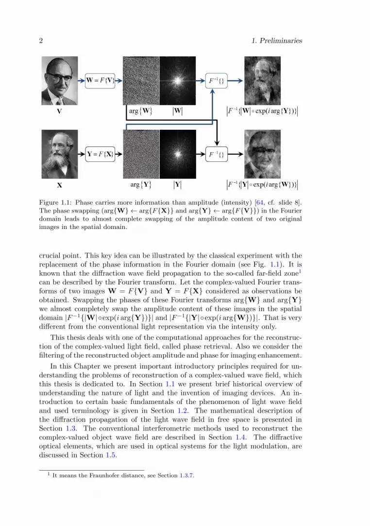
Figure 1.1: Phase carries more information than amplitude (intensity) [64, cf. slide 8].The phase swapping (arg{W} ← arg{F{X}} and arg{Y} ← arg{F{V}}) in the Fourierdomain leads to almost complete swapping of the amplitude content of two originalimages in the spatial domain.

crucial point. This key idea can be illustrated by the classical experiment with thereplacement of the phase information in the Fourier domain (see Fig. 1.1). It isknown that the diffraction wave field propagation to the so-called far-field zone1

can be described by the Fourier transform. Let the complex-valued Fourier trans-forms of two images W = F{V} and Y = F{X} considered as observations beobtained. Swapping the phases of these Fourier transforms arg{W} and arg{Y}we almost completely swap the amplitude content of these images in the spatialdomain |F−1{|W|◦exp(i arg{Y})}| and |F−1{|Y|◦exp(i arg{W})}|. That is verydifferent from the conventional light representation via the intensity only.

This thesis deals with one of the computational approaches for the reconstruc-tion of the complex-valued light field, called phase retrieval. Also we consider thefiltering of the reconstructed object amplitude and phase for imaging enhancement.

In this Chapter we present important introductory principles required for un-derstanding the problems of reconstruction of a complex-valued wave field, whichthis thesis is dedicated to. In Section 1.1 we present brief historical overview ofunderstanding the nature of light and the invention of imaging devices. An in-troduction to certain basic fundamentals of the phenomenon of light wave fieldand used terminology is given in Section 1.2. The mathematical description ofthe diffraction propagation of the light wave field in free space is presented inSection 1.3. The conventional interferometric methods used to reconstruct thecomplex-valued object wave field are described in Section 1.4. The diffractiveoptical elements, which are used in optical systems for the light modulation, arediscussed in Section 1.5.

1 It means the Fraunhofer distance, see Section 1.3.7.

1.1. Historical overview 3

1.1 Historical overview

The history of direct imaging began in the ancient times [179, 220]. For instance,the oldest lens artifact, Nimrud lens, unearthed by Austen Henry Layard, is dat-ing back over three thousands years to ancient Assyria. Another artifact, a well-preserved flat-convex lens of rock crystal in a frame made 2500 years BC, wasdiscovered by Heinrich Schliemann during his famous excavations of Troy. Asmall lens of crystal made around 1600 BC is found in the ruins of the palaceof Knossos on Crete. Ancient Egyptian statues were decorated with rock crystals,semi-precious stones and glass to imitate eyes. The Babylonians manufacturedconvex lenses from polished crystals, often quartz. Lenses made of the artificialmaterial – glass – dating 600–400 BC were found in Sargon (Mesopotamia). How-ever, since these lenses had poor magnifying qualities, they were most likely usedin ornamentation or as curiosities.

The first documented works on the nature of light and vision occurred toward themiddle of the first millennium BC in oriental and Greek schools of philosophy.Chinese Mohism dealt with the ray propagation, reflection and refraction of light:in particular, Chinese philosopher Mozi (ca. 470 – ca. 391 BC) wrote on the useof concave mirrors to focus the sun’s rays [179]. In India, the Samkhva, Nyaya,and Vaisheshika approximately from the sixth to fifth century BC constructed atheory of light and made light or fire (tejas) one of the five elements of the world;the two latter schools distinguished between the fire from luminaries and the firefrom the eye, and conceived both as diverging streams of atoms [39].

In the sixth century BC, a few bold Greek thinkers rejected the traditional ap-peal to supernatural forces in the explanation of natural phenomena and replacedthese forces with causes to be found in nature itself. The ancient Greeks helddiverse (emission/extramission and reception/intromission [173, 188]) theories ofvisual perception that differed from modern optics in essential manner: their spec-ulations about light were hindered by the lack of knowledge about how the eyeworks. Plato combined the analysis of visual perception by Pythagoras, Empe-docles and Democritus in his dialogue Timaeus (ca. 360 BC): sight is possibleupon the notion that eyes are composed of some “internal fire” which goes outfrom eyes to investigate objects and is interacted with the “external fire”of visi-ble light (“day light”reflected or emitted from luminous sources) [65]. Some earlyideas of the Greeks, however, were correct. Aristophanes in his play (The clouds,423 BC) describes the light focus effect of a lens. The philosopher and statesmanEmpedocles of Agrigentum (ca. 490 – 430 BC) believed that the light travels withfinite speed, and the philosopher and scientist Aristotle (384 – 322 BC) rightlyexplained the rainbow as a kind of reflection from raindrops.

The ancient Greek philosophers (Plato, Aristotle and the Stoics) did not pro-vide any precise understanding of visual appearances and deceptions, they reliedmore on philosophical debate and pure thought rather than on experimentationsto prove ideas, and their theories were essentially qualitative. There was, how-ever, the Greek geometrical optics according to which the perception of imagedepended on the incidence of visual rays on the various points of the objects [39].In about 300 BC, Euclid wrote Optica, in which he studied the light propagationand postulated that light travelled in straight lines. Where Euclid had limited his

4 1. Preliminaries

analysis to simple direct vision, Hero of Alexandria (ca. 10 – 70 AD) extended theprinciples of geometrical optics to consider problems of reflection (catoptrics). Inhis Catoptrica, Hero demonstrated the equality of the incident and reflected an-gles on the grounds that this is the shortest path between the source and point ofobservation (Hero’s principle, e.g., [190, Chapter 1.1]). The use of optical devicescan be illustrated by, e.g., “Archimedes heat ray”: Archimedes may have usedmirrors acting collectively as parabolic reflectors to burn ships during the Siege ofSyracuse (ca. 214 – 212 BC).

The renowned Roman emperor Nero was said to watch the gladiatorial gamesusing an emerald (presumably concave to correct for myopia [182]). Both Plinythe Elder (23 – 79 AD) and Seneca the Younger (3 BC – 65 AD) described themagnifying effect of a glass globe filled with water. Claudius Ptolemy (ca. 90 – ca.168 AD2) extended the study of vision beyond direct and reflected vision: he alsostudied the nature of refraction. His works and records of experimental data onoptics was further used by the Islamic scholar and scientist Alhazen (Abu Ali al-Hasan ibn al-Haitham, 965 – ca. 1040). This Egyptian scientist made significantcontributions to the principles of optics, as well as to physics, astronomy, mathe-matics, ophthalmology, philosophy and visual perception, what strongly influencedthe further study of light. He investigated the magnification produced by lenses,reflection and refraction. Following the ancient Greek physician and philosopherGalen of Pergamon (ca. 129 – ca. 200), Alhazen described the process of sight,the structure of the eye, image formation in the eye, and the visual system. Inhis Kitab al-Manaz. ir he extended the work of Ptolemy on binocular vision; gave afull account of the principle of camera obscura. Using Alhazen’s work, the Englishphilosopher and Franciscan, Roger Backon (ca. 1214 – 1294), studied in his OpusMajus the magnification by convex lenses and suggested the application of lensesin the correction of defective eyesight. Around 12843 spectacles were invented.

The inventor of optical microscope is unknown. Dutch spectacle-makers HansJanssen and his son Zacharias are often said to have invented the first compoundmicroscope around 1595. While experimenting with several lenses in a tube, theydiscovered a great magnification of objects what was a forerunner of the com-pound microscope and telescope. Hans Lippershey, a German-Dutch lensmaker,is generally credited with the earliest recorded design for an optical telescope (arefracting telescope) in 1608. A description of Lippershey’s instrument quicklyreached Galileo Galilei, who created his own improved version in 1609, “perspicil-lum,”with which he made the observations of the Moon, the stars, and the moonsof Jupiter found in his Sidereus Nuncius of 1610. The refraction law was namedafter the Dutch mathematician Willebrord Snellius: he discovered the law empir-ically in 1621. However, the French philosopher Rene Descartes was the first howpublished (in his La Dioptrique, 1637) the now familiar formulation of the law ofrefraction in terms of sines.

The effects of diffraction of light were first carefully observed and characterizedby Francesco Maria Grimaldi, who also coined the term diffraction, from the Latin

2 Note, that we hereafter consider the historical overview and dates for the Current Era onlyand the year label AD is therefore omitted.

3 Salvino D’Armato degli Armati of Florence is credited with inventing the first wearable eyeglasses, but the modern evidence suggests that this was a hoax.

1.1. Historical overview 5

diffringere, “to break into pieces”, referring to light breaking up into different di-rections. The results of Grimaldi’s observations were published posthumously in1665 [85]. The interference generated by thin films was observed and describedby Robert Hooke (1635–1703). James Gregory (1638–1675) observed the diffrac-tion patterns caused by a bird feather, which was effectively the first diffractiongrating. In 1704 Isaac Newton described in his Opticks multiple-prism dispersionin terms of the corpuscular theory of light. Christiaan Huygens constructed themathematical basis for the wave theory of light and published it in his Traite dela lumiere in 1690. He proposed that light was transmitted through an all per-vading luminiferous aether that is made up of small elastic particles each of whichcan act as a secondary source of wavelets. The interference principle introducedby English polymath Thomas Young (1773–1829) and the Huygens principle wereused by Augustin-Jean Fresnel (1788–1827) to calculate the diffraction patterns ofdifferent objects [125]. The polarization of light was described by Young, Fresneland Francois Arago (1786–1853) as a vibration in the aether transverse to the di-rection of propagation [198]. In 1811 Fresnel and Arago discovered that two beamsof light, polarized in perpendicular directions, did not interfere. Such physical ex-periments on polarization, interference and diffraction were convincing argumentsin favour of the wave theory and helped to overturn Newton’s corpuscular theory(about 1840 [198]). The relations between light, electricity and magnetism wererecognized by Michael Faraday (1791–1867). These phenomena were summarizedby James Clerk Maxwell in A treatise on electricity and magnetism (1873) in thiswell known equations. The further works of Heinrich Hertz (1857 – 1894), MaxPlanck (1858 – 1947), Albert Einstein (1879 – 1955), Louis de Broglie (1892 –1987), Arthur Compton (1892 – 1962), Niels Bohr (1885 – 1962) and many others,and the construction of quantum mechanics were convincing evidence that thereis no aether, and all particles exhibit both wave and particle properties (wave–particle duality). Nowadays light is interpreted as a stream of massless particles,photons, which in many physical effects exhibit the properties of electromagneticwaves.

In the nineteenth century there was a revolutionary step in imaging – a pho-tographic camera: the first permanent photograph was made in 1826 by JosephNiepce and the daguerreotype (introduced in 1839) was the first commercially suc-cessful photographic process. Photographic plates/films combine three functions:image recording, image storage and image display. X-ray imaging is originatedfrom the works by Wilhelm Conrad Rontgen (1895, the first Nobel Price in 1901)[236]. In 1907, Russian scientist Boris Rosing used a cathode ray tube (CRT) inthe receiving end of an experimental video signal to form a picture: he managedto display simple geometric shapes onto the screen. The CRT technology was usedas a display device (in particular, for television). Further, in 1931, the electronmicroscope was constructed by German physicist Ernst Ruska (Nobel Prize inPhysics, 1986) and electrical engineer Max Knoll. The works of Otto Lehmannand Viktor Nikolaevich Zvetkov on liquid crystals (LCs), and the invention ofthe charge-coupled device (CCD) by Willard Boyle and George Smith (Bell Labs,1969; Nobel Prize in Physics, 2009) gave a powerful tool for modern sophisticatedtechniques of image acquisition, processing and imaging. With the invention of thelaser (around 1960, [82, 141]) and the computer the process of interpenetration of

6 1. Preliminaries

optics and electronics has begun. One of the consequences of that process was theappearance of new optical elements recalculated or reprogramming by computer(spatial light modulators, SLMs [47, 159, 207]) in the late 1960s. The developmentof computer technologies and new materials gave the real possibility of numericalcalculation of complex characteristics of a light field.

1.2 Foundations for description of light field

Let us describe the physical properties of light waves and the primary used phe-nomena – interference and diffraction, which take place because of the wave natureof light.

1.2.1 Light intensity

The only parameter of light which is directly amenable to sensor – eye, photo-diode, CCD-target, etc. – is the intensity (and in a rough scale the frequencyas color) [125]. Here we consider a monochromatic light field in a nonmagneticand nondispersive medium. Intensity is defined by the energy flux (optical power)through an area per time. Let E(x, y, z) be the complex amplitude of the electricfield. From the Maxwell equations for an electromagnetic wave propagation in anisotropic medium the light intensity I is [56, 190]

I(x, y, z) =cε0n

2· |E(x, y, z)|2, (1.1)

where n is the refractive index of the optical medium, ε0 is the vacuum permittiv-ity4 and c0 is the vacuum velocity of light. Thus, the intensity of a monochromaticwave is simply proportional to the absolute square of its complex amplitude, andthe amplitude of the light wave is defined as

a(x, y, z) =√I(x, y, z). (1.2)

Taking into account that there is no sensor which can follow the frequency oflight5, the momentary intensity is not measurable, and we have to integrate overa measuring time6 T

I(x, y, z) =1

T

T/2∫−T/2

E(x, y, z, t)E∗(x, y, z, t)dt, (1.3)

where the proportionality constant c0ε0n2 is hereafter omitted for simplicity, and

T � 0 is much longer than the time of an optical cycle but much shorter than anyother time of interest [125, 190].

4 The electric permittivity of vacuum ε0 ≈ (1/36π) · 10−9 [F/m].5 For instance, the visible light frequency range extends from about 384 up to 769 THz.6 Note that in general the flow of electromagnetic power is governed by the time average of

the Poynting vector ~E(x, y, z, t) × ~H(x, y, z, t) = Re{~E(x, y, z) · ei2πvt} × Re{ ~H(x, y, z) · ei2πvt},where ~E(x, y, z, t) and ~H(x, y, z, t) are the electric- and magnetic-field vectors, v is an optical

frequency. The optical intensity is the magnitude of the vector Re{ ~S(x, y, z)}, where ~S(x, y, z) =12~E(x, y, z)× ~H∗(x, y, z) may be regarded as a complex Poynting vector [190, cf. §5.3].

1.2. Foundations for description of light field 7

1.2.2 Phase of light wave field

In addition to the intensity, there is also the phase of the light field. In general, thephase of a wave field is a function of the position in 3D space and time, becauseit describes the part of a complete wave oscillation. In this work we consider aharmonic wave function of the monochromatic light in the form [79, 80]

U(x, y, z, t) = Re{a(x, y, z) · ei(φ(x,y,z)−2πvt)} = Re{u(x, y, z) · e−i2πvt}, (1.4)

where v is the optical frequency, U(x, y, z, t) represents any of the scalar com-ponents of the electric (or magnet) field. The time dependent term 2πvt in Eq.(1.4) is known a priori: it is spatial-independent, but constantly changes in time.Thus, this time-dependent term is equal for all light wave field having the samewavelength λ (frequency v) and propagating in exactly the same medium withrefraction index n. φ(x, y, z) describes the spatial distribution of the phase. Prac-tically it may also be of importance the wavefront – the surface of equal phaseφ(x, y, z) = const (even rather φ(x, y, z) − 2πvt = const), which represents thestructure and behavior of light waves (see Fig. 1.2).

The phase is defined here in the interval [−π, π). In order to correct jumpsmodulo 2π and overcome the discontinuity, where two adjacent phase values haveextreme values of either −π or π (or close to them), one produces so-called phaseunwrapping, depending on the sign of the jump underlying phase change. Forinstance, if the phase difference between two neighboring pixels is less than −π(larger then π), one adds (subtracts) multipliers of 2π to the following pixels on-ward, what result in a (piecewise) continuous phase distribution [194, Chapter2.7.6]. For 2D phase distributions the problem becomes more complicated be-cause a proper path of processing is required. Such a path is typically found inaccordance with the structure of the phase distribution7.

Note that the phase unwrapping can only be performed in the areas with nophase singularities8, i.e. zeros of the light wave field (points of zero intensity) [51].Phase unwrapping and phase singularities are out of scope of this thesis.

Figure 1.2: ”Redistribution” of the optical intensity by the phase [64, cf. slide 9]. Lighttravels in direction perpendicular to the wave front φ(x, y, z) = const. In addition, weobtain dimmer spot where light wave spreads out, and brighter one – where light isconcentrated.

7 See, e.g., [72] for basic principles of 2D phase unwrapping, and powerful algorithms of 2Dphase unwrapping from noisy data like [44, 45, 222].

8 In these points the phase gradient becomes infinite, and the phase variation along a closedloop around such points is always an integer multiple of 2π [70, 163].

8 1. Preliminaries

1.2.3 Polarization of light

Since the light is an electromagnetic vector wave field, we need to mention aboutthe polarization. The polarization of light at a fixed position is traditionally de-termined by the time course of the electric-field vector ~E(x, y, z, t). In a sim-ple (isotropic) medium, this vector lies in a plane tangential to the wavefrontat that position. For monochromatic light, any two orthogonal components ofthe complex-amplitude vector ~E(x, y, z) in that plane vary sinusoidally with time,with amplitudes and phases that are generally different, so that the endpoint ofthe vector ~E(x, y, z) traces an ellipse. Since the wavefront generally has differentdirections at different positions, the plane, the orientation, and the shape of theellipse also vary with the position [190, cf. Fig. 6.0-1]. We consider a monochro-matic light wave traveling in the z direction, and assume that the light wave isvibrating in a single plane. Thus, we consider a plane polarized wave in the xyplane. Let us write the polarization vector of the light for this case as [81, cf. Eq.(4.3-1)], [190, cf. Eqs. (6.1-3), (6.1-4)]

~E(z, t) =

[Ex(z, t)

Ey(z, t)

]=

[axe

iφx cos(i2π( zλ − vt))aye

iφy cos(i2π( zλ − vt))

], (1.5)

what describes the state of polarization in that plane. For a plane wave thewavefronts are parallel to transverse planes and the polarization ellipses are thesame everywhere (see [190, Fig. 6.0-1]). The orientation and ellipticity of thepolarization ellipse determine the state of polarization of the plane wave, whereasthe size of the ellipse is determined by the optical intensity. When the ellipsedegenerates into a straight line or becomes a circle, the wave is said to be linearlypolarized or circularly polarized, respectively. The polarized light can be describedvia the so-called Jones vector [79, 125]

q =

[axe

iφx

ayeiφy

]. (1.6)

The linearly polarized light with polarization direction at an angle θ is definedby q =

[cos θsin θ

]and represented via its time course and the trajectory of the endpoint

of the vector ~E(z, t) (Eq. (1.5)) at a fixed time t as it is illustrated in Fig. 1.3.

Figure 1.3: Linearly (plane) polarized light: (a) time course at a fixed position z, (b) asnapshot of the trajectory of the endpoint of the vector ~E(z, t) at a fixed time t [190, cf.Fig. 6.1-3].

1.2. Foundations for description of light field 9

In this thesis a monochromatic linearly polarized light wave is considered.Firstly, such a light wave is completely characterized at every point of space by itsintensity/amplitude and phase only [190], what significantly simplify the mathe-matical apparatus used to describe the free space wave field propagation. Secondly,our choice is based on the conventional approach in laser optics. Nevertheless, itcan be used different wavelengths λ (frequencies v), and our work can be appliedin a hyperspectral imaging system (see, e.g., [105, 184]).

1.2.4 Diffraction and interference of light waves

Diffraction refers to various phenomena which occur when a wave encounters anobstacle. Following Grimaldi’s experiments, when a light wave is transmittedthrough a small aperture in an opaque screen and travels some distance in freespace, one may observe a quite specific intensity distribution called the diffractionpattern. If light were treated as rays, the diffraction pattern would be a shadowof the aperture. Because of the wave nature of light, however, the diffractionpattern may deviate slightly or substantially from the aperture shadow (see [85,pg. 9]), depending on the distance between the aperture and observation plane,the wavelength, and the dimensions of the aperture [190]. The term diffractioncan be defined as any deviation of light rays from rectilinear paths which cannotbe interpreted as reflection, refraction or bending of light rays in a medium witha continuously varying refractive index [79, 204].

The initial step in the evolution of the wave theory that would explain diffrac-tion effects was made by Huygens in 1678. He expressed the intuitive convictionthat if each point on the wavefront of a disturbance were considered to be a newsource of a “secondary” spherical disturbance, then the wavefront at a later in-stant could be found by constructing the “envelope” of the secondary wavelets9,as illustrated in Fig. 1.4 [79, 194].

Figure 1.4: Huygens’ envelope construction [79, cf. Fig. 3.4].

9 “Each element of a wavefront may be regarded as the centre of a secondary disturbancewhich gives rise to spherical wavelets ”; and moreover “the position of the wavefront at anylater time is the envelope of all such wavelets ” [20, Chapter 3.3.3].

10 1. Preliminaries

Figure 1.5: Young’s double-slit interferometer: a point source of light illuminates twonarrow adjacent slits in a screen, and the image of the light that passes through the slitsis observed on a second screen. The dark and light regions are called interference fringes,the constructive (greater amplitude than either one) and destructive (lesser amplitude)interference of light waves [190].

In 1803 further significant progress occurred: Thomas Young strengthened thewave theory of light by introducing the critical concept of interference, according towhich two coherent waves superimpose to form a resultant wave of greater or loweramplitude (intensity). The idea was a radical one at those time, because light couldbe added to light and produce darkness (see Young’s double-slit interferometer inFig. 1.5, [204, cf. Fig. 114, Eq. (26.14)]). Generally, it is difficult to determinethe exact difference between interference and diffraction. We rather refer to thefollowing quotation from the known Feynman lectures [55, Chapter 30-1]: “Noone has ever been able to define the difference between interference and diffractionsatisfactorily. It is just a question of usage, and there is no specific, importantphysical difference between them. The best we can do, roughly speaking, is to saythat when there are only a few sources, say two, interfering, then the result isusually called interference, but if there is a large number of them, it seems that theword diffraction is more often used”.

The ideas of Huygens and Young were brought together in 1818 in the famousmemoir of Fresnel (the Huygens–Fresnel principle [20, 190]), and further put on afirmer mathematical foundation by Gustav Kirchhoff, who showed in 1882 that theamplitudes and phases ascribed to the secondary sources by Fresnel were indeedlogical consequences of the wave nature of light. The Kirchhoff theory was alsomodified by Arnold Sommerfeld (1896), who gave the first truly rigorous solutionof a diffraction problem using the theory of Green’s functions [79, 80]. In thisthesis the used mathematical apparatus of the diffraction propagation is based on

1.2. Foundations for description of light field 11

the Kirchhoff and Rayleigh–Sommerfeld theories treated as a scalar phenomenon,neglecting the fundamentally vectorial nature of the electromagnetic fields.

1.2.5 Coherence of light waves

Note that with the sunlight or lamplight we rarely observe interference. Only lightof sufficient coherence will exhibit this effect. Roughly speaking, coherence meansthe ability of light waves to interfere. Precisely, coherence describes the correlationbetween individual light waves10 [125]. Let we consider the concept of interfer-ence. Since the time-dependent part in Eq. (1.4) is known a priori, we considerthe complex amplitude of a monochromatic light wave which is purely spatiallydependent. When two or more light waves are simultaneously present in the sameregion of space and time, the total wave function is the sum of the individualwave functions. This basic principle of superposition follows from the linearity ofthe wave equation, in particular for monochromatic waves of the same frequency(wavelength), the superposition principle carries over to the complex amplitudes,which follows from the linearity of the Helmholtz equation [190, Chapter 2.2].If two monochromatic waves with complex amplitudes u1(x, y, z) =

√I1e

iφ1 andu2(x, y, z) =

√I2e

iφ2 are superposed, the result is a monochromatic wave of thesame frequency that has a complex amplitude [190, 194]

u(x, y, z) = u1(x, y, z) + u2(x, y, z). (1.7)

Figure 1.6: Young’s double-slit experiment showing the source of the phase shift geomet-rically (one-dimensional case). Two slits are idealized as two closely located point sourcesS1 and S2 of a monochromatic light with the wavelength λ. The point A is the observationpoint with the abscissa x. A projection screen is parallel to the plane of the sources S1

and S2. The distance between these planes z is much larger than the size of the sources,distance between the light sources d� z and linear dimensions of the observations areax � z. The path difference of the interfering waves is r1 − r2 = S2D = d sin θ ≈ xd

z

[190, 204, 205].

10 Temporal coherence describes the correlation with itself as it behaves at different timeinstants and spatial coherence describes the mutual correlation of different parts of the samewavefront (see [125]).

12 1. Preliminaries

Taking into account that the intensity of a monochromatic wave function isthe absolute square of its complex amplitude, the intensity of the total wave is

I = |u|2 = |u1 + u2|2 = |u1|2 + |u2|2 + u1u∗2 + u∗1u2 = (1.8)

= I1 + I2 + 2√I1I2 · cos(φ2 − φ1).

This relation, called the interference equation (interferogram [194]), demon-strates that the amplitude of u is sensitive not only to the magnitudes of the con-stituent waves u1 and u2, but also to the phase difference φ2 − φ1 = 2π

λ (r2 − r1).In contrast to that, the sum of two incoherent waves is simply11 I = I1 + I2.

Interference is accompanied by a spatial redistribution of the optical intensitywithout a violation of power conservation [190, cf. Fig. 2.5-1]. Furthermore,I in Eq. (1.8) has its maximum and minimum value for φ2 − φ1 = 2πm andφ2 − φ1 = 2π(m + 1

2 ), respectively (m ∈ Z), what is called constructive anddestructive interference (see Fig. 1.5). The interpretation via an object shape canbe given by the path difference r1 − r2 of interfering waves (by replacing 2π ← λ,Fig. 1.6): the maximum and minimum of I can be defined as r1 − r2 = λm andr1 − r2 = λ(m+ 1

2 ), respectively [204].

1.2.6 Holography and holograms

Holography got its name from the Greek words oλoς (holos) meaning “whole/entire”and γραϕη (graphe) meaning “to write”. It is a means for recording and recon-structing the whole information contained in an optical wavefront, namely ampli-tude and phase, and not just intensity as ordinary photography does. Holographyessentially is a clever combination of interference and diffraction. In 1948 DennisGabor (1900 – 1979) presented holography as a lensless process for image forma-tion by reconstructed wavefronts [68]. Invention of holography was motivated bythe desire to improve resolution power of electron microscopes that was limited bythe fundamental limitations of the electron optics and avoid the previous aberra-tions. But the interest in holography declined after a few years, mainly because ofthe poor quality of the holographic images obtained in those days [125]. Moreover,powerful sources of coherent light were also not available at that date, and holog-raphy remained an “optical paradox” until the invention of lasers. The very firstimplementation of holography was demonstrated in the early 1960s by EmmettLeith and Juris Upatnieks [133] and by Yuri Nikolaevich Denisyuk [41].

In holography, one records the interference patterns between two optical waves:an object uobj (reflected from or transmitted through the object) and a special“reference”uref ones. Since recording media respond typically to the light intensityonly12, one detects the intensity of the coherent superposition of these waves:

11 The complex degree of coherence is hereafter assumed to be equal to 1, what correspondsto the full coherence of waves [125, 190]. In case of incoherent waves this factor is equal to 0,hence there will be no additional (latter) term in Eq. (1.8).

12 Optical media for recording holograms may be classified into three categories:amplitude/intensity-only (e.g., CCD), phase-only (kinoform [134, 135]) and combined amplitude-phase media [207, 236].

1.3. Principles of scalar diffraction theory 13

I(x, y) = |uobj(x, y) + uref (x, y)|2 = (1.9)

= |uobj(x, y)|2 + |uref (x, y)|2︸ ︷︷ ︸DC term

+ u∗obj(x, y)uref (x, y) + uobj(x, y)u∗ref (x, y),

where the last term in the sum is proportional to the complex amplitude of thewave field which travels from the object. That is what we call the hologram [236].It is denoted here by I(x, y) in order to distinguish it from the simple sum ofintensities of two waves, I(x, y) 6= I1(x, y) + I2(x, y).

The optical reconstruction is achieved by illuminating a recording mediumwith the reference beam [125, 194, 232, 234, 236]. Since the wave field uobj on adetector is formed by the forward diffraction propagation from the object to thesensor plane, the numerical reconstruction is to compute this complex-valued uobj(e.g., by phase shifting) and to perform the backward wave field propagation.

1.3 Principles of scalar diffraction theory

An electromagnetic field is described by two related vector fields that are func-tions of the position in the Cartesian coordinate system and time: the electric field~E(x, y, z, t) and the magnetic field ~H(x, y, z, t). Since in this thesis the linearly po-larized light is used, a monochromatic light field may be completely characterizedwithin the scope of the scalar wave theory at every point in space by means of itsamplitude and phase [120]. Therefore, in order to define light in free space oneuses six scalar functions of position and time, which must satisfy the celebratedset of coupled partial differential equations known as Maxwell’s equations [190].

1.3.1 Maxwell’s wave equation

For a medium with no currents and charges, these equations for the electric- andmagnetic-field vectors can be written as follows [79, cf. Eq. (3-2)]

∇ · ~E(x, y, z, t) = 0, (1.10)

∇ · ~H(x, y, z, t) = 0, (1.11)

∇× ~E(x, y, z, t) = −µm∂ ~H(x, y, z, t)

∂t, (1.12)

∇× ~H(x, y, z, t) = εm∂~E(x, y, z, t)

∂t, (1.13)

where µm and εm are the magnetic permeability and electric permittivity, respec-tively, of the medium within which the light wave is propagating. The vectoroperators ∇· and ∇× represent the divergence and curl (rotor), respectively.

In this thesis the propagation of light is considered in free space (vacuum or air).In a linear, isotropic, homogeneous (εm = const), nonmagnetic and nondispersivemedium both µm and εm are always equal to the constants of free space 4,13

13 Magnetic permeability of vacuum µ0 = 4π · 10−7 [H/m] .

14 1. Preliminaries

µm = µ0, εm = ε0. (1.14)

Let U = U(x, y, z, t) represents any of the scalar field components of the electricor magnetic field. The light field at any point of free space (with the refractiveindex n ∼= 1) can be found from the scalar wave equation [79]

∇2U − 1

c2· ∂

2U∂t2

= 0, (1.15)

derived from Maxwell’s equations14, where the Laplace operator ∇2 = ∂2/∂x2 +∂2/∂y2 + ∂2/∂z2 and c = 1√

µ0ε0is the speed of light in vacuum.

Indeed, applying the curl operation to the left and right sides of Eq. (1.12)and using the vector equation

∇× (∇× ~E(x, y, z, t)) = ∇(∇ · ~E(x, y, z, t))−∇2~E(x, y, z, t), (1.16)

we arrive at

∇2~E(x, y, z, t)− 1

c2· ∂

2~E(x, y, z, t)

∂t2= 0. (1.17)

The magnetic field satisfies an identical equation

∇2 ~H(x, y, z, t)− 1

c2· ∂

2 ~H(x, y, z, t)

∂t2= 0. (1.18)

Since both ~E(x, y, z, t) and ~H(x, y, z, t) satisfy the identical vector wave equation,an identical scalar wave equation is obeyed by all components of those vectors[56, 79], and two vector wave equations (1.17) and (1.18) are divided into sixscalar wave equations similar to Eq. (1.15), but with respect to the individualcomponents Ex, Ey, Ez,Hx,Hy,Hz. The behavior of all components of the electricand magnetic field is fully described by the single scalar wave Eq. (1.15).

1.3.2 Helmholtz wave equations

As it is mentioned above (see Section 1.2.3), the consideration of this thesis islimited (for simplicity) to the propagation of monochromatic light waves (hereafterwave field propagation). In such a case, a light field at the position (x,y,z) andtime t can be accurately described by a scalar wave function of the form [20, Eq.(25)]

U(x, y, z, t) = Re{u(x, y, z) · e−i2πvt}, (1.19)

where v is the optical frequency as in Eq. (1.4). The complex function [20, 79, 190]

u(x, y, z) = a(x, y, z) · exp(iφ(x, y, z)) (1.20)

14 Note that, following [56], the general solution of the one-dimensional wave equation is thesum of two arbitrary functions of the form of d’Alambert formula U = U(x, t) = h(x−ct)+g(x+ct)[56, cf. Eq. (20.24)], [125, cf. Eq. (2.6)], representing two waves travelling with the speed c: thewave h travels toward positive x, and g – toward negative x. This is the superposition of thewaves existing at the same time.

1.3. Principles of scalar diffraction theory 15

Figure 1.7: The wave vector ~k and the plane cutting off segments ckx

, cky

and ckz

on the

Cartesian coordinate axes. The angles between ~k and the x, y and z axes are denotedby α, β and γ, respectively.

works as an adequate description of a light wave, because the time dependencee−i2πvt is deterministic. Here a and φ are the amplitude and phase of the lightwave, respectively. The complex amplitude of the light wave (1.20) depends onlyon the spatial position and is often called a phasor. Substituting Eq. (1.19) in Eq.(1.15) it follows that u(x, y, z) must obey the time-independent equation

(∇2 + k2) · u(x, y, z) = 0, (1.21)

where k denotes the wave number given by k = 2π/λ, and λ = v/c is the wave-length of the monochromatic light wave in the dielectric medium. This equation isknown as the Helmholz equation. The most straightforward solutions of Eq. (1.21)are those which describe uniform plane and symmetric spherical waves.

For a plane wave [138, Eq. (III.3)]

u(x, y, z) = a · e±i~k~r = a · e±i(kxx+kyy+kzz), a = const, (1.22)

where kx, ky, kz and x, y, z are the projections of the wave vector ~k and theradius-vector ~r onto the Cartesian coordinate axes, respectively. Substituting Eq.(1.22) in Eq. (1.21) we arrive at

k2x + k2

y + k2z = k2 =

(2π

λ

)2

. (1.23)

The equal-phase surfaces is defined from the relation

kxx+ kyy + kzz = c = const, (1.24)

which represents an equation of the plane which cuts off the segments ckx

, cky

andckz

on the coordinate axes (see Fig. 1.7).

In this thesis the waves generated by a source are assumed to be propagating

16 1. Preliminaries

outward15 from this source [56]. Thus, the full expression for the plane wave is ofthe form

U(x, y, z, t) = a · ei(kxx+kyy+kzz−2πvt), (1.25)

i.e. Eq. (1.22) is given for t = 0. If t = t1 > 0 the wave surface is describedby the expression kxx + kyy + kzz = c + 2πvt1 representing the equation of theplane which cuts off segments c+2πvt1

kx, c+2πvt1

kyand c+2πvt1

kzon the coordinate

axes. It follows that the plane wave propagates parallel to itself. If c = c(x, y, z) =kxx+ kyy + kzz − 2πvt1 as we have seen before, then

∇c =∂c

∂x· ~jx +

∂c

∂y· ~jy +

∂c

∂z· ~jz = (1.26)

= kx · ~jx + ky · ~jy + kz · ~jz = ~kx + ~ky + ~kz = ~k,

i.e. the propagation direction of the plane wave coincides with the direction of thewave vector. ~jx, ~jy and ~jz are hereafter the unit vectors in Cartesian coordinates.

The Helmholtz wave equation (1.21) in spherical coordinates is of the form

1

r· ∂

2

∂r2(ru) +

1

r2 sin θ· ∂∂θ

(sin θ∂u

∂θ) +

1

r2 sin2 θ

∂2u

∂ϕ2+ k2u = 0, (1.27)

where variables r, θ and ϕ are defined from equations x = r sin θ cosϕ, y =

r sin θ sinϕ and z = r cos θ. For the symmetric spherical waves ∂u(r,θ,ϕ)∂θ = 0 and

∂u(r,θ,ϕ)∂ϕ = 0 due to the circular symmetry, therefore Eq. (1.27) can be simplified

as [56, cf. Eq. (20.34)] (∂2

∂r2+ k2

)· ru(r, θ, ϕ) = 0. (1.28)

Then, for a diverging (expanding [79], outgoing [56]) spherical wave we arriveat

u(r, θ, ϕ) = aeikr

r, a = const, (1.29)

and the equal-phase surfaces is determined from the identity kr = const, hencer = const. Taking into account that r =

√x2 + y2 + z2 the wave propagation

direction is defined by

∇kr = k∇r = k ·(xr· ~jx +

y

r· ~jy +

z

r· ~jz)

=k

r~r, (1.30)

i.e. the spherical wave propagates along the radius-vector ~r. Eq. (1.29) can berewritten as

u(x, y, z) = aeik√x2+y2+z2√

x2 + y2 + z2. (1.31)

Note that the wave source is assumed to be at the origin and r is only realpositive (z > 0 [56]). One observes that the amplitude a

r decreases proportionallyto 1

r , and at a long distance from the origin the spherical wave locally approximatesa plane wave [125].

15 Although Maxwell’s equations would allow either possibilities, we will put an additionalfact, that only the outgoing wave solution makes ”physical sense” [56]. Thus, in contrast to thegeneral solution by d’Alembert’s formula [20, § 1.3, Eq. (8)], [56, Eq. (20.24)], here we considerthe wave field propagation in the positive c direction only.

1.3. Principles of scalar diffraction theory 17

1.3.3 Paraxial approximation and angular spectrum

It can be shown [79, 138] that the complex amplitude and spatial Fourier compo-nents of the monochromatic wave field distribution can be decomposed by planewaves travelling in different directions.

Let us consider the plane wave given by Eq. (1.22). Denote the angles between

the wave vector ~k and the Cartesian coordinate axes x, y and z by α, β andγ, respectively (see Fig. 1.7). Then, cosα = kx

k , cosβ =kyk , cos γ = kz

k and~k = k · (cosα · ~jx + cosβ · ~jy + cos γ · ~jz). Taking into account Eq. (1.23),

cos2 α+ cos2 β + cos2 γ = 1. (1.32)

It is of interest to describe paraxial waves whose propagation direction almostcoincides with the direction of the optical axis z (propagates in the positive zdirection), i.e. the angle γ is small, α and β are close to π

2 . Then, cos γ ≈ 1 and

cosα ≈ π

2− α , α1, cosβ ≈ π

2− β , β1. (1.33)

According to Eq. (1.32) the propagation direction is fully determined by only

two angles. The projections of the wave vector ~k onto the xz and yz planes are

equal to kxz =√k2x + k2

z and kyz =√k2y + k2

z , respectively (see Fig. 1.8). The

angles between these projections and the z axis αxz and βyz can be found from

sinαxz =kx√k2x + k2

z

, sinβyz =ky√k2y + k2

z

. (1.34)

Since for the paraxial approximation kz � kx, kz � ky and kz ≈ k

sinαxz ≈ kxk

= cosα = sinα1, (1.35)

sinβyz ≈ kyk

= cosβ = sinβ1,

Figure 1.8: The wave vector ~k and its projections onto the coordinate axes and coordinateplanes. In case of the paraxial approximation, the angles between the projections of ~konto the (x,z) and (y,z) planes and the z axis are close to π

2−α and π

2−β (see Fig. 1.7).

18 1. Preliminaries

what results in αxz ≈ α1, βyz ≈ β1. Therefore the plane wave can be describe asa two-dimensional harmonic oscillation with the frequencies (kα1,kβ1) [138]

u(x, y, z) = a · eikzeik(α1x+β1y), a = const. (1.36)

In the Fourier decomposition of u the complex amplitude of the plane-wave

component with the angular frequencies (α1

λ ,β1

λ ) is U(α1

λ ,β1

λ , z)dα1

λ dβ1

λ . The

two-dimensional Fourier transform of the function u across the xy plane

U

(α1

λ,β1

λ, z

)=

∞∫∫−∞

u(x, y, z) · e−i2π(α1λ x+

β1λ y)dxdy (1.37)

is called the angular spectrum of the wave u(x, y, z).

1.3.4 Plane wave decomposition

Suppose that the complex amplitude of the wave field across the xy plane at thedistance z0 > 0 is given by u(x, y, z0), where its angular spectrum is of the form

U (kx, ky, z0) =

∞∫∫−∞

u(x, y, z0) · e−i(kxx+kyy)dxdy. (1.38)

Here γ = 0. Note that the angular frequencies are chosen as kx = k cosα, ky =

k cosβ (cf. Eq. (1.37)). Let us calculate u(x, y, z0 + z)∣∣∣z=const

, the wave field

distribution at a parallel plane, which appears at the distances z from (to theright of) the first plane. It is known that u(x, y, z0) must satisfy the HelmholtzEq. (1.21) at all source-free points [79]. Therefore, direct multiplication of Eq.(1.21) by e−i(kxx+kyy) and its integration with respect to x and y shows that theangular spectrum must satisfy the homogeneous second order differential equation(see [138, Chapter III, §2] for the derivation)

d2

dz2U (kx, ky, z) + (k2 − k2

x − k2y) · U (kx, ky, z) = 0, (1.39)

yielding

U (kx, ky, z) = c1(kx, ky) · eiz√k2−k2

x−k2y + c2(kx, ky) · e−iz

√k2−k2

x−k2y , (1.40)

where c1(kx, ky) and c2(kx, ky) are integration constants determined from theboundary conditions. The first term in Eq. (1.40) corresponds to the direct,outgoing wave, and the second term – to the incoming wave. Since the wave fieldpropagation is assumed to be taken in a homogeneous medium from the source inthe positive direction of z, the second term is equal to zero due to lack of sourcesfor the incoming wave, c2 = 0. Then

U (kx, ky, z0 + z)∣∣∣z=const

= c1(kx, ky) · ei(z0+z)√k2−k2

x−k2y , (1.41)

1.3. Principles of scalar diffraction theory 19

where c1(kx, ky) can be found from the initial condition at the plane z = z0

U(kx, ky, z)∣∣∣z=z0

= U (kx, ky, z0) = c1(kx, ky) · eiz0√k2−k2

x−k2y . (1.42)

Thus, we arrive at

U (kx, ky, z0 + z)∣∣∣z=const

= U (kx, ky, z0) · eiz√k2−k2

x−k2y , (1.43)

i.e. a layer of free space works as a filter, where the transfer function is of the form

Hz(kx, ky) = eiz√k2−k2

x−k2y . (1.44)

Note that |H(kx, ky)| = 1, φ(kx, ky) = z√k2 − k2

x − k2y for k2

x + k2y ≤ k2.

For√k2x + k2

y > k the module of the transfer function decreases according to

e−z√k2x+k2

y−k2

, φ(kx, ky) = 0. Hence, a layer of free space behaves as a low-pass filter with a finite bandwidth equal to k = 2π

λ . The wave components withwavelengths less than λ are rapidly attenuated by the propagation phenomenonwith increasing of the distance z. Since the distances z and z0 are taken muchlarger than a few wavelengths, we can completely drop the evanescent componentsof the spectrum, i.e. exclude from our consideration the case of k2

x + k2y > k2 [79].

The subindex “z” in Eq. (1.44) just emphasizes that Hz is a 2D transfer functioncalculated for the space layer of the width z.

The inverse Fourier transform of Eq. (1.43) yields the plane wave decompositionintegral

u (x, y, z0 + z)∣∣∣z=const

= (1.45)

=1

4π2

∞∫∫−∞

U(kx, ky, z0) · (eiz√k2−k2

x−k2y︸ ︷︷ ︸

U(kx,ky,z0+z)

∣∣∣z=const

ei(kxx+kyy))dkxdky =

= F−1{F{u(x, y, z0)}(kx, ky) ·Hz(kx, ky)}(x, y),

which represents the wave field in free space u (x, y, z0 + z) as a superposition

of plane waves ei(kxx+kyy+z√k2−k2

x−k2y) (cf. Eq.(1.36)) weighted by the complex

amplitude U(kx, ky, z0), where z0, z �0.The 3D Fourier transform of a scalar function u(x, y, z) can be defined as

U (kx, ky, kz) =

∞∫∫∫−∞

u(x, y, z) · e−i(kxx+kyy+kzz)dxdydz. (1.46)

Similar to Eq. (1.39), we apply the Helmholtz Eq. (1.21), but this time considerthe integration with respect to x, y and z. It results in

(k2 − k2x − k2

y − k2z) · U (kx, ky, kz) = 0, (1.47)

20 1. Preliminaries

i.e. the Fourier transform U (kx, ky, kz) must by equal to zero for the spatialfrequencies kx, ky and kz outside the sphere (1.23) known as Ewald’s sphere.

It should be noticed that the plane wave decomposition (1.45) is valid undercertain conditions related mainly to the existence and invertibility of the Fouriertransform of the wave field distributions at the mentioned transverse planes,namely: the pairs u (x, y, z0), U (kx, ky, z0) and u (x, y, z0 + z), U (kx, ky, z0 + z).We refer to, e.g., [79, Section 2.1.1], [130] for discussion on the existence andsufficient conditions of the Fourier transform to be obeyed.

1.3.5 Rayleigh–Sommerfeld diffraction integral

In Section 1.3.4 we demonstrate that the wave field propagation phenomenon actsas a linear space-invariant system described by a relatively simple transfer functionHz. In many situations it is more convenient to define a layer of free spacenot bythe 2D transfer function using Eq. (1.44) or (in case of spatial frequencies v1 = kx

λk ,

v2 =kyλk ) using [79, cf. Eq. (3-74)]

Hz(v1, v2) =

{exp(i 2π

λ z√

1− λ2(v21 + v2

2)),√v2

1 + v22 <

1λ

0, otherwise, (1.48)

but with an impulse response, calculated as the inverse Fourier transform of Hz

hz(x, y) =1

4π2

∞∫∫−∞

eiz√k2−k2

x−k2y · ei(kxx+kyy)dkxdky = (1.49)

=

∞∫∫−∞

ei2πzλ

√1−(λvx)2+(λvy)2 · ei2π(v1x+v2y)dv1dv2.

The expression describing the wave field in an arbitrary point (x,y,z0 + z)∣∣∣z=const

by the wave field at the transverse xy plane z = z0 is defined in the form

u(x, y, z0 + z)∣∣∣z=const

=

∞∫∫−∞

u(ξ, η, z0) · hz(x− ξ, y − η)dξdη, (1.50)

where the impulse response of free space propagation

hz(x− ξ, y − η) =1

iλcos θ · e

ikr

r

(1− 1

ikr

), (1.51)

r =√

(x− ξ)2 + (y − η)2 + z2

and cos θ = zr describes the direction of radiation. θ = 0 corresponds to the

maximum of radiation and if θ = π2 these is no radiation (see Fig. 1.9).

Note that the physical interpretation of the impulse response is a wave fieldgenerated by a 2D point source. A common derivation of the impulse responsestarts from the Green’s theorem [79, Eq. (3-14)] and a prudent choice of an

1.3. Principles of scalar diffraction theory 21

Figure 1.9: Geometrical scheme of the diffraction problem. The wave field at the ξηplane is localized only in the finite area denoted by S.

auxiliary function: a spherical wave as the Green’s function [20, 79] with theSommerfeld radiation condition (see, e.g., [79, Eq. (3-22)]).

Eq. (1.50) shows that the field u(x, y, z0 + z)∣∣∣z=const

is calculated as a two-

dimensional convolution between the initial (given) field u(ξ, η, z0) and the diffrac-tion kernel (1.51). Therefore, the free space wave field propagation to the distancez is represented as a linear shift-invariant system with the impulse response hz[167, 168].

Note that the diffraction kernel hz has a circular symmetry with respect tothe z axis. The field of a 2D point source consists of two terms: the first termdescribes the radiation field decaying as 1

r , and the second one – the inductionfield decaying according to 1

r2 .We are interesting in the radiation field. The expression for it can be found

assuming that 1− 1ikr =

√1 + 1

k2r2 ei arctan 1

kr ≈ 1 for 1kr � 1. It follows that even

for r ≈ λ the radiation field of a point source is hz ≈ ziλeikr

r2 (hz ≈ eikr

iλr for theparaxial approximation θ ≈ 0). Thus, the Rayleigh–Sommerfeld diffraction kernelcan be represented in the form

hz(x− ξ, y − η) =z

iλ· e

ikr

r2, (1.52)

i.e. omitting the second term in brackets in Eq. (1.51), Eq. (1.50) can be rewrittenas follows

u(x, y, z0 + z)∣∣∣z=const

=z

iλ

∞∫∫−∞

u(ξ, η, z0)eikr

r2dξdη, (1.53)

what is known as the Rayleigh–Sommerfeld diffraction integral.Despite the apparent differences of the angular spectrum decomposition (ASD)

method (Eqs. (1.43) and (1.45)) and the first Rayleigh–Sommerfeld (RS) solution(Eq. (1.53)), these two approaches yield identical predictions of diffracted wavefields [79]. The proof can be found, e.g., in [138, Chapter III.3] or [197].

1.3.6 Fresnel approximation

The Rayleigh–Sommerfeld diffraction integral (1.53) is quite complex, and it canbe essentially simplified using additional restrictions imposed on the interesting

22 1. Preliminaries

region of space. First of all, we note that the wave field at the plane z = z0 is, inpractice, localized in a finite region S16(see Fig. 1.9), so we can use finite limitsof integration

u(x, y, z0 + z)∣∣∣z=const

= (1.54)

=z

iλ

∫∫S

u(ξ, η, z0)eik√

(x−ξ)2+(y−η)2+z2

(x− ξ)2 + (y − η)2 + z2dξdη.

We are considering the wave field at the xy observation plane parallel to the ξηplane at the normal distance z to it. The size of the space layer is characterized bythe following important parameters: the size S of the initial wave field (source), thedistance between these planes and the lateral distances x, y from the longitudinalaxis z.

Let us assume that the wave field at the observation plane is many wavelengthsfrom the source (diffracting aperture), i.e. the distance between the points P0 andP1 in Fig. 1.9 r =

√(x− ξ)2 + (y − η)2 + z2 � λ [79]. Moreover, the distance

z > 0 is taken much larger than the maximum lateral dimension of the apertureS [80]. Then, taking into account these assumptions, we can say that cos θ ≈ 117,and r2 in the denominator of Eq. (1.54) is only slightly different from z2.

The component r in the exponent cannot be replaced by z, because the occur-ring error is multiplied by the very large k . Then, the phase changes are muchlarger than 2π, but these phase changes even by a fraction of a radian can resultin significant difference of the value of the exponent. Let us rewrite

r =√

(x− ξ)2 + (y − η)2 + z2 = z ·√

1 +(x− ξ)2 + (y − η)2

z2, (1.55)

where b = (x−ξ)2+(y−η)2

z2 < 1 is assumed to be small. In order to represent Eq.(1.54) in a simpler and more usable manner, we use the approximation based onthe binomial expansion of the square root

√1 + b = 1 +

b

2− b2

8+ ... (1.56)

Retaining only the first two terms of the expansion Eq. (1.56), we arrive atthe so-called Fresnel approximation

r ≈ z +(x− ξ)2 + (y − η)2

2z, (1.57)

and the approximation error does not exceed [(x−ξ)2+(y−η)2]2

8z3 , because the Tay-lor series in the brackets in Eq. (1.56) is alternating. Taking into account that

16 Following [79] we have an infinite opaque screen with a hole of finite size, diffracting apertureS at the ξη plane which is illuminated in the positive z direction.

17 with an accuracy better than 5% , if the angle θ is less than 18 degrees [80].

1.3. Principles of scalar diffraction theory 23

u(ξ, η, z0) = 0 outside the region S, the resulting expression for the field at theobservation xy plane therefore becomes

u(x, y, z0 + z)∣∣∣z=const

= (1.58)

=eikz

iλz

∞∫∫−∞

u(ξ, η, z0)eik2z ((x−ξ)2+(y−η)2)dξdη =

= {u(ξ, η, z0) ~ gz(ξ, η)}(x, y, z0 + z)∣∣∣z=const

,

what can be considered as the convolution of the function u(ξ, η, z0) with the kernel

gz(ξ, η) =eikz

iλzeik2z (ξ2+η2). (1.59)

Another form of the result (1.58) is found if the term eik2z (x2+y2) is factored

outside the integral signs, yielding [79, cf. Eq. (4-17)]

u( xλz,y

λz, z0 + z

) ∣∣∣z=const

= (1.60)

=eikz

iλzeik2z (x2+y2)

∞∫∫−∞

[u(ξ, η, z0)eik2z (ξ2+η2)]e−i2π(ξ xλz+η y

λz )dξdη =

=eikz

iλzeiπλz((

xλz )2+( yλz )2)F{u(ξ, η, z0)e

ik2z (ξ2+η2)}

( xλz,y

λz

),

which we recognize (aside from multiplicative factors) to be the 2D Fourier trans-form of the product of the complex field just to the right of the diffracting apertureby a quadratic phase exponential.

The results in the form of Eq. (1.58) and Eq. (1.60) are known as the Fresneldiffraction integral.

Considering the approximation in the exponent (1.57), which is the most crit-ical approximation, it can be seen that the spherical secondary wavelets of theHuygens–Fresnel principle have been replaced by wavelets with parabolic wave-fronts. Such an approximation imposes certain restrictions on the relative sizes ofS, the observation field at the xy plane and the distance z. A sufficient conditionfor accuracy would be that the maximum phase change, induced by dropping theb2/8 term, be much less than 1 radian, what is met if

z3 � π

4λ[(x− ξ)2 + (y − η)2]2max. (1.61)

However, for the Fresnel approximation to yield accurate results, it is only nec-essary that the higher-order terms of the expansion not change the value of theFresnel diffraction integral significantly [79]. If the distance z is small and thecondition (1.61) is not fulfilled, k/2z generally becomes large and oscillations ofthe quadratic phase factor in Eq. (1.59) so fast that the major contribution tothe integral will come only from the points (ξ, η) close to (x,y) where the phasechanges are minimal [80]. To investigate the approximation error more completely,

24 1. Preliminaries

Figure 1.10: A circle of the radius c/2 and an ellipse with semi-axes c/√

2 and c/2 whichis close to the circle.

let us consider the equal-phase surfaces of the functions eik√

(x−ξ)2+(y−η)2+z2and

eikzeik2z ((x−ξ)2+(y−η)2) determining by the identities (x − ξ)2 + (y − η)2 + z2 = c21

and z + (x−ξ)2+(y−η)2

2z = c2, respectively. The first identity represents a sphere ofradius c1 centred at the point (ξ,η). Let us rewrite

z +ς2

2z= c⇔ ς2

c2

2

+

(z − c

2

)2(c2

)2 = 1, (1.62)

what gives an ellipse with semi-axes c√2

and c2 and centred at the point (0, c2 ). In

Eq. (1.62) and further in this Section ς2 = (x− ξ)2 + (y − η)2, then the sphericalsurface can be of the form

ς2 + z2 = c21. (1.63)

In order to estimate the approximation error, we are considering the differenceof the surface given by (1.62) from the spherical surface (1.63). If these twosurfaces intersect with each other for x = ξ and y = η, then c = c1. In Fig. 1.10the ellipse (1.62) and the circle ς2 + z2 = c2 are depicted. We use a spheroid as anapproximation for the spherical surface. Let us draw a line 0N through the centerof the sphere. 0N intersects the spherical and elliptical surfaces at the points Nand M , respectively. These surfaces are close to each other, when MN is small.Taking into account that 0N = c, the coordinates of the point M is (ς,z) andusing Eqs. (1.56), (1.62) and (1.63) we arrive at

MN = 0N − 0M = c−√ς2 + z2 = (1.64)

= c− z ·(

1 +ς2

2z2− ς4

8z4+ ...

)=

ς4

8z4+ ....

According to the Rayleigh criterion, a spherical surface can be approximatedby an elliptical one if MN does not exceed one-tenth of the wavelength, i.e. in

our case ς4

8z3 ≤ λ10 or

((x− ξ)2 + (y − η)2)2 ≤ 0.8z3λ ≤ z3λ. (1.65)

Let us consider the worst case when the inequality in Eq. (1.65) is satisfied.Suppose that the region S is a rectangular of the size 2a×2b, then for x > 0, y > 0

1.3. Principles of scalar diffraction theory 25

we take ξ = −a and η = −b. Let R =√a2 + b2 be a parameter characterized the

size of the radiation source and % =√x2 + y2 determines the position of the point

P1 at the xy plane. Let we replace ς by the larger value R + % ≥ ς. Thus, theFresnel diffraction integral in Eqs. (1.58) or (1.60) is valid when [138, Table III.1]

z ≥ 3

√(R+ %)4

λ,

what defines the lower limit for z. Taking into account that [83]

∞∫−∞

e−iαx2±iβxdx =

√π

iα· e−β2

4iα , (1.66)

we can say that the transfer function Gz, corresponding to the Fresnel diffractionkernel gz in Eq. (1.59), is of the form

Gz(v1, v2) =

∞∫∫−∞

eikz

iλzeik2z (x2+y2) · e−i2π(v1x+v2y)dxdy = (1.67)

=eikz

iλz

∞∫−∞

eik2z x

2−i2πv1xdx

∞∫−∞

eik2z y

2−i2πv2ydy =

= exp

(i2π

λz

)· exp(−iπλz(v2

1 + v22))

or

Gz(kx, ky) = exp(ikz) · exp

(−iz

k2x + k2

y

2k

). (1.68)

Then, similar to Eq. (1.45),

u(x, y, z0 + z)∣∣∣z=const

= (1.69)

=eikz

4π2

∞∫∫−∞

u(kx, ky, z0)e−iz2k (k2

x+k2y)ei(kxx+kyy)dkxdky =

= eikz∞∫∫−∞

u(v1, v2, z0)e−πiλz(v21+v2

2)e2πi(v1x+v2y)dv1dv2 =

= F−1{F{u(x, y, z0)}(v1, v2) ·Gz(v1, v2)}(x, y),

what is met again for√v2

1 + v22 � 1

λ . Then the approximation error is negligible.It implies that the angles of the plane wave decomposition α, β and γ are small

cos2 α =k2x

k2 � 1, cos2 β =k2y

k2 � 1, cos2 γ =k2z

k2 � 1. Hence only a small portionof the field bandwidth is required to be covered, but the high-frequency details ofthe wave field at the observation plane are lost (see Eq. (1.68)). It is recognizedthat the Fresnel approximation for the transfer function is valid for [138]

(v2x + v2

y)2max

8k3· z ≤ 0.1 · 2π, (1.70)

26 1. Preliminaries

what defines the upper limit for z.

1.3.7 Fraunhofer approximation

If the size of the radiation source S is small, and the distance z is significantlylarge, then the terms of the second order with respect to variables ξ and η in(x−ξ)2+(y−η)2

2z can be neglected as

(x− ξ)2 + (y − η)2

2z≈ x2 + y2

2z− xξ + yη

z, (1.71)

and the expression for the wave field at an arbitrary point in free space can begiven as (cf. Eq. (1.60))

u

(kx

z,ky

z, z0 + z

) ∣∣∣z=const

= (1.72)

=eikz

iλzeik2z (x2+y2)

∞∫∫−∞

u(ξ, η, z0)e−i(ξkxz +η kyz )dξdη =

=eikz

iλzei

z2k (( kxz )2+( kyz )2)F{u(ξ, η, z0)}

(kx

z,ky

z

),

what is known as the Fraunhofer approximation. Thus, the wave field at an ar-bitrary point in the Fraunhofer approximation is proportionally to the Fouriertransform of the wave field at the plane z0:∣∣∣∣u(x, y, z0 + z)

∣∣∣z=const

∣∣∣∣ =1

λz

∣∣∣∣U (kxz , kyz , z0

) ∣∣∣∣. (1.73)

Neglecting the term ξ2+η2

2z , one assumes the maximum error (for a rectangular

region S) in phase equal to k a2+b2

2z . Using the Rayleigh criterion, we obtain

ka2 + b2

2z≤ 0.1 · 2π, i.e. z ≥ 5

R2

λ, (1.74)

where R =√a2 + b2 is (again) a parameter characterized the size of the radiation

source [138], what defines the (far-field) region for the Fraunhofer approximation.

1.4 Interferometric methods of light field recon-struction

There are many methods to recover the complex amplitude of the wave field, oftenquite sophisticated. For instance, the conventional setup of the Shack–Hartmannwavefront sensor [97, 181, 195] is a 2D array of microleses (often called lenslets),and the wavefront of the incident wave is determined via displacements of focusedspots, generated by an illuminated array of microlenses, from their reference posi-tions as it is illustrated in Fig. 1.11. Since only tilts are measured, discontinuous

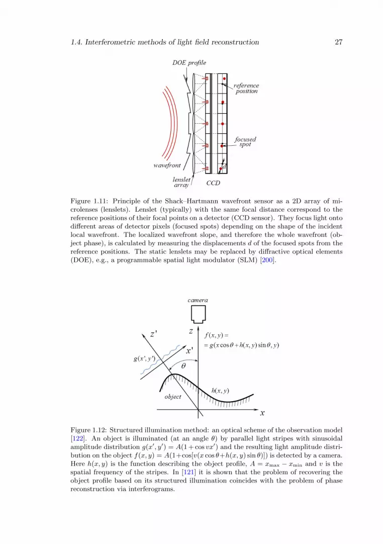
1.4. Interferometric methods of light field reconstruction 27

Figure 1.11: Principle of the Shack–Hartmann wavefront sensor as a 2D array of mi-crolenses (lenslets). Lenslet (typically) with the same focal distance correspond to thereference positions of their focal points on a detector (CCD sensor). They focus light ontodifferent areas of detector pixels (focused spots) depending on the shape of the incidentlocal wavefront. The localized wavefront slope, and therefore the whole wavefront (ob-ject phase), is calculated by measuring the displacements d of the focused spots from thereference positions. The static lenslets may be replaced by diffractive optical elements(DOE), e.g., a programmable spatial light modulator (SLM) [200].

Figure 1.12: Structured illumination method: an optical scheme of the observation model[122]. An object is illuminated (at an angle θ) by parallel light stripes with sinusoidalamplitude distribution g(x′, y′) = A(1 + cos vx′) and the resulting light amplitude distri-bution on the object f(x, y) = A(1+cos[v(x cos θ+h(x, y) sin θ)]) is detected by a camera.Here h(x, y) is the function describing the object profile, A = xmax − xmin and v is thespatial frequency of the stripes. In [121] it is shown that the problem of recovering theobject profile based on its structured illumination coincides with the problem of phasereconstruction via interferograms.

28 1. Preliminaries

steps in the wavefront can not be detected by the Shack-Hartmann sensor. How-ever, the sensor can work using partially coherent light sources, which are gener-ally cheaper than lasers [3]. The Shack–Hartmann sensor based approach seemsto be close to shearography by means of recalculation of the phase by spatialdisplacement of the incident wavefront from the reference one. One uses a sim-ple adjustment method, and the typical arrangement contains no moveable parts,what leads to low demands regarding the mechanical stability and environmentnoise. Moreover, an array of static lenslets may be replaced by a diffractive opticalelement (see Section 1.5 and Appendix B.2), e.g., by a digital micromirror deviceor a liquid crystal based spatial light modulator (LC-SLM).

A volumetric representation of an object, 3D shapes can be achieved by the2D structured images of objects ([122], see Fig. 1.12): one distinguishes moiretopography [213], the shear moire topography [14], Fourier transform profilom-etry [215], the phase profilometry [209]. These methods are very similar to theconventional interferometry based methods: the Fourier transform method [214]and the method of allocation of the centres of bands [237]. In this case thereis no strict restriction imposed on the light coherence. Despite the apparent (atfirst glance) simplicity and low cost of the structured illumination based methods,they have essential disadvantages: the sensitivity to background illumination, theresult significantly depends on the structure of the object and lighting conditions,complexity of mathematical methods and computational algorithms [87].

In this thesis we consider two fundamental light coherence based approachesused to determine the phase of light wave fields and reconstruct the complex objectamplitude: interferometric and phase-retrieval methods. They accumulate boththe relative simplicity of the optical system and the numerical methods. In thisSection we consider the established interferometric techniques, namely: phase shiftholography and shearography, linked by the common mathematical apparatus. InSection 1.4.4 certain limitations of the interferometric methods are presented. Inthe next Chapter 2 the phase-retrieval approaches are discussed.

1.4.1 Phase shifting method

The coherent superposition of two waves is the basic principle of all interferencebased methods. Here we present the extraction of the phase information from aset of observed interferograms obtained using the Michelson interferometer18 withthe phase shifting method (see [194]).

Let u1(x, y) and u2(x, y) be complex amplitudes of transverse wave fields, whichare linearly polarized in the same direction. Let u1 =

√I1e

iφ1 and u2 =√I2e

iφ2

propagate in different directions as it is illustrated in Fig. 1.13. The resultinginterference pattern at the sensor plane can be found similarly to Eq. (1.8) I =I1 + I2 + 2

√I1I2 cos(∆φ), where ∆φ = φ2 − φ1 is the phase difference between

these two waves. Due to the ambiguity of the arguments of the cosine, the phasedifference cannot be directly determined from the measurement. However, the

18 An interferometer is an optical instrument that splits a wave into two waves using a beamsplitter: delays them by (in general) unequal distances, redirects them using mirrors, recombinesthem using another (or the same) beam splitter, and detects the intensity of their superposition.Three classical interferomenters, the Mach-Zehnder, Michelson and Sagnac interferometers, aredescribed, e.g., in [190, Chapter 2.5].

1.4. Interferometric methods of light field reconstruction 29

Figure 1.13: A scheme of the Michelson interferometer, where BS denotes a beam split-ter. Two complex amplitude u1 and u2 are propagated at different distances r1 and r2,respectively, and superposed at the observation (sensor) plane.

complex amplitude u1 can be found from a number of recorded interferograms byshifting the phase of u2 [67, 228]. The phase shift is often realized by translatinga mirror of the optical setup in Fig. 1.13 via piezoelectric transducers. Thus, theintensities of interference pattern is defined as

Ir(x, y) = |u1(x, y) + u2(x, y) exp(iθr)|2 = I1 + I2 + (1.75)

+ u∗1(x, y)u2(x, y) exp(iθr) + u1(x, y)u∗2(x, y) exp(−iθr), r = 1, ...K,

where {θr} are phase shifts of u2. In order to reconstruct the term u1(x, y), whichcan represent the object wavefront, K holograms are summed up with the samephase shifts used during their recording [236]

I(x, y) =1

K

K∑r=1

Ir(x, y) exp(iθr) = u1(x, y) · u∗2(x, y) + (1.76)

+(|u1(x, y)|2 + |u2(x, y)|2) · 1

K

K∑r=1

exp(iθr) +

+(u∗1(x, y) · u2(x, y)) · 1

K

K∑r=1

exp(i2θr).

It can be shown that at least three exposures {Ir}3r=1 (e.g., with phase shiftsθr = {0, 2π/3, 4π/3}) are required in this method. Assume that θr = rθ0 ∀ r. Fora perfect reconstruction of the first term u1(x, y) · u∗2(x, y) phases {θr} should befound from the following expressions [83]

K∑r=1

exp(irθ0) =exp(iKθ0)− 1

exp(iθ0)− 1exp(iθ0) = 0, (1.77)

30 1. Preliminaries

K∑r=1

exp(i2rθ0) =exp(iKθ0)− 1

exp(iθ0)− 1

exp(iKθ0) + 1

exp(iθ0) + 1exp(iθ0) = 0. (1.78)

The solution for Eq. (1.77) is θr = 2π rK for any integer K ≥ 3. For K = 2 the

solution θ0 = π does not satisfy Eq. (1.78) as [83]

exp(i2θ0)− 1

exp(iθ0)− 1

exp(i2θ0) + 1

exp(iθ0) + 1exp(iθ0) = 2. (1.79)

Thus, the complex-valued wave field u1 can be therefore found by, e.g., three orfour holograms exposures. Let {Ir} be the interferograms with the correspondingphase shifts θr = {0, π2 , π,

3π2 } for r = {0, 1, 2, 3}, respectively. Then

u1(x, y) =I0(x, y)− I2(x, y) + i[2I1(x, y)− I0(x, y)− I2(x, y)]

4u∗2(x, y), (1.80)

u1(x, y) =I0(x, y)− I2(x, y) + i[I1(x, y)− I3(x, y)]

4u∗2(x, y). (1.81)

Note that the intensity distribution of the interferograms can be also repre-sented in the form (cf. Eq. (1.75))

Ir(x, y) = I1(x, y) + I2(x, y)︸ ︷︷ ︸IDC(x,y)

+ 2√I1(x, y)I2(x, y) cos(∆φ(x, y) + θr), (1.82)

thus, the (wrapped) phase difference can be found, e.g., using four shifts as

W{∆φ(x, y)} = arg{I0(x, y)− I2(x, y) + i(I3(x, y)− I1(x, y))}. (1.83)

1.4.2 Digital holography

First experiments in numerical reconstruction of optical holograms date back tothe late 1960s – early 1970s [78, 127]. The widespread use of computers and re-placement of photographic plates by a CCD sensor is considered to be an origin ofdigital holography: numerical wave field reconstruction in digital holography be-came properly available only since its practical confirmation (starting from 1994,[192]). A quick and effective method for both the wave field reconstruction and reg-istration was necessary, and CCD based systems showed its efficiency and usability:all data could be sent direct to a computer without any additional operations.

A typical scheme of recording a digital hologram is illustrated in Fig. 1.14. Aplane laser beam is divided by a beam splitter19 (BS) into two beams: a referencebeam, which falls directly onto a digital sensor (uref ), and an object beam, whichilluminates an object and after being scattered from the investigating object, alsotravels to the sensor (uobj).

The numerical reconstruction of the hologram consists of applying to therecorded hologram (1.9) a transform that implements the backward wave field

19 It is assumed that a beam splitter reflects 50% of the incident light and transmits the other50% [125].

1.4. Interferometric methods of light field reconstruction 31

Figure 1.14: Schematic diagram of a digital holographic setup with the Mach–Zenderinterferometer. The intensity of the interference patterns, generated by superposed object(diffracted by an object) and (unchanged) reference beams, is detected on a sensor.

propagation from the sensor plane to the object plane. Recall that the holo-gram exposure I contains a zero order DC term of diffraction and two conju-gated (twin virtual and real) images. In order to obtain the complex-valuedobject wave field, one has either to eliminate other three terms before the re-construction or apply the reconstruction transform to the entire hologram andonly than extract the interesting term. The latter solution is known as the so-called off-axis recording hologram (the classical Leith-Upatnieks’s method, see,e.g., [79, 80, 125, 190, 194, 232, 234, 236]). Typically it can be found using thefirst Rayleigh–Sommerfeld diffraction integral20 as [192, cf. Eq. (1)], [194, cf. Eq.(3.1)]

Γ(ξ, η) =iz

λ

∫∫I(x, y)uref (x, y)

exp(−ikr)r2

dxdy, (1.84)

where r =√

(ξ − x)2 + (η − y)2 + z2 is the distance between a point in the holo-gram plane and a point in the reconstruction plane, z is the distance between theobject and sensor planes. In off-axis holography [132, 133], a spatial offset anglebetween the reference and object beams is introduced. When this angle exceedsa minimum allowable angle (discussed in, e.g., [79, § 9.4.3]), the twin images arenot contaminated by each other nor by other, say DC, wave components. Thus,the object wave field is extracted.

The method of eliminating interfering terms in recorded holograms before thereconstruction is called on-axis or in-line holography21. In the on-axis methodof recording holograms the object and reference beams are collinear, and severalexposures of holograms {Ir}Kr=1 of the object are recorded with phase shifting{θr}Kr=1 of the reference beam as it is discussed before. This method can berealized via the mentioned phase shifting method using a moveable mirror or aspatial light modulator (digital phase shifting holography [228, 230]). In this casethe recorded holograms are of the form:

20 see Section 1.3.521 Note while Gabor had no sources giving light with sufficient coherence, he had to produce

in-line holograms where object and reference waves were travelling in the same direction orthog-onally to the hologram. Leith and Upatniks were the first who took advantage of the coherenceof laser light and who gave the object and the reference beams different directions [125].

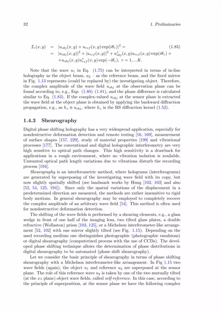
32 1. Preliminaries

Ir(x, y) = |uobj(x, y) + uref (x, y) exp(iθr)|2 = (1.85)

= |uobj(x, y)|2 + |uref (x, y)|2 + u∗obj(x, y)uref (x, y) exp(iθr) +

+uobj(x, y)u∗ref (x, y) exp(−iθr), r = 1, ...K.

Note that the wave u1 in Eq. (1.75) can be interpreted in terms of in-lineholography as the object beam, u2 – as the reference beam, and the fixed mirrorin Fig. 1.13 represents (could be replaced by) the investigating object. Therefore,the complex amplitude of the wave field uobj at the observation plane can befound according to, e.g., Eqs. (1.80)–(1.81), and the phase difference is calculatedsimilar to Eq. (1.83). If the complex-valued uobj at the sensor plane is extractedthe wave field at the object plane is obtained by applying the backward diffractionpropagation, e.g., as hz ~ uobj , where hz is the RS diffraction kernel (1.52).

1.4.3 Shearography

Digital phase shifting holography has a very widespread application, especially fornondestructive deformation detection and remote testing [16, 169], measurementof surface shapes [157, 229], study of material properties [199] and vibrationalprocesses [177]. The conventional and digital holographic interferometry are veryhigh sensitive to optical path changes. This high sensitivity is a drawback forapplications in a rough environment, where no vibration isolation is available.Unwanted optical path length variations due to vibrations disturb the recordingprocess [194].

Shearography is an interferometric method, where holograms (interferograms)are generated by superposing of the investigating wave field with its copy, butnow slightly spatially shifted (see landmark works by Hung [102, 103] and also[52, 54, 125, 194]). Since only the spatial variations of the displacement in apredetermined direction are measured, the methods are rather insensitive to rigidbody motions. In general shearography may be employed to completely recoverthe complex amplitude of an arbitrary wave field [54]. This method is often usedfor nondestructive deformation detection.

The shifting of the wave fields is performed by a shearing elements, e.g., a glasswedge in front of one half of the imaging lens, two tilted glass plates, a doublerefractive (Wollaston) prism [103, 125], or a Michelson interferometer-like arrange-ment [52, 102] with one mirror slightly tilted (see Fig. 1.15). Depending on theused recording medium one distinguishes photographic (photographic emulsions)or digital shearography (computerized process with the use of CCDs). The devel-oped phase shifting technique allows the determination of phase distributions indigital shearography to be automated (phase shift shearography).

Let we consider the basic principle of shearography in terms of phase shiftingshearography with a Michelson interferometer-like arrangement. In Fig 1.15 twowave fields (again), the object u1 and reference u2 are superposed at the sensorplane. The role of this reference wave u2 is taken by one of the two mutually tilted(at the xz plane) object wave fields, called self-reference. In this case, according tothe principle of superposition, at the sensor plane we have the following complex

1.4. Interferometric methods of light field reconstruction 33

Figure 1.15: Arrangement for digital shear interferometer. The input object wave isdivided by a beam splitter (BS), so two wave, the object u1 and so-called self-referencewave u2, travel along different ways and superpose at the sensor plane. Since the fixedmirror is here tilted in the xz plane, u1 is shifted on a sensor by d.

amplitude:

u(x, y) = u1(x, y) + u2(x+ d, y) = (1.86)

=√I1(x, y)eiφ(x,y) +

√I2(x+ d, y)eiφ(x+d,y),

where the spacing between the two correlated areas of the object surface d iscalled the share. The shearographic image (interference pattern of u) may bemathematically represented [52, 102, 103, 125] as follows [54, cf. Eq. (3)]

I(x, y) = I1(x, y) + I2(x+ d, y)︸ ︷︷ ︸IDC(x,y)

+ 2√I1(x, y)I2(x+ d, y)︸ ︷︷ ︸

Im(x,y)

· cos(ϕ(x, y)), (1.87)

where ϕ(x, y) = φ(x, y) − φ(x + d, y) is the phase difference due to shearing,IDC(x, y) is again the DC term as in Eq. (1.82) and Im(x, y) is a modula-tion of the interference. Deformation of the object results in the wave fields√I1(x, y)ei(φ(x,y)+∆φ(x,y)) and

√I2(x, y)ei(φ(x+d,y)+∆φ(x+d,y)) and their superpo-

sition yields [103, cf. Eq. (2)]

I ′(x, y) = IDC(x, y) + Im(x, y) cos(ϕ(x, y) + ∆ϕ(x, y)), (1.88)

where ∆ϕ(x, y) denotes a phase change due to the object surface deformation.According to the described phase shifting method with four phase shifts θr ={0, π2 , π,

3π2 } one records four exposures Ir(x, y) = IDC(x, y)+Im(x, y) cos(ϕ(x, y)+

θr) and I ′r(x, y) = IDC(x, y)+Im(x, y) cos(ϕ(x, y)+∆ϕ(x, y)+θr) for these phaseshifts, r = {1, 2, 3, 4}. Then, the phase differences can be found similar to Eq.(1.83) as [54, cf. Eq. (5)]

W{ϕ(x, y)} = arg{I0(x, y)− I2(x, y) + i(I3(x, y)− I1(x, y))}, (1.89)

34 1. Preliminaries

and the process is repeated for the deformed patterns, yielding [54, cf. Eq. (5)]

W{ϕ(x, y) + ∆ϕ(x, y)} = arg{I ′0(x, y)− I ′2(x, y) + i(I ′3(x, y)− I ′1(x, y))}. (1.90)

Therefore, the phase change due to the deformation ∆ϕ(x, y) is subsequentlydetermined by subtracting of the unwrapped phase ϕ(x, y) + ∆ϕ(x, y) from theunwrapped ϕ(x, y) [102, 103].

1.4.4 Limitation of interferometric techniques

Let us summarize certain limitations of the interferometric (holographic) methods:

• Since these methods are based on the superposition principle, they have anessential demand regarding the temporal/spatial coherence. The insufficientcoherence leads to poor imaging of interference patterns (the additional in-terference component of Eq. (1.8) is small).

• The superposition of two waves requires considerable efforts to align opticalcomponents on an optical system, and the proper alignment is very timeconsuming and troublesome. In some cases it is very difficult to realizefitting and fine overlapping of the investigating object wave uobj ≡ u1 withthe reference wave uref ≡ u2 [3].

• Since these two waves travel along their separate paths, the result of measure-ments is high sensitive to various environmental disturbances as vibrationsor thermal fluctuations. Thus, the experimental configuration must be iso-lated from vibration to a large extent. In particular, it is of importancefor temporal phase shifting, because the mechanical stability over the entireperiod of measurement must be ensured [3].

• Experimental arrangements for interferometric methods are technically quitecomplex and therefore expensive due to the use of many optical componentssuch as beam splitters, lenses, etc. Moreover, the more complex opticalsystem, the more sources of various distortions to be compensated.

1.5 Diffractive optical elements (DOEs)

The phase change can be easily realized using not a moveable mirror but diffractiveoptical elements, e.g., with LC-SLMs, by the modulation of a light wave field.Let us consider the modulating optical elements which help realizing the linearoperations to obtain a desired wave field distribution for various applications.

The modulating optical systems may contain both classical optical elements,such as lenses, prisms or beam splitters, and quite sophisticated ones with a fixedprofile/relief or reconfigurable (electronically controlled) structure. The light mod-ulation in such an optical system is primarily based on diffractive media whichtransform either the amplitude or phase of the incident beam.

One of the straightforward applications of such modulating optical elements isthe wave field synthesis/design, i.e. generating of a desired volumetric light wavefield distribution within a region of interest in 3D space.

1.5. Diffractive optical elements (DOEs) 35

1.5.1 DOEs with fixed profiles

The first modulating optical element, called diffractive optical element (DOE), is adiffraction grating constructed more than two hundreds years ago [207]. It had bi-nary amplitude or phase transmittance and looked like a transmissive or reflectiveplate with a thin microrelief, calculated according to the diffraction theory. Forinstance, the simplest amplitude one-dimensional diffraction grating is a flat opti-cal transparency22 with alternate light and dark stripes of the same width d. Afterone-dimensional binary amplitude and phase diffraction gratings one constructedtwo-dimensional radially-symmetric gratings (zone plates). The essential develop-ment of diffraction optics was held back by the absence of suitable materials andtechnologies of their processing which would have allowed accurate constructingof diffraction patterns with a complex surface/profile. The use of computers madea revolution in the creation of DOEs: in the late 1960s computers were used forthe synthesis of holograms of mathematically determined objects. First computergenerated holograms were again binary, invented by Lohmann [23, 24, 139]. Theywere printed on a computer line printer, then optically reduced and reconstructedin optical setups using coherent laser illumination [233]. The recording mediumwas represented in the form of square cells. A full transparent opening inside eachcell modulates both the amplitude (by the size of the opening) and phase (bya shift of the opening within cells) of the desired object [221], [236, Lecture 5].Then, the use of more sophisticated devices capable of recording grey scale imageswas suggested for recording computer generated holograms [128]. In addition, thekey problem of coding – recording on a physical medium complex-valued functionsand construction of corresponding amplitude-phase transparencies – has been re-solved. Progress in microelectronics and laser technology gave in the 1980s thephotoplotter and electron-beam lithography, what made the problem of creationof DOEs with a complex profile practically realizable, e.g., creation of DOEs withunique characteristics, unattainable in the traditional optics, such as focusators oflaser beam.

1.5.2 Reconfigurable DOEs: spatial light modulators (SLMs)

Generally, DOEs can be specified by the numeric value (binary and with a complexprofile), amplitude-phase characteristics of the transmission function (amplitude,phase, or complex-valued) and by the specifics of their microrelief: the linearor circular gratings, zone plate/kinoform lens, computer generated hologram andspatial light modulator (see, e.g., [207, 236] for more details).

Spatial light modulators (SLMs) are reconfigurable DOEs, which give a sig-nificant flexibility of the optical system to modulate the light wave field and findvery widely application of light wave field synthesis. SLMs are based on liquidcrystals, microelectromechanical systems or magneto- and acusto-optic modula-

22 If such a grating is illuminated by the monochromatic light beam with the wavelength λ,which is incident normal to the plane of the grating, a number of light beams will be formed asthe result of diffraction on a periodic structure of stripes. These beams will travel at differentangles θp corresponding to various diffraction orders. The angle θp depends on the grating periodd, and assuming that the angles are small θp = pλ

d, where p = 0,±1,±2... The light intensity

changes in the inverse proportion to p as I(θp) ∼ ( 2λπdθp

sin(πd2λθp))2 ≈ 1

(2p+1)2[207].

36 1. Preliminaries

tors (see [47, 101, 159] for mode details). Digital micromirror devices (DMDs) area type of such a reconfigurable devices which modulate an incident wave by reflec-tion [221]. These devices consist of a large 2D array of electronically controlledmicromirrors taking one of a few present angles [43]. In [124] one of pioneeringworks, where DMDs are used to reconstruct a binary hologram, is presented. Aholographic 3D image projection by DMD is presented in [100]. At present time,one uses typically the electronically reconfigurable SLMs23, and commodity SLMsare primarily based on liquid crystals. The main principle of LCs, and thereforeliquid crystal based SLMs (LC-SLMs), is based on birefringence, i.e. the refractiveindex of liquid crystals depends on the orientation of molecules of LCs, which,in turn, can be controlled by apply an electrical charge. In general one distin-guishes optically and electrically addressed LC-SLMs depending on the way theelectrical charge is applied to a LC. The optically addressed SLMs use incoherentlight to control the orientation of the liquid crystal molecules. The intensity ofthe incoming incoherent light is sensed by a photo-sensor, which transforms thelight intensity into an electrical charge directly over the liquid crystal. In electri-cally addressed SLMs the voltage to the liquid crystals is applied via an electrodesconnected with a silicon chip of pixel cells.

The structure of DOEs or data which is required to be programmed on SLMsare commonly calculated by iterative projection methods (see, e.g., [121, 122, 207,238]) derived based on the mentioned Gerchberg–Saxton algorithm [71]. Thisalgorithm can be used to specify the desired volumetric wave field [203]. In [11]the amplitude and phase are tried to be separately controlled by two phase-onlySLMs (double-phase hologram for the complex modulation). SLMs (and moregenerally DOEs) may be used extensively in holographic data storage [90, 210],optical computing and imaging [12, 15, 86] and as a component of a holographicdisplay technology [25, 126, 172]. They also often find application in phase-contrastmicroscopy and holographic optical tweezers [131, 161, 176, 187]. For instance, theShack–Hartmann wavefront sensor illustrated in Fig. 1.11 can be realized using aDMD or an LC-SLM. Typically there are LC-SLMs for the amplitude- and phase-only modulations.

The structure of an LC-SLM in the used 4f optical system and the resultingtransfer function of a phase modulating SLM is presented in Appendix B.2.

23 Note, however, that DMDs are still very attractive as they provide higher contrast ratio,brightness and optical efficiency comparing to SLMs [221].

Chapter 2

Introduction to phaseretrieval

Previously, in Section 1.4, the recovering quantitative phase information from in-terference patterns by interferometric (holographic) techniques is considered. Inthis Chapter we deal with the diffraction propagation of a light wave field, whereeach point of the illuminated object is a source of interfering secondary wavelets.The so-called phase retrieval is an alternative approach used to estimate the phaseof a complex-valued light wave field from a number of the spatial intensity measure-ments of diffraction patterns at different observation planes. The main advantagein comparison with the conventional interference based methods is that no dis-tinct reference wave is required. Thus, phase retrieval has relatively low demandsregarding both the coherence of light and the mechanical stability of the experi-mental arrangement [3]. Moreover, the optical system for phase-retrieval methodsare often simpler, more robust with respect to disturbances such as vibration and,what is also important, cheaper comparing with interferometric methods with areference beam. In other hand, the complex-valued wave field and, in particular,the phase can not be computed so straightforward as before: see Eqs. (1.80)–(1.81) and (1.83). Let us overview the used diffraction propagation model and theconventional phase recovering techniques more in detail, and consider the author’scontribution in the development of parallel iterative phase-retrieval algorithms.

2.1 Plane-to-plane propagation modeling

A typical setup of the diffraction wave field propagation is illustrated in Fig. 2.1.Let a plane laser beam illuminates an object, and being scattered by it (or passedthrough a transparent object) travels in the direction to a sensor along the opticalaxis z. The light wave field which appears immediately after the object is typicallycalled the object wave field [79, 80] denoted hereafter by u0(ξ, η). The correspond-ing ξη plane, where the transverse u0 is defined, is called the object plane. Thisobject wave field, propagated to a sensor according to the Huygens–Fresnel princi-ple, results in the diffracted wave field uz(x, y) at the observation plane. The link

37

38 2. Introduction to phase retrieval

Figure 2.1: Propagation model of the diffracted wave field. The transverse ξη objectplane is parallel to the observation xy plane at the distance z from it. The link betweenthe object u0(ξ, η) and sensor uz(x, y) wave fields is defined in the convolutional formby uz(x, y) = {u0 ~ az}(x, y), where az denotes a shift-invariant diffraction kernel of theforward wave field propagation from the object to the observation/sensor plane.

between these two transverse wave fields in terms of the scalar diffraction theoryis formulated with the used plane-to-plane propagation model as follows

uz(x, y) = {u0 ~ az}(x, y) =

∞∫∫−∞

u0(ξ, η) · az(x− ξ, y − η)dξdη, (2.1)

where az is a shift-invariant diffraction kernel1 of the wave field propagation fromthe object to the sensor plane and the subindex z emphasizes the propagationdistance between these planes.

If the complex amplitude uz(x, y) at the sensor plane is given (e.g., from anumber of hologram exposures {Ir}), the object wave field is calculated by thebackward wave field propagation from the sensor to the object plane. If the diffrac-tion kernel az is invertible, the estimate of the complex-valued transverse wave fieldat the object plane u0 is calculated as

u0(ξ, η) =

∞∫∫−∞

uz(x, y) · a−z(x− ξ, y − η)dxdy, (2.2)

Eq. (2.1) can be represented via a linear diffraction operator uz(x, y) =Dz{u0}(x, y) = {u0 ~ az}(x, y), and the object reconstruction according to Eq.(2.2) – via the inverse operator u0(ξ, η) = D−1

z {uz}(ξ, η) = {uz ~a−z}(ξ, η). Notethat the size of the detector (photographic plate, CCD sensor) is finite. The esti-mate u0(ξ, η) is perfect (precise for any u0, u0 = u0) only if uz(x, y) is given forthe whole transverse xy plane, i.e. the detector is of infinite size [125]. The finitesize of the sensor (given measurements) may lead to the ill-posedness of the inverseproblem of the object wave field u0 reconstruction and, as the result, to corrupted(e.g., blurred) wave field reconstructions. Note also, that the observations (e.g.,{Ir}) are generally noisy due to various disturbances of the optical path such as

1 The diffraction propagation for the near-field zone is typically defined by the Rayleigh–Sommerfeld solution of the Maxwell–Helmholtz equation or its Fresnel approximation, see Section1.3.5 and 1.3.6.

2.2. Free space diffraction propagation models 39

Figure 2.2: An experimental configuration for multi-plane phase retrieval. The intensityof the light wave field scattered by an object is recorded across a sequence of differentobservation planes using a sensor which moves along the optical axis z. Here the objectwave field is denoted by u0 and the intensity observations {|ur|2}, r = 1, ...K are obtainedat the distances zr = z1 + (r − 1) ·∆z, where z1 is the distance between the object andthe first measurement plane and ∆z is the fixed distance between following transverseobservation planes.

vibration, dust and so on. In addition, the problem of the object wave field recon-struction is complicated due to nonlinearity of the computation (unwrapping) ofthe object phase (see Eq. (1.83)).

2.2 Free space diffraction propagation models

The straightforward experimental setup for recording the result of the free spacediffraction propagation to different distances {zr} can be realized by a moveablesensor as it is illustrated in Fig. 2.2 or [7, Fig. 1]: a CCD camera is sequentiallymoved between K measurement planes (separated by a distance ∆z) using a mo-torized precision stage. Here the wave field propagation through the space layerof the width zr can be described via the (say, ASD, Eq. (1.48)) transfer functionsor (e.g., RS (1.52) or Fresnel (1.59)) diffraction kernels. If the diffraction opera-tor Dzr corresponding to the forward wave field propagation to the distance zr isinvertible (in particular, in [197] it is shown that the RS diffraction operator Dzris invertible) and the complex-valued wave field ur(x, y) at the r-th sensor planeis given, one can reconstruct the wave field at the object plane with the inversediffraction operator D−1

zr , namely u0(ξ, η) = D−1zr {ur}(ξ, η) by various methods.

One distinguishes the following conventional continuous methods of the complex-valued wave field reconstruction [125]

• reconstruction via the Rayleigh–Sommerfeld diffraction integral (zr � λ,con. Eq. (1.52))

ur(x, y) = F−1{F{u0}(v1, v2) · F{hr}(v1, v2)}(x, y), (2.3)

u0(ξ, η) = F−1{F{ur}(v1, v2) · (F{hr}(v1, v2))∗}(ξ, η);

• reconstruction via the angular spectrum decomposition (con. Eq. (1.45))

u0(ξ, η) = F−1{F{ur}(v1, v2) ·H∗r (v1, v2)}(x, y); (2.4)

40 2. Introduction to phase retrieval

• reconstruction with the Fresnel approximation of the diffraction kernel (zr �√ξ2 + η2, con. Eq. (1.59))

ur(x, y) = F−1{F{u0}(v1, v2) · F{gr}(v1, v2)}(x, y), (2.5)

u0(ξ, η) = F−1{F{ur}(v1, v2) · (F{gr}(v1, v2))∗}(x, y);

• reconstruction via the Fresnel approximation in terms of chirp functions2(con.Eq. (1.60))

u0(ξ, η) =e−ikzr

−iλzre−ik2zr

(ξ2+η2)F−1{ur(

x

λzr,y

λzr

)e−ik2zr

(x2+y2)}(ξ, η); (2.6)

• reconstruction using the Fresnel transfer function (con. Eq. (1.69))

u0(ξ, η) = F−1{F{ur}(v1, v2) ·G∗r(v1, v2)}(x, y). (2.7)

The subindex r emphasizes the calculation of the transfer functions (Hr, Gr)and diffraction kernels (hr, gr) of the diffraction wave field propagation to variousdistances {zr}Kr=1, r = 1, ...K. Note that, the free space wave field propagationcan be also imitated by the 4f configuration using a phase modulating LC-SLM[4, 53] (see Section 5.1).

2.3 Inverse problem of phase retrieval

Phase retrieval is exploited in many engineering and scientific areas as astronomy[36, 63], crystallography [73, 96, 153], microscopy [71, 155] aberrations estima-tion/correction [62, 174], diffraction and 3D imaging, tomography, remote sensing,nondestructive testing, material analysis to name just a few. We refer to the books[104, 211] and review articles (e.g., [59, 107, 119, 140]) for descriptions of variousinstances of the phase-retrieval problem and further references.

From the mathematical point of view, recovering the phase information can bestated as an inverse problem [91, 109], where the measured intensities of diffractionpatterns represent the observed effect caused by (aside from the amplitude) aunknown object phase. Since the wave fields at the sensor planes are assumed tobe generated by radiation from the object plane, in this thesis the reconstructionof the phases, missed in measurements, is produced through the object planedistribution considered as the only unknown variable. Following Eq. (2.1), theproblem of multi-plane phase retrieval can be formulated as [91]∣∣∣∣ur(x, y)

∣∣∣∣2︸ ︷︷ ︸output

=

∣∣∣∣∞∫∫−∞

u0(ξ, η)︸ ︷︷ ︸input

· ar(x− ξ, y − η)︸ ︷︷ ︸system

dξdη

∣∣∣∣2, r = 1, ...K, (2.8)

2 A chirp is a signal in which the frequency of oscillations linearly increases/decreases de-pending on the spatial coordinates [125, Chapter A.13]. The exponential one-dimensional chirpfunction of infinite support can be presented as c(t) = exp(iαπt2) with its Fourier transform

as again a scaled chirp function with a constant amplitude F{c(t)}(v) = i√α

exp(−π v2

α). This

function got its name from applications in testing transmission systems for acoustic signals, andis of the extensively usage in diffraction theory.

2.4. Overview of phase-retrieval techniques and our contribution 41

where the investigating complex-valued object u0 is the input of the optical systemand the diffraction kernels {ar}Kr=1 give the mathematical description of the usedcoherent imaging system of the wave field propagation at different distances fromthe object plane {zr}r. In contrast to Eq. (2.1), we use here the subindex r toemphasize various distances of the diffraction propagation. In this formulation,the direct problem is to compute the output – a number of intensity observations{|ur|2} as the result of the forward wave field propagation of the object wave fieldu0 to distances {zr}r (see Section 2.2), the output of the optical system for varioussettings. The goal of the inverse problem is to determine the input of the systemthat gives rise to the (noisy) measurements of the output [91]. Note that sincethe phase φr of the wave field at the r-th sensor plane ur = |ur|eiφr is absent, theintegral in Eq. (2.8) can not be directly inverted (similar to Eq. (2.2)).

2.4 Overview of phase-retrieval techniques and ourcontribution

In the past decades, the inverse problem of phase retrieval is treated in two fun-damentally different ways: by deterministic or iterative approaches.

2.4.1 Deterministic phase retrieval

The deterministic approaches are based on the so-called transport-of-phase [217,cf. Eq. (5)] and transport-of-intensity (TIE, [217, cf. Eq. (4)]) equations origi-nated by Teague [216, 217, 218]. The main idea is to derive formulas which describea one-to-one relation between the measured intensity and the undetected phase.These formulas are calculated via physical properties of the light waves, mainlydirectly from the Maxwell–Helmholtz wave equations (see, e.g., [120]), typicallyprovided the light wave propagation in only one direction, say along the z axis. Inaddition, TIE based methods are widely used to define the phase of a monochro-matic light field [120, 218]. The phase of a wave field is shown to be retrieved bycomputing the axial intensity derivative ∂

∂z I(x, y, z), and the direct solution canbe found from two [217] or multiple defocusing images [6, 206]. Note that sincethe intensity derivative can not recorded directly, it is obtained by the central,forward and backward finite differences [206, cf. Eqs. (1)]:

∂

∂zI(x, y, z = 0) =

I(x, y,∆z)− I(x, y,−∆z)

2∆z, (2.9)

∂

∂zI(x, y, z = 0) =

I(x, y,∆z)− I(x, y, 0)

∆z, (2.10)

∂

∂zI(x, y, z = 0) =

I(x, y,−∆z)− I(x, y, 0)

−∆z. (2.11)

The conventional image is denoted by I(x, y, z = 0) and (also measured) diversityimages are {...I(x, y,−∆z), I(x, y,∆z), ...}. In Fig. 2.3 the recording process ofthe phase-diversity images is illustrated.

The phase diversity incorporates the additional information on the wave fieldpropagation and allows improving the phase imaging by multiple measurements

42 2. Introduction to phase retrieval

Figure 2.3: Optical layout of a phase-diversity system. If the conventional image is de-graded by aberrations in the optical system, the phase-diversity images will be thereforedegraded by the combination of the same aberrations and a known amount of defocus.The reconstruction is performed by a number of diversity images recorded at different dis-tances z by various defocusing ±∆z,±2∆z, .... Dashed lines in the right image representthe positions of a sensor to measure the diversity images [6, 171, 174, 202].

with various defocusing ∆z [206]. We refer to [120] for the phase gradient basedmethod and to the mentioned works by Teague and [3, 6, 171, 174, 202] for theadditional details.

TIE based techniques are relatively fast, computationally efficient and can beimplemented in many existing systems. Nevertheless, their are very sensitive toinaccuracy of the optical setup such as misalignment at the xy plane, misfocusing(with respect to z) and noise. In general, TIE based techniques are recognized tofail in the case of a significant large amount of noise [171, 224].

2.4.2 Iterative phase retrieval

Perhaps the first efficient iterative algorithm for phase retrieval is originated byGerchberg and Saxton [71], initially for a single measurement plane. It is shownin Section 1.3.7 that the wave field propagation to the far field, the Fraunhoferregion, is proportional to the Fourier transform (see Eqs. (1.72)–(1.73)). Origi-nally, the Gerchberg–Saxton (GS) algorithm was applied in the specific case, wherethe intensity of the wave field is known across a spatial and the correspondingFourier domain, e.g., at the far-field zone or at the focal plane of a lens [138, 238].In Fig. 2.4 a two lenses scheme of the conventional iterative Gerchberg–Saxtonphase-retrieval algorithm is presented. The common idea consists of the iterativereplacement of the estimated amplitude at the object |u0(ξ, η)| and Fourier (ob-servation) planes |uF (kξf ,

kηf )| by measured or a priori information keeping the

computed phase.

The work on the GS algorithms was continued and improved by many authors(see, e.g., [57, 231]). It is shown that such iterative phase recovering can be realizednot only with respect to the object plane [57], but also to measurement planes,using defocus images only (e.g., Misell’s variation of the GS algorithm [155]). In1982 Fienup systematized the earlier works and introduced some, for now classi-

2.4. Overview of phase-retrieval techniques and our contribution 43

Algorithm: Gerchberg–Saxton error-reduction phase retrieval (GS)

Initialization: φ00(ξ, η) = φinit0 (ξ, η) for t = 0

Repeat for t = 0, 1, 2, ...1. Object update by a priori a0(ξ, η), say a0(ξ, η) = 1:ut0(ξ, η) = a0(ξ, η) · exp(iφt0(ξ, η))2. Forward propagation and calculation of the phase φtFφtF (kξf ,

kηf ) = arg{ e

ikf

iλf ei f2k (( kξf )2+( kηf )2)F{a0 ◦ exp(iφt0)}(kξf ,

kηf )}

3. Update of the Fourier image by the measured aF (kξf ,kηf ) =

√IF (kξf ,

kηf ):

utF (kξf ,kηf ) = aF (kξf ,

kηf ) · exp(iφtF (kξf ,

kηf ))

4. Backward propagation and calculation of the object phase φt+10 (ξ, η)

φt+10 (ξ, η) = arg{i e

−ikf

λf e−ik2f (ξ2+η2)F−1{aF ◦ exp(iφtF )}

End on t

cal, types of phase-retrieval algorithms3[59]: error-reduction (GS), gradient search(steepest-descent) methods and input-output algorithm (further developed to thehybrid input-output algorithm, see, e.g., [212]). Similar methods are proposedfor fractional Fourier and Fresnel transforms [238] instead of Fourier transformsas the transfer functions of the wave field propagation for both the wave fieldreconstruction [238] and optical design [58, 111].

In [31, 59, 201] it is shown that the prior knowledge about the wave field andits support is employed (as constraints) for successful phase retrieval, to make thesolution unique. However, in practice, when the intensity information containsmeasurement noise, the iterative scheme is accompanied with problems of conver-gence (the convergence rate depends on the investigating object and in some casesis quite slow [60, 61]), stagnation [61, 201] and uncertainty [212] (more than onesolution consistent with the noisy measurements). It makes phase retrieval a diffi-cult ill-posed inverse problem. In general, the problem of the uniqueness of phaseretrieval is open4: even if in practical situations the phase-retrieval problems dohave unique solutions and reasonably reliable reconstruction algorithms have beendeveloped [154] in the presence of noise, it has not yielded any quantitative resultson the probability of uniqueness for any given level of noise [201].

Despite the fact that solutions are in general not unique [31, 201], the ambiguityof the reconstructed phase can be substantially reduced using a number of obser-vations [6] either at the sensor plane [7, 178] or diffraction patterns with spatialphase/amplitude modulations at the object plane [22, 241], what can be appliedfor both the reconstruction [106, 240] and synthesis [203]. It is recognized that a

3 The common idea is always the same: replace the calculated amplitude at the observationplane by the measured one and modify the calculated object wave field.

4 We refer to, e.g., [31, cf. Fig. 7] for more details. Note also than whether the objects arediscrete or continuous, it is easy to make up cases that they are ambiguous. If, for instance,c(x, y) and d(x, y) are two functions of finite support with Fourier transforms C(v1, v2) andD(v1, v2), respectively, then the convolutions q1 = c(x, y)~d(x, y) and q2 = c(x, y)~d∗(−x,−y)are different objects as long as neither c nor d is conjugate centrosymmetric. They have Fouriertransforms Q1(v1, v2) = C(v1, v2) · D(v1, v2) and Q2(v1, v2) = C(v1, v2) · D∗(v1, v2) that havethe same modulus |Q1(v1, v2)| = |Q2(v1, v2)| = |C(v1, v2)| · |D(v1, v2)| and the objects q1 andq2 are therefore ambiguous.

44 2. Introduction to phase retrieval

Figure 2.4: The scheme of the iterative error-reduction GS phase-retrieval algorithm[59, 238] and the optical setup for its implementation [138, 238]. Two lenses with thesame focal distances f are arranged to provide accurate mapping of the object wave fieldu0 into the Fourier plane giving the wave field uF (v1, v2) = F{u0}(v1, v2), v1 = kξ

f,

v2 = kηf

. The backward propagation is numerically calculated via the inverse Fouriertransform. At each iteration (t = 0, 1, ..) the amplitude of the wave field at the objectat0(ξ, η) = |ut0(ξ, η)| and the observation (Fourier) plane at+1

F (v1, v2) = |ut+1F (v1, v2)| are

updated by the prior information (e.g., a0(ξ, η) = 1) or given measurements (typicallyaF =

√IF , where IF is the (noisy) intensity observation). The initial guess for the object

phase φinit0 is typically taken randomly. The multiplicative components connected withthe Fourier transform in GS are omitted for simplicity.

proper choice of the initial guess and/or applying additional constraints/penaltiescan also be employed to improve the uniqueness of the solution, helps to overcomethe convergence uncertainty, decrease the influence of the noise and, as the result,leads to better reconstruction quality. Here we wish also to mentioned that theproblem with misalignments, say with the displacement of a sensor can be solvedby, e.g., the recent work by M. Agour [3, 4].

It is recognized that the iterative multi-plane (K > 2 in Eq. (2.8)) phase-retrieval techniques are more flexible, effective (e.g., iteratively the misfocusingerror may be compensated by aggregating of a number of estimates) and robust toa significantly large amount of noise in measurements with respect to deterministicapproaches. Thus, iterative phase retrieval is considered to be more productive fortreating the phase problem*.

It is found [3, §4.1],[120] that the the complex-valued 3D wave field can beobtained by four intensity measurements of diffraction patterns, K = 4. It is,however, not sufficient in case of noise and possible (mechanical) distortions ofthe optical system. In contrast to the deterministic TIE based methods with asignificantly large number of observation from K = 3 [217] up to K = 80 [223],the iterative phase-retrieval algorithms usually operate with 5–10 (including in ourpapers P4–P7), up to 20 [7, 8] intensity measurements.

Note also, that the distance between the sensor plane ∆z in both the referred[7, 8] and our works [P4, cf. Fig. 3] is found experimentally. Rather we presentour recommendations how to choose ∆z depending on K and object size. Notethat this distance does not necessarily have to be equal for all sensor planes. Byusing the concept of spatial correlation for wave fields at the sensor planes, forboth their complex amplitude and the measured intensity of these fields, we can

2.4. Overview of phase-retrieval techniques and our contribution 45

infer, which planes are suitable to retrieve the phase and which are not [69, cf.Fig. 1] to choose proper distances between the sensor planes. The accurate choiceof ∆z is our further work.

2.4.3 Successive iterative multi-plane phase retrieval

Traditionally, the iterative phase-retrieval methods are used to reconstruct thevolumetric wave field represented at a number of sensor planes. Let us describe theprocedure of the whole wave field reconstruction, namely: the sequence of phasedistributions {φr}Kr=1 associated with the individual propagation states throughthe captured volume. Let ur(x, y) =

√Ir(x, y) exp(iφr(x, y)), r = 1, ...K, denote

2D transverse complex-valued wave field distributions at the observation planeswith given (noisy) intensities {Ir(x, y)}Kr=1. The index r corresponds to a distancezr = z1 + (r − 1) · ∆z between the parallel object and the r − th observationplanes, ∆z is a fixed distance between the observation planes. The optical setupof data acquisition is presented in Fig. 2.2. Then, the circular algorithm, wherethe volumetric wave field is reconstructed by wave field propagation from onemeasurement plane to another one (ignoring the object plane), can be written asfollows

uχ(t+1) = Dzχ(t+1)−zχ(t)

{√Iχ(t) · uχ(t) · |uχ(t)|−1

}, t = 1, 2... (2.12)

Let uχ(1) =√Iχ(1)e

φχ(1) be the initial guess of the wave field distribution atthe χ(1)-th observation plane, which consists of the measured amplitude Iχ(1) and(for example) random phase φχ(1). The subindex χ(t), t = 1, 2... shows the serialnumber of the observation plane, where the estimates of the wave field uχ(t) arecalculated. Here Dzχ(t+1)−zχ(t)

{·} denotes an invertible operator of the wave fieldpropagation from the χ(t)-th to the χ(t + 1)-th observation plane, which may berepresented via, e.g., ASD [7, 8, 178]. This operator represents5 the forward wavefield propagation to the distance ∆z = |zχ(t+1) − zχ(t)| if zχ(t+1) > zχ(t) or thebackward propagation to the same distance if zχ(t+1) < zχ(t), zχ(t+1) 6= zχ(t).The operation in the curly brackets means a replacement of the amplitude of thecalculated estimate at the χ(t)-th sensor plane by the amplitude from the intensityobservations, keeping the phase of the estimate uχ(t). The formula (2.12) definesthe modern iterative circular algorithm known as the single-beam multiple-intensityphase reconstruction (SBMIR, [7, 8, 178]) algorithm used in our works P3–P5,P7 as a reference method.

There is no specific rule determining the sequence of the sensor planes in a set.For instance, the index of the sensor plane in a sequence for the so-called forward-forward (FF, from the K-th to the first sensor plane) and forward-backward (FB,from the K-th to the (K − 1)-th sensor plane) algorithms (see [8, cf. Fig. 2]) canbe found as follows:

χ(t) =

{αK(t), for FFα2K−2(t)− 2αK(α2K−2(t))βK(α2K−2(t)), for FB,

(2.13)

5 Evidently Dz1±z2{·} = Dz1{D±z2{·}} = D±z2{Dz1{·}}, thus Dz1−z2{·} can be consideredas the backward propagation to the distance z2 and then forward propagation to z1.

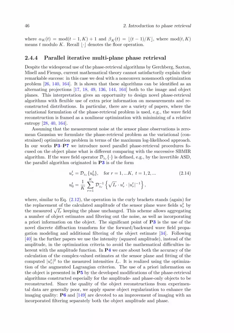
46 2. Introduction to phase retrieval

where αK(t) = mod(t − 1,K) + 1 and βK(t) = b(t − 1)/Kc, where mod(t,K)means t modulo K. Recall b·c denotes the floor operation.

2.4.4 Parallel iterative multi-plane phase retrieval

Despite the widespread use of the phase-retrieval algorithms by Gerchberg, Saxton,Misell and Fienup, current mathematical theory cannot satisfactorily explain theirremarkable success: in this case we deal with a nonconvex nonsmooth optimizationproblem [26, 140, 164]. It is shown that these algorithms can be identified as analternating projections [17, 18, 49, 136, 144, 164] both to the image and objectplanes. This interpretation gives an opportunity to design novel phase-retrievalalgorithms with flexible use of extra prior information on measurements and re-constructed distributions. In particular, there are a variety of papers, where thevariational formulation of the phase-retrieval problem is used, e.g., the wave fieldreconstruction is framed as a nonlinear optimization with minimizing of a relativeentropy [28, 40, 164].

Assuming that the measurement noise at the sensor plane observations is zero-mean Gaussian we formulate the phase-retrieval problem as the variational (con-strained) optimization problem in terms of the maximum log-likelihood approach.In our works P3–P7 we introduce novel parallel phase-retrieval procedures fo-cused on the object plane what is different comparing with the successive SBMIRalgorithm. If the wave field operator Dzr{·} is defined, e.g., by the invertible ASD,the parallel algorithm originated in P3 is of the form

utr = Dzr{ut0}, for r = 1, ...K, t = 1, 2, ... (2.14)

ut0 =1

K

K∑r=1

D−1zr

{√Ir · utr · |utr|−1

},

where, similar to Eq. (2.12), the operation in the curly brackets stands (again) forthe replacement of the calculated amplitude of the sensor plane wave fields utr bythe measured

√Ir keeping the phase unchanged. This scheme allows aggregating

a number of object estimates and filtering out the noise, as well as incorporatinga priori information on the object. The significant point of P3 is the use of thenovel discrete diffraction transform for the forward/backward wave field propa-gation modeling and additional filtering of the object estimate [34]. Following[40] in the further papers we use the intensity (squared amplitude), instead of theamplitude, in the optimization criteria to avoid the mathematical difficulties in-herent with the amplitude function. In P4 we care about both the accuracy of thecalculation of the complex-valued estimates at the sensor plane and fitting of thecomputed |utr|2 to the measured intensities Ir. It is realized using the optimiza-tion of the augmented Lagrangian criterion. The use of a priori information onthe object is presented in P5 by the developed modifications of the phase-retrievalalgorithms constructed especially for the amplitude- and phase-only objects to bereconstructed. Since the quality of the object reconstructions from experimen-tal data are generally poor, we apply sparse object regularization to enhance theimaging quality: P6 and [149] are devoted to an improvement of imaging with anincorporated filtering separately both the object amplitude and phase.

2.4. Overview of phase-retrieval techniques and our contribution 47

The conventional phase-retrieval techniques are mainly based on an ideal wavefield propagation modeling. In practice, wave fields in real coherent imaging sys-tems and their observations are different from those predicted by theory due tonon-idealities of optical system (misalignment, misfocusing, aberrations), dust onoptical elements, reflections, vibration and so on. Hence, the propagation opera-tors Dzr{·} can not fully describe the propagation through the real optical path,and the wave field reconstructions obtained by numerical simulations (i.e. theoret-ical results) and using real experimental data can be dramatically different. Thereare many various numerical approaches, which are used for calibration [227], filter-ing parasitic reflections [33], compensating for curvature introduced by microscopeobjective [175], for aberrations [242] or astigmatism [84]. However, the sources ofdifferent distortions in the optical path are hard to localize and specify. In P7 wedo not even try to identify these particular sources but estimate and compensatetheir accumulated effects. In other words, we assumed that there is a general-ized pupil function [79, §6.4.1] at the object plane which describes distortions inthe coherent imaging system manifested at the sensor plane, and this cumulativedisturbance of the light wave field in the optical path can be recalculated to theentrance pupil of the optical system (in particular, of the 4f configuration). We re-fer to the cumulative distortions as “background” disturbances. Thus, in our workthis background is estimated and compensated in order to achieve sharp imagingof the investigating object. Moreover, we also incorporate some prior informationon the true object wave field to enhance the reconstruction quality: in P7 thereconstruction of a binary object with unknown lower and upper levels using sucha background compensation and object sparse modeling is presented.

Chapter 3

Discrete diffractiontransform (DDT)

The Rayleigh–Sommerfeld diffraction integral can not be solved analytically, ex-cept for very few situations, and in most practical applications the integral can becalculated only numerically. In general, the RS diffraction formula is not widelyused – usually one computes the result of the light diffraction by its Fresnel ap-proximation [158]. In this Chapter we consider the discrete diffraction propagationmodel based on the Fresnel approximation and describe its modifications with av-eraging within pixels of the discrete object and sensor wave field distributionsresulting in an accurate pixel-to-pixel modeling of the diffraction propagation.

Following the notations in Sections 2.1, u0(ξ, η) and uz(x, y) = Dz{u0}(x, y)denote transverse complex amplitudes at the object and measurement (sensor)planes, respectively, as it is illustrated in Fig. 2.1. Numerical computations requirediscrete data of finite size, hence the integrals are discretized over the finite supportof integration [221], within the region where u0(ξ, η) 6= 0 (region S in Eq. (1.54)and Fig. 1.9): in particular, the object u0(ξ, η) is assumed to be localized in a rect-angular of the size Nξ∆ξ×Nη∆η. For discrete modeling, the continuous argumentsare replaced by the digital ones with a corresponding replacement of the continu-ous functions by their discrete counterparts: u0(ξ, η) → u0[l] = u0(l1∆ξ, l2∆η),uz(x, y) → uz[l

′] = uz(l′1∆x, l

′2∆y), uF ( v1

λf ,v2

λf ) → uF [n] = uF (∆1

λf n1,∆2

λf n2)

with 2D integer arguments. Different variables l = (l1, l2), n = (n1, n2) andl′ = (l′1, l

′2) ∈ Z2 are chosen for the object, Fourier and sensor domains, respec-

tively. This discretization is dictated by the use of digital devices such as a CCDsensor or a pixelated SLM as a 2D array of liquid crystal cells. Thus, we here-after consider the discrete wave fields at the object u0[l], Fourier uF [n] and sensorplanes uz[l

′] with pixel (pitch) sizes ∆ξ ×∆η, ∆1×∆2 and ∆x×∆y, respectively,and the corresponding supports Nξ ×Nη, N1 ×N2 and Nx ×Ny, respectively. Ingeneral, u0, uF and uz are of different image and pixel size.

It should be mentioned that in this thesis and in all our publications (in P1–P7and [112, 114, 115, 149]) we consider the discrete object wave field distribution inthe form (cf. Eq. (1.20))

u0 = a0 ◦ exp(iφ0), (3.1)

49

50 3. Discrete diffraction transform (DDT)

where a0 = |u0| is the vector of the object amplitude and φ0 is the vector ofthe object phase, φ0 = arg{u0}. The amplitude modulation (AM) of the objectmeans that the phase φ0[l] = 0 ∀l and the amplitude is defined by the vectorizedtest-image 0 < c[l] ≤ 1, i.e. u0 = c. In our experiments we use chessboard, logo,Lena or Baboon test-images as c. Analogically the phase modulation (PM) of theobject is represented by the phase only: the amplitude is constant, in particulara0[l] = 1 ∀l, and the object phase vector is defined by the vectorized test-image asu0 = exp(iπ(c− 1

2 )).

Since the phase estimate φ0 from the intensity measurements can be obtainedup to an arbitrary constant only, the RMSE or PSNR values for the object phaseare calculated for φ0 = (φ0−mean(φ0−φ0))−φ0 in order to eliminate this phase

ambiguity. Here mean(φ0−φ0) stands for the mean value of the estimation errorcalculated over the test-image φ0.

Evidently, we have no absolute phase and arg{u0} gives the wrapped objectphase estimate. However, in this text the estimate of the object phase is consideredto be localized in the interval [−π, π) and not exceeding π by its absolute value.The issues related to phase unwrapping and phase singularities are beyond thescope of this thesis.

3.1 Discrete modeling of diffraction propagation

It is straightforward to obtain digital models for the forward/backward wave fieldpropagations by taking the Riemann sums instead of the integrals in the diffrac-tion transforms mentioned in Section 2.2. Following the well-known Whittaker–Nyquist–Kotelnikov–Shannon theorem the transformation of Eqs. (2.1)–(2.2) intoa discrete convolution is correct, if at least one of the integrands in the continuousconvolution is bandlimited [168]. According to Eq. (1.23) the Fourier spectrum ofu(x, y, z) is supported on a sphere of radius 2π/λ and hence u0(ξ, η) is bandlimitedto k = 2π/λ. The principal difficulty of discretization in the space domain followsfrom the fact that the diffraction kernel is modulated by a high-frequency har-monic component. The required sampling rate, governed by the Nyquist samplingrate is unacceptably too high for practical purposes: in our case λ is significantlysmall, say λ = 532nm. Fortunately, we have an attractive alternative in the fre-quency domain. Firstly, it follows from Eqs. (1.48), (1.67) that for |v1| � 1/λ

and |v2| � 1/λ the phase φ = 2πzλ

√1− λ2(v2

1 + v22) ≈ 2πz

λ − πzλ(v21 + v2

2) is

slowly varying in v1 and v2 [111]. Secondly, for the object and sensor planes offinite support, the convolution in Eqs. (2.1)–(2.2) involves only a sub-range of thefull support of az whose size equals to the sum of the supports of these planes[167, 221]. Since no components of az for large radial distances are required1, thusthe impulse response can be sampled with respect to the involved bandwidth, andthe convolutions – discretized [221].

The discrete convolutional models as sampled versions of the formulas (2.1)–(2.2) are of the following form:

1 In case of the Fresnel approximation, it is also mentioned that the high-frequency details ofthe sensor wave field are lost.

3.2. Forward DDT with averaging 51

uz(l′1∆x, l

′2∆y) =

∑l1,l2

u0(l1∆ξ, l2∆η) · az(l′1∆x − l1∆ξ, l′2∆y − l2∆η) ·∆ξ∆η,(3.2)

u0(l1∆ξ, l2∆η) =∑l′1,l′2

uz(l′1∆x, l

′2∆y) · a−z(l1∆ξ − l′1∆x, l2∆η − l′2∆y) ·∆x∆y,(3.3)

where the hat in u0 means an estimate of u0. These formulas are valid for arbitraryparameter values, i.e. for any size of the object and diffraction planes and thepixels at these planes. In particular, the discrete Fresnel transform (az = gz) forthe forward and backward wave field propagation can be represented using thediscrete convolution in the follows matrix form [P1, cf. Eqs. (15)–(16)]

Uz = ∆η∆ξ ·Cx ·U0 ·CTy , (3.4)

U0 = ∆x∆y ·CHx ·Uz ·C∗y, (3.5)

where Cy = (Cy[l′2, l2])Ny×Nη , Cx = (Cx[l′1, l1])Nx×Nξ are the Fresnel transformmatrices calculated according to

Cx[l′1, l1] =eiπzλ

√iλz

exp

(iπ

λz(l′1∆x − l1∆ξ)

2

), (3.6)

Cy[l′2, l2] =eiπzλ

√iλz

exp

(iπ

λz(l′2∆y − l2∆η)2

). (3.7)

Following P1, we call the transforms defined by Eq. (3.4) and Eq. (3.5)Matrix Discrete Fresnel Transform (M–DFrT) and Matrix Inverse Discrete FresnelTransform (M–IDFrT), respectively.

3.2 Forward DDT with averaging

Let us assume that the input of our model is defined by a pixelwise constantdistribution what may be determined, e.g., by an SLM with 100% fill factor ofpixels; and the output is also discrete defined by the outputs of the (CCD) sen-sor pixels. Here we introduce the forward discrete diffraction transform (DDT)for such pixelwise invariant distributions which enables an accurate discrete-to-discrete modeling due to the precise integration in Eq. (2.1).

Let the 2D discrete wave field distributions at the object u0 and observa-tion/sensor uz planes of the size Nξ × Nη and Nx × Ny be pixelwise constantwithin the rectangular pixels ∆ξ × ∆η and ∆x × ∆y, respectively. Then, takinginto account Eq. (3.2), the integral (2.1) can be represented in the form

uz(x, y) = (3.8)

=

Nξ/2−1∑l1=−Nξ/2

Nη/2−1∑l2=−Nη/2

u0[l1, l2]

∆ξ/2∫−∆ξ/2

∆η/2∫−∆η/2

az(x− l1∆ξ + ξ, y − l2∆η + η)dξdη,

u0[l1, l2] = u0(l1∆ξ + ξ, l2∆η + η), |η| ≤ ∆η/2, |ξ| ≤ ∆ξ/2,

52 3. Discrete diffraction transform (DDT)

i.e. the integration is performed within each pixel of the object wave field assumedto be pixelwise constant, and the sum is calculated over Nξ × Nη pixels of theinput rectangular array. Let the output of a sensor pixel be the mean value of thedistribution impinging on this pixel (averaging within sensor pixels)

uz[l′1, l′2] =

1

∆x∆y

∆x/2∫−∆x/2

∆y/2∫−∆y/2

uz(l′1∆x + ξ′, l′2∆y + η′)dξ′dη′. (3.9)

Inserting Eq. (3.8) into Eq. (3.9) we arrive at the following spatial domain DDT

uz[l′1, l′2] =

∑Nξ/2−1

l1=−Nξ/2

∑Nη/2−1

l2=−Nη/2dz[l′1, l1; l′2, l2] · u0[l1, l2], (3.10)

l′1 = −Nx/2, ..., Nx/2− 1, l′2 = −Ny/2, ..., Ny/2− 1

with the diffraction kernel dz[l′1, l1; l′2, l2] calculated as

dz[l′1, l1; l′2, l2] =

1

∆x∆y

∆x/2∫−∆x/2

∆ξ/2∫−∆ξ/2

dξdξ′× (3.11)

∆y/2∫−∆y/2

∆η/2∫−∆η/2

az(l′1∆x − l1∆ξ + ξ′ + ξ, l′2∆y − l2∆η + η′ + η)dηdη′,

l′1 = −Nx/2, ..., Nx/2− 1, l1 = −Nξ/2, ..., Nξ/2− 1,

l′2 = −Ny/2, ..., Ny/2− 1, l2 = −Nη/2, ..., Nη/2− 1.

The kernel dz in Eq. (3.11) is an averaged (pixelwise double-averaged) versionof the original kernel az in Eq. (2.1): the smoothing in Eq. (3.11) takes intoconsideration discretization for both the object and sensor arrays. For the Fresneldiffraction kernel az = gz the kernel dz allows the following factorization

dz[l′1, l1; l′2, l2] = Ax[l′1, l1] ·Ay[l′2, l2], (3.12)

where

Ax[l′1, l1] = (3.13)

eiπzλ

∆x

√iλz

∆x/2∫−∆x/2

∆ξ/2∫−∆ξ/2

exp

(iπ

λz(l′1∆x − l1∆ξ + ξ′ + ξ)2

)dξdξ′,

Ay[l′2, l2] = (3.14)

eiπzλ

∆y

√iλz

∆y/2∫−∆y/2

∆η/2∫−∆η/2

exp

(iπ

λz(l′2∆y − l2∆η + η′ + η)2

)dηdη′

represent the transform matrices with respect to rows and columns, respectively.

3.2. Forward DDT with averaging 53

Figure 3.1: Principal setup of a discrete-to-discrete wave field propagation model. HereU0 and Uz denotes the discrete object and sensor plane 2D wave field distributions. Theaccurate link between them is given by vec{Uz} = (Ax⊗Ay) ·vec{U0}, where transformmatrices Ax and Ay manipulate rows and columns of the input matrix U0, respectively.

3.2.1 Two-matrix DDT (M–DDT)

Inserting (3.12) into (3.10) we arrive at

Uz[l′1, l′2] =

Nξ/2−1∑l1=−Nξ/2

Nη/2−1∑l2=−Nη/2

Ax[l′1, l1] ·U0[l1, l2] ·Ay[l2, l′2], (3.15)

what defines the matrix form of the discrete input–output forward propagationmodel

Uz = Ax ·U0 ·ATy . (3.16)

Let u0 = vec{U0} and uz = vec{Uz} denote the column vectors constructedby vectorization of the discrete wave field distributions at the object and sensorplanes [99]. Then, Eq. (3.16) can be rewritten in even more compact form

uz = A · u0, A = Ax ⊗Ay, (3.17)

where the vectors uz and u0 have the lengths #uz = Nx ·Ny and #u0 = Nξ ·Nη,respectively, and the transform matrix A ∈ CNxNy×NξNη .

The formulas (3.16)–(3.17) define what we call the Matrix Discrete DiffractionTransform (M− DDT ) with so-called averaged matrices Ax (Eq. (3.13)) andAy (Eq. (3.14)). In Fig. 3.1 a discrete-to-discrete wave field propagation modeldescribed in terms of M–DDT is illustrated.

3.2.2 Simplification of M–DDT

Let the pixels’ sizes be so small that the averaging in the forward propagationintegrals (3.11) is not essential. Then the diffraction transform kernel can becalculated significantly simpler. The corresponding matrices with no averagingare denoted by By and Bx, respectively, and defined as follows

54 3. Discrete diffraction transform (DDT)

Bx[l′1, l1] = lim∆ξ,∆x→0

Ax[l′1, l1] = (3.18)

=∆ξe

iπzλ

√iλz

exp

(iπ

λz(l′1∆x − l1∆ξ)

2

)= ∆ξ ·Cy[l′1, l1],

l′1 = −Nx/2, ..., Nx/2− 1, l1 = −Nξ/2, ..., Nξ/2− 1,

By[l′2, l2] = lim∆η,∆y→0

Ay[l′2, l2] = (3.19)

=∆ηe

iπzλ

√iλz

exp

(iπ

λz(l′2∆y − l2∆η)2

)= ∆η ·Cy[l′2, l2],

l′2 = −Ny/2, ..., Ny/2− 1, l2 = −Nη/2, ..., Nη/2− 1,

where Cx and Cy are calculated according to Eqs. (3.6)–(3.7). The relations

Bx = ∆ξ ·Cx, By = ∆η ·Cy (3.20)

mean that within the scalar factors ∆ξ and ∆η the matrices Bx and By areidentical to the matrices of M–DFrT Cx and Cy. Bx and By are called the non-averaged matrices in order to emphasize that the averaging effect is omitted.

The kernel dz[l′1, l1; l′2, l2] in Eq. (3.11) becomes shift-invariant and depends

on the differences of the arguments l′1 − l1 and l′2 − l2 as soon as the pixels atthe object and sensor planes take equal sizes, ∆ξ = ∆x and ∆η = ∆y. In thisparticular case M–DDT is essentially simpler to calculate because the transformmatrices in Eqs. (3.14)–(3.13) are symmetrical with respect to the differences ofindices: Ay[l′2, l2] = Ay[l′2− l2] = Ay[l2− l′2], Ax[l′1, l1] = Ax[l′1− l1] = Ax[l1− l′1].If ∆η = ∆y = ∆x = ∆ξ and Nx = Nξ = Ny = Ny, then Ax = Ay and only onetransform matrix in Eq. (3.16) is required.

If the pixel and image at the object and sensor planes are, in general, rectangu-lar of the same size, i.e. ∆η = ∆y = ∆a, ∆x = ∆ξ = ∆b and Nx = Nξ, Ny = Ny,then Eqs. (3.10) and (3.11) can be simplified as follows

uz[l′1, l′2] =

Nξ/2−1∑l1=−Nξ/2

Nη/2−1∑l2=−Nη/2

dz[l′1 − l1, l′2 − l2] · u0[l1, l2], (3.21)

l′1 = −Nx/2, ..., Nx/2− 1, l′2 = −Ny/2, ..., Ny/2− 1,

where dz here is a large diffraction transform matrix defined as follows

dz[l1, l2] =1

∆a∆b

∆a/2∫∫−∆a/2

∆b/2∫∫−∆b/2

az(l1∆a + ξ′ + ξ, l2∆b + η′ + η)dξdξ′dηdη′, (3.22)

l1 = −Nξ +Nx2

+ 1, ...,Nξ +Nx

2− 1, l2 = −Nη +Ny

2+ 1, ...,

Nη +Ny2

− 1.

Note that the support of dz in Eq. (3.22) is larger comparing with what wehave in Eq. (3.11). Moreover, for the Fresnel diffraction kernel az = gz of such anenlarger size, dz allows the following factorization [111, cf. Eqs. (23), (24)]

dz[l1, l2] = ρz[l1] · ρz[l2], where

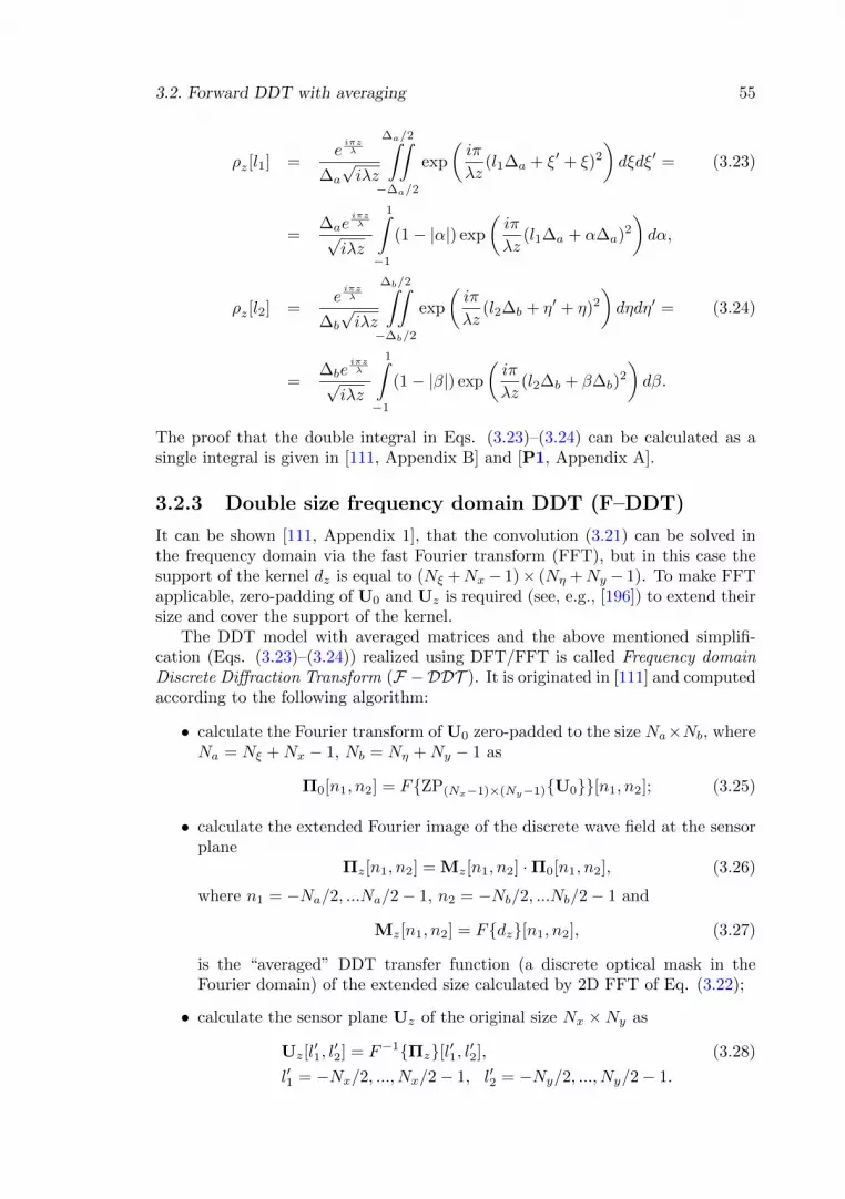
3.2. Forward DDT with averaging 55

ρz[l1] =eiπzλ

∆a

√iλz

∆a/2∫∫−∆a/2

exp

(iπ

λz(l1∆a + ξ′ + ξ)2

)dξdξ′ = (3.23)

=∆ae

iπzλ

√iλz

1∫−1

(1− |α|) exp

(iπ

λz(l1∆a + α∆a)2

)dα,

ρz[l2] =eiπzλ

∆b

√iλz

∆b/2∫∫−∆b/2

exp

(iπ

λz(l2∆b + η′ + η)2

)dηdη′ = (3.24)

=∆be

iπzλ

√iλz

1∫−1

(1− |β|) exp

(iπ

λz(l2∆b + β∆b)

2

)dβ.

The proof that the double integral in Eqs. (3.23)–(3.24) can be calculated as asingle integral is given in [111, Appendix B] and [P1, Appendix A].

3.2.3 Double size frequency domain DDT (F–DDT)

It can be shown [111, Appendix 1], that the convolution (3.21) can be solved inthe frequency domain via the fast Fourier transform (FFT), but in this case thesupport of the kernel dz is equal to (Nξ +Nx− 1)× (Nη +Ny − 1). To make FFTapplicable, zero-padding of U0 and Uz is required (see, e.g., [196]) to extend theirsize and cover the support of the kernel.

The DDT model with averaged matrices and the above mentioned simplifi-cation (Eqs. (3.23)–(3.24)) realized using DFT/FFT is called Frequency domainDiscrete Diffraction Transform (F −DDT ). It is originated in [111] and computedaccording to the following algorithm:

• calculate the Fourier transform of U0 zero-padded to the size Na×Nb, whereNa = Nξ +Nx − 1, Nb = Nη +Ny − 1 as

Π0[n1, n2] = F{ZP(Nx−1)×(Ny−1){U0}}[n1, n2]; (3.25)

• calculate the extended Fourier image of the discrete wave field at the sensorplane

Πz[n1, n2] = Mz[n1, n2] ·Π0[n1, n2], (3.26)

where n1 = −Na/2, ...Na/2− 1, n2 = −Nb/2, ...Nb/2− 1 and

Mz[n1, n2] = F{dz}[n1, n2], (3.27)

is the “averaged” DDT transfer function (a discrete optical mask in theFourier domain) of the extended size calculated by 2D FFT of Eq. (3.22);

• calculate the sensor plane Uz of the original size Nx ×Ny as

Uz[l′1, l′2] = F−1{Πz}[l′1, l′2], (3.28)

l′1 = −Nx/2, ..., Nx/2− 1, l′2 = −Ny/2, ..., Ny/2− 1.

56 3. Discrete diffraction transform (DDT)

Note that for small pixels’ sizes the kernel smoothing effect in Eq. (3.23)–(3.24)becomes negligible and instead of Eq. (3.22) we arrive at the simple formula [111,cf. Eq. (14)]

dz[l1, l2] −→∆a,∆b→0

∆a∆b · gz(l1∆a, l2∆b). (3.29)

If the diffraction kernel dz used in Eq. (3.27) is defined according to the simplifica-tion (3.29), then the resulting Mz in Eq. (3.26) is called the non-averaged F–DDTtransfer function.

It is found that for the same pixel and image sizes at the object and sensorplanes F–DDT (3.25)–(3.28) and M–DDT (3.16) give the same result of the forwarddiffraction propagation Uz. F–DDT is computationally faster, but the M–DDTmodel is more flexible because it is valid for arbitrary settings of the optical setup.Moreover, in contrast to F–DDT, M–DDT does not require zero-padding for theaccurate calculation.

3.3 Sampling conditions

Traditionally the discrete models of the free space diffraction propagation areconsidered as approximation for underlying continuous ones given in continuousvariables and in integral forms (see Section 2.2). In particular, the discrete model ofEq. (1.60) and Eq. (2.6) for the Fresnel approximation az = gz can be representedas follows

uz

(l′1

∆x

λz, l′2

∆y

λz

)=eikz

iλzeiπλz ((l′1∆x)2+(l′2∆y)2)∆ξ∆η × (3.30)

×∑l1,l2

u0(l1∆ξ, l2∆η) · e iπλz ((l1∆ξ)2+(l2∆η)2)e−i2π(l1l

′1

∆ξ∆x

λz +l2l′2

∆η∆yλz ),

u0(l1∆ξ, l2∆η) =e−ikz

−iλze−iπλz ((l1∆ξ)

2+(l2∆η)2)∆x∆y × (3.31)

×∑l′1,l′2

uz

(l′1

∆x

λz, l′2

∆y

λz

)· e−iπλz ((l′1∆x)2+(l′2∆y)2)ei2π(l1l

′1

∆ξ∆x

λz +l2l′2

∆η∆yλz ).

The sampling and aliasing issues are of importance for these approximationsas they define preconditions for reconstruction of continuous signals from sampledones [111]. The motivation for the above mentioned DDT models is different:for the pixelwise constant wave field distributions at the object and sensor planethe constructed discrete-to-discrete model is precise as the accurate integrationof diffraction propagation (2.1) is assumed. In this development the standard as-sumptions concerning the sampling and bandlimitedness can be omitted as theyare replaced by the hypothesis that the object plane distribution is piecewise con-stant or well approximated by this sort of distribution.

Note that Eqs. (3.2)–(3.3) (or, in particular, Eqs. (3.30)–(3.31)) are valid forarbitrary parameter values, but even if the diffraction kernel az is invertible, theperfect reconstruction in Eq. (3.3) is not guaranteed, i.e., in general, u0 6= u0. We

3.4. Numerical implementation 57

are looking for such a condition, which results in the inversion

u0[l′′1 , l′′2 ] =

∑l1,l2

u0[l1, l2]× (3.32)

×∑l′1,l′2

a−z[l′′1 − l′1, l′′2 − l′2] · az[l′1 − l1, l′2 − l2] ·∆x∆ξ∆y∆η︸ ︷︷ ︸

δl′′1 ,l1·δl′′2 ,l2

providing the perfect reconstruction u0[l′′1 , l′′2 ] = u0[l′′1 , l

′′2 ]. Here δl′′1 ,l1or δl′′2 ,l2 de-

notes the Kronecker delta (8).Suppose the discrete wave field distributions at the object and sensor planes

are of the same size Nx×Ny. It can be seen [125, 236] that provided the samplingcondition [P1, cf. Eqs. (11)]

∆x∆ξNx = λ · z, ∆η∆yNy = λ · z, (3.33)

Eqs. (3.30)–(3.31) can be rewritten via DFTs as follows

uz

(l′1

∆x

λz, l′2

∆y

λz

)= ei(kz−

π2 ) · e iπλz ((l′1∆x)2+(l′2∆y)2) × (3.34)

×F{u0(l1∆ξ, l2∆η) · e iπλz ((l1∆ξ)2+(l2∆η)2)}∆ξ∆η

λz,

u0(l1∆ξ, l2∆η) = e−i(kz−π2 )e

−iπλz ((l1∆ξ)

2+(l2∆η)2) × (3.35)

×F−1{uz(l′1

∆x

λz, l′2

∆y

λz

)· e−iπλz ((l′1∆x)2+(l′2∆y)2)}NxNy

∆x∆y

λz;

and, substituting Eq. (3.34) into Eq. (3.35), we arrive at the perfect reconstructionu0 = u0. Eq. (3.33) is used in our works to calculate the condition for the perfectobject wave field reconstruction.

More generally, if the image and pixel sizes at the object and sensor planesare equal (Nx = Nξ, ∆x = ∆ξ and Ny = Nη, ∆y = ∆η), then, provided thesampling condition (3.33), we can treat Eqs. (3.2)–(3.3) as a discrete shift-invariantconvolution and apply DFT (12) to both parts of these equations [125] yielding[P1, cf. Eqs. (6)–(7)]

uz[l′1, l′2] = F−1{F{u0} [n1, n2] · F{az} [n1, n2]}[l′1, l′2], (3.36)

u0[l1, l2] = F−1{F{uz} [n1, n2] · (F{az} [n1, n2])∗}[l1, l2], (3.37)

where for the invertible diffraction kernel u0 = u0.

3.4 Numerical implementation

These formulas (3.30)–(3.31) and (3.36)–(3.36) represent the conventional discretewave field propagation models. F–DDT from Section 3.2.3 gives an accurate for-ward wave field propagation via the frequency domain. Note that the numericalcalculation via DFT is time-consuming: O(N2) complexity for 1D DFT.

58 3. Discrete diffraction transform (DDT)

The computation of the discrete wave field propagation is typically based on thefast Fourier transform (1D FFT has O(N logN) complexity): it is the commonlyused, traditional approach [13, 235], because the computation time of algorithmscan be reduced by order of magnitude. Shen and Wang [196] enhance the FFTbased approach by introducing weights in the discrete convolution, whose valuesare found by Simpson’s rule for numerical integration. Naskov and Logofatu [158]use different sampling intervals (unequal sampling step) for the object and sensorplanes in order to widen the spatial range of accuracy of the discrete convolu-tion. As a result, they obtain a scaled convolution which is still computed fast inO(N logN) calculations by the use of the discrete fractional Fourier transform.In[9] the RS impulse response is approximated by polynomial and parabolic phasors.We also wish to mention that the discrete space domain modeling for holographyis discussed in details in [125], the accuracy of the frequency domain approachcan be found in [166], and interesting developments concern continuous and dis-crete Fresnel transforms and their multiresolution versions can be found in, e.g.,[5, 165, 235]. We also usually realize the wave field propagation with FFT.

Note, while the parameters λ, z,∆ξ,∆η,∆x,∆y ∈ R+ are generally real pos-itive numbers, the image size is defined in pixels, i.e. Ny, Nx, Nξ,Ny ∈ N. Wewish to say that using the conventional FFT routines (say, Fortran or C/C++libraries) the accurate choice of parameters is out of our control. For instance, wechoose the image sizes as integer multiples of 2 (the conventional size of an imagefor FFT should be a power of 2). Thus, the accurate diffraction propagation canbe computed only for a certain sequence of propagation distances with respect topositive integer image sizes

N ′x = 2d λ · z2∆x∆ξ

e, N ′y = 2d λ · z2∆η∆y

e, (3.38)

where d·e denotes the ceiling operation.Indeed, let z be an arbitrary distance, ∆x = ∆y, ∆ξ = ∆η and λ are given

and fixed. λ·z∆x∆ξ

and λ·z2∆η∆y

are equal, but most likely not integer. Then, the

propagation distance corresponding to the sampling condition and valid for theimplementation via FFT (Eq. (3.38)) is z′ =

∆x∆ξ

λ N ′x =∆x∆ξ

λ · 2d λ·z2∆x∆ξ

e. There-

fore, in this thesis and in our publications the so-called in-focus distance [125] withrespect to x or y directions, corresponding to the perfect object reconstruction, isdefined by

zf,x =∆x∆ξ

λN ′x, zf,y =

∆η∆y

λN ′y. (3.39)

If zf,y = zf,x the in-focus distance is simply denoted by zf . The influence of thesampling condition on the reconstruction quality is well presented in [P1, Fig. 2].

Evidently the propagation distance should be taken with the step2∆x∆ξ

λ or2∆η∆y

λ for the x and y directions2, namely: z = zf,x ±m · 2∆x∆ξ

λ or z = zf,x ±m · 2∆η∆y

λ , m ∈ N. Otherwise FFT automatically (and unpredictable) modifiesparameters of the optical setup, including the propagation distance, to satisfy

1Nx

=∆x∆ξ

λz and 1Ny

=∆y∆η

λz .

2 This step is found from the minimal distance between two positive integer even numbers

N2 > N1: e.g., z2 − z1 =∆x∆ξλ

(N2 −N1).

3.5. Inverse of M–DDT 59

3.5 Inverse of M–DDT

The conventional wave field reconstruction models [125, 236] are based on digitalapproximations of the inverse operator D−1

z {·} and, the discrete algorithms (see,e.g., Eq. (3.5)) inherit the principal limitation of the integral inverse operator justbecause of the finite size of the sensor plane. In contrast to it, we follows to anotherapproach, the so-called inverse imaging : the object reconstruction is performedby the numerical inverse of the forward propagation operator Dz. For example,the reconstruction of U0 from Uz in case of M–DFrT can be also obtained as asolution of the equation (3.4). For the nonsingular Cy,z and Cx,z we arrive at thefollowing backward propagation modeling

U0 =1

∆η∆ξ·C−1

x ·Uz ·C−Ty , (3.40)

and it is different from Eq. (3.5) because in general C−1x 6= CH

x and C−Ty 6= C∗y,

and the inverse of M–DFrT has a place if and only if CHy Cy = I and CH

x Cx = Iare the identity matrices. This condition can be guaranteed under the conditions(3.33) and has no place in the general case.

Following Eq. (3.17), the linear observation model of a holographic scenario isdefined as follows

uz = A · u0 + ε, (3.41)

where u0 ∈ CNξNη is the object vector, A ∈ CNxNy×NξNη is the M–DDT trans-form matrix and the vector uz ∈ CNxNy describes the result of the forwarddiffraction propagation to the distance z. Here and in our works P1–P2 and[114, 115] the complex-valued uz is assumed to be corrupted by the additive cir-cular symmetric complex zero-mean Gaussian noise [77]. It means that the realand imaginary components of the random noise vector ε[l′] are not correlated(the expectation E〈Re{ε[l′]} · Im{ε[l′]}〉 = 0), independent and identically dis-tributed (i.i.d.) according to the normal distribution, Re{ε[l′]} ∼ N

(0, σ2

)and

Im{ε[l′]} ∼ N(0, σ2

)with the same standard deviation σ > 0 3.

The simplest way to recover the estimate of the object wave field distribution u0

is applying the inverse of the transform matrix to the given (noisy) complex-valueddata according to the naive reconstruction: u0 = A−1 · uz [109]. This inverse ofM–DDT gives an acceptable reconstruction of the pixelwise object distribution(depending on the noise level σ in ε), if the M–DDT operator is non-singular. Ingeneral case such a straightforward approach of the wave field reconstruction willtypically fail due to the ill conditioning of the transform matrix (see [P1, Fig. 9]).

The concept of well-posed and ill-posed inverse problems goes back to JacquesHadamard (1865–1963) at the beginning of the 20th century (e.g., [88]). Accord-ing to Hadamard’s definition for mathematical models of physical phenomena awell-posed problem must have a solution (existence), at most one solution (unique-ness), and this solution must depend continuously on the input data (stability).

3 Recall that values of the used test-image vary from 0 to 1, and in case of AM for the wavefield at the object plane σ=0.01 represents a small amount of noise (1%). However, we deal withnoisy (complex-valued) diffraction patterns at the sensor plane, and for a large distance of thewave field propagation, say z > 2 · zf , even such a small noise may cause significant degradationsof the object reconstruction due to ill-posedness of the propagation operator.

60 3. Discrete diffraction transform (DDT)

A problem is defined as ill-posed, if the solution is not unique or if it is not acontinuous function of the data, i.e. if an arbitrary small perturbation of the datacan cause an arbitrarily large perturbation of the solution [91]. Further we fo-cus on the problem of the backward wave field propagation computed using theinverse of M–DDT, the object reconstruction accuracy and imaging obtained inour numerical simulations from synthetic data. In this thesis and in P1–P2 and[114, 115] the problem related to the ambiguity of the object phase is out of scope.

3.5.1 Ill-posedness in M–DDT

Traditionally any discussion about the properties of the transform matrices re-quires knowledge of its singular value decomposition (SVD). The conventionalnumerical “tools” that allows explicit analysis of the diffraction transform andpossible difficulties related to Hadamard’s conditions, are the numerical rank andconditioning number calculated by SVD of the DDT matrices.

It is well-known that the matrix A = (Ay ⊗Ax) can be rewritten using theSVD decomposition [99]

A = (ΛyDyVHy )⊗(ΛxDxV

Hx ) = (Λy ⊗Λx)(Dy ⊗Dx)(Vy ⊗Vx)H , (3.42)

where Λy,Λx and Vy,Vx are square orthogonal matrices of eigenvectors, andDy,Dx are the diagonal matrices with the real-valued nonnegative singular valuesχy[j] (j = 1, ...min(Nη, Ny)) and χx[s] (s = min(Nξ, Nx)), respectively, appearingin nonincreasing order.

Let us assume for a moment that there is no noise in the complex-valuedobservation data: ε in Eq. (3.41) is a zero vector. The least square (LS) estimateu0 is a solution of the normal equation

AHuz = AHA · u0, (3.43)

where [160, 99]

AHA = AHx Ax ⊗AH

y Ay = (Vy ⊗Vx)(DTy Dy ⊗DT

xDx)(Vy ⊗Vx)H . (3.44)

The rank of the Hermitian matrices AHy Ay or AH

x Ax is, from a mathematicalpoint of view, the number of linearly independent rows (columns) or these matrices.The rank is equal to the number of strictly positive singular values (χy[j])2 or(χx[s])2, respectively, and the maximum value of (χy[j])2 or (χx[s])2 is equal tomin(Nη, Ny) or min(Nξ, Nx), respectively. In the presence of errors (in practice,the measurement data always has some noise, particularly by approximation anddiscretization errors, and even computer simulated data are corrupted with round-off errors) this definition is not useful. Thus, we use, from a practical point of view,the numerical rank as the number of rows (columns) of AH

y Ay or AHx Ax, which

are almost linearly independent with respect to some error level [91, cf. Chapter3]. Hence, the numerical rank of the square matrices AH

y Ay and AHx Ax is defined

regarding to a tolerance τε by [91, cf. Eq. (3.3)]

rank(AHy Ay) = max

j(j : (χy[j])2 > τε), (3.45)

rank(AHx Ax) = max

s(s : (χx[s])2 > τε),

3.5. Inverse of M–DDT 61

where the tolerance τε = 10−12 is taken experimentally (as in P1) and it is thesame for both AH

y Ay and AHx Ax.

The conditioning number of AHy Ay and AH

x Ax is defined as the ratio betweenthe largest and the smallest singular values of these matrices

cond(AHy Ay) =

(χy[1])2

(χy[min(Nη, Ny)])2, cond(AH

x Ax) =(χx[1])2

(χx[min(Nξ, Nx)])2.

(3.46)

For simplicity, we typically consider the case, when Nx = Nξ and Ny = Nη.It is known that the conditioning number (the rank) of the matrix AHA is

the product of the conditioning numbers (ranks) calculated separately for thematrices AH

x Ax and AHy Ay [99]. In general, this statement is not true for the

numerical rank: rank is computed depending on the chosen tolerance4. It is,however, much simpler to work with the individual transform matrices AH

y Ay

and AHx Ax due to their much smaller dimensions comparing with AHA. For the

same reason, it is simpler to characterize the conditioning of M–DDT using condor rank of the matrices AH

y Ay and AHx Ax separately. Therefore, the numerical

rank rank(AHA) is hereafter defined by the product of the numerical ranks ofAHx Ax and AH

y Ay as a more rigorous, even though rough, evaluation, i.e.

cond(AHA) = cond(AHx Ax) · cond(AH

y Ay), (3.47)

rank(AHA) = rank(AHx Ax) · rank(AH

y Ay).

In addition, such cond and rank of AHA serve as a conventional indicator of thereconstruction quality.

For rectangular object and sensor planes the perfect reconstruction U0 = U0

is achieved provided the following assumptions:

1. The support of the sensor plane distribution is equal to or larger than thesupport of the object plane distribution Nx ≥ Nξ and Ny ≥ Nη, otherwiseit is already referred to super resolution methods. In addition, we introducehere the size ratio of these image qx = Nx/Nξ ≥ 1, qy = Ny/Nη ≥ 1;

2. AHy Ay and AH

x Ax are full rank matrices, i.e.

rank(AHx Ax) = Nξ, rank(AH

y Ay) = Nη.

To address the second statement, we use the numerical rank calculated byEq. (3.45), and the perfect reconstruction is replaced by the numerical perfectreconstruction, i.e. those which provides practically high reconstruction accuracy

4 For instance, in the experiment with rectangular pixels of the size ∆η = ∆y = 5µm,∆x = ∆ξ = 8µm and square images Nx = Nξ = Ny = Ny = 64 for z = 2 · zy provided Eqs.

(3.39), the numerical ranks rank(AHx Ax) = 61, rank(AH

y Ay) = 43 for the tolerance τε = 10−12

and maxj,s

(j, s : (χy [j])2 ·(χx[s])2 > τ2ε) = 3152, where rank(AH

x Ax)·rank(AHy Ay) = 2623. Note

that the strict relation between the numerical ranks of AHA and the individual matrices AHx Ax

and AHy Ay is out of scope of this thesis.

62 3. Discrete diffraction transform (DDT)

in RMSE or PSNR. If the conditions 1 and 2 are held, then the numerical perfectreconstruction is given by the formula

U0 = (AHx Ax)−1AH

x ·Uz ·A∗y(ATy A∗y)−1, (3.48)

or, in other words,u0 = (AHA)−1AH · uz (3.49)

In addition, the transform matrices AHy Ay and AT

xA∗x in Eq. (3.48) become wellconditioned and invertible. Thus, in case of the same pixels’ size ∆x = ∆ξ and∆y = ∆η the object estimate is defined by u0 = AH · uz or

U0 = AHx ·Uz ·A∗y, (3.50)

what represents M–IDFrT model with averaged matrices. Here and in P2 weadditionally consider the reconstruction quality obtained by this scheme.

Let the size ratios qx = qy = 1 and the conditions (3.33) be fulfilled. Then,taking into account Eqs. (3.20) and

λz

∆2ξNx

BHx Bx =

λz

NxCHx Cx = I,

λz

∆2ηNy

BTy B∗y =

λz

NyCTy C∗y = I, (3.51)

we can express the object reconstruction via the non-averaged matrices as

U0 = (BHx Bx)−1BH

x ·Uz ·B∗y(BTy B∗y)−1 = (3.52)

(λz)2

∆2ξNx∆2

ηNyBHx ·Uz ·B∗y =

(λz)2

∆ξNx∆ηNyCHx ·Uz ·C∗y

or, provided the same pixels, as U0 = BHx ·Uz ·B∗y.

The numerical study in P1–P2 and [114, 115] shows that, depending on theparameters of the propagation system (the propagation distance z, the pixel andimages sizes), the matrices Ay and Ax are correctly ill conditioned [91], i.e. this ill-posedness is a part of the formulation of the diffraction propagation model usingM–DDT. Providing the accurate forward wave field propagation the transformmatrices for z larger than the in-focus distances become numerically singular andEqs. (3.48)–(3.50) – practically useless: they give either unstable results highlysensitive regarding to the parameter variations and observation noise or just fail.

3.5.2 Conditioning of M–DDT and inverse reconstructionaccuracy

It can be shown that the numerical rank and the conditioning number of thetransform matrices AH

y Ay and AHx Ax (in general, AHA) can be used as a good

indicator of the accuracy of the object distribution reconstruction. rank and condin Eqs. (3.45)–(3.47) are seriously dependent on the sensor size, pixel size, propa-gation distance z and on the the parameters qx and qy, which define a redundancyof the sensor with respect to the object distribution5.

5 The larger sensor image is, the better accuracy of reconstruction for the object plane.

3.5. Inverse of M–DDT 63

Firstly, let us consider the conditioning number in case of square images andpixels of the same size at the object and sensor plane, Nx = Ny, qx = qy = 1 and∆ξ = ∆η = ∆x = ∆y. It can be seen that the minimum value of cond correspondsexactly to the in-focus distance z = zf (Eqs. (3.33) and (3.39), see [P2, Fig. 5],[114, Fig. 4(a)]), what results in the best reconstruction quality in RMSE (cf.[P2, Fig. 4], [114, Fig. 4(b)]). This distance z = zf also corresponds to the peakof the curve of the numerical rank computed for the averaged matrices (see [P1,Fig. 3], [115, Fig. 1(top image)]). However, even for slightly smaller z = 0.95 · zf(larger z = 1.05 · zf ) distances the conditioning number grows rapidly increasingby orders of magnitude, and the reconstruction of the object distribution becomesmore and more questionable for distances different from zf .

For large propagation distances z > zf , precisely z > zf,x, z > zf,y there is aproblem related to the support of the discrete diffraction kernel. In [125, ChapterA.13] it is mentioned that the continuous diffraction kernels are chirp-like functionsof infinite extent, where the frequency of the oscillations increases together withthe radial distances from the origin and decreases for larger propagation distances.But things dramatically change, if we investigate the finite chirp function, whichrepresents only a section of the infinite one in a finite interval. Let us considerthe used Fresnel diffraction kernel (1.59). It is easy to see that, provided thesampling conditions Eqs. (3.33) and (3.39), the support of the discrete kernel is∆ξ

∆xN ′x ×

∆η

∆yN ′y, and in case of the same pixel size at the object and sensor plane

regarding to the x and y direction the support is N ′x ×N ′y because

exp(iπ∆2

ξ

λzx(l1 +N ′x)2) = (3.53)

= exp(i2π∆ξ

∆xl1)︸ ︷︷ ︸ ·

=1, if ∆ξ=∆x

exp(iπ∆2

ξ

λzxl21) · exp(iπ

∆ξ

∆xN ′x),

exp(iπ∆ξ

∆xN ′x) =

{−1, odd N ′x, ∆ξ = ∆x

1, even N ′x, ∆ξ = ∆x

analogically

exp(iπ∆2

y

λzy(l2 +N ′y)2) = exp(

iπ∆2y

λzyl22), (3.54)

if N ′y is even6 and ∆η = ∆y. For z < zf,x, z < zf,y the mentioned support size

becomes larger than the available 2D measurement array (e.g., for z = 12 · zf the

kernel support is exactly two times smaller than the image size), what is indicatedby the numerical rank close to its maximum value.

In case of z > zf,x, z > zf,y we lose the high-frequency components of thekernel. Hence, the reconstruction quality will be (much) worse, what is indicatedby the conditioning number which immediately becomes very large and numericalranks of the M–DDT transform matrices which start to decrease monotonically.In Fig. 3.2 we demonstrate the Fresnel diffraction kernel calculated on square32N′x× 3

2N′y grid, N ′x = N ′y = 256 for square pixels ∆η = ∆y = ∆x = ∆ξ = 3.45µm

6 It could be another reason to choose the image sizes as integer multiples of 2.

64 3. Discrete diffraction transform (DDT)

Figure 3.2: The Fresnel diffraction kernel gz(l1∆ξl2∆η) = eikz

iλzeik2z

((l1∆ξ)2+(l2∆η)2)

calculated on the grid 32N ′ξ × 3

2N ′η samples, N ′ξ = N ′η = 256, with square pixels

∆η = ∆y = ∆x = ∆ξ = 3.45 µm for the propagation distances (from left to right

column-wise) z = { 34· zf , zf and 3

2· zf} , zf =

∆x∆ξN′x

λ=

∆x∆ξN′y

λ. The support of the

kernel N ′x ×N ′y is marked by a dashed square. The real part Re{gz} is presented in thetop row, and the imaginary part Im{gz} – in the bottom row, respectively.

for different propagation distances: z = 34 · zf , z = zf and z = 3

2 · zf . The realpart of this kernel is presented for the corresponding distances in the top row:Re{g3/4·zf [l1, l2]} in Fig. 3.2(a); Re{gzf } in Fig. 3.2(b) and Re{g3/2·zf } in Fig.3.2(c), respectively. The imaginary part is shown in the bottom row: Im{g3/4·zf }in Fig. 3.2(d); Re{gzf } and Im{gzf } in Fig. 3.2(e) and Im{g3/2·zf } in Fig. 3.2(f),respectively. The support of the kernel of the size N ′x ×N ′y corresponding to the

in-focus distance zf =∆x∆ξN

′x

λ =∆y∆ηN

′y

λ is marked by a dashed square. It canbe seen that for larger distances we operate with smaller and smaller portion ofthe kernel support with low frequencies only.

It is well known that the Kronecker delta can be expressed as a summation

of complex exponents δl′,l′′ = 1N

∑N/2−1l=−N/2 exp(±i2π l

N [l′ − l′′]). The decay of

the matrix conditioning [P2, Fig. 5] and, as the result, decreasing of the objectreconstruction accuracy [P1, Fig. 4] for z < zf can be explained by the failure ofthe assumption (3.32): for 1

2 ·zf < z < zf the numerical size (in pixels) of the useddiffract kernel is larger than its support, but the number of components is not amultiple of N . For z = 1

2 · z we have a multiple redundancy, i.e. the used sizeis precisely two times larger than the diffraction kernel support. In this case theaveraging of the M–DDT matrices practically provides a very good imaging: seeFig. 3.3, [P1, Fig. 8] and [P2, Fig. 3] for AM. While the reconstructions by M–

3.5. Inverse of M–DDT 65

Figure 3.3: Amplitude reconstruction for the close distance z = 12· zf , AM, Lena test-

image. The results are obtained (a) by the inverse M–DDT as |U0| = |A−1x Ax · U0 ·

ATyA−Ty | ; (b) by M–IDFrT with the averaged matrices as |U0| = |AH

x Ax ·U0 ·ATyA∗y|.

M–IDFrT with the non-averaged matrices calculated by (c) |U0| = c0 ·|CHx Cx ·U0 ·CT

yC∗y|

or (d) |U0| = c0∆ξ∆η

· |CHx Ax ·U0 ·AT

yC∗y| fails due to aliasing. Here c0 = (λz)2

NxNy.

IDFrT with non-averaged matrices are completely destroyed by the aliasing effects(see Fig. 3.3(c) and Fig. 3.3(d7)), the reconstruction imaging by the averagedmatrices is good: the inverse of M–DDT (cf. Eq. (3.48)) results in a numericallyperfect imaging, Fig. 3.3(a); M–IDFrT with the averaged matrices gives a goodreconstruction quality corrupted however by certain “waves” on the borders, Fig.3.3(b). For even smaller z < 1

2 · z we have larger redundancy: the conditioningnumber [P2, Fig. 5], numerical rank [P1, Fig. 3] as well as the RMSE curve [P2,Fig. 4] become erratic, but the inverse of M–DDT result in a good imaging.

For the redundant sensor size with, say qx = qy = {2, 4}, the numerical ranks

are also decreasing functions for z >qx·∆x∆ξN

′x

λ and/or z >qy·∆y∆ηN

′x

λ , but rankof the averaged matrices for z ≤ zf take the maximum value up to the very smalldistances z (in P1–P2, [114, 115] more details are presented). It means that M–DDT with the averaged matrices is able to give object reconstructions of the very

high accuracy for the whole interval λ� z ≤ min(qx·∆x∆ξN

′x

λ ,qy·∆y∆ηN

′x

λ ).

7 We additionally present the object reconstruction from the accurate M–DDT measurementdata by M–IDFrT with the non-averaged matrices.

66 3. Discrete diffraction transform (DDT)

3.5.3 Regularization of inverse M–DDT

Since we always deal with noisy data at least due to discretization and computa-tional rounding errors, it is necessary to incorporate some additional informationabout the used transformation or the desired solution in order to modify theproblem and to single out a useful and stable solution. This is the purpose of reg-ularization. We use the regularization for the numerical treatment of Eqs. (3.48)and (3.50) with ill conditioned transform matrices.

Traditionally, ill conditioning problems belong to one of these two classes: rank-deficient and discrete ill-posed problems. No regularization method is superior tothe other methods. Rather, each method has its advantages, depending on theproperties of the transform matrices and application in which it is used. In ourcase both methods, described below, can be used to obtain a regularized inversesolution, however in P1–P2 we use the classical Tikhonov regularization becauseit is found to be more stable for large amount of noise, simpler and enables betterimaging in case of large propagation distances.

Regularization by truncation

Rank-deficient problems are characterized by the transform matrix, having a clus-ter of small singular values, and there is a well-determined gap between large andsmall singular values. This implies that one or more rows (columns) of trans-form matrices are nearly linear combinations of some or all of the remaining rows(columns). Therefore, the matrices Ay and Ax contain almost redundant infor-mation, and the key to the numerical treatment of such problems is to extract thelinearly independent information in these matrices, to arrive at another problemwith a well conditioned matrices [91].

This problem can be dealt using the truncated SVD

U0 = VxD+τxD

TxΛH

x ·Uz ·Λ∗yDyD+τyV

Ty . (3.55)

Here the components of the diagonal matrix D+τx = diag({χ+

x [s]}) ∈ RNξ×Nξ isexpressed via the truncated vector of the singular values [91, cf. Eq. (2.3)]

χ+x [s] =

{1/(χx[s])2, s = 1, ...τx0 s > τx

(3.56)

where τx ≤ rank(AHx Ax) is the threshold, which characterizes the number of non-

zero singular values. Similarly, the non-zero components of D+τy = diag({χ+

y [j]})are χ+

y [j] = 1/χ2y[j] for j = 1, ...τy, τy ≤ rank(AH

y Ay). That technique iscalled regularization by truncation [109]. In addition, the sensitivity of the LS

solutions U0 to perturbations of the transform matrices and measurements Uz

can be measured by

cond(AHy Ay) =

(χy[1])2

(χy[rank(AHy Ay)])2

, (3.57)

cond(AHx Ax) =

(χx[1])2

(χx[rank(AHx Ax)])2

.

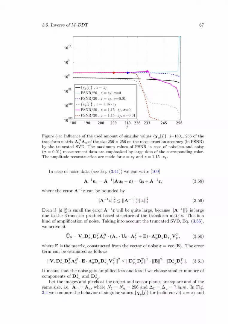
3.5. Inverse of M–DDT 67

180 190 200 209 219 226 233 245 25610

−15

10−10

10−5

100

105

1010

j

{χy[j]} , z = zf

PSNR/20 , z = zf , σ=0

PSNR/20 , z = zf , σ=0.01

{χy[j]} , z = 1.15 · zf

PSNR/20 , z = 1.15 · zf , σ=0

PSNR/20 , z = 1.15 · zf , σ=0.01

Figure 3.4: Influence of the used amount of singular values {χy[j]}, j=180,...256 of the

transform matrix AHy Ay of the size 256 × 256 on the reconstruction accuracy (in PSNR)

by the truncated SVD. The maximum values of PSNR in case of noiseless and noisy(σ = 0.01) measurement data are emphasized by large dots of the corresponding color.The amplitude reconstruction are made for z = zf and z = 1.15 · zf .

In case of noise data (see Eq. (3.41)) we can write [109]

A−1uz = A−1(Au0 + ε) = u0 + A−1ε, (3.58)

where the error A−1ε can be bounded by

||A−1ε||22 ≤ ||A−1||22·||ε||

22 (3.59)

Even if ||ε||22 is small the error A−1ε will be quite large, because ||A−1||2F is largedue to the Kronecker product based structure of the transform matrix. This is akind of amplification of noise. Taking into account the truncated SVD, Eq. (3.55),we arrive at

U0 = VxD+τxD

TxΛH

x · (Ax ·U0 ·ATy + E) ·Λ∗yDyD

+τyV

Ty , (3.60)

where E is the matrix, constructed from the vector of noise ε = vec{E}. The errorterm can be estimated as follows

||VxD+τxD

TxΛH

x ·E ·Λ∗yDyD+τyV

Ty ||

2 ≤ ||D+τx

DTx ||

2 · ||E||2 · ||D+τyD

Ty ||. (3.61)

It means that the noise gets amplified less and less if we choose smaller number ofcomponents of D+

τx and D+τy .

Let the images and pixels at the object and sensor planes are square and of thesame size, i.e. Ax = Ay, where Nξ = Nη = 256 and ∆ξ = ∆η = 7.4µm. In Fig.3.4 we compare the behavior of singular values {χy[j]} for (solid curve) z = zf and

68 3. Discrete diffraction transform (DDT)

Figure 3.5: Amplitude reconstruction using the regularization by truncation, Eq. (3.55),for noiseless data σ=0 and z = 1.15 · zf . The reconstruction is performed for dif-ferent number of singular values τx = τy: (a) τx=210, RMSE=0.0294; (b) τx=233,RMSE=0.0118 (c) τx=235, the reconstruction fails.

(dashed-dotted curve) for z = 1.15 · zf , and consider the reconstruction quality ofan amplitude-only object (AM) in PSNR from noiseless and noisy data dependingon the number of involved {χy[j]} (sorted in descending order). Note that thegap between large and small singular values becomes more and more evident with

Figure 3.6: Amplitude reconstruction (AM, Lena test-image) obtained using the regu-larization by truncation, Eq. (3.55), τx = τy, for different distances, noisy and noise-less data: (a) z = zf , τx=256, σ=0, RMSE=1.6·10−14; (b) z = zf , τx=219, σ=0.01,RMSE=0.0344; (c) z = 1.15 ·zf , τx=233, σ=0, RMSE=0.0118; (d) z = 1.15 ·zf , τx=209,σ=0.01, RMSE=0.039.

3.5. Inverse of M–DDT 69

increasing the propagation distance. While the singular values {χy[j]} decreasemonotonically for z = zf , in case of z = 1.15 · zf their values decreases rapidly(by approximately eight orders of magnitude): see {χy[j]} in the interval fromj ∈ [226, 235].

In case of noiseless data (σ = 0, solid curves) the peaks of PSNR can beeasily seen in τy = 256 and τy = 233 for z = zf and z = 1.15 · zf , respectively.Nevertheless, in Fig. 3.5 it is illustrated the choice of the proper number of singularvalues is not trivial: the reconstruction with too small singular values fails, buttoo small number of used singular values leads to a significant degradation ofthe object reconstruction. For noisy data, σ = 0.01, we have a gently slopingcurve of PSNR: a slow, monotonic increase and then a fairly rapid decrease (morerapid decay for larger distances z). In Fig. 3.4 it is shown that the best resultsfor noisy data are for τx = 219 if z = zf and for τx = 209 if z = 1.15 · zf ,respectively. Here τx = τy. In Fig. 3.6 the object amplitude reconstructions forthese optimal number of singular values τx with respect to PSNR are illustrated:Fig. 3.6(a) demonstrates the practically perfect reconstruction; in Fig. 3.6(c)we have slightly worse reconstruction accuracy and imaging, respectively. Theamplitude reconstructions from noisy data in Fig. 3.6(b) and Fig. 3.6(d) lookequally poor due to strong degradation by “wave” artifacts.

Tikhonov’s regularization

Discrete ill-posed problems arise technically from the discretization of ill-posedproblems when all singular values of transform matrices decay gradually (on theaverage) to zero and there is no precise notion of a proper numerical rank for thesematrices (cf. Fig. 3.5(b) and 3.5(c)). Then, such an ill-posed problem needs tobe reformulated for numerical treatment. Typically this involves additional as-sumptions, such as smoothness of solution or a priori information on the objectdistribution. This is a classical regularization process, and Tikhonov’s regulariza-tion [91, 109, 219] is a common and well-known form of regularization of linearill-posed problems.

Although many types of additional information about u0 is possible in princi-ple, the dominating approach to regularize the discrete ill-posed problems is therequirement that the `2 norm of the solution must be small. An initial estimateu†0 of the solution may be also included in the side constraint. Thus, instead ofthe solving the conventional LS problem min

u0

||uz − A · u0|| one is looking for a

regularized estimate of u0 that defined by minimization of the quadratic criterion

u0 = arg minu0

||uz −A · u0||22 + µ2 · ||L(u0 − u†0)||22, (3.62)

where L could be, for instance, a differentiation matrix (discretized differentialoperator [91, 95, 109]). For discrete ill-posed problems, the goal is to find a balance

between the residual norm ||uz−A · u0||22 and the penalty ||L(u0−u†0)||22 (the sizeof the solution) that matches the errors in the data as well as one’s expectationsto the computed solution [91]. The regularization parameter µ2 serves for thispurpose. In our work (as in P1–P2 and [114, 115]) we have no initial estimate

(i.e. u†0[l] = 0 ∀l) and the matrix L in Eq. (3.62) is, for simplicity, the identity

70 3. Discrete diffraction transform (DDT)

matrix L = I. Thus, we are looking for the regularized estimate of the object asthe solution of the following optimization problem

U0 = arg minU0

||Uz −Ax ·U0 ·ATy ||2F + µ2 · ||U0||2F or (3.63)

u0 = arg minu0

||uz −A · u0||22 + µ2 · ||u0||22 (3.64)

|| · ||2F in Eq. (3.63) denotes the quadratic Frobenius matrix norm. The reg-ularization penalty ||U0||2F or ||u0||22 enables to obtain a bounded and smoothobject estimate and the regularization parameter µ2 controls the level of thesmoothness of this estimate. The regularized inverse u0 defined as a minimizer ofJ = ||uz −A · u0||2 + µ2||u0||2 is calculated by [P1, Appendix B]

∂

∂uH0uHz uz − uHz Au0 − uH0 AHuz − uH0 AHAu0 + µ2uH0 u0 = 0

Using SVD (3.44), the accurate solution can be given in the form of the Tikhonovregularized inverse (RI)

u0 = (AHA+µ2I)−1︸ ︷︷ ︸A−1µ

AH · uz = (3.65)

= (Vy ⊗Vx)((DTy Dy ⊗DT

xDx) + µ2I)−1(DTy ⊗DT

x )(ΛHy ⊗ΛH

x ) · uz.

Note, however, that the approximate Tikhonov RI originated in P1 and givenby

U0 ≈ (AHx Ax + µI)

−1AHx ·Uz ·A∗y(A

Ty A∗y + µI)

−1= (3.66)

= Vx(DTxDx + µI)−1ΛH

x ·Uz ·Λ∗y(DTy Dy + µI)−1VH

x

is, in general, computationally simpler because of the significantly smaller dimen-sion of transform matrices. Comparing the latter equation with Eq. (3.48), notethat the inverse of AH

x Ax and ATy A∗y is just replaced by the inverse of their reg-

ularized versions AHy Ay + µI and AT

xA∗x + µI. Using Eqs. (3.51) and (3.52) wemay rewrite the approximate regularized inverse solution for non-averaged matri-ces [P1, cf. Eq. (44)] as follows

U0 ≈(λz)2

∆2ξNx∆2

ηNy(B′x +

µλz

∆2ξNx

I)−1

BHx ·Uz ·B∗y(B

′y +

µλz

∆2ηNy

I)−1, (3.67)

B′x =λz

∆2ξNx

BHx Bx, B′y =

λz

∆2ηNy

BTxB∗x.

3.6 Actual results and accuracy prediction

The comparison of the reconstruction accuracy obtained by the approximate Tikho-nov RI and by M–IDFrT (with no regularization, µ = 0) using the averaged ornon-averaged matrices can be found in [P2, Fig. 2]. Following this text theseresults are obtained by Eq. (3.66) or Eq. (3.67) for the regularized inverse and by

3.6. Actual results and accuracy prediction 71

Eqs. (3.48)–(3.50) or Eq. (3.52) for M–IDFrT. It can be seen that M–IDFrT issystematically worse than M–DDT for z > 1.5 · zf . However, as it is also shown inFig. 3.3, that averaging allows significantly improving the reconstruction qualitycomparing with the conventional Fresnel diffraction transform.

In [114, Fig. 3] and [115, Fig. 2] it is illustrated the comparison of the ampli-tude reconstruction accuracy by different methods: M–DDT with the approximate

12 18 33.4 42.8 52.2 77 92.4 107.8 123.20

0.2

0.4

0.6

0.8

1

z, [mm]

rank(Θ

)/N

Θ = AHy Ay,N = Nξ

Θ = AHx Ax, N = Nη

Θ = AHA, N = Nξ ·Nη

12 18 33.4 42.8 52.2 77 92.4 107.8 123.2

100

105

1010

z, [mm]

cond(Θ

)/N

2

Θ = AHy Ay,N = Nξ

Θ = AHx Ax, N = Nη

Θ = AHA, N = Nξ ·Nη

12 18 33.4 42.8 52.2 77 92.4 107.8 123.220

30

40

50

60

z, [mm]

PSNR

zf,x

zf,x

zf,x

zf,y

zf,y

zf,y

truncated SVD

accurate Tikhonov RI

approximate Tikhonov RI

Figure 3.7: The amplitude reconstruction quality (in PSNR [dB], bottom image) versusconditioning number (cond, middle image) and the numerical rank (rank for τε = 10−12,top image) of the transform matrices AH

y Ay, AHx Ax and AHA for rectangular pixels

of the same size at the object and sensor plane 8×5 (µm). The results are obtained bythe truncated SVD, Eq. (3.55); Tikhonov accurate (Eq. (3.65), µ2=10−24) and approx-imate regularized inverse (Eq. (3.66), µ=10−12) for z ∈ [

zf,y2, 2 · zf,x]. zf,y =24.1mm,

zf,x =61.6mm, AM, Baboon test-image (512×512 pixels), σ=0.

72 3. Discrete diffraction transform (DDT)

solution (3.66), F–DDT (Eqs. (3.25)–(3.28)), M–IDFrT with no averaging, andconventional convolutional methods of the single (conv1, Eq. (3.29)) and doublesize (conv2, zero-padding as in F–DDT or [196]). It is found that the best resultis almost always in favor of M–DDT.

In Fig. 3.7 and [P1, Fig. 10] the comparison of the amplitude reconstruc-tion accuracy with respect to the numerical rank and conditioning number condfor noiseless data is presented. The results are given for square images of thesize 512 × 512 and rectangular pixels at the object and sensor planes of the size∆ξ = ∆x = 8µm, ∆η = ∆y = 5µm. The conditioning number cond(AHA) hastwo local minima corresponding to zf,x = 61.6mm and zf,y = 24.1mm (see Fig.3.7(middle image)), thus the single in-focus distance for the M–DDT algorithm isrecommended to be chosen with respect to the numerical rank as an alternative.

12 18 33.4 42.8 52.2 77 92.4 107.8 123.20

0.2

0.4

0.6

0.8

1

z, [mm]

rank(Θ

)/N

zf,xzf,y

Θ = AHy Ay,N = Nξ

Θ = AHx Ax, N = Nη

Θ = AHA, N = Nξ ·Nη

12 18 33.4 42.8 52.2 77 92.4 107.8 123.220

22

24

26

28

30

z, [mm]

PSNR

zf,xzf,y

truncated SVD

accurate Tikhonov RI

approximate Tikhonov RI

Figure 3.8: The amplitude reconstruction quality in PSNR (bottom image) versus rankfor τε = 0.02 (top image) of the transform matrices AH

y Ay, AHx Ax and AHA for rectan-

gular pixels of the same size at the object and sensor plane 8×5 (µm). The results are cal-culated by the truncated SVD, Eq.(3.55); Tikhonov accurate (Eq. (3.65), µ2=0.0015) andapproximate regularized inverse (Eq. (3.66), µ=0.01) for z ∈ [

zf,y2, 2·zf,x]. zf,y =24.1mm,

zf,x =61.6mm, Baboon test-image (512×512 pixels), noisy measurement data σ=0.01.

3.6. Actual results and accuracy prediction 73

Figure 3.9: Amplitude reconstruction by (a) the truncated SVD, RMSE=0.052, τx =τy=429, (b) the accurate Tikhonov RI, RMSE=0.047, and (c) the approximate TikhonovRI, RMSE=0.049 for square pixels ∆ξ = ∆η = ∆x = ∆y = 7.4µm. The results are givenfor AM, Baboon test-image (512×512 pixels), z = 1.15 · zf noisy data σ=0.01.

The one-to-one relation between rank(AHA) and the reconstruction accuracy inPSNR in Fig. 3.7 is obvious, so we take zf = min(zf,x, zf,y) [P1, cf. Eq. (51)]corresponding to the best accuracy in the interval [zf,y, zf,x]. The similar behaviorcan be seen for noisy data, σ = 0.01: see in Fig. 3.8.

Recall that in case of σ = 0 we calculate rank for the tolerance τε = 10−12

and take a quite small regularization parameter µ = 10−12 . For noisy data σ =0.01 the numerical rank is calculated regarding to the essentially larger toleranceτε = 0.02 for all z. Analogically, the regularization parameter is taken much largerand different in the accurate and approximate model of the Tikhonov regularizedinverse: µ2 = 0.0015 and µ = 0.01, respectively. If we take, say, µ = 0.0387 for theapproximate Tikhonov scheme, the reconstruction accuracy will be systematicallyworse up to 20% in PSNR.

The curves corresponding to the approximate solution of the Tikhonov regu-larization (3.66) and the regularization by truncation (3.55) are almost completelymerged in Figs. 3.7 and 3.8 with a slight superiority (about 5% in RMSE forσ = 0.01) in M–DDT. Nevertheless, the reconstructing imaging of the TikhonovRI in general is better (see Fig. 3.9), and the operation with the regularization pa-rameter is much simpler and computationally efficient comparing with the calcula-tion of SVD and choice of a proper number of singular values for the regularizationby truncation.

Table 3.1: The reconstruction accuracy (in PSNR) of the object amplitude (AM, Baboontest-image, 512×512 pixels) found by (column-wise, from left to right) the truncated SVD,the accurate and approximate Tikhonov RI for rectangular pixels.

PSNR [dB]z σ τy τx Eq. (3.55) Eq. (3.65) Eq. (3.66)

z = zf,y σ = 0 512 476 39.71 41.79 39.75z = zf,y σ = 0.01 466 464 27.73 28.55 28.12z = zf,x σ = 0 217 512 25.11 25.44 25.12z = zf,x σ = 0.01 203 466 23.49 23.86 23.62

74 3. Discrete diffraction transform (DDT)

The reconstruction imaging of the object amplitudes by the truncated SVD,accurate and approximate Tikhonov RI in the key points z = zf,y and z = zf,xboth for noiseless and noisy data is found to be very close (for z = zf,x becomesworse comparing with the results for z = zf,y due to some blurring regarding to ydirection (columns) of these images). Thus, we limit ourself by the reconstructionaccuracy presented in Table 3.1. In this Table we also present the numbers of theused singular values τy and τx (for the regularization by truncation), computedaccording to Eqs. (3.45) for the mentioned experimentally found tolerance τε.Obviously the best result is in favor of the accurate Tikhonov RI.

The comparison of the amplitude reconstructions by the mentioned techniquesfor AM, square pixels and noisy data σ=0.01 but for z = 1.15 · zf is illustratedin Fig. 3.9. Here, it can be convinced in a better imaging of the Tikhonov RIwith respect to the regularization by truncation. The use of the approximatesolution in P1–P2 is dictated by two main reasons. Firstly, the approximate RIis computationally simpler: the straightforward inverse of the huge matrix AHArequires computing of SVD. Secondly, it is found that (depending on the choice ofthe proper µ) there is no crucial difference in imaging between the accurate andapproximate RI, and the reconstruction accuracy in RMSE by Eq. (3.65) is thegreatest 5% better than by Eq. (3.66) for σ = 0.01 (20% for σ = 0) in case ofz = zf,y and this otherness decays not exceeding 4% (6%).

3.7 Choosing the Tikhonov regularization param-eter

The regularization parameter µ in P1–P2 and [114, 115] is chosen experimentallyjust for simplicity. However, it is well known that there are many parameter-choicestrategies, which are based on either an estimate of the norm of the perturbation||uz − Au0||2 = ||ε||2 (Morozov discrepancy principle, MDP [191, 156]) or theextraction of some additional information from the given residual and regular-ization errors: e.g., generalized cross validation [75], L-curve [93], U-curve [123],quasi-optimality criterion [95], normalized cumulative periodogram [94].

MDP

If the complex-valued measurements are given, we could evaluate the noise levelσ using, e.g., the Daubechies wavelets [66, cf. Eqs. (9), (10)]: the expectation

E〈‖ε‖2〉 = NxNyσ2 [109, cf. Eq. (2.14)]. For the same image and pixel sizes at the

object and sensor planes in some cases8[109, §2.3, Theorem 2.6] the regularizationparameter µ can be found as the unique zero of the following function:

8 The regularization parameter µ is calculated provided limµ→0 ||uz −AA−1µ uz ||22 ≤ ||uz −

AA−1µ uz ||22 ≤ ||uz ||22 (see Eq. (3.65) for A−1

µ ).

3.7. Choosing the Tikhonov regularization parameter 75

0 1 2 3 4 5−2

0

2

4

6

8

10

ln(αμ)

ln(β

μ)

−1.4 −1.2 −1 −0.8 −0.6 −0.4−2

−1

0

1

2

3

4

lg(μ)

c(μ)

ρτε,σ(μ)/100

Figure 3.10: Choosing the regularization parameter µ by (left image) L-curve with re-spect to the maximum curvature in the left corner, and by (right image) NCP (theminimum of the function c(µ)) or MDP (zero of the function ρτε,σ(µ)). The correspond-ing optimal µ are marked by bold geometrical elements. In the left image the line of theL-curve going upward corresponds to smaller µ, and the curve to the right correspondsto overregularized solutions with larger µ.

ρτε,σ(µ) =

rank(AHA)∑s=1

(χ2[s]

χ2[s] + µ2((ΛH

y ⊗ΛHx )uz)[s]

)2

+ (3.68)

+

NxNy∑s=rank(AHA)+1

((ΛH

y ⊗ΛHx )uz)[s]

)2 −NxNyσ2,

where the singular values in decreasing order of AHA are represented as thefollowing vector χ = vec{χx · χTy } = vec{χy · χTx }. Recall χy and χx are the

column vectors of the singular values of AHy Ay and AH

x Ax, respectively. Thecurve of the function ρτε,σ(µ) and the optimal µ by MDP are presented in Fig.3.10.

Since it is difficult to isolate the impact of the diffraction propagation andaccurately estimate the measurement noise σ, then the first type of parameter-choice methods, discrepancy principle based approach is not suitable. It is foundthat MDP works well only for small noise level (in our synthetic tests σ < 0.02)and small propagation distances, say z < 1.5 · zf . Moreover, the criterion function(3.68) depends on the numerical rank rank(AHA) or, equivalently, on the properchoice of the tolerance τε.

Further we present certain methods of the second type of the methods forchoosing regularization parameters, which is found to enable a good estimate of

76 3. Discrete diffraction transform (DDT)

µ both for the noiseless and noisy data. It should be emphasized that all thesecriteria could be easily computed in parallel.

GCV

Generalized cross validation (GCV) is based on the philosophy that if an arbitraryelement of uz is left out, then a regularized solution should predict this observationwell. The GCV estimate of the regularization parameter µ can be taken from themeasurement data by minimization of the GCV criterion function [75, 95, 180]

Γ(µ) =||AA−1

µ AHuz − uz||22trace(AA−1

µ AH−I)2=||c ◦ vec{ΛH

x UzΛ∗y}||22

(sum(c))2, (3.69)

where A−1µ is defined in Eq. (3.65), trace means the trace of a square matrix

defined by a sum of the elements on the main diagonal. c in Eq. (3.69) is a vectorconstructed from the diagonal elements of the matrix

diag(c) = (Dy ⊗Dx)((DTy Dy ⊗DT

xDx) + µ2I)−1(DTy ⊗DT

x )− I.

The result of choosing of the regularization parameter µ by minimization of theGCV criterion function Γ(µ) is presented in Fig. 3.11.

L-curve

Perhaps the most convenient graphical tool for analysis of discrete ill-posed prob-lems is the so-called L-curve, which is a plot (for all valid regularization parametersµ) of the norm ||A−1

µ AHuz||2 of the regularized solution versus the corresponding

residual norm ||uz −AA−1µ AHuz||2. It is known that under certain assumptions

the L-curve

(||uz −AA−1µ AHuz||2, ||A−1

µ AHuz||2 = (αµ, βµ)

for Tikhonov regularization (3.65) has two characteristic parts: a horizontal part,where the regularized solution u0 is dominated by regularization errors and almostvertical part, where u0 is dominated by residual errors. In this way, the L-curveclearly displays the compromise between minimization of these two quantities,which is the heart of any regularization method [91, 95, 109]. In many cases it isadvantageous to consider the L-curve in a log-log scale (lnαµ, lnβµ). Moreover,the behavior of the L-curve is easily seen in such a scale. The optimal value ofµ in terms of the L-curve method is thought to be chosen corresponding to thepoint of maximum curvature, as near the corner as possible (see Fig. 3.10). Anyone-dimensional optimization routine can be used to locate the value of that cor-responds to the maximum curvature9. This point can be easily found numericallyby minimizing the curvature function of the L-curve [93, cf. Eq. (8)]

κ(µ) =αµβµ − αµβµ(αµ

2 + βµ2)3/2

, (3.70)

9 It can be, e.g., corner routine in [95].

3.7. Choosing the Tikhonov regularization parameter 77

−1.4 −1.2 −1 −0.8 −0.6 −0.420

21

22

23

24

lg(μ)

PSNR

oracle

GCV

L− curve

U − curve

Q

NCP

MDP

−1.4 −1.2 −1 −0.8 −0.6 −0.4−7.5

−7

−6.5

−6

−5.5

−5

−4.5

lg(μ)

lg(Γ(μ))

κ(μ)− 5

ln(U(μ))− 4.5

lg(Q(μ))− 4

Figure 3.11: The optimal results of different parameter-choice methods and the corre-sponding reconstruction accuracy by the chosen µ marked by bold geometrical elements.The reconstruction quality is given in PSNR for AM (Lena test-image), z = 1.5 ·zf , noisydata σ = 0.03. The curve of NCP and MDP criterion functions are given before in Fig.3.10.

where the accents ˙ and ¨ in Eq. (3.70) denote the numerical differentiation oper-ations of the first and second order, respectively, with respect to the regularizationparameter µ. The result of the minimization of this criterion function is depictedin Fig. 3.11.

U-curve

Following [123, cf. Eq. (9)], the U-curve is defined as U(µ) = 1αµ

+ 1βµ

with

three characteristic parts: the “vertical”parts corresponding to the regularizationparameter, for which αµ and βµ are dominated by each other, and a “horizontal”

78 3. Discrete diffraction transform (DDT)

part, which corresponds to the regularization parameter, where αµ and βµ areclose to each other. In our experiments we choose the regularization parameter µconsidering the U-curve in the log scale

lnU(µ) = ln(αµ + βµ)− ln(αµβµ). (3.71)

The behavior of such a lnU -curve is presented in Fig. 3.11. In our caselnU(µ) has a large horizontal part for small µ and then U-like curve to the rightfor relatively large µ with further very rapid increasing of lnU(µ). In Fig. 3.11 wepresent only a left part of this U-like curve. Following the L-curve method we arelooking for a proper µ in the corner between the large horizontal part of lnU(µ)and the left vertical part, namely: we take the point of maximum curvature9.

Quasi-optimality criterion

Quasi-optimality criterion (Q) [92, 156] means that the regularization parameterµ is calculated by minimizing the following function [95, cf. Eq. (2.64)]

Q(µ) =

NxNy∑s=1

(χ2[s]

χ2[s] + µ2· µ2

χ2[s] + µ2((ΛH

y ⊗ΛHx )uz)[s]

)21/2

. (3.72)

It is shown in Fig. 3.11 that the minimum of the criterion function Q(µ) can beeasily found, but only in a reasonable range of values, say µ ∈ [10−10, 1] as it isemphasized in P1. For larger values of the regularization parameter, say µ > 1,the curve of Q(µ) has a local maximum and then decreases monotonically.

NCP

The normalized cumulative periodogram (NCP) [95] is basically a cumulated powerspectrum, and its computation requires one fast Fourier transform per residualvector (uz −AA−1

µ AHuz). The NCP criterion function is calculated according to[94, Eq. (3.8)]. The expected NCP for white noise is a straight line, and we use theminimum distance from the NCP to a straight line denoted by c(µ) as the criterionto be minimize in order to choose the regularization parameter µ (see Fig. 3.10).This criterion is found to work unstable for relatively large distances z > 2 · zfand large amount of noise, say σ = 0.05, thus we recommend to use in general thelatter four mentioned methods: GCV, L- and U-curves, and quasi-optimality.

3.8 Conclusions

Here the developed two-matrix model for the accurate discrete diffraction propa-gation is presented. The contribution of the author of this thesis is the analysis ofM–DDT (originated in P1), its properties and resulting reconstruction quality fordifferent parameters of the optical system: the size of the object and given mea-surements, pixel size, propagation distances z, etc. It is of importance becauseM–DDT (as well as F–DDT) is used in our phase-retrieval algorithms P3–P6.Generally, M–DDT (F–DDT) may be employed in many application areas where

3.8. Conclusions 79

the precise discrete-to-discrete model is dictated by the use of digital devices (inSLM–CCD setups): e.g., for the wave field synthesis [111, 112] or holographicprojection [125, 126].

In Section 3.5.3 we refine certain aspects related to the straightforward ap-proach of the backward propagation for ill-posed matrices using the regularizationby truncation. It is shown that in case of noiseless or a small amount of noisethe truncated SVD is a good alternative for relatively fast implementation of theinverse of M–DDT, if the matrices of the eigenvectors are given. However, sincethe proper numerical rank can not be accurately determined, and due to the useof time-consuming SVD we typically use the Tikhonov RI model, which gives, inaddition, a better reconstruction accuracy, especially for large z and noisy data.

Figures 3.7 and 3.8 clarify our choice of a single in-focus distance in case ofrectangular images or pixels at the object and sensor planes: zf = min(zf,x, zf,y)[P1, Eq. (51)].

Here we present the accurate M–DDT propagation model in the Kroneckerproduct form and visually explanation our suggestion to use the approximateTikhonov RI in P1. The accurate model systematically gives a better recon-struction accuracy, but it is very difficult in use due to a very high dimension ofthe transform matrix A.

It is also shown that the potential reconstruction accuracy can be predicted bythe numerical rank or conditioning of individual matrices related to the transformof rows and columns of images (Eqs. (3.47)). It is connected to our furtherprediction analysis via a sum of such individual transform matrices in Section 4.3.

Finally, in Section 3.7 we consider the choosing of the Tikhonov regularizationparameter µ : it is found that the conventional methods work quite well for theinterferometric model where (noisy) complex-valued measurements are given. Theproblem consists of the noise level and ill-posedness of the transform matrix. Ingeneral case GCV, L-/U-curve or quasi-optimal methods enables a proper choiceof µ. However, the situation is dramatically different in case of phase-retrievalwhen the phase is not given and we deal with a number of different sensor planes.This case of the parameter choosing is out of scope of this thesis but is our furtherwork to be done.

Chapter 4

Multi-plane iterative phaseretrieval

It has been mentioned that a conventional commodity sensor detects only the in-tensity of the light wave field and the phase is lost in this physical measurements.In practice we have no complex-valued observation uz in the single plane discretediffraction model (Fig. 3.1), and the object u0 can not be estimated straightfor-ward by the backward wave field propagation according to, e.g., the conventionalpropagation models (see Section 2.2) or by the inverse of M–DDT from Section3.5. Following the idea of the numerical recalculation of the object wave field froma number of intensity observations from Section 2.4, in this Chapter we considerdeveloped computational parallel iterative* multi-plane phase-retrieval algorithms,initially with no incorporate object filtering, as they were improved. In Section4.2 the initial multi-plane scenario of phase retrieval, the MF–DDT algorithm ispresented. Then, in Section 4.4 the augmented Lagrangian based parallel phase-retrieval algorithm and its modification for the known object structure: for theamplitude- (Section 4.4.3, the AL–A algorithm) and phase-only (Section 4.4.4 and4.4.5, the gradient descent and Gauss–Newton AL–Ph algorithms) object to bereconstructed.

4.1 Propagation models

A volumetric wave field is generated by a single transverse object wave field u0(ξ, η)(see Fig. 2.2), however the 3D wave field is given only in a number of noisy intensityobservations {|ur(x, y)|2}Kr=1, at K different sensor planes parallel to the objectplane at distances zr = z1 +(r−1) ·∆z from it. Here z1 is the distance between theobject and the first sensor plane, ∆z is a fixed distance between the observationplanes. We need to recover the phase in {ur(x, y)}r and then reconstruct thecomplex-valued object u0 using these complex-valued estimates ur, r = 1, ...K.

Again, it is assumed that the wave field distributions at the object and sensorplanes are pixelated, i.e. they are pixel-wise invariant. Thus, we arrive at adiscrete-to-discrete model but now with a number of wave field distributions as

81

82 4. Multi-plane iterative phase retrieval

Figure 4.1: Discrete model of the multi-plane phase retrieval. U0[l1, l2] and Ur[l′1, l′2]

(r = 1, ...K) are discrete 2D complex amplitudes at the object and measurement planes,respectively (cf. Fig. 2.2). ∆z is a fixed distance between the measurement planes.

it is illustrated in Fig. 4.1. The link between the wave field distributions at theobject and sensor planes is given in the following general form

ur = Ar · u0, r = 1, ...K, (4.1)

where the column vectors u0 and ur denote the input and output of the coherentimaging system and Ar is a transform matrix described the forward wave fieldpropagation from the object to the r-th sensor plane P4. Let us consider thediscrete diffraction propagation model used to calculate the sensor plane wavefield distributions ur.

4.1.1 Free space propagation

Let Mr be a discrete 2D distribution of the transfer function corresponding to thefree space diffraction propagation to the distance zr. It can be computed as thesampled version of the conventional ASD Hr or the Fresnel transfer function Gr;via the Fourier transform of the RS [196] or Fresnel diffraction kernels (with orwithout averaging, see Section 3.2.3). Following the propagation model (3.36) theresult of the free space forward wave field propagation of the single size can berepresented as follows

ur = vec{F−1{F{U0} ◦Mr}}, r = 1, ...K. (4.2)

Note that in case of the double size Mr and realization via FFT (e.g., usingF–DDT as in P4–P5, [149]) the difference consists of the zero-padding of theobject ZPN ′x×N ′y{U0} and extraction of the center part of the resulting sensorplane distribution according to Eqs. (3.25)–(3.28). The image size at the objectplane is taken as a multiple of 2 and the size of the sensor plane is defined by Eqs.(3.38); N1 = N ′x +Nξ, N2 = N ′y +Nη.

The forward wave field propagation can be also calculated by M–DDT (see Eqs.(3.16)–(3.17) in Section 3.2.1) what enables the accurate pixel-to-pixel mappingu0 to ur for images and pixels of different sizes at the object and the r-th sensor

4.2. Multiple plane Frequency DDT (MF–DDT) 83

planes. Again we obtain a single transform matrix in the form of the Kroneckerproduct

ur = Ar · u0, Ar = Xr ⊗Yr, r = 1, ...K, (4.3)

where Yr and Xr are the averaged M–DDT transform matrices with respect to y(columns) and x (rows) directions of the object image. These transform matricesare calculated according to Eqs. (3.14)–(3.13), but, in contrast to what we havein Section 3.2.1, for different propagation distances zr. It is emphasized by theadditional subindices r of the transform matrices.

4.1.2 Observation model

Assume that we make a set of K experiments, and therefore a number of intensitymeasurements at the sensor planes are given. Then, we can formulate the phaseproblem to be solved as follows: reconstruct the complex-valued object distributionu0 using the noisy intensity observations {or}r, which can be represented by thefollowing vector-matrix notation1

or = |ur|2 + εr, r = 1, ...K, (4.4)

where, in contrast to Eq. (3.41), the noise is assumed to be real-valued i.i.d. zero-mean Gaussian (for simplicity and referring to the central limit theorem) withthe variance σ2

r, εr[l′] ∼ N (0, σ2

r), independent for different r. The error εr isconsidered as a result of various small degradation factors such as sensor noise.Note that it can be also used more complex distributions for εr, such as Poissonianor mixed Poissonian–Gaussian [66].

4.2 Multiple plane Frequency DDT (MF–DDT)

As it is mentioned in Section 2.4, the stability and convergence of the iterativephase-retrieval algorithms as well as the accuracy of the resulting solutions arenot guaranteed in case of presence of noise. In P3 and [146] we developed ourinitial multi-plane iterative phase-retrieval techniques which enables a significantlyimprovement of the reconstruction quality by the aggregation of a number of theobject estimates computed in the parallel phase-retrieval procedure.

In Section 2.4.3 we discuss the reconstruction of the volumetric wave field bythe circular wave field propagation from one sensor plane to another one as itis presented in [8, Fig. 2]. Then, Eq. (2.12), describing the modern successiveSBMIR phase-retrieval algorithm, can be rewritten in our vector-matrix notationsas follows

uχ(t+1) = Aχ(t+1),χ(t) ·[√

oχ(t)

|uχ(t)|◦ uχ(t)

], t = 1, 2, ... (4.5)

where Aχ(t+1),χ(t) is the transform matrix of the wave field propagation from theχ(t)-th to χ(t + 1)-th sensor plane, and the index of the sensor plane is defined

1 In order to avoid negative values of or[l′], in our numerical simulations we generate theobservations as or[l′] = max(|ur[l′]|2 + εr[l′], c0), where c0 is a small positive DC constant(typically c0 = 10−4).

84 4. Multi-plane iterative phase retrieval

by Eq. (2.13). The operation in the square brackets of Eq. (4.5) is element-

wise, i.e.

√oχ(t)

|uχ(t)|is a vector obtained by the element-wise division of the vector

of the amplitude obtained from the given noisy intensity√

oχ(t) at the χ(t)-th

sensor plane by the calculated amplitude |uχ(t)|. Thus,

[√oχ(t)

|uχ(t)|◦ uχ(t)

]is a

vector computed by means of a replacement of the module of uχ(t) by√

oχ(t),keeping the calculated phase at that plane. Moreover, the initial guess for thephase can also be a random vector.

In contrast to successive phase-retrieval algorithms, we focus on the objectplane. A multi-plane variation of GS is derived from the LS estimation of u0

assuming that complex-valued wave field estimates at the sensor plane ur areavailable. Following the variational maximum likelihood (ML) approach for theGaussian noise distribution in the observation model (4.4), the object reconstruc-tion is formulated by the following criterion function to be minimized (cf. Eq.(3.64))

J =

K∑r=1

1

σ2r

||ur −Ar · u0||22 + µ · ||u0||22, (4.6)

where σ2r is the variance of the noise at the r-th sensor plane. The quadratic

term in Eq. (4.6) appears as the minus logarithm of the Gaussian likelihoodfunction corresponding to the propagation model (4.1). The following penaltyterm is the regularization including prior information on the object distributionu0 to be reconstructed. The regularization parameter µ in Eq. (4.6) defines abalance between the residual error of the propagation model and a priori givenby the penalty. Numerous forms for the penalty are used in literature on digitalimage processing derived from speculations varying from probabilistic modeling ofimage distribution priors to heuristic constructions [91, 109], but in P3–P5 and[146, 147] we again use a simple but efficient quadratic Tikhonov’s penalty [219]as for M–DDT.

In P3 we originate the Multiple plane Frequency DDT (MF −DDT ) phase-retrieval algorithm. In MF–DDT the wave fields at all measurement planes are

Algorithm: MF −DDTInput: {or}Kr=1

Initialization: u00

Repeat for t = 0, 1, 2, ...Repeat for r = 1, ...K1. Forward propagation:utr = Ar · ut0End on r2. Object update:

ut+10 =

(∑Kr=1

1σ2rAHr Ar + µ · I

)−1

·∑Kr=1

1σ2rAHr ·[√

or|utr|◦ utr

]=

=∑Kr=1

1σ2rA−1µ AH

r ·[√

or|utr|◦ utr

]End on t

4.3. Conditioning and reconstruction accuracy 85

computed by the free space forward diffraction propagation (Step 1) using M–DDTor F–DDT. The object update (Step 2) is computed from the minimum condition∂∂u∗0J =

∑Kr=1

1σ2 [AH

r Aru0 − Arur] + µ · u0 = 0. The amplitude is kept to be

equal to the square root of the noisy intensity from the sensor plane observationsimilar to SBMIR (4.5) and the phase is iteratively replaced.

Note that the object wave field reconstruction in MF–DDT can be interpretedas the summation of K object estimates calculated by the backward propagationof {utr}r with the transform matrices A−1

µ AHr . In contrast to Eq. (3.65), we

calculate the inverse of a sum of the averaged transform matrices AHr Ar,

A−1µ =

(K∑r=1

1

σ2r

AHr Ar + µ · I

)−1

, (4.7)

where K ≥ 1 and the size of the matrix A−1µ is NxNξ ×NyNη.

In case of well conditioning and invertibility of the propagation transform ma-trices (e.g., for small distances z1 < zf or if we use ASD instead of M–DDT)

AHr Ar = I and no regularization is required, µ = 0. If σ2

r = σ2 ∀r, then A−1µ = σ2

K∀r and the MF–DDT algorithm has much simpler form [P4, cf. Eq. (5)]

utr = Ar · ut0, t = 0, 1, ... (4.8)

ut+10 =

1

K

K∑r=1

AHr ·[√

or|utr|

◦ utr

].

4.3 Conditioning and reconstruction accuracy

It is found that the quality of phase retrieval can be indicated by the numericalrank (rank(

∑Kr=1 AH

r Ar)) or conditioning number (cond(∑Kr=1 AH

r Ar)) of a sumof averaged transform matrices analogically to the way it is presented in Section3.5.2. The interesting point is that despite the decrease of rank(

∑Kr=1 AH

r Ar),K > 1, the behaviour of rank or cond for z1 > zf looks similar to what we havefor K=1. For z1 < zf , however, rank takes its maximum value (see Fig. 4.2and Fig. 4.4, for K=5), and cond significantly decreases (see Fig. 4.3 and Fig.4.5). As before, larger rank or smaller cond corresponds to a better reconstructionaccuracy: see [P4, Fig. 2 and Table 1] for z = 1

2 · zf and K = {3, 5, 10}.In general, due to the very large dimension of the transform matrices Ar,

it is difficult to calculate rank or cond for the sum of AHr Ar ∈ CNξNη×NξNη .

However, we have found that rank(∑Kr=1 XH

r Xr)·rank(∑Kr=1 YH

r Yr) can be used

as a good evaluation of rank(∑Kr=1 AH

r Ar). Indeed, since rank(Xr ⊗ Yr) =rank(Xr) · rank(Yr) [99] and

K∑r=1

AHr Ar =

K∑r=1

(XHr Xr ⊗YH

r Yr) = (4.9)

=

(K∑r=1

XHr Xr

)⊗

(K∑r=1

YHr Yr

)−

K∑s,r=1s6=r

(XHs Xs ⊗YH

r Yr),

86 4. Multi-plane iterative phase retrieval

0.5 1 1.5 2 2.50.2

0.3

0.4

0.5

0.6

0.7

0.8

0.9

1rank(Q

)/N

ξ/N

η

z1/zf

Q = AH1 A1

Q = XH1 X1 ⊗YH

1 Y1

Q =∑5

r=1AHr Ar

Q =∑5

r=1XHr Xr ⊗

∑5r=1Y

Hr Yr

Figure 4.2: Comparison of the numerical ranks of the averaged matrices∑Kr=1 A

Hr Ar

and∑Kr=1 X

Hr Xr ⊗

∑Kr=1 Y

Hr Yr for K = {1, 5}, ∆z = 0.5 µm, zf = 4.1 mm, square

images (Nξ = Nη = 48) and pixels (∆ξ = ∆η = 6.7 µm) of the same size at the objectand sensor planes.

then rank(∑Kr=1 AH

r Ar) can be bounded as

rank

(K∑r=1

XHr Xr

)rank

(K∑r=1

YHr Yr

)≤ rank

(K∑r=1

AHr Ar

)+ (4.10)

+ rank

K∑s,r=1s6=r

(XHs Xs ⊗YH

r Yr)

≤ K∑r=1

rank(XHr Xr)rank(YH

r Yr),

0.5 1 1.5 2 2.5

100

1010

1020

1030

cond(Q

)/N

2 ξ/N

2 η

z1/zf

Q = AH1 A1

Q = XH1 X1 ⊗YH

1 Y1

Q =∑5

r=1AHr Ar

Q =∑5

r=1XHr Xr ⊗

∑5r=1Y

Hr Yr

Figure 4.3: Comparison of the conditioning number of the averaged matrices∑Kr=1 A

Hr Ar

and∑Kr=1 X

Hr Xr ⊗

∑Kr=1 Y

Hr Yr for K = {1, 5} and the same settings as in Fig. 4.2.

4.3. Conditioning and reconstruction accuracy 87

0.5 1 1.5 2 2.5

0.2

0.3

0.4

0.5

0.6

0.7

0.8

0.9

1

rank(Q

)/N

ξ/N

η

z1/zf

K = 1, τε = 10−3.8

K = 5, τε = 10−3.8

K = 1, τε = 10−12

K = 5, τε = 10−12

Figure 4.4: Comparison of the numerical ranks of the averaged matrices Q =∑Kr=1 X

Hr Xr⊗

∑Kr=1 Y

Hr Yr computed by different tolerances τε = 10−12 and τε = 10−3.8

for K = {1, 5}. Here ∆z = 2 µm, zf = 21.6 mm, square images (Nξ = Nη = 256) andpixels (∆ξ = ∆η = 6.7 µm) of the same size at the object and sensor planes (see P4).

In practice

rank

(K∑r=1

XHr Xr

)rank

(K∑r=1

YHr Yr

)−rank

K∑s,r=1s6=r

(XHs Xs ⊗YH

r Yr)

(4.11)

is often negative and therefore Eq. (4.11) is useless as the lower bound for

rank(∑Kr=1 AH

r Ar).

0.5 1 1.5 2 2.5

100

1010

1020

1030

cond(Q

)/N

2 ξ/N

2 η

z1/zf

K = 1, τε = 10−3.8

K = 5, τε = 10−3.8

Figure 4.5: Conditioning number of the averaged matrices Q =∑Kr=1 X

Hr Xr ⊗∑K

r=1 YHr Yr for K = {1, 5} and settings similar to Fig. 4.4.

88 4. Multi-plane iterative phase retrieval

Thus, we omit the second term and arrive at

rank

(K∑r=1

XHr Xr

)rank

(K∑r=1

YHr Yr

)≤ rank

(K∑r=1

AHr Ar

). (4.12)

Fig. 4.2 demonstrate the use of Eq. (4.12). In Fig. 4.3 it is shown that aninequality similar to Eq. (4.12) can be used for the conditioning numbers withrespect to the individual transform matrices XH

r Xr and YHr Yr too.

Since for z = zf the transform matrices should be well-posed and no regular-ization should be required, then the tolerance τε used for the calculation of rankis taken with respect to z = zf as follows

τε = maxτε

(τε : rank(XH1 X1) · rank(YH

1 Y1) = Nξ ·Nη). (4.13)

In Fig. 4.4 we present the comparison of the computed numerical ranks for thetolerance τε = 10−3.8 found according to Eq. (4.13) and τε = 10−12 as before inour experiments with the M-DDT matrices in Chapter 3.5. It can be seen that forsmaller tolerance rank(

∑Kr=1 XH

r Xr ⊗∑Kr=1 YH

r Yr) becomes only slightly largerbut it may lead to an uncertainty in the behavior of the numerical rank in thecase when the propagation distance is near zf or z < zf . For instance, we havementioned that for say z = 1.05 · zf there is no perfect reconstruction so rankshould indicate that.

A proper selection of the regularization parameter µ is an important point ofthe variation formulation in inverse imaging. However, it is difficult to use thestraightforward parameter-choice methods, like the L-curve or U-curve mentionedin Section 3.7 for the multiple plane phase-retrieval scenario. Moreover, it ishard to realize the direct computation of the inverse of A−1

µ (Eq. (4.7)) due toits very large dimension. Thus, the Tikhonov parameter µ in P3–P5 and [146,147] is chosen experimentally, and the analysis of the choosing the regularizationparameter is beyond the scope of this thesis.

4.4 Augmented Lagrangian technique

It is found that in case of noiseless data (σ = 0) or small amount of noise (say, σ =0.01) the parallel MF–DDT phase-retrieval algorithm gives a better reconstructionaccuracy comparing with the successive one by example of SBMIR (more detailsare given in P3 and [146]). However, the situation is dramatically different ingeneral case with a significant noise level of the intensity observations σ > 0.01and z > zf resulting in strongly ill conditioning of the diffraction propagationoperators.

The regularization only is found not to be enough2 – some additional constantsrelated to both the wave field amplitude and phase (or to the real and imaginaryparts) are required in order to balance the accurate forward wave field propagationand fitting to the given observations.

2 Proper regularization parameters for MF–DDT and the augmented Lagrangian based phase-retrieval algorithm are chosen experimentally. The corresponding Matlab code for phase retrievalis available on the project web page [1].

4.4. Augmented Lagrangian technique 89

4.4.1 Variational formulation of phase retrieval

Let us consider the variational ML formulation of the augmented Lagrangian basedphase-retrieval algorithm with respect to noisy measurements. The straightfor-ward setting for the Gaussian noise distributions in the observation model (4.4)results in the following criterion (cf. Eq. (4.6))

J =∑r

1

2σ2r

||or − |ur|2||22 + µ · ||u0||22, (4.14)

where the first summand is the quadratic fidelity term corresponding to the obser-vation model (see P4 for metrics for the fidelity terms) and the second term is theTikhonov regularization. Using this new criterion (4.14) we require the accurateforward wave field propagation (4.1), and formulate the object reconstruction asthe following constrained optimization

u0 = arg minu0

K∑r=1

1

2σ2r

||or − |ur|2||22 + µ · ||u0||22 (4.15)

subject to ur = Ar · u0, r = 1, ...K.

The regularization parameter µ in Eq. (4.15) defines a balance between theprior information on the object and the fitting of calculated intensities of the wavefields at the sensor planes to the given observations. If µ = 0 the solution u0

minimizes∑r

1

2σ2r

||or − |ur|2||22 ignoring the fact that the data {or}r are noisy.

It can result in noisy and non-smooth u0. If µ > 0 and (comparatively) large,then the noise effects are well suppressed but the solution u0 can be oversmoothedand important features lost. The additional constraint corresponds to the forwardpropagation of the object to different sensor planes. The constrained optimizationproblem (4.15) can be represented using the augmented Lagrangian [98, 185] sothe criterion (with complex-valued variables) to be minimized is of the form

JAL({or},u0, {ur}, {Λr}) =

K∑r=1

1

σ2r

[1

2||or − |ur|2||22 + (4.16)

+1

γr||ur −Ar · u0||22 +

2

γrRe{ΛH

r (ur −Ar · u0)}] + µ · ||u0||22,

where {Λr} ∈ CNxNy are the Lagrange multipliers. We refer to [162, Chapters15–17] for more details on the theory of the augmented Lagrangian method.

In Eq. (4.16) the constraint ur−Ar ·u0 = 0 is used both in the quadratic andlinear terms with the positive penalty coefficients 1

γr. If we keep only the quadratic

terms the augmented Lagrangian becomes the penalty criterion. As a rule it leadsto computational difficulties because this criterion can be very ill conditioned. Ifwe keep only the linear term the augmented Lagrangian becomes the standardLagrangian. However, the saddle point of this standard Lagrangian is unstable.It results in the problems of numerical solutions. The stability of the saddle pointof the augmented Lagrangian is one of the principal advantages of this criterion[74]. Note that the linear terms 1

γrΛHr (ur − Ar · u0) and 1

γrΛTr (ur − Ar · u0)∗

90 4. Multi-plane iterative phase retrieval

in JAL are mutually conjugate, i.e. we control the real and imaginary part of thediscrepancy ur −Ar · u0.

4.4.2 Augmented Lagrangian algorithm (AL)

A search of this saddle point requires the minimization of the criterion (4.16) on u0

and {ur}, and maximization on the vectors of the Lagrange multipliers {Λr}. Theoptimization of the AL criterion can be realized by partitioning of the variablesu0 and {ur} into several blocks according to their roles following the alternatingdirection method of multipliers (ADMM, see, e.g., [2, 46]) and optimizing of (4.16)with respect to each block by fixing all other blocks at each inner iteration [19] asin the following algorithm

Repeat for t = 1, 2, ... (4.17)

Repeat for r = 1, ...K

ut+1r = arg min

urJAL(or,u

t0,ur,Λ

tr)

Λt+1r = Λt

r + αr · (utr −Ar · ut0)

End on r

ut+10 = arg min

uoJAL({or},u0, {ut+1

r }, {Λtr})

End on t

It leads to the iterative parallel augmented Lagrangian (AL) based algorithm [P4,cf. Eqs. (21)] presented below.

Algorithm: ALInput: {or}Kr=1

Initialization: u00, {Λ0

r}Kr=1

Repeat for t = 0, 1, 2, ...Repeat for r = 1, ...K1. Forward propagation:

ut+1/2r = Ar · ut0

2. Fitting to observations:

ut+1r [l′] = G(or[l

′],ut+1/2r [l′],Λt

r[l′]) ∀l′

3. Lagrange multipliers update:

Λt+1r = Λt

r + αr · (ut+1r − u

t+1/2r )

End on r4. Object update:

ut+10 =

(∑Kr=1

1γrσ

2rAHr Ar + µ · I

)−1

·∑Kr=1

1γrσ

2rAHr · (ut+1

r + Λtr)

End on t

Note that the optimization on the Lagrange multipliers {Λtr} in Eqs. (4.17) is

produced in the gradient direction ∂JAL/∂Λ∗r = 0. The updating step αr ∈ [0, 1][162] is taken to improve the convergence of AL. The derivation of the augmentedLagrangian based phase-retrieval algorithm, namely: the optimization of JAL on

4.4. Augmented Lagrangian technique 91

10 20 30 40 50 60 70 80 90 1000.04

0.05

0.06

0.07

0.08

0.09

0.1

0.11

number of iterations

RM

SE(|u

0|)

AL,σ = 0.02,μ = 0.0025

MF −DDT,σ = 0.02,μ = 0.05

AL,σ = 0,μ = 0.0005

MF −DDT,σ = 0,μ = 0.025

Figure 4.6: Convergence of the MF–DDT P3 and AL P4 algorithms in case of theamplitude reconstruction from noisy (σ = 0.02) and noiseless intensity observations forz = 2 · zf . The RMSE (solid) curves for MF–DDT are erratic, and for noisy data RMSEstarts to monotonically increase (thick solid curve), i.e. MF–DDT diverges.

Figure 4.7: Amplitude reconstruction by MF–DDT and AL (100 iterations) from noisyand noiseless measurement data for z = 2 · zf , K = 5, AM. The first row correspondsto the amplitude estimates reconstructed from noisy data (σ = 0.02) by (a) AL P4,µ = 0.0025, RMSE(|u0|)=0.048 and (b) MF–DDT P3, µ = 0.05, RMSE(|u0|)=0.062. Inthe second row there are results obtained from noiseless observations: (c) AL, µ = 0.0005,RMSE(|u0|)=0.041 and (d) MF–DDT, µ = 0.025, RMSE(|u0|)=0.044.

92 4. Multi-plane iterative phase retrieval

u0 and ur according to the minimum condition ∂JAL/∂u∗0 = 0 and ∂JAL/∂u∗r = 0,respectively, is presented in Appendices A.1 and A.2.

The initialization concerns the object (e.g., u00[l] = 1

2 ) and Lagrange multipliersvectors (e.g., Λ0

r[l] = 0). In Step 1 of AL we calculate the forward propagationof the object estimate ut0 to K sensor planes. Step 2 gives the updates ut+1

r

to “reconcile” the estimates ut+1/2r numerically with the observations or. The

operator defining this update ut+1r is denoted by G and described by Eqs. (A.4)–

(A.6). Step 3 returns the update for the Lagrange multipliers Λt+1r similar to

what we have in Eqs. (4.17). Step 4 gives the update for the object wave fieldcalculated from the corrected image estimates ut+1

r and the Lagrange multipliersΛtr. Note that Step 4 has the structure that is typical for the parallel algorithm:

the multiple estimates of u0 obtained from K sensor planes are aggregated intothe final update for the object reconstruction.

It can be seen that the main difference of the AL algorithm from MF–DDTconsists of the the estimation of the wave fields at the sensor plane3 (Step 2 ofAL). In Figs. 4.6 and 4.7 the comparison of the amplitude reconstruction qualityobtained by MF–DDT and AL phase-retrieval algorithms P4, [147] for z = 2 · zfand the synthetic noisy with σ = 0.02 are presented. The forward and backwardpropagations are always performed using F–DDT with averaging. It is obviousthat the reconstruction imaging is in favour of AL for both noisy and noiselessdata (left column in Fig. 4.7). Here we would like to emphasize the divergenceof MF–DDT (thick curve, Fig. 4.6) in case of larger amount of noise and strongill-posedness of the transform matrix. Moreover, it is found that for larger z or σthe reconstruction imaging becomes even worse (cf. Fig. 4.7(b)). Thus, AL, as ourfurther development of the parallel phase-retrieval algorithm, becomes significantmore powerful tool for the object wave field reconstruction from noisy data andlarge propagation distances.

The discussion about the object reconstruction quality by the AL algorithmfor AM and PM and comparison of AL with SBMIR are presented in [P4, Section3] and [147, Section 4]. Evidently that a priori information on the object cansignificantly improve the reconstruction quality, and further we consider somemodification of the AL algorithm developed especially for known object structures,for AM and PM.

4.4.3 AL for amplitude object (AL–A)

Note that the object estimation in the AL algorithm is presented for an arbitrary,complex-valued object (3.1) by means that no prior information on its structureis given. In many cases the object phase is known (say, the phase is constant in athin glass transparency), and the only unknown variable is the object amplitude.

For the amplitude modulation of the object (AM) u0 = a0, φ0[l] = 0 theanalytical solution of the object update (Step 4 of AL) is defined by ∂JAL/∂a0 = 0,

3 In [118, Appendix B] it is shown that for small noise level σ and/or large γr (i.e. the strongdomination of the fidelity terms related to the forward propagation) the updating of utr can besignificantly simplified: {utr} can be computed by the replacement of the amplitude estimateswith the given (noisy) measurements as in MF–DDT or SBMIR. Figs. 4.6 and 4.7 for σ = 0prove our words that this modification may be used only for well-posed transform matrices or,at least, for distances close to zf .

4.4. Augmented Lagrangian technique 93

Figure 4.8: Amplitude reconstruction by (a-c) the AL phase-retrieval algorithm and by(d-f) its modification AL–A developed for AM (see Eq. (4.18)). The amplitude estimatesare given for z = 2 · zf , σ = 0, µ = 0.005 and different number of observations (from leftto right) K = {3, 5, 10}. Reconstruction accuracy for (a/b/c) is PSNR=18.7/22.8/24;and for (d/e/f) PSNR=26/26.1/26.2.

0 20 40 60 80 10010

12

14

16

18

20

22

24

26

number of iteration

PSNR(|u

0|)

K = 3,AL

K = 3,AL−A

K = 5,AL

K = 5,AL−A

K = 10,AL

K = 10,AL−A

Figure 4.9: Convergence rate of the AL and AL–A phase-retrieval algorithms for z = 2·zfand K = {3, 5, 10} for the experiments described in [P4, Fig. 2 and Table 1].

94 4. Multi-plane iterative phase retrieval

namely the optimal solution of the amplitude estimate is

at+10 =

(K∑r=1

1

γrσ2r

Re{AHr Ar}+ µ · I

)−1

·K∑r=1

1

γrσ2r

Re{AHr (ut+1

r + Λtr)}. (4.18)

The derivation of Eq. (4.18) is given in Appendix A.2.1. Practically, the onlydifference is that at each iteration we should keep only the real part of the objectestimate ut+1

0 and the imaginary part (object phase) should be always set equalto zero. Thus, we arrive at the modification of the AL algorithm for AM, denotedby AL−A.

Algorithm: AL−AInput: {or}Kr=1

Initialization: a00, {Λ0

r}Kr=1

Repeat for t = 0, 1, 2, ...Repeat for r = 1, ...K1. Forward propagation:

ut+1/2r = Ar · at0

2. Fitting to observations:

ut+1r [l′] = G(or[l

′],ut+1/2r [l′],Λt

r[l′]) ∀l′

3. Lagrange multipliers update:

Λt+1r = Λt

r + αr · (ut+1r − u

t+1/2r )

End on r4. Object amplitude update:

at+10 =

(∑Kr=1

1γrσ

2r

Re{AHr Ar}+ µ · I

)−1

·∑Kr=1

1γrσ

2r

Re{AHr (ut+1

r + Λtr)}

End on t

In contrast to AL, the initialization concerns (except the Lagrange multipliers)the object amplitude only (e.g., a0

0[l] = 12 as before), i.e. we care only about the

object amplitude.

The visual comparison of the reconstruction quality by AL and AL–A is pre-sented in Fig. 4.8: the top row corresponds to the AL amplitude reconstructionsfor z = 2 · zf and different number of observations K = {3, 5, 10}. In the bottomrow we present the object amplitudes obtained by AL–A. It can be seen that theAL–A results look much better than what we have by AL, but they are almostidentical in spite of various K. The convergence (in PSNR) for these settingsfor both AL and AL–A are illustrated in Fig. 4.9. It is found that numericallythe reconstruction accuracy of AL–A is approximately two-three times better inRMSE comparing with AL. Moreover the convergence of AL–A is much faster:here 50 iterations is enough while the AL reconstruction even after 100 iterationsdemonstrate worse imaging. All these results are computed for the Tiknonov reg-ularization parameter µ = 0.005. Note also that even for insufficient K = 3 < 4(see Section 2.4.2) the AL–A gives a good reconstruction quality.

4.4. Augmented Lagrangian technique 95

4.4.4 AL for phase object (AL–Ph): gradient descent algo-rithm

Let us consider the phase-only object wave field, i.e. the object of the form u0 =a · exp(iφ0), where a ∈ R+ is a (in general unknown) scalar variable. In outexperiments it is typically equal to 1.

Let us assume for a moment that a is known. Then, the minimum conditionon φ0 for JAL can be presented as follows (see Eq. (A.16) in Appendix A.2.2)

∂

∂φ0

JAL = 2 Im{(a · e−iφ0) ◦K∑r=1

1

γrσ2r

AHr (Ar(a · eiφ0)− ur −Λr)} = 0. (4.19)

The update of the object phase at the t-th iteration is performed by the iterativegradient descent algorithm due to a huge dimension of the transform matrices.Provided the initial guess φ0

0,t = φt0 the object phase is calculated as follows

Repeat for s = 0, 1, 2, ...S − 1 (4.20)

us0,t+1/2 = a · exp(iφs0,t)

∆φs0,t = 2 Im{(us0,t+1/2)∗ ◦K∑r=1

1

γrσ2r

AHr (Ar(u

s0,t+1/2)− ut+1

r −Λtr)}

φs+10,t = φs0,t − β ·∆φ

s0,t

End on s

where us0,t+1/2 is the auxiliary estimate of the object, ∆φs0,t is here the phase

gradient. The result of Eqs. (4.20) for the t-th iteration is the object phaseestimate at the (t + 1)-th iteration, in terms of Eq. (4.20) ut+1

0 = a · exp(iφS0,t).In P5 the number of iterations S and the updating step β are fixed for simplicity.Since the fixed updating step may result in divergence of the algorithm, β couldbe also defined as, e.g., a fractional step, i.e. the step size in the process of descentis divided into a certain value.

If the magnitude of the object a is known, we use its true value, denoted in P5as “a0”, i.e. ut+1

0 = a0 · exp(iφS0,t). If the scalar a is unknown, then the amplitudeestimate is calculated after the update of the phase as

χ =

K∑r=1

1

γrσ2r

||Ar exp(iφS0,t)||22 + µ ·NξNη, (4.21)

at+1 =1

χ

K∑r=1

1

γrσ2r

Re{(exp(−iφS0,t))T ·AHr (ut+1

r + Λtr)}.

The derivation is presented in Appendix A.2.2. Thus, the object estimate is there-fore of the form ut+1

0 = at+1 · exp(iφS0,t).Eqs. (4.20)–(4.21) define the modification of the AL algorithm for PM denoted

by AL− Ph with the conventional gradient descent method for the estimation ofthe object phase. The initialization concerns both the object amplitude (e.g.,a0 = 1

2 , if a0 is unknown) and the phase (it could be, e.g., a random or zerovector).

96 4. Multi-plane iterative phase retrieval

Algorithm: AL− Ph, gradient descentInput: {or}Kr=1

Initialization: φ00,1 ≡ φ

S0,0, a0, {Λ0

r}Kr=1

Repeat for t = 0, 1, 2, ...

a =

{a0, if a0 is givenat, otherwise

Repeat for r = 1, ...K1. Forward propagation:

ut+1/2r = Ar · [a · exp(iφS0,t)]

2. Fitting to observations:

ut+1r [l′] = G(or[l

′],ut+1/2r [l′],Λt

r[l′]) ∀l′

3. Lagrange multipliers update:

Λt+1r = Λt

r + αr · (ut+1r − u

t+1/2r )

End on r4. Object phase update:

φ00,t+1 = φS0,t

Repeat for s = 0, 1, 2, ...S − 1us0,t+1 = a · exp(iφs0,t+1)

∆φs0,t = 2 Im{(us0,t+1)∗ ◦∑Kr=1

1γrσ

2rAHr (Ar · us0,t+1 − ut+1

r −Λtr)}

φs+10,t+1 = φs0,t+1 − β ·∆φ

s0,t

End on s5. Amplitude recalculation, if a0 is not given

χ =∑Kr=1

1γrσ

2r||Ar exp(iφS0,t+1)||22 + µ ·NξNη

at+1 = 1χ

∑Kr=1

1γrσ

2r

Re{(exp(−iφS0,t+1))T ·AHr (ut+1

r + Λtr)}

End on t

In P5 we present the comparison of the wave field reconstruction of AL–Ph(gradient descent) with AL and SBMIR. The AL–Ph algorithm demonstrates fasterconvergence [P5, cf. Fig. 3] and significantly better reconstruction accuracy,especially by example of the smooth Mexican Hat object [P5, cf. Fig. 5]. Theconvergence of the object magnitude in case of a0={0.85, 1, 1.25} is illustratedin [P5, Fig. 4]. It is found that a larger number of observations K leads toa faster convergence, but results in significant oscillations around a0. Moreover,these oscillations are larger for larger a0.

4.4.5 AL for phase object (AL–Ph): Gauss–Newton algo-rithm

The Gauss–Newton (GN) method is a modification of the well-known Newton–Raphson method used to solve (non-linear) LS problems, in particular for opti-mization of criterion functions. Unlike Newton’s method, the GN algorithm hasthe advantage that second derivatives, which can be challenging to compute, arenot required. Moreover, GN is essentially simpler because it is not so vulnera-ble to the initial guess as Newton’s method. The GN algorithm of the objectphase recovering is also iterative and follows from the linearization of the residual

4.4. Augmented Lagrangian technique 97

10 20 30 40 50 60 70 80 90 100

0

5

10

13

15

20

22

number of iterations

PSNR(˜ φ

0)

AL

AL− Ph

AL− Ph, GN1

AL− Ph, GN2

SBMIR

Figure 4.10: Convergence of the phase-retrieval algorithms used for the reconstruction ofa phase-only object by AL (dashed-dotted curve); AL–Ph, gradient descent with the fixedupdating step β (dashed curve, [P5, cf. Fig. 3]); AL–Ph, Gauss–Newton method withthe fixed updating steps β and ζ (AL–Ph GN1, solid thin curve); AL–Ph, Gauss–Newtonmethod with the fractional steps β and ζ (AL–Ph GN2, solid thick curve); and SBMIR([8], dotted curve). These results are obtained for z = 2 · zf and noisy measurementsσ=0.05, PM with the known a0=1, K=5, chessboard test-image. β and ζ in AL–Ph GN2are divided by 2 and the number of iterations S and Q are doubled each 10 iterations.The curves of PSNR for GN1 and GN2 are overlapped up to the 30th iteration.

Figure 4.11: Fragments of the phase reconstruction obtained using different phase-retrieval algorithms: (a) by AL, PSNR=12.2, (b) by AL–Ph, gradient descent with thefixed updating step β, PSNR =13.9, (c) by AL–Ph, GN1 with the fixed updating steps βand ζ, PSNR=12.7, (d) by AL–Ph, GN2 with the fractional steps β and ζ, PSNR=21.1,(e) by SBMIR, PSNR=4.7. These results are given for z = 2 ·zf and noisy measurementsσ=0.05, PM with the known a0=1, K=5, chessboard test-image after 100 iterations, seeFig. 4.10, [P5, cf. Fig. 2].

98 4. Multi-plane iterative phase retrieval

ur −Ar · u0 in the AL criterion (4.16) as

ur −Ar · u0 ≈ ur −Ar · [a · exp(iφ0)]− ∂

∂φ0

(Ar · [a · exp(iφ0)]) ·ϕ0, (4.22)

i.e. it is obtained by ignoring the second-order derivative terms (only the first twoterms of the Taylor series are taken). Here ϕ0 is a small phase increment. Thus,the forward wave field propagation can be presented by (see Eq. (A.20))

ur = Ar · [a · exp(iφ0)] + iArΓ ·ϕ0, (4.23)

where Γ is the diagonal matrix with the object vector components in the maindiagonal, Γ = diag(a · exp(iφ0)) ∈ CNξNη×NξNη . Then, the phase update in termsof the GN algorithm is of the form (cf. Eq. (4.20))

φt+10 = φt0 + β ·ϕ0 = φt0 −

β

2·Υ−1 · ∂

∂φ0

JAL = (4.24)

= φt0 − β ·

(K∑r=1

1

γrσ2r

Re{ΓTATr A∗rΓ

∗}

)−1

×

× Im{(ut0)∗ ◦K∑r=1

1

γrσ2r

AHr (Aru

t0 − ut+1

r −Λtr)},

70 80 90 100 110 120

−2

−1.5

−1

−0.5

0

0.5

1

1.5

2

φ0

true AL AL− Ph, GN1 AL− Ph, GN2

Figure 4.12: Cross-section of the reconstructed phases by (dashed-dotted curve) by AL,PSNR=12.2; by (solid thin curve) AL–Ph, GN1 with the fixed updating steps β and ζ,PSNR=12.7 and by (solid thick curve) AL–Ph GN2 with the fractional steps β and ζ,PSNR=21.1. The true phase is depicted by a dashed curve. These results are presentedfor experiments illustrated in Fig. 4.11.

4.4. Augmented Lagrangian technique 99

where β is the updating step and the matrix

Υ =

K∑r=1

1

γrσ2r

Re{ΓTATr A∗rΓ

∗} ∈ CNξNη×NξNη (4.25)

is a sort of approximation of the Hessian matrix, computed for Γ = diag(a ·exp(iφt0)). The phase increment ϕ0 in Eq. (4.24) is derived in Appendix A.3.

Due to a huge dimension of the matrix Υ (Eq. (4.25)) we use an additionaliterative procedure to compute the phase increment. Thus, we arrive at the fol-lowing algorithm, which results in the update of the object phase estimate φ0,t atthe t-th iteration

Repeat for s = 0, 1, 2, ...S − 1 (4.26)

us0,t = at · exp(iφs0,t)

∆φs0,t = Im{(us0,t)∗ ◦K∑r=1

1

γrσ2r

AHr (Aru

s0,t − ur −Λr)}

Γs = diag(at · exp(iφs0,t)), Υs =

K∑r=1

1

γrσ2r

Re{(Γs)TATr A∗r(Γ

s)∗}

Repeat for q = 0, 1, 2, ...Q− 1

ϕq+10,t = ϕq0,t − ζ ·

[Υs ·ϕq0,t + ∆φs0,t

]End on q

φs+10,t = φs0,t + β ·ϕQ0,1

End on s

where Γs and Υs are the s-th iterations of the auxiliary (above mentioned) ma-trices, ζ is a new updating step for the estimate of the phase increment ϕ0,t.Together, Eqs. (4.21) and Eqs. (4.26) result in the AL–Ph phase-retrieval algo-rithm with the phase estimation by the Gauss–Newton method. Here we denotethis algorithm “AL−Ph,GN” in order to distinguish it from the gradient descentimplementation from Section 4.4.4.

Thus, the main difference of the GN version of AL–Ph from the gradient de-scent implementation consists of the calculation of the descent direction what mayessentially improves the phase reconstruction quality and the convergence rateof the phase-retrieval algorithm, though the convergence of this algorithm is notguaranteed.

In Fig. 4.10 we present the convergence of AL, SBMIR and various modificationof AL–Ph in case of the phase reconstruction from significantly noisy data (σ =0.05) and ill-posed transform matrices (z = 2 · zf ). The result by the AL–Phalgorithm with the fixed updating steps β and ζ is depicted with a solid thin curveand denoted by GN1. It can be seen that this algorithm demonstrates the fastestconvergence, but after about 40 iterations the PSNR curve for this algorithm startsto be erratic with some tendency to decrease.

In order to overcome this problem we take in AL–Ph fractional steps: each 10steps we divide β and ζ by 2 and double S and Q. The result for the fractional

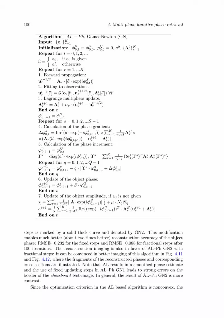
100 4. Multi-plane iterative phase retrieval

Algorithm: AL− Ph, Gauss–Newton (GN)Input: {or}Kr=1

Initialization: φ00,1 ≡ φ

S0,0, ϕQ0,0 = 0, a0, {Λ0

r}Kr=1

Repeat for t = 0, 1, 2, ...

a =

{a0, if a0 is givenat, otherwise

Repeat for r = 1, ...K1. Forward propagation:

ut+1/2r = Ar · [a · exp(iφS0,t)]

2. Fitting to observations:

ut+1r [l′] = G(or[l

′],ut+1/2r [l′],Λt

r[l′]) ∀l′

3. Lagrange multipliers update:

Λt+1r = Λt

r + αr · (ut+1r − u

t+1/2r )

End on r

φ00,t+1 = φS0,t

Repeat for s = 0, 1, 2, ...S − 14. Calculation of the phase gradient:

∆φs0,t = Im{(a · exp(−iφs0,t+1)) ◦∑Kr=1

1γrσ

2rAHr ×

×(Ar(a · exp(iφs0,t+1))− ut+1r −Λt

r)}5. Calculation of the phase increment:

ϕ00,t+1 = ϕQ0,t

Γs = diag(at · exp(iφs0,t)), Υs =∑Kr=1

1γrσ

2r

Re{(Γs)TATr A∗r(Γ

s)∗}Repeat for q = 0, 1, 2, ...Q− 1

ϕq+10,t+1 = ϕq0,t+1 − ζ ·

[Υs ·ϕq0,t+1 + ∆φs0,t

]End on q6. Update of the object phase:

φs+10,t+1 = φs0,t+1 + β ·ϕQ0,t+1

End on s7. Update of the object amplitude, if a0 is not given

χ =∑Kr=1

1γrσ

2r||Ar exp(iφS0,t+1)||22 + µ ·NξNη

at+1 = 1χ

∑Kr=1

1γrσ

2r

Re{(exp(−iφS0,t+1))T ·AHr (ut+1

r + Λtr)}

End on t

steps is marked by a solid thick curve and denoted by GN2. This modificationenables much better (about two times better) reconstruction accuracy of the objectphase: RMSE=0.232 for the fixed steps and RMSE=0.088 for fractional steps after100 iterations. The reconstruction imaging is also in favor of AL–Ph GN2 withfractional steps: it can be convinced in better imaging of this algorithm in Fig. 4.11and Fig. 4.12, where the fragments of the reconstructed phases and correspondingcross-sections are illustrated. Note that AL results in a smoothed phase estimateand the use of fixed updating steps in AL–Ph GN1 leads to strong errors on theborder of the chessboard test-image. In general, the result of AL–Ph GN2 is morecontrast.

Since the optimization criterion in the AL based algorithm is nonconvex, the

4.4. Augmented Lagrangian technique 101

0 20 40 60 80 100

0,7

0,80,85

0,9

1

1,1

1,21,25

1,3

1,4

1,5

number of iterations

a

0 20 40 60 80 100

0,7

0,80,85

0,9

1

1,1

1,21,25

1,3

1,4

1,5

number of iterations

a

AL− Ph,K = 10

AL− Ph, GN1,K = 10

AL− Ph,K = 5

AL− Ph, GN1,K = 5

Figure 4.13: Convergence of the object magnitude recovering by (dashed curve) AL–Ph,gradient descent [P5, cf. Fig. 4] and by (solid curve) AL–Ph, GN1. These results aregiven for PM with unknown a0={0.85,1,1.25}, z = 2 · zf , noisy measurements σ=0.05,chessboard test-image and different number of observations: (left image) K=5, (rightimage) K=10.

result is strongly depends on the initial guess of the algorithm. According to ourexperiments, AL–Ph GN2 with fractional updating steps demonstrates the bestreconstruction accuracy for various initial guesses. However, the computationalcomplexity of the Gaussian–Newton AL–Ph algorithm is significantly higher com-paring with the original AL or the gradient descent AL–Ph algorithm. The crucialpoint is that due to very high dimension of the matrix Υ (Eq. (4.25)) we use anadditional loop for the calculation of the phase increment: in particular, at eachs-th step (see Eq. (4.26)) we perform K · N2

ξN2η + Q · NxNyN2

ξN2η multiplica-

tions and additions to calculate Υs and, in addition, Q ·N2ξN

2η operations to find

Υs ·ϕq0,t+1. The computational time (in averaged for one iteration) for the AL andAL–Ph algorithms is presented in Table 4.1. These results are obtain by MonteCarlo simulation with averaging over 50 samples.

It can be seen a linear growth of the computational time with respect to the

Table 4.1: Computational time (in seconds for one iteration) for AL, the gradient de-scent AL–Ph and Gauss–Newton AL–Ph (AL–Ph GN1 with the fixed updating steps)algorithms.

AlgorithmsNξ ×Nη K AL AL–Ph AL–Ph GN1128×128 5 0.15 0.6 5.1128×128 10 0.28 1.2 10.6256×256 5 0.6 3.75 35256×256 10 1.25 7.35 68.6

102 4. Multi-plane iterative phase retrieval

dimension of the problem. Note, however, that the computational time for AL–Phincreases faster than for AL because of additional loops. Moreover, this time mayincrease in times in case of the fractional updating steps.

In Fig. 4.13 we illustrate the convergence of the gradient descent AL–Ph andAL–Ph GN1 (with fixed updating steps) algorithms in case of recovering the objectmagnitude a for PM, a0 = {0.85, 1, 1.25}. The GN1 version of the phase-retrievalalgorithm gives better convergence rate for both K = 5 and K = 10 comparingwith the gradient descent AL–Ph P5. However, it can be also seen that theoscillations around a0 are more significant for GN1.

4.5 Conclusions

In this Chapter we firstly consider our initial development of the parallel itera-tive MF–DDT phase-retrieval algorithm P3 with simultaneous aggregating of anumber of object estimates and therefore noise suppressing. The replacement ofthe computed amplitudes of the wave field at the sensor planes by ones obtainedfrom measurements is used analogically to the successive SBMIR phase-retrievalalgorithm. Further we reformulate the optimization problem: provided the accu-rate forward diffraction propagation we are looking for the fit of the calculatedintensity of the sensor plane wave field distribution to the observation. It resultsin the augmented Lagrangian phase-retrieval algorithm originated in P4. The useof a priori information on the object is firstly presented in P5 by example of themodification of the AL algorithm for PM. The AL–Ph phase-retrieval algorithmdemonstrates a significant improvement of the reconstruction accuracy (about twotimes in RMSE). In this text we gather all of these algorithms together and presentthem in order of their development. Note that in Chapter 4 we have no additionalobject filtering.

In Section 4.3 it is shown that the potential object reconstruction accuracy fromK wave field estimates at the sensor planes can be indicated by the rank of thesums of individual matrices rank(

∑Kr=1 XH

r Xr) · rank(∑Kr=1 YH

r Yr), where thetransform matrix of the diffraction propagation to the distance zr is Ar = Xr⊗Yr.This handy tool can clarify the resulting good imaging by AL for z = 1

2 · zf andz = zf : compare the maximum value of the numerical rank in Fig. 4.4 with verygood reconstruction quality in [P4, cf. Fig.2, Table 1].

In Section 4.4.3 we introduce the modification of the AL algorithm developedfor the amplitude-only object denoted by AL–A. Figure 4.9 demonstrate a betterconvergence rate and reconstruction accuracy (about 50% in RMSE for K=5). InSection 4.4.5 we present the modification of AL for the phase-only object, where thephase update is computed by the Gauss–Newton method (this algorithm is denotedby AL–Ph GN). It is shown that AL–Ph GN converges much faster comparing withthe gradient descent based AL–Ph algorithm or the AL algorithms (especially withfractional updating steps, see Fig. 4.10) and gives much sharper, contrast objectphase reconstruction (see Fig. 4.11).

Chapter 5

Phase retrieval with sparseobject regularization

It is found P3 that the spatially adaptive regularization (realized via BM3D filter[34, 35]) results in a significant improvement in imaging. Thus, sparse modelingis decided to be incorporated into the AL phase-retrieval algorithm because ofhigh performance and flexibility of this technique [48]. Sparse modeling of theobject is recognized to allow overcoming the loss of information related to theill-posedness of forward propagation operators, wiping out different corruptingartifacts, filtering noise, and therefore enhancing the resulting quality. In thisChapter we consider the improvement of the reconstruction accuracy and imagingby the incorporate separate filtering of the object amplitude and phase (numericalexperiments and some additional information can be found in P5–P6, [149]).Moreover, here we also discuss the use of the object sparse modeling in a moresophisticated phase-retrieval method with compensation of distortions arising sueto the forward diffraction propagation in the 4f optical system P7.

5.1 Observation models

In Section 2.2 we consider the forward wave field propagation computed via theRS and Fresnel diffraction integral, by the ASD or Fresnel transfer functions,and the result of the free space diffraction propagation, precisely the intensitymeasurements of diffraction patterns are (fairly) obtained at different distancesfrom the object. Despite the simplicity of the mathematical apparatus of the free-space setup, in practise the optical system is bulky and expensive due to the use ofa motorized sensor. In addition, the recording process of intensity measurementsis relatively slow due to the movement of the sensor.

Note that the transfer function of ASD (Eq. (1.44)) or its Fresnel approxima-tion (Eq. (1.67)) describes a pure phase modulation. It is shown in [4, 53] that a4f configuration can be used to imitate the lensless optical system for the multi-plane phase-retrieval scenario. The forward wave field propagation, presented inFig. 2.2, can be realized by the phase modulation of the Fourier transform of the

103

104 5. Phase retrieval with sparse object regularization

Figure 5.1: Experimental 4f optical setup for measurement recording [53]. The lensesL1 and L2 in the 4f configuration provides an accurate propagation of the transverseobject wave field u0(ξ, η) to the parallel observation (sensor) plane giving the wave fieldur(x, y). An optical mask with the complex-valued transmittance Mr(

v1λf, v2λf

) locatedat the Fourier plane (a phase modulating SLM) enables linear filter operations.

object wave field using the phase-only LC-SLM placed in the Fourier domain ofthe 4f optical system as it is illustrated in Fig. 5.1. The principal feature is thatin this case the sensor plane is immobile and fixed at the distance 4f from theobject plane.

5.1.1 4f configuration in phase-retrieval scenario

The lenses L1 and L2 with the focal length f arranged in the 4f configurationprovides an accurate propagation of the object wave field u0(ξ, η) to the par-allel measurement plane. Let us consider an ideal optical path with no distor-tions/aberrations. It can be shown (see Appendix B.1) that the wave field at theFourier plane (at the back focal plane of the first lens L1) is given as follows

uF

(v1

λf,v2

λf

)=ei2kf

iλfF{u0(ξ, η)}

(v1

λf,v2

λf

), (5.1)

where v = (v1, v2) ∈ R2 are the spatial frequencies. If the optical mask (SLM)inserted at the Fourier plane has the complex-valued transmittance Mr(

v1

λf ,v2

λf ),then the output of the optical system is defined as

ur(x, y) =ei2kf

iλfF{uF

(v1

λf,v2

λf

)· Mr

(v1

λf,v2

λf

)}(−x,−y) = (5.2)

= −ei4kf · {u0 ~ F{Mr

(v1

λf,v2

λf

)}}(−x,−y), r = 1, ...K.

Depending on the used optical masks {Mr(v1

λf ,v2

λf )}, a number of various wave

field distributions {ur}Kr=1 can be generated at the sensor plane corresponding todifferent complex-valued transmittances. For instance, the imitation of the freespace propagation via the Fourier transform of complex amplitudes of the object

5.2. Sparse modeling and BM3D filtering 105

and the sensor plane wave field distributions is of the form [118]

Ur

(v1

λf,v2

λf

)= −ei4kf · U0

(− v1

λf,− v2

λf

)· Mr

(− v1

λf,− v2

λf

), (5.3)

where r = 1, ...K and, taking into account that the Fourier transforms are givenin a scaled spatial coordinates1, the optical mask corresponding to ASD is [53]

Mr

(v1

λf,v2

λf

)= exp

ikzr√

1− v21

f2− v2

2

f2

(5.4)

for various distances zr of the wave field propagation.

5.1.2 Discrete modeling of 4f configuration

The discrete model of Eqs. (5.1)–(5.2) provided the sampling conditions

1

Nξ=

∆1∆ξ

λf,

1

Nη=

∆2∆η

λf,

1

N1=

∆1∆x

λf,

1

N2=

∆2∆y

λf, (5.5)

can be represented in the form

ur = −ei4kf · vec{F{F{U0} ◦Mr}}, r = 1, ...K. (5.6)

The 2D transfer function Mr in Eq. (5.6) by means of the real optical mask (seeEq. (B.10) in Appendix B.2) is very different from what is used in the free spacepropagation model (Eq. (4.2)) due to a finite size of the used phase modulatingLC-SLM and the fact that the active area of SLM cells is, in general, smaller thanthe full size of a pixel (i.e. the fill factor is not 100%). Further the discrete modelsof the diffraction propagation in 4f configuration (5.6) is applied in order to obtainthe required vectors of intensity measurements {or} (see Eq.(4.4)).

For simplicity, we use Eq. (B.9) for both the synthetic numerical experiments(in P6, [149]) and processing of experimental data from the 4f optical system witha phase modulating LC-SLM in the Fourier domain (in P6–P7). In the second casethe changes from the theoretically predicted result of the wave field propagationand nonidealities related to, e.g., the bandlimitedness of the transfer functionor various distortions in the optical path of the used coherent imaging system(Fig. 5.1) are considered as disturbances in the optical path2 to be estimated andcompensated.

5.2 Sparse modeling and BM3D filtering

According to the sparsity hypothesis it is assumed that the object amplitudea0 ∈ Rn and phase φ0 ∈ Rn can be separately approximated with small num-bers of non-zero components of basis functions (n = NξNη). Note that there isno prior information on the object modulation as before in AL–A (Section 4.4.3)

1 Substituting v1λf

= η1, v1λf

= η1 in Eq. (1.48) we obtain Eq. (5.4).2 The problem of disturbances compensation is discussed in Section 5.3.

106 5. Phase retrieval with sparse object regularization

and AL–Ph (see Sections 4.4.4, P5 and Section 4.4.5). In addition, the ideal basisfunctions for the object approximation are unknown a priori as well, and they areselected from a given set of potential bases (dictionaries). In general, sparse imageapproximation can be given in the synthesis or analysis form as follows:

θa = Φa · |u0|, θφ = Φφ · W−1{arg{u0}}, (analysis)a0 = Ψa · θa, φ0 = Ψφ · θφ, (synthesis)

(5.7)

where Ψa,Ψφ and Φa, Φφ are the frame transform matrices, and the vector θa,θφ ∈ Rm can be considered as a spectrum in a parametric data adaptive approx-imation (m � n). Recall that W denotes the wrapping operator (see Eq. (1))and, hence, W−1 in Eqs. (5.7) is an unwrapping operator (which can be realizedby, e.g., [44, 222]).

As it is mentioned in Chapter 3 here and in P5–P7, [149] the recovered ob-ject argument is assumed to be in the interval [−π, π) and therefore no unwrap-ping procedure is required; thus, the wrapping/unwrapping operators are hereafteromitted.

Subindices a and φ in Eqs. (5.7) are shown for the amplitude and phase, re-spectively. It is recognized that, in contrast to classical orthonormal bases (m=n),overcomplete frames based modeling (m� n) is a much more efficient for imaging[48, 89] and results in a better wave field reconstruction accuracy.

The sparsity of approximation is characterized by either the `0 or `1 norms. Asmaller value of the norm means a higher sparsity of approximation. Note thatresults obtained by `0 or `1 norms are shown to be closed to each other [42], whatallows replacing the nonconvex `0 norm by the convex `1 norm in many variationalsettings. The main intention is to find sparsest (shortest) models for phase andamplitude with smallest values of the `0 or `1 norms. The separate sparse modelingfor the object phase and amplitude is realized via the powerful BM3D-frame filter,specified for denoising and other imaging problems [37, 38, 117].

Taking into account the sparse modeling for the object amplitude and phase,the wave field reconstruction is performed by minimization of the following crite-rion [P6, Eq. (7)]

J =

K∑r=1

1

2σ2||or − |ur|2||22 + τa · ||θa||p + τφ · ||θφ ||p subject to (5.8)

ur = Ar · u0, r = 1, ...K, (forward propagation) (5.9)

θa = Φa · |u0|, θφ = Φφ · arg{u0}, (analysis) (5.10)

a0 = Ψa · θa, φ0 = Ψφ · θφ, (synthesis) (5.11)

where regularization terms for phase and amplitude are taken using the `p norms(p = {0, 1}). The positive parameters τa and τϕ in Eq. (5.8) define a balancebetween the fitting of the calculated |ur|2 to the given observation or, smoothnessof the wave field reconstruction and the complexity of the used model: cardinalityof spectra θa , θφ of the object amplitude and phase.

5.2. Sparse modeling and BM3D filtering 107

5.2.1 Multi-objective optimization

It is shown in [38] that a multi-objective optimization can be much more efficientthan the minimization of the single criterion J from Eqs. (5.8)–(5.11) due to asimpler implementation (filtering and inverse procedure are decoupled) and result-ing better reconstruction quality3. Thus, instead of the constrained minimizationof (5.8)–(5.11) we arrive at the unconstrained minimization of two criterion func-tions J1 and J2 with changing the constraints for sparse modeling by the quadraticpenalties with positive weights

J1({or},u0, {ur}, {Λtr},v0) =

K∑r=1

1

σ2[1

2||or − |ur|2||22 + (5.12)

+1

γr||ur −Ar · u0||22 +

2

γrRe{ΛH

r · (ur −Ar · u0)}+1

γ0

||u0 − v0||22,

J2(θa,θφ,u0) = τa · ||θa||p +1

2γa||θa −Φa · |u0|||22 + (5.13)

+τφ· ||θφ||p +

1

2γφ||θφ −Φφ · arg{u0}||22,

where in Eq. (5.12) v0 = Ψaθa◦exp(i ·Ψφθφ) is an approximation of the complex-valued object distribution u0.

Note that in contrast to [118] and similar to AL we involve the quadratic andlinear penalties related to the forward propagation model (ur = Ar · u0) withthe same positive parameters 1

γr. Thus, J1 becomes the augmented Lagrangian

objective function at least with respect to this particular constraint.

The analysis and synthesis constraints in Eq. (5.10) and Eq. (5.11) are replacedby quadratic penalties with the corresponding positive parameters 1

γa, 1γφ

and 1γ0

in Eq. (5.13) and Eq. (5.12), what is a standard tools to deal with constrainedoptimization [19]. Note also that the criterion J2 is separable with respect to θaand θφ, thus it can be rewritten as J2 = J2,a + J2,φ, where

J2,a(θa, |u0|) = τa · ||θa||p +1

2γa||θa −Φa · |u0|||22, (5.14)

J2,φ(θφ, arg{u0}) = τφ· ||θφ||p +

1

2γφ||θφ −Φφ · arg{u0}||22.

It is recognized [38, 117] that the minimization of J1 on u0 in general resultsin increasing of J2 and vice versa, optimization of J2 with respect to spectra θaand θφ increases J1. This problem can be interpreted in terms of the game theoryas a noncooperative interaction between the players. A compromise in this selfishbehavior can be found in the fixed point (u?0,θ?a,θ?φ) of the optimization calledgeneralized Nash equilibrium [50, 110, 129]. Then, the complex-valued object wave

3 Note that in [38] different models, such as analysis- and synthesis-only based object recon-structions, are considered.

108 5. Phase retrieval with sparse object regularization

field is reconstructed using decoupling of the inverse procedure and BM3D-framefiltering of the object amplitude and phase as [P6, cf. Eq. (10)]

θ?a = arg minθaJ2,a(θa, |u?0|)

θ?φ = arg minθφJ2,φ(θφ, arg{u?0})

v?0 = Ψaθ?a ◦ exp(i ·Ψϕθ

?ϕ)

u?0 = arg minu0,{ur}

max{Λr}

J1({or},u0, {ur}, {Λtr},v?0)

. (5.15)

Taking into account Eq. (4.17), the problem (5.15) can be realized with thefollowing iterative algorithm

Repeat for t = 0, 1, 2, ...

θta = arg minθaJ2,a(θa, |ut0|) (5.16)

θtφ = arg minθφJ2,φ(θφ, arg{ut0}) (5.17)

vt+10 = Ψaθ

ta ◦ exp(i ·Ψφθ

tφ) (5.18)

Repeat for r = 1, ...K

ut+1r = arg min

urJ1(or,u

t0,ur,Λ

tr,v

t+10 ) (5.19)

Λt+1r = Λt

r + αr · (utr −Ar · ut0) (5.20)

End on r

ut+10 = arg min

uoJ1({or},u0, {ut+1

r }, {Λtr},vt+1

0 ) (5.21)

End on t

Depending on the chosen `0 or `1 norm in J2 the so-called hard or soft thresh-olding, respectively, is appeared in the calculation of the spectrum for the objectamplitude θta and phase θtφ in Eqs. (5.16) and (5.17). Indeed, in Eqs. (5.14)we consider the optimization problem with respect to θa or θφ in the following

Figure 5.2: Fragments of the reconstructed object amplitude (128×64) computed using(a) SBMIR, RMSE=0.35, (b) AL, RMSE=0.23 and (c) D–AL, RMSE=0.026. The resultsare presented for synthetic data with the true object amplitude a0[l] = 1.

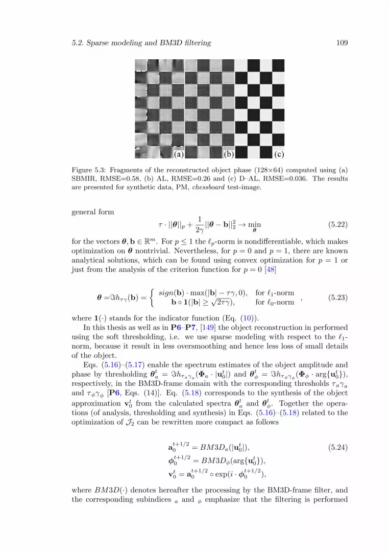
5.2. Sparse modeling and BM3D filtering 109

Figure 5.3: Fragments of the reconstructed object phase (128×64) computed using (a)SBMIR, RMSE=0.58, (b) AL, RMSE=0.26 and (c) D–AL, RMSE=0.036. The resultsare presented for synthetic data, PM, chessboard test-image.

general form

τ · ||θ||p +1

2γ||θ − b||22 → min

θ(5.22)

for the vectors θ,b ∈ Rm. For p ≤ 1 the `p-norm is nondifferentiable, which makesoptimization on θ nontrivial. Nevertheless, for p = 0 and p = 1, there are knownanalytical solutions, which can be found using convex optimization for p = 1 orjust from the analysis of the criterion function for p = 0 [48]

θ ==hτγ(b) =

{sign(b) ·max(|b| − τγ, 0), for `1-norm

b ◦ 1(|b| ≥√

2τγ), for `0-norm, (5.23)

where 1(·) stands for the indicator function (Eq. (10)).In this thesis as well as in P6–P7, [149] the object reconstruction in performed

using the soft thresholding, i.e. we use sparse modeling with respect to the `1-norm, because it result in less oversmoothing and hence less loss of small detailsof the object.

Eqs. (5.16)–(5.17) enable the spectrum estimates of the object amplitude andphase by thresholding θta = =hτaγa(Φa · |ut0|) and θtφ = =hτφγφ(Φφ · arg{ut0}),respectively, in the BM3D-frame domain with the corresponding thresholds τaγaand τφγφ [P6, Eqs. (14)]. Eq. (5.18) corresponds to the synthesis of the object

approximation vt0 from the calculated spectra θta and θtφ. Together the opera-tions (of analysis, thresholding and synthesis) in Eqs. (5.16)–(5.18) related to theoptimization of J2 can be rewritten more compact as follows

at+1/20 = BM3Da(|ut0|), (5.24)

φt+1/20 = BM3Dφ(arg{ut0}),

vt0 = at+1/20 ◦ exp(i · φt+1/2

0 ),

where BM3D(·) denotes hereafter the processing by the BM3D-frame filter, andthe corresponding subindices a and φ emphasize that the filtering is performed

110 5. Phase retrieval with sparse object regularization

with different parameters and different transform matrices Ψa, Ψφ and Φa, Φφ

for the amplitude and phase, respectively. In our implementation the analysisand synthesis operations, the thresholding and calculation of the frame transformmatrices Ψ and Φ are integrated in a single block of the BM3D filter.

The optimization steps for J1 in Eqs. (5.19)–(5.21) related to the calculation ofthe complex-valued wave field estimates {ut+1

r } at the sensor planes, updating ofthe Lagrange multipliers {Λt+1

r } and the object ut+10 are similar to what we have

for the AL algorithm (see Appendix A.1 and Appendix A.2 taking into account

that ∂∂u∗0J1 =

∑Kr=1

1γrσ

2rAHr Aru0+ 1

γ0·u0−

∑Kr=1

1γrσ

2rAHr ·(ur+Λr)+ 1

γ0v0 = 0).

5.2.2 Decoupled augmented Lagrangian (D–AL) algorithm

Eqs. (5.24) and solutions of Eqs. (5.19)–(5.21) result in the iterative algorithmcalled Decoupled Augmented Lagrangian (D − AL) because of decoupling the in-corporated BM3D-frame object pre-filtering in Step 1 and the inverse procedureof the object wave field reconstruction from the noisy observations and filteredobject approximation vt0 in Step 6.

Note that the initialization here consists not only of the Lagrange multipliersbut also of a proper object estimate. Besides, the object initialization is not trivialsince a balance between the denoising and a “freedom” for the further enhancementof the object reconstruction by filtering. It is shown [P6, Fig. 2] that lack of

10 20 30 40 50 60

0,5

0,91

1,1

1,5

a0

10 20 30 40 50 60

−2

−1,5

−1

0

1

1,5

2

φ0

true SBMIR AL D− AL

true SBMIR AL D− AL

Figure 5.4: Cross-sections of the reconstructed object amplitude (top image) and objectphase (bottom image) for the results presented in Figs. 5.2 and 5.3, respectively. Thickcurve corresponds to D–AL, dashed curve – to SBMIR and dashed-dotted curve – to AL.

5.3. Sparse reconstruction with background compensation in 4f configuration 111

Algorithm: D −ALInput: {or}Kr=1

Initialization: u00, {Λ0

r}Repeat for t = 0, 1, 2...1. BM3D filtering:

at+1/20 = BM3Da(|ut0|),φt+1/20 = BM3Dφ(arg{ut0})

2. Object approximation synthesis:

vt+10 = a

t+1/20 ◦ exp(i · φt+1/2

0 )Repeat for r = 1, ...K3. Forward propagation:

ut+1/2r = Ar · ut0

4. Fitting to observations:

ut+1r [l′] = G(or[l

′],ut+1/2r [l′],Λt

r[l′]) ∀l′

5. Lagrange multipliers update:

Λt+1r = Λt

r + αr · (ut+1r − u

t+1/2r )

End on r6. Object update:

ut+10 =

(∑Kr=1

1γrσ

2rAHr Ar + 1

γ0· I)−1

·∑Kr=1

1γrσ

2rAHr · (ut+1

r + Λtr) + 1

γ0vt+1

0

End on t

preprocessing (too noisy initial u00) results in a deterioration of the convergence

rate and as a result noisy reconstruction corrupted by diffraction artifacts (“waves”on border of the geometrical elements [P6, Fig. 3]). Excess of preprocessing leads,in most cases, to oversmoothed reconstructions and loss of small components.

It is shown by multiple numerical simulations that the D–AL algorithm enablesan essential enhancement of the reconstruction quality for both the reconstructionthe amplitude- (see P6 for details) or phase-only objects [149] from noisy obser-vation data. In particular, in Figs. 5.2 and 5.3 we present the comparison of theobject amplitude and phase reconstruction for PM obtained by SBMIR, AL andD–AL. In Fig. 5.4 the corresponding cross-section of the amplitude and phaseestimates is illustrated. It is obvious that the reconstruction imaging is in favorof D–AL. For syntactic data the reconstruction accuracy of D–AL, even withoutprior information on the object modulation, is up to ten times better (in RMSE)comparing with AL or SBMIR. Nevertheless, it is difficult to obtain good imagingin case of experimental data, when the measurements are essentially corrupted andsuch distortions can not be represented via simple i.i.d. additive Gaussian noise.

5.3 Sparse reconstruction with background com-pensation in 4f configuration

In a real optical system the intensity observations are very different from theoret-ical results and the observation model can not be described by Eqs. (4.1) withthe additive Gaussian (or Poissonian–Gaussian) noise. The systematic distortions

112 5. Phase retrieval with sparse object regularization

Figure 5.5: Influence of the distortions in the coherent imaging system on the intensityobservations. Simulations of the corrupting effect: (a) noisy intensity with no distortions,σ = 0.02 and (b) intensity observation with realistic synthetic degradations.

appear due to many factors such as non-ideality of optical system (misalignment,misfocusing, aberrations), dust on optical elements, reflections, vibration to namejust a few. In Fig. 5.5 we present the result of a realistic distortions arising inthe optical path of a coherent imaging system4 on the imaging of the intensitymeasurements at the sensor plane. Evidently the wave field reconstructions ob-tained by phase-retrieval algorithms from such disturbed data are traditionallynoisy, blurred and corrupted. Imaging of the reconstructed objects even usingstrong filtering (e.g., by BM3D-frame filter with large thresholding parameters forthe object amplitude and phase, soft or hard thresholding) is poor: see [P6, Figs.5 and 6]. Moreover, the reconstruction from the experimental data is very sen-sitive to disturbing factors in case of ill-posedness of the diffraction propagationtransform matrices. In particular, one of the strongest sources of disturbances inthe used 4f optical system [53] imitating the forward free space wave propagationis the phase modulating LC-SLM (realizing different optical masks, Eq. (B.10))because of its location in the Fourier domain.

5.3.1 Cumulative disturbance model in imaging system

Let u0(ξ, η) be a true 2D object wave field at the entrance pupil of the opticalsystem. Taking into consideration the non-ideality of the optical system, we in-troduce a disturbed object wave field u0(ξ, η) as a product of a typically unknownbackground (cumulative distortion) wave field uB(ξ, η) by the true object wavefield u0(ξ, η) as

u0(ξ, η) = u0(ξ, η) · uB(ξ, η), (5.25)

where the diacritic ˜ emphasizes the difference of the disturbed object u0 fromthe ideal one u0. The phase-retrieval techniques mentioned in Chapter 4 are ableto give the reconstruction of the disturbed wave field u0(ξ, η) only and not able toseparate the background in order to estimate the true wave field u0(ξ, η).

4 The presented disturbances are simulated by the data obtained from the 4f optical systempresented in Fig. 5.1.

5.3. Sparse reconstruction with background compensation in 4f configuration 113

Taking into account the used vector-matrix notation and the distortions in thereal optical system (Eq. (5.25)), the forward wave field propagation model fromthe object to the sensor plane can be given in the form (cf. Eq. (4.1))

ur = Ar · u0, r = 1, ...K, (5.26)

whereu0 = u0 ◦ uB (5.27)

is a complex-valued column vector, corresponding to the disturbed object discrete2D wave field distribution, u0 is a complex-valued true object wave field. All essen-tial nonidealities and differences of the observation obtained by real optical masksMr (see Eqs. (B.10)) from the ideal one (Eq. (B.9)) are considered as componentsof the complex-valued background uB to be estimated and compensated.

5.3.2 SPAR–BC algorithm

In order to filter the above mention disturbances of the optical path out, we developtwo step phase-retrieval algorithm. Firstly, we perform special calibration proce-dure: record a set of observation data {oBr } imitating the diffraction propagationof the free space object (test-image u0[l] = 1 ∀l) by

oBr = |Ar · uB |2 + εr, r = 1, ...K, (5.28)

where u0 = uB , and then estimate the vector of the background uB from theseintensity measurements. The error vector εr in Eq. (5.28) describes the additiveGaussian zero-mean noise of a small level (e.g., sensor noise, εr[l

′] ∼ N (0, σ2r)).

Then, we record a set of intensity measurements {or}r for the investigating objectu0 according to

or = |Ar · (u0 ◦ uB)|2 + εr, r = 1, ...K, (5.29)

and reconstruct the object u0, namely: both the object amplitude a0 and phaseφ0, using the computed background uB .

At first glance, this problem looks trivial: one may find uB and an estimatefor the disturbed object u0 and then recalculate the object as u0[l] = u0[l]/uB [l].However, a priori information about the object, which could be used in sparsemodeling, concerns the true object wave field u0 but not the disturbed one u0.Hence, the iterative recalculation of the object estimate (ut0[l] = ut0[l]/uB [l], t =0, 1, 2, ...) is required, and the structure of the resulting phase-retrieval algorithmis therefore essentially different from the trivial guess. More details can be foundin P7.

Background reconstruction

Since no prior information on the background is given, it is straightforward toreconstruct uB from {oBr } as before

uB = arg minuB ,{ur}

max{Λr}

JAL({oBr },uB , {ur}, {Λr}) (5.30)

by the AL algorithm. While u0 = uB , then ur = Ar · uB , r = 1, ...K in Eq.(5.30), and uB is one of the arguments of the AL criterion function. This stage isshown in the upper block of Fig. 5.6 highlighted by a dashed line.

114 5. Phase retrieval with sparse object regularization

Figure 5.6: Two-steps phase retrieval with background compensation. The upper blockhighlighted by a dashed line represents the background calibration procedure, where thecomplex-valued estimate uB is found by AL (or D–AL). The reconstruction of the (true)object u0 using the background compensation by the SPAR–BC algorithm is under thecalibration procedure block.

Sparse modeling of the true object

Since the prior information is given for the true object, then, taking into accountthe sparse modeling for the true object amplitude and phase from Section 5.2, thewave field reconstruction is performed by minimization of the following criterion

J =

K∑r=1

1

2σ2||or − |ur|2||22 + τa · ||θa||p + τφ · ||θφ ||p subject to (5.31)

ur = Ar · u0, r = 1, ...K, (forward propagation) (5.32)

u0 = u0 ◦ uB , (disturbed object) (5.33)

θa = Φa · |u0|, θφ = Φφ · arg{u0}, (true object analysis) (5.34)

a0 = Ψa · θa, φ0 = Ψφ · θφ, (true object synthesis) (5.35)

where, in contrast to D–AL P6, the distortions arising due to the forward wavepropagation are involved in the forward wave field propagation model (Eq. (5.32)).Following the multi-objective optimization, instead of the constrained optimizationthe criterion J (Eqs. (5.31)–(5.35)) we arrive at the alternating minimization oftwo criteria: J1 with respect to the disturbed object u0 = u0 ◦ uB and J2 =J2,a + J2,φ with respect to the spectra of the true object.

J1({or}, u0, {ur}, {Λtr},v0) =

K∑r=1

1

σ2[1

2||or − |ur|2||22 + (5.36)

+1

γr||ur −Ar · u0||22 +

2

γrRe{ΛH

r · (ur −Ar · u0)}+1

γ0

||u0 − v0||22,

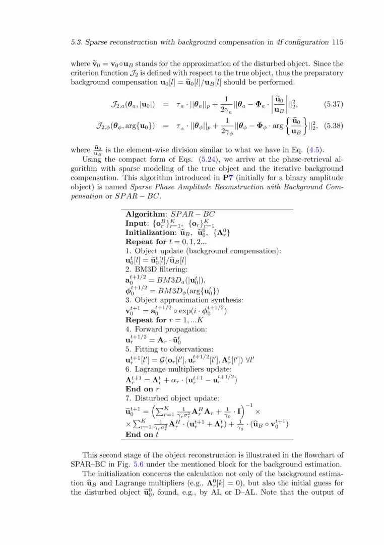
5.3. Sparse reconstruction with background compensation in 4f configuration 115

where v0 = v0◦uB stands for the approximation of the disturbed object. Since thecriterion function J2 is defined with respect to the true object, thus the preparatorybackground compensation u0[l] = u0[l]/uB [l] should be performed.

J2,a(θa, |u0|) = τa · ||θa||p +1

2γa||θa −Φa ·

∣∣∣∣ u0

uB

∣∣∣∣||22, (5.37)

J2,φ(θφ, arg{u0}) = τφ· ||θφ||p +

1

2γφ||θφ −Φφ · arg

{u0

uB

}||22, (5.38)

where u0

uBis the element-wise division similar to what we have in Eq. (4.5).

Using the compact form of Eqs. (5.24), we arrive at the phase-retrieval al-gorithm with sparse modeling of the true object and the iterative backgroundcompensation. This algorithm introduced in P7 (initially for a binary amplitudeobject) is named Sparse Phase Amplitude Reconstruction with Background Com-pensation or SPAR−BC.

Algorithm: SPAR−BCInput: {oBr }Kr=1, {or}Kr=1

Initialization: uB , u00, {Λ0

r}Repeat for t = 0, 1, 2...1. Object update (background compensation):ut0[l] = ut0[l]/uB [l]2. BM3D filtering:

at+1/20 = BM3Da(|ut0|),φt+1/20 = BM3Dφ(arg{ut0})

3. Object approximation synthesis:

vt+10 = a

t+1/20 ◦ exp(i · φt+1/2

0 )Repeat for r = 1, ...K4. Forward propagation:

ut+1/2r = Ar · ut0

5. Fitting to observations:

ut+1r [l′] = G(or[l

′],ut+1/2r [l′],Λt

r[l′]) ∀l′

6. Lagrange multipliers update:

Λt+1r = Λt

r + αr · (ut+1r − u

t+1/2r )

End on r7. Disturbed object update:

ut+10 =

(∑Kr=1

1γrσ

2rAHr Ar + 1

γ0· I)−1

××∑Kr=1

1γrσ

2rAHr · (ut+1

r + Λtr) + 1

γ0· (uB ◦ vt+1

0 )

End on t

This second stage of the object reconstruction is illustrated in the flowchart ofSPAR–BC in Fig. 5.6 under the mentioned block for the background estimation.

The initialization concerns the calculation not only of the background estima-tion uB and Lagrange multipliers (e.g., Λ0

r[k] = 0), but also the initial guess forthe disturbed object u0

0, found, e.g., by AL or D–AL. Note that the output of

116 5. Phase retrieval with sparse object regularization

the SPAR–BC phase-retrieval algorithm is not the estimate of the disturbed u0

(Step 7), but the estimate of the true object wave field u0 by the backgroundcompensation calculated in Step 1.

5.3.3 SPAR–BC for binary amplitude object

In P7 we consider the reconstruction of a binary object with the amplitude givenin the form

a0[l] = |u0[l]| ={β1, for l ∈ X1,β0, for l ∈ X0,

, (5.39)

where β0 ∈ R+ and β1 ∈ R+ stand for the lower and upper levels of the object am-plitude signal, respectively. The set X1 defines the indices of the upper level andthe set X0 defines the indices of the lower level, X0∪X1 = {l : l = {1, 2, ...NξNη}}.Both these levels β0, β1 and the sets X0, X1 are unknown and should be recon-structed.

We incorporate the knowledge about the object amplitude (Eq. (5.39)) in thecriterion J2,a as an additional constraint. To deal with such a new criterion, aspecial modification of the filtering procedure is developed targeted on an essentialimprovement of the reconstruction of the binary object amplitude. The BM3Dfiltering (Step 2 of SPAR–BC) is replaced by

at+1/30 = BM3Da(|ut0| − β

t0) + βt0 (5.40)

at+1/20 = BM3Da(a

t+1/30 − βt1) + βt1

where the estimates of the lower βt0 and upper levels βt1 are calculated as mediansof at0 = |ut0| over the corresponding subsets Xt

0 = {at0 : 0 ≤ at0 ≤ ρt} andXt

1 = {at0 : at0 > ρt}

βt0 = medianat0∈Xt0(at0), (5.41)

βt1 = medianat0∈Xt1(at0)

For estimation of subsets Xt0 and Xt

1, corresponding to small and large valuesof at0, we use the thresholding parameter ρt calculated using the Otsu algorithm[170]. In the procedures (5.40), successive subtractions of βt0 and βt1 makes theimage flatter first in the area of low values of binary amplitude signal and afterthat in the area of its high values. Experiments show that this flattening enablesmuch more efficient filtering of artifacts for the estimate of a0 in case of binaryobject.

For the phase filtering we make the flattening procedure simpler because forthe considered u0 the phase should be zero. The median of the object phase iscalculated only ones as ϕt0 = median(arg{ut0}) without partitioning in two subsetsas for the object amplitude. Finally, the BM3D-frame filtering and update of theobject approximation (Steps 2 and 3 in SPAR–BC) are replaced by

5.3. Sparse reconstruction with background compensation in 4f configuration 117

Figure 5.7: Sparse object reconstruction with background compensation by SPAR–BC.Fragments of (a) the AL amplitude estimate of the disturbed object |u0

0| used as theinitial guess for SPAR–BC; (b) the AL amplitude estimate of the background |uB |; (c)the initial guess for the object amplitude |u0

0| computed by background compensation;(d) the resulting reconstruction of the object amplitude |u0|.

at+1/30 = BM3Da(|ut0| − β

t0) + βt0 (5.42)

at+1/20 = BM3Da(a

t+1/30 − βt1) + βt1

φt+1/20 = BM3Dφ(arg{ut0} −ϕt0)

vt+10 = a

t+1/20 ◦ exp(i · (φt+1/2

0 +ϕt0))

The results of the object reconstruction from experimental data by SPAR–BC are obtained using this modified BM3D-frame filtering: in practice, Step 2 ofSPAR–BC is defined exactly by Eqs. (5.42).

In Fig 5.7 we illustrate some results obtained by the SPAR–BC algorithmfrom experimental data. In Figs. 5.7(a) and 5.7(b) the initial data of this algo-rithm are presented: the amplitude estimates of the disturbed object |u0

0| and thebackground |uB |, respectively. The result of the background compensation, i.e.the initial guess of the object amplitude calculated by |u0

0[l]| = |u00[l]|/|uB [l]| is

demonstrated in Fig. 5.7(c). The resulting object amplitude computed by iterativebackground compensation and BM3D-frame filtering is illustrated in Fig. 5.7(d).Please, compare visual quality of the object amplitude reconstructions shown Fig.5.7(c) and 5.7(d). Since we have no true complex-valued background, it is impos-sible to obtain directly good imaging of the object. The iterative BM3D filtering

118 5. Phase retrieval with sparse object regularization

allows to consistently wiping out the artifacts related to the inaccurate backgroundreconstruction. In general, the SPAR–BC reconstruction in Figs. 5.7(d) looks veryclose to the original binary object.

5.4 Discussion and further work

As it is mentioned in Section 2.4, in the parallel phase retrieval we deal with non-convex optimization problem, thus, strictly speaking, there is no guarantee of theuniqueness of the resulting solution, and there could be some problems with theconvergence of the phase-retrieval algorithm (very low convergence rate [P6 cf.Fig. 2], stagnation, etc.). Nevertheless the developed AL based algorithms canbe considered as heuristic greedy algorithms giving local optima (AL, AL–A, AL–Ph) [162] or stationary, fixed points (D–AL and SPAR–BC) [38]. The accuratederivation of the convergence of the algorithms in case of nonconvex nonsmoothcriterion function is beyond the scope of this thesis. However, our multiple nu-merical experiments with synthetic and experimental data show that these ALbased phase-retrieval algorithms have a good convergence rate and reconstructionquality (see more details in P4–P7), in many cases better comparing with thestate-of-the-art algorithms such as SBMIR [7, 8, 178]. The use and incorporationof a priori information on the object to the algorithms (see AL–A, AL–Ph P5 andSPAR–BC P7) significantly improves the reconstruction accuracy and enhancesimaging even more.

Note that the considered AL based algorithms are quite time consuming be-cause of the large dimension of the images and use of a number of sensor planes (inour experiments typically K=5). However, the computational performance can besignificantly improved using the advantage of the parallel processing: componentsof the vectors |ut0| and |utr|, |Λt

r| (for different r) can be found independently ateach t-th iteration of our algorithms. It is shown in P6 that our implementationof D–AL on a graphic processing unit5 (GPU) gives an essential acceleration fromtwo up to 10 times and more.

The algorithm parameters such as the Tikhonov regularization parameter µ,penalty coefficients γr for the Lagrange multipliers6, penalty coefficients for theadditional constraints for the object analysis and synthesis in the BM3D domainγa , γφ and threshold parameters τa, τφ are found in our numerical simulationsmanually, by minimizing RMSE(γr, µ,K,∆z, z1, σr) for AL (see, e.g., [P4, Fig.3]) ; or more general – by minimizing RMSE(γr, τaγa, τφγφ, γ0,K,∆z, z1, σr) forD–AL [149] and SPAR–BC, just because these parameters are interconnected.Indeed, for a certain propagation distance z1 and distance between the sensorplanes ∆z RMSE curve decreases starting from certain K. Larger number ofused observations means that we involve more blurred measurements. Despite asmall deviation in the numerical ranks (see Fig. 4.4), we use more and more ill-posed transform matrices corresponding to larger zr. In addition, the choice of theparameters also depends on the noise level in the given intensity measurements σr,the type and size of the object (relative size of the important components of the

5 The BM3D-frame filter used in this work is realized on a central processing unit (CPU).6 In our works P6–P7 and [149] small object details are recovered with slowly updating

Lagrange multipliers.

5.4. Discussion and further work 119

object). It is difficult to use the conventional parameter-choice methods (e.g., tofind the Tikhonov regularization parameter µ, see Section 3.7) for the multi-planephase-retrieval: more sophisticated tools to find proper parameters [108, 186] arerequired.

Thus, in our papers P4–P7, [149] we present rather our recommendations forthe values of the algorithm parameters. In case of the use of real experimental datawe rely on the results of numerical simulations. Our further work concerns theadaptive selection of the parameter as well as an automatic tuning of the filteringfor noisy experimental data.

5.4.1 Synthetic background in SPAR–BC: object “restora-tion”

The discussion about the object reconstruction of a binary amplitude-only objectwith background compensating is presented in Sections 5.3.2 – 5.3.3 and in ourrecent paper P7. However, the presented results are obtained in case of additionalexperiments for the background estimation. But, what if these is no backgroundestimation? In Fig. 5.8 we illustrate our numerical experiment of phase retrievalby SPAR–BC with a synthetic background used to imitate the distortions in theoptical path. The results are shown for the same parameter setting of the imagingsystem as in P7, including the size of the images and pixels’ sizes.

Figure 5.8: Numerical simulation to illustrate the influence of background compensatingon the reconstruction imaging. (a) The true binary amplitude object. (b) The ampli-tude of a synthetic complex-valued background |uB |. (c) The amplitude estimate of thedisturbed object found by AL, RMSE=0.4. (d) The reconstructed true object amplitudea0 obtained by SPAR–BC, RMSE=0.043.

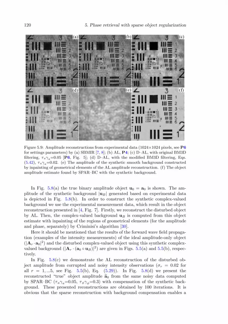
120 5. Phase retrieval with sparse object regularization

Figure 5.9: Amplitude reconstructions from experimental data (1024×1024 pixels, see P6for settings parameters) by (a) SBMIR [7, 8]; (b) AL, P4; (c) D–AL, with original BM3Dfiltering, τaγa=0.05 [P6, Fig. 5]; (d) D–AL, with the modified BM3D filtering, Eqs.(5.42), τaγa=0.02. (e) The amplitude of the synthetic smooth background constructedby inpainting of geometrical elements of the AL amplitude reconstruction. (f) The objectamplitude estimate found by SPAR–BC with the synthetic background.

In Fig. 5.8(a) the true binary amplitude object u0 = a0 is shown. The am-plitude of the synthetic background |uB | generated based on experimental datais depicted in Fig. 5.8(b). In order to construct the synthetic complex-valuedbackground we use the experimental measurement data, which result in the objectreconstruction presented in [4, Fig. 7]. Firstly, we reconstruct the disturbed objectby AL. Then, the complex-valued background uB is computed from this objectestimate with inpainting of the regions of geometrical elements (for the amplitudeand phase, separately) by Criminisi’s algorithm [30].

Here it should be mentioned that the results of the forward wave field propaga-tion (examples of the intensity measurements) of the ideal amplitude-only object(|Ar ·a0|2) and the disturbed complex-valued object using this synthetic complex-valued background (|Ar · (a0 ◦ uB)|2) are given in Figs. 5.5(a) and 5.5(b), respec-tively.

In Fig. 5.8(c) we demonstrate the AL reconstruction of the disturbed ob-ject amplitude from corrupted and noisy intensity observations (σr = 0.02 forall r = 1, ...5, see Fig. 5.5(b), Eq. (5.29)). In Fig. 5.8(d) we present thereconstructed “true” object amplitude a0 from the same noisy data computedby SPAR–BC (τaγa=0.05, τφγφ=0.3) with compensation of the synthetic back-ground. These presented reconstructions are obtained by 100 iterations. It isobvious that the sparse reconstruction with background compensation enables a

5.4. Discussion and further work 121

Figure 5.10: The corresponding top left fragments of the images (of the size 128 × 128 )illustrated in Fig. 5.9.

significant improvement of the reconstruction accuracy (in our numerical simula-tions – up to in order of amplitude in RMSE) and imaging enhancement in caseof strong corruption of the given observations. The background estimate “under-takes” strong fluctuations, which would be difficult to compensate by filtering.

However, it is much more important that the previously unsuccessful objectreconstructions can be significantly improved either by the additional calibrationprocedure (if the used optical system with the same settings is available), as inthe original SPAR–BC algorithm, or by the synthetic background generated fromthe reconstructed disturbed object.

In Fig. 5.9 some examples of the amplitude object reconstruction by differentphase-retrieval methods are shown. The presented results are 1024×1024 pixelslarge and obtain from the experimental date of the optical system with param-eters discussed in P6. Figures 5.9(a) – 5.9(d) illustrate the amplitude estimatescomputed by SBMIR, AL, D–AL P6 and D–AL with the modified BM3D filteringaccording to Eqs. (5.42), respectively. D–AL is computed with soft thresholding.In Fig. 5.9(e) we present the amplitude of a synthetic background constructedagain by inpainting of the AL object reconstruction (separately, the amplitude andphase) and further smoothing by the BM3D filter. In Fig. 5.9(f) we demonstratethe reconstructed object amplitude obtained by SPAR–BC using this syntheticbackground. We call such a modification of the SPAR–BC algorithm, where onlymeasurements for the object are required {or}, object “restoration” by analogywith the restoration of old photos that have lost their imaging quality with time.It can be seen that this procedure suppresses remaining noise (cf. 5.9 (d)), of

122 5. Phase retrieval with sparse object regularization

cause, with some oversmoothing, but with no strong degradations (cf. 5.9(c)). InFig. 5.10 top left fragments of the mentioned images illustrated in Fig. 5.9 of thesize 128×128 pixels are presented.

The main point is the selection of geometric elements on the AL object re-construction. It can be made manually or using the conventional Otsu algorithm[170], while it is originated especially for binarization of gray-scale images.

5.4.2 Exploitation of parallel AL based algorithms

The resulting parallel multi-plane AL based algorithms may be used for variousapplication, where a good imaging of the complex-valued wave field is required:in optical nondestructive testing, in microscopy to analyse, e.g., blood cells (a liveblood specimen) or in astronomy for, say, the James Webb space telescope. In ourworks P6–P7 we present the results of the object reconstruction only by phaseretrieval. Our further work concerns also the comparison of the obtained resultswith the holographic approach especially using the accurate M–DDT technique.Also we are planning to implement the SPAR–BC algorithm for smooth amplitudeand phase objects.

In addition, it is shown in P7 that the modified BM3D filtering (Eqs. (5.42))works as a classifier for the noisy binary object estimate. The estimate of theamplitude levels are found using the Otsu method, but the BM3D filtering shiftsthe value of the pixel at0[l] to one of these two levels βt0 or βt1 depending on thelocal neighborhood. Thus, such a modification can be used as an advanced toolfor binarization of noisy and corrupted objects.

Appendix A: Derivations ofAL algorithms

Here we provide some details of optimization of the AL criteria on {ur} and u0

defining the proposed phase-retrieval algorithms.

A.1 Minimization of JAL on ur

The AL criterion (cf. Eq. (4.16))

JAL({or},u0, {ur}, {Λr}) = µ · ||u0||22 +

K∑r=1

1

σ2r

[1

2||or − |ur|2||22 + (A.1)

+1

γr||ur −Ar · u0||22 +

1

γrΛHr (ur −Ar · u0) +

1

γrΛTr (ur −Ar · u0)∗],

is additive with respect to the vectors ur and their components. Thus, the mini-mization of JAL on ur can be produced separately for every r and l′. The minimumcondition for ur[l

′]

∂JAL∂u∗r [l

′]=

1

σ2r

(|ur[l′]|2 − or[l′]) · ur[l′] +

1

γrσ2r

(ur[l′]− ςr[l′] + Λr[l

′]) = 0 (A.2)

results in

ur[l′] =

(Ar · u0)[l′]−Λr[l′]

γr(|ur[l′]|2 − or[l′]) + 1=ςr[l′]

κr[l′]. (A.3)

Taking the module from the left and right sides of Eq. (A.3) we arrive at the cubicequation with respect to |ur[l′]|:

|ur[l′]|3 + |ur[l′]| ·(

1

γr− or[l

′]

)− sign(κr[l

′]) · |ςr[l′]|

γr= 0. (A.4)

The last equation may have one or three real solutions. We are looking for anonnegative one for |ur[l′]|. Let us denote this solution for Eq. (A.4) as |u†r[l′]|.If the nonnegative real-valued root of Eq. (A.4) is found, then the correspondingcomplex-valued estimate of the wave field at the sensor plane ur[l

′] is calculatedaccording to Eq. (A.3) as follows

ur[l′] =

(Ar · u0)[l′]−Λr[l′]

γr(|u†r[l′]|2 − or[l′]) + 1

. (A.5)

123

124 Appendix A: Derivations of AL algorithms

For brevity, we denote the nonlinear algorithm giving the nonnegative real-valuedroot of Eq. (A.4) and computing Eq. (A.5) as

ur[l′] = G(or[l

′],ur[l′],Λr[l

′]). (A.6)

It defines Step 2 of our AL based phase-retrieval algorithms. We refer to P4 and[118] for more details.

A.2 Minimization of JAL on u0

In these derivative calculations, the differentiation of a scalar by a vector resultsin a vector of derivatives: ∂JAL

∂u0= [ ∂JAL∂u0[1] , ..., ∂JAL

∂u0[NξNη ] ]T , provided that u0 =

[u0[1], ...,u0[NξNη]]T . The minimum condition ∂JAL∂u∗0

= 0 gives the object estimate

in the form

u0 =

(K∑r=1

1

γrσ2r

AHr Ar + µ · I

)−1

·K∑r=1

1

γrσ2r

AHr (ur + Λr), (A.7)

what defines Step 4 of the AL algorithm.

Further we are looking for the object estimate in case of the amplitude (AM)and phase modulations (PM) of the object. The solutions are derived from theminimum conditions ∂JAL/∂a0 = 0 and ∂JAL/∂φ0 = 0. Note that the very firstfidelity term of Eq. (A.1) does not depend on the object, it depends neither ona0 ∈ RNξNη nor on φ0 ∈ RNξNη . Let us rewrite Eq. (A.1) as

JAL(u0, {ur}, {Λr}) = (A.8)

=

K∑r=1

1

σ2r

[1

γr||ur −Ar · u0||22 +

2

γrRe{ΛH

r (ur −Ar · u0)}] + µ · ||u0||22 =

=

K∑r=1

1

σ2r

[1

γrAr(u0,ur) +

1

γrBr(u0,ur,Λr)] + µ · ||u0||22

and consider the optimization of JAL on a0 and φ0 in parts.

A.2.1 Analytical solution: update of the object amplitude

The derivative of the scalar uTr ·A∗r ·u∗0 with respect to the vector a0 is (AHr ur) ◦

exp(−iφ0) because

∂

∂a0[l](uTr ·A∗r · u∗0) =

∂

∂a0[l]

∑l′

ur[l′]∑s

A∗r [l′, s]u∗0[s] = (A.9)

= exp(−iφ0[l]) ·∑l′

ur[l′]A∗r [l

′, l] = (AHr ur)[l] · exp(−iφ0[l]),

A.2. Minimization of JAL on u0 125

where u∗0 = a0 ◦ e−iφ0 . Hence

∂

∂a0Ar(u0,ur) = (A.10)

=∂

∂a0||ur −Ar · u0||22 =

∂

∂a0[−uTr ·A∗r · u∗0 − uT0 ·AT

r · u∗r +

+uT0 ·ATr ·A∗r · u∗0] = −[AH

r ur ◦ exp(−iφ0) + (AHr ur ◦ exp(−iφ0))∗] +

+AHr Aru0 ◦ exp(−iφ0) + (AH

r Aru0 ◦ exp(−iφ0))∗ =

= 2 Re{AHr (Aru0 − ur) ◦ exp(−iφ0)}.

Analogically

∂

∂a0Br(u0,ur,Λr) =

∂

∂a02 Re{ΛH

r · (ur −Ar · u0)} = (A.11)

=∂

∂a0[−ΛT

r ·A∗r · u∗0 −ΛHr ·Ar · u0] = −[AH

r Λr ◦ exp(−iφ0) +

+ (AHr Λr ◦ exp(−iφ0))∗] = −2 Re{AH

r Λr ◦ exp(−iφ0)}.

Together Eqs. (A.10)–(A.11) give the minimum condition with respect to a0 inthe form

∂

∂a0JAL = (A.12)

=

K∑r=1

2

γrσ2r

Re{AHr (Aru0 − ur −Λr) ◦ exp(−iφ0)}+ 2µ · u0 ◦ exp(−iφ0) = 0.

In case of AM (φ0[l] = 0 ∀l), we arrive at the following analytical solution

a0 =

(K∑r=1

1

γrσ2r

Re{AHr Ar}+ µ · I

)−1

·K∑r=1

1

γrσ2r

Re{AHr (ut+1

r + Λtr)}, (A.13)

what determines the update of the object amplitude in Step 4 of the AL–A algo-rithm.

A.2.2 Analytical solution: update of the object phase

Let us consider the phase modulation of the object (PM) in the form u0 = a ·eiφ0 ,where a is unknown constant. Taking into account that u∗0 = a · e−iφ0 , thederivative of Ar with respect to φ0 results in

∂

∂φ0

Ar(u0,ur) = (A.14)

= i(AHr ur ◦ u∗0)− i(AH

r ur ◦ u∗0)∗ + i(u∗0 ◦AHr Aru0)∗ − i(u∗0 ◦AH

r Aru0) =

= 2 Im{u∗0 ◦AHr Aru0} − 2 Im{u∗0 ◦AH

r ur} = 2 Im{u∗0 ◦AHr (Aru0 − ur)}.

Analogically

∂

∂φ0

Br(u0,ur,Λr) =∂

∂φ0

[−ΛTr A∗ru

∗0 −ΛH

r Aru0] = (A.15)

= i(AHr Λr ◦ u∗0)− i(AH

r Λr ◦ u∗0)∗ = −2 Im{AHr Λr ◦ u∗0}.

126 Appendix A: Derivations of AL algorithms

Eq. (A.14) and Eq. (A.15) give the minimum condition with respect to φ0 in theform

∂

∂φ0

JAL = 2 Im{u∗0 ◦K∑r=1

1

γrσ2r

AHr (Aru0 − ur −Λr)} = (A.16)

= 2 Im{(a · e−iφ0) ◦K∑r=1

1

γrσ2r

AHr (Ar(a · eiφ0)− ur −Λr)} = 0,

what determines the phase update in the gradient descent AL–Ph algorithm.If the phase is defined, then the unknown scalar a is calculated from the con-

dition ∂∂aJAL = 0 (cf. Eq. (A.12)) as

χ =

K∑r=1

1

γrσ2r

||Ar exp(iφ0)||22 + µ ·NξNη, (A.17)

a =1

χ

K∑r=1

1

γrσ2r

Re{exp(−iφT0 ) ·AHr (ur + Λr)}. (A.18)

It gives Step 5 and Step 7 in the gradient descent and Gauss–Newton AL–Phalgorithms, respectively.

A.3 Approximate solution: Gauss–Newton AL–Ph algorithm

The object phase φ0 can be also found using the iterative Gauss–Newton methodderived from the linearization

Ar(u0,ur) + Br(u0,ur,Λr) = (A.19)

= ||ur −Ar · u0||22 + 2 Re{ΛHr · (ur −Ar · u0)} ≈

≈(

ur −Aru0 −∂

∂φ0

(Aru0) ·ϕ0

)H·(

ur −Aru0 −∂

∂φ0

(Aru0) ·ϕ0

)+

+2 Re{ΛHr · (ur −Aru0 −

∂

∂φ0

(Aru0) ·ϕ0)} , Sr(a,φ0,ϕ0,ur,Λr),

where ϕ0 ∈ RNξNη is a small increment of the object phase. For PM of the formu0 = a · eiφ0 it can be shown that the derivative of the vector Ar ·u0 with respectto the vector φ0 is

∂

∂φ0

(Ar · u0) = iArΓ, Γ = diag(a · exp(iφ0)) (A.20)

as

∂

∂φ0[l](Ar · u0) =

∂

∂φ0[l]

∑s

Ar[l′, s](a · exp(iφ0[s])) = (A.21)

= iAr[l′, l] · (a · exp(iφ0[l])) ∀l′

A.3. Approximate solution: Gauss–Newton AL–Ph algorithm 127

Thus, we arrive at

Sr(a,φ0,ϕ0,ur,Λr) = (A.22)

= (ur −Ar · u0 − iArΓ ·ϕ0)H(ur −Ar · u0 − iArΓ ·ϕ0) +

+2 Re{ΛHr · (ur −Ar · u0 − iArΓ ·ϕ0)}.

The extremal condition ∂∂ϕ0

∑r

1γrσ

2rSr = 0 gives us the increment ϕ0. We take

only those components of Sr which depend on ϕ0, i.e. further we use the criterion

Sr = −uHr · iArΓ ·ϕ0 + uH0 AHr · iArΓ ·ϕ0 + (A.23)

+iϕT0 · ΓHAHr · ur − iϕT0 · ΓHAH

r ·Aru0 +

+ϕT0 · ΓHAHr ·ArΓ ·ϕ0 −

−ΛHr · iArΓ ·ϕ0 + iϕT0 · ΓHAH

r ·Λr.

In order to find ϕ0 we compute ∂∂ϕ0

∑Kr=1

1γrσ

2rSr and set it equal to zero.

Taking into account that [142]

∂

∂xxTA = AT ,

∂

∂xxTAx = xTAT + xTA (A.24)

(uHr ·Ar) · Γ = (uHr ·Ar) ◦ (a · exp(iφT0 )) = uHr Ar ◦ uT0 , (A.25)

we arrive at

K∑r=1

2

γrσ2r

Re{ΓHAHr ArΓ} ·ϕ0 + 2 Im{u∗0 ◦

K∑r=1

1

γrσ2r

AHr (Aru0 − ur −Λr)} = 0.

(A.26)Eq. (A.26) can be rearranged to obtain the following normal equation

− ∂

∂φ0

JAL =

K∑r=1

2

γrσ2r

Re{ΓTATr A∗rΓ

∗} ·ϕ0, (A.27)

what results in

ϕ0 = −1

2

(K∑r=1

1

γrσ2r

Re{ΓTATr A∗rΓ

∗}

)−1

· ∂

∂φ0

JAL = (A.28)

= −

(K∑r=1

1

γrσ2r

Re{ΓTATr A∗rΓ

∗}

)−1

· Im{u∗0 ◦K∑r=1

1

γrσ2r

AHr (Aru0 − ur −Λr)}.

It determined the update of the object phase in the Gauss–Newton AL–Ph algo-rithm. If the phase is determined, the scalar object amplitude is defined by Eqs.(A.17)–(A.18).

Appendix B: 4f configurationfor phase retrieval

B.1 4f optical system

Let us consider the wave field propagation model in the 4f configuration with areflective phase modulating spatial light modulator (SLM) placed at the Fourierplane as it is presented in Fig. 5.1. The lenses L1 and L2 with the same focaldistance f arranged in a 4f configuration provides mapping of the object wavefield to the Fourier plane and then to the sensor plane. The wave field at theFourier transform plane uF ( v

λf ) can be easily found as the result of convolution of

the wave field u′(ξ), ξ = (ξ1, ξ2) falling to the lens L1 with the Fresnel diffractionkernel gf (ξ − x) of the wave field propagation to the distance f

u′(ξ) = {u0 ~ gf}(ξ) =eikf

iλf

∞∫∫−∞

u0(x)eik2f ||ξ−x||

2

dx, (B.1)

Recall that the transverse wave field distributions u0(x), uF ( vλf ) and ur(y) are

given in the 2D spatial coordinates x = (x1, x2), v = (v1, v2), y = (y1, y2) ∈ R2.Since the lens transmittance [125, cf. Eq. (2.85)], [138, see Table VI.1]

T (ξ) = e−ik2f ||ξ||

2

, (B.2)

then the link between the wave field at the object and Fourier planes is defined asfollows

uF

(v

λf

)=

eikf

iλf

∞∫∫−∞

u′(ξ)e−ik2f ||ξ||

2︸ ︷︷ ︸T (ξ)

eik2f ||v−ξ||

2

dξ = (B.3)

=ei2kf

iλf

∞∫∫−∞

u0(x)ei

k2f ||v||

2

iλf

∞∫∫−∞

eik2f ||ξ−x||

2

e−ikf 〈v,ξ〉dξdx,

where 〈v, x〉 = v1x1 + v2x2 denotes the inner product of two vectors.

Using the change of variables q = (q1, q2) = ξ − x = (ξ1 − x1, ξ2 − x2) and

129

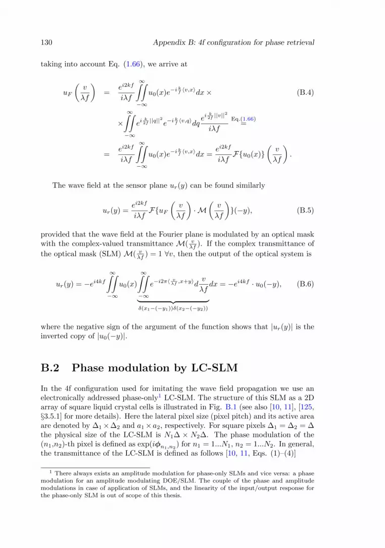
130 Appendix B: 4f configuration for phase retrieval

taking into account Eq. (1.66), we arrive at

uF

(v

λf

)=

ei2kf

iλf

∞∫∫−∞

u0(x)e−ikf 〈v,x〉dx× (B.4)

×∞∫∫−∞

eik2f ||q||

2

e−ikf 〈v,q〉dq

eik2f ||v||

2

iλf

Eq.(1.66)=

=ei2kf

iλf

∞∫∫−∞

u0(x)e−ikf 〈v,x〉dx =

ei2kf

iλfF{u0(x)}

(v

λf

).

The wave field at the sensor plane ur(y) can be found similarly

ur(y) =ei2kf

iλfF{uF

(v

λf

)· M

(v

λf

)}(−y), (B.5)

provided that the wave field at the Fourier plane is modulated by an optical maskwith the complex-valued transmittance M( v

λf ). If the complex transmittance of

the optical mask (SLM) M( vλf ) = 1 ∀v, then the output of the optical system is

ur(y) = −ei4kf∞∫∫−∞

u0(x)

∞∫∫−∞

e−i2π〈vλf ,x+y〉d

v

λf︸ ︷︷ ︸δ(x1−(−y1))δ(x2−(−y2))

dx = −ei4kf · u0(−y), (B.6)

where the negative sign of the argument of the function shows that |ur(y)| is theinverted copy of |u0(−y)|.

B.2 Phase modulation by LC-SLM

In the 4f configuration used for imitating the wave field propagation we use anelectronically addressed phase-only1 LC-SLM. The structure of this SLM as a 2Darray of square liquid crystal cells is illustrated in Fig. B.1 (see also [10, 11], [125,§3.5.1] for more details). Here the lateral pixel size (pixel pitch) and its active areaare denoted by ∆1×∆2 and a1×a2, respectively. For square pixels ∆1 = ∆2 = ∆the physical size of the LC-SLM is N1∆ × N2∆. The phase modulation of the(n1,n2)-th pixel is defined as exp(iφn1,n2

) for n1 = 1...N1, n2 = 1...N2. In general,the transmittance of the LC-SLM is defined as follows [10, 11, Eqs. (1)–(4)]

1 There always exists an amplitude modulation for phase-only SLMs and vice versa: a phasemodulation for an amplitude modulating DOE/SLM. The couple of the phase and amplitudemodulations in case of application of SLMs, and the linearity of the input/output response forthe phase-only SLM is out of scope of this thesis.

B.2. Phase modulation by LC-SLM 131

M(v1, v2) = [∑N1

n1=1

∑N2

n2=1exp(iφn1,n2

)× (B.7)

×δ(v1 − (n1 −N1/2− 1)∆1, v2 − (n2 −N2/2− 1)∆2)×

×rect

(v1

N1∆1

)rect

(v2

N2∆2

)︸ ︷︷ ︸

aperture of the LC-SLM

] ~ [rect

(v1

a1

)rect

(v2

a2

)︸ ︷︷ ︸area of the LC-SLM cell

],

where rect(·) is the rectangular function (Eq. (9)).Note that φ in Eq. (B.7) is a finite size 2D matrix. It can also be consid-

ered as an infinite sparse 2D matrix with non-zeros components for n1 = 1...N1,n2 = 1...N2 or the corresponding discrete 2D function φ(n1∆1, n2∆2) [76]. Thus,M(v1, v2) in Eq. (B.7) can be rewritten as

M(v1, v2) = (B.8)

{[∑∞

n1=−∞

∑∞

n2=−∞δ(v1 − (n1 −N1/2− 1)∆, v2 − (n2 −N2/2− 1)∆2)×

× exp(iφ((n1 −N1/2− 1)∆1, (n2 −N2/2− 1)∆2))] ~

~[rect

(v1

a1

)rect

(v2

a2

)]} · rect

(v1

N1∆1

)rect

(v2

N2∆2

).

In a discrete model with the SLM as a N1 ×N2 array of liquid crystal cells of thepixel size ∆1 ×∆2 the sampled representation of ASD, the discrete distributionsof the optical masks (5.4) to be programmed into the SLM are

Mr[n1, n2] =

∞∫∫−∞

Mr

(v1

λf,v2

λf

)rect

(v1

λfN1∆1

)× (B.9)

× rect

(v2

λfN2∆2

)δ(v1 − n1∆1, v2 − n2∆2)dv1dv2 =

= exp

ikzr√

1− (|n1∆1|2 + |n2∆2|2)

f2︸ ︷︷ ︸φn1,n2

in Eq.(B.7)

,

where r = 1, ...K and n1 = −N1/2...N1/2 − 1, n2 = −N2/2...N2/2 − 1 for thecentral symmetry. Here and in our publications we assume, for simplicity, 100%fill factor of the SLM cells, i.e. a1 = ∆1, a2 = ∆2. Note that the resultingsignal at the sensor plane is significantly different from what we have by the free-space propagation model, namely: taking into account that F{rect( v

λf∆ )}(x) =∫rect( v

λf∆ )e−i2πvλf xdv = sinc(x∆) · λf∆, Eq. (5.2) can be rewritten as

ur(x, y) = −ei4kf {u0(−x,−y) ~ [(λf)2 sinc(−x∆1) sinc(−y∆2)× (B.10)

×∆1∆2 · F{∑N1/2−1

n1=−N1/2

∑N2/2−1

n2=−N2/2Mr[n1, n2] · rect

(v1

λfN1∆1

)×

× rect

(v2

λfN2∆2

)δ

(v1

λf− n1∆1,

v2

λf− n2∆2

)}(−x,−y)]}, r = 1, ...K.

132 Appendix B: 4f configuration for phase retrieval

Figure B.1: Structure of the pixelated phase-only LC-SLM as a 2D array of square liquidcrystal cells. Following [10, Fig. 1], ∆ and a denote the lateral size of the pixel (pixelpitch) and its active area, respectively. Here these sizes are presented to be the samewith respect to the x- and y-direction [125, cf. Fig. 3.41].

The flexibility of the optical model with an SLM is the ability to use (in prin-ciple) completely arbitrary values in Mr[n1, n2] provided the invertibility of theresulting transfer functions. Moreover, the reprogramming of the SLM (tens ofmilliseconds) is much faster then the change of the optical setup (replacement ofa sensor).

In the wave field propagation models for phase retrieval we use ASD (Eq.(B.9)), F–DDT or M–DDT (P3–P7), and do not consider complex diffractionkernels describing the real transfer functions of LC-SLMs (Eq. (B.10)). Instead ofthis, all changes from the theoretically predicted results of the wave field propaga-tion and nonidealities related to, e.g., the bandlimitedness of the transfer functionor various distortions in the optical path of the used coherent imaging system(Fig. 5.1) are considered as a cumulative disturbance of the object wave field, a“background” to be estimated and compensated (see Section 5.3, P7).

References

[1] Matlab code with additional materials is available on the web page of our projecthttp://www.cs.tut.fi/∼lasip/DDT .

[2] M. Afonso, J. Bioucas-Dias, and M. Figueiredo, “Fast image recovery using variablesplitting and constrained optimization,” IEEE Trans. on Image Proc. 19, 2345–2356(2010).

[3] M. Agour, “Determination of the complex amplitude of monochromatic light froma set of intensity observations,” PhD thesis, Universitat Bremen (2011).

[4] M. Agour, C. Falldorf, C. v. Kopylow, R. B. Bergmann, “Automated compensationof misalignment in phase retrieval based on a spatial light modulator,” Appl. Opt.50, 4779–4787 (2011).

[5] I. Aizenberg and J. Astola, “Discrete generalized Fresnel functions and transformsin an arbitrary discrete basis,” IEEE Trans on Signal Processing 54, 4261–4270(2006).

[6] L. Allen and M. P. Oxley, “Phase retrieval from series of images obtained by defocusvariation,” Opt. Commun. 199, 65–75 (2001).

[7] P. Almoro, G. Pedrini, and W. Osten, “Complete wavefront reconstruction usingsequential intensity measurements of a volume speckle field,” Appl. Opt. 45, 8596–8605 (2006).

[8] P. Almoro, A. M. Maallo, and S. Hanson, “Fast-convergent algorithm for speckle-based phase retrieval and a design for dynamic wavefront sensing,” Appl. Opt. 48,1485–1493 (2009).

[9] L. A. D’Arcio, J. J. M. Braat, and H. J. Frankena, “Numerical evaluation of diffrac-tion integrals for apertures of complicated shape,” J. Opt. Soc. Am. A 11, 2664–2674 (1994).

[10] V. M. Arrizon, E. Carreon and M. Testorf, “Implementation of Fourier array illu-minators using pixelated SLM: efficiency limitations,” Optics Comm. 160, 207–213(1999).

[11] V. M. Arrizon, D. Sanchez-de-la-Llave and L. A. Gonzalez, “Holographic imple-mentation of complex filters with phase-only pixelated spatial light modulators,”Proc. SPIE 4435, 96–106 (2001).

[12] V. M. Arrizon and D. Sanchez-de-la-Llave, “Double-phase holograms implementedwith phase-only spatial light modulators: performance evaluation and improve-ment,” Appl. Opt. 41, 3436–3447 (2002).

[13] J. Astola and L. P. Yaroslavsky ed., Advances in signal transforms: theory andapplications, (Hindawi, 2007).

[14] A. Asundi and K. H. Yung, “Phase-shifting and logical moire,” J. Opt. Soc. Am.A 8, 1591–1600 (1991).

[15] K. A. Bauchert, S. A. Serati, G. D. Sharp and D. J. McKnight, “Complexphase/amplitude spatial light modulator advances and use in a multispectral opticalcorrelator”, Proc. SPIE 3073, 170–177 (1997).

133

134 REFERENCES

[16] T. Baumbach, W. Osten, C. von Kopylow, and W. Juptner, “Remote metrology bycomparative digital holography,” Appl. Opt. 45, 925–934 (2006).

[17] H. H. Bauschke, P. L. Combettes, and D. R. Luke, “Phase retrieval, error reductionalgorithm, and Fienup variants: a view from convex optimization,” J. Opt. Soc. Am.A 19, 1334–1345 (2002).

[18] H. H. Bauschke, P. L. Combettes, and D. R. Luke, “Hybrid projectionreectionmethod for phase retrieval,” J. Opt. Soc. Am. A 20, 1025–1034 (2003).

[19] D. P. Bertsekas and J. N. Tsitsiklis, Parallel and distributed computation: numericalmethods, (Prentice-Hall, 1989).

[20] M. Born and E. Wolf, Principles of optics: electromagnetic theory of propagation,interference and diffraction of light, 7th ed. (Cambridge University Press, 2000).

[21] W. E. Boyce and R. C. DiPrima, Elementary differential equations and boundaryvalue problems, 7th ed. (John Wiley, 2001).

[22] G. R. Brady and J. R. Fienup. “Nonlinear optimization algorithm for retrieving thefull complex pupil function,” Opt. Express 14, 474–486 (2006).

[23] B. R. Brown, A. W. Lohmann, “Complex spatial filtering with binary masks,” Appl.Opt. 5, 967-969 (1966).

[24] B. R. Brown, A. Lohmann, “Computer generated binary holograms,” IMB J. Res.Dev. 13, 160-168 (1969).

[25] E. Buckley, A. Cable, N. Lawrence, and T. Wilkinson, “Viewing angle enhancementfor two- and three-dimensional holographic displays with random superresolutionphase masks,” Appl. Opt. 45, 7334–7341 (2006).

[26] J. Burke and D. R. Luke, “Variational analysis applied to the problem of opticalphase retrieval,” SIAM J. on Control and Optim. 42, 576–595 (2003).

[27] W. S. C. Chang, Principles of lasers and optics, (Cambridge University Press,2005).

[28] K. Choi and A. D. Lanterman, “Phase retrieval from noisy data based on mini-mization of penalized I-divergence,” J. Opt. Soc. Am. A 24, 34–49 (2007).

[29] J. N. Clark, C. T. Putkunz, M. A. Pfeifer, A. G. Peele, G. J. Williams, B. Chen,K. A. Nugent, C. Hall, W. Fullagar, S. Kim, and I. McNulty, “Use of a complexconstraint in coherent diffractive imaging,” Opt. Express 18, 1981–1993 (2010).

[30] A. Criminisi, P. Perez, and K. Toyama, “Object removal by exemplar-based in-painting,” CVPR’03, (2003).

[31] T. R. Crimmins and J. R. Fienup, “Uniqueness of phase retrieval for functions withsufficiently disconnected support,” J. Opt. Soc. Am. 73, 218–221 (1983).

[32] E. Cuche, F. Bevilacqua, and C. Depeursinge, “Digital holography for quantitativephase contrast imaging,” Opt. Lett. 24, 291–293 (1999).

[33] E. Cuche, P. Marquet, and C. Depeursinge, “Spatial filtering for zero-order andtwin-image elimination in digital off-axis holography,” Appl. Opt. 39, 4070–4075(2000).

[34] K. Dabov, A. Foi, V. Katkovnik, and K. Egiazarian, “Image denoising with block-matching and 3D filtering,” Proc. SPIE 6064 (2006).

[35] K. Dabov, A. Foi, V. Katkovnik, and K. Egiazarian, “Image restoration by sparse3D transform-domain collaborative filtering,” Proc. SPIE 6812 (2008).

[36] J. C. Dainty and J. R. Fienup, “Phase retrieval and image reconstruction for astron-omy,” in H. Stark, ed., Image recovery: theory and application, (Academic Press,1987), 231–275.

[37] A. Danielyan, V. Katkovnik, and K. Egiazarian, “Image deblurring by augmentedLagrangian with BM3D frame prior,” in Workshop on Information Theoretic Meth-ods in Science and Engineering (WITMSE), Tampere, Finland, (2010).

REFERENCES 135

[38] A. Danielyan, V. Katkovnik, and K. Egiazarian, “BM3D frames and variationalimage deblurring,” IEEE Trans. on Image Proc. 21, 1715–1728 (2012).

[39] O. Darrigol, A history of optics from greek antiquity to the nineteenth century,(Oxford University Press, 2012).

[40] R. W. Deming, “Phase retrieval from intensity-only data by relative entropy mini-mization,” J. Opt. Soc. Am. A 24, 3666–3679 (2007).

[41] Y. N. Denisyuk, “Photographic reconstruction of the optical properties of an objectin its own scattered field,” Sov. Phys. Dokl. 7, 543–545 (1962).

[42] D. L. Donoho, “Compressed sensing,” IEEE Trans. Inf. Theory 52, 1289–1306(2006).

[43] D. Dudley, W. Duncan, and J. Slaughter, “Emerging digital micromirror device(DMD) applications,” Proc. SPIE 4985, 14–29 (2003), available online.

[44] J. Bioucas-Dias and J. Leitao, “The ZpM algorithm for interferometric image re-construction in SAR/SAS,” IEEE Trans. on Image Proc. 11, 408–422, (2002).

[45] J. Bioucas-Dias, V. Katkovnik, J. Astola, and K. Egiazarian, “Absolute phase esti-mation: adaptive local denoising and global unwrapping,” Appl. Opt. 47, 5358–5369(2008).

[46] J. Eckstein and D. Bertsekas, “On the Douglas–Rachford splitting method and theproximal point algorithm for maximal monotone operators,” Math. Program. 5,293–318 (1992).

[47] U. Efron, ed., Spatial light modulator technology: materials, devices, and applica-tions, (Marcel Dekker, New York, 1995).

[48] M. Elad, Sparse and redundant representations: from theory to applications in signaland image processing, (Springer, 2010).

[49] V. Elser, “Phase retrieval by iterated projections,” J. Opt. Soc. Am. A 20, 40–55(2003).

[50] F. Facchinei, and C. Kanzow, “Generalized Nash equilibrium problems,” 4OR 5,173–210 (2007).

[51] C. Falldorf, W. Osten, F. Elandaloussi, E. Kolenovic, and W. Juptner. “Features ofthe subjective speckle eld and their use for noise-immune unwrapping,” in W. Osten,W. Juptner, and M. Kujawinska eds., Optical Measurement Systems for IndustrialInspection II: Application in Industrial Design, Proc. SPIE 4398, 238–246 (2001).

[52] C. Falldorf, E. Kolenovic, and W. Osten, “Speckle shearography using a multibandlight source,” Opt. Lasers Eng. 40, 543–552 (2003).

[53] C. Falldorf, M. Agour, C. v. Kopylow, and R. B. Bergmann, “Phase retrieval bymeans of a spatial light modulator in the Fourier domain of an imaging system,”Appl. Opt. 49, 1826–1830 (2010).

[54] C. Falldorf, “Measuring the complex amplitude of wave fields by means of shearinterferometry,” J. Opt. Soc. Am. A 28, 1636–1647 (2011).

[55] R. P. Feynman, R. B. Leighton, and M. L. Sands, Mainly The Feynman lectures onphysics, Vol. I: Mainly Mechanics, Radiation, and Heat, (Addison-Wesley, 1963).

[56] R. P. Feynman, R. B. Leighton, and M. L. Sands, Mainly The Feynman lectures onphysics, Vol. II: Mainly electromagnetism and matter, (Addison-Wesley, 1963).

[57] J. R. Fienup, “Reconstruction of an object from the modulus of its Fourier trans-form,” Opt. Lett. 3, 27–29 (1978).

[58] J. R. Fienup, “Iterative method applied to image reconstruction and to computergenerated holograms,” Opt. Eng. 19, 297–305 (1980).

[59] J. R. Fienup, “Phase retrieval algorithms: a comparison,” Appl. Opt. 21, 2758–2769(1982).

[60] J. R. Fienup, “Phase retrieval using boundary conditions,” J. Opt. Soc. Am. A 3,284–288 (1986).

136 REFERENCES

[61] J. R. Fienup and C. C. Wackerman, “Phase-retrieval stagnation problems and so-lutions,” J. Opt. Soc. Am. A 3, 1897–1907 (1986).

[62] J. R. Fienup, “Phase retrieval for the Hubble Space Telescope using iterative prop-agation algorithms,” in A. G. Tescher, ed., Applications of digital image processingXIV, Proc. Soc. Photo-Opt. Instrum. Eng. 1567 (1991), 327–332.

[63] J. R. Fienup, “Phase-retrieval algorithms for a complicated optical system,” Appl.Opt. 32, 1737–1746 (1993).

[64] J. R. Fienup, “Phase retrieval for imaging and wavefront sensing,” General dynam-ics distinguished lecture at EECS department of the University of Michigan, (2006),available online.

[65] S. Finger, Origins of neuroscience. a history of explorations into brain function,(Oxford University Press, 1994).

[66] A. Foi, M. Trimeche, V. Katkovnik, and K. Egiazarian, “Practical Poissonian-Gaussian noise modeling and fitting for single image raw-data,” IEEE Trans. ImageProcess. 17, 1737–1754, (2008), available online.

[67] L. M. Frantz, A. A. Sawchuk, and W. von der Ohe, “Optical phase measurementin real time,” Appl. Opt. 18, 3301–3306 (1979).

[68] D. Gabor, “A new microscopic principle,” Nature 161, 777–778, (1948).

[69] O. El Gawhary and H. P. Urbach, “Spatial correlation for propagated fields and thephase problem,” 8th EOS Topical meeting on Diffractive Optics 2012 (DO 2012),Delft, Netherlands, (2012).

[70] G. Gbur and T. D. Visser, “Phase singularities and coherence vortices in linearoptical systems” Optics Comm. 259, 428–435 (2006).

[71] R. W. Gerchberg and W. O. Saxton, “A practical algorithm for the determinationof the phase from image and diffraction plane pictures,” Optik 35, 237-246 (1972).

[72] D. C. Ghiglia and M. D. Pritt, Two-dimensional phase unwrapping: theory, algo-rithms, and software, (Wiley, 1998).

[73] C. Giacovazzo, Direct phasing in crystallography: fundamentals and applications,(Oxford University Press, 1998).

[74] P. E. Gill, W. Murray, M. A. Saunders, and M. H. Wright, “Some theoreticalproperties of an augmented Lagrangian merit function,” in P. M. Pardalos ed.,Advances in optimization and parallel computing, (North-Holland, 1992), 101–128.

[75] G. H. Golub, M. Heath and G. Wahba, “Generalized cross-validation as a methodfor choosing a good ridge parameter,” Technometrics 21, 215–223 (1979).

[76] R. C. Gonzalez and R. E. Woods, Digital image processing, 2nd ed. (Prentice Hall,2002).

[77] N. R. Goodman, “Statistical analysis based on a certain multivariate complex Gaus-sian distribution (an introduction),” Ann. Math. Statist. 34, 152-177 (1963).

[78] J. W. Goodman and R. W. Lawrence, “Digital image formation from electronicallydetected holograms,” Appl. Phys. Letters 11, 77–79 (1967).

[79] J. W. Goodman, Introduction to Fourier Optics, 2nd ed. (McGraw-Hill, 1996).

[80] J. W. Goodman, Introduction to Fourier Optics, (ed. G. I. Kosourov, Russian trans-lation: translated by V. U. Gelitsky and M. P. Golovey, Mir, 1970).

[81] J. W. Goodman, Statistical optics, (Wiley-Blackwell, 2000).

[82] G. Gould, “The LASER, Light amplification by stimulated emission of radiation,” inP. A. Franken and R. H. Sands, eds., The ann arbor conference on pptical pumping,the University of Michigan, (1959).

[83] I. S. Gradstein, I. M. Ryzhik, Tables of integrals, series, and products, 5th ed.,(Academic Press, 1994); I. S. Gradstein, I. M. Ryzhik, Tables of integrals, series,and products, (FizMatLit, 1963), in Russian.

REFERENCES 137

[84] S. Grilli, P. Ferraro, S. D. Nicola, A. Finizio, G. Pierattini, and R. Meucci, “Wholeoptical wavefields reconstruction by digital holography, ” Opt. Express 9, 294–302(2001).

[85] F. M. Grimaldi, “Physico-mathesis de lvmine, coloribvs, et iride, aliisque adnexislibri duo,” 1–11 (Bologna, Vittorio Bonati, 1665).

[86] M. T. Gruneisen, M. B. Garvin, R. C. Dymale, and J. R. Rotge, “Mosaic imagingwith spatial light modulator technology,” Appl. Opt. 45, 7211–7223 (2006).

[87] I. P. Gurov, “Computer photonics: principles, problems and prospects,” Scientificand Technical Journal ITMO 21, 5–20 (2005), in Russian.

[88] J. Hadamard, Lectures on Cauchy’s problem in linear partial differential equations,(Yale University Press, 1923).

[89] D. Han, K. Kornelson, D. Larson, and E. Weber, Frames for Undergraduates, (Stu-dent Mathematical Library, AMS, 2007).

[90] M. Handschy, M. J. O’callaghan, C. M. Walker, “Phase mask for use in holographicdata storge,” European Patent EP1751746.

[91] P. C. Hansen, Rank-deficient and discrete ill-posed problems: numerical aspects oflinear inversion, (SIAM, 1987).

[92] P.C. Hansen, “Analysis of discrete ill-posed problems by means of the L-curve,”SIAM Rev. 34, 561–580 (1992).

[93] P.C. Hansen and D. P. O’Leary, “The use of the L-curve in the regularization ofdiscrete ill- posed problems,” SIAM J. Sci. Comput. 14, 487–1503 (1993).

[94] P. C. Hansen, M. Kilmer and R. H. Kjeldsen, “Exploiting residual information inthe parameter choice for discrete ill-posed problems,” BIT 46, 41–59, (2006).

[95] P. C. Hansen, “Regularization Tools Version 4.0 for Matlab 7.3,” Numer. Algo.46, 189–194 (2007); P. C. Hansen, Regularization Tools Version 4.1 for Matlab 7.3,(2008), available online ; Matlab code is available here.

[96] R. W. Harrison, “Phase problem in crystallography,” J. Opt. Soc. Am. A 10, 1046–1055 (1993).

[97] J. F. Hartmann, “Bemerkungen uber den Bau und die Justirung von Spektro-graphen,” Zt. Instrumentenkd. 20, 47–58 (1900).

[98] M. R. Hestenes, “Multiplier and gradient methods,” JOTA 4, 303–320 (1969).

[99] R. A. Horn, C. R. Johnson, Topics in Matrix Analysis, (Cambridge UniversityPress, 1991).

[100] M. Huebschman, B. Munjuluri, and H. Garner, “Dynamic holographic 3-D imageprojection,” Opt. Express 11, 437–445 (2003).

[101] J. P. Huignard, “Spatial light modulators and their applications,” J. Optics 18,181–186 (1987).

[102] Y. Y. Hung and J.Q. Wang, “Dual-beam phase shift shearography for measurementof in-plane strains,” Opt. Lasers Eng. 24, 403–413 (1996).

[103] Y. Y. Hung and H.P. Ho, “Shearography: an optical measurement technology andapplications,” Mater. Sci. Eng. R 49, 61–87 (2005).

[104] N. E. Hurt, Phase retrieval and zero crossings: mathematical methods in imagereconstruction, (Kluwer Academic Publishers, 1989).

[105] M.-D. Iordache, J. Bioucas-Dias, and A. Plaza, “Total variation spatial regulariza-tion for sparse hyperspectral unmixing,” IEEE Trans Geosci Rem Sens. PP, 1–19(2012).

[106] V. Yu. Ivanov, V. P. Sivokon, and M. A. Vorontsov, “Phase retrieval from a set ofintensity measurements: theory and experiment,” J. Opt. Soc. Am. A 9, 1515–1524(1992).

[107] P. Jaming, “Uniqueness results for the phase retrieval problem of fractional Fouriertransforms of variable order,” arXiv/1009.3418 (2010), available online .

138 REFERENCES

[108] B. Jin and J. Zou “Augmented Tikhonov regularization,” Inverse Problems 25,025001 (2009).

[109] J. Kaipio and E. Somersalo, Statistical and computational inverse problems,(Springer, 2005), available online .

[110] C. Kanzow, “Einfuhrung in die Spieltheorie. Theorie und Numerik von Nash Gle-ichgewichtsproblemen,” Universitat Wurzburg (2007), in German, available online.

[111] V. Katkovnik, J. Astola, and K. Egiazarian, “Wavefield reconstruction and designas discrete inverse problems,” 3DTV08, 265–268 (2008).

[112] V. Katkovnik, J. Astola, and K. Egiazarian, “Discrete diffraction transform forpropagation, reconstruction, and design of wavefield distributions,” Appl. Opt. 47,3481–3493 (2008).

[113] V. Katkovnik, A. Migukin, and J. Astola, “Backward discrete wave field propa-gation modeling as an inverse problem: toward perfect reconstruction of wave fielddistributions,” Appl. Opt. 48, 3407–3423 (2009).

[114] V. Katkovnik, A.Migukin, and J. Astola, “Digital 2D wavefield reconstructionbased on novel two-matrix forward/backward propagation modeling”, ISMTII’2009,St. Petersburg, Russia, (2009).

[115] V. Katkovnik, A. Migukin, and J. Astola, “Computational inverse holographicimaging: toward perfect reconstruction of wavefield distributions,” in W. Osten,M. Kujawinska eds., Fringe 2009, 6th International workshop on advanced opticalmetrology, (Springer, 2009), 542–549.

[116] V. Katkovnik, A. Migukin, and J. Astola, “Computational inverse coherent wavefield imaging, ” ICIP (2009), 3773–3776.

[117] V. Katkovnik, A. Danielyan, and K. Egiazarian, “Decoupled inverse and denoisingfor image deblurring: variational BM3D-frame technique,” ICIP (2011), 3514 –3517.

[118] V. Katkovnik and J. Astola, “Phase retrieval via spatial light modulator phasemodulation in 4f optical setup: numerical inverse imaging with sparse regularizationfor phase and amplitude,” J. Opt. Soc. Am. A 29, 105–116 (2012).

[119] M. V. Klibanov, P. E. Sacks, and A. V. Tikhonravov, “The phase retrieval problem,”Inverse problems 11, 1–28 (1995).

[120] E. Kolenovic. “Correlation between intensity and phase in monochromatic light,”J. Opt. Soc. Am. A 22, 899–906 (2005).

[121] V. V. Kotlyar, P.G. Serafimovich and O.K. Zalyalov, “Noise-insensitive iterativemethod for interferogram processing,” Opt. and Laser Technology 27, 251–254(1995).

[122] V. V. Kotlyar and O. K. Zalyalov, “Iterative reconstruction algorithm three-dimensional shape of the object,” Computer Optics 16, 71–73 (1996), in Russian,available online .

[123] D. Krawczyk-Stando and M. Rudnicki, “Regularization parameterselection in dis-crete ill-posed problems - the use of the U-curve,” Int. J. Appl. Math. Comput. Sci.17, 157–164 (2007).

[124] T. Kreis, P. Aswendt, R. Hofling, “Hologram reconstruction using a digital mi-cromirror device,” Opt. Commun. 40, 926–933 (2001).

[125] T. Kreis, Handbook of Holographic Interferometry: Optical and Digital Methods,(Wiley-VCH, 2005).

[126] T. Kreis, “Digital holography methods in 3D-TV,” Proc. of 3DTV-Con 01, Kos(2007).

[127] M. A. Kronrod, N. S. Merzlyakov, and L. P. Yaroslavskii, “Reconstruction of ahologram with a computer,” Sov. Phys. Tech. Phys. 17, 333–334 (1972) in Russian.

[128] M. A. Kronrod, N. S. Merzlyakov and L. P. Yaroslavsky, “Computer synthesis oftransparency holograms,” Sov. Phys. Tech. Phys. 13, 414–418 (1972) in Russian.

REFERENCES 139

[129] A. A. Kulkarni and U. V. Shanbhag, “New insights on generalized Nash gameswith shared constraints: constrained and variational equilibria,” IEEE Conf. onDecision and Control (CDC/CCC 2009), 151–156 (2009).

[130] E. Lalor, “Conditions for the validity of the angular spectrum of plane waves,” J.Opt. Soc. Am. A 58, 1235–1237 (1968).

[131] M. J. Langa and S. M. Block, “Resource Letter: LBOT-1: Laser-based opticaltweezers,” Am. J. Phys. 71, 201–215 (2003).

[132] E. N. Leith and J. Upatnieks, “Reconstructed wavefronts and communication the-ory,” J. Opt. Soc. Am. 52, 1123–1128 (1962).

[133] E. N. Leith and J. Upatnieks, “Wavefront Reconstruction with Continuous-ToneObjects,” J. Opt. Soc. Am. 53, 1377–1381 (1963).

[134] L. B. Lesem, P. M. Hirsch and J. A. Jordan, “Computer synthesis of holograms for3-D display,” Commun. of associat. for comp. machinery 11, 661–674, (1968).

[135] L. B. Lesem, P. M. Hirsch and J. A. Jordan, “Kinoform,” IBM Journ. Res. Dev.13, 150–155 (1969).

[136] A. Levi and H. Stark, “Image restoration by the method of generalized projectionswith application to restoration from magnitude,” J. Opt. Soc. Am. A 1, 932–943(1984).

[137] G. N. Lewis, “The conservation of photons,” Nature 118, 874-875 (1926).

[138] O. N. Litvinenko, Basics of radiooptics, (Technica, 1974) in Russian.

[139] A. W. Lohmann and D. P. Paris, “Binary Fraunhofer holograms, generated bycomputer,” Appl. Opt. 6, 1739–1748 (1967).

[140] D. R. Luke, J. V. Burke, and R. Lyon, “Optical wavefront reconstruction: theoryand numerical methods,” SIAM Rev. 44, 169–224 (2002).

[141] T. H. Maiman, “Stimulated optical radiation in ruby,” Nature 187, 493–494 (1960).

[142] J. R. Magnus, H. Neudecker, Matrix Differential Calculus with Applications inStatistics and Econometrics, (Wiley, 1999).

[143] D. Malacara, M. Servın, M. and Z. Malacara, Interferogram analysis for opticaltesting, 2nd ed., (Taylor & Francis, 2005).

[144] S. Marchesini, “Phase retrieval and saddle-point optimization,” J. Opt. Soc. Am.A 24, 3289–3296 (2007).

[145] A. Migukin, V. Katkovnik, and J. Astola, “Multiple plane phase retrieval basedon inverse regularized imaging and discrete diffraction transform,” AIP Conf. Proc.1236, 81–86 (2010).

[146] A. Migukin, V. Katkovnik, and J. Astola, “3D Wave field phase retrieval frommulti-plane observations, ” IEEE Conf. 3DTV-CON, Tampere, Finland, 2010.

[147] A. Migukin, V. Katkovnik, and J. Astola, “Phase retrieval from multiple planeobservations: constrained variational formalization and augmented Lagrangian re-cursive algorithm, ”in Workshop on Information Theoretic Methods in Science andEngineering, WITMSE’2010, Tampere, Finland, 2010.

[148] A. Migukin, V. Katkovnik, and J. Astola, “Wave field reconstruction from mul-tiple plane intensity-only data: augmented Lagrangian algorithm, ” J. Opt. Soc.Am. A 28, 993–1002 (2011).

[149] A. Migukin, V. Katkovnik, and J. Astola, “Advanced phase retrieval: max-imum likelihood technique with sparse regularization of phase and amplitude,”arXiv:1108.3251v1.

[150] A. Migukin, V. Katkovnik, and J. Astola, “Optimal phase retrieval from multi-ple observations with Gaussian noise: augmented Lagrangian algorithm for phaseobjects,”in P. H. Lehmann, W. Osten, and K. Gastinger eds., Optical measurementsystems for instrumental inspection VII, Proc. SPIE 8082, 80820L, 2011.

140 REFERENCES

[151] A. Migukin, V. Katkovnik, and J. Astola, “Advanced multi-plane phase retrievalusing Graphic Processing Unit: augmented Lagrangian technique with sparse reg-ularization,”in F. Wyrowski, J. T. Sheridan, J. Tervo, and Y. Meuret eds., OpticalModelling and Design II, Proc. SPIE 8429, 84291N, 2012.

[152] A. Migukin, M. Agour, and V. Katkovnik, “Phase retrieval with backgroundcompensation in 4f optical system: decoupled augmented Lagrangian technique forbinary amplitude object, ” Appl. Opt. 52, A269–A280 (2013).

[153] R. P. Millane, “Phase retrieval in crystallography and optics,” J. Opt. Soc. Am. A7, 394–411 (1990).

[154] R. P. Millane, “Multidimensional phase problems,” J. Opt. Soc. Am. A 13, 725-734(1996).

[155] D. L. Misell, “A method for the solution of the phase problem in electron mi-croscopy,” J. Phys. D 6, L6–L9 (1973).

[156] V. A. Morozov, Methods for solving incorrectly posed problems, (Springer, 1984).

[157] M. Mosarraf, G. Sheoran, D. Singh, and C. Shakher, “Contouring of diffused objectsby using digital holography,” Opt Lasers Eng. 45, 684–689 (2007).

[158] V. Nascov and P. Catalin Logofatu, “Fast computation algorithm for the Rayleigh-Sommerfeld diffraction formula using a type of scaled convolution,” Appl. Opt. 48,4310–4319 (2009)

[159] J. A. Neff, R. A. Athale, and S. H. Lee, “Two-dimensional spatial light modulators:a tutorial,” IEEE Proc. 78, 826–855 (1990).

[160] H. Neudecker, “Some theorems on matrix differentiation with special reference toKronecker matrix products,” J. Amer. Statist. Assoc. 64, 953—963 (1969).

[161] K. C. Neuman and S. M. Blocka, “Optical trapping, Review of scientific instru-ments,” Am. Institute of Phys. 75, 2787-2809 (2004).

[162] J. Nocedal and S. J. Wright, Numerical optimization, 2nd. ed., (Springer, 2006).

[163] J. F. Nye and M. V. Berry, “Dislocations in wave trains,” Proc. R. Soc. Lond. A336, 165–190 (1974).

[164] F. S. Oktem and R. E. Blahut, “Schulz-Snyder phase retrieval algorithm as an al-ternating minimization algorithm,” in Computational Optical Sensing and Imaging,OSA Technical Digest (2011), paper CMC3.

[165] L. Onural, “Some mathematical properties of the uniformly sampled quadraticphase function and associated issues in digital Fresnel diffraction simulations,” Opt.Eng. 43, 2557–2563 (2004).

[166] L. Onural, “Exact analysis of the effects of sampling of the scalar diffraction field,”J. Opt. Soc. Am. A 24, 359–367 (2007).

[167] A. V. Oppenheim and R. W. Schafer, Digital signal processing, (Prentice-Hall,1975).

[168] A. V. Oppenheim and R. W. Schafer, Discrete-time signal processing, (Prentice-Hall, 1989).

[169] W. Osten, T. Baumbach, and W. Juptner, “Comparative digital holography,”OpticsLett. 27, 1764–1766 (2002).

[170] N. Otsu. “A threshold selection method from gray-level histograms,” IEEE Trans-actions of Systems, Man and Cybernetics 9, 62–66 (1979).

[171] D. Paganin, A. Barty, P. J. McMahon, and K. Nugent, “Quantitative phase-amplitude microscopy. III. The effects of noise,” J. Microsc. 214, 51–61 (2004).

[172] D. G. Papazoglou, M. Loulakis, G. Siganakis and N. A. Vainos, “Holographic read- write projector of video images,” Opt. Express 10, 280–285 (2002).

[173] D. A. Park, The fire within the eye: a historical essay on the nature and meaningof light, (Princeton University Press, 1997).

REFERENCES 141

[174] R. G. Paxman, T. J. Schulz, and J. R. Fienup, “Joint estimation of object andaberrations by using phase diversity,” J. Opt. Soc. Am. A 9, 1072–1085 (1992).

[175] G. Pedrini, S. Schedin, and H. J. Tiziani, “Aberration compensation in digitalholographic reconstruction of microscopic objects,” J. Mod. Opt. 48, 1035–1041(2001).

[176] G. Pedrini and H. J. Tiziani, “Short-coherence digital microscopy by use of a lenslessholographic imaging system,” Appl Opt. 41, 4489–4496 (2002).

[177] G. Pedrini, S. Schedin, and H. J. Tiziani, “Pulsed digital holography combined withlaser vibrometry for 3D measurements of vibrating objects,” Opt. Lasers Eng. 38,117–129 (2002).

[178] G. Pedrini, W. Osten, and Y. Zhang, “Wave-front reconstruction from a sequenceof interferograms recorded at different planes,” Opt. Lett. 30, 833–835 (2005).

[179] S. Perkowitz, Empire of light: a history of discovery in science and art, (JosephHenry Press, 1996).

[180] R. Piche, “Regularization operators for multidimentional inverse problems withKronecker product structure,” ECCOMAS2004, (2004), available online .

[181] B. C. Platt and R. V. Shack, “History and principles of Shack-Hartmann wavefrontsensing,” J. Refract Surg. 17, S573–S577 (2001), available online .

[182] Pliny the Elder, The Natural History (eds. J. Bostock, M.D., F.R.S., H. T. Riley,Esq., B.A., London. Taylor and Francis, Red Lion Court, Fleet Street, 1855), BookXXXVII, Chap. 16.

[183] B. T. Polyak, Introduction to optimization, (Nauka, 1983), in Russian; B. T. Polyak,Introduction to optimization, (Optimization Software, 1987).

[184] N. Ponomarenko, V. Lukin, M. Zriakhov, and A. Kaarna, “Improved grouping andnoise cancellation for automatic lossy compression of AVIRIS images,” in J. Blanc-Talon, D. Bone, W. Philips, D. Popescu, and P. Scheunders, ed., Advanced conceptsfor intelligent vision systems, (Springer, 2010), 261–271.

[185] M. J. D. Powell, “A method for nonlinear constraints in minimization problems,”in R. Fletcher, ed., Optimization, (Academic Press, 1969), 283–298.

[186] G. V. Rocha and B. Yu, “Greedy and relaxed approximations to model selection:a simulation study,” in P. Grunwald, P. Myllymaki, I. Tabus, M. Weinberger andB. Yu eds., Festschrift in honor of Jorma Rissannen on the occasion of his 75thbirthday, (TICSP Report # 38, 2008), 63–80.

[187] P. Rodrigo, R. Eriksen, V. Daria, and J. Gluckstad, “Shack-Hartmann multiple-beam optical tweezers,” Opt. Express 11, 208–214 (2003).

[188] V. Ronchi, The nature of light: an historical study, (Heinemann, 1970).

[189] W. Rudin, Principles of mathematical analysis, 3rd. ed., (McGraw-Hill, 1976).

[190] B. E. A. Saleh and M. C. Teich, Fundamentals of photonics (2nd ed., John Wileyand Sons, Inc., 2007).

[191] O. Scherzer, “The use of Morozov’s discrepancy principle for Tikhonov regulariza-tion for solving nonlinear ill-posed problems,” Computing 51, 45–60 (1993).

[192] U. Schnars and W. Juptner, “Direct recording of holograms by a CCD target andnumerical reconstruction,” Appl. Opt. 33, 179–181 (1994).

[193] U. Schnars and W. Juptner, “Digital recording and numerical reconstruction ofholograms,” Meas. Sci. Technol. 13, R85–R101 (2002).

[194] U. Schnars and W. Juptner, Digital holography: digital hologram recording, numer-ical reconstruction, and related techniques, (Springer, 2005).

[195] R. V. Shack and B. C. Platt, “Production and use of a lenticular Hartmann screen,”J. Opt. Soc. Am. 61, 656–660 (1971).

[196] F. Shen and A. Wang, “Fast-Fourier-transform based numerical integration methodfor the Rayleigh-Sommerfeld diffraction formula,” Appl. Opt. 45, 1102–1110 (2006).

142 REFERENCES

[197] G. S. Sherman, “Integral-transform formulation of diffraction theory,” J. Opt. Soc.Am. 57, 1490-1498 (1967).

[198] T. J. J. See, “New Theory of the Aether,” Astronomische Nachrichten 212, 385–454(1921).

[199] S. Seebacher, W. Osten, T. Baumbach, and W. Juptner, “The determination ofmaterial parameters of microcomponents using digital holography,” Opt. LasersEng. 36, 103-126 (2001).

[200] L. Seifert, J. Liesener, H.J. Tiziani, “The adaptive Shack–Hartmann sensor,”Opt.Commun. 216, 313–319 (2003).

[201] J. H. Seldin and J. R. Fienup, “Numerical investigation of the uniqueness of phaseretrieval,” J. Opt. Soc. Am. A 7, 412–427 (1990).

[202] A. Semichaevsky and M. Testorf, “Phase-space interpretation of deterministic phaseretrieval,” J. Opt. Soc. Am. A 21, 2173–2179 (2004).

[203] G. Sinclair, J. Leach, P. Jordan, G. Gibson, E. Yao, Z. Laczik, M. Padgett, and J.Courtial, “Interactive application in holographic optical tweezers of a multi-planeGerchberg-Saxton algorithm for three-dimensional light shaping,” Opt. Express 12,1665–1670 (2004).

[204] D. V. Sivuhin, General physics course, vol. 4, Optics, (Phyzmatlit, 2005), in Rus-sian.

[205] G. Sluder, and D. E. Wolf , Digital microscopy, (Elsevier Academic Press, 2007).

[206] M. Soto and E. Acosta, “Improved phase imaging from intensity measurements inmultiple planes,” Appl. Opt. 46, 7978–7981 (2007).

[207] V. A. Soyfer, ed., Methods of computer optics, 2nd ed., (FisMatLit, 2003), in Rus-sian.

[208] V. A. Soyfer, ed., Computer image processing, Part I: Basic concepts and theory,(VDM Verlag Dr. Muller, 2010); V. A. Soyfer, ed., Computer image processing,Part II: Methods and algorithms, (VDM Verlag Dr. Muller, 2010).

[209] V. Srinivasan, H. C. Liu, and M. Halioua, “Automated phase-measuring profilom-etry of 3-D diffuse objects,” Appl. Opt. 23, 3105–3108 (1984).

[210] E. Stapparets, “Combined spatial light modulator and phase mask for holographicstorge system,” U.S. Pat. No. 5914802.

[211] H. Stark, ed., Image recovery: theory and application, (Academic Press, 1987).

[212] H. Takajo, T. Takahashi, R. Ueda, and M. Taninaka, “Study on the convergenceproperty of the hybrid input–output algorithm used for phase retrieval,” J. Opt.Soc. Am. A 15, 2849–2861 (1998).

[213] H. Takasaki, “Moire topography,” Appl. Opt. 9, 1467–1472 (1970).

[214] M. Takeda, H. Ina, and S. Kobayashi, “Fourier-transform method of fringe-patternanalysis for computer-based topography and interferometry,” J. Opt. Soc. Am. 72,156–160 (1982).

[215] M. Takeda and K. Mutoh, “Fourier transform profilometry for the automatic mea-surement of 3-D object shapes,” Appl. Opt. 22, 3977–3982 (1983).

[216] M. R. Teague, “Irradiance moments: their propagation and use for unique retrievalof phase,” J. Opt. Soc. Am. 72, 1199–1209 (1982).

[217] M. R. Teague, “Deterministic phase retrieval: a Green’s function solution,” J. Opt.Soc. Am. 73, 1434–1441 (1983).

[218] M. R. Teague, “Image formation in terms of the transport equation,” J. Opt. Soc.Am. A 2, 2019–2026 (1985).

[219] A. N. Tikhonov and V.Y. Arsenin. Solution of ill-posed problems (Wiley, 1977).

[220] S. Tolansky, Revolution in optics, (Penguin, 1968).

[221] V. Uzunov, “Light field reconstruction and synthesis from irregularly distributeddata points,” PhD thesis, Tampere University of Technology, (2011).

REFERENCES 143

[222] G. Valadao and J. Bioucas-Dias, “PUMA: Phase unwrapping via max flows,” IEEETrans. Image Process. 16, 698–709 (2007).

[223] L. Waller, Y. Luo, S. Y. Yang, and G. Barbastathis, “Transport of intensity phaseimaging in a volume holographic microscope,” Opt. Lett. 35, 2961–2963 (2010).

[224] L. Waller, M. Tsang, S. Ponda, S. Y. Yang, and G. Barbastathis, “Phase andamplitude imaging from noisy images by Kalman filtering,” Opt. Express 19, 2805–2814 (2011).

[225] Z. Wang, A. C. Bovik, H. R. Sheikh and E. P. Simoncelli, “Image quality assessment:From error visibility to structural similarity,” IEEE Trans. Image Process. 13, 600–612 (2004), available online.

[226] K. B. Wolf and G. Krotzsch, “Geometry and dynamics in refracting systems,” Eur.J. of Phys. 16, 14–20 (1995).

[227] Q. Xue, Z. Wang, J. Huang, and J. Gao, “The elimination of the errors in thecalibration image of 3D measurement with Structured Light,” Proc. SPIE 8430,84300N, (2012).

[228] I. Yamaguchi, J. Kato, S. Ohta, and J. Mizuno, “Image formation in phase-shiftingdigital holography and applications to microscopy,” Appl. Opt. 40, 6177–6186(2001).

[229] I. Yamaguchi, J. Kato, and S. Ohta, “Surface shape measurement by phase shiftingdigital holography,” Opt. Rev. 8, 85–89 (2001).

[230] I. Yamaguchi, T. Matsumura, and J. Kato, “Phase-shifting color digital hologra-phy,” Opt. Lett. 27, 1108–1110 (2002).

[231] G. Yang, , B. Dong, B. Gu, J. Zhuang, and O. Ersoy, “Gerchberg–Saxton and Yang–Gu algorithms for phase retrieval in a nonunitary transform system: a comparison,”Appl. Opt. 33, 209–218 (1994).

[232] L. Yaroslavsky, Digital signal processing in optics and holography: introduction todigital optics, (Radio i Svyaz, 1987) in Russian.

[233] L. Yaroslavsky and M. Eden, Fundamentals of digital optics, (Birkhuser, 1996).

[234] L. Yaroslavsky, Digital holography and digital image processing: principles, methods,algorithms, (Kluwer Academic, 2004).

[235] L. P. Yaroslavsky, “Discrete transforms, fast algorithms, and point spread functionsof numerical reconstruction of digitally recorded holograms,” in J. Astola and L. P.Yaroslavsky ed., Advances in signal transforms: theory and applications, (Hindawi,2007), 93–141.

[236] L. Yaroslavsky and J. Astola, Introduction to digital holography, (Bentham e-books,2009), lectures are available online.

[237] T. Yatagai, S. Nakadata, M. Idesawa and H. Saito, “Automatic fringe analysis usingdigital image processing techniques” Opt. Eng. 21, 432–435 (1982).

[238] Z. Zalevsky, D. Mendlovic, and R. G. Dorsch, “Gerchberg-Saxton algorithm appliedin the fractional Fourier or the Fresnel domain,” Opt. Lett. 21, 842–844 (1996).

[239] F. Zernike, “Phase contrast, a new method for the microscopic observation of trans-parent objects,” Physica 9, 686–693 (1942).

[240] Y. Zhang, G. Pedrini, W. Osten, and H. Tiziani, “Whole optical wave field recon-struction from double or multi in-line holograms by phase retrieval algorithm,” Opt.Express 11, 3234–3241 (2003).

[241] F. Zhang, G. Pedrini, and W. Osten, “Phase retrieval of arbitrary complex-valuedfields through aperture-plane modulation,” Phys. Rev. A, 75 043805 (2007).

[242] S. M. Zhao, J. Leach, L. Y. Gong, J. Ding, and B. Y. Zheng, “Aberration correc-tions for free-space optical communications in atmosphere turbulence using orbitalangular momentum states,” Opt. Express 20, 452–461 (2012).