- 1 -S

Supporting Online Materials

For

Microwave assisted synthesis, microstructure and physical properties of Rare-Earth

Chromites

Jesús Prado-Gonjal1, Rainer Schmidt2*, Juan-Jose Romero3, David Ávila1, Ulises Amador4,

Emilio Morán1

1 Dpto. Química Inorgánica, Facultad de CC. Químicas, Universidad Complutense de

Madrid, 28040 Madrid (Spain)

2 Dpto. Física Aplicada III, Facultad de CC. Físicas, GFMC, Universidad Complutense de

Madrid, 28040 Madrid (Spain)

3 Instituto de Ceramica y Vidrio, CSIC, C/Kelsen 5, 28049 Madrid (Spain)

4 Dpto. Química, Facultad de Farmacia, Universidad San Pablo - CEU, 28668 Boadilla del

Monte - Madrid (Spain)

*Corresponding author. Email: rainerxschmidt@googlemail.com

- 2 -S

Part I. X-ray diffraction pattern & Rietveld refinement parameters, S3

Part II. Scanning electron microscopy, S8

Part III. Raman spectroscopy, S9

Part IV. Magnetic structure, S11

Part V. Dielectric spectroscopy, S12

- 3 -S

Part I. X-ray diffraction & Rietveld refinement parameters

Supporting Online Materials (SOM) Figure 1 shows the powder X-ray diffraction (XRD)

patterns of the (RE)CrO3 series. Tables 1a and 1b summarize all structural parameters

obtained from Rietveld refinements of the XRD pattern using FullProf software and the χ 2,

Rwp, Rexp and RB values obtained for each fit. Tables 2a and 2b summarize additional

parameters such as bonding angles and bonding distances.

SOM Figure 1: XRD patterns of (RE)CrO3 powders

.

- 4 -S

Table 1a: Structural parameters for (RE)CrO3 obtained from refining XRD data

LaCrO3 PrCrO3 NdCrO3 SmCrO3 EuCrO3 GdCrO3 TbCrO3

a (Å) 5.4790(1) 5.47986(7) 5.48649(3) 5.48848(6) 5.51039(9) 5.52582(7) 5.51909(5)

b (Å) 7.7616(2) 7.7154(1) 7.69419(5) 7.62627(8) 7.6255(1) 7.60635(9) 7.57856(7)

c (Å) 5.5164(1) 5.45034(7) 5.42108(3) 5.35381(6) 5.34191(8) 5.31376(7) 5.29434(5)

RE position 4c

x 0.0178(2) 0.0354(1) 0.0419(1) 0.0505(1) 0.0541(2) 0.0585(2) 0.0604(2)

z -0.0035(5) -0.0074(4) -0.0087(2) -0.0103(3) -0.0119(5) -0.0131

(4) -0.0144(3)

U*100 (Å2) 0.19(2) 0.15(2) 0.27(3) 0.09(2) 0.10(3) 0.28(6) 0.17(3)

Cr position 4b

U*100 (Å2) 0.11(2) 0.12(2) 0.17(3) 0.26(3) 0.13(2) 0.13(3) 0.14(2)

O(1) position 4c

x 0.496(4) 0.483(2) 0.480(1) 0.480 (1) 0.463(2) 0.468(2) 0.465(2)

z 0.064(4) 0.081 (2) 0.089(1) 0.088 (1) 0.095(2) 0.098 (2) 0.100(2)

Occ 1.00(1) 1.00(1) 1.00(2) 1.00(1) 1.00(2) 1.00(2) 1.00(1)

U*100 (Å2) 0.24(5) 0.11(3) 0.07(2) 0.10(2) 0.24(3) 0.14(3) 0.17(2)

O(2) position 8d

x 0.280(2) 0.290(2) 0.285(1) 0.285(2) 0.282(2) 0.292 (2) 0.296 (2)

y 0.033(1) 0.033(1) 0.0403(7) 0.0434(9) 0.048(1) 0.048(1) 0.0500(9)

z -0.271(3) -0.287(2) -0.287(1) -0.290(1) -0.289(2) -0.294(2) -0.298(1)

Occ 1.01(1) 1.00(1) 1.00(1) 1.00(2) 1.00(1) 1.00(2) 1.01(2)

U*100 (Å2) 0.24(5) 0.11(3) 0.07(2) 0.10(2) 0.24(3) 0.14(3) 0.17(2)

χχχχ 2 1.28 0.93 1.14 2.02 1.41 0.92 0.97

Rwp / Rexp (%/%) 4.70 / 4.15 4.52 / 4.69 4.53 / 4.25 1.77 / 1.24 3.04 / 2.70 2.68 / 2.78 3.19 / 3.24

RBragg 4.29 3.07 3.89 4.02 4.58 4.68 2.27

S.G. Pnma: 4c (x ¼ z), 4b (0 0 ½), 8d (xyz)

- 5 -S

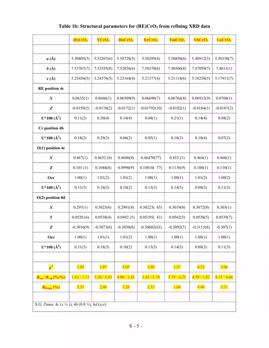
Table 1b: Structural parameters for (RE)CrO3 from refining XRD data

DyCrO3 YCrO3 HoCrO3 ErCrO3 TmCrO3 YbCrO3 LuCrO3

a (Å) 5.50805(5) 5.52267(6) 5.50728(5) 5.50289(4) 5.50850(6) 5.48912(5) 5.50150(7)

b (Å) 7.53767(7) 7.53555(8) 7.52026(6) 7.50370(6) 7.50506(8) 7.47059(7) 7.4811(1)

c (Å) 5.25436(5) 5.24376(5) 5.23164(4) 5.21377(4) 5.21114(6) 5.18258(5) 5.17911(7)

RE position 4c

X 0.0635(1) 0.0666(1) 0.06509(9) 0.06698(7) 0.06766(8) 0.06912(9) 0.0704(1)

Z -0.0159(2) -0.0170(2) -0.0172(1) -0.01792(10) -0.0182(1) -0.0184(1) -0.0187(2)

U*100 (Å2) 0.11(2) 0.30(4) 0.14(4) 0.04(1) 0.21(1) 0.14(4) 0.08(2)

Cr position 4b

U*100 (Å2) 0.18(2) 0.29(3) 0.06(2) 0.05(1) 0.18(3) 0.10(4) 0.07(2)

O(1) position 4c

X 0.467(1) 0.4652 (8) 0.4686(9) 0.46470(77) 0.453 (1) 0.464(1) 0.466(1)

Z 0.101 (1) 0.1044(8) 0.0990(9) 0.10810( 77) 0.1136(9) 0.108(1) 0.110(1)

Occ 1.00(1) 1.01(2) 1.01(2) 1.00(1) 1.00(1) 1.01(2) 1.00(2)

U*100 (Å2) 0.31(3) 0.18(3) 0.10(2) 0.13(3) 0.14(5) 0.08(3) 0.11(3)

O(2) position 8d

X 0.297(1) 0.3023(6) 0.2991(8) 0.30223( 65) 0.3019(8) 0.3072(8) 0.303(1)

Y 0.0520 (6) 0.0538(4) 0.0492 (5) 0.05195( 41) 0.0562(5) 0.0538(5) 0.0539(7)

Z -0.3016(9) -0.3073(6) -0.3030(8) -0.30602(63) -0.3092(7) -0.3115(8) -0.307(1)

Occ 1.00(1) 1.01(1) 1.01(2) 1.00(1) 1.00(1) 1.00(1) 1.00(1)

U*100 (Å2) 0.31(3) 0.18(3) 0.10(2) 0.13(3) 0.14(5) 0.08(3) 0.11(3)

χχχχ 2 2.03 1.07 5.05 3.88 1.37 6.32 3.06

Rwp / Rexp (%/%) 1.62 / 1.13 5.20 / 5.03 4.06 / 1.81 3.43 / 1.74 5.19 / 4.25 4.59 / 1.82 8.15 / 4.66

RBragg (%) 5.31 2.46 3.20 2.33 1.68 4.40 5.71

S.G. Pnma: 4c (x ¼ z), 4b (0 0 ½), 8d (xyz)

- 6 -S

Table 2a: Selected structural information for (RE)CrO3 obtained from XRD data. Angles are

given in degrees and distances in [Å]

LaCrO3 PrCrO3 NdCrO3 SmCrO3 EuCrO3 GdCrO3 TbCrO3

tolerance factor

0.92338 0.91006 0.90431 0.89315 0.88883 0.88415 0.87984

a Tilt angle θθθθ 9.4 11.5 12.2 12.9 13.4 14.4 15.2

b Tilt angle ϕϕϕϕ 9.4 11.5 12.2 12.9 13.4 14.4 15.2

c Tilt angle µµµµ 10.3 13.2 14.4 14.2 16.0 16.1 16.5

Cr-O(1) × 2 1.972(2) 1.981(2) 1.986(2) 1.967(2) 1.968(1) 1.980(3) 1.976(2)

Cr-O(2) × 2 1.94(2) 1.96(1) 1.967(6) 1.955(8) 1.970(3) 1.974(9) 1.970(8)

Cr-O(2)’ × 2 2.00(2) 1.98(1) 1.977(6) 1.978(8) 1.985(4) 1.984(9) 1.992(8)

Average B’-O 1.971(6) 1.975(4) 1.977(2) 1.966(3) 1.974(1) 1.979(3) 1.980(3)

For S.G. Pnma only a B-site exists with co-ordination: B’-O(1) × 2, B’-O(2) × 2 and B’-O(2)’ × 2

For S.G. Pnma the tilting scheme in Glazer’s notation (a-a-c+) implies that θθθθ ≈ ϕϕϕϕ

a With [101] for Pnma

b With [10-1] for Pnma

c With [010] for Pnma

- 7 -S

Table 2b: Selected structural information for (RE)CrO3 obtained from XRD data. Angles are

given in degrees and distances in [Å]

DyCrO3 YCrO3 HoCrO3 ErCrO3 TmCrO3 YbCrO3 LuCrO3

tolerance factor 0.87552 0.87264 0.87156 0.86796 0.86436 0.86076 0.85716

a Tilt angle θθθθ 15.9 17.00 15.8 16.6 17.4 17.7 17.0

b Tilt angle ϕϕϕϕ 15.9 17.00 15.8 16.6 17.4 17.7 17.0

c Tilt angle µµµµ 16.6 17.1 16.2 17.6 19.0 17.6 17.8

Cr-O(1) × 2 1.966(2) 1.971(1) 1.958(1) 1.968(1) 1.984(2) 1.960(2) 1.965(2)

Cr-O(2) × 2 1.979(5) 1.988(4) 1.968(4) 1.970(3) 1.983(4) 1.972(5) 1.968(6)

Cr-O(2)’ × 2 1.979(5) 1.993(3) 1.978(4) 1.985(4) 1.991(4) 1.990(5) 1.984(6)

Average B’-O 1.975(2) 1.984(1) 1.968(2) 1.974(1) 1.986(1) 1.974(2) 1.972(2)

For S.G. Pnma only a B-site exists with co-ordination: B’-O(1) × 2, B’-O(2) × 2 and B’-O(2)’ × 2

For S.G. Pnma the tilting scheme in Glazer’s notation (a-a-c+) implies that θθθθ ≈ ϕϕϕϕ

a With [101] for Pnma

b With [10-1] for Pnma

c With [010] for Pnma

- 8 -S

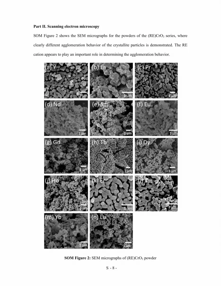
Part II. Scanning electron microscopy

SOM Figure 2 shows the SEM micrographs for the powders of the (RE)CrO3 series, where

clearly different agglomeration behavior of the crystallite particles is demonstrated. The RE

cation appears to play an important role in determining the agglomeration behavior.

SOM Figure 2: SEM micrographs of (RE)CrO3 powder

- 9 -S

Part III. Raman spectroscopy

The positions of several selected Raman modes and how they develop across the (RE)CrO3

series are summarized in Table 3. SOM Figure 3 shows plots of Raman wave number vs RE

ionic radius IOR for several selected modes. It can be seen that certain Raman modes show

stronger dependence on IOR than others. The positions of the Ag(3) and Ag(5) Raman modes

with the strongest dependence on IOR are plotted in SOM Figure 4 vs octahedral perovskite

tilting angle to highlight an approximately linear dependence.

Table 3: Wave numbers of selected Raman modes for (RE)CrO3

(RE)CrO3 Raman mode wave numbers in [cm-1]

Ag(2) Ag(3) Ag(4) Ag(5) Ag(6) B1g(2) B2g(1) B3g(3)

LaCrO3 120 154 254 278 442 353 135 594

PrCrO3 133 196 281 324 454 371 152 583

NdCrO3 130 192 278 320 451 367 144 579

SmCrO3 140 235 312 368 470 387 155 572

EuCrO3 135 235 306 372 460 149 557

GdCrO3 143 257 328 394 482 162 574

TbCrO3 139 259 329 395 478 154 561

DyCrO3 145 269 344 415 492 405 164 572

YCrO3 (189) 284 345 429 495 412 (221) 569

HoCrO3 144 278 344 423 500 409 163 571

ErCrO3 149 282 353 442 (520) (395) 168 575

TmCrO3 144 282 353 442 506 414 163 571

YbCrO3 144 282 358 451 511 418 168 580

LuCrO3 138 291 356 454 515 417 162

- 10 -S

SOM Figure 3: Wave numbers of selected Raman modes in (RE)CrO3 vs IOR.

SOM Figure 4: Wave numbers vs octahedral tilt angle θθθθ. Solid lines are guide to the eyes.

100

200

300

400

500

600

1 1.05 1.1 1.15 1.2 1.25

Wave number (cm-1)

RE Ionic Radius IOR (Å)

B3g(3)

Ag(6)

Ag(5)

B1g(2)

Ag(4)

Ag(3)

B2g(1)

Ag(2)

10 12 14 16 18

150

200

250

300

350

400

450

Ag(3)W

ave number (cm-1)

Octahedral Tilt Angle (°)

Ag(5)

- 11 -S

Part IV. Magnetic structure

Table 4 shows the magnetic parameters extracted from magnetization vs temperature curves

(Neel temperatures TN1, TN2) and from Curie-Weiss fits (Curie and Weiss constants C, Θ , and

effective magnetization µeff). The Neel temperature TN1 marks the onset of antiferromagnetic

Cr3+-Cr3+ ordering, TN2 marks the onset of antiferromagnetic ordering of the (RE)3+ spins.

Table 4: Magnetic parameters for (RE)CrO3 obtained from magnetization

measurements

TN1 Cr3+ (K) TN2 RE3+ (K) C (µB) Θ (K) Total µeff (µB)

(RE)CrO3 Experim. Literature Experim. Literature1,2 Experim. Theoretical

LaCrO3 288 282 - - - - - 3.87

PrCrO3 239 239 2 2 3.3 -160 5.15 5.21

NdCrO3 226 224 11 10 3.8 -189 5.54 5.29

SmCrO3 191 193 - - 3.4 -314 5.21 5.46

EuCrO3 185 181 - - 3.4 -198 5.23 5.15

GdCrO3 171 170 3 4 7.3 -29 7.65 8.83

TbCrO3 159 158 4.5 4 12.9 -26 10.17 10.46

DyCrO3 149 146 2 2 15.7 -24 11.21 11.33

YCrO3 141 140 - - 2.51 -408 4.48 3.87

HoCrO3 142 141 - 12 15.7 -21 11.22 11.28

ErCrO3 136 133 14 17 12.8 -24 10.12 10.33

TmCrO3 125 124 3 4 8.6 -32 8.30 8.49

YbCrO3 120 118 4 3 4.4 -99 5.92 5.97

LuCrO3 109 112 - - 2.4 -174 4.42 3.87

1.) Goodenough J.B., Longo J.M.: Landolt-Börnstein New Series III, ed. Hellwege K.-H., Hellwege A.M. (Springer, Berlin,

1970) Vol.4, Part A, p.228. 2.) Sardar K., Lees M. R., Kashtiban R. J., Sloan J., Walton R. I., Chem. Mater. 2011, 23, 48

- 12 -S

The effective magnetic moments µeff, originating from the Cr3+ cations were calculated from

the Curie constants C according to µeff2 = 8C. The theoretical value for µeff was regarded a

combination of Cr3+ and (RE)3+, where µeff(Cr3+) = 3.87 µB, obtained from the equation µeff =

2[S(S+1)]1/2 with the multiplicity S = 3/2. For (RE)3+ µeff = gL[J(J+1)]½ where gL is the Landé

g-factor (gL = (3/2)+[(S(S+1)-L(L-1))/2J(J+1)]), J is the total angular momentum and L

corresponds to the maximum orbital angular momentum. All µeff values are displayed in SOM

Figure 5, together with theoretical values in agreement with Landolt-Börnstein tables. For the

LaCrO3 sample TN1 is high and no sufficient 1/χ vs T data points were available at high T to

perform a Curie-Weiss fit.

SOM Figure 5 Effective magnetic moment µeff for the (RE)CrO3 series as determined from

the respective Curie-Weiss fits and plotted vs IOR. Theoretical values were calculated from

Landolt-Börnstein tables.

1.00 1.05 1.10 1.15 1.20 1.25

4

6

8

10

12

Tolerance Factor t

Experimental values

Theoretical values

µµ µµeff (

µµ µµB)

RE Ionic Radius IOR (Å)

0.84 0.86 0.88 0.90 0.92 0.94

1.00 1.05 1.10 1.15 1.20 1.25

Y La

Pr

NdSm

Eu

Gd

Tb

DyHo

Er

Tm

Lu

Yb

- 13 -S

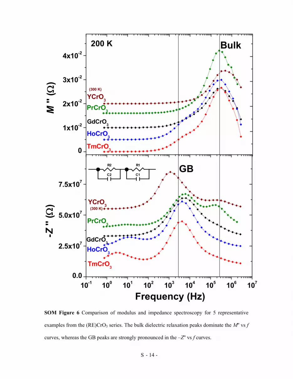
Part V. Dielectric spectroscopy

The impedance spectroscopy data obtained for all pellets from the (RE)CrO3 series were

analyzed to extract bulk and GB resistivity (ρ 1, ρ 2) and permittivity (ε 1, ε 2). The bulk and

GB relaxations were approximated by an equivalent circuit consisting of two ideal RC

elements connected in series (see Inset in SOM Figure 6), where the non-ideality was

neglected. R1 and C1 describe the intrinsic bulk resistivity ρ1 and bulk permittivity ε1

respectively, whereas R2 and C2 describe the extrinsic GB resistivity ρ2 and GB permittivity

ε2 respectively. The ρ1, ρ2, ε1 and ε2 values were extracted by the following procedure:

1.) The bulk and GB resistivity values ρ1 and ρ2 were obtained from the estimated

diameter of the respective semicircle in the –Z'' vs Z' plots.

2.) The bulk and GB permittivity values ε1 and ε2 were obtained from the peak

frequency fmax of the bulk or GB dielectric relaxation peaks according to equation (1)

shown below. The bulk dielectric relaxation peak was displayed clearly in plots of the

imaginary part of the modulus function M'' vs f (SOM Figure 6, upper panel), whereas

the GB peak was best displayed in plots of -Z'' vs f (SOM Figure 6, lower panel).

In SOM Figure 6 the curves for the Ho-, Gd-, Pr-, and Y-containing samples are shifted up the

M'' and –Z'' y-axes by increasing amounts for demonstration purposes. The –Z'' vs f curves

were normalized to render the peak heights comparable to enable equivalent resolution for all

samples within the same graph.

The approximate conditions for a bulk or GB relaxation peak maximum to occur are shown in

equation 1 for both notations, M'' vs f and -Z'' vs f, using the framework of the brick work

layer and RC element model for ideal relaxations. The approximate peak ordinates are

distinctively different for M''(fmax) and –Z''(fmax) (equation 2), which guarantees that in the M''

vs f notation the smallest capacitance (bulk) and in the -Z'' vs f notation the largest resistance

(GB) are most strongly pronounced.

- 14 -S

SOM Figure 6 Comparison of modulus and impedance spectroscopy for 5 representative

examples from the (RE)CrO3 series. The bulk dielectric relaxation peaks dominate the M'' vs f

curves, whereas the GB peaks are strongly pronounced in the –Z'' vs f curves.

10-1

100

101

102

103

104

105

106

107

0.0

2.5x107

5.0x107

7.5x107

Z'' [ ΩΩ ΩΩ]

Frequency [Hz]

0.00E+000

2.50E+007

5.00E+007

7.50E+007

(300 K)

YCrO3

PrCrO3

GdCrO3

HoCrO3

TmCrO3

0

1x10-2

2x10-2

3x10-2

4x10-2

M''

0.00

0.01

0.02

0.03

0.04

(300 K)

YCrO3

PrCrO3

GdCrO3

HoCrO3

TmCrO3

GB

Bulk200 K

R2

C2

R1

C1

Frequency (Hz)

-Z ''( ΩΩ ΩΩ)

M''( ΩΩ ΩΩ)

- 15 -S

This is clearly evident in SOM Figure 6, where the main bulk peaks in M'' vs f clearly

dominate over the secondary GB peaks, whereas the main GB peaks in -Z'' vs f clearly

dominate over the secondary bulk peaks. In fact, some of the secondary peaks cannot be

resolved at all in the respective notation.

202max

101max 2

1)''(;

2

1)''(

εερπεερπ≈−≈ ZfMf ; (eq.1)

2)('';

2

1)('' 2

max1

max

ρ

ε≈−≈ fZfM ; (eq.2)

The resistivity values obtained were plotted on Arrhenius axes and the activation energies EA

were determined. The bulk and GB activation energies, dielectric permittivity and the

resistivity at 200 K are summarized in Table 5. The bulk and GB resistivity vs reciprocal

temperature curves are presented in the SOM Figures 7 and 8, whereas the bulk permittivity

values vs temperature plots are shown in SOM Figure 9. The bulk permittivity ε1 vs T curves

show considerable scatter in several instances, which is a reflection of the limited accuracy of

the manual data analysis method employed.

- 16 -S

Table 5: Dielectric parameter for (RE)CrO3 obtained from impedance spectroscopy

(RE)CrO3 Activation Energy EA

in [eV] Dielectric Permittivity

[dimensionless] Resistivity at 200 K in

[ΩΩΩΩcm]

Bulk GB Bulk ε 1 GB ε 2 Bulk ρ 1 GB ρ 2

LaCrO3 0.22 0.29 15.6 2520 3.92 106 4.45 105

PrCrO3 0.21 17.2 407 4.11 105 8.89 105

NdCrO3 0.23 0.3 15.8 258 5.17 104 1.96 107

SmCrO3 0.22 0.26 23.7 90.2

EuCrO3 0.26 0.29 18.7 283 1.70 105 6.93 106

GdCrO3 0.27 0.31 27.1 177 1.96 105 1.93 106

TbCrO3 0.30 12.5 318 1.05 107 8.40 106

DyCrO3 0.27 0.28 17.3 47.4 5.40 105 1.15 107

YCrO3 0.32 0.33 21.7 1740 8.00 107 5.04 108

HoCrO3 0.26 0.28 12.9 76.8 4.27 105 5.62 106

ErCrO3 0.27 0.29 14.1 181 4.27 105 2.42 106

TmCrO3 0.25 0.29 14.4 102 3.93 105 4.66 106

YbCrO3 0.28 19.6 164 1.97 106 1.14 1010

LuCrO3 0.28 0.27 20.0 97.4 1.28 106 3.11 107

- 17 -S

SOM Figure 7a & b: Bulk resistivity ρ 1 plotted vs reciprocal temperature 1/T. Solid lines

are guide to the eyes, indicating good linearity and Arrhenius behavior.

1.E+04

1.E+05

1.E+06

1.E+07

1.E+08

1.E+09

0.003 0.004 0.005 0.006 0.007

1/T in 1/K

Bulk resistivity ρρ ρρ

1Y

La

Pr

Nd

Eu

Sm

Gd

(a)

1.E+04

1.E+05

1.E+06

1.E+07

1.E+08

1.E+09

0.004 0.005 0.006 0.007

1/T in 1/K

Bulk resistivity ρρ ρρ

1

Ho

DyTm

Er

LuYb

(b)

- 18 -S

SOM Figure 8a & b: GB resistivity ρ 2 plotted vs reciprocal temperature 1/T. Solid lines are

guide to the eyes, indicating good linearity and Arrhenius behavior.

1.E+04

1.E+05

1.E+06

1.E+07

1.E+08

1.E+09

1.E+10

0.003 0.004 0.005 0.006 0.007

1/T in 1/K

GB resistivity ρρ ρρ

2Y

La

Nd

Eu

Sm

Gd

(a)

1.E+05

1.E+06

1.E+07

1.E+08

1.E+09

1.E+10

1.E+11

0.004 0.005 0.006 0.007

1/T in 1/K

GB resistivity ρρ ρρ

2

Ho

DyTm

Er

LuYb

(b)

- 19 -S

SOM Figure 9a & b: Bulk permittivity ε 1 plotted vs temperature T. In several curves the

data scatter is considerable as a reflection of the limited accuracy of the manual data analysis.

0

5

10

15

20

25

30

35

120 170 220 270

Bulk permittivity εε εε1

Temperature in K

Y

LaPrNd

Eu

Sm

Gd

(a)

0

5

10

15

20

25

30

35

120 140 160 180 200 220 240

Bulk permittivity εε εε1

Temperature in K

Ho

Dy

Tm

ErLu

Tb

(b)