Jaehwan Kim BSc MSc - CORE

MONITORING CONCRETE PERFORMANCE

UNDER SIMULATED AND NATURAL CHLORIDE

ENVIRONMENTS

By

Jaehwan Kim BSc MSc

Submitted for the degree of Doctor of Philosophy

School of Energy, Geoscience, Infrastructure and Society

Institute for Infrastructure and Environment

Heriot-Watt University

April 2018

The copyright in this thesis is owned by the author. Any quotation from the thesis or use of any of the information contained in it must acknowledge this thesis as the source of the quotation or information.

i

ABSTRACT

Deterioration of reinforced concrete structures caused by chloride-induced corrosion is

well-known in the construction industry, but it is still difficult to evaluate the performance

of the structures due to various exposure conditions and characteristics of concrete,

especially containing supplementary cementitious materials (SCMs). In this study,

comprehensive assessments of both chloride transport and corrosion initiation/propagation

were, therefore, performed to study the performance of concrete subjected to a chloride

environment. Chloride transport in concrete was assessed using the migration/diffusion

coefficient, porosity/degree of saturation and electrical resistance/resistivity. The electrical

resistivity of the concrete was used as a single 'performance' factor. In addition to chloride

transport, the condition of steel embedded in concrete was monitored using electrochemical

methods. The electrical resistance/resistivity of concrete was monitored over a period of

382 days and then analysed using a normalisation technique to identify the chloride

transport and corrosion process. In addition, the condition of concrete slabs (18 years old)

retrieved from the Dornoch Firth marine exposure site (representing XS3 environmental

exposure class) were evaluated using the same procedures conducted in the laboratory. In

monitoring the electrical resistance/resistivity, the activation energy was calculated to

reflect the environmental conditions, in this instance diurnal and annual temperature

variation. Finally, for time to corrosion initiation, the ClinConc model was combined with

two new environmental factors and during corrosion propagation, the polarisation

resistance was estimated using a fitting method.

ii

DEDICATION

To my beloved wife and son

Hye Jung and Doyun

To my parents

Chang Sun, Kim and Hyang In, Jwa

For their endless love, support and encouragement

iii

ACKNOWLEDGEMENTS

Most of all, I would like to thank Prof. W. John McCarter for his patience, valuable

comments and guidance for the last 4 years. I would like to thank Dr. Gerard Starrs and

Dr Benny Suryanto for their support. The help of the Technical staff in the experimental

work is also gratefully acknowledged.

I would like to express my gratitude to my parents-in-law Kibal, Ryu and Ok Nam, Lee

for their unfailing moral support. I am also thankful for heart-warming kindness from the

family of my brother-in-law: Chung Seok, Yu and Yunhee, Park.

Finally, I am indebted to my father, Chang Sun Kim, my mother, Hyang In, Jwa and my

younger sister, Min Kyeong, Kim for their unseen support throughout this entire journey.

I have been inspired and encouraged by the belief of my wife, Hye Jung, Yu and my son,

Doyun, Kim, who made this thesis possible.

iv

DECLARATION STATEMENT

v

TABLE OF CONTENTS

ABSTRACT ....................................................................................................................... i

DEDICATION .................................................................................................................. ii

ACKNOWLEDGEMENTS ............................................................................................. iii

DECLARATION STATEMENT..................................................................................... iv

TABLE OF CONTENTS .................................................................................................. v

LIST OF FIGURES .......................................................................................................... x

LIST OF TABLES .......................................................................................................... xv

LIST OF ABBREVIATIONS ........................................................................................ xvi

LIST OF SYMBOLS .................................................................................................... xvii

LIST OF PUBLICATIONS ........................................................................................... xix

1. INTRODUCTION ........................................................................................................ 1

1.1 Background ....................................................................................................................................... 1

1.2 Objectives .......................................................................................................................................... 2

1.3 Outline of thesis ................................................................................................................................. 4

2. REVIEW OF CHLORIDE-INDUCED CORROSION OF STEEL IN CONCRETE .. 7

2.1 Introduction ....................................................................................................................................... 7

2.2 Overview of concrete durability ........................................................................................................ 7

2.2.1 Changing trend for durability evaluation .................................................................................... 8

2.2.2 Performance factors ................................................................................................................... 15

2.3 Chloride transport ............................................................................................................................ 17

2.3.1 Mass transport and flow in concrete transport systems ............................................................. 17

2.3.2 Influencing factors ..................................................................................................................... 19

2.4 Chloride-induced corrosion of steel................................................................................................. 25

2.4.1 Corrosion mechanism ................................................................................................................ 25

2.4.2 Chloride threshold level ............................................................................................................ 28

2.4.3 Influencing factors of steel corrosion ........................................................................................ 31

2.5 Electrical resistivity ......................................................................................................................... 33

2.5.1 Factors influencing resistivity measurements............................................................................ 34

2.5.2 Representation of electrical resistivity ...................................................................................... 36

2.6 Summary ......................................................................................................................................... 37

vi

3. A METHODOLOGICAL REVIEW OF CHLORIDE-INDUCED CORROSION OF

STEEL IN CONCRETE .................................................................................................. 38

3.1 Introduction ..................................................................................................................................... 38

3.2 Measurement for chloride transport in concrete .............................................................................. 38

3.2.1 Non-electrical methods.............................................................................................................. 39

3.2.2 Electrical method....................................................................................................................... 40

3.2.3 Porosity/degree of saturation ..................................................................................................... 42

3.3 Measurements for steel corrosion .................................................................................................... 43

3.3.1 Half-cell potential measurement................................................................................................ 43

3.3.2 Macrocell current ...................................................................................................................... 43

3.3.3 Polarisation resistance ............................................................................................................... 44

3.3.4 Electrochemical impedance spectroscopy ................................................................................. 48

3.3.5 Commercial equipment ............................................................................................................. 54

3.3.6 Mass loss ................................................................................................................................... 55

3.4 Measurements for electrical resistivity of concrete ......................................................................... 56

3.5 Overview of predictive models........................................................................................................ 57

3.5.1 Transport models ....................................................................................................................... 58

3.5.2 Corrosion models ...................................................................................................................... 63

3.6 Summary ......................................................................................................................................... 64

4. EXPERIMENTAL PROGRAMME ............................................................................ 66

4.1 Introduction ..................................................................................................................................... 66

4.2 Materials and concrete mix preparation in laboratory ..................................................................... 66

4.3 Sample specifications ...................................................................................................................... 67

4.4 Curing and exposure regime ............................................................................................................ 74

4.5 Sample preparation .......................................................................................................................... 75

4.6 Marine exposure conditions and samples in field ............................................................................ 78

4.7 Summary ......................................................................................................................................... 80

5. CHLORIDE TRANSPORT AND PERFORMANCE FACTORS .............................. 84

5.1 Introduction ..................................................................................................................................... 84

5.2 Experimental ................................................................................................................................... 85

5.2.1 Compressive strength ................................................................................................................ 85

5.2.2 Porosity/saturation degree ......................................................................................................... 85

5.2.3 Chloride profiling ...................................................................................................................... 86

vii

5.2.4 Migration test ............................................................................................................................ 88

5.2.5 Electrical resistivity of concrete ................................................................................................ 88

5.3 Results and discussion ..................................................................................................................... 90

5.3.1 Development of compressive strength ...................................................................................... 90

5.3.2 Pore conditions in unsaturated concrete .................................................................................... 93

5.3.3 Diffusion/Migration coefficient ................................................................................................ 97

5.3.4 Electrical resistivity of concrete .............................................................................................. 104

5.3.5 Relation between compressive strength and electrical resistivity ........................................... 109

5.3.6 Relation between transport properties and electrical resistivity .............................................. 113

5.4 Summary ....................................................................................................................................... 120

6. CHLORIDE-INDUCED CORROSION OF STEEL WITH PERFORMANCE OF

CONCRETE ................................................................................................................... 122

6.1 Introduction ................................................................................................................................... 122

6.2 Experimental ................................................................................................................................. 123

6.2.1 Half-cell potential .................................................................................................................... 123

6.2.2 Macrocell current .................................................................................................................... 123

6.2.3 DC polarisation techniques ..................................................................................................... 125

6.2.4 Electrochemical impedance spectroscopy ............................................................................... 129

6.2.5 Mass loss and visual inspection ............................................................................................... 130

6.3 Results and discussion ................................................................................................................... 131

6.3.1 Corrosion potential with time .................................................................................................. 131

6.3.2 Macrocell current with time .................................................................................................... 135

6.3.3 Parameters for electrochemical techniques ............................................................................. 137

6.3.4 Determination of corrosion rate............................................................................................... 147

6.3.5 Visual inspection for corrosion ............................................................................................... 156

6.3.6 Determination of time to corrosion initiation .......................................................................... 160

6.4 Summary ....................................................................................................................................... 161

7. MONITORING THE ELECTRICAL RESISTANCE OF CONCRETE .................. 163

7.1 Introduction ................................................................................................................................... 163

7.2 Experimental ................................................................................................................................. 164

7.2.1 Experimental set-up ................................................................................................................. 164

7.2.2 Electrical measurement ........................................................................................................... 165


viii

7.3.1 Electrical resistance monitoring .............................................................................................. 167

7.3.2 Chloride transport monitoring ................................................................................................. 175

7.3.3 Corrosion monitoring .............................................................................................................. 181

7.4 Summary ....................................................................................................................................... 188

8. EVALUATING THE SERVICE LIFE OF CONCRETE STRUCTURES ............... 189

8.1 Introduction ................................................................................................................................... 189

8.2 Experimental ................................................................................................................................. 189

8.2.1 Experiments for chloride transport .......................................................................................... 189

8.2.2 Experiments for corrosion ....................................................................................................... 190

8.2.3 Monitoring electrical resistance using a remote-control system ............................................. 191


8.3.1 Evaluating chloride transport .................................................................................................. 191

8.3.2 Evaluating the corrosion of steel ............................................................................................. 204

8.3.3 Evaluating the electrical resistance of 18-year-old concrete ................................................... 209

8.4 Summary ....................................................................................................................................... 218

9. CONCLUSIONS AND RECOMMENDATIONS FOR FUTHER WORK .............. 219

9.1 Electrical resistance and transport properties – laboratory-based studies ...................................... 219

9.2 Electrical resistance and transport properties – Marine Exposure Site .......................................... 220

9.3 Electrochemical parameters for the corrosion of steel ................................................................... 221

9.4 Monitoring electrical resistance ..................................................................................................... 223

9.5 Mix design – binders and w/b........................................................................................................ 224

9.6 Predictive models – transport and corrosion model ....................................................................... 224

9.7 Recommendations for further research .......................................................................................... 225

REFERENCES ............................................................................................................... 227

APPENDIX .................................................................................................................... 244

APPENDIX A : EQUATIONS USED WITHIN TEXT ................................................ 244

A.1 Diffusion coefficient in unsaturated concrete (equation 3.14): ..................................................... 244

A.2 Degree of hydration ...................................................................................................................... 245

APPENDIX B : EXPERIMENTAL SET-UPS .............................................................. 246

B.1 Slab sample fabrication ................................................................................................................. 246

B1.1 Stainless-steel pin electrodes and steels in plywood mould .................................................... 246

B1.2 Mild-steel ................................................................................................................................. 247

B1.3 Demoulded slabs after air-curing ............................................................................................. 248

ix

B1.4 Chloride profiling ............................................................................................................... 249

APPENDIX C : TEST RESULTS ................................................................................. 250

C.1 Test results in Chapter 5 ............................................................................................................... 250

C1.1 Compressive strength/electrical resistivity with samples (100 mm cube) ............................... 250

C1.2 Measuring weight change (Chapter 5.3.2)/electrical resistivity (Chapter 5.3.4) for degree of

saturation/porosity test ..................................................................................................................... 251

C1.3 Migration coefficient & Resistivity ......................................................................................... 253

C1.4 Chloride profiling .................................................................................................................... 254


C2.1 Corrosion potential monitoring/macrocell current monitoring ................................................ 256

C2.2 Parameters from galvanostatic pulse measurement ................................................................. 262

C2.3 Parameters from potentiostatic measurement .......................................................................... 269

C2.4 Parameters from linear polarisation resistance measurement .................................................. 276

C2.5 Electrochemical impedance spectroscopy (Nyquist plot) ........................................................ 277

C2.6 Potentiodynamic plot (Tafel’s plot) ......................................................................................... 283

C.3 Teste results in Chapter 7 .............................................................................................................. 289

C3.1 Monitoring electrical resistance using 2-pin electrodes ........................................................... 289

C3.2 Monitoring electrical resistance using 4-pin electrodes ........................................................... 292


C4.1 Chloride profiles from 18 years-old samples retrieved from Dornoch .................................... 295

C4.2 Measuring weight change of field concrete for degree of saturation/porosity ......................... 295

C4.3 Monitoring electrical resistance of field concrete in Dornoch ................................................. 297

C4.4 Electrochemical parameters of steel in field concrete from polarisation techniques ............... 298

C4.5 Electrochemical impedance spectroscopy (Nyquist plot) for field samples ............................ 299

C4.6 Potentiodynamic plot for field samples ................................................................................... 300

APPENDIX D MODELLING ....................................................................................... 301

D.1 Prediction of compressive strength ............................................................................................... 301

D.2 Input values in the ClinConc model (Excel version) .................................................................... 302

D.3 Determination of Kexp with regression method ............................................................................. 303

x

LIST OF FIGURES

1.1 Failure modes of concrete structures modified by author (Gifford, 2005). ........................ 1

1.2 Flow chart of the research programme. .............................................................................. 6

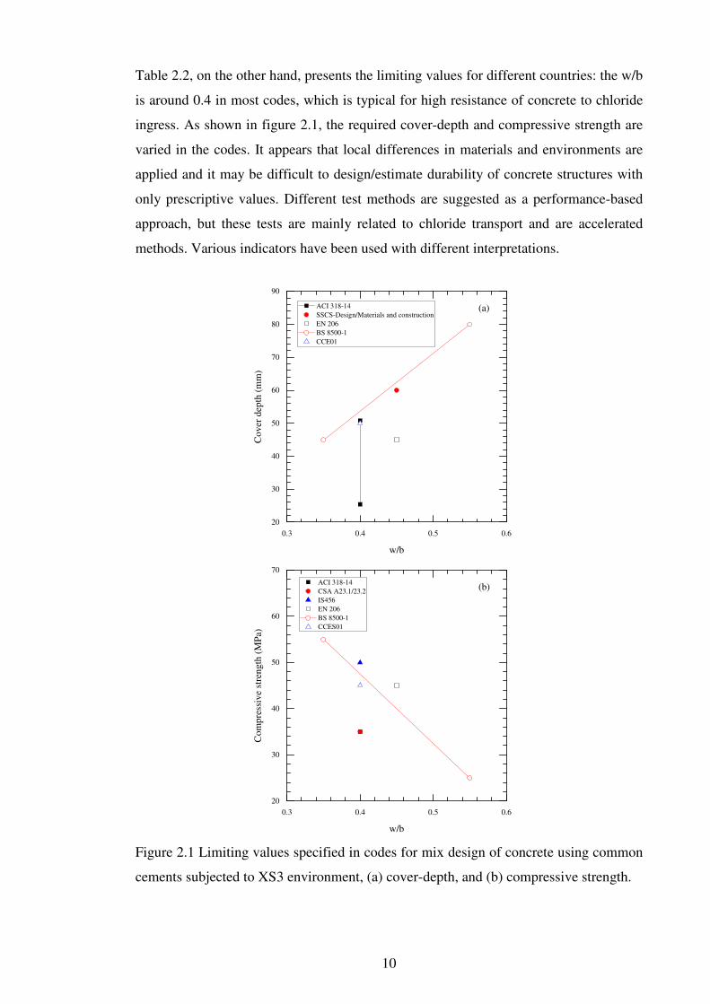
2.1 Limiting values specified in codes for mix design of concrete (using common cements)

subjected to XS3 environment, (a) cover-depth, and (b) compressive strength. .............. 10

2.2 A modified example of the prediction of chloride profile in unsaturated concrete (Song et

al., 2008a) modified by the author. ................................................................................... 24

2.3 Relative diffusion rate with saturation degree of PC concrete (Kumar, 2010) replotted by the

author. ..................................................................................................................................... 24

2.4 The service life of reinforced concrete structures and possible limit states. ..................... 26

2.5 Schematics for chloride-induced corrosion of steel in concrete. ....................................... 27

2.6 Pourbaix diagram for iron showing the most stable products at a given pH and potential

(Roberge, 2008). ............................................................................................................... 33

2.7 Schematics for Evans diagram (a) with an increase in chlorides and (b) with a decrease in

oxygen availability............................................................................................................ 33

2.8 The relationship between electrical resistivity and diffusivity (Sengul, 2014). ................ 35

3.1 Classification of techniques for chloride transport ........................................................... 39

3.2 Test set-ups for (a) AASHTO T259 and (b) NT Build 443 .............................................. 40

3.3 Graphical scheme to compare the potentials of the most commonly used reference electrodes

(Roberge, 2008) ................................................................................................................................... 44

3.4 Set-up for polarisation resistance measurement ................................................................ 45

3.5 (a) Linear polarisation curve and (b) cyclic polarisation curve ........................................ 48

3.6 Nyquist format for data presentation ................................................................................ 50

3.7 Bode format for data presentation ..................................................................................... 50

3.8 Equivalent electrical circuits for analysis of steel corrosion in concrete/mortar (refer to table

3.4). ......................................................................................................................................... 52

3.9 Examples of current confinement method using (a) GalvaPulse and (b) GECOR 6 (Nygaard

et al., 2009) modified by the author (∆E potential difference in the steel at different

locations for controlling the guard-ring) ........................................................................... 54

3.10 Set-up for (a) two-electrode and (b) four-electrode method (the Wenner method). ......... 57

4.1 (a) Cubic sample for compressive strength and electrical resistivity test, (b) cylinder sample

for migration test (NT build 492) and electrical resistivity test and (c) slab sample used for

monitoring corrosion parameters and electrical resistance ............................................... 69

4.2 Schematics of concrete slab (dimensions in mm): (a) isometric (b) end elevation, A-A, (c)

end elevation, B-B and (d) end elevation, C-C; SS (steel having small exposed area), LS

(steel having large exposed area). ..................................................................................... 71

4.3 Steel configuration in slab (a) before casting and (b) after demoulding ........................... 72

xi

4.4 Arrangement of electrodes for monitoring electrical resistance of concrete subjected to

chloride attack; (a) electrode arrays for chloride transport, and (b), (c) and (d) electrode

arrays for corrosion propagation ....................................................................................... 74

4.5 Cutting the plain slab for chloride profiling and the saturation test .................................. 76

4.6 (a) Cutting process from the sectioned slice and (b) a sample for the degree of saturation

test ..................................................................................................................................... 77

4.7 (a) Drilling process from the sectioned slice and (b) a drilled sample for collecting powder .. 77

4.8 Sample cutting for migration/electrical resistivity test ..................................................... 77

4.9 (a) Location of marine exposure site, (b) position of frames installed in XS3 environment,

(c) breaking waves during the period of rising tide, and (d) retrieved samples positioned in

the frame. .......................................................................................................................... 79

5.1 Examples of curve fitting from the chloride profile data. ................................................. 87

5.2 Schematic of testing arrangement for end-to-end electrical resistance measurements ..... 89

5.3 Development of compressive strength. ............................................................................. 91

5.4 Comparison between measured and predicted values for compressive strength at different

ages and different binders (expect for values at 28 days). ................................................ 93

5.5 Colour change with phenolphthalein indicator (CEM I, w/b=0.4). .................................. 94

5.6 Degree of saturation profiles for the concrete mixes. ....................................................... 96

5.7 Effect of exponent n on the decrease ratio of the diffusion coefficient with time (Dt diffusion

coefficient at time, t, and Dref diffusion coefficient at time, tref [=1 year]). ........................... 98

5.8 Development of migration coefficients with time. ......................................................... 100

5.9 Time-averaged diffusion coefficient at time t from chloride profiling. .......................... 100

5.10 Chloride profiles at 390 days. ......................................................................................... 102

5.11 Relation between the migration coefficient at 365 (closed markers) and 180 (open markers)

days and the diffusion coefficient at 390 days. ............................................................... 104

5.12 Development of electrical resistivity for samples (100 × 100 × 100 mm) used in the

compressive strength test. ............................................................................................... 106

5.13 Development of electrical resistivity for samples (Ø 100 × 50 ± 3 mm) used in the NT Build

492 test. ........................................................................................................................................ 107

5.14 Comparison between electrical resistivity of migration test samples before and after vacuum

saturation with saturated Ca(OH)2 solution. .............................................................................. 107

5.15 Example of resistivity profiles at the end of a wet/dry cycle (CEM I concrete, w/b=0.6). .... 109

5.16 An increase ratio of electrical resistivity with a dry phase at 10 mm cover depth (ρdry

electrical resistivity at the end of final drying phase [390 days] and ρwet electrical resistivity

at the end of final wetting phase [382 days]). ................................................................. 109

5.17 Estimated resistivity of pore solution with time and binder types using NIST model. ... 112

5.18 The relation between normalised resistivity and compressive strength with binder type. .. 113

xii

5.19 Relation between saturation degree and resistivity with binder type (a) w/b=0.4 and (b)

w/b=0.6 (outliners [open markers] are removed from fitting equations). ....................... 116

5.20 Schematic diagram for chloride distribution in samples after migration test (Tang, 1996a). . 117

5.21 Relation between the migration coefficient and bulk electrical resistivity irrespective of

binder types and w/b. ...................................................................................................... 119

5.22 Schematic diagram for assumption of chloride distribution in terms of the suggested parameter

() after the migration test in this study. .................................................................................. 119

6.1 Half-cell potential technique. .......................................................................................... 124

6.2 Macrocell current technique. ........................................................................................... 124

6.3 DC polarisation technique. .............................................................................................. 125

6.4 Calculating the polarisation resistance from the linear polarisation curve. .................... 126

6.5 Evaluation of the Tafel slope in a potentiodynamic polarisation test including reverse scan. 127

6.6 Calculating the polarisation resistance using the GP. ..................................................... 128

6.7 Calculating the polarisation resistance using the PT. ...................................................... 129

6.8 Simulation of electrochemical spectra of steel in concrete; R_Conc and R_IF=400 Ω,

CPE_Conc and CPE_IF=1×10-9 Fs-0.3 for concrete and R_CP and R_Steel =3000 Ω and

CEP_CP and CEP_Steel=0.01 Fs-0.3 for steel and equivalent electrical circuit (insert). 130

6.9 (a) Corroded steel immersed in hydrochloric acid solution for mass loss test and (b) pit depth

estimation using digital microscope ........................................................................................... 131

6.10 Sample notation used in the presentation of experimental results. ................................. 131

6.11 Corrosion potential monitoring from 42 days for (a) steel with small exposure area, and (b)

steel with large exposure area at 25 mm cover depth in CEM I (w/b=0.6) concrete. ........ 133

6.12 Corrosion potential of passivated steel over the period 42-382 days for concretes (a)

(w/b=0.4) and (b) (w/b=0.6). .......................................................................................... 134

6.13 Macrocell current monitoring with time, steel with (a) short exposure area and (b) large

exposure area. ................................................................................................................. 136

6.14 Macrocell current distribution of steel in concrete. ........................................................ 137

6.15 Ohmic resistance with time for (a) CEM I, (b) CEM III/A, and (c) CEM II/B-V concrete. .. 139

6.16 Polarisation resistance of passivated steel with mix design. ........................................... 140

6.17 Nyquist plot for passivated steel embedded in concrete with time (CEM I concrete,

w/b=0.4). .............................................................................................................. 141

6.18 Polarisation resistance of steel having a small exposure area in CEM I (w/b = 0.6) concrete

with time. .............................................................................................................................. 142

6.19 Polarisation resistance of steel having a large exposure area in CEM I (w/b = 0.6) concrete

with time. .............................................................................................................................. 143

6.20 Randle circuit in the steel-concrete system (R_conc electrical resistance of concrete, R_steel

electrical resistance of steel and C_steel capacitance of steel). ........................................... 144

6.21 Capacitance monitoring for passivated steel using the GP technique. ............................ 145

xiii

6.22 Capacitance monitoring for active steel using the GP technique (CEM I concrete,

w/b=0.6). .............................................................................................................. 145

6.23 Time constant vs corrosion potential. ............................................................................. 146

6.24 Schematic showing total charge and charge by double layer.......................................... 148

6.25 B values of steel using the PT technique for (a) passive state and (b) active state with time. 150

6.26 Variation in B value with βa (βc =127 mV/dec). ............................................................. 151

6.27 Calculating the averaged corrosion rate from monitoring data. ...................................... 155

6.28 Comparison of corrosion rate between polarisation techniques and mass loss. .............. 156

6.29 Corrosion products of iron (Köliö et al. 2015). .............................................................. 157

6.30 Crack patterns on the concrete surface and corroded steels (‘LS’ on left side and ‘SS’ on

right side) extracted from samples for CEM I (w/b=0.6) concretes. .............................. 158

6.31 Sectioned loss of steel with a small exposure area (SS) and a large exposure area (LS) for

CEM I (w/b=0.6) concretes. ........................................................................................... 159

7.1 Distribution of aggregate around electrodes. .................................................................. 164

7.2 (a) Schematic diagram showing conduction in concrete and (b) a three-phase model for

concrete (adapted from McCarter et al. (2001)). .........................................................166

7.3 Example of monitoring electrical resistance with 2-pin electrode arrangements (for CEM I

concrete, w/b=0.4). ......................................................................................................... 168

7.4 Example of monitoring electrical resistance with 4-pin electrode arrangements (for CEM I

concrete, w/b=0.4). ......................................................................................................... 169

7.5 Correction of electrical resistance for temperature and monitoring the temperature of

concrete using a thermistor embedded in concrete at 25 mm of cover depth (CEM I

concrete, w/b=0.4). .....................................................................................................171

7.6 Convective effect with concrete having (a) w/b=0.4 and (b) w/b=0.6 at end of initial cycle

(49 and 54 days) and at end of final cycle (376and 382 days). ...................................... 173

7.7 Normalised resistance of concrete with (a) w/b = 0.4 and (b) w/b = 0.6 at 70mm depth. .. 175

7.8 Normalised resistance of concrete (w/b=0.4) considering chloride effects for (a) CEM I, (b)

CEM III/A, and (c) CEM II/B-V concretes using 2-pin electrode arrangement. ............... 178

7.9 Normalised resistance of concrete (w/b=0.6) with time considering chloride effects for (a)

CEM I, (b) CEM III/A, and (c) CEM II/B-V concretes using 2-pin electrode

arrangement. ................................................................................................................... 180

7.10 The normalised resistance, Ncorr × Ncl, of concrete (a) w/b=0.4 and (b) w/b=0.6 at 25 mm

cover dpethusing 4-pin electrode arrangement. ...........................................................183

7.11 The normalised resistance, Ncorr, of concrete with time for concrete samples using 4-pin

electrode arrangement. .................................................................................................... 184

7.12 Normalised resistance, Ncorr and Ncorr× Ncl, with time of exposure for CEM I (w/b=0.6)

concrete at (a) 25 and (b) 70mm depth using 4-pin electrode arrangement (‘open markers’

Ncorr, and ‘closed markers’ Ncorr× Ncl ). ........................................................................... 186

xiv

7.13 Schematics for cracking caused by chloride-induced corrosion; (a) Case 1 corresponding to

Sample No. 1 at 25 mm depth, (b) Case 2 corresponding to Sample No. 1 at 70 mm depth

and (c) Case 3 corresponding to Sample No. 2 and No. 3 at 70 mm depth. ....................... 187

8.1 Electrical resistance measurement using a multiplexer in conjunction with a data logger. .... 190

8.2 Chloride profiling of 18-year-old concrete (retrieved from the field) exposed to the XS3

environment. ................................................................................................................... 193

8.3 Degree of saturation and porosity with depths for (a) PC, (b) GGBS/40, and (c) FA/30

concretes retrieved from the field. ..............................................................................194

8.4 Relation between saturation degree and resistivity with binder type (outliners [open markers]

are removed from fitting equations). .................................................................................... 195

8.5 The relationship between degree of saturation and relative ratio of diffusion coefficient, Ks

(adapted from Kumar (2010)). ........................................................................................ 197

8.6 Example of the adjustment of a chloride profile (obtained from field specimen) using the

modified ClinConc model introducing environmental factors Ks and Kexp. ....................... 198

8.7 Temperature variation in concrete exposed to the field site and the laboratory. ............. 198

8.8 Measured profile and predicted profiles from the modified ClinConc model for (a) CEM I, (b)

CEM III/A, and (c) CEM II/B-V concrete with w/b=0.4, and (d) CEM I, (e) CEM III/A, and (f)

CEM II/B-V with w/b=0.6 subjected to a wet/dry cyclic regime in the laboratory. ............... 201

8.9 Measured profile and predicted profiles from the modified ClinConc model for (a) PC, (b)

GGBS/40, and (c) FA/30 concrete subjected to the field site (XS3). ............................. 202

8.10 Fitting data obtained from the PC concrete using (a) GP technique, and (b) Tafel extrapolation

technique. .............................................................................................................................. 205

8.11 Change in polarisation resistance of steel in CEM I (w/b=0.6) concrete in the laboratory

after depassivation (large and small area of exposed steel presented) ............................ 209

8.12 Comparison of resistivity obtained from the bulk concrete with resistivity obtained from the

embedded electrode. ............................................................................................................. 210

8.13 Electrical resistivity with depth without temperature correction for (a) PC, (b) GGBS/40, and

(c) FA/30 concrete at the Dornoch site. ............................................................................... 212

8.14 Data in figure 8.13 (a) plotted in Arrhenius format. ....................................................... 213

8.15 Variation of activation energy with depth. ...................................................................... 214

8.16 Electrical resistivity with depth after temperature correction for (a) PC, (b) GGBS/40, and

(c) FA/30 concretes at the Dornoch site. ........................................................................ 215

8.17 Normalised electrical resistivity of concrete at the Dornoch site.................................... 217

xv

LIST OF TABLES

2.1 Exposure environments for concrete structures subjected to chloride environments classified

in the codes ............................................................................................................................. 11

2.2 Limiting values for concrete structures subjected to marine environments classified in the

codes corresponding to XS3 in adjusted subclasses ......................................................... 13

2.3 Ranges of corrosion current density values (RILEM TC 154-EMC, 2004) ..................... 16

2.4 Corrosion condition related with half-cell potential measurement (ASTM International,

2015) ................................................................................................................................. 16

2.5 Published CTL values obtained from concrete ................................................................. 30

3.1 Chloride ion penetrability based on charge passed (ASTM International, 2012) ............ 41

3.2 Probability of corrosion (ASTM International, 2015) ...................................................... 44

3.3 Variation in reported B value for active steel.................................................................... 46

3.4 Experimental set-up details for using EIS measurement .................................................. 53

3.5 Aging functions used in erf solution to Fick’s equation ................................................... 60

3.6 Summary for typical transport models (Tang, 2005) ........................................................ 62

3.7 Summary for empirical corrosion models ......................................................................... 65

4.1 Chemical compositions and fineness for binder type ....................................................... 68

4.2 Concrete mixes used in the experimental programme (Laboratory samples) ................... 68

4.3 Mix design used in field samples (McCarter et al., 2012) ................................................ 79

4.4 Overall frameworks for experimental programme ............................................................ 81

4.5 Summary of research related to performance-based approach ......................................... 83

5.1 Average porosity (%) with depth at 382 and 390 days. .................................................... 95

5.2 Surface chloride concentration and diffusion coefficient obtained from chloride profiles at

390 days .......................................................................................................................... 103

5.3 Archie’s exponent with binder ........................................................................................ 115

5.4 Ranking order with performance factors ........................................................................ 120

6.1 Parameters obtained from Tafel extrapolation ................................................................ 152

6.2 Corrosion rate of steel in concrete using mass loss method (CEM I, w/b=0.6) .............. 154

6.3 Range of corrosion current values (RILEM TC 154-EMC, 2004) ................................. 154

6.4 Time to visual cracks on the surface of CEM I (w/b=0.6) concrete ............................... 157

6.5 Time to corrosion initiation (in days) for CEM I (w/b = 0.6) concrete using different

techniques ....................................................................................................................... 161

8.1 Input parameters for the ClinConc model ....................................................................... 200

8.2 Environmental factors used in modified ClinConc model .............................................. 203

8.3 The predicted time to attain chloride threshold level at the steel depth .......................... 204

8.4 Corrosion parameters of steel for field samples at 18 years ........................................... 206

8.5 Corrosion parameters of steel for laboratory samples at 382 days ................................. 207

8.6 Regression parameters for polarisation resistance of laboratory samples ....................... 209

xvi

LIST OF ABBREVIATIONS

Latin letter

AC Alternating current

CP Corrosion potential

CPE Constant element phase

CSE Copper-copper(II) sulfate electrode

CTL Chloride threshold level

DC Direct current

EDP Equivalent durability performance

EIS Electrochemical impedance spectroscopy

FA Fly ash

GDP Gross domestic product

GGBS Ground granulated blast-furnace slag

GP Galvanostatic pulse polarisation

LPR Linear polarisation resistance

LS Steel with long exposed area

MC Macrocell current

ML Mass loss

OCP Open circuit potential

PC Portland cement

PDP Potentiodynamic polarisation

pH Potential of hydrogen

PT Potentiostatic polarisation

RH Relative humidity

SCE Saturated calomel electrode

SCM(s) Supplementary cementitious material(s)

SS Steel with small exposed area

TEP Tefel extrapolation

W/D Wet/dry cyclic regime

w/b Water to binder ratio

VI Visual inspection

Index

a Anode

app Apparent

c Cathode

cl Chloride

corr Corrosion

conc Concrete

dry Dry condition of sample

hyd Hydration

pit Pitting corrosion

pore Pore solution

sat Saturated condition of sample

vsat Vacuum saturated condition of sample

w Distilled water

0 Original or initial in general

xvii

LIST OF SYMBOLS

Symbol unit Description and definitions

Latin letters

A m2 or cm2 Area

a Constant in general

B mV Stern-Geary constant

b Constant in general

C Chloride concentration

Cb %, by weight of binder Bound chloride concentration

Cdl F Double layer capacitance

Cf %, by weight of binder Free chloride concentration

Cp F Capacitance

Cs %, by weight of binder Surface chloride concentration

Ct %, by weight of binder Total chloride concentration

c Constant in general

Dd m2/s Diffusion coefficient

Dm m2/s Migration coefficient

d Constant in general

E mV or V Electrical potential

Ea kJ/mol Activation energy

F Formation factor

F J/(V·mol) Faraday constant (=96,487 J/(V·mol))

f Hz Frequency

fc MPa Compressive strength

I mA or A Current

i mA/m2 Current density

J Flux

L mm or m Length

M kg/m3 Unit mass

M g/mol Atomic weight

m g or kg Mass

N Normalised value

n Archie’s exponent

R Ω Electrical resistance

R J/(K·mol) Gas constant

Rp Ω/m2 Polarisation resistance

Sr % Degree of saturation

T K or C Temperature

t sec or days Time

V µm/year Corrosion velocity

V cm3 Volume

Z Ω Impedance

z Absolute value of ion valence

xviii

Greek Letter

β mV/dec Tafel slope

δ g/cm3 Density

Ø % Porosity

ξ Tortuosity

ρ Ω·m Electrical resistivity

σ S/m Electrical conductivity

τ sec Time constant

xix

LIST OF PUBLICATIONS

Publications

1. Kim, J., McCarter, W.J., Suryanto, B., Nanukuttan, S., Basheer, P.A.M. and Chrisp,

T.M., 2016. Chloride ingress into marine exposed concrete: A comparison of

empirical- and physically- based models. Cement and Concrete Composites, 72

(September), 133-143.

In preparation

1. Kim, J., McCarter, W.J., Suryanto, B., Monitoring electrical resistance of concrete

subjected to a simulated chloride environment.

2. Kim, J., McCarter, W.J., Suryanto, B., Performance assessment of 18 years-old

concrete exposed to XS3 environment.

3. Kim, J., McCarter, W.J., Suryanto, B., Evaluating performance of concrete using

electrical resistivity.

1

CHAPTER 1

INTRODUCTION

1.1 Background

Even though the alkaline environment provided by concrete forms a passive layer on steel

surfaces, corrosion of steel is unavoidable in concrete structures. Among common factors

contributing to the deterioration of concrete structures (see figure 1.1), corrosion accounts

for 38% (Tilly, 2005), and this deterioration results in considerable economic loss both

indirectly and directly. According to a survey conducted by Nwaubani and Katsanos

(2014), the annual corrosion costs are estimated to be in the range of 2 – 6.2% of gross

domestic product (GDP) for many developed countries, including the US, Canada, Japan,

Australia, and the UK. The indirect cost of corrosion, for instance traffic congestion,

delays in product transport, and wear and tear on automobiles, is conservatively estimated

to be at least as much as direct costs (Koch et al., 2002).

Figure 1.1 Primary factors affecting the durability of concrete structures (Tilly, 2005).

Chloride-induced corrosion is considered to be the most important deterioration

mechanism in reinforced concrete structures and many cases for deteriorated reinforced

concrete by chloride-induced corrosion have been reported. For example, the Tay bridge

in Scotland, UK; the Midland Links motorway viaducts in England, UK; the Ynys-y-

Gwas bridge in Wales, UK; a 45-year old concrete located over the Pittwater Estuary in

2

Tasmania, Australia; Ponte Moesa bridge in Switzerland, and the Nile channel bridge and

Mid-bay bridge in Florida, USA were diagnosed with chloride-induced corrosion of steel

in the structures caused by de-icing salt or seawater (Wood, 1997; Angst et al., 2012;

Christodoulou et al., 2014; Powers et al., 2004). A wide range of studies on this topic

have been undertaken around the world, ranging from design methods to material

properties.

It is apparent that developments in materials and testing and monitoring techniques are

contributing to advancing our knowledge of durability and performance of concrete

structures. To this end, the concept of a performance-based approach is generally

accepted as the best way forward in terms of the specification of concrete (Alexander and

Thomas, 2015; RILEM TC 230-PSC, 2016). A performance-based approach is central to

improved durability of concrete structures and is beneficial for both engineers and

owners. However, it is necessary to establish a testing methodology to assess concrete

durability and performance using such an approach. In addition, tests performed on

concrete in the laboratory should be representative of the behaviour of concrete exposed

to field conditions. Finally, the developments of reliable models are required to reflect

ambient environmental conditions as the latter are crucial in deterioration processes in

concrete. This leads to an improved understanding of the durability/performance

evaluation of concrete structures exposed to aggressive environments, especially chloride

environments. Thus, these must be considered in the development of a performance-based

approach.

1.2 Objectives

This study aims to investigate methods of durability/performance evaluation associated

with a performance-based approach. The thrust has been to examine the application of

the electrical properties of concrete as a performance factor to evaluate the service life of

concrete structures subjected to chloride environments using both laboratory and field

data.

The study is divided into three parts:

(i) establishing the relationship between the electrical properties of concrete and a

range of parameters related to chloride transport;

3

(ii) monitoring the electrochemical properties at the steel and concrete interface caused

by chloride ingress or chloride-induced corrosion; and,

(iii) monitoring electrical resistance of concrete using embedded electrodes.

Chloride transport parameters including degree of saturation and diffusion coefficient are

highly correlated with electrical properties of concrete as electrical conduction through

concrete occurs via the pore fluid in the continuous pore network. In this study, corrosion

activity at the steel and concrete interface was detected using non-destructive methods

based on electrochemical theory. The parameters used are generally representative of

chloride-induced corrosion of steel in concrete. Electrical properties were measured from

embedded electrodes and analysed, including influencing factors to which the property is

sensitive. In addition, the experimental results were used to update a physical model with

due consideration to environmental factors. Furthermore, the influence of binder type and

water/binder (w/b) on electrical properties was also investigated.

In summary, the following investigative programme was carried out.

(a) Transport parameters:

(1) evaluate the degree of saturation and porosity of concrete subjected to wet/dry

cycles;

(2) evaluate the diffusion/migration coefficient of concrete with type of binder

and w/b; and,

(3) evaluate the electrical properties of samples prior to the above measurements

to establish the relationship between electrical properties and other related

parameters.

(b) Corrosion parameters:

(1) evaluate the corrosion rate of steel with type of binder and w/b using

electrochemical measurements;

(2) estimate the B constant for calculation of corrosion rate using Tafel’s slope

with binder types and w/b;

(3) compare the corrosion rate/behaviour of steel using qualitative/quantitative

methods and destructive/non-destructive methods; and,

(4) evaluate the behaviour of corrosion propagation of steel with time.

4

(c) Monitoring electrical properties of concrete:

(1) evaluate factors influencing the electrical properties of concrete, e.g. moisture

content and temperature;

(2) monitor the electrical properties of concrete with chloride ingress and

corrosion propagation; and,

(3) establish a method for monitoring the electrical properties of concrete

subjected to chloride ingress.

(d) Prediction of service life of concrete:

(1) update the existing ClinConc model for chloride transport using field/lab-

environmental factors;

(2) propose a corrosion model using a simple empirical equation; and,

(3) determine the activation energy to reflect an exposure condition.

1.3 Outline of thesis

The thesis presents a literature review, experimental design and execution, modelling,

and verification of chloride ingress and subsequent corrosion of reinforcement steel into

concrete.

Chapters 2 and 3 review the existing work on deterioration of concrete structures by

chloride-induced corrosion. Application to the ‘real world’ is a challenge, while the

theoretical background is now well established. It is necessary to bridge the gap between

laboratory studies and ‘real world’ structures. In this respect, Chapter 2 considers chloride

diffusion and chloride-induced corrosion, including a range of relevant variables. Current

design codes are also reviewed, allowing for the development of a performance-based

approach. Chapter 3 reviews a number of experimental and modelling techniques which

provide the development of an integrated ‘performance’ factor and refinement of the

current models.

Chapter 4 presents the experimental programme comprising three parts, including

chloride transport, steel corrosion, and electrical resistance monitoring. This chapter

introduces the overall framework in terms of experimental work, including sample

fabrication, exposure conditions and materials.

5

Chapter 5 reports the results obtained from the laboratory study related to chloride

transport. The investigation includes chloride migration/diffusion, electrical properties

(resistivity) and moisture content of unsaturated concrete. Performance factors specified

in current codes and the literature are evaluated with electrical resistivity.

Chapter 6 reports the results obtained from the laboratory study related to steel corrosion.

A number of corrosion techniques are employed to evaluate the corrosion rate. The

required parameters are investigated to detect and evaluate chloride-induced corrosion.

Chapter 7 evaluates a monitoring system using the electrical resistance of concrete

subjected to a chloride environment. The chapter introduces the methodology to analyse

data on the electrical resistance of concrete exposed to a chloride solution. From the

results, a change in electrical resistance of concrete is also explained with chloride

transport and the chloride-induced corrosion behaviour of steel

Chapter 8 evaluates the parameters used in the previous chapters with data obtained from

field samples. Based on the results from the field samples, environmental factors are

introduced to update the existing model for chloride transport. For the corrosion model,

a simplified empirical equation is suggested using the polarisation resistance with time

instead of the corrosion rate with time. Furthermore, to analyse the electrical resistivity

of field samples, the chapter presents a correction factor for ambient environments in the

field (activation energy).

Finally, Chapter 9 draws conclusions from the above studies, highlighting several

findings and proposing a number of recommendations for further research. It further

describes the continuation of several the experiments presents in this thesis.

Figure 1.2 provides a diagrammatic representation of the thesis.

6

Figure 1.2 Flow chart of the research programme.

7

CHAPTER 2

REVIEW OF CHLORIDE-INDUCED CORROSION OF STEEL IN

CONCRETE

2.1 Introduction

In marine/highway structures, corrosion caused by chloride ingress is the main concern

regarding the durability of reinforced concrete. In addition, it is still a challenge to

evaluate/predict the service life of these structures due to the inhomogeneity of concrete,

environmental exposure conditions and unstandardized methods for analysis.

Furthermore, although new materials with high performance are rapidly being developed,

their application is limited in practice due to lack of knowledge about their long-term

behaviour.

To address these limitations, specifying the durability of concrete is changing from a

‘deemed to safety approach’ to a ‘performance-based approach’. In other words, the

limitations can be flexibly managed using a performance-based approach which is based

on experimental data on the properties of concrete instead of on an empirical relationship.

Performance factors and numerical models are being vigorously developed, but there is

currently a lack of field application.

This chapter presents an outline of the process of chloride-induced corrosion in reinforced

concrete, detailing the causes and mechanisms concerning chloride transport and

corrosion of steel in concrete. Current trends in specification are also described.

2.2 Overview of concrete durability

Concrete is an excellent material for durability/performance, but the deterioration of

concrete structures is also unavoidable, primarily due to the presence of (ferrous) steel

reinforcement. Deterioration processes include chloride attack, carbonation, sulphate

attack, and freeze/thaw damage. To control the durability of concrete subjected to

aggressive environments, two strategies are available: (i) avoidance and (ii) optimisation

of material performance (Altmann and Mechtcherine, 2013; Alexander and Nganga,

2016). The former entails preventing deterioration directly, such as by coating the steel

8

with an impervious material, whilst the latter consists of enduring/resisting deterioration

within the service life, for example by using supplementary cementitious materials

(SCMs) and/or increasing cover depth (a performance-based approach). A performance-

based approach thus involves explicitly evaluating material properties with performance

factors obtained from performance tests and simulating the performance of structures

from deterioration models. The results from the models are also supported by data from

performance tests, combined with exposure conditions.

Although BS EN 206 (British Standards Institution, 2014) still defines a prescriptive

design method for durability, Section 5.3.3 of this code allows for performance-related

methods and defines concrete on the basis of an equivalent durability procedure (EDP);

further detail on the EDP is presented in PD CEN/TR 16563 (British Standards

Institution, 2013a). To fully implement the concept of a performance-based approach, the

following are considered crucial:

(i) Long-term experience with local materials and practices, and detailed knowledge

of the local environment;

(ii) Test methods based on approved and proven tests that are representative of actual

conditions and have approved performance criteria; and,

(iii) Analytical models that have been calibrated against test-data representative of

actual conditions in practice.

Regarding each condition above, long-term monitoring of the target structure relates to

(i); evaluation of concrete performance using well-established tests such as the migration

test (Nordtest, 1999) relates to (ii); and updating the parameters used in predictive models

considering ‘real situation’ relates to (iii).

2.2.1 Changing trend for durability evaluation

The trend for controlling the durability of concrete appears to be moving towards the

performance-based approach and away from the prescriptive method (British Standards

Institution, 2013a, 2014). The prescriptive method stipulates limiting parameters such as

minimum binder content, type of binder, cover depth, exposure class and maximum w/b.

Concrete is then deemed to satisfy the durability requirement during the intended service

life of the structure. However, as these limiting values are strongly dependent on previous

9

experience (Alexander and Thomas, 2015), this approach cannot cope with the rapid

development of materials. The durability of concrete, which is defined as the ability to

resist aggressive agents in a given environment during the service life, cannot be covered

by a simple mix of parameters and a wide range of exposure conditions.

In a performance-based approach, predictive models are helpful as concrete structures can

be readily simulated using various environmental scenarios, but the simulated results

should be corroborated by both performance tests and field conditions (Polder and De

Rooij, 2005; Val and Trapper, 2008; Baroghel-Bouny et al., 2014). A performance test is

essentially used to evaluate ‘potential ability’ and ‘quality control’. The test provides

information on performance of a candidate mix, leading to the selection of a mix for the

target structure based on pre-qualification. The test on the supplied concrete is also carried

out with samples replicated in laboratory or extracted from a ‘real structure’ for the purpose

of quality control. Both cases are primarily aimed at assessing the as-built quality of the

structure with equivalent durability procedures (British Standards Institution, 2013a).

Although the durability indicators based on performance tests and predictive models have

developed rapidly, the move to the specifications for concrete durability in terms of a

performance-based approach is slow due to risk in practical use. Specifications are

currently close to a ‘hybrid method’, including exposure class, prescriptive values and the

values from performance tests (Kessy et al., 2015). In addition, avoidance methods, such

as coated steel and surface treatments, are also recommended in the specifications, but

there are no quantitative results for this method (Japan Society of Civil Engineers, 2010a;

Li et al., 2008; ACI Committee 318, 2014; British Standards Institution, 2014). The

characteristics of the specifications used in several countries are investigated and

presented in table 2.1 and table 2.2. Note that the part related to chloride-induced

corrosion is only summarized in these tables. As shown in table 2.1, a sub-category for

chloride environments impinging on concrete structures is described within different

codes. Overall, this sub-category consists of two or three zones and the tidal/splash zone

is considered to be the most vulnerable. Interestingly, the local peculiarities of each

country are reflected in their codes. For example, in the case of China, a sub-category

with temperature is included due to the country’s large geographic area with a varied

climate. Canada considers a deterioration process combining chloride attack with freeze-

thawing and has the highest severity regarding chloride attack among the codes listed in

the table. Japan is an island country, and hence airborne chlorides are intimately

categorised with regions and distance from coast.

10

Table 2.2, on the other hand, presents the limiting values for different countries: the w/b

is around 0.4 in most codes, which is typical for high resistance of concrete to chloride

ingress. As shown in figure 2.1, the required cover-depth and compressive strength are

varied in the codes. It appears that local differences in materials and environments are

applied and it may be difficult to design/estimate durability of concrete structures with

only prescriptive values. Different test methods are suggested as a performance-based

approach, but these tests are mainly related to chloride transport and are accelerated

methods. Various indicators have been used with different interpretations.

Figure 2.1 Limiting values specified in codes for mix design of concrete using common

cements subjected to XS3 environment, (a) cover-depth, and (b) compressive strength.

0.3 0.4 0.5 0.6

20

30

40

50

60

70

80

90

ACI 318-14

SSCS-Design/Materials and construction

EN 206

BS 8500-1

CCE01

Co

ver

dep

th (

mm

)

w/b

(a)

0.3 0.4 0.5 0.6

20

30

40

50

60

70

ACI 318-14

CSA A23.1/23.2

IS456

EN 206

BS 8500-1

CCES01

Co

mp

ress

ive

stre

ngth

(M

Pa)

w/b

(b)

11

Table 2.1 Exposure environments for concrete structures subjected to chloride environments classified in the codes

Code (year)

Exposure class Sub-classes Description Sub-classes

adjusted to EN 206

Nation Reference

ACI 318-14

(2014)

Corrosion protection of reinforcement

C2 Concrete exposed to moisture and an external source of chloride from deicing chemicals, salt, brackish water, seawater, or spray from these sources

XS1,2,3 XD1,2,3

USA ACI

Committee 318 (2014)

CSA A23.1/23.2

(2009) Chloride

C-XL Structurally reinforced concrete exposed to chlorides or other severe environments with or without freezing-and- thawing conditions, with higher durability performance expectations than the C-1, A-1, or S-1 classes

+

Canada Kessy et al.(2015) C-1

Structurally reinforced concrete exposed to chlorides with or without freezing-and-thawing conditions. Examples: bridge decks, parking decks and ramps, portions of marine structures located within the tidal and splash zones, concrete exposed to seawater spray, and salt water pools

XS3/XD3

C-3 Continuously submerged concrete exposed to chlorides but not to freezing and thawing. Examples: underwater portions of marine structures.

XS2/XD2

AS 3600 (2001)

Sea water

B-2 Coastal (up to 1 km from coastline excluding tidal and splash zone) XS1

Australia

Kulkarni (2009), Kessy et al.(2015)

B-2 Permanently submerged XS2

C In tidal and splash zone XS3

Chlorides B-1 Near-coastal (1–50 km from coastline) any climatic zone XD1

IS456 (2000)

Chlorides

Moderate Concrete surfaces sheltered from saturated salt air in coastal area XD1

India Kulkarni (2009)

Severe Concrete completely immersed sea water; concrete exposed to coastal environment XS2, XS1

Very severe Concrete surfaces exposed to sea water spray XS3

Extreme Surface of members in tidal zone, members in direct contact with liquid/solid aggressive chemicals

XS3/XD3

EN 206 (2014)

Sea water

XS1 Exposed to airborne salt but not in direct contact with sea water XS1

Europe

British Standards Institution

(2014)

XS2 Permanently submerged XS2

XS3 Tidal, splash and spray zones XS3

Chlorides other than sea

water XD1

Concrete structures exposed to airborne chlorides Parts of structures exposed to slightly chloride conditions

XD1

XD2 Reinforced concrete surfaces totally immersed in water containing chloride XD2

XD3 Parts of bridges exposed to spray containing chlorides, e.g. pavements and car park slabs

XD3

12

(continued)

CCES01 (2004)

Marine

C Bridge pier permanently in sea water, 1–1.5 m under lowest water level (Immersion seawater)

XS2

China Li et al. (2008)

D Members situated at 100–300 m from the coast line or 15 m above the sea level (Slight air borne salt)

XS1

E Members exposed to the tidal and splash zones of sea water, or within 1.5 m under the lowest water level in a mild climate (yearly average temperature <20 °C) (Tidal and splash zones in mild climate)

XS3

F Members exposed to the tidal and splash zones of sea water, or within 1.5 m under the lowest water level in a hot climate (yearly average temperature near or above 20 °C) (Tidal and splash zones in hot climate)

XS3

Chlorides other than sea

water

C Slight deicing frog Immersion in chloride water Water with low chloride content and drying–wetting cycles

XD1,2

D Deicing salt spray Water with medium chloride content and drying–wetting cycles

XD3

E Direct contact with deicing salt solution Heavy spray of deicing salt Water with high chloride content and drying–wetting cycle

XD3

SSCS-Design (2010)

Reinforcement corrosion

Corrosive

Environment of marine structures submerged in seawater In comparison to the normal environment, environment with more frequent cyclic drying and wetting, and underground environment below the level of underground water containing especially corrosive (or detrimental) substances, which may cause harmful corrosion of reinforcement.

XS2/XD3

Japan

Japan Society of

Civil Engineers (2010a) Severely

corrosive

Environment of marine structures subjected to tides, splash, or exposed to severe ocean winds etc. Environment in which reinforcement is subjected to detrimental influences considerably

XS3/XD3

SANS 10100-2 (2014)

Marine Very severe All exposed surfaces of structures within 30 km from the sea XS1,XS2,XS3 South Africa

Smith (2016)

13

Table 2.2 Limiting values for concrete structures subjected to marine environments classified in the codes corresponding to XS3 in adjusted subclasses

Code

Limiting values with prescriptive approach Limiting values with performance-based approach

Nation References Min. Cover depth

(mm) Max. w/b

Min. binder content (kg/m3)

Min. fc (MPa)

Additions Test Limiting value

(days)

Max. chloride content

(% by wt. cem.)

ACI 318-14 (2014)

25.4 – 50. 8* 0.4 + 35 + ASTM C 1202 + 0.15** USA ACI

Committee 318 (2014)

CSA A23.1/23.2 (2009)

+ 0.4 + 35 Air

content/ curing type

ASTM C 1202 < 1500 C (56 d) (with no single value > 1750 C)

+ Canada Kessy et al.(2015)

AS 3600 (2001)

40*** 470 >50 >32 at 7

day + + + Australia

Kulkarni (2009)

IS456 (2000)

75 0.4 360 50 + + + + India Kulkarni (2009)

EN 206 (2014)

45 0.45 340 45 +

NT build 492 ≤ 5×10-12 m2/s

(97 d)

0.40

Germany


( 2013, 2014)

Resistivity < 10 kΩ·cm Italia

NT build 492 +

(28 – 364 d) The Netherlands

NT build 443 +

(31 d)

NT build 492 +

(28 d)

Portugal LNEC E 393 +

(28 d)

NP 12390-3 +

(28 d)

Resistivity +

(28 d) Spain

14

(continued)

BS 8500-1 (2016)

45-80 0.35-0.55 320-380 25-55 + + + 0.30 British


(2016)

CCES01 (2004)

50 0.4 340 45 + NT Build 355 ≤6×10-12 m2/s + China Li et al. (2008)

SSCS-Design/Materials and

constructions (2010)

60 0.45# 330 +

Surface chloride content##

(13 kg/m3)

JSCE 571 (migration test)

+

1.2 kg/m3 Japan

Japan Society of

Civil Engineers (2010a, 2010b)

JSCE 572 (Immersion

test) +

SANS 10100-2 (2014)

65 + + 50 + + + + South Africa Smith (2016)

Note

*Reinforcement size is considered for determination of cover depth **Water soluble chloride content (% by weight of cement) ***Cover depth is adjustable and is determined by strength # Diffusion coefficient is estimated with equation C.5.2.25/26 in Standards specifications for concrete structures – 2007 ‘Design’ ## Cover depth is estimated with surface chloride content and diffusion coefficient using Fick’s 2nd law

15

2.2.2 Performance factors

Performance factors (or durability indicators) are typical parameters used for describing

performance-based concepts. They reflect concrete characteristics with ‘physical,

chemical and electro-chemical parameters in the view of engineers’ and should thereby

fulfil efficiency and accuracy at the same time (Alexander and Thomas, 2015). In

addition, the factors become important when short-term data in laboratory are correlated

with long-term data in the field (Alexander et al., 2008). To date, various parameters,

strongly related to the deterioration mechanism of concrete, have been employed and have

evaluated durability of concrete both directly and indirectly. Among them, parameters

related to chloride-induced corrosion are discussed below.

As a physical parameter, compressive strength, as a performance factor, is conventional

for a prescriptive approach but is more closely related to a mechanical property than a

material property of concrete. In other words, the compressive strength from well-

controlled laboratory samples cannot be fully representative of the characteristics of cover

concrete directly exposed to aggressive environments. In addition, the compressive

strength at 28-days is useful to confirm a rapid quality control, but could detract from the

durability of concrete. However, it is still the preferred factor for engineers due to the

rapid and reliable acquisition of data and the indirect reference by using the maximum

water-to-cement ratio. Porosity is also an important factor, as deterioration of concrete

occurs by the movement of aggressive agents through an inter-connected pore network.

Thus, this parameter is quantified using the oven-dry method or mercury intrusion

porosimetry.

Diffusivity is expressed by the migration coefficient and diffusion coefficient for chloride

transport in concrete. Diffusion occurs due to concentration gradients established within

a medium, but migration is generated by a difference in electrical potential. Although

diffusivity is sensitive to various factors including age, environmental condition and type

of binder, this is a determining factor to describe an initiation phase in chloride-induced

corrosion of concrete. Meanwhile, electrical resistivity is one of the electro-chemical

parameters and is informative regarding durability of concrete. In addition, its

measurement is easy and low cost. The electrical resistivity of concrete involves

information on all parameters including diffusivity (Van Noort et al., 2016), the condition

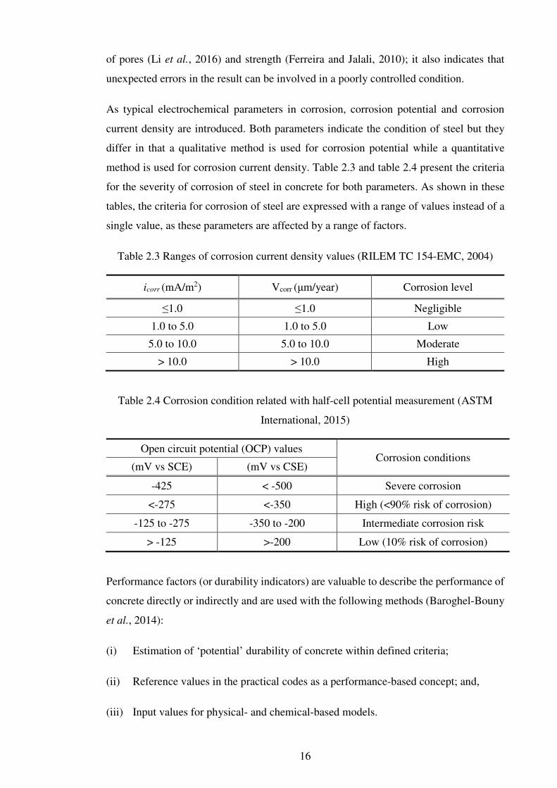
16

of pores (Li et al., 2016) and strength (Ferreira and Jalali, 2010); it also indicates that

unexpected errors in the result can be involved in a poorly controlled condition.

As typical electrochemical parameters in corrosion, corrosion potential and corrosion

current density are introduced. Both parameters indicate the condition of steel but they

differ in that a qualitative method is used for corrosion potential while a quantitative

method is used for corrosion current density. Table 2.3 and table 2.4 present the criteria

for the severity of corrosion of steel in concrete for both parameters. As shown in these

tables, the criteria for corrosion of steel are expressed with a range of values instead of a

single value, as these parameters are affected by a range of factors.

Table 2.3 Ranges of corrosion current density values (RILEM TC 154-EMC, 2004)

icorr (mA/m2) Vcorr (µm/year) Corrosion level

≤1.0 ≤1.0 Negligible

1.0 to 5.0 1.0 to 5.0 Low

5.0 to 10.0 5.0 to 10.0 Moderate

> 10.0 > 10.0 High

Table 2.4 Corrosion condition related with half-cell potential measurement (ASTM

International, 2015)

Open circuit potential (OCP) values Corrosion conditions

(mV vs SCE) (mV vs CSE)

-425 < -500 Severe corrosion

<-275 <-350 High (<90% risk of corrosion)

-125 to -275 -350 to -200 Intermediate corrosion risk

> -125 >-200 Low (10% risk of corrosion)

Performance factors (or durability indicators) are valuable to describe the performance of

concrete directly or indirectly and are used with the following methods (Baroghel-Bouny

et al., 2014):

(i) Estimation of ‘potential’ durability of concrete within defined criteria;

(ii) Reference values in the practical codes as a performance-based concept; and,

(iii) Input values for physical- and chemical-based models.

17

Any parameter related to the performance of concrete can be a performance factor.

Regarding the latter, a number of parameters related to concrete performance have been

proposed/developed, but data are significantly scattered due to various conditions,

including experimental set-up and environmental conditions. Therefore, it is necessary to

integrate a number of indicators with minimum indicators. By doing so, the scatter in the

data is expected to decrease to some extent.

2.3 Chloride transport

Chlorides dissolved in the pore solution move through the inter-connected pore system.

As a result, transport rate is affected by the pore structure and the interaction between

chlorides and cement hydrates. Considering that aggregates have a low permeability in

concrete, the transport properties of cement paste are controlled by w/b, binder content.

The type of binder is a leading factor to determine the transport properties of concrete.

Various driving forces in concrete result in different transport mechanisms including

diffusion by concentration gradient, absorption by moisture gradient, permeability by

pressure gradient, migration in electrical field and wick-action by a combination of water

absorption and water vapour diffusion. Although diffusion and absorption generally

coexist in concrete due to unsaturated conditions, the absorption range controlled by

a low moisture content is relatively small, especially in a marine environment, and thus

diffusion becomes the dominant mechanism for chloride transport.

The following section discusses the basic mechanisms and laws governing chloride

diffusion, influencing factors and measurements.

2.3.1 Mass transport and flow in concrete transport systems

Ions in an ideal solution are governed by the Nernst-Planck equation based on mass

conservation:

= − − E +

(2.1)

where is the flux of ith ion, is the diffusion coefficient of ith ion, is the

concentration of ith ion, is the ion mobility, E is the electrical potential and is the

average mass velocity.

18

According to equation (2.1), ion movement is determined by diffusion, migration and

convection and thus the equation extends Fick’s law. Considering that diffusion of

chlorides is the main mechanism and the spatial distribution, i.e. non-steady state

condition, is given, the Nernst-Planck equation can be simplified as Fick’s second law as

follows:

=

(2.2)

where is the chloride concentration, is the transport distance of chlorides and is

the chloride diffusion coefficient.

Chloride transport can be accelerated using an applied electrical field. This principle is

frequently applied to concrete so as to reduce time to evaluate the quality of concrete or

to initiate corrosion. Considering that the convection term in equation (2.1) is neglected,

i.e. ion mobility is controlled by the diffusion coefficient by the Nernst-Einstein relation,

migration-diffusion of chloride in non-steady state conditions is equated as follows (Tang,

1996a):

=

(2.3)

= − −

E

(2.4)

where is the chloride migration coefficient, is the concentration gradient of free

chloride (), is the absolute value of ion valence (1 for the chloride ion), is the

solution temperature (K), is the gas constant (8.314 J/(K·mol)), and is the Faraday

constant (96,487 J/(V·mol)).

In steady-state conditions, equation (2.4) can be simplified as given in equation (2.5)

below, because the flux is constant irrespective of time and space provided that a constant

chloride exists through the bulk solution. Hence, the equation only represents the

migration process,

= −

E (2.5)

19

In general, chloride transport is described by the above equations; however, the governing

equation for modelling or analysis is determined by the main transport mechanism and

concrete condition. The description of chloride transport in concrete is not straightforward

due to various influencing factors. In the process of transport through inter-connected

liquid-filled pores, a portion of chlorides reacts with the cement matrix either physically

or chemically. In the following section, the factors influencing transport processes are

discussed.

2.3.2 Influencing factors

Effect of pore structure

As concrete is a porous material, dissolved aggressive agents move through the

(connected) pore system which can eventually lead to deterioration. Consequently, the

pore structure is a main factor in determining the rate of deterioration. In concrete, there

are two general types of pores: meso- and micro-pores. The meso-pores are visible

including entrained and occluded air voids. The entrained air voids are around 0.1 mm in

diameter evenly distributed throughout the cement paste and in some cases they are

deliberately formed. On the other hand, entrapped air voids up to several millimetres in

diameter are formed by improper compacting procedures. The voids are considered to

have an insignificant influence on transport because they have less connectivity (Glass

and Buenfeld, 2000a).

Capillary pores, gel pores, and the interfacial-transition zone could be included at the

micro-scale. These pores are, typically, distributed in cement pastes. Capillary pores, up

to a few microns, provide the main path for chloride transport into concrete. They are

randomly distributed with an inter-connected system (Neville, 2011). The size of

capillary pores decreases with the process of hydration. The gel pores, up to 2 or 3 nm in

nominal diameter, are much smaller than the capillary pores. These pores comprise 28%

of total volume in the gel. The interfacial-transition zone between cement paste and

aggregates can be observed and has high porosity due to the wall effect. There are two

opposing effects within the interfacial-transition zone: one is to restrict the movement of

aggressive ions due to its isolated formation, and the other is that the ions percolate into

the inner concrete rapidly when the amount of aggregate increases.

20

Transport rate is dominated by the connectivity or tortuosity of the pore network, which

is affected by a number of factors including environmental conditions and material

properties. For example, the hydration process reduces the transport rate of chlorides as

the inter-connected capillary pores are isolated by the development of the gel. For dried

concrete, ionic movement is also limited due to the loss of pore-fluid connectivity in the

concrete.

Effect of chloride binding

Chlorides are present in concrete as two types: bound chloride and free chloride. In the

process of transport in concrete, some chlorides are bound by hydration products either

physically or chemically, while the remaining chlorides, termed free chloride, move

inward. Free chlorides lead to steel corrosion by destroying the passive layer on the steel

surface. For this reason, chloride binding is important in the evaluation of concrete

durability in the case of chloride attack.

Chlorides present in pore water react with tri-calcium aluminate, denoted by C3A

(3CaO·Al2O3), or tetra-calcium almuminoferrite, denoted by C4AF (4CaO·Al2O3·Fe2O3),

to form Fridel’s salt (C3A·CaCl2·10H2O) or its analogue (C3F·CaCl2·10H2O) (Hirao et

al., 2005). Binding is also established with the adsorption to calcium silicate, denoted by

C-S-H. Adsorption is described by ionic exchange between chlorides in the pore solution

and hydroxides from C-S-H, which takes place in the electrical double-layer at the C-S-

H/pore solution interface or by inserting chlorides into C-S-H interlayer spaces (Florea

and Brouwers, 2012). Chloride binding capacity by physical binding is 20% of that by

chemical binding; however, the mass of C-S-H is much higher than monosulface hydrate

(AFm: C3A·CaSO4·12H2O), which is the main hydrate in chemical binding. Hence, it is

assumed that physical binding is predominant compared to chemical binding (Hirao et

al., 2005), particularly, for binders with larger quantity of CaO-SiO2 elements.

Chloride binding affects transport process by a refinement of pore structure and a decrease

of free chloride in the pore-water. When chloride was present in concrete, the density of

C-S-H increased and total porosity decreased (Midgley and Illston, 1984; Suryavanshi et

al., 1995) and the formation of Fridel’s salt decreased the pore space via the pore blocking

effect (Andrade et al., 2011). The concentration relation between bound chlorides and

free chlorides at a given temperature is the chloride binding isotherm, of which there are

21

three types: linear, Langmuir and Freundlich isotherm. Tuutti (1982) proposed the linear

binding isotherm as follows:

= a ∙ (2.6)

where is the concentration of bound chloride, is the concentration of free chlorides,

and a is a constant.

Arya et al. (1990) modified the linear relation by adding the intercepts of the bound or

total chloride axis. The relation has sometimes been found in field-exposed samples,

which has been attributed to the leaching of hydroxides (Sandberg, 1999). However, a

non-linear relationship between bound and free chlorides has been generally accepted.

Both Langmuir and Freundlich isotherms are typical for describing the non-linear

relationship as shown in equations (2.7) and (2.8), respectively. Tang and Nilsson (1993)

found that the Langmuir and the Freundlich isotherms are suitable at a range of chloride

concentration < 0.05 mol and > 0.05 mol, respectively. The authors suggested that the

adsorption process in a high chloride concentration is more complex than monolayer

adsorption. It is notable that the Freundlich isotherm can cover chlorides dissolved in

seawater and is simpler in mathematical calculations. In addition to chloride

concentration, chloride binding is also sensitive to cementitious materials and hydration

products (Song et al., 2008b).

(a) Langmuir isotherm:

= a ∙ 1 + b ∙

(2.7)

(b) Freundlich isotherm:

= c ∙ & (2.8)

where a and b are Langmuir’s parameters, and c and d are Freundlich’s parameters,

which vary with binder content and the binder and pore solution compositions.

Effect of concrete mix

Both pore structure and chloride binding are influenced by factors such as type of binder

and w/b. Aggregate itself is regarded as an impermeable material, and thus the transport

22

through aggregate is negligible due to low permeability. Although it has been reported

that transport rate is influenced by aggregate distribution and aggregate-to-cement-paste-

volume ratio (Oh et al., 2002; Andrade et al., 2011), the characteristic of cement paste

(e.g. the connected capillary pores in the cement matrix) is more crucial in determining

the transport rate.

According to previous studies (Leng et al., 2000; Yu and Ye, 2013; Bostanci et al., 2016),

SCMs are advantageous as they form a finer/disconnected pore network to create denser

concrete due to the pozzolanic reaction. Moreover, it has also been reported that for

concrete using SCMs, pore structures are refined by the particle size distributing in the

range 10 to 100 nm (Hussain and Rasheeduzafar, 1994). Concretes using SCMs bind more

chlorides than ordinary Portland cement (PC) concrete because cement pastes containing

ground granulated blast-furnace slag (GGBS) and fly ash (FA) are favourable to form

C3A or C4AF by chemical composition in cementitious materials (Luo et al., 2003;

Thomas et al., 2012; Song et al., 2008a). In addition, large amounts of C-S-H formed in

concrete using SCMs are helpful to bind chlorides due to the large surface area of C-S-H

available for adsorption (Hirao et al., 2005; Tang and Nilsson, 1993).

It is well known that concrete with a high w/b has a low resistance to chloride transport

due to a high (connected) porosity, but for chloride transport it is of interest that w/b is

linked with cement content. First, it has been observed that the surface chloride content

decreases with an increase in w/b at a given cement content; this is because a thick skin

layer of concrete with a high w/b enhances dielectric activity between hydroxyl ions in

concrete skin and chloride ions in the external source, and thus the repulsive force

between these ions prevents the accumulation of chlorides in the concrete surface (Song

et al., 2008a). Blended concrete shows higher surface chloride contents than PC concrete

because of its higher binding capacity. The build-up of chloride on the concrete surface

can result from the binding effect, which increases the content of total chloride on the

concrete surface (Tang and Nilsson, 2000; Glass and Buenfeld, 2000b). In addition, the

binding effect is dependent on the concentration of chloride; thereby, the binding capacity

increases with an increase in the ingress depth of chloride into concrete (Glass and

Buenfeld, 2000b).

23

Effect of degree of saturation

The moisture condition of concrete is decisive in determining transport properties and it

varies depending on environmental conditions such as temperature, exposure

duration/location and relative humidity. Ionic diffusion takes place through the liquid

phase in the inter-connected pore system; hence, the degree of saturation is one of the

main influences on transport properties. It is also accepted that unsaturated concrete, (i.e.

concrete above the mid-tide/splash zone in a marine environment) is more vulnerable to

chloride-induced corrosion than saturated concrete, (i.e. concrete below the mid-tide

level) (British Standards Institution, 2016), due to absorption of chloride and high

availability of oxygen for the corrosion process. Hence, the degree of saturation should

be considered when evaluating the chloride transport.

For unsaturated concrete, both diffusion and absorption have been simultaneously

considered as chloride transport mechanisms in many studies (Nilsson, 2000; Sleiman et

al., 2009; Kumar, 2010; Baroghel-Bouny et al., 2014). Chloride profiles in unsaturated

concretes sometimes show that the chloride contents are decreased in the surface concrete,

which is attributed to moisture transport during wet/dry cycles (see figure 2.2). However,

in addition to moisture transport, various reasons for this shape have been presented,

including (i) the skin effect or wall effect, (ii) the dielectric reaction between the concrete

surface and chloride environment, (iii) the washing-out effect, (iv) leaching, and

(v) carbonation. Moreover, the convective zone (< 3.99 ± 1.05 mm in marine structures,

(Gao et al., 2017)) formed in concrete subjected to chloride environments is relatively

small compared to the cover depth, and thus diffusion is only considered as a transport

mechanism during the regression analysis with experimental data, as shown figure 2.2.

In addition, Tang (2003) reported that capillary pores were almost saturated in the

submerged zone while degree of capillary saturations was ~80% in the splash zone,

irrespective of depth from the surface of the concrete subjected to a marine environment.

Chloride ingress was severe, with the following order: submerged > splash > atmospheric

zone (Tang, 2003). It seems reasonable that diffusion is taken as the main transport

mechanism, but the difference in the transport rate should be considered with unsaturated

concrete. When only diffusion is considered, it has been reported that the diffusion

coefficient becomes smaller with a decrease in the degree of saturation (Yokozeki et al.,

2003; Kumar, 2010; Nilsson, 2000; Nanukuttan et al., 2008). As shown in figure 2.3, it

is noteworthy that the diffusion coefficient is dramatically decreased when degree of

24

saturation reduces. In summary, considering chloride ingress and the relation between the

degree of saturation and the diffusion coefficient, the durability of concrete structures

subjected to chloride environments, in particular marine environments, is estimated only

using diffusion at degree of saturation larger than 20 %.

Figure 2.2 A modified example of the prediction of chloride profile in unsaturated

concrete (Song et al., 2008a) modified by the author.

Figure 2.3 Relative diffusion rate with saturation degree of PC concrete (Kumar, 2010)

replotted by the author.

0 5 10 15

0

1

2

3

4

5

Measured value

Predicted line

Chlo

ride

con

cen

trat

ion (

%, b

y w

eigh

t o

f bin

der

)

Depth (mm)

Omitted range in prediction

0 20 40 60 80 100

0

20

40

60

80

100

w/b=0.4

w/b=0.5

w/b=0.6

Rel

ativ

e d

iffu

sio

n r

atio

(v

s sa

tura

ted

co

nd

ito

n)

(%)

Sr (%)

25

2.4 Chloride-induced corrosion of steel

The concrete cover protects the reinforcing steel from the ambient environment. A low

permeability slows down the ingress of aggressive agents and the high alkalinity of the

pore solution provides a stable oxide layer on the steel surface. However, in the case of

the corrosion of steel in concrete subjected to chloride environments, attention has mainly

been paid to the presence of chloride, which triggers the local destruction of the passive

layer.

In Tuutti’s model (1982), the service life of a concrete structure is divided into two stages:

(i) corrosion initiation and (ii) corrosion propagation. The corrosion initiation stage

relates to chloride ingress through the cover-zone concrete before destroying the passive

film, while the corrosion propagation stage describes the active condition for corrosion

after the chloride content at the steel depth exceeds the threshold level. For chloride-

induced corrosion, to estimate the service life of concrete, the corrosion propagation stage

is considered in addition to the initiation of corrosion corresponding to chloride transport.

Meanwhile, the limit of the serviceability, which refers to user comfort, aesthetic aspects

and functionality, is defined as the limit that indicates whether the performance of the

concrete structure is acceptable or not according to Vrouwenvelder and Schießl (1999).

As shown in figure 2.4, the limit states to define the service life of a concrete structure

include (i) depassivation of steel in the reinforced concrete structure exposed to a chloride

environment corresponding to the end of the corrosion initiation stage in Tuutti’s model;

(ii) the acceptable crack width by chloride-induced corrosion, which is limited to 0.3 mm;

(iii) the loss of performance of the concrete structures by spalling of concrete and section

loss of steel which cause a fatal accident; and (iv) excessive deflection and collapse.

The following section reviews chloride-induced corrosion including the depassivation

process and influencing factors. In addition, the critical chloride threshold level for

corrosion resistance is also investigated.

2.4.1 Corrosion mechanism

Corrosion requires both oxygen and water, and metallic corrosion involves redox

reactions occurring simultaneously. Corrosion depends on environmental conditions, i.e.

acid and neutral/alkaline conditions, as follows.

26

Figure 2.4 The service life of reinforced concrete structures and possible limit states.

In acidic conditions,

Fe + 2H+ → Fe2+ + H2(g) (2.9)

In neutral/alkaline conditions,

4Fe + 6H2O + 3O2 → 4Fe(OH)3↓ (2.10)

2Fe(OH)3 → Fe2O3 + 3H2O (2.11)

Steel corrosion in concrete is described as an electrochemical process consisting of two

half-cell reactions including oxidation in the anodic area and reduction in the cathodic

area. In a highly alkaline environment, such as concrete with a pH in the range 12.5–13.5,

steel is protected by a thin oxide layer, called a passive layer. Once chlorides dissolved

in the pore solution reach the steel surface, the passive film is locally destroyed by

adsorption of Cl-, and then chloride-induced corrosion is triggered. In addition, corrosion

accelerates as Cl- also competes with OH- for adsorption on the steel surface. This

corrosion can occur even in an alkaline environment such as concrete when chloride

content exceeds the threshold level. After depassivation, the electrons from the iron move

through the metal to the cathode, and the cathodic reaction is affected by the pH of the

pore solution and the potential at the steel surface. An electric circuit is formed by an

ionic exchange current through the electrolyte to maintain electro-neutrality between

oxidation in the anode and reduction in the cathode. Thereby, the corrosion rate is

controlled by one dominate factor in an electrochemical cell consisting of the anode in

27

steel (R) resistance and *+ current in the anode), the cathode in steel (R, resistance and *-

current in the cathode), steel itself (R. resistance and * current in steel), and concrete

(R,/0, concrete resistance and *-12- current through concrete), as shown in figure 2.5.

Therefore, the performance or the durability of the reinforced concrete structure is lost by

corrosion, which leads to cracking, spalling, and a reduced cross-section area of

reinforcement.

The anodic reaction and chloride effect in concrete can be summarised as follows:

2NaCl or CaCl2 → 2Na+ or Ca2+ + 2Cl- (dissolution of chloride) (2.12)

Fe → Fe2+ + 2e- (dissolution of iron) (2.13)

Fe2+ + 2(OH)- → Fe(OH)2 (precipitation of rust) (2.14)

2Fe(OH)2 + H2O + O2 → 2Fe(OH)3 (oxidation of rust) (2.15)

Fe2+ + 2 Cl- → FeCl2 (precipitation of green rust) (2.16)

4FeCl2 + O2 + 6H2O → 4FeOOH + 8HCl (oxidation of green rust) (2.17)

The cathodic reaction in concrete is:

O2 + 2H2O + 4e- → 4(OH)- (hydrolysis) (2.18)

Figure 2.5 Schematics for chloride-induced corrosion of steel in concrete.

28

The types of corrosion, including uniform corrosion and pitting corrosion, are determined

by the spatial distribution of the anode and cathode on the steel surface or the resistivity

of concrete. Uniform corrosion (microcell corrosion) is distributed in the overall steel

surface and is generally detected in reinforced concrete degraded by carbonation. Pitting

corrosion (macrocell corrosion) occurs in small areas of steel surface but is more severe

by cross-section loss of the reinforcing steel and is detected in chloride-contaminated

reinforced concrete.

In theory, under localised (or pitting) corrosion, a significant difference between the

electrical potential of the anode and the cathode exists. However, it is difficult to measure

the potentials in a pure anode and a pure cathode, which are important to model corrosion

propagation in practice as the measured potential is affected by concrete resistivity, cover

depth, oxygen availability and anode-to-cathode area ratio (Pour-Ghaz et al., 2009). In

addition, the potential in the cathode is also decreased by the lowered potential in the

anode caused by corrosion and the range influencing the potential in the cathode, called

a correlation length, is up to 2 m from the anode (Keßler et al., 2014; Ji et al., 2013).

Hence, measured potential using the half-cell potential technique was sometimes shown

as a corrosion potential gradient between anode and cathode in pitting corrosion (Keßler

et al., 2014; Liam et al., 1992), and it is recommended that corrosion evaluation is carried

out with the gradient instead of an absolute value (RILEM TC 154-EMC, 2003). Although

various detection methods for corrosion have been suggested, the measured corrosion

values remain scattered, including corrosion potential and corrosion rate. The corrosion

process is also sensitive to the exposure environment as the process is controlled by

oxygen and moisture availability in addition to chloride concentration. The following

sections review the influencing factors and measurement techniques affecting the

corrosion process.

2.4.2 Chloride threshold level

Chloride threshold level (CTL) is defined differently from two standpoints: (i) the

scientific view and (ii) the engineering view (Angst et al., 2009). In the former, the CTL

is a tolerated chloride level for depassivation, while in the latter the CTL is considered to

be the accumulated chloride content up to ‘the acceptable deterioration’. The CTL based

on the engineering view is pragmatic, but the criterion for the degree of deterioration is

ambiguous, leading to a high scatter in the CTL. In the scientific view, although the

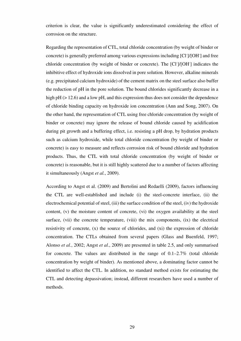
29

criterion is clear, the value is significantly underestimated considering the effect of

corrosion on the structure.

Regarding the representation of CTL, total chloride concentration (by weight of binder or

concrete) is generally preferred among various expressions including [Cl-]/[OH-] and free

chloride concentration (by weight of binder or concrete). The [Cl-]/[OH-] indicates the

inhibitive effect of hydroxide ions dissolved in pore solution. However, alkaline minerals

(e.g. precipitated calcium hydroxide) of the cement matrix on the steel surface also buffer

the reduction of pH in the pore solution. The bound chlorides significantly decrease in a

high pH (> 12.6) and a low pH, and this expression thus does not consider the dependence

of chloride binding capacity on hydroxide ion concentration (Ann and Song, 2007). On

the other hand, the representation of CTL using free chloride concentration (by weight of

binder or concrete) may ignore the release of bound chloride caused by acidification

during pit growth and a buffering effect, i.e. resisting a pH drop, by hydration products

such as calcium hydroxide, while total chloride concentration (by weight of binder or

concrete) is easy to measure and reflects corrosion risk of bound chloride and hydration

products. Thus, the CTL with total chloride concentration (by weight of binder or

concrete) is reasonable, but it is still highly scattered due to a number of factors affecting

it simultaneously (Angst et al., 2009).

According to Angst et al. (2009) and Bertolini and Redaelli (2009), factors influencing

the CTL are well-established and include (i) the steel-concrete interface, (ii) the

electrochemical potential of steel, (iii) the surface condition of the steel, (iv) the hydroxide

content, (v) the moisture content of concrete, (vi) the oxygen availability at the steel

surface, (vii) the concrete temperature, (viii) the mix components, (ix) the electrical

resistivity of concrete, (x) the source of chlorides, and (xi) the expression of chloride

concentration. The CTLs obtained from several papers (Glass and Buenfeld, 1997;

Alonso et al., 2002; Angst et al., 2009) are presented in table 2.5, and only summarised

for concrete. The values are distributed in the range of 0.1–2.7% (total chloride

concentration by weight of binder). As mentioned above, a dominating factor cannot be

identified to affect the CTL. In addition, no standard method exists for estimating the

CTL and detecting depassivation; instead, different researchers have used a number of

methods.

30

Table 2.5 Published CTL values obtained from concrete

Authors Year CTL

(%, total chloride) Detection method

Exposure condition

Cited in

Gouda 1970 0.75, 1, 2 GP +

Alonso et al. (2002)

Page 1991 2.5 CP +

Arup 1996 1.7-2.7 PP +

Stratfull 1975 0.2-1.4 CP Field

Angst et al. (2009)

Vassie 1984 0.25-1.5 CP Field

Hope and lp 1987 0.1-0.19 LPR, EIS, VI, ML W/D

Thomas 1996 0.2-0.65, 0.7 ML Field

Sandberg 1998 0.4-1.5 CP Field

Zimmermann 2000 0.2-0.4 MC Field

Fluge 2001 0.72 VI Field

Morris et al 2004 0.4-1.3 LPR, CP Field

Kaesche 1959 0.32 GDP, VI Sub

Baumel 1959 0.57-1.09 PDP, VI Sub

Gouda and Halaka 1970 0.45, 0.15 GP +

Locke and Siman 1980 0.4-0.8 LPR Air

Schies and Raupach 1990 0.48-2.02 MC +

Lambert, page et al 1991 1.5-2.5 LPR, CP, ML +

Schiessl and Breit 1996 0.5-1.5 MC Air

Oh et al 2003 0.68-0.97 CP, VI 95% RH

Morris et al 2004 0.4-1.3 LPR, CP Sub/Air

Nygaard and Geiker 2005 0.52-0.75 PT +

Mannera et al. 2008 0.6-2.0 LPR, CP Air

Glass and Buenfeld (1997)

Henriken 1993 0.3-0.7 + Field

Treadway et al 1989 0.32-1.96 ML Field

Bamforth and Chapman-Andrews

1994 0.4 + Field

Tuutti 1993 0.5-1.4 + +

Lukas 1985 1.8-2.2 + Field

* GP: galvanostatic pulse polarisation, CP: corrosion potential, PT: potentiostatic

polarisation, LPR: linear polarisation resistance, EIS: electrochemical impedance

spectroscopy, VI: visual inspection, ML: mass loss, MC: macrocell current, GDP:

galvanodynamic polarisation, PDP: potentiodynamic polarisation, W/D: wet/dry cyclic

regime

31

2.4.3 Influencing factors of steel corrosion

The corrosion process involves electrical phenomena combined with chemical reaction.

Electrical potentials, which are required for ionic dissolution at the anodic site and

reduction reaction at the cathodic site, can be represented by the Nernst equations:

E) = E)3 − (= 1) 56

7Fe:;7<;

(2.19)

E, = E,3 − (= 4) 56

7HO;7O;7OH@;A

(2.20)

where E) and E, are the electrode potential for oxidation at the anode and cathode,

respectively (V); E)3 and E,3 are the standard electrode potential of steel at the anode and

cathode, respectively (V); 7Fe; is the activity of an Fe molecule in the steel bar (=1);

7Fe:; is the concentration of Fe2+ in the electrolyte (mol/l); 7OH@;is the concentration

of OH- in the electrolyte (mol/l) (log7OH@; = FG − 14 ); 7O; is the concentration of

oxygen (mol/l); 7HO; is the amount of capillary water (l/m3); is the absolute value of

ion valence; is the solution temperature (K); is the gas constant (8.314 J/(K·mol));

and is the Faraday constant (96,487 J/(V·mol)).

The difference of electrical potential in the corrosion cell triggers the electromotive force,

leading to corrosion current flowing through the electrolyte from anode to cathode. From

the above equations and figure 2.5, it is evident that the corrosion process is affected by

the following factors:

(i) the availability of oxygen and water;

(ii) the concentration of Fe2+; and,

(iii) the pH of the pore solution in the vicinity of steel.

In addition, the corrosion process is also influenced by external sources such as

temperature, aggressive agents, and the concrete resistivity in the region of the corrosion

activity. Poubaix (or the equilibrium potential/pH) and Evans diagrams are useful in

explaining the corrosion process from depassivation to propagation. The two diagrams

32

depict the effects of the influencing factors on the corrosion process. In general, steel

embedded in concrete is protected by the formation of a passive film including alkaline

hydrates, i.e. a calcium hydroxide layer and oxide film. The oxide film such as magnetite,

denoted by Fe3O4, is formed in a high-pH environment, which reacts with aggressive ions

(i.e. chlorides), as shown in figure 2.6, and thus retards direct dissolution of the steel. On

the other hand, the inhibitive effect of calcium hydroxide on corrosion is evident by

maintaining a high pH of the pore solution, but the formation of the layer appears to be

irregular (Glass et al., 2001) and thus the inhibitive effect is randomly distributed along

the bar. Before the depassivation process, the role of oxygen and moisture is negligible

as steel dissolution is very low.

However, once chloride reaches the steel depth, the depassivation process is immediately

triggered and the anodic reaction proceeds rapidly, as shown in figure 2.7 (a) in the Evans

diagram. After depassivation, the corrosion rate is controlled by factors other than

chlorides (Angst et al., 2011a). For the cathodic reaction, availability of oxygen is crucial,

and thus the corrosion rate in saturated concrete is reduced compared to the unsaturated

concrete, as shown in figure 2.7 (b). Conversely, a low moisture-content in concrete

increases its electrical resistivity, leading to prevention of corrosion cell formation. It has

been reported that the critical degree of water saturation to accelerate corrosion is ~ 70 –

80% (Ožbolt et al., 2011). Anodic dissolution is, on the other hand, affected by type of

steel (Freire et al., 2011), as it is well known that noble materials such as stainless-steel

show high resistance to corrosion. Moreover, corrosion propagation is controlled by the

concrete itself. SCMs produce a disconnected pore network (hence, high electrical

resistivity), so ionic movement between the anode and cathode is reduced. However, the

pH of the pore solution in SCM concrete is lowered in comparison to that in PC concrete.

A lower pH results in an increase in corrosion rate as well as rapid depassivation. These

two competing effects make the corrosion resistance of SCMs controversial.

It has been reported that chloride content in the tidal/splash zone is lower than in the

submerged zone (Tang, 2003), but it is accepted concrete in the tidal/splash zone is prone

to the most severe deterioration. It can be deduced that chloride content at the steel depth

is not the only factor to determine service life of a structure, although higher chloride

content increases the possibility of corrosion. In addition, it should be noted that the CTL

in the laboratory is lower than that found in the field.

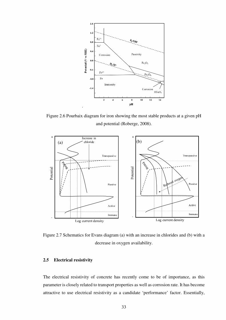
33

.

Figure 2.6 Pourbaix diagram for iron showing the most stable products at a given pH

and potential (Roberge, 2008).

Figure 2.7 Schematics for Evans diagram (a) with an increase in chlorides and (b) with a

decrease in oxygen availability.

2.5 Electrical resistivity

The electrical resistivity of concrete has recently come to be of importance, as this

parameter is closely related to transport properties as well as corrosion rate. It has become

attractive to use electrical resistivity as a candidate ‘performance’ factor. Essentially,

(b) (a)

34

electrical resistance is measured in a non-destructive manner and the electrical resistivity

is calculated. Resistivity is a geometrically independent parameter and for a prismatic

sample is given by:

H = RIJ

(2.21)

where H is the electrical resistivity (Ω·m), R is the electrical resistance (Ω), I is the area

contact with electrode (m2) and J is the length between two electrodes (m). The

resistivity, however, is sensitive to a number of influencing factors which must be

considered. The next section critically reviews these influencing factors.

2.5.1 Factors influencing resistivity measurements

Pore solution in concrete

The pore solution within the cementitious binder comprises Na+, Ca2+, K+, SO42-, OH- and

Cl- , and its resistivity varies depending on the SCMs and degree of hydration. To account

for the effect of the pore solution, the formation factor, F, is introduced as follows:

F = H KLMHN (2.22)

where H KLM is the bulk resistivity of the concrete (Ω·m) and HN is the pore solution

resistivity (Ω·m).

Provided that an accurate resistivity of the pore solution is determined, it should be

relatively easy to estimate the transport property or corrosion process. However, it is

another challenge to measure the resistivity of the pore solution in concrete, and pore-

fluid extraction technique is not practical. The model based on the empirical equation can

be used (Snyder et al., 2003). In this study, the resistivity of the pore solution is estimated

using the model provided by National Institute of Standards and Technology (NIST,

USA) (Bentz, 2007), in which the resistivity is calculated with the oxide composition of

the binder and degree of hydration.

35

Environment

Concrete structures are influenced by their ambient environment (e.g. exposure

conditions, wetting/drying action and temperature), which changes the moisture-state of

concrete cover-zone. The changing moisture state alters the resistivity of the concrete,

which decreases with increasing degree of saturation. The changing degree of saturation

also affects ionic transport in concrete. Figure 2.8 shows the relationship between the

electrical resistivity and the diffusivity in concrete (Sengul, 2014). Moreover, the

temperature to which concrete is exposed also influences the resistivity of concrete. It is

well known that the resistivity decreases with an increase in temperature. In this respect,

Polder (2001) states that the electrical resistivity for saturated and for dry concrete is

changed by 3% and 5% for each degree of absolute temperature change, respectively. An

activation energy approach using an Arrhenius relationship can be used to standardise

measurements to a reference temperature (McCarter et al., 2012).

The movement of chlorides into concrete influences its resistivity due to the reduction in

resistivity of the pore solution. However, it should be mentioned that the binding process

of chloride in concrete could refine the pore structure, leading to an increase in the bulk

resistivity of concrete due to a restricted electrical path. In summary, the factors

influencing resistivity mentioned above should be considered to evaluate the transport

properties or the corrosion process using this parameter.

Figure 2.8 The relationship between electrical resistivity and diffusivity (Sengul, 2014).

36

Hydration

In concrete, chemical reactions continuously occur and subsequently lead to a refined

pore structure. Moreover, it has been reported that the electrical resistivity increases with

the hydration process (McCarter et al., 2013a). This trend is clearer for SCM concrete.

The effect of hydration on the electrical resistivity is not negligible for analysis, and it is

difficult to extract a change of electrical resistivity by hydration from the measured

resistivity of concrete, especially exposed to a chloride environment at an early age. For

example, the presence of chlorides in the pore solution generally leads to a decrease in

the electrical resistivity, while the electrical resistivity increases with both hydration and

chloride binding. Theses phenomena occur at the same time. In addition, the latent

hydration for SCM concrete requires a longer measurement period to minimise the

hydration effect on the electrical resistivity. Consequently, significantly limited data are

available for concrete, in particular subjected to a chloride environment, considering the

hydration effect.

2.5.2 Representation of electrical resistivity

Resistivity (equation (2.21)) is independent of the volume of the sample, whereas

resistance depends upon the size and shape of sample. To account for different

geometrical arrangements of electrodes, calibration of the electrode system may be

required using computational modelling or an experiment (Angst et al., 2011c; McCarter

et al., 2012). Meanwhile, although the absolute comparison with the values obtained from

experiments is not established, the normalisation method is useful (McCarter et al., 2001):

OP1QR = HSH3 =RTR3

(2.23)

where OP1QR is the normalised resistivity or resistance, HS and S are the electrical

resistivity (Ω·m) or resistance (Ω) at time t, and H3 and 3 are resistivity

(Ω·m)/resistance (Ω) measured at that respective electrode position taken at a datum point

in time.

This expression can minimise the effect of influencing factors on the electrical resistivity,

and especially the effect of the pore solution. However, the expression represents a

37

relative value rather than an absolute value; thereby, the result is only useful for the

description of a trend and not for quantification.

2.6 Summary

This chapter reviews the mechanisms and influencing factors in terms of deterioration of

reinforced concrete caused by chloride-induced corrosion. In literature, it was found that

a wide range of influencing factors influences on chloride transport and chloride-induced

corrosion of steel in reinforced concretes and due to these, there are scatters in data such

as CTL and diffusion coefficient. Especially, environmental factors such as degree of

saturation and temperature are not readily simulated in the laboratory to represent the

field concrete; thereby field study is also required to reflect these conditions properly.

Although evaluating performance of concrete is increasingly emphasized, specification,

especially in UK, only specifies a prescriptive method. This is because a dearth of

information on the relationship between values obtained from performance factors and

those from the field. In addition, it is generally accepted that chloride transport rate is a

performance factor to reinforced concrete subjected to chloride environments according

to specifications, but the representations or testing methods for evaluation of chloride

transport are various; thereby it is inevitable to show the scatters in data. To overcome

this limitation, a representative parameter to describe performance of reinforced concrete

subjected to chloride environments is required. In this study, electrical resistivity as a

representative parameter was chosen as the resistivity is highly correlated to both chloride

transport rate and corrosion rate of steel which are main factors to describe deterioration

of reinforced concrete in chloride environments.

The following chapter reviews the methodology to evaluate the performance of reinforced

concrete subjected to chloride environments.

38

CHAPTER 3

A METHODOLOGICAL REVIEW OF CHLORIDE-INDUCED

CORROSION OF STEEL IN CONCRETE

3.1 Introduction

The premature deterioration of reinforced concrete structures leads to a significant drain

on resources in terms of repair and maintenance. To date, various test methods and

modelling have been suggested to estimate the service life of concrete structures, but it is

still difficult to accurately evaluate this because influencing factors, including differences

in techniques, differences in analysis, and differences in exposed environments, result in

errors.

This chapter presents a methodological review of chloride transport in chloride-induced

corrosion, measurements and existing predictive models. A range of electrochemical

techniques, visual observation, mass loss, and predictive models relating to corrosion

propagation are also summarised for chloride-induced corrosion propagation. In addition,

the chapter reviews the electrical resistance measurement as a non-destructive method,

which includes chloride transport and steel corrosion.

3.2 Measurement for chloride transport in concrete

According to Tuutti’s model, chloride transport processes are important during the

initiation phase of chloride-induced corrosion. Various methods have been developed to

evaluate the chloride transport properties of concrete and this review focuses on those

that are widely used. Electrical resistance measurements for evaluating pore structure are

also reviewed. Figure 3.1 presents techniques that are classified with the test conditions,

including type of parameters measured and test set-up. The sub-categories are explained

in the following sections.

39

Figure 3.1 Classification of techniques for chloride transport

3.2.1 Non-electrical methods

Diffusion tests are based on the principle that chloride transport occurs due to a

concentration gradient. The result is expressed with a chloride profile, i.e. the chloride

content with respect to the penetration depth, and then the diffusion coefficient and

surface chloride content are estimated from the chloride profile using regression analysis

and error function based on Fick’s law.

Two tests are specified in the codes: AASHTO T259 (Stanish et al., 1997), called the

ponding test, and NT Build 443 (Nordtest, 1995), called the bulk diffusion test. In the

ponding test as shown in figure 3.2 (a), sorption and wick-action are considered in

addition to diffusion as the sample is dried for 28-days prior to the measurement.

Furthermore, one side of the sample is exposed to a 50% RH environment during the test.

Although all possible transport mechanisms that can be found in a structure are described,

the behaviour of chloride transport is exaggerated compared to the real behaviour (Stanish

et al., 1997). The bulk diffusion test as shown in figure 3.2 (b), on the other hand,

measures chloride transport by establishing a concentration gradient across the sample. A

chloride solution (2.8 mol NaCl) is applied to the sample for ≥ 35 days, and this solution

is higher than the chloride content (3% NaCl) in the ponding test for 90 days.

Recently, all immersion, inversion and ponding tests in BS EN 12390-11 (British

Standards Institution, 2015a) have been prescribed as a diffusion test; the 3% NaCl

solution and 90-day test duration are also suggested. These tests describe a behaviour of

chloride transport similar to that in a structure, but they can be both time-consuming and

40

laborious. Hence, it may be better to use the tests to obtain an input value for modelling

and not evaluating the quality of concrete.

Figure 3.2 Test set-ups for (a) AASHTO T259 and (b) NT Build 443

3.2.2 Electrical method

The migration test accelerates chloride ingress using an electrical field and is suitable to

evaluate concrete quality in the laboratory and to obtain an input parameter for predictive

modelling. Migration testing is attractive in determining the chloride transport property

of concrete, although the application of an electrical field is still controversial (Spiesz and

Brouwers, 2012). Migration testing is subdivided into several types depending on whether

41

chlorides pass through the sample or not, namely non-steady state and steady state of

concrete, and depends on applied voltage and duration.

ASTM C1202 ‘Electrical indication of concrete’s ability to resist chloride ion

penetration’ (ASTM International, 2012) is a typical migration test used as a performance

factor in North America. The test measures a total passed charge through the sample, Φ

100 × 50 mm with an applied potential difference of 60 V between two electrolytes during

a period of 6 hours. The solutions filled in the cells are 3.0% NaCl as the catholyte and

0.3 mol NaOH as the anolyte, respectively. The chloride permeability of concrete is rated

as shown in Table 3.1. However, this test has been criticised due to (i) the joule heating

effect by applying a high voltage, and (ii) the current measurement related to the chemical

composition of the pore solution in addition to chlorides.

Table 3.1 Chloride ion penetrability based on charge passed (ASTM International,

2012)

Charge passed (coulombs) Chloride ion penetrability

>4,000 High

2,000 to 4,000 Moderate

1,000 to 2,000 Low

100 to 1,000 Very low

<100 Negligible

NT Build 492 is an update of ASTM C 1202 using a lower applied voltage and an increase

in the amount of catholyte (Nordtest, 1999). In addition, the applied voltage and

measurement time are adjustable with an initial current measured at 30 V. 10% NaCl

solution and 0.3 mol NaOH are filled in the cathodic compartment and the anodic

compartment, respectively. The migration coefficient is calculated based on the

penetration depth using a colorimetric method. This test is widely used in Europe as a

performance factor, although the simplified equation used for estimating the migration

coefficient has been criticised (Spiesz et al., 2012)

Another test is the multiregime test (Castellote et al., 2001; Andrade et al., 2011), where

the migration cell is similar to the cell used in ASTM C1202, but the applied voltage is

12 V. Distilled water is used as the anolyte and a 1 mol NaCl solution is filled in the

cathodic compartment. The conductivity of the solution in the anodic compartment is

42

measured, and the steady state and the non-steady state migration coefficients are

calculated. The required time for chloride break-through is longer than in the other

discussed tests. Monitoring the solution in a downstream cell is also laborious.

3.2.3 Porosity/degree of saturation

Porosity and degree of saturation are important parameters in chloride transport,

reflecting both concrete properties and environmental conditions. The test for porosity is

well documented and the degree of saturation,UQ, can be estimated from an additional

measurement. The porosity, φ , is given as

∅(%) =Y

Z[\]^_`ab[ca@defgh[cij]_ × 100

(3.1)

UQ(%) = mn+NLo −mQpmn+S −mQp × 100

(3.2)

where qn1Lro2S is the density of the saturating medium (g/cm3), mn+NLois the mass of

the sample (g), sn+NLo is the volume of the sample (cm3) and mn+S and mQp are the

mass of the sample in saturated and dried conditions (g), respectively.

According to ASTM C642 (ASTM International, 2013), it is recommended that a sample

be oven-dried at ~110 ± 5ºC for no less than 24 hours to achieve a dried weight. The

temperature for drying has been criticised as it can lead to the formation of micro-cracks.

However, this micro-cracking can be minimised by conducting the drying phase at a

lower temperature of 50 ± 5ºC (Gallé 2001). The solvents for saturation are different with

the specifications, corresponding to 1,1,1-trichlorethane in BS 1881-124 or water in

ASTM C642 (British Standards Institution, 2015b; ASTM International, 2013). The

degree of saturation is estimated using the original weight of the sample before the

treatment process. Although it is difficult to directly estimate the transport rate with

porosity and degree of saturation, they are essential in chloride transport in the modelling

and estimation of quality of concrete.

43

3.3 Measurements for steel corrosion

Corrosion and corrosion rate measurement are important in the management of structures.

The following presents inherent limitations and basic principles of corrosion monitoring

to obtain reliable interpretation of data. Moreover, basic information on commonly used

corrosion techniques is also provided.

3.3.1 Half-cell potential measurement

Metals have a natural potential which occurs by a reaction with the surrounding

environment. The potential is measured with respect to a standard reference electrode,

such as a copper-copper sulphate electrode (CSE), a saturated calomel electrode (SCE),

or a silver-silver chloride electrode, as shown in figure 3.3. This technique is specified in

ASTM C876, in which corrosion is indicated by the probability of corrosion, as given in

table 3.2 (ASTM International, 2015). The key requirement for the measurement is to

maintain sufficient moisture in the concrete for the formation of an electrical circuit, and

the measured potential changes less than ± 20 mV within a 5-minute period. Although

this technique is practical and widely used in the field, the measurement is sensitive to

various factors including concrete resistivity, type of binder, moisture content and

temperature. The use of the potential gradient is recommended in corrosion detection

instead of the absolute value specified in ASTM C876 (RILEM TC 154-EMC, 2003).

This technique is qualitative and is appropriate as an auxiliary method.

3.3.2 Macrocell current

The macrocell technique measures the current between separate metals (corroding anode

and cathode) in a corrosion cell. For reinforced concrete, the steel exposed to the corrosive

environment is the anode and the steel with a low possibility of corrosion (or a noble

material such as stainless-steel, graphite, or titanium) is the cathode.

The macrocell current, also called the galvanic current, indicates the initiation of

corrosion with a sudden increase, but the quantification of the corrosion rate using this

technique is questionable. As the measured current represents the whole steel condition,

the technique is inappropriate to evaluate localised or pitting corrosion. Moreover, the

macrocell current is dependent on the distance between the two electrodes (Elsener, 2002)

44

as it is influenced by the electrical resistance of concrete. As this technique is non-

destructive, it is useful to monitor macrocell current for corrosion of steel with time

(Raupach, 1996; Elsener, 2002).

Figure 3.3 Graphical scheme to compare the potentials of the most commonly used

reference electrodes (Roberge, 2008)

Table 3.2 Probability of corrosion (ASTM International, 2015)

Potential (mV vs CSE)

Potential (mV vs Calomel electrode)

Probability of corrosion

> -200 > -126 Low (<10 %)

-200 to -350 -126 to -276 Intermediate

< -350 < -276 High (>90 %)

3.3.3 Polarisation resistance

The polarisation resistance technique is an important method in estimating the corrosion

rate in concrete structures. The basic principle is to measure a change in electrical

potential or current of the steel due to an electrical perturbation using a counter electrode.

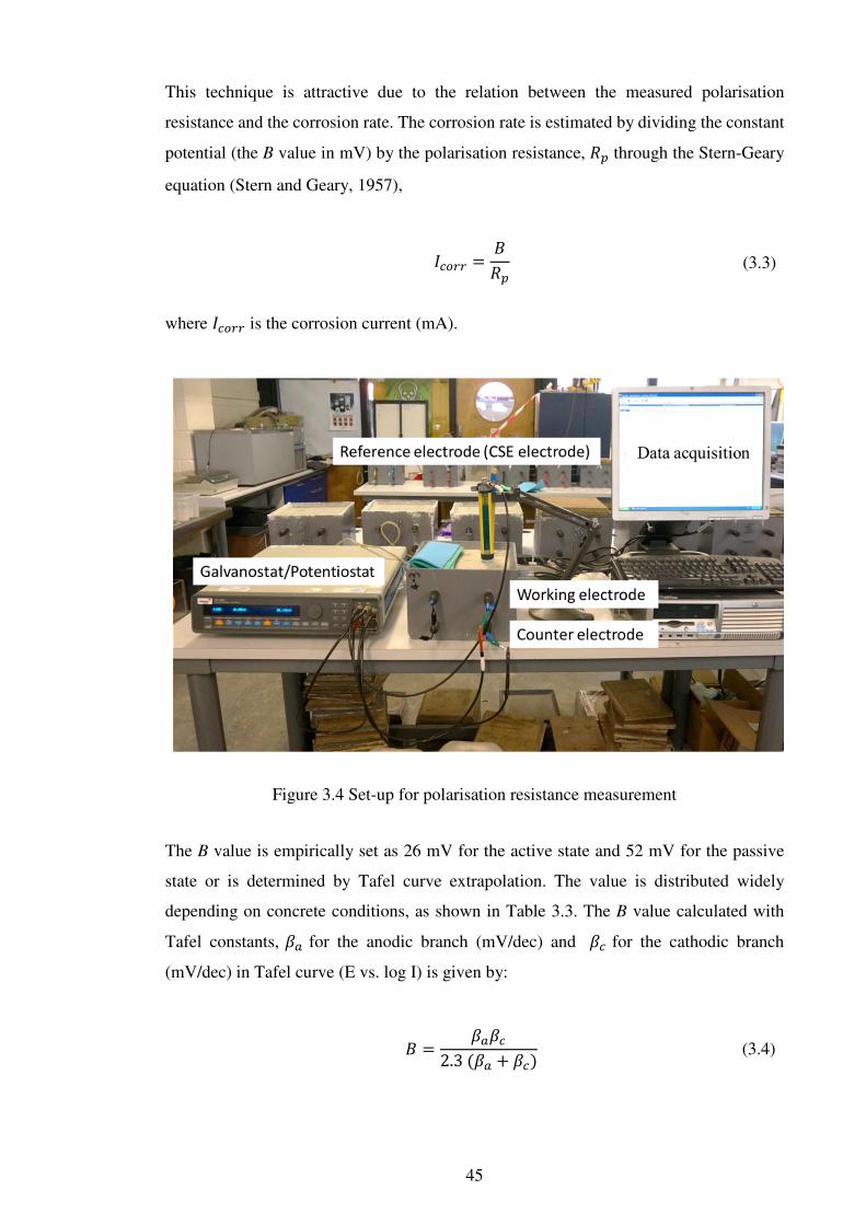
45

This technique is attractive due to the relation between the measured polarisation

resistance and the corrosion rate. The corrosion rate is estimated by dividing the constant

potential (the B value in mV) by the polarisation resistance, N through the Stern-Geary

equation (Stern and Geary, 1957),

*-1QQ = tN

(3.3)

where *-1QQ is the corrosion current (mA).

Figure 3.4 Set-up for polarisation resistance measurement

The B value is empirically set as 26 mV for the active state and 52 mV for the passive

state or is determined by Tafel curve extrapolation. The value is distributed widely

depending on concrete conditions, as shown in Table 3.3. The B value calculated with

Tafel constants, u+ for the anodic branch (mV/dec) and u- for the cathodic branch

(mV/dec) in Tafel curve (E vs. log I) is given by:

t = u+u-2.3(u+ + u-)

(3.4)

46

Table 3.3 Variation in reported B value for active steel

B (mV) Method Sample types Reference

21 - 37 Experiment Simulated pore

solution Garcés et al. (2005)

2.2 – 37.1 Experiments /simulation

Concrete Michel et al. (2016)

8 - 17 Simulation Concrete Song (2000)

63 - 86 Experiment Concrete Chang et al (2008a)

4 - 43 Experiment Simulated pore

solution and mortar Vedalakshmi et al. (2009a)

19 – 26.8 Experiment Sea water Zou et al. (2011)

For concrete structures, the ohmic resistance should be considered when using the

polarisation resistance technique. Even though a wetted concrete is assumed to be a highly

conductive material (electrolyte) between the working electrode and counter electrode,

the electrical resistance of concrete, called ohmic drop, is considerably higher than the

electrical resistance of pore solution. Hence, the corrosion current is underestimated when

the concrete resistance is neglected. In addition, it is unclear that the polarised area of

steel is defined in large structures using a small counter electrode (Andrade and Alonso,

2001). If the steel is passive, the applied current spreads (e.g. 50 cm) from the application

point; thereby, the true polarised area is wider than the assumed polarised area.

Conversely, in the active state, especially in pitting corrosion, the current applied from

the counter electrode is drained towards the small corrosion spot on the steel. The

polarised area, which is assumed to be the area of the counter electrode, is larger than the

true polarised area. Thus, the calculated corrosion rate is under- or overestimated using

the assumed polarised area. From an empirical relationship (González et al., 1995), the

corrosion rate for pitting corrosion is 8 – 10 times higher than the corrosion rate measured

using the polarisation technique. Although the auxiliary electrode, called the guard-ring

system, is used to confine the polarised area, a dispersion or confinement effect for the

polarisation is not fully resolved (Nygaard et al., 2009).

To estimate the corrosion rate using polarisation techniques, the polarisation resistance

needs to be measured. Depending on the electrical source or the method for applying a

perturbation to the steel, various techniques are suggested, such as the potentiodynamic

47

technique using a voltage sweep, the potentiostatic technique using a constant voltage,

the galvanostatic technique using a constant current, the galvanodynamic technique using

a current sweep and electrochemical impedance spectroscopy using an AC voltage sweep.

The potentiodynamic technique can be divided into several branches depending on the

voltage sweep range, with or without a reverse scan. The linear polarisation resistance

technique (LPR) is the most general method due to its simple interpretation and rapid

response. The measurement is performed within a small voltage sweep in the range of ±

30 mV at the corrosion potential. The low scan rate, which is <10 mV/min (RILEM TC

154-EMC, 2004), is generally set to allow the maintenance of the reaction equilibrium.

In this potential range, the relation between the applied potential and the corresponding

current is linear (Figure 3.5(a)), and thus the polarisation resistance is calculated using

Ohm’s law,

N = ∆y∆*

(3.5)

where Nis the polarisation resistance (Ω), ∆y is the change in voltage (mV), and∆* is

the change in current (mA).

The Tafel extrapolation technique (TEP), or cyclic potentiodynamic technique, is similar

to LPR, but a wide voltage range is swept. The range is from -200 to +1,000 mV with

respect to the corrosion potential. Due to the large sweep range, a rapid scan rate is

generally set at 60–120 mV/min. However, a high scan rate can induce unbalanced

reaction, leading to a distorted result to estimate corrosion rate. In addition, the large

perturbation leads to a disturbance of the corrosion environment of steel, and this

technique could thus be considered destructive. However, it is necessary to determine the

B value as given in equation (3.4). The cyclic potentiodynamic technique is useful to

determine corrosion behaviour using reverse scan and repeated sweeps. Figure 3.5 (b)

describes the pitting corrosion state of steel using this technique. As can be seen, the

pitting potential (Epit) and the protection or re-passivation potential (Epro) are observed

from the curve. If Epro is more positive than Epit, there is no pitting tendency, but if Epro is

more negative than Epit, pitting could happen. Neither technique can directly measure an

ohmic drop, but most commercial equipment provides an ohmic compensation function.

48

Figure 3.5 (a) Linear polarisation curve and (b) cyclic polarisation curve

Galvanostatic pulse technique (GP) is preferred in the field. The basic principle is to apply

a constant current (10–100 µA) to the steel. This suddenly increases the voltage from the

corrosion potential within a very short time. The sudden increase is considered to be an

‘ohmic drop’. The interpretation is based on the equivalent electrical circuit, which can

reflect a non-linear relationship between the applied current and the corresponding

voltage. This technique also requires a very short time (less than 10s) to achieve a result.

However, there is no criterion to set an applied current in the specification, and thus

caution is required when applying this technique because a large perturbation is induced

by an applied current.

The pontentiostatic technique (PT) is a reverse method of the GP technique. A constant

voltage is applied to the steel until a constant current is achieved. The static current is

determined as the corrosion current. However, the require time to achieve the constant

current can be long. As a consequence, this technique is not preferred, although in the

present study it is applied to estimate the B value. The interpretation process for

calculating the B value is addressed in Section 6.3.4 in detail.

3.3.4 Electrochemical impedance spectroscopy

The electrochemical impedance spectroscopy (EIS) technique is elaborate compared to

the techniques described above. Using a wide range of frequency (0.1 mHz – 100 kHz),

EIS provides all electrical characteristics of the interface, as well as a simple faradic and

non-faradic component. In addition, using an alternating current to perturb the steel

49

electrode makes it possible to minimise disturbance to the concrete/steel system. The

measured impedance is expressed with a complex form consisting of a real part

(resistance) and an imaginary part (reactive), as follows:

z() = z|() − z||() (3.6)

where ω is the angular frequency ( = 2~, f is frequency (Hz)), z|() is the real part,

z||() is the imaginary part, and = √−1.

There are two types of representation of EIS data: the Nyquist format and the Bode format

(Barsoukov and Macdonald, 2005).

(i) Nyquist format: The real part (z|() ) and the imaginary part (z||()) are

expressed on the x-axis and the y-axis, respectively (figure 3.6). The impedance can

be represented with a vector length (|z()|) and the angle between this vector and

the x-axis. This representation cannot express the frequency directly.

(ii) Bode format: Both the modulus impedance and phase shift on the y-axis are plotted

with respect to the frequency on the x-axis (figure 3.7). The Bode format explicitly

shows frequency information, unlike the Nyquist format.

The EIS technique does have limitations. To investigate the interface or condition of steel

in concrete, a very low frequency is required, which is time-consuming. In the presence

of concrete, the passive layer on the steel and localised corrosion, the response can be

ambiguous, leading to difficulty in the interpretation. In general, an equivalent electrical

circuit are used to analyse EIS data; circuits suggested by researchers are shown in figure

3.8 and table 3.4. It is worth noting that all circuits are able to fit any impedance data, but

physical meaning regarding elements used in the circuit are variable even if the same

elements are employed in the different circuits. In addition, the transmission line model,

which is a complex circuit, provides better fitting and mechanistic characters for the

corrosion process, e.g. pitting corrosion, diffusion processes and presence of passive film

(Kranc and Sagüés, 1992; Chen and Orazem, 2015), but its application is not

straightforward for engineers. The following review excludes the transmission line

model.

50

Figure 3.6 Nyquist format for data presentation

Figure 3.7 Bode format for data presentation

In most electrical equivalent circuits to analyse the steel/concrete interface, the response

of bulk concrete (Rc) is simplified with a single resistor, as shown in figure 3.8, for which

the high frequency limit is set as an origin even though capacitances exist at high

frequencies in addition to resistances. It may be concluded that an error in analysis is

involved depending on the high frequency limit to determine the concrete resistance.

Moreover, a charge transfer resistance (Rct) in conjunction with a constant phase element

(CPEdl) for the double-layer are used to represent the steel-concrete interface.

To describe the presence of the low frequency tail (<0.01 Hz) representing the diffusion

control of oxygen in the vicinity of the steel surface in the Nyquist plot, a Warburg

impedance in series with the charge transfer resistance is introduced, which extracts the

0 50 100 150 200 250 300

-250

-200

-150

-100

-50

0

(a)

Z'(ω)

iZ''(

ω)

Increasing frequency

10-3

10-1

101

103

105

1E-4

0.01

1

100

Frequency (Hz)

Ζ

(b)

-100

-80

-60

-40

-20

0

θ

51

Faradic process in the interface (Circuits A-2, B-2 and B-3). This phenomenon can

explain why it is difficult for traditional DC measurements to achieve the steady-state in

a prolonged period of time. However, when a Warburg impedance is introduced, it is

uncertain whether fitting is correct or not as this tail cannot always be observed, even at

low frequency (Montemor et al., 2000).

The elements (Rif and CPEif) representing the response in the intermediate frequency

range are introduced in the circuits (all circuits B and C), but the physical meaning is

varied. For example, the response for the intermediate frequency in R-CPE series circuits

(Circuit B) is described by the effect on the interfacial layer between mortar and steel

(Pereira et al., 2015), dielectric properties of concrete (Choi et al., 2006) and the effect

of a surface film on steel (Park et al., 2005). Meanwhile, hierarchical R-CPE series

circuits (Circuit C) are used to describe the response at the intermediate frequencies. This

response is considered with redox transformation on the steel (Morozov et al., 2013;

Bautista et al., 2015) but according to Dhouibi et al. (2002), the response in the circuit

(Circuit C-3) is separated into hydration products formed in cement pores around the steel

surface (Rcif and CPEcif) and redox transformation (Rif and CPEif).

In a steel/concrete system, depressed semi-circles are plotted due to the non-ideal

behaviour of capacitance (i.e. the decrease in capacitance with increasing frequency),

which is represented by a pseudo-capacitance or constant phase element (CPE). This is

explained by the uneven surface of steel and the heterogeneous nature of concrete (Feliu

et al., 1998); however, there is no consensus on a detailed description of its physical

origin. Nonetheless, the CPE element is useful as a flexible parameter to improve curve

fitting to impedance spectra (Jorcin et al., 2006), as shown in the following equation.

z|| () = 1N3()+

(3.7)

where = √−1, 3 is a coefficient and is the exponent (0 < < 1); if a =1, the circuit

is an ideal capacitor (N3).

Clearly, an impedance spectrum in a Nyquist plot consists of a concrete response and a

steel response, approximating two semi-circles. The electrical circuits are expanded to

describe additional semi-circles or tails with a combination of resistor and capacitor or

CPE, or a Warburg element. However, the roles of some elements used in the circuit are

still unclear, so that it is necessary to define each of them.

52

A-1 A-2

B-1 B-2 B-3

C-1 C-2 C-3

Figure 3.8 Equivalent electrical circuits for analysis of steel corrosion in concrete/mortar (refer to table 3.4).

53

Table 3.4 Experimental set-up details for using EIS measurement

Electrical equivalent circuit in figure 3.8

Sample type

Location Exposure condition Counter electrode

type

Steel condition

Reference electrode

Reference

A-1 Concrete Lab Immersion

(3.5% NaCl) Graphite

(Ex) Passive SCE Choi et al. (2006)

A-2 Concrete Field Atmospheric zone

Elastomer (Ex)

Passive/ active

Activated titanium rod

Pech-Canul and Castro (2002)

Mortar Lab Pre-mixed (3% CaCl2)

N.I. Passive/ active

N.I Feliu et al. (1998)

B-1 Concrete Lab

Immersion (3.5% NaCl)

Graphite (Ex)

Active SCE Choi et al. (2006)

Concrete Lab Immersion

(3.5% NaCl) Graphite

(In) Passive/ active

CSE Park et al. (2005)

B-2 Concrete Lab Partial or full immersion

(3% NaCl) Steel (In)

Passive/ active

SCE Montemor et al.

(2000)

B-3 Mortar Lab Wet/dry cycle

(3% NaCl) Stainless steel (Ex)

Passive/ active

SCE Pereira et al. (2015)

C-1

Mortar Lab Immersion (sea water) and

premixed (0.1, 1.0 and 3.6% Cl-) Graphite

(Ex) Passive/ active

SCE Deus et al. (2014)

Mortar Lab Immersion (3.5% NaCl) and

premixed (3% CaCl2)

Copper cylinder

(Ex)

Passive/ active

SCE Bautista et al. (2015)

C-2 Mortar Lab Partial immersion

(3% NaCl) Titanium

(Ex) Passive/ active

SCE Morozov et al. (2013)

C-3 Concrete Lab Immersion (3% NaCl)

Stainless steel (Ex)

Passive/ active

SCE Dhouibi et al. (2002)

* Ex: external counter electrode, In: embedded counter electrode in sample, ** N.I. No information, *** SCE: standard calomel electrode,

CSE: copper copper-sulphate electrode.

54

3.3.5 Commercial equipment

Non-destructive methods for detecting and quantifying corrosion in concrete structures

are attractive. To date, commercial instruments for on-site investigation are available but

the measured values vary depending on the electrochemical techniques and control

methods for applied current (referred to as confinement techniques). Therefore, results

are still ambiguous when on-site investigation is carried out.

Typical commercial instruments include GECOR 6 and GalvaPulse. Both instruments

measure a potential shift using the galvanostatic technique, but for the GECOR 6 the

result is analysed using a linear relationship between polarisation potential and current,

while for the GalvaPulse this is done with exponential curve fitting using a simple Randle

circuit. In addition to their analysis method, their current confinement methods are also

different. The potential difference of steel between different locations is kept constant as

an initial value, i.e. the potential difference before applying current, for both instruments.

However, while applying current to the guard-ring is constant over the measurement for

the GalvaPulse, an increase in current is applied for the GECOR 6.

Figure 3.9 Examples of current confinement method using (a) GalvaPulse and (b)

GECOR 6 (Nygaard et al., 2009) modified by the author (∆E potential difference in the

steel at different locations for controlling the guard-ring)

55

Nygaard et al. (2009) investigated the corrosion rate of steel in concrete using these two

commercial instruments. For the passive state, corrosion rates were overestimated

because the predefined polarisation lengths were smaller than the real polarised lengths.

Changes of electrical potential in steel caused by polarisation, corresponding to +176 mV

for the GECOR 6 and +76 mV for the GalvaPulse, were large, leading to a violation in

linearity between current and potential and a destructive environment at the concrete-steel

interface. In contrast, the measured corrosion rates were underestimated due to self-

confinement behaviour, which resulted in a smaller polarisation length compared to the

predefined length. The authors concluded that correction factors must be determined to

evaluate the corrosion rate correctly.

3.3.6 Mass loss

The corrosion rate of steel is directly determined by the mass loss method. ASTM G1

(ASTM International, 2011) suggests a wide range of solutions to clean corrosion

products from the steel surface, although a suspension based on hydrochloric acid is

generally used to clean corroded steel in concrete. Mass change is calculated using mass

difference between steel before corrosion and cleaned steel after corrosion,

mL1nn = bm3 −mg − m L (3.8)

where mL1nn is the mass loss of steel by corrosion products (), m3 is the initial mass of

steel before corrosion (), m is the mass of steel after cleaning corrosion products (), and m L is the mass loss for the cleaning process (). The average corrosion rate is then determined using Faraday’s law as follows:

= mL1nnIoN × 1000

(3.9)

where is the average corrosion rate (mA/m2), is Faraday’s constant (= 96,487 C/mol), is the duration of the test (), is the atomic mass of material (< ≈ 55.85/m5), IoN is the exposure area of steel contributing to the corrosion process (m2), and is the number of electrons transferred in the corrosion process (= 2 ∶ < → <: +2<@).

56

With time, the corrosion rate obtained from the mass loss method is an average value,

while electrochemical measurements obtain the instantaneous corrosion rate. To compare

the two values, it is necessary to integrate the instantaneous corrosion rate with test time.

3.4 Measurements for electrical resistivity of concrete

The electrical resistivity of concrete is measured using at least two electrodes. This

property gives an indirect assessment of the permeation properties and is being vigorously

researched as a factor to measure performance and durability of concrete. The basic

principle is to measure both current and voltage-drop, and then calculate the resistance

using Ohm’s law. The resistivity is obtained by multiplying the cell geometrical factor,

which will depend on the electrode arrangement.

This technique uses current sources that can be either alternating current (AC) or direct

current (DC). A two- or four-electrode configuration can be used, with electrodes being

embedded and/or externally applied. The AC technique (within a frequency range of 50

– 1,000 Hz) is preferred to the DC technique to minimise the polarisation of electrode

(McCarter et al., 2015). Intimate contact between electrodes and concrete can be achieved

by embedding electrodes within the concrete, while the geometrical factor for external

electrodes can be easily estimated to calculate the electrical resistivity. Two- and four-

electrode methods are typical (see Figure 3.10). The voltage is applied and then the

current is measured for the sample between two electrodes, while four electrodes are

positioned equidistantly. The AC current is injected through the outer two electrodes, and

then the inner two electrodes measure the voltage drop. This technique is known as the

Wenner method. The resistivity of concrete is obtained using the following equation for

the Wenner method:

H+NN = 2~R (3.10)

where H+NNis the apparent resistivity of the concrete (Ω·m), a is the electrode spacing (m),

and R is the resistance (Ω).

The Wenner method was developed in soil science, but is now widely used in civil

engineering. It has been confirmed that the formula is applicable to concrete, although

the assumptions for equation (3.10) are not completely satisfied in concrete: (i) electrodes

are not point-shaped, (ii) the concrete volume is not semi-infinite, and (iii) the domain

57

has inhomogeneous resistivity (Angst and Elsener, 2014). It is apparent that the resistivity

measurement is useful to estimate transport properties in concrete, but it has also been

reported that the value is sensitive to various factors such as the degree of contact between

the electrode and the concrete, the contact solution, and the influence of the concrete

surface itself (Lataste, 2010).

Nevertheless, the Wenner method is attractive for both on-site and laboratory

measurements as it is inexpensive and relatively easy to use. The error level, related to

the measurement process itself or to material variability, is also acceptable: for example,

the tolerance in the field is approximately ± 20% (Polder, 2001). This is because of

limitations relating to moisture, chloride and temperature variations, and it is difficult to

control all factors when investigating a change of the resistivity. However, this technique

is widely used to investigate the performance and durability of concrete structures in

terms of assessing the risk of corrosion (Basheer et al., 2002; Polder and Peelen, 2002),

the moisture/ionic ingress (Gjørv et al., 1977; Streicher and Alexander, 1995; McCarter

et al., 2005) and the cracking in concrete (Lataste et al., 2003).

Figure 3.10 Set-up for (a) two-electrode and (b) four-electrode method (the Wenner

method).

3.5 Overview of predictive models

Various predictive models have been developed to estimate the service life of concrete

structures. These models are useful to simulate a range of situations without the need for

long-term experiments and monitoring, especially regarding the corrosion of steel in

(a) (b)

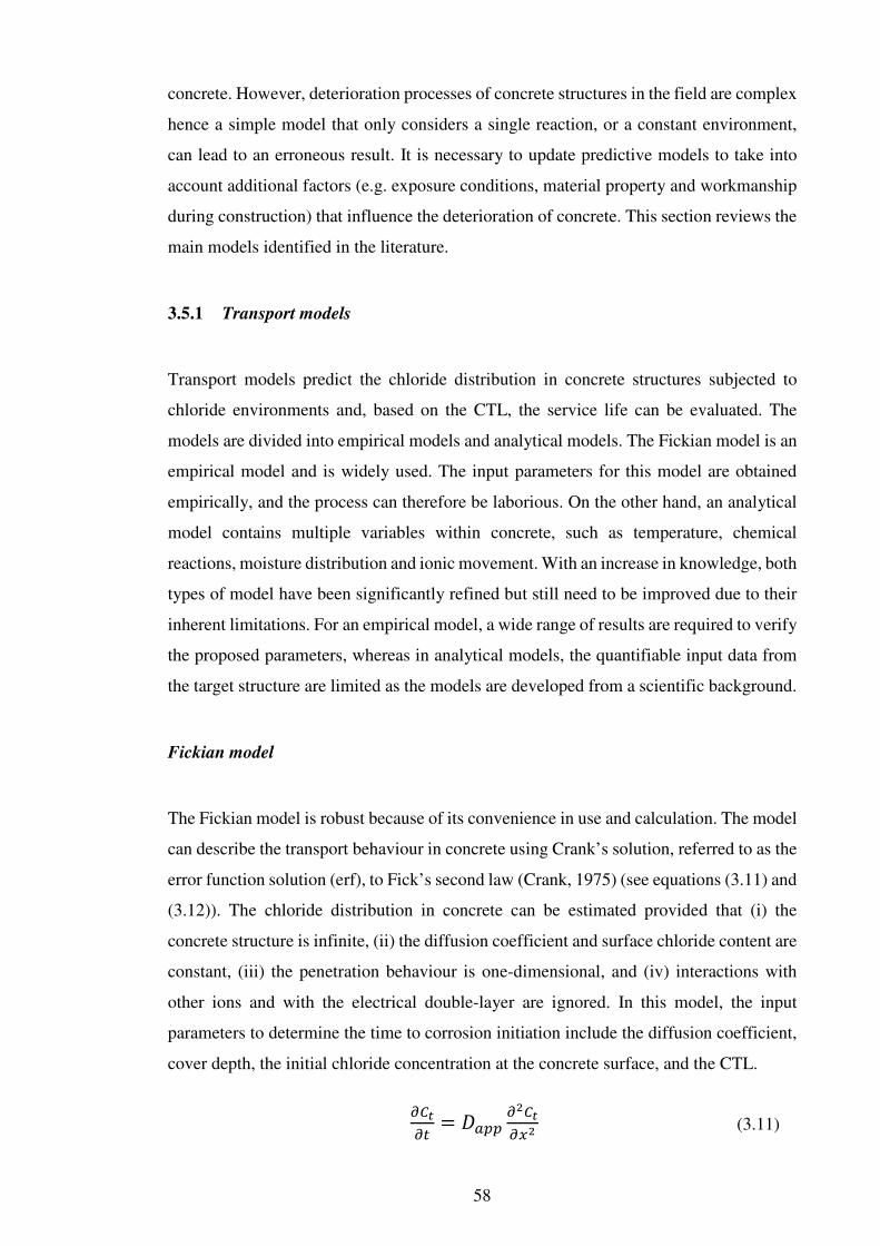
58

concrete. However, deterioration processes of concrete structures in the field are complex

hence a simple model that only considers a single reaction, or a constant environment,

can lead to an erroneous result. It is necessary to update predictive models to take into

account additional factors (e.g. exposure conditions, material property and workmanship

during construction) that influence the deterioration of concrete. This section reviews the

main models identified in the literature.

3.5.1 Transport models

Transport models predict the chloride distribution in concrete structures subjected to

chloride environments and, based on the CTL, the service life can be evaluated. The

models are divided into empirical models and analytical models. The Fickian model is an

empirical model and is widely used. The input parameters for this model are obtained

empirically, and the process can therefore be laborious. On the other hand, an analytical

model contains multiple variables within concrete, such as temperature, chemical

reactions, moisture distribution and ionic movement. With an increase in knowledge, both

types of model have been significantly refined but still need to be improved due to their

inherent limitations. For an empirical model, a wide range of results are required to verify

the proposed parameters, whereas in analytical models, the quantifiable input data from

the target structure are limited as the models are developed from a scientific background.

Fickian model

The Fickian model is robust because of its convenience in use and calculation. The model

can describe the transport behaviour in concrete using Crank’s solution, referred to as the

error function solution (erf), to Fick’s second law (Crank, 1975) (see equations (3.11) and

(3.12)). The chloride distribution in concrete can be estimated provided that (i) the

concrete structure is infinite, (ii) the diffusion coefficient and surface chloride content are

constant, (iii) the penetration behaviour is one-dimensional, and (iv) interactions with

other ions and with the electrical double-layer are ignored. In this model, the input

parameters to determine the time to corrosion initiation include the diffusion coefficient,

cover depth, the initial chloride concentration at the concrete surface, and the CTL.

aS = +NN a

(3.11)

59

S(, ) = (n − 3) 1 − < 2+NN

(3.12)

where Ct is the total chloride concentration (free and bound chloride) at the exposure time,

t (sec), at depth x (m) from the surface; +NN is the apparent diffusion coefficient (m2/s); n is the equilibrium chloride concentration on the concrete surface; and 3 is the initial

chloride concentration of the concrete before the exposure to the chloride environment.

There are, however, some limitations when applying the Fickian model to real structures

to evaluate their service life. This is because the input parameters involve a number of

uncertainties: (i) the diffusion coefficient is time-dependent, which decreases with

increasing time resulting from the hydration process (Pack et al., 2010); (ii) it is incorrect

to assume that the surface chloride content is constant, as the chlorides build-up at the

surface of concrete with time (Ann et al., 2009); (iii) the transport behaviour within the

concrete skin layer is different compared to that of the inner concrete (Andrade et al.,

1997); and (iv) the error function model is only valid to describe the diffusion

phenomenon (Saetta et al., 1993).

To overcome these limitations, numerous studies have introduced the concept of age-

factors for the chloride diffusion coefficient and surface chloride concentration to

consider the time-dependent properties of concrete, as shown in Table 3.5. It is

noteworthy that the input data cannot be generalised without considering environmental

conditions. In other words, the values obtained from a particular test, such as the diffusion

coefficient and surface chloride content, are only valid for the target structure as the

values contain environmental conditions corresponding to that structure.

Flux-based models

Flux-based models, referred to as physical models, are based on scientific theory. Their

accuracy for prediction is superior to that of empirical models. However, the large amount

of input data (e.g. initial amount of cement hydrates, chemical composition of pore

solution and chloride binding) is not easily available and must be quantified through tests.

In addition, the models cannot be easily modified or updated as the coding using the finite

element method or finite difference method is complex.

60

Table 3.5 Aging functions used in erf solution to Fick’s equation

Surface chloride concentration, Cs

Apparent diffusion coefficient ,Dapp Reference

Co (constant) +NN() = Qo1 − Qo ) Mangat and Molloy

(1994)

Co (constant) +NN() = Qo Qo ) Maage et al. (1996),

Bamforth (1999)

Co (constant) +NN() = Qo(1 − a) Qo) @) − @) − Stanish and Thomas

(2003)

Co(1-e-bt) Dapp (constant) Kassir and Ghosn

(2002)

1 1√ Dapp (constant) Amey et al. (1998)

Cotb +NN() = Qo Qo ) Costa and Appleton

(1999)

Co[1-e-b(t-tref

)] +NN() = Qo(1 − a) Qo ) − Qo Maheswaran and Sanjayan (2004)

1√ + c +NN = Qo1 −m 1 + @+ − @+ Qo + Petcherdchoo (2013)

1756(d + 1); + c +NN() = Qo(1 − ) Qo + Pack et al. (2010)

Note: Co, a, b, c, and d are regression values; tref the reference time; Dref the diffusion

coefficient at time tref; t the time at the first exposure to chlorides; t the time of exposure to

chlorides; and t is the age of the concrete (i.e. t = tI + tR).

Physical models have a governing differential equation that is solved instead of a closed-

form equation such as the Crank equation. As noted above, additional equations are

required as different phenomena, including moisture distribution, chloride binding and

temperature distribution, are included with respect to a micro-structural environment. For

chloride transport, the typical governing equation is Fick’s law or the Nernst-Einstein

relation as given in equations (3.13) and (3.14) and the mass-balance equation is solved

using equation (3.15) (Tang, 1996a; Samson and Marchand, 2007).

= S

(3.13)

61

= −∇S + ∇yS + S∇ ln − S

(3.14)

( + ) = −∇J (3.15)

In the above equations, is the flux of total chloride ion, is the diffusion coefficient, S is the total chloride concentration, is the charge number for the diffusing ion (Cl- =

1), is Faraday’s constant, is the gas constant (8.314 J/(K·mol)), T is temperature (K), y is the electrostatic potential, is the chemical activity coefficient, u is the average

velocity of the fluid under the capillary suction, is the free chloride concentration, and is the bound chloride concentration.

The transport property is significantly affected by various parameters including moisture

distribution, material properties and temperature, hence the relation between the

parameters and diffusion in unsaturated concrete is normally expressed by equation (3.16)

(Xi and Bažant, 1999). The functions in terms of each variables are arranged in the

Appendix A.1.

= £¤¥ , 3¦ ()§(G)A() bg (3.16)

where 3 is the curing time (days), w/b is the water-to-cement ratio, is the volume

fraction of aggregate in concrete, and H is the humidity.

In addition, only the free chlorides move in concrete transport, and it is necessary to

consider the bound chlorides involved in either the chemical reaction or physical

adsorption. The relation between bound and free chlorides is equated with the Langmuir or

Freundlich binding isotherm shown in equation (2.8) and (2.9), respectively. According to

Tang and Nilsson (1993), constants for both binding isotherms irrespective of w/b are

suggested as a = 5.41 and b = 0.013 in the Langmuir binding isotherm and c = 101.14 and d = 0.38 in the Freundlich binding isotherm. The temperature in the concrete influences the

propagation of ions and the moisture distribution. The relation with temperature is also

expressed through the Arrhenius relationship. Table 3.6 summarises the main transport

models.

62

Table 3.6 Summary for typical transport models (Tang, 2005)

Type Model’s

name Governing equation Main input parameters Characteristics

Empirical model

DuraCrete Fick’s 2nd law (Erfc function)

Time dependent diffusion coefficient Constant surface chloride content

• Using correction factors to reflect the field condition

• Simple method

HETEK Fick’s 2nd law

(Mejlbro-Poulsen function)

Time dependent diffusion coefficient Time dependent surface chloride

content

• Estimating all parameters from mix compositions and environmental conditions

• Being sensitive with quality of measurement

LIFE 365 Fick’s 2nd law

(Numerical solution)

Time dependent diffusion coefficient Time dependent surface chloride

content

• Considers the effect of temperature on diffusion coefficient

• Considers environmental conditions

• User friendly interface

Physical model

ClinConc Fick’s 1st law Migration coefficient at 6 months

Mix compositions

• Considering chloride binding, the effect of temperature variations and alkali leaching

• Only treating cases with saturated concrete exposed in submerged conditions

STADIUM Nernst-Planck flux

equation

A number of input parameters including various types for transport rate,

environmental conditions and chloride binding isotherm

• Being available to describe complex chloride transport behaviour

• Difficulty in practical application due to a lot of input data

63

3.5.2 Corrosion models

Corrosion models predict the corrosion rate of steel in concrete subjected to aggressive

environments. The loss of steel cross-section, or the volume expansion of corrosion

products on the steel surface, is directly related to failure (end of service life) of concrete

structures. The corrosion model is of interest in evaluating the residual service life or in

the practical management of the structure.

In a similar fashion to the transport models, there are two types of corrosion models:

empirical and analytical. In the empirical models, the solution establishes the relation

between corrosion rate and factors influencing the corrosion process based on laboratory

testing. The calculation process is relatively simple, but the result becomes less accurate

when conditions, e.g. steel type, types of aggressive agent, concrete material properties

etc., are different compared to conditions proposed in the model. In addition, the

applicability is low as laboratory testing is carried out using accelerated methods

including pre-mixed chloride during casting or wet/dry cycles to reduce time to corrosion

initiation.

Analytical models have also been developed to improve knowledge of the corrosion

behaviour of steel in concrete. As these models are based on electrochemical theory,

Laplace’s equation for electric potential or Ohm’s law based on an equivalent circuit is

used as the governing equation. Non-linear boundary conditions are applied on the steel

surface using the Stern-Geary polarisation equation (Stern and Geary, 1957) or the Butler-

Volmer kinetics equation (Pour-Ghaz, 2007). While the theoretical background used in

the models enhances their accuracy, their openness is significantly limited to the users.

Moreover, multiple corrosion processes within complex geometries require a large

amount of computation; hence, these models are more appropriate for comprehensive

academic research than for practical use.

The Stern-Geary polarisation equation is given by,

E) = E)3 + u+5 +3+

(3.17)

E, = E,3 + u-5 -3- −2.303- 5 ©© − -

(3.18)

64

and the Butler-Volmer kinetics equation is given by,

+ = 3+<ª«@¬®®¯c

(3.19)

- = 3-<¬®®@¬«¯°

(3.20)

where E) and E, are the anodic and cathodic potentials (V), - is the number of electrons

involved in the cathodic reaction, R is the universal gas constant (8.314 J/(mol·K)), F is

Faraday’s constant (96,487 C/mol), T is temperature (K), © is the limiting current density

(A/m2), + and - are the anodic and cathodic current densities (A/m2), u+ and u- are the

anodic and cathodic Tafel slopes (V/dec), 3+ and 3- are the anodic and cathodic

exchange current densities (A/m2), E,/±± is the corrosion potential (V), and E)3 and E,3 are

the equilibrium potential for anodic and cathodic reactions (V).

Table 3.7 summarises typical empirical corrosion models. This review has shown that

modelling the corrosion process in concrete is difficult due to unpredictable factors such

as steel conditions, concrete properties and environmental conditions. In addition,

obtaining corrosion results through the experiments is time-consuming to establish the

empirical relation.

3.6 Summary

This chapter presents a methodological review including measurements and predictive

models related to chloride transport in concrete and chloride induced corrosion,

respectively. To date, a number of well-established methods and predictive models have

been developed. However, most methods are destructive and laborious for chloride

transport and there is no standardized method for corrosion test. Alternatively, electrical

resistance measurement is non-destructive and easy, but this method is still close to a

qualitative method; thereby it is necessary to made relation between traditional method

and resistance method to improve the applicability of the electrical resistance

measurement. Finally, to reflect the environmental conditions located in the reinforced

concrete, it is necessary to add the parameters in predictive models. Therefore, the

applicability of the models is improved.

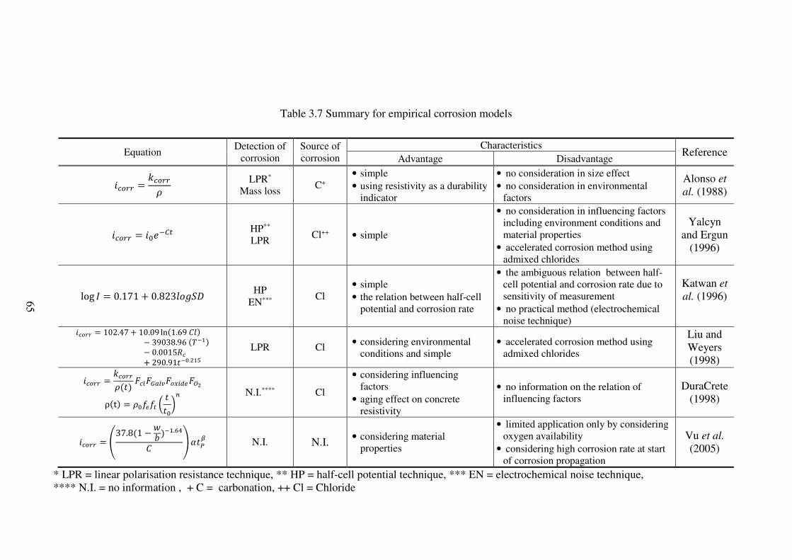
65

Table 3.7 Summary for empirical corrosion models

Equation Detection of

corrosion Source of corrosion

Characteristics Reference

Advantage Disadvantage

-1QQ = ²-1QQH LPR*

Mass loss C+

• simple

• using resistivity as a durability indicator

• no consideration in size effect

• no consideration in environmental factors

Alonso et al. (1988)

-1QQ = 3<@S HP** LPR

Cl++ • simple

• no consideration in influencing factors including environment conditions and material properties

• accelerated corrosion method using admixed chlorides

Yalcyn and Ergun

(1996)

log * = 0.171 + 0.8235U HP

EN*** Cl

• simple

• the relation between half-cell potential and corrosion rate

• the ambiguous relation between half-cell potential and corrosion rate due to sensitivity of measurement

• no practical method (electrochemical noise technique)

Katwan et al. (1996)

-1QQ = 102.47 + 10.09 ln(1.695)− 39038.96(@)− 0.0015-+ 290.91@3.¨

LPR Cl • considering environmental

conditions and simple • accelerated corrosion method using

admixed chlorides

Liu and Weyers (1998) -1QQ = ²-1QQH() -L¶+Lr1o·

ρ(t) = H3oS 32

N.I.**** Cl

• considering influencing factors

• aging effect on concrete resistivity

• no information on the relation of influencing factors

DuraCrete (1998)

-1QQ = 37.8(1 − ¤¥)@.¹A º N.I. N.I. • considering material

properties

• limited application only by considering oxygen availability

• considering high corrosion rate at start of corrosion propagation

Vu et al. (2005)

* LPR = linear polarisation resistance technique, ** HP = half-cell potential technique, *** EN = electrochemical noise technique, **** N.I. = no information , + C = carbonation, ++ Cl = Chloride

66

CHAPTER 4

EXPERIMENTAL PROGRAMME

4.1 Introduction

A number of studies have investigated chloride-induced corrosion of steel in concrete

structures, but a gap still remains between field studies and laboratory studies due to (i) a

lack of long-term data, (ii) different environmental conditions, and, (iii) various test

methods. To reduce this gap, mix proportions and materials used in the laboratory samples

in the present study were similar to those in the samples installed in the field (the Dornoch

Firth in northern Scotland). A range of test methods were carried out including (i)

compressive strength test, (ii) migration/diffusion test, (iii) porosity/degree of saturation

test, (iv) polarisation resistance, (v) half-cell potential, (vi) macrocell current technique,

(vii) mass loss of steel measurement, and (viii) visual observation of the corrosion activity

on the surface of the steel.

From laboratory test using accelerated methods by reducing cover-depth and a wet/dry

cyclic exposure regime, supporting information was obtained about chloride-induced

corrosion. The following sections describe the experimental programme, from sample

fabrication to experimental set-up.

4.2 Materials and concrete mix preparation in laboratory

Three binders comprising ordinary Portland cement (PC), CEM I 52.5N to BS EN 197-1

(British Standards Institution, 2015c), fly ash (FA) conforming to BS EN 450-1 (British

Standards Institution, 2012a), and ground granulated blast-furnace slag (GGBS)

conforming to BS EN 15167-1 (British Standards Institution, 2006) were used to prepare

concrete samples.

The coarse and matching fine aggregates were crushed granite. The coarse aggregate was

4/20 mm grade while the fine aggregate was ≤4 mm. Prior to casting, the aggregate was

conditioned to a saturated surface condition to avoid absorption of the mixing water. A

slump test was carried out to ensure the consistency of the mix. Workability of all

concrete mixes was designated as S3 specified in BS 8500-1 (British Standards

67

Institution, 2016). For the low water-to-binder ratio (w/b=0.4), the slump test was

performed to adjust the optimised dosage of superplasticizer before the main mixing. A

mid-range, water reducer/plasticizer (SikaPlast 15RM) conforming to BS EN 934-2

(British Standards Institution, 2012b) was used throughout.

Experimental work was undertaken on six concrete mixes consisting of high/low w/b (w/b =

0.4 and 0.6) and SCM such as GGBS and FA; 40% GGBS denoted by CEM III/A, and 30%

FA denoted by CEM II/B-V, respectively, based on BS EN 197-1 (British Standards

Institution, 2015c). The concrete mixes with low w/b were similar to the concrete used at the

Dornoch field site, whereas concrete mix for high w/b were designed conforming to XD1

environmental exposure class with an intended service life of at least 50 years (> 35 + ∆c mm

cover depth) or at least 100 years (> 50 + ∆c mm cover depth) (corrosion induced by chloride

other than seawater, e.g. de-icing salt) in BS 8500-1 (British Standards Institution, 2016).

Concrete samples were mixed in accordance with BS 1881-125 (British Standards

Institution, 2013b) using a concrete pan mixer (0.1 m3 capacity); an additional mixing

time of 2 minutes was used for low w/b concrete. To achieve uniformity, all samples for

each mix were fabricated from the same batch. Three replicates per type of experiment

were fabricated for each mix. The chemical compositions of binders and mix design

details used in this study are presented in table 4.1 and table 4.2. Sample specifications

are described in the following section.

4.3 Sample specifications

The samples cast comprised (i) 100 mm cubes cast in steel moulds for electrical resistivity

measurement and compressive strength test, (ii) cylinders (Ø 100 × 300 mm) for the

migration test (NT Build 492) and resistivity measurements using a PVC mould, and (iii) 250

× 250 × 152 mm slabs with a 18-mm dyke to facilitate a wet/dry cycle regime using the

plywood. A total of three samples were cast for each sample type. Slabs were used for

chloride profiling, resistivity measurement, resistance measurement using stainless-steel pin

electrodes, and corrosion measurements. The sample used in this study is shown in figure 4.1.

Prior to casting, all moulds were cleaned and oiled with Sika Release Mould Formwork

Release Agent to facilitate the demoulding process and to prevent mixing water loss by

the plywood during casting/curing. All samples were filled in two layers, each layer

compacted using a vibrating table.

68

Table 4.1 Chemical compositions and fineness for binder type

% by weight SiO2 Al2O3 Fe2O3 CaO MgO TiO2 P2O5 SO3 K2O Na2O Fineness

(% retained on 45µm)

CEM I (PC) 20.68 4.83 3.17 63.95 2.53 + + 2.80 0.54 0.08 +

FA 51.00 27.40 4.60 3.40 1.40 1.60 0.30 0.70 1.00 0.20 < 29.8

GGBS 33.27 13.38 0.56 41.21 8.49 0.9 + 0.62 0.5 0.33 < 7.8

Notes: All values except the fineness were taken from the technical specification provided by the suppliers, + not determined,

Table 4.2 Concrete mixes used in the experimental programme (Laboratory samples)

Mix designation w/b Water

(kg/m3)

Total binder (kg/m3)

CEM I (kg/m3)

GGBS (kg/m3)

FA (kg/m3)

Coarse agg.

(kg/m3)

Fine agg.

(kg/m3)

Plast (kg/m3)

Slump (mm)

CEM I (PC)

0.4 184 460 460 + + 1012 650 1.84 140

0.6 180 300 300 + + 1101 707 + 110

CEM III/A (GGBS/40)

0.4 180 450 270 180 + 1016 652 1.35 100

0.6 180 300 180 120 + 1096 704 + 110

CEM II/B-V (FA/30)

0.4 212 530 370 + 160 890 571 1.59 130

0.6 180 300 210 + 90 1078 692 + 100

Note: * w/b=water/binder ratio; Coarse agg.=Coarse aggregate and Fine agg.=Fine aggregate; and Plast=Plasticizer

69

(a) Cuboidal sample (b) Cylinder sample (c) Slab sample

Figure 4.1 (a) Cubic sample for compressive strength and electrical resistivity test, (b) cylinder sample for migration test (NT build 492) and electrical

resistivity test and (c) slab sample used for monitoring corrosion parameters and electrical resistance

70

For corrosion measurements and electrical resistance monitoring, each of the three slabs

contained four mild steel bars (Ø 16 × 350 mm), seven pairs of stainless-steel (316 L

Marine grade) pins (Ø 2.4 × 110 mm), and one thermistor positioned at the steel depth

(25 mm from exposure surface) to correct concrete resistance for temperature fluctuations

(see figure 4.2). For chloride profiling and degree of saturation/porosity, one plain slab

was additionally cast per mix with a dyke.

Figure 4.2 shows a schematic diagram for slabs containing mild steel bars for corrosion

monitoring and stainless-steel pin electrodes for electrical resistance measurement.

Photographs of the mould with steel and stainless steel electrode, and concrete slab

samples are presented in Appendix B.1.

The details concerning the mild steel bars and stainless-steel pin electrodes are as follows.

(1) Mild steel for corrosion measurements

(i) General treatments

Prior to casting, all steels were degreased with acetone and weighed. The exposed area

was limited using heat-shrink sleeving. Electrical connection to the steel was made

using a copper wire. The wire consisting of a crocodile clip attached at one end of all

mild steels and then both ends of the mild steel were wrapped with heat-shrink sleeving

to prevent corrosion.

After demoulding, the protruding ends of the steels were again sealed with heat-shrink

sleeving. Prior to sealing the protruding ends of the steels were sandblasted to remove

any blemishes, e.g. cement paste and corrosion products formed on the steels during

casting and curing.

(ii) Two steel bars at 25 mm from the exposure surface (acting as working electrodes)

One steel bar had 150 mm of length of exposed area accounting for 75.40 cm2, denoted

by LS (steel with long exposed area). The other had two 50 mm lengths of exposed

area accounting for 50.27 cm2, denoted by SS (steel with small exposed area) (see the

Appendix B1.2 and figure 4.3). The centre of the SS with 50 mm of length was

insulated to position stainless-steel pin electrodes for measuring concrete resistance,

and one thermistor for measuring temperature.

71

(d)

Figure 4.2 Schematics of concrete slab (dimensions in mm): (a) isometric (b) end elevation, A-A, (c) end elevation, B-B and (d) end elevation, C-C; SS

(steel having small exposed area), LS (steel having large exposed area).

(a) (b)

(c)

72

(iii) Two steels at 100 mm cover depth, positioned in parallel to each working electrode

(acting as counter electrodes)

Both steels at this depth had 150mm of length of exposed area and were used as a

counter electrode when corrosion tests were performed in a three-electrode

arrangement, i.e. working electrode, counter electrode and reference electrode. In

addition, the counter electrodes located under the LS (the working electrode) played a

role as a cathode and was thereby always connected with the LS for increasing cathode

area, except during measurements.

(a)

(b)

Figure 4.3 Steel configuration in slab (a) before casting and (b) after demoulding

73

(2) Stainless-steel pin electrodes used for concrete resistance monitoring

(i) General treatments

For stainless-steel pin electrodes, seven sets of electrodes were installed at discrete

positions within the concrete slab sample, and consisted of two arrangements: two-pin

electrode and four-pin electrode (see figure 4.4). All electrodes were sleeved with a

heat-shrink sleeving to expose their 20-mm tip. Each electrode pair had a centre-to-

centre spacing of 10 mm and the exposure length was set to the same size with nominal

maximum aggregate to minimise an error caused by aggregate trapped between

electrodes. To account for the influence of temperature, a thermistor was embedded at

the steel depth.

(ii) Two-pin electrode arrangement for monitoring the electrical resistance

In this configuration, a pair of two-pin electrodes was mounted at four discrete

positions – 5, 15, 25, and 35 mm – within the surface region of the slab (figure 4.4 (a)).

These electrodes monitored local resistances due to (a) chloride movement,

(b) a change of moisture condition, and (c) a change of pore structure.

(iii) Four-pin electrode arrangement for monitoring the electrical resistance

A four-pin electrode arrangement was mounted at three positions, including 25 mm

and 70 mm cover depth installed on different sides, respectively. At 25-mm cover

depth, a four-pin electrode was positioned on the sleeved part of the steel (i.e. on the

centre of the SS), which prevented interference of the electrical field by steel during

the measurement (figure 4.4 (b)). Two sets of four-pin electrodes were mounted on the

other sides. One electrode was positioned between two mild steel bars (i.e. between

the LS [the working electrode] and the counter electrode) at 70 mm of cover depth on

one side (figure 4.4(c)), while the other one was placed on the other side containing

two-pin electrodes (figure 4.4(d)). The electrodes aimed to monitor the resistance

caused by the corrosion process as well as the chloride and hydration process. In

addition, to monitor a change in electrical resistance caused by hydration, two-pin

electrode which is centrally positioned in four-pin electrode arrangement at 70 mm

cover depth (figure 4.4 (a)) was used.

74

(a)

(b)

(c)

(d)

Figure 4.4 Arrangement of electrodes for monitoring electrical resistance of concrete

subjected to chloride attack; (a) electrode arrays for chloride transport, and (b), (c) and

(d) electrode arrays for corrosion propagation

4.4 Curing and exposure regime

After casting, all samples were covered with a heavy-duty polythene sheet to prevent

evaporation of water from the concrete surface. The cube samples were de-moulded after

24 hours and then stored in a curing tank at 20 ± 1ºC until required times for

measurements (compressive strength and bulk resistivity). The cylinder samples (Ø 100

75

× 300 mm) for the migration test were cured in the same curing tank without de-moulding

to minimise leaching of hydrates and to simulate taking cores in a real structure.

The slab samples were kept in the mould and wrapped with polythene for seven days.

After de-moulding, all faces of the sample, except for the face with the dyke, were double-

coated with an epoxy-based paint. To minimise moisture loss during air curing, the

samples were again wrapped with polythene and then further cured for 28 days at 20 ± 3

ºC, so no moisture was lost during curing.

A cyclic wet/dry regime was used in the laboratory to accelerate chloride-induced

corrosion in concrete. Although other accelerated methods, such as the impressed current

method (Austin et al., 2004), pre-mixed chloride method (Martinez et al., 2015; Michel

et al., 2013; Manera et al., 2008) and simulated pore solution method (Sánchez-Moreno

et al., 2009; Ghods et al., 2010; Chen and Orazem, 2015) are relatively common due to

the short time they require, the method used in this study is more realistic to simulate the

effects of chloride on steel and concrete. The exposure solution comprised sodium

chloride (NaCl) dissolved in distilled water at 20 ± 3ºC to give a concentration of 19.6 g/l

Cl- (0.55 mol). This concentration is representative of the chloride content in the North

Sea (McCarter et al., 2008). Prior to starting wet/dry cycles, slabs were saturated for 7

days with distilled water. The samples were consequently contaminated by chloride

solution from 42 days of concrete age using a dyke formed in the concrete surface. During

the drying period, the chloride solution was removed from the surface and then the surface

was exposed to a controlled laboratory environment (20 ± 3ºC and 50 ± 2% RH). The

cyclic wet/dry regime, especially the drying period, was sequentially adjusted to prevent

rapid ingress of chloride caused by the absorption effect. The regime increased from a

weekly to a bi-weekly regime, i.e. 2 days drying and 5 days wetting for the first month, 5

days drying and 2 days wetting for the second month, and 8 days drying and 6 days

wetting for the remaining period. The drying period increased step-wise, as the rate of

chloride transport by cyclic drying is faster than by pure diffusion.

4.5 Sample preparation

For chloride profiling, the degree of saturation test and the migration test, samples were

additionally prepared from concretes prior to measurements. The plain slab (250 × 250 ×

152 mm slab with a 18-mm dyke, without stainless-steel pin electrodes and mild steel) was

split into thin slices in sequence for the degree of saturation test and profiling. To minimise

76

the change of chloride distribution and moisture distribution within the concrete, all cutting

was carried out with a diamond saw (3.5 mm thickness) without water. As seen in Figure

4.5, a layer was first extracted for the degree of saturation test at the end of the final wet

cycle (382 days), and then the remaining part was sealed with a polythene except for the

working surface (the side with a dyke). At the end of the final dry cycle (390 days), two

slices were extracted from the remaining part, one (50 × 250 × 152 mm) for the degree of

saturation test and the other (100 × 250 × 152 mm) for chloride profiling.

Figure 4.5 Cutting the plain slab for chloride profiling and the saturation test

To prepare samples for the degree of saturation test, the slice (50 × 250 × 152 mm) was

sectioned to obtain five cubes (50 × 50 × 20 mm) from the concrete surface up to 100 mm

of depth (see figure 4.6). The experimental procedures following cutting are described in

Chapter 5.2.2. Meanwhile, for chloride profiling, powders were obtained from the slice

(100 × 250 × 152 mm) using a hammer-drilling machine at 390 days. The investigated

depth for all concretes was 0-32 mm using a 4-mm diameter drill bit except for CEM I

(w/b=0.6) concrete, where the depth increment was a 8-mm diameter drill bit due to larger

contamination of chloride. The lateral parts of the slice for collecting powder were drilled

parallel to the concrete surface. Several holes (approximately 6–8 holes at each depth)

were drilled up to 30 mm depth and taken to be representative of bulk concrete powder,

as shown in figure 4.7. The powder was sieved with a 125 µm sieve and at least 10 g of

powder was collected at every depth.

77

(a)

(b)

Figure 4.6 (a) Cutting process from the sectioned slice and (b) a sample for the degree

of saturation test

(a)

(b)

Figure 4.7 (a) Drilling process from the sectioned slice and (b) a drilled sample for

collecting powder

For samples using the migration test/electrical resistivity measurement, the cylinder (Ø

100 × 300 mm) was sectioned using a water-cooled diamond saw to extract slices (Ø 100

× 50 ± 3 mm) from the central portion of the cylinder. Three replicates were subsequently

obtained from one cylinder, as shown in figure 4.8.

Figure 4.8 Sample cutting for migration/electrical resistivity test

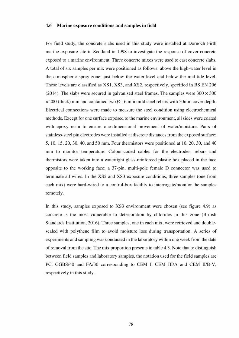
78

4.6 Marine exposure conditions and samples in field

For field study, the concrete slabs used in this study were installed at Dornoch Firth

marine exposure site in Scotland in 1998 to investigate the response of cover concrete

exposed to a marine environment. Three concrete mixes were used to cast concrete slabs.

A total of six samples per mix were positioned as follows: above the high-water level in

the atmospheric spray zone; just below the water-level and below the mid-tide level.

These levels are classified as XS1, XS3, and XS2, respectively, specified in BS EN 206

(2014). The slabs were secured in galvanised steel frames. The samples were 300 × 300

× 200 (thick) mm and contained two Ø 16 mm mild steel rebars with 50mm cover depth.

Electrical connections were made to measure the steel condition using electrochemical

methods. Except for one surface exposed to the marine environment, all sides were coated

with epoxy resin to ensure one-dimensional movement of water/moisture. Pairs of

stainless-steel pin electrodes were installed at discrete distances from the exposed surface:

5, 10, 15, 20, 30, 40, and 50 mm. Four thermistors were positioned at 10, 20, 30, and 40

mm to monitor temperature. Colour-coded cables for the electrodes, rebars and

thermistors were taken into a watertight glass-reinforced plastic box placed in the face

opposite to the working face; a 37-pin, multi-pole female D connector was used to

terminate all wires. In the XS2 and XS3 exposure conditions, three samples (one from

each mix) were hard-wired to a control-box facility to interrogate/monitor the samples

remotely.

In this study, samples exposed to XS3 environment were chosen (see figure 4.9) as

concrete is the most vulnerable to deterioration by chlorides in this zone (British

Standards Institution, 2016). Three samples, one in each mix, were retrieved and double-

sealed with polythene film to avoid moisture loss during transportation. A series of

experiments and sampling was conducted in the laboratory within one week from the date

of removal from the site. The mix proportion presents in table 4.3. Note that to distinguish

between field samples and laboratory samples, the notation used for the field samples are

PC, GGBS/40 and FA/30 corresponding to CEM I, CEM III/A and CEM II/B-V,

respectively in this study.

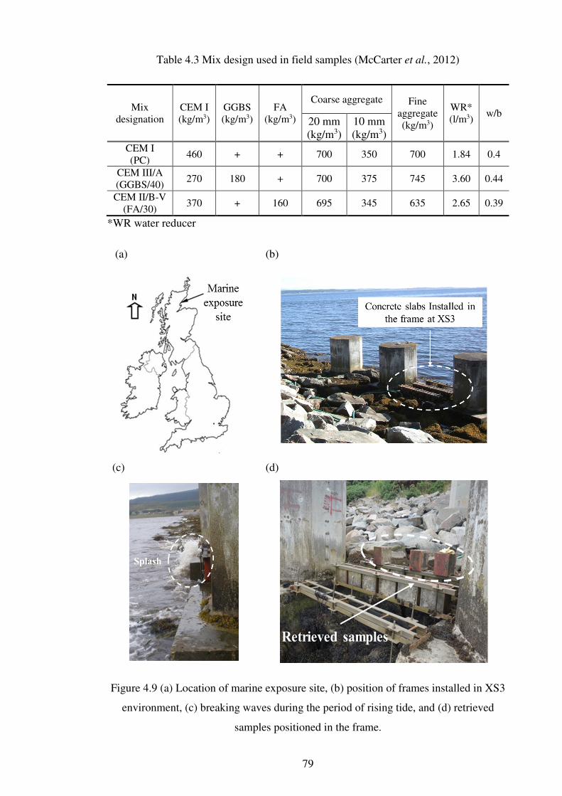
79

Table 4.3 Mix design used in field samples (McCarter et al., 2012)

Mix designation

CEM I (kg/m3)

GGBS (kg/m3)

FA (kg/m3)

Coarse aggregate Fine aggregate (kg/m3)

WR* (l/m3)

w/b 20 mm (kg/m3)

10 mm (kg/m3)

CEM I (PC)

460 + + 700 350 700 1.84 0.4

CEM III/A (GGBS/40)

270 180 + 700 375 745 3.60 0.44

CEM II/B-V (FA/30)

370 + 160 695 345 635 2.65 0.39

*WR water reducer

(a) (b)

(c) (d)

Figure 4.9 (a) Location of marine exposure site, (b) position of frames installed in XS3

environment, (c) breaking waves during the period of rising tide, and (d) retrieved

samples positioned in the frame.

80

4.7 Summary

Chloride-induced corrosion of reinforcement can be divided into two stage, before and

after corrosion initiation. In turn, different methods were applied depending on the

condition of the concrete. In general, the period before time to onset of corrosion is

referred to as the initiation period, where tests were related to chloride transport within

concrete, while corrosion propagation indicates the process after corrosion has initiated,

which was evaluated with the amount of corrosion (or corrosion rate) on the surface of

the steel. Therefore, both parameters related to corrosion and chloride transport were

evaluated with time. Due to the on-going hydration process, especially in concrete

containing SCMs, it was necessary to monitor continuously instead of one-off

measurement. Monitoring electrical resistance of concrete using stainless steel electrodes

with different depths was also carried out to evaluate chloride ingress and corrosion

behaviour of steel in concrete subjected to chloride environments.

In order to reflect exposure condition in the field, 18-years old samples exposed to marine

environment (XS3) was retrieved from field site in Dornoch Firth and then the tests,

which were used in the laboratory samples, were performed. Parameters such as the

diffusion/migration coefficient, porosity, degree of saturation and polarisation resistance

are used in modelling, together with mix design and are discussed in Chapter 8. Table 4.4

presents the overall experimental programme comprising sample type and test details; the

experimental procedures are described in the corresponding sections. The relationship

between durability assessment and required parameters are presented in table 4.5.

81

Table 4.4 Overall frameworks for experimental programme

Chapter Classification Sample Measurement

Types (Replicate)

Dimension (mm) Test Type Time (days)

5

Material /environmental

properties

Concrete (3)

100 × 100 × 100 Compressive strength D

28, 90, 180, 365 Resistivity ND

Concrete (1)

50 × 50 × 20 Porosity/saturation degree D

382, 390 Resistivity ND

Transport

Concrete (3)

Ø 100 × 50 Migration D

180, 270, 365 Resistivity ND

Concrete (1)

100 × 250 × 152 Chloride profile D 390

6 Corrosion Concrete

(3) 250 × 250 × 152

Half-cell potential ND/NQ

42 – 382 (Every end of wet/dry cycle) Macrocell current

Linear polarisation

ND/Q 186 – 382

(Every end of wet cycle) Galvanostatic pulse

Potentiostatic

Electrochemical impedance spectroscopy ND/Q Specific dates**

Tafel extrapolation ND/Q 382

Mass loss D/Q 382 (for corroded samples)

7

Electrical resistance monitoring

Concrete (3)

250 × 250 × 152

Two-pin electrodes for chloride transport ND 42 – 382

(Every end of wet/dry cycle) Four-pin electrodes for corrosion process ND

82

* D destructive method, ND non-destructive method, Q Quantitative method, NQ Qualitative method

** CEM I (w/b=0.4): 186, 270 and 382 days, CEM I (w/b=0.6): 186, 228 and 382 days, CEM III/A (w/b=0.4): 186, 228 and 382 days, CEM III/A (w/b=0.6): 186, 270 and

382 days, CEM II/B-V (w/b=0.4): 186, 228 and 382 days and CEM II/B-V (w/b=0.6): 186, 228 and 382 days

Table 4.4 (continued)

8

Environmental properties

Concrete (1)

50 × 50 × 20 Porosity/saturation degree Resistivity

D ND

18 years

Transport Concrete

(1) 100 × 300 × 200 Chloride profile D

Corrosion Concrete

(1) 300 × 300 × 200

Half-cell potential ND/NQ

Linear polarisation

ND/Q Galvanostatic pulse

Potentiostatic

Electrochemical impedance spectroscopy ND/Q

Tafel extrapolation ND/Q

Electrical resistance monitoring

Concrete (1)

300 × 300 × 200 Two-pin electrodes for chloride transport

ND

83

Table 4.5 Summary of research related to performance-based approach

Requirements Phases in

service life Types Main parameters Description

Test methods

Initiation

Transport rate

Diffusion/migration coefficient

• Investigate the relation between migration and diffusion coefficients

Chloride binding

Binding isotherm • Review the binding isotherm from literature review

Electrical resistivity

Resistivity • Investigate the relation between migration coefficient and electrical resistivity of concrete

• Monitor concrete resistivity with chloride transport

Propagation

Electrical parameters

Corrosion potential, Macrocell current, Polarisation resistance

• Investigate time to corrosion initiation and development of corrosion rate with time

• Compare the corrosion values with various electrochemical tests

Tafel’s constant

B constant • Investigate B values for calculation of corrosion rate using Tafel’s method and simple

monitoring techniques including potentiostatic tests

Electrical resistivity

Resistivity • Monitor concrete resistivity after corrosion initiation

• Investigate the relation between corrosion process and concrete resistivity

Environmental conditions

Initiation Physical properties

Degree of saturation • Investigate the relation between electrical resistivity of concrete and saturation degree and then

establish the relation using Arch’s law

Propagation Physical properties

Oxygen availability • Investigate cathodic branch in Tafel slope

Chloride content • Investigate the effect of Tafel constant on chlorides

Models

Initiation Physical model

Migration coefficient

• Estimate chloride profile using ClinCon model with migration coefficients

• Update environmental factors corresponding to XS3 area with comparison between estimated

chloride profile and that from the field samples

• Determine chloride threshold level with updated chloride profiles and corrosion rates

Propagation Empirical model

Polarisation resistance • Estimate corrosion rate with time

• Establish an empirical relation of polarisation resistance with time

84

CHAPTER 5

CHLORIDE TRANSPORT AND PERFORMANCE FACTORS

5.1 Introduction

Ideally, a performance factor should quantify those concrete properties related to

deterioration, leading to an improved understanding of concrete durability. There has

been a growing interest in such factors as they are essential in a performance-based

approach. Essentially, factors should be easy to apply and reliable as well as being

appropriate for the particular deterioration mechanism(s) for the structure, and their

numerical values should also be satisfied with suitable performance limiting values

(Andrade et al., 2013).

Chloride-induced corrosion in structures is described by Tuutti’s model comprising the

initiation and propagation phases. During the initiation phase, chlorides move into

concrete from an external source, such as sea-water or de-icing salt due to concentration

gradient. In this phase, the degree of saturation of the pore system and the chemical

composition of the pore solution are important as chlorides penetrate the pore solution.

After depassivation (the propagation phase), the corrosion process is controlled by

electrochemical parameters on the steel surface including oxygen availability, moisture

content and concrete resistivity. These properties must be included in a performance-

based test for the target structure. The electrical resistivity of concrete is a powerful

candidate as a performance factor, as this parameter is easily and rapidly evaluated. In

addition, resistivity quantifies a number of variables including environmental conditions

and concrete properties and it is believed that this single parameter could be developed

as a viable, performance factor, especially in chloride transport.

This section analyses performance factors related to chloride transport, including the

compressive strength, migration/diffusion coefficient, electrical resistivity, degree of

saturation and porosity. These parameters are then correlated with the electrical resistivity

of concrete. The measured values are also applied to a predictive model as input

parameters in this study (Chapter 8). Experiments were carried out on laboratory samples;

the details of the experimental set-up and test samples are described in Chapter 4.

85

5.2 Experimental

A range of experiments were conducted to assess the transport properties of concrete,

including migration/diffusion tests, electrical resistivity test and degree of saturation test;

compressive strength and porosity tests were also measured. This section outlines the

experimental procedures used to measure the aforementioned parameters.

5.2.1 Compressive strength

Compressive strength tests were undertaken in accordance with BS EN 12390-3 (British

Standards Institution, 2009). The samples were cured in a water bath at 20 ± 2ºC until the

test date, and three replicates per mix were measured at 28, 90, 180, and 365 days. An

average of three replicate measurements is presented as strength value for test age of 28,

90, 180, and 365 days.

5.2.2 Porosity/saturation degree

At the end of final wet/dry cycle, small cubes of concrete (ca. 50 × 50 × 20 mm) described

in Section 4.5 (figure 4.6) were swan to a depth of 100 mm from the concrete surface to

estimate the degree of saturation and porosity. For each depth, only one replicate was

obtained.

After cutting, the weight and electrical resistance of the samples were immediately

measured before loss of moisture to the surrounding environment which was at 20 ± 3ºC

and 50 ± 2% RH; samples were then dried in an oven at 50 ± 2ºC. The low drying

temperature prevented any potential change in microstructure due to micro-cracking and

the difference in weight change per each measurement was marginal for the different

drying temperature (Streicher and Alexander, 1995; Otieno et al., 2014). Saturation was

carried out using distilled water in a vacuum chamber. A pressure of 30 mbar was

maintained for 4 hours and then the sample was placed in the chamber until weighing. To

determine the equilibrium condition at each stage, the mass of each sample was

periodically measured using a scale of ± 0.01 g accuracy. The equilibrium was assumed

to be achieved when the following criterion was satisfied:

86

»m() − m(:)m(:) » × 100 ≤ 0.1(%) (5.1)

where m() is the mass (g) measured at time and m(:) is the mass (g) measured

after time :.

The degree of saturation and porosity were then calculated as follows:

UQ(%) = m1 −mQpmrn+S −mQp × 100 (5.2)

∅(%) = 1q¿ bmrn+S −mQpgsn+NLo × 100 (5.3)

where UQ is degree of saturation (%), m1 is the original sample mass (g), mQp is the

dried sample mass (g), mrn+S is the vacuum saturated sample mass (g), ∅ is porosity (%), q¿ is the density of distilled water (=1 g/cm3), and sn+NLo is the sample volume (cm3).

5.2.3 Chloride profiling

A chloride profile was established by plotting the total chloride content versus depth. A

non-linear curve fitting method was then used to determine the diffusion coefficient from

the chloride profile.

To simplify the chloride analysis, Chloride QuanTab® strips (manufactured by HACH)

were used. To measure the chloride concentration, the concrete dust in a 100 ml glass

beaker was weighed using a scale with an accuracy of ± 0.001 g. The chloride in the

powder sample was dissolved in a diluted nitric acid solution of 50 ml (~ 2 mol HNO3)

at 80 ± 2ºC for 4–5 minutes. The suspension was neutralised with Na(OH)2, maintaining

a pH of 6-8 in a suspension, as Chloride QuanTab® strips are only valid in a neutral

solution. The neutralised suspension was then allowed to cool to room temperature and

filtered. The chloride content was measured with a Chloride QuanTab® strip with ppm

unit. Although various representations have been suggested for chloride content in

concrete, total chloride concentration (by weight of binder or concrete) is a typical

representation (Glass and Buenfeld, 1997). This is because total chlorides participate in

the corrosion process (Glass et al., 2000) and the measurement is convenient compared

87

to other methods. In this method, the measured chloride concentration is converted into

total chloride concentration (by weight of binder) using the following equation assuming

uniform distributions of cement and chloride at the sampling depth (Song et al., 2008a):

S(%) = sn1LKS12 × nn1LKS12mKnS × M 2oQM-12-QoSo

× 100 (5.4)

where S is the total chloride content by mass of cement (%), sn1LKS12 is the suspension

volume (l), nn1LKS12 is the chloride content dissolved in the suspension (g/l), mKnS is

the mass of concrete dust (g), M 2oQ is the unit mass for binder (kg/m3), and M-12-QoSo

is the unit mass for concrete (kg/m3).

The apparent chloride diffusion coefficient was determined by fitting the error function

solution to Fick’s second law for non-steady state diffusion in a semi-infinite medium. A

curve was fitted to the chloride profile with a surface chloride content and a diffusion

coefficient using the Newton-Rapshon method in the Mathcad® program. Due to the

erratic behaviour at the outermost layer, two methods were simultaneously carried out:

(i) fitting with all points and (ii) fitting with points omitting the first point. Figure 5.1

illustrates an example of the determination of the diffusion coefficient and surface

chloride concentration using curve fitting. The background chloride concentration, i.e.

pre-existing chloride concentration in mix ingredients, was neglected in analysing the

chloride profiles because there was only a very low amount of chloride.

Figure 5.1 Examples of curve fitting from the chloride profile data.

0 5 10 15 20 25 30

0

2

4

6

8

10

Cs= 6.1%

D= 5.61×10-12

m2/s

r2= 0.87

Meaured values (40% GGBS,w/b=0.6)

Fitted line (including first point)

Fitted line (excluding first point)

Chlo

ride

con

cen

trat

ion (

%, by w

eigh

t of

bin

der

)

Depth (mm)

Cs= 8.0%

D= 3.75×10-12

m2/s

r2= 0.97

Convective zone

88

5.2.4 Migration test

Accelerated chloride migration testing was carried out using the NT Build 492 method

(Nordtest, 1999), which is widely used in Europe. The measurements using the sample

(Ø 100 × 50 ± 3 mm) were performed at 180, 270, and 365 days to minimise the hydration

effect of SCMs. The samples were vacuum-saturated under a pressure of 30 mbar for 24

hours in a desiccator containing saturated Ca(OH)2 solution (4 g/l). After saturation, the

electrical resistivity was measured using the end-to-end electrode configuration with two

stainless-steel plates. The details of resistivity measurement are described in Section

5.2.5.

Test procedures for the migration test conformed to the NT Build specification except for

measurement time and voltage. For all samples, the applied voltage was fixed at 30 V and

the measurement time was increased except for the CEM I (w/b = 0.6) concrete, in which

the applied voltage was 20 V due to the rapid ingress of chlorides. This method is similar

to the original version proposed by Tang (1996b) to minimise the effect of voltage on the

chloride transport rate and is still controversial (Spiesz and Brouwers, 2012).

After completing the migration test, chloride penetration depth was measured using a

colorimetric method with 0.1 mol AgNO3 solution. The migration coefficient was then

calculated using the following equation (Nordtest, 1999):

= 0.0239(273 + )(E − 2) − 0.0238Á(273 + )J × E − 2 (5.5)

where is temperature of the NaOH solution (ºC), y is the applied voltage (V), is the

average chloride penetration depth (mm) and J is the sample thickness (mm).

5.2.5 Electrical resistivity of concrete

To establish the relation between performance factors and electrical resistivity, electrical

resistance of concrete was measured using a HP 4263B LCR meter. The measurements

were performed on concrete samples used for the compressive strength test, the migration

test and porosity/degree of saturation. For the compressive strength test, the electrical

resistance of the concrete samples (100 mm cube) was measured before the test, while for

89

the migration test samples (Ø 100 × 50 ± 3 mm) the electrical measurement was

performed between saturating and migration test. For samples measuring porosity/degree

of saturation (ca. 50 × 50 × 20 mm), the measurements were carried out at each

equilibrium state and original condition, respectively.

The end-to-end measurement method was carried out at a frequency of 1 kHz and signal

amplitude of 350 mV, which minimised electrode polarisation effects (McCarter and

Brousseau, 1990). Before measurements, sample surfaces were dried with a synthetic

sponge. To achieve intimate contact, synthetic sponges (2 mm thickness) were placed

between the electrodes and the concrete, and a mass of 2 kg was placed on the upper

electrode to ensure uniform contact. The synthetic sponge was soaked in saturated

Ca(OH)2 solution and squeezed until no water dripped to reduce any surface conduction

effects (Newlands et al., 2007). The overall testing arrangement is shown in figure 5.2.

The averaged resistivity for three replicates per mix is expressed in this study. The

resistivity (or reciprocal conductivity) of bulk concrete was calculated as

H = IJ R = 1Â (5.6)

where H is the resistivity (Ω·m), Â is the conductivity (S/m), I is the cross-sectional area

(m2), L is the sample thickness (m), and R is the resistance (Ω).

Figure 5.2 Schematic of testing arrangement for end-to-end electrical resistance

measurements

90

5.3 Results and discussion

5.3.1 Development of compressive strength

Compressive strength is used in durability design as part of code requirements, although

it is considered that this parameter cannot fully reflect the durability properties of concrete

(Alexander et al., 2008). However, according to PD/CEN 16563 (British Standards

Institution, 2013a), where compressive strength is specified as part of the durability

provision, this parameter is considered to be the reference parameter in the quality control

of concrete. It is accepted that compressive strength is essential at the ultimate limit state.

Compressive strength at 28 days is generally used in the design stage but data beyond 28

days are required to describe the durability and performance (or serviceability) of

concrete. Strength development is ongoing due to continuous hydration but slows down

after 28 days. The use of pozzolanic materials or latent hydraulic binders such as FA and

GGBS lead to a slower development in compressive strength (Ann et al., 2008), but

continuous refinement of microstructure over a longer time scale.

The development of strength for the concretes is presented in figure 5.3. The values are

average values for three replicates per mix, with the error bars being ± one standard

deviation. The overall trend is that compressive strength increased with time irrespective

of the type of binder. Even though the compressive strength of SCMs concretes at 28-

days were lower than that of CEM I concrete, the strength development from 28 – 365

days for the CEM III/A concrete (46% for w/b=0.4 and 35% for w/b=0.6) and CEM II/B-

V concrete (69% for w/b=0.4 and 81% for w/b=0.6) was higher than those for the CEM

I concrete (44% for w/b=0.4 and 30% for w/b=0.6) due to pozzolanic reaction (Ann et al.

2008). The continuous increase in the strength for SCM concretes is a characteristic of

this type of concrete. An insoluble and dense calcium silicate hydrate gel is formed in the

cement matrix resulting from the reaction of siliceous oxide in SCMs with calcium

hydroxide in the pore solution of the binder. The SCMs subsequently lead to refinement

of pore structure and an increase in binding capacity of chloride in concrete (Yuan et al.,

2009). Compressive strength at 365 days was ranked as CEM I (w/b=0.4) > CEM II/B-V

(w/b=0.4) > CEM III/A (w/b=0.4) > CEM I (w/b=0.6) > CEM III/A (w/b=0.6) > CEM

II/B-V (w/b=0.6) concrete. Considering the compressive strength as a performance factor,

it would be reasonable to consider development of compressive strength for SCM

concrete instead of compressive strength at 28 days.

91

Figure 5.3 Development of compressive strength.

Compressive strength is considerably affected by concrete mix design, and the prediction

of compressive strength within the mix design is still valuable. Abram’s equation

(equation (5.7)) is first proposed to predict compressive strength depending on the w/b

(Abd elaty, 2014) and is then developed further considering SCMs. Another type is the

power equation, which is a general form in concrete technology (Abd elaty, 2014)

(equation (5.8)). The equations are described below:

- = a ∙ b@, = ¤Ã + ² + (5.7)

- = c ∙ @& (5.8)

where - is the compressive strength (MPa), x is w/b, c is CEM I content (kg/m3), f is FA

content (kg/m3), s is GGBS content (kg/m3), k is the efficiency factor and a, b, c, and d

are empirically determined parameters.

Both equations are only available to estimate the compressive strength at a certain age

(usually 28 days) so that it is necessary to introduce an additional factor to explain time

dependency. It is notable that durability/performance of concrete is correlated with time

dependency of compressive strength rather than compressive strength at 28 days, as the

continuous hydration for SCMs results in the development of compressive strength as

well as durability/performance. The development of compressive strength in concrete,

0 100 200 300 400

0

25

50

75

100

CEM I (w/b=0.4)

CEM III/A (w/b=0.4)

CEM II/B-V (w/b=0.4)

CEM I (w/b=0.6)

CEM III/A (w/b=0.6)


Com

pre

ssiv

e st

ren

gth

(M

Pa)

Age (days)

92

which follows a logarithmic form with time (Abd elaty, 2014), is related to clinker

minerals in the cement paste,

-,S = a ∙ 56() + b (5.9)

where a is a constant for strength gain, b is a constant for strength grade and t is age

(days).

Recently, constants have been determined based on comprehensive data on compressive

strength using the fitting method, and they can be estimated using the following equations

(Abd elaty, 2014). It was confirmed that development of compressive strength is

attributed to the hydration of clinker minerals,

a = 1.4035 ln(b) + 2.9956 (5.10)

b = 0.005b-,Äg.3 (5.11)

Whether the long-term strength can be estimated accurately for concrete using SCMs is

questionable due to the limitation of the logarithmic form, which shows an asymptotic

behaviour with time instead of a continuous increase, and due to the lack of long-term

data. However, the suggested equation is useful to estimate compressive strength with

time in the view of a performance-based concept, although only compressive strength at

28 days is required in the code. Thus, it is necessary to secure additional data for long-

term strength of concrete using SCMs to refine the model.

To estimate the time dependency in the compressive strength of concrete, figure 5.4

compares measured values and estimated values in this study using equation (5.9) (see

Appendix D.1). The solid line indicates the line of equality. Although the difference

increased by up to 20% in the high strength range from ~70 MPa, the estimated value was

significantly close to the measured values. However, a latent hydration effect in the SCMs

was not fully reflected in the empirical equation. Therefore, it was necessary to collect

additional data on compressive strength of concrete using SCMs.

93

Figure 5.4 Comparison between measured and predicted values for compressive

strength at different ages and different binders (expect for values at 28 days).

5.3.2 Pore conditions in unsaturated concrete

Concrete is a porous material and durability is determined by the pore structure.

Currently, it is believed that two transport mechanisms, diffusion and absorption, co-exist

in unsaturated concrete, i.e. concrete subjected to a wet/dry cyclic regime or the tidal zone

in marine environments. Therefore, two mechanisms are simultaneously reflected to

model the transport behaviour in unsaturated concrete. However, to introduce these two

mechanisms in modelling is complex as there is no reference to distinguish between the

diffusion and absorption rates in unsaturated concrete (Nilsson, 2000). For example, to

trigger absorption, data on the degree of saturation of concrete have rarely been

investigated. Alternatively, one transport mechanism, generally diffusion, is mainly

considered for simplification of the calculation, but is still debated by researchers

(Marchand and Samson, 2009). Therefore, it is necessary to investigate the degree of

saturation and porosity in addition to direct measurement of transport rate.

It is generally agreed that the more porous the concrete, the less resistant it is to chloride

ingress; thus, porosity can be used as a performance factor. In the present study, the porosity

of concrete was evaluated (refer to Chapter 4) at different depths and is tabulated in table

5.1. Firstly, porosity at 390 days was ranked as CEM I (w/b=0.4) < CEM III/A (w/b=0.4)

< CEM I (w/b=0.6) < CEM III/A (w/b=0.6) < CEM II/B-V (w/b=0.6) < CEM II/B-V

(w/b=0.6) concrete. It is evident that concrete with a low w/b is dense except for CEM

0 40 80 120

0

40

80

120

w/b=0.4

CEM I (w/b=0.4)

CEM III/A (w/b=0.4)


CEM I (w/b=0.6)

CEM III/A (w/b=0.6)


Pre

dic

ted

co

mpre

ssiv

e st

reng

th (

MP

a)

Measured compressive strength (MPa)

Line of

equ

ality

w/b=0.6

94

II/B-V concrete. For the latter, the difference in porosity is marginal with changing w/b.

Furthermore, CEM III/A (11.47% for w/b=0.4 and 12.44% for w/b=0.6) and CEM II/B-V

(13.81% for w/b-0.4 and 13.91% for w/b=0.6) concretes show higher porosity compared to

CEM I concrete (10.0% for w/b=0.4 and 12.3% for w/b=0.6). These trends are more

prominent for the low w/b. This may be caused by the large portion of micro-pores due to

the fine particles of SCMs. On the other hand, porosities at 10-mm depth for each mix are

lower than at other depths regardless of type of binder and w/b. One possible reason is pore

densification caused by carbonation, but in this study, carbonation was not observed as

shown in figure 5.5. It can be seen that the formation of Fridel’s salt by chloride binding or

denser C-S-H morphology by Cl- reduces porosity in this region (Suryavanshi et al., 1995).

Figure 5.5 Colour change with phenolphthalein indicator (CEM I, w/b=0.4).

Table 5.1 shows that porosity is significantly affected by w/b, and furthermore that SCMs

lead to higher porosity for low w/b. This result is in contrast to the results of the chloride

profiling/migration test in this study and the previous study on SCMs (Bamforth et al.,

1997). The pore network of concrete containing SCMs is more disconnected; thereby the

concrete has high resistance to chloride transport. Therefore, it should be noted that

porosity itself cannot be fully explained with resistance to chloride transport in concrete.

This is because pore tortuosity, connectivity, and pore size also affect ionic transport.

The degree of saturation (Sr) is also an important factor in determining the main transport

mechanism. Sr was evaluated (refer to Chapter 4) with depth and is shown in Figure 5.6.

Sr values are similar at each depth except for the surface layer (0-20 mm) regardless of

the wet/dry process. It is worth noting that Sr decreases with depth, especially for CEM

III/A concrete. In addition, concretes with low w/b have a lower Sr.

95

Table 5.1 Average porosity (%) with depth at 382 and 390 days.

Depth (mm)

w/b=0.4 w/b=0.6

CEM I CEM III/A CEM II/B-V CEM I CEM III/A CEM II/B-V

10 8.1 10.4 13.2 10.9 11.7 12.4

30 10.3 11.6 13.7 11.8 12.8 13.8

50 10.5 11.9 13.6 12.7 12.4 14.1

70 10.6 11.9 13.6 12.7 11.9 14.3

90 10.5 11.6 15.0 13.5 13.4 15.0

Average 10.0 11.5 13.8 12.3 12.4 13.9

Based on the results, self-desiccation is significantly influenced with w/b and type of

binder (Li et al., 2014), especially in CEM III/A concrete, leading to a reduced amount

of pore solution. Continuous hydration within disconnected pore network is beneficial to

resist chloride transport due to lower moisture content as well as refined pore network.

In other words, in the region beneath the convective zone, chloride resistance is controlled

by w/b and type of binder, which also determines the degree of saturation.

As shown in figure 5.6, for the convective zone, i.e. the surface ~ 20 mm, it is evident that

concrete is virtually saturated (> 90% saturation) after the wetting phase (382 days), while

Sr values range from 75 to 93% after 8 days of drying (390 days) under room temperature

and relative humidity of 20 ± 2ºC and 50 ± 2% RH. This shows that the drying process is

slower than expected. On the other hand, the outermost layer in the CEM II/B-V concrete,

especially with a high w/b, is vulnerable to drying compared to other concretes, however,

beneath this layer, Sr values for CEM II/B-V concretes are higher than for other concretes.

From both results, it can be deduced that higher porosity makes the outmost layer of CEM

II/B-V concrete vulnerable to drying, but other influencing factors, e.g. small pore size,

tortuosity and the presence of disconnected pores, prevent further drying in CEM II/B-V

concrete.

As noted above, the degree of saturation is significant in determining the main mechanism

of chloride transport in concrete. Although absorption may occur in concrete as the outer

layer is affected by the wet/drying process, in the field, the convective zone is limited (Gao

et al., 2017). In this section, convective zones were observed in the surface 0-20 mm for all

concretes; however, this zone may be overestimated due to the thickness of the sample.

This is discussed in Chapter 7. In addition, at depths > 20 mm, concretes were unsaturated,

and Sr values were stable, irrespective of wet/dry process. Thus, a low Sr value could result

96

in a low diffusion due to a low portion of pore solution. Consequently, chloride transport

in concrete structures subjected to a wet/drying cyclic regime, especially in the tidal zone

of marine structures, is primarily controlled by diffusion. It is possible that the pure

diffusion rate in unsaturated conditions is lower than in the fully saturated condition.

(a) CEM I (w/b=0.4) (b) CEM I (w/b=0.6)

(c) CEM III/A (w/b=0.4) (d) CEM III/A (w/b=0.6)

(e) CEM II/B-V (w/b=0.4) (f) CEM II/B-V (w/b=0.6)

Figure 5.6 Degree of saturation profiles for the concrete mixes.

0 20 40 60 80 100

70

80

90

100

After the final wetting cycle (382 days)

After the final drying cycle (390 days)

Sr (

%)

Depth (mm)

0 20 40 60 80 100

70

80

90

100



Sr (

%)

Depth (mm)

Missing data

0 20 40 60 80 100

70

80

90

100



Sr (

%)

Depth (mm)

0 20 40 60 80 100

70

80

90

100



Sr (

%)

Depth (mm)

0 20 40 60 80 100

70

80

90

100



Sr (

%)

Depth (mm)

0 20 40 60 80 100

70

80

90

100



Sr (

%)

Depth (mm)

97

5.3.3 Diffusion/Migration coefficient

As diffusivity in concrete is directly related to performance and durability, empirically

determined values are applied to predictive models. Different methods in the literatures

are employed to determine diffusion/migration coefficients (Stanish et al., 1997). The

diffusion coefficient is obtained from field or laboratory samples by curve fitting with the

‘erf’ function solution, and the migration coefficient is obtained using the NT Build 492

method, which is widely used in European countries (British Standards Institution, 2014).

The age of the concrete specified in studies for the migration/diffusion coefficient is

relatively short. For example, 28 days is used in the LIFE 365 model (Ehlen, 2014) and

Duracrete model (Altmann et al., 2012), and 180 days in the ClinConc model (Tang,

2008). For immersion testing, the salt solution is maintained for 90 days in AASHTO

T259 (Stanish et al., 1997) and 35-120 days in NT Build 443 (Nordtest, 1995). An aging

factor that reflects both hydration and binding effects may be employed to the diffusion

coefficient in the evaluation of the long-term durability of concrete, especially for SCMs.

Combined effects on the aging factor subsequently lead to higher scatter in the results.

The aging factors also vary across studies. For example, the values from exposure trials

and structures have been reported to be 0.3 for CEM I concrete, 0.62 for CEM III/A

concrete, and 0.7 for CEM II/B-V concrete (Bamforth et al., 1997), while the values for

CEM I and CEM II/B-V concretes have been reported as -0.03 and 1.0, respectively

(Andrade et al., 2011). The sensitivity of the aging factor to the diffusion coefficient is

shown in figure 5.7, where it can be observed that the diffusion coefficient is significantly

affected by the aging factor. When the aging factor is increased from 0.4 to 0.8, the

diffusion coefficient at 100-years exposure time decreases 6.3 times. Hence,

misinterpretation of the aging factor results in an error in evaluating the service life of

concrete structures. To reduce the error, it is desirable to eliminate this factor or to retain

a large amount of data to evaluate the factor.

98

Figure 5.7 Effect of exponent n on the decrease ratio of the diffusion coefficient with

time (Dt diffusion coefficient at time, t, and Dref diffusion coefficient at time, tref

[=1 year]).

Diffusion coefficients obtained from field investigations are valuable, as environmental

exposure conditions are quantified in addition to concrete properties. However, diffusion

coefficients obtained from field data are not always comparable to diffusion coefficients

obtained from laboratory testing, as exposure condition influences the diffusion

coefficient. In other words, it is necessary to reduce the discrepancy between the field and

the laboratory data to improve the accuracy of the predictive model.

To use the diffusion/migration coefficient correctly with a performance-based approach,

two limitations must be considered: (i) the hydration effect, and (ii) the difference

between the field and the laboratory conditions in the transport rate. To overcome these

limitations, it is necessary to determine the migration and diffusion coefficients of both

laboratory and field samples through long-term exposure. The migration coefficient is

widely used to predict chloride transport in concrete, especially in the Duracrete model,

the ClinConc model. In addition, this coefficient is also used to evaluate the resistance to

chloride penetration specified in the European codes as the basis of a performance-based

approach. In this study, the migration coefficients from NT Build 492 were adopted for

the ClinConc model to estimate chloride transport.

The changes in migration coefficient with time are presented in figure 5.8. Mean values are

plotted with the error bar representing ± one standard deviation. As expected, the

coefficients of concrete containing SCMs are much lower than those of CEM I concrete,

1 10 100

0.01

0.1

1

n=0.4

n=0.5

n=0.6

n=0.8

Dt/D

ref

Time (years)

Dt/D

ref=(t/t

ref)

-n

99

irrespective of w/b and exposure time. In addition, the w/b considerably influences chloride

transport. Migration coefficients for concretes with the low w/b (w/b=0.4) are 2–3 times

lower than those for concretes with the high w/b (w/b=0.6) irrespective of type of binder.

On the other hand, CEM I concrete show 3.1–6.7 times higher migration coefficients at 365

days compared to CEM III/A and CEM II/B-V concretes. It is clear that SCMs are

significantly beneficial to the resistance of chloride transport due to the refinement of their

pore structures by fineness of cementitious materials and the continuous hydration effect.

In general, the migration coefficients for all concretes show a continuous decrease with

time. For example, the decrease between 180 and 365 days is 60% for CEM II/B-V

concretes with both w/b=0.4 and 0.6; 40-45% for CEM III/A concretes with both w/b=0.4

and 0.6; and 30% for CEM I concrete with w/b=0.4. In contrast, CEM I (w/b=0.6) concrete

shows only a 2% reduction during this period. Migration coefficient at 365 days was ranked

as CEM II/B-V (w/b=0.4) < CEM III/A (w/b=0.4) < CEM II/B-V (w/b=0.6) < CEM III/A

(w/b=0.6) < CEM I (w/b=0.4) < CEM I (w/b=0.6) concrete.

Although the developments of the migration coefficient of concrete using SCMs are

advantageous with respect to durability, it is evident that this phenomenon makes the

computational model difficult. For example, the ClinConc model uses a migration

coefficient at 6 months to estimate chloride profile. The main assumption in this model is

that the migration coefficient is stable at that age, and the aging effect, i.e. a reduction in

chloride transport, is considered only caused by chloride binding (Tang, 2008). Thereby,

when migration coefficients at 6 months are used to estimate chloride profiles for SCM

concrete, it is possible that the predicted values are overestimated without consideration

of aging factors. Moreover, provided that the aging factor of SCM concrete exposed to a

long-term chloride environment (i.e. a field site) is used, the predicted value may be

underestimated. This is because the aging factor contains both the binding effect and the

hydration effect.

Clearly, the migration coefficient becomes an increasingly important parameter for the

predictive model of chloride transport, as well as a performance factor. However, as

shown in the result for concretes, and particularly those using SCMs, there are limitations

to determining durability with the migration coefficient at an early age, normally 28 days,

and in finding the intrinsic diffusion coefficient considering only the hydration effect.

Therefore, it is necessary to find the aging factor or long-term data for the migration

coefficient to improve the accuracy of the model.

100

Figure 5.8 Development of migration coefficients with time.

Chloride profiling describes a ‘real’ chloride distribution in concrete compared to the

migration test, but is laborious and time-consuming. Chloride profiling only gives the

‘time-averaged’ diffusion coefficient, which is not instantaneous; thus, use of the

estimated diffusion coefficient is limited in the predictive model. In addition, it is difficult

to determine whether the measured diffusion coefficient in the laboratory can be

representative of field concrete, as chloride transport behaviour is sensitive to exposure

conditions.

Figure 5.9 Time-averaged diffusion coefficient at time t from chloride profiling.

150 200 250 300 350 400

0

5

10

15

20

CEM I (w/b=0.4)

CEM III/A (w/b=0.4)


CEM I (w/b=0.6)

CEM III/A (w/b=0.6)


Mig

rati

on c

oef

fici

ent

(×10

-12 m

2/s

)

Time (days)

101

+ro = 1 − 3Å ()SS« (5.12)

where +ro is the time-averaged diffusion coefficient obtained from chloride profiling at

time t, and 3 is the time of first exposure to chlorides.

The diffusion coefficients obtained from chloride profiling in the laboratory are useful to

upgrade the transport model. The existing models for chloride transport focus on chloride

movement in saturated concrete, but concretes in accelerated laboratory testing or the

field are generally in an unsaturated condition. Therefore, the new parameters, or the new

model, should be developed to reflect these conditions. In this study, chloride profiling

was performed with concrete subjected to a wet/dry cyclic regime in the laboratory. Based

on the results, environmental factors are evaluated to add to the existing model (the

ClinConc). This is described in Chapter 8. The diffusion coefficient and chloride transport

resistance of concrete are discussed using chloride profiles in this Chapter.

Figure 5.10 presents the chloride profiles for CEM I, CEM III/A, and CEM II/B-V

concretes with different w/b subjected to a wet/dry cyclic regime at 390 days. It can be

observed that concretes with a low w/b have a higher resistance to chloride transport. At

steel depth, chloride concentrations for concrete at the high w/b (w/b = 0.6) are 3.4% for

CEM I concrete, 0.8% for CEM III/A concrete, and 1.04 % for CEM II/B-V concrete, all

of which are higher than the 0.3% in BS 8500-1 (British Standards Institution, 2016) and

0.4% in BS EN 206 (British Standards Institution, 2014) as CTL. However, corrosion

was only detected for CEM I (w/b = 0.6) concrete. Details of the corrosion behaviour are

discussed in Chapter 6. All concretes with w/b = 0.4 have a low chloride concentration

(less than 0.4% by weight of binder) at the steel depth, but determination of the CTL is

still controversial. In particular, the CTLs for CEM II/B-V concrete show evidently

contrasting results to those of Thomas and Matthews (2004), however, in this study,

SCMs show a high resistance to corrosion initiation as well as chloride transport. On the

other hand, at the point nearest to the exposure surface, an erratic behaviour of CEM II/B-

V (w/b = 0.4/0.6) and CEM III/A (w/b = 0.6) concretes was observed, which is attributed

to the wet/dry cyclic regime or the wash-out effect (Song et al., 2008a; Nilsson, 2000) in

figure 5.10.

At the time of sampling, the specimen was in a dry condition and the behaviour was more

apparent in concretes with w/b = 0.6. From the results, it can be deduced that the

convective zone is less than 6 mm considering an erratic behaviour is contributed to

102

absorption. Hence, absorption is another transport mechanism in these concretes in

addition to diffusion, but the boundary between diffusion and absorption cannot be

quantified in this study.

Figure 5.10 Chloride profiles at 390 days.

As the coefficients of determination, denoted r2 (see Appendix C1.4), for curve fitting

excluding the first point were higher than those including the first point, and as the erratic

behaviour at the first point led to an error, the diffusion coefficient and surface chloride

content were evaluated with chloride profiles excluding the first point. Diffusion is

considered as the main transport mechanism. The diffusion coefficient and surface

chloride concentration are presented in table 5.2. Surface chloride concentrations for

concretes containing SCMs were higher than for CEM I concretes, irrespective of w/b.

0 5 10 15 20 25 30

0

1

2

3

4

5

6

Chloride threshold level (0.4%)

CEM I (w/b=0.4)

CEM III/A (w/b=0.4)


Ch

lori

de

conce

ntr

atio

n (

%, b

y w

eigh

t of

bin

der

)

Depth (mm)

(a) w/b=0.4

Steel depth (25 mm)

0 10 20 30 40 50 60 70

0

1

2

3

4

5

6

7

(b) w/b=0.6

Steel depth (25 mm)

Chloride threshold level (0.4%)

CEM I (w/b=0.6)

CEM III/A (w/b=0.6)


Ch

lori

de

con

cen

trat

ion

(%

, b

y w

eig

ht

of

bin

der

)

Depth (mm)

103

This is because an increase in total chloride concentration at the exposure surface is

attributed to high chloride binding for SCM concretes or the porous surface region of

these concretes (Song et al., 2008a). Meanwhile, diffusion coefficients show an opposite

compared to surface chloride concentration, and are in the following order; CEM III/A

(w/b=0.4) < CEM II/B-V (w/b=0.4) < CEM I (w/b=0.4) < CEM III/A (w/b=0.6) < CEM

II/B-V (w/b=0.6) < CEM I (w/b=0.6) concrete. It is also notable that the largest increase

for both the surface chloride concentration and the diffusion coefficient were shown in

CEM I concrete with an increase in w/b. It seems that the accumulating chloride

concentration at the concrete surface, and the transport rate of chloride in concrete, are

affected by exposure conditions, such as a wet/drying cyclic regime as well as chloride

binding, as CEM I (w/b=0.6) concrete was vulnerable to resistance to chloride transport

in a wet/dry condition due to a rapid drying.

Table 5.2 Surface chloride concentration and diffusion coefficient obtained from

chloride profiles at 390 days

Binder w/b Cs*

(%, by weight of binder) Dd**

(× 10-12 m2/s) r2

CEM I 0.4 2.91 2.81 0.93

0.6 5.89 22.0 0.94

CEM III/A 0.4 6.74 0.77 0.98

0.6 8.00 3.75 0.87

CEM II/B-V 0.4 5.60 1.19 0.98

0.6 7.01 4.36 0.94

*Cs surface chloride concentration, **Dd diffusion coefficient

Figure 5.11 presents the comparison between the migration and diffusion coefficients

measured in this study. The migration coefficients at 365 days are similar to the diffusion

coefficients at 390 days assuming that a change in diffusion coefficient is marginal within

25 days, while the migration coefficients at 180 days are significantly higher than the

diffusion coefficients at 390 days. It was also observed that the migration coefficient is

proportional to the diffusion coefficient (Tang, 1996b, 2001). Thus, migration coefficients

at 28 days or 6 months are sometimes used as an input parameter in computational models

to predict chloride transport. However, caution should be taken to directly replace the

diffusion coefficient by the migration coefficient for the chloride transport model, and

especially for the ‘erf’ model. In addition, the concretes used in this study were subjected

to a wet/dry cyclic regime, which will cause an increase in transport rate, especially for

concretes with a high w/b, due to the drying phase (refer to table 5.2). In summary,

104

migration coefficients for CEM II/B-V concretes are lower than those for other concretes,

but diffusion coefficients for these concretes are marginally higher than those for CEM

III/A concretes. This indicates that the slow hydration process by pozzolanic reaction

increases chloride transport rate and high chloride binding reduce the rate. Therefore, it is

necessary to clearly establish the relation between the hydration process/chloride binding

and chloride transport for concrete, and especially SCM concrete.

Figure 5.11 Relation between the migration coefficient at 365 (closed markers) and 180

(open markers) days and the diffusion coefficient at 390 days.

5.3.4 Electrical resistivity of concrete

The electrical resistivity of concrete, as a non-destructive method, is useful to describe

chloride-induced corrosion as it is strongly related to the corrosion rate in concrete as well

as chloride transport (Polder, 2001). However, although electrical resistivity is

advantageous, interpretation of results can be difficult. The result is affected by several

factors including chemical composition of the pore solution, geometrical constrains,

concrete inhomogeneity, presence of steel and temperature (Kurumisawa and Nawa,

2016). As in Polder (2001), Newlands et al.(2007) and McCarter et al. (2015), the

resistivity of bulk concrete is generally measured by applying AC current using a

frequency response analyser or LCR meter. The frequency with which to determine bulk

resistance varies depending on the researcher, ranging from 50 Hz to 1 kHz (McCarter et

al., 2015). It has been reported that the measured resistances of the same concrete can

differ by up to ~ 3 times, depending on experimental set-up and conditions (Newlands et

0 5 10 15 20 25

0

5

10

15

20

25

CEM I (w/b=0.4)

CEM I (w/b=0.6)

CEM III/A (w/b=0.4)

CEM III/A (w/b=0.6)



Mig

rati

on

coef

fici

ent

at 1

80 a

nd 3

65

day

s (×

10

-12 m

2/s

)

Diffusion coefficient at 390 days (×10-12

m2/s)

105

al., 2007). To minimise the effects on the resistivity of concrete, the measurement should

be carried out under the same condition. In addition, for concrete structures subjected to

chloride environments, it is specified in most codes that concretes exposed to XS3/XD3

are vulnerable to chloride-induced corrosion due to the high availability of oxygen and

the rapid ingress of chloride from the wet/drying cycle. As a consequence, these concretes

are likely to be sensitive to the resistivity of concrete as they are unsaturated (Chrisp et

al., 2002; Polder and Peelen, 2002). From the literature review, it is evident that the

degree of saturation significantly affects the transport rate and transport mechanism.

In this section, electrical resistivity is estimated with time and degree of saturation. The

resistivity is closely related to the durability of concrete, especially in the chloride

transport. As a result, the measured values are correlated with the performance factors

such as the migration coefficient and compressive strength. The relation between degree

of saturation and resistivity is also presented. Prior to the compressive strength tests and

migration tests, the electrical resistance was measured using the end-to-end resistance

method described in figure 5.2, and the resistivity was calculated using equation (5.6).

Figure 5.12 presents the electrical resistivity of the samples (100 mm cube) used in the

compressive strength test. The resistivity of CEM I concretes was lower than that of SCM

concretes irrespective of w/b except at 28-days. At 28-days, the electrical resistivity of the

CEM II/B-V (w/b = 0.4 and 0.6) concretes was 62.9 Ω·m and 65.4 Ω·m, respectively, which

are lower than that of the CEM I (w/b = 0.4) concrete (75.8 Ω·m). However, trend was

reversed after ~ 37 days. This is due to the densification of the pore structure by pozzolanic

reaction in the intervening period, although the resistivity of the pore solution will also

influence concrete resistivity. It can be observed that the development of the resistivity of

concrete is different depending on type of binder. The resistivity for CEM I concretes was

almost stable throughout the duration of the testing period, unlike SCM concretes. The

rate of increase in resistivity for the CEM III/A (w/b = 0.6) concrete was reduced after ~

90 days, whereas the resistivity of CEM II/B-V (w/b = 0.4 and 0.6) and CEM III/A (w/b

= 0.4) concretes continuously increased with time. All concretes with w/b = 0.6 had lower

resistivity than those concretes with w/b = 0.4 from 28 days and 90 days. An increase rate

in resistivity of CEM II/B-V concrete with a low w/b was higher than with a high w/b.

According to McCarter et al. (2015), in terms of the resistance to corrosion, concrete can

be classified as follows: at 365 days CEM III/A and CEM II/B-V concretes have a very

high range of corrosion resistance, CEM I (w/b = 0.4) concrete has a high range, and

CEM I (w/b = 0.6) concrete has a low/moderate range.

106

Figure 5.12 Development of electrical resistivity for samples (100 × 100 × 100 mm)

used in the compressive strength test.

Figure 5.13 shows the resistivity of concrete (Ø 100 × 50 ± 3 mm) used in the migration

tests. Similar trends were observed with those samples used for compressive strength

testing. The CEM II/B-V (w/b = 0.4) concretes showed the highest resistivity, followed

by CEM III/A (w/b = 0.4) concrete. At 365 days, the resistivity of CEM II/B-V (w/b =

0.6) concrete was still lower than CEM III/A (w/b = 0.4). The vacuum saturating using

Ca(OH)2 results in a large drop in the electrical resistivity. The increase in resistivity

over the test period was apparent for CEM II/B-V and CEM III/A (w/b = 0.4) concretes,

while other concretes showed only a marginal increase.

It is notable that the electrical resistivity of the samples for the migration test is slightly

lower than that of samples for the compressive strength test. According to Newlands et al.

(2007), lower resistivity is attributed to the vacuum saturation process with a saturated

calcium hydroxide solution (Ca(OH)2). To confirm the effect of the saturation process on

electrical resistivity, the electrical measurements before and after vacuum saturation were

carried out for 3 samples (Ø 100 × 50 ± 3 mm) per a mix at 365 days. The results are shown

in figure 5.14. The reduction in electrical resistivity was ~ 9.0 – 22.8%, but it was observed

that the points diverged from the line of equality with increasing concrete resistivity. The

rate was higher than that in Spiesz and Brouwers’ (2012) study (6.0 – 14.2%), which used

mortar. It is noteworthy that concrete with higher electrical resistivity showed a larger

reduction. It is possible that parts of connected micro-pores are partly or totally unsaturated

0 100 200 300 400

0

100

200

300

400

500

Low

Low/moderate

High

CEM I (w/b=0.4)

CEM III/A (w/b=0.4)


CEM I (w/b=0.6)

CEM III/A (w/b=0.6)


Ele

ctri

cal

resi

stiv

ity

(Ω

⋅m)

Time (days)

Very high

107

in the normal condition, especially in concrete with a low w/b, but that a high pressure leads

to these pores filling with the solution.

Figure 5.13 Development of electrical resistivity for samples (Ø 100 × 50 ± 3 mm) used

in the NT Build 492 test.

Figure 5.14 Comparison between electrical resistivity of migration test samples before

and after vacuum saturation with saturated Ca(OH)2 solution.

Considering that the development of resistivity is related to pore structure, durability, and

performance, the concretes can be ranked as follows: CEM II/B-V (w/b=0.4) > CEM

III/A (w/b=0.4) > CEM II/B-V (w/b=0.6) > CEM III/A (w/b=0.6) > CEM I (w/b=0.4) >

0 100 200 300 400

0

100

200

300

400

500

Low

Low/moderate

High

CEM I (w/b=0.4)

CEM III/A (w/b=0.4)


CEM I (w/b=0.6)

CEM III/A (w/b=0.6)


Ele

ctri

cal

resi

stiv

ity

(Ω

⋅m)

Time (days)

Very high

0 200 400 600

0

200

400

600

CEM I (w/b=0.4)

CEM III/A (w/b=0.4)


CEM I (w/b=0.6)

CEM III/A (w/b=0.6)


Ele

ctri

cal

resi

stiv

ity

aft

er v

accu

m s

atura

tio

n a

t 3

65

day

s (Ω

⋅m)

Electrical resistivity before vaccum saturation at 365 days (Ω⋅m)

Line of

equ

ality

108

CEM I (w/b=0.6). This order is in line with the result of migration testing. It can be

deduced that electrical property is closely related to migration behaviour in concrete.

In addition to electrical resistivity regarding chloride transport, the relation between

moisture content and electrical resistivity was also investigated, as concrete is generally

in an unsaturated condition. This section considers the electrical resistivity in terms of

concrete (50 × 50 × 20 mm) subjected to a wet/dry cyclic regime, which was also used in

the degree of saturation test (Section 5.2.2 and 5.3.2).

The electrical resistivity of concrete versus depth profile is shown in figure 5.15 (as an

example), and all profiles are presented in the Appendix C.2. Because sampling time was

short, including cutting, and measuring electrical resistance and weighing, and sampling

was carried out at 382 and 390 days, the chloride movement and hydration effect on the

electrical resistance are negligible. The difference in resistivity between drying and

wetting profiles was only evident within 20 mm of cover depth for all concretes.

Considering that the convective zone was only a few millimetres, from the results on

chloride profiling, the zone obtained from the electrical resistivity was overestimated due

to the large sampling size (20 mm thickness). However, the resistivity was observed to

be stable at deeper levels, which indicates that the moisture distribution remained

unchanged. Hence, it is reasonable to assume that diffusion was the main chloride

transport mechanism for the samples used in this study.

To describe the drying effect at the exposure surface, figure 5.16 shows an increased rate

of electrical resistivity in the dry phase (at 390 days) compared to the wet phase (at 382

days) at 10 mm cover depth (a nominal cover depth). The electrical resistivity increased

during the drying phase, and this trend was especially observed in concretes with a high

w/b. The reason for the large increase in electrical resistivity of the concrete is the more

(connected) porous concrete. It is notable that the resistivity of the CEM II/B-V concrete

increased more than that of the CEM III/A concrete. From the result, it can be deduced

that CEM II/B-V concretes at the concrete surface may be more susceptible as they

contain more free chloride.

109

Figure 5.15 Example of resistivity profiles at the end of a wet/dry cycle (CEM I

concrete, w/b=0.6).

Figure 5.16 An increase ratio of electrical resistivity with a dry phase at 10 mm cover

depth (ρdry electrical resistivity at the end of final drying phase [390 days] and ρwet

electrical resistivity at the end of final wetting phase [382 days]).

5.3.5 Relation between compressive strength and electrical resistivity

Compressive strength is still used in practice as a factor to evaluate the durability of

concrete structures. To estimate compressive strength, the sample must be crushed in a

0 20 40 60 80 100

0

50

100

150

200

Electrical resistance at the end of wetting (382 days)

Electrical resitance at the end of drying (390 days)

Ele

ctri

cal

resi

stiv

ity

(Ω

⋅m)

Depth (mm)

Convective effect

CEM I

(w/b=0.4)

CEM III/A

(w/b=0.4)

CEM II/B-V

(w/b=0.4)

CEM I

(w/b=0.6)

CEM III/A

(w/b=0.6)

CEM II/B-V

(w/b=0.6)

0

1

2

3

ρ dry

/ρw

et

110

compressive machine. As the test is destructive, engineers have increasingly studied

electrical resistivity as a non-destructive method to predict strength (Ferreira and Jalali,

2010; Lübeck et al., 2012).

The developments of resistivity and compressive strength with time display a similar

trend: an asymptotic curve due to hydration processes. Thus, the relation between

compressive strength and resistivity has been observed as a linear correlation. There are

two ways of to describe this relation (Ferreira and Jalali, 2010):

(i) an empirical model with a regression method; and,

(ii) a theoretical model describing the hydration process.

In the empirical model, time or w/b is used as a variable, as shown in equations (5.13)

and (5.14). The equation used depends on the variables,

Æ = a + b (5.13)

Æ = cd¿/ (5.14)

where Æ is the compressive strength or resistivity; w/b is the water-to-binder ratio; is

time; and a, b, c, and d are constants.

Meanwhile, a theoretical model considers the nucleation and the growth of cementitious

materials, and adjusts to the prediction of strength development. The physical meaning

for constants reduces the errors in the fitting process, but it is difficult to determine the

maximum values,

Æ = Æ+ £1 − <@+SÇ¦ (5.15)

where Æ is the compressive strength or electrical resistivity; a is the growth rate dependent

on temperature; ¥ is the dominant morphology of the formation process; and Æ+ is the

maximum compressive strength or electrical resistivity when → ∞.

From the previous studies (Ferreira and Jalali, 2010; Lübeck et al., 2012), these equations

were used to predict the relation between the compressive strength and resistivity at 28

111

days. Each fitting was performed to obtain constants and the models were then verified,

but the investigated periods up to 91 days were short for estimating the values of SCM

concretes.

The electrical resistivity of concrete (or its reciprocal of conductivity) is influenced by

the resistivity of the pore solution as well as the pore network. Other influencing factors

include type of binder, degree of hydration, and mix design (Snyder et al., 2003). The

development of resistivity can be grouped by type of binder, while the effect of hydration

degree on the resistivity of the pore solution is relatively negligible after ~ 28 days (Bu

and Weiss, 2014). The compressive strength is related to pore structure and mineral

phases instead of pore-fluid chemistry. However, when the relation between compressive

strength and electrical resistivity is established, the effect of the pore solution should be

eliminated, which can be expressed in the following format (McCarter et al., 2000):

OP = H-12-,SHN1Qo_Ä (5.16)

where OP is the normalised resistivity; H-12- is the resistivity of concrete (Ω·m) at time,

t; and HN1Qo_Ä is the resistivity of the pore solution at 28 days (Ω·m).

Prior to evaluating the relationship between performance factors and electrical resistivity,

electrical resistivity of pore solution depending on binder types was estimate. Figure 5.17

shows pore solution resistivity with time using the NIST model (http://ciks.cbt.nist.gov/

poresolncalc.html) (Snyder et al., 2003; Bentz, 2007). In this model, the degree of

hydration and mix proportions are required as input parameters. To estimate the degree

of hydration at 28 days, the power’s law based on the effective w/b was used (see

Appendix A.2) (Tang, 1996a). CEM III/A and CEM II/B-V are assumed to be equivalent

to 60% of cement (0.6) and 40% of cement (0.4), respectively, according to BS EN 206

(British Standards Institution, 2014). The chemical composition of binders and mix

proportions are described in table 4.1 and table 4.2, respectively. It is evident that the pore

solution resistivity is different for each binder type, but a change in the resistivity of the

pore solution caused by the hydration process is marginal.

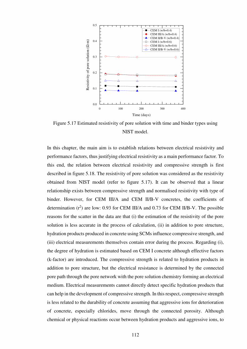
112

Figure 5.17 Estimated resistivity of pore solution with time and binder types using

NIST model.

In this chapter, the main aim is to establish relations between electrical resistivity and

performance factors, thus justifying electrical resistivity as a main performance factor. To

this end, the relation between electrical resistivity and compressive strength is first

described in figure 5.18. The resistivity of pore solution was considered as the resistivity

obtained from NIST model (refer to figure 5.17). It can be observed that a linear

relationship exists between compressive strength and normalised resistivity with type of

binder. However, for CEM III/A and CEM II/B-V concretes, the coefficients of

determination (r2) are low: 0.93 for CEM III/A and 0.73 for CEM II/B-V. The possible

reasons for the scatter in the data are that (i) the estimation of the resistivity of the pore

solution is less accurate in the process of calculation, (ii) in addition to pore structure,

hydration products produced in concrete using SCMs influence compressive strength, and

(iii) electrical measurements themselves contain error during the process. Regarding (i),

the degree of hydration is estimated based on CEM I concrete although effective factors

(k-factor) are introduced. The compressive strength is related to hydration products in

addition to pore structure, but the electrical resistance is determined by the connected

pore path through the pore network with the pore solution chemistry forming an electrical

medium. Electrical measurements cannot directly detect specific hydration products that

can help in the development of compressive strength. In this respect, compressive strength

is less related to the durability of concrete assuming that aggressive ions for deterioration

of concrete, especially chlorides, move through the connected porosity. Although

chemical or physical reactions occur between hydration products and aggressive ions, to

0 100 200 300 400

0.0

0.1

0.2

0.3

0.4

0.5

CEM I (w/b=0.4)

CEM III/A (w/b=0.4)


CEM I (w/b=0.6)

CEM III/A (w/b=0.6)


Res

isti

vit

y o

f p

ore

so

luti

on

(Ω

⋅m)

Time (days)

113

the best of the author’s knowledge, the relation between the compressive strength and the

reactions can be ambiguous. Finally, the tolerance range for electrical measurements is

approximately 20%, thereby leading to the scatter in the data (Polder, 2001).

Figure 5.18 The relation between normalised resistivity and compressive strength with

binder type.

5.3.6 Relation between transport properties and electrical resistivity

To assess the transport properties of concrete, different techniques are used to evaluate a

parameter. These techniques can be laborious and destructive. On the other hand, the

electrical resistance measurement is practical due to its ease of measurement and its link

with pore structures. However, its values tend to be qualitative. To improve the

applicability of electrical resistance or resistivity, it is necessary to establish a direct

relationship with transport properties. In this section, the relationship between transport

properties (e.g. degree of saturation and migration coefficient) and electrical resistivity

are established from the experimental results.

For porous materials, Archie’s law is employed to express the relationship between

electrical resistivity and degree of saturation (Archie, 1942), but the interpretability of the

conductivity of fully saturated porous materials using the following equation is debatable.

Hn+SHS = UQ2 (5.17)

0 1000 2000 3000 4000 5000

20

30

40

50

60

70

80

90

CEM I

CEM III/A

CEM II/B-V

Fitted line for CEM I

Fitted line for CEM III/A

Fitted line for CEM II/B-V

y=0.03x+28.23, r2=0.93

y=0.01x+28.54, r2=0.73

Co

mp

ress

ive

stre

ng

th (

MP

a)

Nρ

y=0.06x+23.24, r2=0.99

114

where HSis the measured electrical resistivity for the unsaturated condition, Hn+S is the

electrical resistivity for the saturated condition, UQ is the saturation degree, and 6 is

Archie’s exponent

To improve the discrepancy between the experimental and predicted data, percolation

theory is incorporated into the equation. Percolation theory focuses on geometrical or

physical properties of materials. For cementitious materials, percolation through capillary

pores has been reported by McCarter and Garvin (1989). Based on the percolation theory,

the model is extended to describe the electrical conductivity, σ (the reciprocal of

resistivity), of a composite material composed of different phases (Li et al., 2016),

UQ Ë«Y/i@ËaY/iË«Y/i:£YÌÍ°Í° ¦ËaY/i + (1 − UQ) Î ËcYi@ËaYiËcYi:£YÌÍ°Í° ¦ËaYiÏ = 0

(5.18)

where U- is the threshold or critical saturation degree for pore solution percolation in the

microstructure of the material, and Â+ is the conductivity of the air phase.

As Â+ ≈ 0, he equation above can be simplified as follows:

H3HS = ÂSÂ3 = UQ − U-1 − U-

(5.19)

In the equation above, the degree of saturation, Sr, in Archie’s law is replaced by the

degree of the saturation based on the percolation theory. Although the modified Archie

law explains the relation between electrical resistivity and degree of saturation for porous

material, it is difficult to define the critical saturation degree, i.e. U-. As the range for Sr

is narrow in this study, Archie’s law (equation (5.17)) is used to establish the relation.

Figure 5.19 presents the relative electrical resistivity with Sr. The outliners indicated by

‘open’ markers on the figure have been removed from the fitting. In addition, the values

for the fully saturated condition are fixed to improve the fitting result.

As shown in figure 5.19, the ratio of resistivity between the saturated condition and

measured (unsaturated) condition generally decreases with degree of saturation. It can be

observed that Archie’s exponents depend on w/b and type of binder. The estimated

exponents are presented in table 5.3. For w/b = 0.4, the exponents for CEM I, CEM III/A

and CEM II/B-V concretes are 1.61, 2.16, and 5.16, respectively, while for CEM III/A

115

and CEM II/B-V concretes with w/b=0.6 they are 3.48 and 6.91. The exponents imply

that CEM II/B-V concrete is the most sensitive to a change in resistivity with moisture

content, while resistivity change for CEM I concrete is insensitive to degree of saturation.

However, to explain the relationship, the number of samples per mix is too small and the

measured range is narrow. Moreover, w/b is also an important factor to determine the

electrical resistivity. Concrete with a high w/b is sensitive to a change in the electrical

resistivity as moisture can be retained/lost due to more porous materials. For CEM I

(w/b=0.6) concrete, the relation is not displayed as it was irregular due to the chloride

contamination of the concrete. This erratic behaviour, which is displayed as ‘open’

markers in both figures, were also observed in other concretes. The markers correspond

to surface layers (0-20 mm cover depth) in the samples. This may be because the presence

in the sample of crystallised chlorides, which are not bound chlorides, further reduced the

resistivity of the sample during the saturation process.

Table 5.3 Archie’s exponent with binder

Binder w/b Archie’s exponent

CEM I 0.4 1.61

0.6 +

CEM III/A 0.4 2.16

0.6 3.48

CEM II/B-V 0.4 5.61

0.6 6.91

* + not determined

The most important parameter for chloride transport is the chloride transport rate, i.e. the

diffusion coefficient or sorptivity. However, its measurement is considerably time-

consuming and destructive, although accelerated methods have been developed. Among

the accelerated methods, NT Build 492 is widely used to determine an input value in

predictive models or to evaluate the durability of samples as a performance factor. As

shown in figure 5.20, Tang (1996a) expected that after the NT Build 492 test, the chloride

penetration front within the sample would be sharp, called a ‘tsunami shape’. The

measured chloride profiles, however, were non-linear curves (S-shaped curves) (Andrade

et al., 1999; Spiesz and Brouwers, 2013). Tang (1996a) hypothesized that the possible

reasons for these S-shaped curves are pore distribution and the movement of other ions.

In other words, although the chloride profile obtained from NT Build 492 is not

116

completely in line with that based on the background theory, NT Build 492 is still

attractive as the migration coefficient can be readily calculated from this method.

Meanwhile, it is increasingly attractive to use non-invasive methods. Among these

methods, the electrical resistance method is the most relevant because ionic ingress

through concrete coincides with the electrical conduction path, but it is difficult to obtain

the migration coefficient with the electrical resistivity directly.

Figure 5.19 Relation between saturation degree and resistivity with binder type (a)

w/b=0.4 and (b) w/b=0.6 (outliners [open markers] are removed from fitting equations).

Studies have been conducted to determine the relationship between the electrical

resistivity and transport rate (Sengul, 2014; Lim et al., 2016; Van Noort et al., 2016), but

so far, the relations have been obtained empirically. This means that a number of

50 60 70 80 90 100

0.0

0.2

0.4

0.6

0.8

1.0

ρ0/ρt=S

5.61

r

r2=0.94

ρ0/ρt=S

2.61

r

r2=0.78

ρ0/ρt=S

1.61

r

r2=0.68

CEM I (w/b=0.4)

CEM III/A (w/b=0.4)


ρ 0/ρt

Sr (%)

50 60 70 80 90 100

0.0

0.2

0.4

0.6

0.8

1.0

ρ0/ρt=S

6.91

r

r2=0.90

ρ0/ρt=S

3.48

r

r2=0.61

CEM III/A (w/b=0.6)


ρ 0/ρt

Sr (%)

117

experiments have to be carried out to establish the relation and constants in empirical

equations have no physical meanings. Therefore, in the present study, the relationship

between the migration coefficient and the electrical resistivity is investigated using a

simplified Nernst-Planck equation.

Figure 5.20 Schematic diagram for chloride distribution in samples after migration test

(Tang, 1996a).

The diffusion flux of ions in a porous material is expressed by the Nernst-Planck equation

(Kurumisawa and Nawa, 2016):

= o + o y

(5.20)

where is the flux of an ion species, o is the effective diffusion coefficient, is the

concentration of an ion species, is the valence number of an ion species, is the gas

constant, is Faraday’s constant, y is the electrical field and is the position of the

medium.

Provided that no concentration gradient within a porous medium and an external potential

is large enough, the above equation can be simplified as follows:

= o Ð

(5.21)

118

Flux is converted into the current density, and then substituting the current density with

the electrical resistivity gives the following relation:

1H = o = o ∙ a ∙ (5.22)

where H is the bulk electrical resistivity and ‘a’ is a constant (=ÑÒÓRÔ ).

Based on equation (5.22), it is apparent that the migration coefficient is correlated with

electrical resistivity. Moreover, previous studies (Sengul and Gjørv, 2009; Van Noort et

al., 2016) have reported that the electrical resistivity is correlated to the migration

coefficient. Namely, high electrical resistivity of concrete indicates high resistance to

chloride transport. To improve the applicability of the electrical resistivity of concrete to

determine the transport rate, the physical parameter, , in equation (5.22) must be

evaluated.

The relationship between the electrical resistivity and migration coefficient is

established based on the above equations, as described in Figure 5.21. Note that the

resistivity (equation (5.22)) was estimated with the samples (Ø 100 × 50 ± 3 mm) used

in the migration test after Ca(OH)2 saturation. The outliner indicated by an ‘open’

marker on this figure has been omitted from the fitting. Based on equation (5.22), the

constant () obtained in this study indicates the chloride concentration in a porous

medium; is 0.356 mol/l of chloride was uniformly distributed in the sample. In a study

by Streicher and Alexander (1995), a concrete sample was pre-saturated with 5 mol/l of

chloride solution to apply equation (5.22), which is valid in steady-state processes. The

migration coefficient obtained from NT Build 492, on the other hand, is determined in

non-steady state conditions, so the assumptions shown in figure 5.22 are required to

calculate the migration coefficient using equation (5.22), as follows: (i) the average

chloride concentration in the sample applied to NT Build 492 over the chloride

contaminated depth is equal to 0.356 mol/l (see figure 5.21), therefore the migration

coefficient measured in NT Build 492 is equal to the migration coefficient obtained

from a sample saturated with 0.356 mol/l of chloride, and (ii) the chloride binding is

ignored. However, this study was only carried out for the migration test and the

electrical resistance measurement. To verify the suggestion regarding the relationship

between migration coefficient and electrical resistivity (equation (5.22), it would be

119

necessary to conduct experiments for chloride profiling of the sample (Ø 100 × 50 ± 3

mm) directly after the migration test, and then to calculate the average value for chloride

concentration within the chloride contaminated area.

Figure 5.21 Relation between the migration coefficient and bulk electrical resistivity

irrespective of binder types and w/b.

Figure 5.22 Schematic diagram for assumption of chloride distribution in terms of the

suggested parameter () after the migration test in this study.

0 100 200 300 400 500

0

100

200

300

1/(De⋅a)=0.356⋅ρ

r2=0.86

1/(

De⋅a

) (Ω

⋅m⋅l/

mol)

ρ (Ω⋅m)

120

5.4 Summary

This section investigated performance factors (compressive strength, transport rate,

degree of saturation, and porosity) regarding chloride transport, and then correlated them

with the electrical resistivity. The general findings are summarised below.

• The performance factors investigated in this study are ranked in table 5.4

except for degree of saturation. It was confirmed that w/b and type of binder

are crucial to improve the durability/performance of concrete. Compressive

strength and porosity are more influenced by w/b, while diffusion/migration

coefficients and resistivity are influenced by type of binder.

• Diffusion/migration coefficients are less related to compressive strength and

porosity. Therefore, care is required to explain transport property with only

compressive strength or porosity. The ranking order of the migration

coefficients is similar to that of the resistivity, as the pore network is

determinant for the parameters.

Table 5.4 Ranking order with performance factors

w/b Binder Durability indicators

fc,365 Ø Dd Dm ρ

0.4

CEM I 1 1 3 5 5

CEM III/A 3 2 1 2 4

CEM II/B-V 2 5 2 1 1

0.6

CEM I 4 3 6 6 6

CEM III/A 5 4 4 4 3

CEM II/B-V 6 6 5 3 2

fc,365 = compressive strength at 365 days, Dd=diffusion coefficient at 390 days, Dm=migration coefficient at 365 days, Ø=porosity at 390 days, and

ρ=resistivity at 365 days; rank order: 1 → 6 (good → bad)

• All samples subjected to a wet/dry cyclic regime were in an unsaturated

condition even though the degrees of saturation of the sample were measured

after the wetting phase. Except for the surface layer, the degrees of saturation

were stable across depths, but the degree of saturation varied with type of

121

binder. It was observed that the surface layer in CEM II/B-V concrete was the

most sensitive to the drying effect.

• The transport rate decreased with time irrespective of type of binder. The

diffusion coefficients were linearly related to the migration coefficient.

However, caution must be taken to ensure that the latter is directly used in the

transport model using the ‘erf’ function.

• The electrical resistivity was closely related to performance factors. The

compressive strength first had a linear relation with the electrical resistivity,

but it was necessary to reduce the scatters in the results by estimating the

degree of hydration and the resistivity of the pore solution. On the other hand,

the relationship between the migration coefficient and the electrical resistivity

was established from the fitting, and the constant (0.356 mol/l) was suggested.

The constant is useful for calculating the migration coefficient with electrical

resistivity, but additional investigation is required to verify the constant.

• According to the result for the diffusion coefficient, CEM III/A concretes have

higher resistance to chloride transport than CEM II/B-V concretes. Therefore,

it can be deduced that CEM II/B-V concrete is beneficial to prevent chloride

transport based on the result of migration coefficient, but CEM III/A concrete

is more efficient to improve the chloride resistance of concrete as a

replacement as the hydration process in CEM III/A concrete is relatively

helpful in forming a dense pore structure earlier than in CEM II/B-V concrete.

122

CHAPTER 6

CHLORIDE-INDUCED CORROSION OF STEEL WITH

PERFORMANCE OF CONCRETE

6.1 Introduction

The corrosion of steel in reinforced concrete, from the initiation to the propagation phase,

has been extensively investigated and a number of models regarding the corrosion

propagation have also been developed (see Section 3.5.2). Most models require

electrochemical parameters to estimate the development of corrosion, and these are

generally determined from laboratory tests in which variables such as environmental

conditions and material properties are well-controlled. To achieve corrosion within a

short time period, accelerated methods are employed, such as wet/dry cyclic regimes

(Polder and Peelen, 2002; Vedalakshmi et al., 2009b; Angst et al., 2011b; Pereira et al.,

2015), application of current to the steel (Austin et al., 2004) and pre-mixed chloride in

the concrete (Elsener, 2002; Videm, 2007; Nygaard et al., 2009; Martinez et al., 2015).

However, corrosion parameters obtained from controlled or accelerated conditions could

be inappropriate in estimating the corrosion behaviour of field structures. For example,

the B value, i.e. the Stern-Geary constant, is, essentially, required to determine the

corrosion rate of steel in an electrochemical measurement. This can be estimated with

Tafel’s constants (equation (3.4)) or an empirical value, corresponding to 26 mV for the

active state and 52 mV for passive state of steel. However, the value can vary depending

on the concrete or steel condition, which is affected by environmental conditions from

literatures. In this regard, it has been reported that Tafel’s constants are distributed within

a wide range. Therefore, determining the B value without considering concrete or

environmental conditions leads to misinterpretation of data or an unreliable prediction of

the residual life of the concrete structure.

In this section, a range of electrochemical techniques are applied to laboratory samples to

estimate corrosion rate and determine whether corrosion occurred. Furthermore, the B

values for the laboratory samples are estimated and compared using the Tafel

extrapolation technique and a simple monitoring technique using the potentiostatic

method. Based on the results, the chapter then discusses the methodology and

quantification for corrosion products.

123

6.2 Experimental

The samples used in this study are described in Chapter 4. The following corrosion

measurements were carried out: the half-cell potential, macrocell current, linear

polarisation, Tafel extrapolation, potentiostatic, galvanostatic pulse and electrochemical

impedance spectroscopy. To secure depolarisation time, the time-gap between

measurements was more than 10 minutes for recovering the corrosion potential. The

experimental set-up for each measurement is described below.

Comprehensive corrosion tests were conducted for two steels with different exposure

areas per sample, as mentioned in Section 4.3. Detailed schedules are presented for each

test (table 4.3) with monitoring data up to 382 days. In the case of those samples in which

corrosion was detected on the steel, the steel was retrieved from the concrete after 382

days. Visual observation and mass loss tests were then undertaken. All measurements

were performed for each mix in one day.

6.2.1 Half-cell potential

For the half-cell potential measurement, a copper-copper sulphate electrode (CSE)

(model 8-A manufactured by Farwest corrosion control) was used as a reference

electrode. The measurement for two steel bars at 25 mm cover depth was carried out at

the end of both wetting and drying phases, from 42 days up to 382 days. At the end of the

dry phase, a synthetic sponge saturated with 19.8 g/l NaCl solution was placed on the

surface of the sample for 10 minutes before the measurement to obtain electrical

connectivity between the working electrodes and the reference electrode. The potential

reading between two electrodes was performed with a high impedance multi-meter (1705

True RMS programmable multi-meter) (see figure 6.1).

6.2.2 Macrocell current

The current flowing between the steel bar at 25 mm and 100 mm cover depth was

monitored at the end of every wetting and drying phase by measuring the potential drop

across a resistor (R=10 kΩ) using a high impedance multi-meter as shown in figure 6.2.

To avoid the sudden drop in the potential, the measurements were carried out 5 minutes

after connection with the resistor. For electrically connected steels with a large exposure

124

area, more than 10 minutes were given to depolarise. To calculate the macrocell current

density, the unmasked area of steel embedded in concrete is considered as the exposure

steel area. The following equation based on Ohms’s law is used:

+-Q1 = ∆ER × IoN (6.1)

where +-Q1 is the macrocell current density (mA/cm2), ∆E is the potential drop between

two steels (V), R is the resistor (=10 kΩ), and I is the exposure area of steel (cm2).

Figure 6.1 Half-cell potential technique.

Figure 6.2 Macrocell current technique.

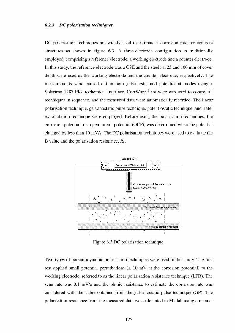
125

6.2.3 DC polarisation techniques

DC polarisation techniques are widely used to estimate a corrosion rate for concrete

structures as shown in figure 6.3. A three-electrode configuration is traditionally

employed, comprising a reference electrode, a working electrode and a counter electrode.

In this study, the reference electrode was a CSE and the steels at 25 and 100 mm of cover

depth were used as the working electrode and the counter electrode, respectively. The

measurements were carried out in both galvanostat and potentiostat modes using a

Solartron 1287 Electrochemical Interface. CorrWare ® software was used to control all

techniques in sequence, and the measured data were automatically recorded. The linear

polarisation technique, galvanostatic pulse technique, potentiostatic technique, and Tafel

extrapolation technique were employed. Before using the polarisation techniques, the

corrosion potential, i.e. open-circuit potential (OCP), was determined when the potential

changed by less than 10 mV/s. The DC polarisation techniques were used to evaluate the

B value and the polarisation resistance, Rp.

Figure 6.3 DC polarisation technique.

Two types of potentiodynamic polarisation techniques were used in this study. The first

test applied small potential perturbations (± 10 mV at the corrosion potential) to the

working electrode, referred to as the linear polarisation resistance technique (LPR). The

scan rate was 0.1 mV/s and the ohmic resistance to estimate the corrosion rate was

considered with the value obtained from the galvanostatic pulse technique (GP). The

polarisation resistance from the measured data was calculated in Matlab using a manual

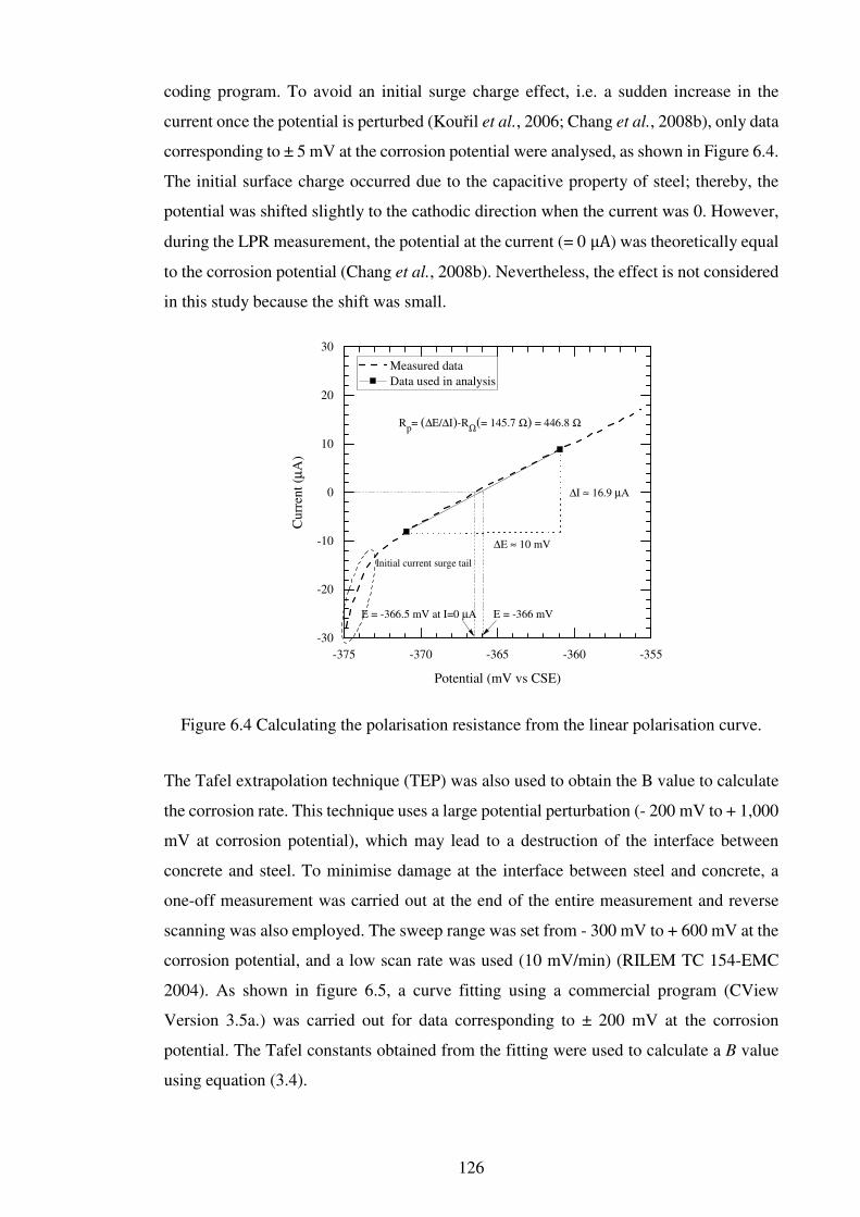
126

coding program. To avoid an initial surge charge effect, i.e. a sudden increase in the

current once the potential is perturbed (Kouřil et al., 2006; Chang et al., 2008b), only data

corresponding to ± 5 mV at the corrosion potential were analysed, as shown in Figure 6.4.

The initial surface charge occurred due to the capacitive property of steel; thereby, the

potential was shifted slightly to the cathodic direction when the current was 0. However,

during the LPR measurement, the potential at the current (= 0 μA) was theoretically equal

to the corrosion potential (Chang et al., 2008b). Nevertheless, the effect is not considered

in this study because the shift was small.

Figure 6.4 Calculating the polarisation resistance from the linear polarisation curve.

The Tafel extrapolation technique (TEP) was also used to obtain the B value to calculate

the corrosion rate. This technique uses a large potential perturbation (- 200 mV to + 1,000

mV at corrosion potential), which may lead to a destruction of the interface between

concrete and steel. To minimise damage at the interface between steel and concrete, a

one-off measurement was carried out at the end of the entire measurement and reverse

scanning was also employed. The sweep range was set from - 300 mV to + 600 mV at the

corrosion potential, and a low scan rate was used (10 mV/min) (RILEM TC 154-EMC

2004). As shown in figure 6.5, a curve fitting using a commercial program (CView

Version 3.5a.) was carried out for data corresponding to ± 200 mV at the corrosion

potential. The Tafel constants obtained from the fitting were used to calculate a B value

using equation (3.4).

-375 -370 -365 -360 -355

-30

-20

-10

0

10

20

30

∆I ≈ 16.9 µA

∆E ≈ 10 mV

E = -366 mV

Rp= (∆E/∆I)-RΩ(= 145.7 Ω) = 446.8 Ω

Measured data

Data used in analysis

Cu

rren

t (µ

A)

Potential (mV vs CSE)

E = -366.5 mV at I=0 µΑ

Initial current surge tail

127

Figure 6.5 Evaluation of the Tafel slope in a potentiodynamic polarisation test including

reverse scan.

For the galvanostatic pulse technique (GP), a constant current was applied to the working

electrode and the change in potential with the applied current was measured. The applied

current was fixed at 25 µA irrespective of the steel condition, unlike in previous studies

(Birbilis et al., 2004; González et al., 2004; Elsener, 2005), and the duration was 10s.

From the result, polarisation resistance and ohmic resistance were estimated using a

modified Randle circuit with equation (6.2) as shown in Figure 6.6. For the fitting

purpose, an exponential analysis to calculate the polarisation/ohmic resistances was

carried out using Matlab software.

ES() = *2× + *2N Ø1 − e@£SÙ¦`Ú (6.2)

where ES() is the potential of steel with measuring time t; *2 is the applied current; N

is the polarisation resistance; × is the ohmic resistance; Û is the time constant (=NL); 6 is the non-ideality exponent (0<6 ≤1); and L is the double layer capacitance.

Finally, the potentiostatic technique (PT) was used to calculate the B value as well as the

polarisation resistance (Poursaee, 2010). The constant voltage, i.e. 10 mV at corrosion

potential, was applied to the anodic direction for 100s. To minimise ‘destruction’ of the

1E-8 1E-7 1E-6 1E-5 1E-4 0.001 0.01

-1000

-800

-600

-400

-200

0

200

βc = 340 mV/dec

βa = 550 mV/dec

Corrosion potential

Measured data

Analysed data

Pote

nti

al (

mV

vs

CS

E)

Absolute current (A)

Corrosion current

128

corrosion environment, the applied potential was deliberately injected at the corrosion

potential for 100s.

Figure 6.6 Calculating the polarisation resistance using the GP.

Analysis of the polarisation resistance was conducted with data on anodic potential pulse.

In this analysis, the following equation for ohmic resistance and corrected polarisation

resistance was used; it is also based on a modified Randle circuit (Feliu et al., 1986).

*S() = y2×b× + Ng ÜÝÝÝÞ× + N<ß

@Sd]RjRàRà:Rj á

âãããä (6.3)

where *S() is the current of steel with measuring time t, y2 is the applied potential, N

is the polarisation resistance, × is the ohmic resistance and L is the double layer

capacitance.

In addition to the fitting process as shown in figure 6.7, the total charge in the polarisation

process was calculated using the integration with respect to the total applied time. The

details on the calculation of the B value are described in Section 6.3.4.

-15 -10 -5 0 5 10 15

-170

-160

-150

-140

-130

Polarisaton potential

Corrosion potential

as applied current starts Ohmic potential

Exposure area : 75.4 cm2

Applied current: 25 µΑΑpplied time : 10 s

Simulated (r2=0.99)

Measured

Pote

nti

al (

mV

vs

CS

E)

Time (sec)

Experimental setup

129

Figure 6.7 Calculating the polarisation resistance using the PT.

6.2.4 Electrochemical impedance spectroscopy

Electrochemical impedance spectroscopy (EIS) is possibly the most powerful method to

determine corrosion behaviour. Over the last few decades, a considerable number of studies

have used it to investigate the corrosion of steel. However, this technique is still challenging

due to the ambiguous interpretation of steel corrosion in concrete, although the ohmic

resistance and polarisation resistance can be obtained using a simple electrical circuit. A

wide frequency range is used in this measurement and to provide information on the

interface behaviour between concrete and steel. In addition, in contrast to DC polarisation

techniques, this technique is appropriate for corrosion monitoring in laboratory conditions

as the working electrode is perturbed with an alternating current (AC).

In this study, the electrochemical impedance of steel embedded in concrete was measured

using a Solartron 1260A Impedance/Gain-phase Analyzer in conjunction with a Solartron

Analytical 1287 Electrochemical Interface. The sinusoidal wave of 10 mV r.m.s. at

corrosion potential was applied over a frequency range of 5 mHz–100 kHz using a

logarithmic sweep with 10 frequency points per decade. The corrosion potential was

within <10 mV/min. Curve fitting was performed with ZView® (Scribener Associates

Inc.). The equivalent electrical circuit used in this study is shown in figure 6.8 and

consisted of an interfacial effect, concrete resistance, and polarisation resistance.

To improve fitting of the depressed semi-circle for the Nyquist plot, constant phase

elements (CPE) were employed instead of capacitance elements.

0 20 40 60 80 100

0

5

10

15

Measured

Simulated(r2=0.96)

Cu

rren

t (µ

A)

Time (sec)

Exposure area : 50.3 cm2

Applied potential: +10 mV

Αpplied time : 100 s

Experimental setup

130

Figure 6.8 Simulation of electrochemical spectra of steel in concrete; R_Conc and

R_IF=400 Ω, CPE_Conc and CPE_IF=1×10-9 Fs-0.3 for concrete and R_CP and R_Steel

=3000 Ω and CEP_CP and CEP_Steel=0.01 Fs-0.3 for steel and equivalent electrical

circuit (insert).

6.2.5 Mass loss and visual inspection

Mass loss is useful to determine the rate of corrosion, but it is not practical for site

application as rust on the steel surface is directly eliminated. In this study, the mass loss

method was only used for samples (CEM I concrete, w/b = 0.6) containing corroded

steels. After 382 days, the steel bars were retrieved from the concrete samples. They were

then immersed in 500 ml of 60% hydrochloric acid for 20 minutes and the steel was

subsequently cleaned with distilled water. The mass of the cleaned steel was measured

with a scale of ± 0.01 g accuracy after approximately 1 hour of drying. The mass loss was

calculated with steel weights before casting and after cleaning. To reduce errors caused

by the cleaning procedure (i.e. to estimate a background loss), the procedure described

above was also used with non-corroded steel. From the three non-corroded steels, the

average background loss was determined. After a mass loss measurement, the

characteristics of the pit corrosion on the steel surface were recorded and the maximum

pit depths were quantified using a digital microscope at low magnification, combined

with computer-based image analysis (Portable Capture Pro software provided by Veho).

Before capturing pit depth, the part of the steel containing maximum pit depth was cut to

0 500 1000 1500 2000 2500 3000 3500 4000

-2500

-2000

-1500

-1000

-500

0

Dec

reas

ing

frequ

ency 1 mHz

Depressed semi-circle

0.01 mHz1 kHz

R_Conc

CPE_Conc

R_IF

CPE_IF

R_CP

CPE_CP

R_Steel

CPE_Steel

Ohmic resistance

/ Concrete response

Polarisation resistance

/ Steel response

Concrete/steel interface

Z'(ω) (Ω)

iZ''(

ω) (

Ω)

Concrete

131

obtain a cross-section. The pit depths were then estimated with the captured image using

the software.

(a) (b)

Figure 6.9 (a) Corroded steel immersed in hydrochloric acid solution for mass loss test

and (b) pit depth estimation using digital microscope


6.3.1 Corrosion potential with time

It should first be noted that the notation used for the steel samples in this Chapter are

denoted as follows:

Figure 6.10 Sample notation used in the presentation of experimental results.

The half-cell potential results (monitoring the change from the passive to the active state

of steel in CEM I (w/b = 0.6) concrete are shown in figure 6.11. In this study, corrosion

132

on the steel was only detected in CEM I (w/b = 0.6) concretes. After immersion in the

chloride solution, a sharp decrease in the potential was evident for all samples, resulting

from an increase in the electrical conductivity of the concrete by contamination of the

chloride solution (Elsener, 2002). In the passive state, the fluctuations of corrosion

potentials were observed with a wet/dry cyclic regime before reaching a corrosion

threshold potential, -350 mV, according to ASTM C 876 (ASTM International, 2015).

It seems that the corrosion potential is sensitive to exposure conditions in addition to

the condition of the steel itself. After an initial decrease, corrosion potentials slowly

increased during the passive period, which may indicate the enhancement of corrosion

resistance with a growth of the passive layer (Angst et al., 2011c) or may also indicate

chloride binding. However, the explanation for the growth of the passive layer with a

continuous increase in the potential is unclear with only corrosion potentials. Section

6.3.3 further discusses this.

The corrosion behaviour of steel in concrete detected by corrosion potential is divided

into three types: (i) a sharp decrease in corrosion potential, (ii) a relatively gradual

decrease in corrosion potential ranging between -250 mV and -350 mV, and (iii) a

decrease in corrosion potential followed by a repassivation period (Angst et al., 2011c).

This behaviour was also observed in the present study, as shown in figure 6.11. The time

to initiation varied between 171 days and 317 days even though the steels were in the

same sample and/or the same mix design. This implies that local effects, such as

localized conditions of steel and concrete significantly influence the depassivation

process in addition to environmental conditions including chloride content, oxygen

availability and moisture content. In addition, corrosion potentials were observed to

continuously decrease with time after depassivation. The experimental conditions, i.e.

wet/dry cyclic regime, which provided sufficient oxygen and moisture, appear to

contribute to the acceleration of the corrosion process. Based on the results, the trends

for corrosion can be explained using the half-cell potential monitoring technique,

although this technique is limited to quantifying a critical corrosion rate (Reou and Ann,

2009).

133

Figure 6.11 Corrosion potential monitoring from 42 days for (a) steel with small exposure

area, and (b) steel with large exposure area at 25 mm cover depth in CEM I (w/b=0.6)

concrete.

Figure 6.12 shows the distribution of the corrosion potential of steel in concrete (apart from

CEM I concrete, w/b = 0.6). These steels were passivated during the whole experimental

period, with the averaged value indicated and the minimum and maximum value

corresponding to 42 days and 382 days, respectively. The boxes represent ± one standard

deviation. In the passive condition, corrosion potentials were generally similar, regardless

of w/b and type of binder. It was shown that corrosion potentials in concretes with a low

w/b were more positive compared to in concretes with a high w/b. This is because concrete

is more (electrically) conductive at the high w/b, leading to lower corrosion potential.

0 100 200 300 400

-800

-600

-400

-200

0

Plateau

Gradual dropSudden drop

Increase

Dec

reas

e

317 days191 days 223 days

(a)

Corrosion threshold potential

CEM I-0.6-SS-1

CEM I-0.6-SS-2

CEM I-0.6-SS-3

Corr

osi

on

pote

nti

al (

mV

vs

CS

E)

Time (days)

Repassivation

0 100 200 300 400

-800

-600

-400

-200

0

192 days 269 days171 days

CEM I-0.6-LS-1

CEM I-0.6-LS-2

CEM I-0.6-LS-2

Corr

osi

on

pote

nti

al (

mV

vs

CS

E)

Time (days)

Corrosion threshold potential

(b)

134

Moreover, it was observed that corrosion potentials moved to the positive direction with

time. As mentioned above, this trend, i.e. an increase of potential with time, may be related

to the growth of the passive layer due to oxygen availability or related to pore blocking due

to chloride binding. Although the fluctuation in corrosion potential for CEM I (w/b = 0.4)

concrete was the most severe, the most positive value in corrosion potential was observed

in this concrete. Provided that an increase in corrosion potential is only related to a growth

of the passive layer, it should be possible to have a high CTL for CEM I (w/b = 0.4) concrete.

However, this could not be confirmed in the present study and the literature shows that the

CTL is still controversial. Therefore, it seems that an increase in the corrosion potential,

particularly for CEM I (w/b=0.4) concrete, also relates to the lower moisture content caused

by the hydration process or a chemical reaction, such as the formation of Fridel’s salt.

Figure 6.12 Corrosion potential of passivated steel over the period 42-382 days for

concretes (a) (w/b=0.4) and (b) (w/b=0.6).

CEM I-

0.4-SS-Ave

CEM I-

0.4-LS-Ave

CEM III/A-

0.4-SS-Ave

CEM III/A-

0.4-LS-Ave

CEM II/B-V-

0.4-SS-Ave

CEM II/B-V-

0.4-LS-Ave

-250

-200

-150

-100

-50

0

Corr

osi

on

pote

nti

al (

mV

vs

CS

E)

Average ± one standard deviation

Minimum ~ Maximum

Average line

Measured data

Increasing exposure duration

(a) w/b=0.4

CEM III/A-

0.6-SS-Ave

CEM III/A-

0.6-LS-Ave

CEM II/B-V-

0.6-SS-Ave

CEM II/B-V-

0.6-LS-Ave

-200

-150

-100

-50

0

Co

rro

sio

n p

ote

nti

al (

mV

vs

CS

E)


Minimum ~ Maximum

Average line

Measured data

Increasing exposure duration

(b) w/b=0.6

135

6.3.2 Macrocell current with time

It is relatively easy to detect corrosion using macrocell current measurement as, after

depassivation, the corrosion potential changes leading to an abrupt increase in macrocell

current. This technique is well-established in ASTM G109 (ASTM International, 2007)

as a standard method; however, its use is questionable for the quantification of the

corrosion rate (Reou and Ann, 2009). Hence, in this study, only corrosion trends are

described using the technique.

Before depassivation, the macrocell currents were stable. In other words, a short-circuit,

i.e. 0 mA/m2, seemed to be established between the counter and working electrodes

because the same type of steel was used as the counter electrode. As the counter electrodes

were located at 100 mm of cover depth, macrocell current values were sometimes in the

cathodic direction (Vedalakshmi et al., 2008; Xu et al., 2016). Based on the results, the

corrosion potential of steel located with a deeper cover depth was more negative than that

of steel in a cover depth close to the surface of concrete, although the difference in the

value was marginal. Similar to corrosion potential, macrocell currents changed

dramatically after depassivation, as shown in figure 6.13. It was observed that the current

increased up to 130 nA/cm2 due to a change in condition of the working electrode. After

an abrupt increase, the current continuously increased with time. The results are closely

in line with those of half-cell potential monitoring. In addition, after depassivation, a

fluctuation in the current was evident. This indicates that the propagation of corrosion is

affected by environmental conditions such as degree of saturation and temperature, as the

condition of counter electrode was still stable. It is notable that the macrocell current for

CEM I-0.6-LS-3 was abnormal after 334 days, as shown in Figure 6.13 (b). The current

suddenly dropped at that time. This implies that the counter electrode was also corroding,

but the chloride-induced corrosion of steel at 100 mm depth was negligible for the

following reasons:

(i) there was a low chloride content at 100 mm of cover depth based on chloride

profiling; and,

(ii) there was no corrosion detected at the other counter electrodes in the same sample or

the other samples.

The possible explanation for the abnormal behaviour is the presence of internal cracking

caused by the corrosion products of the working electrode. The internal crack leads to

136

acceleration of chloride ingress partly to the counter electrode, initiating corrosion of the

counter electrode. During the corrosion propagation period, cracking is the main concern;

it results in accelerating deterioration of the concrete structure. However, considering that

the crack pattern is highly random and the time period between the corrosion initiation

and the observation of visual cracking on the concrete surface is short (approximately 135

days in this study), it is reasonable to assume that the service life of a concrete structure

is determined at the initiation of corrosion.

Figure 6.13 Macrocell current monitoring with time, steel with (a) short exposure area

and (b) large exposure area.

For passivated steel, except for steel in CEM I (w/b=0.6) concrete (see figure 6.13),

shown in figure 6.14, the macrocell current is close to 0 nA/cm2, regardless of mix and

0 100 200 300 400

0

100

200

300

400

CEM I-0.6-SS-1

CEM I-0.6-SS-2

CEM I-0.6-SS-3

Mac

roce

ll c

urr

ent

(nA

/cm

2)

Time (days)

(a)

Corrosion detection of

the working electrode

0 100 200 300 400

0

100

200

300

400


the counter electrode

CEM I-0.6-LS-1

CEM I-0.6-LS-2

CEM I-0.6-LS-3

Mac

roce

ll c

urr

ent

(nA

/cm

2)

Time (days)

(b)


the working electrode

137

type of steel. During the passivated condition of the steel, macrocell current between

anodic and cathodic regions is negligible. Although this technique is also a qualitative

method, it is beneficial in the detection of corrosion.

Figure 6.14 Macrocell current distribution of steel in concrete.

6.3.3 Parameters for electrochemical techniques

This section presents the parameters obtained from the electrochemical techniques. These

parameters are useful to determine the corrosion rate and the corrosion behaviour of the

steel.

Ohmic resistance

Ohmic resistance, i.e. electrical resistance of the concrete, is an important parameter to

determine corrosion rate. In general, a highly conductive material is present between the

counter electrode and working electrode in the electrochemical set-up for uniform

polarisation; thus, the resistance for a conductive material, i.e. electrolyte, is negligible.

For a saturated concrete, the ohmic resistance has sometimes been neglected assuming

that a saturated condition leads to a lower resistance of concrete. However, polarisation

CEM

I-

0.4-

SS-Ave

CEM

I-

0.4-

LS-Ave

CEM

III/A

-

0.4-

SS-Ave

CEM

III/A

-

0.4-

LS-Ave

CEM

II/B

-V-

0.4-

SS-Ave

CEM

II/B

-V-

0.4-

LS-Ave

CEM

III/A

-

0.6-

SS-Ave

CEM

III/A

-

0.6-

LS-Ave

CEM

II/B

-V-

0.6-

SS-Ave

CEM

II/B

-V-

0.6-

LS-Ave

-4

-2

0

2

4

6M

acro

cell

curr

ent (n

A/c

m2)


Minimum ~ Maximum

Average line

Measured data

138

resistance of steel in concrete can be highly overestimated, especially steel embedded in

the high electrical resistance of SCM concretes, without considering ohmic resistance.

Equipment can compensate for ohmic resistance automatically, and polarisation

resistance can therefore be measured directly. However, to understand the role of concrete

in the corrosion process, and find differences in ohmic resistance using polarisation

techniques, the measurements were carried out without a function for ohmic resistance

compensation involved in the equipment (Solartron 1287 Electrochemical Interface) in

this study. Ohmic resistances were measured for the GP, PT, and EIS techniques. The

analysis methods are described in Section 6.2.

Figure 6.15 shows the ohmic resistances for the three types of binders. The resistances of

CEM II/B-V concrete were the highest, ranging from 3.9 to 9.3 Ω·m2 at 382 days, and

the resistances of CEM I concrete were the lowest, ranging from 0.9 to 3.6 Ω·m2 at 382

days. For CEM I concrete, ohmic resistances were stable or slightly decreased, while

ohmic resistances of CEM III/A and CEM II/B-V concrete continuously increased due to

the latent hydration process and pozzolanic reaction. The pozzolanic reaction in the CEM

II/B-V concrete resulted in a high electrical resistance of concrete, leading to more

disconnected pore structure which retarded the chloride ingress into the concrete. It is

also evident that concretes with a high w/b had lower ohmic resistance compared to

concrete with a low w/b, resulting from a more porous material at the high w/b.

Depending on the technique employed, ohmic resistances are different. The differences

between the GP technique and the EIS technique are < 10%, whereas the ohmic resistance

for the PT technique is ~ 52.1% higher than that yielded from the other techniques. It

seems that the ohmic resistance in the PT technique involves a double layer effect on the

steel surface, and the total current increment may result in charging the steel as well as

ohmic resistance, once a constant voltage is applied to the steel. It is necessary to further

investigate this effect.

139

Figure 6.15 Ohmic resistance with time for (a) CEM I, (b) CEM III/A, and (c) CEM

II/B-V concrete.

150 200 250 300 350 400

0

1

2

3

4

5

CEM I (w/b=0.4)-GP

CEM I (w/b=0.4)-PT

CEM I (w/b=0.4)-EIS

CEM I (w/b=0.6)-GP

CEM I (w/b=0.6)-PT

CEM I (w/b=0.6)-EIS

Ohm

ic r

esis

tance

(Ω

⋅m2 )

Time (days)

(a) CEM I

150 200 250 300 350 400

0

2

4

6

8

CEM III/A (w/b=0.4)-GP

CEM III/A (w/b=0.4)-PT

CEM III/A (w/b=0.4)-EIS

CEM III/A (w/b=0.6)-GP

CEM III/A (w/b=0.6)-PT

CEM III/A (w/b=0.6)-EIS

Ohm

ic r

esis

tance

(Ω

⋅m2 )

Time (days)

(b) CEM III/A

150 200 250 300 350 400

0

2

4

6

8

10

12

CEM II/B-V (w/b=0.4)-GP

CEM II/B-V (w/b=0.4)-PT

CEM II/B-V (w/b=0.4)-EIS

CEM II/B-V (w/b=0.6)-GP

CEM II/B-V (w/b=0.6)-PT

CEM II/B-V (w/b=0.6)-EIS

Ohm

ic r

esis

tance

(Ω

⋅m2 )

Time (days)

(c) CEM II/B-V

140

Polarisation resistance, Rp

Polarisation resistance is directly related to corrosion rate and is essential when

determining corrosion rate based on Ohm’s law. In this study, polarisation resistances

were measured using different techniques; in addition, the ohmic resistances in the linear

polarisation resistance technique was used with those obtained from the GP technique.

In this study, polarisation resistances for the passive state of steel are described with

different techniques and mix designs. It is possible to neglect corrosion rate in the passive

state of steel due to the high polarisation resistance compared to that in the active state.

The values in the passive state range from 75 to 163 Ω·m2, although the values depend

on type of binder. In addition, it was observed that polarisation resistance in CEM I

concrete (w/b = 0.4) was the highest, which coincides with this concrete having the most

positive value for corrosion potential in Section 6.3.1. The formation of the passive layer

is favourable in CEM I concrete (w/b = 0.4) due to the high availability of oxygen, and

thereby the CTL in CEM I concrete (w/b = 0.4) may be the highest. However, as

previously mentioned, the results cannot be confirmed in this study.

Figure 6.16 Polarisation resistance of passivated steel with mix design.

In the EIS technique, the polarisation resistance in the low frequency range

(5 mHz – 1 kHz in this study), corresponding to the diameter of the semi-circular arc,

could not be analysed in the passive state due to the straight line formed in this region

(see figure 6.17). Various reasons have been suggested for this response, including (i) the

GP LPR PT GP LPR PT GP LPR PT GP LPR PT GP LPR PT

CEM I-0.4-Mix-Ave CEM II/B-V-0.4-Mix-Ave CEM II/B-V-0.6-Mix-Ave CEM III/A-0.4-Mix-Ave CEM III/A-0.6-Mix-Ave

0

50

100

150

200

250

Pola

risa

tion r

esis

tance

(Ω

⋅m2 )

141

diffusion process of ions caused by the passive layer (Bisquert and Compte, 2001) and

(ii) the part of a very large semi-circle, i.e. size effect (Dhouibi et al., 2002). However,

the presence of the line remains unclear. Therefore, this study omits the polarisation

resistance in the passive state using EIS due to the ‘infinite’ values obtained.

Figure 6.17 Nyquist plot for passivated steel embedded in concrete with time (CEM I

concrete, w/b=0.4).

For CEM I (w/b = 0.6) concrete, changes in polarisation resistance were observed from

the passive to the active state. After depassivation, polarisation resistances for all samples

of CEM I (w/b = 0.6) dramatically decreased, irrespective of the technique used. There

was a hundredfold drop from the polarisation resistance in the passive state to that in the

active state. As shown in figure 6.18 and figure 6.19, the polarisation resistances were

variable depending on technique, but the differences were reduced once the condition of

steel changed from the passive (40 – 57%) to the active state (14 – 43%). It appears that

the reduced scatter with the techniques resulted in reaching a steady-state for corroded

steel in transient and the polarisation process rapidly ended in the active state. In addition,

for the half-cell potential and macrocell current measurement, corrosion potentials and

macrocell currents consistently increased or decreased, whereas polarisation resistances

for all samples were generally stable after depassivation. To this end, it is difficult to

determine corrosion rate using the half-cell potential or macrocell current only, and

a lower corrosion potential does not necessarily indicate a higher corrosion rate. Finally,

considering polarisation resistance for evaluating corrosion of steel, the GP technique is

the most effective due to its rapid response (< 10s).

0 500 1000 1500 2000 2500

-5000

-4000

-3000

-2000

-1000

0

10 mHz

5 mHz

Z'(ω) (Ω)

186 days

270 days

382 days

iZ''(

ω) (

Ω)

100 mHz

Increasing exposure time

250 300 350 400

-300

-250

-200

-150

-100

-50

0

1kHz

1Hz

100 kHz

Z'(ω) (Ω)

iZ''(

ω) (

Ω)

142

Figure 6.18 Polarisation resistance of steel having a small exposure area in CEM I

(w/b = 0.6) concrete with time.

150 200 250 300 350 400

0.1

1

10

100

GP

PT

LPR

EIS

Pola

risa

tion r

esis

tance

(Ω

⋅m2 )

Time (days)

(a) CEM I-0.6-SS-1

150 200 250 300 350 400

0.1

1

10

100

1000

GP

PT

LPR

EIS

Po

lari

sati

on

res

ista

nce

(Ω

⋅m2 )

Time (days)

(b) CEM I-0.6-SS-2

150 200 250 300 350 400

0.1

1

10

100

1000

GP

PT

LPR

EIS

Po

lari

sati

on

res

ista

nce

(Ω

⋅m2 )

Time (days)

(c) CEM I-0.6-SS-3

143

Figure 6.19 Polarisation resistance of steel having a large exposure area in CEM I (w/b = 0.6) concrete with time.

150 200 250 300 350 400

1

10

GP

PT

LPR

EIS

Po

lari

sati

on

res

ista

nce

(Ω

⋅m2 )

Time (days)

(a) CEM I-0.6-LS-1

150 200 250 300 350 400

0.1

1

10

100

1000

GP

PT

LPR

EIS

Po

lari

sati

on

res

ista

nce

(Ω

⋅m2 )

Time (days)

(b) CEM I-0.6-LS-2

150 200 250 300 350 400

0.1

1

10

100

1000

GP

PT

LPR

EIS

Pola

risa

tion r

esis

tance

(Ω

⋅m2 )

Time (days)

(c) CEM I-0.6-LS-3

144

Capacitance

In this study, the capacitance obtained from the GP technique is a measure of the steel

condition itself. A high capacitance could support a porous surface of the steel, as an

increase in polarisable length on the steel surface provides more electric charge (Freire et

al., 2011). Corrosion, therefore, results in an increase in capacitance, as the dense passive

layer becomes porous during depassivation process (see figure 6.20). Figure 6.21 presents

the capacitance of passivated steel. For passivated steel, the capacitance decreased with

time, regardless of the concrete mix, from 7% for CEM II/B-V (w/b=0.4) concrete to 30%

for CEM III/A (w/b = 0.4) concrete. After a rapid passivation during the early stages

(Sánchez et al., 2007), the passive layer on the steel surface seemed to be enhanced

because there was enough oxygen availability. Irrespective of w/b, the highest

capacitance was observed for the CEM II/B-V concrete, corresponding to 2.73 F/m2 for

CEM II/B-V (w/b = 0.4) concrete and 2.78 F/m2 for CEM II/B-V (w/b = 0.6) concrete at

382 days, while CEM I concretes had the lowest capacitance, corresponding to 1.38 F/m2

for CEM I (w/b=0.4) concrete. Although the thickness of the passive layer could not be

determined, it would appear that the passive layer on the steel in the CEM II/B-V concrete

was more porous. Montemor et al. (1998) reported that the passive layer of steel in CEM

II/B-V concrete is thicker and porous due to alkali ions, although the mechanism behind

this is still unclear. The porous structure is partly susceptible to corrosion due to the

presence of the thin layer (Ghods et al., 2013), but it would be beneficial in retarding the

propagation of corrosion since a myriad of pit corrosion leads to relatively uniform

corrosion.

(a) Passive state (b) Active state

Figure 6.20 Randle circuit in the steel-concrete system (R_conc electrical resistance of

concrete, R_steel electrical resistance of steel and C_steel capacitance of steel).

145

Figure 6.21 Capacitance monitoring for passivated steel using the GP technique.

For CEM I (w/b = 0.6) concretes, it was observed that capacitances increased after

depassivation. This indicates that chlorides result in the formation of a pit. An increase in

capacitance with time also supports the enhancement of a corrosion pit. However, the

capacitance of CEM I-0.6-SS-3 in figure 6.22 is different compared to the others, as the

value was stable during the measurement and the corrosion products were distributed

uniformly. This is discussed in Section 6.3.5.

Figure 6.22 Capacitance monitoring for active steel using the GP technique

(CEM I concrete, w/b=0.6).

150 200 250 300 350 400

1

2

3

4

5

CEM I-0.4-Mix-Ave

CEM III/A-0.4-Mix-Ave

CEM II/B-V-0.4-Mix-Ave



Cap

acit

ance

(F

/m2)

Time (days)

200 250 300 350 400

0

5

10

15

20

CEM I-0.6-SS-1

CEM I-0.6-SS-2

CEM I-0.6-SS-3

CEM I-0.6-LS-1

CEM I-0.6-LS-2

CEM I-0.6-LS-3

Cap

acit

ance

(F

/m2)

Time (days)

146

Time-constant

In addition to ohmic resistance and polarisation resistance, several parameters can be

obtained which are useful in determining whether corrosion is occurring or not, or to

evaluate the condition of the steel. The time constant is the time required to charge

a capacitor by ~ 63% of the difference from an initial value, or to discharge a capacitor

to ~ 36.8% (Gonzalez et al., 2001); it is an indicator for the electrochemical condition of

steel embedded in concrete. If the electrical circuit consists of a resistor in parallel with a

capacitor, the time constant, τ, is equal to the product of the resistance and the capacitance

(τ = RCp), and is independent of the testing configuration. The time-constant is given with

respect to corrosion potential for all samples in figure 6.23. In the active state, this

constant corresponded to < 50s, which was lower than in the passive state corresponding

to > 70s and is in agreement with previously reported data (Birbilis and Holloway, 2007).

It appears that less adherent/porous corrosion products on the steel surface are conductive

to charge/discharge electrons during the polarisation process, leading to rapid response in

the time constant (Birbilis et al., 2004). A long time-constant in the passive state can

explain why it is difficult to achieve the steady state when using the direct current (DC)

polarisation technique and is due to the low capacitance and diffusion process. Clearly, it

is beneficial to use the time constant to determine the steel condition, but it appears to be

a qualitative indicator instead of a quantitative one.

Figure 6.23 Time constant vs corrosion potential.

-800 -600 -400 -200 0

1

10

100

1000

10000

Critical time constant: 50 sec

Galvanostatic pulse

Potentiostatic

Tim

e co

nst

ant

(sec

)

Corrosion potential (mV vs CSE)

Corrosion threshold potential: 350 mV

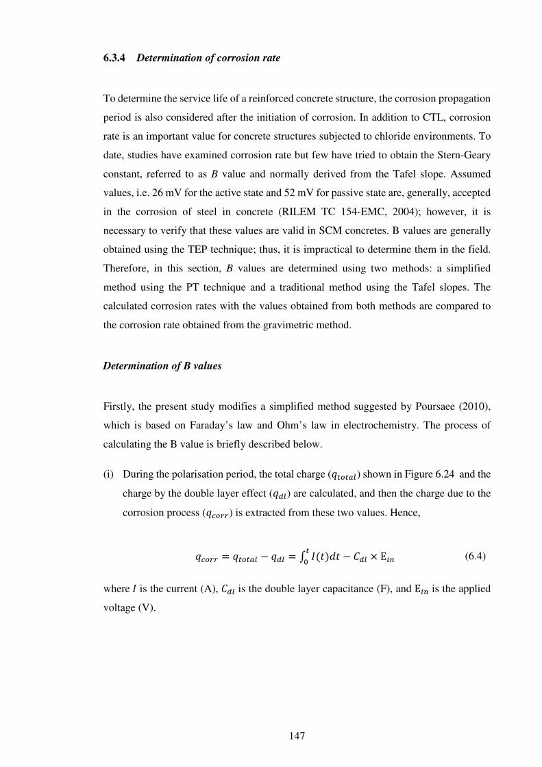
147

6.3.4 Determination of corrosion rate

To determine the service life of a reinforced concrete structure, the corrosion propagation

period is also considered after the initiation of corrosion. In addition to CTL, corrosion

rate is an important value for concrete structures subjected to chloride environments. To

date, studies have examined corrosion rate but few have tried to obtain the Stern-Geary

constant, referred to as B value and normally derived from the Tafel slope. Assumed

values, i.e. 26 mV for the active state and 52 mV for passive state are, generally, accepted

in the corrosion of steel in concrete (RILEM TC 154-EMC, 2004); however, it is

necessary to verify that these values are valid in SCM concretes. B values are generally

obtained using the TEP technique; thus, it is impractical to determine them in the field.

Therefore, in this section, B values are determined using two methods: a simplified

method using the PT technique and a traditional method using the Tafel slopes. The

calculated corrosion rates with the values obtained from both methods are compared to

the corrosion rate obtained from the gravimetric method.

Determination of B values

Firstly, the present study modifies a simplified method suggested by Poursaee (2010),

which is based on Faraday’s law and Ohm’s law in electrochemistry. The process of

calculating the B value is briefly described below.

(i) During the polarisation period, the total charge (åS1S+L) shown in Figure 6.24 and the

charge by the double layer effect (åL) are calculated, and then the charge due to the

corrosion process (å-1QQ) is extracted from these two values. Hence,

å-1QQ = åS1S+L − åL = æ *()S3 − L × E2 (6.4)

where* is the current (A), L is the double layer capacitance (F), and E2 is the applied

voltage (V).

148

Figure 6.24 Schematic showing total charge and charge by double layer.

(ii) Using Faraday’s law, the corrosion rate during the polarisation period is calculated

assuming that corrosion by the polarisation effect is uniform,

mL1nn = å-1QQ × ×

(6.5)

L1nn = mL1nnqnSooL × IoN × × 10 (6.6)

-1QQ = L1nn11.6

(6.7)

where mL1nn is mass loss during the polarisation time, t (year); is the atomic weight of

steel (≈55.85 g/mol); is the number of equivalent exchanged electrons (Fe2+ ≈ 2); is

Faraday’s constant (≈ 96,487 C/mol); L1nn is the penetration depth (mm/year); qnSooL is

the density of the steel used (≈7.83 g/cm3); IoN is exposure area (cm2); and -1QQ is

corrosion rate (mA/cm2).

(iii) To determine the B value, the calculated corrosion rate is divided by the

polarisation resistance:

0 20 40 60 80 100

10

20

30

40

50

60

Consumed charge by double layer

Measured data

Cu

rren

t (µ

Α)

Time (sec)

Total consumed charge

149

t = -1QQ × N (6.8)

wheret is a constant (mV) and N is the polarisation resistance (Ω·cm2).

This process has advantages in determining the B value: the technique is non-destructive

and rapid and the analysis is simple. However, as studies using this method are limited,

an extensive study needs to be performed to verify the method. The Tafel method, on the

other hand, is the traditional method to determine the B value, but the destructive

environment and time taken for the technique have limited the number of studies using it.

In addition, determining the Tafel region remains controversial (McCafferty, 2005). In

the present study, the Tafel slope was determined using the traditional method instead of

using new methods proposed in previous studies (Flitt and Schweinsberg, 2005;

Mansfeld, 2005; Alfaro, 2014). These new methods are still controversial in their

application for reinforced concrete and use complex calculations that are inappropriate

for practical purposes.

It is evident that the B value for steel in concrete has not yet been fully studied, and the

value could be different from the proposed 26 mV or 52 mV. According to a theoretical

analysis by Song (2000), the B value for steel in concrete can range from 8 mV to infinity

depending on the test and steel conditions. As shown in the previous section, polarisation

resistances are similar regardless of the technique; hence, the B value becomes an

additional factor to reduce the difference between the real value and the measured value.

In this study, the B value was calculated using equation (6.4) – (6.8) with data obtained

from the PT technique. This is presented in figure 6.25. The values during the passive

state are distributed between 6.5 and 8.0 mV and the difference in the values over time is

minimal (figure 6.25 (a)). The calculated value is ~7 times lower than the value proposed

in RILEM TC 154-EMC (2004). The difference is directly related to the estimated

corrosion rate, and the B values vary with the conditions of concrete; thereby, it is difficult

to evaluate the corrosion rate accurately. As shown in figure 6.25 (b), the values decrease

to ~ 3 mV after depassivation.

150

Figure 6.25 B values of steel using the PT technique for (a) passive state and (b) active

state with time.

The B value from the Tafel slope was calculated at 382 days and table 6.1 presents the

Tafel slope and the B value with the mix used in this study. Before discussing the B value,

it should be noted that the anodic constant (u+) is significantly higher for the passive state,

so its influence on the B value was first evaluated, as shown in figure 6.26. The B value

increases within the u+ range of 1–10,000 mV/dec, and then attains a stable value for

βa > 10,000 mV/dec; βa is therefore expressed at >10,000 mV/dec using the Tafel

extrapolation technique (table 6.1).

150 200 250 300 350 400

6

7

8

9

CEM I-0.4-Mix-Ave





B (

mV

)

Time (days)

(a) Passive state

200 250 300 350 400

2

4

6

8

10

CEM I-0.6-SS-1

CEM I-0.6-SS-2

CEM I-0.6-SS-3

CEM I-0.6-LS-1

CEM I-0.6-LS-2

CEM I-0.6-LS-3

B (

mV

)

Time (days)

(b) Active state

151

Figure 6.26 Variation in B value with βa (βc =127 mV/dec).

For the passive state, except for CEM I (w/b=0.6) concrete, B values range from 23.6 mV

to 68.7 mV for all samples. Low B values, ranging from 23.6 mV to 37.9 mV, are caused

by fitting error as u+ was calculated from 181.6 to 473.8 mV/dec, which is lower than u+

for the active state. When error values are omitted, B values in the passive state are

distributed in the range of 41.2 – 68.7 mV, which is similar to the proposed value of 52

mV for the passive condition. For the active state, the B values calculated using the TEP

technique should be compared to the B values proposed in the previous study (RILEM

TC 154-EMC, 2004) and the B values calculated using a simplified method in this study.

Considering the calculation process, a reduced u+ by vigorous anodic reaction results in

a decrease in the B value (see figure 6.26), but the B values increased to 96.0 mV. In the

cathodic constant (u-), the difference between active state and passive state is also evident. u- lies within the range of 106.6–158.2 mV/dec for the passive state, while the values lie

within the range of 303.3–357.1 mV/dec for the active state. The increase in cathodic

constant had more influence on the B value than anodic constant in this study. This

implies that the consumption of oxygen on the polarised area is higher than the supply

leading to an increase in the cathodic slope. There are two reasons for lack of oxygen for

cathodic reaction: (i) the concretes were saturated as the measurement was conducted

after the end of the wetting phase, and (ii) the electrochemical reaction in the anode was

faster than in the cathode due to severe corrosion on the steel surface. After depassivation,

the cathodic reaction is a more important factor in the corrosion process.

100

101

102

103

104

105

106

107

0

10

20

30

40

50

60

B (

mV

)

βa (mV/dec)

152

Table 6.1 Parameters obtained from Tafel extrapolation

Sample notation u+(mV/dec) u- (mV/dec) B (mV)

Sample notation u+(mV/dec) u- (mV/dec) B (mV)

Mix Steel type Mix Steel type

CEM I-0.4-

SS-1 2701.4 139.7 57.7

CEM I-0.6-

SS-1 585.9 331.3 91.9

SS-2 > 10,000 130.9 56.8 SS-2 604.6 348.3 96.0

SS-3 292.8 94.2 30.9 SS-3 407.6 303.3 75.5

LS-1 > 10,000 127.1 55.2 LS-1 466.4 357.1 87.9

LS-2 > 10,000 128.8 55.6 LS-2 411.7 336.3 80.4

LS-3 181.6 77.5 23.6 LS-3 443.8 342.8 84.1

CEM III/A-0.4-

SS-1 > 10,000 153.2 66.5

CEM III/A-0.6-

SS-1 > 10,000 121.3 52.6

SS-2 > 10,000 139.6 60.6 SS-2 > 10,000 123.1 53.5

SS-3 > 10,000 135.6 58.9 SS-3 1745.0 117.1 47.7

LS-1 > 10,0000 128.5 55.8 LS-1 873.4 106.6 41.2

LS-2 2599.7 127.3 52.7 LS-2 > 10,000 118.9 51.6

LS-3 > 10,000 132.0 57.3 LS-3 196.9 78.0 24.3

CEM II/B-V-0.4-

SS-1 > 10,000 128.7 55.9

CEM II/B-V-0.6-

SS-1 3651.7 135.0 56.5

SS-2 > 10,000 145.4 63.1 SS-2 > 10,000 158.2 68.7

SS-3 337.4 95.9 32.4 SS-3 473.8 107.1 37.9

LS-1 > 10,000 145.4 63.1 LS-1 > 10,000 140.0 60.8

LS-2 > 10,000 152.7 66.3 LS-2 > 10,000 132.0 57.3

LS-3 616.2 112.4 41.3 LS-3 > 10,000 127.5 55.4

153

Verification of corrosion rate

The corrosion rate (i.e. corrosion density, mA/m2) of steel is important in determining the

service life of concrete structures subjected to chloride-induced corrosion. The most

accurate method to determine the corrosion rate is mass loss of steel. According to

González et al. (1995), the corrosion rate measured by mass loss method is up to 10 times

higher than the rate measured by polarisation techniques when pitting corrosion occurs

on the steel. Nevertheless, it still is necessary to investigate a correction factor between

the mass loss technique and the polarisation technique. To compare the corrosion rates

obtained by these two techniques, it is necessary to define the corrosion rate.

The corrosion rate by mass loss is the time-averaged value during the whole experimental

period, whereas corrosion rates obtained from polarisation techniques represent the

instantaneous corrosion rate. For the purpose of comparison, the polarisation resistance

obtained from polarisation techniques (i.e. LPR, GP, and PT technique) was averaged

with time. In addition, different B values were used to calculate the corrosion rate based

on Ohm’s law, including (i) the B value from the TEP technique, (ii) the B value from

a simplified method, and (iii) a traditional B value. Subsequently, the corrosion rates with

different polarisation techniques and B values were compared with the averaged

corrosion rate obtained from the mass loss method. Note that corrosion rates were only

evaluated for samples in which corrosion occurred, i.e. the CEM I (w/b=0.6) concrete.

The corrosion rate obtained from the mass loss method was calculated using Faraday’s

law (equation (3.9)). The calculated corrosion rate and mass loss data are presented in

table 2.1. The observed corrosion rates are severe except for in CEM I-0.6-SS-3. As noted

above, the corrosion rate obtained from the mass loss method is the average value over

the whole exposure time, and implies that an instantaneous value at 382 days will be

higher than the average value. From visual inspection, cracks were also detected on the

exposure surface of concrete. Hence, severe corrosion, i.e. > 10 mA/m2, can lead to

cracking. Cracking is considered in detail in the visual inspection section (Section 6.3.5).

154

Table 6.2 Corrosion rate of steel in concrete using mass loss method (CEM I, w/b=0.6)

Binder type CEM I-0.6-

Steel type SS-1* LS-1 SS-2 LS-2 SS-3 LS-3

Mass before corrosion (g)

551.23 551.37 551.25 551.22 551.21 551.32

Mass after treatment (g)

550.31 550.40 550.63 550.33 550.94 549.99

Mass loss considering background loss** (g)

0.84 0.89 0.54 0.81 0.19 1.25

icorr (mA/m2)

17.50 12.36 11.25 11.25 4.00 17.36

* steel sample notation: ‘SS’ indicates steel with a small exposure area and ‘LS’ indicates steel

with a large exposure area (see Chapter 4.3), and the number indicates the number of replicates

** Background loss: 0.08g

Table 6.3 Range of corrosion current values (RILEM TC 154-EMC, 2004)

icorr (mA/m2) Vcorr (µm/y) Corrosion level

≤1.0 ≤1.0 Negligible

1.0 – 5.0 1.0 – 5.0 Low

5.0 – 10.0 5.0 – 10.0 Moderate

> 10.0 > 10.0 High

As show in figure 6.27, the shaded part was integrated with time and then divided by the

total exposure time to estimate the averaged corrosion rate. To calculate the corrosion

rate, polarisation resistances obtained from different techniques were used. Different B

values were also used in the calculation; these were estimated from the PT technique, the

TEP technique, and a traditional value (i.e. 26 mV for active state). Before corrosion

measurement, i.e. 0–185 days, the corrosion rate was set as 0 mA/m2. During this period,

all samples, expect for CEM I-0.6-LS-1, were in the passive state, and the integrated

corrosion rate in the passive state is negligible compared to the value in the active state.

For CEM I-0.6-LS-1, the range corresponding to 0 mA/m2 was set based on the corrosion

potential measurement.

155

Figure 6.27 Calculating the averaged corrosion rate from monitoring data.

Figure 6.28 presents a comparison of the corrosion rate obtained by mass loss with the

averaged corrosion rate using the different polarisation techniques and different B values.

Although different polarisation techniques were used, differences in the obtained

polarisation resistances were marginal, as described in figure 6.18 and figure 6.19. When

the B value obtained from the PT technique was used, the corrosion rates were

approximately 5.2– 26.5 times lower than when the mass loss method B value was used.

This is in line with a previous study in which the pitting factor was considered to be 10

(González et al., 1995). Average differences using the Tafel method and traditional value

(26 mV) were ~ 53% and ~ 28%, respectively. The differences were dramatically reduced

compared to using B value obtained from the PT technique. In addition, considering B

values were changed by the corrosion process, the error may be lower. After

depassivation, the B value in the active state increased compared to that in the passive

state in the TEP technique, and the B values obtained by the TEP technique were

calculated at the end of all measurements, i.e. at 382 days. Therefore, it is possible that

the corrosion rates calculated using B values from the TEP technique were overestimated

compared to the real values.

It is noteworthy that the B value was used to determine corrosion rate using the

electrochemical techniques and, depending on the value used in the calculation, the error

could be significant. Thus, further investigation is required to determine the B value.

Although the traditional B values (i.e. 26 mV for active state and 52 mV for passive state)

are reasonable to calculate corrosion rate, it would be more useful to determine the

0 100 200 300 400

0

10

20

30

40

Co

rro

sio

n r

ate

(mA

/m2)

Time (days)

Average value

156

severity of corrosion using the integrated polarisation resistance without the B value, or

using the monitored B value.

Figure 6.28 Comparison of corrosion rate between polarisation techniques and mass

loss.

6.3.5 Visual inspection for corrosion

Electrochemical techniques are non-destructive. Hence, to prove the accumulation of

corrosion products, or severity of corrosion, it was necessary to conduct a visual

inspection. To this end, steels were extracted from the concrete samples and cleaned, and

then the mass loss of steel by corrosion and the formation of pit were investigated using

a digital microscope.

Before crushing the concrete samples containing corroded steels (CEM I concrete,

w/b=0.6), cracks on the exposure surface were detected for the samples. Cracking occurs

because of the volume expansion of corrosion products, which vary depending on their

type (oxide-type rusts or hydroxide-type rusts) as shown in figure 6.29. Although the

chemical compositions of corrosion products were not analysed in this study, the main

product can be deduced as Fe(OH)3 because of the sufficient supply of oxygen during the

wet/dry cyclic regime.

1 10 100

1

10

100

B obtained from TEP

B = 26 mV

PT (B from PT)

GP (B from PT)

LPR (B from PT)

PT (B from TEP)

GP (B from TEP)

LPR (B from TEP)

PT (B=26 mV)

GP (B=26 mV)

LPR (B=26 mV)

Co

rrosi

on

rat

e fr

om

pola

risa

tion

tec

hniq

ue

(mA

/m2)

Corrosion rate from mass loss (mA/m2)

Equal

ity o

f lin

e

B obtained from PT

157

Figure 6.29 Corrosion products of iron (Köliö et al. 2015).

As shown in figure 6.30, the position of visual cracking on the surface coincided with the

corroded area on the steel, indicating that cracking started from the steel depth and was

caused by an expansion of corrosion products. In addition, green rust was found in the

corrosion products, in particular for steel in CEM I-0.6-SS/LS-3, and it is known that the

green colour in this rust results from chlorides (Koleva et al. 2006). No corrosion was

detected on the opposite side of the corroded area on the steel; in other words, corrosion

was generated at the steel surface close to the exposed concrete surface. The time is shown

in table 6.4 when visual cracks on the concrete surface were observed. In summary, the

passive film was destroyed when chlorides reached the steel depth, and the corrosion

products formed through electrochemical reaction to cause cracking and spalling of the

concrete. It was also observed that corrosion distribution was localised instead of uniform,

which is indicative of pitting corrosion.

Table 6.4 Time to visual cracks on the surface of CEM I (w/b=0.6) concrete

Concrete type CEM I-0.6-

Steel type-replication No. SS-1 LS-1 SS-2 LS-2 SS-3 LS-3

Time to visual cracking (days) 312 321 369 382 N.D. 327

* N.D. = No detection

158

(a) CEM I-0.6-LS/SS-1

(b) CEM I -0.6-LS/SS-2

(c) CEM I -0.6-LS/SS-3

Figure 6.30 Crack patterns on the concrete surface and corroded steels (‘LS’ on left side

and ‘SS’ on right side) extracted from samples for CEM I (w/b=0.6) concretes.

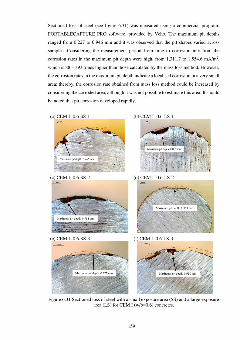
159

Sectioned loss of steel (see figure 6.31) was measured using a commercial program:

PORTABLECAPTURE PRO software, provided by Veho. The maximum pit depths

ranged from 0.227 to 0.946 mm and it was observed that the pit shapes varied across

samples. Considering the measurement period from time to corrosion initiation, the

corrosion rates in the maximum pit depth were high, from 1,311.7 to 1,554.6 mA/m2,

which is 88 – 393 times higher than those calculated by the mass loss method. However,

the corrosion rates in the maximum pit depth indicate a localised corrosion in a very small

area; thereby, the corrosion rate obtained from mass loss method could be increased by

considering the corroded area, although it was not possible to estimate this area. It should

be noted that pit corrosion developed rapidly.

(a) CEM I -0.6-SS-1 (b) CEM I -0.6-LS-1

(c) CEM I -0.6-SS-2 (d) CEM I -0.6-LS-2

(e) CEM I -0.6-SS-3 (f) CEM I -0.6-LS-3

Figure 6.31 Sectioned loss of steel with a small exposure area (SS) and a large exposure area (LS) for CEM I (w/b=0.6) concretes.

160

6.3.6 Determination of time to corrosion initiation

Various corrosion monitoring techniques have been developed, and some have been used

commercially (Nygaard 2008). However, as described above, it is difficult to quantify

corrosion rate, especially for pitting corrosion. In this section, time to corrosion initiation

for CEM I (w/b = 0.6) concretes is briefly evaluated with the techniques used in this study

including the half-cell potential, macrocell current and polarisation techniques.

For the half-cell potential measurement, the measured potential is used to determine the

corrosion state of the steel. The presence of corrosion is determined when a dramatic

decrease in the potential is observed instead of an absolute value. Second, macrocell

current is measured directly by a zero-resistance ammeter or multi-meter combined with

a specific resistor. The measured current increases abruptly when corrosion is detected.

Third, the polarisation resistance obtained using electrochemical techniques is

considerably reduced in the active state of steel compared to in the passive state. Finally,

in the EIS technique, the presence of two distinct semi-circles in the Nyquist plot indicates

corrosion on the steel surface.

The time to corrosion initiation is presented in Table 6.5. Corrosion initiation time using

the EIS technique was excluded as the time interval between each measurement was large.

Times to corrosion initiation are slightly different. One reason for this difference is the

different measurement cycles, i.e. the end of every wet (6-days) /dry (8-days) cycle for

the macrocell current and half-cell potential techniques (every ~ 1 week), and the end of

every wet cycle for the polarisation technique (every 2 weeks). It is interesting that for

CEM I-0.6-SS-1, corrosion potential rebounded after corrosion potential dropped and for

CEM I-0.6-SS-1 and CEM I-0.6-SS-2, macrocell currents were opposite. This is

considered as the repassivation of the steel (Ann et al., 2010); thereby the interpretation

to determine time to corrosion initiation with half-cell potential and macrocell current

requires caution. In other words, according to ASTM C876 (ASTM International, 2015),

the possibility of corrosion under -350 mV vs CSE is 90%; hence, even though the

corrosion potential drops, no corrosion can be detected. Thus, all measurements are

adequate to detect corrosion, but the detecting times vary depending on the technique due

to influencing factors, including the detecting method and the condition of material.

To reduce the error, it is suggested that more than one technique be used to detect

corrosion, and continuous monitoring is more effective than a one-off measurement.

161

Table 6.5 Time to corrosion initiation (in days) for CEM I (w/b = 0.6) concrete using

different techniques

Concrete type CEM I-0.6-

Steel type-replication No. SS-1 LS-1 SS-2 LS-2 SS-3 LS-3

Macrocell current technique

194 172 222 270 320 194

Polarisation techniques 200 N.D.* 228 270 326 200

Half-cell potential 191 171 223 269 317 192

* N.D. = not determined due to corrosion presence when measurement was carried out

6.4 Summary

This section evaluated steel corrosion in concrete subjected to a simulated chloride

environment. A range of techniques were used, including non-destructive and destructive

techniques. During the experimental period, the corrosion of steel was only detected for

CEM I (w/b=0.6) concretes. A summary of the findings follows.

• Electrochemical parameters, i.e. ohmic resistance, polarisation resistance,

capacitance, corrosion potential and time constant, differed across techniques,

type of binder, condition of material and exposure duration. Error with the

techniques was marginal, while the B value was sensitive in determining the

corrosion rate. To improve the accuracy of evaluation of the corrosion rate,

the B value must be set accurately. Hence, this value should be further

investigated.

• To determine the corrosion state of steel, the half-cell potential, macrocell

current and mass loss techniques are easier than the polarisation techniques,

but both half-cell potential and macrocell current techniques are qualitative,

and the mass loss technique is destructive. The EIS technique is sophisticated

but interpretation requires expert knowledge and the measurement is sensitive

to experimental conditions. The TEP technique is destructive and time-

consuming, although it can be used to estimate the B value. The PT technique

is rapid and less destructive than other DC techniques, but during analysis, the

capacitance value cannot be extracted directly, leading to an error in

estimating the polarisation resistance. Finally, the LPR technique is

162

convenient, but it cannot evaluate ohmic resistance. Therefore, among the

techniques used in this study, the GP technique is the most practical to

evaluate corrosion of steel due to its rapid response and easy analysis

• The corrosion rates with different B values were compared with the corrosion

rate from the mass loss method. According to González et al. (1995), for

chloride-induced corrosion, the corrosion rate obtained from the mass loss

method is 10 times higher than that obtained from the polarisation technique.

However, in this study, the difference was sensitive to B values. The

difference in corrosion rate between non-destructive methods and destructive

methods using the B value obtained from the TEP technique and a traditional

value (=26 mV) were ~ 53% and ~ 28%, respectively. On the other hand, the

corrosion rates using the B value obtained from the PT technique were 6.3-

15.6 times lower than the rates from the mass loss method.

• From the visual inspection, cracking on the concrete surface was observed.

This was caused by chloride-induced corrosion. This cracking happened

within a short time after depassivation in this study. Hence, it is reasonable to

determine the limit state of concrete structures in marine environments with

time to corrosion. In addition, it would be more appropriate to set the

propagation period as a fixed value, such as LIFE 365 (Ehlen 2012), instead

of calculating the value using computational modelling in terms of practical

application as corrosion rate is influenced by a wide range of factors that

cannot be controlled.

163

CHAPTER 7

MONITORING THE ELECTRICAL RESISTANCE OF CONCRETE

7.1 Introduction

The service life of reinforced concrete is determined by the performance of the concrete

cover-zone as the latter plays an important role in preventing the ingress of aggressive

agents. Steel corrosion caused by chloride attack is the main concern in evaluating

durability and performance of reinforced concretes. The deterioration rate, including the

rate of chloride ingress and the corrosion propagation rate, is influenced by the

permeation properties of the cover concrete. Although the laboratory methods for chloride

transport and estimating corrosion of steel have been developed, it is difficult to fully use

these methods for field concrete due to limitations such as environmental exposure

conditions, workmanship and material properties. Chloride profiling and half-cell

potential mapping are laborious, and one-off investigations are therefore usually carried

out. However, these investigations are limited in covering various influencing factors

because of environmental exposure conditions.

To overcome these limitations, it is necessary to monitor the concrete cover-zone

(covercrete) to study concrete under a range of exposure conditions over an extended

period (McCarter et al., 2001, 2005). For example, Schieβl’s ladder system can be used

to detect corrosion of steel at discrete points within cover concrete (McCarter and

Vennesland, 2004), but water, ionic and moisture movement are not detected with this

system. Alternatively, electrical resistance measurements, using embedded electrode

arrays (McCarter et al., 2001, 2005) or multi-ring electrodes (Du Plooy et al., 2013), can

monitor moisture and ionic movement, but their interpretation requires caution since the

measured values contain various effects such as a change in chloride content, a change in

degree of saturation and a change in temperature.

This Chapter monitors the electrical resistance of the concrete within the covercrete and

on the steel surface to study chloride movement and corrosion propagation.

164

7.2 Experimental

The sample and electrode details used in this study are presented in Chapter 4. Embedded

electrode arrangements can have limitations. The electrode arrangement could cause

interference with the natural distribution of the aggregate even though the electrode tip

was enough large (> maximum aggregate size). When the aggregate (a non-conductive

material) was congested between electrodes, the measured resistance could be

significantly larger compared to the original resistivity of concrete. In addition,

calibration is required to calculate electrical resistivity when using this method as the

electrical field between electrodes is non-uniform. Thus, the resistivity, which is

independent of electrode geometry, could not be calculated with equation (2.21) but was,

instead, determined using a geometrical factor obtained from an empirical relation

(McCarter et al., 2013a) or computation model (Angst et al., 2011c). Nevertheless, this

method is attractive. After installation of the electrodes in concrete structures, the

measurement can be continuously monitored without considering the service life of the

electrode.

Figure 7.1 Distribution of aggregate around electrodes.

7.2.1 Experimental set-up

Electrical resistance measurements were manually taken using an LCR meter (Hewlet

Packard 4263B) with a signal amplitude of 350 mV at 1 kHz. These values were used to

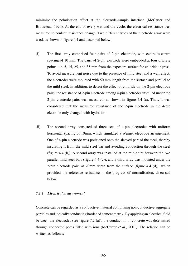
165

minimise the polarisation effect at the electrode-sample interface (McCarter and

Brousseau, 1990). At the end of every wet and dry cycle, the electrical resistance was

measured to confirm resistance change. Two different types of the electrode array were

used, as shown in figure 4.4 and described below:

(i) The first array comprised four pairs of 2-pin electrode, with centre-to-centre

spacing of 10 mm. The pairs of 2-pin electrode were embedded at four discrete

points, i.e. 5, 15, 25, and 35 mm from the exposure surface for chloride ingress.

To avoid measurement noise due to the presence of mild steel and a wall effect,

the electrodes were mounted with 50 mm length from the surface and parallel to

the mild steel. In addition, to detect the effect of chloride on the 2-pin electrode

pairs, the resistance of 2-pin electrode among 4-pin electrodes installed under the

2-pin electrode pairs was measured, as shown in figure 4.4 (a). Thus, it was

considered that the measured resistance of the 2-pin electrode in the 4-pin

electrode only changed with hydration.

(ii) The second array consisted of three sets of 4-pin electrodes with uniform

horizontal spacing of 10mm, which simulated a Wenner electrode arrangement.

One of 4-pin electrode was positioned onto the sleeved part of the steel, thereby

insulating it from the mild steel bar and avoiding conduction through the steel

(figure 4.4 (b)). A second array was installed at the mid-point between the two

parallel mild steel bars (figure 4.4 (c)), and a third array was mounted under the

2-pin electrode pairs at 70mm depth from the surface (figure 4.4 (d)), which

provided the reference resistance in the progress of normalisation, discussed

below.

7.2.2 Electrical measurement

Concrete can be regarded as a conductive material comprising non-conductive aggregate

particles and ionically conducting hardened cement matrix. By applying an electrical field

between the electrodes (see figure 7.2 (a)), the conduction of concrete was determined

through connected pores filled with ions (McCarter et al., 2001). The relation can be

written as follows:

166

H KLM = HN çUQ∅

(7.1)

where H KLM is the resistivity of bulk concrete (Ω·m), HN is the resistivity by ionic

concentration in the pore solution (Ω·m),ç is the tortuosity of the capillary pores between

a pair of electrodes, UQis the saturation degree of the pore and ∅ is the porosity.

According to the above equation, the resistance of concrete is influenced by pore

structure, degree of saturation and chemistry of the pore solution. In other words, the

resistance of concrete decreases due to the ingress of ions (chlorides) or an increase in

moisture content, while resistance increases due to hydration, a reduction in moisture

content due to drying and refinement of the pore by chemical reaction between cement

hydrates and ions dissolved in the pore solution, e.g. the formation of Fridel’s salt.

Figure 7.2 (a) Schematic diagram showing conduction in concrete and (b) a three-phase

model for concrete (adapted from McCarter et al. (2001)).

The electrical resistance is influenced by various factors simultaneously; hence, it is easier

to analyse data with the expression of the resistance (or resistivity) with normalisation

than the absolute method. This expression can control the measured values with a

controlled parameters, but is qualitative. The relative value is expressed by the reference

value, as follows:

OR RSRQo

(7.2)

167

where OR is the normalised resistance, and RS and RQ are the measured resistances (Ω) at

time, t, and reference time, r.

In this study, the entire process of chloride-induced corrosion in reinforced concrete was

investigated with electrical resistance measurement. The resistance monitoring data were

analysed with influencing factors including moisture movement, chloride-content and

ionic movement caused by corrosion. The results are presented in the following sections.


Electrical resistance is sensitive to concrete properties or conditions, as shown in equation

7.1. Under well-controlled conditions (laboratory conditions), electrical resistance is

measured with a controlled parameter, but in the field, it is combined with all influencing

factors. For practical purposes, it is necessary to investigate the analysis method for the

electrical resistance of concrete. This study monitored the electrical resistance of concrete

subjected to a simulated chloride environment.

7.3.1 Electrical resistance monitoring

Electrical resistance is increasingly garnering interest from engineers and researcher

because it is an easy and rapid method. However, the data analysis is still difficult for the

following reasons: (i) the value fluctuates with temperature; (ii) the value is sensitive to

moisture content, and (iii) the value is affected by hydration or chemical reactions in

concrete. Therefore, in this study these factors are considered or offset to improve the

analysis.

As-measured electrical resistance

Figure 7.3 and 7.4 present examples of as-measured data for the different electrode

arrangements. Figure 7.3 shows that at 5 mm depth, the electrical resistance fluctuated

significantly with time compared to other depths. The main reason is the changing

moisture content in this region. Differences in the resistance between the end of the

wetting phase and the end of the drying phase within a cycle were irregular as, in addition

168

to moisture-content, influencing factors such as temperature, refinement of the pores and

chlorides in the pore solution affected the results.

Figure 7.3 Example of monitoring electrical resistance with 2-pin electrode

arrangements (for CEM I concrete, w/b=0.4).

This study also included 4-pin electrode measurements. To this end, the equation referred

to as a modified Wenner equation (equation (7.3)) can be used to convert the measured

resistance into resistivity, which is independent of geometry. However, the theoretical

background for the assumption of the equation are not perfectly valid (Angst and Elsener,

2014). Figure 7.4 presents the electrical resistivity using the 4-pin electrode measurement.

All values increased continuously with depth, and the oscillation of the resistivity

resulting from the wet/dry cyclic regime was minimal. This implies that a reduction in

moisture content by drying or a sudden inflow of chloride by capillary sorption, especially

at steel depth (25 mm depth), is marginal. Note that as-measured resistance is also

required to quantify concrete properties.

H 4πaR (7.3)

where H is the resistivity (Ω·m), R is the resistance (Ω) and a is the electrode spacing (m).

0 100 200 300 400

0

2

4

6

8

5 mm

15 mm

25 mm

35 mm

Res

ista

nce

(k

Ω)

Time (days)

Start a wet/dry cyclic regime with chloride solution

Dry

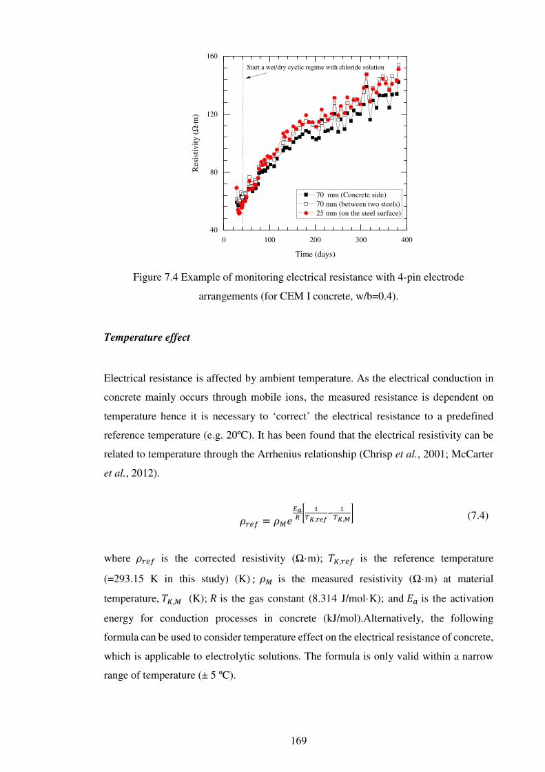
169

Figure 7.4 Example of monitoring electrical resistance with 4-pin electrode

arrangements (for CEM I concrete, w/b=0.4).

Temperature effect

Electrical resistance is affected by ambient temperature. As the electrical conduction in

concrete mainly occurs through mobile ions, the measured resistance is dependent on

temperature hence it is necessary to ‘correct’ the electrical resistance to a predefined

reference temperature (e.g. 20ºC). It has been found that the electrical resistivity can be

related to temperature through the Arrhenius relationship (Chrisp et al., 2001; McCarter

et al., 2012).

HQo Hé<êcë Y

ìí,e_@Y

ìí,î

(7.4)

where HQo is the corrected resistivity (Ω·m); ï,Qo is the reference temperature

(=293.15 K in this study) (K) ; Hé is the measured resistivity (Ω·m) at material

temperature,ï,é (K); is the gas constant (8.314 J/mol·K); and y+ is the activation

energy for conduction processes in concrete (kJ/mol).Alternatively, the following

formula can be used to consider temperature effect on the electrical resistance of concrete,

which is applicable to electrolytic solutions. The formula is only valid within a narrow

range of temperature (± 5 ºC).

0 100 200 300 400

40

80

120

160

Start a wet/dry cyclic regime with chloride solution

70 mm (Concrete side)

70 mm (between two steels)

25 mm (on the steel surface)

Res

isti

vit

y (

Ω⋅m

)

Time (days)

170

In this study, equation (7.5) was used to reflect the effect of temperature for laboratory

samples. The α value (the temperature coefficient) for concrete, irrespective of type of

binder and w/b, was taken as 0.035 ºC-1 following McCarter et al. (2005). This was done

because (i) there is a dearth of information on the activation energy for concrete mixes,

(ii) the temperature fluctuation is narrow in laboratory conditions, and (iii) the change in

the electrical resistance by temperature is marginal compared to other effects.

HQo Héð1 + º(,é − ,Qo)ñ (7.5)

Where ,é or ,Qo is the material temperature or the reference temperature (ºC), º is

the temperature coefficient (ºC-1).

The values measured by the thermistor were converted into ‘Celsius degree’ using

equation (7.6), are presented in figure 7.5 (McCarter et al., 2012). The temperature in the

laboratory fluctuated within a narrow range (~ 19 – 23ºC). Thus, the influence of

temperature on resistance was negligible. However, with larger fluctuations of

temperature in field conditions, temperature correction must be considered. As shown in

figure 7.5, the trend line for the resistance becomes smoother after correction of the

resistance with the temperature coefficient. Note that all electrical resistance presented in

this study were corrected to a reference temperature of 20 ºC.

7a + b56R + c(56R)§;@ − 273.15 (7.6)

where R is the measured resistance by the thermistor (Ω); is temperature (ºC); and a, b,

and c are coefficients depending on the type of thermistor accounting for 1.28×10-3,

2.36×10-4, and 9.31×10-8 K-1, respectively.

Convective effect

Under a wet/dry cyclic regime (e.g. tidal action), drying involves moisture movement

from inside the concrete to the exposed surface, thereby creating a moisture gradient,

while aggressive ions additionally/rapidly penetrate into concrete during wetting. The

region influenced by the wet/dry phase has been termed ‘the convective zone’, and it is

generally considered that the transport mechanism within this zone is different from that

of concrete have a stable moisture condition.

171

Figure 7.5 Correction of electrical resistance for temperature and monitoring the

temperature of concrete using a thermistor embedded in concrete at 25 mm of cover

depth (CEM I concrete, w/b=0.4).

For example, in the tidal-zone of marine structures, a successive supply of chlorides by

wetting occurs, along with evaporation and salt crystallisation by drying. Seawater

absorption within the convective zone leads to rapid chloride ingress. Therefore, it is

necessary to confirm the convective zone of concrete subjected to a wet/dry cyclic regime.

As both the transport mechanism and the electrical resistance of concrete depend on

degree of saturation, this study used a change in electrical resistance to evaluate the

convective zone in which absorption dominates as transport mechanism.

The convective zone can be defined as a change in the electrical resistance of concrete

subjected to a wet/dry cyclic regime. Within the convective zone, it can be observed that

the electrical resistance changes with the wet/dry phase as the degree of saturation

changes. This is quantified as:

o RòóTR&±ô

(7.7)

where o is the electrical resistance ratio and RòóT and R&±ô are the electrical resistance

after the end of wetting (6 days) and drying (8 days) within one cycle, respectively.

0 100 200 300 400

0

1

2

3

4

5

As-measured resistance

Corrected resistance at 20 °C

Temperature

Time (days)

Ele

ctri

cal

resi

stan

ce a

t 2

5 m

m c

ov

er d

epth

(k

Ω)

14

16

18

20

22

24

Tem

per

atu

re a

t 2

5 m

m c

ov

er d

epth

(°C

)

172

Figure 7.6 shows r with depth. A value close to 1.0 indicates that degree of saturation was

stable even though the surface of concrete was subjected to a wet/dry cyclic regime; a

value lower than 1.0 occurs within the convective zone as the electrical resistance

increased due to drying. Note that some values were measured with more than 1.0. These

values are considered to reflect either an increase in resistance due to the hydration

process during wetting or a minor error during measurement.

The convective zone was found to be well-formed with an increase in w/b. For example,

the r at 15 mm was close to 1.0 for concretes with w/b =0.4 regardless of type of binder,

while the ratios for CEM III/A (w/b=0.6) concrete and CEM II/B-V (w/b=0.6) concrete

were close to 1.0 at 25 mm of cover depth. All values for CEM I (w/b=0.6) concrete were

less than 1.0 at all depths. This is because the pore structure in concretes with high w/b

have an increased connectivity as well as a high porosity; thereby, an increase in w/b

results in a rapid ingress of aggressive ions in concrete.

It was also observed that the convective zone changed with time, especially for CEM II/B-

V concrete. This result is similar to that of a previous study (Chrisp et al., 2002). For CEM

II/B-V concrete, irrespective of w/b, the convective zone was reduced with increasing

wet/dry cycles due to on-going hydration and pozzolanic reaction. For CEM I and CEM

III/A concretes, the change in the convective zone with time was relatively small due to

rapid hydration compared to CEM II/B-V concrete. Finally, the convective zones for CEM

II/B-V (w/b=0.6) concrete and CEM III/A (w/b=0.6) concrete decreased with exposure

duration, while the reduction was not observed in CEM I (w/b=0.6) concrete.

The convective zone can be estimated with electrical resistance profiling using small cube

samples and chloride profiling (see Sections 5.3.2 and 5.3.3). The estimated convective

zones for all samples were within 30 mm using bulk resistance measurements. The

convective zones were formed within < 6 mm depth in some samples, corresponding to

CEM II/B-V (w/b=0.4 and 0.6) concretes and CEM III/A (w/b=0.6) concrete; however, the

convective zones obtained in this study (Section 7.3.1) were < 15 mm for all (w/b=0.4)

concretes, < 25 mm for CEM III/A (w/b=0.6) and CEM II/B-V (w/b=0.6) concretes, and >

35 mm for CEM I (w/b=0.6) concrete due to large depths in the cube samples. From the

chloride profiling results (Section 5.3.3), it was difficult to determine the convective zone.

On the other hand, the presence of the convective zone indicates that different transport

mechanisms, i.e. absorption and diffusion, coexist in concrete. Thus, the governing

equation for complex transport mechanisms in the computational modelling becomes

173

complex compared to a governing equation for single transport mechanism. In other words,

using a single value for transport rate is easier than using multiple values. In addition, there

is no reference (e.g. the critical degree of saturation) to determine the boundary depending

on the transport mechanism although this is beyond the scope of the present investigation.

Figure 7.6 Convective effect with concrete having (a) w/b=0.4 and (b) w/b=0.6 at end of

initial cycle (49 and 54 days) and at end of final cycle (376and 382 days).

Hydration process

The electrical resistance generally increases with time as the hydration process leads to

refined pore structure. The hydration effect on the electrical resistance is high in early age

0 10 20 30 40

0.0

0.5

1.0

1.5

CEM I (Initial cycle)

CEM III/A (Initial cycle)

CEM II/B-V (Initial cycle)

CEM I (Final cycle)

CEM III/A (Final cycle)

CEM II/B-V (Final cycle)

r e (=

Rw

et/R

dry

)

Depth (mm)

(a) w/b=0.4

15 mm

0 10 20 30 40

0.0

0.5

1.0

1.5

CEM I (Initial cycle)

CEM III/A (Initial cycle)

CEM II/B-V (Initial cycle)

CEM I (Final cycle)

CEM III/A (Final cycle)

CEM II/B-V (Final cycle)

r e (=

Rw

et/R

dry

)

Depth (mm)

(b) w/b=0.6

25 mm

174

and for SCMs, the effect has been observed to last for 300 days (McCarter et al., 2013a).

To describe the deterioration process (e.g. chloride transport or corrosion) using the

electrical resistance, a change of electrical resistance is considered due to hydration. It

has been reported that the electrical resistivity continuously increases even though the

sample is exposed to a solution of chlorides (Polder and Peelen, 2002; McPolin et al.,

2005). Consequently, it is difficult to understand the deterioration of reinforced concrete

by chloride ingress without considering the hydration process and its influence on

electrical resistivity.

To consider the effect of hydration on electrical resistance, the latter was monitored at

70 mm using a 2-pin electrode measurement. For comparison, the normalised values (OR) are presented with type of binder and w/b in equation (7.8):

OR RTR±óõ

(7.8)

where RT is the electrical resistance at time (t days) and R±óõ is the reference electrical

resistance at 42 days.

Figure 7.7 presents OR at 70 mm depth. It could be observed that the normalised resistances

for most samples increased with time, except for CEM I (w/b=0.6) concrete. However, the

increments evidently differed with type of binder, in particular for CEM II/B-V concrete.

Firstly, the resistances for all CEM II/B-V concretes were up to 15 times higher at 382 days

than at 42 days. This large and continuous increase was due to pozzolanic reaction and the

hydration was continuous even after 382-days. Although the increments for CEM I and

CEM III/A concretes were moderate, the increasing trend was similar to CEM II/B-V

concrete; thereby the ongoing hydration could lead to a continuous chloride binding

physically, especially at the surface of concrete due to the additional formation of hydrates

(e.g. C-S-H gel). In other words, chloride binding is considered to be continuous until

completion of hydration rather than an instant chemical reaction. Hence, it can be explained

that a build-up of chloride at the surface was caused by ongoing hydration. On the other

hand, for CEM I (w/b = 0.6) concrete, the electrical resistance increased until ~ 250 days,

and became stable. This indicates that hydration is almost complete after 250 days

considering chloride content and moisture movement at 70 mm. Thus, it can be confirmed

that the hydration period is significantly influenced by w/b and type of binder.

175

Figure 7.7 Normalised resistance of concrete with (a) w/b = 0.4 and (b) w/b = 0.6 at

70mm cover depth.

7.3.2 Chloride transport monitoring

Chloride itself does not deteriorate concrete, but the performance of concrete structures

is degraded when free chlorides reach the steel depth. Thus, it is clearly important to

detect, or monitor, the movement of chloride to determine the service life of concrete

structures. In this sense, many studies have been conducted to determine the CTL on the

steel surface (Alonso et al., 2000; Nygaard and Geiker, 2005; Meira et al., 2014) or to

quantify the chloride transport rate (Nokken et al., 2006; Safehian and Ramezanianpour,

2015; Kim et al., 2016). Determining chloride content in the field (e.g. chloride profiling)

is destructive and time-consuming (Andrade et al., 2014). Laboratory data on chloride

0 100 200 300 400

0

5

10

15

CEM I

CEM III/A

CEM II/B-V

NR a

t 7

0 m

m c

ov

er d

epth

Time (days)

(a) w/b=0.4

0 100 200 300 400

0

5

10

15

CEM I

CEM III/A

CEM II/B-V

NR a

t 7

0 m

m c

ov

er d

epth

Time (days)

(b) w/b=0.6

176

transport has relied on using accelerated methods such as NT Build 492; however, these

data are limited in their reflection of realistic environments such as unsaturated conditions

or temperature variations. In the present study, chloride movement in concrete was

monitored by monitoring changes in electrical resistance.

As presented in equation (7.9), the electrical resistance of concrete is related to the

resistance of the pore solution, degree of saturation and pore structure. However, it is

difficult to measure the resistance of the pore solution and tortuosity. Therefore, the

normalisation method is applied to simplify the interpretation and is beneficial because

the geometry factor is not considered.

RT HN,S JçSI∅SUQ,S

(7.9)

where S is the electrical resistance of concrete, HN,S is the electrical resistivity of the pore

solution, I is the electrode area, J is the length between electrodes, UQ,S is the degree of

saturation, çS is the tortuosity and ∅S is the porosity at the measurement time, t.

The electrical resistance changes depending on the pore-structure, pore solution and

moisture-content with time (equation (7.10)). However, the value corresponding to each

variable cannot be easily separated from the data in the case of chloride-contaminated

concrete, as chlorides dissolved in the pore solution decrease electrical resistance while

bound chlorides increase the resistance due to densification of the pore structure (Andrade

et al., 2011). On the other hand, considering that main variables affecting the electrical

resistance are chloride and hydration and the degree of saturation is stable (Oöe = 1), these

variables can be substituted by: hydration (= O÷p) and the chloride effect (= OL).

OR RTR±óõ HN,SHN,Qo

∅QoUQ,QoçS∅SUQ,SçQo OP ∙ Oø ∙ Nöe ∙ Nú

(7.10)

OR O-L ∙ O÷p (7.11)

where OP is the normalised resistivity for pore solution, Oø is the normalised porosity,

Nöe is the normalised degree of saturation and Nú is the normalised tortuosity.

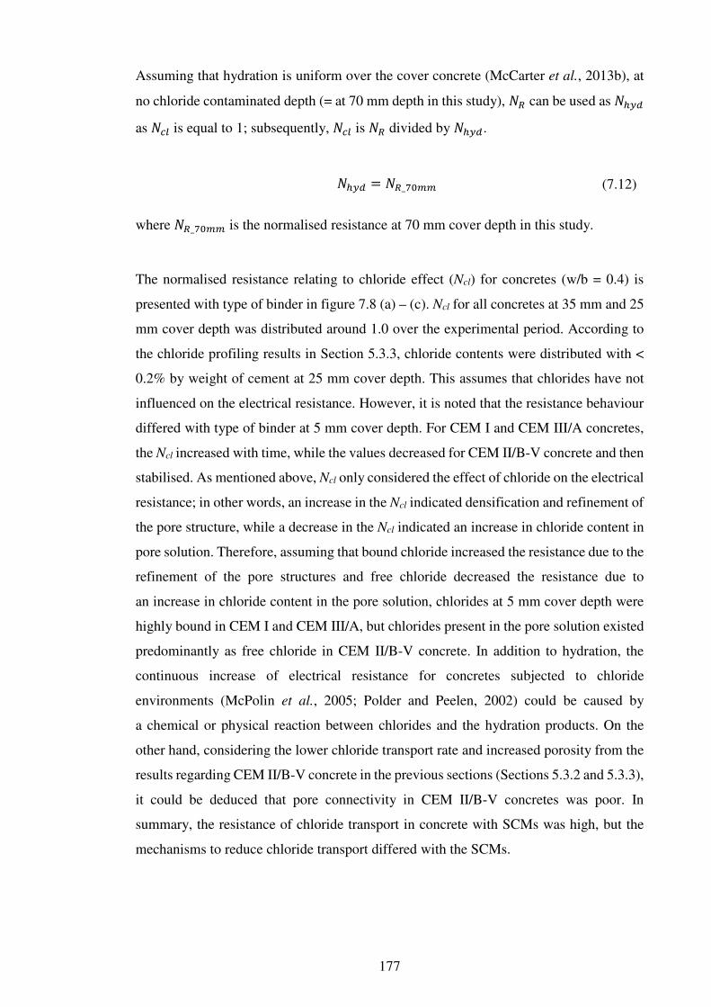
177

Assuming that hydration is uniform over the cover concrete (McCarter et al., 2013b), at

no chloride contaminated depth (= at 70 mm depth in this study), OR can be used as O÷p

as O-L is equal to 1; subsequently, O-L is OR divided by O÷p.

O÷p OR_û3 (7.12)

where OR_û3 is the normalised resistance at 70 mm cover depth in this study.

The normalised resistance relating to chloride effect (Ncl) for concretes (w/b = 0.4) is

presented with type of binder in figure 7.8 (a) – (c). Ncl for all concretes at 35 mm and 25

mm cover depth was distributed around 1.0 over the experimental period. According to

the chloride profiling results in Section 5.3.3, chloride contents were distributed with <

0.2% by weight of cement at 25 mm cover depth. This assumes that chlorides have not

influenced on the electrical resistance. However, it is noted that the resistance behaviour

differed with type of binder at 5 mm cover depth. For CEM I and CEM III/A concretes,

the Ncl increased with time, while the values decreased for CEM II/B-V concrete and then

stabilised. As mentioned above, Ncl only considered the effect of chloride on the electrical

resistance; in other words, an increase in the Ncl indicated densification and refinement of

the pore structure, while a decrease in the Ncl indicated an increase in chloride content in

pore solution. Therefore, assuming that bound chloride increased the resistance due to the

refinement of the pore structures and free chloride decreased the resistance due to

an increase in chloride content in the pore solution, chlorides at 5 mm cover depth were

highly bound in CEM I and CEM III/A, but chlorides present in the pore solution existed

predominantly as free chloride in CEM II/B-V concrete. In addition to hydration, the

continuous increase of electrical resistance for concretes subjected to chloride

environments (McPolin et al., 2005; Polder and Peelen, 2002) could be caused by

a chemical or physical reaction between chlorides and the hydration products. On the

other hand, considering the lower chloride transport rate and increased porosity from the

results regarding CEM II/B-V concrete in the previous sections (Sections 5.3.2 and 5.3.3),

it could be deduced that pore connectivity in CEM II/B-V concretes was poor. In

summary, the resistance of chloride transport in concrete with SCMs was high, but the

mechanisms to reduce chloride transport differed with the SCMs.

178

Figure 7.8 Normalised resistance of concrete (w/b=0.4) considering chloride effects for

(a) CEM I, (b) CEM III/A, and (c) CEM II/B-V concretes using 2-pin electrode

arrangement.

0 100 200 300 400

0.5

1.0

1.5

2.0

2.5

5 mm

15 mm

25 mm

35 mm

Ncl

Time (days)

(a) CEM I (w/b=0.4)

0 100 200 300 400

0.5

1.0

1.5

2.0

2.5

5 mm

15 mm

25 mm

35 mm

Ncl

Time (days)

(b) CEM III/A (w/b=0.4)

0 100 200 300 400

0.0

0.5

1.0

1.5

5 mm

15 mm

25 mm

35 mm

Ncl

Time (days)

(c) CEM II/B-V (w/b=0.4)

179

Figure 7.9 shows the normalised resistance (Ncl) of concrete with a high w/b (=0.6). First,

in CEM I and CEM II/B-V concretes (w/b=0.6), all values were lower than 1.0

irrespective of cover depth. Furthermore, the greater the depth of the measurement, the

higher the value of Ncl. This is also related to free chloride content. At 25 mm and 35 mm

cover depth, chloride in CEM I (w/b = 0.6) concretes was detected after ~70 days, while

CEM II/B-V (w/b = 0.6) concretes were influenced by chlorides across all depths from

initial exposure time. This is because slower hydration in CEM II/B-V concrete leads to

rapid ingress of chloride at an early age. Pozzolanic reaction reduces further penetration

or accumulation of chloride at the depth as the Ncl became stable after ~ 130 days, i.e. the

normalised resistances decreased during the initial period and then stabilised. Considering

that surface chloride content increases with exposure time, stabilization can indicate that

equilibrium was established between chloride binding rate and chloride ingress from the

external source.

For CEM III/A (w/b=0.6) concrete, the value decreased due to free chlorides starting from

256 days at 15 mm depth, while the value at 25 mm depth slightly increased from 242

days. The opposite detection was observed. The electrical resistance measured was an

averaged value corresponding to a nominal depth ± 5 mm (Chrisp et al., 2002) and the

change in Ncl indicated that chloride was detected by both electrodes at 15 mm and 25

mm cover depth. Starting from 256 days, free chloride was dominant at 15 mm, while at

25 mm bound chloride was dominant from 242 days. This explains that chloride binding

is dependent on chloride concentration. The value at 35 mm cover depth remained at

~ 1.0 during the measurement due to lack of chloride ingress.

As can be seen in figures 7.8 and 7.9, different behaviour of chlorides were observed in

concrete with the influence of the w/b and type of binder. Free chlorides dissolved in the

pore solution penetrate into the concrete, leading to a reduction of electrical resistance

due to an increase in ionic content of the pore solution. Bound chlorides are not available

for conduction and result in an increase in electrical resistance. For chemical binding,

chlorides react with calcium aluminate hydrates including monosulfate hydrates (AFm:

C3A·CaSO4·12H2O); Friedel’s salt is then formed by ionic exchange of SO42- with Cl-

(Hirao et al. 2005). It is known that the pore structure becomes denser through the

process.

C3A·CaSO4·12H2O + 2NaCl →

C3A·CaCl2·10H2O (Friedel’s salt) + 2Na+ + SO42- + 2H2O

(7.13)

180

Figure 7.9 Normalised resistance of concrete (w/b=0.6) with time considering chloride

effects for (a) CEM I, (b) CEM III/A, and (c) CEM II/B-V concretes using 2-pin

electrode arrangement.

0 100 200 300 400

0.0

0.5

1.0

1.5

5 mm

15 mm

25 mm

35 mm

Ncl

Time (days)

(a) CEM I (w/b=0.6)

~70 days

0 100 200 300 400

0.0

0.5

1.0

1.5

2.0

256 days

5 mm

15 mm

25 mm

35 mm

Ncl

Time (days)

(b) CEM III/A (w/b=0.6)

242 days

0 100 200 300 400

0.0

0.5

1.0

1.5

5 mm

15 mm

25 mm

35 mm

Ncl

Time (days)

(c) CEM II/B-V (w/b=0.6)

181

However, Hirao et al. (2005), reported that physical binding is more prominent in

cementitious materials than chemical binding. Among hydrates in cement, C-S-H (CaO-

SiO2-nH2O) is thought to bind chlorides with its large surface area. The ionic exchange

between Cl- in the pore solution and OH- in the C-S-H layer is established during the

process. It should be noted that the conductivity of the pore solution increases due to the

higher conductivity of OH- caused by the simple ionic exchange by physical chloride

binding; however, in this study, the electrical resistance showed an increasing trend for

the low w/b at 5 mm cover depth. From the results, it can be deduced that physical binding

can also contribute to a densification of pore structures and a reduction in the electrical

resistance by OH- can be cancelled out by leaching. However, additional investigation is

required to confirm the mechanism for chloride binding physically and to quantify

chloride transport rate using electrical resistance measurement.

7.3.3 Corrosion monitoring

The previous section confirmed the changes in electrical resistance by chloride transport,

and monitored the electrical resistance for chloride transport. On the other hand, with

regard to the electrochemical reaction, the electrical resistance measurement can also

detect corrosion of steel caused by chlorides. Theoretically, ionic movement between the

cathode and anode is required for propagation of corrosion as the corrosion process is

electrochemical. During the corrosion of steel in concrete, ions formed in the cathode area

move into the anodic area through the pore network; hence, the movement to sustain

corrosion is influenced by the electrical resistance of the concrete. In addition, it has

previously been reported that the cathodic area is largely distributed up to a few meters

from the anodic site (Elsener, 2002), although concrete resistance is an important factor

to determine the anodic/cathodic ratio. Therefore, to investigate the ionic movement

through concrete during the corrosion process, electrical resistances were monitored at

the steel depth and 70 mm of cover depth, respectively.

Normalizing technique used was also employed here as an analysis method. Although the

electrode arrangements are described in Section 4.3 and in figure 4.4, to ensure

understanding, the arrangements are briefly summarised below.

(i) 4-pin electrode system at 25 mm cover depth, i.e. steel depth, were positioned

above the insulated steel in the transverse direction. The electrical resistance

change of concrete was monitored using corrosion on the steel (figure 4.4 (b)).

182

(ii) 4-pin electrode system at 70 mm cover depth was positioned between two steel

bars which were connected electrically to form a large cathode area. The electrical

resistance change of concrete was monitored the between anode and cathode

areas, corresponding to upper and bottom steel, respectively (figure 4.4(c)).

(iii) 4-pin electrode system at 70 mm of cover depth were installed under the 2-pin

electrode system and were used for the detection of chloride transport. The

electrical resistance (Rconc) obtained by the electrodes was used as a reference

value (figure 4.4 (d)).

To evaluate a change in the electrical resistance caused by corrosion process, a variable

(= Ncorr) is added in equation (7.14) and Ncorr is NR divided by Nhyd · Ncl

OR O-L ∙ O÷p ∙ O-1QQ (7.14)

Nhyd is defined as OR°\`° (= the normalized resistance for Rconc) in this study as the

electrical resistance (Rconc) is only related to hydration which has not been influenced by

chlorides (Ncorr and Ncl = 1). Note that Ncl is negligible at 70 mm cover depth, but at 25

mm, the electrical resistance is affected by chlorides, especially in CEM I (w/b=0.6) and

CEM II/B-V (w/b=0.6) concrete; thereby Ncl should be considered at 25 mm cover depth.

In this study, the Ncl at 25 mm cover depth from the previous section (Section 7.3.2) is

used. Data containing errors due to faulty electrodes were omitted from the calculation

(see Appendix C3.2).

Figure 7.10 presents the normalised resistance (Ncorr × Ncl) before correction at 25 mm

cover depth. Two trends were observed at 25 mm cover depth as shown in the previous

section, one is that the values were >1.0, and the other that the values were <1.0. From

the result, the normalised resistance at 25 mm is primarily affected by chlorides; thereby

values >1.0 indicates that more bound chlorides are formed, but values <1.0 would

indicate increasing chloride content within the pore solution before the correction. The

general trend for the 4-pin electrode measurements is similar to that for the 2-pin electrode

measurements, but the values for the 4-pin electrode measurements were slightly greater

than those for the 2-pin electrode measurement. Especially, for CEM III/A (w/b=0.6)

concrete, the normalised resistance using the 4-pin electrodes was < 1.0 at 25 mm cover

depth, but the normalised resistance using the 2-pin electrode was ~ 1.0 over the test

183

period. It appears that the measurement range for the 4-pin electrode arrangement is wider

than that for the 2-pin electrode arrangement.

Figure 7.10 The normalised resistance, Ncorr × Ncl, of concrete (a) w/b=0.4 and (b)

w/b=0.6 at 25 mm cover depth using 4-pin electrode arrangement.

Except for CEM I (w/b=0.6) concrete, the data in the passive state were averaged from

three replicates. The passive state of steel was determined by electrochemical

measurements including polarisation techniques, macrocell current measurement, and

half-cell potential measurement. For CEM I (w/b=0.6) concrete, the depassivation times

for the steel were variable; as a result, data for each steel is presented.

Figure 7.11 presents Ncorr for steel in the passive state, except for CEM I (w/b=0.6)

concrete. The Ncorr at both 20 mm and 70 mm cover depth remained at ~1.0 for all samples

throughout the test period. There appeared to be no influencing factors at that depth other

than the hydration process. After correction, it appears that all values at 25 mm cover

depth were shifted toward 1.0. It indicates that ionic movement from the cathode to the

anode is negligible in the passive state.

0 100 200 300 400

0.8

1.0

1.2

CEM I

CEM III/A

CEM II/B-V

Ncl

× N

corr

Time (days)

(a) w/b=0.4

0 100 200 300 400

0.4

0.6

0.8

1.0

1.2

CEM I

CEM III/A

CEM II/B-V

Ncl

× N

corr

Time (days)

(b) w/b=0.6

184

(a) CEM I (w/b=0.4) (b) CEM I (w/b=0.6)



Figure 7.11 The normalised resistance, Ncorr, of concrete with time for concrete samples

using 4-pin electrode arrangement.

0 100 200 300 400

0.8

1.0

1.2

25 mm (Average: 1.02)


Nco

rr

Time (days)

0 100 200 300 400

0.8

1.0

1.2

Nco

rr

Time (days)

Figure 7.12 for CEM I (w/b=0.6)

0 100 200 300 400

0.8

1.0

1.2



Nco

rr

Time (days)

0 100 200 300 400

0.8

1.0

1.2



Nco

rr

Time (days)

0 100 200 300 400

0.8

1.0

1.2



Nco

rr

Time (days)

0 100 200 300 400

0.8

1.0

1.2



Nco

rr

Time (days)

185

The normalised electrical resistance in the active state of steel is shown in figure 7.12.

From the results, whether the resistance changed because of the corrosion process remains

unclear compared to time to corrosion initiation obtained from half-cell potential

measurement. At 25 mm, a decrease in the resistance (Ncorr× Ncl) started from an initial

period before the correction of Ncl and the values (Ncorr) were shifted toward 1.0 after

correction. The primary factor to change the resistance was chlorides inclusion in the pore

solution rather than ionic movement by corrosion process. Also, a change in the resistance

(Ncorr) caused by the ionic movement after corrosion of steel at 70 mm depth was not

distinguished from the measured resistance. It is possible that concrete resistance

confined ionic movement within a smaller area than expected. In this case, the range of

ionic movement would be limited.

From figure 7.12, it is interesting to note that for Sample No.1 among three replicates

(CEM I concrete, w/b=0.6), Ncorr increased after 257 days at 25 mm depth (Figure 7.12

(a)) and after 229 days at 70 mm depth (figure 7.12 (b)). Time to corrosion initiation for

each steel, based on the result of corrosion tests (i.e. half-cell potential measurement) was

191 and 171 days, respectively, and cracks on the surface of Sample No.1 were observed

at ~320 days. It could be deduced from the results that an increase in the Ncorr is caused

by internal cracking caused by corrosion products on the steel surface.

A decrease in Ncorr was evident at 70 mm depth in Samples No.2 and 3 at 313 and 243

days, respectively. It is postulated that cracks accelerated the ingress of chloride.

Furthermore, it was confirmed that the counter electrode, located at 100 mm from the

concrete surface, was also corroded for Sample No. 3. Considering that chloride

concentration at 100 mm obtained from the chloride profile (figure 5.9 in Chapter 5) is

negligible, corrosion on the counter electrode at 100 mm would be related to a rapid

ingress of chloride caused by cracks. From the visual inspection, it is interesting that

corrosion products were formed on the upper steel surface, i.e. close to the exposure

surface of concrete, but that cracks were formed in both directions, i.e. the upper direction

and bottom direction from the result in figure 7.12 (b). In addition, as cracking behaviour

is random, it is difficult to predict. This result is incompatible with the cracking by

corrosion model in particular (Chen and Leung, 2015).

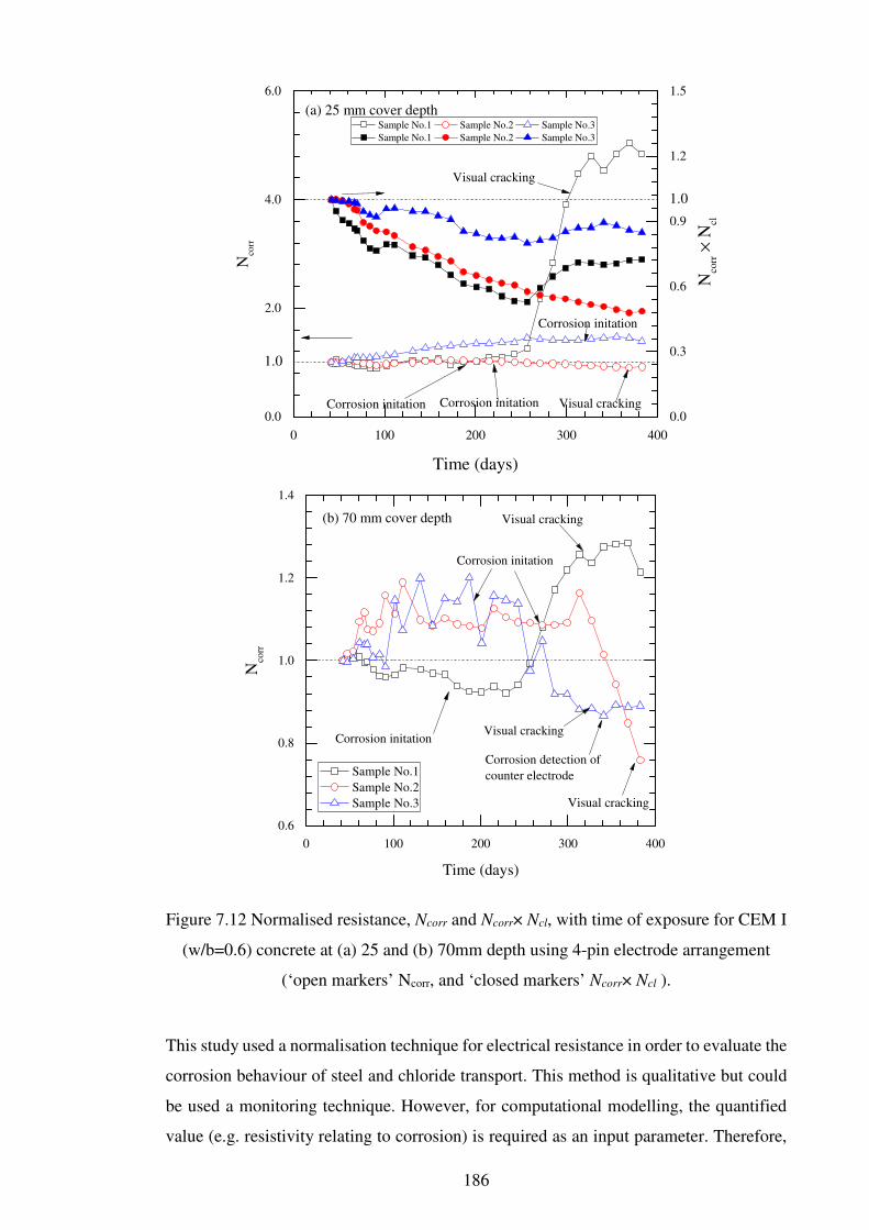
186

Figure 7.12 Normalised resistance, Ncorr and Ncorr× Ncl, with time of exposure for CEM I

(w/b=0.6) concrete at (a) 25 and (b) 70mm depth using 4-pin electrode arrangement

(‘open markers’ Ncorr, and ‘closed markers’ Ncorr× Ncl ).

This study used a normalisation technique for electrical resistance in order to evaluate the

corrosion behaviour of steel and chloride transport. This method is qualitative but could

be used a monitoring technique. However, for computational modelling, the quantified

value (e.g. resistivity relating to corrosion) is required as an input parameter. Therefore,

0 100 200 300 400

0.0

2.0

4.0

6.0

Visual cracking

Visual cracking

Corrosion initation

Corrosion initation

Sample No.1 Sample No.2 Sample No.3

Sample No.1 Sample No.2 Sample No.3

Time (days)

Nco

rr

Corrosion initation

1.0

0.0

0.3

0.6

0.9

1.2

1.5

Nco

rr ×

Νcl

(a) 25 mm cover depth

1.0

0 100 200 300 400

0.6

0.8

1.0

1.2

1.4


counter electrode

Visual cracking

Visual cracking

Corrosion initation

Corrosion initation

(b) 70 mm cover depth

Sample No.1

Sample No.2

Sample No.3

Nco

rr

Time (days)

Visual cracking

187

to deepen the understanding of the corrosion mechanism, and to refine the computational

model for corrosion propagation, further research is required to identify the resistivity or

normalised value relating to corrosion.

(a) Case 1

Accumulation of corrosion Isolated crack to the lateral direction and

visual crack (b) Case 2

Accumulation of corrosion Connected crack to the bottom and

isolated crack (c) Case 3

Accumulation of corrosion Connected crack to the bottom

Figure 7.13 Schematics for cracking caused by chloride-induced corrosion; (a) Case 1

corresponding to Sample No. 1 at 25 mm depth, (b) Case 2 corresponding to Sample

No. 1 at 70 mm depth and (c) Case 3 corresponding to Sample No. 2 and No. 3 at 70

mm depth.

188

7.4 Summary

Electrical resistance monitoring was employed to observe the deterioration of concrete

subjected to a chloride environment. Tests were conducted up to 382 days. Chloride-

induced corrosion of steel was only detected in CEM I (w/b = 0.6) concrete.

The main findings are summarised below.

• The electrical resistance of concrete changed due to chlorides and hydration. w/b

is a significant factor to determine the electrical resistance for chloride ingress.

For a low w/b, the resistances increased with time except for CEM II/B-V

(w/b=0.4) concrete, while the resistances of concrete with a high w/b decreased

with time at the chloride-contaminated depth of concrete. Regarding the effect of

hydration on the electrical resistance, the normalised resistances for CEM I and

CEM III/A concrete moderately increased with time, but the normalised resistance

for CEM II/B-V concrete continuously increased with time due to pozzolanic

reaction at 70 mm depth.

• After depassivation, a change of electrical resistance was expected due to ionic

movement by electrochemical reaction. However, the movement by

electrochemical reaction was not distinguished from the measured resistance

because a change of electrical resistance caused by chlorides was dominant.

Interestingly, the electrical resistance increased or decreased after cracking, but

further investigation is required to determine crack patterns, which seemed to be

random here.

• To analyse the data regarding the electrical resistance, a normalised value was

used instead of the absolute value, i.e. the electrical resistivity. When a sample is

influenced by various factors simultaneously, caution is required in the

interpretation. This method is useful to control the influencing factors through the

analysis process. However, the method is qualitative; therefore, it is difficult to

determine a value for computational modelling. On the other hand, it is reasonable

for understanding the deterioration behaviour of concrete.

189

CHAPTER 8

EVALUATING THE SERVICE LIFE OF CONCRETE

STRUCTURES

8.1 Introduction

To obtain adequate service life performance, a performance-based approach has been

gaining popularity over the prescribed approach. As part of the performance-based

approach, predictive models relating to chloride transport or corrosion propagation are

attractive. This is because there are limitations to obtaining laboratory/field data about

concrete structures with regard to their long-term behaviour, whereas this behaviour is

readily predicted through computational simulation (Ožbolt et al. 2011).

To improve the accuracy of the predictive model, field data are essential, particularly if

the model has been developed based on laboratory studies. Therefore, it is necessary that

the differences between field and laboratory conditions are reflected and the model should

be refined with data obtained from field tests. This chapter presents a case study of

concrete samples exposed to both the field and laboratory environments to update an

existing model (ClinConc). Furthermore, the Chapter also discusses a comprehensive

suite of tests (including the electrical resistance measurement) undertaken to evaluate the

performance of concrete in the field.

8.2 Experimental

8.2.1 Experiments for chloride transport

To observe the long-term chloride transport behaviour of concrete exposed to a marine

environment, and to obtain input data to update the predictive model, three tests were

performed relating to chloride transport: the acid-soluble chloride test (sampling in

Section 4.4.1 and measurement in Section 5.2.3), the degree of saturation test (sampling

in Section 4.4.1 and measurement in Section 5.2.2) and the electrical resistance test. In

addition, sample details and exposure condition are described in Section 4.6.

The electrical resistance of concrete was measured using embedded stainless-steel pin

electrodes at discrete distances from the concrete surface. The measurement was

190

performed with an auto ranging logger using an AC voltage of amplitude 350 mV at

a fixed frequency of 1 kHz, as shown in figure 8.1. To verify the applicability of the

stainless-steel pin electrodes, the electrical resistivity of small cubes extracted from the

electrode-embedded concrete was measured along with the degree of saturation to find

input data to update the predictive model. Sampling for small cubes and measurement

procedures are also given in Sections 4.4.1 and 5.2.2, respectively. To minimise the

moisture loss during the measurement, the samples were kept in a sealed condition, as

shown in figure 8.1.

Figure 8.1 Electrical resistance measurement using a multiplexer in conjunction with

a data logger.

8.2.2 Experiments for corrosion

The main concern regarding the deterioration of concrete structures exposed to chloride

environments, especially a marine environment, is chloride-induced corrosion. The

condition of steel was investigated using several electrochemical techniques including

LPR, GP, EIS, PT and TEP. The experimental set-up and procedures for the techniques

are given in Chapter 6.

The measurements were carried out for two steels embedded in each concrete slab as

working electrodes. The embedded stainless-steel rod (Ø 6 × 200 mm) was used as

191

a counter electrode in the polarisation techniques. The exposed area of the working

electrode was 100.53 cm2 (Ø 16 × 200 mm).

8.2.3 Monitoring electrical resistance using a remote-control system

Electrical resistances of concrete exposed to a long-term marine environment were

directly monitored using a remote interrogated system. Data from the Dornoch field site

is received by a modem using a dial-up approach and the uploaded data are recovered in

an Excel file using a software utility installed in the office-based computer. To manage

the system effectively, the entire system is powered by a rechargeable battery using

a solar panel (McCarter et al., 2012). The main purpose of monitoring electrical resistance

in this study was to investigate the activation energy of mature concretes with temperature

as the hydration of concrete, especially containing SCMs, affects the electrical resistance

at an early age (< 300 days), leading to an overestimation of the activation energy of

concrete. The time interval between measurement cycles was set to a 6-hour cycle for

samples exposed to the XS3 environment. The monitoring period was approximately

1 month (29 September, 2016 – 26 Octorber, 2016).


8.3.1 Evaluating chloride transport

The main concern regarding the corrosion of steel in concrete is chloride concentration at

the steel depth so having an accurate prediction of this content allows for a better

estimation of the service life of the concrete structure. To evaluate performance, the

following parameters relating to chloride transport were examined: chloride profiling,

porosity and degree of saturation. This section investigates the updated parameters for the

ClinConc model (Kim et al., 2016), referred to as environmental factors, and modifies

them for estimating chloride distribution.

192

Case studies for transport parameters

Chloride concentrations for the three samples retrieved from the field were measured with

depth. The samples had been exposed to the marine environment corresponding to XS3

for 18 years. Figure 8.2 presents the chloride profiles for PC, GGBS/40 and FA/30

concretes. As expected, PC concrete had the highest chloride concentration at all depths.

The chloride concentrations at the steel depth (50 mm cover depth) were 0.84, 0.15, and

0.25% by weight of binder for PC, GGBS/40, and FA/30 concrete, respectively.

Meanwhile, it is accepted that the CTL for total chloride content in concrete is 0.4% by

weight of binder according to BS EN 206 (British Standards Institution, 2014); however,

for PC concrete, although the chloride concentration at the steel depth was higher than

the accepted threshold level, no corrosion was detected with corrosion testing. However,

the threshold value is still controversial due to many influential factors. In a chloride

profile, erratic behaviour can be observed when a sample is exposed to wet/dry cyclic

regime. The retrieved samples in this study were also exposed to long-term tidal action,

but in the chloride profiles, erratic behaviour was not observed in the outer layer. Erratic

behaviour is not necessarily observed in sample subjected to wet/dry cyclic regime

(Nanukuttan et al., 2008), but, from the result or the shape of the chloride profiles, it could

be deduced that the main transport mechanism was diffusion and not absorption.

An analysis was conducted using Fick’s second law to calculate the diffusion coefficient

and surface chloride concentration. The first point was excluded in the progress of the

calculation although there was no erratic behaviour in the outer layer. The diffusion

coefficients were evaluated 1.39×10-12, 4.21×10-13, and 4.21×10-13 m2/s for PC,

GGBS/40, and FA/30 concrete, respectively and the surface chloride concentrations were

4.54, 4.46, and 5.56% (by weight of binder), respectively. SCM concretes were observed

to be beneficial in resisting chloride transport.

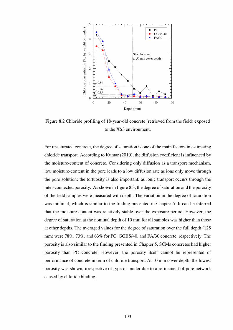
193

Figure 8.2 Chloride profiling of 18-year-old concrete (retrieved from the field) exposed

to the XS3 environment.

For unsaturated concrete, the degree of saturation is one of the main factors in estimating

chloride transport. According to Kumar (2010), the diffusion coefficient is influenced by

the moisture-content of concrete. Considering only diffusion as a transport mechanism,

low moisture-content in the pore leads to a low diffusion rate as ions only move through

the pore solution; the tortuosity is also important, as ionic transport occurs through the

inter-connected porosity. As shown in figure 8.3, the degree of saturation and the porosity

of the field samples were measured with depth. The variation in the degree of saturation

was minimal, which is similar to the finding presented in Chapter 5. It can be inferred

that the moisture-content was relatively stable over the exposure period. However, the

degree of saturation at the nominal depth of 10 mm for all samples was higher than those

at other depths. The averaged values for the degree of saturation over the full depth (125

mm) were 78%, 73%, and 63% for PC, GGBS/40, and FA/30 concrete, respectively. The

porosity is also similar to the finding presented in Chapter 5. SCMs concretes had higher

porosity than PC concrete. However, the porosity itself cannot be represented of

performance of concrete in term of chloride transport. At 10 mm cover depth, the lowest

porosity was shown, irrespective of type of binder due to a refinement of pore network

caused by chloride binding.

0 20 40 60 80 100

0

1

2

3

4

5

0.150.26

PC

GGBS/40

FA/30

Ch

lori

de

con

centr

atio

n (

%, b

y w

eig

ht

of

bin

der

)

Depth (mm)

Steel location

at 50 mm cover depth

0.84

194

Figure 8.3 Degree of saturation and porosity with depths for (a) PC, (b) GGBS/40, and

(c) FA/30 concretes retrieved from the field.

0 30 60 90 120 150

9

10

11

12

13

Porosity (Ave:10.3%)

Sr (Ave: 83%)

Depth (mm)

Po

rosi

ty (

%)

(a) PC

60

70

80

90

100

Sr (

%)

0 30 60 90 120

9

10

11

12

13


Sr (Ave:73.3%)

Depth (mm)

Po

rosi

ty (

%)

(b) GGBS/40

60

70

80

90

100

Sr (

%)

0 30 60 90 120 150

10

11

12

13

14

15

16


Sr (Ave: 67.3%)

Depth (mm)

Poro

sity

(%

)

(c) FA/30

60

70

80

90

100

Sr (

%)

195

The relation between degree of saturation and resistivity for long-term exposed samples

was investigated using Archie’s law, as described in figure 8.4. The first two points

corresponding to the values at 10 and 30 mm cover depth from the exposure surface

(‘open’ marks on figure 8.4 indicate outliers), were omitted in the fitting due to the high

concentration of chloride in the outer layer of concrete, which led to low electrical

resistivity. The ratio (P[caPa , see equation (5.23)) decreased as the degree of saturation

decreased, as shown in figure 8.4 (similar to figure 5.19) and the exponents in Archie’s

equation were observed to be lower than the values in the early age samples in

Chapter 5, corresponding to 1.33, 2.16, and 2.7 for PC, GGBS/40, and FA/30 concrete,

respectively. Thus, these exponents are influenced by concrete age, in particular

continuous hydration and by type of binder. However, further research is required to

determine the exact relationship.

Figure 8.4 Relation between saturation degree and resistivity with binder type (outliners

[open markers] are removed from fitting equations).

The Nernst-Einstein equation establishes the relation between the diffusion coefficient of

a porous material and electrical resistivity (McCarter et al., 2000) as follows:

50 60 70 80 90 100

0.0

0.3

0.6

0.9

1.2

1.5

ρ0/ρt = S

2.7r

r2=0.93

ρ0/ρt = S

1.33r

r2=0.87

PC

GGBS/40

FA/30

ρ sat/ρ

t

Sr (%)

ρ0/ρt = S

2.16r

r2=0.98

196

o3 ≈ HNH KLM

(8.1)

where o is the effective diffusion coefficient in the porous material, 3 is a diffusion

coefficient of the desired ion at infinite dilution, HN is the resistivity of the interstitial pore

fluid, and H KLM is the bulk resistivity of the saturated material.

The diffusion coefficient decreases with a decrease in moisture content (Kumar, 2010).

Furthermore, in this study, the diffusion coefficient for concrete containing SCMs largely

decreased with time compared to that for PC concrete. Thus, it can be inferred that

a reduction of the exponent is related to an aging factor in the diffusion coefficient. Again,

additional research is required due to the narrow range considered in the current analysis.

Determination of environmental factors

A number of chloride transport models have been developed for concrete, and the

theoretical background is now well established (see Chapter 3). However, the models are

generally only valid for concrete subjected to a certain situation. To overcome this, two

environmental factors applied to the ClinConc model, which only considers the saturated

condition of concrete. The main purpose of the environmental factors is to consider the

unsaturated condition of concrete. Two environmental factors are (i) Ks taking into

account the reduction of the diffusion coefficient with the degree of saturation, and

(ii) Kexp describing the degree of contact of the concrete with aggressive solution, chloride

solution. The process used to estimate the factors is briefly described below.

(i) The relation in terms of Ks is formulated from the work of Kumar (2010) (figure 8.5)

as follows:

ün ýdý[ca UQA.Ä¹§@§.AA

þÇ

(8.2)

where n+S is the diffusion coefficient in saturated concrete; and is the diffusion

coefficient in unsaturated concrete including saturation degree, UQ, and water-to-binder

ratio, ¿ .

197

(ii) To account for the effect of exposure conditions on chloride accumulation, an

environmental factor, Kexp, is introduced into the ClinConc model. The basic

information about the equation used in the ClinConc model has been presented

elsewhere (Tang 1996b, 2008). In this study, Kexp is added in the function to calculate

the total chloride from the free chloride content:

S üoN ×Φbg (8.3)

where S is total chloride content, Φ is the functional relationship within the ClinConc

model and is free chloride content.

Figure 8.5 The relationship between degree of saturation and relative ratio of diffusion

coefficient, Ks (adapted from Kumar (2010)).

To evaluate the Kexp. the predicted ClinConc profile is adjusted by incrementally

modifying the Kexp factor such that it maps onto the actual profile. Figure 8.6 provides an

example of the adjusted curve considering Kexp. In the calculation process, the main focus

is on estimating Kexp, as Ks is easily calculated from the degree of saturation measured

directly from the sample and less affects the chloride profile. The environmental factors

for samples subjected to a cyclic wet/dry regime in the laboratory are also investigated.

As shown in figure 8.7, the variation in temperature in the laboratory and the field are

significantly different. The temperature was stable at ~ 20ºC in the well-controlled

laboratory, while the concrete located in the field was influenced by seasonal temperature,

i.e. ~ 15ºC in the summer and ~ 3ºC in the winter season. To simplify the calculation, the

0 20 40 60 80 100

0.0

0.2

0.4

0.6

0.8

1.0

PC (w/b=0.4)

PC (w/b=0.5)

PC (w/b=0.6)

Ks

Sr (%)

Ks=D

a/D

0=S

4.863-3.441⋅w/b

198

averaged values for the samples exposed to both conditions were applied when

calculating the chloride content with the ClinConc model.

Figure 8.6 Example of the adjustment of a chloride profile (obtained from field specimen)

using the modified ClinConc model introducing environmental factors Ks and Kexp.

Figure 8.7 Temperature variation in concrete exposed to the field site and the laboratory.

Table 8.1 presents the input parameters used in the ClinConc model containing

environmental factors. Ks could be estimated from equation (8.2) while Kexp values were

found using the least square method between the measured and the predicted value. In

addition, Kexp is representative of the exposure condition. Therefore, figure 8.8 and 8.9

0 10 20 30 40 50 60

0

2

4

6

8

Measured data

ClinConc: Ks=1.0;K

exp=1.0

ClinConc: Ks=1.0;K

exp=0.45

ClinConc: Ks=0.8;K

exp=1.0

Ch

lori

de

con

centr

atio

n (

%, b

y w

eig

ht

of

bin

der

)

Depth (mm)

0 50 100 150 200 250 300 350

0

5

10

15

20

25

30

9 °C

(Summer)

Field sample

Laboratory sample

Tem

per

atu

re (

°C)

Time (days)

(Winter)

20.6 °C

199

also present the predicted chloride concentrations using the averaged values of Kexp for

all samples which were exposed to the same condition.

As shown in figure 8.8 and 8.9, the predicted values are similar to the measured values.

In addition, the Kexp values evaluated are in good agreement when samples are in the same

exposure condition and have the similar w/b. As shown in table 8.2, for samples exposed

in the field (w/b = 0.39 – 0.44), Kexp ranges from 0.60 to 0.82 (average value = 0.70),

while for concretes exposed to the laboratory, Kexp is distributed from 0.62 to 0.86

(average value = 0.76) and from 1.93 to 2.09 (average value = 2.01) corresponding to w/b

= 0.4 and 0.6, respectively. The main assumption for Kexp is that the contact degree of

chloride proportionally decreases from the saturated condition (fully immersed condition

in chloride solution). Therefore, the value should be lower than 1.0. However, it was

estimated from the fitting process that the values for laboratory concretes (w/b = 0.6) were

greater than 1.0. From the results, it could be deduced that another transport mechanism,

i.e. absorption, which accelerates chloride ingress, affected the chloride transport in

addition to diffusion. However, it is difficult to determine absorption behaviour in the

chloride profiling. Although the value of Kexp >1.0 is invalid based on the assumption, it

can indicate that absorption occurs in concrete.

For CEM III/A (w/b = 0.4) concrete, measured chloride content in the outer layer was

higher than that predicted by the modified ClinConc model. This is due to high bound

chloride by physical absorption or chemical binding. However, the Kexp values were lower

than 1.0 because the values corresponding to the first two points (up to 6 mm nominal

depth) were omitted in the process of fitting. It should be noted that the convective zone for

laboratory concretes (w/b = 0.4) was observed within 10 - 15 mm from the electrical

resistance measurement, and it is accepted that the convective zone (or wet/dry cyclic

region) is subtracted in the fitting process with Fick’s second law (Keßler et al., 2014). It

can be assumed that diffusion is the only transport mechanism in the regions below the

convective zone. However, the results of this study show that the chloride transport

mechanism beyond the convective zone is more complex than only diffusion, especially for

laboratory concretes with a high w/b. Therefore, environmental factors or complex

transport mechanisms should be introduced in the transport model to improve the accuracy

of the results. It should also be noted that continuous updating is required in terms of the

estimated values for environmental factors, as Ks values are limited in estimating various

materials including blended concretes and Kexp is only estimated from the fitting process.

200

Table 8.1 Input parameters for the ClinConc model

Exposure condition Field Lab

Sample designation PC GGBS/40 FA/30 CEM I

(w/b=0.4) CEM III/A (w/b=0.4)


CEM I (w/b=0.6)

CEM III/A (w/b=0.6)


Cement content(kg/m3) 460 270 370 460 270 370 300 180 210

Slag content(kg/m3) (k value*)

+ 180 (0.6)

+ + 180 (0.6)

+ + 120 (0.6)

+

Fly ash content (kg/m3) (k value*)

+ + 160 (0.4)

+ + 160 (0.4)

+ + 90

(0.4)

Water content (l/m3) 184 198 206.7 184 180 212 180 180 180

Average saturation degree 0.83 0.73 0.67 0.82 0.84 0.83 0.85 0.87 0.88

Average Temperature 9 20.6

Concrete age at first exposure (days)

35 42

Exposure duration (years) 18 1.07

Chloride concentration applied at the surface (g/l)

19.6 19.6

Migration coefficient at 6 months (m2/s)

8.87 3.33 2.92 8.87 3.33 2.92 21.05 6.43 7.46

* an equivalent binder assumption (San Nicolas et al., 2014) replacing the term ‘w/b’ with w/(cement +k×supplementary cementitious materials) defined in BS EN 206 (British Standards Institution, 2014) Note: Input values for the ClinConc model refer to Appendix D.2

201

Figure 8.8 Measured profile and predicted profiles from the modified ClinConc model

for (a) CEM I, (b) CEM III/A, and (c) CEM II/B-V concrete with w/b=0.4, and (d)

CEM I, (e) CEM III/A, and (f) CEM II/B-V with w/b=0.6 subjected to a wet/dry cyclic

regime in the laboratory.

0 20 40 60

0

1

2

3

4

5

Predicted line (Kexp

: 0.85, r2=0.93)


: 0.78, r2=0.92)

CEM I (w/b=0.4)

Chlo

ride

conce

ntr

atio

n (

%,

by w

eigh

t of

bin

der

)

Depth (mm)

(a) CEM I (w/b=0.4)

0 20 40 60 80 100

0

1

2

3

4

5

6

7


: 2.09, r2=0.93)

Predicted line (Kexp:

2.01, r2=0.92)

CEM I (w/b=0.6)

Chlo

ride

conce

ntr

atio

n (

%,

by w

eigh

t of

bin

der

)

Depth (mm)

(b) CEM I (w/b=0.6)

0 20 40 60

0

1

2

3

4

5


: 0.62, r2=0.94)


: 0.78, r2=0.84)

CEM III/A (w/b=0.4)

Chlo

ride

conce

ntr

atio

n (

%,

by w

eigh

t of

bin

der

)

Depth (mm)

(c) CEM III/A (w/b=0.4)

0 20 40 60

0

1

2

3

4

5

6

7


: 2.02, r2=0.85)


: 2.01, r2=0.85)

CEM III/A (w/b=0.6)

Chlo

ride

conce

ntr

atio

n (

%,

by w

eigh

t of

bin

der

)

Depth (mm)

(d) CEM III/A (w/b=0.6)

0 20 40 60

0

1

2

3

4

5


: 0.87, r2=0.98)


: 0.78, r2=0.97)


Chlo

ride

conce

ntr

atio

n (

%,

by w

eigh

t of

bin

der

)

Depth (mm)

(e) CEM II/B-V (w/b=0.4)

0 20 40 60

0

1

2

3

4

5

6

7


: 1.93, r2=0.92)


: 2.01, r2=0.92)


Chlo

ride

conce

ntr

atio

n (

%,

by w

eigh

t of

bin

der

)

Depth (mm)

(f) CEM II/B-V (w/b=0.6)

202

Figure 8.9 Measured profile and predicted profiles from the modified ClinConc model

for (a) PC, (b) GGBS/40, and (c) FA/30 concrete subjected to the field site (XS3).

0 20 40 60 80 100

0

2

4

6

8


: 0.60, r2=0.88)


: 0.70, r2=0.75)

PC-Field

Ch

lori

de

conce

ntr

atio

n (

%,

by

wei

ght

of

bin

der

)

Depth (mm)

(a) PC

0 20 40 60 80 100

0

2

4

6


: 0.67, r2=0.94)


: 0.70, r2=0.94)

GGBS/40-Field

Ch

lori

de

con

cen

trat

ion

(%

, b

y w

eigh

t o

f b

ind

er)

Depth (mm)

(b) GGBS/40

0 20 40 60 80 100

0

2

4

6

8


: 0.82, r2=0.79)


: 0.70, r2=0.77)

FA/30-Field

Ch

lori

de

con

cen

trat

ion

(%

, b

y w

eigh

t o

f b

ind

er)

Depth (mm)

(c) FA/30

203

Table 8.2 Environmental factors used in modified ClinConc model

Environmental factors

Field Laboratory

PC (w/b=0.4)

GGBS/40 (w/b=0.44)

FA/30 (w/b=0.39)

CEM I (w/b=0.4)

CEM III/A

(w/b=0.4)

CEM II/B-V

(w/b=0.4)

CEM I (w/b=0.6)

CEM III/A

(w/b=0.6)

CEM II/B-V

(w/b=0.6)

Ks 0.42 0.35 0.24 0.50 0.55 0.53 0.64 0.68 0.67

Kexp 0.60 0.67 0.82 0.79 0.62 0.86 2.09 2.02 1.93

Average Kexp 0.70 0.76 2.01

Time to corrosion based on chloride threshold level

Experiments and computational modelling of chloride transport are necessary to

determine the corrosion initiation of the steel based on CTL. To predict or estimate time

to corrosion, information on both the CTL and the chloride transport rate are required,

but a number of influencing factors limit an accurate prediction. Empirically based

models have sometimes introduced a probabilistic approach to reduce or contain the error.

However, a large data-set from the field is required to apply this method (Bertolini and

Redaelli 2009) and it is time-consuming. Hence, analytical models are more useful to

determine the chloride transport behaviour. As suggested above, the model should be

continuously updated and in this study, two analyses were carried out: (i) determining the

CTL for CEM I (w/b = 0.6) concrete using a modified ClinConc model with two

environmental factors, and (ii) predicting time to corrosion for other concretes with the

CTL obtained from CEM I (w/b = 0.6) concrete.

Before estimating the time to corrosion, the CTL was determined. To this end, the

environmental factors obtained from the previous section and the time to corrosion

initiation from Chapter 6 were used, respectively. The predicted values at 25 mm of cover

depth range from 2.0 to 2.8% of total chloride content, and the average and standard

deviation are 2.3% and 0.3%, respectively. These values are significantly higher than the

accepted value (0.4% by weight of binder) but is similar to a previous study (Angst et al.,

2011c). A higher CTL was required in this study because for the PC concrete exposed in

the field and for the CEM III/A (w/b = 0.6) and CEM II/B-V (w/b = 0.6) concrete in the

laboratory, the chloride contents were also higher than 0.4% at steel depth, and no

corrosion on the steel was detected. In addition, as CTLs vary widely due to various steel

conditions and materials, in this study the CTLs used to estimate the time to corrosion

were set as both 2.32% and 0.4%, for laboratory and fields samples.

204

Except for the CEM I (w/b=0.6) concrete in the laboratory, table 8.3 presents the predicted

initiation times for different mixes and different exposure conditions. Although SCMs are

beneficial in increasing the corrosion-free life, their effect on time to corrosion initiation

is low compared to other factors. The life for SCM concretes is 1.8 – 5 times longer than

that for PC (or CEM I) concrete, but the effect of CTL is moderate when it increases from

0.4% to 2.3%. On the other hand, it was observed that an increase in w/b distinctly led to

a reduction in the corrosion-free life, ranging from 12.1 to 23.3 times. When cover depth

was doubled (between 25 mm for laboratory samples and 50 mm for field samples),

corrosion-free life increased from 16.2 to 37.7 times. This implies that a large difference

in the corrosion-free life with cover depth and w/b is closely related to the sorption effect

of the wet/dry cyclic regime. Therefore, the best way to increase the service life of

concrete structures subjected to a wet/dry cyclic regime is to reduce the convective region

using lower w/b or using SCMs, especially GGBS. It is possible that the fully saturated

condition is more beneficial in improving the concrete performance than the unsaturated

condition. In other words, moisture movement is a key factor to prevent concrete

deterioration by chloride attack.

Table 8.3 The predicted time to attain chloride threshold level at the steel depth

Time to reach chloride threshold level (years)

Field

(cover depth = 50 mm) Laboratory

(cover depth = 25 mm)

CTL* PC

(w/b=0.4) GGBS/40

(w/b=0.44) FA/30

(w/b=0.39) CEM I

(w/b=0.4) CEM III/A (w/b=0.4)

CEM II/B-V

(w/b=0.4)

CEM I (w/b=0.6)

CEM III/A (w/b=0.6)

CEM II/B-V

(w/b=0.6)

0.4 22.7 49.4 113.2 1.4 2.5 3 0.2** 0.4 0.4

2.3 78.8 213 391.7 16.3 31.4 36.2 0.7** 2.6 2.2

* Chloride threshold level (%, by weight of binder), ** detection of corrosion

8.3.2 Evaluating the corrosion of steel

After depassivation, corrosion products lead to cracking in the concrete. The cracks

formed in the concrete accelerate ingress of chlorides, which dramatically reduces the

service life of concrete structures. In addition, it is difficult to determine a single CTL, as

shown in previous studies (see table 2.5) and the present one. To accurately diagnose the

conditions of concrete structures, corrosion detection methods are routinely employed. In

this study, parameters relating to steel corrosion were measured using several techniques

for the field samples and laboratory samples. Moreover, the corrosion propagation of the

205

steel with time was investigated for only those laboratory samples (CEM I concrete,

w/b=0.6) in which corrosion occurred.

Field studies for corrosion parameters

As mentioned above, a range of electrochemical techniques were undertaken to determine

the steel condition regarding field samples. Only the results of the GP and TEP techniques

are presented here (table 8.4), while other test results presented in Appendix C.4. The

corrosion potential and time constant are useful parameters to rapidly determine corrosion

for all steels. In this study, corrosion potentials ranged from -98.85 to -120.40 mV, which

indicates that the steels were in the passive state (ASTM International, 2015). The time

constants were also high, ranging from 66.80 to 260.25s. All parameters indicate a passive

state of the steel. Thus, it is reasonable to consider the steel condition as being in the

passive state.

Figure 8.10 Fitting data obtained from the PC concrete using (a) GP technique, and

(b) Tafel extrapolartion technique.

Polarisation resistance obtained from the GP technique and Tafel slopes obtained from the

TEP technique are necessary to quantify the corrosion rate; the measurement details are

given in Section 6.2.3. Overall, the polarisation resistance in the passive state of steel for

both field and laboratory samples was high, ranging from 66.25 to 123.70 Ω·m2 for the

former and from 80.76 to 136.20 Ω·m2 for the latter, respectively, thereby indicating that

the corrosion rates were negligible. It is interesting that anodic slopes in the passive state

for the field samples were significantly reduced compared to those for the laboratory

samples (table 8.5). From the result, it could be deduced that chlorides reaching the steel

0 2 4 6 8 10

-150

-140

-130

-120

-110

Experimental setup

Exposure area of steel: 100.53 cm2

Applied current: 25 µΑTime: 10 sec

Measured data

Fitted data (r2=0.99)

Corr

osi

on

po

tenti

al (

mV

vs

CS

E)

Time (sec)

(a) Galvanostatic pulse technique

Fitting result (see equation (6.2))

Ohmic resistance: 260.96 ΩPolarisation resistance: 8866.87 ΩTime constant: 142.71 sec

β: 0.87

1E-8 1E-7 1E-6 1E-5 1E-4 0.001

-0.50

-0.25

0.00

0.25

0.50

0.75

Fitting result

βa: 475.67 mV/dec

βc: 62.85 mV/dec

B: 24.14 mV

Experimental setup

Exposure area of steel: 100.53 cm2

Scan range: -300 - + 600mV (vs CSE)

Scan rate: 10 mV/min

Measured data

Chlo

ride

conce

ntr

atio

n (

%,

by w

eigh

t of

bin

der

)

Current (A)

(b) Tafel extrapolation technique

206

could react with the passive film, leading to depassivation. In addition, B values from the

Tafel slopes were calculated and were distributed around 26 mV, corresponding to the

active state in the B value which is generally accepted (table 8.4). The B value appeared to

be affected by the slope of the cathodic branch, which was determined by availability of

oxygen. The availability of oxygen was lower for the laboratory samples than for the field

samples, as the TEP test was conducted on the laboratory samples at the end of the wetting

cycle (i.e. saturated condition), whereas on the field samples the surface was in a dry

condition (transport time from field to laboratory and tide time). This condition led to a

more active reaction in the cathodic branch for the field samples. To quantify the corrosion

rate, particularly in electrochemical techniques, information on B values was required and

the values were observed to be sensitive to concrete condition. Therefore, to determine the

service life of a concrete structure with corrosion rate, it is first necessary to investigate the

B value.

Ohmic resistances clearly differed with type of binder. Concretes containing SCMs had a

high ohmic resistance compared to PC and CEM I concrete. In addition to type of binder,

w/b also affected ohmic resistance and the effect of w/b on the resistance was marginal for

CEM III/A concrete compared to other concretes. On the other hand, differences in the

ohmic resistances with the exposure duration (between 382 days and 18 years) were small

for PC (CEM I) concrete and GGBS/40 (CEM III/A) concrete, but the ohmic resistance of

FA/30 concrete (the field sample at 18 years) was 1.7 times higher than that of CEM II/B-

V concrete (the laboratory sample at 382 days) due to pozzolanic reaction. Although the

effect of ohmic resistance on the corrosion rate was marginal (less than 10 % to determine

the polarisation resistance), the value should be considered even if concrete is saturated, as

the polarisation resistance decreases dramatically after depassivation.

Table 8.4 Corrosion parameters of steel for field samples at 18 years

PC GGBS/40 FA/30

AVE STD AVE STD AVE STD

Ohmic resistance* (Ω·m2) 2.45 0.21 3.50 0.00 12.50 0.71

Polarisation resistance*(Ω·m2) 97.40 11.74 66.25 24.82 123.70 15.56

Corrosion potential (mV) -120.40 29.13 -98.85 5.73 -111.35 21.43

Time constant* (s) 177.40 49.07 66.80 25.31 260.25 47.31

Anodic slope** (mV/dec) 592.05 164.54 519.70 136.75 1,006.59 107.93

Cathodic slope** (mV/dec) 66.55 5.16 75.05 5.73 71.44 1.03

B value (mV) 25.95 2.62 28.45 2.90 28.99 0.18

* Data obtained using the Galvanostatic pulse technique ** Data obtained using the Tafel slope

AVE average; STD standard deviation

207

Table 8.5 Corrosion parameters of steel for laboratory samples at 382 days

CEM I

(w/b=0.4) CEM III/A (w/b=0.4)


CEM I (w/b=0.6)

CEM III/A (w/b=0.6)


AVE STD AVE STD AVE STD AVE STD AVE STD AVE STD

Ohmic resistance* (Ω·m2) 2.17 0.27 3.53 0.14 7.26 0.73 0.93 0.09 3.06 0.23 4.23 0.41

Polarisation resistance*(Ω·m2) 84.53 35.98 80.78 33.86 136.76 42.27 1.56 0.58 136.20 29.30 113.63 38.65

Corrosion potential (mV) -101.57 43.94 -127.17 3.30 -121.92 12.51 -564.05 48.65 -149.62 6.99 -145.37 14.86

Time constant* (s) 126.75 93.89 158.01 96.25 366.23 126.41 13.54 6.52 311.01 99.06 335.93 181.04

Anodic slope** (mV/dec) >10,000 + >10,000 + >10,000 + 434.03 172.08 >10,000 + >10,000 +

Cathodic slope** (mV/dec) 116.37 24.61 136.03 9.56 130.08 22.20 279.92 92.51 110.83 17.09 133.30 16.67

B value (mV) 46.63 15.22 58.63 4.71 53.68 13.77 73.43 25.57 45.15 11.17 56.10 10.14

* Data obtained using the Galvanostatic pulse technique ** Data obtained using the Tafel slope + Not determined AVE average; STD standard deviation

208

Prediction for the propagation of corrosion (laboratory sample)

As shown in the previous section, the B value is sensitive and is difficult to determine the

corrosion rate directly. On the other hand, in Chapter 6 polarisation resistances were

observed to be similar irrespective of electrochemical technique, especially for steel in

the active state. Thus, it is reasonable to estimate the development of polarisation

resistance after depassivation to determine corrosion propagation. In this study, as only

the corrosion of steel for CEM I (w/b=0.6) concrete in the laboratory was detected

regarding corrosion propagation, only changes in the polarisation resistance data on the

CEM I (w/b=0.6) concrete were evaluated.

Firstly, time to corrosion initiation was chosen with a half-cell potential measurement.

After depassivation, polarisation resistances were plotted with time as shown in Figure

8.11, irrespective of steel replicates in CEM I (w/b=0.6) concrete. The polarisation

resistances rapidly decreased in the initial period, i.e. up to ~50 days after depassivation,

the values then stablise around 1.5 Ω·m2 during the remaining period. This implies that

the depassivation process and anodic reaction on the steel happened at the same time in

the initial period, and then anodic dissolution on the steel only reacted after full

depassivation. The corrosion products then accumulated on the steel surface. However,

care should be taken in interpreting the polarisation resistance, as the exposure condition

was stable for the samples in this study, and the polarisation resistance could thus be

stable after full depassivated conditions. If samples were exposed to the field, polarisation

resistance could fluctuate with time.

To estimate the trend for the polarisation resistance with time, the regression method

using a power-law equation was employed, viz;

N ∙ @ (8.4)

where N is the polarisation resistance (Ω·m2) at time, t (days), and a and b are the

constant.

The parameters from each sample were extracted; and presented in Table 8.6. The

regression parameters, i.e. a and b, represent the initial corrosion rate after the first

depassivation, and the rate for stabilisation.

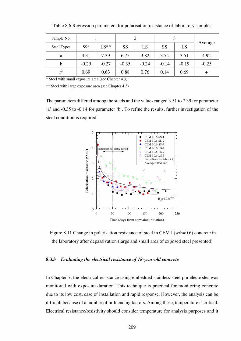
209

Table 8.6 Regression parameters for polarisation resistance of laboratory samples

Sample No. 1 2 3 Average

Steel Types SS* LS** SS LS SS LS

a 4.31 7.39 6.75 3.82 3.74 3.51 4.92

b -0.29 -0.27 -0.35 -0.24 -0.14 -0.19 -0.25

r2 0.69 0.63 0.88 0.76 0.14 0.69 +

* Steel with small exposure area (see Chapter 4.3)

** Steel with large exposure area (see Chapter 4.3)

The parameters differed among the steels and the values ranged 3.51 to 7.39 for parameter

‘a’ and -0.35 to -0.14 for parameter ‘b’. To refine the results, further investigation of the

steel condition is required.

Figure 8.11 Change in polarisation resistance of steel in CEM I (w/b=0.6) concrete in

the laboratory after depassivation (large and small area of exposed steel presented)

8.3.3 Evaluating the electrical resistance of 18-year-old concrete

In Chapter 7, the electrical resistance using embedded stainless-steel pin electrodes was

monitored with exposure duration. This technique is practical for monitoring concrete

due to its low cost, ease of installation and rapid response. However, the analysis can be

difficult because of a number of influencing factors. Among these, temperature is critical.

Electrical resistance/resistivity should consider temperature for analysis purposes and it

0 50 100 150 200 250

0

1

2

3

4

5

Stable period

CEM I-0.6-SS-1

CEM I-0.6-SS-2

CEM I-0.6-SS-3

CEM I-0.6-LS-1

CEM I-0.6-LS-2

CEM I-0.6-LS-3

Fitted line (see table 8.7)

Average fitted line

Pola

risa

tion

res

ista

nce

(Ω

⋅m2 )

Time (days from corrosion initiation)

Rp=4.92t

-0.25

Initial period

210

is now accepted that the correction of electrical resistivity/resistance can be undertaken

using an Arrhenius relationship with activation energy. In this study, the activation energy

was estimated for long-term exposure field samples. The change in electrical

resistance/resistivity due to hydration will be negligible as the samples were 18 years old.

Because it is independent of electrode geometry, electrical resistivity is more useful for

application than electrical resistance. To evaluate electrical resistivity, a geometry factor

should be obtained from either computational models or experiments (Lataste, 2010).

In a previous study, the geometry factor for the field samples used in the present study

corresponded to 0.0125 m ± 5% (McCarter et al., 2012). To verify this geometry factor,

the electrical resistivity from embedded stainless-steel pin electrodes was compared with

the resistivity of the prismatic sample (50×50×20 (thickness) mm) directly extracted from

the concrete containing the electrodes. For the cube sample, the sampling and

measurement methods are the same as in Section 4.5 and Section 5.2.5, respectively. The

results are shown in figure 8.12. A slight difference exists between the two measurements,

but it was concluded that the geometry factor (0.0125 m) used in this study was

appropriate. Subsequently, the electrical resistances monitored by the remote interrogated

system were converted to electrical resistivity (described in Section 8.2.4).

Figure 8.12 Comparison of resistivity obtained from the bulk concrete with resistivity

obtained from the embedded electrode.

Figure 8.13 presents as-measured electrical resistivity with type of binder and depth.

During monitoring, some of the data were lost due to technical problems which remain

0 30 60 90 120 150

0

200

400

600

800

1000

1200 PC-Resistivity of square sample

PC-Resistivity by electrode

GGBS/40-Resistivity of square sample

GGBS/40-Resistivity by electrode

FA/30-Resistivity of square sample

FA/30-Resistivity by electrode

ρ (Ω

⋅m)

Depth (mm)

211

unclear. The electrical resistivity was lowest for PC concrete and highest for FA/30

concrete located in the field. On the other hand, the electrical resistivity at the outer layer,

i.e. at 5–10 mm cover depth, was lower than at other depths for PC and FA/30 concrete

while for GGBS/40 concrete the values at the outer layers were higher than at other

depths. This is because high chloride binding at the outer layer leads to refinement of pore

structure and a lower amount of free chloride at the outer layer in GGBS/40 concrete

while low electrical resistivity of concrete is due to free chloride in FA/30 concrete. This

is in line with the other results in this study (see figure 7.7 and figure 7.8 in Section 7.3.2).

On the other hand, unlike CEM I (w/b=0.4) concrete (in figure 7.7(a)), the free chloride

at the outer layer in PC concrete mainly affected the electrical resistivity. It seems that

the rate of chloride binding significantly decreases or have been exhausted in 18-year-old

PC concrete. It is evident that the electrical resistivity for all samples fluctuated with time.

To account for this fluctuation, a correction for temperature effects was required.

Determination of activation energy

An Arrhenius relationship between electrical resistivity and temperature can be expressed

as follows (McCarter et al., 2012):

HÔ H3<êcëì (8.5)

56HÔ 56H3 + y+

(8.6)

whereHÔ is the resistivity of concrete (Ω·m) at temperature, T (K) (T=293.15 K in this

study), H3 is a constant (Ω·m), is the gas constant (8.314 J/mol·K) and y+ is the

activation energy for conduction processes in concrete (J/mol).

The activation energy can be evaluated using the relationship described in equation (8.5).

To illustrate this, figure 8.14 presents the resistivity values in figure 8.13 (a) described

against the cover-zone temperature at each depth in the format of equation (8.6) over

a period of 27 days.

212

Figure 8.13 Electrical resistivity with depth without temperature correction for (a) PC,

(b) GGBS/40, and (c) FA/30 concrete at the Dornoch site.

0 10 20 30

50

100

150

200

250

300

No data

collection

No data

collection

5 mm 10 mm 15 mm 20 mm

30 mm 40 mm 50 mm

ρ (Ω

⋅m)

Time (days)

(a) PC-Field sample

No data

collection

0 10 20 30

0

200

400

600

800

1000

1200

1400

No data

collection

No data

collection

No data

collection

5 mm 10 mm 15 mm 20 mm

30 mm 40 mm 50 mm

ρ (Ω

⋅m)

Time (days)

(b) GGBS/40-Field sample

0 10 20 30

0

300

600

900

1200

1500

No data

collection

No data

collection

No data

collection

5 mm 10 mm 15 mm 20 mm

30 mm 40 mm 50 mm

ρ (Ω

⋅m)

Time (days)

(c) FA/30-Field sample

213

Figure 8.14 Data in figure 8.13 (a) plotted in Arrhenius format.

The activation energies were calculated for,

(i) data based on the whole period; and,

(ii) data based on each part of the period.

For the part-period method, each discontinuous line was considered as one part,

consisting of a total of (roughly) three parts. The average values were estimated. Clearly,

the Arrhenius relationship using activation energy is important to account for the

influence of temperature on electrical resistivity (McCarter et al., 2012). However, it was

still necessary to verify whether the activation energy was constant over the whole depth,

especially in the convective zone where moisture distribution is unstable.

Figure 8.15 presents the activation energy estimated using the two methods with depth.

The activation energies for all samples ranged from 26.1 to 37.9 kJ/mol which are similar

to the results in previous study (McCarter et al., 2012). It is interesting that differences in

activation energy were marginal below 20 mm of cover depth, whereas larger differences

were observed in the outer layers (5 – 15 mm) with different methods. This must indicate

that moisture content is also an important factor in estimating the activation energy

although it is difficult to evaluate the activation energy with different moisture contents

experimentally, and it is reasonable to average the value obtained from monitoring. With

the averaged activation energy, the electrical resistivity was corrected to a reference

3.45 3.50 3.55 3.60 3.65

6.00

6.25

6.50

6.75

7.00

7.25 5 mm

10 mm

15 mm

20 mm

30 mm

40 mm

50 mm

ln(ρ

)

1000/T (K-1

)

214

temperature (at 20ºC); the result is presented in figure 8.16. It can be observed that the

fluctuations are removed. Therefore, to accurately analyse the electrical resistivity of

concrete, especially in the field, the effect of the temperature must be considered.

Figure 8.15 Variation of activation energy with depth.

Normalised electrical resistance

Electrical resistance monitoring of concrete subjected to chloride environments could be

used to detect ionic movement within the cover-zone, especially the movement of

chloride ions present in the pore solution. However, it is difficult to evaluate the effect of

chloride on electrical resistivity for concrete at an early age due to hydration. Some

investigations, including the present study, have reported that electrical resistivity

increases with time even though chloride ingress was observed (Polder and Peelen, 2002;

McPolin et al., 2005). In this section, the effect of chloride ingress on electrical resistivity

is investigated in samples of long-term exposure, as the hydration effect is negligible in

mature samples (~18 years old).

0 10 20 30 40 50 60

25

30

35

40

PC (Whole period)

PC (part period)

GGBS/40 (Whole period)

GGBS/40 (part period)

FA/30 (Whole period)

FA/30 (part period)A

ctiv

atio

n e

ner

gy (

kJ/

mol)

Depth (mm)

215

Figure 8.16 Electrical resistivity with depth after temperature correction for (a) PC, (b)

GGBS/40, and (c) FA/30 concretes at the Dornoch site.

0 10 20 30

60

80

100

120

140

160

180

5 mm 10 mm 15 mm 20 mm

30 mm 40 mm 50 mm

ρ (Ω

⋅m)

Time (days)

(a) PC-Field sample

0 10 20 30

0

200

400

600

800

5 mm 10 mm 15 mm 20 mm

30 mm 40 mm 50 mm

ρ (Ω

⋅m)

Time (days)


0 10 20 30

200

400

600

800

5 mm 10 mm 15 mm 20 mm

30 mm 40 mm 50 mm

ρ (Ω

⋅m)

Time (days)


216

After applying the activation energy to obtain the equivalent resistivity at a reference

temperature, the electrical resistivity was normalised with the resistivity value at the first

measurement point (at 0 days), as shown in figure 8.17. The Nρ () value remained

stable with depth and time for all samples, although slight fluctuations were detected and

attributed to a wet/dry cyclic regime in the tidal zone. The Nρ value decreased with time

at 5 mm cover depth. This seemed to be caused by chloride ingress; however, considering

the entire exposure period (18 years), the reduction for 27 days would be negligible.

Long-term data are required to confirm the effect of chloride on electrical resistivity. It is

suggested here that an electrical resistivity measurement could be exploited to detect

chloride ingress of concrete exposed to a chloride-rich environment. However, regular

monitoring is essential in this respect.

217

Figure 8.17 Normalised electrical resistivity of concrete at the Dornoch site.

0 10 20 30

0.8

0.9

1.0

1.1

1.2

5 mm 10 mm 15 mm 20 mm

30 mm 40 mm 50 mm

Νρ

Time (days)

(a) PC-Field sample

0 10 20 30

0.7

0.8

0.9

1.0

1.1

1.2

1.3

5 mm 15 mm 20 mm 30 mm

40 mm 50 mm

Νρ

Time (days)


0 10 20 30

0.8

0.9

1.0

1.1

1.2

5 mm 10 mm 15 mm 20 mm

30 mm 40 mm 50 mm

Νρ

Time (days)


218

8.4 Summary

This study predicted the chloride transport in concrete using the ClinConc and the

corrosion rate of steel embedded in concrete using an empirical model. The data used

were obtained from samples exposed to a marine environment for 18 years and from

samples exposed to a laboratory environment for 382 days. The main findings are

summarised below:

• To update the chloride transport model, two environmental parameters, Ks and

Kexp, were introduced and determined. Different exposure conditions between the

laboratory and the field, i.e. different wet/dry cyclic regime, leads to the different

transport behaviour. In the field, the chloride transport was mainly diffusion, and

the sorption effect was negligible. In contrast, in the laboratory samples,

especially in concrete with a high w/b, this effect was considerable. It was

observed that Kexp was greater than 1.0 for the high w/b (=0.6) and this is due to

the sorption mechanism.

• After depassivation, the polarisation resistance was evaluated as a function of

time. As mentioned in Chapter 6, polarisation resistance is less sensitive than

corrosion rate. The empirical relation between polarisation resistance and time

was expressed using Power’s law. Consequently, it was observed that corrosion

propagation became stable with time. However, further research is required

regarding the parameters used in the empirical equation.

• To consider the effect of temperature on electrical resistivity, the activation energy

was evaluated in the field samples connected to the remote-control system. It was

observed that the activation energy differed with depth and type of binder, ranging

from 26.12 to 37.9 kJ/mol. It was confirmed that the outer layers of the samples

were sensitive to the exposed environment namely the wet/dry cycle and the

chloride content in the pore solution based on the estimation of the activation

energy.

219

CHAPTER 9

CONCLUSIONS AND RECOMMENDATIONS FOR FUTHER

WORK

The work presented evaluated the performance of reinforced concrete subjected to

a chloride environment with the chloride-induced corrosion of the embedded steel studied

at various stages: chloride ingress, corrosion initiation and corrosion propagation. In

addition, the electrical resistance/resistivity of concrete was monitored during chloride

ingress. Although many studies have examined chloride transport and the chloride-

induced corrosion of steel, their results are scattered due to various influencing factors

including type of binder, test techniques, modelling method and exposure conditions. The

conclusions of this study are summarised below, along with recommendations further

work.

9.1 Electrical resistance and transport properties – laboratory-based studies

Concrete samples with two levels of w/b (=0.4 and 0.6) and OPC, 30% FA and 60% GGBS,

were used to establish the relation between transport properties and electrical

resistances/resistivity. The electrical resistivity of each sample was measured to establish

the relationship between the resistivity and various parameters such as the degree of

saturation, migration test and compressive strength. In addition, to accelerate chloride

ingress and to estimate chloride concentration, concrete slabs were exposed to a chloride

solution under a wet/dry cyclic regime as this represents a more realistic situation than

adding chlorides to the mixing water. The conclusions regarding this relationship are:

• Compressive strength is a ‘traditional’ factor used to determine the performance

of concrete. The relationship between electrical resistivity and compressive

strength was established although a scatter in the result was observed. Based on

the result in this study, whilst compressive strength is important in the quality

control of concreting operations, it cannot be used to assess the performance of

concrete related to chloride transport.

• The basic parameters including porosity, degree of saturation, migration and

diffusion coefficient, and electrical resistivity were investigated with regard to

chloride transport. These parameters changed with time, especially in SCM

220

concretes, and the w/b was observed to be crucial to determine durability and

performance of concrete. In terms of migration coefficient/electrical resistivity,

CEM II/B-V (w/b=0.4) concrete was superior but the diffusion coefficient of

CEM III/A (w/b=0.4) concrete was the lowest. Porosity was beneficial for

CEM I (w/b=0.4) concrete. The results suggest that it is necessary to evaluate

concrete durability with more than one parameter to assess the resistance of

chloride transport as chloride transport in concrete is determined by various

factors, e.g. degree of saturation and chloride bindings. In addition, the curing

time in CEM II/B-V concrete is crucial to determine the performance to chloride

transport.

• The electrical resistivity was highly sensitive to moisture. Archie’s law was

introduced to show the relationship between electrical resistivity and degree of

saturation. The sensitivity of resistivity to degree of saturation was in the order:

CEM II/B-V concrete (very sensitive) > CEM III/A concrete > CEM I concrete

(less sensitive). On the other hand, comparing the laboratory and field data, the

exponent for CEM II/B-V (or FA/30) concrete decreased from 5.61 at 382 days

to 2.7 at 18 years, while the value for CEM I (or PC) concrete was stable as 1.61

at 382 days and 1.33 at 18 years; the exponent is highly related to hydration

process. In addition, the electrical resistivity was found to be affected by the

degree of chloride contamination.

• The electrical resistivity was observed to be in inverse proportion to the migration

coefficient, irrespective of type of binder. Based on a simplified Nernst-Planck

equation, the constant (chloride concentration in the steady state) was required to

convert the electrical resistivity into the migration coefficient directly, and the

value for the constant was ~ 0.356 mol/l. However, to refine this value, additional

studies are required.

9.2 Electrical resistance and transport properties – Marine Exposure Site

Site-based research is important as the durability/performance of concrete is influenced

by its surrounding environment as well as its material properties. Samples exposed to

a chloride environment for an extended period of time were extracted from the field and

investigated with regard to the transport properties, including porosity/degree of

221

saturation and diffusion coefficient. The test results were used to evaluate the condition

of the concrete and as input parameters in the predictive model (ClinConc model in study).

The findings are summarised below:

• When using the ‘erf’ function to analyse chloride distribution, the diffusion

coefficient and surface chloride content were the main input parameters. The

diffusion coefficient of PC concrete (1.39×10-12 m2/s) was higher than those of

GGBS/40 and FA/30 concrete (4.21×10-13 m2/s), but the surface chloride contents

for PC, GGBS/40, and FA/30 concrete (4.54, 4.46, and 5.56% by weight of

binder) were similar.

• Although the samples were exposed to the XS3 environment (tidal zone), degrees

of saturation were stable across depth except for the outer layer (0 – 20 mm).

Averaged degrees of saturation were 0.81, 0.73, and 0.67 corresponding to PC,

GGBS/40, and FA/30 concrete, respectively. The unsaturated condition leads to

a lower diffusion rate; therefore, the chloride ingress in the XS3 environment

could be lower than that in the XS2 environment when sorption is not considered

(i.e. convective zone is ignored).

• There is little difference in average porosity over the cover region between

CEM I concrete at 390 days and PC concrete at 18 years, corresponding to 10.0%

and 10.3%, respectively. On the other hand, porosities from 390 days to 18 years

decreased by 0.6% for GGBS/40 (or CEM III/A) concrete and 1.3% for FA/30 (or

CEM II/B-V) concrete. On-going hydration in SCMs concrete was observed to be

beneficial to improve porosity, but porosity itself cannot be representative of

a performance factor regarding chloride transport.

9.3 Electrochemical parameters for the corrosion of steel

To assess the corrosion of embedded steel in concrete, various techniques were applied

to the samples: non-destructive methods included linear polarisation, half-cell potential,

and macro-cell current; the destructive methods employed was the mass loss test. In spite

of the wet/dry cyclic regime only the CEM I (w/b=0.6) concrete showed signs of

corrosion activity after 382 days. The electrochemical parameters obtained from the

corrosion measurements were investigated to understand corrosion behaviour and B

222

values for calculating corrosion rate were estimated. The findings are summarised in the

following:

• After depassivation, polarisation resistance, corrosion potential, and macro-cell

current changed dramatically, but time to corrosion initiation varied with steel.

It is evident that all techniques can detect corrosion activity on the steel. The

polarisation resistance ranged from 1 to 10 Ω·m2 for the active state and 75 to

163 Ω·m2 for the passive state.

• In addition to the polarisation resistance and corrosion potential, the corrosion

behaviour was observed using capacitance and time constant. For capacitance,

the values increased after depassivation, indicating that the surface of the steel

became uneven. On the other hand, the time constant easily indicated the

condition of steel. In the results, time constants were < 50s for the active state

and > 50s for the passive state.

• The propagation of corrosion was quantified by the corrosion rate, which was

estimated using the B value. The B value (active state) obtained from this study

(TEP technique) was not a single value but was, instead, distributed across

a wide range, i.e. 75.5 – 96.0 mV. The B values varied with steel condition and

exposure duration.

• Ohmic resistance is also an important factor in determining corrosion rate.

Although the ohmic resistance was marginal in the passive state, the value for

the active state accounted for up to 50% of the total resistance (=polarisation

resistance and ohmic resistance). The corrosion rate would be underestimated

without due consideration of the ohmic resistance.

• The corrosion rates obtained from the galvanostatic pulse technique and the mass

loss test were compared. The corrosion rate was affected by the B values (i.e. the

traditional value, Tafel extrapolation method and simplified method using

a potentiostatic technique), and the difference in the rate obtained by different

techniques was minimum when a traditional value was applied, i.e. 26 mV.

223

9.4 Monitoring electrical resistance

The electrical resistance of the samples was monitored to evaluate a change in concrete

properties by chloride ingress. To track chloride transport and detect corrosion behaviour

for up to 382 days of concrete age, stainless-steel pins were installed in concrete in

discrete depths. The activation energy was determined to account for the effect of

temperature on electrical resistivity of concrete in the field. The normalisation resistance

was introduced to consider the chloride effect (Ncl), hydration effect (Nhyd) and corrosion

effect (Ncorr). The findings are summarised as follows:

• Regardless of type of binder, as-measured resistances at the outer layer were

sensitive to the surrounding environments, such as the chloride solution,

temperature and wet/dry periods. The convective zone was observed in the

wet/dry cyclic regime which increased with an increase in w/b due to high

porosity.

• For a low w/b, the normalised resistance increased with time, while for a high

w/b it decreased after considering the hydration effect on the electrical

resistance. This indicates that bound chloride leads to an increase in electrical

resistance and free chloride causes a decrease in electrical resistance.

• A change in the electrical resistance caused by the corrosion process of steel, i.e.

ionic movement from the cathode to the anode, could not be extracted in this

study. From the result, it could be deduced that the change in the electrical

resistance by ionic movement is smaller than by chloride ions dissolved in pore

solution. However, the normalised resistance (Ncorr) could detect cracking

behaviour in this study. It was observed that Ncorr increased markedly without

any sign of corrosion; an increase in Ncorr is caused by the formation of cracks.

• The electrical resistivity fluctuated with temperature. It was shown that the

electrical resistance/resistivity measurement could be corrected to an equivalent

resistance at a reference temperature through the use of an Arrhenius

relationship. The activation energy for the field samples ranged from 26.12 to

37.9 kJ/mol and depended on type of binder and moisture content at the time of

measurement.

224

9.5 Mix design – binders and w/b

Six concrete mixes were used in the study: three types of binder and two w/b. The

evaluation was carried out from chloride transport to corrosion propagation. For chloride

transport, performance factors included porosity/degree of saturation, diffusion/migration

coefficients and electrical resistivity; for corrosion propagation, polarisation resistance,

ohmic resistance, time constant, capacitance and electrical resistivity were used. The

following summarises the durability performance of the mix compositions:

• In the investigation of pore structure relating to transport properties, concrete

with SCMs had higher porosity than CEM I (or PC) concrete irrespective of

w/b. However, transport rates for concrete with SCMs were lower than those for

CEM I (or PC). In particular, the rate is more sensitive to w/b. Therefore,

porosity is one of the durability indicators but it cannot fully reflect transport

properties.

• Steel corrosion was only detected for CEM I (w/b=0.6) concrete. Therefore,

a direct comparison regarding corrosion propagation cannot be made.

Nonetheless, SCM, i.e. FA and GGBS, are beneficial as they have a high

resistance to chloride-induced corrosion due to their higher resistance to

chloride ingress.

• Electrical resistivity as a performance factor was measured with binder and

time. At an early age (28 days), the electrical resistivity of CEM II/B-V concrete

was lower than that of CEM I and CEM III/A concretes, and CEM III/A concrete

had the highest resistivity. On the other hand, the resistivity of CEM II/B-V

concrete was the highest at 382 days, followed by that of CEM III/A concrete.

Therefore, in the view of long-term durability, SCM concrete is beneficial.

9.6 Predictive models – transport and corrosion model

Predictive modelling is beneficial for describing the deterioration of concrete exposed to

a chloride environment. To simulate the deterioration process, two types of models are

required: a chloride transport model and a corrosion propagation model. Regarding the

transport model, the ClinConc model was updated using two environmental factors, Kexp

and Ks. These factors were determined for both field and laboratory samples (table 8.2).

225

An empirical relation for corrosion development was determined using the limited

corrosion results as corrosion of steel was only detected in CEM I (w/b=0.6) concrete

(laboratory sample). The findings for the models are summarised as follows:

• The environmental factors were determined as input parameters in the ClinConc

model. For field samples, Kexp is related to the exposure condition and was

evaluated as 0.70, irrespective of type of binder, while Ks values, which are related

to the degree of saturation, were 0.42, 0.35, and 0.24 for PC, GGBS/40, and FA/30

concretes, respectively. Thus, it can be concluded that FA/30 concrete is the most

beneficial for resisting long-term chloride ingress in concrete. Meanwhile, Ks

coefficient for laboratory samples, was similar for different binders with the same

w/b due to their similar degree of saturation. Therefore, it can be stated that degree

of saturation is also an important environmental factor. It is interesting to note that

Kexp for laboratory concrete with w/b=0.6 is > 1.0 implying a higher w/b leads to

more rapid chloride ingress.

• Simulating corrosion behaviour is difficult due to the complex electrochemical

reactions in concrete, and it is virtually impossible to reflect all the influencing

factors in concrete. In addition, in this study the corrosion rate varied with the B

value, therefore an empirical relation using polarisation resistance was introduced.

It was observed that the polarisation resistance quickly became stable after

depassivation.

9.7 Recommendations for further research

The following are recommendations for further research.

• In this study, the relationship between the migration coefficient and the electrical

resistivity was established using the Nernst-Planck relation. However, the

assumption of a uniform distribution of chloride content over the sample was not

valid for the sample in non-steady state. Instead, it was assumed that the average

value for the chloride profile was a constant (0.356 mol/l) (figure 5.20), but this

was not confirmed through the experiment. To verify the suggested equation,

further test work is required for chloride profiling after migration testing.

226

• Polarisation resistances were measured using GP, LPR, PT and EIS techniques.

It was confirmed that differences in the polarisation resistances obtained from

different techniques were small, but the B value was very sensitive to analysis

methods. In addition, although a simplified method to estimate the B value was

used, the verification for the result was not sufficient due to the limited data on

corroding samples. Therefore, further research is recommended regarding the use

of the B value to estimate accurate corrosion rates. Furthermore, work of longer

duration is also recommended to detect the corrosion of steel embedded in SCM

concrete.

• The electrical resistance was monitored with depth to confirm the chloride

transport and corrosion behaviour. It was observed that the electrical resistance

decreased with chloride contamination, but a change in the resistance due to the

corrosion process could not be extracted from the measured resistance. As an

analysis method, a normalisation expression for the electrical resistance was used.

However, this expression is qualitative hence further work should be undertaken

to quantify a change of electrical resistivity caused by chloride content in concrete

and to develop an analysis method for monitoring electrical resistance to detect

corrosion.

• This study suggested a modified transport model using environmental factors. To

verify the model or evaluate the factors, both laboratory and field samples were

used. However, the factors must be updated with time and exposure conditions.

It is recommended that further studies be conducted on concrete samples in

different exposure conditions to refine the model. Furthermore, corrosion

behaviour was expressed by the polarisation resistance, but the relation was

established with limited data and further research should be carried out in this

respect. Finally, a probabilistic method for estimating chloride transport and

describing corrosion propagation is recommended to improve the accuracy of the

model, as various influencing factors exist simultaneously in the deterioration

process.

227

REFERENCES

Abd elaty, M. abd allah, 2014. Compressive strength prediction of Portland cement concrete with age using a new model. HBRC Journal, 10(2), 145–155.

ACI Committee 318, 2014. Building code requirements for structural concrete (ACI 318-14) and commentary on building code requirements for structural concrete (ACI 318R-14). Michigan: American Concrete Institute.

Alexander, M.G., Ballim, Y., and Stanish, K., 2008. A framework for use of durability indexes in performance-based design and specifications for reinforced concrete structures. Materials and Structures, 41(5), 921–936.

Alexander, M.G., and Nganga, G., 2016. Introduction: Importance of marine concrete structures and durability design, in M. Alexander (ed.) Marine concrete structures: design, durability and performance. Elsevier Ltd. [Online]. Available at: http://www.sciencedirect.com/science/article/pii/B9780081000816000015.

Alexander, M.G., and Thomas, M.D.A., 2015. Service life prediction and performance testing - Current developments and practical applications. Cement and Concrete Research, 78(A), 155–164.

Alfaro, M., 2014. Modeling of polarization curves not exhibiting a Tafel region using Excel spreadsheets. Alexandria Engineering Journal, 53(4), 977–983.

Alonso, C., Andrade, C., Castellote, M., and Castro, P., 2000. Chloride threshold values to depassivate reinforcing bars embedded in a standardized OPC mortar. Cement and Concrete Research, 30(7), 1047–1055.

Alonso, C., Andrade, C., and González, J.A., 1988. Relation between resistivity and corrosion rate of reinforcements in carbonated mortar made with several cement types. Cement and Concrete Research, 18(5), 687–698.

Alonso, C., Castellote, M., and Andrade, C., 2002. Chloride threshold dependence of pitting potential of reinforcements. Electrochimica Acta, 47(21), 3469–3481.

Altmann, F., and Mechtcherine, V., 2013. Durability design strategies for new cementitious materials. Cement and Concrete Research, 54(December), 114–125.

Altmann, F., Sickert, J.U., Mechtcherine, V., and Kaliske, M., 2012. A fuzzy-probabilistic durability concept for strain-hardening cement-based composites (SHCCs) exposed to chlorides: Part 1: Concept development. Cement and Concrete Composites, 34(6), 754–762.

Amey, S.L., Johnson, D.A., Miltenberger, M.A., and Farzam, H., 1998. Predicting the service life of concrete marine structures: an environmental methodology. ACI Structural Journal, 95(2), 205–214.

Andrade, C., and Alonso, C., 2001. On-site measurements of corrosion rate of reinforcements. Construction and Building Materials, 15(2–3), 141–145.

228

Andrade, C., Castellote, M., Alonso, C., and González, C., 1999. Relation between colourimetric chloride penetration depth and charge passed in migration tests of the type of standard ASTM C1202-91. Cement and Concrete Research, 29(3), 417–421.

Andrade, C., Castellote, M., and D’Andrea, R., 2011. Measurement of ageing effect on chloride diffusion coefficients in cementitious matrices. Journal of Nuclear Materials, 412(1), 209–216.

Andrade, C., D’Andrea, R., and Rebolledo, N., 2014. Chloride ion penetration in concrete: The reaction factor in the electrical resistivity model. Cement and Concrete Composites, 47(March), 41–46.

Andrade, C., Diez, J.M., and Alonso, C., 1997. Mathematical modeling of a concrete surface `skin effect’ on diffusion in chloride contaminated media. Advanced Cement Based Materials, 6(2), 39–44.

Andrade, C., Prieto, M., Tanner, P., Tavares, F., and D’Andrea, R., 2013. Testing and modelling chloride penetration into concrete. Construction and Building Materials, 39(February), 9–18.

Angst, U., Elsener, B., Jamali, A., and Adey, B., 2012. Concrete cover cracking owing to reinforcement corrosion - Theoretical considerations and practical experience. Materials and Corrosion, 63(12), 1069–1077.

Angst, U., Elsener, B., Larsen, C.K., and Vennesland, Ø., 2011a. Chloride induced reinforcement corrosion: Rate limiting step of early pitting corrosion. Electrochimica Acta, 56(17), 5877–5889.

Angst, U., Elsener, B., Larsen, C.K., and Vennesland, Ø., 2009. Critical chloride content in reinforced concrete - A review. Cement and Concrete Research, 39(12), 1122–1138.

Angst, U., Rønnquist, A., Elsener, B., Larsen, C.K., and Vennesland, Ø., 2011b. Probabilistic considerations on the effect of specimen size on the critical chloride content in reinforced concrete. Corrosion Science, 53(1), 177–187.

Angst, U.M., and Elsener, B., 2014. On the applicability of the wenner method for resistivity measurements of concrete. ACI Materials Journal, 111(6), 661–672.

Angst, U.M., Elsener, B., Larsen, C.K., and Vennesland, Ø., 2011c. Chloride induced reinforcement corrosion: Electrochemical monitoring of initiation stage and chloride threshold values. Corrosion Science, 53(4), 1451–1464.

Ann, K.Y., Ahn, J.H., and Ryou, J.S., 2009. The importance of chloride content at the concrete surface in assessing the time to corrosion of steel in concrete structures. Construction and Building Materials, 23(1), 239–245.

Ann, K.Y., Kim, T.S., Kim, J.H., and Kim, S.H., 2010. The resistance of high alumina cement against corrosion of steel in concrete. Construction and Building Materials, 24(8), 1502–1510.

Ann, K.Y., Moon, H.Y., Kim, Y.B., and Ryou, J., 2008. Durability of recycled aggregate concrete using pozzolanic materials. Waste Management, 28(6), 993–999.

229

Ann, K.Y., and Song, H.W., 2007. Chloride threshold level for corrosion of steel in concrete. Corrosion Science, 49(11), 4113–4133.

Archie, G.E., 1942. The electrical resistivity log as an aid in determining some reservoir characteristics. Transactions of the AIME, 146(1), 54–62.

Arya, C., Buenfeld, N.R., and Newman, J.B., 1990. Factors influencing chloride-binding in concrete. Cement and Concrete Research, 20(2), 291–300.

ASTM International, 2015. ASTM C876 Standard test method for corrosion potentials of uncoated reinforcing steel in concrete. Pennsylvania: ASTM International.

ASTM International, 2013. ASTM C642 Standard Test method for density, absorption, and voids in hardened concrete. Pennsylvania: ASTM International.

ASTM International, 2012. ASTM C1202 Standard test method for electrical indication of concrete’s ability to resist chloride ion penetration. Pennsylvania: ASTM International.

ASTM International, 2011. ASTM G1 Standard Practice for Preparing, Cleaning, and Evaluating Corrosion Test Specimens. Pennsylvania: ASTM International.

ASTM International, 2007. ASTM G109 Standard test method for determining the effects of chemical admixtures on the corrosion of embedded steel reinforcement in concrete exposed to chloride environments. Pennsylvania: ASTM International.

Austin, S.A., Lyons, R., and Ing, M.J., 2004. The electrochemical behaviour of steel reinforced concrete during accelerated corrosion testing. Corrosion, 60(2), 203–212.

Bamforth, P.B., 1999. The derivation of input data for modelling chloride ingress from eight-year UK coastal exposure trials. Magazine of Concrete Research, 51(2), 87–96.

Bamforth, P.B., Price, W.F., and Emerson, M., 1997. An international review of chloride ingress into structural concrete. Report 1303S/96/9092. Wokingham: Transport Research Laboratory.

Baroghel-Bouny, V., Thiéry, M., and Wang, X., 2014. Performance-based assessment of durability and prediction of RC structure service life: transport properties as input data for physical models. Materials and Structures, 47(10), 1669–1691.

Barsoukov, E., and Macdonald, J.R., 2005. Impedance spectroscopy theory, experiment, and application. 2nd ed. [Online]New Jersey: John Wiley & Sons.

Basheer, P.A.., Gilleece, P.R.., Long, A.E., and McCarter, W.J., 2002. Monitoring electrical resistance of concretes containing alternative cementitious materials to assess their resistance to chloride penetration. Cement and Concrete Composites, 24(5), 437–449.

Bautista, A., Paredes, E.C., Velasco, F., and Alvarez, S.M., 2015. Corrugated stainless steels embedded in mortar for 9 years: Corrosion results of non-carbonated, chloride-contaminated samples. Construction and Building Materials, 93(September), 350–359.

230

Bentz, D.P., 2007. A virtual rapid chloride permeability test. Cement and Concrete Composites, 29(10), 723–731.

Bertolini, L., and Redaelli, E., 2009. Depassivation of steel reinforcement in case of pitting corrosion: detection techniques for laboratory studies. Materials and Corrosion, 60(8), 608–616.

Birbilis, N., and Holloway, L.J., 2007. Use of the time constant to detect corrosion speed in reinforced concrete structures. Cement and Concrete Composites, 29(4), 330–336.

Birbilis, N., Nairn, K.M., and Forsyth, M., 2004. On the electrochemical response and interfacial properties of steel-Ca(OH)2 and the steel-concrete system measured using galvanostatic pulses. Electrochimica Acta, 49(25), 4331–4339.

Bisquert, J., and Compte, A., 2001. Theory of the electrochemical impedance of anomalous diffusion. Journal of Electroanalytical Chemistry, 499(1), 112–120.

Bostanci, Ş.C., Limbachiya, M., and Kew, H., 2016. Portland slag and composites cement concretes: Engineering and durability properties. Journal of Cleaner Production, 112(1), 542–552.

British Standards Institution, 2016. BS 8500-1+A1 Concrete-Complementary British Standard to BS EN 206 — Part 1: Method of specifying and guidance for the specifier. London: British Standards Institution.

British Standards Institution, 2015a. BS EN 12390-11 Testing hardened concrete Part 11: Determination of the chloride resistance of concrete, unidirectional diffusion. London: British Standards Institution.

British Standards Institution, 2015b. BS 1881-124 Testing concrete – Part 124 : Methods for analysis of hardened concrete. London: British Standards Institution.

British Standards Institution, 2015c. BS EN 197-1 Cement Part 1 : Composition , specifications and conformity criteria for common cements. London: British Standards Institution.

British Standards Institution, 2014. BS EN 206 Concrete — Specification, performanc, production and conformity. London: British Standards Institution.

British Standards Institution, 2013a. PD CEN/TR 16563 Principles of the equivalent durability procedure. London: British Standards Institution.

British Standards Institution, 2013b. BS 1881-125 Testing concrete — Part 125 : Methods for mixing and sampling fresh concrete in the laboratory. London: British Standards Institution.

British Standards Institution, 2012a. BS EN 450-1 Fly ash for concrete — Part 1: Definition, specifications and conformity critera. London: British Standards Institution.

British Standards Institution, 2012b. BS EN 934-2+A1 Admixtures for concrete, mortar and grout — Part2: Concrete admixtures-Definations, requirements, conformity, marking and labelling. London: British Standards Institution.

231

British Standards Institution, 2009. BS EN 12390-3 Testing hardened concrete — Part3: Compressive strength of test specimens. London: British Standards Institution.

British Standards Institution, 2006. BS EN 15167-1 Ground granulated blast furnace slag for use in concrete , mortar and grout — Part 1: Definations, specifications and conformity criteria. London: British Standards Institution.

Bu, Y., and Weiss, J., 2014. The influence of alkali content on the electrical resistivity and transport properties of cementitious materials. Cement and Concrete Composites, 51(August), 49–58.

Castellote, M., Andrade, C., and Alonso, C., 2001. Measurement of the steady and non-steady-state chloride diffusion coefficients in a migration test by means of monitoring the conductivity in the anolyte chamber. Comparison with natural diffusion tests. Cement and Concrete Research, 31(10), 1411–1420.

Chang, Z.T., Cherry, B., and Marosszeky, M., 2008a. Polarisation behaviour of steel bar samples in concrete in seawater. Part 2: A polarisation model for corrosion evaluation of steel in concrete. Corrosion Science, 50(11), 3078–3086.

Chang, Z.T., Cherry, B., and Marosszeky, M., 2008b. Polarisation behaviour of steel bar samples in concrete in seawater. Part 1: Experimental measurement of polarisation curves of steel in concrete. Corrosion Science, 50(2), 357–364.

Chen, E., and Leung, C.K.Y., 2015. Finite element modeling of concrete cover cracking due to non-uniform steel corrosion. Engineering Fracture Mechanics, 134(November), 61–78.

Chen, Y.M., and Orazem, M.E., 2015. Impedance analysis of ASTM A416 tendon steel corrosion in alkaline simulated pore solutions. Corrosion Science, 104(March), 26–35.

Choi, Y.S., Kim, J.G., and Lee, K.M., 2006. Corrosion behavior of steel bar embedded in fly ash concrete. Corrosion Science, 48(7), 1733–1745.

Chrisp, T.M., McCarter, W.J., Starrs, G., Basheer, P.A.M., and Blewett, J., 2002. Depth-related variation in conductivity to study cover-zone concrete during wetting and drying. Cement and Concrete Composites, 24(5), 415–426.

Chrisp, T.M., Starrs, G., McCarter, W.J., Rouchotas, E., and Blewett, J., 2001. Temperature-conductivity relationships for concrete: An activation energy approach. Journal of Materials Science Letters, 20(12), 1085–1087.

Christodoulou, C., Sharifi, A., Das, S., and Goodier, C., 2014. Cathodic protection on the UK’s Midland Links motorway viaducts. Proceedings of the Institution of Civil Engineers-Bridge Engineering, 167(BE1), 43–53.

Costa, A., and Appleton, J., 1999. Chloride penetration into concrete in marine environment - Part II : Prediction of long term chloride penetration. Materials and Structures, 32(June), 354–359.

Crank, J., 1975. The Mathematics of diffusion. 2nd ed. Oxford: Clarendon Press.

232

Deus, J.M., Díaz, B., Freire, L., and Nóvoa, X.R., 2014. The electrochemical behaviour of steel rebars in concrete: An Electrochemical Impedance Spectroscopy study of the effect of temperature. Electrochimica Acta, 131(June), 106–115.

Dhouibi, L., Triki, E., and Raharinaivo, A., 2002. The application of electrochemical impedance spectroscopy to determine the long-term effectiveness of corrosion inhibitors for steel in concrete. Cement and Concrete Composites, 24(1), 35–43.

DuraCrete, 1998. Modelling of degradation: DuraCrete, probabilistic performance based durability design of concrete structures. Project BE95-1347. European Union.

Ehlen, M., 2014. LIFE-365 Service Life Prediction Model, Version 2.2.1 -Users Manual[online]. Available at: http://www.life-365.org/download/ Life365_v2.2.1_ Users_Manual.pdf, (Accessed 01/1/2014).

Elsener, B., 2005. Corrosion rate of steel in concrete-Measurements beyond the Tafel law. Corrosion Science, 47(12), 3019–3033.

Elsener, B., 2002. Macrocell corrosion of steel in concrete - Implications for corrosion monitoring. Cement and Concrete Composites, 24(1), 65–72.

Feliu, S., Gonzalez, J.A., Andrade, C., and Feliu, V., 1986. The determination of the corrosion rate of steel in concrete by a non-stationary method. Corrosion Science, 26(11), 961–970.

Feliu, V., González, J.A., Andrade, C., and Feliu, S., 1998. Equivalent circuit for modelling the steel-concrete interface. I. Experimental evidence and theoretical predictions. Corrosion Science, 40(6), 975–993.

Ferreira, R.M., and Jalali, S., 2010. NDT measurements for the prediction of 28-day compressive strength. NDT&E International, 43(2), 55–61.

Flitt, H.J., and Schweinsberg, D.P., 2005. Evaluation of corrosion rate from polarisation curves not exhibiting a Tafel region. Corrosion Science, 47(12), 3034–3052.

Florea, M.V.A., and Brouwers, H.J.H., 2012. Chloride binding related to hydration products-Part I: Ordinary Portland cement. Cement and Concrete Research, 42(2), 282–290.

Freire, L., Carmezim, M.J., Ferreira, M.G.S., and Montemor, M.F., 2011. The electrochemical behaviour of stainless steel AISI 304 in alkaline solutions with different pH in the presence of chlorides. Electrochimica Acta, 56(14), 5280–5289.

Gao, Y. hong, Zhang, J. zhi, Zhang, S., and Zhang, Y. rong, 2017. Probability distribution of convection zone depth of chloride in concrete in a marine tidal environment. Construction and Building Materials, 140(June), 485–495.

Garcés, P., Andrade, M.C., Saez, A., and Alonso, M.C., 2005. Corrosion of reinforcing steel in neutral and acid solutions simulating the electrolytic environments in the micropores of concrete in the propagation period. Corrosion Science, 47(2), 289–306.

Ghods, P., Isgor, O.B., Carpenter, G.J.C., Li, J., McRae, G.A., and Gu, G.P., 2013. Nano-scale study of passive films and chloride-induced depassivation of carbon steel rebar

233

in simulated concrete pore solutions using FIB/TEM. Cement and Concrete Research, 47(May), 55–68.

Ghods, P., Isgor, O.B., McRae, G.A., and Gu, G.P., 2010. Electrochemical investigation of chloride-induced depassivation of black steel rebar under simulated service conditions. Corrosion Science, 52(5), 1649–1659.

Gjørv, O.E., Vennesland, Ø., and El-Busaidy, 1977. Electrical resistivity of concrete in the oceans, Offshore Technology Conference, 1977. pp.581–589

Glass, G.K., and Buenfeld, N.R., 2000a. Chloride-induced corrosion of steel in concrete. Progress in Structural Engineering and Materials, 2(4), 448–458.

Glass, G.K., and Buenfeld, N.R., 2000b. The influence of chloride binding on the chloride induced corrosion risk in reinforced concrete. Corrosion Science, 42(2), 329–344.

Glass, G.K., and Buenfeld, N.R., 1997. The presentation of the chloride threshold level for corrosion of steel in concrete. Corrosion Science, 39(5), 1001–1013.

Glass, G.K., Reddy, B., and Buenfeld, N.R., 2000. The participation of bound chloride in passive film breakdown on steel in concrete. Corrosion Science, 42(11), 2013–2021.

Glass, G.K., Yang, R., Dickhaus, T., and Buenfeld, N.R., 2001. Backscattered electron imaging of the steel-concrete interface. Corrosion Science, 43(4), 605–610.

González, J.A., Andrade, C., Alonso, C., and Feliu, S., 1995. Comparison of rates of general corrosion and maximum pitting penetration on concrete embedded steel reinforcement. Cement and Concrete Research, 25(2), 257–264.

Gonzalez, J.A., Cobo, A., Gonzalez, M.N., and Feliu, S., 2001. On-site determination of corrosion rate inreinforced concrete structures by use of galvanostatic pulses. Corrosion Science, 43(4), 611–625.

González, J.A., Miranda, J.M., and Feliu, S., 2004. Considerations on reproducibility of potential and corrosion rate measurements in reinforced concrete. Corrosion Science, 46(10), 2467–2485.

Hirao, H., Yamada, K., Takahashi, H., and Zibara, H., 2005. Chloride binding of cement estimated by binding isotherms of hydrates. Journal of Advanced Concrete Technology, 3(1), 77–84.

Hussain, S.E., and Rasheeduzafar, S., 1994. Corrosion resistance performance of fly ash blended cement concrete. ACI Materials Journal, 91(3), 264–272.

Japan Society of Civil Engineers, 2010a. Standard specifications for concrete structures-2007 ‘Design’. Tokyo: Japan Society of Civil Engineers.

Japan Society of Civil Engineers, 2010b. Standard Specifications for Concrete Structures - 2007 ‘Materials and construction’. Tokyo: Japan Society of Civil Engineers.

Ji, Y.S., Zhao, W., Zhou, M., Ma, H.R., and Zeng, P., 2013. Corrosion current distribution of macrocell and microcell of steel bar in concrete exposed to chloride environments. Construction and Building Materials, 47(October), 104–110.

234

Jorcin, J.B., Orazem, M.E., Pébère, N., and Tribollet, B., 2006. CPE analysis by local electrochemical impedance spectroscopy. Electrochimica Acta, 51(8–9), 1473–1479.

Kassir, M.K., and Ghosn, M., 2002. Chloride-induced corrosion of reinforced concrete bridge decks. Cement and Concrete Research, 32(1), 139–143.

Katwan, M.J., Hodgkiess, T., and Arthur, P.D., 1996. Electrochemical noise technique for the prediction of corrosion rate of steel in concrete. Materials and Structures, 29(5), 286–294.

Keßler, S., Fischer, J., Straub, D., and Gehlen, C., 2014. Updating of service-life prediction of reinforced concrete structures with potential mapping. Cement and Concrete Composites, 47(March), 47–52.

Kessy, J.G., Alexander, M.G., and Beushausen, H., 2015. Concrete durability standards: International trends and the South African context. Journal of The South African Institution of Civil Engineering, 57(1), 47–58.

Kim, J., McCarter, W.J., Suryanto, B., Nanukuttan, S., Basheer, P.A.M., and Chrisp, T.M., 2016. Chloride ingress into marine exposed concrete: A comparison of empirical- and physically- based models. Cement and Concrete Composites, 72(September), 133–145.

Koch, G.H., Brongers, M.P.H., Thompson, N.G., Virmani, Y.P., and Payer, J.H., 2002. Corrosion costs and preventive strategies in the United States. FHWA-RD-01-156. Texas: NACE Internationals.

Kouřil, M., Novák, P., and Bojko, M., 2006. Limitations of the linear polarization method to determine stainless steel corrosion rate in concrete environment. Cement and Concrete Composites, 28(3), 220–225.

Kulkarni, V.R., 2009. Exposure classes for designing durable concrete. The Indian Concrete Journal, 83(3), 23–43.

Kumar, A., 2010. Water flow and transport of chloride in unsaturated concrete. MSc. University of Saskatchewan.

Kurumisawa, K., and Nawa, T., 2016. Electrical Conductivity and chloride ingress in hardened cement paste. Journal of Advanced Concrete Technology, 14(3), 87–94.

Lataste, J.F., 2010. Electrical resistivity for the evaluation of reinforced concrete structures, in C. Maierhofer, H.-W. Reinhardt, and G. Dobmann (eds.) Non-destructive evaluation of reinforced concrete structures: Volume 2: Non-destructive testing methods. Woodhead Publishing. [Online]. Available at: http://dx.doi.org/ 10.1533/9781845699604.2.243.

Lataste, J.F., Sirieix, C., Breysse, D., and Frappa, M., 2003. Electrical resistivity measurement applied to cracking assessment on reinforced concrete structures in civil engineering. NDT&E International, 36(6), 383–394.

Leng, F., Feng, N., and Lu, X., 2000. An experimental study on the properties of resistance to diffusion of chloride ions of fly ash and blast furnace slag concrete. Cement and Concrete Research, 30(6), 989–992.

235

Li, K., Chen, Z., and Lian, H., 2008. Concepts and requirements of durability design for concrete structures: an extensive review of CCES01. Materials and Structures, 41(4), 717–731.

Li, K., Zeng, Q., Luo, M., and Pang, X., 2014. Effect of self-desiccation on the pore structure of paste and mortar incorporating 70% GGBS. Construction and Building Materials, 51(January), 329–337.

Li, Q., Xu, S., and Zeng, Q., 2016. The effect of water saturation degree on the electrical properties of cement-based porous material. Cement and Concrete Composites, 70(July), 35–47.

Liam, K.C., Roy, S.K., and Northwoodf, D.O., 1992. Chloride ingress measurements and corrosion potential mapping study of a 24-year-old reinforced concrete jetty structure in a tropical marine environment. Magazine of Concrete Research, 44(160), 205–215.

Lim, T.Y.D., Teng, S., Bahador, S.D., and GjØrv, O.E., 2016. Durability of very-high-strength concrete with supplementary cementitious materials for marine environments. ACI Materials Journal, 113(1), 95–103.

Liu, T., and Weyers, R.., 1998. Modeling the dynamic corrosion process in chloride contaminated concrete structures. Cement and Concrete Research, 28(3), 365–379.

Lübeck, A., Gastaldini, A.L.G., Barin, D.S., and Siqueira, H.C., 2012. Compressive strength and electrical properties of concrete with white Portland cement and blast-furnace slag. Cement and Concrete Composites, 34(3), 392–399.

Luo, R., Cai, Y., Wang, C., and Huang, X., 2003. Study of chloride binding and diffusion in GGBS concrete. Cement and Concrete Research, 33(1), 1–7.

Maage, M., Helland, S., Poulsen, E., Vennesland, O., and Carlsen, J.E., 1996. Service life prediction of existing concrete structures exposed to marine environment. ACI Materials Journal, 93(6), 602–608.

Maheswaran, T., and Sanjayan, J.G., 2004. A semi-closed-form solution for chloride diffusion in concrete with time-varying parameters. Magazine of Concrete Research, 56(6), 359–366.

Manera, M., Vennesland, Ø., and Bertolini, L., 2008. Chloride threshold for rebar corrosion in concrete with addition of silica fume. Corrosion Science, 50(2), 554–560.

Mangat, P.S., and Molloy, B.T., 1994. Prediction of long term chloride concentration in concrete. Materials and Structures, 27(6), 338–346.

Mansfeld, F., 2005. Tafel slopes and corrosion rates obtained in the pre-Tafel region of polarization curves. Corrosion Science, 47(12), 3178–3186.

Marchand, J., and Samson, E., 2009. Predicting the service-life of concrete structures - Limitations of simplified models. Cement and Concrete Composites, 31(8), 515–521.

236

Martinez, I., Rozas, F., Ramos-Cillan, S., González, M., and Castellote, M., 2015. Chloride Electroremediation in reinforced structures: Preliminary electrochemical tests to detect the steel repassivation during the treatment. Electrochimica Acta, 181(November), 288–300.

McCafferty, E., 2005. Validation of corrosion rates measured by the Tafel extrapolation method. Corrosion Science, 47(12), 3202–3215.

McCarter, W.J., and Brousseau, R., 1990. The A.C. response of hardened cement paste. Cement and Concrete Research, 20(6), 891–900.

McCarter, W.J., Chrisp, T.M., Butler, A., and Basheer, P.A.M., 2001. Near-surface sensors for condition monitoring of cover-zone concrete. Construction and Building Materials, 15(2–3), 115–124.

McCarter, W.J., Chrisp, T.M., Starrs, G., Adamson, A., Basheer, P.A.M., Nanukuttan, S., et al., 2013a. Characterization of physio-chemical processes and hydration kinetics in concretes containing supplementary cementitious materials using electrical property measurements. Cement and Concrete Research, 50(August), 26–33.

McCarter, W.J., Chrisp, T.M., Starrs, G., Adamson, A., Owens, E., Basheer, P.A.M., et al., 2012. Developments in performance monitoring of concrete exposed to extreme environments. Journal of Infrastructure Systems, 18(3), 167–175.

McCarter, W.J., Chrisp, T.M., Starrs, G., Basheer, P.A.M., and Blewett, J., 2005. Field monitoring of electrical conductivity of cover-zone concrete. Cement and Concrete Composites, 27(7–8), 809–817.

McCarter, W.J., and Garvin, S., 1989. Dependence of electrical impedance of cement-based materials on their moisture condition. Journal of Physics D: Applied Physics, 22(11), 1773–1776.

McCarter, W.J., Linfoot, B.T., Chrisp, T.M., and Starrs, G., 2008. Performance of concrete in XS1, XS2 and XS3 environments. Magazine of Concrete Research, 60(4), 261–270.

McCarter, W.J., Starrs, G., Adamson, A., Chrisp, T.M., Basheer, P.A.M., Nanukuttan, S., et al., 2013b. Influence of different european cements on the hydration of cover-Zone concrete during the curing and postcuring periods. Journal of Materials in Civil Engineering, 25(9), 1335–1343.

McCarter, W.J., Starrs, G., and Chrisp, T.M., 2000. Electrical conductivity, diffusion, and permeability of Portland cement-based mortars. Cement and Concrete Research, 30(9), 1395–1400.

McCarter, W.J., Taha, H.M., Suryanto, B., and Starrs, G., 2015. Two-point concrete resistivity measurements: interfacial phenomena at the electrode–concrete contact zone. Measurement Science and Technology, 26(8), 85007.

McCarter, W.J., and Vennesland, Ø., 2004. Sensor systems for use in reinforced concrete structures. Construction and Building Materials, 18(6), 351–358.

237

McPolin, D., Basheer, P.A.M., Long, A.E., Grattan, K.T.V., and Sun, T., 2005. Obtaining progressive chloride profiles in cementitious materials. Construction and Building Materials, 19(9), 666–673.

Meira, G.R., Andrade, C., Vilar, E.O., and Nery, K.D., 2014. Analysis of chloride threshold from laboratory and field experiments in marine atmosphere zone. Construction and Building Materials, 55(March), 289–298.

Michel, A., Nygaard, P.V., and Geiker, M.R., 2013. Experimental investigation on the short-term impact of temperature and moisture on reinforcement corrosion. Corrosion Science, 72(July), 26–34.

Michel, A., Otieno, M., Stang, H., and Geiker, M.R., 2016. Propagation of steel corrosion in concrete: Experimental and numerical investigations. Cement and Concrete Composites, 70(July), 171–182.

Midgley, H.G., and Illston, J.M., 1984. The penetration of chlorides into hardened cement pastes. Cement and Concrete Research, 14(4), 546–558.

Montemor, M.F., Simoes, A.M.P., and Ferreira, M.G.S., 1998. Analytical characterization of the passive film formed on steel in solutions simulating the concrete interstitial electrolyte. Corrosion, 54(5), 347–353.

Montemor, M.F., Simoes, A.M.P., and Salta, M.M., 2000. Effect of fly ash on concrete reinforcement corrosion studied by EIS. Cement and Concrete Composites, 22(3), 175–185.

Morozov, Y., Castela, A.S., Dias, A.P.S., and Montemor, M.F., 2013. Chloride-induced corrosion behavior of reinforcing steel in spent fluid cracking catalyst modified mortars. Cement and Concrete Research, 47(May), 1–7.

Nanukuttan, S. V., Basheer, L., McCarter, W.J., Robinson, D.J., and Basheer, P.A.M., 2008. Full-scale marine exposure tests on treated and untreated concretes-Initial 7-year results. ACI Materials Journal, 105(1), 81–87.

Neville, A.M., 2011. Properties of Concrete. 5th ed. London: Pearson.

Newlands, M., Jones, R., Kandasami, S., and Harrison, T., 2007. Sensitivity of electrode contact solutions and contact pressure in assessing electrical resistivity of concrete. Materials and Structures, 41(4), 621–632.

Nilsson, L.O., 2000. A numerical model for combined diffusion and convection of chloride in non-saturated concrete, Second International RILEM Workshop on Testing and Modelling the Chloride Ingress into Concrete, Bagneux. 2000. Bagneux: RILEM Publications SARL, pp.261–275

Nokken, M., Boddy, A., Hooton, R.D., and Thomas, M.D.A., 2006. Time dependent diffusion in concrete-three laboratory studies. Cement and Concrete Research, 36(1), 200–207.

Van Noort, R., Hunger, M., and Spiesz, P., 2016. Long-term chloride migration coefficient in slag cement-based concrete and resistivity as an alternative test method. Construction and Building Materials, 115(July), 746–759.

238

Nordtest, 1999. NT Build 492 Concrete, mortar and cement-based repair materials: Chloride migration coefficient from non-steady-state migration experiments. Espoo: Nordtest.

Nordtest, 1995. NT build 443 Concrete Concrete, hardened: Accelerated chloride penetration. Espoo: Nordtest.

Nwaubani, S.O., and Katsanos, A., 2014. Effect of alternative de-icers on the corrosion resistance of reinforced concrete bridges and highway structures, in M. Aliofkhazraei (ed.) Developments in Corrosion Protection. InTech. [Online]. Available at: https://www.intechopen.com/books/developments-in-corrosion-protection/effect-of-alternative-de-icers-on-the-corrosion-resistance-of-reinforced-concrete-bridges-and-highwa.

Nygaard, P. V., Geiker, M.R., and Elsener, B., 2009. Corrosion rate of steel in concrete: evaluation of confinement techniques for on-site corrosion rate measurements. Materials and Structures, 42(8), 1059–1076.

Nygaard, P.V., and Geiker, M.R., 2005. A method for measuring the chloride threshold level required to initiate reinforcement corrosion in concrete. Materials and Structures, 38(May), 489–494.

Oh, B.H., Cha, S.W., Jang, B.S., and Jang, S.., 2002. Development of high-performance concrete having high resistance to chloride penetration. Nuclear Engineering and Design, 212(1–3), 221–231.

Otieno, M., Beushausen, H., and Alexander, M., 2014. Effect of chemical composition of slag on chloride penetration resistance of concrete. Cement and Concrete Composites, 46(February), 56–64.

Ožbolt, J., Balabanić, G., and Kušter, M., 2011. 3D Numerical modelling of steel corrosion in concrete structures. Corrosion Science, 53(12), 4166–4177.

Pack, S.-W., Jung, M.-S., Song, H.-W., Kim, S.-H., and Ann, K.Y., 2010. Prediction of time dependent chloride transport in concrete structures exposed to a marine environment. Cement and Concrete Research, 40(2), 302–312.

Park, Z.T., Choi, Y.S., Kim, J.G., and Chung, L., 2005. Development of a galvanic sensor system for detecting the corrosion damage of the steel embedded in concrete structure: Part 2. Laboratory electrochemical testing of sensors in concrete. Cement and Concrete Research, 35(9), 1814–1819.

Pech-Canul, M.A., and Castro, P., 2002. Corrosion measurements of steel reinforcement in concrete exposed to a tropical marine atmosphere. Cement and Concrete Research, 32(3), 491–498.

Pereira, E.V., Salta, M.M., and Fonseca, I.T.E., 2015. On the measurement of the polarisation resistance of reinforcing steel with embedded sensors: A comparative study. Materials and Corrosion, 66(10), 1029–1038.

Petcherdchoo, A., 2013. Time dependent models of apparent diffusion coefficient and surface chloride for chloride transport in fly ash concrete. Construction and Building Materials, 38(January), 497–507.

239

Du Plooy, R., Palma Lopes, S., Villain, G., and Dérobert, X., 2013. Development of a multi-ring resistivity cell and multi-electrode resistivity probe for investigation of cover concrete condition. NDT&E International, 54(March), 27–36.

Polder, R.B., 2001. Test methods for on site measurement of resistivity of concrete - a RILEM TC-154 technical recommendation. Construction and Building Materials, 15(2–3), 125–131.

Polder, R.B., and Peelen, W.H.A., 2002. Characterisation of chloride transport and reinforcement corrosion in concrete under cyclic wetting and drying by electrical resistivity. Cement and Concrete Composites, 24(5), 427–435.

Polder, R.B., and De Rooij, M.R., 2005. Durability of marine concrete structures - Field investigations and modelling. Heron, 50(3), 133–154.

Pour-Ghaz, M., 2007. A novel approach for practical modelling of steel corrosion in concrete. MSc. Carleton University.

Pour-Ghaz, M., Burkan Isgor, O., and Ghods, P., 2009. Quantitative interpretation of Half-cell potential measurements in concrete structures. Journal of Materials in Civil Engineering, 21(9), 467–475.

Poursaee, A., 2010. Potentiostatic transient technique, a simple approach to estimate the corrosion current density and Stern-Geary constant of reinforcing steel in concrete. Cement and Concrete Research, 40(9), 1451–1458.

Powers, R.G., Sagues, A.A., and Virmani, Y.P., 2004. Corrosion of post-tensioned tendons in Florida Bridges. FL/DOT/SMO/04-475. Florida Department of Transportation.

Raupach, M., 1996. Chloride-induced macrocell corrosion of steel in concrete - Theoretical background and practical consequences. Construction and Building Materials, 10(5), 329–338.

Reou, J.S., and Ann, K.Y., 2009. Electrochemical assessment on the corrosion risk of steel embedment in OPC concrete depending on the corrosion detection techniques. Materials Chemistry and Physics, 113(1), 78–84.

RILEM TC 154-EMC, 2004. Test methods for on-site corrosion rate measurement of steel reinforcement in concrete by means of the polarization resistance method. Materials and Structures, 37(November), 623–643.

RILEM TC 154-EMC, 2003. Half-cell potential measurements-Potential mapping on reinforced concrete structures. Materials and Structures, 36(August), 461–471.

RILEM TC 230-PSC, 2016. Performance-based specifications and control of concrete durability: State-of-the-art report. H. Beushausen and L. Fernandez Luco (eds.)[Online]Springer.

Roberge, P.R., 2008. Corrosion engineering: Principles and practice. New York: McGraw-Hill.

Saetta, A.V., Scotta, R., and Vitaliani, R.V., 1993. Analysis of chloride diffusion into partially saturated concrete. ACI Materials Journal, 90(5), 441–451.

240

Safehian, M., and Ramezanianpour, A.A., 2015. Prediction of RC structure service life from field long term chloride diffusion. Computers and Concrete, 15(4), 589–606.

Samson, E., and Marchand, J., 2007. Modeling the transport of ions in unsaturated cement-based materials. Computers and Structures, 85(23–24), 1740–1756.

San Nicolas, R., Cyr, M., and Escadeillas, G., 2014. Performance-based approach to durability of concrete containing flash-calcined metakaolin as cement replacement. Construction and Building Materials, 55(March), 313–322.

Sánchez-Moreno, M., Takenouti, H., García-Jareño, J.J., Vicente, F., and Alonso, C., 2009. A theoretical approach of impedance spectroscopy during the passivation of steel in alkaline media. Electrochimica Acta, 54(28), 7222–7226.

Sánchez, M., Gregori, J., Alonso, C., García-Jareño, J.J., Takenouti, H., and Vicente, F., 2007. Electrochemical impedance spectroscopy for studying passive layers on steel rebars immersed in alkaline solutions simulating concrete pores. Electrochimica Acta, 52(27), 7634–7641.

Sandberg, P., 1999. Studies of chloride binding in concrete exposed in a marine environment. Cement and Concrete Research, 29(4), 473–477.

Sengul, O., 2014. Use of electrical resistivity as an indicator for durability. Construction and Building Materials, 73(December), 434–441.

Sengul, O., and Gjørv, O.E., 2009. Electrical resistivity measurements for quality control during concrete construction. ACI Materials Journal, 105(6), 541–547.

Sleiman, H., Amiri, O., and Aït-Mokhtar, A., 2009. Chloride transport in unsaturated cement-based materials. European Journal of Environmental and Civil Engineering, 13(4), 489–499.

Smith, P.E., 2016. Design and specification of marine concrte structures, in M. Alexander (ed.) Marine concrete structures: design, durability and performance. Elsevier Ltd. [Online]. Available at: http://www.sciencedirect.com/science/ article/pii/B9780081000816000039.

Snyder, K.A., Feng, X., Keen, B.D., and Mason, T.O., 2003. Estimating the electrical conductivity of cement paste pore solutions from OH-, K+ and Na+ concentrations. Cement and Concrete Research, 33(6), 793–798.

Song, G., 2000. Theoretical analysis of the measurement of polarisation resistance in reinforced concrete. Cement and Concrete Composites, 22(6), 407–415.

Song, H.W., Lee, C.H., and Ann, K.Y., 2008a. Factors influencing chloride transport in concrete structures exposed to marine environments. Cement and Concrete Composites, 30(2), 113–121.

Song, H.W., Lee, C.H., Jung, M.S., and Ann, K.Y., 2008b. Development of chloride binding capacity in cement pastes and influence of the pH of hydration products. Canadian Journal of Civil Engineering, 35(12), 1427–1434.

Spiesz, P., Ballari, M.M., and Brouwers, H.J.H., 2012. RCM: A new model accounting for the non-linear chloride binding isotherm and the non-equilibrium conditions

241

between the free- and bound-chloride concentrations. Construction and Building Materials, 27(1), 293–304.

Spiesz, P., and Brouwers, H.J.H., 2013. The apparent and effective chloride migration coefficients obtained in migration tests. Cement and Concrete Research, 48(June), 116–127.

Spiesz, P., and Brouwers, H.J.H., 2012. Influence of the applied voltage on the Rapid Chloride Migration (RCM) test. Cement and Concrete Research, 42(8), 1072–1082.

Stanish, K., and Thomas, M., 2003. The use of bulk diffusion tests to establish time-dependent concrete chloride diffusion coefficients. Cement and Concrete Research, 33(1), 55–62.

Stanish, K.D., Hooton, R.D., and Thomas, M.D.A., 1997. Testing the chloride penetration resistance of concrete : A literature review. DTFH61-97-R-00022. Washington: FHWA.

Stern, M., and Geary, A.L., 1957. Electrochemical polarization I. A theoretical analysis of the shape of polarization curves. Journal of The Electrochemical Society, 104(9), 56–63.

Streicher, P.E., and Alexander, M.G., 1995. A chloride conduction test for concrete. Cement and Concrete Research, 25(6), 1284–1294.

Tang, L., 2008. Engineering expression of the ClinConc model for prediction of free and total chloride ingress in submerged marine concrete. Cement and Concrete Research, 38(8–9), 1092–1097.

Tang, L., 2005. Resistance of concrete to chloride ingress – From laboratory tests to in-field performance. EU-Project CHLORTEST(G6RD-CT-2002-00855). Boras: SP Swedish National Testing and Research.

Tang, L., 2003. Chloride ingress in concrete exposed to marine environment: Field data up to 10 years exposure. SP Report 2003:16. Boras: SP Swedish National Testing and Resaerch Institute.

Tang, L., 2001. Precision of the Nordic test methods for measuring the chloride diffusion/migration coefficients of concrete. Materials and Structures, 34(Octorber), 479–485.

Tang, L., 1996a. Chloride transport in concrete-measurement and prediction. PhD. Chalmers University of Technology.

Tang, L., 1996b. Electrically accelerated methods for determining chloride diffusivity in concrete—current development. Magazine of Concrete Research, 48(176), 173–179.

Tang, L., and Nilsson, L.-O., 2000. Modeling of chloride penetration into concrete – Tracing five years’ field exposure. Concrete Science and Engineering, 2(8), 170–175.

Tang, L., and Nilsson, L.-O., 1993. Chloride binding capacity and binding isotherms of OPC pastes and mortars. Cement and Concrete Research, 23(2), 247–253.

242

Tilly, G., 2005. Performances of concrete repairs in practice[PowerPoint presentation], Gillford and Partners, UK. Available at: http://projects.bre.co.uk/conrepnet /members/mw5/mw5p3.pdf, (Accessed 15/6/2017).

Thomas, M.D.A., Hooton, R.D., Scott, A., and Zibara, H., 2012. The effect of supplementary cementitious materials on chloride binding in hardened cement paste. Cement and Concrete Research, 42(1), 1–7.

Thomas, M.D.A., and Matthews, J.D., 2004. Performance of pfa concrete in a marine environment - 10-year results. Cement and Concrete Composites, 26(1), 5–20.

Tuutti, K., 1982. Corrosion of steel in concrete. Stockholm: Swedish Cement and Concrete Research Institute.

Val, D.V., and Trapper, P.A., 2008. Probabilistic evaluation of initiation time of chloride-induced corrosion. Reliability Engineering and System Safety, 93(3), 364–372.

Vedalakshmi, R., Manoharan, S., Song, H.W., and Palaniswamy, N., 2009a. Application of harmonic analysis in measuring the corrosion rate of rebar in concrete. Corrosion Science, 51(11), 2777–2789.

Vedalakshmi, R., Rajagopal, K., and Palaniswamy, N., 2008. Longterm corrosion performance of rebar embedded in blended cement concrete under macro cell corrosion condition. Construction and Building Materials, 22(3), 186–199.

Vedalakshmi, R., Saraswathy, V., Song, H.W., and Palaniswamy, N., 2009b. Determination of diffusion coefficient of chloride in concrete using Warburg diffusion coefficient. Corrosion Science, 51(6), 1299–1307.

Videm, K., 2007. Electrochemical studies of steel in cement mortar containing chloride and micro-silica. Corrosion Science, 49(4), 1702–1717.

Vrouwenvelder, T., and Schießl, P., 1999. Durability aspects of probabilistic ultimate limit state design. Heron, 44(1), 19–29.

Vu, K., Stewart, M.G., and Mullard, J., 2005. Corrosion-induced cracking: Experimental data and predictive models. ACI Structural Journal, 102(5), 719–726.

Wood, G.M., 1997. Tay Road Bridge: Analysis of Chloride Ingress Variability & Prediction of Long Term Deterioration. Construction and Building Materials, 11(8), 249–254.

Xi, Y., and Bažant, Z.P., 1999. Modeling chloride penetration in saturated concrete. Journal of Materials in Civil Engineering, 11(1), 58–65.

Xu, Y., Li, K., Liu, L., Yang, L., Wang, X., and Huang, Y., 2016. Experimental study on rebar corrosion using the galvanic sensor combined with the electronic resistance technique. Sensors, 16(9), 1–19.

Yalçyn, H., and Ergun, M., 1996. The prediction of corrosion rates of reinforcing steels in concrete. Cement and Concrete Research, 26(10), 1593–1599.

Yokozeki, K., Watanabe, K., Hayashi, D., Sakata, N., and Otsuki, N., 2003. Model for estimating ion diffusion coefficients in cementitious materials considering hydration reaction and temperature dependence. Proceedings of JSCE, 58(725), 105–119.

243

Yu, Z., and Ye, G., 2013. New perspective of service life prediction of fly ash concrete. Construction and Building Materials, 48(November), 764–771.

Yuan, Q., Shi, C., De Schutter, G., Audenaert, K., and Deng, D., 2009. Chloride binding of cement-based materials subjected to external chloride environment - A review. Construction and Building Materials, 23(1), 1–13.

Zou, Y., Wang, J., and Zheng, Y.Y., 2011. Electrochemical techniques for determining corrosion rate of rusted steel in seawater. Corrosion Science, 53(1), 208–216.

244

APPENDIX

APPENDIX A: EQUATIONS USED WITHIN TEXT

A.1 Diffusion coefficient in unsaturated concrete (equation 3.14):

To solve the main function (equation (3.14)) in which diffusion coefficient in unsaturated

concrete is influenced by different influencing factors, the sub-functions suggested by Xi

& Bažant (1999) are required as follows;

£¤Ã , 3¦ = 28 − 362500 + 14 + (28 − 3)300 £¤Ã ¦¹.¨¨

() = -N1 + (1 − )3 + 1+-N − 1

= 2£1 − bsN − sN-g¦U (∅ − ∅)A.

§(G) = 1 + (1 − G)A(1 − G-)A

@

A() = <F Øy+ 13 − 1Ú

bg = 1 − ²12bg

where 3 is the curing time (days), w/c is water to cement ratio, is the volume fraction

of aggregate in concrete + and -N is the diffusivities of aggregates and cement paste, ∅ is the porosity, U is the surface area (the monolayer capacity), ∅ is the critical porosity

(3% for cement paste), G- is the critical humidity level (=0.75), y+ is the activation

energy of the diffusion process, 3 is the reference temperature (=296K), ²12 is a

constant (=8.33) and m is a constant (=0.5)

245

A.2 Degree of hydration

Degree of hydration was calculated with the following equations. To estimate the

resistivity of pore solution, degree of hydration was used as the input parameter.

ºS = º+<@ 7L2(S);

º+ 1, ¤ ¥ ≥ 0.39¤ ¥0.39,¤ ¥ < 0.39

I = − 56 £ ºº+¦756();@

t =56 Î56 £º.¨pº+¦56 £ ºº+¦Ï56 56()56b.¨pg

For OPC, º.¨pº+ =

1, ¤ ¥ ≥ 0.6251.265 ×¤ ¥ ,¤ ¥ < 0

º = 0.48 × ¤ ¥ × <@cR £Ô@ §¦

where ºS is the degree of hydration at time t (hour), ºS is the maximum degree of

hydration; º is the degree of hydration at 1 day (hour); º.¨p is the degree of hydration

at 2.5 years (hour); ¤ ¥ is the effective water to binder ratio; is gas constant, is

absolute constant (K); and y+ is activation energy (y+ = 36²/m5, ≥ 293ü or y+ = 65²/m5, < 293ü).

246

APPENDIX B: EXPERIMENTAL SET-UPS

B.1 Slab sample fabrication

B1.1 Stainless-steel pin electrodes and steels in plywood mould

For slab samples to monitor the electrical resistance/corrosion rate of steel, plywood

mould was fabricated. Plywood plate (trapezoid shape) was additionally attached on the

bottom of the mould to make a dyke. To install stainless-steel pin electrodes and the mild

steels, holes were directly made on the plywood.

Figure B.1 Installation of stainless-steel pin electrodes in plywood mould

Figure B.2 Installation of four steels in plywood mould

247

B1.2 Mild-steel

After degreasing, two types of steels using heat-shrinkage sleeving were prepared. The

difference between the steels is the exposed area; i) small exposed area (50.27 cm2) and

ii) large exposed area (75.40 cm2).

Figure B.3 Steel with small exposure area using heat-shrinkage sleeving

Figure B.4 Steel with large exposure area using heat-shrinkage sleeving

248

B1.3 Demoulded slabs after air-curing

Figure B.5 2-pin electrode arrangements for chloride transport

Figure B.6 4-pin electrode arrangements at 70 mm depth for corrosion process

Figure B.7 4-pin electrode arrangements at 25 mm depth for corrosion process

249

B1.4 Chloride profiling

Measuring chloride content in filtered solution using Chloride QuanTab® strip

Chloride QuanTab® strip was put into the filtered solution. Silver dichromate in the strip

reacts with chloride to produce white marks. The white mark represents chloride

concentration as ppm unit.

(a)

(b)

Figure B.8 (a) Measuring chloride concentration in the suspension using QuanTab®

strip and (b) reading chloride concentration with discoloration QuanTab® strip

250

APPENDIX C: TEST RESULTS

C.1 Test results in Chapter 5

C1.1 Compressive strength/electrical resistivity with samples (100 mm cube)

w/b Binder Age (days) Compressive strength (MPa) Electrical resistivity (Ω·m)

No. 1 No. 2 No. 3 AVE STD No. 1 No. 2 No. 3 AVE STD

0.4

CEM I

28 66.31 54.97 73.35 64.88 9.27 79.98 73.14 74.22 75.78 3.68

90 82.20 75.14 70.20 75.85 6.03 89.83 96.18 98.51 94.84 4.49

180 85.70 81.70 85.30 84.23 2.20 117.46 117.04 111.83 115.44 3.14

365 93.20 93.90 92.40 93.17 0.75 135.00 139.37 139.50 137.96 2.57

CEI III/A

28 53.83 54.81 53.16 53.93 0.83 113.44 108.12 114.63 112.06 3.46

90 71.85 72.09 63.70 69.21 4.78 199.92 216.03 204.41 206.79 8.31

180 68.29 72.09 70.04 70.14 1.90 236.81 209.38 246.37 230.85 19.20

365 78.99 77.37 79.33 78.56 1.05 304.21 302.86 297.38 301.48 3.61

CEM II/B-V

28 50.51 47.80 48.68 49.00 1.38 63.30 64.12 61.30 62.91 1.45

90 58.75 66.49 53.53 59.59 6.52 158.56 144.59 154.41 152.52 7.18

180 72.20 69.84 70.73 70.92 1.19 258.04 237.34 241.00 245.46 11.05

365 84.00 81.70 82.90 82.87 1.15 479.48 460.50 457.84 465.94 11.80

0.6

CEM I

28 38.81 39.24 36.99 38.35 1.19 49.46 46.43 46.46 47.45 1.74

90 42.09 42.66 44.41 43.05 1.21 71.18 67.60 66.33 68.37 2.52

180 45.94 46.51 48.51 46.99 1.35 64.95 70.07 66.20 67.07 2.67

365 47.77 50.53 50.75 49.68 1.66 75.68 81.52 72.59 76.60 4.54

CEI III/A

28 36.54 36.49 37.24 36.76 0.42 85.77 89.37 87.70 87.61 1.80

90 45.23 44.42 47.19 45.61 1.42 175.71 189.24 186.63 183.86 7.18

180 32.76 50.58 56.73 46.69 12.45 214.12 220.69 226.76 220.52 6.32

365 49.34 51.05 48.08 49.49 1.49 229.74 234.57 233.53 232.61 2.54

CEM II/B-V

28 23.13 25.05 24.20 24.13 0.96 60.60 67.36 68.13 65.36 4.15

90 30.08 32.34 32.87 31.76 1.48 151.15 155.81 164.09 157.02 6.56

180 36.31 39.94 37.80 38.02 1.82 206.05 178.98 212.39 199.14 17.75

365 42.03 44.87 43.94 43.61 1.45 363.75 353.95 364.24 360.65 5.81

AVE Average and STD Standard deviation

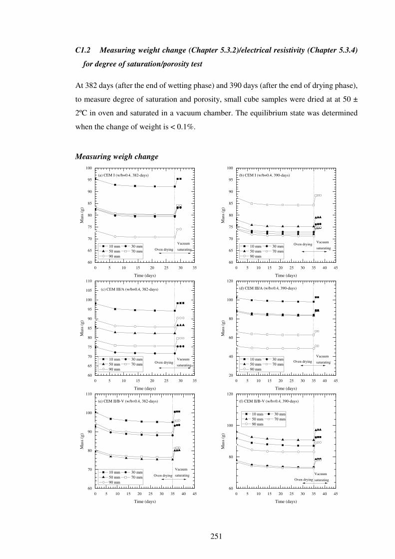
251

C1.2 Measuring weight change (Chapter 5.3.2)/electrical resistivity (Chapter 5.3.4)

for degree of saturation/porosity test

At 382 days (after the end of wetting phase) and 390 days (after the end of drying phase),

to measure degree of saturation and porosity, small cube samples were dried at at 50 ±

2ºC in oven and saturated in a vacuum chamber. The equilibrium state was determined

when the change of weight is < 0.1%.

Measuring weigh change

0 5 10 15 20 25 30 35

60

65

70

75

80

85

90

95

100

Vacuum

saturating

Mas

s (g

)

Time (days)

10 mm 30 mm

50 mm 70 mm

90 mm

Oven drying

(a) CEM I (w/b=0.4, 382-days)

0 5 10 15 20 25 30 35 40 45

60

65

70

75

80

85

90

95

100

Vacuum

saturating

Mas

s (g

)

Time (days)

10 mm 30 mm

50 mm 70 mm

90 mm

Oven drying

(b) CEM I (w/b=0.4, 390-days)

0 5 10 15 20 25 30 35

60

65

70

75

80

85

90

95

100

105

110

Vacuum

saturating

Mas

s (g

)

Time (days)

10 mm 30 mm

50 mm 70 mm

90 mm

Oven drying

(c) CEM III/A (w/b=0.4, 382-days)

0 5 10 15 20 25 30 35 40 45

20

40

60

80

100

120

Vacuum

saturating

Mas

s (g

)

Time (days)

10 mm 30 mm

50 mm 70 mm

90 mm

Oven drying

(d) CEM III/A (w/b=0.4, 390-days)

0 5 10 15 20 25 30 35 40 45

60

70

80

90

100

110

Vacuum

saturating

Mas

s (g

)

Time (days)

10 mm 30 mm

50 mm 70 mm

90 mm

Oven drying

(e) CEM II/B-V (w/b=0.4, 382-days)

0 5 10 15 20 25 30 35 40 45

60

80

100

120

Vacuum

saturating

Mas

s (g

)

Time (days)

10 mm 30 mm

50 mm 70 mm

90 mm

Oven drying

(f) CEM II/B-V (w/b=0.4, 390-days)

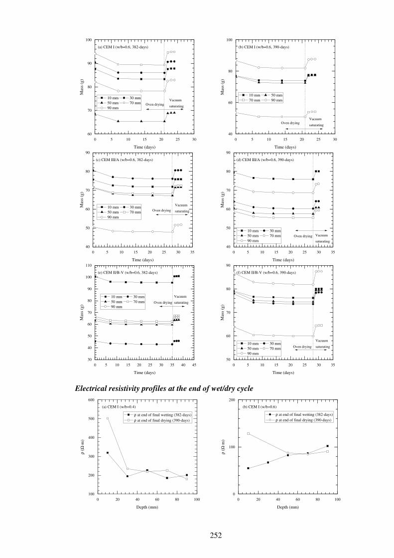
252

Electrical resistivity profiles at the end of wet/dry cycle

0 5 10 15 20 25 30

60

70

80

90

100

Vacuum

saturating

Mas

s (g

)

Time (days)

10 mm 30 mm

50 mm 70 mm

90 mmOven drying

(a) CEM I (w/b=0.6, 382-days)

0 5 10 15 20 25 30

40

60

80

100

Vacuum

saturating

Mas

s (g

)

Time (days)

10 mm 50 mm

70 mm 90 mm

Oven drying

(b) CEM I (w/b=0.6, 390-days)

0 5 10 15 20 25 30 35

40

50

60

70

80

90

Vacuum

saturating

Mas

s (g

)

Time (days)

10 mm 30 mm

50 mm 70 mm

90 mm

Oven drying

(c) CEM III/A (w/b=0.6, 382-days)

0 5 10 15 20 25 30 35

40

50

60

70

80

90

Vacuum

saturating

Mas

s (g

)

Time (days)

10 mm 30 mm

50 mm 70 mm

90 mmOven drying

(d) CEM III/A (w/b=0.6, 390-days)

0 5 10 15 20 25 30 35 40 45

30

40

50

60

70

80

90

100

110

Vacuum

saturating

Mas

s (g

)

Time (days)

10 mm 30 mm

50 mm 70 mm

90 mmOven drying

(e) CEM II/B-V (w/b=0.6, 382-days)

0 5 10 15 20 25 30 35

50

60

70

80

90

Vacuum

saturating

Mas

s (g

)

Time (days)

10 mm 30 mm

50 mm 70 mm

90 mm

Oven drying

(f) CEM II/B-V (w/b=0.6, 390-days)

0 20 40 60 80 100

100

200

300

400

500

600

ρ at end of final wetting (382-days)

ρ at end of final drying (390-days)

ρ (Ω

⋅m)

Depth (mm)

(a) CEM I (w/b=0.4)

0 20 40 60 80 100

0

100

200



ρ (Ω

⋅m)

Depth (mm)

(b) CEM I (w/b=0.6)

253

C1.3 Migration coefficient & Resistivity

w/b Binder

Age

(days)

Migration coefficient (ⅹ10-12m2/s) Resisvity (Ω·m)

No.1 No.2 No.3 No.1 No.2 No.3

0.4

CEM I

180 9.07 8.87 8.68 97.20 99.18 97.67

270 8.12 6.15 8.12 98.35 92.90 93.78

365 6.77 7.09 5.00 101.66 108.29 121.04

CEM III/A

180 3.78 2.80 3.41 183.68 167.24 179.27

270 3.41 + 3.77 240.04 229.62 232.59

365 2.10 1.89 2.18 274.33 304.53 268.77

CEM II/B-V

180 2.52 3.16 3.06 281.82 287.50 271.88

270 2.55 2.68 + 316.28 312.47 334.84

365 1.37 0.81 1.52 444.21 395.04 403.45

0.6

CEM I

180 21.91 20.58 20.65 50.27 50.82 48.70

270 23.04 23.34 21.79 54.23 54.92 57.52

365 20.66 23.56 18.01 58.33 59.88 48.84

CEM III/A

180 7.22 5.94 6.13 149.23 154.75 159.55

270 4.99 5.30 4.47 173.04 173.87 181.11

365 2.68 3.55 4.44 193.00 183.40 181.22

CEM II/B-V

180 6.29 7.44 8.65 147.11 146.26 143.98

270 4.37 5.23 4.44 216.64 220.24 218.33

365 2.79 3.08 3.53 269.40 276.78 255.19

0 20 40 60 80 100

200

300

400

500

600

700



ρ (Ω

⋅m)

Depth (mm)

(c) CEM III/A (w/b=0.4)

0 20 40 60 80 100

200

300

400

500

600



ρ (Ω

⋅m)

Depth (mm)

(d) CEM III/A (w/b=0.6)

0 20 40 60 80 100

500

600

700

800

900



ρ (Ω

⋅m)

Depth (mm)

(e) CEM II/B-V (w/b=0.4)

0 20 40 60 80 100

200

300

400

500

600



ρ (Ω

⋅m)

Depth (mm)

(f) CEM II/B-V (w/b=0.6)

254

C1.4 Chloride profiling

w/b= 0.4

CEM I (%, by weight of binder) CEM III/A (%, by weight of binder) CEM II/B-V (%, by weight of binder)

Depth (mm)

Measured value

Predicted value*

Predicted value**

Measured value

Predicted value*

Predicted value**

Measured value

Predicted value*

Predicted value**

0 + 2.89 2.91 5.38 6.75 3.15 5.60

2 2.55 2.56 2.58 4.27 4.35 5.28 2.29 2.77 4.61

6 1.75 1.92 1.93 2.78 2.52 2.74 2.91 2.04 2.82

10 1.75 1.36 1.36 0.98 1.22 1.12 1.24 1.40 1.48

14 0.77 0.90 0.90 0.40 0.49 0.35 0.77 0.89 0.66

18 0.52 0.56 0.56 0.34 0.16 0.09 0.35 0.53 0.25

22 0.24 0.32 0.32 0.20 0.04 0.02 0.21 0.29 0.08

26 0.13 0.17 0.17 0.14 0.01 0.00 0.12 0.15 0.02

30 0.12 0.09 0.09 0.00 0.00 0.00 0.11 0.07 0.00

40 + 0.01 0.01 + 0.00 0.00 + 0.01 0.00

50 + 0.00 0.00 + 0.00 0.00 + 0.00 0.00

* including first point (at 2 mm cover depth) and ** excluding first point (at 2 mm cover depth)

Diffusion coefficient/Surface chloride

Fitting result including first point (at 2 mm cover depth) Fitting result excluding first point (at 2 mm cover depth)

Cs D r2 Cs D r2

CEM I (w/b=0.4) 2.89 2.85 0.96 2.91 2.81 0.93

CEM III/A (w/b=0.4) 5.38 1.02 0.99 6.75 0.77 0.98

CEM II/B-V (w/b=0.4) 3.15 2.52 0.87 5.60 1.19 0.98

Cs surface chloride concentration (%, by weight of binder), D diffusion coefficient (m2/s), r2 determinant coefficient

255

w/b= 0.6

CEM I (%, by weight of binder) CEM III/A (%, by weight of binder) CEM II/B-V (%, by weight of binder)

Depth (mm)

Measured value

Predicted value*

Predicted value**

Measured value

Predicted value*

Predicted value**

Measured value

Predicted value*

Predicted value**

0 + 6.12 5.89 + 6.09 8.00 6.12 7.02

2 5.73 5.59 5.40 4.50 5.59 7.20 5.10 5.61 6.37

6 4.36 4.58 4.45 5.64 4.61 5.65 5.35 4.61 5.10

10 3.09 3.62 3.55 4.32 3.70 4.24 3.22 3.67 3.93

14 3.59 2.77 2.75 2.77 2.87 3.03 3.48 2.83 2.91

18 2.38 2.05 2.06 2.13 2.16 2.06 1.98 2.11 2.06

22 1.17 1.46 1.49 1.96 1.57 1.33 1.45 1.52 1.40

26 0.62 1.00 1.04 0.41 1.10 0.82 0.90 1.06 0.91

30 0.70 0.66 0.70 0.21 0.75 0.47 0.45 0.71 0.56

40 + 0.37 0.41 + 0.24 0.10 + 0.22 0.14

50 + 0.20 0.22 + 0.06 0.01 + 0.05 0.02

* including first point (at 2 mm cover depth) and ** excluding first point (at 2 mm cover depth)

Diffusion coefficient/Surface chloride

Fitting result including first point (at 2 mm cover depth) Fitting result excluding first point (at 2 mm cover depth)

Cs D r2 Cs D r2

CEM I (w/b=0.6) 5.89 21.99 0.90 6.12 20.72 0.94

CEM III/A (w/b=0.6) 8.00 3.75 0.97 6.09 5.61 0.87

CEM II/B-V (w/b=0.6) 7.02 4.36 0.95 6.12 5.39 0.94

Cs surface chloride concentration (%, by weight of binder), D diffusion coefficient (m2/s), r2 determinant coefficient

256


C2.1 Corrosion potential monitoring/macrocell current monitoring

CEM I (w/b=0.4) Type of

measurement Corrosion potential (mV) Macrocell current (nA/cm2)

Type of steel SS LS SS LS

Age (days) No.1 No.2 No.3 No.1 No.2 No.3 No.1 No.2 No.3 No.1 No.2 No.3

42 -84 -79 -65 -76 -66 -59 1.59 0.40 0.60 -1.33 0.44 0.53

47 -183.7 -167.2 -163.8 -165.6 -150.8 -150.3 1.99 2.88 1.89 1.33 1.33 1.90

49 -183.6 -180.4 -174.2 -174.5 -158.3 -164.7 0.42 1.47 3.24 0.54 1.87 0.90

54 -167.1 -158.2 -165.4 -162.1 -143.2 -151.6 -0.52 0.30 0.46 0.17 -0.40 0.09

56 -168.1 -173.2 -169.7 -160.1 -146.2 -152.9 -0.02 1.59 2.59 -0.03 -0.03 0.01

61 -159.4 -163.1 -151.6 -157.3 -146.1 -140.1 -0.18 -0.10 -0.04 0.16 -0.08 0.12

63 -198.7 -194.7 -180 -191.2 -188.9 -167.6 1.03 -0.40 0.40 0.11 -0.07 -0.03

67 -147.5 -144.3 -154.6 -145.7 -136.6 -143.4 0.22 0.16 0.08 -0.08 -0.05 -0.04

68 -187.5 -175.8 -178.3 -172.1 -170.7 -169.5 0.86 -0.22 0.10 -0.05 -0.07 -0.01

70 -176.1 -175.4 -162.3 -158.9 -148.7 -153.8 1.53 -0.16 0.02 -0.05 -0.05 0.11

75 -187.1 -179.9 -180.4 -180.7 -174.3 -177.9 0.22 -0.22 0.08 -0.08 -0.07 0.01

77 -158.7 -147.1 -157.1 -154.3 -139.2 -147 0.24 -0.42 0.46 -0.25 -0.20 0.01

82 -184.8 -174.4 -174.1 -173.6 -164.4 -172.7 -0.58 -0.12 0.06 -0.07 -0.03 0.01

84 -156 -143.6 -143.1 -150.6 -135.1 -138.5 0.02 -0.54 0.10 -0.08 -0.04 0.01

89 -183.9 -167 -173.4 -172.7 -161.6 -170.1 0.06 -0.18 0.02 -0.27 -0.13 -0.01

91 -169 -151.5 -152.5 -161.8 -142.1 -147 1.03 0.50 0.22 -0.21 -0.08 -0.08

96 -186.2 -169.3 -169 -165.9 -161.5 -165.3 0.84 -0.02 -0.04 -0.05 -0.03 0.03

102 -160.1 -115.9 -105.6 -137 -100 -104.7 1.31 -0.02 0.16 -0.07 0.01 -0.03

110 -172 -159.4 -166.2 -166.1 -154.2 -154.2 0.02 -0.18 0.44 -0.16 -0.07 -0.03

116 -140.1 -121.1 -84.18 -130.2 -102.6 -81.3 0.40 -0.12 0.34 -0.07 0.01 -0.07

130 -162.3 -162.3 -168 -152.4 -152.4 -141.4 0.36 -0.02 1.25 -0.12 -0.04 -0.01

133 -155.2 -148.8 -140.6 -148.7 -131 -127.5 0.36 0.24 0.66 -0.08 0.01 -0.05

138 -179.9 -167.3 -164.4 -167.7 -157.4 -159.8 0.62 -0.08 0.04 -0.16 -0.08 -0.04

144 -136.1 -101.5 -71.5 -127.1 -94.8 -76.5 1.79 -0.66 -0.20 -0.15 -0.01 0.04

152 -161.4 -137.9 -143.8 -161.2 -142.8 -142.5 0.20 -0.14 0.02 -0.08 -0.03 0.01

158 -131.8 -99.9 -71.2 -116.6 -111.2 -80.5 0.32 -0.48 -0.16 -0.08 -0.04 0.01

166 -163.8 -133.1 -120.4 -145.6 -125.1 -119.8 0.62 -1.07 -0.40 -0.15 -0.04 -0.05

172 -126.8 -83.5 -59 -107.8 -73.8 -60.3 0.48 -0.32 0.02 -0.01 0.04 0.03

180 -156.7 -145.7 -168 -162.6 -149.9 -146.3 -0.28 -0.88 0.16 -0.08 -0.03 -0.01

186 -153 -120 -100.2 -146.1 -115.1 -105.9 0.70 -0.99 -0.02 -0.04 0.04 -0.05

194 -172.6 -138.2 -125.3 -129.8 -134.6 -142.1 1.21 -1.11 -0.22 -0.07 -0.01 -0.01

200 -177.9 -169.3 -81.76 -180.2 -133.7 -88.38 -0.26 0.30 -0.06 -0.07 -0.01 -0.04

208 -190 -177.2 -151.6 -190.4 -145.8 -138.1 0.08 -0.24 0.60 -0.05 -0.07 0.07

214 -155.9 -131.4 -63.7 -164.3 -99.57 -66.5 0.24 0.02 0.02 -0.01 -0.05 0.01

222 -184.5 -136.1 -123 -180.1 -139.6 -92 0.40 -0.20 0.20 -0.04 -0.01 0.01

228 -138.8 -125.9 -63.8 -141.8 -110.6 -65.4 1.79 -0.95 -0.16 -0.04 -0.05 -0.03

236 -168.3 -154.6 -158.2 -161.9 -138.7 -135.6 0.46 -0.18 -0.02 -0.25 -0.01 -0.01

242 -130.1 -121.9 -79.8 -137 -106.7 -81.9 0.34 -0.26 -0.06 -0.04 -0.01 -0.03

250 -177.4 -139.6 -161.3 -169.3 -115.3 -150.5 0.30 -0.22 -0.02 -0.11 -0.04 0.01

256 -169.7 -129.6 -84.7 -171.1 -125.5 -89.1 0.38 -0.06 0.46 -0.01 0.27 0.15

264 -177.3 -121 -130.2 -168.8 -99.3 -122.2 0.30 -0.36 0.02 -0.21 -0.05 0.01

270 -152.1 -109.8 -94 -159.8 -98.2 -2.4 0.38 -0.52 -0.08 -0.04 -0.01 -0.01

278 -171.6 -98.5 -117.5 -170.3 -100.2 -111.6 0.16 -0.12 -0.02 -0.04 -0.01 0.01

284 -139.2 -88.3 -74.8 -136.1 -85.1 -79.1 0.50 -0.42 -0.10 -0.07 -0.04 -0.01

292 -164.5 -129.6 -130.8 -158.7 -115.3 -128.1 0.44 -0.32 0.02 -0.05 -0.01 0.01

298 -133.2 -89 -75.9 -129.5 -71.6 -75.4 0.52 -0.42 -0.02 -0.09 -0.05 -0.04

306 -170.5 -131.1 -121.7 -174.6 -112.4 -122.4 0.84 -0.28 0.02 -0.44 -0.12 0.05

312 -127.7 -94.8 -71.8 -127 -85.3 -70.8 -0.54 -1.39 -0.93 -0.53 -0.24 -0.23

320 -158.7 -114.9 -123.8 -153.4 -106.9 -122.7 0.74 -0.48 -0.02 -0.11 -0.05 0.01

326 -123.8 -90.4 -74 -115.3 -78.7 -70.3 0.20 -0.16 -0.02 -0.05 -0.03 -0.03

334 -146.1 -100.9 -110.9 -145.7 -102.1 -108.1 0.26 -0.20 -0.02 -0.04 -0.01 -0.01

340 -126.7 -79.6 -75.6 -137.5 -76.8 -70.2 -0.56 -1.49 -0.95 -0.44 -0.16 -0.21

348 -151.5 -104.9 -111.1 -146.7 -98.2 -109.2 0.66 -0.38 -0.20 -0.08 -0.04 -0.03

354 -131 -65.6 -60.9 -130.8 -63.1 -70.1 -0.20 0.40 -0.02 -0.40 -0.01 -0.27

362 -151.4 -98.4 -120.9 -151.3 -84.6 -117.9 0.24 -0.16 -0.02 -0.11 -0.03 -0.01

368 -119.9 -81.5 -41.8 -118.2 -77.5 -42.3 0.38 -0.30 -0.04 -0.24 -0.16 -0.09

376 -152.1 -110.9 -96.8 -148.5 -104.7 -91.9 0.22 -0.10 -0.02 -0.03 0.01 -0.01

382 -146.1 -118 -54.4 -149.4 -93 -48.5 0.14 -0.06 -0.02 -0.03 -0.03 -0.01

257

CEM III (w/b=0.4) Type of




42 -108.1 -100.3 -61.7 -85.1 -103.7 -56.0 -0.30 0.54 0.18 -0.54 0.07 -0.07

47 -131.1 -125.6 -114.9 -125.0 -126.4 -115.2 -0.46 0.20 0.04 -0.24 -0.05 -0.56

49 -159.8 -161.5 -162.9 -158.6 -157.7 -157.7 -1.05 0.42 0.08 -0.24 -0.08 -0.07

54 -150.2 -148.9 -148.3 -148.5 -145.9 -145.7 -0.18 0.06 -0.06 -0.80 -0.32 -0.24

56 -165.7 -161.5 -162.6 -164.9 -155.6 -157.0 -0.54 0.32 -0.06 -0.42 -0.23 -0.20

61 -143.9 -144.2 -143.2 -144.9 -140.2 -140.0 -0.30 0.14 -0.04 -0.27 -0.15 -0.08

63 -172.7 -166.8 -167.8 -167.2 -159.9 -163.3 -0.26 0.04 -0.08 -0.25 -0.15 -0.13

67 -139.8 -141.0 -139.9 -140.9 -138.9 -136.3 -0.28 0.06 -0.06 -0.29 -0.09 -0.11

68 -163.3 -162.8 -164.8 -158.5 -154.4 -159.2 -0.52 0.02 -0.14 -0.53 -0.38 -0.41

70 -137.1 -143.0 -148.5 -139.3 -135.8 -134.5 -0.60 0.46 0.76 -0.32 -0.17 -0.12

75 -167.1 -172.3 -169.5 -166.9 -161.9 -164.7 -0.52 0.50 -0.12 -0.48 -0.24 -0.16

77 -144.4 -144.5 -142.4 -143.5 -140.7 -139.3 -0.50 0.10 -0.10 -0.41 -0.23 -0.12

80 -178.0 -179.2 -187.3 -171.5 -158.0 -163.9 -0.30 0.04 0.60 -0.36 -0.21 -0.15

82 -159.1 -147.1 -145.4 -146.3 -140.8 -144.6 -0.10 0.06 -0.08 -0.34 -0.21 -0.16

96 -183.0 -171.5 -175.6 -170.3 -164.6 -171.2 -0.24 -0.12 0.02 -0.23 -0.15 -0.11

102 -140.8 -141.7 -137.6 -142.4 -138.2 -133.7 -0.16 -0.04 -0.04 -0.20 -0.15 -0.08

110 -168.6 -161.8 -164.3 -168.2 -157.9 -158.3 -0.30 -0.10 0.06 -0.25 -0.16 -0.11

116 -139.5 -133.4 -135.5 -138.5 -126.7 -128.7 -0.28 -0.04 0.18 -0.34 -0.11 -0.05

124 -150.5 -145.1 -154.0 -151.6 -137.3 -145.7 -1.35 0.88 -0.32 -0.13 -0.07 -0.04

130 -135.0 -134.0 -127.8 -134.4 -129.6 -125.7 -0.32 -0.10 -0.22 -0.27 -0.13 -0.05

138 -144.0 -141.2 -142.9 -149.5 -140.1 -141.9 -0.24 -0.06 -0.16 -0.09 -0.11 -0.08

144 -149.4 -156.6 -146.0 -150.5 -149.6 -145.0 -0.14 0.04 -0.16 -0.17 -0.09 -0.05

152 -142.4 -150.8 -148.6 -145.3 -148.0 -150.6 -0.18 0.14 -0.20 -0.11 -0.05 -0.01

158 -150.7 -152.6 -141.5 -149.1 -143.0 -140.4 -0.38 0.70 -0.38 -0.40 -0.15 -0.05

166 -135.3 -124.8 -141.3 -144.2 -143.5 -142.6 -0.60 0.46 -0.56 -0.40 -0.21 -0.11

172 -155.2 -151.6 -140.6 -152.5 -144.3 -136.9 -0.32 0.66 -0.50 -0.24 -0.09 -0.04

180 -174.9 -162.7 -158.4 -170.5 -157.2 -158.7 -0.04 -0.06 -0.10 -0.11 -0.05 -0.03

186 -137.5 -138.3 -153.4 -136.3 -135.7 -154.6 -0.08 -0.10 -0.08 -0.15 -0.08 -0.04

194 -163.1 -155.9 -153.0 -163.4 -154.2 -155.7 -0.10 0.06 -0.18 -0.08 0.01 -0.03

200 -151.7 -131.8 -141.7 -151.8 -143.6 -141.3 -0.10 -0.12 -0.22 -0.11 -0.04 -0.04

208 -170.3 -166.0 -166.4 -165.9 -161.7 -163.9 -0.06 -0.04 -0.06 -0.11 -0.05 -0.03

214 -144.4 -140.8 -140.2 -144.8 -140.9 -135.4 -0.22 -0.20 -0.08 -0.61 -0.33 -0.12

222 -163.5 -160.3 -151.4 -163.5 -157.9 -154.1 -0.08 -0.12 -0.04 -0.12 -0.07 -0.09

228 -143.1 -148.0 -134.9 -143.6 -140.3 -134.1 -0.08 0.30 -0.06 -0.07 -0.01 -0.01

236 -160.8 -160.1 -153.1 -163.1 -155.1 -151.3 -0.10 -0.08 -0.10 -0.58 -0.24 -0.05

242 -146.8 -143.7 -139.5 -151.9 -144.1 -135.8 -0.04 -0.06 -0.06 -0.11 -0.04 -0.01

250 -158.8 -152.8 -146.6 -158.0 -150.9 -144.7 -0.20 0.50 -0.44 -0.24 -0.13 -0.04

256 -143.8 -136.5 -126.7 -144.0 -139.9 -129.9 0.22 -0.34 -0.38 0.13 -0.07 -0.03

264 -159.3 -154.8 -146.8 -159.2 -150.8 -146.4 -0.18 -0.56 -0.40 -0.27 -0.13 -0.03

270 -141.5 -133.8 -129.1 -137.3 -134.3 -127.3 -0.08 -0.14 -0.16 -0.08 -0.09 0.01

278 -153.9 -147.0 -140.2 -153.0 -144.1 -138.7 -0.04 -0.14 -0.14 -0.11 -0.04 0.01

284 -138.0 -132.7 -128.1 -138.5 -132.4 -127.5 -0.04 -0.08 -0.10 -0.08 -0.04 -0.03

292 -148.8 -154.3 -145.0 -159.2 -147.9 -146.1 -0.06 -0.34 -0.26 -0.16 -0.08 -0.05

298 -142.4 -134.4 -131.6 -144.2 -138.5 -130.6 -1.03 -1.57 -0.32 -0.61 -0.15 -0.05

306 -140.9 -146.8 -144.8 -138.5 -147.2 -142.4 -0.06 -0.44 -0.24 -0.77 -0.52 -0.08

312 -141.3 -140.9 -127.3 -136.1 -132.0 -126.1 0.04 -0.12 -0.10 -0.05 -0.03 -0.01

320 -165.2 -162.1 -153.5 -158.7 -153.7 -153.5 0.08 -0.24 -0.10 -0.07 -0.04 -0.03

326 -135.4 -132.8 -124.4 -131.5 -135.1 -122.4 -0.02 -0.26 -0.14 -0.34 -0.17 -0.07

334 -144.8 -134.8 -138.1 -142.2 -133.1 -136.8 -0.02 -0.16 -0.06 -0.29 -0.11 0.04

340 -134.3 -128.7 -121.8 -134.0 -131.9 -122.6 -0.22 -0.32 -0.22 -0.15 -0.11 -0.05

348 -143.0 -144.4 -139.6 -142.0 -142.1 -136.3 -0.50 -0.34 -0.10 0.01 -0.03 -0.33

354 -126.8 -124.8 -123.9 -128.3 -125.1 -121.8 -0.02 -0.06 -0.04 -0.03 -0.01 -0.01

362 -127.5 -126.4 -115.1 -127.9 -125.5 -111.7 -0.04 -0.08 -0.04 -0.03 -0.01 0.01

368 -132.5 -128.6 -122.6 -134.2 -132.0 -121.6 -0.08 -0.12 -0.08 -0.11 -0.07 -0.01

376 -128.1 -121.4 -128.6 -126.8 -123.0 -124.9 0.02 -0.08 -0.04 -0.07 -0.04 -0.01

382 -131.3 -128.0 -124.6 -129.1 -127.9 -122.1 -0.02 -0.08 -0.04 -0.15 -0.08 -0.01

258

CEM II/B-V (w/b=0.4) Type of




42 -108.5 -86.3 -109.3 -123.1 -84.8 -110.2 1.77 0.66 3.00 0.60 2.18 1.03

47 -138.4 -125.8 -138.7 -148.2 -129.2 -143.9 0.44 -0.08 1.13 0.23 1.34 0.60

49 -165.2 -164.3 -176.4 -164.5 -171.8 -172.0 0.62 -0.42 1.55 -0.11 0.60 -0.05

54 -167.8 -154.3 -167.2 -156.5 -161.0 -163.1 0.38 -0.92 1.67 -0.17 0.32 -0.03

56 -178.5 -164.1 -176.3 -168.8 -170.7 -170.8 0.12 -0.62 0.54 -0.23 -0.04 -0.16

61 -161.0 -146.0 -157.7 -147.9 -153.9 -154.8 0.04 -1.63 0.92 -0.60 0.32 -0.40

63 -176.6 -165.7 -173.6 -167.4 -173.5 -169.9 0.02 -1.75 0.68 -0.40 0.08 -0.24

67 -157.7 -141.4 -152.8 -143.1 -148.4 -150.5 -0.06 -0.68 0.10 -0.24 0.07 -0.15

68 -176.6 -161.9 -169.5 -160.0 -172.4 -166.5 -0.14 -1.59 0.12 -0.58 0.13 -0.37

70 -158.6 -142.0 -153.1 -145.1 -149.3 -151.3 -0.12 -1.37 0.02 -0.46 0.11 -0.29

73 -181.2 -161.6 -185.6 -161.7 -170.0 -169.2 -0.16 -1.15 -0.06 -0.41 0.04 -0.32

75 -157.4 -143.0 -156.3 -143.1 -152.2 -152.0 -0.16 -1.33 -0.06 -0.37 0.04 -0.34

89 -182.6 -166.7 -175.7 -170.7 -174.1 -175.8 -0.08 -1.21 -0.50 -0.25 -0.03 -0.27

91 -158.0 -141.3 -151.5 -145.0 -148.3 -149.6 -0.06 -0.68 -0.18 -0.19 -0.01 -0.15

96 -175.0 -161.0 -167.7 -163.8 -168.7 -166.4 -0.08 -0.76 -0.24 -0.27 0.01 -0.20

102 -150.6 -136.1 -146.1 -135.5 -140.6 -147.3 -0.06 -0.99 -0.22 -0.17 0.03 -0.13

110 -168.1 -160.4 -162.7 -155.1 -161.3 -163.7 -0.04 -0.36 -0.18 -0.15 -0.01 0.05

116 -143.1 -131.3 -141.9 -144.2 -134.1 -137.4 -0.12 -0.74 -0.30 -0.13 0.03 -0.11

124 -142.6 -134.3 -144.0 -138.5 -147.5 -151.4 -0.50 -2.73 -1.19 -0.27 -0.13 -0.13

130 -137.9 -121.9 -134.8 -118.7 -130.5 -132.5 -0.16 -0.62 -0.32 -0.12 0.01 -0.11

138 -159.1 -144.5 -156.4 -153.8 -157.4 -160.2 -0.14 -0.48 -0.28 -0.11 -0.03 -0.16

144 -150.6 -137.3 -148.3 -142.9 -145.5 -148.2 -0.30 -1.05 -0.62 -0.15 0.01 -0.08

152 -164.8 -154.8 -161.2 -149.1 -159.7 -158.6 -0.12 -0.86 -0.56 -0.17 -0.01 -0.16

158 -148.8 -131.7 -143.4 -133.5 -138.4 -143.1 -0.10 -0.50 -0.36 -0.15 -0.01 -0.11

166 -168.5 -150.7 -161.4 -157.8 -156.0 -163.7 -0.06 -0.82 -0.52 -0.03 0.11 -0.11

172 -137.8 -128.4 -134.1 -125.1 -131.7 -132.7 -0.06 -0.28 -0.20 -0.11 -0.03 -0.11

180 -165.9 -151.5 -160.1 -149.6 -166.9 -158.2 -0.06 -0.40 -0.22 -0.07 0.03 -0.08

186 -140.5 -126.2 -133.9 -125.0 -130.6 -128.6 -0.10 -0.32 -0.28 -0.15 -0.05 -0.11

194 -153.9 -145.8 -149.4 -144.8 -151.9 -150.7 -0.16 -0.54 -0.28 -0.09 -0.01 -0.11

200 -147.7 -129.8 -140.4 -129.6 -134.0 -136.2 0.02 -0.36 -0.14 -0.11 -0.04 -0.12

208 -159.5 -141.6 -151.9 -145.0 -140.9 -145.6 -0.08 -1.15 -0.32 -0.05 -0.01 -0.04

214 -142.8 -128.1 -138.9 -130.7 -135.3 -136.0 -0.10 -0.64 0.62 -0.32 -0.01 -0.33

222 -158.7 -147.7 -160.8 -141.6 -151.3 -152.8 -0.24 -1.05 0.02 -0.53 0.16 -0.62

228 -140.9 -126.9 -136.0 -127.1 -130.7 -130.3 -0.18 -0.50 -0.18 -0.13 -0.03 -0.08

236 -130.3 -125.5 -124.3 -126.1 -132.5 -130.1 -0.60 -0.86 -0.70 -0.07 -0.01 -0.11

242 -137.3 -125.9 -144.6 -125.0 -132.2 -133.7 -0.06 -0.44 -0.32 -0.07 -0.01 -0.07

250 -151.8 -141.0 -146.0 -137.4 -146.0 -146.3 -0.12 -0.44 -0.30 -0.08 -0.01 -0.09

256 -148.0 -123.4 -128.5 -129.2 -127.8 -130.2 -0.10 -0.52 -0.44 -0.08 -0.03 -0.11

264 -145.4 -141.7 -141.2 -132.5 -145.3 -144.2 -0.10 -0.38 -0.36 -0.16 -0.01 -0.19

270 -136.1 -125.0 -125.7 -123.1 -127.8 -126.7 -0.14 -0.93 -0.93 -0.05 0.01 -0.07

278 -146.2 -144.1 -141.5 -135.5 -143.9 -142.6 -0.16 -0.78 -0.95 -0.11 -0.04 -0.11

284 -138.2 -124.9 -127.4 -127.9 -130.5 -131.1 -0.08 -0.30 -0.32 -0.09 -0.82 0.04

292 -142.0 -130.6 -133.9 -129.8 -134.9 -133.7 -0.12 -0.62 -0.66 -0.07 -0.01 -0.08

298 -136.0 -125.1 -128.5 -123.8 -128.1 -128.1 -0.04 -0.24 -0.26 -0.13 0.01 -0.15

306 -118.6 -141.6 -140.6 -111.3 -142.0 -149.7 -0.12 -0.62 -0.76 -0.08 -0.01 -0.08

312 -128.3 -114.2 -116.8 -120.0 -120.2 -120.5 -0.16 -0.54 -0.64 -0.20 -0.01 -0.24

320 -141.9 -127.4 -147.0 -131.7 -133.6 -149.2 -0.06 -0.20 -0.22 -0.09 0.01 -0.12

326 -127.3 -111.4 -115.3 -116.8 -116.4 -116.6 -0.12 -0.64 -0.74 -0.29 -0.04 -0.37

334 -130.2 -121.7 -120.1 -119.3 -124.2 -121.4 -0.02 -0.24 -0.32 -0.03 0.01 -0.04

340 -124.9 -112.2 -120.2 -115.1 -114.6 -119.3 -0.06 -0.44 -0.48 -0.03 0.01 -0.05

348 -134.1 -123.0 -127.5 -120.7 -122.2 -120.9 -0.02 -0.16 -0.14 -0.03 0.01 -0.04

354 -126.3 -113.6 -115.2 -123.1 -119.7 -120.3 -0.18 -0.38 -0.40 -0.11 -0.04 -0.11

362 -132.3 -120.0 -124.1 -127.5 -125.1 -126.0 0.02 -0.38 -0.44 -0.05 0.11 -0.16

368 -131.8 -118.6 -115.8 -121.8 -118.8 -120.6 -0.02 -0.16 -0.20 -0.07 -0.01 -0.11

376 -135.4 -121.2 -123.3 -127.2 -127.8 -133.7 0.02 -0.08 -0.04 0.40 0.40 -0.04

382 -141.2 -108.7 -116.7 -133.1 -113.5 -118.3 0.02 -0.24 -0.40 -0.07 -0.01 -0.20

259

CEM I (w/b=0.6) Type of




42 -88.9 -111.1 -91.5 -99.8 -110.7 -83.7 1.99 2.98 1.99 2.79 1.72 2.92

47 -188.5 -196.6 -192 -210.01 -187.5 -185.1 -3.28 1.41 2.51 0.01 3.69 5.23

49 -189.2 -203.7 -191 -197.6 -203.5 -189.6 -1.39 0.08 0.14 0.32 -0.01 0.86

54 -178.8 -178.8 -166 -185.5 -170.9 -164.7 -0.62 0.54 0.20 0.81 0.61 1.22

56 -193 -197.7 -200 -202.6 -189.3 -183.5 -0.99 0.20 1.19 0.40 0.13 0.13

61 -155.2 -138.8 -127 -173 -142.3 -108.18 -0.62 0.18 0.26 0.56 0.33 0.50

63 -175.7 -166 -168 -188.8 -168.3 -152.4 -0.74 0.10 0.30 0.34 0.41 0.92

67 -152.7 -148.4 -142 -165.5 -145.3 -119.6 -0.62 0.18 0.22 0.46 0.31 0.69

68 -162.2 -144.5 -141 -175.3 -149.9 -116.04 -0.66 0.10 0.24 0.37 0.25 0.61

70 -157.1 -144.5 -143 -167.1 -147.7 -133.9 -0.38 0.10 0.24 -0.34 0.23 0.45

75 -166.7 -169.1 -158 -177.9 -166.3 -157 -0.62 0.06 0.16 0.31 0.21 0.41

77 -164.9 -159.5 -147 -157.2 -149.1 -141.2 -0.68 0.06 0.14 0.23 0.12 0.34

82 -168.5 -170.2 -176 -179.7 -167.5 -167.7 -0.48 -0.06 0.18 -0.25 0.15 0.40

84 -154.2 -154.4 -153 -163 -151.3 -148.8 -0.68 0.02 0.30 0.25 0.19 0.40

89 -168.2 -172.8 -166 -176.5 -161.8 -157 -0.46 -0.12 0.06 0.21 0.09 0.34

91 -143.6 -147.4 -147 -155.1 -151.5 -143.7 -0.80 -0.20 0.10 0.31 0.25 0.58

96 -167.3 -173.8 -163 -182.4 -167.8 -166.3 -0.66 -0.28 0.02 0.23 0.24 0.42

102 -119.7 -124.8 -139 -133.3 -146.3 -120 -0.95 -0.30 -0.02 0.20 0.45 0.50

106 -157.9 -162.7 -162 -172.4 -165.6 -156 -1.59 -0.90 -0.30 0.29 0.60 1.01

111 -126.6 -126.5 -128 -142.3 -133.1 -122.5 -0.68 -0.42 -0.10 0.09 0.37 0.36

125 -158.7 -168.6 -169 -176.3 -162.2 -170.7 -0.82 -0.60 -0.22 0.07 0.38 0.33

131 -134.1 -134.3 -140 -145 -136.9 -118.6 -1.11 -0.60 -0.12 0.01 0.17 0.25

138 -175.5 -175.7 -178 -179.3 -170.6 -172.8 -0.54 -0.34 -0.20 0.01 -0.04 0.42

144 -120.9 -125.2 -134 -132.4 -131.4 -120.2 -0.50 -0.66 -0.16 -0.04 0.07 0.34

152 -198.1 -155.3 -153 -190.7 -159 -161.9 0.95 -2.13 -0.36 0.01 -0.66 0.58

158 -207.8 -136.2 -127 -150.1 -144.4 -129.3 4.08 -0.88 -0.36 0.11 0.13 0.31

166 -213.8 -166.6 -161 -170.8 -171.6 -168 3.92 -0.97 -0.52 0.01 0.09 0.24

172 -351.4 -147.2 -142 -379.2 -156.5 -141.5 72.49 -0.66 -0.40 75.45 0.01 0.21

180 -316.6 -179.2 -175 -415.6 -186.3 -173.5 28.70 -0.44 -1.75 100.23 -0.01 0.16

186 -290.6 -163.6 -144 -432.7 -149.9 -141.8 38.77 -1.33 -0.93 129.42 -0.01 0.12

194 -386.7 -175.5 -162 -440.8 -169.9 -443.4 100.88 -1.15 -1.71 129.67 -0.01 129.58

200 -384.7 -296.3 -125 -439.5 -135.3 -401.3 132.13 48.54 -1.71 151.46 -0.05 139.79

208 -398.3 -270.1 -160 -434.8 -170.5 -433.4 110.01 6.35 -0.40 112.98 -0.01 112.03

214 -398.1 -262.2 -128 -433.5 -149.4 -418.3 129.46 13.25 -0.40 132.53 0.03 134.59

222 -423.4 -339.3 -160 -450.6 -238.7 -448.8 135.47 49.47 -1.67 125.93 11.49 140.05

228 -424.8 -388 -136 -453.8 -254.9 -442.3 152.66 98.55 -0.46 141.62 19.34 155.70

236 -453.3 -408.6 -170 -466.4 -276.9 -472.1 170.28 92.24 -0.08 138.59 14.88 150.05

242 -465.3 -421.6 -135 -467.6 -254.4 -467.2 201.23 136.98 -1.11 161.80 13.47 182.36

250 -465.1 -460.9 -160 -480.4 -263 -476 166.94 144.90 -0.64 142.16 7.43 156.42

256 -486.5 -435.8 -138 -489.7 -222.2 -493.9 220.61 157.73 -0.76 180.37 7.00 198.41

264 -476.1 -460.7 -173 -485 -257.8 -494.4 196.58 151.80 -0.34 154.44 9.11 166.45

270 -510 -442.8 -231 -508.6 -377.8 -530.2 252.24 164.31 6.31 194.43 94.32 238.06

278 -500.5 -470.8 -233 -508 -411.7 -529.9 227.01 154.80 3.98 172.41 103.65 206.76

284 -523.1 -465.3 -207 -545.4 -417.9 -545 270.94 165.23 2.63 225.86 124.73 260.61

292 -505.9 -486.9 -221 -529.5 -422.1 -536.4 229.40 170.84 3.28 189.26 117.43 216.05

298 -545 -470.8 -217 -574.5 -408.2 -567.1 288.84 177.96 3.04 250.80 111.30 331.96

306 -521.3 -478.9 -223 -538 -538 -538.9 235.25 161.41 3.12 198.94 98.77 239.26

312 -568.5 -469 -200 -585 -432.6 -570.8 329.82 182.73 2.15 271.22 140.61 334.48

320 -528.5 -486.4 -431 -550.5 -458.3 -549.1 263.58 173.66 144.10 220.16 142.71 263.13

326 -586.9 -503.5 -452 -603 -479.6 -578.6 344.74 197.89 172.49 285.15 171.75 333.42

334 -550.6 -500.8 -457 -575.4 -490.7 -554.1 280.29 176.85 159.86 242.71 161.80 247.35

340 -598.4 -514.1 -450 -620.5 -502.2 -594.3 327.23 212.45 170.50 284.08 192.44 27.32

348 -539.2 -503.7 -428 -574.7 -493.1 -532.8 277.70 192.48 156.20 231.96 181.03 26.74

354 -593.8 -532.5 -446 -609.5 -532.5 -604.4 370.00 241.69 186.49 301.46 229.31 87.35

362 -549.2 -512.8 -464 -583.7 -503.3 -547 279.09 204.50 180.27 240.85 197.75 18.01

368 -602.1 -549 -470 -613.1 -562.5 -598.9 380.55 273.92 208.55 307.43 274.01 111.01

376 -562.6 -542.6 -491 -577.1 -549.1 -562.8 311.32 229.36 205.69 256.37 224.67 16.09

382 -578.1 -548.3 -478 -616.8 -565.5 -597.9 314.90 269.54 218.62 274.80 283.82 140.19

260

CEM III/A (w/b=0.6) Type of




42 -135.5 -139 -116.5 -127.4 -120.9 -122.7 -6.52 2.17 2.41 -0.64 -3.74 0.40

47 -171.6 -174 -167.6 -162.6 -160.6 -169.6 -6.19 1.09 1.21 -0.11 -2.32 -0.12

49 -179.7 -171 -174.4 -173.4 -169.2 -179.5 -7.60 1.25 1.33 -0.13 -1.25 -0.17

54 -165.8 -173 -165 -160.9 -158.3 -168.1 -7.94 0.92 1.09 -0.17 -2.04 -0.41

56 -175.6 -183 -174.3 -172.2 -167.3 -178.8 -9.03 1.37 1.23 -0.16 -2.41 -0.38

61 -174.1 -162 -157 -153.2 -166.6 -165.7 -6.35 0.84 0.62 -0.40 -5.00 -0.32

63 -168.3 -178 -169 -166.2 -166.9 -175.1 -8.33 0.93 0.88 -0.42 -4.26 -0.33

67 -152.1 -161 -154.3 -151.2 -155 -157.6 -5.63 0.82 0.99 -0.32 -3.28 -0.44

68 -165 -175 -166.4 -164.5 -165 -171.3 -4.89 0.76 0.60 -0.42 -3.08 -0.23

70 -150 -159 -153.1 -148.9 -152.2 -157.4 -4.58 0.16 0.50 -0.32 -2.88 -0.25

75 -172.1 -181 -174.8 -170.3 -169.6 -179.1 -2.80 0.44 0.12 -0.32 -1.18 -0.41

77 -152.8 -161 -155 -152.4 -151.4 -160.9 -4.08 0.18 0.36 -0.37 -1.10 -0.32

81 -168.7 -179 -163.7 -165.7 -166.9 -176.4 -3.32 -0.18 0.16 -0.44 -0.98 -0.44

83 -160.6 -171 -164.9 -160.7 -158.6 -176.3 -2.94 -0.06 0.04 -0.31 -0.46 -0.12

96 -178 -178 -169.3 -177.2 -168.4 -178.4 -1.01 -0.16 0.06 -0.23 -0.58 -0.13

102 -162.4 -164 -155.8 -164.3 -156.9 -166.7 -0.50 0.22 0.04 -0.01 -0.58 -0.13

110 -171.6 -177 -169.2 -171.3 -174.8 -184.8 -0.26 0.24 0.10 -0.11 -0.44 0.03

116 -153.1 -160 -149.8 -155.4 -142.8 -157.8 -0.48 -0.54 -0.02 -0.11 -1.01 -0.12

124 -149.6 -148 -150.6 -159.4 -146.9 -155 -0.32 1.39 0.02 -0.58 -0.56 -0.17

130 -148.8 -163 -147 -147.8 -142.4 -158.9 -0.48 0.74 0.02 -0.23 -0.46 -0.12

138 -151.3 -177 -156.6 -152.2 -152.9 -167.9 -0.38 0.80 0.02 -0.17 -0.45 -0.07

144 -158 -176 -154.4 -157.6 -151.4 -162.9 -0.22 0.72 0.02 -0.12 -0.12 -0.01

152 -166.5 -182 -160.1 -164 -156 -169.8 -0.24 1.07 0.02 -0.16 -0.17 0.04

158 -162.2 -184 -158.1 -157.1 -156 -167.2 -0.34 1.25 0.08 -0.50 -0.37 -0.01

166 -142.7 -144 -139.4 -139.8 -134.2 -155.7 -0.34 1.01 -0.02 -0.15 -0.15 -0.01

172 -154.6 -168 -151.8 -149.8 -148.7 -159.5 -0.52 1.25 -0.02 -0.16 -0.54 0.11

180 -170.4 -186 -157.8 -169.3 -162.7 -159.5 -0.28 1.55 0.08 -0.15 -0.11 0.01

186 -148.6 -163 -151.2 -132.3 -143.5 -158.3 0.16 -0.74 -0.10 0.05 0.08 -0.04

194 -158.5 -149 -128.5 -161.2 -148.9 -132.1 -0.12 0.32 -0.02 0.03 -0.01 0.11

200 -155.2 -174 -131.3 -157.6 -146.8 -159.6 -0.02 1.17 0.02 -0.03 -0.07 0.03

208 -175.2 -186 -171.4 -177.6 -159.3 -177.9 -0.12 0.74 0.02 0.11 -0.16 0.03

214 -156.2 -168 -151.3 -157.7 -148.7 -161.6 -0.08 0.54 0.02 -0.05 -0.08 0.03

222 -172.1 -185 -169.6 -169.8 -164.9 -174.2 -0.18 0.78 0.02 -0.13 -0.12 0.03

228 -157.1 -196 -156.6 -157.8 -156.3 -166 -0.08 1.13 0.08 -0.09 -0.09 0.16

236 -167.3 -183 -165 -165.9 -166.8 -176.7 -0.10 0.62 0.02 -0.11 -0.07 0.07

242 -153.2 -179 -149.3 -150.2 -147.2 -159 -0.06 0.36 0.04 -0.08 -0.08 0.17

250 -129.5 -163 -148.4 -130.7 -134 -132.1 -0.04 0.92 0.90 -0.12 -0.09 0.04

256 -155.2 -162 -155 -153.8 -148.8 -158.2 -0.04 0.72 0.76 -0.08 -0.08 0.04

264 -167.2 -173 -150.1 -167 -150.6 -153.3 -0.26 1.17 0.40 -0.57 -0.60 0.21

270 -155 -168 -155 -149.8 -146.2 -151.8 -0.04 0.24 0.06 -0.07 -0.07 0.01

278 -157.9 -152 -147.3 -158 -133.4 -147.9 -0.12 0.68 0.18 -0.09 -0.09 0.03

284 -152.6 -159 -150.4 -150.2 -145.3 -154.4 -0.06 0.28 0.06 -0.08 -0.09 0.01

292 -168.4 -178 -164.1 -169.5 -159.4 -171.4 -0.06 0.32 0.04 -0.13 -0.13 0.01

298 -152.7 -166 -152.8 -154.1 -148.6 -157.9 -0.04 0.32 0.02 -0.05 -0.05 0.17

306 -167.4 -170 -161.5 -162.6 -157.1 -167.6 -0.08 0.22 0.02 -0.20 -0.17 -0.01

312 -151.3 -162 -148.3 -150.5 -145.3 -155.8 -0.50 -0.18 -0.44 -0.13 -0.24 -0.12

320 -153.8 -151 -139.8 -151.7 -143.2 -147.9 -0.18 0.90 0.12 -0.07 -0.04 0.03

326 -153.5 -161 -148.3 -147 -142.1 -165.1 -0.46 -0.14 -0.48 -0.07 -0.38 0.07

334 -135 -136 -116.1 -137.7 -121.9 -122.2 -0.04 0.26 0.04 -0.08 -0.05 0.03

340 -148.3 -157 -148.6 -148.6 -141.9 -151.7 -0.08 0.26 0.12 -0.29 -0.20 0.05

348 -162.4 -172 -162.1 -160.9 -159.2 -169.4 -0.06 0.18 0.02 -0.11 -0.08 -0.01

354 -147.1 -156 -143.8 -145.5 -138.3 -152.2 -0.52 -0.26 -0.54 -0.29 -0.27 -0.07

362 -143.5 -155 -144.8 -140.1 -138.7 -148.3 -0.04 0.38 0.02 -0.11 -0.09 0.01

368 -150.8 -158 -148.8 -146.9 -139.7 -154.7 -0.40 0.06 0.04 -0.31 -0.11 -0.09

376 -155.9 -157 -150 -151.6 -146 -156.5 -0.04 0.12 0.02 -0.13 -0.12 0.04

382 -154.7 -158 -147.6 -146.2 -138.4 -153.2 -0.30 -0.36 -0.64 -0.33 -0.42 -0.08

261

CEM II/B-V (w/b=0.6) Type of




42 -105.0 -118.0 -120.6 -151.7 -117.7 -263.5 1.05 3.40 3.58 5.09 3.10 5.00

47 -175.3 -188.1 -194.6 -214.2 -187.2 -254.6 0.66 1.83 2.51 3.22 2.19 9.79

49 -178.6 -176.6 -182.6 -182.4 -182.1 -186.9 -1.23 -3.38 -0.34 -1.11 -0.45 -0.08

54 -167.2 -172.8 -180.9 -185.7 -176.4 -181.6 0.44 0.90 2.53 1.76 1.49 1.67

56 -176.7 -173.8 -180.5 -174.8 -177.5 -183.4 -1.05 -1.49 0.18 -0.60 -0.89 0.15

61 -169.5 -174.0 -183.3 -187.1 -175.0 -173.0 0.52 0.84 2.07 1.59 1.27 0.73

63 -169.0 -169.8 -175.9 -173.1 -172.4 -179.4 -0.48 -1.21 0.26 -0.61 -0.12 0.33

67 -159.8 -162.7 -171.3 -177.7 -164.7 -167.2 0.30 0.20 1.77 1.27 0.62 0.66

68 -171.1 -171.3 -182.2 -172.3 -175.2 -182.8 -0.10 -0.44 0.86 -0.31 -0.03 0.52

70 -162.3 -164.7 -174.0 -171.0 -164.0 -168.9 0.38 0.36 1.59 0.66 0.58 0.80

74 -172.5 -173.5 -178.0 -174.4 -173.0 -184.3 -0.58 -1.65 0.28 -1.37 -0.44 0.17

76 -176.0 -169.1 -178.3 -175.8 -182.7 -176.5 -0.12 -0.44 0.26 -0.16 -0.03 0.07

89 -169.8 -169.7 -173.7 -168.0 -174.5 -174.7 -0.26 -0.64 0.02 -0.24 -0.11 -0.01

91 -160.0 -157.8 -161.9 -162.9 -161.9 -163.7 -0.24 -0.52 0.18 -0.25 -0.07 0.07

96 -166.6 -166.9 -171.1 -166.9 -171.7 -171.3 -0.26 -0.44 0.02 -0.21 -0.05 0.01

102 -150.4 -149.4 -150.6 -152.6 -152.1 -155.1 0.16 0.32 -0.08 0.13 0.01 -0.04

110 -163.8 -164.8 -165.9 -164.6 -169.5 -171.0 0.52 -0.66 0.46 -0.41 0.84 -0.29

116 -144.3 -143.1 -143.0 -143.1 -145.1 -150.5 -0.14 -0.44 -0.04 -0.11 -0.04 -0.04

124 -158.1 -157.8 -161.0 -159.4 -162.7 -166.4 -0.36 -0.44 -0.20 -0.25 -0.07 -0.01

130 -140.9 -137.7 -141.6 -142.0 -138.5 -145.9 -0.64 -0.72 -0.22 -0.50 -0.13 0.11

138 -156.3 -153.7 -159.6 -160.1 -156.7 -166.9 -0.30 -1.65 -0.76 -0.69 -0.19 -0.04

144 -153.8 -152.8 -154.9 -154.2 -156.5 -159.4 -0.38 -0.44 0.14 -0.23 -0.08 -0.01

152 -164.1 -165.7 -166.6 -166.9 -170.0 -172.6 -0.56 -0.70 -0.32 -0.17 -0.04 -0.01

158 -150.2 -149.4 -150.0 -149.6 -151.0 -153.0 -0.16 -0.22 -0.10 -0.11 -0.04 -0.03

166 -146.0 -150.1 -149.2 -143.6 -161.5 -155.2 -1.11 -1.41 -0.68 -0.17 -0.04 -0.24

172 -146.5 -145.6 -144.8 -145.5 -144.8 -148.0 -0.32 -0.30 -0.18 -0.11 -0.03 -0.03

180 -153.9 -149.2 -161.5 -152.0 -158.8 -162.7 0.22 0.42 -0.10 -0.20 -0.56 0.28

186 -143.2 -133.1 -143.8 -144.6 -128.8 -147.1 -0.12 -0.20 -0.12 -0.09 -0.08 -0.05

194 -158.4 -154.6 -162.1 -158.4 -160.9 -165.1 -0.22 -0.26 -0.16 -0.09 -0.05 -0.03

200 -148.8 -144.5 -145.8 -147.3 -145.4 -150.3 -0.10 -0.18 -0.12 -0.12 -0.07 -0.05

208 -159.4 -156.9 -163.5 -157.8 -163.0 -163.8 -0.54 -0.74 -0.48 -0.07 -0.04 -0.03

214 -143.6 -143.1 -138.8 -143.2 -137.8 -150.0 -0.14 -0.16 -0.12 -0.08 -0.05 -0.03

222 -159.3 -152.6 -156.6 -160.0 -164.7 -161.2 -0.20 -0.24 -1.99 -0.11 -0.07 -0.05

228 -143.7 -140.8 -142.4 -143.8 -144.7 -148.8 -0.64 -0.76 -0.52 -0.08 -0.07 -0.04

236 -150.5 -146.7 -154.5 -148.8 -154.4 -156.0 -0.20 -0.66 -0.54 -0.03 -0.27 0.01

242 -143.0 -134.3 -135.4 -142.8 -141.1 -140.8 -0.22 0.12 -0.10 -0.08 -0.13 -0.12

250 -158.8 -175.8 -166.1 -159.6 -152.8 -158.2 -0.26 -0.36 -0.30 -0.08 -0.05 -0.05

256 -145.2 -142.9 -140.0 -144.9 -144.8 -146.1 -0.12 -0.06 -0.20 -0.07 -0.08 -0.05

264 -149.7 -140.9 -148.8 -147.7 -145.2 -153.3 -0.12 -0.16 -0.14 -0.05 -0.04 -0.04

270 -137.8 -133.0 -134.3 -137.4 -139.6 -142.4 -0.40 -0.60 -0.48 -0.29 -0.25 -0.15

278 -146.9 -135.0 -141.6 -145.0 -149.0 -143.5 0.86 -0.38 -0.20 -0.21 0.66 -0.03

284 -143.9 -138.5 -140.5 -142.9 -144.7 -147.9 -0.18 -0.22 -0.20 -0.12 -0.09 -0.08

292 -150.1 -147.3 -153.0 -150.3 -151.4 -152.8 -0.14 -0.16 -0.16 -0.05 -0.01 -0.03

298 -141.2 -138.6 -140.7 -142.3 -141.2 -145.0 -1.37 -0.36 -0.04 -0.25 -0.21 -0.15

306 -151.5 -146.4 -165.1 -146.7 -150.5 -154.3 -1.67 -0.58 -0.10 -0.07 -0.11 -0.07

312 -144.9 -146.5 -140.5 -140.8 -139.1 -140.7 -0.86 0.64 -0.04 -0.07 -0.11 -0.05

320 -148.9 -150.7 -147.0 -148.0 -149.9 -150.2 -0.44 -0.04 -0.24 -0.12 -0.13 -0.09

326 -139.2 -142.6 -136.6 -137.9 -137.1 -145.0 0.18 -0.06 -0.26 -0.21 -0.12 -0.11

334 -143.2 -149.1 -148.7 -143.8 -145.3 -145.6 -0.16 0.08 0.10 -0.16 0.36 -0.19

340 -134.9 -158.9 -157.0 -135.3 -136.9 -139.5 -0.02 0.44 0.78 -0.07 -0.08 -0.08

348 -144.2 -145.5 -166.7 -141.2 -143.8 -144.9 -0.12 0.06 0.34 -0.09 -0.05 -0.04

354 -136.0 -142.3 -156.4 -132.8 -133.7 -138.4 -0.10 0.16 0.46 -0.01 -0.03 -0.03

362 -146.2 -129.3 -198.7 -143.5 -125.4 -146.9 -0.10 0.02 2.27 -0.03 -0.01 -0.01

368 -137.5 -167.9 -176.5 -135.2 -134.6 -139.2 -0.10 1.37 0.44 -0.05 -0.05 -0.04

376 -146.3 -173.8 -167.6 -144.8 -148.8 -151.0 -0.06 0.56 0.34 -0.01 -0.04 0.01

382 -148.5 -167.4 -156.8 -129.2 -133.2 -137.1 -0.06 1.39 0.30 -0.01 -0.01 -0.03

262

C2.2 Parameters from galvanostatic pulse measurement

The following equations is used to obtain the parameters (refer to equation (6.2) in

Chapter 6).

sS() = *+NN× − *+NNN 1 − <£@SÙ ¦

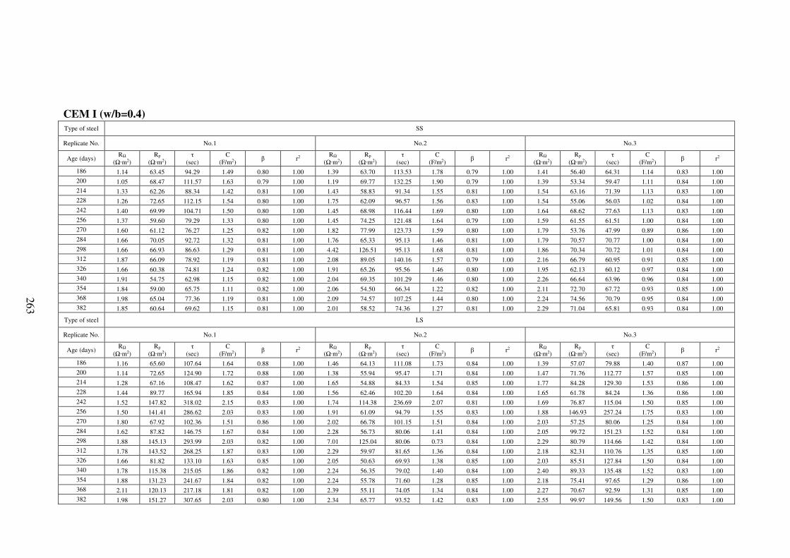
263

CEM I (w/b=0.4)

Type of steel SS

Replicate No. No.1 No.2 No.3

Age (days) RΩ

(Ω·m2) Rp

(Ω·m2) τ

(sec) C

(F/m2) β r2

RΩ

(Ω·m2) Rp

(Ω·m2) τ

(sec) C

(F/m2) β r2

RΩ

(Ω·m2) Rp

(Ω·m2) τ

(sec) C

(F/m2) β r2

186 1.14 63.45 94.29 1.49 0.80 1.00 1.39 63.70 113.53 1.78 0.79 1.00 1.41 56.40 64.31 1.14 0.83 1.00

200 1.05 68.47 111.57 1.63 0.79 1.00 1.19 69.77 132.25 1.90 0.79 1.00 1.39 53.34 59.47 1.11 0.84 1.00

214 1.33 62.26 88.34 1.42 0.81 1.00 1.43 58.83 91.34 1.55 0.81 1.00 1.54 63.16 71.39 1.13 0.83 1.00

228 1.26 72.65 112.15 1.54 0.80 1.00 1.75 62.09 96.57 1.56 0.83 1.00 1.54 55.06 56.03 1.02 0.84 1.00

242 1.40 69.99 104.71 1.50 0.80 1.00 1.45 68.98 116.44 1.69 0.80 1.00 1.64 68.62 77.63 1.13 0.83 1.00

256 1.37 59.60 79.29 1.33 0.80 1.00 1.45 74.25 121.48 1.64 0.79 1.00 1.59 61.55 61.51 1.00 0.84 1.00

270 1.60 61.12 76.27 1.25 0.82 1.00 1.82 77.99 123.73 1.59 0.80 1.00 1.79 53.76 47.99 0.89 0.86 1.00

284 1.66 70.05 92.72 1.32 0.81 1.00 1.76 65.33 95.13 1.46 0.81 1.00 1.79 70.57 70.77 1.00 0.84 1.00

298 1.66 66.93 86.63 1.29 0.81 1.00 4.42 126.51 95.13 1.68 0.81 1.00 1.86 70.34 70.72 1.01 0.84 1.00

312 1.87 66.09 78.92 1.19 0.81 1.00 2.08 89.05 140.16 1.57 0.79 1.00 2.16 66.79 60.95 0.91 0.85 1.00

326 1.66 60.38 74.81 1.24 0.82 1.00 1.91 65.26 95.56 1.46 0.80 1.00 1.95 62.13 60.12 0.97 0.84 1.00

340 1.91 54.75 62.98 1.15 0.82 1.00 2.04 69.35 101.29 1.46 0.80 1.00 2.26 66.64 63.96 0.96 0.84 1.00

354 1.84 59.00 65.75 1.11 0.82 1.00 2.06 54.50 66.34 1.22 0.82 1.00 2.11 72.70 67.72 0.93 0.85 1.00

368 1.98 65.04 77.36 1.19 0.81 1.00 2.09 74.57 107.25 1.44 0.80 1.00 2.24 74.56 70.79 0.95 0.84 1.00

382 1.85 60.64 69.62 1.15 0.81 1.00 2.01 58.52 74.36 1.27 0.81 1.00 2.29 71.04 65.81 0.93 0.84 1.00

Type of steel LS


Age (days) RΩ

(Ω·m2) Rp

(Ω·m2) τ

(sec) C

(F/m2) β r2

RΩ

(Ω·m2) Rp

(Ω·m2) τ

(sec) C

(F/m2) β r2

RΩ

(Ω·m2) Rp

(Ω·m2) τ

(sec) C

(F/m2) β r2

186 1.16 65.60 107.64 1.64 0.88 1.00 1.46 64.13 111.08 1.73 0.84 1.00 1.39 57.07 79.88 1.40 0.87 1.00

200 1.14 72.65 124.90 1.72 0.88 1.00 1.38 55.94 95.47 1.71 0.84 1.00 1.47 71.76 112.77 1.57 0.85 1.00

214 1.28 67.16 108.47 1.62 0.87 1.00 1.65 54.88 84.33 1.54 0.85 1.00 1.77 84.28 129.30 1.53 0.86 1.00

228 1.44 89.77 165.94 1.85 0.84 1.00 1.56 62.46 102.20 1.64 0.84 1.00 1.65 61.78 84.24 1.36 0.86 1.00

242 1.52 147.82 318.02 2.15 0.83 1.00 1.74 114.38 236.69 2.07 0.81 1.00 1.69 76.87 115.04 1.50 0.85 1.00

256 1.50 141.41 286.62 2.03 0.83 1.00 1.91 61.09 94.79 1.55 0.83 1.00 1.88 146.93 257.24 1.75 0.83 1.00

270 1.80 67.92 102.36 1.51 0.86 1.00 2.02 66.78 101.15 1.51 0.84 1.00 2.03 57.25 80.06 1.25 0.84 1.00

284 1.62 87.82 146.75 1.67 0.84 1.00 2.28 56.73 80.06 1.41 0.84 1.00 2.05 99.72 151.23 1.52 0.84 1.00

298 1.88 145.13 293.99 2.03 0.82 1.00 7.01 125.04 80.06 0.73 0.84 1.00 2.29 80.79 114.66 1.42 0.84 1.00

312 1.78 143.52 268.25 1.87 0.83 1.00 2.29 59.97 81.65 1.36 0.84 1.00 2.18 82.31 110.76 1.35 0.85 1.00

326 1.66 81.82 133.10 1.63 0.85 1.00 2.05 50.63 69.93 1.38 0.85 1.00 2.03 85.51 127.84 1.50 0.84 1.00

340 1.78 115.38 215.05 1.86 0.82 1.00 2.24 56.35 79.02 1.40 0.84 1.00 2.40 89.33 135.48 1.52 0.83 1.00

354 1.88 131.23 241.67 1.84 0.82 1.00 2.24 55.78 71.60 1.28 0.85 1.00 2.18 75.41 97.65 1.29 0.86 1.00

368 2.11 120.13 217.18 1.81 0.82 1.00 2.39 55.11 74.05 1.34 0.84 1.00 2.27 70.67 92.59 1.31 0.85 1.00

382 1.98 151.27 307.65 2.03 0.80 1.00 2.34 65.77 93.52 1.42 0.83 1.00 2.55 99.97 149.56 1.50 0.83 1.00

264

CEM III/A (w/b=0.4)

Type of steel SS


Age (days) RΩ

(Ω·m2) Rp

(Ω·m2) τ

(sec) C

(F/m2) β r2

RΩ

(Ω·m2) Rp

(Ω·m2) τ

(sec) C

(F/m2) β r2

RΩ

(Ω·m2) Rp

(Ω·m2) τ

(sec) C

(F/m2) β r2

186 2.40 90.37 242.06 2.68 0.73 1.00 2.46 89.72 224.85 2.51 0.74 1.00 2.46 114.21 268.05 2.35 0.77 1.00

200 2.61 82.22 198.61 2.42 0.73 1.00 2.26 80.62 182.58 2.26 0.75 1.00 2.50 109.23 243.01 2.22 0.76 1.00

214 2.75 87.92 217.43 2.47 0.72 1.00 2.60 96.33 238.10 2.47 0.74 1.00 2.54 95.05 195.28 2.05 0.77 1.00

228 2.72 68.08 144.21 2.12 0.74 1.00 2.45 92.30 218.36 2.37 0.75 1.00 2.66 87.70 170.55 1.94 0.77 1.00

242 3.03 75.05 158.05 2.11 0.74 1.00 2.77 88.36 196.81 2.23 0.75 1.00 2.88 79.09 140.89 1.78 0.77 1.00

256 3.13 85.05 187.13 2.20 0.74 1.00 2.90 97.43 228.79 2.35 0.74 1.00 2.54 80.93 144.35 1.78 0.77 1.00

270 3.26 106.85 254.50 2.38 0.73 1.00 3.08 71.91 135.67 1.89 0.75 1.00 3.02 75.34 124.83 1.66 0.76 1.00

284 3.11 56.80 96.93 1.71 0.74 1.00 3.04 84.63 180.61 2.13 0.74 1.00 2.98 67.43 107.32 1.59 0.76 1.00

298 3.24 58.06 101.81 1.75 0.74 1.00 3.00 66.61 125.05 1.88 0.74 1.00 3.04 67.28 107.52 1.60 0.76 1.00

312 3.31 60.33 105.32 1.75 0.74 1.00 3.31 72.52 136.33 1.88 0.74 1.00 3.08 51.38 67.21 1.31 0.79 1.00

326 3.26 47.72 74.18 1.55 0.74 1.00 2.98 56.39 93.16 1.65 0.76 1.00 3.19 76.42 129.84 1.70 0.75 1.00

340 2.77 56.51 90.08 1.59 0.75 1.00 3.14 65.94 118.43 1.80 0.74 1.00 3.24 71.00 113.81 1.60 0.75 1.00

354 4.00 45.88 64.00 1.39 0.77 1.00 3.49 61.74 98.92 1.60 0.75 1.00 3.41 71.18 104.39 1.47 0.76 1.00

368 3.79 51.40 64.00 1.59 0.77 1.00 3.49 69.99 119.43 1.71 0.74 1.00 3.51 66.22 92.31 1.39 0.76 1.00

382 3.49 52.97 77.09 1.46 0.73 1.00 3.34 68.95 117.21 1.70 0.74 1.00 3.46 64.07 88.12 1.38 0.76 1.00

Type of steel LS


Age (days) RΩ

(Ω·m2) Rp

(Ω·m2) τ

(sec) C

(F/m2) β r2

RΩ

(Ω·m2) Rp

(Ω·m2) τ

(sec) C

(F/m2) β r2

RΩ

(Ω·m2) Rp

(Ω·m2) τ

(sec) C

(F/m2) β r2

186 2.24 128.64 298.47 2.32 0.82 1.00 2.23 109.54 351.05 3.20 0.77 1.00 2.25 128.95 378.63 2.94 0.81 1.00

200 2.69 138.90 328.65 2.37 0.80 1.00 2.23 89.29 260.64 2.92 0.77 1.00 2.65 126.13 370.78 2.94 0.79 1.00

214 2.64 124.27 273.28 2.20 0.81 1.00 2.42 95.61 281.80 2.95 0.76 1.00 2.42 131.01 375.70 2.87 0.80 1.00

228 2.91 141.34 345.15 2.44 0.79 1.00 2.79 95.39 294.31 3.09 0.74 1.00 2.79 120.35 348.41 2.89 0.78 1.00

242 3.34 144.39 348.08 2.41 0.78 1.00 3.06 97.60 299.30 3.07 0.74 1.00 3.80 121.30 352.93 2.91 0.77 1.00

256 3.10 109.71 230.28 2.10 0.79 1.00 3.04 77.09 205.72 2.67 0.75 1.00 3.02 126.81 374.10 2.95 0.78 1.00

270 3.32 147.32 342.08 2.32 0.78 1.00 3.20 61.81 139.44 2.26 0.75 1.00 3.20 116.11 317.03 2.73 0.77 1.00

284 3.39 119.02 253.45 2.13 0.78 1.00 3.19 87.52 234.23 2.68 0.74 1.00 3.14 114.44 311.63 2.72 0.78 1.00

298 3.57 137.33 322.12 2.35 0.77 1.00 3.28 88.90 253.91 2.86 0.73 1.00 3.21 109.11 296.89 2.72 0.77 1.00

312 3.44 118.40 252.53 2.13 0.78 1.00 3.20 68.01 161.33 2.37 0.74 1.00 3.18 116.34 322.54 2.77 0.77 1.00

326 3.29 142.18 331.36 2.33 0.78 1.00 3.15 77.13 199.38 2.58 0.73 1.00 3.34 97.81 250.19 2.56 0.77 1.00

340 3.54 134.10 299.05 2.23 0.77 1.00 3.53 66.34 155.53 2.34 0.73 1.00 3.25 102.61 263.26 2.57 0.77 1.00

354 3.75 99.13 184.37 1.86 0.78 1.00 3.74 64.75 139.23 2.15 0.73 1.00 3.62 100.73 247.62 2.46 0.76 1.00

368 3.96 127.41 261.85 2.06 0.77 1.00 3.83 59.70 119.96 2.01 0.73 1.00 3.77 103.30 250.54 2.43 0.76 1.00

382 3.75 138.66 304.08 2.19 0.76 1.00 3.58 55.62 107.15 1.93 0.74 1.00 3.56 104.38 254.43 2.44 0.76 1.00

265


Type of steel SS


Age (days) RΩ

(Ω·m2) Rp

(Ω·m2) τ

(sec) C

(F/m2) β r2

RΩ

(Ω·m2) Rp

(Ω·m2) τ

(sec) C

(F/m2) β r2

RΩ

(Ω·m2) Rp

(Ω·m2) τ

(sec) C

(F/m2) β r2

186 3.08 169.68 300.63 1.77 0.80 1.00 3.34 110.15 326.08 2.96 0.76 1.00 2.87 78.14 242.64 3.11 0.80 1.00

200 3.57 172.41 293.50 1.70 0.80 1.00 3.67 110.05 313.73 2.85 0.75 1.00 3.07 129.71 499.26 3.85 0.77 1.00

214 3.81 167.95 288.94 1.72 0.80 1.00 4.05 100.20 272.13 2.72 0.75 1.00 3.33 126.89 487.70 3.84 0.77 1.00

228 4.24 176.45 297.72 1.69 0.80 1.00 4.51 104.02 285.72 2.75 0.74 1.00 3.86 131.55 507.93 3.86 0.76 1.00

242 4.52 179.60 309.83 1.73 0.79 1.00 4.83 105.05 291.00 2.77 0.73 1.00 4.03 126.91 493.84 3.89 0.75 1.00

256 4.92 158.62 255.16 1.61 0.80 1.00 4.91 88.12 222.60 2.53 0.74 1.00 4.25 123.30 475.49 3.86 0.75 1.00

270 5.37 189.11 324.47 1.72 0.78 1.00 5.87 88.08 205.81 2.34 0.75 1.00 4.92 128.35 492.25 3.84 0.74 1.00

284 4.96 179.67 322.92 1.80 0.78 1.00 5.19 94.44 258.98 2.74 0.73 1.00 4.54 82.69 263.80 3.19 0.76 1.00

298 5.60 163.31 269.09 1.65 0.78 1.00 5.71 86.85 213.05 2.45 0.73 1.00 4.90 120.57 464.45 3.85 0.74 1.00

312 5.99 185.33 314.24 1.70 0.78 1.00 6.21 96.57 243.82 2.52 0.72 1.00 5.41 120.59 462.56 3.84 0.73 1.00

326 5.95 174.12 293.87 1.69 0.78 1.00 6.11 93.90 237.73 2.53 0.72 1.00 5.38 116.54 445.29 3.82 0.73 1.00

340 6.26 176.30 295.59 1.68 0.77 1.00 6.53 64.89 128.73 1.98 0.74 1.00 5.59 121.70 462.16 3.80 0.73 1.00

354 7.25 174.80 271.38 1.55 0.77 1.00 7.46 83.57 179.07 2.14 0.72 1.00 6.41 102.50 338.52 3.30 0.72 1.00

368 7.21 168.34 262.19 1.56 0.77 1.00 7.80 55.27 95.78 1.73 0.76 1.00 6.41 97.98 325.74 3.32 0.72 1.00

382 7.04 188.73 311.80 1.65 0.77 1.00 7.20 87.31 196.88 2.25 0.72 1.00 6.21 93.10 297.71 3.20 0.73 1.00

Type of steel LS


Age (days) RΩ

(Ω·m2) Rp

(Ω·m2) τ

(sec) C

(F/m2) β r2

RΩ

(Ω·m2) Rp

(Ω·m2) τ

(sec) C

(F/m2) β r2

RΩ

(Ω·m2) Rp

(Ω·m2) τ

(sec) C

(F/m2) β r2

186 3.08 156.05 566.78 3.63 0.80 1.00 3.79 174.70 489.15 2.80 0.79 1.00 3.10 221.61 745.95 3.37 0.82 1.00

200 3.37 160.78 584.60 3.64 0.79 1.00 4.32 175.19 480.43 2.74 0.79 1.00 3.36 175.37 539.73 3.08 0.82 1.00

214 3.59 156.92 575.62 3.67 0.79 1.00 4.84 175.18 489.22 2.79 0.78 1.00 3.92 185.95 591.85 3.18 0.81 1.00

228 4.47 134.65 470.62 3.50 0.77 1.00 5.47 165.38 452.83 2.74 0.77 1.00 4.36 196.53 653.26 3.32 0.80 1.00

242 4.64 132.42 459.85 3.47 0.77 1.00 5.63 170.02 479.31 2.82 0.76 1.00 4.78 182.69 601.91 3.29 0.80 1.00

256 4.90 141.47 535.79 3.79 0.76 1.00 5.83 161.53 449.25 2.78 0.76 1.00 5.09 182.10 614.93 3.38 0.79 1.00

270 5.48 132.52 464.83 3.51 0.76 1.00 6.63 166.62 447.96 2.69 0.76 1.00 5.55 161.75 509.19 3.15 0.79 1.00

284 5.10 123.70 453.47 3.67 0.76 1.00 5.95 153.49 433.20 2.82 0.76 1.00 5.07 159.69 545.68 3.42 0.78 1.00

298 5.69 131.32 475.45 3.62 0.75 1.00 6.84 148.20 389.59 2.63 0.76 1.00 5.87 146.73 468.77 3.19 0.78 1.00

312 6.16 121.40 416.57 3.43 0.75 1.00 7.20 163.88 439.31 2.68 0.75 1.00 6.29 159.30 516.97 3.25 0.77 1.00

326 6.15 124.74 448.00 3.59 0.74 1.00 7.18 158.91 438.81 2.76 0.75 1.00 6.16 152.39 505.73 3.32 0.77 1.00

340 6.40 118.51 408.35 3.45 0.74 1.00 7.38 166.04 455.91 2.75 0.75 1.00 6.68 149.52 474.49 3.17 0.77 1.00

354 7.41 142.16 525.07 3.69 0.72 1.00 8.74 152.94 383.00 2.50 0.74 1.00 7.52 159.18 497.23 3.12 0.77 1.00

368 7.19 130.55 457.60 3.51 0.73 1.00 8.51 146.38 368.04 2.51 0.74 1.00 7.49 162.09 525.94 3.24 0.76 1.00

382 7.27 120.95 403.51 3.34 0.74 1.00 8.48 162.61 424.25 2.61 0.74 1.00 7.33 167.83 563.22 3.36 0.76 1.00

266

CEM I (w/b=0.6) Type of steel SS


Age (days) RΩ

(Ω·m2) Rp

(Ω·m2) τ

(sec) C

(F/m2) β r2

RΩ

(Ω·m2) Rp

(Ω·m2) τ

(sec) C

(F/m2) β r2

RΩ

(Ω·m2) Rp

(Ω·m2) τ

(sec) C

(F/m2) β r2

186 0.84 21.81 102.74 4.71 0.68 1.00 0.72 128.48 595.20 4.63 0.77 1.00 0.73 115.02 513.58 4.47 0.78 1.00

200 0.79 2.66 8.45 3.17 0.70 1.00 0.71 56.73 310.88 5.48 0.73 1.00 0.81 99.89 404.65 4.05 0.79 1.00

214 0.94 2.12 8.35 3.93 0.73 1.00 0.72 75.59 409.75 5.42 0.74 1.00 0.80 109.87 470.29 4.28 0.78 1.00

228 0.86 1.57 5.25 3.35 0.71 1.00 0.76 4.20 12.98 3.09 0.71 1.00 0.75 110.49 498.60 4.51 0.77 1.00

242 0.89 1.14 4.45 3.91 0.78 1.00 0.84 2.06 6.57 3.19 0.74 1.00 0.75 120.55 583.65 4.84 0.76 1.00

256 0.87 1.05 4.63 4.42 0.80 1.00 0.90 1.76 7.00 3.99 0.76 1.00 0.82 109.66 472.18 4.31 0.77 1.00

270 0.85 0.94 6.12 6.50 0.82 1.00 0.85 1.70 7.40 4.35 0.75 1.00 0.85 86.74 463.10 5.34 0.75 1.00

284 0.84 1.04 7.36 7.10 0.75 1.00 0.82 1.82 8.34 4.57 0.73 1.00 0.77 90.42 450.52 4.98 0.75 1.00

298 0.80 0.98 6.89 7.01 0.77 1.00 0.85 1.49 7.86 5.28 0.74 1.00 0.82 83.29 395.63 4.75 0.76 1.00

312 0.80 1.16 9.87 8.53 0.75 1.00 0.82 1.45 7.97 5.51 0.75 1.00 0.78 12.57 46.53 3.70 0.71 1.00

326 0.80 1.08 9.07 8.39 0.73 1.00 0.82 1.72 10.95 6.36 0.72 1.00 0.91 2.44 15.25 6.25 0.71 0.99

340 0.83 1.18 12.76 10.84 0.70 1.00 0.79 1.45 9.42 6.50 0.70 1.00 0.97 1.82 8.31 4.56 0.80 1.00

354 0.79 1.17 11.36 9.68 0.73 1.00 0.80 1.17 9.38 8.02 0.72 1.00 0.86 1.74 7.44 4.28 0.75 1.00

368 0.79 1.22 11.91 9.80 0.69 1.00 0.78 0.98 8.30 8.48 0.72 1.00 0.84 1.47 6.63 4.51 0.77 1.00

382 0.86 1.08 9.01 8.34 0.72 1.00 0.85 1.06 11.31 10.68 0.74 1.00 0.91 1.42 6.83 4.80 0.79 1.00

Type of steel LS


Age (days) RΩ

(Ω·m2) Rp

(Ω·m2) τ

(sec) C

(F/m2) β r2

RΩ

(Ω·m2) Rp

(Ω·m2) τ

(sec) C

(F/m2) β r2

RΩ

(Ω·m2) Rp

(Ω·m2) τ

(sec) C

(F/m2) β r2

186 0.69 3.48 5.69 1.64 0.76 1.00 0.90 121.79 522.22 4.29 0.78 1.00 0.87 136.92 557.61 4.07 0.79 1.00

200 0.89 2.82 6.89 2.44 0.78 1.00 1.01 113.69 473.08 4.16 0.78 1.00 1.04 2.16 7.34 3.39 0.76 1.00

214 0.96 3.03 8.03 2.65 0.77 1.00 1.03 130.24 569.62 4.37 0.78 1.00 1.04 2.01 7.39 3.68 0.75 1.00

228 0.87 2.66 6.43 2.42 0.75 1.00 0.95 95.44 527.30 5.53 0.74 1.00 1.06 2.18 9.08 4.16 0.73 1.00

242 0.99 2.13 5.71 2.68 0.78 1.00 1.07 34.44 114.17 3.31 0.78 1.00 1.06 1.82 8.87 4.88 0.75 1.00

256 1.00 2.17 7.71 3.55 0.76 1.00 1.04 82.67 358.80 4.34 0.77 1.00 1.06 1.56 8.26 5.31 0.79 1.00

270 0.96 2.15 7.96 3.70 0.76 1.00 1.10 3.50 10.49 3.00 0.74 1.00 1.06 1.24 7.48 6.01 0.81 1.00

284 1.01 2.08 9.56 4.59 0.76 1.00 1.12 1.91 6.25 3.27 0.77 1.00 1.05 1.42 11.33 7.99 0.79 1.00

298 0.95 1.98 10.78 5.45 0.72 1.00 1.09 2.76 10.81 3.91 0.73 1.00 1.02 1.65 18.05 10.93 0.71 1.00

312 0.96 2.13 11.93 5.61 0.73 1.00 1.07 1.78 7.63 4.29 0.72 1.00 1.02 1.42 12.00 8.47 0.74 1.00

326 0.97 1.70 9.16 5.39 0.73 1.00 1.09 1.25 6.33 5.06 0.73 1.00 1.01 1.57 18.70 11.88 0.69 1.00

340 1.03 1.70 10.64 6.25 0.76 1.00 1.05 1.18 6.76 5.72 0.72 1.00 0.89 2.53 43.99 17.39 0.59 1.00

354 0.93 1.20 6.40 5.36 0.69 1.00 0.99 1.22 9.19 7.51 0.70 1.00 0.86 1.28 10.52 8.19 0.67 1.00

368 0.99 1.89 11.61 6.14 0.72 1.00 1.03 1.27 12.67 10.00 0.69 1.00 0.88 1.24 10.07 8.11 0.67 1.00

382 1.01 2.48 19.62 7.90 0.68 1.00 1.06 1.27 11.00 8.68 0.74 1.00 0.89 2.07 23.45 11.33 0.63 1.00

267

CEM III/A(w/b=0.6) Type of steel SS


Age (days) RΩ

(Ω·m2) Rp

(Ω·m2) τ

(sec) C

(F/m2) β r2

RΩ

(Ω·m2) Rp

(Ω·m2) τ

(sec) C

(F/m2) β r2

RΩ

(Ω·m2) Rp

(Ω·m2) τ

(sec) C

(F/m2) β r2

186 2.02 116.10 347.33 2.99 0.77 1.00 2.12 156.83 278.04 1.77 0.80 1.00 2.13 137.24 374.28 2.73 0.77 1.00

200 2.17 134.35 421.33 3.14 0.76 1.00 2.34 157.56 268.68 1.71 0.79 1.00 2.32 129.82 328.47 2.53 0.77 1.00

214 2.20 127.13 398.71 3.14 0.75 1.00 2.36 166.16 283.36 1.71 0.79 1.00 2.32 129.34 330.68 2.56 0.76 1.00

228 2.10 131.33 422.16 3.21 0.76 1.00 2.23 176.81 321.86 1.82 0.79 1.00 2.30 145.92 406.77 2.79 0.75 1.00

242 2.39 129.39 385.90 2.98 0.76 1.00 2.40 163.60 268.67 1.64 0.79 1.00 2.42 134.47 340.91 2.54 0.75 1.00

256 2.47 120.49 348.06 2.89 0.76 1.00 2.45 151.18 243.03 1.61 0.79 1.00 2.67 127.73 313.94 2.46 0.75 1.00

270 2.32 115.81 319.97 2.76 0.75 1.00 2.64 115.35 155.59 1.35 0.80 1.00 2.68 129.45 307.49 2.38 0.75 1.00

284 2.43 125.64 367.10 2.92 0.75 1.00 2.56 149.18 231.67 1.55 0.79 1.00 2.65 118.13 270.58 2.29 0.75 1.00

298 2.46 113.00 308.37 2.73 0.75 1.00 2.62 125.05 175.04 1.40 0.80 1.00 2.55 122.84 282.74 2.30 0.75 1.00

312 2.62 110.14 287.64 2.61 0.75 1.00 2.71 118.90 156.59 1.32 0.80 1.00 2.69 116.90 250.91 2.15 0.75 1.00

326 2.45 108.68 289.71 2.67 0.75 1.00 2.62 178.23 290.75 1.63 0.78 1.00 2.71 130.51 309.61 2.37 0.74 1.00

340 2.61 111.27 293.10 2.63 0.75 1.00 2.82 153.79 226.57 1.47 0.79 1.00 2.81 130.86 301.33 2.30 0.74 1.00

354 2.75 110.24 273.54 2.48 0.75 1.00 2.89 123.94 159.58 1.29 0.79 1.00 2.94 119.76 248.39 2.07 0.75 1.00

368 2.78 105.70 264.23 2.50 0.74 1.00 2.94 124.90 161.51 1.29 0.79 1.00 2.99 123.27 262.24 2.13 0.74 1.00

382 2.75 120.92 324.40 2.68 0.74 1.00 2.90 117.26 148.33 1.27 0.79 1.00 2.95 121.45 258.22 2.13 0.74 1.00

Type of steel LS


Age (days) RΩ

(Ω·m2) Rp

(Ω·m2) τ

(sec) C

(F/m2) β r2

RΩ

(Ω·m2) Rp

(Ω·m2) τ

(sec) C

(F/m2) β r2

RΩ

(Ω·m2) Rp

(Ω·m2) τ

(sec) C

(F/m2) β r2

186 2.26 121.82 303.21 2.49 0.81 1.00 2.21 144.78 485.25 3.35 0.80 1.00 2.33 162.01 362.08 2.23 0.83 1.00

200 2.35 161.04 451.33 2.80 0.79 1.00 2.59 136.69 457.72 3.35 0.78 1.00 2.52 215.74 363.08 2.50 0.83 1.00

214 2.43 160.47 461.08 2.87 0.78 1.00 2.53 135.61 445.32 3.28 0.78 1.00 2.53 204.20 364.08 2.40 0.83 1.00

228 2.46 151.68 429.36 2.83 0.79 1.00 2.56 133.99 455.82 3.40 0.77 1.00 2.52 195.06 365.08 2.41 0.83 1.00

242 2.70 155.64 435.88 2.80 0.78 1.00 2.65 132.92 428.40 3.22 0.77 1.00 2.66 191.99 366.08 2.32 0.83 1.00

256 2.76 153.08 427.29 2.79 0.77 1.00 3.07 131.32 437.16 3.33 0.76 1.00 2.82 165.28 367.08 2.13 0.83 1.00

270 2.87 152.57 420.43 2.76 0.77 1.00 2.87 140.70 464.76 3.30 0.76 1.00 2.87 202.12 368.08 2.30 0.83 1.00

284 2.80 145.39 397.22 2.73 0.77 1.00 2.78 128.49 404.48 3.15 0.77 1.00 2.84 199.13 369.08 2.33 0.83 1.00

298 2.93 148.69 417.29 2.81 0.76 1.00 2.89 136.50 446.30 3.27 0.76 1.00 3.20 168.51 370.08 2.19 0.83 1.00

312 2.85 153.16 421.87 2.75 0.76 1.00 2.99 130.42 406.87 3.12 0.76 1.00 3.17 197.01 371.08 2.30 0.83 1.00

326 3.26 135.52 353.34 2.61 0.78 1.00 2.99 125.74 382.17 3.04 0.76 1.00 2.90 182.12 372.08 2.23 0.83 1.00

340 3.03 143.47 386.02 2.69 0.76 1.00 3.04 122.26 364.98 2.99 0.76 1.00 3.04 203.81 373.08 2.35 0.83 1.00

354 3.27 140.16 365.73 2.61 0.76 1.00 3.23 132.83 410.11 3.09 0.75 1.00 3.10 202.53 374.08 2.26 0.83 1.00

368 3.18 144.52 391.33 2.71 0.75 1.00 3.21 131.08 413.02 3.15 0.75 1.00 3.23 189.93 375.08 2.21 0.83 1.00

382 3.14 154.06 434.34 2.82 0.75 1.00 3.34 115.14 324.69 2.82 0.76 1.00 3.29 188.34 376.08 2.20 0.83 1.00

268

CEM II/B-V (w/b=0.6) Type of steel SS


Age (days) RΩ

(Ω·m2) Rp

(Ω·m2) τ

(sec) C

(F/m2) β r2

RΩ

(Ω·m2) Rp

(Ω·m2) τ

(sec) C

(F/m2) β r2

RΩ

(Ω·m2) Rp

(Ω·m2) τ

(sec) C

(F/m2) β r2

186 1.70 98.19 338.15 3.44 0.78 1.00 1.86 117.69 341.20 2.90 0.79 1.00 2.06 123.42 400.83 3.25 0.81 1.00

200 1.84 109.27 382.00 3.50 0.77 1.00 2.07 108.77 291.40 2.68 0.78 1.00 2.19 136.07 453.99 3.34 0.80 1.00

214 1.89 126.96 471.88 3.72 0.76 1.00 2.15 123.77 352.06 2.84 0.77 1.00 2.30 146.07 498.19 3.41 0.79 1.00

228 2.15 90.18 275.57 3.06 0.77 1.00 2.36 112.11 303.78 2.71 0.77 1.00 2.48 162.06 567.15 3.50 0.79 1.00

242 2.25 87.31 267.17 3.06 0.76 1.00 2.55 87.66 208.64 2.38 0.78 1.00 2.65 144.59 488.01 3.38 0.79 1.00

256 2.00 74.36 366.51 4.93 0.76 1.00 2.63 106.37 265.09 2.49 0.77 1.00 2.74 151.46 514.48 3.40 0.78 1.00

270 2.65 94.54 269.52 2.85 0.75 1.00 2.99 103.19 237.79 2.30 0.77 1.00 3.05 140.50 433.53 3.09 0.79 1.00

284 2.58 76.87 206.60 2.69 0.75 1.00 2.85 88.19 193.00 2.19 0.78 1.00 3.01 150.66 498.76 3.31 0.78 1.00

298 2.89 77.69 214.48 2.76 0.75 1.00 3.16 108.98 256.51 2.35 0.77 1.00 3.37 134.95 411.85 3.05 0.78 1.00

312 2.99 82.32 226.14 2.75 0.74 1.00 3.20 115.96 286.56 2.47 0.76 1.00 3.43 135.41 426.82 3.15 0.78 1.00

326 4.00 63.92 226.14 3.66 0.74 1.00 3.35 114.44 278.27 2.43 0.76 1.00 3.54 145.15 461.00 3.18 0.77 1.00

340 3.13 64.30 146.18 2.27 0.75 1.00 3.52 88.56 184.76 2.09 0.77 1.00 3.68 149.41 476.43 3.19 0.78 1.00

354 3.61 60.49 127.09 2.10 0.75 1.00 3.82 72.40 130.67 1.80 0.77 1.00 3.84 149.95 485.31 3.24 0.76 1.00

368 3.39 51.20 99.56 1.94 0.76 1.00 3.81 91.53 192.75 2.11 0.76 1.00 3.90 138.12 433.01 3.13 0.77 1.00

382 3.61 71.64 163.83 2.29 0.74 1.00 4.04 78.17 147.47 1.89 0.77 1.00 4.11 139.04 433.32 3.12 0.77 1.00

Type of steel LS


Age (days) RΩ

(Ω·m2) Rp

(Ω·m2) τ

(sec) C

(F/m2) β r2

RΩ

(Ω·m2) Rp

(Ω·m2) τ

(sec) C

(F/m2) β r2

RΩ

(Ω·m2) Rp

(Ω·m2) τ

(sec) C

(F/m2) β r2

186 2.12 122.95 460.45 3.74 0.78 1.00 2.09 190.65 763.32 4.00 0.81 1.00 2.17 157.95 587.38 3.72 0.82 1.00

200 2.39 119.47 421.01 3.52 0.78 1.00 2.38 173.28 660.87 3.81 0.81 1.00 2.34 172.16 648.92 3.77 0.81 1.00

214 2.40 118.19 413.78 3.50 0.78 1.00 2.52 145.17 521.00 3.59 0.81 1.00 2.40 208.82 840.66 4.03 0.81 1.00

228 2.73 116.19 385.85 3.32 0.77 1.00 2.75 154.48 556.79 3.60 0.80 1.00 2.66 147.87 519.15 3.51 0.81 1.00

242 2.76 106.54 348.53 3.27 0.77 1.00 2.81 136.52 483.83 3.54 0.79 1.00 2.61 195.60 738.69 3.78 0.81 1.00

256 3.84 116.18 218.94 1.88 0.76 1.00 3.11 160.28 586.73 3.66 0.79 1.00 3.03 155.92 558.79 3.58 0.80 1.00

270 3.18 96.26 268.18 2.79 0.77 1.00 3.39 145.64 490.49 3.37 0.79 1.00 3.27 169.79 610.41 3.60 0.79 1.00

284 3.25 104.18 316.89 3.04 0.76 1.00 3.42 164.11 604.54 3.68 0.78 1.00 3.23 159.35 585.66 3.68 0.79 1.00

298 3.48 113.54 347.20 3.06 0.75 1.00 3.76 154.02 542.25 3.52 0.78 1.00 3.56 143.23 486.57 3.40 0.79 1.00

312 3.57 108.29 327.36 3.02 0.75 1.00 3.85 132.92 444.94 3.35 0.78 1.00 3.57 142.85 496.80 3.48 0.79 1.00

326 3.66 108.20 328.90 3.04 0.75 1.00 4.09 145.45 514.63 3.54 0.77 1.00 3.77 146.63 503.62 3.43 0.79 1.00

340 3.96 94.11 257.99 2.74 0.75 1.00 4.13 145.98 513.55 3.52 0.77 1.00 3.95 152.48 537.68 3.53 0.78 1.00

354 4.12 104.27 293.03 2.81 0.74 1.00 4.53 143.30 482.81 3.37 0.76 1.00 4.17 157.55 539.47 3.42 0.78 1.00

368 4.03 94.69 256.64 2.71 0.75 1.00 4.56 134.18 451.60 3.37 0.76 1.00 4.31 138.59 471.70 3.40 0.77 1.00

382 4.33 89.77 226.87 2.53 0.75 1.00 4.82 138.22 458.53 3.32 0.76 1.00 4.50 164.91 585.59 3.55 0.77 1.00

269

C2.3 Parameters from potentiostatic measurement

The following equations is used to obtain the parameters (refer to equation (6.3) in

Chapter 6).

*S() = y+NN×(× + N) ÜÝÝÝÞ× + N<ß

@Sd]RjRàRà:Rj á

âãããä

270



Age (days) RΩ

(Ω·m2) Rp

(Ω·m2) τ

(sec) C

(F/m2) r2

RΩ

(Ω·m2) Rp

(Ω·m2) τ

(sec) C

(F/m2) r2

RΩ

(Ω·m2) Rp

(Ω·m2) τ

(sec) C

(F/m2) r2

186 2.50 97.14 2.22 0.91 0.95 2.53 81.46 2.66 1.08 0.95 2.34 95.99 1.77 0.78 0.95

200 2.45 99.32 2.20 0.92 0.95 2.60 88.04 2.77 1.10 0.95 2.67 102.04 2.03 0.78 0.95

214 2.34 99.14 2.15 0.94 0.95 2.43 100.66 2.53 1.07 0.95 2.55 131.91 1.84 0.74 0.95

228 2.92 108.95 2.63 0.92 0.96 2.84 125.55 2.92 1.05 0.96 2.85 191.28 2.05 0.73 0.95

242 2.92 103.77 2.52 0.89 0.95 3.12 150.03 3.01 0.98 0.95 3.10 266.17 2.17 0.71 0.95

256 3.18 91.99 3.52 1.66 0.95 3.25 174.96 3.37 1.06 0.96 3.40 375.19 2.47 0.73 0.96

270 2.87 138.70 2.41 0.85 0.95 3.16 190.02 3.01 0.97 0.96 3.08 231.19 2.16 0.71 0.95

284 2.88 116.66 2.39 0.85 0.95 3.06 162.61 2.86 0.95 0.95 3.33 373.64 2.30 0.70 0.95

298 2.64 116.96 2.17 0.84 0.94 2.86 107.48 2.57 0.92 0.95 3.29 332.42 2.27 0.70 0.95

312 2.81 102.18 2.15 0.79 0.94 3.37 131.55 3.00 0.91 0.96 3.38 154.49 2.16 0.65 0.96

326 2.91 129.57 2.43 0.85 0.95 3.30 120.49 3.19 0.99 0.96 3.36 226.05 2.36 0.71 0.95

340 3.11 115.90 2.53 0.83 0.94 3.32 143.67 3.09 0.95 0.95 3.34 200.88 2.27 0.69 0.95

354 3.31 128.88 2.76 0.85 0.95 3.40 178.64 3.09 0.93 0.95 3.61 401.76 2.40 0.67 0.95

368 3.03 124.51 2.39 0.81 0.94 3.25 192.42 2.89 0.90 0.95 3.51 238.85 2.28 0.66 0.95

382 3.68 109.93 2.96 0.83 0.96 3.63 128.30 3.20 0.91 0.96 3.46 141.14 2.24 0.66 0.96

Type of steel LS


Age (days) RΩ

(Ω·m2) Rp

(Ω·m2) τ

(sec) C

(F/m2) r2

RΩ

(Ω·m2) Rp

(Ω·m2) τ

(sec) C

(F/m2) r2

RΩ

(Ω·m2) Rp

(Ω·m2) τ

(sec) C

(F/m2) r2

186 1.81 105.18 2.06 1.16 0.97 2.25 85.54 2.52 1.15 0.96 2.09 91.72 2.05 1.01 0.97

200 1.92 102.61 2.28 1.21 0.98 2.36 81.08 2.74 1.20 0.96 2.35 94.49 2.46 1.07 0.97

214 2.03 106.28 2.36 1.18 0.98 2.42 76.95 2.74 1.17 0.96 2.45 134.33 2.45 1.02 0.97

228 2.20 149.65 2.48 1.14 0.97 2.66 93.11 2.94 1.14 0.97 2.69 207.07 2.61 0.98 0.97

242 2.60 188.50 2.87 1.12 0.97 3.18 99.75 3.40 1.11 0.97 3.19 132.99 3.11 1.00 0.97

256 2.66 115.76 3.02 1.16 0.97 3.42 206.35 3.73 1.09 0.96 3.10 214.89 3.05 1.00 0.97

270 2.64 189.75 2.91 1.12 0.97 3.33 218.89 3.60 1.10 0.96 2.98 256.40 2.88 0.98 0.97

284 2.73 225.43 3.02 1.12 0.97 3.26 272.45 3.56 1.10 0.96 3.04 372.77 2.97 0.98 0.96

298 2.86 199.32 3.16 1.12 0.97 3.23 157.93 3.47 1.10 0.96 3.10 162.25 3.04 1.00 0.97

312 2.43 93.23 2.44 1.03 0.97 3.45 132.48 3.42 1.02 0.96 3.26 158.57 3.03 0.95 0.97

326 2.54 248.74 2.78 1.10 0.97 3.13 232.29 3.35 1.09 0.96 3.08 205.64 3.07 1.01 0.96

340 3.05 166.27 3.36 1.12 0.97 3.35 144.74 3.53 1.08 0.96 3.50 136.98 3.43 1.00 0.97

354 3.75 128.37 4.07 1.11 0.97 3.33 209.54 3.40 1.04 0.96 3.21 253.25 3.00 0.94 0.97

368 3.11 146.02 3.30 1.09 0.97 3.98 148.90 3.98 1.03 0.96 3.22 205.56 3.06 0.96 0.96

382 3.25 133.70 3.37 1.06 0.97 3.53 148.05 3.54 1.03 0.96 3.82 133.44 3.64 0.98 0.97

271

CEM III/A (w/b=0.4) Type of steel SS


Age (days) RΩ

(Ω·m2) Rp

(Ω·m2) τ

(sec) C

(F/m2) r2

RΩ

(Ω·m2) Rp

(Ω·m2) τ

(sec) C

(F/m2) r2

RΩ

(Ω·m2) Rp

(Ω·m2) τ

(sec) C

(F/m2) r2

186 4.36 92.22 5.69 1.37 0.97 3.97 114.45 5.12 1.34 0.96 4.19 154.58 4.99 1.22 0.97

200 4.44 96.91 5.78 1.36 0.97 4.20 85.78 5.36 1.34 0.97 4.24 140.57 4.99 1.21 0.97

214 4.65 95.60 5.87 1.32 0.97 5.88 109.33 6.36 1.23 0.97 4.16 103.70 4.58 1.14 0.97

228 4.56 129.91 5.59 1.27 0.96 4.30 109.85 7.36 1.26 0.97 4.15 148.50 4.61 1.14 0.96

242 5.00 108.91 6.07 1.27 0.96 4.52 104.39 5.57 1.29 0.96 4.62 125.95 5.01 1.12 0.96

256 4.62 103.08 5.55 1.26 0.96 4.36 117.13 5.27 1.25 0.96 4.51 140.67 5.00 1.14 0.96

270 5.31 108.46 6.12 1.21 0.95 4.88 106.46 5.66 1.21 0.96 5.00 107.06 5.17 1.08 0.96

284 5.04 102.86 5.85 1.22 0.96 4.75 95.95 5.50 1.21 0.96 4.84 115.24 5.06 1.09 0.96

298 5.14 107.30 5.98 1.22 0.96 4.81 100.16 5.54 1.21 0.96 4.98 124.83 5.21 1.09 0.96

312 5.20 101.26 5.89 1.19 0.96 5.01 99.26 5.59 1.17 0.96 4.83 122.56 4.83 1.04 0.96

326 5.26 97.87 6.03 1.21 0.96 5.09 94.32 5.85 1.21 0.96 5.12 119.18 5.27 1.07 0.96

340 7.24 104.70 7.03 1.36 0.96 5.14 89.75 5.83 1.20 0.96 5.00 113.45 5.07 1.06 0.96

354 5.84 106.46 6.15 1.11 0.96 5.54 93.01 5.93 1.13 0.96 5.63 109.81 5.30 0.99 0.96

368 5.88 115.67 6.20 1.11 0.96 5.52 103.07 5.99 1.14 0.96 5.61 151.53 5.46 1.01 0.96

382 6.02 99.96 6.47 1.14 0.96 5.64 103.70 6.08 1.14 0.96 5.59 113.51 5.32 1.00 0.96

Type of steel LS


Age (days) RΩ

(Ω·m2) Rp

(Ω·m2) τ

(sec) C

(F/m2) r2

RΩ

(Ω·m2) Rp

(Ω·m2) τ

(sec) C

(F/m2) r2

RΩ

(Ω·m2) Rp

(Ω·m2) τ

(sec) C

(F/m2) r2

186 3.72 128.84 4.90 1.35 0.98 3.77 89.26 6.01 1.66 0.97 3.52 116.93 5.61 1.64 0.98

200 4.07 119.52 5.24 1.33 0.98 4.39 99.48 6.71 1.60 0.98 3.70 113.75 5.78 1.62 0.97

214 4.05 108.36 5.15 1.32 0.97 4.40 88.02 6.84 1.63 0.97 3.80 126.17 5.86 1.59 0.98

228 4.70 167.38 5.79 1.27 0.98 4.21 108.03 6.46 1.60 0.97 4.27 100.44 6.44 1.57 0.98

242 4.57 131.88 5.69 1.29 0.98 4.58 83.34 6.86 1.58 0.97 4.42 109.68 6.52 1.53 0.98

256 4.46 126.58 5.53 1.28 0.97 4.37 99.41 6.56 1.57 0.97 4.09 113.37 6.10 1.55 0.98

270 4.95 129.90 5.87 1.23 0.97 4.94 88.15 6.99 1.49 0.97 4.58 98.67 6.48 1.48 0.98

284 4.83 122.02 5.78 1.24 0.97 4.87 88.28 7.10 1.54 0.97 4.74 100.96 6.83 1.51 0.98

298 4.84 116.64 5.77 1.24 0.97 5.20 92.53 7.62 1.55 0.97 4.64 102.72 6.63 1.49 0.98

312 4.97 115.96 5.84 1.23 0.97 5.13 89.85 7.11 1.46 0.97 4.66 97.07 6.47 1.46 0.98

326 4.73 116.57 5.59 1.23 0.97 4.78 89.65 6.81 1.50 0.96 4.56 97.85 6.35 1.46 0.97

340 4.99 110.60 5.72 1.20 0.97 5.41 82.80 7.63 1.50 0.97 4.66 94.80 6.41 1.44 0.97

354 5.51 111.71 6.23 1.19 0.97 6.00 85.75 7.92 1.41 0.97 5.09 101.33 6.66 1.37 0.97

368 5.69 128.52 6.34 1.16 0.97 5.80 85.35 7.76 1.43 0.97 5.26 103.49 6.95 1.39 0.97

382 5.68 115.74 6.39 1.18 0.97 5.39 87.73 7.09 1.40 0.97 5.26 102.34 6.90 1.38 0.97

272



Age (days) RΩ

(Ω·m2) Rp

(Ω·m2) τ

(sec) C

(F/m2) r2

RΩ

(Ω·m2) Rp

(Ω·m2) τ

(sec) C

(F/m2) r2

RΩ

(Ω·m2) Rp

(Ω·m2) τ

(sec) C

(F/m2) r2

186 4.75 165.44 4.54 0.98 0.98 5.06 105.79 7.54 1.56 0.98 3.91 89.49 7.43 1.98 0.98

200 4.93 150.79 4.72 0.99 0.98 5.52 110.41 8.10 1.54 0.98 4.42 93.90 8.36 1.98 0.98

214 5.46 184.83 5.07 0.95 0.98 6.06 97.27 8.52 1.49 0.98 4.82 86.80 8.61 1.89 0.98

228 5.83 210.44 5.42 0.95 0.98 6.39 130.22 9.12 1.50 0.98 5.16 134.36 9.33 1.88 0.98

242 6.23 202.26 5.75 0.95 0.98 6.69 113.68 9.28 1.47 0.98 5.45 112.41 9.70 1.87 0.99

256 6.42 178.50 6.00 0.97 0.97 7.56 113.64 10.39 1.47 0.98 5.69 103.45 10.16 1.88 0.98

270 7.27 175.56 6.42 0.92 0.98 7.79 104.64 10.44 1.44 0.98 6.26 103.52 10.73 1.82 0.99

284 6.75 158.54 6.28 0.97 0.98 7.20 101.62 10.27 1.53 0.98 5.90 91.94 10.61 1.91 0.99

298 7.57 182.11 6.87 0.95 0.98 7.94 103.89 10.91 1.48 0.98 6.56 100.14 11.39 1.85 0.98

312 7.74 169.07 6.95 0.94 0.98 8.51 107.76 11.48 1.45 0.98 7.04 99.40 12.03 1.83 0.99

326 8.02 162.10 7.25 0.95 0.98 8.51 106.37 11.38 1.45 0.98 7.05 98.47 12.01 1.83 0.99

340 8.65 172.79 7.61 0.92 0.98 9.07 104.90 11.90 1.42 0.98 7.49 99.34 12.62 1.81 0.99

354 9.71 197.69 8.18 0.88 0.98 10.30 111.66 12.71 1.35 0.98 8.60 101.13 13.61 1.72 0.99

368 9.46 186.95 8.18 0.91 0.98 9.99 112.92 12.76 1.39 0.98 8.53 98.24 13.63 1.74 0.99

382 9.16 170.70 7.99 0.92 0.98 9.69 105.11 12.53 1.41 0.98 7.95 109.76 12.87 1.74 0.99

Type of steel LS


Age (days) RΩ

(Ω·m2) Rp

(Ω·m2) τ

(sec) C

(F/m2) r2

RΩ

(Ω·m2) Rp

(Ω·m2) τ

(sec) C

(F/m2) r2

RΩ

(Ω·m2) Rp

(Ω·m2) τ

(sec) C

(F/m2) r2

186 4.36 132.73 7.92 1.88 0.99 5.35 160.95 7.60 1.47 0.98 4.38 147.49 7.62 1.79 0.98

200 4.84 109.87 8.62 1.86 0.99 6.09 152.13 8.55 1.46 0.98 4.83 153.21 8.19 1.75 0.99

214 5.20 128.69 9.18 1.84 0.99 6.16 213.99 8.45 1.41 0.98 5.16 177.57 8.43 1.68 0.99

228 5.78 135.41 10.18 1.84 0.99 6.79 150.48 9.22 1.42 0.98 5.67 157.19 9.39 1.72 0.99

242 5.95 136.04 10.30 1.81 0.99 7.33 145.33 9.90 1.42 0.98 5.95 159.36 9.75 1.70 0.99

256 6.26 102.21 10.67 1.81 0.99 7.49 140.86 10.15 1.43 0.99 6.28 145.14 10.38 1.72 0.99

270 8.85 128.62 11.67 1.61 0.99 8.53 140.31 11.12 1.38 0.99 6.54 136.76 10.41 1.67 0.99

284 6.37 118.42 11.37 1.88 0.99 7.78 130.13 10.69 1.46 0.99 6.43 120.18 10.73 1.76 0.99

298 7.14 108.33 12.24 1.83 0.99 8.71 129.76 11.57 1.42 0.99 7.21 126.53 11.73 1.72 0.99

312 7.37 112.79 12.40 1.79 0.99 9.27 137.44 12.14 1.40 0.99 7.90 114.65 12.58 1.70 0.99

326 7.95 109.25 13.47 1.82 0.99 9.33 130.52 12.18 1.40 0.99 7.97 117.60 12.68 1.70 0.99

340 8.18 106.40 13.41 1.77 0.99 9.67 134.90 12.35 1.37 0.99 8.05 124.81 12.69 1.68 0.99

354 9.69 102.64 15.04 1.70 0.99 11.18 139.38 13.55 1.31 0.99 9.45 129.76 14.19 1.61 0.99

368 9.23 116.05 14.76 1.73 0.99 11.23 145.82 13.80 1.32 0.99 9.36 130.73 14.23 1.63 0.99

382 9.15 104.99 14.67 1.74 0.99 10.79 132.09 13.51 1.35 0.99 9.10 144.32 14.09 1.65 0.99

273



Age (days) RΩ

(Ω·m2) Rp

(Ω·m2) τ

(sec) C

(F/m2) r2

RΩ

(Ω·m2) Rp

(Ω·m2) τ

(sec) C

(F/m2) r2

RΩ

(Ω·m2) Rp

(Ω·m2) τ

(sec) C

(F/m2) r2

186 1.83 15.49 4.68 2.86 0.96 1.63 69.74 2.76 1.74 0.97 1.61 74.14 2.94 1.86 0.97

200 1.44 2.06 4.41 5.19 0.96 1.59 29.17 3.17 2.11 0.96 1.54 93.90 2.79 1.84 0.96

214 1.52 2.13 7.53 8.50 0.92 1.61 23.93 3.17 2.10 0.97 1.96 101.87 3.28 1.70 0.96

228 1.39 1.62 8.03 10.71 0.92 1.40 3.70 4.06 3.99 0.97 1.67 114.82 3.08 1.88 0.97

242 1.26 1.34 8.36 12.90 0.92 1.27 1.86 4.12 5.46 0.96 1.63 95.16 2.97 1.85 0.96

256 1.26 1.25 12.22 19.47 0.92 1.33 1.57 6.30 8.73 0.93 1.70 93.93 3.02 1.80 0.96

270 1.23 1.53 21.43 31.50 0.93 1.29 1.82 8.23 10.88 0.91 1.68 74.04 3.51 2.14 0.96

284 1.22 1.40 19.88 30.47 0.92 1.19 1.42 5.25 8.12 0.93 1.64 57.45 3.18 1.99 0.96

298 1.13 1.17 11.57 20.15 0.93 1.24 1.58 6.79 9.79 0.94 1.73 64.02 3.39 2.01 0.96

312 1.08 1.37 13.18 21.81 0.95 1.20 1.65 7.83 11.25 0.92 1.61 54.29 3.17 2.03 0.96

326 1.03 1.30 13.16 22.87 0.94 1.10 1.25 6.38 10.94 0.95 1.27 1.58 5.70 8.09 0.93

340 1.07 1.23 13.86 24.16 0.95 1.15 1.43 8.97 14.11 0.94 1.24 1.84 5.15 6.94 0.93

354 1.02 1.09 10.61 20.12 0.95 1.08 1.04 7.85 14.84 0.94 1.22 1.54 5.37 7.87 0.94

368 1.03 1.15 12.50 23.01 0.95 1.08 0.93 9.80 19.59 0.96 1.22 1.46 6.94 10.46 0.92

382 1.19 1.27 13.45 21.88 0.95 1.08 1.16 12.23 21.85 0.96 1.17 1.41 5.61 8.78 0.95

Type of steel LS


Age (days) RΩ

(Ω·m2) Rp

(Ω·m2) τ

(sec) C

(F/m2) r2

RΩ

(Ω·m2) Rp

(Ω·m2) τ

(sec) C

(F/m2) r2

RΩ

(Ω·m2) Rp

(Ω·m2) τ

(sec) C

(F/m2) r2

186 1.53 2.96 2.85 2.82 0.97 1.86 68.80 3.30 1.83 0.97 1.78 82.33 2.84 1.63 0.97

200 1.52 2.69 3.37 3.48 0.93 1.82 75.33 3.28 1.85 0.97 1.41 1.78 3.45 4.39 0.98

214 1.62 2.93 3.89 3.73 0.94 1.94 66.95 3.49 1.85 0.97 1.49 1.82 5.17 6.30 0.95

228 1.46 2.39 3.63 4.00 0.93 1.99 35.79 4.04 2.14 0.97 1.60 1.75 11.67 13.97 0.90

242 1.49 2.38 4.90 5.35 0.93 2.01 43.77 4.25 2.21 0.97 1.52 1.72 9.67 11.96 0.93

256 1.54 2.14 7.10 7.92 0.91 1.98 58.25 3.84 2.01 0.97 1.31 1.40 6.51 9.61 0.96

270 1.59 2.30 11.72 12.46 0.90 1.73 3.54 5.85 5.03 0.95 1.46 1.76 15.40 19.30 0.94

284 1.40 1.68 6.95 9.10 0.94 1.55 1.82 5.00 5.96 0.97 1.39 1.74 9.80 12.66 0.94

298 1.33 1.63 6.50 8.89 0.96 1.65 2.50 6.31 6.34 0.95 1.31 1.35 10.56 15.88 0.96

312 1.47 2.42 10.62 11.62 0.94 1.52 1.53 6.28 8.23 0.95 1.34 1.48 12.81 18.21 0.96

326 1.38 1.73 8.46 11.01 0.95 1.44 0.88 6.41 11.73 0.96 1.29 1.11 11.38 19.03 0.96

340 1.38 1.70 9.00 11.83 0.95 1.38 1.08 7.04 11.65 0.96 1.29 1.22 11.03 17.58 0.97

354 1.33 1.53 7.59 10.65 0.97 1.20 0.82 4.55 9.33 0.99 1.24 1.07 10.64 18.57 0.97

368 1.32 1.49 8.13 11.61 0.96 1.27 0.97 9.55 17.41 0.97 1.28 1.09 11.52 19.61 0.97

382 1.39 1.78 8.00 10.27 0.96 1.31 1.26 9.65 15.05 0.97 1.38 1.36 13.62 19.82 0.96

274

CEM III/A (w/b=0.6) Type of steel SS


Age (days) RΩ

(Ω·m2) Rp

(Ω·m2) τ

(sec) C

(F/m2) r2

RΩ

(Ω·m2) Rp

(Ω·m2) τ

(sec) C

(F/m2) r2

RΩ

(Ω·m2) Rp

(Ω·m2) τ

(sec) C

(F/m2) r2

186 3.52 98.33 4.99 1.47 0.97 3.45 134.07 3.09 0.92 0.97 5.02 116.14 5.50 1.14 0.98

200 3.55 102.65 4.98 1.45 0.97 3.73 145.71 3.25 0.89 0.97

214 3.46 100.14 4.87 1.46 0.97 3.94 145.60 3.43 0.89 0.97 4.03 107.82 4.87 1.26 0.97

228 3.63 103.86 5.03 1.43 0.97 3.94 139.03 3.36 0.88 0.97 3.97 115.89 4.73 1.23 0.97

242 3.51 102.66 4.73 1.39 0.97 4.11 141.71 3.43 0.86 0.97 3.98 103.16 4.59 1.20 0.97

256 3.59 106.00 4.88 1.41 0.97 4.12 143.98 3.40 0.85 0.97 4.28 102.74 4.97 1.21 0.97

270 3.81 108.29 5.15 1.40 0.97 4.18 158.22 3.35 0.82 0.97 4.42 110.79 4.91 1.15 0.97

284 3.85 98.48 5.08 1.37 0.97 4.32 141.08 3.49 0.83 0.97 4.31 103.85 4.81 1.16 0.97

298 4.00 100.33 5.32 1.38 0.97 4.40 145.13 3.52 0.83 0.97 4.49 107.29 4.99 1.16 0.97

312 4.03 99.55 5.22 1.35 0.97 4.41 151.60 3.44 0.80 0.97 4.66 110.77 4.99 1.12 0.97

326 3.94 100.32 5.09 1.34 0.97 4.32 146.79 3.38 0.81 0.96 4.45 106.60 4.84 1.13 0.97

340 4.14 104.13 5.30 1.33 0.97 4.49 146.93 3.44 0.79 0.96 4.62 110.33 4.92 1.11 0.97

354 4.39 101.44 5.43 1.29 0.97 4.77 150.40 3.59 0.78 0.97 4.83 112.63 4.97 1.07 0.96

368 4.32 104.22 5.46 1.32 0.97 4.73 149.88 3.63 0.79 0.97 4.89 110.89 5.09 1.09 0.96

382 4.32 104.22 5.46 1.32 0.97 4.73 149.88 3.63 0.79 0.97 4.89 110.89 5.09 1.09 0.96

Type of steel LS


Age (days) RΩ

(Ω·m2) Rp

(Ω·m2) τ

(sec) C

(F/m2) r2

RΩ

(Ω·m2) Rp

(Ω·m2) τ

(sec) C

(F/m2) r2

RΩ

(Ω·m2) Rp

(Ω·m2) τ

(sec) C

(F/m2) r2

186 3.47 111.49 4.80 1.43 0.98 3.47 105.84 5.72 1.70 0.98 3.52 130.03 4.42 1.29 0.98

200 3.70 106.31 5.08 1.42 0.98 3.70 96.13 5.97 1.67 0.98 3.75 146.07 4.66 1.27 0.98

214 4.08 119.86 5.62 1.43 0.98 3.82 96.64 6.14 1.67 0.98

228 3.89 149.26 5.29 1.40 0.97 3.77 99.11 5.99 1.65 0.98 3.94 138.40 4.70 1.23 0.98

242 3.96 122.98 5.26 1.37 0.98 3.89 96.22 6.05 1.62 0.98 3.95 140.23 4.64 1.21 0.98

256 4.06 116.41 5.41 1.38 0.98 4.03 106.72 6.23 1.60 0.98 4.06 138.21 4.81 1.22 0.98

270 4.66 108.93 6.11 1.37 0.98 4.18 109.88 6.31 1.56 0.98 4.30 133.38 4.89 1.17 0.98

284 4.39 117.92 5.75 1.36 0.98 4.20 97.15 6.29 1.56 0.98 4.22 132.44 4.87 1.19 0.98

298 4.38 117.22 5.75 1.36 0.98 4.26 97.84 6.43 1.58 0.98 4.21 132.51 4.79 1.17 0.98

312 4.50 117.33 5.82 1.34 0.98 4.37 98.06 6.36 1.52 0.98 4.30 133.49 4.84 1.16 0.98

326 4.75 105.67 6.27 1.38 0.98 4.36 99.71 6.50 1.56 0.98 4.22 125.07 4.81 1.18 0.98

340 4.36 114.30 5.50 1.31 0.97 4.37 99.38 6.35 1.52 0.98 4.41 134.03 4.91 1.15 0.98

354 4.80 116.27 5.93 1.29 0.97 4.76 104.14 6.72 1.48 0.98 4.63 135.69 5.06 1.13 0.98

368 4.99 113.93 6.33 1.32 0.98 4.79 101.62 6.90 1.51 0.98 4.70 139.52 5.18 1.14 0.98

382 4.99 113.93 6.33 1.32 0.98 4.79 101.62 6.90 1.51 0.98 4.70 139.52 5.18 1.14 0.98

275



Age (days) RΩ

(Ω·m2) Rp

(Ω·m2) τ

(sec) C

(F/m2) r2

RΩ

(Ω·m2) Rp

(Ω·m2) τ

(sec) C

(F/m2) r2

RΩ

(Ω·m2) Rp

(Ω·m2) τ

(sec) C

(F/m2) r2

186 2.14 53.58 5.94 2.89 0.98 3.02 86.60 4.35 1.49 0.97 2.89 104.51 4.97 1.77 0.98

200 3.07 81.31 5.09 1.72 0.97 2.98 77.99 4.93 1.72 0.97 3.18 131.32 5.38 1.73 0.98

214 3.26 86.70 5.11 1.63 0.97 3.53 96.98 4.72 1.39 0.97 3.52 112.72 5.70 1.67 0.98

228 3.43 86.59 5.35 1.62 0.97 3.69 101.91 4.88 1.37 0.97 3.58 116.61 5.85 1.69 0.98

242 3.44 85.64 5.38 1.63 0.97 3.81 99.08 5.02 1.37 0.97 3.68 117.02 5.93 1.66 0.98

256 3.73 101.55 5.84 1.63 0.97 4.00 95.62 5.30 1.38 0.97 3.82 108.73 6.15 1.67 0.98

270 4.10 81.95 5.95 1.52 0.97 4.51 97.17 5.62 1.30 0.97 4.26 105.85 6.52 1.59 0.98

284 3.94 76.70 5.96 1.59 0.97 4.25 92.75 5.54 1.36 0.97 4.06 102.46 6.49 1.66 0.98

298 4.27 80.10 6.21 1.53 0.97 4.70 106.42 5.85 1.30 0.97 4.56 107.33 7.03 1.61 0.98

312 4.42 81.61 6.43 1.53 0.97 4.80 92.52 6.00 1.31 0.97 4.57 111.02 7.13 1.62 0.98

326 4.70 80.35 6.75 1.52 0.97 5.05 92.77 6.27 1.31 0.97 4.79 108.97 7.33 1.60 0.98

340 4.92 81.55 6.86 1.48 0.97 5.18 92.77 6.36 1.30 0.97 5.01 103.59 7.69 1.61 0.98

354 5.10 80.94 6.90 1.44 0.97 5.76 98.17 6.83 1.26 0.97 5.37 107.72 8.00 1.56 0.98

368 5.12 82.65 7.08 1.47 0.97 5.70 95.81 6.95 1.29 0.97 5.33 107.54 8.17 1.61 0.98

382 5.60 83.07 7.57 1.44 0.97 5.97 96.67 7.19 1.28 0.97 5.67 108.30 8.49 1.58 0.98

Type of steel LS


Age (days) RΩ

(Ω·m2) Rp

(Ω·m2) τ

(sec) C

(F/m2) r2

RΩ

(Ω·m2) Rp

(Ω·m2) τ

(sec) C

(F/m2) r2

RΩ

(Ω·m2) Rp

(Ω·m2) τ

(sec) C

(F/m2) r2

186 4.27 120.77 4.88 1.18 0.97 2.85 85.26 5.36 1.95 0.98 2.88 86.50 5.59 2.00 0.98

200 3.43 76.92 6.02 1.84 0.97 3.35 134.26 6.19 1.89 0.98 3.34 116.25 6.35 1.95 0.99

214 3.80 93.48 6.44 1.76 0.98 3.54 105.12 6.35 1.85 0.98 3.48 99.91 6.40 1.90 0.98

228 3.81 99.25 6.27 1.71 0.98 3.70 117.66 6.62 1.84 0.98 3.60 101.30 6.62 1.90 0.99

242 3.97 99.02 6.44 1.69 0.98 3.99 107.49 7.05 1.83 0.98 3.82 99.65 6.92 1.88 0.98

256 4.09 92.83 6.58 1.68 0.98 4.14 108.54 7.31 1.83 0.98 4.04 99.68 7.39 1.90 0.99

270 4.55 86.40 6.83 1.58 0.98 4.63 107.54 7.78 1.75 0.98 4.41 103.46 7.60 1.79 0.99

284 4.44 81.54 7.03 1.67 0.98 4.35 95.95 7.67 1.84 0.98 3.74 16.29 4.27 1.40 1.00

298 5.03 84.76 7.64 1.61 0.98 4.95 106.84 8.35 1.77 0.98 4.75 101.42 8.21 1.81 0.99

312 5.14 85.82 7.77 1.60 0.98 5.08 110.73 8.59 1.77 0.98 4.63 98.19 8.03 1.82 0.99

326 5.36 86.69 8.04 1.59 0.98 5.42 103.85 9.02 1.75 0.98 5.16 100.92 8.85 1.80 0.99

340 5.53 90.56 8.14 1.56 0.98 5.55 106.15 9.07 1.72 0.98 5.31 100.92 8.95 1.77 0.99

354 5.99 91.58 8.45 1.50 0.98 6.16 109.28 9.83 1.69 0.99 5.63 102.21 9.24 1.73 0.99

368 5.75 94.27 8.34 1.54 0.98 6.16 108.03 9.98 1.71 0.99 5.55 100.99 9.27 1.76 0.99

382 6.16 90.22 8.67 1.50 0.98 6.39 114.66 10.14 1.68 0.99 5.94 106.98 9.72 1.73 0.99

276

C2.4 Parameters from linear polarisation resistance measurement

Polarisation resistance (Rp, (Ω·m2) )

w/b CEM I (w/b=0.4) CEM I (w/b=0.6)


Age(days) No.1 No.2 No.3 No.1 No.2 No.3 No.1 No.2 No.3 No.1 No.2 No.3

186 79.74 74.17 89.16 78.80 66.15 73.08 12.91 42.79 60.40 3.64 58.21 65.19

200 84.80 67.29 93.75 80.00 59.13 104.21 2.50 25.56 59.12 3.12 51.85 2.03

214 84.24 72.96 94.38 85.83 68.63 87.50 2.36 23.34 53.26 3.18 55.16 1.70

228 91.32 83.46 97.20 61.58 80.83 76.68 1.90 4.06 64.61 3.04 27.07 1.81

242 83.91 62.63 61.11 50.46 48.31 67.96 1.97 2.00 44.83 2.97 32.81 2.10

256 86.94 86.18 114.83 95.72 76.50 101.89 1.38 1.71 41.75 2.40 35.62 1.37

270 88.05 81.16 103.26 84.02 39.75 80.82 1.17 1.84 40.49 2.12 3.41 1.32

284 89.89 80.86 98.00 90.68 72.66 78.10 1.23 1.90 45.73 1.85 2.15 1.64

298 89.37 35.68 98.22 88.40 61.09 85.12 1.18 1.82 42.11 1.98 2.90 1.49

312 99.09 89.84 117.84 64.69 68.35 90.06 1.22 1.78 17.33 2.17 1.74 1.69

326 97.70 94.21 97.02 83.31 74.62 101.86 1.16 1.45 1.94 1.83 1.10 1.22

340 94.50 88.86 153.06 104.09 88.54 93.57 1.05 1.52 2.10 1.78 1.17 1.47

354 101.05 85.05 108.82 105.59 87.97 96.91 1.07 1.04 1.86 1.83 1.20 1.29

368 96.56 96.28 104.46 105.49 76.54 97.95 1.06 1.07 1.69 1.62 1.12 1.25

382 95.84 92.64 125.58 102.29 96.69 98.52 1.15 1.08 1.53 2.02 1.30 1.55

w/b CEM III/A (w/b=0.4) CEM III/A (w/b=0.6)



186 59.50 63.85 81.01 76.84 54.30 68.62 68.41 116.82 77.97 76.74 63.74 99.57

200 59.71 61.68 80.28 77.31 51.34 65.40 69.44 112.67 73.14 76.55 66.33 98.68

214 60.99 63.33 70.76 77.50 51.25 66.54 71.78 112.52 76.34 72.49 66.25 101.36

228 63.60 67.05 82.95 78.98 54.03 61.06 72.40 116.84 78.74 77.36 64.27 100.07

242 66.11 66.32 84.21 79.44 55.89 62.27 71.47 116.99 79.55 76.92 67.01 102.47

256 65.03 67.81 79.18 76.78 54.41 65.81 72.00 121.74 61.49 76.24 64.90 100.24

270 60.92 68.23 79.49 80.93 58.12 52.77 52.67 118.91 78.87 77.44 64.47 101.88

284 64.91 68.40 78.66 63.47 54.21 64.67 71.01 121.68 78.96 74.69 66.18 99.78

298 62.74 66.25 81.71 78.89 51.49 62.61 68.97 121.90 79.76 74.64 64.14 88.57

312 64.73 64.44 42.27 79.29 59.43 65.82 70.85 125.64 82.89 76.24 66.01 103.91

326 9.78 68.19 79.99 78.67 53.71 65.14 71.15 121.15 79.71 67.29 64.42 102.94

340 60.00 64.43 76.90 76.15 51.72 62.68 70.59 126.53 81.70 78.10 66.72 102.06

354 74.70 68.32 80.02 82.78 53.04 63.37 71.67 125.89 82.14 79.79 64.49 103.82

368 64.89 67.07 88.56 81.50 56.15 66.32 68.78 125.26 80.81 57.27 65.57 100.86

382 112.92 69.07 80.85 76.38 55.21 63.56 74.92 124.90 82.15 74.82 67.39 101.30

w/b CEM II/B-V (w/b=0.4) CEM II/B-V (w/b=0.6)



186 118.22 57.22 48.08 57.98 71.74 63.90 34.94 67.46 67.81 52.01 63.18 62.20

200 99.85 56.74 49.04 52.70 70.92 64.96 54.79 51.55 68.58 55.83 61.96 58.89

214 118.33 56.35 30.24 57.12 70.33 64.79 57.62 68.49 71.45 54.17 60.54 61.32

228 111.63 56.10 47.42 51.34 69.75 43.63 56.37 67.76 69.76 54.69 65.35 60.67

242 109.78 56.15 47.61 37.89 64.93 58.40 52.64 65.58 69.68 53.64 61.20 60.09

256 107.62 54.58 45.73 46.94 64.67 57.70 51.61 67.88 68.13 51.42 60.65 56.82

270 111.77 52.59 46.38 46.77 46.67 57.64 55.78 67.57 68.58 55.68 59.54 59.93

284 106.91 49.03 43.23 47.96 58.75 55.92 50.73 65.74 63.66 50.92 55.12 56.01

298 104.40 50.69 43.46 45.57 59.59 51.20 39.68 67.24 64.61 52.30 56.84 55.99

312 97.24 51.19 42.81 45.40 59.44 50.61 49.15 63.57 65.33 51.51 57.49 55.50

326 100.18 49.16 42.58 43.86 56.40 48.92 49.64 63.82 65.50 51.67 53.58 53.66

340 102.99 49.00 41.11 41.23 57.00 48.92 50.12 62.97 63.59 51.75 55.78 54.91

354 99.02 51.55 41.18 40.11 56.87 49.48 52.71 64.84 62.95 52.56 52.29 54.95

368 103.69 50.36 42.11 43.37 54.06 47.71 50.40 61.38 57.69 50.77 52.02 53.99

382 104.53 48.91 42.57 42.13 56.15 47.10 48.07 59.90 58.24 51.82 53.89 52.42

277

C2.5 Electrochemical impedance spectroscopy (Nyquist plot)

CEM I (w/b=0.4)-SS CEM I (w/b=0.4)-LS

No.1 No.1

No.2 No.2

No.3 No.3

500 1000 1500 2000

-6,000

-4,000

-2,000

0

100 mHz

10 mHz

186 days

270 days

382 days

Fitted

iZ''(

ω)

(Ω)

Z'(ω) (Ω)

5 mHz

250 300 350 400 450

-50

-100

-150

-200

-250

1Hz100 kHz

0 400 800 1200

-4,000

-2,000

0

100 mHz

10 mHz

186 days

270 days

382 days

Fitted

iZ''(

ω)

(Ω)

Z'(ω) (Ω)

5 mHz

100 150 200 250 300

-50

-100

-150

100 kHz

1Hz

1Hz

100 kHz

0 500 1000 1500 2000 2500

-6,000

-4,000

-2,000

0

100 mHz

10 mHz

186 days

270 days

382 days

Fitted

iZ''(

ω)

(Ω)

Z'(ω) (Ω)

5 mHz

0 200 400 600

-50

-100

-150

-200

-250

100 kHz

1Hz1Hz100 kHz

0 500 1000 1500

-4,000

-2,000

0

100 mHz

10 mHz

186 days

270 days

382 days

Fitted

iZ''(

ω)

(Ω)

Z'(ω) (Ω)

5 mHz

100 150 200 250 300 350

-50

-100

-150

100 kHz

1Hz1Hz

100 kHz

0 400 800 1200 1600 2000 2400 2800

-6,000

-4,000

-2,000

0

100 mHz

10 mHz

186 days

270 days

382 days

Fitted

iZ''(

ω)

(Ω)

Z'(ω) (Ω)

5 mHz

200 400

-200

100 kHz

1Hz

1Hz100 kHz

0 400 800 1200 1600

-4,000

-2,000

0

100 mHz

10 mHz

186 days

270 days

382 days

Fitted

iZ''(

ω)

(Ω)

Z'(ω) (Ω)

5 mHz

100 150 200 250 300

-50

-100

-150

100 kHz

1Hz 1Hz

100 kHz

278

CEM III/A (w/b=0.4)-SS CEM III/A (w/b=0.4)-LS

No.1 No.1

No.2 No.2

No.3 No.3

0 400 800 1200 1600 2000 2400 2800

-5,000

-4,000

-3,000

-2,000

-1,000

0

100 mHz

10 mHz

186 days

228 days

382 days

Fitted

iZ''(

ω)

(Ω)

Z'(ω) (Ω)

5 mHz

400 600 800

-100

-200

-300

-400

100 kHz

1Hz1Hz

100 kHz

0 400 800 1200

-3,000

-2,000

-1,000

0

100 mHz

10 mHz

186 days

228 days

382 days

Fitted

iZ''(

ω)

(Ω)

Z'(ω) (Ω)

5 mHz

300 350 400 450 500 550

-50

-100

-150

-200

-250

100 kHz

1Hz

1Hz

100 kHz

0 400 800 1200 1600 2000 2400

-4,000

-3,000

-2,000

-1,000

0

100 mHz

10 mHz

186 days

228 days

382 days

Fitted

iZ''(

ω)

(Ω)

Z'(ω) (Ω)

5 mHz

300 450 600

-50

-100

-150

-200

-250

-300

-350

-400

100 kHz

1Hz1Hz

100 kHz

0 400 800 1200

-3,000

-2,000

-1,000

0

100 mHz

10 mHz

186 days

228 days

382 days

Fitted

iZ''(

ω)

(Ω)

Z'(ω) (Ω)

5 mHz

200 250 300 350 400 450 500

-50

-100

-150

-200

-250

100 kHz

1Hz1Hz

100 kHz

0 400 800 1200 1600 2000 2400

-5,000

-4,000

-3,000

-2,000

-1,000

0

100 mHz

10 mHz

186 days

228 days

382 days

Fitted

iZ''(

ω)

(Ω)

Z'(ω) (Ω)

5 mHz

250300350400450500550600650700750

-50

-100

-150

-200

-250

-300

-350

100 kHz

1Hz 1Hz

100 kHz

0 400 800 1200

-2,000

-1,000

0

100 mHz

10 mHz

186 days

228 days

382 days

Fitted

iZ''(

ω)

(Ω)

Z'(ω) (Ω)

5 mHz

250 300 350 400 450 500 550

-50

-100

-150

-200

100 kHz

1Hz

1Hz

100 kHz

279

CEM II/B-V (w/b=0.4)-SS CEM II/B-V (w/b=0.4)-LS

No.1 No.1

No.2 No.2

No.3 No.3

0 400 800 1200 1600 2000 2400 2800 3200 3600

-8,000

-7,000

-6,000

-5,000

-4,000

-3,000

-2,000

-1,000

0

10 mHz

186 days

228 days

382 days

Fitted

iZ''(

ω)

(Ω)

Z'(ω) (Ω)

5 mHz

600 900 1200 1500 1800

-300

-600

-900

100 mHz100 kHz

1Hz 1Hz

100 kHz

0 500 1000 1500 2000

-5,000

-4,000

-3,000

-2,000

-1,000

0

10 mHz

5 mHz

10 mHz

186 days

228 days

382 days

Fitted

iZ''(

ω)

(Ω)

Z'(ω) (Ω)

5 mHz

400 600 800 1000 1200

-50

-100

-150

-200

-250

-300

-350

-400

-450

100 mHz

100 mHz

100 kHz

1Hz1Hz

100 kHz

0 400 800 1200 1600 2000 2400 2800 3200

-6,000

-5,000

-4,000

-3,000

-2,000

-1,000

0

5 mHz

10 mHz

186 days

228 days

382 days

Fitted

iZ''(

ω)

(Ω)

Z'(ω) (Ω)

5 mHz

300 600 900 1200 1500 1800

-100

-200

-300

-400

-500

-600

-700

100 mHz

100 kHz

1Hz 1Hz

100 kHz

0 400 800 1200 1600 2000

-5,000

-4,000

-3,000

-2,000

-1,000

0

10 mHz

186 days

228 days

382 days

Fitted

iZ''(

ω)

(Ω)

Z'(ω) (Ω)

5 mHz400 800 1200

-200

-400

-600

100 kHz

1Hz

1Hz

100 kHz

0 400 800 1200 1600 2000 2400

-5,000

-4,000

-3,000

-2,000

-1,000

0

10 mHz

186 days

228 days

382 days

Fitted

iZ''(

ω)

(Ω)

Z'(ω) (Ω)

5 mHz

400 800 1200

-200

-400

-600

100 mHz

100 kHz

1Hz1Hz

100 kHz

0 400 800 1200 1600

-4,000

-3,000

-2,000

-1,000

0

10 mHz10 mHz

186 days

228 days

382 days

Fitted

iZ''(

ω)

(Ω)

Z'(ω) (Ω)

5 mHz200 400 600 800 1000 1200

-50

-100

-150

-200

-250

-300

-350

-400

-450

-500

100 kHz

1Hz 1Hz

100 kHz

280


No.1 No.1

No.2 No.2

No.3 No.3

300 600 900 1200

-1,000

-800

-600

-400

-200

0

100 mHz10 mHz

5 mHz

10 mHz

186 days

228 days

382 days

Fitted

iZ''(

ω)

(Ω)

Z'(ω) (Ω)

5 mHz120 160 200 240 280 320 360

-20

-40

-60

-80

-100

-120

10 mHz

100 mHz

5 mHz100 kHz

0 100 200 300 400 500 600 700 800

-600

-500

-400

-300

-200

-100

0

100 mHz10 mHz

5 mHz

10 mHz10 mHz

186 days

228 days

382 days

Fitted

iZ''(

ω)

(Ω)

Z'(ω) (Ω)

5 mHz

80 120 160 200 240

-20

-40

-60

-80

100 kHz

0 300 600 900 1200 1500

-4,000

-3,000

-2,000

-1,000

0

5 mHz

10 mHz

10 mHz

186 days

228 days

382 days

Fitted

iZ''(

ω)

(Ω)

Z'(ω) (Ω)

5 mHz

120 160 200 240 280 320 360

-100

-200

-300

-400

10 mHz

5 mHz

100 mHz

0 200 400 600 800

-2,500

-2,000

-1,500

-1,000

-500

0

10 mHz

186 days

228 days

382 days

FittediZ

''(ω

) (Ω

)

Z'(ω) (Ω)

5 mHz

120 180 240

0

-60

-120

-180

-240

100 kHz

10 mHz

5 mHz

100 mHz

0 200 400 600 800 1000

-2,500

-2,000

-1,500

-1,000

-500

0

10 mHz5 mHz

10 mHz

186 days

228 days

382 days

Fitted

iZ''(

ω)

(Ω)

Z'(ω) (Ω)

5 mHz

160 200 240 280

-60

-120

-180

-240

-300

-360

1 mHz

100 mHz

100 kHz

0 200 400 600 800

-400

-300

-200

-100

0

100 mHz

10 mHz

5 mHz

10 mHz

186 days

228 days

382 days

Fitted

iZ''(

ω)

(Ω)

Z'(ω) (Ω)

5 mHz

120 160

-20

-40

-60

100 kHz

281


No.1 No.1

No.2 No.2

No.3 No.3

0 500 1000 1500 2000

-6,000

-4,000

-2,000

0

100 mHz

10 mHz

186 days

270 days

382 days

Fitted

iZ''(

ω)

(Ω)

Z'(ω) (Ω)

5 mHz

360 400 440 480 520 560 600 640

0

-200

1 Hz 1 Hz

100 kHz

0 300 600 900 1200 1500

-3,000

-2,000

-1,000

0

100 mHz

10 mHz

186 days

270 days

382 days

Fitted

iZ''(

ω)

(Ω)

Z'(ω) (Ω)

5 mHz

280 320 360 400 440 480

-200

100 kHz

1 Hz 1 Hz

100 kHz

0 500 1000 1500 2000 2500

-6,000

-4,000

-2,000

0

100 mHz

10 mHz

186 days

270 days

382 days

Fitted

iZ''(

ω)

(Ω)

Z'(ω) (Ω)

5 mHz

300 400 500 600 700

-100

-200

-300

100 kHz

1 Hz1 Hz

100 kHz

0 300 600 900 1200

-3,000

-2,500

-2,000

-1,500

-1,000

-500

0

100 mHz

10 mHz

186 days

270 days

382 days

Fitted

iZ''(

ω)

(Ω)

Z'(ω) (Ω)

5 mHz

280 320 360 400 440

-50

-100

-150

1 Hz1 Hz

100 kHz

0 500 1000 1500 2000 2500

-5,000

-4,000

-3,000

-2,000

-1,000

0

100 mHz

10 mHz

186 days

270 days

382 days

Fitted

iZ''(

ω)

(Ω)

Z'(ω) (Ω)

5 mHz

400 500 600 700

0

-100

-200

-300

100 kHz

1 Hz 1 Hz

100 kHz

0 300 600 900 1200 1500

-3,200

-2,400

-1,600

-800

0

100 mHz

10 mHz

186 days

270 days

382 days

Fitted

iZ''(

ω)

(Ω)

Z'(ω) (Ω)

5 mHz

240 280 320 360 400 440 480

0

-200

100 kHz

1 Hz 1 Hz

100 kHz

282


No.1 No.1

No.2 No.2

No.3 No.3

0 500 1000 1500 2000 2500

-6,000

-5,000

-4,000

-3,000

-2,000

-1,000

0

10 mHz

5 mHz

10 mHz

186 days

228 days

382 days

Fitted

iZ''(

ω)

(Ω)

Z'(ω) (Ω)

5 mHz10020030040050060070080090010001100

-50

-100

-150

-200

-250

-300

-350

-400

-450

100 kHz

100 mHz

100 mHz

1 Hz

100 kHz

0 300 600 900 1200 1500

-3,500

-3,000

-2,500

-2,000

-1,500

-1,000

-500

0

10 mHz

186 days

228 days

382 days

Fitted

iZ''(

ω)

(Ω)

Z'(ω) (Ω)

5 mHz

200 300 400 500 600

-50

-100

-150

-200

-250

100 mHz

1 Hz

100 kHz

0 500 1000 1500 2000 2500

-6,000

-5,000

-4,000

-3,000

-2,000

-1,000

0

10 mHz10 mHz

186 days

228 days

382 days

Fitted

iZ''(

ω)

(Ω)

Z'(ω) (Ω)

5 mHz300 400 500 600 700 800 9001000

-50

-100

-150

-200

-250

-300

-350

-400

-450

100 kHz

100 mHz

100 mHz

1 Hz1 Hz

100 kHz

0 300 600 900 1200 1500

-3,500

-3,000

-2,500

-2,000

-1,500

-1,000

-500

0

10 mHz

5 mHz

10 mHz

186 days

228 days

382 days

Fitted

iZ''(

ω)

(Ω)

Z'(ω) (Ω)

5 mHz100 200 300 400 500 600

-50

-100

-150

-200

-250

1 Hz

100 mHz

1 Hz

100 kHz

0 400 800 1200 1600 2000

-6,000

-5,000

-4,000

-3,000

-2,000

-1,000

0

10 mHz

5 mHz

10 mHz

186 days

228 days

382 days

Fitted

iZ''(

ω)

(Ω)

Z'(ω) (Ω)

5 mHz

200 300 400 500 600 700 800

-50

-100

-150

-200

-250

-300

-350

-400

-450

100 kHz

1 Hz

100 mHz

1 Hz

100 kHz

0 300 600 900 1200 1500

-3,500

-3,000

-2,500

-2,000

-1,500

-1,000

-500

0

10 mHz

5 mHz

10 mHz

186 days

228 days

382 days

Fitted

iZ''(

ω)

(Ω)

Z'(ω) (Ω)

5 mHz200 300 400 500 600

-50

-100

-150

-200

-250

1 Hz

100 kHz100 kHz

100 mHz

1 Hz

100 kHz

283

C2.6 Potentiodynamic plot (Tafel’s plot)


No.1 No.1

No.2 No.2

No.3 No.3

1E-9 1E-8 1E-7 1E-6 1E-5 1E-4

-0.4

-0.2

0.0

0.2

0.4

Po

ten

tial

(V

)

Current (A)

Forward scan

Reverse scan

1E-9 1E-8 1E-7 1E-6 1E-5 1E-4 0.001

-0.4

-0.2

0.0

0.2

0.4

Po

ten

tial

(V

)

Current (A)

Forward scan

Reverse scan

1E-9 1E-8 1E-7 1E-6 1E-5 1E-4

-0.4

-0.3

-0.2

-0.1

0.0

0.1

0.2

0.3

Po

tenti

al (

V)

Current (A)

Forward scan

Reverse scan

1E-9 1E-8 1E-7 1E-6 1E-5 1E-4

-0.4

-0.2

0.0

0.2

0.4

Po

ten

tial

(V

)

Current (A)

Forward scan

Reverse scan

1E-9 1E-8 1E-7 1E-6 1E-5 1E-4

-0.4

-0.2

0.0

0.2

0.4

0.6

Pote

nti

al (

V)

Current (A)

Forward scan

Reverse scan

1E-9 1E-8 1E-7 1E-6 1E-5 1E-4 0.001-0.6

-0.4

-0.2

0.0

0.2

0.4

0.6

Pote

nti

al (

V)

Current (A)

Forward scan

Reverse scan

284


No.1 No.1

No.2 No.2

No.3 No.3

1E-9 1E-8 1E-7 1E-6 1E-5 1E-4

-0.4

-0.2

0.0

0.2

0.4P

ote

nti

al (

V)

Current (A)

Forward scan

Reverse scan

1E-9 1E-8 1E-7 1E-6 1E-5 1E-4

-0.4

-0.2

0.0

0.2

0.4

Po

ten

tial

(V

)

Current (A)

Forward scan

Reverse scan

1E-9 1E-8 1E-7 1E-6 1E-5 1E-4

-0.4

-0.2

0.0

0.2

0.4

Pote

nti

al (

V)

Current (A)

Forward scan

Reverse scan

1E-9 1E-8 1E-7 1E-6 1E-5 1E-4

-0.4

-0.2

0.0

0.2

0.4

Pote

nti

al (

V)

Current (A)

Forward scan

Reverse scan

1E-9 1E-8 1E-7 1E-6 1E-5 1E-4

-0.4

-0.2

0.0

0.2

0.4

Pote

nti

al (

V)

Current (A)

Forward scan

Reverse scan

1E-9 1E-8 1E-7 1E-6 1E-5 1E-4

-0.4

-0.2

0.0

0.2

0.4

Pote

nti

al (

V)

Current (A)

Forward scan

Reverse scan

285


No.1 No.1

No.2 No.2

No.3 No.3

1E-9 1E-8 1E-7 1E-6 1E-5 1E-4

-0.4

-0.2

0.0

0.2

0.4P

ote

nti

al (

V)

Current (A)

Forward scan

Reverse scan

1E-9 1E-8 1E-7 1E-6 1E-5 1E-4

-0.4

-0.2

0.0

0.2

0.4

Po

ten

tial

(V

)

Current (A)

Forward scan

Reverse scan

1E-9 1E-8 1E-7 1E-6 1E-5 1E-4

-0.4

-0.2

0.0

0.2

0.4

Pote

nti

al (

V)

Current (A)

Forward scan

Reverse scan

1E-9 1E-8 1E-7 1E-6 1E-5 1E-4

-0.4

-0.2

0.0

0.2

0.4

Pote

nti

al (

V)

Current (A)

Forward scan

Reverse scan

1E-9 1E-8 1E-7 1E-6 1E-5 1E-4

-0.4

-0.2

0.0

0.2

0.4

Pote

nti

al (

V)

Current (A)

Forward scan

Reverse scan

1E-9 1E-8 1E-7 1E-6 1E-5 1E-4

-0.4

-0.2

0.0

0.2

0.4

Pote

nti

al (

V)

Current (A)

Forward scan

Reverse scan

286


No.1 No.1

No.2 No.2

No.3 No.3

1E-7 1E-6 1E-5 1E-4 0.001-1.0

-0.8

-0.6

-0.4

-0.2

0.0

Po

ten

tial

(V

)

Current (A)

Forward scan

Reverse scan

1E-7 1E-6 1E-5 1E-4 0.001-1.0

-0.8

-0.6

-0.4

-0.2

0.0

Po

ten

tial

(V

)

Current (A)

Forward scan

Reverse scan

1E-7 1E-6 1E-5 1E-4 0.001-1.0

-0.8

-0.6

-0.4

-0.2

0.0

Pote

nti

al (

V)

Current (A)

Forward scan

Reverse scan

1E-7 1E-6 1E-5 1E-4 0.001-1.0

-0.8

-0.6

-0.4

-0.2

0.0

Pote

nti

al (

V)

Current (A)

Forward scan

Reverse scan

1E-7 1E-6 1E-5 1E-4 0.001-1.0

-0.8

-0.6

-0.4

-0.2

0.0

Pote

nti

al (

V)

Current (A)

Forward scan

Reverse scan

1E-7 1E-6 1E-5 1E-4 0.001-1.0

-0.8

-0.6

-0.4

-0.2

0.0

Pote

nti

al (

V)

Current (A)

Forward scan

Reverse scan

287


No.1 No.1

No.2 No.2

No.3 No.3

1E-9 1E-8 1E-7 1E-6 1E-5 1E-4

-0.4

-0.2

0.0

0.2

0.4P

ote

nti

al (

V)

Current (A)

Forward scan

Reverse scan

1E-9 1E-8 1E-7 1E-6 1E-5 1E-4

-0.4

-0.2

0.0

0.2

0.4

Po

ten

tial

(V

)

Current (A)

Forward scan

Reverse scan

1E-9 1E-8 1E-7 1E-6 1E-5 1E-4

-0.4

-0.2

0.0

0.2

0.4

Pote

nti

al (

V)

Current (A)

Forward scan

Reverse scan

1E-9 1E-8 1E-7 1E-6 1E-5 1E-4

-0.4

-0.2

0.0

0.2

0.4

Pote

nti

al (

V)

Current (A)

Forward scan

Reverse scan

1E-9 1E-8 1E-7 1E-6 1E-5 1E-4

-0.4

-0.2

0.0

0.2

0.4

Pote

nti

al (

V)

Current (A)

Forward scan

Reverse scan

1E-9 1E-8 1E-7 1E-6 1E-5 1E-4

-0.4

-0.2

0.0

0.2

0.4

Pote

nti

al (

V)

Current (A)

Forward scan

Reverse scan

288


No.1 No.1

No.2 No.2

No.3 No.3

1E-9 1E-8 1E-7 1E-6 1E-5 1E-4

-0.4

-0.2

0.0

0.2

0.4P

ote

nti

al (

V)

Current (A)

Forward scan

Reverse scan

1E-9 1E-8 1E-7 1E-6 1E-5 1E-4

-0.4

-0.2

0.0

0.2

0.4

Po

ten

tial

(V

)

Current (A)

Forward scan

Reverse scan

1E-9 1E-8 1E-7 1E-6 1E-5 1E-4

-0.4

-0.2

0.0

0.2

0.4

Pote

nti

al (

V)

Current (A)

Forward scan

Reverse scan

1E-9 1E-8 1E-7 1E-6 1E-5 1E-4

-0.4

-0.2

0.0

0.2

0.4

Pote

nti

al (

V)

Current (A)

Forward scan

Reverse scan

1E-9 1E-8 1E-7 1E-6 1E-5 1E-4

-0.4

-0.2

0.0

0.2

0.4

Pote

nti

al (

V)

Current (A)

Forward scan

Reverse scan

1E-9 1E-8 1E-7 1E-6 1E-5 1E-4

-0.4

-0.2

0.0

0.2

0.4

Pote

nti

al (

V)

Current (A)

Forward scan

Reverse scan

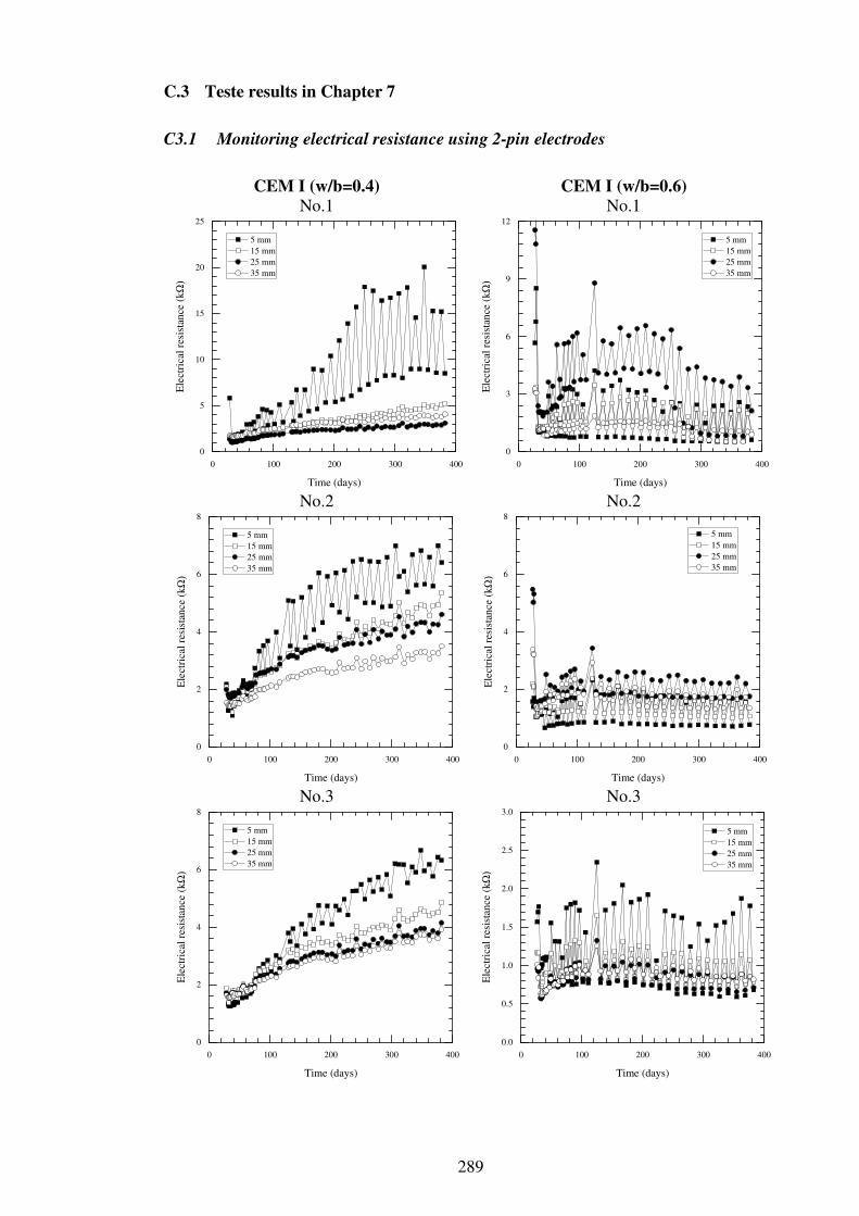
289

C.3 Teste results in Chapter 7

C3.1 Monitoring electrical resistance using 2-pin electrodes

CEM I (w/b=0.4) CEM I (w/b=0.6) No.1 No.1

No.2 No.2

No.3 No.3

0 100 200 300 400

0

5

10

15

20

25

5 mm

15 mm

25 mm

35 mm

Ele

ctri

cal

resi

stan

ce (

kΩ

)

Time (days)

0 100 200 300 400

0

3

6

9

12

5 mm

15 mm

25 mm

35 mm

Ele

ctri

cal

resi

stan

ce (

kΩ

)Time (days)

0 100 200 300 400

0

2

4

6

8

5 mm

15 mm

25 mm

35 mm

Ele

ctri

cal

resi

stan

ce (

kΩ

)

Time (days)

0 100 200 300 400

0

2

4

6

8

5 mm

15 mm

25 mm

35 mm

Ele

ctri

cal

resi

stan

ce (

kΩ

)

Time (days)

0 100 200 300 400

0

2

4

6

8

5 mm

15 mm

25 mm

35 mm

Ele

ctri

cal

resi

stan

ce (

kΩ

)

Time (days)

0 100 200 300 400

0.0

0.5

1.0

1.5

2.0

2.5

3.0

5 mm

15 mm

25 mm

35 mm

Ele

ctri

cal

resi

stan

ce (

kΩ

)

Time (days)

290

CEM III/A (w/b=0.4) CEM III/A (w/b=0.6) No.1 No.1

No.2 No.2

No.3 No.3

0 100 200 300 400

0

5

10

15

20

5 mm

15 mm

25 mm

35 mmE

lect

rica

l re

sist

ance

(kΩ

)

Time (days)

0 100 200 300 400

0

5

10

15

20

5 mm

15 mm

25 mm

35 mm

Ele

ctri

cal

resi

stan

ce (

kΩ

)

Time (days)

0 100 200 300 400

0

10

20

30

40

50

5 mm

15 mm

25 mm

35 mm

Ele

ctri

cal

resi

stan

ce (

kΩ

)

Time (days)

0 100 200 300 400

0

20

40

60

80

5 mm

15 mm

25 mm

35 mm

Ele

ctri

cal

resi

stan

ce (

kΩ

)

Time (days)

0 100 200 300 400

0

10

20

30

40

50

5 mm

15 mm

25 mm

35 mm

Ele

ctri

cal

resi

stan

ce (

kΩ

)

Time (days)

0 100 200 300 400

0

10

20

30

40

50

5 mm

15 mm

25 mm

35 mm

Ele

ctri

cal

resi

stan

ce (

kΩ

)

Time (days)

291

CEM II/B-V (w/b=0.4) CEM II/B-V (w/b=0.6) No.1 No.1

No.2 No.2

No.3 No.3

0 100 200 300 400

0

15

30

45

60

75

90

5 mm

15 mm

25 mm

35 mmE

lect

rica

l re

sist

ance

(kΩ

)

Time (days)

0 100 200 300 400

0

5

10

15

20

5 mm

15 mm

25 mm

35 mm

Ele

ctri

cal

resi

stan

ce (

kΩ

)

Time (days)

0 100 200 300 400

0

5

10

15

20

5 mm

15 mm

25 mm

35 mm

Ele

ctri

cal

resi

stan

ce (

kΩ

)

Time (days)

0 100 200 300 400

0

5

10

15

20

5 mm

15 mm

25 mm

35 mm

Ele

ctri

cal

resi

stan

ce (

kΩ

)

Time (days)

0 100 200 300 400

0

5

10

15

20

5 mm

15 mm

25 mm

35 mm

Ele

ctri

cal

resi

stan

ce (

kΩ

)

Time (days)

0 100 200 300 400

0

10

20

30

40

5 mm

15 mm

25 mm

35 mm

Ele

ctri

cal

resi

stan

ce (

kΩ

)

Time (days)

292

C3.2 Monitoring electrical resistance using 4-pin electrodes

CEM I (w/b=0.4) CEM I (w/b=0.6) No.1 No.1

No.2 No.2

No.3 No.3

0 100 200 300 400

0

300

600

900

1200

1500

1800

25 mm

70 mm-1

70 mm-2

Ele

ctri

cal

resi

stan

ce (

Ω)

Time (days)

0 100 200 300 400

0

150

300

450

600

750

25 mm

70 mm-1

70 mm-2

Ele

ctri

cal

resi

stan

ce (

Ω)

Time (days)

0 100 200 300 400

0

300

600

900

1200

1500

1800

25 mm

70 mm-1

70 mm-2

Ele

ctri

cal

resi

stan

ce (

Ω)

Time (days)

0 100 200 300 400

0

150

300

450

600

25 mm

70 mm-1

70 mm-2

Ele

ctri

cal

resi

stan

ce (

Ω)

Time (days)

0 100 200 300 400

0

300

600

900

1200

1500

1800

25 mm

70 mm-1

70 mm-2

Ele

ctri

cal

resi

stan

ce (

Ω)

Time (days)

0 100 200 300 400

0

300

600

900

25 mm

70 mm-1

70 mm-2

Ele

ctri

cal

resi

stan

ce (

Ω)

Time (days)

293

CEM III/A (w/b=0.4) CEM III/A (w/b=0.6) No.1 No.1

No.2 No.2

No.3 No.3

0 100 200 300 400

0

300

600

900

1200

1500

1800

2100

25 mm

70 mm-1

70 mm-2

Ele

ctri

cal

resi

stan

ce (

Ω)

Time (days)

0 100 200 300 400

0

900

1800

2700

3600

25 mm

70 mm-1

70 mm-2

Ele

ctri

cal

resi

stan

ce (

Ω)

Time (days)

Faulty electrode

0 100 200 300 400

0

600

1200

1800

2400

25 mm

70 mm-1

70 mm-2

Ele

ctri

cal

resi

stan

ce (

Ω)

Time (days)

0 100 200 300 400

0

600

1200

1800

2400

25 mm

70 mm-1

70 mm-2

Ele

ctri

cal

resi

stan

ce (

Ω)

Time (days)

0 100 200 300 400

0

600

1200

1800

2400

3000

25 mm

70 mm-1

70 mm-2

Ele

ctri

cal

resi

stan

ce (

Ω)

Time (days)

0 100 200 300 400

0

600

1200

1800

2400

25 mm

70 mm-1

70 mm-2

Ele

ctri

cal

resi

stan

ce (

Ω)

Time (days)

294

CEM II/B-V (w/b=0.4) CEM II/B-V (w/b=0.6) No.1 No.1

No.2 No.2

No.3 No.3

0 100 200 300 400

0

1000

2000

3000

4000

5000

25 mm

70 mm-1

70 mm-2

Ele

ctri

cal

resi

stan

ce (

Ω)

Time (days)

0 100 200 300 400

0

600

1200

1800

2400

3000

25 mm

70 mm-1

70 mm-2

Ele

ctri

cal

resi

stan

ce (

Ω)

Time (days)

0 100 200 300 400

0

1000

2000

3000

4000

5000

6000

25 mm

70 mm-1

70 mm-2

Ele

ctri

cal

resi

stan

ce (

Ω)

Time (days)

0 100 200 300 400

0

600

1200

1800

2400

3000

3600

25 mm

70 mm-1

70 mm-2

Ele

ctri

cal

resi

stan

ce (

Ω)

Time (days)

0 100 200 300 400

0

1500

3000

4500

25 mm

70 mm-1

70 mm-2

Ele

ctri

cal

resi

stan

ce (

Ω)

Time (days)

0 100 200 300 400

0

600

1200

1800

2400

3000

25 mm

70 mm-1

70 mm-2

Ele

ctri

cal

resi

stan

ce (

Ω)

Time (days)

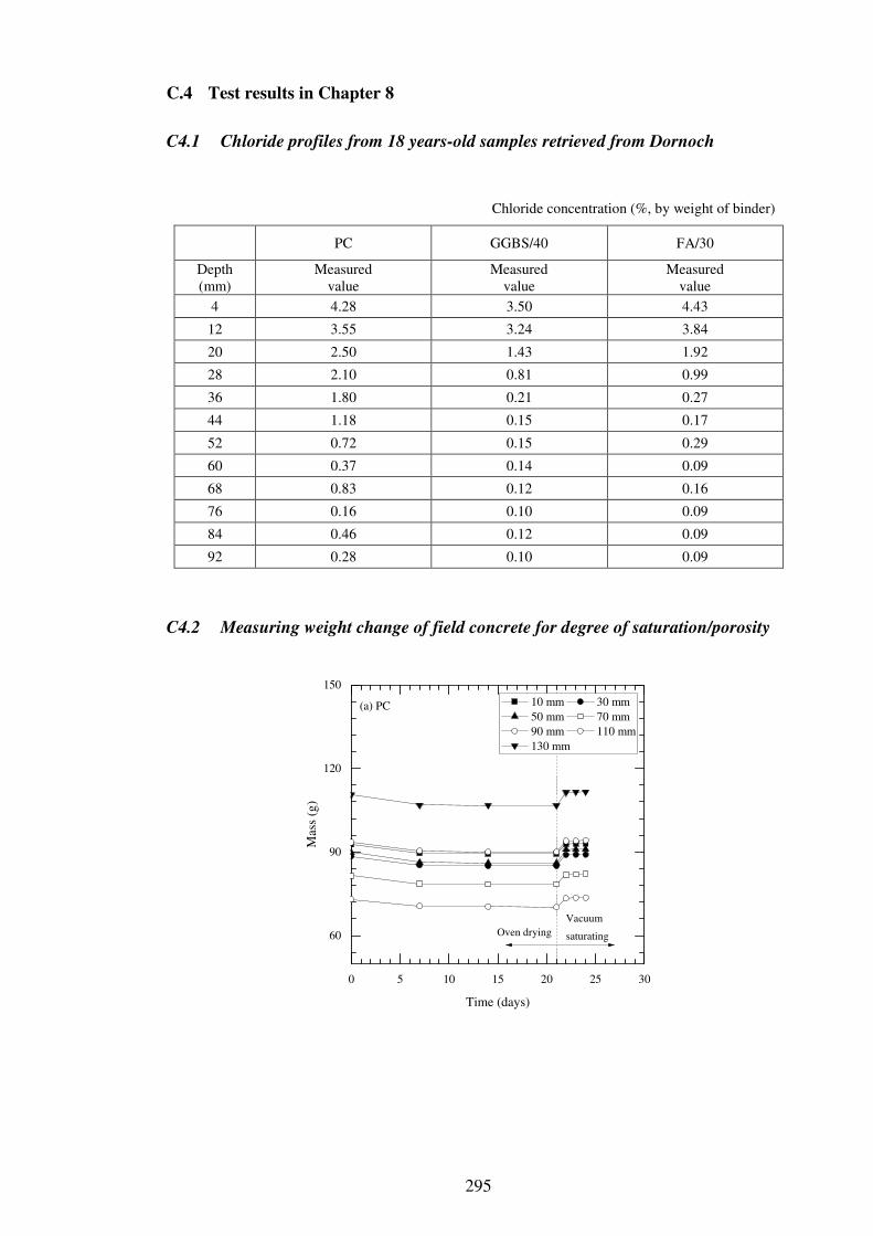
295


C4.1 Chloride profiles from 18 years-old samples retrieved from Dornoch

Chloride concentration (%, by weight of binder)

PC GGBS/40 FA/30

Depth (mm)

Measured value

Measured value

Measured value

4 4.28 3.50 4.43

12 3.55 3.24 3.84

20 2.50 1.43 1.92

28 2.10 0.81 0.99

36 1.80 0.21 0.27

44 1.18 0.15 0.17

52 0.72 0.15 0.29

60 0.37 0.14 0.09

68 0.83 0.12 0.16

76 0.16 0.10 0.09

84 0.46 0.12 0.09

92 0.28 0.10 0.09

C4.2 Measuring weight change of field concrete for degree of saturation/porosity

0 5 10 15 20 25 30

60

90

120

150

Vacuum

saturating

Mas

s (g

)

Time (days)

10 mm 30 mm

50 mm 70 mm

90 mm 110 mm

130 mm

Oven drying

(a) PC

296

0 5 10 15 20 25 30

60

90

120

150

Vacuum

saturating

Mas

s (g

)

Time (days)

10 mm 30 mm

50 mm 70 mm

90 mm 110 mm

130 mm

Oven drying

(b) GGBS/40

0 5 10 15 20 25 30

60

90

120

150

Vacuum

saturating

Mas

s (g

)

Time (days)

10 mm 30 mm

50 mm 70 mm

90 mm 110 mm

130 mm

Oven drying

(C) FA/30

297

C4.3 Monitoring electrical resistance of field concrete in Dornoch

(a) PC

(b) GGBS/40

(c) FA/30

0 5 10 15 20 25 30

10

12

14

16

18

20

22

24

Ele

ctri

cal

resi

stan

ce (

kΩ

)

Time (days)

5 mm 10 mm

15 mm 20 mm

30 mm 40 mm

50 mm

(a) PC

0 5 10 15 20 25 30

40

80

120

Ele

ctri

cal

resi

stan

ce (

kΩ

)

Time (days)

5 mm 10 mm

15 mm 20 mm

30 mm 40 mm

50 mm

(b) GGBS/40

0 5 10 15 20 25 30

20

40

60

80

100

120

Ele

ctri

cal

resi

stan

ce (

kΩ

)

Time (days)

5 mm 10 mm

15 mm 20 mm

30 mm 40 mm

50 mm

(c) FA/30

298

C4.4 Electrochemical parameters of steel in field concrete from polarisation techniques

Measurement Galvnostatic Potentiostatic Linear polarisation

resistance

RΩ

(Ω·m2) Rp

(Ω·m2) τ

(sec) C

(F/m2) β

r2 RΩ

(Ω·m2) Rp

(Ω·m2) τ

(sec) C

(F/m2) r2

Rp

(Ω·m2) r2

PC-No.1 227.81 10512.44 212.11 0.02 0.86 1.00 312.70 10236.54 4.21 0.01 0.98 6495.74 0.83

PC-No.2 260.96 8866.87 142.71 0.02 0.87 1.00 329.60 11746.09 3.86 0.01 0.98 9258.98 0.96

GGBS/40-No.1 345.81 8337.45 84.68 0.01 0.79 1.00 604.47 11712.91 4.31 0.01 0.96 9567.27 0.96

GGBS/40-No.2 347.71 4840.02 48.86 0.01 0.81 1.00 559.88 8142.56 4.73 0.01 0.95 6530.81 0.96

FA/30-No.1 1188.21 11213.13 226.84 0.02 0.79 1.00 1417.68 14085.98 18.45 0.01 0.99 5356.95 0.92

FA/30-No.2 1289.11 13398.49 293.71 0.02 0.80 1.00 1493.29 15429.34 19.62 0.01 0.99 5073.11 0.92

299

C4.5 Electrochemical impedance spectroscopy (Nyquist plot) for field samples

PC-No.1 PC-No.2

GGBS/40-No.1 GGBS/40-No.2

FA/30-No.1 FA/30-No.2

0 200 400 600 800

-2000

-1600

-1200

-800

-400

0

100 kHz

Z' (ω) (Ω)

iZ''

(ω) (

Ω)

5 mHz

0 400 800 1200

-2000

-1600

-1200

-800

-400

0

100 kHz

Z' (ω) (Ω)

iZ''

(ω) (

Ω)

5 mHz

0 400 800 1200 1600

-3000

-2400

-1800

-1200

-600

0

100 kHz

Z' (ω) (Ω)

iZ''

(ω) (

Ω)

5 mHz

0 400 800 1200 1600

-2400

-2000

-1600

-1200

-800

-400

0

100 kHz

Z' (ω) (Ω)

iZ''

(ω) (

Ω)

5 mHz

0 200 400 600 800 1000 1200 1400 1600 1800 2000

-2000

-1600

-1200

-800

-400

0

100 kHz

Z' (ω) (Ω)

iZ''

(ω) (

Ω)

5 mHz

0 400 800 1200 1600 2000

-2000

-1600

-1200

-800

-400

0

100 kHz

Z' (ω) (Ω)

iZ''

(ω) (

Ω)

5 mHz

300

C4.6 Potentiodynamic plot for field samples

PC-No.1 PC-No.2

GGBS/40-No.1 GGBS/40-No.2

FA/30-No.1 FA/30-No.2

1E-11 1E-9 1E-7 1E-5 1E-3-0.4

-0.2

0.0

0.2

0.4

0.6

0.8 Forward scan

Reverse scan

Po

ten

tial

(V

)

Current (A)

1E-11 1E-9 1E-7 1E-5 1E-3-0.4

-0.2

0.0

0.2

0.4

0.6

0.8 Forward scan

Reverse scan

Po

ten

tial

(V

)

Current (A)

1E-11 1E-9 1E-7 1E-5 1E-3-0.4

-0.2

0.0

0.2

0.4

0.6

0.8 Forward scan

Reverse scan

Po

ten

tial

(V

)

Current (A)

1E-11 1E-9 1E-7 1E-5 1E-3-0.4

-0.2

0.0

0.2

0.4

0.6

0.8 Forward scan

Reverse scan

Po

ten

tial

(V

)

Current (A)

1E-11 1E-9 1E-7 1E-5 1E-3-0.4

-0.2

0.0

0.2

0.4

0.6

0.8 Forward scan

Reverse scan

Po

ten

tial

(V

)

Current (A)

1E-11 1E-9 1E-7 1E-5 1E-3-0.4

-0.2

0.0

0.2

0.4

0.6

0.8 Forward scan

Reverse scan

Po

ten

tial

(V

)

Current (A)

301

APPENDIX D MODELLING

D.1 Prediction of compressive strength

Input values in equation (5.9) to predict the compressive strength of concrete

w/b Binder A B

0.4

CEM I 8.62 55.11

CEM III/A 7.98 34.98

CEM II/B-V 7.58 26.14

0.6

CEM I 6.82 15.25

CEM III/A 6.69 13.89

CEM II/B-V 5.39 5.50

302

D.2 Input values in the ClinConc model (in Excel version)

303

D.3 Determination of Kexp with regression method

Field sample (a) PC

(b) GGBS/40

(c) FA/30

0.0 0.2 0.4 0.6 0.8 1.0

0.0

0.2

0.4

0.6

0.8

1.0

Kexp

for PC (=0.60)

Average Kexp

(=0.70)

r2

Kexp

0.0 0.2 0.4 0.6 0.8 1.0

0.0

0.2

0.4

0.6

0.8

1.0

Kexp

for GGBS/40 (=0.67)

Average Kexp

(=0.70)

r2

Kexp

0.0 0.2 0.4 0.6 0.8 1.0

0.0

0.2

0.4

0.6

0.8

1.0

Kexp

for FA/30 (=0.82)

Average Kexp

(=0.70)

r2

Kexp

304

Laboratory sample

(a) CEM I (w/b=0.4) (b) CEM I (w/b=0.6)



0.0 0.2 0.4 0.6 0.8 1.0

0.0

0.2

0.4

0.6

0.8

1.0

Kexp

for CEM I (w/b=0.4) (=0.85)

Average Kexp

(=0.78)

r2

Kexp

1.0 1.2 1.4 1.6 1.8 2.0 2.2

0.0

0.2

0.4

0.6

0.8

1.0

Kexp

for CEM I (w/b=0.6) (=2.09)

Average Kexp

(=2.01)

r2

Kexp

0.0 0.2 0.4 0.6 0.8 1.0

0.0

0.2

0.4

0.6

0.8

1.0

Kexp

for CEM III/A(w/b=0.4) (=0.62)

Average Kexp

(=0.78)

r2

Kexp

1.0 1.2 1.4 1.6 1.8 2.0 2.2

0.0

0.2

0.4

0.6

0.8

1.0

Kexp

for CEM III/A (w/b=0.6) (=2.02)

Average Kexp

(=2.01)

r2

Kexp

0.0 0.2 0.4 0.6 0.8 1.0

0.0

0.2

0.4

0.6

0.8

1.0

Kexp

for CEM II/B-V (w/b=0.4) (=0.87)

Average Kexp

(=0.78)

r2

Kexp

1.0 1.2 1.4 1.6 1.8 2.0 2.2

0.0

0.2

0.4

0.6

0.8

1.0

Kexp

for CEM II/B-V (w/b=0.6) (=1.93)

Average Kexp

(=2.01)

r2

Kexp

Documents

Jaehwan Kim BSc MSc - CORE