Embed Size (px)
Citation preview
Undergraduate Texts in Mathematics
Je� rey Ho� steinJill PipherJoseph H. Silverman
An Introduction to Mathematical Cryptography Second Edition
Undergraduate Texts in Mathematics
Undergraduate Texts in Mathematics
Series Editors:
Sheldon AxlerSan Francisco State University, San Francisco, CA, USA
Kenneth RibetUniversity of California, Berkeley, CA, USA
Advisory Board:
Colin Adams, Williams College, Williamstown, MA, USAAlejandro Adem, University of British Columbia, Vancouver, BC, CanadaRuth Charney, Brandeis University, Waltham, MA, USAIrene M. Gamba, The University of Texas at Austin, Austin, TX, USARoger E. Howe, Yale University, New Haven, CT, USADavid Jerison, Massachusetts Institute of Technology, Cambridge, MA, USAJeffrey C. Lagarias, University of Michigan, Ann Arbor, MI, USAJill Pipher, Brown University, Providence, RI, USAFadil Santosa, University of Minnesota, Minneapolis, MN, USAAmie Wilkinson, University of Chicago, Chicago, IL, USA
Undergraduate Texts in Mathematics are generally aimed at third- and fourth-year undergraduate mathematics students at North American universities. These textsstrive to provide students and teachers with new perspectives and novel approaches.The books include motivation that guides the reader to an appreciation of interre-lations among different aspects of the subject. They feature examples that illustratekey concepts as well as exercises that strengthen understanding.
More information about this series at http://www.springer.com/series/666
Jeffrey Hoffstein • Jill PipherJoseph H. Silverman
An Introductionto MathematicalCryptography
Second Edition
123
Jeffrey HoffsteinDepartment of MathematicsBrown UniversityProvidence, RI, USA
Joseph H. SilvermanDepartment of MathematicsBrown UniversityProvidence, RI, USA
Jill PipherDepartment of MathematicsBrown UniversityProvidence, RI, USA
ISSN 0172-6056 ISSN 2197-5604 (electronic)ISBN 978-1-4939-1710-5 ISBN 978-1-4939-1711-2 (eBook)DOI 10.1007/978-1-4939-1711-2Springer New York Heidelberg Dordrecht London
Library of Congress Control Number: 2014946354
© Springer Science+Business Media New York 2008, 2014This work is subject to copyright. All rights are reserved by the Publisher, whether the whole or part ofthe material is concerned, specifically the rights of translation, reprinting, reuse of illustrations, recitation,broadcasting, reproduction on microfilms or in any other physical way, and transmission or informationstorage and retrieval, electronic adaptation, computer software, or by similar or dissimilar methodologynow known or hereafter developed. Exempted from this legal reservation are brief excerpts in connectionwith reviews or scholarly analysis or material supplied specifically for the purpose of being entered andexecuted on a computer system, for exclusive use by the purchaser of the work. Duplication of this pub-lication or parts thereof is permitted only under the provisions of the Copyright Law of the Publisher’slocation, in its current version, and permission for use must always be obtained from Springer. Permis-sions for use may be obtained through RightsLink at the Copyright Clearance Center. Violations are liableto prosecution under the respective Copyright Law.The use of general descriptive names, registered names, trademarks, service marks, etc. in this publicationdoes not imply, even in the absence of a specific statement, that such names are exempt from the relevantprotective laws and regulations and therefore free for general use.While the advice and information in this book are believed to be true and accurate at the date of publica-tion, neither the authors nor the editors nor the publisher can accept any legal responsibility for any errorsor omissions that may be made. The publisher makes no warranty, express or implied, with respect to thematerial contained herein.
Printed on acid-free paper
Springer is part of Springer Science+Business Media (www.springer.com)
Preface
The creation of public key cryptography by Diffie and Hellman in 1976 and thesubsequent invention of the RSA public key cryptosystem by Rivest, Shamir,and Adleman in 1978 are watershed events in the long history of secret com-munications. It is hard to overestimate the importance of public key cryp-tosystems and their associated digital signature schemes in the modern worldof computers and the Internet. This book provides an introduction to thetheory of public key cryptography and to the mathematical ideas underlyingthat theory.
Public key cryptography draws on many areas of mathematics, includingnumber theory, abstract algebra, probability, and information theory. Eachof these topics is introduced and developed in sufficient detail so that thisbook provides a self-contained course for the beginning student. The onlyprerequisite is a first course in linear algebra. On the other hand, studentswith stronger mathematical backgrounds can move directly to cryptographicapplications and still have time for advanced topics such as elliptic curvepairings and lattice-reduction algorithms.
Among the many facets of modern cryptography, this book chooses to con-centrate primarily on public key cryptosystems and digital signature schemes.This allows for an in-depth development of the necessary mathematics re-quired for both the construction of these schemes and an analysis of theirsecurity. The reader who masters the material in this book will not only bewell prepared for further study in cryptography, but will have acquired a realunderstanding of the underlying mathematical principles on which moderncryptography is based.
Topics covered in this book include Diffie–Hellman key exchange, discretelogarithm based cryptosystems, the RSA cryptosystem, primality testing, fac-torization algorithms, digital signatures, probability theory, information the-ory, collision algorithms, elliptic curves, elliptic curve cryptography, pairing-based cryptography, lattices, lattice-based cryptography, and the NTRU cryp-tosystem. A final chapter very briefly describes some of the many other aspectsof modern cryptography (hash functions, pseudorandom number generators,
v
vi Preface
zero-knowledge proofs, digital cash, AES, etc.) and serves to point the readertoward areas for further study.
Electronic Resources: The interested reader will find additional materialand a list of errata on the Mathematical Cryptography home page:
www.math.brown.edu/~jhs/MathCryptoHome.html
This web page includes many of the numerical exercises in the book, allowingthe reader to cut and paste them into other programs, rather than having toretype them.
No book is ever free from error or incapable of being improved. We wouldbe delighted to receive comments, good or bad, and corrections from ourreaders. You can send mail to us at
Acknowledgments: We, the authors, would like the thank the followingindividuals for test-driving this book and for the many corrections and helpfulsuggestions that they and their students provided: Liat Berdugo, AlexanderCollins, Samuel Dickman, Michael Gartner, Nicholas Howgrave-Graham, Su-Ion Ih, Saeja Kim, Yuji Kosugi, Yesem Kurt, Michelle Manes, Victor Miller,David Singer, William Whyte. In addition, we would like to thank the manystudents at Brown University who took Math 158 and helped us improve theexposition of this book.
Acknowledgments for the Second Edition: We would like to thankthe following individuals for corrections and suggestions that have beenincorporated into the second edition: Stefanos Aivazidis, Nicole Andre,John B. Baena, Carlo Beenakker, Robert Bond, Reinier Broker, Camp-bell Hewett, Rebecca Constantine, Stephen Constantine, Christopher Davis,Maria Fox, Steven Galbraith, Motahhareh Gharahi, David Hartz, JeremyHuddleston, Calvin Jongsma, Maya Kaczorowski, Yamamoto Kato, JonathanKatz, Chan-Ho Kim, Ariella Kirsch, Martin M. Lauridsen, Kelly McNeilly,Ryo Masuda, Shahab Mirzadeh, Kenneth Ribet, Jeremy Roach, HemlalSahum, Ghassan Sarkis, Frederick Schmitt, Christine Schwartz, Wei Shen,David Singer, Michael Soltys, David Spies, Bruce Stephens, Paulo Tanimoto,Patrick Vogt, Ralph Wernsdorf, Sebastian Welsch, Ralph Wernsdorf, EdwardWhite, Pomona College Math 113 (Spring 2009), University of California atBerkeley Math 116 (Spring 2009, 2010).
Providence, USA Jeffrey HoffsteinJill Pipher
Joseph H. Silverman
Contents
Preface v
Introduction xiii
1 An Introduction to Cryptography 1
1.1 Simple Substitution Ciphers . . . . . . . . . . . . . . . . . . . . 1
1.1.1 Cryptanalysis of Simple Substitution Ciphers . . . . . . 4
1.2 Divisibility and Greatest Common Divisors . . . . . . . . . . . 10
1.3 Modular Arithmetic . . . . . . . . . . . . . . . . . . . . . . . . 19
1.3.1 Modular Arithmetic and Shift Ciphers . . . . . . . . . . 23
1.3.2 The Fast Powering Algorithm . . . . . . . . . . . . . . . 24
1.4 Prime Numbers, Unique Factorization, and Finite Fields . . . . 26
1.5 Powers and Primitive Roots in Finite Fields . . . . . . . . . . . 29
1.6 Cryptography Before the Computer Age . . . . . . . . . . . . 34
1.7 Symmetric and Asymmetric Ciphers . . . . . . . . . . . . . . . 37
1.7.1 Symmetric Ciphers . . . . . . . . . . . . . . . . . . . . . 37
1.7.2 Encoding Schemes . . . . . . . . . . . . . . . . . . . . . 39
1.7.3 Symmetric Encryption of Encoded Blocks . . . . . . . . 40
1.7.4 Examples of Symmetric Ciphers . . . . . . . . . . . . . 41
1.7.5 Random Bit Sequences and Symmetric Ciphers . . . . . 44
1.7.6 Asymmetric Ciphers Make a First Appearance . . . . . 46
Exercises . . . . . . . . . . . . . . . . . . . . . . . . . . . . . . . . . 47
2 Discrete Logarithms and Diffie–Hellman 61
2.1 The Birth of Public Key Cryptography . . . . . . . . . . . . . 61
2.2 The Discrete Logarithm Problem . . . . . . . . . . . . . . . . . 64
2.3 Diffie–Hellman Key Exchange . . . . . . . . . . . . . . . . . . . 67
2.4 The Elgamal Public Key Cryptosystem . . . . . . . . . . . . . 70
2.5 An Overview of the Theory of Groups . . . . . . . . . . . . . . 74
2.6 How Hard Is the Discrete Logarithm Problem? . . . . . . . . . 77
2.7 A Collision Algorithm for the DLP . . . . . . . . . . . . . . . 81
vii
viii Contents
2.8 The Chinese Remainder Theorem . . . . . . . . . . . . . . . . 832.8.1 Solving Congruences with Composite Moduli . . . . . . 86
2.9 The Pohlig–Hellman Algorithm . . . . . . . . . . . . . . . . . 882.10 Rings, Quotients, Polynomials, and Finite Fields . . . . . . . . 94
2.10.1 An Overview of the Theory of Rings . . . . . . . . . . . 952.10.2 Divisibility and Quotient Rings . . . . . . . . . . . . . . 962.10.3 Polynomial Rings and the Euclidean Algorithm . . . . . 982.10.4 Polynomial Ring Quotients and Finite Fields . . . . . . 102
Exercises . . . . . . . . . . . . . . . . . . . . . . . . . . . . . . . . . 107
3 Integer Factorization and RSA 1173.1 Euler’s Formula and Roots Modulo pq . . . . . . . . . . . . . . 1173.2 The RSA Public Key Cryptosystem . . . . . . . . . . . . . . . 1233.3 Implementation and Security Issues . . . . . . . . . . . . . . . . 1263.4 Primality Testing . . . . . . . . . . . . . . . . . . . . . . . . . 128
3.4.1 The Distribution of the Set of Primes . . . . . . . . . . 1333.4.2 Primality Proofs Versus Probabilistic Tests . . . . . . . 136
3.5 Pollard’s p− 1 Factorization Algorithm . . . . . . . . . . . . . 1373.6 Factorization via Difference of Squares . . . . . . . . . . . . . 1413.7 Smooth Numbers and Sieves . . . . . . . . . . . . . . . . . . . . 150
3.7.1 Smooth Numbers . . . . . . . . . . . . . . . . . . . . . . 1503.7.2 The Quadratic Sieve . . . . . . . . . . . . . . . . . . . . 1553.7.3 The Number Field Sieve . . . . . . . . . . . . . . . . . . 162
3.8 The Index Calculus and Discrete Logarithms . . . . . . . . . . 1663.9 Quadratic Residues and Quadratic Reciprocity . . . . . . . . . 1693.10 Probabilistic Encryption . . . . . . . . . . . . . . . . . . . . . . 177Exercises . . . . . . . . . . . . . . . . . . . . . . . . . . . . . . . . . 180
4 Digital Signatures 1934.1 What Is a Digital Signature? . . . . . . . . . . . . . . . . . . . 1934.2 RSA Digital Signatures . . . . . . . . . . . . . . . . . . . . . . 1964.3 Elgamal Digital Signatures and DSA . . . . . . . . . . . . . . . 198Exercises . . . . . . . . . . . . . . . . . . . . . . . . . . . . . . . . . 203
5 Combinatorics, Probability, and Information Theory 2075.1 Basic Principles of Counting . . . . . . . . . . . . . . . . . . . 208
5.1.1 Permutations . . . . . . . . . . . . . . . . . . . . . . . . 2105.1.2 Combinations . . . . . . . . . . . . . . . . . . . . . . . . 2115.1.3 The Binomial Theorem . . . . . . . . . . . . . . . . . . 213
5.2 The Vigenere Cipher . . . . . . . . . . . . . . . . . . . . . . . . 2145.2.1 Cryptanalysis of the Vigenere Cipher: Theory . . . . . . 2185.2.2 Cryptanalysis of the Vigenere Cipher: Practice . . . . . 223
5.3 Probability Theory . . . . . . . . . . . . . . . . . . . . . . . . 2285.3.1 Basic Concepts of Probability Theory . . . . . . . . . . 228
Contents ix
5.3.2 Bayes’s Formula . . . . . . . . . . . . . . . . . . . . . . 233
5.3.3 Monte Carlo Algorithms . . . . . . . . . . . . . . . . . . 236
5.3.4 Random Variables . . . . . . . . . . . . . . . . . . . . . 238
5.3.5 Expected Value . . . . . . . . . . . . . . . . . . . . . . . 244
5.4 Collision Algorithms and Meet-in-the-Middle Attacks . . . . . . 246
5.4.1 The Birthday Paradox . . . . . . . . . . . . . . . . . . . 246
5.4.2 A Collision Theorem . . . . . . . . . . . . . . . . . . . . 247
5.4.3 A Discrete Logarithm Collision Algorithm . . . . . . . . 250
5.5 Pollard’s ρ Method . . . . . . . . . . . . . . . . . . . . . . . . . 253
5.5.1 Abstract Formulation of Pollard’s ρ Method . . . . . . . 254
5.5.2 Discrete Logarithms via Pollard’s ρ Method . . . . . . . 259
5.6 Information Theory . . . . . . . . . . . . . . . . . . . . . . . . 263
5.6.1 Perfect Secrecy . . . . . . . . . . . . . . . . . . . . . . . 263
5.6.2 Entropy . . . . . . . . . . . . . . . . . . . . . . . . . . . 269
5.6.3 Redundancy and the Entropyof Natural Language . . . . . . . . . . . . . . . . . . . . 275
5.6.4 The Algebra of Secrecy Systems . . . . . . . . . . . . . 277
5.7 Complexity Theory and P Versus NP . . . . . . . . . . . . . . 278
Exercises . . . . . . . . . . . . . . . . . . . . . . . . . . . . . . . . . 282
6 Elliptic Curves and Cryptography 299
6.1 Elliptic Curves . . . . . . . . . . . . . . . . . . . . . . . . . . . 299
6.2 Elliptic Curves over Finite Fields . . . . . . . . . . . . . . . . . 306
6.3 The Elliptic Curve Discrete Logarithm Problem . . . . . . . . . 310
6.3.1 The Double-and-Add Algorithm . . . . . . . . . . . . . 312
6.3.2 How Hard Is the ECDLP? . . . . . . . . . . . . . . . . . 315
6.4 Elliptic Curve Cryptography . . . . . . . . . . . . . . . . . . . 316
6.4.1 Elliptic Diffie–Hellman Key Exchange . . . . . . . . . . 316
6.4.2 Elliptic Elgamal Public Key Cryptosystem . . . . . . . 319
6.4.3 Elliptic Curve Signatures . . . . . . . . . . . . . . . . . 321
6.5 The Evolution of Public Key Cryptography . . . . . . . . . . . 321
6.6 Lenstra’s Elliptic Curve Factorization Algorithm . . . . . . . . 324
6.7 Elliptic Curves over F2 and over F2k . . . . . . . . . . . . . . . 329
6.8 Bilinear Pairings on Elliptic Curves . . . . . . . . . . . . . . . . 336
6.8.1 Points of Finite Order on Elliptic Curves . . . . . . . . 337
6.8.2 Rational Functions and Divisors on Elliptic Curves . . . 338
6.8.3 The Weil Pairing . . . . . . . . . . . . . . . . . . . . . . 340
6.8.4 An Efficient Algorithm to Compute the Weil Pairing . . 343
6.8.5 The Tate Pairing . . . . . . . . . . . . . . . . . . . . . . 346
6.9 The Weil Pairing over Fields of Prime Power Order . . . . . . . 347
6.9.1 Embedding Degree and the MOV Algorithm . . . . . . 347
6.9.2 Distortion Maps and a Modified Weil Pairing . . . . . . 350
6.9.3 A Distortion Map on y2 = x3 + x . . . . . . . . . . . . . 352
x Contents
6.10 Applications of the Weil Pairing . . . . . . . . . . . . . . . . . 356
6.10.1 Tripartite Diffie–Hellman Key Exchange . . . . . . . . . 356
6.10.2 ID-Based Public Key Cryptosystems . . . . . . . . . . . 358
Exercises . . . . . . . . . . . . . . . . . . . . . . . . . . . . . . . . . 361
7 Lattices and Cryptography 373
7.1 A Congruential Public Key Cryptosystem . . . . . . . . . . . . 373
7.2 Subset-Sum Problems and Knapsack Cryptosystems . . . . . . 377
7.3 A Brief Review of Vector Spaces . . . . . . . . . . . . . . . . . 384
7.4 Lattices: Basic Definitions and Properties . . . . . . . . . . . . 388
7.5 Short Vectors in Lattices . . . . . . . . . . . . . . . . . . . . . . 395
7.5.1 The Shortest and the Closest Vector Problems . . . . . 395
7.5.2 Hermite’s Theorem and Minkowski’s Theorem . . . . . 396
7.5.3 The Gaussian Heuristic . . . . . . . . . . . . . . . . . . 400
7.6 Babai’s Algorithm . . . . . . . . . . . . . . . . . . . . . . . . . 403
7.7 Cryptosystems Based on Hard Lattice Problems . . . . . . . . 407
7.8 The GGH Public Key Cryptosystem . . . . . . . . . . . . . . . 409
7.9 Convolution Polynomial Rings . . . . . . . . . . . . . . . . . . 412
7.10 The NTRU Public Key Cryptosystem . . . . . . . . . . . . . . 416
7.10.1 NTRUEncrypt . . . . . . . . . . . . . . . . . . . . . . . 417
7.10.2 Mathematical Problems for NTRUEncrypt . . . . . . . 422
7.11 NTRUEncrypt as a Lattice Cryptosystem . . . . . . . . . . . . 425
7.11.1 The NTRU Lattice . . . . . . . . . . . . . . . . . . . . . 425
7.11.2 Quantifying the Security of an NTRU Lattice . . . . . . 427
7.12 Lattice-Based Digital Signature Schemes . . . . . . . . . . . . . 428
7.12.1 The GGH Digital Signature Scheme . . . . . . . . . . . 428
7.12.2 Transcript Analysis . . . . . . . . . . . . . . . . . . . . . 430
7.12.3 Rejection Sampling . . . . . . . . . . . . . . . . . . . . . 431
7.12.4 Rejection Sampling Applied to an Abstract SignatureScheme . . . . . . . . . . . . . . . . . . . . . . . . . . . 433
7.12.5 The NTRU Modular Lattice Signature Scheme . . . . . 434
7.13 Lattice Reduction Algorithms . . . . . . . . . . . . . . . . . . 436
7.13.1 Gaussian Lattice Reduction in Dimension 2 . . . . . . . 436
7.13.2 The LLL Lattice Reduction Algorithm . . . . . . . . . . 439
7.13.3 Using LLL to Solve apprCVP . . . . . . . . . . . . . . . 448
7.13.4 Generalizations of LLL . . . . . . . . . . . . . . . . . . . 449
7.14 Applications of LLL to Cryptanalysis . . . . . . . . . . . . . . . 450
7.14.1 Congruential Cryptosystems . . . . . . . . . . . . . . . . 451
7.14.2 Applying LLL to Knapsacks . . . . . . . . . . . . . . . . 451
7.14.3 Applying LLL to GGH . . . . . . . . . . . . . . . . . . . 452
7.14.4 Applying LLL to NTRU . . . . . . . . . . . . . . . . . . 453
Exercises . . . . . . . . . . . . . . . . . . . . . . . . . . . . . . . . . 454
Contents xi
8 Additional Topics in Cryptography 4718.1 Hash Functions . . . . . . . . . . . . . . . . . . . . . . . . . . . 4728.2 Random Numbers and Pseudorandom Number . . . . . . . . . 4748.3 Zero-Knowledge Proofs . . . . . . . . . . . . . . . . . . . . . . . 4778.4 Secret Sharing Schemes . . . . . . . . . . . . . . . . . . . . . . 4808.5 Identification Schemes . . . . . . . . . . . . . . . . . . . . . . . 4818.6 Padding Schemes and the Random Oracle Model . . . . . . . . 4828.7 Building Protocols from Cryptographic Primitives . . . . . . . 4858.8 Blind Digital Signatures, Digital Cash, and Bitcoin . . . . . . . 4878.9 Homomorphic Encryption . . . . . . . . . . . . . . . . . . . . . 4908.10 Hyperelliptic Curve Cryptography . . . . . . . . . . . . . . . . 4948.11 Quantum Computing . . . . . . . . . . . . . . . . . . . . . . . . 4978.12 Modern Symmetric Cryptosystems: DES and AES . . . . . . . 499
List of Notation 503
References 507
Index 517

Introduction
Principal Goals of (Public Key) Cryptography• Allow two people to exchange confidential information,even if they have never met and can communicate onlyvia a channel that is being monitored by an adversary.• Allow a person to attach a digital signature to a document,so that any other person can verify the validity of thesignature, but no one can forge a signature on any otherdocument.
The security of communications and commerce in a digital age relies on themodern incarnation of the ancient art of codes and ciphers. Underlying thebirth of modern cryptography is a great deal of fascinating mathematics,some of which has been developed for cryptographic applications, but muchof which is taken from the classical mathematical canon. The principal goalof this book is to introduce the reader to a variety of mathematical topicswhile simultaneously integrating the mathematics into a description of modernpublic key cryptography.
For thousands of years, all codes and ciphers relied on the assumptionthat the people attempting to communicate, call them Bob and Alice, sharea secret key that their adversary, call her Eve, does not possess. Bob uses thesecret key to encrypt his message, Alice uses the same secret key to decryptthe message, and poor Eve, not knowing the secret key, is unable to performthe decryption. A disadvantage of these private key cryptosystems is that Boband Alice need to exchange the secret key before they can get started.
During the 1970s, the astounding idea of public key cryptography burstupon the scene.1 In a public key cryptosystem, Alice has two keys, a publicencryption key KPub and a private (secret) decryption key KPri. Alice pub-lishes her public key KPub, and then Adam and Bob and Carl and everyoneelse can use KPub to encrypt messages and send them to Alice. The ideaunderlying public key cryptography is that although everyone in the worldknows KPub and can use it to encrypt messages, only Alice, who knows theprivate key KPri, is able to decrypt messages.
1A brief history of cryptography is given is Sects. 1.6, 2.1, 6.5, and 7.7.xiii
xiv Introduction
The advantages of a public key cryptosystem are manifold. For example,Bob can send Alice an encrypted message even if they have never previouslybeen in direct contact. But although public key cryptography is a fascinatingtheoretical concept, it is not at all clear how one might create a public keycryptosystem. It turns out that public key cryptosystems can be based onhard mathematical problems. More precisely, one looks for a mathematicalproblem that is initially hard to solve, but that becomes easy to solve if oneknows some extra piece of information.
Of course, private key cryptosystems have not disappeared. Indeed, theyare more important than ever, since they tend to be significantly more effi-cient than public key cryptosystems. Thus in practice, if Bob wants to sendAlice a long message, he first uses a public key cryptosystem to send Alicethe key for a private key cryptosystem, and then he uses the private keycryptosystem to encrypt his message. The most efficient modern private keycryptosystems, such as DES and AES, rely for their security on repeated ap-plication of various mixing operations that are hard to unmix without theprivate key. Thus although the subject of private key cryptography is of boththeoretical and practical importance, the connection with fundamental un-derlying mathematical ideas is much less pronounced than it is with publickey cryptosystems. For that reason, this book concentrates almost exclusivelyon public key cryptography, especially public key cryptosystems and digitalsignatures.
Modern mathematical cryptography draws on many areas of mathematics,including especially number theory, abstract algebra (groups, rings, fields),probability, statistics, and information theory, so the prerequisites for studyingthe subject can seem formidable. By way of contrast, the prerequisites forreading this book are minimal, because we take the time to introduce eachrequired mathematical topic in sufficient depth as it is needed. Thus thisbook provides a self-contained treatment of mathematical cryptography forthe reader with limited mathematical background. And for those readers whohave taken a course in, say, number theory or abstract algebra or probability,we suggest briefly reviewing the relevant sections as they are reached and thenmoving on directly to the cryptographic applications.
This book is not meant to be a comprehensive source for all things cryp-tographic. In the first place, as already noted, we concentrate on public keycryptography. But even within this domain, we have chosen to pursue a smallselection of topics to a reasonable mathematical depth, rather than provid-ing a more superficial description of a wider range of subjects. We feel thatany reader who has mastered the material in this book will not only be wellprepared for further study in cryptography, but will have acquired a realunderstanding of the underlying mathematical principles on which moderncryptography is based.
However, this does not mean that the omitted topics are unimportant.It simply means that there is a limit to the amount of material that canbe included in a book (or course) of reasonable length. As in any text, the
Introduction xv
choice of particular topics reflects the authors’ tastes and interests. For theconvenience of the reader, the final chapter contains a brief survey of areasfor further study.
A Guide to Mathematical Topics: This book includes a significant amountof mathematical material on a variety of topics that are useful in cryptography.The following list is designed to help coordinate the mathematical topics thatwe cover with subjects that the class or reader may have already studied.
Congruences, primes, and finite fields — Sects. 1.2, 1.3, 1.4, 1.5, 2.10.4The Chinese remainder theorem — Sect. 2.8
Euler’s formula — Sect. 3.1Primality testing — Sect. 3.4
Quadratic reciprocity — Sect. 3.9Factorization methods — Sects. 3.5, 3.6, 3.7, 6.6
Discrete logarithms — Sects. 2.2, 3.8, 5.4, 5.5, 6.3Group theory — Sect. 2.5
Rings, polynomials, and quotient rings — Sects. 2.10 and 7.9Combinatorics and probability — Sects. 5.1 and 5.3
Information and complexity theory — Sects. 5.6 and 5.7Elliptic curves — Sects. 6.1, 6.2, 6.7, 6.8Linear algebra — Sects. 7.3
Lattices — Sects. 7.4, 7.5, 7.6, 7.13
Intended Audience and Prerequisites: This book provides a self-con-tained introduction to public key cryptography and to the underlying math-ematics that is required for the subject. It is suitable as a text for advancedundergraduates and beginning graduate students. We provide enough back-ground material so that the book can be used in courses for students with noprevious exposure to abstract algebra or number theory. For classes in whichthe students have a stronger background, the basic mathematical materialmay be omitted, leaving time for some of the more advanced topics.
The formal prerequisites for this book are few, beyond a facility withhigh school algebra and, in Chap. 6, analytic geometry. Elementary calculusis used here and there in a minor way, but is not essential, and linear alge-bra is used in a small way in Chap. 3 and more extensively in Chap. 7. Noprevious knowledge is assumed for mathematical topics such as number the-ory, abstract algebra, and probability theory that play a fundamental role inmodern cryptography. They are covered in detail as needed.
However, it must be emphasized that this is a mathematics book with itsshare of formal definitions and theorems and proofs. Thus it is expected thatthe reader has a certain level of mathematical sophistication. In particular,students who have previously taken a proof-based mathematics course willfind the material easier than those without such background. On the otherhand, the subject of cryptography is so appealing that this book makes agood text for an introduction-to-proofs course, with the understanding that
xvi Introduction
the instructor will need to cover the material more slowly to allow the studentstime to become comfortable with proof-based mathematics.
Suggested Syllabus: This book contains considerably more material thancan be comfortably covered by beginning students in a one semester course.However, for more advanced students who have already taken courses in num-ber theory and abstract algebra, it should be possible to do most of the remain-ing material. We suggest covering the majority of the topics in Chaps. 1–4,possibly omitting some of the more technical topics, the optional materialon the Vigenere cipher, and the section on ring theory, which is not useduntil much later in the book. The next three chapters on information theory(Chap. 5), elliptic curves (Chap. 6), and lattices (Chap. 7) are mostly indepen-dent of one another, so the instructor has the choice of covering one or twoof them in detail or all of them in less depth. We offer the following syllabusas an example of one of the many possibilities. We have indicated that somesections are optional. Covering the optional material leaves less time for thelater chapters at the end of the course.
Chapter 1. An Introduction to Cryptography.Cover all sections.
Chapter 2. Discrete Logarithms and Diffie–Hellman.Cover Sects. 2.1–2.7. Optionally cover the more mathematically sophis-ticated Sects. 2.8–2.9 on the Pohlig–Hellman algorithm. Omit Sect. 2.10on first reading.
Chapter 3. Integer Factorization and RSA.Cover Sects. 3.1–3.5 and 3.9–3.10. Optionally, cover the more mathemat-ically sophisticated Sects. 3.6–3.8, dealing with smooth numbers, sieves,and the index calculus.
Chapter 4. Digital Signatures.Cover all sections.
Chapter 5. Probability Theory and Information Theory.Cover Sects. 5.1, 5.3, and 5.4. Optionally cover the more mathemati-cally sophisticated sections on Pollard’s ρ method (Sect. 5.5), informa-tion theory (Sect. 5.6), and complexity theory (Sect. 5.7). The materialon the Vigenere cipher in Sect. 5.2 nicely illustrates the use of statisticsin cryptanalysis, but is somewhat off the main path.
Chapter 6. Elliptic Curves.Cover Sects. 6.1–6.4. Cover other sections as time permits, but note thatSects. 6.7–6.10 on pairings require finite fields of prime power order,which are described in Sect. 2.10.4.
Chapter 7. Lattices and Cryptography.Cover Sects. 7.1–7.8. (If time is short, one may omit either or both ofSects. 7.1 and 7.2.) Cover either Sects. 7.13–7.14 on the LLL lattice re-duction algorithm or Sects. 7.9–7.11 on the NTRU cryptosystem, or
Introduction xvii
both, as time permits. (The NTRU sections require the material onpolynomial rings and quotient rings covered in Sect. 2.10.)
Chapter 8. Additional Topics in Cryptography.The material in this chapter points the reader toward other importantareas of cryptography. It provides a good list of topics and referencesfor student term papers and presentations.
Further Notes for the Instructor: Depending on how much of the hardermathematical material in Chaps. 2–5 is covered, there may not be time todelve into both Chaps. 6 and 7, so the instructor may need to omit eitherelliptic curves or lattices in order to fit the other material into one semester.
We feel that it is helpful for students to gain an appreciation of the originsof their subject, so we have scattered a handful of sections throughout the bookcontaining some brief comments on the history of cryptography. Instructorswho want to spend more time on mathematics may omit these sections withoutaffecting the mathematical narrative.
Changes in the Second Edition:• The chapter on digital signatures has been moved, since we felt thatthis important topic should be covered earlier in the course. More pre-cisely, RSA, Elgamal, and DSA signatures are now described in the shortChap. 4, while the material on elliptic curve signatures is covered in thebrief Sect. 6.4.3. The two sections on lattice-based signatures from the firstedition have been extensively rewritten and now appear as Sect. 7.12.
• Numerous new exercises have been included.
• Numerous typographical and minor mathematical errors have been cor-rected, and notation has been made more consistent from chapter tochapter.
• Various explanations have been rewritten or expanded for clarity, espe-cially in Chaps. 5–7.
• New sections on digital cash and on homomorphic encryption have beenadded to the additional topics in Chap. 8; see Sects. 8.8 and 8.9.
Chapter 1
An Introductionto Cryptography
1.1 Simple Substitution Ciphers
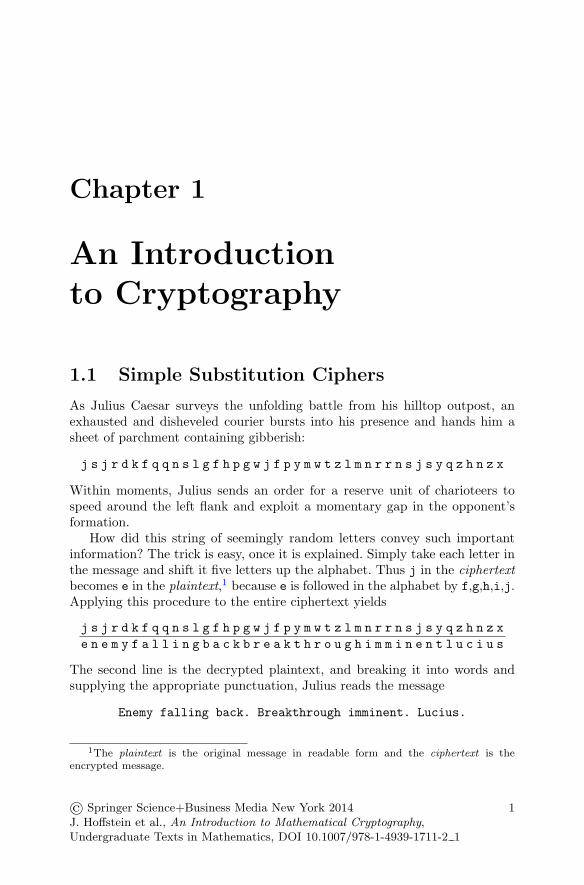
As Julius Caesar surveys the unfolding battle from his hilltop outpost, anexhausted and disheveled courier bursts into his presence and hands him asheet of parchment containing gibberish:
j s j r d k f q q n s l g f h p g w j f p y m w t z l m n r r n s j s y q z h n z x
Within moments, Julius sends an order for a reserve unit of charioteers tospeed around the left flank and exploit a momentary gap in the opponent’sformation.
How did this string of seemingly random letters convey such importantinformation? The trick is easy, once it is explained. Simply take each letter inthe message and shift it five letters up the alphabet. Thus j in the ciphertextbecomes e in the plaintext,1 because e is followed in the alphabet by f,g,h,i,j.Applying this procedure to the entire ciphertext yields
j s j r d k f q q n s l g f h p g w j f p y m w t z l m n r r n s j s y q z h n z x
e n e m y f a l l i n g b a c k b r e a k t h r o u g h i m m i n e n t l u c i u s
The second line is the decrypted plaintext, and breaking it into words andsupplying the appropriate punctuation, Julius reads the message
Enemy falling back. Breakthrough imminent. Lucius.
1The plaintext is the original message in readable form and the ciphertext is theencrypted message.
© Springer Science+Business Media New York 2014J. Hoffstein et al., An Introduction to Mathematical Cryptography,Undergraduate Texts in Mathematics, DOI 10.1007/978-1-4939-1711-2 1
1

2 1. An Introduction to Cryptography
There remains one minor quirk that must be addressed. What happens whenJulius finds a letter such as d? There is no letter appearing five letters before din the alphabet. The answer is that he must wrap around to the end of thealphabet. Thus d is replaced by y, since y is followed by z,a,b,c,d.
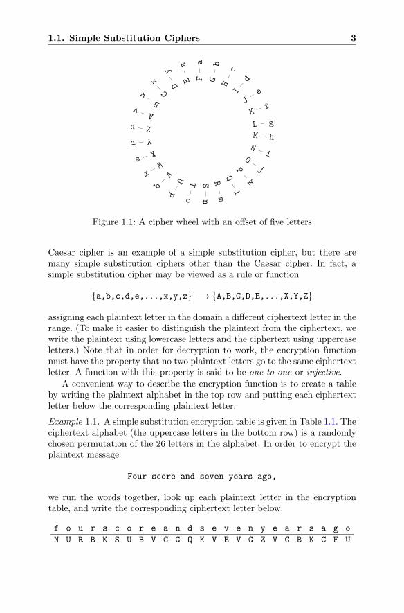
This wrap-around effect may be conveniently visualized by placing thealphabet abcd...xyz around a circle, rather than in a line. If a second alpha-bet circle is then placed within the first circle and the inner circle is rotatedfive letters, as illustrated in Fig. 1.1, the resulting arrangement can be usedto easily encrypt and decrypt Caesar’s messages. To decrypt a letter, simplyfind it on the inner wheel and read the corresponding plaintext letter fromthe outer wheel. To encrypt, reverse this process: find the plaintext letter onthe outer wheel and read off the ciphertext letter from the inner wheel. Andnote that if you build a cipherwheel whose inner wheel spins, then you are nolonger restricted to always shifting by exactly five letters. Cipher wheels ofthis sort have been used for centuries.2
Although the details of the preceding scene are entirely fictional, and inany case it is unlikely that a message to a Roman general would have beenwritten in modern English(!), there is evidence that Caesar employed thisearly method of cryptography, which is sometimes called the Caesar cipherin his honor. It is also sometimes referred to as a shift cipher, since eachletter in the alphabet is shifted up or down. Cryptography, the methodology ofconcealing the content of messages, comes from the Greek root words kryptos,meaning hidden,3 and graphikos, meaning writing. The modern scientific studyof cryptography is sometimes referred to as cryptology.
In the Caesar cipher, each letter is replaced by one specific substituteletter. However, if Bob encrypts a message for Alice4 using a Caesar cipherand allows the encrypted message to fall into Eve’s hands, it will take Evevery little time to decrypt it. All she needs to do is try each of the 26 possibleshifts.
Bob can make his message harder to attack by using a more complicatedreplacement scheme. For example, he could replace every occurrence of a
by z and every occurrence of z by a, every occurrence of b by y and everyoccurrence of y by b, and so on, exchanging each pair of letters c ↔ x,. . . ,m↔ n.
This is an example of a simple substitution cipher, that is, a cipher in whicheach letter is replaced by another letter (or some other type of symbol). The
2A cipher wheel with mixed up alphabets and with encryption performed using differentoffsets for different parts of the message is featured in a fifteenth century monograph byLeon Batista Alberti [63].
3The word cryptic, meaning hidden or occult, appears in 1638, while crypto- as a prefixfor concealed or secret makes its appearance in 1760. The term cryptogram appears muchlater, first occurring in 1880.
4In cryptography, it is traditional for Bob and Alice to exchange confidential mes-sages and for their adversary Eve, the eavesdropper, to intercept and attempt to read theirmessages. This makes the field of cryptography much more personal than other areas ofmathematics and computer science, whose denizens are often X and Y !
1.1. Simple Substitution Ciphers 3
F–a
G–b
H–c
I–d
J – e
K – f
L – g
M – hN – i
O – jP–k
Q–l
R–m
S–n
T–o
U–p
V–q
W–r
X–s
Y–t
Z–uA–v
B–w C–x
D–y
E–z
Figure 1.1: A cipher wheel with an offset of five letters
Caesar cipher is an example of a simple substitution cipher, but there aremany simple substitution ciphers other than the Caesar cipher. In fact, asimple substitution cipher may be viewed as a rule or function
{a,b,c,d,e,...,x,y,z} −→ {A,B,C,D,E,...,X,Y,Z}
assigning each plaintext letter in the domain a different ciphertext letter in therange. (To make it easier to distinguish the plaintext from the ciphertext, wewrite the plaintext using lowercase letters and the ciphertext using uppercaseletters.) Note that in order for decryption to work, the encryption functionmust have the property that no two plaintext letters go to the same ciphertextletter. A function with this property is said to be one-to-one or injective.
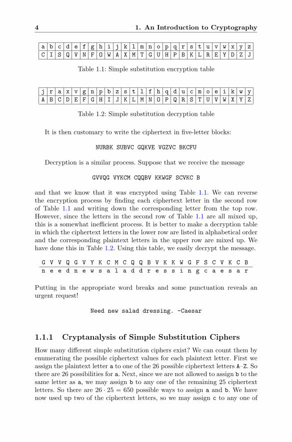
A convenient way to describe the encryption function is to create a tableby writing the plaintext alphabet in the top row and putting each ciphertextletter below the corresponding plaintext letter.
Example 1.1. A simple substitution encryption table is given in Table 1.1. Theciphertext alphabet (the uppercase letters in the bottom row) is a randomlychosen permutation of the 26 letters in the alphabet. In order to encrypt theplaintext message
Four score and seven years ago,
we run the words together, look up each plaintext letter in the encryptiontable, and write the corresponding ciphertext letter below.
f o u r s c o r e a n d s e v e n y e a r s a g o
N U R B K S U B V C G Q K V E V G Z V C B K C F U
4 1. An Introduction to Cryptography
a b c d e f g h i j k l m n o p q r s t u v w x y z
C I S Q V N F O W A X M T G U H P B K L R E Y D Z J
Table 1.1: Simple substitution encryption table
j r a x v g n p b z s t l f h q d u c m o e i k w y
A B C D E F G H I J K L M N O P Q R S T U V W X Y Z
Table 1.2: Simple substitution decryption table
It is then customary to write the ciphertext in five-letter blocks:
NURBK SUBVC GQKVE VGZVC BKCFU
Decryption is a similar process. Suppose that we receive the message
GVVQG VYKCM CQQBV KKWGF SCVKC B
and that we know that it was encrypted using Table 1.1. We can reversethe encryption process by finding each ciphertext letter in the second rowof Table 1.1 and writing down the corresponding letter from the top row.However, since the letters in the second row of Table 1.1 are all mixed up,this is a somewhat inefficient process. It is better to make a decryption tablein which the ciphertext letters in the lower row are listed in alphabetical orderand the corresponding plaintext letters in the upper row are mixed up. Wehave done this in Table 1.2. Using this table, we easily decrypt the message.
G V V Q G V Y K C M C Q Q B V K K W G F S C V K C B
n e e d n e w s a l a d d r e s s i n g c a e s a r
Putting in the appropriate word breaks and some punctuation reveals anurgent request!
Need new salad dressing. -Caesar
1.1.1 Cryptanalysis of Simple Substitution Ciphers
How many different simple substitution ciphers exist? We can count them byenumerating the possible ciphertext values for each plaintext letter. First weassign the plaintext letter a to one of the 26 possible ciphertext letters A–Z. Sothere are 26 possibilities for a. Next, since we are not allowed to assign b to thesame letter as a, we may assign b to any one of the remaining 25 ciphertextletters. So there are 26 · 25 = 650 possible ways to assign a and b. We havenow used up two of the ciphertext letters, so we may assign c to any one of
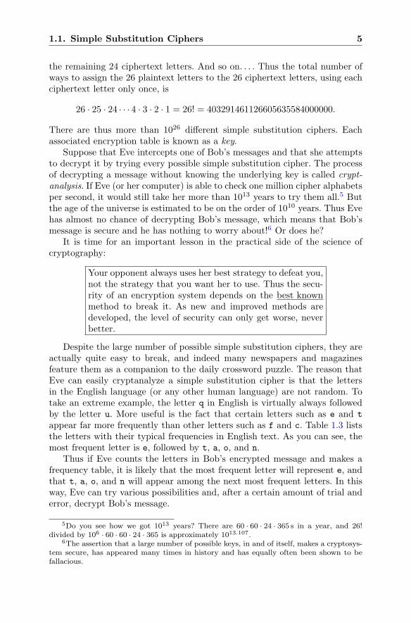
1.1. Simple Substitution Ciphers 5
the remaining 24 ciphertext letters. And so on. . . . Thus the total number ofways to assign the 26 plaintext letters to the 26 ciphertext letters, using eachciphertext letter only once, is
26 · 25 · 24 · · · 4 · 3 · 2 · 1 = 26! = 403291461126605635584000000.
There are thus more than 1026 different simple substitution ciphers. Eachassociated encryption table is known as a key.
Suppose that Eve intercepts one of Bob’s messages and that she attemptsto decrypt it by trying every possible simple substitution cipher. The processof decrypting a message without knowing the underlying key is called crypt-analysis. If Eve (or her computer) is able to check one million cipher alphabetsper second, it would still take her more than 1013 years to try them all.5 Butthe age of the universe is estimated to be on the order of 1010 years. Thus Evehas almost no chance of decrypting Bob’s message, which means that Bob’smessage is secure and he has nothing to worry about!6 Or does he?
It is time for an important lesson in the practical side of the science ofcryptography:
Your opponent always uses her best strategy to defeat you,not the strategy that you want her to use. Thus the secu-rity of an encryption system depends on the best knownmethod to break it. As new and improved methods aredeveloped, the level of security can only get worse, neverbetter.
Despite the large number of possible simple substitution ciphers, they areactually quite easy to break, and indeed many newspapers and magazinesfeature them as a companion to the daily crossword puzzle. The reason thatEve can easily cryptanalyze a simple substitution cipher is that the lettersin the English language (or any other human language) are not random. Totake an extreme example, the letter q in English is virtually always followedby the letter u. More useful is the fact that certain letters such as e and t
appear far more frequently than other letters such as f and c. Table 1.3 liststhe letters with their typical frequencies in English text. As you can see, themost frequent letter is e, followed by t, a, o, and n.
Thus if Eve counts the letters in Bob’s encrypted message and makes afrequency table, it is likely that the most frequent letter will represent e, andthat t, a, o, and n will appear among the next most frequent letters. In thisway, Eve can try various possibilities and, after a certain amount of trial anderror, decrypt Bob’s message.
5Do you see how we got 1013 years? There are 60 · 60 · 24 · 365 s in a year, and 26!divided by 106 · 60 · 60 · 24 · 365 is approximately 1013.107.
6The assertion that a large number of possible keys, in and of itself, makes a cryptosys-tem secure, has appeared many times in history and has equally often been shown to befallacious.
6 1. An Introduction to Cryptography
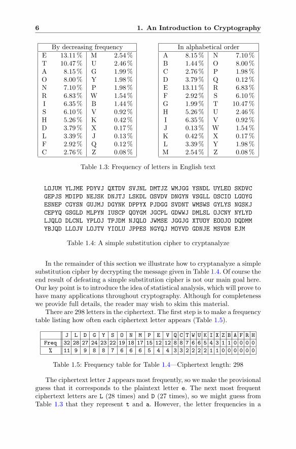
By decreasing frequencyE 13.11% M 2.54%T 10.47% U 2.46%A 8.15% G 1.99%O 8.00% Y 1.98%N 7.10% P 1.98%R 6.83% W 1.54%I 6.35% B 1.44%S 6.10% V 0.92%H 5.26% K 0.42%D 3.79% X 0.17%L 3.39% J 0.13%F 2.92% Q 0.12%C 2.76% Z 0.08%
In alphabetical orderA 8.15% N 7.10%B 1.44% O 8.00%C 2.76% P 1.98%D 3.79% Q 0.12%E 13.11% R 6.83%F 2.92% S 6.10%G 1.99% T 10.47%H 5.26% U 2.46%I 6.35% V 0.92%J 0.13% W 1.54%K 0.42% X 0.17%L 3.39% Y 1.98%M 2.54% Z 0.08%
Table 1.3: Frequency of letters in English text
LOJUM YLJME PDYVJ QXTDV SVJNL DMTJZ WMJGG YSNDL UYLEO SKDVC
GEPJS MDIPD NEJSK DNJTJ LSKDL OSVDV DNGYN VSGLL OSCIO LGOYG
ESNEP CGYSN GUJMJ DGYNK DPPYX PJDGG SVDNT WMSWS GYLYS NGSKJ
CEPYQ GSGLD MLPYN IUSCP QOYGM JGCPL GDWWJ DMLSL OJCNY NYLYD
LJQLO DLCNL YPLOJ TPJDM NJQLO JWMSE JGGJG XTUOY EOOJO DQDMM
YBJQD LLOJV LOJTV YIOLU JPPES NGYQJ MOYVD GDNJE MSVDN EJM
Table 1.4: A simple substitution cipher to cryptanalyze
In the remainder of this section we illustrate how to cryptanalyze a simplesubstitution cipher by decrypting the message given in Table 1.4. Of course theend result of defeating a simple substitution cipher is not our main goal here.Our key point is to introduce the idea of statistical analysis, which will prove tohave many applications throughout cryptography. Although for completenesswe provide full details, the reader may wish to skim this material.
There are 298 letters in the ciphertext. The first step is to make a frequencytable listing how often each ciphertext letter appears (Table 1.5).
J L D G Y S O N M P E V Q C T W U K I X Z B A F R H
Freq 32 28 27 24 23 22 19 18 17 15 12 12 8 8 7 6 6 5 4 3 1 1 0 0 0 0
% 11 9 9 8 8 7 6 6 6 5 4 4 3 3 2 2 2 2 1 1 0 0 0 0 0 0
Table 1.5: Frequency table for Table 1.4—Ciphertext length: 298
The ciphertext letter J appears most frequently, so we make the provisionalguess that it corresponds to the plaintext letter e. The next most frequentciphertext letters are L (28 times) and D (27 times), so we might guess fromTable 1.3 that they represent t and a. However, the letter frequencies in a
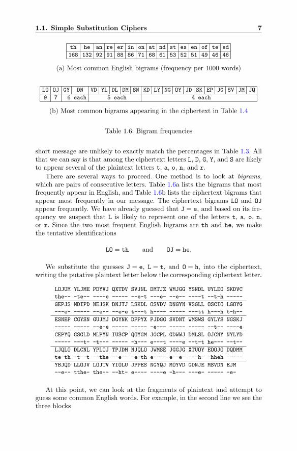
1.1. Simple Substitution Ciphers 7
th he an re er in on at nd st es en of te ed
168 132 92 91 88 86 71 68 61 53 52 51 49 46 46
(a) Most common English bigrams (frequency per 1000 words)
LO OJ GY DN VD YL DL DM SN KD LY NG OY JD SK EP JG SV JM JQ
9 7 6 each 5 each 4 each
(b) Most common bigrams appearing in the ciphertext in Table 1.4
Table 1.6: Bigram frequencies
short message are unlikely to exactly match the percentages in Table 1.3. Allthat we can say is that among the ciphertext letters L, D, G, Y, and S are likelyto appear several of the plaintext letters t, a, o, n, and r.
There are several ways to proceed. One method is to look at bigrams,which are pairs of consecutive letters. Table 1.6a lists the bigrams that mostfrequently appear in English, and Table 1.6b lists the ciphertext bigrams thatappear most frequently in our message. The ciphertext bigrams LO and OJ
appear frequently. We have already guessed that J = e, and based on its fre-quency we suspect that L is likely to represent one of the letters t, a, o, n,or r. Since the two most frequent English bigrams are th and he, we makethe tentative identifications
LO = th and OJ = he.
We substitute the guesses J = e, L = t, and O = h, into the ciphertext,writing the putative plaintext letter below the corresponding ciphertext letter.
LOJUM YLJME PDYVJ QXTDV SVJNL DMTJZ WMJGG YSNDL UYLEO SKDVC
the-- -te-- ----e ----- --e-t ---e- --e-- ----t --t-h -----
GEPJS MDIPD NEJSK DNJTJ LSKDL OSVDV DNGYN VSGLL OSCIO LGOYG
---e- ----- --e-- --e-e t---t h---- ----- ---tt h---h t-h--
ESNEP CGYSN GUJMJ DGYNK DPPYX PJDGG SVDNT WMSWS GYLYS NGSKJ
----- ----- --e-e ----- ----- -e--- ----- ----- --t-- ----e
CEPYQ GSGLD MLPYN IUSCP QOYGM JGCPL GDWWJ DMLSL OJCNY NYLYD
----- ---t- -t--- ----- -h--- e---t ----e --t-t he--- --t--
LJQLO DLCNL YPLOJ TPJDM NJQLO JWMSE JGGJG XTUOY EOOJO DQDMM
te-th -t--t --the --e-- -e-th e---- e--e- ---h- -hheh -----
YBJQD LLOJV LOJTV YIOLU JPPES NGYQJ MOYVD GDNJE MSVDN EJM
--e-- tthe- the-- --ht- e---- ----e -h--- ---e- ----- -e-
At this point, we can look at the fragments of plaintext and attempt toguess some common English words. For example, in the second line we see thethree blocks
8 1. An Introduction to Cryptography
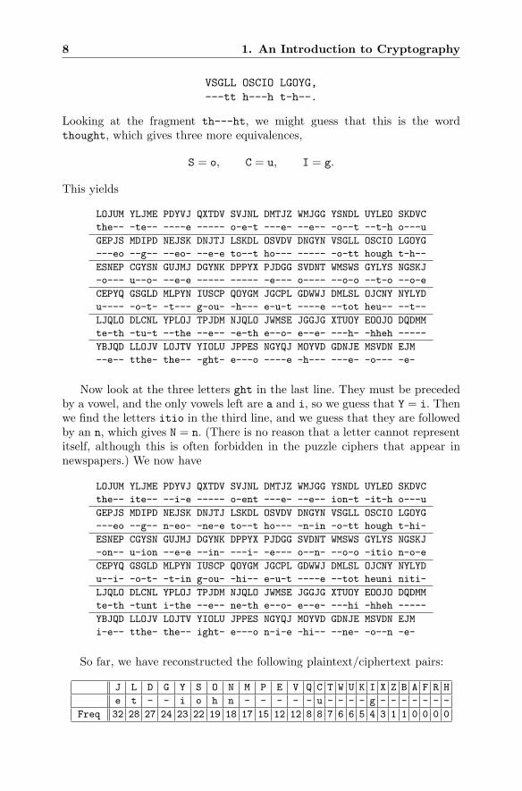
VSGLL OSCIO LGOYG,
---tt h---h t-h--.
Looking at the fragment th---ht, we might guess that this is the wordthought, which gives three more equivalences,
S = o, C = u, I = g.
This yields
LOJUM YLJME PDYVJ QXTDV SVJNL DMTJZ WMJGG YSNDL UYLEO SKDVC
the-- -te-- ----e ----- o-e-t ---e- --e-- -o--t --t-h o---u
GEPJS MDIPD NEJSK DNJTJ LSKDL OSVDV DNGYN VSGLL OSCIO LGOYG
---eo --g-- --eo- --e-e to--t ho--- ----- -o-tt hough t-h--
ESNEP CGYSN GUJMJ DGYNK DPPYX PJDGG SVDNT WMSWS GYLYS NGSKJ
-o--- u--o- --e-e ----- ----- -e--- o---- --o-o --t-o --o-e
CEPYQ GSGLD MLPYN IUSCP QOYGM JGCPL GDWWJ DMLSL OJCNY NYLYD
u---- -o-t- -t--- g-ou- -h--- e-u-t ----e --tot heu-- --t--
LJQLO DLCNL YPLOJ TPJDM NJQLO JWMSE JGGJG XTUOY EOOJO DQDMM
te-th -tu-t --the --e-- -e-th e--o- e--e- ---h- -hheh -----
YBJQD LLOJV LOJTV YIOLU JPPES NGYQJ MOYVD GDNJE MSVDN EJM
--e-- tthe- the-- -ght- e---o ----e -h--- ---e- -o--- -e-
Now look at the three letters ght in the last line. They must be precededby a vowel, and the only vowels left are a and i, so we guess that Y = i. Thenwe find the letters itio in the third line, and we guess that they are followedby an n, which gives N = n. (There is no reason that a letter cannot representitself, although this is often forbidden in the puzzle ciphers that appear innewspapers.) We now have
LOJUM YLJME PDYVJ QXTDV SVJNL DMTJZ WMJGG YSNDL UYLEO SKDVC
the-- ite-- --i-e ----- o-ent ---e- --e-- ion-t -it-h o---u
GEPJS MDIPD NEJSK DNJTJ LSKDL OSVDV DNGYN VSGLL OSCIO LGOYG
---eo --g-- n-eo- -ne-e to--t ho--- -n-in -o-tt hough t-hi-
ESNEP CGYSN GUJMJ DGYNK DPPYX PJDGG SVDNT WMSWS GYLYS NGSKJ
-on-- u-ion --e-e --in- ---i- -e--- o--n- --o-o -itio n-o-e
CEPYQ GSGLD MLPYN IUSCP QOYGM JGCPL GDWWJ DMLSL OJCNY NYLYD
u--i- -o-t- -t-in g-ou- -hi-- e-u-t ----e --tot heuni niti-
LJQLO DLCNL YPLOJ TPJDM NJQLO JWMSE JGGJG XTUOY EOOJO DQDMM
te-th -tunt i-the --e-- ne-th e--o- e--e- ---hi -hheh -----
YBJQD LLOJV LOJTV YIOLU JPPES NGYQJ MOYVD GDNJE MSVDN EJM
i-e-- tthe- the-- ight- e---o n-i-e -hi-- --ne- -o--n -e-
So far, we have reconstructed the following plaintext/ciphertext pairs:
J L D G Y S O N M P E V Q C T W U K I X Z B A F R H
e t - - i o h n - - - - - u - - - - g - - - - - - -
Freq 32 28 27 24 23 22 19 18 17 15 12 12 8 8 7 6 6 5 4 3 1 1 0 0 0 0
1.1. Simple Substitution Ciphers 9
Recall that the most common letters in English (Table 1.3) are, in order ofdecreasing frequency,
e, t, a, o, n, r, i, s, h.
We have already assigned ciphertext values to e, t, o, n, i, h, so we guessthat D and G represent two of the three letters a, r, s. In the third line wenotice that GYLYSN gives -ition, so clearly G must be s. Similarly, on thefifth line we have LJQLO DLCNL equal to te-th -tunt, so D must be a, not r.Substituting these new pairs G = s and D = a gives
LOJUM YLJME PDYVJ QXTDV SVJNL DMTJZ WMJGG YSNDL UYLEO SKDVC
the-- ite-- -ai-e ---a- o-ent a--e- --ess ionat -it-h o-a-u
GEPJS MDIPD NEJSK DNJTJ LSKDL OSVDV DNGYN VSGLL OSCIO LGOYG
s--eo -ag-a n-eo- ane-e to-at ho-a- ansin -ostt hough tshis
ESNEP CGYSN GUJMJ DGYNK DPPYX PJDGG SVDNT WMSWS GYLYS NGSKJ
-on-- usion s-e-e asin- a--i- -eass o-an- --o-o sitio nso-e
CEPYQ GSGLD MLPYN IUSCP QOYGM JGCPL GDWWJ DMLSL OJCNY NYLYD
u--i- sosta -t-in g-ou- -his- esu-t sa--e a-tot heuni nitia
LJQLO DLCNL YPLOJ TPJDM NJQLO JWMSE JGGJG XTUOY EOOJO DQDMM
te-th atunt i-the --ea- ne-th e--o- esses ---hi -hheh a-a--
YBJQD LLOJV LOJTV YIOLU JPPES NGYQJ MOYVD GDNJE MSVDN EJM
i-e-a tthe- the-- ight- e---o nsi-e -hi-a sane- -o-an -e-
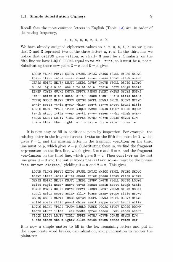
It is now easy to fill in additional pairs by inspection. For example, themissing letter in the fragment atunt i-the on the fifth line must be l, whichgives P = l, and the missing letter in the fragment -osition on the thirdline must be p, which gives W = p. Substituting these in, we find the fragmente-p-ession on the first line, which gives Z = x and M = r, and the fragment-on-lusion on the third line, which gives E = c. Then consi-er on the lastline gives Q = d and the initial words the-riterclai-e- must be the phrase“the writer claimed,” yielding U = w and V = m. This gives
LOJUM YLJME PDYVJ QXTDV SVJNL DMTJZ WMJGG YSNDL UYLEO SKDVC
thewr iterc laime d--am oment ar-ex press ionat witch o-amu
GEPJS MDIPD NEJSK DNJTJ LSKDL OSVDV DNGYN VSGLL OSCIO LGOYG
scleo ragla nceo- ane-e to-at homam ansin mostt hough tshis
ESNEP CGYSN GUJMJ DGYNK DPPYX PJDGG SVDNT WMSWS GYLYS NGSKJ
concl usion swere asin- alli- leass oman- propo sitio nso-e
CEPYQ GSGLD MLPYN IUSCP QOYGM JGCPL GDWWJ DMLSL OJCNY NYLYD
uclid sosta rtlin gwoul dhisr esult sappe artot heuni nitia
LJQLO DLCNL YPLOJ TPJDM NJQLO JWMSE JGGJG XTUOY EOOJO DQDMM
tedth atunt ilthe -lear nedth eproc esses --whi chheh adarr
YBJQD LLOJV LOJTV YIOLU JPPES NGYQJ MOYVD GDNJE MSVDN EJM
i-eda tthem the-m ightw ellco nside rhima sanec roman cer
It is now a simple matter to fill in the few remaining letters and put inthe appropriate word breaks, capitalization, and punctuation to recover theplaintext:
10 1. An Introduction to Cryptography
The writer claimed by a momentary expression, a twitch of a mus-cle or a glance of an eye, to fathom a man’s inmost thoughts. Hisconclusions were as infallible as so many propositions of Euclid.So startling would his results appear to the uninitiated that untilthey learned the processes by which he had arrived at them theymight well consider him as a necromancer.7
1.2 Divisibility and Greatest Common Divisors
Much of modern cryptography is built on the foundations of algebra andnumber theory. So before we explore the subject of cryptography, we need todevelop some important tools. In the next four sections we begin this devel-opment by describing and proving fundamental results in these areas. If youhave already studied number theory in another course, a brief review of thismaterial will suffice. But if this material is new to you, then it is vital to studyit closely and to work out the exercises provided at the end of the chapter.
At the most basic level, Number Theory is the study of the natural numbers
1, 2, 3, 4, 5, 6, . . . ,
or slightly more generally, the study of the integers
. . . ,−5,−4,−3,−2,−1, 0, 1, 2, 3, 4, 5, . . . .
The set of integers is denoted by the symbol Z. Integers can be added, sub-tracted, and multiplied in the usual way, and they satisfy all the usual rulesof arithmetic (commutative law, associative law, distributive law, etc.). Theset of integers with their addition and multiplication rules are an example ofa ring. See Sect. 2.10.1 for more about the theory of rings.
If a and b are integers, then we can add them, a+ b, subtract them, a− b,and multiply them, a · b. In each case, we get an integer as the result. Thisproperty of staying inside of our original set after applying operations to apair of elements is characteristic of a ring.
But if we want to stay within the integers, then we are not always ableto divide one integer by another. For example, we cannot divide 3 by 2, sincethere is no integer that is equal to 3
2 . This leads to the fundamental conceptof divisibility.
Definition. Let a and b be integers with b �= 0. We say that b divides a, orthat a is divisible by b, if there is an integer c such that
a = bc.
We write b | a to indicate that b divides a. If b does not divide a, then wewrite b � a.
7A Study in Scarlet (Chap. 2), Sir Arthur Conan Doyle.
1.2. Divisibility and Greatest Common Divisors 11
Example 1.2. We have 847 | 485331, since 485331 = 847 · 573. On the otherhand, 355 � 259943, since when we try to divide 259943 by 355, we get aremainder of 83. More precisely, 259943 = 355 · 732 + 83, so 259943 is not anexact multiple of 355.
Remark 1.3. Notice that every integer is divisible by 1. The integers that aredivisible by 2 are the even integers, and the integers that are not divisibleby 2 are the odd integers.
There are a number of elementary divisibility properties, some of whichwe list in the following proposition.
Proposition 1.4. Let a, b, c ∈ Z be integers.(a) If a | b and b | c, then a | c.(b) If a | b and b | a, then a = ±b.(c) If a | b and a | c, then a | (b+ c) and a | (b− c).
Proof. We leave the proof as an exercise for the reader; see Exercise 1.6.
Definition. A common divisor of two integers a and b is a positive integer dthat divides both of them. The greatest common divisor of a and b is, asits name suggests, the largest positive integer d such that d | a and d | b.The greatest common divisor of a and b is denoted gcd(a, b). If there is nopossibility of confusion, it is also sometimes denoted by (a, b). (If a and b areboth 0, then gcd(a, b) is not defined.)
It is a curious fact that a concept as simple as the greatest common divisorhas many applications. We’ll soon see that there is a fast and efficient methodto compute the greatest common divisor of any two integers, a fact that haspowerful and far-reaching consequences.
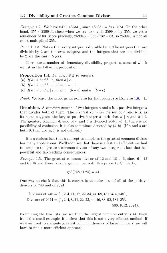
Example 1.5. The greatest common divisor of 12 and 18 is 6, since 6 | 12and 6 | 18 and there is no larger number with this property. Similarly,
gcd(748, 2024) = 44.
One way to check that this is correct is to make lists of all of the positivedivisors of 748 and of 2024.
Divisors of 748 = {1, 2, 4, 11, 17, 22, 34, 44, 68, 187, 374, 748},Divisors of 2024 = {1, 2, 4, 8, 11, 22, 23, 44, 46, 88, 92, 184, 253,
506, 1012, 2024}.
Examining the two lists, we see that the largest common entry is 44. Evenfrom this small example, it is clear that this is not a very efficient method. Ifwe ever need to compute greatest common divisors of large numbers, we willhave to find a more efficient approach.
12 1. An Introduction to Cryptography
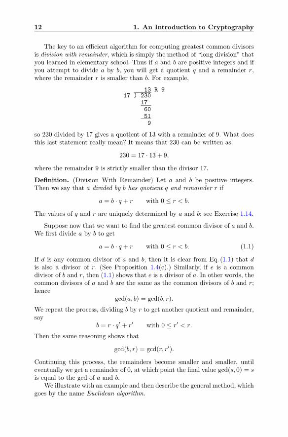
The key to an efficient algorithm for computing greatest common divisorsis division with remainder, which is simply the method of “long division” thatyou learned in elementary school. Thus if a and b are positive integers and ifyou attempt to divide a by b, you will get a quotient q and a remainder r,where the remainder r is smaller than b. For example,
13 R 917 ) 230
1760519
so 230 divided by 17 gives a quotient of 13 with a remainder of 9. What doesthis last statement really mean? It means that 230 can be written as
230 = 17 · 13 + 9,
where the remainder 9 is strictly smaller than the divisor 17.
Definition. (Division With Remainder) Let a and b be positive integers.Then we say that a divided by b has quotient q and remainder r if
a = b · q + r with 0 ≤ r < b.
The values of q and r are uniquely determined by a and b; see Exercise 1.14.
Suppose now that we want to find the greatest common divisor of a and b.We first divide a by b to get
a = b · q + r with 0 ≤ r < b. (1.1)
If d is any common divisor of a and b, then it is clear from Eq. (1.1) that dis also a divisor of r. (See Proposition 1.4(c).) Similarly, if e is a commondivisor of b and r, then (1.1) shows that e is a divisor of a. In other words, thecommon divisors of a and b are the same as the common divisors of b and r;hence
gcd(a, b) = gcd(b, r).
We repeat the process, dividing b by r to get another quotient and remainder,say
b = r · q′ + r′ with 0 ≤ r′ < r.
Then the same reasoning shows that
gcd(b, r) = gcd(r, r′).
Continuing this process, the remainders become smaller and smaller, untileventually we get a remainder of 0, at which point the final value gcd(s, 0) = sis equal to the gcd of a and b.
We illustrate with an example and then describe the general method, whichgoes by the name Euclidean algorithm.
1.2. Divisibility and Greatest Common Divisors 13
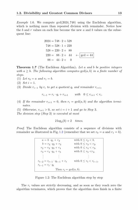
Example 1.6. We compute gcd(2024, 748) using the Euclidean algorithm,which is nothing more than repeated division with remainder. Notice howthe b and r values on each line become the new a and b values on the subse-quent line:
2024 = 748 · 2 + 528
748 = 528 · 1 + 220
528 = 220 · 2 + 88
220 = 88 · 2 + 44 ← gcd = 44
88 = 44 · 2 + 0
Theorem 1.7 (The Euclidean Algorithm). Let a and b be positive integerswith a ≥ b. The following algorithm computes gcd(a, b) in a finite number ofsteps.(1) Let r0 = a and r1 = b.
(2) Set i = 1.
(3) Divide ri−1 by ri to get a quotient qi and remainder ri+1,
ri−1 = ri · qi + ri+1 with 0 ≤ ri+1 < ri.
(4) If the remainder ri+1 = 0, then ri = gcd(a, b) and the algorithm termi-nates.
(5) Otherwise, ri+1 > 0, so set i = i+ 1 and go to Step 3.
The division step (Step 3) is executed at most
2 log2(b) + 2 times.
Proof. The Euclidean algorithm consists of a sequence of divisions withremainder as illustrated in Fig. 1.2 (remember that we set r0 = a and r1 = b).
a = b ·q1 + r2 with 0 ≤ r2 < b,b = r2 ·q2 + r3 with 0 ≤ r3 < r2,
r2 = r3 ·q3 + r4 with 0 ≤ r4 < r3,r3 = r4 ·q4 + r5 with 0 ≤ r5 <r4,
......
...rt−2 = rt−1 · qt−1 + rt with 0 ≤ rt < rt−1,rt−1 = rt · qt
Then rt = gcd(a, b).
Figure 1.2: The Euclidean algorithm step by step
The ri values are strictly decreasing, and as soon as they reach zero thealgorithm terminates, which proves that the algorithm does finish in a finite
14 1. An Introduction to Cryptography
number of steps. Further, at each iteration of Step 3 we have an equation ofthe form
ri−1 = ri · qi + ri+1.
This equation implies that any common divisor of ri−1 and ri is also a divisorof ri+1, and similarly it implies that any common divisor of ri and ri+1 is alsoa divisor of ri−1. Hence
gcd(ri−1, ri) = gcd(ri, ri+1) for all i = 1, 2, 3, . . . . (1.2)
However, as noted earlier, we eventually get to an ri that is zero, say rt+1 = 0.Then rt−1 = rt · qt, so
gcd(rt−1, rt) = gcd(rt · qt, rt) = rt.
But Eq. (1.2) says that this is equal to gcd(r0, r1), i.e., to gcd(a, b), which com-pletes the proof that the last nonzero remainder in the Euclidean algorithmis equal to the greatest common divisor of a and b.
It remains to estimate the efficiency of the algorithm. We noted abovethat since the ri values are strictly decreasing, the algorithm terminates, andindeed since r1 = b, it certainly terminates in at most b steps. However, thisupper bound is far from the truth. We claim that after every two iterationsof Step 3, the value of ri is at least cut in half. In other words:
Claim: ri+2 <12ri for all i = 0, 1, 2, . . . .
We prove the claim by considering two cases.
Case I: ri+1 ≤ 12ri
We know that the ri values are strictly decreasing, so
ri+2 < ri+1 ≤ 12ri.
Case II: ri+1 >12ri
Consider what happens when we divide ri by ri+1. The value of ri+1 isso large that we get
ri = ri+1 · 1 + ri+2 with ri+2 = ri − ri+1 < ri − 12ri =
12ri.
We have now proven our claim that ri+2 <12ri for all i. Using this inequality
repeatedly, we find that
r2k+1 <1
2r2k−1 <
1
4r2k−3 <
1
8r2k−5 <
1
16r2k−7 < · · · <
1
2kr1 =
1
2kb.
Hence if 2k ≥ b, then r2k+1 < 1, which forces r2k+1 to equal 0 and the algo-rithm to terminate. In terms of Fig. 1.2, the value of rt+1 is 0, so we have
1.2. Divisibility and Greatest Common Divisors 15
t+ 1 ≤ 2k + 1, and thus t ≤ 2k. Further, there are exactly t divisions per-formed in Fig. 1.2, so the Euclidean algorithm terminates in at most 2k iter-ations. Choose the smallest such k, so 2k ≥ b > 2k−1. Then
# of iterations ≤ 2k = 2(k − 1) + 2 < 2 log2(b) + 2,
which completes the proof of Theorem 1.7.
Remark 1.8. We proved that the Euclidean algorithm applied to a and b witha ≥ b requires no more than 2 log2(b) + 2 iterations to compute gcd(a, b). Thisestimate can be somewhat improved. It has been proven that the Euclideanalgorithm takes no more than 1.45 log2(b) + 1.68 iterations, and that theaverage number of iterations for randomly chosen a and b is approximately0.85 log2(b) + 0.14; see [66].
Remark 1.9. One way to compute quotients and remainders is by longdivision, as we did on page 12. You can speed up the process using a sim-ple calculator. The first step is to divide a by b on your calculator, which willgive a real number. Throw away the part after the decimal point to get thequotient q. Then the remainder r can be computed as
r = a− b · q.
For example, let a = 2387187 and b = 27573. Then a/b ≈ 86.57697748, soq = 86 and
r = a− b · q = 2387187− 27573 · 86 = 15909.
If you need just the remainder, you can instead take the decimal part (alsosometimes called the fractional part) of a/b and multiply it by b. Continuingwith our example, the decimal part of a/b ≈ 86.57697748 is 0.57697748, andmultiplying by b = 27573 gives
27573 · 0.57697748 = 15909.00005604.
Rounding this off gives r = 15909.
After performing the Euclidean algorithm on two numbers, we can workour way back up the process to obtain an extremely interesting formula. Beforegiving the general result, we illustrate with an example.
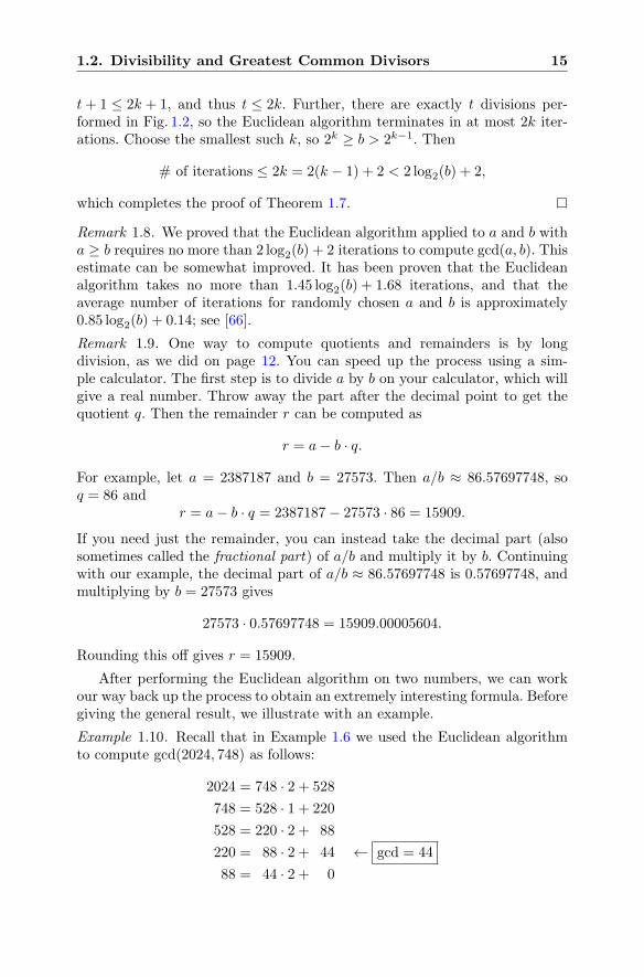
Example 1.10. Recall that in Example 1.6 we used the Euclidean algorithmto compute gcd(2024, 748) as follows:
2024 = 748 · 2 + 528
748 = 528 · 1 + 220
528 = 220 · 2 + 88
220 = 88 · 2 + 44 ← gcd = 44
88 = 44 · 2 + 0
16 1. An Introduction to Cryptography
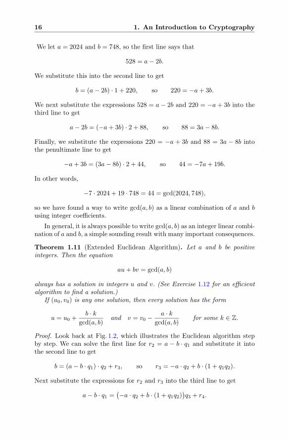
We let a = 2024 and b = 748, so the first line says that
528 = a− 2b.
We substitute this into the second line to get
b = (a− 2b) · 1 + 220, so 220 = −a+ 3b.
We next substitute the expressions 528 = a− 2b and 220 = −a+ 3b into thethird line to get
a− 2b = (−a+ 3b) · 2 + 88, so 88 = 3a− 8b.
Finally, we substitute the expressions 220 = −a + 3b and 88 = 3a − 8b intothe penultimate line to get
−a+ 3b = (3a− 8b) · 2 + 44, so 44 = −7a+ 19b.
In other words,
−7 · 2024 + 19 · 748 = 44 = gcd(2024, 748),
so we have found a way to write gcd(a, b) as a linear combination of a and busing integer coefficients.
In general, it is always possible to write gcd(a, b) as an integer linear combi-nation of a and b, a simple sounding result with many important consequences.
Theorem 1.11 (Extended Euclidean Algorithm). Let a and b be positiveintegers. Then the equation
au+ bv = gcd(a, b)
always has a solution in integers u and v. (See Exercise 1.12 for an efficientalgorithm to find a solution.)
If (u0, v0) is any one solution, then every solution has the form
u = u0 +b · k
gcd(a, b)and v = v0 −
a · kgcd(a, b)
for some k ∈ Z.
Proof. Look back at Fig. 1.2, which illustrates the Euclidean algorithm stepby step. We can solve the first line for r2 = a − b · q1 and substitute it intothe second line to get
b = (a− b · q1) · q2 + r3, so r3 = −a · q2 + b · (1 + q1q2).
Next substitute the expressions for r2 and r3 into the third line to get
a− b · q1 =(−a · q2 + b · (1 + q1q2)
)q3 + r4.
1.2. Divisibility and Greatest Common Divisors 17
After rearranging the terms, this gives
r4 = a · (1 + q2q3)− b · (q1 + q3 + q1q2q3).
The key point is that r4 = a · u + b · v, where u and v are integers. It doesnot matter that the expressions for u and v in terms of q1, q2, q3 are rathermessy. Continuing in this fashion, at each stage we find that ri is the sum ofan integer multiple of a and an integer multiple of b. Eventually, we get tort = a ·u+ b ·v for some integers u and v. But rt = gcd(a, b), which completesthe proof of the first part of the theorem. We leave the second part as anexercise (Exercise 1.11).
An especially important case of the extended Euclidean algorithm ariseswhen the greatest common divisor of a and b is 1. In this case we give a and ba special name.
Definition. Let a and b be integers. We say that a and b are relatively primeif gcd(a, b) = 1.
More generally, any equation
Au+Bv = gcd(A,B)
can be reduced to the case of relatively prime numbers by dividing both sidesby gcd(A,B). Thus
A
gcd(A,B)u+
B
gcd(A,B)v = 1,
where a = A/ gcd(A,B) and b = B/ gcd(A,B) are relatively prime and sat-isfy au+bv = 1. For example, we found earlier that 2024 and 748 have greatestcommon divisor 44 and satisfy
−7 · 2024 + 19 · 748 = 44.
Dividing both sides by 44, we obtain
−7 · 46 + 19 · 17 = 1.
Thus 2024/44 = 46 and 748/44 = 17 are relatively prime, and u = −7 andv = 19 are the coefficients of a linear combination of 46 and 17 that equals 1.
In Example 1.10 we explained how to substitute the values from theEuclidean algorithm in order to solve au + bv = gcd(a, b). Exercise 1.12describes an efficient computer-oriented algorithm for computing u and v.If a and b are relatively prime, we now describe a more conceptual version ofthis substitution procedure. We first illustrate with the example a = 73 andb = 25. The Euclidean algorithm gives
73 = 25 · 2 + 23
18 1. An Introduction to Cryptography
25 = 23 · 1 + 2
23 = 2 · 11 + 1
2 = 1 · 2 + 0.
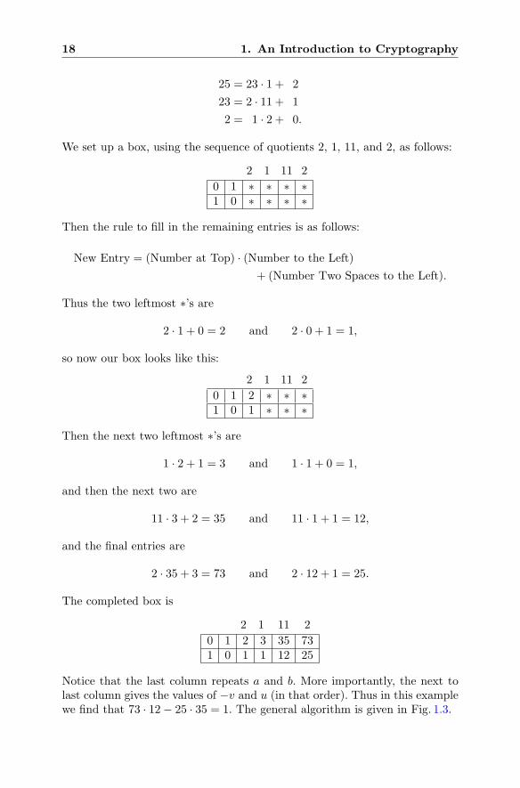
We set up a box, using the sequence of quotients 2, 1, 11, and 2, as follows:
2 1 11 2
0 1 ∗ ∗ ∗ ∗1 0 ∗ ∗ ∗ ∗
Then the rule to fill in the remaining entries is as follows:
New Entry = (Number at Top) · (Number to the Left)
+ (Number Two Spaces to the Left).
Thus the two leftmost ∗’s are
2 · 1 + 0 = 2 and 2 · 0 + 1 = 1,
so now our box looks like this:
2 1 11 2
0 1 2 ∗ ∗ ∗1 0 1 ∗ ∗ ∗
Then the next two leftmost ∗’s are
1 · 2 + 1 = 3 and 1 · 1 + 0 = 1,
and then the next two are
11 · 3 + 2 = 35 and 11 · 1 + 1 = 12,
and the final entries are
2 · 35 + 3 = 73 and 2 · 12 + 1 = 25.
The completed box is
2 1 11 2
0 1 2 3 35 731 0 1 1 12 25
Notice that the last column repeats a and b. More importantly, the next tolast column gives the values of −v and u (in that order). Thus in this examplewe find that 73 · 12− 25 · 35 = 1. The general algorithm is given in Fig. 1.3.
1.3. Modular Arithmetic 19
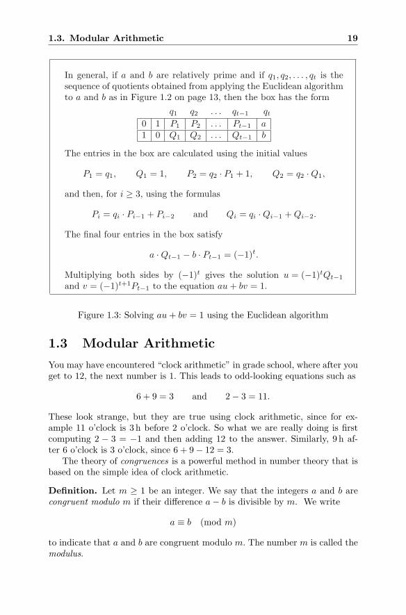
In general, if a and b are relatively prime and if q1, q2, . . . , qt is thesequence of quotients obtained from applying the Euclidean algorithmto a and b as in Figure 1.2 on page 13, then the box has the form
q1 q2 . . . qt−1 qt
0 1 P1 P2 . . . Pt−1 a1 0 Q1 Q2 . . . Qt−1 b
The entries in the box are calculated using the initial values
P1 = q1, Q1 = 1, P2 = q2 · P1 + 1, Q2 = q2 · Q1,
and then, for i ≥ 3, using the formulas
Pi = qi · Pi−1 + Pi−2 and Qi = qi · Qi−1 + Qi−2.
The final four entries in the box satisfy
a · Qt−1 − b · Pt−1 = (−1)t.
Multiplying both sides by (−1)t gives the solution u = (−1)tQt−1and v = (−1)t+1Pt−1 to the equation au + bv = 1.
Figure 1.3: Solving au+ bv = 1 using the Euclidean algorithm
1.3 Modular Arithmetic
You may have encountered “clock arithmetic” in grade school, where after youget to 12, the next number is 1. This leads to odd-looking equations such as
6 + 9 = 3 and 2− 3 = 11.
These look strange, but they are true using clock arithmetic, since for ex-ample 11 o’clock is 3 h before 2 o’clock. So what we are really doing is firstcomputing 2 − 3 = −1 and then adding 12 to the answer. Similarly, 9 h af-ter 6 o’clock is 3 o’clock, since 6 + 9− 12 = 3.
The theory of congruences is a powerful method in number theory that isbased on the simple idea of clock arithmetic.
Definition. Let m ≥ 1 be an integer. We say that the integers a and b arecongruent modulo m if their difference a− b is divisible by m. We write
a ≡ b (mod m)
to indicate that a and b are congruent modulo m. The number m is called themodulus.
20 1. An Introduction to Cryptography
Our clock examples may be written as congruences using the modulusm = 12:
6 + 9 = 15 ≡ 3 (mod 12) and 2− 3 = −1 ≡ 11 (mod 12).
Example 1.12. We have
17 ≡ 7 (mod 5), since 5 divides 10 = 17− 7.
On the other hand,
19 �≡ 6 (mod 11), since 11 does not divide 13 = 19− 6.
Notice that the numbers satisfying
a ≡ 0 (mod m)
are the numbers that are divisible by m, i.e., the multiples of m.
The reason that congruence notation is so useful is that congruences be-have much like equalities, as the following proposition indicates.
Proposition 1.13. Let m ≥ 1 be an integer.(a) If a1 ≡ a2 (mod m) and b1 ≡ b2 (mod m), then
a1 ± b1 ≡ a2 ± b2 (mod m) and a1 · b1 ≡ a2 · b2 (mod m).
(b) Let a be an integer. Then
a · b ≡ 1 (mod m) for some integer b if and only if gcd(a,m) = 1.
Further, if a · b1 ≡ a · b2 ≡ 1 (mod m), then b1 ≡ b2 (mod m). We call bthe (multiplicative) inverse of a modulo m.
Proof. (a) We leave this as an exercise; see Exercise 1.15.(b) Suppose first that gcd(a,m) = 1. Then Theorem 1.11 tells us that we canfind integers u and v satisfying au+mv = 1. This means that au− 1 = −mvis divisible by m, so by definition, au ≡ 1 (mod m). In other words, we cantake b = u.
For the other direction, suppose that a has an inverse modulo m, saya · b ≡ 1 (mod m). This means that ab− 1 = cm for some integer c. It followsthat gcd(a,m) divides ab− cm = 1, so gcd(a,m) = 1. This completes theproof that a has an inverse modulo m if and only if gcd(a,m) = 1. It remainsto show that the inverse is unique modulo m.
So suppose that a · b1 ≡ a · b2 ≡ 1 (mod m). Then
b1 ≡ b1 · 1 ≡ β1 · (a · b2) ≡ (b1 · a) · b2 ≡ 1 · b2 ≡ b2 (mod m),
which completes the proof of Proposition 1.13.
1.3. Modular Arithmetic 21
Proposition 1.13(b) says that if gcd(a,m) = 1, then there exists aninverse b of a modulo m. This has the curious consequence that the fractiona−1 = 1/a has a meaningful interpretation in the world of integers modulo m,namely a−1 modulo m is the unique number b modulo m satisfying the con-gruence ab ≡ 1 (mod m).
Example 1.14. We takem = 5 and a = 2. Clearly gcd(2, 5) = 1, so there existsan inverse to 2 modulo 5. The inverse of 2 modulo 5 is 3, since 2·3 ≡ 1 (mod 5),so 2−1 ≡ 3 (mod 5). Similarly gcd(4, 15) = 1 so 4−1 exists modulo 15. In fact4 · 4 ≡ 1 (mod 15) so 4 is its own inverse modulo 15.
We can even work with fractions a/d modulom as long as the denominatoris relatively prime to m. For example, we can compute 5/7 modulo 11 by firstobserving that 7 · 8 ≡ 1 (mod 11), so 7−1 ≡ 8 (mod 11). Then
5
7= 5 · 7−1 ≡ 5 · 8 ≡ 40 ≡ 7 (mod 11).
Remark 1.15. In the preceding examples it was easy to find inverses mod-ulo m by trial and error. However, when m is large, it is more challengingto compute a−1 modulo m. Note that we showed that inverses exist by us-ing the extended Euclidean algorithm (Theorem 1.11). In order to actuallycompute the u and v that appear in the equation au +mv = gcd(a,m), wecan apply the Euclidean algorithm directly as we did in Example 1.10, orwe can use the somewhat more efficient box method described at the end ofthe preceding section, or we can use the algorithm given in Exercise 1.12.In any case, since the Euclidean algorithm takes at most 2 log2(b) + 2 itera-tions to compute gcd(a, b), it takes only a small multiple of log2(m) steps tocompute a−1 modulo m.
We now continue our development of the theory of modular arithmetic.If a divided by m has quotient q and remainder r, it can be written as
a = m · q + r with 0 ≤ r < m.
This shows that a ≡ r (mod m) for some integer r between 0 and m− 1, soif we want to work with integers modulo m, it is enough to use the integers0 ≤ r < m. This prompts the following definition.
Definition. We write
Z/mZ = {0, 1, 2, . . . ,m− 1}
and call Z/mZ the ring of integers modulo m. We add and multiply elementsof Z/mZ by adding or multiplying them as integers and then dividing theresult by m and taking the remainder in order to obtain an element in Z/mZ.
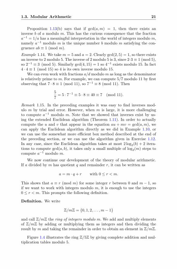
Figure 1.4 illustrates the ring Z/5Z by giving complete addition and mul-tiplication tables modulo 5.
22 1. An Introduction to Cryptography
+ 0 1 2 3 40 0 1 2 3 41 1 2 3 4 02 2 3 4 0 13 3 4 0 1 24 4 0 1 2 3
· 0 1 2 3 40 0 0 0 0 01 0 1 2 3 42 0 2 4 1 33 0 3 1 4 24 0 4 3 2 1
Figure 1.4: Addition and multiplication tables modulo 5
Remark 1.16. If you have studied ring theory, you will recognize that Z/mZ
is the quotient ring of Z by the principal ideal mZ, and that the num-bers 0, 1, . . . ,m− 1 are actually coset representatives for the congruenceclasses that comprise the elements of Z/mZ. For a discussion of congruenceclasses and general quotient rings, see Sect. 2.10.2.
Definition. Proposition 1.13(b) tells us that a has an inverse modulo m ifand only if gcd(a,m) = 1. Numbers that have inverses are called units. Wedenote the set of all units by
(Z/mZ)∗ = {a ∈ Z/mZ : gcd(a,m) = 1}= {a ∈ Z/mZ : a has an inverse modulo m}.
The set (Z/mZ)∗ is called the group of units modulo m.
Notice that if a1 and a2 are units modulo m, then so is a1a2. (Do you seewhy this is true?) So when we multiply two units, we always get a unit. Onthe other hand, if we add two units, we often do not get a unit.
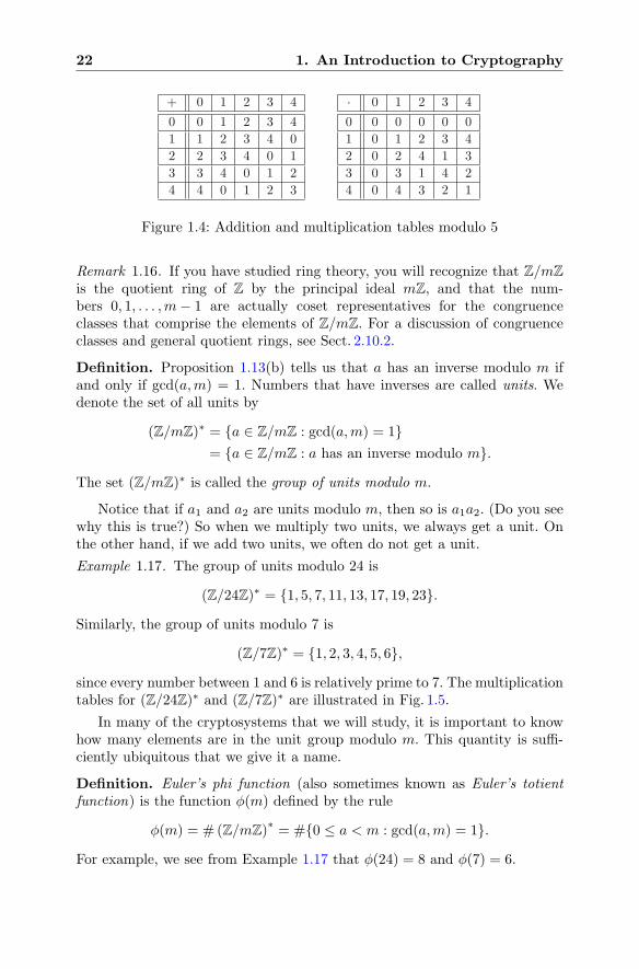
Example 1.17. The group of units modulo 24 is
(Z/24Z)∗ = {1, 5, 7, 11, 13, 17, 19, 23}.
Similarly, the group of units modulo 7 is
(Z/7Z)∗ = {1, 2, 3, 4, 5, 6},
since every number between 1 and 6 is relatively prime to 7. The multiplicationtables for (Z/24Z)∗ and (Z/7Z)∗ are illustrated in Fig. 1.5.
In many of the cryptosystems that we will study, it is important to knowhow many elements are in the unit group modulo m. This quantity is suffi-ciently ubiquitous that we give it a name.
Definition. Euler’s phi function (also sometimes known as Euler’s totientfunction) is the function φ(m) defined by the rule
φ(m) = # (Z/mZ)∗= #{0 ≤ a < m : gcd(a,m) = 1}.
For example, we see from Example 1.17 that φ(24) = 8 and φ(7) = 6.
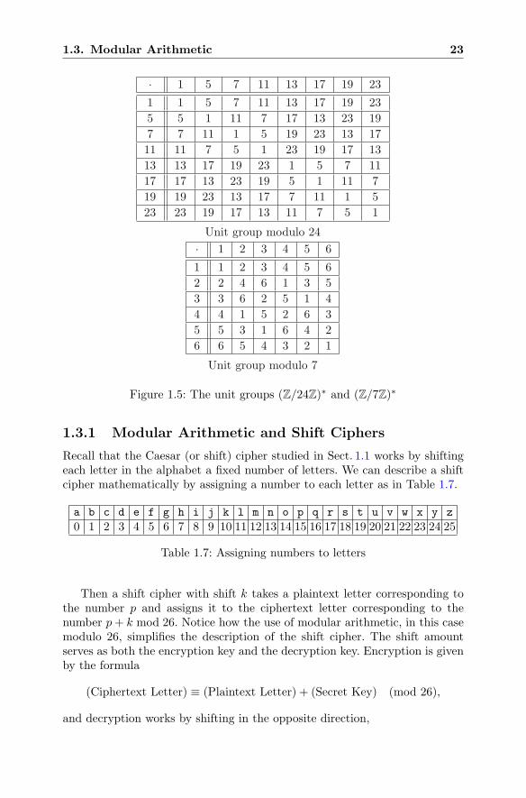
1.3. Modular Arithmetic 23
· 1 5 7 11 13 17 19 23
1 1 5 7 11 13 17 19 235 5 1 11 7 17 13 23 197 7 11 1 5 19 23 13 1711 11 7 5 1 23 19 17 1313 13 17 19 23 1 5 7 1117 17 13 23 19 5 1 11 719 19 23 13 17 7 11 1 523 23 19 17 13 11 7 5 1
Unit group modulo 24· 1 2 3 4 5 6
1 1 2 3 4 5 62 2 4 6 1 3 53 3 6 2 5 1 44 4 1 5 2 6 35 5 3 1 6 4 26 6 5 4 3 2 1
Unit group modulo 7
Figure 1.5: The unit groups (Z/24Z)∗ and (Z/7Z)∗
1.3.1 Modular Arithmetic and Shift Ciphers
Recall that the Caesar (or shift) cipher studied in Sect. 1.1 works by shiftingeach letter in the alphabet a fixed number of letters. We can describe a shiftcipher mathematically by assigning a number to each letter as in Table 1.7.
a b c d e f g h i j k l m n o p q r s t u v w x y z
0 1 2 3 4 5 6 7 8 9 10 11 12 13 14 15 16 17 18 19 20 21 22 23 24 25
Table 1.7: Assigning numbers to letters
Then a shift cipher with shift k takes a plaintext letter corresponding tothe number p and assigns it to the ciphertext letter corresponding to thenumber p+ k mod 26. Notice how the use of modular arithmetic, in this casemodulo 26, simplifies the description of the shift cipher. The shift amountserves as both the encryption key and the decryption key. Encryption is givenby the formula
(Ciphertext Letter) ≡ (Plaintext Letter) + (Secret Key) (mod 26),
and decryption works by shifting in the opposite direction,
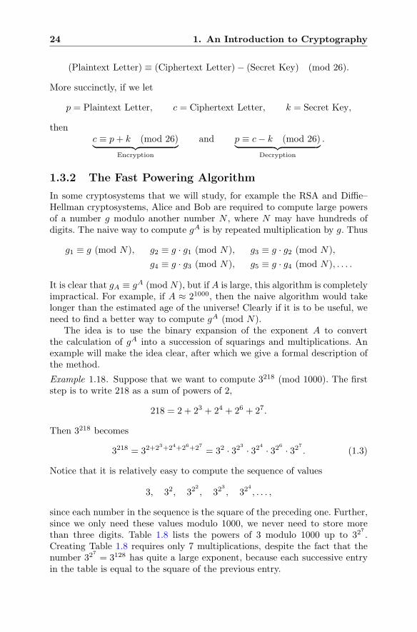
24 1. An Introduction to Cryptography
(Plaintext Letter) ≡ (Ciphertext Letter)− (Secret Key) (mod 26).
More succinctly, if we let
p = Plaintext Letter, c = Ciphertext Letter, k = Secret Key,
thenc ≡ p+ k (mod 26)︸ ︷︷ ︸
Encryption
and p ≡ c− k (mod 26)︸ ︷︷ ︸
Decryption
.
1.3.2 The Fast Powering Algorithm
In some cryptosystems that we will study, for example the RSA and Diffie–Hellman cryptosystems, Alice and Bob are required to compute large powersof a number g modulo another number N , where N may have hundreds ofdigits. The naive way to compute gA is by repeated multiplication by g. Thus
g1 ≡ g (mod N), g2 ≡ g · g1 (mod N), g3 ≡ g · g2 (mod N),
g4 ≡ g · g3 (mod N), g5 ≡ g · g4 (mod N), . . . .
It is clear that gA ≡ gA (mod N), but if A is large, this algorithm is completelyimpractical. For example, if A ≈ 21000, then the naive algorithm would takelonger than the estimated age of the universe! Clearly if it is to be useful, weneed to find a better way to compute gA (mod N).
The idea is to use the binary expansion of the exponent A to convertthe calculation of gA into a succession of squarings and multiplications. Anexample will make the idea clear, after which we give a formal description ofthe method.
Example 1.18. Suppose that we want to compute 3218 (mod 1000). The firststep is to write 218 as a sum of powers of 2,
218 = 2 + 23 + 24 + 26 + 27.
Then 3218 becomes
3218 = 32+23+24+26+27 = 32 · 323 · 324 · 326 · 327 . (1.3)
Notice that it is relatively easy to compute the sequence of values
3, 32, 322
, 323
, 324
, . . . ,
since each number in the sequence is the square of the preceding one. Further,since we only need these values modulo 1000, we never need to store morethan three digits. Table 1.8 lists the powers of 3 modulo 1000 up to 32
7
.Creating Table 1.8 requires only 7 multiplications, despite the fact that thenumber 32
7
= 3128 has quite a large exponent, because each successive entryin the table is equal to the square of the previous entry.
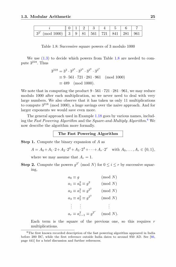
1.3. Modular Arithmetic 25
i 0 1 2 3 4 5 6 7
32i
(mod 1000) 3 9 81 561 721 841 281 961
Table 1.8: Successive square powers of 3 modulo 1000
We use (1.3) to decide which powers from Table 1.8 are needed to com-pute 3218. Thus
3218 = 32 · 323 · 324 · 326 · 327
≡ 9 · 561 · 721 · 281 · 961 (mod 1000)
≡ 489 (mod 1000).
We note that in computing the product 9 · 561 · 721 · 281 · 961, we may reducemodulo 1000 after each multiplication, so we never need to deal with verylarge numbers. We also observe that it has taken us only 11 multiplicationsto compute 3218 (mod 1000), a huge savings over the naive approach. And forlarger exponents we would save even more.
The general approach used in Example 1.18 goes by various names, includ-ing the Fast Powering Algorithm and the Square-and-Multiply Algorithm.8 Wenow describe the algorithm more formally.
The Fast Powering Algorithm
Step 1. Compute the binary expansion of A as
A = A0+A1 ·2+A2 ·22+A3 ·23+ · · ·+Ar ·2r with A0, . . . , Ar ∈ {0, 1},
where we may assume that Ar = 1.
Step 2. Compute the powers g2i
(mod N) for 0 ≤ i ≤ r by successive squar-ing,
a0 ≡ g (mod N)
a1 ≡ a20 ≡ g2 (mod N)
a2 ≡ a21 ≡ g22
(mod N)
a3 ≡ a22 ≡ g23
(mod N)
......
...
ar ≡ a2r−1 ≡ g2r
(mod N).
Each term is the square of the previous one, so this requires rmultiplications.
8The first known recorded description of the fast powering algorithm appeared in Indiabefore 200 BC, while the first reference outside India dates to around 950 AD. See [66,page 441] for a brief discussion and further references.
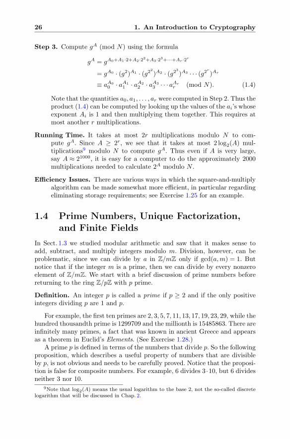
26 1. An Introduction to Cryptography
Step 3. Compute gA (mod N) using the formula
gA = gA0+A1·2+A2·22+A3·23+···+Ar·2r
= gA0 · (g2)A1 · (g22)A2 · (g23)A3 · · · (g2r )Ar
≡ aA00 · aA1
1 · aA22 · aA3
3 · · · aArr (mod N). (1.4)
Note that the quantities a0, a1, . . . , ar were computed in Step 2. Thus theproduct (1.4) can be computed by looking up the values of the ai’s whoseexponent Ai is 1 and then multiplying them together. This requires atmost another r multiplications.
Running Time. It takes at most 2r multiplications modulo N to com-pute gA. Since A ≥ 2r, we see that it takes at most 2 log2(A) mul-tiplications9 modulo N to compute gA. Thus even if A is very large,say A ≈ 21000, it is easy for a computer to do the approximately 2000multiplications needed to calculate 2A modulo N .
Efficiency Issues. There are various ways in which the square-and-multiplyalgorithm can be made somewhat more efficient, in particular regardingeliminating storage requirements; see Exercise 1.25 for an example.
1.4 Prime Numbers, Unique Factorization,and Finite Fields
In Sect. 1.3 we studied modular arithmetic and saw that it makes sense toadd, subtract, and multiply integers modulo m. Division, however, can beproblematic, since we can divide by a in Z/mZ only if gcd(a,m) = 1. Butnotice that if the integer m is a prime, then we can divide by every nonzeroelement of Z/mZ. We start with a brief discussion of prime numbers beforereturning to the ring Z/pZ with p prime.
Definition. An integer p is called a prime if p ≥ 2 and if the only positiveintegers dividing p are 1 and p.
For example, the first ten primes are 2, 3, 5, 7, 11, 13, 17, 19, 23, 29, while thehundred thousandth prime is 1299709 and the millionth is 15485863. There areinfinitely many primes, a fact that was known in ancient Greece and appearsas a theorem in Euclid’s Elements. (See Exercise 1.28.)
A prime p is defined in terms of the numbers that divide p. So the followingproposition, which describes a useful property of numbers that are divisibleby p, is not obvious and needs to be carefully proved. Notice that the proposi-tion is false for composite numbers. For example, 6 divides 3 ·10, but 6 dividesneither 3 nor 10.
9Note that log2(A) means the usual logarithm to the base 2, not the so-called discretelogarithm that will be discussed in Chap. 2.
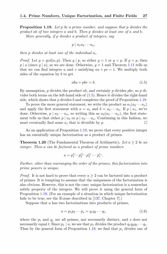
1.4. Prime Numbers, Unique Factorization, and Finite Fields 27
Proposition 1.19. Let p be a prime number, and suppose that p divides theproduct ab of two integers a and b. Then p divides at least one of a and b.
More generally, if p divides a product of integers, say
p | a1a2 · · · an,
then p divides at least one of the individual ai.
Proof. Let g = gcd(a, p). Then g | p, so either g = 1 or g = p. If g = p, thenp | a (since g | a), so we are done. Otherwise, g = 1 and Theorem 1.11 tells usthat we can find integers u and v satisfying au+ pv = 1. We multiply bothsides of the equation by b to get
abu+ pbv = b. (1.5)
By assumption, p divides the product ab, and certainly p divides pbv, so p di-vides both terms on the left-hand side of (1.5). Hence it divides the right-handside, which shows that p divides b and completes the proof of Proposition 1.19.
To prove the more general statement, we write the product as a1(a2 · · · an)and apply the first statement with a = a1 and b = a2 · · · an. If p | a1, we’redone. Otherwise, p | a2 · · · an, so writing this as a2(a3 · · · an), the first state-ment tells us that either p | a2 or p | a3 · · · an. Continuing in this fashion, wemust eventually find some ai that is divisible by p.
As an application of Proposition 1.19, we prove that every positive integerhas an essentially unique factorization as a product of primes.
Theorem 1.20 (The Fundamental Theorem of Arithmetic). Let a ≥ 2 be aninteger. Then a can be factored as a product of prime numbers
a = pe11 · pe22 · pe33 · · · perr .
Further, other than rearranging the order of the primes, this factorization intoprime powers is unique.
Proof. It is not hard to prove that every a ≥ 2 can be factored into a productof primes. It is tempting to assume that the uniqueness of the factorization isalso obvious. However, this is not the case; unique factorization is a somewhatsubtle property of the integers. We will prove it using the general form ofProposition 1.19. (For an example of a situation in which unique factorizationfails to be true, see the E-zone described in [137, Chapter 7].)
Suppose that a has two factorizations into products of primes,
a = p1p2 · · · ps = q1q2 · · · qt, (1.6)
where the pi and qj are all primes, not necessarily distinct, and s does notnecessarily equal t. Since p1 | a, we see that p1 divides the product q1q2q3 · · · qt.Thus by the general form of Proposition 1.19, we find that p1 divides one of
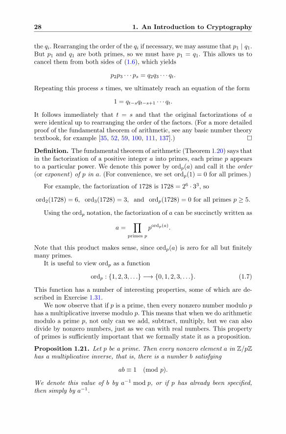
28 1. An Introduction to Cryptography
the qi. Rearranging the order of the qi if necessary, we may assume that p1 | q1.But p1 and q1 are both primes, so we must have p1 = q1. This allows us tocancel them from both sides of (1.6), which yields
p2p3 · · · ps = q2q3 · · · qt.
Repeating this process s times, we ultimately reach an equation of the form
1 = qt−sqt−s+1 · · · qt.
It follows immediately that t = s and that the original factorizations of awere identical up to rearranging the order of the factors. (For a more detailedproof of the fundamental theorem of arithmetic, see any basic number theorytextbook, for example [35, 52, 59, 100, 111, 137].)
Definition. The fundamental theorem of arithmetic (Theorem 1.20) says thatin the factorization of a positive integer a into primes, each prime p appearsto a particular power. We denote this power by ordp(a) and call it the order(or exponent) of p in a. (For convenience, we set ordp(1) = 0 for all primes.)
For example, the factorization of 1728 is 1728 = 26 · 33, so
ord2(1728) = 6, ord3(1728) = 3, and ordp(1728) = 0 for all primes p ≥ 5.
Using the ordp notation, the factorization of a can be succinctly written as
a =∏
primes p
pordp(a).
Note that this product makes sense, since ordp(a) is zero for all but finitelymany primes.
It is useful to view ordp as a function
ordp : {1, 2, 3, . . .} −→ {0, 1, 2, 3, . . .}. (1.7)
This function has a number of interesting properties, some of which are de-scribed in Exercise 1.31.
We now observe that if p is a prime, then every nonzero number modulo phas a multiplicative inverse modulo p. This means that when we do arithmeticmodulo a prime p, not only can we add, subtract, multiply, but we can alsodivide by nonzero numbers, just as we can with real numbers. This propertyof primes is sufficiently important that we formally state it as a proposition.
Proposition 1.21. Let p be a prime. Then every nonzero element a in Z/pZhas a multiplicative inverse, that is, there is a number b satisfying
ab ≡ 1 (mod p).
We denote this value of b by a−1 mod p, or if p has already been specified,then simply by a−1.
1.5. Powers and Primitive Roots in Finite Fields 29
Proof. This proposition is a special case of Proposition 1.13(b) using the primemodulus p, since if a ∈ Z/pZ is not zero, then gcd(a, p) = 1.
Remark 1.22. The extended Euclidean algorithm (Theorem 1.11) gives us anefficient computational method for computing a−1 mod p. We simply solvethe equation
au+ pv = 1 in integers u and v,
and then u = a−1 mod p. For an alternative method of computing a−1 mod p,see Remark 1.26.
Proposition 1.21 can be restated by saying that if p is prime, then
(Z/pZ)∗ = {1, 2, 3, 4, . . . , p− 1}.
In other words, when the 0 element is removed from Z/pZ, the remainingelements are units and closed under multiplication.
Definition. If p is prime, then the set Z/pZ of integers modulo p with itsaddition, subtraction, multiplication, and division rules is an example of afield. If you have studied abstract algebra (or see Sect. 2.10), you know thata field is the general name for a (commutative) ring in which every nonzeroelement has a multiplicative inverse. You are already familiar with some otherfields, for example the field of real numbers R, the field of rational numbers(fractions) Q, and the field of complex numbers C.
The field Z/pZ of integers modulo p has only finitely many elements. Itis a finite field and is often denoted by Fp. Thus Fp and Z/pZ are really justtwo different notations for the same object.10 Similarly, we write F
∗p inter-
changeably for the group of units (Z/pZ)∗. Finite fields are of fundamentalimportance throughout cryptography, and indeed throughout all of mathe-matics.
Remark 1.23. Although Z/pZ and Fp are used to denote the same concept,equality of elements is expressed somewhat differently in the two settings. Fora, b ∈ Fp, the equality of a and b is denoted by a = b, while for a, b ∈ Z/pZ,the equality of a and b is denoted by equivalence modulo p, i.e., a ≡ b (mod p).
1.5 Powers and Primitive Rootsin Finite Fields
The application of finite fields in cryptography often involves raising elementsof Fp to high powers. As a practical matter, we know how to do this effi-ciently using the powering algorithm described in Sect. 1.3.2. In this section
10Finite fields are also sometimes called Galois fields, after Evariste Galois, who studiedthem in the nineteenth century. Yet another notation for Fp is GF(p), in honor of Galois.And yet one more notation for Fp that you may run across is Zp, although in number theorythe notation Zp is more commonly reserved for the ring of p-adic integers.
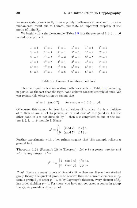
30 1. An Introduction to Cryptography
we investigate powers in Fp from a purely mathematical viewpoint, prove afundamental result due to Fermat, and state an important property of thegroup of units F∗
p.We begin with a simple example. Table 1.9 lists the powers of 1, 2, 3, . . . , 6
modulo the prime 7.
11 ≡ 1 12 ≡ 1 13 ≡ 1 14 ≡ 1 15 ≡ 1 16 ≡ 1
21 ≡ 2 22 ≡ 4 23 ≡ 1 24 ≡ 2 25 ≡ 4 26 ≡ 1
31 ≡ 3 32 ≡ 2 33 ≡ 6 34 ≡ 4 35 ≡ 5 36 ≡ 1
41 ≡ 4 42 ≡ 2 43 ≡ 1 44 ≡ 4 45 ≡ 2 46 ≡ 1
51 ≡ 5 52 ≡ 4 53 ≡ 6 54 ≡ 2 55 ≡ 3 56 ≡ 1
61 ≡ 6 62 ≡ 1 63 ≡ 6 64 ≡ 1 65 ≡ 6 66 ≡ 1
Table 1.9: Powers of numbers modulo 7
There are quite a few interesting patterns visible in Table 1.9, includingin particular the fact that the right-hand column consists entirely of ones. Wecan restate this observation by saying that
a6 ≡ 1 (mod 7) for every a = 1, 2, 3, . . . , 6.
Of course, this cannot be true for all values of a, since if a is a multipleof 7, then so are all of its powers, so in that case an ≡ 0 (mod 7). On theother hand, if a is not divisible by 7, then a is congruent to one of the val-ues 1, 2, 3, . . . , 6 modulo 7. Hence
a6 ≡{1 (mod 7) if 7 � a,
0 (mod 7) if 7 | a.
Further experiments with other primes suggest that this example reflects ageneral fact.
Theorem 1.24 (Fermat’s Little Theorem). Let p be a prime number andlet a be any integer. Then
ap−1 ≡{1 (mod p) if p � a,
0 (mod p) if p | a.
Proof. There are many proofs of Fermat’s little theorem. If you have studiedgroup theory, the quickest proof is to observe that the nonzero elements in Fp
form a group F∗p of order p− 1, so by Lagrange’s theorem, every element of F∗
p
has order dividing p− 1. For those who have not yet taken a course in grouptheory, we provide a direct proof.
1.5. Powers and Primitive Roots in Finite Fields 31
If p | a, then it is clear that every power of a is divisible by p. So we onlyneed to consider the case that p � a. We now look at the list of numbers
a, 2a, 3a, . . . , (p− 1)a reduced modulo p. (1.8)
There are p− 1 numbers in this list, and we claim that they are all different.To see why, take any two of them, say ja mod p and ka mod p, and supposethat they are the same. This means that
ja ≡ ka (mod p), and hence that (j − k)a ≡ 0 (mod p).
Thus p divides the product (j − k)a. Proposition 1.19 tells us that either pdivides j − k or p divides a. However, we have assumed that p does not di-vide a, so we conclude that p divides j − k. But both j and k are between 1and p− 1, so their difference j − k is between −(p− 2) and p− 2. There isonly one number between −(p− 2) and p− 2 that is divisible by p, and thatnumber is zero! This proves that j − k = 0, which means that ja = ka. Wehave thus shown that the p− 1 numbers in the list (1.8) are all different. Theyare also nonzero, since 1, 2, 3, . . . , p− 1 and a are not divisible by p.
To recapitulate, we have shown that the list of numbers (1.8) consists ofp− 1 distinct numbers between 1 and p− 1. But there are only p− 1 distinctnumbers between 1 and p− 1, so the list of numbers (1.8) must simply be thelist of numbers 1, 2, . . . , p− 1 in some mixed up order.
Now consider what happens when we multiply together all of the numbersa, 2a, 3a, . . . , (p−1)a in the list (1.8) and reduce the product modulo p. This isthe same as multiplying together all of the numbers 1, 2, 3, . . . , p− 1 modulo p,so we get a congruence
a · 2a · 3a · · · (p− 1)a ≡ 1 · 2 · 3 · · · (p− 1) (mod p).
There are p − 1 copies of a appearing on the left-hand side. We factor theseout and use factorial notation (p− 1)! = 1 · 2 · · · (p− 1) to obtain
ap−1 · (p− 1)! ≡ (p− 1)! (mod p).
Finally, we are allowed to cancel (p− 1)! from both sides, since it is notdivisible by p. (We are using the fact that Fp is a field, so we are allowed todivide by any nonzero number.) This yields
ap−1 ≡ 1 (mod p),
which completes the proof of Fermat’s “little” theorem.11
11You may wonder why Theorem 1.24 is called a “little” theorem. The reason is todistinguish it from Fermat’s “big” theorem, which is the famous assertion that xn+yn = zn
has no solutions in positive integers x, y, z if n ≥ 3. It is unlikely that Fermat himself couldprove this big theorem, but in 1996, more than three centuries after Fermat’s era, AndrewWiles finally found a proof.
32 1. An Introduction to Cryptography
Example 1.25. The number p = 15485863 is prime, so Fermat’s little theorem(Theorem 1.24) tells us that
215485862 ≡ 1 (mod 15485863).
Thus without doing any computing, we know that the number 215485862 − 1,a number having more than two million digits, is a multiple of 15485863.
Remark 1.26. Fermat’s little theorem (Theorem 1.24) and the fast power-ing algorithm (Sect. 1.3.2) provide us with a reasonably efficient method ofcomputing inverses modulo p, namely
a−1 ≡ ap−2 (mod p).
This congruence is true because if we multiply ap−2 by a, then Fermat’s theo-rem tells us that the product is equal to 1 modulo p. This gives an alternativeto the extended Euclidean algorithm method described in Remark 1.22. Inpractice, the two algorithms tend to take about the same amount of time,although there are variants of the Euclidean algorithm that are somewhatfaster in practice; see for example [66, Chapter 4.5.3, Theorem E].
Example 1.27. We compute the inverse of 7814 modulo 17449 in two ways.First,
7814−1 ≡ 781417447 ≡ 1284 (mod 17449).
Second, we use the extended Euclidean algorithm to solve
7814u+ 17449v = 1.
The solution is (u, v) = (1284,−575), so 7814−1 ≡ 1284 (mod 17449).
Example 1.28. Consider the number m = 15485207. Using the powering al-gorithm, it is not hard to compute (on a computer)
2m−1 = 215485206 ≡ 4136685 (mod 15485207).
We did not get the value 1, so it seems that Fermat’s little theorem is not truefor m. What does that tell us? If m were prime, then Fermat’s little theoremsays that we would have obtained 1. Hence the fact that we did not get 1proves that the number m = 15485207 is not prime.
Think about this for a minute, because it’s actually a bit astonishing. Bya simple computation, we have conclusively proven that m is not prime, yetwe do not know any of its factors!12
Fermat’s little theorem tells us that if a is an integer not divisible by p,then ap−1 ≡ 1 (mod p). However, for any particular value of a, there maywell be smaller powers of a that are congruent to 1. We define the order of amodulo p to be the smallest exponent k ≥ 1 such that13
12The prime factorization of m is m = 15485207 = 3853 · 4019.13We earlier defined the order of p in a to be the exponent of p when a is factored into
primes. Thus unfortunately, the word “order” has two different meanings. You will need tojudge which one is meant from the context.
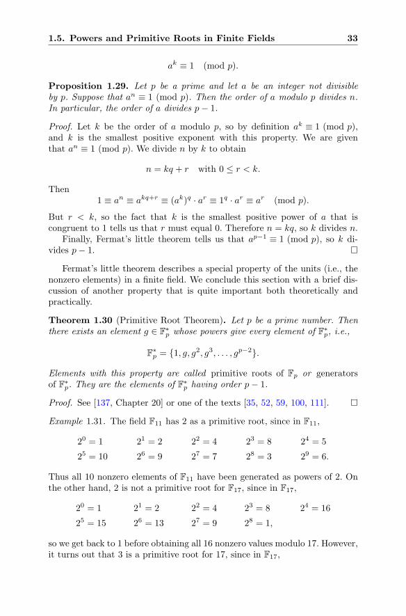
1.5. Powers and Primitive Roots in Finite Fields 33
ak ≡ 1 (mod p).
Proposition 1.29. Let p be a prime and let a be an integer not divisibleby p. Suppose that an ≡ 1 (mod p). Then the order of a modulo p divides n.In particular, the order of a divides p− 1.
Proof. Let k be the order of a modulo p, so by definition ak ≡ 1 (mod p),and k is the smallest positive exponent with this property. We are giventhat an ≡ 1 (mod p). We divide n by k to obtain
n = kq + r with 0 ≤ r < k.
Then1 ≡ an ≡ akq+r ≡ (ak)q · ar ≡ 1q · ar ≡ ar (mod p).
But r < k, so the fact that k is the smallest positive power of a that iscongruent to 1 tells us that r must equal 0. Therefore n = kq, so k divides n.
Finally, Fermat’s little theorem tells us that ap−1 ≡ 1 (mod p), so k di-vides p− 1.
Fermat’s little theorem describes a special property of the units (i.e., thenonzero elements) in a finite field. We conclude this section with a brief dis-cussion of another property that is quite important both theoretically andpractically.
Theorem 1.30 (Primitive Root Theorem). Let p be a prime number. Thenthere exists an element g ∈ F
∗p whose powers give every element of F∗
p, i.e.,
F∗p = {1, g, g2, g3, . . . , gp−2}.
Elements with this property are called primitive roots of Fp or generatorsof F∗
p. They are the elements of F∗p having order p− 1.
Proof. See [137, Chapter 20] or one of the texts [35, 52, 59, 100, 111].
Example 1.31. The field F11 has 2 as a primitive root, since in F11,
20 = 1 21 = 2 22 = 4 23 = 8 24 = 5
25 = 10 26 = 9 27 = 7 28 = 3 29 = 6.
Thus all 10 nonzero elements of F11 have been generated as powers of 2. Onthe other hand, 2 is not a primitive root for F17, since in F17,
20 = 1 21 = 2 22 = 4 23 = 8 24 = 16
25 = 15 26 = 13 27 = 9 28 = 1,
so we get back to 1 before obtaining all 16 nonzero values modulo 17. However,it turns out that 3 is a primitive root for 17, since in F17,
34 1. An Introduction to Cryptography
30 = 1 31 = 3 32 = 9 33 = 10 34 = 13 35 = 5
36 = 15 37 = 11 38 = 16 39 = 14 310 = 8 311 = 7
312 = 4 313 = 12 314 = 2 315 = 6.
Remark 1.32. If p is large, then the finite field Fp has quite a few primitiveroots. The precise formula says that Fp has exactly φ(p− 1) primitive roots,where φ is Euler’s phi function (see page 22). For example, you can check thatthe following is a complete list of the primitive roots for F29:
{2, 3, 8, 10, 11, 14, 15, 18, 19, 21, 26, 27}.
This agrees with the value φ(28) = 12. More generally, if k divides p− 1, thenthere are exactly φ(k) elements of F∗
p having order k.
1.6 Cryptography Before the Computer Age
We pause for a short foray into the history of pre-computer cryptography.Our hope is that these brief notes will whet your appetite for further readingon this fascinating subject, in which political intrigue, daring adventure, andromantic episodes play an equal role with technical achievements.
The origins of cryptography are lost in the mists of time, but presumablysecret writing arose shortly after people started using some form of writtencommunication, since one imagines that the notion of confidential informationmust date back to the dawn of civilization. There are early recorded descrip-tions of ciphers being used in Roman times, including Julius Caesar’s shiftcipher from Sect. 1.1, and certainly from that time onward, many civilizationshave used both substitution ciphers, in which each letter is replaced by an-other letter or symbol, and transposition ciphers, in which the order of theletters is rearranged.
The invention of cryptanalysis, that is, the art of decrypting messageswithout previous knowledge of the key, is more recent. The oldest survivingtexts, which include references to earlier lost volumes, are by Arab scholarsfrom the fourteenth and fifteenth centuries. These books describe not onlysimple substitution and transposition ciphers, but also the first recorded in-stance of a homophonic substitution cipher, which is a cipher in which a singleplaintext letter may be represented by any one of several possible ciphertextletters. More importantly, they contain the first description of serious methodsof cryptanalysis, including the use of letter frequency counts and the likelihoodthat certain pairs of letters will appear adjacent to one another. Unfortunately,most of this knowledge seems to have disappeared by the seventeenth century.
Meanwhile, as Europe emerged from the Middle Ages, political states inItaly and elsewhere required secure communications, and both cryptographyand cryptanalysis began to develop. The earliest known European homo-phonic substitution cipher dates from 1401. The use of such a cipher suggests
1.6. Cryptography Before the Computer Age 35
contemporary knowledge of cryptanalysis via frequency analysis, since theonly reason to use a homophonic system is to make such cryptanalysis moredifficult.
In the fifteenth and sixteenth centuries there arose a variety of what areknown as polyalphabetic ciphers. (We will see an example of a polyalphabeticcipher, called the Vigenere cipher, in Sect. 5.2.) The basic idea is that eachletter of the plaintext is enciphered using a different simple substitution ci-pher. The name “polyalphabetic” refers to the use of many different cipheralphabets, which were used according to some sort of key. If the key is rea-sonably long, then it takes a long time for the any given cipher alphabet tobe used a second time. It wasn’t until the nineteenth century that statisticalmethods were developed to reliably solve such systems, although there areearlier recorded instances of cryptanalysis via special tricks or lucky guessesof part of the message or the key. Jumping forward several centuries, we notethat the machine ciphers that played a large role in World War II were, inessence, extremely complicated polyalphabetic ciphers.
Ciphers and codes14 for both political and military purposes becomeincreasingly widespread during the eighteenth, nineteenth, and early twentiethcenturies, as did cryptanalytic methods, although the level of sophisticationvaried widely from generation to generation and from country to country. Forexample, as the United States prepared to enter World War I in 1917, theU.S. Army was using ciphers, inferior to those invented in Italy in the 1600s,that any trained cryptanalyst of the time would have been able to break in afew hours!
The invention and widespread deployment of long-range communicationmethods, especially the telegraph, opened the need for political, military, andcommercial ciphers, and there are many fascinating stories of intercepted anddecrypted telegraph messages playing a role in historical events. One exam-ple, the infamous Zimmerman telegram, will suffice. With the United Statesmaintaining neutrality in 1917 as Germany battled France and Britain onthe Western Front, the Germans decided that their best hope for victory wasto tighten their blockade of Britain by commencing unrestricted submarinewarfare in the Atlantic. This policy, which meant sinking ships from neutralcountries, was likely to bring the United States into the war, so Germany de-cided to offer an alliance to Mexico. In return for Mexico invading the UnitedStates, and thus distracting it from the ground war in Europe, Germany pro-posed giving Mexico, at the conclusion of the war, much of present-day Texas,New Mexico, and Arizona. The British secret service intercepted this commu-nication, and despite the fact that it was encrypted using one of Germany’s
14In classical terminology, a code is a system in which each word of the plaintext isreplaced with a code word. This requires sender and receiver to share a large dictionary inwhich plaintext words are paired with their ciphertext equivalents. Ciphers operate on theindividual letters of the plaintext, either by substitution, transposition, or some combina-tion. This distinction between the words “code” and “cipher” seems to have been largelyabandoned in today’s literature.
36 1. An Introduction to Cryptography
most secure cryptosystems, they were able to decipher the cable and pass itscontents on to the United States, thereby helping to propel the United Statesinto World War I.
The invention and development of radio communications around 1900caused an even more striking change in the cryptographic landscape, espe-cially in urgent military and political situations. A general could now instan-taneously communicate with all of his troops, but unfortunately the enemycould listen in on all of his broadcasts. The need for secure and efficient ci-phers became paramount and led to the invention of machine ciphers, such asGermany’s Enigma machine. This was a device containing a number of rotors,each of which had many wires running through its center. Before a letter wasencrypted, the rotors would spin in a predetermined way, thereby altering thepaths of the wires and the resultant output. This created an immensely com-plicated polyalphabetic cipher in which the number of cipher alphabets wasenormous. Further, the rotors could be removed and replaced in a vast numberof different starting configurations, so breaking the system involved knowingboth the circuits through the rotors and figuring out that day’s initial rotorconfiguration.
Despite these difficulties, during World War II the British managed todecipher a large number of messages encrypted on Enigma machines. Theywere aided in this endeavor by Polish cryptographers who, just before hos-tilities commenced, shared with Britain and France the methods that theyhad developed for attacking Enigma. But determining daily rotor configura-tions and analyzing rotor replacements was still an immensely difficult task,especially after Germany introduced an improved Enigma machine having anextra rotor. The existence of Britain’s ULTRA project to decrypt Enigma re-mained secret until 1974, but there are now several popular accounts. Militaryintelligence derived from ULTRA was of vital importance in the Allied wareffort.
Another WWII cryptanalytic success was obtained by United States cryp-tographers against a Japanese cipher machine that they code-named Purple.This machine used switches, rather than rotors, but again the effect was tocreate an incredibly complicated polyalphabetic cipher. A team of cryptogra-phers, led by William Friedman, managed to reconstruct the design of the Pur-ple machine purely by analyzing intercepted encrypted messages. They thenbuilt their own machine and proceeded to decrypt many important diplomaticmessages.
In this section we have barely touched the surface of the history of cryptog-raphy from antiquity through the middle of the twentieth century. Good start-ing points for further reading include Simon Singh’s light introduction [139]and David Kahn’s massive and comprehensive, but fascinating and quite read-able, book The Codebreakers [63].
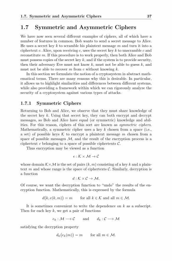
1.7. Symmetric and Asymmetric Ciphers 37
1.7 Symmetric and Asymmetric Ciphers
We have now seen several different examples of ciphers, all of which have anumber of features in common. Bob wants to send a secret message to Alice.He uses a secret key k to scramble his plaintext message m and turn it into aciphertext c. Alice, upon receiving c, uses the secret key k to unscramble c andreconstitute m. If this procedure is to work properly, then both Alice and Bobmust possess copies of the secret key k, and if the system is to provide security,then their adversary Eve must not know k, must not be able to guess k, andmust not be able to recover m from c without knowing k.
In this section we formulate the notion of a cryptosystem in abstract math-ematical terms. There are many reasons why this is desirable. In particular,it allows us to highlight similarities and differences between different systems,while also providing a framework within which we can rigorously analyze thesecurity of a cryptosystem against various types of attacks.
1.7.1 Symmetric Ciphers
Returning to Bob and Alice, we observe that they must share knowledge ofthe secret key k. Using that secret key, they can both encrypt and decryptmessages, so Bob and Alice have equal (or symmetric) knowledge and abil-ities. For this reason, ciphers of this sort are known as symmetric ciphers.Mathematically, a symmetric cipher uses a key k chosen from a space (i.e.,a set) of possible keys K to encrypt a plaintext message m chosen from aspace of possible messages M, and the result of the encryption process is aciphertext c belonging to a space of possible ciphertexts C.
Thus encryption may be viewed as a function
e : K ×M→ C
whose domain K×M is the set of pairs (k,m) consisting of a key k and a plain-text m and whose range is the space of ciphertexts C. Similarly, decryption isa function
d : K × C →M.
Of course, we want the decryption function to “undo” the results of the en-cryption function. Mathematically, this is expressed by the formula
d(k, e(k,m)
)= m for all k ∈ K and all m ∈M.
It is sometimes convenient to write the dependence on k as a subscript.Then for each key k, we get a pair of functions
ek :M−→ C and dk : C −→M
satisfying the decryption property
dk(ek(m)
)= m for all m ∈M.
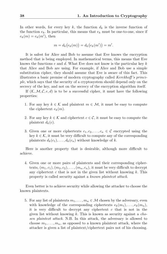
38 1. An Introduction to Cryptography
In other words, for every key k, the function dk is the inverse function ofthe function ek. In particular, this means that ek must be one-to-one, since ifek(m) = ek(m
′), then
m = dk(ek(m)
)= dk
(ek(m
′))= m′.
It is safest for Alice and Bob to assume that Eve knows the encryptionmethod that is being employed. In mathematical terms, this means that Eveknows the functions e and d. What Eve does not know is the particular key kthat Alice and Bob are using. For example, if Alice and Bob use a simplesubstitution cipher, they should assume that Eve is aware of this fact. Thisillustrates a basic premise of modern cryptography called Kerckhoff’s princi-ple, which says that the security of a cryptosystem should depend only on thesecrecy of the key, and not on the secrecy of the encryption algorithm itself.
If (K,M, C, e, d) is to be a successful cipher, it must have the followingproperties:
1. For any key k ∈ K and plaintext m ∈ M, it must be easy to computethe ciphertext ek(m).
2. For any key k ∈ K and ciphertext c ∈ C, it must be easy to compute theplaintext dk(c).
3. Given one or more ciphertexts c1, c2, . . . , cn ∈ C encrypted using thekey k ∈ K, it must be very difficult to compute any of the correspondingplaintexts dk(c1), . . . , dk(cn) without knowledge of k.
Here is another property that is desirable, although more difficult toachieve.
4. Given one or more pairs of plaintexts and their corresponding cipher-texts, (m1, c1), (m2, c2), . . . , (mn, cn), it must be very difficult to decryptany ciphertext c that is not in the given list without knowing k. Thisproperty is called security against a known plaintext attack.
Even better is to achieve security while allowing the attacker to choose theknown plaintexts.
5. For any list of plaintextsm1, . . . ,mn ∈M chosen by the adversary, evenwith knowledge of the corresponding ciphertexts ek(m1), . . . , ek(mn),it is very difficult to decrypt any ciphertext c that is not in thegiven list without knowing k. This is known as security against a cho-sen plaintext attack. N.B. In this attack, the adversary is allowed tochoose m1, . . . ,mn, as opposed to a known plaintext attack, where theattacker is given a list of plaintext/ciphertext pairs not of his choosing.
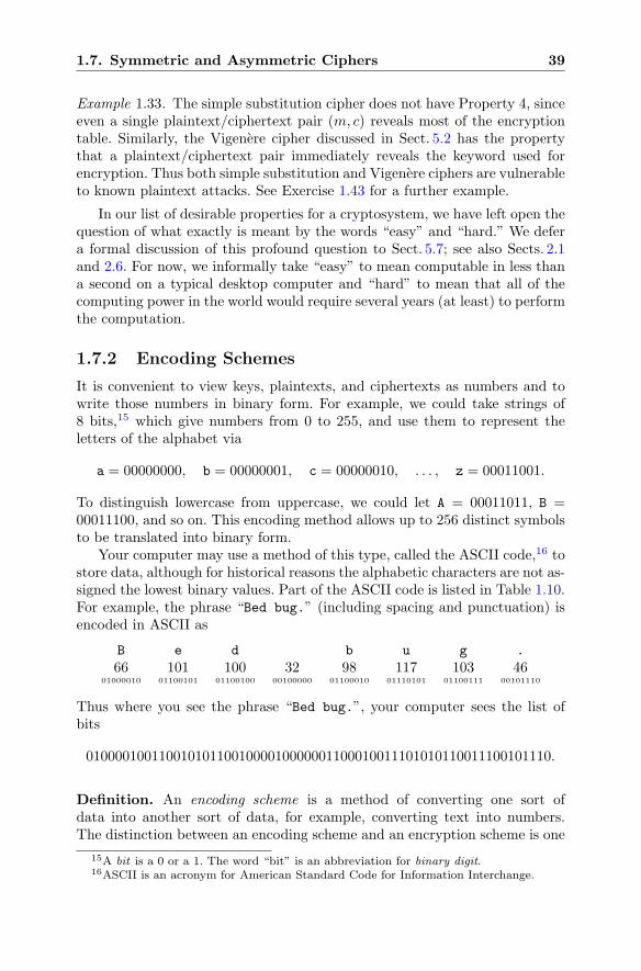
1.7. Symmetric and Asymmetric Ciphers 39
Example 1.33. The simple substitution cipher does not have Property 4, sinceeven a single plaintext/ciphertext pair (m, c) reveals most of the encryptiontable. Similarly, the Vigenere cipher discussed in Sect. 5.2 has the propertythat a plaintext/ciphertext pair immediately reveals the keyword used forencryption. Thus both simple substitution and Vigenere ciphers are vulnerableto known plaintext attacks. See Exercise 1.43 for a further example.
In our list of desirable properties for a cryptosystem, we have left open thequestion of what exactly is meant by the words “easy” and “hard.” We defera formal discussion of this profound question to Sect. 5.7; see also Sects. 2.1and 2.6. For now, we informally take “easy” to mean computable in less thana second on a typical desktop computer and “hard” to mean that all of thecomputing power in the world would require several years (at least) to performthe computation.
1.7.2 Encoding Schemes
It is convenient to view keys, plaintexts, and ciphertexts as numbers and towrite those numbers in binary form. For example, we could take strings of8 bits,15 which give numbers from 0 to 255, and use them to represent theletters of the alphabet via
a = 00000000, b = 00000001, c = 00000010, . . . , z = 00011001.
To distinguish lowercase from uppercase, we could let A = 00011011, B =00011100, and so on. This encoding method allows up to 256 distinct symbolsto be translated into binary form.
Your computer may use a method of this type, called the ASCII code,16 tostore data, although for historical reasons the alphabetic characters are not as-signed the lowest binary values. Part of the ASCII code is listed in Table 1.10.For example, the phrase “Bed bug.” (including spacing and punctuation) isencoded in ASCII as
B e d b u g .
66 101 100 32 98 117 103 4601000010 01100101 01100100 00100000 01100010 01110101 01100111 00101110
Thus where you see the phrase “Bed bug.”, your computer sees the list ofbits
0100001001100101011001000010000001100010011101010110011100101110.
Definition. An encoding scheme is a method of converting one sort ofdata into another sort of data, for example, converting text into numbers.The distinction between an encoding scheme and an encryption scheme is one
15A bit is a 0 or a 1. The word “bit” is an abbreviation for binary digit.16ASCII is an acronym for American Standard Code for Information Interchange.
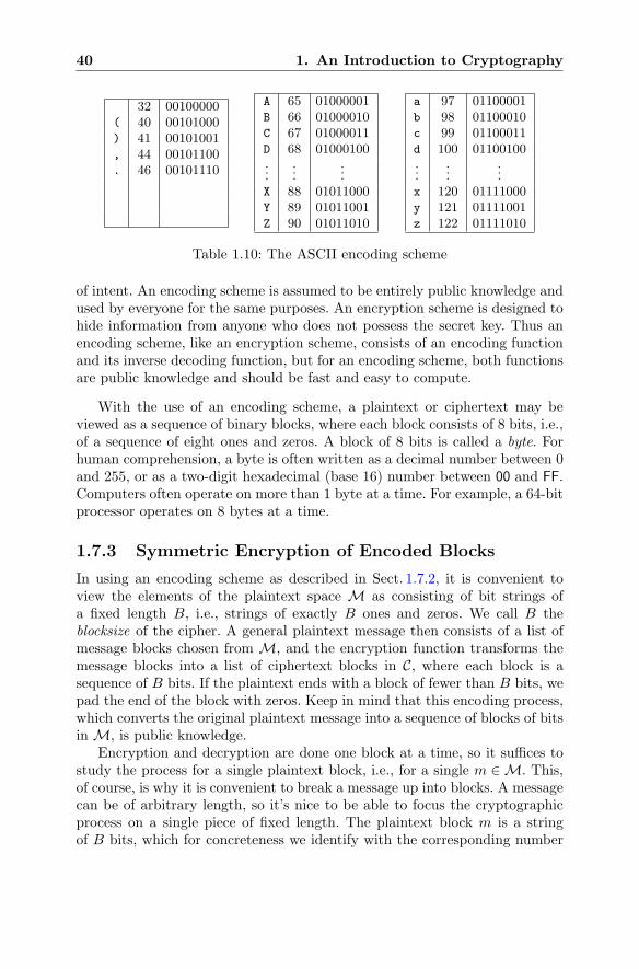
40 1. An Introduction to Cryptography
32 00100000( 40 00101000) 41 00101001, 44 00101100. 46 00101110
A 65 01000001B 66 01000010C 67 01000011D 68 01000100...
......
X 88 01011000Y 89 01011001Z 90 01011010
a 97 01100001b 98 01100010c 99 01100011d 100 01100100...
......
x 120 01111000y 121 01111001z 122 01111010
Table 1.10: The ASCII encoding scheme
of intent. An encoding scheme is assumed to be entirely public knowledge andused by everyone for the same purposes. An encryption scheme is designed tohide information from anyone who does not possess the secret key. Thus anencoding scheme, like an encryption scheme, consists of an encoding functionand its inverse decoding function, but for an encoding scheme, both functionsare public knowledge and should be fast and easy to compute.
With the use of an encoding scheme, a plaintext or ciphertext may beviewed as a sequence of binary blocks, where each block consists of 8 bits, i.e.,of a sequence of eight ones and zeros. A block of 8 bits is called a byte. Forhuman comprehension, a byte is often written as a decimal number between 0and 255, or as a two-digit hexadecimal (base 16) number between 00 and FF.Computers often operate on more than 1 byte at a time. For example, a 64-bitprocessor operates on 8 bytes at a time.
1.7.3 Symmetric Encryption of Encoded Blocks
In using an encoding scheme as described in Sect. 1.7.2, it is convenient toview the elements of the plaintext space M as consisting of bit strings ofa fixed length B, i.e., strings of exactly B ones and zeros. We call B theblocksize of the cipher. A general plaintext message then consists of a list ofmessage blocks chosen from M, and the encryption function transforms themessage blocks into a list of ciphertext blocks in C, where each block is asequence of B bits. If the plaintext ends with a block of fewer than B bits, wepad the end of the block with zeros. Keep in mind that this encoding process,which converts the original plaintext message into a sequence of blocks of bitsin M, is public knowledge.
Encryption and decryption are done one block at a time, so it suffices tostudy the process for a single plaintext block, i.e., for a single m ∈M. This,of course, is why it is convenient to break a message up into blocks. A messagecan be of arbitrary length, so it’s nice to be able to focus the cryptographicprocess on a single piece of fixed length. The plaintext block m is a stringof B bits, which for concreteness we identify with the corresponding number
1.7. Symmetric and Asymmetric Ciphers 41
in binary form. In other words, we identify M with the set of integers msatisfying 0 ≤ m < 2B via
list of B bits of m︷ ︸︸ ︷mB−1mB−2 · · ·m2m1m0 ←→
integer between 0 and 2B − 1︷ ︸︸ ︷mB−1 · 2B−1 + · · ·+m2 · 22 +m1 · 2 +m0 .
Here m0,m1, . . . ,mB−1 are each 0 or 1.Similarly, we identify the key space K and the ciphertext space C with sets
of integers corresponding to bit strings of a certain blocksize. For notationalconvenience, we denote the blocksizes for keys, plaintexts, and ciphertextsby Bk, Bm, and Bc. They need not be the same. Thus we have identified K,M,and C with sets of positive integers
K = {k ∈ Z : 0 ≤ k < 2Bk},M = {m ∈ Z : 0 ≤ m < 2Bm},C = {c ∈ Z : 0 ≤ c < 2Bc}.
An important question immediately arises: how large should Alice and Bobmake the set K, or equivalently, how large should they choose the key block-size Bk? If Bk is too small, then Eve can check every number from 0 to 2Bk − 1until she finds Alice and Bob’s key. More precisely, since Eve is assumed toknow the decryption algorithm d (Kerckhoff’s principle), she takes each k ∈ Kand uses it to compute dk(c). Assuming that Eve is able to distinguish betweenvalid and invalid plaintexts, eventually she will recover the message.
This attack is known as an exhaustive search attack (also sometimes re-ferred to as a brute-force attack), since Eve exhaustively searches through thekey space. With current technology, an exhaustive search is considered to beinfeasible if the space has at least 280 elements. Thus Bob and Alice shoulddefinitely choose Bk ≥ 80.
For many cryptosystems, especially the public key cryptosystems that formthe core of this book, there are refinements on the exhaustive search attackthat effectively replace the size of the space with its square root. These meth-ods are based on the principle that it is easier to find matching objects (col-lisions) in a set than it is to find a particular object in the set. We describesome of these meet-in-the-middle or collision attacks in Sects. 2.7, 5.4, 5.5, 7.2,and 7.10. If meet-in-the-middle attacks are available, then Alice and Bobshould choose Bk ≥ 160.
1.7.4 Examples of Symmetric Ciphers
Before descending further into a morass of theory and notation, we pause togive a mathematical description of some elementary symmetric ciphers.
42 1. An Introduction to Cryptography
Let p be a large prime,17 say 2159 < p < 2160. Alice and Bob take theirkey space K, plaintext space M, and ciphertext space C to be the same set,
K =M = C = {1, 2, 3, . . . , p− 1}.
In fancier terminology, K = M = C = F∗p are all taken to be equal to the
group of units in the finite field Fp.Alice and Bob randomly select a key k ∈ K, i.e., they select an integer k
satisfying 1 ≤ k < p, and they decide to use the encryption function ek de-fined by
ek(m) ≡ k ·m (mod p). (1.9)
Here we mean that ek(m) is set equal to the unique positive integer between 1and p that is congruent to k ·m modulo p. The corresponding decryptionfunction dk is
dk(c) ≡ k′ · c (mod p),
where k′ is the inverse of k modulo p. It is important to note that although pis very large, the extended Euclidean algorithm (Remark 1.15) allows us tocalculate k′ in fewer than 2 log2 p+ 2 steps. Thus finding k′ from k counts as“easy” in the world of cryptography.
It is clear that Eve has a hard time guessing k, since there are approxi-mately 2160 possibilities from which to choose. Is it also difficult for Eve torecover k if she knows the ciphertext c? The answer is yes, it is still difficult.Notice that the encryption function
ek :M−→ C
is surjective (onto) for any choice of key k. This means that for every c ∈ Cand any k ∈ K there exists an m ∈ M such that ek(m) = c. Further, anygiven ciphertext may represent any plaintext, provided that the plaintext isencrypted by an appropriate key. Mathematically, this may be rephrased bysaying that given any ciphertext c ∈ C and any plaintext m ∈M, there existsa key k such that ek(m) = c. Specifically this is true for the key
k ≡ m−1 · c (mod p). (1.10)
This shows that Alice and Bob’s cipher has Properties 1–3 as listed on page 38,since anyone who knows the key k can easily encrypt and decrypt, but it ishard to decrypt if you do not know the value of k. However, this cipher doesnot have Property 4, since even a single plaintext/ciphertext pair (m, c) allowsEve to recover the private key k using the formula (1.10).
17There are in fact many primes in the interval 2159 < p < 2160. The prime numbertheorem implies that almost 1% of the numbers in this interval are prime. Of course, thereis also the question of identifying a number as prime or composite. There are efficient teststhat do this, even for very large numbers. See Sect. 3.4.
1.7. Symmetric and Asymmetric Ciphers 43
It is also interesting to observe that if Alice and Bob define their encryptionfunction to be simply multiplication of integers ek(m) = k ·m with no reduc-tion modulo p, then their cipher still has Properties 1 and 2, but Property 3fails. If Eve tries to decrypt a single ciphertext c = k ·m, she still faces the(moderately) difficult task of factoring a large number. However, if she man-ages to acquire several ciphertexts c1, c2, . . . , cn, then there is a good chancethat
gcd(c1, c2, . . . , cn) = gcd(k ·m1, k ·m2, . . . , k ·mn)
= k · gcd(m1,m2, . . . ,mn)
equals k itself or a small multiple of k. Note that it is an easy task to computethe greatest common divisor.
This observation provides our first indication of how reduction modulo phas a wonderful “mixing” effect that destroys properties such as divisibility.However, reduction is not by itself the ultimate solution. Consider the vulner-ability of the cipher (1.9) to a known plaintext attack. As noted above, if Evecan get her hands on both a ciphertext c and its corresponding plaintext m,then she easily recovers the key by computing
k ≡ m−1 · c (mod p).
Thus even a single plaintext/ciphertext pair suffices to reveal the key, so theencryption function ek given by (1.9) does not have Property 4 on page 38.
There are many variants of this “multiplication-modulo-p” cipher. Forexample, since addition is more efficient than multiplication, there is an“addition-modulo-p” cipher given by
ek(m) ≡ m+ k (mod p) and dk(c) ≡ c− k (mod p),
which is nothing other than the shift or Caesar cipher that we studied inSect. 1.1. Another variant, called an affine cipher, is a combination of the shiftcipher and the multiplication cipher. The key for an affine cipher consists oftwo integers k = (k1, k2) and encryption and decryption are defined by
ek(m) ≡ k1 ·m+ k2 (mod p),
dk(c) ≡ k′1 · (c− k2) (mod p),(1.11)
where k′1 is the inverse of k1 modulo p.The affine cipher has a further generalization called the Hill cipher, in
which the plaintext m, the ciphertext c, and the second part of the key k2 arereplaced by column vectors consisting of n numbers modulo p. The first part ofthe key k1 is taken to be an n-by-n matrix with mod p integer entries. Encryp-tion and decryption are again given by (1.11), but now multiplication k1 ·mis the product of a matrix and a vector, and k′1 is the inverse matrix of k1modulo p. Both the affine cipher and the Hill cipher are vulnerable to knownplaintext attacks; see Exercises 1.43. and 1.44.
44 1. An Introduction to Cryptography
Example 1.34. As noted earlier, addition is generally faster than multiplica-tion, but there is another basic computer operation that is even faster thanaddition. It is called exclusive or and is denoted by XOR or ⊕. At the lowestlevel, XOR takes two individual bits β ∈ {0, 1} and β′ ∈ {0, 1} and yields
β ⊕ β′ =
{0 if β and β′ are the same,
1 if β and β′ are different.(1.12)
If you think of a bit as a number that is 0 or 1, then XOR is the same asaddition modulo 2. More generally, the XOR of 2 bit strings is the result ofperforming XOR on each corresponding pair of bits. For example,
10110⊕ 11010 = [1⊕ 1] [0⊕ 1] [1⊕ 0] [1⊕ 1] [0⊕ 0] = 01100.
Using this new operation, Alice and Bob have at their disposal yet anotherbasic cipher defined by
ek(m) = k ⊕m and dk(c) = k ⊕ c.
Here K,M, and C are the sets of all binary strings of length B, or equivalently,the set of all numbers between 0 and 2B − 1.
This cipher has the advantage of being highly efficient and completelysymmetric in the sense that ek and dk are the same function. If k is chosenrandomly and is used only once, then this cipher is known as Vernam’s one-time pad. In Sect. 5.57 we show that the one-time pad is provably secure.Unfortunately, it requires a key that is as long as the plaintext, which makesit too cumbersome for most practical applications. And if k is used to encryptmore than one plaintext, then Eve may be able to exploit the fact that
c⊕ c′ = (k ⊕m)⊕ (k ⊕m′) = m⊕m′
to extract information aboutm orm′. It’s not obvious how Eve would proceedto find k, m, or m′, but simply the fact that the key k can be removed soeasily, revealing the potentially less random quantity m⊕m′, should make acryptographer nervous. Further, this method is vulnerable in some situationsto a known plaintext attack; see Exercise 1.48.
1.7.5 Random Bit Sequences and Symmetric Ciphers
We have arrived, at long last, at the fundamental question regarding thecreation of secure and efficient symmetric ciphers. Is it possible to use a singlerelatively short key k (say consisting of 160 random bits) to securely andefficiently send arbitrarily long messages? Here is one possible construction.Suppose that we could construct a function
R : K × Z −→ {0, 1}
1.7. Symmetric and Asymmetric Ciphers 45
with the following properties:
1. For all k ∈ K and all j ∈ Z, it is easy to compute R(k, j).
2. Given an arbitrarily long sequence of integers j1, j2, . . . , jn and given allof the values R(k, j1), R(k, j2), . . . , R(k, jn), it is hard to determine k.
3. Given any list of integers j1, j2, . . . , jn and given all of the values
R(k, j1), R(k, j2), . . . , R(k, jn),
it is hard to guess the value of R(k, j) with better than a 50% chanceof success for any value of j not already in the list.
If we could find a function R with these three properties, then we coulduse it to turn an initial key k into a sequence of bits
R(k, 1), R(k, 2), R(k, 3), R(k, 4), . . . , (1.13)
and then we could use this sequence of bits as the key for a one-time pad asdescribed in Example 1.34.
The fundamental problem with this approach is that the sequence ofbits (1.13) is not truly random, since it is generated by the function R. In-stead, we say that the sequence of bits (1.13) is a pseudorandom sequence andwe call R a pseudorandom number generator.
Do pseudorandom number generators exist? If so, they would provide ex-amples of the one-way functions defined by Diffie and Hellman in their ground-breaking paper [38], but despite more than a quarter century of work, no onehas yet proven the existence of even a single such function. We return to thisfascinating subject in Sects. 2.1 and 8.2. For now, we content ourselves witha few brief remarks.
Although no one has yet conclusively proven that pseudorandom numbergenerators exist, many candidates have been suggested, and some of theseproposals have withstood the test of time. There are two basic approachesto constructing candidates for R, and these two methods provide a good il-lustration of the fundamental conflict in cryptography between security andefficiency.
The first approach is to repeatedly apply an ad hoc collection of mixingoperations that are well suited to efficient computation and that appear tobe very hard to untangle. This method is, disconcertingly, the basis for mostpractical symmetric ciphers, including the Data Encryption Standard (DES)and the Advanced Encryption Standard (AES), which are the two systemsmost widely used today. See Sect. 8.12 for a brief description of these modernsymmetric ciphers.
The second approach is to construct R using a function whose efficientinversion is a well-known mathematical problem that is believed to be difficult.This approach provides a far more satisfactory theoretical underpinning for asymmetric cipher, but unfortunately, all known constructions of this sort arefar less efficient than the ad hoc constructions, and hence are less attractivefor real-world applications.
46 1. An Introduction to Cryptography
1.7.6 Asymmetric Ciphers Make a First Appearance
If Alice and Bob want to exchange messages using a symmetric cipher, theymust first mutually agree on a secret key k. This is fine if they have the oppor-tunity to meet in secret or if they are able to communicate once over a securechannel. But what if they do not have this opportunity and if every commu-nication between them is monitored by their adversary Eve? Is it possible forAlice and Bob to exchange a secret key under these conditions?
Most people’s first reaction is that it is not possible, since Eve sees everypiece of information that Alice and Bob exchange. It was the brilliant insightof Diffie and Hellman18 that under certain hypotheses, it is possible. Thesearch for efficient (and provable) solutions to this problem, which is calledpublic key (or asymmetric) cryptography, forms one of the most interestingparts of mathematical cryptography and is the principal focus of this book.
We start by describing a nonmathematical way to visualize public keycryptography. Alice buys a safe with a narrow slot in the top and puts hersafe in a public location. Everyone in the world is allowed to examine the safeand see that it is securely made. Bob writes his message to Alice on a piece ofpaper and slips it through the slot in the top of the safe. Now only a personwith the key to the safe, which presumably means only Alice, can retrieveand read Bob’s message. In this scenario, Alice’s public key is the safe, theencryption algorithm is the process of putting the message in the slot, and thedecryption algorithm is the process of opening the safe with the key. Note thatthis setup is not far-fetched; it is used in the real world. For example, the nightdeposit slot at a bank has this form, although in practice the “slot” must bewell protected to prevent someone from inserting a long thin pair of tongs andextracting other people’s deposits!
A useful feature of our “safe-with-a-slot” cryptosystem, which it shareswith actual public key cryptosystems, is that Alice needs to put only one safein a public location, and then everyone in the world can use it repeatedlyto send encrypted messages to Alice. There is no need for Alice to providea separate safe for each of her correspondents. And there is also no need forAlice to open the safe and remove Bob’s message before someone else such asCarl or Dave uses it to send Alice a message.
We are now ready to give a mathematical formulation of an asymmetriccipher. As usual, there are spaces of keys K, plaintextsM, and ciphertexts C.However, an element k of the key space is really a pair of keys,
k = (kpriv, kpub),
called the private key and the public key, respectively. For each public key kpubthere is a corresponding encryption function
ekpub:M−→ C,
18The history is actually somewhat more complicated than this; see our brief discussionin Sect. 2.1 and the references listed there for further reading.
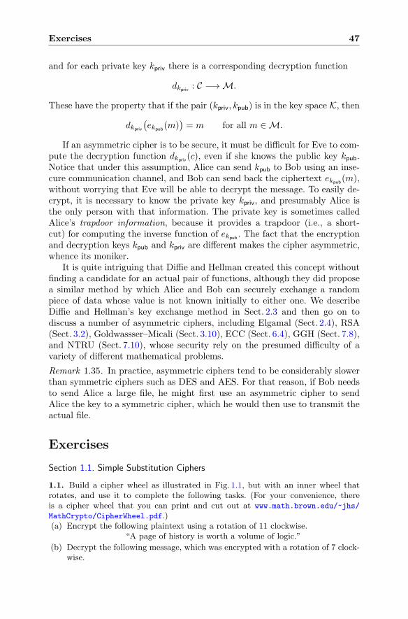
Exercises 47
and for each private key kpriv there is a corresponding decryption function
dkpriv : C −→M.
These have the property that if the pair (kpriv, kpub) is in the key space K, then
dkpriv
(ekpub
(m))= m for all m ∈M.
If an asymmetric cipher is to be secure, it must be difficult for Eve to com-pute the decryption function dkpriv(c), even if she knows the public key kpub.Notice that under this assumption, Alice can send kpub to Bob using an inse-cure communication channel, and Bob can send back the ciphertext ekpub
(m),without worrying that Eve will be able to decrypt the message. To easily de-crypt, it is necessary to know the private key kpriv, and presumably Alice isthe only person with that information. The private key is sometimes calledAlice’s trapdoor information, because it provides a trapdoor (i.e., a short-cut) for computing the inverse function of ekpub
. The fact that the encryptionand decryption keys kpub and kpriv are different makes the cipher asymmetric,whence its moniker.
It is quite intriguing that Diffie and Hellman created this concept withoutfinding a candidate for an actual pair of functions, although they did proposea similar method by which Alice and Bob can securely exchange a randompiece of data whose value is not known initially to either one. We describeDiffie and Hellman’s key exchange method in Sect. 2.3 and then go on todiscuss a number of asymmetric ciphers, including Elgamal (Sect. 2.4), RSA(Sect. 3.2), Goldwassser–Micali (Sect. 3.10), ECC (Sect. 6.4), GGH (Sect. 7.8),and NTRU (Sect. 7.10), whose security rely on the presumed difficulty of avariety of different mathematical problems.
Remark 1.35. In practice, asymmetric ciphers tend to be considerably slowerthan symmetric ciphers such as DES and AES. For that reason, if Bob needsto send Alice a large file, he might first use an asymmetric cipher to sendAlice the key to a symmetric cipher, which he would then use to transmit theactual file.
Exercises
Section 1.1. Simple Substitution Ciphers
1.1. Build a cipher wheel as illustrated in Fig. 1.1, but with an inner wheel thatrotates, and use it to complete the following tasks. (For your convenience, thereis a cipher wheel that you can print and cut out at www.math.brown.edu/~jhs/
MathCrypto/CipherWheel.pdf.)(a) Encrypt the following plaintext using a rotation of 11 clockwise.
“A page of history is worth a volume of logic.”
(b) Decrypt the following message, which was encrypted with a rotation of 7 clock-wise.
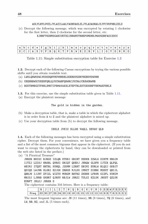
48 Exercises
AOLYLHYLUVZLJYLAZILAALYAOHUAOLZLJYLAZAOHALCLYFIVKFNBLZZLZ
(c) Decrypt the following message, which was encrypted by rotating 1 clockwisefor the first letter, then 2 clockwise for the second letter, etc.
XJHRFTNZHMZGAHIUETXZJNBWNUTRHEPOMDNBJMAUGORFAOIZOCC
a b c d e f g h i j k l m n o p q r s t u v w x y z
S C J A X U F B Q K T P R W E Z H V L I G Y D N M O
Table 1.11: Simple substitution encryption table for Exercise 1.3
1.2. Decrypt each of the following Caesar encryptions by trying the various possibleshifts until you obtain readable text.(a) LWKLQNWKDWLVKDOOQHYHUVHHDELOOERDUGORYHOBDVDWUHH
(b) UXENRBWXCUXENFQRLQJUCNABFQNWRCJUCNAJCRXWORWMB
(c) BGUTBMBGZTFHNLXMKTIPBMAVAXXLXTEPTRLEXTOXKHHFYHKMAXFHNLX
1.3. For this exercise, use the simple substitution table given in Table 1.11.(a) Encrypt the plaintext message
The gold is hidden in the garden.
(b) Make a decryption table, that is, make a table in which the ciphertext alphabetis in order from A to Z and the plaintext alphabet is mixed up.
(c) Use your decryption table from (b) to decrypt the following message.
IBXLX JVXIZ SLLDE VAQLL DEVAU QLB
1.4. Each of the following messages has been encrypted using a simple substitutioncipher. Decrypt them. For your convenience, we have given you a frequency tableand a list of the most common bigrams that appear in the ciphertext. (If you do notwant to recopy the ciphertexts by hand, they can be downloaded or printed fromthe web site listed in the preface.)(a) “A Piratical Treasure”
JNRZR BNIGI BJRGZ IZLQR OTDNJ GRIHT USDKR ZZWLG OIBTM NRGJN
IJTZJ LZISJ NRSBL QVRSI ORIQT QDEKJ JNRQW GLOFN IJTZX QLFQL
WBIMJ ITQXT HHTBL KUHQL JZKMM LZRNT OBIMI EURLW BLQZJ GKBJT
QDIQS LWJNR OLGRI EZJGK ZRBGS MJLDG IMNZT OIHRK MOSOT QHIJL
QBRJN IJJNT ZFIZL WIZTO MURZM RBTRZ ZKBNN LFRVR GIZFL KUHIM
MRIGJ LJNRB GKHRT QJRUU RBJLW JNRZI TULGI EZLUK JRUST QZLUK
EURFT JNLKJ JNRXR S
The ciphertext contains 316 letters. Here is a frequency table:
R J I L Z T N Q B G K U M O S H W F E D X V
Freq 33 30 27 25 24 20 19 16 15 15 13 12 12 10 9 8 7 6 5 5 3 2
The most frequent bigrams are: JN (11 times), NR (8 times), TQ (6 times), andLW, RB, RZ, and JL (5 times each).
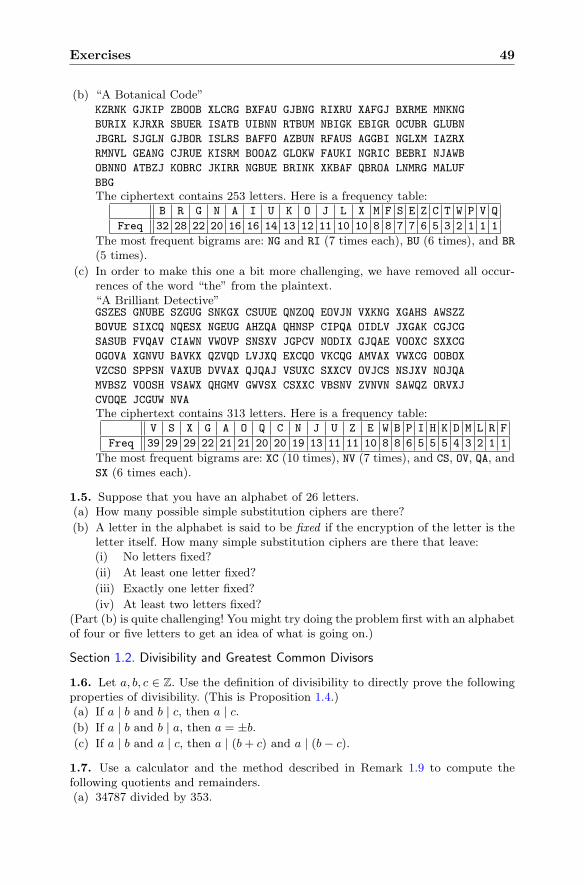
Exercises 49
(b) “A Botanical Code”KZRNK GJKIP ZBOOB XLCRG BXFAU GJBNG RIXRU XAFGJ BXRME MNKNG
BURIX KJRXR SBUER ISATB UIBNN RTBUM NBIGK EBIGR OCUBR GLUBN
JBGRL SJGLN GJBOR ISLRS BAFFO AZBUN RFAUS AGGBI NGLXM IAZRX
RMNVL GEANG CJRUE KISRM BOOAZ GLOKW FAUKI NGRIC BEBRI NJAWB
OBNNO ATBZJ KOBRC JKIRR NGBUE BRINK XKBAF QBROA LNMRG MALUF
BBG
The ciphertext contains 253 letters. Here is a frequency table:B R G N A I U K O J L X M F S E Z C T W P V Q
Freq 32 28 22 20 16 16 14 13 12 11 10 10 8 8 7 7 6 5 3 2 1 1 1
The most frequent bigrams are: NG and RI (7 times each), BU (6 times), and BR
(5 times).
(c) In order to make this one a bit more challenging, we have removed all occur-rences of the word “the” from the plaintext.“A Brilliant Detective”GSZES GNUBE SZGUG SNKGX CSUUE QNZOQ EOVJN VXKNG XGAHS AWSZZ
BOVUE SIXCQ NQESX NGEUG AHZQA QHNSP CIPQA OIDLV JXGAK CGJCG
SASUB FVQAV CIAWN VWOVP SNSXV JGPCV NODIX GJQAE VOOXC SXXCG
OGOVA XGNVU BAVKX QZVQD LVJXQ EXCQO VKCQG AMVAX VWXCG OOBOX
VZCSO SPPSN VAXUB DVVAX QJQAJ VSUXC SXXCV OVJCS NSJXV NOJQA
MVBSZ VOOSH VSAWX QHGMV GWVSX CSXXC VBSNV ZVNVN SAWQZ ORVXJ
CVOQE JCGUW NVA
The ciphertext contains 313 letters. Here is a frequency table:V S X G A O Q C N J U Z E W B P I H K D M L R F
Freq 39 29 29 22 21 21 20 20 19 13 11 11 10 8 8 6 5 5 5 4 3 2 1 1
The most frequent bigrams are: XC (10 times), NV (7 times), and CS, OV, QA, andSX (6 times each).
1.5. Suppose that you have an alphabet of 26 letters.(a) How many possible simple substitution ciphers are there?
(b) A letter in the alphabet is said to be fixed if the encryption of the letter is theletter itself. How many simple substitution ciphers are there that leave:(i) No letters fixed?
(ii) At least one letter fixed?
(iii) Exactly one letter fixed?
(iv) At least two letters fixed?(Part (b) is quite challenging! You might try doing the problem first with an alphabetof four or five letters to get an idea of what is going on.)
Section 1.2. Divisibility and Greatest Common Divisors
1.6. Let a, b, c ∈ Z. Use the definition of divisibility to directly prove the followingproperties of divisibility. (This is Proposition 1.4.)(a) If a | b and b | c, then a | c.(b) If a | b and b | a, then a = ±b.(c) If a | b and a | c, then a | (b+ c) and a | (b− c).
1.7. Use a calculator and the method described in Remark 1.9 to compute thefollowing quotients and remainders.(a) 34787 divided by 353.
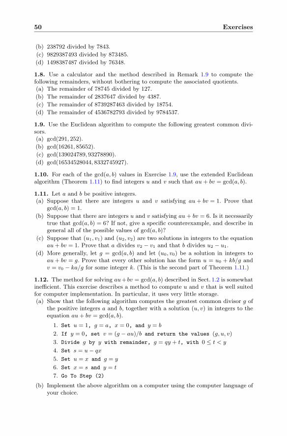
50 Exercises
(b) 238792 divided by 7843.
(c) 9829387493 divided by 873485.
(d) 1498387487 divided by 76348.
1.8. Use a calculator and the method described in Remark 1.9 to compute thefollowing remainders, without bothering to compute the associated quotients.(a) The remainder of 78745 divided by 127.
(b) The remainder of 2837647 divided by 4387.
(c) The remainder of 8739287463 divided by 18754.
(d) The remainder of 4536782793 divided by 9784537.
1.9. Use the Euclidean algorithm to compute the following greatest common divi-sors.(a) gcd(291, 252).
(b) gcd(16261, 85652).
(c) gcd(139024789, 93278890).
(d) gcd(16534528044, 8332745927).
1.10. For each of the gcd(a, b) values in Exercise 1.9, use the extended Euclideanalgorithm (Theorem 1.11) to find integers u and v such that au+ bv = gcd(a, b).
1.11. Let a and b be positive integers.(a) Suppose that there are integers u and v satisfying au+ bv = 1. Prove that
gcd(a, b) = 1.
(b) Suppose that there are integers u and v satisfying au+ bv = 6. Is it necessarilytrue that gcd(a, b) = 6? If not, give a specific counterexample, and describe ingeneral all of the possible values of gcd(a, b)?
(c) Suppose that (u1, v1) and (u2, v2) are two solutions in integers to the equationau+ bv = 1. Prove that a divides v2 − v1 and that b divides u2 − u1.
(d) More generally, let g = gcd(a, b) and let (u0, v0) be a solution in integers toau+ bv = g. Prove that every other solution has the form u = u0 + kb/g andv = v0 − ka/g for some integer k. (This is the second part of Theorem 1.11.)
1.12. The method for solving au+ bv = gcd(a, b) described in Sect. 1.2 is somewhatinefficient. This exercise describes a method to compute u and v that is well suitedfor computer implementation. In particular, it uses very little storage.(a) Show that the following algorithm computes the greatest common divisor g of
the positive integers a and b, together with a solution (u, v) in integers to theequation au+ bv = gcd(a, b).
1. Set u = 1, g = a, x = 0, and y = b
2. If y = 0, set v = (g − au)/b and return the values (g, u, v)
3. Divide g by y with remainder, g = qy + t, with 0 ≤ t < y
4. Set s = u− qx
5. Set u = x and g = y
6. Set x = s and y = t
7. Go To Step (2)
(b) Implement the above algorithm on a computer using the computer language ofyour choice.
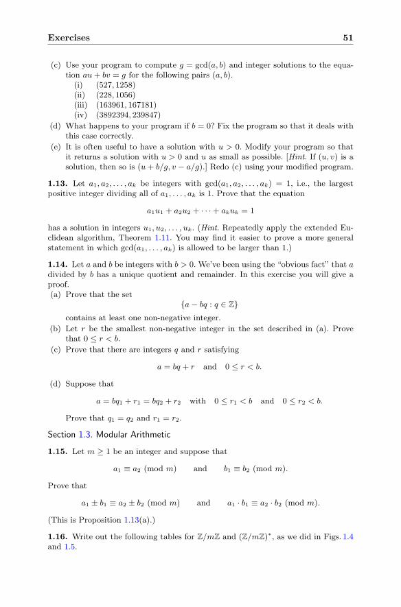
Exercises 51
(c) Use your program to compute g = gcd(a, b) and integer solutions to the equa-tion au+ bv = g for the following pairs (a, b).
(i) (527, 1258)(ii) (228, 1056)(iii) (163961, 167181)(iv) (3892394, 239847)
(d) What happens to your program if b = 0? Fix the program so that it deals withthis case correctly.
(e) It is often useful to have a solution with u > 0. Modify your program so thatit returns a solution with u > 0 and u as small as possible. [Hint. If (u, v) is asolution, then so is (u+ b/g, v − a/g).] Redo (c) using your modified program.
1.13. Let a1, a2, . . . , ak be integers with gcd(a1, a2, . . . , ak) = 1, i.e., the largestpositive integer dividing all of a1, . . . , ak is 1. Prove that the equation
a1u1 + a2u2 + · · ·+ akuk = 1
has a solution in integers u1, u2, . . . , uk. (Hint. Repeatedly apply the extended Eu-clidean algorithm, Theorem 1.11. You may find it easier to prove a more generalstatement in which gcd(a1, . . . , ak) is allowed to be larger than 1.)
1.14. Let a and b be integers with b > 0. We’ve been using the “obvious fact” that adivided by b has a unique quotient and remainder. In this exercise you will give aproof.(a) Prove that the set
{a− bq : q ∈ Z}contains at least one non-negative integer.
(b) Let r be the smallest non-negative integer in the set described in (a). Provethat 0 ≤ r < b.
(c) Prove that there are integers q and r satisfying
a = bq + r and 0 ≤ r < b.
(d) Suppose that
a = bq1 + r1 = bq2 + r2 with 0 ≤ r1 < b and 0 ≤ r2 < b.
Prove that q1 = q2 and r1 = r2.
Section 1.3. Modular Arithmetic
1.15. Let m ≥ 1 be an integer and suppose that
a1 ≡ a2 (mod m) and b1 ≡ b2 (mod m).
Prove that
a1 ± b1 ≡ a2 ± b2 (mod m) and a1 · b1 ≡ a2 · b2 (mod m).
(This is Proposition 1.13(a).)
1.16. Write out the following tables for Z/mZ and (Z/mZ)∗, as we did in Figs. 1.4and 1.5.
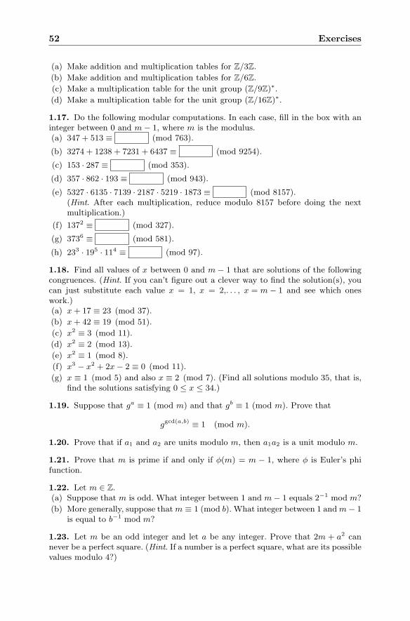
52 Exercises
(a) Make addition and multiplication tables for Z/3Z.
(b) Make addition and multiplication tables for Z/6Z.
(c) Make a multiplication table for the unit group (Z/9Z)∗.(d) Make a multiplication table for the unit group (Z/16Z)∗.
1.17. Do the following modular computations. In each case, fill in the box with aninteger between 0 and m− 1, where m is the modulus.(a) 347 + 513 ≡ (mod 763).
(b) 3274 + 1238 + 7231 + 6437 ≡ (mod 9254).
(c) 153 · 287 ≡ (mod 353).
(d) 357 · 862 · 193 ≡ (mod 943).
(e) 5327 · 6135 · 7139 · 2187 · 5219 · 1873 ≡ (mod 8157).(Hint. After each multiplication, reduce modulo 8157 before doing the nextmultiplication.)
(f) 1372 ≡ (mod 327).
(g) 3736 ≡ (mod 581).
(h) 233 · 195 · 114 ≡ (mod 97).
1.18. Find all values of x between 0 and m − 1 that are solutions of the followingcongruences. (Hint. If you can’t figure out a clever way to find the solution(s), youcan just substitute each value x = 1, x = 2,. . . , x = m− 1 and see which oneswork.)(a) x+ 17 ≡ 23 (mod 37).
(b) x+ 42 ≡ 19 (mod 51).
(c) x2 ≡ 3 (mod 11).
(d) x2 ≡ 2 (mod 13).
(e) x2 ≡ 1 (mod 8).
(f) x3 − x2 + 2x− 2 ≡ 0 (mod 11).
(g) x ≡ 1 (mod 5) and also x ≡ 2 (mod 7). (Find all solutions modulo 35, that is,find the solutions satisfying 0 ≤ x ≤ 34.)
1.19. Suppose that ga ≡ 1 (mod m) and that gb ≡ 1 (mod m). Prove that
ggcd(a,b) ≡ 1 (mod m).
1.20. Prove that if a1 and a2 are units modulo m, then a1a2 is a unit modulo m.
1.21. Prove that m is prime if and only if φ(m) = m − 1, where φ is Euler’s phifunction.
1.22. Let m ∈ Z.(a) Suppose that m is odd. What integer between 1 and m− 1 equals 2−1 mod m?
(b) More generally, suppose thatm ≡ 1 (mod b). What integer between 1 andm− 1is equal to b−1 mod m?
1.23. Let m be an odd integer and let a be any integer. Prove that 2m + a2 cannever be a perfect square. (Hint. If a number is a perfect square, what are its possiblevalues modulo 4?)
Exercises 53
1.24. (a) Find a single value x that simultaneously solves the two congruences
x ≡ 3 (mod 7) and x ≡ 4 (mod 9).
(Hint. Note that every solution of the first congruence looks like x = 3+7y forsome y. Substitute this into the second congruence and solve for y; then usethat to get x.)
(b) Find a single value x that simultaneously solves the two congruences
x ≡ 13 (mod 71) and x ≡ 41 (mod 97).
(c) Find a single value x that simultaneously solves the three congruences
x ≡ 4 (mod 7), x ≡ 5 (mod 8), and x ≡ 11 (mod 15).
(d) Prove that if gcd(m,n) = 1, then the pair of congruences
x ≡ a (mod m) and x ≡ b (mod n)
has a solution for any choice of a and b. Also give an example to show that thecondition gcd(m,n) = 1 is necessary.
1.25. Let N , g, and A be positive integers (note that N need not be prime).Prove that the following algorithm, which is a low-storage variant of the square-and-multiply algorithm described in Sect. 1.3.2, returns the value gA (mod N). (InStep 4 we use the notation �x� to denote the greatest integer function, i.e., round xdown to the nearest integer.)
Input. Positive integers N , g, and A.1. Set a = g and b = 1.2. Loop while A > 0.
3. If A ≡ 1 (mod 2), set b = b · a (mod N).4. Set a = a2 (mod N) and A = �A/2�.5. If A > 0, continue with loop at Step 2.
6. Return the number b, which equals gA (mod N).
1.26. Use the square-and-multiply algorithm described in Sect. 1.3.2, or the moreefficient version in Exercise 1.25, to compute the following powers.(a) 17183 (mod 256).
(b) 2477 (mod 1000).
(c) 11507 (mod 1237).
1.27. Consider the congruence
ax ≡ c (mod m).
(a) Prove that there is a solution if and only if gcd(a,m) divides c.
(b) If there is a solution, prove that there are exactly gcd(a,m) distinct solutionsmodulo m.
(Hint. Use the extended Euclidean algorithm (Theorem 1.11).)
Section 1.4. Prime Numbers, Unique Factorization, and Finite Fields
54 Exercises
1.28. Let {p1, p2, . . . , pr} be a set of prime numbers, and let
N = p1p2 · · · pr + 1.
Prove that N is divisible by some prime not in the original set. Use this fact todeduce that there must be infinitely many prime numbers. (This proof of the infini-tude of primes appears in Euclid’s Elements. Prime numbers have been studied forthousands of years.)
1.29. Without using the fact that every integer has a unique factorization intoprimes, prove that if gcd(a, b) = 1 and if a | bc, then a | c. (Hint. Use the fact thatit is possible to find a solution to au+ bv = 1.)
1.30. Compute the following ordp values:(a) ord2(2816).
(b) ord7(2222574487).
(c) ordp(46375) for each of p = 3, 5, 7, and 11.
1.31. Let p be a prime number. Prove that ordp has the following properties.(a) ordp(ab) = ordp(a) + ordp(b). (Thus ordp resembles the logarithm function,
since it converts multiplication into addition!)
(b) ordp(a+ b) ≥ min{ordp(a), ordp(b)
}.
(c) If ordp(a) �= ordp(b), then ordp(a+ b) = min{ordp(a), ordp(b)
}.
A function satisfying properties (a) and (b) is called a valuation.
Section 1.5. Powers and Primitive Roots in Finite Fields
1.32. For each of the following primes p and numbers a, compute a−1 mod p in twoways: (i) Use the extended Euclidean algorithm. (ii) Use the fast power algorithmand Fermat’s little theorem. (See Example 1.27.)(a) p = 47 and a = 11.
(b) p = 587 and a = 345.
(c) p = 104801 and a = 78467.
1.33. Let p be a prime and let q be a prime that divides p− 1.(a) Let a ∈ F
∗p and let b = a(p−1)/q. Prove that either b = 1 or else b has order q.
(Recall that the order of b is the smallest k ≥ 1 such that bk = 1 in F∗p. Hint.
Use Proposition 1.29.)
(b) Suppose that we want to find an element of F∗p of order q. Using (a), we can
randomly choose a value of a ∈ F∗p and check whether b = a(p−1)/q satisfies b �=
1. How likely are we to succeed? In other words, compute the value of the ratio
#{a ∈ F∗p : a(p−1)/q �= 1}#F∗
p
.
(Hint. Use Theorem 1.30.)
1.34. Recall that g is called a primitive root modulo p if the powers of g give allnonzero elements of Fp.(a) For which of the following primes is 2 a primitive root modulo p?
(i) p = 7 (ii) p = 13 (iii) p = 19 (iv) p = 23
Exercises 55
(b) For which of the following primes is 3 a primitive root modulo p?(i) p = 5 (ii) p = 7 (iii) p = 11 (iv) p = 17
(c) Find a primitive root for each of the following primes.(i) p = 23 (ii) p = 29 (iii) p = 41 (iv) p = 43
(d) Find all primitive roots modulo 11. Verify that there are exactly φ(10) of them,as asserted in Remark 1.32.
(e) Write a computer program to check for primitive roots and use it to find allprimitive roots modulo 229. Verify that there are exactly φ(228) of them.
(f) Use your program from (e) to find all primes less than 100 for which 2 is aprimitive root.
(g) Repeat the previous exercise to find all primes less than 100 for which 3 is aprimitive root. Ditto to find the primes for which 4 is a primitive root.
1.35. Let p be a prime such that q = 12(p − 1) is also prime. Suppose that g is an
integer satisfying
g �≡ 0 (mod p) and g �≡ ±1 (mod p) and gq �≡ 1 (mod p).
Prove that g is a primitive root modulo p.
1.36. This exercise begins the study of squares and square roots modulo p.(a) Let p be an odd prime number and let b be an integer with p � b. Prove that
either b has two square roots modulo p or else b has no square roots modulo p.In other words, prove that the congruence
X2 ≡ b (mod p)
has either two solutions or no solutions in Z/pZ. (What happens for p = 2?What happens if p | b?)
(b) For each of the following values of p and b, find all of the square roots of bmodulo p.
(i) (p, b) = (7, 2) (ii) (p, b) = (11, 5)(iii) (p, b) = (11, 7) (iv) (p, b) = (37, 3)
(c) How many square roots does 29 have modulo 35? Why doesn’t this contradictthe assertion in (a)?
(d) Let p be an odd prime and let g be a primitive root modulo p. Then anynumber a is equal to some power of g modulo p, say a ≡ gk (mod p). Provethat a has a square root modulo p if and only if k is even.
1.37. Let p ≥ 3 be a prime and suppose that the congruence
X2 ≡ b (mod p)
has a solution.(a) Prove that for every exponent e ≥ 1 the congruence
X2 ≡ b (mod pe) (1.14)
has a solution. (Hint. Use induction on e. Build a solution modulo pe+1 bysuitably modifying a solution modulo pe.)
(b) Let X = α be a solution to X2 ≡ b (mod p). Prove that in (a), we can find asolution X = β to X2 ≡ b (mod pe) that also satisfies β ≡ α (mod p).
56 Exercises
(c) Let β and β′ be two solutions as in (b). Prove that β ≡ β′ (mod pe).
(d) Use Exercise 1.36 to deduce that the congruence (1.14) has either two solutionsor no solutions modulo pe.
1.38. Compute the value of2(p−1)/2 (mod p)
for every prime 3 ≤ p < 20. Make a conjecture as to the possible values of2(p−1)/2 (mod p) when p is prime and prove that your conjecture is correct.
Section 1.6. Cryptography by Hand
1.39. Write a 2–5 page paper on one of the following topics, including both cryp-tographic information and placing events in their historical context:(a) Cryptography in the Arab world to the fifteenth century.
(b) European cryptography in the fifteenth and early sixteenth centuries.
(c) Cryptography and cryptanalysis in Elizabethan England.
(d) Cryptography and cryptanalysis in the nineteenth century.
(e) Cryptography and cryptanalysis during World War I.
(f) Cryptography and cryptanalysis during World War II.(Most of these topics are too broad for a short term paper, so you should choose aparticular aspect on which to concentrate.)
1.40. A homophonic cipher is a substitution cipher in which there may be more thanone ciphertext symbol for each plaintext letter. Here is an example of a homophoniccipher, where the more common letters have several possible replacements.
a b c d e f g h i j k l m n o p q r s t u v w x y z
! 4 # $ 1 % & * ( ) 3 2 = + [ 9 ] { } : ; 7 < > 5 ?
♥ ◦ � ℵ 6 ↗ � ♦ ∧ ↘ Δ ∇ 8 ♣ Ω ∨ ⊗ ♠ �Θ ∞ ⇑ � • � ⊕ ⇐↙ ⇓ ⇒ ↖
Decrypt the following message.
( % Δ ♠ ⇒ � # 4 ∞ : ♦ 6 ↗ � [ ℵ 8 % 2 [ 7 ⇓ ♣ ↘ ♥ 5 � ∇
1.41. A transposition cipher is a cipher in which the letters of the plaintext remainthe same, but their order is rearranged. Here is a simple example in which themessage is encrypted in blocks of 25 letters at a time.19 Take the given 25 lettersand arrange them in a 5-by-5 block by writing the message horizontally on the lines.For example, the first 25 letters of the message
Now is the time for all good men to come to the aid...
is written as
N O W I S
T H E T I
M E F O R
A L L G O
O D M E N
19If the number of letters in the message is not an even multiple of 25, then extra randomletters are appended to the end of the message.
Exercises 57
Now the cipehrtext is formed by reading the letters down the columns, which givesthe ciphertext
NTMAO OHELD WEFLM ITOGE SIRON.
(a) Use this transposition cipher to encrypt the first 25 letters of the message
Four score and seven years ago our fathers...
(b) The following message was encrypted using this transposition cipher.Decrypt it.
WNOOA HTUFN EHRHE NESUV ICEME
(c) There are many variations on this type of cipher. We can form the letters into arectangle instead of a square, and we can use various patterns to place the lettersinto the rectangle and to read them back out. Try to decrypt the followingciphertext, in which the letters were placed horizontally into a rectangle ofsome size and then read off vertically by columns.
WHNCE STRHT TEOOH ALBAT DETET SADHE
LEELL QSFMU EEEAT VNLRI ATUDR HTEEA
(For convenience, we’ve written the ciphertext in 5 letter blocks, but thatdoesn’t necessarily mean that the rectangle has a side of length 5.)
Section 1.7. Symmetric Ciphers and Asymmetric Ciphers
1.42. Encode the following phrase (including capitalization, spacing and punctua-tion) into a string of bits using the ASCII encoding scheme given in Table 1.10.
Bad day, Dad.
1.43. Consider the affine cipher with key k = (k1, k2) whose encryption and de-cryption functions are given by (1.11) on page 43.(a) Let p = 541 and let the key be k = (34, 71). Encrypt the message m = 204.
Decrypt the ciphertext c = 431.
(b) Assuming that p is public knowledge, explain why the affine cipher is vulnerableto a known plaintext attack. (See Property 4 on page 38.) How many plain-text/ciphertext pairs are likely to be needed in order to recover the privatekey?
(c) Alice and Bob decide to use the prime p = 601 for their affine cipher. Thevalue of p is public knowledge, and Eve intercepts the ciphertexts c1 = 324and c2 = 381 and also manages to find out that the corresponding plaintextsare m1 = 387 and m2 = 491. Determine the private key and then use it toencrypt the message m3 = 173.
(d) Suppose now that p is not public knowledge. Is the affine cipher still vulnerableto a known plaintext attack? If so, how many plaintext/ciphertext pairs arelikely to be needed in order to recover the private key?
1.44. Consider the Hill cipher defined by (1.11),
ek(m) ≡ k1 ·m+ k2 (mod p) and dk(c) ≡ k−11 · (c− k2) (mod p),
wherem, c, and k2 are column vectors of dimension n, and k1 is an n-by-n matrix.
58 Exercises
(a) We use the vector Hill cipher with p = 7 and the key k1 = ( 1 32 2 ) and k2 = ( 5
4 ).(i) Encrypt the message m = ( 2
1 ).(ii) What is the matrix k−1
1 used for decryption?(iii) Decrypt the message c = ( 3
5 ).
(b) Explain why the Hill cipher is vulnerable to a known plaintext attack.
(c) The following plaintext/ciphertext pairs were generated using a Hill cipher withthe prime p = 11. Find the keys k1 and k2.
m1 = ( 54 ) , c1 = ( 1
8 ) , m2 = ( 810 ) , c2 = ( 8
5 ) , m3 = ( 71 ) , c3 = ( 8
7 ) .
(d) Explain how any simple substitution cipher that involves a permutation of thealphabet can be thought of as a special case of a Hill cipher.
1.45. Let N be a large integer and let K = M = C = Z/NZ. For each of thefunctions
e : K ×M −→ Clisted in (a)–(c), answer the following questions:
• Is e an encryption function?
• If e is an encryption function, what is its associated decryption function d?
• If e is not an encryption function, can you make it into an encryption functionby using some smaller, yet reasonably large, set of keys?
(a) ek(m) ≡ k −m (mod N).
(b) ek(m) ≡ k ·m (mod N).
(c) ek(m) ≡ (k +m)2 (mod N).
1.46. (a) Convert the 12 bit binary number 110101100101 into a decimal integerbetween 0 and 212 − 1.
(b) Convert the decimal integer m = 37853 into a binary number.
(c) Convert the decimal integer m = 9487428 into a binary number.
(d) Use exclusive or (XOR) to “add” the bit strings 11001010⊕ 10011010.
(e) Convert the decimal numbers 8734 and 5177 into binary numbers, combinethem using XOR, and convert the result back into a decimal number.
1.47. Alice and Bob choose a key space K containing 256 keys. Eve builds a special-purpose computer that can check 10,000,000,000 keys per second.(a) How many days does it take Eve to check half of the keys in K?
(b) Alice and Bob replace their key space with a larger set containing 2B differentkeys. How large should Alice and Bob choose B in order to force Eve’s computerto spend 100 years checking half the keys? (Use the approximation that thereare 365.25 days in a year.)
For many years the United States government recommended a symmetric ciphercalled DES that used 56 bit keys. During the 1990s, people built special purposecomputers demonstrating that 56 bits provided insufficient security. A new sym-metric cipher called AES, with 128 bit keys, was developed to replace DES. SeeSect. 8.12 for further information about DES and AES.
1.48. Explain why the cipher
ek(m) = k ⊕m and dk(c) = k ⊕ c
Exercises 59
defined by XOR of bit strings is not secure against a known plaintext attack.Demonstrate your attack by finding the private key used to encrypt the 16-bit ci-phertext c = 1001010001010111 if you know that the corresponding plaintext ism = 0010010000101100.
1.49. Alice and Bob create a symmetric cipher as follows. Their private key k is alarge integer and their messages (plaintexts) are d-digit integers
M = {m ∈ Z : 0 ≤ m < 10d}.
To encrypt a message, Alice computes√k to d decimal places, throws away the part
to the left of the decimal point, and keeps the remaining d digits. Let α be thisd-digit number. (For example, if k = 87 and d = 6, then
√87 = 9.32737905 . . . and
α = 327379.)Alice encrypts a message m as
c ≡ m+ α (mod 10d).
Since Bob knows k, he can also find α, and then he decrypts c by comput-ing m ≡ c− α (mod 10d).(a) Alice and Bob choose the secret key k = 11 and use it to encrypt 6-digit integers
(i.e., d = 6). Bob wants to send Alice the message m = 328973. What is theciphertext that he sends?
(b) Alice and Bob use the secret key k = 23 and use it to encrypt 8-digit integers.Alice receives the ciphertext c = 78183903. What is the plaintext m?
(c) Show that the number α used for encryption and decryption is given by theformula
α =⌊10d(√
k − �√k �)⌋,
where �t� denotes the greatest integer that is less than or equal to t.
(d) (Challenge Problem) If Eve steals a plaintext/ciphertext pair (m, c), then it isclear that she can recover the number α, since α ≡ c−m (mod 10d). If 10d islarge compared to k, can she also recover the number k? This might be useful,for example, if Alice and Bob use some of the other digits of
√k to encrypt
subsequent messages.
1.50. Bob and Alice use a cryptosystem in which their private key is a (large)prime k and their plaintexts and ciphertexts are integers. Bob encrypts a message mby computing the product c = km. Eve intercepts the following two ciphertexts:
c1 = 12849217045006222, c2 = 6485880443666222.
Use the gcd method described in Sect. 1.7.4 to find Bob and Alice’s private key.
Chapter 2
Discrete Logarithmsand Diffie–Hellman
2.1 The Birth of Public Key Cryptography
In 1976, Whitfield Diffie and Martin Hellman published their now famouspaper [38] entitled “New Directions in Cryptography.” In this paper theyformulated the concept of a public key encryption system and made severalgroundbreaking contributions to this new field. A short time earlier, RalphMerkle had independently isolated one of the fundamental problems and in-vented a public key construction for an undergraduate project in a computerscience class at Berkeley, but this was little understood at the time. Merkle’swork “Secure communication over insecure channels” appeared in 1982 [83].
However, it turns out that the concept of public key encryption was orig-inally discovered by James Ellis while working at the British GovernmentCommunications Headquarters (GCHQ). Ellis’s discoveries in 1969 were clas-sified as secret material by the British government and were not declassi-fied and released until 1997, after his death. It is now known that two otherresearchers at GCHQ, Malcolm Williamson and Clifford Cocks, discoveredthe Diffie–Hellman key exchange algorithm and the RSA public key encryp-tion system, respectively, before their rediscovery and public dissemination byDiffie, Hellman, Rivest, Shamir, and Adleman. To learn more about the fas-cinating history of public key cryptography, see for example [37, 42, 63, 139].
The Diffie–Hellman publication was an extremely important event—it setforth the basic definitions and goals of a new field of mathematics/computerscience, a field whose existence was dependent on the then emerging age ofthe digital computer. Indeed, their paper begins with a call to arms:
© Springer Science+Business Media New York 2014J. Hoffstein et al., An Introduction to Mathematical Cryptography,Undergraduate Texts in Mathematics, DOI 10.1007/978-1-4939-1711-2 2
61
62 2. Discrete Logarithms and Diffie–Hellman
We stand today on the brink of a revolution in cryptography.
An original or breakthrough scientific idea is often called revolutionary, butin this instance, as the authors were fully aware, the term revolutionary wasrelevant in another sense. Prior to the publication of “New Directions. . . ,”encryption research in the United States was the domain of the National Se-curity Agency, and all information in this area was classified. Indeed, until themid-1990s, the United States government treated cryptographic algorithms asmunitions, which meant that their export was prosecutable as a treasonableoffense. Eventually, the government realized the futility of trying to preventfree and open discussion about abstract cryptographic algorithms and thedubious legality of restricting domestic use of strong cryptographic methods.However, in order to maintain some control, the government continued to re-strict export of high security cryptographic algorithms if they were “machinereadable.” Their object, to prevent widespread global dissemination of so-phisticated cryptography programs to potential enemies of the United States,was laudable,1 but there were two difficulties that rendered the government’spolicy unworkable.
First, the existence of optical scanners creates a very blurry line between“machine readable” and “human text.” To protest the government’s policy,people wrote a three line version of the RSA algorithm in a programminglanguage called perl and printed it on tee shirts and soda cans, thereby makingthese products into munitions. In principle, wearing an “RSA enabled” teeshirt on a flight from New York to Europe subjected the wearer to a largefine and a 10 year jail term. Even more amusing (or frightening, dependingon your viewpoint), tattoos of the RSA perl code made people’s bodies intonon-exportable munitions!
Second, although these and other more serious protests and legal chal-lenges had some effect, the government’s policy was ultimately rendered mootby a simple reality. Public key algorithms are quite simple, and although itrequires a certain expertise to implement them in a secure fashion, the world isfull of excellent mathematicians and computer scientists and engineers. Thusgovernment restrictions on the export of “strong crypto” simply encouragedthe creation of cryptographic industries in other parts of the world. The gov-ernment was able to slow the adoption of strong crypto for a few years, butit is now possible for anyone to purchase for a nominal sum cryptographicsoftware that allows completely secure communications.2
1It is surely laudable to keep potential weapons out of the hands of one’s enemies,but many have argued, with considerable justification, that the government also had theless benign objective of preventing other governments from using communication methodssecure from United States prying.
2Of course, one never knows what cryptanalytic breakthroughs have been made by thescientists at the National Security Agency, since virtually all of their research is classified.The NSA is reputed to be the world’s largest single employer of Ph.D.s in mathematics.However, in contrast to the situation before the 1970s, there are now far more cryptographersemployed in academia and in the business world than there are in government agencies.
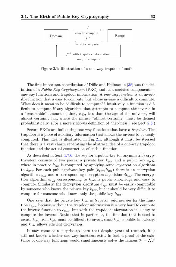
2.1. The Birth of Public Key Cryptography 63
Domain Range
f
easy to compute
f−1
f−1
hard to compute
with trapdoor information
easy to compute
Figure 2.1: Illustration of a one-way trapdoor function
The first important contribution of Diffie and Hellman in [38] was the def-inition of a Public Key Cryptosystem (PKC) and its associated components—one-way functions and trapdoor information. A one-way function is an invert-ible function that is easy to compute, but whose inverse is difficult to compute.What does it mean to be “difficult to compute”? Intuitively, a function is dif-ficult to compute if any algorithm that attempts to compute the inverse ina “reasonable” amount of time, e.g., less than the age of the universe, willalmost certainly fail, where the phrase “almost certainly” must be definedprobabilistically. (For a more rigorous definition of “hardness,” see Sect. 2.6.)
Secure PKCs are built using one-way functions that have a trapdoor. Thetrapdoor is a piece of auxiliary information that allows the inverse to be easilycomputed. This idea is illustrated in Fig. 2.1, although it must be stressedthat there is a vast chasm separating the abstract idea of a one-way trapdoorfunction and the actual construction of such a function.
As described in Sect. 1.7.6, the key for a public key (or asymmetric) cryp-tosystem consists of two pieces, a private key kpriv and a public key kpub,where in practice kpub is computed by applying some key-creation algorithmto kpriv. For each public/private key pair (kpriv, kpub) there is an encryptionalgorithm ekpub
and a corresponding decryption algorithm dkpriv . The encryp-tion algorithm ekpub
corresponding to kpub is public knowledge and easy tocompute. Similarly, the decryption algorithm dkpriv must be easily computableby someone who knows the private key kpriv, but it should be very difficult tocompute for someone who knows only the public key kpub.
One says that the private key kpriv is trapdoor information for the func-tion ekpub
, because without the trapdoor information it is very hard to computethe inverse function to ekpub
, but with the trapdoor information it is easy tocompute the inverse. Notice that in particular, the function that is used tocreate kpub from kpriv must be difficult to invert, since kpub is public knowledgeand kpriv allows efficient decryption.
It may come as a surprise to learn that despite years of research, it isstill not known whether one-way functions exist. In fact, a proof of the exis-tence of one-way functions would simultaneously solve the famous P = NP
64 2. Discrete Logarithms and Diffie–Hellman
problem in complexity theory.3 Various candidates for one-way functions havebeen proposed, and some of them are used by modern public key encryptionalgorithms. But it must be stressed that the security of these cryptosystemsrests on the assumption that inverting the underlying function (or finding theprivate key from the public one) is a hard problem.
The situation is somewhat analogous to theories in physics that gain cred-ibility over time, as they fail to be disproved and continue to explain or gen-erate interesting phenomena. Diffie and Hellman made several suggestionsin [38] for one-way functions, including knapsack problems and exponenti-ation mod q, but they did not produce an example of a PKC, mainly forlack of finding the right trapdoor information. They did, however, describe apublic key method by which certain material could be securely shared overan insecure channel. Their method, which is now called Diffie–Hellman keyexchange, is based on the assumption that the discrete logarithm problem(DLP) is difficult to solve. We discuss the DLP in Sect. 2.2, and then describeDiffie–Hellman key exchange in Sect. 2.3. In their paper, Diffie and Hellmanalso defined a variety of cryptanalytic attacks and introduced the importantconcepts of digital signatures and one-way authentication, which we discussin Chap. 4 and Sect. 8.5.
With the publication of [38] in 1976, the race was on to invent a practicalpublic key cryptosystem. Within 2 years, two major papers describing publickey cryptosystems were published: the RSA scheme of Rivest, Shamir, andAdleman [110] and the knapsack scheme of Merkle and Hellman [84]. Of thesetwo, only RSA has withstood the test of time, in the sense that its underly-ing hard problem of integer factorization is still sufficiently computationallydifficult to allow RSA to operate efficiently. By way of contrast, the knap-sack system of Merkle and Hellman was shown to be insecure at practicalcomputational levels [124]. However, the cryptanalysis of knapsack systemsintroduces important links to hard computational problems in the theory ofinteger lattices that we explore in Chap. 7.
2.2 The Discrete Logarithm Problem
The discrete logarithm problem is a mathematical problem that arises in manysettings, including the mod p version described in this section and the ellipticcurve version that will be studied later, in Chap. 6. The first published publickey construction, due to Diffie and Hellman [38], is based on the discrete log-arithm problem in a finite field Fp, where recall that Fp is a field with a primenumber of elements. (See Sect. 1.4.) For convenience, we interchangeably usethe notations Fp and Z/pZ for this field, and we use equality notation for ele-ments of Fp and congruence notation for elements of Z/pZ (cf. Remark 1.23).
3The P = NP problem is one of the so-called Millennium Prizes, each of which has a$1,000,000 prize attached. See Sect. 5.7 for more on P versus NP .
2.2. The Discrete Logarithm Problem 65
Let p be a (large) prime. Theorem 1.30 tells us that there exists a primitiveelement g. This means that every nonzero element of Fp is equal to some powerof g. In particular, gp−1 = 1 by Fermat’s little theorem (Theorem 1.24), andno smaller positive power of g is equal to 1. Equivalently, the list of elements
1, g, g2, g3, . . . , gp−2 ∈ F∗p
is a complete list of the elements in F∗p in some order.
Definition. Let g be a primitive root for Fp and let h be a nonzero elementof Fp. The Discrete Logarithm Problem (DLP) is the problem of finding anexponent x such that
gx ≡ h (mod p).
The number x is called the discrete logarithm of h to the base g and is denotedby logg(h).
Remark 2.1. An older term for the discrete logarithm is the index, denotedby indg(h). The index terminology is still commonly used in number theory. Itis also convenient if there is a danger of confusion between ordinary logarithmsand discrete logarithms, since, for example, the quantity log2 frequently occursin both contexts.
Remark 2.2. The discrete logarithm problem is a well-posed problem, namelyto find an integer exponent x such that gx = h. However, if there is one so-lution, then there are infinitely many, because Fermat’s little theorem (The-orem 1.24) tells us that gp−1 ≡ 1 (mod p). Hence if x is a solution to gx = h,then x+ k(p− 1) is also a solution for every value of k, because
gx+k(p−1) = gx · (gp−1)k ≡ h · 1k ≡ h (mod p).
Thus logg(h) is defined only up to adding or subtracting multiples of p− 1.In other words, logg(h) is really defined modulo p− 1. It is not hard to verify(Exercise 2.3(a)) that logg gives a well-defined function4
logg : F∗p −→
Z
(p− 1)Z. (2.1)
Sometimes, for concreteness, we refer to “the” discrete logarithm as the integerx lying between 0 and p− 2 satisfying the congruence gx ≡ h (mod p).
Remark 2.3. It is not hard to prove (see Exercise 2.3(b)) that
logg(ab) = logg(a) + logg(b) for all a, b ∈ F∗p.
4If you have studied complex analysis, you may have noticed an analogy with the com-plex logarithm, which is not actually well defined on C
∗. This is due to the fact that e2πi = 1,so log(z) is well defined only up to adding or subtracting multiples of 2πi. The complexlogarithm thus defines an isomorphism from C
∗ to the quotient group C/2πiZ, analogousto (2.1).
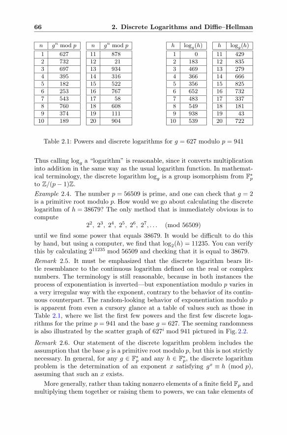
66 2. Discrete Logarithms and Diffie–Hellman
n gn mod p
1 627
2 732
3 697
4 395
5 182
6 253
7 543
8 760
9 374
10 189
n gn mod p
11 878
12 21
13 934
14 316
15 522
16 767
17 58
18 608
19 111
20 904
h logg(h)
1 0
2 183
3 469
4 366
5 356
6 652
7 483
8 549
9 938
10 539
h logg(h)
11 429
12 835
13 279
14 666
15 825
16 732
17 337
18 181
19 43
20 722
Table 2.1: Powers and discrete logarithms for g = 627 modulo p = 941
Thus calling logg a “logarithm” is reasonable, since it converts multiplicationinto addition in the same way as the usual logarithm function. In mathemat-ical terminology, the discrete logarithm logg is a group isomorphism from F
∗p
to Z/(p− 1)Z.
Example 2.4. The number p = 56509 is prime, and one can check that g = 2is a primitive root modulo p. How would we go about calculating the discretelogarithm of h = 38679? The only method that is immediately obvious is tocompute
22, 23, 24, 25, 26, 27, . . . (mod 56509)
until we find some power that equals 38679. It would be difficult to do thisby hand, but using a computer, we find that log2(h) = 11235. You can verifythis by calculating 211235 mod 56509 and checking that it is equal to 38679.
Remark 2.5. It must be emphasized that the discrete logarithm bears lit-tle resemblance to the continuous logarithm defined on the real or complexnumbers. The terminology is still reasonable, because in both instances theprocess of exponentiation is inverted—but exponentiation modulo p varies ina very irregular way with the exponent, contrary to the behavior of its contin-uous counterpart. The random-looking behavior of exponentiation modulo pis apparent from even a cursory glance at a table of values such as those inTable 2.1, where we list the first few powers and the first few discrete loga-rithms for the prime p = 941 and the base g = 627. The seeming randomnessis also illustrated by the scatter graph of 627i mod 941 pictured in Fig. 2.2.
Remark 2.6. Our statement of the discrete logarithm problem includes theassumption that the base g is a primitive root modulo p, but this is not strictlynecessary. In general, for any g ∈ F
∗p and any h ∈ F
∗p, the discrete logarithm
problem is the determination of an exponent x satisfying gx ≡ h (mod p),assuming that such an x exists.
More generally, rather than taking nonzero elements of a finite field Fp andmultiplying them together or raising them to powers, we can take elements of
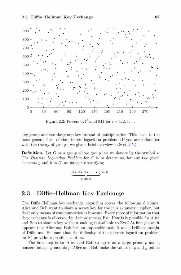
2.3. Diffie–Hellman Key Exchange 67
0 30 60 90 120 150 180 210 240 2700
100
200
300
400
500
600
700
800
900
Figure 2.2: Powers 627i mod 941 for i = 1, 2, 3, . . .
any group and use the group law instead of multiplication. This leads to themost general form of the discrete logarithm problem. (If you are unfamiliarwith the theory of groups, we give a brief overview in Sect. 2.5.)
Definition. Let G be a group whose group law we denote by the symbol �.The Discrete Logarithm Problem for G is to determine, for any two givenelements g and h in G, an integer x satisfying
g � g � g � · · · � g︸ ︷︷ ︸
x times
= h.
2.3 Diffie–Hellman Key Exchange
The Diffie–Hellman key exchange algorithm solves the following dilemma.Alice and Bob want to share a secret key for use in a symmetric cipher, buttheir only means of communication is insecure. Every piece of information thatthey exchange is observed by their adversary Eve. How is it possible for Aliceand Bob to share a key without making it available to Eve? At first glance itappears that Alice and Bob face an impossible task. It was a brilliant insightof Diffie and Hellman that the difficulty of the discrete logarithm problemfor F∗
p provides a possible solution.The first step is for Alice and Bob to agree on a large prime p and a
nonzero integer g modulo p. Alice and Bob make the values of p and g public
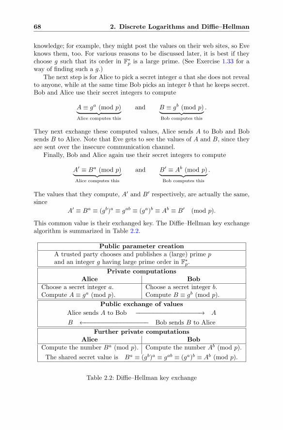
68 2. Discrete Logarithms and Diffie–Hellman
knowledge; for example, they might post the values on their web sites, so Eveknows them, too. For various reasons to be discussed later, it is best if theychoose g such that its order in F
∗p is a large prime. (See Exercise 1.33 for a
way of finding such a g.)The next step is for Alice to pick a secret integer a that she does not reveal
to anyone, while at the same time Bob picks an integer b that he keeps secret.Bob and Alice use their secret integers to compute
A ≡ ga (mod p)︸ ︷︷ ︸Alice computes this
and B ≡ gb (mod p)︸ ︷︷ ︸Bob computes this
.
They next exchange these computed values, Alice sends A to Bob and Bobsends B to Alice. Note that Eve gets to see the values of A and B, since theyare sent over the insecure communication channel.
Finally, Bob and Alice again use their secret integers to compute
A′ ≡ Ba (mod p)︸ ︷︷ ︸Alice computes this
and B′ ≡ Ab (mod p)︸ ︷︷ ︸Bob computes this
.
The values that they compute, A′ and B′ respectively, are actually the same,since
A′ ≡ Ba ≡ (gb)a ≡ gab ≡ (ga)b ≡ Ab ≡ B′ (mod p).
This common value is their exchanged key. The Diffie–Hellman key exchangealgorithm is summarized in Table 2.2.
Public parameter creationA trusted party chooses and publishes a (large) prime pand an integer g having large prime order in F
∗p.
Private computationsAlice Bob
Choose a secret integer a. Choose a secret integer b.Compute A ≡ ga (mod p). Compute B ≡ gb (mod p).
Public exchange of values
Alice sends A to Bob −−−−−−−−−−−−−−−−−−→ A
B ←−−−−−−−−−−−−−−−−−− Bob sends B to Alice
Further private computationsAlice Bob
Compute the number Ba (mod p). Compute the number Ab (mod p).
The shared secret value is Ba ≡ (gb)a ≡ gab ≡ (ga)b ≡ Ab (mod p).
Table 2.2: Diffie–Hellman key exchange
2.3. Diffie–Hellman Key Exchange 69
Example 2.7. Alice and Bob agree to use the prime p = 941 and theprimitive root g = 627. Alice chooses the secret key a = 347 and computesA = 390 ≡ 627347 (mod 941). Similarly, Bob chooses the secret key b = 781and computes B = 691 ≡ 627781 (mod 941). Alice sends Bob the number 390and Bob sends Alice the number 691. Both of these transmissions are doneover an insecure channel, so both A = 390 and B = 691 should be consideredpublic knowledge. The numbers a = 347 and b = 781 are not transmitted andremain secret. Then Alice and Bob are both able to compute the number
470 ≡ 627347·781 ≡ Ab ≡ Ba (mod 941),
so 470 is their shared secret.Suppose that Eve sees this entire exchange. She can reconstitute Alice’s
and Bob’s shared secret if she can solve either of the congruences
627a ≡ 390 (mod 941) or 627b ≡ 691 (mod 941),
since then she will know one of their secret exponents. As far as is known,this is the only way for Eve to find the secret shared value without Alice’s orBob’s assistance.
Of course, our example uses numbers that are much too small to afford Al-ice and Bob any real security, since it takes very little time for Eve’s computerto check all possible powers of 627 modulo 941. Current guidelines suggestthat Alice and Bob choose a prime p having approximately 1000 bits (i.e.,p ≈ 21000) and an element g whose order is prime and approximately p/2.Then Eve will face a truly difficult task.
In general, Eve’s dilemma is this. She knows the values of A and B, so sheknows the values of ga and gb. She also knows the values of g and p, so if shecan solve the DLP, then she can find a and b, after which it is easy for her tocompute Alice and Bob’s shared secret value gab. It appears that Alice andBob are safe provided that Eve is unable to solve the DLP, but this is notquite correct. It is true that one method of finding Alice and Bob’s sharedvalue is to solve the DLP, but that is not the precise problem that Eve needsto solve. The security of Alice’s and Bob’s shared key rests on the difficultyof the following, potentially easier, problem.
Definition. Let p be a prime number and g an integer. The Diffie–HellmanProblem (DHP) is the problem of computing the value of gab (mod p) fromthe known values of ga (mod p) and gb (mod p).
It is clear that the DHP is no harder than the DLP. If Eve can solve theDLP, then she can compute Alice and Bob’s secret exponents a and b from theintercepted values A = ga and B = gb, and then it is easy for her to computetheir shared key gab. (In fact, Eve needs to compute only one of a and b.) Butthe converse is less clear. Suppose that Eve has an algorithm that efficientlysolves the DHP. Can she use it to also efficiently solve the DLP? The answeris not known.
70 2. Discrete Logarithms and Diffie–Hellman
2.4 The Elgamal Public Key Cryptosystem
Although the Diffie–Hellman key exchange algorithm provides a method ofpublicly sharing a random secret key, it does not achieve the full goal of beinga public key cryptosystem, since a cryptosystem permits exchange of specificinformation, not just a random string of bits. The first public key cryptosys-tem was the RSA system of Rivest, Shamir, and Adleman [110], which theypublished in 1978. RSA was, and still is, a fundamentally important discovery,and we discuss it in detail in Chap. 3. However, although RSA was historicallyfirst, the most natural development of a public key cryptosystem following theDiffie–Hellman paper [38] is a system described by Taher Elgamal in 1985 [41].The Elgamal public key encryption algorithm is based on the discrete log prob-lem and is closely related to Diffie–Hellman key exchange from Sect. 2.3. Inthis section we describe the version of the Elgamal PKC that is based on thediscrete logarithm problem for F∗
p, but the construction works quite generallyusing the DLP in any group. In particular, in Sect. 6.4.2 we discuss a versionof the Elgamal PKC based on elliptic curve groups.
The Elgamal PKC is our first example of a public key cryptosystem, sowe proceed slowly and provide all of the details. Alice begins by publishinginformation consisting of a public key and an algorithm. The public key issimply a number, and the algorithm is the method by which Bob encryptshis messages using Alice’s public key. Alice does not disclose her private key,which is another number. The private key allows Alice, and only Alice, todecrypt messages that have been encrypted using her public key.
This is all somewhat vague and applies to any public key cryptosystem. Forthe Elgamal PKC, Alice needs a large prime number p for which the discretelogarithm problem in F
∗p is difficult, and she needs an element g modulo p of
large (prime) order. She may choose p and g herself, or they may have beenpreselected by some trusted party such as an industry panel or governmentagency.
Alice chooses a secret number a to act as her private key, and she computesthe quantity
A ≡ ga (mod p).
Notice the resemblance to Diffie–Hellman key exchange. Alice publishes herpublic key A and she keeps her private key a secret.
Now suppose that Bob wants to encrypt a message using Alice’s pub-lic key A. We will assume that Bob’s message m is an integer between 2and p. (Recall that we discussed how to convert messages into numbers inSect. 1.7.2.) In order to encrypt m, Bob first randomly chooses another num-ber k modulo p.5 Bob uses k to encrypt one, and only one, message, and then
5Most public key cryptosystems require the use of random numbers in order to operatesecurely. The generation of random or random-looking integers is actually a delicate process.We discuss the problem of generating pseudorandom numbers in Sect. 8.2, but for now weignore this issue and assume that Bob has no trouble generating random numbers modulo p.

2.4. The Elgamal Public Key Cryptosystem 71
he discards it. The number k is called a random element ; it exists for the solepurpose of encrypting a single message.
Bob takes his plaintext message m, his random element k, and Alice’spublic key A and uses them to compute the two quantities
c1 ≡ gk (mod p) and c2 ≡ mAk (mod p).
(Remember that g and p are public parameters, so Bob also knows their val-ues.) Bob’s ciphertext, i.e., his encryption of m, is the pair of numbers (c1, c2),which he sends to Alice.
How does Alice decrypt Bob’s ciphertext (c1, c2)? Since Alice knows a, shecan compute the quantity
x ≡ (ca1)−1 (mod p).
She can this by first computing c11 (mod p) using the fast power algorithm, andthen computing the inverse using the extended Euclidean algorithm. Alterna-tively, she can just use fast powering to compute cp−1−a
1 (mod p). Alice nextmultiplies c2 by x, and lo and behold, the resulting value is the plaintext m.To see why, we expand the value of x · c2 and find that
x · c2 ≡ (ca1)−1 · c2 (mod p), since x ≡ (ca1)
−1 (mod p),
≡ (gak)−1 · (mAk) (mod p), since c1 ≡ gk, c2 ≡ mAk (mod p),
≡ (gak)−1 · (m(ga)k) (mod p), since A ≡ ga (mod p),
≡ m (mod p), since the gak terms cancel out.
The Elgamal public key cryptosystem is summarized in Table 2.3.What is Eve’s task in trying to decrypt the message? Eve knows the pub-
lic parameters p and g, and she also knows the value of A ≡ ga (mod p),since Alice’s public key A is public knowledge. If Eve can solve the dis-crete logarithm problem, then she can find a and decrypt the message. Moreprecisely, it’s enough for Eve to solve the Diffie–Hellman problem; see Exer-cise 2.9. Otherwise it appears difficult for Eve to find the plaintext, althoughthere are subtleties, some of which we’ll discuss after doing an example withsmall numbers.
Example 2.8. Alice uses the prime p = 467 and the primitive root g = 2. Shechooses a = 153 to be her private key and computes her public key
A ≡ ga ≡ 2153 ≡ 224 (mod 467).
Bob decides to send Alice the messagem = 331. He chooses a random element,say he chooses k = 197, and he computes the two quantities
c1 ≡ 2197 ≡ 87 (mod 467) and c2 ≡ 331 · 224197 ≡ 57 (mod 467).
The pair (c1, c2) = (87, 57) is the ciphertext that Bob sends to Alice.
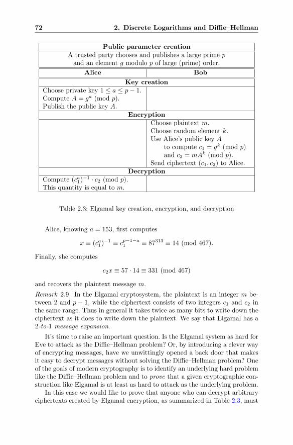
72 2. Discrete Logarithms and Diffie–Hellman
Public parameter creationA trusted party chooses and publishes a large prime pand an element g modulo p of large (prime) order.
Alice Bob
Key creationChoose private key 1 ≤ a ≤ p− 1.Compute A = ga (mod p).Publish the public key A.
EncryptionChoose plaintext m.Choose random element k.Use Alice’s public key A
to compute c1 = gk (mod p)and c2 = mAk (mod p).
Send ciphertext (c1, c2) to Alice.Decryption
Compute (ca1)−1 · c2 (mod p).
This quantity is equal to m.
Table 2.3: Elgamal key creation, encryption, and decryption
Alice, knowing a = 153, first computes
x ≡ (ca1)−1 ≡ cp−1−a
1 ≡ 87313 ≡ 14 (mod 467).
Finally, she computes
c2x ≡ 57 · 14 ≡ 331 (mod 467)
and recovers the plaintext message m.
Remark 2.9. In the Elgamal cryptosystem, the plaintext is an integer m be-tween 2 and p − 1, while the ciphertext consists of two integers c1 and c2 inthe same range. Thus in general it takes twice as many bits to write down theciphertext as it does to write down the plaintext. We say that Elgamal has a2-to-1 message expansion.
It’s time to raise an important question. Is the Elgamal system as hard forEve to attack as the Diffie–Hellman problem? Or, by introducing a clever wayof encrypting messages, have we unwittingly opened a back door that makesit easy to decrypt messages without solving the Diffie–Hellman problem? Oneof the goals of modern cryptography is to identify an underlying hard problemlike the Diffie–Hellman problem and to prove that a given cryptographic con-struction like Elgamal is at least as hard to attack as the underlying problem.
In this case we would like to prove that anyone who can decrypt arbitraryciphertexts created by Elgamal encryption, as summarized in Table 2.3, must
2.4. The Elgamal Public Key Cryptosystem 73
also be able to solve the Diffie–Hellman problem. Specifically, we would liketo prove the following:
Proposition 2.10. Fix a prime p and base g to use for Elgamal encryption.Suppose that Eve has access to an oracle that decrypts arbitrary Elgamal ci-phertexts encrypted using arbitrary Elgamal public keys. Then she can use theoracle to solve the Diffie–Hellman problem described on page 69.
Conversely, if Eve can solve the Diffie–Hellman problem, then she canbreak the Elgamal PKC.
Proof. Rather than giving a compact formal proof, we will be more discursiveand explain how one might approach the problem of using an Elgamal oracle tosolve the Diffie–Hellman problem. Recall that in the Diffie–Hellman problem,Eve is given the two values
A ≡ ga (mod p) and B ≡ gb (mod p),
and she is required to compute the value of gab (mod p). Keep in mind thatshe knows both of the values of A and B, but she does not know either of thevalues a and b.
Now suppose that Eve can consult an Elgamal oracle. This means thatEve can send the oracle a prime p, a base g, a purported public key A, anda purported cipher text (c1, c2). Referring to Table 2.3, the oracle returns toEve the quantity
(ca1)−1 · c2 (mod p).
If Eve wants to solve the Diffie–Hellman problem, what values of c1 and c2should she choose? A little thought shows that c1 = B = gb and c2 = 1 aregood choices, since with this input, the oracle returns (gab)−1 (mod p), andthen Eve can take the inverse modulo p to obtain gab (mod p), thereby solvingthe Diffie–Hellman problem.
But maybe the oracle is smart enough to know that it should never decryptciphertexts having c2 = 1. Eve can still fool the oracle by sending it random-looking ciphertexts as follows. She chooses an arbitrary value for c2 and tellsthe oracle that the public key is A and that the ciphertext is (B, c2). Theoracle returns to her the supposed plaintext m that satisfies
m ≡ (ca1)−1 · c2 ≡ (Ba)−1 · c2 ≡ (gab)−1 · c2 (mod p).
After the oracle tells Eve the value of m, she simply computes
m−1 · c2 ≡ gab (mod p)
to find the value of gab (mod p). It is worth noting that although, with theoracle’s help, Eve has computed gab (mod p), she has done so without knowl-edge of a or b, so she has solved only the Diffie–Hellman problem, not thediscrete logarithm problem.
We leave the proof of the converse, i.e., that a Diffie–Hellman oracle breaksthe Elgamal PKC, as an exercise; see Exercise 2.9.
74 2. Discrete Logarithms and Diffie–Hellman
2.5 An Overview of the Theory of Groups
For readers unfamiliar with the theory of groups, we briefly introduce a fewbasic concepts that should help to place the study of discrete logarithms, bothhere and in Chap. 6, into a broader context.
We’ve just spent some time talking about exponentiation of elements in F∗p.
Since exponentiation is simply repeated multiplication, this seems like a goodplace to start. What we’d like to do is to underline some important propertiesof multiplication in F
∗p and to point out that these attributes appear in many
other contexts.The properties are:
• There is an element 1 ∈ F∗p satisfying 1 · a = a for every a ∈ F
∗p.
• Every a ∈ F∗p has an inverse a−1 ∈ F
∗p satisfying a · a−1 = a−1 · a = 1.
• Multiplication is associative: a · (b · c) = (a · b) · c for all a, b, c ∈ F∗p.
• Multiplication is commutative: a · b = b · a for all a, b ∈ F∗p.
Suppose that instead of multiplication in F∗p, we substitute addition in Fp. We
also use 0 in place of 1 and −a in place of a−1. Then all four properties arestill true:
• 0 + a = a for every a ∈ Fp.
• Every a ∈ Fp has an inverse −a ∈ Fp with a+ (−a) = (−a) + a = 0.
• Addition is associative, a+ (b+ c) = (a+ b) + c for all a, b, c ∈ Fp.
• Addition is commutative, a+ b = b+ a for all a, b ∈ Fp.
Sets and operations that behave similarly to multiplication or addition areso widespread that it is advantageous to abstract the general concept and talkabout all such systems at once. The leads to the notion of a group.
Definition. A group consists of a set G and a rule, which we denote by �,for combining two elements a, b ∈ G to obtain an element a � b ∈ G. Thecomposition operation � is required to have the following three properties:
[Identity Law] There is an e ∈ G such thate � a = a � e = a for every a ∈ G.
[Inverse Law] For every a ∈ G there is a (unique) a−1 ∈ Gsatisfying a � a−1 = a−1 � a = e.
[Associative Law] a � (b � c) = (a � b) � c for all a, b, c ∈ G.If, in addition, composition satisfies the
[Commutative Law] a � b = b � a for all a, b ∈ G,then the group is called a commutative group or an abelian group.
If G has finitely many elements, we say that G is a finite group. The orderof G is the number of elements in G; it is denoted by |G| or #G.
2.5. An Overview of the Theory of Groups 75
Example 2.11. Groups are ubiquitous in mathematics and in the physicalsciences. Here are a few examples, the first two repeating those mentionedearlier:
(a) G = F∗p and � = multiplication. The identity element is e = 1. Propo-
sition 1.21 tells us that inverses exist. Then G is a finite group of or-der p− 1.
(b) G = Z/NZ and � = addition. The identity element is e = 0 and theinverse of a is −a. This G is a finite group of order N .
(c) G = Z and � = addition. The identity element is e = 0 and the inverseof a is −a. This group G is an infinite group.
(d) Note that G = Z and � = multiplication is not a group, since mostelements do not have multiplicative inverses inside Z.
(e) However, G = R∗ and � = multiplication is a group, since all elements
have multiplicative inverses inside R∗.
(f) An example of a noncommutative group is
G =
{(a bc d
): a, b, c, d ∈ R and ad− bc �= 0
}
with operation � = matrix multiplication. The identity element ise = ( 1 0
0 1 ) and the inverse is given by the familiar formula
(a bc d
)−1
=
(d
ad−bc−b
ad−bc−cad−bc
aad−bc
).
Notice that G is noncommutative, since for example, ( 1 10 1 ) (
1 11 0 ) is not
equal to ( 1 11 0 ) (
1 10 1 ).
(g) More generally, we can use matrices of any size. This gives the generallinear group
GLn(R) ={n-by-n matrices A with real coefficients and det(A) �= 0
}
and operation � = matrix multiplication. We can form other groupsby replacing R with some other field, for example, the finite field Fp.(See Exercise 2.15.) The group GLn(Fp) is clearly a finite group, butcomputing its order is an interesting exercise.
Let g be an element of a group G and let x be a positive integer. Then gx
means that we apply the group operation to x copies of the element g,
gx = g � g � g � · · · � g︸ ︷︷ ︸
x repetitions
.
76 2. Discrete Logarithms and Diffie–Hellman
For example, exponentiation gx in the group F∗p has the usual meaning, multi-
ply x copies of g. But “exponentiation” gx in the group Z/NZ means to add xcopies of g. Admittedly, it is more common to write the quantity “add x copiesof g” as x ·g, but this is just a matter of notation. The key concept underlyingexponentiation in a group is repeated application of the group operation toan element of the group.
It is also convenient to give a meaning to gx when x is not positive. So if xis a negative integer, we define gx to be (g−1)|x|. For x = 0, we set g0 = e,the identity element of G.
We now introduce a key concept used in the study of groups.
Definition. Let G be a group and let a ∈ G be an element of the group.Suppose there exists a positive integer d with the property that ad = e. Thesmallest such d is called the order of a. If there is no such d, then a is said tohave infinite order.
We next prove two propositions describing important properties of theorders of group elements. These are generalizations of Theorem 1.24 (Fermat’slittle theorem) and Proposition 1.29, which deal with the group G = F
∗p. The
proofs are essentially the same.
Proposition 2.12. Let G be a finite group. Then every element of G hasfinite order. Further, if a ∈ G has order d and if ak = e, then d | k.
Proof. Since G is finite, the sequence
a, a2, a3, a4, . . .
must eventually contain a repetition. That is, there exist positive integers iand j with j < i such that ai = aj . Multiplying both sides by a−j and applyingthe group laws leads to ai−j = e. Since i− j > 0, this proves that some powerof a is equal to e. We let d be the smallest positive exponent satisfying ad = e.
Now suppose that k ≥ d also satisfies ak = e. We divide k by d to obtain
k = dq + r with 0 ≤ r < d.
Using the fact that ak = ad = e, we find that
e = ak = adq+r = (ad)q � ar = eq � ar = ar.
But d is the smallest positive power of a that is equal to e, so we musthave r = 0. Therefore k = dq, so d | k.
Proposition 2.13 (Lagrange’s Theorem). Let G be a finite group and leta ∈ G. Then the order of a divides the order G.
More precisely, let n = |G| be the order of G and let d be the order of a,i.e., ad is the smallest positive power of a that is equal to e. Then
an = e and d | n.
2.6. How Hard Is the Discrete Logarithm Problem? 77
Proof. We give a simple proof in the case that G is commutative. For a proofin the general case, see any basic algebra textbook, for example [40, §3.2]or [45, §2.3].
Since G is finite, we can list its elements as
G = {g1, g2, . . . , gn}.
We now multiply each element of G by a to obtain a new set, which we call Sa,
Sa = {a � g1, a � g2, . . . , a � gn}.
We claim that the elements of Sa are distinct. To see this, suppose thata � gi = a � gj . Multiplying both sides by a−1 yields gi = gj .
6 Thus Sa
contains n distinct elements, which is the same as the number of elementsof G. Therefore Sa = G, so if we multiply together all of the elements of Sa,we get the same answer as multiplying together all of the elements of G. (Notethat we are using the assumption that G is commutative.) Thus
(a � g1) � (a � g2) � · · · � (a � gn) = g1 � g2 � · · · � gn.
We can rearrange the order of the product on the left-hand side (again usingthe commutativity) to obtain
an � g1 � g2 � · · · � gn = g1 � g2 � · · · � gn.
Now multiplying by (g1 � g2 � · · · � gn)−1 yields an = e, which proves thefirst statement, and then the divisibility of n by d follows immediately fromProposition 2.12.
2.6 How Hard Is the Discrete LogarithmProblem?
Given a group G and two elements g, h ∈ G, the discrete logarithm prob-lem asks for an exponent x such that gx = h. What does it mean to talkabout the difficulty of this problem? How can we quantify “hard”? A naturalmeasure of hardness is the approximate number of operations necessary fora person or a computer to solve the problem using the most efficient methodcurrently known. For example, we can solve the discrete logarithm problemby computing the list of values g, g2, g3, . . . until we find one that is equalto h. If g has order n, then this algorithm is guaranteed to find the solution
6We are being somewhat informal here, as is usually done when one is working withgroups. Here is a more formal proof. We are given that a�gi = a�gj . We use this assumptionand the group law axioms to computegi = e � gi = (a−1 � a) � gi = a−1 � (a � gi) = a−1 � (a � gj) = (a−1 � a) � gj = e � gj = gj .
78 2. Discrete Logarithms and Diffie–Hellman
in at most n multiplications, but if n is large, say n > 280, then it is not apractical algorithm with the computing power available today.
Alternatively, we might try choosing random values of x, compute gx, andcheck if gx = h. Using the fast exponentiation method described in Sect. 1.3.2,it takes a small multiple of log2(x) modular multiplications to compute gx.If n and x are k-bit numbers, that is, they are each approximately 2k, then thistrial-and-error approach requires about k·2k multiplications. If we are workingin the group F
∗p and if we treat modular addition as our basic operation,
then modular multiplication of two k-bit numbers takes (approximately) k2
basic operations, so solving the DLP by trial-and-error takes a small multipleof k2 · 2k basic operations.
We are being somewhat imprecise when we talk about “small multiples”of 2k or k · 2k or k2 · 2k. This is because when we want to know whether acomputation is feasible, numbers such as 3 · 2k and 10 · 2k and 100 · 2k meanpretty much the same thing if k is large. The important property is thatthe constant multiple is fixed as k increases. Order notation was inventedto make these ideas precise.7 It is prevalent throughout mathematics andcomputer science and provides a handy way to get a grip on the magnitudeof quantities.
Definition (Order Notation). Let f(x) and g(x) be functions of x takingvalues that are positive. We say that “f is big-O of g” and write
f(x) = O(g(x)
)
if there are positive constants c and C such that
f(x) ≤ cg(x) for all x ≥ C.
In particular, we write f(x) = O(1) if f(x) is bounded for all x ≥ C.
The next proposition gives a method that can sometimes be used to provethat f(x) = O
(g(x)
).
Proposition 2.14. If the limit
limx→∞
f(x)
g(x)
exists (and is finite), then f(x) = O(g(x)
).
Proof. Let L be the limit. By definition of limit, for any ε > 0 there is aconstant Cε such that
∣∣∣∣f(x)
g(x)− L∣∣∣∣ < ε for all x > Cε.
7Although we use the same word for the order of a finite group and the order of growthof a function, they are two different concepts. Make sure that you don’t confuse them.
2.6. How Hard Is the Discrete Logarithm Problem? 79
In particular, taking ε = 1, we find that
f(x)
g(x)< L+ 1 for all x > C1.
Hence by definition, f(x) = O(g(x)
)with c = L+ 1 and C = C1.
Example 2.15. We have 2x3 − 3x2 + 7 = O(x3), since
limx→∞
2x3 − 3x2 + 7
x3= 2.
Similarly, we have x2 = O(2x), since
limx→∞
x2
2x= 0.
(If you don’t know the value of this limit, use L’Hopital’s rule twice.)However, note that we may have f(x) = O
(g(x)
)even if the limit of
f(x)/g(x) does not exist. For example, the limit
limx→∞
(x+ 2) cos2(x)
x
does not exist, but
(x+ 2) cos2(x) = O(x), since (x+ 2) cos2(x) ≤ x+ 2 ≤ 2x for all x ≥ 2.
Example 2.16. Here are a few more examples of big-O notation. We leave theverification as an exercise.
(a) x2 +√x = O
(x2). (d) (ln k)375 = O
(k0.001
).
(b) 5 + 6x2 − 37x5 = O(x5). (e) k22k = O
(e2k).
(c) k300 = O(2k). (f) N102N = O
(eN).
Order notation allows us to define several fundamental concepts that areused to get a rough handle on the computational complexity of mathematicalproblems.
Definition. Suppose that we are trying to solve a certain type of mathemat-ical problem, where the input to the problem is a number whose size mayvary. As an example, consider the Integer Factorization Problem, whose inputis a number N and whose output is a prime factor of N . We are interestedin knowing how long it takes to solve the problem in terms of the size of theinput. Typically, one measures the size of the input by its number of bits,since that is how much storage it takes to record the input.
Suppose that there is a constant A ≥ 0, independent of the size of theinput, such that if the input is O(k) bits long, then it takes O(kA) steps tosolve the problem. Then the problem is said to be solvable in polynomial time.
80 2. Discrete Logarithms and Diffie–Hellman
If we can take A = 1, then the problem is solvable in linear time, and if we cantake A = 2, then the problem is solvable in quadratic time. Polynomial-timealgorithms are considered to be fast algorithms.
On the other hand, if there is a constant c > 0 such that for inputs ofsize O(k) bits, there is an algorithm to solve the problem in O
(eck)steps,
then the problem is solvable in exponential time. Exponential-time algorithmsare considered to be slow algorithms.
Intermediate between polynomial-time algorithms and exponential-timealgorithms are subexponential-time algorithms. These have the property thatfor every ε > 0, they solve the problem in Oε
(eεk)steps. This notation
means that the constants c and C appearing in the definition of order no-tation are allowed to depend on ε. For example, in Chap. 3 we will studya subexponential-time algorithm for the integer factorization problem whoserunning time is O
(ec
√k log k
)steps.
As a general rule of thumb in cryptography, problems solvable in polyno-mial time are considered to be “easy” and problems that require exponentialtime are viewed as “hard,” with subexponential time lying somewhere in be-tween. However, bear in mind that these are asymptotic descriptions that areapplicable only as the variables become very large. Depending on the big-Oconstants and on the size of the input, an exponential problem may be easierthan a polynomial problem. We illustrate these general concepts by consider-ing the discrete logarithm problem in various groups.
Example 2.17. We start with our original discrete logarithm problem gx = hin G = F
∗p. If the prime p is chosen between 2k and 2k+1, then g, h, and p
all require at most k bits, so the problem can be stated in O(k)-bits. (Noticethat O(k) is the same as O(log2 p).)
If we try to solve the DLP using the trial-and-error method mentionedearlier, then it takes O(p) steps to solve the problem. Since O(p) = O(2k),this algorithm takes exponential time. (If we consider instead multiplicationor addition to be the basic operation, then the algorithm takes O(k · 2k)or O(k2 · 2k) steps, but these distinctions are irrelevant; the running time isstill exponential, since for example it is O(3k).)
However, there are faster ways to solve the DLP in F∗p, some of which
are very fast but work only for some primes, while others are less fast, butwork for all primes. For example, the Pohlig–Hellman algorithm described inSect. 2.9 shows that if p− 1 factors entirely into a product of small primes,then the DLP is quite easy. For arbitrary primes, the algorithm described inSect. 2.7 solves the DLP in O(
√p log p) steps, which is much faster than O(p),
but still exponential. Even better is the index calculus algorithm described in
Sect. 3.8. The index calculus solves the DLP in O(ec√
(log p)(log log p)) steps, soit is a subexponential algorithm.
Example 2.18. We next consider the DLP in the group G = Fp, where nowthe group operation is addition. The DLP in this context asks for a solution xto the congruence
2.7. A Collision Algorithm for the DLP 81
x · g ≡ h (mod p),
where g and h are given elements of Z/pZ. As described in Sect. 1.3, wecan solve this congruence using the extended Euclidean algorithm (Theo-rem 1.11) to compute g−1 (mod p) and setting x ≡ g−1 · h (mod p). Thistakes O(log p) steps (see Remark 1.15), so there is a linear-time algorithm tosolve the DLP in the additive group Fp. This is a very fast algorithm, so theDLP in Fp with addition is not a good candidate for use as a one-way functionin cryptography.
This is an important lesson to learn. The discrete logarithm problems indifferent groups may display different levels of difficulty for their solution.Thus the DLP in Fp with addition has a linear-time solution, while the bestknown general algorithm to solve the DLP in F
∗p with multiplication is subex-
ponential. In Chap. 6 we discuss another sort of group called an elliptic curve.The discrete logarithm problem for elliptic curves is believed to be even moredifficult than the DLP for F∗
p. In particular, if the elliptic curve group is cho-sen carefully and has N elements, then the best known algorithm to solve theDLP requires O(
√N) steps. Thus it currently takes exponential time to solve
the elliptic curve discrete logarithm problem (ECDLP).
2.7 A Collision Algorithm for the DLP
In this section we describe a discrete logarithm algorithm due to Shanks. Itis an example of a collision, or meet-in-the-middle, algorithm. Algorithms ofthis type are discussed in more detail in Sects. 5.4 and 5.5. Shanks’s algorithmworks in any group, not just F∗
p, and the proof that it works is no more difficultfor arbitrary groups, so we state and prove it in full generality.
We begin by recalling the running time of the trivial brute-force algorithmto solve the DLP.
Proposition 2.19 (Trivial Bound for DLP). Let G be a group and let g ∈ Gbe an element of order N . (Recall that this means that gN = e and thatno smaller positive power of g is equal to the identity element e.) Then thediscrete logarithm problem
gx = h (2.2)
can be solved in O(N) steps and O(1) storage, where each step consists ofmultiplication by g.
Proof. We simply compute g, g2, g3, . . ., where each successive value is ob-tained by multiplying the previous value by g, so we only need to store twovalues at a time. If a solution to gx = h exists, then h will appear before wereach gN .
Remark 2.20. If we work in F∗p, then each computation of gx (mod p) re-
quires O((log p)k) computer operations, where the constant k and the implied
82 2. Discrete Logarithms and Diffie–Hellman
big-O constant depend on the computer and the algorithm used for modularmultiplication. Then the total number of computer steps, or running time,is O(N(log p)k). In general, the factor contributed by the O((log p)k) is neg-ligible, so we will suppress it and simply refer to the running time as O(N).
The idea behind a collision algorithm is to make two lists and look foran element that appears in both lists. For the discrete logarithm problemdescribed in Proposition 2.19, the running time of a collision algorithm is alittle more than O(
√N ) steps, which is a huge savings over O(N) if N is
large.
Proposition 2.21 (Shanks’s Babystep–Giantstep Algorithm). Let G be agroup and let g ∈ G be an element of order N ≥ 2. The following algo-rithm solves the discrete logarithm problem gx = h in O(
√N · logN) steps
using O(√N) storage.
(1) Let n = 1 + �√N �, so in particular, n >
√N .
(2) Create two lists,
List 1: e, g, g2, g3, . . . , gn,
List 2: h, h · g−n, h · g−2n, h · g−3n, . . . , h · g−n2
.
(3) Find a match between the two lists, say gi = hg−jn.
(4) Then x = i+ jn is a solution to gx = h.
Proof. We begin with a couple of observations. First, when creating List 2,we start by computing the quantity u = g−n and then compile List 2 bycomputing h, h · u, h · u2, . . . , h · un. Thus creating the two lists takes approx-imately 2n multiplications.8 Second, assuming that a match exists, we canfind a match in a small multiple of n log(n) steps using standard sorting andsearching algorithms, so Step (3) takes O(n log n) steps. Hence the total run-ning time for the algorithm is O(n log n) = O(
√N logN). For this last step
we have used the fact that n ≈√N , so
n log n ≈√N log
√N =
1
2
√N logN.
Third, the lists in Step (2) have length n, so require O(√N) storage.
In order to prove that the algorithm works, we must show that Lists 1and 2 always have a match. To see this, let x be the unknown solution togx = h and write x as
x = nq + r with 0 ≤ r < n.
8Multiplication by g is a “baby step” and multiplication by u = g−n is a “giant step,”whence the name of the algorithm.
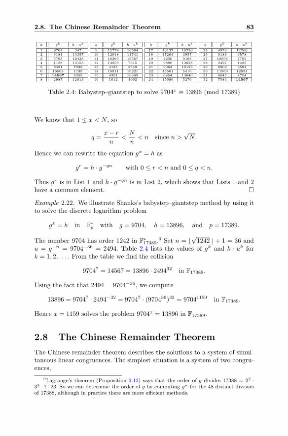
2.8. The Chinese Remainder Theorem 83
k gk h · uk
1 9704 347
2 6181 13357
3 5763 12423
4 1128 13153
5 8431 7928
6 16568 1139
7 14567 6259
8 2987 12013
k gk h · uk
9 15774 16564
10 12918 11741
11 16360 16367
12 13259 7315
13 4125 2549
14 16911 10221
15 4351 16289
16 1612 4062
k gk h · uk
17 10137 10230
18 17264 3957
19 4230 9195
20 9880 13628
21 9963 10126
22 15501 5416
23 6854 13640
24 15680 5276
k gk h · uk
25 4970 12260
26 9183 6578
27 10596 7705
28 2427 1425
29 6902 6594
30 11969 12831
31 6045 4754
32 7583 14567
Table 2.4: Babystep–giantstep to solve 9704x ≡ 13896 (mod 17389)
We know that 1 ≤ x < N , so
q =x− rn
<N
n< n since n >
√N .
Hence we can rewrite the equation gx = h as
gr = h · g−qn with 0 ≤ r < n and 0 ≤ q < n.
Thus gr is in List 1 and h · g−qn is in List 2, which shows that Lists 1 and 2have a common element.
Example 2.22. We illustrate Shanks’s babystep–giantstep method by using itto solve the discrete logarithm problem
gx = h in F∗p with g = 9704, h = 13896, and p = 17389.
The number 9704 has order 1242 in F∗17389.
9 Set n = �√1242 � + 1 = 36 and
u = g−n = 9704−36 = 2494. Table 2.4 lists the values of gk and h · uk fork = 1, 2, . . . . From the table we find the collision
97047 = 14567 = 13896 · 249432 in F17389.
Using the fact that 2494 = 9704−36, we compute
13896 = 97047 · 2494−32 = 97047 · (970436)32 = 97041159 in F17389.
Hence x = 1159 solves the problem 9704x = 13896 in F17389.
2.8 The Chinese Remainder Theorem
The Chinese remainder theorem describes the solutions to a system of simul-taneous linear congruences. The simplest situation is a system of two congru-ences,
9Lagrange’s theorem (Proposition 2.13) says that the order of g divides 17388 = 22 ·33 · 7 · 23. So we can determine the order of g by computing gn for the 48 distinct divisorsof 17388, although in practice there are more efficient methods.
84 2. Discrete Logarithms and Diffie–Hellman
x ≡ a (mod m) and x ≡ b (mod n), (2.3)
with gcd(m,n) = 1, in which case the Chinese remainder theorem says thatthere is a unique solution modulo mn.
The first recorded instance of a problem of this type appears in a Chinesemathematical work from the late third or early fourth century. It actuallydeals with the harder problem of three simultaneous congruences.
We have a number of things, but we do not know exactly howmany. If we count them by threes, we have two left over. If wecount them by fives, we have three left over. If we count them bysevens, we have two left over. How many things are there? [Sun TzuSuan Ching (Master Sun’s Mathematical Manual) circa 300 AD,volume 3, problem 26.]
The Chinese remainder theorem and its generalizations have many appli-cations in number theory and other areas of mathematics. In Sect. 2.9 we willsee how it can be used to solve certain instances of the discrete logarithmproblem. We begin with an example in which we solve two simultaneous con-gruences. As you read this example, notice that it is not merely an abstractstatement that a solution exists. The method that we describe is really analgorithm that allows us to find the solution.
Example 2.23. We look for an integer x that simultaneously solves both ofthe congruences
x ≡ 1 (mod 5) and x ≡ 9 (mod 11). (2.4)
The first congruence tells us that x ≡ 1 (mod 5), so the full set of solutionsto the first congruence is the collection of integers
x = 1 + 5y, y ∈ Z. (2.5)
Substituting (2.5) into the second congruence in (2.4) gives
1 + 5y ≡ 9 (mod 11), and hence 5y ≡ 8 (mod 11). (2.6)
We solve for y by multiplying both sides of (2.6) by the inverse of 5 mod-ulo 11. This inverse exists because gcd(5, 11) = 1 and can be computed usingthe procedure described in Proposition 1.13 (see also Remark 1.15). How-ever, in this case the modulus is so small that we find it by trial and error;thus 5 · 9 = 45 ≡ 1 (mod 11).
In any case, multiplying both sides of (2.6) by 9 yields
y ≡ 9 · 8 ≡ 72 ≡ 6 (mod 11).
Finally, substituting this value of y into (2.5) gives the solution
x = 1 + 5 · 6 = 31
to the original problem.
2.8. The Chinese Remainder Theorem 85
The procedure outlined in Example 2.23 can be used to derive a generalformula for the solution of two simultaneous congruences (see Exercise 2.20),but it is much better to learn the method, rather than memorizing a for-mula. This is especially true because the Chinese remainder theorem appliesto systems of arbitrarily many simultaneous congruences.
Theorem 2.24 (Chinese Remainder Theorem). Let m1,m2, . . . ,mk be a col-lection of pairwise relatively prime integers. This means that
gcd(mi,mj) = 1 for all i �= j.
Let a1, a2, . . . , ak be arbitrary integers. Then the system of simultaneous con-gruences
x ≡ a1 (mod m1), x ≡ a2 (mod m2), . . . , x ≡ ak (mod mk) (2.7)
has a solution x = c. Further, if x = c and x = c′ are both solutions, then
c ≡ c′ (mod m1m2 · · ·mk). (2.8)
Proof. Suppose that for some value of i we have already managed to find asolution x = ci to the first i simultaneous congruences,
x ≡ a1 (mod m1), x ≡ a2 (mod m2), . . . , x ≡ ai (mod mi). (2.9)
For example, if i = 1, then c1 = a1 works. We are going to explain how tofind a solution to one more congruence,
x ≡ a1 (mod m1), x ≡ a2 (mod m2), . . . , x ≡ ai+1 (mod mi+1).
The idea is to look for a solution having the form
x = ci +m1m2 · · ·miy.
Notice that this value of x still satisfies all of the congruences (2.9), so weneed merely choose y so that it also satisfies x ≡ ai+1 (mod mi+1). In otherwords, we need to find a value of y satisfying
ci +m1m2 · · ·miy ≡ ai+1 (mod mi+1).
Proposition 1.13(b) and the fact that gcd(mi+1,m1m2 · · ·mi) = 1 imply thatwe can always do this. This completes the proof of the existence of a solution.We leave to you the task of proving that different solutions satisfy (2.8); seeExercise 2.21.
The proof of the Chinese remainder theorem (Theorem 2.24) is easily con-verted into an algorithm for finding the solution to a system of simultaneouscongruences. An example suffices to illustrate the general method.
86 2. Discrete Logarithms and Diffie–Hellman
Example 2.25. We solve the three simultaneous congruences
x ≡ 2 (mod 3), x ≡ 3 (mod 7), x ≡ 4 (mod 16). (2.10)
The Chinese remainder theorem says that there is a unique solution mod-ulo 336, since 336 = 3 · 7 · 16. We start with the solution x = 2 to the firstcongruence x ≡ 2 (mod 3). We use it to form the general solution x = 2 + 3yand substitute it into the second congruence to get
2 + 3y ≡ 3 (mod 7).
This simplifies to 3y ≡ 1 (mod 7), and we multiply both sides by 5 (since 5 isthe inverse of 3 modulo 7) to get y ≡ 5 (mod 7). This gives the value
x = 2 + 3y = 2 + 3 · 5 = 17
as a solution to the first two congruences in (2.10).The general solution to the first two congruences is thus x = 17 + 21z. We
substitute this into the third congruence to obtain
17 + 21z ≡ 4 (mod 16).
This simplifies to 5z ≡ 3 (mod 16). We multiply by 13, which is the inverseof 5 modulo 16, to obtain
z ≡ 3 · 13 ≡ 39 ≡ 7 (mod 16).
Finally, we substitute this into x = 17 + 21z to get the solution
x = 17 + 21 · 7 = 164.
All other solutions are obtained by adding and subtracting multiples of 336to this particular solution.
2.8.1 Solving Congruences with Composite Moduli
It is usually easiest to solve a congruence with a composite modulus by firstsolving several congruences modulo primes (or prime powers) and then fittingtogether the solutions using the Chinese remainder theorem. We illustratethe principle in this section by discussing the problem of finding square rootsmodulo m. It turns out that it is relatively easy to compute square rootsmodulo a prime. Indeed, for primes congruent to 3 modulo 4, it is extremelyeasy to find square roots, as shown by the following proposition.
Proposition 2.26. Let p be a prime satisfying p ≡ 3 (mod 4). Let a be aninteger such that the congruence x2 ≡ a (mod p) has a solution, i.e., suchthat a has a square root modulo p. Then
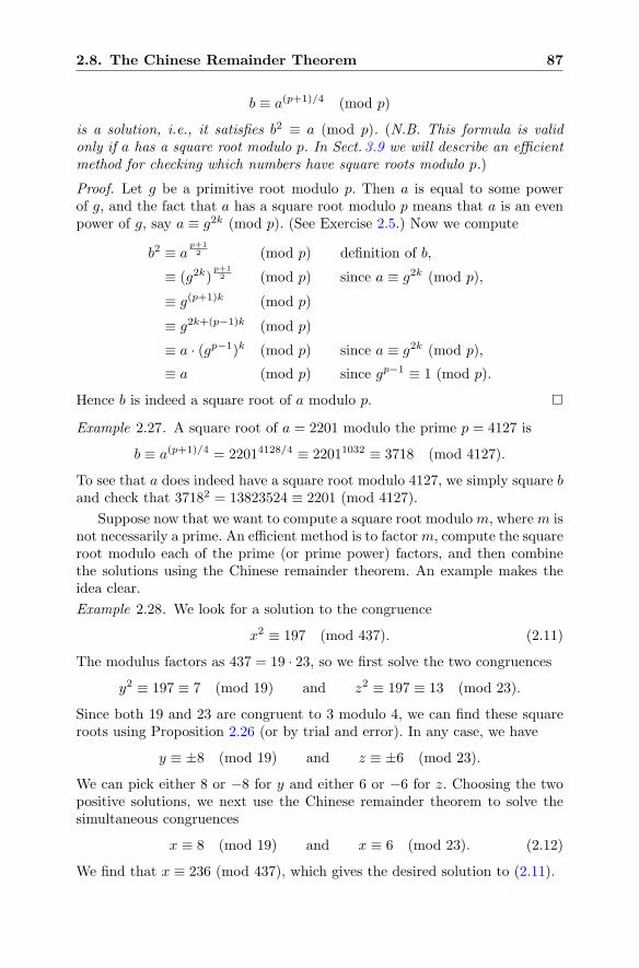
2.8. The Chinese Remainder Theorem 87
b ≡ a(p+1)/4 (mod p)
is a solution, i.e., it satisfies b2 ≡ a (mod p). (N.B. This formula is validonly if a has a square root modulo p. In Sect. 3.9 we will describe an efficientmethod for checking which numbers have square roots modulo p.)
Proof. Let g be a primitive root modulo p. Then a is equal to some powerof g, and the fact that a has a square root modulo p means that a is an evenpower of g, say a ≡ g2k (mod p). (See Exercise 2.5.) Now we compute
b2 ≡ ap+12 (mod p) definition of b,
≡ (g2k)p+12 (mod p) since a ≡ g2k (mod p),
≡ g(p+1)k (mod p)
≡ g2k+(p−1)k (mod p)
≡ a · (gp−1)k (mod p) since a ≡ g2k (mod p),
≡ a (mod p) since gp−1 ≡ 1 (mod p).
Hence b is indeed a square root of a modulo p.
Example 2.27. A square root of a = 2201 modulo the prime p = 4127 is
b ≡ a(p+1)/4 = 22014128/4 ≡ 22011032 ≡ 3718 (mod 4127).
To see that a does indeed have a square root modulo 4127, we simply square band check that 37182 = 13823524 ≡ 2201 (mod 4127).
Suppose now that we want to compute a square root modulom, wherem isnot necessarily a prime. An efficient method is to factorm, compute the squareroot modulo each of the prime (or prime power) factors, and then combinethe solutions using the Chinese remainder theorem. An example makes theidea clear.
Example 2.28. We look for a solution to the congruence
x2 ≡ 197 (mod 437). (2.11)
The modulus factors as 437 = 19 · 23, so we first solve the two congruences
y2 ≡ 197 ≡ 7 (mod 19) and z2 ≡ 197 ≡ 13 (mod 23).
Since both 19 and 23 are congruent to 3 modulo 4, we can find these squareroots using Proposition 2.26 (or by trial and error). In any case, we have
y ≡ ±8 (mod 19) and z ≡ ±6 (mod 23).
We can pick either 8 or −8 for y and either 6 or −6 for z. Choosing the twopositive solutions, we next use the Chinese remainder theorem to solve thesimultaneous congruences
x ≡ 8 (mod 19) and x ≡ 6 (mod 23). (2.12)
We find that x ≡ 236 (mod 437), which gives the desired solution to (2.11).
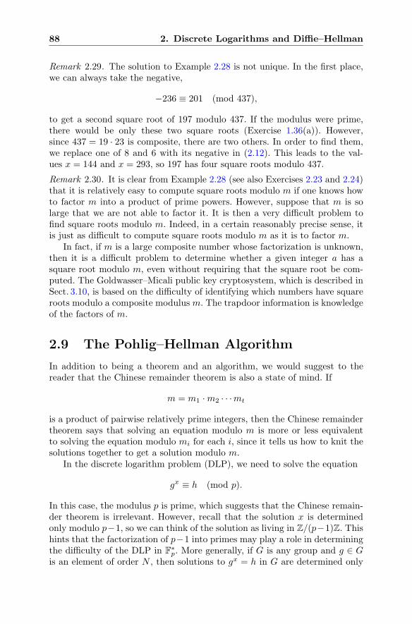
88 2. Discrete Logarithms and Diffie–Hellman
Remark 2.29. The solution to Example 2.28 is not unique. In the first place,we can always take the negative,
−236 ≡ 201 (mod 437),
to get a second square root of 197 modulo 437. If the modulus were prime,there would be only these two square roots (Exercise 1.36(a)). However,since 437 = 19 · 23 is composite, there are two others. In order to find them,we replace one of 8 and 6 with its negative in (2.12). This leads to the val-ues x = 144 and x = 293, so 197 has four square roots modulo 437.
Remark 2.30. It is clear from Example 2.28 (see also Exercises 2.23 and 2.24)that it is relatively easy to compute square roots modulo m if one knows howto factor m into a product of prime powers. However, suppose that m is solarge that we are not able to factor it. It is then a very difficult problem tofind square roots modulo m. Indeed, in a certain reasonably precise sense, itis just as difficult to compute square roots modulo m as it is to factor m.
In fact, if m is a large composite number whose factorization is unknown,then it is a difficult problem to determine whether a given integer a has asquare root modulo m, even without requiring that the square root be com-puted. The Goldwasser–Micali public key cryptosystem, which is described inSect. 3.10, is based on the difficulty of identifying which numbers have squareroots modulo a composite modulusm. The trapdoor information is knowledgeof the factors of m.
2.9 The Pohlig–Hellman Algorithm
In addition to being a theorem and an algorithm, we would suggest to thereader that the Chinese remainder theorem is also a state of mind. If
m = m1 ·m2 · · ·mt
is a product of pairwise relatively prime integers, then the Chinese remaindertheorem says that solving an equation modulo m is more or less equivalentto solving the equation modulo mi for each i, since it tells us how to knit thesolutions together to get a solution modulo m.
In the discrete logarithm problem (DLP), we need to solve the equation
gx ≡ h (mod p).
In this case, the modulus p is prime, which suggests that the Chinese remain-der theorem is irrelevant. However, recall that the solution x is determinedonly modulo p−1, so we can think of the solution as living in Z/(p−1)Z. Thishints that the factorization of p−1 into primes may play a role in determiningthe difficulty of the DLP in F
∗p. More generally, if G is any group and g ∈ G
is an element of order N , then solutions to gx = h in G are determined only
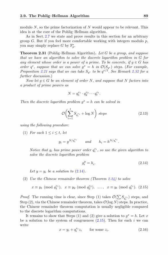
2.9. The Pohlig–Hellman Algorithm 89
modulo N , so the prime factorization of N would appear to be relevant. Thisidea is at the core of the Pohlig–Hellman algorithm.
As in Sect. 2.7 we state and prove results in this section for an arbitrarygroup G. But if you feel more comfortable working with integers modulo p,you may simply replace G by F
∗p.
Theorem 2.31 (Pohlig–Hellman Algorithm). Let G be a group, and supposethat we have an algorithm to solve the discrete logarithm problem in G forany element whose order is a power of a prime. To be concrete, if g ∈ G hasorder qe, suppose that we can solve gx = h in O(Sqe) steps. (For example,Proposition 2.21 says that we can take Sqe to be qe/2. See Remark 2.32 for afurther discussion.)
Now let g ∈ G be an element of order N , and suppose that N factors intoa product of prime powers as
N = qe11 · qe22 · · · qett .
Then the discrete logarithm problem gx = h can be solved in
O( t∑
i=1
Sqeii
+ logN
)steps (2.13)
using the following procedure:
(1) For each 1 ≤ i ≤ t, let
gi = gN/qeii and hi = hN/q
eii .
Notice that gi has prime power order qeii , so use the given algorithm tosolve the discrete logarithm problem
gyi = hi. (2.14)
Let y = yi be a solution to (2.14).
(2) Use the Chinese remainder theorem (Theorem 2.24) to solve
x ≡ y1 (mod qe11 ), x ≡ y2 (mod qe22 ), . . . , x ≡ yt (mod qett ). (2.15)
Proof. The running time is clear, since Step (1) takes O(∑Sq
eii) steps, and
Step (2), via the Chinese remainder theorem, takesO(logN) steps. In practice,the Chinese remainder theorem computation is usually negligible comparedto the discrete logarithm computations.
It remains to show that Steps (1) and (2) give a solution to gx = h. Let xbe a solution to the system of congruences (2.15). Then for each i we canwrite
x = yi + qeii zi for some zi. (2.16)
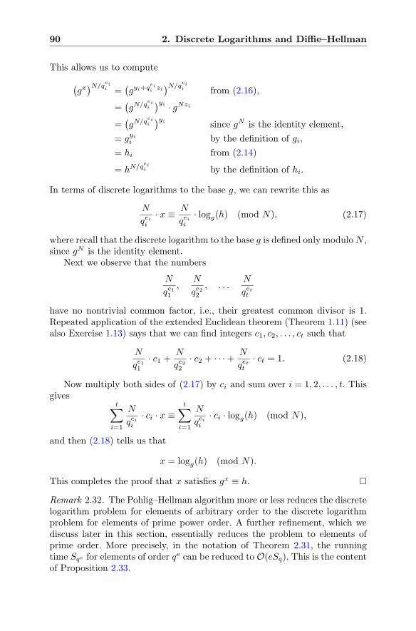
90 2. Discrete Logarithms and Diffie–Hellman
This allows us to compute
(gx)N/q
eii =
(gyi+q
eii zi)N/q
eii from (2.16),
=(gN/q
eii
)yi · gNzi
=(gN/q
eii
)yisince gN is the identity element,
= gyi
i by the definition of gi,
= hi from (2.14)
= hN/qeii by the definition of hi.
In terms of discrete logarithms to the base g, we can rewrite this as
N
qeii· x ≡ N
qeii· logg(h) (mod N), (2.17)
where recall that the discrete logarithm to the base g is defined only moduloN ,since gN is the identity element.
Next we observe that the numbers
N
qe11,
N
qe22, . . .
N
qett
have no nontrivial common factor, i.e., their greatest common divisor is 1.Repeated application of the extended Euclidean theorem (Theorem 1.11) (seealso Exercise 1.13) says that we can find integers c1, c2, . . . , ct such that
N
qe11· c1 +
N
qe22· c2 + · · ·+
N
qett· ct = 1. (2.18)
Now multiply both sides of (2.17) by ci and sum over i = 1, 2, . . . , t. Thisgives
t∑
i=1
N
qeii· ci · x ≡
t∑
i=1
N
qeii· ci · logg(h) (mod N),
and then (2.18) tells us that
x = logg(h) (mod N).
This completes the proof that x satisfies gx ≡ h.
Remark 2.32. The Pohlig–Hellman algorithm more or less reduces the discretelogarithm problem for elements of arbitrary order to the discrete logarithmproblem for elements of prime power order. A further refinement, which wediscuss later in this section, essentially reduces the problem to elements ofprime order. More precisely, in the notation of Theorem 2.31, the runningtime Sqe for elements of order qe can be reduced to O(eSq). This is the contentof Proposition 2.33.
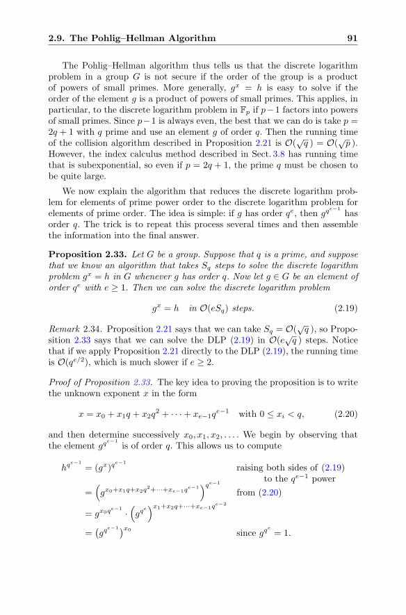
2.9. The Pohlig–Hellman Algorithm 91
The Pohlig–Hellman algorithm thus tells us that the discrete logarithmproblem in a group G is not secure if the order of the group is a productof powers of small primes. More generally, gx = h is easy to solve if theorder of the element g is a product of powers of small primes. This applies, inparticular, to the discrete logarithm problem in Fp if p−1 factors into powersof small primes. Since p−1 is always even, the best that we can do is take p =2q + 1 with q prime and use an element g of order q. Then the running timeof the collision algorithm described in Proposition 2.21 is O(
√q ) = O(
√p ).
However, the index calculus method described in Sect. 3.8 has running timethat is subexponential, so even if p = 2q + 1, the prime q must be chosen tobe quite large.
We now explain the algorithm that reduces the discrete logarithm prob-lem for elements of prime power order to the discrete logarithm problem forelements of prime order. The idea is simple: if g has order qe, then gq
e−1
hasorder q. The trick is to repeat this process several times and then assemblethe information into the final answer.
Proposition 2.33. Let G be a group. Suppose that q is a prime, and supposethat we know an algorithm that takes Sq steps to solve the discrete logarithmproblem gx = h in G whenever g has order q. Now let g ∈ G be an element oforder qe with e ≥ 1. Then we can solve the discrete logarithm problem
gx = h in O(eSq) steps. (2.19)
Remark 2.34. Proposition 2.21 says that we can take Sq = O(√q ), so Propo-
sition 2.33 says that we can solve the DLP (2.19) in O(e√q ) steps. Notice
that if we apply Proposition 2.21 directly to the DLP (2.19), the running timeis O(qe/2), which is much slower if e ≥ 2.
Proof of Proposition 2.33. The key idea to proving the proposition is to writethe unknown exponent x in the form
x = x0 + x1q + x2q2 + · · ·+ xe−1q
e−1 with 0 ≤ xi < q, (2.20)
and then determine successively x0, x1, x2, . . . . We begin by observing thatthe element gq
e−1
is of order q. This allows us to compute
hqe−1
= (gx)qe−1
raising both sides of (2.19)to the qe−1 power
=(gx0+x1q+x2q
2+···+xe−1qe−1)qe−1
from (2.20)
= gx0qe−1 ·
(gq
e)x1+x2q+···+xe−1q
e−2
=(gq
e−1)x0since gq
e
= 1.
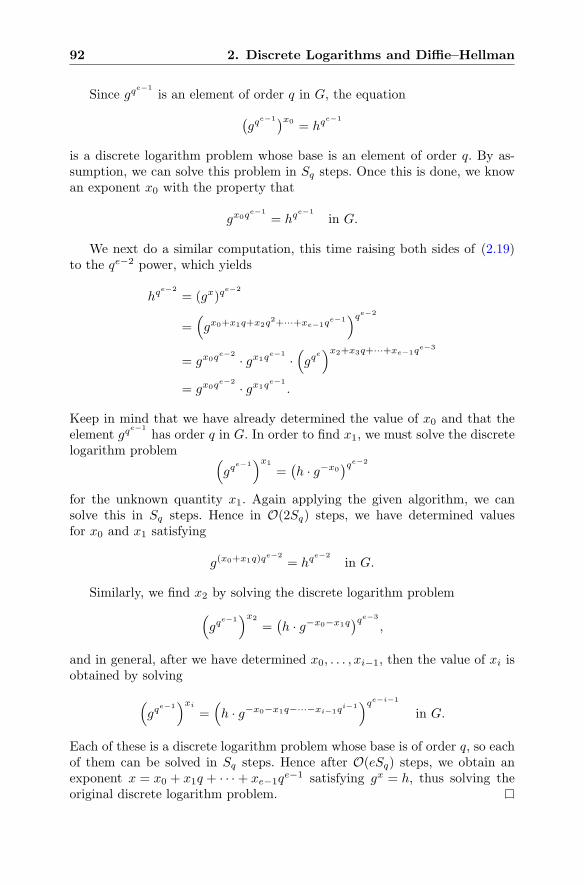
92 2. Discrete Logarithms and Diffie–Hellman
Since gqe−1
is an element of order q in G, the equation
(gq
e−1)x0= hq
e−1
is a discrete logarithm problem whose base is an element of order q. By as-sumption, we can solve this problem in Sq steps. Once this is done, we knowan exponent x0 with the property that
gx0qe−1
= hqe−1
in G.
We next do a similar computation, this time raising both sides of (2.19)to the qe−2 power, which yields
hqe−2
= (gx)qe−2
=(gx0+x1q+x2q
2+···+xe−1qe−1)qe−2
= gx0qe−2 · gx1q
e−1 ·(gq
e)x2+x3q+···+xe−1q
e−3
= gx0qe−2 · gx1q
e−1
.
Keep in mind that we have already determined the value of x0 and that theelement gq
e−1
has order q in G. In order to find x1, we must solve the discretelogarithm problem (
gqe−1)x1
=(h · g−x0
)qe−2
for the unknown quantity x1. Again applying the given algorithm, we cansolve this in Sq steps. Hence in O(2Sq) steps, we have determined valuesfor x0 and x1 satisfying
g(x0+x1q)qe−2
= hqe−2
in G.
Similarly, we find x2 by solving the discrete logarithm problem
(gq
e−1)x2
=(h · g−x0−x1q
)qe−3
,
and in general, after we have determined x0, . . . , xi−1, then the value of xi isobtained by solving
(gq
e−1)xi
=(h · g−x0−x1q−···−xi−1q
i−1)qe−i−1
in G.
Each of these is a discrete logarithm problem whose base is of order q, so eachof them can be solved in Sq steps. Hence after O(eSq) steps, we obtain anexponent x = x0 + x1q + · · ·+ xe−1q
e−1 satisfying gx = h, thus solving theoriginal discrete logarithm problem.
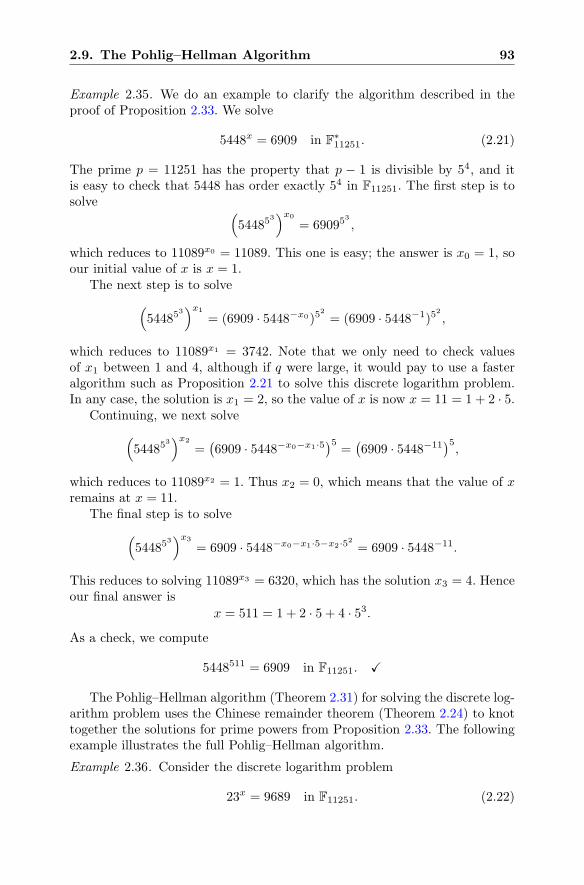
2.9. The Pohlig–Hellman Algorithm 93
Example 2.35. We do an example to clarify the algorithm described in theproof of Proposition 2.33. We solve
5448x = 6909 in F∗11251. (2.21)
The prime p = 11251 has the property that p − 1 is divisible by 54, and itis easy to check that 5448 has order exactly 54 in F11251. The first step is tosolve
(54485
3)x0
= 690953
,
which reduces to 11089x0 = 11089. This one is easy; the answer is x0 = 1, soour initial value of x is x = 1.
The next step is to solve
(54485
3)x1
= (6909 · 5448−x0)52
= (6909 · 5448−1)52
,
which reduces to 11089x1 = 3742. Note that we only need to check valuesof x1 between 1 and 4, although if q were large, it would pay to use a fasteralgorithm such as Proposition 2.21 to solve this discrete logarithm problem.In any case, the solution is x1 = 2, so the value of x is now x = 11 = 1 + 2 · 5.
Continuing, we next solve
(54485
3)x2
=(6909 · 5448−x0−x1·5)5 =
(6909 · 5448−11
)5,
which reduces to 11089x2 = 1. Thus x2 = 0, which means that the value of xremains at x = 11.
The final step is to solve
(54485
3)x3
= 6909 · 5448−x0−x1·5−x2·52 = 6909 · 5448−11.
This reduces to solving 11089x3 = 6320, which has the solution x3 = 4. Henceour final answer is
x = 511 = 1 + 2 · 5 + 4 · 53.
As a check, we compute
5448511 = 6909 in F11251. �
The Pohlig–Hellman algorithm (Theorem 2.31) for solving the discrete log-arithm problem uses the Chinese remainder theorem (Theorem 2.24) to knottogether the solutions for prime powers from Proposition 2.33. The followingexample illustrates the full Pohlig–Hellman algorithm.
Example 2.36. Consider the discrete logarithm problem
23x = 9689 in F11251. (2.22)
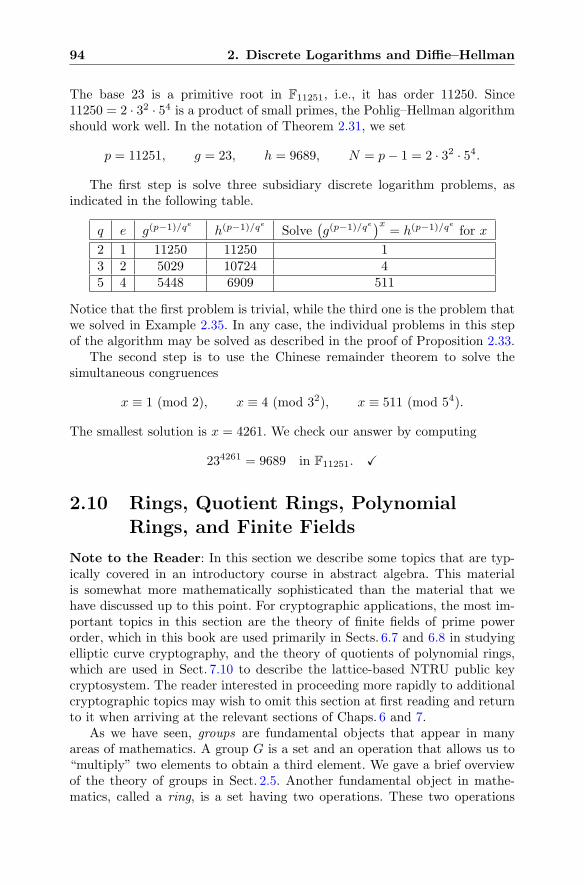
94 2. Discrete Logarithms and Diffie–Hellman
The base 23 is a primitive root in F11251, i.e., it has order 11250. Since11250 = 2 · 32 · 54 is a product of small primes, the Pohlig–Hellman algorithmshould work well. In the notation of Theorem 2.31, we set
p = 11251, g = 23, h = 9689, N = p− 1 = 2 · 32 · 54.
The first step is solve three subsidiary discrete logarithm problems, asindicated in the following table.
q e g(p−1)/qe h(p−1)/qe Solve(g(p−1)/qe
)x= h(p−1)/qe for x
2 1 11250 11250 13 2 5029 10724 45 4 5448 6909 511
Notice that the first problem is trivial, while the third one is the problem thatwe solved in Example 2.35. In any case, the individual problems in this stepof the algorithm may be solved as described in the proof of Proposition 2.33.
The second step is to use the Chinese remainder theorem to solve thesimultaneous congruences
x ≡ 1 (mod 2), x ≡ 4 (mod 32), x ≡ 511 (mod 54).
The smallest solution is x = 4261. We check our answer by computing
234261 = 9689 in F11251. �
2.10 Rings, Quotient Rings, PolynomialRings, and Finite Fields
Note to the Reader: In this section we describe some topics that are typ-ically covered in an introductory course in abstract algebra. This materialis somewhat more mathematically sophisticated than the material that wehave discussed up to this point. For cryptographic applications, the most im-portant topics in this section are the theory of finite fields of prime powerorder, which in this book are used primarily in Sects. 6.7 and 6.8 in studyingelliptic curve cryptography, and the theory of quotients of polynomial rings,which are used in Sect. 7.10 to describe the lattice-based NTRU public keycryptosystem. The reader interested in proceeding more rapidly to additionalcryptographic topics may wish to omit this section at first reading and returnto it when arriving at the relevant sections of Chaps. 6 and 7.
As we have seen, groups are fundamental objects that appear in manyareas of mathematics. A group G is a set and an operation that allows us to“multiply” two elements to obtain a third element. We gave a brief overviewof the theory of groups in Sect. 2.5. Another fundamental object in mathe-matics, called a ring, is a set having two operations. These two operations
2.10. Rings, Quotients, Polynomials, and Finite Fields 95
are analogous to ordinary addition and multiplication, and they are linked bythe distributive law. In this section we begin with a brief discussion of thegeneral theory of rings, then we discuss how to form one ring from anotherby taking quotients, and we conclude by examining in some detail the case ofpolynomial rings.
2.10.1 An Overview of the Theory of Rings
You are already familiar with many rings, for example the ring of integerswith the operations of addition and multiplication. We abstract the funda-mental properties of these operations and use them to formulate the followingfundamental definition.
Definition. A ring is a set R that has two operations, which we denote by +and �,10 having the following properties:
Properties of +[Identity Law ] There is an additive identity 0 ∈ R such that
0 + a = a+ 0 = a for every a ∈ R.[Inverse Law ] For every element a ∈ R there is an additive
inverse b ∈ R such that a+ b = b+ a = 0.
[Associative Law ] a+ (b+ c) = (a+ b) + c for all a, b, c ∈ R.[Commutative Law ] a+ b = b+ a for all a, b ∈ R,Briefly, if we look at R with only the operation +, then it is a commutativegroup with (additive) identity element 0.
Properties of �[Identity Law ] There is a multiplicative identity 1 ∈ R such that
1 � a = a � 1 = a for every a ∈ R.[Associative Law ] a � (b � c) = (a � b) � c for all a, b, c ∈ R.[Commutative Law ] a � b = b � a for all a, b ∈ R,Thus if we look at R with only the operation �, then it is almost a commu-tative group with (multiplicative) identity element 1, except that elementsare not required to have multiplicative inverses.
Property Linking + and �[Distributive Law ] a � (b+ c) = a � b+ a � c for all a, b, c ∈ R.
Remark 2.37. More generally, people sometimes work with rings that do notcontain a multiplicative identity, and also with rings for which � is not com-mutative, i.e., a � b might not be equal to b � a. So to be formal, our ringsare really commutative rings with (multiplicative) identity. However, all of therings that we use will be of this type, so we will just call them rings.
10Addition in a ring is virtually always denoted by +, but there are many differentnotations for multiplication. In this book use a � b, ab, or simply ab, depending on thecontext.
96 2. Discrete Logarithms and Diffie–Hellman
Every element of a ring has an additive inverse, but there may be manynonzero elements that do not have multiplicative inverses. For example, in thering of integers Z, the only elements that have multiplicative inverses are 1and −1.
Definition. A (commutative) ring in which every nonzero element has amultiplicative inverse is called a field.
Example 2.38. Here are a few examples of rings and fields with which you areprobably already familiar.
(a) R = Q, � = multiplication, and addition is as usual. The multiplicativeidentity element is 1. Every nonzero element has a multiplicative inverse,so Q is a field.
(b) R = Z, � = multiplication, and addition is as usual. The multiplicativeidentity element is 1. The only elements that have multiplicative inversesare 1 and −1, so Z is a ring, but it is not a field.
(c) R = Z/nZ, n is any positive integer, � = multiplication, and additionis as usual. The multiplicative identity element is 1. Here R is always aring, and it is a field if and only if n is prime.
(d) R = Fp, p is any prime integer, � = multiplication, and addition isas usual. The multiplicative identity element is 1. By Proposition 1.21,every nonzero element has a multiplicative inverse, so Fp is a field.
(e) The collection of all polynomials with coefficients taken from Z forms aring under the usual operations of polynomial addition and multiplica-tion. This ring is denoted by Z[x]. Thus we write
Z[x] = {a0 + a1x+ a2x2 + · · ·+ anx
n : n ≥ 0 and a0, a1, . . . , an ∈ Z}.
For example, 1+x2 and 3−7x4+23x9 are polynomials in the ring Z[x],as are 17 and −203.
(f) More generally, if R is any ring, we can form a ring of polynomials whosecoefficients are taken from the ring R. For example, the ring R mightbe Z/qZ or a finite field Fp. We discuss these general polynomial rings,denoted by R[x], in Sect. 7.9.
2.10.2 Divisibility and Quotient Rings
The concept of divisibility, originally introduced for the integers Z in Sect. 1.2,can be generalized to any ring.
Definition. Let a and b be elements of a ring R with b �= 0. We say that bdivides a, or that a is divisible by b, if there is an element c ∈ R such that
a = b � c.
2.10. Rings, Quotients, Polynomials, and Finite Fields 97
As before, we write b | a to indicate that b divides a. If b does not divide a,then we write b � a.
Remark 2.39. The basic properties of divisibility given in Proposition 1.4apply to rings in general. The proof for Z works for any ring. Similarly, it istrue in every ring that b | 0 for any b �= 0. (See Exercise 2.30.) However, notethat not every ring is as nice as Z. For example, there are rings with nonzeroelements a and b whose product a � b is 0. An example of such a ring is Z/6Z,in which 2 and 3 are nonzero, but 2 · 3 = 6 = 0.
Recall that an integer is called a prime if it has no nontrivial factors. Whatis a trivial factor? We can “factor” any integer by writing it as a = 1 · a andas a = (−1)(−a), so these are trivial factorizations. What makes them trivialis the fact that 1 and −1 have multiplicative inverses. In general, if R is a ringand if u ∈ R is an element that has a multiplicative inverse u−1 ∈ R, then wecan factor any element a ∈ R by writing it as a = u−1 · (ua). Elements thathave multiplicative inverses and elements that have only trivial factorizationsare special elements of a ring, so we give them special names.
Definition. Let R be a ring. An element u ∈ R is called a unit if it has amultiplicative inverse, i.e., if there is an element v ∈ R such that u � v = 1.
An element a of a ring R is said to be irreducible if a is not itself a unitand if in every factorization of a as a = b � c, either b is a unit or c is a unit.
Remark 2.40. The integers have the property that every integer factorsuniquely into a product of irreducible integers, up to rearranging the orderof the factors and throwing in some extra factors of 1 and −1. (Note that apositive irreducible integer is simply another name for a prime.) Not everyring has this important unique factorization property, but in the next sectionwe prove that the ring of polynomials with coefficients in a field is a uniquefactorization ring.
We have seen that congruences are a very important and powerful mathe-matical tool for working with the integers. Using the definition of divisibility,we can extend the notion of congruence to arbitrary rings.
Definition. Let R be a ring and choose a nonzero element m ∈ R. We saythat two elements a and b of R are congruent modulo m if their differencea− b is divisible by m. We write
a ≡ b (mod m)
to indicate that a and b are congruent modulo m.
Congruences for arbitrary rings satisfy the same equation-like propertiesas they do in the original integer setting.
Proposition 2.41. Let R be a ring and let m ∈ R with m �= 0. If
a1 ≡ a2 (mod m) and b1 ≡ b2 (mod m),
then
a1 ± b1 ≡ a2 ± b2 (mod m) and a1 � b1 ≡ a2 � b2 (mod m).
98 2. Discrete Logarithms and Diffie–Hellman
Proof. We leave the proof as an exercise; see Exercise 2.32.
Remark 2.42. Our definition of congruence captures all of the properties thatwe need in this book. However, we must observe that there exists a moregeneral notion of congruence modulo ideals. For our purposes, it is enoughto work with congruences modulo principal ideals, which are ideals that aregenerated by a single element.
An important consequence of Proposition 2.41 is a method for creating newrings from old rings, just as we created Z/qZ from Z by looking at congruencesmodulo q.
Definition. Let R be a ring and let m ∈ R with m �= 0. For any a ∈ R,we write a for the set of all a′ ∈ R such that a′ ≡ a (mod m). The set a iscalled the congruence class of a, and we denote the collection of all congruenceclasses by R/(m) or R/mR. Thus
R/(m) = R/mR = {a : a ∈ R}.
We add and multiply congruence classes using the obvious rules
a+ b = a+ b and a � b = a � b. (2.23)
We call R/(m) the quotient ring of R by m. This name is justified by the nextproposition.
Proposition 2.43. The formulas (2.23) give well-defined addition and multi-plication rules on the set of congruence classes R/(m), and they make R/(m)into a ring.
Proof. We leave the proof as an exercise; see Exercise 2.43.
2.10.3 Polynomial Rings and the Euclidean Algorithm
In Example 2.38(f) we observed that if R is any ring, then we can create apolynomial ring with coefficients taken from R. This ring is denoted by
R[x] = {a0 + a1x+ a2x2 + · · ·+ anx
n : n ≥ 0 and a0, a1, . . . , an ∈ R}.
The degree of a nonzero polynomial is the exponent of the highest power of xthat appears. Thus if
a(x) = a0 + a1x+ a2x2 + · · ·+ anx
n
with an �= 0, then a(x) has degree n. We denote the degree of a by deg(a),and we call an the leading coefficient of a(x). A nonzero polynomial whoseleading coefficient is equal to 1 is called a monic polynomial. For example,3 + x2 is a monic polynomial, but 1 + 3x2 is not.
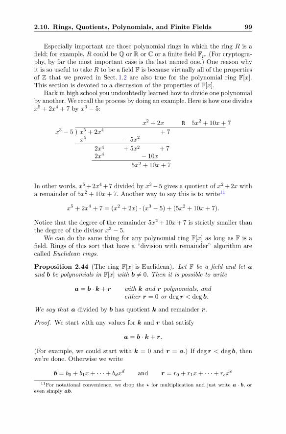
2.10. Rings, Quotients, Polynomials, and Finite Fields 99
Especially important are those polynomial rings in which the ring R is afield; for example, R could be Q or R or C or a finite field Fp. (For cryptogra-phy, by far the most important case is the last named one.) One reason whyit is so useful to take R to be a field F is because virtually all of the propertiesof Z that we proved in Sect. 1.2 are also true for the polynomial ring F[x].This section is devoted to a discussion of the properties of F[x].
Back in high school you undoubtedly learned how to divide one polynomialby another. We recall the process by doing an example. Here is how one dividesx5 + 2x4 + 7 by x3 − 5:
x2 + 2x R 5x2 + 10x+ 7
x3 − 5 ) x5 + 2x4 + 7x5 − 5x2
2x4 + 5x2 + 72x4 − 10x
5x2 + 10x+ 7
In other words, x5+2x4+7 divided by x3−5 gives a quotient of x2+2x witha remainder of 5x2 + 10x+ 7. Another way to say this is to write11
x5 + 2x4 + 7 = (x2 + 2x) · (x3 − 5) + (5x2 + 10x+ 7).
Notice that the degree of the remainder 5x2 +10x+7 is strictly smaller thanthe degree of the divisor x3 − 5.
We can do the same thing for any polynomial ring F[x] as long as F is afield. Rings of this sort that have a “division with remainder” algorithm arecalled Euclidean rings.
Proposition 2.44 (The ring F[x] is Euclidean). Let F be a field and let aand b be polynomials in F[x] with b �= 0. Then it is possible to write
a = b · k + r with k and r polynomials, andeither r = 0 or deg r < deg b.
We say that a divided by b has quotient k and remainder r.
Proof. We start with any values for k and r that satisfy
a = b · k + r.
(For example, we could start with k = 0 and r = a.) If deg r < deg b, thenwe’re done. Otherwise we write
b = b0 + b1x+ · · ·+ bdxd and r = r0 + r1x+ · · ·+ rex
e
11For notational convenience, we drop the � for multiplication and just write a · b, oreven simply ab.
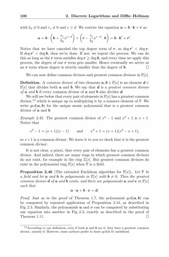
100 2. Discrete Logarithms and Diffie–Hellman
with bd �= 0 and re �= 0 and e ≥ d. We rewrite the equation a = b · k + r as
a = b ·(k +
rebdxe−d
)+
(r − re
bdxe−d · b
)= b · k′ + r′.
Notice that we have canceled the top degree term of r, so deg r′ < deg r.If deg r′ < deg b, then we’re done. If not, we repeat the process. We can dothis as long as the r term satisfies deg r ≥ deg b, and every time we apply thisprocess, the degree of our r term gets smaller. Hence eventually we arrive atan r term whose degree is strictly smaller than the degree of b.
We can now define common divisors and greatest common divisors in F[x].
Definition. A common divisor of two elements a, b ∈ F[x] is an element d ∈F[x] that divides both a and b. We say that d is a greatest common divisorof a and b if every common divisor of a and b also divides d.
We will see below that every pair of elements in F[x] has a greatest commondivisor,12 which is unique up to multiplying it by a nonzero element of F. Wewrite gcd(a, b) for the unique monic polynomial that is a greatest commondivisor of a and b.
Example 2.45. The greatest common divisor of x2 − 1 and x3 + 1 is x + 1.Notice that
x2 − 1 = (x+ 1)(x− 1) and x3 + 1 = (x+ 1)(x2 − x+ 1),
so x+1 is a common divisor. We leave it to you to check that it is the greatestcommon divisor.
It is not clear, a priori, that every pair of elements has a greatest commondivisor. And indeed, there are many rings in which greatest common divisorsdo not exist, for example in the ring Z[x]. But greatest common divisors doexist in the polynomial ring F[x] when F is a field.
Proposition 2.46 (The extended Euclidean algorithm for F[x]). Let F bea field and let a and b be polynomials in F[x] with b �= 0. Then the greatestcommon divisor d of a and b exists, and there are polynomials u and v in F[x]such that
a · u+ b · v = d.
Proof. Just as in the proof of Theorem 1.7, the polynomial gcd(a, b) canbe computed by repeated application of Proposition 2.44, as described inFig. 2.3. Similarly, the polynomials u and v can be computed by substitutingone equation into another in Fig. 2.3, exactly as described in the proof ofTheorem 1.11.
12According to our definition, even if both a and b are 0, they have a greatest commondivisor, namely 0. However, some authors prefer to leave gcd(0, 0) undefined.
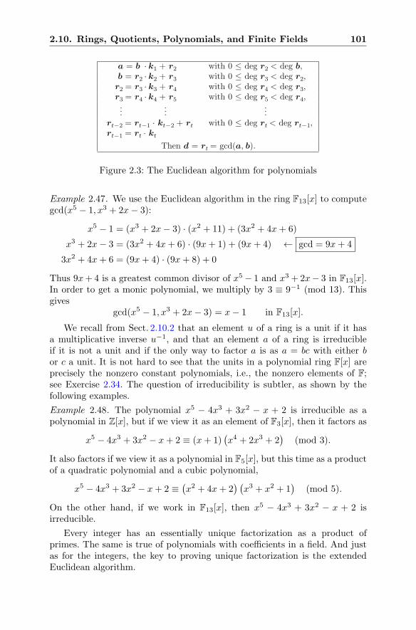
2.10. Rings, Quotients, Polynomials, and Finite Fields 101
a = b · k1 + r2 with 0 ≤ deg r2 < deg b,b = r2 · k2 + r3 with 0 ≤ deg r3 < deg r2,
r2 = r3 · k3 + r4 with 0 ≤ deg r4 < deg r3,r3 = r4 · k4 + r5 with 0 ≤ deg r5 < deg r4,...
......
rt−2 = rt−1 · kt−2 + rt with 0 ≤ deg rt < deg rt−1,rt−1 = rt · kt
Then d = rt = gcd(a, b).
Figure 2.3: The Euclidean algorithm for polynomials
Example 2.47. We use the Euclidean algorithm in the ring F13[x] to computegcd(x5 − 1, x3 + 2x− 3):
x5 − 1 = (x3 + 2x− 3) · (x2 + 11) + (3x2 + 4x+ 6)
x3 + 2x− 3 = (3x2 + 4x+ 6) · (9x+ 1) + (9x+ 4) ← gcd = 9x+ 4
3x2 + 4x+ 6 = (9x+ 4) · (9x+ 8) + 0
Thus 9x+4 is a greatest common divisor of x5 − 1 and x3 +2x− 3 in F13[x].In order to get a monic polynomial, we multiply by 3 ≡ 9−1 (mod 13). Thisgives
gcd(x5 − 1, x3 + 2x− 3) = x− 1 in F13[x].
We recall from Sect. 2.10.2 that an element u of a ring is a unit if it hasa multiplicative inverse u−1, and that an element a of a ring is irreducibleif it is not a unit and if the only way to factor a is as a = bc with either bor c a unit. It is not hard to see that the units in a polynomial ring F[x] areprecisely the nonzero constant polynomials, i.e., the nonzero elements of F;see Exercise 2.34. The question of irreducibility is subtler, as shown by thefollowing examples.
Example 2.48. The polynomial x5 − 4x3 + 3x2 − x + 2 is irreducible as apolynomial in Z[x], but if we view it as an element of F3[x], then it factors as
x5 − 4x3 + 3x2 − x+ 2 ≡ (x+ 1)(x4 + 2x3 + 2
)(mod 3).
It also factors if we view it as a polynomial in F5[x], but this time as a productof a quadratic polynomial and a cubic polynomial,
x5 − 4x3 + 3x2 − x+ 2 ≡(x2 + 4x+ 2
) (x3 + x2 + 1
)(mod 5).
On the other hand, if we work in F13[x], then x5 − 4x3 + 3x2 − x + 2 isirreducible.
Every integer has an essentially unique factorization as a product ofprimes. The same is true of polynomials with coefficients in a field. And justas for the integers, the key to proving unique factorization is the extendedEuclidean algorithm.
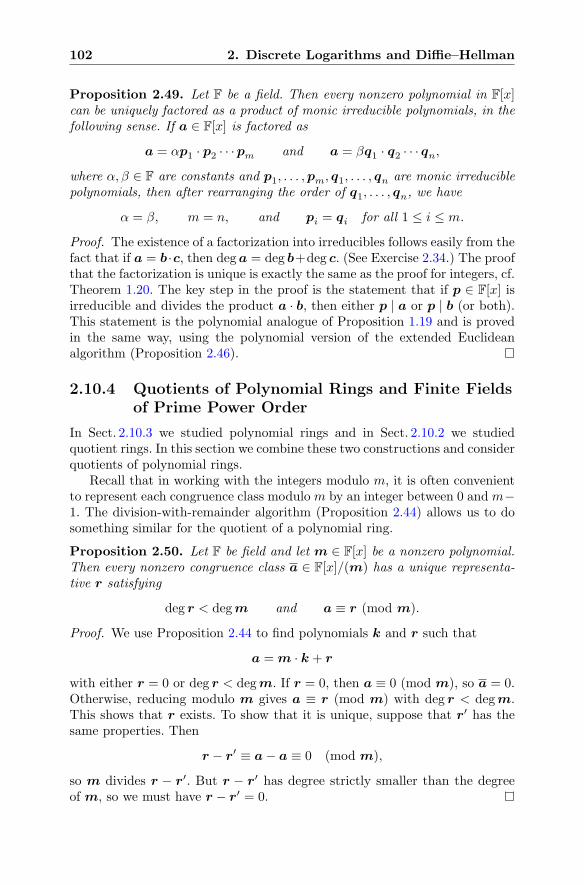
102 2. Discrete Logarithms and Diffie–Hellman
Proposition 2.49. Let F be a field. Then every nonzero polynomial in F[x]can be uniquely factored as a product of monic irreducible polynomials, in thefollowing sense. If a ∈ F[x] is factored as
a = αp1 · p2 · · ·pm and a = βq1 · q2 · · · qn,
where α, β ∈ F are constants and p1, . . . ,pm, q1, . . . , qn are monic irreduciblepolynomials, then after rearranging the order of q1, . . . , qn, we have
α = β, m = n, and pi = qi for all 1 ≤ i ≤ m.
Proof. The existence of a factorization into irreducibles follows easily from thefact that if a = b ·c, then dega = deg b+deg c. (See Exercise 2.34.) The proofthat the factorization is unique is exactly the same as the proof for integers, cf.Theorem 1.20. The key step in the proof is the statement that if p ∈ F[x] isirreducible and divides the product a · b, then either p | a or p | b (or both).This statement is the polynomial analogue of Proposition 1.19 and is provedin the same way, using the polynomial version of the extended Euclideanalgorithm (Proposition 2.46).
2.10.4 Quotients of Polynomial Rings and Finite Fieldsof Prime Power Order
In Sect. 2.10.3 we studied polynomial rings and in Sect. 2.10.2 we studiedquotient rings. In this section we combine these two constructions and considerquotients of polynomial rings.
Recall that in working with the integers modulo m, it is often convenientto represent each congruence class modulom by an integer between 0 andm−1. The division-with-remainder algorithm (Proposition 2.44) allows us to dosomething similar for the quotient of a polynomial ring.
Proposition 2.50. Let F be field and let m ∈ F[x] be a nonzero polynomial.Then every nonzero congruence class a ∈ F[x]/(m) has a unique representa-tive r satisfying
deg r < degm and a ≡ r (mod m).
Proof. We use Proposition 2.44 to find polynomials k and r such that
a = m · k + r
with either r = 0 or deg r < degm. If r = 0, then a ≡ 0 (mod m), so a = 0.Otherwise, reducing modulo m gives a ≡ r (mod m) with deg r < degm.This shows that r exists. To show that it is unique, suppose that r′ has thesame properties. Then
r − r′ ≡ a− a ≡ 0 (mod m),
so m divides r − r′. But r − r′ has degree strictly smaller than the degreeof m, so we must have r − r′ = 0.
2.10. Rings, Quotients, Polynomials, and Finite Fields 103
Example 2.51. Consider the ring F[x]/(x2 + 1). Proposition 2.50 says thatevery element of this quotient ring is uniquely represented by a polynomial ofthe form
α+ βx with α, β ∈ F.
Addition is performed in the obvious way,
α1 + β1x + α2 + β2x = (α1 + α2) + (β1 + β2)x.
Multiplication is similar, except that we have to divide the final result byx2 + 1 and take the remainder. Thus
α1 + β1x · α2 + β2x = α1α2 + (α1β2 + α2β1)x+ β1β2x2
= (α1α2 − β1β2) + (α1β2 + α2β1)x.
Notice that the effect of dividing by x2+1 is the same as replacing x2 with −1.The intuition is that in the quotient ring F[x]/(x2 + 1), we have made thequantity x2 + 1 equal to 0. Notice that if we take F = R in this example,then R[x]/(x2 + 1) is simply the field of complex numbers C.
We can use Proposition 2.50 to count the number of elements in a poly-nomial quotient ring when F is a finite field.
Corollary 2.52. Let Fp be a finite field and let m ∈ Fp[x] be a nonzero poly-nomial of degree d ≥ 1. Then the quotient ring Fp[x]/(m) contains exactly pd
elements.
Proof. From Proposition 2.50 we know that every element of Fp[x]/(m) isrepresented by a unique polynomial of the form
a0 + a1x+ a2x2 + · · ·+ ad−1x
d−1 with a0, a1, . . . , ad−1 ∈ Fp.
There are p choices for a0, and p choices for a1, and so on, leading to a totalof pd choices for a0, a1, . . . , ad.
We next give an important characterization of the units in a polynomialquotient ring. This will allow us to construct new finite fields.
Proposition 2.53. Let F be a field and let a,m ∈ F[x] be polynomialswith m �= 0. Then a is a unit in the quotient ring F[x]/(m) if and only if
gcd(a,m) = 1.
Proof. Suppose first that a is a unit in F[x]/(m). By definition, this meansthat we can find some b ∈ F[x](m) satisfying a·b = 1. In terms of congruences,this means that a · b ≡ 1 (mod m), so there is some c ∈ F[x] such that
a · b− 1 = c ·m.
104 2. Discrete Logarithms and Diffie–Hellman
It follows that any common divisor of a and m must also divide 1. There-fore gcd(a,m) = 1.
Next suppose that gcd(a,m) = 1. Then Proposition 2.46 tells us thatthere are polynomials u,v ∈ F[x] such that
a · u+m · v = 1.
Reducing modulo m yields
a · u ≡ 1 (mod m),
so u is an inverse for a in F[x]/(m).
An important instance of Proposition 2.53 is the case that the modulus isan irreducible polynomial.
Corollary 2.54. Let F be a field and let m ∈ F[x] be an irreducible polyno-mial. Then the quotient ring F[x]/(m) is a field, i.e., every nonzero elementof F[x]/(m) has a multiplicative inverse.
Proof. Replacing m by a constant multiple, we may assume that m is a monicpolynomial. Let a ∈ F[x]/(m). There are two cases to consider. First, sup-pose that gcd(a,m) = 1. Then Proposition 2.53 tells us that a is a unit, sowe are done. Second, suppose that d = gcd(a,m) �= 1. Then in particular,we know that d |m. But m is monic and irreducible, and d �= 1, so we musthave d = m. We also know that d | a, so m | a. Hence a = 0 in F[x]/(m).This completes the proof that every nonzero element of F[x]/(m) has a mul-tiplicative inverse.
Example 2.55. The polynomial x2 + 1 is irreducible in R[x]. The quotientring R[x]/(x2+1) is a field. Indeed, it is the field of complex numbers C, wherethe “variable” x plays the role of i =
√−1, since in the ring R[x]/(x2 +1) we
have x2 = −1.By way of contrast, the polynomial x2−1 is clearly not irreducible in R[x].
The quotient ring R[x]/(x2 − 1) is not a field. In fact,
(x− 1) · (x+ 1) = 0 in R[x]/(x2 − 1).
Thus ring R[x]/(x2−1) has nonzero elements whose product is 0, which meansthat they certainly cannot be units. (Nonzero elements of a ring whose productis 0 are called zero divisors.)
If we apply Corollary 2.54 to a polynomial ring with coefficients in a finitefield Fp, we can create new finite fields with a prime power number of elements.
Corollary 2.56. Let Fp be a finite field and let m ∈ Fp[x] be an irreduciblepolynomial of degree d ≥ 1. Then Fp[x]/(m) is a field with pd elements.
Proof. We combine Corollary 2.54, which says that Fp[x]/(m) is a field, withCorollary 2.52, which says that Fp[x]/(m) has pd elements.
2.10. Rings, Quotients, Polynomials, and Finite Fields 105
Example 2.57. It is not hard to check that the polynomial x3 + x + 1 isirreducible in F2[x] (see Exercise 2.37), so F2[x]/(x
3 + x + 1) is a field witheight elements. Proposition 2.50 tells us that the following are representativesfor the eight elements in this field:
0, 1, x, x2, 1 + x, 1 + x2, x+ x2, 1 + x+ x2.
Addition is easy as long as you remember to treat the coefficients modulo 2,so for example,
(1 + x) + (x+ x2) = 1 + x2.
Multiplication is also easy, just multiply the polynomials, divide by x3+x+1,and take the remainder. For example,
(1 + x) · (x+ x2) = x+ 2x2 + x3 = 1,
so 1 + x and x + x2 are multiplicative inverses. The complete multiplicationtable for F2[x]/(x
3 + x+ 1) is described in Exercise 2.38.
Example 2.58. When is the polynomial x2 + 1 irreducible in the ring Fp[x]?If it is reducible, then it factors as
x2 + 1 = (x+ α)(x+ β) for some α, β ∈ Fp.
Comparing coefficients, we find that α+ β = 0 and αβ = 1; hence
α2 = α · (−β) = −αβ = −1.
In other words, the field Fp has an element whose square is −1. Conversely,if α ∈ Fp satisfies α2 = −1, then x2 + 1 = (x − α)(x + α) factors in Fp[x].This proves that
x2 + 1 is irreducible in Fp[x] if and only if −1 is not a square in Fp.
Quadratic reciprocity, which we study later in Sect. 3.9, then tells us that
x2 + 1 is irreducible in Fp[x] if and only if p ≡ 3 (mod 4).
Let p be a prime satisfying p ≡ 3 (mod 4). Then the quotient fieldFp[x]/(x
2 + 1) is a field containing p2 elements. It contains an element x thatis a square root of −1. So we can view Fp[x]/(x
2 + 1) as a sort of analogue ofthe complex numbers and can write its elements in the form
a+ bi with a, b ∈ Fp,
where i is simply a symbol with the property that i2 = −1. Addition, sub-traction, multiplication, and division are performed just as in the complexnumbers, with the understanding that instead of real numbers as coefficients,we are using integers modulo p. So for example, division is done by the usual“rationalizing the denominator” trick,
106 2. Discrete Logarithms and Diffie–Hellman
a+ bi
c+ di=a+ bi
c+ di· c− dic− di =
(ac+ bd) + (bc− ad)ic2 + d2
.
Note that there is never a problem of 0 in the denominator, since the assump-tion that p ≡ 3 (mod 4) ensures that c2 + d2 �= 0 (as long as at least one of cand d is nonzero). These fields of order p2 will be used in Sect. 6.9.3.
In order to construct a field with pd elements, we need to find an irreduciblepolynomial of degree d in Fp[x]. It is proven in more advanced texts that thereis always such a polynomial, and indeed generally many such polynomials.Further, in a certain abstract sense it doesn’t matter which irreducible poly-nomial we choose: we always get the same field. However, in a practical senseit does make a difference, because practical computations in Fp[x]/(m) aremore efficient if m does not have very many nonzero coefficients.
We summarize some of the principal properties of finite fields in the fol-lowing theorem.
Theorem 2.59. Let Fp be a finite field.(a) For every d ≥ 1 there exists an irreducible polynomial m ∈ Fp[x] of
degree d.
(b) For every d ≥ 1 there exists a finite field with pd elements.
(c) If F and F′ are finite fields with the same number of elements, then there
is a way to match the elements of F with the elements of F′ so that
the addition and multiplication tables of F and F′ are the same. (The
mathematical terminology is that F and F′ are isomorphic.)
Proof. We know from Proposition 2.56 that (a) implies (b). For proofs of (a)and (c), see any basic algebra or number theory text, for example [40,§§13.5, 14.3], [53, Section 7.1], or [59, Chapter 7].
Definition. We write Fpd for a field with pd elements. Theorem 2.59 assuresus that there is at least one such field and that any two fields with pd elementsare essentially the same, up to relabeling their elements. These fields arealso sometimes called Galois fields and denoted by GF(pd) in honor of thenineteenth-century French mathematician Evariste Galois, who studied them.
Remark 2.60. It is not difficult to prove that if F is a finite field, then F has pd
elements for some prime p and some d ≥ 1. (The proof uses linear algebra;see Exercise 2.41.) So Theorem 2.59 describes all finite fields.
Remark 2.61. For cryptographic purposes, it is frequently advantageous towork in a field F2d , rather than in a field Fp with p large. This is due to thefact that the binary nature of computers often enables them to work moreefficiently with F2d . A second reason is that sometimes it is useful to havea finite field that contains smaller fields. In the case of Fpd , one can showthat every field Fpe with e | d is a subfield of Fpd . Of course, if one is going touse F2d for Diffie–Hellman key exchange or Elgamal encryption, it is necessaryto choose 2d to be of approximately the same size as one typically chooses p.
Exercises 107
Let F be a finite field having q elements. Every nonzero element of F has aninverse, so the group of units F∗ is a group of order q− 1. Lagrange’s theorem(Theorem 2.13) tells us that every element of F∗ has order dividing q − 1, so
aq−1 = 1 for all a ∈ F.
This is a generalization of Fermat’s little theorem (Theorem 1.24) to arbitraryfinite fields. The primitive root theorem (Theorem 1.30) is also true for allfinite fields.
Theorem 2.62. Let F be a finite field having q elements. Then F has aprimitive root, i.e., there is an element g ∈ F such that
F∗ = {1, g, g2, g3, . . . , gq−2}.
Proof. You can find a proof of this theorem in any basic number theory text-book; see for example [59, §4.1] or [137, Chapter 28].
Exercises
Section 2.1. Diffie–Hellman and RSA
2.1. Write a one page essay giving arguments, both pro and con, for the followingassertion:
If the government is able to convince a court that there is a valid reasonfor their request, then they should have access to an individual’s privatekeys (even without the individual’s knowledge), in the same way thatthe government is allowed to conduct court authorized secret wiretapsin cases of suspected criminal activity or threats to national security.
Based on your arguments, would you support or oppose the government being giventhis power? How about without court oversight? The idea that all private keys shouldbe stored at a secure central location and be accessible to government agencies (withor without suitably stringent legal conditions) is called key escrow.
2.2. Research and write a one to two page essay on the classification of cryptographicalgorithms as munitions under ITAR (International Traffic in Arms Regulations).How does that act define “export”? What are the potential fines and jail terms forthose convicted of violating the Arms Export Control Act? Would teaching non-classified cryptographic algorithms to a college class that includes non-US citizensbe considered a form of export? How has US government policy changed from theearly 1990s to the present?
Section 2.2. The Discrete Logarithm Problem
2.3. Let g be a primitive root for Fp.(a) Suppose that x = a and x = b are both integer solutions to the congruence
gx ≡ h (mod p). Prove that a ≡ b (mod p− 1). Explain why this implies thatthe map (2.1) on page 65 is well-defined.
108 Exercises
(b) Prove that logg(h1h2) = logg(h1) + logg(h2) for all h1, h2 ∈ F∗p.
(c) Prove that logg(hn) = n logg(h) for all h ∈ F
∗p and n ∈ Z.
2.4. Compute the following discrete logarithms.(a) log2(13) for the prime 23, i.e., p = 23, g = 2, and you must solve the congruence
2x ≡ 13 (mod 23).
(b) log10(22) for the prime p = 47.
(c) log627(608) for the prime p = 941. (Hint. Look in the second column of Table 2.1on page 66.)
2.5. Let p be an odd prime and let g be a primitive root modulo p. Prove that ahas a square root modulo p if and only if its discrete logarithm logg(a) modulo p−1is even.
Section 2.3. Diffie–Hellman Key Exchange
2.6. Alice and Bob agree to use the prime p = 1373 and the base g = 2 for aDiffie–Hellman key exchange. Alice sends Bob the value A = 974. Bob asks yourassistance, so you tell him to use the secret exponent b = 871. What value B shouldBob send to Alice, and what is their secret shared value? Can you figure out Alice’ssecret exponent?
2.7. Let p be a prime and let g be an integer. The Decision Diffie–Hellman Problemis as follows. Suppose that you are given three numbers A, B, and C, and supposethat A and B are equal to
A ≡ ga (mod p) and B ≡ gb (mod p),
but that you do not necessarily know the values of the exponents a and b. Determinewhether C is equal to gab (mod p). Notice that this is different from the Diffie–Hellman problem described on page 69. The Diffie–Hellman problem asks you toactually compute the value of gab.(a) Prove that an algorithm that solves the Diffie–Hellman problem can be used to
solve the decision Diffie–Hellman problem.
(b) Do you think that the decision Diffie–Hellman problem is hard or easy? Why?See Exercise 6.40 for a related example in which the decision problem is easy, butit is believed that the associated computational problem is hard.
Section 2.4. The Elgamal Public Key Cryptosystem
2.8. Alice and Bob agree to use the prime p = 1373 and the base g = 2 forcommunications using the Elgamal public key cryptosystem.(a) Alice chooses a = 947 as her private key. What is the value of her public key A?
(b) Bob chooses b = 716 as his private key, so his public key is
B ≡ 2716 ≡ 469 (mod 1373).
Alice encrypts the message m = 583 using the random element k = 877. Whatis the ciphertext (c1, c2) that Alice sends to Bob?
(c) Alice decides to choose a new private key a = 299 with associated public keyA ≡ 2299 ≡ 34 (mod 1373). Bob encrypts a message using Alice’s public keyand sends her the ciphertext (c1, c2) = (661, 1325). Decrypt the message.
Exercises 109
(d) Now Bob chooses a new private key and publishes the associated public key B =893. Alice encrypts a message using this public key and sends the ciphertext(c1, c2) = (693, 793) to Bob. Eve intercepts the transmission. Help Eve bysolving the discrete logarithm problem 2b ≡ 893 (mod 1373) and using the valueof b to decrypt the message.
2.9. Suppose that Eve is able to solve the Diffie–Hellman problem described onpage 69. More precisely, assume that if Eve is given two powers gu and gv mod p,then she is able to compute guv mod p. Show that Eve can break the Elgamal PKC.
2.10. The exercise describes a public key cryptosystem that requires Bob and Aliceto exchange several messages. We illustrate the system with an example.
Bob and Alice fix a publicly known prime p = 32611, and all of the other numbersused are private. Alice takes her message m = 11111, chooses a random exponenta = 3589, and sends the number u = ma (mod p) = 15950 to Bob. Bob chooses arandom exponent b = 4037 and sends v = ub (mod p) = 15422 back to Alice. Al-ice then computes w = v15619 ≡ 27257 (mod 32611) and sends w = 27257 to Bob.Finally, Bob computes w31883 (mod 32611) and recovers the value 11111 of Alice’smessage.(a) Explain why this algorithm works. In particular, Alice uses the numbers
a = 3589 and 15619 as exponents. How are they related? Similarly, how areBob’s exponents b = 4037 and 31883 related?
(b) Formulate a general version of this cryptosystem, i.e., using variables, and showthat it works in general.
(c) What is the disadvantage of this cryptosystem over Elgamal? (Hint. How manytimes must Alice and Bob exchange data?)
(d) Are there any advantages of this cryptosystem over Elgamal? In particular, canEve break it if she can solve the discrete logarithm problem? Can Eve break itif she can solve the Diffie–Hellman problem?
Section 2.5. An Overview of the Theory of Groups
2.11. The group S3 consists of the following six distinct elements
e, σ, σ2, τ, στ, σ2τ,
where e is the identity element and multiplication is performed using the rules
σ3 = e, τ2 = e, τσ = σ2τ.
Compute the following values in the group S3:(a) τσ2 (b) τ(στ) (c) (στ)(στ) (d) (στ)(σ2τ).Is S3 a commutative group?
2.12. Let G be a group, let d ≥ 1 be an integer, and define a subset of G by
G[d] = {g ∈ G : gd = e}.
(a) Prove that if g is in G[d], then g−1 is in G[d].
(b) Suppose that G is commutative. Prove that if g1 and g2 are in G[d], then theirproduct g1 � g2 is in G[d].
(c) Deduce that if G is commutative, then G[d] is a group.
110 Exercises
(d) Show by an example that if G is not a commutative group, then G[d] need notbe a group. (Hint. Use Exercise 2.11.)
2.13. Let G and H be groups. A function φ : G→ H is called a (group) homomor-phism if it satisfies
φ(g1 � g2) = φ(g1) � φ(g2) for all g1, g2 ∈ G.
(Note that the product g1 � g2 uses the group law in the group G, while the prod-uct φ(g1) � φ(g2) uses the group law in the group H.)(a) Let eG be the identity element of G, let eH be the identity element of H, and
let g ∈ G. Prove that
φ(eG) = eH and φ(g−1) = φ(g)−1.
(b) Let G be a commutative group. Prove that the map φ : G → G definedby φ(g) = g2 is a homomorphism. Give an example of a noncommutative groupfor which this map is not a homomorphism.
(c) Same question as (b) for the map φ(g) = g−1.
2.14. Prove that each of the following maps is a group homomorphism.(a) The map φ : Z → Z/NZ that sends a ∈ Z to a mod N in Z/NZ.
(b) The map φ : R∗ → GL2(R) defined by φ(a) =(a 00 a−1
).
(c) The discrete logarithm map logg : F∗p → Z/(p−1)Z, where g is a primitive root
modulo p.
2.15. (a) Prove that GL2(Fp) is a group.
(b) Show that GL2(Fp) is a noncommutative group for every prime p.
(c) Describe GL2(F2) completely. That is, list its elements and describe the multi-plication table.
(d) How many elements are there in the group GL2(Fp)?
(e) How many elements are there in the group GLn(Fp)?
Section 2.6. How Hard Is the Discrete Logarithm Problem?
2.16. Verify the following assertions from Example 2.16.
(a) x2 +√x = O
(x2). (d) (ln k)375 = O
(k0.001
).
(b) 5 + 6x2 − 37x5 = O(x5). (e) k22k = O
(e2k).
(c) k300 = O(2k). (f) N102N = O
(eN).
Section 2.7. A Collision Algorithm for the DLP
2.17. Use Shanks’s babystep–giantstep method to solve the following discrete log-arithm problems. (For (b) and (c), you may want to write a computer programimplementing Shanks’s algorithm.)(a) 11x = 21 in F71.
(b) 156x = 116 in F593.
(c) 650x = 2213 in F3571.
Section 2.8. The Chinese Remainder Theorem
Exercises 111
2.18. Solve each of the following simultaneous systems of congruences (or explainwhy no solution exists).(a) x ≡ 3 (mod 7) and x ≡ 4 (mod 9).
(b) x ≡ 137 (mod 423) and x ≡ 87 (mod 191).
(c) x ≡ 133 (mod 451) and x ≡ 237 (mod 697).
(d) x ≡ 5 (mod 9), x ≡ 6 (mod 10), and x ≡ 7 (mod 11).
(e) x ≡ 37 (mod 43), x ≡ 22 (mod 49), and x ≡ 18 (mod 71).
2.19. Solve the 1700-year-old Chinese remainder problem from the Sun Tzu SuanChing stated on page 84.
2.20. Let a, b,m, n be integers with gcd(m,n) = 1. Let
c ≡ (b− a) ·m−1 (mod n).
Prove that x = a+ cm is a solution to
x ≡ a (mod m) and x ≡ b (mod n), (2.24)
and that every solution to (2.24) has the form x = a+ cm+ ymn for some y ∈ Z.
2.21. (a) Let a, b, c be positive integers and suppose that
a | c, b | c, and gcd(a, b) = 1.
Prove that ab | c.(b) Let x = c and x = c′ be two solutions to the system of simultaneous congru-
ences (2.7) in the Chinese remainder theorem (Theorem 2.24). Prove that
c ≡ c′ (mod m1m2 · · ·mk).
2.22. For those who have studied ring theory, this exercise sketches a shortproof of the Chinese remainder theorem. Let m1, . . . ,mk be integers and letm = m1m2 · · ·mk be their product.(a) Prove that the map
Z
mZ−−−−−→ Z
m1Z× Z
m2Z× · · · × Z
mkZ
a mod m −−−−−→ (a mod m1, a mod m2, . . . , a mod mk)
(2.25)
is a well-defined homomorphism of rings. (Hint. First define a homomorphismfrom Z to the right-hand side of (2.25), and then show thatmZ is in the kernel.)
(b) Assume that m1, . . . ,mk are pairwise relatively prime. Prove that the mapgiven by (2.25) is one-to-one. (Hint. What is the kernel?)
(c) Continuing with the assumption that the numbers m1, . . . ,mk are pairwiserelatively prime, prove that the map (2.25) is onto. (Hint. Use (b) and countthe size of both sides.)
(d) Explain why the Chinese remainder theorem (Theorem 2.24) is equivalent tothe assertion that (b) and (c) are true.
2.23. Use the method described in Sect. 2.8.1 to find square roots modulo thefollowing composite moduli.
112 Exercises
(a) Find a square root of 340 modulo 437. (Note that 437 = 19 · 23.)(b) Find a square root of 253 modulo 3143.
(c) Find four square roots of 2833 modulo 4189. (The modulus factors as 4189 =59 · 71. Note that your four square roots should be distinct modulo 4189.)
(d) Find eight square roots of 813 modulo 868.
2.24. Let p be an odd prime, let a be an integer that is not divisible by p, andlet b be a square root of a modulo p. This exercise investigates the square root of amodulo powers of p.(a) Prove that for some choice of k, the number b+ kp is a square root of a mod-
ulo p2, i.e., (b+ kp)2 ≡ a (mod p2).
(b) The number b = 537 is a square root of a = 476 modulo the prime p = 1291.Use the idea in (a) to compute a square root of 476 modulo p2.
(c) Suppose that b is a square root of a modulo pn. Prove that for some choice of j,the number b+ jpn is a square root of a modulo pn+1.
(d) Explain why (c) implies the following statement: If p is an odd prime and if ahas a square root modulo p, then a has a square root modulo pn for every powerof p. Is this true if p = 2?
(e) Use the method in (c) to compute the square root of 3 modulo 133, giventhat 92 ≡ 3 (mod 13).
2.25. Suppose n = pq with p and q distinct odd primes.(a) Suppose that gcd(a, pq) = 1. Prove that if the equation x2 ≡ a (mod n) has
any solutions, then it has four solutions.
(b) Suppose that you had a machine that could find all four solutions for somegiven a. How could you use this machine to factor n?
Section 2.9. The Pohlig–Hellman Algorithm
2.26. Let Fp be a finite field and let N | p − 1. Prove that F∗p has an element of
order N . This is true in particular for any prime power that divides p − 1. (Hint.Use the fact that F∗
p has a primitive root.)
2.27. Write out your own proof that the Pohlig–Hellman algorithm works in theparticular case that p− 1 = q1 · q2 is a product of two distinct primes. This providesa good opportunity for you to understand how the proof works and to get a feel forhow it was discovered.
2.28. Use the Pohlig–Hellman algorithm (Theorem 2.31) to solve the discrete log-arithm problem
gx = a in Fp
in each of the following cases.(a) p = 433, g = 7, a = 166.
(b) p = 746497, g = 10, a = 243278.
(c) p = 41022299, g = 2, a = 39183497. (Hint. p = 2 · 295 + 1.)
(d) p = 1291799, g = 17, a = 192988. (Hint. p− 1 has a factor of 709.)
Section 2.10. Rings, Quotient Rings, Polynomial Rings, and Finite Fields
Exercises 113
2.29. Let R be a ring with the property that the only way that a product a · b canbe 0 is if a = 0 or b = 0. (In the terminology of Example 2.55, the ring R has no zerodivisors.) Suppose further that R has only finitely many elements. Prove that R is afield. (Hint. Let a ∈ R with a �= 0. What can you say about the map R → R definedby b → a · b?)
2.30. Let R be a ring. Prove the following properties of R directly from the ringaxioms described in Sect. 2.10.1.(a) Prove that the additive identity element 0 ∈ R is unique, i.e., prove that there
is only one element in R satisfying 0 + a = a+ 0 = 0 for every a ∈ R.
(b) Prove that the multiplicative identity element 1 ∈ R is unique.
(c) Prove that every element of R has a unique additive inverse.
(d) Prove that 0 � a = a � 0 = 0 for all a ∈ R.
(e) We denote the additive inverse of a by −a. Prove that −(−a) = a.
(f) Let −1 be the additive inverse of the multiplicative identity element 1 ∈ R.Prove that (−1) � (−1) = 1.
(g) Prove that b | 0 for every nonzero b ∈ R.
(h) Prove that an element of R has at most one multiplicative inverse.
2.31. Let R and S be rings. A function φ : R → S is called a (ring) homomorphismif it satisfies
φ(a+ b) = φ(a) + φ(b) and φ(a � a) = φ(a) � φ(a) for all a, b,∈ R.
(a) Let 0R, 0S , 1R and 1S denote the additive and multiplicative identities of Rand S, respectively. Prove that
φ(0R) = 0S , φ(1R) = 1S , φ(−a) = −φ(a), φ(a−1) = φ(a)−1,
where the last equality holds for those a ∈ R that have a multiplicative inverse.
(b) Let p be a prime, and let R be a ring with the property that pa = 0 forevery a ∈ R. (Here pa means to add a to itself p times.) Prove that the map
φ : R −→ R, φ(a) = ap
is a ring homomorphism. It is called the Frobenius homomorphism.
2.32. Prove Proposition 2.41.
2.33. Prove Proposition 2.43. (Hint. First use Exercise 2.32 to prove that the con-gruence classes a+ b and a � b depend only on the congruence classes of a and b.)
2.34. Let F be a field and let a and b be nonzero polynomials in F[x].(a) Prove that deg(a · b) = deg(a) + deg(b).
(b) Prove that a has a multiplicative inverse in F[x] if and only if a is in F, i.e., ifand only if a is a constant polynomial.
(c) Prove that every nonzero element of F[x] can be factored into a product ofirreducible polynomials. (Hint. Use (a), (b), and induction on the degree of thepolynomial.)
(d) Let R be the ring Z/6Z. Give an example to show that (a) is false for somepolynomials a and b in R[x].
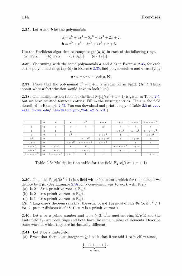
114 Exercises
2.35. Let a and b be the polynomials
a = x5 + 3x4 − 5x3 − 3x2 + 2x+ 2,
b = x5 + x4 − 2x3 + 4x2 + x+ 5.
Use the Euclidean algorithm to compute gcd(a, b) in each of the following rings.(a) F2[x] (b) F3[x] (c) F5[x] (d) F7[x].
2.36. Continuing with the same polynomials a and b as in Exercise 2.35, for eachof the polynomial rings (a)–(d) in Exercise 2.35, find polynomials u and v satisfying
a · u+ b · v = gcd(a, b).
2.37. Prove that the polynomial x3 + x + 1 is irreducible in F2[x]. (Hint. Thinkabout what a factorization would have to look like.)
2.38. The multiplication table for the field F2[x]/(x3 + x+1) is given in Table 2.5,
but we have omitted fourteen entries. Fill in the missing entries. (This is the fielddescribed in Example 2.57. You can download and print a copy of Table 2.5 at www.math.brown.edu/~jhs/MathCrypto/Table2.5.pdf.)
0 1 x x2 1 + x 1 + x2 x + x2 1 + x + x2
0 0 0 0 0 0 0 0 0
1 0 1 x 1 + x2 x + x2 1 + x + x2
x 0 x x2 x + x2 1 1 + x2
x2 0 x + x2 1 + x + x2 x 1 + x2 1
1 + x 0 x + x2 1 + x + x2 1 + x2 1 x
1 + x2 0 1 + x2 1 x 1 + x + x2 1 + x
x + x2 0 x + x2 1 + x2 1 1 + x x
1 + x + x2 0 1 + x + x2 1 + x2 1 x 1 + x
Table 2.5: Multiplication table for the field F2[x]/(x3 + x+ 1)
2.39. The field F7[x]/(x2 +1) is a field with 49 elements, which for the moment we
denote by F49. (See Example 2.58 for a convenient way to work with F49.)(a) Is 2 + 5x a primitive root in F49?
(b) Is 2 + x a primitive root in F49?
(c) Is 1 + x a primitive root in F49?(Hint. Lagrange’s theorem says that the order of u ∈ F49 must divide 48. So if uk �= 1for all proper divisors k of 48, then u is a primitive root.)
2.40. Let p be a prime number and let e ≥ 2. The quotient ring Z/peZ and thefinite field Fpe are both rings and both have the same number of elements. Describesome ways in which they are intrinsically different.
2.41. Let F be a finite field.(a) Prove that there is an integer m ≥ 1 such that if we add 1 to itself m times,
1 + 1 + · · ·+ 1︸ ︷︷ ︸m ones
,
Exercises 115
then we get 0. Note that here 1 and 0 are the multiplicative and additive identityelements of the field F. If the notation is confusing, you can let u and z be themultiplicative and additive identity elements of F, and then you need to provethat u+ u+ · · ·+ u = z. (Hint. Since F is finite, the numbers 1, 1 + 1, 1 + 1 +1,. . . cannot all be different.)
(b) Let m be the smallest positive integer with the property described in (a). Provethat m is prime. (Hint. If m factors, show that there are nonzero elementsin F whose product is zero, so F cannot be a field.) This prime is called thecharacteristic of the field F.
(c) Let p be the characteristic of F. Prove that F is a finite-dimensional vectorspace over the field Fp of p elements.
(d) Use (c) to deduce that F has pd elements for some d ≥ 1.
Chapter 3
Integer Factorizationand RSA
3.1 Euler’s Formula and Roots Modulo pq
The Diffie–Hellman key exchange method and the Elgamal public keycryptosystem studied in Sects. 2.3 and 2.4 rely on the fact that it is easyto compute powers an mod p, but difficult to recover the exponent n if youknow only the values of a and an mod p. An essential result that we used toanalyze the security of Diffie–Hellman and Elgamal is Fermat’s little theorem(Theorem 1.24),
ap−1 ≡ 1 (mod p) for all a �≡ 0 (mod p).
Fermat’s little theorem expresses a beautiful property of prime numbers.It is natural to ask what happens if we replace p with a number m that isnot prime. Is it still true that am−1 ≡ 1 (mod m)? A few computations suchas Example 1.28 in Sect. 1.4 will convince you that the answer is no. In thissection we investigate the correct generalization of Fermat’s little theoremwhen m = pq is a product of two distinct primes, since this is the case that ismost important for cryptographic applications. We leave the general case foryou to do in Exercises 3.4 and 3.5.
As usual, we begin with an example. What do powers modulo 15 look like?If we make a table of squares and cubes modulo 15, they do not look veryinteresting, but many fourth powers are equal to 1 modulo 15. More precisely,we find that
a4 ≡ 1 (mod 15) for a = 1, 2, 4, 7, 8, 11, 13, and 14;
a4 �≡ 1 (mod 15) for a = 3, 5, 6, 9, 10, and 12.
© Springer Science+Business Media New York 2014J. Hoffstein et al., An Introduction to Mathematical Cryptography,Undergraduate Texts in Mathematics, DOI 10.1007/978-1-4939-1711-2 3
117
118 3. Integer Factorization and RSA
What distinguishes the list of numbers 1, 2, 4, 7, 8, 11, 13, 14 whose fourthpower is 1 modulo 15 from the list of numbers 3, 5, 6, 9, 10, 12, 15 whose fourthpower is not 1 modulo 15? A moment’s reflection shows that each of thenumbers 3, 5, 6, 9, 10, 12, 15 has a nontrivial factor in common with the modu-lus 15, while the numbers 1, 2, 4, 7, 8, 11, 13, 14 are relatively prime to 15. Thissuggests that some version of Fermat’s little theorem should be true if thenumber a is relatively prime to the modulus m, but the correct exponent touse is not necessarily m− 1.
For m = 15 we found that the right exponent is 4. Why does 4 work? Wecould simply check each value of a, but a more enlightening argument wouldbe better. In order to show that a4 ≡ 1 (mod 15), it is enough to check thetwo congruences
a4 ≡ 1 (mod 3) and a4 ≡ 1 (mod 5). (3.1)
This is because the two congruences (3.1) say that
3 divides a4 − 1 and 5 divides a4 − 1,
which in turn imply that 15 divides a4 − 1.The two congruences in (3.1) are modulo primes, so we can use Fermat’s
little theorem to check that they are true. Thus
a4 = (a2)2 = (a(3−1))2 ≡ 12 ≡ 1 (mod 3),
a4 = a5−1 ≡ 1 (mod 5).
If you think about these two congruences, you will see that the crucial propertyof the exponent 4 is that it is a multiple of p− 1 for both p = 3 and p = 5.Notice that this is not true of 14, which does not work as an exponent. Withthis observation, we are ready to state the fundamental formula that underliesthe RSA public key cryptosystem.
Theorem 3.1 (Euler’s Formula for pq). Let p and q be distinct primes and let
g = gcd(p− 1, q − 1).
Then
a(p−1)(q−1)/g ≡ 1 (mod pq) for all a satisfying gcd(a, pq) = 1.
In particular, if p and q are odd primes, then
a(p−1)(q−1)/2 ≡ 1 (mod pq) for all a satisfying gcd(a, pq) = 1.
Proof. By assumption we know that p does not divide a and that g dividesq − 1, so we can compute
a(p−1)(q−1)/g =(a(p−1)
)(q−1)/g
since (q − 1)/g is an integer,
3.1. Euler’s Formula and Roots Modulo pq 119
≡ 1(q−1)/g (mod p) since ap−1 ≡ 1 (mod p)
from Fermat’s little theorem,
≡ 1 (mod p) since 1 to any power is 1!
The exact same computation, reversing the roles of p and q, shows that
a(p−1)(q−1)/g ≡ 1 (mod q).
This proves that a(p−1)(q−1)/g − 1 is divisible by both p and by q; hence it isdivisible by pq, which completes the proof of Theorem 3.1.
Diffie–Hellman key exchange and the Elgamal public key cryptosystem(Sects. 2.3 and 2.4) rely for their security on the difficulty of solving equationsof the form
ax ≡ b (mod p),
where a, b, and p are known quantities, p is a prime, and x is the unknown vari-able. The RSA public key cryptosystem, which we study in the next section,relies on the difficulty of solving equations of the form
xe ≡ c (mod N),
where now the quantities e, c, and N are known and x is the unknown. Inother words, the security of RSA relies on the assumption that it is difficultto take eth roots modulo N .
Is this a reasonable assumption? If the modulus N is prime, then it turnsout that it is comparatively easy to compute eth roots modulo N , as describedin the next proposition.
Proposition 3.2. Let p be a prime and let e ≥ 1 be an integer satisfyinggcd(e, p−1) = 1. Proposition 1.13 tells us that e has an inverse modulo p− 1,say
de ≡ 1 (mod p− 1).
Then the congruencexe ≡ c (mod p) (3.2)
has the unique solution x ≡ cd (mod p).
Proof. If c ≡ 0 (mod p), then x ≡ 0 (mod p) is the unique solutionand we are done. So we assume that c �≡ 0 (mod p). The proof is then aneasy application of Fermat’s little theorem (Theorem 1.24). The congruencede ≡ 1 (mod p− 1) means that there is an integer k such that
de = 1 + k(p− 1).
Now we check that cd is a solution to xe ≡ c (mod p):
(cd)e ≡ cde (mod p) law of exponents,
120 3. Integer Factorization and RSA
≡ c1+k(p−1) (mod p) since de = 1 + k(p− 1),
≡ c · (cp−1)k (mod p) law of exponents again,
≡ c · 1k (mod p) from Fermat’s little theorem,
≡ c (mod p).
This completes the proof that x = cd is a solution to xe ≡ c (mod p).In order to see that the solution is unique, suppose that x1 and x2 are both
solutions to the congruence (3.2). We’ve just proven that zde ≡ z (mod p) forany nonzero value z, so we find that
x1 ≡ xde1 ≡ (xe1)d ≡ cd ≡ (xe2)
d ≡ xde2 ≡ x2 (mod p).
Thus x1 and x2 are the same modulo p, so (3.2) has at most one solution.
Example 3.3. We solve the congruence
x1583 ≡ 4714 (mod 7919),
where the modulus p = 7919 is prime. Proposition 3.2 says that first we needto solve the congruence
1583d ≡ 1 (mod 7918).
The solution, using the extended Euclidean algorithm (Theorem 1.11; seealso Remark 1.15 and Exercise 1.12), is d ≡ 5277 (mod 7918). Then Proposi-tion 3.2 tells us that
x ≡ 47145277 ≡ 6059 (mod 7919)
is a solution to x1583 ≡ 4714 (mod 7919).
Remark 3.4. Proposition 3.2 includes the assumption that gcd(e, p − 1) = 1.If this assumption is omitted, then the congruence xe ≡ c (mod p) will have asolution for some, but not all, values of c. Further, if it does have a solution,then it will have more than one. See Exercise 3.2 for further details.
Proposition 3.2 shows that it is easy to take eth roots if the modulus is aprime p. The situation for a composite modulus N looks similar, but there is acrucial difference. If we know how to factor N , then it is again easy to computeeth roots. The following proposition explains how to do this if N = pq is aproduct of two primes. The general case is left for you to do in Exercise 3.6.
Proposition 3.5. Let p and q be distinct primes and let e ≥ 1 satisfy
gcd(e, (p− 1)(q − 1)
)= 1.
3.1. Euler’s Formula and Roots Modulo pq 121
Proposition 1.13 tells us that e has an inverse modulo (p− 1)(q − 1), say
de ≡ 1 (mod (p− 1)(q − 1)).
Then the congruencexe ≡ c (mod pq) (3.3)
has the unique solution x ≡ cd (mod pq).
Proof. We assume that gcd(c, pq) = 1; see Exercise 3.3 for the other cases. Theproof of Proposition 3.5 is almost identical to the proof of Proposition 3.2, butinstead of using Fermat’s little theorem, we use Euler’s formula (Theorem 3.1).The congruence de ≡ 1 (mod (p− 1)(q − 1)) means that there is an integer ksuch that
de = 1 + k(p− 1)(q − 1).
Now we check that cd is a solution to xe ≡ c (mod pq):
(cd)e ≡ cde (mod pq) law of exponents,
≡ c1+k(p−1)(q−1) (mod pq) since de = 1 + k(p− 1)(q − 1),
≡ c · (c(p−1)(q−1))k (mod pq) law of exponents again,
≡ c · 1k (mod pq) from Euler’s formula (Theorem 3.1),
≡ c (mod pq).
This completes the proof that x = cd is a solution to the congruence (3.3). Itremains to show that the solution is unique. Suppose that x = u is a solutionto (3.3). Then
u ≡ ude−k(p−1)(q−1) (mod pq) since de = 1 + k(p− 1)(q − 1),
≡ (ue)d · (u(p−1)(q−1))−k (mod pq)
≡ (ue)d · 1−k (mod pq) using Euler’s formula (Theorem 3.1),
≡ cd (mod pq) since u is a solution to (3.3).
Thus every solution to (3.3) is equal to cd (mod pq), so this is the uniquesolution.
Remark 3.6. Proposition 3.5 gives an algorithm for solving xe ≡ c (mod pq)that involves first solving de ≡ 1 (mod (p − 1)(q − 1)) and then computingcd mod pq. We can often make the computation faster by using a smallervalue of d. Let g = gcd(p− 1, q − 1) and suppose that we solve the followingcongruence for d:
de ≡ 1
(mod
(p− 1)(q − 1)
g
).
Euler’s formula (Theorem 3.1) says that a(p−1)(q−1)/g ≡ 1 (mod pq). Hencejust as in the proof of Proposition 3.5, if we write de = 1+ k(p− 1)(q− 1)/g,then
(cd)e = cde = c1+k(p−1)(q−1)/g = c · (c(p−1)(q−1)/g)k ≡ c (mod pq).
122 3. Integer Factorization and RSA
Thus using this smaller value of d, we still find that cd mod pq is a solutionto xe ≡ c (mod pq).
Example 3.7. We solve the congruence
x17389 ≡ 43927 (mod 64349),
where the modulus N = 64349 = 229 · 281 is a product of the two primesp = 229 and q = 281. The first step is to solve the congruence
17389d ≡ 1 (mod 63840),
where 63840 = (p − 1)(q − 1) = 228 · 280. The solution, using the methoddescribed in Remark 1.15 or Exercise 1.12, is d ≡ 53509 (mod 63840). ThenProposition 3.5 tells us that
x ≡ 4392753509 ≡ 14458 (mod 64349)
is the solution to x17389 ≡ 43927 (mod 64349).We can save ourselves a little bit of work by using the idea described in
Remark 3.6. We have
g = gcd(p− 1, q − 1) = gcd(228, 280) = 4,
so (p− 1)(q − 1)/g = (228)(280)/4 = 15960, which means that we can find avalue of d by solving the congruence
17389d ≡ 1 (mod 15960).
The solution is d ≡ 5629 (mod 15960), and then
x ≡ 439275629 ≡ 14458 (mod 64349)
is the solution to x17389 ≡ 43927 (mod 64349). Notice that we obtainedthe same solution, as we should, but that we needed to raise 43927 toonly the 5629th power, while using Proposition 3.5 directly required us toraise 43927 to the 53509th power. This saves some time, although not quiteas much as it looks, since recall that computing cd mod N takes time O(ln d).Thus the faster method takes about 80% as long as the slower method, sinceln(5629)/ ln(53509) ≈ 0.793.
Example 3.8. Alice challenges Eve to solve the congruence
x9843 ≡ 134872 (mod 30069476293).
The modulus 30069476293 is not prime, since (cf. Example 1.28)
230069476293−1 ≡ 18152503626 �≡ 1 (mod 30069476293).
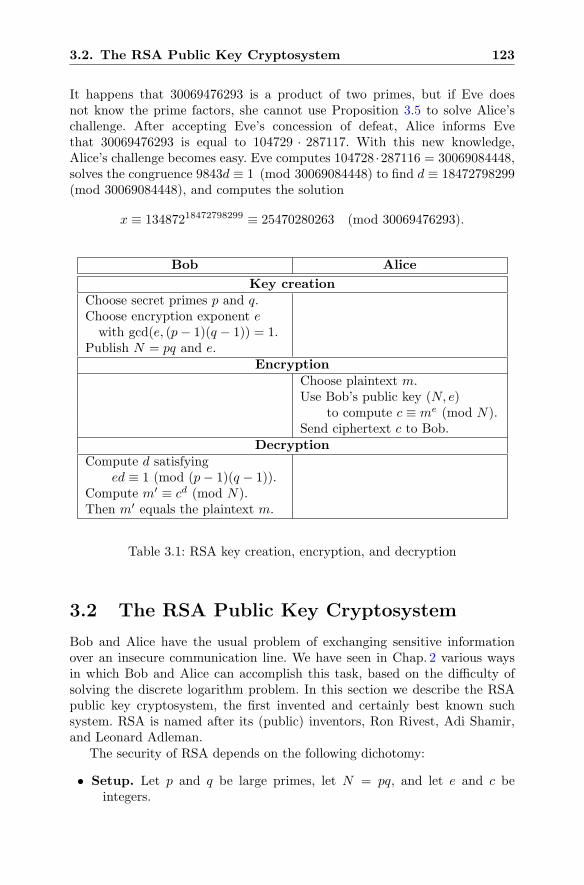
3.2. The RSA Public Key Cryptosystem 123
It happens that 30069476293 is a product of two primes, but if Eve doesnot know the prime factors, she cannot use Proposition 3.5 to solve Alice’schallenge. After accepting Eve’s concession of defeat, Alice informs Evethat 30069476293 is equal to 104729 · 287117. With this new knowledge,Alice’s challenge becomes easy. Eve computes 104728 ·287116 = 30069084448,solves the congruence 9843d ≡ 1 (mod 30069084448) to find d ≡ 18472798299(mod 30069084448), and computes the solution
x ≡ 13487218472798299 ≡ 25470280263 (mod 30069476293).
Bob Alice
Key creationChoose secret primes p and q.Choose encryption exponent e
with gcd(e, (p− 1)(q − 1)) = 1.Publish N = pq and e.
EncryptionChoose plaintext m.Use Bob’s public key (N, e)
to compute c ≡ me (mod N).Send ciphertext c to Bob.
DecryptionCompute d satisfying
ed ≡ 1 (mod (p− 1)(q − 1)).Compute m′ ≡ cd (mod N).Then m′ equals the plaintext m.
Table 3.1: RSA key creation, encryption, and decryption
3.2 The RSA Public Key Cryptosystem
Bob and Alice have the usual problem of exchanging sensitive informationover an insecure communication line. We have seen in Chap. 2 various waysin which Bob and Alice can accomplish this task, based on the difficulty ofsolving the discrete logarithm problem. In this section we describe the RSApublic key cryptosystem, the first invented and certainly best known suchsystem. RSA is named after its (public) inventors, Ron Rivest, Adi Shamir,and Leonard Adleman.
The security of RSA depends on the following dichotomy:
• Setup. Let p and q be large primes, let N = pq, and let e and c beintegers.
124 3. Integer Factorization and RSA
• Problem. Solve the congruence xe ≡ c (mod N) for the variable x.
• Easy. Bob, who knows the values of p and q, can easily solve for x asdescribed in Proposition 3.5.
• Hard. Eve, who does not know the values of p and q, cannot easily find x.
• Dichotomy. Solving xe ≡ c (mod N) is easy for a person who possessescertain extra information, but it is apparently hard for all other people.
The RSA public key cryptosystem is summarized in Table 3.1. Bob’s secretkey is a pair of large primes p and q. His public key is the pair (N, e) consistingof the product N = pq and an encryption exponent e that is relatively primeto (p− 1)(q − 1). Alice takes her plaintext and converts it into an integer mbetween 1 and N . She encrypts m by computing the quantity
c ≡ me (mod N).
The integer c is her ciphertext, which she sends to Bob. It is then a simplematter for Bob to solve the congruence xe ≡ c (mod N) to recover Alice’smessage m, because Bob knows the factorization N = pq. Eve, on the otherhand, may intercept the ciphertext c, but unless she knows how to factor N ,she presumably has a difficult time trying to solve xe ≡ c (mod N).
Example 3.9. We illustrate the RSA public key cryptosystem with a smallnumerical example. Of course, this example is not secure, since the numbersare so small that it would be easy for Eve to factor the modulus N . Secureimplementations of RSA use moduli N with hundreds of digits.
RSA Key Creation• Bob chooses two secret primes p = 1223 and q = 1987. Bob computes hispublic modulus
N = p · q = 1223 · 1987 = 2430101.
• Bob chooses a public encryption exponent e = 948047 with the propertythat
gcd(e, (p− 1)(q − 1)) = gcd(948047, 2426892) = 1.
RSA Encryption• Alice converts her plaintext into an integer
m = 1070777 satisfying 1 ≤ m < N.
• Alice uses Bob’s public key (N, e) = (2430101, 948047) to compute
c ≡ me (mod N), c ≡ 1070777948047 ≡ 1473513 (mod 2430101).
• Alice sends the ciphertext c = 1473513 to Bob.
3.2. The RSA Public Key Cryptosystem 125
RSA Decryption• Bob knows (p− 1)(q − 1) = 1222 · 1986 = 2426892, so he can solve
ed ≡ 1 (mod (p− 1)(q − 1)), 948047 · d ≡ 1 (mod 2426892),
for d and find that d = 1051235.• Bob takes the ciphertext c = 1473513 and computes
cd (mod N), 14735131051235 ≡ 1070777 (mod 2430101).
The value that he computes is Alice’s message m = 1070777.
Remark 3.10. The quantities N and e that form Bob’s public key are called,respectively, the modulus and the encryption exponent. The number d thatBob uses to decrypt Alice’s message, that is, the number d satisfying
ed ≡ 1 (mod (p− 1)(q − 1)), (3.4)
is called the decryption exponent. It is clear that encryption can be donemore efficiently if the encryption exponent e is a small number, and similarly,decryption is more efficient if the decryption exponent d is small. Of course,Bob cannot choose both of them to be small, since once one of them is selected,the other is determined by the congruence (3.4). (This is not strictly true, sinceif Bob takes e = 1, then also d = 1, so both d and e are small. But then theplaintext and the ciphertext are identical, so taking e = 1 is a very bad idea!)
Notice that Bob cannot take e = 2, since he needs e to be relatively primeto (p− 1)(q − 1). Thus the smallest possible value for e is e = 3. As far as isknown, taking e = 3 is as secure as taking a larger value of e, although somedoubts are raised in [22]. People who want fast encryption, but are worriedthat e = 3 is too small, often take e = 216 + 1 = 65537, since it takes onlysixteen squarings and one multiplication to compute m65537 via the square-and-multiply algorithm described in Sect. 1.3.2.
An alternative is for Bob to use a small value for d and use the congru-ence (3.4) to determine e, so e would be large. However, it turns out thatthis may lead to an insecure version of RSA. More precisely, if d is smallerthan N1/4, then the theory of continued fractions allows Eve to break RSA.See [17, 18, 19, 149] for details.
Remark 3.11. Bob’s public key includes the number N = pq, which is aproduct of two secret primes p and q. Proposition 3.5 says that if Eve knowsthe value of (p− 1)(q − 1), then she can solve xe ≡ c (mod N), and thus candecrypt messages sent to Bob.
Expanding (p− 1)(q − 1) gives
(p− 1)(q − 1) = pq − p− q + 1 = N − (p+ q) + 1. (3.5)
Bob has published the value of N , so Eve already knows N . Thus if Evecan determine the value of the sum p+ q, then (3.5) gives her the valueof (p− 1)(q − 1), which enables her to decrypt messages.
126 3. Integer Factorization and RSA
In fact, if Eve knows the values of p+ q and pq, then it is easy for her tocompute the values of p and q. She simply uses the quadratic formula to findthe roots of the polynomial
X2 − (p+ q)X + pq,
since this polynomial factors as (X−p)(X− q), so its roots are p and q. Thusonce Bob publishes the value of N = pq, it is no easier for Eve to find thevalue of (p− 1)(q − 1) than it is for her to find p and q themselves.
We illustrate with an example. Suppose that Eve knows that
N = pq = 66240912547 and (p− 1)(q − 1) = 66240396760.
She first uses (3.5) to compute
p+ q = N + 1− (p− 1)(q − 1) = 515788.
Then she uses the quadratic formula to factor the polynomial
X2 − (p+ q)X +N = X2 − 515788X + 66240912547
= (X − 241511)(X − 274277).
This gives her the factorization N = 66240912547 = 241511 · 274277.Remark 3.12. One final, but very important, observation. We have shown thatit is no easier for Eve to determine (p− 1)(q − 1) than it is for her to factor N .But this does not prove that that Eve must factor N in order to decrypt Bob’smessages. The point is that what Eve really needs to do is to solve congruencesof the form xe ≡ c (mod N), and conceivably there is an efficient algorithm tosolve such congruences without knowing the value of (p− 1)(q − 1). No oneknows whether such a method exists, although see [22] for a suggestion thatcomputing roots modulo N may be easier than factoring N .
3.3 Implementation and Security Issues
Our principal focus in this book is the mathematics of the hard problemsunderlying modern cryptography, but we would be remiss if we did not atleast briefly mention some of the security issues related to implementation.The reader should be aware that we do not even scratch the surface of thisvast and fascinating subject, but simply describe some examples to show thatthere is far more to creating a secure communications system than simplyusing a cryptosystem based on an intractable mathematical problem.
Example 3.13 (Woman-in-the-Middle Attack). Suppose that Eve is not simplyan eavesdropper, but that she has full control over Alice and Bob’s commu-nication network. In this case, she can institute what is known as a man-in-the-middle attack. We describe this attack for Diffie–Hellman key exchange,but it exists for most public key constructions. (See Exercise 3.12.)
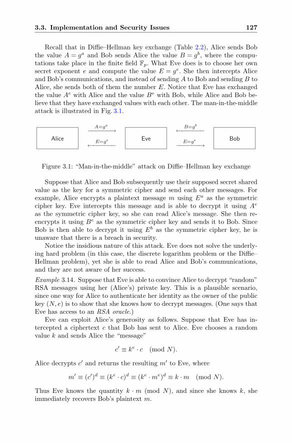
3.3. Implementation and Security Issues 127
Recall that in Diffie–Hellman key exchange (Table 2.2), Alice sends Bobthe value A = ga and Bob sends Alice the value B = gb, where the compu-tations take place in the finite field Fp. What Eve does is to choose her ownsecret exponent e and compute the value E = ge. She then intercepts Aliceand Bob’s communications, and instead of sending A to Bob and sending B toAlice, she sends both of them the number E. Notice that Eve has exchangedthe value Ae with Alice and the value Be with Bob, while Alice and Bob be-lieve that they have exchanged values with each other. The man-in-the-middleattack is illustrated in Fig. 3.1.
Alice−−−−−−→
←−−−−−−Eve
B=gbA=ga
←−−−−−−E=geE=ge
−−−−−−→Bob
Figure 3.1: “Man-in-the-middle” attack on Diffie–Hellman key exchange
Suppose that Alice and Bob subsequently use their supposed secret sharedvalue as the key for a symmetric cipher and send each other messages. Forexample, Alice encrypts a plaintext message m using Ea as the symmetriccipher key. Eve intercepts this message and is able to decrypt it using Ae
as the symmetric cipher key, so she can read Alice’s message. She then re-encrypts it using Be as the symmetric cipher key and sends it to Bob. SinceBob is then able to decrypt it using Eb as the symmetric cipher key, he isunaware that there is a breach in security.
Notice the insidious nature of this attack. Eve does not solve the underly-ing hard problem (in this case, the discrete logarithm problem or the Diffie–Hellman problem), yet she is able to read Alice and Bob’s communications,and they are not aware of her success.
Example 3.14. Suppose that Eve is able to convince Alice to decrypt “random”RSA messages using her (Alice’s) private key. This is a plausible scenario,since one way for Alice to authenticate her identity as the owner of the publickey (N, e) is to show that she knows how to decrypt messages. (One says thatEve has access to an RSA oracle.)
Eve can exploit Alice’s generosity as follows. Suppose that Eve has in-tercepted a ciphertext c that Bob has sent to Alice. Eve chooses a randomvalue k and sends Alice the “message”
c′ ≡ ke · c (mod N).
Alice decrypts c′ and returns the resulting m′ to Eve, where
m′ ≡ (c′)d ≡ (ke · c)d ≡ (ke ·me)d ≡ k ·m (mod N).
Thus Eve knows the quantity k · m (mod N), and since she knows k, sheimmediately recovers Bob’s plaintext m.
128 3. Integer Factorization and RSA
There are two important observations to make. First, Eve has decryptedBob’s message without knowing or gaining knowledge of how to factor N , sothe difficulty of the underlying mathematical problem is irrelevant. Second,since Eve has used k to mask Bob’s ciphertext, Alice has no way to tell thatEve’s message is in any way related to Bob’s message. Thus Alice sees onlythe values ke · c (mod N) and k ·m (mod N), which to her look random whencompared to c and m.
Example 3.15. Suppose that Alice publishes two different exponents e1 and e2for use with her public modulus N and that Bob encrypts a single plaintext musing both of Alice’s exponents. If Eve intercepts the ciphertexts
c1 ≡ me1 (mod N) and c2 ≡ me2 (mod N),
she can take a solution to the equation
e1 · u+ e2 · v = gcd(e1, e2)
and use it to compute
cu1 · cv2 ≡ (me1)u · (me2)v ≡ me1·u+e2·v ≡ mgcd(e1,e2) (mod N).
If it happens that gcd(e1, e2) = 1, Eve has recovered the plaintext. (SeeExercise 3.13 for a numerical example.) More generally, if Bob encrypts asingle message using several exponents e1, e2, . . . , er, then Eve can recover theplaintext if gcd(e1, e2, . . . , er) = 1. The moral is that Alice should use at mostone encryption exponent for a given modulus.
3.4 Primality Testing
Bob has finished reading Sects. 3.2 and 3.3 and is now ready to communicatewith Alice using his RSA public/private key pair. Or is he? In order to createan RSA key pair, Bob needs to choose two very large primes p and q. It’s notenough for him to choose two very large, but possibly composite, numbers pand q. In the first place, if p and q are not prime, Bob will need to know howto factor them in order to decrypt Alice’s message. But even worse, if p and qhave small prime factors, then Eve may be able to factor pq and break Bob’ssystem.
Bob is thus faced with the task of finding large prime numbers. More pre-cisely, he needs a way of distinguishing between prime numbers and compositenumbers, since if he knows how to do this, then he can choose large randomnumbers until he hits one that is prime. We discuss later (Sect. 3.4.1) the like-lihood that a randomly chosen number is prime, but for now it is enough toknow that he has a reasonably good chance of success. Hence what Bob reallyneeds is an efficient way to tell whether a very large number is prime.
3.4. Primality Testing 129
For example, suppose that Bob chooses the rather large number
n = 31987937737479355332620068643713101490952335301
and he wants to know whether n is prime. First Bob searches for small factors,but he finds that n is not divisible by any primes smaller than 1000000. Sohe begins to suspect that maybe n is prime. Next he computes the quantity2n−1 mod n and he finds that
2n−1 ≡ 1281265953551359064133601216247151836053160074 (mod n). (3.6)
The congruence (3.6) immediately tells Bob that n is a composite number,although it does not give him any indication of how to factor n. Why? RecallFermat’s little theorem, which says that if p is prime, then ap−1 ≡ 1 (mod p)(unless p divides a). Thus if n were prime, then the right-hand side of (3.6)would equal 1; since it does not equal 1, Bob concludes that n is not prime.
Before continuing the saga of Bob’s quest for large primes, we state aconvenient version of Fermat’s little theorem that puts no restrictions on a.
Theorem 3.16 (Fermat’s Little Theorem, Version 2). Let p be a prime num-ber. Then
ap ≡ a (mod p) for every integer a. (3.7)
Proof. If p � a, then the first version of Fermat’s little theorem (Theorem 1.24)implies that ap−1 ≡ 1 (mod p). Multiplying both sides by a proves that (3.7)is true. On the other hand, if p | a, then both sides of (3.7) are 0 modulo p.
Returning to Bob’s quest, we find him undaunted as he randomly choosesanother large number,
n = 2967952985951692762820418740138329004315165131. (3.8)
After checking for divisibility by small primes, Bob computes 2n mod n andfinds that
2n ≡ 2 (mod n). (3.9)
Does (3.9) combined with Fermat’s little theorem 3.16 prove that n is prime?The answer is NO! Fermat’s theorem works in only one direction:
If p is prime, then ap ≡ a (mod p).
There is nothing to prevent an equality such as (3.9) being true for compositevalues of n, and indeed a brief search reveals examples such as
2341 ≡ 2 (mod 341) with 341 = 11 · 31.
However, in some vague philosophical sense, the fact that 2n ≡ 2 (mod n)makes it more likely that n is prime, since if the value of 2n mod n had turnedout differently, we would have known that n was composite. This leads us tomake the following definition.
130 3. Integer Factorization and RSA
Definition. Fix an integer n. We say that an integer a is a witness for (thecompositeness of ) n if
an �≡ a (mod n).
As we observed earlier, a single witness for n combined with Fermat’s littletheorem (Theorem 3.16) is enough to prove beyond a shadow of a doubt that nis composite.1 Thus one way to assess the likelihood that n is prime is to trya lot of numbers a1, a2, a3, . . . . If any one of them is a witness for n, then Bobknows that n is composite; and if none of them is a witness for n, then Bobsuspects, but does not know for certain, that n is prime.
Unfortunately, intruding on this idyllic scene are barbaric numbers suchas 561. The number 561 is composite, 561 = 3·11·17, yet 561 has no witnesses!In other words,
a561 ≡ a (mod 561) for every integer a.
Composite numbers having no witnesses are called Carmichael numbers, afterR.D. Carmichael, who in 1910 published a paper listing 15 such numbers.The fact that 561 is a Carmichael number can be verified by checking eachvalue a = 0, 1, 2, . . . , 560, but see Exercise 3.14 for an easier method and formore examples of Carmichael numbers. Although Carmichael numbers arerather rare, Alford, Granville, and Pomerance [5] proved in 1994 that thereare infinitely many of them. So Bob needs something stronger than Fermat’slittle theorem in order to test whether a number is (probably) prime. Whatis needed is a better test for compositeness. The following property of primenumbers is used to formulate the Miller–Rabin test, which has the agreeableproperty that every composite number has a large number of witnesses.
Proposition 3.17. Let p be an odd prime and write
p− 1 = 2kq with q odd.
Let a be any number not divisible by p. Then one of the following two condi-tions is true:(i) aq is congruent to 1 modulo p.
(ii) One of aq, a2q, a4q,. . . , a2k−1q is congruent to −1 modulo p.
Proof. Fermat’s little theorem (Theorem 1.24) tells us that ap−1 ≡ 1 (mod p).This means that when we look at the list of numbers
aq, a2q, a4q, . . . , a2k−1q, a2
kq,
we know that the last number in the list, which equals ap−1, is congruentto 1 modulo p. Further, each number in the list is the square of the previousnumber. Therefore one of the following two possibilities must occur:
1In the great courthouse of mathematics, witnesses never lie!
3.4. Primality Testing 131
(i) The first number in the list is congruent to 1 modulo p.
(ii) Some number in the list is not congruent to 1 modulo p, but when itis squared, it becomes congruent to 1 modulo p. But the only numbersatisfying both
b �≡ 1 (mod p) and b2 ≡ 1 (mod p)
is −1, so one of the numbers in the list is congruent to −1 modulo p.
This completes the proof of Proposition 3.17.
Input. Integer n to be tested, integer a as potential witness.
1. If n is even or 1 < gcd(a, n) < n, return Composite.
2. Write n− 1 = 2kq with q odd.
3. Set a = aq (mod n).
4. If a ≡ 1 (mod n), return Test Fails.
5. Loop i = 0, 1, 2, . . . , k − 1
6. If a ≡ −1 (mod n), return Test Fails.
7. Set a = a2 mod n.
8. End i loop.
9. Return Composite.
Table 3.2: Miller–Rabin test for composite numbers
Definition. Let n be an odd number and write n− 1 = 2kq with q odd. Aninteger a satisfying gcd(a, n) = 1 is called a Miller–Rabin witness for (thecompositeness of ) n if both of the following conditions are true:(a) aq �≡ 1 (mod n).
(b) a2iq �≡ −1 (mod n) for all i = 0, 1, 2, . . . , k − 1.
It follows from Proposition 3.17 that if there exists an a that is a Miller–Rabin witness for n, then n is definitely a composite number. This leads tothe Miller–Rabin test for composite numbers described in Table 3.2.
Now suppose that Bob wants to check whether a large number n is prob-ably a prime. To do this, he runs the Miller–Rabin test using a bunch ofrandomly selected values of a. Why is this better than using the Fermat’slittle theorem test? The answer is that there are no Carmichael-like numbersfor the Miller–Rabin test, and in fact, every composite number has a lot ofMiller–Rabin witnesses, as described in the following proposition.
Proposition 3.18. Let n be an odd composite number. Then at least 75% ofthe numbers a between 1 and n− 1 are Miller–Rabin witnesses for n.
132 3. Integer Factorization and RSA
Proof. The proof is not hard, but we will not give it here. See for example [132,Theorem 10.6].
Consider now Bob’s quest to identify large prime numbers. He takes hispotentially prime number n and he runs the Miller–Rabin test on n for (say)10 different values of a. If any a value is a Miller–Rabin witness for n, thenBob knows that n is composite. But suppose that none of his a values is aMiller–Rabin witness for n. Proposition 3.18 says that if n were composite,then each time Bob tries a value for a, he has at least a 75% chance ofgetting a witness. Since Bob found no witnesses in 10 tries, it is reasonable2
to conclude that the probability of n being composite is at most (25%)10,which is approximately 10−6. And if this is not good enough, Bob can use100 different values of a, and if none of them proves n to be composite, thenthe probability that n is actually composite is less than (25%)100 ≈ 10−60.
Example 3.19. We illustrate the Miller–Rabin test with a = 2 and the numbern = 561, which, you may recall, is a Carmichael number. We factor
n− 1 = 560 = 24 · 35
and then compute
235 ≡ 263 (mod 561),
22·35 ≡ 2632 ≡ 166 (mod 561),
24·35 ≡ 1662 ≡ 67 (mod 561),
28·35 ≡ 672 ≡ 1 (mod 561).
The first number 235 mod 561 is neither 1 nor −1, and the other numbers inthe list are not equal to −1, so 2 is a Miller–Rabin witness to the fact that 561is composite.
Example 3.20. We do a second example, taking n = 172947529 and
n− 1 = 172947528 = 23 · 21618441.
We apply the Miller–Rabin test with a = 17 and find that
1721618441 ≡ 1 (mod 172947529).
2Unfortunately, although this deduction seems reasonable, it is not quite accurate. Inthe language of probability theory, we need to compute the conditional probability that nis composite given that the Miller–Rabin test fails 10 times; and we know the conditionalprobability that the Miller–Rabin test succeeds at least 75% of the time if n is composite.See Sect. 5.3.2 for a discussion of conditional probabilities and Exercise 5.30 for a derivationof the correct formula, which says that the probability (25%)10 must be approximatelymultiplied by ln(n).
3.4. Primality Testing 133
Thus 17 is not a Miller–Rabin witness for n. Next we try a = 3, but unfortu-nately
321618441 ≡ −1 (mod 172947529),
so 3 also fails to be a Miller–Rabin witness. At this point we might suspectthat n is prime, but if we try another value, say a = 23, we find that
2321618441 ≡ 40063806 (mod 172947529),
232·21618441 ≡ 2257065 (mod 172947529),
234·21618441 ≡ 1 (mod 172947529).
Thus 23 is a Miller–Rabin witness and n is actually composite. In fact, n is aCarmichael number, but it’s not so easy to factor (by hand).
3.4.1 The Distribution of the Set of Primes
If Bob picks a number at random, what is the likelihood that it is prime? Theanswer is provided by one of number theory’s most famous theorems. In orderto state the theorem, we need a definition.
Definition. For any number X, let
π(X) = (# of primes p satisfying 2 ≤ p ≤ X).
For example, π(10) = 4, since the primes between 2 and 10 are 2, 3, 5, and 7.
Theorem 3.21 (The Prime Number Theorem).
limX→∞
π(X)
X/ ln(X)= 1.
Proof. The prime number theorem was proven independently by Hadamardand de la Vallee Poussin in 1896. The proof is unfortunately far beyond thescope of this book. The most direct proof uses complex analysis; see for ex-ample [7, Chapter 13].
Example 3.22. How many primes would we expect to find between 900000and 1000000? The prime number theorem says that
(Number of primes between 900000 and 1000000
)
= π(1000000)− π(900000) ≈ 1000000
ln 1000000− 900000
ln 900000= 6737.62 . . . .
In fact, it turns out that there are exactly 7224 primes between 900000and 1000000.
For cryptographic purposes, we need even larger primes. For example,we might want to use primes having approximately 300 decimal digits, oralmost equivalently, primes that are 1024 bits in length, since 21024 ≈ 10308.25.
134 3. Integer Factorization and RSA
How many primes p satisfy 21023 < p < 21024? The prime number theoremgives us an answer:
# of 1024 bit primes = π(21024)− π(21023) ≈ 21024
ln 21024− 21023
ln 21023≈ 21013.53.
So there should be lots of primes in this interval.
Intuitively, the prime number theorem says that if we look at all of thenumbers between 1 and X, then the proportion of them that are prime isapproximately 1/ ln(X). Turning this statement around, the prime numbertheorem says:
A randomly chosen number N hasprobability 1/ ln(N) of being prime.
(3.10)
Of course, taken at face value, statement (3.10) is utter nonsense. A chosennumber either is prime or is not prime; it cannot be partially prime andpartially composite! A better interpretation of (3.10) is that it describes howmany primes one expects to find in an interval around N . See Exercise 3.19 fora more precise statement of (3.10) that is both meaningful and mathematicallycorrect.
Example 3.23. We illustrate statement (3.10) and the prime number theoremby searching for 1024-bit primes, i.e., primes that are approximately 21024.Statement (3.10) says that the probability that a random number N ≈ 21024
is prime is approximately 0.14%. Thus on average, Bob checks about 700 ran-domly chosen numbers of this size before finding a prime.
If he is clever, Bob can do better. He knows that he doesn’t want a numberthat is even, nor does he want a number that is divisible by 3, nor divisibleby 5, etc. Thus rather than choosing numbers completely at random, Bobmight restrict attention (say) to numbers that are relatively prime to 2, 3, 5, 7and 11. To do this, he first chooses a random number that is relatively primeto 2·3·5·7·11 = 2310, say he chooses 1139. Then he considers only numbers Nof the form
N = 2 · 3 · 5 · 7 · 11 ·K + 1139 = 2310K + 1139. (3.11)
The probability that an N of this form is prime is approximately (see Exer-cise 3.20)
2
1· 32· 54· 76· 1110· 1
ln(N)≈ 4.8
ln(N).
So if Bob chooses a random number N of the form (3.11) with N ≈ 21024,then the probability that it is prime is approximately 0.67%. Thus he onlyneeds to check 150 numbers to have a good chance of finding a prime.
3.4. Primality Testing 135
We used the Miller–Rabin test with 100 randomly chosen values of a tocheck the primality of
2310K + 1139 for each 21013 ≤ K ≤ 21013 + 1000.
We found that 2310(21013+J)+1139 is probably prime for the following 12 val-ues of J :
J ∈ {41, 148, 193, 251, 471, 585, 606, 821, 851, 865, 910, 911}.This is a bit better than the 7 values predicted by the prime number theorem.The smallest probable prime that we found is 2310 · (21013 + 41) + 1139, whichis equal to the following 308 digit number:
20276714558261473373313940384387925462194955182405899331133959349334105522983
75121272248938548639688519470034484877532500936544755670421865031628734263599742737518719
78241831537235413710389881550750303525056818030281312537212445925881220354174468221605146
327969430834440565497127875070636801598203824198219369.
Remark 3.24. There are many deep open questions concerning the distributionof prime numbers, of which the most important and famous is certainly theRiemann hypothesis.3 The usual way to state the Riemann hypothesis requiressome complex analysis. The Riemann zeta function ζ(s) is defined by theseries
ζ(s) =∞∑
n=1
1
ns,
which converges when s is a complex number with real part greater than 1. Ithas an analytic continuation to the entire complex plane with a simple poleat s = 1 and no other poles. The Riemann hypothesis says that if ζ(σ+it) = 0with σ and t real and 0 ≤ σ ≤ 1, then in fact σ = 1
2 .At first glance, this somewhat bizarre statement appears to have little
relation to prime numbers. However, it is not hard to show that ζ(s) is alsoequal to the product
ζ(s) =∏
p prime
(1− 1
ps
)−1
,
so ζ(s) incorporates information about the set of prime numbers.There are many statements about prime numbers that are equivalent to
the Riemann hypothesis. For example, recall that the prime number theorem(Theorem 3.21) says that π(X) is approximately equal to X/ ln(X) for largevalues of X. The Riemann hypothesis is equivalent to the following moreaccurate statement:
π(X) =
∫ X
2
dt
ln t+O
(√X · ln(X)
). (3.12)
This conjectural formula is stronger than the prime number theorem, sincethe integral is approximately equal to X/ ln(X). (See Exercise 3.21.)
3The Riemann hypothesis is another of the $1,000,000 Millennium Prize problems.
136 3. Integer Factorization and RSA
3.4.2 Primality Proofs Versus Probabilistic Tests
The Miller–Rabin test is a powerful and practical method for finding largenumbers that are “probably prime.” Indeed, Proposition 3.18 says that everycomposite number has many Miller–Rabin witnesses, so 50 or 100 repetitionsof the Miller–Rabin test provide solid evidence that n is prime. However, thereis a difference between evidence for a statement and a rigorous proof that thestatement is correct. Suppose that Bob is not satisfied with mere evidence.He wants to be completely certain that his chosen number n is prime.
In principle, nothing could be simpler. Bob checks to see whether n is di-visible by any of the numbers 1, 2, 3, 4, . . . up to
√n. If none of these numbers
divides n, then Bob knows, with complete certainty, that n is prime. Unfor-tunately, if n is large, say n ≈ 21000, then the sun will have burnt out beforeBob finishes his task. Notice that the running time of this naive algorithmis O(
√n), which means that it is an exponential-time algorithm according
to the definition in Sect. 2.6, since√n is exponential in the number of bits
required to write down the number n.It would be nice if we could use the Miller–Rabin test to efficiently and
conclusively prove that a number n is prime. More precisely, we would like apolynomial-time algorithm that proves primality. If a generalized version ofthe Riemann hypothesis is true, then the following proposition says that thiscan be done. (We discussed the Riemann hypothesis in Remark 3.24.)
Proposition 3.25. If a generalized version of the Riemann hypothesis istrue, then every composite number n has a Miller–Rabin witness a for itscompositeness satisfying
a ≤ 2(lnn)2.
Proof. See [87] for a proof that every composite number n has a wit-ness satisfying a = O
((lnn)2
), and [9, 10] for the more precise estimate
a ≤ 2(lnn)2.
Thus if the generalized Riemann hypothesis is true, then we can provethat n is prime by applying the Miller–Rabin test using every a smallerthan 2(lnn)2. If some a proves that n is composite, then n is composite,and otherwise, Proposition 3.25 tells us that n is prime. Unfortunately, theproof of Proposition 3.25 assumes that the generalized Riemann hypothesisis true, and no one has yet been able to prove even the original Riemannhypothesis, despite almost 150 years of work on the problem.
After the creation of public key cryptography, and especially after thepublication of the RSA cryptosystem in 1978, it became of great interest tofind a polynomial-time primality test that did not depend on any unprovenhypotheses. Many years of research culminated in 2002, when M. Agrawal, N.Kayal, and N. Saxena [1] found such an algorithm. Subsequent improvementsto their algorithm have given the following result.
3.5. Pollard’s p − 1 Factorization Algorithm 137
Theorem 3.26 (AKS Primality Test). For every ε > 0, there is an algorithmthat conclusively determines whether a given number n is prime in no morethan O
((lnn)6+ε
)steps.
Proof. The original algorithm was published in [1]. Further analysis and refine-ments may be found in [76]. The monograph [36] contains a nice descriptionof primality testing, including the AKS test.
Remark 3.27. The result described in Theorem 3.26 represents a triumph ofmodern algorithmic number theory. The significance for practical cryptogra-phy is less clear, since the AKS algorithm is much slower than the Miller–Rabin test. In practice, most people are willing to accept that a number isprime if it passes the Miller–Rabin test for (say) 50–100 randomly chosenvalues of a.
3.5 Pollard’s p − 1 Factorization Algorithm
We saw in Sect. 3.4 that it is relatively easy to check whether a large numberis (probably) prime. This is good, since the RSA cryptosystem needs largeprimes in order to operate.
Conversely, the security of RSA relies on the apparent difficulty of factor-ing large numbers. The study of factorization dates back at least to ancientGreece, but it was only with the advent of computers that people started todevelop algorithms capable of factoring very large numbers. The paradox ofRSA is that in order to make RSA more efficient, we want to use a modu-lus N = pq that is as small as possible. On the other hand, if an opponentcan factor N , then our encrypted messages are not secure. It is thus vitalto understand how hard it is to factor large numbers, and in particular, tounderstand the capabilities of the different algorithms that are currently usedfor factorization.
In the next few sections we discuss, with varying degrees of detail, someof the known methods for factoring large integers. A further method usingelliptic curves is described in Sect. 6.6. Those readers interested in pursuingthis subject might consult [28, 34, 109, 150] and the references cited in thoseworks.
We begin with an algorithm called Pollard’s p − 1 method. Although notuseful for all numbers, there are certain types of numbers for which it is quiteefficient. Pollard’s method demonstrates that there are insecure RSA modulithat at first glance appear to be secure. This alone warrants the study ofPollard’s method. In addition, the p− 1 method provides the inspiration forLenstra’s elliptic curve factorization method, which we study later, in Sect. 6.6.
We are presented with a number N = pq and our task is to determinethe prime factors p and q. Suppose that by luck or hard work or some othermethod, we manage to find an integer L with the property that
138 3. Integer Factorization and RSA
p− 1 divides L and q − 1 does not divide L.
This means that there are integers i, j, and k with k �= 0 satisfying
L = i(p− 1) and L = j(q − 1) + k.
Consider what happens if we take a randomly chosen integer a and com-pute aL. Fermat’s little theorem (Theorem 1.24) tells us that4
aL = ai(p−1) = (ap−1)i ≡ 1i ≡ 1 (mod p),
aL = aj(q−1)+k = ak(aq−1)j ≡ ak · 1j ≡ ak (mod q).
The exponent k is not equal to 0, so it is quite unlikely that ak will becongruent to 1 modulo q. Thus with very high probability, i.e., for most choicesof a, we find that
p divides aL − 1 and q does not divide aL − 1.
But this is wonderful, since it means that we can recover p via the simple gcdcomputation
p = gcd(aL − 1, N).
This is all well and good, but where, you may ask, can we find an expo-nent L that is divisible by p− 1 and not by q − 1? Pollard’s observation isthat if p− 1 happens to be a product of many small primes, then it will di-vide n! for some not-too-large value of n. So here is the idea. For each numbern = 2, 3, 4, . . . we choose a value of a and compute
gcd(an! − 1, N).
(In practice, we might simply take a = 2.) If the gcd is equal to 1, then wego on to the next value of n. If the gcd ever equals N , then we’ve been quiteunlucky, but a different a value will probably work. And if we get a numberstrictly between 1 and N , then we have a nontrivial factor of N and we’redone.
Remark 3.28. There are two important remarks to make before we putPollard’s idea into practice. The first concerns the quantity an! − 1. Evenfor a = 2 and quite moderate values of n, say n = 100, it is not feasible tocompute an! − 1 exactly. Indeed, the number 2100! has more than 10157 digits,which is larger than the number of elementary particles in the known universe!Luckily, there is no need to compute it exactly. We are interested only in thegreatest common divisor of an! − 1 and N , so it suffices to compute
an! − 1 (mod N)
4We have assumed that p � a and q � a, since if p and q are very large, this will almostcertainly be the case. Further, if by some chance p | a and q � a, then we can recover p asp = gcd(a,N).
3.5. Pollard’s p − 1 Factorization Algorithm 139
and then take the gcd with N . Thus we never need to work with numberslarger than N .
Second, we do not even need to compute the exponent n!. Instead, assum-ing that we have already computed an! mod N in the previous step, we cancompute the next value as
a(n+1)! ≡(an!)n+1
(mod N).
This leads to the algorithm described in Table 3.3.
Remark 3.29. How long does it take to compute the value of an! mod N? Thefast exponentiation algorithm described in Sect. 1.3.2 gives a method for com-puting ak mod N in at most 2 log2 k steps, where each step is a multiplicationmodulo N . Stirling’s formula5 says that if n is large, then n! is approximatelyequal to (n/e)n. So we can compute an! mod N in 2n log2(n) steps. Thus it isfeasible to compute an! mod N for reasonably large values of n.
Input. Integer N to be factored.
1. Set a = 2 (or some other convenient value).
2. Loop j = 2, 3, 4, . . . up to a specified bound.
3. Set a = aj mod N .
4. Compute d = gcd(a− 1, N)†.5. If 1 < d < N then success, return d.
6. Increment j and loop again at Step 2.
† For added efficiency, choose an appropriate k andcompute the gcd in Step 4 only every kth iteration.
Table 3.3: Pollard’s p− 1 factorization algorithm
Example 3.30. We use Pollard’s p−1 method to factorN = 13927189. Startingwith gcd(29!− 1, N) and taking successively larger factorials in the exponent,we find that
29! − 1 ≡ 13867883 (mod 13927189), gcd(29! − 1, 13927189) = 1,
210! − 1 ≡ 5129508 (mod 13927189), gcd(210! − 1, 13927189) = 1,
211! − 1 ≡ 4405233 (mod 13927189), gcd(211! − 1, 13927189) = 1,
212! − 1 ≡ 6680550 (mod 13927189), gcd(212! − 1, 13927189) = 1,
213! − 1 ≡ 6161077 (mod 13927189), gcd(213! − 1, 13927189) = 1,
214! − 1 ≡ 879290 (mod 13927189), gcd(214! − 1, 13927189) = 3823.
The final line gives us a nontrivial factor p = 3823 of N . This factor isprime, and the other factor q = N/p = 13927189/3823 = 3643 is also prime.
5Stirling’s formula says more precisely that ln(n!) = n ln(n)− n+ 12ln(2πn) +O(1/n).
140 3. Integer Factorization and RSA
The reason that an exponent of 14! worked in this instance is that p− 1 factorsinto a product of small primes,
p− 1 = 3822 = 2 · 3 · 72 · 13.
The other factor satisfies q − 1 = 3642 = 2 · 3 · 607, which is not a product ofsmall primes.
Example 3.31. We present one further example using larger numbers. LetN = 168441398857. Then
250! − 1 ≡ 114787431143 (mod N), gcd(250! − 1, N) = 1,
251! − 1 ≡ 36475745067 (mod N), gcd(251! − 1, N) = 1,
252! − 1 ≡ 67210629098 (mod N), gcd(252! − 1, N) = 1,
253! − 1 ≡ 8182353513 (mod N), gcd(253! − 1, N) = 350437.
So using 253! − 1 yields the prime factor p = 350437 of N , and the other(prime) factor is 480661. We were lucky, of course, that p− 1 is a product ofsmall factors,
p− 1 = 350436 = 22 · 3 · 19 · 29 · 53.Remark 3.32. Notice that it is easy for Bob and Alice to avoid the dangers ofPollard’s p− 1 method when creating RSA keys. They simply check that theirchosen secret primes p and q have the property that neither p− 1 nor q − 1factors entirely into small primes. From a cryptographic perspective, the im-portance of Pollard’s method lies in the following lesson. Most people wouldnot expect, at first glance, that factorization properties of p− 1 and q − 1should have anything to do with the difficulty of factoring pq. The moral isthat even if we build a cryptosystem based on a seemingly hard problem suchas integer factorization, we must be wary of special cases of the problem that,for subtle and nonobvious reasons, are easier to solve than the general case.We have already seen an example of this in the Pohlig–Hellman algorithm forthe discrete logarithm problem (Sect. 2.9), and we will see it again later whenwe discuss elliptic curves and the elliptic curve discrete logarithm problem.
Remark 3.33. We have not yet discussed the likelihood that Pollard’s p − 1algorithm succeeds. Suppose that p and q are randomly chosen primes of aboutthe same size. Pollard’s method works if at least one of p− 1 or q − 1 factorsentirely into a product of small prime powers. Clearly p− 1 is even, so wecan pull off a factor of 2, but after that, the quantity 1
2 (p− 1) should behavemore or less like a random number of size approximately 1
2p. This leads to thefollowing question:
What is the probability that a randomly chosen integer ofsize approximately n divides B! (B-factorial)?
Notice in particular that if n divides B!, then every prime � dividing n mustsatisfy � ≤ B. A number whose prime factors are all less than or equal to B
3.6. Factorization via Difference of Squares 141
is called a B-smooth number. It is thus natural to ask for the probability thata randomly chosen integer of size approximately n is a B-smooth number.Turning this question around, we can also ask:
Given n, how large should we choose B so that a randomlychosen integer of size approximately n has a reasonablygood probability of being a B-smooth number?
The efficiency (or lack thereof) of all modern methods of integer factoriza-tion is largely determined by the answer to this question. We study smoothnumbers in Sect. 3.7.
3.6 Factorization via Difference of Squares
The most powerful factorization methods known today rely on one of thesimplest identities in all of mathematics,
X2 − Y 2 = (X + Y )(X − Y ). (3.13)
This beautiful formula says that a difference of squares is equal to a product.The potential applicability to factorization is immediate. In order to factor anumber N , we look for an integer b such that the quantity N + b2 is a perfectsquare, say equal to a2. Then N + b2 = a2, so
N = a2 − b2 = (a+ b)(a− b),
and we have effected a factorization of N .
Example 3.34. We factorN = 25217 by looking for an integer bmakingN + b2
a perfect square:
25217 + 12 = 25218 not a square,
25217 + 22 = 25221 not a square,
25217 + 32 = 25226 not a square,
25217 + 42 = 25233 not a square,
25217 + 52 = 25242 not a square,
25217 + 62 = 25253 not a square,
25217 + 72 = 25266 not a square,
25217 + 82 = 25281 = 1592 Eureka! ** square **.
Then we compute
25217 = 1592 − 82 = (159 + 8)(159− 8) = 167 · 151.
142 3. Integer Factorization and RSA
If N is large, then it is unlikely that a randomly chosen value of b willmake N + b2 into a perfect square. We need to find a clever way to select b.An important observation is that we don’t necessarily need to write N itselfas a difference of two squares. It often suffices to write some multiple kN of Nas a difference of two squares, since if
kN = a2 − b2 = (a+ b)(a− b),
then there is a reasonable chance that the factors of N are separated by theright-hand side of the equation, i.e., that N has a nontrivial factor in commonwith each of a+ b and a− b. It is then a simple matter to recover the factorsby computing gcd(N, a+ b) and gcd(N, a− b). We illustrate with an example.
Example 3.35. We factor N = 203299. If we make a list of N + b2 for valuesof b = 1, 2, 3, . . ., say up to b = 100, we do not find any square values. So nextwe try listing the values of 3N + b2 and we find
3 · 203299 + 12 = 609898 not a square,
3 · 203299 + 22 = 609901 not a square,
3 · 203299 + 32 = 609906 not a square,
3 · 203299 + 42 = 609913 not a square,
3 · 203299 + 52 = 609922 not a square,
3 · 203299 + 62 = 609933 not a square,
3 · 203299 + 72 = 609946 not a square,
3 · 203299 + 82 = 609961 = 7812 Eureka! ** square **.
Thus3 · 203299 = 7812 − 82 = (781 + 8)(781− 8) = 789 · 773,
so when we compute
gcd(203299, 789) = 263 and gcd(203299, 773) = 773,
we find nontrivial factors of N . The numbers 263 and 773 are prime, so thefull factorization of N is 203299 = 263 · 773.Remark 3.36. In Example 3.35, we made a list of values of 3N + b2. Whydidn’t we try 2N + b2 first? The answer is that if N is odd, then 2N + b2
can never be a square, so it would have been a waste of time to try it. Thereason that 2N + b2 can never be a square is as follows (cf. Exercise 1.23).We compute modulo 4,
2N + b2 ≡ 2 + b2 ≡{2 + 0 ≡ 2 (mod 4) if b is even,
2 + 1 ≡ 3 (mod 4) if b is odd.
Thus 2N+b2 is congruent to either 2 or 3 modulo 4. But squares are congruentto either 0 or 1 modulo 4. Hence if N is odd, then 2N + b2 is never a square.
3.6. Factorization via Difference of Squares 143
The multiples of N are the numbers that are congruent to 0 modulo N ,so rather than searching for a difference of squares a2 − b2 that is a multipleof N , we may instead search for distinct numbers a and b satisfying
a2 ≡ b2 (mod N). (3.14)
This is exactly the same problem, of course, but the use of modular arithmetichelps to clarify our task.
In practice it is not feasible to search directly for integers a and b satis-fying (3.14). Instead we use a three-step process as described in Table 3.4.This procedure, in one form or another, underlies most modern methods offactorization.
1. Relation Building: Find many integers a1, a2, a3, . . . , ar with theproperty that the quantity ci ≡ a2i (mod N) factors as a product ofsmall primes.
2. Elimination: Take a product ci1ci2 · · · cis of some of the ci’s so thatevery prime appearing in the product appears to an even power. Thenci1ci2 · · · cis = b2 is a perfect square.
3. GCD Computation: Let a = ai1ai2 · · · ais and compute the greatestcommon divisor d = gcd(N, a− b). Since
a2 = (ai1ai2 · · · ais)2 ≡ a2i1a
2i2 · · · a
2is ≡ ci1ci2 · · · cis ≡ b2 (mod N),
there is a reasonable chance that d is a nontrivial factor of N .
Table 3.4: A three step factorization procedure
Example 3.37. We factor N = 914387 using the procedure described inTable 3.4. We first search for integers a with the property that a2 mod Nis a product of small primes. For this example, we ask that each a2 mod N bea product of primes in the set {2, 3, 5, 7, 11}. Ignoring for now the question ofhow to find such a, we observe that
18692 ≡ 750000 (mod 914387) and 750000 = 24 · 3 · 56,19092 ≡ 901120 (mod 914387) and 901120 = 214 · 5 · 11,33872 ≡ 499125 (mod 914387) and 499125 = 3 · 53 · 113.
None of the numbers on the right is a square, but if we multiply them together,then we do get a square. Thus
18692 · 19092 · 33872 ≡ 750000 · 901120 · 499125 (mod 914387)
≡ (24 · 3 · 56)(214 · 5 · 11)(3 · 53 · 113) (mod 914387)
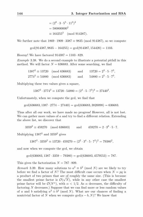
144 3. Integer Factorization and RSA
= (29 · 3 · 55 · 112)2
= 5808000002
≡ 1642552 (mod 914387).
We further note that 1869 · 1909 · 3387 ≡ 9835 (mod 914387), so we compute
gcd(914387, 9835− 164255) = gcd(914387, 154420) = 1103.
Hooray! We have factored 914387 = 1103 · 829.Example 3.38. We do a second example to illustrate a potential pitfall in thismethod. We will factor N = 636683. After some searching, we find
13872 ≡ 13720 (mod 636683) and 13720 = 23 · 5 · 73,27742 ≡ 54880 (mod 636683) and 54880 = 25 · 5 · 73.
Multiplying these two values gives a square,
13872 · 27742 ≡ 13720 · 54880 = (24 · 5 · 73)2 = 274402.
Unfortunately, when we compute the gcd, we find that
gcd(636683, 1387 · 2774− 27440) = gcd(636683, 3820098) = 636683.
Thus after all our work, we have made no progress! However, all is not lost.We can gather more values of a and try to find a different relation. Extendingthe above list, we discover that
33592 ≡ 459270 (mod 636683) and 459270 = 2 · 38 · 5 · 7.
Multiplying 13872 and 33592 gives
13872 · 33592 ≡ 13720 · 459270 = (22 · 34 · 5 · 72)2 = 793802,
and now when we compute the gcd, we obtain
gcd(636683, 1387 · 3359− 79380) = gcd(636683, 4579553) = 787.
This gives the factorization N = 787 · 809.Remark 3.39. How many solutions to a2 ≡ b2 (mod N) are we likely to trybefore we find a factor of N? The most difficult case occurs when N = pq isa product of two primes that are of roughly the same size. (This is becausethe smallest prime factor is O(
√N), while in any other case the smallest
prime factor will be O(Nα), with α < 1/2. As α decreases, the difficulty offactoring N decreases.) Suppose that we can find more or less random valuesof a and b satisfying a2 ≡ b2 (mod N). What are our chances of finding anontrivial factor of N when we compute gcd(a− b,N)? We know that
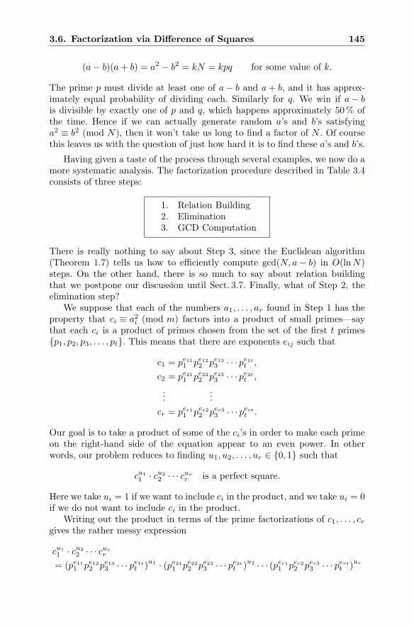
3.6. Factorization via Difference of Squares 145
(a− b)(a+ b) = a2 − b2 = kN = kpq for some value of k.
The prime p must divide at least one of a− b and a+ b, and it has approx-imately equal probability of dividing each. Similarly for q. We win if a− bis divisible by exactly one of p and q, which happens approximately 50% ofthe time. Hence if we can actually generate random a’s and b’s satisfyinga2 ≡ b2 (mod N), then it won’t take us long to find a factor of N . Of coursethis leaves us with the question of just how hard it is to find these a’s and b’s.
Having given a taste of the process through several examples, we now do amore systematic analysis. The factorization procedure described in Table 3.4consists of three steps:
1. Relation Building2. Elimination3. GCD Computation
There is really nothing to say about Step 3, since the Euclidean algorithm(Theorem 1.7) tells us how to efficiently compute gcd(N, a− b) in O(lnN)steps. On the other hand, there is so much to say about relation buildingthat we postpone our discussion until Sect. 3.7. Finally, what of Step 2, theelimination step?
We suppose that each of the numbers a1, . . . , ar found in Step 1 has theproperty that ci ≡ a2i (mod m) factors into a product of small primes—saythat each ci is a product of primes chosen from the set of the first t primes{p1, p2, p3, . . . , pt}. This means that there are exponents eij such that
c1 = pe111 pe122 pe133 · · · pe1tt ,
c2 = pe211 pe222 pe233 · · · pe2tt ,
......
cr = per11 per22 per33 · · · pertt .
Our goal is to take a product of some of the ci’s in order to make each primeon the right-hand side of the equation appear to an even power. In otherwords, our problem reduces to finding u1, u2, . . . , ur ∈ {0, 1} such that
cu11 · cu2
2 · · · curr is a perfect square.
Here we take ui = 1 if we want to include ci in the product, and we take ui = 0if we do not want to include ci in the product.
Writing out the product in terms of the prime factorizations of c1, . . . , crgives the rather messy expression
cu11 · cu2
2 · · · curr
= (pe111 pe122 pe133 · · · pe1tt )u1 · (pe211 pe222 pe233 · · · pe2tt )
u2 · · · (per11 per22 per33 · · · pertt )ur
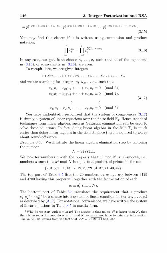
146 3. Integer Factorization and RSA
= pe11u1+e21u2+···+er1ur1 · pe12u1+e22u2+···+er2ur
2 · · · pe1tu1+e2tu2+···+erturt ·
(3.15)
You may find this clearer if it is written using summation and productnotation,
r∏
i=1
cuii =
t∏
j=1
p∑r
i=1 eijui
j . (3.16)
In any case, our goal is to choose u1, . . . , ur such that all of the exponentsin (3.15), or equivalently in (3.16), are even.
To recapitulate, we are given integers
e11, e12, . . . , e1t, e21, e22, . . . , e2t, . . . , er1, er2, . . . , ert
and we are searching for integers u1, u2, . . . , ur such that
e11u1 + e21u2 + · · ·+ er1ur ≡ 0 (mod 2),
e12u1 + e22u2 + · · ·+ er2ur ≡ 0 (mod 2),
......
e1tu1 + e2tu2 + · · ·+ ertur ≡ 0 (mod 2).
(3.17)
You have undoubtedly recognized that the system of congruences (3.17)is simply a system of linear equations over the finite field F2. Hence standardtechniques from linear algebra, such as Gaussian elimination, can be used tosolve these equations. In fact, doing linear algebra in the field F2 is mucheasier than doing linear algebra in the field R, since there is no need to worryabout round-off errors.
Example 3.40. We illustrate the linear algebra elimination step by factoringthe number
N = 9788111.
We look for numbers a with the property that a2 mod N is 50-smooth, i.e.,numbers a such that a2 mod N is equal to a product of primes in the set
{2, 3, 5, 7, 11, 13, 17, 19, 23, 29, 31, 37, 41, 43, 47}.The top part of Table 3.5 lists the 20 numbers a1, a2, . . . , a20 between 3129and 4700 having this property,6 together with the factorization of each
ci ≡ a2i (mod N).
The bottom part of Table 3.5 translates the requirement that a productcu11 cu2
2 · · · cu2020 be a square into a system of linear equation for (u1, u2, . . . , u20)
as described by (3.17). For notational convenience, we have written the systemof linear equations in Table 3.5 in matrix form.
6Why do we start with a = 3129? The answer is that unless a2 is larger than N , thenthere is no reduction modulo N in a2 mod N , so we cannot hope to gain any information.The value 3129 comes from the fact that
√N =
√9788111 ≈ 3128.6.
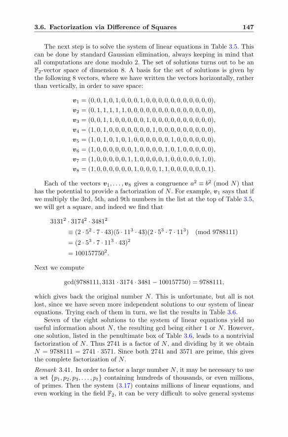
3.6. Factorization via Difference of Squares 147
The next step is to solve the system of linear equations in Table 3.5. Thiscan be done by standard Gaussian elimination, always keeping in mind thatall computations are done modulo 2. The set of solutions turns out to be anF2-vector space of dimension 8. A basis for the set of solutions is given bythe following 8 vectors, where we have written the vectors horizontally, ratherthan vertically, in order to save space:
v1 = (0, 0, 1, 0, 1, 0, 0, 0, 1, 0, 0, 0, 0, 0, 0, 0, 0, 0, 0, 0),
v2 = (0, 1, 1, 1, 1, 1, 0, 0, 0, 0, 0, 0, 0, 0, 0, 0, 0, 0, 0, 0),
v3 = (0, 0, 1, 1, 0, 0, 0, 0, 0, 1, 0, 0, 0, 0, 0, 0, 0, 0, 0, 0),
v4 = (1, 0, 1, 0, 0, 0, 0, 0, 0, 0, 1, 0, 0, 0, 0, 0, 0, 0, 0, 0),
v5 = (1, 0, 1, 0, 1, 0, 1, 0, 0, 0, 0, 0, 0, 1, 0, 0, 0, 0, 0, 0),
v6 = (1, 0, 0, 0, 0, 0, 0, 1, 0, 0, 0, 0, 1, 0, 1, 0, 0, 0, 0, 0),
v7 = (1, 0, 0, 0, 0, 0, 1, 1, 0, 0, 0, 0, 1, 0, 0, 0, 0, 0, 1, 0),
v8 = (1, 0, 0, 0, 0, 0, 0, 1, 0, 0, 0, 1, 1, 0, 0, 0, 0, 0, 0, 1).
Each of the vectors v1, . . . ,v8 gives a congruence a2 ≡ b2 (mod N) thathas the potential to provide a factorization of N . For example, v1 says that ifwe multiply the 3rd, 5th, and 9th numbers in the list at the top of Table 3.5,we will get a square, and indeed we find that
31312 · 31742 · 34812
≡ (2 · 52 · 7 · 43)(5 · 113 · 43)(2 · 53 · 7 · 113) (mod 9788111)
= (2 · 53 · 7 · 113 · 43)2
= 1001577502.
Next we compute
gcd(9788111, 3131 · 3174 · 3481− 100157750) = 9788111,
which gives back the original number N . This is unfortunate, but all is notlost, since we have seven more independent solutions to our system of linearequations. Trying each of them in turn, we list the results in Table 3.6.
Seven of the eight solutions to the system of linear equations yield nouseful information about N , the resulting gcd being either 1 or N . However,one solution, listed in the penultimate box of Table 3.6, leads to a nontrivialfactorization of N . Thus 2741 is a factor of N , and dividing by it we obtainN = 9788111 = 2741 · 3571. Since both 2741 and 3571 are prime, this givesthe complete factorization of N .
Remark 3.41. In order to factor a large number N , it may be necessary to usea set {p1, p2, p3, . . . , pt} containing hundreds of thousands, or even millions,of primes. Then the system (3.17) contains millions of linear equations, andeven working in the field F2, it can be very difficult to solve general systems
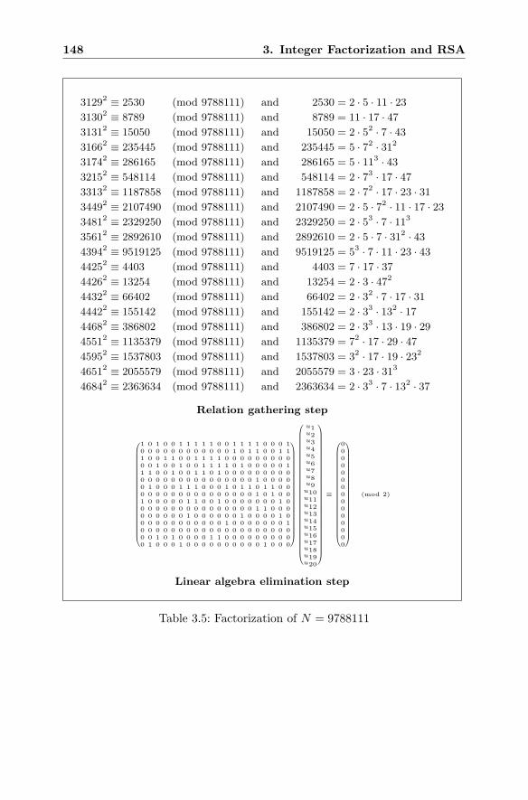
148 3. Integer Factorization and RSA
31292 ≡ 2530 (mod 9788111) and 2530 = 2 · 5 · 11 · 2331302 ≡ 8789 (mod 9788111) and 8789 = 11 · 17 · 4731312 ≡ 15050 (mod 9788111) and 15050 = 2 · 52 · 7 · 4331662 ≡ 235445 (mod 9788111) and 235445 = 5 · 72 · 312
31742 ≡ 286165 (mod 9788111) and 286165 = 5 · 113 · 4332152 ≡ 548114 (mod 9788111) and 548114 = 2 · 73 · 17 · 4733132 ≡ 1187858 (mod 9788111) and 1187858 = 2 · 72 · 17 · 23 · 3134492 ≡ 2107490 (mod 9788111) and 2107490 = 2 · 5 · 72 · 11 · 17 · 2334812 ≡ 2329250 (mod 9788111) and 2329250 = 2 · 53 · 7 · 113
35612 ≡ 2892610 (mod 9788111) and 2892610 = 2 · 5 · 7 · 312 · 4343942 ≡ 9519125 (mod 9788111) and 9519125 = 53 · 7 · 11 · 23 · 4344252 ≡ 4403 (mod 9788111) and 4403 = 7 · 17 · 3744262 ≡ 13254 (mod 9788111) and 13254 = 2 · 3 · 472
44322 ≡ 66402 (mod 9788111) and 66402 = 2 · 32 · 7 · 17 · 3144422 ≡ 155142 (mod 9788111) and 155142 = 2 · 33 · 132 · 1744682 ≡ 386802 (mod 9788111) and 386802 = 2 · 33 · 13 · 19 · 2945512 ≡ 1135379 (mod 9788111) and 1135379 = 72 · 17 · 29 · 4745952 ≡ 1537803 (mod 9788111) and 1537803 = 32 · 17 · 19 · 232
46512 ≡ 2055579 (mod 9788111) and 2055579 = 3 · 23 · 313
46842 ≡ 2363634 (mod 9788111) and 2363634 = 2 · 33 · 7 · 132 · 37
Relation gathering step
⎛
⎜⎜⎜⎜⎜⎜⎜⎜⎜⎜⎜⎜⎜⎜⎜⎜⎜⎜⎜⎜⎜⎜⎜⎝
1 0 1 0 0 1 1 1 1 1 0 0 1 1 1 1 0 0 0 10 0 0 0 0 0 0 0 0 0 0 0 1 0 1 1 0 0 1 11 0 0 1 1 0 0 1 1 1 1 0 0 0 0 0 0 0 0 00 0 1 0 0 1 0 0 1 1 1 1 0 1 0 0 0 0 0 11 1 0 0 1 0 0 1 1 0 1 0 0 0 0 0 0 0 0 00 0 0 0 0 0 0 0 0 0 0 0 0 0 0 1 0 0 0 00 1 0 0 0 1 1 1 0 0 0 1 0 1 1 0 1 1 0 00 0 0 0 0 0 0 0 0 0 0 0 0 0 0 1 0 1 0 01 0 0 0 0 0 1 1 0 0 1 0 0 0 0 0 0 0 1 00 0 0 0 0 0 0 0 0 0 0 0 0 0 0 1 1 0 0 00 0 0 0 0 0 1 0 0 0 0 0 0 1 0 0 0 0 1 00 0 0 0 0 0 0 0 0 0 0 1 0 0 0 0 0 0 0 10 0 0 0 0 0 0 0 0 0 0 0 0 0 0 0 0 0 0 00 0 1 0 1 0 0 0 0 1 1 0 0 0 0 0 0 0 0 00 1 0 0 0 1 0 0 0 0 0 0 0 0 0 0 1 0 0 0
⎞
⎟⎟⎟⎟⎟⎟⎟⎟⎟⎟⎟⎟⎟⎟⎟⎟⎟⎟⎟⎟⎟⎟⎟⎠
⎛
⎜⎜⎜⎜⎜⎜⎜⎜⎜⎜⎜⎜⎜⎜⎜⎜⎜⎜⎜⎜⎜⎜⎜⎜⎜⎜⎜⎜⎜⎜⎜⎜⎜⎝
u1u2u3u4u5u6u7u8u9u10u11u12u13u14u15u16u17u18u19u20
⎞
⎟⎟⎟⎟⎟⎟⎟⎟⎟⎟⎟⎟⎟⎟⎟⎟⎟⎟⎟⎟⎟⎟⎟⎟⎟⎟⎟⎟⎟⎟⎟⎟⎟⎠
≡
⎛
⎜⎜⎜⎜⎜⎜⎜⎜⎜⎜⎜⎜⎜⎜⎜⎜⎜⎜⎜⎜⎜⎜⎜⎝
000000000000000
⎞
⎟⎟⎟⎟⎟⎟⎟⎟⎟⎟⎟⎟⎟⎟⎟⎟⎟⎟⎟⎟⎟⎟⎟⎠
(mod 2)
Linear algebra elimination step
Table 3.5: Factorization of N = 9788111
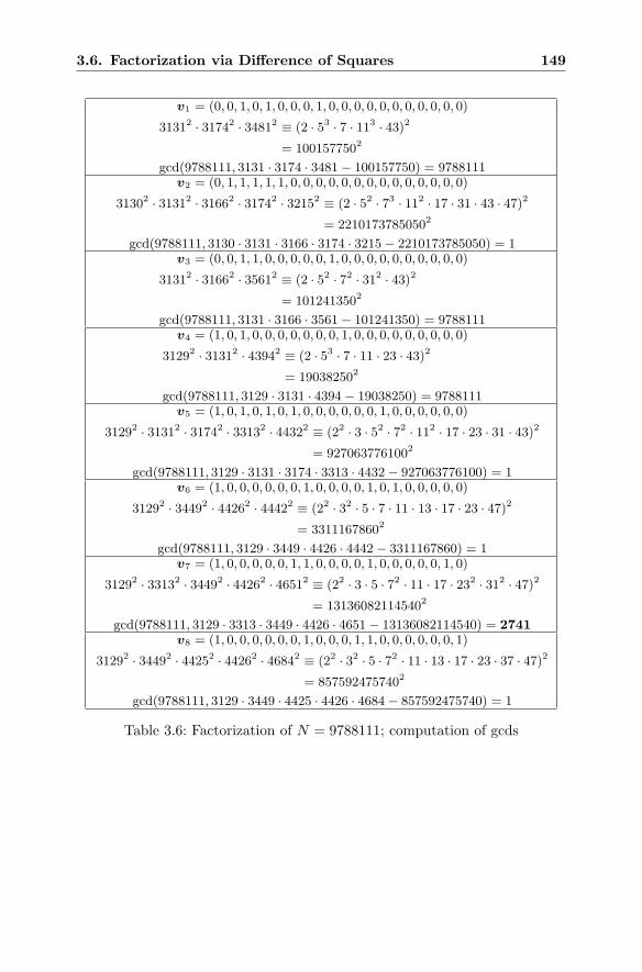
3.6. Factorization via Difference of Squares 149
v1 = (0, 0, 1, 0, 1, 0, 0, 0, 1, 0, 0, 0, 0, 0, 0, 0, 0, 0, 0, 0)
31312 · 31742 · 34812 ≡ (2 · 53 · 7 · 113 · 43)2
= 1001577502
gcd(9788111, 3131 · 3174 · 3481− 100157750) = 9788111v2 = (0, 1, 1, 1, 1, 1, 0, 0, 0, 0, 0, 0, 0, 0, 0, 0, 0, 0, 0, 0)
31302 · 31312 · 31662 · 31742 · 32152 ≡ (2 · 52 · 73 · 112 · 17 · 31 · 43 · 47)2
= 22101737850502
gcd(9788111, 3130 · 3131 · 3166 · 3174 · 3215− 2210173785050) = 1v3 = (0, 0, 1, 1, 0, 0, 0, 0, 0, 1, 0, 0, 0, 0, 0, 0, 0, 0, 0, 0)
31312 · 31662 · 35612 ≡ (2 · 52 · 72 · 312 · 43)2
= 1012413502
gcd(9788111, 3131 · 3166 · 3561− 101241350) = 9788111v4 = (1, 0, 1, 0, 0, 0, 0, 0, 0, 0, 1, 0, 0, 0, 0, 0, 0, 0, 0, 0)
31292 · 31312 · 43942 ≡ (2 · 53 · 7 · 11 · 23 · 43)2
= 190382502
gcd(9788111, 3129 · 3131 · 4394− 19038250) = 9788111v5 = (1, 0, 1, 0, 1, 0, 1, 0, 0, 0, 0, 0, 0, 1, 0, 0, 0, 0, 0, 0)
31292 · 31312 · 31742 · 33132 · 44322 ≡ (22 · 3 · 52 · 72 · 112 · 17 · 23 · 31 · 43)2
= 9270637761002
gcd(9788111, 3129 · 3131 · 3174 · 3313 · 4432− 927063776100) = 1v6 = (1, 0, 0, 0, 0, 0, 0, 1, 0, 0, 0, 0, 1, 0, 1, 0, 0, 0, 0, 0)
31292 · 34492 · 44262 · 44422 ≡ (22 · 32 · 5 · 7 · 11 · 13 · 17 · 23 · 47)2
= 33111678602
gcd(9788111, 3129 · 3449 · 4426 · 4442− 3311167860) = 1v7 = (1, 0, 0, 0, 0, 0, 1, 1, 0, 0, 0, 0, 1, 0, 0, 0, 0, 0, 1, 0)
31292 · 33132 · 34492 · 44262 · 46512 ≡ (22 · 3 · 5 · 72 · 11 · 17 · 232 · 312 · 47)2
= 131360821145402
gcd(9788111, 3129 · 3313 · 3449 · 4426 · 4651− 13136082114540) = 2741v8 = (1, 0, 0, 0, 0, 0, 0, 1, 0, 0, 0, 1, 1, 0, 0, 0, 0, 0, 0, 1)
31292 · 34492 · 44252 · 44262 · 46842 ≡ (22 · 32 · 5 · 72 · 11 · 13 · 17 · 23 · 37 · 47)2
= 8575924757402
gcd(9788111, 3129 · 3449 · 4425 · 4426 · 4684− 857592475740) = 1
Table 3.6: Factorization of N = 9788111; computation of gcds
150 3. Integer Factorization and RSA
of this size. However, it turns out that the systems of linear equations used infactorization are quite sparse, which means that most of their coefficients arezero. (This is plausible because if a number A is a product of primes smallerthan B, then one expects A to be a product of approximately ln(A)/ ln(B) dis-tinct primes.) There are special techniques for solving sparse systems of linearequations that are much more efficient than ordinary Gaussian elimination;see for example [31, 72].
3.7 Smooth Numbers, Sieves, and BuildingRelations for Factorization
In this section we describe the two fastest known methods for doing “hard”factorization problems, i.e., factoring numbers of the form N = pq, where pand q are primes of approximately the same order of magnitude. We beginwith a discussion of smooth numbers, which form the essential tool for buildingrelations. Next we describe in some detail the quadratic sieve, which is a fastmethod for finding the necessary smooth numbers. Finally, we briefly describethe number field sieve, which is similar to the quadratic sieve in that it providesa fast method for finding smooth numbers of a certain form. However, when Nis extremely large, the number field sieve is much faster than the quadraticsieve, because by working in a ring larger than Z, it uses smaller auxiliarynumbers in its search for smooth numbers.
3.7.1 Smooth Numbers
The relation building step in the three step factorization procedure describedin Table 3.4 requires us to find many integers with the property that a2 mod Nfactors as a product of small primes. As noted at the end of Sect. 3.5, thesehighly factorizable numbers have a name.
Definition. An integer n is called B-smooth if all of its prime factors are lessthan or equal to B.
Example 3.42. Here are the first few 5-smooth numbers and the first fewnumbers that are not 5-smooth:
5-smooth: 2, 3, 4, 5, 6, 8, 9, 10, 12, 15, 16, 18, 20, 24, 25, 27, 30, 32, 36, . . .
Not 5-smooth: 7, 11, 13, 14, 17, 19, 21, 22, 23, 26, 28, 29, 31, 33, 34, 35, 37, . . .
Definition. The function ψ(X,B) counts B-smooth numbers,
ψ(X,B) = Number of B-smooth integers n such that 1 < n ≤ X.
For example,ψ(25, 5) = 15,
3.7. Smooth Numbers and Sieves 151
since the 5-smooth numbers between 1 and 25 are the 15 numbers
2, 3, 4, 5, 6, 8, 9, 10, 12, 15, 16, 18, 20, 24, 25.
In order to evaluate the efficiency of the three step factorization method,we need to understand how ψ(X,B) behaves for large values of X and B.It turns out that in order to obtain useful results, the quantities B and Xmust increase together in just the right way. An important theorem in thisdirection was proven by Canfield, Erdos, and Pomerance [24].
Theorem 3.43 (Canfield, Erdos, Pomerance). Fix a number 0 < ε < 12 , and
let X and B increase together while satisfying
(lnX)ε < lnB < (lnX)1−ε.
For notational convenience, we let
u =lnX
lnB.
Then the number of B-smooth numbers less than X satisfies
ψ(X,B) = X · u−u(1+o(1)).
Remark 3.44. We’ve used little-o notation here for the first time. The ex-pression o(1) denotes a function that tends to 0 as X tends to infinity. Moregenerally, we write
f(X) = o(g(X)
)
if the ratio f(X)/g(X) tends to 0 as X tends to infinity. Note that this isdifferent from the big-O notation introduced in Sect. 2.6, where recall thatf(X) = O
(g(X)
)means that f(X) is smaller than a multiple of g(X).
The question remains of how we should choose B in terms of X. It turnsout that the following curious-looking function L(X) is what we will need:
L(X) = e√
(lnX)(ln lnX). (3.18)
Then, as an immediate consequence of Theorem 3.43, we obtain a fundamentalestimate for ψ.
Corollary 3.45. For any fixed value of c with 0 < c < 1,
ψ(X,L(X)c
)= X · L(X)−(1/2c)(1+o(1)) as X →∞.
Proof. Note that if B = L(X)c and if we take any ε < 12 , then
lnB = c lnL(X) = c√(lnX)(ln lnX)
satisfies (lnX)ε < lnB < (lnX)1−ε. So we can apply Theorem 3.43 with
152 3. Integer Factorization and RSA
u =lnX
lnB=
1
c·√
lnX
ln lnX
to deduce that ψ(X,L(X)c
)= X · u−u(1+o(1)). It is easily checked (see Exer-
cise 3.32) that this value of u satisfies
u−u(1+o(1)) = L(X)−(1/2c)(1+o(1)),
which completes the proof of the corollary.
The function L(X) = e√
(lnX)(ln lnX) and other similar functions appearprominently in the theory of factorization due to their close relationship tothe distribution of smooth numbers. It is thus important to understand howfast L(X) grows as a function of X.
Recall that in Sect. 2.6 we defined big-O notation and used it to discussthe notions of polynomial, exponential, and subexponential running times.What this meant was that the number of steps required to solve a problemwas, respectively, polynomial, exponential, and subexponential in the numberof bits required to describe the problem. As a supplement to big-O notation,it is convenient to introduce two other ways of comparing the rate at whichfunctions grow.
Definition (Order Notation). Let f(X) and g(X) be functions of X whosevalues are positive. Recall that we write
f(X) = O(g(X)
)
if there are positive constants c and C such that
f(X) ≤ cg(X) for all X ≥ C.
Similarly, we say that f is big-Ω of g and write
f(X) = Ω(g(X)
)
if there are positive constants c and C such that7
f(X) ≥ cg(X) for all X ≥ C.
Finally, if f is both big-O and big-Ω of g, we say that f is big-Θ of g andwrite f(X) = Θ
(g(X)
).
7Note: Big-Ω notation as used by computer scientists and cryptographers does notmean the same thing as the big-Ω notation of mathematicians. In mathematics, especiallyin the field of analytic number theory, the expression f(n) = Ω
(g(n)
)means that there is
a constant c such that there are infinitely many integers n such that f(n) ≥ cg(n). In thisbook we use the computer science definition.
3.7. Smooth Numbers and Sieves 153
Remark 3.46. In analytic number theory there is an alternative version oforder notation that is quite intuitive. For functions f(X) and g(X), we write
f(X)� g(X) if f(X) = O(g(X)
),
f(X)� g(X) if f(X) = Ω(g(X)
),
f(X)�� g(X) if f(X) = Θ(g(X)
).
The advantage of this notation is that it is transitive, just as the usual “greaterthan” and “less than” relations are transitive. For example, if f � g and g �h, then f � h.
Definition. With this notation in place, a function f(X) is said to growexponentially if there are positive constants α and β such that
Ω(Xα) = f(X) = O(Xβ),
and it is said to grow polynomially if there are positive constants α and βsuch that
Ω((lnX)α
)= f(X) = O
((lnX)β
).
In the alternative notation of Remark 3.46, exponential growth and polyno-mial growth are written, respectively, as
Xα � f(X)� Xβ and (lnX)α � f(X)� (lnX)β .
A function that falls in between these two categories is called subexponen-tial. Thus f(X) is subexponential if for every positive constant α, no matterhow large, and for every positive constant β, no matter how small,
Ω((lnX)α
)= f(X) = O(Xβ). (3.19)
(In the alternative notation, this becomes (lnX)α � f(X)� Xβ .)Note that there is a possibility for confusion, since these definitions do
not correspond to the usual meaning of exponential and polynomial growththat one finds in calculus. What is really happening is that “exponential” and“polynomial” refer to growth rates in the number of bits that it takes to writedown X, i.e., exponential or polynomial functions of log2(X).
Remark 3.47. The function L(X) falls into the subexponential category. Weleave this for you to prove in Exercise 3.30. See Table 3.7 for a rough idea ofhow fast L(X) grows as X increases.
Suppose that we attempt to factor N by searching for values a2 (mod N)that are B-smooth. In order to perform the linear equation elimination step,we need (at least) as many B-smooth numbers as there are primes less than B.We need this many because in the elimination step, the smooth numberscorrespond to the variables, while the primes less than B correspond to theequations, and we need more variables than equations. In order to ensure that
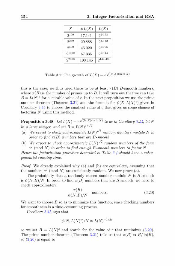
154 3. Integer Factorization and RSA
X lnL(X) L(X)
2100 17.141 224.73
2250 29.888 243.12
2500 45.020 264.95
21000 67.335 297.14
22000 100.145 2144.48
Table 3.7: The growth of L(X) = e√
(lnX)(ln lnX)
this is the case, we thus need there to be at least π(B) B-smooth numbers,where π(B) is the number of primes up to B. It will turn out that we can takeB = L(N)c for a suitable value of c. In the next proposition we use the primenumber theorem (Theorem 3.21) and the formula for ψ(X,L(X)c) given inCorollary 3.45 to choose the smallest value of c that gives us some chance offactoring N using this method.
Proposition 3.48. Let L(X) = e√
(lnX)(ln lnX) be as in Corollary 3.45, let N
be a large integer, and set B = L(N)1/√2.
(a) We expect to check approximately L(N)√2 random numbers modulo N in
order to find π(B) numbers that are B-smooth.
(b) We expect to check approximately L(N)√2 random numbers of the form
a2 (mod N) in order to find enough B-smooth numbers to factor N .Hence the factorization procedure described in Table 3.4 should have a subex-ponential running time.
Proof. We already explained why (a) and (b) are equivalent, assuming thatthe numbers a2 (mod N) are sufficiently random. We now prove (a).
The probability that a randomly chosen number modulo N is B-smoothis ψ(N,B)/N . In order to find π(B) numbers that are B-smooth, we need tocheck approximately
π(B)
ψ(N,B)/Nnumbers. (3.20)
We want to choose B so as to minimize this function, since checking numbersfor smoothness is a time-consuming process.
Corollary 3.45 says that
ψ(N,L(N)c)/N ≈ L(N)−1/2c,
so we set B = L(N)c and search for the value of c that minimizes (3.20).The prime number theorem (Theorem 3.21) tells us that π(B) ≈ B/ ln(B),so (3.20) is equal to
3.7. Smooth Numbers and Sieves 155
π(L(N)c
)
ψ(N,L(N)c
)/N
≈ L(N)c
c lnL(N)· 1
L(N)−1/2c= L(N)c+1/2c · 1
c lnL(N).
The factor L(N)c+1/2c dominates this last expression, so we choose the valueof c that minimizes the quantity c+ 1
2c . This is an elementary calculus prob-
lem. It is minimized when c = 1√2, and the minimum value is
√2. Thus if we
choose B ≈ L(N)1/√2, then we need to check approximately L(N)
√2 values
in order to find π(B) numbers that are B-smooth, and hence to find enoughrelations to factor N .
Remark 3.49. Proposition 3.48 suggests that we need to check approxi-
mately L(N)√2 randomly chosen numbers modulo N in order to find enough
smooth numbers to factor N . There are various ways to decrease the searchtime. In particular, rather than using random values of a to compute numbersof the form a2 (mod N), we might instead select numbers a that are only alittle bit larger than
√N . Then a2 (mod N) is O(
√N ), so is more likely to
be B-smooth than is a number that is O(N). Reworking the calculation inProposition 3.48, one finds that it suffices to check approximately L(N) ran-dom numbers of the form a2 (mod N) with a close to
√N . This is a significant
savings over L(N)√2. See Exercise 3.33 for further details.
Remark 3.50. When estimating the effort needed to factor N , we havecompletely ignored the work required to check whether a given numberis B-smooth. For example, if we check for B-smoothness using trial division,i.e., dividing by each prime less than B, then it takes approximately π(B)trial divisions to check for B-smoothness. Taking this additional effort intoaccount in the proof of Proposition 3.48, one finds that it takes approxi-
mately L(N)√2 trial divisions to find enough smooth numbers to factor N ,
even using values of a ≈√N as in Remark 3.49.
The quadratic sieve, which we describe in Sect. 3.7.2, uses a more efficientmethod for generating B-smooth numbers and thereby reduces the runningtime down to L(N). (See Table 3.7 for a reminder of how L(N) grows and why
a running time of L(N) is much better than a running time of L(N)√2.) In
Exercise 3.29 we ask you to estimate how long it takes to perform L(N) opera-tions on a moderately fast computer. For a number of years it was thought thatno factorization algorithm could take fewer than a fixed power of L(N) steps,but the invention of the number field sieve (Sect. 3.7.3) showed this to be
incorrect. The number field sieve, whose running time of ec3√
(lnN)(ln lnN)2 isfaster than L(N)ε for every ε > 0, achieves its speed by moving beyond therealm of the ordinary integers.
3.7.2 The Quadratic Sieve
In this section we address the final piece of the puzzle that must be solved inorder to factor large numbers via the difference of squares method describedin Sect. 3.6:
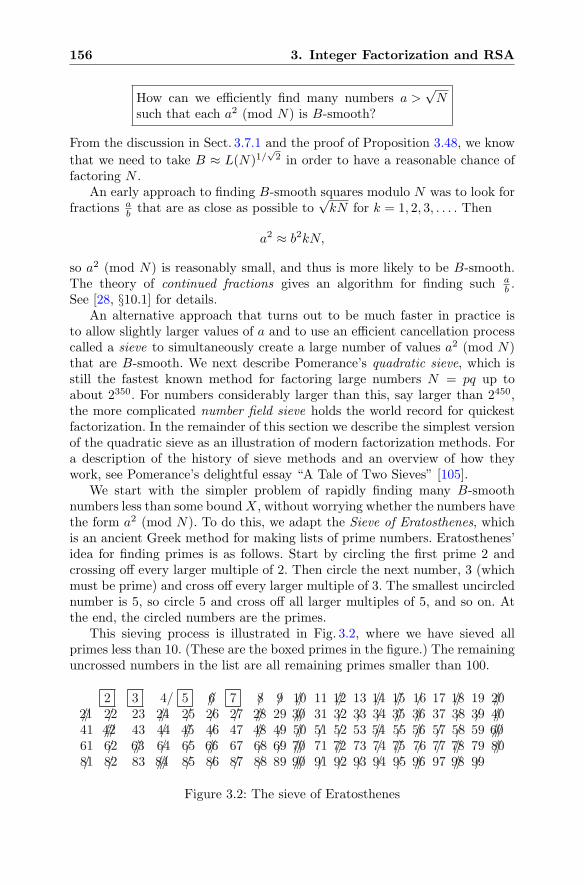
156 3. Integer Factorization and RSA
How can we efficiently find many numbers a >√N
such that each a2 (mod N) is B-smooth?
From the discussion in Sect. 3.7.1 and the proof of Proposition 3.48, we know
that we need to take B ≈ L(N)1/√2 in order to have a reasonable chance of
factoring N .An early approach to finding B-smooth squares modulo N was to look for
fractions ab that are as close as possible to
√kN for k = 1, 2, 3, . . . . Then
a2 ≈ b2kN,
so a2 (mod N) is reasonably small, and thus is more likely to be B-smooth.The theory of continued fractions gives an algorithm for finding such a
b .See [28, §10.1] for details.
An alternative approach that turns out to be much faster in practice isto allow slightly larger values of a and to use an efficient cancellation processcalled a sieve to simultaneously create a large number of values a2 (mod N)that are B-smooth. We next describe Pomerance’s quadratic sieve, which isstill the fastest known method for factoring large numbers N = pq up toabout 2350. For numbers considerably larger than this, say larger than 2450,the more complicated number field sieve holds the world record for quickestfactorization. In the remainder of this section we describe the simplest versionof the quadratic sieve as an illustration of modern factorization methods. Fora description of the history of sieve methods and an overview of how theywork, see Pomerance’s delightful essay “A Tale of Two Sieves” [105].
We start with the simpler problem of rapidly finding many B-smoothnumbers less than some boundX, without worrying whether the numbers havethe form a2 (mod N). To do this, we adapt the Sieve of Eratosthenes, whichis an ancient Greek method for making lists of prime numbers. Eratosthenes’idea for finding primes is as follows. Start by circling the first prime 2 andcrossing off every larger multiple of 2. Then circle the next number, 3 (whichmust be prime) and cross off every larger multiple of 3. The smallest uncirclednumber is 5, so circle 5 and cross off all larger multiples of 5, and so on. Atthe end, the circled numbers are the primes.
This sieving process is illustrated in Fig. 3.2, where we have sieved allprimes less than 10. (These are the boxed primes in the figure.) The remaininguncrossed numbers in the list are all remaining primes smaller than 100.
2 3 4/ 5 //6 7 //0291//8171/61//51//4131//2111//01/9/8//04/93/8373//63//53/43/33/2313///0392//82/72/62/52//4232/22//12///0695/85/75//65/55//4535/25/15//05/94//8474/64//54/4434///2414//0897//87/77/67//57/4737//2717///07/96/8676//66/56/46//36/2616
/99//8979//69/59/49/39/29/19///0998/88/78/68/58///4838/28/18
Figure 3.2: The sieve of Eratosthenes
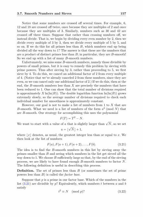
3.7. Smooth Numbers and Sieves 157
Notice that some numbers are crossed off several times. For example, 6,12 and 18 are crossed off twice, once because they are multiples of 2 and oncebecause they are multiples of 3. Similarly, numbers such as 30 and 42 arecrossed off three times. Suppose that rather than crossing numbers off, weinstead divide. That is, we begin by dividing every even number by 2, then wedivide every multiple of 3 by 3, then we divide every multiple of 5 by 5, andso on. If we do this for all primes less than B, which numbers end up beingdivided all the way down to 1? The answer is that these are the numbers thatare a product of distinct primes less than B; in particular, they are B-smooth!So we end up with a list of many B-smooth numbers.
Unfortunately, we miss some B-smooth numbers, namely those divisible bypowers of small primes, but it is easy to remedy this problem by sieving withprime powers. Thus after sieving by 3, rather than proceeding to 5, we firstsieve by 4. To do this, we cancel an additional factor of 2 from every multipleof 4. (Notice that we’ve already canceled 2 from these numbers, since they areeven, so we can cancel only one additional factor of 2.) If we do this, then at theend, the B-smooth numbers less than X are precisely the numbers that havebeen reduced to 1. One can show that the total number of divisions requiredis approximately X ln(ln(B)). The double logarithm function ln(ln(B)) growsextremely slowly, so the average number of divisions required to check eachindividual number for smoothness is approximately constant.
However, our goal is not to make a list of numbers from 1 to X that areB-smooth. What we need is a list of numbers of the form a2 (mod N) thatare B-smooth. Our strategy for accomplishing this uses the polynomial
F (T ) = T 2 −N.We want to start with a value of a that is slightly larger than
√N , so we set
a = �√N�+ 1,
where �x� denotes, as usual, the greatest integer less than or equal to x. Wethen look at the list of numbers
F (a), F (a+ 1), F (a+ 2), . . . , F (b). (3.21)
The idea is to find the B-smooth numbers in this list by sieving away theprimes smaller than B and seeing which numbers in the list get sieved all theway down to 1. We choose B sufficiently large so that, by the end of the sievingprocess, we are likely to have found enough B-smooth numbers to factor N .The following definition is useful in describing this process.
Definition. The set of primes less than B (or sometimes the set of primepowers less than B) is called the factor base.
Suppose that p is a prime in our factor base. Which of the numbers in thelist (3.21) are divisible by p? Equivalently, which numbers t between a and bsatisfy
t2 ≡ N (mod p)? (3.22)
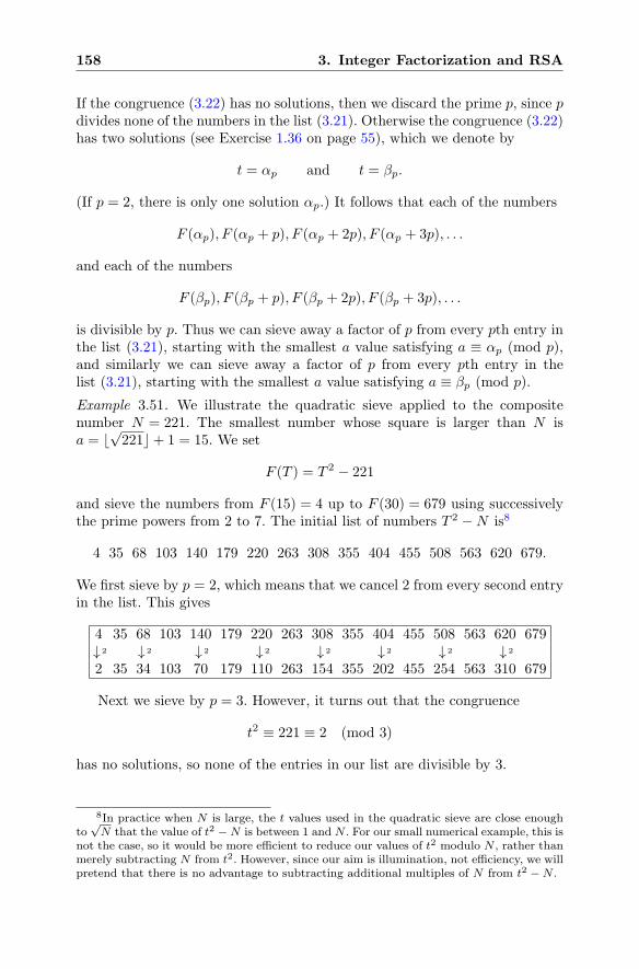
158 3. Integer Factorization and RSA
If the congruence (3.22) has no solutions, then we discard the prime p, since pdivides none of the numbers in the list (3.21). Otherwise the congruence (3.22)has two solutions (see Exercise 1.36 on page 55), which we denote by
t = αp and t = βp.
(If p = 2, there is only one solution αp.) It follows that each of the numbers
F (αp), F (αp + p), F (αp + 2p), F (αp + 3p), . . .
and each of the numbers
F (βp), F (βp + p), F (βp + 2p), F (βp + 3p), . . .
is divisible by p. Thus we can sieve away a factor of p from every pth entry inthe list (3.21), starting with the smallest a value satisfying a ≡ αp (mod p),and similarly we can sieve away a factor of p from every pth entry in thelist (3.21), starting with the smallest a value satisfying a ≡ βp (mod p).
Example 3.51. We illustrate the quadratic sieve applied to the compositenumber N = 221. The smallest number whose square is larger than N isa = �
√221�+ 1 = 15. We set
F (T ) = T 2 − 221
and sieve the numbers from F (15) = 4 up to F (30) = 679 using successivelythe prime powers from 2 to 7. The initial list of numbers T 2 −N is8
4 35 68 103 140 179 220 263 308 355 404 455 508 563 620 679.
We first sieve by p = 2, which means that we cancel 2 from every second entryin the list. This gives
4 35 68 103 140 179 220 263 308 355 404 455 508 563 620 679↓ 2 ↓ 2 ↓ 2 ↓ 2 ↓ 2 ↓ 2 ↓ 2 ↓ 2
2 35 34 103 70 179 110 263 154 355 202 455 254 563 310 679
Next we sieve by p = 3. However, it turns out that the congruence
t2 ≡ 221 ≡ 2 (mod 3)
has no solutions, so none of the entries in our list are divisible by 3.
8In practice when N is large, the t values used in the quadratic sieve are close enoughto
√N that the value of t2 −N is between 1 and N . For our small numerical example, this is
not the case, so it would be more efficient to reduce our values of t2 modulo N , rather thanmerely subtracting N from t2. However, since our aim is illumination, not efficiency, we willpretend that there is no advantage to subtracting additional multiples of N from t2 −N .
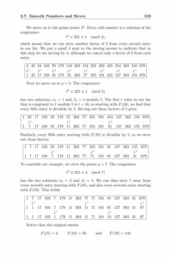
3.7. Smooth Numbers and Sieves 159
We move on to the prime power 22. Every odd number is a solution of thecongruence
t2 ≡ 221 ≡ 1 (mod 4),
which means that we can sieve another factor of 2 from every second entryin our list. We put a small 4 next to the sieving arrows to indicate that inthis step we are sieving by 4, although we cancel only a factor of 2 from eachentry.
2 35 34 103 70 179 110 263 154 355 202 455 254 563 310 679↓ 4 ↓ 4 ↓ 4 ↓ 4 ↓ 4 ↓ 4 ↓ 4 ↓ 4
1 35 17 103 35 179 55 263 77 355 101 455 127 563 155 679
Next we move on to p = 5. The congruence
t2 ≡ 221 ≡ 1 (mod 5)
has two solutions, α5 = 1 and β5 = 4 modulo 5. The first t value in our listthat is congruent to 1 modulo 5 is t = 16, so starting with F (16), we find thatevery fifth entry is divisible by 5. Sieving out these factors of 5 gives
1 35 17 103 35 179 55 263 77 355 101 455 127 563 155 679↓ 5 ↓ 5 ↓ 5
1 7 17 103 35 179 11 263 77 355 101 91 127 563 155 679
Similarly, every fifth entry starting with F (19) is divisible by 5, so we sieveout those factors
1 7 17 103 35 179 11 263 77 355 101 91 127 563 155 679↓ 5 ↓ 5 ↓ 5
1 7 17 103 7 179 11 263 77 71 101 91 127 563 31 679
To conclude our example, we sieve the prime p = 7. The congruence
t2 ≡ 221 ≡ 4 (mod 7)
has the two solutions α7 = 2 and β7 = 5. We can thus sieve 7 away fromevery seventh entry starting with F (16), and also every seventh entry startingwith F (19). This yields
1 7 17 103 7 179 11 263 77 71 101 91 127 563 31 679↓ 7 ↓ 7 ↓ 7
1 1 17 103 7 179 11 263 11 71 101 91 127 563 31 97↓ 7 ↓ 7
1 1 17 103 1 179 11 263 11 71 101 13 127 563 31 97
Notice that the original entries
F (15) = 4, F (16) = 35, and F (19) = 140
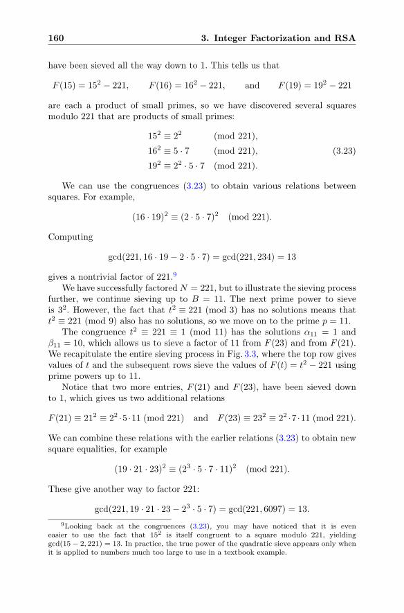
160 3. Integer Factorization and RSA
have been sieved all the way down to 1. This tells us that
F (15) = 152 − 221, F (16) = 162 − 221, and F (19) = 192 − 221
are each a product of small primes, so we have discovered several squaresmodulo 221 that are products of small primes:
152 ≡ 22 (mod 221),
162 ≡ 5 · 7 (mod 221),
192 ≡ 22 · 5 · 7 (mod 221).
(3.23)
We can use the congruences (3.23) to obtain various relations betweensquares. For example,
(16 · 19)2 ≡ (2 · 5 · 7)2 (mod 221).
Computing
gcd(221, 16 · 19− 2 · 5 · 7) = gcd(221, 234) = 13
gives a nontrivial factor of 221.9
We have successfully factoredN = 221, but to illustrate the sieving processfurther, we continue sieving up to B = 11. The next prime power to sieveis 32. However, the fact that t2 ≡ 221 (mod 3) has no solutions means thatt2 ≡ 221 (mod 9) also has no solutions, so we move on to the prime p = 11.
The congruence t2 ≡ 221 ≡ 1 (mod 11) has the solutions α11 = 1 andβ11 = 10, which allows us to sieve a factor of 11 from F (23) and from F (21).We recapitulate the entire sieving process in Fig. 3.3, where the top row givesvalues of t and the subsequent rows sieve the values of F (t) = t2 − 221 usingprime powers up to 11.
Notice that two more entries, F (21) and F (23), have been sieved downto 1, which gives us two additional relations
F (21) ≡ 212 ≡ 22 ·5 ·11 (mod 221) and F (23) ≡ 232 ≡ 22 ·7 ·11 (mod 221).
We can combine these relations with the earlier relations (3.23) to obtain newsquare equalities, for example
(19 · 21 · 23)2 ≡ (23 · 5 · 7 · 11)2 (mod 221).
These give another way to factor 221:
gcd(221, 19 · 21 · 23− 23 · 5 · 7) = gcd(221, 6097) = 13.
9Looking back at the congruences (3.23), you may have noticed that it is eveneasier to use the fact that 152 is itself congruent to a square modulo 221, yieldinggcd(15− 2, 221) = 13. In practice, the true power of the quadratic sieve appears only whenit is applied to numbers much too large to use in a textbook example.
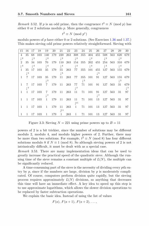
3.7. Smooth Numbers and Sieves 161
Remark 3.52. If p is an odd prime, then the congruence t2 ≡ N (mod p) haseither 0 or 2 solutions modulo p. More generally, congruences
t2 ≡ N (mod pe)
modulo powers of p have either 0 or 2 solutions. (See Exercises 1.36 and 1.37.)This makes sieving odd prime powers relatively straightforward. Sieving with
15 16 17 18 19 20 21 22 23 24 25 26 27 28 29 304 35 68 103 140 179 220 263 308 355 404 455 508 563 620 679↓2 ↓2 ↓2 ↓2 ↓2 ↓2 ↓2 ↓2
2 35 34 103 70 179 110 263 154 355 202 455 254 563 310 679↓4 ↓4 ↓4 ↓4 ↓4 ↓4 ↓4 ↓4
1 35 17 103 35 179 55 263 77 355 101 455 127 563 155 679↓5 ↓5 ↓5
1 7 17 103 35 179 11 263 77 355 101 91 127 563 155 679↓5 ↓5 ↓5
1 7 17 103 7 179 11 263 77 71 101 91 127 563 31 679↓7 ↓7 ↓7
1 1 17 103 7 179 11 263 11 71 101 91 127 563 31 97↓7 ↓7
1 1 17 103 1 179 11 263 11 71 101 13 127 563 31 97↓11
1 1 17 103 1 179 11 263 1 71 101 13 127 563 31 97↓11
1 1 17 103 1 179 1 263 1 71 101 13 127 563 31 97
Figure 3.3: Sieving N = 221 using prime powers up to B = 11
powers of 2 is a bit trickier, since the number of solutions may be differentmodulo 2, modulo 4, and modulo higher powers of 2. Further, there maybe more than two solutions. For example, t2 ≡ N (mod 8) has four differentsolutions modulo 8 if N ≡ 1 (mod 8). So although sieving powers of 2 is notintrinsically difficult, it must be dealt with as a special case.
Remark 3.53. There are many implementation ideas that can be used togreatly increase the practical speed of the quadratic sieve. Although the run-ning time of the sieve remains a constant multiple of L(N), the multiple canbe significantly reduced.
A time-consuming part of the sieve is the necessity of dividing every pth en-try by p, since if the numbers are large, division by p is moderately compli-cated. Of course, computers perform division quite rapidly, but the sievingprocess requires approximately L(N) divisions, so anything that decreasesthis time will have an immediate effect. A key idea to speed up this step isto use approximate logarithms, which allows the slower division operations tobe replaced by faster subtraction operations.
We explain the basic idea. Instead of using the list of values
F (a), F (a+ 1), F (a+ 2), . . . ,
162 3. Integer Factorization and RSA
we use a list of integer values that are approximately equal to
logF (a), logF (a+ 1), logF (a+ 2), logF (a+ 3), . . . .
In order to sieve p from F (t), we subtract an integer approximation of log pfrom the integer approximation to logF (t), since by the rule of logarithms,
logF (t)− log p = logF (t)
p.
If we were to use exact values for the logarithms, then at the end of the sievingprocess, the entries that are reduced to 0 would be precisely the values of F (t)that are B-smooth. However, since we use only approximate logarithm values,at the end we look for entries that have been reduced to a small number. Thenwe use division on only those few entries to find the ones that are actuallyB-smooth.
A second idea that can be used to speed the quadratic sieve is to use thepolynomial F (t) = t2−N only until t reaches a certain size, and then replaceit with a new polynomial. For details of these two implementation ideas andmany others, see for example [28, §10.4], [34], or [109] and the references thatthey list.
3.7.3 The Number Field Sieve
The number field sieve is a factorization method that works in a ring that islarger than the ordinary integers. The full details are very complicated, so inthis section we are content to briefly explain some of the ideas that go intomaking the number field sieve the fastest known method for factoring largenumbers of the form N = pq, where p and q are primes of approximately thesame order of magnitude.
In order to factor N , we start by finding a nonzero integer m and anirreducible monic polynomial f(x) ∈ Z[x] of small degree satisfying
f(m) ≡ 0 (mod N).
Example 3.54. Suppose that we want to factor the number N = 229
+1. Thenwe could take m = 2103 and f(x) = x5 + 8, since
f(m) = f(2103) = 2515 + 8 = 8(2512 + 1) ≡ 0 (mod 229
+ 1).
Let d be the degree of f(x) and let β be a root of f(x). (Note that β mightbe a complex number.) We will work in the ring
Z[β] = {c0 + c1β + c2β2 + · · ·+ cd−1β
d−1 ∈ C : c0, c1, . . . , cd−1 ∈ Z}.
Note that although we have written Z[β] as a subring of the complex numbers,it isn’t actually necessary to deal with real or complex numbers. We can workwith Z[β] purely algebraically, since it is equal to the quotient ring Z[x]/(f(x)).(See Sect. 2.10.2 for information about quotient rings.)
3.7. Smooth Numbers and Sieves 163
Example 3.55. We give an example to illustrate how one performs additionand multiplication in the ring Z[β]. Let f(x) = 1 + 3x− 2x3 + x4, let β be aroot of f(x), and consider the ring Z[β]. In order to add the elements
u = 2− 4β + 7β2 + 3β3 and v = 1 + 2β − 4β2 − 2β3,
we simply add their coefficients,
u+ v = 3− 2β + 3β2 + β3.
Multiplication is a bit more complicated. First we multiply u and v, treating βas if it were a variable,
uv = 2− 9β2 + 29β3 − 14β4 − 26β5 − 6β6.
Then we divide by f(β) = 1 + 3β − 2β3 + β4, still treating β as a variable,and keep the remainder,
uv = 92 + 308β + 111β2 − 133β3 ∈ Z[β].
The next step in the number field sieve is to find a large number of pairsof integers (a1, b1), . . . , (ak, bk) that simultaneously satisfy
k∏
i=1
(ai − bim) is a square in Z and
k∏
i=1
(ai − biβ) is a square in Z[β].
Thus there is an integer A ∈ Z and an element α ∈ Z[β] such that
k∏
i=1
(ai − bim) = A2 andk∏
i=1
(ai − biβ) = α2. (3.24)
By definition of Z[β], we can find an expression for α of the form
α = c0 + c1β + c2β2 + · · ·+ cd−1β
d−1 with c0, c1, . . . , cd−1 ∈ Z. (3.25)
Recall our original assumption f(m) ≡ 0 (mod N). This means that wehave
m ≡ β (mod N) in the ring Z[β].
So on the one hand, (3.24) becomes
A2 ≡ α2 (mod N) in the ring Z[β],
while on the other hand, (3.25) becomes
α ≡ c0 + c1m+ c2m2 + · · ·+ cd−1m
d−1 (mod N) in the ring Z[β].
164 3. Integer Factorization and RSA
Hence
A2 ≡ (c0 + c1m+ c2m2 + · · ·+ cd−1m
d−1)2 (mod N).
Thus we have created a congruence A2 ≡ B2 (mod N) that is valid in the ringof integers Z, and as usual, there is then a good chance that gcd(A − B,N)will yield a nontrivial factor of N .
How do we find the (ai, bi) pairs to make both of the products (3.24) intosquares? For the first product, we can use a sieve-type algorithm, similar to themethod used in the quadratic sieve, to find values of a− bm that are smooth,and then use linear algebra to find a subset with the desired property.
Pollard’s idea is to simultaneously do something similar for the secondproduct while working in the ring Z[β]. Thus we look for pairs of integers (a, b)such that the quantity a − bβ is “smooth” in Z[β]. There are many seriousissues that arise when we try to do this, including the following:1. The ring Z[β] usually does not have unique factorization of elements into
primes or irreducible elements. So instead, we factor the ideal (a−bβ) intoa product of prime ideals. We say that a− bβ is smooth if the prime idealsappearing in the factorization are small.
2. Unfortunately, even ideals in the ring Z[β] may not have unique factoriza-tion as a product of prime ideals. However, there is a slightly larger ring,called the ring of integers of Q(β), in which unique factorization of idealsis true.
3. Suppose that we have managed to make the ideal (∏(ai − biβ)) into the
square of an ideal in Z[β]. There are two further problems. First, it neednot be the square of an ideal generated by a single element. Second, evenif it is equal to an ideal of the form (γ)2, we can conclude only that
∏(a−
i − biβ) = uγ2 for some unit u ∈ Z[β]∗, and generally the ring Z[β] hasinfinitely many units.
It would take us too far afield to explain how to deal with these potentialdifficulties. Suffice it to say that through a number of ingenious ideas dueto Adleman, Buhler, H. Lenstra, Pomerance, and others, the obstacles wereovercome, leading to a practical factorization method. (See [105] for a niceoverview of the number field sieve and some of the ideas used to turn it froma theoretical construction into a working algorithm.)
However, we will comment further on the first step in the algorithm. Inorder to get started, we need an integer m and a monic irreducible polyno-mial f(x) of small degree such that f(m) ≡ 0 (mod N). The trick is first tochoose the desired degree d of f , next to choose an integer m satisfying
(N/2)1/d < m < N1/d,
and then to write N as a number to the base m,
N = c0 + c1m+ c2m2 + · · ·+ cd−1m
d−1 + cdmd with 0 ≤ ci < m.
3.7. Smooth Numbers and Sieves 165
The condition on m ensures that cd = 1, so we can take f to be the monicpolynomial
f(x) = c0 + c1x+ c2x2 + · · ·+ cd−1x
d−1 + xd.
We also need f(x) to be irreducible, but if f(x) factors in Z[x], say f(x) =g(x)h(x), then N = f(m) = g(m)h(m) gives a factorization of N and we aredone. So now we have an f(x) and an m, which allows us to get started usingthe number field sieve.
There is no denying the fact that the number field sieve is much morecomplicated than the quadratic sieve. So why is it useful? The reason has todo with the size of the numbers that must be considered. Recall that for thequadratic sieve, we sieved to find smooth numbers of the form
(�√N �+ k
)2 −N for k = 1, 2, 3, . . . .
So we needed to pick out the smooth numbers from a set of numbers whosesize is a little larger than
√N . For the number field sieve one ends up looking
for smooth numbers of the form
(a−mb) · bdf(a/b), (3.26)
and it turns out that by a judicious choice ofm and f , these numbers are muchsmaller than
√N . In order to describe how much smaller, we use a general-
ization of the subexponential function L(N) that was so useful in describingthe running time of the quadratic sieve.
Definition. For any 0 < ε < 1, we define the function
Lε(X) = e(lnX)ε(ln lnX)1−ε
.
Notice that with this notation, the function L(X) defined in Sect. 3.7.1is L1/2(X).
Then one can show that the numbers (3.26) used by the number fieldsieve have size a small power of L2/3(N). To put this into perspective, thequadratic sieve works with numbers having approximately half as many digitsas N , while the number field sieve uses numbers K satisfying
(Number of digits of K) ≈ (Number of digits of N)2/3.
This leads to a vastly improved running time for sufficiently large values of N .
Theorem 3.56. Under some reasonable assumptions, the expected runningtime of the number field sieve to factor the number N is L1/3(N)c for a smallvalue of c.
For general numbers, the best known value of c in Theorem 3.56 is a bitless than 2, while for special numbers such as 22
9
+ 1 it is closer to 1.5. Ofcourse, the number field sieve is sufficiently complicated that it becomes fasterthan other methods only when N is sufficiently large. As a practical matter,the quadratic sieve is faster for numbers smaller than 10100, while the numberfield sieve is faster for numbers larger than 10130.
166 3. Integer Factorization and RSA
3.8 The Index Calculus Method for ComputingDiscrete Logarithms in Fp
The index calculus is a method for solving the discrete logarithm problem in afinite field Fp. The algorithm uses smooth numbers and bears some similarityto the sieve methods that we have studied in this chapter, which is why wecover it here, rather than in Chap. 2, where we originally discussed discretelogarithms.
The idea behind the index calculus is fairly simple. We want to solve thediscrete logarithm problem
gx ≡ h (mod p), (3.27)
where the prime p and the integers g and h are given. For simplicity, we willassume that g is a primitive root modulo p, so its powers give all of F∗
p.Rather than solving (3.27) directly, we instead choose a value B and solve
the discrete logarithm problem
gx ≡ � (mod p) for all primes � ≤ B.
In other words, we compute the discrete logarithm logg(�) for every primesatisfying � ≤ B.
Having done this, we next look at the quantities
h · g−k (mod p) for k = 1, 2, . . .
until we find a value of k such that h · g−k (mod p) is B-smooth. For thisvalue of k we have
h · g−k ≡∏
�≤B
�e� (mod p) (3.28)
for certain exponents e�. We rewrite (3.28) in terms of discrete logarithms as
logg(h) ≡ k +∑
�≤B
e� · logg(�) (mod p− 1), (3.29)
where recall that discrete logarithms are defined only modulo p−1. But we areassuming that we already computed logg(�) for all primes � ≤ B. Hence (3.29)gives the value of logg(h).
It remains to explain how to find logg(�) for small primes �. Again the ideais simple. For a random selection of exponents i we compute
gi ≡ gi (mod p) with 0 < gi < p.
If gi is not B-smooth, then we discard it, while if gi is B-smooth, then we canfactor it as
gi =∏
�≤B
�u�(i).
3.8. The Index Calculus and Discrete Logarithms 167
In terms of discrete logarithms, this gives the relation
i ≡ logg(gi) ≡∑
�≤B
u�(i) · logg(�) (mod p− 1). (3.30)
Notice that the only unknown quantities in the formula (3.30) are the dis-crete logarithm values logg(�). So if we can find more than π(B) equationslike (3.30), then we can use linear algebra to solve for the logg(�) “variables.”
This method of solving the discrete logarithm problem in Fp is called theindex calculus, where recall from Sect. 2.2 that index is an older name fordiscrete logarithm. The index calculus first appears in work of Western andMiller [148] in 1968, so it predates by a few years the invention of public keycryptography. The method was independently rediscovered by several cryp-tographers in the 1970s after the publication of the Diffie–Hellman paper [38].
Remark 3.57. A minor issue that we have ignored is the fact that the lin-ear equations (3.30) are congruences modulo p − 1. Standard linear algebramethods such as Gaussian elimination do not work well modulo compositenumbers, because there are numbers that do not have multiplicative inverses.The Chinese remainder theorem (Theorem 2.24) solves this problem. First wesolve the congruences (3.30) modulo q for each prime q dividing p− 1. Then,if q appears in the factorization of p − 1 to a power qe, we lift the solutionfrom Z/qZ to Z/qeZ. Finally, we use the Chinese remainder theorem to com-bine solutions modulo prime powers to obtain a solution modulo p − 1. Incryptographic applications one should choose p such that p− 1 is divisible bya large prime; otherwise, the Pohlig–Hellman algorithm (Sect. 2.9) solves thediscrete logarithm problem. For example, if we select p = 2q+1 with q prime,then the index calculus requires us to solve simultaneous congruences (3.30)modulo q and modulo 2.
There are many implementation issues that arise and tricks that have beendeveloped in practical applications of the index calculus. We do not pursuethese matters here, but are content to present a small numerical exampleillustrating how the index calculus works.
Example 3.58. We let p be the prime p = 18443 and use the index calculusto solve the discrete logarithm problem
37x ≡ 211 (mod 18443).
We note that g = 37 is a primitive root modulo p = 18443 We take B = 5,so our factor base is the set of primes {2, 3, 5}. We start by taking randompowers of g = 37 modulo 18443 and pick out the ones that are B-smooth.A couple of hundred attempts gives four equations:
g12708 ≡ 23 · 34 · 5 (mod 18443), g11311 ≡ 23 · 52 (mod 18443),
g15400 ≡ 23 · 33 · 5 (mod 18443), g2731 ≡ 23 · 3 · 54 (mod 18443).(3.31)
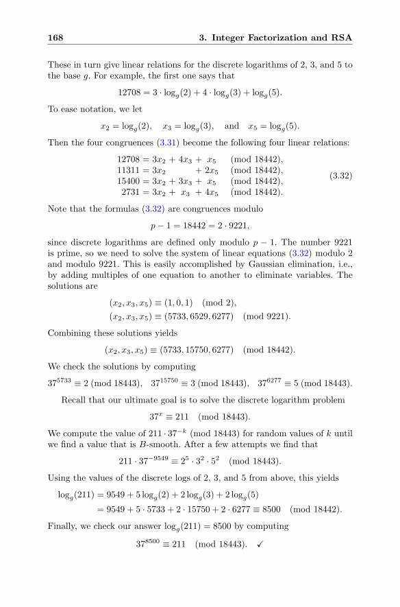
168 3. Integer Factorization and RSA
These in turn give linear relations for the discrete logarithms of 2, 3, and 5 tothe base g. For example, the first one says that
12708 = 3 · logg(2) + 4 · logg(3) + logg(5).
To ease notation, we let
x2 = logg(2), x3 = logg(3), and x5 = logg(5).
Then the four congruences (3.31) become the following four linear relations:
12708 = 3x2 + 4x3 + x5 (mod 18442),11311 = 3x2 + 2x5 (mod 18442),15400 = 3x2 + 3x3 + x5 (mod 18442),2731 = 3x2 + x3 + 4x5 (mod 18442).
(3.32)
Note that the formulas (3.32) are congruences modulo
p− 1 = 18442 = 2 · 9221,
since discrete logarithms are defined only modulo p − 1. The number 9221is prime, so we need to solve the system of linear equations (3.32) modulo 2and modulo 9221. This is easily accomplished by Gaussian elimination, i.e.,by adding multiples of one equation to another to eliminate variables. Thesolutions are
(x2, x3, x5) ≡ (1, 0, 1) (mod 2),
(x2, x3, x5) ≡ (5733, 6529, 6277) (mod 9221).
Combining these solutions yields
(x2, x3, x5) ≡ (5733, 15750, 6277) (mod 18442).
We check the solutions by computing
375733 ≡ 2 (mod 18443), 3715750 ≡ 3 (mod 18443), 376277 ≡ 5 (mod 18443).
Recall that our ultimate goal is to solve the discrete logarithm problem
37x ≡ 211 (mod 18443).
We compute the value of 211 · 37−k (mod 18443) for random values of k untilwe find a value that is B-smooth. After a few attempts we find that
211 · 37−9549 ≡ 25 · 32 · 52 (mod 18443).
Using the values of the discrete logs of 2, 3, and 5 from above, this yields
logg(211) = 9549 + 5 logg(2) + 2 logg(3) + 2 logg(5)
= 9549 + 5 · 5733 + 2 · 15750 + 2 · 6277 ≡ 8500 (mod 18442).
Finally, we check our answer logg(211) = 8500 by computing
378500 ≡ 211 (mod 18443). �
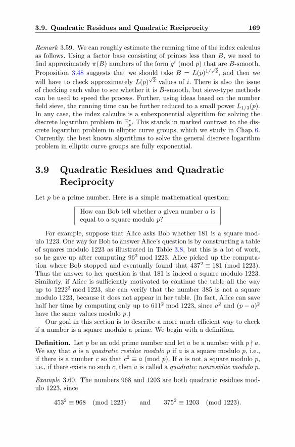
3.9. Quadratic Residues and Quadratic Reciprocity 169
Remark 3.59. We can roughly estimate the running time of the index calculusas follows. Using a factor base consisting of primes less than B, we need tofind approximately π(B) numbers of the form gi (mod p) that are B-smooth.
Proposition 3.48 suggests that we should take B = L(p)1/√2, and then we
will have to check approximately L(p)√2 values of i. There is also the issue
of checking each value to see whether it is B-smooth, but sieve-type methodscan be used to speed the process. Further, using ideas based on the numberfield sieve, the running time can be further reduced to a small power L1/3(p).In any case, the index calculus is a subexponential algorithm for solving thediscrete logarithm problem in F
∗p. This stands in marked contrast to the dis-
crete logarithm problem in elliptic curve groups, which we study in Chap. 6.Currently, the best known algorithms to solve the general discrete logarithmproblem in elliptic curve groups are fully exponential.
3.9 Quadratic Residues and QuadraticReciprocity
Let p be a prime number. Here is a simple mathematical question:
How can Bob tell whether a given number a isequal to a square modulo p?
For example, suppose that Alice asks Bob whether 181 is a square mod-ulo 1223. One way for Bob to answer Alice’s question is by constructing a tableof squares modulo 1223 as illustrated in Table 3.8, but this is a lot of work,so he gave up after computing 962 mod 1223. Alice picked up the computa-tion where Bob stopped and eventually found that 4372 ≡ 181 (mod 1223).Thus the answer to her question is that 181 is indeed a square modulo 1223.Similarly, if Alice is sufficiently motivated to continue the table all the wayup to 12222 mod 1223, she can verify that the number 385 is not a squaremodulo 1223, because it does not appear in her table. (In fact, Alice can savehalf her time by computing only up to 6112 mod 1223, since a2 and (p− a)2have the same values modulo p.)
Our goal in this section is to describe a more much efficient way to checkif a number is a square modulo a prime. We begin with a definition.
Definition. Let p be an odd prime number and let a be a number with p � a.We say that a is a quadratic residue modulo p if a is a square modulo p, i.e.,if there is a number c so that c2 ≡ a (mod p). If a is not a square modulo p,i.e., if there exists no such c, then a is called a quadratic nonresidue modulo p.
Example 3.60. The numbers 968 and 1203 are both quadratic residues mod-ulo 1223, since
4532 ≡ 968 (mod 1223) and 3752 ≡ 1203 (mod 1223).
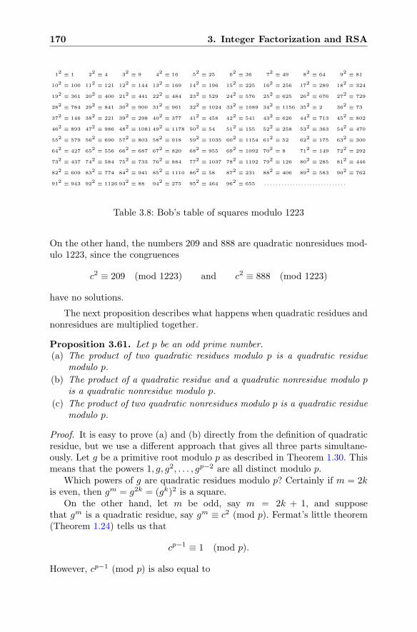
170 3. Integer Factorization and RSA
12 ≡ 1 2
2 ≡ 4 32 ≡ 9 4
2 ≡ 16 52 ≡ 25 6
2 ≡ 36 72 ≡ 49 8
2 ≡ 64 92 ≡ 81
102 ≡ 100 11
2 ≡ 121 122 ≡ 144 13
2 ≡ 169 142 ≡ 196 15
2 ≡ 225 162 ≡ 256 17
2 ≡ 289 182 ≡ 324
192 ≡ 361 20
2 ≡ 400 212 ≡ 441 22
2 ≡ 484 232 ≡ 529 24
2 ≡ 576 252 ≡ 625 26
2 ≡ 676 272 ≡ 729
282 ≡ 784 29
2 ≡ 841 302 ≡ 900 31
2 ≡ 961 322 ≡ 1024 33
2 ≡ 1089 342 ≡ 1156 35
2 ≡ 2 362 ≡ 73
372 ≡ 146 38
2 ≡ 221 392 ≡ 298 40
2 ≡ 377 412 ≡ 458 42
2 ≡ 541 432 ≡ 626 44
2 ≡ 713 452 ≡ 802
462 ≡ 893 47
2 ≡ 986 482 ≡ 1081 49
2 ≡ 1178 502 ≡ 54 51
2 ≡ 155 522 ≡ 258 53
2 ≡ 363 542 ≡ 470
552 ≡ 579 56
2 ≡ 690 572 ≡ 803 58
2 ≡ 918 592 ≡ 1035 60
2 ≡ 1154 612 ≡ 52 62
2 ≡ 175 632 ≡ 300
642 ≡ 427 65
2 ≡ 556 662 ≡ 687 67
2 ≡ 820 682 ≡ 955 69
2 ≡ 1092 702 ≡ 8 71
2 ≡ 149 722 ≡ 292
732 ≡ 437 74
2 ≡ 584 752 ≡ 733 76
2 ≡ 884 772 ≡ 1037 78
2 ≡ 1192 792 ≡ 126 80
2 ≡ 285 812 ≡ 446
822 ≡ 609 83
2 ≡ 774 842 ≡ 941 85
2 ≡ 1110 862 ≡ 58 87
2 ≡ 231 882 ≡ 406 89
2 ≡ 583 902 ≡ 762
912 ≡ 943 92
2 ≡ 1126 932 ≡ 88 94
2 ≡ 275 952 ≡ 464 96
2 ≡ 655 . . . . . . . . . . . . . . . . . . . . . . . . . . . . .
Table 3.8: Bob’s table of squares modulo 1223
On the other hand, the numbers 209 and 888 are quadratic nonresidues mod-ulo 1223, since the congruences
c2 ≡ 209 (mod 1223) and c2 ≡ 888 (mod 1223)
have no solutions.
The next proposition describes what happens when quadratic residues andnonresidues are multiplied together.
Proposition 3.61. Let p be an odd prime number.(a) The product of two quadratic residues modulo p is a quadratic residue
modulo p.
(b) The product of a quadratic residue and a quadratic nonresidue modulo pis a quadratic nonresidue modulo p.
(c) The product of two quadratic nonresidues modulo p is a quadratic residuemodulo p.
Proof. It is easy to prove (a) and (b) directly from the definition of quadraticresidue, but we use a different approach that gives all three parts simultane-ously. Let g be a primitive root modulo p as described in Theorem 1.30. Thismeans that the powers 1, g, g2, . . . , gp−2 are all distinct modulo p.
Which powers of g are quadratic residues modulo p? Certainly if m = 2kis even, then gm = g2k = (gk)2 is a square.
On the other hand, let m be odd, say m = 2k + 1, and supposethat gm is a quadratic residue, say gm ≡ c2 (mod p). Fermat’s little theorem(Theorem 1.24) tells us that
cp−1 ≡ 1 (mod p).
However, cp−1 (mod p) is also equal to
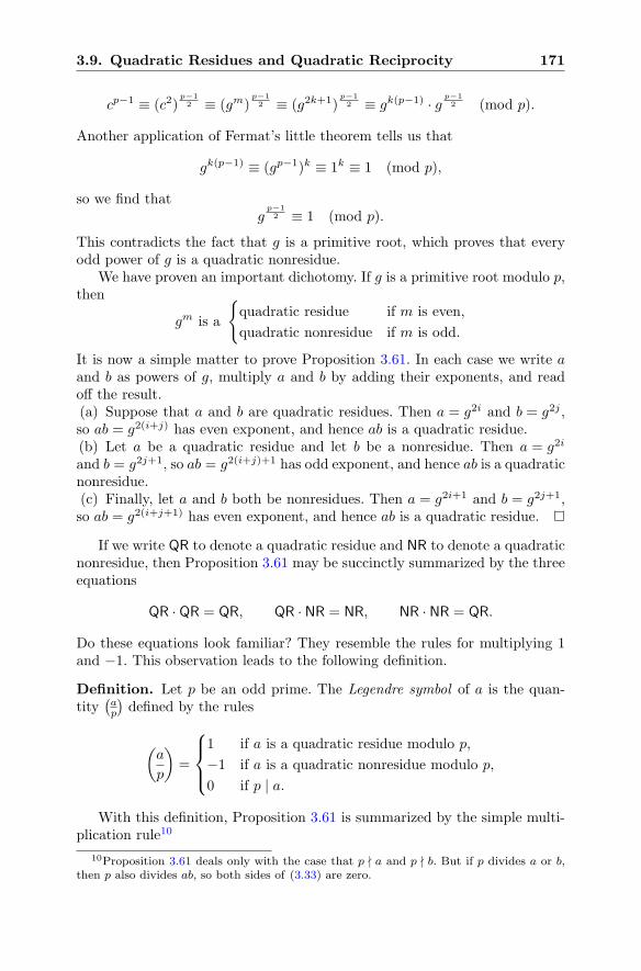
3.9. Quadratic Residues and Quadratic Reciprocity 171
cp−1 ≡ (c2)p−12 ≡ (gm)
p−12 ≡ (g2k+1)
p−12 ≡ gk(p−1) · g
p−12 (mod p).
Another application of Fermat’s little theorem tells us that
gk(p−1) ≡ (gp−1)k ≡ 1k ≡ 1 (mod p),
so we find thatg
p−12 ≡ 1 (mod p).
This contradicts the fact that g is a primitive root, which proves that everyodd power of g is a quadratic nonresidue.
We have proven an important dichotomy. If g is a primitive root modulo p,then
gm is a
{quadratic residue if m is even,
quadratic nonresidue if m is odd.
It is now a simple matter to prove Proposition 3.61. In each case we write aand b as powers of g, multiply a and b by adding their exponents, and readoff the result.(a) Suppose that a and b are quadratic residues. Then a = g2i and b = g2j ,so ab = g2(i+j) has even exponent, and hence ab is a quadratic residue.(b) Let a be a quadratic residue and let b be a nonresidue. Then a = g2i
and b = g2j+1, so ab = g2(i+j)+1 has odd exponent, and hence ab is a quadraticnonresidue.(c) Finally, let a and b both be nonresidues. Then a = g2i+1 and b = g2j+1,so ab = g2(i+j+1) has even exponent, and hence ab is a quadratic residue.
If we write QR to denote a quadratic residue and NR to denote a quadraticnonresidue, then Proposition 3.61 may be succinctly summarized by the threeequations
QR · QR = QR, QR · NR = NR, NR · NR = QR.
Do these equations look familiar? They resemble the rules for multiplying 1and −1. This observation leads to the following definition.
Definition. Let p be an odd prime. The Legendre symbol of a is the quan-tity
(ap
)defined by the rules
(a
p
)=
⎧⎪⎨
⎪⎩
1 if a is a quadratic residue modulo p,
−1 if a is a quadratic nonresidue modulo p,
0 if p | a.
With this definition, Proposition 3.61 is summarized by the simple multi-plication rule10
10Proposition 3.61 deals only with the case that p � a and p � b. But if p divides a or b,then p also divides ab, so both sides of (3.33) are zero.
172 3. Integer Factorization and RSA
(a
p
)(b
p
)=
(ab
p
). (3.33)
We also make the obvious, but useful, observation that
If a ≡ b (mod p), then
(a
p
)=
(b
p
). (3.34)
Thus in computing(ap
), we may reduce a modulo p into the interval from 0
to p− 1. It is worth adding a cautionary note: The notation for the Legendresymbol resembles a fraction, but it is not a fraction!
Returning to our original question of determining whether a given numberis a square modulo p, the following beautiful and powerful theorem providesa method for determining the answer.
Theorem 3.62 (Quadratic Reciprocity). Let p and q be odd primes.
(a)
(−1p
)=
{1 if p ≡ 1 (mod 4),
−1 if p ≡ 3 (mod 4).
(b)
(2
p
)=
{1 if p ≡ 1 or 7 (mod 8),
−1 if p ≡ 3 or 5 (mod 8).
(c)
(p
q
)=
⎧⎪⎪⎨
⎪⎪⎩
(q
p
)if p ≡ 1 (mod 4) or q ≡ 1 (mod 4),
−(q
p
)if p ≡ 3 (mod 4) and q ≡ 3 (mod 4).
Proof. We do not give a proof of quadratic reciprocity, but you will find a proofin any introductory number theory textbook, such as [35, 52, 59, 100, 111].
The name “quadratic reciprocity” comes from property (c), which tells ushow
(pq
)is related to its “reciprocal”
(qp
). It is worthwhile spending some time
contemplating Theorem 3.62, because despite the simplicity of its statement,quadratic reciprocity is saying something quite unexpected and profound. Thevalue of
(pq
)tells us whether p is a square modulo q. Similarly,
(qp
)tells us
whether q is a square modulo p. There is no a priori reason to suspect thatthese questions should have anything to do with one another. Quadratic reci-procity tells us that they are intimately related, and indeed, related by a verysimple rule.
Similarly, parts (a) and (b) of quadratic reciprocity give us some surprisinginformation. The first part says that the question whether −1 is a squaremodulo p is answered by the congruence class of p modulo 4, and the secondpart says that question whether 2 is a square modulo p is answered by thecongruence class of p modulo 8.
We indicated earlier that quadratic reciprocity can be used to determinewhether a is a square modulo p. The way to apply quadratic reciprocity is touse (c) to repeatedly flip the Legendre symbol, where each time that we flip,we’re allowed to reduce the top number modulo the bottom number. This
3.9. Quadratic Residues and Quadratic Reciprocity 173
leads to a rapid reduction in the size of the numbers, as illustrated by thefollowing example.
Example 3.63. We check whether −15750 is a quadratic residue modulo 37907using quadratic reciprocity to compute the Legendre symbol
(−1575037907
).
(−1575037907
)=
(−1
37907
)(15750
37907
)Multiplication rule (3.33)
= −(15750
37907
)Quadratic Reciprocity 3.62(a)
= −(2 · 32 · 53 · 7
37907
)Factor 15750
= −(
2
37907
)(3
37907
)2(5
37907
)3(7
37907
)
Multiplication rule (3.33)
= −(
2
37907
)(5
37907
)(7
37907
)since (−1)2 = 1
=
(5
37907
)(7
37907
)Quadratic Reciprocity 3.62(b)
=
(37907
5
)×−
(37907
7
)Quadratic Reciprocity 3.62(c)
= −(2
5
)(2
7
)since 37907 ≡ 2 (mod 5)and 37907 ≡ 2 (mod 7)
= −(−1)× 1 Quadratic Reciprocity 3.62(b)
= 1.
Thus(−15750
37907
)= 1, so we conclude that −15750 is a square modulo 37907.
Note that our computation using Legendre symbols does not tell us how tosolve c2 ≡ −15750 (mod 37907); it tells us only that there is a solution. Forthose who are curious, we mention that c = 10982 is a solution.
Example 3.63 shows how quadratic reciprocity can be used to evaluate theLegendre symbol. However, you may have noticed that in the middle of ourcalculation, we needed to factor the number 15750. We were lucky that 15750is easy to factor, but suppose that we were faced with a more difficult fac-torization problem. For example, suppose that we want to determine whetherp = 228530738017 is a square modulo q = 9365449244297. It turns out thatboth p and q are prime.11 Hence we can use quadratic reciprocity to compute(228530738017
9365449244297
)=
(9365449244297
228530738017
)since 228530738017 ≡ 1 (mod 4),
=
(224219723617
228530738017
)reducing 9365449244297modulo 228530738017.
11If you don’t believe that p and q are prime, use Miller–Rabin (Table 3.2) to check.
174 3. Integer Factorization and RSA
Unfortunately, the number 224219723617 is not prime, so we cannot applyquadratic reciprocity directly, and even more unfortunately, it is not an easynumber to factor (by hand). So it appears that quadratic reciprocity is usefulonly if the intermediate calculations lead to numbers that we are able to factor.
Luckily, there is a fancier version of quadratic reciprocity that completelyeliminates this difficulty. In order to state it, we need to generalize the defini-tion of the Legendre symbol.
Definition. Let a and b be integers and let b be odd and positive. Supposethat the factorization of b into primes is
b = pe11 pe22 p
e33 · · · pett .
The Jacobi symbol(ab
)is defined by the formula
(a
b
)=
(a
p1
)e1( ap2
)e2( ap3
)e3
· · ·(a
pt
)et
.
Notice that if b is itself prime, then(ab
)is the original Legendre symbol, so
the Jacobi symbol is a generalization of the Legendre symbol. Also note thatwe define the Jacobi symbol only for odd positive values of b.
Example 3.64. Here is a simple example of a Jacobi symbol, computed directlyfrom the definition:
(123
323
)=
(123
17 · 19
)=
(123
17
)(123
19
)=
(4
17
)(9
19
)= 1.
Here is a more complicated example:(
171337608
536134436237
)
=
(171337608
293 · 59 · 672 · 83
)
=
(171337608
29
)3(171337608
59
)(171337608
67
)2(171337608
83
)
=
(171337608
29
)(171337608
59
)(171337608
83
)
=
(11
29
)(15
59
)(44
83
)
= (−1) · 1 · 1 = −1.
From the definition, it appears that we need to know how to factor bin order to compute the Jacobi symbol
(ab
), so we haven’t gained anything.
However, it turns out that the Jacobi symbol inherits most of the propertiesof the Legendre symbol, which will allow us to compute
(ab
)extremely rapidly
without doing any factorization at all. We start with the basic multiplicationand reduction properties.
3.9. Quadratic Residues and Quadratic Reciprocity 175
Proposition 3.65. Let a, a1, a2, b, b1, b2 be integers with b, b1, and b2 positiveand odd.
(a)
(a1a2b
)=
(a1b
)(a2b
)and
(a
b1b2
)=
(a
b1
)(a
b2
).
(b) If a1 ≡ a2 (mod b), then
(a1b
)=
(a2b
).
Proof. Both parts of Proposition 3.65 follow easily from the definition ofthe Jacobi symbol and the corresponding properties (3.33) and (3.34) of theLegendre symbol.
Now we come to the amazing fact that the Jacobi symbol satisfies exactlythe same reciprocity law as the Legendre symbol.
Theorem 3.66 (Quadratic Reciprocity: Version II). Let a and b be integersthat are odd and positive.
(a)
(−1b
)=
{1 if b ≡ 1 (mod 4),
−1 if b ≡ 3 (mod 4).
(b)
(2
b
)=
{1 if b ≡ 1 or 7 (mod 8),
−1 if b ≡ 3 or 5 (mod 8).
(c)
(a
b
)=
⎧⎪⎪⎨
⎪⎪⎩
(b
a
)if a ≡ 1 (mod 4) or b ≡ 1 (mod 4),
−(b
a
)if a ≡ 3 (mod 4) and b ≡ 3 (mod 4).
Proof. It is not hard to use the original version of quadratic reciprocity forthe Legendre symbol (Theorem 3.62) to prove the more general version for theJacobi symbol. See for example [59, Proposition 5.2.2] or [137, Theorem 22.2].
Example 3.67. When we tried to use the original version of quadratic reci-procity (Theorem 3.62) to compute
(2285307380179365449244297
), we ran into the problem
that we needed to factor the number 224219723617. Using the new and im-proved version of quadratic reciprocity (Theorem 3.66), we can perform thecomputation without doing any factoring:(
228530738017
9365449244297
)
=
(9365449244297
228530738017
)
=
(224219723617
228530738017
)
=
(228530738017
224219723617
)
=
(4311014400
224219723617
)
=
(210 · 4209975224219723617
)
=
(224219723617
4209975
)
=
(665092
4209975
)
=
(22 · 1662734209975
)
=
(4209975
166273
)
=
(53150
166273
)
=
(2 · 26575166273
)
=
(26575
166273
)
=
(166273
26575
)
=
(6823
26575
)
= −(26575
6823
)
= −(6106
6823
)
= −(2 · 30536823
)
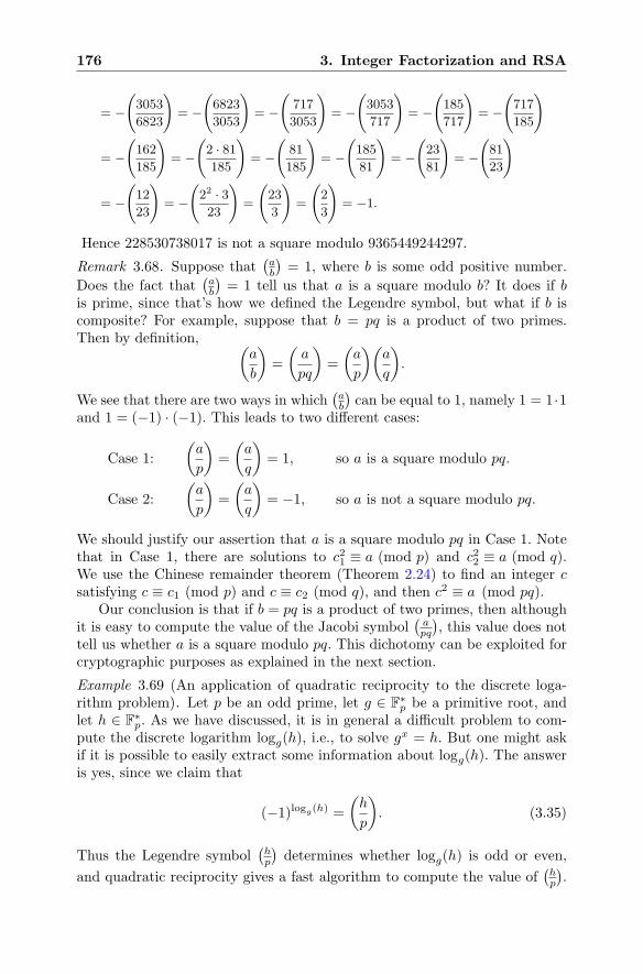
176 3. Integer Factorization and RSA
= −(3053
6823
)
= −(6823
3053
)
= −(
717
3053
)
= −(3053
717
)
= −(185
717
)
= −(717
185
)
= −(162
185
)
= −(2 · 81185
)
= −(
81
185
)
= −(185
81
)
= −(23
81
)
= −(81
23
)
= −(12
23
)
= −(22 · 323
)
=
(23
3
)
=
(2
3
)
= −1.
Hence 228530738017 is not a square modulo 9365449244297.
Remark 3.68. Suppose that(ab
)= 1, where b is some odd positive number.
Does the fact that(ab
)= 1 tell us that a is a square modulo b? It does if b
is prime, since that’s how we defined the Legendre symbol, but what if b iscomposite? For example, suppose that b = pq is a product of two primes.Then by definition, (
a
b
)=
(a
pq
)=
(a
p
)(a
q
).
We see that there are two ways in which(ab
)can be equal to 1, namely 1 = 1 ·1
and 1 = (−1) · (−1). This leads to two different cases:
Case 1:
(a
p
)=
(a
q
)= 1, so a is a square modulo pq.
Case 2:
(a
p
)=
(a
q
)= −1, so a is not a square modulo pq.
We should justify our assertion that a is a square modulo pq in Case 1. Notethat in Case 1, there are solutions to c21 ≡ a (mod p) and c22 ≡ a (mod q).We use the Chinese remainder theorem (Theorem 2.24) to find an integer csatisfying c ≡ c1 (mod p) and c ≡ c2 (mod q), and then c2 ≡ a (mod pq).
Our conclusion is that if b = pq is a product of two primes, then althoughit is easy to compute the value of the Jacobi symbol
(apq
), this value does not
tell us whether a is a square modulo pq. This dichotomy can be exploited forcryptographic purposes as explained in the next section.
Example 3.69 (An application of quadratic reciprocity to the discrete loga-rithm problem). Let p be an odd prime, let g ∈ F
∗p be a primitive root, and
let h ∈ F∗p. As we have discussed, it is in general a difficult problem to com-
pute the discrete logarithm logg(h), i.e., to solve gx = h. But one might askif it is possible to easily extract some information about logg(h). The answeris yes, since we claim that
(−1)logg(h) =
(h
p
). (3.35)
Thus the Legendre symbol(hp
)determines whether logg(h) is odd or even,
and quadratic reciprocity gives a fast algorithm to compute the value of(hp
).
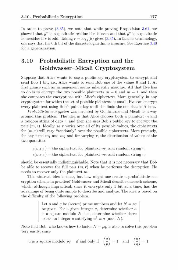
3.10. Probabilistic Encryption 177
In order to prove (3.35), we note that while proving Proposition 3.61, weshowed that gr is a quadratic residue if r is even and that gr is a quadraticnonresidue if r is odd. Taking r = logg(h) gives (3.35). In fancier terminology,one says that the 0th bit of the discrete logarithm is insecure. See Exercise 3.40for a generalization.
3.10 Probabilistic Encryption and theGoldwasser–Micali Cryptosystem
Suppose that Alice wants to use a public key cryptosystem to encrypt andsend Bob 1 bit, i.e., Alice wants to send Bob one of the values 0 and 1. Atfirst glance such an arrangement seems inherently insecure. All that Eve hasto do is to encrypt the two possible plaintexts m = 0 and m = 1, and thenshe compares the encryptions with Alice’s ciphertext. More generally, in anycryptosystem for which the set of possible plaintexts is small, Eve can encryptevery plaintext using Bob’s public key until she finds the one that is Alice’s.
Probabilistic encryption was invented by Goldwasser and Micali as a wayaround this problem. The idea is that Alice chooses both a plaintext m anda random string of data r, and then she uses Bob’s public key to encrypt thepair (m, r). Ideally, as r varies over all of its possible values, the ciphertextsfor (m, r) will vary “randomly” over the possible ciphertexts. More precisely,for any fixed m1 and m2 and for varying r, the distribution of values of thetwo quantities
e(m1, r) = the ciphertext for plaintext m1 and random string r,
e(m2, r) = the ciphertext for plaintext m2 and random string r,
should be essentially indistinguishable. Note that it is not necessary that Bobbe able to recover the full pair (m, r) when he performs the decryption. Heneeds to recover only the plaintext m.
This abstract idea is clear, but how might one create a probabilistic en-cryption scheme in practice? Goldwasser and Micali describe one such scheme,which, although impractical, since it encrypts only 1 bit at a time, has theadvantage of being quite simple to describe and analyze. The idea is based onthe difficulty of the following problem.
Let p and q be (secret) prime numbers and let N = pqbe given. For a given integer a, determine whether ais a square modulo N , i.e., determine whether thereexists an integer u satisfying u2 ≡ a (mod N).
Note that Bob, who knows how to factor N = pq, is able to solve this problemvery easily, since
a is a square modulo pq if and only if
(a
p
)= 1 and
(a
q
)= 1.
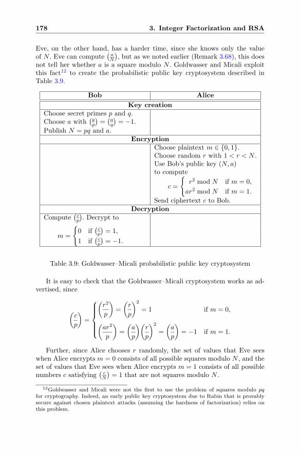
178 3. Integer Factorization and RSA
Eve, on the other hand, has a harder time, since she knows only the valueof N . Eve can compute
(aN
), but as we noted earlier (Remark 3.68), this does
not tell her whether a is a square modulo N . Goldwasser and Micali exploitthis fact12 to create the probabilistic public key cryptosystem described inTable 3.9.
Bob Alice
Key creationChoose secret primes p and q.Choose a with
(ap
)=(aq
)= −1.
Publish N = pq and a.Encryption
Choose plaintext m ∈ {0, 1}.Choose random r with 1 < r < N .Use Bob’s public key (N, a)to compute
c =
{r2 mod N if m = 0,
ar2 mod N if m = 1.
Send ciphertext c to Bob.Decryption
Compute(cp
). Decrypt to
m =
{0 if
(cp
)= 1,
1 if(cp
)= −1.
Table 3.9: Goldwasser–Micali probabilistic public key cryptosystem
It is easy to check that the Goldwasser–Micali cryptosystem works as ad-vertised, since
(c
p
)=
⎧⎪⎪⎪⎨
⎪⎪⎪⎩
(r2
p
)=
(r
p
)2
= 1 if m = 0,
(ar2
p
)=
(a
p
)(r
p
)2
=
(a
p
)= −1 if m = 1.
Further, since Alice chooses r randomly, the set of values that Eve seeswhen Alice encrypts m = 0 consists of all possible squares modulo N , and theset of values that Eve sees when Alice encrypts m = 1 consists of all possiblenumbers c satisfying
(cN
)= 1 that are not squares modulo N .
12Goldwasser and Micali were not the first to use the problem of squares modulo pqfor cryptography. Indeed, an early public key cryptosystem due to Rabin that is provablysecure against chosen plaintext attacks (assuming the hardness of factorization) relies onthis problem.
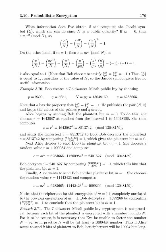
3.10. Probabilistic Encryption 179
What information does Eve obtain if she computes the Jacobi sym-bol
(cN
), which she can do since N is a public quantity? If m = 0, then
c ≡ r2 (mod N), so (c
N
)=
(r2
N
)=
(r
N
)2
= 1.
On the other hand, if m = 1, then c ≡ ar2 (mod N), so
(c
N
)=
(ar2
N
)=
(a
N
)=
(a
pq
)=
(a
p
)(a
q
)= (−1) · (−1) = 1
is also equal to 1. (Note that Bob chose a to satisfy(ap
)=(aq
)= −1.) Thus
(cN
)
is equal to 1, regardless of the value of N , so the Jacobi symbol gives Eve nouseful information.
Example 3.70. Bob creates a Goldwasser–Micali public key by choosing
p = 2309, q = 5651, N = pq = 13048159, a = 6283665.
Note that a has the property that(ap
)=(aq
)= −1. He publishes the pair (N, a)
and keeps the values of the primes p and q secret.Alice begins by sending Bob the plaintext bit m = 0. To do this, she
chooses r = 1642087 at random from the interval 1 to 13048158. She thencomputes
c ≡ r2 ≡ 16420872 ≡ 8513742 (mod 13048159),
and sends the ciphertext c = 8513742 to Bob. Bob decrypts the ciphertextc = 8513742 by computing
(85137422309
)= 1, which gives the plaintext bit m = 0.
Next Alice decides to send Bob the plaintext bit m = 1. She chooses arandom value r = 11200984 and computes
c ≡ ar2 ≡ 6283665 · 112009842 ≡ 2401627 (mod 13048159).
Bob decrypts c = 2401627 by computing(24016272309
)= −1, which tells him that
the plaintext bit m = 1.Finally, Alice wants to send Bob another plaintext bit m = 1. She chooses
the random value r = 11442423 and computes
c ≡ ar2 ≡ 6283665 · 114424232 ≡ 4099266 (mod 13048159).
Notice that the ciphertext for this encryption ofm = 1 is completely unrelatedto the previous encryption of m = 1. Bob decrypts c = 4099266 by computing(40992662309
)= −1 to conclude that the plaintext bit is m = 1.
Remark 3.71. The Goldwasser–Micali public key cryptosystem is not practi-cal, because each bit of the plaintext is encrypted with a number modulo N .For it to be secure, it is necessary that Eve be unable to factor the numberN = pq, so in practice N will be (at least) a 1000-bit number. Thus if Alicewants to send k bits of plaintext to Bob, her ciphertext will be 1000k bits long.
180 Exercises
Thus the Goldwasswer–Micali public key cryptosystem has a message expan-sion ratio of 1000, since the ciphertext is 1000 times as long as the plaintext. Ingeneral, the Goldwasswer–Micali public key cryptosystem expands a messageby a factor of log2(N).
There are other probabilistic public key cryptosystems whose message ex-pansion is much smaller. Indeed, we have already seen one: the random ele-ment k used by the Elgamal public key cryptosystem (Sect. 2.4) makes Elga-mal a probabilistic cryptosystem. Elgamal has a message expansion ratio of 2,as explained in Remark 2.9. Later, in Sect. 7.10, we will see another proba-bilistic cryptosystem called NTRU. More generally, it is possible, and indeedusually desirable, to take a deterministic cryptosystem such as RSA and turnit into a probabilistic system, even at the cost of increasing its message ex-pansion ratio. (See Exercise 3.43 and Sect. 8.6.)
Exercises
Section 3.1. Euler’s Theorem and Roots Modulo pq
3.1. Solve the following congruences.(a) x19 ≡ 36 (mod 97).
(b) x137 ≡ 428 (mod 541).
(c) x73 ≡ 614 (mod 1159).
(d) x751 ≡ 677 (mod 8023).
(e) x38993 ≡ 328047 (mod 401227). (Hint. 401227 = 607 · 661.)
3.2. This exercise investigates what happens if we drop the assumption thatgcd(e, p − 1) = 1 in Proposition 3.2. So let p be a prime, let c �≡ 0 (mod p), lete ≥ 1, and consider the congruence
xe ≡ c (mod p). (3.36)
(a) Prove that if (3.36) has one solution, then it has exactly gcd(e, p− 1) distinctsolutions. (Hint. Use primitive root theorem (Theorem 1.30), combined withthe extended Euclidean algorithm (Theorem 1.11) or Exercise 1.27.)
(b) For how many non-zero values of c (mod p) does the congruence (3.36) have asolution?
3.3. Let p and q be distinct primes and let e and d be positive integers satisfying
de ≡ 1 (mod (p− 1)(q − 1)).
Suppose further that c is an integer with gcd(c, pq) > 1. Prove that
x ≡ cd (mod pq) is a solution to the congruence xe ≡ c (mod pq),
thereby completing the proof of Proposition 3.5.
Exercises 181
3.4. Recall from Sect. 1.3 that Euler’s phi function φ(N) is the function defined by
φ(N) = #{0 ≤ k < N : gcd(k,N) = 1}.
In other words, φ(N) is the number of integers between 0 and N − 1 that arerelatively prime to N , or equivalently, the number of elements in Z/NZ that haveinverses modulo N .(a) Compute the values of φ(6), φ(9), φ(15), and φ(17).
(b) If p is prime, what is the value of φ(p)?
(c) Prove Euler’s formula
aφ(N) ≡ 1 (mod N) for all integers a satisfying gcd(a,N) = 1.
(Hint. Mimic the proof of Fermat’s little theorem (Theorem 1.24), but instead oflooking at all of the multiples of a as was done in (1.8), just take the multiples kaof a for values of k satisfying gcd(k,N) = 1.)
3.5. Euler’s phi function has many beautiful properties.(a) If p and q are distinct primes, how is φ(pq) related to φ(p) and φ(q)?
(b) If p is prime, what is the value of φ(p2)? How about φ(pj)? Prove that yourformula for φ(pj) is correct. (Hint. Among the numbers between 0 and pj − 1,remove the ones that have a factor of p. The ones that are left are relativelyprime to p.)
(c) Let M and N be integers satisfying gcd(M,N) = 1. Prove the multiplicationformula
φ(MN) = φ(M)φ(N).
(d) Let p1, p2, . . . , pr be the distinct primes that divide N . Use your results from (b)and (c) to prove the following formula:
φ(N) = Nr∏
i=1
(1− 1
pi
).
(e) Use the formula in (d) to compute the following values of φ(N).
(i) φ(1728). (ii) φ(1575). (iii) φ(889056) (Hint. 889056 = 25 · 34 · 73).
3.6. Let N , c, and e be positive integers satisfying the conditions gcd(N, c) = 1 andgcd(e, φ(N)
)= 1.
(a) Explain how to solve the congruence
xe ≡ c (mod N),
assuming that you know the value of φ(N). (Hint. Use the formula inExercise 3.4(c).)
(b) Solve the following congruences. (The formula in Exercise 3.5(d) may be helpfulfor computing the value of φ(N).)
(i) x577 ≡ 60 (mod 1463).
(ii) x959 ≡ 1583 (mod 1625).
(iii) x133957 ≡ 224689 (mod 2134440).
182 Exercises
Section 3.2. The RSA Public Key Cryptosystem
3.7. Alice publishes her RSA public key: modulus N = 2038667 and exponente = 103.(a) Bob wants to send Alice the message m = 892383. What ciphertext does Bob
send to Alice?
(b) Alice knows that her modulus factors into a product of two primes, one of whichis p = 1301. Find a decryption exponent d for Alice.
(c) Alice receives the ciphertext c = 317730 from Bob. Decrypt the message.
3.8. Bob’s RSA public key has modulus N = 12191 and exponent e = 37. Alicesends Bob the ciphertext c = 587. Unfortunately, Bob has chosen too small a modu-lus. Help Eve by factoring N and decrypting Alice’s message. (Hint. N has a factorsmaller than 100.)
3.9. For each of the given values of N = pq and (p − 1)(q − 1), use the methoddescribed in Remark 3.11 to determine p and q.(a) N = pq = 352717 and (p− 1)(q − 1) = 351520.
(b) N = pq = 77083921 and (p− 1)(q − 1) = 77066212.
(c) N = pq = 109404161 and (p− 1)(q − 1) = 109380612.
(d) N = pq = 172205490419 and (p− 1)(q − 1) = 172204660344.
3.10. A decryption exponent for an RSA public key (N, e) is an integer d with theproperty that ade ≡ a (mod N) for all integers a that are relatively prime to N .(a) Suppose that Eve has a magic box that creates decryption exponents for (N, e)
for a fixed modulus N and for a large number of different encryption expo-nents e. Explain how Eve can use her magic box to try to factor N .
(b) Let N = 38749709. Eve’s magic box tells her that the encryption exponente = 10988423 has decryption exponent d = 16784693 and that the encryp-tion exponent e = 25910155 has decryption exponent d = 11514115. Use thisinformation to factor N .
(c) Let N = 225022969. Eve’s magic box tells her the following three encryp-tion/decryption pairs for N :
(70583995, 4911157), (173111957, 7346999), (180311381, 29597249).
Use this information to factor N .
(d) Let N = 1291233941. Eve’s magic box tells her the following three encryp-tion/decryption pairs for N :
(1103927639, 76923209), (1022313977, 106791263), (387632407, 7764043).
Use this information to factor N .
3.11. Here is an example of a public key system that was proposed at a cryptographyconference. It was designed to be more efficient than RSA.
Alice chooses two large primes p and q and she publishes N = pq. It is assumedthat N is hard to factor. Alice also chooses three random numbers g, r1, and r2modulo N and computes
g1 ≡ gr1(p−1) (mod N) and g2 ≡ gr2(q−1) (mod N).
Exercises 183
Her public key is the triple (N, g1, g2) and her private key is the pair of primes (p, q).Now Bob wants to send the messagem to Alice, wherem is a number modulo N .
He chooses two random integers s1 and s2 modulo N and computes
c1 ≡ mgs11 (mod N) and c2 ≡ mgs22 (mod N).
Bob sends the ciphertext (c1, c2) to Alice.Decryption is extremely fast and easy. Alice uses the Chinese remainder theorem
to solve the pair of congruences
x ≡ c1 (mod p) and x ≡ c2 (mod q).
(a) Prove that Alice’s solution x is equal to Bob’s plaintext m.
(b) Explain why this cryptosystem is not secure.
Section 3.3. Implementation and Security Issues
3.12. Formulate a man-in-the-middle attack, similar to the attack described inExample 3.13 on page 126, for the following public key cryptosystems.(a) The Elgamal public key cryptosystem (Table 2.3 on page 72).
(b) The RSA public key cryptosystem (Table 3.1 on page 123).
3.13. Alice decides to use RSA with the public key N = 1889570071. In order toguard against transmission errors, Alice has Bob encrypt his message twice, onceusing the encryption exponent e1 = 1021763679 and once using the encryptionexponent e2 = 519424709. Eve intercepts the two encrypted messages
c1 = 1244183534 and c2 = 732959706.
Assuming that Eve also knows N and the two encryption exponents e1 and e2, usethe method described in Example 3.15 to help Eve recover Bob’s plaintext withoutfinding a factorization of N .
Section 3.4. Primality Testing
3.14. We stated that the number 561 is a Carmichael number, but we never checkedthat a561 ≡ a (mod 561) for every value of a.(a) The number 561 factors as 3 · 11 · 17. First use Fermat’s little theorem to prove
that
a561 ≡ a (mod 3), a561 ≡ a (mod 11), and a561 ≡ a (mod 17)
for every value of a. Then explain why these three congruences imply thata561 ≡ a (mod 561) for every value of a.
(b) Mimic the idea used in (a) to prove that each of the following numbers is aCarmichael number. (To assist you, we have factored each number into primes.)
(i) 1729 = 7 · 13 · 19(ii) 10585 = 5 · 29 · 73(iii) 75361 = 11 · 13 · 17 · 31(iv) 1024651 = 19 · 199 · 271
(c) Prove that a Carmichael number must be odd.
184 Exercises
(d) Prove that a Carmichael number must be a product of distinct primes.
(e) Look up Korselt’s criterion in a book or online, write a brief description of how itworks, and use it to show that 29341 = 13·37·61 and 172947529 = 307·613·919are Carmichael numbers.
3.15. Use the Miller–Rabin test on each of the following numbers. In each case,either provide a Miller–Rabin witness for the compositeness of n, or conclude that nis probably prime by providing 10 numbers that are not Miller–Rabin witnessesfor n.
(a) n = 1105. (Yes, 5 divides n, but this is just a warm-up exercise!)(b) n = 294409 (c) n = 294439(d) n = 118901509 (e) n = 118901521(f) n = 118901527 (g) n = 118915387
3.16. Looking back at Exercise 3.10, let’s suppose that for a given N , the magic boxcan produce only one decryption exponent. Equivalently, suppose that an RSA keypair has been compromised and that the private decryption exponent correspondingto the public encryption exponent has been discovered. Show how the basic idea inthe Miller–Rabin primality test can be applied to use this information to factor N .
3.17. The function π(X) counts the number of primes between 2 and X.(a) Compute the values of π(20), π(30), and π(100).
(b) Write a program to compute π(X) and use it to compute π(X) and the ratioπ(X)/(X/ ln(X)) for X = 100, X = 1000, X = 10000, and X = 100000. Doesyour list of ratios make the prime number theorem plausible?
3.18. Let
π1(X) = (# of primes p between 2 and X satisfying p ≡ 1 (mod 4)),
π3(X) = (# of primes p between 2 and X satisfying p ≡ 3 (mod 4)).
Thus every prime other than 2 gets counted by either π1(X) or by π3(X).(a) Compute the values of π1(X) and π3(X) for each of the following values of X.
(i) X = 10. (ii) X = 25. (iii) X = 100.
(b) Write a program to compute π1(X) and π3(X) and use it to compute theirvalues and the ratio π3(X)/π1(X) for X = 100, X = 1000, X = 10000, andX = 100000.
(c) Based on your data from (b), make a conjecture about the relative sizes of π1(X)and π3(X). Which one do you think is larger? What do you think is the limitof the ratio π3(X)/π1(X) as X → ∞?
3.19. We noted in Sect. 3.4 that it really makes no sense to say that the number nhas probability 1/ ln(n) of being prime. Any particular number that you chooseeither will be prime or will not be prime; there are no numbers that are 35% primeand 65% composite! In this exercise you will prove a result that gives a more sensiblemeaning to the statement that a number has a certain probability of being prime.You may use the prime number theorem (Theorem 3.21) for this problem.(a) Fix a (large) number N and suppose that Bob chooses a random number n in
the interval 12N ≤ n ≤ 3
2N . If he repeats this process many times, prove that
approximately 1/ ln(N) of his numbers will be prime. More precisely, define
Exercises 185
P (N) =number of primes between 1
2N and 3
2N
number of integers between 12N and 3
2N
=
[Probability that an integer n in theinterval 1
2N ≤ n ≤ 3
2N is a prime number
],
and prove that
limN→∞
P (N)
1/ ln(N)= 1.
This shows that if N is large, then P (N) is approximately 1/ ln(N).
(b) More generally, fix two numbers c1 and c2 satisfying c2 > c1 > 0. Bob choosesrandom numbers n in the interval c1N ≤ n ≤ c2N . Keeping c1 and c2 fixed, let
P (c1, c2;N) =
[Probability that an integer n in the inter-val c1N ≤ n ≤ c2N is a prime number
].
In the following formula, fill in the box with a simple function of N so that thestatement is true:
limN→∞
P (c1, c2;N)= 1.
3.20. Continuing with the previous exercise, explain how to make mathematicalsense of the following statements.(a) A randomly chosen odd number N has probability 2/ ln(N) of being prime.
(What is the probability that a randomly chosen even number is prime?)
(b) A randomly chosen number N satisfying N ≡ 1 (mod 3) has probability3/(2 ln(N)) of being prime.
(c) A randomly chosen number N satisfying N ≡ 1 (mod 6) has probability3/ ln(N) of being prime.
(d) Let m = p1p2 · · · pr be a product of distinct primes and let k be a numbersatisfying gcd(k,m) = 1. What number should go into the box to make state-ment (3.37) correct? Why?
A randomly chosen number N satisfying
N ≡ k (mod m) has probability / ln(N)of being prime.
(3.37)
(e) Same question, but for arbitrary m, not just for m that are products of distinctprimes.
3.21. The logarithmic integral function Li(X) is defined to be
Li(X) =
∫ X
2
dt
ln t.
(a) Prove that
Li(X) =X
lnX+
∫ X
2
dt
(ln t)2+O(1).
(Hint. Integration by parts.)
186 Exercises
(b) Compute the limit
limX→∞
Li(X)
X/ lnX.
(Hint. Break the integral in (a) into two pieces, 2 ≤ t ≤√X and
√X ≤ t ≤ X,
and estimate each piece separately.)
(c) Use (b) to show that formula (3.12) on page 135 implies the prime numbertheorem (Theorem 3.21).
Section 3.5. Pollard’s p− 1 Factorization Algorithm
3.22. Use Pollard’s p− 1 method to factor each of the following numbers.
(a) n = 1739 (b) n = 220459 (c) n = 48356747
Be sure to show your work and to indicate which prime factor p of n has the propertythat p− 1 is a product of small primes.
3.23. A prime of the form 2n − 1 is called a Mersenne prime.(a) Factor each of the numbers 2n−1 for n = 2, 3, . . . , 10. Which ones are Mersenne
primes?
(b) Find the first seven Mersenne primes. (You may need a computer.)
(c) If n is even and n > 2, prove that 2n − 1 is not prime.
(d) If 3 | n and n > 3, prove that 2n − 1 is not prime.
(e) More generally, prove that if n is a composite number, then 2n − 1 is not prime.Thus all Mersenne primes have the form 2p − 1 with p a prime number.
(f) What is the largest known Mersenne prime? Are there any larger primes known?(You can find out at the “Great Internet Mersenne Prime Search” web site www.mersenne.org/prime.htm.)
(g) Write a one page essay on Mersenne primes, starting with the discoveries ofFather Mersenne and ending with GIMPS.
Section 3.6. Factorization via Difference of Squares
3.24. For each of the following numbers N , compute the values of
N + 12, N + 22, N + 32, N + 42, . . .
as we did in Example 3.34 until you find a value N + b2 that is a perfect square a2.Then use the values of a and b to factor N .
(a) N = 53357 (b) N = 34571 (c) N = 25777 (d) N = 64213
3.25. For each of the listed values of N , k, and binit, factor N by making a list ofvalues of k ·N + b2, starting at b = binit and incrementing b until k ·N + b2 is aperfect square. Then take greatest common divisors as we did in Example 3.35.
(a) N = 143041 k = 247 binit = 1(b) N = 1226987 k = 3 binit = 36(c) N = 2510839 k = 21 binit = 90
3.26. For each part, use the data provided to find values of a and b satisfyinga2 ≡ b2 (mod N), and then compute gcd(N, a− b) in order to find a nontrivial factorof N , as we did in Examples 3.37 and 3.38.
Exercises 187
(a) N = 61063
18822 ≡ 270 (mod 61063) and 270 = 2 · 33 · 518982 ≡ 60750 (mod 61063) and 60750 = 2 · 35 · 53
(b) N = 52907
3992 ≡ 480 (mod 52907) and 480 = 25 · 3 · 57632 ≡ 192 (mod 52907) and 192 = 26 · 37732 ≡ 15552 (mod 52907) and 15552 = 26 · 35
9762 ≡ 250 (mod 52907) and 250 = 2 · 53
(c) N = 198103
11892 ≡ 27000 (mod 198103) and 27000 = 23 · 33 · 53
16052 ≡ 686 (mod 198103) and 686 = 2 · 73
23782 ≡ 108000 (mod 198103) and 108000 = 25 · 33 · 53
28152 ≡ 105 (mod 198103) and 105 = 3 · 5 · 7
(d) N = 2525891
15912 ≡ 5390 (mod 2525891) and 5390 = 2 · 5 · 72 · 1131822 ≡ 21560 (mod 2525891) and 21560 = 23 · 5 · 72 · 1147732 ≡ 48510 (mod 2525891) and 48510 = 2 · 32 · 5 · 72 · 1152752 ≡ 40824 (mod 2525891) and 40824 = 23 · 36 · 754012 ≡ 1386000 (mod 2525891) and 1386000 = 24 · 32 · 53 · 7 · 11
Section 3.7. Smooth Numbers, Sieves, and Building Relations for Factorization
3.27. Compute the following values of ψ(X,B), the number of B-smooth numbersbetween 2 and X (see page 150).
(a) ψ(25, 3) (b) ψ(35, 5) (c) ψ(50, 7) (d) ψ(100, 5) (e) ψ(100, 7)
3.28. An integer M is called B-power-smooth if every prime power pe dividing Msatisfies pe ≤ B. For example, 180 = 22 · 32 · 5 is 10-power-smooth, since the largestprime power dividing 180 is 9, which is smaller than 10.(a) Suppose that M is B-power-smooth. Prove that M is also B-smooth.
(b) Suppose thatM is B-smooth. Is it always true thatM is also B-power-smooth?Either prove that it is true or give an example for which it is not true.
(c) The following is a list of 20 randomly chosen numbers between 1 and 1000,sorted from smallest to largest. Which of these numbers are 10-power-smooth?Which of them are 10-smooth?
{84, 141, 171, 208, 224, 318, 325, 366, 378, 390, 420, 440,504, 530, 707, 726, 758, 765, 792, 817}
188 Exercises
(d) Prove thatM isB-power-smooth if and only ifM divides the least common mul-tiple of [1, 2, . . . , B]. (The least common multiple of a list of numbers k1, . . . , kris the smallest number K that is divisible by every number in the list.)
3.29. Let L(N) = e√
(lnN)(ln lnN) as usual. Suppose that a computer does onebillion operations per second.(a) How many seconds does it take to perform L(2100) operations?
(b) How many hours does it take to perform L(2250) operations?
(c) How many days does it take to perform L(2350) operations?
(d) How many years does it take to perform L(2500) operations?
(e) How many years does it take to perform L(2750) operations?
(f) How many years does it take to perform L(21000) operations?
(g) How many years does it take to perform L(22000) operations?(For simplicity, you may assume that there are 365.25 days in a year.)
3.30. Prove that the function L(X) = e√
(lnX)(ln lnX) is subexponential. That is,prove the following two statements.(a) For every positive constant α, no matter how large, L(X) = Ω
((lnX)α
).
(b) For every positive constant β, no matter how small, L(X) = O(Xβ).
3.31. For any fixed positive constants a and b, define the function
Fa,b(X) = e(lnX)1/a(ln lnX)1/b .
Prove the following properties of Fa,b(X).(a) If a > 1, prove that Fa,b(X) is subexponential.
(b) If a = 1, prove that Fa,b(X) = Ω(Xα) for every α > 0. Thus Fa,b(X) growsfaster than every exponential function, so one says that Fa,b(X) has superex-ponential growth.
(c) What happens if a < 1?
3.32. This exercise asks you to verify an assertion in the proof of Corollary 3.45.
Let L(X) be the usual function L(X) = e√
(lnX)(ln lnX).(a) Prove that there is a value of ε > 0 such that
(lnX)ε < lnL(X) < (lnX)1−ε for all X > 10.
(b) Let c > 0, let Y = L(X)c, and let u = (lnX)/(lnY ). Prove that
u−u = L(X)−12c
(1+o(1)).
3.33. Proposition 3.48 assumes that we choose random numbers a modulo N , com-pute a2 (mod N), and check whether the result is B-smooth. We can achieve betterresults if we take values for a of the form
a =⌊√
N⌋+ k for 1 ≤ k ≤ K.
(For simplicity, you may treat K as a fixed integer, independent of N . More rigor-ously, it is necessary to take K equal to a power of L(N), which has a small effecton the final answer.)
Exercises 189
(a) Prove that a2−N ≤ 2K√N+K2, so in particular, a2 (mod N) is smaller than
a multiple of√N .
(b) Prove that L(√N ) ≈ L(N)1/
√2 by showing that
limN→∞
logL(√N )
logL(N)1/√2= 1.
More generally, prove that in the same sense, L(N1/r) ≈ L(N)1/√r for any
fixed r > 0.
(c) Re-prove Proposition 3.48 using this better choice of values for a. Set B =L(N)c and find the optimal value of c. Approximately how many relations areneeded to factor N?
3.34. Illustrate the quadratic sieve, as was done in Fig. 3.3 (page 161), by sievingprime powers up to B on the values of F (T ) = T 2 −N in the indicated range.(a) Sieve N = 493 using prime powers up to B = 11 on values from F (23) to F (38).
Use the relation(s) that you find to factor N .
(b) Extend the computations in (a) by using prime powers up to B = 16 andsieving values from F (23) to F (50). What additional value(s) are sieved downto 1 and what additional relation(s) do they yield?
3.35. Let Z[β] be the ring described in Example 3.55, i.e., β is a root of f(x) =1 + 3x− 2x3 + x4. For each of the following pairs of elements u, v ∈ Z[β], computethe sum u+ v and the product uv. Your answers should involve only powers of β upto β3.(a) u = −5− 2β + 9β2 − 9β3 and v = 2 + 9β − 7β2 + 7β3.
(b) u = 9 + 9β + 6β2 − 5β3 and v = −4− 6β − 2β2 − 5β3.
(c) u = 6− 5β + 3β2 + 3β3 and v = −2 + 7β + 6β2.
Section 3.8. The Index Calculus and Discrete Logarithms
3.36. This exercise asks you to use the index calculus to solve a discrete logarithmproblem. Let p = 19079 and g = 17.(a) Verify that gi (mod p) is 5-smooth for each of the values i = 3030, i = 6892,
and i = 18312.
(b) Use your computations in (a) and linear algebra to compute the discrete loga-rithms logg(2), logg(3), and logg(5). (Note that 19078 = 2 · 9539 and that 9539is prime.)
(c) Verify that 19 · 17−12400 (mod p) is 5-smooth.
(d) Use the values from (b) and the computation in (c) to solve the discrete loga-rithm problem
17x ≡ 19 (mod 19079).
Section 3.9. Quadratic Residues and Quadratic Reciprocity
3.37. Let p be an odd prime and let a be an integer with p � a.(a) Prove that a(p−1)/2 is congruent to either 1 or −1 modulo p.
(b) Prove that a(p−1)/2 is congruent to 1 modulo p if and only if a is a quadraticresidue modulo p. (Hint. Let g be a primitive root for p and use the fact, provenduring the course of proving Proposition 3.61, that gm is a quadratic residue ifand only if m is even.)
190 Exercises
(c) Prove that a(p−1)/2 ≡(ap
)(mod p). (This holds even if p | a.)
(d) Use (c) to prove Theorem 3.62(a), that is, prove that
(−1
p
)
=
{1 if p ≡ 1 (mod 4),
−1 if p ≡ 3 (mod 4).
3.38. Prove that the three parts of the quadratic reciprocity theorem (Theo-rem 3.62) are equivalent to the following three concise formulas, where p and qare odd primes:
(a)
(−1
p
)
= (−1)p−12 (b)
(2
p
)
= (−1)p2−1
8 (c)
(p
q
)(q
p
)
= (−1)p−12
· q−12
3.39. Let p be a prime satisfying p ≡ 3 (mod 4).(a) Let a be a quadratic residue modulo p. Prove that the number
b ≡ ap+14 (mod p)
has the property that b2 ≡ a (mod p). (Hint. Write p+12
as 1 + p−12
and useExercise 3.37.) This gives an easy way to take square roots modulo p for primesthat are congruent to 3 modulo 4.
(b) Use (a) to compute the following square roots modulo p. Be sure to check youranswers.
(i) Solve b2 ≡ 116 (mod 587).
(ii) Solve b2 ≡ 3217 (mod 8627).
(iii) Solve b2 ≡ 9109 (mod 10663).
3.40. Let p be an odd prime, let g ∈ F∗p be a primitive root, and let h ∈ F
∗p. Write
p− 1 = 2sm with m odd and s ≥ 1, and write the binary expansion of logg(h) as
logg(h) = ε0 + 2ε2 + 4ε2 + 8ε3 + · · · with ε0, ε1, . . . ∈ {0, 1}.
Give an algorithm that generalizes Example 3.69 and allows you to rapidly com-pute ε0, ε1, . . . , εs−1, thereby proving that the first s bits of the discrete logarithmare insecure. You may assume that you have a fast algorithm to compute squareroots in F
∗p, as provided for example by Exercise 3.39(a) if p ≡ 3 (mod 4). (Hint.
Use Example 3.69 to compute the 0th bit, take the square root of either h or g−1h,and repeat.)
3.41. Let p be a prime satisfying p ≡ 1 (mod 3). We say that a is a cubic residuemodulo p if p � a and there is an integer c satisfying a ≡ c3 (mod p).(a) Let a and b be cubic residues modulo p. Prove that ab is a cubic residue mod-
ulo p.
(b) Give an example to show that (unlike the case with quadratic residues) it ispossible for none of a, b, and ab to be a cubic residue modulo p.
(c) Let g be a primitive root modulo p. Prove that a is a cubic residue modulo pif and only if 3 | logg(a), where logg(a) is the discrete logarithm of a to thebase g.
Exercises 191
(d) Suppose instead that p ≡ 2 (mod 3). Prove that for every integer a there isan integer c satisfying a ≡ c3 (mod p). In other words, if p ≡ 2 (mod 3), showthat every number is a cube modulo p.
Section 3.10. Probabilistic Encryption and the Goldwasser–Micali Cryptosystem
3.42. Perform the following encryptions and decryptions using the Goldwasser–Micali public key cryptosystem (Table 3.9).(a) Bob’s public key is the pair N = 1842338473 and a = 1532411781. Alice en-
crypts 3 bits and sends Bob the ciphertext blocks
1794677960, 525734818, and 420526487.
Decrypt Alice’s message using the factorization
N = pq = 32411 · 56843.
(b) Bob’s public key is N = 3149 and a = 2013. Alice encrypts 3 bits and sendsBob the ciphertext blocks 2322, 719, and 202. Unfortunately, Bob used primesthat are much too small. Factor N and decrypt Alice’s message.
(c) Bob’s public key is N = 781044643 and a = 568980706. Encrypt the3 bits 1, 1, 0 using, respectively, the three random values
r = 705130839, r = 631364468, r = 67651321.
3.43. Suppose that the plaintext space M of a certain cryptosystem is the set ofbit strings of length 2b. Let ek and dk be the encryption and decryption functionsassociated with a key k ∈ K. This exercise describes one method of turning the orig-inal cryptosystem into a probabilistic cryptosystem. Most practical cryptosystemsthat are currently in use rely on more complicated variants of this idea in order tothwart certain types of attacks. (See Sect. 8.6 for further details.)
Alice sends Bob an encrypted message by performing the following steps:
1. Alice chooses a b-bit message m′ to be encrypted.
2. Alice chooses a string r consisting of b random bits.
3. Alice sets m = r ‖ (r ⊕m′), where ‖ denotes concatenation13 and ⊕ denotesexclusive or (see Sect. 1.7.4). Notice that m has length 2b bits.
4. Alice computes c = ek(m) and sends the ciphertext c to Bob.
(a) Explain how Bob decrypts Alice’s message and recovers the plaintext m′. Weassume, of course, that Bob knows the decryption function dk.
(b) If the plaintexts and the ciphertexts of the original cryptosystem have thesame length, what is the message expansion ratio of the new probabilisticcryptosystem?
(c) More generally, if the original cryptosystem has a message expansion ratio of μ,what is the message expansion ratio of the new probabilistic cryptosystem?
13The concatenation of 2 bit strings is formed by placing the first string before the secondstring. For example, 1101 ‖ 1001 is the bit string 11011001.
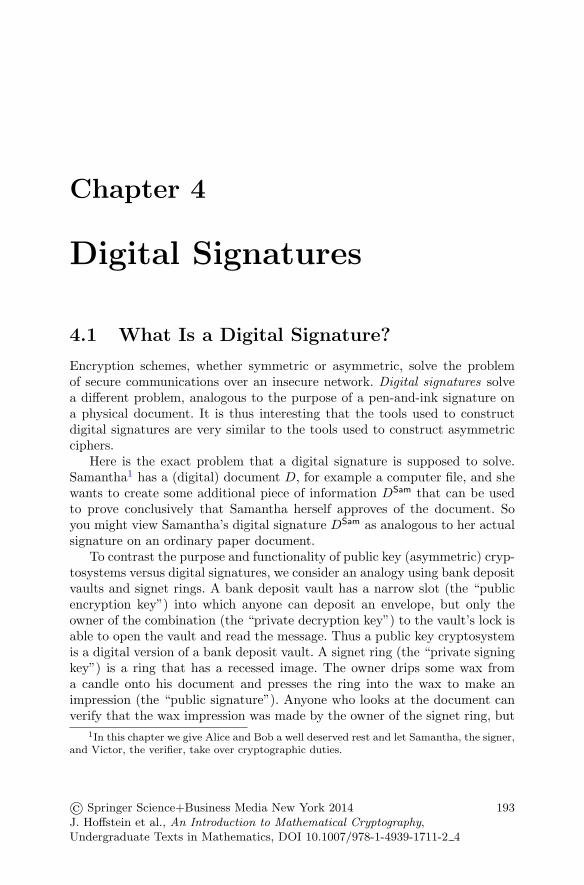
Chapter 4
Digital Signatures
4.1 What Is a Digital Signature?
Encryption schemes, whether symmetric or asymmetric, solve the problemof secure communications over an insecure network. Digital signatures solvea different problem, analogous to the purpose of a pen-and-ink signature ona physical document. It is thus interesting that the tools used to constructdigital signatures are very similar to the tools used to construct asymmetricciphers.
Here is the exact problem that a digital signature is supposed to solve.Samantha1 has a (digital) document D, for example a computer file, and shewants to create some additional piece of information DSam that can be usedto prove conclusively that Samantha herself approves of the document. Soyou might view Samantha’s digital signature DSam as analogous to her actualsignature on an ordinary paper document.
To contrast the purpose and functionality of public key (asymmetric) cryp-tosystems versus digital signatures, we consider an analogy using bank depositvaults and signet rings. A bank deposit vault has a narrow slot (the “publicencryption key”) into which anyone can deposit an envelope, but only theowner of the combination (the “private decryption key”) to the vault’s lock isable to open the vault and read the message. Thus a public key cryptosystemis a digital version of a bank deposit vault. A signet ring (the “private signingkey”) is a ring that has a recessed image. The owner drips some wax froma candle onto his document and presses the ring into the wax to make animpression (the “public signature”). Anyone who looks at the document canverify that the wax impression was made by the owner of the signet ring, but
1In this chapter we give Alice and Bob a well deserved rest and let Samantha, the signer,and Victor, the verifier, take over cryptographic duties.
© Springer Science+Business Media New York 2014J. Hoffstein et al., An Introduction to Mathematical Cryptography,Undergraduate Texts in Mathematics, DOI 10.1007/978-1-4939-1711-2 4
193
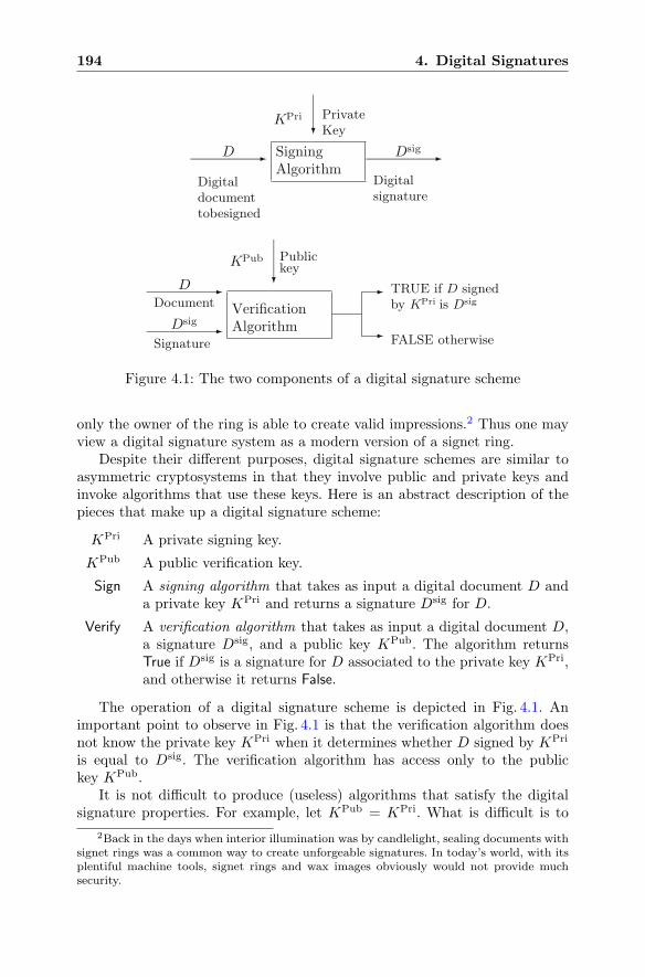
194 4. Digital Signatures
Digitaldocumenttobesigned
D SigningAlgorithm
KPri PrivateKey
Dsig
Digitalsignature
DDocument
Dsig
Signature
VerificationAlgorithm
TRUE if D signedby KPri is Dsig
FALSE otherwise
KPub Publickey
Figure 4.1: The two components of a digital signature scheme
only the owner of the ring is able to create valid impressions.2 Thus one mayview a digital signature system as a modern version of a signet ring.
Despite their different purposes, digital signature schemes are similar toasymmetric cryptosystems in that they involve public and private keys andinvoke algorithms that use these keys. Here is an abstract description of thepieces that make up a digital signature scheme:
KPri A private signing key.
KPub A public verification key.
Sign A signing algorithm that takes as input a digital document D anda private key KPri and returns a signature Dsig for D.
Verify A verification algorithm that takes as input a digital document D,a signature Dsig, and a public key KPub. The algorithm returnsTrue if Dsig is a signature for D associated to the private key KPri,and otherwise it returns False.
The operation of a digital signature scheme is depicted in Fig. 4.1. Animportant point to observe in Fig. 4.1 is that the verification algorithm doesnot know the private key KPri when it determines whether D signed by KPri
is equal to Dsig. The verification algorithm has access only to the publickey KPub.
It is not difficult to produce (useless) algorithms that satisfy the digitalsignature properties. For example, let KPub = KPri. What is difficult is to
2Back in the days when interior illumination was by candlelight, sealing documents withsignet rings was a common way to create unforgeable signatures. In today’s world, with itsplentiful machine tools, signet rings and wax images obviously would not provide muchsecurity.
4.1. What Is a Digital Signature? 195
create a digital signature scheme in which the owner of the private key KPri isable to create valid signatures, but knowledge of the public key KPub does notreveal the private key KPri. Necessary general conditions for a secure digitalsignature scheme include the following:
• GivenKPub, an attacker cannot feasibly determineKPri, nor can she de-termine any other private key that produces the same signatures asKPri.
• Given KPub and a list of signed documents D1, . . . , Dn with their sig-natures Dsig
1 , . . . , Dsign , an attacker cannot feasibly determine a valid
signature on any document D that is not in the list D1, . . . , Dn.
The second condition is rather different from the situation for encryptionschemes. In public key encryption, an attacker can create as many cipher-text/plaintext pairs as she wants, since she can create them using the knownpublic key. However, each time a digital signature scheme is used to sign anew document, it is revealing a new document/signature pair, which providesnew information to an attacker. The second condition says that the attackergains nothing beyond knowledge of that new pair. An attack on a digital sig-nature scheme that makes use of a large number of known signatures is calleda transcript attack. (See Sect. 7.12 for further discussion.)
Remark 4.1. Digital signatures are at least as important as public key cryp-tosystems for the conduct of business in a digital age, and indeed, one mightargue that they are of greater importance. To take a significant instance, yourcomputer undoubtedly receives program and system upgrades over the Inter-net. How can your computer tell that an upgrade comes from a legitimatesource, in this case the company that wrote the program in the first place?The answer is a digital signature. The original program comes equipped withthe company’s public verification key. The company uses its private signingkey to sign the upgrade and sends your computer both the new program andthe signature. Your computer can use the public key to verify the signature,thereby verifying that the program comes from a trusted source, before in-stalling it on your system.
We must stress, however, that although this conveys the idea of how adigital signature might be used, it is a vastly oversimplified explanation. Real-world applications of digital signature schemes require considerable care toavoid a variety of subtle, but fatal, security problems. In particular, as digitalsignatures proliferate, it can become problematic to be sure that a purportedpublic verification key actually belongs to the supposed owner. And clearlyan adversary who tricks you into using her verification key, instead of the realone, will then be able to convince you to accept all of her forged documents.
Remark 4.2. The natural capability of most digital signature schemes is tosign only a small amount of data, say b bits, where b is between 80 and 1000.It is thus quite inefficient to sign a large digital document D, both because ittakes a lot of time to sign each b bits of D and because the resulting digitalsignature is likely to be as large as the original document.
196 4. Digital Signatures
The standard solution to this problem is to use a hash function, which isan easily computable function
Hash : (arbitrary size documents) −→ {0, 1}k
that is very hard to invert. (More generally, one wants it to be very difficultto find two distinct inputs D and D′ whose outputs Hash(D) and Hash(D′)are the same.) Then, rather than signing her document D, Samantha insteadcomputes and signs the hash Hash(D). For verification, Victor computes andverifies the signature on Hash(D).
There are also security advantages to signing a hash of D, including in-trinsically linking the signature to the entire document, and preventing an ad-versary from choosing random signatures and determining which documentsthey sign. For a brief introduction to hash functions and references for furtherreading, see Sect. 8.1. We will not concern ourselves further with such issuesin this chapter.
Remark 4.3. There are many variants of the basic digital signature paradigm.For example, a blinded signature is one in which the signer does not knowthe contents of the document being signed. This could be useful, for example,if voters want an election official to sign their votes without revealing whatthose votes are. Further material on blinded signatures, with an RSA-styleexample and applications to digital cash systems, are given in Sect. 8.8.
In this chapter we discuss digital signature schemes whose underlying hardproblems are integer factorization and the discrete logarithm problem in F
∗p.
Subsequent chapters include descriptions of digital signature schemes basedon the discrete logarithm problem in elliptic curve groups (Sect. 6.4.3) and onhard lattice problems (Sect. 7.12).
4.2 RSA Digital Signatures
The original RSA paper described both the RSA encryption scheme and anRSA digital signature scheme. The idea is very simple. The setup is the sameas for RSA encryption, Samantha chooses two large secret primes p and qand she publishes their product N = pq and a public verification exponent e.Samantha uses her knowledge of the factorization of N to solve the congruence
de ≡ 1(mod(p− 1)(q − 1)
). (4.1)
Note that if Samantha were doing RSA encryption, then e would be herencryption exponent and d would be her decryption exponent. However, inthe present setup d is her signing exponent and e is her verification exponent.
In order to sign a digital document D, which we assume to be an integerin the range 1 < D < N , Samantha computes
S ≡ Dd (mod N).
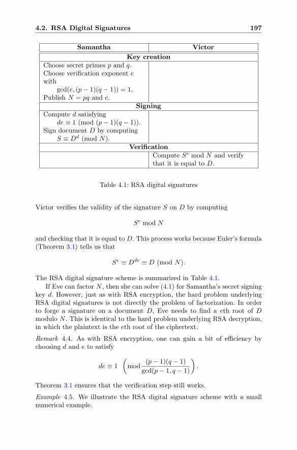
4.2. RSA Digital Signatures 197
Samantha Victor
Key creationChoose secret primes p and q.Choose verification exponent ewith
gcd(e, (p− 1)(q − 1)) = 1.Publish N = pq and e.
SigningCompute d satisfying
de ≡ 1 (mod (p− 1)(q − 1)).Sign document D by computing
S ≡ Dd (mod N).Verification
Compute Se mod N and verifythat it is equal to D.
Table 4.1: RSA digital signatures
Victor verifies the validity of the signature S on D by computing
Se mod N
and checking that it is equal to D. This process works because Euler’s formula(Theorem 3.1) tells us that
Se ≡ Dde ≡ D (mod N).
The RSA digital signature scheme is summarized in Table 4.1.
If Eve can factor N , then she can solve (4.1) for Samantha’s secret signingkey d. However, just as with RSA encryption, the hard problem underlyingRSA digital signatures is not directly the problem of factorization. In orderto forge a signature on a document D, Eve needs to find a eth root of Dmodulo N . This is identical to the hard problem underlying RSA decryption,in which the plaintext is the eth root of the ciphertext.
Remark 4.4. As with RSA encryption, one can gain a bit of efficiency bychoosing d and e to satisfy
de ≡ 1
(mod
(p− 1)(q − 1)
gcd(p− 1, q − 1)
).
Theorem 3.1 ensures that the verification step still works.
Example 4.5. We illustrate the RSA digital signature scheme with a smallnumerical example.
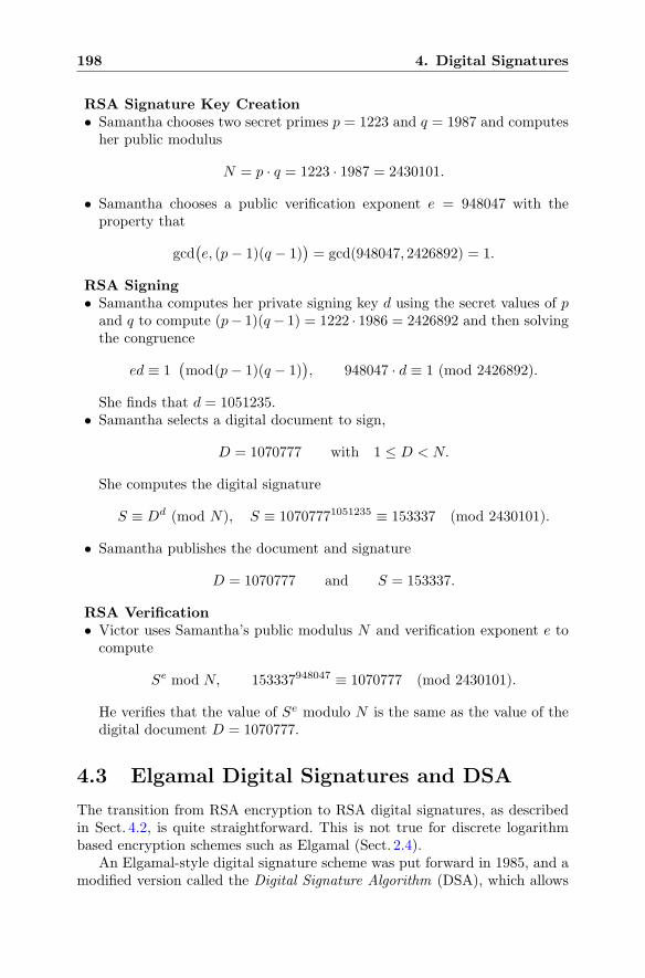
198 4. Digital Signatures
RSA Signature Key Creation• Samantha chooses two secret primes p = 1223 and q = 1987 and computesher public modulus
N = p · q = 1223 · 1987 = 2430101.
• Samantha chooses a public verification exponent e = 948047 with theproperty that
gcd(e, (p− 1)(q − 1)
)= gcd(948047, 2426892) = 1.
RSA Signing• Samantha computes her private signing key d using the secret values of p
and q to compute (p− 1)(q− 1) = 1222 · 1986 = 2426892 and then solvingthe congruence
ed ≡ 1(mod(p− 1)(q − 1)
), 948047 · d ≡ 1 (mod 2426892).
She finds that d = 1051235.• Samantha selects a digital document to sign,
D = 1070777 with 1 ≤ D < N.
She computes the digital signature
S ≡ Dd (mod N), S ≡ 10707771051235 ≡ 153337 (mod 2430101).
• Samantha publishes the document and signature
D = 1070777 and S = 153337.
RSA Verification• Victor uses Samantha’s public modulus N and verification exponent e tocompute
Se mod N, 153337948047 ≡ 1070777 (mod 2430101).
He verifies that the value of Se modulo N is the same as the value of thedigital document D = 1070777.
4.3 Elgamal Digital Signatures and DSA
The transition from RSA encryption to RSA digital signatures, as describedin Sect. 4.2, is quite straightforward. This is not true for discrete logarithmbased encryption schemes such as Elgamal (Sect. 2.4).
An Elgamal-style digital signature scheme was put forward in 1985, and amodified version called the Digital Signature Algorithm (DSA), which allows
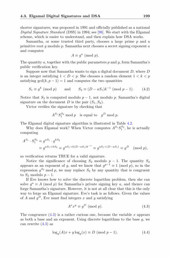
4.3. Elgamal Digital Signatures and DSA 199
shorter signatures, was proposed in 1991 and officially published as a nationalDigital Signature Standard (DSS) in 1994; see [98]. We start with the Elgamalscheme, which is easier to understand, and then explain how DSA works.
Samantha, or some trusted third party, chooses a large prime p and aprimitive root g modulo p. Samantha next chooses a secret signing exponent aand computes
A ≡ ga (mod p).
The quantity a, together with the public parameters p and g, form Samantha’spublic verification key.
Suppose now that Samantha wants to sign a digital document D, where Dis an integer satisfying 1 < D < p. She chooses a random element 1 < k < psatisfying gcd(k, p− 1) = 1 and computes the two quantities
S1 ≡ gk (mod p) and S2 ≡ (D − aS1)k−1 (mod p− 1). (4.2)
Notice that S2 is computed modulo p − 1, not modulo p. Samantha’s digitalsignature on the document D is the pair (S1, S2).
Victor verifies the signature by checking that
AS1SS21 mod p is equal to gD mod p.
The Elgamal digital signature algorithm is illustrated in Table 4.2.Why does Elgamal work? When Victor computes AS1SS2
1 , he is actuallycomputing
AS1 · SS21 ≡ gaS1 · gkS2
≡ gaS1+kS2 ≡ gaS1+k(D−aS1)k−1 ≡ gaS1+(D−aS1) ≡ gD (mod p),
so verification returns TRUE for a valid signature.Notice the significance of choosing S2 modulo p − 1. The quantity S2
appears as an exponent of g, and we know that gp−1 ≡ 1 (mod p), so in theexpression gS2 mod p, we may replace S2 by any quantity that is congruentto S2 modulo p− 1.
If Eve knows how to solve the discrete logarithm problem, then she cansolve ga ≡ A (mod p) for Samantha’s private signing key a, and thence canforge Samantha’s signature. However, it is not at all clear that this is the onlyway to forge an Elgamal signature. Eve’s task is as follows. Given the valuesof A and gD, Eve must find integers x and y satisfying
Axxy ≡ gD (mod p). (4.3)
The congruence (4.3) is a rather curious one, because the variable x appearsas both a base and an exponent. Using discrete logarithms to the base g, wecan rewrite (4.3) as
logg(A)x+ y logg(x) ≡ D (mod p− 1). (4.4)
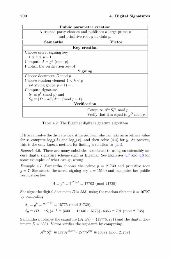
200 4. Digital Signatures
Public parameter creationA trusted party chooses and publishes a large prime p
and primitive root g modulo p.
Samantha Victor
Key creationChoose secret signing key
1 ≤ a ≤ p− 1.Compute A = ga (mod p).Publish the verification key A.
SigningChoose document D mod p.Choose random element 1 < k < p
satisfying gcd(k, p− 1) = 1.Compute signatureS1 ≡ gk (mod p) andS2 ≡ (D− aS1)k
−1 (mod p− 1).Verification
Compute AS1SS21 mod p.
Verify that it is equal to gD mod p.
Table 4.2: The Elgamal digital signature algorithm
If Eve can solve the discrete logarithm problem, she can take an arbitrary valuefor x, compute logg(A) and logg(x), and then solve (4.4) for y. At present,this is the only known method for finding a solution to (4.4).
Remark 4.6. There are many subtleties associated to using an ostensibly se-cure digital signature scheme such as Elgamal. See Exercises 4.7 and 4.8 forsome examples of what can go wrong.
Example 4.7. Samantha chooses the prime p = 21739 and primitive rootg = 7. She selects the secret signing key a = 15140 and computes her publicverification key
A ≡ ga ≡ 715140 ≡ 17702 (mod 21739).
She signs the digital document D = 5331 using the random element k = 10727by computing
S1 ≡ gk ≡ 710727 ≡ 15775 (mod 21739),
S2 ≡ (D − aS1)k−1 ≡ (5331− 15140 · 15775) · 6353 ≡ 791 (mod 21738).
Samantha publishes the signature (S1, S2) = (15775, 791) and the digital doc-ument D = 5331. Victor verifies the signature by computing
AS1SS21 ≡ 1770215775 · 15775791 ≡ 13897 (mod 21739)
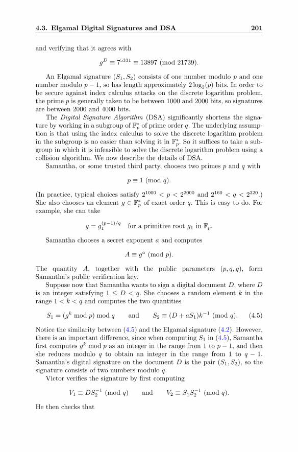
4.3. Elgamal Digital Signatures and DSA 201
and verifying that it agrees with
gD ≡ 75331 ≡ 13897 (mod 21739).
An Elgamal signature (S1, S2) consists of one number modulo p and onenumber modulo p− 1, so has length approximately 2 log2(p) bits. In order tobe secure against index calculus attacks on the discrete logarithm problem,the prime p is generally taken to be between 1000 and 2000 bits, so signaturesare between 2000 and 4000 bits.
The Digital Signature Algorithm (DSA) significantly shortens the signa-ture by working in a subgroup of F∗
p of prime order q. The underlying assump-tion is that using the index calculus to solve the discrete logarithm problemin the subgroup is no easier than solving it in F
∗p. So it suffices to take a sub-
group in which it is infeasible to solve the discrete logarithm problem using acollision algorithm. We now describe the details of DSA.
Samantha, or some trusted third party, chooses two primes p and q with
p ≡ 1 (mod q).
(In practice, typical choices satisfy 21000 < p < 22000 and 2160 < q < 2320.)She also chooses an element g ∈ F
∗p of exact order q. This is easy to do. For
example, she can take
g = g(p−1)/q1 for a primitive root g1 in Fp.
Samantha chooses a secret exponent a and computes
A ≡ ga (mod p).
The quantity A, together with the public parameters (p, q, g), formSamantha’s public verification key.
Suppose now that Samantha wants to sign a digital document D, where Dis an integer satisfying 1 ≤ D < q. She chooses a random element k in therange 1 < k < q and computes the two quantities
S1 = (gk mod p) mod q and S2 ≡ (D + aS1)k−1 (mod q). (4.5)
Notice the similarity between (4.5) and the Elgamal signature (4.2). However,there is an important difference, since when computing S1 in (4.5), Samanthafirst computes gk mod p as an integer in the range from 1 to p− 1, and thenshe reduces modulo q to obtain an integer in the range from 1 to q − 1.Samantha’s digital signature on the document D is the pair (S1, S2), so thesignature consists of two numbers modulo q.
Victor verifies the signature by first computing
V1 ≡ DS−12 (mod q) and V2 ≡ S1S
−12 (mod q).
He then checks that
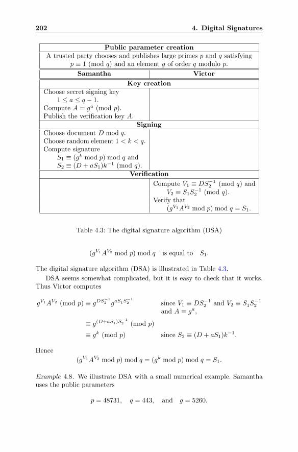
202 4. Digital Signatures
Public parameter creationA trusted party chooses and publishes large primes p and q satisfying
p ≡ 1 (mod q) and an element g of order q modulo p.
Samantha Victor
Key creationChoose secret signing key
1 ≤ a ≤ q − 1.Compute A = ga (mod p).Publish the verification key A.
SigningChoose document D mod q.Choose random element 1 < k < q.Compute signature
S1 ≡ (gk mod p) mod q andS2 ≡ (D + aS1)k
−1 (mod q).Verification
Compute V1 ≡ DS−12 (mod q) and
V2 ≡ S1S−12 (mod q).
Verify that(gV1AV2 mod p) mod q = S1.
Table 4.3: The digital signature algorithm (DSA)
(gV1AV2 mod p) mod q is equal to S1.
The digital signature algorithm (DSA) is illustrated in Table 4.3.
DSA seems somewhat complicated, but it is easy to check that it works.Thus Victor computes
gV1AV2 (mod p) ≡ gDS−12 gaS1S
−12 since V1 ≡ DS−1
2 and V2 ≡ S1S−12
and A ≡ ga,
≡ g(D+aS1)S−12 (mod p)
≡ gk (mod p) since S2 ≡ (D + aS1)k−1.
Hence
(gV1AV2 mod p) mod q = (gk mod p) mod q = S1.
Example 4.8. We illustrate DSA with a small numerical example. Samanthauses the public parameters
p = 48731, q = 443, and g = 5260.
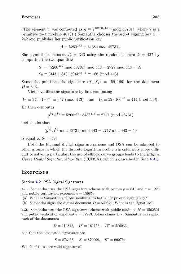
Exercises 203
(The element g was computed as g ≡ 748730/443 (mod 48731), where 7 is aprimitive root modulo 48731.) Samantha chooses the secret signing key a =242 and publishes her public verification key
A ≡ 5260242 ≡ 3438 (mod 48731).
She signs the document D = 343 using the random element k = 427 bycomputing the two quantities
S1 = (5260427 mod 48731) mod 443 = 2727 mod 443 = 59,
S2 ≡ (343 + 343 · 59)427−1 ≡ 166 (mod 443).
Samantha publishes the signature (S1, S2) = (59, 166) for the documentD = 343.
Victor verifies the signature by first computing
V1 ≡ 343 · 166−1 ≡ 357 (mod 443) and V2 ≡ 59 · 166−1 ≡ 414 (mod 443).
He then computes
gV1AV2 ≡ 5260357 · 3438414 ≡ 2717 (mod 48731)
and checks that
(gV1AV2 mod 48731) mod 443 = 2717 mod 443 = 59
is equal to S1 = 59.
Both the Elgamal digital signature scheme and DSA can be adapted toother groups in which the discrete logarithm problem is ostensibly more diffi-cult to solve. In particular, the use of elliptic curve groups leads to the EllipticCurve Digital Signature Algorithm (ECDSA), which is described in Sect. 6.4.3.
Exercises
Section 4.2. RSA Digital Signatures
4.1. Samantha uses the RSA signature scheme with primes p = 541 and q = 1223and public verification exponent e = 159853.(a) What is Samantha’s public modulus? What is her private signing key?
(b) Samantha signs the digital document D = 630579. What is the signature?
4.2. Samantha uses the RSA signature scheme with public modulus N = 1562501and public verification exponent e = 87953. Adam claims that Samantha has signedeach of the documents
D = 119812, D′ = 161153, D′′ = 586036,
and that the associated signatures are
S = 876453, S′ = 870099, S′′ = 602754.
Which of these are valid signatures?
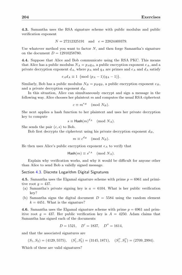
204 Exercises
4.3. Samantha uses the RSA signature scheme with public modulus and publicverification exponent
N = 27212325191 and e = 22824469379.
Use whatever method you want to factor N , and then forge Samantha’s signatureon the document D = 12910258780.
4.4. Suppose that Alice and Bob communicate using the RSA PKC. This meansthat Alice has a public modulus NA = pAqA, a public encryption exponent eA, and aprivate decryption exponent dA, where pA and qA are primes and eA and dA satisfy
eAdA ≡ 1(mod (pA − 1)(qA − 1)
).
Similarly, Bob has a public modulus NB = pBqB , a public encryption exponent eB ,and a private decryption exponent dB .
In this situation, Alice can simultaneously encrypt and sign a message in thefollowing way. Alice chooses her plaintextm and computes the usual RSA ciphertext
c ≡ meB (mod NB).
She next applies a hash function to her plaintext and uses her private decryptionkey to compute
s ≡ Hash(m)dA (mod NA).
She sends the pair (c, s) to Bob.Bob first decrypts the ciphertext using his private decryption exponent dB ,
m ≡ cdB (mod NB).
He then uses Alice’s public encryption exponent eA to verify that
Hash(m) ≡ seA (mod NA).
Explain why verification works, and why it would be difficult for anyone otherthan Alice to send Bob a validly signed message.
Section 4.3. Discrete Logarithm Digital Signatures
4.5. Samantha uses the Elgamal signature scheme with prime p = 6961 and primi-tive root g = 437.(a) Samantha’s private signing key is a = 6104. What is her public verification
key?
(b) Samantha signs the digital document D = 5584 using the random elementk = 4451. What is the signature?
4.6. Samantha uses the Elgamal signature scheme with prime p = 6961 and prim-itive root g = 437. Her public verification key is A = 4250. Adam claims thatSamantha has signed each of the documents
D = 1521, D′ = 1837, D′′ = 1614,
and that the associated signatures are
(S1, S2) = (4129, 5575), (S′1, S
′2) = (3145, 1871), (S′′
1 , S′′2 ) = (2709, 2994).
Which of these are valid signatures?
Exercises 205
4.7. Let p be a prime, let i and j be integers with gcd(j, p − 1) = 1, and let A bearbitrary. Set
S1 ≡ giAj (mod p), S2 ≡ −S1j−1 (mod p− 1), D ≡ −S1ij
−1 (mod p− 1).
Prove that (S1, S2) is a valid Elgamal signature on the document D for the verifi-cation key A. Thus Eve can produce signatures on random documents.
4.8. Suppose that Samantha is using the Elgamal signature scheme and that she iscareless and uses the same random element k to sign two documents D and D′.(a) Explain how Eve can tell at a glance whether Samantha has made this mistake.
(b) If the signature on D is (S1, S2) and the signature on D′ is (S′1, S
′2), explain
how Eve can recover a, Samantha’s private signing key.
(c) Apply your method from (b) to the following example and recover Samantha’ssigning key a, where Samantha is using the prime p = 348149, base g = 113459,and verification key A = 185149.
D = 153405, S1 = 208913, S2 = 209176,
D′ = 127561, S′1 = 208913, S′
2 = 217800.
4.9. Samantha uses DSA with public parameters (p, q, g) = (22531, 751, 4488). Shechooses the secret signing key a = 674.(a) What is Samantha’s public verification key?
(b) Samantha signs the document D = 244 using the random element k = 574.What is the signature?
4.10. Samantha uses DSA with public parameters (p, q, g) = (22531, 751, 4488). Herpublic verification key is A = 22476.(a) Is (S1, S2) = (183, 260) a valid signature on the document D = 329?
(b) Is (S1, S2) = (211, 97) a valid signature on the document D = 432?
4.11. Samantha’s DSA public parameters are (p, q, g) = (103687, 1571, 21947), andher public verification key is A = 31377. Use whatever method you prefer (brute-force, collision, index calculus,. . . ) to solve the DLP and find Samantha’s privatesigning key. Use her key to sign the document D = 510 using the random elementk = 1105.
Chapter 5
Combinatorics, Probability,and Information Theory
In considering the usefulness and practicality of a cryptographic system, it isnecessary to measure its resistance to various forms of attack. Such attacksinclude simple brute-force searches through the key or message space, some-what faster searches via collision or meet-in-the-middle algorithms, and moresophisticated methods that are used to compute discrete logarithms, factorintegers, and find short vectors in lattices. We have already studied some ofthese algorithms in Chaps. 2 and 3, and we will see the others in this and laterchapters. In studying these algorithms, it is important to be able to analyzehow long they take to solve the targeted problem. Such an analysis generallyrequires tools from combinatorics, probability theory, and information theory.In this chapter we present, in a largely self-contained form, an introductionto these topics.
We start with basic principles of counting, and continue with the devel-opment of the foundations of probability theory, primarily in the discrete set-ting. Subsequent sections introduce (discrete) random variables, probabilitydensity functions, conditional probability and Bayes’s formula. The applica-tions of probability theory to cryptography are legion. We cover in some detailMonte Carlo algorithms and collision algorithms and their uses in cryptogra-phy. We also include a section on the statistical cryptanalysis of a historicallyinteresting polyalphabetic substitution cipher called the Vigenere cipher, butwe note that the material on the Vigenere cipher is not used elsewhere in thebook, so it may be omitted by the reader who wishes to proceed more rapidlyto the more modern cryptographic material.
© Springer Science+Business Media New York 2014J. Hoffstein et al., An Introduction to Mathematical Cryptography,Undergraduate Texts in Mathematics, DOI 10.1007/978-1-4939-1711-2 5
207
208 5. Combinatorics, Probability, and Information Theory
The chapter concludes with a very short introduction to the concept ofcomplexity and the notions of polynomial-time and nondeterministic polyno-mial-time algorithms. This section, if properly developed, would be a book initself, and we can only give a hint of the powerful ideas and techniques usedin this subject.
5.1 Basic Principles of Counting
As I was going to St. Ives,I met a man with seven wives,
Each wife had seven sacks,Each sack had seven cats.
Each cat had seven kits.Kits, cats, sacks, and wives,
How many were going to St. Ives?
The trick answer to this ancient riddle is that there is only one person goingto St. Ives, namely the narrator, since all of the other people and animalsand objects that he meets in the rhyme are not traveling to St. Ives, they aretraveling away from St. Ives! However, if we are in a pedantic, rather than aclever, frame of mind, we might instead ask the natural question: How manypeople, animals, and objects does the narrator meet?
The answer is
2801 = 1︸︷︷︸man
+ 7︸︷︷︸wives
+ 72︸︷︷︸sacks
+ 73︸︷︷︸cats
+ 74︸︷︷︸kits
.
The computation of this number employs basic counting principles that arefundamental to the probability calculations used in cryptography and in manyother areas of mathematics. We have already seen an example in Sect. 1.1.1,where we computed the number of different simple substitution ciphers.
A cipher is said to be combinatorially secure if it is not feasible to breakthe system by exhaustively checking every possible key.1 This depends tosome extent on how long it takes to check each key, but more importantly,it depends on the number of keys. In this section we develop some basiccounting techniques that are used in a variety of ways to analyze the securityof cryptographic constructions.
Example 5.1 (A Basic Counting Principle). Bob is at a restaurant thatfeatures two appetizers, egg rolls and fried wontons, and 20 main dishes. As-suming that he plans to order one appetizer and one main dish, how manypossible meals could Bob order?
We need to count the number of pairs (x, y), where x is either “egg roll” or“fried wonton” and y is a main dish. The total number is obtained by letting x
1Sometimes the length of the search can be significantly shortened by matching pieces ofkeys taken from two or more lists. Such an attack is called a collision or meet-in-the-middleattack; see Sect. 5.4.
5.1. Basic Principles of Counting 209
vary over the 2 possibilities and letting y vary over the 20 possibilities, andthen counting up the total number of pairs
(ER, 1), (ER, 2), . . . , (ER, 20), (FW, 1), (FW, 2), . . . , (FW, 20).
The answer is that there are 40 possibilities, which we compute as
40 = 2︸︷︷︸appetizers
· 20︸︷︷︸main dishes
.
In this example, we first counted the number of ways of assigning an appe-tizer (egg roll or fried wonton) to the variable x. It is convenient to view thisassignment as the outcome of an experiment. That is, we perform an experi-ment whose outcome is either “egg roll” or “fried wonton,” and we assign theoutcome’s value to x. Similarly, we perform a second independent experimentwhose possible outcomes are any one of the 20 main courses, and we assignthat value to y. The total number of outcomes of the two experiments is theproduct of the number of outcomes for each one individually. This leads tothe following basic counting principle:
Basic Counting PrincipleIf two experiments are performed, one of whichhas n possible outcomes and the other of whichhas m possible outcomes, then there are nmpossible outcomes of performing both experi-ments.
More generally, if k independent experiments are performed and if thenumber of possible outcomes of the ith experiment is ni, then the total numberof outcomes for all of the experiments is the product n1n2 · · ·nk. It is easy toderive this result by writing xi for the outcome of the ith experiment. Thenthe outcome of all k experiments is the value of the k-tuple (x1, x2, . . . , xk),and the total number of possible k-tuples is the product n1n2 · · ·nk.Example 5.2. Suppose that Bob also wants to order dessert, and that thereare five desserts on the menu. We are now counting triples (x, y, z), where xis one of the two appetizers, y is one of the 20 main dishes, and z is one ofthe five desserts. Hence the total number of meals is
200 = 2︸︷︷︸appetizers
· 20︸︷︷︸main courses
· 5︸︷︷︸desserts
.
The basic counting principle is used in the solution of the pedantic versionof the St. Ives problem. For example, the number of cats traveling from St.Ives is
# of cats = 343 = 73 = 1︸︷︷︸man
· 7︸︷︷︸wives
· 7︸︷︷︸sacks
· 7︸︷︷︸cats
.
The earliest published version of the St. Ives riddle dates to around 1730, butsimilar problems date back to antiquity; see Exercise 5.1.
210 5. Combinatorics, Probability, and Information Theory
5.1.1 Permutations
The numbers 1, 2, . . . , 10 are typically listed in increasing order, but supposeinstead we allow the order to be mixed. Then how many different ways arethere to list these ten integers? Each possible configuration is called a permu-tation of 1, 2, . . . , 10. The problem of counting the number of possible permu-tations of a given list of objects occurs in many forms and contexts throughoutmathematics.
Each permutation of 1, 2, . . . , 10 is a sequence of all ten distinct integersin some order. For example, here is a random choice: 8, 6, 10, 3, 9, 2, 4, 7, 5, 1.How can we create all of the possibilities? It’s easiest to create them by listingthe numbers one at a time, say from left to right. We thus start by assigning anumber to the first position. There are ten choices. Next we assign a numberto the second position, but for the second position there are only nine choices,because we already used up one of the integers in the first position. (Rememberthat we are not allowed to use an integer twice.) Then there are eight integersleft as possibilities for the third position, because we already used two integersin the first two positions. And so on. Hence the total number of permutationsof 1, 2, . . . , 10 is
10! = 10 · 9 · 8 · · · 2 · 1.
The value of 10! is 3628800, so between three and four million.Notice how we are using the basic counting principle. The only subtlety
is that the outcome of the first experiment reduces the number of possibleoutcomes of the second experiment, the results of the first two experimentsfurther reduce the number of possible outcomes of the third experiment, andso on.
Definition. Let S be a set containing n distinct objects. A permutation of Sis an ordered list of the objects in S. A permutation of the set {1, 2, . . . , n} issimply called a permutation of n.
Proposition 5.3. Let S be a set containing n distinct objects. Then there areexactly n! different permutations of S.
Proof. Our discussion of the permutations of {1, . . . , 10} works in general.Thus suppose that S contains n objects and that we want to create a permu-tation of S. There are n choices for the first entry, then n− 1 choices for thesecond entry, then n− 2 choices for the third entry, etc. This leads to a totalof n · (n− 1) · (n− 2) · · · 2 · 1 possible permutations.
Remark 5.4 (Permutations and Simple Substitution Ciphers). By definition,a permutation of the set {a1, a2, . . . , an} is a list consisting of the ai’s in someorder. We can also describe a permutation by using a bijective (i.e., one-to-oneand onto) function
π : {1, 2, . . . , n} −→ {1, 2, . . . , n}.
5.1. Basic Principles of Counting 211
The function π determines the permutation
(aπ(1), aπ(2), . . . , aπ(n)),
and given a permutation, it is easy to write down the corresponding function.Now suppose that we take the set of letters {A, B, C, . . . , Z}. A permuta-
tion π of this set is just another name for a simple substitution cipher, where πacts as the encryption function. Thus π tells us that A gets sent to the π(1)stletter, and B gets sent to the π(2)nd letter, and so on. In order to decrypt, weuse the inverse function π−1.
Example 5.5. Sometimes one needs to count the number of possible permuta-tions of n objects when some of the objects are indistinguishable. For example,there are six permutations of three distinct objects A,B,C,
ABC, CAB, BCA, ACB, BAC, and CBA,
but if two of them are indistinguishable, say A,A,B, then there are only threedifferent arrangements,
AAB, ABA, and BAA.
To illustrate the idea in a more complicated case, we count the numberof different letter arrangements of the five letters A,A,A,B,B. If the fiveletters were distinguishable, say they were labeled A1, A2, A3, B1, B2, thenthere would be 5! permutations. However, permutations such as
A1A2B1B2A3 and A2A3B2B1A1
become the same when the subscripts are dropped, so we have overcountedin arriving at the number 5!. How many different arrangements have beencounted more than once?
For example, in any particular permutation, the two B’s have been placedinto specific positions, but we can always switch them and get the same un-subscripted list. This means that we need to divide 5! by 2 to compensatefor overcounting the placement of the B’s. Similarly, once the three A’s havebeen placed into specific positions, we can permute them among themselvesin 3! ways, so we need to divide 5! by 3! to compensate for overcounting theplacement of the A’s. Hence there are 5!
3!·2! = 10 different letter arrangementsof the five letters A,A,A,B,B.
5.1.2 Combinations
A permutation is a way of arranging a set of objects into a list. A combinationis similar, except that now the order of the list no longer matters. We startwith an example that is typical of problems involving combinations.
212 5. Combinatorics, Probability, and Information Theory
Example 5.6. Five people (Alice, Bob, Carl, Dave, and Eve2) are orderinga meal at a Chinese restaurant. The menu contains 20 different items. Eachperson gets to choose one dish, no dish may be ordered twice, and they planto share the food. How many different meals are possible?
Alice orders first and she has 20 choices for her dish. Then Bob orders fromthe remaining 19 dishes, and then Carl chooses from the remaining 18 dishes,and so on. It thus appears that there are 20 · 19 · 18 · 17 · 16 = 1860480 possi-ble meals. However, the order in which the dishes are ordered is immaterial.If Alice orders fried rice and Bob orders egg rolls, or if Alice orders egg rollsand Bob orders fried rice, the meal is the same. Unfortunately, we did nottake this into account when we arrived at the number 1860480.
Let’s number the dishes D1, D2, . . . , D20. Then, for example, we want tocount the two possible dinners
D1, D5, D7, D18, D20 and D5, D18, D20, D7, D1
as being the same, although the order of the dishes is different. To correct theovercount, note that in the computation 20 · 19 · 18 · 17 · 16 = 1860480, everypermutation of any set of five dishes was counted separately, but we reallywant to count these permutations as giving the same meal. Thus we shoulddivide 1860480 by the number of ways to permute the five distinct dishes ineach possible order, i.e., we should divide by 5!. Hence the total number ofdifferent meals is
20 · 19 · 18 · 17 · 165!
= 15504.
It is often convenient to rewrite this quantity entirely in terms of factorialsby multiplying the numerator and the denominator by 15! to get
20 · 19 · 18 · 17 · 165!
=(20 · 19 · 18 · 17 · 16) · (15 · 14 · · · 3 · 2 · 1)
5! · 15! =20!
5! · 15! .
Definition. Let S be a set containing n distinct objects. A combination of robjects of S is a subset consisting of exactly r distinct elements of S, wherethe order of the objects in the subset does not matter.
Proposition 5.7. The number of possible combinations of r objects chosenfrom a set of n objects is equal to
(n
r
)=
n!
r!(n− r)! .
Remark 5.8. The symbol(nr
)is called a combinatorial symbol or a binomial
coefficient. It is read as “n choose r.” Note that by convention, zero factorialis set equal to 1, so
(n0
)= n!
n!·0! = 1. This makes sense, since there is only oneway to choose zero objects from a set.
2You may wonder why Alice and Bob, those intrepid exchangers of encrypted secretmessages, are sitting down for a meal with their cryptographic adversary Eve. In the realworld, this happens all the time, especially at cryptography conferences!
5.1. Basic Principles of Counting 213
Proof of Proposition 5.7. If you understand the discussion in Example 5.6,then the proof of the general case is clear. The number of ways to make anordered list of r distinct elements from the set S is
n(n− 1)(n− 2) · · · (n− r + 1),
since there are n choices for the first element, then n− 1 choices for the secondelement, and so on until we have selected r elements. Then we need to divideby r! in order to compensate for the ways to permute the r elements in oursubset. Dividing by r! accounts for the fact that we do not care in which orderthe r elements were chosen. Hence the total number of combinations is
n(n− 1)(n− 2) · · · (n− r + 1)
r!=
n!
r!(n− r)! .
Example 5.9. Returning to the five people ordering a meal at the Chineserestaurant, suppose that they want the order to consist of two vegetariandishes and three meat dishes, and suppose that the menu contains 5 vege-tarian choices and 15 meat choices. Now how many possible meals can theyorder? There are
(52
)possibilities for the two vegetarian dishes and there
are(153
)choices for the three meat dishes. Hence by our basic counting prin-
ciple, there are (5
2
)·(15
3
)= 10 · 455 = 4550
possible meals.
5.1.3 The Binomial Theorem
You may have seen the combinatorial numbers(nr
)appearing in the binomial
theorem,3 which gives a formula for the nth power of the sum of two numbers.
Theorem 5.10 (The Binomial Theorem).
(x+ y)n =
n∑
j=0
(n
j
)xjyn−j . (5.1)
Proof. Let’s start with a particular case, say n = 3. If we multiply out theproduct
3The binomial theorem’s fame extends beyond mathematics. Moriarty, SherlockHolmes’s arch enemy, “wrote a treatise upon the Binomial Theorem,” on the strength ofwhich he won a mathematical professorship. And Major General Stanley, that very Modelof a Modern Major General, proudly informs the Pirate King and his cutthroat band:
About Binomial Theorem I’m teeming with a lot o’ news—With many cheerful facts about the square of the hypotenuse.(The Pirates of Penzance, W.S. Gilbert and A. Sullivan 1879)
214 5. Combinatorics, Probability, and Information Theory
(x+ y)3 = (x+ y) · (x+ y) · (x+ y), (5.2)
the result is a sum of terms x3, x2y, xy2, and y3. There is only one x3 term,since to get x3 we must take x from each of the three factors in (5.2). Howmany copies of x2y are there? We can get x2y in several ways. For example,we could take x from the first two factors and y from the last factor. Or wecould take x from the first and third factors and take y from the second factor.Thus we get x2y by choosing two of the three factors in (5.2) to give x (notethat the order doesn’t matter), and then the remaining factor gives y. Thereare thus
(32
)= 3 ways to get x2y. Similarly, there are
(31
)= 3 ways to get xy2
and only one way to get y3. Hence
(x+ y)3 =
(3
3
)x3 +
(3
2
)x2y +
(3
1
)xy2 +
(3
0
)y3 = x3 + 3x2y + 3xy2 + y3.
The general case is exactly the same. When multiplied out, the product
(x+ y)n = (x+ y) · (x+ y) · (x+ y) · · · (x+ y) (5.3)
is a sum of terms xn, xn−1y, . . . , xyn−1, yn. We get copies of xjyn−j by choos-ing x from any j of the factors in (5.3) and then taking y from the other n− jfactors. Thus we get
(nj
)copies of xjyn−j . Summing over the possible values
of j gives (5.1), which completes the proof of the binomial theorem.
Example 5.11. We use the binomial theorem to compute
(2t+ 3)4 =
(4
4
)(2t)4 +
(4
3
)(2t)3 · 3 +
(4
2
)(2t)2 · 32 +
(4
1
)2t · 33 +
(4
0
)34
= 16t4 + 4 · 8t3 · 3 + 6 · 4t2 · 9 + 4 · 2t · 27 + 81
= 16t4 + 96t3 + 216t2 + 216t+ 81.
5.2 The Vigenere Cipher
The simple substitution ciphers that we studied in Sect. 1.1 are examples ofmonoalphabetic ciphers, since every plaintext letter is encrypted using onlyone cipher alphabet. As cryptanalytic methods became more sophisticated inRenaissance Italy, correspondingly more sophisticated ciphers were invented(although it seems that they were seldom used in practice). Consider howmuch more difficult a task is faced by the cryptanalyst if every plaintextletter is encrypted using a different ciphertext alphabet. This ideal resurfacesin modern cryptography in the form of the one-time pad, which we discussin Sect. 5.6, but in this section we discuss a less complicated polyalphabeticcipher called the Vigenere cipher4 dating back to the sixteenth century.
4This cipher is named after Blaise de Vigenere (1523–1596), whose 1586 book Traictedes Chiffres describes the known ciphers of his time. These include polyalphabetic cipherssuch as the “Vigenere cipher,” which according to [63] Vigenere did not invent, and aningenious autokey system (see Exercise 5.19), which he did.
5.2. The Vigenere Cipher 215
The Vigenere cipher works by using different shift ciphers to encrypt dif-ferent letters. In order to decide how far to shift each letter, Bob and Alicefirst agree on a keyword or phrase. Bob then uses the letters of the keyword,one by one, to determine how far to shift each successive plaintext letter. If thekeyword letter is a, there is no shift, if the keyword letter is b, he shifts by 1,if the keyword letter is c, he shifts by 2, and so on. An example illustrates theprocess:
Example 5.12. Suppose that the keyword is dog and the plaintext is yellow.The first letter of the keyword is d, which gives a shift of 3, so Bob shiftsthe first plaintext letter y forward by 3, which gives the ciphertext letter b.(Remember that a follows z.) The second letter of the keyword is o, whichgives a shift of 14, so Bob shifts the second plaintext letter e forward by 14,which gives the ciphertext letter s. The third letter of the keyword is g, whichgives a shift of 6, so Bob shifts the third plaintext letter l forward by 6, whichgives the ciphertext letter r.
Bob has run out of keyword letters, so what does he do now? He simplystarts again with the first letter of the keyword. The first letter of the keywordis d, which again gives a shift of 3, so Bob shifts the fourth plaintext letter lforward by 3, which gives the ciphertext letter o. Then the second keywordletter o tells him to shift the fifth plaintext letter o forward by 14, giving theciphertext letter c, and finally the third keyword letter g tells him to shift thesixth plaintext letter w forward by 6, giving the ciphertext letter c.
In conclusion, Bob has encrypted the plaintext yellow using the keyworddog and obtained the ciphertext bsrocc.
Even this simple example illustrates two important characteristics of theVigenere cipher. First, the repeated letters ll in the plaintext lead to non-identical letters ro in the ciphertext, and second, the repeated letters cc in theciphertext correspond to different letters ow of the plaintext. Thus a straight-forward frequency analysis as we used to cryptanalyze simple substitutionciphers (Sect. 1.1.1) is not going to work for the Vigenere cipher.
A useful tool for doing Vigenere encryption and decryption, at least if nocomputer is available (as was typically the case in the sixteenth century!), isthe so-called Vigenere tableau illustrated in Table 5.1. The Vigenere tableauconsists of 26 alphabets arranged in a square, with each alphabet shifted onefurther than the alphabet to its left. In order to use a given keyword letterto encrypt a given plaintext letter, Bob finds the plaintext letter in the toprow and the keyword letter in the first column. He then looks for the letter inthe tableau lying below the plaintext letter and to the right of the keywordletter. That is, he locates the encrypted letter at the intersection of the rowbeginning with the keyword letter and the column with the plaintext letteron top.
For example, if the keyword letter is d and the plaintext letter is y, Boblooks in the fourth row (which is the one that starts with d) and in the next
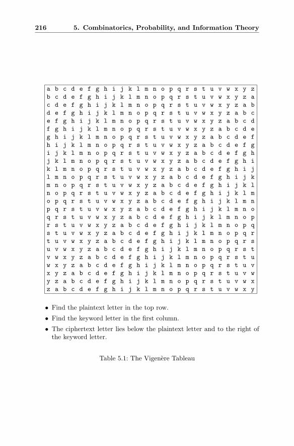
216 5. Combinatorics, Probability, and Information Theory
a b c d e f g h i j k l m n o p q r s t u v w x y z
b c d e f g h i j k l m n o p q r s t u v w x y z a
c d e f g h i j k l m n o p q r s t u v w x y z a b
d e f g h i j k l m n o p q r s t u v w x y z a b c
e f g h i j k l m n o p q r s t u v w x y z a b c d
f g h i j k l m n o p q r s t u v w x y z a b c d e
g h i j k l m n o p q r s t u v w x y z a b c d e f
h i j k l m n o p q r s t u v w x y z a b c d e f g
i j k l m n o p q r s t u v w x y z a b c d e f g h
j k l m n o p q r s t u v w x y z a b c d e f g h i
k l m n o p q r s t u v w x y z a b c d e f g h i j
l m n o p q r s t u v w x y z a b c d e f g h i j k
m n o p q r s t u v w x y z a b c d e f g h i j k l
n o p q r s t u v w x y z a b c d e f g h i j k l m
o p q r s t u v w x y z a b c d e f g h i j k l m n
p q r s t u v w x y z a b c d e f g h i j k l m n o
q r s t u v w x y z a b c d e f g h i j k l m n o p
r s t u v w x y z a b c d e f g h i j k l m n o p q
s t u v w x y z a b c d e f g h i j k l m n o p q r
t u v w x y z a b c d e f g h i j k l m n o p q r s
u v w x y z a b c d e f g h i j k l m n o p q r s t
v w x y z a b c d e f g h i j k l m n o p q r s t u
w x y z a b c d e f g h i j k l m n o p q r s t u v
x y z a b c d e f g h i j k l m n o p q r s t u v w
y z a b c d e f g h i j k l m n o p q r s t u v w x
z a b c d e f g h i j k l m n o p q r s t u v w x y
• Find the plaintext letter in the top row.
• Find the keyword letter in the first column.
• The ciphertext letter lies below the plaintext letter and to the right ofthe keyword letter.
Table 5.1: The Vigenere Tableau
5.2. The Vigenere Cipher 217
to last column (which is the one headed by y). This row and column intersectat the letter b, so the corresponding ciphertext letter is b.
Decryption is just as easy. Alice uses the row containing the keyword letterand looks in that row for the ciphertext letter. Then the top of that column isthe plaintext letter. For example, if the keyword letter is g and the ciphertextletter is r, Alice looks in the row starting with g until she finds r and thenshe moves to the top of that column to find the plaintext letter l.
Example 5.13. We illustrate the use of the Vigenere tableau by encryptingthe plaintext message
The rain in Spain stays mainly in the plain,
using the keyword flamingo. Since the key word has eight letters, the firststep is to split the plaintext into eight-letter blocks,
theraini | nspainst | aysmainl | yinthepl | ain.
Next we write the keyword beneath each block of plaintext, where for conve-nience we label lines P, K, and C to indicate, respectively, the plaintext, thekeyword, and the ciphertext.
P t h e r a i n i n s p a i n s t a y s m a i n l y i n t h e p l a i n
K f l a m i n g o f l a m i n g o f l a m i n g o f l a m i n g o f l a
Finally, we encrypt each letter using the Vigenere tableau. The initial plaintextletter t and initial keyword letter f combine in the Vigenere tableau to yieldthe ciphertext letter y, the second plaintext letter h and second keywordletter l combine in the Vigenere tableau to yield the ciphertext letter s, andso on. Continuing in this fashion, we complete the encryption process.
P t h e r a i n i n s p a i n s t a y s m a i n l y i n t h e p l a i n
K f l a m i n g o f l a m i n g o f l a m i n g o f l a m i n g o f l a
C y s e d i v t w s d p m q a y h f j s y i v t z d t n f p r v z f t n
Splitting the ciphertext into convenient blocks of five letters each, we are readyto transmit our encrypted message
ysedi vtwsd pmqay hfjsy ivtzd tnfpr vzftn.
Remark 5.14. As we already pointed out, the same plaintext letter in aVigenere cipher is represented in the ciphertext by many different letters.However, if the keyword is short, there will be a tendency for repetitive partsof the plaintext to end up aligned at the same point in the keyword, in whichcase they will be identically enciphered. This occurs in Example 5.13, wherethe ain in rain and in mainly are encrypted using the same three keywordletters ing, so they yield the same ciphertext letters ivt. This repetition inthe ciphertext, which appears separated by 16 letters, suggests that the key-word has length dividing 16. Of course, not every occurrence of ain in the
218 5. Combinatorics, Probability, and Information Theory
plaintext yields the same ciphertext. It is only when two occurrences line upwith the same part of the keyword that repetition occurs.
In the next section we develop the idea of using ciphertext repetitions toguess the length of the keyword, but here we simply want to make the pointthat short keywords are less secure than long keywords.5 On the other hand,Bob and Alice find it easier to remember a short keyword than a long one.We thus see the beginnings of the eternal struggle in practical (as opposed topurely theoretical) cryptography, namely the battle between
Efficiency (and ease of use)←−−−− versus −−−−→ Security.
As a further illustration of this dichotomy, we consider ways in whichBob and Alice might make their Vigenere-type cipher more secure. They cancertainly make Eve’s job harder by mixing up the letters in the first row of theirVigenere tableau and then rotating this “mixed alphabet” in the subsequentrows. Unfortunately, a mixed alphabet makes encryption and decryption morecumbersome, plus it means that Bob and Alice must remember (or write downfor safekeeping!) not only their keyword, but also the mixed alphabet. Andif they want to be even more secure, they can use different randomly mixedalphabets in every row of their Vigenere tableau. But if they do that, thenthey will certainly need to keep a written copy of the tableau, which is aserious security risk.
5.2.1 Cryptanalysis of the Vigenere Cipher: Theory
At various times in history it has been claimed that Vigenere-type ciphers,especially with mixed alphabets, are “unbreakable.” In fact, nothing could befurther from the truth. If Eve knows Bob and Alice, she may be able to guesspart of the keyword and proceed from there. (How many people do you knowwho use some variation of their name and birthday as an Internet password?)But even without lucky guesses, elementary statistical methods developed inthe nineteenth century allow for a straightforward cryptanalysis of Vigenere-type ciphers. In the interest of simplicity, we stick with the original Vigenere,i.e., we do not allow mixed alphabets in the tableau.
You may wonder why we take the time to cryptanalyze the Vigenere cipher,since no one these days uses the Vigenere for secure communications. Theanswer is that our exposition is designed principally to introduce you to the useof statistical tools in cryptanalysis. This builds on and extends the elementaryapplication of frequency tables as we used them in Sect. 1.1.1 to cryptanalyzesimple substitution ciphers. In this section we describe the theoretical toolsused to cryptanalyze the Vigenere, and in the next section we apply thosetools to decrypt a sample ciphertext. If at any point you find that the theoryin this section becomes confusing, it may help to turn to Sect. 5.2.2 and seehow the theory is applied in practice.
5More typically one uses a key phrase consisting of several words, but for simplicity weuse the term “keyword” to cover both single keywords and longer key phrases.
5.2. The Vigenere Cipher 219
The first goal in cryptanalyzing a Vigenere cipher is to find the length ofthe keyword, which is sometimes called the blocksize or the period. We alreadysaw in Remark 5.14 how this might be accomplished by looking for repeatedfragments in the ciphertext. The point is that certain plaintext fragmentssuch as the occur quite frequently, while other plaintext fragments such as ugwoccur infrequently or not at all. Among the many occurrences of the letters thein the plaintext, a certain percentage of them will line up with exactly thesame part of the keyword.
This leads to the Kasiski method, first described by a German militaryofficer named Friedrich Kasiski in his book Die Geheimschriften und dieDechiffrir-kunst6 published in 1863. One looks for repeated fragments withinthe ciphertext and compiles a list of the distances that separate the repeti-tions. The key length is likely to divide many of these distances. Of course, acertain number of repetitions will occur by pure chance, but these are random,while the ones coming from repeated plaintext fragments are always divisibleby the key length. It is generally not hard to pick out the key length from thisdata.
There is another method of guessing the key length that works withindividual letters, rather than with fragments consisting of several letters.The underlying idea can be traced all the way back to the frequency tableof English letters (Table 1.3), which shows that some letters are more likelyto occur than others. Suppose now that you are presented with a ciphertextencrypted using a Vigenere cipher and that you guess that it was encryptedusing a keyword of length 5. This means that every fifth letter was encryptedusing the same rotation, so if you pull out every fifth letter and form them intoa string, this entire string was encrypted using a single substitution cipher.Hence the string’s letter frequencies should look more or less as they do in En-glish, with some letters much more frequent and some much less frequent. Andthe same will be true of the string consisting of the 2nd, 7th, 12th,. . . lettersof the ciphertext, and so on. On the other hand, if you guessed wrong and thekey length is not five, then the string consisting of every fifth letter should bemore or less random, so its letter frequencies should look different from thefrequencies in English.
How can we quantify the following two statements so as to be able todistinguish between them?
String 1 has letter frequencies similar to those in Table 1.3. (5.4)
String 2 has letter frequencies that look more or less random. (5.5)
One method is to use the following device.
Definition. Let s = c1c2c3 · · · cn be a string of n alphabetic characters. Theindex of coincidence of s, denoted by IndCo(s), is the probability that tworandomly chosen characters in the string s are identical.
6Cryptography and the Art of Decryption.
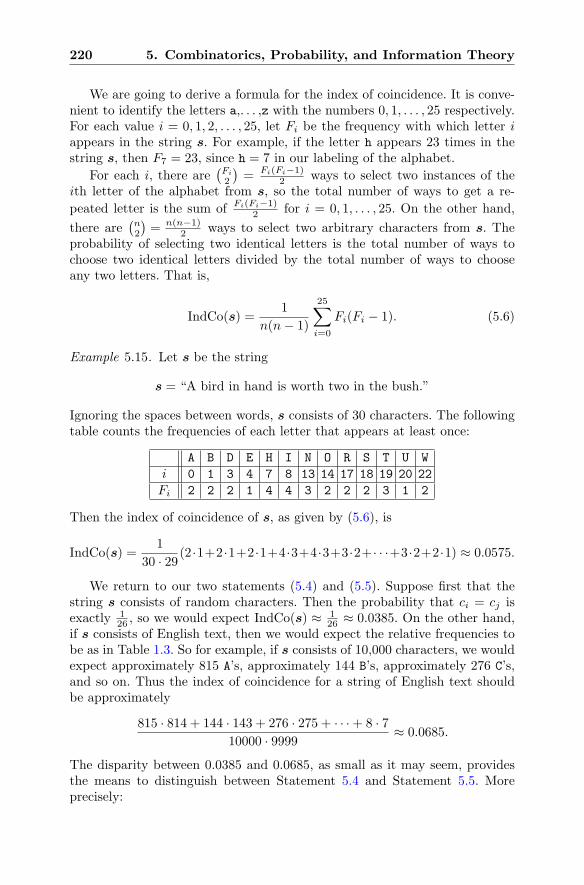
220 5. Combinatorics, Probability, and Information Theory
We are going to derive a formula for the index of coincidence. It is conve-nient to identify the letters a,. . . ,z with the numbers 0, 1, . . . , 25 respectively.For each value i = 0, 1, 2, . . . , 25, let Fi be the frequency with which letter iappears in the string s. For example, if the letter h appears 23 times in thestring s, then F7 = 23, since h = 7 in our labeling of the alphabet.
For each i, there are(Fi
2
)= Fi(Fi−1)
2 ways to select two instances of theith letter of the alphabet from s, so the total number of ways to get a re-
peated letter is the sum of Fi(Fi−1)2 for i = 0, 1, . . . , 25. On the other hand,
there are(n2
)= n(n−1)
2 ways to select two arbitrary characters from s. Theprobability of selecting two identical letters is the total number of ways tochoose two identical letters divided by the total number of ways to chooseany two letters. That is,
IndCo(s) =1
n(n− 1)
25∑
i=0
Fi(Fi − 1). (5.6)
Example 5.15. Let s be the string
s = “A bird in hand is worth two in the bush.”
Ignoring the spaces between words, s consists of 30 characters. The followingtable counts the frequencies of each letter that appears at least once:
A B D E H I N O R S T U W
i 0 1 3 4 7 8 13 14 17 18 19 20 22
Fi 2 2 2 1 4 4 3 2 2 2 3 1 2
Then the index of coincidence of s, as given by (5.6), is
IndCo(s) =1
30 · 29(2·1+2·1+2·1+4·3+4·3+3·2+· · ·+3·2+2·1) ≈ 0.0575.
We return to our two statements (5.4) and (5.5). Suppose first that thestring s consists of random characters. Then the probability that ci = cj isexactly 1
26 , so we would expect IndCo(s) ≈ 126 ≈ 0.0385. On the other hand,
if s consists of English text, then we would expect the relative frequencies tobe as in Table 1.3. So for example, if s consists of 10,000 characters, we wouldexpect approximately 815 A’s, approximately 144 B’s, approximately 276 C’s,and so on. Thus the index of coincidence for a string of English text shouldbe approximately
815 · 814 + 144 · 143 + 276 · 275 + · · ·+ 8 · 710000 · 9999 ≈ 0.0685.
The disparity between 0.0385 and 0.0685, as small as it may seem, providesthe means to distinguish between Statement 5.4 and Statement 5.5. Moreprecisely:
5.2. The Vigenere Cipher 221
If IndCo(s) ≈ 0.068, then s looks like simple substitution English. (5.7)
If IndCo(s) ≈ 0.038, then s looks like random letters. (5.8)
Of course, the value of IndCo(s) will tend to fluctuate, especially if s is fairlyshort. But the moral of (5.7) and (5.8) is that larger values of IndCo(s) make itmore likely that s is English encrypted with some sort of simple substitution,while smaller values of IndCo(s) make it more likely that s is random.
Now suppose that Eve intercepts a message s that she believes was en-crypted using a Vigenere cipher and wants to check whether the keyword haslength k. Her first step is to break the string s into k pieces s1, s2, . . . , sk,where s1 consists of every kth letter starting from the first letter, s2 consistsof every kth letter starting from the second letter, and so on. In mathematicalterms, if we write s = c1c2c3 . . . cn, then
si = cici+kci+2kci+3k . . . .
Notice that if Eve’s guess is correct and the keyword has length k, then each siconsists of characters that were encrypted using the same shift amount, soalthough they do not decrypt to form actual words (remember that si isevery kth letter of the text), the pattern of their letter frequencies will looklike English. On the other hand, if Eve’s guess is incorrect, then the si stringswill be more or less random.
Thus for each k, Eve computes IndCo(si) for i = 1, 2, . . . , k and checkswhether these numbers are closer to 0.068 or closer to 0.038. She does thisfor k = 3, 4, 5, . . . until she finds a value of k for which the average valueof IndCo(s1), IndCo(s2), . . . , IndCo(sk) is large, say greater than 0.06. Thenthis k is probably the correct blocksize.
We assume now that Eve has used the Kasiski test or the index of coinci-dence test to determine that the keyword has length k. That’s a good start,but she’s still quite far from her goal of finding the plaintext. The next stepis to compare the strings s1, s2, . . . , sk to one another. The tool she uses tocompare different strings is called the mutual index of coincidence. The gen-eral idea is that each of the k strings has been encrypted using a differentshift cipher. If the string si is shifted by βi and the string sj is shifted by βj ,then one would expect the frequencies of si to best match those of sj whenthe symbols in si are shifted by an additional amount
σ ≡ βj − βi (mod 26).
This leads to the following useful definition.
Definition. Let
s = c1c2c3 . . . cn and t = d1d2d3 . . . dm
be strings of alphabetic characters. The mutual index of coincidence of sand t, denoted by MutIndCo(s, t), is the probability that a randomly chosencharacter from s and a randomly chosen character from t will be the same.
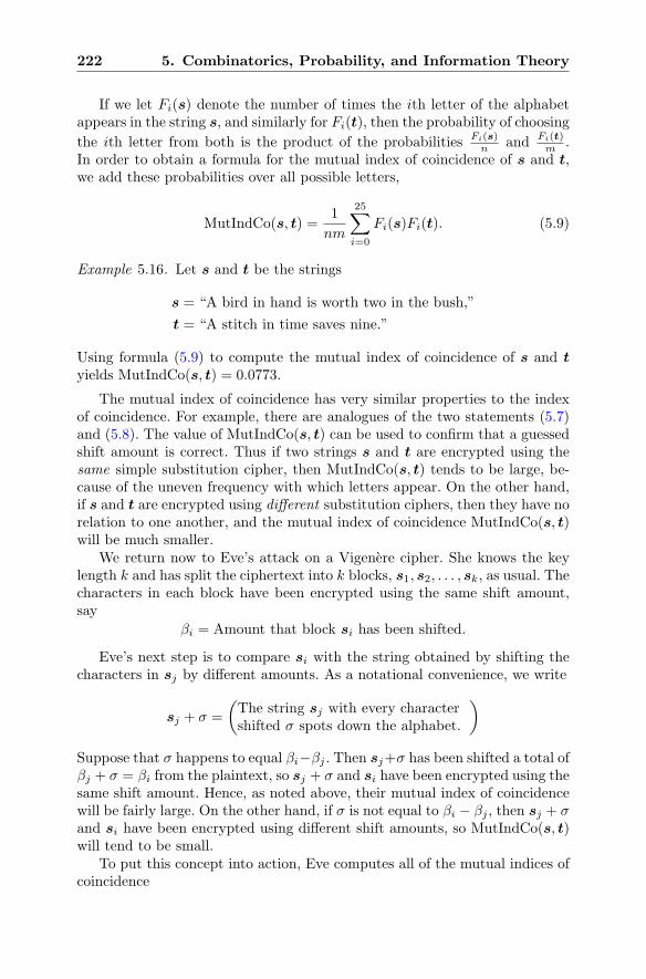
222 5. Combinatorics, Probability, and Information Theory
If we let Fi(s) denote the number of times the ith letter of the alphabetappears in the string s, and similarly for Fi(t), then the probability of choosing
the ith letter from both is the product of the probabilities Fi(s)n and Fi(t)
m .In order to obtain a formula for the mutual index of coincidence of s and t,we add these probabilities over all possible letters,
MutIndCo(s, t) =1
nm
25∑
i=0
Fi(s)Fi(t). (5.9)
Example 5.16. Let s and t be the strings
s = “A bird in hand is worth two in the bush,”
t = “A stitch in time saves nine.”
Using formula (5.9) to compute the mutual index of coincidence of s and tyields MutIndCo(s, t) = 0.0773.
The mutual index of coincidence has very similar properties to the indexof coincidence. For example, there are analogues of the two statements (5.7)and (5.8). The value of MutIndCo(s, t) can be used to confirm that a guessedshift amount is correct. Thus if two strings s and t are encrypted using thesame simple substitution cipher, then MutIndCo(s, t) tends to be large, be-cause of the uneven frequency with which letters appear. On the other hand,if s and t are encrypted using different substitution ciphers, then they have norelation to one another, and the mutual index of coincidence MutIndCo(s, t)will be much smaller.
We return now to Eve’s attack on a Vigenere cipher. She knows the keylength k and has split the ciphertext into k blocks, s1, s2, . . . , sk, as usual. Thecharacters in each block have been encrypted using the same shift amount,say
βi = Amount that block si has been shifted.
Eve’s next step is to compare si with the string obtained by shifting thecharacters in sj by different amounts. As a notational convenience, we write
sj + σ =
(The string sj with every charactershifted σ spots down the alphabet.
)
Suppose that σ happens to equal βi−βj . Then sj+σ has been shifted a total ofβj + σ = βi from the plaintext, so sj + σ and si have been encrypted using thesame shift amount. Hence, as noted above, their mutual index of coincidencewill be fairly large. On the other hand, if σ is not equal to βi − βj , then sj + σand si have been encrypted using different shift amounts, so MutIndCo(s, t)will tend to be small.
To put this concept into action, Eve computes all of the mutual indices ofcoincidence
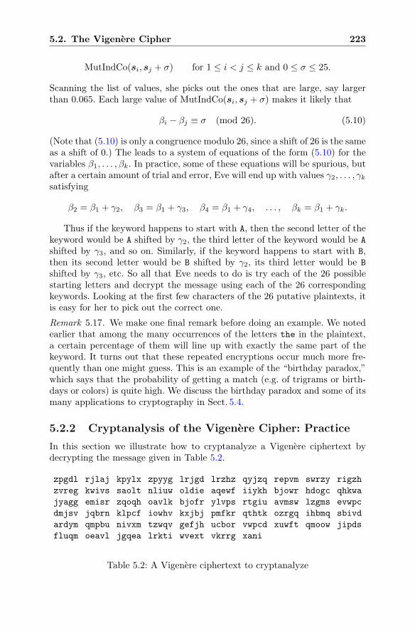
5.2. The Vigenere Cipher 223
MutIndCo(si, sj + σ) for 1 ≤ i < j ≤ k and 0 ≤ σ ≤ 25.
Scanning the list of values, she picks out the ones that are large, say largerthan 0.065. Each large value of MutIndCo(si, sj + σ) makes it likely that
βi − βj ≡ σ (mod 26). (5.10)
(Note that (5.10) is only a congruence modulo 26, since a shift of 26 is the sameas a shift of 0.) The leads to a system of equations of the form (5.10) for thevariables β1, . . . , βk. In practice, some of these equations will be spurious, butafter a certain amount of trial and error, Eve will end up with values γ2, . . . , γksatisfying
β2 = β1 + γ2, β3 = β1 + γ3, β4 = β1 + γ4, . . . , βk = β1 + γk.
Thus if the keyword happens to start with A, then the second letter of thekeyword would be A shifted by γ2, the third letter of the keyword would be Ashifted by γ3, and so on. Similarly, if the keyword happens to start with B,then its second letter would be B shifted by γ2, its third letter would be B
shifted by γ3, etc. So all that Eve needs to do is try each of the 26 possiblestarting letters and decrypt the message using each of the 26 correspondingkeywords. Looking at the first few characters of the 26 putative plaintexts, itis easy for her to pick out the correct one.
Remark 5.17. We make one final remark before doing an example. We notedearlier that among the many occurrences of the letters the in the plaintext,a certain percentage of them will line up with exactly the same part of thekeyword. It turns out that these repeated encryptions occur much more fre-quently than one might guess. This is an example of the “birthday paradox,”which says that the probability of getting a match (e.g. of trigrams or birth-days or colors) is quite high. We discuss the birthday paradox and some of itsmany applications to cryptography in Sect. 5.4.
5.2.2 Cryptanalysis of the Vigenere Cipher: Practice
In this section we illustrate how to cryptanalyze a Vigenere ciphertext bydecrypting the message given in Table 5.2.
zpgdl rjlaj kpylx zpyyg lrjgd lrzhz qyjzq repvm swrzy rigzh
zvreg kwivs saolt nliuw oldie aqewf iiykh bjowr hdogc qhkwa
jyagg emisr zqoqh oavlk bjofr ylvps rtgiu avmsw lzgms evwpc
dmjsv jqbrn klpcf iowhv kxjbj pmfkr qthtk ozrgq ihbmq sbivd
ardym qmpbu nivxm tzwqv gefjh ucbor vwpcd xuwft qmoow jipds
fluqm oeavl jgqea lrkti wvext vkrrg xani
Table 5.2: A Vigenere ciphertext to cryptanalyze
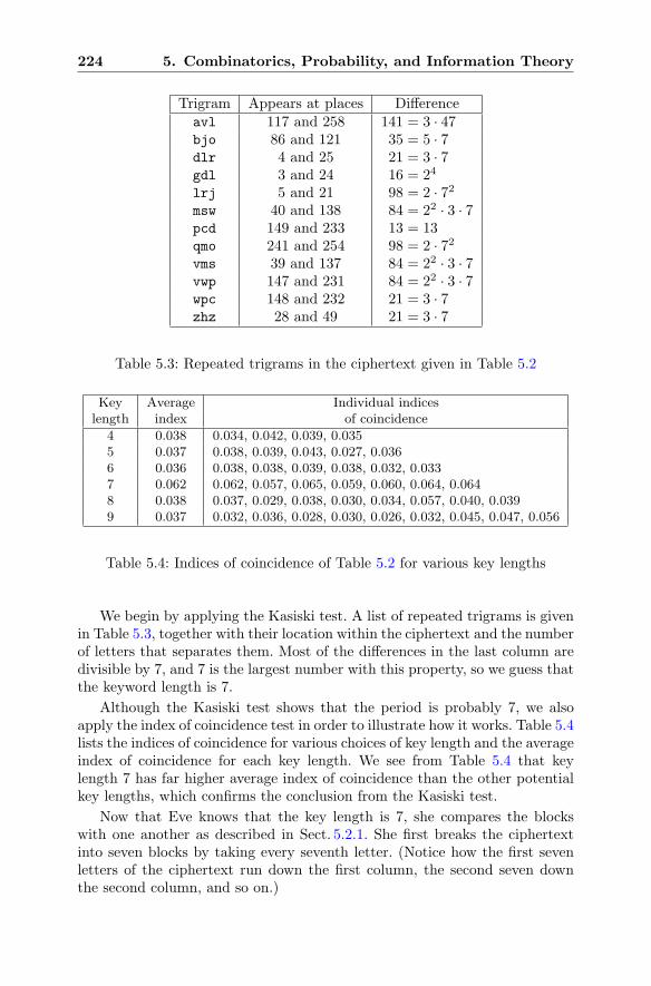
224 5. Combinatorics, Probability, and Information Theory
Trigram Appears at places Differenceavl 117 and 258 141 = 3 · 47bjo 86 and 121 35 = 5 · 7dlr 4 and 25 21 = 3 · 7gdl 3 and 24 16 = 24
lrj 5 and 21 98 = 2 · 72msw 40 and 138 84 = 22 · 3 · 7pcd 149 and 233 13 = 13qmo 241 and 254 98 = 2 · 72vms 39 and 137 84 = 22 · 3 · 7vwp 147 and 231 84 = 22 · 3 · 7wpc 148 and 232 21 = 3 · 7zhz 28 and 49 21 = 3 · 7
Table 5.3: Repeated trigrams in the ciphertext given in Table 5.2
Key Average Individual indiceslength index of coincidence
4 0.038 0.034, 0.042, 0.039, 0.0355 0.037 0.038, 0.039, 0.043, 0.027, 0.0366 0.036 0.038, 0.038, 0.039, 0.038, 0.032, 0.0337 0.062 0.062, 0.057, 0.065, 0.059, 0.060, 0.064, 0.0648 0.038 0.037, 0.029, 0.038, 0.030, 0.034, 0.057, 0.040, 0.0399 0.037 0.032, 0.036, 0.028, 0.030, 0.026, 0.032, 0.045, 0.047, 0.056
Table 5.4: Indices of coincidence of Table 5.2 for various key lengths
We begin by applying the Kasiski test. A list of repeated trigrams is givenin Table 5.3, together with their location within the ciphertext and the numberof letters that separates them. Most of the differences in the last column aredivisible by 7, and 7 is the largest number with this property, so we guess thatthe keyword length is 7.
Although the Kasiski test shows that the period is probably 7, we alsoapply the index of coincidence test in order to illustrate how it works. Table 5.4lists the indices of coincidence for various choices of key length and the averageindex of coincidence for each key length. We see from Table 5.4 that keylength 7 has far higher average index of coincidence than the other potentialkey lengths, which confirms the conclusion from the Kasiski test.
Now that Eve knows that the key length is 7, she compares the blockswith one another as described in Sect. 5.2.1. She first breaks the ciphertextinto seven blocks by taking every seventh letter. (Notice how the first sevenletters of the ciphertext run down the first column, the second seven downthe second column, and so on.)
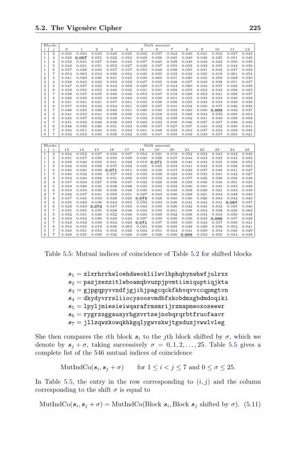
5.2. The Vigenere Cipher 225
Blocks Shift amounti j 0 1 2 3 4 5 6 7 8 9 10 11 12
1 2 0.025 0.034 0.045 0.049 0.025 0.032 0.037 0.042 0.049 0.031 0.032 0.037 0.0431 3 0.023 0.067 0.055 0.022 0.034 0.049 0.036 0.040 0.040 0.046 0.025 0.031 0.0461 4 0.032 0.041 0.027 0.040 0.045 0.037 0.045 0.028 0.049 0.042 0.042 0.030 0.0391 5 0.043 0.021 0.031 0.052 0.027 0.049 0.037 0.050 0.033 0.033 0.035 0.044 0.0301 6 0.037 0.036 0.030 0.037 0.037 0.055 0.046 0.038 0.035 0.031 0.032 0.037 0.0321 7 0.054 0.063 0.034 0.030 0.034 0.040 0.035 0.032 0.042 0.025 0.019 0.061 0.0542 3 0.041 0.029 0.036 0.041 0.045 0.038 0.060 0.031 0.020 0.045 0.056 0.029 0.0302 4 0.028 0.043 0.042 0.032 0.032 0.047 0.035 0.048 0.037 0.040 0.028 0.051 0.0372 5 0.047 0.037 0.032 0.044 0.059 0.029 0.017 0.044 0.060 0.034 0.037 0.046 0.0392 6 0.033 0.035 0.052 0.040 0.032 0.031 0.031 0.029 0.055 0.052 0.043 0.028 0.0232 7 0.038 0.037 0.035 0.046 0.046 0.054 0.037 0.018 0.029 0.052 0.041 0.026 0.0373 4 0.029 0.039 0.033 0.048 0.044 0.043 0.030 0.051 0.033 0.034 0.034 0.040 0.0383 5 0.021 0.041 0.041 0.037 0.051 0.035 0.036 0.038 0.025 0.043 0.034 0.039 0.0363 6 0.037 0.034 0.042 0.034 0.051 0.029 0.027 0.041 0.034 0.040 0.037 0.046 0.0363 7 0.046 0.023 0.028 0.040 0.031 0.040 0.045 0.039 0.020 0.030 0.069 0.042 0.0374 5 0.041 0.033 0.041 0.038 0.036 0.031 0.056 0.032 0.026 0.034 0.049 0.029 0.0544 6 0.035 0.037 0.032 0.039 0.041 0.033 0.032 0.039 0.042 0.031 0.049 0.039 0.0584 7 0.031 0.032 0.046 0.038 0.039 0.042 0.033 0.056 0.046 0.027 0.027 0.036 0.0365 6 0.048 0.036 0.026 0.031 0.033 0.039 0.037 0.027 0.037 0.045 0.032 0.040 0.0415 7 0.030 0.051 0.043 0.031 0.034 0.041 0.048 0.032 0.053 0.037 0.024 0.029 0.0456 7 0.032 0.033 0.030 0.038 0.032 0.035 0.047 0.050 0.049 0.033 0.057 0.050 0.021
Blocks Shift amounti j 13 14 15 16 17 18 19 20 21 22 23 24 25
1 2 0.034 0.052 0.037 0.030 0.037 0.054 0.021 0.018 0.052 0.052 0.043 0.042 0.0461 3 0.031 0.037 0.038 0.050 0.039 0.040 0.026 0.037 0.044 0.043 0.023 0.045 0.0321 4 0.039 0.040 0.032 0.041 0.028 0.019 0.071 0.038 0.040 0.034 0.045 0.026 0.0521 5 0.042 0.032 0.038 0.037 0.032 0.045 0.045 0.033 0.041 0.043 0.035 0.028 0.0631 6 0.040 0.030 0.028 0.071 0.051 0.033 0.036 0.047 0.029 0.037 0.046 0.041 0.0271 7 0.040 0.032 0.049 0.037 0.035 0.035 0.039 0.023 0.043 0.035 0.041 0.042 0.0272 3 0.054 0.040 0.028 0.031 0.039 0.033 0.052 0.046 0.037 0.026 0.028 0.036 0.0482 4 0.047 0.034 0.027 0.038 0.047 0.042 0.026 0.038 0.029 0.046 0.040 0.061 0.0252 5 0.034 0.026 0.035 0.038 0.048 0.035 0.033 0.032 0.040 0.041 0.045 0.033 0.0362 6 0.033 0.034 0.036 0.036 0.048 0.040 0.041 0.049 0.058 0.028 0.021 0.043 0.0492 7 0.042 0.037 0.041 0.059 0.031 0.027 0.043 0.046 0.028 0.021 0.044 0.048 0.0403 4 0.037 0.045 0.033 0.028 0.029 0.073 0.026 0.040 0.040 0.026 0.043 0.042 0.0433 5 0.035 0.029 0.036 0.044 0.055 0.034 0.033 0.046 0.041 0.024 0.041 0.067 0.0373 6 0.023 0.043 0.074 0.047 0.033 0.043 0.030 0.026 0.042 0.045 0.032 0.035 0.0403 7 0.035 0.035 0.035 0.028 0.048 0.033 0.035 0.041 0.038 0.052 0.038 0.029 0.0624 5 0.032 0.041 0.036 0.032 0.046 0.035 0.039 0.042 0.038 0.034 0.043 0.036 0.0484 6 0.034 0.034 0.036 0.029 0.043 0.037 0.039 0.036 0.039 0.033 0.066 0.037 0.0284 7 0.043 0.032 0.039 0.034 0.029 0.071 0.037 0.039 0.030 0.044 0.037 0.030 0.0415 6 0.052 0.035 0.019 0.036 0.063 0.045 0.030 0.039 0.049 0.029 0.036 0.052 0.0415 7 0.040 0.031 0.034 0.052 0.026 0.034 0.051 0.044 0.041 0.039 0.034 0.046 0.0296 7 0.029 0.035 0.039 0.032 0.028 0.039 0.026 0.036 0.069 0.052 0.035 0.034 0.038
Table 5.5: Mutual indices of coincidence of Table 5.2 for shifted blocks
s1 = zlxrhrrhwloehdweoklilwvlhphqbynwhwfjulrxx
s2 = pazjzezzitlwboamqbvuzpjpvmtiimiquptiqjkta
s3 = gjpgqpyvvndfjgjihjpagcqckfkhvqvvccqpmgtvn
s4 = dkydyvrrsliiocysoosvmdbfxkobdmxgbdmdoqiki
s5 = lpyljmiesieiwqarafrmsmrijrzmapmeoxoseewr
s6 = rygrzsggauayrhgzvrtsejnobqrqrbtfruofaavr
s7 = jllzqwzkowqkhkgqlygwvskwjtgsduzjvwwlvleg
She then compares the ith block si to the jth block shifted by σ, which wedenote by sj + σ, taking successively σ = 0, 1, 2, . . . , 25. Table 5.5 gives acomplete list of the 546 mutual indices of coincidence
MutIndCo(si, sj + σ) for 1 ≤ i < j ≤ 7 and 0 ≤ σ ≤ 25.
In Table 5.5, the entry in the row corresponding to (i, j) and the columncorresponding to the shift σ is equal to
MutIndCo(si, sj + σ) = MutIndCo(Block si,Block sj shifted by σ). (5.11)
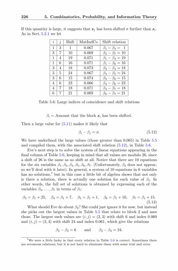
226 5. Combinatorics, Probability, and Information Theory
If this quantity is large, it suggests that sj has been shifted σ further than si.As in Sect. 5.2.1 we let
i j Shift MutIndCo Shift relation
1 3 1 0.067 β1 − β3 = 13 7 10 0.069 β3 − β7 = 101 4 19 0.071 β1 − β4 = 191 6 16 0.071 β1 − β6 = 163 4 18 0.073 β3 − β4 = 183 5 24 0.067 β3 − β5 = 243 6 15 0.074 β3 − β6 = 154 6 23 0.066 β4 − β6 = 234 7 18 0.071 β4 − β7 = 186 7 21 0.069 β6 − β7 = 21
Table 5.6: Large indices of coincidence and shift relations
βi = Amount that the block si has been shifted.
Then a large value for (5.11) makes it likely that
βi − βj = σ. (5.12)
We have underlined the large values (those greater than 0.065) in Table 5.5and compiled them, with the associated shift relation (5.12), in Table 5.6.
Eve’s next step is to solve the system of linear equations appearing in thefinal column of Table 5.6, keeping in mind that all values are modulo 26, sincea shift of 26 is the same as no shift at all. Notice that there are 10 equationsfor the six variables β1, β3, β4, β5, β6, β7. (Unfortunately, β2 does not appear,so we’ll deal with it later). In general, a system of 10 equations in 6 variableshas no solutions,7 but in this case a little bit of algebra shows that not onlyis there a solution, there is actually one solution for each value of β1. Inother words, the full set of solutions is obtained by expressing each of thevariables β3, . . . , β7 in terms of β1:
β3 = β1 + 25, β4 = β1 + 7, β5 = β1 + 1, β6 = β1 + 10, β7 = β1 + 15.(5.13)
What should Eve do about β2? She could just ignore it for now, but insteadshe picks out the largest values in Table 5.5 that relate to block 2 and usesthose. The largest such values are (i, j) = (2, 3) with shift 6 and index 0.060and (i, j) = (2, 4) with shift 24 and index 0.061, which give the relations
β2 − β3 = 6 and β2 − β4 = 24.
7We were a little lucky in that every relation in Table 5.6 is correct. Sometimes thereare erroneous relations, but it is not hard to eliminate them with some trial and error.
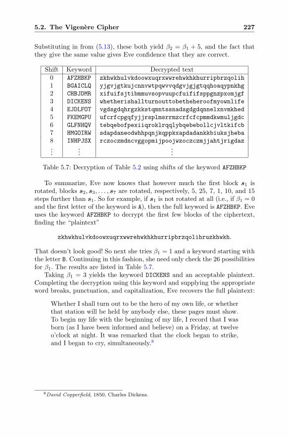
5.2. The Vigenere Cipher 227
Substituting in from (5.13), these both yield β2 = β1 + 5, and the fact thatthey give the same value gives Eve confidence that they are correct.
Shift Keyword Decrypted text0 AFZHBKP zkhwkhulvkdoowxuqrxwwrehwkhkhurripbrzqolih
1 BGAICLQ yjgvjgtkujcnnvwtpqwvvqdgvjgjgtqqhoaqypnkhg
2 CHBJDMR xifuifsjtibmmuvsopvuupcfuififsppgnzpxomjgf
3 DICKENS whetherishallturnouttobetheheroofmyownlife
4 EJDLFOT vgdsgdqhrgzkkstqmntssnadsgdgdqnnelxnvmkhed
5 FKEMGPU ufcrfcpgqfyjjrsplmsrrmzcrfcfcpmmdkwmuljgdc
6 GLFNHQV tebqebofpexiiqroklrqqlybqebebollcjvltkifcb
7 HMGOIRW sdapdaneodwhhpqnjkqppkxapdadankkbiuksjheba
8 INHPJSX rczoczmdncvggopmijpoojwzoczczmjjahtjrigdaz...
......
Table 5.7: Decryption of Table 5.2 using shifts of the keyword AFZHBKP
To summarize, Eve now knows that however much the first block s1 isrotated, blocks s2, s3, . . . , s7 are rotated, respectively, 5, 25, 7, 1, 10, and 15steps further than s1. So for example, if s1 is not rotated at all (i.e., if β1 = 0and the first letter of the keyword is A), then the full keyword is AFZHBKP. Eveuses the keyword AFZHBKP to decrypt the first few blocks of the ciphertext,finding the “plaintext”
zkhwkhulvkdoowxuqrxwwrehwkhkhurripbrzqolihruzkhwkh.
That doesn’t look good! So next she tries β1 = 1 and a keyword starting withthe letter B. Continuing in this fashion, she need only check the 26 possibilitiesfor β1. The results are listed in Table 5.7.
Taking β1 = 3 yields the keyword DICKENS and an acceptable plaintext.Completing the decryption using this keyword and supplying the appropriateword breaks, punctuation, and capitalization, Eve recovers the full plaintext:
Whether I shall turn out to be the hero of my own life, or whetherthat station will be held by anybody else, these pages must show.To begin my life with the beginning of my life, I record that I wasborn (as I have been informed and believe) on a Friday, at twelveo’clock at night. It was remarked that the clock began to strike,and I began to cry, simultaneously.8
8David Copperfield, 1850, Charles Dickens.
228 5. Combinatorics, Probability, and Information Theory
5.3 Probability Theory
5.3.1 Basic Concepts of Probability Theory
In this section we introduce the basic ideas of probability theory in the dis-crete setting. A probability space consists of two pieces. The first is a finiteset Ω consisting of all possible outcomes of an experiment and the second isa method for assigning a probability to each possible outcome. In mathemat-ical terms, a probability space is a finite set of outcomes Ω, called the samplespace, and a function
Pr : Ω −→ R.
We want the function Pr to satisfy our intuition that
Pr(ω) = “probability that event ω occurred.”
In particular, the value of Pr(ω) should be between 0 and 1.
Example 5.18. Consider the toss of a single coin. There are two outcomes,heads and tails, so we let Ω be the set {H,T}. Assuming that it is a fair coin,each outcome is equally likely, so Pr(H) = Pr(T ) = 1
2 .
Example 5.19. Consider the roll of two dice. The sample space Ω is the fol-lowing set of 36 pairs of numbers:
Ω ={(n,m) : n,m ∈ Z with 1 ≤ n,m ≤ 6
}.
As in Example 5.18, each possible outcome is equally likely. For example,the probability of rolling (6, 6) is the same as the probability of rolling (3, 4).Hence
Pr((n,m)
)=
1
36
for any choice of (n,m). Note that order matters in this scenario. We mightimagine that one die is red and the other is blue, so “red 3 and blue 5” is adifferent outcome from “red 5 and blue 3.”
Example 5.20. Suppose that an urn contains 100 balls, of which 21 are redand the rest are blue. If we pick 10 balls at random (without replacement),what is the probability that exactly 3 of them are red?
The total number of ways of selecting 10 balls from among 100 is(10010
).
Similarly, there are(213
)ways to select 3 red balls from among the 21 that are
red, and there are(797
)ways to pick the other 7 balls from among the 79
that are blue. There are thus(213
)(797
)ways to select exactly 3 red balls
and exactly 7 blue balls. Hence the probability of picking exactly 3 red ballsin 10 tries is
Pr
(exactly 3 red balls in10 attempts
)=
(213
)(797
)
(10010
) =20271005
91015876≈ 0.223.
5.3. Probability Theory 229
We are typically more interested in computing the probability of compoundevents. These are subsets of the sample space that may include more than oneoutcome. For example, in the roll of two dice in Example 5.19, we might beinterested in the probability that at least one of the dice shows a 6. Thiscompound event is the subset of Ω consisting of all outcomes that include thenumber six, which is the set{(1, 6), (2, 6), (3, 6), (4, 6), (5, 6), (6, 6), (6, 1), (6, 2), (6, 3), (6, 4), (6, 5)
}.
Suppose that we know the probability of each particular outcome. Howthen do we compute the probability of compound events or of events consistingof repeated independent trials of an experiment? Analyzing this problem leadsto the idea of independence of events, a concept that gives probability theorymuch of its complexity and richness.
The formal theory of probability is an axiomatic theory. You have probablyseen such theories when you studied Euclidean geometry and when you studiedabstract vector spaces. In an axiomatic theory, one starts with a small list ofbasic axioms and derives from them additional interesting facts and formulas.The axiomatic theory of probability allows us to derive formulas to computethe probabilities of compound events. In this book we are content with aninformal presentation of the theory, but for those who are interested in a morerigorous axiomatic treatment of probability theory, see for example [112, §2.3].
We begin with some definitions.
Definition. A sample space (or set of outcomes) is a finite9 set Ω. Eachoutcome ω ∈ Ω is assigned a probability Pr(ω), where we require that theprobability function
Pr : Ω −→ R
satisfy the following two properties:
(a) 0 ≤ Pr(ω) ≤ 1 for all ω ∈ Ω and (b)∑
ω∈Ω
Pr(ω) = 1. (5.14)
Notice that (5.14)(a) corresponds to our intuition that every outcomehas a probability between 0 (if it never occurs) and 1 (if it always occurs),while (5.14)(b) says that some outcome must occur, so Ω contains all possibleoutcomes for the experiment.
Definition. An event is any subset of Ω. We assign a probability to an eventE ⊂ Ω by setting
Pr(E) =∑
ω∈E
Pr(ω). (5.15)
In particular, Pr(∅) = 0 by convention, and Pr(Ω) = 1 from (5.14)(b).
9General (continuous) probability theory also deals with infinite sample spaces Ω, inwhich case only certain subsets of Ω are allowed to be events and are assigned probabilities.There are also further restrictions on the probability function Pr : Ω → R. For our study ofcryptography in this book, it suffices to use discrete (finite) sample spaces.
230 5. Combinatorics, Probability, and Information Theory
Definition. We say that two events E and F are disjoint if E ∩ F = ∅.
It is clear that
Pr(E ∪ F ) = Pr(E) + Pr(F ) if E and F are disjoint,
since then E ∪ F is the collection of all outcomes in either E or F . WhenE and F are not disjoint, the probability of the event E ∪ F is not the sumof Pr(E) and Pr(F ), since the outcomes common to both E and F shouldnot be counted twice. Thus we need to subtract the outcomes common to Eand F , which gives the useful formula
Pr(E ∪ F ) = Pr(E) + Pr(F )− Pr(E ∩ F ). (5.16)
(See Exercise 5.20.)
Definition. The complement of an event E is the event Ec consisting of alloutcomes that are not in E, i.e.,
Ec = {ω ∈ Ω : ω /∈ E}.
The probability of the complementary event is given by
Pr(Ec) = 1− Pr(E). (5.17)
It is sometimes easier to compute the probability of the complement of anevent E and then use (5.17) to find Pr(E).
Example 5.21. We continue with Example 5.19 in which Ω consists of thepossible outcomes of rolling two dice. Let E be the event
E = {at least one six is rolled}.
We can write down E explicitly; it is the set
E ={(1, 6), (6, 1), (2, 6), (6, 2), (3, 6), (6, 3), (4, 6), (6, 4), (5, 6), (6, 5), (6, 6)
}.
Each of these 11 outcomes has probability 136 , so
Pr(E) =∑
ω∈E
Pr(ω) =11
36.
We can then compute the probability of not rolling a six as
Pr(no sixes are rolled) = Pr(Ec) = 1− Pr(E) =25
36.
Next consider the event F defined by
F = {no number higher than two is rolled}.
5.3. Probability Theory 231
Notice thatF =
{(1, 1), (1, 2), (2, 1), (2, 2)
}
is disjoint from E, so the probability of either rolling a six or else rolling nonumber higher than two is
Pr(E ∪ F ) = Pr(E) + Pr(F ) =11
36+
4
36=
15
36.
For nondisjoint events, the computation is more complicated, since weneed to avoid double counting outcomes. Consider the event G defined by
G = {doubles},
i.e., G ={(1, 1), (2, 2), (3, 3), (4, 4), (5, 5), (6, 6)
}. Then E and G both contain
the outcome (6, 6), so their union E ∪G only contains 16 outcomes, not 17.Thus the probability of rolling either a six or doubles is 16
36 . We can alsocompute this probability using formula (5.16),
Pr(E ∪G) = Pr(E) + Pr(G)− Pr(E ∩G) = 11
36+
6
36− 1
36=
16
36=
4
9.
To conclude this example, let H be the event
H = {the sum of the two dice is at least 4}.
We could compute Pr(H) directly, but it is easier to compute the probabilityof Hc. Indeed, there are only three outcomes that give a sum smaller than 4,namely
Hc ={(1, 1), (1, 2), (2, 1)
}.
Thus Pr(Hc) = 336 = 1
12 , and then Pr(H) = 1− Pr(Hc) = 1112 .
Suppose now that E and F are events. The event consisting of both Eand F is the intersection E ∩ F , so the probability that both E and F occuris
Pr(E and F ) = Pr(E ∩ F ).As the next example makes clear, the probability of the intersection of twoevents is not a simple function of the probabilities of the individual events.
Example 5.22. Consider the experiment consisting of drawing two cards froma deck of cards, where the second card is drawn without replacing the firstcard. Let E and F be the following events:
E = {the first card drawn is a king},F = {the second card drawn is a king}.
Clearly Pr(E) = 113 . It is also true that Pr(F ) = 1
13 , since with no informationabout the value of the first card, there’s no difference between events E and F .(If this seems unclear, suppose instead that the deck of cards were dealt to 52
232 5. Combinatorics, Probability, and Information Theory
people. Then the probability that any particular person gets a king is 113 ,
regardless of whether they received the first card or the second card or. . . .)However, it is also clear that if we know whether event E has occurred, thenthat knowledge does affect the probability of F occurring. More precisely, if Eoccurs, then there are only 3 kings left in the remaining 51 cards, so F is lesslikely, while if E does not occur, then there are 4 kings left and F is morelikely. Mathematically we find that
Pr(F if E has occurred) =3
51and Pr(F if E has not occurred) =
4
51.
Thus the probability of both E and F occurring, i.e., the probability of draw-ing two consecutive kings, is smaller than the product of Pr(E) and Pr(F ),because the occurrence of the event E makes the event F less likely. Thecorrect computation is
Pr(drawing two kings) = Pr(E ∩ F )= Pr(E) · Pr(F given that E has occurred)
=1
13· 3
51=
1
221≈ 0.0045.
LetG = {the second card drawn is an ace}.
Then the occurrence of E makes G more likely, since if the first card is knownto be a king, then there are still four aces left. Thus if we know that E occurs,then the probability of G increases from 4
52 to 451 .
Notice, however, that if we change the experiment and require that the firstcard be replaced in the deck before the second card is drawn, then whether Eoccurs has no effect at all on F . Thus using this card replacement scenario,the probability that E and F both occur is simply the product
Pr(E) Pr(F ) =
(1
13
)2
≈ 0.006.
We learn two things from the discussion in Example 5.22. First, we seethat the probability of one event can depend on whether another event hasoccurred. Second, we develop some probabilistic intuitions that lead to themathematical definition of independence.
Definition. Two events E and F are said to be independent if
Pr(E ∩ F ) = Pr(E) · Pr(F ),
where recall that the probability of the intersection Pr(E ∩ F ) is the proba-bility that both E and F occur. In other words, E and F are independentif the probability of their both occurring is the product of their individualprobabilities of occurring.
5.3. Probability Theory 233
Example 5.23. A coin is tossed 10 times and the results recorded. What arethe probabilities of the following events?
E1 = {the first five tosses are all heads}.E2 = {the first five tosses are heads and the rest are tails}.E3 = {exactly five of the ten tosses are heads}.
The result of any one toss is independent of the result of any other toss,so we can compute the probability of getting H on the first five tosses bymultiplying together the probability of getting H on any one of these tosses.Assuming that it is a fair coin, the answer to our first question is thus
Pr(E1) =
(1
2
)5
=1
32≈ 0.031.
In order to compute the probability of E2, note that we are now asking forthe probability that our sequence of tosses is exactly HHHHHTTTTT. Againusing the independence of the individual tosses, we see that
Pr(E2) =
(1
2
)10
=1
1024≈ 0.00098.
The computation of Pr(E3) is a little trickier, because it asks for exactlyfive H’s to occur, but places no restriction on when they occur. If we were tospecify exactly when the five H’s and the five T’s occur, then the probabilitywould be 1
210 , just as it was for E2. So all that we need to do is to counthow many ways we can distribute five H’s and five T’s into ten spots, orequivalently, how many different sequences we can form consisting of five H’sand five T’s. This is simply the number of ways of choosing five locationsfrom ten possible locations, which is given by the combinatorial symbol
(105
).
Hence dividing the number of outcomes satisfying E3 by the total number ofoutcomes, we find that
Pr(E3) =
(10
5
)· 1
210=
252
1024=
63
256≈ 0.246.
Thus there is just under a 25% chance of getting exactly five heads in tentosses of a coin.
5.3.2 Bayes’s Formula
As we saw in Example 5.22, there is a connection between the probabilitythat two events E and F occur simultaneously and the probability that one ofthem occurs if we know that the other one has occurred. The former quantityis simply Pr(E ∩ F ). The latter quantity is called the conditional probabilityof F on E.
234 5. Combinatorics, Probability, and Information Theory
Definition. The conditional probability of F on E is denoted by
Pr(F | E) = Pr(F given that E has occurred).
The probability that both E and F occur is related to the conditionalprobability of F on E by the formula
Pr(F | E) =Pr(F ∩ E)
Pr(E). (5.18)
The intuition behind (5.18), which is usually taken as the definition of theconditional probability Pr(F | E), is simple. On the left-hand side, we areassuming that E occurs, so our sample space or universe is now E insteadof Ω. We are asking for the probability that the event F occurs in this smalleruniverse of outcomes, so we should compute the proportion of the event Fthat is included in the event E, divided by the total size of the event E itself.This gives the right-hand side of (5.18).
Formula (5.18) immediately implies that
Pr(F | E) Pr(E) = Pr(F ∩ E) = Pr(E ∩ F ) = Pr(E | F ) Pr(F ).
Dividing both sides by Pr(F ) gives a preliminary version of Bayes’sformula:
Pr(E | F ) = Pr(F | E) Pr(E)
Pr(F )(Bayes’s formula). (5.19)
This formula is useful if we know the conditional probability of F on E andwant to know the reverse conditional probability of E on F .
Sometimes it is easier to compute the probability of an event by dividingit into a union of disjoint events, as in the next proposition, which includesanother version of Bayes’s formula.
Proposition 5.24. Let E and F be events.
(a) Pr(E) = Pr(E | F ) Pr(F ) + Pr(E | F c) Pr(F c). (5.20)
(b) Pr(E | F ) = Pr(F | E) Pr(E)
Pr(F | E) Pr(E) + Pr(F | Ec) Pr(Ec)(Bayes’s formula).
(5.21)
Proof. The proof of (a) illustrates how one manipulates basic probabilityformulas.
Pr(E | F ) Pr(F ) + Pr(E | F c) Pr(F c)
= Pr(E ∩ F ) + Pr(E ∩ F c) from (5.18),
= Pr((E ∩ F ) ∪ (E ∩ F c)
)since E ∩ F and E ∩ F c are disjoint,
= Pr(E) since F ∪ F c = Ω.
5.3. Probability Theory 235
This completes the proof of (a).In order to prove (b), we reverse the roles of E and F in (a) to get
Pr(F ) = Pr(F | E) Pr(E) + Pr(F | Ec) Pr(Ec), (5.22)
and then substitute (5.22) into the denominator of (5.19) to obtain (5.21).
Here are some examples that illustrate the use of conditional probabilities.Bayes’s formula will be applied in the next section.
Example 5.25. We are given two urns10 containing gold and silver coins.Urn #1 contains 10 gold coins and 5 silver coins, and Urn #2 contains 2 goldcoins and 8 silver coins. An urn is chosen at random, and then a coin is pickedat random. What is the probability of choosing a gold coin?
LetE = {a gold coin is chosen}.
The probability of E depends first on which urn was chosen, and then onwhich coin is chosen in that urn. It is thus natural to break E up accordingto the outcome of the event
F = {Urn #1 is chosen}.
Notice that F c is the event that Urn #2 is chosen. The decompositionformula (5.20) says that
Pr(E) = Pr(E | F ) Pr(F ) + Pr(E | F c) Pr(F c).
The key point here is that it is easy to compute the conditional probabilitieson the right-hand side, and similarly easy to compute Pr(F ) and Pr(F c). Thus
Pr(E | F ) = 10
15=
2
3, Pr(E | F c) =
2
10=
1
5, Pr(F ) = Pr(F c) =
1
2.
Using these values, we can compute
Pr(E) = Pr(E | F ) Pr(F ) + Pr(E | F c) Pr(F c) =2
3· 12+
1
5· 12=
13
30≈ 0.433.
Example 5.26 (The Three Prisoners Problem). The three prisoners problem isa classical problem about conditional probability. Three prisoners, Alice, Bob,and Carl, are informed by their jailer that the next day, one of them will bereleased from prison, but that the other two will have to serve life sentences.The jailer says that he will not tell any prisoner what will happen to him orher. But Alice, who reasons that her chances of going free are now 1
3 , asksthe jailer to give her the name of one prisoner, other than herself, who will
10The authors of [51, chapter 1] explain the ubiquity of urns in the field of probabilitytheory as being connected with the French phrase aller aux urnes (to vote).
236 5. Combinatorics, Probability, and Information Theory
not go free. The jailer tells Alice that Bob will remain in jail. Now what areAlice’s chances of going free? Has the probability changed? Alice could arguethat she now has a 1
2 chance of going free, since Bob will definitely remainbehind. On the other hand, it also seems reasonable to argue that since oneof Bob or Carl had to stay in jail, this new information could not possiblychange the odds for Alice.
In fact, either answer may be correct. It depends on the strategy that thejailer follows in deciding which name to give to Alice (assuming that Aliceknows which strategy is being used). If the jailer picks a name at randomwhenever both Bob and Carl are possible choices, then Alice’s chances offreedom have not changed. However, if the jailer names Bob whenever possi-ble, and otherwise names Carl, then the new information does indeed changeAlice’s probability of release to 1
2 . See Exercise 5.26.There are many other versions of the three prisoners problem, including
the “Monty Hall problem” that is a staple of popular culture. Exercise 5.27describes the Monty Hall problem and other fun applications of these ideas.
5.3.3 Monte Carlo Algorithms
There are many algorithms whose output is not guaranteed to be correct. Forexample, Table 3.2 in Sect. 3.4 describes the Miller–Rabin algorithm, whichis used to check whether a given large number is prime. In practice, one runsthe algorithm many times to obtain an output that is “probably” correct.In applying these so-called Monte Carlo or probabilistic algorithms, it is im-portant to be able to compute a confidence level, which is the probability thatthe output is indeed correct. In this section we describe how to use Bayes’sformula to do such a computation.
The basic scenario consists of a large (possibly infinite) set of integers Sand an interesting property A. For example, S could be the set of all integers,or more realistically S might be the set of all integers between, say, 21024
and 21025. An example of an interesting property A is the property of beingcomposite.
Now suppose that we are looking for numbers that do not have property A.Using the Miller–Rabin test, we might be looking for integers between 21024
and 21025 that are not composite, i.e., that are prime. In general, supposethat we are given an integer m in S and that we want to know whether m hasproperty A. Usually we know approximately how many of the integers in Shave property A. For example, we might know that 99% of elements haveproperty A and that the other 1% do not. However, it may be difficult todetermine with certainty that any particularm ∈ S does not have property A.So instead we settle for a faster algorithm that is not absolutely certain to becorrect.
A Monte Carlo algorithm for property A takes as its input both a num-ber m ∈ S to be tested and a randomly chosen number r and returns asoutput either Yes or No according to the following rules:

5.3. Probability Theory 237
(1) If the algorithm returns Yes, then m definitely has property A. In con-ditional probability notation, this says that
Pr(m has property A | algorithm returns Yes) = 1.
(2) If m has property A, then the algorithm returns Yes for at least 50% ofthe choices for r.11 Using conditional probability notation,
Pr(algorithm returns Yes | m has property A) ≥ 1
2.
Now suppose that we run the algorithm N times on an integer m ∈ S,using N different randomly chosen values for r. If even a single trial re-turns Yes, then we know that m has property A. But suppose instead thatall N trials return the answer No. How confident can we be that our integerdoes not have property A? In probability terminology, we want to estimate
Pr(m does not have property A | algorithm returns No N times).
More precisely, we want to show that if N is large, then this probability isclose to 1.
We define two events:
E = {an integer in S does not have property A},F = {the algorithm returns No N times in a row}.
We are interested in the conditional probability Pr(E | F ), that is, theprobability that m does not have property A, given the fact that the al-gorithm returned No N times. We can compute this probability using Bayes’sformula (5.21),
Pr(E | F ) = Pr(F | E) Pr(E)
Pr(F | E) Pr(E) + Pr(F | Ec) Pr(Ec).
We are given that 99% of the elements in S have property A, so
Pr(E) = 0.01 and Pr(Ec) = 0.99.
Next consider Pr(F | E). If m does not have property A, which is our assump-tion on this conditional probability, then the algorithm always returns No,since Property (1) of the Monte Carlo method tells us that a Yes outputforces m to have property A. In symbols, Property (1) says that
Pr(No | not A) = Pr(A | Yes) = 1.
11More generally, the success rate in a Monte Carlo algorithm need not be 50%, butmay instead be any positive probability that is not too small. For the Miller–Rabin testdescribed in Sect. 3.4, the corresponding probability is 75%. See Exercise 5.28 for details.
238 5. Combinatorics, Probability, and Information Theory
It follows that Pr(F | E) = Pr(No | not A)N = 1.Finally, we must compute the value of Pr(F | Ec). Since the algorithm is
run N independent times, we have
Pr(F | Ec) = Pr(Output is No | m has property A)N
=(1− Pr(Output is Yes | m has property A)
)N
≤(1− 1
2
)N
from Property (2) of the Monte Carlo method,
=1
2N.
Substituting these values into Bayes’s formula, we find that if the algorithmreturns No N times in a row, then the probability that the integer m does nothave property A is
Pr(E | F ) ≥ 1 · (0.01)1 · (0.01) + 2−N · (0.99) =
1
1 + 99 · 2−N= 1− 99
2N + 99.
Notice that if N is large, the lower bound is very close to 1.For example, if we run the algorithm 100 times and get 100 No answers,
then the probability that m does not have property A is at least
99
99 + 2−100≈ 1− 10−32.1.
So for most practical purposes, it is safe to conclude that m does not haveproperty A.
5.3.4 Random Variables
We are generally more interested in the consequences of an experiment, forexample the net loss or gain from a game of chance, than in the experimentitself. Mathematically, this means that we are interested in functions that aredefined on events and that take values in some set.
Definition. A random variable is a function
X : Ω −→ R
whose domain is the sample space Ω and that takes values in the real numbers.More generally, a random variable is a function X : Ω→ S whose range maybe any set; for example, S could be a set of keys or a set of plaintexts.
We note that since our sample spaces are finite, a random variable takeson only finitely many values. Random variables are useful for defining events.For example, if X : Ω → R is a random variable, then any real number xdefines three interesting events,
{ω ∈ Ω : X(ω) ≤ x}, {ω ∈ Ω : X(ω) = x}, {ω ∈ Ω : X(ω) > x}.
5.3. Probability Theory 239
Definition. Let X : Ω → R be a random variable. The probability densityfunction of X, denoted by fX(x), is defined to be
fX(x) = Pr(X = x).
In other words, fX(x) is the probability that X takes on the value x. Some-times we write f(x) if the random variable is clear.
Remark 5.27. In probability theory, people often use the distribution functionof X, which is the function
FX(x) = Pr(X ≤ x),
instead of the density function. Indeed, when studying probability theory forinfinite sample spaces, it is essential to use FX . However, since our samplespaces are finite, and thus our random variables are finite and discrete, thetwo notions are essentially interchangeable. For simplicity, we will stick todensity functions.
There are a number of standard density functions that occur frequentlyin discrete probability calculations. We briefly describe a few of the morecommon ones.
Example 5.28 (Uniform Distribution). Let S be a set containing N elements;for example, S could be the set S = {0, 1, . . . , N − 1}. Let X be a randomvariable satisfying
fX(j) = Pr(X = j) =
⎧⎨
⎩
1
Nif j ∈ S,
0 if j /∈ S.
This random variable X is said to be uniformly distributed or to have uniformdensity, since each of the outcomes in S is equally likely.
Example 5.29 (Binomial Distribution). Suppose that an experiment has twooutcomes, success or failure. Let p denote the probability of success. Theexperiment is performed n times and the random variable X records thenumber of successes. The sample space Ω consists of all binary strings ω =b1b2 . . . bn of length n, where bi = 0 if the i’th experiment is a failure and bi = 1if the i’th experiment is a success. Then the value of the random variable Xat ω is simplyX(ω) = b1+b2+· · ·+bn, which is the number of successes. Usingthe random variable X, we can express the probability of a single event ω as
Pr({ω}) = pX(ω)(1− p)n−X(ω).
(Do you see why this is the correct formula?) This allows us to compute theprobability of exactly k successes as
fX(k) = Pr(X = k)
=∑
ω∈Ω, X(ω)=k
Pr({ω})
240 5. Combinatorics, Probability, and Information Theory
=∑
ω∈Ω, X(ω)=k
pX(ω)(1− p)n−X(ω)
=∑
ω∈Ω, X(ω)=k
pk(1− p)n−k
= #{ω ∈ Ω : X(ω) = k
}pk(1− p)n−k
=
(n
k
)pk(1− p)n−k.
Here the last line follows from the fact that there are(nk
)ways to select
exactly k of the n experiments to be successes. The function
fX(k) =
(n
k
)pk(1− p)n−k (5.23)
is called the binomial density function.
Example 5.30 (Hypergeometric Distribution). An urn contains N balls ofwhich m are red and N −m are blue. From this collection, n balls are chosenat random without replacement. Let X denote the number of red balls chosen.Then X is a random variable taking on the integer values
0 ≤ X(ω) ≤ min{m,n}.
In the case that n ≤ m, an argument similar to the one that we gave inExample 5.20 shows that the density function of X is given by the formula
fX(i) = Pr(X = i) =
(m
i
)(N −mn− i
)
(N
n
) . (5.24)
This is called the hypergeometric density function.
Example 5.31 (Geometric Distribution). We give one example of an infiniteprobability space. Suppose that we repeatedly toss an unfair coin, where theprobability of getting heads is some number 0 < p < 1. Let X be the randomvariable giving the total number of coin tosses required before heads appearsfor the first time. Note that it is possible for X to take on any positive integervalue, since it is possible (although unlikely) that we could have a tremen-dously long string of tails.12
The sample space Ω consists of all binary strings ω = b1b2b3 . . ., wherebi = 0 if the i’th toss is tails and bi = 1 if the i’th toss is heads. Note that Ω is
12For an amusing commentary on long strings of heads, see Act I of Tom Stoppard’sRosencrantz and Guildenstern Are Dead.
5.3. Probability Theory 241
an infinite set. We assign probabilities to certain events, i.e. to certain subsetsof Ω, by specifying the values of some initial tosses. So for any given finitebinary string γ1γ2 . . . γn, we assign a probability
Pr({ω ∈ Ω : ω starts γ1γ2 . . . γn}
)= p(# of γi equal to 1)(1−p)(# of γi equal to 0).
The random variable X is defined by
X(ω) = X(b1b2b3 . . .) = (smallest i such that bi = 1).
Then
{X = n} ={ω ∈ Ω : X(ω) = n
}={000 . . . 00︸ ︷︷ ︸n − 1 zeros
1bn+1bn+2 . . .},
which gives the formula
fX(n) = Pr(X = n) = (1− p)n−1p for n = 1, 2, 3, . . . . (5.25)
A random variable with the density function (5.25) is said to have a geometricdensity, because the sequence of probabilities fX(1), fX(2), fX(3), . . . form ageometric progression.13 Later, in Example 5.37, we compute the expectedvalue of this X by summing an infinite geometric series.
Earlier we studied aspects of probability theory involving two or moreevents interacting in various ways. We now discuss material that allows usstudy the interaction of two or more random variables.
Definition. LetX and Y be two random variables. The joint density functionof X and Y , denoted by fX,Y (x, y), is the probability that X takes the value xand Y takes the value y. Thus14
fX,Y (x, y) = Pr(X = x and Y = y).
Similarly, the conditional density function, denoted by fX|Y (x | y), is the prob-ability that X takes the value x, given that Y takes the value y:
fX|Y (x | y) = Pr(X = x | Y = y).
We say that X and Y are independent if
13A sequence a1, a2, a3, . . . is called a geometric progression if all of the ratios an+1/anare the same. Similarly, the sequence is an arithmetic progression if all of the differencesan+1 − an are the same.
14Note that the expression Pr(X = x and Y = y) is really shorthand for the probabilityof the event {
ω ∈ Ω : X(ω) = x and Y (ω) = y}.
If you find yourself becoming confused about probabilities expressed in terms of values ofrandom variables, it often helps to write them out explicitly in terms of an event, i.e., asthe probability of a certain subset of Ω.
242 5. Combinatorics, Probability, and Information Theory
fX,Y (x, y) = fX(x)fY (y) for all x and y.
This is equivalent to the events {X = x} and {Y = y} being independent inthe earlier sense of independence that is defined on page 232. If there is nochance for confusion, we sometimes write f(x, y) and f(x | y) for fX,Y (x, y)and fX|Y (x | y), respectively.Example 5.32. An urn contains four gold coins and three silver coins. A coin isdrawn at random, examined, and returned to the urn, and then a second coin israndomly drawn and examined. Let X be the number of gold coins drawn andlet Y be the number of silver ones. To find the joint density function fX,Y (x, y),we need to compute the probability of the event {X = x and Y = y}. To helpexplain the calculation, we define two additional random variables. Let
F =
{1 if first pick is gold,
0 if first pick is silver,and S =
{1 if second pick is gold,
0 if second pick is silver.
Notice that X = F + S and Y = 2 − X = 2 − F − S. Further, the randomvariables F and S are independent, and Pr(F = 1) = Pr(S = 1) = 4
7 . We cancompute fX,Y (1, 1) as follows:
fX,Y (1, 1) = Pr(X = 1 and Y = 1)
= Pr(F = 1 and S = 0) + Pr(F = 0 and S = 1)
= Pr(F = 1) · Pr(S = 0) + Pr(F = 0) · Pr(S = 1)
=4
7· 37+
3
7· 47=
24
49≈ 0.4898.
In other words, the probability of drawing one gold coin and one silver coinis about 0.4898. The computation of the other values of fX,Y is similar.
These computations were easy because F and S are independent. How doour computations change if the first coin is not replaced before the secondcoin is selected? Then the probability of getting a silver coin on the secondpick depends on whether the first pick was gold or silver. For example, theearlier computation of fX,Y (1, 1) changes to
fX,Y (1, 1) = Pr(X = 1 and Y = 1)
= Pr(F = 1 and S = 0) + Pr(F = 0 and S = 1)
= Pr(S = 0 | F = 1)Pr(F = 1) + Pr(S = 1 | F = 0)Pr(F = 0)
=3
6· 47+
4
6· 37=
4
7≈ 0.5714.
Thus the chance of getting exactly one gold coin and exactly one silver coinis somewhat larger if the coins are not replaced after each pick.
We remark that this last computation is a special case of the hypergeo-metric distribution; see Example 5.30. Thus the value fX,Y (1, 1) =
47 may be
computed using (5.24) with N = 7, m = 4, n = 2, and i = 1, which yields(41
)(31
) /(72
)= 4
7 .
5.3. Probability Theory 243
The following restatement of Bayes’s formula is often convenient for cal-culations involving conditional probabilities.
Theorem 5.33 (Bayes’s formula). Let X and Y be random variables andassume that fY (y) > 0. Then
fX|Y (x | y) =fX(x)fY |X(y | x)
fY (y).
In particular,
X and Y are independent ⇐⇒ fX|Y (x | y) = fX(x) for all x and y.
Example 5.34. In this example we use Bayes’s formula to explore the inde-pendence of pairs of random variables taken from a triple (X,Y, Z). Let Xand Y be independent random variables taking on values +1 and −1 withprobability 1
2 each, and let Z = XY . Then Z also takes on the values +1and −1, and we have
fZ(1) =∑
x∈{−1,+1}
∑
y∈{−1,+1}Pr(Z = 1 | X = x and Y = y) · fX,Y (x, y).
(5.26)If (X,Y ) = (+1,−1) or (X,Y ) = (−1,+1), then Z �= 1, so only the two termswith (x, y) = (1, 1) and (x, y) = (−1,−1) appear in the sum (5.26). For thesetwo terms, we have Pr(Z = 1 | X = x and Y = y) = 1, so
fZ(1) = Pr(X = 1 and Y = 1) + Pr(X = −1 and Y = −1)
=1
2· 12+
1
2· 12=
1
2.
It follows that fZ(−1) = 1− fZ(1) is also equal to 12 .
Next we compute the joint probability density of Z and X. For example,
fZ,X(1, 1) = Pr(Z = 1 and X = 1)
= Pr(X = 1 and Y = 1)
=1
4since X and Y are independent,
= fZ(1)fX(1).
Similar computations show that
fZ,X(z, x) = fZ(z)fX(x) for all z, x ∈ {−1,+1},
so by Theorem 5.33, Z and X are independent. The argument works equallywell for Z and Y , so Z and Y are also independent. Thus among the threerandom variables X, Y , and Z, any pair of them are independent. Yet wewould not want to call the three of them together an independent family,since the value of Z is determined by the values of X and Y . This promptsthe following definition.
244 5. Combinatorics, Probability, and Information Theory
Definition. A family of two or more random variables {X1, X2, . . . , Xn} isindependent if the events
{X1 = x1 and X2 = x2 and · · · and Xn = xn}
are independent for every choice of x1, x2, . . . , xn.
Notice that the random variables X, Y and Z = XY in Example 5.34 arenot an independent family, since
Pr(Z = 1 and X = 1 and Y = −1) = 0,
while
Pr(Z = 1) · Pr(X = 1) · Pr(Y = −1) = 1
8.
5.3.5 Expected Value
The expected value of a random variableX is the average of its values weightedby their probability of occurrence. The expected value thus provides a roughinitial indication of the behavior of X.
Definition. Let X be a random variable that takes on the values x1, . . . , xn.The expected value (or mean) of X is the quantity
E(X) =
n∑
i=1
xi · fX(xi) =
n∑
i=1
xi · Pr(X = xi). (5.27)
Example 5.35. Let X be the random variable whose value is the sum of thenumbers appearing on two tossed dice. The possible values of X are the inte-gers between 2 and 12, so
E(X) =
12∑
i=2
i · Pr(X = i).
There are 36 ways for the two dice to fall, as indicated in Table 5.8a. We readoff from that table the number of ways that the sum can equal i for each valueof i between 2 and 12 and compile the results in Table 5.8b. The probabilitythat X = i is 1
36 times the total number of ways that two dice can sum to i,so we can use Table 5.8b to compute
E(X) = 2 · 1
36+ 3 · 2
36+ 4 · 3
36+ 5 · 4
36+ 6 · 5
36+ 7 · 6
36
+ 8 · 5
36+ 9 · 4
36+ 10 · 3
36+ 11 · 2
36+ 12 · 1
36= 7.
This answers makes sense, since the middle value is 7, and for any integer j,the value of X is just as likely to be 7 + j as it is to be 7− j.
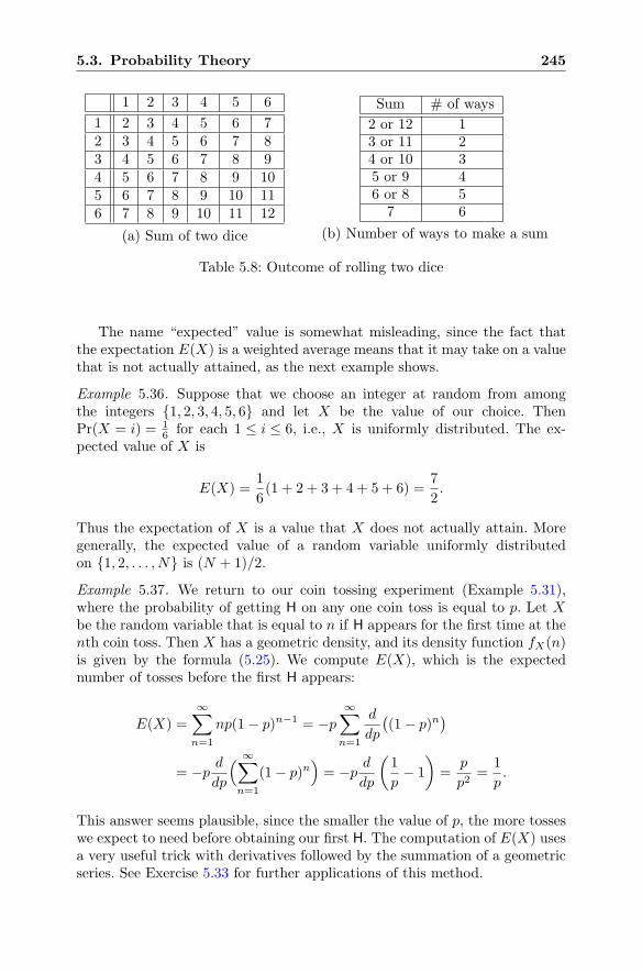
5.3. Probability Theory 245
1 2 3 4 5 6
1 2 3 4 5 6 72 3 4 5 6 7 83 4 5 6 7 8 94 5 6 7 8 9 105 6 7 8 9 10 116 7 8 9 10 11 12
(a) Sum of two dice
Sum # of ways
2 or 12 13 or 11 24 or 10 35 or 9 46 or 8 5
7 6
(b) Number of ways to make a sum
Table 5.8: Outcome of rolling two dice
The name “expected” value is somewhat misleading, since the fact thatthe expectation E(X) is a weighted average means that it may take on a valuethat is not actually attained, as the next example shows.
Example 5.36. Suppose that we choose an integer at random from amongthe integers {1, 2, 3, 4, 5, 6} and let X be the value of our choice. ThenPr(X = i) = 1
6 for each 1 ≤ i ≤ 6, i.e., X is uniformly distributed. The ex-pected value of X is
E(X) =1
6(1 + 2 + 3 + 4 + 5 + 6) =
7
2.
Thus the expectation of X is a value that X does not actually attain. Moregenerally, the expected value of a random variable uniformly distributedon {1, 2, . . . , N} is (N + 1)/2.
Example 5.37. We return to our coin tossing experiment (Example 5.31),where the probability of getting H on any one coin toss is equal to p. Let Xbe the random variable that is equal to n if H appears for the first time at thenth coin toss. Then X has a geometric density, and its density function fX(n)is given by the formula (5.25). We compute E(X), which is the expectednumber of tosses before the first H appears:
E(X) =
∞∑
n=1
np(1− p)n−1 = −p∞∑
n=1
d
dp
((1− p)n
)
= −p ddp
( ∞∑
n=1
(1− p)n)= −p d
dp
(1
p− 1
)=
p
p2=
1
p.
This answer seems plausible, since the smaller the value of p, the more tosseswe expect to need before obtaining our first H. The computation of E(X) usesa very useful trick with derivatives followed by the summation of a geometricseries. See Exercise 5.33 for further applications of this method.
246 5. Combinatorics, Probability, and Information Theory
5.4 Collision Algorithmsand Meet-in-the-Middle Attacks
A simple, yet surprisingly powerful, search method is based on the observationthat it is usually much easier to find matching objects than it is to find aparticular object. Methods of this sort go by many names, including meet-in-the-middle attacks and collision algorithms.
5.4.1 The Birthday Paradox
The fundamental idea behind collision algorithms is strikingly illustrated bythe famous birthday paradox. In a random group of 40 people, consider thefollowing two questions:
(1) What is the probability that someone has the same birthday as you?
(2) What is the probability that at least two people share the same birthday?
It turns out that the answers to (1) and (2) are very different. As a warm-up,we start by answering the easier first question.
A rough answer is that since any one person has a 1-in-365 chance ofsharing your birthday, then in a crowd of 40 people, the probability of some-one having your birthday is approximately 40
365 ≈ 11%. However, this is anoverestimate, since it double counts the occurrences of more than one personin the crowd sharing your birthday.15 The exact answer is obtained by com-puting the probability that none of the people share your birthday and thensubtracting that value from 1.
Pr
(someone hasyour birthday
)= 1− Pr
(none of the 40 peoplehas your birthday
)
= 1−40∏
i=1
Pr
(ith person does nothave your birthday
)
= 1−(364
365
)40
≈ 10.4%.
Thus among 40 strangers, there is only slightly better than a 10% chance thatone of them shares your birthday.
Now consider the second question, in which you win if any two of the peoplein the group have the same birthday. Again it is easier to compute the prob-ability that all 40 people have different birthdays. However, the computation
15If you think that 40365
is the right answer, think about the same situation with 366
people. The probability that someone shares your birthday cannot be 366365
, since that’slarger than 1.
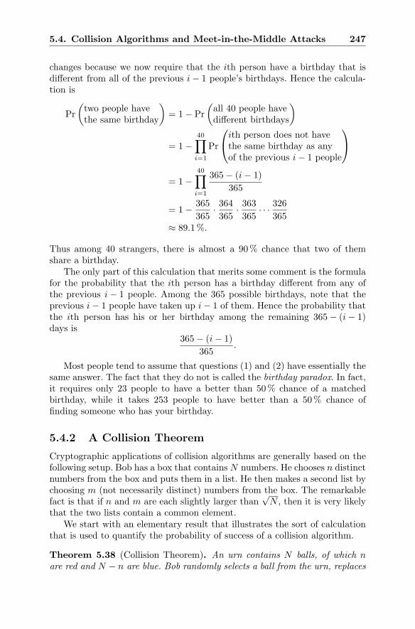
5.4. Collision Algorithms and Meet-in-the-Middle Attacks 247
changes because we now require that the ith person have a birthday that isdifferent from all of the previous i− 1 people’s birthdays. Hence the calcula-tion is
Pr
(two people havethe same birthday
)= 1− Pr
(all 40 people havedifferent birthdays
)
= 1−40∏
i=1
Pr
⎛
⎝ith person does not havethe same birthday as anyof the previous i− 1 people
⎞
⎠
= 1−40∏
i=1
365− (i− 1)
365
= 1− 365
365· 364365
· 363365
· · · 326365
≈ 89.1%.
Thus among 40 strangers, there is almost a 90% chance that two of themshare a birthday.
The only part of this calculation that merits some comment is the formulafor the probability that the ith person has a birthday different from any ofthe previous i− 1 people. Among the 365 possible birthdays, note that theprevious i− 1 people have taken up i− 1 of them. Hence the probability thatthe ith person has his or her birthday among the remaining 365− (i− 1)days is
365− (i− 1)
365.
Most people tend to assume that questions (1) and (2) have essentially thesame answer. The fact that they do not is called the birthday paradox. In fact,it requires only 23 people to have a better than 50% chance of a matchedbirthday, while it takes 253 people to have better than a 50% chance offinding someone who has your birthday.
5.4.2 A Collision Theorem
Cryptographic applications of collision algorithms are generally based on thefollowing setup. Bob has a box that contains N numbers. He chooses n distinctnumbers from the box and puts them in a list. He then makes a second list bychoosing m (not necessarily distinct) numbers from the box. The remarkablefact is that if n and m are each slightly larger than
√N , then it is very likely
that the two lists contain a common element.We start with an elementary result that illustrates the sort of calculation
that is used to quantify the probability of success of a collision algorithm.
Theorem 5.38 (Collision Theorem). An urn contains N balls, of which nare red and N − n are blue. Bob randomly selects a ball from the urn, replaces
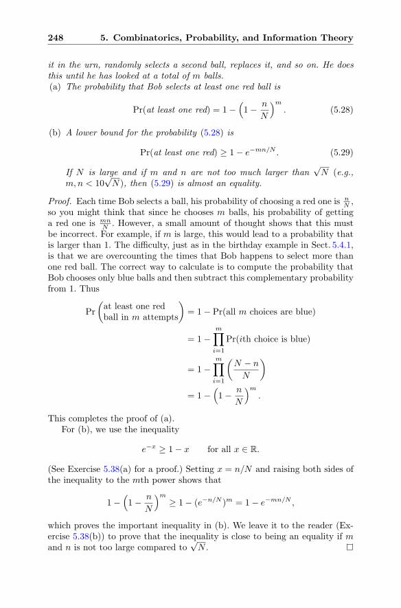
248 5. Combinatorics, Probability, and Information Theory
it in the urn, randomly selects a second ball, replaces it, and so on. He doesthis until he has looked at a total of m balls.(a) The probability that Bob selects at least one red ball is
Pr(at least one red) = 1−(1− n
N
)m. (5.28)
(b) A lower bound for the probability (5.28) is
Pr(at least one red) ≥ 1− e−mn/N . (5.29)
If N is large and if m and n are not too much larger than√N (e.g.,
m,n < 10√N), then (5.29) is almost an equality.
Proof. Each time Bob selects a ball, his probability of choosing a red one is nN ,
so you might think that since he chooses m balls, his probability of gettinga red one is mn
N . However, a small amount of thought shows that this mustbe incorrect. For example, if m is large, this would lead to a probability thatis larger than 1. The difficulty, just as in the birthday example in Sect. 5.4.1,is that we are overcounting the times that Bob happens to select more thanone red ball. The correct way to calculate is to compute the probability thatBob chooses only blue balls and then subtract this complementary probabilityfrom 1. Thus
Pr
(at least one redball in m attempts
)= 1− Pr(all m choices are blue)
= 1−m∏
i=1
Pr(ith choice is blue)
= 1−m∏
i=1
(N − nN
)
= 1−(1− n
N
)m.
This completes the proof of (a).For (b), we use the inequality
e−x ≥ 1− x for all x ∈ R.
(See Exercise 5.38(a) for a proof.) Setting x = n/N and raising both sides ofthe inequality to the mth power shows that
1−(1− n
N
)m≥ 1− (e−n/N )m = 1− e−mn/N ,
which proves the important inequality in (b). We leave it to the reader (Ex-ercise 5.38(b)) to prove that the inequality is close to being an equality if mand n is not too large compared to
√N .
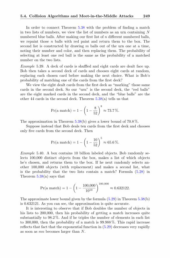
5.4. Collision Algorithms and Meet-in-the-Middle Attacks 249
In order to connect Theorem 5.38 with the problem of finding a matchin two lists of numbers, we view the list of numbers as an urn containing Nnumbered blue balls. After making our first list of n different numbered balls,we repaint those n balls with red paint and return them to the box. Thesecond list is constructed by drawing m balls out of the urn one at a time,noting their number and color, and then replacing them. The probability ofselecting at least one red ball is the same as the probability of a matchednumber on the two lists.
Example 5.39. A deck of cards is shuffled and eight cards are dealt face up.Bob then takes a second deck of cards and chooses eight cards at random,replacing each chosen card before making the next choice. What is Bob’sprobability of matching one of the cards from the first deck?
We view the eight dealt cards from the first deck as “marking” those samecards in the second deck. So our “urn” is the second deck, the “red balls”are the eight marked cards in the second deck, and the “blue balls” are theother 44 cards in the second deck. Theorem 5.38(a) tells us that
Pr(a match) = 1−(1− 8
52
)8
≈ 73.7%.
The approximation in Theorem 5.38(b) gives a lower bound of 70.8%.Suppose instead that Bob deals ten cards from the first deck and chooses
only five cards from the second deck. Then
Pr(a match) = 1−(1− 10
52
)5
≈ 65.6%.
Example 5.40. A box contains 10 billion labeled objects. Bob randomly se-lects 100,000 distinct objects from the box, makes a list of which objectshe’s chosen, and returns them to the box. If he next randomly selects an-other 100,000 objects (with replacement) and makes a second list, whatis the probability that the two lists contain a match? Formula (5.28) inTheorem 5.38(a) says that
Pr(a match) = 1−(1− 100,000
1010
)100,000
≈ 0.632122.
The approximate lower bound given by the formula (5.29) in Theorem 5.38(b)is 0.632121. As you can see, the approximation is quite accurate.
It is interesting to observe that if Bob doubles the number of objects inhis lists to 200,000, then his probability of getting a match increases quitesubstantially to 98.2%. And if he triples the number of elements in each listto 300,000, then the probability of a match is 99.988%. This rapid increasereflects that fact that the exponential function in (5.29) decreases very rapidlyas soon as mn becomes larger than N .
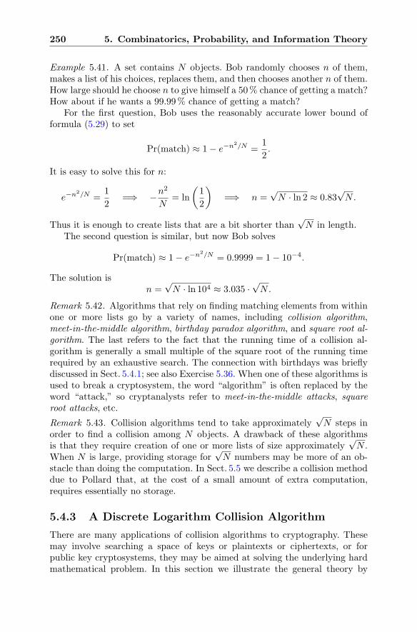
250 5. Combinatorics, Probability, and Information Theory
Example 5.41. A set contains N objects. Bob randomly chooses n of them,makes a list of his choices, replaces them, and then chooses another n of them.How large should he choose n to give himself a 50% chance of getting a match?How about if he wants a 99.99% chance of getting a match?
For the first question, Bob uses the reasonably accurate lower bound offormula (5.29) to set
Pr(match) ≈ 1− e−n2/N =1
2.
It is easy to solve this for n:
e−n2/N =1
2=⇒ −n
2
N= ln
(1
2
)=⇒ n =
√N · ln 2 ≈ 0.83
√N.
Thus it is enough to create lists that are a bit shorter than√N in length.
The second question is similar, but now Bob solves
Pr(match) ≈ 1− e−n2/N = 0.9999 = 1− 10−4.
The solution isn =
√N · ln 104 ≈ 3.035 ·
√N.
Remark 5.42. Algorithms that rely on finding matching elements from withinone or more lists go by a variety of names, including collision algorithm,meet-in-the-middle algorithm, birthday paradox algorithm, and square root al-gorithm. The last refers to the fact that the running time of a collision al-gorithm is generally a small multiple of the square root of the running timerequired by an exhaustive search. The connection with birthdays was brieflydiscussed in Sect. 5.4.1; see also Exercise 5.36. When one of these algorithms isused to break a cryptosystem, the word “algorithm” is often replaced by theword “attack,” so cryptanalysts refer to meet-in-the-middle attacks, squareroot attacks, etc.
Remark 5.43. Collision algorithms tend to take approximately√N steps in
order to find a collision among N objects. A drawback of these algorithmsis that they require creation of one or more lists of size approximately
√N .
When N is large, providing storage for√N numbers may be more of an ob-
stacle than doing the computation. In Sect. 5.5 we describe a collision methoddue to Pollard that, at the cost of a small amount of extra computation,requires essentially no storage.
5.4.3 A Discrete Logarithm Collision Algorithm
There are many applications of collision algorithms to cryptography. Thesemay involve searching a space of keys or plaintexts or ciphertexts, or forpublic key cryptosystems, they may be aimed at solving the underlying hardmathematical problem. In this section we illustrate the general theory by
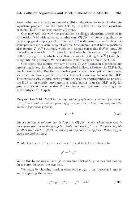
5.4. Collision Algorithms and Meet-in-the-Middle Attacks 251
formulating an abstract randomized collision algorithm to solve the discretelogarithm problem. For the finite field Fp, it solves the discrete logarithmproblem (DLP) in approximately
√p steps.
One may well ask why the probabilistic collision algorithm described inProposition 5.44 with expected running time O
(√N)is interesting, since the
baby step–giant step algorithm from Sect. 2.7 is deterministic and solves thesame problem in the same amount of time. One answer is that both algorithmsalso require O
(√N)storage, which is a serious constraint if N is large. So
the collision algorithm in Proposition 5.44 may be viewed as a warm-up forPollard’s ρ algorithm, which is a collision algorithm taking O
(√N)time, but
using only O(1) storage. We will discuss Pollard’s algorithm in Sect. 5.5.One might also inquire why any of these O
(√N)collision algorithms are
interesting, since, the index calculus described in Sect. 3.8 solves the DLP in Fp
much more rapidly. But there are other groups, such as elliptic curve groups,for which collision algorithms are the fastest known way to solve the DLP.This explains why elliptic curve groups are used in cryptography; at present,the DLP in an elliptic curve group is much harder than the DLP in F
∗p for
groups of about the same size. Elliptic curves and their use in cryptographyis the subject of Chap. 6.
Proposition 5.44. Let G be a group, and let g ∈ G be an element of order N ,i.e., gN = e and no smaller power of g is equal to e. Then, assuming that thediscrete logarithm problem
gx = h (5.30)
has a solution, a solution can be found in O(√N)steps, where each step is
an exponentiation in the group G. (Note that since gN = e, the powering al-gorithm from Sect. 1.3.2 lets us raise g to any power using fewer than 2 log2Ngroup multiplications.)
Proof. The idea is to write x as x = y − z and look for a solution to
gy = h · gz.
We do this by making a list of gy values and a list of h · gz values and lookingfor a match between the two lists.
We begin by choosing random exponents y1, y2, . . . , yn between 1 and Nand computing the values
gy1 , gy2 , gy3 , . . . , gyn in G. (5.31)
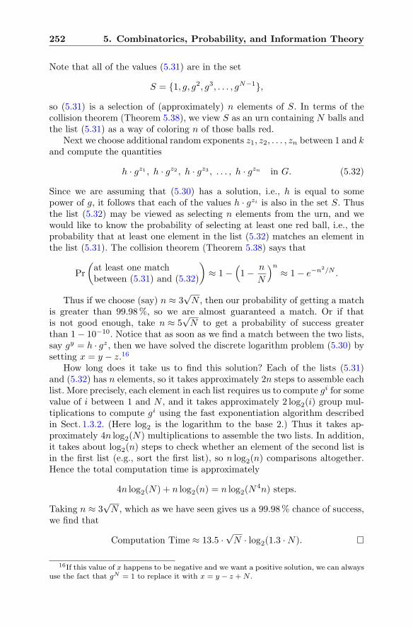
252 5. Combinatorics, Probability, and Information Theory
Note that all of the values (5.31) are in the set
S = {1, g, g2, g3, . . . , gN−1},
so (5.31) is a selection of (approximately) n elements of S. In terms of thecollision theorem (Theorem 5.38), we view S as an urn containing N balls andthe list (5.31) as a way of coloring n of those balls red.
Next we choose additional random exponents z1, z2, . . . , zn between 1 and kand compute the quantities
h · gz1 , h · gz2 , h · gz3 , . . . , h · gzn in G. (5.32)
Since we are assuming that (5.30) has a solution, i.e., h is equal to somepower of g, it follows that each of the values h · gzi is also in the set S. Thusthe list (5.32) may be viewed as selecting n elements from the urn, and wewould like to know the probability of selecting at least one red ball, i.e., theprobability that at least one element in the list (5.32) matches an element inthe list (5.31). The collision theorem (Theorem 5.38) says that
Pr
(at least one matchbetween (5.31) and (5.32)
)≈ 1−
(1− n
N
)n≈ 1− e−n2/N .
Thus if we choose (say) n ≈ 3√N , then our probability of getting a match
is greater than 99.98%, so we are almost guaranteed a match. Or if thatis not good enough, take n ≈ 5
√N to get a probability of success greater
than 1− 10−10. Notice that as soon as we find a match between the two lists,say gy = h · gz, then we have solved the discrete logarithm problem (5.30) bysetting x = y − z.16
How long does it take us to find this solution? Each of the lists (5.31)and (5.32) has n elements, so it takes approximately 2n steps to assemble eachlist. More precisely, each element in each list requires us to compute gi for somevalue of i between 1 and N , and it takes approximately 2 log2(i) group mul-tiplications to compute gi using the fast exponentiation algorithm describedin Sect. 1.3.2. (Here log2 is the logarithm to the base 2.) Thus it takes ap-proximately 4n log2(N) multiplications to assemble the two lists. In addition,it takes about log2(n) steps to check whether an element of the second list isin the first list (e.g., sort the first list), so n log2(n) comparisons altogether.Hence the total computation time is approximately
4n log2(N) + n log2(n) = n log2(N4n) steps.
Taking n ≈ 3√N , which as we have seen gives us a 99.98% chance of success,
we find that
Computation Time ≈ 13.5 ·√N · log2(1.3 ·N).
16If this value of x happens to be negative and we want a positive solution, we can alwaysuse the fact that gN = 1 to replace it with x = y − z +N .
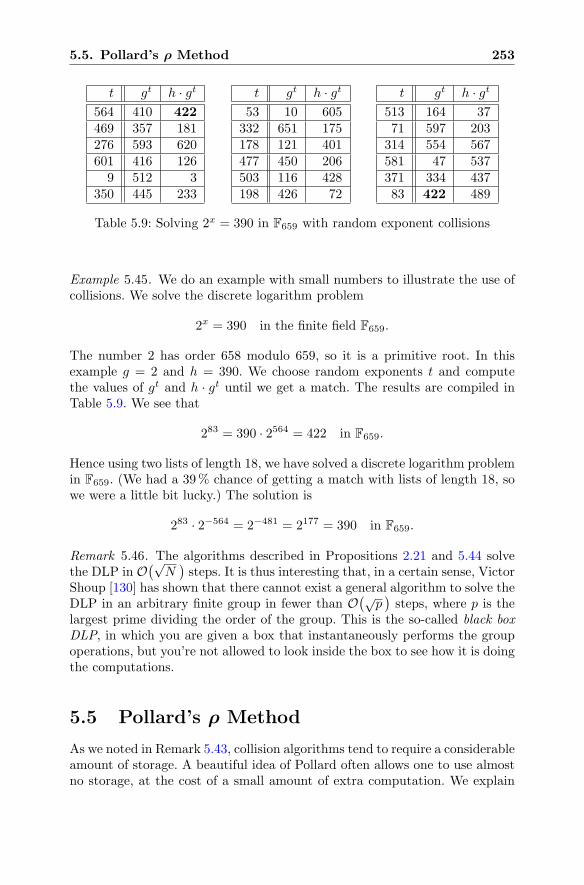
5.5. Pollard’s ρ Method 253
t gt h · gt564 410 422469 357 181276 593 620601 416 126
9 512 3350 445 233
t gt h · gt53 10 605
332 651 175178 121 401477 450 206503 116 428198 426 72
t gt h · gt513 164 3771 597 203
314 554 567581 47 537371 334 43783 422 489
Table 5.9: Solving 2x = 390 in F659 with random exponent collisions
Example 5.45. We do an example with small numbers to illustrate the use ofcollisions. We solve the discrete logarithm problem
2x = 390 in the finite field F659.
The number 2 has order 658 modulo 659, so it is a primitive root. In thisexample g = 2 and h = 390. We choose random exponents t and computethe values of gt and h · gt until we get a match. The results are compiled inTable 5.9. We see that
283 = 390 · 2564 = 422 in F659.
Hence using two lists of length 18, we have solved a discrete logarithm problemin F659. (We had a 39% chance of getting a match with lists of length 18, sowe were a little bit lucky.) The solution is
283 · 2−564 = 2−481 = 2177 = 390 in F659.
Remark 5.46. The algorithms described in Propositions 2.21 and 5.44 solvethe DLP in O
(√N)steps. It is thus interesting that, in a certain sense, Victor
Shoup [130] has shown that there cannot exist a general algorithm to solve theDLP in an arbitrary finite group in fewer than O
(√p)steps, where p is the
largest prime dividing the order of the group. This is the so-called black boxDLP, in which you are given a box that instantaneously performs the groupoperations, but you’re not allowed to look inside the box to see how it is doingthe computations.
5.5 Pollard’s ρ Method
As we noted in Remark 5.43, collision algorithms tend to require a considerableamount of storage. A beautiful idea of Pollard often allows one to use almostno storage, at the cost of a small amount of extra computation. We explain
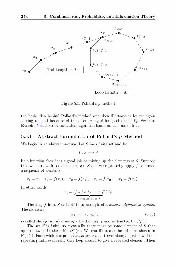
254 5. Combinatorics, Probability, and Information Theory
Tail Length = T
Loop Length = M
x0
x1
x2
x3
xT−1
xT
xT+1
xT+2
xT+3
xT+4
xM+T−4
xM+T−3
xM+T−2
xM+T−1
xM+T
Figure 5.1: Pollard’s ρ method
the basic idea behind Pollard’s method and then illustrate it by yet againsolving a small instance of the discrete logarithm problem in Fp. See alsoExercise 5.44 for a factorization algorithm based on the same ideas.
5.5.1 Abstract Formulation of Pollard’s ρ Method
We begin in an abstract setting. Let S be a finite set and let
f : S −→ S
be a function that does a good job at mixing up the elements of S. Supposethat we start with some element x ∈ S and we repeatedly apply f to createa sequence of elements
x0 = x, x1 = f(x0), x2 = f(x1), x3 = f(x2), x4 = f(x3), . . . .
In other words,xi = (f ◦ f ◦ f ◦ · · · ◦ f
︸ ︷︷ ︸i iterations of f
)(x).
The map f from S to itself is an example of a discrete dynamical system.The sequence
x0, x1, x2, x3, x4, . . . (5.33)
is called the (forward) orbit of x by the map f and is denoted by O+f (x).
The set S is finite, so eventually there must be some element of S thatappears twice in the orbit O+
f (x). We can illustrate the orbit as shown inFig. 5.1. For a while the points x0, x1, x2, x3, . . . travel along a “path” withoutrepeating until eventually they loop around to give a repeated element. Then
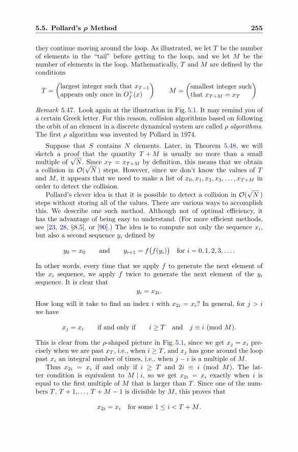
5.5. Pollard’s ρ Method 255
they continue moving around the loop. As illustrated, we let T be the numberof elements in the “tail” before getting to the loop, and we let M be thenumber of elements in the loop. Mathematically, T and M are defined by theconditions
T =
(largest integer such that xT−1
appears only once in O+f (x)
)M =
(smallest integer suchthat xT+M = xT
)
Remark 5.47. Look again at the illustration in Fig. 5.1. It may remind you ofa certain Greek letter. For this reason, collision algorithms based on followingthe orbit of an element in a discrete dynamical system are called ρ algorithms.The first ρ algorithm was invented by Pollard in 1974.
Suppose that S contains N elements. Later, in Theorem 5.48, we willsketch a proof that the quantity T +M is usually no more than a smallmultiple of
√N . Since xT = xT+M by definition, this means that we obtain
a collision in O(√N ) steps. However, since we don’t know the values of T
and M , it appears that we need to make a list of x0, x1, x2, x3, . . . , xT+M inorder to detect the collision.
Pollard’s clever idea is that it is possible to detect a collision in O(√N )
steps without storing all of the values. There are various ways to accomplishthis. We describe one such method. Although not of optimal efficiency, ithas the advantage of being easy to understand. (For more efficient methods,see [23, 28, §8.5], or [90].) The idea is to compute not only the sequence xi,but also a second sequence yi defined by
y0 = x0 and yi+1 = f(f(yi)
)for i = 0, 1, 2, 3, . . . .
In other words, every time that we apply f to generate the next element ofthe xi sequence, we apply f twice to generate the next element of the yisequence. It is clear that
yi = x2i.
How long will it take to find an index i with x2i = xi? In general, for j > iwe have
xj = xi if and only if i ≥ T and j ≡ i (mod M).
This is clear from the ρ-shaped picture in Fig. 5.1, since we get xj = xi pre-cisely when we are past xT , i.e., when i ≥ T , and xj has gone around the looppast xi an integral number of times, i.e., when j − i is a multiple of M .
Thus x2i = xi if and only if i ≥ T and 2i ≡ i (mod M). The lat-ter condition is equivalent to M | i, so we get x2i = xi exactly when i isequal to the first multiple of M that is larger than T . Since one of the num-bers T , T + 1,. . . , T +M − 1 is divisible by M , this proves that
x2i = xi for some 1 ≤ i < T +M .
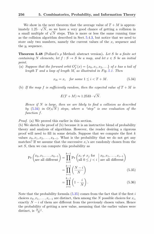
256 5. Combinatorics, Probability, and Information Theory
We show in the next theorem that the average value of T +M is approx-imately 1.25 ·
√N , so we have a very good chance of getting a collision in
a small multiple of√N steps. This is more or less the same running time
as the collision algorithm described in Sect. 5.4.3, but notice that we need tostore only two numbers, namely the current values of the xi sequence andthe yi sequence.
Theorem 5.48 (Pollard’s ρ Method: abstract version). Let S be a finite setcontaining N elements, let f : S → S be a map, and let x ∈ S be an initialpoint.(a) Suppose that the forward orbit O+
f (x) = {x0, x1, x2, . . .} of x has a tail oflength T and a loop of length M, as illustrated in Fig. 5.1. Then
x2i = xi for some 1 ≤ i < T +M . (5.34)
(b) If the map f is sufficiently random, then the expected value of T +M is
E(T +M) ≈ 1.2533 ·√N.
Hence if N is large, then we are likely to find a collision as describedby (5.34) in O(
√N ) steps, where a “step” is one evaluation of the
function f .
Proof. (a) We proved this earlier in this section.(b) We sketch the proof of (b) because it is an instructive blend of probabilitytheory and analysis of algorithms. However, the reader desiring a rigorousproof will need to fill in some details. Suppose that we compute the first kvalues x0, x1, x2, . . . , xk−1. What is the probability that we do not get anymatches? If we assume that the successive xi’s are randomly chosen from theset S, then we can compute this probability as
Pr
(x0, x1, . . . , xk−1
are all different
)=
k−1∏
i=1
Pr
(xi �= xj forall 0 ≤ j < i
∣∣∣∣x0, x1, . . . , xi−1
are all different
)
=
k−1∏
i=1
(N − iN
)(5.35)
=
k−1∏
i=1
(1− i
N
). (5.36)
Note that the probability formula (5.35) comes from the fact that if the first ichoices x0, x1, . . . , xi−1 are distinct, then among the N possible choices for xi,exactly N − i of them are different from the previously chosen values. Hencethe probability of getting a new value, assuming that the earlier values weredistinct, is N−i
N .
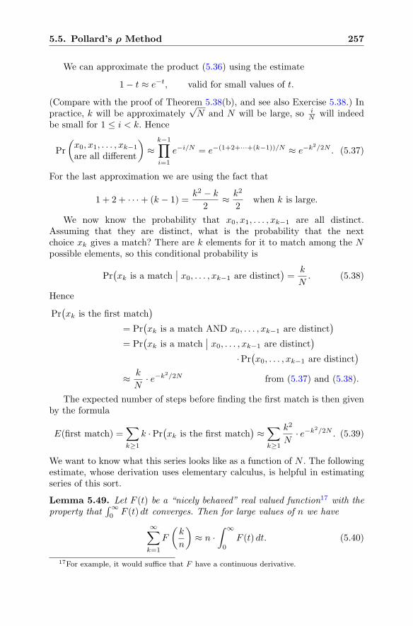
5.5. Pollard’s ρ Method 257
We can approximate the product (5.36) using the estimate
1− t ≈ e−t, valid for small values of t.
(Compare with the proof of Theorem 5.38(b), and see also Exercise 5.38.) Inpractice, k will be approximately
√N and N will be large, so i
N will indeedbe small for 1 ≤ i < k. Hence
Pr
(x0, x1, . . . , xk−1
are all different
)≈
k−1∏
i=1
e−i/N = e−(1+2+···+(k−1))/N ≈ e−k2/2N . (5.37)
For the last approximation we are using the fact that
1 + 2 + · · ·+ (k − 1) =k2 − k
2≈ k2
2when k is large.
We now know the probability that x0, x1, . . . , xk−1 are all distinct.Assuming that they are distinct, what is the probability that the nextchoice xk gives a match? There are k elements for it to match among the Npossible elements, so this conditional probability is
Pr(xk is a match
∣∣ x0, . . . , xk−1 are distinct
)=
k
N. (5.38)
Hence
Pr(xk is the first match
)
= Pr(xk is a match AND x0, . . . , xk−1 are distinct
)
= Pr(xk is a match
∣∣ x0, . . . , xk−1 are distinct
)
·Pr(x0, . . . , xk−1 are distinct
)
≈ k
N· e−k2/2N from (5.37) and (5.38).
The expected number of steps before finding the first match is then givenby the formula
E(first match) =∑
k≥1
k ·Pr(xk is the first match
)≈∑
k≥1
k2
N· e−k2/2N . (5.39)
We want to know what this series looks like as a function of N . The followingestimate, whose derivation uses elementary calculus, is helpful in estimatingseries of this sort.
Lemma 5.49. Let F (t) be a “nicely behaved” real valued function17 with theproperty that
∫∞0F (t) dt converges. Then for large values of n we have
∞∑
k=1
F
(k
n
)≈ n ·
∫ ∞
0
F (t) dt. (5.40)
17For example, it would suffice that F have a continuous derivative.
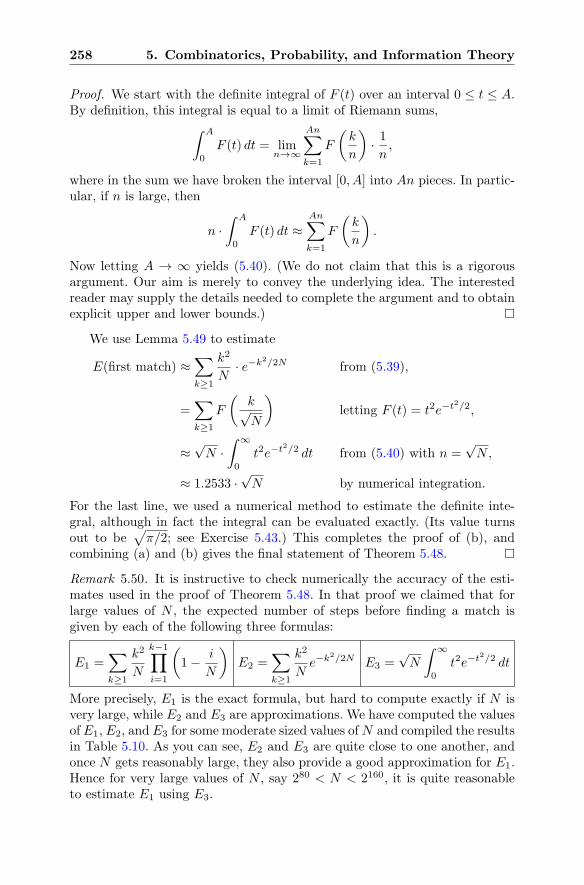
258 5. Combinatorics, Probability, and Information Theory
Proof. We start with the definite integral of F (t) over an interval 0 ≤ t ≤ A.By definition, this integral is equal to a limit of Riemann sums,
∫ A
0
F (t) dt = limn→∞
An∑
k=1
F
(k
n
)· 1n,
where in the sum we have broken the interval [0, A] into An pieces. In partic-ular, if n is large, then
n ·∫ A
0
F (t) dt ≈An∑
k=1
F
(k
n
).
Now letting A → ∞ yields (5.40). (We do not claim that this is a rigorousargument. Our aim is merely to convey the underlying idea. The interestedreader may supply the details needed to complete the argument and to obtainexplicit upper and lower bounds.)
We use Lemma 5.49 to estimate
E(first match) ≈∑
k≥1
k2
N· e−k2/2N from (5.39),
=∑
k≥1
F
(k√N
)letting F (t) = t2e−t2/2,
≈√N ·∫ ∞
0
t2e−t2/2 dt from (5.40) with n =√N ,
≈ 1.2533 ·√N by numerical integration.
For the last line, we used a numerical method to estimate the definite inte-gral, although in fact the integral can be evaluated exactly. (Its value turnsout to be
√π/2; see Exercise 5.43.) This completes the proof of (b), and
combining (a) and (b) gives the final statement of Theorem 5.48.
Remark 5.50. It is instructive to check numerically the accuracy of the esti-mates used in the proof of Theorem 5.48. In that proof we claimed that forlarge values of N , the expected number of steps before finding a match isgiven by each of the following three formulas:
E1 =∑
k≥1
k2
N
k−1∏
i=1
(1− i
N
)E2 =
∑
k≥1
k2
Ne−k2/2N E3 =
√N
∫ ∞
0
t2e−t2/2 dt
More precisely, E1 is the exact formula, but hard to compute exactly if N isvery large, while E2 and E3 are approximations. We have computed the valuesof E1, E2, and E3 for some moderate sized values ofN and compiled the resultsin Table 5.10. As you can see, E2 and E3 are quite close to one another, andonce N gets reasonably large, they also provide a good approximation for E1.Hence for very large values of N , say 280 < N < 2160, it is quite reasonableto estimate E1 using E3.
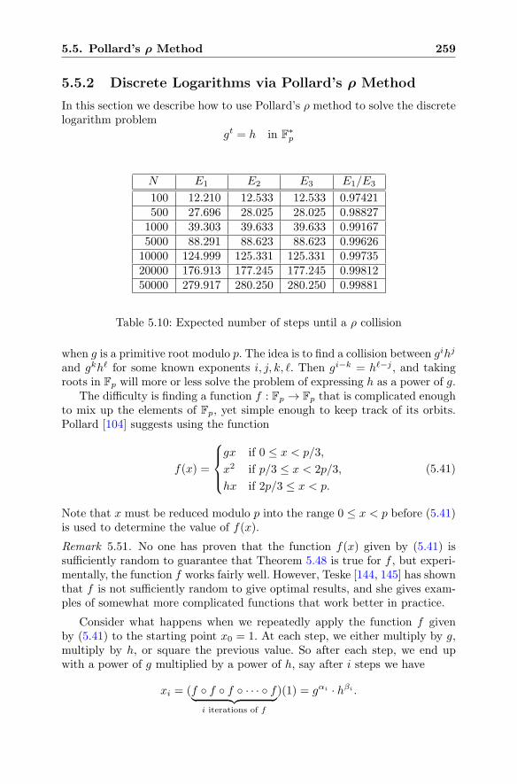
5.5. Pollard’s ρ Method 259
5.5.2 Discrete Logarithms via Pollard’s ρ Method
In this section we describe how to use Pollard’s ρ method to solve the discretelogarithm problem
gt = h in F∗p
N E1 E2 E3 E1/E3
100 12.210 12.533 12.533 0.97421500 27.696 28.025 28.025 0.988271000 39.303 39.633 39.633 0.991675000 88.291 88.623 88.623 0.99626
10000 124.999 125.331 125.331 0.9973520000 176.913 177.245 177.245 0.9981250000 279.917 280.250 280.250 0.99881
Table 5.10: Expected number of steps until a ρ collision
when g is a primitive root modulo p. The idea is to find a collision between gihj
and gkh� for some known exponents i, j, k, �. Then gi−k = h�−j , and takingroots in Fp will more or less solve the problem of expressing h as a power of g.
The difficulty is finding a function f : Fp → Fp that is complicated enoughto mix up the elements of Fp, yet simple enough to keep track of its orbits.Pollard [104] suggests using the function
f(x) =
⎧⎪⎨
⎪⎩
gx if 0 ≤ x < p/3,
x2 if p/3 ≤ x < 2p/3,
hx if 2p/3 ≤ x < p.
(5.41)
Note that x must be reduced modulo p into the range 0 ≤ x < p before (5.41)is used to determine the value of f(x).
Remark 5.51. No one has proven that the function f(x) given by (5.41) issufficiently random to guarantee that Theorem 5.48 is true for f , but experi-mentally, the function f works fairly well. However, Teske [144, 145] has shownthat f is not sufficiently random to give optimal results, and she gives exam-ples of somewhat more complicated functions that work better in practice.
Consider what happens when we repeatedly apply the function f givenby (5.41) to the starting point x0 = 1. At each step, we either multiply by g,multiply by h, or square the previous value. So after each step, we end upwith a power of g multiplied by a power of h, say after i steps we have
xi = (f ◦ f ◦ f ◦ · · · ◦ f︸ ︷︷ ︸
i iterations of f
)(1) = gαi · hβi .
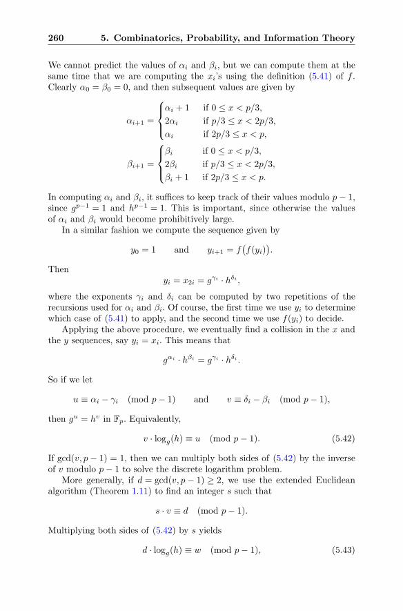
260 5. Combinatorics, Probability, and Information Theory
We cannot predict the values of αi and βi, but we can compute them at thesame time that we are computing the xi’s using the definition (5.41) of f .Clearly α0 = β0 = 0, and then subsequent values are given by
αi+1 =
⎧⎪⎨
⎪⎩
αi + 1 if 0 ≤ x < p/3,
2αi if p/3 ≤ x < 2p/3,
αi if 2p/3 ≤ x < p,
βi+1 =
⎧⎪⎨
⎪⎩
βi if 0 ≤ x < p/3,
2βi if p/3 ≤ x < 2p/3,
βi + 1 if 2p/3 ≤ x < p.
In computing αi and βi, it suffices to keep track of their values modulo p− 1,since gp−1 = 1 and hp−1 = 1. This is important, since otherwise the valuesof αi and βi would become prohibitively large.
In a similar fashion we compute the sequence given by
y0 = 1 and yi+1 = f(f(yi)
).
Thenyi = x2i = gγi · hδi ,
where the exponents γi and δi can be computed by two repetitions of therecursions used for αi and βi. Of course, the first time we use yi to determinewhich case of (5.41) to apply, and the second time we use f(yi) to decide.
Applying the above procedure, we eventually find a collision in the x andthe y sequences, say yi = xi. This means that
gαi · hβi = gγi · hδi .
So if we let
u ≡ αi − γi (mod p− 1) and v ≡ δi − βi (mod p− 1),
then gu = hv in Fp. Equivalently,
v · logg(h) ≡ u (mod p− 1). (5.42)
If gcd(v, p− 1) = 1, then we can multiply both sides of (5.42) by the inverseof v modulo p− 1 to solve the discrete logarithm problem.
More generally, if d = gcd(v, p− 1) ≥ 2, we use the extended Euclideanalgorithm (Theorem 1.11) to find an integer s such that
s · v ≡ d (mod p− 1).
Multiplying both sides of (5.42) by s yields
d · logg(h) ≡ w (mod p− 1), (5.43)
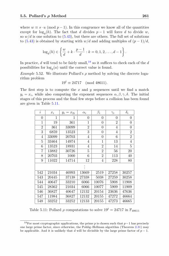
5.5. Pollard’s ρ Method 261
where w ≡ s · u (mod p− 1). In this congruence we know all of the quantitiesexcept for logg(h). The fact that d divides p− 1 will force d to divide w,so w/d is one solution to (5.43), but there are others. The full set of solutionsto (5.43) is obtained by starting with w/d and adding multiples of (p− 1)/d,
logg(h) ∈{w
d+ k · p− 1
d: k = 0, 1, 2, . . . , d− 1
}.
In practice, d will tend to be fairly small,18 so it suffices to check each of the dpossibilities for logg(a) until the correct value is found.
Example 5.52. We illustrate Pollard’s ρ method by solving the discrete loga-rithm problem
19t ≡ 24717 (mod 48611).
The first step is to compute the x and y sequences until we find a matchyi = xi, while also computing the exponent sequences α, β, γ, δ. The initialstages of this process and the final few steps before a collision has been foundare given in Table 5.11.
i xi yi = x2i αi βi γi δi
0 1 1 0 0 0 01 19 361 1 0 2 02 361 33099 2 0 4 03 6859 13523 3 0 4 24 33099 20703 4 0 6 25 33464 14974 4 1 13 46 13523 18931 4 2 14 57 13882 30726 5 2 56 208 20703 1000 6 2 113 409 11022 14714 12 4 228 80
...542 21034 46993 13669 2519 27258 30257543 20445 37138 27338 5038 27259 30258544 40647 33210 6066 10076 5908 11908545 28362 21034 6066 10077 5909 11909546 36827 40647 12132 20154 23636 47636547 11984 36827 12132 20155 47272 46664548 33252 33252 12133 20155 47273 46665
Table 5.11: Pollard ρ computations to solve 19t = 24717 in F48611
18For most cryptographic applications, the prime p is chosen such that p−1 has preciselyone large prime factor, since otherwise, the Pohlig–Hellman algorithm (Theorem 2.31) maybe applicable. And it is unlikely that d will be divisible by the large prime factor of p− 1.
262 5. Combinatorics, Probability, and Information Theory
From the table we see that x1096 = x548 = 33252 in F48611. The associatedexponent values are
α548 = 12133, β548 = 20155, γ548 = 47273, δ548 = 46665,
so we know that
1912133 · 2471720155 = 1947273 · 2471746665 in F48611.
(Before proceeding, we should probably check this equality to make sure thatwe didn’t made an arithmetic error.) Moving the powers of 19 to one sideand the powers of 24717 to the other side yields 19−35140 = 2471726510, andadding 48610 = p− 1 to the exponent of 19 gives
1913470 = 2471726510 in F48611. (5.44)
We next observe that
gcd(26510, 48610) = 10 and 970 · 26510 ≡ 10 (mod 48610).
Raising both sides of (5.44) to the 970th power yields
1913470·970 = 1913065900 = 1938420 = 2471710 in F48611.
Hence
10 · log19(24717) ≡ 38420 (mod 48610),
which means that
log19(24717) ≡ 3842 (mod 4861).
The possible values for the discrete logarithm are obtained by adding multiplesof 4861 to 3842, so log19(24717) is one of the numbers in the set
{3842, 8703, 13564, 18425, 23286, 28147, 33008, 37869, 42730, 47591}.
To complete the solution, we compute 19 raised to each of these 10 valuesuntil we find the one that is equal to 24717:
193842 = 16580, 198703 = 29850, 1913564 = 23894, 1918425 = 20794,
1923286 = 10170, 1928147 = 32031, 1933008 = 18761, 1937869 = 24717 .
This gives the solution log19(24717) = 37869. We check our answer
1937869 = 24717 in F48611. �
5.6. Information Theory 263
5.6 Information Theory
In 1948 and 1949, Claude Shannon published two papers [126, 127] that formthe mathematical foundation of modern cryptography. In these papers hedefines the concept of perfect (or unconditional) secrecy, introduces the idea ofentropy of natural language and statistical analysis, provides the first proofsof security using probability theory, and gives precise connections betweenprovable security and the size of the key, plaintext, and ciphertext spaces.
In public key cryptography, one is interested in how computationally dif-ficult it is to break the system. The issue of security is thus a relative one—agiven cryptosystem is hard to break if one assumes that some underlyingproblem is hard to solve. It requires some care to formulate these conceptsproperly. In this section we briefly introduce Shannon’s ideas and explain theirrelevance to symmetric key systems. In [127], Shannon develops a theory ofsecurity for cryptosystems that assumes that no bounds are placed on the com-putational resources that may be brought to bear against them. For example,symmetric ciphers such as the simple substitution cipher (Sect. 1.1) and theVigenere cipher (Sect. 5.2) are not computationally secure. With unlimitedresources—indeed with very limited resources—an adversary can easily breakthese ciphers. If we seek unconditional security, we must either seek new algo-rithms or modify the implementation of known algorithms. In fact, Shannonshows that perfectly secure cryptosystems must have at least as many keys asplaintexts and that every key must be used with equal probability. This meansthat most practical cryptosystems are not unconditionally secure. We discussthe notion of perfect security in Sect. 5.6.1.
In [126] Shannon develops a mathematical theory that measures theamount of information that is revealed by a random variable. When the ran-dom variable represents the possible plaintexts or ciphertexts or keys of acipher that is used to encrypt a natural language such as English, we obtaina framework for the rigorous mathematical study of cryptographic security.Shannon adopted the word entropy for this measure because of its formalsimilarity to Boltzmann’s definition of entropy in statistical mechanics, andalso because Shannon viewed language as a stochastic process, i.e., as a sys-tem governed by probabilities that produces a sequence of symbols. Later,the physicist E.T. Jaynes [60] argued that thermodynamic entropy could beinterpreted as an application of a certain information-theoretic entropy. Asa measure of “uncertainty” of a system, the logarithmic formula for entropyis determined, up to a constant, by requiring that it be continuous, mono-tonic, and satisfy a certain additive property. We discuss information-theoreticentropy and its application to cryptography in Sect. 5.6.2.
5.6.1 Perfect Secrecy
A cryptosystem has perfect secrecy if the interception of a ciphertext givesthe cryptanalyst no information about the underlying plaintext and no
264 5. Combinatorics, Probability, and Information Theory
information about any future encrypted messages. To formalize this concept,we introduce random variables M , C, and K representing the finite numberof possible messages, ciphertexts, and keys. In other words, M is a randomvariable whose values are the possible messages (plaintexts), C is a randomvariable whose values are the possible ciphertexts, and K is a random vari-able whose values are the possible keys used for encryption and decryption.We let fM , fC , and fK be the associated density functions.19 The density func-tions fM , fK , and fC are related to one another via the encryption/decryptionformula dk(ek(m)) = m, which we will exploit shortly to prove (5.47).
We also have the joint densities and the conditional densities of all pairsof these random variables, such as f(C,M)(c,m) and fC|M (c | m), and soforth. We will let the variable names simplify the notation. For example,we write f(c | m) for fC|M (c | m), the conditional probability density of therandom variables C and M , i.e.,
f(c | m) = Pr(C = c given that M = m).
Similarly, we write f(m) for fM (m), the probability that M = m.
Definition. A cryptosystem has perfect secrecy if
f(m | c) = f(m) for all m ∈M and all c ∈ C. (5.45)
What does (5.45) mean? It says that the probability of any particularplaintext, Pr(M = m), is independent of the ciphertext. Intuitively, this meansthat the ciphertext reveals no knowledge of the plaintext.
Bayes’s formula (Theorem 5.33) says that
f(m | c)f(c) = f(c | m)f(m),
which implies that perfect secrecy is equivalent to the condition
f(c | m) = f(c) for all c ∈ C and all m ∈M with f(m) �= 0. (5.46)
Formula (5.46) says that the appearance of any particular ciphertext is equallylikely, independent of the plaintext.
If we know fK and fM , then fC is determined. To see this, we note thatfor a given key k, the probability that the ciphertext equals c is the same asthe probability that the decryption of c is the plaintext, assuming of course
19As is typical, we have omitted reference to the underlying sample spaces. To be com-pletely explicit, we have three probability spaces with sample spaces ΩM , ΩC , and ΩK andprobability functions PrM , PrC , and PrK . Then M , C and K are random variables
M : ΩM → M, K : ΩK → K, C : ΩC → C.Then by definition, the density function fM is
fM (m) = Pr(M = m) = PrM({ω ∈ ΩM : M(ω) = m}),
and similarly for K and C.
5.6. Information Theory 265
that c is the encryption of some plaintext for key k. This allows us to com-pute the total probability fC(c) by summing over all possible keys and usingthe decomposition formula (5.20) of Proposition 5.24, or more precisely, itsgeneralization described in Exercise 5.23. As usual, we let K denote the setof all possible keys and ek : M → C and dk : C → M be the encryptionand decryption functions for the key k ∈ K. Then the probability that theciphertext is equal to c is given by the formula
m1 m2 m3
k1 c2 c1 c3k2 c1 c3 c2
Table 5.12: Encryption of messages with keys k1 and k2
fC(c) =∑
k ∈ K suchthat c = ek(m)for some m ∈ M
fK(k)fM(dk(c)
); (5.47)
see also Exercise 5.47. We note that if the encryption map ek :M→ C is ontofor all keys k, which is often true in practice, then the sum in (5.47) is overall k ∈ K.Example 5.53. Consider the Shift Cipher described in Sect. 1.1. Suppose thateach of the 26 possible keys (shift amounts) is chosen with equal probabilityand that each plaintext character is encrypted using a new, randomly chosen,shift amount. Then it is not hard to check that the resulting cryptosystemhas perfect secrecy; see Exercise 5.46.
Recall that an encryption function is one-to-one, meaning that each mes-sage gives rise to a unique ciphertext. This implies that there are at least asmany ciphertexts as plaintexts (messages). Perfect secrecy gives additionalrestrictions on the relative size of the key, message, and ciphertext spaces.We first investigate an example of a (tiny) cryptosystem that does not haveperfect secrecy.
Example 5.54. Suppose that a cryptosystem has two keys k1 and k2, threemessages m1, m2, and m3, and three ciphertexts c1, c2, and c3. Assume thatthe density function for the message random variable satisfies
fM (m1) = fM (m2) =1
4and fM (m3) =
1
2. (5.48)
Suppose further that Table 5.12 describes how the different keys act on themessages to produce ciphertexts.
For example, the encryption of the plaintext m1 with the key k1 is theciphertext c2. Under the assumption that the keys are used with equal prob-ability, we can use (5.47) to compute the probability that the ciphertext isequal to c1:
266 5. Combinatorics, Probability, and Information Theory
f(c1) = f(k1)fM (dk1(c1)) + f(k2)fM (dk2
(c1))
= f(k1)f(m2) + f(k2)f(m1)
=1
2· 14+
1
2· 14=
1
4.
On the other hand, we see from the table that f(c1 | m3) = 0. Hence thiscryptosystem does not have perfect secrecy.
This matches our intuition, since it is clear that seeing a ciphertext leakssome information about the plaintext. For example, if we see the ciphertext c1,then we know that the message was either m1 or m2, it cannot be m3.
As noted earlier, the number of ciphertexts must be at least as large asthe number of plaintexts, since otherwise, decryption is not possible. It turnsout that one consequence of perfect secrecy is that the number of keys mustalso be at least as large as the number of plaintexts.
Proposition 5.55. If a cryptosystem has perfect secrecy, then #K ≥ #C+,where C+ = {m ∈ M : f(m) > 0} is the set of plaintexts that have a positiveprobability of being selected.
Proof. We start by fixing some ciphertext c ∈ C with f(c) > 0. Perfect secrecyin the form of (5.46) tells us that
f(c | m) = f(c) > 0 for all m ∈ C+.
This says that there is a positive probability that m ∈ C+ encrypts to c,so in particular there is at least one key k satisfying ek(m) = c. Further, ifwe start with a different plaintext m′ ∈ C+, then we get a different key k′,since otherwise ek(m) = c = ek(m
′), which would contradict the one-to-oneproperty of ek.
To recapitulate, we have shown that for every m ∈ C+, the set
{k ∈ K : ek(m) = c}
is nonempty, and further, these sets are disjoint for different m’s. Thus eachplaintext m ∈ C+ is matched with one or more keys, and different m’s arematched with different keys, which shows that the number of keys is at leastas large as the number of plaintexts in C+.
Given the restriction on the relative sizes of the key, ciphertext, and plain-text spaces in systems with perfect secrecy, namely
#K ≥ #M and #C ≥ #M,
it is most efficient to assume that the key space, the plaintext space, andthe ciphertext space are all of equal size. Assuming this, Shannon proves atheorem characterizing perfect secrecy.
5.6. Information Theory 267
Theorem 5.56. Suppose that a cryptosystem satisfies
#K = #M = #C,
i.e., the numbers of keys, plaintexts, and ciphertexts are all equal. Then thesystem has perfect secrecy if and only if the following two conditions hold :(a) Each key k ∈ K is used with equal probability.
(b) For a given message m ∈ M and ciphertext c ∈ C, there is exactly onekey k ∈ K that encrypts m to c.
Proof. Suppose first that a cryptosystem has perfect secrecy. We start byverifying (b). For any plaintext m ∈ M and ciphertext c ∈ C, consider the(possibly empty) set of keys that encrypt m to c,
Sm,c ={k ∈ K : ek(m) = c
}.
We are going to prove that if the cryptosystem has perfect secrecy, then infact #Sm,c = 1 for every m ∈ M and every c ∈ C, which is equivalent tostatement (b) of the theorem. We do this in three steps.
Claim 1. If m �= m′, then Sm,c ∩ Sm′,c = ∅.
Suppose that k ∈ Sm,c ∩ Sm′,c. Then ek(m) = c = ek(m′), which implies that
m = m′, since the encryption function ek is injective. This proves Claim 1.
Claim 2. If the cryptosystem has perfect secrecy, then Sm,c is nonemptyfor every m and c.
We use the perfect secrecy assumption in the form f(m, c) = f(m)f(c). Weknow that every m ∈M is a valid plaintext for at least one key, so f(m) > 0.Similarly, every c ∈ C appears as the encryption of at least one plaintext usingsome key, so f(c) > 0. Hence perfect secrecy implies that
f(m, c) > 0 for all m ∈M and all c ∈ C. (5.49)
But the formula f(m, c) > 0 is simply another way of saying that c is apossible encryption of m. Hence there must be at least one key k ∈ K satis-fying ek(m) = c, i.e., there is some key k ∈ Sm,c. This completes the proof ofClaim 2.
Claim 3. If the cryptosystem has perfect secrecy, then #Sm,c = 1.
Fix a ciphertext c ∈ C. Then
#K ≥ #
( ⋃
m∈MSm,c
)since K contains every Sm,c,
=∑
m∈M#Sm,c since the Sm,c are disjoint from Claim 1,
268 5. Combinatorics, Probability, and Information Theory
≥ #M since #Sm,c ≥ 1 from Claim 2,
= #K since #K = #M by assumption.
Thus all of these inequalities are equalities, so in particular,
∑
m∈M#Sm,c = #M.
Then the fact (Claim 2) that every #Sm,c is greater than or equal to 1 impliesthat every #Sm,c must equal 1. This completes the proof of Claim 3.
As noted above, Claim 3 is equivalent to statement (b) of the theorem. We turnnow to statement (a). Consider the set of triples
(k,m, c) ∈ K ×M× C satisfying ek(m) = c.
Clearly k and m determine a unique value for c, and (b) says that m and cdetermine a unique value for k. It is also not hard, using a similar argumentand the assumption that #M = #C, to show that c and k determine a uniquevalue for m; see Exercise 5.48.
For any triple (k,m, c) satisfying ek(m) = c, we compute
f(m) = f(m | c) by perfect secrecy,
=f(m, c)
f(c)definition of conditional probability,
=f(m, k)
f(c)since any two of m, k, c determine the third,
=f(m)f(k)
f(c)since M and K are independent.
(There are cryptosystems in which the message forms part of the key; see forexample Exercise 5.19, in which case M and K would not be independent.)
Canceling f(m) from both sides, we have shown that
f(k) = f(c) for every k ∈ K and every c ∈ C. (5.50)
Note that our proof shows that (5.50) is true for every k and every c, becauseExercise 5.48 tells us that for every (k, c) there is a (unique) m satisfy-ing ek(m) = c.
We sum (5.50) over all c ∈ C and divide by #C to obtain
f(k) =1
#C∑
c∈Cf(c) =
1
#C .
This shows that f(k) is constant, independent of the choice of k ∈ K, whichis precisely the assertion of (a). At the same time we have proven the usefulfact that f(c) is constant, i.e., every ciphertext is used with equal probability.
5.6. Information Theory 269
In the other direction, if a cryptosystem has properties (a) and (b), thenthe steps outlined to prove perfect secrecy of the shift cipher in Exercise 5.46can be applied in this more general setting. We leave the details to the reader.
Example 5.57 (The one-time pad). Vernam’s one-time pad, patented in 1917,is an extremely simple, perfectly secret, albeit very inefficient, cryptosystem.The key k consists of a string of binary digits k0k1 . . . kN . It is used to encrypt abinary plaintext stringm = m0m1 . . .mN by XOR’ing the two strings togetherbit by bit. See (1.12) on page 44 for a description of the XOR operation, whichfor convenience we will denote by ⊕. Then the ciphertext c = c0c1 . . . cN isgiven by
ci = ki ⊕mi for i = 0, 1, . . . , N .
Each key is used only once and then discarded, whence the name of the system.Since every key is used with equal probability, and since there is exactly onekey that encrypts a given m to a given c, namely the key m⊕ c, Theorem 5.56shows that Vernam’s one-time pad has perfect secrecy.
Unfortunately, if Bob and Alice want to use a Vernam one-time pad toexchange N bits of information, they must already know N bits of sharedsecret information to use as the key. This makes one-time pads much too inef-ficient for large-scale communication networks. However, there are situationsin which they have been used, such as top secret communications betweendiplomatic offices or for short messages between spies and their home bases.
It is also worth noting that a one-time pad remains completely secure onlyas long as its keys are never reused. When a key pad is used more than once,either due to error or to the difficulty of providing enough key material, thenthe cryptosystem may be vulnerable to cryptanalysis. This occurred in thereal world when the Soviet Union reused some one-time pads during WorldWar II. The United States mounted a massive cryptanalytic effort called theVENONA project that successfully decrypted a number of documents.
5.6.2 Entropy
In efficient cryptosystems, a single key must be used to encrypt many differ-ent plaintexts, so perfect secrecy is not possible. At best we can hope to buildcryptosystems that are computationally secure. Unfortunately, anything lessthan perfect secrecy leaves open the possibility that a list of ciphertexts willreveal significant information about the key. To study this phenomenon, Shan-non introduced the concept of entropy, which is a measure of the uncertaintyin a system. Thus if we view fX(x) = Pr(X = x) as being the probability thatthe outcome of a certain experiment is equal to x, then the entropy of X willbe small if the outcome of a single experiment reveals a significant amount ofinformation about the random variable X.
Let X be a random variable taking on finitely many values x1, x2, . . . , xn,and let p1, p2, . . . , pn be the associated probabilities,
270 5. Combinatorics, Probability, and Information Theory
pi = fX(xi) = Pr(X = xi).
The entropy H(X) of X is a number that depends only on the probabili-ties p1, . . . , pn of the possible outcomes of X, so we write20
H(X) = H(p1, . . . , pn).
We would like to capture the idea that H is the expected value of a randomvariable that measures the uncertainty that the outcome xi has occurred. Thusthe larger the value of H(X), the less information about X that is revealedby the outcome of an experiment.
What properties should H possess?
Property H1 The function H should be continuous in the variables pi.
This reflects the intuition that a small change in pi should produce a smallchange in the amount of information revealed by X.
Property H2 Let Xn be the random variable that is uniformly distributed
on a set {x1, . . . , xn}, i.e., the random variable Xn has n possible outcomes,each occurring with probability 1
n . Then
H(Xn+1) > H(Xn) for all n ≥ 1.
This reflects the intuition that if all outcomes are equally likely, then theuncertainty should increase as the number of outcomes increases.
Property H3 The third property is subtler. It says that if an outcome
of X is thought of as a choice, and if that choice can be broken down intotwo successive choices, then the original value of H is a weighted sum of thevalues of H for the successive choices. In order to quantify this intuition, weconsider random variables X, Y , and Z1, . . . , Zn taking values in the sets
X : Ω −→ {xij : 1 ≤ i ≤ n and 1 ≤ j ≤ mi},Y :Ω −→ {Z1, . . . , Zn},Zi :Ω −→ {xij : 1 ≤ j ≤ mi},
and satisfying
Pr(X = xij) = Pr(Y = Zi and Zi = xij).
This reflects the intuition that the outcome X = xij is being broken downinto the successive choices Y = Zi followed by Zi = xij . Then Property H3 isthe formula
H(X) = H(Y ) +
n∑
i=1
Pr(Y = Zi)H(Zi).
20Although this notation is useful, it is important to remember that the domain of His the set of random variables, not the set of n-tuples for some fixed value of n. Thus thedomain of H is itself a set of functions.
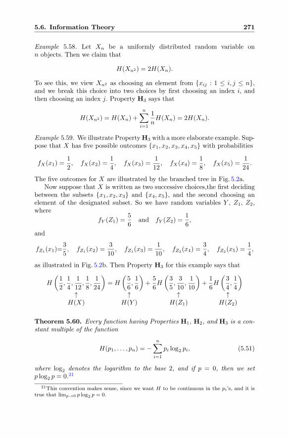
5.6. Information Theory 271
Example 5.58. Let Xn be a uniformly distributed random variable onn objects. Then we claim that
H(Xn2) = 2H(Xn).
To see this, we view Xn2 as choosing an element from {xij : 1 ≤ i, j ≤ n},and we break this choice into two choices by first choosing an index i, andthen choosing an index j. Property H3 says that
H(Xn2) = H(Xn) +
n∑
i=1
1
nH(Xn) = 2H(Xn).
Example 5.59. We illustrate PropertyH3 with a more elaborate example. Sup-pose that X has five possible outcomes {x1, x2, x3, x4, x5} with probabilities
fX(x1) =1
2, fX(x2) =
1
4, fX(x3) =
1
12, fX(x4) =
1
8, fX(x5) =
1
24.
The five outcomes for X are illustrated by the branched tree in Fig. 5.2a.Now suppose that X is written as two successive choices,the first deciding
between the subsets {x1, x2, x3} and {x4, x5}, and the second choosing anelement of the designated subset. So we have random variables Y , Z1, Z2,where
fY (Z1) =5
6and fY (Z2) =
1
6,
and
fZ1(x1)=
3
5, fZ1
(x2) =3
10, fZ1
(x3) =1
10, fZ2
(x4) =3
4, fZ2
(x5) =1
4,
as illustrated in Fig. 5.2b. Then Property H3 for this example says that
H
(1
2,1
4,1
12,1
8,1
24
)= H
(5
6,1
6
)+
5
6H
(3
5,3
10,1
10
)+
1
6H
(3
4,1
4
)
↑ ↑ ↑ ↑H(X) H(Y ) H(Z1) H(Z2)
Theorem 5.60. Every function having Properties H1, H2, and H3 is a con-stant multiple of the function
H(p1, . . . , pn) = −n∑
i=1
pi log2 pi, (5.51)
where log2 denotes the logarithm to the base 2, and if p = 0, then we setp log2 p = 0.21
21This convention makes sense, since we want H to be continuous in the pi’s, and it istrue that limp→0 p log2 p = 0.
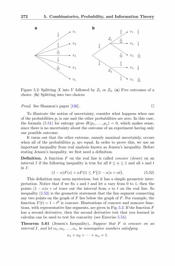
272 5. Combinatorics, Probability, and Information Theory
12
14
112
18
124
x1
x2
x3
x3
x5
x1
x2
x3
x3
x5
56
16
35
310
110
34
14
12
14
112
18
124
Z2
Z1
a b
Figure 5.2: Splitting X into Y followed by Z1 or Z2. (a) Five outcomes of achoice. (b) Splitting into two choices
Proof. See Shannon’s paper [126].
To illustrate the notion of uncertainty, consider what happens when oneof the probabilities pi is one and the other probabilities are zero. In this case,the formula (5.51) for entropy gives H(p1, . . . , pn) = 0, which makes sense,since there is no uncertainty about the outcome of an experiment having onlyone possible outcome.
It turns out that the other extreme, namely maximal uncertainly, occurswhen all of the probabilities pi are equal. In order to prove this, we use animportant inequality from real analysis known as Jensen’s inequality. Beforestating Jensen’s inequality, we first need a definition.
Definition. A function F on the real line is called concave (down) on aninterval I if the following inequality is true for all 0 ≤ α ≤ 1 and all s and tin I:
(1− α)F (s) + αF (t) ≤ F((1− α)s+ αt
). (5.52)
This definition may seem mysterious, but it has a simple geometric inter-pretation. Notice that if we fix s and t and let a vary from 0 to 1, then thepoints (1 − α)s + αt trace out the interval from s to t on the real line. Soinequality (5.52) is the geometric statement that the line segment connectingany two points on the graph of F lies below the graph of F . For example, thefunction F (t) = 1− t2 is concave. Illustrations of concave and noncave func-tions, with representative line segments, are given in Fig. 5.3. If the function Fhas a second derivative, then the second derivative test that you learned incalculus can be used to test for concavity (see Exercise 5.54).
Theorem 5.61 (Jensen’s Inequality). Suppose that F is concave on aninterval I, and let α1, α2, . . . , αn be nonnegative numbers satisfying
α1 + α2 + · · ·+ αn = 1.
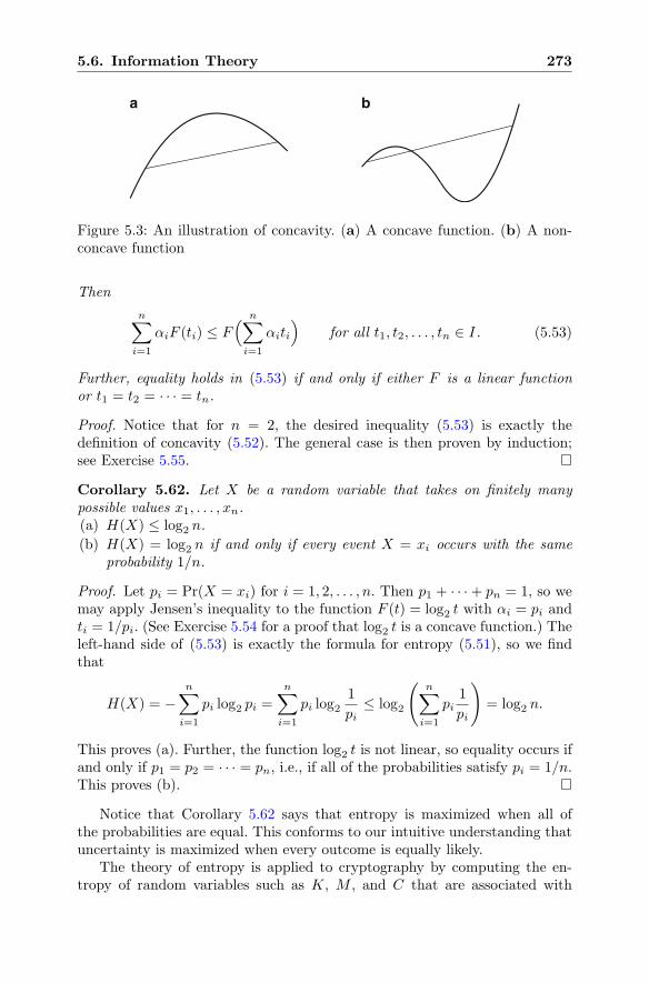
5.6. Information Theory 273
a b
Figure 5.3: An illustration of concavity. (a) A concave function. (b) A non-concave function
Then
n∑
i=1
αiF (ti) ≤ F( n∑
i=1
αiti
)for all t1, t2, . . . , tn ∈ I. (5.53)
Further, equality holds in (5.53) if and only if either F is a linear functionor t1 = t2 = · · · = tn.
Proof. Notice that for n = 2, the desired inequality (5.53) is exactly thedefinition of concavity (5.52). The general case is then proven by induction;see Exercise 5.55.
Corollary 5.62. Let X be a random variable that takes on finitely manypossible values x1, . . . , xn.(a) H(X) ≤ log2 n.
(b) H(X) = log2 n if and only if every event X = xi occurs with the sameprobability 1/n.
Proof. Let pi = Pr(X = xi) for i = 1, 2, . . . , n. Then p1 + · · ·+ pn = 1, so wemay apply Jensen’s inequality to the function F (t) = log2 t with αi = pi andti = 1/pi. (See Exercise 5.54 for a proof that log2 t is a concave function.) Theleft-hand side of (5.53) is exactly the formula for entropy (5.51), so we findthat
H(X) = −n∑
i=1
pi log2 pi =
n∑
i=1
pi log21
pi≤ log2
(n∑
i=1
pi1
pi
)
= log2 n.
This proves (a). Further, the function log2 t is not linear, so equality occurs ifand only if p1 = p2 = · · · = pn, i.e., if all of the probabilities satisfy pi = 1/n.This proves (b).
Notice that Corollary 5.62 says that entropy is maximized when all ofthe probabilities are equal. This conforms to our intuitive understanding thatuncertainty is maximized when every outcome is equally likely.
The theory of entropy is applied to cryptography by computing the en-tropy of random variables such as K, M , and C that are associated with
274 5. Combinatorics, Probability, and Information Theory
the cryptosystem and comparing the actual values with the maximum pos-sible values. Clearly the more entropy there is, the better for the user, sinceincreased uncertainty makes the cryptanalyst’s job harder.
For instance, consider a shift cipher and the random variable K associ-ated with its keys. The random variable K has 26 possible values, since theshift may be any integer between 0 and 25, and each shift amount is equallyprobable, so K has maximal entropy H(K) = log2(26).
Example 5.63. We consider the system with two keys described in Exam-ple 5.54 on page 265. Each key is equally likely, so H(K) = log2(2) = 1. Simi-larly, we can use the plaintext probabilities for this system as given by (5.48)to compute the entropy of the random variableM associated to the plaintexts.
H(M) = −1
4log2
(1
4
)− 1
4log2
(1
4
)− 1
2log2
(1
2
)=
3
2= 1.5.
Notice that H(M) is slightly smaller than log2(3) ≈ 1.585, which would bethe maximal possible entropy for M in a cryptosystem with three plaintexts.
We now introduce the concept of conditional entropy and its applicationto secrecy systems. Suppose that a signal is sent over a noisy channel, whichmeans that the signal may be distorted during transmission. Shannon [126]defines the equivocation to be the conditional entropy of the original signal,given the received signal. He uses this quantity to measure the amount of un-certainty in transmissions across a noisy channel. Shannon [127] later observedthat a noisy communication channel is also a model for a secrecy system. Theoriginal signal (the plaintext) is “distorted” by applying the encryption pro-cess, and the received signal (the ciphertext) is thus a noisy version of theoriginal signal. In this way, the notion of equivocation can be applied to cryp-tography, where a large equivocation says that the ciphertext conceals mostinformation about the plaintext.
Definition. Let X and Y be random variables, and let x1, . . . , xn be thepossible values of X and y1, . . . , ym the possible values of Y . The equivocation,or conditional entropy, of X on Y is the quantity H(X | Y ) defined by
H(X | Y ) = −n∑
i=1
m∑
j=1
fY (yj)fX|Y (xi | yj) log2 fX|Y (xi | yj).
When X = K is the key random variable and Y = C is the cipher-text random variable, the quantity H(K | C) is called the key equivocation.It measures the total amount of information about the key revealed by theciphertext, or more precisely, it is the expected value of the conditional en-tropy H(K | c) of K given a single observation c of C. The key equivocationcan be determined by computing all of the conditional probabilities f(k | c)of the cryptosystem. Alternatively, one can use the following result.
5.6. Information Theory 275
Proposition 5.64. The key equivocation of a cryptosystem (K,Mcal, C) isrelated to the individual entropies of K, M , and C by the formula
H(K | C) = H(K) +H(M)−H(C). (5.54)
Proof. We leave the proof as an exercise; see Exercise 5.57
Example 5.65. We compute the key equivocation of the cryptosystem de-scribed in Examples 5.54 and 5.63. We already computed H(K) = 1 andH(M) = 3
2 , so it remains to compute H(C). To do this, we need the val-ues of f(c) for each ciphertext c ∈ C. We already computed f(c1) =
14 , and a
similar computation using (5.48) and Table 5.12 yields
f(c2) = f(k1)f(m1) + f(k2)f(m3) =
(1
2
)(1
4
)+
(1
2
)(1
2
)=
3
8,
f(c3) = f(k1)f(m3) + f(k2)f(m2) =
(1
2
)(1
2
)+
(1
2
)(1
4
)=
3
8.
Therefore,
H(C) = −1
4log2
(1
4
)− 2 · 3
8log2
(3
8
)≈ 1.56,
and using (5.54), we find that
H(K | C) = H(K) +H(M)−H(C) ≈ 1 + 1.5− 1.56 ≈ 0.94.
5.6.3 Redundancy and the Entropyof Natural Language
Suppose that the plaintext is written in a natural language such as English.22
Then nearby letters, or nearby bits if the letters are converted to ASCII, areheavily dependent on one another, rather than looking random. For exam-ple, correlations between successive letters (bigrams or trigrams) can aid thecryptanalyst, as we saw when we cryptanalyzed a simple substitution cipherin Sect. 1.1. In this section we use the notion of entropy to quantify the re-dundancy inherent in a natural language.
We start by approximating the entropy of a single letter in English text.Let L denote the random variable whose values are the letters of the Englishlanguage E with their associated probabilities as given in Table 1.3 on page 6.For example, the table says that
fL(A) = 0.0815, fL(B) = 0.0144, fL(C) = 0.0276, . . . , fL(Z) = 0.0008.
22It should be noted that when implementing a modern public key cipher, one generallycombines the plaintext with some random bits and then performs some sort of invertibletransformation so that the resulting secondary plaintext looks more like a string of randombits. See Sect. 8.6.
276 5. Combinatorics, Probability, and Information Theory
We can use the values in Table 1.3 to compute the entropy of a single letterin English text,
H(L) = 0.0815 log2(0.0815) + · · ·+ 0.0008 log2(0.0008) ≈ 4.132.
If every letter were equally likely, the entropy would be log2(26) ≈ 4.7. Thefact that the entropy is only 4.132 shows that some letters in English are moreprevalent than others.
The concept of entropy can be used to measure the amount of informationconveyed by a language. Shannon [126] shows that H(L) can be interpretedas the average number of bits of information conveyed by a single letter of alanguage. The value of H(L) that we computed does reveal some redundancy:it says that a letter conveys only 4.132 bits of information on average, althoughit takes 4.7 bits on average to specify a letter in the English alphabet.
The fact that natural languages contain redundancy is obvious. For ex-ample, you will probably be able to read the following sentence, despite ourhaving removed almost 40% of the letters:
Th prblms o crptgry nd scrcy sysms frnsh n ntrstng aplcatn o comm thry.
However, the entropy H(L) of a single letter does not take into accountcorrelations between nearby letters, so it alone does not give a good value forthe redundancy of the English language E. As a first step, we should take intoaccount the correlations between pairs of letters (bigrams). Let L2 denote therandom variable whose values are pairs of English letters as they appear intypical English text. Some bigrams appear fairly frequently, for example
fL2(TH) = 0.00315 and fL2(AN) = 0.00172.
Others, such as JX and ZQ, never occur. Just as Table 1.3 was created ex-perimentally by counting the letters in a long sample text, we can create afrequency table of bigrams and use it to obtain an experimental value for L2.This leads to a value of H(L2) ≈ 7.12, so on average, each letter of E hasentropy equal to half this value, namely 3.56. Continuing, we could exper-imentally compute the entropy of L3, which is the random variable whosevalues are trigrams (triples of letters), and then 1
3H(L3) would be an evenbetter approximation to the entropy of E. Of course, we need to analyze agreat deal of text in order to obtain a reliable estimate for trigram frequencies,and the problem becomes even harder as we look at L4, L5, L6, and so on.However, this idea leads to the following important concept.
Definition. Let L be a language (e.g., English or French or C++), and foreach n ≥ 1, let Ln denote the random variables whose values are stringsof n consecutive characters of L. The entropy of L is defined to be the quan-tity23
23To be rigorous, one should really define upper and lower densities using liminf andlimsup, since it is not clear that limit defining H(L) exists. We will not worry about suchniceties here.
5.6. Information Theory 277
H(L) = limn→∞
H(Ln)
n.
Although it is not possible to precisely determine the entropy of the Englishlanguage E, experimentally it appears that
1.0 ≤ H(E) ≤ 1.5.
This means that despite the fact that it requires almost five bits to representeach of the 26 letters used in English, each letter conveys less than one and ahalf bits of information. Thus English is approximately 70% redundant!24
5.6.4 The Algebra of Secrecy Systems
Wemake only a few brief remarks about the algebra of cryptosystems. In [127],Shannon considers ways of building new cryptosystems by taking algebraiccombinations of old ones. The new systems are described in terms of linearcombinations and products of the original encryption transformations.
Example 5.66 (Summation Systems). If R and T are two secrecy systems,then Shannon defines the weighted sum of R and T to be
S = pR+ qT, where p+ q = 1.
The meaning of this notation is as follows. First one chooses either R or T ,where the probability of choosing R is p and the probability of choosing T is q.Imagine that the choice is made by flipping an unbalanced coin, but note thatboth Bob and Alice need to have a copy of the output of the coin tosses. Inother words, the list of choices, or a method for generating the list of choices,forms part of their private key.
The notion of summation extends to the sum of any number of secrecysystems. The systems R and T need to have the same message space, butthey need not act on messages in a similar way. For example, the system Rcould be a substitution cipher and the system T could be a shift cipher. Asanother example, suppose that Ti is the shift cipher that encrypts a letterof the alphabet by shifting it i places. Then the system that encrypts bychoosing a shift at random and encrypting according to the chosen shift is thesummation cipher
25∑
i=0
1
26Ti.
Example 5.67 (Product Systems). In order to define the product of two cryp-tosystems, it is necessary that the ciphertexts of the first system be plaintextsfor the second system. Thus let
24This does not mean that one can remove 70% of the letters and still have an intelligiblemessage. What it means is that in principle, it is possible to take a long message thatrequires 4.7 bits to specify each letter and to compress it into a form that takes only 30% asmany bits.
278 5. Combinatorics, Probability, and Information Theory
e :M→ C and e′ :M′ → C′
by two encryption functions, and suppose that C = M′, or more generally,that C ⊆ M′. Then the product system e′ · e is defined to be the compositionof e and e′,
e′ · e :M e−−−−→ C ⊆M′ e′−−−−→ C′.Product ciphers provide a means to strengthen security. They were used in thedevelopment of DES, the Digital Encryption Standard [97], the first nationalstandard for symmetric encryption. DES features several rounds of a ciphercalled S-box encryption, so it is a multiple product of a cipher with itself.Further, each round consists of the composition of several different transfor-mations. The use of product ciphers continues to be of importance in thedevelopment of new symmetric ciphers, including AES, the Advanced En-cryption Standard. See Sect. 8.12 for a brief discussion of DES and AES.
5.7 Complexity Theory and P Versus NPA decision problem is a problem in a formal system that has a yes or noanswer. For example, PRIME is the decision problem of determining whethera given integer is a prime. We discussed this problem in Sect. 3.4. Anotherexample is the decision Diffie–Hellman problem (Exercise 2.7): given ga modp and gb mod p, determine whether a given number C is equal to gab modp. Complexity theory attempts to understand and quantify the difficulty ofsolving particular decision problems.
The early history of this field is fascinating, as mathematicians tried tocome to grips with the limitations on provability within formal systems.In 1936, Alan Turing proved that there is no algorithm that solves the haltingproblem. That is, there is no algorithm to determine whether an arbitrarycomputer program, given an arbitrary input, eventually halts execution. Sucha problem is called undecidable. Earlier in that same year, Alonzo Churchhad published a proof of undecidability of a problem in the lambda calculus.He and Turing then showed that the lambda calculus and the notion of Tur-ing machine are essentially equivalent. The breakthroughs on the theory ofundecidability that appeared in the 1930s and 1940s began as a response toHilbert’s questions about the completeness of axiomatic systems and whetherthere exist unsolvable mathematical problems. Indeed, both Church and Tur-ing were influenced by Godel’s discovery in 1930 that all sufficiently strong andprecise axiomatic systems are incomplete, i.e., they contain true statementsthat are unprovable within the system.
There are uncountably many undecidable problems in mathematics, someof which have simple and interesting formulations. Here is an example of aneasy to state undecidable problem called Post’s correspondence problem [106].Suppose that you are given a sequence of pairs of strings,
(s1, t1), (s2, t2), (s3, t3), . . . , (sk, tk),
5.7. Complexity Theory and P Versus NP 279
where a string is simply a list of characters from some alphabet containingat least two letters. The correspondence problem asks you to decide whetherthere is an integer r ≥ 1 and a list of indices
i1, i2, . . . , ir between 1 and k (5.55)
such that the concatenations
si1 ‖ si2 ‖ · · · ‖ sir and ti1 ‖ ti2 ‖ · · · ‖ tir are equal. (5.56)
Note that if we bound the value of r, say r ≤ r0, then the problem becomesdecidable, since there are only a finite number of concatentations to check. Theproblem with r restricted in this way is called the bounded Post correspondenceproblem.
On the other end of the spectrum are decision problems for which thereexist quick algorithms leading to their solutions. We have already talked aboutalgorithms being fast if they run in polynomial time and slow if they takeexponential time; see the discussion in Sects. 2.6 and 3.4.2.
Definition. A decision problem belongs to the class P if there exists apolynomial-time algorithm that solves it. That is, given an input of length n,the answer will be produced in a polynomial (in n) number of steps. One saysthat the decision problems in P are those that can be solved in polynomialtime.
The concept of verification in polynomial time has some subtlety thatcan be captured only by a more precise definition, which we do not give.The class NP is defined by the concept of a polynomial-time algorithm ona “nondeterministic” machine. This means, roughly speaking, that we areallowed to guess a solution, but the verification time to check that the guessedsolution is correct must be polynomial in the length of the input.
An example of a decision problem in P is that of determining whethertwo integers have a nontrivial common factor. This problem is in P becausethe Euclidean algorithm takes fewer than O(n3) steps. (Note that in thissetting, the Euclidean algorithm takes more than O(n) steps, since we needto take account of the time it takes to add, subtract, multiply, and divide n-bitnumbers.) Another decision problem in P is that of determining whether agiven integer is prime. The famous AKS algorithm, Theorem 3.26, takes fewerthan O(n7) steps to check primality.
Definition. A decision problem belongs to the class NP if a yes-instance ofthe problem can be verified in polynomial time.
For example, the bounded Post correspondence problem is in NP . It isclear that if you are given a list of indices (5.55) of bounded length such thatthe concatenations (5.56) are alleged to be the same, it takes a polynomialnumber of steps to verify that the concatenations are indeed the same. On the
280 5. Combinatorics, Probability, and Information Theory
other hand, exhaustively checking all possible concatenations of length upto r0 takes an exponential (in r0) number of steps. It is less clear, but can beproven, that one cannot find a solution in a polynomial number of steps.
This brings us to one of the most famous open questions in all of mathe-matics and computer science25:
Does P = NP?
Since the status of P versus NP is currently unresolved, it is useful tocharacterize problems in terms of their relative difficulty. We say that prob-lem A can be (polynomial-time) reduced to problem B if there is a constructivepolynomial-time transformation that takes any instance of A and maps it toan instance of B. Thus any algorithm for solving B can be transformed intoan algorithm for solving A. Hence if problem B belongs to P, and if A isreducible to B, then A also belongs to P. The intuition is that if A can bereduced to B, then solving A is no harder than solving B (up to a polynomialamount of computation).
Stephen Cook’s 1971 paper [30] entitled “The Complexity of TheoremProving Procedures” laid the foundations of the theory of NP-completeness.In this paper, Cook works with a certain NP problem called “Satisfiability”(abbreviated SAT). The SAT problem asks, given a Boolean expression in-volving only variables, parentheses, OR, AND and NOT, whether there existsan assignment of truth values that makes the expression true. Cook provesthat SAT has the following properties:
1. Every NP problem is polynomial-time reducible to SAT.
2. If there exists any problem in NP that fails to be in P, then SAT is notin P.
A problem that has these two properties is said to be NP-complete. Sincethe publication of Cook’s paper, many other problems have been shown tobe NP-complete.
A related notion is that of NP-hardness. We say that a problem is NP-hard if it has the reducibility property (1), although the problem itself need notbelong to NP. All NP-complete problems are NP-hard, but not conversely.For example, the halting problem is NP-hard, but not NP-complete.
In order to put our informal discussion onto a firm mathematical footing,it is necessary to introduce some formalism. We start with a finite set ofsymbols Σ, and we denote by Σ∗ the set of all (finite) strings of these symbols.A subset of Σ∗ is called a language. A decision problem is defined to be theproblem of deciding whether an input string belongs to a language. The precisedefinitions of P and NP are then given within this formal framework, which
25As mentioned in Sect. 2.1, the question of whether P = NP is one of the $1,000,000Millennium Prize problems.
5.7. Complexity Theory and P Versus NP 281
we shall not develop further here. For an excellent introduction to the theoryof complexity, see [46], and for additional material on complexity theory as itrelates to cryptography, see for example [143, Chapters 2 and 3].
Up to now we have been discussing the complexity theory of decision prob-lems, but not every problem has a yes/no answer. For example, the problem ofinteger factorization (given a composite number, find a nontrivial factor) hasa solution that is an integer, as does the discrete logarithm problem (given gand h in a F
∗p, find an x such that gx = h). It is possible to formulate a
theory of complexity for general computational problems, but we are contentto give two examples. First, the integer factorization problem is in NP , sincegiven an integer N and a putative factor m, it can be verified in polynomial-time that m divides N . Second, the discrete logarithm problem is in NP,since given a supposed solution x, one can verify in polynomial time (usingthe fast powering algorithm) that gx = h. It is not known whether either ofthese computational problems is in P, i.e., there are no known polynomial-time algorithms for either integer factorization or for discrete logarithms. Thecurrent general consensus seems to be that they are probably not in P.
We turn now to the role of complexity theory in some of the problemsthat arise in cryptography. The problems of factoring integers and findingdiscrete logarithms are presumed to be difficult, since no one has yet discov-ered polynomial-time algorithms to produce solutions. However, the problemof producing a solution (this is called the function problem) may be differentfrom the decision problem of determining whether a solution exists. Here is aversion of the factoring problem phrased as a decision problem:
Does there exist a nontrivial factor of N that is less than k?
As we can see, a yes instance of this problem (i.e., N is composite) has a(trivial) polynomial-time verification algorithm, and so this decision problembelongs to NP. It can also be shown that the complementary problem belongsto NP. That is, if N is a no instance (i.e., N is prime), then the primalityof N can be verified in polynomial time on a nondeterministic Turing machine.When both the yes and no instances of a problem can be verified in polynomialtime, the decision problem is said to belong to the class co-NP . Since it iswidely believed that NP is not the same as co-NP , it was also believedthat factoring is not an NP-complete problem. In 2004, Agrawal, Kayal andSaxena [1] showed that the decision problem of determining whether a numberis prime does indeed belong to P, settling the long-standing question whetherthis decision problem could be NP-complete.
A cryptosystem is only as secure as its underlying hard problem, so itwould be desirable to construct cryptosystems based on NP-hard problems.There has been a great deal of interest in building efficient public key cryp-tosystems of this sort. A major difficulty is that one needs not only an NP-hard problem, but also a trapdoor to the problem to use for decryption. Thishas led to a number of cryptosystems that are based special cases of NP-hard problems, but it is not known whether these special cases are themselvesNP-hard.
282 Exercises
The first example of a public key cryptosystem built around an NP-complete problem was the knapsack cryptosystem of Merkle and Hellman.More precisely, they based their cryptosystem on the subset-sum problem,which asks the following:
Given n positive integers a1, . . . , an and a targetsum S, find a subset of the ai such that
ai1 + ai2 + · · ·+ ait = S.
The subset-sum problem is NP-complete, since one can show that any in-stance of SAT can be reduced to an instance of the subset-sum problem, andvice versa. In order to build a public key cryptosystem based on the (hard)subset-sum problem, Merkle and Hellman needed to build a trapdoor into theproblem. They did this by using only certain special cases of the subset-sumproblem, but unfortunately it turned out that these special cases are signifi-cantly easier than the general case and their cryptosystem was broken. Anddespite further work by a number of cryptographers, no one has been able tobuild a subset-sum cryptosystem that is both efficient and secure. See Sect. 7.2for a detailed discussion of how subset-sum cryptosystems work and how theyare broken.
Another cautionary note in going from theory to practice comes from thefact that even if a certain collection of problems is NP-hard, that does notmean that every problem in the collection is hard. In some sense,NP-hardnessmeasures the difficulty of the hardest problem in the collection, not the averageproblem. It would not be good to base a cryptosystem on a problem for whicha few instances are very hard, but most instances are very easy. Ideally, wewant to use a collection of problems with the property that most instances areNP-hard. An interesting example is the closest vector problem (CVP), whichinvolves finding a vector in lattice that is close to a given vector. We discusslattices and CVP in Chap. 7, but for now we note that CVP is NP-hard.Our interest in CVP stems from a famous result of Ajtai and Dwork [4] inwhich they construct a cryptosystem based on CVP in a certain set of lattices.They show that the average difficulty of solving CVP for their lattices can bepolynomially reduced to solving the hardest instance of CVP in a similar set oflattices (of somewhat smaller dimension). Although not practical, their publickey cryptosystem was the first construction exhibiting worst-case/average-case equivalence.
Exercises
Section 5.1. Basic Principles of Counting
5.1. The Rhind papyrus is an ancient Egyptian mathematical manuscript that ismore than 3500 years old. Problem 79 of the Rhind papyrus poses a problem thatcan be paraphrased as follows: there are seven houses; in each house lives seven cats;
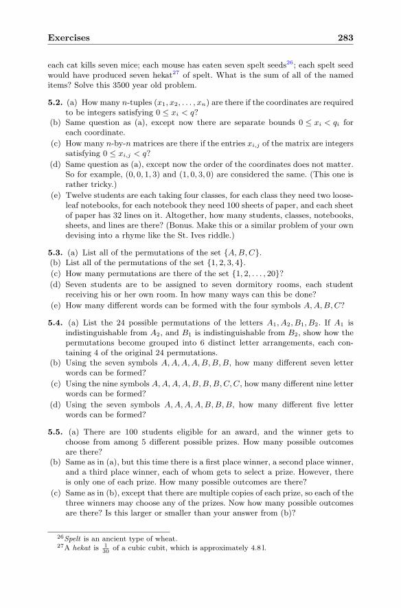
Exercises 283
each cat kills seven mice; each mouse has eaten seven spelt seeds26; each spelt seedwould have produced seven hekat27 of spelt. What is the sum of all of the nameditems? Solve this 3500 year old problem.
5.2. (a) How many n-tuples (x1, x2, . . . , xn) are there if the coordinates are requiredto be integers satisfying 0 ≤ xi < q?
(b) Same question as (a), except now there are separate bounds 0 ≤ xi < qi foreach coordinate.
(c) How many n-by-n matrices are there if the entries xi,j of the matrix are integerssatisfying 0 ≤ xi,j < q?
(d) Same question as (a), except now the order of the coordinates does not matter.So for example, (0, 0, 1, 3) and (1, 0, 3, 0) are considered the same. (This one israther tricky.)
(e) Twelve students are each taking four classes, for each class they need two loose-leaf notebooks, for each notebook they need 100 sheets of paper, and each sheetof paper has 32 lines on it. Altogether, how many students, classes, notebooks,sheets, and lines are there? (Bonus. Make this or a similar problem of your owndevising into a rhyme like the St. Ives riddle.)
5.3. (a) List all of the permutations of the set {A,B,C}.(b) List all of the permutations of the set {1, 2, 3, 4}.(c) How many permutations are there of the set {1, 2, . . . , 20}?(d) Seven students are to be assigned to seven dormitory rooms, each student
receiving his or her own room. In how many ways can this be done?
(e) How many different words can be formed with the four symbols A,A,B,C?
5.4. (a) List the 24 possible permutations of the letters A1, A2, B1, B2. If A1 isindistinguishable from A2, and B1 is indistinguishable from B2, show how thepermutations become grouped into 6 distinct letter arrangements, each con-taining 4 of the original 24 permutations.
(b) Using the seven symbols A,A,A,A,B,B,B, how many different seven letterwords can be formed?
(c) Using the nine symbols A,A,A,A,B,B,B,C,C, how many different nine letterwords can be formed?
(d) Using the seven symbols A,A,A,A,B,B,B, how many different five letterwords can be formed?
5.5. (a) There are 100 students eligible for an award, and the winner gets tochoose from among 5 different possible prizes. How many possible outcomesare there?
(b) Same as in (a), but this time there is a first place winner, a second place winner,and a third place winner, each of whom gets to select a prize. However, thereis only one of each prize. How many possible outcomes are there?
(c) Same as in (b), except that there are multiple copies of each prize, so each of thethree winners may choose any of the prizes. Now how many possible outcomesare there? Is this larger or smaller than your answer from (b)?
26Spelt is an ancient type of wheat.27A hekat is 1
30of a cubic cubit, which is approximately 4.8 l.
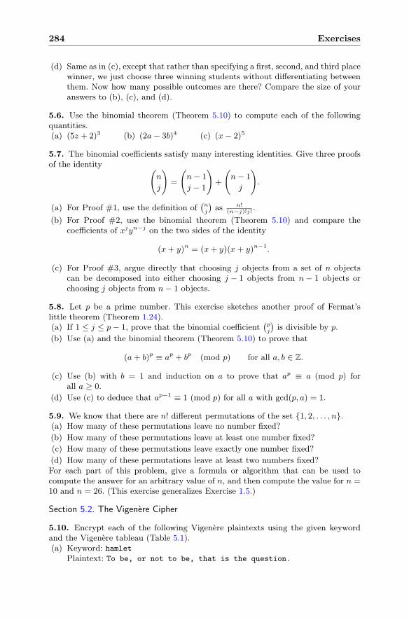
284 Exercises
(d) Same as in (c), except that rather than specifying a first, second, and third placewinner, we just choose three winning students without differentiating betweenthem. Now how many possible outcomes are there? Compare the size of youranswers to (b), (c), and (d).
5.6. Use the binomial theorem (Theorem 5.10) to compute each of the followingquantities.(a) (5z + 2)3 (b) (2a− 3b)4 (c) (x− 2)5
5.7. The binomial coefficients satisfy many interesting identities. Give three proofsof the identity (
n
j
)
=
(n− 1
j − 1
)
+
(n− 1
j
)
.
(a) For Proof #1, use the definition of(nj
)as n!
(n−j)!j!.
(b) For Proof #2, use the binomial theorem (Theorem 5.10) and compare thecoefficients of xjyn−j on the two sides of the identity
(x+ y)n = (x+ y)(x+ y)n−1.
(c) For Proof #3, argue directly that choosing j objects from a set of n objectscan be decomposed into either choosing j − 1 objects from n− 1 objects orchoosing j objects from n− 1 objects.
5.8. Let p be a prime number. This exercise sketches another proof of Fermat’slittle theorem (Theorem 1.24).(a) If 1 ≤ j ≤ p− 1, prove that the binomial coefficient
(pj
)is divisible by p.
(b) Use (a) and the binomial theorem (Theorem 5.10) to prove that
(a+ b)p ≡ ap + bp (mod p) for all a, b ∈ Z.
(c) Use (b) with b = 1 and induction on a to prove that ap ≡ a (mod p) forall a ≥ 0.
(d) Use (c) to deduce that ap−1 ≡ 1 (mod p) for all a with gcd(p, a) = 1.
5.9. We know that there are n! different permutations of the set {1, 2, . . . , n}.(a) How many of these permutations leave no number fixed?
(b) How many of these permutations leave at least one number fixed?
(c) How many of these permutations leave exactly one number fixed?
(d) How many of these permutations leave at least two numbers fixed?For each part of this problem, give a formula or algorithm that can be used tocompute the answer for an arbitrary value of n, and then compute the value for n =10 and n = 26. (This exercise generalizes Exercise 1.5.)
Section 5.2. The Vigenere Cipher
5.10. Encrypt each of the following Vigenere plaintexts using the given keywordand the Vigenere tableau (Table 5.1).(a) Keyword: hamlet
Plaintext: To be, or not to be, that is the question.
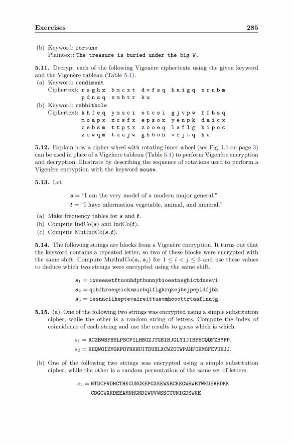
Exercises 285
(b) Keyword: fortunePlaintext: The treasure is buried under the big W.
5.11. Decrypt each of the following Vigenere ciphertexts using the given keywordand the Vigenere tableau (Table 5.1).(a) Keyword: condiment
Ciphertext: r s g h z b m c x t d v f s q h n i g q x r n b m
p d n s q s m b t r k u
(b) Keyword: rabbitholeCiphertext: k h f e q y m s c i e t c s i g j v p w f f b s q
m o a p x z c s f x e p s o x y e n p k d a i c x
c e b s m t t p t x z o o e q l a f l g k i p o c
z s w q m t a u j w g h b o h v r j t q h u
5.12. Explain how a cipher wheel with rotating inner wheel (see Fig. 1.1 on page 3)can be used in place of a Vigenere tableau (Table 5.1) to perform Vigenere encryptionand decryption. Illustrate by describing the sequence of rotations used to perform aVigenere encryption with the keyword mouse.
5.13. Let
s = “I am the very model of a modern major general.”
t = “I have information vegetable, animal, and mineral.”
(a) Make frequency tables for s and t.
(b) Compute IndCo(s) and IndCo(t).
(c) Compute MutIndCo(s, t).
5.14. The following strings are blocks from a Vigenere encryption. It turns out thatthe keyword contains a repeated letter, so two of these blocks were encrypted withthe same shift. Compute MutIndCo(si, sj) for 1 ≤ i < j ≤ 3 and use these valuesto deduce which two strings were encrypted using the same shift.
s1 = iwseesetftuonhdptbunnybioeatneghictdnsevi
s2 = qibfhroeqeickxmirbqlflgkrqkejbejpepldfjbk
s3 = iesnnciiheptevaireittuevmhooottrtaaflnatg
5.15. (a) One of the following two strings was encrypted using a simple substitutioncipher, while the other is a random string of letters. Compute the index ofcoincidence of each string and use the results to guess which is which.
s1 = RCZBWBFHSLPSCPILHBGZJTGBIBJGLYIJIBFHCQQFZBYFP,
s2 = KHQWGIZMGKPOYRKHUITDUXLXCWZOTWPAHFOHMGFEVUEJJ.
(b) One of the following two strings was encrypted using a simple substitutioncipher, while the other is a random permutation of the same set of letters.
s1 = NTDCFVDHCTHKGUNGKEPGXKEWNECKEGWEWETWKUEVHDKK
CDGCWXKDEEAMNHGNDIWUVWSSCTUNIGDSWKE
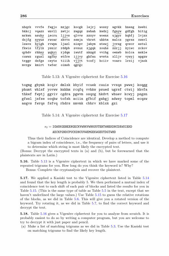
286 Exercises
nhqrk vvvfe fwgjo mzjgc kocgk lejrj wossy wgvkk hnesg kwebi
bkkcj vqazx wnvll zetjc zwgqz zwhah kwdxj fgnyw gdfgh bitig
mrkwn nsuhy iecru ljjvs qlvvw zzxyv woenx ujgyr kqbfj lvjzx
dxjfg nywus rwoar xhvvx ssmja vkrwt uhktm malcz ygrsz xwnvl
lzavs hyigh rvwpn ljazl nispv jahym ntewj jvrzg qvzcr estul
fkwis tfylk ysnir rddpb svsux zjgqk xouhs zzrjj kyiwc zckov
qyhdv rhhny wqhyi rjdqm iwutf nkzgd vvibg oenwb kolca mskle
cuwwz rgusl zgfhy etfre ijjvy ghfau wvwtn xlljv vywyj apgzw
trggr dxfgs ceyts tiiih vjjvt tcxfj hciiv voaro lrxij vjnok
mvrgw kmirt twfer oimsb qgrgc
Table 5.13: A Vigenere ciphertext for Exercise 5.16
togmg gbymk kcqiv dmlxk kbyif vcuek cuuis vvxqs pwwej koqgg
phumt whlsf yovww knhhm rcqfq vvhkw psued ugrsf ctwij khvfa
thkef fwptj ggviv cgdra pgwvm osqxg hkdvt whuev kcwyj psgsn
gfwsl jsfse ooqhw tofsh aciin gfbif gabgj adwsy topml ecqzw
asgvs fwrqs fsfvq rhdrs nmvmk cbhrv kblxk gzi
Table 5.14: A Vigenere ciphertext for Exercise 5.17
s2 = IGWSKGEHEXNGECKVWNKVWNKSUTEHTWHEKDNCDXWSIEKD
AECKFGNDCPUCKDNCUVWEMGEKWGEUTDGTWHD
Thus their Indices of Coincidence are identical. Develop a method to computea bigram index of coincidence, i.e., the frequency of pairs of letters, and use itto determine which string is most likely the encrypted text.
(Bonus: Decrypt the encrypted texts in (a) and (b), but be forewarned that theplaintexts are in Latin.)
5.16. Table 5.13 is a Vigenere ciphertext in which we have marked some of therepeated trigrams for you. How long do you think the keyword is? Why?
Bonus: Complete the cryptanalysis and recover the plaintext.
5.17. We applied a Kasiski test to the Vigenere ciphertext listed in Table 5.14and found that the key length is probably 5. We then performed a mutual index ofcoincidence test to each shift of each pair of blocks and listed the results for you inTable 5.15. (This is the same type of table as Table 5.5 in the text, except that wehaven’t underlined the large values.) Use Table 5.15 to guess the relative rotationsof the blocks, as we did in Table 5.6. This will give you a rotated version of thekeyword. Try rotating it, as we did in Table 5.7, to find the correct keyword anddecrypt the text.
5.18. Table 5.16 gives a Vigenere ciphertext for you to analyze from scratch. It isprobably easiest to do so by writing a computer program, but you are welcome totry to decrypt it with just paper and pencil.(a) Make a list of matching trigrams as we did in Table 5.3. Use the Kasiski test
on matching trigrams to find the likely key length.
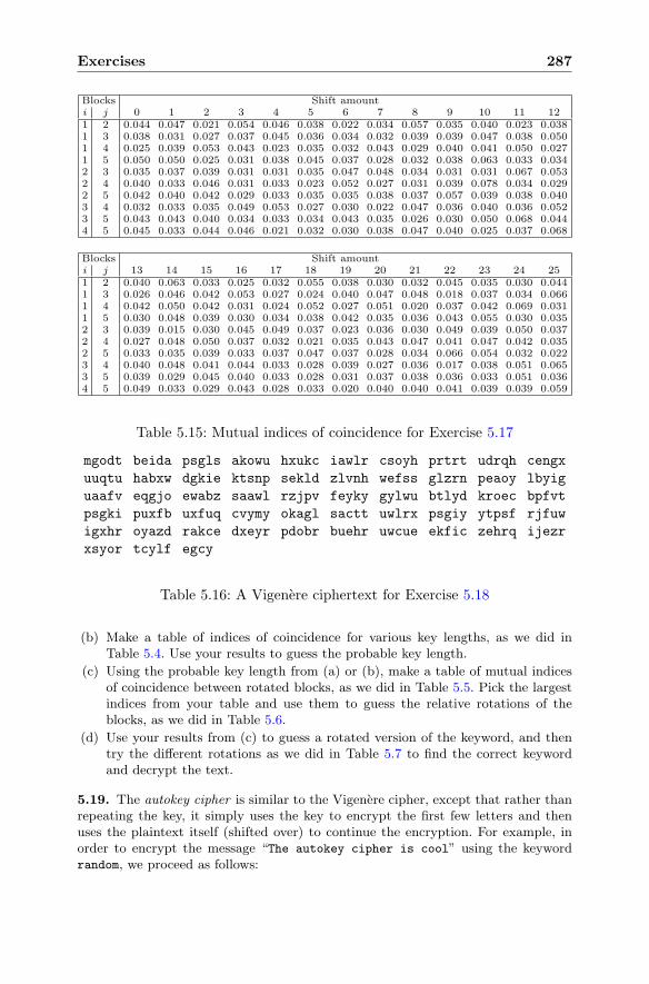
Exercises 287
Blocks Shift amounti j 0 1 2 3 4 5 6 7 8 9 10 11 121 2 0.044 0.047 0.021 0.054 0.046 0.038 0.022 0.034 0.057 0.035 0.040 0.023 0.0381 3 0.038 0.031 0.027 0.037 0.045 0.036 0.034 0.032 0.039 0.039 0.047 0.038 0.0501 4 0.025 0.039 0.053 0.043 0.023 0.035 0.032 0.043 0.029 0.040 0.041 0.050 0.0271 5 0.050 0.050 0.025 0.031 0.038 0.045 0.037 0.028 0.032 0.038 0.063 0.033 0.0342 3 0.035 0.037 0.039 0.031 0.031 0.035 0.047 0.048 0.034 0.031 0.031 0.067 0.0532 4 0.040 0.033 0.046 0.031 0.033 0.023 0.052 0.027 0.031 0.039 0.078 0.034 0.0292 5 0.042 0.040 0.042 0.029 0.033 0.035 0.035 0.038 0.037 0.057 0.039 0.038 0.0403 4 0.032 0.033 0.035 0.049 0.053 0.027 0.030 0.022 0.047 0.036 0.040 0.036 0.0523 5 0.043 0.043 0.040 0.034 0.033 0.034 0.043 0.035 0.026 0.030 0.050 0.068 0.0444 5 0.045 0.033 0.044 0.046 0.021 0.032 0.030 0.038 0.047 0.040 0.025 0.037 0.068
Blocks Shift amounti j 13 14 15 16 17 18 19 20 21 22 23 24 251 2 0.040 0.063 0.033 0.025 0.032 0.055 0.038 0.030 0.032 0.045 0.035 0.030 0.0441 3 0.026 0.046 0.042 0.053 0.027 0.024 0.040 0.047 0.048 0.018 0.037 0.034 0.0661 4 0.042 0.050 0.042 0.031 0.024 0.052 0.027 0.051 0.020 0.037 0.042 0.069 0.0311 5 0.030 0.048 0.039 0.030 0.034 0.038 0.042 0.035 0.036 0.043 0.055 0.030 0.0352 3 0.039 0.015 0.030 0.045 0.049 0.037 0.023 0.036 0.030 0.049 0.039 0.050 0.0372 4 0.027 0.048 0.050 0.037 0.032 0.021 0.035 0.043 0.047 0.041 0.047 0.042 0.0352 5 0.033 0.035 0.039 0.033 0.037 0.047 0.037 0.028 0.034 0.066 0.054 0.032 0.0223 4 0.040 0.048 0.041 0.044 0.033 0.028 0.039 0.027 0.036 0.017 0.038 0.051 0.0653 5 0.039 0.029 0.045 0.040 0.033 0.028 0.031 0.037 0.038 0.036 0.033 0.051 0.0364 5 0.049 0.033 0.029 0.043 0.028 0.033 0.020 0.040 0.040 0.041 0.039 0.039 0.059
Table 5.15: Mutual indices of coincidence for Exercise 5.17
mgodt beida psgls akowu hxukc iawlr csoyh prtrt udrqh cengx
uuqtu habxw dgkie ktsnp sekld zlvnh wefss glzrn peaoy lbyig
uaafv eqgjo ewabz saawl rzjpv feyky gylwu btlyd kroec bpfvt
psgki puxfb uxfuq cvymy okagl sactt uwlrx psgiy ytpsf rjfuw
igxhr oyazd rakce dxeyr pdobr buehr uwcue ekfic zehrq ijezr
xsyor tcylf egcy
Table 5.16: A Vigenere ciphertext for Exercise 5.18
(b) Make a table of indices of coincidence for various key lengths, as we did inTable 5.4. Use your results to guess the probable key length.
(c) Using the probable key length from (a) or (b), make a table of mutual indicesof coincidence between rotated blocks, as we did in Table 5.5. Pick the largestindices from your table and use them to guess the relative rotations of theblocks, as we did in Table 5.6.
(d) Use your results from (c) to guess a rotated version of the keyword, and thentry the different rotations as we did in Table 5.7 to find the correct keywordand decrypt the text.
5.19. The autokey cipher is similar to the Vigenere cipher, except that rather thanrepeating the key, it simply uses the key to encrypt the first few letters and thenuses the plaintext itself (shifted over) to continue the encryption. For example, inorder to encrypt the message “The autokey cipher is cool” using the keywordrandom, we proceed as follows:
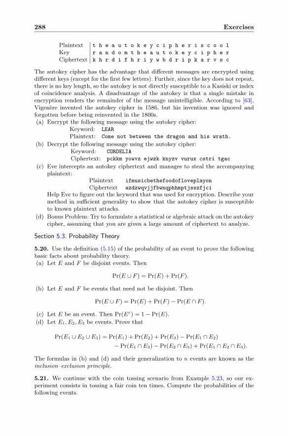
288 Exercises
Plaintext t h e a u t o k e y c i p h e r i s c o o l
Key r a n d o m t h e a u t o k e y c i p h e r
Ciphertext k h r d i f h r i y w b d r i p k a r v s c
The autokey cipher has the advantage that different messages are encrypted usingdifferent keys (except for the first few letters). Further, since the key does not repeat,there is no key length, so the autokey is not directly susceptible to a Kasiski or indexof coincidence analysis. A disadvantage of the autokey is that a single mistake inencryption renders the remainder of the message unintelligible. According to [63],Vigenere invented the autokey cipher in 1586, but his invention was ignored andforgotten before being reinvented in the 1800s.(a) Encrypt the following message using the autokey cipher:
Keyword: LEAR
Plaintext: Come not between the dragon and his wrath.
(b) Decrypt the following message using the autokey cipher:Keyword: CORDELIA
Ciphertext: pckkm yowvz ejwzk knyzv vurux cstri tgac
(c) Eve intercepts an autokey ciphertext and manages to steal the accompanyingplaintext:
Plaintext ifmusicbethefoodofloveplayon
Ciphertext azdzwqvjjfbwnqphhmptjsszfjci
Help Eve to figure out the keyword that was used for encryption. Describe yourmethod in sufficient generality to show that the autokey cipher is susceptibleto known plaintext attacks.
(d) Bonus Problem: Try to formulate a statistical or algebraic attack on the autokeycipher, assuming that you are given a large amount of ciphertext to analyze.
Section 5.3. Probability Theory
5.20. Use the definition (5.15) of the probability of an event to prove the followingbasic facts about probability theory.(a) Let E and F be disjoint events. Then
Pr(E ∪ F ) = Pr(E) + Pr(F ).
(b) Let E and F be events that need not be disjoint. Then
Pr(E ∪ F ) = Pr(E) + Pr(F )− Pr(E ∩ F ).
(c) Let E be an event. Then Pr(Ec) = 1− Pr(E).
(d) Let E1, E2, E3 be events. Prove that
Pr(E1 ∪ E2 ∪ E3) = Pr(E1) + Pr(E2) + Pr(E3)− Pr(E1 ∩ E2)
− Pr(E1 ∩ E3)− Pr(E2 ∩ E3) + Pr(E1 ∩ E2 ∩ E3).
The formulas in (b) and (d) and their generalization to n events are known as theinclusion–exclusion principle.
5.21. We continue with the coin tossing scenario from Example 5.23, so our ex-periment consists in tossing a fair coin ten times. Compute the probabilities of thefollowing events.
Exercises 289
(a) The first and last tosses are both heads.
(b) Either the first toss or the last toss (or both) are heads.
(c) Either the first toss or the last toss (but not both) are heads.
(d) There are exactly k heads and 10 − k tails. Compute the probability for eachvalue of k between 0 and 10. (Hint. To save time, note that the probability ofexactly k heads is the same as the probability of exactly k tails.)
(e) There is an even number of heads.
(f) There is an odd number of heads.
5.22. Alice offers to make the following bet with you. She will toss a fair coin 14times. If exactly 7 heads come up, she will give you $4; otherwise you must giveher $1. Would you take this bet? If so, and if you repeated the bet 10000 times, howmuch money would you expect to win or lose?
5.23. Let E and F be events.(a) Prove that Pr(E | E) = 1. Explain in words why this is reasonable.
(b) If E and F are disjoint, prove that Pr(F | E) = 0. Explain in words why thisis reasonable.
(c) Let F1, . . . , Fn be events satisfying Fi ∩ Fj = ∅ for all i �= j. We saythat F1, . . . , Fn are pairwise disjoint. Prove then that
Pr
( n⋃
i=1
Fi
)=
n∑
i=1
Pr(Fi).
(d) Let F1, . . . , Fn be pairwise disjoint as in (c), and assume further that
F1 ∪ · · · ∪ Fn = Ω,
where recall that Ω is the entire sample space. Prove the following generalversion of the decomposition formula (5.20) in Proposition 5.24(a):
Pr(E) =n∑
i=1
Pr(E | Fi) Pr(Fi).
(e) Prove a general version of Bayes’s formula:
Pr(Fi | E) =Pr(E | Fi) Pr(Fi)
Pr(E | F1) Pr(F1) + Pr(E | F2) Pr(F2) + · · ·+ Pr(E | Fn) Pr(Fn).
5.24. There are two urns containing pens and pencils. Urn #1 contains three pensand seven pencils and Urn #2 contains eight pens and four pencils.(a) An urn is chosen at random and an object is drawn. What is the probability
that it is a pencil?
(b) An urn is chosen at random and an object is drawn. If the object drawn is apencil, what is the probability that it came from Urn #1?
(c) If an urn is chosen at random and two objects are drawn simultaneously, whatis the probability that both are pencils?
5.25. An urn contains 20 silver coins and 10 gold coins. You are the sixth personin line to randomly draw and keep a coin from the urn.(a) What is the probability that you draw a gold coin?
290 Exercises
(b) If you draw a gold coin, what is the probability that the five people ahead ofyou all drew silver coins?
5.26. Consider the three prisoners scenario described in Example 5.26. Let A, B,and C denote respectively the events that Alice is to be released, Bob is to bereleased, and Carl is to be released, which we assume to be equally likely, so Pr(A) =Pr(B) = Pr(C) = 1
3. Also let J be the event that the jailer tells Aice that Bob is to
stay in jail.(a) Compute the values of Pr(B | J), Pr(J | B), and Pr(J | C).
(b) Compute the values of Pr(J | Ac) and Pr(Jc | Ac), where the event Ac is theevent that Alice stays in jail.
(c) Suppose that if Alice is the one who is to be released, then the jailer flips a faircoin to decide whether to tell Alice that Bob stays in jail or that Carl stays injail. What is the value of Pr(A | J)?
(d) Suppose instead that if Alice is the one who is to be released, then the jaileralways tells her that Bob will stay in jail. Now what is the value of Pr(A | J)?
Other similar problems with counterintuitive conclusions include the Monty Hallproblem (Exercise 5.27), Bertrand’s box paradox, and the principle of restrictedchoice in contract bridge.
5.27. (The Monty Hall Problem) Monty Hall gives Dan the choice of three curtains.Behind one curtain is a car, while behind the other two curtains are goats. Danchooses a curtain, but before it is opened, Monty Hall opens one of the other curtainsand reveals a goat. He then offers Dan the option of keeping his original curtain orswitching to the remaining closed curtain. The Monty Hall problem is to figure outDan’s best strategy: “To stick or to switch?”(a) What is the probability that Dan wins the car if he always sticks to his first
choice of curtain? What is the probability that Dan wins the car if he alwaysswitches curtains? Which is his best strategy? (If the answer seems counter-intuitive, suppose instead that there are 1000 curtains and that Monty Hallopens 998 goat curtains. Now what are the winning probabilities for the twostrategies?)
(b) Suppose that we give Monty Hall another option, namely he’s allowed to forceDan to stick with his first choice of curtain. Assuming that Monty Hall dislikesgiving away cars, now what is Dan’s best strategy, and what is his probabilityof winning a car?
(c) More generally, suppose that there are N curtains and M cars, and supposethat Monty Hall opens K curtains that have goats behind them. Compute theprobabilities
Pr(Dan wins a car | Dan sticks), Pr(Dan wins a car | Dan switches).
Which is the better strategy?
5.28. Let S be a set, let A be a property of interest, and suppose that for m ∈ S,we have
Pr(m does not have property A) = δ.
Suppose further that a Monte Carlo algorithm applied to m and a random number rsatisfy:
Exercises 291
(1) If the algorithm returns Yes, then m definitely has property A.
(2) If m has property A, then the probability that the algorithm returns Yes is atleast p.
Notice that we can restate (1) and (2) as conditional probabilities:
(1) Pr(m has property A | algorithm returns Yes) = 1,
(2) Pr(algorithm returns Yes | m has property A) ≥ p.
Suppose that we run the algorithm N times on the number m, and suppose thatthe algorithm returns No every single time. Derive a lower bound, in terms of δ, p,and N , for the probability that m does not have property A. (This generalizes theversion of the Monte Carlo method that we studied in Sect. 5.3.3 with δ = 0.01 andp = 1
2. Be careful to distinguish p from 1− p in your calculations.)
5.29. We continue with the setup described in Exercise 5.28.(a) Suppose that δ = 9
10and p = 3
4. If we run the algorithm 25 times on the
input m and always get back No, what is the probability that m does not haveproperty A?
(b) Same question as (a), but this time we run the algorithm 100 times.
(c) Suppose that δ = 99100
and p = 12. How many times should we run the algorithm
on m to be 99% confident that m does not have property A, assuming thatevery output is No?
(d) Same question as (c), except now we want to be 99.9999% confident.
5.30. If an integer n is composite, then the Miller–Rabin test has at least a 75%chance of succeeding in proving that n is composite, while it never misidentifies aprime as being composite. (See Table 3.2 in Sect. 3.4 for a description of the Miller–Rabin test.) Suppose that we run the Miller–Rabin test N times on the integer nand that it fails to prove that n is composite. Show that the probability that n isprime satisfies (approximately)
Pr(n is prime | the Miller–Rabin test fails N times) ≥ 1− ln(n)
4N.
(Hint. Use Exercise 5.28 with appropriate choices of A, S, δ, and p. You may alsouse the estimate from Sect. 3.4.1 that the probability that n is prime is approxi-mately 1/ ln(n).)
5.31. It is natural to assume that if Pr(E | F ) is significantly larger than Pr(E),then somehow F is causing E. Baye’s formula illustrates the fallacy of this sort ofreasoning, since it says that
Pr(E | F )
Pr(E)=
Pr(F | E)
Pr(F ).
So if F is “causing” E, then the same reasoning shows that E is “causing” F . Allthat one can really say is that E and F are correlated with one another, in the sensethat either one of them being true makes it more likely that the other one is true.It is incorrect to deduce a cause-and-effect relation.
Here is a concrete example. Testing shows that first graders are more likely to begood spellers if their shoe sizes are larger than average. This is an experimental fact.Hence if we stretch a child’s foot, it will make them a better speller! Alternatively,
292 Exercises
by Baye’s formula, if we give them extra spelling lessons, then their feet will growfaster! Explain why these last two assertions are nonsense, and describe what’s reallygoing on.
5.32. Let fX(k) be the binomial density function (5.23). Prove directly, using thebinomial theorem, that
∑nk=0 fX(k) = 1.
5.33. In Example 5.37 we used a differentiation trick to compute the value of theinfinite series
∑∞n=1 np(1−p)
n−1. This exercise further develops this useful technique.The starting point is the formula for the geometric series
∞∑
n=0
xn =1
1− xfor |x| < 1 (5.57)
and the differential operator
D = xd
dx.
(a) Using the fact that D(xn) = nxn, prove that
∞∑
n=1
nxn =x
(1− x)2(5.58)
by applying D to both sides of (5.57). For which x does the left-hand sideof (5.58) converge? (Hint. Use the ratio test.)
(b) Applying D again, prove that
∞∑
n=0
n2xn =x+ x2
(1− x)3. (5.59)
(c) More generally, prove that for every value of k there is a polynomial Fk(x) suchthat ∞∑
n=0
nkxn =Fk(x)
(1− x)k+1. (5.60)
(Hint. Use induction on k.)
(d) The first few polynomials Fk(x) in (c) are F0(x) = 1, F1(x) = x, and F2(x) =x+x2. These follow from (5.57), (5.58), and (5.59). Compute F3(x) and F4(x).
(e) Prove that the polynomial Fk(x) in (c) has degree k.
5.34. In each case, compute the expectation of the random variable X.(a) The values of X are uniformly distributed on the set {0, 1, 2, . . . , N − 1}. (See
Example 5.28.)
(b) The values of X are uniformly distributed on the set {1, 2, . . . , N}.(c) The values of X are uniformly distributed on the set {1, 3, 7, 11, 19, 23}.(d) X is a random variable with a binomial density function; see formula (5.23) in
Example 5.29 on page 240.
5.35. Let X be a random variable on the probability space Ω. It might seem morenatural to define the expected value of X by the formula
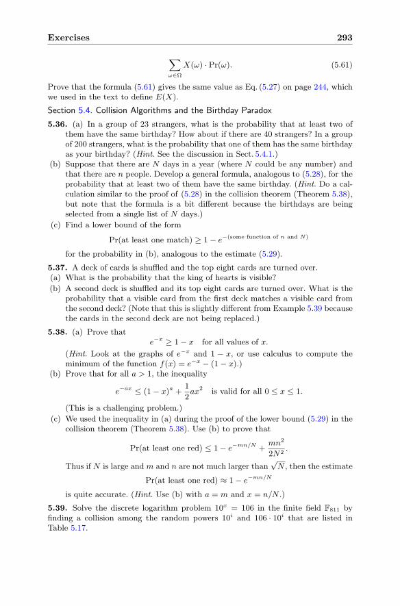
Exercises 293
∑
ω∈Ω
X(ω) · Pr(ω). (5.61)
Prove that the formula (5.61) gives the same value as Eq. (5.27) on page 244, whichwe used in the text to define E(X).
Section 5.4. Collision Algorithms and the Birthday Paradox
5.36. (a) In a group of 23 strangers, what is the probability that at least two ofthem have the same birthday? How about if there are 40 strangers? In a groupof 200 strangers, what is the probability that one of them has the same birthdayas your birthday? (Hint. See the discussion in Sect. 5.4.1.)
(b) Suppose that there are N days in a year (where N could be any number) andthat there are n people. Develop a general formula, analogous to (5.28), for theprobability that at least two of them have the same birthday. (Hint. Do a cal-culation similar to the proof of (5.28) in the collision theorem (Theorem 5.38),but note that the formula is a bit different because the birthdays are beingselected from a single list of N days.)
(c) Find a lower bound of the form
Pr(at least one match) ≥ 1− e−(some function of n and N)
for the probability in (b), analogous to the estimate (5.29).
5.37. A deck of cards is shuffled and the top eight cards are turned over.(a) What is the probability that the king of hearts is visible?
(b) A second deck is shuffled and its top eight cards are turned over. What is theprobability that a visible card from the first deck matches a visible card fromthe second deck? (Note that this is slightly different from Example 5.39 becausethe cards in the second deck are not being replaced.)
5.38. (a) Prove thate−x ≥ 1− x for all values of x.
(Hint. Look at the graphs of e−x and 1 − x, or use calculus to compute theminimum of the function f(x) = e−x − (1− x).)
(b) Prove that for all a > 1, the inequality
e−ax ≤ (1− x)a +1
2ax2 is valid for all 0 ≤ x ≤ 1.
(This is a challenging problem.)
(c) We used the inequality in (a) during the proof of the lower bound (5.29) in thecollision theorem (Theorem 5.38). Use (b) to prove that
Pr(at least one red) ≤ 1− e−mn/N +mn2
2N2.
Thus if N is large andm and n are not much larger than√N , then the estimate
Pr(at least one red) ≈ 1− e−mn/N
is quite accurate. (Hint. Use (b) with a = m and x = n/N .)
5.39. Solve the discrete logarithm problem 10x = 106 in the finite field F811 byfinding a collision among the random powers 10i and 106 · 10i that are listed inTable 5.17.
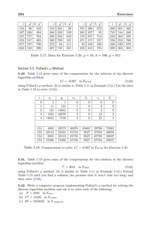
294 Exercises
i gi h · gi
116 96 444
497 326 494
225 757 764
233 517 465
677 787 700
622 523 290
i gi h · gi
519 291 28
286 239 193
298 358 642
500 789 101
272 24 111
307 748 621
i gi h · gi
791 496 672
385 437 95
178 527 714
471 117 237
42 448 450
258 413 795
i gi h · gi
406 801 562
745 194 289
234 304 595
556 252 760
326 649 670
399 263 304
Table 5.17: Data for Exercise 5.39, g = 10, h = 106, p = 811
Section 5.5. Pollard’s ρ Method
5.40. Table 5.18 gives some of the computations for the solution of the discretelogarithm problem
11t = 41387 in F81799 (5.62)
using Pollard’s ρ method. (It is similar to Table 5.11 in Example 5.52.) Use the datain Table 5.18 to solve (5.62).
i xi yi αi βi γi δi
0 1 1 0 0 0 0
1 11 121 1 0 2 0
2 121 14641 2 0 4 0
3 1331 42876 3 0 12 2
4 14641 7150 4 0 25 4...
151 4862 33573 40876 45662 29798 73363
152 23112 53431 81754 9527 37394 48058
153 8835 23112 81755 9527 67780 28637
154 15386 15386 81756 9527 67782 28637
Table 5.18: Computations to solve 11t = 41387 in F81799 for Exercise 5.40
5.41. Table 5.19 gives some of the computations for the solution of the discretelogarithm problem
7t = 3018 in F7963 (5.63)
using Pollard’s ρ method. (It is similar to Table 5.11 in Example 5.52.) ExtendTable 5.19 until you find a collision (we promise that it won’t take too long) andthen solve (5.63).
5.42. Write a computer program implementing Pollard’s ρ method for solving thediscrete logarithm problem and use it to solve each of the following:(a) 2t = 2495 in F5011.
(b) 17t = 14226 in F17959.
(c) 29t = 5953042 in F15239131.
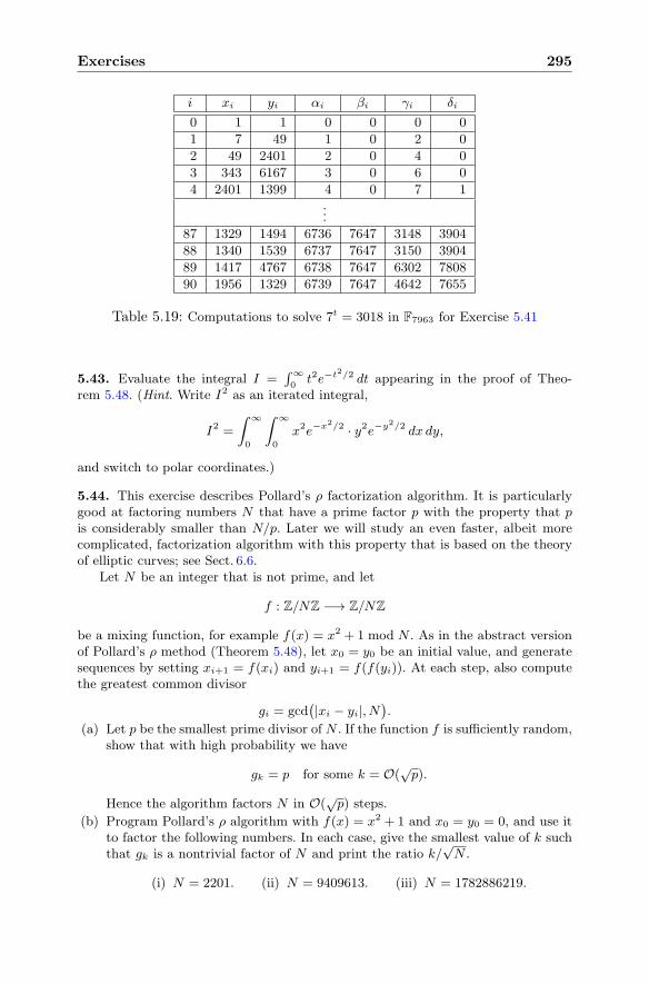
Exercises 295
i xi yi αi βi γi δi
0 1 1 0 0 0 0
1 7 49 1 0 2 0
2 49 2401 2 0 4 0
3 343 6167 3 0 6 0
4 2401 1399 4 0 7 1...
87 1329 1494 6736 7647 3148 3904
88 1340 1539 6737 7647 3150 3904
89 1417 4767 6738 7647 6302 7808
90 1956 1329 6739 7647 4642 7655
Table 5.19: Computations to solve 7t = 3018 in F7963 for Exercise 5.41
5.43. Evaluate the integral I =∫∞0t2e−t2/2 dt appearing in the proof of Theo-
rem 5.48. (Hint. Write I2 as an iterated integral,
I2 =
∫ ∞
0
∫ ∞
0
x2e−x2/2 · y2e−y2/2 dx dy,
and switch to polar coordinates.)
5.44. This exercise describes Pollard’s ρ factorization algorithm. It is particularlygood at factoring numbers N that have a prime factor p with the property that pis considerably smaller than N/p. Later we will study an even faster, albeit morecomplicated, factorization algorithm with this property that is based on the theoryof elliptic curves; see Sect. 6.6.
Let N be an integer that is not prime, and let
f : Z/NZ −→ Z/NZ
be a mixing function, for example f(x) = x2 + 1 mod N . As in the abstract versionof Pollard’s ρ method (Theorem 5.48), let x0 = y0 be an initial value, and generatesequences by setting xi+1 = f(xi) and yi+1 = f(f(yi)). At each step, also computethe greatest common divisor
gi = gcd(|xi − yi|, N
).
(a) Let p be the smallest prime divisor of N . If the function f is sufficiently random,show that with high probability we have
gk = p for some k = O(√p).
Hence the algorithm factors N in O(√p) steps.
(b) Program Pollard’s ρ algorithm with f(x) = x2 + 1 and x0 = y0 = 0, and use itto factor the following numbers. In each case, give the smallest value of k suchthat gk is a nontrivial factor of N and print the ratio k/
√N .
(i) N = 2201. (ii) N = 9409613. (iii) N = 1782886219.
296 Exercises
(c) Repeat your computations in (b) using the function f(x) = x2 + 2. Do therunning times change?
(d) Explain what happens if you run Pollard’s ρ algorithm and N is prime.
(e) Explain what happens if you run Pollard’s ρ algorithm with f(x) = x2 and anyinitial values for x0.
(f) Try running Pollard’s ρ algorithm with the function f(x) = x2 − 2. Explainwhat is happening. (Hint. This part is more challenging. It may help to use theidentity fn(u+ u−1) = u2n + u−2n , which you can prove by induction.)
Section 5.6. Information Theory
5.45. Consider the cipher that has three keys, three plaintexts, and four ciphertextsthat are combined using the following encryption table (which is similar to Table 5.12used in Example 5.54 on page 265).
m1 m2 m3
k1 c2 c4 c1k2 c1 c3 c2k3 c3 c1 c2
Suppose further that the plaintexts and keys are used with the following probabili-ties:
f(m1) = f(m2) =2
5, f(m3) =
1
5, f(k1) = f(k2) = f(k3) =
1
3.
(a) Compute f(c1), f(c2), f(c3), and f(c4).
(b) Compute f(c1 | m1), f(c1 | m2), and f(c1 | m3). Does this cryptosystem haveperfect secrecy?
(c) Compute f(c2 | m1) and f(c3 | m1).
(d) Compute f(k1 | c3) and f(k2 | c3).
5.46. Suppose that a shift cipher is employed such that each key, i.e., each shiftamount from 0 to 25, is used with equal probability and such that a new key ischosen to encrypt each successive letter. Show that this cryptosystem has perfectsecrecy by filling in the details of the following steps.(a) Show that
∑k∈K fM (dk(c)) = 1 for every ciphertext c ∈ C.
(b) Compute the ciphertext density function fC using (5.47), which in this casesays that
fC(c) =∑
k∈KfK(k)fM (dk(c)).
(c) Compare fC(c) to fC|M (c | m).
5.47. Give the details of the proof of (5.47), which says that
fC(c) =∑
k ∈ K suchthat c ∈ ek(M)
fK(k)fM(dk(c)
).
(Hint. Use the decomposition formula from Exercise 5.23(d)).
Exercises 297
5.48. Suppose that a cryptosystem has the same number of plaintexts as it doesciphertexts (#M = #C). Prove that for any given key k ∈ K and any given ci-phertext c ∈ C, there is a unique plaintext m ∈ M that encrypts to c using thekey k. (We used this fact during the proof of Theorem 5.56. Notice that the proofdoes not require the cryptosystem to have perfect secrecy; all that is needed is that#M = #C.)
5.49. Let Sm,c ={k ∈ K : ek(m) = c
}be the set used during the proof of
Theorem 5.56. Prove that if c �= c′, then Sm,c ∩ Sm,c′ = ∅. (Prove this for anycryptosystem; it is not necessary to assume perfect secrecy.)
5.50. Suppose that a cryptosystem satisfies #K = #M = #C and that it hasperfect secrecy. Prove that every ciphertext is used with equal probability and thatevery plaintext is used with equal probability. (Hint. We proved one of these duringthe course of proving Theorem 5.56. The proof of the other is similar.)
5.51. Prove the “only if” part of Theorem 5.56, i.e., prove that if a cryptosystemwith an equal number of keys, plaintexts, and ciphertexts satisfies conditions (a)and (b) of Theorem 5.56, then it has perfect secrecy.
5.52. LetXn be a uniformly distributed random variable on n objects, and let r ≥ 1.Prove directly from Property H3 of entropy that
H(Xnr ) = rH(Xn).
This generalizes Example 5.58.
5.53. Let X, Y , and Z1, . . . , Zm be random variables as described in Property H3
on page 270. Let
pi = Pr(Y = Zi) and qij = Pr(Zi = xij), so Pr(X = xij) = piqij .
With this notation, Property H3 says that
H
((piqij) 1≤i≤n
1≤j≤mi
)= H
((pi)1≤i≤n
)+
n∑
i=1
piH((qij)1≤j≤mi
).
(See Example 5.59.) Then the formula (5.51) for entropy given in Theorem 5.60implies that
n∑
i=1
mi∑
j=1
piqij log2(piqij) =
n∑
i=1
pi log2(pi) +
n∑
i=1
pi
mi∑
j=1
qij log2(qij). (5.64)
Prove directly that (5.64) is true. (Hint. Remember that the probabilities satisfy∑i pi = 1 and
∑j qij = 1.)
5.54. Let F (x) be a twice differentiable function with the property that F ′′(x) < 0for all x in its domain. Prove that F is concave in the sense of (5.52). Conclude inparticular that the function F (x) = log x is concave for all x > 0.
5.55. Use induction to prove Jensen’s inequality (Theorem 5.61).
5.56. Let X and Y be independent random variables.
298 Exercises
(a) Prove that the equivocation H(X | Y ) is equal to the entropy H(X).
(b) If H(X | Y ) = H(X), is it necessarily true that X and Y are independent?
5.57. Prove that key equivocation satisfies the formula
H(K | C) = H(K) +H(M)−H(C)
as described in Proposition 5.64.
5.58. We continue with the cipher described in Exercise 5.45.(a) Compute the entropies H(K), H(M), and H(C).
(b) Compute the key equivocation H(K | C).
5.59. Suppose that the key equivocation of a certain cryptosystem vanishes, i.e.,suppose that H(K | C) = 0. Prove that even a single observed ciphertext uniquelydetermines which key was used.
5.60. Write a computer program that reads a text file and performs the followingtasks:[1] Convert all alphabetic characters to lowercase and convert all strings of con-
secutive nonalphabetic characters to a single space. (The reason for leaving ina space is that when you count bigrams and trigrams, you will want to knowwhere words begin and end.)
[2] Count the frequency of each letter a-to-z, print a frequency table, and use yourfrequency table to estimate the entropy of a single letter in English, as we didin Sect. 5.6.3 using Table 1.3.
[3] Count the frequency of each bigram aa, ab,. . . ,zz, being careful to includeonly bigrams that appear within words. (As an alternative, also allow bigramsthat either start or end with a space, in which case there are 272 − 1 = 728possible bigrams.) Print a frequency table of the 25 most common bigrams andtheir probabilities, and use your full frequency table to estimate the entropy ofbigrams in English. In the notation of Sect. 5.6.3, this is the quantity H(L2).Compare 1
2H(L2) with the value of H(L) from step [1].
[4] Repeat [3], but this time with trigrams. Compare 13H(L3) with the values
of H(L) and 12H(L2) from [2] and [3]. (Note that for this part, you will need a
large quantity of text in order to get some reasonable frequencies.)Try running your program on some long blocks of text. For example, the followingnoncopyrighted material is available in the form of ordinary text files from ProjectGutenberg at http://www.gutenberg.org/. To what extent are the letter frequen-cies similar and to what extent do they differ in these different texts?(a) Alice’s Adventures in Wonderland by Lewis Carroll,
http://www.gutenberg.org/etext/11
(b) Relativity: the Special and General Theory by Albert Einstein,http://www.gutenberg.org/etext/5001
(c) The Old Testament (translated from the original Hebrew, of course!),http://www.gutenberg.org/etext/1609
(d) 20000 Lieues Sous Les Mers (20000 Leagues Under the Sea) by Jules Verne,http://www.gutenberg.org/etext/5097. Note that this one is a little trickier,since first you will need to convert all of the letters to their unaccented forms.
Chapter 6
Elliptic Curvesand Cryptography
The subject of elliptic curves encompasses a vast amount of mathematics.1
Our aim in this section is to summarize just enough of the basic theory forcryptographic applications. For additional reading, there are a number of sur-vey articles and books devoted to elliptic curve cryptography [14, 68, 81, 135],and many others that describe the number theoretic aspects of the theory ofelliptic curves, including [25, 65, 73, 74, 136, 134, 138].
6.1 Elliptic Curves
An elliptic curve2 is the set of solutions to an equation of the form
Y 2 = X3 +AX +B.
Equations of this type are called Weierstrass equations after the mathe-matician who studied them extensively during the nineteenth century. Twoexamples of elliptic curves,
E1 : Y 2 = X3 − 3X + 3 and E2 : Y 2 = X3 − 6X + 5,
are illustrated in Fig. 6.1.
1Indeed, even before elliptic curves burst into cryptographic prominence, a well-knownmathematician [73] opined that “it is possible to write endlessly on elliptic curves!”
2A word of warning. You may recall from high school geometry that an ellipse is ageometric object that looks like a squashed circle. Elliptic curves are not ellipses, andindeed, despite their somewhat unfortunate name, elliptic curves and ellipses have only themost tenuous connection with one another.
© Springer Science+Business Media New York 2014J. Hoffstein et al., An Introduction to Mathematical Cryptography,Undergraduate Texts in Mathematics, DOI 10.1007/978-1-4939-1711-2 6
299
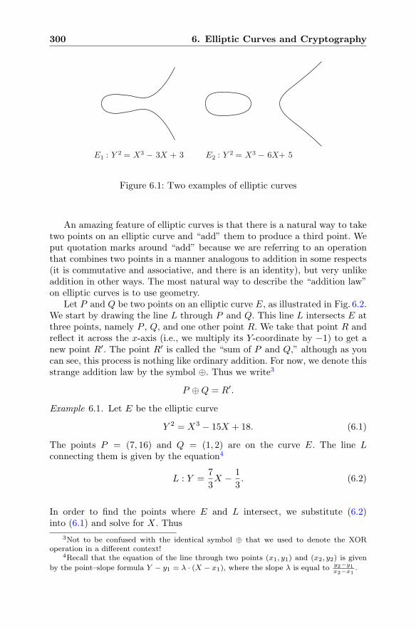
300 6. Elliptic Curves and Cryptography
E2 : Y 2 = X3 − 6X+ 5E1 : Y 2 = X3 − 3X + 3
Figure 6.1: Two examples of elliptic curves
An amazing feature of elliptic curves is that there is a natural way to taketwo points on an elliptic curve and “add” them to produce a third point. Weput quotation marks around “add” because we are referring to an operationthat combines two points in a manner analogous to addition in some respects(it is commutative and associative, and there is an identity), but very unlikeaddition in other ways. The most natural way to describe the “addition law”on elliptic curves is to use geometry.
Let P and Q be two points on an elliptic curve E, as illustrated in Fig. 6.2.We start by drawing the line L through P and Q. This line L intersects E atthree points, namely P , Q, and one other point R. We take that point R andreflect it across the x-axis (i.e., we multiply its Y-coordinate by −1) to get anew point R′. The point R′ is called the “sum of P and Q,” although as youcan see, this process is nothing like ordinary addition. For now, we denote thisstrange addition law by the symbol ⊕. Thus we write3
P ⊕Q = R′.
Example 6.1. Let E be the elliptic curve
Y 2 = X3 − 15X + 18. (6.1)
The points P = (7, 16) and Q = (1, 2) are on the curve E. The line Lconnecting them is given by the equation4
L : Y =7
3X − 1
3. (6.2)
In order to find the points where E and L intersect, we substitute (6.2)into (6.1) and solve for X. Thus
3Not to be confused with the identical symbol ⊕ that we used to denote the XORoperation in a different context!
4Recall that the equation of the line through two points (x1, y1) and (x2, y2) is given
by the point–slope formula Y − y1 = λ · (X − x1), where the slope λ is equal to y2−y1x2−x1
.
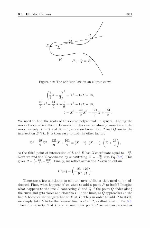
6.1. Elliptic Curves 301
P
Q
R
P ⊕ Q = R′
L
E
Figure 6.2: The addition law on an elliptic curve
(7
3X − 1
3
)2
= X3 − 15X + 18,
49
9X2 − 14
9X +
1
9= X3 − 15X + 18,
0 = X3 − 49
9X2 − 121
9X +
161
9.
We need to find the roots of this cubic polynomial. In general, finding theroots of a cubic is difficult. However, in this case we already know two of theroots, namely X = 7 and X = 1, since we know that P and Q are in theintersection E ∩ L. It is then easy to find the other factor,
X3 − 49
9X2 − 121
9X +
161
9= (X − 7) · (X − 1) ·
(X +
23
9
),
so the third point of intersection of L and E has X-coordinate equal to − 239 .
Next we find the Y-coordinate by substituting X = − 239 into Eq. (6.2). This
gives R =(− 23
9 ,−17027
). Finally, we reflect across the X-axis to obtain
P ⊕Q =
(−23
9,170
27
).
There are a few subtleties to elliptic curve addition that need to be ad-dressed. First, what happens if we want to add a point P to itself? Imaginewhat happens to the line L connecting P and Q if the point Q slides alongthe curve and gets closer and closer to P . In the limit, as Q approaches P , theline L becomes the tangent line to E at P . Thus in order to add P to itself,we simply take L to be the tangent line to E at P , as illustrated in Fig. 6.3.Then L intersects E at P and at one other point R, so we can proceed as
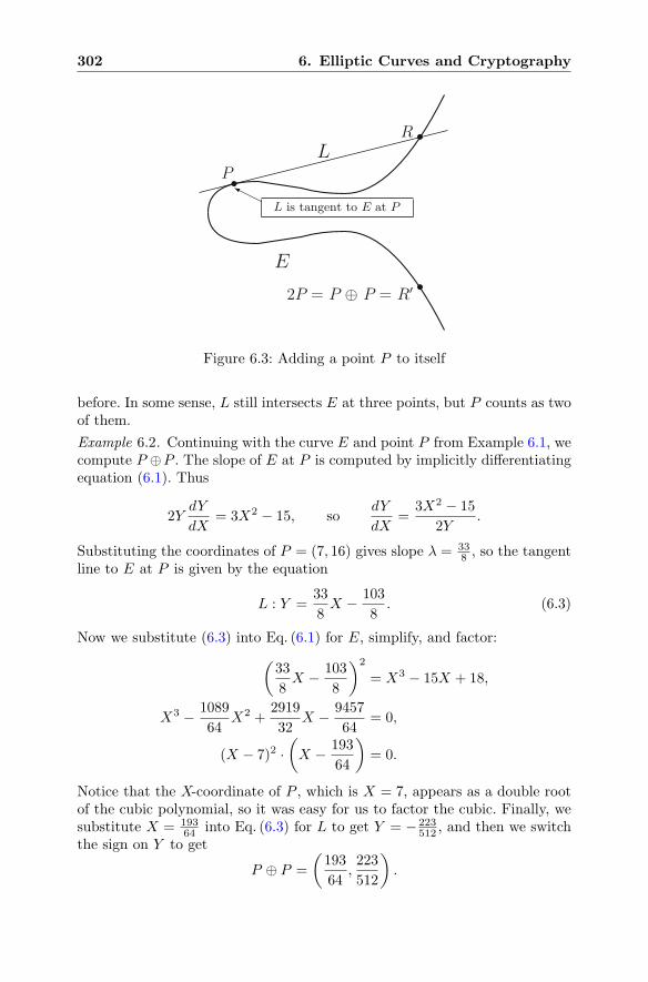
302 6. Elliptic Curves and Cryptography
P
R
2P = P ⊕ P = R′
L is tangent to E at P
L
E
Figure 6.3: Adding a point P to itself
before. In some sense, L still intersects E at three points, but P counts as twoof them.
Example 6.2. Continuing with the curve E and point P from Example 6.1, wecompute P ⊕P . The slope of E at P is computed by implicitly differentiatingequation (6.1). Thus
2YdY
dX= 3X2 − 15, so
dY
dX=
3X2 − 15
2Y.
Substituting the coordinates of P = (7, 16) gives slope λ = 338 , so the tangent
line to E at P is given by the equation
L : Y =33
8X − 103
8. (6.3)
Now we substitute (6.3) into Eq. (6.1) for E, simplify, and factor:
(33
8X − 103
8
)2
= X3 − 15X + 18,
X3 − 1089
64X2 +
2919
32X − 9457
64= 0,
(X − 7)2 ·(X − 193
64
)= 0.
Notice that the X-coordinate of P , which is X = 7, appears as a double rootof the cubic polynomial, so it was easy for us to factor the cubic. Finally, wesubstitute X = 193
64 into Eq. (6.3) for L to get Y = − 223512 , and then we switch
the sign on Y to get
P ⊕ P =
(193
64,223
512
).
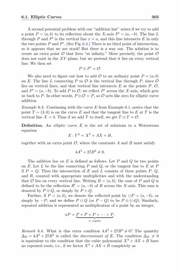
6.1. Elliptic Curves 303
A second potential problem with our “addition law” arises if we try to adda point P = (a, b) to its reflection about the X-axis P ′ = (a,−b). The line Lthrough P and P ′ is the vertical line x = a, and this line intersects E in onlythe two points P and P ′. (See Fig. 6.4.) There is no third point of intersection,so it appears that we are stuck! But there is a way out. The solution is tocreate an extra point O that lives “at infinity.” More precisely, the point Odoes not exist in the XY -plane, but we pretend that it lies on every verticalline. We then set
P ⊕ P ′ = O.
We also need to figure out how to add O to an ordinary point P = (a, b)on E. The line L connecting P to O is the vertical line through P , since Olies on vertical lines, and that vertical line intersects E at the points P , O,and P ′ = (a,−b). To add P to O, we reflect P ′ across the X-axis, which getsus back to P . In other words, P ⊕O = P , so O acts like zero for elliptic curveaddition.
Example 6.3. Continuing with the curve E from Example 6.1, notice that thepoint T = (3, 0) is on the curve E and that the tangent line to E at T is thevertical line X = 3. Thus if we add T to itself, we get T ⊕ T = O.
Definition. An elliptic curve E is the set of solutions to a Weierstrassequation
E : Y 2 = X3 +AX +B,
together with an extra point O, where the constants A and B must satisfy
4A3 + 27B2 �= 0.
The addition law on E is defined as follows. Let P and Q be two pointson E. Let L be the line connecting P and Q, or the tangent line to E at Pif P = Q. Then the intersection of E and L consists of three points P , Q,and R, counted with appropriate multiplicities and with the understandingthat O lies on every vertical line. Writing R = (a, b), the sum of P and Q isdefined to be the reflection R′ = (a,−b) of R across the X-axis. This sum isdenoted by P ⊕Q, or simply by P +Q.
Further, if P = (a, b), we denote the reflected point by �P = (a,−b), orsimply by −P ; and we define P � Q (or P − Q) to be P ⊕ (�Q). Similarly,repeated addition is represented as multiplication of a point by an integer,
nP = P + P + P + · · ·+ P︸ ︷︷ ︸n copies
.
Remark 6.4. What is this extra condition 4A3 + 27B2 �= 0? The quantityΔE = 4A3 + 27B2 is called the discriminant of E. The condition ΔE �= 0is equivalent to the condition that the cubic polynomial X3 +AX +B haveno repeated roots, i.e., if we factor X3 +AX +B completely as
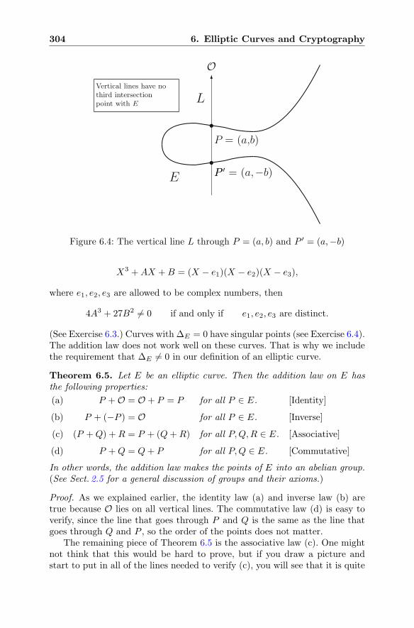
304 6. Elliptic Curves and Cryptography
E
L
O
P = (a,b)
P ′ = (a,−b)P
Vertical lines have nothird intersectionpoint with E
Figure 6.4: The vertical line L through P = (a, b) and P ′ = (a,−b)
X3 +AX +B = (X − e1)(X − e2)(X − e3),
where e1, e2, e3 are allowed to be complex numbers, then
4A3 + 27B2 �= 0 if and only if e1, e2, e3 are distinct.
(See Exercise 6.3.) Curves with ΔE = 0 have singular points (see Exercise 6.4).The addition law does not work well on these curves. That is why we includethe requirement that ΔE �= 0 in our definition of an elliptic curve.
Theorem 6.5. Let E be an elliptic curve. Then the addition law on E hasthe following properties:
(a) P +O = O + P = P for all P ∈ E. [Identity]
(b) P + (−P ) = O for all P ∈ E. [Inverse]
(c) (P +Q) +R = P + (Q+R) for all P,Q,R ∈ E. [Associative]
(d) P +Q = Q+ P for all P,Q ∈ E. [Commutative]
In other words, the addition law makes the points of E into an abelian group.(See Sect. 2.5 for a general discussion of groups and their axioms.)
Proof. As we explained earlier, the identity law (a) and inverse law (b) aretrue because O lies on all vertical lines. The commutative law (d) is easy toverify, since the line that goes through P and Q is the same as the line thatgoes through Q and P , so the order of the points does not matter.
The remaining piece of Theorem 6.5 is the associative law (c). One mightnot think that this would be hard to prove, but if you draw a picture andstart to put in all of the lines needed to verify (c), you will see that it is quite
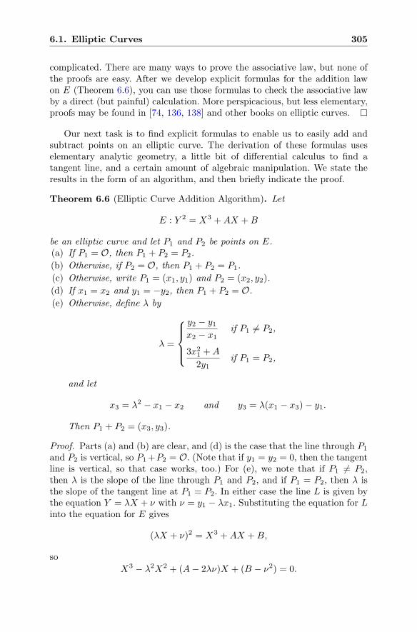
6.1. Elliptic Curves 305
complicated. There are many ways to prove the associative law, but none ofthe proofs are easy. After we develop explicit formulas for the addition lawon E (Theorem 6.6), you can use those formulas to check the associative lawby a direct (but painful) calculation. More perspicacious, but less elementary,proofs may be found in [74, 136, 138] and other books on elliptic curves.
Our next task is to find explicit formulas to enable us to easily add andsubtract points on an elliptic curve. The derivation of these formulas useselementary analytic geometry, a little bit of differential calculus to find atangent line, and a certain amount of algebraic manipulation. We state theresults in the form of an algorithm, and then briefly indicate the proof.
Theorem 6.6 (Elliptic Curve Addition Algorithm). Let
E : Y 2 = X3 +AX +B
be an elliptic curve and let P1 and P2 be points on E.(a) If P1 = O, then P1 + P2 = P2.
(b) Otherwise, if P2 = O, then P1 + P2 = P1.
(c) Otherwise, write P1 = (x1, y1) and P2 = (x2, y2).
(d) If x1 = x2 and y1 = −y2, then P1 + P2 = O.
(e) Otherwise, define λ by
λ =
⎧⎪⎪⎨
⎪⎪⎩
y2 − y1x2 − x1
if P1 �= P2,
3x21 +A
2y1if P1 = P2,
and let
x3 = λ2 − x1 − x2 and y3 = λ(x1 − x3)− y1.
Then P1 + P2 = (x3, y3).
Proof. Parts (a) and (b) are clear, and (d) is the case that the line through P1
and P2 is vertical, so P1+P2 = O. (Note that if y1 = y2 = 0, then the tangentline is vertical, so that case works, too.) For (e), we note that if P1 �= P2,then λ is the slope of the line through P1 and P2, and if P1 = P2, then λ isthe slope of the tangent line at P1 = P2. In either case the line L is given bythe equation Y = λX + ν with ν = y1 − λx1. Substituting the equation for Linto the equation for E gives
(λX + ν)2 = X3 +AX +B,
so
X3 − λ2X2 + (A− 2λν)X + (B − ν2) = 0.
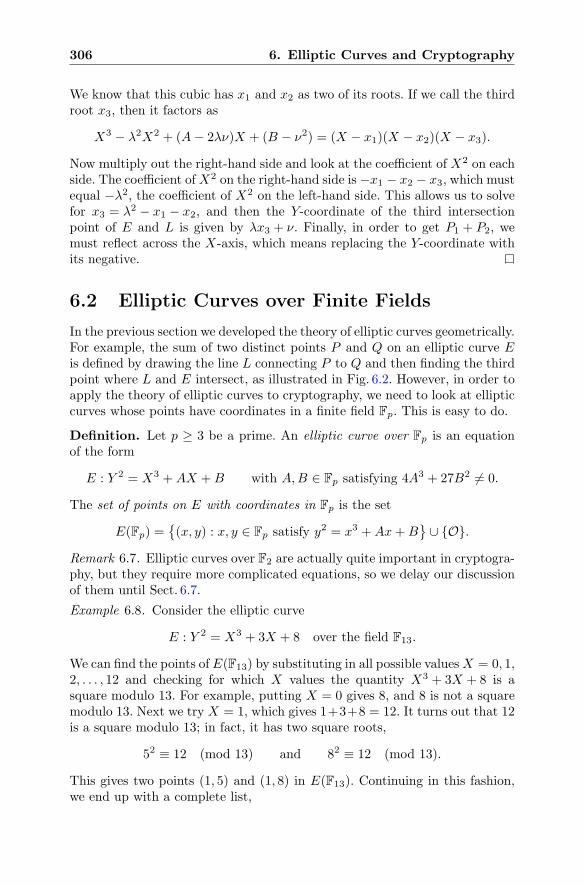
306 6. Elliptic Curves and Cryptography
We know that this cubic has x1 and x2 as two of its roots. If we call the thirdroot x3, then it factors as
X3 − λ2X2 + (A− 2λν)X + (B − ν2) = (X − x1)(X − x2)(X − x3).
Now multiply out the right-hand side and look at the coefficient of X2 on eachside. The coefficient ofX2 on the right-hand side is −x1 − x2 − x3, which mustequal −λ2, the coefficient of X2 on the left-hand side. This allows us to solvefor x3 = λ2 − x1 − x2, and then the Y-coordinate of the third intersectionpoint of E and L is given by λx3 + ν. Finally, in order to get P1 + P2, wemust reflect across the X-axis, which means replacing the Y-coordinate withits negative.
6.2 Elliptic Curves over Finite Fields
In the previous section we developed the theory of elliptic curves geometrically.For example, the sum of two distinct points P and Q on an elliptic curve Eis defined by drawing the line L connecting P to Q and then finding the thirdpoint where L and E intersect, as illustrated in Fig. 6.2. However, in order toapply the theory of elliptic curves to cryptography, we need to look at ellipticcurves whose points have coordinates in a finite field Fp. This is easy to do.
Definition. Let p ≥ 3 be a prime. An elliptic curve over Fp is an equationof the form
E : Y 2 = X3 +AX +B with A,B ∈ Fp satisfying 4A3 + 27B2 �= 0.
The set of points on E with coordinates in Fp is the set
E(Fp) ={(x, y) : x, y ∈ Fp satisfy y2 = x3 +Ax+B
}∪ {O}.
Remark 6.7. Elliptic curves over F2 are actually quite important in cryptogra-phy, but they require more complicated equations, so we delay our discussionof them until Sect. 6.7.
Example 6.8. Consider the elliptic curve
E : Y 2 = X3 + 3X + 8 over the field F13.
We can find the points of E(F13) by substituting in all possible valuesX = 0, 1,2, . . . , 12 and checking for which X values the quantity X3 + 3X + 8 is asquare modulo 13. For example, putting X = 0 gives 8, and 8 is not a squaremodulo 13. Next we try X = 1, which gives 1+3+8 = 12. It turns out that 12is a square modulo 13; in fact, it has two square roots,
52 ≡ 12 (mod 13) and 82 ≡ 12 (mod 13).
This gives two points (1, 5) and (1, 8) in E(F13). Continuing in this fashion,we end up with a complete list,
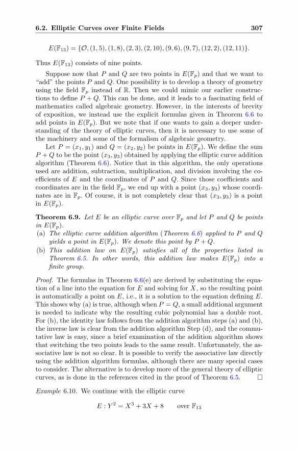
6.2. Elliptic Curves over Finite Fields 307
E(F13) = {O, (1, 5), (1, 8), (2, 3), (2, 10), (9, 6), (9, 7), (12, 2), (12, 11)}.
Thus E(F13) consists of nine points.
Suppose now that P and Q are two points in E(Fp) and that we want to“add” the points P and Q. One possibility is to develop a theory of geometryusing the field Fp instead of R. Then we could mimic our earlier construc-tions to define P +Q. This can be done, and it leads to a fascinating field ofmathematics called algebraic geometry. However, in the interests of brevityof exposition, we instead use the explicit formulas given in Theorem 6.6 toadd points in E(Fp). But we note that if one wants to gain a deeper under-standing of the theory of elliptic curves, then it is necessary to use some ofthe machinery and some of the formalism of algebraic geometry.
Let P = (x1, y1) and Q = (x2, y2) be points in E(Fp). We define the sumP +Q to be the point (x3, y3) obtained by applying the elliptic curve additionalgorithm (Theorem 6.6). Notice that in this algorithm, the only operationsused are addition, subtraction, multiplication, and division involving the co-efficients of E and the coordinates of P and Q. Since those coefficients andcoordinates are in the field Fp, we end up with a point (x3, y3) whose coordi-nates are in Fp. Of course, it is not completely clear that (x3, y3) is a pointin E(Fp).
Theorem 6.9. Let E be an elliptic curve over Fp and let P and Q be pointsin E(Fp).(a) The elliptic curve addition algorithm (Theorem 6.6) applied to P and Q
yields a point in E(Fp). We denote this point by P +Q.
(b) This addition law on E(Fp) satisfies all of the properties listed inTheorem 6.5. In other words, this addition law makes E(Fp) into afinite group.
Proof. The formulas in Theorem 6.6(e) are derived by substituting the equa-tion of a line into the equation for E and solving for X, so the resulting pointis automatically a point on E, i.e., it is a solution to the equation defining E.This shows why (a) is true, although when P = Q, a small additional argumentis needed to indicate why the resulting cubic polynomial has a double root.For (b), the identity law follows from the addition algorithm steps (a) and (b),the inverse law is clear from the addition algorithm Step (d), and the commu-tative law is easy, since a brief examination of the addition algorithm showsthat switching the two points leads to the same result. Unfortunately, the as-sociative law is not so clear. It is possible to verify the associative law directlyusing the addition algorithm formulas, although there are many special casesto consider. The alternative is to develop more of the general theory of ellipticcurves, as is done in the references cited in the proof of Theorem 6.5.
Example 6.10. We continue with the elliptic curve
E : Y 2 = X3 + 3X + 8 over F13
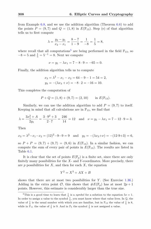
308 6. Elliptic Curves and Cryptography
from Example 6.8, and we use the addition algorithm (Theorem 6.6) to addthe points P = (9, 7) and Q = (1, 8) in E(F13). Step (e) of that algorithmtells us to first compute
λ =y2 − y1x2 − x1
=8− 7
1− 9=
1
−8 =1
5= 8,
where recall that all computations5 are being performed in the field F13, so−8 = 5 and 1
5 = 5−1 = 8. Next we compute
ν = y1 − λx1 = 7− 8 · 9 = −65 = 0.
Finally, the addition algorithm tells us to compute
x3 = λ2 − x1 − x2 = 64− 9− 1 = 54 = 2,
y3 = −(λx3 + ν) = −8 · 2 = −16 = 10.
This completes the computation of
P +Q = (1, 8) + (9, 7) = (2, 10) in E(F13).
Similarly, we can use the addition algorithm to add P = (9, 7) to itself.Keeping in mind that all calculations are in F13, we find that
λ =3x21 +A
2y1=
3 · 92 + 3
2 · 7 =246
14= 12 and ν = y1 − λx1 = 7− 12 · 9 = 3.
Then
x3 = λ2−x1−x2 = (12)2−9−9 = 9 and y3 = −(λx3+ν) = −(12·9+3) = 6,
so P + P = (9, 7) + (9, 7) = (9, 6) in E(F13). In a similar fashion, we cancompute the sum of every pair of points in E(F13). The results are listed inTable 6.1.
It is clear that the set of points E(Fp) is a finite set, since there are onlyfinitely many possibilities for the X- and Y-coordinates. More precisely, thereare p possibilities for X, and then for each X, the equation
Y 2 = X3 +AX +B
shows that there are at most two possibilities for Y . (See Exercise 1.36.)Adding in the extra point O, this shows that #E(Fp) has at most 2p+ 1points. However, this estimate is considerably larger than the true size.
5This is a good time to learn that 15is a symbol for a solution to the equation 5x = 1.
In order to assign a value to the symbol 15, you must know where that value lives. In Q, the
value of 15is the usual number with which you are familiar, but in F13 the value of 1
5is 8,
while in F11 the value of 15is 9. And in F5 the symbol 1
5is not assigned a value.
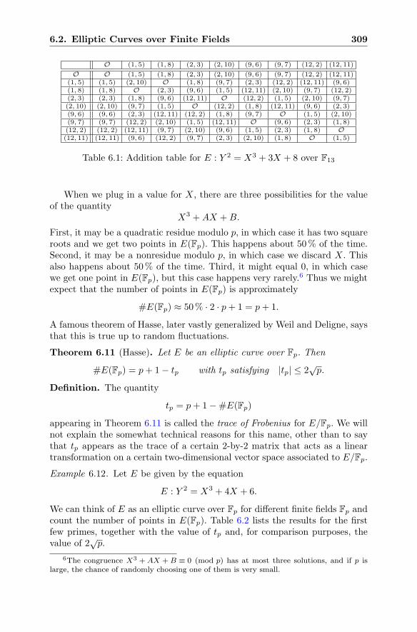
6.2. Elliptic Curves over Finite Fields 309
O (1, 5) (1, 8) (2, 3) (2, 10) (9, 6) (9, 7) (12, 2) (12, 11)
O O (1, 5) (1, 8) (2, 3) (2, 10) (9, 6) (9, 7) (12, 2) (12, 11)(1, 5) (1, 5) (2, 10) O (1, 8) (9, 7) (2, 3) (12, 2) (12, 11) (9, 6)(1, 8) (1, 8) O (2, 3) (9, 6) (1, 5) (12, 11) (2, 10) (9, 7) (12, 2)(2, 3) (2, 3) (1, 8) (9, 6) (12, 11) O (12, 2) (1, 5) (2, 10) (9, 7)(2, 10) (2, 10) (9, 7) (1, 5) O (12, 2) (1, 8) (12, 11) (9, 6) (2, 3)(9, 6) (9, 6) (2, 3) (12, 11) (12, 2) (1, 8) (9, 7) O (1, 5) (2, 10)(9, 7) (9, 7) (12, 2) (2, 10) (1, 5) (12, 11) O (9, 6) (2, 3) (1, 8)(12, 2) (12, 2) (12, 11) (9, 7) (2, 10) (9, 6) (1, 5) (2, 3) (1, 8) O(12, 11) (12, 11) (9, 6) (12, 2) (9, 7) (2, 3) (2, 10) (1, 8) O (1, 5)
Table 6.1: Addition table for E : Y 2 = X3 + 3X + 8 over F13
When we plug in a value for X, there are three possibilities for the valueof the quantity
X3 +AX +B.
First, it may be a quadratic residue modulo p, in which case it has two squareroots and we get two points in E(Fp). This happens about 50% of the time.Second, it may be a nonresidue modulo p, in which case we discard X. Thisalso happens about 50% of the time. Third, it might equal 0, in which casewe get one point in E(Fp), but this case happens very rarely.6 Thus we mightexpect that the number of points in E(Fp) is approximately
#E(Fp) ≈ 50% · 2 · p+ 1 = p+ 1.
A famous theorem of Hasse, later vastly generalized by Weil and Deligne, saysthat this is true up to random fluctuations.
Theorem 6.11 (Hasse). Let E be an elliptic curve over Fp. Then
#E(Fp) = p+ 1− tp with tp satisfying |tp| ≤ 2√p.
Definition. The quantity
tp = p+ 1−#E(Fp)
appearing in Theorem 6.11 is called the trace of Frobenius for E/Fp. We willnot explain the somewhat technical reasons for this name, other than to saythat tp appears as the trace of a certain 2-by-2 matrix that acts as a lineartransformation on a certain two-dimensional vector space associated to E/Fp.
Example 6.12. Let E be given by the equation
E : Y 2 = X3 + 4X + 6.
We can think of E as an elliptic curve over Fp for different finite fields Fp andcount the number of points in E(Fp). Table 6.2 lists the results for the firstfew primes, together with the value of tp and, for comparison purposes, thevalue of 2
√p.
6The congruence X3 +AX +B ≡ 0 (mod p) has at most three solutions, and if p islarge, the chance of randomly choosing one of them is very small.
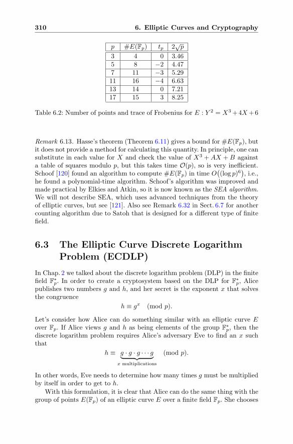
310 6. Elliptic Curves and Cryptography
p #E(Fp) tp 2√p
3 4 0 3.465 8 −2 4.477 11 −3 5.2911 16 −4 6.6313 14 0 7.2117 15 3 8.25
Table 6.2: Number of points and trace of Frobenius for E : Y 2 = X3+4X+6
Remark 6.13. Hasse’s theorem (Theorem 6.11) gives a bound for #E(Fp), butit does not provide a method for calculating this quantity. In principle, one cansubstitute in each value for X and check the value of X3 +AX +B againsta table of squares modulo p, but this takes time O(p), so is very inefficient.Schoof [120] found an algorithm to compute #E(Fp) in time O
((log p)6
), i.e.,
he found a polynomial-time algorithm. Schoof’s algorithm was improved andmade practical by Elkies and Atkin, so it is now known as the SEA algorithm.We will not describe SEA, which uses advanced techniques from the theoryof elliptic curves, but see [121]. Also see Remark 6.32 in Sect. 6.7 for anothercounting algorithm due to Satoh that is designed for a different type of finitefield.
6.3 The Elliptic Curve Discrete LogarithmProblem (ECDLP)
In Chap. 2 we talked about the discrete logarithm problem (DLP) in the finitefield F
∗p. In order to create a cryptosystem based on the DLP for F
∗p, Alice
publishes two numbers g and h, and her secret is the exponent x that solvesthe congruence
h ≡ gx (mod p).
Let’s consider how Alice can do something similar with an elliptic curve Eover Fp. If Alice views g and h as being elements of the group F
∗p, then the
discrete logarithm problem requires Alice’s adversary Eve to find an x suchthat
h ≡ g · g · g · · · g︸ ︷︷ ︸
x multiplications
(mod p).
In other words, Eve needs to determine how many times g must be multipliedby itself in order to get to h.
With this formulation, it is clear that Alice can do the same thing with thegroup of points E(Fp) of an elliptic curve E over a finite field Fp. She chooses
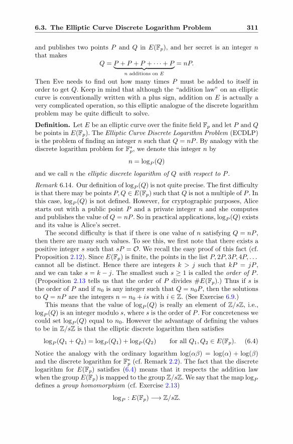
6.3. The Elliptic Curve Discrete Logarithm Problem 311
and publishes two points P and Q in E(Fp), and her secret is an integer nthat makes
Q = P + P + P + · · ·+ P︸ ︷︷ ︸n additions on E
= nP.
Then Eve needs to find out how many times P must be added to itself inorder to get Q. Keep in mind that although the “addition law” on an ellipticcurve is conventionally written with a plus sign, addition on E is actually avery complicated operation, so this elliptic analogue of the discrete logarithmproblem may be quite difficult to solve.
Definition. Let E be an elliptic curve over the finite field Fp and let P and Qbe points in E(Fp). The Elliptic Curve Discrete Logarithm Problem (ECDLP)is the problem of finding an integer n such that Q = nP . By analogy with thediscrete logarithm problem for F∗
p, we denote this integer n by
n = logP (Q)
and we call n the elliptic discrete logarithm of Q with respect to P .
Remark 6.14. Our definition of logP (Q) is not quite precise. The first difficultyis that there may be points P,Q ∈ E(Fp) such that Q is not a multiple of P . Inthis case, logP (Q) is not defined. However, for cryptographic purposes, Alicestarts out with a public point P and a private integer n and she computesand publishes the value of Q = nP . So in practical applications, logP (Q) existsand its value is Alice’s secret.
The second difficulty is that if there is one value of n satisfying Q = nP ,then there are many such values. To see this, we first note that there exists apositive integer s such that sP = O. We recall the easy proof of this fact (cf.Proposition 2.12). Since E(Fp) is finite, the points in the list P, 2P, 3P, 4P, . . .cannot all be distinct. Hence there are integers k > j such that kP = jP ,and we can take s = k − j. The smallest such s ≥ 1 is called the order of P .(Proposition 2.13 tells us that the order of P divides #E(Fp).) Thus if s isthe order of P and if n0 is any integer such that Q = n0P , then the solutionsto Q = nP are the integers n = n0 + is with i ∈ Z. (See Exercise 6.9.)
This means that the value of logP (Q) is really an element of Z/sZ, i.e.,logP (Q) is an integer modulo s, where s is the order of P . For concreteness wecould set logP (Q) equal to n0. However the advantage of defining the valuesto be in Z/sZ is that the elliptic discrete logarithm then satisfies
logP (Q1 +Q2) = logP (Q1) + logP (Q2) for all Q1, Q2 ∈ E(Fp). (6.4)
Notice the analogy with the ordinary logarithm log(αβ) = log(α) + log(β)and the discrete logarithm for F∗
p (cf. Remark 2.2). The fact that the discretelogarithm for E(Fp) satisfies (6.4) means that it respects the addition lawwhen the group E(Fp) is mapped to the group Z/sZ. We say that the map logPdefines a group homomorphism (cf. Exercise 2.13)
logP : E(Fp) −→ Z/sZ.
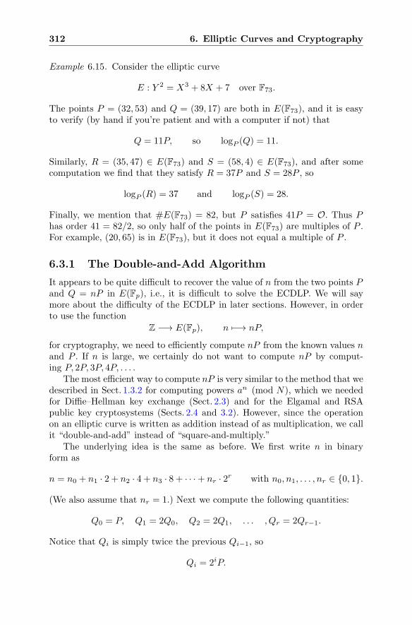
312 6. Elliptic Curves and Cryptography
Example 6.15. Consider the elliptic curve
E : Y 2 = X3 + 8X + 7 over F73.
The points P = (32, 53) and Q = (39, 17) are both in E(F73), and it is easyto verify (by hand if you’re patient and with a computer if not) that
Q = 11P, so logP (Q) = 11.
Similarly, R = (35, 47) ∈ E(F73) and S = (58, 4) ∈ E(F73), and after somecomputation we find that they satisfy R = 37P and S = 28P , so
logP (R) = 37 and logP (S) = 28.
Finally, we mention that #E(F73) = 82, but P satisfies 41P = O. Thus Phas order 41 = 82/2, so only half of the points in E(F73) are multiples of P .For example, (20, 65) is in E(F73), but it does not equal a multiple of P .
6.3.1 The Double-and-Add Algorithm
It appears to be quite difficult to recover the value of n from the two points Pand Q = nP in E(Fp), i.e., it is difficult to solve the ECDLP. We will saymore about the difficulty of the ECDLP in later sections. However, in orderto use the function
Z −→ E(Fp), n �−→ nP,
for cryptography, we need to efficiently compute nP from the known values nand P . If n is large, we certainly do not want to compute nP by comput-ing P, 2P, 3P, 4P, . . . .
The most efficient way to compute nP is very similar to the method that wedescribed in Sect. 1.3.2 for computing powers an (mod N), which we neededfor Diffie–Hellman key exchange (Sect. 2.3) and for the Elgamal and RSApublic key cryptosystems (Sects. 2.4 and 3.2). However, since the operationon an elliptic curve is written as addition instead of as multiplication, we callit “double-and-add” instead of “square-and-multiply.”
The underlying idea is the same as before. We first write n in binaryform as
n = n0 + n1 · 2 + n2 · 4 + n3 · 8 + · · ·+ nr · 2r with n0, n1, . . . , nr ∈ {0, 1}.
(We also assume that nr = 1.) Next we compute the following quantities:
Q0 = P, Q1 = 2Q0, Q2 = 2Q1, . . . , Qr = 2Qr−1.
Notice that Qi is simply twice the previous Qi−1, so
Qi = 2iP.
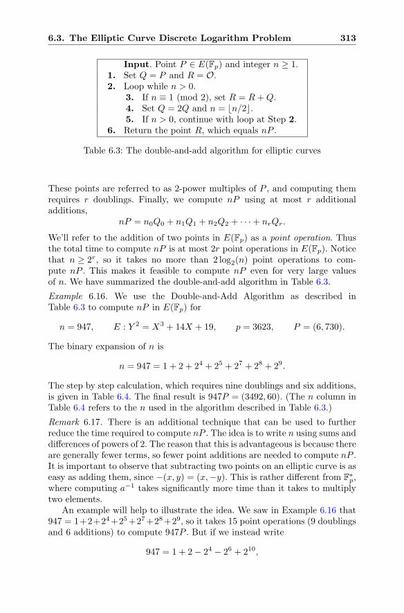
6.3. The Elliptic Curve Discrete Logarithm Problem 313
Input. Point P ∈ E(Fp) and integer n ≥ 1.1. Set Q = P and R = O.2. Loop while n > 0.
3. If n ≡ 1 (mod 2), set R = R+Q.4. Set Q = 2Q and n = �n/2�.5. If n > 0, continue with loop at Step 2.
6. Return the point R, which equals nP .
Table 6.3: The double-and-add algorithm for elliptic curves
These points are referred to as 2-power multiples of P , and computing themrequires r doublings. Finally, we compute nP using at most r additionaladditions,
nP = n0Q0 + n1Q1 + n2Q2 + · · ·+ nrQr.
We’ll refer to the addition of two points in E(Fp) as a point operation. Thusthe total time to compute nP is at most 2r point operations in E(Fp). Noticethat n ≥ 2r, so it takes no more than 2 log2(n) point operations to com-pute nP . This makes it feasible to compute nP even for very large valuesof n. We have summarized the double-and-add algorithm in Table 6.3.
Example 6.16. We use the Double-and-Add Algorithm as described inTable 6.3 to compute nP in E(Fp) for
n = 947, E : Y 2 = X3 + 14X + 19, p = 3623, P = (6, 730).
The binary expansion of n is
n = 947 = 1 + 2 + 24 + 25 + 27 + 28 + 29.
The step by step calculation, which requires nine doublings and six additions,is given in Table 6.4. The final result is 947P = (3492, 60). (The n column inTable 6.4 refers to the n used in the algorithm described in Table 6.3.)
Remark 6.17. There is an additional technique that can be used to furtherreduce the time required to compute nP . The idea is to write n using sums anddifferences of powers of 2. The reason that this is advantageous is because thereare generally fewer terms, so fewer point additions are needed to compute nP .It is important to observe that subtracting two points on an elliptic curve is aseasy as adding them, since −(x, y) = (x,−y). This is rather different from F
∗p,
where computing a−1 takes significantly more time than it takes to multiplytwo elements.
An example will help to illustrate the idea. We saw in Example 6.16 that947 = 1+2+24+25+27+28+29, so it takes 15 point operations (9 doublingsand 6 additions) to compute 947P . But if we instead write
947 = 1 + 2− 24 − 26 + 210,
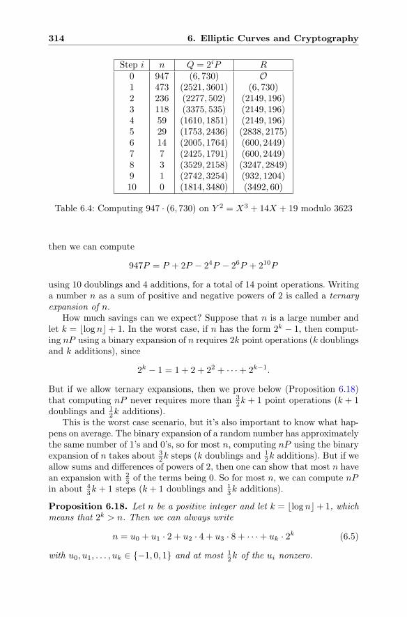
314 6. Elliptic Curves and Cryptography
Step i n Q = 2iP R0 947 (6, 730) O1 473 (2521, 3601) (6, 730)2 236 (2277, 502) (2149, 196)3 118 (3375, 535) (2149, 196)4 59 (1610, 1851) (2149, 196)5 29 (1753, 2436) (2838, 2175)6 14 (2005, 1764) (600, 2449)7 7 (2425, 1791) (600, 2449)8 3 (3529, 2158) (3247, 2849)9 1 (2742, 3254) (932, 1204)10 0 (1814, 3480) (3492, 60)
Table 6.4: Computing 947 · (6, 730) on Y 2 = X3 + 14X + 19 modulo 3623
then we can compute
947P = P + 2P − 24P − 26P + 210P
using 10 doublings and 4 additions, for a total of 14 point operations. Writinga number n as a sum of positive and negative powers of 2 is called a ternaryexpansion of n.
How much savings can we expect? Suppose that n is a large number andlet k = �log n�+ 1. In the worst case, if n has the form 2k − 1, then comput-ing nP using a binary expansion of n requires 2k point operations (k doublingsand k additions), since
2k − 1 = 1 + 2 + 22 + · · ·+ 2k−1.
But if we allow ternary expansions, then we prove below (Proposition 6.18)that computing nP never requires more than 3
2k + 1 point operations (k + 1doublings and 1
2k additions).This is the worst case scenario, but it’s also important to know what hap-
pens on average. The binary expansion of a random number has approximatelythe same number of 1’s and 0’s, so for most n, computing nP using the binaryexpansion of n takes about 3
2k steps (k doublings and 12k additions). But if we
allow sums and differences of powers of 2, then one can show that most n havean expansion with 2
3 of the terms being 0. So for most n, we can compute nPin about 4
3k + 1 steps (k + 1 doublings and 13k additions).
Proposition 6.18. Let n be a positive integer and let k = �log n�+ 1, whichmeans that 2k > n. Then we can always write
n = u0 + u1 · 2 + u2 · 4 + u3 · 8 + · · ·+ uk · 2k (6.5)
with u0, u1, . . . , uk ∈ {−1, 0, 1} and at most 12k of the ui nonzero.
6.3. The Elliptic Curve Discrete Logarithm Problem 315
Proof. The proof is essentially an algorithm for writing n in the desired form.We start by writing n in binary,
n = n0 + n1 · 2 + n2 · 4 + · · ·+ nk−1 · 2k−1 with n0, . . . , nk−1 ∈ {0, 1}.
Working from left to right, we look for the first occurrence of two or moreconsecutive nonzero ni coefficients. For example, suppose that
ns = ns+1 = · · · = ns+t−1 = 1 and ns+t = 0
for some t ≥ 2. In other words, the quantity
2s + 2s+1 + · · ·+ 2s+t−1 + 0 · 2s+t (6.6)
appears in the binary expansion of n. We observe that
2s + 2s+1 + · · ·+ 2s+t−1 + 0 · 2s+t = 2s(1 + 2 + 4 + · · ·+ 2t−1) = 2s(2t − 1),
so we can replace (6.6) with−2s + 2s+t.
Repeating this procedure, we end up with an expansion of n of the form (6.5)in which no two consecutive ui are nonzero. (Note that although the originalbinary expansion went up to only 2k−1, the new expansion might go up to 2k.)
6.3.2 How Hard Is the ECDLP?
The collision algorithms described in Sect. 5.4 are easily adapted to any group,for example to the group of points E(Fp) on an elliptic curve. In order tosolve Q = nP , Eve chooses random integers j1, . . . , jr and k1, . . . , kr between 1and p and makes two lists of points:
List #1. j1P, j2P, j3P, . . . , jrP,
List #2. k1P +Q, k2P +Q, k3P +Q, . . . , krP +Q.
As soon as she finds a match (collision) between the two lists, she is done,since if she finds juP = kvP +Q, then Q = (ju − kv)P provides the solution.As we saw in Sect. 5.4, if r is somewhat larger than
√p, say r ≈ 3
√p, then
there is a very good chance that there will be a collision.This naive collision algorithm requires quite a lot of storage for the two
lists. However, it is not hard to adapt Pollard’s ρ method from Sect. 5.5 todevise a storage-free collision algorithm with a similar running time. (See Ex-ercise 6.13.) In any case, there are certainly algorithms that solve the ECDLPfor E(Fp) in O(
√p ) steps.
We have seen that there are much faster ways to solve the discrete loga-rithm problem for F∗
p. In particular, the index calculus described in Sect. 3.8
316 6. Elliptic Curves and Cryptography
has a subexponential running time, i.e., the running time is O(pε) for ev-ery ε > 0. The principal reason that elliptic curves are used in cryptographyis the fact that there are no index calculus algorithms known for the ECDLP,and indeed, there are no general algorithms known that solve the ECDLP infewer than O(
√p ) steps. In other words, despite the highly structured nature
of the group E(Fp), the fastest known algorithms to solve the ECDLP are nobetter than the generic algorithm that works equally well to solve the discretelogarithm problem in any group. This fact is sufficiently important that itbears highlighting.
The fastest known algorithm tosolve ECDLP in E(Fp) takes ap-proximately
√p steps.
Thus the ECDLP appears to be much more difficult than the DLP. Recall,however, there are some primes p for which the DLP in F
∗p is comparatively
easy. For example, if p− 1 is a product of small primes, then the Pohlig–Hellman algorithm (Theorem 2.31) gives a quick solution to the DLP in F
∗p.
In a similar fashion, there are some elliptic curves and some primes for whichthe ECDLP in E(Fp) is comparatively easy. We discuss some of these specialcases, which must be avoided in the construction of secure cryptosystems, inSect. 6.9.1.
6.4 Elliptic Curve Cryptography
It is finally time to apply elliptic curves to cryptography. We start with theeasiest application, Diffie–Hellman key exchange, which involves little morethan replacing the discrete logarithm problem for the finite field Fp withthe discrete logarithm problem for an elliptic curve E(Fp). We then describeelliptic analogues of the Elgamal public key cryptosystem and the digitalsignature algorithm (DSA).
6.4.1 Elliptic Diffie–Hellman Key Exchange
Alice and Bob agree to use a particular elliptic curve E(Fp) and a particularpoint P ∈ E(Fp). Alice chooses a secret integer nA and Bob chooses a secretinteger nB . They compute the associated multiples
Alice computes this︷ ︸︸ ︷QA = nAP and
Bob computes this︷ ︸︸ ︷QB = nBP ,
and they exchange the values of QA and QB . Alice then uses her secret multi-plier to compute nAQB , and Bob similarly computes nBQA. They now havethe shared secret value
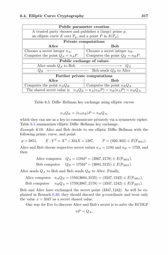
6.4. Elliptic Curve Cryptography 317
Public parameter creationA trusted party chooses and publishes a (large) prime p,an elliptic curve E over Fp, and a point P in E(Fp).
Private computationsAlice Bob
Chooses a secret integer nA. Chooses a secret integer nB .Computes the point QA = nAP . Computes the point QB = nBP .
Public exchange of valuesAlice sends QA to Bob −−−−−−−−−−−−−−−−−−→ QA
QB ←−−−−−−−−−−−−−−−−−− Bob sends QB to Alice
Further private computationsAlice Bob
Computes the point nAQB . Computes the point nBQA.The shared secret value is nAQB = nA(nBP ) = nB(nAP ) = nBQA.
Table 6.5: Diffie–Hellman key exchange using elliptic curves
nAQB = (nAnB)P = nBQA,
which they can use as a key to communicate privately via a symmetric cipher.Table 6.5 summarizes elliptic Diffie–Hellman key exchange.
Example 6.19. Alice and Bob decide to use elliptic Diffie–Hellman with thefollowing prime, curve, and point:
p = 3851, E : Y 2 = X3 + 324X + 1287, P = (920, 303) ∈ E(F3851).
Alice and Bob choose respective secret values nA = 1194 and nB = 1759, andthen
Alice computes QA = 1194P = (2067, 2178) ∈ E(F3851),
Bob computes QB = 1759P = (3684, 3125) ∈ E(F3851).
Alice sends QA to Bob and Bob sends QB to Alice. Finally,
Alice computes nAQB = 1194(3684, 3125) = (3347, 1242) ∈ E(F3851),
Bob computes nBQA = 1759(2067, 2178) = (3347, 1242) ∈ E(F3851).
Bob and Alice have exchanged the secret point (3347, 1242). As will be ex-plained in Remark 6.20, they should discard the y-coordinate and treat onlythe value x = 3347 as a secret shared value.
One way for Eve to discover Alice and Bob’s secret is to solve the ECDLP
nP = QA,
318 6. Elliptic Curves and Cryptography
since if Eve can solve this problem, then she knows nA and can use it tocompute nAQB . Of course, there might be some other way for Eve to com-pute their secret without actually solving the ECDLP. The precise problemthat Eve needs to solve is the elliptic analogue of the Diffie–Hellman problemdescribed on page 69.
Definition. Let E(Fp) be an elliptic curve over a finite field and let P ∈E(Fp). The Elliptic Curve Diffie–Hellman Problem is the problem of comput-ing the value of n1n2P from the known values of n1P and n2P .
Remark 6.20. Elliptic Diffie–Hellman key exchange requires Alice and Bobto exchange points on an elliptic curve. A point Q in E(Fp) consists of twocoordinates Q = (xQ, yQ), where xQ and yQ are elements of the finite field Fp,so it appears that Alice must send Bob two numbers in Fp. However, thosetwo numbers modulo p do not contain as much information as two arbitrarynumbers, since they are related by the formula
y2Q = x3Q +AxQ +B in Fp.
Note that Eve knows A and B, so if she can guess the correct value of xQ,then there are only two possible values for yQ, and in practice it is not toohard for her to actually compute the two values of yQ.
There is thus little reason for Alice to send both coordinates of QA to Bob,since the y-coordinate contains so little additional information. Instead, shesends Bob only the x-coordinate of QA. Bob then computes and uses one ofthe two possible y-coordinates. If he happens to choose the “correct” y, thenhe is using QA, and if he chooses the “incorrect” y (which is the negative ofthe correct y), then he is using −QA. In any case, Bob ends up computingone of
±nBQA = ±(nAnB)P.
Similarly, Alice ends up computing one of ±(nAnB)P . Then Alice and Bobuse the x-coordinate as their shared secret value, since that x-coordinate isthe same regardless of which y they use.
Example 6.21. Alice and Bob decide to exchange another secret value usingthe same public parameters as in Example 6.19:
p = 3851, E : Y 2 = X3 + 324X + 1287, P = (920, 303) ∈ E(F3851).
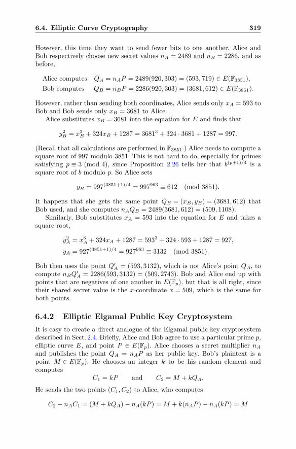
6.4. Elliptic Curve Cryptography 319
However, this time they want to send fewer bits to one another. Alice andBob respectively choose new secret values nA = 2489 and nB = 2286, and asbefore,
Alice computes QA = nAP = 2489(920, 303) = (593, 719) ∈ E(F3851),
Bob computes QB = nBP = 2286(920, 303) = (3681, 612) ∈ E(F3851).
However, rather than sending both coordinates, Alice sends only xA = 593 toBob and Bob sends only xB = 3681 to Alice.
Alice substitutes xB = 3681 into the equation for E and finds that
y2B = x3B + 324xB + 1287 = 36813 + 324 · 3681 + 1287 = 997.
(Recall that all calculations are performed in F3851.) Alice needs to compute asquare root of 997 modulo 3851. This is not hard to do, especially for primessatisfying p ≡ 3 (mod 4), since Proposition 2.26 tells her that b(p+1)/4 is asquare root of b modulo p. So Alice sets
yB = 997(3851+1)/4 = 997963 ≡ 612 (mod 3851).
It happens that she gets the same point QB = (xB , yB) = (3681, 612) thatBob used, and she computes nAQB = 2489(3681, 612) = (509, 1108).
Similarly, Bob substitutes xA = 593 into the equation for E and takes asquare root,
y2A = x3A + 324xA + 1287 = 5933 + 324 · 593 + 1287 = 927,
yA = 927(3851+1)/4 = 927963 ≡ 3132 (mod 3851).
Bob then uses the point Q′A = (593, 3132), which is not Alice’s point QA, to
compute nBQ′A = 2286(593, 3132) = (509, 2743). Bob and Alice end up with
points that are negatives of one another in E(Fp), but that is all right, sincetheir shared secret value is the x-coordinate x = 509, which is the same forboth points.
6.4.2 Elliptic Elgamal Public Key Cryptosystem
It is easy to create a direct analogue of the Elgamal public key cryptosystemdescribed in Sect. 2.4. Briefly, Alice and Bob agree to use a particular prime p,elliptic curve E, and point P ∈ E(Fp). Alice chooses a secret multiplier nAand publishes the point QA = nAP as her public key. Bob’s plaintext is apoint M ∈ E(Fp). He chooses an integer k to be his random element andcomputes
C1 = kP and C2 =M + kQA.
He sends the two points (C1, C2) to Alice, who computes
C2 − nAC1 = (M + kQA)− nA(kP ) =M + k(nAP )− nA(kP ) =M
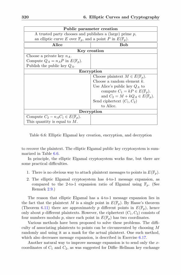
320 6. Elliptic Curves and Cryptography
Public parameter creationA trusted party chooses and publishes a (large) prime p,an elliptic curve E over Fp, and a point P in E(Fp).
Alice Bob
Key creationChoose a private key nA.Compute QA = nAP in E(Fp).Publish the public key QA.
EncryptionChoose plaintext M ∈ E(Fp).Choose a random element k.Use Alice’s public key QA to
compute C1 = kP ∈ E(Fp).and C2 =M + kQA ∈ E(Fp).
Send ciphertext (C1, C2)to Alice.
DecryptionCompute C2 − nAC1 ∈ E(Fp).This quantity is equal to M .
Table 6.6: Elliptic Elgamal key creation, encryption, and decryption
to recover the plaintext. The elliptic Elgamal public key cryptosystem is sum-marized in Table 6.6.
In principle, the elliptic Elgamal cryptosystem works fine, but there aresome practical difficulties.
1. There is no obvious way to attach plaintext messages to points in E(Fp).
2. The elliptic Elgamal cryptosystem has 4-to-1 message expansion, ascompared to the 2-to-1 expansion ratio of Elgamal using Fp. (SeeRemark 2.9.)
The reason that elliptic Elgamal has a 4-to-1 message expansion lies inthe fact that the plaintext M is a single point in E(Fp). By Hasse’s theorem(Theorem 6.11) there are approximately p different points in E(Fp), henceonly about p different plaintexts. However, the ciphertext (C1, C2) consists offour numbers modulo p, since each point in E(Fp) has two coordinates.
Various methods have been proposed to solve these problems. The diffi-culty of associating plaintexts to points can be circumvented by choosing Mrandomly and using it as a mask for the actual plaintext. One such method,which also decreases message expansion, is described in Exercise 6.17.
Another natural way to improve message expansion is to send only the x-coordinates of C1 and C2, as was suggested for Diffie–Hellman key exchange
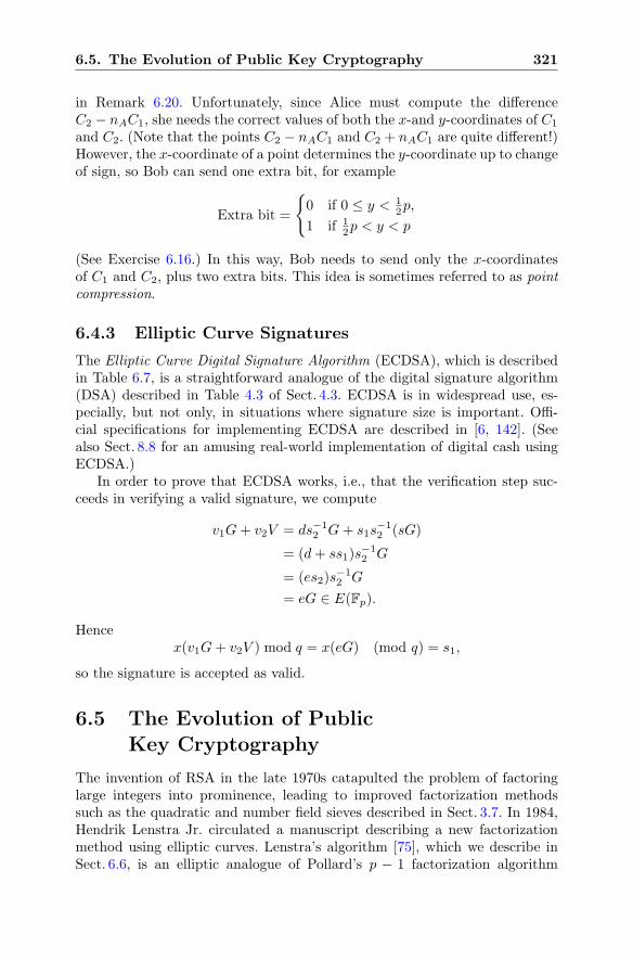
6.5. The Evolution of Public Key Cryptography 321
in Remark 6.20. Unfortunately, since Alice must compute the differenceC2 − nAC1, she needs the correct values of both the x-and y-coordinates of C1
and C2. (Note that the points C2 − nAC1 and C2 + nAC1 are quite different!)However, the x-coordinate of a point determines the y-coordinate up to changeof sign, so Bob can send one extra bit, for example
Extra bit =
{0 if 0 ≤ y < 1
2p,
1 if 12p < y < p
(See Exercise 6.16.) In this way, Bob needs to send only the x-coordinatesof C1 and C2, plus two extra bits. This idea is sometimes referred to as pointcompression.
6.4.3 Elliptic Curve Signatures
The Elliptic Curve Digital Signature Algorithm (ECDSA), which is describedin Table 6.7, is a straightforward analogue of the digital signature algorithm(DSA) described in Table 4.3 of Sect. 4.3. ECDSA is in widespread use, es-pecially, but not only, in situations where signature size is important. Offi-cial specifications for implementing ECDSA are described in [6, 142]. (Seealso Sect. 8.8 for an amusing real-world implementation of digital cash usingECDSA.)
In order to prove that ECDSA works, i.e., that the verification step suc-ceeds in verifying a valid signature, we compute
v1G+ v2V = ds−12 G+ s1s
−12 (sG)
= (d+ ss1)s−12 G
= (es2)s−12 G
= eG ∈ E(Fp).
Hencex(v1G+ v2V ) mod q = x(eG) (mod q) = s1,
so the signature is accepted as valid.
6.5 The Evolution of PublicKey Cryptography
The invention of RSA in the late 1970s catapulted the problem of factoringlarge integers into prominence, leading to improved factorization methodssuch as the quadratic and number field sieves described in Sect. 3.7. In 1984,Hendrik Lenstra Jr. circulated a manuscript describing a new factorizationmethod using elliptic curves. Lenstra’s algorithm [75], which we describe inSect. 6.6, is an elliptic analogue of Pollard’s p − 1 factorization algorithm
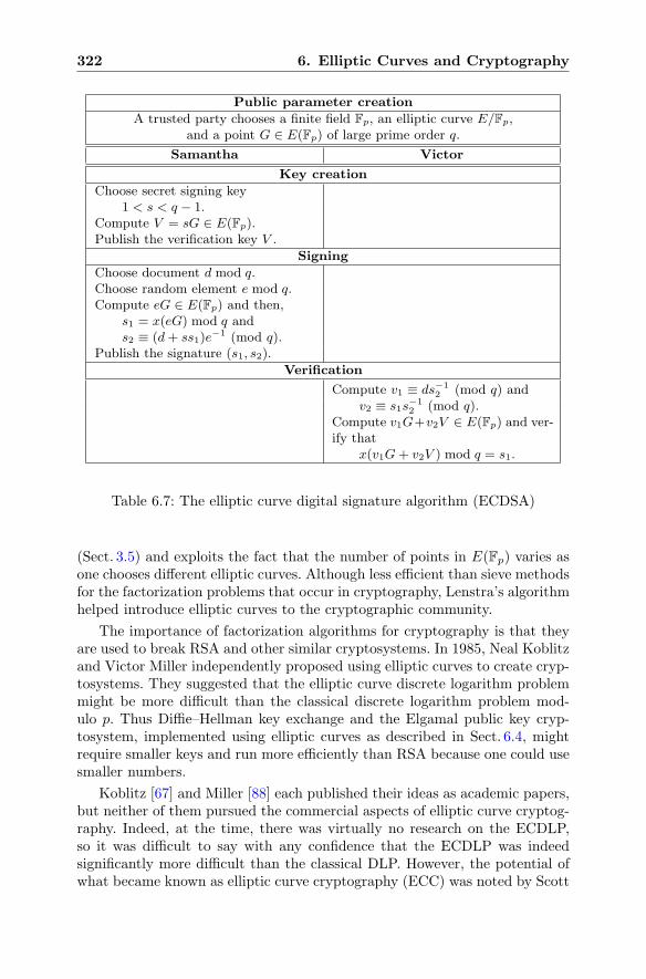
322 6. Elliptic Curves and Cryptography
Public parameter creation
A trusted party chooses a finite field Fp, an elliptic curve E/Fp,and a point G ∈ E(Fp) of large prime order q.
Samantha Victor
Key creation
Choose secret signing key1 < s < q − 1.
Compute V = sG ∈ E(Fp).Publish the verification key V .
Signing
Choose document d mod q.Choose random element e mod q.Compute eG ∈ E(Fp) and then,
s1 = x(eG) mod q ands2 ≡ (d+ ss1)e
−1 (mod q).Publish the signature (s1, s2).
Verification
Compute v1 ≡ ds−12 (mod q) and
v2 ≡ s1s−12 (mod q).
Compute v1G+v2V ∈ E(Fp) and ver-ify that
x(v1G+ v2V ) mod q = s1.
Table 6.7: The elliptic curve digital signature algorithm (ECDSA)
(Sect. 3.5) and exploits the fact that the number of points in E(Fp) varies asone chooses different elliptic curves. Although less efficient than sieve methodsfor the factorization problems that occur in cryptography, Lenstra’s algorithmhelped introduce elliptic curves to the cryptographic community.
The importance of factorization algorithms for cryptography is that theyare used to break RSA and other similar cryptosystems. In 1985, Neal Koblitzand Victor Miller independently proposed using elliptic curves to create cryp-tosystems. They suggested that the elliptic curve discrete logarithm problemmight be more difficult than the classical discrete logarithm problem mod-ulo p. Thus Diffie–Hellman key exchange and the Elgamal public key cryp-tosystem, implemented using elliptic curves as described in Sect. 6.4, mightrequire smaller keys and run more efficiently than RSA because one could usesmaller numbers.
Koblitz [67] and Miller [88] each published their ideas as academic papers,but neither of them pursued the commercial aspects of elliptic curve cryptog-raphy. Indeed, at the time, there was virtually no research on the ECDLP,so it was difficult to say with any confidence that the ECDLP was indeedsignificantly more difficult than the classical DLP. However, the potential ofwhat became known as elliptic curve cryptography (ECC) was noted by Scott
6.5. The Evolution of Public Key Cryptography 323
Vanstone and Ron Mullin, who had started a cryptographic company calledCerticom in 1985. They joined with other researchers in both academia andthe business world to promote ECC as an alternative to RSA and Elgamal.
All was not smooth sailing. For example, during the late 1980s, variouscryptographers proposed using so-called supersingular elliptic curves for addedefficiency, but in 1990, the MOV algorithm (see Sect. 6.9.1) showed that su-persingular curves are vulnerable to attack. Some saw this as an indictment ofECC as a whole, while others pointed out that RSA also has weak instancesthat must be avoided, e.g., RSA must avoid using numbers that can be easilyfactored by Pollard’s p− 1 method.
The purely mathematical question of whether ECC provided a secure andefficient alternative to RSA was clouded by the fact that there were com-mercial and financial issues at stake. In order to be commercially successful,cryptographic methods must be standardized for use in areas such as commu-nications and banking. RSA had the initial lead, since it was invented first,but RSA was patented, and some companies resisted the idea that standardsapproved by trade groups or government bodies should mandate the use ofa patented technology. Elgamal, after it was invented in 1985, provided aroyalty-free alternative, so many standards specified Elgamal as an alterna-tive to RSA. In the meantime, ECC was growing in stature, but even as lateas 1997, more than a decade after its introduction, leading experts indicatedtheir doubts about the security of ECC.7
A major dilemma pervading the field of cryptography is that no one knowsthe actual difficulty of the supposedly hard problems on which it is based.Currently, the security of public key cryptosystems depends on the percep-tion and consensus of experts as to the difficulty of problems such as integerfactorization and discrete logarithms. All that can be said is that “such-and-such a problem has been extensively studied for N years, and here is thefastest known method for solving it.” Proponents of factorization-based cryp-tosystems point to the fact that, in some sense, people have been trying tofactor numbers since antiquity; but in truth, the modern theory of factor-ization requires high-speed computing devices and barely predates the inven-tion of RSA. Serious study of the elliptic curve discrete logarithm problemstarted in the late 1980s, so modern factorization methods have a 10–15 yearhead start on ECDLP. In Chap. 7 we will describe public key cryptosystems(NTRU, GGH) whose security is based on certain hard problems in the the-ory of lattices. Lattices have been extensively investigated since the nineteenthcentury, but again the invention and analysis of modern computational algo-rithms is much more recent, having been initiated by fundamental work of
7In 1997, the RSA corporation posted the following quote by RSA co-inventor RonRivest on its website: “But the security of cryptosystems based on elliptic curves is not wellunderstood, due in large part to the abstruse nature of elliptic curves. . . .
Over time, this may change, but for now trying to get an evaluation of the security ofan elliptic-curve cryptosystem is a bit like trying to get an evaluation of some recentlydiscovered Chaldean poetry. Until elliptic curves have been further studied and evaluated,I would advise against fielding any large-scale applications based on them.”
324 6. Elliptic Curves and Cryptography
Lenstra, Lenstra, and Lovasz in the early 1980s. Lattices appeared as a toolfor cryptanalysis during the 1980s and as a means of creating cryptosystemsin the 1990s.
RSA, the first public key cryptosystem, was patented by its inventors.The issue of patents in cryptography is fraught with controversy. One mightargue that the RSA patent, which ran from 1983 to 2000, set back the useof cryptography by requiring users to pay licensing fees. However, it is alsotrue that in order to build a company, an inventor needs investors willing torisk their money, and it is much easier to raise funds if there is an exclusiveproduct to offer. Further, the fact that RSA was originally the “only gamein town” meant that it automatically received extensive scrutiny from theacademic community, which helped to validate its security.
The invention and eventual commercial implementation of ECC followed adifferent path. Since neither Koblitz nor Miller applied for a patent, the basicunderlying idea of ECC became freely available for all to use. This led Cer-ticom and other companies to apply for patents giving improvements to thebasic ECC idea. Some of these improvements were based on significant newresearch ideas, while others were less innovative and might almost be char-acterized as routine homework problems.8 Unfortunately, the United StatesPatents and Trademark Office (USPTO) does not have the expertise to effec-tively evaluate the flood of cryptographic patent applications that it receives.The result has been a significant amount of uncertainty in the marketplace asto which versions of ECC are free and which require licenses, even assumingthat all of the issued patents can withstand a legal challenge.
6.6 Lenstra’s Elliptic Curve FactorizationAlgorithm
Pollard’s p − 1 factorization method, which we discussed in Sect. 3.5, findsfactors of N = pq by searching for a power aL with the property that
aL ≡ 1 (mod p) and aL �≡ 1 (mod q).
Fermat’s little theorem tells us that this is likely to work if p− 1 divides Land q − 1 does not divide L. So what we do is to take L = n! for some moderatevalue of n. Then we hope that p− 1 or q − 1, but not both, is a product ofsmall primes, hence divides n!. Clearly Pollard’s method works well for somenumbers, but not for all numbers. The determining factor is whether p− 1or q − 1 is a product of small primes.
What is it about the quantity p− 1 that makes it so important for Pollard’smethod? The answer lies in Fermat’s little theorem. Intrinsically, p− 1 is
8For example, at the end of Sect. 6.4.2 we described how to save bandwidth in ellipticElgamal by sending the x-coordinate and one additional bit to specify the y-coordinate.This idea is called “point compression” and is covered by US Patent 6,141,420.
6.6. Lenstra’s Elliptic Curve Factorization Algorithm 325
important because there are p− 1 elements in F∗p, so every element α of F∗
p
satisfies αp−1 = 1. Now consider that last statement as it relates to the themeof this chapter, which is that the points and the addition law for an ellipticcurve E(Fp) are very much analogous to the elements and the multiplicationlaw for F
∗p. Hendrik Lenstra [75] made this analogy precise by devising a
factorization algorithm that uses the group law on an elliptic curve E in placeof multiplication modulo N .
In order to describe Lenstra’s algorithm, we need to work with an ellipticcurve modulo N , where the integer N is not prime, so the ring Z/NZ is nota field. However, suppose that we start with an equation
E : Y 2 = X3 +AX +B
and suppose that P = (a, b) is a point on E modulo N , by which we meanthat
b2 ≡ a3 +A · a+B (mod N).
Then we can apply the elliptic curve addition algorithm (Theorem 6.6) tocompute 2P, 3P, 4P, . . ., since the only operations required by that algorithmare addition, subtraction, multiplication, and division (by numbers relativelyprime to N).
Example 6.22. Let N = 187 and consider the elliptic curve
E : Y 2 = X3 + 3X + 7
modulo 187 and the point P = (38, 112), that is on E modulo 187. In orderto compute 2P mod 187, we follow the elliptic curve addition algorithm andcompute
1
2y(P )=
1
224≡ 91 (mod 187),
λ =3x(P )2 +A
2y(P )=
4335
224≡ 34 · 91 ≡ 102 (mod 187),
x(2P ) = λ2 − 2x(P ) = 10328 ≡ 43 (mod 187),
y(2P ) = λ(x(P )− x(2P )
)− y(P ) = 102(38− 43)− 112 ≡ 126 (mod 187).
Thus 2P = (43, 126) as a point on the curve E modulo 187.For clarity, we have written x(P ) and y(P ) for the x-and y-coordinates
of P , and similarly for 2P . Also, during the calculation we needed to find thereciprocal of 224 modulo 187, i.e., we needed to solve the congruence
224d ≡ 1 (mod 187).
This was easily accomplished using the extended Euclidean algorithm (The-orem 1.11; see also Remark 1.15 and Exercise 1.12), since it turns out thatgcd(224, 187) = 1.
326 6. Elliptic Curves and Cryptography
We next compute 3P = 2P + P in a similar fashion. In this case, we areadding distinct points, so the formula for λ is different, but the computationis virtually the same:
1
x(2P )− x(P ) =1
5≡ 75 (mod 187),
λ =y(2P )− y(P )x(2P )− x(P ) =
14
5≡ 14 · 75 ≡ 115 (mod 187),
x(3P ) = λ2 − x(2P )− x(P ) = 13144 ≡ 54 (mod 187),
y(3P ) = λ(x(P )− x(3P )
)− y(P ) = 115(38− 54)− 112 ≡ 105 (mod 187).
Thus 3P = (54, 105) on the curve E modulo 187. Again we needed to computea reciprocal, in this case, the reciprocal of 5 modulo 187. We leave it to you tocontinue the calculations. For example, it is instructive to check that P + 3Pand 2P + 2P give the same answer, namely 4P = (93, 64).
Example 6.23. Continuing with Example 6.22, we attempt to compute 5P forthe point P = (38, 112) on the elliptic curve
E : Y 2 = X3 + 3X + 7 modulo 187.
We already computed 2P = (43, 126) and 3P = (54, 105). The first step incomputing 5P = 3P + 2P is to compute the reciprocal of
x(3P )− x(2P ) = 54− 43 = 11 modulo 187.
However, when we apply the extended Euclidean algorithm to 11 and 187, wefind that gcd(11, 187) = 11, so 11 does not have a reciprocal modulo 187.
It seems that we have hit a dead end, but in fact, we have struck it rich!Notice that since the quantity gcd(11, 187) is greater than 1, it gives us adivisor of 187. So our failure to compute 5P also tells us that 11 divides 187,which allows us to factor 187 as 187 = 11 · 17. This idea underlies Lenstra’selliptic curve factorization algorithm.
We examine more closely why we were not able to compute 5P modulo 187.If we instead look at the elliptic curve E modulo 11, then a quick computationshows that the point
P = (38, 112) ≡ (5, 2) (mod 11) satisfies 5P = O in E(F11).
This means that when we attempt to compute 5P modulo 11, we end up withthe point O at infinity, so at some stage of the calculation we have tried todivide by zero. But here “zero” means zero in F11, so we actually end uptrying to find the reciprocal modulo 11 of some integer that is divisible by 11.
Following the lead from Examples 6.22 and 6.23, we replace multiplicationmodulo N in Pollard’s factorization method with addition modulo N on anelliptic curve. We start with an elliptic curve E and a point P on E modulo Nand we compute
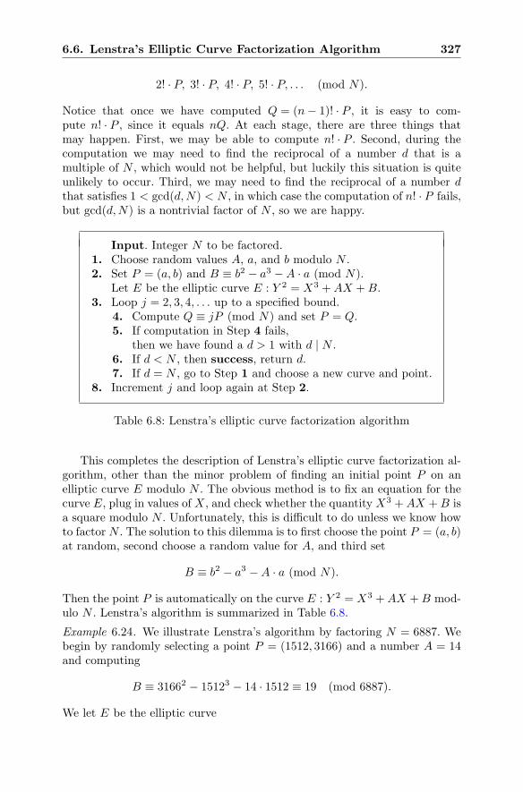
6.6. Lenstra’s Elliptic Curve Factorization Algorithm 327
2! · P, 3! · P, 4! · P, 5! · P, . . . (mod N).
Notice that once we have computed Q = (n− 1)! · P , it is easy to com-pute n! · P , since it equals nQ. At each stage, there are three things thatmay happen. First, we may be able to compute n! · P . Second, during thecomputation we may need to find the reciprocal of a number d that is amultiple of N , which would not be helpful, but luckily this situation is quiteunlikely to occur. Third, we may need to find the reciprocal of a number dthat satisfies 1 < gcd(d,N) < N , in which case the computation of n! · P fails,but gcd(d,N) is a nontrivial factor of N , so we are happy.
Input. Integer N to be factored.1. Choose random values A, a, and b modulo N .2. Set P = (a, b) and B ≡ b2 − a3 −A · a (mod N).
Let E be the elliptic curve E : Y 2 = X3 +AX +B.3. Loop j = 2, 3, 4, . . . up to a specified bound.
4. Compute Q ≡ jP (mod N) and set P = Q.5. If computation in Step 4 fails,
then we have found a d > 1 with d | N .6. If d < N , then success, return d.7. If d = N , go to Step 1 and choose a new curve and point.
8. Increment j and loop again at Step 2.
Table 6.8: Lenstra’s elliptic curve factorization algorithm
This completes the description of Lenstra’s elliptic curve factorization al-gorithm, other than the minor problem of finding an initial point P on anelliptic curve E modulo N . The obvious method is to fix an equation for thecurve E, plug in values of X, and check whether the quantity X3 +AX +B isa square modulo N . Unfortunately, this is difficult to do unless we know howto factor N . The solution to this dilemma is to first choose the point P = (a, b)at random, second choose a random value for A, and third set
B ≡ b2 − a3 −A · a (mod N).
Then the point P is automatically on the curve E : Y 2 = X3 +AX +B mod-ulo N . Lenstra’s algorithm is summarized in Table 6.8.
Example 6.24. We illustrate Lenstra’s algorithm by factoring N = 6887. Webegin by randomly selecting a point P = (1512, 3166) and a number A = 14and computing
B ≡ 31662 − 15123 − 14 · 1512 ≡ 19 (mod 6887).
We let E be the elliptic curve
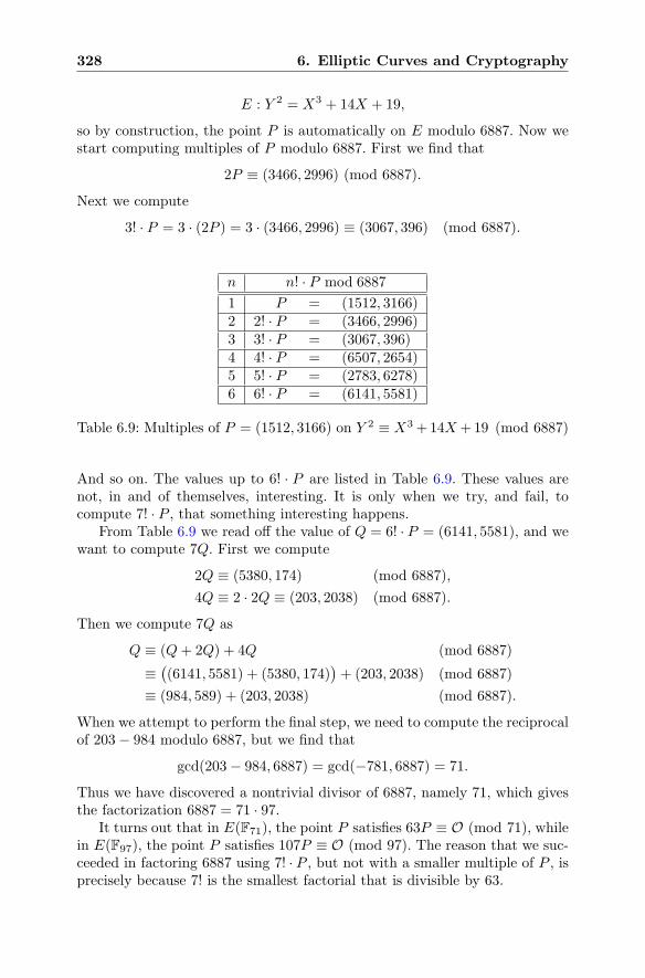
328 6. Elliptic Curves and Cryptography
E : Y 2 = X3 + 14X + 19,
so by construction, the point P is automatically on E modulo 6887. Now westart computing multiples of P modulo 6887. First we find that
2P ≡ (3466, 2996) (mod 6887).
Next we compute
3! · P = 3 · (2P ) = 3 · (3466, 2996) ≡ (3067, 396) (mod 6887).
n n! · P mod 6887
1 P = (1512, 3166)2 2! · P = (3466, 2996)3 3! · P = (3067, 396)4 4! · P = (6507, 2654)5 5! · P = (2783, 6278)6 6! · P = (6141, 5581)
Table 6.9: Multiples of P = (1512, 3166) on Y 2 ≡ X3+14X +19 (mod 6887)
And so on. The values up to 6! · P are listed in Table 6.9. These values arenot, in and of themselves, interesting. It is only when we try, and fail, tocompute 7! · P , that something interesting happens.
From Table 6.9 we read off the value of Q = 6! · P = (6141, 5581), and wewant to compute 7Q. First we compute
2Q ≡ (5380, 174) (mod 6887),
4Q ≡ 2 · 2Q ≡ (203, 2038) (mod 6887).
Then we compute 7Q as
Q ≡ (Q+ 2Q) + 4Q (mod 6887)
≡((6141, 5581) + (5380, 174)
)+ (203, 2038) (mod 6887)
≡ (984, 589) + (203, 2038) (mod 6887).
When we attempt to perform the final step, we need to compute the reciprocalof 203− 984 modulo 6887, but we find that
gcd(203− 984, 6887) = gcd(−781, 6887) = 71.
Thus we have discovered a nontrivial divisor of 6887, namely 71, which givesthe factorization 6887 = 71 · 97.
It turns out that in E(F71), the point P satisfies 63P ≡ O (mod 71), whilein E(F97), the point P satisfies 107P ≡ O (mod 97). The reason that we suc-ceeded in factoring 6887 using 7! · P , but not with a smaller multiple of P , isprecisely because 7! is the smallest factorial that is divisible by 63.
6.7. Elliptic Curves over F2 and over F2k 329
Remark 6.25. In Sect. 3.7 we discussed the speed of sieve factorization meth-ods and saw that the average running time of the quadratic sieve to factor acomposite number N is approximately
O(e√
(logN)(log logN))
steps. (6.7)
Notice that the running time depends on the size of the integer N .On the other hand, the most naive possible factorization method, namely
trying each possible divisor 2, 3, 4, 5, . . ., has a running time that depends onthe smallest prime factor of N . More precisely, this trial division algorithmtakes exactly p steps, where p is the smallest prime factor of N . If it happensthat N = pq with p and q approximately the same size, then the running timeis approximately
√N , which is much slower than sieve methods; but if N
happens to have a very small prime factor, trial division may be helpful infinding it.
It is an interesting and useful property of the elliptic curve factorizationalgorithm that its expected running time depends on the smallest prime factorof N , rather than on N itself. (See Exercise 5.44 for another, albeit slower,factorization algorithm with this property.) More precisely, if p is the smallestfactor of N , then the elliptic curve factorization algorithm has average runningtime approximately
O(e√
2(log p)(log log p))
steps. (6.8)
If N = pq is a product of two primes with p ≈ q, the running timesin (6.7) and (6.8) are approximately equal, and then the fact that a sieve step ismuch faster than an elliptic curve step makes sieve methods faster in practice.However, the elliptic curve method is quite useful for finding moderately largefactors of extremely large numbers, because its running time depends on thesmallest prime factor.
6.7 Elliptic Curves over F2 and over F2k
Computers speak binary, so they are especially well suited to doing calcu-lations modulo 2. This suggests that it might be more efficient to use ellip-tic curves modulo 2. Unfortunately, if E is an elliptic curve defined over F2,then E(F2) contains at most 5 points, so E(F2) is not useful for cryptographicpurposes.
However, there are other finite fields in which 2 = 0. These are thefields F2k containing 2k elements. Recall from Sect. 2.10.4 that for every primepower pk there exists a field Fpk with pk elements; and further, up to rela-beling the elements, there is exactly one such field. So we can take an ellipticcurve whose Weierstrass equation has coefficients in a field Fpk and look atthe group of points on that curve having coordinates in Fpk . Hasse’s theorem(Theorem 6.11) is true in this more general setting.
330 6. Elliptic Curves and Cryptography
Theorem 6.26 (Hasse). Let E be an elliptic curve over Fpk . Then
#E(Fpk) = pk + 1− tpk with tpk satisfying |tpk | ≤ 2pk/2.
Example 6.27. We work with the field
F9 = {a+ bi : a, b ∈ F3}, where i2 = −1.
(See Example 2.58 for a discussion of Fp2 for primes p ≡ 3 (mod 4).) Let Ebe the elliptic curve over F9 defined by the equation
E : Y 2 = X3 + (1 + i)X + (2 + i).
By trial and error we find that there are 10 points in E(F9),
(2i, 1 + 2i), (2i, 2 + i), (1 + i, 1 + i), (1 + i, 2 + 2i), (2, 0),
(2 + i, i), (2 + i, 2i), (2 + 2i, 1), (2 + 2i, 2), O.
Points can be doubled or added to one another using the formulas for theaddition of points, always keeping in mind that i2 = −1 and that we areworking modulo 3. For example, you can check that
(2, 0) + (2 + i, 2i) = (2i, 1 + 2i) and 2(1 + i, 2 + 2i) = (2 + i, i).
Our goal is to use elliptic curves over F2k for cryptography, but there isone difficulty that we must first address. The problem is that we cheated alittle bit when we defined an elliptic curve as a curve given by a Weierstrassequation Y 2 = X3 + AX + B satisfying Δ = 4A3 + 27B2 �= 0. In fact, thecorrect definition of the discriminant Δ is
Δ = −16(4A3 + 27B2).
As long as we work in a field where 2 �= 0, then the condition Δ �= 0 isthe same with either definition, but for fields such as F2k where 2 = 0, wehave Δ = 0 for every standard Weierstrass equation. The solution is to enlargethe collection of allowable Weierstrass equations.
Definition. An elliptic curve E is the set of solutions to a generalized Weier-strass equation
E : Y 2 + a1XY + a3Y = X3 + a2X2 + a4X + a6,
together with an extra point O. The coefficients a1, . . . , a6 are required tosatisfy Δ �= 0, where the discriminant Δ is defined in terms of certain quan-tities b2, b4, b6, b8 as follows:
b2 = a21 + 4a2, b4 = 2a4 + a1a3, b6 = a23 + 4a6,
b8 = a21a6 + 4a2a6 − a1a3a4 + a2a23 − a24,
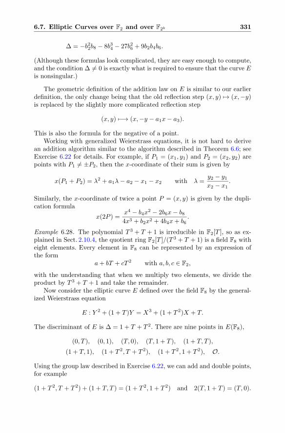
6.7. Elliptic Curves over F2 and over F2k 331
Δ = −b22b8 − 8b34 − 27b26 + 9b2b4b6.
(Although these formulas look complicated, they are easy enough to compute,and the condition Δ �= 0 is exactly what is required to ensure that the curve Eis nonsingular.)
The geometric definition of the addition law on E is similar to our earlierdefinition, the only change being that the old reflection step (x, y) �→ (x,−y)is replaced by the slightly more complicated reflection step
(x, y) �−→ (x,−y − a1x− a3).
This is also the formula for the negative of a point.Working with generalized Weierstrass equations, it is not hard to derive
an addition algorithm similar to the algorithm described in Theorem 6.6; seeExercise 6.22 for details. For example, if P1 = (x1, y1) and P2 = (x2, y2) arepoints with P1 �= ±P2, then the x-coordinate of their sum is given by
x(P1 + P2) = λ2 + a1λ− a2 − x1 − x2 with λ =y2 − y1x2 − x1
.
Similarly, the x-coordinate of twice a point P = (x, y) is given by the dupli-cation formula
x(2P ) =x4 − b4x2 − 2b6x− b84x3 + b2x2 + 4b4x+ b6
.
Example 6.28. The polynomial T 3 + T + 1 is irreducible in F2[T ], so as ex-plained in Sect. 2.10.4, the quotient ring F2[T ]/(T
3 + T + 1) is a field F8 witheight elements. Every element in F8 can be represented by an expression ofthe form
a+ bT + cT 2 with a, b, c ∈ F2,
with the understanding that when we multiply two elements, we divide theproduct by T 3 + T + 1 and take the remainder.
Now consider the elliptic curve E defined over the field F8 by the general-ized Weierstrass equation
E : Y 2 + (1 + T )Y = X3 + (1 + T 2)X + T.
The discriminant of E is Δ = 1 + T + T 2. There are nine points in E(F8),
(0, T ), (0, 1), (T, 0), (T, 1 + T ), (1 + T, T ),
(1 + T, 1), (1 + T 2, T + T 2), (1 + T 2, 1 + T 2), O.
Using the group law described in Exercise 6.22, we can add and double points,for example
(1 + T 2, T + T 2) + (1 + T, T ) = (1 + T 2, 1 + T 2) and 2(T, 1 + T ) = (T, 0).
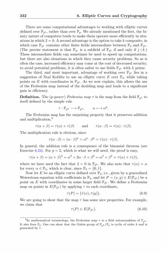
332 6. Elliptic Curves and Cryptography
There are some computational advantages to working with elliptic curvesdefined over F2k , rather than over Fp. We already mentioned the first, the bi-nary nature of computers tends to make them operate more efficiently in situ-ations in which 2 = 0. A second advantage is the option to take k composite, inwhich case F2k contains other finite fields intermediate between F2 and F2k .(The precise statement is that F2j is a subfield of F2k if and only if j | k.)These intermediate fields can sometimes be used to speed up computations,but there are also situations in which they cause security problems. So as isoften the case, increased efficiency may come at the cost of decreased security;to avoid potential problems, it is often safest to use fields F2k with k prime.
The third, and most important, advantage of working over F2k lies in asuggestion of Neal Koblitz to use an elliptic curve E over F2, while takingpoints on E with coordinates in F2k . As we now explain, this allows the useof the Frobenius map instead of the doubling map and leads to a significantgain in efficiency.
Definition. The (p-power) Frobenius map τ is the map from the field Fpk toitself defined by the simple rule
τ : Fpk −→ Fpk , α �−→ αp.
The Frobenius map has the surprising property that it preserves additionand multiplication,9
τ(α+ β) = τ(α) + τ(β) and τ(α · β) = τ(α) · τ(β).The multiplication rule is obvious, since
τ(α · β) = (α · β)p = αp · βp = τ(α) · τ(β).In general, the addition rule is a consequence of the binomial theorem (seeExercise 6.24). For p = 2, which is what we will need, the proof is easy,
τ(α+ β) = (α+ β)2 = α2 + 2α · β + β2 = α2 + β2 = τ(α) + τ(β),
where we have used the fact that 2 = 0 in F2k . We also note that τ(α) = αfor every α ∈ F2, which is clear, since F2 = {0, 1}.
Now let E be an elliptic curve defined over F2, i.e., given by a generalizedWeierstrass equation with coefficients in F2, and let P = (x, y) ∈ E(F2k) be apoint on E with coordinates in some larger field F2k . We define a Frobeniusmap on points in E(F2k) by applying τ to each coordinate,
τ(P ) =(τ(x), τ(y)
). (6.9)
We are going to show that the map τ has some nice properties. For example,we claim that
τ(P ) ∈ E(F2k). (6.10)
9In mathematical terminology, the Frobenius map τ is a field automorphism of Fpk .
It also fixes Fp. One can show that the Galois group of Fpk/Fp is cyclic of order k and isgenerated by τ .
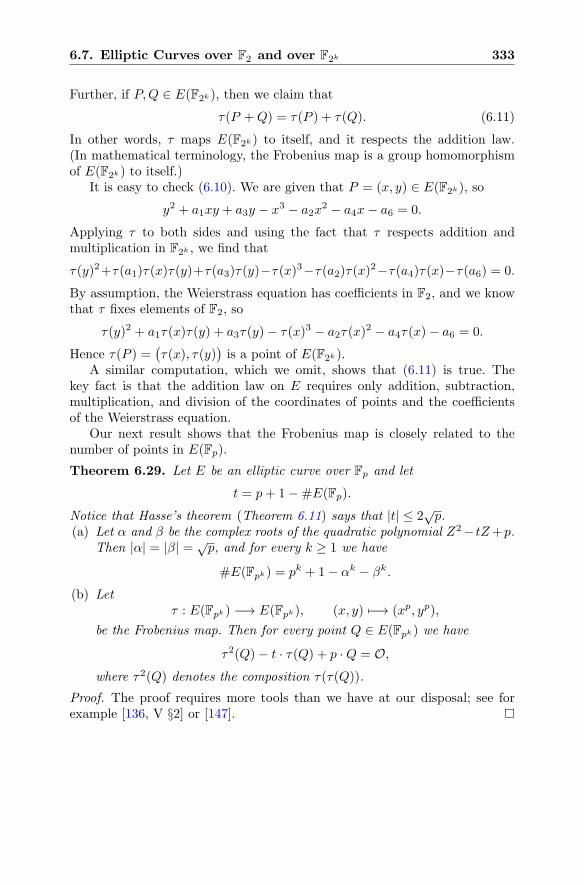
6.7. Elliptic Curves over F2 and over F2k 333
Further, if P,Q ∈ E(F2k), then we claim that
τ(P +Q) = τ(P ) + τ(Q). (6.11)
In other words, τ maps E(F2k) to itself, and it respects the addition law.(In mathematical terminology, the Frobenius map is a group homomorphismof E(F2k) to itself.)
It is easy to check (6.10). We are given that P = (x, y) ∈ E(F2k), so
y2 + a1xy + a3y − x3 − a2x2 − a4x− a6 = 0.
Applying τ to both sides and using the fact that τ respects addition andmultiplication in F2k , we find that
τ(y)2+τ(a1)τ(x)τ(y)+τ(a3)τ(y)−τ(x)3−τ(a2)τ(x)2−τ(a4)τ(x)−τ(a6) = 0.
By assumption, the Weierstrass equation has coefficients in F2, and we knowthat τ fixes elements of F2, so
τ(y)2 + a1τ(x)τ(y) + a3τ(y)− τ(x)3 − a2τ(x)2 − a4τ(x)− a6 = 0.
Hence τ(P ) =(τ(x), τ(y)
)is a point of E(F2k).
A similar computation, which we omit, shows that (6.11) is true. Thekey fact is that the addition law on E requires only addition, subtraction,multiplication, and division of the coordinates of points and the coefficientsof the Weierstrass equation.
Our next result shows that the Frobenius map is closely related to thenumber of points in E(Fp).
Theorem 6.29. Let E be an elliptic curve over Fp and let
t = p+ 1−#E(Fp).
Notice that Hasse’s theorem (Theorem 6.11) says that |t| ≤ 2√p.
(a) Let α and β be the complex roots of the quadratic polynomial Z2− tZ+p.Then |α| = |β| = √p, and for every k ≥ 1 we have
#E(Fpk) = pk + 1− αk − βk.
(b) Letτ : E(Fpk) −→ E(Fpk), (x, y) �−→ (xp, yp),
be the Frobenius map. Then for every point Q ∈ E(Fpk) we have
τ2(Q)− t · τ(Q) + p ·Q = O,where τ2(Q) denotes the composition τ(τ(Q)).
Proof. The proof requires more tools than we have at our disposal; see forexample [136, V §2] or [147].
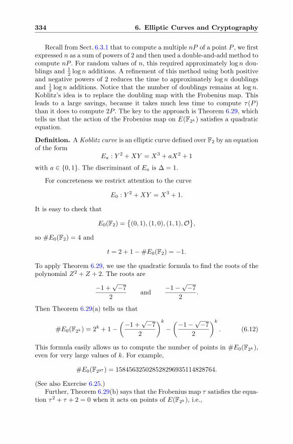
334 6. Elliptic Curves and Cryptography
Recall from Sect. 6.3.1 that to compute a multiple nP of a point P , we firstexpressed n as a sum of powers of 2 and then used a double-and-add method tocompute nP . For random values of n, this required approximately log n dou-blings and 1
2 log n additions. A refinement of this method using both positiveand negative powers of 2 reduces the time to approximately log n doublingsand 1
3 log n additions. Notice that the number of doublings remains at log n.Koblitz’s idea is to replace the doubling map with the Frobenius map. Thisleads to a large savings, because it takes much less time to compute τ(P )than it does to compute 2P . The key to the approach is Theorem 6.29, whichtells us that the action of the Frobenius map on E(F2k) satisfies a quadraticequation.
Definition. A Koblitz curve is an elliptic curve defined over F2 by an equationof the form
Ea : Y 2 +XY = X3 + aX2 + 1
with a ∈ {0, 1}. The discriminant of Ea is Δ = 1.
For concreteness we restrict attention to the curve
E0 : Y 2 +XY = X3 + 1.
It is easy to check that
E0(F2) ={(0, 1), (1, 0), (1, 1),O
},
so #E0(F2) = 4 and
t = 2 + 1−#E0(F2) = −1.
To apply Theorem 6.29, we use the quadratic formula to find the roots of thepolynomial Z2 + Z + 2. The roots are
−1 +√−7
2and
−1−√−7
2.
Then Theorem 6.29(a) tells us that
#E0(F2k) = 2k + 1−(−1 +
√−7
2
)k
−(−1−
√−7
2
)k
. (6.12)
This formula easily allows us to compute the number of points in #E0(F2k),even for very large values of k. For example,
#E0(F297) = 158456325028528296935114828764.
(See also Exercise 6.25.)Further, Theorem 6.29(b) says that the Frobenius map τ satisfies the equa-
tion τ2 + τ + 2 = 0 when it acts on points of E(F2k), i.e.,
6.7. Elliptic Curves over F2 and over F2k 335
τ2(P ) + τ(P ) + 2P = O for all P ∈ E(F2k).
The idea now is to write an arbitrary integer n as a sum of powers of τ , subjectto the assumption that τ2 = −2− τ . Say we have written n as
n = v0 + v1τ + v2τ2 + · · ·+ v�τ
� with vi ∈ {−1, 0, 1}.
Then we can compute nP efficiently using the formula
nP = (v0 + v1τ + v2τ2 + · · ·+ v�τ
�)P
= v0P + v1τ(P ) + v2τ2(P ) + · · ·+ v�τ
�(P ).
This takes less time than using the binary or ternary method because it is fareasier to compute τ i(P ) than it is to compute 2iP .
Proposition 6.30. Let n be a positive integer. Then n can be written in theform
n = v0 + v1τ + v2τ2 + · · ·+ v�τ
� with vi ∈ {−1, 0, 1}, (6.13)
under the assumption that τ satisfies τ2 = −2 − τ . Further, this can alwaysbe done with � ≈ 2 log n and with at most 1
3 of the vi nonzero.
Proof. The proof is similar to Proposition 6.18, the basic idea being that wewrite integers as 2a + b with b ∈ {0, 1,−1} and replace 2 with −τ − τ2;see Exercise 6.27. With more work, it is possible to find an expansion (6.13)with � ≈ log n and approximately 1
3 of the vi nonzero; see [29, §15.1].
Example 6.31. We illustrate Proposition 6.30 with a numerical example.Let n = 7. Then
7 = 1 + 3 · 2 = 1 + 3 · (−τ − τ2) = 1− 3τ − 3τ2 = 1− τ − τ2 − 2τ − 2τ2
= 1− τ − τ2 − (−τ − τ2)τ − (−τ − τ2)τ2 = 1− τ + 2τ3 + τ4
= 1− τ + (−τ − τ2)τ3 + τ4 = 1− τ − τ5.
Thus 7 = 1− τ − τ5.Remark 6.32. As we have seen, computing #E(F2k) for Koblitz curves isvery easy. However, for general elliptic curves over F2k , this is a more difficulttask. The SEA algorithm and its variants [120, 121] that we mentioned in Re-mark 6.13 are reasonably efficient at counting the number of points in E(Fq)for any fields with a large number of elements. Satoh [113] devised an alter-native method that is often faster than SEA when q = pe for a small prime pand (moderately) large exponent e. Satoh’s original paper dealt only with thecase p ≥ 3, but subsequent work [44, 140] covers also the cryptographicallyimportant case of p = 2.
336 6. Elliptic Curves and Cryptography
6.8 Bilinear Pairings on Elliptic Curves
You have probably seen examples of bilinear pairings in a linear algebra class.For example, the dot product is a bilinear pairing on the vector space R
n,
β(v,w) = v ·w = v1w1 + v2w2 + · · ·+ vnwn.
It is a pairing in the sense that it takes a pair of vectors and returns a num-ber, and it is bilinear in the sense that it is a linear transformation in eachof its variables. In other words, for any vectors v1,v2,w1,w2 and any realnumbers a1, a2, b1, b2, we have
β(a1v1 + a2v2,w) = a1β(v1,w) + a2β(v2,w),
β(v, b1w1 + b2w2) = b1β(v,w1) + b2β(v,w2).(6.14)
More generally, if A is any n-by-n matrix, then the function β(v,w) = vAwt
is a bilinear pairing on Rn, where we write v as a row vector and we write wt,
the transpose of w, as a column vector.
Another bilinear pairing that you have seen is the determinant map on R2.
Thus if v = (v1, v2) and w = (w1, w2), then
δ(v,w) = det
(v1 v2w1 w2
)= v1w2 − v2w1
is a bilinear map. The determinant map has the further property that it isalternating, which means that if we switch the vectors, the value changes sign,
δ(v,w) = −δ(w,v).
Notice that the alternating property implies that δ(v,v) = 0 for everyvector v.
The bilinear pairings that we discuss in this section are similar in that theytake as input two points on an elliptic curve and give as output a number.However, the bilinearity condition is slightly different, because the outputvalue is a nonzero element of a finite field, so the sum on the right-hand sideof (6.14) is replaced by a product.
Bilinear pairings on elliptic curves have a number of important crypto-graphic applications. For most of these applications it is necessary to workwith finite fields Fpk of prime power order. Fields of prime power order arediscussed in Sect. 2.10.4, but even if you have not covered that material, youcan just imagine a field that is similar to Fp, but that has p
k elements. (N.B.The field Fpk is very different from the ring Z/pkZ; see Exercise 2.40.) Stan-dard references for the material used in this section are [136] and [147].
6.8. Bilinear Pairings on Elliptic Curves 337
6.8.1 Points of Finite Order on Elliptic Curves
We begin by briefly describing the points of finite order on an elliptic curve.
Definition. Let m ≥ 1 be an integer. A point P ∈ E satisfying mP = Ois called a point of order m in the group E. We denote the set of points oforder m by
E[m] ={P ∈ E : mP = O
}.
Such points are called points of finite order or torsion points.It is easy to see that if P and Q are in E[m], then P +Q and −P are also
in E[m], so E[m] is a subgroup of E. If we want the coordinates of P to lie in aparticular field K, for example in Q or R or C or Fp, then we write E(K)[m].(See Exercise 2.12.)
The group of points of order m has a fairly simple structure, at least if weallow the coordinates of the points to be in a sufficiently large field.
Proposition 6.33. Let m ≥ 1 be an integer.(a) Let E be an elliptic curve over Q or R or C. Then
E(C)[m] ∼= Z/mZ× Z/mZ
is a product of two cyclic groups of order m.
(b) Let E be an elliptic curve over Fp and assume that p does not divide m.Then there exists a value of k such that
E(Fpjk)[m] ∼= Z/mZ× Z/mZ for all j ≥ 1.
Proof. For the proof, which is beyond the scope of this book, see any standardtext on elliptic curves, for example [136, Corollary III.6.4].
Remark 6.34. Notice that if � is prime and if K is a field such that
E(K)[�] = Z/�Z× Z/�Z,
then we may view E[�] as a 2-dimensional vector space over the field Z/�Z.And even if m is not prime,
E(K)[m] = Z/mZ× Z/mZ
still has a “basis” {P1, P2} in the sense that every point P = E[m] can bewritten as a linear combination
P = aP1 + bP2
for a unique choice of coefficients a, b ∈ Z/mZ. Of course, if m is large, it maybe very difficult to find a and b. Indeed, if P is a multiple of P1, then findingthe value of a is the same as solving the ECDLP for P and P1.
338 6. Elliptic Curves and Cryptography
6.8.2 Rational Functions and Divisors on Elliptic Curves
In order to define the Weil and Tate pairings, we need to explain how a rationalfunction on an elliptic curve is related to its zeros and poles. We start withthe simpler case of a rational function of one variable. A rational function isa ratio of polynomials
f(X) =a0 + a1X + a2X
2 + · · ·+ anXn
b0 + b1X + b2X2 + · · ·+ bmXm.
Any nonzero polynomial can be factored completely if we allow complex num-bers, so a nonzero rational function can be factored as
f(X) =a(X − α1)
e1(X − α2)e2 · · · (X − αr)
er
b(X − β1)d1(X − β2)d2 · · · (X − βs)ds.
We may assume that α1, . . . , αr, β1, . . . , βs are distinct numbers, sinceotherwise we can cancel some of the terms in the numerator with someof the terms in the denominator. The numbers α1, . . . , αr are called the zerosof f(X) and the numbers β1, . . . , βs are called the poles of f(X). The expo-nents e1, . . . , er, d1, . . . , ds are the associated multiplicities. We keep track ofthe zeros and poles of f(X) and their multiplicities by defining the divisorof f(X) to be the formal sum
div(f(X)
)= e1[α1] + e2[α2] + · · ·+ er[αr]− d1[β1]− d2[β2]− · · · − dr[βr].
Note that this is simply a convenient shorthand way of saying that f(X) hasa zero of multiplicity e1 at α1, a zero of multiplicity e2 at α2, etc.
If E is an elliptic curve,
E : Y 2 = X3 +AX +B,
and if f(X,Y ) is a nonzero rational function of two variables, we may view fas defining a function on E by writing points as P = (x, y) and setting f(P ) =f(x, y). Then just as for rational functions of one variable, there are pointsof E where the numerator of f vanishes and there are points of E where thedenominator of f vanishes, so f has zeros and poles on E. Further, one canassign multiplicities to the zeros and poles, so f has an associated divisor
div(f) =∑
P∈E
nP [P ].
In this formal sum, the coefficients nP are integers, and only finitely many ofthe nP are nonzero, so div(f) is a finite sum. Of course, the coordinates ofthe zeros and poles of f may require moving to a larger field. For example,if E is defined over Fp, then the poles and zeros of f have coordinates in Fpk
for some k, but the value of k will, in general, depend on the function f .
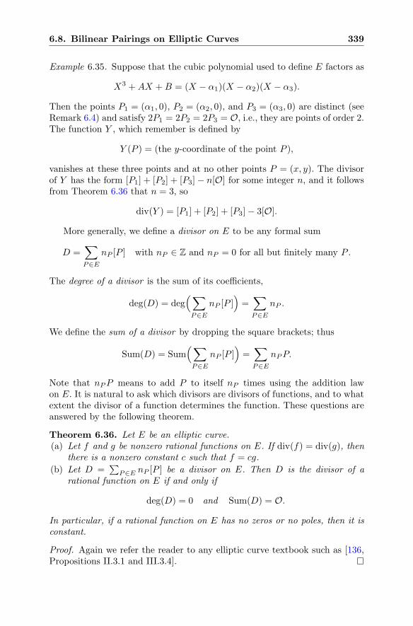
6.8. Bilinear Pairings on Elliptic Curves 339
Example 6.35. Suppose that the cubic polynomial used to define E factors as
X3 +AX +B = (X − α1)(X − α2)(X − α3).
Then the points P1 = (α1, 0), P2 = (α2, 0), and P3 = (α3, 0) are distinct (seeRemark 6.4) and satisfy 2P1 = 2P2 = 2P3 = O, i.e., they are points of order 2.The function Y , which remember is defined by
Y (P ) = (the y-coordinate of the point P ),
vanishes at these three points and at no other points P = (x, y). The divisorof Y has the form [P1] + [P2] + [P3]− n[O] for some integer n, and it followsfrom Theorem 6.36 that n = 3, so
div(Y ) = [P1] + [P2] + [P3]− 3[O].
More generally, we define a divisor on E to be any formal sum
D =∑
P∈E
nP [P ] with nP ∈ Z and nP = 0 for all but finitely many P .
The degree of a divisor is the sum of its coefficients,
deg(D) = deg(∑
P∈E
nP [P ])=∑
P∈E
nP .
We define the sum of a divisor by dropping the square brackets; thus
Sum(D) = Sum(∑
P∈E
nP [P ])=∑
P∈E
nPP.
Note that nPP means to add P to itself nP times using the addition lawon E. It is natural to ask which divisors are divisors of functions, and to whatextent the divisor of a function determines the function. These questions areanswered by the following theorem.
Theorem 6.36. Let E be an elliptic curve.(a) Let f and g be nonzero rational functions on E. If div(f) = div(g), then
there is a nonzero constant c such that f = cg.
(b) Let D =∑
P∈E nP [P ] be a divisor on E. Then D is the divisor of arational function on E if and only if
deg(D) = 0 and Sum(D) = O.
In particular, if a rational function on E has no zeros or no poles, then it isconstant.
Proof. Again we refer the reader to any elliptic curve textbook such as [136,Propositions II.3.1 and III.3.4].
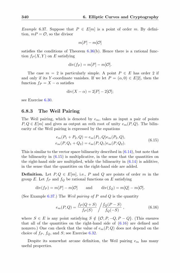
340 6. Elliptic Curves and Cryptography
Example 6.37. Suppose that P ∈ E[m] is a point of order m. By defini-tion, mP = O, so the divisor
m[P ]−m[O]
satisfies the conditions of Theorem 6.36(b). Hence there is a rational func-tion fP (X,Y ) on E satisfying
div(fP ) = m[P ]−m[O].
The case m = 2 is particularly simple. A point P ∈ E has order 2 ifand only if its Y -coordinate vanishes. If we let P = (α, 0) ∈ E[2], then thefunction fP = X − α satisfies
div(X − α) = 2[P ]− 2[O];
see Exercise 6.30.
6.8.3 The Weil Pairing
The Weil pairing, which is denoted by em, takes as input a pair of pointsP,Q ∈ E[m] and gives as output an mth root of unity em(P,Q). The bilin-earity of the Weil pairing is expressed by the equations
em(P1 + P2, Q) = em(P1, Q)em(P2, Q),
em(P,Q1 +Q2) = em(P,Q1)em(P,Q2).(6.15)
This is similar to the vector space bilinearity described in (6.14), but note thatthe bilinearity in (6.15) is multiplicative, in the sense that the quantities onthe right-hand side are multiplied, while the bilinearity in (6.14) is additive,in the sense that the quantities on the right-hand side are added.
Definition. Let P,Q ∈ E[m], i.e., P and Q are points of order m in thegroup E. Let fP and fQ be rational functions on E satisfying
div(fP ) = m[P ]−m[O] and div(fQ) = m[Q]−m[O].
(See Example 6.37.) The Weil pairing of P and Q is the quantity
em(P,Q) =fP (Q+ S)
fP (S)
/fQ(P − S)fQ(−S)
, (6.16)
where S ∈ E is any point satisfying S /∈ {O, P,−Q,P − Q}. (This ensuresthat all of the quantities on the right-hand side of (6.16) are defined andnonzero.) One can check that the value of em(P,Q) does not depend on thechoice of fP , fQ, and S; see Exercise 6.32.
Despite its somewhat arcane definition, the Weil pairing em has manyuseful properties.
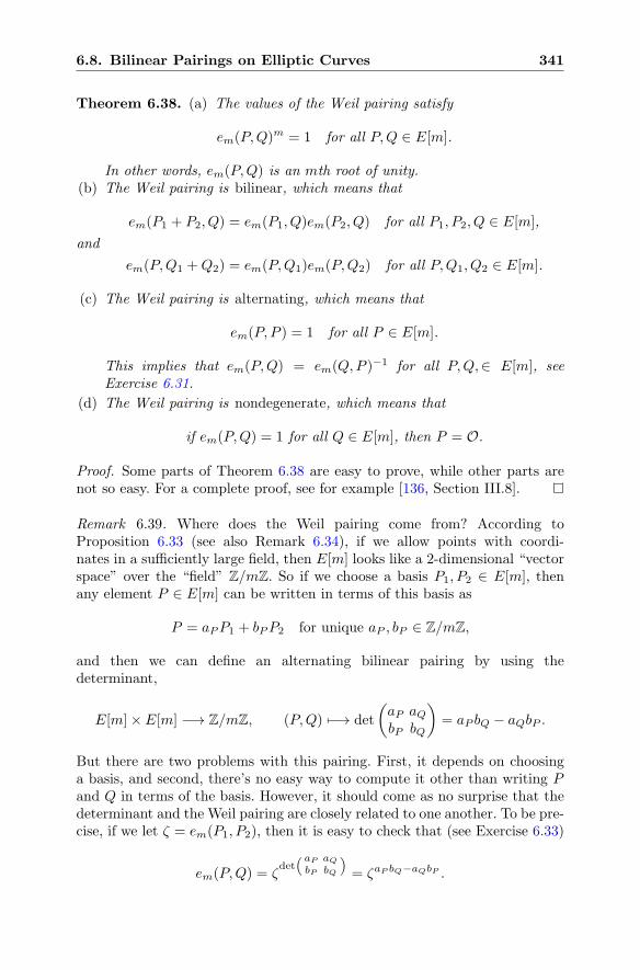
6.8. Bilinear Pairings on Elliptic Curves 341
Theorem 6.38. (a) The values of the Weil pairing satisfy
em(P,Q)m = 1 for all P,Q ∈ E[m].
In other words, em(P,Q) is an mth root of unity.(b) The Weil pairing is bilinear, which means that
em(P1 + P2, Q) = em(P1, Q)em(P2, Q) for all P1, P2, Q ∈ E[m],
and
em(P,Q1 +Q2) = em(P,Q1)em(P,Q2) for all P,Q1, Q2 ∈ E[m].
(c) The Weil pairing is alternating, which means that
em(P, P ) = 1 for all P ∈ E[m].
This implies that em(P,Q) = em(Q,P )−1 for all P,Q,∈ E[m], seeExercise 6.31.
(d) The Weil pairing is nondegenerate, which means that
if em(P,Q) = 1 for all Q ∈ E[m], then P = O.
Proof. Some parts of Theorem 6.38 are easy to prove, while other parts arenot so easy. For a complete proof, see for example [136, Section III.8].
Remark 6.39. Where does the Weil pairing come from? According toProposition 6.33 (see also Remark 6.34), if we allow points with coordi-nates in a sufficiently large field, then E[m] looks like a 2-dimensional “vectorspace” over the “field” Z/mZ. So if we choose a basis P1, P2 ∈ E[m], thenany element P ∈ E[m] can be written in terms of this basis as
P = aPP1 + bPP2 for unique aP , bP ∈ Z/mZ,
and then we can define an alternating bilinear pairing by using thedeterminant,
E[m]× E[m] −→ Z/mZ, (P,Q) �−→ det
(aP aQbP bQ
)= aP bQ − aQbP .
But there are two problems with this pairing. First, it depends on choosinga basis, and second, there’s no easy way to compute it other than writing Pand Q in terms of the basis. However, it should come as no surprise that thedeterminant and the Weil pairing are closely related to one another. To be pre-cise, if we let ζ = em(P1, P2), then it is easy to check that (see Exercise 6.33)
em(P,Q) = ζdet
( aP aQ
bP bQ
)
= ζaP bQ−aQbP .
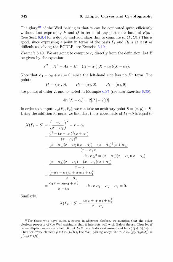
342 6. Elliptic Curves and Cryptography
The glory10 of the Weil pairing is that it can be computed quite efficientlywithout first expressing P and Q in terms of any particular basis of E[m].(See Sect. 6.8.4 for a double-and-add algorithm to compute em(P,Q).) This isgood, since expressing a point in terms of the basis P1 and P2 is at least asdifficult as solving the ECDLP; see Exercise 6.10.
Example 6.40. We are going to compute e2 directly from the definition. Let Ebe given by the equation
Y 2 = X3 +Ax+B = (X − α1)(X − α2)(X − α3).
Note that α1 + α2 + α3 = 0, since the left-hand side has no X2 term. Thepoints
P1 = (α1, 0), P2 = (α2, 0), P3 = (α3, 0),
are points of order 2, and as noted in Example 6.37 (see also Exercise 6.30),
div(X − αi) = 2[Pi]− 2[O].
In order to compute e2(P1, P2), we can take an arbitrary point S = (x, y) ∈ E.Using the addition formula, we find that the x-coordinate of P1−S is equal to
X(P1 − S) =(
−yx− α1
)2
− x− α1
=y2 − (x− α1)
2(x+ α1)
(x− α1)2
=(x− α1)(x− α2)(x− α3)− (x− α1)
2(x+ α1)
(x− α1)2
since y2 = (x− α1)(x− α2)(x− α3),
=(x− α2)(x− α3)− (x− α1)(x+ α1)
x− α1
=(−α2 − α3)x+ α2α3 + α2
1
x− α1
=α1x+ α2α3 + α2
1
x− α1since α1 + α2 + α3 = 0.
Similarly,
X(P2 + S) =α2x+ α1α3 + α2
2
x− α2.
10For those who have taken a course in abstract algebra, we mention that the otherglorious property of the Weil pairing is that it interacts well with Galois theory. Thus let Ebe an elliptic curve over a field K, let L/K be a Galois extension, and let P,Q ∈ E(L)[m].Then for every element g ∈ Gal(L/K), the Weil pairing obeys the rule em
(g(P ), g(Q)
)=
g(em(P,Q)
).
6.8. Bilinear Pairings on Elliptic Curves 343
Using the rational functions fPi= X − αi and assuming that P1 and P2 are
distinct nonzero points in E[2], we find directly from the definition of em that
e2(P1, P2) =fP1
(P2 + S)
fP1(S)
/fP2
(P1 − S)fP2
(−S)
=X(P2 + S)− α1
X(S)− α1
/X(P1 − S)− α2
X(−S)− α2
=
α2x+α1α3+α22
x−α2− α1
x− α1
/α1x+α2α3+α2
1
x−α1− α2
x− α2
=(α2 − α1)x+ α1α3 + α2
2 + α1α2
(α1 − α2)x+ α2α3 + α21 + α1α2
=(α2 − α1)x+ α2
2 − α21
(α1 − α2)x+ α21 − α2
2
since α1 + α2 + α3 = 0,
= −1.
6.8.4 An Efficient Algorithm to Computethe Weil Pairing
In this section we describe a double-and-add method that can be used toefficiently compute the Weil pairing. The key idea, which is due to VictorMiller [89], is an algorithm to rapidly evaluate certain functions with specifieddivisors, as explained in the next theorem. (For further material on Miller’salgorithm, see [136, Section XI.8].)
Theorem 6.41. Let E be an elliptic curve and let P = (xP , yP ) and Q =(xQ, yQ) be nonzero points on E.(a) Let λ be the slope of the line connecting P and Q, or the slope of the
tangent line to E at P if P = Q. (If the line is vertical, we let λ = ∞.)Define a function gP,Q on E as follows :
gP,Q =
⎧⎨
⎩
y − yP − λ(x− xP )x+ xP + xQ − λ2
if λ �=∞,
x− xP if λ =∞.
Thendiv(gP,Q) = [P ] + [Q]− [P +Q]− [O]. (6.17)
(b) (Miller’s Algorithm) Let m ≥ 1 and write the binary expansion of m as
m = m0 +m1 · 2 +m2 · 22 + · · ·+mn−12n−1
with mi ∈ {0, 1} and mn−1 �= 0. The following algorithm returns a func-tion fP whose divisor satisfies
div(fP ) = m[P ]− [mP ]− (m− 1)[O],
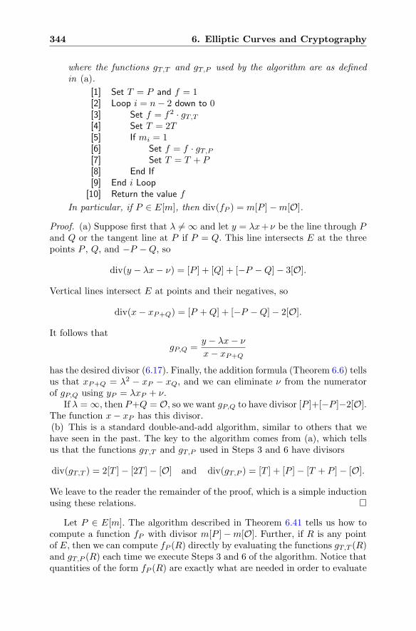
344 6. Elliptic Curves and Cryptography
where the functions gT,T and gT,P used by the algorithm are as definedin (a).
[1] Set T = P and f = 1[2] Loop i = n− 2 down to 0[3] Set f = f2 · gT,T
[4] Set T = 2T[5] If mi = 1[6] Set f = f · gT,P
[7] Set T = T + P[8] End If[9] End i Loop[10] Return the value f
In particular, if P ∈ E[m], then div(fP ) = m[P ]−m[O].
Proof. (a) Suppose first that λ �=∞ and let y = λx+ ν be the line through Pand Q or the tangent line at P if P = Q. This line intersects E at the threepoints P , Q, and −P −Q, so
div(y − λx− ν) = [P ] + [Q] + [−P −Q]− 3[O].
Vertical lines intersect E at points and their negatives, so
div(x− xP+Q) = [P +Q] + [−P −Q]− 2[O].
It follows that
gP,Q =y − λx− νx− xP+Q
has the desired divisor (6.17). Finally, the addition formula (Theorem 6.6) tellsus that xP+Q = λ2 − xP − xQ, and we can eliminate ν from the numeratorof gP,Q using yP = λxP + ν.
If λ =∞, then P+Q = O, so we want gP,Q to have divisor [P ]+[−P ]−2[O].The function x− xP has this divisor.(b) This is a standard double-and-add algorithm, similar to others that wehave seen in the past. The key to the algorithm comes from (a), which tellsus that the functions gT,T and gT,P used in Steps 3 and 6 have divisors
div(gT,T ) = 2[T ]− [2T ]− [O] and div(gT,P ) = [T ] + [P ]− [T + P ]− [O].
We leave to the reader the remainder of the proof, which is a simple inductionusing these relations.
Let P ∈ E[m]. The algorithm described in Theorem 6.41 tells us how tocompute a function fP with divisor m[P ]−m[O]. Further, if R is any pointof E, then we can compute fP (R) directly by evaluating the functions gT,T (R)and gT,P (R) each time we execute Steps 3 and 6 of the algorithm. Notice thatquantities of the form fP (R) are exactly what are needed in order to evaluate
6.8. Bilinear Pairings on Elliptic Curves 345
the Weil pairing em(P,Q). More precisely, given nonzero points P,Q ∈ E[m],we choose a point S /∈ {O, P,−Q,P −Q} and use Theorem 6.41 to evaluate
em(P,Q) =fP (Q+ S)
fP (S)
/fQ(P − S)fQ(−S)
by computing each of the functions at the indicated point.
Remark 6.42. For added efficiency, one can compute fP (Q + S) and fP (S)simultaneously, and similarly for fQ(P −S) and fQ(−S). Further savings areavailable using the Tate pairing, which is a variant of the Weil pairing thatwe describe briefly in Sect. 6.8.5.
Example 6.43. We take the elliptic curve
y2 = x3 + 30x+ 34 over the finite field F631.
The curve has #E(F631) = 650 = 2 · 52 · 13 points, and it turns out that ithas 25 points of order 5. The points
P = (36, 60) and Q = (121, 387)
generate the points of order 5 in E(F631). In order to compute the Weil pairingusing Miller’s algorithm, we want a point S that is not in the subgroup spannedby P and Q. We take S = (0, 36). The point S has order 130. Then Miller’salgorithm gives
fP (Q+ S)
fP (S)=
103
219= 473 ∈ F631.
Reversing the roles of P and Q and replacing S by −S, Miller’s algorithmalso gives
fQ(P − S)fQ(−S)
=284
204= 88 ∈ F631.
Finally, taking the ratio of these two values yields
e5(P,Q) =473
88= 242 ∈ F631.
We check that (242)5 = 1, so e5(P,Q) is a fifth root of unity in F631.Continuing to work on the same curve, we take P ′ = (617, 5) and Q′ =
(121, 244). Then a similar calculation gives
fP ′(Q′ + S)
fP ′(S)=
326
523= 219 and
fQ′(P ′ − S)fQ′(−S) =
483
576= 83,
and taking the ratio of these two values yields
e5(P′, Q′) =
219
83= 512 ∈ F631.
It turns out that P ′ = 3P and Q′ = 4Q. We check that
e5(P,Q)12 = 24212 = 512 = e5(P′, Q′) = e5(3P, 4Q),
which illustrates the bilinearity property of the Weil pairing.
346 6. Elliptic Curves and Cryptography
6.8.5 The Tate Pairing
The Weil pairing is a nondegenerate bilinear form on elliptic curves definedover any field. For elliptic curves over finite fields there is another pairing,called the Tate pairing (or sometimes the Tate–Lichtenbaum pairing), thatis often used in cryptography because it is computationally somewhat moreefficient than the Weil pairing. In this section we briefly describe the Tatepairing. (For further material on the Tate pairing, see [136, Section XI.9].)
Definition. Let E be an elliptic curve over Fq, let � be a prime, let P ∈E(Fq)[�], and let Q ∈ E(Fq). Choose a rational function fP on E with
div(fP ) = �[P ]− �[O].
The Tate pairing of P and Q is the quantity
τ(P,Q) =fP (Q+ S)
fP (S)∈ F
∗q ,
where S is any point in E(Fq) such that fP (Q+S) and fP (S) are defined andnonzero. It turns out that the value of the Tate pairing is well-defined onlyup to multiplying it by the �th power of an element of F∗
q . If q ≡ 1 (mod �),we define the (modified) Tate pairing of P and Q to be
τ(P,Q) = τ(P,Q)(q−1)/� =
(fP (Q+ S)
fP (S)
)(q−1)/�
∈ F∗q .
Theorem 6.44. Let E be an elliptic curve over Fq and let � be a prime with
q ≡ 1 (mod �) and E(Fq)[�] ∼= Z/�Z.
Then the modified Tate pairing gives a well-defined map
τ : E(Fq)[�]× E(Fq)[�] −→ F∗q
having the following properties :(a) Bilinearity:
τ(P1+P2, Q) = τ(P1, Q)τ(P2, Q) and τ(P,Q1+Q2) = τ(P,Q1)τ(P,Q2).
(b) Nondegeneracy:
τ(P, P ) is a primitive �th root of unity for all nonzero P ∈ E(Fq)[�].
(A primitive �th root of unity is a number ζ �= 1 such that ζ� = 1.)
In applications such as tripartite Diffie–Hellman (Sect. 6.10.1) and ID-based cryptography (Sect. 6.10.2), one may use the Tate pairing in place ofthe Weil pairing. Note that Miller’s algorithm gives an efficient way to computethe Tate pairing, since Theorem 6.41(b) explains how to rapidly compute thevalue of fP .
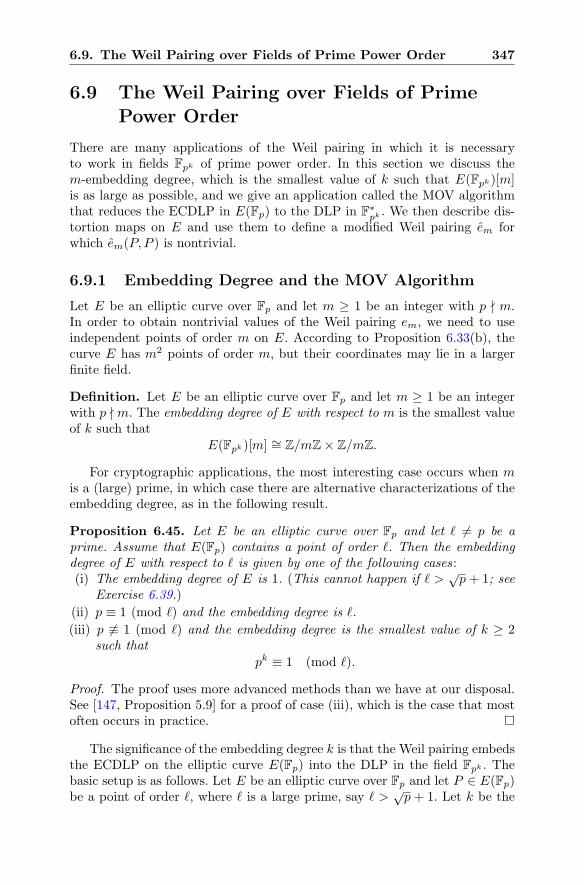
6.9. The Weil Pairing over Fields of Prime Power Order 347
6.9 The Weil Pairing over Fields of PrimePower Order
There are many applications of the Weil pairing in which it is necessaryto work in fields Fpk of prime power order. In this section we discuss them-embedding degree, which is the smallest value of k such that E(Fpk)[m]is as large as possible, and we give an application called the MOV algorithmthat reduces the ECDLP in E(Fp) to the DLP in F
∗pk . We then describe dis-
tortion maps on E and use them to define a modified Weil pairing em forwhich em(P, P ) is nontrivial.
6.9.1 Embedding Degree and the MOV Algorithm
Let E be an elliptic curve over Fp and let m ≥ 1 be an integer with p � m.In order to obtain nontrivial values of the Weil pairing em, we need to useindependent points of order m on E. According to Proposition 6.33(b), thecurve E has m2 points of order m, but their coordinates may lie in a largerfinite field.
Definition. Let E be an elliptic curve over Fp and let m ≥ 1 be an integerwith p � m. The embedding degree of E with respect to m is the smallest valueof k such that
E(Fpk)[m] ∼= Z/mZ× Z/mZ.
For cryptographic applications, the most interesting case occurs when mis a (large) prime, in which case there are alternative characterizations of theembedding degree, as in the following result.
Proposition 6.45. Let E be an elliptic curve over Fp and let � �= p be aprime. Assume that E(Fp) contains a point of order �. Then the embeddingdegree of E with respect to � is given by one of the following cases :(i) The embedding degree of E is 1. (This cannot happen if � >
√p+ 1; see
Exercise 6.39.)
(ii) p ≡ 1 (mod �) and the embedding degree is �.
(iii) p �≡ 1 (mod �) and the embedding degree is the smallest value of k ≥ 2such that
pk ≡ 1 (mod �).
Proof. The proof uses more advanced methods than we have at our disposal.See [147, Proposition 5.9] for a proof of case (iii), which is the case that mostoften occurs in practice.
The significance of the embedding degree k is that the Weil pairing embedsthe ECDLP on the elliptic curve E(Fp) into the DLP in the field Fpk . Thebasic setup is as follows. Let E be an elliptic curve over Fp and let P ∈ E(Fp)be a point of order �, where � is a large prime, say � >
√p + 1. Let k be the
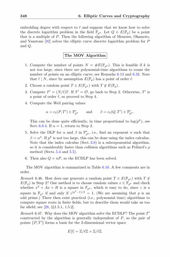
348 6. Elliptic Curves and Cryptography
embedding degree with respect to � and suppose that we know how to solvethe discrete logarithm problem in the field Fpk . Let Q ∈ E(Fp) be a pointthat is a multiple of P . Then the following algorithm of Menezes, Okamoto,and Vanstone [82] solves the elliptic curve discrete logarithm problem for Pand Q.
The MOV Algorithm
1. Compute the number of points N = #E(Fpk). This is feasible if k isnot too large, since there are polynomial-time algorithms to count thenumber of points on an elliptic curve; see Remarks 6.13 and 6.32. Notethat � | N , since by assumption E(Fp) has a point of order �.
2. Choose a random point T ∈ E(Fpk) with T /∈ E(Fp).
3. Compute T ′ = (N/�)T . If T ′ = O, go back to Step 2. Otherwise, T ′ isa point of order �, so proceed to Step 4.
4. Compute the Weil pairing values
α = e�(P, T′) ∈ F
∗pk and β = e�(Q,T
′) ∈ F∗pk .
This can be done quite efficiently, in time proportional to log(pk), seeSect. 6.8.4. If α = 1, return to Step 2.
5. Solve the DLP for α and β in F∗pk , i.e., find an exponent n such that
β = αn. If pk is not too large, this can be done using the index calculus.Note that the index calculus (Sect. 3.8) is a subexponential algorithm,so it is considerably faster than collision algorithms such as Pollard’s ρmethod (Sects. 5.4 and 5.5).
6. Then also Q = nP , so the ECDLP has been solved.
The MOV algorithm is summarized in Table 6.10. A few comments are inorder.
Remark 6.46. How does one generate a random point T ∈ E(Fpk) with T /∈E(Fp) in Step 2? One method is to choose random values x ∈ Fpk and checkwhether x3 + Ax + B is a square in Fpk , which is easy to do, since z is a
square in Fpk if and only if z(pk−1)/2 = 1. (We are assuming that p is an
odd prime.) There then exist practical (i.e., polynomial time) algorithms tocompute square roots in finite fields, but to describe them would take us toofar afield; see [28, §§1.5.1, 1.5.2].Remark 6.47. Why does the MOV algorithm solve the ECDLP? The point T ′
constructed by the algorithm is generally independent of P , so the pair ofpoints {P, T ′} forms a basis for the 2-dimensional vector space
E[�] = Z/�Z× Z/�Z.
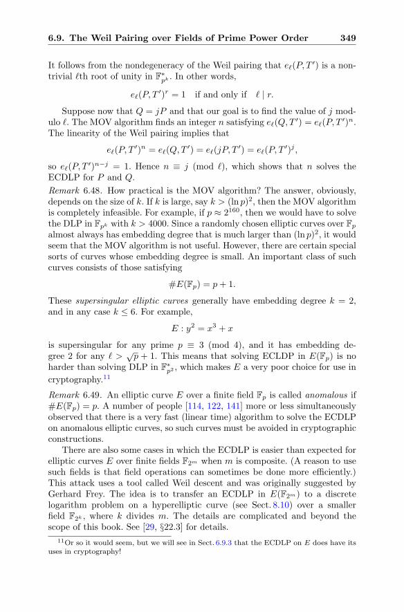
6.9. The Weil Pairing over Fields of Prime Power Order 349
It follows from the nondegeneracy of the Weil pairing that e�(P, T′) is a non-
trivial �th root of unity in F∗pk . In other words,
e�(P, T′)r = 1 if and only if � | r.
Suppose now that Q = jP and that our goal is to find the value of j mod-ulo �. The MOV algorithm finds an integer n satisfying e�(Q,T
′) = e�(P, T′)n.
The linearity of the Weil pairing implies that
e�(P, T′)n = e�(Q,T
′) = e�(jP, T′) = e�(P, T
′)j ,
so e�(P, T′)n−j = 1. Hence n ≡ j (mod �), which shows that n solves the
ECDLP for P and Q.
Remark 6.48. How practical is the MOV algorithm? The answer, obviously,depends on the size of k. If k is large, say k > (ln p)2, then the MOV algorithmis completely infeasible. For example, if p ≈ 2160, then we would have to solvethe DLP in Fpk with k > 4000. Since a randomly chosen elliptic curves over Fp
almost always has embedding degree that is much larger than (ln p)2, it wouldseem that the MOV algorithm is not useful. However, there are certain specialsorts of curves whose embedding degree is small. An important class of suchcurves consists of those satisfying
#E(Fp) = p+ 1.
These supersingular elliptic curves generally have embedding degree k = 2,and in any case k ≤ 6. For example,
E : y2 = x3 + x
is supersingular for any prime p ≡ 3 (mod 4), and it has embedding de-gree 2 for any � >
√p + 1. This means that solving ECLDP in E(Fp) is no
harder than solving DLP in F∗p2 , which makes E a very poor choice for use in
cryptography.11
Remark 6.49. An elliptic curve E over a finite field Fp is called anomalous if#E(Fp) = p. A number of people [114, 122, 141] more or less simultaneouslyobserved that there is a very fast (linear time) algorithm to solve the ECDLPon anomalous elliptic curves, so such curves must be avoided in cryptographicconstructions.
There are also some cases in which the ECDLP is easier than expected forelliptic curves E over finite fields F2m when m is composite. (A reason to usesuch fields is that field operations can sometimes be done more efficiently.)This attack uses a tool called Weil descent and was originally suggested byGerhard Frey. The idea is to transfer an ECDLP in E(F2m) to a discretelogarithm problem on a hyperelliptic curve (see Sect. 8.10) over a smallerfield F2k , where k divides m. The details are complicated and beyond thescope of this book. See [29, §22.3] for details.
11Or so it would seem, but we will see in Sect. 6.9.3 that the ECDLP on E does have itsuses in cryptography!
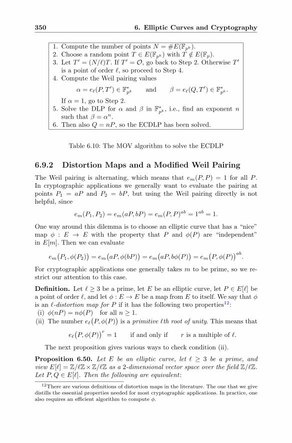
350 6. Elliptic Curves and Cryptography
1. Compute the number of points N = #E(Fpk).2. Choose a random point T ∈ E(Fpk) with T /∈ E(Fp).3. Let T ′ = (N/�)T . If T ′ = O, go back to Step 2. Otherwise T ′
is a point of order �, so proceed to Step 4.4. Compute the Weil pairing values
α = e�(P, T′) ∈ F
∗pk and β = e�(Q,T
′) ∈ F∗pk .
If α = 1, go to Step 2.5. Solve the DLP for α and β in F
∗pk , i.e., find an exponent n
such that β = αn.6. Then also Q = nP , so the ECDLP has been solved.
Table 6.10: The MOV algorithm to solve the ECDLP
6.9.2 Distortion Maps and a Modified Weil Pairing
The Weil pairing is alternating, which means that em(P, P ) = 1 for all P .In cryptographic applications we generally want to evaluate the pairing atpoints P1 = aP and P2 = bP , but using the Weil pairing directly is nothelpful, since
em(P1, P2) = em(aP, bP ) = em(P, P )ab = 1ab = 1.
One way around this dilemma is to choose an elliptic curve that has a “nice”map φ : E → E with the property that P and φ(P ) are “independent”in E[m]. Then we can evaluate
em(P1, φ(P2)
)= em
(aP, φ(bP )
)= em
(aP, bφ(P )
)= em
(P, φ(P )
)ab.
For cryptographic applications one generally takes m to be prime, so we re-strict our attention to this case.
Definition. Let � ≥ 3 be a prime, let E be an elliptic curve, let P ∈ E[�] bea point of order �, and let φ : E → E be a map from E to itself. We say that φis an �-distortion map for P if it has the following two properties12:(i) φ(nP ) = nφ(P ) for all n ≥ 1.
(ii) The number e�(P, φ(P )
)is a primitive �th root of unity. This means that
e�(P, φ(P )
)r= 1 if and only if r is a multiple of �.
The next proposition gives various ways to check condition (ii).
Proposition 6.50. Let E be an elliptic curve, let � ≥ 3 be a prime, andview E[�] = Z/�Z×Z/�Z as a 2-dimensional vector space over the field Z/�Z.Let P,Q ∈ E[�]. Then the following are equivalent :
12There are various definitions of distortion maps in the literature. The one that we givedistills the essential properties needed for most cryptographic applications. In practice, onealso requires an efficient algorithm to compute φ.
6.9. The Weil Pairing over Fields of Prime Power Order 351
(a) P and Q form a basis for the vector space E[�].
(b) P �= O and Q is not a multiple of P .
(c) e�(P,Q) is a primitive �th root of unity.
(d) e�(P,Q) �= 1.
Proof. It is clear that (a) implies (b), since a basis consists of independentvectors. Conversely, suppose that (a) is false. This means that there is a linearrelation
uP + vQ = O with u, v ∈ Z/�Z not both 0.
If v = 0, then P = O, so (b) is false. And if v �= 0, then v has an inversein Z/�Z, so Q = −v−1uP is a multiple of P , again showing that (b) is false.This completes the proof that (a) and (b) are equivalent.
To ease notation, we letζ = e�(P,Q).
From the definition of the Weil pairing, we know that ζ� = 1. Let r ≥ 1 bethe smallest integer such that ζr = 1. Use the extended Euclidean algorithm(Theorem 1.11) to write the greatest common divisor of r and � as
sr + t� = gcd(r, �) for some s, t ∈ Z.
Thenζgcd(r,�) = ζsr+t� = (ζr)s(ζ�)t = 1.
The minimality of r tells us that r = gcd(r, �), so r | �. Since � is prime, itfollows that either r = 1, so ζ = 1, or else r = �. This proves that (c) and (d)are equivalent.
We next verify that (a) implies (d). So we are given that P and Q are abasis for E[�]. In particular, P �= O, so the nondegeneracy of the Weil pairingtells us that there is a point R ∈ E[�] with e�(P,R) �= 1. Since P and Q are abasis for E[�], we can write R as a linear combination of P and Q, say
R = uP + vQ.
Then the bilinearity and alternating properties of the Weil pairing yield
1 �= e�(P,R) = e�(P, uP + vQ) = e�(P, P )ue�(P,Q)v = e�(P,Q)v.
Hence e�(P,Q) �= 1, which shows that (d) is true.Finally, we show that (d) implies (b) by assuming that (b) is false and
deducing that (d) is false. The assumption that (b) is false means that ei-ther P = O or Q = uP for some u ∈ Z/�Z. But if P = O, then e�(P,Q) =e�(O, Q) = 1 by bilinearity, while if Q = uP , then
e�(P,Q) = e�(P, uP ) = e�(P, P )u = 1u = 1
by the alternating property of e�. Thus in both cases we find that e�(P,Q) = 1,so (d) is false.
352 6. Elliptic Curves and Cryptography
Definition. Let E be an elliptic curve, let P ∈ E[�], and let φ be an �-distortion map for P . The modified Weil pairing e� on E[�] (relative to φ) isdefined by
e�(Q,Q′) = e�
(Q,φ(Q′)
).
In cryptographic applications, the modified Weil pairing is evaluated atpoints that are multiples of P . The crucial property of the modified Weilpairing is its nondegeneracy, as described in the next result.
Proposition 6.51. Let E be an elliptic curve, let P ∈ E[�], let φ be an �-distortion map for P , and let e� be the modified Weil pairing relative to φ.Let Q and Q′ be multiples of P . Then
e�(Q,Q′) = 1 if and only if Q = O or Q′ = O.
Proof. We are given that Q and Q′ are multiples of P , so we can write themas Q = sP and Q′ = tP . The definition of distortion map and the linearity ofthe Weil pairing imply that
e�(Q,Q′) = e�(sP, tP ) = e�
(sP, φ(tP )
)= e�
(sP, tφ(P )
)= e�
(P, φ(P )
)st.
The quantity e�(P, φ(P )
)is a primitive �th root of unity, so
e�(Q,Q′) = 1 ⇐⇒ � | st
⇐⇒ � | s or � | t⇐⇒ Q = O or Q′ = O.
6.9.3 A Distortion Map on y2 = x3 + x
In order to use the modified Weil pairing for cryptographic purposes, we needto give at least one example of an elliptic curve with a distortion map. In thissection we give such an example for the elliptic curve y2 = x3 + x over thefield Fp with p ≡ 3 (mod 4). (See Exercise 6.43 for another example.) We startby describing the map φ.
Proposition 6.52. Let E be the elliptic curve
E : y2 = x3 + x
over a field K and suppose that K has an element α ∈ K satisfying α2 = −1.Define a map φ by
φ(x, y) = (−x, αy) and φ(O) = O.
(a) Let P ∈ E(K). Then φ(P ) ∈ E(K), so φ is a map from E(K) to itself.
6.9. The Weil Pairing over Fields of Prime Power Order 353
(b) The map φ respects the addition law on E,13
φ(P1 + P2) = φ(P1) + φ(P2) for all P1, P2 ∈ E(K).
In particular, φ(nP ) = nφ(P ) for all P ∈ E(K) and all n ≥ 1.
Proof. (a) Let P = (x, y) ∈ E(K). Then
(αy)2 = −y2 = −(x3 + x) = (−x)3 + (−x),
so φ(P ) = (−x, αy) ∈ E(K).(b) Suppose that P1 = (x1, y1) and P2 = (x2, y2) are distinct points. Thenusing the elliptic curve addition algorithm (Theorem 6.6), we find that thex-coordinate of φ(P1) + φ(P2) is
x(φ(P1) + φ(P2)
)=
(αy2 − αy1
(−x2)− (−x1)
)2
− (−x1)− (−x2)
= α2
(y2 − y1x2 − x1
)2
+ x1 + x2
= −((
y2 − y1x2 − x1
)2
− x1 − x2
)
= −x(P1 + P2).
Similarly, the y-coordinate of φ(P1) + φ(P2) is
y(φ(P1) + φ(P2)
)=
(αy2 − αy1
(−x2)− (−x1)
)(−x1 − x
(φ(P1) + φ(P2)
))− αy1
= −α(y2 − y1x2 − x1
)(−x1 + x(P1 + P2)
)− αy1
= α
((y2 − y1x2 − x1
)(x1 − x(P1 + P2)
)+ y1
)
= αy(P1 + P2).
Hence
φ(P1) + φ(P2) =(−x(P1 + P2), αy(P1 + P2)
)= φ(P1 + P2).
This handles the case that P1 �= P2. We leave the case P1 = P2 for the reader;see Exercise 6.38.
We now have the tools needed to construct a distortion map on thecurve y2 = x3 + x over certain finite fields.
13In the language of abstract algebra, the map φ is a homomorphism of the group E(K)to itself; see Exercise 2.13. In the language of algebraic geometry, a homomorphism froman elliptic curve to itself is called an isogeny.
354 6. Elliptic Curves and Cryptography
Proposition 6.53. Fix the following quantities.• A prime p satisfying p ≡ 3 (mod 4).
• The elliptic curve E : y2 = x3 + x.
• An element α ∈ Fp2 satisfying α2 = −1.• The map φ(x, y) = (−x, αy).• A prime � ≥ 3 such that there exists a nonzero point P ∈ E(Fp)[�].
Then φ is an �-distortion map for P , i.e., the quantity
e�(P, P ) = e�(P, φ(P ))
is a primitive �th root of unity.
Proof. We first note that Fp does not contain an element satisfying α2 = −1.This is part of quadratic reciprocity (Theorem 3.62), but it is also easy toprove directly from the fact that F
∗p is a group of order p − 1, so it cannot
have any elements of order 4, since p ≡ 3 (mod 4).However, the field Fp2 of order p2 does contain a square root of−1, since if g
is a primitive root for F∗p2 (see Theorem 2.62), then α = g(p
2−1)/4 satisfies α4 =
1 and α2 �= 1, so α2 = −1.Since P �= O, it is clear that φ(P ) �= O. Since P is a point of order �,
Proposition 6.52(b) says that
�φ(P ) = φ(�P ) = φ(O) = O,
so φ(P ) is a point of order �. We are going to prove that φ(P ) is not a multipleof P , and then Proposition 6.50 tells us that e�(P, φ(P )) is a primitive �throot of unity.
Suppose to the contrary that φ(P ) is a multiple of P . We write P =(x, y) ∈ E(Fp). The coordinates of P are in Fp, so the coordinates of anymultiple of P are also in Fp. Thus the coordinates of φ(P ) = (−x, αy) wouldbe in Fp. But α /∈ Fp, since Fp does not contain a square root of −1, so wemust have y = 0. Then P = (x, 0) is a point of order 2, which is not possible,since P is a point of order � with � ≥ 3. Hence φ(P ) is not a multiple of Pand we are done.
Remark 6.54. We recall from Example 2.58 that if p ≡ 3 (mod 4), then thefield with p2 elements looks like
Fp2 = {a+ bi : a, b ∈ Fp},
where i satisfies i2 = −1. This makes it quite easy to work with the field Fp2
in the context of Proposition 6.53.
Example 6.55. We take E : y2 = x3 + x and the prime p = 547. Then
#E(F547) = 548 = 22 · 137.
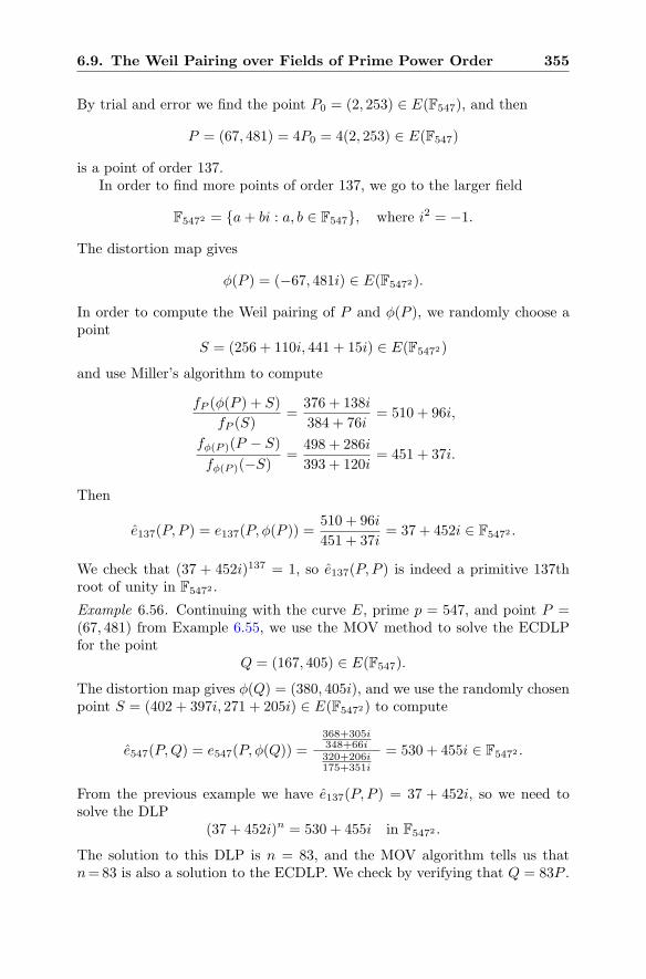
6.9. The Weil Pairing over Fields of Prime Power Order 355
By trial and error we find the point P0 = (2, 253) ∈ E(F547), and then
P = (67, 481) = 4P0 = 4(2, 253) ∈ E(F547)
is a point of order 137.In order to find more points of order 137, we go to the larger field
F5472 = {a+ bi : a, b ∈ F547}, where i2 = −1.
The distortion map gives
φ(P ) = (−67, 481i) ∈ E(F5472).
In order to compute the Weil pairing of P and φ(P ), we randomly choose apoint
S = (256 + 110i, 441 + 15i) ∈ E(F5472)
and use Miller’s algorithm to compute
fP (φ(P ) + S)
fP (S)=
376 + 138i
384 + 76i= 510 + 96i,
fφ(P )(P − S)fφ(P )(−S)
=498 + 286i
393 + 120i= 451 + 37i.
Then
e137(P, P ) = e137(P, φ(P )) =510 + 96i
451 + 37i= 37 + 452i ∈ F5472 .
We check that (37 + 452i)137 = 1, so e137(P, P ) is indeed a primitive 137throot of unity in F5472 .
Example 6.56. Continuing with the curve E, prime p = 547, and point P =(67, 481) from Example 6.55, we use the MOV method to solve the ECDLPfor the point
Q = (167, 405) ∈ E(F547).
The distortion map gives φ(Q) = (380, 405i), and we use the randomly chosenpoint S = (402 + 397i, 271 + 205i) ∈ E(F5472) to compute
e547(P,Q) = e547(P, φ(Q)) =368+305i348+66i320+206i175+351i
= 530 + 455i ∈ F5472 .
From the previous example we have e137(P, P ) = 37 + 452i, so we need tosolve the DLP
(37 + 452i)n = 530 + 455i in F5472 .
The solution to this DLP is n = 83, and the MOV algorithm tells us thatn=83 is also a solution to the ECDLP. We check by verifying that Q = 83P .
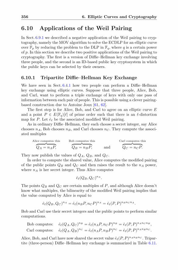
356 6. Elliptic Curves and Cryptography
6.10 Applications of the Weil Pairing
In Sect. 6.9.1 we described a negative application of the Weil pairing to cryp-tography, namely the MOV algorithm to solve the ECDLP for an elliptic curveover Fp by reducing the problem to the DLP in Fq, where q is a certain powerof p. In this section we describe two positive applications of the Weil pairing tocryptography. The first is a version of Diffie–Hellman key exchange involvingthree people, and the second is an ID-based public key cryptosystem in whichthe public keys can be selected by their owners.
6.10.1 Tripartite Diffie–Hellman Key Exchange
We have seen in Sect. 6.4.1 how two people can perform a Diffie–Hellmankey exchange using elliptic curves. Suppose that three people, Alice, Bob,and Carl, want to perform a triple exchange of keys with only one pass ofinformation between each pair of people. This is possible using a clever pairing-based construction due to Antoine Joux [61, 62].
The first step is for Alice, Bob, and Carl to agree on an elliptic curve Eand a point P ∈ E(Fq)[�] of prime order such that there is an �-distortionmap for P . Let e� be the associated modified Weil pairing.
As in ordinary Diffie–Hellman, they each choose a secret integer, say Alicechooses nA, Bob chooses nB , and Carl chooses nC . They compute the associ-ated multiples
Alice computes this︷ ︸︸ ︷QA = nAP,
Bob computes this︷ ︸︸ ︷QB = nBP, and
Carl computes this︷ ︸︸ ︷QC = nCP.
They now publish the values of QA, QB , and QC .In order to compute the shared value, Alice computes the modified pairing
of the public points QB and QC and then raises the result to the nA power,where nA is her secret integer. Thus Alice computes
e�(QB , QC)nA .
The points QB and QC are certain multiples of P , and although Alice doesn’tknow what multiples, the bilinearity of the modified Weil pairing implies thatthe value computed by Alice is equal to
e�(QB , QC)nA = e�(nBP, nCP )
nA = e�(P, P )nBnCnA .
Bob and Carl use their secret integers and the public points to perform similarcomputations.
Bob computes: e�(QA, QC)nB = e�(nAP, nCP )
nB = e�(P, P )nAnCnB ,
Carl computes: e�(QA, QB)nC = e�(nAP, nBP )
nC = e�(P, P )nAnBnC .
Alice, Bob, and Carl have now shared the secret value e�(P, P )nAnBnC . Tripar-
tite (three-person) Diffie–Hellman key exchange is summarized in Table 6.11.
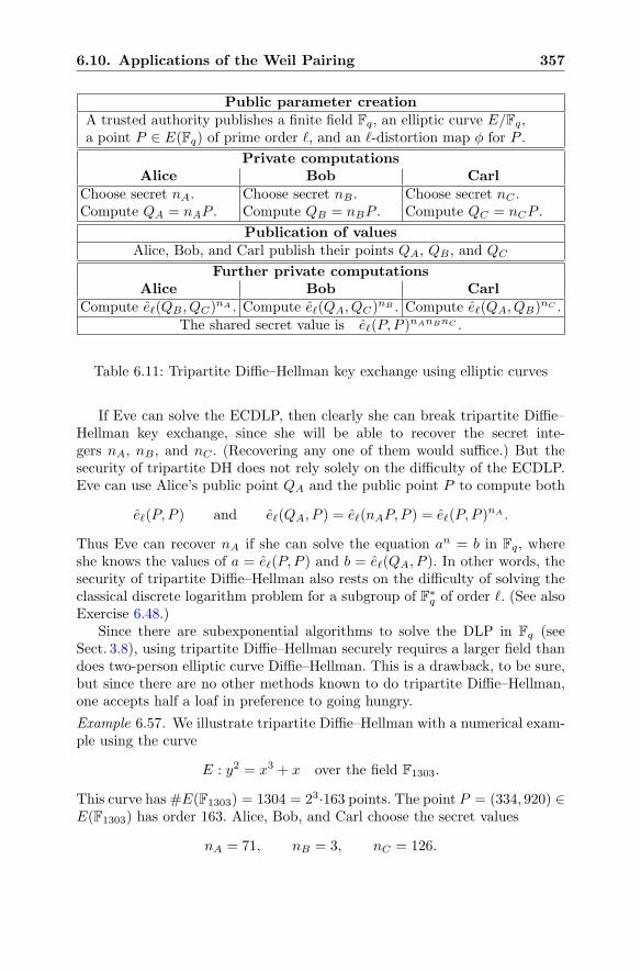
6.10. Applications of the Weil Pairing 357
Public parameter creationA trusted authority publishes a finite field Fq, an elliptic curve E/Fq,a point P ∈ E(Fq) of prime order �, and an �-distortion map φ for P .
Private computationsAlice Bob Carl
Choose secret nA. Choose secret nB . Choose secret nC .Compute QA = nAP . Compute QB = nBP . Compute QC = nCP .
Publication of valuesAlice, Bob, and Carl publish their points QA, QB , and QC
Further private computationsAlice Bob Carl
Compute e�(QB , QC)nA . Compute e�(QA, QC)
nB . Compute e�(QA, QB)nC .
The shared secret value is e�(P, P )nAnBnC .
Table 6.11: Tripartite Diffie–Hellman key exchange using elliptic curves
If Eve can solve the ECDLP, then clearly she can break tripartite Diffie–Hellman key exchange, since she will be able to recover the secret inte-gers nA, nB , and nC . (Recovering any one of them would suffice.) But thesecurity of tripartite DH does not rely solely on the difficulty of the ECDLP.Eve can use Alice’s public point QA and the public point P to compute both
e�(P, P ) and e�(QA, P ) = e�(nAP, P ) = e�(P, P )nA .
Thus Eve can recover nA if she can solve the equation an = b in Fq, whereshe knows the values of a = e�(P, P ) and b = e�(QA, P ). In other words, thesecurity of tripartite Diffie–Hellman also rests on the difficulty of solving theclassical discrete logarithm problem for a subgroup of F∗
q of order �. (See alsoExercise 6.48.)
Since there are subexponential algorithms to solve the DLP in Fq (seeSect. 3.8), using tripartite Diffie–Hellman securely requires a larger field thandoes two-person elliptic curve Diffie–Hellman. This is a drawback, to be sure,but since there are no other methods known to do tripartite Diffie–Hellman,one accepts half a loaf in preference to going hungry.
Example 6.57. We illustrate tripartite Diffie–Hellman with a numerical exam-ple using the curve
E : y2 = x3 + x over the field F1303.
This curve has #E(F1303) = 1304 = 23·163 points. The point P = (334, 920) ∈E(F1303) has order 163. Alice, Bob, and Carl choose the secret values
nA = 71, nB = 3, nC = 126.
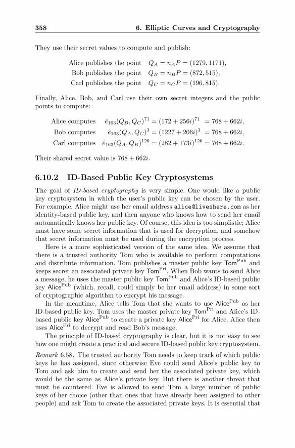
358 6. Elliptic Curves and Cryptography
They use their secret values to compute and publish:
Alice publishes the point QA = nAP = (1279, 1171),
Bob publishes the point QB = nBP = (872, 515),
Carl publishes the point QC = nCP = (196, 815).
Finally, Alice, Bob, and Carl use their own secret integers and the publicpoints to compute:
Alice computes e163(QB , QC)71 = (172 + 256i)71 = 768 + 662i,
Bob computes e163(QA, QC)3 = (1227 + 206i)3 = 768 + 662i,
Carl computes e163(QA, QB)126 = (282 + 173i)126 = 768 + 662i.
Their shared secret value is 768 + 662i.
6.10.2 ID-Based Public Key Cryptosystems
The goal of ID-based cryptography is very simple. One would like a publickey cryptosystem in which the user’s public key can be chosen by the user.For example, Alice might use her email address [email protected] as heridentity-based public key, and then anyone who knows how to send her emailautomatically knows her public key. Of course, this idea is too simplistic; Alicemust have some secret information that is used for decryption, and somehowthat secret information must be used during the encryption process.
Here is a more sophisticated version of the same idea. We assume thatthere is a trusted authority Tom who is available to perform computationsand distribute information. Tom publishes a master public key TomPub andkeeps secret an associated private key TomPri. When Bob wants to send Alicea message, he uses the master public key TomPub and Alice’s ID-based publickey AlicePub (which, recall, could simply be her email address) in some sortof cryptographic algorithm to encrypt his message.
In the meantime, Alice tells Tom that she wants to use AlicePub as herID-based public key. Tom uses the master private key TomPri and Alice’s ID-based public key AlicePub to create a private key AlicePri for Alice. Alice thenuses AlicePri to decrypt and read Bob’s message.
The principle of ID-based cryptography is clear, but it is not easy to seehow one might create a practical and secure ID-based public key cryptosystem.
Remark 6.58. The trusted authority Tom needs to keep track of which publickeys he has assigned, since otherwise Eve could send Alice’s public key toTom and ask him to create and send her the associated private key, whichwould be the same as Alice’s private key. But there is another threat thatmust be countered. Eve is allowed to send Tom a large number of publickeys of her choice (other than ones that have already been assigned to otherpeople) and ask Tom to create the associated private keys. It is essential that
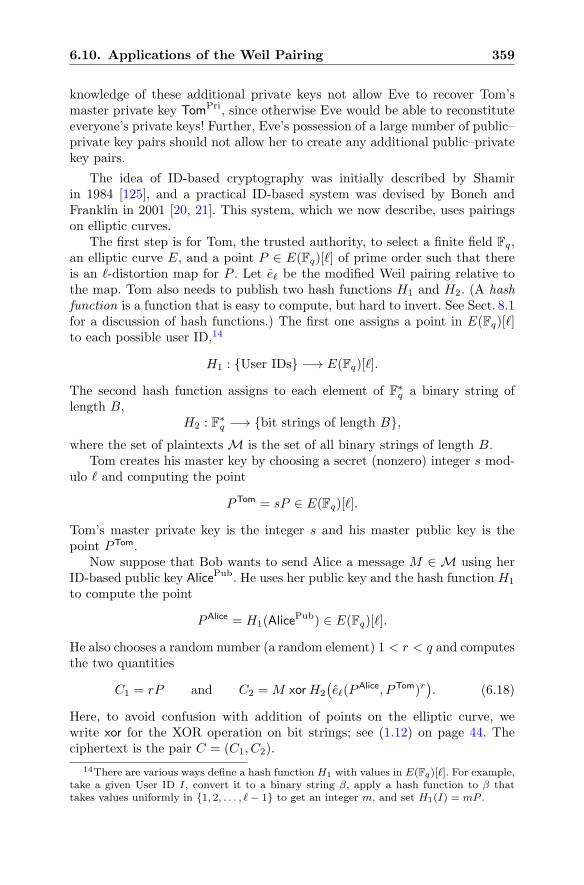
6.10. Applications of the Weil Pairing 359
knowledge of these additional private keys not allow Eve to recover Tom’smaster private key TomPri, since otherwise Eve would be able to reconstituteeveryone’s private keys! Further, Eve’s possession of a large number of public–private key pairs should not allow her to create any additional public–privatekey pairs.
The idea of ID-based cryptography was initially described by Shamirin 1984 [125], and a practical ID-based system was devised by Boneh andFranklin in 2001 [20, 21]. This system, which we now describe, uses pairingson elliptic curves.
The first step is for Tom, the trusted authority, to select a finite field Fq,an elliptic curve E, and a point P ∈ E(Fq)[�] of prime order such that thereis an �-distortion map for P . Let e� be the modified Weil pairing relative tothe map. Tom also needs to publish two hash functions H1 and H2. (A hashfunction is a function that is easy to compute, but hard to invert. See Sect. 8.1for a discussion of hash functions.) The first one assigns a point in E(Fq)[�]to each possible user ID,14
H1 : {User IDs} −→ E(Fq)[�].
The second hash function assigns to each element of F∗q a binary string of
length B,H2 : F∗
q −→ {bit strings of length B},where the set of plaintexts M is the set of all binary strings of length B.
Tom creates his master key by choosing a secret (nonzero) integer s mod-ulo � and computing the point
PTom = sP ∈ E(Fq)[�].
Tom’s master private key is the integer s and his master public key is thepoint PTom.
Now suppose that Bob wants to send Alice a message M ∈ M using herID-based public key AlicePub. He uses her public key and the hash function H1
to compute the point
PAlice = H1(AlicePub) ∈ E(Fq)[�].
He also chooses a random number (a random element) 1 < r < q and computesthe two quantities
C1 = rP and C2 =M xorH2
(e�(P
Alice, PTom)r). (6.18)
Here, to avoid confusion with addition of points on the elliptic curve, wewrite xor for the XOR operation on bit strings; see (1.12) on page 44. Theciphertext is the pair C = (C1, C2).
14There are various ways define a hash function H1 with values in E(Fq)[�]. For example,take a given User ID I, convert it to a binary string β, apply a hash function to β thattakes values uniformly in {1, 2, . . . , �− 1} to get an integer m, and set H1(I) = mP .
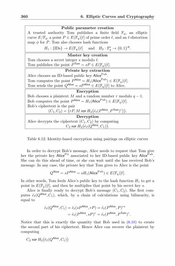
360 6. Elliptic Curves and Cryptography
Public parameter creationA trusted authority Tom publishes a finite field Fq, an ellipticcurve E/Fq, a point P ∈ E(Fq)[�] of prime order �, and an �-distortionmap φ for P . Tom also chooses hash functions
H1 : {IDs} → E(Fq)[�] and H2 : F∗q → {0, 1}B .
Master key creationTom chooses a secret integer s modulo �.Tom publishes the point PTom = sP ∈ E(Fq)[�].
Private key extraction
Alice chooses an ID-based public key AlicePub.
Tom computes the point PAlice = H1(AlicePub) ∈ E(Fq)[�].
Tom sends the point QAlice = sPAlice ∈ E(Fq)[�] to Alice.
EncryptionBob chooses a plaintext M and a random number r modulo q − 1.
Bob computes the point PAlice = H1(AlicePub) ∈ E(Fq)[�].
Bob’s ciphertext is the pair(C1, C2) =
(rP,M xorH2
(e�(P
Alice, PTom)r)).
DecryptionAlice decrypts the ciphertext (C1, C2) by computing
C2 xorH2
(e�(Q
Alice, C1)).
Table 6.12: Identity-based encryption using pairings on elliptic curves
In order to decrypt Bob’s message, Alice needs to request that Tom giveher the private key AlicePri associated to her ID-based public key AlicePub.She can do this ahead of time, or she can wait until she has received Bob’smessage. In any case, the private key that Tom gives to Alice is the point
QAlice = sPAlice = sH1(AlicePub) ∈ E(Fq)[�].
In other words, Tom feeds Alice’s public key to the hash function H1 to get apoint in E(Fq)[�], and then he multiplies that point by his secret key s.
Alice is finally ready to decrypt Bob’s message (C1, C2). She first com-putes e�(Q
Alice, C1), which, by a chain of calculations using bilinearity, isequal to
e�(QAlice, C1) = e�(sP
Alice, rP ) = e�(PAlice, P )rs
= e�(PAlice, sP )r = e�(P
Alice, PTom)r.
Notice that this is exactly the quantity that Bob used in (6.18) to createthe second part of his ciphertext. Hence Alice can recover the plaintext bycomputing
C2 xorH2
(e�(Q
Alice, C1))
Exercises 361
=(M xorH2
(e�(P
Alice, PTom)r))
xorH2
(e�(P
Alice, PTom)r)=M.
The last step follows becauseM xorN xorN =M for any bit stringsM and N .
The full process of ID-based encryption is summarized in Table 6.12.
Exercises
Section 6.1. Elliptic Curves
6.1. Let E be the elliptic curve E : Y 2 = X3 − 2X + 4 and let P = (0, 2) andQ = (3,−5). (You should check that P and Q are on the curve E.)(a) Compute P ⊕Q.
(b) Compute P ⊕ P and Q⊕Q.
(c) Compute P ⊕ P ⊕ P and Q⊕Q⊕Q.
6.2. Check that the points P = (−1, 4) and Q = (2, 5) are points on the ellipticcurve E : Y 2 = X3 + 17.(a) Compute the points P ⊕Q and P &Q.
(b) Compute the points 2P and 2Q.
(Bonus. How many points with integer coordinates can you find on E?)
6.3. Suppose that the cubic polynomial X3 +AX +B factors as
X3 +AX +B = (X − e1)(X − e2)(X − e3).
Prove that 4A3 + 27B2 = 0 if and only if two (or more) of e1, e2, and e3 are thesame. (Hint. Multiply out the right-hand side and compare coefficients to relate Aand B to e1, e2, and e3.)
6.4. Sketch each of the following curves, as was done in Fig. 6.1 on page 300.(a) E : Y 2 = X3 − 7X + 3.
(b) E : Y 2 = X3 − 7X + 9.
(c) E : Y 2 = X3 − 7X − 12.
(d) E : Y 2 = X3 − 3X + 2.
(e) E : Y 2 = X3.
Notice that the curves in (d) and (e) have ΔE = 0, so they are not elliptic curves.How do their pictures differ from the pictures in (a), (b), and (c)? Each of thecurves (d) and (e) has one point that is somewhat unusual. These unusual pointsare called singular points.
Section 6.2. Elliptic Curves over Finite Fields
6.5. For each of the following elliptic curves E and finite fields Fp, make a list ofthe set of points E(Fp).(a) E : Y 2 = X3 + 3X + 2 over F7.
(b) E : Y 2 = X3 + 2X + 7 over F11.
362 Exercises
(c) E : Y 2 = X3 + 4X + 5 over F11.
(d) E : Y 2 = X3 + 9X + 5 over F11.
(e) E : Y 2 = X3 + 9X + 5 over F13.
6.6. Make an addition table for E over Fp, as we did in Table 6.1.(a) E : Y 2 = X3 + X + 2 over F5.
(b) E : Y 2 = X3 + 2X + 3 over F7.
(c) E : Y 2 = X3 + 2X + 5 over F11.You may want to write a computer program for (c), since E(F11) has a lot of points!
6.7. Let E be the elliptic curve
E : y2 = x3 + x+ 1.
Compute the number of points in the group E(Fp) for each of the following primes:(a) p = 3. (b) p = 5. (c) p = 7. (d) p = 11.
In each case, also compute the trace of Frobenius
tp = p+ 1−#E(Fp)
and verify that |tp| is smaller than 2√p.
Section 6.3. The Elliptic Curve Discrete Logarithm Problem
6.8. Let E be the elliptic curve
E : y2 = x3 + x+ 1
and let P = (4, 2) and Q = (0, 1) be points on E modulo 5. Solve the elliptic curvediscrete logarithm problem for P and Q, that is, find a positive integer n such thatQ = nP .
6.9. Let E be an elliptic curve over Fp and let P and Q be points in E(Fp). Assumethat Q is a multiple of P and let n0 > 0 be the smallest solution to Q = nP . Alsolet s > 0 be the smallest solution to sP = O. Prove that every solution to Q = nPlooks like n0 + is for some i ∈ Z. (Hint. Write n as n = is + r for some 0 ≤ r < sand determine the value of r.)
6.10. Let {P1, P2} be a basis for E[m]. The Basis Problem for {P1, P2} is to expressan arbitrary point P ∈ E[m] as a linear combination of the basis vectors, i.e., tofind n1 and n2 so that P = n1P1 + n2P2. Prove that an algorithm that solves thebasis problem for {P1, P2} can be used to solve the ECDLP for points in E[m].
6.11. Use the double-and-add algorithm (Table 6.3) to compute nP in E(Fp) foreach of the following curves and points, as we did in Fig. 6.4.
(a) E : Y 2 = X3 + 23X + 13, p = 83, P = (24, 14), n = 19;
(b) E : Y 2 = X3 + 143X + 367, p = 613, P = (195, 9), n = 23;
(c) E : Y 2 = X3 + 1828X + 1675, p = 1999, P = (1756, 348), n = 11;
(d) E : Y 2 = X3 + 1541X + 1335, p = 3221, P = (2898, 439), n = 3211.
Exercises 363
6.12. Convert the proof of Proposition 6.18 into an algorithm and use it to writeeach of the following numbers n as a sum of positive and negative powers of 2 withat most 1
2�log n� + 1 nonzero terms. Compare the number of nonzero terms in the
binary expansion of n with the number of nonzero terms in the ternary expansionof n.(a) 349. (b) 9337. (c) 38728. (d) 8379483273489.
6.13. In Sect. 5.5 we gave an abstract description of Pollard’s ρ method, and inSect. 5.5.2 we gave an explicit version to solve the discrete logarithm problem in Fp.Adapt this material to create a Pollard ρ algorithm to solve the ECDLP.
Section 6.4. Elliptic Curve Cryptography
6.14. Alice and Bob agree to use elliptic Diffie–Hellman key exchange with theprime, elliptic curve, and point
p = 2671, E : Y 2 = X3 + 171X + 853, P = (1980, 431) ∈ E(F2671).
(a) Alice sends Bob the point QA = (2110, 543). Bob decides to use the secretmultiplier nB = 1943. What point should Bob send to Alice?
(b) What is their secret shared value?
(c) How difficult is it for Eve to figure out Alice’s secret multiplier nA? If you knowhow to program, use a computer to find nA.
(d) Alice and Bob decide to exchange a new piece of secret information using thesame prime, curve, and point. This time Alice sends Bob only the x-coordinatexA = 2 of her point QA. Bob decides to use the secret multiplier nB = 875.What single number modulo p should Bob send to Alice, and what is theirsecret shared value?
6.15. Exercise 2.10 on page 109 describes a multistep public key cryptosystem basedon the discrete logarithm problem for Fp. Describe a version of this cryptosystemthat uses the elliptic curve discrete logarithm problem. (You may assume that Aliceand Bob know the order of the point P in the group E(Fp), i.e., they know thesmallest integer N ≥ 1 with the property that NP = O.)
6.16. A shortcoming of using an elliptic curve E(Fp) for cryptography is the factthat it takes two coordinates to specify a point in E(Fp). However, as discussedbriefly at the end of Sect. 6.4.2, the second coordinate actually conveys very littleadditional information.(a) Suppose that Bob wants to send Alice the value of a point R ∈ E(Fp). Explain
why it suffices for Bob to send Alice the x-coordinate of R = (xR, yR) togetherwith the single bit
βR =
{0 if 0 ≤ yR < 1
2p,
1 if 12p < yR < p.
(You may assume that Alice is able to efficiently compute square roots mod-ulo p. This is certainly true, for example, if p ≡ 3 (mod 4); see Proposi-tion 2.26.)
(b) Alice and Bob decide to use the prime p = 1123 and the elliptic curve
E : Y 2 = X3 + 54X + 87.
364 Exercises
Bob sends Alice the x-coordinate x = 278 and the bit β = 0. What point is Bobtrying to convey to Alice? What about if instead Bob had sent β = 1?
6.17. The Menezes–Vanstone variant of the elliptic Elgamal public key cryptosystemimproves message expansion while avoiding the difficulty of directly attaching plain-texts to points in E(Fp). The MV-Elgamal cryptosystem is described in Table 6.13on page 365.(a) The last line of Table 6.13 claims that m′
1 = m1 and m′2 = m2. Prove that this
is true, so the decryption process does work.
(b) What is the message expansion of MV-Elgamal?
(c) Alice and Bob agree to use
p = 1201, E : Y 2 = X3 + 19X + 17, P = (278, 285) ∈ E(Fp),
for MV-Elgamal. Alice’s secret value is nA = 595. What is her public key?Bob sends Alice the encrypted message ((1147, 640), 279, 1189). What is theplaintext?
6.18. This exercise continues the discussion of the MV-Elgamal cryptosystem de-scribed in Table 6.13 on page 365.(a) Eve knows the elliptic curve E and the ciphertext values c1 and c2. Show how
Eve can use this knowledge to write down a polynomial equation (modulo p)that relates the two pieces m1 and m2 of the plaintext. In particular, if Evecan figure out one piece of the plaintext, then she can recover the other pieceby finding the roots of a certain polynomial modulo p.
(b) Alice and Bob exchange a message using MV-Elgamal with the prime, ellipticcurve, and point in Exercise 6.17(c). Eve intercepts the ciphertext
((269, 339), 814, 1050),
and through other sources she discovers that the first part of the plaintextis m1 = 1050. Use your algorithm in (a) to recover the second part of theplaintext.
6.19. Section 6.4.3 describes ECDSA, an elliptic analogue of DSA. Formulate anelliptic analogue of the simpler Elgamal digital signature algorithm described inTable 4.2 in Sect. 4.3.
6.20. This exercise asks you to compute some numerical instances of the ellipticcurve digital signature algorithm described in Table 6.7 for the public parameters
E : y2 = x3 + 231x+ 473, p = 17389, q = 1321, G = (11259, 11278) ∈ E(Fp).
You should begin by verifying that G is a point of order q in E(Fp).(a) Samantha’s private signing key is s = 542. What is her public verification
key? What is her digital signature on the document d = 644 using the randomelement e = 847?
(b) Tabitha’s public verification key is V = (11017, 14637). Is (s1, s2) = (907, 296)a valid signature on the document d = 993?
(c) Umberto’s public verification key is V = (14594, 308). Use any method thatyou want to find Umberto’s private signing key, and then use the private key toforge his signature on the document d = 516 using the random element e = 365.
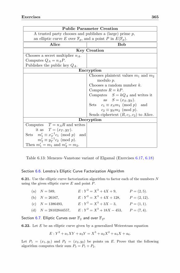
Exercises 365
Public Parameter CreationA trusted party chooses and publishes a (large) prime p,an elliptic curve E over Fp, and a point P in E(Fp).
Alice Bob
Key CreationChooses a secret multiplier nA.Computes QA = nAP .Publishes the public key QA.
EncryptionChooses plaintext values m1 and m2
modulo p.Chooses a random number k.Computes R = kP .Computes S = kQA and writes it
as S = (xS , yS).Sets c1 ≡ xSm1 (mod p) and
c2 ≡ ySm2 (mod p).Sends ciphertext (R, c1, c2) to Alice.
DecryptionComputes T = nAR and writes
it as T = (xT , yT ).Sets m′
1 ≡ x−1T c1 (mod p) and
m′2 ≡ y−1
T c2 (mod p).Then m′
1 = m1 and m′2 = m2.
Table 6.13: Menezes–Vanstone variant of Elgamal (Exercises 6.17, 6.18)
Section 6.6. Lenstra’s Elliptic Curve Factorization Algorithm
6.21. Use the elliptic curve factorization algorithm to factor each of the numbers Nusing the given elliptic curve E and point P .
(a) N = 589, E : Y 2 = X3 + 4X + 9, P = (2, 5).
(b) N = 26167, E : Y 2 = X3 + 4X + 128, P = (2, 12).
(c) N = 1386493, E : Y 2 = X3 + 3X − 3, P = (1, 1).
(d) N = 28102844557, E : Y 2 = X3 + 18X − 453, P = (7, 4).
Section 6.7. Elliptic Curves over F2 and over F2k
6.22. Let E be an elliptic curve given by a generalized Weierstrass equation
E : Y 2 + a1XY + a3Y = X3 + a2X2 + a4X + a6.
Let P1 = (x1, y1) and P2 = (x2, y2) be points on E. Prove that the followingalgorithm computes their sum P3 = P1 + P2.
366 Exercises
First, if x1 = x2 and y1 + y2 + a1x2 + a3 = 0, then P1 + P2 = O.
Otherwise define quantities λ and ν as follows:
[If x1 �= x2] λ =y2 − y1x2 − x1
, ν =y1x2 − y2x1x2 − x1
,
[If x1 = x2] λ =3x21 + 2a2x1 + a4 − a1y1
2y1 + a1x1 + a3, ν =
−x31 + a4x1 + 2a6 − a3y12y1 + a1x1 + a3
.
Then
P3 = P1 + P2 = (λ2 + a1λ− a2 − x1 − x2, −(λ+ a1)x3 − ν − a3).
6.23. Let F8 = F2[T ]/(T3 + T +1) be as in Example 6.28, and let E be the elliptic
curve
E : Y 2 +XY + Y = X3 + TX + (T + 1).
(a) Calculate the discriminant of E.
(b) Verify that the points
P = (1 + T + T 2, 1 + T ), Q = (T 2, T ), R = (1 + T + T 2, 1 + T 2),
are in E(F8) and compute the values of P +Q and 2R.
(c) Find all of the points in E(F8).
(d) Find a point P ∈ E(F8) such that every point in E(F8) is a multiple of P .
6.24. Let τ(α) = αp be the Frobenius map on Fpk .(a) Prove that
τ(α+β) = τ(α)+ τ(β) and τ(α ·β) = τ(α) · τ(β) for all α, β ∈ Fpk .
(Hint. For the addition formula, use the binomial theorem (Theorem 5.10).)
(b) Prove that τ(α) = α for all α ∈ Fp.
(c) Let E be an elliptic curve over Fp and let τ(x, y) = (xp, yp) be the Frobeniusmap from E(Fpk ) to itself. Prove that
τ(P +Q) = τ(P ) + τ(Q) for all P ∈ E(Fpk ).
6.25. Let E0 be the Koblitz curve Y 2 + XY = X3 + 1 over the field F2, and forevery k ≥ 1, let
tk = 2k + 1−#E(F2k ).
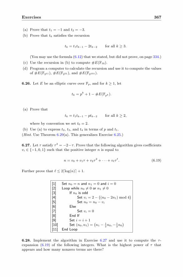
Exercises 367
(a) Prove that t1 = −1 and t2 = −3.
(b) Prove that tk satisfies the recursion
tk = t1tk−1 − 2tk−2 for all k ≥ 3.
(You may use the formula (6.12) that we stated, but did not prove, on page 334.)
(c) Use the recursion in (b) to compute #E(F16).
(d) Program a computer to calculate the recursion and use it to compute the valuesof #E(F211), #E(F231), and #E(F2101).
6.26. Let E be an elliptic curve over Fp, and for k ≥ 1, let
tk = pk + 1−#E(Fpk ).
(a) Prove that
tk = t1tk−1 − ptk−2 for all k ≥ 2,
where by convention we set t0 = 2.
(b) Use (a) to express t2, t3, and t4 in terms of p and t1.
(Hint. Use Theorem 6.29(a). This generalizes Exercise 6.25.)
6.27. Let τ satisfy τ2 = −2−τ . Prove that the following algorithm gives coefficientsvi ∈ {−1, 0, 1} such that the positive integer n is equal to
n = v0 + v1τ + v2τ2 + · · ·+ v�τ
�. (6.19)
Further prove that � ≤ 2'log(n)(+ 1.
[1] Set n0 = n and n1 = 0 and i = 0[2] Loop while n0 �= 0 or n1 �= 0[3] If n0 is odd[4] Set vi = 2−
((n0 − 2n1) mod 4
)
[5] Set n0 = n0 − vi[6] Else[7] Set vi = 0[8] End If[9] Set i = i+ 1[10] Set (n0, n1) =
(n1 − 1
2n0,− 1
2n0
)
[11] End Loop
6.28. Implement the algorithm in Exercise 6.27 and use it to compute the τ -expansion (6.19) of the following integers. What is the highest power of τ thatappears and how many nonzero terms are there?
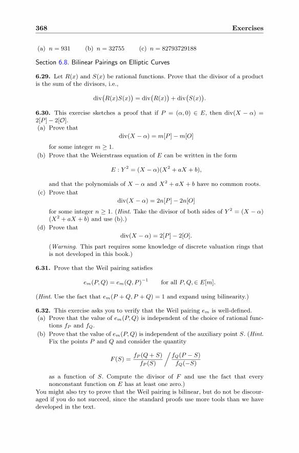
368 Exercises
(a) n = 931 (b) n = 32755 (c) n = 82793729188
Section 6.8. Bilinear Pairings on Elliptic Curves
6.29. Let R(x) and S(x) be rational functions. Prove that the divisor of a productis the sum of the divisors, i.e.,
div(R(x)S(x)
)= div
(R(x)
)+ div
(S(x)
).
6.30. This exercise sketches a proof that if P = (α, 0) ∈ E, then div(X − α) =2[P ]− 2[O].(a) Prove that
div(X − α) = m[P ]−m[O]
for some integer m ≥ 1.
(b) Prove that the Weierstrass equation of E can be written in the form
E : Y 2 = (X − α)(X2 + aX + b),
and that the polynomials of X − α and X2 + aX + b have no common roots.
(c) Prove that
div(X − α) = 2n[P ]− 2n[O]
for some integer n ≥ 1. (Hint. Take the divisor of both sides of Y 2 = (X − α)(X2 + aX + b) and use (b).)
(d) Prove that
div(X − α) = 2[P ]− 2[O].
(Warning. This part requires some knowledge of discrete valuation rings thatis not developed in this book.)
6.31. Prove that the Weil pairing satisfies
em(P,Q) = em(Q,P )−1 for all P,Q,∈ E[m].
(Hint. Use the fact that em(P +Q,P +Q) = 1 and expand using bilinearity.)
6.32. This exercise asks you to verify that the Weil pairing em is well-defined.(a) Prove that the value of em(P,Q) is independent of the choice of rational func-
tions fP and fQ.
(b) Prove that the value of em(P,Q) is independent of the auxiliary point S. (Hint.Fix the points P and Q and consider the quantity
F (S) =fP (Q+ S)
fP (S)
/fQ(P − S)
fQ(−S)
as a function of S. Compute the divisor of F and use the fact that everynonconstant function on E has at least one zero.)
You might also try to prove that the Weil pairing is bilinear, but do not be discour-aged if you do not succeed, since the standard proofs use more tools than we havedeveloped in the text.
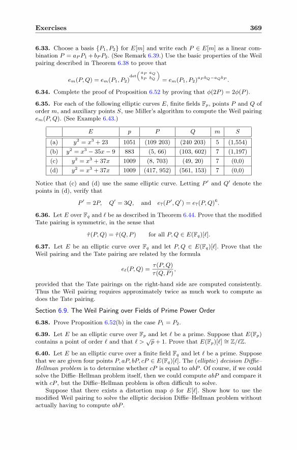
Exercises 369
6.33. Choose a basis {P1, P2} for E[m] and write each P ∈ E[m] as a linear com-bination P = aPP1 + bPP2. (See Remark 6.39.) Use the basic properties of the Weilpairing described in Theorem 6.38 to prove that
em(P,Q) = em(P1, P2)det
(aP aQ
bP bQ
)
= em(P1, P2)aP bQ−aQbP .
6.34. Complete the proof of Proposition 6.52 by proving that φ(2P ) = 2φ(P ).
6.35. For each of the following elliptic curves E, finite fields Fp, points P and Q oforder m, and auxiliary points S, use Miller’s algorithm to compute the Weil pairingem(P,Q). (See Example 6.43.)
E p P Q m S
(a) y2 = x3 + 23 1051 (109 203) (240 203) 5 (1,554)
(b) y2 = x3 − 35x− 9 883 (5, 66) (103, 602) 7 (1,197)
(c) y2 = x3 + 37x 1009 (8, 703) (49, 20) 7 (0,0)
(d) y2 = x3 + 37x 1009 (417, 952) (561, 153) 7 (0,0)
Notice that (c) and (d) use the same elliptic curve. Letting P ′ and Q′ denote thepoints in (d), verify that
P ′ = 2P, Q′ = 3Q, and e7(P′, Q′) = e7(P,Q)6.
6.36. Let E over Fq and � be as described in Theorem 6.44. Prove that the modifiedTate pairing is symmetric, in the sense that
τ(P,Q) = τ(Q,P ) for all P,Q ∈ E(Fq)[�].
6.37. Let E be an elliptic curve over Fq and let P,Q ∈ E(Fq)[�]. Prove that theWeil pairing and the Tate pairing are related by the formula
e�(P,Q) =τ(P,Q)
τ(Q,P ),
provided that the Tate pairings on the right-hand side are computed consistently.Thus the Weil pairing requires approximately twice as much work to compute asdoes the Tate pairing.
Section 6.9. The Weil Pairing over Fields of Prime Power Order
6.38. Prove Proposition 6.52(b) in the case P1 = P2.
6.39. Let E be an elliptic curve over Fp and let � be a prime. Suppose that E(Fp)contains a point of order � and that � >
√p+ 1. Prove that E(Fp)[�] ∼= Z/�Z.
6.40. Let E be an elliptic curve over a finite field Fq and let � be a prime. Supposethat we are given four points P, aP, bP, cP ∈ E(Fq)[�]. The (elliptic) decision Diffie–Hellman problem is to determine whether cP is equal to abP . Of course, if we couldsolve the Diffie–Hellman problem itself, then we could compute abP and compare itwith cP , but the Diffie–Hellman problem is often difficult to solve.
Suppose that there exists a distortion map φ for E[�]. Show how to use themodified Weil pairing to solve the elliptic decision Diffie–Hellman problem withoutactually having to compute abP .
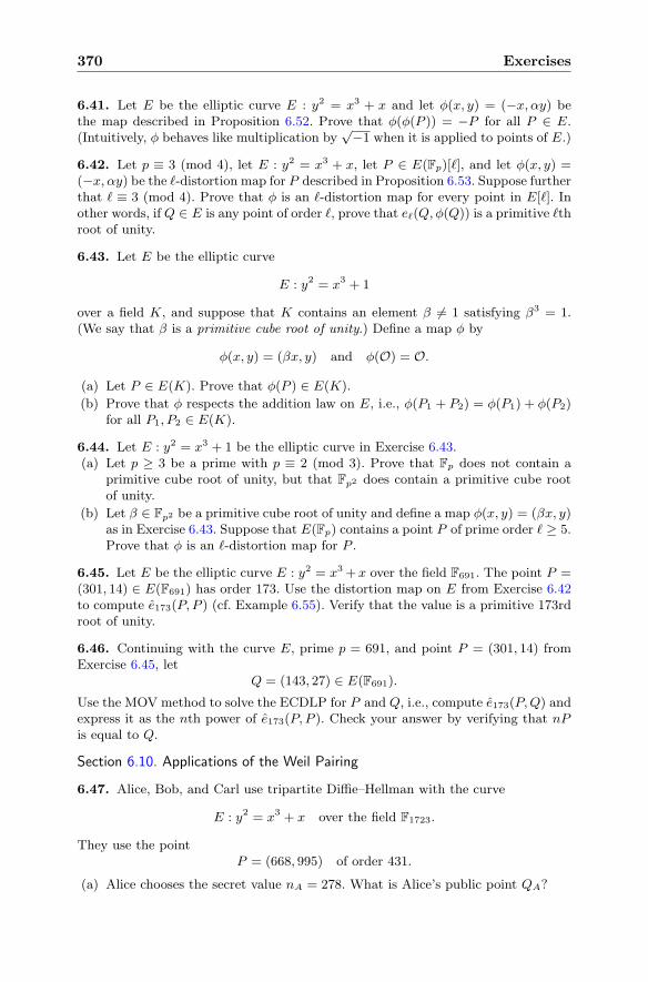
370 Exercises
6.41. Let E be the elliptic curve E : y2 = x3 + x and let φ(x, y) = (−x, αy) bethe map described in Proposition 6.52. Prove that φ(φ(P )) = −P for all P ∈ E.(Intuitively, φ behaves like multiplication by
√−1 when it is applied to points of E.)
6.42. Let p ≡ 3 (mod 4), let E : y2 = x3 + x, let P ∈ E(Fp)[�], and let φ(x, y) =(−x, αy) be the �-distortion map for P described in Proposition 6.53. Suppose furtherthat � ≡ 3 (mod 4). Prove that φ is an �-distortion map for every point in E[�]. Inother words, if Q ∈ E is any point of order �, prove that e�(Q,φ(Q)) is a primitive �throot of unity.
6.43. Let E be the elliptic curve
E : y2 = x3 + 1
over a field K, and suppose that K contains an element β �= 1 satisfying β3 = 1.(We say that β is a primitive cube root of unity.) Define a map φ by
φ(x, y) = (βx, y) and φ(O) = O.
(a) Let P ∈ E(K). Prove that φ(P ) ∈ E(K).
(b) Prove that φ respects the addition law on E, i.e., φ(P1 + P2) = φ(P1) + φ(P2)for all P1, P2 ∈ E(K).
6.44. Let E : y2 = x3 + 1 be the elliptic curve in Exercise 6.43.(a) Let p ≥ 3 be a prime with p ≡ 2 (mod 3). Prove that Fp does not contain a
primitive cube root of unity, but that Fp2 does contain a primitive cube rootof unity.
(b) Let β ∈ Fp2 be a primitive cube root of unity and define a map φ(x, y) = (βx, y)as in Exercise 6.43. Suppose that E(Fp) contains a point P of prime order � ≥ 5.Prove that φ is an �-distortion map for P .
6.45. Let E be the elliptic curve E : y2 = x3 +x over the field F691. The point P =(301, 14) ∈ E(F691) has order 173. Use the distortion map on E from Exercise 6.42to compute e173(P, P ) (cf. Example 6.55). Verify that the value is a primitive 173rdroot of unity.
6.46. Continuing with the curve E, prime p = 691, and point P = (301, 14) fromExercise 6.45, let
Q = (143, 27) ∈ E(F691).
Use the MOV method to solve the ECDLP for P and Q, i.e., compute e173(P,Q) andexpress it as the nth power of e173(P, P ). Check your answer by verifying that nPis equal to Q.
Section 6.10. Applications of the Weil Pairing
6.47. Alice, Bob, and Carl use tripartite Diffie–Hellman with the curve
E : y2 = x3 + x over the field F1723.
They use the pointP = (668, 995) of order 431.
(a) Alice chooses the secret value nA = 278. What is Alice’s public point QA?
Exercises 371
(b) Bob’s public point is QB = (1275, 1550) and Carl’s public point is QC =(897, 1323). What is the value of e431(QB , QC)?
(c) What is their shared value?
(d) Bob’s secret value is nB = 224. Verify that e431(QA, QC)nB is the same as the
value that you got in (c).
(e) Figure out Carl’s secret value nC . (Since P has order 431, you can do this ona computer by trying all possible values.)
6.48. Show that Eve can break tripartite Diffie–Hellman key exchange as describedin Table 6.10.1 if she knows how to solve the Diffie–Hellman problem (page 69) forthe field Fq.
6.49. In this exercise we consider what is required to break the identity-basedencryption scheme described in Table 6.12 on page 360.(a) Show that if Eve can solve the discrete logarithm problem in either E(Fq) or
in F∗q , then she can recover Tom’s secret key s, which means that she can do
anything that Tom can do, including decrypting everyone’s ciphtertexts.
(b) Suppose that Eve only knows how to solve the elliptic curve Diffie–Hellmanproblem in E(Fq), as described on page 318. Show that she can decrypt allciphertexts.
(c) What if Eve only knows how to solve the Diffie–Hellman problem in F∗q . Can
she still decrypt all ciphertexts?
Chapter 7
Lattices and Cryptography
The security of all of the public key cryptosystems that we have previouslystudied has been based, either directly or indirectly, on either the difficultyof factoring large numbers or the difficulty of finding discrete logarithms in afinite group. In this chapter we investigate a new type of hard problem arisingin the theory of lattices that can be used as the basis for a public key cryp-tosystem. Lattice-based cryptosystems offer several potential advantages overearlier systems, including faster encryption/decryption and so-called quantumresistance. The latter means that at present there are no known quantum al-gorithms to rapidly solve hard lattice problems; see Sect. 8.11. Further, wewill see that the theory of lattices has applications in cryptography beyondsimply providing a new source of hard problems.
Recall that a vector space V over the real numbers R is a set of vectors,where two vectors can be added together and a vector can be multiplied by areal number. A lattice is similar to a vector space, except that we are restrictedto multiplying the vectors in a lattice by integers. This seemingly minor re-striction leads to many interesting and subtle questions. Since the subject oflattices can appear somewhat abstruse and removed from the everyday re-ality of cryptography, we begin this chapter with two motivating examplesin which lattices are not mentioned, but where they are lurking in the back-ground, waiting to be used for cryptanalysis. We then review the theory ofvector spaces in Sect. 7.3 and formally introduce lattices in Sect. 7.4.
7.1 A Congruential Public Key Cryptosystem
In this section we describe a toy model of a real public key cryptosystem. Thisversion turns out to have an unexpected connection with lattices of dimen-sion 2, and hence a fatal vulnerability, since the dimension is so low. However,
© Springer Science+Business Media New York 2014J. Hoffstein et al., An Introduction to Mathematical Cryptography,Undergraduate Texts in Mathematics, DOI 10.1007/978-1-4939-1711-2 7
373
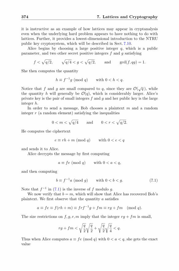
374 7. Lattices and Cryptography
it is instructive as an example of how lattices may appear in cryptanalysiseven when the underlying hard problem appears to have nothing to do withlattices. Further, it provides a lowest-dimensional introduction to the NTRUpublic key cryptosystem, which will be described in Sect. 7.10.
Alice begins by choosing a large positive integer q, which is a publicparameter, and two other secret positive integers f and g satisfying
f <√q/2,
√q/4 < g <
√q/2, and gcd(f, qg) = 1.
She then computes the quantity
h ≡ f−1g (mod q) with 0 < h < q.
Notice that f and g are small compared to q, since they are O(√q ), while
the quantity h will generally be O(q), which is considerably larger. Alice’sprivate key is the pair of small integers f and g and her public key is the largeinteger h.
In order to send a message, Bob chooses a plaintext m and a randominteger r (a random element) satisfying the inequalities
0 < m <√q/4 and 0 < r <
√q/2.
He computes the ciphertext
e ≡ rh+m (mod q) with 0 < e < q
and sends it to Alice.Alice decrypts the message by first computing
a ≡ fe (mod q) with 0 < a < q,
and then computing
b ≡ f−1a (mod g) with 0 < b < g. (7.1)
Note that f−1 in (7.1) is the inverse of f modulo g.We now verify that b = m, which will show that Alice has recovered Bob’s
plaintext. We first observe that the quantity a satisfies
a ≡ fe ≡ f(rh+m) ≡ frf−1g + fm ≡ rg + fm (mod q).
The size restrictions on f, g, r,m imply that the integer rg + fm is small,
rg + fm <
√q
2
√q
2+
√q
2
√q
4< q.
Thus when Alice computes a ≡ fe (mod q) with 0 < a < q, she gets the exactvalue
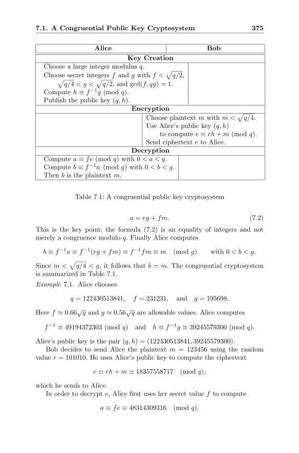
7.1. A Congruential Public Key Cryptosystem 375
Alice Bob
Key CreationChoose a large integer modulus q.
Choose secret integers f and g with f <√q/2,√
q/4 < g <√q/2, and gcd(f, qg) = 1.
Compute h ≡ f−1g (mod q).Publish the public key (q, h).
Encryption
Choose plaintext m with m <√q/4.
Use Alice’s public key (q, h)to compute e ≡ rh+m (mod q).
Send ciphertext e to Alice.Decryption
Compute a ≡ fe (mod q) with 0 < a < q.Compute b ≡ f−1a (mod g) with 0 < b < g.Then b is the plaintext m.
Table 7.1: A congruential public key cryptosystem
a = rg + fm. (7.2)
This is the key point: the formula (7.2) is an equality of integers and notmerely a congruence modulo q. Finally Alice computes
b ≡ f−1a ≡ f−1(rg + fm) ≡ f−1fm ≡ m (mod g) with 0 < b < g.
Since m <√q/4 < g, it follows that b = m. The congruential cryptosystem
is summarized in Table 7.1.
Example 7.1. Alice chooses
q = 122430513841, f = 231231, and g = 195698.
Here f ≈ 0.66√q and g ≈ 0.56
√q are allowable values. Alice computes
f−1 ≡ 49194372303 (mod q) and h ≡ f−1g ≡ 39245579300 (mod q).
Alice’s public key is the pair (q, h) = (122430513841, 39245579300).Bob decides to send Alice the plaintext m = 123456 using the random
value r = 101010. He uses Alice’s public key to compute the ciphertext
e ≡ rh+m ≡ 18357558717 (mod q),
which he sends to Alice.In order to decrypt e, Alice first uses her secret value f to compute
a ≡ fe ≡ 48314309316 (mod q).
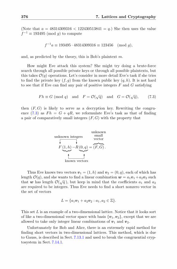
376 7. Lattices and Cryptography
(Note that a = 48314309316 < 122430513841 = q.) She then uses the valuef−1 ≡ 193495 (mod g) to compute
f−1a ≡ 193495 · 48314309316 ≡ 123456 (mod g),
and, as predicted by the theory, this is Bob’s plaintext m.
How might Eve attack this system? She might try doing a brute-forcesearch through all possible private keys or through all possible plaintexts, butthis takes O(q) operations. Let’s consider in more detail Eve’s task if she triesto find the private key (f, g) from the known public key (q, h). It is not hardto see that if Eve can find any pair of positive integers F and G satisfying
Fh ≡ G (mod q) and F = O(√q) and G = O(
√q), (7.3)
then (F,G) is likely to serve as a decryption key. Rewriting the congru-ence (7.3) as Fh = G + qR, we reformulate Eve’s task as that of findinga pair of comparatively small integers (F,G) with the property that
F (1, h)︸ ︷︷ ︸
−R (0, q)︸ ︷︷ ︸
=︷ ︸︸ ︷(F,G) .
known vectors
unknown integers
unknownsmallvector
Thus Eve knows two vectors v1 = (1, h) and v2 = (0, q), each of which haslength O(q), and she wants to find a linear combination w = a1v1+a2v2 suchthat w has length O(
√q ), but keep in mind that the coefficients a1 and a2
are required to be integers. Thus Eve needs to find a short nonzero vector inthe set of vectors
L = {a1v1 + a2v2 : a1, a2 ∈ Z}.
This set L is an example of a two-dimensional lattice. Notice that it looks sortof like a two-dimensional vector space with basis {v1,v2}, except that we areallowed to take only integer linear combinations of v1 and v2.
Unfortunately for Bob and Alice, there is an extremely rapid method forfinding short vectors in two-dimensional lattices. This method, which is dueto Gauss, is described in Sect. 7.13.1 and used to break the congruential cryp-tosystem in Sect. 7.14.1.
7.2. Subset-Sum Problems and Knapsack Cryptosystems 377
7.2 Subset-Sum Problems and KnapsackCryptosystems
The first attempt to base a cryptosystem on an NP-complete problem1 wasmade by Merkle and Hellman in the late 1970s [84]. They used a version ofthe following mathematical problem, which generalizes the classical knapsackproblem.
The Subset-Sum ProblemSuppose that you are given a list of positive integers(M1,M2, . . . ,Mn) and another integer S. Find a subset ofthe elements in the list whose sum is S. (You may assumethat there is at least one such subset.)
Example 7.2. Let M = (2, 3, 4, 9, 14, 23) and S = 21. Then a bit of trial anderror yields the subset {3, 4, 14} whose sum is 21, and it is not hard to checkthat this is the only subset that sums to 21. Similarly, if we take S = 29, thenwe find that {2, 4, 23} has the desired sum. But in this case there is a secondsolution, since {2, 4, 9, 14} also sums to 29.
Here is another way to describe the subset-sum problem. The list
M = (M1,M2, . . . ,Mn)
of positive integers is public knowledge. Bob chooses a secret binary vectorx = (x1, x2, . . . , xn), i.e., each xi may be either 0 or 1. Bob computes the sum
S =
n∑
i=1
xiMi
and sends S to Alice. The subset-sum problem asks Alice to find either theoriginal vector x or another binary vector giving the same sum. Notice thatthe vector x tells Alice which Mi to include in S, since Mi is in the sum Sif and only if xi = 1. Thus specifying the binary vector x is the same asspecifying a subset of M .
It is clear that Alice can find x by checking all 2n binary vectors of length n.A simple collision algorithm allows Alice to cut the exponent in half.
Proposition 7.3. Let M = (M1,M2, . . . ,Mn) and let (M , S) be a subset-sum problem. For all sets of integers I and J satisfying
I ⊂ {i : 1 ≤ i ≤ 12n} and J ⊂ {j : 1
2n < j ≤ n},
compute and make a list of the values
1NP-complete problems are discussed in Sect. 5.7. However, if you have not read thatsection, suffice it to say that NP-complete problems are considered to be very hard to solvein a computational sense.
378 7. Lattices and Cryptography
AI =∑
i∈I
Mi and BJ = S −∑
j∈J
Mj .
Then these lists include a pair of sets I0 and J0 satisfying AI0 = BJ0 , andthe sets I0 and J0 give a solution to the subset-sum problem,
S =∑
i∈I0
Mi +∑
j∈J0
Mj .
The number of entries in each list is at most 2n/2, so the running time of thealgorithm is O(2n/2+ε), where ε is some small value that accounts for sortingand comparing the lists.
Proof. It suffices to note that if x is a binary vector giving a solution to thegiven subset-sum problem, then we can write the solution as
∑
1≤i≤ 12n
xiMi = S −∑
12n<i≤n
xiMi.
The number of subsets I and J is O(2n/2), since they are subsets of sets oforder n/2.
If n is large, then in general it is difficult to solve a random instance ofa subset-sum problem. Suppose, however, that Alice possesses some secretknowledge or trapdoor information about M that enables her to guaranteethat the solution x is unique and that allows her to easily find x. Then Alicecan use the subset sum problem as a public key cryptosystem. Bob’s plaintextis the vector x, his encrypted message is the sum S =
∑xiMi, and only Alice
can easily recover x from knowledge of S.But what sort of sneaky trick can Alice use to ensure that she can solve
this particular subset-sum problem, but that nobody else can? One possibilityis to use a subset-sum problem that is extremely easy to solve, but somehowto disguise the easy solution from other people.
Definition. A superincreasing sequence of integers is a list of positive integersr = (r1, r2, . . . , rn) with the property that
ri+1 ≥ 2ri for all 1 ≤ i ≤ n− 1.
The following estimate explains the name of such sequences.
Lemma 7.4. Let r = (r1, r2, . . . , rn) be a superincreasing sequence. Then
rk > rk−1 + · · ·+ r2 + r1 for all 2 ≤ k ≤ n.
Proof. We give a proof by induction on k. For k = 2 we have r2 ≥ 2r1 > r1,which gets the induction started. Now suppose that the lemma is true for
7.2. Subset-Sum Problems and Knapsack Cryptosystems 379
some 2 ≤ k < n. Then first using the superincreasing property and next theinduction hypothesis, we find that
rk+1 ≥ 2rk = rk + rk > rk + (rk−1 + · · ·+ r2 + r1).
This shows that the lemma is also true for k + 1.
A subset-sum problem in which the integers in M form a superincreasingsequence is very easy to solve.
Proposition 7.5. Let (M , S) be a subset-sum problem in which the integersin M form a superincreasing sequence. Assuming that a solution x exists, itis unique and may be computed by the following fast algorithm:
Loop i from n down to 1
If S ≥Mi, set xi = 1 and subtract Mi from S
Else set xi = 0
End Loop
Proof. The assumption that M is a superincreasing sequence means thatMi+1 ≥ 2Mi. We are given that a solution exists, so to distinguish it from thevector x produced by the algorithm, we call the actual solution y. Thus weare assuming that y ·M = S and we need to show that x = y.
We prove by downward induction that xk = yk for all 1 ≤ k ≤ n. Ourinductive hypothesis is that xi = yi for all k < i ≤ n and we need to provethat xk = yk. (Note that we allow k = n, in which case our inductive hypoth-esis is vacuously true.) The hypothesis means that when we performed thealgorithm from i = n down to i = k + 1, we had xi = yi at each stage. Sobefore executing the loop with i = k, the value of S has been reduced to
Sk = S −n∑
i=k+1
xiMi =
n∑
i=1
yiMi −n∑
i=k+1
xiMi =
k∑
i=1
yiMi.
Now consider what happens when we execute the loop with i = k. There aretwo possibilities:
(1) yk = 1 =⇒ Sk ≥Mk =⇒ xk = 1, �(2) yk = 0 =⇒ Sk ≤Mk−1 + · · ·+M1 < Mk =⇒ xk = 0. �
(Note that in Case (2) we have used Lemma 7.4 to deduce thatMk−1+· · ·+M1
is strictly smaller than Mk.) In both cases we get xk = yk, which completesthe proof that x = y. Further, it shows that the solution is unique, since wehave shown that any solution agrees with the output of the algorithm, whichby its nature returns a unique vector x for any given input S.
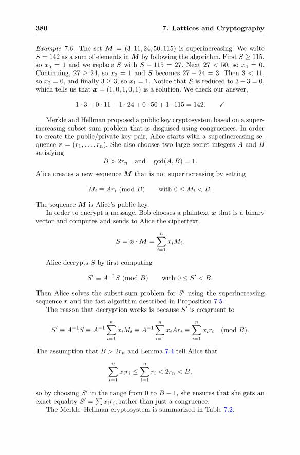
380 7. Lattices and Cryptography
Example 7.6. The set M = (3, 11, 24, 50, 115) is superincreasing. We writeS = 142 as a sum of elements in M by following the algorithm. First S ≥ 115,so x5 = 1 and we replace S with S − 115 = 27. Next 27 < 50, so x4 = 0.Continuing, 27 ≥ 24, so x3 = 1 and S becomes 27 − 24 = 3. Then 3 < 11,so x2 = 0, and finally 3 ≥ 3, so x1 = 1. Notice that S is reduced to 3− 3 = 0,which tells us that x = (1, 0, 1, 0, 1) is a solution. We check our answer,
1 · 3 + 0 · 11 + 1 · 24 + 0 · 50 + 1 · 115 = 142. �
Merkle and Hellman proposed a public key cryptosystem based on a super-increasing subset-sum problem that is disguised using congruences. In orderto create the public/private key pair, Alice starts with a superincreasing se-quence r = (r1, . . . , rn). She also chooses two large secret integers A and Bsatisfying
B > 2rn and gcd(A,B) = 1.
Alice creates a new sequence M that is not superincreasing by setting
Mi ≡ Ari (mod B) with 0 ≤Mi < B.
The sequence M is Alice’s public key.In order to encrypt a message, Bob chooses a plaintext x that is a binary
vector and computes and sends to Alice the ciphertext
S = x ·M =
n∑
i=1
xiMi.
Alice decrypts S by first computing
S′ ≡ A−1S (mod B) with 0 ≤ S′ < B.
Then Alice solves the subset-sum problem for S′ using the superincreasingsequence r and the fast algorithm described in Proposition 7.5.
The reason that decryption works is because S′ is congruent to
S′ ≡ A−1S ≡ A−1n∑
i=1
xiMi ≡ A−1n∑
i=1
xiAri ≡n∑
i=1
xiri (mod B).
The assumption that B > 2rn and Lemma 7.4 tell Alice that
n∑
i=1
xiri ≤n∑
i=1
ri < 2rn < B,
so by choosing S′ in the range from 0 to B − 1, she ensures that she gets anexact equality S′ =
∑xiri, rather than just a congruence.
The Merkle–Hellman cryptosystem is summarized in Table 7.2.
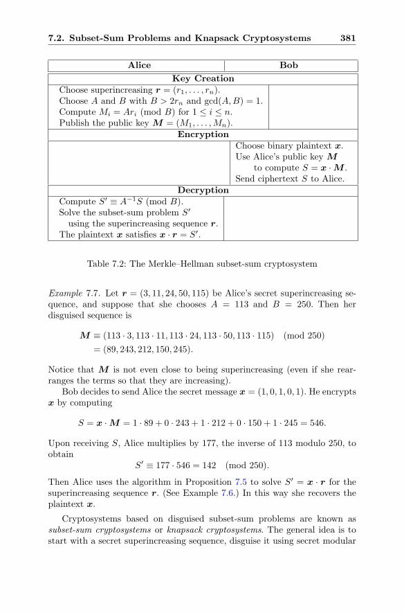
7.2. Subset-Sum Problems and Knapsack Cryptosystems 381
Alice Bob
Key CreationChoose superincreasing r = (r1, . . . , rn).Choose A and B with B > 2rn and gcd(A,B) = 1.Compute Mi = Ari (mod B) for 1 ≤ i ≤ n.Publish the public key M = (M1, . . . ,Mn).
EncryptionChoose binary plaintext x.Use Alice’s public key M
to compute S = x ·M .Send ciphertext S to Alice.
DecryptionCompute S′ ≡ A−1S (mod B).Solve the subset-sum problem S′
using the superincreasing sequence r.The plaintext x satisfies x · r = S′.
Table 7.2: The Merkle–Hellman subset-sum cryptosystem
Example 7.7. Let r = (3, 11, 24, 50, 115) be Alice’s secret superincreasing se-quence, and suppose that she chooses A = 113 and B = 250. Then herdisguised sequence is
M ≡ (113 · 3, 113 · 11, 113 · 24, 113 · 50, 113 · 115) (mod 250)
= (89, 243, 212, 150, 245).
Notice that M is not even close to being superincreasing (even if she rear-ranges the terms so that they are increasing).
Bob decides to send Alice the secret message x = (1, 0, 1, 0, 1). He encryptsx by computing
S = x ·M = 1 · 89 + 0 · 243 + 1 · 212 + 0 · 150 + 1 · 245 = 546.
Upon receiving S, Alice multiplies by 177, the inverse of 113 modulo 250, toobtain
S′ ≡ 177 · 546 = 142 (mod 250).
Then Alice uses the algorithm in Proposition 7.5 to solve S′ = x · r for thesuperincreasing sequence r. (See Example 7.6.) In this way she recovers theplaintext x.
Cryptosystems based on disguised subset-sum problems are known assubset-sum cryptosystems or knapsack cryptosystems. The general idea is tostart with a secret superincreasing sequence, disguise it using secret modular
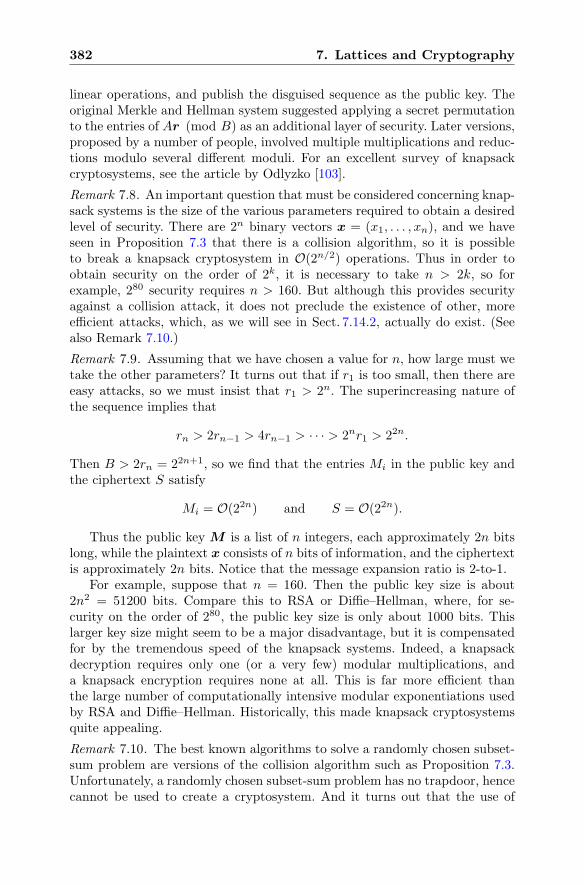
382 7. Lattices and Cryptography
linear operations, and publish the disguised sequence as the public key. Theoriginal Merkle and Hellman system suggested applying a secret permutationto the entries of Ar (mod B) as an additional layer of security. Later versions,proposed by a number of people, involved multiple multiplications and reduc-tions modulo several different moduli. For an excellent survey of knapsackcryptosystems, see the article by Odlyzko [103].
Remark 7.8. An important question that must be considered concerning knap-sack systems is the size of the various parameters required to obtain a desiredlevel of security. There are 2n binary vectors x = (x1, . . . , xn), and we haveseen in Proposition 7.3 that there is a collision algorithm, so it is possibleto break a knapsack cryptosystem in O(2n/2) operations. Thus in order toobtain security on the order of 2k, it is necessary to take n > 2k, so forexample, 280 security requires n > 160. But although this provides securityagainst a collision attack, it does not preclude the existence of other, moreefficient attacks, which, as we will see in Sect. 7.14.2, actually do exist. (Seealso Remark 7.10.)
Remark 7.9. Assuming that we have chosen a value for n, how large must wetake the other parameters? It turns out that if r1 is too small, then there areeasy attacks, so we must insist that r1 > 2n. The superincreasing nature ofthe sequence implies that
rn > 2rn−1 > 4rn−1 > · · · > 2nr1 > 22n.
Then B > 2rn = 22n+1, so we find that the entries Mi in the public key andthe ciphertext S satisfy
Mi = O(22n) and S = O(22n).
Thus the public key M is a list of n integers, each approximately 2n bitslong, while the plaintext x consists of n bits of information, and the ciphertextis approximately 2n bits. Notice that the message expansion ratio is 2-to-1.
For example, suppose that n = 160. Then the public key size is about2n2 = 51200 bits. Compare this to RSA or Diffie–Hellman, where, for se-curity on the order of 280, the public key size is only about 1000 bits. Thislarger key size might seem to be a major disadvantage, but it is compensatedfor by the tremendous speed of the knapsack systems. Indeed, a knapsackdecryption requires only one (or a very few) modular multiplications, anda knapsack encryption requires none at all. This is far more efficient thanthe large number of computationally intensive modular exponentiations usedby RSA and Diffie–Hellman. Historically, this made knapsack cryptosystemsquite appealing.
Remark 7.10. The best known algorithms to solve a randomly chosen subset-sum problem are versions of the collision algorithm such as Proposition 7.3.Unfortunately, a randomly chosen subset-sum problem has no trapdoor, hencecannot be used to create a cryptosystem. And it turns out that the use of
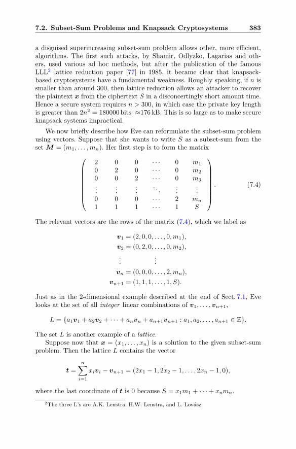
7.2. Subset-Sum Problems and Knapsack Cryptosystems 383
a disguised superincreasing subset-sum problem allows other, more efficient,algorithms. The first such attacks, by Shamir, Odlyzko, Lagarias and oth-ers, used various ad hoc methods, but after the publication of the famousLLL2 lattice reduction paper [77] in 1985, it became clear that knapsack-based cryptosystems have a fundamental weakness. Roughly speaking, if n issmaller than around 300, then lattice reduction allows an attacker to recoverthe plaintext x from the ciphertext S in a disconcertingly short amount time.Hence a secure system requires n > 300, in which case the private key lengthis greater than 2n2 = 180000 bits ≈176 kB. This is so large as to make secureknapsack systems impractical.
We now briefly describe how Eve can reformulate the subset-sum problemusing vectors. Suppose that she wants to write S as a subset-sum from theset M = (m1, . . . ,mn). Her first step is to form the matrix
⎛
⎜⎜⎜⎜⎜⎜⎜⎝
2 0 0 · · · 0 m1
0 2 0 · · · 0 m2
0 0 2 · · · 0 m3
......
.... . .
......
0 0 0 · · · 2 mn
1 1 1 · · · 1 S
⎞
⎟⎟⎟⎟⎟⎟⎟⎠
. (7.4)
The relevant vectors are the rows of the matrix (7.4), which we label as
v1 = (2, 0, 0, . . . , 0,m1),
v2 = (0, 2, 0, . . . , 0,m2),
......
vn = (0, 0, 0, . . . , 2,mn),
vn+1 = (1, 1, 1, . . . , 1, S).
Just as in the 2-dimensional example described at the end of Sect. 7.1, Evelooks at the set of all integer linear combinations of v1, . . . ,vn+1,
L = {a1v1 + a2v2 + · · ·+ anvn + an+1vn+1 : a1, a2, . . . , an+1 ∈ Z}.
The set L is another example of a lattice.Suppose now that x = (x1, . . . , xn) is a solution to the given subset-sum
problem. Then the lattice L contains the vector
t =
n∑
i=1
xivi − vn+1 = (2x1 − 1, 2x2 − 1, . . . , 2xn − 1, 0),
where the last coordinate of t is 0 because S = x1m1 + · · ·+ xnmn.
2The three L’s are A.K. Lenstra, H.W. Lenstra, and L. Lovasz.
384 7. Lattices and Cryptography
We now come to the crux of the matter. Since the xi are all 0 or 1, all ofthe 2xi − 1 values are ±1, so the vector t is quite short, ‖t‖ =
√n. On
the other hand, we have seen that mi = O(22n) and S = O(22n), so thevectors generating L all have lengths ‖vi‖ = O(22n). Thus it is unlikely that Lcontains any nonzero vectors, other than t, whose length is as small as
√n. If
we postulate that Eve knows an algorithm that can find small nonzero vectorsin lattices, then she will be able to find t, and hence to recover the plaintext x.
Algorithms that find short vectors in lattices are called lattice reduction al-gorithms. The most famous of these is the LLL algorithm, to which we alludedearlier, and its variants such as LLL-BKZ. The remainder of this chapter isdevoted to describing lattices, cryptosystems based on lattices, the LLL al-gorithm, and cryptographic applications of LLL. A more detailed analysis ofknapsack cryptosystems is given in Sect. 7.14.2; see also Example 7.33.
7.3 A Brief Review of Vector Spaces
Before starting our discussion of lattices, we pause to remind the reader ofsome important definitions and ideas from linear algebra. Vector spaces can bedefined in vast generality,3 but for our purposes in this chapter, it is enough toconsider vector spaces that are contained in R
m for some positive integer m.We start with the basic definitions that are essential for studying vector
spaces.
Vector Spaces. A vector space V is a subset of Rm with the property that
α1v1 + α2v2 ∈ V for all v1,v2 ∈ V and all α1, α2 ∈ R.
Equivalently, a vector space is a subset of Rm that is closed under ad-dition and under scalar multiplication by elements of R.
Linear Combinations. Let v1,v2, . . . ,vk ∈ V . A linear combination ofv1,v2, . . . ,vk ∈ V is any vector of the form
w = α1v1 + α2v2 + · · ·+ αkvk with α1, . . . , αk ∈ R.
The collection of all such linear combinations,
{α1v1 + · · ·+ αkvk : α1, . . . , αk ∈ R},
is called the span of {v1, . . . ,vk}.
Independence. A set of vectors v1,v2, . . . ,vk ∈ V is (linearly) independentif the only way to get
α1v1 + α2v2 + · · ·+ αkvk = 0 (7.5)
is to have α1 = α2 = · · · = αk = 0. The set is (linearly) dependent if wecan make (7.5) true with at least one αi nonzero.
3For example, we saw in Sect. 3.6 a nice application of vector spaces over the field F2.
7.3. A Brief Review of Vector Spaces 385
Bases. A basis for V is a set of linearly independent vectors v1, . . . ,vn thatspan V . This is equivalent to saying that every vector w ∈ V can bewritten in the form
w = α1v1 + α2v2 + · · ·+ αnvn
for a unique choice of α1, . . . , αn ∈ R.
We next describe the relationship between different bases and the impor-tant concept of dimension.
Proposition 7.11. Let V ⊂ Rm be a vector space.
(a) There exists a basis for V .
(b) Any two bases for V have the same number of elements. The number ofelements in a basis for V is called the dimension of V .
(c) Let v1, . . . ,vn be a basis for V and let w1, . . . ,wn be another set of nvectors in V . Write each wj as a linear combination of the vi,
w1 = α11v1 + α12v2 + · · ·+ α1nvn,
w2 = α21v1 + α22v2 + · · ·+ α2nvn,
......
wn = αn1v1 + αn2v2 + · · ·+ αnnvn.
Then w1, . . . ,wn is also a basis for V if and only if the determinant ofthe matrix ⎛
⎜⎜⎜⎝
α11 α12 · · · α1n
α21 α22 · · · α2n
......
. . ....
αn1 αn2 · · · αnn
⎞
⎟⎟⎟⎠
is not equal to 0.
We next explain how to measure lengths of vectors in Rn and the angles
between pairs of vectors. These important concepts are tied up with the notionof dot product and the Euclidean norm.
Definition. Let v,w ∈ V ⊂ Rm and write v and w using coordinates as
v = (x1, x2, . . . , xm) and w = (y1, y2, . . . , ym).
The dot product of v and w is the quantity
v ·w = x1y1 + x2y2 + · · ·+ xmym.
We say that v and w are orthogonal to one another if v ·w = 0.
386 7. Lattices and Cryptography
The length, or Euclidean norm, of v is the quantity
‖v‖ =√x21 + x22 + · · ·+ x2m.
Notice that dot products and norms are related by the formula
v · v = ‖v‖2.
Proposition 7.12. Let v,w ∈ V ⊂ Rm.
(a) Let θ be the angle between the vectors v and w, where we place the startingpoints of v and w at the origin 0. Then
v ·w = ‖v‖ ‖w‖ cos(θ), (7.6)
(b) (Cauchy–Schwarz inequality)
|v ·w| ≤ ‖v‖ ‖w‖. (7.7)
Proof. For (a), see any standard linear algebra textbook. We observe thatthe Cauchy–Schwarz inequality (b) follows immediately from (a), but we feelthat it is of sufficient importance to warrant a direct proof. If w = 0, there isnothing to prove, so we may assume that w �= 0. We consider the function
f(t) = ‖v − tw‖2 = (v − tw) · (v − tw)
= v · v − 2tv ·w + t2w ·w= ‖v‖2 − 2tv ·w + t2‖w‖2.
We know that f(t) ≥ 0 for all t ∈ R, so we choose the value of t that min-imizes f(t) and see what it gives. This minimizing value is t = v · w/‖w‖2.Hence
0 ≤ f
(v ·w‖w‖2
)= ‖v‖2 − (v ·w)2
‖w‖2 .
Simplifying this expression and taking square roots gives the desired result.
Definition. An orthogonal basis for a vector space V is a basis v1, . . . ,vn
with the property that
vi · vj = 0 for all i �= j.
The basis is orthonormal if in addition, ‖vi‖ = 1 for all i.
There are many formulas that become much simpler using an orthogonalor orthonormal basis. In particular, if v1, . . . ,vn is an orthogonal basis andif v = a1v1 + · · ·+ anvn is a linear combination of the basis vectors, then
‖v‖2 = ‖a1v1 + · · ·+ anvn‖2
= (a1v1 + · · ·+ anvn) · (a1v1 + · · ·+ anvn)
7.3. A Brief Review of Vector Spaces 387
=n∑
i=1
n∑
j=1
aiaj(vi · vj)
=
n∑
i=1
a2i ‖vi‖2 since vi · vj = 0 for i �= j.
If the basis is orthonormal, then this further simplifies to ‖v‖2 =∑a2i .
There is a standard method, called the Gram–Schmidt algorithm, for cre-ating an orthonormal basis. We describe a variant of the usual algorithm thatgives an orthogonal basis, since it is this version that is most relevant for ourlater applications.
Theorem 7.13 (Gram–Schmidt Algorithm). Let v1, . . . ,vn be a basis fora vector space V ⊂ R
m. The following algorithm creates an orthogonal ba-sis v∗
1, . . . ,v∗n for V :
Set v∗1 = v1.
Loop i = 2, 3, . . . , n.
Compute μij = vi · v∗j/‖v∗
j‖2 for 1 ≤ j < i.
Set v∗i = vi −
∑i−1j=1 μijv
∗j .
End Loop
The two bases have the property that
Span{v1, . . . ,vi} = Span{v∗1, . . . ,v
∗i } for all i = 1, 2, . . . , n.
Proof. The proof of orthogonality is by induction, so we suppose that thevectors v∗
1, . . . ,v∗i−1 are pairwise orthogonal and we need to prove that v∗
i isorthogonal to all of the previous starred vectors. To do this, we take any k < iand compute
v∗i · v∗
k =
⎛
⎝vi −i−1∑
j=1
μijv∗j
⎞
⎠ · v∗k
= vi · v∗k − μik‖v∗
k‖2 since v∗k · v∗
j = 0 for j �= k,
= 0 from the definition of μik.
To prove the final statement about the spans, we note first that it is clearfrom the definition of v∗
i that vi is in the span of v∗1, . . . ,v
∗i . We prove the
other inclusion by induction, so we suppose that v∗1, . . . ,v
∗i−1 are in the span
of v1, . . . ,vi−1 and we need to prove that v∗i is in the span of v1, . . . ,vi. But
from the definition of v∗i , we see that it is in the span of v∗
1, . . . ,v∗i−1,vi, so
we are done by the induction hypothesis.
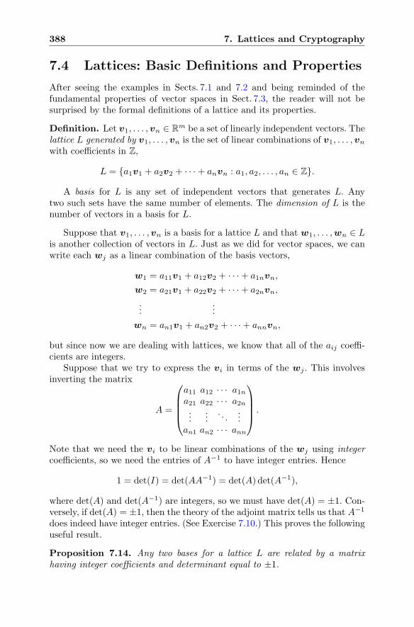
388 7. Lattices and Cryptography
7.4 Lattices: Basic Definitions and Properties
After seeing the examples in Sects. 7.1 and 7.2 and being reminded of thefundamental properties of vector spaces in Sect. 7.3, the reader will not besurprised by the formal definitions of a lattice and its properties.
Definition. Let v1, . . . ,vn ∈ Rm be a set of linearly independent vectors. The
lattice L generated by v1, . . . ,vn is the set of linear combinations of v1, . . . ,vn
with coefficients in Z,
L = {a1v1 + a2v2 + · · ·+ anvn : a1, a2, . . . , an ∈ Z}.
A basis for L is any set of independent vectors that generates L. Anytwo such sets have the same number of elements. The dimension of L is thenumber of vectors in a basis for L.
Suppose that v1, . . . ,vn is a basis for a lattice L and that w1, . . . ,wn ∈ Lis another collection of vectors in L. Just as we did for vector spaces, we canwrite each wj as a linear combination of the basis vectors,
w1 = a11v1 + a12v2 + · · ·+ a1nvn,
w2 = a21v1 + a22v2 + · · ·+ a2nvn,
......
wn = an1v1 + an2v2 + · · ·+ annvn,
but since now we are dealing with lattices, we know that all of the aij coeffi-cients are integers.
Suppose that we try to express the vi in terms of the wj . This involvesinverting the matrix
A =
⎛
⎜⎜⎜⎝
a11 a12 · · · a1na21 a22 · · · a2n...
.... . .
...an1 an2 · · · ann
⎞
⎟⎟⎟⎠.
Note that we need the vi to be linear combinations of the wj using integercoefficients, so we need the entries of A−1 to have integer entries. Hence
1 = det(I) = det(AA−1) = det(A) det(A−1),
where det(A) and det(A−1) are integers, so we must have det(A) = ±1. Con-versely, if det(A) = ±1, then the theory of the adjoint matrix tells us that A−1
does indeed have integer entries. (See Exercise 7.10.) This proves the followinguseful result.
Proposition 7.14. Any two bases for a lattice L are related by a matrixhaving integer coefficients and determinant equal to ±1.
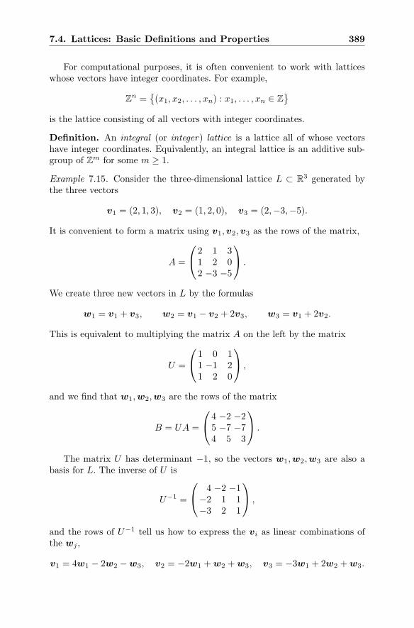
7.4. Lattices: Basic Definitions and Properties 389
For computational purposes, it is often convenient to work with latticeswhose vectors have integer coordinates. For example,
Zn =
{(x1, x2, . . . , xn) : x1, . . . , xn ∈ Z
}
is the lattice consisting of all vectors with integer coordinates.
Definition. An integral (or integer) lattice is a lattice all of whose vectorshave integer coordinates. Equivalently, an integral lattice is an additive sub-group of Zm for some m ≥ 1.
Example 7.15. Consider the three-dimensional lattice L ⊂ R3 generated by
the three vectors
v1 = (2, 1, 3), v2 = (1, 2, 0), v3 = (2,−3,−5).
It is convenient to form a matrix using v1,v2,v3 as the rows of the matrix,
A =
⎛
⎝2 1 31 2 02 −3 −5
⎞
⎠ .
We create three new vectors in L by the formulas
w1 = v1 + v3, w2 = v1 − v2 + 2v3, w3 = v1 + 2v2.
This is equivalent to multiplying the matrix A on the left by the matrix
U =
⎛
⎝1 0 11 −1 21 2 0
⎞
⎠ ,
and we find that w1,w2,w3 are the rows of the matrix
B = UA =
⎛
⎝4 −2 −25 −7 −74 5 3
⎞
⎠ .
The matrix U has determinant −1, so the vectors w1,w2,w3 are also abasis for L. The inverse of U is
U−1 =
⎛
⎝4 −2 −1
−2 1 1−3 2 1
⎞
⎠ ,
and the rows of U−1 tell us how to express the vi as linear combinations ofthe wj ,
v1 = 4w1 − 2w2 −w3, v2 = −2w1 +w2 +w3, v3 = −3w1 + 2w2 +w3.
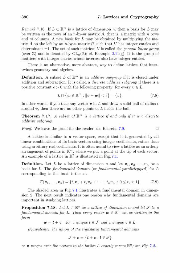
390 7. Lattices and Cryptography
Remark 7.16. If L ⊂ Rm is a lattice of dimension n, then a basis for L may
be written as the rows of an n-by-m matrix A, that is, a matrix with n rowsand m columns. A new basis for L may be obtained by multiplying the ma-trix A on the left by an n-by-n matrix U such that U has integer entries anddeterminant ±1. The set of such matrices U is called the general linear group(over Z) and is denoted by GLn(Z); cf. Example 2.11(g). It is the group ofmatrices with integer entries whose inverses also have integer entries.
There is an alternative, more abstract, way to define lattices that inter-twines geometry and algebra.
Definition. A subset L of Rm is an additive subgroup if it is closed underaddition and subtraction. It is called a discrete additive subgroup if there is apositive constant ε > 0 with the following property: for every v ∈ L,
L ∩{w ∈ R
m : ‖v −w‖ < ε}= {v}. (7.8)
In other words, if you take any vector v in L and draw a solid ball of radius εaround v, then there are no other points of L inside the ball.
Theorem 7.17. A subset of Rm is a lattice if and only if it is a discrete
additive subgroup.
Proof. We leave the proof for the reader; see Exercise 7.9.
A lattice is similar to a vector space, except that it is generated by alllinear combinations of its basis vectors using integer coefficients, rather thanusing arbitrary real coefficients. It is often useful to view a lattice as an orderlyarrangement of points in R
m, where we put a point at the tip of each vector.An example of a lattice in R
2 is illustrated in Fig. 7.1.
Definition. Let L be a lattice of dimension n and let v1,v2, . . . ,vn be abasis for L. The fundamental domain (or fundamental parallelepiped) for Lcorresponding to this basis is the set
F(v1, . . . ,vn) = {t1v1 + t2v2 + · · ·+ tnvn : 0 ≤ ti < 1}. (7.9)
The shaded area in Fig. 7.1 illustrates a fundamental domain in dimen-sion 2. The next result indicates one reason why fundamental domains areimportant in studying lattices.
Proposition 7.18. Let L ⊂ Rn be a lattice of dimension n and let F be a
fundamental domain for L. Then every vector w ∈ Rn can be written in the
formw = t+ v for a unique t ∈ F and a unique v ∈ L.
Equivalently, the union of the translated fundamental domains
F + v ={t+ v : t ∈ F}
as v ranges over the vectors in the lattice L exactly covers Rn; see Fig. 7.2.
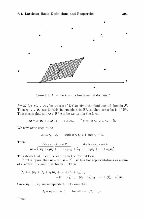
7.4. Lattices: Basic Definitions and Properties 391
F
L
Figure 7.1: A lattice L and a fundamental domain F
Proof. Let v1, . . . ,vn be a basis of L that gives the fundamental domain F .Then v1, . . . ,vn are linearly independent in R
n, so they are a basis of Rn.This means that any w ∈ R
n can be written in the form
w = α1v1 + α2v2 + · · ·+ αnvn for some α1, . . . , αn ∈ R.
We now write each αi as
αi = ti + ai with 0 ≤ ti < 1 and ai ∈ Z.
Then
w =
this is a vector t ∈ F︷ ︸︸ ︷t1v1 + t2v2 + · · ·+ tnvn +
this is a vector v ∈ L︷ ︸︸ ︷a1v1 + a2v2 + · · ·+ anvn .
This shows that w can be written in the desired form.Next suppose that w = t + v = t′ + v′ has two representations as a sum
of a vector in F and a vector in L. Then
(t1 + a1)v1 + (t2 + a2)v2 + · · ·+ (tn + an)vn
= (t′1 + a′1)v1 + (t′2 + a′2)v2 + · · ·+ (t′n + a′n)vn.
Since v1, . . . ,vn are independent, it follows that
ti + ai = t′i + a′i for all i = 1, 2, . . . , n.
Hence
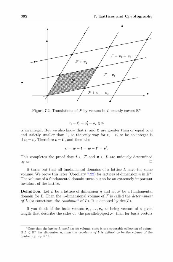
392 7. Lattices and Cryptography
FF + v1
F + v2
F + v1 − v2
F + v1 + v2
Figure 7.2: Translations of F by vectors in L exactly covers Rn
ti − t′i = a′i − ai ∈ Z
is an integer. But we also know that ti and t′i are greater than or equal to 0
and strictly smaller than 1, so the only way for ti − t′i to be an integer isif ti = t′i. Therefore t = t′, and then also
v = w − t = w − t′ = v′.
This completes the proof that t ∈ F and v ∈ L are uniquely determinedby w.
It turns out that all fundamental domains of a lattice L have the samevolume. We prove this later (Corollary 7.22) for lattices of dimension n in R
n.The volume of a fundamental domain turns out to be an extremely importantinvariant of the lattice.
Definition. Let L be a lattice of dimension n and let F be a fundamentaldomain for L. Then the n-dimensional volume of F is called the determinantof L (or sometimes the covolume4 of L). It is denoted by det(L).
If you think of the basis vectors v1, . . . ,vn as being vectors of a givenlength that describe the sides of the parallelepiped F , then for basis vectors
4Note that the lattice L itself has no volume, since it is a countable collection of points.If L ⊂ R
n has dimension n, then the covolume of L is defined to be the volume of thequotient group R
n/L.
7.4. Lattices: Basic Definitions and Properties 393
of given lengths, the largest volume is obtained when the vectors are pairwiseorthogonal to one another. This leads to the following important upper boundfor the determinant of a lattice.
Proposition 7.19 (Hadamard’s Inequality). Let L be a lattice, take anybasis v1, . . . ,vn for L, and let F be a fundamental domain for L. Then
detL = Vol(F) ≤ ‖v1‖ ‖v2‖ · · · ‖vn‖. (7.10)
The closer that the basis is to being orthogonal, the closer that Hadamard’sinequality (7.10) comes to being an equality.
It is fairly easy to compute the determinant of a lattice L if its dimensionis the same as its ambient space, i.e., if L is contained in R
n and L hasdimension n. This formula, which luckily is the case that is of most interestto us, is described in the next proposition. See Exercise 7.14 to learn how tocompute the determinant of a lattice in the general case.
Proposition 7.20. Let L ⊂ Rn be a lattice of dimension n, let v1,v2, . . . ,vn
be a basis for L, and let F = F(v1, . . . ,vn) be the associated fundamentaldomain as defined by (7.9). Write the coordinates of the ith basis vector as
vi = (ri1, ri2, . . . , rin)
and use the coordinates of the vi as the rows of a matrix,
F = F (v1, . . . ,vn) =
⎛
⎜⎜⎜⎝
r11 r12 · · · r1nr21 r22 · · · r2n...
.... . .
...rn1 rn2 · · · rnn
⎞
⎟⎟⎟⎠. (7.11)
Then the volume of F is given by the formula
Vol(F(v1, . . . ,vn)
)=∣∣det(F (v1, . . . ,vn)
)∣∣.
Proof. The proof uses multivariable calculus. We can compute the volumeof F as the integral of the constant function 1 over the region F ,
Vol(F) =∫
Fdx1 dx2 · · · dxn.
The fundamental domain F is the set described by (7.9), so we make a changeof variables from x = (x1, . . . , xn) to t = (t1, . . . , tn) according to the formula
(x1, x2, . . . , xn) = t1v1 + t2v2 + · · ·+ tnvn.
394 7. Lattices and Cryptography
In terms of the matrix F = F (v1, . . . ,vn) defined by (7.11), the change ofvariables is given by the matrix equation x = tF . The Jacobian matrix of thischange of variables is F , and the fundamental domain F is the image under Fof the unit cube Cn = [0, 1]n, so the change of variables formula for integralsyields
∫
Fdx1 dx2 · · · dxn =
∫
FCn
dx1 dx2 · · · dxn =
∫
Cn
| detF | dt1 dt2 · · · dtn
= | detF |Vol(Cn) = | detF |.
Example 7.21. The lattice in Example 7.15 has determinant
detL = | detA| =
∣∣∣∣∣∣det
⎛
⎝2 1 31 2 02 −3 −5
⎞
⎠
∣∣∣∣∣∣= | − 36| = 36.
Corollary 7.22. Let L ⊂ Rn be a lattice of dimension n. Then every fun-
damental domain for L has the same volume. Hence det(L) is an invariantof the lattice L, independent of the particular fundamental domain used tocompute it.
Proof. Let v1, . . . ,vn and w1, . . . ,wn be two fundamental domains for L,and let F (v1, . . . ,vn) and F (w1, . . . ,wn) be the associated matrices (7.11)obtained by using the coordinates of the vectors as the rows of the matrices.Then Proposition 7.14 tells us that
F (v1, . . . ,vn) = AF (w1, . . . ,wn) (7.12)
for some n-by-n matrix with integer entries and det(A) = ±1. Now applyingProposition 7.20 twice yields
Vol(F(v1, . . . ,vn)
)
=∣∣det(F (v1, . . . ,vn)
)∣∣ from Proposition 7.20,
=∣∣det(AF (w1, . . . ,wn)
)∣∣ from (7.12),
=∣∣det(A)
∣∣∣∣det(F (w1, . . . ,wn)
)∣∣ since det(AB) = det(A) det(B),
=∣∣det(F (w1, . . . ,wn)
)∣∣ since det(A) = ±1,= Vol
(F(w1, . . . ,wn)
)from Proposition 7.20.
7.5. Short Vectors in Lattices 395
7.5 Short Vectors in Lattices
The fundamental computational problems associated to a lattice are those offinding a shortest nonzero vector in the lattice and of finding a vector in thelattice that is closest to a given nonlattice vector. In this section we discussthese problems, mainly from a theoretical perspective. Section 7.13 is devotedto a practical method for finding short and close vectors in a lattice.
7.5.1 The Shortest Vector Problem and the ClosestVector Problem
We begin with a description of two fundamental lattice problems.
The Shortest Vector Problem (SVP): Find a shortest nonzero vector in alattice L, i.e., find a nonzero vector v ∈ L that minimizes the Euclideannorm ‖v‖.
The Closest Vector Problem (CVP): Given a vector w ∈ Rm that is not
in L, find a vector v ∈ L that is closest to w, i.e., find a vector v ∈ Lthat minimizes the Euclidean norm ‖w − v‖.
Remark 7.23. Note that there may be more than one shortest nonzero vectorin a lattice. For example, in Z
2, all four of the vectors (0,±1) and (±1, 0) aresolutions to SVP. This is why SVP asks for “a” shortest vector and not “the”shortest vector. A similar remark applies to CVP.
We have seen in Sects. 7.1 and 7.2 that a solution to SVP can be used tobreak various cryptosystems. We will see more examples later in this chapter.
Both SVP and CVP are profound problems, and both become computa-tionally difficult as the dimension n of the lattice grows. On the other hand,even approximate solutions to SVP and CVP turn out to have surprisinglymany applications in different fields of pure and applied mathematics. In fullgenerality, CVP is known to be NP-hard and SVP is NP-hard under a certain“randomized reduction hypothesis.”5
In practice, CVP is considered to be “a little bit harder” than SVP, sinceCVP can often be reduced to SVP in a slightly higher dimension. For exam-ple, the (n+ 1)-dimensional SVP used to solve the knapsack cryptosystem inSect. 7.2 can be naturally formulated as an n-dimensional CVP. For a proofthat SVP is no harder than CVP, see [50], and for a thorough discussion ofthe complexity of different types of lattice problems, see [86].
Remark 7.24. In full generality, both SVP and CVP are considered to be ex-tremely hard problems, but in practice it is difficult to achieve this idealized“full generality.” In real world scenarios, cryptosystems based on NP-hard
5This hypothesis means that the class of polynomial-time algorithms is enlarged toinclude those that are not deterministic, but will, with high probability, terminate in poly-nomial time with a correct result. See Ajtai [3] for details.
396 7. Lattices and Cryptography
or NP-complete problems tend to rely on a particular subclass of problems,either to achieve efficiency or to allow the creation of a trapdoor. When thisis done, there is always the possibility that some special property of the cho-sen subclass of problems makes them easier to solve than the general case.We have already seen this with the knapsack cryptosystem in Sect. 7.2. Thegeneral knapsack problem is NP-complete, but the disguised superincreasingknapsack problem that was suggested for use in cryptography is much easierto solve than the general knapsack problem.
There are many important variants of SVP and CVP that arise both intheory and in practice. We describe a few of them here.
Shortest Basis Problem (SBP) Find a basis v1, . . . ,vn for a lattice thatis shortest in some sense. For example, we might require that
max1≤i≤n
‖vi‖ or
n∑
i=1
‖vi‖2
be minimized. There are thus many different versions of SBP, dependingon how one decides to measure the “size” of a basis.
Approximate Shortest Vector Problem (apprSVP) Let ψ(n) be a func-tion of n. In a lattice L of dimension n, find a nonzero vector thatis no more than ψ(n) times longer than a shortest nonzero vector. Inother words, if vshortest is a shortest nonzero vector in L, find a nonzerovector v ∈ L satisfying
‖v‖ ≤ ψ(n)‖vshortest‖.
Each choice of function ψ(n) gives a different apprSVP. As specific ex-amples, one might ask for an algorithm that finds a nonzero v ∈ Lsatisfying
‖v‖ ≤ 3√n‖vshortest‖ or ‖v‖ ≤ 2n/2‖vshortest‖.
Clearly an algorithm that solves the former is much stronger than onethat solves the latter, but even the latter may be useful if the dimensionis not too large.
Approximate Closest Vector Problem (apprCVP) This is the same asapprSVP, but now we are looking for a vector that is an approximatesolution to CVP, instead of an approximate solution to SVP.
7.5.2 Hermite’s Theorem and Minkowski’s Theorem
How long is the shortest nonzero vector in a lattice L? The answer dependsto some extent on the dimension and the determinant of L. The next resultgives an explicit upper bound in terms of dim(L) and det(L) for the shortestnonzero vector in L.
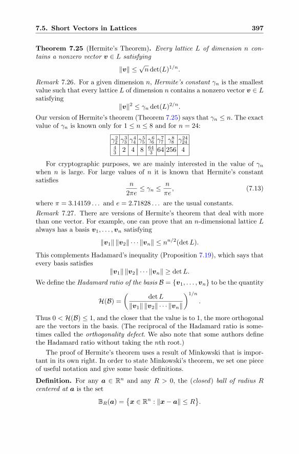
7.5. Short Vectors in Lattices 397
Theorem 7.25 (Hermite’s Theorem). Every lattice L of dimension n con-tains a nonzero vector v ∈ L satisfying
‖v‖ ≤√ndet(L)1/n.
Remark 7.26. For a given dimension n, Hermite’s constant γn is the smallestvalue such that every lattice L of dimension n contains a nonzero vector v ∈ Lsatisfying
‖v‖2 ≤ γn det(L)2/n.
Our version of Hermite’s theorem (Theorem 7.25) says that γn ≤ n. The exactvalue of γn is known only for 1 ≤ n ≤ 8 and for n = 24:
γ22 γ33 γ
44 γ
55 γ
66 γ
77 γ88 γ2424
43 2 4 8 64
3 64 256 4
For cryptographic purposes, we are mainly interested in the value of γnwhen n is large. For large values of n it is known that Hermite’s constantsatisfies
n
2πe≤ γn ≤
n
πe, (7.13)
where π = 3.14159 . . . and e = 2.71828 . . . are the usual constants.
Remark 7.27. There are versions of Hermite’s theorem that deal with morethan one vector. For example, one can prove that an n-dimensional lattice Lalways has a basis v1, . . . ,vn satisfying
‖v1‖ ‖v2‖ · · · ‖vn‖ ≤ nn/2(detL).
This complements Hadamard’s inequality (Proposition 7.19), which says thatevery basis satisfies
‖v1‖ ‖v2‖ · · · ‖vn‖ ≥ detL.
We define the Hadamard ratio of the basis B = {v1, . . . ,vn} to be the quantity
H(B) =(
detL
‖v1‖ ‖v2‖ · · · ‖vn‖
)1/n
.
Thus 0 < H(B) ≤ 1, and the closer that the value is to 1, the more orthogonalare the vectors in the basis. (The reciprocal of the Hadamard ratio is some-times called the orthogonality defect. We also note that some authors definethe Hadamard ratio without taking the nth root.)
The proof of Hermite’s theorem uses a result of Minkowski that is impor-tant in its own right. In order to state Minkowski’s theorem, we set one pieceof useful notation and give some basic definitions.
Definition. For any a ∈ Rn and any R > 0, the (closed) ball of radius R
centered at a is the set
BR(a) ={x ∈ R
n : ‖x− a‖ ≤ R}.
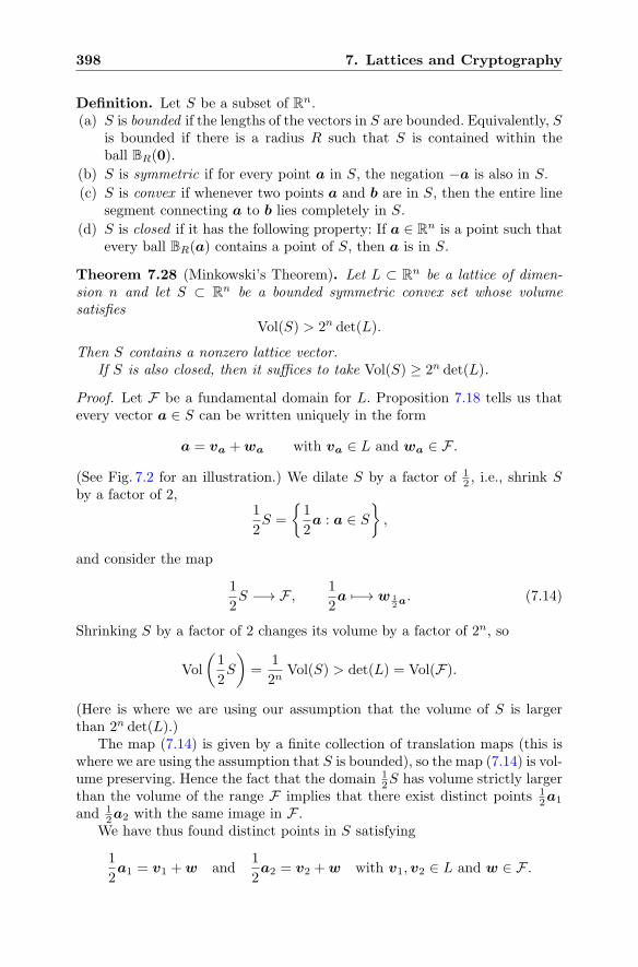
398 7. Lattices and Cryptography
Definition. Let S be a subset of Rn.(a) S is bounded if the lengths of the vectors in S are bounded. Equivalently, S
is bounded if there is a radius R such that S is contained within theball BR(0).
(b) S is symmetric if for every point a in S, the negation −a is also in S.
(c) S is convex if whenever two points a and b are in S, then the entire linesegment connecting a to b lies completely in S.
(d) S is closed if it has the following property: If a ∈ Rn is a point such that
every ball BR(a) contains a point of S, then a is in S.
Theorem 7.28 (Minkowski’s Theorem). Let L ⊂ Rn be a lattice of dimen-
sion n and let S ⊂ Rn be a bounded symmetric convex set whose volume
satisfiesVol(S) > 2n det(L).
Then S contains a nonzero lattice vector.If S is also closed, then it suffices to take Vol(S) ≥ 2n det(L).
Proof. Let F be a fundamental domain for L. Proposition 7.18 tells us thatevery vector a ∈ S can be written uniquely in the form
a = va +wa with va ∈ L and wa ∈ F .
(See Fig. 7.2 for an illustration.) We dilate S by a factor of 12 , i.e., shrink S
by a factor of 2,1
2S =
{1
2a : a ∈ S
},
and consider the map
1
2S −→ F , 1
2a �−→ w 1
2a. (7.14)
Shrinking S by a factor of 2 changes its volume by a factor of 2n, so
Vol
(1
2S
)=
1
2nVol(S) > det(L) = Vol(F).
(Here is where we are using our assumption that the volume of S is largerthan 2n det(L).)
The map (7.14) is given by a finite collection of translation maps (this iswhere we are using the assumption that S is bounded), so the map (7.14) is vol-ume preserving. Hence the fact that the domain 1
2S has volume strictly largerthan the volume of the range F implies that there exist distinct points 1
2a1
and 12a2 with the same image in F .
We have thus found distinct points in S satisfying
1
2a1 = v1 +w and
1
2a2 = v2 +w with v1,v2 ∈ L and w ∈ F .
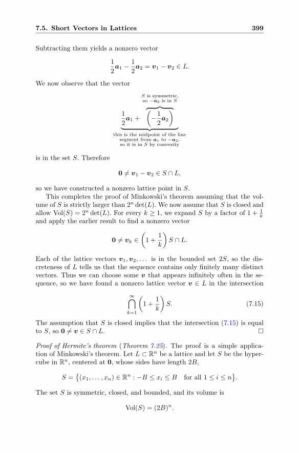
7.5. Short Vectors in Lattices 399
Subtracting them yields a nonzero vector
1
2a1 −
1
2a2 = v1 − v2 ∈ L.
We now observe that the vector
1
2a1 +
S is symmetric,so −a2 is in S
︷ ︸︸ ︷(−1
2a2
)
︸ ︷︷ ︸this is the midpoint of the line
segment from a1 to −a2,so it is in S by convexity
is in the set S. Therefore
0 �= v1 − v2 ∈ S ∩ L,
so we have constructed a nonzero lattice point in S.This completes the proof of Minkowski’s theorem assuming that the vol-
ume of S is strictly larger than 2n det(L). We now assume that S is closed andallow Vol(S) = 2n det(L). For every k ≥ 1, we expand S by a factor of 1 + 1
kand apply the earlier result to find a nonzero vector
0 �= vk ∈(1 +
1
k
)S ∩ L.
Each of the lattice vectors v1,v2, . . . is in the bounded set 2S, so the dis-creteness of L tells us that the sequence contains only finitely many distinctvectors. Thus we can choose some v that appears infinitely often in the se-quence, so we have found a nonzero lattice vector v ∈ L in the intersection
∞⋂
k=1
(1 +
1
k
)S. (7.15)
The assumption that S is closed implies that the intersection (7.15) is equalto S, so 0 �= v ∈ S ∩ L.
Proof of Hermite’s theorem (Theorem 7.25). The proof is a simple applica-tion of Minkowski’s theorem. Let L ⊂ R
n be a lattice and let S be the hyper-cube in R
n, centered at 0, whose sides have length 2B,
S ={(x1, . . . , xn) ∈ R
n : −B ≤ xi ≤ B for all 1 ≤ i ≤ n}.
The set S is symmetric, closed, and bounded, and its volume is
Vol(S) = (2B)n.
400 7. Lattices and Cryptography
So if we set B = det(L)1/n, then Vol(S) = 2n det(L) and we can applyMinkowski’s theorem to deduce that there is a vector 0 �= a ∈ S ∩L. Writingthe coordinates of a as (a1, . . . , an), by definition of S we have
‖a‖ =√a21 + · · ·+ a2n ≤
√nB =
√n det(L)1/n.
This completes the proof of Theorem 7.25.
7.5.3 The Gaussian Heuristic
It is possible to improve the constant appearing in Hermite’s theorem (Theo-rem 7.25) by applying Minkowski’s theorem (Theorem 7.28) to a hypersphere,rather than a hypercube. In order to do this, we need to know the volume ofa ball in R
n. The following material is generally covered in advanced calculusclasses.
Definition. The gamma function Γ(s) is defined for s > 0 by the integral
Γ(s) =
∫ ∞
0
tse−t dt
t. (7.16)
The gamma function is a very important function that appears in manymathematical formulas. We list a few of its basic properties.
Proposition 7.29. (a) The integral (7.16) defining Γ(s) is convergent forall s > 0.
(b) Γ(1) = 1 and Γ(s+1) = sΓ(s). This allows us to extend Γ(s) to all s ∈ R
with s �= 0,−1,−2, . . . .(c) For all integers n ≥ 1 we have Γ(n+ 1) = n!. Thus Γ(s) interpolates the
values of the factorial function to all real (and even complex ) numbers.
(d) Γ( 12 ) =√π.
(e) (Stirling’s formula) For large values of s we have
Γ(1 + s)1/s ≈ s
e. (7.17)
(More precisely, ln Γ(1 + s) = ln(s/e)s + 12 ln(2πs) +O(1) as s→∞.)
Proof. The properties of the gamma function are described in real and com-plex analysis textbooks; see for example [2] or [43].
The formula for the volume of a ball in n-dimensional space involves thegamma function.
Theorem 7.30. Let BR(a) be a ball of radius R in Rn. Then the volume
of BR(a) is
Vol(BR(a)
)=
πn/2Rn
Γ(1 + n/2). (7.18)
7.5. Short Vectors in Lattices 401
For large values of n, the volume of the ball BR(a) ⊂ Rn is approximately
given by
Vol(BR(a)
)1/n ≈√
2πe
nR. (7.19)
Proof. See [43, §5.9], for example, for a proof of the formula (7.18) giving thevolume of a ball.
We can use (7.18) and Stirling’s formula (7.17) to prove (7.19). Thus
Vol(BR(a)
)1/n=
π1/2R
Γ(1 + n/2)1/n≈ π1/2R
(n/2e)1/2=
√2πe
nR.
Remark 7.31. Theorem 7.30 allows us to improve Theorem 7.25 for largevalues of n. The ball BR(0) is bounded, closed, convex, and symmetric, soMinkowski’s theorem (Theorem 7.28) says that if we choose R such that
Vol(BR(0)
)≥ 2n det(L),
then the ball BR(0) contains a nonzero lattice point. Assuming that n is large,we can use (7.19) to approximate the volume of BR(0), so we need to choose Rto satisfy √
2πe
nR � 2 det(L)1/n.
Hence for large n there exists a nonzero vector v ∈ L satisfying
‖v‖ �√
2n
πe· (detL)1/n.
This improves the estimate in Theorem 7.25 by a factor of√2/πe ≈ 0.484.
Although exact bounds for the size of a shortest vector are unknown whenthe dimension n is large, we can estimate its size by a probabilistic argumentthat is based on the following principle:
Let BR(0) be a large ball centered at 0. Then the number of latticepoints in BR(0) is approximately equal to the volume of BR(0)divided by the volume of a fundamental domain F .
This is reasonable, since #(BR(0) ∩ L
)should be approximately the number
of copies of F that fit into BR(0). (See Exercise 7.15 for a more rigorousjustification.)
For example, if we let L = Z2, then this principle says that the area of
a circle is approximately the number of integer points inside the circle. Theproblem of estimating the error term in
#{(x, y) ∈ Z
2 : x2 + y2 ≤ R2}= πR2 + (error term)
402 7. Lattices and Cryptography
is a famous classical problem. In higher dimensions, the problem becomesmore difficult because, as n increases, the error created by lattice points nearthe boundary of the ball can be quite large until R becomes very large. Thusthe estimate
#{v ∈ L : ‖v‖ ≤ R
}≈
Vol(BR(0)
)
Vol(F) (7.20)
is somewhat problematic when n is large and R is not too large. Still, one canask for the value of R that makes the right-hand side (7.20) equal to 1, sincein some sense this is the value of R for which we might expect to first find anonzero lattice point in the ball.
Assuming that n is large, we use the estimate (7.19) from Theorem 7.30.We set
(2πe
n
)n/2
Rn ≈ Vol(BR(0)
)equal to Vol(F) = det(L),
and we solve for
R ≈√
n
2πe(detL)1/n.
This leads to the following heuristic.
Definition. Let L be a lattice of dimension n. The Gaussian expected shortestlength is
σ(L) =
√n
2πe(detL)1/n. (7.21)
The Gaussian heuristic says that a shortest nonzero vector in a “randomlychosen lattice” will satisfy
‖vshortest‖ ≈ σ(L).
More precisely, if ε > 0 is fixed, then for all sufficiently large n, a randomlychosen lattice of dimension n will satisfy
(1− ε)σ(L) ≤ ‖vshortest‖ ≤ (1 + ε)σ(L).
(See [133] for some mathematical justification of this heuristic principle.)
Remark 7.32. For small values of n, it is better to use the exact formula (7.18)for the volume of BR(0), so the Gaussian expected shortest length for small n is
σ(L) =(Γ(1 + n/2) det(L)
)1/n/√π. (7.22)
For example, when n = 6, then (7.21) gives σ(L) = 0.5927(detL)1/6, while(7.22) gives σ(L) = 0.7605(detL)1/6, which is a significant difference. On theother hand, if n = 100, then they give
σ(L) = 2.420(detL)1/100 and σ(L) = 2.490(detL)1/100,
respectively, so the difference is much smaller.
7.6. Babai’s Algorithm 403
Example 7.33. Let (m1, . . . ,mn, S) be a knapsack problem. The associatedlattice LM ,S is generated by the rows of the matrix (7.4) given on page 383.The matrix LM ,S has dimension n+ 1 and determinant detLM ,S = 2nS. Asexplained in Sect. 7.2, the number S satisfies S = O(22n), so S1/n ≈ 4. Thisallows us to approximate the Gaussian shortest length as
σ(LM ,S) =
√n+ 1
2πe(detLM ,S)
1/(n+1) =
√n+ 1
2πe(2nS)1/(n+1)
≈√
n
2πe· 2S1/n ≈
√n
2πe· 8 ≈ 1.936
√n.
On the other hand, as explained in Sect. 7.2, the lattice LM ,S contains avector t of length
√n, and knowledge of t reveals the solution to the subset-
sum problem. Hence solving SVP for the lattice LM ,S is very likely to solvethe subset-sum problem. For a further discussion of the use of lattice methodsto solve subset-sum problems, see Sect. 7.14.2.
We will find that the Gaussian heuristic is useful in quantifying the diffi-culty of locating short vectors in lattices. In particular, if the actual shortestvector of a particular lattice L is significantly shorter than σ(L), then latticereduction algorithms such as LLL seem to have a much easier time locatingthe shortest vector.
A similar argument leads to a Gaussian heuristic for CVP. Thus if L ⊂ Rn
is a random lattice of dimension n and w ∈ Rn is a random point, then we
expect that the lattice vector v ∈ L closest to w satisfies
‖v −w‖ ≈ σ(L).
And just as for SVP, if L contains a point that is significantly closer than σ(L)to w, then lattice reduction algorithms have an easier time solving CVP.
7.6 Babai’s Algorithm and Using a “Good”Basis to Solve apprCVP
If a lattice L ⊂ Rn has a basis v1, . . . ,vn consisting of vectors that are pairwise
orthogonal, i.e., such that
vi · vj = 0 for all i �= j,
then it is easy to solve both SVP and CVP. Thus to solve SVP, we observethat the length of any vector in L is given by the formula
‖a1v1 + a2v2 + · · ·+ anvn‖2 = a21‖v1‖2 + a22‖v2‖2 + · · ·+ a2n‖vn‖2.
Since a1, . . . , an ∈ Z, we see that the shortest nonzero vector(s) in L aresimply the shortest vector(s) in the set {±v1, . . . ,±vn}.
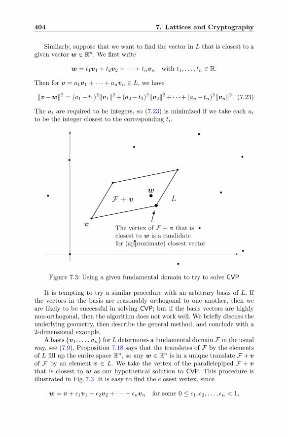
404 7. Lattices and Cryptography
Similarly, suppose that we want to find the vector in L that is closest to agiven vector w ∈ R
n. We first write
w = t1v1 + t2v2 + · · ·+ tnvn with t1, . . . , tn ∈ R.
Then for v = a1v1 + · · ·+ anvn ∈ L, we have
‖v−w‖2 = (a1− t1)2‖v1‖2+(a2− t2)2‖v2‖2+ · · ·+(an− tn)2‖vn‖2. (7.23)
The ai are required to be integers, so (7.23) is minimized if we take each aito be the integer closest to the corresponding ti.
v
F + vw
The vertex of F + v that isclosest to w is a candidatefor (approximate) closest vector
L
Figure 7.3: Using a given fundamental domain to try to solve CVP
It is tempting to try a similar procedure with an arbitrary basis of L. Ifthe vectors in the basis are reasonably orthogonal to one another, then weare likely to be successful in solving CVP; but if the basis vectors are highlynon-orthogonal, then the algorithm does not work well. We briefly discuss theunderlying geometry, then describe the general method, and conclude with a2-dimensional example.
A basis {v1, . . . ,vn} for L determines a fundamental domain F in the usualway, see (7.9). Proposition 7.18 says that the translates of F by the elementsof L fill up the entire space R
n, so any w ∈ Rn is in a unique translate F + v
of F by an element v ∈ L. We take the vertex of the parallelepiped F + vthat is closest to w as our hypothetical solution to CVP. This procedure isillustrated in Fig. 7.3. It is easy to find the closest vertex, since
w = v + ε1v1 + ε2v2 + · · ·+ εnvn for some 0 ≤ ε1, ε2, . . . , εn < 1,
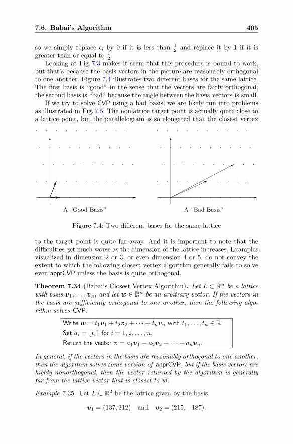
7.6. Babai’s Algorithm 405
so we simply replace εi by 0 if it is less than 12 and replace it by 1 if it is
greater than or equal to 12 .
Looking at Fig. 7.3 makes it seem that this procedure is bound to work,but that’s because the basis vectors in the picture are reasonably orthogonalto one another. Figure 7.4 illustrates two different bases for the same lattice.The first basis is “good” in the sense that the vectors are fairly orthogonal;the second basis is “bad” because the angle between the basis vectors is small.
If we try to solve CVP using a bad basis, we are likely run into problemsas illustrated in Fig. 7.5. The nonlattice target point is actually quite close toa lattice point, but the parallelogram is so elongated that the closest vertex
A “Good Basis” A “Bad Basis”
Figure 7.4: Two different bases for the same lattice
to the target point is quite far away. And it is important to note that thedifficulties get much worse as the dimension of the lattice increases. Examplesvisualized in dimension 2 or 3, or even dimension 4 or 5, do not convey theextent to which the following closest vertex algorithm generally fails to solveeven apprCVP unless the basis is quite orthogonal.
Theorem 7.34 (Babai’s Closest Vertex Algorithm). Let L ⊂ Rn be a lattice
with basis v1, . . . ,vn, and let w ∈ Rn be an arbitrary vector. If the vectors in
the basis are sufficiently orthogonal to one another, then the following algo-rithm solves CVP.
Write w = t1v1 + t2v2 + · · ·+ tnvn with t1, . . . , tn ∈ R.
Set ai = �ti! for i = 1, 2, . . . , n.
Return the vector v = a1v1 + a2v2 + · · ·+ anvn.
In general, if the vectors in the basis are reasonably orthogonal to one another,then the algorithm solves some version of apprCVP, but if the basis vectors arehighly nonorthogonal, then the vector returned by the algorithm is generallyfar from the lattice vector that is closest to w.
Example 7.35. Let L ⊂ R2 be the lattice given by the basis
v1 = (137, 312) and v2 = (215,−187).
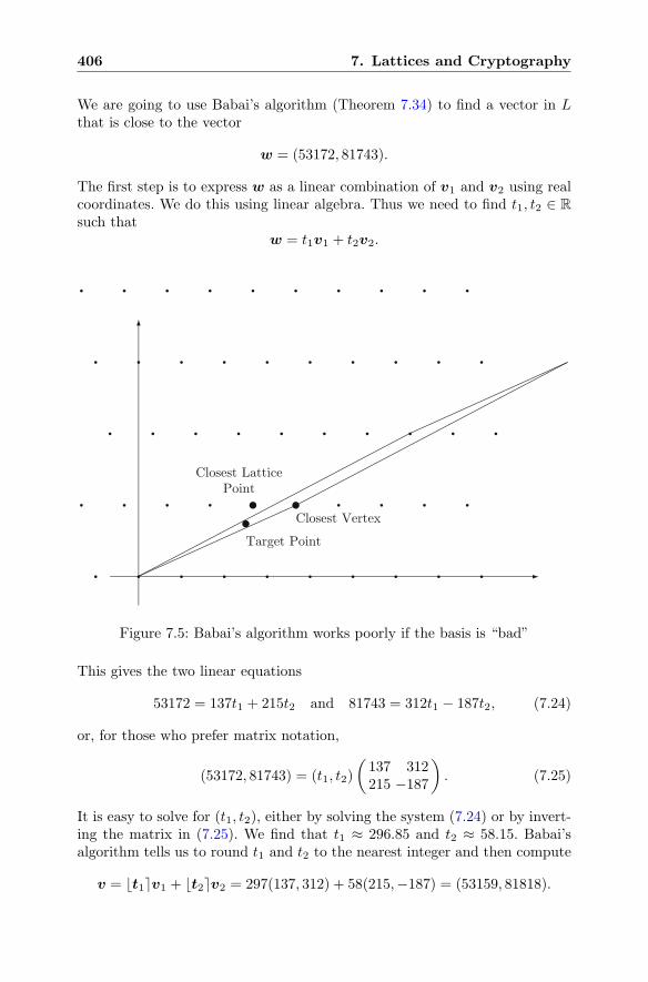
406 7. Lattices and Cryptography
We are going to use Babai’s algorithm (Theorem 7.34) to find a vector in Lthat is close to the vector
w = (53172, 81743).
The first step is to express w as a linear combination of v1 and v2 using realcoordinates. We do this using linear algebra. Thus we need to find t1, t2 ∈ R
such thatw = t1v1 + t2v2.
Target Point
Closest Vertex
Closest LatticePoint
Figure 7.5: Babai’s algorithm works poorly if the basis is “bad”
This gives the two linear equations
53172 = 137t1 + 215t2 and 81743 = 312t1 − 187t2, (7.24)
or, for those who prefer matrix notation,
(53172, 81743) = (t1, t2)
(137 312215 −187
). (7.25)
It is easy to solve for (t1, t2), either by solving the system (7.24) or by invert-ing the matrix in (7.25). We find that t1 ≈ 296.85 and t2 ≈ 58.15. Babai’salgorithm tells us to round t1 and t2 to the nearest integer and then compute
v = �t1!v1 + �t2!v2 = 297(137, 312) + 58(215,−187) = (53159, 81818).
7.7. Cryptosystems Based on Hard Lattice Problems 407
Then v is in L and v should be close to w. We find that
‖v −w‖ ≈ 76.12
is indeed quite small. This is to be expected, since the vectors in the givenbasis are fairly orthogonal to one another, as is seen by the fact that theHadamard ratio
H(v1,v2) =
(det(L)
‖v1‖‖v2‖
)1/2
≈(
92699
(340.75)(284.95)
)1/2
≈ 0.977
is reasonably close to 1.We now try to solve the same closest vector problem in the same lattice,
but using the new basis
v′1 = (1975, 438) = 5v1 + 6v2 and v′
2 = (7548, 1627) = 19v1 + 23v2.
The system of linear equations
(53172, 81743) = (t1, t2)
(1975 4387548 1627
)(7.26)
has the solution (t1, t2) ≈ (5722.66,−1490.34), so we set
v′ = 5723v′1 − 1490v′
2 = (56405, 82444).
Then v′ ∈ L, but v′ is not particularly close to w, since
‖v′ −w‖ ≈ 3308.12.
The nonorthogonality of the basis {v′1,v
′2} is shown by the smallness of the
Hadamard ratio
H(v′1,v
′2) =
(det(L)
‖v1‖‖v2‖
)1/2
≈(
92699
(2022.99)(7721.36)
)1/2
≈ 0.077.
7.7 Cryptosystems Based on HardLattice Problems
During the mid-1990s, several cryptosystems were introduced whose un-derlying hard problem was SVP and/or CVP in a lattice L of large di-mension n. The most important of these, in alphabetical order, were theAjtai–Dwork cryptosystem [4], the GGH cryptosystem of Goldreich, Gold-wasser, and Halevi [49], and the NTRU cryptosystem proposed by Hoffstein,Pipher, and Silverman [54].
The motivation for the introduction of these cryptosystems was twofold.First, it is certainly of interest to have cryptosystems based on a variety ofhard mathematical problems, since then a breakthrough in solving one math-ematical problem does not compromise the security of all systems. Second,
408 7. Lattices and Cryptography
lattice-based cryptosystems are frequently much faster than factorization ordiscrete logarithm-based systems such as Elgamal, RSA, and ECC. Roughlyspeaking, in order to achieve k bits of security, encryption and decryptionfor Elgamal, RSA, and ECC require O(k3) operations, while encryption anddecryption for lattice-based systems require only O(k2) operations.6 Further,the simple linear algebra operations used by lattice-based systems are veryeasy to implement in hardware and software. However, it must be noted thatthe security analysis of lattice-based cryptosystems is not nearly as well un-derstood as it is for factorization and discrete logarithm-based systems. Soalthough lattice-based systems are the subject of much current research, theirreal-world implementations are few in comparison with older systems.
The Ajtai–Dwork system is particularly interesting because Ajtai andDwork showed that their system is provably secure unless a worst-case latticeproblem can be solved in polynomial time. Offsetting this important theoret-ical result is the practical limitation that the key size turns out to be O(n4),which leads to enormous keys. Nguyen and Stern [95] subsequently showedthat any practical and efficient implementation of the Ajtai–Dwork system isinsecure.
The basic GGH cryptosystem, which we explain in more detail in Sect. 7.8,is a straightforward application of the ideas that we have already discussed.Alice’s private key is a good basis Bgood for a lattice L and her public key isa bad basis Bbad for L. Bob’s message is a binary vector m, which he uses toform a linear combination
∑miv
badi of the vectors in Bbad. He then perturbs
the sum by adding a small random vector r. The resulting vector w differsfrom a lattice vector v by the vector r. Since Alice knows a good basis for L,she can use Babai’s algorithm to find v, and then she expresses v in termsof the bad basis to recover m. Eve, on the other hand, knows only the badbasis Bbad, so she is unable to solve CVP in L.
A public key in the GGH cryptosystem is a bad basis for the lattice L,so it consists of n2 (large) numbers. In the original proposal, the key sizewas O(n3 log n), but using an idea of Micciancio [85], it is possible to reducethe key size to O(n2 log n) bits.
Goldreich, Goldwasser and Halevi conjectured that for n > 300, the CVPunderlying GGH would be intractable. However, the effectiveness of LLL-typelattice reduction algorithms on lattices of high dimension had not, at thattime, been closely studied. Nguyen [92] showed that a transformation of theoriginal GGH encryption scheme reduced the problem to an easier CVP. Thisenabled him to solve the proposed GGH challenge problems in dimensions upto 350. For n > 400, the public key is approximately 128 kB.
The NTRU public key cryptosystem [54], whose original public presenta-tion took place at the Crypto ’96 rump session, is most naturally described interms of quotients of polynomial rings. However, the hard problem underlying
6There are various tricks that one can use to reduce these estimates. For example, usinga small encryption exponent reduces RSA encryption to O(k2) operations, while usingproduct-form polynomials reduces NTRU encryption to O(k log k) operations.
7.8. The GGH Public Key Cryptosystem 409
NTRU is easily transformed into an SVP (for key recovery) or a CVP (forplaintext recovery) in a special class of lattices. The NTRU lattices, whichare described in Sect. 7.11, are lattices of even dimension n = 2N consistingof all vectors (x,y) ∈ Z
2N satisfying
y ≡ xH (mod q)
for some fixed positive integer q that is a public parameter. (In practice, q =O(n).) The matrix H, which is the public key, is an N -by-N circulant matrix.This means that each successive row of H is a rotation of the previous row,so in order to describe H, it suffices to specify its first row. Thus the publickey has size O(n log n), which is significantly smaller than GGH.
The NTRU private key is a single short vector (f , g) ∈ L. The setconsisting of the short vector (f , g), together with its partial rotations,gives N = 1
2 dim(L) independent short vectors in L. This allows the ownerof (f , g) to solve certain instances of CVP in L and thereby recover the en-crypted plaintext. (For details, see Sect. 7.11 and Exercise 7.36.) Thus thesecurity of the plaintext relies on the difficulty of solving CVP in the NTRUlattice. Further, the vector (f , g) and its rotations are almost certainly theshortest nonzero vectors in L, so NTRU is also vulnerable to a solution of SVP.
7.8 The GGH Public Key Cryptosystem
Alice begins by choosing a set of linearly independent vectors
v1,v2, . . . ,vn ∈ Zn
that are reasonably orthogonal to one another. One way to do this is to fix aparameter d and choose the coordinates of v1, . . . ,vn randomly between −dand d. Alice can check that her choice of vectors is good by computing theHadamard ratio (Remark 7.27) of her basis and verifying that it is not toosmall. The vectors v1, . . . ,vn are Alice’s private key. For convenience, we let Vbe the n-by-n matrix whose rows are the vectors v1, . . . ,vn, and we let L bethe lattice generated by these vectors.
Alice next chooses an n-by-n matrix U with integer coefficients anddet(U) = ±1. One way to create U is as a product of a large number ofrandomly chosen elementary matrices. She then computes
W = UV.
The row vectors w1, . . . ,wn of W are a new basis for L. They are Alice’spublic key.
When Bob wants to send a message to Alice, he selects a small vector mwith integer coordinates as his plaintext, e.g., m might be a binary vector.Bob also chooses a small random perturbation vector r that acts as a ran-dom element. For example, he might choose the coordinates of r randomly
410 7. Lattices and Cryptography
between −δ and δ, where δ is a fixed public parameter. He then computes thevector
e = mW + r =n∑
i=1
miwi + r,
which is his ciphertext. Notice that e is not a lattice point, but it is close tothe lattice point mW , since r is small.
Alice Bob
Key creationChoose a good basis v1, . . . ,vn.Choose an integer matrix U
satisfying det(U) = ±1.Compute a bad basis w1, . . . ,wn
as the rows of W = UV .Publish the public key w1, . . . ,wn.
EncryptionChoose small plaintext vector m.Choose random small vector r.Use Alice’s public key to compute
e = x1w1 + · · ·+ xnwn + r.Send the ciphertext e to Alice.
DecryptionUse Babai’s algorithm to compute
the vector v ∈ L closest to e.Compute vW−1 to recover m.
Table 7.3: The GGH cryptosystem
Decryption is straightforward. Alice uses Babai’s algorithm, as describedin Theorem 7.34, with the good basis v1, . . . ,vn to find a vector in L that isclose to e. Since she is using a good basis and r is small, the lattice vectorthat she finds is mW . She then multiplies by W−1 to recover m. The GGHcryptosystem is summarized in Table 7.3.
Example 7.36. We illustrate the GGH cryptosystem with a 3-dimensionalexample. For Alice’s private good basis we take
v1 = (−97, 19, 19), v2 = (−36, 30, 86), v3 = (−184,−64, 78).
The lattice L spanned by v1, v2, and v3 has determinant det(L) = 859516,and the Hadamard ratio of the basis is
H(v1,v2,v3) =(det(L)/‖v1‖ ‖v2‖ ‖v3‖
)1/3 ≈ 0.74620.
7.8. The GGH Public Key Cryptosystem 411
Alice multiplies her private basis by the matrix
U =
⎛
⎝4327 −15447 234543297 −11770 178715464 −19506 29617
⎞
⎠ ,
which has determinant det(U) = −1, to create her public basis
w1 = (−4179163,−1882253, 583183),w2 = (−3184353,−1434201, 444361),w3 = (−5277320,−2376852, 736426).
The Hadamard ratio of the public basis is very small,
H(v1,v2,v3) =(det(L)/‖w1‖ ‖w2‖ ‖w3‖
)1/3 ≈ 0.0000208.
Bob decides to send Alice the plaintext m = (86,−35,−32) using therandom element r = (−4,−3, 2). The corresponding ciphertext is
e = (86,−35,−32)
⎛
⎝−4179163 −1882253 583183−3184353 −1434201 444361−5277320 −2376852 736426
⎞
⎠+ (−4,−3, 2)
= (−79081427,−35617462, 11035473).Alice uses Babai’s algorithm to decrypt. She first writes e as a linear
combination of her private basis with real coefficients,
e ≈ 81878.97v1 − 292300.00v2 + 443815.04v3.
She rounds the coefficients to the nearest integer and computes a lattice vector
v = 81879v1 − 292300v2 + 443815v3 = (−79081423,−35617459, 11035471)that is close to e. She then recovers m by expressing v as a linear combinationof the public basis and reading off the coefficients,
v = 86w1 − 35w2 − 32w3.
Now suppose that Eve tries to decrypt Bob’s message, but she knows onlythe public basis w1,w2,w3. If she applies Babai’s algorithm using the publicbasis, she finds that
e ≈ 75.76w1 − 34.52w2 − 24.18w3.
Rounding, she obtains a lattice vector
v′ = 76w1 − 35w2 − 24w3 = (−79508353,−35809745, 11095049)that is somewhat close to e. However, this lattice vector gives the incorrectplaintext (76,−35,−24), not the correct plaintext m = (86,−35,−32). It isinstructive to compare how well Babai’s algorithm did for the different bases.We find that
‖e− v‖ ≈ 5.39 and ‖e− v′‖ ≈ 472004.09
412 7. Lattices and Cryptography
Of course, the GGH cryptosystem is not secure in dimension 3, since evenif we use numbers that are large enough to make an exhaustive search im-practical, there are efficient algorithms to find good bases in low dimension.In dimension 2, an algorithm for finding a good basis dates back to Gauss. Apowerful generalization to arbitrary dimension, known as the LLL algorithm,is covered in Sect. 7.13.
Remark 7.37. We observe that GGH is an example of a probabilistic cryp-tosystem (see Sect. 3.10), since a single plaintext leads to many different ci-phertexts due to the choice of the random perturbation r. This leads to apotential danger if Bob sends the same message twice using different randomperturbations, or sends different messages using the same random perturba-tion. One possible solution is to choose the random perturbation r deter-ministically by applying a hash function (Sect. 8.1) to the plaintext m, butthis causes other security issues. See Exercises 7.20 and 7.21 for a furtherdiscussion.
Remark 7.38. An alternative version of GGH reverses the roles of m and r,so the ciphertext has the form e = rW +m. Alice finds rW by computing thelattice vector closest to e, and then she recovers the plaintext as m = e−rW .
7.9 Convolution Polynomial Rings
In this section we describe the special sort of polynomial quotient ringsthat are used by the NTRU public key cryptosystem, which is the topic ofSects. 7.10 and 7.11. The reader who is unfamiliar with basic ring theoryshould read Sect. 2.10 before continuing.
Definition. Fix a positive integer N . The ring of convolution polynomials(of rank N) is the quotient ring
R =Z[x]
(xN − 1).
Similarly, the ring of convolution polynomials (modulo q) is the quotient ring
Rq =(Z/qZ)[x]
(xN − 1).
Proposition 2.50 tells us that every element of R or Rq has a uniquerepresentative of the form
a0 + a1x+ a2x2 + · · ·+ aN−1x
N−1
with the coefficients in Z or Z/qZ, respectively. We observe that it is easier todo computations in the rings R and Rq than it is in more general polynomialquotient rings, because the polynomial xN − 1 has such a simple form. The
7.9. Convolution Polynomial Rings 413
point is that when we mod out by xN − 1, we are simply requiring xN toequal 1. So any time xN appears, we replace it by 1. For example, if we havea term xk, then we write k = iN + j with 0 ≤ j < N and set
xk = xiN+j = (xN )i · xj = 1i · xj = xj .
In brief, the exponents on the powers of x may be reduced modulo N .
It is often convenient to identify a polynomial
a(x) = a0 + a1x+ a2x2 + · · ·+ aN−1x
N−1 ∈ R
with its vector of coefficients
(a0, a1, a2, . . . , aN−1) ∈ ZN ,
and similarly with polynomials in Rq. Addition of polynomials corresponds tothe usual addition of vectors,
a(x) + b(x)←→ (a0 + b0, a1 + b1, a2 + b2, . . . , aN−1 + bN−1).
The rule for multiplication in R is a bit more complicated. We write � formultiplication in R and Rq, to distinguish it from standard multiplication ofpolynomials.
Proposition 7.39. The product of two polynomials a(x), b(x) ∈ R is givenby the formula
a(x) � b(x) = c(x) with ck =∑
i+j≡k (mod N)
aibk−i, (7.27)
where the sum defining ck is over all i and j between 0 and N−1 satisfying thecondition i+ j ≡ k (mod N). The product of two polynomials a(x), b(x) ∈ Rq
is given by the same formula, except that the value of ck is reduced modulo q.
Proof. We first compute the usual polynomial product of a(x) and b(x), afterwhich we use the relation xN = 1 to combine the terms. Thus
a(x) � b(x) =
(N−1∑
i=0
aixi
)
�
⎛
⎝N−1∑
j=0
bjxj
⎞
⎠
=
2N−2∑
k=0
⎛
⎝∑
i+j=k
aibj
⎞
⎠xk
=
N−1∑
k=0
⎛
⎝∑
i+j=k
aibj
⎞
⎠xk +
2N−2∑
k=N
⎛
⎝∑
i+j=k
aibj
⎞
⎠xk−N
414 7. Lattices and Cryptography
=
N−1∑
k=0
⎛
⎝∑
i+j=k
aibj
⎞
⎠xk +
N−2∑
k=0
⎛
⎝∑
i+j=k+N
aibj
⎞
⎠xk
=N−1∑
k=0
( ∑
i+j≡k (mod N)
aibj
)xk.
Example 7.40. We illustrate multiplication in the convolution rings R and Rq
with an example. We take N = 5 and let a(x), b(x) ∈ R be the polynomials
a(x) = 1− 2x+ 4x3 − x4 and b(x) = 3 + 4x− 2x2 + 5x3 + 2x4.
Then
a(x) � b(x) = 3− 2x− 10x2 + 21x3 + 5x4 − 16x5 + 22x6 + 3x7 − 2x8
= 3− 2x− 10x2 + 21x3 + 5x4 − 16 + 22x+ 3x2 − 2x3
= −13 + 20x− 7x2 + 19x3 + 5x4 in R = Z[x]/(x5 − 1).
If we work instead in the ring R11, then we reduce the coefficients modulo 11to obtain
a(x) � b(x) = 9 + 9x+ 4x2 + 8x3 + 5x4 in R11 = (Z/11Z)[x]/(x5 − 1).
Remark 7.41. The convolution product of two vectors is given by
(a0, a1, a2, . . . , aN−1) � (b0, b1, b2, . . . , bN−1) = (c0, c1, c2, . . . , cN−1),
where the ck are defined by (7.27). We use � interchangeably to denote con-volution multiplication in the rings R and Rq and the convolution product ofvectors.
There is a natural map from R to Rq in which we simply reduce thecoefficients of a polynomial modulo q. This reduction modulo q map satisfies
(a(x) + b(x)
)mod q =
(a(x) mod q
)+(b(x) mod q
), (7.28)
(a(x) � b(x)
)mod q =
(a(x) mod q
)�(b(x) mod q
). (7.29)
(In mathematical terminology, the map R→ Rq is a ring homomorphism.)It is often convenient to have a consistent way of going in the other direc-
tion. Among the many ways of lifting, we choose the following.
Definition. Let a(x) ∈ Rq. The center-lift of a(x) to R is the unique poly-nomial a′(x) ∈ R satisfying
a′(x) mod q = a(x)
whose coefficients are chosen in the interval
−q2< a′i ≤
q
2.
For example, if q = 2, then the center-lift of a(x) is a binary polynomial.
7.9. Convolution Polynomial Rings 415
Remark 7.42. It is important to observe that the lifting map does not satisfythe analogs of (7.28) and (7.29). In other words, the sum or product of thelifts need not be equal to the lift of the sum or product.
Example 7.43. Let N = 5 and q = 7, and consider the polynomial
a(x) = 5 + 3x− 6x2 + 2x3 + 4x4 ∈ R7.
The coefficients of the center-lift of a(x) are chosen from {−3,−2, . . . , 2, 3},so
Center-lift of a(x) = −2 + 3x+ x2 + 2x3 − 3x4 ∈ R.
Similarly, the lift of b(x) = 3 + 5x2 − 6x3 + 3x4 is 3− 2x2 + x3 + 3x4. Noticethat
(Lift of a) � (Lift of b) = 20x+ 10x2 − 11x3 − 14x4
and
(Lift of a � b) = −x+ 3x2 + 3x3
are not equal to one another, although they are congruent modulo 7.
Example 7.44. Very few polynomials in R have multiplicative inverses, butthe situation is quite different in Rq. For example, let N = 5 and q = 2. Thenthe polynomial 1 + x+ x4 has an inverse in R2, since in R2 we have
(1 + x+ x4) � (1 + x2 + x3) = 1 + x+ x2 + 2x3 + 2x4 + x6 + x7 = 1.
(Since N = 5, we have x6 = x and x7 = x2.) When q is a prime, the ex-tended Euclidean algorithm for polynomials (Proposition 2.46) tells us whichpolynomials are units and how to compute their inverses in Rq.
Proposition 7.45. Let q be prime. Then a(x) ∈ Rq has a multiplicativeinverse if and only if
gcd(a(x), xN − 1
)= 1 in (Z/qZ)[x]. (7.30)
If (7.30) is true, then the inverse a(x)−1 ∈ Rq can be computed usingthe extended Euclidean algorithm (Proposition 2.46) to find polynomi-als u(x),v(x) ∈ (Z/qZ)[x] satisfying
a(x)u(x) + (xN − 1)v(x) = 1.
Then a(x)−1 = u(x) in Rq.
Proof. Proposition 2.46 says that we can find polynomials u(x) and v(x) inthe polynomial ring (Z/qZ)[x] satisfying
a(x)u(x) + (xN − 1)v(x) = gcd(a(x), xN − 1
).
416 7. Lattices and Cryptography
If the gcd is equal to 1, then reducing modulo xN − 1 yields a(x) � u(x) = 1in Rq. Conversely, if a(x) is a unit in Rq, then we can find a polynomial u(x)such that a(x) � u(x) = 1 in Rq. By definition of Rq, this means that
a(x)u(x) ≡ 1 (mod (xN − 1)),
so by definition of congruences, there is a polynomial v(x) satisfying
a(x)u(x)− 1 = (xN − 1)v(x) in (Z/qZ)[x].
Example 7.46. We let N = 5 and q = 2 and give the full details for computing(1 + x+ x4)−1 in R2. First we use the Euclidean algorithm to compute thegreatest common divisor of 1 + x+ x4 and 1− x5 in (Z/2Z)[x]. (Note thatsince we are working modulo 2, we have 1− x5 = 1 + x5.) Thus
x5 + 1 = x · (x4 + x+ 1) + (x2 + x+ 1),
x4 + x+ 1 = (x2 + x)(x2 + x+ 1) + 1.
So the gcd is equal to 1, and using the usual substitution method yields
1 = (x4 + x+ 1) + (x2 + x)(x2 + x+ 1)
= (x4 + x+ 1) + (x5 + 1 + x(x4 + x+ 1))
= (x4 + x+ 1)(x3 + x2 + 1) + (x5 + 1)(x2 + x).
Hence(1 + x+ x4)−1 = 1 + x2 + x3 in R2.
(See Exercise 1.12 for an efficient computer algorithm and Fig. 1.3 for the“magic box method” to compute a(x)−1 in Rq.)
Remark 7.47. The ring Rq makes perfect sense regardless of whether q isprime, and indeed there are situations in which it can be advantageous totake q composite, for example q = 2k. In general, if q is a power of a prime p,then in order to compute the inverse of a(x) in Rq, one first computes theinverse in Rp, then “lifts” this value to an inverse in Rp2 , and then lifts toan inverse in Rp4 , and so on. (See Exercise 7.27.) Similarly, if q = q1q2 · · · qr,where each qi = pki
i is a prime power, one first computes inverses in Rqi andthen combines the inverses using the Chinese remainder theorem.
7.10 The NTRU Public Key Cryptosystem
Cryptosystems based on the difficulty of integer factorization or the discretelogarithm problem are group-based cryptosystems, because the underlyinghard problem involves only one operation. For RSA, Diffie–Hellman, andElgamal, the group is the group of units modulo m for some modulus m that
7.10. The NTRU Public Key Cryptosystem 417
may be prime or composite, and the group operation is multiplication mod-ulo m. For ECC, the group is the set of points on an elliptic curve modulo pand the group operation is elliptic curve addition.
Rings are algebraic objects that have two operations, addition and mul-tiplication, which are connected via the distributive law. In this section wedescribe NTRUEncrypt, the NTRU public key cryptosystem. NTRUEncryptis most naturally described using convolution polynomial rings, but the un-derlying hard mathematical problem can also be interpreted as SVP or CVPin a lattice. We discuss the connection with lattices in Sect. 7.11.
7.10.1 NTRUEncrypt
In this section we describe NTRUEncrypt, the NTRU (pronounced en-tru)public key cryptosystem. We begin by fixing an integer N ≥ 1 and two mod-uli p and q, and we let R, Rp, and Rq be the convolution polynomial rings
R =Z[x]
(xN − 1), Rp =
(Z/pZ)[x]
(xN − 1), Rq =
(Z/qZ)[x]
(xN − 1),
described in Sect. 7.9. As usual, we may view a polynomial a(x) ∈ R as anelement of Rp or Rq by reducing its coefficients modulo p or q. In the otherdirection, we use center-lifts to move elements from Rp or Rq to R. We makevarious assumptions on the parameters N , p and q, in particular we requirethat N be prime and that gcd(N, q) = gcd(p, q) = 1. (The reasons for theseassumptions are explained in Exercises 7.32 and 7.37.)
We need one more piece of notation before describing NTRUEncrypt.
Definition. For any positive integers d1 and d2, we let
T (d1, d2) =
⎧⎨
⎩a(x) ∈ R :
a(x) has d1 coefficients equal to 1,a(x) has d2 coefficients equal to −1,a(x) has all other coefficients equal to 0
⎫⎬
⎭.
Polynomials in T (d1, d2) are called ternary (or trinary) polynomials. They areanalogous to binary polynomials, which have only 0’s and 1’s as coefficients.
We are now ready to describe NTRUEncrypt. Alice (or some trusted au-thority) chooses public parameters (N, p, q, d) satisfying the guidelines de-scribed earlier (or see Table 7.4). Alice’s private key consists of two randomlychosen polynomials
f(x) ∈ T (d+ 1, d) and g(x) ∈ T (d, d). (7.31)
Alice computes the inverses
F q(x) = f(x)−1 in Rq and F p(x) = f(x)−1 in Rp. (7.32)
418 7. Lattices and Cryptography
(If either inverse fails to exist, she discards this f(x) and chooses a new one.We mention that Alice chooses f(x) in T (d + 1, d), rather than in T (d, d),because elements in T (d, d) never have inverses in Rq; see Exercise 7.24.)
Alice next computes
h(x) = F q(x) � g(x) in Rq. (7.33)
The polynomial h(x) is Alice’s public key. Her private key, which she’ll needto decrypt messages, is the pair
(f(x),F p(x)
). Alternatively, Alice can just
store f(x) and recompute F p(x) when she needs it.Bob’s plaintext is a polynomial m(x) ∈ R whose coefficients satisfy − 1
2p <mi ≤ 1
2p, i.e., the plaintext m is a polynomial in R that is the center-liftof a polynomial in Rp. Bob chooses a random polynomial (a random ele-ment) r(x) ∈ T (d, d) and computes7
e(x) ≡ ph(x) � r(x) +m(x) (mod q). (7.34)
Bob’s ciphertext e(x) is in the ring Rq.On receiving Bob’s ciphertext, Alice starts the decryption process by com-
putinga(x) ≡ f(x) � e(x) (mod q). (7.35)
She then center lifts a(x) to an element of R and does a mod p computation,
b(x) ≡ F p(x) � a(x) (mod p). (7.36)
Assuming that the parameters have been chosen properly, we now verify thatthe polynomial b(x) is equal to the plaintext m(x).
NTRUEncrypt, the NTRU public key cryptosystem, is summarized inTable 7.4.
Proposition 7.48. If the NTRUEncrypt parameters (N, p, q, d) are chosento satisfy
q > (6d+ 1) p, (7.37)
then the polynomial b(x) computed by Alice in (7.36) is equal to Bob’s plain-text m(x).
Proof. We first determine more precisely the shape of Alice’s preliminary cal-culation of a(x). Thus
a(x) ≡ f(x) � e(x) (mod q) from (7.35),
≡ f(x) �(ph(x) � r(x) +m(x)
)(mod q) from (7.34),
≡ pf(x) � F q(x) � g(x) � r(x) + f(x) �m(x) (mod q) from (7.33).
≡ pg(x) � r(x) + f(x) �m(x) (mod q) from (7.32).
7Note that when we write a congruence of polynomials modulo q, we really mean thatthe computation is being done in Rq .
7.10. The NTRU Public Key Cryptosystem 419
Public parameter creationA trusted party chooses public parameters (N, p, q, d) with N and pprime, gcd(p, q) = gcd(N, q) = 1, and q > (6d+ 1)p.
Alice Bob
Key creationChoose private f ∈ T (d+ 1, d)
that is invertible in Rq and Rp.Choose private g ∈ T (d, d).Compute F q, the inverse of f inRq.Compute F p, the inverse of f inRp.Publish the public key h = F q � g.
EncryptionChoose plaintext m ∈ Rp.Choose a random r ∈ T (d, d).Use Alice’s public key h tocompute e ≡ pr�h+m (mod q).
Send ciphertext e to Alice.
DecryptionCompute
f � e ≡ pg � r + f �m (mod q).Center-lift to a ∈ R and compute
m ≡ F p � a (mod p).
Table 7.4: NTRUEncryt: the NTRU public key cryptosystem
Consider the polynomial
pg(x) � r(x) + f(x) �m(x), (7.38)
computed exactly in R, rather than modulo q. We need to bound its largestpossible coefficient. The polynomials g(x) and r(x) are in T (d, d), so if, in theconvolution product g(x)�r(x), all of their 1’s match up and all of their −1’smatch up, the largest possible coefficient of g(x)�r(x) is 2d. Similarly, f(x) ∈T (d+1, d) and the coefficients of m(x) are between − 1
2p and12p, so the largest
possible coefficient of f(x)�m(x) is (2d+1)· 12p. So even if the largest coefficientof g(x) � r(x) happens to coincide with the largest coefficient of r(x) �m(x),the largest coefficient of (7.38) has magnitude at most
p · 2d+ (2d+ 1) · 12p =
(3d+
1
2
)p.
Thus our assumption (7.37) ensures that every coefficient of (7.38) has mag-nitude strictly smaller than 1
2q. Hence when Alice computes a(x) modulo q
420 7. Lattices and Cryptography
(i.e., in Rq) and then lifts it to R, she recovers the exact value (7.38). In otherwords,
a(x) = pg(x) � r(x) + f(x) �m(x) (7.39)
exactly in R, and not merely modulo q.The rest is easy. Alice multiplies a(x) by F p(x), the inverse of f(x) mod-
ulo p, and reduces the result modulo p to obtain
b(x) ≡ F p(x) � a(x) (mod p) from (7.36),
≡ F p(x) �(pg(x) � r(x) + f(x) �m(x)
)(mod p) from (7.39),
≡ F p(x) � f(x) �m(x) (mod p) reducing mod p,
≡m(x) (mod p). from (7.32).
Hence b(x) and m(x) are the same modulo p.
Remark 7.49. The condition q > (6d + 1)p in Proposition 7.48 ensures thatdecryption never fails. However, an examination of the proof shows that de-cryption is likely to succeed even for considerably smaller values of q, since itis highly unlikely that the positive and negative coefficients of g(x) and r(x)will exactly line up, and similarly for f(x) and m(x). So for additional effi-ciency and to reduce the size of the public key, it may be advantageous tochoose a smaller value of q. It then becomes a delicate problem to estimatethe probability of decryption failure. It is important that the probability ofdecryption failure be very small (e.g., smaller than 2−80), since decryptionfailures have the potential to reveal private key information to an attacker.
Remark 7.50. Notice that NTRUEncrypt is an example of a probabilisticcryptosystem (Sect. 3.10), since a single plaintext m(x) has many differentencryptions ph(x)�r(x)+m(x) corresponding to different choices of the ran-dom element r(x). As is common for such systems, cf. Remark 7.37 for GGH,it is a bad idea for Bob to send the same message twice using different randomelements, just as it is inadvisable for Bob to use the same random element tosend two different plaintexts; see Exercise 7.34. Various ways of amelioratingthis danger for GGH, which also apply mutatis mutandis to NTRUEncrypt,are described in Exercises 7.20 and 7.21.
Remark 7.51. The polynomial f(x) ∈ T (d + 1, d) has small coefficients, butthe coefficients of its inverse F q(x) ∈ Rq tend to be randomly and uniformlydistributed modulo q. (This is not a theorem, but it is an experimentallyobserved fact.) For example, let N = 11 and q = 73 and take a randompolynomial
f(x) = x10 + x8 − x3 + x2 − 1 ∈ T (3, 2).Then f(x) is invertible in Rq, and its inverse
F q(x) = 22x10+33x9+15x8+33x7−10x6+36x5−33x4−30x3+12x2−32x+28
7.10. The NTRU Public Key Cryptosystem 421
has random-looking coefficients. Similarly, in practice the coefficients of thepublic key and the ciphertext,
h(x) ≡ F q(x) � g(x) (mod q) and e(x) ≡ pr(x) � h(x) +m(x) (mod q),
also appear to be randomly distributed modulo q.
Remark 7.52. As noted in Sect. 7.7, a motivation for using lattice-based cryp-tosystems is their high speed compared to discrete logarithm and factoriza-tion-based cryptosystems. How fast is NTRUEncrypt? The most time consum-ing part of encryption and decryption is the convolution product. In general, aconvolution product a�b requires N2 multiplications, since each coefficient isessentially the dot product of two vectors. However, the convolution productsrequired by NTRUEncrypt have the form r �h, f �e, and F p �a, where r, f ,and F p are ternary polynomials. Thus these convolution products can becomputed without any multiplications; they each require approximately 2
3N2
additions and subtractions. (If d is smaller than N/3, the first two requireonly 2
3dN additions and subtractions.) Thus NTRUEncrypt encryption anddecryption take O(N2) steps, where each step is extremely fast.
Example 7.53. We present a small numerical example of NTRUEncrypt withpublic parameters
(N, p, q, d) = (7, 3, 41, 2).
We have41 = q > (6d+ 1)p = 39,
so Proposition 7.48 ensures that decryption will work. Alice chooses
f(x) = x6−x4+x3+x2−1 ∈ T (3, 2) and g(x) = x6+x4−x2−x ∈ T (2, 2).
She computes the inverses
F q(x) = f(x)−1 mod q = 8x6 + 26x5 + 31x4 + 21x3 + 40x2 + 2x+ 37 ∈ Rq,
F p(x) = f(x)−1 mod p = x6 + 2x5 + x3 + x2 + x+ 1 ∈ Rp.
She stores(f(x),F p(x)
)as her private key and computes and publishes her
public key
h(x) = F q(x) � g(x) = 20x6 + 40x5 + 2x4 + 38x3 + 8x2 + 26x+ 30 ∈ Rq.
Bob decides to send Alice the message
m(x) = −x5 + x3 + x2 − x+ 1
using the random element
r(x) = x6 − x5 + x− 1.
422 7. Lattices and Cryptography
Bob computes and sends to Alice the ciphertext
e(x) ≡ pr(x)�h(x)+m(x) ≡ 31x6+19x5+4x4+2x3+40x2+3x+25 (mod q).
Alice’s decryption of Bob’s message proceeds smoothly. First she computes
f(x) � e(x) ≡ x6 + 10x5 + 33x4 + 40x3 + 40x2 + x+ 40 (mod q). (7.40)
She then center-lifts (7.40) modulo q to obtain
a(x) = x6 + 10x5 − 8x4 − x3 − x2 + x− 1 ∈ R.
Finally, she reduces a(x) modulo p and computes
F p(x) � a(x) ≡ 2x5 + x3 + x2 + 2x+ 1 (mod p). (7.41)
Center-lifting (7.41) modulo p retrieves Bob’s plaintext m(x) = −x5 + x3 +x2 − x+ 1.
7.10.2 Mathematical Problems for NTRUEncrypt
As noted in Remark 7.51, the coefficients of the public key h(x) appear to berandom integers modulo q, but there is a hidden relationship
f(x) � h(x) ≡ g(x) (mod q), (7.42)
where f(x) and g(x) have very small coefficients. Thus breaking NTRUEn-crypt by finding the private key comes down to solving the following problem:
The NTRU Key Recovery ProblemGiven h(x), find ternary polynomials f(x) and g(x) satis-fying f(x) � h(x) ≡ g(x) (mod q).
Remark 7.54. The solution to the NTRU key recovery problem is not unique,because if
(f(x), g(x)
)is one solution, then
(xk � f(x), xk � g(x)
)is also a
solution for every 0 ≤ k < N . The polynomial xk � f(x) is called a rotationof f(x) because the coefficients have been cyclically rotated k positions. Rota-tions act as private decryption keys in the sense that decryption with xk�f(x)yields the rotated plaintext xk �m(x).
More generally, any pair of polynomials(f(x), g(x)
)with sufficiently small
coefficients and satisfying (7.42) serves as an NTRU decryption key. For ex-ample, if f(x) is the original decryption key and if θ(x) has tiny coefficients,then θ(x) � f(x) may also work as a decryption key.
Remark 7.55. Why would one expect the NTRU key recovery problem tobe a hard mathematical problem? A first necessary requirement is that theproblem not be practically solvable by a brute-force or collision search. Wediscuss such searches later in this section. More importantly, in Sect. 7.11.2
7.10. The NTRU Public Key Cryptosystem 423
we prove that solving the NTRU key recovery problem is (almost certainly)equivalent to solving SVP in a certain class of lattices. This relates the NTRUproblem to a well-studied problem, albeit for a special collection of lattices.The use of lattice reduction is currently the best known method to recover anNTRU private key from the public key. Is lattice reduction the best possiblemethod? Just as with integer factorization and the various discrete logarithmproblems underlying other cryptosystems, no one knows for certain whetherfaster algorithms exist. So the only way to judge the difficulty of the NTRU keyrecovery problem is to note that it has been well studied by the mathematicaland cryptographic community. Then a quantitative estimate of the difficultyof solving the problem is obtained by applying the fastest algorithm currentlyknown.
How hard is Eve’s task if she tries a brute-force search of all possibleprivate keys? Note that Eve can determine whether she has found the privatekey f(x) by verifying that f(x)�h(x) (mod q) is a ternary polynomial. (In alllikelihood, the only polynomials with this property are the rotations of f(x),but if Eve happens to find another ternary polynomial with this property, itwill serve as a decryption key.)
So we need to compute the size of the set of ternary polynomials. Ingeneral, we can specify an element of T (d1, d2) by first choosing d1 coefficientsto be 1 and then choosing d2 of the remaining N − d coefficients to be −1.Hence
#T (d1, d2) =(N
d1
)(N − d1d2
)=
N !
d1! d2! (N − d1 − d2)!. (7.43)
We remark that this number is maximized if d1 and d2 are both approxi-mately N/3.
For a brute-force search, Eve must try each polynomial in T (d + 1, d)until she finds a decryption key, but note that all of the rotations of f(x)are decryption keys, so there are N winning choices. Hence it will take Eveapproximately #T (d+ 1, d)/N tries to find some rotation of f(x).
Example 7.56. We consider the set of NTRUEncrypt parameters
(N, p, q, d) = (251, 3, 257, 83).
(This set does not satisfy the q > (6d + 1)p requirement, so there may be arare decryption failure; see Remark 7.49.) Eve expects to check approximately
T (84, 83)251
=1
251
(251
84
)(167
83
)≈ 2381.6
polynomials before finding a decryption key.
Remark 7.57. Not surprisingly, if Eve has a sufficient amount of storage,she can use a collision algorithm to search for the private key. (This was
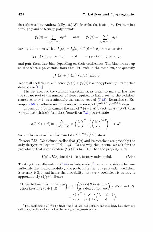
424 7. Lattices and Cryptography
first observed by Andrew Odlyzko.) We describe the basic idea. Eve searchesthrough pairs of ternary polynomials
f1(x) =∑
0≤i<N/2
aixi and f2(x) =
∑
N/2≤i<N
aixi
having the property that f1(x) + f2(x) ∈ T (d+ 1, d). She computes
f1(x) � h(x) (mod q) and − f2(x) � h(x) (mod q)
and puts them into bins depending on their coefficients. The bins are set upso that when a polynomial from each list lands in the same bin, the quantity
(f1(x) + f2(x)
)� h(x) (mod q)
has small coefficients, and hence f1(x) + f2(x) is a decryption key. For furtherdetails, see [101].
The net effect of the collision algorithm is, as usual, to more or less takethe square root of the number of steps required to find a key, so the collision-search security is approximately the square root of (7.43). Returning to Ex-
ample 7.56, a collision search takes on the order of√2381.6 ≈ 2190.8 steps.
In general, if we maximize the size of T (d+1, d) by setting d ≈ N/3, thenwe can use Stirling’s formula (Proposition 7.29) to estimate
#T (d+ 1, d) ≈ N !
((N/3)!)3≈(N
e
)N
·((
N
3e
)N/3)−3
≈ 3N .
So a collision search in this case take O(3N/2/√N ) steps.
Remark 7.58. We claimed earlier that f(x) and its rotations are probably theonly decryption keys in T (d + 1, d). To see why this is true, we ask for theprobability that some random f(x) ∈ T (d+ 1, d) has the property that
f(x) � h(x) (mod q) is a ternary polynomial. (7.44)
Treating the coefficients of (7.44) as independent8 random variables that areuniformly distributed modulo q, the probability that any particular coefficientis ternary is 3/q, and hence the probability that every coefficient is ternary isapproximately (3/q)N . Hence
(Expected number of decryp-tion keys in T (d+ 1, d)
)≈ Pr
(f(x) ∈ T (d+ 1, d)is a decryption key
)×#T (d+ 1, d)
=
(3
q
)N (N
d+ 1
)(N − d− 1
d
).
8The coefficients of f(x) � h(x) (mod q) are not entirely independent, but they aresufficiently independent for this to be a good approximation.
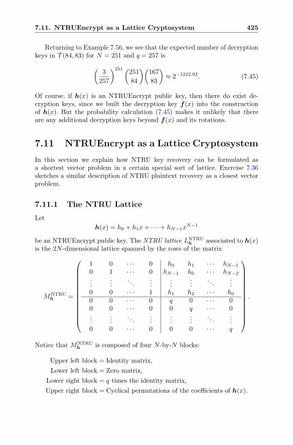
7.11. NTRUEncrypt as a Lattice Cryptosystem 425
Returning to Example 7.56, we see that the expected number of decryptionkeys in T (84, 83) for N = 251 and q = 257 is
(3
257
)251(251
84
)(167
83
)≈ 2−1222.02. (7.45)
Of course, if h(x) is an NTRUEncrypt public key, then there do exist de-cryption keys, since we built the decryption key f(x) into the constructionof h(x). But the probability calculation (7.45) makes it unlikely that thereare any additional decryption keys beyond f(x) and its rotations.
7.11 NTRUEncrypt as a Lattice Cryptosystem
In this section we explain how NTRU key recovery can be formulated asa shortest vector problem in a certain special sort of lattice. Exercise 7.36sketches a similar description of NTRU plaintext recovery as a closest vectorproblem.
7.11.1 The NTRU Lattice
Let
h(x) = h0 + h1x+ · · ·+ hN−1xN−1
be an NTRUEncrypt public key. The NTRU lattice LNTRUh associated to h(x)
is the 2N -dimensional lattice spanned by the rows of the matrix
MNTRUh =
⎛
⎜⎜⎜⎜⎜⎜⎜⎜⎜⎜⎜⎜⎝
1 0 · · · 0 h0 h1 · · · hN−1
0 1 · · · 0 hN−1 h0 · · · hN−2
......
. . ....
......
. . ....
0 0 · · · 1 h1 h2 · · · h00 0 · · · 0 q 0 · · · 00 0 · · · 0 0 q · · · 0...
.... . .
......
.... . .
...0 0 · · · 0 0 0 · · · q
⎞
⎟⎟⎟⎟⎟⎟⎟⎟⎟⎟⎟⎟⎠
.
Notice that MNTRUh is composed of four N -by-N blocks:
Upper left block = Identity matrix,
Lower left block = Zero matrix,
Lower right block = q times the identity matrix,
Upper right block = Cyclical permutations of the coefficients of h(x).
426 7. Lattices and Cryptography
It is often convenient to abbreviate the NTRU matrix as
MNTRUh =
(I h0 qI
), (7.46)
where we view (7.46) as a 2-by-2 matrix with coefficients in R.We are going to identify each pair of polynomials
a(x) = a0 + a1x+ · · ·+ aN−1xN−1 and b(x) = b0 + b1x+ · · ·+ bN−1x
N−1
in R with a 2N -dimensional vector
(a, b) = (a0, a1, . . . , aN−1, b0, b1, . . . , bN−1) ∈ Z2N .
We now suppose that the NTRUEncrypt public key h(x) was created usingthe private polynomials f(x) and g(x) and compute what happens when wemultiply the NTRU matrix by a carefully chosen vector.
Proposition 7.59. Assuming that f(x) �h(x) ≡ g(x) (mod q), let u(x) ∈ Rbe the polynomial satisfying
f(x) � h(x) = g(x) + qu(x). (7.47)
Then
(f ,−u)MNTRUh = (f , g), (7.48)
so the vector (f , g) is in the NTRU lattice LNTRUh .
Proof. It is clear that the first N coordinates of the product (7.48) are thevector f , since the left-hand side ofMNTRU
h is the identity matrix atop the zeromatrix. Next consider what happens when we multiply the column ofMNTRU
h
whose top entry is hk by the vector (f ,−u). We get the quantity
hkf0 + hk−1f1 + · · ·+ hk+1fN−1 − quk,
which is the kth entry of the vector f(x) � h(x)− qu(x). From (7.47), this isthe kth entry of the vector g, so the secondN coordinates of the product (7.48)form the vector g. Finally, (7.48) says that we can get the vector (f , g) bytaking a certain linear combination of the rows of MNTRU
h . Hence (f , g) ∈LNTRUh .
Remark 7.60. Using the abbreviation (7.46) and multiplying 2-by-2 matriceshaving coefficients in R, the proof of Proposition 7.59 becomes the succinctcomputation
(f ,−u)(1 h0 q
)= (f ,f � h− qu) = (f , g).
Proposition 7.61. Let (N, p, q, d) be NTRUEncrypt parameters, where forsimplicity we will assume that
p = 3 and d ≈ N/3 and q ≈ 6pd ≈ 2pN.
Let LNTRUh be an NTRU lattice associated to the private key (f , g).
7.11. NTRUEncrypt as a Lattice Cryptosystem 427
(a) det(LNTRUh ) = qN .
(b)∥∥(f , g)
∥∥ ≈
√4d ≈
√4N/3 ≈ 1.155
√N .
(c) The Gaussian heuristic predicts that the shortest nonzero vector in theNTRU lattice has length
σ(LNTRUh
)≈√Nq/πe ≈ 0.838N.
Hence if N is large, then there is a high probability that the shortest nonzerovectors in LNTRU
h are (f , g) and its rotations. Further,
∥∥(f , g)
∥∥
σ(L)≈ 1.38√
N,
so the vector (f , g) is a factor of O(1/√N ) shorter than predicted by the
Gaussian heuristic.
Proof. (a) Proposition 7.20 says that det(LNTRUh ) is equal to the determinant
of the matrix MNTRUh . The matrix is upper triangular, so its determinant is
the product of the diagonal entries, which equals qN .
(b) Each of f and g has (approximately) d coordinates equal to 1 and dcoordinates equal to −1.(c) Using (a) and keeping in mind that LNTRU
h has dimension 2N , we estimatethe Gaussian expected shortest length using the formula (7.21),
σ(LNTRUh
)=
√2N
2πe(detL)1/2N =
√Nq
πe≈√
6
πeN.
7.11.2 Quantifying the Security of an NTRU Lattice
Proposition 7.61 says that Eve can determine Alice’s private NTRU key if shecan find a shortest vector in the NTRU lattice LNTRU
h . Thus the security ofNTRUEncrypt depends at least on the difficulty of solving SVP in LNTRU
h .More generally, if Eve can solve apprSVP in LNTRU
h to within a factor ofapproximately N ε for some ε < 1
2 , then the short vector that she finds willprobably serve as a decryption key.
This leads to the question of how to estimate the difficulty of finding ashort, or shortest, vector in an NTRU lattice. The LLL algorithm that wedescribe in Sect. 7.13.2 runs in polynomial time and solves apprSVP to withina factor of 2N , but ifN is large, LLL does not find very small vectors in LNTRU
h .In Sect. 7.13.4 we describe a generalization of the LLL algorithm, called BKZ-LLL, that is able to find very small vectors. The BKZ-LLL algorithm includesa blocksize parameter β, and it solves apprSVP to within a factor of β2N/β ,but its running time is exponential in β.
428 7. Lattices and Cryptography
Unfortunately, the operating characteristics of standard lattice reductionalgorithms such as BKZ-LLL are not nearly as well understood as are theoperating characteristics of sieves, the index calculus, or Pollard’s ρ method.This makes it difficult to predict theoretically how well a lattice reductionalgorithm will perform on any given class of lattices. Thus in practice, thesecurity of a lattice-based cryptosystem such as NTRUEncrypt must be de-termined experimentally.
Roughly, one takes a sequence of parameters (N, q, d) in whichN grows andsuch that certain ratios involving N , q, and d are held approximately constant.For each set of parameters, one runs many experiments using BKZ-LLL withincreasing block size β until the algorithm finds a short vector in LNTRU
h .Then one plots the logarithm of the average running time against N , verifiesthat the points approximately lie on line, and computes the best-fitting line
log(Running Time) = AN +B. (7.49)
After doing this for many values of N up to the point at which the com-putations become infeasible, one can use the line (7.49) to extrapolate theexpected amount of time it would take to find a private key vector in anNTRU lattice LNTRU
h for larger values of N . Such experiments suggest thatvalues of N in the range from 250 to 1000 yield security levels comparable tocurrently secure implementations of RSA, Elgamal, and ECC. Details of suchexperiments are described in [102].
Remark 7.62. Proposition 7.61 says that the short target vectors in an NTRUlattice are O(
√N ) shorter than predicted by the Gaussian heuristic. Theoret-
ically and experimentally, it is true that if a lattice of dimension n has a vectorthat is extremely small, say O(2n) shorter than the Gaussian prediction, thenlattice reduction algorithms such as LLL and its variants are very good atfinding the tiny vector. It is a natural and extremely interesting question toask whether vectors that are only O(nε) shorter than the Gaussian predictionmight similarly be easier to find. At this time, no one knows the answer tothis question.
7.12 Lattice-Based Digital Signature Schemes
We have already seen digital signatures schemes whose security depends on theinteger factorization problem (Sect. 4.2) and on the discrete logarithm prob-lem in the multiplicative group (Sect. 4.3) or in an elliptic curve (Sect. 6.4.3).In this section we briefly discuss how digital signature schemes may be con-structed from hard lattice problems.
7.12.1 The GGH Digital Signature Scheme
It is easy to convert the CVP idea underlying GGH encryption into a lattice-based digital signature scheme. Samantha knows a good (i.e., short and
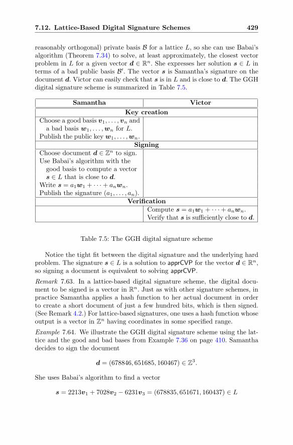
7.12. Lattice-Based Digital Signature Schemes 429
reasonably orthogonal) private basis B for a lattice L, so she can use Babai’salgorithm (Theorem 7.34) to solve, at least approximately, the closest vectorproblem in L for a given vector d ∈ R
n. She expresses her solution s ∈ L interms of a bad public basis B′. The vector s is Samantha’s signature on thedocument d. Victor can easily check that s is in L and is close to d. The GGHdigital signature scheme is summarized in Table 7.5.
Samantha Victor
Key creationChoose a good basis v1, . . . ,vn and
a bad basis w1, . . . ,wn for L.Publish the public key w1, . . . ,wn.
SigningChoose document d ∈ Z
n to sign.Use Babai’s algorithm with the
good basis to compute a vectors ∈ L that is close to d.
Write s = a1w1 + · · ·+ anwn.Publish the signature (a1, . . . , an).
VerificationCompute s = a1w1 + · · ·+ anwn.Verify that s is sufficiently close to d.
Table 7.5: The GGH digital signature scheme
Notice the tight fit between the digital signature and the underlying hardproblem. The signature s ∈ L is a solution to apprCVP for the vector d ∈ R
n,so signing a document is equivalent to solving apprCVP.
Remark 7.63. In a lattice-based digital signature scheme, the digital docu-ment to be signed is a vector in R
n. Just as with other signature schemes, inpractice Samantha applies a hash function to her actual document in orderto create a short document of just a few hundred bits, which is then signed.(See Remark 4.2.) For lattice-based signatures, one uses a hash function whoseoutput is a vector in Z
n having coordinates in some specified range.
Example 7.64. We illustrate the GGH digital signature scheme using the lat-tice and the good and bad bases from Example 7.36 on page 410. Samanthadecides to sign the document
d = (678846, 651685, 160467) ∈ Z3.
She uses Babai’s algorithm to find a vector
s = 2213v1 + 7028v2 − 6231v3 = (678835, 651671, 160437) ∈ L
430 7. Lattices and Cryptography
that is quite close to d,‖s− d‖ ≈ 34.89.
Samantha next uses linear algebra to express s in terms of the bad basis,
s = 1531010w1 − 553385w2 − 878508w3,
where w1,w2,w3 are the vectors on page 410. She publishes
(1531010,−553385,−878508)
as her signature for the document d. Victor verifies the signature by using thepublic basis to compute
s = 1531010w1 − 553385w2 − 878508w3 = (678835, 651671, 160437),
which is automatically a vector in L, and then verifying that ‖s−d‖ ≈ 34.89is small.
We observe that if Eve attempts to sign d using Babai’s algorithm withthe bad basis {w1,w2,w3}, then the signature that she obtains is
s′ = (2773584, 1595134,−131844) ∈ L.
This vector is not a good solution to apprCVP, since ‖s′ − d‖ > 106.
Remark 7.65 (Key Size Issues). The GGH signature scheme suffers the samedrawback as the GGH cryptosystem, namely security requires lattices ofhigh dimension, which in turn lead to very large public verification keys;cf. Sect. 7.7. It is thus tempting to use an NTRU lattice LNTRU as the pub-lic key, but there is an initial difficulty because LNTRU has dimension 2N ,so the known (secret) short vector (f , g) and its rotations (xi � f , xi � g)for 0 ≤ i < N give only half a very short basis for LNTRU. Using a techniquedescribed in [55], it is possible to extend the half-basis to a full basis thatis short enough to make an NTRU signature scheme feasible. However, bothGGH and NTRU signature schemes have a more serious shortcoming whichwe now describe.
7.12.2 Transcript Analysis
In any digital signature scheme, each document/signature pair (d, s) revealssome information about the private signing key v, since at the very least, it re-veals that the document d signed with the private key v yields the signature s.Hence a sufficiently long transcript of signed documents
(d1, s1), (d2, s2), (d3, s3), . . . , (dr, sr) (7.50)
may reveal information about either the signing key or how to sign additionaldocuments.
7.12. Lattice-Based Digital Signature Schemes 431
We illustrate with the GGH signature scheme. By construction, the sig-nature s is created using Babai’s algorithm to solve apprCVP with the goodbasis v1, . . . ,vn and target vector d. It follows that the difference d − s hasthe form
d− s =
n∑
i=1
εi(d, s)vi with∣∣εi(d, s)
∣∣ ≤ 1
2.
As d and s vary, the εi(d, s) values are more or less randomly distributedbetween − 1
2 and 12 . Hence the transcript (7.50) reveals to an adversary a large
number of points that are randomly scattered in the fundamental domain
F ={ε1v1 + ε2v2 + · · ·+ εnvn : − 1
2 < ε1, . . . , εn ≤ 12
}
spanned by the good secret basis v1, . . . ,vn. Using this collection of points, itmay be possible to (approximately) recover the basis vectors spanning the fun-damental domain F . An algorithm to perform this task was given by Nguyenand Regev [93, 94]. They used their algorithm to break instances of GGH indimension n with a transcript consisting of roughly n2 signatures, and theygave similar applications to NTRU signatures. It is possible to blunt these at-tacks by introducing small biased perturbations into each signature [55, 56],but the process is inefficient and may still be subject to transcript attacks [39].
7.12.3 Rejection Sampling
An alternative method of thwarting transcript attacks was proposed byLyubashevsky [80, 79, 78]. It is based on an idea from statistics called rejectionsampling, in which one generates samples from a desired probability distri-bution by using samples from another distribution. There are now a numberof proposed digital signature schemes that use rejection sampling to achievetranscript security. In this section we discuss rejection sampling as a generaltechnique, after which we apply rejection sampling to an abstract signaturescheme (Sect. 7.12.4) and illustrate the method with a specific lattice-basedscheme (Sect. 7.12.5).
The notion of rejection sampling was introduced by J. von Neumann in1951 [146]. His aim was to produce samples from a distribution F (x), whichis itself hard to sample, by using another distribution G(x) whose samplesare easy to produce.9 The use of rejection sampling in the context of foilinga transcript attack on a digital signature scheme amounts to a clever reversal ofthis situation. Imagine that the signature scheme somehow generates samplesthat can be used to produce a distribution G(x). The signature scheme isvulnerable to a transcript attack if this distribution G(x) possesses featuresthat provide information about the private key, since then sufficiently manysamples may reveal the key. In order to foil a transcript attack, one wantsto hide the unique identifying features of G(x). Under certain circumstances,
9Distribution functions are discussed in Sect. 5.3.4.
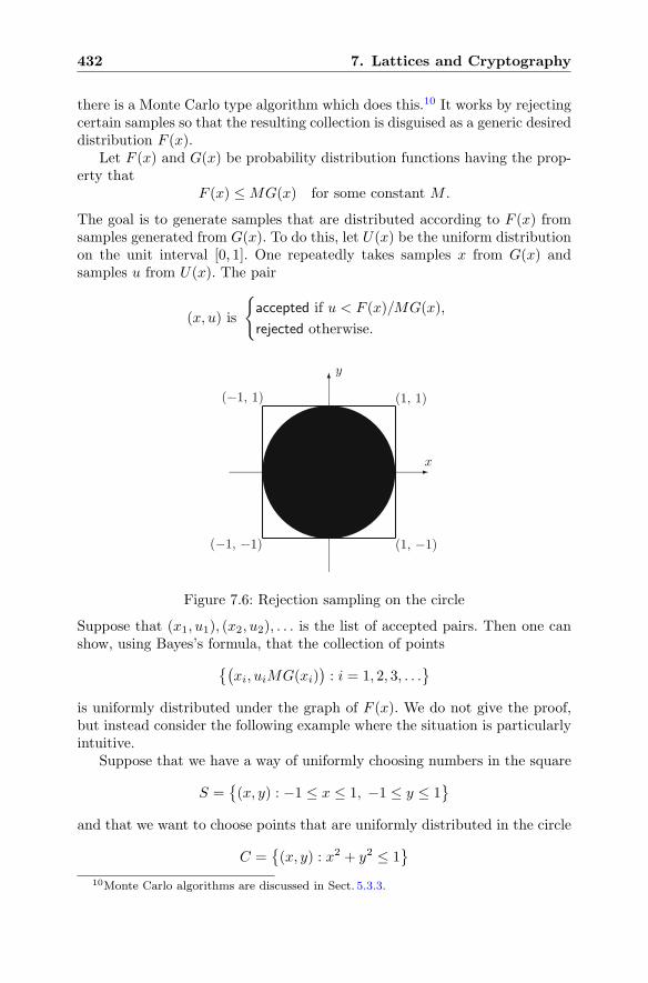
432 7. Lattices and Cryptography
there is a Monte Carlo type algorithm which does this.10 It works by rejectingcertain samples so that the resulting collection is disguised as a generic desireddistribution F (x).
Let F (x) and G(x) be probability distribution functions having the prop-erty that
F (x) ≤MG(x) for some constant M .
The goal is to generate samples that are distributed according to F (x) fromsamples generated from G(x). To do this, let U(x) be the uniform distributionon the unit interval [0, 1]. One repeatedly takes samples x from G(x) andsamples u from U(x). The pair
(x, u) is
{accepted if u < F (x)/MG(x),
rejected otherwise.
y
x
(−1, 1)
(−1, −1) (1, −1)
(1, 1)
Figure 7.6: Rejection sampling on the circle
Suppose that (x1, u1), (x2, u2), . . . is the list of accepted pairs. Then one canshow, using Bayes’s formula, that the collection of points
{(xi, uiMG(xi)
): i = 1, 2, 3, . . .
}
is uniformly distributed under the graph of F (x). We do not give the proof,but instead consider the following example where the situation is particularlyintuitive.
Suppose that we have a way of uniformly choosing numbers in the square
S ={(x, y) : −1 ≤ x ≤ 1, −1 ≤ y ≤ 1
}
and that we want to choose points that are uniformly distributed in the circle
C ={(x, y) : x2 + y2 ≤ 1
}
10Monte Carlo algorithms are discussed in Sect. 5.3.3.
7.12. Lattice-Based Digital Signature Schemes 433
as illustrated in Fig. 7.6. So our samples are points (x, y) in the plane, and ouruniform distribution functions on the circle and the square are, respectively,11
FC(x, y) =
⎧⎨
⎩
1
πif x2 + y2 ≤ 1,
0 otherwise;
GS(x, y) =
⎧⎨
⎩
1
4if −1 ≤ x ≤ 1 and 1 ≤ y ≤ 1,
0 otherwise.
For all (x, y) we clearly have
FC(x, y) ≤MGS(x, y) with M =4
π,
since FC(x, y)/GS(x, y) =M if (x, y) is in the circle, and equals 0 otherwise.Now the pair
((x, y), u
), where (x, y) is uniformly sampled from the square
and u is uniformly sampled from the interval [0, 1], will be accepted if and onlyif FC(x, y)/MGS(x, y) = 1, which means it is accepted if and only if (x, y) isin the circle. In brief, rejection sampling amounts to choosing points uniformlyin the square and rejecting those points which do not lie in the circle. Theresult is a collection of points uniformly distributed in the circle.
7.12.4 Rejection Sampling Applied to an AbstractSignature Scheme
In this section we describe, abstractly, how rejection sampling can be used toprotect a digital signature scheme from transcript attacks. Note that we aredescribing the properties that such a scheme should have, without giving anyindication of how one might create such a scheme. (Just as Diffie and Hellmandescribed what a public key cryptosystem should do, without providing anexample of such a system.)
We consider an abstract digital signature scheme (KPri,KPub, Sign,Verify)as described in Sect. 4.1. We assume further that the signing algorithm Signuses three inputs, the private key KPri, the document hash D being signed,and a random number R. Rejection sampling introduces a conditional prop-erty P. In order to sign D, Samantha chooses a random R and computes thesignature S = Sign(KPri, D,R). If S has property P, then she publishes S asthe signature on D; but if S does not have property P, then she rejects S,chooses a new value for R, and repeats the process. This means that in anytranscript of Samantha’s signatures (D1, S1), (D2, S2), . . . , every Si has prop-erty P.
Now for the tricky part. We want the attacker Eve, using only thepublic key KPub, to be able to create a list of pairs (D′
1, S′1), (D
′2, S
′2), . . .
satisfying:
11Why does FC have the 1/π and GS have the 1/4? It’s because the total probabilities∫∞−∞ FC(x, y) dx dy and
∫∞−∞ GS(x, y) dx dy must equal 1.
434 7. Lattices and Cryptography
(i) S′i is a valid signature on D′
i for the key KPub, i.e.,
Verify(KPub, D′i, S
′i) = TRUE for all i.
(ii) The distribution of Eve’s fake transcript (D′1, S
′1), (D
′2, S
′2), . . . is indis-
tinguishable from a transcript that Samantha creates using her privatekey KPri.Property (i) may seem problematic, since it says that Eve can produce an
unlimited number of valid document/signature pairs (D,S). However, recallthat D is really a hash of the actual document being signed. (See Sects. 4.2and 8.1 for a discussion of hash functions and their uses.) So although wewant Eve to be able to easily create valid (D,S) pairs, she will not know whatdocument she has signed, because she is not able to invert the hash function.In other words, although Eve can create valid pairs (D,S), if someone handsher a particular D, she will not be able to find an associated S. Thus security,as always, relies on various (reasonable) assumptions, in this case that we havea sufficiently cryptographically secure hash function.
7.12.5 The NTRU Modular Lattice Signature Scheme
Lyubashevsky gave an example of a transcript-secure signature scheme basedon the learning with errors (LWE) problem. We briefly sketch a new rejection-sampling signature scheme called NTRUMLS (NTRU modular lattice signa-ture scheme) that uses NTRU lattices [57].12 We set one piece of notation.The sup norm of a polynomial a(x) = a0 + a1x+ · · ·+ aN−1x
N−1 is denoted
‖a‖∞ = max{|a0|, |a1|, . . . , |aN−1|
}.
The basic set-up for NTRUMLS is similar to the set-up for NTRUEn-crypt in Sect. 7.10, with parameters (N, p, q), private key polynomials f and gwith small coefficients, and public key polynomial h ≡ f−1 � g (mod q).13
NTRUMLS also uses a public rejection parameter B and a public hash func-tion that takes a digital document μ and a public key h and creates a pair ofmod p polynomials:
Hash : {documents} × {public keys} −→ {pairs of mod p polynomials}Hash(μ,h) = (sp, tp).
An NTRUMLS signature on the document μ for the public key h is a pair ofpolynomials (s, t) satisfying the following three conditions:
12NTRUMLS was released in 2014, so it is very new. We present it as an illustration ofhow rejection sampling might work in practice, but as with all new systems, NTRUMLSwill require years of scrutiny before it can be deemed secure.
13There are some further minor requirements that we omit, since our aim is to illustratethe idea of rejection sampling. See Exercise 7.42.
7.12. Lattice-Based Digital Signature Schemes 435
(a) t ≡ s � h (mod q).
(b) s ≡ sp (mod p) and t ≡ tp (mod p), where (sp, tp) = Hash(μ,h).
(c) ‖s‖∞ ≤ 12q −B and ‖t‖∞ ≤ 1
2q −B.
Here are some further remarks on the three signing conditions:
(a) This ties the signature to the signing key. It is equivalent to the assertionthat (s, t) is in the lattice LNTRU
h associated to h; cf. Sect. 7.11.1.
(b) This ties the signature (s, t) to the document hash (sp, tp). It is equiv-alent to the assertion that the difference (s, t) − (sp, tp) is in the lat-tice (pZ)2N .
(c) This is the rejection sampling condition, since it says that we rejectthe signature (s, t) if it is too large. Note the tension inherent in thiscondition. If B is too large, then it will be difficult to generate signatures,while one can show that if B is not large enough, then transcripts leakprivate key information.
Using the private key (f , g), it is not hard to create a pair (s, t) satisfyingconditions (a) and (b). Further, for appropriately chosen values of p, q, and B,one can show that it will not take too many tries to find an (s, t) that alsosatisfies condition (c). (See Exercise 7.42 for details.)
The transcript security analysis relies on the following two facts. The proof,which we omit (see [57]), relies on various reasonable randomness assumptions.
• When the signing algorithm is applied to a given document hash (sp, tp),each pair (s, t) satisfying conditions (a), (b), (c) has an equal probabilityof being chosen as the signature.
• Suppose that an attacker creates a list of (s, t) pairs by randomly choos-ing s’s satisfying ‖s‖∞ ≤ 1
2q − B, computing t ≡ s � h (mod q), andkeeping the pair (s, t) if ‖t‖∞ ≤ 1
2q − B. Then the reduction of his listmodulo p is uniformly randomly distributed among all pairs of mod ppolynomials. (Note that the each of the attacker’s (s, t) pairs is a validsignature on the document hash (s mod p, t mod p) for the verificationkey h. He is thus able to create an arbitrarily long transcript of valid sig-natures, but he not able to specify, a priori, the tp parts of the documenthashes that he is signing.)
These two facts show that an attacker, using only the public key h, cancreate a transcript of signed document hashes that is indistinguishable froma transcript created using the private key (f , g). Hence the latter transcriptcontains no information about the private key. We refer the reader to the ref-erences [57, 80, 79, 78] for further details on NTRUMLS and other transcript-secure lattice-based signature schemes.
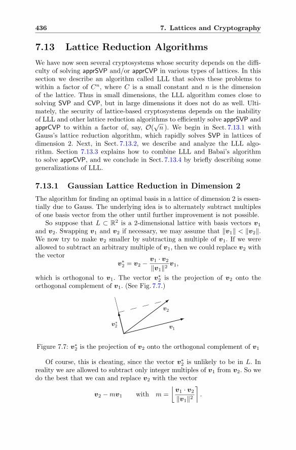
436 7. Lattices and Cryptography
7.13 Lattice Reduction Algorithms
We have now seen several cryptosystems whose security depends on the diffi-culty of solving apprSVP and/or apprCVP in various types of lattices. In thissection we describe an algorithm called LLL that solves these problems towithin a factor of Cn, where C is a small constant and n is the dimensionof the lattice. Thus in small dimensions, the LLL algorithm comes close tosolving SVP and CVP, but in large dimensions it does not do as well. Ulti-mately, the security of lattice-based cryptosystems depends on the inabilityof LLL and other lattice reduction algorithms to efficiently solve apprSVP andapprCVP to within a factor of, say, O(
√n ). We begin in Sect. 7.13.1 with
Gauss’s lattice reduction algorithm, which rapidly solves SVP in lattices ofdimension 2. Next, in Sect. 7.13.2, we describe and analyze the LLL algo-rithm. Section 7.13.3 explains how to combine LLL and Babai’s algorithmto solve apprCVP, and we conclude in Sect. 7.13.4 by briefly describing somegeneralizations of LLL.
7.13.1 Gaussian Lattice Reduction in Dimension 2
The algorithm for finding an optimal basis in a lattice of dimension 2 is essen-tially due to Gauss. The underlying idea is to alternately subtract multiplesof one basis vector from the other until further improvement is not possible.
So suppose that L ⊂ R2 is a 2-dimensional lattice with basis vectors v1
and v2. Swapping v1 and v2 if necessary, we may assume that ‖v1‖ < ‖v2‖.We now try to make v2 smaller by subtracting a multiple of v1. If we wereallowed to subtract an arbitrary multiple of v1, then we could replace v2 withthe vector
v∗2 = v2 −
v1 · v2
‖v1‖2v1,
which is orthogonal to v1. The vector v∗2 is the projection of v2 onto the
orthogonal complement of v1. (See Fig. 7.7.)
v1
v2
v2∗
Figure 7.7: v∗2 is the projection of v2 onto the orthogonal complement of v1
Of course, this is cheating, since the vector v∗2 is unlikely to be in L. In
reality we are allowed to subtract only integer multiples of v1 from v2. So wedo the best that we can and replace v2 with the vector
v2 −mv1 with m =
⌊v1 · v2
‖v1‖2⌉.
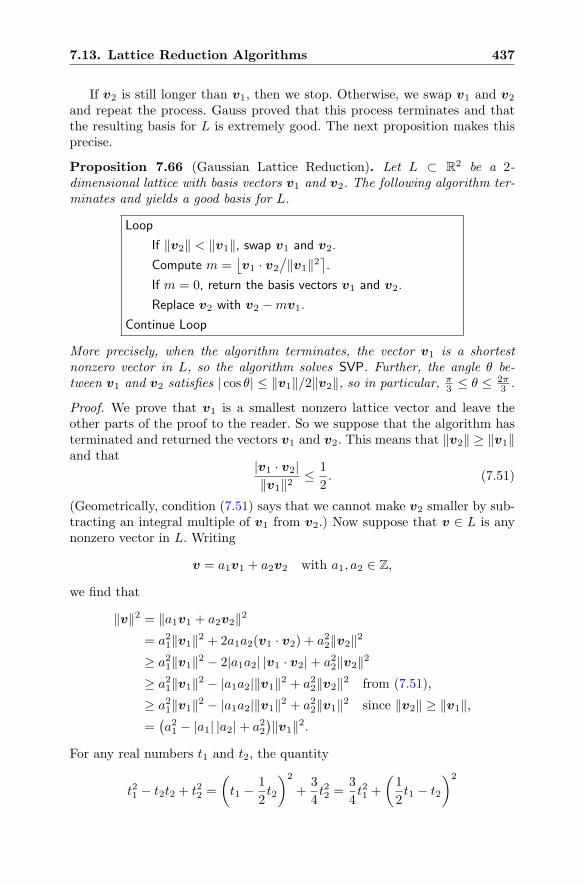
7.13. Lattice Reduction Algorithms 437
If v2 is still longer than v1, then we stop. Otherwise, we swap v1 and v2
and repeat the process. Gauss proved that this process terminates and thatthe resulting basis for L is extremely good. The next proposition makes thisprecise.
Proposition 7.66 (Gaussian Lattice Reduction). Let L ⊂ R2 be a 2-
dimensional lattice with basis vectors v1 and v2. The following algorithm ter-minates and yields a good basis for L.
Loop
If ‖v2‖ < ‖v1‖, swap v1 and v2.
Compute m =⌊v1 · v2
/‖v1‖2
⌉.
If m = 0, return the basis vectors v1 and v2.
Replace v2 with v2 −mv1.
Continue Loop
More precisely, when the algorithm terminates, the vector v1 is a shortestnonzero vector in L, so the algorithm solves SVP. Further, the angle θ be-tween v1 and v2 satisfies | cos θ| ≤ ‖v1‖/2‖v2‖, so in particular, π
3 ≤ θ ≤ 2π3 .
Proof. We prove that v1 is a smallest nonzero lattice vector and leave theother parts of the proof to the reader. So we suppose that the algorithm hasterminated and returned the vectors v1 and v2. This means that ‖v2‖ ≥ ‖v1‖and that
|v1 · v2|‖v1‖2
≤ 1
2. (7.51)
(Geometrically, condition (7.51) says that we cannot make v2 smaller by sub-tracting an integral multiple of v1 from v2.) Now suppose that v ∈ L is anynonzero vector in L. Writing
v = a1v1 + a2v2 with a1, a2 ∈ Z,
we find that
‖v‖2 = ‖a1v1 + a2v2‖2
= a21‖v1‖2 + 2a1a2(v1 · v2) + a22‖v2‖2
≥ a21‖v1‖2 − 2|a1a2| |v1 · v2|+ a22‖v2‖2
≥ a21‖v1‖2 − |a1a2|‖v1‖2 + a22‖v2‖2 from (7.51),
≥ a21‖v1‖2 − |a1a2|‖v1‖2 + a22‖v1‖2 since ‖v2‖ ≥ ‖v1‖,=(a21 − |a1| |a2|+ a22
)‖v1‖2.
For any real numbers t1 and t2, the quantity
t21 − t2t2 + t22 =
(t1 −
1
2t2
)2
+3
4t22 =
3
4t21 +
(1
2t1 − t2
)2
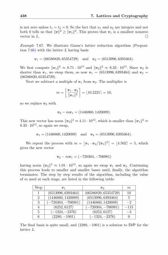
438 7. Lattices and Cryptography
is not zero unless t1 = t2 = 0. So the fact that a1 and a2 are integers and notboth 0 tells us that ‖v‖2 ≥ ‖v1‖2. This proves that v1 is a smallest nonzerovector in L.
Example 7.67. We illustrate Gauss’s lattice reduction algorithm (Proposi-tion 7.66) with the lattice L having basis
v1 = (66586820, 65354729) and v2 = (6513996, 6393464).
We first compute ‖v1‖2 ≈ 8.71 · 1015 and ‖v2‖2 ≈ 8.33 · 1013. Since v2 isshorter than v1, we swap them, so now v1 = (6513996, 6393464) and v2 =(66586820, 65354729).
Next we subtract a multiple of v1 from v2. The multiplier is
m =
⌊v1 · v2
‖v1‖2⌉= �10.2221! = 10,
so we replace v2 with
v2 −mv1 = (1446860, 1420089).
This new vector has norm ‖v2‖2 ≈ 4.11 · 1012, which is smaller than ‖v1‖2 ≈8.33 · 1013, so again we swap,
v1 = (1446860, 1420089) and v2 = (6513996, 6393464).
We repeat the process with m =⌊v1 · v2
/‖v1‖2
⌉= �4.502! = 5, which
gives the new vector
v2 −mv1 = (−720304,−706981)
having norm ‖v2‖2 ≈ 1.01 · 1012, so again we swap v1 and v2. Continuingthis process leads to smaller and smaller bases until, finally, the algorithmterminates. The step by step results of the algorithm, including the valueof m used at each stage, are listed in the following table:
Step v1 v2 m
1 (6513996, 6393464) (66586820, 65354729) 102 (1446860, 1420089) (6513996, 6393464) 53 (−720304,−706981) (1446860, 1420089) −24 (6252, 6127) (−720304,−706981) −1155 (−1324,−2376) (6252, 6127) −36 (2280,−1001) (−1324,−2376) 0
The final basis is quite small, and (2280,−1001) is a solution to SVP for thelattice L.
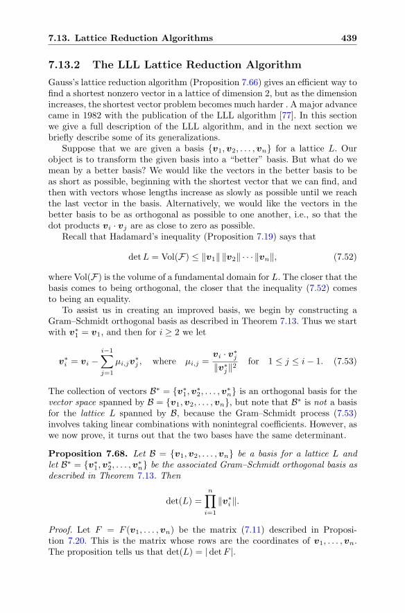
7.13. Lattice Reduction Algorithms 439
7.13.2 The LLL Lattice Reduction Algorithm
Gauss’s lattice reduction algorithm (Proposition 7.66) gives an efficient way tofind a shortest nonzero vector in a lattice of dimension 2, but as the dimensionincreases, the shortest vector problem becomes much harder . A major advancecame in 1982 with the publication of the LLL algorithm [77]. In this sectionwe give a full description of the LLL algorithm, and in the next section webriefly describe some of its generalizations.
Suppose that we are given a basis {v1,v2, . . . ,vn} for a lattice L. Ourobject is to transform the given basis into a “better” basis. But what do wemean by a better basis? We would like the vectors in the better basis to beas short as possible, beginning with the shortest vector that we can find, andthen with vectors whose lengths increase as slowly as possible until we reachthe last vector in the basis. Alternatively, we would like the vectors in thebetter basis to be as orthogonal as possible to one another, i.e., so that thedot products vi · vj are as close to zero as possible.
Recall that Hadamard’s inequality (Proposition 7.19) says that
detL = Vol(F) ≤ ‖v1‖ ‖v2‖ · · · ‖vn‖, (7.52)
where Vol(F) is the volume of a fundamental domain for L. The closer that thebasis comes to being orthogonal, the closer that the inequality (7.52) comesto being an equality.
To assist us in creating an improved basis, we begin by constructing aGram–Schmidt orthogonal basis as described in Theorem 7.13. Thus we startwith v∗
1 = v1, and then for i ≥ 2 we let
v∗i = vi −
i−1∑
j=1
μi,jv∗j , where μi,j =
vi · v∗j
‖v∗j‖2
for 1 ≤ j ≤ i− 1. (7.53)
The collection of vectors B∗ = {v∗1,v
∗2, . . . ,v
∗n} is an orthogonal basis for the
vector space spanned by B = {v1,v2, . . . ,vn}, but note that B∗ is not a basisfor the lattice L spanned by B, because the Gram–Schmidt process (7.53)involves taking linear combinations with nonintegral coefficients. However, aswe now prove, it turns out that the two bases have the same determinant.
Proposition 7.68. Let B = {v1,v2, . . . ,vn} be a basis for a lattice L andlet B∗ = {v∗
1,v∗2, . . . ,v
∗n} be the associated Gram–Schmidt orthogonal basis as
described in Theorem 7.13. Then
det(L) =
n∏
i=1
‖v∗i ‖.
Proof. Let F = F (v1, . . . ,vn) be the matrix (7.11) described in Proposi-tion 7.20. This is the matrix whose rows are the coordinates of v1, . . . ,vn.The proposition tells us that det(L) = | detF |.
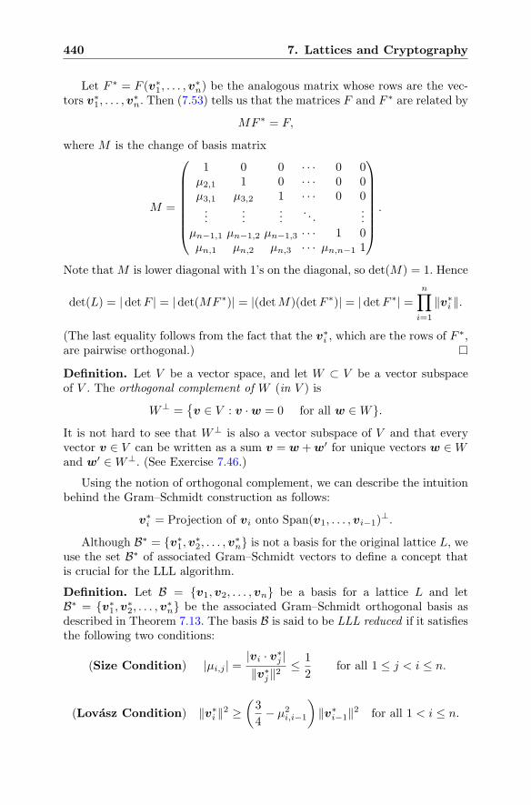
440 7. Lattices and Cryptography
Let F ∗ = F (v∗1, . . . ,v
∗n) be the analogous matrix whose rows are the vec-
tors v∗1, . . . ,v
∗n. Then (7.53) tells us that the matrices F and F ∗ are related by
MF ∗ = F,
where M is the change of basis matrix
M =
⎛
⎜⎜⎜⎜⎜⎜⎜⎝
1 0 0 · · · 0 0μ2,1 1 0 · · · 0 0μ3,1 μ3,2 1 · · · 0 0...
......
. . ....
μn−1,1 μn−1,2 μn−1,3 · · · 1 0μn,1 μn,2 μn,3 · · · μn,n−1 1
⎞
⎟⎟⎟⎟⎟⎟⎟⎠
.
Note thatM is lower diagonal with 1’s on the diagonal, so det(M) = 1. Hence
det(L) = | detF | = | det(MF ∗)| = |(detM)(detF ∗)| = | detF ∗| =n∏
i=1
‖v∗i ‖.
(The last equality follows from the fact that the v∗i , which are the rows of F ∗,
are pairwise orthogonal.)
Definition. Let V be a vector space, and let W ⊂ V be a vector subspaceof V . The orthogonal complement of W (in V ) is
W⊥ ={v ∈ V : v ·w = 0 for all w ∈W}.
It is not hard to see that W⊥ is also a vector subspace of V and that everyvector v ∈ V can be written as a sum v = w +w′ for unique vectors w ∈Wand w′ ∈W⊥. (See Exercise 7.46.)
Using the notion of orthogonal complement, we can describe the intuitionbehind the Gram–Schmidt construction as follows:
v∗i = Projection of vi onto Span(v1, . . . ,vi−1)
⊥.
Although B∗ = {v∗1,v
∗2, . . . ,v
∗n} is not a basis for the original lattice L, we
use the set B∗ of associated Gram–Schmidt vectors to define a concept thatis crucial for the LLL algorithm.
Definition. Let B = {v1,v2, . . . ,vn} be a basis for a lattice L and letB∗ = {v∗
1,v∗2, . . . ,v
∗n} be the associated Gram–Schmidt orthogonal basis as
described in Theorem 7.13. The basis B is said to be LLL reduced if it satisfiesthe following two conditions:
(Size Condition) |μi,j | =|vi · v∗
j |‖v∗
j‖2≤ 1
2for all 1 ≤ j < i ≤ n.
(Lovasz Condition) ‖v∗i ‖2 ≥
(3
4− μ2
i,i−1
)‖v∗
i−1‖2 for all 1 < i ≤ n.
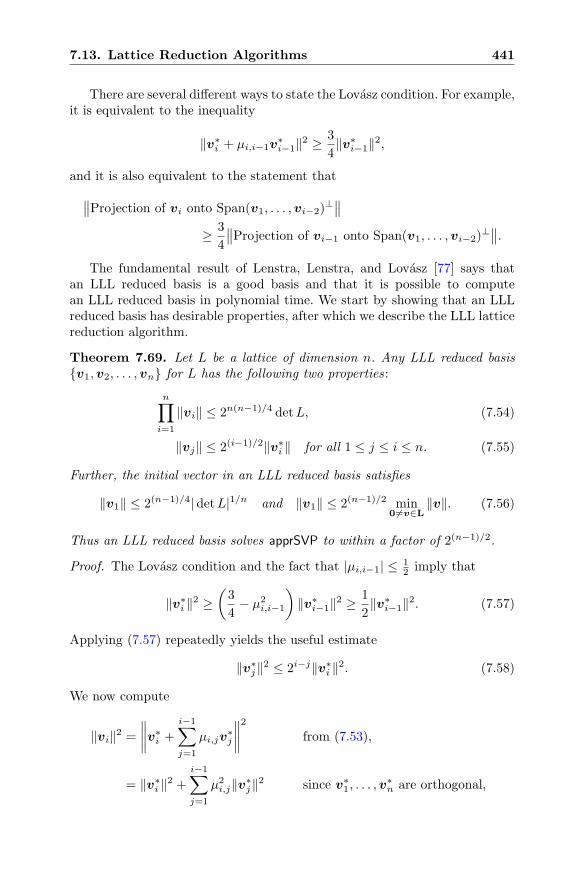
7.13. Lattice Reduction Algorithms 441
There are several different ways to state the Lovasz condition. For example,it is equivalent to the inequality
‖v∗i + μi,i−1v
∗i−1‖2 ≥
3
4‖v∗
i−1‖2,
and it is also equivalent to the statement that
∥∥Projection of vi onto Span(v1, . . . ,vi−2)
⊥∥∥
≥ 3
4
∥∥Projection of vi−1 onto Span(v1, . . . ,vi−2)
⊥∥∥.
The fundamental result of Lenstra, Lenstra, and Lovasz [77] says thatan LLL reduced basis is a good basis and that it is possible to computean LLL reduced basis in polynomial time. We start by showing that an LLLreduced basis has desirable properties, after which we describe the LLL latticereduction algorithm.
Theorem 7.69. Let L be a lattice of dimension n. Any LLL reduced basis{v1,v2, . . . ,vn} for L has the following two properties :
n∏
i=1
‖vi‖ ≤ 2n(n−1)/4 detL, (7.54)
‖vj‖ ≤ 2(i−1)/2‖v∗i ‖ for all 1 ≤ j ≤ i ≤ n. (7.55)
Further, the initial vector in an LLL reduced basis satisfies
‖v1‖ ≤ 2(n−1)/4| detL|1/n and ‖v1‖ ≤ 2(n−1)/2 min0 �=v∈L
‖v‖. (7.56)
Thus an LLL reduced basis solves apprSVP to within a factor of 2(n−1)/2.
Proof. The Lovasz condition and the fact that |μi,i−1| ≤ 12 imply that
‖v∗i ‖2 ≥
(3
4− μ2
i,i−1
)‖v∗
i−1‖2 ≥1
2‖v∗
i−1‖2. (7.57)
Applying (7.57) repeatedly yields the useful estimate
‖v∗j‖2 ≤ 2i−j‖v∗
i ‖2. (7.58)
We now compute
‖vi‖2 =
∥∥∥∥v
∗i +
i−1∑
j=1
μi,jv∗j
∥∥∥∥
2
from (7.53),
= ‖v∗i ‖2 +
i−1∑
j=1
μ2i,j‖v∗
j‖2 since v∗1, . . . ,v
∗n are orthogonal,
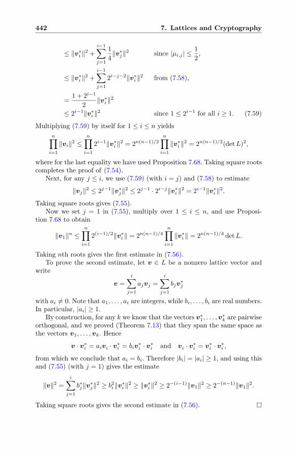
442 7. Lattices and Cryptography
≤ ‖v∗i ‖2 +
i−1∑
j=1
1
4‖v∗
j‖2 since |μi,j | ≤1
2,
≤ ‖v∗i ‖2 +
i−1∑
j=1
2i−j−2‖v∗i ‖2 from (7.58),
=1 + 2i−1
2‖v∗
i ‖2
≤ 2i−1‖v∗i ‖2 since 1 ≤ 2i−1 for all i ≥ 1. (7.59)
Multiplying (7.59) by itself for 1 ≤ i ≤ n yields
n∏
i=1
‖vi‖2 ≤n∏
i=1
2i−1‖v∗i ‖2 = 2n(n−1)/2
n∏
i=1
‖v∗i ‖2 = 2n(n−1)/2(detL)2,
where for the last equality we have used Proposition 7.68. Taking square rootscompletes the proof of (7.54).
Next, for any j ≤ i, we use (7.59) (with i = j) and (7.58) to estimate
‖vj‖2 ≤ 2j−1‖v∗j‖2 ≤ 2j−1 · 2i−j‖v∗
i ‖2 = 2i−1‖v∗i ‖2.
Taking square roots gives (7.55).Now we set j = 1 in (7.55), multiply over 1 ≤ i ≤ n, and use Proposi-
tion 7.68 to obtain
‖v1‖n ≤n∏
i=1
2(i−1)/2‖v∗i ‖ = 2n(n−1)/4
n∏
i=1
‖v∗i ‖ = 2n(n−1)/4 detL.
Taking nth roots gives the first estimate in (7.56).To prove the second estimate, let v ∈ L be a nonzero lattice vector and
write
v =i∑
j=1
ajvj =i∑
j=1
bjv∗j
with ai �= 0. Note that a1, . . . , ai are integers, while bi, . . . , bi are real numbers.In particular, |ai| ≥ 1.
By construction, for any k we know that the vectors v∗1, . . . ,v
∗k are pairwise
orthogonal, and we proved (Theorem 7.13) that they span the same space asthe vectors v1, . . . ,vk. Hence
v · v∗i = aivi · v∗
i = biv∗i · v∗
i and vi · v∗i = v∗
i · v∗i ,
from which we conclude that ai = bi. Therefore |bi| = |ai| ≥ 1, and using thisand (7.55) (with j = 1) gives the estimate
‖v‖2 =
i∑
j=1
b∗j‖v∗j‖2 ≥ b2i ‖v∗
i ‖2 ≥ ‖v∗i ‖2 ≥ 2−(i−1)‖v1‖2 ≥ 2−(n−1)‖v1‖2.
Taking square roots gives the second estimate in (7.56).
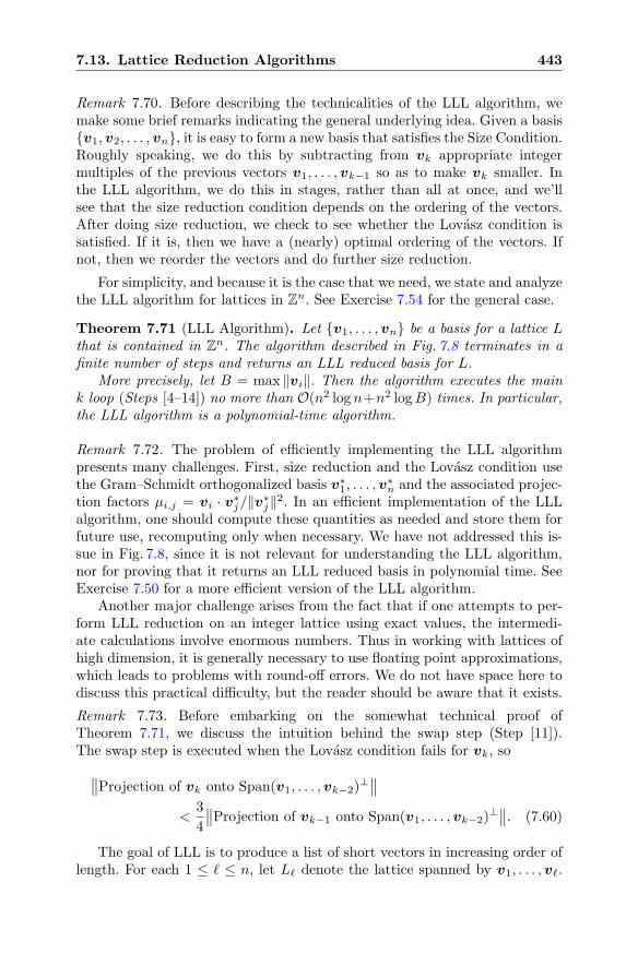
7.13. Lattice Reduction Algorithms 443
Remark 7.70. Before describing the technicalities of the LLL algorithm, wemake some brief remarks indicating the general underlying idea. Given a basis{v1,v2, . . . ,vn}, it is easy to form a new basis that satisfies the Size Condition.Roughly speaking, we do this by subtracting from vk appropriate integermultiples of the previous vectors v1, . . . ,vk−1 so as to make vk smaller. Inthe LLL algorithm, we do this in stages, rather than all at once, and we’llsee that the size reduction condition depends on the ordering of the vectors.After doing size reduction, we check to see whether the Lovasz condition issatisfied. If it is, then we have a (nearly) optimal ordering of the vectors. Ifnot, then we reorder the vectors and do further size reduction.
For simplicity, and because it is the case that we need, we state and analyzethe LLL algorithm for lattices in Z
n. See Exercise 7.54 for the general case.
Theorem 7.71 (LLL Algorithm). Let {v1, . . . ,vn} be a basis for a lattice Lthat is contained in Z
n. The algorithm described in Fig. 7.8 terminates in afinite number of steps and returns an LLL reduced basis for L.
More precisely, let B = max ‖vi‖. Then the algorithm executes the maink loop (Steps [4–14]) no more than O(n2 log n+n2 logB) times. In particular,the LLL algorithm is a polynomial-time algorithm.
Remark 7.72. The problem of efficiently implementing the LLL algorithmpresents many challenges. First, size reduction and the Lovasz condition usethe Gram–Schmidt orthogonalized basis v∗
1, . . . ,v∗n and the associated projec-
tion factors μi,j = vi · v∗j/‖v∗
j‖2. In an efficient implementation of the LLLalgorithm, one should compute these quantities as needed and store them forfuture use, recomputing only when necessary. We have not addressed this is-sue in Fig. 7.8, since it is not relevant for understanding the LLL algorithm,nor for proving that it returns an LLL reduced basis in polynomial time. SeeExercise 7.50 for a more efficient version of the LLL algorithm.
Another major challenge arises from the fact that if one attempts to per-form LLL reduction on an integer lattice using exact values, the intermedi-ate calculations involve enormous numbers. Thus in working with lattices ofhigh dimension, it is generally necessary to use floating point approximations,which leads to problems with round-off errors. We do not have space here todiscuss this practical difficulty, but the reader should be aware that it exists.
Remark 7.73. Before embarking on the somewhat technical proof ofTheorem 7.71, we discuss the intuition behind the swap step (Step [11]).The swap step is executed when the Lovasz condition fails for vk, so
∥∥Projection of vk onto Span(v1, . . . ,vk−2)
⊥∥∥
<3
4
∥∥Projection of vk−1 onto Span(v1, . . . ,vk−2)
⊥∥∥. (7.60)
The goal of LLL is to produce a list of short vectors in increasing order oflength. For each 1 ≤ � ≤ n, let L� denote the lattice spanned by v1, . . . ,v�.
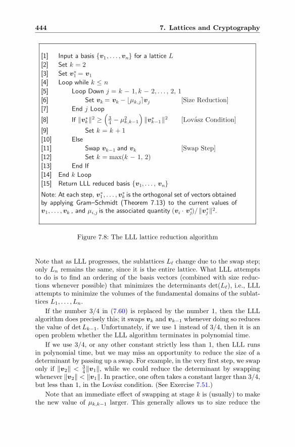
444 7. Lattices and Cryptography
[1] Input a basis {v1 , . . . ,vn} for a lattice L[2] Set k = 2[3] Set v1 = v1
∗
[4] Loop while k ≤ n[5] Loop Down j = k − 1, k − 2, . . . , 2, 1[6] Set vk = vk − �μk,j�vj [Size Reduction][7] End j Loop
[8] If ‖vk∗‖2 ≥
(34 − μk,k−1
2)
‖vk−1∗ ‖2 [Lovasz Condition]
[9] Set k = k + 1[10] Else[11] Swap vk−1 and vk [Swap Step][12] Set k = max(k − 1, 2)[13] End If[14] End k Loop[15] Return LLL reduced basis {v1, . . . , vn}Note: At each step, v1
∗, . . . ,vk is the orthogonal set of vectors obtained∗
by applying Gram–Schmidt (Theorem 7.13) to the current values ofv1, . . . ,vk , and μi,j is the associated quantity (vi · vj)/∗ ‖vj
∗‖2.
´
Figure 7.8: The LLL lattice reduction algorithm
Note that as LLL progresses, the sublattices L� change due to the swap step;only Ln remains the same, since it is the entire lattice. What LLL attemptsto do is to find an ordering of the basis vectors (combined with size reduc-tions whenever possible) that minimizes the determinants det(L�), i.e., LLLattempts to minimize the volumes of the fundamental domains of the sublat-tices L1, . . . , Ln.
If the number 3/4 in (7.60) is replaced by the number 1, then the LLLalgorithm does precisely this; it swaps vk and vk−1 whenever doing so reducesthe value of detLk−1. Unfortunately, if we use 1 instead of 3/4, then it is anopen problem whether the LLL algorithm terminates in polynomial time.
If we use 3/4, or any other constant strictly less than 1, then LLL runsin polynomial time, but we may miss an opportunity to reduce the size of adeterminant by passing up a swap. For example, in the very first step, we swaponly if ‖v2‖ < 3
4‖v1‖, while we could reduce the determinant by swappingwhenever ‖v2‖ < ‖v1‖. In practice, one often takes a constant larger than 3/4,but less than 1, in the Lovasz condition. (See Exercise 7.51.)
Note that an immediate effect of swapping at stage k is (usually) to makethe new value of μk,k−1 larger. This generally allows us to size reduce the
7.13. Lattice Reduction Algorithms 445
new vk using the new vk−1, so swapping results in additional size reductionamong the basis vectors, making them more orthogonal.
Proof (sketch) of Theorem 7.71. For simplicity, and because it is the casethat we need, we will assume that L ⊂ Z
n is a lattice whose vectors haveintegral coordinates.
It is clear that if the LLL algorithm terminates, then it terminates withan LLL reduced basis, since the j-loop (Steps [5–7]) ensures that the basissatisfies the size condition, and the fact that k = n+1 on termination meansthat every vector in the basis has passed the Lovasz condition test in Step [8].
However, it is not clear that the algorithm actually terminates, becausethe k-increment in Step [9] is offset by the k-decrement in Step [12]. What wewill do is show that Step [12] is executed only a finite number of times. Sinceeither Step [9] or Step [12] is executed on each iteration of the k-loop, thisensures that k eventually becomes larger than n and the algorithm terminates.
Let v1, . . . ,vn be a basis of L and let v∗1, . . . ,v
∗n be the associated Gram–
Schmidt orthogonalized basis from Theorem 7.13. For each � = 1, 2, . . . , n,we let
L� = lattice spanned by v1,. . . ,v�,
and we define quantities
d� =
�∏
i=1
‖v∗i ‖2 and D =
n∏
�=1
d� =
n∏
i=1
‖v∗i ‖2(n+1−i).
Using an argument similar to the proof of Theorem 7.68, one can showthat det(L�)
2 = d�; see Exercise 7.14(b,d).During the LLL algorithm, the value of D changes only when we execute
the swap step (Step [11]). More precisely, when [11] is executed, the only d�that changes is dk−1, since if � < k− 1, then d� involves neither v
∗k−1 nor v∗
k,while if � ≥ k, then the product defining d� includes both v∗
k−1 and v∗k, so the
product doesn’t change if we swap them.We can estimate the change in dk−1 by noting that when [11] is executed,
the Lovasz condition in Step [8] is false, so we have
‖v∗k‖2 <
(3
4− μ2
k,k−1
)‖v∗
k−1‖2 ≤3
4‖v∗
k−1‖2.
Hence the effect of swapping v∗k and v∗
k−1 in Step [11] is to change the valueof dk−1 as follows:
dnewk−1 = ‖v∗1‖2 · ‖v∗
2‖2 · · · ‖v∗k−2‖2 · ‖v∗
k‖2
= ‖v∗1‖2 · ‖v∗
2‖2 · · · ‖v∗k−2‖2 · ‖v∗
k−1‖2 ·‖v∗
k‖2‖v∗
k−1‖2
= doldk−1 ·‖v∗
k‖2‖v∗
k−1‖2≤ 3
4doldk−1.
446 7. Lattices and Cryptography
Hence if the swap step [11] is executed N times, then the value of D is reducedby a factor of at least (3/4)N , since each swap reduces the value of some d�by at least a factor of 3/4 and D is the product of all of the d�’s.
Since we have assumed that the lattice L is contained in Zn, the basis
vectors v1, . . . ,v� of L� have integer coordinates. It follows from the definitionof d� and Exercise 7.14(d) that
d� =�∏
i=1
‖v∗i ‖2 = det
((vi · vj
)1≤i,j≤�
),
which shows d� is a positive integer. Hence
D =n∏
�=1
d� ≥ 1. (7.61)
Hence D is bounded away from 0 by a constant depending only on the di-mension of the lattice L, so it can be multiplied by 3/4 only a finite numberof times. This proves that the LLL algorithm terminates.
In order to give an upper bound on the running time, we do some fur-ther estimations. Let Dinit denote the initial value of D for the original basis,let Dfinal denote the value of D for the basis when the LLL algorithm termi-nates, and as above, let N denote the number of times that the swap step(Step [11]) is executed. (Note that the k loop is executed at most 2N + ntimes, so it suffices to find a bound for N .) The lower bound for D is valid forevery basis produced during the execution of the algorithm, so by our earlierresults we know that
1 ≤ Dfinal ≤ (3/4)NDinit.
Taking logarithms yields (note that log(3/4) < 1)
N = O(logDinit).
To complete the proof, we need to estimate the size of Dinit. But this is easy,since by the Gram–Schmidt construction we certainly have ‖v∗
i ‖ ≤ ‖vi‖, so
Dinit =
n∏
i=1
‖v∗i ‖n+1−i ≤
n∏
i=1
‖vi‖n+1−i ≤(max1≤i≤n
‖vi‖)2(1+2+···+n)
= Bn2+n.
Hence logDinit = O(n2 logB).
Remark 7.74. Rather than counting the number of times that the main loopis executed, we might instead count the number of basic arithmetic operationsrequired by LLL. This means counting how many times the internal j-loopis executed and also how many times we perform operations on the coordi-nates of a vector. For example, adding two vectors or multiplying a vectorby a constant is n basic operations. Counted in this way, it is proven in [77]that the LLL algorithm (if efficiently implemented) terminates after no morethan O
(n6(logB)3
)basic operations.
7.13. Lattice Reduction Algorithms 447
Example 7.75. We illustrate the LLL algorithm on the 6-dimensional lattice Lwith (ordered) basis given by the rows of the matrix
M =
⎛
⎜⎜⎜⎜⎜⎝
19 2 32 46 3 3315 42 11 0 3 2443 15 0 24 4 1620 44 44 0 18 150 48 35 16 31 31
48 33 32 9 1 29
⎞
⎟⎟⎟⎟⎟⎠.
The smallest vector in this basis is ‖v2‖ = 51.913.The output from LLL is the basis consisting of the rows of the matrix
MLLL =
⎛
⎜⎜⎜⎜⎜⎝
7 −12 −8 4 19 9−20 4 −9 16 13 16
5 2 33 0 15 −9−6 −7 −20 −21 8 −12
−10 −24 21 −15 −6 −117 4 −9 −11 1 31
⎞
⎟⎟⎟⎟⎟⎠.
We check that both matrices have the same determinant,
det(M) = det(MLLL) = ±777406251.Further, as expected, the LLL reduced matrix has a much better (i.e., larger)Hadamard ratio than the original matrix,
H(M) = 0.46908 and H(MLLL) = 0.88824,
so the vectors in the LLL basis are more orthogonal. (The Hadamard ratiois defined in Remark 7.27.) The smallest vector in the LLL reduced basis is‖v1‖ = 26.739, which is a significant improvement over the original basis. Thismay be compared with the Gaussian expected shortest length (Remark 7.32)of σ(L) = (3! detL)1/3/
√π = 23.062.
The LLL algorithm executed 19 swap steps (Step [11] in Fig. 7.8). Thesequence of k values from start to finish was
2, 2, 3, 2, 3, 4, 3, 2, 2, 3, 4, 5, 4, 3, 2, 3, 4, 5, 4, 3, 4, 5, 6, 5,
4, 3, 4, 5, 6, 5, 4, 3, 2, 2, 3, 2, 3, 4, 5, 6.
Notice how the algorithm almost finished twice (it got to k = 6) before finallyterminating the third time. This illustrates how the value of k moves up anddown as the algorithm proceeds.
We next reverse the order of the rows of M and apply LLL. Then LLLexecutes only 11 swap steps and gives the basis
MLLL =
⎛
⎜⎜⎜⎜⎜⎝
−7 12 8 −4 −19 −920 −4 9 −16 −13 −16
−28 11 12 −9 17 −14−6 −7 −20 −21 8 −12−7 −4 9 11 −1 −3110 24 −21 15 6 11
⎞
⎟⎟⎟⎟⎟⎠.
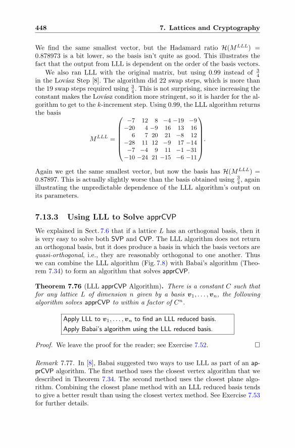
448 7. Lattices and Cryptography
We find the same smallest vector, but the Hadamard ratio H(MLLL) =0.878973 is a bit lower, so the basis isn’t quite as good. This illustrates thefact that the output from LLL is dependent on the order of the basis vectors.
We also ran LLL with the original matrix, but using 0.99 instead of 34
in the Lovasz Step [8]. The algorithm did 22 swap steps, which is more thanthe 19 swap steps required using 3
4 . This is not surprising, since increasing theconstant makes the Lovasz condition more stringent, so it is harder for the al-gorithm to get to the k-increment step. Using 0.99, the LLL algorithm returnsthe basis
MLLL =
⎛
⎜⎜⎜⎜⎜⎝
−7 12 8 −4 −19 −9−20 4 −9 16 13 16
6 7 20 21 −8 12−28 11 12 −9 17 −14−7 −4 9 11 −1 −31
−10 −24 21 −15 −6 −11
⎞
⎟⎟⎟⎟⎟⎠.
Again we get the same smallest vector, but now the basis has H(MLLL) =0.87897. This is actually slightly worse than the basis obtained using 3
4 , againillustrating the unpredictable dependence of the LLL algorithm’s output onits parameters.
7.13.3 Using LLL to Solve apprCVP
We explained in Sect. 7.6 that if a lattice L has an orthogonal basis, then itis very easy to solve both SVP and CVP. The LLL algorithm does not returnan orthogonal basis, but it does produce a basis in which the basis vectors arequasi-orthogonal, i.e., they are reasonably orthogonal to one another. Thuswe can combine the LLL algorithm (Fig. 7.8) with Babai’s algorithm (Theo-rem 7.34) to form an algorithm that solves apprCVP.
Theorem 7.76 (LLL apprCVP Algorithm). There is a constant C such thatfor any lattice L of dimension n given by a basis v1, . . . ,vn, the followingalgorithm solves apprCVP to within a factor of Cn.
Apply LLL to v1, . . . ,vn to find an LLL reduced basis.
Apply Babai’s algorithm using the LLL reduced basis.
Proof. We leave the proof for the reader; see Exercise 7.52.
Remark 7.77. In [8], Babai suggested two ways to use LLL as part of an ap-prCVP algorithm. The first method uses the closest vertex algorithm that wedescribed in Theorem 7.34. The second method uses the closest plane algo-rithm. Combining the closest plane method with an LLL reduced basis tendsto give a better result than using the closest vertex method. See Exercise 7.53for further details.
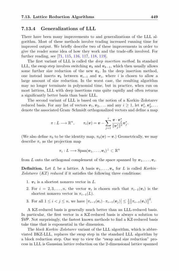
7.13. Lattice Reduction Algorithms 449
7.13.4 Generalizations of LLL
There have been many improvements to and generalizations of the LLL al-gorithm. Most of these methods involve trading increased running time forimproved output. We briefly describe two of these improvements in order togive the reader some idea of how they work and the trade-offs involved. Forfurther reading, see [71, 115, 116, 117, 118, 119].
The first variant of LLL is called the deep insertion method. In standardLLL, the swap step involves switching vk and vk−1, which then usually allowssome further size reduction of the new vk. In the deep insertion method,one instead inserts vk between vi−1 and vi, where i is chosen to allow alarge amount of size reduction. In the worst case, the resulting algorithmmay no longer terminate in polynomial time, but in practice, when run onmost lattices, LLL with deep insertions runs quite rapidly and often returnsa significantly better basis than basic LLL.
The second variant of LLL is based on the notion of a Korkin–Zolotarevreduced basis. For any list of vectors v1,v2, . . . and any i ≥ 1, let v∗
1,v∗2, . . .
denote the associated Gram–Schmidt orthogonalized vectors and define a map
π : L −→ Rn, πi(v) = v −
i∑
j=1
v · v∗j
‖v∗j‖2
v∗j .
(We also define π0 to be the identity map, π0(v) = v.) Geometrically, we maydescribe πi as the projection map
πi : L −→ Span(v1, . . . ,vi)⊥ ⊂ R
n
from L onto the orthogonal complement of the space spanned by v1, . . . ,vi.
Definition. Let L be a lattice. A basis v1, . . . ,vn for L is called Korkin–Zolotarev (KZ ) reduced if it satisfies the following three conditions:
1. v1 is a shortest nonzero vector in L.
2. For i = 2, 3, . . . , n, the vector vi is chosen such that πi−1(vi) is theshortest nonzero vector in πi−1(L).
3. For all 1 ≤ i < j ≤ n, we have∣∣πi−1(vi) · πi−1(vj)
∣∣ ≤ 1
2
∥∥πi−1(vi)
∥∥2.
A KZ-reduced basis is generally much better than an LLL-reduced basis.In particular, the first vector in a KZ-reduced basis is always a solution toSVP. Not surprisingly, the fastest known methods to find a KZ-reduced basistake time that is exponential in the dimension.
The block Korkin–Zolotarev variant of the LLL algorithm, which is abbre-viated BKZ-LLL, replaces the swap step in the standard LLL algorithm bya block reduction step. One way to view the “swap and size reduction” pro-cess in LLL is Gaussian lattice reduction on the 2-dimensional lattice spanned
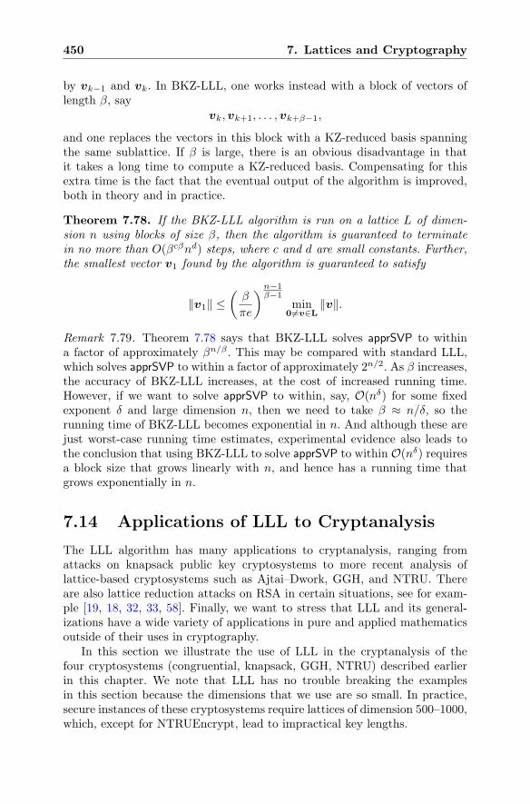
450 7. Lattices and Cryptography
by vk−1 and vk. In BKZ-LLL, one works instead with a block of vectors oflength β, say
vk,vk+1, . . . ,vk+β−1,
and one replaces the vectors in this block with a KZ-reduced basis spanningthe same sublattice. If β is large, there is an obvious disadvantage in thatit takes a long time to compute a KZ-reduced basis. Compensating for thisextra time is the fact that the eventual output of the algorithm is improved,both in theory and in practice.
Theorem 7.78. If the BKZ-LLL algorithm is run on a lattice L of dimen-sion n using blocks of size β, then the algorithm is guaranteed to terminatein no more than O(βcβnd) steps, where c and d are small constants. Further,the smallest vector v1 found by the algorithm is guaranteed to satisfy
‖v1‖ ≤(β
πe
)n−1β−1
min0 �=v∈L
‖v‖.
Remark 7.79. Theorem 7.78 says that BKZ-LLL solves apprSVP to withina factor of approximately βn/β . This may be compared with standard LLL,which solves apprSVP to within a factor of approximately 2n/2. As β increases,the accuracy of BKZ-LLL increases, at the cost of increased running time.However, if we want to solve apprSVP to within, say, O(nδ) for some fixedexponent δ and large dimension n, then we need to take β ≈ n/δ, so therunning time of BKZ-LLL becomes exponential in n. And although these arejust worst-case running time estimates, experimental evidence also leads tothe conclusion that using BKZ-LLL to solve apprSVP to within O(nδ) requiresa block size that grows linearly with n, and hence has a running time thatgrows exponentially in n.
7.14 Applications of LLL to Cryptanalysis
The LLL algorithm has many applications to cryptanalysis, ranging fromattacks on knapsack public key cryptosystems to more recent analysis oflattice-based cryptosystems such as Ajtai–Dwork, GGH, and NTRU. Thereare also lattice reduction attacks on RSA in certain situations, see for exam-ple [19, 18, 32, 33, 58]. Finally, we want to stress that LLL and its general-izations have a wide variety of applications in pure and applied mathematicsoutside of their uses in cryptography.
In this section we illustrate the use of LLL in the cryptanalysis of thefour cryptosystems (congruential, knapsack, GGH, NTRU) described earlierin this chapter. We note that LLL has no trouble breaking the examplesin this section because the dimensions that we use are so small. In practice,secure instances of these cryptosystems require lattices of dimension 500–1000,which, except for NTRUEncrypt, lead to impractical key lengths.
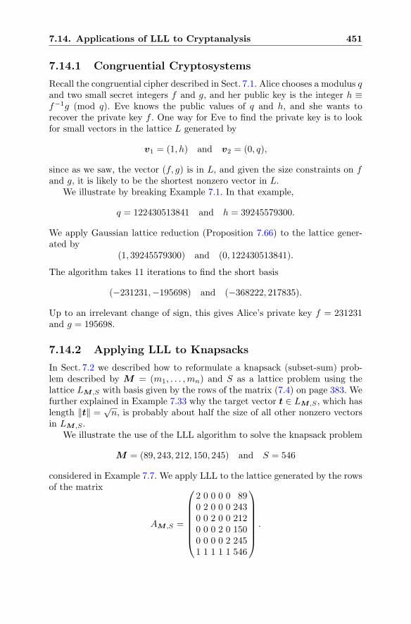
7.14. Applications of LLL to Cryptanalysis 451
7.14.1 Congruential Cryptosystems
Recall the congruential cipher described in Sect. 7.1. Alice chooses a modulus qand two small secret integers f and g, and her public key is the integer h ≡f−1g (mod q). Eve knows the public values of q and h, and she wants torecover the private key f . One way for Eve to find the private key is to lookfor small vectors in the lattice L generated by
v1 = (1, h) and v2 = (0, q),
since as we saw, the vector (f, g) is in L, and given the size constraints on fand g, it is likely to be the shortest nonzero vector in L.
We illustrate by breaking Example 7.1. In that example,
q = 122430513841 and h = 39245579300.
We apply Gaussian lattice reduction (Proposition 7.66) to the lattice gener-ated by
(1, 39245579300) and (0, 122430513841).
The algorithm takes 11 iterations to find the short basis
(−231231,−195698) and (−368222, 217835).
Up to an irrelevant change of sign, this gives Alice’s private key f = 231231and g = 195698.
7.14.2 Applying LLL to Knapsacks
In Sect. 7.2 we described how to reformulate a knapsack (subset-sum) prob-lem described by M = (m1, . . . ,mn) and S as a lattice problem using thelattice LM ,S with basis given by the rows of the matrix (7.4) on page 383. Wefurther explained in Example 7.33 why the target vector t ∈ LM ,S , which haslength ‖t‖ = √n, is probably about half the size of all other nonzero vectorsin LM ,S .
We illustrate the use of the LLL algorithm to solve the knapsack problem
M = (89, 243, 212, 150, 245) and S = 546
considered in Example 7.7. We apply LLL to the lattice generated by the rowsof the matrix
AM ,S =
⎛
⎜⎜⎜⎜⎜⎜⎝
2 0 0 0 0 890 2 0 0 0 2430 0 2 0 0 2120 0 0 2 0 1500 0 0 0 2 2451 1 1 1 1 546
⎞
⎟⎟⎟⎟⎟⎟⎠
.
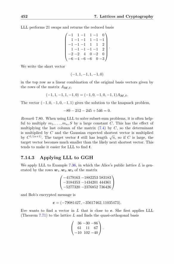
452 7. Lattices and Cryptography
LLL performs 21 swaps and returns the reduced basis⎛
⎜⎜⎜⎜⎜⎜⎝
−1 1 −1 1 −1 01 −1 −1 1 −1 −1
−1 −1 −1 1 1 21 −1 −1 −1 −1 2
−2 −2 4 0 −2 0−6 −4 −6 −6 0 −3
⎞
⎟⎟⎟⎟⎟⎟⎠
.
We write the short vector
(−1, 1,−1, 1,−1, 0)
in the top row as a linear combination of the original basis vectors given bythe rows of the matrix AM ,S ,
(−1, 1,−1, 1,−1, 0) = (−1, 0,−1, 0,−1, 1)AM ,S .
The vector (−1, 0,−1, 0,−1, 1) gives the solution to the knapsack problem,
−89− 212− 245 + 546 = 0.
Remark 7.80. When using LLL to solve subset-sum problems, it is often help-ful to multiply m1, . . . ,mn, S by a large constant C. This has the effect ofmultiplying the last column of the matrix (7.4) by C, so the determinantis multiplied by C and the Gaussian expected shortest vector is multipliedby C1/(n+1). The target vector t still has length
√n, so if C is large, the
target vector becomes much smaller than the likely next shortest vector. Thistends to make it easier for LLL to find t.
7.14.3 Applying LLL to GGH
We apply LLL to Example 7.36, in which the Alice’s public lattice L is gen-erated by the rows w1,w2,w3 of the matrix
⎛
⎝−4179163 −1882253 583183−3184353 −1434201 444361−5277320 −2376852 736426
⎞
⎠
and Bob’s encrypted message is
e = (−79081427,−35617462, 11035473).
Eve wants to find a vector in L that is close to e. She first applies LLL(Theorem 7.71) to the lattice L and finds the quasi-orthogonal basis
⎛
⎝36 −30 −8661 11 67
−10 102 −40
⎞
⎠ .
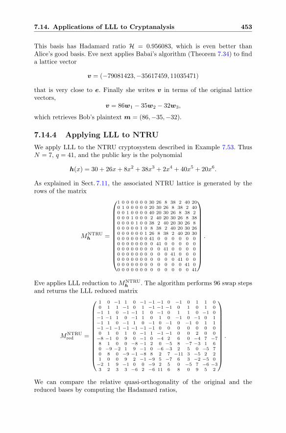
7.14. Applications of LLL to Cryptanalysis 453
This basis has Hadamard ratio H = 0.956083, which is even better thanAlice’s good basis. Eve next applies Babai’s algorithm (Theorem 7.34) to finda lattice vector
v = (−79081423,−35617459, 11035471)
that is very close to e. Finally she writes v in terms of the original latticevectors,
v = 86w1 − 35w2 − 32w3,
which retrieves Bob’s plaintext m = (86,−35,−32).
7.14.4 Applying LLL to NTRU
We apply LLL to the NTRU cryptosystem described in Example 7.53. ThusN = 7, q = 41, and the public key is the polynomial
h(x) = 30 + 26x+ 8x2 + 38x3 + 2x4 + 40x5 + 20x6.
As explained in Sect. 7.11, the associated NTRU lattice is generated by therows of the matrix
MNTRUh =
⎛
⎜⎜⎜⎜⎜⎜⎜⎜⎜⎜⎜⎜⎝
1 0 0 0 0 0 0 30 26 8 38 2 40 200 1 0 0 0 0 0 20 30 26 8 38 2 400 0 1 0 0 0 0 40 20 30 26 8 38 20 0 0 1 0 0 0 2 40 20 30 26 8 380 0 0 0 1 0 0 38 2 40 20 30 26 80 0 0 0 0 1 0 8 38 2 40 20 30 260 0 0 0 0 0 1 26 8 38 2 40 20 300 0 0 0 0 0 0 41 0 0 0 0 0 00 0 0 0 0 0 0 0 41 0 0 0 0 00 0 0 0 0 0 0 0 0 41 0 0 0 00 0 0 0 0 0 0 0 0 0 41 0 0 00 0 0 0 0 0 0 0 0 0 0 41 0 00 0 0 0 0 0 0 0 0 0 0 0 41 00 0 0 0 0 0 0 0 0 0 0 0 0 41
⎞
⎟⎟⎟⎟⎟⎟⎟⎟⎟⎟⎟⎟⎠
.
Eve applies LLL reduction to MNTRUh . The algorithm performs 96 swap steps
and returns the LLL reduced matrix
MNTRUred =
⎛
⎜⎜⎜⎜⎜⎜⎜⎜⎜⎜⎜⎜⎝
1 0 −1 1 0 −1 −1 −1 0 −1 0 1 1 00 1 1 −1 0 1 −1 −1 −1 0 1 0 1 0−1 1 0 −1 −1 1 0 −1 0 1 1 0 −1 0−1 −1 1 0 −1 1 0 1 0 −1 0 −1 0 1−1 1 0 −1 1 0 −1 0 −1 0 −1 0 1 1−1 −1 −1 −1 −1 −1 −1 0 0 0 0 0 0 00 1 0 1 0 −1 1 −1 −1 0 0 2 0 0−8 −1 0 9 0 −1 0 −4 2 6 0 −4 7 −78 1 0 0 −8 −1 2 0 −5 8 −7 −3 1 60 −9 −2 1 9 −1 0 −6 −3 2 5 0 −5 70 8 0 −9 −1 −8 8 2 7 −11 3 −5 2 21 0 0 9 2 −1 −9 5 −7 6 3 −2 −5 0−2 1 9 −1 0 0 −9 2 5 0 −5 7 −6 −33 2 3 3 −6 2 −6 11 6 8 0 9 5 2
⎞
⎟⎟⎟⎟⎟⎟⎟⎟⎟⎟⎟⎟⎠
.
We can compare the relative quasi-orthogonality of the original and thereduced bases by computing the Hadamard ratios,
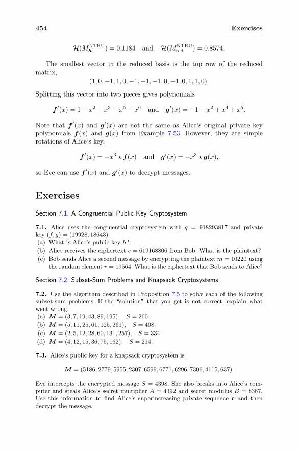
454 Exercises
H(MNTRUh ) = 0.1184 and H(MNTRU
red ) = 0.8574.
The smallest vector in the reduced basis is the top row of the reducedmatrix,
(1, 0,−1, 1, 0,−1,−1,−1, 0,−1, 0, 1, 1, 0).
Splitting this vector into two pieces gives polynomials
f ′(x) = 1− x2 + x3 − x5 − x6 and g′(x) = −1− x2 + x4 + x5.
Note that f ′(x) and g′(x) are not the same as Alice’s original private keypolynomials f(x) and g(x) from Example 7.53. However, they are simplerotations of Alice’s key,
f ′(x) = −x3 � f(x) and g′(x) = −x3 � g(x),
so Eve can use f ′(x) and g′(x) to decrypt messages.
Exercises
Section 7.1. A Congruential Public Key Cryptosystem
7.1. Alice uses the congruential cryptosystem with q = 918293817 and privatekey (f, g) = (19928, 18643).(a) What is Alice’s public key h?
(b) Alice receives the ciphertext e = 619168806 from Bob. What is the plaintext?
(c) Bob sends Alice a second message by encrypting the plaintext m = 10220 usingthe random element r = 19564. What is the ciphertext that Bob sends to Alice?
Section 7.2. Subset-Sum Problems and Knapsack Cryptosystems
7.2. Use the algorithm described in Proposition 7.5 to solve each of the followingsubset-sum problems. If the “solution” that you get is not correct, explain whatwent wrong.(a) M = (3, 7, 19, 43, 89, 195), S = 260.
(b) M = (5, 11, 25, 61, 125, 261), S = 408.
(c) M = (2, 5, 12, 28, 60, 131, 257), S = 334.
(d) M = (4, 12, 15, 36, 75, 162), S = 214.
7.3. Alice’s public key for a knapsack cryptosystem is
M = (5186, 2779, 5955, 2307, 6599, 6771, 6296, 7306, 4115, 637).
Eve intercepts the encrypted message S = 4398. She also breaks into Alice’s com-puter and steals Alice’s secret multiplier A = 4392 and secret modulus B = 8387.Use this information to find Alice’s superincreasing private sequence r and thendecrypt the message.
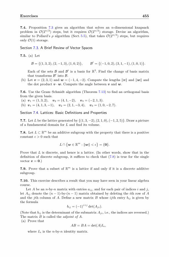
Exercises 455
7.4. Proposition 7.3 gives an algorithm that solves an n-dimensional knapsackproblem in O(2n/2) steps, but it requires O(2n/2) storage. Devise an algorithm,similar to Pollard’s ρ algorithm (Sect. 5.5), that takes O(2n/2) steps, but requiresonly O(1) storage.
Section 7.3. A Brief Review of Vector Spaces
7.5. (a) Let
B = {(1, 3, 2), (2,−1, 3), (1, 0, 2)}, B′ = {(−1, 0, 2), (3, 1,−1), (1, 0, 1)}.
Each of the sets B and B′ is a basis for R3. Find the change of basis matrix
that transforms B′ into B.(b) Let v = (2, 3, 1) and w = (−1, 4,−2). Compute the lengths ‖v‖ and ‖w‖ and
the dot product v ·w. Compute the angle between v and w.
7.6. Use the Gram–Schmidt algorithm (Theorem 7.13) to find an orthogonal basisfrom the given basis.(a) v1 = (1, 3, 2), v2 = (4, 1,−2), v3 = (−2, 1, 3).
(b) v1 = (4, 1, 3,−1), v2 = (2, 1,−3, 4), v3 = (1, 0,−2, 7).
Section 7.4. Lattices: Basic Definitions and Properties
7.7. Let L be the lattice generated by {(1, 3,−2), (2, 1, 0), (−1, 2, 5)}. Draw a pictureof a fundamental domain for L and find its volume.
7.8. Let L ⊂ Rm be an additive subgroup with the property that there is a positive
constant ε > 0 such that
L ∩{w ∈ R
m : ‖w‖ < ε}= {0}.
Prove that L is discrete, and hence is a lattice. (In other words, show that in thedefinition of discrete subgroup, it suffices to check that (7.8) is true for the singlevector v = 0.)
7.9. Prove that a subset of Rm is a lattice if and only if it is a discrete additivesubgroup.
7.10. This exercise describes a result that you may have seen in your linear algebracourse.
Let A be an n-by-n matrix with entries aij , and for each pair of indices i and j,let Aij denote the (n− 1)-by-(n− 1) matrix obtained by deleting the ith row of Aand the jth column of A. Define a new matrix B whose ijth entry bij is given bythe formula
bij = (−1)i+j det(Aji).
(Note that bij is the determinant of the submatrix Aji, i.e., the indices are reversed.)The matrix B is called the adjoint of A.(a) Prove that
AB = BA = det(A)In,
where In is the n-by-n identity matrix.
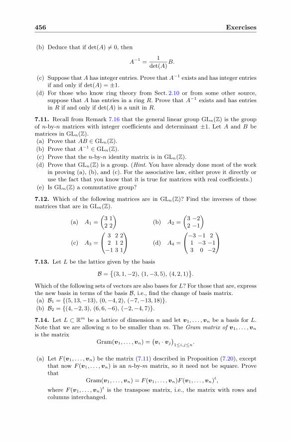
456 Exercises
(b) Deduce that if det(A) �= 0, then
A−1 =1
det(A)B.
(c) Suppose that A has integer entries. Prove that A−1 exists and has integer entriesif and only if det(A) = ±1.
(d) For those who know ring theory from Sect. 2.10 or from some other source,suppose that A has entries in a ring R. Prove that A−1 exists and has entriesin R if and only if det(A) is a unit in R.
7.11. Recall from Remark 7.16 that the general linear group GLn(Z) is the groupof n-by-n matrices with integer coefficients and determinant ±1. Let A and B bematrices in GLn(Z).(a) Prove that AB ∈ GLn(Z).
(b) Prove that A−1 ∈ GLn(Z).
(c) Prove that the n-by-n identity matrix is in GLn(Z).
(d) Prove that GLn(Z) is a group. (Hint. You have already done most of the workin proving (a), (b), and (c). For the associative law, either prove it directly oruse the fact that you know that it is true for matrices with real coefficients.)
(e) Is GLn(Z) a commutative group?
7.12. Which of the following matrices are in GLn(Z)? Find the inverses of thosematrices that are in GLn(Z).
(a) A1 =
(3 12 2
)(b) A2 =
(3 −22 −1
)
(c) A3 =
⎛
⎝3 2 22 1 2−1 3 1
⎞
⎠ (d) A4 =
⎛
⎝−3 −1 21 −3 −13 0 −2
⎞
⎠
7.13. Let L be the lattice given by the basis
B ={(3, 1,−2), (1,−3, 5), (4, 2, 1)
}.
Which of the following sets of vectors are also bases for L? For those that are, expressthe new basis in terms of the basis B, i.e., find the change of basis matrix.(a) B1 = {(5, 13,−13), (0,−4, 2), (−7,−13, 18)}.(b) B2 = {(4,−2, 3), (6, 6,−6), (−2,−4, 7)}.
7.14. Let L ⊂ Rm be a lattice of dimension n and let v1, . . . ,vn be a basis for L.
Note that we are allowing n to be smaller than m. The Gram matrix of v1, . . . ,vn
is the matrixGram(v1, . . . ,vn) =
(vi · vj
)1≤i,j≤n
.
(a) Let F (v1, . . . ,vn) be the matrix (7.11) described in Proposition (7.20), exceptthat now F (v1, . . . ,vn) is an n-by-m matrix, so it need not be square. Provethat
Gram(v1, . . . ,vn) = F (v1, . . . ,vn)F (v1, . . . ,vn)t,
where F (v1, . . . ,vn)t is the transpose matrix, i.e., the matrix with rows and
columns interchanged.
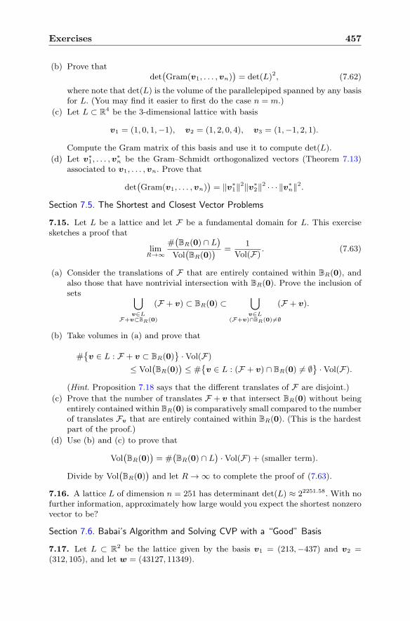
Exercises 457
(b) Prove thatdet(Gram(v1, . . . ,vn)
)= det(L)2, (7.62)
where note that det(L) is the volume of the parallelepiped spanned by any basisfor L. (You may find it easier to first do the case n = m.)
(c) Let L ⊂ R4 be the 3-dimensional lattice with basis
v1 = (1, 0, 1,−1), v2 = (1, 2, 0, 4), v3 = (1,−1, 2, 1).
Compute the Gram matrix of this basis and use it to compute det(L).
(d) Let v∗1, . . . ,v
∗n be the Gram–Schmidt orthogonalized vectors (Theorem 7.13)
associated to v1, . . . ,vn. Prove that
det(Gram(v1, . . . ,vn)
)= ‖v∗
1‖2‖v∗2‖2 · · · ‖v∗
n‖2.
Section 7.5. The Shortest and Closest Vector Problems
7.15. Let L be a lattice and let F be a fundamental domain for L. This exercisesketches a proof that
limR→∞
#(BR(0) ∩ L
)
Vol(BR(0)
) =1
Vol(F). (7.63)
(a) Consider the translations of F that are entirely contained within BR(0), andalso those that have nontrivial intersection with BR(0). Prove the inclusion ofsets ⋃
v∈LF+v⊂BR(0)
(F + v) ⊂ BR(0) ⊂⋃
v∈L(F+v)∩BR(0) �=∅
(F + v).
(b) Take volumes in (a) and prove that
#{v ∈ L : F + v ⊂ BR(0)
}·Vol(F)
≤ Vol(BR(0)
)≤ #
{v ∈ L : (F + v) ∩ BR(0) �= ∅
}·Vol(F).
(Hint. Proposition 7.18 says that the different translates of F are disjoint.)
(c) Prove that the number of translates F + v that intersect BR(0) without beingentirely contained within BR(0) is comparatively small compared to the numberof translates Fv that are entirely contained within BR(0). (This is the hardestpart of the proof.)
(d) Use (b) and (c) to prove that
Vol(BR(0)
)= #
(BR(0) ∩ L
)·Vol(F) + (smaller term).
Divide by Vol(BR(0)
)and let R → ∞ to complete the proof of (7.63).
7.16. A lattice L of dimension n = 251 has determinant det(L) ≈ 22251.58. With nofurther information, approximately how large would you expect the shortest nonzerovector to be?
Section 7.6. Babai’s Algorithm and Solving CVP with a “Good” Basis
7.17. Let L ⊂ R2 be the lattice given by the basis v1 = (213,−437) and v2 =
(312, 105), and let w = (43127, 11349).
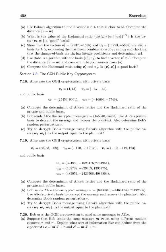
458 Exercises
(a) Use Babai’s algorithm to find a vector v ∈ L that is close to w. Compute thedistance ‖v −w‖.
(b) What is the value of the Hadamard ratio(det(L)/‖v1‖‖v2‖
)1/2? Is the ba-
sis {v1,v2} a “good” basis?
(c) Show that the vectors v′1 = (2937,−1555) and v′
2 = (11223,−5888) are also abasis for L by expressing them as linear combinations of v1 and v2 and checkingthat the change-of-basis matrix has integer coefficients and determinant ±1.
(d) Use Babai’s algorithm with the basis {v′1,v
′2} to find a vector v′ ∈ L. Compute
the distance ‖v′ −w‖ and compare it to your answer from (a).
(e) Compute the Hadamard ratio using v′1 and v′
2. Is {v′1,v
′2} a good basis?
Section 7.8. The GGH Public Key Cryptosystem
7.18. Alice uses the GGH cryptosystem with private basis
v1 = (4, 13), v2 = (−57,−45),
and public basis
w1 = (25453, 9091), w2 = (−16096,−5749).
(a) Compute the determinant of Alice’s lattice and the Hadamard ratio of theprivate and public bases.
(b) Bob sends Alice the encrypted message e = (155340, 55483). Use Alice’s privatebasis to decrypt the message and recover the plaintext. Also determine Bob’srandom perturbation r.
(c) Try to decrypt Bob’s message using Babai’s algorithm with the public ba-sis {w1,w2}. Is the output equal to the plaintext?
7.19. Alice uses the GGH cryptosystem with private basis
v1 = (58, 53,−68), v2 = (−110,−112, 35), v3 = (−10,−119, 123)
and public basis
w1 = (324850,−1625176, 2734951),
w2 = (165782,−829409, 1395775),
w3 = (485054,−2426708, 4083804).
(a) Compute the determinant of Alice’s lattice and the Hadamard ratio of theprivate and public bases.
(b) Bob sends Alice the encrypted message e = (8930810,−44681748, 75192665).Use Alice’s private basis to decrypt the message and recover the plaintext. Alsodetermine Bob’s random perturbation r.
(c) Try to decrypt Bob’s message using Babai’s algorithm with the public ba-sis {w1,w2,w3}. Is the output equal to the plaintext?
7.20. Bob uses the GGH cryptosystem to send some messages to Alice.(a) Suppose that Bob sends the same message m twice, using different random
elements r and r′. Explain what sort of information Eve can deduce from theciphertexts e = mW + r and e′ = mW + r′.
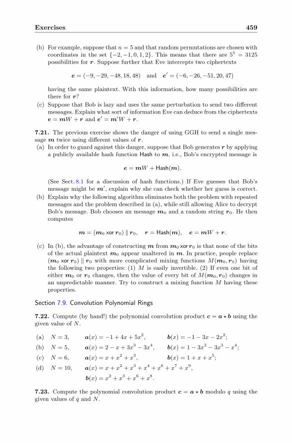
Exercises 459
(b) For example, suppose that n = 5 and that random permutations are chosen withcoordinates in the set {−2,−1, 0, 1, 2}. This means that there are 55 = 3125possibilities for r. Suppose further that Eve intercepts two ciphertexts
e = (−9,−29,−48, 18, 48) and e′ = (−6,−26,−51, 20, 47)
having the same plaintext. With this information, how many possibilities arethere for r?
(c) Suppose that Bob is lazy and uses the same perturbation to send two differentmessages. Explain what sort of information Eve can deduce from the ciphertextse = mW + r and e′ = m′W + r.
7.21. The previous exercise shows the danger of using GGH to send a single mes-sage m twice using different values of r.(a) In order to guard against this danger, suppose that Bob generates r by applying
a publicly available hash function Hash to m, i.e., Bob’s encrypted message is
e = mW + Hash(m).
(See Sect. 8.1 for a discussion of hash functions.) If Eve guesses that Bob’smessage might be m′, explain why she can check whether her guess is correct.
(b) Explain why the following algorithm eliminates both the problem with repeatedmessages and the problem described in (a), while still allowing Alice to decryptBob’s message. Bob chooses an message m0 and a random string r0. He thencomputes
m = (m0 xor r0) ‖ r0, r = Hash(m), e = mW + r.
(c) In (b), the advantage of constructing m from m0 xorr0 is that none of the bitsof the actual plaintext m0 appear unaltered in m. In practice, people replace(m0 xor r0) ‖ r0 with more complicated mixing functions M(m0, r0) havingthe following two properties: (1) M is easily invertible. (2) If even one bit ofeither m0 or r0 changes, then the value of every bit of M(m0, r0) changes inan unpredictable manner. Try to construct a mixing function M having theseproperties.
Section 7.9. Convolution Polynomial Rings
7.22. Compute (by hand!) the polynomial convolution product c = a � b using thegiven value of N .
(a) N = 3, a(x) = −1 + 4x+ 5x2, b(x) = −1− 3x− 2x2;
(b) N = 5, a(x) = 2− x+ 3x3 − 3x4, b(x) = 1− 3x2 − 3x3 − x4;
(c) N = 6, a(x) = x+ x2 + x3, b(x) = 1 + x+ x5;
(d) N = 10, a(x) = x+ x2 + x3 + x4 + x6 + x7 + x9,
b(x) = x2 + x3 + x6 + x8.
7.23. Compute the polynomial convolution product c = a � b modulo q using thegiven values of q and N .
460 Exercises
(a) N = 3, q = 7, a(x) = 1 + x, b(x) = −5 + 4x+ 2x2;
(b) N = 5, q = 4, a(x) = 2 + 2x− 2x2 + x3 − 2x4,
b(x) = −1 + 3x− 3x2 − 3x3 − 3x4;
(c) N = 7, q = 3, a(x) = x+ x3, b(x) = x+ x2 + x4 + x6;
(d) N = 10, q = 2, a(x) = x2 + x5 + x7 + x8 + x9,
b(x) = 1 + x+ x3 + x4 + x5 + x7 + x8 + x9.
7.24. Let a(x) ∈ (Z/qZ)[x], where q is a prime.(a) Prove that
a(1) ≡ 0 (mod q) if and only if (x− 1) | a(x) in (Z/qZ)[x].
(b) Suppose that a(1) ≡ 0 (mod q). Prove that a(x) is not invertible in Rq.
7.25. Let N = 5 and q = 3 and consider the two polynomials
a(x) = 1 + x2 + x3 ∈ R3 and b(x) = 1 + x2 − x3 ∈ R3.
One of these polynomials has an inverse in R3 and the other does not. Compute theinverse that exists, and explain why the other doesn’t exist.
7.26. For each of the following values of N , q, and a(x), either find a(x)−1 in Rq
or show that the inverse does not exist.(a) N = 5, q = 11, and a(x) = x4 + 8x+ 3;
(b) N = 5, q = 13, and a(x) = x3 + 2x− 3.
(c) N = 7, q = 23, and a(x) = 20x6 + 8x5 + 4x4 + 15x3 + 19x2 + x+ 8.
7.27. This exercise illustrates how to find inverses in
Rm =(Z/mZ)[x]
(xN − 1)
when m is a prime power pe.(a) Let f(x) ∈ Z[x]/(XN − 1) be a polynomial, and suppose that we have already
found a polynomial F (x) such that
f(x) � F (x) ≡ 1 (mod pi)
for some i ≥ 1. Prove that the polynomial
G(x) = F (x) �(2− f(x) � F (x)
)
satisfies
f(x) � G(x) ≡ 1 (mod p2i).
(b) Suppose that we know an inverse of f(x) modulo p. Using (a) repeatedly, howmany convolution multiplications does it take to compute the inverse of f(x)modulo pe?
Exercises 461
(c) Use the method in (a) to compute the following inverses modulo m = pe, whereto ease your task, we have given you the inverse modulo p.
(i) N = 5, m = 24, f(x) = 7 + 3x+ x2,
f(x)−1 ≡ 1 + x2 + x3 (mod 2).
(ii) N = 5, m = 27, f(x) = 22 + 11x+ 5x2 + 7x3,
f(x)−1 ≡ 1 + x2 + x3 (mod 2).
(iii) N = 7, m = 55, f(x) = 112 + 34x+ 239x2 + 234x3 + 105x4
+ 180x5 + 137x6,
f(x)−1 ≡ 1 + 3x2 + 2x4 (mod 5).
7.28. Let a ∈ RN be a fixed vector.
(a) Suppose that b is an N -dimensional vector whose coefficients are chosenrandomly from the set {−1, 0, 1}. Prove that the expected values of ‖b‖2and ‖a � b‖2 are given by
E(‖b‖2
)=
2
3N and E
(‖a � b‖2
)= ‖a‖2E
(‖b‖2
).
(b) More generally, suppose that the coefficients of b are chosen at random fromthe set of integers {−T,−T + 1, . . . , T − 1, T}. Compute the expected valuesof ‖b‖2 and ‖a � b‖2 as in (a).
(c) Suppose now that the coefficients of b are real numbers that are chosen uni-formly and independently in the interval from −R to R. Prove that
E(‖b‖2
)=R2N
3and E
(‖a � b‖2
)= ‖a‖2E
(‖b‖2
).
(Hint. The most direct way to do (c) is to use continuous probability theory. Asan alternative, let the coefficients of b be chosen uniformly and independentlyfrom the set {jR/T : −T ≤ j ≤ T}, redo the computation from (b), and thenlet T → ∞.)
(d) For each of the scenarios described in (a), (b), and (c), prove that
E(‖a+ b‖2
)= ‖a‖2 + E
(‖b‖2
).
Section 7.10. The NTRU Public Key Cryptosystem
7.29. Alice and Bob agree to communicate using NTRUEncrypt with
(N, p, q) = (7, 3, 37).
Alice’s private key is
f(x) = −1 +X −X3 +X4 +X5,
F 3(x) = 1 +X −X2 +X4 +X5 +X6.
(You can check that f � F 3 ≡ 1 (mod 3).) Alice receives the ciphertext
e(x) = 2 + 8X2 − 16X3 − 9X4 − 18X5 − 3X6.
from Bob. Decipher the message and find the plaintext.
462 Exercises
7.30. Alice and Bob decide to communicate using NTRUEncrypt with parameters(N, p, q) = (7, 3, 29). Alice’s public key is
h(x) = 3 + 14X − 4X2 + 13X3 − 6X4 + 2X5 + 7X6.
Bob sends Alice the plaintext message m(x) = 1 + X − X2 − X3 − X6 using therandom element r(x) = −1 +X2 −X5 +X6.(a) What ciphertext does Bob send to Alice?
(b) Alice’s private key is f(x) = −1 +X −X2 +X4 +X6 and F 3(x) = 1 +X +X2 +X4 +X5 −X6. Check your answer in (a) by using f and F 3 to decryptthe message.
7.31. What is the message expansion of NTRUEncrypt in terms of N , p, and q?
7.32. The guidelines for choosing NTRUEncrypt public parameters (N, p, q, d) re-quire that gcd(p, q) = 1. Prove that if p | q, then it is very easy for Eve to decryptthe message without knowing the private key. (Hint. First do the case that p = q.)
7.33. The guidelines for choosing NTRUEncrypt public parameters (N, p, q, d) in-clude the assumption that gcd(N, q) = 1. Suppose instead that Alice takes q = N ,where as always, N is an odd prime.(a) Make a change of variables x = y+ 1 in the ring Z[x]/(xN − 1), and show that
the NTRU lattice takes a simpler form.
(b) Can you find an efficient way to break NTRU in the case that q = N that doesinvolve lattice reduction? (This appears to be an open problem.)
7.34. Alice uses NTRUEncrypt with p = 3 to send messages to Bob.(a) Suppose that Alice uses the same random element r(x) to encrypt two dif-
ferent plaintexts m1(x) and m2(x). Explain how Eve can use the two cipher-texts e1(x) and e2(x) to determine approximately 2
9of the coefficients ofm1(x).
(See Exercise 7.38 for a way to exploit this information.)
(b) For example, suppose that N = 8, so there are 38 possibilities for m1(x).Suppose that Eve intercepts two ciphertexts
e1(x) = 32 + 21x− 9x2 − 20x3 − 29x4 − 29x5 − 19x6 + 38x7,
e2(x) = 33 + 21x− 7x2 − 19x3 − 31x4 − 27x5 − 19x6 + 38x7,
that were encrypted using the same random element r(x). How many coeffi-cients of m1(x) can she determine exactly? How many possibilities are therefor m1(x)?
(c) Formulate a similar attack if Alice uses two different random elements r1(x)and r2(x) to encrypt the same plaintext m(x). (Hint. Do it first assumingthat h(x) has an inverse in Rq. The problem is harder without this assumption.)
7.35. This exercise describes a variant of NTRUEncrypt that eliminates a step inthe decryption algorithm at the cost of requiring slightly larger parameters. Supposethat the NTRUEncrypt private key polynomials f(x) and g(x) are chosen to satisfy
f(x) = 1 + pf0(x) ≡ 1 (mod p) and g(x) = pg0(x) ≡ 0 (mod p),
and that NTRU encryption is changed to
e(x) ≡ h(x) � r(x) +m(x) (mod q).
(The change is the omission of p before h(x).)
Exercises 463
(a) Prove that if q is sufficiently large, then the following algorithm correctlydecrypts the message:
• Compute a(x) ≡ f(x) � e(x) (mod q) and center-lift to an element of R.
• Compute a(x) (mod p). The result is m(x).Note that this eliminates the necessity to multiply a(x) by f(x)−1 (mod p).
(a) Suppose that we choose f0, g0 ∈ T (d, d), and that we also assume that m isternary. Prove that decryption works provided q > 8dp + 2. (Hint. Mimic theproof of Proposition 7.48.)
Section 7.11. NTRU as a Lattice Cryptosystem
7.36. This exercise explains how to formulate NTRU message recovery as a closestvector problem. Let h(x) be an NTRU public key and let
e(x) ≡ pr(x) � h(x) +m(x) (mod q)
be a message encrypted using h(x).(a) Prove that the vector (pr, e−m) is in LNTRU
h .
(b) Prove that the lattice vector in (a) is almost certainly the closest lattice vectorto the known vector (0, e). Hence solving CVP reveals the plaintext m. (Forsimplicity, you may assume that d ≈ N/3 and q ≈ 2N , as we did in Proposi-tion 7.61.)
(c) Show how one can reduce the lattice-to-target distance, without affecting thedeterminant, by using instead a modified NTRU lattice of the form
(1 ph0 q
).
7.37. The guidelines for choosing NTRUEncrypt public parameters (N, p, q, d) in-clude the requirement that N be prime. To see why, suppose (say) that N is even.Explain how Eve can recover the private key by solving a lattice problem in dimen-sion N , rather than in dimension 2N . Hint. Use the natural map
Z[x]/(xN − 1) → Z[x]/(xN/2 − 1).
7.38. Suppose that Bob and Alice are using NTRUEncrypt to exchange messagesand that Eve intercepts a ciphertext e(x) for which she already knows part of theplaintext m(x). (This is not a ludicrous assumption; see Exercise 7.34, for example.)More precisely, suppose that Eve knows t of the coefficients of m(x). Explain howto set up a CVP to find m(x) using a lattice of dimension 2N − 2t.
Section 7.12. Lattice-Based Digital Signature Schemes
7.39. Samantha uses the GGH digital signature scheme with private and publicbases
v1 = (−20,−8, 1), w1 = (−248100, 220074, 332172),
v2 = (14, 11, 23), w2 = (−112192, 99518, 150209),
v3 = (−18, 1,−12), w3 = (−216150, 191737, 289401).
What is her signature on the document
d = (834928, 123894, 7812738)?
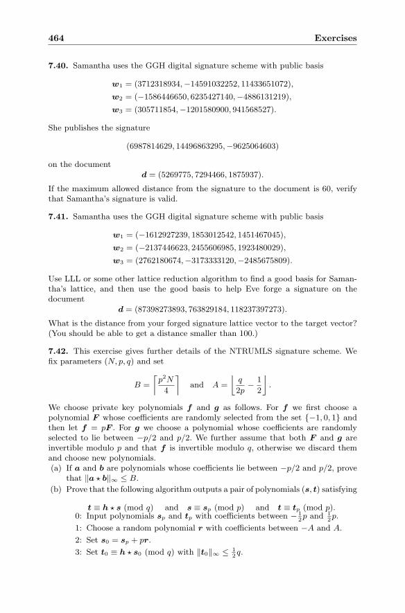
464 Exercises
7.40. Samantha uses the GGH digital signature scheme with public basis
w1 = (3712318934,−14591032252, 11433651072),
w2 = (−1586446650, 6235427140,−4886131219),
w3 = (305711854,−1201580900, 941568527).
She publishes the signature
(6987814629, 14496863295,−9625064603)
on the document
d = (5269775, 7294466, 1875937).
If the maximum allowed distance from the signature to the document is 60, verifythat Samantha’s signature is valid.
7.41. Samantha uses the GGH digital signature scheme with public basis
w1 = (−1612927239, 1853012542, 1451467045),
w2 = (−2137446623, 2455606985, 1923480029),
w3 = (2762180674,−3173333120,−2485675809).
Use LLL or some other lattice reduction algorithm to find a good basis for Saman-tha’s lattice, and then use the good basis to help Eve forge a signature on thedocument
d = (87398273893, 763829184, 118237397273).
What is the distance from your forged signature lattice vector to the target vector?(You should be able to get a distance smaller than 100.)
7.42. This exercise gives further details of the NTRUMLS signature scheme. Wefix parameters (N, p, q) and set
B =
⌈p2N
4
⌉and A =
⌊q
2p− 1
2
⌋.
We choose private key polynomials f and g as follows. For f we first choose apolynomial F whose coefficients are randomly selected from the set {−1, 0, 1} andthen let f = pF . For g we choose a polynomial whose coefficients are randomlyselected to lie between −p/2 and p/2. We further assume that both F and g areinvertible modulo p and that f is invertible modulo q, otherwise we discard themand choose new polynomials.(a) If a and b are polynomials whose coefficients lie between −p/2 and p/2, prove
that ‖a � b‖∞ ≤ B.
(b) Prove that the following algorithm outputs a pair of polynomials (s, t) satisfying
t ≡ h � s (mod q) and s ≡ sp (mod p) and t ≡ tp (mod p).0: Input polynomials sp and tp with coefficients between − 1
2p and 1
2p.
1: Choose a random polynomial r with coefficients between −A and A.
2: Set s0 = sp + pr.
3: Set t0 ≡ h � s0 (mod q) with ‖t0‖∞ ≤ 12q.
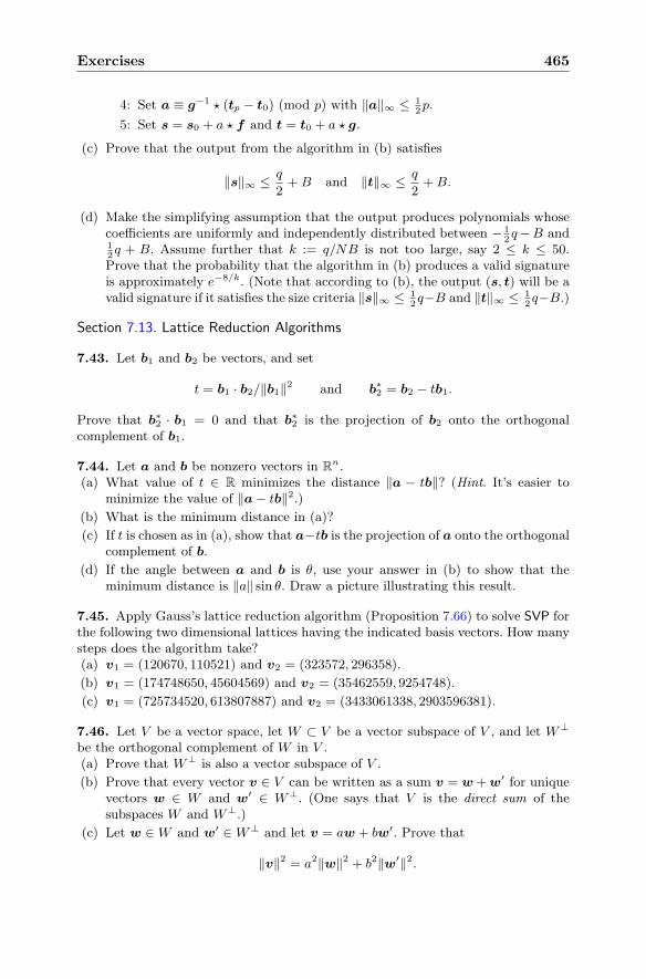
Exercises 465
4: Set a ≡ g−1 � (tp − t0) (mod p) with ‖a‖∞ ≤ 12p.
5: Set s = s0 + a � f and t = t0 + a � g.
(c) Prove that the output from the algorithm in (b) satisfies
‖s‖∞ ≤ q
2+B and ‖t‖∞ ≤ q
2+B.
(d) Make the simplifying assumption that the output produces polynomials whosecoefficients are uniformly and independently distributed between − 1
2q−B and
12q + B. Assume further that k := q/NB is not too large, say 2 ≤ k ≤ 50.
Prove that the probability that the algorithm in (b) produces a valid signatureis approximately e−8/k. (Note that according to (b), the output (s, t) will be avalid signature if it satisfies the size criteria ‖s‖∞ ≤ 1
2q−B and ‖t‖∞ ≤ 1
2q−B.)
Section 7.13. Lattice Reduction Algorithms
7.43. Let b1 and b2 be vectors, and set
t = b1 · b2/‖b1‖2 and b∗2 = b2 − tb1.
Prove that b∗2 · b1 = 0 and that b∗2 is the projection of b2 onto the orthogonalcomplement of b1.
7.44. Let a and b be nonzero vectors in Rn.
(a) What value of t ∈ R minimizes the distance ‖a − tb‖? (Hint. It’s easier tominimize the value of ‖a− tb‖2.)
(b) What is the minimum distance in (a)?
(c) If t is chosen as in (a), show that a−tb is the projection of a onto the orthogonalcomplement of b.
(d) If the angle between a and b is θ, use your answer in (b) to show that theminimum distance is ‖a‖ sin θ. Draw a picture illustrating this result.
7.45. Apply Gauss’s lattice reduction algorithm (Proposition 7.66) to solve SVP forthe following two dimensional lattices having the indicated basis vectors. How manysteps does the algorithm take?(a) v1 = (120670, 110521) and v2 = (323572, 296358).
(b) v1 = (174748650, 45604569) and v2 = (35462559, 9254748).
(c) v1 = (725734520, 613807887) and v2 = (3433061338, 2903596381).
7.46. Let V be a vector space, let W ⊂ V be a vector subspace of V , and let W⊥
be the orthogonal complement of W in V .(a) Prove that W⊥ is also a vector subspace of V .
(b) Prove that every vector v ∈ V can be written as a sum v = w+w′ for uniquevectors w ∈ W and w′ ∈ W⊥. (One says that V is the direct sum of thesubspaces W and W⊥.)
(c) Let w ∈W and w′ ∈W⊥ and let v = aw + bw′. Prove that
‖v‖2 = a2‖w‖2 + b2‖w′‖2.
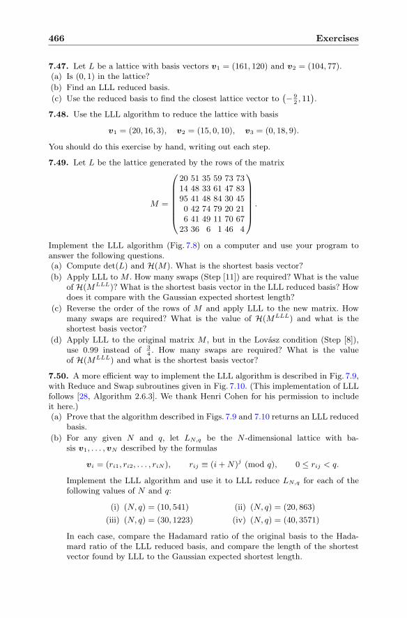
466 Exercises
7.47. Let L be a lattice with basis vectors v1 = (161, 120) and v2 = (104, 77).(a) Is (0, 1) in the lattice?
(b) Find an LLL reduced basis.
(c) Use the reduced basis to find the closest lattice vector to(− 9
2, 11).
7.48. Use the LLL algorithm to reduce the lattice with basis
v1 = (20, 16, 3), v2 = (15, 0, 10), v3 = (0, 18, 9).
You should do this exercise by hand, writing out each step.
7.49. Let L be the lattice generated by the rows of the matrix
M =
⎛
⎜⎜⎜⎜⎜⎜⎝
20 51 35 59 73 7314 48 33 61 47 8395 41 48 84 30 450 42 74 79 20 216 41 49 11 70 67
23 36 6 1 46 4
⎞
⎟⎟⎟⎟⎟⎟⎠
.
Implement the LLL algorithm (Fig. 7.8) on a computer and use your program toanswer the following questions.(a) Compute det(L) and H(M). What is the shortest basis vector?
(b) Apply LLL to M . How many swaps (Step [11]) are required? What is the valueof H(MLLL)? What is the shortest basis vector in the LLL reduced basis? Howdoes it compare with the Gaussian expected shortest length?
(c) Reverse the order of the rows of M and apply LLL to the new matrix. Howmany swaps are required? What is the value of H(MLLL) and what is theshortest basis vector?
(d) Apply LLL to the original matrix M , but in the Lovasz condition (Step [8]),use 0.99 instead of 3
4. How many swaps are required? What is the value
of H(MLLL) and what is the shortest basis vector?
7.50. A more efficient way to implement the LLL algorithm is described in Fig. 7.9,with Reduce and Swap subroutines given in Fig. 7.10. (This implementation of LLLfollows [28, Algorithm 2.6.3]. We thank Henri Cohen for his permission to includeit here.)(a) Prove that the algorithm described in Figs. 7.9 and 7.10 returns an LLL reduced
basis.
(b) For any given N and q, let LN,q be the N -dimensional lattice with ba-sis v1, . . . ,vN described by the formulas
vi = (ri1, ri2, . . . , riN ), rij ≡ (i+N)j (mod q), 0 ≤ rij < q.
Implement the LLL algorithm and use it to LLL reduce LN,q for each of thefollowing values of N and q:
(i) (N, q) = (10, 541) (ii) (N, q) = (20, 863)
(iii) (N, q) = (30, 1223) (iv) (N, q) = (40, 3571)
In each case, compare the Hadamard ratio of the original basis to the Hada-mard ratio of the LLL reduced basis, and compare the length of the shortestvector found by LLL to the Gaussian expected shortest length.
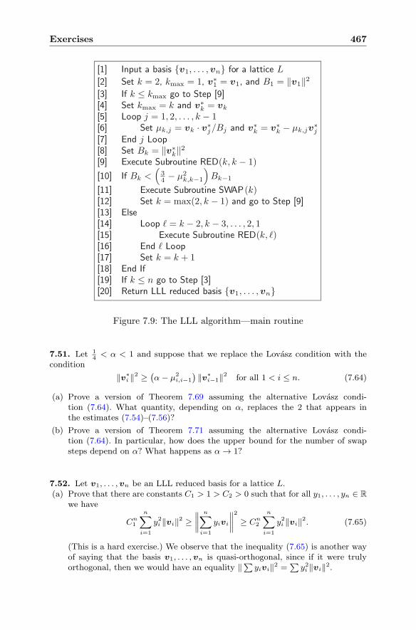
Exercises 467
{v1, . . . ,vn} for a lattice L
k = 2, kmax = 1, v∗1 = v1, and B1 = ‖v1‖2
k ≤ kmax go to Step [9]kmax = k and v∗
k = vk
j = 1, 2, . . . , k − 1μk,j = vk · v∗
j/Bj and v∗k = v∗
k − μk,jv∗j
j LoopBk = ‖v∗
k‖2
(k, k − 1)Bk <
(34 − μ2
k,k−1
)Bk−1
(k)k = max(2, k − 1) and go to Step [9]
� = k − 2, k − 3, . . . , 2, 1(k, �)
� Loopk = k + 1
k ≤ n go to Step [3]{v1, . . . ,vn}
[1] Input a basis[2] Set[3] If[4] Set[5] Loop[6] Set[7] End[8] Set[9] Execute Subroutine RED
[10] If[11] Execute Subroutine SWAP[12] Set[13] Else[14] Loop[15] Execute Subroutine RED[16] End[17] Set[18] End If[19] If[20] Return LLL reduced basis
Figure 7.9: The LLL algorithm—main routine
7.51. Let 14< α < 1 and suppose that we replace the Lovasz condition with the
condition
‖v∗i ‖2 ≥
(α− μ2
i,i−1
)‖v∗
i−1‖2 for all 1 < i ≤ n. (7.64)
(a) Prove a version of Theorem 7.69 assuming the alternative Lovasz condi-tion (7.64). What quantity, depending on α, replaces the 2 that appears inthe estimates (7.54)–(7.56)?
(b) Prove a version of Theorem 7.71 assuming the alternative Lovasz condi-tion (7.64). In particular, how does the upper bound for the number of swapsteps depend on α? What happens as α→ 1?
7.52. Let v1, . . . ,vn be an LLL reduced basis for a lattice L.(a) Prove that there are constants C1 > 1 > C2 > 0 such that for all y1, . . . , yn ∈ R
we have
Cn1
n∑
i=1
y2i ‖vi‖2 ≥∥∥∥∥
n∑
i=1
yivi
∥∥∥∥
2
≥ Cn2
n∑
i=1
y2i ‖vi‖2. (7.65)
(This is a hard exercise.) We observe that the inequality (7.65) is another wayof saying that the basis v1, . . . ,vn is quasi-orthogonal, since if it were trulyorthogonal, then we would have an equality ‖
∑yivi‖2 =
∑y2i ‖vi‖2.
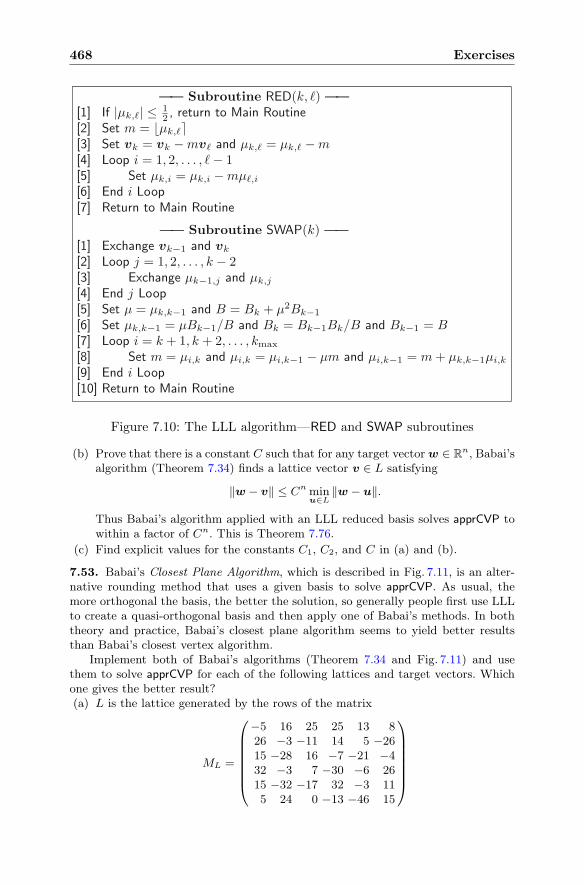
468 Exercises
—— Subroutine RED(k, �) ——|μk,�| ≤ 1
2 , return to Main Routinem = �μk,��vk = vk − mv� and μk,� = μk,� − m
i = 1, 2, . . . , � − 1μk,i = μk,i − mμ�,i
i Loop
—— Subroutine SWAP(k) ——vk−1 and vk
j = 1, 2, . . . , k − 2μk−1,j and μk,j
j Loopμ = μk,k−1 and B = Bk + μ2Bk−1μk,k−1 = μBk−1/B and Bk = Bk−1Bk/B and Bk−1 = B
i = k + 1, k + 2, . . . , kmaxm = μi,k and μi,k = μi,k−1 − μm and μi,k−1 = m + μk,k−1μi,k
i Loop
[1] If[2] Set[3] Set[4] Loop[5] Set[6] End[7] Return to Main Routine
[1] Exchange[2] Loop[3] Exchange[4] End[5] Set[6] Set[7] Loop[8] Set[9] End[10] Return to Main Routine
Figure 7.10: The LLL algorithm—RED and SWAP subroutines
(b) Prove that there is a constant C such that for any target vector w ∈ Rn, Babai’s
algorithm (Theorem 7.34) finds a lattice vector v ∈ L satisfying
‖w − v‖ ≤ Cn minu∈L
‖w − u‖.
Thus Babai’s algorithm applied with an LLL reduced basis solves apprCVP towithin a factor of Cn. This is Theorem 7.76.
(c) Find explicit values for the constants C1, C2, and C in (a) and (b).
7.53. Babai’s Closest Plane Algorithm, which is described in Fig. 7.11, is an alter-native rounding method that uses a given basis to solve apprCVP. As usual, themore orthogonal the basis, the better the solution, so generally people first use LLLto create a quasi-orthogonal basis and then apply one of Babai’s methods. In boththeory and practice, Babai’s closest plane algorithm seems to yield better resultsthan Babai’s closest vertex algorithm.
Implement both of Babai’s algorithms (Theorem 7.34 and Fig. 7.11) and usethem to solve apprCVP for each of the following lattices and target vectors. Whichone gives the better result?(a) L is the lattice generated by the rows of the matrix
ML =
⎛
⎜⎜⎜⎜⎜⎜⎝
−5 16 25 25 13 826 −3 −11 14 5 −2615 −28 16 −7 −21 −432 −3 7 −30 −6 2615 −32 −17 32 −3 115 24 0 −13 −46 15
⎞
⎟⎟⎟⎟⎟⎟⎠
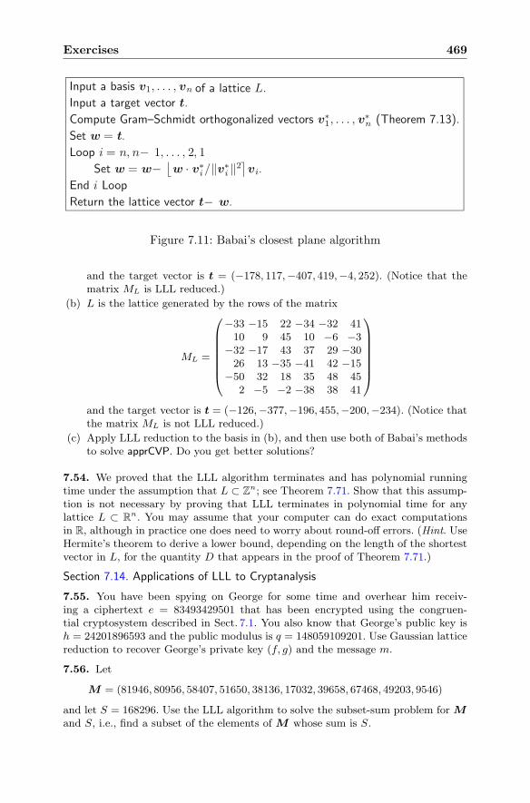
Exercises 469
Input a basis v1, . . . , vn of a lattice L.Input a target vector t.Compute Gram–Schmidt orthogonalized vectors v∗
1, . . . , v∗n (Theorem 7.13).
Set w = t.Loop i = n, n− 1, . . . , 2, 1
Set w = w− ⌊w · v∗i/‖v∗
i ‖2⌉vi.
End i LoopReturn the lattice vector t− w.
Figure 7.11: Babai’s closest plane algorithm
and the target vector is t = (−178, 117,−407, 419,−4, 252). (Notice that thematrix ML is LLL reduced.)
(b) L is the lattice generated by the rows of the matrix
ML =
⎛
⎜⎜⎜⎜⎜⎜⎝
−33 −15 22 −34 −32 4110 9 45 10 −6 −3
−32 −17 43 37 29 −3026 13 −35 −41 42 −15
−50 32 18 35 48 452 −5 −2 −38 38 41
⎞
⎟⎟⎟⎟⎟⎟⎠
and the target vector is t = (−126,−377,−196, 455,−200,−234). (Notice thatthe matrix ML is not LLL reduced.)
(c) Apply LLL reduction to the basis in (b), and then use both of Babai’s methodsto solve apprCVP. Do you get better solutions?
7.54. We proved that the LLL algorithm terminates and has polynomial runningtime under the assumption that L ⊂ Z
n; see Theorem 7.71. Show that this assump-tion is not necessary by proving that LLL terminates in polynomial time for anylattice L ⊂ R
n. You may assume that your computer can do exact computationsin R, although in practice one does need to worry about round-off errors. (Hint. UseHermite’s theorem to derive a lower bound, depending on the length of the shortestvector in L, for the quantity D that appears in the proof of Theorem 7.71.)
Section 7.14. Applications of LLL to Cryptanalysis
7.55. You have been spying on George for some time and overhear him receiv-ing a ciphertext e = 83493429501 that has been encrypted using the congruen-tial cryptosystem described in Sect. 7.1. You also know that George’s public key ish = 24201896593 and the public modulus is q = 148059109201. Use Gaussian latticereduction to recover George’s private key (f, g) and the message m.
7.56. Let
M = (81946, 80956, 58407, 51650, 38136, 17032, 39658, 67468, 49203, 9546)
and let S = 168296. Use the LLL algorithm to solve the subset-sum problem for Mand S, i.e., find a subset of the elements of M whose sum is S.
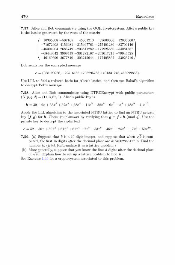
470 Exercises
7.57. Alice and Bob communicate using the GGH cryptosystem. Alice’s public keyis the lattice generated by the rows of the matrix
⎛
⎜⎜⎜⎜⎝
10305608 −597165 45361210 39600006 12036060−71672908 4156981 −315467761 −275401230 −83709146−46304904 2685749 −203811282 −177925680 −54081387−68449642 3969419 −301282167 −263017213 −79944525−46169690 2677840 −203215644 −177405867 −53923216
⎞
⎟⎟⎟⎟⎠.
Bob sends her the encrypted message
e = (388120266,−22516188, 1708295783, 1491331246, 453299858).
Use LLL to find a reduced basis for Alice’s lattice, and then use Babai’s algorithmto decrypt Bob’s message.
7.58. Alice and Bob communicate using NTRUEncrypt with public parameters(N, p, q, d) = (11, 3, 67, 3). Alice’s public key is
h = 39 + 9x+ 33x2 + 52x3 + 58x4 + 11x5 + 38x6 + 6x7 + x8 + 48x9 + 41x10.
Apply the LLL algorithm to the associated NTRU lattice to find an NTRU privatekey (f , g) for h. Check your answer by verifying that g ≡ f � h (mod q). Use theprivate key to decrypt the ciphertext
e = 52 + 50x+ 50x2 + 61x3 + 61x4 + 7x5 + 53x6 + 46x7 + 24x8 + 17x9 + 50x10.
7.59. (a) Suppose that k is a 10 digit integer, and suppose that when√k is com-
puted, the first 15 digits after the decimal place are 418400286617716. Find thenumber k. (Hint. Reformulate it as a lattice problem.)
(b) More generally, suppose that you know the first d-digits after the decimal placeof
√K. Explain how to set up a lattice problem to find K.
See Exercise 1.49 for a cryptosystem associated to this problem.
Chapter 8
Additional Topicsin Cryptography
The emphasis of this book has been on the mathematical underpinnings ofpublic key cryptography. We have developed most of the mathematics fromscratch and in sufficient depth to enable the reader to understand both theunderlying mathematical principles and how they are applied in cryptographicconstructions. Unfortunately, in achieving this laudable goal, we have nowreached the end of a hefty textbook with many important cryptographic topicsleft untouched.
This final chapter contains a few brief words about some of these additionaltopics. The reader should keep in mind that each of these areas is importantand that the brevity of our coverage reflects only a lack of space, not a lack ofinterest. We hope that you will view this chapter as a challenge to go out andlearn more about mathematical cryptography. In particular, each section inthis chapter provides a good starting point for a term paper or class project.
We also note that we have made no attempt to provide a full history ofthe topics covered, nor have we tried to give credit to all of the researchersworking in these areas. For the convenience of the reader and the instructor,here is a list of the topics introduced in this chapter:Section 8.1 Hash FunctionsSection 8.2 Random Numbers and Pseudorandom Number GeneratorsSection 8.3 Zero-Knowledge ProofsSection 8.4 Secret Sharing SchemesSection 8.5 Identification SchemesSection 8.6 Padding Schemes, the Random Oracle Model, and Provable
Security
© Springer Science+Business Media New York 2014J. Hoffstein et al., An Introduction to Mathematical Cryptography,Undergraduate Texts in Mathematics, DOI 10.1007/978-1-4939-1711-2 8
471
472 8. Additional Topics in Cryptography
Section 8.7 Building Protocols from Cryptographic PrimitivesSection 8.8 Blind Digital Signatures, Digital Cash, and BitcoinSection 8.9 Homomorphic EncryptionSection 8.10 Hyperelliptic Curve CryptographySection 8.11 Quantum ComputingSection 8.12 Modern Symmetric Cryptosystems: DES and AES
8.1 Hash Functions
There are many cryptographic constructions for which one needs a functionthat is easy to compute, but hard to invert. We have seen a number of exam-ples, including digital signatures (Remark 4.2), randomization of plaintextsin probabilistic cryptosystems (Exercise 7.21), and ID based cryptography(Sect. 6.10.2).
Definition. A hash function takes as input an arbitrarily long document Dand returns a short bit string H. The primary properties that a hash func-tion Hash should possess are as follows:
• Computation of Hash(D) should be fast and easy, roughly linear time.
• Inversion of Hash should be difficult, meaning exponential time. Moreprecisely, given a hash value H, it should be difficult to find any docu-ment D such that Hash(D) = H.
• For many applications it is also important that Hash be collisionresistant. This means that it should be hard to find two different doc-uments D1 and D2 whose hash values Hash(D1) and Hash(D2) are thesame.
Remark 8.1. Why do we want our hash function to be collision resistant?Suppose that Eve can find two documents D1 and D2 that have the samehash value Hash(D1) = Hash(D2), and suppose that D1 says “Pay the bearer$5” and that D2 says “Pay the bearer $500.” Eve can give Alice $5 andask her to sign D1. Since Alice has actually signed Hash(D1), she has alsosigned Hash(D2), so Eve can go to the bank, present the signature as beingon D2, and get paid $500.
In practice, most hash functions use a mixing algorithmM that transformsa bit string of length n into another bit string of length n. Then Hash worksby breaking a long document into blocks and successively usingM to combineeach block with the previously processed material.
Thus to compute H(D), we first append extra 0 bits to D so that thelength of D is an even multiple of n bits. This allows us to write D as aconcatenation
D = D1 ‖D2 ‖D3 ‖D4 ‖ · · · ‖Dk
of bit strings of length n. (See Exercise 3.43 for a discussion of concatenation.)
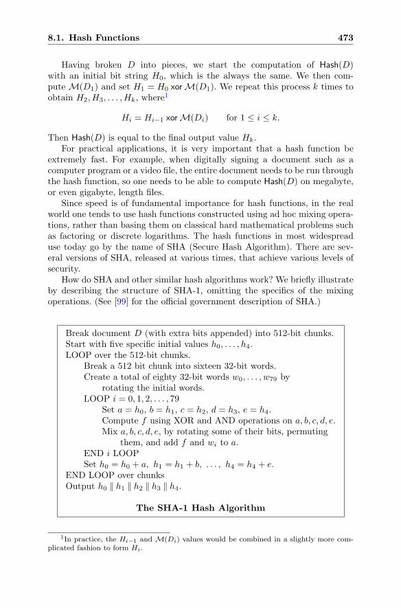
8.1. Hash Functions 473
Having broken D into pieces, we start the computation of Hash(D)with an initial bit string H0, which is the always the same. We then com-pute M(D1) and set H1 = H0 xorM(D1). We repeat this process k times toobtain H2, H3, . . . , Hk, where
1
Hi = Hi−1 xorM(Di) for 1 ≤ i ≤ k.
Then Hash(D) is equal to the final output value Hk.For practical applications, it is very important that a hash function be
extremely fast. For example, when digitally signing a document such as acomputer program or a video file, the entire document needs to be run throughthe hash function, so one needs to be able to compute Hash(D) on megabyte,or even gigabyte, length files.
Since speed is of fundamental importance for hash functions, in the realworld one tends to use hash functions constructed using ad hoc mixing opera-tions, rather than basing them on classical hard mathematical problems suchas factoring or discrete logarithms. The hash functions in most widespreaduse today go by the name of SHA (Secure Hash Algorithm). There are sev-eral versions of SHA, released at various times, that achieve various levels ofsecurity.
How do SHA and other similar hash algorithms work? We briefly illustrateby describing the structure of SHA-1, omitting the specifics of the mixingoperations. (See [99] for the official government description of SHA.)
Break document D (with extra bits appended) into 512-bit chunks.Start with five specific initial values h0, . . . , h4.LOOP over the 512-bit chunks.
Break a 512 bit chunk into sixteen 32-bit words.Create a total of eighty 32-bit words w0, . . . , w79 by
rotating the initial words.LOOP i = 0, 1, 2, . . . , 79
Set a = h0, b = h1, c = h2, d = h3, e = h4.Compute f using XOR and AND operations on a, b, c, d, e.Mix a, b, c, d, e, by rotating some of their bits, permuting
them, and add f and wi to a.END i LOOPSet h0 = h0 + a, h1 = h1 + b, . . . , h4 = h4 + e.
END LOOP over chunksOutput h0 ‖ h1 ‖ h2 ‖ h3 ‖ h4.
The SHA-1 Hash Algorithm
1In practice, the Hi−1 and M(Di) values would be combined in a slightly more com-plicated fashion to form Hi.
474 8. Additional Topics in Cryptography
Remark 8.2. Notice that SHA-1 has an inner loop that is repeated 80 times.We say that SHA-1 has 80 rounds. Each round involves various mixing op-erations that use the results from the previous round together with a smallamount of new data. For SHA-1, the new data used in the ith round is the32-bit word wi. This idea of repeating a simple mixing operation is typicalof modern hash functions, pseudorandom number generators (Sect. 8.2), andsymmetric ciphers such as DES and AES (Sect. 8.12). In principle, one couldmake SHA-1 faster by doing fewer rounds, but if one uses too few rounds,then there are known methods to break the system. It is an area of ongoingresearch to understand how many rounds are necessary to make SHA-1 andsimilar round-based systems secure.
The original SHA, which was later amended as SHA-1 to fix a minorsecurity flaw, is a hash function whose output has length 160 bits. Startingaround 2005 and continuing to the present day, various attacks have beendeveloped for SHA-1, originally for fewer than 80 rounds, but eventually forthe full 80-round SHA-1 implementation. To give a rough idea of progress, asof 2012 researchers have theoretical methods that they claim will find a SHA-1collision in around 261 operations, much less than the ostensible 280 securitylevel.
This prompted the development and publication in 2001 of a suite of hashfunctions known collectively as SHA-2. The individual hash functions in SHA-2 are called SHA-n, where n ∈ {224, 256, 384, 512} indicates the block size.2
As with SHA-1, these hash functions were developed internally by the NSA.They are similar in some ways to SHA-1, but have so far resisted any seriousattacks when the full number of rounds are used. However, given the attackson SHA-1, it was felt desirable to create an alternative hash function basedon different principles, so in 2007 the United States government opened a5-year competition to design a new general purpose hash function to be calledSHA-3. The winner of the competition, announced in 2012, was created byG. Bertoni, J. Daemen, G. Van Assche, and M. Peeters. As of 2014, a draftstandard for SHA-3 is available, but a final standardization document is notyet ready.
8.2 Random Numbers and PseudorandomNumber Generators
We have seen that many cryptographic constructions require the use ofrandom numbers. For example:
2This means that a direct search takes approximately 2n steps to invert SHA-n, anda naive collision algorithm takes approximately 2n/2 steps to find a collision for SHA-n.Of course, none of this proves that SHA is secure, and indeed the difficulty of inverting orfinding collisions for SHA is not related, as far as is known, to any standard mathematicalproblem.
8.2. Random Numbers and Pseudorandom Number 475
• The key creation phase of virtually all cryptosystems requires the userto choose one or more random (prime) numbers. The same is true forcreating keys in digital signature schemes.
• The Elgamal public key cryptosystem (Sect. 2.4) uses a random element(random number) during the encryption process, and ElGamal-type dig-ital signature schemes such as DSA and ECDSA (Sect. 4.3) use a randomelement for signing.
• The NTRU public key cryptosystem (Sect. 7.10) also uses a randomelement during the encryption process.
• The entire premise of probabilistic encryption schemes (Sect. 3.10) is toincorporate randomness into the encryption process.
• Even completely deterministic cryptosystems such as RSA gain impor-tant security features when some randomness is incorporated into theplaintext; see Sect. 8.6.
Ideally, we would like a device that generates a completely random listof 0s and 1s. Such devices exist, at least if one believes that quantum the-ory is correct. They are based on measuring the radioactive decay of atoms.According to quantum theory, given an atom of some radioactive substance,there is a number T such that the atom has a 50% chance of decaying inthe next T seconds, but there is no way of predicting in advance whether theatom will decay. So the device can wait T seconds and then output a 1 if theatom decays and a 0 if it does not decay. The device then chooses another (un-decayed) atom and repeats the process. In principle, this gives a completelyrandom unpredictable bit string.3 Unfortunately, as a practical matter, it isexpensive to build a Geiger counter into every computer!
Modern cryptosystems avoid this problem by starting with a random seedand feeding it and other data into a function to produce a long random-lookingbit string. A function of this sort is called a pseudorandom number genera-tor (PRNG). Notice the contradiction in the terminology. A pseudorandomnumber generator is a function, so the output that it produces is not randomat all, the output is completely determined by the input. However, one hopesthat it should be difficult to distinguish output of a PRNG from the outputof a true random number generator.
One model of a PRNG is as a function of two variables F (X,Y ). In orderto get started, Alice chooses a truly random seed value S. (Or if not trulyrandom, then as random as she can make it.) She then computes the numbers
R0 = F (0, S), R1 = F (1, S), R2 = F (2, S), . . . .
The list of bits R0 ‖R1 ‖R2 ‖ · · · is Alice’s (pseudo)random bit string.
3In practice, more sophisticated measurements of radioactivity are used, but the under-lying principle is that quantum theory gives precise probabilities that certain measurableevents will occur over a given time period.
476 8. Additional Topics in Cryptography
In order to be useful for cryptography, a PRNG should have the followingtwo properties:
1. If Eve knows the first k bits of Alice’s random bit string, she should haveno better than a 50% chance of predicting whether the next bit will bea 0 or a 1. More precisely, there should not be a fast (e.g., polynomial-time) algorithm that can predict the next bit with better than 50%chance of success.
2. Suppose that Eve somehow learns part of Alice’s random bit string, forexample, suppose that she finds out the values of Rt, Rt+1, Rt+2, . . . .This should not help Eve to determine the earlier part R0, R1, . . . , Rt−1
of Alice’s string.
A PRNG with these properties is said to be cryptographically secure.
Example 8.3. One can build a PRNG out of a hash function Hash by choosingan initial random value S and setting
Ri = Hash(i ‖ S).
(See Sect. 8.1 for a discussion of hash functions.) Of course, not every hashfunction yields a cryptographically secure PRNG.
Example 8.4. One can also build a PRNG from a symmetric (i.e., privatekey) cryptosystem, for example DES or AES (see Sect. 8.12). Here is one wayto build a PRNG that has been accepted as a public standard. Start with arandom seed S and a keyK for the cryptosystem, and let EK be the associatedencryption function. Each time a random number is required, use some systemparameters, e.g., the date and time as returned by the computer’s CPU, toform a number D and encrypt D using the key K, say
C = EK(D).
Then output the “random” number
R = EK(C xor S)
and replace S with EK(R xor C).
Remark 8.5. Alternatively, a PRNG can be used as a symmetric cipher. Theseed value S is Alice and Bob’s private key. In order to send a message M ,Alice breaksM into piecesM =M0 ‖M1 ‖M2 ‖ · · · . She then encrypts the ithpiece of the message as
Ci =Mi xorRi.
Since Bob knows the seed value S, he can compute the same pseudorandomstringR0‖R1‖R2‖· · · that Alice used to encrypt, so he can recover the messageas Mi = Ci xor Ri. (Notice that if the Ri were truly random, then Alice andBob would be using a one-time pad. However, in that case, they would needto have exchanged all of the Ri’s before sending encrypted messages.)
8.3. Zero-Knowledge Proofs 477
Remark 8.6. PRNGs that are based on hash functions such as SHA orsymmetric ciphers such as DES or AES are fast and, as far as is known, crypto-graphically secure, but the security is not based on reduction to a well-knownmathematical problem. There are PRNGs whose security can be reduced tothe difficulty of solving a hard mathematical problem such as factoring, butsuch PRNGs are much slower and thus not used in practice.
8.3 Zero-Knowledge Proofs
In this section we introduce you to two new characters: Peggy, the prover,and Victor, the verifier. Informally, a zero-knowledge proof is a procedurethat allows Peggy to convince Victor that a certain fact is true without givingVictor any information that would let Victor convince other people that thefact is true. As with many cryptographic constructions, this seems at firstglance to be impossible. For example, how could Peggy (in New York) convinceVictor (in California) that her house is red without sending Victor a pictureof the house? And if she sends Victor a picture, then Victor can show thepicture to other people as proof of Peggy’s house color.4
In practice, an (interactive) zero-knowledge proof generally involves a num-ber of challenge–response communication rounds between Peggy and Victor.In a typical round, Victor sends Peggy a challenge, Peggy sends back a re-sponse, and then Victor evaluates the response and decides whether to acceptor reject it. After a certain number of rounds, a good zero-knowledge proofshowing that a quantity y has some property P should satisfy the followingtwo conditions:
Completeness If y does have property P, then Victor should always acceptPeggy’s responses as being valid.
Soundness If y does not have property P, then there should be only a verysmall probability that Victor accepts all of Peggy’s responses as beingvalid.
In addition to being both sound and complete, a zero-knowledge proofshould not convey useful information to Victor, whence the name. Beforeattempting to describe the somewhat subtle idea contained in the phrase“zero-knowledge,” we pause to present a concrete example of a zero-know-ledge proof.
Example 8.7. Peggy chooses two large primes p and q and publishes theirproduct N . Peggy’s task is to prove to Victor that a certain number y is asquare modulo N without revealing to Victor any information that would helphim to prove to other people that y is a square modulo N . We note that sincePeggy knows how to factor N , if y is a square modulo N , then she can find asquare root for y, say x, satisfying
4This house color scenario is just an informal analogy. Since Victor and Peggy undoubt-edly both own Photoshop, a picture of Peggy’s house doesn’t actually prove anything!
478 8. Additional Topics in Cryptography
x2 ≡ y (mod N).
In each round, Peggy and Victor perform the following steps:
1. Peggy chooses a random number r modulo N . She computes and sendsto Victor the number
s ≡ r2 (mod N).
2. Victor randomly chooses a value β ∈ {0, 1} and sends β to Peggy.
3. Peggy computes and sends to Victor the number
z ≡{r (mod N) if β = 0,
xr (mod N) if β = 1.
4. Victor computes z2 (mod N) and checks that
z2 ≡{s (mod N) if β = 0,
ys (mod N) if β = 1.
If this is true, Victor accepts Peggy’s response; otherwise, he rejects it.
Peggy and Victor repeat this procedure n times, where n is reasonably large,say n = 80. If all of Peggy’s responses are acceptable, then Victor acceptsPeggy’s proof that y is a square modulo N ; otherwise, he rejects her proof.
It is easy to check completeness and soundness. For completeness, notethat if y is a square modulo N , then the z that Peggy sends to Victor satisfiesz ≡ xβr (mod N), so
z2 ≡ x2βr2 ≡ yβs (mod N).
Thus Victor always accepts Peggy’s response.Conversely, suppose that y is not a square modulo N . Then regardless of
how Peggy chooses s, only one of the two values s and ys is a square moduloN .Hence there is a 50% chance that Peggy will not be able to answer Victor’schallenge, since half the time Victor will require Peggy to prove that s is asquare and half the time he will require her to prove that ys is a square.Thus if y is not a square, then the probability that Peggy can provide validresponses to n different challenges is 2−n. So if Peggy is able to send 80 validresponses, Victor should be convinced that y is indeed a square modulo N .
We now consider in what sense Peggy’s zero-knowlege proof that y hasproperty P should not help Victor to subsequently prove to anyone else that yhas property P. Informally, the idea is that Victor should be able to gener-ate lists of bogus responses that are indistinguishable from lists of genuineresponses created by Peggy. The conclusion is that Peggy’s responses do notgive Victor any information, because if they did, he could get the same sort
8.3. Zero-Knowledge Proofs 479
of information using his self-generated bogus lists of responses. Rather thangiving the precise mathematical formulation of this idea, which involves thestatement that two probability distributions are identical, we are content topresent an example.
Example 8.8. Continuing with the zero-knowledge proof described in Example8.7, suppose that Victor has finished talking to Peggy, and now he wants toconvince some other verifier, say Valerie, that y is a square modulo N . At theend of his communications with Peggy, Victor has amassed a list of triples
(s1, β1, z1), (s2, β2, z2), (s3, β3, z3), . . . ,
where each triple satisfies
z2i ≡ yβisi (mod N).
Thus if βi = 0, then Victor knows a square root of si modulo N , and if βi =1,then Victor knows a square root of ysi modulo N , but unless the list is ex-tremely long, it is unlikely that there will be any values of s for which Victorknows a square root modulo N of both s and ys. And if Victor knows only oneof these two square roots, then there is a 50% chance that he will be unableto answer each of Valerie’s challenges. Hence Peggy’s responses are of minimalhelp to Victor if he wants to prove to Valerie that y is a square modulo N .
Even more is true. Without talking to Peggy at all, Victor can createlists of triples (s1, β1, z1), (s2, β2, z2), . . . that are indistinguishable from validlists generated by Peggy and Victor together. For example, if, when actuallytalking to Peggy, Victor chooses β = 0 and β = 1 randomly in Step 2, thenhe can generate a similar list of triples (s, β, z) without talking to Peggy byrandomly choosing z mod N and β ∈ {0, 1} and setting
s ≡ z2(yβ)−1 (mod N).
This informal argument shows why the data that Peggy sends to Victor duringtheir interaction does not help Victor prove to anyone else that y is a squaremodulo N . If it did, then Victor could use his self-generated list of triples forthe same purpose.
Remark 8.9. There are various levels of zero knowledge. For example, there isperfect zero-knowledge, in which Victor’s bogus list of responses is statisticallyidentical to Peggy’s actual list; there is statistical zero-knowledge, in whichthe bogus list is statistically extremely close to the actual list; and there iscomputational zero-knowledge, which means that there is no efficient algorithmthat can distinguish a bogus list from an actual list. The proof that “y is asquare modulo N” described in Example 8.7 is an example of a perfect zero-knowledge proof.
480 8. Additional Topics in Cryptography
8.4 Secret Sharing Schemes
A secret sharing scheme does what its name suggests: it provides a way ofsharing a secret among several people. For example, the combination to avault in a bank might be shared among the president and two vice-presidentsby giving each of them one third of the combination. It then requires all threeof them to open the vault. Alternatively, we might give half to the presidentand the other half to each vice-president. Then the vault can be opened bythe president and either of his vice-presidents.
However, this example does not meet the requirements of a true secretsharing scheme, since knowledge of any part of the vault’s combination makesit easier to guess the full combination. In a true secret sharing scheme amonga group of n people, no subgroup of n − 1 people should be able to gain anadvantage in discovering the secret.
It is not hard to construct such a scheme. For example, to share a secretnumber S mod m among n people, select n− 1 random numbers
D1, D2, . . . , Dn−1 modulo m,
and set
Dn ≡ S −D1 −D2 − · · · −Dn−1 (mod m).
The ith participant receives the value of Di, and it requires all n values torecover the secret
S ≡ D1 +D2 + · · ·+Dn (mod m).
More generally, suppose that we want to share a secret among n people insuch a way that any t of them can recover the secret, but no t − 1 of themcan do so. These are called (t, n) threshold sharing schemes, where n is thenumber of participants and t is the threshold of the scheme. Threshold secretsharing schemes with t < n are more difficult to construct; the first ones wereinvented independently by Adi Shamir [123] and George Blakley [15] in 1979.
We briefly describe Shamir’s secret sharing scheme for n participants andthreshold t. The underlying idea is that it takes k + 1 values to determinea polynomial of degree k. Thus a linear polynomial ax+ b is determinedby two values (a line is determined by two points), a quadratic polyno-mial ax2 + bx+ c by three values, etc.
Suppose that we want to share a secret number S among n people so thatany t of them can recover S, but fewer than t cannot. We set a0 = S, chooserandom numbers a1, a2, . . . , at−1, and form the polynomial
f(x) = a0 + a1x+ a2x2 + · · ·+ at−1x
t−1.
Next we choose n random values for x, say x1, x2, . . . , xn, and compute
yi = f(xi) for 1 ≤ i ≤ n.
8.5. Identification Schemes 481
(In practice, one might simply take xi = i.) The ith participant is given thevalue yi.
Suppose now that t of the participants want to recover the secret, whereto ease notation, we will assume that they are participants 1 through t. Aftersharing their yi values, these t participants can form the following system ofequations:
y1 = f(x1) = a0 + a1x1 + a2x21 + · · ·+ at−1x
t−11 ,
y2 = f(x2) = a0 + a1x2 + a2x22 + · · ·+ at−1x
t−12 ,
......
yt = f(xt) = a0 + a1xt + a2x2t + · · ·+ at−1x
t−1t .
The participants know all of the xi and yi values, so they know this systemof t linear equations for the t unknown values a0, a1, . . . , at−1. They can nowsolve the system, e.g., using Gaussian elimination, to find the aj values andthus recover the secret value a0 = S. (In practice, a more efficient way toreconstruct f(x) is to use what are known as Lagrange interpolation polyno-mials.)
8.5 Identification Schemes
An identification scheme is an algorithm that permits Alice to prove to Bobthat she is really Alice. If Alice is meeting Bob face to face, then Alice mightuse her driver’s license or passport for this purpose. But the problem becomesmore difficult when Bob and Alice are communicating over an insecure net-work. An important feature of a secure identification scheme is that if Evelistens to Bob and Alice’s exchange of information, she should not be able toimpersonate Alice. Indeed, even Bob should not be able to impersonate Alice.
Identification schemes typically operate by performing a challenge andresponse. This means that Bob starts by sending some sort of challenge toAlice. Alice’s response to the challenge demonstrates her identity by showingthat she has knowledge that only Alice possesses. Sometimes there is morethan one round of challenges and responses.
In practice, the first step is for some trusted authority (TA) to issue privateand public identification keys to Alice. Before doing this, the TA actuallyverifies Alice’s identity, say by meeting her and looking at her passport. Then,when Bob issues Alice the challenge, she uses her private key to create theresponse, and Bob verifies the response using Alice’s public key. However, thisis too simplistic. How can Bob be sure that Alice’s purported public key wascreated for the real Alice? The answer is that when the TA issues Alice’sidentification keys, he also gives Alice a digital signature on a hash of heridentity and her public key. Part of Bob’s verification routine then includesusing the TA’s public verification key to check the signature on Alice’s publicinformation.
482 8. Additional Topics in Cryptography
There are many identification schemes based on the usual underlying hardproblems. For example, there are identification schemes due to Schnorr andto Okamoto that use the discrete logarithm problem, there is an RSA-stylescheme due to Guillou and Quisquater that relies on exponentiation modulo acomposite modulus, and there is an identification scheme due to Feige, Fiat,and Shamir whose security is based on the difficulty of taking square rootsmodulo a composite modulus.
Identification schemes are closely related to digital signatures (Chap. 4)and to zero-knowledge proofs (Sect. 8.3). The latter connection is clear, sinceAlice identifies herself by demonstrating that she has a piece of information.Ideally, Alice should prove that she has this knowledge without giving Bob orEve any useful information about the proof.
For the relation with digital signatures, it is a standard observation thatany challenge–response identification scheme can be turned into a digital sig-nature scheme. The trick is to use a hash of the document being signed asthe challenge. Alice’s response serves as the signature. Since a secure hashfunction prevents Alice from having any a priori knowledge of Hash(D), thehash value truly acts as a random challenge. Bob can then easily verify Alice’ssignature on D by computing Hash(D) and checking that Alice’s signature isthe correct response for the challenge Hash(D). Conversely, all of the digitalsignature schemes described in Chap. 4 can be used as identification schemes,with the hash of the document being replaced by Bob’s challenge and Alice’ssignature serving as the response.
8.6 Padding Schemes, the Random OracleModel, and Provable Security
Alice asks Bob to send her a bit string x consisting of 1024 bits. Bob issupposed to use Alice’s 1024-bit RSA public key (N, e) and apply the followingalgorithm: Bob first computes y ≡ xe (mod N), then computes z = N xor x,and finally transmits the concatenation y ‖ z to Alice.
Of course, this is completely silly. Eve can simply ignore y and recover ximmediately after peeling off z. The question is, why is this cryptosystemparticularly silly? What if another system that we actually use is equally sillyfor some reason that would be obvious if only we were a bit smarter. Forexample, Exercise 3.11 describes a somewhat complicated cryptosystem thatappears to require knowledge of the factorization of an integer into two primesto break, but in fact, the public key already gives away the factorization.
Our problem boils down to the following. We have convinced ourselvesthat a certain process, for example RSA encryption, is hard to reverse unlessan adversary possesses a key piece of information. We have a cryptosystemthat uses this process to encrypt a message. But how do we know for surethat the only way to decrypt the message is to invert the process? It’s a littlelike protecting a treasure in your house by building an incredibly strong lock
8.6. Padding Schemes and the Random Oracle Model 483
on the front door, but then walking off and leaving a side door open. What’smissing is a guarantee that the only way to steal the treasure is by openingthe front door, and by that we mean opening it by picking the lock, not bycutting a hole in the door or knocking it off its hinges.
In order to solve this problem, cryptographers try to do a precise analysisand to give a proof of security for a given cryptosystem. The ultimate goalis to nail down exactly the underlying hard problem, and then to construct aproof showing that anyone who can break the cryptosystem can also solve thehard problem. Even more challenging, the argument has to be correct! Suchanalyses and arguments make up a significant part of modern-day academiccryptography.
Consider the RSA cryptosystem, for example. RSA is based on the hard-ness of the problem of factorization, but it is not clear at all that breakingRSA is equivalent to factorization. That is, the ability to quickly factor largenumbers would enable one to break RSA, but there might be another way tosolve the RSA problem without directly solving the problem of factorization.It is tempting to circumvent this difficulty by defining the hard problem thatRSA is based on to be precisely the hard problem on which RSA is based.This gains you theoretical security, since your proof of security is now a tau-tology, and it might even gain you a little bit of practical security, since thepassing of years lends credence to the belief that the RSA problem itself isfundamentally hard.
The other cryptosystems that we have studied have similar difficulties.For example, Diffie–Hellman key exchange and the Elgamal cryptosystem arenot known to be equivalent to the discrete logarithm problem, and discretelogarithm digital signature schemes such as DSA (Sect. 4.3) rely on the dif-ficulty of solving a strange equation in which the unknown quantity appearsas both a base and an exponent. Similarly, the security of NTRUEncrypt is(probabilistically) equivalent to the problem of solving the shortest or closestvector problems in a certain class of lattices. Thus if SVP or CVP were solvedfor general lattices, then NTRUEncrypt would certainly be broken, but it isalso possible that there is an easier way to solve SVP or CVP in the NTRUlattices due to their special form.
In 1979 Rabin [108] introduced a method of public key encryption basedon taking square roots modulo a composite modulus N = pq. The novelty ofRabin’s cryptosystem was that he could prove that an adversary capable ofdecrypting arbitrary ciphertexts could also, with high probability, factor themodulus. This is, on the face of it, quite encouraging. On the other hand,it also means that Rabin’s cryptosystem is susceptible to a chosen ciphertextattack, since Rabin’s proof essentially says that a decryption oracle allows oneto factor the modulus.
At first glance, the whole notion of chosen ciphertext attacks seems coun-terintuitive and artificial. After all, why would Alice blindly return the de-cryption of any ciphertext given to her. The answer is that these days Aliceis a computer program, and computer programs will do anything that they
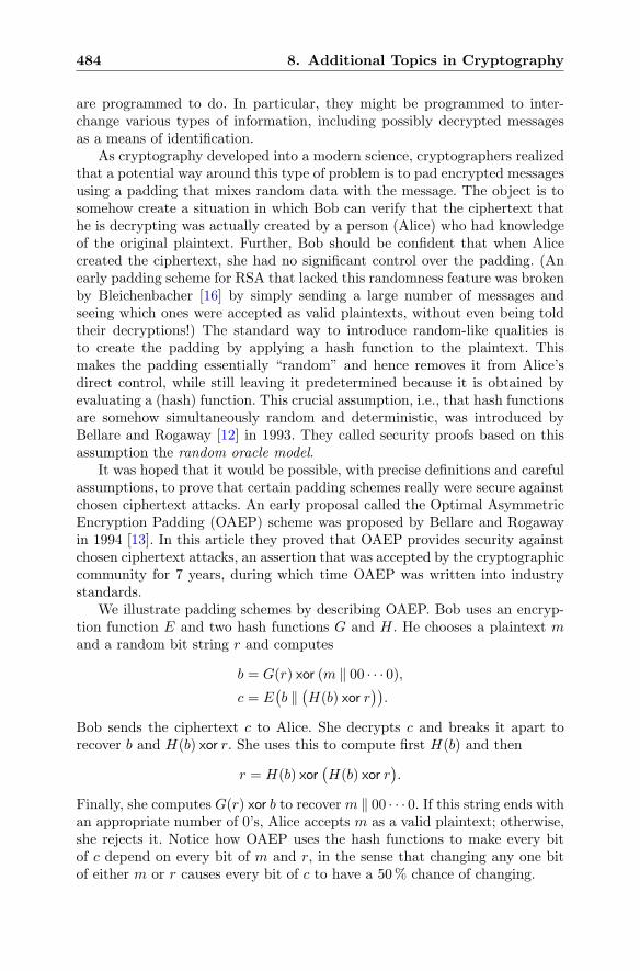
484 8. Additional Topics in Cryptography
are programmed to do. In particular, they might be programmed to inter-change various types of information, including possibly decrypted messagesas a means of identification.
As cryptography developed into a modern science, cryptographers realizedthat a potential way around this type of problem is to pad encrypted messagesusing a padding that mixes random data with the message. The object is tosomehow create a situation in which Bob can verify that the ciphertext thathe is decrypting was actually created by a person (Alice) who had knowledgeof the original plaintext. Further, Bob should be confident that when Alicecreated the ciphertext, she had no significant control over the padding. (Anearly padding scheme for RSA that lacked this randomness feature was brokenby Bleichenbacher [16] by simply sending a large number of messages andseeing which ones were accepted as valid plaintexts, without even being toldtheir decryptions!) The standard way to introduce random-like qualities isto create the padding by applying a hash function to the plaintext. Thismakes the padding essentially “random” and hence removes it from Alice’sdirect control, while still leaving it predetermined because it is obtained byevaluating a (hash) function. This crucial assumption, i.e., that hash functionsare somehow simultaneously random and deterministic, was introduced byBellare and Rogaway [12] in 1993. They called security proofs based on thisassumption the random oracle model.
It was hoped that it would be possible, with precise definitions and carefulassumptions, to prove that certain padding schemes really were secure againstchosen ciphertext attacks. An early proposal called the Optimal AsymmetricEncryption Padding (OAEP) scheme was proposed by Bellare and Rogawayin 1994 [13]. In this article they proved that OAEP provides security againstchosen ciphertext attacks, an assertion that was accepted by the cryptographiccommunity for 7 years, during which time OAEP was written into industrystandards.
We illustrate padding schemes by describing OAEP. Bob uses an encryp-tion function E and two hash functions G and H. He chooses a plaintext mand a random bit string r and computes
b = G(r) xor (m ‖ 00 · · · 0),c = E
(b ‖(H(b) xor r
)).
Bob sends the ciphertext c to Alice. She decrypts c and breaks it apart torecover b and H(b) xor r. She uses this to compute first H(b) and then
r = H(b) xor(H(b) xor r
).
Finally, she computes G(r) xor b to recoverm ‖ 00 · · · 0. If this string ends withan appropriate number of 0’s, Alice accepts m as a valid plaintext; otherwise,she rejects it. Notice how OAEP uses the hash functions to make every bitof c depend on every bit of m and r, in the sense that changing any one bitof either m or r causes every bit of c to have a 50% chance of changing.
8.7. Building Protocols from Cryptographic Primitives 485
Unfortunately, it was shown by Shoup in 2001 [131] that one of theassumptions in the security proof of OAEP was unreasonable, in the sensethat it assumed that no amount of probing of a certain piece of informationcould produce useful information. This embarrassing incident underlined oneof the fundamental limitations of security proofs. Just as it is possible for acomplicated cryptographic system to be insecure because the cryptographerhas protected it only against the lines of attack that he knows, a “proof ofsecurity” is only as secure as the validity of its assumptions (not to mentionthe correctness of its logic). Shoup proposed a variant called OAEP+ andgave a correct proof of its security in the random oracle model.
One might think that for the purposes of analyzing the security of a cryp-tosystem, it is very reasonable to assume that hash functions behave exactlyas they are supposed to behave, with no hidden flaws, biases, or weaknesses.However, there have been fierce arguments regarding the use of the randomoracle model as the basis for the security of cryptosystems, with the resultthat an alternative (stronger) assumption called the standard model has beendeveloped to provide what has become known as provable security. For somehint of the controversy that this has engendered, see for example [69].
For an overview of this subject we recommend the highly readable surveyarticles of Koblitz and Menezes [70] and Bellare [11]. Koblitz and Menezesremark that “The first books on cryptography that the two of us wrote in ournaive youth suffer from this defect: the sections on security deal only withthe problem of inverting the one-way function.” (Also included is a footnoteclarifying the meaning of the word “youth.”) This quotation highlights thetendency of those trained in pure mathematics, when introduced to the field ofpublic key cryptography, to concentrate primarily on the concept of (trapdoor)one-way functions, to the exclusion of the many practical issues that arisein real-world implementations. Indeed, the authors of the present book mustadmit that even with full knowledge of this pitfall, it is the quest to construct,understand, and apply new one-way functions to cryptographic systems thatdraws them to the subject.5
8.7 Building Protocols from CryptographicPrimitives
The use of public key cryptography and digital signature schemes in the realworld involves far more than simply implementing one or two basic algorithms.Applications almost always involve a number of different cryptographic primi-tives. For example, a public key might itself be digitally signed, and the publickey cryptosystem, whose plaintexts are padded using a hash function, might beused to send the key for a symmetric cipher. So this single application involves
5And unfortunately, the authors of this book cannot even offer up youth, by anydefinition, as an excuse for their behavior.
486 8. Additional Topics in Cryptography
choosing a public key cryptosystem and digital signature scheme (e.g., RSA),a hash function (e.g., SHA-1), a padding scheme (e.g., OAEP+), and a sym-metric cipher (e.g., AES).
However, even this simple description is far from sufficient. For example,are Bob and Alice using RSA with 1024-bit keys or with 2048-bit keys? Howlong are their AES keys? Exactly how do they use their hash function or sym-metric cipher to generate pseudorandom numbers? And even if they specifyall of the obvious parameters and decide how to use all of the cryptographicprimitives, they’re still not ready to communicate. They need to agree on for-matting. This may seem pedantic, but it is very important. Before Bob andAlice exchange messages, they need to specify the exact meaning of each byteof the data, e.g., which bytes are the ciphertext, which bytes are the signature,etc. Even something as seemingly trivial as the order in which data is storedin memory and transmitted between computers can cause total system failureif not specifically addressed.6
A cryptographic protocol is a complete description of everything that isneeded in order to implement a cryptographic procedure. The term is not en-tirely precise, but it generally refers to the way in which one or more crypto-graphic algorithms are to be implemented and coordinated with one another.
The theory of cryptographic protocols, especially their creation and proofsof security, is a subject in its own right, with numerous articles and books de-voted to the topic. We note that even if one assumes that the underlyingcryptographic primitives such as RSA or ECC are secure, it is extremely easyto use such primitives to create a seemingly secure protocol that is, in fact,vulnerable to attack. This is especially true if one designs the protocol pri-marily with a view toward efficiency and flexibility; it is vital that securityconsiderations be given top priority. Further, given the complexity of any pro-tocol that is formed by fitting together several cryptographic primitives, itcan be difficult to give even a convincing heuristic argument that the pro-tocol has no security weaknesses. In brief, the construction and analysis ofcryptographic protocols is not for the faint of heart, but it is of fundamentalimportance if modern cryptography is to be of any use in the real world.
In order for computers in far-flung parts of the world to communicate se-curely (or at all), someone needs to sit down and specify precise cryptographicprotocols. This is normally done by standard-setting bodies that are formedeither by the government or by representatives from the relevant industries.Even restricting to the field of secure communications, there are many suchbodies in existence, each of which consumes countless man-hours of effortand innumerable reams of paper7 as it spends years issuing draft versions
6Data stored on a computer as least-significant-byte first is said to be in little-endian for-mat, while the reverse order is called big-endian. These amusing names come from Gulliver’sTravels, in which the inhabitants of one kingdom are required to crack their soft-boiled eggsat the “little end,” while those in a rival kingdom crack their eggs at the “big end.”
7We ask the reader to excuse our hyperbole. In particular, the aforementioned reams ofpaper are figurative, having largely been replaced by megabytes of disk space.
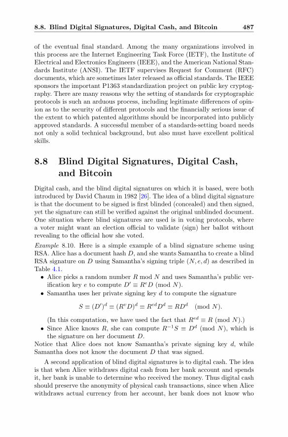
8.8. Blind Digital Signatures, Digital Cash, and Bitcoin 487
of the eventual final standard. Among the many organizations involved inthis process are the Internet Engineering Task Force (IETF), the Institute ofElectrical and Electronics Engineers (IEEE), and the American National Stan-dards Institute (ANSI). The IETF supervises Request for Comment (RFC)documents, which are sometimes later released as official standards. The IEEEsponsors the important P1363 standardization project on public key cryptog-raphy. There are many reasons why the setting of standards for cryptographicprotocols is such an arduous process, including legitimate differences of opin-ion as to the security of different protocols and the financially serious issue ofthe extent to which patented algorithms should be incorporated into publiclyapproved standards. A successful member of a standards-setting board needsnot only a solid technical background, but also must have excellent politicalskills.
8.8 Blind Digital Signatures, Digital Cash,and Bitcoin
Digital cash, and the blind digital signatures on which it is based, were bothintroduced by David Chaum in 1982 [26]. The idea of a blind digital signatureis that the document to be signed is first blinded (concealed) and then signed,yet the signature can still be verified against the original unblinded document.One situation where blind signatures are used is in voting protocols, wherea voter might want an election official to validate (sign) her ballot withoutrevealing to the official how she voted.
Example 8.10. Here is a simple example of a blind signature scheme usingRSA. Alice has a document hash D, and she wants Samantha to create a blindRSA signature on D using Samantha’s signing triple (N, e, d) as described inTable 4.1.• Alice picks a random number R mod N and uses Samantha’s public ver-ification key e to compute D′ ≡ ReD (mod N).
• Samantha uses her private signing key d to compute the signature
S ≡ (D′)d ≡ (RvD)d ≡ RedDd ≡ RDd (mod N).
(In this computation, we have used the fact that Red ≡ R (mod N).)
• Since Alice knows R, she can compute R−1S ≡ Dd (mod N), which isthe signature on her document D.
Notice that Alice does not know Samantha’s private signing key d, whileSamantha does not know the document D that was signed.
A second application of blind digital signatures is to digital cash. The ideais that when Alice withdraws digital cash from her bank account and spendsit, her bank is unable to determine who received the money. Thus digital cashshould preserve the anonymity of physical cash transactions, since when Alicewithdraws actual currency from her account, her bank does not know who
488 8. Additional Topics in Cryptography
she gives it to. (Of course, her bank can record the serial numbers of thebills that she receives and then track those bills as they move through thebanking system.) Cryptographic methods adding various enhancements, suchas off-line transactions and safeguards against double spending of digital cashunits, were described in later work of Chaum, his co-authors, and others; seefor example [27].
A potential weakness of these digital cash systems is the necessity of hav-ing a trusted central authority, be it a bank, an e-cash company, or a govern-ment, that is responsible for issuing cash and safe-guarding the security of thesystem. In principle, the fiat currencies issued by any government have thisweakness, since at any time the issuing body might decide to (say) halve thevalue of everyone’s wealth by doubling the amount of available currency. Inthe short term, this would make the government very rich, since they wouldsuddenly have a lot of extra cash to spend. In practice, it would lead to run-away inflation.8
The article “Bitcoin: A Peer-to-Peer Electronic Cash System” [91] pro-posed a practical way to create a digital cash system without requiring atrusted central authority. The idea is to digitally sign and cryptographicallyjoin every transaction into a massive linked chain. To prevent a small group ofusers from modifying the chain and, say, repudiating or canceling a payment,the system is designed so that it takes a significant amount of computingpower to add a transaction to the chain. People who do these time-consumingmining computations that keep the system running are rewarded with a smallfraction of a bitcoin. The complete transaction chain is stored on myriad com-puters and is always available for public scrutiny.
There is much hype and much controversy surrounding Bitcoin, includingfor example the question of whether a currency that is not backed by anythingtangible can have value.9 This being a mathematical text, we will also notpursue the fascinating economic and sociological issues raised by Bitcoin, norwill we discuss how Bitcoin has been used as a (highly) speculative investmenttool and as a way of concealing illegal activities. Instead, we turn to thecryptographic protocols that underlie Bitcoin.
Bitcoin uses the elliptic curve digital signature algorithm (ECDSA,Sect. 6.4.3) to sign transactions. It uses the specific elliptic curve, prime,and point (E, p, P ) denoted by secp256k1 in the Standards for EfficientCryptography document [142, page 21]. Based on our current knowledge ofthe difficulty of solving the ECDHP, this provides approximately 128 bitsecurity. Since it’s fun to see the actual public parameters used to secure the
8Many economists feel that a small amount of inflation is a good thing, since it encour-ages investment while allowing governments to slowly outgrow their accumulated debts.
9In fairness, it is not entirely clear in what sense the “full faith and credit of the UnitedStates government” that backs US currency is tangible, although one can argue that thisfaith and credit represents the taxing authority of the government on the US economy,whose productivity and output are eminently tangible.
8.8. Blind Digital Signatures, Digital Cash, and Bitcoin 489
Bitcoin chain, we list them here. The Bitcoin curve is
E : y2 = x3 + 7,
and the prime
p = 2256 − 232 − 29 − 28 − 27 − 26 − 24 − 1
was chosen to have low Hamming weight, which speeds up computations inthe field Fp. The prime p and curve E have the further property that
N = #E(Fp) = p+ 1− 432420386565659656852420866390673177327
is prime, which means that every non-zero point in E(Fp) has order N . Thepublic point P = (x, y) ∈ E(Fp) specified by the secp256k1 standard is
x = 5506626302227734366957871889516853432625060345377
7594175500187360389116729240,
y = 3267051002075881697808308513050704318447127338065
9243275938904335757337482424.
As mentioned earlier, Bitcoin miners perform time-consuming calculationsin order to add bitcoin transactions to the chain. They do this by findingan input to the hash function SHA-25610 (see Sect. 8.1) that is tied to thetransaction(s) and has output containing a specified number of leading (ortrailing) zeros. Over time, as more CPU power is devoted to mining, theSHA-256 requirements are constantly being strengthened so that it alwaystakes 5–10min on average for a transaction to be added to the chain. Again,the purpose of this requirement is to prevent any small group from going backand altering the existing chain.
We close this section with a few interesting Bitcoin tidbits:• Unlike ordinary currency, it is possible to create Bitcoins that can onlybe spent using two signatures, or two out of three signatures, etc.
• The total number of bitcoins is designed to stabilize at 21,000,000. Thiswill, in principle, eliminate bitcoin inflation (which many would argue isa bug, not a feature, of a currency).
• As with all protocols that rely on factorization or discrete logarithm basedcryptography, the construction of quantum computers (Sect. 8.11) willrequire switching to a quantum secure cryptosystem. The logistics of sucha switch are likely to be problematic without considerable preparation andforethought.
10It is interesting that the hash function SHA-256 used by Bitcoin provides 256 bitsecurity, while the ECDSA signature scheme secp256k1 provides only 128 bit security.
490 8. Additional Topics in Cryptography
8.9 Homomorphic Encryption
The basic RSA PKC has an interesting multiplicativity property. Supposethat Bob sends Alice two ciphertexts c1 and c2 associated to the plaintexts m1
and m2. Then the ciphertext associated to the product m1m2 is the productof the ciphtertexts c1c2. This is true because
c1c2 ≡ me1m
e2 ≡ (m1m2)
e (mod N).
On the other hand, the ciphertext associated to m1 +m2 is almost certainlynot the sum of the ciphtertexts c1 + c2, since in general
(m1 +m2)e �≡ me
1 +me2 (mod N).
A fully homomorphic cryptosystem is one that respects both addition andmultiplication. Since homomorphic encryption involves two operations, thissuggests that the correct setting for homomorphic encryption is ring theory;see Sect. 2.10. In particular, we recall from Exercise 2.31 that if R and S arerings, then a ring homomorphism φ : R→ S is a function satisfying
φ(a+ b) = φ(a) + φ(b) and φ(a � b) = φ(a) � φ(b) for all a, b,∈ R.
Definition. A fully homomorphic encryption scheme (FHE scheme) is an en-cryption scheme (K,M, C, e, d) with the property that the plaintext spaceMand the ciphertext space C are rings and such that for every key k ∈ K, theencryption function
ek :M−→ Cis a ring homomorphism.11
Example 8.11. Here is an example of an FHE scheme. Let M = C = Fpd bea finite field with pd elements (see Sect. 2.10.4), and let K = {1, 2, . . . , d− 1}.Then for each k ∈ K, the encryption function
ek(m) = mpk
is fully homomorphic, with decryption function dk(c) = cpd−k
. (We are using
the fact that apd
= a and (a + b)p = ap + bp for all elements a, b ∈ Fpd .) Ofcourse, this cryptosystem is either very insecure, if d is small, or completelyimpractical, if d is large.
11We like this definition of FHE because it stresses the homomorphism in the name, butwe note that the standard definition allows more general constructions. Thus a cryptosystemis said to be fully homomorphic if it is possible to compute any function or circuit onencrypted data without knowing the decryption key. Thus one only needs to do additionand multiplication on encryptions of F2, and it is not strictly necessary for the ciphteretxtspace to be a ring.
8.9. Homomorphic Encryption 491
The search for a secure and practical FHE scheme started shortly afterthe invention of RSA in the 1970s, but it remained an elusive goal until CraigGentry devised the first such system in 2009 [47, 48]. Although neither Gen-try’s original system, nor subsequent improvements, are fast enough to beused in practical applications, research continues on this important topic.
Why, one might ask, is homomorphic encryption interesting or useful? Theanswer is that using the basic operations of addition and multiplication (evenjust moduo 2), one can perform any computation that can be done by anycomputer. Consider the following scenario. Bob has a large amount of data toanalyze, but the analysis requires a tremendous amount of computing power,far more than Bob possesses. Alice, on the other hand, owns a lot of computersand is happy to rent computing time to Bob.12 Unfortunately, the data thatBob needs to analyze is confidential; for example, it might include medical orfinancial records. So what Bob would like to do is the following:
• Encrypt the data, and also encrypt the computer program that willanalyze the data.
• Send the encrypted data and the encrypted program to Alice.
• Have Alice run the encrypted program using the encrypted data withoutdecrypting either.
• Receive the encrypted output from Alice, which he then decrypts.
The miracle of an FHE scheme is that it allows Alice to run an encryptedcomputer program on encrypted data and produce encrypted output, withoutever seeing any of Bob’s unencrypted material.
Gentry’s original FHE scheme has two components. First he constructs asystem that is “somewhat homomorphic,” and then he uses an ingenious boot-strapping procedure to make it fully homomorphic. The following definitionwill be used to quantify the notion of “somewhat homomorphic.”
Definition. A monic monomial in n variables is a polynomial of the form
M(X1, . . . , Xn) = Xe11 X
e22 · · ·Xen
n with e1, . . . , en ≥ 0.
The degree of M is deg(M) = e1 + · · ·+ en. More generally, let
P (X1, . . . , Xn) =M1(X1, . . . , Xn) + · · ·+Mr(X1, . . . , Xn)
be a sum of monic monomials, and let d = maxdegMi. Then we say that P hasadditive level r and multiplicative level d. We write Levela(P ) and Levelm(P ),respectively, for the additive and multiplicative levels of P
Every computation in a ring R may be viewed as evaluating some polyno-mial P (X1, . . . , Xn) at some point (a1, . . . , an) ∈ Rn, although this may firstrequire simplification using the distributive law. For example,
12This situation is quite realistic. There are many companies, large and small, from whichone can rent computing power.
492 8. Additional Topics in Cryptography
(((a1 + a2 + a3) � a4) + a5) � a6 = a1a4a6 + a2a4a6 + a3a4a6 + a5a6
= P (a1, . . . , a6)
with
P (X1, . . . , X6) = X1X4X6 +X2X4X6 +X3X4X6 +X5X6.
We note that in order to compute P (a1, . . . , an), we need to do atmost Levela(P ) additions of quantities, each of which is a product of atmost Levelm(P ) elements of R.
Definition. Let (K,M, C, e, d) be a cryptosystem such that M and C arerings. We say that it is a leveled homomorphic cryptosystem of level (La, Lm)if for every key k ∈ K, every polynomial P (X1, . . . , Xn) satisfying
Levela(P ) ≤ La and Levelm(P ) ≤ Lm,
and every m1, . . . ,mn ∈M, we have
dk(P(ek(m1), . . . , ek(mn)
))= P (m1, . . . ,mn),
i.e., P(ek(m1), . . . , ek(mn)
)is a valid encryption of P (m1, . . . ,mn) for the
key k.
Informally, a cryptosystem is leveled homomorphic if encryption ek is aring homomorphism when it is applied to expressions that involve a limitednumber of additions and multiplications in the ringM. Leveled homomorphiccryptosystems are interesting for two reasons. First, Gentry’s bootstrappingmethod sometimes allows one to turn a leveled system into a fully homomor-phic system, albeit at a significant loss of efficiency. Second, if the levels La
and Lm are sufficiently large, then even a leveled system may be useful inpractice.
A number of leveled homomorphic cryptosystems have been proposed, andthe construction of secure and efficient systems is an active area of research.We illustrate by briefly explaining how the NTRU cryptosystem described inSect. 7.10 can be used as a leveled homomorphic system.
Example 8.12 (Leveled Homomorphic NTRUEncrypt). To simplify the expo-sition, we use a variant of NTRUEncrypt in which we assume that the privatekey polynomials f(x) and g(x) are chosen to satisfy
f(x) ≡ 1 (mod p) and g(x) ≡ 0 (mod p); (8.1)
see Exercise 7.35. The NTRU plaintext and ciphertext spaces are ringsM = Rp and C = Rq, and encryption of a plaintext m(x) using the (public)key h(x) ≡ f(x)−1 � g(x) (mod q) and random element r(x) is given by theformula
e(x) ≡ h(x) � r(x) +m(x) (mod q).
8.9. Homomorphic Encryption 493
Decryption is done by first computing the center-lift of f(x) � e(x) (mod q),and then reducing the result modulo p. Just as in the proof of Proposition 7.48,see also Exercise 7.35, decryption works provided that every coefficient of thepolynomial
g(x) � r(x) + f(x) �m(x)
(without any reduction) has magnitude smaller than 12q.
We now consider two ciphtertexts e1 and e2. We claim that if q is largeenough, then the decryption of e1 + e2 using the private key f yields theplaintext m1 +m2, and similarly, the decryption of e1 � e2 using the privatekey f2 yields the plaintext m1 �m2. To see why, we compute
f � (e1 + e2) ≡ (g � r1 + f �m1) + (pg � r2 + f �m2) (mod q)
≡ g � (r1 + r2) + f � (m1 +m2) (mod q),
so if q is large enough, then the center-lift is exactly the polynomial
g � (r1 + r2) + f � (m1 +m2).
Using (8.1), we see that when we reduce modulo p, we get m1+m2 (mod p).Similarly,
f2 � (e1 � e2) ≡ (g � r1 + f �m1) � (g � r2 + f �m2) (mod q)
≡ g � (g � r1 � r2 + f � r1 �m2 + f � r2 �m1)
+ f2 � (m1 �m2) (mod q).
So again, if q is large enough, then the center-lift gives us exactly the polyno-mial
g � (g � r1 � r2 + f � r1 �m2 + f � r2 �m1) + f2 � (m1 �m2),
and reducing modulo p gives m1 �m2 (mod p).We have just shown that if q is large enough, then e1 + e2 is an NTRU
encryption ofm1+m2 and e1�e2 is an NTRU encryption ofm1�m2, althoughfor the latter the decryption key is f2. In leveled homomorphic terminology,if q is large enough, then the addition property says that NTRUEncrypt isleveled homomorphic with level (2, 1), and the multiplication property saysthat it is leveled homomorphic with level (1, 2). Further, it is clear that byincreasing q, we can create leveled homomorphic versions of NTRUEncryptof any level.
In order to derive a rough relationship between the value of q and thelevels achieved, we make the simplifying assumption that f , g, m, and r havecoefficients between −p and p, and we put no restriction on the number ofnonzero coefficients.
Let P (X1, . . . , Xn) be a sum of monic monomials, and to ease notation,let
494 8. Additional Topics in Cryptography
α = α(P ) = Levela(P ) and μ = μ(P ) = Levelm(P ).
It is also convenient to use the homogenized version of P defined by
P ∗(X0, . . . , Xn) = Xμ0 P (X1/X0, . . . , Xn/X0),
so P ∗ is a sum of monic monomials, each of which has degree exactly μ.Let m1, . . . ,mn be plaintexts, and let e1, . . . , en be associated ciphertexts.Then P (e1, . . . , en) decrypts correctly to P (m1, . . . ,mn) using the decryptionkey fμ if the largest coefficient of
P (f , g � r1 + f �m1, . . . , g � rn + f �mn) (8.2)
has magnitude smaller than 12q.
We observe that if a1, . . . ,at ∈ R have coefficients between −C and C,then the largest coefficient of the product a1 � · · · � at is at most CtN t−1,obtained for example if every coefficient of every ai is C. Hence the largestcoefficient of
g � ri + f �mi
is at most 2p2N . The monomials appearing in (8.2) are products of μ ex-pressions of the form g � ri + f �mi with 0 ≤ i ≤ n, where for conveniencewe set r0 = 0 and m0 = 1. So the monomials in (8.2) have coefficients thatare at most (2p2N)μNμ−1, which is smaller than (2pN)2μ. Finally, we notethat (8.2) is a sum of at most α monomials, and hence the largest coeffi-cient in (8.2) is at most α(2pN)2μ. This proves that P (e1, . . . , en) decryptscorrectly to P (m1, . . . ,mn) using the decryption key fμ if q satisfies
q > 2α(2pN)2μ.
Thus the size of q increases linearly with the number of additions, but expo-nentially with the number of multiplications
8.10 Hyperelliptic Curve Cryptography
A hyperelliptic curve of genus g is the set of solutions to an equation of theform13
C : Y 2 = X2g+1 +A1X2g + · · ·+A2gX +A2g+1,
with the added requirement that the polynomial F (X) = X2g+1+ · · ·+A2g+1
have distinct roots.14 And just as for elliptic curves, we throw in one extrapoint O that lives “at infinity.” Thus an elliptic curve is a curve of genus 1.
13When working over a field F2k , one uses the more general form Y 2 + Y = F (X).14When one is working over C, the distinct roots condition means complex roots. Over a
finite field Fp, the condition may be formulated by requiring that the discriminant of F (X)not vanish, or equivalently that gcd
(F (X), F ′(X)
)= 1, where F ′(X) is obtained by formally
differentiating F (X).
8.10. Hyperelliptic Curve Cryptography 495
In general there is no addition law for the individual points on a hyper-elliptic curve, but it is possible to define an addition law for collections ofpoints. Roughly speaking, we can take two collections of g points, say
{P1, P2, . . . , Pg} and {Q1, Q2, . . . , Qg},
and “add” them to obtain a new collection of g points {R1, R2, . . . , Rg}. Thisgeneralizes the addition law on an elliptic curve, but a precise formulation issomewhat more complicated.
To describe the addition law exactly, we define a divisor on C to be aformal sum of points
n1[P1] + n2[P2] + · · ·+ nr[Pr] with P1, . . . , Pr ∈ C and n1, . . . , nr ∈ Z.
Note that a divisor is simply a convenient shorthand for a finite set of points,each of which has an attached multiplicity. In particular, if f(X,Y ) is a ra-tional function on C, then we can attach a divisor to f(X,Y ) by listing thepoints where f vanishes and the points where f has poles, with their appro-priate multiplicities. The degree of a divisor is the sum of its multiplicities,
deg(D) = deg(n1[P1] + n2[P2] + · · ·+ nr[Pr]
)= n1 + n2 + · · ·+ nr.
(See Sect. 6.8.2 for a discussion of rational functions and divisors on ellipticcurves.)
We next define the divisor group of C, denoted by Div(C), to be the setof divisors on C. Note that we can add and subtract divisors by adding andsubtracting the multiplicities of each point. We also let Div0(C) be the set ofdivisors of degree 0. One can prove that the divisor of a function always hasdegree 0. Two divisors D1 and D2 are said to be linearly equivalent if
D1 −D2 = divisor of a function.
We write Jac0(C) for the set of divisors of degree 0, with the understand-ing that linearly equivalent divisors are considered to be identical. Theset Jac0(C), with the addition law obtained by adding the multiplicities ofpoints, is called the Jacobian variety of C. It is the higher-genus analogue ofelliptic curves and their addition laws.
A crucial property of Jac0(C) is that it can be described as the set of solu-tions to a system of polynomial equations, and the addition law may also bedescribed using polynomials. So if we take solutions with coordinates in Fp,then we obtain a group (i.e., a set with an addition law) that is completelyanalogous to the group E(Fp) of points on an elliptic curve. For notationalconvenience, let J = Jac0(C) and J(Fp) be the points on Jac0(C) with coor-dinates in Fp. The Hyperelliptic Curve Discrete Logarithm Problem (HCDLP)is as follows:
Given P and Q in J(Fp), find an integer m such that Q = mP .
496 8. Additional Topics in Cryptography
It is clear how one can use hyperelliptic curves for public key cryptography bymimicking the constructions for the multiplicative group (Sects. 2.3 and 2.4)and for elliptic curves (Sect. 6.4). This leads to hyperelliptic Diffie–Hellmankey exchange and the hyperelliptic Elgamal public key cryptosystem.
The primary, and from cryptographic purposes fundamental, differencebetween elliptic curves and hyperelliptic curves is that the latter have largergroups of points. More precisely, there is an analogue of Hasse’s theorem(Theorem 6.11), due to Andre Weil, which says that
#J(Fp) = pg +O(pg−
12
).
For example, a hyperelliptic curve of genus 2 has approximately p2 points.
As with elliptic curves, one hopes that the best algorithms to solve theHCDLP are collision algorithms such as Pollard’s ρ algorithm. (But see Re-mark 8.13.) Since the group J(Fp) has approximately pg elements, this meansthat it takes O(pg/2) steps to solve HCDLP. Thus using curves with g > 1allows us to achieve security levels equivalent to those on elliptic curves whileusing a smaller prime p.
However, as g gets large, the computational complexity of the addition lawbecomes formidable (and there are also security issues), so for concreteness,we consider the case g = 2. Then J(Fp) has approximately p2 elements andit takes O(p) steps to solve the HCDLP. This may be compared with anelliptic curve, for which #E(Fp) ≈ p and ECDLP takes O(
√p ) steps to solve.
Thus J(Fp) allows us to use primes with approximately half as many digits.This does not lead to a significant speed advantage, because the addition lawon J is significantly more complicated than the addition law on E. However,it does mean that ciphertexts, and even more importantly, digital signatures,are half as large using J as they are using E. This becomes a large advantageon highly constrained devices such as radio frequency identification (RFID)tags.
Remark 8.13. It is not actually true that the best known methods to solvethe HCDLP are collision algorithms. If the genus g of the curve is moderatelylarge compared to the prime p, then Adleman, DeMarrais, and Huang foundan index calculus algorithm that solves the HCDLP in subexponential time.They show that if 2g+ 1 ≥ (ln p)1+ε for some ε > 0, then the HCDLP can besolved in L(p2g+1)c steps for some small constant c. In the opposite direction,if p is large, say p > g!, then Gaudry found an algorithm to solve the HCDLPin O(g3p2+ε) steps. This is not helpful if g = 1 or 2, but it is significantif g ≥ 3 and p is large. This is one of the reasons that only hyperelliptic curvesof genus 2 and 3 are being seriously considered for use in cryptography.
Finally, just as for elliptic curves, there are various attacks on the HCDLPusing versions of the Weil and Tate pairing (see Sect. 6.9.1), but it is easy toavoid such attacks by appropriate choices of parameters.
8.11. Quantum Computing 497
8.11 Quantum Computing
The value of each bit in a classical computer is either 0 or 1. In a quantumcomputer, each so-called quantum bit (qubit) may simultaneously takes onevery value between 0 and 1 with varying probabilities. This added flexibil-ity allows many computations, including integer factorization and discretelogarithm problems, to be done very quickly. Thus a working quantum com-puter with sufficiently many qubits would break RSA and both the classicaland the elliptic curve versions of Elgamal. (However, there is at present nopolynomial-time quantum algorithm that solve the shortest or closest latticevector problems.)
Tempting though it is, we will not use this opportunity to give a seriousintroduction to quantum mechanics. The aim of this section is fairly modest.We sketch the basic ideas behind one remarkable application of quantum me-chanics to cryptography: Shor’s polynomial-time quantum algorithm [128] forfactoring integers and for finding discrete logarithms. The following presen-tation owes a great deal to Shor’s accessible and beautifully written exposi-tion [129], which would serve as a nice start for the interested reader familiarwith the concept of a Hilbert space. For those with a less robust backgroundin mathematics and quantum theory, see for example [64].
The fundamental unit of information in classical computers is the binarydigit (bit), represented as a 0 or 1. Bits are manipulated according to theprinciples of Boolean logic, in which connectives such as AND and OR oper-ate on pairs of bits in the usual way, and NOT reverses 0 and 1. Sequences ofbits are manipulated by Boolean logic gates, using these Boolean rules, and asuccession of gates yields an end state, or computation. A quantum computermanipulates quantum bits (qubits) via quantum logic gates, which are sup-posed to simulate the laws of quantum mechanics, especially properties suchas superposition and entanglement, which give the field of quantum mechanicsits distinctive nonclassical characteristics.
A qubit with two states is typically represented using ket notation,15 inwhich |0〉 denotes the 0-state and |1〉 the 1-state. Then the (pure) states ofthe system have the form
α |0〉+ β |1〉 ,where α and β are complex numbers satisfying |α|2 + |β|2 = 1.
In an n-component system, the 2n basis elements are represented by se-quences such as |si〉 = |0110 . . . 0〉 consisting of a list of n zeros and ones, anda state of the system is
2n−1∑
i=0
αi |si〉 , where∑
|αi|2 = 1. (8.3)
15The rather strange word ket is the latter half of the word bracket. In quantummechanicsthere is also bra notation 〈x| and a “bracket pairing” 〈x|y〉.
498 8. Additional Topics in Cryptography
A sum (8.3) is called a superposition of states. There are other quantum statesknown as “mixed” states that we do not discuss here, so we omit the wordpure in the rest of this discussion. Thus a quantum state is represented by avector of complex numbers of length 2n such that sum of the squares of theirmoduli is equal to one. These are called complex unit vectors.
Just as for classical computers, manipulating qubits via quantum logicgates requires the notion of a change of state. A quantum change of state isthe result of applying a unitary linear transformation16 to one of the complexunit vectors representing a state. Actually, there are additional restrictions onwhich unitary transformations are permitted for changes of state. One of theserestrictions is the requirement of locality : the unitary matrices should operateon only a fixed finite number of bits. It turns out that 2-bit transformationsform the building blocks of the allowable transformations.
The quantum-mechanical interpretation of the αi’s is that |αi|2 representsthe probability that a measurement of the system yields state |si〉. It is theprobabilistic interpretation of the complex coefficients of these vectors thatencodes the physical realities observed in experiment and predicted by physicaltheory.
In [129], Shor describes a quantum polynomial-time algorithm to find (withhigh probability) the order r of a number x mod n. (Recall that the orderof x is the smallest integer r ≥ 1 such that xr ≡ 1 mod n.) Factorizationcan be reduced to the problem of finding the order of an integer, because if xis chosen randomly and has even order r, then gcd (xr/2 − 1, n) is likely tobe a nontrivial odd factor of n. (See [87].) Shor also gives a polynomial-timequantum algorithm to solve the discrete logarithm problem in F
∗p, and such
algorithms also exist for the elliptic curve discrete logarithm problem [107].Interestingly, there are still no polynomial-time (or even subexponential-time)quantum algorithms to solve the shortest or closest vector problems, so lattice-based cryptosystems are currently secure even against the construction of aquantum computer.17
The basic building block of Shor’s algorithm is a quantum version of theFast Fourier Transform. In order to find the order r of a number a modulo n,we choose q to be a power of 2 in the interval between n2 and 2n2. Then forany 0 < a < q, the state |a〉 is obtained from the binary representation of thenumber a. The Fourier transform of |a〉 is the state
1
q1/2
q−1∑
c=0
|c〉 exp(2πiac/q).
16A unitary linear transformation is given by a matrix with determinant one whoseconjugate transpose is equal to its inverse.
17This is not strictly true because there is a general quantum search algorithm thatessentially cuts searches by a square root. So if a quantum computer were built, the keysize of lattice-based cryptosystems might need to double. But this would be a small pricecompared to the devastation that a working quantum computer would cause to factorizationand discrete logarithm-based systems.
8.12. Modern Symmetric Cryptosystems: DES and AES 499
It turns out that this transformation can be achieved in polynomial time.Shor then applies the quantum Fourier transform to a certain superpositionof states and measures the resulting system. The key computation shows thatthe probability of seeing state |c〉 is relatively large if there exists a rationalnumber d
r ∈ Q satisfying ∣∣∣∣c
q− d
r
∣∣∣∣ <
1
2q.
(Recall that r is the order of a.) Using the continued fraction expansion of theknown rational number c
q , it is not hard to determine the fraction dr in lowest
terms, since q > n2.There remains only the “minor” challenge of building a functioning quan-
tum computer. Research in this field has focused on the issue of decoherence,which involves controlling the errors in quantum computation introduced bythe interaction of the computer with its environment. There is already a vastliterature on quantum computing and quantum computers, reflecting to someextent the large amount of government funding that has been allocated to thesubject. One place to start gathering resources about quantum computers isthe website for NIST’s Quantum Information Program at qubit.nist.gov.
Finally, we would be remiss if we did not mention the theory of quantumcryptography. The idea is to use quantum-mechanical principles such as theHeisenberg uncertainty principle or the entanglement of quantum states toperform a completely secure key exchange. In particular, if Eve attempts toread either Bob’s or Alice’s transmission, then quantum theory says that shemust alter the data, so Bob and Alice will know that their communicationhas been compromised.
8.12 Modern Symmetric Cryptosystems:DES and AES
In Sect. 1.7.1 we gave an abstract formulation of symmetric ciphers, and inSect. 1.7.4 we described several elementary examples. Not surprisingly, noneof the examples in Sect. 1.7.4 is secure. Modern symmetric ciphers such asthe Data Encryption Standard (DES) and the Advanced Encryption Standard(AES) are based on ad hoc mixing operations, rather than on intractablemathematical problems used by asymmetric ciphers. The reason that DESand AES and other symmetric ciphers are used in practice is that they aremuch faster than asymmetric ciphers. Thus if Alice wants to send Bob a longmessage, she first uses an asymmetric cipher such as RSA to send Bob a keyfor a symmetric cipher, and then she uses a symmetric cipher such as DES orAES to send the actual data.
DES was created by a team of cryptographers at IBM in the early 1970s,and with some modifications suggested by the United States National SecurityAgency (NSA), it was officially adopted in 1977 as a government standard
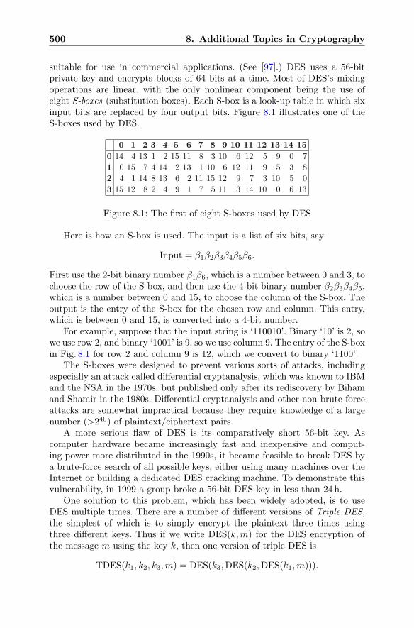
500 8. Additional Topics in Cryptography
suitable for use in commercial applications. (See [97].) DES uses a 56-bitprivate key and encrypts blocks of 64 bits at a time. Most of DES’s mixingoperations are linear, with the only nonlinear component being the use ofeight S-boxes (substitution boxes). Each S-box is a look-up table in which sixinput bits are replaced by four output bits. Figure 8.1 illustrates one of theS-boxes used by DES.
0 1 2 3 4 5 6 7 8 9 10 11 12 13 14 150 14 4 13 1 2 15 11 8 3 10 6 12 5 9 0 71 0 15 7 4 14 2 13 1 10 6 12 11 9 5 3 82 4 1 14 8 13 6 2 11 15 12 9 7 3 10 5 03 15 12 8 2 4 9 1 7 5 11 3 14 10 0 6 13
Figure 8.1: The first of eight S-boxes used by DES
Here is how an S-box is used. The input is a list of six bits, say
Input = β1β2β3β4β5β6.
First use the 2-bit binary number β1β6, which is a number between 0 and 3, tochoose the row of the S-box, and then use the 4-bit binary number β2β3β4β5,which is a number between 0 and 15, to choose the column of the S-box. Theoutput is the entry of the S-box for the chosen row and column. This entry,which is between 0 and 15, is converted into a 4-bit number.
For example, suppose that the input string is ‘110010’. Binary ‘10’ is 2, sowe use row 2, and binary ‘1001’ is 9, so we use column 9. The entry of the S-boxin Fig. 8.1 for row 2 and column 9 is 12, which we convert to binary ‘1100’.
The S-boxes were designed to prevent various sorts of attacks, includingespecially an attack called differential cryptanalysis, which was known to IBMand the NSA in the 1970s, but published only after its rediscovery by Bihamand Shamir in the 1980s. Differential cryptanalysis and other non-brute-forceattacks are somewhat impractical because they require knowledge of a largenumber (>240) of plaintext/ciphertext pairs.
A more serious flaw of DES is its comparatively short 56-bit key. Ascomputer hardware became increasingly fast and inexpensive and comput-ing power more distributed in the 1990s, it became feasible to break DES bya brute-force search of all possible keys, either using many machines over theInternet or building a dedicated DES cracking machine. To demonstrate thisvulnerability, in 1999 a group broke a 56-bit DES key in less than 24 h.
One solution to this problem, which has been widely adopted, is to useDES multiple times. There are a number of different versions of Triple DES,the simplest of which is to simply encrypt the plaintext three times usingthree different keys. Thus if we write DES(k,m) for the DES encryption ofthe message m using the key k, then one version of triple DES is
TDES(k1, k2, k3,m) = DES(k3,DES(k2,DES(k1,m))).
8.12. Modern Symmetric Cryptosystems: DES and AES 501
A variation replaces the middle DES encryption by a DES decryption; this hasthe effect that setting k1 = k2 = k3 = k yields ordinary DES encryption. An-other variation, used by the electronics payment industry, takes k1 = k3, whichreduces key size at the cost of some security reduction. Finally, since threeDES encryptions triple the encryption time, another version called DES-Xuses a single DES encryption combined with initial and final XOR operationswith two 64-bit keys. Thus DES-X looks like
DESX(k1, k2, k3,m) = k3 xorDES(k2,m xor k1).
Although DES and its variants were widely deployed, it suffers from shortand inflexible key and block sizes. Further, although DES is fast when im-plemented in specialized hardware, it is comparatively slow in software. So in1997 the United States National Institute of Standards (NIST) organized anopen competition to choose a replacement for DES. There were many submis-sions, and after several years of analysis and several international conferencesdevoted to the selection process, NIST announced in 2000 that the Rijndaelcipher, invented by the Belgian cryptographers J. Daemen and V. Rijmen, hadbeen chosen as AES. Since that time AES has been widely adopted, althoughvariants of DES are still in use.18
AES is a block cipher in which the plaintext–ciphertext blocks are 128 bitsin length and the key size may be 128, 192, or 256 bits. AES is similar toDES in that it encrypts and decrypts by repeating a basic operation severaltimes. In the case of AES, there are 10, 12, or 14 rounds depending on the sizeof the key. AES is also similar to DES in that it uses an S-box to provide theall-important nonlinearity to the encryption process. However, AES’s S-boxis constructed using the operation of taking multiplicative inverses in thefield F28 with 28 elements. (See Sect. 2.10.4 for a discussion of finite fieldswith a prime power number of elements.) Many of AES’s basic operations use128 bit blocks, which are broken up into 16 bytes. Each byte consists of 8 bitsand is treated as an element of the field F28 . Then various operations, includinginversion, are performed in F28 . The details of AES are too complicated togive here, but they are designed to be very fast when implemented in eithersoftware or hardware. The interested reader will find a full description in theofficial NIST publication FIPS PUB 197 [96] and in many other sources.
18All of the AES finalists (MARS, RC6, Rijndael, Serpent, Twofish) were believed to besecure, and none was clearly superior in all aspects. So the choice of Rijndael was based onits balance of flexibility, ease of implementation, and speed in both hardware and software.
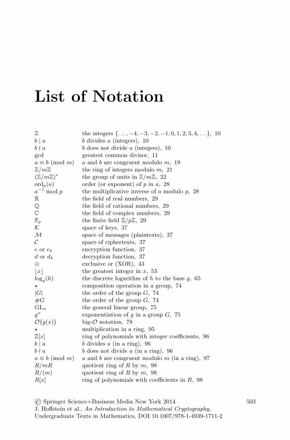
List of Notation
Z the integers {. . . ,−4,−3,−2,−1, 0, 1, 2, 3, 4, . . .}, 10b | a b divides a (integers), 10b � a b does not divide a (integers), 10gcd greatest common divisor, 11a ≡ b (mod m) a and b are congruent modulo m, 19Z/mZ the ring of integers modulo m, 21(Z/mZ)∗ the group of units in Z/mZ, 22ordp(a) order (or exponent) of p in a, 28a−1 mod p the multiplicative inverse of a modulo p, 28R the field of real numbers, 29Q the field of rational numbers, 29C the field of complex numbers, 29Fp the finite field Z/pZ, 29K space of keys, 37M space of messages (plaintexts), 37C space of ciphertexts, 37e or ek encryption function, 37d or dk decryption function, 37⊕ exclusive or (XOR), 43�x� the greatest integer in x, 53logg(h) the discrete logarithm of h to the base g, 65� composition operation in a group, 74|G| the order of the group G, 74#G the order of the group G, 74GLn the general linear group, 75gx exponentiation of g in a group G, 75O(g(x)
)big-O notation, 78
� multiplication in a ring, 95Z[x] ring of polynomials with integer coefficients, 96b | a b divides a (in a ring), 96b � a b does not divide a (in a ring), 96a ≡ b (mod m) a and b are congruent modulo m (in a ring), 97R/mR quotient ring of R by m, 98R/(m) quotient ring of R by m, 98R[x] ring of polynomials with coefficients in R, 98
© Springer Science+Business Media New York 2014J. Hoffstein et al., An Introduction to Mathematical Cryptography,Undergraduate Texts in Mathematics, DOI 10.1007/978-1-4939-1711-2
503
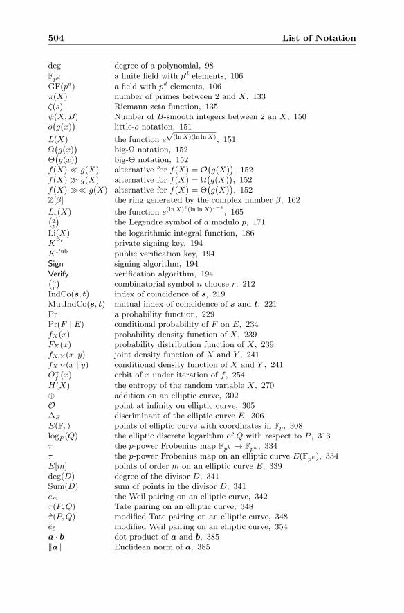
504 List of Notation
deg degree of a polynomial, 98
Fpd a finite field with pd elements, 106
GF(pd) a field with pd elements, 106π(X) number of primes between 2 and X, 133ζ(s) Riemann zeta function, 135ψ(X,B) Number of B-smooth integers between 2 an X, 150o(g(x)
)little-o notation, 151
L(X) the function e√
(lnX)(ln lnX), 151Ω(g(x)
)big-Ω notation, 152
Θ(g(x)
)big-Θ notation, 152
f(X) + g(X) alternative for f(X) = O(g(X)
), 152
f(X) , g(X) alternative for f(X) = Ω(g(X)
), 152
f(X) ,+ g(X) alternative for f(X) = Θ(g(X)
), 152
Z[β] the ring generated by the complex number β, 162
Lε(X) the function e(lnX)ε(ln lnX)1−ε
, 165(ap
)the Legendre symbol of a modulo p, 171
Li(X) the logarithmic integral function, 186KPri private signing key, 194
KPub public verification key, 194Sign signing algorithm, 194Verify verification algorithm, 194(nr
)combinatorial symbol n choose r, 212
IndCo(s, t) index of coincidence of s, 219MutIndCo(s, t) mutual index of coincidence of s and t, 221Pr a probability function, 229Pr(F | E) conditional probability of F on E, 234fX(x) probability density function of X, 239FX(x) probability distribution function of X, 239fX,Y (x, y) joint density function of X and Y , 241fX,Y (x | y) conditional density function of X and Y , 241O+
f (x) orbit of x under iteration of f , 254
H(X) the entropy of the random variable X, 270⊕ addition on an elliptic curve, 302O point at infinity on elliptic curve, 305ΔE discriminant of the elliptic curve E, 306E(Fp) points of elliptic curve with coordinates in Fp, 308logP (Q) the elliptic discrete logarithm of Q with respect to P , 313τ the p-power Frobenius map Fpk → Fpk , 334τ the p-power Frobenius map on an elliptic curve E(Fpk ), 334E[m] points of order m on an elliptic curve E, 339deg(D) degree of the divisor D, 341Sum(D) sum of points in the divisor D, 341em the Weil pairing on an elliptic curve, 342τ(P,Q) Tate pairing on an elliptic curve, 348τ(P,Q) modified Tate pairing on an elliptic curve, 348e� modified Weil pairing on an elliptic curve, 354a · b dot product of a and b, 385‖a‖ Euclidean norm of a, 385
List of Notation 505
GLn(Z) the special linear group (over Z), 390det(L) the determinant (covolume) of the lattice L, 392γn Hermite constant, 397H(B) the Hadamard ratio of the basis B, 397BR(a) closed ball of radius R centered at a, 397Γ(s) the gamma function, 400σ(L) Gaussian expected shortest length of a vector in L, 402R the convolution polynomial ring Z[x]/(xN − 1), 412Rq the convolution polynomial ring (Z/qZ)[x]/(xN − 1), 412a � b multiplication in convolution polynomial ring, 413� convolution product of vectors, 414T (d1, d2) ternary polynomial, 417LNTRU
h the NTRU lattice associated to h(x), 425MNTRU
h matrix for the NTRU lattice associated to h(x), 425‖a‖∞ sup norm of a, 434B∗ Gram–Schmidt orthogonal basis associated to B, 439
W⊥ the orthogonal complement of W , 440Hash a hash function, 472Div(C) group of divisors on a curve, 495Div0(C) group of divisors of degree 0 on a curve, 495Jac0(C) the Jacobian variety of the curve C, 495J(Fp) the group of points modulo p on the Jacobian Jac0(C), 495|0〉 ket notation in quantum mechanics, 497
References
[1] M. Agrawal, N. Kayal, N. Saxena, PRIMES is in P. Ann. Math. (2) 160(2),781–793 (2004)
[2] L.V. Ahlfors, Complex Analysis: An Introduction to the Theory of AnalyticFunctions of One Complex Variable. International Series in Pure and AppliedMathematics, 3rd edn. (McGraw-Hill, New York, 1978)
[3] M. Ajtai, The shortest vector problem in L2 is NP-hard for randomized reduc-tions (extended abstract), in STOC ’98: Proceedings of the Thirtieth AnnualACM Symposium on Theory of Computing, Dallas (ACM, New York, 1998),pp. 10–19
[4] M. Ajtai, C. Dwork, A public-key cryptosystem with worst-case/average-caseequivalence, in STOC ’97, El Paso (ACM, New York, 1999), pp. 284–293(electronic)
[5] W.R. Alford, A. Granville, C. Pomerance, There are infinitely manyCarmichael numbers. Ann. Math. (2) 139(3), 703–722 (1994)
[6] ANSI-ECDSA, Public key cryptography for the financial services industry:the elliptic curve digital signature algorithm (ECDSA). ANSI Report X9.62,American National Standards Institute, 1998
[7] T.M. Apostol, Introduction to Analytic Number Theory. Undergraduate Textsin Mathematics (Springer, New York, 1976)
[8] L. Babai, On Lovasz’ lattice reduction and the nearest lattice point problem.Combinatorica 6(1), 1–13 (1986)
[9] E. Bach, Explicit bounds for primality testing and related problems. Math.Comput. 55(191), 355–380 (1990)
[10] E. Bach, J. Shallit, Algorithmic Number Theory: Efficient Algorithms. Foun-dations of Computing Series, vol. 1 (MIT, Cambridge, 1996).
[11] M. Bellare, Practice oriented provable-security, in Proceedings of the First In-ternational Workshop on Information Security—ISW ’97, Tatsunokuchi. Vol-ume of 1396 Lecture Notes in Computer Science (Springer, Berlin, 1998)
[12] M. Bellare, P. Rogaway, Random oracles are practical: a paradigm for de-signing efficient protocols, in Proceedings of the First Annual Conference onComputer and Communications Security, Fairfax, 1993, pp. 62–73
© Springer Science+Business Media New York 2014J. Hoffstein et al., An Introduction to Mathematical Cryptography,Undergraduate Texts in Mathematics, DOI 10.1007/978-1-4939-1711-2
507
508 References
[13] M. Bellare, P. Rogaway, Optimal asymmetric encryption, in Advances inCryptology—EUROCRYPT ’94, Perugia. Volume 950 of Lecture Notes inComputer Science (Springer, Berlin, 1995), pp. 92–111
[14] I.F. Blake, G. Seroussi, N.P. Smart, Elliptic Curves in Cryptography. Volume265 of London Mathematical Society Lecture Note Series (Cambridge Univer-sity Press, Cambridge, 2000)
[15] G. Blakley, Safeguarding cryptographic keys, in Proceedings of AFIPS Na-tional Computer Conference, Zurich, vol. 48, 1979, pp. 313–317
[16] D. Bleichenbacher, Chosen ciphertext attacks against protocols based on RSAencryption standard PKCS #1, in Advances in Cryptology—CRYPTO 1998,Santa Barbara. Volume 1462 of Lecture Notes in Computer Science (Springer,Berlin, 1998), pp. 1–12
[17] J. Blomer, A. May, Low secret exponent RSA revisited, in Cryptography andLattices, Providence, 2001. Volume 2146 of Lecture Notes in Computer Science(Springer, Berlin, 2001), pp. 4–19
[18] D. Boneh, G. Durfee, Cryptanalysis of RSA with private key d less thanN0.292,in Advances in Cryptology—EUROCRYPT ’99, Prague. Volume 1592 of Lec-ture Notes in Computer Science (Springer, Berlin, 1999), pp. 1–11
[19] D. Boneh, G. Durfee, Cryptanalysis of RSA with private key d less thanN0.292.IEEE Trans. Inf. Theory 46(4), 1339–1349 (2000)
[20] D. Boneh, M. Franklin, Identity-based encryption from the Weil pairing, inAdvances in Cryptology—CRYPTO 2001, Santa Barbara. Volume 2139 of Lec-ture Notes in Computer Science (Springer, Berlin, 2001), pp. 213–229
[21] D. Boneh, M. Franklin, Identity-based encryption from the Weil pairing. SIAMJ. Comput. 32(3), 586–615 (electronic) (2003)
[22] D. Boneh, R. Venkatesan, Breaking RSA may not be equivalent to factoring(extended abstract), in Advances in Cryptology—EUROCRYPT ’98, Espoo.Volume 1403 of Lecture Notes in Computer Science (Springer, Berlin, 1998),pp. 59–71
[23] R.P. Brent, An improved Monte Carlo factorization algorithm. BIT 20(2),176–184 (1980)
[24] E.R. Canfield, P. Erdos, C. Pomerance, On a problem of Oppenheim concern-ing “factorisatio numerorum”. J. Number Theory 17(1), 1–28 (1983)
[25] J.W.S. Cassels, Lectures on Elliptic Curves. Volume 24 of London Mathemat-ical Society Student Texts (Cambridge University Press, Cambridge, 1991)
[26] D. Chaum, Blind signatures for untraceable payments, in Advances inCryptology—CRYPTO ’82, Santa Barbara. Lecture Notes in Computer Sci-ence (Plenum Press, New York/London, 1983), pp. 199–203
[27] D. Chaum, A. Fiat, M. Naor, Untraceable electronic cash, in Advances inCryptology—CRYPTO 1988, Santa Barbara. Volume 403 of Lecture Notes inComputer Science (Springer, 1988), pp. 319–327
[28] H. Cohen, A Course in Computational Algebraic Number Theory. Volume 138of Graduate Texts in Mathematics (Springer, Berlin, 1993)
References 509
[29] H. Cohen, G. Frey, R. Avanzi, C. Doche, T. Lange, K. Nguyen, F. Vercauteren(eds.), Handbook of Elliptic and Hyperelliptic Curve Cryptography. DiscreteMathematics and Its Applications (Boca Raton) (Chapman & Hall/CRC,Boca Raton, 2006)
[30] S.A. Cook, The complexity of theorem-proving procedures, in STOC ’71:Proceedings of the Third Annual ACM Symposium on Theory of Computing,Shaker Heights (ACM, New York, 1971), pp. 151–158
[31] D. Coppersmith, Solving homogeneous linear equations over GF(2) via blockWiedemann algorithm. Math. Comput. 62(205), 333–350 (1994)
[32] D. Coppersmith, Small solutions to polynomial equations, and low exponentRSA vulnerabilities. J. Cryptol. 10(4), 233–260 (1997)
[33] D. Coppersmith, Finding small solutions to small degree polynomials, in Cryp-tography and Lattices, Providence, 2001. Volume 2146 of Lecture Notes inComputer Science (Springer, Berlin, 2001), pp. 20–31
[34] R. Crandall, C. Pomerance, Prime Numbers (Springer, New York, 2001)
[35] H. Davenport, The Higher Arithmetic (Cambridge University Press, Cam-bridge, 1999)
[36] M. Dietzfelbinger, Primality Testing in Polynomial Time: From RandomizedAlgorithms to “PRIMES is in P”. Volume 3000 of Lecture Notes in ComputerScience (Springer, Berlin, 2004)
[37] W. Diffie, The first ten years of public key cryptology, G.J. Simmons (ed.),in Contemporary Cryptology (IEEE, New York, 1992), pp. 135–175
[38] W. Diffie, M.E. Hellman, New directions in cryptography. IEEE Trans. Inf.Theory IT-22(6), 644–654 (1976)
[39] L. Ducas, P.Q. Nguyen, Learning a zonotope and more: cryptanalysis ofNTRUSign countermeasures, in Advances in Cryptology—ASIACRYPT 2012,Beijing. Volume 7658 of Lecture Notes in Computer Science (Springer, Berlin,2012), pp. 433–450
[40] D.S. Dummit, R.M. Foote, Abstract Algebra, 3rd edn. (Wiley, Hoboken, 2004)
[41] T. ElGamal, A public key cryptosystem and a signature scheme based ondiscrete logarithms. IEEE Trans. Inf. Theory 31(4), 469–472 (1985)
[42] J. Ellis, The story of non-secret encryption, 1987 (released by CSEG in 1997).https://cryptocellar.web.cern.ch/cryptocellar/cesg/ellis.pdf
[43] W. Fleming, Functions of Several Variables. Undergraduate Texts in Mathe-matics, 2nd edn. (Springer, New York, 1977)
[44] M. Fouquet, P. Gaudry, R. Harley, An extension of Satoh’s algorithm and itsimplementation. J. Ramanujan Math. Soc. 15(4), 281–318 (2000)
[45] J. Fraleigh, A First Course in Abstract Algebra, 7th edn. (Addison Welsley,Boston/London, 2002)
[46] M.R. Garey, D.S. Johnson, Computers and Intractability: A Guide to the The-ory of NP-Completeness. A Series of Books in the Mathematical Sciences (W.H. Freeman, San Francisco, 1979)
510 References
[47] C. Gentry, A Fully Homomorphic Encryption Scheme, PhD thesis, StanfordUniversity, 2009. crypto.stanford.edu/craig
[48] C. Gentry, Fully homomorphic encryption using ideal lattices, in STOC’09—Proceedings of the 2009 ACM International Symposium on Theory of Com-puting, Bethesda (ACM, New York, 2009), pp. 169–178
[49] O. Goldreich, S. Goldwasser, S. Halevi, Public-key cryptosystems from latticereduction problems, in Advances in Cryptology—CRYPTO ’97, Santa Bar-bara, 1997. Volume 1294 of Lecture Notes in Computer Science (Springer,Berlin, 1997), pp. 112–131
[50] O. Goldreich, D. Micciancio, S. Safra, J.-P. Seifert, Approximating shortestlattice vectors is not harder than approximating closest lattice vectors. Inf.Process. Lett. 71(2), 55–61 (1999)
[51] G.R. Grimmett, D.R. Stirzaker, Probability and Random Processes, 3rd edn.(Oxford University Press, New York, 2001)
[52] G.H. Hardy, E.M. Wright, An Introduction to the Theory of Numbers, 5th edn.(The Clarendon Press/Oxford University Press, New York, 1979)
[53] I.N. Herstein, Topics in Algebra, 2nd edn. (Xerox College Publishing, Lexing-ton, 1975)
[54] J. Hoffstein, J. Pipher, J.H. Silverman, NTRU: a ring-based public key cryp-tosystem, in Algorithmic Number Theory, Portland, 1998. Volume 1423 ofLecture Notes in Computer Science (Springer, Berlin, 1998), pp. 267–288
[55] J. Hoffstein, N. Howgrave-Graham, J. Pipher, J.H. Silverman, W. Whyte,NTRUSign: digital signatures using the NTRU lattice, in Topics in Cryp-tology—CT-RSA 2003. Volume 2612 of Lecture Notes in Computer Science(Springer, Berlin, 2003), pp. 122–140. https://www.securityinnovation.
com/uploads/Crypto/NTRUSign-preV2.pdf
[56] J. Hoffstein, N. Howgrave-Graham, J. Pipher, J.H. Silverman, W. Whyte,Performance improvements and a baseline parameter generation algorithmfor NTRUSign. Presented at Workshop on Mathematical Problems and Tech-niques in Cryptology, Barcelona, 2005. https://www.securityinnovation.com/uploads/Crypto/NTRUSignParams-2005-08.pdf
[57] J. Hoffstein, J. Pipher, J. Schanck, J. Silverman, W. Whyte, Transcript se-cure signatures based on modular lattices. Cryptology ePrint archive, report2014/457, 2014. http://eprint.iacr.org/2014/457
[58] N. Howgrave-Graham, Approximate integer common divisors, in Cryptographyand Lattices, Providence, 2001. Volume 2146 of Lecture Notes in ComputerScience (Springer, Berlin, 2001), pp. 51–66
[59] K. Ireland, M. Rosen, A Classical Introduction to Modern Number Theory.Volume 84 of Graduate Texts in Mathematics (Springer, New York, 1990)
[60] E.T. Jaynes, Information theory and statistical mechanics. Phys. Rev. (2) 106,620–630 (1957)
[61] A. Joux, A one round protocol for tripartite Diffie-Hellman, in AlgorithmicNumber Theory, Leiden, 2000. Volume 1838 of Lecture Notes in ComputerScience (Springer, Berlin, 2000), pp. 385–393
References 511
[62] A. Joux, A one round protocol for tripartite Diffie-Hellman. J. Cryptol. 17(4),263–276 (2004)
[63] D. Kahn, The Codebreakers: The Story of Secret Writing (Scribner Book, NewYork, 1996)
[64] P. Kaye, R. Laflamme, M. Mosca, An Introduction to Quantum Computing(Oxford University Press, Oxford, 2007)
[65] A.W. Knapp, Elliptic Curves. Volume 40 of Mathematical Notes (PrincetonUniversity Press, Princeton, 1992)
[66] D. Knuth, The Art of Computer Programming, Vol. 2: Seminumerical Algo-rithms, 2nd edn. (Addison-Wesley, Reading, 1981)
[67] N. Koblitz, Elliptic curve cryptosystems. Math. Comput. 48(177), 203–209(1987)
[68] N. Koblitz, Algebraic Aspects of Cryptography. Volume 3 of Algorithms andComputation in Mathematics (Springer, Berlin, 1998)
[69] N. Koblitz, The uneasy relationship between mathematics and cryptography.Not. Am. Math. Soc. 54, 972–979 (2007)
[70] N. Koblitz, A.J. Menezes, Another look at “provable security”. J. Cryptol.20(1), 3–37 (2007)
[71] J.C. Lagarias, H.W. Lenstra Jr., C.-P. Schnorr, Korkin–Zolotarev bases andsuccessive minima of a lattice and its reciprocal lattice. Combinatorica 10(4),333–348 (1990)
[72] B.A. LaMacchia, A.M. Odlyzko, Solving large sparse linear systems over finitefields, in Advances in Cryptology—CRYPTO ’90, Santa Barbara, 1990. LectureNotes in Computer Science (Springer, Berlin, 1990)
[73] S. Lang, Elliptic Curves: Diophantine Analysis. Volume 231 of Grundlehrender Mathematischen Wissenschaften (Fundamental Principles of Mathemati-cal Sciences) (Springer, Berlin, 1978)
[74] S. Lang, Elliptic Functions. Volume 112 of Graduate Texts in Mathematics,2nd edn. (Springer, New York, 1987). With an appendix by J. Tate
[75] H.W. Lenstra Jr., Factoring integers with elliptic curves. Ann. Math. (2)126(3), 649–673 (1987)
[76] H.W. Lenstra jr., C. Pomerance, Primality testing with Gaussian periods(2011). https://www.math.dartmouth.edu/~carlp/PDF/complexity12.pdf
[77] A.K. Lenstra, H.W. Lenstra Jr., L. Lovasz, Factoring polynomials with ratio-nal coefficients. Math. Ann. 261(4), 515–534 (1982)
[78] V. Lyubashevsky, Lattice-based identification schemes secure under active at-tacks, in Public Key Cryptography—PKC 2008, Barcelona. Volume 4939 ofLecture Notes in Computer Science (Springer, Berlin, 2008), pp. 162–179
[79] V. Lyubashevsky, Fiat-Shamir with aborts: applications to lattice andfactoring-based signatures, in Advances in Cryptology—ASIACRYPT 2009,Tokyo. Volume 5912 of Lecture Notes in Computer Science (Springer, Berlin,2009), pp. 598–616
512 References
[80] V. Lyubashevsky, Lattice signatures without trapdoors, in Advances inCryptology—EUROCRYPT 2012, Cambridge. Volume 7237 of Lecture Notesin Computer Science (Springer, Heidelberg, 2012), pp. 738–755
[81] A. Menezes, Elliptic Curve Public Key Cryptosystems. The Kluwer Interna-tional Series in Engineering and Computer Science, 234 (Kluwer Academic,Boston, 1993)
[82] A.J. Menezes, T. Okamoto, S.A. Vanstone, Reducing elliptic curve logarithmsto logarithms in a finite field. IEEE Trans. Inf. Theory 39(5), 1639–1646 (1993)
[83] R.C. Merkle, Secure communications over insecure channels, in Secure Com-munications and Asymmetric Cryptosystems, ed. by G.J. Simmons. Volume 69of AAAS Selected Symposium Series (Westview, Boulder, 1982), pp. 181–196
[84] R.C. Merkle, M.E. Hellman, Hiding information and signatures in trapdoorknapsacks, in Secure Communications and Asymmetric Cryptosystems, ed. byG.J. Simmons. Volume 69 of AAAS Selected Symposium Series (Westview,Boulder, 1982), pp. 197–215
[85] D. Micciancio, Improving lattice based cryptosystems using the Hermite nor-mal form, in Cryptography and Lattices, Providence, 2001. Volume 2146 ofLecture Notes in Computer Science (Springer, Berlin, 2001), pp. 126–145
[86] D. Micciancio, S. Goldwasser, Complexity of Lattice Problems: A Crypto-graphic Perspective. The Kluwer International Series in Engineering and Com-puter Science, 671 (Kluwer Academic, Boston, 2002)
[87] G.L. Miller, Riemann’s hypothesis and tests for primality. J. Comput. Syst.Sci. 13(3), 300–317 (1976). Working papers presented at the ACM-SIGACTSymposium on the Theory of Computing, Albuquerque, 1975
[88] V.S. Miller, Use of elliptic curves in cryptography, in Advances in Cryptology—CRYPTO ’85, Santa Barbara, 1985. Volume 218 of Lecture Notes in ComputerScience (Springer, Berlin, 1986), pp. 417–426
[89] V.S. Miller, The Weil pairing, and its efficient calculation. J. Cryptol. 17(4),235–261 (2004). Updated and expanded version of unpublished manuscriptShort programs for functions on curves, 1986
[90] P.L. Montgomery, Speeding the Pollard and elliptic curve methods of factor-ization. Math. Comput. 48(177), 243–264 (1987)
[91] S.p. Nakamoto, Bitcoin: a peer-to-peer electronic cash system (2009).https://bitcoin.org/bitcoin.pdf
[92] P. Nguyen, Cryptanalysis of the Goldreich–Goldwasser–Halevi cryptosystemfrom crypto’97, in Advances in Cryptology—CRYPTO ’99, Santa Barbara,1999. Volume 1666 of Lecture Notes in Computer Science (Springer, Berlin,1999), pp. 288–304
[93] P. Nguyen, O. Regev, Learning a parallelepiped: cryptanalysis of GGH andNTRU signatures, in Advances in Cryptology—EUROCRYPT ’06, St. Peters-burg. Volume 4004 of Lecture Notes in Computer Science (Springer, Berlin,2006)
[94] P.Q. Nguyen, O. Regev, Learning a parallelepiped: cryptanalysis of GGH andNTRU signatures. J. Cryptol. 22(2), 139–160 (2009)
References 513
[95] P. Nguyen, J. Stern, Cryptanalysis of the Ajtai-Dwork cryptosystem, in Ad-vances in Cryptology—CRYPTO ’98, Santa Barbara, 1998. Volume 1462 ofLecture Notes in Computer Science (Springer, Berlin, 1998), pp. 223–242
[96] NIST–AES, Advanced Encryption Standard (AES). FIPS Publication 197,National Institue of Standards and Technology, 2001. http://csrc.nist.gov/publications/fips/fips197/fips-197.pdf
[97] NIST–DES, Data Encryption Standard (DES). FIPS Publication 46-3, Na-tional Institue of Standards and Technology, 1999. http://csrc.nist.gov/publications/fips/fips46-3/fips46-3.pdf
[98] NIST–DSS, Digital Signature Standard (DSS). FIPS Publication 186-2, Na-tional Institue of Standards and Technology, 2004. http://csrc.nist.gov/publications/fips/fips180-2/fips180-2withchangenotice.pdf
[99] NIST–SHS, Secure Hash Standard (SHS). FIPS Publication 180-2, Na-tional Institue of Standards and Technology, 2003. http://csrc.nist.gov/publications/fips/fips180-2/fips180-2.pdf
[100] I. Niven, H.S. Zuckerman, H.L. Montgomery, An Introduction to the Theoryof Numbers (Wiley, New York, 1991)
[101] NTRU Cryptosystems, A meet-in-the-middle attack on an NTRU privatekey. Technical report, 1997, updated 2003. Tech. Note 004, https://www.
securityinnovation.com/uploads/Crypto/NTRUTech004v2.pdf
[102] NTRU Cryptosystems, Estimated breaking times for NTRU lattices.Technical report, 1999, updated 2003. Tech. Note 012, https://www.
securityinnovation.com/uploads/Crypto/NTRUTech012v2.pdf
[103] A.M. Odlyzko, The rise and fall of knapsack cryptosystems, in Cryptology andComputational Number Theory, Boulder, 1989. Volume 42 of Proceedings ofSymposia in Applied Mathematics (American Mathematical Society, Provi-dence, 1990), pp. 75–88
[104] J.M. Pollard, Monte Carlo methods for index computation (mod p). Math.Comput. 32(143), 918–924 (1978)
[105] C. Pomerance, A tale of two sieves. Not. Am. Math. Soc. 43(12), 1473–1485(1996)
[106] E.L. Post, A variant of a recursively unsolvable problem. Bull. Am. Math. Soc.52, 264–268 (1946)
[107] J. Proos, C. Zalka, Shor’s discrete logarithm quantum algorithm for ellipticcurves. Quantum Inf. Comput. 3(4), 317–344 (2003)
[108] M.O. Rabin, Digitized signatures and public-key functions as intractible asfactorization. Technical report, MIT Laboratory for Computer Science, 1979.Technical Report LCS/TR-212
[109] H. Riesel, Prime Numbers and Computer Methods for Factorization. Volume126 of Progress in Mathematics (Birkhauser, Boston, 1994)
[110] R.L. Rivest, A. Shamir, L. Adleman, A method for obtaining digital signaturesand public-key cryptosystems. Commun. ACM 21(2), 120–126 (1978)
[111] K.H. Rosen, Elementary Number Theory and Its Applications, 4th edn.(Addison-Wesley, Reading, 2000)
514 References
[112] S. Ross, A First Course in Probability, 9th edn. (Pearson, England, 2001)
[113] T. Satoh, The canonical lift of an ordinary elliptic curve over a finite field andits point counting. J. Ramanujan Math. Soc. 15(4), 247–270 (2000)
[114] T. Satoh, K. Araki, Fermat quotients and the polynomial time discrete log al-gorithm for anomalous elliptic curves. Comment. Math. Univ. St. Paul. 47(1),81–92 (1998)
[115] C.-P. Schnorr, A hierarchy of polynomial time lattice basis reduction algo-rithms. Theor. Comput. Sci. 53(2–3), 201–224 (1987)
[116] C.P. Schnorr, Fast LLL-type lattice reduction. Inf. Comput. 204(1), 1–25(2006)
[117] C.-P. Schnorr, M. Euchner, Lattice basis reduction: improved practical al-gorithms and solving subset sum problems, in Fundamentals of Computa-tion Theory, Gosen, 1991. Volume 529 of Lecture Notes in Computer Science(Springer, Berlin, 1991), pp. 68–85
[118] C.-P. Schnorr, M. Euchner, Lattice basis reduction: improved practical al-gorithms and solving subset sum problems. Math. Program. 66(2, Ser. A),181–199 (1994)
[119] C.P. Schnorr, H.H. Horner, Attacking the Chor–Rivest cryptosystem byimproved lattice reduction, in Advances in Cryptology—EUROCRYPT ’95,Saint-Malo, 1995. Volume 921 of Lecture Notes in Computer Science (Springer,Berlin, 1995), pp. 1–12
[120] R. Schoof, Elliptic curves over finite fields and the computation of square rootsmod p. Math. Comput. 44(170), 483–494 (1985)
[121] R. Schoof, Counting points on elliptic curves over finite fields. J. Theor. Nom-bres Bordx. 7(1), 219–254 (1995). Les Dix-huitiemes Journees Arithmetiques,Bordeaux, 1993
[122] I.A. Semaev, Evaluation of discrete logarithms in a group of p-torsion points ofan elliptic curve in characteristic p. Math. Comput. 67(221), 353–356 (1998)
[123] A. Shamir, How to share a secret. Commun. ACM 22(11), 612–613 (1979)
[124] A. Shamir, A polynomial-time algorithm for breaking the basic Merkle-Hellman cryptosystem. IEEE Trans. Inf. Theory 30(5), 699–704 (1984)
[125] A. Shamir, Identity-based cryptosystems and signature schemes, in Advancesin Cryptology, Santa Barbara, 1984. Volume 196 of Lecture Notes in ComputerScience (Springer, Berlin, 1985), pp. 47–53
[126] C.E. Shannon, A mathematical theory of communication. Bell Syst. Tech. J.27, 379–423, 623–656 (1948)
[127] C.E. Shannon, Communication theory of secrecy systems. Bell Syst. Tech. J.28, 656–715 (1949)
[128] P.W. Shor, Algorithms for quantum computation: discrete logarithms andfactoring, in 35th Annual Symposium on Foundations of Computer Science,Santa Fe, 1994 (IEEE Computer Society, Los Alamitos, 1994), pp. 124–134
[129] P.W. Shor, Polynomial-time algorithms for prime factorization and discretelogarithms on a quantum computer. SIAM J. Comput. 26(5), 1484–1509(1997)
References 515
[130] V. Shoup, Lower bounds for discrete logarithms and related problems, in Ad-vances in Cryptology—EUROCRYPT ’97, Konstanz. Volume 1233 of LectureNotes in Computer Science (Springer, Berlin, 1997), pp. 256–266
[131] V. Shoup, OAEP reconsidered, in Advances in Cryptology—CRYPTO 2001,Santa Barbara. Volume 2139 of Lecture Notes in Computer Science (Springer,Berlin, 2001), pp. 239–259
[132] V. Shoup, A Computational Introduction to Number Theory and Algebra(Cambridge University Press, 2005). http://shoup.net/ntb/ntb-b5.pdf
[133] C.L. Siegel, A mean value theorem in geometry of numbers. Ann. Math. (2)46, 340–347 (1945)
[134] J.H. Silverman, Advanced Topics in the Arithmetic of Elliptic Curves. Volume151 of Graduate Texts in Mathematics (Springer, New York, 1994)
[135] J.H. Silverman, Elliptic curves and cryptography, in Public-Key Cryptography,Les Diablerets. Volume 62 of Proceedings of Symposia in Applied Mathematics(American Mathematical Society, Providence, 2005), pp. 91–112
[136] J.H. Silverman, The Arithmetic of Elliptic Curves. Volume 106 of GraduateTexts in Mathematics, 2nd edn. (Springer, Dordrecht, 2009)
[137] J.H. Silverman, A Friendly Introduction to Number Theory, 4th edn. (Pearson,Upper Saddle River, 2013)
[138] J.H. Silverman, J. Tate, Rational Points on Elliptic Curves. UndergraduateTexts in Mathematics (Springer, New York, 1992)
[139] S. Singh, The Code Book: The Science of Secrecy from Ancient Egypt to Quan-tum Cryptography Reprint edn. (Anchor, New York, 2000)
[140] B. Skjernaa, Satoh’s algorithm in characteristic 2. Math. Comput. 72(241),477–487 (electronic) (2003)
[141] N.P. Smart, The discrete logarithm problem on elliptic curves of trace one. J.Cryptol. 12(3), 193–196 (1999)
[142] Standards for Efficient Cryptography, SEC 2: recommended elliptic curvedomain parameters (Version 1), 20 Sept 2000. http://www.secg.org/
collateral/sec2_final.pdf
[143] J. Talbot, D. Welsh, Complexity and Cryptography: An Introduction (Cam-bridge University Press, Cambridge, 2006)
[144] E. Teske, Speeding up Pollard’s rho method for computing discrete logarithms,in Algorithmic Number Theory, Portland, 1998. Volume 1423 of Lecture Notesin Computer Science (Springer, Berlin, 1998), pp. 541–554
[145] E. Teske, Square-root algorithms for the discrete logarithm problem (a survey),in Public-Key Cryptography and Computational Number Theory, Warsaw, 2000(de Gruyter, Berlin, 2001), pp. 283–301
[146] J. Von Neumann, Various techniques used in connection with ran-dom digits. Natl. Bur. Stand. Appl. Math. Ser. 12(36–38), 1 (1951).Reprinted in von Neumann’s Collected Works, 5 (1963), PergamonPress, pp. 768–770. https://dornsifecms.usc.edu/assets/sites/520/
docs/VonNeumann-ams12p36-38.pdf

516 References
[147] L.C. Washington, Elliptic Curves: Number Theory and Cryptography. DiscreteMathematics and Its Applications (Chapman & Hall/CRC, Boca Raton, 2003)
[148] A.E. Western, J.C.P. Miller, Tables of Indices and Primitive Roots. RoyalSociety Mathematical Tables, vol. 9 (Published for the Royal Society at theCambridge University Press, London, 1968)
[149] M.J. Wiener, Cryptanalysis of short RSA secret exponents. IEEE Trans. Inf.Theory 36(3), 553–558 (1990)
[150] S.Y. Yan, Primality Testing and Integer Factorization in Public-Key Cryp-tography. Volume 11 of Advances in Information Security (Kluwer Academic,Boston, 2004)
Index
abelian group, 74, 304addition law on elliptic curve, 300, 303
adding point to self, 301formulas for, 305, 325properties of, 304works over finite field, 307
addition law on hyperelliptic curve, 495additive subgroup, 390, 455adjoint matrix, 388, 455Adleman, Leonard, 61, 123, 496Advanced Encryption Standard, see
AESAES, 45, 58, 278, 499
competition to choose, 501S-box, 501used to build PRNG, 476
affine cipher, 43, 57Agrawal, M., 136, 281Ajtai–Dwork cryptosystem, 407, 408Ajtai, Miklos, 282, 407Ajtai, Miklos, 408AKS primality test, 137, 279, 281Alberti, Leon Batista, 2Alford, W.R., 130algebraic geometry, 307algorithm
BKZ-LLL, 427collision, 81, 208, 246, 250, 315decryption, 63double-and-add, 312, 313encryption, 63exponential time, 80, 136export of cryptographic, 62, 107fast powering, 24, 25, 32, 53, 54,
251, 281Frobenius-and-add, 335, 367lattice reduction, 384linear time, 80
LLL, 384, 427, 443, 444Monte Carlo, 236, 290, 291, 432MOV, 348, 370, 496Pohlig–Hellman, 89polynomial-time, 80, 137, 279, 281,
310, 335probabilistic, 236signing, 194subexponential-time, 80, 154, 161,
165, 169, 329verification, 194
Alice, 2alternating pairing, 336, 341, 368angle between vectors, 386anomalous elliptic curve, 349ANSI, 487apprCVP, see approximate closest vector
problemapproximate closest vector problem,
396, 429LLL solves, 448, 468
approximate shortest vector problem,396
LLL solves, 443, 450apprSVP, see approximate shortest
vector problemarithmetic progression, 241arithmetic, fundamental theorem of,
27ASCII, 39, 57, 275associative law, 74, 95, 304asymmetric cipher, 46
bank vault analogy, 193key, 46, 63
Atkin, A.O.L., 310attack, 38, 41
brute-force, 41chosen plaintext, 38
© Springer Science+Business Media New York 2014J. Hoffstein et al., An Introduction to Mathematical Cryptography,Undergraduate Texts in Mathematics, DOI 10.1007/978-1-4939-1711-2
517
518 Index
collision, 41exhaustive search, 41known plaintext, 38, 59, 288man-in-the-middle, 126, 183meet-in-the-middle, 41
autokey cipher, 287average case versus hardest case
equivalence, 282, 408axiomatic theory, 229
Babai closest plane algorithm, 448, 468Babai closest vertex algorithm, 403,
405, 410, 429, 448, 453, 468Babai, L., 403babystep–giantstep algorithm, 82bad basis, 405ball, 397
volume, 400basis, 385
bad, 405good, 405Gram matrix, 456Gram–Schmidt algorithm, 387, 439Hadamard ratio, 397, 407LLL reduced, 440of a lattice, 388orthogonal, 386orthonormal, 386quasi-orthogonal, 448, 452, 453,
467, 468basis problem, 362Bayes’s formula, 234, 237, 243, 264, 432
general version, 289Bellare, Mihir, 484, 485Bertoni, G., 474Bertrand’s box paradox, 290big-endian, 486big-O, see order notationbig-Ω notation, 152bigram, 7, 275
entropy, 276, 298index of coincidence, 286
big-Θ notation, 152bijective function, 210bilinear pairing
alternating, 336, 341, 368dot product, 336elliptic curve, 336nondegenerate, 352
Tate, 346Weil, 340
binary digit, 39, 497binary expansion, 25, 312, 363binary polynomial, 417binomial distribution, 239, 292
expected value, 292binomial symbol, 212
identity, 284binomial theorem, 213, 284, 292, 332,
366birthday paradox, 223, 246, 247, 293birthday paradox algorithm, see
collision algorithmbit, 39, 497
eight in a byte, 40bit security, 176, 190bit string, 40
concatenation, 191, 279, 472exclusive or, 44, 473
Bitcoin, 487, 488BKZ-LLL algorithm, 427, 449, 450black box discrete logarithm problem,
253Blakley, George, 480Bleichenbacher, D., 484blind digital signature, 196, 487block, 40block Korkin–Zolotarev algorithm, 427,
449, 450blocksize, 40, 219Bob, 2Boneh, Dan, 359bounded Post correspondence problem,
279is NP, 279
bounded set, 398box method to solve au+ bv = 1, 18,
416brute-force attack, 41
DLP, 81NTRU, 423
B-smooth number, see smooth numberbyte, 40
Caesar cipher, 1, 2, 23, 34, 48Caesar, Julius, 1, 2, 34calculus, multivariable, 393Canfield, E.R., 151
Index 519
Canfield–Erdos–Pomerance theorem,151, 154
card problem, 231, 249, 293Carmichael number, 130, 183
infinitely many, 130is product of distinct odd primes,
183Korselt criterion, 184
Carmichael, R.D., 130Carroll, Lewis, 298Cauchy–Schwarz inequality, 386center-lift, 414Certicom, 323
patents, 324Chaldean poetry, 323challenge-and-response, 481change-of-basis formula, 385, 388change-of-basis matrix, 388change-of-variable formula, 393characteristic, 115Chaum, D., 487Chinese remainder theorem, 83–86, 89,
167, 176, 183, 416as a state of mind, 88ring theory proof, 111
chosen ciphertext attack, 483chosen plaintext attack, 38Church, Alonzo, 278cipher
affine, 43, 57asymmetric, 46autokey, 287blocksize, 40Caesar, 1, 2, 23, 34, 48combinatorially secure, 208examples of symmetric, 41Hill, 43, 57homophonic, 34, 56monoalphabetic, 214one-time pad, 44, 269, 476polyalphabetic, 35, 214shift, 2, 23, 34, 265, 296simple substitution, 2, 34, 48, 211,
263, 285symmetric, 37–39, 263, 499transposition, 34, 56Vigenere, 35, 214–227, 263,
284–287cipher machine, 36
ciphertext, 1blocksize, 41entropy, 274random variable, 264space of, 37
cipherwheel, 2, 47, 285clock arithmetic, 19closed ball, 397
volume, 400closed set, 398closest plane algorithm, 448, 468closest vector problem, 395, 483
approximate, 396, 429at least as hard as SVP, 395average case versus hardest case,
282, 408Babai algorithm, 403cryptosystems based on, 407is NP-hard, 395LLL solves approximate, 448, 468no quantum algorithm known, 498NTRU plaintext recovery, 463
closest vertex algorithm, see Babaiclosest vertex algorithm
Cocks, Clifford, 61code, 35, 39
ASCII, 39, 57Codebreakers, The, 36coding scheme, 39Cohen, Henri, 466coin toss experiment, 233, 240, 288, 289collision algorithm, 208, 246, 250, 315,
496discrete logarithm problem, 81,
251, 293NTRU, 424requiring little storage, 256subset-sum problem, 377
collision attack, 41collision resistance, 472collision theorem, 247combination, 211–213
number of, 212combinatorial security, 208combinatorial symbol, 212common divisor, 11, 100commutative group, 74, 304commutative law, 74, 95, 304commutative ring, 95
520 Index
complement, probability of, 230, 288completeness, 477complex numbers, 29, 103complexity theory, 278
average case versus hardest case,282, 408
composite numberMiller–Rabin test, 131, 135, 184,
291small witness for, 136test for, 32, 129witness for, 130, 131, 291
compound event, 229zero-knowledge proof, 479concatenation, 191, 279, 472concave function, 272
geometric interpretation, 272second derivative test, 272, 297
conditional density function, 241for key, plaintext, and ciphertext,
264conditional entropy, 274, 298conditional probability, 234
Monty Hall problem, 290congruence, 19, 97
behaves like equality, 20, 51, 97Chinese remainder theorem, 85Euler formula, 118, 181fraction modulo m, 21group of units, 22, 52multiplicative inverse, 20, 28, 29,
32, 54ring modulo m, 21, 98root modulo N , 181root modulo p, 119root modulo pq, 120, 180simultaneous, 85square root modulo m, 87square root modulo p, 86, 108, 190square root modulo pn, 112
congruence class, 98, 102congruential cryptosystem, 373
lattice attack, 376, 451random element, 374
co-NP, 281continued fraction, 156, 499convex set, 398convolution polynomial ring, 412
center-lift, 414
formula for product, 413inverses in, 415, 460
looks random, 420modulo pk, 416, 460
modulo q, 412norm of product, 461reduction modulo q map, 414rotation, 422speed of multiplication, 421vector of coefficients, 413
convolution product, 414expected value of norm, 461norm of, 461
Cook, Stephen, 280counting principle, 208, 209cryptanalysis, 5, 34
Arabic, 34differential, 500substitution cipher, 4–10Vigenere cipher, 218
cryptogram, 2cryptographic protocol, 486cryptographically secure PRNG, 476cryptography, 2
asymmetric, 46export of, 62, 107ID-based, 358implementation issues, 126Kerckhoff’s principle, 38practical lesson, 5public key, 46the role of patents in, 323, 324
cryptology, 2cryptosystem
Ajtai–Dwork, 407, 408autokey, 287Caesar, 2combinatorially secure, 208congruential, 373Elgamal, 70, 496elliptic Elgamal, 319GGH, 407, 409, 410Goldwasser–Micali, 178hyperelliptic, 494knapsack, 282, 380, 381lattice-based, 407MV-Elgamal, 364, 365NTRU, 323, 407, 416, 417, 419one-time pad, 44, 269, 476
Index 521
perfect secrecy, 264probabilistic, 177, 412
conversion to, 191, 475, 484product, 277RSA, 124subset-sum, 282, 380, 381substitution, 2, 211, 263, 285summation of, 277transposition, 56Vigenere, 214, 263, 284
cube root of unity, 370cubic polynomial, 301, 303, 361cubic residue, 190CVP, see closest vector problem
Daemen, J., 474, 501Data Encryption Standard, see DESdecision problem, 278
Diffie–Hellman, 108, 278elliptic Diffie–Hellman, 369NP-complete, 280NP-hard, 280P, 279polynomial-time, 279polynomial-time reduction, 280primality, 278satisfiability, 280undecidable, 278
decryptionis a function, 37
decryption exponent, 125, 182decryption failure, 420decryption function, 3, 46, 63, 211
ECC, 319Elgamal, 70GGH, 410knapsack, 380NTRU, 418RSA, 124
decryption table, 4deep insertion method, 449degree
of a polynomial, 98of divisor, 339, 495of product is sum of degrees, 113
Deligne, Pierre, 309DeMarais, J., 496density
binomial, 240
geometric, 241hypergeometric, 240uniform, 239
density function, 239conditional, 241for key, plaintext, and ciphertext,
264joint, 241
dependent vectors, 384derangement, 284DES, 45, 58, 278, 499
DES-X, 501S-box, 500triple, 500used to build PRNG, 476
determinant, 336of Gram–Schmidt basis, 439of lattice, 392of lattice for m �= n, 457of NTRU lattice, 427Weil pairing, 341Weil pairing is, 369
DHP, see Diffie–Hellman problemdifference of squares, 141, 143differential cryptanalysis, 500differentiation trick, 245, 292Diffie–Hellman decision problem, 108,
278, 369Diffie–Hellman key exchange, 67–69, 483
elliptic, 316, 363hyperelliptic, 496man-in-the-middle attack, 126tripartite, 356, 370, 371
Diffie–Hellman problem, 69, 108, 109,371
Elgamal oracle solves, 73elliptic, 318
Diffie, Whitfield, 45, 61digital cash, 487digital signature, 193, 482
blind, 196, 487Elgamal, 198elliptic curve, 321, 322forgery on random document, 205GGH, 428, 429hash function used in, 196, 429lattice-based, 428NTRUMLS, 434real-world applications, 195
522 Index
rejection sampling, 431RSA, 196, 197signet ring analogy, 193signing algorithm, 194transcript attack, 195, 430, 431verification algorithm, 194
Digital Signature Algorithm (DSA),199, 201, 202
Digital Signature Standard (DSS), 199dimension, 385
of a lattice, 388direct sum, 465discrete additive subgroup, 390, 455discrete dynamical system, 254discrete logarithm, 65
coverts product to sum, 65, 108,311
defined modulo order of base, 65,107
irregular behavior, 66is even if and only if has square
root, 108is homomorphism, 110of a power, 108
discrete logarithm problem (DLP),64–67, 357
babystep–giantstep algorithm, 82base not a primitive root, 66base of prime power order, 91bit security, 176, 190black box, 253brute-force algorithm, 81collision algorithm, 81, 251, 293Elgamal digital signature, 199elliptic curve, see elliptic curve
discrete logarithm problemfinite field, 65for addition modulo p, 81group, 67how hard is the. . . , 77hyperelliptic curve, 349, 495index calculus, 166, 316, 348is NP, 281parity computed using quadratic
reciprocity, 176Pohlig–Hellman algorithm, 89Pollard ρ algorithm, 259quantum algorithm, 498time to solve, 80
discriminant, 494cubic polynomial, 303, 361elliptic curve, 303, 330equal to zero, 361
disjoint events, 230, 289distortion map, 350, 356, 359, 369
for y2 = x3 + x, 352, 354, 370for y2 = x3 + 1, 370
distributionbinomial, 239, 292function, 239, 431geometric, 240hypergeometric, 240uniform, 239
distributive law, 95divisibility, 10, 96
properties of, 11, 49division with remainder, 12, 49–51, 99
computing on a calculator, 15divisor, 338, 495
common, 11, 100degree of, 339, 495group of, 495is divisor of rational function if. . . ,
339linearly equivalent, 495of degree zero, 495of product is sum of, 368on elliptic curve, 339on hyperelliptic curve, 495sum of, 339
DLP, see discrete logarithm problemdot product, 336, 385double-and-add algorithm, 312, 313
ternary method, 314Doyle, Sir Arthur Conan , 10DSA, see Digital Signature AlgorithmDSS, see Digital Signature StandardDwork, Cynthia, 282, 407, 408dynamical system, 254
ECC, 316–321Chaldean poetry, 323Diffie–Hellman key exchange, 316,
363Elgamal, 319invention of, 322message expansion, 320point compression, 321, 363
Index 523
send only x coordinate, 318, 321,363
versus RSA, 323ECDHP, see elliptic curve
Diffie–Hellman problemECDLP, see elliptic curve discrete
logarithm problemECDSA, see elliptic curve digital
signature algorithmefficiency versus security, 218Einstein, Albert, 298Elements, of Euclid, 26, 54Elgamal, 70–73, 483
Diffie–Hellman oracle decrypts, 109digital signature, 198
discrete logarithm problem, 199forged on random document, 205random element, 199repeated use of random element,
205signature length, 201
elliptic, 319hyperelliptic, 496is probabilistic, 180man-in-the-middle attack, 183Menezes–Vanstone variant, 364,
365message expansion, 72, 320oracle solves Diffie–Hellman
problem, 73public parameters, 70random element, 475send only x coordinate, 321, 363
Elgamal, Taher, 70elimination step in linear algebra, 146Elkies, Noam, 310elliptic curve, 299, 303
adding point to reflection, 303adding point to self, 301addition law, 300, 303, 304
formulas, 305, 325works over finite field, 307
anomalous, 349basis problem, 362bilinear pairing, 336cryptography, see ECCdegree of divisor, 339Diffie–Hellman problem, 318discriminant, 303, 330
distortion map, 350, 356, 359, 369for y2 = x3 + x, 352, 354, 370for y2 = x3 + 1, 370
divisor, 339is divisor of rational function
if. . . , 339of rational function, 338
double-and-add algorithm, 312,313
embedding degree, 347example over F8, 331factorization algorithm, 321,
324–329running time, 329
Frobenius-and-add algorithm, 335,367
Frobenius map, 332Frobenius used to count points, 333generalized Weierstrass equation,
330, 365genus one, 494Hasse theorem, 309, 330homomorphism, 353is not an ellipse, 299isogeny, 353Koblitz, 334, 366Miller algorithm, 343, 355modified Weil pairing, 352, 356,
359number of points in finite field,
309, 330order of point, 311over field with pk elements, 330over finite field, 306point at infinity, 303point counting, 310, 335point of finite order, 337point operation, 313rational function, 338
with no zeros or poles, 339Satoh algorithm, 335SEA algorithm, 310, 335singular point, 361sum of divisor, 339supersingular, 323, 349Tate pairing, 346torsion point, 337torsion subgroup structure, 337Weierstrass equation, 299, 330
524 Index
Weil pairing, 340zero discriminant, 361
elliptic curve cryptography, see ECCElliptic Curve Digital Signature
Algorithm (ECDSA), 203,321, 322, 488
elliptic curve discrete logarithm, 311defined modulo order of P , 311takes sum to sum, 311
elliptic curve discrete logarithmproblem, 81, 310, 311, 357
how hard is the. . . , 315is homomorphism, 311MOV algorithm, 323, 348, 370on anomalous curve, 349Pollard ρ algorithm, 363quantum algorithm, 498Weil descent, 349
elliptic Diffie–Hellman decisionproblem, 369
elliptic Diffie–Hellman problem, 318Ellis, James, 61embedding degree, 347
prime, 347small, 349
encoding scheme, 39–40encryption exponent, 125, 182encryption function, 3, 46, 63, 211
ECC, 319Elgamal, 70GGH, 410is a function, 37knapsack, 380NTRU, 418RSA, 124
encryption table, 3English frequency table, 6, 219Enigma machine, 36entropy, 263, 269, 270, 297
bigram, 276, 298conditional, 274equivocation, 274, 298for key, plaintext, and ciphertext,
274is at most log2 n, 273is sum of p log p, 271measures uncertainty, 272of a language, 276of a single letter, 275
properties of, 270trigram, 276, 298
equivocation, 274, 298key, 274, 298
Eratosthenes, sieve of, 156Erdos, Paul, 151escrow, key, 107Euclid, 26, 54Euclidean algorithm, 13, 50, 145, 279
extended, 16, 27, 29, 50, 81, 100,102, 120, 260, 325, 351, 415
running time, 13, 15Euclidean norm, 386Euclidean ring, 99Euler formula, 118, 121, 181, 197Euler φ function, 22, 34, 52, 181
product formula for, 181value at prime, 181
Eve, 2even integer, 11event, 228, 229
compound, 229disjoint, 230, 289independent, 229, 232, 241, 244pairwise disjoint, 289
exclusive or, 44, 58, 59, 359, 473exhaustive search attack, 41expected value, 244
alternative formula, 292binomial distribution, 292of geometric distribution, 245of uniform distribution, 245, 292
experiment, 209exponent of a prime dividing a number,
28exponential growth, 153exponential time algorithm, 80, 136exponentiation to a negative power, 76export of cryptographic algorithms, 62,
107extended Euclidean algorithm, 16, 27,
50, 81, 90, 120, 260, 325, 351box method, 18, 416computes inverses modulo p, 29, 54for polynomial ring, 100, 102, 415
factor base, 157, 169factorial, 31
gamma function interpolates, 400
Index 525
number of permutations, 210Stirling’s formula, 139, 400, 424
factorizationelimination step, 145gcd step, 145harder than roots mod N?, 126Lenstra elliptic curve algorithm,
321, 324–329running time, 329
linear algebra elimination step, 146number field sieve, 162number of relations needed, 154Pollard p− 1 algorithm, 137, 139,
322, 324Pollard ρ algorithm, 295probability of success, 144quadratic sieve, 155running time, 154, 155subexponential algorithm, 154three step procedure, 143unique, 27via difference of squares, 141, 143
fast Fourier transform, 498fast powering algorithm, 24, 25, 53, 251,
281computes inverses modulo p, 32, 54double-and-add, 312
Fermat little theorem, 30, 33, 117–119,129, 170, 284, 324
Euler formula generalizes, 118, 181generalization to finite field, 107
FHE scheme, 490field, 29, 96
characteristic, 115examples of, 29, 96finite, 29Galois, 106quotient polynomial ring, 104with 2d elements, 106with p2 elements, 105, 330, 336,
354with pd elements, 104, 106, 329
finite field, 29characteristic, 115discrete logarithm problem, 65–66elliptic curve over, 306exponentiation, 74Frobenius map, 332Galois group, 332
generalization of Fermat littletheorem, 107
generator of F∗p, 33, 54, 55
has element of order N forN | p− 1, 112
has prime power number ofelements, 115
isomorphic, 106linear algebra over, 146multiplicative inverse, 29, 32, 54number of primitive roots, 34order of an element, 32, 54powers in, 29–34primitive root, 33, 54, 55, 107, 114,
170, 354quadratic residue, 169, 309square root, 55, 86, 108, 158, 161,
169, 190, 309, 363two with same number of elements,
106used in AES, 501with 2d elements, 106with 49 elements, 114with 8 elements, 114with p2 elements, 105, 330, 336,
354with pd elements, 104, 106, 329
finite group, 74finite order, 76
point on elliptic curve, 337forgery on random document, 205formal language, 280fraction modulo m, 21Franklin, Matthew, 359frequency analysis, 6, 215frequency table, 6, 48, 219Frey, Gerhard, 349Friedman, William, 36Frobenius-and-add algorithm, 335, 367Frobenius map, 113, 332
elliptic curve, 332is field automorphism, 332, 366is homomorphism, 333respects elliptic curve addition,
333, 366trace of, 309, 362used to count points, 333
fully homomorphic encryption, 490function
526 Index
bijective, 210concave, 272encryption/decryption, 3, 46, 63,
211exponential growth, 153iteration of, 254one-to-one, 3, 210, 265one-way, 63onto, 210polynomial growth, 153rational, 338, 368, 495subexponential growth, 153trapdoor, 63
fundamental domain, 390, 431all have same volume, 394determinant formula for volume,
393translates cover Rn, 390, 398, 404,
457volume, 392, 457
fundamental parallelepiped, 390fundamental theorem of arithmetic, 27
Galois, Evariste, 29, 106Galois field, 29, 106Galois group, 332
Weil pairing invariant for, 342gamma function, 400
interpolates factorial, 400Stirling’s formula, 400
Gaudry, P., 496Gaussian elimination, 146, 481
modulo composite number, 167Gaussian heuristic, 400, 402, 447
exact value, 402for CVP, 403NTRU lattice, 427subset sum lattice, 403, 451
Gaussian lattice reduction, 436, 437solves SVP, 437
gcd, see greatest common divisorgeneral linear group, 75, 110, 390, 456generalized Weierstrass equation, 330,
365Gentry, C., 491genus, 494geometric distribution, 240
expected value, 245geometric progression, 241
geometric series, 292
GGH, 407, 409, 410
digital signature, 428, 429
transcript attack, 430
is probabilistic, 412
lattice reduction attack, 452
public key size, 408
random element, 409
repeated plaintext, 458
repeated random element, 412, 458
Gilbert, W.S., 213
GIMPS, 186
GLn, see general linear group
GLn(Z), 390, 456
Godel incompleteness, 278
Goldreich, Oded, 407
Goldwasser–Micali public keycryptosystem, 88, 178
message expansion, 180
Goldwasser, Shafi, 407
good basis, 405
Gram matrix, 456
Gram–Schmidt algorithm, 387, 439
determinant of basis, 439
Granville, Andrew, 130
great Internet Mersenne prime search,186
greatest common divisor, 11, 100
equals au+ bv, 16, 27, 29, 50, 54,100
Euclidean algorithm, 13, 50, 145
of relatively prime integers, 17
polynomial ring, 103
solve au+ bv efficiently, 50
greatest integer function, 53, 59, 157
group, 74–77
abelian, 74, 304
commutative, 74, 304
discrete logarithm problem, 67
elements of order dividing d, 109
examples of, 75
finite, 74
general linear, 390, 456
homomorphism, 110, 311
Lagrange theorem, 76
noncommutative, 75
of divisors, 495
of points on elliptic curve, 304
Index 527
of tuples on hyperelliptic curve,495
order of, 74order of element, 76order of element divides order of
group, 76Pohlig–Hellman algorithm, 89
group exponentiation, 75group of units, 22, 52Gulliver’s Travels, 486
H (entropy), 270Hadamard inequality, 393, 397, 439Hadamard ratio, 397, 407, 409, 447, 453
reciprocal of orthogonality defect,397
Halevi, Shai, 407halting problem, 278
is NP-hard, 280hardest case versus average case
equivalence, 282, 408hash function, 196, 359, 429, 472
collision resistant, 196, 472difficult to invert, 472rounds, 474used to build PRNG, 476
Hasse, Helumt, 309Hasse theorem, 309, 330, 333HCC, see hyperelliptic curve
cryptographyHCDLP, see hyperelliptic curve discrete
logarithm problemHeisenberg uncertainty principle, 499Hellman, Martin, 45, 61, 282, 377, 380Hermite constant, 397Hermite theorem, 396, 397, 399hexadecimal, 40Hilbert question, 278Hilbert space, 497Hill cipher, 43, 57Hoffstein, Jeffrey, 407homomorphic encryption, 490homomorphism, 110, 113, 311, 353, 490
Frobenius, 113Frobenius map is, 333group, 110ring, 111, 414
homophonic substitution cipher, 34, 56Huang, M., 496
hyperelliptic curve, 349, 494addition law, 495divisor, 495divisor group, 495Jacobian variety, 495number of points in finite field, 496
hyperelliptic curve cryptography, 494has shorter signatures, 496
hyperelliptic curve discrete logarithmproblem, 349, 495
index calculus, 496MOV algorithm, 496solution for big p, 496
hyperelliptic Diffie–Hellman keyexchange, 496
hyperelliptic Elgamal public keycryptosystem, 496
hypergeometric distribution, 240
IATR, 107IBM, 499ID-based cryptography, 358
hash function, 359, 360random element, 359
ideal, 98identification scheme, 481identity law, 74, 95, 304IEEE, 487IETF, 487IFP, see integer factorization problemimplementation, 126inclusion–exclusion principle, 288independent events, 229, 232, 241, 244independent vectors, 384index, 65, 167index calculus, 80, 166–169, 201, 348
factor base, 169none known for ECDLP, 316running time, 169subexponential algorithm, 169
index of coincidence, 219, 285, 287for bigrams, 286formula for, 220mutual, 221, 285–287
infinite order, 76infinite series
differentiation trick, 245, 292geometric, 292
infinity, point at, 303
528 Index
information theory, 263injective function, 3, 210, 265integer, 10
divisibility, 10division with remainder, 12, 49–51even/odd, 11greatest common divisor, 11modulo m, 21order of p in, 28relatively prime, 17unique factorization of, 27
integer factorization problem, 79is NP, 281quantum algorithm, 498subexponential algorithm, 154
integral lattice, 389international traffic in arms regulations
(IATR), 107interpolation polynomial, 481intersection, 231
probability of, 231–233inverse
in convolution polynomial ring,415, 460
looks random, 420in polynomial ring, 101, 113of a matrix, 456
inverse law, 74, 95, 304inverse modulo m, 20inverse modulo p, 28, 29, 32, 54irreducible element, 97irreducible polynomial, 102
depends on coefficient ring, 101of every degree exists, 106quotient ring is field, 104
isogeny, 353isomorphism, 106iteration, 254
Jacobi symbol, 174, 179multiplication formula, 175quadratic reciprocity, 175
Jacobian variety, 495group of points with coordinates
in Fp, 495Jaynes, E.T., 263Jensen inequality, 272, 297joint density function, 241
for key, plaintext, and ciphertext,264
Joux, Antoine, 356
Kasiski, Friedrich, 219Kasiski method, 219, 286Kayal, N., 136, 281Kerckhoff’s principle, 38, 41ket notation, 497key, 5, 44
asymmetric cipher, 46, 63blocksize, 41creation uses random number, 475ECC, 319Elgamal, 70entropy, 274equivocation, 274, 298GGH, 409knapsack, 380NTRU, 417private/public, 46, 63random variable, 264RSA, 124space of, 37substitution cipher, 5used once, 269
key escrow, 107key exchange
Diffie–Hellman, 67, 496elliptic Diffie–Hellman, 316, 363tripartite Diffie–Hellman, 356, 370,
371key recovery problem for NTRU, 422knapsack cryptosystem, 64, 282, 380,
381faster than RSA, 382lattice reduction attack, 451message expansion, 382
knapsack problem, 377Pollard ρ algorithm, 455
known plaintext attack, 38, 59, 288Koblitz curve, 334, 366
Frobenius-and-add algorithm, 335,367
Koblitz, Neal, 322, 332, 485Korkin–Zolotarev reduced basis, 449Korselt criterion, 184kryptos, 2KZ reduced basis, 449
Index 529
L(X), 151is subexponential, 153, 188
Lε(X), 165Lagarias, Jeffrey, 383Lagrange interpolation polynomial, 481Lagrange theorem, 30, 76, 107lambda calculus, 278language, 280
entropy of, 276lattice, 373, 388
all fundamental domains havesame volume, 394
approximate closest vectorproblem, 396
approximate shortest vectorproblem, 396
associated to subset-sum problem,383, 403, 451
Babai algorithm, 403basis, 388change-of-basis formula, 388change-of-basis matrix, 388closest vector problem, 395covolume, 392determinant, 392
for m �= n, 457digital signature, 428dimension, 388fundamental domain, 390, 431Gaussian heuristic, 400, 402, 447
for CVP, 403Gram matrix of basis, 456Gram–Schmidt basis has same
determinant, 439Hadamard inequality, 393, 439Hadamard ratio, 397, 407, 409,
447, 453Hermite theorem, 396, 397,
399integral, 389is discrete additive subgroup, 390,
455Korkin–Zolotarev reduced basis,
449large symmetric convex set
contains lattice point, 398Minkowski theorem, 396, 398,
401NTRU, 409, 425
orthogonality defect, 397quasi-orthogonal basis, 448, 452,
453, 467, 468reduction, see lattice reductionshortest basis problem, 396shortest vector problem, 395translates of F cover Rn, 390, 398,
404, 457volume, 392
lattice-based cryptosystems, 407faster than RSA and ECC, 408
lattice problemCVP average case versus hardest
case, 408lattice reduction, 384, 436
attack on congruentialcryptosystem, 376, 451
attack on GGH, 452attack on knapsack cryptosystem,
451attack on NTRU, 453attack on RSA, 450BKZ-LLL, 449, 450CVP average case versus hardest
case, 282efficient implementation of LLL,
466finding very short vectors, 428Gaussian, 436, 437LLL, 439matrix scaling, 452
leading coefficient, 98learning with errors, 434least common multiple, 188Legendre symbol, 171
computes parity of discretelogarithm, 176
Jacobi symbol, 174multiplication formula, 172
length, 386Lenstra factorization algorithm, 321,
324–329running time, 329
Lenstra, Arjen, 383Lenstra, Hendrik, 321, 325, 383L’Hopital’s rule, 79Li(X), 185Lichtenbaum pairing, 346linear algebra, 146, 384–387, 481
530 Index
modulo composite number, 167sparse system of equations, 150
linear combination, 384linear equivalence, 495linear time algorithm, 80little-endian, 486little theorem (of Fermat), see Fermat
little theoremlittle-o notation, 151LLL algorithm, 384, 427, 443, 444
attack on congruentialcryptosystem, 451
attack on GGH, 452attack on knapsack cryptosystem,
451attack on NTRU, 453attack on RSA, 450deep insertion method, 449efficient implementation, 443, 466finding very short vectors, 428is polynomial-time, 443Lovasz condition, 440, 467matrix scaling, 452running time, 443, 446size condition, 440subset-sum problem solution, 451swap step, 443
LLL reduced basis, 440properties of, 441
logarithmcomplex, 65, 311discrete, see discrete logarithmis concave, 273, 297
logarithmic integral, 135, 185Lovasz condition, 440
relaxed, 467Lovasz, L., 383LWE, 434
machine cipher, 36Major General Stanley, 213man-in-the-middle attack, 126, 183master key, 358matrix, 43, 57
adjoint, 388, 455formula for inverse, 456
mean, 244meet-in-the-middle algorithm, see
collision algorithm
meet-in-the-middle attack, see collisionalgorithm
Menezes, Alfred, 348, 485Menezes–Vanstone Elgamal
cryptosystem, 364, 365Merkle–Hellman cryptosystem, 380, 381Merkle, Ralph, 61, 282, 377, 380Mersenne prime, 186message expansion, 72
Elgamal, 72elliptic Elgamal, 320Goldwasser–Micali, 180MV-Elgamal, 364NTRU, 462subset-sum cryptosystem, 382
Micciancio, Daniele, 408Millennium Prize, 64, 135, 280Miller algorithm, 343, 355
computes Tate pairing, 346Miller, J.C.P., 167Miller–Rabin test, 131, 135, 184, 236,
291probability of success, 131, 291
Miller–Rabin witness, 131smaller than 2(lnn)2, 136
Miller, Victor, 322, 343Minkowski theorem, 396, 398, 401modified Tate pairing, 346
is symmetric, 369modified Weil pairing, 352, 356, 359
is nondegenerate, 352modular arithmetic, 19–22modulus, 19
RSA, 125monic polynomial, 98, 162monoalphabetic cipher, 214Monte Carlo algorithm, 236, 290, 291,
432Bayes’s formula, 237
Monty Hall problem, 236, 290Moriarty, 213MOV algorithm, 323, 348, 370, 496Mullin, Ron, 323multiplicative inverse
exist in field, 96in polynomial ring, 101, 113modulo m, 20modulo p, 28, 29, 32, 54
multiplicity of zero or pole, 338, 495
Index 531
munition, cryptographic algorithm is, 62mutual index of coincidence, 221,
285–287MV-Elgamal cryptosystem, 364, 365
message expansion, 364
National Institute of Standards, 499,501
National Security Agency, 62, 499natural language, 275Nguyen, Phong, 408, 431NIST, 499, 501noncommutative group, 75nondegenerate pairing, 352nonresidue, 169, 309
is odd power of primitive root, 171Legendre symbol, 171product of two, 170
norm, 386expected value, 461of product is product of norms, 461sup, 434
NP, 278, 279co-NP, 281
NP-complete, 280, 377trapdoor, 281
NP-hard, 280, 395randomized reduction hypothesis,
395trapdoor, 281
NSA, see National Security AgencyNTRU, 323, 407, 416, 417, 483
brute-force attack, 423closest vector problem attack on
plaintext, 463collision algorithm, 424CVP attack on plaintext, 463decryption failure, 420digital signature
transcript attack, 431expected number of decryption
keys, 424gcd(p, q) = 1, 462key recovery problem, 422lattice, see NTRU latticelattice reduction attack, 453matrix, 425
abbreviated form, 426
modular lattice signature scheme,434
N is prime, 463public key size, 409public parameters, 417, 462, 463random element, 418, 475
repeated, 420, 462repeated plaintext, 462rotation of key, 422security determined
experimentally, 428speed, 421SVP attack on key, 427
NTRU lattice, 409, 425abbreviated form, 426contains private key vector, 426contains short vector, 426determinant, 427Gaussian heuristic, 427SVP, 427
NTRUEncrypt, 416, 417, 419NTRUMLS, 434number field sieve, 162–165, 169
running time, 165number theory, 10
OAEP, 484odd integer, 11Odlyzko, Andrew, 383, 424Okamoto, Tatsuaki, 348one-time pad, 44, 45, 269, 476
has perfect secrecy, 269VENONA project, 269
one-to-one function, 3, 210, 265one-way function, 45, 63
solves P = NP problem, 63onto function, 210optimal asymmetric encryption
padding, 484oracle, 73, 127, 482orbit, 254order
infinite, 76notation (big-O), see order
notationof a group, 74of a number modulo a prime, 32,
54
532 Index
of a prime dividing a number, 28,54
of element divides order of group,33, 76
of element of group, 76of point on elliptic curve, 311ordp is valuation, 54point of finite, 337
order notation, 78, 151, 152alternative, 153verify using limit, 78
orthogonal basis, 386Gram–Schmidt algorithm, 387, 439solves SVP and CVP, 403
orthogonal complement, 440, 465orthogonal projection, 440orthogonal vectors, 385orthogonality defect, 397orthonormal basis, 386outcome of an experiment, 209
P, 278, 279P1363 project, 487padding scheme, 482pairwise disjoint events, 289parallelepiped, 390patents in cryptography, 323, 324Peeters, M., 474perfect secrecy, 264
conditions for, 267, 297number of keys ≥ number of
plaintexts, 266one-time pad has, 269shift cipher, 265, 296
zero-knowledge proof, 479period of Vigenere cipher, 219permutation, 210–211, 283
leaving elements fixed, 284of n, 210there are n! of n, 210with some indistinguishable
objects, 211, 283φ function, see Euler φ functionπ(X), 133, 184Pipher, Jill, 407Pirates of Penzance, 213PKC, see public key cryptosystemplaintext, 1
blocksize, 40
entropy, 274random variable, 264space of, 37
plaintext attack, 38, 59, 288P = NP problem, 63, 280P �= NP problem, 278Pohlig–Hellman algorithm, 80, 88, 89,
140, 167, 261point at infinity, 303point compression, 321, 324, 363point of finite order, 337polar coordinates, 295pole, 338
multiplicity, 338, 495Pollard p− 1 algorithm, 137, 139, 322,
324Pollard ρ algorithm, 253, 294, 348, 496
abstract version, 254, 256discrete logarithm problem, 259expected running time, 256factorization, 295for elliptic curve, 315, 363for subset-sum problem, 455sufficiently random function, 259
polyalphabetic cipher, 35, 214polynomial
binary, 417degree, 98discriminant, 494interpolation, 481irreducible, 102leading coefficient, 98monic, 98, 162ternary, 417unique factorization of, 102vector of coefficients, 413
polynomial growth, 153polynomial ring, 96, 98
convolution, 412greatest common divisor, 100,
103irreducible polynomial of every
degree exists, 106is Euclidean, 99norm of convolution product, 461number of elements in quotient,
103quotient, 102, 162quotient by irreducible is field, 104
Index 533
unit, 101, 113units in quotient, 103
polynomial-time algorithm, 80, 137,279, 281
count points on elliptic curve, 310count points on¡ elliptic curve, 335LLL, 443to solve decision problem, 279
polynomial-time reduction, 280Pomerance, Carl, 130, 151, 156Post correspondence problem, 278
bounded, 279is NP, 279
power-smooth number, 187primality testing, 128–137, 278
AKS test, 137, 279, 281exponential time algorithm, 136polynomial-time algorithm, 137,
279, 281witness for compositeness, 130,
131, 136, 291prime, 26
congruent to 1 modulo 4, 184congruent to 3 modulo 4, 184counting function, 133, 184dividing a product, 27infinitely many, 26, 54largest known, 186Mersenne, 186Miller–Rabin test, 131, 135, 184,
291order of dividing a number, 28probability of being, 134, 184, 185,
291Riemann hypothesis, 135searching for large, 134tests for, see primality testingunique factorization into product
of, 27prime number theorem, 133, 154, 184
implied by Riemann hypothesis,135
logarithmic integral, 186primitive cube root of unity, 370primitive root, 33, 54, 55, 107, 114, 170,
354even powers are squares, 171number of, 34
primitive root of unity, 346, 350
principal ideal, 98prisoners problem, 235private key, 46, 63
ECC, 319Elgamal, 70GGH, 409is trapdoor information, 63knapsack, 380master, 358NTRU, 417RSA, 124
PRNG, 475based on hard math problem, 477built from hash function, 476built from symmetric cipher, 476cryptographically secure, 476output is not random, 475properties of, 476used to build symmetric cipher,
476probabilistic algorithm, see Monte
Carlo algorithmprobabilistic encryption, 177, 412, 475
changing cryptosystem into, 191,475, 484
Elgamal, 180probability
conditional, 234of collision, 247of complement, 230, 288of intersection, 231–233of union of disjoint events, 234of union of events, 230, 288
union of disjoint subevents, 265, 289probability density function, 239probability distribution
binomial, 239, 292function, 239, 431geometric, 240hypergeometric, 240uniform, 239
probability function, 228, 229probability space, 228, 229probability theory, 228
Bayes’s formula, 234, 243, 264card problem, 231, 249, 293coin toss experiment, 233, 240,
288, 289conditional density function, 241
534 Index
entropy, 270expected value, 244is axiomatic theory, 229joint density function, 241random variable, 238urn problem, 228, 235, 240, 242,
247, 289projection map, 449protocol, 486provable security, 482, 485pseudorandom number, 70pseudorandom number generator, see
PRNGpseudorandom sequence, 45public key, 46, 63
ECC, 319Elgamal, 70GGH, 408, 409knapsack, 380master, 358NTRU, 409, 418RSA, 124
public key cryptosystem, 46, 63bank vault analogy, 193congruential, 373Elgamal, 70, 496elliptic Elgamal, 319GGH, 407, 409, 410Goldwasser–Micali, 178hyperelliptic, 494ID-based, 358key exchange, 67, 316, 356, 363,
370, 371, 496knapsack, 282, 380, 381multistep, 109, 363MV-Elgamal, 364, 365NTRU, 323, 407, 416, 417, 419probabilistic, 177, 412RSA, 124
purple cipher machine, 36
quadratic nonresidue, 169quadratic reciprocity, 172, 190, 354
computes parity of discretelogarithm, 176
Jacobi symbol version, 175quadratic residue, 169, 309
is even power of primitive root, 171Legendre symbol, 171
modulo pq, 176, 177product of two, 170zero-knowledge proof, 477
quadratic sieve, 155–162factor base, 157implementation tricks, 161running time, 161, 329
quadratic-time algorithm, 80quantum bit, 497quantum computing, 373, 497quantum cryptography, 499quantum entanglement, 499quantum state, 498quantum theory generates random bits,
475quasi-orthogonal basis, 448, 452, 453,
467, 468qubit, 497quotient polynomial ring, 102, 162
by irreducible is field, 104number of elements, 103units in, 103
quotient ring, 22, 98
Rabin cryptosystem, 483radio frequency identification tag, 496random element, 71, 199, 201, 319, 359,
374, 409, 418danger if repeated, 205, 412, 420,
458, 462random number generation, 475
random number, 45, 70, 474quantum theory generates, 475
random oracle model, 482, 484random perturbation, 409, 412random variable, 238
entropy, 270expected value, 244for key, plaintext, and ciphertext,
264independent events, 244probability density function, 239
rational function, 338divisor, 338, 495pole, 338, 495with no zeros or poles, 339with same divisor, 339zero, 338, 495
rational numbers, 29
Index 535
real numbers, 29reciprocity, see quadratic reciprocityreduced basis, 440
properties of, 441redundancy, 275Regev, Oded, 431rejection sampling, 431relation building, 143
number of relations needed, 154quadratic sieve, 155running time, 154, 155
relatively prime, 17remainder, 12, 99residue, 169, 309
cubic, 190restricted choice, 290RFC, 487RFID tag, 496Rhind papyrus, 282ρ algorithm, see Pollard ρ algorithmRiemann hypothesis, 135
generalized, 136implies prime number theorem, 135
Rijmen, V., 501Rijndael, 501ring, 10, 95
commutative with identity, 95divisibility, 96division with remainder, 99Euclidean, 99examples of, 96greatest common divisor, 100homomorphism, 111, 113, 414, 490ideal, 98identity is unique, 113infinitely many units, 164inverse is unique, 113irreducible element, 97is field if inverses exist, 96modulo m, 98of integers modulo m, 21of polynomials with coefficients in,
98polynomial, 96quotient, 22, 98unit, 22, 97zero divisor, 97, 104, 113
Rivest, Ron, 61, 123Rogaway, Phillip, 484
rootmodulo N , 181
easier than factorization?, 126modulo p, 119modulo pq, 120, 180
root of unity, 346, 350cube, 370
rotation, 422Rosencrantz and Guildenstern Are
Dead, 240rounds, 474
zero-knowledge proof, 477RSA, 64, 70, 123–126, 483
blinded digital signature, 487break if know
encryption/decryption pair,182, 184
breaking equivalent to factoring?,126
decryption exponent, 125, 182different exponent attack, 183digital signature, 196, 197encryption exponent, 125lattice reduction attack, 450man-in-the-middle attack, 183modulus, 125multiple exponent attack, 128oracle attack, 127patented cryptosystem, 323, 324security depends on dichotomy, 123small decryption exponent, 125small encryption exponent, 125versus ECC, 323
running time, 13, 15, 26, 79–82, 89, 90,136, 154, 155, 161, 165, 169,250, 256, 329, 427, 428, 443,446, 450
Saint Ives riddle, 208, 283sample space, 228, 229, 238satisfiability (SAT), 280Satoh algorithm, 335Satoh, Takakazu, 335Saxena, N., 136, 281S-box, 500, 501SBP, see shortest basis problemSchoof algorithm, 310Schoof, Rene, 310SEA algorithm, 310, 335
536 Index
second derivative test, 272, 297secrecy system, 277secret sharing scheme, 480
Shamir, 480threshold, 480
Secure Hash Algorithm, see SHAsecurity versus efficiency , 218sequence, superincreasing, 378, 379series
differentiation trick, 292geometric, 292
SHA, 473–474competition to choose new, 474
Shamir secret sharing scheme, 480Shamir, Adi, 61, 123, 359, 383, 480, 500Shanks’s babystep–giantstep algorithm,
82Shannon, Claude, 263, 269Sherlock Holmes, 213shift cipher, 2, 23, 34
entropy, 274perfect security, 265, 296
Shor algorithm, 498Shor, Peter, 498shortest basis problem, 396shortest vector problem, 395, 483
approximate, 396BKZ-LLL solves approximate, 450cryptosystems based on, 407Gaussian lattice reduction solves,
437Hermite theorem, 397is NP-hard, 395LLL solves approximate, 443no harder than CVP, 395no quantum algorithm known, 498NTRU lattice, 427solution ≤ √
n det(L)1/n, 397subset-sum lattice, 403, 451
Shoup, Victor, 485sieve, 150
factor base, 157index calculus, 169number field, 162–165, 169of Eratosthenes, 156quadratic, 155–162running time, 161, 165, 329
signature, see digital signaturesigner, 193
signet ring, 193signing algorithm, 194signing exponent, 196signing key, 194Silverman, Joseph, 407simple substitution cipher, see
substitution ciphersingular point, 361size condition, 440smooth number, 141, 150
counting function, 150, 151power, 187
soundness, 477span, 384sparse system of linear equations, 150square-and-multiply algorithm, 25, 53,
312computes inverses modulo p, 32, 54
square rootin finite field, 55, 158, 161, 169,
190, 309, 363modulo m, 87modulo p, 55, 86, 108, 158, 161
for p ≡ 3 (mod 4), 86, 190, 363modulo pe, 55, 112, 161modulo pq, 176, 177
square root algorithm, see collisionalgorithm
standard model, 485standard setting body, 486Standards for Efficient Cryptography,
488statistical zero-knowledge proof, 479Stirling’s formula, 139, 400, 424Stoppard, Tom, 240subexponential growth, 153
L(X), 153, 188subexponential-time algorithm, 80, 154,
161, 165, 169, 329subset-sum cryptosystem, 282, 380, 381
faster than RSA, 382message expansion, 382
subset-sum lattice, 383Gaussian heuristic, 403, 451
subset-sum problem, 282, 377associated lattice, 383, 403, 451collision algorithm, 377disguised by congruence, 380is NP-complete, 282
Index 537
LLL solution, 451Pollard ρ algorithm, 455superincreasing, 379
substitution box, 500substitution cipher, 2, 34, 48, 211, 263,
285cryptanalysis of, 4–10homophonic, 34, 56key, 5number of, 4, 49
Sullivan, A., 213sum of points in divisor, 339Sun Tzu Suan Ching, 84, 111sup norm, 434superexponential growth, 188superincreasing sequence, 378superincreasing subset-sum problem,
379superposition of states, 498supersingular elliptic curve, 323, 349SVP, see shortest vector problemswap step in LLL, 443symmetric cipher, 37–39, 263, 499
built from PRNG, 476examples, 41key, 44one-time pad, 44, 476used to build PRNG, 476
symmetric group, 109symmetric set, 398
tableau, Vigenere, 216, 284, 285Tate–Lichtenbaum pairing, 346Tate pairing, 346, 496
is bilinear, 346is nondegenerate, 346Miller algorithm, 346modified, 346, 369related to Weil pairing, 369
τ -adic expansion, 335, 367ternary expansion, 314, 363ternary polynomial, 417
number of, 423, 424Teske, Edlyn, 259thermodynamics, 263three prisoners problem, 235threshold secret sharing scheme, 480Tom (trusted authority), 358torsion point, 337
embedding degree, 347totient function, see Euler φ functiontrace of Frobenius, 309, 362transcript attack, 195, 430, 431transposition cipher, 34, 56trapdoor function, 47, 63
NP-hard problem, 281trigram, 223, 224, 275, 286
entropy, 276, 298trinary expansion, see ternary
expansiontrinary polynomial, 417tripartite Diffie–Hellman key exchange,
356, 370, 371triple DES, 500trusted authority, 358, 481Turing, Alan, 278
ULTRA project, 36uncertainty, 272undecidable problem, 278
Post correspondence problem, 278uniform distribution, 239
expected value, 245, 292union, probability of, 230, 288unique factorization, 27, 102
fails in Z[β], 164unit, 22, 97
in polynomial ring, 101, 113infinitely many, 164product of two is, 52
unitary linear transformation, 498United States Patents and Trademark
Office, 324urn problem, 228, 235, 240, 242, 247,
289USPTO, 324
valuation, 54Van Assche, G., 474Vanstone, Scott, 323, 348vector, 43, 115, 147, 373, 384
angle between, 386independence of, 384norm, 386of coefficients of polynomial, 413orthogonal, 385orthogonal projection, 436
vector space, 115, 147, 373, 384
538 Index
angle between vectors, 386basis, 385bounded set, 398Cauchy–Schwarz inequality, 386change-of-basis formula, 385closed ball, 397closed set, 398convex set, 398convolution product, 414dimension, 385direct sum, 465discrete additive subgroup, 390,
455dot product, 385Gram–Schmidt algorithm, 387, 439norm of vector, 386orthogonal basis, 386orthogonal complement, 440, 465orthogonal projection, 440orthogonality, 385orthonormal basis, 386projection map, 449symmetric set, 398volume of ball, 400
VENONA project, 269verification algorithm, 194verification exponent, 196verification key, 194verifier, 193Vernam’s one-time pad, 44, 269, 476
has perfect secrecy, 269Verne, Jules, 298Vigenere cipher, 35, 214–227, 263,
284–287blocksize, 219cryptanalysis, 218Kasiski method, 219, 286
Vigenere tableau, 216, 284, 285Vigenere, Blaise de, 214, 288volume of fundamental domain, 392,
393, 457von Neumann, J., 431
Weierstrass equation, 299, 330addition algorithm for generalized,
365
Weil descent, 349Weil pairing, 340, 496
and the determinant, 341applications, 356double-and-add method to
compute, 343equals determinant, 369Galois invariance, 342is alternating, 341, 350, 368is bilinear, 341is nondegenerate, 352is well-defined, 368Miller algorithm, 343, 355modified, 352, 356, 359related to Tate pairing, 369values are mth roots of unity,
341Weil, Andre, 309, 496Western, A.E., 167Wiles, Andrew, 31Williamson, Malcolm, 61witness, 130
Miller–Rabin, 131, 136, 291woman-in-the-middle attack, 126World War I, 35World War II, 36, 269
XOR, 44, 58, 59, 359, 473
youth, lack thereof, 485
Z, 10zero, 338
multiplicity, 338, 495zero divisor, 97, 104, 113zero-knowledge proof, 477, 482
completeness, 477computational, 479perfect, 479rounds, 477soundness, 477square modulo N , 477statistical, 479
zeta function, 135Zimmerman telegram, 35


