Jet Streams of the Atmosphere

By Herbert Riehl

Department of Atmospheric Science Colorado State University

Fort Collins, Colorado

May 1962

CER62HR35

Jet Streams of the Atmosphere

by

Herbert Riehl

Technical Report No. 32

Department of Atmospheric Science

Colorado State University

Fort Collins. Colorado

May 1962

The price for this report is $1.50. Copies may be obtained from the

Department of Atmospheric Science Colorado State University

Fort Collins, Colorado

May 1962

JET STREAMS OF THE ATMOSPHERE

by

Herbert Riehl

Colorado State University

With a chapter on The Jet Stream and Aircraft Operations

by Cdr. J. W. Hinkelman, Jr., USN

Technical Paper Number 32 Department of Atmospheric Science

Colorado State University Fort Collins. Colorado

CER62HR35

FOREWORD

The presence of jet streams in the atmosphere is one of the most important and exciting facts in the field of Atmospheric Science. The practical impact created by the narrow bands of high wind speed goes far beyond air route planning, downstream with the current, upstream at a judicious distance from the core. Missile flight planning must take account of this current. The cloud systems that bring rain and snow to the ground often are shaped by the jet stream and in their turn may react on it. Many features of surface cli­mate are closely related to jet stream incidence. In the field of theory, the observed concentration of kinetic energy into narrow cores is a highly challenging problem. No theory of the general circulation and of the daily weather disturbances will be satisfactory without an explanation of the wind concentration and its role in the mechanics and energy transformations of the atmosphere. Closely allied are problems of smaller scale; for example the turbulence sometimes experienced by subsonic jets and other aircraft at the height of the jet­stream core.

Almost a decade has passed since preparation of the first comprehensive monograph entitled "The Jet Stream" by H. Riehl and Collaborators. It was published by the U. S. Navy (NAVAER 50-1R-249) and sub­sequently, in expanded form, by the American Meteorological Society as Monograph #7.

Since that time, the large increase in the rawin network over the globe has furnished a new wealth of data on jet stream occurrence and on the gross structure of the current. Special research missions have con­tributed to our knowledge of finer structural details, as have satellite observations to the description of the associated cloud systems. Jet-stream like velocity concentrations have been generated in geophysical model experiments.

With so much additional information it appears appropriate to give a new state-of-the-art resume con­cerning this very challenging area of modern meteorology, which should be welcome to meteorologists as reference and text material. Moreover, Dr. Riehl has managed to present the subject with minimum use of mathematics. This volume, therefore, should be a valuable guide to aviators and others concerned with aero­space problems and use who require a succinct presentation without the burden of cumbersome derivations of formulae.

Special attention is directed to Chapter X which contains an outline of procedures for numerical jet stream analysis. This may be considered as a large step forward toward objective forecasting -- a subject neglected in much of the research effort. Commander J. W. Hinkelman USN, currently detailed to the Fed­eral Aviation Agency, is the author of Chapter XI. There, he has undertaken one of the very rare, yet much needed, analyses that connect meteorology proper with the requirements of one of its chief consumers. Cdr. Hinkelman's clear statement of the present position and his ideas about the future should prove to become important guides in the development of meteorological aids to aviation.

As in case of the first monograph, the writing of this volume was supported by the U. S. Navy Weather Research Facility, NAS, Norfolk, Va. We may hope that the present edition will enjoy as wide a circulation as its predecessor for the benefit of increased understanding and application of the intriguing, yet by no means fully explained, phenomenon of the jet stream.

Fort Collins, Colorado May 1962

Elmar R. Reiter Associate Professor of Atmospheric Science

ACKNOWLEDGEMENTS

Thanks of the author are due to the U. S. Navy Weather Research Facility, NAS, Norfolk, Va., and especially to Capt. D. F. Rex, Cdr. C. A. Palmer and Mr. A. L. Morris, for encouraging and supporting the writing of this monograph. Thanks are due also to Mrs. P. Eggleston for editing the text and for styling the volume, and to Mrs. H. Sargent for preparing the manuscript.

Publication of the monograph was facilitated by the Administration of Colorado State University.

H. RIEHL

T ABLE OF CONTENTS

Foreword ....

I. Introduction

II. Wind Structure of the Jet Stream

Data Sources and Errors . Highest Wind Speeds in Jet Streams Vertical Wind Structure. Lateral Wind Profiles. . . . . . Horizontal View . . . . . . . . . Vertical Cross Sections of Wind

III. Thermal Structure of the Jet Stream .

Thermal Wind. . . . . . . . . . Stratospheric Temperature Field Vertical Cross Sections. Temperature Charts . . . . . . Dewpoint Cross Section .....

IV. A Jet Stream Example - 6 March 1958

The Jet Stream from Balloon Soundings The Jet Stream from Aircraft Reconnaissance

V. The Subtropical Jet Stream . . . . . . . . . .

The Subtropical Jet Stream of Winter . The Subtropical Jet Stream in Summer

VI. The Polar Night Jet Stream ..

VII. Fluctuations of the Jet Stream

Individual Currents . . . Hemispheric Fluctuations

VIII. The Jet Stream in Relation to Weather and Cyclones

Jet Streams and Cyclones ...... . Clouds and Precipitation in Jet Streams Clear-Air Turbulence

IX. Climatic Aspects of the Jet Stream ..... .

Mean Circulation . . . . . . . . . . . . Mean Cross Sections for Various Longitudes

X. High-Level Wind Analysis

Evaluation of Balloon Soundings Secondary Wind Fluctuations . LMW Parameters . . . . . . . . Analysis of Jet Stream Charts .

XI. The Jet Stream and Aircraft Operations

Introduction . . . . . . . . . Aircraft Operational Aspects Navigational Aspects . Meteorological Aspects Flight Planning . . . . Air Operations and Air Traffic Management of the Future

Page

3

3 3 4 5 7

12

14

14 16 17 18 19

24

24 27

30

30 36

42

48

48 48

53

53 57 63

65

65 68

74

74 75 78 80

85

85 85 85 86 87 91

Table of Contents - Cont'd.

XII. On the Formation and Maintenance of Jet Streams

The Work of C. -G. Rossby ... General Circulation Calculations On the Energy of Jet Streams Transverse Circulation Potential Vorticity Field Model Experiments

Bibliography . . . . . . . . . . . .

Page

93

93 96 97

102 104 107

113

I. INTRODUCTION

Flight missions in the altitude range from :30,000 to 40,000 feet have become commonplace in the military services; since the 1950's, regular commercial service has begun. Sounding balloons penetrate to the tropopause and beyond at many points around the globe. At least once daily they provide information on wind, temperature and heights of isobaric surfaces to great altitudes. New types of measuring equipment, such as transosond.e balloons, furnish data. All of these sources of in­formation document amply that the air currents of the tropopause region in the temperate zone and in other climatic belts pos sess narrow, high­velocity cores, bordered on both sides by broad expanses of more sluggish motion.

The leadership in the early phases of jet stream research was carried by C .-G. Rossby. He looked for evidence of high -velocity cores from the late 1930's, following his work on the Gulf Stream (Rossby 1936), a narrow ocean current with speeds of meters per second embedded in an environment with speeds of centimeters per second (fig. 1. 1). At first Rossby met discouragement because winds at 10,000 feet-a standard level for upper-air anal­ysis for many years - varied only gradually with latitude. Then, in the early 1940' s, reports began to arrive that spoke of extraordinary wind speeds encountered by high-altitude bombing planes. Near 30, 000 feet these winds on occasion attained the speed of the planes themselves.

With the rise in aircraft ceilings, the frequency of radiosonde ascents reaching the tropopause also increased. Beginning in 1945 maps of the tropo­pause region and vertical cross sections to 300 mb and higher could be drawn in several parts of the northern hemisphere. With use of geostrophic or gradient wind formulae, wind speeds were calcu­lated on these charts and sections. In startling similarity to the Gulf Stream picture, these calcu­lations revealed that the flow configuration aloft, especially in the middle latitudes in winter, is suggestive of a broad stream of air meandering eastward around the hemisphere in wave-like pat­terns, with the energy of motion concentrated in narrow bands of high speed.

In analogy with fluid dynamics, Rossby (Rossby 1947 a, Staff Members, University of Chicago, 1947) called the newly discovered current 'jet stream' . This name has been widely accepted, though its merits may be disputed. During the initial phases of research, it seemed likely that there was a single jet stream around each hemisphere. Follow­ing extension of the sounding networks in arctic and tropical regions, plus the advent of rawins, this simple picture had to be amended, especially in

winter. During that season we encounter three dis­tinct jet stream systems:

1) The 'subtropical' jet stream, which marks the poleward limit of the trade wind cell of the gen­eral circulation;

2) the 'polar front' jet stream, which is as­sociated with the principal frontal zones and cyclones of middle and subpolar latitudes; and

200

400

600

~ Q)

W 800 6 I t­o.. ~IOOO

1200

1400

1600

1800

-20 -10 -5

40--_

o I

---10

-100

-" \ \ r 5

\ \

40 80 120 ".1. I. I "II .1

Nautical Miles

" "- "------o

Fig. 1.1 Vertical cross section through the Gulf Stream off Chesapeake Bay, looking downstream. Solid lines are lines of equal velocity of ocean current (cm/ sec), depicting narrow high -speed core. Dash­ed lines are isotherms (OC) portraying abrupt temperature drop from right to left across the Gulf Stream (adapted from Iselin, 1936).

3) the 'polar night' jet stream, situated high in the stratosphere in and around the Arctic and Antarctic circles.

Fig. 1.2 shows the approximate location of subtropical and polar front jet streams in the north­ern hemisphere winter.

Fig. 1. 2 Mean axis of subtropical jet stream during winter (solid), and area of prin­cipal activity of polar front jet stream in this season (shaded).

-2-

While there may be other currents resembling jet streams at still higher altitudes, our knowledge about them is as yet too scant to warrant treatment in a textbook. The discussion will be restricted to the three current systems just mentioned. Though they occur in widely different geographic locations, their basic structure is similar. We shall begin with a description of this basic structure.

Note on References: The main purpose of this volume is to serve as a text for class or self­instruction. Therefore the number of literature references is quite limited and, with few exceptions, reference is made only to books and periodicals with wide distribution so that they will be accessible to most readers. F"or complete documentation through 1956, including papers in non-standard pub­lications not readily available, the reader is referred to Technical Note No. 19 (WMO - No. 71 TP. 27), Secretariat of the World Meteorological Organiza­tion, Avenue de la Paix, Geneva, Switzerland.

Note on Units: Much of the information presented in this text has been derived from a great variety of source material. An effort has been made to re­draft and relabel diagrams taken from the literature to reduce the large number of different units em­ployed in meteorology, but it has not been possible to introduce a standard system of units throughout.

In most diagrams wind is expressed in knots. A short barb denotes 5 knots, a long one· 10 knots, a triangle 50 knots and a rectangle 100 knots. Thus, a wind of 175 knots is represented symbolically by

II. WIND STRUCTURE OF THE JET STREAM

The jet stream may be visualized as a core containing high wind velocities, meandering around the hemisphere. A description of its instantaneous structure must take into account variations in all three dimensions. Even casual acquaintance with high -altitude wind fields will show that this struc­ture can be most varied. Therefore only some basic features of jet stream structure and behavior can be depicted here. The precise geometries of the examples in this and later sections cannot be expected to apply rigidly in each individual situa­tion.

Data Sources and Errors

Observations used to determine the wind field of jet streams are radiosonde and raw in ascents, aircraft traverses and constant pressure balloons. In the early days of jet stream research in the 1940's, wind measurements in the high troposphere were few. Hence winds were calculated on constant­pressure charts or vertical cross sections with the geostrophic or gradient wind formulae. This ap­proach was successful in providing a good general view, but it suffered from two drawbacks. First, the approximation formulae can be considered valid only within certain limits, and these limits depend on the particulars of a given situation. Second, in order to calculate a wind, two radiosonde ascents are necessary. The slope of constant-pressure surface between two stations gives the mean geo­strophic wind component normal to the line connect­ing these stations. This component is subject to random and systematic errors in radiosonde ob­servations, usually cumulative with height. A calculated wind can be grossly in error, especially if the distance between the two stations is small.

Most examples in this text are based on direct wind determinations. But wind as measured by any of the methods mentioned is also subject to error. Sources for such errors will be discussed in detail in Section X. Moreover, there are real wind fluc­tuations on a scale smaller than that of the general jet stream envelope. The scale of these so-called striations, also referred to as 'noise', normally is an order of magnitude less than that of the general current. In depicting broadscale jet stream as­pects, these striations must be smoothed much as surface isobars must be smoothed in drawing sur­face weather maps for large areas. This rule has been followed in the illustrations in this text. How­ever, isotachs (lines of equal wind speed) generally have been kept within 20 percent of reported speeds; and temperatures within 1-2oC of reported temperatures.

-3-

Highest Wind Speeds in Jet Streams

An observation of high wind speed does not by itself warrant use of the term 'jet stream'. It is necessary for large vertical and horizontal shears to exist which limit vertical and lateral extent of strong winds, in order for a 'core' to exist. More­over, the word 'stream' implies that the core must possess considerable length.

For the sake of definition, the World Meteoro­logical Organization (1958) has proposed the follow­ing description: 'Normally a jet stream is thousands of kilometers in length, hundreds of kilometers in width and also some kilometers in depth. The vertical shear of wind is of the order 5-10 m/sec per km and the lateral shear is of the order 5 m/sec per 100 km. An arbitrary lower limit of 30 m/ sec is assigned to the speed of the wind along the axis of a jet stream. '

This definition, based on experience with upper-air charts, by no means requires extra­ordinary core speeds in order for a wind system to be called a jet stream. Central speeds of 60-100 knots are common in tropical jet streams, both easterly and westerly, and in higher latitude cur­rents during summer. Core speeds of 120-150 knots are frequent in subtropical and polar jet streams of winter. Qualitatively, a middle latitude jet stream of winter may be considered 'strong' when winds in the core exceed 150 knots. Currents with speeds in excess of 200 knots are likely to oc­cur over North America at least several times during a winter season; over eastern Asia such speeds are much more common. There are a few valid observations of winds in excess of 250 knots, but all reports received so far of wind speed above 300 knots have proved erroneous. It is probable that the upper limit of core speed lies near 300 knots.

If one visualizes a current with dimensions as given by the definition of the World Meteorological Organization, he finds that the jet stream can be likened to a thin, narrow ribbon. A system with such a shape cannot bee portrayed on true scale on vertical cross section~ where a description of vertical and horizontal gradients is desired. On such sections the vertical distance is always exag­gerated, usually about 100: 1. This scale distortion must be borne in mind when cross sections are examined.

Vertical Wind Structure

Fig. 2. 1 portrays the vertical profile of wind speed in a strong jet stream moving toward the North American continent from the Pacific (cf. fig. 2.11). As is common in practically all sound­ings through jet streams, the wind direction was practically constant with height. The wind speed increased fairly steadily in the low and middle troposphere, more rapidly in the high troposphere; there shears reached 50 knots in 5, 000 feet. The maximum wind was well defined, with the height of the level of strongest wind near :35, 000 feet. Just above the core the shear was even greater than be­low, and this holds for the majority of wind profiles, though not for all. As yet it is uncertain how large vertical shears can become. But at times quite extraordinary soundings are encountered, for in­stance on 1 April 1953, over Puerto Rico (fig. 8.16). Though the current was relatively weak on that oc­casion, the shear approached 80 knots in 4, 000 feet.

'" :! III

-0 0 0

::: "" 'Qi :r:

60~ !

50~ I

!

40i

I

30

1 1

20

Seattle, April 21, 1958, OO~

DO 280-290· above 12,000ft

•

o '--"=--4-'-0-60 120 160

V(knots)

200

Fig. 2.1 Vertical wind profile at Seattle, Wash­ington, 21 April 1958, 03Z.

In middle latitudes shear and maximum wind are often correlated; the stronger the jet stream, the stronger the vertical shears above and below the core. From an extensive survey of rawin as­cents over the United States, Endlich et al (1955) developed a model relating strongest speed and shears (fig. 2.2). The sharp peak at the level of strongest wind must not be taken literally; it is meant merely to emphasize a rapid transition from one regime of shear to another.

Reiter (1958) has approached jet stream re­presentation from a somewhat different viewpoint. Because of real small-scale fluctuations, there is no guarantee that the precise shape of soundings as reproduced in fig. 2.1 is representative of more than the immediate vicinity of the location where the balloon ascended, even without inaccuracies in sounding evaluation. Such errors, however, must

-4-

also be taken into account when assessing the re­presentativeness of an ascent. Some of the uncer­tainty can be eliminated by performing a vertical integration and defining a 'layer of maximum wind' (LMW). This layer may be assigned a speed, direction, thickness and mean altitude.

f '00r-..--..--..--..--..--.,-.,...-.,--..-..----------, ~ "8

i lO . r 60

~! 40 s c 20

~ p4

m ~ m 10 ~ ~ ~ ~ ~ ~ = _ ~ SP£f.D IICHOTS)

Fig. 2.2 Model of variation of vertical wind pro­files with jet speed (Endlich, Solot and Thur, 1955).

Quantitative definition of the LMW is arbitrary. In order to obtain a conservative measure of the jet stream core Reiter took as mean speed of the layer a value corresponding to 90 percent of the highest speed on the profile, marked by the heavy dot in fig. 2.1. He defined the thickness of the layer as the vertical distance over which speeds exceed 80 per­cent of the highest speed. Other definitions can of course, be formulated, but it was found that a broader definition would lead to thicknesses so great that the jet stream core becomes obscured. Even so the thickness in the Seattle sounding, represented by the vertical line in fig. 2.1, was nearly 10, 000 feet.

Reiter also computed the average decay of wind speed above and below the jet core, and found that the wind in the mean decreases to 50 percent of peak speed about 5.5 km below and 5 km above the core (fig. 2. 3). The peak in this diagram also must be regarded as merely schematic. Usually

Thsdsl k

i ;::f ~ « 5~ 2

£ I

Fig. 2.3

J~-----------------4

4 15

201-6 25J ____ LI __ -"-I _

o 50 Wind speed (% of maximum)

Average percent decrease of wind speed above and below level of maximum wind (Reiter, 1958).

it is difficult to ascertain the actual sharpness of a peak from teletype messages, but there appears to be some correlation between peakiness and the thickness of the LMW. When the depth of the layer is shallow, the peak tends to be prominent while in deep currents the strongest wind is merely marked by maximum curvature on the height-speed diagram (fig. 2.4).

Thsnds KM of fee'

6 20

15

~4 " 10 ...

CI.I

1: CI.I 2 u 5 1;;

--E ~O 0

CI.I Co> c 0 5 "In

:c; 2 "0

Co> 10 t CI.I >4

15

;<

~6 20

'-~

\ ~

',,- ~ , " " " ,

"- " , '-. :\ -..

'-. , ~

" -~/~/

,/ / / /

,- / / / ,-

/ / ,. / / /

/ /

/ /'

50 80

Wind speed (% of maximum)

100

Fig. 2.4 Model of vertical distribution of wind speed assuming that 45 percent of thickness of layer of maximum wind lies above jet axis and 55 percent below Solid line as in fig. 2.:i; dash -dotted: LMW thickness 2200 m; dashed: LMW thickness 5000 rn (Reiter, 1 958).

Arakawa (1956) has prepared a remarkable scatter diagram of soundings taken at Tateno, Japan, which is a little north of Tokyo. Mean winter jet stream speeds over Japan are perhaps the highest in the world and the direction is largely westerly. Hence the balloons were released at a site 88 km west of Tateno and followed from there and from Tateno. The balloons could be tracked successfully at Tateno after the evaluation angle at the release site had become too small. This arrangement diminished the problem brought about by low elevation angles in determining wind speeds (Section X), so that Arakawa's diagram (fig. 2.5) may be accepted as giving an excellent portrayal of the mean jet stream structure. The mean alti­tude of the core was near 12 km with speed of about 170 knots; shears average 70 kn/5 km below and 80 kn/5 km above the level of maximum wind.

Lateral Wind Profiles

If a high-velocity current is to be entitled 'jet stream', it must possess strong lateral shears in addition to strong vertical shears; otherwise one

-5-

cannot speak of a core of high energy flow in re­latively quiescent surroundings. Lateral wind profiles are usually determined on constant-pressure charts, although these are slightly inclined against the vertical. For aircraft flying at constant­pressure altitude, it is this type of wind profile that is most important.

Rawin observations and aircraft traverses have yielded a wide spectrum of lateral velocity profiles. Variation is greater on the cyclonic than on the anticyclonic shear side where there is a limiting condition, namely that the absolute vorticity should not be negative. The background for this condition will be explored further in the last sec­tions. At present it will suffice to note that, except in strongly curving currents, the relative vorticity is determined mainly by the shear. To the left of the jet axis, looking downstream, the relative vorti­city is cyclonic and thus the absolute vorticity ex­ceeds the Coriolis parameter. To the right ofthe axis the relative vorticity is anticyclonic and the ab­solute vorticity is smaller than the Coriolis para­meter. The limit is reached when the anticyclonic shear attains the value of the Coriolis parameter which happens frequently. Through the control of dynamic factors the extreme wind profile to be ex­pected on the anticyclone side is stabilized.

5

~L ~ ... ~~ ;~. .. -~-!. .. 70

': .. 1 _. .-.-

.--. , . :.l 0

:.-~~ :, ..

--'

G;~r-m _. ~.l~:r -

·,1-f- -,.. ;.t: . --f- . : ~ 'J • ~ .. -..

5 f- f- . + .. ~ -

~ ~~ .. • iii .

I-- ~ ~, ~;-; ..

0-- ----: ~r-.. .. & ~: • .

~~~ . . ~ .. 1-.

I--- - ,,--f-- ~ .. 1--1-... '~ .,~. .. - - I-

60

50

40 ~

I ii

30-10

20

.~ .. r- • - - -

I-- - -I- - - ,

- -f- -I-- I-- -~-f- - -100

Knols 200 30

Fig. 2.5 Scatter diagram of vertical wind dis­tributions observed at Tateno, Japan {Arakawa, 1956).

Fig. 2.6 contains profiles of wind speed nor~ mal to the jet axis for the current described in figs. 2.11-12. Both profiles intersect the axis near the location of strongest wind along the axis as closely as the strongest wind can be found. To the right of the axis the mean shear over :iOO miles was 80 knots, hence the relative vorticity

~4 ~ 1 -0.8 x 10 sec ,a little smaller than the Coriolis parameter. On the left side the mean shear over the same distance was 100 knots which equals the

Coriolis parameter. This feature, that the shear to the left of the axis exceeds the shear to the right, is observed in most instances on constant­pressure surfaces.

The profile for 22 April intersected the jet stream center almost exactly (fig. 2. 12), indicat­ing that the current weakened from the preceding day. The shears, however, did not change in the core, so that the profile had the same shape as on 21 April, but with reduced central speed.

300mb April 21-22,1958

500 -

~ 400 ., u

300 't ..., E 200 ., >

100 :;= 0

OJ J a:

'E 100 ...: :::l 0 200 ..s ~ 300 c: o t; 400 Ci

500

Fig. 2.6

April 21,00i!

April 22,00i!

200

V(knots)

Profiles of wind speed normal to jet axis at :{OO mb over western United States. Center of profile taken in high-speed center just east of Pacific coast on 21 April (fig. 2.11); cross section outlined for 22 April in fig. 2.12.

Various attempts have been made to compute regression equations for the shape of the wind profile on both sides of the axis; these could be used as an aid in isotach analysis and in central wind estimates given only sparse wind data on the periphery of a current. Results of such computa­tions have proved only of limited value because of the variety of wind structures encountered. End­lich and McLean (1957) have prepared profiles for several types of jet streams from research flight data. For purposes of comparison, all winds were expressed in percent of the strongest speed for each profile (fig. 2.7). Reiter (1958) used the same technique to determine the shears in the Layer of Maximum Wind (fig. 2.8) for strong jet streams. According to the slope of the lines in this diagram, the central speed will be four times

as large as it is over a station situated 350 n. miles to the left of the axis and 2.3 times as large as the speed over a station situated a similar dis­tance to the right of the axis. Since these are mean shears in a sample with large scatter, they can only serve as a rough guide.

-6 -

WIND SPEED (1. OF CQRESPE!O)

Fig. 2.7 Profiles of distribution of wind speed (in percent of core speed) for different types of jet streams encountered by Project Jet Stream of the U. S. Air Force (Endlich and McLean, 1957) .

Several aircraft traverses through strong jet streams made by the United States Navy and by British aircraft in middle latitudes produced pro­files (fig. 2. 0) which on the cyclonic side were considerably stronger than the mean profiles, with a doubling of speed per 160 km toward the jet axis (Riehl, Berry and Maynard,1955). Shears ap­proaching or even slightly exceeding this value

have been noted also by Endlich and McLean, but it is probable that the curve of fig. 2. 9 essentially indicates maximum shears to be expected. On the anticyclonic side the shears given by these aircraft traverses were equal to the Coriolis parameter close to the jet axis and decreased slowly with dis­tance from the core.

On many occasions the wind speed ceases to weaken outward from a jet axis and may even start to increase again. This indicates that the limit of the particular current has been reached and that the profile has been extended into an area of uniform flow or under the influence of another jet stream.

:[ i'

> 4~

" " }l 21

.'

,.,

I L.I __ .J..! ~ j ,--'-__

300 200 100 ~..:_ 1 ___ -----L.-_ L-

100 200 300 CYCLONIC ANTICYCLONIC

Distance normal to Jet axis (n. mi.)

Fig. 2.8 Distribution of wind speedin layer of maximum wind normal to jet axis for strong jet streams, expressed in terms of the ratio of core speed to the. speed at any station (Reiter,1958).

100 "0 90

'" 80 .. a.

en 70 0 60 .. cr c:

50· ~ Ul

40 0 ... c: III 30· (J

... &:'

20 . " L ____

0 100 200 300 400 Distance (km.l From Jet Axis

Fig. 2.9 Percent decrease of wind speed normal to jet axis to left of core looking down­stream for several strong jet streams obtained by United States research air­craft (Riehl, Berry, Maynard,1955).

Horizontal View

Until very recently, a convenient way to find jet streams on high-tropospheric constant-pressure charts consisted in locatipg the areas without wind

40---'1"-__ 60-__ _

,..~'---80

reports. Due to distance of the balloons from the observing sites, winds could not be computed in the high-velocity region of the upper troposphere, though radiosonde signals were still being received clearly. Fortunately, instrument improvements are over­coming this problem, though at the time of this writing there are still many situations over North America where the wi.nd most needed to describe a jet stream core is missing. Nevertheless, a fair approximation of the jet stream envelope can usually be drawn over the continent and in several other regions of the world .

If this section were to contain merely samples of all of the most important jet stream configura­tions and their evolution with time, a huge set of illustrations would be needed. The reason for this lies in the fact that there are variable wind shears and curvatures along the jet axis of jet streams in addition to the vertical and lateral shears just dis­cussed. Jet stream intensity and shape undergo changes with time.

A current usually is not continuous around the hemisphere in middle latitudes, but has a beginning and an end. The length of a well-developed current is generally several thousand miles. Hence, within the station network over North America we may ob­serve,.the front or tail end of a jet stream, but rarely both ends of the same current. At times, the data suffice to depict the front end of one current and the

JJ---~-40

~--20

80 -------_._---_.-

Fig. 2.10 300-mb winds, 20 April 1958, OOZ. Solid lines are jet stream axes, isotach analysis in knots, S denotes slow areas.

-7-

tail end of anothe r one. This happened during the period 20-22 April 1958, illustrated in figs. 2.10ff.

On the first day of this period (fig. 2.10) the evidence points to a region of highest speed near the northwestern coast of the United States or in the eastern Pacific. Lack of data over the ocean pre­cludes extension of the detailed analysis in this direction. The jet stream axis, which will be de­fined as the axis along which the highest wind speeds are found, extended southeastward from the state of Washington toward New Mexico with gradually di­minishing speeds. Over Texas and Oklahoma there was no jet stream at 300 mb, substantiated by the dense station network in that area. There is some indication of another jet stream over Labrador; its roots can be traced southwestward to Nebraska. though this extension of the analysis is somewhat tenuous.

Streamlines have not been drawn in fig. 2.10 for clarity of presentation, but there are enough winds to demonstrate that the flow over North Ameri­ca executed a fairly regular sinusoidal oscillation, with ridges near both coasts and a trough in the middle of the continent. Highest speeds, therefore, were located in the ridges, and the jet stream was discontinuous across the trough. The air lost kinet­ic energy in the northwesterly flow and gained kinetic energy when moving from southwest. This happens frequently though not always. At times, the strongest speeds will occ~r in troughs, though from

experience it appears far easier to obtain high ve­locities in ridges than in troughs.

Note that a third current, the subtropical jet stream, is weakly indicated over Florida-Cuba. The core of this current is normally located at a higher altitude than that of the middle latitude jet streams, so that the subtropical jet stream tends to be far more pronounced on 200 -mb charts.

On 21 April (fig. 2.11) speeds on the west coast rose to the highest of the series, indicating that the center of the jet stream was on the coast. Such centers of strongest speed along an axis will be called 'high-speed centers'. The maximum aOO-mb speed was 185 knots at Tatoosh Island, but this wind does not appear to fit with those of Seattle and Port­land. Examination of the Tatoosh message revealed that a speed of 205 knots was reported at 33,000 feet and that thereafter the wind was not reported at several standard levels, to be resumed at much higher altitudes. This report was therefore asses­sed as somewhat unreliable and has been modified in the analysis.

Wind speeds also rose over the Rockies along the axis, and the axis itself was displaced eastward by about 50 longitude over the central and southern Rockies. The lateral shear was fairly uniform on the anticyclonic side of the axis decreasing slowly downstream. On the cyclonic side the shear was more variable, with very large values just north of the high-speed center, also decreasing downstream.

----------------------------------------------- -----_______________ .~ __________ --J

Fig. 2.11 300-mb winds, 21 April 1958, OOZ. Dashed line is previous jet axis position.

-8-

The amplitude of the streamline configuration increased from the preceding day. The pattern was no longer of a symmetrical wave type but featured a sharp trough elongated NNW -SSE. Coincident with this change a remarkable strengthening oc­curred in the southwesterly jet stream farther east, though it remained separated from the western current by an area of slow motion over the southern United States. Shears in this current were very strong on both sides of the axis, especially on the cyclonic side; this agrees with Dickson's suggestion (1955) that shears often are strongest upstream from high-speed centers where the air gains kinetic energy.

In fig. 2.11 the wind vectors diverge down­stream along the northwesterly axis and they con­verge along the southwesterly axis, at least south of the Great Lakes. Such fanning and contraction occurs many times when marked velocity gradients exist along an axis. This indicates that the flow tends to be geostrophic and non-divergent, though of course a completely ge'ostrophic current is im­possible in regions where air accelerates or de­celerates. The streamline patterns have given rise to descriptive terminology; one speaks of the region upstream of a high-speed center as entrance or confluence zone, of the region downstream as exit or difluence zone. --

s ~

Fig. 2. 11 marks the high point of the develop­ment. By 22 April (fig. 2.12) the western high­speed center had passed inland with diminishing intensity. Winds in the Pacific northwest especially at Tatoosh, Seattle and Spokane. In this region the jet axis dropped southward while still advancing to­ward the east over the Rockies. The 'nose' of the current apparently made contact with the subtrop­ical jet stream over the Gulf of Mexico, and this resulted in the appearance of strengthening south­westerly winds over the southeastern United States. The center of the southwesterly jet passed off into the area of sparse data in Canada, but available winds indicate that it, too, lost intensity.

Layer of Maximum Wind: The preceding series of charts brings out the highly variable character of jet streams, and their growth and decay as it occurs in middle latitudes. Of course, the situation often is not as complicated as in this instance; in areas such as the subtropics day-to-day variations in current structure are much smaller. On the other hand, winds at 300 mb or at another high­tropospheric constant-pressure surface in many cases produce an impression of velocity distributione much more complex than actually present. This is again due to the 'noise' of rawin ascents, both real and caused by ascent evaluation techniques. The

r J, .' ' ,/"

80

Fig. 2.12 300-mb winds, 22 April 1958, OOZ, and layout of cross section for fig. 2.16.

-9-

current of figs. 2.10-11 was so strong that the ob­servational noise did not obscure the approximate position of the axis and the wind distribution along the axis. But in many weaker situations the noise will suffice to destroy the coherence of a chart; one obtains the impression that many minor jet 'fingers' are present.

In order to decide on the reality of such fingers and to obtain analyses which are as stable and reli­able as can be produced, it will again be of value to work with data integrated over a layer of limited depth. This is readily accomplished by plotting charts of the LMW. Analysis of such charts enables one to follow the core whose altitude may vary along the axis so that it 'cuts' up or down through constants pressure surfaces. Actually such height variations occur; the amount of vertical oscillation is quite variable but it averages only 1 km (about 30 mb) over a distance 1000 km upstream and d'lwnstream from a high-speed center. This is a small vertical displacement, often within range of error in drawing charts; it is much less than the average thickness of the LMW. Other evidence indicates that the core tends to be lower in troughs than in ridges.

s ,/

~ 80

Fig. 2.13 illustrates the LMW analysis for 21 April; on this occasion the height variation of the core was indeed small and highest speeds, as far as can be determined, were located where the altitude of the axis was lowest. Propagation and weakening of the western high-speed center is well demonstrated by comparison of figs. 2.13 and 2.14. In addition, fig. 2.14 reveals that marked strengthening of the subtropical jet stream occurred in the 24-hour in­terval. This could not be observed from figs. 2.11-12 because the subtropical jet stream, as is common, was centered near 200 mb and was only weakly reflected at 300 mb.

Kinetic energy: As evident from the LMW analyses, wind speeds over the western United States decreas­ed downstream along the jet axis from the coast, especially on 21 April. The high-speed center itself propagated at 30 knots on 21-22 April, while the speed of the air exceeded 100 knots over the greatest portion of the axis. Hence the isotachs of the LMW moved much more slowly than the wind, and it fol­lows that individual air parcels moving in the jet stream decelerated. Apart from friction, the

40J-.. 35

~------IOO

i>...---P5 7

Fig. 2.13 Layer of maximum wind chart, 21 April 1958, OOZ. Wind arrows with barbs denote complete LMW winds. Height of LMW (lOOO's feet) entered to right of wind arrows, thickness of LMW (1000's feet) underneath. Open arrows indicate incomplete wind sounding, then letter T (top) is entered and height of top of sounding (1000's feet); or complete sounding without LMW. Speed entered in rear of arrow; B denotes barotropic sounding with nearly uniform speed; a height (lOOO's feet) at head of sounding indicates level of maximum wind.

-10-

296

300

304

308

312

316

80

100

8~ ____ 00

39~ ,... ::/6 S 80

Fig. 2.14 LMW chart, 22 April 1858, OOZ.

292 296

Fig. 2.15 300-mb contours (1oo's feet) 21 April 1858, OOZ, and jet axes from fig. 2.11. Numbers along axes denote observed wind speeds at the indicated points.

-11-

100

p

150

mb 200

250

300

400

500

60

700

800

900

40

IOOO~~~ ______ ~ ______ ~~~=-__ ~~ __ -=~ ____ ~~ ____ ~~ __ ~ 764 662 576 469 572 365 386 280 815 RAP LND DEN SLC A80 LAS YUM

Fig. 2.16 Vertical cross section of wind speed(knots) along the Hne indicated in fig. 2.12 over western United States. International index numbers used for stations. Dash -dotted line is level of maximum wind.

mechanism for deceleration is motlOn toward higher pressure or greater height's on constant-pressure surfaces. For demonstration of such cross -isobar flow it would be necessary to establish the angle between streamlines and contours. This is difficult because the angel is normally small at high wind speeds.

The simple scheme of fig. 2.15, however, regularly holds in case of a pronounced high-speed center with large gradients of wind speed along the axis (Riehl, 1 954a). This figure contains 300-mb contours for 21 April and the jet stream axis from fig. 2.11. The western axis crossed contours from low to high heights, looking downstream; the eastern axis from high to low heights. Now a jet stream is not a streamline or a trajectory, but normally the wind blows nearly parallel to a well-marked axis as in fig. 2. 11. Moreover, the air moved very rapid ly; on 21 April it passed from the west coast to Texas in 6 to 8 hours.

For a first approximation, we may try the as­sumption that the axis approximates a trajectory and that the map may be considered nearly station­ary for the few hours during which the air crossed

-12-

the mountains. Then stationary Bernoulli flow pre­vails and the velocity gradient along the axis may be computed for frictionless flow. Loss or gain of kinetic energy is proportional to the contour inter­val crossed by the axis as explained in more detail in Section XII, which also contains an acceleration nomogram (fig. 12.11). Using this nomogram a decrease of speed from 170 knots to 90 knots should occur along the northwesterly current, and an in­crease from the 50-knot isotach to 130 knots over Lake Michigan along the southwesterly current. These increments correspond quite well to the ob­served ones. Hence, for a rough guide the axis may be treated as a trajectory in situations with well marked currents, and the calculation will aid in estimating central speeds.

Vertical Cross Sections of Wind

The view of the wind field is completed by examining vertical cross sections, illustrated for 22 April 1958, in fig. 2.16. Some of the plotted ascents are a little ragged at high levels due to difficulties in reading. elevation angles or due to small-scale wind fluctuations. Nevertheless, all

Denver, April 22,1958

60

22,122

50

40

.... .. ~ /' ., 30 ~

/' -0 /' 0 '/ Q /'

.... 20 , 22,00l ~ / CI 0Qj ." :I: "/

10 ~

!:v

0 40 80 120 160

V(knots)

Fig. 2.17 Vertical wind profiles at Denver, Colo­rado, 22 April 1958, OOOOZ and 1200Z.

-13-

winds have been plotted as reported, but the ana­lysis is slightly smoothed. Unfortunately, the criti­cal Denver (469) wind terminated at 300 mb, so that there Is no precise way of placing the core. Failure of an important sounding is the rule rather than the exception in strong jet streams. When this happens, the analysis can often be solidified with interpolation from an earlier or later sounding. According to fig. 2.17 the wind at 200 mb still exceeded 140 knots 12 hours after the time of fig. 2.16, although the lower winds had started to decline as the high-speed center moved eastward. It appears reasonable to assume a central wind near 160 knots for fig. 2. 16. * With this interpolation the core structure is deter­mined. The level of strongest wind sloped downward across the jet axis from southwest to northeast to a point about 200 miles north of the axis; then it rose again. The 'root' of the jet stream extended down­ward to the middle troposphere where it can be re­cognized weakly at 500 mb.

':' For quantitative techniques of vertical extrapola­tion of wind soundings see Section X.

III. THERMAL STRUCTURE OF THE JET STREAM

Thermal Wind

The vertical wind structure of jet streams nor­mally is related to the horizontal temperature in a definite way. This occurs because the atmosphere is nearly hydrostatic and winds tend to be geostro­phic. Although it was stated at the opening of the last ·section that geostrophic calculations can lead to erroneous results, it is nevertheless true that they yield a good first approximation to the wind when applied with adequate safeguards in broad currents which do not curve too strongly.

We shall consider at first the west-east compo­nent of motion. The geostrophic wind Ug' when computed on an isobaric surface, is given by

u = - .a.. (ah \ (1) g f ay)"

p

where g is the acceleration of gravity, f the Coriolis parameter, h the height of an isobaric surface, and y a horizontal coordinate, normal to and increasing toward the left of Ug (i. e. north­ward). When equation (1) is differentiated with respect to height (z) and the hydrostatic relation is introduced, one obtains the well known geostro­phic thermal wind equation,

au (aT) ~=_L _ az fT ay ,

p (2)

where T is temperature. This formula specifies the connection between wind and temperature fields; it says that when the west wind increases with height the temperature must decrease from right to left, looking downstream, across the layer with positive shear. Conversely, given cold and warm reser­voirs, such as polar and equatorial regions, the wind encircling these reservoirs, i. e. the west wind, will increase upward.

So far the statement is general and applies to any vertical wind profile in a geostrophic and hydro­static field. The speed of a westerly jet stream is obtained by integrating the thermal wind equation from the ground to the top of the layer with poleward directed temperature gradient, that is, to the tropo­pause region. Thus,

u.-u =_~(aT)H J 0 fT ay ,

(3)

where Uj is the westerly jet speed, Uo the surface wind speed, and H the level of maximum wind. Often the surface wind can be neglected compared to the jet stream speed; then ui may be computed from the horizontal gradient of the mean tropo­spheric virtual temperature alone. If so, the shear across the current is given by

-14-

(4)

where a constant height of the level of maximum wind has been assumed and the computation is re­stricted to a limited belt, so that the variation of Coriolis parameter with latitude may be neglected. Usually the wind direction varies very little with height through jet streams, as already brought out.

In the lowest 300 mb, marked turning of wind with height is very common. If, however, the lat­eral shears in this lower layer are small and can be neglected in comparison with the shears in the jet, equations (4) and (5) may be generalized for winds of arbitrary direction. Given Vj .as the geostro­phic jet speed and n as the co-ordinate normal to V

j,

aVj = _ .a.. (a2T)H

an fT an 2 (5)

The tropospheric temperature gradient must have a maximum at the jet axis where aVj/ an = o. Lateral 'packing' of isotherms is strongest under the jet axis where then the major fronts may be expected to be situated; the isotherm concentration weakens out­ward from the axis in both directions. Because of the decrease of Coriolis parameter toward the trop­ics, a weaker temperature field will balance a jet speed profile there than in middle and high latitudes.

A thickness analysis for the layer 1000-300 mb or 1000-250 mb is best suited to represent the T field. But the isotherms on some constant-pressure surface in the middle of the layer, say 500 mb, often will serve as good qualitative indicators. Isotherm analysis at 500 mb at times has led to spectacular results, as in fig. 3.1. There a major fraction of the equator-to-pole temperature gradient is concen­trated in a narrow meandering 'ribbon' which encir­cles the globe, often referred to as the polar front at 500 mb.

The concentration of the temperature contrast and its relation to the jet stream core is well brought out by fig. 3.2, one of the earliest cross sections through a jet stream, drawn by Palmen (1948). Besides the main polar front, this diagram shows a subsidence inversion in the subtropics, a secondary polar front and an arctic front. These features are only of minor importance for the broad configuration of the temperature field.

The jet stream core in fig. 3.2 was situated at the altitude where the meridional temperature gra­dient reversed. From hydrostatic considerations, this must be the level where the slope of isobaric surfaces will be strongest. The diagram, of course,

Fig. 3.1 Temperature distribution (oe) at 500 mb, 6 February 1952, 03Z (Bradbury and Palmen,1953). The heavy line marks the approximate southern limit of the polar air including the frontal zone.

was computed with the geostrophic assumption, hence jet stream core and level of reversal of tem­perature gradient coincide of necessity. Wind measurements collected since that time have con­firmed the general validity of the relations apparent in fig. 3.2. One can.make a fair estimate of the core altitude given only temperature data.

From cross sections such as fig. 3.2, Palmen concluded that one can often assume a jet stream core to lie above the intercept of strong polar fronts with the 500-mb surface. This rule, of course, is meant as a general guide only. If a leeway of about 200 miles is permitted, it can frequently be applied with success. Section VIII contains illustrations of a jet stream over North America during 16-18 No­vember 1958; in this instance the rule worked well indeed. On the other hand. not all surface fronts are connected with jet streams because the airmass contrast may be confined to a shallow layer. Nor do jet streams invariably have fronts underneath them; they may cross the 500-mb temperature concentra­tion when the latter is not very strong, as occurred in the 21 April 1958 situation (fig. 3.8). Jet stream and polar front may be associated along a portion of

-15-

the jet stream axis only. Extreme cases have been described (Newton 1954) where front and jet stream were coupled on one cross section normal to the cur­rent and where only a frontless baroclinic zone could be detected above 700 mb as little as 500 km downstream from the first section, while the jet stream approximately retained its shape and inten­sity. Separation of the whole baroclinic field of the troposphere into a lower portion associated with a surface front, and an entirely separate entity as­sociated with the jet stream, can at times be demonstrated in a spectacular manner (Riehl>1948) (fig. 3.3). In such cases there are no inversions or stable layers on the soundings in middle and upper troposphere, and it is not satisfactory to force a simple frontal construction on the whole field by drawing two heavy lines enclosing the whole baro­clinic layer.

Finally, in low latitudes and also in middle latitudes in summer, the temperature field up to 500 mb may be quite indifferent; yet a strong jet stream can exist with center near 200-150 mb in association with thermal gradients confined to the upper troposphere.

The geostrophic thermal wind relation, in spite of its value in most types of flow fields cannot be expected to perform well in all circumstances. Where the flow is strongly accelerated, marked de­viations will occur (Newton and Carson,1953). This happens predominantly in fields with large curvature of flow, especially when the curvature is anticyclonic. When a jet stream winds around a narrow ridge of great north -south extent, geostrophic departures can become extreme. For illustration, we shall consider a simple case, gradient flow without change of wind direction with height. The balance of forces is then given by

2 ..Y...- + fV oh R - g an (6)

where V is the wind speed and R the radius of trajectory curvature, taken positive when cyclonic. The gradient thermal wind is

av gr = _ g fr + 2V g;\1 aT oz \ R -) T on (7)

Given V" 30 m/sec and R = -1500 km, 2V / R = - O. 4 x 10 -4sec -1 or nearly half the value of the Coriolis parameter at latitude 400 , following Newton and Carson. The computed geostrophic shear would give only half the actual vertical shear or, conversely, strong vertical shears can occur in very weak temperature fields. For V = 50 m/sec, R = -1000 km, 2V/R = -10-4sec-1 and the whole calculation breaks down. When R is cyclonic, the situation is not nearly so critical. The geostrophic shear over estimates the actual shear, but since the two terms in the denominator are then additive, the error is generally not serious.

Stratospheric Temperature Field

From the geostrophic formula, the slope of isobaric surface must decrease above the level of strongest wind, given approximately balanced flow. Considering the thermal wind relation, this means that colder air must be located to the right than to the left of the jet stream axis, just the opposite from the troposphere. Such reversal of temperature gradient with height is indeed necessary if winds reach a peak value at some altitude and if they are nearly geostrophic.

Fig. 3.2 and all jet stream analyses that have been made, verify existence of the temperature re­versal. For a striking illustration, the 200-mb temperature distribution of fig. 3.2 has been put into graph form in fig. 3.4. The cold layer south of the jet axis and the warm layer to its north are clearly evident. A further remarkable fact is ap­parent, typical of most cases, that the warm band north of the jet stream core in the low stratosphere did not extend to the pole, and that the cold band south of the axis did not reach to the equator. This furnishes undisputable proof that the low-strato­spheric temperature field in middle latitudes cannot be explained as due to advection of a warm arctic stratosphere from the polar zone and a cold tropical sub-stratosphere from the equatorial belt. High­level air masses of the type found south of the jet stream in middle latitudes near 200 mb in winter do not exist at this level near the equator. It follows that the temperature distribution above the jet stream core is produced dynamically through vertical mo­tion - ascent south and descent north of the core.

100'r---~-------------r------~----------'-------r-----'---'-~--'-----'----r--r-~--~

p -70

150 I

mb: \

-55 --50 - -- ____ _

400 -45 -'----- __ _

-40-- ~

-35 --500 -40

:;J~~~~<:-:-- ,-eoo.... I

-JO / I

900 --15.......... I

1000 -20 ---20 70" " ..........

202 918 THULE AflCTIC e.o,y CORAL. HARBOUR NOTTINCTIAM IS

-20"" 50' 836

t¥lOOSONE.E

)

---70

220 211 202 030 TPA MIA HAVANA

Fig. 3.2 Vertical cross section approximately at 800 W from Havana to Thule, 17 January 1947, 03Z (Palmen,1948). Frontal boundaries, inversions or tropopause surfaces are indicated by thick solid lines when distinct, and by thick dashed lines when not distinct. Thin solid lines indicate geostrophic wind velocity (knots) perpendicular to the section (zonal wind), dashed lines iso­therms (OC).

-16-

Tropopause Structure; Since the level of reversal of the temperature field often coincides with the tropopause, attempts have been made to locate the level of strongest wind from tropopause analyses. This has proved a difficult undertaking. The tropo­pause often lies above the level of maximum wind (fig. 4.5), hence it is not a perfect core indicator (Endlich and McLean,1957). Besides, tropopause analysis is very complicated because a single and simple tropopause is only rarely observed in middle latitudes; more often, the tropopause is ill defined or there is a multiple structure, and many assump­tions and definitions of an arbitrary character are needed in drawing tropopause fields. Nevertheless, it is of interest that a tropopause 'gap' is apparent in figs. 3.2 and 3.3. North of latitude 500 we ob­serve a 'polar' tropopause, in this case located near 300 mb but occasionally found at 400 mb or even lower. Another tropopause, just south of the jet center, appears near 200 mb. This tropopause, wit-h a characteristic potential temperature of 330-3350 A, is not the 'tropical' tropopause of classical description but a middle latitude feature produced in connection with the jet stream through ascent equatorward of the axis as just deduced from the 200-mb temperature field. The tropical tropopause occurs in figs. 3.2 and 3.3 and in fig. 3.6 at much higher altitudes.

In recent years various authors have modified tropopause analyses as shown in fig. 3.2. They have connected the polar tropopause with the lower boun­dary of the polar front, also the middle latitude tropopause with the upper boundary of the front. The reasons for such constructions are not always easy to follow. Fortunately, it appears unnecessary to discuss these analyses further in the context of jet stream description. The uncertain portion of the analyses is located just in the boundary between troposphere and stratosphere where lateral tempe­rature gradients are very weak and where, therefore, the placing of boundary lines will have little effect on mass and wind computations.

Vertical Cross Sections

Mean cross sections; The temperature errors in any given sounding may distort a cross section considerably at times and render wind calculations worthless. In order to eliminate these errors as much as possible, Palm~n and Newton (1948) have used the migrating polar front at 500 mb as refer­ence surface and computed a mean cross section with respect to this front. Fig. 3.5 shows this section, obtained from 12 individual maps along 800

W for December, 1946. It is noteworthy that the jet stream shows up as distinctly in this mean section,

100~----~-----r----~----~--~--__ ------~----__ --___

p

200

mb

300

400

290_ 600

285 __

800

1000 764 662 562 441 353 259 253 250 BIS RAP LBF DOC OKC FWH SAT BRO

Fig. 3.3. North-south vertical cross section from Bismarck, North Dakota to Brownsville, Texas, 29 January 1947, 03Z {Riehl, 1948). Solid lines denote geostrophic west wind speed (knots), dashed lines isentropes {OAL Heavy solid lines indicate frontal boundaries and tropopauses, heavy dashed lines subsidence inversions.

-17-

70

60

50

z

30

~J -70

~~ -60

T 200 (0 C )

L __ -50

Fig. 3.4 Profile of 200-mb temperatures along section of fig. 3.2.

computed with reference to the front, as in daily sections. This indicates that jet stream and front are closely linked when the sample for averaging is properly selected.

The meridional temperature gradient in fig. 3.5 was by no means confined t6 the frontal layer, in spite of the selection of strong frontal situations. In the polar air, the temperature gradient almost van­ished north of latitude 500 above 800-700 mb. In the warm air, on the other hand, the isotherms retained a marked slope almost to the level of strongest wind. It follows from thermal wind considerations that the total vertical shear will not be confined to the frontal zone though it will be largest there. In fig. 3.5 the wind speed changed as much as 40 knots from lower to upper boundary of the front at latitude 46 0 under­neath the jet core. The surface wind was about 18 knots; it was 55 knots at the lower boundary of the front, 95 knots at the upper boundary, and 135 knots at 300 mb. Thus, the total increase of wind was 37 knots in the cold air, 40 knots in the front and 40 knots in the warm upper air mass. In spite of the strong concentration of shear in the front, the latter contributed only one third of the total increase of wind through the troposphere.

Cross Section for 22 April 1958: As already stressed, it should not be inferred from cross sections such as fig. 3.5 that a close association between jet stream and polar front always occurs. Research workers have tended to pick for analysis situations featuring strong fronts in the middle of winter. Such illustrations are found in most publi-

-18 -

cations, and this has evoked the impression that a general correlation exists between jet stream and polar front. The vertical section drawn through the Rocky Mountains on 22 April 1958, (fig. 3.6, cf. also figs. 2.12, 2.16) illustrates a situation where the jet stream is not connected with a strong polar front at the location of the section. On this day no stable layers or inversions were reported on any sounding between 700 mb and the tropopause. The isotherms from 00 C to -500 C sloped from SW to NE with roughly uniform spacing along the vertical. Higher up, there was evidence of three tropopauses: the polar tropopause in the north; then, after the typical gap, the middle latitude tropopause which occurred in two distinct layers; and finally the tro­pical tropopause at high altitudes in the south. The jet core lay just below the northern portion of the middle latitude tropopause.

Glancing over fig. 3.6, the reader may be sur­prised that an intense jet stream existed at all on 22 April in the area of the section. The isotherms look quite indifferent; at first glance one might ex­pect a general increase of wind with height from the thermal wind relation, but not more. It is possible, however, to bring the salient features of the tempe­rature field into stronger focus. Because of the large temperature lapse rate along the vertical, de­tails of the horizontal gradients are obscured in all but strong frontal situations. This difficulty can be overcome by computing departures from some mean atmosphere, such as the U. S. Standard Atmosphere, and drawing cross sections of temperature anomaly.

Fig. 3. 7 was constructed by determining at first the average vertical temperature structure from the eight soundings in the cross section of fig. 3.6 and then computing deviations of the individual ascents from the mean sounding. The resulting pattern, after slight smoothing, is quite spectacular and at once clarifies the picture. Over the largest part of the section the isolines of temperature anomaly in the troposphere were nearly vertical and concentrated in the middle portions where the verti­cal wind shear was largest. The whole troposphere from the ground to about 300 mb contributed uni­formly to the total baroclinity, a picture far different from that obtained in cases with strong fronts. Fig. 3.7 also reveals the reversal of horizontal tempera­ture gradients with height very clearly, with the jet core centered in the 'col' between the two warm and the two cold temperature anomaly regions.

Temperature Charts

Figs. 3.8, 3. 9 and 3.10 show the jet stream axis of fig. 2.11 superimposed on three temperature charts from 500 to 200 mb. At 500 mb (fig. 3.8) little correlation existed between position of the jet stream and isotherm configuration. The western axis crossed toward higher and the eastern axis toward lower temperatures, indicating that the amplitude of the jet stream configuration exceeded that of the isotherms. In contrast, axes have been observed to parallel the 'ribbon' of strongest iso­therm concentration in many other cases (see Section VIII); at least over the Pacific 500-mb

100

P -55

150 30 40/ 25 60

mb zo

200

-57.5 ---.

250

300

-52.5-·-·

-50- -- -- -"

400

-40-·- --- - - ---~--

500 -35-

-30- --" 600

-25-~ ---

700

800

/ 900

/ 10 /-=-20 -20 -15

-55 "-

80 "'-100

/ /

-10

100 80

-60

50

__ -60

_-55

1000 ~~ __________ ~ ____________ ~~ __________ ~~ __________ ~~ ____________ ~.-________ -.,~

60· N 55· 50· 35· N 30·

Fig. 3.5 Mean temperature and zonal component of geostrophic wind, computed from 12 cases in December, 1946. The cross section lies along the meridian 800 W. Heavy lines indicate mean positions of frontal boundaries. Thin dashed lines are isotherms (OC, slanting num­bers) and solid lines are isolines of westerly component of wind (knots, upright numbers). Means were computed with respect to the polar front (Palm~n and Newton,1948).

temperatures provide a good means for pilots cross­ing to and from the Japanese Isles to orient them­selves with respect to the jet stream (Pan American World Airways.1953). At 300 mb (fig. 3.9), the temperature gradient was still directed from warm to cold across the jet axes looking downstream, indicating that the level of strongest wind was situa­ted above 300 mb everywhere. Isotherms and axes were nearly parallel at this level. In the west, the winds were also parallel to the isotherms, which differs from the 500-mb picture; in the east there was a definite component from warm to cold air along the axis as at 500 mb.

The 200-mb chart (fig. 3.10) gives clear evi­dence of the reversal of temperature gradient with height. At this level temperatures were warmer to the left than to the right of both axes; the cold ribbon mentioned earlier extended along both axes with

-19-

variable intensity. The flow paralleled the iso­therms in the west but crossed markedly from high to low temperatures across the eastern axis suggest­ing ascent there.

Dewpoint Cross Section

The moisture distribution and the vertical motions associated with jet streams have been in­ferred from cloudiness and precipitation analyses in most studies. Interesting and important analyses of the moisture field as given by the dewpoint de­pression are due to Vuorela (1957). He noted that very dry air is often located within the frontal zone underneath jet streams. At times the gradient of dewpoint depression becomes extreme as in fig. 3.11, which also contains arrows indicating the direction of vertical motion as inferred by Vuorela.

100

p

150

mb 200

250

300

400

500

600

700

-60 -60 1°

-61 -_LL.l--1 JO j-~~ __ ~56 / -58 __ I

,/ I __

/ 1-~7 ,,/

-50~5; I /' I /

I I

,I II .-49

-65

-66

-66

60, , -84

\ ·-69

-70 \

.-J.~~-r-C

/

, / i-49 I 1- 48 /

I /

'/ I -47

I

/ " '" / /w / ,/ /" .

\ -70 \ \ \ \

-6~ -to""" //i~;V-~:----:-I /,/ / -~9

I / / / ~ -- ~::~,--=k~:-=~~---t--1-60 I / II /"'-58/ 'to .'"'r.- \

/ I-50 I / :45 -5;"-_~~~ -58/ \ -54 I / / / -:' 100 80

-55

/ /1 / I -57 J ...... ' / I / I .Y

i ....... £.....-~ • .J._~":-5} / -50\ 1-_-L~-4-+----~,t---~----+---50

I -46 I -46

\ \ I \ ,,~I \' \ \" II \\ \,,'-// -49 \. ,'-46- -1=_4 .<: -41,/

\ 1 \. " ',!-40 ,/ \," , .... --1=/ // "\ -!!7 ". X-4

°-1 /",/

-46

/ I / L __ --~Lf----~/~--~---40

/ -38 I -37 -37 I /

/ 1---~--+---/~-----+--30

\ 1 ~' ......... - -

_40 __ ._-42 ____ ~-41 " "~32 ,,~ T----

1// / -2_8 ___ /'1-25 -.122 _21 40

~~~------~~20

-30--------'" ...... , I J------i -28" "").-21. 1-22 -IL- _ -- 1-14

',~--- -9

-20--_____ ..:.-21~ '-16 .-13 1 __ - ....

'-29

...­/" _ ,...-' __ --j---IO

-8

____ --~-O

...... I ! ~ .... ~1-2 ...... ·-5 -+---~ 10

'-1 ;-;- - =---r------_.;.). • -!:--..:~~:t;8~~,.. ... ~1~,2 I !5 .,2, __ -+----120

800 14 1'3 '1',~4 23

29

26 --30 900 I ~,' II 20

o II 30 1000L-____ L-________ ~ ________ ~ __ _L ______ _L' ______ ~ ________ ~ __________ ~3_6 __ ~

764 662 576 469 572 365 BI S RAP LND DEN SLC ABO

386 LAS

280 YUM

Fig. 3.6 Vertical cross section of temperature (OC, solid lines) and of wind speed (knots, dashed lines), 22 April 1958, OOZ, along same line as fig. 2.16. Heavy lines denote inversions and tropopauses.

-20-

100

P 150

mb 200

250

300

400

500

600

700

BOO

900

1000

IOv 10

8

-/0

-12

c

-/2

764 BIS

-10 -8 -6 -4 -2

662 RAP

576 469 LND DEN

o

\ ____ c_

----------------=~~: _----4 ~ __ ------~~=---------2

2 4

572 SLC

----------------0 ------------- 2

6

365 ABO

8

___ -------4 __ ----------6

------8

386 LAS

/0

~--IO

w

280 YUM

Fig. 3.7 Vertical cross section of temperature anomaly (OC) for the thermal field of fig. 3.6. Deviations taken with respect to mean sounding computed from all soundings in the section.

-31 -34. -31.

c -30.

-20 --_

;-13 •

-13

-12 -13

-12

V' ,_ }/.J ~

:.r.,I' ,

(t,.~ .-'

16

-,,-~. ~~.-, /'~~ ___ -/2

Fig. :~. 8 500-mb isotherms (OC), 21 April 1953, OOZ, and jet axes.

-21-

Fig. 3.9 300-mb isotherms (DC), 21 April 1958, OOZ, and jet axes.

,----------_._-------_._-_ ..

-58

~,

-60

------------ _ .. -_.

Fig. 3.10 200-mb isotherms (DC), and winds, 21 April 1958, OOZ, also 300-mb jet axes.

-22-

150 .0 ........ , ,.. .... 80

r'· i ./ \ \ \ ,," /

i / '\-120 \

" i / /' \ , \ i I / \ P i I ./ \ \ /

i 1 .I i I j .I / i i mb i

I .I i ; ; 300

i I i I i i i 12 i IS I I 4

i 400

,-, " \ I I

: I , I

500

, I , I I ,

) I

600

I I 700 ,/ ~

" I /40, I ". I A \

I 1\ \ ,1 "'"

(,' ",,-=---::::'> t

16

800 12 8

900 4

1000

4

WO VA LI LU LR so GA

�o_--_SOOICII---O

Fig. 3.11 Vertical cross section of dewpoint depression along a line extending NE-SW from Scandinavia across Britain to the ship station Weather Observer (WO) on 7 November 1952, (Vuorela,1957). Frontal boundaries and tropopauses are indicated by heavy solid lines when distinct, and by heavy dashed lines when not distinct. Thin dash-dotted lines are observed wind speeds (knots). Thin solid lines are isolines of dewpoint depression (OC) and the arrows indicate the main direc­tions of vertical movement as inferred from the humidity distribution.

-23-

IV. A JET STREAM EXAMPLE - 6 MARCH 1958

After the preceding detailed discussion of jet stream structure, it will be of advantage to see how all the pieces fit together in a composite illustra­tion. For this purpose, the situation of 6 March 1958 has been chosen. At that time a strong jet stream extended through the center of the United States, well documented by many wind soundings. Moreover, a research-aircraft flight was made through this current by Navy A3D aircraft, specially equipped for research missions with Doppler radar navigation equipment, vortex thermometer, turbu­lence recorder, and photopanel, described in detail by U. S. Navy (1959). This will afford an oppor­tunity to compare the jet stream structure as determined from maps and as observed in detail by an airplane.

The Jet Stream from Balloon Soundings

Even without the help of time continuity, the upper wind structure over the United States is readily determined from fig. 4.1. Time continuity, however, confirms all major features. Very little

60

~ 6O~5 65>----!1

40)-- "'\

S ~4~ 40~ 40~ / 42

/~13 T-40

65{/- 40 sa/7 90~ 60

smoothing of the LMW data was required in drawing isotachs. Only the wind at El Paso, Texas, had to be completely rejected as will be readily understood from a glance at the chart.

The major jet stream axis curved clockwise over the country from Texas to Virginia. Core LMW speeds were 160 knots at the east coast and also over Texas, So that in this instance a definite high-speed center was not present over the conti­nent. The current apparently organized over the data-void of the tropical eastern Pacific. Its down­stream extent into the Atlantic must have been considerable, as judged from the Bermuda report. A current split is indicated near the Texas - Mexico border. Of course winds were lacking in this area to confirm the analYSiS, but the existence of a separate current branch along the Gulf coast, the weakest feature of fig. 4.1 due to lack of sufficient data, is substantiated by time continuity.

With central wind speed roughly uniform along the main current, the axis followed the 39, ODD-foot

~38 10

Fig. 4.1 LMW chart for 6 March 1958, OOGCT. Notation as in fig. 2.13. Light solid line along east coast outlines cross section shown in this section, heavy dashed line indicates research air­plane track.

-24-

contour of the 200-mb surface closely, while the Gulf coast axis sloped from 39,500 feet over Texas to 40,000 feet over Florida. This corresponds to a decrease from 160 knots to 120 knots, assuming that the axis denotes a trajectory, not a bad result considering the observed downstream decrease in speed. The slight break of the 160-knot isotach in the middle of the country was suggested by the wind reports in that area 12 and 24 hours later, which showed that the maximum over the southwest in fig. 4. 1 propagated eastward along the axis.

Over the western states the principal current was narrow, with strong shears on both sides. It gradually widened downstream without loss of cen­tral intensity. On a cross section drawn through the current over Oklahoma the distance with LMW speed in excess of 120 knots was about 250 miles. At the east coast this distance had more than dou­bled, indicating that a large mass of air had become entrained into the current over the central part of the country. Streamlines did not converge appre­ciably' if at all, over the central and eastern United States; no 'confluence' was coupled with increasing rate of flow which suggests strong geostrophic de­partures and a pronounced source of kinetic energy over the east. This subject will be taken up in Section XI.

It is of interest that, while anticyclonic condi­tions prevailed over the southern United States, a precipitation area developed from a weak frontal system over the Plains states propagating eastward. A low pressure center 'gradually emerged in this precipitation area over the southern Great Lakes. The upper outflow from this disturbance presumably contributed at least in part to the broadening of the jet stream over the eastern states. In addition, entra~nment into the current in the high atmosphere also occurred. In fig. 4.1, the wind arrows pointed toward higher speeds north of the axis everywhere west of the Mississippi where the winds had a south

60~ I

50~ i

¥ 40~ - I

o ~ 30

.t: C7' ';;; 20 :I:

I

14 I

I

Norfolk. Mor, 6,1958, OOe

DO 290-300° above 14,OOOft

o '--'---'----4"c0,---..L 80 120 160

V(knots)

200

Fig. 4.2 Vertical wind profile (knots) at Norfolk, Va., 6 March 1958, OOGCT. Heavy dot marks LMW speed and vertical line LMW thickness.

-25-

component. During the next 12 hours the axis moved northward about 120 miles (at a rate of 10 knots) and LMW winds of 160-170 knots were then recorded at places such as Dayton, Ohio, and Topeka, Kansas. It foUows from this that actual acceleration occurred in the clockwise curving current north of the axis which was sufficient to overcome the advection of lower wind speeds from upstream so that the 1et axis actually moved north­ward.

200 mb Mar, 6,1958, OO~

PWM

400

ACK

300 0

HEM ~ 0

200 :J <> '" ;-0

DCA 100 ~ ;!,

J ::u '" s: ORF

c' HAT '" 100 -+

0

c... l

200 ~ ~ ~

CHS 300

400

JAX

40 80 120 160 200 V (knots)

Fig. 4.3 Profile of wind speed (knots) at 200 mb along cross section indicated in fig. 4.1, 6 March 1958, OOGCT. See next figure for international index numbers of stations.

One can also see that in the west the mean height of the LMW sloped downward across the axis to a low point at about 36,000 feet roughly 200 miles on the cyclonic side, then rose again to 45,000 feet at the northwestern extremity of the current just before the onset of barotropic soundings. In the east, such a rise of the mean height was not in evidence. There the height of the axis was steady near 38,000 feet.

The thickness of the LMW varied irregularly, and it is best to assign a uniform thickness of around 10,000 feet to the whole current.

The Norfolk sounding (fig. 4.2) is typical of what was observed along the whole length of the current: a marked concentration of the jet stream into a narrow layer. Up to 28,000 feet the wind speed rose only 80 knots from the ground. Then there was a sharp change in the slope of the profile and in the next 11,000 feet the shear was 100 knots.

Above the level of maximum wind, speeds at first dropped very rapidly and the shear even exceeded that observed below the core. Still higher up, how­ever, the shear became quite weak. In summary, the jet stream was compressed into a shallow layer, typical especially of clockwise curving currents. Considering the high core speed, the LMW thickness of only 8,000-10,000 feet was exceptionally small. Also common in anticyclonic jet streams, the core altitude was high -:38, 000 feet.

Fig. 4.2 suggests that the 200-mb surface, with heights near 39,000 feet along the core, was the standard level with strongest velocities. According­ly, fig. 4.:{ portrays the wind speed distribution at 200 mb along the cross section laid out in fig. 4.1. All observations fitted well, so that the profile could be drawn without difficulty. North of the axis, the shear was 50 knots /100 miles between the center of the current over North Carolina and Washington, D. C.; this is about 50 percent more than the Coriolis parameter. South of the axis one must go 180 miles to find a speed as low as at Washington. Thus the typical difference between shears on the two sides of jet streams is well demonstrated by fig. 4.3.

A glance at the whole core structure reveals a somewhat different picture (fig. 4.4). In this dia­gram, as in fig. 2.16, all winds have been plotted as reported; some smoothing has been done in the

60

100

p

150

mb 200

250

300

400

500

600

700

800

900

1000

606 506 PWM ACK

486 IDL

405 DCA

308 ORF

304 HAT

analysis. Outstanding is the fact that the surface of maximum wind sloped downward from the core on the north side to a minimum height near Idlewild Airport (IDL). Therefore, the shear measured along the axis was less than the 200-mb shear bet­ween the core and Washington. The height variation of the axis was in accord with the description of the LMW mean height of Section II: a decrease in height across the axis from anticyclonic to cyclonic side to a point about 200 miles to the left of the axis, fol­lowed by a rise toward the barotropic area.

From fig. 4.4 the jet stream of 6 March, like the one of 22 April 1958, was confined entirely to the high troposphere. Even at 300-mb speeds were almost constant from New York to Florida. Ac­cordingly' the temperature distribution (fig. 4.5) showed only a slow northward decrease of tempera­ture above a shallow cold dome which did not extend beyond the 700 -mb surface. Except for the sloping stable layer introduced by the low -level front, the temperature anomaly analysis (fig. 4.6) resembled that of 22 April 1958, over the western United States. Anomaly lines were nearly vertical through a deep layer with roughly uniform baroclinity. Again, the jet stream core was situated in the 'col' between the two warm and cold areas. This feature occurs with sufficient regularity that in the absence of wind data a jet stream position can be deduced

208 CHS

206 JAX

211 TPA

Fig. 4.4 Vertical wind cross section along line on fig. 4.1, 6 March 1958, OOGCT. Isotachs in knots; heavy dash-dotted line is level of maximum wind.

-26-

with fair confidence from cross sections such as fig. 3. 6 and 4. 6.

The 200 -mb temperature field (fig. 4. 7) was characterized by a broad cold area over the central United States between the two jet streams. From there temperatures rose toward both tropics and Canada. As appropriate for a surface situated near the level of maximum wind, temperature gradients were weak in the vicinity of the jet axis. Isotherms were concentrated farther north and south, in con­trast to what would be observed at a constant­pressure surface above the level of maximum wind. The most remarkable feature was the warm trough in the north which had no counterpart in the wind field. This trough moved eastward rather slowly, much more slowly than the winds blowing through it. From this it follows that descent must have occurred west of the trough and ascent to the east, and this ascent was coupled with the precipitation area at lower elevations.

The Jet Stream from Aircraft Reconnaissance

The U. S. Navy A3D research airplane took off from Patuxent River Naval Air Station, Maryland, about 10: 30 a. m. local time on 5 March for a return trip along the route outlined in fig. 4.1. It was scheduled to fly the southbound leg at 240 mb, the

60 40 /

100 L56

/ /

P / /

/ 150 -54/

mb 200

250

300 -41 -44

60

-5 -- ---45

\ -35 \ -----40 \ -- -36

400 -31 \ -36 -~ ....... -34 .......

" .......

-30 " ----"-

-27 ____

500 -23 -23 "- -23 -23

-20 "-

""18 ~15 -15 ............... 600 -'2

-'5 - ---700

-10 -9 -s

800 -4 -6 -3 -6 1-8

900 -I

1000 0 3

4

northbound leg at 220 mb. Due to traffic control, however, the aircraft had w climb abovE; 200 mb for part of the southbound trip.

Wind and temperature were recorded every 1 CJ'

seconds during the flight. From the spot observa­tions, two-minute average values were computed on a one-minute overlapping basis. These values have been plotted in fig. 4.8. In view of the speed of the airplane, each value represents a mean over roughly 15 miles.

The wind direction during the flight was nearly westerly; it changed very little with time or space, hence has been omitted from fig. 4.8. Smooth curves obviously can be fitted to the wind speed profiles so that individual values of speeds do not deviate more than 10 percent from the smooth dis­tribution except at 'a few points. To the extent that the flight is representative of jet stream conditions, it demonstrates the limit of determinacy of jet stream wind structure from aerological networks with spacing of stations as found over the United States and some other areas of the world. Given 10 percent of the wind speed of a smooth profile for the 'microstructure', its energy will have the order of one percent of the mean flow and can there­fore be considered as 'noise'. This 'noise', even

-59 -77 -70

--------- -60 ....... _----62 -811 C

-14

-100 -10

-12

-10-70

-63 -- _66 120 -65 /'

/' -61

/ /120 ~

-6~60

I 60 __ .-'::;;;'--51 -55

/ /

/ / -50 / /'

/ /' /100 /' /' -4§- -46

-- /" -------- -40

-~-- -3 -38 80 -31

/ /

/ - 2L30

6'0-28 ./

./ /' ------ -g!.,.--- -24 / -2~20

/' /' -14

/ -15 __ --- -'3 -10.10

40 -9 ----- -I ---- 0

10 1 10 12 8 8 1

10!9-, '4 14

606 506 486 405 308 304 208 206 211 PWM ACK IDL DCA ORF HAT CHS JAX TPA

Fig. 4.5 Vertical cross section along line on fig. 4. L 6 March 1958, OOGCT. Heavy solid lines are fronts and tropopauses, heavy dash-dotted line is level of maximum wind, light solid lines isotherms (OC), light dashed lines isotachs (knots).

-27-

100

P

150

mb 200

250

300

400

500

600

700

~' 8 6

4

2

0 -2 -4

-6

-8 -8'0 -6

-4

606 PNM

506 Act<

486 IDL

-2

4

405 DCA

J

o 308 304 ORF HAT

-( -\ ~~ ~ -----===-4

4

208 CHS

6

206 JAX

-2 o 2

4

_----6

8

211 TPA

8

Fig. 4.6 Temperature anomaly section, 6 March 1958, OOGCT. Deviations from mean atmosphere computed ,for the section as in fig. 3.7.

Fig. 4. 7 ~UO-mb temperatures (OC) and winds, 6 Match 1958, OOGCT, and jet axis of LMW.

-28 -

if it could be charted accurately at any given instant, is normally an impermanent feature of the jet stream complex, that is, it varies along all three space co­ordinates on a time scale one order of magnitude less than that of the mean current (hours instead of days). It follows that the limit of predictability at a single level, when averaged over 10-20 miles hori­zontally, is about 10 percent of the smooth profile, assuming the latter can be forecast with precision. A similar conclusion had been reached previously by Riehl (1956).

Since the entire flight time of the mission was only about three hours at altitude, winds only min­utes apart can be compared near the southern terminal of the flight and up to three hours apart in the north portion. It is striking that the southern­most striation at 220 mb was completely absent at 240 mb. Possibly the aircraft touched the lowest portion of the Gulf Coast jet stream at 220 mb, a cur­rent which, seenfromfig. 4.1, was quite weak over northern Florida with very high core elevation -45,000 feet. The striations at 220 and 240 mb were uncorrelated along the whole route, but nothing further can be concluded because we cannot ascer­tain whether the lack of correlation was in space, or time, or both. Nevertheless, it is noteworthy that the vertical 'shear' - assuming this term is ad­missable here - was very small along southern and central portions of the flight route, but became very large near and north of Greensboro (GSO), wIth maximum of 60 knots in 2,000 feet near latitude 370

This may be a feature introduced by time fluctuations but a similar, though less extreme, transition of

N S 240 .1 mb l

5 Morch 1958 1540 -1841 Z

.. 220 1 mb

FRR 39k

38 '-i

37 :-

GS036~

E '" 35~

"0 ::J

0 34, ...J CAE ~

I

33 ~

1

SAV32 ~ ,

I

I

31r ,

JAX ~ 30i

o· '0

"

. : ...

, , , .

:-o 0

. , '0

o

:

, , .

vertical shear is indicated in fig. 4.4 between the rawin ascents at Charleston (CHS) and Hatteras (HAT).

Comparison of figs. 4.3-5 with fig. 4.8 is, in general, quite favorable, especially when we con­sider that the location is not quite identical and that there is a time difference averaging about 12 hours. The cross sections were drawn several months be­fore the flight data became available, hence the two sets of diagrams were prepared quite independently of each other. Aircraft and radiosonde temperatures fit well, and the detailed temperature profiles reveal that no major feature has been missed in the analy­sis of the raob data. The same is true for the 220-mb wind profile, while from the 240-mb flight information the jet axis would be placed about 100 miles farther south than it is drawn in fig. 4. 4.

This flight, as well as others that have been made, confirms that in general a station density, as maintained over the United States, suffices for adequate determination of the important broad­scale features of flow and temperature field at jet stream altitudes and that the striations possess energy only of meteorological noise. Ultimately, the micropatterns may turn out to be important for jet stream theory. It is clear, however, that for purposes of map analysis with rawinsonde observa­tions, it is permissable and necessary to adjust any wind by 10 percent and occasionally by 15 percent of the reported value for an accurate picture of broad scale jet stream structure. Further comments on this subject will be offered in Section X.

s N

t t

I '" I~ .-L __ ] I J 1 '] L---L-l. __ .. _L. ] _ 1 I

29 1

80 100 120 140 160 80 100 120 140 160 180 -50 -52 -54 -56 -58 -52 -54 -56 -58

V (knots) T (OC)

Fig. 4.8 Wind speed (knots) and temperature (OC) measured by A3D aircraft on route indicated in fig. 4.1, 5 March 1958. S southbound leg, N northbound leg. Two-minute mean winds are plotted every minute; crosses indicate data taken while airplane was at higher altitude. The temperatures are also averaged over two minutes, nonoverlapping.

-29-

v. THE SUBTROPICAL JET STREAM

According to the classical theory of the general circulation, air drifts equatorward near the ground and poleward at high levels. The basic dynamic principle is conservation of absolute angular mo­mentum. In the surface layer this principle is inoperative because of frictional interaction between air and ground; this prevents development of strong easterlies in the equatorward moving masses. Since friction does not play such a large role in the upper layers, a rapid increase in west wind speed with latitude may be expected for the poleward return current at high levels, even if the momentum prin­ciple holds only approximately. If conservation were to be realized fully, westerly shears would indeed be tremendous. Given, for instance, a sub­tropical ridge with no zonal motion at latitude 7. 50, then the west wind speed would be 86 knots at lati­tude 200

, 236 knots at latitude 300, and 464 knots at

latitude 400• In middle latitudes such speeds are not

realized, not even in the extreme. This proves that mechanisms other than the simple meridional cell must determine the actual velocity there. In the tropics, however, the constant momentum profile is approached in winter, though not attained.

In fig. 5.1 we see the latitudinal distribution of zonal wind speed, at 200 mb, computed relative to the subtropical jet stream center of the northern hemisphere in winter, and the profile demanded from conservation of momentum. Up to latitude 27 0

., ;;C « +-., .., E ,g

., .,

10 -

5

J

-5

~ -10 ., o

Ii (observed)

(27.5°)

the curves are fairly parallel. Then there is a breakdown of the observed profile, and this marks the subtropical jet stream axis. While the reasons for the breakdown at this precise latitude are not known, it is nevertheless clear that the subtropical jet stream essentially outlines the poleward limit of the tropical cell of the general circulation.

The Subtropical Jet Stream of Winter

The large increase in rawin stations in the tropics since the early 1950's permits determination of the structure of the subtropical jet stream from wind observations rather than from geostrophic cal­culations based on contour gradients on isobaric surfaces. Krishnamurti (1959a) has analyzed the period December 1955 - February 1956 using wind data, and the following will be based largely on his work.

From individual charts and vertical wind pro­files it is well established that the center of the subtropical jet stream lies near the 200-mb level. Analysis at 200 mb, therefore, is well suited to bring out the features of the core. Fig. 5.2 is an example of such analysis. Evidently there are still large areas where the isotachs must be inter­polated due to lack of observations, especially in

-20 --To- L ----40 ~0----1-8L~ 10~-T~o--L--:1-;4-=0 ~­U (mps)

Fig. 5.1 Observed distribution of west wind speed (u) at 200 mb for December 1955 in coordinate system centered on subtropical jet stream axis, and constant absolute angular momentum profile assuming u = 0 at latitude 7. 50 N.

-30-

Oil,!)

the eastern portions of the Atlantic and Pacific Oceans. As a whole, however, the station density represents a tremendous improvement in just a few years.

The four days shown in fig. 5.2 and most other days of the period December 1955 - February 1956, exhibited broad, simple and regular patterns in the areas with data. Thus interpolation in the areas with few observations is far less risky than it would be if the currents were weak, if the flow pattern were more complicated with features such as many vortices, and if time variations of wind and jet axis orientation were large.

Fig. 5. 2 exhibits three long waves. Ridges overlie eastern North America, eastern Africa and Arabia, and eastern Asia. Troughs are situated over eastern Atlantic and Pacific, and over south­central Asia. There the curvature of the jet axis follows the southern periphery of the Himalayan

ISOTACH ANALYSIS 200 mbs

Mountains. The subtropical jet stream was first noted and described for this part of the hemisphere (Yeh 1950), where the steadiness of the current was ascribed to the stabilizing effect of the huge moun­tain plateau of inner Asia. As the hemispheric data shows, the current is also fairly steady in the other parts of the hemisphere, though not to the same ex­tent. Disturbances travel along the subtropical jet stream axis as they do along the axis of higher latitude currents. These disturbances often take the form of troughs and ridges of short wave length (1000 miles) with high-speed center; they may pro­duce an interruption of normal trade or monsoon weather at the surface, occasionally a weak cyclone. Disturbances usually are of small amplitude except when strong interaction with higher latitude troughs is taking place, and it is difficult to trace them from day to day. In broad outline, the three-wave pattern of fig. 5.2 is conserved.

Looking along the jet axis in this figure we find that speeds are highest in the ridges where the flow

February 25, 26. 27, 28, 1956

.,- .. -."-",,.,~. ~,----~~---.~----o*-----~~L-~---~'-.w-~--.~----~L---~----~----~~~~f,~~~,---~~- -~.-~w~,.~oo

Fig. 5.2 Isotach analysis (knots) of subtropical jet stream s,t 200 mb, 25-28 February 1956 (top to bottom). Heavy line is jet axis, analyses dashed in areas without observations (Krishnamurti,1959a) .

-31-

curvature is clockwise, and lowest in the troughs. The low trough speeds are confirmed by data on the African west coast and over India, the two areas with a station network near a trough. The increase in wind speed from India to Japan has been well established as a general feature by Yeh (1950) and Mohri (1953). Over the eastern Pacific, one can only note that speeds typical of ridges have rarely, if ever, been observed in the Hawaiian Islands.

On the whole, 200-mb wind speeds along the core are very high; the subtropical jet stream is indeed a powerful wind system. Interaction with the polar jet stream occurs mainly in the ridges. Here the principal incursion of high-level tropical air into the higher latitudes takes place and subtropical and polar jet streams often flow side by side, so that it becomes difficult to make a clear distinction between them.

100 ~

p

200

mb

300

400

500

600

700

800 . 900

1000 a

Fig. 5.3

~-1~

10 20 _J __ . .l...-.-

30 40

Cs (mps)

-~. ~~

50 60 70

Vertical distribution of wind components parallel to subtropical jet stream axis, (cs ' mps) averaged around gl~be follow­ing the axis, December 1955 (Krishna­murti, 1 959a).

In order to obtain mean vertical cross sections through the current, the wind speed must be aver­aged following the 200-mb axis on each day. If, as is frequently done in climatic studies, the averaging is performed around latitude circles, lesser core speeds will of necessity be realized because the axis is situated in some areas to the north, in other areas to the south, of any latitude circle intercept­ing the core. In fig. 5.2 the jet axis is nearly parallel to the wind in the core, so that the parallel wind component (cs) nearly represents total speed. If this component is averaged over a longer period, spectacular vertical profiles (fig. 5.3) and cross sections (fig. 5.4) result. Even in the monthly hemispheric mean the central speed attains 70 mps. As in case of the polar jet, vertical shears are some­what stronger above than below the core. Lateral shears increase from the surface to 200 mb (fig. 5. 5). At this level the speed drops to 50 percent of the maximum 40 latitude to the north and 70 latitude to the south of the core. Above 200 mb the shears again diminish rapidly, and the 100-mb velocity profile in fig. 5.5 is almost identical with that at 500 mb.

-32-

200

300

p 1mb)

j 500

o

o /

/ /

/

/ /

-2.5 /

/

1000~~~~~~~~--~~~ __ L-~-L~~ +10 +5 o -5 - 10 -15 -20 -25

--- n I deg. lat.from J axis)

Fig. 5.4 Vertical cross section of wind com­ponent parallel to subtropical jet stream axis (cs , mps) in coordinate system fixed with respect to the jet axis at 200 mb, for December 1955 (Krishna­murti, 1 959a).

In fig. 5.4 a weak wind speed maximum extends to the surface, a feature not representative of all portions of the subtropical jet stream. Often the current is situated directly above the surface sub­tropical high pressure cell, and even more often do we find the 'base' of the subtropical jet stream above 500 mb. The meteorologist working with 700- and . 500-mb charts will, in general, not be aware of the

~?O

20

40

60 C,

knots

80

100

120

140

160 --~ ~ -L-_.L-.... ~ ~_-----L-10 5 J -5 -10 -15 -20

Degrees latitude from Jet OXIS

Fig. 5.5 Lateral distribution of wind component parallel to subtropical jet stream axis (cs J mps) on different isobaric surfaces, in coordinate system fixed with respect to subtropical jet axis, for December 1955 (Krishnamurti,1959a).

subtropical jet stream. It is only at 300 mb and higher that the complex character of the upper wind field becomes fully apparent.

The flow component normal to the jet axis may be averaged in a manner similar to the parallel component, but one must expect small resultants because the normal component averaged around the globe will be the mean ageostrophic wind, while the parallel component is largely geostrophic or grad­ient. In fact, there is doubt whether the normal component can be determined reliably even with the station network available to draw fig. 5.2. On a daily basis this would certainly not be possible. In the monthly average, however, good results have been obtained as depicted in fig. 5.6. Near the ground the air flows from left to right across the axis, looking downstream, i. e. the flow is directed from cold to warm air. In the upper levels the re­·verse holds. Poleward and equatorward flow bal­ance at any latitude, since there are no large net mass shifts from low to high latitudes or vice versa over a period as long as a month. Fig. 5.6 sub­stantiates the fact that the subtropical jet stream lies near the poleward boundary of the tropical general circulation cell. The center of mass circu­lation is situated about 100 latitude to the right of

300

P (mb) 0.5

1 500 0

-0.5

o

700 -1.0 -0.5

-1.5 850

-0.5 -0.5

IOOOL-J--L~~~~-L~~L-~~~~--~

+10 +5 o -5 -10 -15 -20 -25

the axis, and the mass circulation decreases rapidly across the axis. In some other months, even great­er separation of jet axis and center of mass circula­tion has been noted.

An example over the southeastern United States: Mean position and intensity of the subtropical jet stream apparently undergo changes from one winter to the next; these changes are additional to the fluc­tuations that occur within one season. Information on these longer period trends as yet is scanty, be­cause high-altitude rawin ascents are needed to map the current, and these have been available in suffi­cient number for only a few years. Nevertheless, it is probable that the high incidence of intense sub­tropical jet streams over the southeastern United States during the winter of 1957 -58 will not be matched in every year. During this winter polar jet streams were weak or non-existent over the central and northern United States for prolonged periods, and all activity was centered in the sub­tropical jet stream. A long series of cyclones passed through the southern states, coupled with frequent cold outbreaks even over Florida. There, January and February 1958 averaged 8-100 F below normal; such departures are exceedingly strong for the latitude of the peninsula.

100~--____ J~ __________________ -.

200

25---- ------------ --25

o

p (mb)

j 700 -25

-25

850 ,

"- ..... ....... .... --- -----

1000 +10 +5 0 -5 -10 -15 -20 -25

- n (deg. lot. from J axis) _ n (deg. lot. from J oxis)

Fig. 5.6 Left: Vertical cross section of wind component normal to subtropical jet axis (cn , mps), in coordinate system fixed with respect to subtropical jet axis at 200 mb, for December 1955 (Krishnamurti 1959a). Negative sign denotes equatorward flow, positive sign poleward flow. Right: ~trcam function of the mass circulation in vertical plane normal to jet axis (multiply by 101 g/sec for mass transport between isolines).

One of the high points of subtropical jet develop­ment occurred on 11 February 1958, a day on which most rawin ascents from the Caribbean to the south­eastern United States reached the tropopause layer. Fig. 5.7 illustrates the weather situation of the high atmosphere for 11 February, OOZ. Over the United States the air motion was sluggish; all high-energy flow was concentrated near and south of latitude 300

•

A subtropical jet stream of considerablF> intensity

-33-

crossed Florida, well documented by many rawin soundings. It would have been difficult to deduce the sharpness of this current from the contour field of fig. 5.7. While 200-mb heights dropped more rapidly from south to north across Florida than any other portion of the map, the non-linear distribution of contour gradient demanded by the wind field was not observed, or at least obscured by errors in 200 -mb height calculations.

84

.... -59

BO~ -s. "'" -Ss~~~

-50

"---82. -s'

88--__ _

92------~~f--------------

96

104

Fig. 5.7 300-mb chart 11 February 1958, OOGCT. Contours in 100's feet, base 20,000 feet.

The general streamline and contour configura­tion showed a low-latitude trough over Mexico. Due to lack of upper winds over that country, the axis of the subtropical jet stream cannot be placed except over Florida. Evidently, however, the situation corresponds well to those depicted in fig. 5.2: The subtropical jet stream moved from southwest toward a crest over Florida and the Bahamas; farther north a trough was situated approximately at the longitude of the southern jet stream maximum.

Central jet speeds exceeded 200 knots (fig. 5.8) and the current was typically contained in a shallow layer. Vertical shears became extreme above 28,000 feet, amounting to 110 knots/10, 000 feet below the core and slightly more above it. The LMW mean speed was 190 knots, and the thickness of the LMW 8,000 feet. Clearly, this was a core posses­sing strength not readily exceeded in higher lati-

50

... 40 ~

....

.s::.

'~20 :r::

Patrick AFB Feb. 11,1958, OO;!;

40 eo

DD 250 0

above 10,000 ft.

120 160

V (knots)

200

Fig. 5.8 Vertical profile of wind speed at Patrick Air Force Base, Florida, 11 February 1958, OOGCT. Heavy dot is mean wind of LMW, dashed line thickness of LMW.

-34-

tudes in spite of the stronger temperature contrasts available there in the surface layer for concentra­tion into narrow frontal zones.

The lateral wind profile (fig. 5.9) matched the vertical profile in sharpness of wind gradient. On the anticyclonic side, winds decreased to 50 percent of central speed 400 n. miles, on the cyclonic side 200 n. miles from the axis. Such large shears

220 mb Feb.II,1958,00;!;

300

CHS 200

0

JAX ~ 100 0

::> (')

'"

COF J

S-o c:: ,... ~. '-.;

100 ;:0

'" 063

e :c . 200 to

0' <-

077 300

~ (")

'" 3-co

088 400 ...

GTO

80 120 160 200 V (knots)

Fig. 5.9 Lateral profile of wind speed at 220 mb, 11 February 1958, OOGCT, along cross section marked in fig. 5.7.

certainly are worthy of note in flight planning. Com­paring figs. 5. 8 and 5. 9 the vertical shear near the core had a value of 100 knots/2 miles and a lateral shear of 100 knots /200 miles. If it is considered that the lateral extent of the system is two orders of magnitude larger than the vertical extent, if fol­lows that horizontal and vertical shears were practically equal after introduction of this scale factor. A similar geometric relation may be found from comparison of figs. 5.2 and 5.5 and in many other individual situations.

The concentrated nature of the subtropical jet stream is further emphasized in fig. 5.10, in spite of the raggedness of some of the soundings. General­ly, the layer of maximum wind was centered near 38,000 feet, a little lower than average for the sub­tropical jet stream. Lateral shears decreased upward and downward rapidly from the core. At 500 mb there was no evidence of a jet stream over Florida; even at 400 mb only a broad central zone with speeds of 80-100 knots is indicated in a field where the wind generally increased upward along the whole cross section.

Although the strong core of figs. 5. 9 and 5. 10 could not be deduced from the contour field, the overall increase of wind with height and particularly the strong shears over Florida were related to the temperature field (fig. 5.11). In contrast to the

100

i p 1001

150 I~ I

I

mb 200

250

300 I

I 400

500 ~ 60 ~

. ~

~

~~ ~J ~

temperature sections presented earlier for 22 April and 6 March 1958, the one for 11 February exhibits a number of stable layers which, sloping upward to­ward north, contained a certain fraction of the meridional temperature gradient of the whole section. At low altitudes there were several stable layers with subsidence or frontal characteristics. In the middle and higher troposphere all soundings near and south of the jet stream core gave evidence of another sloping stable layer not connected with surface temperature contrasts. This secondary concentration at high altitudes has been observed by Mohri (1953) for the subtropical jet stream over and south of Japan, by Endlich and McLean (1956) for the North American area. The origin of this stable layer is uncertain, but it is frequently en­countered in subtropical jet stream situations. In fig. 5.11 the jet stream core itself is situated between this layer and the tropopause. This tropo­pause was not the tropical one - located near 100 mb in fig. 5. ll-but the middle latitude tropopause described in Section III.

In summary, though the jet stream core was centered south of latitude 300

, its wind and thermal structure did not differ noticeably from that regu­larly encountered in middle and high latitudes. The similarity in structure is maintained even when the core latitude is lower still.

80

1000 8 d ~3~11----~2~0~8~~2~OV6~----7~94~----~O~6~3--~0~76~---0~8~9~--------~~~7~--~

AHN CHS JAX COF GTN

Fig. 5.10 Vertical cross section of wind speed (knots) along cross section marked in fig. 5.7, 11 Feb­ruary 1958, OOGCT. Heavy dash-dotted line indicates level of maximum wind.

-35-

60 _66;70 -7S--

100 -'8 -70 -75 -76

-70 -72

P -72 -70

-6.

150 -'6 -'6 -6' -67 -6'

-'8 mb

-60

-60 -'9

200 -.. -'8 -07 -.6

-53

-50

-'4 -'0

-47 -4' -43 -40

300 -07 -46 -34 -33 -30

40

-'0

-'2 - 9 -27

-2' -10 -2' -20 -I. -16

-17 -15

0 -7 -6 ...

• 7

;~ . ...

10 7 I.

7 20 1000 12

15 20 12 20 26

311 208 794 063 089 367

Fig. 5.11 Vertical cross section of temperature along line marked in fig. 5.7. Heavy lines denote sub-sidence inversions, fronts and tropopauses.

The Subtropical Jet Stream in Summer

There is nothing that shows the close connection between subtropical jet stream and large-scale heat sources of the atmosphere better than the extra­ordinary change that regularly takes place in this current from winter to summer in the northern hemisphere. With the advent of the warmer season the heat source for the atmosphere is extended well into middle latitudes. The large mass circulation of winter that transports heat toward the north pole (fig. 5.6) is greatly weakened, and with this weak­ening the westerly subtropical jet stream disappears as a circumpolar phenomenon. The shift of the heat source is related in part to strong insolation over the large subtropical land masses of the northern hemisphere. From the scanty data available in the southern hemisphere it appears that seasonal changes there are not nearly so strong. This is consistent with the lack of large heated land masses in the sub­tropics and farther south during the southern sum­mer.

In the northern hemisphere, the simple pattern of winter gives way to a more complex circulation arrangement in summer. Over the oceans, the latitudinal shift in heat source is small, as it is in the southern hemisphere. There the trade winds and remnants of the meridional circulation cell of winter remain. Westerly jet streams form inter­mittently. Data over the oceans is scanty, but the network in the central Pacific is sufficient to allow us to draw at least qualitative high-level wind analy-

-36-

ses. Fig. 5.12 shows an isolated high-speed center emanating from the equatorial trough zone and traveling on a clockwise path through the eastern Pacific (Riehl,1954b).

Over North America and Asia the highest tem­peratures in summer overlie the southern parts of the continents, with cooler air both to north and south. This suggests a decrease of westerly winds or an increase of easterly winds with height in the tropical belt south of the heated continents. The North American continent, however, is narrow in the subtropics and as a rule the high-level circula­tion is weak, oscillating between easterly and westerly directions.

Occasionally, an easterly jet stream core does develop (Alaka,1958). Except for the relatively weak core speed, the current of 1-2 August 1 95:~ (fig. 5.13) had all the attributes of a jet stream­strong lateral concentration of wind with nearly zero absolute vorticity on the anticyclonic side (in this case, north), and much stronger cyclonic than anti­cyclonic shear. The shear attained maximum values in the vertical profile through the core, and the layer above 300 mb accounted for nearly all of the kinetic energy (fig. 5.14).

Easterly jet streams form only infrequently over North America, and they do not persist. Over the Asian-African land mass, in contrast, conditions are right to support an easterly jet stream throughout the warm season. A huge belt of heated air is situ-

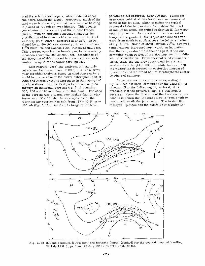
ated there in the subtropics, which extends about one-third around the globe. Moreover, much of the land mass is elevated, so that the source of heating is placed at 700 mb or even higher. This greatly contributes to the warming of the middle tropos­phere. With an extreme seasonal change in the distribution of heat and cold sources, the 150 -knot westerly jet of winter, centered near 250 N, is re­placed by an 80-100 knot easterly jet, centered near 150 N (Sutcliffe and Bannon,1954, Koteswaram,1958). This current overlies the low-tropospheric westerly monsoon above 25,000-30,000 feet. Steadiness of the direction of this current is about as great as in winter, in spite of the lower core speeds.

Koteswaram (1958) has analyzed the easterly jet stream for the summer of 1955; this is the first year for which analyses based on wind observations could be prepared over the entire subtropical belt of Asia and Africa owing to increases in the number of rawin stations. Fig. 5.15 depicts a cross section through an individual current; fig. 5.16 contains 300, 200 and 100-mb charts for this case. The core of the current was situated even higher than in win­ter -near 150-100 mb. In correspondence, the warmest air overlay the belt from 150 - 300 N up to 200 mb (fig. 5.17). An abrupt change of the tem-

~J~,--------~lr:0~--------~I~rO--~07;----H

'0 _

perature field occurred near 100 mb. Temperat­ures were coldest at this level near and somewhat north of the jet axis, which signifies the typical reversal of the temperature field above the level of maximum wind, described in Section III for west­erly jet streams. In accord with the reversal of temperature gradient, the tropopause sloped down­ward from north to south across the jet axis (bottom of fig. 5.17). North of about latitude 20oN, however, temperatures increased northward, an indication that the temperature field there is part of the cir­cumpolar warm region of the stratosphere in middle and polar latitudes. From thermal wind considera­tions, then, the easterly subtropical jet stream weakened with height at 100 mb, while farther north the westerlies decreased or easterlies increased upward toward the broad belt of stratospheric easter­ly winds of summer.

As yet a mass circulation corresponding to fig. 5.6 has not been computed for the easterly jet stream. For the Indian region, at least, it is probable that the pattern of fig. 5.6 wi.ll hold in reverse. From the direction of the low-level mon­soon it is known that the mass flow is from south to north underneath the jet stream. The heated Hi­malayan plateau and the rainfall distribution in-

150 -- --'--64-

-----------'---____ ---L ______ '--____________ -'--___________ • ...l ___ _

170 170 Long

08 04

H

10 -L _____ __ -__ ------' __ --- ---'- --------

Fig. 5.12 200-mb contours (100's feet) and isotachs (knots) (dashed) for the central tropical Pacific, 24 July 1951 (upper) and 25 July 1951 (lower) (RiehL 1954b).

-37-

dicate ascent over northern India and Pakistan. Descent is suggested for the southern parts of the subcontinent where a secondary mid-summer mini­mum of rainfall prevails. Probably, the net drift is southward in the high troposphere.

As in winter, we may suppose that there is a tendency for the absolute angular momentum to be conserved in the southward drift of the tropical cell.

34

32

30

[; v 28 "0 :J

.-+;: +- 26 o ...J

Z 24'

22

20 X I

Fig. 5.13

20 40 60 80

V (knots)

Lateral distribution of easterly wind speed at 200 mb from southeastern United States across Florida and the Bahamas to Cuba, 1-2 August 1953 (Alaka,19 58) .

-38 -

100 mb

200

300

400

500

900

/ I

1000 - ---

----/'

1 10 20

__ -1_ 20 40

L _____ I L __ .I 30 40 50 60 knots 60 80 100 percent

Fig. 5.14 Vertical profile (solid line) of easterly wind component through jet axis at 820 W on 1 August 1953, 03GCT. Dashed line represents curve of cumulative percent­age of kinetic energy from 1000 to 100 mb; for instance, value at 300 mb is 7 percent which means that 7 percent of the kinetic energy of the whole column from the ground to 100 mb lies below 300 mb, 93 percent above.

It is of interest that, when a constant absolute angu­lar momentum profile is computed with respect to the Himalayan plateau, a distribution of easterly wind speeds is obtained that closely resembles the observed one. As yet, however, the reason for the existence of the maximum with the particular speed and at the particular latitude where it occurs, re­mains unknown for the easterlies as for the wester­lies.

/ /

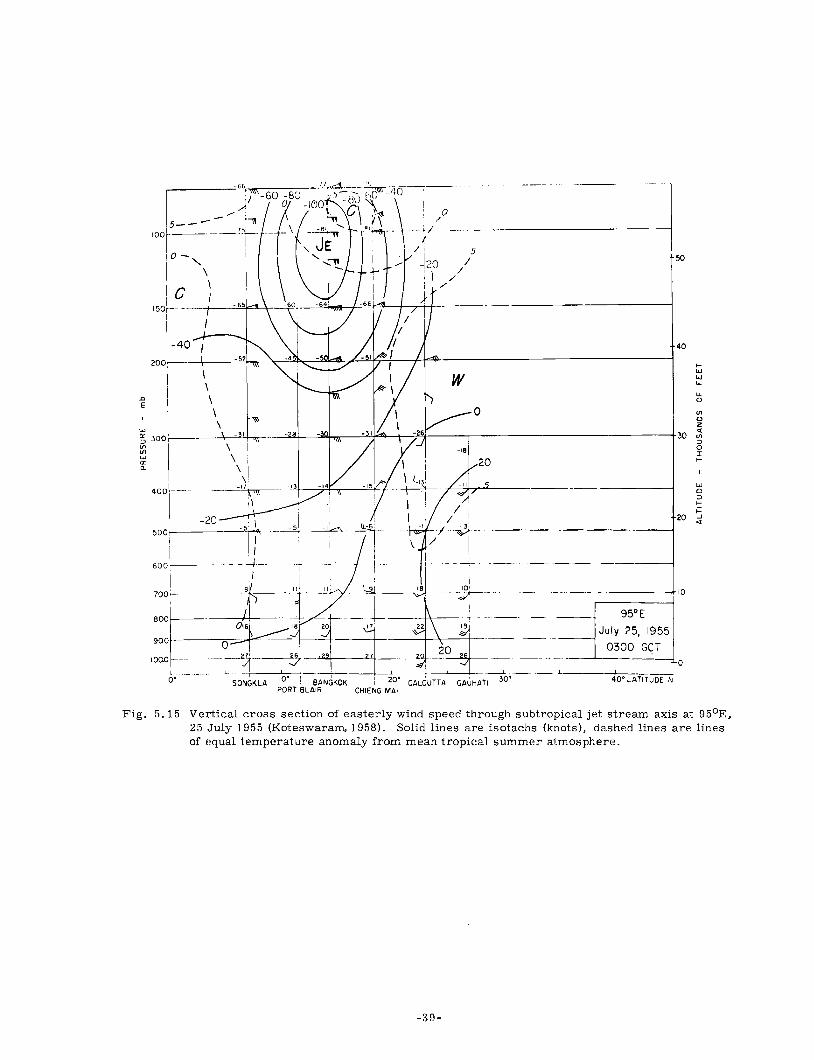
5 I

/

2001------f--~_m_~~~~~~~~fT+___jLt=~---------------___1

I

I 1

-20 500 -~~

I I! 600,----· - .- - - -J----

w

-.<---'71-"7""-"-----------------1

------ ------\

40

30

20

I

I·

8h "i " ::::- !+-----~I- - .. --- - ----- --- --------+10

,J-- ~'" +----t----\---=-t---- - ---

95°E

July 25, 1955

0300 GeT 1000r==---- -.~2Jf -~ --'-""t----'-'-I --"',f-- --- -- _. --.-

I ,! -+-"--__ +---'- ----f:1 ::co-:-: l O· SO~~KLA 10· I BANGKOK 20· CALCUTTA 40· LATITUDE N

PORT BLAIR CHIENG MAl

o

~ w w u.

u. 0

<Il 0 z q

'" ~ 0 r ~

w 0 ~ ~

~ ..J q

Fig. 5.15 Vertical cross section of easterly wind speed through subtropical jet stream axis at 950 B, 25 July 1955 (Koteswaram, 1958). Solid lines are isotachs (knots), dashed lines are lines of equal temperature anomaly from mean tropical summer atmosphere.

-39-

----------.,..-------------

'2~ __ ------~~=;~~~~~~~4€~~~::~~;:~~~~~C 300 mb - Ju Iy 25, 1955

0300 GeT

1 __ _

60 --- ---- ------

Fig. 5.16 Strerunlines and isotachs (knots, negative sign denotes east component) at 300, 200 and 100 mb, 2·5 July 1955, 03GCT (Koteswaram,1958). A denotes anticyclonic circulation, C cyclonic cir­culation. Heavy dashed lines are easterly (J

E) and westerly (J

W) jet strerun axes.

-40-

4~

45

60

w -6

~-70--65

-7 .

-roUro -7030

-71 - "

100 mb Isotherms

July 25,1955 0300 GCT

L---~w~--~--~----=~--~~~--~------'6~0~~----------'9~0--~~~~---~';~~~~~~~~0

90 120

Pressure Tropopause

July 25, 1955

45

30

I~

~ ____ ~w __ ~~ __ ~ ________ -=30~ ______ - ----tO~----__ ------~9~o--~~~-L--~~~~~O~3~O~O~G~CT~

Fig. 5.17 Isotherms (OC) at 200 and 100 mb and isobars of pressure at tropopause (mb), 25 July 1955, 03GCT (Koteswaram, 1958) .

-41-

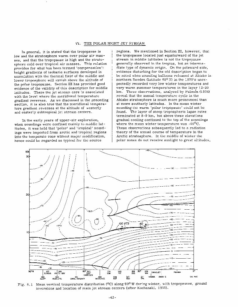
VI. THE POLAR NIGHT JET STREAM

In general, it is stated that the tropopause is low and the stratosphere warm over polar air mas­ses, and that the tropopause is high and the strato­sphere cold over tropical air masses. This relation provides for what has been termed 'compensation': height gradients of isobaric surfaces developed in association with the thermal field of the middle and lower troposphere will vanish above the altitude of the polar tropopause. Section III has provided good evidence of the validity of this description for middle latitudes. There the jet stream core is associated with the level where the meridional temperature gradient reverses. As we discussed in the preceding section, it is also true that the meridional tempera­ture gradient reverses at the altitude of westerly and easterly subtropical jet stream centers.

In the early years of upper-air exploration, when soundings were confined mainly to middle lat­itudes, it was held that 'polar' and 'tropical' sound­ings were imported from arctic and tropical regions into the temperate zone without major modification, hence could be regarded as typical for the source

regions. We mentioned in Section III, however, that the tropopause located just equatorward of the jet stream in middle latitudes is not the tropopause generally observed in the tropics, but an interme­diate type of dynamic origin. On the poleward side, evidence disturbing for the old description began to be noted when sounding balloons released at Abisko in northern Sweden (latitude 680 N) in the 1920's unex­pectedly recorded very low winter temperatures and very warm summer temperatures in the layer 12-20 km. These observations, analyzed by Palmen (1934) reveal that the annual temperature cycle in the Abisko stratosphere is much more pronounced than at more southerly latitudes. In the mean winter sounding the warm 'polar tropopause' could not be found. The layer of steep tropospheric lapse rates terminated at 8-9 km, but above these elevations gradual cooling continued to the top of the soundings where the mean winter temperature was -66 0 C. These observations subsequently led to a radiation theory of the annual course of temperature in the Arctic stratosphere. In the middle of winter the polar zones do not receive sunlight to great altitudes,

KM

3

I \

~ -45~

~ .. ---_ ... 20

90'N

-30

082 ALERT

-----50 ------ 60 -55 I

~---------~ r ------------- --- ------60 ------------

1-55 .-- .----1----------------i ------ ----------~-----

I

--.-.------- ~~====~=:=~ -----------------

___ +25_ ---

PANAMA O'

9'5 211 HAVANA SWAN IS SALINAS CORAL HARBOUR

836 MOOSONEE

528 BUF

3'7 GSO T~A

Fig. 6.1 Mean vertical temperature distribution (OC) along'800 W during winter, with tropopauses, ground inversions and location of main jet stream centers (after Kochanski, 1955).

-42-

and the normal heat source in the ozone layer does not exist. Hence gradual cooling of the ozonosphere takes place throughout the polar night period. The reverse happens during summer, but for our pur­poses we are only interested in the winter soundings. If stratosphere temperatures continue to drop pole­ward through a very deep layer, the wind should increase there with height in the Arctic, and a level of maximum wind should exist at very high altitudes.

For some time evidence on Arctic stratosphere temperatures accumulated only slowly, because the altitudes involved were very high for the available sounding equipment. After expansion of the Arctic network beginning in the 1940's, however, and after the South-Polar Byrd expeditions (Court,1945) the temperature field became well established. It has been further confirmed by the extensive observation programs of the International Geophysical.Year in both polar zones (cf. Wexler,1959). Mean isotherms along 800 W for January are presented in fig. 6.1 (Kochanski,1955), where it must be noted that the

'so -60

-55 1"

-5~("""""" 81.5·····

\ \ \ \ \ \ \ \ \ \ ,

" '----................................... ,.~ ....... .

\ ..... \ .... \.

\ \ i \ \ \

lowest temperatures near the pole have been inter­polated on the basis of comparison with Antarctic soundings. Except for more complete data, this cross section differs very little from that originally published by Palme'n in 1934.

It is clear from fig. 6. 1 that on account of the high-level cold source the thermal wind north of 600 N is westerly to the top of the section, that there­fore a polar night jet stream will exist in the ozono­sphere, with core speed and altitude of the level of strongest wind as yet unknown. At 25 mb in January (fig. 6. 2), a tremendous concentration of height gradient is evident at this surface which is still be­low the level of strongest wind on account of the northward temperature drop. Geostrophic calcula­tion along 900 W yields the zonal wind profile of fig. 6.3 which brings out the concentrated high­energy current of the Arctic strikingly. Considering that winds still increase upward through the 25-mb surface and that the calculation has been made on a seasonal mean chart, the result is indeed formidable.

D

81

/ .................. -55 ...... )" .... .

W , 81.5

. ..... ~ ......................... y

\\ ................. /"/

\, .......... :;-;;".c.~.~ ............................ ;-;55

-55 ..... .... ~.:.:.:..".~~.~ ---

1 C;:'

--81.5

Fig. 6.2 25-mb contours (1000's feet) and isotherms (OC) for winter (after Kochanski, 1955).

It is a remarkable phenomenon, not yet ex­plained, that gradual cooling continues over both polar caps throughout the winter, even though in­cursions of air from lower latitudes could readily eliminate the very cold stratosphere and maintain much warmer winter temperatures. Over the Arctic, at least, such incursions do occur at least a few times during the cold season (Hare,1959); they pro­duce fluctuations in intensity and position of the polar night jet. Therefore, although both subtropi­cal and Arctic jet streams are tied directly to the heat and cold sources of the atmosphere, the polar

-43 -

current is much less steady. Often a deep strato­spheric cyclone is centered over northern Canada which will form, migrate and disappear, although on a time scale much longer than that of most tropo­spheric systems. Daily charts have been drawn at 50 mb and 25 mb for limited periods (Teweles,1958). These reveal that changes in the stratosphere are largely, though not wholly, unrelated to those of the troposphere, and that events in two winters may be quite dissimilar. Most spectacular is the termina­tion of the principal polar-night jet stream period which is coupled with sudden sharp temperature

rises in the Arctic stratosphere and virtual elimina­tion of the north-south temperature gradient there (Godson and Lee,1958). This event, which has been termed 'explosive' warming, has occurred variably between January and late March in the few years when the warming trend could be followed reliably.

z •

90

80

70

... 60 .., E :; 50 ...J

40

30

25mb

at 90° W

Winter

20 IL-"'--~--'-' -o 40 80 Ug (knots)

120

Fig. 6. 3 25 -mb geostrophic west wind profile lUg) computed from fig. 6.2.

Fig. 6.4 illustrates an individual vertical cross section for 26 February 1956, extending from Alert (082) southwestward to Whitehorse (964), prepared by Godson and Lee (1957). The authors give the following discussion: "It was around this time that the jet stream was most intense. The orientation of this cross section is NE-SW, and the strong north­westerly wind in the stratosphere are at right angles to the plane of the cross section. The highest re­ported wind on this cross section is 160 knots around the 80, ODD-foot level at Eureka (917). The strong horizontal temperature gradient below the jet stream is clearly evident; the temperature increases from -70 to -500 C in a distance of nearly 800 miles. South of Resolute (924) the stratosphere is nearly isothermal both in the vertical and horizontal. Owing to the orientation and irregularity there is some doubt as to the reality of the double maxi­mum."

It should also be noted that the highest wind speeds were observed at the top of the balloon runs; from the thermal field it was assumed that the core of the jet stream was located at 25 mb. Very cold temperatures as plotted in fig. 6.1 were not en­countered on 26 February 1956; in fact, there was no reading lower than -700 C. The important Alert sounding, however, terminated just after passing the 100-mb level.

Cross sections such as fig. 6.4 have confirmed the existence of a current with core near 25 mb or higher, and with lateral velocity gradients typical of jet streams. On account of the great altitude of the core, these sections usually contain only a single

-44-

ascent with winds penetrating into the core so that definitive analysis is difficult. For this reason Krishnamurti (1959b) computed a cross section from a large number of observations by means of com­bining all stations of the North American Arctic for a period of several days, during which time fluctua­tions of the current were not excessive. All indi­vidual balloon ascents were to be composited in the jet coordinate system described in Section V for the subtropical jet stream; all data located at similar distances from the axis of the current were to be averaged.

For this purpose it was necessary to carry out daily map analyses and locate the jet stream axis. At 25 mb data were insufficient, but at 50 mb iso­tachs similar to those of fig. 5.2 could be drawn . From the available material a four-day period, 31 December 1957 to 3 January 1958 will be present­ed. All averaging for this period was based on the jet stream axes as determined by the day-to-day analysis. The mean latitude was 65 0 N. The cur­rent was mainly westerly; it curved clockwise over Alaska and western Canada, counterclockwise over eastern North America. Thus the Arctic jet stream executed a wave-like oscillation with ridge near 1500 W and trough near 600 W, or a half-wave length of 900 longitude. If symmetry prevailed around the globe, the Arctic jet would contain two long waves; of course, there is at present no knowledge whether or not such an extrapolation from North American data is permissible. * Even so, it is remarkable that troughs and ridges of a longwave system, with preferred longitudes, occur at the altitude of the Arctic jet. Normally, standing wave positions are considered to be related to longitudinal asymmetries of the earth's surface itself. It remains to be seen whether these can be held to account also for the high-stratospheric flow which might be thought to be well insulated from surface effects by the deep iso­thermal stratum above the tropopause, especially as the correlation between tropospheric and strato­spheric flow patterns appears to be rather small. More cannot be said on this intriguing, yet unsolved, problem at this time.

Averaging of the wind component parallel to the jet axis (cs) for the four days leads to a spectacu­lar diagram (fig. 6.5) which fully confirms the Similarity between Arctic night and other jet streams. The core velocity was not very strong on this occa­sion; winds up to 200 knots have been noted on other days. From fig. 6.5 the core was situated at 26 km or about 85, 000 feet, pressure near 25 mb. Above the core data were very sparse, but there is a sug­gestion that strong shears, comparable to those of the tropospheric jet streams, need not occur. This impression has been strengthened by rocket firings at Fort Churchill (Stroud, 1 959) which indicate that the Arctic jet may extend with undiminished force to very great heights indeed.

* Wexler and Moreland (1958) believe that the strong winds are relatively local features associated with the large stratospheric cyclones.

90

//,-60

\,----_ ... -25

80

70

50 -45 I .... I W

'" "-"-0

m :;

I/l 0

60~ w ::;) a: ::;) I/l

~

0 r .... I

0: "- 60 ....

r 100 <.?

iii r

40 50

150 "- 441~

40 .. , 200 , I I

~ ~ \ ~

~ ~ --'

300 30

-45 --- ---400

20

082 202 917 924 072 051 968 964 Al.eRT THLLE EuREKA RESOLUTE BAY MOULD BAY SACHS HARBOR AKL,AVIK WHITEHORSE

Fig. 6.4 Vertical cross section extending NE -SW from Alert to Whitehorse, 1500 GCT, 26 February 1956 (Lee and Godson,1957). Solid lines are isotachs (knots), dashed lines isotherms (DC). Heavy solid line is tropopause. International station index used.

-45-

The cross section of absolute vorticity (fig. 6.6) is distinguished mainly by absence of a zone of very low vorticity southward of the core, even though the relative vorticity was measured along isentropic surfaces (cf. Section XII). A sharp concentration of vorticity gradient is in evidence at the axis, with values one-third higher than the Coriolis parameter just north of the axis. This is also rather little and should be expected to be exceeded in other cases. An additional fact of interest was brought out by the vorticity analysis. Glancing at fig. 6.5, we see that the shear on the cyclonic side of the axis is stronger than on the anticyclonic side as also found in earlier sections. At least this is true along constant-level or constant-pressure surfaces. When the velocity profile was plotted along an isentropic surface intersecting the core, however, a different and curious result was obtained (fig. 6.7). Along the isentrope shears were nearly uniform; a bilinear velocity profile could be drawn readily which has the same slope (without regard to sign) on both sides of the axis.

'20 '0080 60

20 ~ ~ 8 .. J _4 -8 -~ -~

(cyelofticl 0.. .. I,tit .. " .. .,.1 Alis (anlicyc1ol'licl

:Fig. 6.5 Vertical cross section of wind component parallel to jet axis (cs ' knots) for 31 De­cember 1957 -3 January 1958 (Krishna­murti, 1959b). Coordinate system relative to jet stream axis.

The temperature field was treated in the same manner as described in Sections II and IV. A mean temperature-height sounding was calculated for the data in the sample treated over the four-day period; then deviations from this mean sounding were taken. It turns out (fig. 6.8) that the temperature field of the Arctic jet is identical with that of all the other currents analyzed in this text. Below the level of maximum wind temperatures decrease from right to left across the current, looking downstream. This temperature gradient vanishes at core altitude and then begins to reverse. It should be noted, however, that the reversal in fig. 6.8 is based on very few ob­servations. If the speed of the current remains constant through the ozonosphere in some situations,

-46-

10

16 12 (cyclonic)

8"J~4-8

Degrees latitude from Jet Alis -12 -16

(omicyClonic)

Fig. 6.6 Vertical cross section of absolute vor--4 -1 ticity (10 sec ) computed from fig. 6.5

on isentropic surfaces (Krishnamurti, 1959b).

as suggested above, a neutral lateral temperature field would be expected, at least if winds are geo­strophic. A check was made to see to what extent the c s wind component was geostrophic below 25 mb, and in this case very good agreement between geostrophic and observed winds was obtained in the mean for the cross section.

16

U 12 '2

.!! 0 8 ~~

(,) 4 -; .... ...,

~ J ... -4 ~ .2 ...... -8 :.;:::: u o . .., - a -12 UI'U

~ .2' -16

l!-20 0204060

Fig. 6.7 Wind profile along isentrope passing through center of Arctic jet in fig. 6.5.

5 ..... --

W 5 "\ ---_/

-10

)"-20) ~ C ~ §

20 J 20

5 I

"

5 I I I

16 12 (""Ionic)

I I I / I I \ I \ I \ I " //

........ -~"" •• A ~ ~ ~

1lo9'''' Ioliludt ~ ... Jol Alii (onlicytl.nic)

o

Fig. 6.8 Vertical cross section of temperature anomaly (OC) from mean sounding for section, 31 December 1957 - 3 January 1958 (Krishnamurti, 1959b).

For the polar night jet stream the mean temper­ature-height sounding itself is of interest (fig. 6.9). The atmosphere is isothermal up to the level of maximum wind; then the increase of temperature in the ozone layer begins. Although there is no tropo­pause, the jet stream core nevertheless is situated

-47 -

at an altitude where the stability of the atmosphere increases discontinuously upward. Apparently this is a characteristic position of most, if not all, jet stream cores which has not yet been fully explored. In Section XII this subject will be taken up again when the potential vorticity field of jet streams is discussed.

30

25

15

10

-30 -40 -50 roc

-70

Fig. 6.9 Mean temperature-height sounding for cross section of fig. 6.8 (Krishnamurti, 1959b).

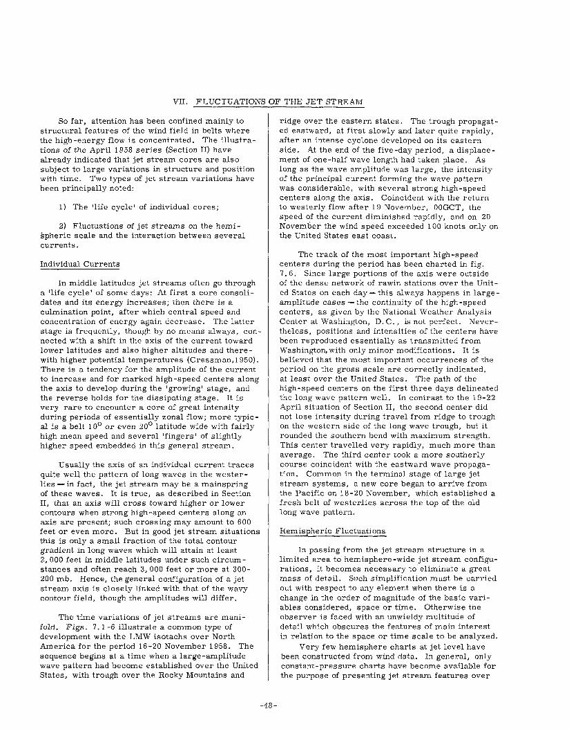
VII. FLUCTUATIONS OF THE JET STREAM

So far, attention has been confined mainly to structural features of the wind field in belts where the high-energy flow is concentrated. The illustra­tions of the April 1958 series (Section II) have already indicated that jet stream cores are also subject to large variations in structure and position with time. Two types of jet stream variations have been principally noted:

1) The 'life cycle' of individual cores;

2) Fluctuations of jet streams on the hemi­spheric scale and the interaction between several currents.

Individual Currents

In middle latitudes jet streams often go through a 'life cycle' of some days: At first a core consoli­dates and its energy increases; then there is a culmination point, after which central speed and concentration of energy again decrease. The latter stage is frequently, though by no means always, con­nected with a shift in the axis of the current toward lower latitudes and also higher altitudes and there­with higher potential temperatures (Cressman, 1950). There is a tendency for the amplitude of the current to increase and for marked high-speed centers along the axis to develop during the' growing' stage, and the reverse holds for the dissipating stage. It is very rare to encounter a core of great intensity during periods of essentially zonal flow; more typic­al is a belt 100 or even 200 latitude wide with fairly high mean speed and several 'fingers' of slightly higher speed embedded in this general stream.

Usually the axis of an individual current traces quite well the pattern of long waves in the wester­lies - in fact, the jet stream may be a mainspring of these waves. It is true, as described in Section II, that an axis will cross toward higher or lower contours when strong high-speed centers along an axis are present; such crossing may amount to 600 feet or even more. But in good jet stream situations this is only a small fraction of the total contour gradient in long waves which will attain at least 2,000 feet in middle latitudes under such circum­stances and often reach 3,000 feet or more at 300-200 mb. Hence, the general configuration of a jet stream axis is closely linked with that of the wavy contour field, though the amplitudes will differ.

The time variations of jet streams are mani­fold. Figs. 7. 1 -6 illustrate a common type of development with the LMW isotachs over North America for the period 16 -20 November 1958. The sequence begins at a time when a large-amplitude wave pattern had become established over the United States, with trough over the Rocky Mountains and

-48-

ridge over the eastern states. The trough propagat­ed eastward, at first slowly and later quite rapidly, after an intense cyclone developed on its eastern side. At the end of the five -day period, a displace­ment of one-half wave length had taken place. As long as the wave amplitude was large, the intensity of the principal current forming the wave pattern was considerable, with several strong high-speed centers along the axis. Coincident with the return to westerly flow after 19 November, OOGCT, the speed of the current diminished rapidly, and on 20 November the wind speed exceeded 100 knots only on the United States east coast.

The track of the most important high-speed centers during the period has been charted in fig. 7.6. Since large portions of the axis were outside of the dense network of rawin stations over the Unit­ed States on each day - this always happens in 1arge­amplitude cases - the continuity of the high -speed centers, as given by the National Weather Analysis Center at Washington, D. C., i.e; not perfect. Never­theless, positions and intensities of the centers have been reproduced essentially as transmitted from Washinl,rton. with only minor modifications. It is believed that the most important occurrences of the period on the gross scale are correctly indicated, at least over the United States. The path of the high -speed centers on the first three days delineated the long wave pattern well. In contrast to the 19-22 April situation of Section II, the second center did not lose intenSity during travel from ridge to trough on the western side of the long wave trough. but it rounded the southern bend with maximum strength. This center travelled very rapidly, much more than average. The third center took a more southerly course coincident with the eastward wave propaga­tion. Common in the terminal stage of large jet stream systems, a new core began to arrive from the Pacific on 18-20 November, which established a fresh belt of westerlies across the top of the old long wave pattern.

Hemispheric Fluctuations

In passing from the jet stream structure in a limited area to hemisphere-wide jet stream configu­rations, it becomes necessary to eliminate a great mass of detail. Such simplification must be carried out with respect to any element when there is a change in the order of magnitude of the basic vari­ables considered. space or time. Otherwise the observer is faced with an unwieldy multitude of detail which obscures the features of main interest in relation to the space or time scale to be analyzed.

Very few hemisphere charts at jet level have been constructed from wind data. In general, only constant-pressure charts have become available for the purpose of presenting jet stream features over

'0

I

-~

Fig. 7.1 Jet stream axes and isotachs (knots), 16 November 1958, OOGCT. Principal high-speed centers are numbered for continuity. J denotes high -speed center, S slow area.

-~ -----,----~---,

Fig. 7.2 Jet stream axes and isotachs, 17 Novem­ber 1958, OOGCT.

Fig. 7.:3 Jet stream axes and isotachs, 18 Novem­ber 1958, OOGCT.

-49-

- -----~-- ~~~.-- ----. '----,--,

"'~"\ .... -.-~~-----"/ \)i, \.. / ._ \

-{~~ \' ,r;": t..,~ '~ / ~,

Fig. 7.4 Jet stream axes and isotachs, 19 Novem­ber 1958, OOGCT.

50

---- _______ 75

Fig. 7.5 Jet stream axes and isotachs, 20 Novem­ber 1958, OOGCT.

Fig. 7.6 Track of principal high-speed centers, 16 -20 November 1958. Position, time and intensity (central closed isotach) given.

large areas. In figs. 7. 7 -11 bands of contour con­cent ration are outlined, based on hemispheric 250-mb analyses prepared by the National Weather Analysis Center. This crude type of representation has the merit of providing at least a broad view of the major currents around the globe. It is easy to conceive of much better charts, given enough rawin observations. Then the variable core altitude of different jet streams could be taken into account; mean speed and amplitude of individual currents could be measured and followed as a function of time. Undoubtedly such charts will eventually come into existence, but for the present, schemes such as those reproduced in figs. 7. 7 -11 must suffice if there is to be any view of the hemispheric scale.

The five charts cover half of November 1958, beginning with the period discussed earlier in this section for the United States. The charts are pre­sented at three-day intervals - a longer time scale must go with the larger distance scale. Detail on jet stream axes, as contained in figs. 7.1-5, has been omitted; in fact, the current followed earlier merely appears as a branch of a circumpolar veloc­ity concentration in fig. 7.7. This is not meant to imply that the current executing the wide southward swing over the western United States branches off from the axis passing over northern Canada in the Pacific and merges again with it over the Atlantic. We merely wish to take the position that from the hemispheric viewpoint on general location of high­speed areas, separation of these axes would be without importance except over North America. The same holds for most other areas where current splits and confluences have been shown. At times two separate branches may really consolidate into a single current, or a single core may break up into two narrower streams. At other times, two cur­rents may flow side by side in close proximity for a while, but remain separate entities and then diverge again. In many areas, especially over the oceans, a clear distinction, even if desired, is not possible due to lack of sufficient observations. This holds notably in the western Pacific where on most charts a broader jet stream zone has been indicated than elsewhere.

Hemispheric jet stream charts, when drawn on the basis of quantitative procedures, can serve several purposes. They can be employed as a prin­ciple for long distance flight routing and for longer period flight planning. They can aid in wind and weather prediction several days in advance. Here we shall merely note some of the most prominent large-scale features evident from the qualitative sketches of figs. 7.7 -11. A circumpolar belt of velocity concentration could be drawn on each map, even though the charts themselves do not extend as far southward in the eastern as in the western part of the hemisphere. The principal belt'meanders' around the globe. At times a fairly regular wave pattern appears, but troughs and ridges more often have an irregular spacing and the band as a whole cannot be described readily in simple terms.

In fig. 7.7 we observe four waves of varying amplitude along a single band, excepting the link

-50-

across Canada. In the south, portions of the sub­tropical jet stream have been entered. Continuity with respect to this current is the poorest of the series - this may be expected from the discussion in Section V. Even a detailed analysis of the high­tropospheric contour field over the southeastern United States did not clearly reveal the high-velocity core so evident from the wind observations. Hence little should be expected from a hemispheric analy­sis based on isolated radiosonde stations over the oceans.

By 21 November (fig. 7.8) the complexity of the jet stream pattern had increased. Several of the troughs noted on 18 November progressed in the 3-day interval, notably over North America and eastern Europe. Most striking was the emergence of two 'blocks' in the central Atlantic and western Pacific Oceans. Blocks are a frequent and peculiar feature of the general circulation, studied exten­sively by Rex (1950, 1951). A concentrated current, usually westerly, breaks into two sharply diverging branches at a certain longitude, and this break often continues or recurs in approximately the same location for days or weeks. In higher latitudes during winter the central Atlantic is one climatically favored location for block formation, and this event is spectacularly shown in fig. 7.8.

It is arguable whether the west Pacific situation des erves the classification of 'block'. Two currents upstream merge into a fairly broad zone and then they separate again farther east, so that one may think merely of a split rather than a block. In any event, the effect is the same as that of a true block for the downstream region. A concentrated west­wind belt in middle latitudes suddenly gives way to an area with light, often easterly winds, on its eastern side; two high-velocity cores bound this area in high and low latitudes.

Changes were relatively small between 21 and 24 November (fig. 7. 9), but then the flow pattern altered sharply (fig. 7. 10). The Atlantic block temporarily weakened; the Pacific split moved rapidly eastward. A large increase in amplitude took place in its northern branch which represents a sharp thrust of tropical air masses poleward. Many major upheavals of the hemispheric flow pat­tern begin with such a solitary thrust whose effect then propagates downstream and increases the amplitude and intensity of the jet core. That this happened in the present case may be seen from the large trough over the Atlantic in fig. 7. 11.

By 27 November a new jet stream core had also begun to develop in very high latitudes over Siberia. This new current became fully established by the end of the month (fig. 7. 11) when its northernmost portion was situated on the Asiatic side of the pole. Thus it appeared as a current with east component­a frequent occurrence. In addition, Atlantic block and Pacific block or split reformed at the longitude where they had first developed about 21 November.

A feature common to all charts of the series, typical of the colder season, is that the principal

~ig. 7.7 Outline of hemispheric flow concentra­tions, 18 November 1958.

Fig. 7.8 Outline of hemispheric flow concentra­tions, 21 November 1958.

Fig. 7.9 Outline of hemispheric flow concentra­tions, 24 November 1958.

-51-

Fig. 7.10 Outline of hemispheric flow concentra­tions, 27 November 1958.

Fig. 7. 11 Outline of hemis pheric flow concentra­tions' 30 November 1958.

Fig. 7.12 Axis of first harmonic of 300-mb flow during winter (Barrett,1958).

high-velocity belt did not lie symmetrically about the pole but that its position was 'eccentric', with a much lower mean latitude over eastern Asia and the Pacific than over the Atlantic. This eccentricity, discussed further in Section IX, is undoubtedly re­lated to action of the whole Asian continent as a cold source which is itself asymmetrically located with respect to the pole. The eccentricity of the flow, studied especially by LaSeur (1954), may be meas­ured in several ways. We may, for instance, calculate the first harmonic of the height distribu­tion at, say, 300 or 200 mb, at different latitudes and then draw the perturbation streamline field arising from this harmonic (fig. 9.11). When a curve is placed through the center of the perturba­tion flow reinforcing the mean westerly wind, a spiral results (fig. 7. 12). From eastern Asia across North America to Europe this spiral repre­sents the actual mean position of most jet stream axes very well. Over Siberia there are northwesterly current links between the low-latitude position of the jet streams over the western Pacific and the high-latitude position over the Atlantic.

As already mentioned, hemispheric jet stream charts can serve as bases for various types of cal­culation concerning mean speed, altitude, latitude and amplitude of jet stream systems and their varia­tion with time. Such numbers, measuring charac­teristics of jet streams over the whole map, may be called hemispheric indices. A simple index which enjoyed popularity mainly during the 1930's and 1940 's, is the index of the strength of the wester­lies, or 'zonal index' (cf. for instance Namias and Clapp,1951). Computed at first at the surface and later in the middle and high troposphere (fig. 7.13), this index measures the mean hemispheric strength of the westerlies as a function of latitude from iso­baric contour charts, i. e. it measures the geo­strophic wind. At times gradual progreSSion of west wind maxima poleward or equatorward are observed as illustrated in fig. 7.13. When this happens, the latitudinal trend is very usefel in qualitative wind and weather forecasts. Unfortuna­tely, trends have not been found to persist with regularity sufficient to serve as basis for routine forecasts. Part of the difficulty may lie in the form of the index itself. As we have noted, the circum-

-52-

70

60

50

~ :J !:::40 ~ ..J

30

20

,," ./ " ..... / ./

l ( , ...... '- ..... -

..... - ---' -'- ~ - ........ --_ • C

10 20

- . ........... l , ...... '[ I ..... b i '~

/ I /

.,/ ....

40 fIl)S

Fig. 7.13 Profile of westerlies at 300 mb: (a) 7 December 1945; (b) 19 December 1945; (c) 29 December 1945. Arrows mark successive positions of strongest west­erly flow with respect to mean for each latitude. Profile averaged from charts extending from Asiatic east coast to Europe via North America (Riehl et aI, 1952).

polar current is asymmetric with respect to the geographic pole in winter; on the average, the flow is strongest near latitude 350 in the western Pacific and near latitude 550 in the Atlantic. A true re­presentation of the mean jet stream strength should at least take this eccentricity into account. When this is done, hemispheric wind profiles are ob­tained which are much more peaked than those com­puted merely for the west component of motion around latitude circles (LaSeur, 1954). Calculations made with respect to the ,iet strerun axes as ob­served on daily charts should prove even more fruitful in describing hemispheric jet stream fluc­tuations. Here is still a field ~f endeavor worthy of research for practical as well as theoretical purposes.

VIII. THE JET STREAM IN RELATION TO WEATHER AND CYCLONES

Jet steams pass over thousands of miles of sub­tropical desert where there is hardly a cloud in the sky and where the surface circulation is anticyclonic. They also lie above the strongest cyclones in the westerlies, with extensive sheets of clouds and pre­cipitation extending along the axis. Thus, the mere existence of a jet stream, in any area, even a very strong one does not of itself imply bad weather there. The converse, however, holds to a much better de­gree of approximation, especially in winter: Cy­clones and extensive bad weather areas tend to be connected with jet streams. This is true especially f<:>r warm front weather associated with cyclones during their formative and mature stages. As noted in Section III, well-developed jet streams are con­nected with strong tropospheric temperature gradi­ents, often concentrated in a polar-front zone. Lateral mass convergence and divergence, and attendant ascent and descent, can attain sufficient magnitude to produce extensive bad weather only in such baroclinic zones.

700mb ~mb

60 60 I 60 , \ I I \

700 mb \ \ \ \ , 300 mb \ \

50 I 50 " 50 \ / " ,

/ \ 700 mb \ Lat. Lat. I Lat.

I / \ 40 \ 40 / 40 I

\ / I I /

/ I ,

,- , I 30 DEC. 6. 1946 30 I 30 I

JAN. 10.1947 b c

0 20 40 60 mph 0 20

b 40

Jet Streams and Cyclones

There are several factors that permit one to distinguish between jet streams that are inactive as weather producers and situations where large cy­clones and widespread precipitation areas develop from them. In the first instance, the amount of weather development will have some correlation with the intensity of the current and the strength of the associated baroclinic zone, other factors being equal. As noted early in s~udies of the upper wind field over the United States (Riehl, 1948) a well formed jet stream is not always present. Three types of situations were noted in a study of the winter of 1946-47 and subsequent seasons (fig. 8.1):

1. Both vertical and lateral shears in the tropo­sphere are small (fig. 8. 1 a). Low pressure centers observed during such periods remain weak.

4

+15-

+10· { 300mb +5' \,9 ,

Max 700 mb ~ \

-5' )9 /

-10' ,-

/9 / COMPOSITE

JAN. 28.1947 -15- /9 9 CASES

d

60 mph 80 100 120 0

c Fig. 8.1 Profiles of the westerlies at 700 mb and 300 mb over North America: a) 6 December 1946;

b) 10 January 1947; and d) for nine cases with pronounced jet stream, averaged with re­spect to wind maximum at 300 mb. Ordinate in drawing (d) gives distance from zone of maximum wind at 300 mb in degrees latitude, numbers along curves indicate number of observations (Riehl, 1948).

2. The lateral shear is small, but the vertical shear is large, indicating a marked north-south temperature gradient, but without much lateral con­centration. Several weak 'fingers I of maximum velocity can be present. The average west-wind profile of the high troposphere across the United States may be as shown in fig. 8. 1b with average speed near 60 knots; at times even a 100 knot aver­age has been observed with two or three lfingers' attaining 120-130 knots. Disturbances observed with this flow pattern move rapidly eastward without much intensification. 'High index I warm cyclones fall in this classification.

3. The lateral shear in the low troposphere is small but a jet stream, well defined by strong ver-

-53 -

tical and horizontal shear, is situated in the upper troposphere. When such a current becomes super­imposed on a strong frontal zone of the low tropo­sphere, intense cyclogenesis may ensue. As already noted, however, the existence of a strong jet stream-as seen, for instance, in a vertical cross section-does not necessarily imply the presence of cyclones and bad weather. Moreover, strong fronts have been known to remain stationary for several days with only shallow wave formation along them. Therefore, jet stream characteristics additional to the general intensity of the baroclinic zone must be sought for a criterion of the type of activity to be expected in association with a current. Such char­acteristics are found by consi.dering variations of jet stream structure along the axis.

Weather Situation of 16-20 November 1958: For an example we shall examine surface developments for the period 16-20 November 1958, over North Amer­ica for which the sequence of events in the LMW has been described in the last section. At the starting date of the series on 16 November (fig. 8.2) un­seasonably warm and humid weather covered the eastern half of the United States, while the Rocky Mountain area and even the Pacific coast experienced the first severe cold outbreak of the winter season. This distribution of temperature anomaly agrees well with the long wave picture outlined by the axis of the major jet stream; this axis has been super­imposed on fig. 8.2 and the subsequent maps from figs. 7.1-5. The freezing isotherm roughly coin­cided with the jet axis and this and the following illustrations.

Fig. 8.2 Surface fronts and isobars, 16 November 1958, 0600GCT; also jet stream axes from Section VII. Dotted line is freezing isotherm at ground. Analysis copied from U.S. Weather Bureau chart.

A deep cyclone had moved from the west to the lee of the Rockies in southern Colorado where, at the maptime of fig. 8.2, it was situated almost di­rectly under the jet stream core, closely connected with the first high-speed center whose path is de­picted in fig. 7.6. In the next 24 hours the center J 1 moved rapidly northeastward. The cyclone, traveling along the jet axis lost contact with it and began to fill after occlusion (fig. 8.3). Widespread bad weather was in progress over large portions of the Great Plains west of the Mississippi as a tropical airmass with dewpoints above 600 F penetrated northward under the secondary jet. Heavy precipita­tion and thunderstorms occurred around the second­ary axis, giving way to heavy snow northwest of the low pressure center.

In the southwest a weak low pressure center, located in southern Nevada in fig. 8.2, had moved eastward to the lee side of the mountains by 17 No­vember. Upon this cyclone the jet stream center previously situated on the Oregon coast, was im­pinging at that time after rapidly rounding the long

-54-

wave trough position on the Arizona-Mexico border with great intensity. When superposition of these two systems- separated by 1000 miles only 24 hours earlier- took place, rapid deepening set in at the surface and a major cyclone formed.

;--"-J'""~ \ \ ..... 1020

'.--------~ ----

Fig. 8.3 Surface fronts and isobars, also jet axes, 17 November 1958, 0600GCT.

This cyclone also followed the jet stream in its path and attained great severity on 18 November (fig. 8.4). Although the displacement was very rapid for a deepening storm, the jet stream center propagated at an even faster rate and overtook the surface disturbance. Subsequent to the separation the surface cyclonic circulation began to diminish again.

On the following day (fig. 8.5) the jet stream center J 3 passed over thc area where the great upheaval had taken place 24 hours earlier. But now the whole Midwest was covered by subsiding polar air so that the high-speed center, though well de­fined and intense like its predecessor, passed over

~IO'6

~-----

Fig. 8. 4 Surface fronts and isobars, also jet axes, 18 November 1958, 0600GCT.

the Plains States unnoticed at the surface. The secondary jet of 16 and 17 November had disappeared and no secondary cyclone formed along the cold front in the southeast, although surface indications were quite favorable for such a development on 19 November.

Fig. 8.5 Surface fronts and isobars, also jet axes, 19 November 1958, 0600GCT.

From the Pacific coast the 'nose' of a new jet stream system entered on that day, accompanied by a weak trough with occluded front and followed on 20 November by a deeper cyclone off the west coast. Fig. 8.6 shows the terminal phase of the jet stream we have followed. At first of great amplitude and intensity, two large cyclones were set off along its axis. At the end it was superimposed on a belt of polar anticyclones. Amplitude and intensity de­clined while a new current system farther north began to dominate the weather over the United States. Comparing figs. 8.2 and 8.6, a definite southward shift of the principal axis was effected in the five days covered by our analysis.

Fig. 8.6 Surface fronts and isobars, also jet axes, 20 November 1958, 0600GCT.

-55-

Although the case discussed was a severe one, it nevertheless brings out quite well the type of as­sociation between jet streams and cyclones, and the life cycle of jet streams with respect to surface phenomena, that can be observed when following maps from day to day. The nature of the associa­tion between cyclongenesis and jet stream is more difficult to ascertain and cannot be explored fully in the present context. Cyclongenesis is a baroclinic process which depends on the sinking of a cold air­mass relative to the s1}rrounding warm air for its energy source. Palmen and Newton (1951), among numerous authors on this subject, demonstrated that cold air subsidence often can be detected clearly by following the 500-mb temperature field. Now it IS a fact, readily ascertained from 500 mb and other charts, that a high-speed center along a jet stream, formed in a long wave ridge and traveling forward from there to the next trough to the east, will move southward in association with a cold dome (cf. also Riehl and Teweles, 1953).

This typical sequence was reenacted during the period illustrated here. On 15 November-one day before our series begins- an extensive cold airmass with 500 mb temperatures below minus 350 C overlay Canada and the northwestern United States. With arrival of the high-speed center J 2 from the Paci­fic, a portion of this cold airmass was driven south­ward and almost isolated from the main body of cold air over Canada (fig. 8.7).

Fig. 8.7 500-mb isotherm (oC), 16 November 1958, OOOOGCT. Heavy dots indicate positions of high-speed centers. Anal­ysis copied from U. S. Weather Bureau chart.

During 16 November the cold air continued to move southward over the western United States, but at the end of the day (fig. 8.8) it was evident that subsidence of the cold dome had begun. The area enclosed by the minus 350 C isotherm had become very small and even the area inside the minus 300 C isotherm had shrunk considerably as the whole body of cold air over the United States became 'cut off' from its high-latitude source region. Subsidence was accelerated greatly on the next day coincident with the intense cyclogenesis (fig. 8.9).

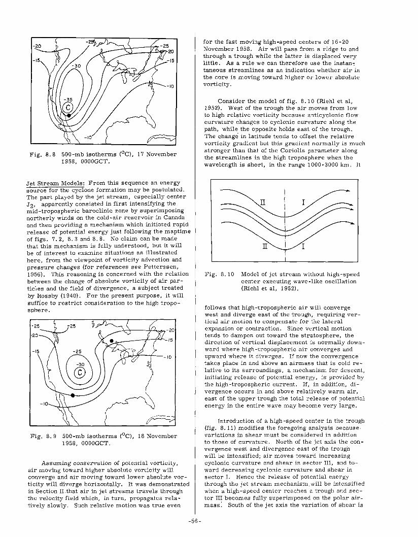
-20

-15

Fig. 8.8 500-mb isotherms (oC), 17 November 1958, OOOOGCT.

Jet Stream Models: From this sequence an energy source for the cyclone formation may be postulated. The part played by the jet stream, especially center J 2, apparently consisted in first intensifying the mid-tropospheric baroclinic zone by superimposing northerly winds on the cold-air reservoir in Canada and then providing a mechanism which initiated rapid release of potential energy just following the maptime of figs. 7.2, 8.3 and 8.8. No claim can be made that this mechanism is fully understood, but it will be of interest to examine situations as illustrated here, from the viewpoint of vorticity advection and pressure changes (for references see Petterssen, 1956). This reasoning is concerned with the relation between the change of absolute vorticity of air par­ticles and the field of divergence, a subject treated by Rossby (1940). For the present purpose, it will suffice to restrict consideration to the high tropo­sph-ere.

__ k-~----~~_-20

Fig. 8.9 500-mb isotherms (oC), 18 November 1958, OOOOGCT.

Assuming conservation of potential vorticity, air moving toward higher absolute vorticity will converge and air moving toward lower absolute vor­ticity will diverge horizontally. It was demonstrated in Section II .that air in jet streams travels through the velocity field which, in turn, propagates rela­tively slowly. Such relative motion was true even

-56 -

for the fast moving high-speed centers of 16-20 November 1958. Air will pass from a ridge to and through a trough while the latter is displaced very little. As a rule we can therefore use the instan: taneous streamlines as an indication whether air in the core is moving toward higher or lower absolute vorticity.

Consider the model of fig. 8. 10 (Riehl et aI, 1952). West of the trough the air moves from low to high relative vorticity because anticyclonic flow curvature changes to cyclonic curvature along the path, while the opposite holds east of the trough. The change in latitude tends to offset the relative vorticity gradient but this gradient normally is much stronger than that of the Coriolis parameter along the streamlines in the high troposphere when the wavelength is short, in the range 1000-3000 km. It

Fig. 8.10 Model of jet stream without high-speed center executing wave-like oscillation (Riehl et aI, 1952).

follows that high-tropospheric air wiil converge west and diverge east of the trough, requiring ver­tical air motion to compensate for the lateral expansion or contraction. Since vertical motion tends to dampen out toward the stratosphere, the direction of vertical displacement is normally down­ward where high-tropospheric air converges and upward where it diverges. If now the convergence takes place in and above an airmass that is cold re­lative to its surroundings, a mechanism for descent, initiating release of potential energy, is provided by the high-tropospheric current. If, in addition, di­vergence occurs in and above relatively warm air, east of the upper trough the total release of potential energy in the entire wave may become very large.

Introduction of a high -speed center in the trough (fig. 8.11) modifies the foregoing analysis because· variations in shear must be considered in addition to those of curvature. North of the jet axis the con­vergence west and divergence east of the trough will be intensified; air moves toward increasing cyclonic curvature and shear in sector III, and to­ward decreasing cyclonic curvature and shear in sector 1. Hence the release of potential energy through the jet stream mechanism. will be intensified when a high-speed center reaches a trough and sec­tor III becomes fully superimposed on the polar air­mass: South of the jet axis the variation of shear is

inverse to that of curvature, so that the sense of vorticity advection is uncertain and will depend on the relative strength of variation of curvature versus that of shear along the streamlines. We may con­clude that superposition of sector IlIon the cold air mass drawn southward by the jet stream over the western United States on 17 November 1958 probably was an important factor in accelerating the potential energy release at the moment when the high-speed center passed through the trough.

Fig. 8.11 Model of jet stream with high-speed center in trough of wave pattern. (Riehl et aI, 1952). Solid lines are schematic streamlines; dashed lines, isotachs.

As noted in Section II, such passage of a high­speed center across a trough line is relatively rare and, we may now add, frequently associated with severe cyclogenesis. High-speed centers are more frequently encountered in ridges; then the model of fig. 8. 12 applies. Incipient developments begin mainly on the warm side of the jet core. Using the foregoing reasoning, the principal motion toward lower absolute vorticity will occur in sector IV and toward higher absolute vorticity in sector II of fig. 8.12. In this arrangement release of potential energy through cold air sinking is not especially favored because sector II is normally situated above relatively warm air. Ascent of the warmest air in sector IV, especially when aided by release of latent heat of condensation and fusion, can initiate at least a moderate potential energy release. Actually, one finds that frequent cyclogenesis occurs in this sec­tor, accompanied by heavy rains, but the degree of cyclonic development is seldom spectacular.

Fig. 8.12 Model of jet stream with high-speed center in ridge of wave pattern. (Riehl et aI, 1952).

-57-

In summary, the foregoing indicates close coupling between cyclogenesis and high-speed centers along the jet stream axis; the latter act as a kind of starter for cyclone formation. A full understanding of the interaction between jet stream and cyclones, however, has not yet been achieved. Further in­vestigations of the coupling mechanism must be carried out before a complete description of this interaction can be offered.

Clouds and Precipitation in Jet Streams

In the preceding section distributions of vertical motion and, by inference, of clouds and precipitation with respect to the jet stream have been determined by dynamic reasoning. It will now be our purpose to ascertain the connection between jet stream and weather as actually observed. More evidence has been gathered about precipitation than about clouds because of the convenient rain gage measurement. Nevertheless, appreciable data on clouds associated with the jet stream - particularly cirrus - have also been obtained.

A Summary Picture of Cloudiness: Several sources of information on cloudiness are available: Statis­tical summaries from surface cloud reports; ob­servations made by high-altitude aircraft, and time-lapse photography. McLean (1957) has made a survey of clouds observed by research flights of the United States Air Force with B-47 and B-29 air­craft in recent years. Flights were made mainly in the southern and central United States during the colder season. In spite of the elXtensive data col­lection the sample proved insufficient to treat different sectors of jet stream separately; results were presented in form of cross sections normal to the current.

As one might expect, the statistic is most sig­nificant for high and middle clouds, especially the former, because the observations were made from above. Almost no clouds were encountered above the level of strongest wind; cirrus generally reached to within several thousand feet of the tropopause on the equatorward side of the axis and no clouds were observed above the tropopause there. A few clouds were noted just above the polar tropopause.

In the upper troposphere clouds were most frequent, according to McLean, from four to five degrees latitude poleward of the core with center of cloudiness 10,000-15,000 feet below the core, and at about the same distance equatorward of the axis with center of cloudiness 5,000-10,000 feet below the level of strongest wind. In the two areas of maximum cloudiness the cloud frequency attained about 30 percent and the frequency of broken or undercast sky about 20 percent. This shows that, on the majority of flights through jet streams, clear skies may be expected and that forecasts in terms of particulars of the jet stream configuration will always be needed.

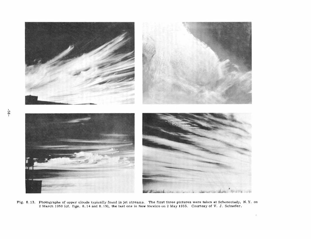
I <J1 00 I

Fig. 8.13. Photographs of upper clouds typically found in jet streams. The first three pictures were taken at Schenectady, N. Y. on 2 March 1953 (cf. figs. 8.14 and 8.15), the last one in New Mexico on 2 May 1955. Courtesy of V. J. Schaefer.

A curious thing noted by McLean is a nearly cloudless region close to the axis itself, in agree­ment with Vuorela's deductions (1953) about strong localized descent in the center of jet streams. McLean comments as follows: "The cirrus clouds sometimes form in bands parallel to the wind im­mediately south of the core with wispy 'mares tails' forming at an angle to the flow. On many occasions, crew members of the research aircraft have report­ed a sharp discontinuity in the cirrus near the core with cloudless skies to the immediate north. The observers also report that in cases where the cirrus extended to the north of the core, there is often a narrow break in the cirrus at the core itself. "

The thickness of the cirrus averaged about 500 feet, but individual layers ranged from a hundred to several thousand feet in depth.

Vorticity Advection: French and Johannessen (1953) j3.ttempted to determine the distribution of cirrus clouds relative to the jet stream from vorticity ad­vection considerations similar to those employed in models 8. 10 through 8. 12. While they did not pre­sent a distribution relative to the jet stream con­figuration, they noted that 80 percent of the cirrus clouds in the sample of aircraft observations used by them occurred in areas of advection of cyclonic vorticity.

Temperature Field Above Core: A method of locating the principal areas with cirrus clouds from upper-air charts consists in inspecting a constant­pressure surface above the level of maximum wind­usually 200 mb over the United States in winter, 150 mb in summer and along the subtropical westerly jet stream. We have seen in Sections III-IV, that strong lateral temperature gradients often occur above the core and that streamlines (contours) may cross isotherms at large angles. Since the iso­therm patterns normally migrate slowly compared to the wind speed, the air will blow 'through' the centers of warm and cold air which, on a constant­pressure surface, are also centers of high and low potential temperature. Now, since the air moves nearly adiabatically in the jet core, i. e. on constant potential temperature surfaces, areas of ascent and descent can be located from the crossing of stream­lines (contours) and isotherms. Because potential temperature increases upward, ascent must take place where the streamlines point from warm to cold air, and descent where they are directed from cold to warm air.

Ascent may also be inferred when a new cold area appears that is not traceable from continuity, and descent when a cold area weakens or disappears. As we just learned from McLean, such vertical motions do not necessarily imply cirrus at the level considered since hardly any clouds have been found above the level of strongest wind in the observation programs so far conducted. Perhaps the strato­spheric air is too dry; perhaps the vertical motion is too weak in the existing stable stratification to permit air to reach the condensation level; perhaps suitable nuclei are lacking. However, the vertical motion usually retains the same sign through deep

-59-

layers of the troposphere, damping out in the upper troposphere and stratosphere. Hence, the distri­bution of cirrus in the high troposphere often may be inferred from vertical motions indicated in the lower stratosphere, especially when considered together with the vorticity advection pattern. It will be re­called that on 6 March 1958, an isolated warm region was located north of the jet stream center at 200 mb in the Middle West (fig. 4.7). Using the reasoning just outlined, it was concluded that air moving toward this warm area from the west was descending while air going away on the eastern side was ascending. The areas of ascent and descent so inferred on that occasion were in accord with the cloudiness and precipitation distribution observed in the lower troposphere.

Cloud Photography: Recognition of middle and high cloud types and patterns associated with middle­latitude jet streams is due mainly to systematic studies through time-lapse photography of such clouds by Schaefer (1953, 1955). Initially, his ob­servations were confined to the New England states, but they were later extended to other parts of North America and of the globe through an extensive pro­gram of time-lapse photography from ground and aircraft.

Schaefer lists four principal types of clouds associated with jet streams, quoted in the following from his 1953 paper:

1. "High clouds (H 4 and H5) - cirrus streamers of great complexity moving at high velocity and showing long tufted streamers, complex shear lines, and massive whorls.

2. High clouds (H9)-cirrocumulus in blanket­like masses scattered in a random fashion although sometimes in a line showing evidence of being at the crest of undulations in the stream. Clouds some­times changing in character, shifting rapidly to cirrus streamers or showing fine structured waves at very high altitude. Some blankets show high­order Tyndall spectra in green, red and other colors when near the sun.

3. Middle clouds (M 4 and M 7)- altocumulus lenticularis wave clouds, sometimes in great pro­fusion with large lateral dimensions in the direction of flow of the stream, often with considerable ver­tical depth and piling up in many layers. Such clouds show little apparent relationship to ground topography, although they are basically 'standing clouds' and, therefore, do not exhibit rapid move­ment except when snow is shed from them. When this occurs, long streams may extend downwind for many miles to emphasize the high-velocity nature of the air. When near the sun, high-order Tyndall spectra colors are commonplace.

4. Middle clouds (M3 and M 5)- altocumulus. A billow-type cloud which may extend from horizon to horizon with the waves in parallel bands at right angles to the air flow. At times the cloud sheet may appear as a relatively thin layer with the units more cellular in form. "

Schaefer suggests that a jet stream core is likely to be situated near an observing site when at least three of these cloud types are observed. He also stresses that it is necessary for the clouds to show coherency to warrant such an inference- i. e. the cloud types must occur and recur in broad arrays rather than in isolated non-recurring patches; fur­ther, that except for the lenticular clouds high speed of cloud matter must be observed. Use of Schaefer's method is, of course, restricted to periods when lower clouds do not obscure the sky and when enough moisture is present in the jet stream to permit cloud formation.

Fig. 8.1:{ presents a set of pictures taken at Schenectady, New York, by Schaefer on 2 March 1953, a day on which one might have expected clear skies over New England from the surface map (fig. 8. 14). A north -south vertical cross section, how­ever, revealed the presence of a jet stream core just north of Schenectady (Schaefer and Hubert, 1955). At 300 mb (fig. 8.15) this current was curv­ing clockwise, with highest speeds east and north of the observation site. The latter, therefore, was situated in an area corresponding to sector IV of fig. 8.12, and the cloudiness can be attributed to high-level divergence with ascent occurring in a region of advection of cyclonic vorticity. Due to the lack of enough 300-mb winds, it is not possible to ascertain the maximum core strength with certainty. Twelve hours later, winds of 160 knots were ob­served along the axis over New England.

'0t)~~'

1020

Fig. 8.14 Surface fronts and isobars, also jet stream axis, 2 March 1953. Dot marks location of Schenectady.

Outstanding photographs of clouds have also been taken along the subtropical jet stream on oc­casions when this current was located quite far south. On 1 April 1953, for instance, an extreme wind concentration along the vertical was observed at San Juan, Puerto Rico, in a situation when the subtropical jet stream center was estimated several degrees latitude north of the island (fig. 8.16). Al­though four-minute overlapping averages were used to eliminate irregularities of the wind profile, the narrow high-speed layer of little more than lOO-mb

-60-

'00

Fig. 8.15 300-mb chart, 2 March 1953, 1500GCT. 300 -mb heights in tens of feet, first digit omitted; temperatures in °C, isotachs in knots.

thickness is spectacular. An expedition from Woods Hole Oceanographic Institution conducted research aircraft flights in the area at that time under the direction of Dr. J. S. Malkus. Remarkable pictures of a row of huge cumulonimbi close to the jet axis were observed from the aircraft. One of the air­craft photos is reproduced in fig. 8. 17, taken from an altitude of 6,000 feet. Fortunately, since the clouds were also being photographed with time-lapse camera from the ground at the same time, Malkus was able to calculate their dimensions and the rate

o

100

P

200

mb

300

400

500

600

700

800

Direction (Deg) 60 120 180 240 300 360

I I i

\ \ I I

I / , i \ \

\ \

I \ \ \ \ \

" ' ..... .... -

/ /

/ /

/ I

I

20 40 60 80 100 Speed (Kt)

Fig. 8.16 Vertical profile of wind direction (dashed) and wind speed (solid) at San Juan, Puerto Rico, 1 April 1953, 0300GCT. Four-minute averaged winds were used for construction of this diagram.

Fig. 8.17 Cumulonimbus extending into fast westerly current shown in fig. 8.16, photographed from an altitude of 6000 ft northeast of Puerto Rico on 1 April 195:3, camera pOinted toward NNE (Malkus and Ronne, 1954). Courtesy of Dr .. J. S. Malkus.

of motion of the cloud matter (Malkus and Ronne, 1954). The horizontal distance from plane to cloud was about 80 miles; the horizontal extent of incli­vidual clouds ranged up to 45 miles; the leaning towers reached a height of over 45,000 feet. The altitude at which the clouds began to slant strongly, agreed well with the sharp shear zone of fig. 8.16 and more precisely with the shear of the Puerto Rican rawin 12 hours later, which was closest in time.

A surge of interest in cloud patterns and their relation to major features of the wind field has developed with the advent of satellites. TIROS I strikingly showed the potentialities of investigating cloud structure by means of photography fr6m great altitudes. In particular, the banded or line structure of clouds, previously recognized mainly for hurri­canes, has been revealed as a dominant feature of most major cloud systems (cf. Widger, 19f1O, also numerous papers by the Satellite Section of the U. S. Weather Bureau). Thus, an extratropical cyclone appears much like an ovcrgrown hurricane, with bands of 1000 miles length and more extendiI,g from the outskirts into the core. Long and narrow cloud bands, oriented more or less parallel to the wind, outline some jet stream cores. On the other hand, there are also large cloud-free areas along jet

-() 1-

streams, especially in the subtropics. These con­firm the general subsidence prevalent over large portions of the subtropical jet stream.

Precipitation: In view of the wide variety of jet stream structures which occur, precipitation oc­casionally will be encountered in almost any position with respect to a high-speed center. On the average, there should be least precipitation in sector III of fig. 8. 11 and in sector II of fig. 8. 12. In the first statistical precipitation study relative to jet streams made by Starrett (1949), these different sectors were not considered separately. Instead, Starrett computed frequency distribution curves normal to the 300-mb jet axis for straight and cyclonically curving currents over the United States in winter. He found that the highest incidence of precipitation almost straddles the jet axis, with slight bias to the poleward side (figs. 8.18-19). Even so, precipita­tion occurred only about 50 percent of the time near the axis, which again indicates that large portions of the core are without precipitation. Twenty-four hour precipitation in cxcess of 4 percent of the monthly average occurred on 25-30 percent of the days analyzed and precipitation in excess of 20 per­cent on 5-10 percent of the occasions, which is rather high.

Since Starrett's study was made over the United States where the jet stream oscillates widely from day to day, averages were taken with respect to in­dividual jet stream positions. In East Asia the winter jet stream maintains a nearly constant lati­tude. There it is of interest to compare the mean upper flow pattern with the mean precipitation pat­pern of winter (Yeh, 1950). The maximum of precipitation practically coincides with the center of the upper jet stream (fig. 8. 20). Rainfall decreas­es northward and southward from there but more rapidly on the south side. Concentration of the pre­cipitation belt is evident from the fact that over considerable areas north and south of the jet axis the gradient of mean winter precipitation exceeds 20 cm in 100 miles. The remarkable agreement between precipitation relative to the jet in the United States as found by Starrett, and the average regional rainfall pattern over China relative to the average position of the jet stream, is possible only if the latitudinal fluctuations of the jet axis over eastern China are restricted to very narrow limits, not only from one day to the next but also from one year to the next.

lOON

5°N MAX. WIND

50 S

Fig. 8.18 Profiles of frequency (percent) of pre­cipitation relative to quasi-uniform (straight) jet streams obtained by averaging from 75 0 W to, 1230 W along jet axis during the winter of 1946-47. Curve 1 includes all precipitation, while curves 4 and 20 include only cases of at least 4 or 20 percent of the monthly normal precipitation respectively. (Starrett, 1949).

lOON

SON

MAX. WIND

50 S

4

50

Fig. 8. 19 Profiles of frequency (percent) of pre­cipitation relative to jet streams with troughs obtained by averaging along jet axis from 200 longitude west to 200 lon­gitude east of troughs. Curves 1, 4, and 20 as in fig. 8.18 (Starrett,1949).

Ramage (1952), looking at the wintertime sub­tropical jet stream from Hong Kong, comments in accordance with Yeh that; "the jet axis coincides with the axis of maximum rainfall; for not only do nearly all extratropical depressions of the region

-62-

/ i,/

Fig. 8.20 Distribution of mean zonal wind speed (knots, solid lines) at 30,000 feet for December 1945 and January 1946; and mean precipitation (centimeters, dashed lines) over China in winter (Yeh, 1950).

form along the jet, but they also travel for most of their life along it." Further; "Wide-spread sub­sidence occurs almost everywhere south of the jet stream ..... over our region (southeast Asia) sub­sidence is both more intense and more confined than over North America. Normal subsidence south of the jet stream occurs over northwest India, but over northeast India and Burma juxtaposition of jet stream and convergent upper southwesterlies seems to re­sult in much more vigorous subsidence downstream. " Ramage also states, "that the southwesterlies con­tribute potently to subsidence as evidenced by the Hong Kong soundings. There, on 90 percent of mid­winter days, strong subsidence inversions usually extending from 800-700 mb up to 300 mb are ob­served." Koteswaram (1953) confirms that winter precipitation along the subtropical jet stream over India-Pakistan is confined to the region north of the axis, with subsidence to the south.

After recognition of the importance of travelling high-speed centers in determining the distribution of precipitation, Jenistra (1953) computed the percent frequency distribution of precipitation occurr.ence in a coordinate system centered on the intersection of jet stream axis and 300-mb trough for the winter of 1951-52. He distinguished between cases when the westerlies were relatively strong in the high and in low latitudes and with this procedure achieved a first approximation toward dividing cases according to the scheme of modelS 8. 11 and 8. 12.

When the w.esterlies were relatively strong in high latitudes, the distribution of west wind speed in troughs and ridges should resemble that of fig. 8.12; when they concentrate in low latitudes the pattern of fig. 8.11 should prevail. Jenista verified that this was actually the case (geostrophically) at 500 mb for the period he analyzed. His results (figs. 8.21 and 8.22) largely corroborate the discussion of the mod­els. Johnson and Daniels (1954) analyzed precipita­tion at selected stations over Great Britain with respect to 'entrance' and 'exit' zones. In the ent­rance zone, twice as much rain occurred to the right

compared to the left side of the axis, looking down­stream; the reverse held for the exit zone. Thus, dynamical calculations and observations yield mutually consistent results, at least for average distributions.

20"W 'O'W TROUGH 10'E 20'E

rr-----'.--2-0 -- @--o--'-1:~--=--------;:'

5' LAT

5' LAT

20'w

Fig. 8.21

IO'W TROUGH 10'E

5'

20 LAT

5' LAT

Percent frequency of precipitation over the United States averaged relative to jet stream axis in 300-mb trough line when the hemispheric index of the west­erlies is above average in low latitudes, (Jenista,1953). Period of study: No­vember 1951 through February 1952. Precipitation occurrence defined as measurable amount observed during 6 hours ending at 06:iOGCT; this inter­val was centered on the time of the upper-air charts.

20'W 10'W TROUGH 20'E

~0,\20 4U

~' 20 LAT

~' LAT

ZO'W IO'W TROUGH

20

10'[

~O

5' LAT

20'[

Fig. 8.22 Percent frequency of precipitation when the hemispheric index of the westerlies is above average in high latitudes. (Jenista,1953, explana­tion as in fig. 8.21).

Clear-Air Turbulence

Turbulence in clear air in the lower troposphere is an event recognized and studied for many y~ars. Usually it occurs with definite and well-known fea­tures of the flow such as unstable air masses, inversion layers and air motion above mountainous territory.

-63 -

With the increasing trend toward high-level flying, clear-air turbulence has also been encoun­tered frequently in the tropopause region. This rather unexpected discovery has led to numerous investigations and several observational "projects . As yet, these studies have failed to yield a definitive solution on the nature of this turbulence, the location of its occurrence and therewith also its prediction. For these reasons, the subject will be treated here only briefly, especially as three thorough reviews of the problem have been undertaken (Newton, Berggren, and Gibbs, 1958, Panofsky, 1958, and Reiter, 1960), which also contain extensive biblio­graphies.

The difficulty, of course, lies first of all in gathering an appropriate sample of representative observations. Most turbulence reports are based on subjective pilot experience. Pilots will differ in their classification of turbulence, and the amount of turbulence noted by them will depend greatly on the type of aircraft they are flying. Turbulence re­ported by one pilot may well not be reported by another one for a variety of reasons connected with the structural aspects of their ship. Another dif­ficulty is due to the patchy nature of the clear-air turbulence. All reports agree that aircraft can enter and leave areas of turbulence without evidence of any obvious reason for onset or cessation. Tur­bulence prevails most frequently in shallow layers less than 500 feet thick, but turbulent layers of several-thousand-feet thickness have also been en­countered (cf. Bannon, 1952). The three­dimensional structure of the atmosphere in the tur­bulence zone is not known except for broad-scale aspects which can be deduced in areas with rawin­raob networks of the type existing over North America and Europe. These reports are insufficient to investigate detailed wind structures with vertical extent on the order of hundreds of feet and lateral extent of only miles as apparently is necessary.

With such an observational background, it is not surprising that a solution to the problem con­cerning the nature of the turbulence has not been found readily. Even the statistical computations on the distribution of the turbulence leave room for doubt as to where the turbulence is most likely to occur. All investigators have looked to the jet stream as a favorable place for turbulence to de­velop because high kinetic energy and large wind shears, lateral and vertical, are present there. Yet the evidence is not convincing that the turbulence is concentrated near jet stream cores. Many flights, including research flights made in aircraft especially instrumented with accelerometers, have encountered turbulence hundreds of miles distance from jet cores while penetration of some intense jet streams took place during smooth flight (cf. Riehl, Berry and Maynard, 1955). Aircraft missions by the U. S. Air Force Project Jet Stream have encountered turbu­lence in the broad belt normal to the jet axis with only weak indications of concentration about 150 nautical miles to the left and 300 nautical miles to the right of the axis (Endlich and McLean, 1957).

The representativeness of all statistical sum­maries has been placed in doubt by an experiment of the Canadian Air Force, reported by Clodman (1957). During a brief series of missions the air­craft were directed on box-type tracks with legs both parallel and normal to the wind. The result was that turbulence was noted aboard the planes much more strongly when flying parallel to the wind than on the normal legs. To Clodman, this suggested anisotropy of the turbulence, with the major axis of the turbulent area oriented along the wind. While the experiment consisted of only seven flights, it suggests nevertheless that the turbulence records in penetrations normal to the jet stream may not have revealed the true extent of the turbulence.

Some analyses of clear-air turbulence have taken physical hypothesis as their point of departure. The Richardson number has been discussed on sev­eral occasions. This number is proportional to the vertical stability of the air and inversely propor­tional to the square of the vertical wind shear. If eddies in the vertical plane produce the turbulence, one might look for high occurrence where the at­mosphere is unstable and the vertical wind shear large, that is, in areas of low Richardson number. This would locate the turbulence underneath jet cores where the lapse rate often is very steep. There is some suggestion of higher turbulence fre­quency beneath than above the core (Endlich and McLean, 1957). But the frequency of turbulence reports above the tropopause is sufficiently high that a simple calculation of the Richardson number from maps and vertical cross sections cannot be relied upon for proper placing of the turbulence zones.

In other hypotheses the lateral rather than the vertical wind shear has been considered. The work on dynamic instability discussed in Section II has led to a model of turbulence associated with negative or at least zero absolute vorticity. According to this model, particles displaced normal to the cur­rent in regions of dynamic instability will tend to

-64-

continue moving farther away from the initial posi­tion. If they conserve their momentum for a limited time during lateral travel, they will inject this momentum into portions of the current with different mean momentum and hence create small­scale wind fluctuations which will be noticed by an airplane as turbulence. Following this reasoning, the turbulence should be restricted to the anticyclonic side of jet stream. Contrary to early expectations, however, turbulence if anything, is more likely to occur on the cyclonic side. According to a theorem by Arakawa (1953) turbulence should be associated with cyclonic shear along the horizontal above cer­tain critical limits. The validity of this theorem also is not fully established. Finally, the incindence of turbulence has also been related to high-speed centers along the core.

The potential mechanisms have not been ex­hausted by the foregOing. For instance, there is also the possibility of gravity waves along the tropo­pause or other stable layers. Following Reiter (1961) moderate to severe clear-air turbulence (away from mountain ranges) occurs in narrow re­gions of warm temperature, mainly north of the jet axis. This suggests an association with sinking motion and stabilization of the atmosphere. Light turbulence, however, should be considered as a random phenomenon according to Reiter.

It is far from certain, that all turbulence can be ascribed to a single generating mechanism. In summary, aircraft entering a jet stream must be prepared to meet turbulence without warning in any portion of the core and also in outlying areas. This is an unsatisfactory statement which clearly points to the need for an extensive observational attack on the problem.

It should also be mentioned that turbulence, at times dangerous, can also be encountered in the tropopause region in jet streams Howing over moun­tain ranges. This is a large and specialized subject, considered outside the scope of this treatment.

IX. CLIMATIC ASPECTS OF THE JET STREAM

In the course of the foregoing sections various climatic aspects of the jet stream have already been treated, notably the subtropical jet stream of sum­mer and winter. Features such as the relation of jet streams to cyclones and various weather phenomena also fall under the heading of climatology if the broad definition of this subject by Jacobs (1947) is accepted. This section will be concerned only with a restricted part of climatology, the mean circulation on hemi­spheric and regional bases.

The principal jet stream zones of the northern hemisphere winter in middle latitudes and in the subtropics were depicted in fig. 1.2. Of these cur­rents the subtropical jet stream is most well-defined and reliable in location. No doubt variations occur from day to day and from year to year; but anyone laying out a flight route from middle latitudes to the equator in winter will include interception of the sub­tropical jet stream by the aircraft with a high degree of confidence in most parts of the hemisphere.

Not so in middle latitudes. Here the current is highly variable from day to day, changing speed, direction and location (cf. Section VII). At times there is no jet stream at all, and often there are only weak fingers superimposed on nearly uniform basi.c flow. Hence a broad band has been drawn in middle latitudes in fig. 1. 2 outlining the area where a jet stream is most likely to be found. The steadi­ness of the subtropical jet stream versus the variability of the polar jet stream has a profound effect upon seasonally-averaged circulation patterns.

Mean Circulation

Petterssen (1950) has prepared cross sections of mean zonal speed for summer and winter (figs. 9.1 and 9.2), bas ed on geostrophic calculations from radiosonde data. Compared to fig. 1.2 we imme­diately see a pronounced difference. The cross sections are much simpler; they contain only one jet stream in each season. In winter, latitude and alti­tude of the core agree with the subtropical jet stream position, but the central speed is much lower. In summer, the core shifts poleward by about 150 lati­tude, the core altitude remains nearly unchanged and the central speed drops to less than 50 percent of that in existence during winter. The altitude of the upper limit of the westerlies is considerably lower in summer than in winter.

Why the large difference between fIgs. 1. 2 and 9. I? Clearly, it is due to differences in clima­tological techniques employed in constructing the two charts. The question raised in fig. 1. 2 was: Where, around the globe, are the principal jet streams most likely to be located? In answering

-65 -

this question we attached the coordinate system for reference to the jet stream axes themselves. Quite another approach has been used in calculating fig. 9.1. There the question was: What is the mean zonal velocity prevailing at a given latitude and alti­tude in each season? The frame of reference is geographically fixed, and it is insensitive to the meanderings of jet stream cores. Suppose, for in­stance, that a single jet stream of unchanging core speed existed and that this current occupied with equal frequency all latitude belts in the course of a season. Then, by geographic averaging, one would obtain a uniform mean wind over the entire latitude range frequented by the current.

It is now clear that fig. 9.1 mainly reflects the subtropical jet stream because this current is strong, quite stable in latitude and mainly westerly. In con­trast, the temperate -zone jet streams migrate rapidly across the latitude circles and individual currents often execute wavelike oscillations of large amplitude. In zonal averaging the meridional flow components of the jet streams cancel, and the west­erly component is spread more or less uniformly over the whole latitude range of the oscillation. Palmen (195la) has stated the matter succinctly: "In order to avoid misunderstanding it should be pointed out that the upper jet stream computed from mean meridional cross sections for seasons or longer periods is not identical with the 'meandering' jet stream associated closely with polar front disturbances. This latter phenomenon can hardly be stu;Iied by the aid of climatological data, as Palmen and Newton (1948) have shown, because of the st.rong irrq,rular displacements of the polar front and the prinCipal air masses. "

Fig. 9. 1, of course, was not calculated for the purpose of depicting jet streams but for the purpose of determining the mean distribution of the wester­lies. This diagram, and all following figures similarly constructed, may be labelled 'mean mass­transport diagrams'. Perhaps the most surprising feature of figs. 9.1 and 9.2 is that, in spite of the

60' 50' 40" 30" 20' LATITUDE

Fig. 9.1 Mean zonal component of the geostrophic wind (knots) in winter, averaged over the northern hemisphere (Petterssen, 1950).

method of averaging and of the variability of jet stream positions, definite cores are nevertheless observed in the horizontal and vertical view even in summer.

It is evident that the mass -transport diagrams should be amplified with a climatology of a different kind to bring out the mean structure of jet streams. Jacobs (1947) has discussed new climatological techniques. There exists a wide field of application of such techniques to the jet stream; as yet this field has hardly been touched. Adoption of coordinates fixed with respect to the jet axis - as done by Krish­namurti (1959a) for the subtropical jet stream- is one such tool. For instance, mean location and intensity of the polar jet stream should not be deter­mined from time-averaged hemisphere charts. A clear picture will result if the latitude and speed of the jet core are tabulated as a function of longitude from daily charts as in Section VII, or even from nve-day mean charts, and if then averages are de­termined as the mean of these tabulations.

Fig. 9.2 Mean zonal component of the geostrophic wind (knots) in summer, averaged over the northern hemisphere (Petterssen, 1950).

In the following, only mass -transport calcula­tions will be treated because these are the only ones existing for presentation. Fig. 9.:{ is a diagram based on 500-mb hemispheric charts from 1946-1951 (U. S. Navy, 1954) which depicts the annual course of mean geostrophic west-wind speed on this surface. The latitude range of the strongest wind belt is fifteen degrees just as in figs. 9.1 and 9.2, but the

• .. ........... 4

\" .... ~ 60 .... _--------

" .. - .... , ~ , , ..... " .... _-----.

to .... FEB IIMII APR MAY ..lUtE JULy AUG SEPT OCT HOY DIC JIll

Fig. 9.3 Seasonal course of geostrophic zonal flow (mps) at 500 mb, averaged around the northern hemisphere. (U. S. Navy, 1954). Heavy line denotes latitude of strongest speed.

-66 -

Fig. 9.4 Mean 200-mb isotachs (knots) for Janu­ary 1949-53 (Wege,1957).

latitude of the core itself is five degrees higher in fig. 9.3 compared to figs. 9.1 and 9.2 in both sea­sons. This slope, hardly ever observed in individual cases, again must be attributed largely to the tech­niques of averaging. The 500-mb mean speed doubles from summer to winter. The difference between the core speeds of fig. 9.3 and figs. 9.1 and 9.2 is 5 mps in summer and 20 mps in winter, cor­responding to the stronger equator-to-pole tempe­rature gradient in the colder season.

Seasonal changes of average jet stream position are depicted further in figs. 9.4 and 9.5 at 200 mb. The isotachs for these charts were computed with the geostrophic formula from mean 200-mb contours for January and July, 1949-1953. Hence the result is very similar to that of figs. 9.1 and 9.2. In win­ter, the subtropical jet stream is delineated by the belt of strongest speeds over Africa, Asia and the western Pacific. Over North America and the At­lantic the mean polar jet stream position is indicat­ed. In summer, a weak maximum encircles the hemisphere near latitude 450 ; over southern Asia there is a suggestion of the summertime easterly jet stream in that season.

Eccentricity of the Westerlies: Although fig. 9.4 shows-amixtureof subtropical and polar jet streams, there is generally good correspondence with the spiral of fig. 7.12. As noted in Section VII, the belt of westerlies does not circulate symmetrically about the North Pole in winter, but about a 'circula­tion pole' which is displaced from the geographic pole toward east Asia and the western Pacific Ocean (LaSeur, 1954). On daily charts this tendency to­ward eccentricity manifests itself by jet stream positions at appreciably lower latitudes in the Pacific compared to the Atlantic Ocean, often by 200 latitude or more.

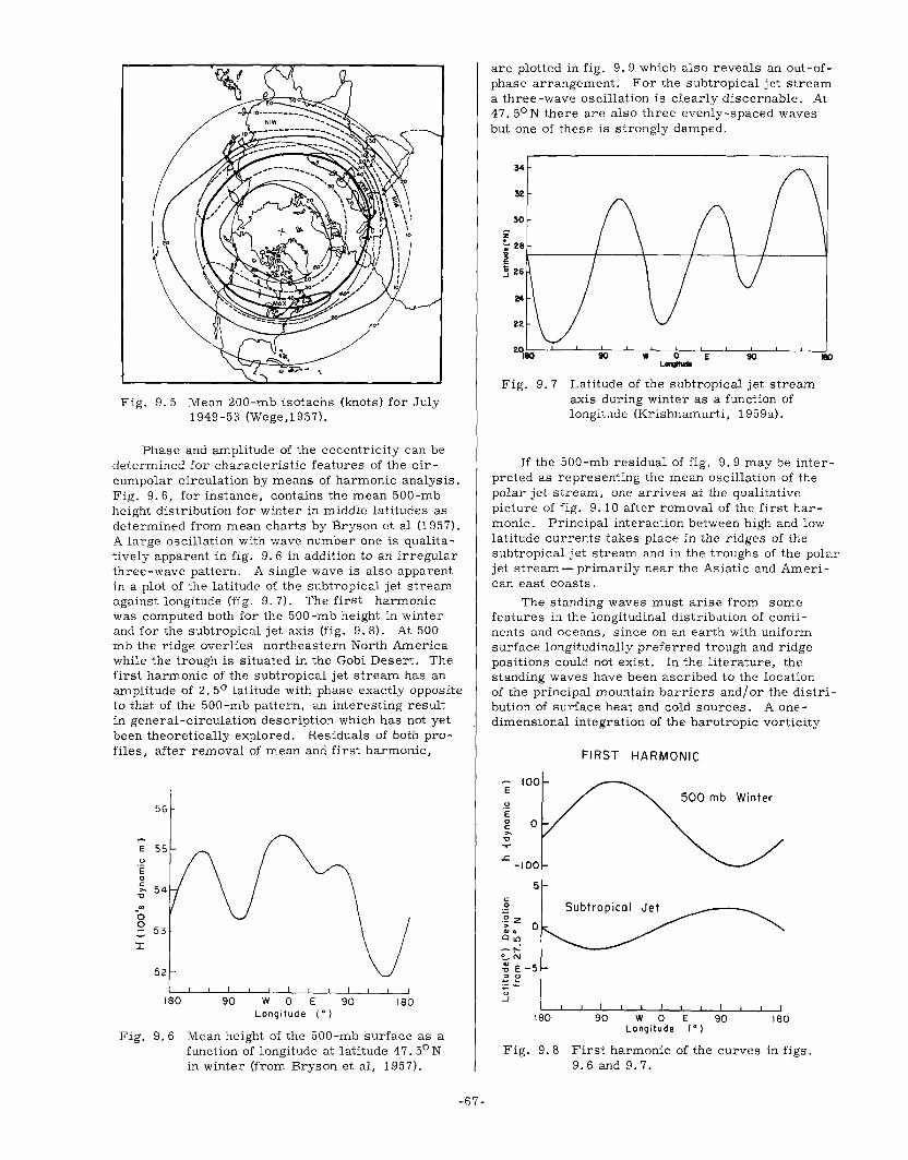
Fig. 9.5 Mean 200-mb isotachs (knots) for July 1949-5:3 (Wege,1957).

Phase and amplitude of the eccentricity can be determined for characteristic features of the cir­cumpolar circulation by means of harmonic analysis. Fig. 9.6, for instance, contains the mean 500-mb height distribution for winter in middle latitudes as determined from mean charts by Bryson et al (1957). A large oscillation with wave number one is qualita­tively apparent in fig. 9.6 in addition to an irregular three-wave pattern. A single wave is also apparent in a plot of the latitude of the subtropical jet stream against longitude (fig. 9. 7). The first harmonic was computed both for the 500 -mb height in winter and for the subtropical jet axis (fig. 9.8). At 500 mb the ridge overlies northeastern North America while the trough is situated in the Gobi Desert. The first harmonic of the subtropical jet stream has an amplitude of 2.50 latitude with phase exactly opposite to that of the 500-mb pattern, an interesting result in general-circulation description which has not yet been theoretically explored. Residuals of both pro­files, after removal of mean and first harmonic,

56

u ·E o ;, "0 .. o o 53

I

52

180 90 WOE Longitude (0)

90 180

Fig. 9.6 Mean height of the 500-mb surface as a function of longitude at latitude 47.5 0 N in winter (from Bryson et aI, 1957).

-67 -

are plotted in fig. 9. 9 which also reveals an out -of­phase arrangement. For the subtropical jet stream a three -wave oscillation is clearly discernable. At 47. 50 N there are also three evenly-spaced waves but one of these is strongly damped.

34

32

30

Z !.. 28 i r-------~~----~----~~--~r--.~------~ ~ 26

24

22

w 0 Larvtudo

90

Fig. 9.7 Latitude of the subtropical jet stream axis during winter as a function of longitude (Krishnamurti, 1959a).

180

If the 500-mb residual of fig. 9.9 may be inter­preted as representing the mean oscillation of the polar jet stream, one arrives at the qualitative picture of fig. 9.10 after removal of the first har­monic. Principal interaction between high and low latitude currents takes place in the ridges of the subtropical jet stream and in the troughs of the polar jet stream-primarily near the Asiatic and Ameri­can east coasts.

The standing waves must arise from some features in the longitudinal distribution of conti­nents and oceans, since on an earth with uniform surface longitudinally preferred trough and ridge positions could not exist. In the literature, the standing waves have been ascribed to the location of the principal mountain barriers and/or the distri­bution of surface heat and cold sources. A one­dimensional integration of the barotropic vorticity

100 E

.!:! E 0 0 ;, "0

~

-100

c .9

~z '" . 0",

-~

5

o '" ~ E-5 ~e :;:­o --'

180

Fig. 9.8

FIRST HARMONIC

500 mb Winter

Subtropical Jet

90 WOE 90 180 Longitude (0)

First harmonic of the curves in figs. 9.6 and 9.7.

_ 200 E

E

RESIDUAL

500 mb Winter

~ Ob'--~~-----7L-----------~~-----,., "0

.<:: -200

180 90 WOE 90 180 Longitude (0)

Fig. 9.9 Residual of the curves in figs. 9.6 and 9.7 after removal of mean and first harmonic.

equation by Charney and Eliassen (1949) yields a remarkably good approximation to the SOO-mb height profile. Harmonic analysis, as .iust applied to fig. 9.6, has been carried out by Barrett (1958) from 200 N to 700 N at intervals of 100 latitude for January and February 1949, at 300 mb. It reveals that the phase of the first harmonic changes with latitude, as evident from the perturbation streamline field for this harmonic (fig. 9.11). Unpublished daily 500-mb analysis for the winter of 1951-52 made at Project AROWA of the United States Navy at Nor­folk, Virginia, for the same belt have yielded a similar result. The quasi-logarithmic spiral of fig. 7.12 was obtained by drawing a curve through the center of the perturbation contours in fig. 9. 11, reinforcing the mean westerlies. Mean location of the spiralling axis of the first harmonic and of the actual mean jet stream locations at 300 mb during January-February 1949, are compared i.n fig. 9.12. The result evidently is very good.

From the preceding analysis two major controls of the general circulation during winter are observed in the jet stream layer that could not be detected fully until the advent of rawin observati.ons and hemisphere-wide data coverage in the upper tropo­sphere. One of these is the huge spiral extending

Fig. 9.10 Model of interaction between sub­tropical and polar jet streams.

-68 -

from equatorial to arctic regions, the other a stand­ing three-wave pattern with phase reversal from polar to subtropical jet streams. On account of the close relation between jet streams and cyclones, one should be able to find a reflection of the spiral of fig. 7.12 and 9.12 in the distribution of surface cyclonic activity. Petterssen (1950) has determined the belt of most frequent weather disturbances in a novel way by considering the alternation (percent) between cyclones and anticyclones. This indicates the distribution of travelling di.sturbances. The ratio of alternation is defined as F IF when

c a F < F or by F IF when F > F ,where F

c a ac c a c and Fa denote the percentage frequencies of occur­rence of cyclone and anticyclone centers, reSllec­tively, in a given square with area of 105 km 2 .

300 "e SO'OAY MEAN

WAVE" t 1 JAN - 28 FEB 1949

.. "- .. , .

... - ..

Fig. 9.11 Perturbation contours (feet) of first harmonic at 300 mb, January-February 1949 (Barnett, 1958).

The result for winter (fig. 9.13) shows a re­markably simple pattern except over North America and parts of Europe. Highest rates of alternation are confined to a narrow belt which trends in a spiral-like manner from the Asiatic east coast near Japan to the polar sea. The spirals of figs. 9.12 and 9.13 are quite parallel, but there is latitude displacement in that the zone of maximum alterna­tion lies south of the spiral in fig. 9. 12. The profound effect of the mean asymmetry of the general circulation and its associated .iet streams on the mean behavior of surface disturbances are well brought out by these diagrams.

Mean Cross Sections for Various Longitudes

North America: Following earlier work by Willett (1944) and Hess (1948) new cross sections of the

mean mass transport across longitude 800 W (figs. 9.14 and 9.15) have been prepared by Kochanski (1955). This is a longitude where a mean upper trough is located in winter and where the flow is, therefore, essentially from the west. Thus the cross sections are normal to the average total flow and bring out the mean wind distribution with lati­tude. But the reader should remember that the structure of the westerlies as portrayed is repre­sentative of mean trough conditions.

!

•• .~, ~':. M

,.,~~~ "

>'r::::'--~~:' ;.';/ : .. \ ~~}

/ "j' ,f " "\ ;, , ... I

I , f

f ' I I" I

I. I I

"

-- JET STREAM AXIS MEAN POSITION

___ - MAXIMUM PERTUR8A lION

vELOCITY WAVE 1

300 MB JAN - FEB 1949

"

- 1 I

Fig. 9.12 Mean jet stream axis (solid) and axis denoting maximum westerly perturba­tion velocity from fig. 9.11 at 300 mb, January-February 1949 (Barrett, 1958).

WINTER

E

Fig. 9.13 Rate of alternation (percent) between cyclones and anticyclones during the winter season, indicating the distri­bution of traveling disturbances. The ration of alternation is defined as the ratio (F IF ) when F <F , or by

c a c a

30

o

F IF ) when F >.1:<' where F and a c c a c

F a denote the percentage frequencies of occurrences of cyclone and anti­cyclone centers, respectively, in a given 100, 000 kIn square (Petterssen, 1950).

"U 20

10

-10 10

~-" km

·10 -10

90 60 Latitude (0 N) 30 0

Fig. 9.14 Mean zonal wind speed (knots) at 800 W in winter (after Kochanski, 1955).

60

SUMMER r---~~~----:ro~,-~----~======~~---o--~o--:-I~S_--_-_-_-_-_-_~_~_='=_~_~_~_~_~_~,s~120

10

km

90 60 Latitude (ON) o

Fig. 9.15 Mean zonal wind speed (knots) at 800 W in summer (after Kochanski, 1955).

-69-

Figs. 9.14 and 9.15 show roughly the same seasonal changes in mean transport as noted in figs. 9. 1 and 9. 2. The core position remains at a nearly constant altitude, and the central speed de­creases by 50 percent from winter to summer. Less latitudinal migration of the jet core is apparent than in the cross sections of Hess, who had obtained a seasonal displacement of 200 longitude. In the win­ter section, agreement with the location of the mean axis position in fig. 9.14 is not good.

%~.---r----,-----,-----~----.-----r---~,

100

80

60

40

20

km

6

Fig. 9.16

APRIL

NOVEMBER : MARCH

Percent position frequency of jet streams as deduced from 500-mb charts in Ul49 and 1950, and topo­graphical sections along longitude 800 E (Ramage, 1952).

Central and Eastern Asia: In this part of the world polar and subtropical jet streams converge from north and south toward the .Japanese Islands. The mean circulation is intimately related to the huge expanse of the central Asian mountain complex. This great elevation of land, with an area of two-thirds of the United States above :1 km, has an approximately elliptical shape. The low -tropospheric air is forced to move around the plateau, and the level of fric­tional interaction between earth and atmosphere is raised. From Taylor's work (1924 and other arti­cles)' and from hydrodynamic model experiments in rotating fluids with obstacles (Long, 1952) we may expect that under the conditions prevailing in central Asia an obstacle such as t11(> plateau will extend its influence throughout the fluid, leading to a split current.

In addition, the surface radiation cold source is also lifted to high altitudes, so that cold air drainage plus subsidence down the mountain slopes will occur. This drainage produces a current from which much of the winter monsoon over India and adjacent waters is derived. We may presume that subsidence is also occurring at high altitudes above the plateau from continuity reasoning, and that this subsidence will keep temperatures relatively warm there re­sulting in a reduction of the meridional temperature gradient. This, in turn, would support the mainte­nance of the split in the westerlies, given geostrophic winds in the mean.

A fr('quency distribution of jet stream positions north and south of the mountains deduced from 500-

Fig. 9.17 300-mb contours (lOO's feet, base 20,000 feet) for the Asiatic ~ontinent, 24 February 1958.

-70-

mb charts by Ramage (1952) at 800 E strikingly illustrates the split (fig. 9. 16). According to this figure the subtropical jet stream is confined by the mountains to a narrow belt, while the latitude of the Siberian current is quite variable. An individual 300-mb chart (fig. 9.17) brings out very clearly the double current structure with nearly calm conditions over the plateau and the high-energy flow over the Pacific coast of Asia. The full strength of the sub­tropical jet stream is not measured on this chart because the altitude is not high enough.

Several mean cross sections have been pub­lished from this area. Of these, Koteswaram's computations over India (1953) have located the sub­tropical jet stream center near 250 N with a speed of over 100 knots (fig. 9.18). From India this cur-

LATITUDE (Deg 1

Fig. 9.18 Mean distribution of geostrophic zonal wind component (mps) over India in winter (Koteswaram.1953).

60

70

eo

100

p • 50

mb 200

250

400

o -55----- - -- --

-50-- __ .. -- -

---

Fig. 9.19 Distribution of mean west wind speed (mps) at 12 kms over the Far East in winter (Mohri, 1953).

rent intensifies downstream to the Japanese area. This intensification, shown in an analysis of mean 12-km isotachs (fig. 9.19) by Mohri (1953), cannot be attributed entirely to the plateau but must be the result of inflow of air from the southwest out of the equatorial trough zone as described by Ramage (1952). Along the Asiatic east coast (fig. 9.20) the mean jet stream speed in winter is among the highest

in the world (Staff Members, Academia Sinica 1957). The summer profile of westerlies (fig. 9.21), in contrast, does not differ much from that at 800 W.

Europe: A mean cross section, constructed for the Greenwich meridian for February 1951 (James 1951) shows a broad flat maximum of 70 knots in the vi­cinity of 40° N (fig. 9. 22). The broad center and low speed in this cross section compared to the pre­ceding winter sections may be attributed to large north-south fluctuations of the jet stream over western Europe, not to weaker intensity of individual currents in that part of the world.

20 65

'9

81 '8 60t ~ .7 ~ ~ .• 55 en

til -'I 50~ ~ IS .. 45

13

'2 '0

35 .0

20'

Fig. 9.20 Distribution of mean zonal west wind speed (knots) and temperature (oC) along longitude 1200 E in winter (Staff members, Academia Sinica, 1957).

-71-

40

50 -40

60

70

-60----

200

-50-------- 16 250

300 -40 ---- ------ -- --- --

40

500 -10--------------

-28

KI,I. OF FT.

-56~ 70:

-56 65 2~ I. -48 60 18

55 17 I. _40

50 15

-32 45 104

-24 13

==~ __ -16 40 12 ------50 35 II

-----40 10

------------30 30 9

-8 26 8 ~~

------ 22 ----- -10

------- ---------0 -----------10

18 5

14 4

10 3

6 2

20 - J

IOOOL.-"~~~004------~----~~~'-------~--~472~~--__ ~,-__ -o~~~~~.-=-~.-~=-22~0.~ ____ ~-;--~~~~5 0 944 004 676 022 092 895 916 951 96.5 696 7S2 327

Fig. 9.21 Mean zonal wind speed (knots) and isotherms (Oe) along longitude 1200 E in summer (Staff members, Academia Sinica, 1957).

Southern Hemisphere: Mean winter and summer sections for the southern hemisphere have been computed along 1500 E and 1700 E (figs. 9.23 and 9.24). It is interesting to note that winter condi­tions differ little at 1700 E in the southern hemi­sphere and 800 W in the northern hemisphere, even though one longitude extends over an ocean and the other crosses the eastern part of a continent. In­tensity and mean altitude of the core are about equal, but the southern current lies a little closer to the equator on the average. The dominance of the subtropical jet stream is even stronger in the southern than in the northern hemisphere. During summer a double structure of the mean core is

apparent at 1700 E, presumably showing polar and subtropical jet streams, since the latter does not

disappear during the southern summer.

40

850

100020 N 10 0

30

80

10

LA I DE 40

Radok and Grant (1957) have discussed further the 200-mb mean flow over the Australia-New Zealand region, especially seasonal variations and anomalies. Some of their conclusions follow: liThe high-tropospheric mean flow over the region of Australia and New Zealand, while simple by northern hemisphere standards, shows clear de­viations from the zonal model often assumed for the southern hemisphere. The majority of the flow distortions observed during the period from Sep­tember 1949 to August 1952 appears to have been caused by transient disturbances; the more signifi­cant remainder included anticyclones which ap­peared in low latitudes over the Australian con­tinent at the beginning of two out of three summers, and diffluence -confluence patterns in preferred blocking regions south of the continent and near New Zealand ...... ".

70 eo

20

20

50 60

Fig. 9.22 Distribution of mean zonal geostrophic west wind speed (knots) along Greenwich meridian for February 1951 (James, 1951).

-72-

LITTLE AMERICA

TAIERI

3Q NORFoLIC IS.

AUCKI.AND

o SANTO TARAWA

NOUMEA KWA ... ALEIN

Fig. 9.23 Distribution of mean zonal geostrophic west wind speed (knots) and temperature (OC) along 1700 E in southern hemisphere, winter (Hutchings, 1950).

20

18

16

14

-40

12 / /

/ /

/ 2 10 ::'::10 Z

-50 ~

8

6 "-"-

"-

-30

4

-20

2

-10 ,E 0 0

80' LITTLE

AMERICA

/

/ /

"

70'

I UST.f.' •

/ /

/ /

80" U5.TF.

I

"-" "

HOiUTIKA

TAl RI AUCKLAND

30' NORFcllC IS

20'

NOUMEA

/ /

/ /

/E

-40

-20

-10

o

10

20

BOUGANVIt.t.E

GUADAL At.

Fig. 9.24 Distribution of mean zonal geostrophic west wind speed (knots) and temperature (OC) along 1700 E in southern hemisphere, summer (Hutchings, 1950).

-73-

X. HIGH-LEVEL WIND ANALYSIS

The decade of the 1950's has witnessed the ad­vent of routine weather analysis and forecasting by machine methods. In view of the multitude of con­siderations and the wide range of experience that may be brought to bear in qualitative analysis, it is debatable whether numerical analysis can fully com­pete with the personal output of a highly skilled analyst. Little doubt, however, exists that even the most experienced staff at a major weather analysis center will find it increasingly difficult to handle the rapidly expanding volume of observations with qua­litative techniques. The number of radiowind sta­tions and the height attained by balloons is increaSing in many parts of the globe. The area covered by maps is also expanding as the questions, to which answers are demanded from meteorologists, more and more concern continental or intercontinental needs and problems. With the rise of jet aircraft, there is every necessity to disseminate high-altitude charts as quickly as possible for flight planning. It must be recognized that machine processing is the only presently known technique that can satisfy the mounting requirements on meteorological infor­mation.

Although the general trend for development of meteorological analysis tools by machine is readily discernible, few machine analyses have actually been performed above 500 mb at the time of this writing. Hence the following discussion of numerical proce­dures necessarily has to have a somewhat prognostic character. Nevertheless, there appears to be no longer any point in writing a chapter concerned with qualitative means of preparing high-level wind charts. For a discussion of such techniques, the reader is referred to the U. S. Navy Bureau of Aeronautics publication entitled The Jet Stream (NAVAER 50-1R-249), which contains detailed in­structions for high-altitude wind representation by qualitative methods which cannot be improved materially at this juncture.

In this section the following topics will be con-sidered:

1. Evaluation of balloon soundings 2. Secondary wind fluctuations 3. Layer-of-Maximum-Wind (LMW)

parameters 4. Objective analySis of LMW and constant­

pressure charts.

Evaluation of Balloon Soundings

While many types of wind measuring equipment are in service aro\lnd the globe, only the GMD-1A of the United States weather services will be dis­cussed as an example. It is recoe:nized that newer equipment will supersede the GMB-1A; nevertheless, the type of analysis here offered is considered to be generally applicable to wind measuring equipment.

-74-

When scanning teletype reports of high­tropospheric winds in jet stream regions, or when inspecting upper-air charts such as the 300-mb surface, one notes quickly that wind directions pre­sent a smooth and consistent appearance. The direction changes very slowly with altitude, if at all, through the jet stream; spatial changes occur· in well-ordered broad-scale arrangements. In contrast, speeds vary irregularly with height and also lateral­ly, so that the jet stream core may not be readily apparent. Qualitative isotach analysis has at times produced complicated patterns featuring several closely adjoining narrow wind maxima whose reality may be doubted.

As an example of irregular wind distributions, fig. 10.1 shows the rawin ascent for Washington, D. C., on 31 December 1958, 2300GCT. Only speeds are reproduced because the direction varied slowly and regularly as normally encountered. Speeds fluctuated only slightly up to 30,000 feet; from there upward the amplitude of the oscillations increased to become large above 35,000 feet.

--,--- T - ---,--~ r r-20 40 60 80 100

V (mps)

Fig. 10.1 Vertical profile of wind speed at Wash­ington, D. C. in westerly jet stream, 31 December 1958. (Riehl and Mihaljan, 1959).

The example chosen is by no means an extreme one. It is one of a series of soundings taken near Washington, D. C., which were analyzed in detail by Riehl and Mihaljan (1959). The elevation angle remained between 70 and 90 above the horizon up­ward from 30,000 feet and the wind fluctuations were not nearly as large as found in some other as­cents. Even so, the magnitude of the fluctuations approached that of the wind itself in the upper part of the run. If such speed variations had to be ac­cepted as real, there would be little prospect of successful wind forecasting or flight planning. In an analysis of earlier Washington soundings Reiter (1958) made an interesting observation. He

plotted the wind profile as given by the teletype message. Then, using the detailed minute-by­minute values of the ascent, he plotted the profile that would have been transmitted on teletype if by international agreement all standard levels were raised 500 meters. Above 25,000 feet a totally different curve resulted. Evidently, if the reported winds are to be taken as representative, the wind profile deduced from a teletype message must not be sensitive to such minor changes in choice of standard altitude to be reported.

It is plausible to assume that at least the major part of the oscillations of fig. 10.1 and similar soundings is due to instrumental short-comings. Arnold (1954) and Lettau (1955) have commented on erratic balloon behavior at high levels suggesting that it might be produced by instabilities inherent to the system of balloon and train rather than by turbulence. In addition, it is reasonable to suggest that, since with strong winds the elevation angle of balloons de­creases rapidly, changes in this angle produced by 'hunting' of the target by the instrument, or iner-

tial periods of the equipment, produce fictitious variations in wind speed.

10 •

9 •

8

7 •

6 •

n 5.

4

3

2

O~·--~~I----~----~---10 20 30

A (mps)

Fig. 10.2 Amplitude of the first 10 harmonics for the sounding of fig. 10. 1.

For purposes of analysis on the synoptic scale some smoothing of the vertical wind profile is neces­sary. Suppose the ascent at Norfolk, Virginia, late on 31 December 1958, showed a maximum speed at 45,000 feet where in fig. 10.1 there is a minimum. Evidently it would not be satisfactory to plot these two 45,000 foot winds on a chart and assume that they indicated the true wind shear between Washing­ton and Norfolk. In the past, vertical profiles have been smoothed by fitting qualitative curves to the teletype messages, but this procedure certainly is not the best one open to the meteorologist. Logical­ly, the complete minute-by-minute sounding must be utilized and a quantitative technique employed for high speed processing.

-75 -

50

10

'0

.~- ---r- ~~ --r-40 60 80 100

V (mps)

Fig. 10.3 Sounding of fig. 10.1 repeated (solid) and computed winds at one-minute intervals determined from first 5 harmonics.

Riehl and Mihaljan (1959) found that even strongly oscillating ascents can be reduced to an orderly behavior with harmonic analysis. For the sample of the Washington soundings they studied, initially the amplitude of the first ten harmonics was computed as illustrated in fig. 10.2 for the sounding of fig. 10. 1. The lower wave numbers produced the general outline of the profile wanted for horizontal analysis while the higher frequencies produced the wiggles to be suppressed. Satisfactory results were obtained by eliminating all frequencies above the first minimum in amplitude, i. e., all wave numbers greater than five in fig. 10.2. Original and smoother soundings are reproduced in fig. 10.3.

As yet, it is not certain whether this technique is the best one which can be devised. But the pro­cedure in general is of a type that must be applied to balloon ascents in order to obtain constant-pressure or LMW winds suitable for determining the lateral wind distribution over large areas.

Secondary Wind Fluctuations

It may be - and one hopes that it will happen-­that balloon sounding equipment someday will become so perfect that the true vertical wind profile can be presented in detail. Even in that event it will be appropriate to carry out the mechanical smoothing procedure just outlined. It is a well-known and fundamental rule of analysis that data must be re­presentative of the scale (time or space) for which analysis is to be performed. Many eddy scales usually are superimposed in the atmosphere. Those which have a magnitude smaller than the one to be considered must be treated as 'noise' and sup­pressed. This principle is always applied in surface wind and isobaric analysis. Observers do not report the instantaneous gust when taking a synoptic observation, but the mean speed over some time. In drawing surface isobars, smooth curves are always fitted to the observations.

The true microstructure of the upper atmo­sphere must be similarly suppressed for synoptic analysis of the jet stream. For rawinsonde data only vertical averaging - or rather averaging which follows the slanting balloon path- can be executed. If, for some reason, the microstructure is inde­pendent: of the path of the balloon or the vertical extent of a perturbation very large, complete elimination will not be possible. This situation, however, need not be expected to exist a priori. While thorough tests have not been conducted for the high troposphere, experience in other layers suggests that the wave length of the microstructure along the balloon track is likely to be sufficiently small to be mostly eliminated by smoothing as in fig. 10.3.

Such smoothing need not prevent information on true microstructure from reaching forecast offices where, at times, an index of wind variance as ob­served by balloons and its synoptic distribution may be desired. Such an index would be furnished by a function of the form

r 1 = I/';=V=i =-=V=o=;) 2;:-,

where Viis the unsmoothed, and V 0 ' the smoothed

wind; the bar indicates averaging over some depth, say the LMW. Considering that turbulence may be related to the energy of the small-scale wind varia­tions, it may also be of interest to calculate the

index r2

= (V. 2 - V 2), which is proportional to the 1 0

perturbation kinetic energy. Both r 1 and r 2 may

be normalized by dividing by V or K, the mean

J

II>

'x « -CLI J

E 2 0 .!: -0 ....J

0" CLI

0 3

--L..

speed or kinetic energy through the depth over which the averaging has been performed. Evidently, these indices will be of value only for soundings where ob­servational errors produce a lower order of variance than the true microstructure. The best estimate that can be made at present is that the order of magnitude of the true noise is 10 percent of the wind. This means that a high order of wind measur­ing accuracy will have to be achieved for the above indices to be meaningful.

Turning to lateral microstructure some data have already been shown in fig. 4.8. Saucier et al (1958) have analyzed the microstructure determined from research flights by the U. S. Air Force; the U. S. Navy (1959) has published a summary of re­search missions carried out under Naval auspices. Fig. 10.4 may serve as further illustration of horizontal wind variations. On 1 November 1954, a B-47 research airplane of the United States Air Force made two fast round trips on the south side of a jet stream over the eastern United States. The wind measuring equipment did not fully possess the accuracy of the Doppler radar navigation equipment, but the profiles may be accepted as quite reliable. As readily seen from fig. 10.4, the two round trips establish the mean wind profile very clearly on each meridian. The mean wind distribution is best re­presented by straight lines, shown on the right hand side of the diagram. The drawing indicates that the wind speed decreased uniformly by 9 knots from 83. 50 W to 81 o W, that the current was not of excep­tional strength and that the lateral shear was relatively small- only two-thirds of the Coriolis parameter. While not indicative of extreme jets, the case may well be representative of average con­ditions.

_---.L __ ...L __ ..L-_~ 4 L.--L- -~.

80 100 120 80 100 120 140 80 100 120 140 V (knots)

Fig. 10.4

V (knots) V (knots)

Wind profiles determined on anticyclonic side of westerly jet stream over the United States on 1 November 1954 by U. S. Air Force B-47 research aircraft. Double profiles obtained from two quick round trips, time separation about'two hours.

-76 -

27'

f~······.·~'.··7' .Its •

... '. "

~

) IS

25'

",. -,_ . . -.J /e,.,' o·

f", ... u,:

J£Jt3. ,

.- ,:,,-, I ....

i,:·,t:/· . "" . , ....

.- !~

I::)." . ----"TO. ~J 18'· ; ." 0 :'

"- ..... ___ 4Uj

a'v~ '7:n--": .: .... T ~ .. ;I ·.~-7: , "'0 '''.: I / .: ~. ,"

; ";, . ' .. , '/ '

!' '; "/:",1 .- --I •. ". .; --.L!!!J ~_

2)----100'

"'7 ' . e$~;

2S-

';-71 -- --" I

, I

lIsa I

27 120 --

'39.", /I

26 '.'--

/

160 lI1

1

30 ';',.' .", HAl 1~ i 31 . i ,8 .• ' .

. ... >~~

----r:GRCi t, \ ~ \. \

Fig. 10.5 Vertical wind profiles arranged geographically, over central and eastern United States on 6 March 1958, OOOGMT. Analysis for this period shown in Section IV. LMW shaded, numbers in upper left corner of diagrams denote LMW parameters. From top to bottom: direction (tens degrees), speed (knots), height (thousands feet), thickness (thousands feet); bracketed numbers extrapo­lated. For discussion of determination of parameters see text. Scale for individual diagrams shown in figs. 10.6-11.

The index r ,defined above, when applied to lateral coordinat~s in fig. 10.4, was 4.7 percent at 83.50 Wand 9.6 percent at 81 0 W after normaliza­tion, therefore, of the order of magnitude found for microstructure in the lower layers of the atmo­sphere. One may wish to relate the downstream increase in microfluctuations to the decay of kinetic energy of the mean current, assuming that there really was a decay and that the difference of 9 knots between the two wind profiles at 83.50 W and 81 0 W did not simply arise from vertical displacements of the jet core. Using the index r 2 the perturbation kinetic energy was 1. 7 percent of the mean kinetic energy at 83. 50 Wand 4. 4 percent at 81 0 W. Since the mean kinetic energy itself decreased by 22 per­cent in the 2. 50 -longitude interval it is very likely that this decay resulted almost wholly from work done against pressure forces and that the down­stream increase in kinetic energy of the micro­structure cannot be related readily to the change ip. mean kinetic energy.

No doubt larger fluctuations are encountered, for instance in thermodynamically unstable air or in shallow layers along temperature inversions. But it is believed that the foregoing computations are reasonably representative of the variance to be reckoned with in average situations. A 10 percent indeterminacy of the synoptic high-level wind at any altitude due to real noise must be accepted in a11 operations making use of such winds. Awareness of this indeterminacy was one of the principal con­siderations that prompted introduction of the concept of the LMW. In the following, procedures for deter­miriing the LMW parameters wil1 be taken up in some detail, but it should be pOinted out that techniques similar to those described here can be applied to any layer for which integration is desired.

LMW Parameters

As an example of wind data as reported over teletype, fig. 10. 5 contains plots of a11 wind sound­ings used for construction of fig. 4.1. As long as qualitative analysis is necessary, the type of work chart shown in this figure is recommended since it permits spatial comparison of the vertical profiles, and therefore enables the meteorologist to carry out a type of three -dimensional analysis. If, in addition, the preceding chart is hung up behind the analysis desk, all four dimensions are available for con­venient inspection. The purpose of LMW analysis is to reduce by one the number of dimensions which the forecaster has to deal. Four types of soundings are encountered in fig. 10.4, and these are the ones that are typically found in all situations. A few of the soundings of fig. 10.4 are repeated in larger format below.

Complete Soundings with LMW (WBS in fig. 10.6, cf. also fig. 4.2): Mean wind direction and speed, height and thickness of the LMW have been deter­mined from a curve fitted free -hand to the reported data pOints. It is considered that an LMW is pre­sent when the mean speed is at least 60 knots and. the thickness of the layer no greater than 15,000

-78 -

feet. Should smoothing of the original data by means of high-speed computers, proposed above, become reality, the qualitative construction of curves will be eliminated. Moreover, it wi11 be easy for a computer to determine also the LMW parameters eliminating al1 qualitative steps.

In the original concept of LMW analysis it was hoped that it would suffice to consider merely sound­ings with complete LMW characteristics, to reject a11 other data and to confine the analysis to areas with LMW. This concept has had to be modified. As yet too many soundings even over North America are 'short runs', i. e. they do not penetrate com­pletely through the jet stream. Further, we also wish to develop methods of horizontal analysis by means of high-speed computers; and, at least with current knowledge and experience, it is difficult to approximate a field of data which is not continuous in space, with.numerical methods. For these rea­sons ba1100n ascents without complete LMW char­acteristics have been incorporated into the analysis scheme.

Soundings with Maximum on Profile but Thickness Greater Than 15,000 Feet and/or Mean Speed Less Than 60 Knots (fig. 10.7, BUF in fig. 10.5). Such soundings wil1 always present a smoothly rounded appearance. The height of the strongest wind, a stable quantity in such cases, is recorded. Mean speed and direction are determined over a layer 15,000 feet thick centered on the maximum wind. In this way, by means of placing an upper limit on the thickness to be considered, a11 four parameters are given, and they can also be attained with automatic methods of sounding evaluation.

Barotropic Soundings with Uniform Speed Along the Vertical (fig. 10.8, LND in fig. 10.5). It is recom­mended to classify an ascent as barotropic when the range of windspeed from 25,000 to 50,000 feet does not exceed 30 knots. Such soundings then yield only one parameter -the mean speed. For continuity of

45

130

%

25

Fig. 10.6 Vertical wind profile at Washington, D. C. (WBC), 6 March 1958, OOOOGMT. LMW shaded, heavy dot indicates mean speed and height.

numerical analysis in middle latitudes, it is sug­gested to determine the direction from a layer of 15, OOO-foot thickness centered at 35,000 feeL The thickness parameter then will be 15,000 feet and the height may be entered as 50,000 feet which is to sig­nify that there is no maximum wind on the profile. In other seasons and areas alternate suitable defini­tions may be adopted.

45

40

~ 35 • .j!!

CII b 0 Q 30 .... 1: !IT 25 :r

20~~--~----~--~ 40 60 80 100

V (knots)

Fig. 10.7 Vertical wind profile at Ruffalo, New York (BUF), fi March 1958, OOOOGMT.

Incomplete Soundings: Unfortunately many ascents do not penetrate to 50,000 feet just near jet stream cores because of excessive distance of the balloons from the observing site. The elevation angle de­creases below ()o a.bove the horizon; for GMD-l A this is considered the limit for sounding evaluation from instrumental considerations. Since the total density of upper-air stations at best is marginal for jet stream analysis, it follows that every effort must be made to incorporate the information from short runs. Of course, only ascents satisfying cer­tain minimum conditions can be included. The suggested minimum - again for middle latitudes mainly in winter- is a top of the sounding at 300 mb (30,000 feet) or at a height of no more than 8000 feet below the estimated LMW height; the speed should be at least 60 knots at this level with positive shear underneath. These conditions are not met, for in­stance, by OKC in fig. 10.5 which sounding, after a scan of the surrounding ascents, must clearly be rejected.

Consider at first the profile for PIA (Peoria, Ill., fig. 10.9). From the earlier discussion of the LMW the mean height tends to vary only little along the axis. Hence one may scan along the wind direc­tion upstream and downstream to determine the mean height of the nearest stations with complete soundings. The average of these heights should yield the best possible approximation for the station with incomplete sounding, usually to about 2, 000 feeL In case of PIA, a mean height of 3fi, 000 feet evidently will be a good estimate. Thus, the sound­ing practically reached the core and upward extra­polation of at most 1, 000 feet is required. Actually,

-79-

the 35, 000 foot wind has been taken as maximum wind in fig. 10.9. With some assumption about the shear above the level of maximum wind all LMW parameters can be computed. In the absence of better information, we may assume equal shears above and below the level of strongest wind, or a somewhat higher shear above the core in view of fig. 2.4. Alternately, the form of profiles of ad­joining stations may be adopted.

45 .--+-: 40 ....

_CII

0 35 0 52 .. or: 30 CI -ij :r:

25

20

Fig_ 10.8 Vertical wind profile at Lander, Wyo­ming (LND), () March 1958, OOOOGMT.

The case of JAN (Jackson, Miss., fig. 10.10) is a little more complicated since the sounding ter­minated at 30,000 feet with indicated LMW height near 41, 000 feet from neighboring stations. Linear extrapolation of the lower portion of the sounding leads to a top speed of 150 knots, but the slightly rounded profiles in the surroundings make a lower estimate more plausible. Utilizing the shape of the ascents at MGM and FSM, a peak speed of 135 knots

Percent of max

45~ 80 100 i ---,

40~ " , ..... K \ 80 % " .....

" ..... - I FNT " ..... ..... i \ ......

-'" " 0

35t Max

0 2 --.c 30

1

0> 'Q; :r:

25 l

20L Ll I ..L-80 100 120 140 160

V ( knots)

Fig. 10. 9 Vertical wind profile at Peoria, Illinois (PIA), fi March 1958, OOOOGMT. Also portions of wind profiles of FNT and TOP, expressed in percent of the maxi­mum wind at these stations. Extrapola­ted part of wind profile dashed.

is obtained. For direction, it appears best to adopt the direction at the top of the sounding. If nearby stations show consistent turning through the LMW, the same amount of turning may be introduced.

The Tampa rawin (fig. 10.11) offers still another problem. The shear was too small for an LMW, too large for a barotropic sounding. The wind profile, therefore, must have had,the character of the second class described above. Assuming a height for the maximum wind of 44,000 feet as given by VPS and JAX, the maximum extrapolated wind will be 85 knots, and the average wind over a layer of 15, OOO-foot thickness centered at 44,000 feet will be 75 knots, if upper and lower shears are equal. All of these extrapolation procedures can be written into machine programs.

55

"-50

,.,.FSM :::. 80% , " " "-

~ 45 "- "-

"- , MGM', \

VI \

'8 40 I Max

I /

2 / / I /

.... 35 / /

.c / "./109 0> 80% Qi / / / J: / /

30 // / 2.5 -

2.0 80 100 12.0 140

V ( knotsl

Fig. 10.10 Vertical wind profile at Jackson, Mis­Sissippi (JAN), 6 March 1958, OOOOGMT. Also portions of wind pro­files at FSM and MGM, expressed in percent of the maximum wind at these stations. Extrapolated part of wind profile dashed.

Shear Chart: As an alternative to the LMW tech­nique, it has been proposed to compute the mean shear over layers of 5, ODD-feet thicknesses just below and above the level of maximum wind (Jo­hannessen, 1056). This information, of course, is readily obtained from the vertical wind profiles; the foregoing techniques of vertical extrapolation can also be utilized for preparation of shear charts. It must be noted, however, that the accuracy in deter­mining the distribution of a higher order quantity, such as shear, will always be lower than that of computing the primitive variable, wind, especially when the latter is integrated over a fairly deep layer. The LMW speed and direction should prove to be a dependable tool for representing the wind field, as also indicated by comparison of LMW winds and aircraft winds on coast-to-coast flights across the United States (U. S. Navy, 1059).

-80-

45 Max. at JAX VPS ,'--

-. ... J

40

III 35

8 o ==-30 ~ ~ r 25

, ,

80 100 V (knots)

Fig. 10.11 Vertical wind profile at Tampa, Florida (TPA), 6 March UJ58, OOOOGMT. Also level of maximum wind at ,JAX and VPS. Extrapolated part of wind profile dashed.

AnalySis of .Jet Stream Charts

Numerical Analysis: After thorough processing of the individual wind runs as just discussed, it should be possible to obtain reliable horizontal analyses through fitting of quadratic surfaces to the LMW parameters with techniques of numerical analysis as used at the Joint Numerical Weather Prediction Center at Washington, D. C. (cf. Gilchrist and Cressman, 1954), or modifications of these tech­niques suited for representation of high-level wind fields.

At the time of this writing, numerical analysis of the LMW is in the experimental stage. It will be of interest to show one of the early attempts. Fig. 10. 12 contains wind direction and speed for the LMW on 26 December 1958, 1200GMT. An un­usually large number of winds appears on this chart, because the rawin ascents were treated with the full set of techniques just discussed." A well-marked jet stream overlay the southeastern United States; in Section XII we shall consider the energetics and the vorticity field associated with this current which traces out one of the ridges of the subtropical jet stream. Quadratic surfaces were fitted to the wind field (Riehl and Mihaljan, 1050). The resulting wind speed distribution (fig. 10.13) approximates the actual speeds quite well and the location of the axes of strongest speed is nearly identical. After perfection of the method it should be possible to place machine-analyzed LMW charts at the disposal of the forecaster only a short time after termination of the balloon ascents, given proper high-speed communication channels.

':' Analysis performed by W. L. Fletcher of American Airlines in a course on Advanced Analysis at the University of Chicago.

rt--r-------___ . ________ _

"-- --AI... -'--

4iJJ,...

160 140"

L::::S----.;.~ 120

Fig. 10.12 LMWwinds andisotach analysis (knots), 26 December 1958, 1200GMT.

Fig. 10.13 Machine-computed wind speeds and isotachs (knots), 26 December 1958, 1200GMT (Riehl

and Mihaljan, 1959). Winds omitted in analysis are underlined.

-81-

Ocean Analysis: A main difficulty in jet stream ana­lysis consists in extending charts across the data­void regions over the oceans. Only limited success, if any, can be expected if techniques such as used to obtain fig. 10.13 are applied over oceans where data are very scant. Nor is there much immediate pros­pect for obtaining a first approximation to analysis from forecasts which extrapolate wind systems into blank regions through the boundaries of areas with more plentiful observations. Before this can be attempted, it will be necessary to develop adequate prediction methods for the areas with sufficient data.

In the following, we shall consider several aids to qualitative .iet stream analysis over the oceans. It should be noted that in time most of these tools probably can be incorporated in quantitative pro­cedures, further that detailed treatment of the available vertical soundings, as discussed above, '!lill great~y assist in placing isolines over oceans.

1. Constant-pressure balloons: Since the early 1950's, a large number of experimental balloons, drifting with the wind on selected constant -pressure surfaces, have been released from North America and Japan. Considered operational since 1957, these balloons have provided highly interesting information on jet streams. For an example, fig. 10.14 shows a flight from Japan to the Atlantic made in the middle of November 1957 (Angel1, 1958). Two waves were clearly traced out by the balloons; the second of these, over the western United States, closely resembled in position and amplitude the disturbance description in Sections VII-VIII which occurred just one year later. Since the balloon paths give an ex­cellent first order approximation to the vector component of air trajectories in a constant-pressure surface, the flight patterns and the variation of speed along a path have considerable theoretical interest in addition to practical utility.

Fig. 10.14 Example of transosonde flight made at 300 mb during November 1957 (Angell, 1958).

-82 -

Constant-pressure balloons can become a major source of upper-air information. Unfortu­nately, operational usc of these balloons is being discontinued at the time of this writing, and one can only hope that this does not mark a permanent de­cision.

2. Aircraft observations: The past decade has witnessed development of Doppler-radar winds and of absolute aircraft altimeters which yield the slope of a constant-pressure surface along a flight path with fair accuracy even at 40,000 feet altitude over water. With these advances in technology, plus improvements in telecommunications systems, ocean traverses by .iet aircraft can become the most important source for observations of the jet stream, provided the necessary administrative steps are taken. Indeed, one can visualize a situation where the density of reports for numerical analysis from aircraft data over limited portions of some oceans may wel1 exceed that of the North American balloon network.

Where pilot reports of wind and altimeter cor­rection from such modern instrumentation are available - especially iJ averages over at least 10-20 miles are reported- a succession of such reports will go far in establishing the wind field around the flight route. The value of data from an individual flight will vary with the weather situation and the course of the aircraft with respect to the upper winds. Normally, flights crossing a jet stream at some angle or passing through a trough or ridge will be more useful than parallel flights. The jet axis can be located and, given temperature measure­ments with accuracy of the vortex thermometer, one can determine in most cases whether the level of maximum wind is situated above or below the air­craft. Lateral shears obtained from the aircraft usually can be extrapolated for some distance along a jet axis.

3. Interpolation formulae: Various attempts have been made to determine regression formulae for the wind distribution across a jet axis, given a wind on the outside of the current and an indication of the position of the axis. Figs. 2.7 through 2.9 are examples of straight line or logarithmic approxi­mations. Unfortunately, such formulae have not proved satisfactory for general use because of the variability of individual .iet stream structures, not only from one current to the next, but also along the axis of one jet stream. The subject, however, has not been fully investigated and it may well be that acceptable methods of statisti cal interpolation will be found in the future.

Only one physical consideration has been ad­vanced, discussed in Section II, which states that the absolute vorticity should not become negative. This rule can be expected to hold when measure­ments are performed over distances of at least 2-3 degrees latitude. Checks should be included in ocean analyses to avoid introduction of areas with negative absolute vorticity.

4. Pressure-wind calculations: It has been the tendency in this section to omit winds computed from height gradients on constant-pressure surfaces in regions with sufficient observations for construction of the upper wind field. Obviously, winds are the best input data to determine the wind field, given adequate wind measurement. Calculations from a differential field are always subject to the errors involved in calculating higher order quantities, even if the wind formulae were exact. As shown in several studies (Hovmoeller, 1952), gross errors can arise in calculating winds in the tropopause re­gion from constant-pressure data.

Over the oceans it is not possible at present to dispense with winds computed from the topography of high-tropospheric constant-pressure surfaces, either drawn directly from observations or built up by differential thickness analysis and extrapolation from below. Comparison of winds measured by air­'craft and of winds computed from radiosonde data over the United States (Riehl, Berry and Maynard, 1955) has shown that such calculations are not likely to yield good spot winds, but fair average winds over contour intervals of 600 to 1,000 feet can be obtained depending on the strength of the contour concentration. Over the oceans, it follows ~ fortiori that only winds over broad bands should be computed. A contour interval of 600 feet certainly is a minimum along oceanic jet streams of middle latitudes.

Following Riehl, Berry and Maynard, the gradient wind approximates the actual wind better than the geostrophic wind when the current is curved and when the calculation is performed over a broad belt as just described. Fig. 10.15 shows a scatter diagram of geostrophic and gradient winds vs. actual winds measured by research aircraft in 1953, which supports this contention. In this diagram, the gradient wind was calculated from the contour cur­vature after allowing for the propagation of troughs and ridges. Inclusion of the motion of the upper waves leads to a better approximation to the curva­ture of air trajectories than the assumption of stationary systems.

~ ;; 200

• X w w a. til 0 160 :z ~ 0 w 120 X > Q: til • • w X til tIl 0 80

iL--,----,-_-,----. --, i~'-80 120 160 200 240

GEOSTROPHIC WIND SPEED (Ktl

For the nearest approach to an LMW -type of calculation, the gradient wind may be determined from the altimeter correction field averaged from 300 to 200 mb in middle latitudes.

5. Single-station data: Time series of weather ship or carrier observations at times can provide a valuable tool for assessing the high-tropospheric flow structure over a considerable area around the ship. Elliott (1955) has described various tech­niques which permit construction of models for a first approximation to the larger-scale flow pattern from such observations. In addition, much may be learned by following quantities such as the 200 -mb temperatures in middle latitudes in winter. Tempe­ratures below minus 600 C, for example, indicate that the jet axis is situated to the left of the ship, looking downstream along the high-tropospheric wind; temperatures above about minus 520 C place the axis to the right. In the absence of wind data, it may be assumed as a first approximation that the tropopause indicates the altitude of strongest wind for the polar front jet stream. This, however, will hold only if a tropopause can be readily identified and if it is reliably computed, i. e., not reported exactly at one of the mandatory levels.

6. Low and mid -tropospheric observations and forecasts: Since wind direction is almost independen of height above about 600 mb in polar jet streams, the direction of the high-tropospheric flow usually is well given by the 500-mb contour field. Further, the correlation between 500-mb height and the thickness of the layer 1,000-500 mb with 300-mb or 250-mb height is very high, so that a fair approximation to high-tropospheric contour fields can be attained, given reliable 1, OOO-mb and 500-mb contour fields. Note that these correlations do not hold equally well in summer and in subtropical jet streams.

Using statistical extrapolation, contours for the jet stream layer can be drawn also from prognostic surface and 500 -mb charts. Barotropic 500 -mb forecasts can be used as an aid in making jet stream prognoses by noting the contour direction and the

~ :;- 200

lli a. til

o 160 :z ~ o ~ 120 Q: w (/) tIl o 80

• X

~-r-'r--'-'--'--'--'-Ir--'--eo 120 160 200 240

GEOST. or GRADIENT WIND SPEED (Kt)

Fig. 10.15 Comparison of computed winds and of winds observed by research aircraft near 300 mb in several jet streams during winter of 1952-53 (Riehl, Berry, Maynard,1955). Left: geo­strophic winds, right: gradient wind correction included. Cases with straight flow marked by dots, with cyclonic flow by crosses and with 'anticyclonic flow by triangles. Computed and observed winds are means over 300-mb contour intervals of 600 to 1000 feet.

-83-

'8,000 '9,000 ~oo Me HEIGHT, F'T

S5

SO

40

35

30

25

20

15

10

"""1--.....--'0 20.000

Fig. 10.16 Frequency distribution of 500-mb con­tour height at axis of strongest 500 -mb wind from 255 maps, August-December 1958, over North America (Fletcher, 1953).

areas with contour concentration at 500 mb. The 'contour field for the jet stream layer can be 'built up' from such prognoses, often quite successfully.

Among other low-level aids, the following may be mentioned:

a. Given a surface analysis with strong fronts and cyclones, one can usually sketch a jet stream axis from the relations noted in Section VIII.

b. As found by Fletcher (1953), the strongest wind at 500 mb occurs most frequently at the latitude of the zero altimeter correction over the United States (fig. 10. Ifi). This is a reasonable result since the maximum slope of the contours will occur with preference in the middle of the height range corresponding to specified climatic conditions. In the high troposphere, however, the frequency dis­tribution becomes bimodal (U. S. Navy, 1959) because of the presence of the subtropical jet stream which often is not reflected at 500 mb (fig. 10.17).

c. Pan American World Airways (195:3) has developed techniques for improving the operational use of winds by commercial air transport planes across the Pacific from data and analyses as con­tained in fig. 3.1. There, the principal lateral temperature gradient at 500 mb was found concen-

300mb He10ht (hundreds of fett)

Fig. 1 D. 17 Frequency distribution of 300-mb height associated with LMW jet stream axes during winter of 1957-58 (U.S. Navy, 1959).

-84-

trated around minus 280 C. This, of course, is an empirical matter, subject to parametric variation with area and season. On the Tokyo-Hawaii flight route, Pan American Airways has noted a strong correlation between the strength of the winds near 500 mb, often well in excess of 100 knots over long distances, and 500-mb temperatures. On the aver­age, winds are strongest along the minus 16 0 C isotherm in winter. Since the airplanes carry ther­mometers, pilots normally can tell from the tem­perature reading and its time trend where they are situated with respect to the jet core and adjust their course accordingly, either to take advantage of stronger winds or to avoid them. The same tech­nique can be used in analysis of charts.

1"-10·'on9·->I

10

20

30

Fig. 10.18 Flow pattern for southern hemisphere, 25 September-5 October 1945, extra­polated eastward from longitudes 160-1700 E using steady st;"te assump­tion for the data of three stations located in the Solomons, Fijis and New Caledonia (Riehl, 1954b).

7. Models: In conclusion of this section, it may be worthwhile to point out that charts as given in fig. 5.2 contain symmetrical wave features to a sufficient degree to warrant experimentation with introduction of wave and jet stream models in blank areas. For judf,,'Ulent of the validity of such models in individual areas on particular days the data in regions with high frequency of observations can be examined. Features such as out -of -phase relations between middle latitude and subtropical wave trains can be utilized in arriving at estimates of the veloci­ty field in data-void areas of the subtropics, as can time series when motion of waves in steady state can be assumed.

Fig. 10.18 shows the flow pattern obtained for the southern Pacific Ocean from three stations situa­ted in the Solomons, Fiji Islands and New Caledonia (Riehl, 1954b). Time sections of these winds showed that the equatorward ends of troughs in the subtropical jet stream, centered in the southern winter between 25 0 and 300 S, passed eastward quite close to the equator. The rate of motion could be determined from the time sections by comparing the time of trough passage at one station with the ti~e of passage at the other stations. Holding this mo­tion constant and assuming steady state, we can convert the time-section data to a space distribution so that, with eastward propagation, the data of the western Pacific 'march out' into the void of the eastern Pacific as shown in the illustration. Maps arrived at in this fashion no doubt will not be per­fect, but in many instances the solution is likely to be far. superior to one obtained without the use of any models at all.

XI. THE JET STREAM AND AIRCRAFT OPERATIONS

Introduction

The advent of aerial navigation has ushered in an era of increasing dependence of the navigational science upon meteorology. Discovery of the jet stream, coincident with the development of turbine­powered aircraft, has had an impact on aerial navigation that is little short of revolutionary. In meteorological circles, this impact has generally gone unnoticed and has been eclipsed by recognition of the jet stream as a significant factor in the ex­planation and prediction of weather events.

To develop an understanding of the influences of the jet stream on aircraft operations, various aspects and peculiarities of high-performance air­craft operating characteristics, air navigation, air-traffic management, air safety, and related meteorological problems must be considered. Only turbine-powered aircraft, particularly the turbo-jet, will be treated here; the major aspects of the prob­lems to be taken up apply to a lesser degree to other aircraft.

Aircraft Operational Aspects

The operating characteristics of turbo-jet air­craft have increased already exacting aviation operational requirements. Cruising speed is about 500 knots and the flight range 3000 nautical miles. This magnifies the air navigation problems, com­pared to those faced in dispatching piston-powered planes; air safety problems are also increased, particularly under instrument flight conditions. Procedures concerning safety and efficiency of air traffic are complex and require absolute adherence to assigned courses and altitudes. Positions, alti­tudes, and other conditions of flight must be dis­seminated at prescribed locations. Estimated times of arrival at various check points and at the destina­tion must be accurately computed so that the flow of traffic can proceed without conflict or delay.

The relatively high fuel consumption, high fuel­to-payload ratio and resultant high cost-per-hour of operation of jet aircraft require very efficient navi­gational procedures and facilities. Accurate wind forecasts playa major role in this area. The cruis­ing altitude range of jet aircraft, between 30,000 and 40,000 feet, is coincident with mean height of the core of polar jet stream.

Since engine and aerodynamic efficiency allow little flexibility in choice of cruising altitude, maxi­mum precision in pre-flight planning is necessary. Jet aircraft optimum-cruise techniques dictate that any selected flight path must have an appreCiable rise along its course which may be accomplished

-85-

either by a steady climb or in several steps. The cruise-climb is necessary because as fuel is con­sumed, wind loading, angle of attack and attendant drag decrease, and over-all engine and aerodynamic efficiency increase with altitude. Severe economic penalties result if jet aircraft cannot cruise -climb and must operate at other than optimum cruise al­titudes. Only rare conditions, determined by analysis of the efficiency balance of vertical wind shears in the jet stream region against aircraft performance curves, warrant deviations from the strict cruise -control requirement (cf. later in this section) .

It follows from the foregoing that (1) the over­all operational flexibility of jet aircraft is limited, (2) the jet stream region is the operational environ­ment of jet aircraft, and (3) in-flight changes or adjustments to flight plans are difficult in areas.

Navigational Aspects

The specific requirements of aerial navigation is to delineate that route with respect to a ground navigational reference system along which a parti­cular flight through the air will consume the least time or the· least amount of fuel. The problem of finding the path between two points along which a moving object in a flowing medium reaches its de­stination in the shortest possible time, dates far back in history. Navigators of sailing ships have learned from experience about the existence of the Etesian winds, the trades and monsoons; they ob­served that easterly winds blow below the horse latitudes and westerly winds farther poleward. The principle of utilizing these winds, applied many centuries ago, is valid for air navigation as it is for sailing.

In the late nineteenth century, empirical tech­niques for most favorable ship routing were de­veloped and later applied to airships. Zermelo (1931) described the navigation problem mathe­matically and developed a set of navigation equations. Soon his results were developed further along ana­lytical and geometric lines (Levi-Civita, 1931), and the relation between this problem and Fermat's principle for the propagation of light in a variable medium was described (Frank, 1933).

The early commercial flights crossed the oceans with aircraft whose performance was so marginal that it was impossible on many occasions to conduct a flight unless the aircraft was routed so as to take advantage of the wind circulation around highs and lows. Frequently, aircraft deviated several hundred miles from the great circle course in order to pass on favorable sides of large pressure

centers (fig. 11. 1). Such routing, involving the same principles used by earlier navigators in sailing between the Old and New World, may be thought of 3.S the first attempt at 'pressure -pattern flying' .

./ .l

Fig. 11.1 Schematic illustration of a minimum flight path across the North Atlantic for a typical pressure pattern.

During World War II, techniques were developed for in-flight determination of the geostrophic wind component and for approximating the optimum -flight path from a weather chart (Bellamy, 1945). A ten percent increase in payload per month (U. S. Navy, 1945) was achieved through the use of these methods which were most applicable when the wind field did not change too rapidly with time. It was also during this period that the jet stream was discovered by pilots who often found themselves stopped and their missions disrupted by very fast winds in the upper troposphere.

In the late 1940 's Bessemoulin and Pone (1949) applied the principles of wave-front theory to mini­mum flight planning in order to construct the shortest path between two points. This technique has been used extensively for aircraft operating at constant-pressure altitude well below the jet stream. Early attempts to apply optimum navigation tech­niques to jet aircraft were generally unsuccessful due to a combination of reasons. The operational characteristics of the aircraft demanded a three­dimensional representation of the wind field at cruise altitudes and utilization of non -existent three­dimensional flight planning techniques. Subsequently, partly through the efforts of Reiter (1957, 1958), and of Bundgaard (U. S. Air Force, 1956), considerable advances were made in representing the field of motion in the jet stream layer. In effect, they have reduced the three-dimensional flight planning prob­lem to a solvable two-dimensional one.

A navigation evaluation and optimum flight planning study concerned with medium distance and transcontinental air operations in the United States

-86 -

was conducted at the Navy Weather Research Faci­lity, Norfolk, during the 1956-57 winter season (U. S. Navy, 1959). Operational jet stream charts and high-level wind forecasting techniques were tested with the objective of optimum flight planning for minimum fuel consumption. Both eastbound and westbound flights were included. During the study minimal flight and great circle flight plans were prepared from LMW and 200-mb wind analyses and prognoses. Comparing LMW minimum flight navi­gation techniques and 200-mb great circle navigation, the time saving over great circle averaged 16 min­utes for 33 eastbound transcontinental flights. On the westbound track the average saving was 34 min­utes; this is exclusive of several westbound great circle flights which could not fly the entire distance to their destination non-stop due to wind conditions.

In addition to these results, the increase in pre­flight planning accuracy achieved by.computing minimum flight paths utilizing LMW winds vs. 200-mb winds was 8 minutes eastbound for an average four-hour coast-to-coast flight, and 14 1/2 minutes for the westbound leg. Use of LMW winds allowed the navigator to take cruise climb into account since the forecast wind was for a relatively thick layer, and the cruise-climb path invariably lay within this layer. Of necessity 200-mb minimum flight compu­tations were for constant-pressure flight. As a part of this program two official transcontinental speed records were set between Los Angeles and New York. Optimum flight planning utilizing the LMW tech­niques contributed materially to the success of these flights.

The economic importance of jet aircraft navi­gational planning is significant, as seen when one converts 15 minutes flight time of jet transports to about 1,000 pounds of fuel expended and considers the equivalent loss of revenue payload.

Meteorological Aspects

The operational characteristics of turbine air­craft do not create radically new problems for the meteorologist. Clearly, however, prediction in the upper troposphere requires a dense and adequate network of observations there. Further, the advent of jet aircraft has lent urgency to the solution of certain problems which had already become pressing over the United States as a consequence of the high volume of piston-powered aircraft traffic and re­lated air traffic management problems.

Wind: Two aspects of conventional meteorological data-gathering, analysis and prognosis in the high troposphere, create most of the meteorological problems faced in jet aircraft operations and navi­gations. In the first place, the availability and reliability of wind observations at flight operating levels is not satisfactory. Secondly, wind forecasts derive.d from constant-pressure prognoses, while generally adequate for aircraft operating in the

middle troposphere, are not acceptable for high speed navigation and air traffic control of aircraft flying at jet stream altitudes.

Improvements in the accuracy of upper-air wind observational equipment, and in the frequency and spatial density of upper-air soundings are necessary to describe three-dimensional wind fields adequately for air navigation purposes. Procedures for elimi­nating spurious fluctuations in the vertical wind soundings and for depicting more accurately the vertical shears must be developed. Some methods for doing this are described in Section X. The pre­sent upper-air network of observing stations and their spacing in the United States may well suit the needs of the meteorological services for describing the state of the free atmosphere. In many respects, however, it is not adequate to determine the wind field for air navigation and air traffic control. Many features of the wind field, particularly of the jet stream, of immediate importance for air navigation, go unnoticed. This is particularly serious when one considers that six-hour wind changes in excess of 60 knots at jet stream levels can occur during the winter season (fig. 11. 2).

Fig. 11.2 Vertical time section of wind speed (knots) at Portland, Oregon, 25 Feb­ruary to 4 March 1954 (Reiter, 1957).

Upper wind forecasts derived by pressure -height prognosis techniques do not present the wind field in the most usable form for aviation operations. Tech­niques of direct wind prognosis, such as have been proposed experimentally for the LMW (Reiter, 1958) must be developed and made amenable to automatic computer processing. As pointed out by Elsaesser (1957), mean vector errors of 12 and 24-hour wind forecasts at 300 and 200 mb exceed 20 and 25 knots respectively, whereas the accuracy for air traffic control computer system imputs must meet the overall system accuracy tolerance of :3 percent or roughly 15 knots. Utilization of persistence of the wind field at any level or in a layer is generally pre­cluded by delays in procedures for observing, processing and disseminating upper wind data. Rapid centralized processing of basic sounding data and dissemination of wind observations would make it possible to use the actual observations as input for short-period planning in most situations.

-87 -

Constant-pressure balloons and Doppler radar navigation aids point the way toward development and utilization of horizontal wind reconnaissance systems to supplement vertical soundings and to aid in pro­viding an accurate three-dimensional description of the upper wind field. Comparisons made between LMW -smoothed winds, aircraft Doppler radar winds and winds derived from analysis of the 250-mb level over the United States (fig. 11.3) show the conser­vative realistic nature and relative compatibility of Doppler radar and LMW winds.

Temperatures: Because of the direct relation be­tween air density and the performance characteris­tics of jet aircraft, forecasts of air temperature at various pressure altitudes are required in addition to the wind prediction. When long distance flights with cruise -climb are planned, the top of initial climb and the maximum operating altitude are de­termined by the temperature in addition to the wind at the top of each climb. This affects both flight fuel economy and air traffic control altitude clear­ance requirements (fig. 11.4). An accuracy of 2:.30 C in forecast spot values is required and attainable with conventional forecasting techniques and the fre­quency and spatial density of upper-air temperature observations over the United States. Aircraft tem­perature observations can be highly valuable in describing the temperature field in other areas if the aircraft are fitted with satisfactory free-air temperature measuring equipment.

Weather: Prediction of significant weather at jet level is a difficult meteorological problem. As yet, the description of the weather at these altitudes is ve.ry meager (cf. Section VIII), and routine weather reports yield very little of practical value about high-troposphere conditions. The meteorologist is dependent on aircraft reports for knowledge of the current situation. Extensive research concerning weather conditions and their prediction in the tropo­pause region is needed; for the utilization of such know ledge establishment of adequate pilot -to­forecaster links is required.

Forecast Service: With the arrival of jet aircraft the volume of air space in which aviation meteorolog­ical services are required has been doubled. Further, the aircraft operate in a region of the atmosphere where variable jet-stream winds exist and, as al­ready mentioned, a very rapid and efficient service of data-gathering, dissemination, processing and predicting is requisite in order to provide meteoro­logical support to fullest capacity. The situation clearly suggests the establishment of a limited number of meteorological offices solely concerned with high altitude flight operatIons, responsible for forecasting high-level conditions and for preparation and distribution of pre-flight planning information including optimum flight tracks.

Flight Planning

Effects of the Wind Field on Aircraft Operations: The effects of the upper wind field on jet aircraft operations may be separated into two categories.

I

l-

I

r I

----------- ... 130

120

110

100

1

90

-j 80~ g

70 25

o 60 tj

Cl. 50 Ul

o Z

403i

30

20

10

~i §; i

-'------"_~ _~_L----'-_L----'-----'-_L---L--'--LI--.JIL--"-~ ~iii

~~ L _L_ L--L-...L _~ _ L

105'W 100 95 90 85 80'W LONGITUDE

Fig. 11.3 Composite profile, Flight No. 14, 24 April 1958. Heavy solid line gives two-minute averaged wind speeds computed from flight data. Dashed line shows wind speeds along flight track ob­tained from the 12002 LMW analysis. Dash -dotted line shows corresponding wind speeds obtained from 1200Z 250-mb analysis. Thin solid line is cruise-climb altitude profile of aircraft. (U.S. Navy, 1959).

Direct effects are produced by the large-scale mo­tion of the air; indircct effects by phenomena such as clear-air and mountain-wave turbulence (cf. Section VIII).

The direct effects of the upper wind field on flight operations may be enumerated as follows:

1. The level at which a flight is most efficient is a function of the distribution of wind with height.

2. The level at which a flight is most effective is a function of the distribution of wind with height.

3. The horizontal wind field structure has a helping or retarding effect on operations and in­fluences the selection of a route.

Depending upon the final result to be attained, the terms 'efficiency' and 'effectiveness' may be given different interpretations. A three-dimensional path may be regarded as the most efficient flight path, if along such a flight path, for a given payload, the fuel consumption that goes with a certain cruising system is minimum. A three-dimensional path between two specified points may be considered the most effective flight path if, under the limita­tions imposed by payload, fuel capacity and cruising system, the time of travel along such a path is a minimum. Since the relation between the fuel con­sumption and time of travel is non-linear, these two flight paths will not coincide ordinarily."

-88 -

Optimum Cruise Altitude: Optimum cruise altitude may be determined for either efficiency or effective­ness.

Efficiency of jet operations depends to a large extent on air density or, roughly, pressure altitude. For example, consider the fuel consumption for maximum range power setting (nautical miles per pound) and true air speed (T AS) as a function of pressure altitude for the Boeing 707. Fig. 11.5 shows that fuel consumption decreases appreciably while true air speed increases. If fuel expended during climbout and variable loading conditions are neglected, the Boeing 707 will operate most econo­mically near operational ceilings under no-wind conditions.

Fig. 11.6 shows the efficiency, measured in nautical miles per pound of fuel consumed, of the Boeing 707 at different pressure altitudes, as a func­tion of headwind and tailwind components. Where the short horizontal line segment joins the 30,000 and 35,000 foot curves, the efficiency is the same at 35,000 feet with a 50 knot wind as at 30,000 feet with a 100 knot wind. Thus, between 30,000 and 35,000 feet, a decrease of tailwind of 10 knots per thousand feet is necessary to keep the efficiency

>:'Aerodynamic and engine performance are inde­pendent functions of altitude, temperature, wing loading, etc.

independent of height. Such shears may occur at high jet-stream core speeds, but they are rare. Between 35,000 and 40,000 feet the necessary shear decreases to 5 knots per 1000 feet.

Cold Atmosphere

Warm Atmosphere

Take OH

Climb and top of climb in a cold and warm atmosphere.

Fig. 11.4 Climb and top of climb in a cold and warm atmosphere.

Fig. 11.7 depicts efficiency as a function of pressure altitude and head or tail wind component. The limiting shear for headwind will occur below the jet axis and for tailwind above the jet axis. A plot of wind against height, i. e. a vertical wind profile, may be superimposed directly on fig. 11.7 to deter­mine the optimum cruise altitude. A gain in per­formance can be achieved by climbing if with increasing altitude the wind profile crosses the performance curves toward greater performance values, while nothing is gained if the profile has the same or a smaller slope. Since the slope of the Boeing 707 performance curve changes markedly above 35,000 feet, vertical wind shears above this level can be used to advantage in optimum-efficiency cruise planning for flights along a strong jet stream for this airplane; however, little can be gained by trying to out climb strong headwinds. It should be noted that fuel consumed in climbing is not consid­ered in the diagrams.

50

40

Q; ~ 30

"'9

Fue~ ) #TAS - 20 .c .g' Ql

I 10

I I

o TI1S {knots) 100 0

L... I 0.00 N. Mi.llb 0·02

Fig. 11. 5 True air speed (TAS) and fuel con­sumption (naut. mi/lb) as a function of pressure altitude for Boeing 707, on relative scale with arbitrary zero setting (Reiter, 1957).

-89 -

For operations that depend on speed (effective­ness) rather than efficiency, the vertical wind structure is of greater importance than for minimal fuel consumption. In fig. 11.8 the solid line denotes the T AS - altitude curve for the Boeing 707 with arbitrary zero setting at the performance near sea level. Maximum ground speed will be realized near 20,000 feet under no-wind conditions, but the slope of the entire curve up to 35,000 feet is so weak as to resemble a barotropic wind sounding. In jet stream situations, therefore, the vertical wind profile will govern the optimum level. This is illustrated for headwind and tailwind in fig. 11.9, where again the Seattle sounding of fig. 2. 1 has been used for demonstration.

" > ii !

-200

r 0.01 n.mi./lb.

1

-100 ~ Headwinds

o Knots

100

Fig. 11.6 Variation of fuel consumption for Boeing 707 for different flight altitudes (pres­sure altitudes) and wind conditions (Reiter, 1957).

Concept of LMW: As demonstrated above, vertical wind. shear is important only under extreme con­ditions for jet aircraft seeking optimum efficiency cruise. From investigations conducted at the Navy Weather Research Facility regarding jet streams and wind shears (U.S. Navy, 1959), jet aircraft will operate most effectively utilizing cruise -climb procedures for no-wind conditions 90 percent of the time. These investigations further showed (fig. 11. 10) that the mean height of the LMW was :3 5, 000 feet and that its mean thickness was 8,000 feet, which includes approximately 84 percent of all jet

aircraft cruise -climb operations. Therefore, the LMW wind is a navigationally useful and effective wind for normal cruise-climb operations of jet air­craft and, as indicated previously, it virtually reduces the optimum flight planning problem to a two -dimensional (horizontal) one.

It was on the basis of reasoning of this type that the LMW was originally proposed as a meteorologic­al parameter suitable to support aircraft operations. The reader may also recall what has been said earlier about the reliability of details of the vertical wind soundings. Possibly, because of the short­comings of balloon run evaluation and perhaps in part due to actual conditions, charts depicting the vertical shear in the jet stream region have re­vealed highly complex and unsteady patterns. It appears more than doubtful that these can be pre­dicted with sufficient accuracy to warrant the use of predicted shear fields in flight planning. In con­trast' the LMW is a conservative parameter; its utilization will fully put at the disposal of air traf­fic management what meteorology has to offer without overstating the meteorological capability.

TAIL WIND

Fig. 11.7 Variation of fuel consumption for Boeing 707 as a function of pressure -altitude and head-or-tailwind. As an example, the Seattle sounding of fig. 2.1 has been plotted both as head -and tail wind.

Minimum flight path: The minimum or optimum flight path is defined as a minimum time path at the most economic cruising level or levels; in general, it is not a great circle, rhumb line, or other simple geometric path with respect to the ground. The question arises whether it is worthwhile to look for path selections alternate to the great circle for determination in order to take advantage of the horizontal wind distribution provided by the jet strearn.

The importance of the horizontal structure of the wind field depends upon total flight time and true air speed (TAS) of the aircraft. An increase in track distance by an appreciable deviation from great circle track must be made good by an over­compensating increase in ground speed. The percent increase of track distance over the rhumb line ap­proximating the great circle between two stations A and B is shown for triangular alternate routes in fig. 11.11 and for arc-shape alternate routes in fig. 11. 12. Generally, the longer the route, the farther an aircraft may deviate from the great circle to seek more favorable winds for a given percentage track increase.

-90-

-'" o o ~30

Fig. 11. 8 TAS-pressure-altitude curve for maxi­mum continuous power setting of the Boeing 707 with arbitrary zero setting at T AS near the surface.

The geometric relations depicted in figs. 11. 11 and 11. 12 are such as to encourage minimal flight planning based on the horizontal wind structure. In fig. 11.11, for instance, ~S is only about 2 per­cent of L for h ~ 0.1 L at X $0.3. Given a great circle path of 2,000 n. n,i. the aircraft can deviate by 200 n. mL from this circle with a track increase of only 40 n. mL If flight duration is 4 hours, the minimal flight path must yield a gain in tail component of more than 10 knots in order to make the deviation worthwhile. In view of the con­centrated isotach patterns observed along jet streams (cf. Section II), it is evident that a much larger gain of tailwind (or avoidance of headwind) can be achieved in many situations. Best results will be obtained, of course, when a strong, narrow jet stream is present; especially when, along a trans­continental route, a trough or ridge line with jet stream is situated near the center of the route rather than at either end.

~ ...J <1:20 w II:: :::l

III ~.IO HEAD-a. WIND

o -160 -80 o 80 KNOTS

160

Fig. 11.9 Addition of the curve in fig. 11.8 and the Seattle sounding of fig. 2.1 for head­and tailwind to demonstrate determination of optimum flight altitude for maximum ground speed.

Air Operations and Air Traffic Management of the Future

Air traffic management requirements have be­come increasingly complex as the number of air­craft and flights have been augmented rapidly. Serious problems have been created in maintaini.ng systematic and efficient flow of traffic through the navigable airspace over the United States. The rapid growth and increased complexity of the national airway and air navigation system in this country has not alleviated, but actually has contributed, to the saturation of the system because inflexibility has come with large size and complexity.

Any such transportation system must allow for and accomodate environmental influences on its operations in order to function successfully and safely, particularly under saturated conditions. The most elaborately instrumented and automated Air Traffic Control (ATC) system will break down un­less strong external influences can be accommo­dated. A thunderstorm in the vicinity of a terminal, severe icing, or very strong winds at cruise levels can completely disrupt an ATC system which does not consider them. Therefore, an automated sys­tem must be flexible enough to program these influences into routine system operations. Such flexibility can result in an efficient, economical and safe overall operation.

120

300 mb Hright (hundreds of feet)

Fig. 11.10 Frequency distribution of the average 300 mb height along which a vertical projection of the LMW jet axis onto the :300 mb surface falls (U. S. Navy, 1959) .

With due consideration for the jet-stream level navigational and operational problems discussed previously, it is logical to assume that any high­level air traffic management system envisioned for the future must be flexible enough to allow for narrow jets of strong wind which move from place to place without respecting fixed airways. Thus it appears that a floating system in which each airway

is relocated at convenient intervals on the basis of the existing or forecast wind distribution should come into existence.

-91-

h (per cenl of Ll

Fig. 11.11 Increase of track distance along a triangular route compared to minimum path L (Reiter, 1957).

If we consider airspace as a natural resource­just as mineral resources and even weather itself are natural resources -the fixed airway system, wherein aircraft separation is obtained and main­tained by time and altitude separation under positive control along these airways, is inefficient and wasteful of this resource. The off-airways portion of the airspace is lost. Lateral separation, in ad­dition to time and altitude separation, accomplished through a flexible or floating airway system is a 'natural' for high-level jet aircraft operations. In

60

50

40

(/)20 <l

'0

'0 20 30 40 50

h (pe, cent of L)

Fig. 11. 12 Increase of track distance along an arc-shaped route compared to mini­mum path length L (Reiter, 1957).

addition, such a system is practical for medium and long haul operations at altitudes above 15, 000 feet regardless of aircraft type.

At jet aircraft operating levels, the jet stream wind fields can be utilized to great advantage. Air­craft flying downstream can ride the jet, aircraft proceeding upstream can purposely avoid it; this by itself will provide lateral separation. For practical purposes, the various routes could be altered as necessary every 12 to 24 hours, or more often as determined by changes in the upper flow configura­tion.

Under such a system delineation, assignment of the optimum route for each individual aircraft would be accomplished by the envisioned air traffic control system itself, wherein winds, hazardous weather, traffic conflicts, etc., would be taken into account prior to clearing each aircraft. The LMW type of analysis and optimum path navigation method des­cribed previously are well suited for this purpose.

-92-

An example of operating such a system can be illustrated by a scheduled Los Angeles -New York commercial jet transport flight. The airline dis­patcher would notify the ATC system of scheduled operations of this flight, cruiSE:! speed, and desired altitudes. The ATC system, through its associated aviation weather system inputs, would automatically compute the optimum track based on jet-level winds, hazardous weather areas, terminal conditions and other traffic, and notify the dispatcher of planned acceptance time into system, route, arrival time, restrictions to cruise altitudes, and nominal termi­nal delays, if any. Undesirable take-off delays, circuitous routings, flight through hazardous weather conditions and prolonged holding and delays in the system would be eliminated.

This co-ordinated operation, conSidering air navigation, traffic management, anel meteorological factors in an integrated fashion, would alleviate, if not eliminate, congestion and tie-ups in the system, provide increased efficiency and economy of opera­tion for the system user, and allow for more complete utilization of airspace.

XII. ON THE FORMATION AND MAINTENANCE OF JET STREAMS

Early intimation of the existence of a high­velocity region of limited width in the upper wester­lies appeared in a cross section published in Physikalische Hydrodynamik (Bjerknes et aI, 1933). This section revealed that the kinetic energy of the westerlies was not uniformly distributed over a broad latitude belt in the high troposphere, in con­trast with the lower layers. Later, Willett (1944) published mean cross sections for North America which again featured definite maxima in the upper westerlies. But the concept of rapid narrow cur­rents was sufficiently foreign to meteorology that such evidence of the structure of the high troposphere did not attract special attention.

The Work of C. - G. Rossby

As stated in the Introduction, recognition of the jet stream as an important part of atmospheric structure and general circulation is due to C. - G. Rossby, whose earlier investigation of the Gulf Stream made him aware of the importance of narrow, high-energy streams (Rossby, 1936). In this re­markable ocean curxent situated off the coast of the eastern United States high-velocity cores with char­acteristic width of the order of only 101 km are regularly encountered, as well known by mariners for centuries. In fig. 12. 1 a typical example of a narrow Gulf Stream has been reproduced.

220

200

180

160

140

120

100

eo

,V'\ o . J \ • 0

r \ . \ J \

r

· \ 60 'I.~\

40 i> b~ f\- ...-0-\ 20 / \,\ .l' fi"lJ \ o -;::-r:! \J I. 0'0

Gl..../ I -20 0

-40

o

Fig. 12.1

20 40 60 eo 100 120 140 160

KM

Profile of surface velocities in Gulf Stream 28 October 1950 (von Arx, 1952).

Based on his work on the role played by con­servation of the vertical component of absolute vorticity in atmospheric dynamics, Rossby's atten­tion was later drawn to certain solar-rotation data which indicated that in the mean this vorticity com­ponent was constant over a broad latitudinal belt on

-93 -

the sun. These observations, together with the discovery of very strong winds in the upper tropo­sphere of middle latitudes by aircraft, suggested the existence of some degree of dynamic similarity bet­ween the currents on sun and earth (Rossby, 1947, Staff Members, 1947). If so, the similarity may be brought out by introduction of appropriate scale fac­tors; Rossby proposed the rate of rotation wand a characteristic length L. For comparison of bodies of widely different size, L may be taken as the radius r of a body whose equatorial velocity is given by ce = rw. If the velocities representative of large-scale current systems (u) are expressed non-dimensionally by u' = u/ce ' a basis for com­paring velocity distributions on various rotating bodies is established. Fig. 12.2 contains plots of several atmospheric jet streams in addition to the solar-rotation data; theoretical lines (solid) repre­sent constant absolute vorticity in higher latitudes and constant absolute angular momentum (zero ab­solute vorticity) equatorward of latitude 400 • These theoretical distributions furnish a fair approximation to the data shown.

50

40

I-SIN ~ cos ~ (Constant vorticity) I+SIN 4:1

Fig. 12.2 Comparison between theoretical wind profiles observed from vorticity and momentum considerations (heavy lines) and some observed geostrophic wind profiles at the tropopause level (thin lines). Large circles represent solar rotation data. All velocities are ex­pressed in percent of the linear equa­torial velocity of the planet (Staff Members, 1947).

In noting that the atmospheric jet stream in middle latitudes, just like the Gulf Stream, is an unsteady system containing large waves of varying amplitude and wave length, Rossby suggested that these waves contain a mechanism for lateral mixing so that ultimately the vertical component of absolute vorticity becomes constant over a wide latitude belt leading to velocity distributions as depicted in fig.

12.2. The equatorial limit of the constant -vorticity region is attained when the lateral shear between winds near the equator and those at the edge of the mixing zone becomes so large that the velocity pro­file approaches that characteristic of constant absolute angular momentum or zero absolute vorti­city. As shown by Bjerknes and Solberg (1929) and others, air particles or currents displaced lati­tudinally in a constant-momentum region will mix freely across the latitude circles if the system is steady, axially symmetric and horizontal (or isen­tropic). The fact that constant momentum actually is attained but not exceeded, except in quite narrow bands equatorward of jet axes, lends weight to Rossby's proposition to call on broad dynamic rea­soning for finding the mechanisms which determine latitude and strength of the maximum wind.

Through the existence of two lateral mixing processes in the train of long waves in the wester­lies- at constant vorticity in high and at constant absolute angular momentum in low latitudes -the jet stream is formed according to Rossby. If the waves in the westerlies have the further property of acting to equalize temperatures in higher latitudes through warm southerly and cold northerly winds, a zone of maximum temperature contrast will be built up in middle latitudes. From hydrostatic reasoning, a maximum slope of the isobaric surfaces, increas­ing upward through the troposphere, will then be introduced in this zone, permitting the jet stream to be in quasi-geostrophic equilibrium.

Since a constant-momentum profile never ex­tends over a wide belt but only over a narrow zone equatorward of jet axes, Rossby computed a high­tropospheric mean velocity distribution for the tropics by assuming constant vorticity transfer between the hemispheres. Therewith a link between southern and northern jet streams was proposed which prior to the International Geophysical Year could not be tested due to lack of observations. The chains of upper-air stations established in the southern hemisphere during the 1950's will permit at least a limited view of interrelations between the

40 40

30 30

N

20

6 ~AN.'58

'0 .. .. ~

~ , 0 ~ 20 50 100 150

-' -'E W (knots)

'0

20

S

30

40

Fig. 12.3a Two meridional profiles of 200 mb west­wind speed, 6 January 1958.

-94-

hemispheres. Fig. 12. 3a shows the type of north­south velocity profiles which can be drawn from late 1957 onward. Zonal wind component has been plotted against latitude along two meridians with good station coverage. Two jet streams - one in each hemi­sphere - are in evidence in the subtropics on both profiles. Since the time of year is January, the northern hemisphere current is by far the stronger. In the equatorial zone easterlies are observed at 1400 E but not at 700 W.

.. ... :::I .. ~

30

20

.::: s

l ___ --::-',~-_-L-..-.--::-'-I=--_ .. -L--1.0 -0.5 0 0.5 1.0

~a (lcr4sec- l)

Fig. 12.3b Meridional profile of absolute vorticity (solid line) obtained after combining the two velocity profiles of fIg. 12. 3a and theoretical profile (dashed line) that should prevail for constant -vorticity transfer.

Following the formulation of turbulent vorticity transfer, the vorticity flux is given by the g:radient multiplied by a constant which measures the turbu­lent mass exchange (Ross by, 1947). If the vorticity flux is constant, the vorticity gradient should also bE constant in a steady-state system without sources or sinks, i. e. the vortiCity itself should be a linear function of latitude. When broadscale latitudinal dis­tributions are considered it is sufficient to repre­sent the vorticity by:

Sa=f-~ a8q,

in the first approximation. Here u is the zonal wind component, q, the latitude, a the radius of the earth and f the Coriolis parameter, given by 2 w sin q, where w is the angular rate of rotation of the earth.

With this definition S a can be determined from fig. 12. :3a. It is not to be expected, of course, that the vorticity-transfer hypothesis can be tested from two individual velocity profiles taken on a single day. In view of the relative steadiness of the sub­tropical jet streams, however, fig. 12. 3a is typical

of the velocity profiles to be found on many days and on many meridians. It will be of some interest to plot the vorticity against latitude from the mean profile of the zonal wind obtained by combining the two individual profiles. This has been done in fig. 12. 3b where the sign of the absolute vorticity has been chosen as positive for northern-hemisphere cyclonic vorticity. The dashed line in fig. 12. 3b shows the vorticity profile that should prevail for constant-vorticity transfer, and it is evident that this profile is well approximated to the extent that can be expected from such a limited sample of ob­servations. Additional computations of constant­vorticity transfer will be offered later in this section.

Rossby's hypothesis has been presented in some detail because it represents the only broad attack on the jet stream problem by means of dynamiC reason­ing. As he emphasized, the hypothesis is not com­plete in that transient states and the energetics have not been treated. He pointed out, however, that since jet streams ar.e observed in such diverse media as atmosphere and ocean, the particular mode of energy infusion should not be expected to deter­mine the ultimate current structure.

At present, the validity of Rossby's analysis is uncertain. It must be admitted that in spite of its attractiveness there are certain factors which make it difficult to accept it as a solution to the whole average velocity distribution of the high troposphere as we once hoped. In fig. 12.2, the lateral shear

equatorward of the jet core exceeds that on the pole­ward side, while actually the reverse is true in practically every instance. The absolute vorticity is not constant poleward of the jet axis but has a pronounced maximum which is apparent even in cal­culations of composite charts and diagrams, for instance the mean cross section prepared by Palmen and Newton (fig. 12.4, cf. fig. 3.5). Mixing at con­stant vorticity over an area bounded by a closed curve cannot, from Stokes' theorem, produce an increase in the velocity component parallel to the boundary. It is necessary to postulate a mechanism of poleward vorticity flux across the middle lati­tudes to account for the vorticity maxima on the poleward side of jet streams.

Another difficulty is introduced by the double jet stream structure observed in both hemispheres, at least during winter. Palmern (1951b) has sought to overcome this problem by assuming that the mechanism proposed by Rossby is applicable only to the middle-latitude jet streams associated with unsteady waves, which he termed 'polar front jet' In Palmen's model (fig. 12.5) another mode of origin is proposed for the relatively steady subtropi­cal current situated near the poleward end of the tradewind cell of the general circulation. This cell is marked by a strong ageostrophic flow in its center situated near latitudes 10-150 N during the northern winter (fig. 12. ti), dying out toward the equatorial trough of low pressure and the subtropical high­p'ressure belt. It covers the whole source region of

100r-----------~-----------r----------~------------r_----------_r----------_,----_,

p 16 16 12 10 6 4 6 B B 6 6

150 _ -365 __________ 360

mb -~~~---: ::-----------:----- :---- ~:::::=:--- ------~~~---~~;: ---------- --- ----.------ --------345

200 ----------- --------340

250 ------335

300 305--____ _

'" 350 300-- ____ _

400 295-- _________________ _

450 -- ............. - --320

500 290-------------- .... -- ...

-------·315

600 285------------ ______________ _

280-- -- -- - - ----- _____________ _ -'- ---

12

700 275-- -- - ---- - -- --- - ___________ _

270------ __ ._. ___________ _ 265 ---____________ _

---800

900

------- -----305

-----300

-----295 --------

-----290 1000~--------~~--------__ L_ __________ L_ __________ L_ __________ L_ __________ ~ __ ~

600 N 5S· 50· 4S· 40· 3S· N 30·

Fig. 12.4 Mean absolute vorticity computed on isobaric surfaces (solid lines, unit 10-5sec -l) and potential temperatures (dashed lines, °A) for wind field of fig. 3.5 (Palmen and Newton, 1 948).

-95-

absolute angular momentum for the atmosphere; this momentum accumulates at the polar limit of the cell which means the appearance of high westerly velocities. The limit is reached at the subtropical ridge which marks the dividing line between surface momentum sources and sinks. From there the momentum is transported toward the pole by dis­turbances of the mean flow, such as waves and vortices (see Mintz, 1951 for an example).

Polar Tropopause

----------~---Dominatinv horizontal

mixinv

90· Lat. 60· Polar 30· front

Tropical tropopaull

o·

Fig. 12.5 Schematic representation of the meridi­onal circulation and associated jet stream in winter according to PalmEfn (1951b).

Irrespective of the merits of Rossby's hypo­thesis in detail, it is clear that the concept of com­paring circulations on different bodies through introduction of characteristic rotation rates and linear dimensions has been an important and fruit­fulone. It has given new impetus, in particular, to experimentation with general circulations in spheres and dishpans where controlled models can be de-

mb 100

200

300

400

500

600

700

800

15° N

ij for DEC - FEB

1955 - 56

m sec-'

Fig. 12.6 Mean meridional wind component (m!s) for latitude 150 N, December 1955 -February 1956, as a function of pres­sure (Palme'n, Riehl, Vuorela, 1958).

-96-

veloped. Fultz (1951), especially, has shown that the ratio R = u!w- which he termed 'Rossby number' - is a very effective tool in comparing general circulation hierarchies. For certain prob-1ems, such as comparing atmospheric jet stream and Gulf Stream, the scale factor L must be chosen to equalize the dimensions of the systems to be com­pared. One may take, for instance, the wave length of the disturbances in the current or, alternately, some length based on the current width. Among several possibilities, the distance over which the kinetic energy decreases from the core to one - half of the maximum value on the cyclonic (or anticyclon­ic) side, appears to be of significance. For an example, this length was calculated for the 200-mb profile of the subtropical jet stream of winter (Section V), for the velocity profile of fig. 12. 1 across the Gulf Stream and for a steady jet stream with three waves in a dishpan experiment bearing remarkable similarity in many respects to the at­mospheric subtropical jet stream (Riehl and Fultz, 1957). The result (fig. 12.7) fully confirms the sim­ilarity of the velocity profiles; the close coincidence of the curves for dishpan and Gulf Str.eam is quite remarkable.

General Circulation Calculations

Since jet streams clearly are an important and integral part of the general circulation, it may be that their structure and behavior, except for certain gross features, can only be determined in a frame­work of models involving whole general circulations.

2

I

L o

-I

-2

-3

-4

o

\ \. Gulf Stream

'- .... f.:(After VonArx) \ ". . "

" """ '.\ ....... .

, :' Subtr. Jet

,'/ :' (Dec 55-200mb)

--~----~----~----~-----~ 2 4 6

u'= ...!L­Lw

8 10

Fig. 12.7 Comparison of three jet-stream systems on a non-dimensional scale, where L is the distance from the jet axis over which the kinetic energy decreases to 50 percent of that at the core.

Development of a series of such general circulations with jet streams through model experiments will be discussed below. Calculations for the atmosphere involving the basic equations of motion have become possible through development of high-speed com­puting equipment. Among various computations that have been performed, the model of Phillips (1956) is most complete. Phillips used a special form of the equations of motion and an approximation of the atmospheric heat and cold sources for stepwise com­putation of the geostrophic wind field in a two-layer model. The two layers were taken from 1000 to 500 mb, and from 500 to 0 mb so that the patterns at 750 and 250 mb give the characteristic mean flow within each layer. In addition to the large-scale motions and energy transformations, simplified ex­pressions for friction and heat diffusion by small eddies were retained in the equations. The compu­tations were executed in a rectangular grid with east-west extent of 6000 km and north-south extent 6f 10,000 km.

The experiment was started from a state of rest, and at first no east-west variations were per­mitted. Due to the operation of the heat source a meridional circulation gradually developed which at 250 mb led to a very broad belt with zonal speeds of 30-35 mps without jet stream. After removal of the restriction on east-west variations and introduction of a weak arbitrary disturbance, a drastic alteration of the flow structure occurred. Isotherms rapidly became concentrated in middle latitudes, and a jet stream with waves appeared; the waves propagated eastward and their amplitude varied with time. Un­fortunately, Phillips did not publish any 250-mb charts; fig. 12.8 is an example of 1000-mb heights and 500-mb temperatures 17 and 20 'days' from the time when east-west variations were first per­mitted. It is seen that these charts look quite realistic. From the 500-mb temperatures one can quite well imagine the form which the 250-mb con­tours must take.

(F) . .. ' 030· ....... . -30 .. H

Fig. 12.8

c7J :~~.:: ... :~~~:;;:;.

..........

~~------

Distribution of 1000 -mb contour height at 200 foot intervals (solid) and 500-mb temperature at 50 C intervals (dashed) after 17 and 20 days in Phillips' (1956) numerical experiment of the general circulation.

-97 -

Growth of the jet stream with time was rapid after the first 'week' as seen even from the be­havior of the mean zonal wind averaged over the entire east-west extent of the grid (fig. 12.9). Al­though the velocity profiles obtained in the late stages of the experiment do not fit on fig. 12.7, the marked velocity concentration in middle latitudes nevertheless is realistic. It follows, at least under the prescribed experimental conditions, that a jet stream cannot develop when the motion is restricted to a vertical cross section in the meridional plane, but only when three-dimensional variations are al­lowed. The precise reason for this circumstance, of course, does not appear explicitly from the cal­culations.

With further development of the basic equations used in general-circulation calculations and in­creased capacity of computing equipment, it is highly probable that future experiments will yield even closer approaches to the observed atmospheric general circulation than Phillips 1 initial computation.

--r-- - --r------r-~I --. ----'-----"T --.--r ------r---' -,----r' --.----_____________________________________________________ -----10

"'f;a;1----.--------<20 30:::::. .;_ .. -30 4Q..~~~ ~---__ -------------------------•• 20~ ~o~~

~~--3O/~ ~ /---------;;;;:-·---~~40

40 50 60 11O~ 60

J "'--- '-------------~:::~~:::~~~80

./~~~~-::~~ ~

~~.-"" '----~----~ ,:~ 430---_______________ . -.. --- Ia:.~~~-_~-:::_::, -20- 0 .,bW----.-. 20__ 30:::-:::::-::::::: 4 ® 0

/0----------------------------______________________________ /0 20

02 610121416182024 30 days

Fig. 12.9 Variation of mean zonal wind component (m/s) at 250 mb with latitude (j) and time in Phillips' (1956) experiment. Regions with easterly winds shaded.

On the Energy of Jet Streams

Jet Streams and Heat Sources: As evident from various pieces of information in the foregoing sec­tions and from the preceding discussion, the jet stream cannot be investigated as an isolated system but must be studied as part of the general circula­tion. Most striking is the relation of jet streams to the heat and cold sources of the atmosphere. A spectacular example has been the subtropical jet stream of the northern hemisphere. During winter, the heat source for the hemisphere is in the trade­wind belt and further south. A large meridional circulation cell of the thermally direct type (fig. 12. 5) transports heat from the equatorial regions northward. At the poleward limit of this cell the subtropical jet stream is found. During summer, in contrast, one cannot speak of a uniform circum­polar heat source in the tropics for the northern hemisphere. Over the continents, epsecially the broad expanse of Asia-Africa, the heat source is

shifted well toward the middle latitudes. Its effec­tiveness for heating the air through turbulent trans­fer from the surface is aided by high land elevations, especially the Himalayan plateau. With this sea­sonal change in heat source the westerly jet stream, continuous around the globe during winter, breaks down and is replaced by an easterly current re­gionally confined to the eastern hemisphere.

These observations leave little doubt regarding the general circumstances that form the background for jet stream formation from the standpoint of energy sources. The annual course of the polar night jet supports the deductions just made about the subtropical jet stream. Further, the intensity of the 'polar front' jet stream decreases from winter to summer.

COLD SOURCE

L~ ~ P, :x: C)

W :x:

P.-H

~

all

HEATL SOURCt.

H

L

Fig. 12. 10 Model of simple heat engine in vertical cross section.

Simple Heat Engine: The well-known model of a simple heat engine is illustrated in fig. 12.10. Mass rises at the heat source and sinks at the cold source which provides for potential-energy release, i. e. the vertical motion acts to lower the mean center of gravity. Transformation of potential to kinetic energy is accomplished through work done by pressure forces with an arrangement of isobars so that pressure drops from heat source to cold source at the top and from cold source to heat source at the bottom. Given such a pressure distribution, the horizontal flow will be directed toward lower pres­sure everywhere, hence there is a production of kinetic energy over the entire cell.

In non-rotating fluid the motion generated by this pressure distribution will be mainly in the plane of the cross section in fig. 12.10; but in rotating fluid where geostrophic or gradient wind balance is closely approached, the kinetic energy will become concentrated almost wholly in the flow component perpendicular to the section. Considering the results

-98 -

of Phillips (1956), one may wonder whether calcula­tions performed by means of a simple two-dimensional cell will yield anything of interest for understanding jet streams. It should now be noted that Phillips' grid had axes oriented east-west and north-south. His mean vertical cross section therefore lies in the meridional plane, and it is the zonal velocity component which is averaged from east to west as a function of latitude in fig. 12.9. In a simple two­dimensional cell with this orientation the zonal wind distribution, apart from effects of friction, must be prescribed by conservation of absolute angular mo­mentum. As shown in Section V, this conservation law would lead to extremely high wind speeds already at latitude 300 • Bjerknes, et al (1933) have demon­strated that because tremendous equatorward­directed accelerations develop under these conditions, such a simple cell is unable to extend itself very far from the equator. This is the basic reason why a large zonally-symmetric cell reaching from heat to cold source is not found in the atmosphere. Bjerknes also pointed out that this difficulty is readily over­come if the flow pattern breaks down zonally into a system of subtropical highs near the ground - or, as we would say now, a system of long waves in the upper westerlies.

Realizing this, one can see whether a simple heat engine can be found in a curvilinear coordinate system which follows the upper wave motion or jet stream. In such a coordinate system the simple transverse cell of fig. 12.10 need not be subject to the severe constraint imposed by the momentum principle. With respect to a cell so defined, the question cap be raised whether the mechanism of kinetic -energy production, sketched in fig. 12. 10, can account for the energy of jet streams.

For a particle travelling horizontally in a steady pressure field and not subject to friction, the varia­tion of kinetic energy may be expressed by

C 2 C 2 o

"2 - -2- = g(zo - z\ . (8)

This is a form of Bernoulli's theorem. C is the 2

wind speed, ~ the kinetic energy per unit mass,

g the acceleration of gravity and z the height of an isobaric surface. The integration is performed over a trajectory beginning at some point marked with subscript zero. The production of kinetic energy by pressure forces has been expressed in terms of the slope of a constant-pressure surface for ready use on upper-air charts. Fig. 12.11 is a nomogram which solves equation (8) graphically. For the sub­tropical jet stream (cf. fig. 5. 2), which is an essentially steady current, we may integrate equation (8) around the entire axis in the coordinate system which follows the axis. The quantities of equation (8) then become space-averaged quantities, which will be denoted by a bar. If the integration is car­ried from the region far equatorward of the jet

stream axis to the axis, C02 « C2 and may be

neglected. Then:

C.2

J ---2- = g(zo - z)p (9)

where the subscript j denotes the jet axis. With this equation Krishnamurti (1959a) has calculated the kinetic energy at the jet axis at 200 mb from data averaged over a whole month; zo and z were de­termined from the 200-mb heights given by radio­sonde observations around the globe. Computed and observed rms velocities were both about 73 mps.

It should be noted that C 2 > C 2 even when monthly data are used because of the dominance of higher speeds in ridges than in troughs. The difference,

however, is not great so that even C2 - the quan­tity most typical of the single cell- is well given by the calculation.

It is seen that the mechanism of kinetic-energy production is adequately expressed by equation (9), also that internal dissipation of kinetic energy due to friction can only be a small effect as far as com­putation of the mean velocity field in the high troposphere is concerned. The role of heat and cold sources in kinetic-energy production can be

brought out more explicitly through introduction of the hydrostatic equation

PI In-

P2

gD RT '

(10)

where R is the gas constant for air, T the mean virtual temperature and D the thickness between the pressure surfaces PI and P2' If 0 denotes

differentiation at constant pressure, o<¥) = 0 or D T

00 = o~, where the subscript m denotes m m

mean values over the distance over which the opera­tion 0 is carried out. We shall take PI and P2

as 1000 and 200 mb and neglect the slope of the 1000-mb surface compared to that of the 200-mb surface. Then oD becomes identical with (zo - z)p of equations (8) or (9), and the latter can be written

C.2

_J_ 2

D g~(T - T),

T 0 m

(11)

where To may denote the temperature at the tropi­cal heat source.

220 240

ACCELERATlor~ - DECELERATION NOMOGRAM

(Computed assuming horizontal motion and stationary pressure pattern)

HOrizontal and vertical lin~s ore wind speeds In knots

Curved lines are height changes In lOa's of feet (measured along the streamlines)

0-" 20 40 60 80 100 120 160 180 200 220 240

Fig. 12.11 Nomogram for computing acceleration and deceleration for stationary horizonal Bernoulli flow.

-99-

Since radiosonde ascents are evaluated with the hydrostatic assumption and since the slope of the 1000-mb surface is known to be small compared to that of the 200-mb surface, equation (11) necessarily gives satisfactory computational results. The main purpose in showing it is to bring out explicitly the relation between a steady temperature field produced by heat and cold sources and the kinetic energy gen­erated by means of this temperature field. It is not necessary to invoke very complicated mechanisms for an explanation of the observed kinetic energy from the viewpoint of energy transformations. The calculations, however, do not go very far toward explaining the subtropical jet stream because in the quantity To - T at most To can be considered as specified by physical conditions. It is not evident why a kinetic energy maximum exists at T as ob­served rather than at some other temperature; further, it is not evident why T occurs at the par­ticular distance from To at which it is found, since radiation need not prescribe the temperature field completely. It is or"interest, nevertheless, that, according to Krishnamurti's calculations, the simple heat engine found by him rotates at such a rate (cf. fi.g. 5.6) that in the descending branch near the jet axis radiation cooling nearly balances the compres­sion heating arising from the descent.

200 mb streamlines _~,--.... S.Pt 18. COZ

Fig. 12.12 200-mb winds and streamlines, 18 Sep­tember 1957, OOGMT. Heavy lines denote jet axes. shading covers areas with speed above 60 knots. A denotes anticyclonic and C cyclonic circula­tion (Riehl, 1959).

time when a tropical storm with central pressure near 1005 mb was located inside the Gulf of Mexico. Two jet streams emanated from this tropical storm in the high troposphere: The one toward northeast represents the outflow directly, and it is of interest that further entrainment of mass took place into this current as it moved from the southwest across the United States. The north-northeasterly jet stream was produced by building up of the anticyclone asso­ciated with the outflow of mass from the hurricane. This building increased the pressure gradient also on the eastern side of the anticyclone and therewith acted to accelerate the flow in this region. A flow structure similar to that of fig. 12. 12 has been ob­served in many other tropical storm cases.

96 ·:'2· .. ' ..... ·" 98-... ..-

o 02 ,04 06

_~ ______ " __ .'f __

Fig. 12.13 300-mb contours (100 1s feet, first digit omitted)' 23 March 1953 (Riehl, 1954a). Heavy line marks jet axis; line extending from east coast to Lake Michigan is path taken by research aircraft.

Middle-Latitude Jet Streams: As stressed already in Section II, equation (8) may be applied with fair suc­cess along the axes of middle-latitude jet streams when velocities and velOcity variations along an axis are large. This implies that in the first approxima­tion an axis can serve as a trajectory; still better results, of course, should be obtained if an actual trajectory in the LMW is available. Figs. 12. D and 12.14 show an example of 300-mb isotachs and con­tours in a situation when the jet stream was crossed

I I 80- .;.,

L_ ~ .... ·.t

Lower-latitude jet streams tend to form not only in connection with the broad trade-wind cell and the general equatorial heat source, but also in many in­dividual situations when there is a thermal heat engine with dimensions of the secondary disturb­ances. The best known of these are hurricanes and tropical storms, circulations which are maintained entirely by means of a temperature field produced through release of latent heat of condensation. The direct connection that often exists between heat source and jet stream formation is well brought out in fig. 12. 12 which depicts the 200 -mb flow at the Fig. 12.14 300-mb isotachs (knots), 23 March 1953.

-100-

from east to west by a research aircraft on the path indicated on the maps. At that time marked cold -air advection was taking place in the region of high­tropospheric acceleration at 500 mb (fig. 12.15) and lower. This cold advection occurred in a narrow band with north-south orientation located practically underneath the jet axis and furthermore located underneath the entire compensating temperature gradient at 200 mb (fig. 12.16). The 500 mb iso­therms moved much more slowly than the wind com­ponent normal to them, indicating subsidence of the cold air. The situation was quite similar to that of November 1958 (figs. 8. 7 through 8. 9). In cases of this type the model of fig. 12. 10 can be applied to the region upstream of high-speed centers; it is not necessary for the complete circuit to be executed in order for the model to hold. Thus, when the bound­aries of the cell are properly determined, the energy cycle of fig. 12. 10 can be seen to be operative in many instances. Palme'n (1958) made a conclusive cpmputation of such energy transformations for 14 October 1954, over the eastern United States, at a time when a large hurricane had entered the con­tinent and was rapidly being transformed to a vigorous extra-tropical cyclone. A strong jet stream emanated from the region of the cyclone toward northeast. Data were sufficient to permit calculation of potential-energy release and produc­tion of kinetic energy. Palme'n was able to show that these two quantities were equal within limits of computational accuracy, and that dissipa­tion of kinetic energy by friction was only a small term for the period when active cold-air subsidence occurred.

Fig. 12.15 500-mb isotherm (oC) and arrows in­dicating flow direction, 23 March 1953.

Situation of 26 December 1958: Based on Palm~n's computations and situations of the type shown in figs. 12. 13 through 12. 16, the hypothesis may be formed that potential-energy release occurs within the area in which a jet stream development takes place; that both of these events, therefore, are geo­graphically closely connected and that one need not seek for distant energy sources in order to explain jet stream formation and maintenance in any given region from energy considerations. This attractive hypothesis conflicts with Rossby's viewpoint, already mentioned, that the particular mode of energy in-

Fig. 12.16 200-mb isotherms (OC), 23 March 1953.

fusion should not be expected to determine the ultimate structure of a current. In the following a case will be described briefly which lends support to Rossby's thesis.

The CMW chart of 26 December 1958 has been reproduced in fig. 10.12. We observe a high-speed center of the subtropical jet stream at a ridge in the wave pattern of this current, just as in fig. 5.2. The current was quite steady at this time and the high-speed center almost stationary, so that local variations need not be considered. In the foregoing section the subtropical jet stream as a whole was related to the heat and cold sources of the entire tropical and subtropical belts. Now we shall inquire about the energy transformations in a limited area, namely the· one which has been enclosed by the box in fig. 10.12. Within this box the principal gain of kinetic energy took place. Given the kinetic energy per unit mass K and neglecting the kinetic energy of the vertical motion,

dK - = - V dt h (12)

d where cit denotes substantial differentiation, V h

is the horizontal wind vector, z the height of a con­stant-pressure surface as before, V the gradient operator on a constant-pressure surface and F the frictional dissipation per unit mass. Because of the

steady state the gain of kinetic energy ~~ will be

equal to the export from the box a.fter integration through the depth of the layer connected with the jet stream. This layer was taken from 1000 to 100 mb but almost all of the kinetic enerl,'Y export took place between 400 and 100 mb. The amount of the export

was 1, 2 . 1011 kj / sec, a large value when it is

considered that Palmen obtained 1,9' 1011 kj/sec for a much larger area with a cyclone of exceptional strength inside his boundaries. In the present case light southerly winds, curving clockwise, prevailed near the ground. There was no cyclone and no bad weather which might be related to the jet stream intensification.

-101-

The export, from equation (12), will be equal to production minus frictional dissipation, or to source minus sink. Now the jet stream was essentially confined to the layer above 500 mb, and our inves­tigation concerns a small area in which much kinetic energy was generated. Hence one might expect the frictional dissipation to be negligible compared to the generation. This proved to be the case so that, to a high degree of approximation, the source was equal to the export. After integration, this source may be represented as the sum of four generating mecha­nisms:

(1) On a constant-pressure-surface boundary work may be done by the air entering and leaving on the surface. If the mass enters at heights of the iso­baric surface greater than those at which it exits, work is done by the surroundings at large upon the region enclosed by the boundary. After this calcu­laJion has been performed on a sufficient number of isobaric surfaces, one contribution to the source of kinetic energy is obtainep after summation.

(2) There may be a net convergence of mass into the area inside the box in one layer of the at­mosphere' and compensating divergence in another layer. When the inflow occurs at high pressure near the ground and the outflow at lower pressures higher up, another contribution to kinetic-energy production by the atmosphere at large is obtained.

(3) Given net inflow and outflow as just de­scribed, there must be net ascent or descent within the box, depending on whether the inflow occurs at high or low altitudes. Therefore, there will be a potentiat-energy change- gain with ascent and loss with descent. It follows that mechanism (2) must act at least partly to bring about potential-energy changes. Actually, mechanisms (2) and (3) tend to cancel, leaving only a small, but nevertheless im­portant, residual for kinetic-energy production.

(4) Within the box there may be a distribution of ascent and descent so that cold air sinks relative to the warm air. This tends to lower the center of gravity and hence acts to produce kinetic energy. When the whole globe is the subject of calculations, this mechanism is the only one that remains of the four, since in this case there are no boundaries.

The principal question to be answered is whether mechanism (4) will also predominate when the com­putation is restricted to smail areas covering in­dividual disturbances. This will depend on whether a suit~ble choice for the boundary can be found. Palm en's boundary covered the eastern and central United States at a time when vigorous ascent of warm air with precipitation was taking place in the Atlantic seaboard states, with subsidence of polar air farther west. Hence, he was able to obtain very nearly a closed system; from his calculations mechanism (4) accounted wholly for the production of kinetic energy. He also showed that this result would not have been obtained, had he limited his calculations to the eastern states alone.

On 26 December 1958 mechanism (4) made

only a negligible contribution-0.02· 1011 kj/sec.

Mechanism (1) yielded 0,6 . 1011 kj/ sec showing that an equal amount must have been contributed by mechanisms (2) and (3) combined for balance. It is seen, then, that the jet stream was not produced by local release of potential energy within the box, but by means of pressure work done upon the bound­aries by the outside atmosphere. The question now arises whether expansion of the box to include ad­joining parts of the southern and central United States would lead to a different result. This would happen if a vigorous .cold-air outbreak with sub­sidence were occurring nearby; one could then think of the combined area of jet stream generation and cold-air subsidence ·as a closed system. But there was no such cold-air outbreak. From inspection of the maps it was uncertain how far and even in what direction the box should be expanded. It was clear, merely, that a very large area would have to be in­cluded, possibly even covering parts of the Pacific Ocean. A particular local source of potential energy could not be assigned, and it follows that the energy source resided in the atmosphere at large, possibly in the whole tropical general-circulation cell.

Transverse Circulation

Direct Cell: Namias and Clapp (1947) have proposed that jet streams should form on an 'entrance' or 'confluence' zone if a pre-existing belt of isotherms

becomes concentrated there, given cold advection at the polar and warm advection at the equatorial mar­gin of the belt (fig. 12. 17). The configuration of this model will retrograde with the wind component normal to the isotherms in the case of purely hori­zontal motion. If, however, warm air ascends and cold air descends, backward motion of the pattern will normally be impeded because of the vertical stability of the atmosphere. Adiabatic compression in the north and adiabatic expansion in the south counteract the field of horizontal advection. Given such vertical motions, the transverse circulation across the jet axis will be in the sense of fig. 12.10 and the high-kinetic-energy flow will be permitted to be in quasi-geostrophic equilibrium because of the isotherm concentration and attendant large slope of high-tropospheric constant-pressure surfaces. As just seen, this model is supported, as far as energy

--4- ---- -T,+I

_ -- ---- -- -=....-«= --- --To+5

-- -- - - - -- - - To+6 WARM B

Fig. 12. 17 Model of streamlines and patterns in 'confluence' zone (Namias and Clapp,

1949).

-102-

transformations are concerned, by the observations of numerous, though by no means all, situations. Little light, however, is shed on the question as to why the whole event occurs in the form described and why narrow high-kinetic-energy currents are produced and maintained. The orientation of flow lines and isotherms as drawn in fig. 12.17 must be regarded as a manifestation rather than as a cause of jet streams, hence can only serve for jet stream descrip~ion.

One difficulty which arises with all thermally­direct circulations lies in the fact that they tend to rotate the isentropes into horizontal planes. By this process kinetic energy is generated through a corresponding decrease of potential energy. But at the same time the solenoid field is weakened and therewith also the slope of high-tropospheric con­stant -pressure surfaces. The geostrophic wind, which can be supported by the mass distribution, not ortly will not be increased but actually decreased. Yet, broadly speakirig, geostrophic equilibrium exists in the first approximation, in spite of certain shortcomings of the geostrophic wind discussed earlier in this text. Thus, for jet stream production and maintenance, we must postulate some means to maintain the solenoid field against the direct cell. For the subtropical jet stream, it was stated that the descending branch near the jet axis is sufficiently slow so that the advection of isentropes downward is balanced by radiation coaling. If a corresponding situation may be assumed for the equatorial branch, then the isentropic slopes in this case are upheld by direct action of heat and cold sources. Along indi­vidual jet streams in middle latitudes a stationary isotach pattern is possible only if the advective pat­tern sketched in fig. 12.17 is strong enough to provide balance against vertical compression or ex­pansion. An interesting situation occurs when moist-adiabatic strati.fication is present on the warm side and the ascending air becomes saturated, form­ing clouds. Then the vertical motion has no effect on the temperature field, and the isotherms will be advected with the wind component normal to them. This can result in rapid strengthening of the "iso­therm ribbon" and of the velocity field. Release of latent heat of condensation and fusion, normally con­sidered to be only a minor factor in energy trans­formations outside the tropics, thus can make an important contribution toward generating kinetic energy within the setting described.

Actually, the middle-latitude isotach pattern seldom is steady. Occasionally, high-speed centers along a jet stream axis will remain stationary or even retrograde slightly for several days, but far more often they propagate downstream. This in­dicates that weakening of the temperature gradient by the transverse circulation prevails over the con­centration by lateral advection in the region up­stream from the high-speed center; downstream, the opposite takes place. The high-energy flow, moving forward from the maximum, enters a region of weaker pressure gradient which causes the air to bank on the righthand side of the current, looking downstream. In many cases this leads to high­tropospheric convergence to the right and divergence

-103-

to the left of the axis, hence to an 'indirect' thermal circulation with ascent of cold and descent of warm air. Such building up of potential energy results in intensification of the lateral temperature gradient, thereby also of the slope of constant-pressure sur­faces in the high troposphere. By this means the high-speed center itself can propagate downstream at constant intensity and in quasi-geostrophic or gradient -wind equilibrium.

Quantitative determination of the cross -stream circulation upstream and downstream of high-speed centers has been attempted by Murray and Daniels (1953). However, it is unclear from their paper whether they were concerned with true cross -axis flow or merely with flow toward higher or lower pressure. In view of illustrations such as fig. 12.13 these two types of circulations are by no means synonymous: Air may cross the contours of a con­stant-pressure surface toward lower or greater heights without crossing the jet axis at all. Murray and Daniels found that the transverse circulation, according to their definition, was from right to left across the current upwind, and in the inverse sense downwind from high-speed centers. In view of the uncertainty of their definition, no further discussion will be offered. However, certain difficulties in­herent in the whole of the view just presented must be pointed out in the subsequent sections.

Indirect Cell: The preceding model of transverse circulations is by no means the only one that has been put forward. Rossby (947), proceeding from ex­perience with the Gulf Stream, took an entirely different view. Fig. 1. 1 shows quite clearly that cold water has been raised relative to warm water, that therefore the slope of the free ocean surface associated with the narrow ocean current has been produced by a thermally-indirect circulation. Noting that the observed field of potential temperature as­sociated with jet streams is very similar to the temperature field connected with the Gulf Stream (cf. fig. 3.3), Rossby proposed the vertical circu­lation model of fig. 12. 18 to account for this distri­bution. The difficulty with this model, of course, lies in the fact that the transverse circulation is indirect both above and below the level of strongest wind, that therefore potential energy is built up everywhere and that this takes place at the expense of kinetic energy since the transverse motion is from low to high pressure across the whole layer of maximum wind.

Given the atmospheric wind energy as energy source for ocean currents, it is quite feasible to interpret the slope of isotherms in water as produced by indirect circulations. But no such outside energy source exists for the atmosphere. Nevertheless, the general configuration of the isotherms in fig. 1.1 and of the tropospheric isentropes in fig. 12. 18 is identical, and this fact remains to be explained as is the origin of the whole pattern of fig. 12.18. Obser­vationally, the transverse flow of the troposphere certainly is not always directed as pictured in fig. 12.18. But, as seen above, direct cells cannot ac­count for the observed slope of isentropes and their

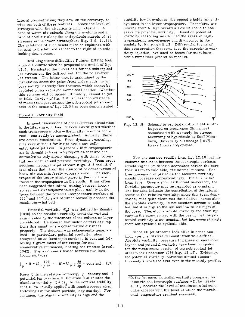
lateral concentration; they act, on the contrary, to wipe out both of these features. Above the level of strongest wind the situation is much clearer. A band of warm air extends along the cyclonic and a band of cold air along the anticyclonic margin of jet streams in the lower stratosphere (fig. 3.9, 12.16). The existence of such bands must be explained with descent to the left and ascent to the right of an axis, looking downstream.

Realizing these difficulties Palmen (1951 b) took a middle course when he proposed the model of fig. 12.5. He adopted the direct cell for the subtropical jet stream and the indirect cell for the polar-front jet stream. The latter then is maintained by the circulation about the polar front underneath the jet core and by unsteady flow features which cannot be depicted on an averaged meridional section. Whether this scheme will be upheld ultimately, cannot as yet be told. In view of fig. 5. 6, at least the existence of mass transport across the subtropical jPt stream axis in the sense of fig. 12.5 has been demonstrated.

Potential Vorticity Field

In most discussions of cross -stream circulation in the literature, it has not been investigated whether such transverse motion - thermally direct or indi­rect - can really be accomplished. Actually, there are severe constraints. From dynamic reasoning, it is very difficult for air to cross any well­established jet axis. In general, high-tropospheric air is thought to have two properties that are con­servative or only slowly changing with time: poten­tial temperature and potential vorticity. From cross sections through the jet stream (figs. 3.3 and 12.4) it is clear that, from the viewpoint of conservation of heat, air can mix freely across a core. The isen­tropes of the lower stratosphere in the north are found in the troposphere in the south. It has often been suggested that lateral mixing between tropo­sphere and stratosphere takes place mainly in the layer between the potential-temperature surfaces of 3300 and 8500 A, part of which normally crosses the maximum-wind belt.

Potential vorticity (I;,p) was defined by Rossby (1940) as the absolute vorticity about the vertical axis divided by the thickness of the column or layer considered. He showed that under certain assump­tions this quantity is a conservative air mass property. The theorem was subsequently general­ized. In particular, potential vorticity, when computed on an isentropic surface, is constant fol­lowing a given mass of air except for non­conservative influences, heating and friction (Ertel, 1942). For a column situated between two isen­tropic surfaces

I;,p = (f+S)e 10e = - (f+l;,) g~ = constant. (13) p oz e 8p

Here I;, is the relative vorticity, p density and e potential temperature. * Equation (13) relates the absolute vorticity (f + 1;,) e to the vertical stability. It is a law usually applied with much success when following air for short periods, say one day. For instance, the absolute vorticity is high and the

stability low in cyclones; the opposite holds for anti­cyclones in the lower troposphere. Therefore, air moving from a High toward a Low will tend to con­serve its potential vorticity. Based on potential vorticity reasoning we deduced the areas of high­tropospheric convergence and divergence in the models 8. 10 through 8. 12. Differential forms of this conservation theorem, i. e. the baroclinic vor­ticity equation, are used as bases for most baro­clinic numerical prediction models.

P 200

mb

300

400

500

1000~N~----------------~~~--~~----------~S

Fig. 12.18 Schematic vertical-motion field super­imposed on isentropes (thin lines) associated with westerly jet stream according to hypothesis by Staff Mem­bers' University of Chicago (1947). Heavy line is tropopause.

Now one can see readily from fig. 12.18 that the isobaric thickness between the isentropic surfaces straddling the jet stream decreases across the core from warm to cold side, the normal picture. For free movement of particles the absolute vorticity should decrease correspondingly. But this is far from true. Over a short latitudinal increment, the Coriolis parameter may be regarded a.s constant. The isotachs indicate the contribution of the lateral shear to the relative vorticity; since this term dom­inates, it is quite clear that the relative, hence also the absolute vorticity, is not constant across an axis but that it is high to the left and low to the right of the core. Thereby, absolute vorticity and stability vary in the same sense, with the result that the po­tential vorticity is not constant but increases strongly from anticyclonic to cyclonic side.

Since all jet streams look alike in cross sec­tion, one quantitative demonstration will suffice. Absolute vorticity, pressure thickness of isentropic layers and potential vorticity have been computed for the mean cross section of the subtropical jet stream for December 1955 (fig. 12.19). Evidently, the potential vorticity increases almost discon­tinuously across the axis even in the monthly profile.

*In the jet core, potential vorticity computed on isobaric and isentropic surfaces will be nearly equal, because the level of maximum wind coin·­cides closely with the level at which the meridi­onal temperature gradient reverses.

-104-

From this it follows that air cannot cross a jet stream axis on a broad front if it conserves its po­tential vorticity. Crossing can occur only in gaps between jet streams or by means of slow seepage produced, for instance, by lateral stresses. One may conceive of the crossing of the mass circulation cell through the subtropical jet stream (fig. 5.6) as produced by such effects, although the validity of this interpretation has not been established.

The jump of potential vorticity across jet stream cores is so striking that Platzman (1949) assumed a discontinuity based on the cross section of Palme'n and Newton (fig. 12.20, cf. fig. 12.4) in a study of waves along the jet stream. From fig. 12.20 one obtains the strong impression that forma­tion and maintenance of jet streams is associated with two regimes of mixing under conservation of potential vorticity, so that ultimately this vorticity becomes constant in each region. This hypothesis is the only one which will permit a quasi-geostrophic jet stream to form and persist, given conservation of potential vorticity as dynamic law. As seen from the thermal wind equation, the potential­temperature field must have the structure of fig. 12. 18 in order for any wind sounding in the core to be approximately geostrophic. All jet stream cross sections indicate that the observed jet structure, conservation of potential vorticity and geostrophic flow are not compatible with free mixing through the cores.

Various investigators have studied the potential­vorticity field (cf. Reed and Danielsen, 1959) and examined the question whether potential vorticity is actually conserved following air trajectories (Newton ct al,1951 and Kleinschmidt, 1951). Although these investigations were affected by limitations of the observations, the authors concluded that important sources of potential vortiCity may exist in the high troposphere, due to the non:"conservative factors.

-10

-20

Fig. 12.19

:: (lO··mb"'lec·')

_~1 . ........L.. _L-..l.- L 0.4 1.2 2.0

Absolute vorticity, pressure thickness and potential vorticity for the layer between the potential-temperature surfaces of 3400 and 3600 A which cross the subtropical jet stream of winter just below and above the level of maximum wind (Krishnamurti, 19 59a). Ordinate gives distance re-1ative to jet axis in degrees latitUde.

-105 -

•••• e ••••••••• ••

North Latitude South

Fig. 12.20 Observed potential-vorticity cross section at level of strongest wind from fig. 12.4 (solid line) (PalmJn and Newton, 1948) and two-layer model·according to Platzmann, 1949 (dotted).

Because of the importance of the subject it will be worthwhile to show a few illustrations from a more recent situation with better rawin coverage.

We shall investigate the jet stream of 26 De­cember 1958 for which the energy transformations were discussed earlier in this section. Fig. 10. 12 depicts the general situation for the LMW .. The cross section of potential vorticity over the whole box of fig. 10. 12 clearly reveals the discontinuity at the jet axis (fig. 12.21). Potential vorticity jumps by an order of magnitude at the jet core which is situated at a potential temperature of 3450 A. On this surface, correspondence with fig. 12.20 is good as the potential vorticity was nearly constant north of the jet axis. Higher up and down, however, there were marked lateral gradients; in particular, a potential-vorticity maximum appeared just north of the jet axis at the top of the diagram.

B(OA)

380

370

360

350

340

330

320

310

789

\?; '---------J

• , 6 _____

0.5- -_ 5 _______

'0.5 4 ----:~ ,------- 0.5 __ 0.5 ------

--"­N 4

_L_ 1- L ___ 1 "---...L __ ----L-..... ._1-__ .1~ 3 2 1 J - 2 -3 -4 S

n I 100's km)

Fig. 12.21 Cross section of potential vorticity (10-2 cgs) for jet stream of 26 De­cember 1958 (fig. 10.12). Ordinate is potential temperature, abscissa distance from jet axis.

We shall follow two trajectories in the layer 360-3700 A of fig. 12.21, i. e. above the level of maximum wind and any tropospheric heat sources. Numerous lower trajectories also could have been chosen. The trajectories and the isotach pattern for the layer are shown in fig. 12.22. One of the trajectories lies north, the other south of the axis. Due to uncertainties of analysis at the axis itself, it was not feasible to include another trajectory in the core of the current. From the data on 26 December and from the 12-hour observations for several periods before and after this maptime, no obvious cross -stream flow could be detected, although the number of upper winds was considerable. This, of course, does not rule out seepage across the axis with a crossing angle of, say, one degree or so; the winds themselves are reported only to the nearest ten degrees. It is evident that reliable determina­tion of mixing across an axis requires special pro­grams of research flights carried out by several well-instrumented jet airplanes.

The transport of mass and momentum in the jet stream increased tremendously from west to east across the area studied. This was true for a very deep layer extending even to the low troposphere. Thus, a large entrainment of mass into the current took place, and this is typical of very many situa­tions where a jet stream intensifies downstream. In the core and higher up the mass was partly drawn in from the sides, partly from below. Lateral en­trainment is indicated in fig. 12. 22 by the fact that the distance between A and A' is about one third more than the distance between Band B I. From the top diagram in fig. 12.23 the pressure along the trajectories decreased, i. e. the height increased so that ascent took place. This occurred in a deep layer both north and south of the axis, with a little more vertical motion on the northern side. As the speed of the air increased downstream, the thickness of the isentropic layer in the north also decreased (center diagram on fig. 12. 23) which provided partly for mass continuity. South of the axis the thickness was constant, except for a slight increase near the east coast.

Fig. 12.22 Isotachs (knots) for the isentropic layer 360-3700 A, 26 December 1958; brack­eted winds extrapolated. Also stream­lines north and south of jet axis across the box in fig. 10.12.

-106 -

:;::~~~ .. .!155 _ ~ ~150 - --------

145 S

,......, 8 .. ~ 7 .. .a 6 E .... 5 u .

4 E u 3

b 2 .::.. ~I

'4../' o

---

-

N

s

A B N W

Fig. 12.2:i Top: Variation of pressure along the two streamlines of fig. 12.22; middle: pressure thickness; bottom: potential vorticity.

The potential vorticity (bottom diagram of fig. 12.23) increased somewhat both in north and south. But the variations are so small that they are fully within the margin of error of the analysis. In the first approximation we can say that the potential vorticity was conserved. It is of interest that the lateral wind shear decreased downstream in the core as the current speed increased, and that the wind profiles are well represented by a bilinear distribu­tion with nearly equal slope, but of opposite sign, on both sides of the axis (fig. 12.24). Quite in agree­ment with the case of 6 March 1958, described in Section IV, the jet stream was sharper at the point where intensification began than at the location of the high-speed center. This is also indicated by the marked broadening of the current. It may be noted that some, though not all, features of the 26 Decem­ber case agree with Rossby's (1951) model of the development of localized jet streams.

The foregoing illustrations bring out clearly the importance of the role occupied by the potential­vorticity field in jet stream structure and formation. It would be quite impossible to generate such a cur­rent in an atmosphere with uniform potential vorti­city along the isentropes. It is necessary for a vorticity gradient to be developed in certain isen­tropic layers by non-conserva.tive influences. Once established, a mechanism may be found for con­centrating this gradient in narrow zones. In the upper troposphere, condensation can at times alter the potential-vorticity field as suggested by Klein­schmidt (1951). But there must be another more

general process, since many jet streams develop without connection with cloudiness - for instance the polar night jet stream, and the jet streams in oceans and model experiments. For the atmosphere it would appear to be worthwhile to study the fields of radiation and heat conduction as possible sources or sinks of potential vorticity.

4

E 2 .:.;

~(J')

g J c

-2

-4~~----~--~~--~-----L-80 100 120 140

V (knots)

Fig. 12.24 Velocity profiles normal to jet axis in the isentropic layer 360-3700 A at western and eastern ends of the box in fig. 12.22.

Model Experiments

It is apparent from the foregoing discussion that the jet stream is a complicated phenomenon which, for the most part, has had to be treated with strongly simplifying assumptions. Often it is very difficult to evaluate the magnitude of the effects which must be neglected. Understanding of atmospheric motion can be greatly advanced if, as in physics,one is en­abled to study the influence of the known variables separately. To some extent "this can be done within the atmosphere. In this section, for instance, we have discussed heat and cold sources in different latitude belts and seasons, jet streams at large and small values of the Coriolis parameter. A more powerful comparison is that between high-velocity cores in atmosphere and ocean (for a detailed com­parison of jet streams and Gulf Streams see Newton, 1959). Similarity of wind and vorticity profiles has been demonstrated in fig. 12.7. Beyond this, the free surface in fig. 1.1 is comparable to, say, the 400-mb surface in the atmosphere because the tem­perature field on the ocean top still has the same gradient as the layer underneath. Hence, it is not necessary to have a level of zero density gradient and a stratosphere to explain the lateral concentra­tion of kinetic energy. Water is nearly incompres­sible within the depth ranges considered in analyses of currents. Density may be treated as a function of temperature alone (in the ocean also of salinity). This permits considerable simplification in dynam­ical treatments without much, if any, loss of validity for application to the atmosphere. Finally,

as seen above, Gulf Stream and jet stream have the same structure in spite of widely-different energy sources.

These analogies, while important, are not fully satisfactory. They do not permit controlled ex­periment, the most powerful tool of science. From the early days of meteorology, therefore, recurrent attempts have been made to recreate atmosphere and ocean in laboratories. Model studies received a strong impetus when Rossby introduced the ratio of ul c e as a means for comparing circulations on bodies with different sizes and rotation rates. Sub­sequently' another characteristic ratio was added (Fultz, 1951), the 'thermal Rossby number' RT = UTI c e where uT is the geostrophic thermal

wind, a function of lateral temperature gradient and rotation rate. A nov'el way to conduct model ex­periments is by way of electronic computers. Phil­lips' (1956) calculation is a prototype of this ap­proach, which undoubtedly will be widely employed in the future.

The following will be concerned with a series of experiments conducted mainly in the hydrodynamics laboratory of the University of Chicago. These ex­periments began in 1946 with studies of the motions and especially of the latitudinal distribution of the zonal wind component, in a thin sheet of fluid en­cased between two concentric glass shells (Fultz, 1949). The shells were rotated and an equatorial heat source was applied. This experimental setup does not fully portray atmospheric conditions, apart from the phYSical differences between water and air. There were two boundary surfaces which retarded the flow frictionally. Moreover, it is practically impossible to have the correct orientation of all forces in the experiment. Gravity, in particular, acts perpendicular to the horizontal motions in the atmosphere, while in the experiment it acts in the same direction everywhere. Nevertheless, remarkably realistic profiles of the zonal.-wind com­ponent with latitude were obtained for the concentric shells at high rotation rates (ca. 16 rpm). These may be compared with the distribution of the 500-mb westerlies (fig. 12.25) determined from fig. 9.3 by dividing the latitudinal velocity distribution in Janu­ary and July with the earth's equatorial velocity (460 mps or about 1000 mph).

Subsequently it was discovered that remarkably close analogies to atmospheric general circulations could be obtained in much simpler apparatus - open dishpans or basins - which differ from the atmos­phere even more than rotating shells because the Cariolis parameter is a constant. The first dish­pans were bought in the hardware store, later more fanciful versions were developed. A wide range of experiments has been undertaken with dishpans. Important null experiments were run with rotation without heating, and heating without rotation. Re­sults were as one should expect them. Rotation without heating led to solid rotation, heating without rotation to the well known circulation found in a smoke -filled room with a hot :r:adiator.

It follows, that combinations of heating and ro­tation rates are necessary to produce general cir­culations of the atmospheric type.

-107 -

70

60

50

z . .. 40 .., ~

"0 30 ....J

20

10

-.05 0.00 +0.05

u/e. ( 500mb)

-.05

I ~

/, /' ,

I I

I 1

",I ... , i,'

I 0: <v. I I

0.00 +0.05

Fig. 12.25 Left: Zonal wind profiles for summer and winter at 500-mb from fig. 9.3, expressed non-dimensionally; right: zonal motion in rotating hemispherical fluid sheet for different rates of heat­ing (Fultz, 1949).

Wide ranges of such combinations have been ef­fected in pans of varying radius and depth; some­times only with heat sources, sometimes with equatorial heat and central cold sources in form of cylinders, sometimes with flush polar cold sources at the bottom. Obstacles resembling mountain ranges and plateaus such as the Himalayas have been introduced with successful results (Long, 1952). It would lead entirely too far within this text to sum­marize the whole range of experiments and their bearing on the understanding of jet streams. Only one of the outstanding discoveries will be discussed. The type of general circulation produced depends in­timately on heating and rotation rates chosen, especially the latter. When certain critical thres­holds are crossed, a general circulation type will break down and go over into another type (Fultz et al, 1956).

The principal determinant is again the ratio , u/ce which, for atmospheric jets, has a character­istic value of 10-1 . At low rates of pan rotation, hi~h-energy flow can be obtained with magnitude of 10 (i. e., one) for u/ce . This type of flow con­tains a steady and symmetrical jet stream. At Rossby numbers of 2-5 x 10-1 symmetrical circu­lations cannot be maintained, presumably for the reason discussed earlier, namely that too strong a

! field of zonal motion is demanded from momentum considerations. Wave trains along a jet take the place of axially-symmetric flow; the waves usually propagate counterclockwise, i. e. with the wester­lies. Steady state can be attained for given com­binations of heating and rotation rates, but the number of waves can be manipulated. When the pan

rotation is increased, sudden formation of new waves can be produced. Increased heating will tend to produce stronger t~mperature gradients, hence acts to decrease the wave number. Finally, at u/ce of 10-1 , which corresponds to atmospheric jet streams, even steady wave trains are difficult to realize. Wave patterns and jet streams that change intensity and amplitude with time make their ap­pearance. Life cycles of these systems can be generated which often bear startling resemblance to those known to the weather forecaster.

Examples of these three classes of general cir­culations with jet streams will be shown briefly.

Symmetrical Flow: Created at rates of pan revolu­tion as low as 1/2 to'l rpm, the jet stream in symmetrical experiments is very powerful. The circulation shown in fig. 12.26 was produced in a pan with radius of 20 cm, water depth of 6 cm, rim equatorial heat source of 100 watts and central cylindrical cold source with radius of 5 cm. 1so­lines up to 1. 2 have been drawn, at the jet center 1. 4 was measured. This corresponds to about 1400 mph on earth; hence the regime clearly does not correspond to atmospheric middle latitudes. It is thought to resemble most closely the tropic!:! where the Coriolis parameter is small, and often has been called a trade-wind cell. Even this analogy, how­ever, is poor, because the atmospheric currents of the tropics are quite unsteady except near the surface and nowhere attain the magnitude of the velocities in fig. 12.26.

:tzj)' 'M

-t// ~~ .• " .. ~~)

,}3 - (j.l 01:, - --"/6 ---- ---d,

01 T

Fig. 12.26 Zonal wind speed (expressed as frac­tion of the equatorial speed of the pan) in symmetrical dishpan experiment. Height (z) and radius (r) expressed in fraction of total height and radius of the dishpan.

The flow in this experiment is highly ageo- 2 strophic because the centrifugal acceleration ve /r

greatly exceeds the Coriolis acceleration fVe in the

jet stream. Here ve is the tangential component

of motion in a cylindrical-coordinate system fixed at the center of the pan and rotating with the pan, r is the radius from the center and f the Coriolis pa-

-108-

rameter. The meridional component of motion, a purely ageostrophic component because of the axial symmetry, is very small in contrast. All ascent and descent takes place very close to the boundaries per­mitting the water to pass sufficiently close to the walls for the required heat exchange by conduction through the walls. A direct transverse cell, as in fig. 12. 10, is in operation. This cell carries all heat transport. Moving from high to low pressure everywhere (westerlies at the top and easterlies at the bottom) it produces kinetic energy over the en­tire cell. As cold water sinks and warm water rises, potential energy is released. The slope of the isotherms is held steady by the action of the heat and cold sources which counteracts the tendency of the transverse circulation to move the cold under­neath the warm water. DiSsipation of kinetic energy by friction holds the total kinetic energy steady. Vaisanen (1959) has shown that excellent agreement is obtained when all energy sources and sinks are individually determined.

In spite of the strength of the jet stream, it attains only one -third of the' s peed that would be ex­pected from conservation of momentum. Since there are no pressure gradients with longitude, only re­tardation through frictional stresses can account for the failure of the actual strength of the winds to

300

200

150

100

Fig. 12.27

0.5 1.0

u'= JL Ce

Variation of jet velocity with heating rate at top surface in symmetrical dish­pan experiments for two angular­rotation rates of the dishpan. Radius of jet core indicated in fractions of the radius of the pan. Cold-source wall at r' = 0.25.

-109-

attain that demanded from the momentum principle. Because of the high relative speeds it is entirely plausible, in line with Vaisanen's computations, that frictional stresses playa much larger role relative to the other forces than in experiments with lower Rossby numbers.

For further insight into symmetrical jet streams, a series of experiments has been carried out in which the strength of the heat source was varied for given rotation rates. Increases of jet stream strength with heat source were observed (fig. 12. 27). The regression lines, best plotted on semi-log pa­per, show however, that the increase of wind and kinetic energy was not proportional to the increase in heat source. Nevertheless, the fact that a posi­tive correlation exists, is interesting in itself and merits further exploration, also in the atmosphere.

_ 4

Fig. 12.28 Velocity (in percent of the equatorial pan velocity) at top surface in steady three-wave dishpan case (Riehl and Fultz, 1957). Heavy solid line marks jet axis, dashed line with arrows tra­jectory crossing over axis.

Steady Wave Trains: At pan, rotation rates of 3-4 rpm with heat source on the order of 100 watts and central cylindrical cold sou~ce, wave trains with wave number from 2 to 6 and even more replace the symmetrical cell. These wave trains usually propagate eastward with the basic westerlies; they are 'steady' in that wave length, amplitude and rate of progression do not change once the pattern is set up as long as experimental conditions are not var­ied. Fig. 12. 28 portrays the surface isotach pattern for a three-wave experiment (Riehl and Fultz, 1957); because all three waves look alike, drawings have been made for only one of these waves. The isotachs resemble those of the jet stream to a surprising extent- even the anticyclonic shear is less than the cyclonic shear, as in the atmospheric cases. The speed is almost uniform along the axis. With u/ce = 0.2 the mean jet velocity is only a little above that for the subtropical jet stream of winter. Except for the eastward propagation of the dishpan waves, this three-wave case and the subtropical jet stream. provide a striking series of analogies which­ever aspects of structure or maintenance of the currents one wishes to touch upon.

COLDS MUTS

Fig. 12.29 Vertical cross section of wind speed (percent of equatorial pan speed) and temperature (departure from 16 0 G) for jet stream in steady three-wave experiment at trough line.

In vertical cross section (fig. 12.29) the dishpan cy.rrent resembles jet streams on the earth. The isotherms slope as they do in fig. 1.1 in the Gulf Stream. A little above tl'le bottom, isotherms and contours of isobaric surfaces are observed which reflect the atmospheric sea level map. A cyclonic center (fig. 12. 30) is situated under the south­western inflection point of the high-level jet, and an anticyclonic center under the northwestern inflection pOint. The warmest water is associated with the Low and the coldest water with the High (fig. 12.31). Vertical motions are arranged just as they are in the atmosphere with re~pect to typical cyclones and anti­cyclones (fig. 12.32). The level of non-divergence lies in the middle of the fluid which corresponds to 600-500 mb for the troposphere, and the rate of vertical displacement corresponds to that of the at­mosphere when it is taken into account that the ratio of vertical to horizontal extent of the fluid is 1: 4 in the dishpan and 1:100 in the atmosphere.

, , \,. ri lem I \

I \ I

: \ H : \ \ I

I \ ' I \ :

",. " : .......... --~...:. .... ---

/-~V , ,- I

" I' , LI I • , I , , . , I , 'I , 'I I '( I , .... -~ ,

Fig. 12.30 Stream function of the geostrophic wind at 1 cm height in steady three-wave ex­periment. Double-dashed line shows the position of the high-level jet.

Such close resemblance must be considered as indicative of a general model of atmospheric struc­ture which will develop in quasi-geostrophic flow with differential heating. Further analysis (Riehl and Fultz, 1958) has shown that a simple heat-engine type of cfrcu1ation and energy cycle is found in the three-wave case when all averaging with longitude is

-110-

performed following the jet axis as described in Section V. It was, in fact, this experiment which suggested application of 'jet coordinates' to the sub­tropical jet stream. In the dishpan case, all heat and momentum transport from equatorial to polar latitudes takes place by means of the ageostrophic motion at the jet axis which is one of the most re­markable features of the axis. Production of kinetic and release of potential energy are also accom­plished by this circulation.

Fig. 12.31 Temperature at 1 cm depth in steady three-wave experiment (departure from 160 C).

One of the most interesting calculations per­formed was a computation of the velocity profile equatorward of the jet axis with the constant­vorticity-transport hypothesis, mentioned at the beginning of this section. This computation was made in the coordinate system following the jet axis for both the dishpan experiment and the subtropical jet stream. Let the s -axis be oriented along the jet stream and the n-axis normal to it. If cn .d.e­notes the velocity component along n, the condlhon for constant vorticity transfer is

s x CT" = constant n a

(14)

along the n-axis. The bar indicates averaging around the dishpan or globe following the jet stream, and the length s appears because it decreases from

Fig. 12.32 Vertical motion (per mille of equatorial pan speed) in steady three-wave experi­ment. Double-dashed line marks jet axis. U is up and D down.

heat source to cold source. Only the mean mass circulation cn and the mean absolute vorticity ra were used for the calculation. Results are given in fig. 12.33; an excellent approximation to the observed velocity profiles is obtained both for dishpan and at­mosphere. It follows, that the constant-vorticity­transfer hypothesis is capable of explaining the velocity distribution equatorward of jet axes from the dynamic viewpoint.

Unsteady Waves with Cycle: When the pan rotation rate is increased to about 10 rpm - other conditions remaining about equal- even the steady waves cannot be maintained. They are replaced by waves whose shape changes with time. A repeating cycle can be developed with period of about 14 revolutions (or 14 days is the atmosphere); this corresponds to the 'index cycle' of the atmosphere. In a series of

open waves the amplitude gradually increases until finally the wave pattern breaks down into vortices­cold Lows and warm Highs. After this CUlmination, the waves are gradually re-established. The time variation of the zonal flow averaged around the pan (fig. 12. 34) is similar to that of fig. 7. 13, except that in the dishpan a regular progression of high zonal speeds from low to high latitudes, or vice versa, has not been obtained. Variations in zonal speed are produced by variable location of high­speed centers along the jet axis. In fig. 12.35- re­presentative of open waves- velocities are concen­trated in the southwest flow and in the ridges. In fig. 12.36- typical of the vortex stage- highest speeds are encountered south of the cold-core

([U])

4

3

2

r' 0.4

0.5

0.6

0.7

Mx I

I 2

Mi I

Mx I

.10

-.05

-.10

-.15

4 8 12 16 20 24 28 cs/ce (10-2 )

Fig. 12.33 Observed velocity profiles (fraction of equatorial pan speed and equatorial velocity of the earth) for three-wave dishpan experiment and subtropical jet stream of winter (solid) and profiles computed with constant-vorticity­transfer hypothesis (dashed).

cyclones; there is even a suggestion of splits in the current east of these Lows. These sequences are quite realistic and lead one to hope that further pur­suit of the model approach, coupled with parallel atmospheric studies, will lead to eventual solution of the jet stream problem.

Mi I

Mx I

1.8

0.8

0.9

3 '''~: _3_.5_3 __ 3._83 ___ 3._85 __ 3_.8_4 ___ - ,M 2 ~ '" I

1.0 3 5 7 9 " 13 15 17 19 21 23 25 27 29

Photo #

Fig. 12.34 Time cross section of mean zonal velocity (percent of equatorial velocity) for unsteady dishpan regime. Ordinate gives radius (fraction of pan radius), abscissa time expressed as number of revolutions, or 'days'. Top: Time variation of zonal speed averaged from he.at source to cold source. Courtesy of Dr. Dave Fultz.

-111-

Fig. 12.35 Photograph of surface velocity field and isotachs during wave stage of unsteady experiment. Courtesy of Dr. Dave Fultz.

-112 -

Fig. 12.36 Photograph of surface velocity field and isotachs during vortex stage of unsteady experiment. Courtesy of Dr . Dave Fultz.

BIBLIOGRAPHY

Alaka, M. A., 1958: A case study of an easterly jet stream in the tropics. Tellus, 10, 24-43.

Angell, J. K., 1958: Transosonde flights for September, October and November 1957. Washington, D. C., U. S. Weather Bureau.

Arakawa, H., 1953: Clear air turbulence near the jet stream. Quart. J. Roy. Meteor. Soc., 79, 162-163.

------, 1956: Characteristics of the low-level jet stream. J. Meteor., 13, 504-506.

Arnold, A., 1954: Turbulence in the stratosphere. Bull. Amer. Meteor. Soc., 35, 377-378.

Bannon, J. K., 1952: Weather systems associated with some occasions of severe turbulence at high altitudes. Meteor. Mag., 81, 97-10l.

Barrett, E., 1958: Some applications of harmonic analysis to the study of the general circulation. Dept. of Meteor., Univ. of Chicago. Ph. D. Thesis, 209 pp.

Bellamy, J. C., 1945: The use of pressure altitude and altimeter corrections in meteorology. J. Meteor., 2, 1-79.

Bessemoulin, J. and R. Pone, 1949: Determination des routes aeriennes a dur~e minimum. Journal Scien­tifique de la Meteorologie, Oct-Dec.

Bjerknes, V. and H. Solberg, 1929: Zellulare Traegheitswellen und Turbulenz. Vidensabsak, Avhand, Oslo, 50, No.7.

------, et aI, 1933: Physikalische Hydrodynamik. Berlin, Julius Springer, 797 pp.

Bradbury, D. and E. Palm en, 1953: On the existence of a polar front zone at the 500-mb level. Bull. Amer. Meteor. Soc., ,34, 56-63.

Bryson, R., et aI, 1957: Normal 500-mb charts for the northern hemisphere. Norfolk, Virginia, U. S. Navy Weather Research Facility, 29 pp.

Charney, J. G. and A. Eliassen, 1949: A numerical method for predicting the perturbations of the middle latitude westerlies. Tellus, 1, 38 -55.

Clodman, J., 1957: Anisotropic high-level turbulence. Quart. J. Roy. Meteor. Soc., 83, 116-120.

Court, Arnold, 1945: Weather observations during 1940-41 at Little America III. Proc. Amer. PhiIp. Soc., 89, 324-343. .

Cressman, G. P., 1950: Variations in the structure of the upper westerlies. J. Meteor., 7, 39-47.

Dickson, R. R., 1955: Aids to jet stream forecasting. Office of the Chief of Naval Operations, NAVAER 50-1 P-533, 53 pp.

Elliott, R. D., 1955: Handbook of single station analysis and forecasting techniques. Washington, D. C., U. S. Navy Bureau of Aeronautics, 192 pp.

Elsaesser, H. W., 1957: Errors in upper-level wind forecasts. Bull. Amer. Meteor. Soc., 3'8, 511-517.

Endlich, R. M. and G. S. McLean, 1957: The structure of the jet stream core. J. Meteor., 14, 543-552.

------, S. B. Solot and H. A. Thur, 1955: The mean vertical structure of the jet stream. Tellus, 7, 308-313.

Ertel, H., 1942: Ein neuer hydrodynamischer Wirbelsatz. Meteor. Zeit., 59, 277-281.

Fletcher, R. D., 1953: The association of wind speed with height of upper-air constant-pressure surfaces. Bull. Amer. Meteor. Soc., 34, 155-159.

Frank, P., 1933: Die schnellste Flugverbindung zwischen zwei Punkten. Z. Angew. Math. Mech., Berlin, 13.

French, J. E. and K. R. Johannessen, 1953: Forecasting high clouds from high-level constant-pressure charts. Proc. Toronto Meteor. Conf. London, Royal Met. Soc., 160-172.

Fultz, D., 1949: A preliminary report on experiments with thermally produced lateral mixing in a rotating hemispherical shell of liquid. J. Meteor., 6, 17-33.

------, 1951: Non-dimensional equations and modeling criteria for the atmosphere. J. Meteor., 8, 262-267.

-113-

Fultz, D., et aI, 1956: Studies in experimental hydrodynamics applied to large-scale meteorological phenom­ena. I. Dept. of Meteor., Univ. of Chicago. Multigraphed.

Gilchrist, B. and G. P. Cressman, 1954: An experiment in objective analysis. Tellus, 6, 309-318.

Godson, W. L. and R. Lee, 1958: High-level fields of wind and temperature over the Canadian Arctic. Beitr. Phys. fro Atm., 31, 40-68.

Hare, F. K., 1959: The disturbed circulation of the Arctic stratosphere. Paper presented at meeting of American Meteorological Society in Chicago, Illinois, March 1959. Abstract in Bull. Amer. Meteor. Soc., 42, p. 92.

Hess, S. L., 1948: Some new meridional cross sections through the atmosphere. J. Meteor., 5, 293-:300.

Hovmoeller, E., 1952: A comparison between observed and computed winds. Tellus, 4, 126-134.

Hutchings, J. W., 1950: A meridional atmospheric cross section for an oceanic region .. r. Meteor., 7, 94-100.

Iselin, C. O'D., 1936: A study of the circulation of the western North Atlantic. Papers in Phys. Ocean. and Meteor., MIT and Woods Hole Ocean. Inst., 4, No.4.

Jacobs, W. C., 1947: Wartime developments in applied climatology. Boston, Meteor. Monogr. 1, No. 1.

James, R. W., 1951: A February cross section along the Greenwich meridian. Meteor. Mag., 80, 341-346.

Jenista, C. 0., Jr., 1953: A statistical study of precipitation distribution as related to various types of mean zonal motion. Bull. Amer. Meteor. Soc., 34, 10-13.

Johannessen, K. R., 1956: Three-dimensional analysis of the jet stream through shear charts. In Pro­ceedings of the Workshop on Stratospheric Analysis and Forecasting, 1-3 February 1956. Wash­ington, D. C., U. S. Weather Bureau, 168 pp.

Johnson, D. H. and S. Daniels, 1954: Rainfall in relation to jet streams. Quart. J. Roy. Meteor. Soc., 80, 212,217.

Kleinschmidt, E., 1951: Ueber Aufbau und Enstehung von Zyklonen. III. Meteor. Rundschau, 4, 89-96.

Kochanski, A., 1955: Cross sections of the mean zonal flow and temperature along 800 W. J. Meteor., 12, 95-106.

Koteswaram, P., 1953: An analysis of the high tropospheric wind circulation over India in winter. Indian J. Meteor. Geoph.,4, 13-21.

------, 1958: The easterly jet stream in the tropics. Tellus, 10, 43-58.

------, C. R. V. Raman, and S. Parthasaraty, 1953: The mean jet stream over India and Burma in winter. Indian J. Meteor. Geoph., 4, No.2.

Krishnamurti, T. N., 1959a: The subtropical jet stream of winter. Dept. of Meteor., Univ. of Chicago. Multigraphed.

------, 1959b: A vertical cross section through the "polar-night" jet stream. Dept. of Meteor., Univ. of Chicago. Multigraphed.

LaSeur, N. E., 1954: On the asymmetry of the middle-latitude circumpolar current. J. Meteor., 11, 43-57.

Lee, R. and W. L. Godson, 1957: The Arctic stratospheric jet stream during the winter of 1955-56. .r. Meteor., 14, 126-135.

Lettau, H., 1955: Turbulence in the stratosphere. Bull. Amer. Meteor. Soc., 36, 178-179.

Levi-Civita, T., 1931: Ueber Zermelo's Luftfahrt Problem. Z. Angew. Math. Mech., Berlin, 11.

Long, R. R., 1952: The flow of a liquid past a barrier in a rotating spherical shell. J. Meteor., 9, 187-199.

Malkus, J. S. and C. Ronne, 1954: On the structure of some cumulonimbus clouds which penetrated the high tropical troposphere. Tellus, 6, 351-366.

McLean, G. S., 1957: Cloud distributions in the vicinity of jet streams. Bull. Amer. Meteor. Soc., 38, 579-584.

Mintz, Y., 1951: The geostrophic poleward flux of angular momentum in the month of January 1949. Tellus, 3, 195-201.

Mohri, K., 1953: On the fields of wind and temperature over Japan and adjacent waters during the winter of 1950-1951. Tellus, 5, 340-358.

-114-

Murray, R. and S. M. Daniels, 1953: Transverse flow at entrance and exit to jet streams. Quart. J. Roy. Meteor. Soc., 79, 236-241.

Namias, J. and P. F. Clapp, 1949: Confluence theory of the high-tropospheric jet stream. J. Meteor., 6, 330-336.

------, and P. F. Clapp, 1951: Observational studies of general circulation patterns. In Compendium of Meteorology, T. F. Malone,ed. Boston, Amer. Meteor. Soc., 551-567.

Newton, C. W., 1954: Frontogenesis and frontolysis as a three -dimensional process. J. Meteor., 11, 449-461.

------, 1959: Synoptic comparisons of jet stream and gulf stream systems. Rossby Memorial Volume.

------, R. Berggren and W. J. Gibbs, 1958: Observational characteristics of the jet stream. Geneva, World Meteor. Org., Technical Note No. 19, 102 pp.

------, and J. E. Carson, 1953: Structure of wind field and variations of vorticity in a summer situa­tion. Tellus, 5, 321-339.

------, et aI, 1951: Structure of shear lines near the tropopause in summer. Tellus, 3, 154-171.

Palmen, E., 1934: Ueber die Temperaturverteilung in der Stratosphaere und ihren Einfluss auf die Dynamik des Wetters. Meteor. Zeit., 51, 17-23.

------, 1948: Oh the distribution of temperature and wind in the upper westerlies. J. Meteor., 5, 20-27.

------, 1951a: The aerology of extratropical disturbances. In Compendium of Meteorology, T. F. Malone, ed. Boston, Amer. Meteor. Soc., 599-620.

------, 1951b: The role of atmospheric disturbances in the general circulation. Quart. J. Roy. Meteor. Soc., 77, 337-354.

------, 1951c: Vertical circulation and release of kinetic energy during the development of hurricane Hazel into an extratropical storm. Tellus, 10, 1-23.

------, and C. W. Newton, 1948: A study of the mean wind and temperature distribution in the vicinity of the polar front in winter. J. Meteor., 5, 220-226.

------, and C. W. Newton, 1951: On the three -dimensional motions in an outbreak of polar air. J. Meteor., 8, 25-39.

------, H. Riehl and L. A. Vuorela, 1958: On the meridional circulation and release of kinetic energy in the tropics. J. Meteor., 15, 271-277.

Pan American World Airways, 1953: Characteristic properties of the jet stream over the Pacific. Case 1. Tech. Rept. No.1 of the Meteor. Dept., Pacific-Alaska Div., South San Francisco, California.

Panofsky, H. A., 1958: An introduction to atmospheric turbulence. NAVAER 50-1P-546, U. S. Navy Weather Research Facility, Norfolk, Virginia, 78 pp.

Petterssen, S., 1950: Some aspects of the general circulation of the atmosphere. Cent. Proc. Roy. Meteor. Soc., 120-155.

------, 1956: Weather analysis and forecasting. New York, McGraw-Hill Book Co., I, 428 pp.

Phillips, N. A., 1956: The general circulation of the atmosphere: A numerical experiment. Quart. J. Roy. Meteor. Soc., 82, 123-164.

Platzman, G. W., 1949: The motion of barotropic disturbances in the upper troposphere. Tellus, 1, 53-64.

Radok, Uwe and A. M. Grant, 1957: Variations in the high tropospheric mean flow over Australia and New Zealand. J. Meteor., 14, 141-149.

Ramage, C. S., 1952: Relationship of general circulation to normal weather over southern Asia and the western Pacific during the cool season. J. Meteor., 9, 403 -408.

Reed, Richard, J. and E. F. Danielsen, 1959: Fronts in the vicinity of the tropopause. Archiv. Meteor. Geoph. Biokl. A, 11, 1-17.

Reiter, E., 1958: The layer of maximum wind. J. Meteor., 15, 27-43.

------, 1960: Turbulenz im wolkenfreien Raum (clear-air turbulence). Berichte d. Deutschen Wetter­dienstes, 61.

------, 1961: Die vertikale Struktur des Strahlstromkernes aus Forschungsfluegen des Project Jet Stream. Berichte d. Deutschen Wetterdienstes, 80.

-115-

Rex, D., 1950: Blocking action in the middle troposphere and its effect upon regional climate. Part I, An aerological study of blocking action. Tellus, 2, 196-212. Part II, The climatology of blocking action. Tellus, 2, 275-302.

------, 1951: The effect of Atlantic blocking action upon European climate. Tellus, 3, 100-113.

Riehl, H., 1948: Jet stream in the upper troposphere and cyclone formation. Trans. Amer. Geophys. Union, 29, 175-186.

------, et aI, 1952: Forecasting in middle latitudes. Boston, Meteor. Monogr. 5, 80 pp.

------, 1954a: Jet stream flight, 23 March 1953. Archiv. Meteor. Geoph., Biokl. A., 7, 56-66.

------, 1954b: Tropical meteorology. New York, McGraw-Hill Book Co., Inc., 392 pp.

------, 1956: Exploration of the jet stream by aircraft during the 1952-1953 winter (correspondence). J. Meteor., 13, 313-314.

------, 1959: One the production of kinetic energy from condensation ·heating. Rossby Memorial Volume.

------, F. A. Berry and H. Maynard, 1955: Exploration of the jet stream by aircraft during the 1952-1953 winter. J. Meteor., 12, 26-35.

------, and D. Fultz, 1957: Jet stream and long waves in a steady rotating dishpan experiment: struc­ture of the circulation. Quart. J. Roy. Meteor. Soc., 83, 215-231.

------, and D. Fultz, 1958: The general circulation in a steady rotating dishpan experiment. Quart. J. Roy. Meteor. Soc., 84, 389-417.

------, and J. Mihaljan, 1959: Analysis of the layer of maximum wind with high-speed computers. Dept. of Meteor., Univ. of Chicago. Multigraphed.

------, and S. Teweles, 1953: A further study of the relations between the jet stream and cyclone formation. -r:ellus, 5, 66-79.

Rossby, C. -G., 1936: Dynamics of steady ocean current in the light of experimental fluid mechanisms. Papers in Phys. Ocean. and Meteor. MIT and Woods Hole Ocean. Inst., 5, No.1.

------, 1940: Planetary flow patterns in the atmosphere. Quart. J. Roy. Meteor. Soc., 66. Sup­plement.

------, 1947: On the distribution of angular velocity in gaseous envelopes under the influence of large­scale horizontal mixing processes. Bull. Amer. Meteor. Soc., 28, 53-68.

------, 1951: Ueber die Vertikalverteilung von Windgeschwindigkeit und Schwerestabilitaet in Frei­strahlbewegungen der oberen Troposphaere. Archiv. Meteor. Geoph. Biokl. A3, 3-23.

Saucier, W. J., et aI, 1958: Wind field near the tropopause. College Station, Texas, The A&M College of Texas, 140 pp.

Schaefer, V. J., 1953: Cloud forms of the jet stream. Tellus, 5, 27 -31.

------, andW. E. Hubert, 1955: A case study of jet stream clouds. Tellus, 7, 301-:~07.

Staff Members, Academia Sinica, Peking, 1957: On the general circulation over eastern Asia (1), Tellus, 9, 432-447.

Staff Members, Dept. of Meteor., Univ. of Chicago, 1947: On the general circulation of the atmosphere in middle latitudes. Bull. Amer. Meteor. Soc., 28, 255-280.

Starrett, L. G., 1949: The relation of precipitation patterns in North America to certain types of jet streams at the 300-mb level. J. Meteor., 6, 347-352.

Stroud, W. G., 1959: Winds and temperatures up to 90 km from rocket firings at Fort Churchill. Paper presented at meeting of American Meteorological Society in Chicago, Illinois, March 1959. Ab­stract in Bull. Amer .. Meteor. Soc., 42, p. 96.

Sutcliffe, R. C. and J. K. Bannon, 1954: Seasonal changes in upper-air conditions in the Mediterranean­Middle East area. Scien. Proc., Int. Assoc. Meteor. (UGGI) Rome, 322-334.

Taylor, G. 1., 1924: Experiments with rotating fluids, Proc. 1st Intern. Congr. Appl. Mech., 89-96.

Teweles, E., 1958: Anomalous warming of the stratosphere over North America in early 1957. Mo. Wea. Rev., 86, 377-396.

-116 -

U. S. Air Force, 1956: The black sheep system of forecasting winds for long range jet aircraft. AWS Tech. Rept. 105-139, Washington, D. C., Hq. Air Weather Service, 48 pp.

U. S. Navy, 1945: Altimetry flight. Report of Project 5-5. Washington, D. C., Chief of Naval Operations, Aviation Training Division.

------, 1954: Description of contour patterns at 500 mb. Project AROWA, Norfolk, Virginia.

-----, 1959: Jet stream probing 1956-1958. NWRF 15-0159-017, U. S. Navy Weather Research Facility, Norfolk, Virginia, 39 pp.

Vaisanen, A., 1959: The general circulation in a symmetrical dishpan experiment. Dept. of Meteor., Univ. of Chicago. Multigraphed.

Von Arx, W. S., 1952: Notes on the surface velocity profile and horizontal shear across the width of the Gulf Stream. Tellus, 4, 211-215.

Vuorela, L. A., 1957: A study of vertical velocity distribution in some jet stream cases over western Europe. Geophysica, Helsinki, 6, No.2.

Wege, Klaus, 1957: Druck, Temperatur und Stroemungsverhaeltnisse in der Stratosphaere ueber der Nord­halbkugel (1949-53). Inst. Meteor. Geoph. d. fro Univ. Berlin, Meteor. Abh. 5, No.4.

Wexler, H. and W. B. Moreland, 1958: Winds and temperatures in the Arctic stratosphere. Polar Atm. Symp., July 1956, Pt. I, Meteor. Section, Pergamon Press, pp. 71-84.

------, 1959: Seasonal and other temperature changes in the Antarctic atmosphere. Quart. J. Roy. Meteor. Soc., 85, 196-208.

Wider, W. K. Jr., 1960: Examples of project TIROS data and their practical meteorological use. GRD Research Notes No. 38. Geophysics Research Directorate, U. S. Air Force, Bedford, Massa­chusetts.

Willett, H. C., 1944: Descriptive Meteorology, New York, Academic Press, 305 pp.

World Meteorological Organization, 1958: Observational characteristics of the jet stream. WMO Tech. Note No. 19 (WMO-No. 71. TP. 27), Geneva, Switzerland.

Yeah, T. C., 1950: The circulation of the high troposphere over China in the winter of 1945-46. Tellus, 2, 173-183.

-117-