Embed Size (px)
Citation preview

ISSN 0973-3302
Volume 40 Number 1 January 2013
A Quarterly Publication of the JASI
http://www.acousticsindia.org
OCIS E TL YA OCI FT S INU DO IAC A
AA A ~Ae ekr xk/ tk s h ku re
JOURNAL OF
ACOUSTI CAL SOCIETY
OF INDIA
Journal of AcousticalSociety of India
The Refereed Journal of the Acoustical Society of India (JASI)JASI
CHIEF EDITOR:Mahavir SinghAcoustics, Ultrasonics & Vibration SectionCSIR-National Physical LaboratoryDr. KS Krishnan RoadNew Delhi 110 012Tel: +91.11.4560.8317Fax: +91.11.4560.9310E-mail: [email protected]
ASSOCIATE SCIENTIFIC EDITOR:Applied Acoustics
Trinath KarControl Component India Pvt. Ltd6th Floor, Warp TowerPlot # 13, 14, &15SJR i-Park, EPIP Zone, Phase 1Whitefield Road, Bangalore 560066
The Journal of Acoustical Society of India is a refereed journal of the Acoustical Society of India (ASI). The ASI is anon-profit national society founded in 31st July, 1971. The primary objective of the society is to advance the science ofacoustics by creating an organization that is responsive to the needs of scientists and engineers concerned with acousticsproblems all around the world.
Manuscripts of articles, technical notes and letter to the editor should be submitted to the Chief Editor. Copies ofarticles on specific topics listed above should also be submitted to the respective Associate Scientific Editor. Manuscriptsare refereed by at least two referees and are reviewed by Publication Committee (all editors) before acceptance. Onacceptance, revised articles with the text and figures scanned as separate files on a diskette should be submitted to theEditor by express mail. Manuscripts of articles must be prepared in strict accordance with the author instructions.
All information concerning subscription, new books, journals, conferences, etc. should be submitted to Chief Editor:
Acoustics, Ultrasonics & Vibration Section, CSIR-National Physical Laboratory, Dr. KS Krishnan Road, New Delhi 110 012, Tel: +91.11.4560.8317, Fax: +91.11.4560.9310, e-mail: [email protected]
Annual subscription price including mail postage is Rs. 2000/= for institutions, companies and libraries and Rs. 2000/=for individuals who are not ASI members. The Journal of Acoustical Society of India will be sent to ASI members freeof any extra charge. Requests for specimen copies and claims for missing issues as well as address changes should besent to the Editorial Office:
Acoustics, Ultrasonics & Vibration Section, CSIR-National Physical Laboratory, Dr. KS Krishnan Road, New Delhi 110 012, Tel: +91.11.4560.8317, Fax: +91.11.4560.9310, e-mail: [email protected]
The journal and all articles and illustrations published herein are protected by copyright. No part of this journal may betranslated, reproduced, stored in a retrieval system, or transmitted, in any form or by any means, electronic, mechanical,photocopying, microfilming, recording or otherwise, without written permission of the publisher.
Copyright © 2007, Acoustical Society of IndiaISSN 0973-330
Editorial Office:
MANAGING EDITOROmkar Sharma
ASSISTANT EDITORSYudhisther KumarAnil Kumar NainNaveen Garg
Acoustics, Ultrasonics & Vibration SectionCSIR-National Physical LaboratoryDr. KS Krishnan RoadNew Delhi 110 012Tel: +91.11. 4560.8317asFax: +91.11.4560.9310E-mail: [email protected]
Printed at Alpha Printers, BG-2/38C, Paschim Vihar, New Delhi-110063 Tel.: 9811848335. JASI is sent to ASI membersfree of charge.
Continuous Wave Doppler SODAR for Mid-range Wind Velocity Profiling
3Journal of Acoustical Society of India
ABSTRACT
The SODAR can be a good candidate for the measurement technology of the wind velocity profilingfor the wind turbine electric generator, which make measurement possible without expensive towerconstruction work for wind velocity meters set-up. The Doppler SODAR using continuous wave isproposed and verified by the experiment. Transducers, a transmitter and a receiver both with sharpdirectivity are used. The wind velocity at the region where the two directivities are crossed can bedetected. The profiling or mapping of the objective area can be made by changing the direction of thetwo directivities. A prototype apparatus is developed for the sound of higher frequency range to scalethe system size down for the experimental easiness. The experimental result shows that the windvelocity of the range over 1 m/sec can be measured with the accuracy of few percents even underinterfering conditions. Velocity mapping including the wind's directions can be obtained. Spatialmeasuring range can be extended by lowering the wave frequency to cope with the propagation loss.The use of the continuous wave is simple in circuitry and expected to be robust for noise comparedwith the pulse type system.
1. INTRODUCTION
In the era of the environmental preservation, the wind turbine electric generation becomes increasingly popular.The wind velocity is the primary concern for selecting the setting-up site. Until now, the wind velocity profilingis made by the wind velocity meters equipped at the selected several places on a tower or a pole put up on thesite. The measured data are transmitted to the computer on the ground for a certain period of time. Theconstruction and maintenance of the tower and its removal after the measurement completion are expensiveand the data are only available at the vertical spots where the meters are placed. For this reason, there is theneed of a means to sense remotely the data more economically without expensive construction work. TheDoppler SODAR approach can be a good candidate for mid- range wind velocity profiling as it does notrequire the construction work but being set up on the ground. The present work is to propose the use of theSODAR with the continuous wave sounding. A simple theory is given and the validity is demonstrated by themodel experiment for remote-sensing the flow velocity in quasi-steady state. The requirement of the system forthis purpose is that the range is around 100m and the measurable wind velocity with reasonable accuracy
Journal of Acoustical Society of India : Vol. 40, No. 1, 2013 (pp. 3-19)
Continuous Wave Doppler SODAR for Mid- rangeWind Velocity Profiling
Y. Kagawa1, T. Fukuda2, T. Yamazaki2, L. Chai3* and M. Singh4
1Emeritus, Okayama University, Okayama, Japan2Electrical and Electronic Engineering Dept, Nihon University College of Industrial
Technology, Narashino, Chiba 275-8575, Japan3Solar Frontier K.K., Japan 4CSIR National Physical Laboratory. New Delhi, India
*e-mail: [email protected]
[Received: 12.11.2012; Revised: 28.12.2012; Accepted: 10.01.2013]
© 2013 Acoustical Society of India
4 Journal of Acoustical Society of India
Y. Kagawa, T. Fukuda, T. Yamazaki, L. Chai and M. Singh
must be 1 from to 10 m/sec. The sound scattering does not come from the moving fluid but from dusts, voids orvortices contained in the moving flow. Therefore, the level of the reflection is as low as 80dB. This is the reasonwhy we discuss the case of a continuous wave sounding. In the experimental demonstration, a simple measuringsystem is assembled and the experiment is carried out in rather short-range environment with a scaled-downmodel at the ultrasonic frequency range. As the frequency increases, the transmission loss increases. Webelieve that the present technique can be applicable to achieve our requirement without much lowering thefrequency in real situation. The transmitter and receiver with sharp directivity must be prepared. The windvelocity is measured for the target position at the cross-point of the two directivities. To verify the result, thevelocity is compared with the reference value measured by the velocity meter placed at the same position asthat of the target. The mechanism of the present approach is also verified by the numerical simulation based onthe discrete Huygens • f modeling (Transmission Line Matrix Modeling,TLM) [1], [2].
2. THEORETICAL BACKGROUND
2.1 Sodar
SODAR stands for the abbreviation of Sound Detecting And Ranging. Its operating mechanism is the same asthat of RADAR except that the sound wave is used for sensing instead of the electromagnetic wave.
The presence of a target in air can be detected by the signal reflected from the target for the emanated wave.An AC pulsed wave is usually employed for the emanation. The direction of the target is generally determinedby the direction to which the wave is transmitted and the distance to the target is determined by the time twicerequired for the reception of the back-scattered pulse. The “Doppler” SODAR utilizes the Doppler effect tosense the target motion due to the frequency shift of the reflected signal to the emitted signal frequency.
The SODAR and the Doppler SODAR techniques have been used for remote-sensing of the atmosphericfluctuation for the meteorological observation [3], [4]. The sounding is only concerned with the relativeatmospheric change high up in the sky. The distance to the target is so long that the AC pulsed sound wave oflow frequency must be chosen. The lower frequency means the lower attenuation and the longer wavelengthcan only accommodate a small number of waves in a single pulse width. This degrades the resolution of thefrequency shift of the reflected wave, which determines the accuracy of the target velocity detection[5],[6]. DopplerSODAR mechanism has also been used for the ultrasonic imaging of the cardiac blood circulation for medicaldiagnosis[7].
The drawback of the AC pulse type mechanism is that the frequency resolution, that is, the velocitymeasurement accuracy depends on the pulse width in which the number of the waves accommodated is notalways enough for reasonable frequency change resolution.
2.2. Doppler Effect -Simple Geometrical Consideration
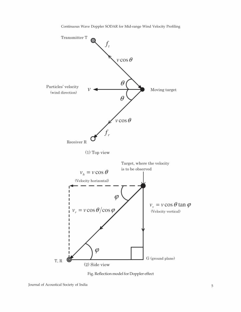
The system measures the velocity of a moving object by the frequency shift of the wave reflected from the objectwhen it is illuminated. We here explain the effect using a simple model. Referring Fig. 1 (a), as the velocity of aparticle moving with velocity v toward the transmitter T at angle q is v cosq (m/sec), the frequency increases to
cos cosT
c cf fc
υ θ υ θλ
+ += = (1.1)
where fT is the frequency of the transmitted wave and c is the propagation velocity of the sound and λ is thewavelength. On the other hand, the frequency fR of the received signal reflected increases to
coscos cosR Tc cf f f
c cυ θ
ν θ υ θ+
= =− −
(1.2)
The Doppler frequency shift is therefore
Continuous Wave Doppler SODAR for Mid-range Wind Velocity Profiling
5Journal of Acoustical Society of India
Fig. Reflection model for Doppler effect
6 Journal of Acoustical Society of India
Y. Kagawa, T. Fukuda, T. Yamazaki, L. Chai and M. Singh
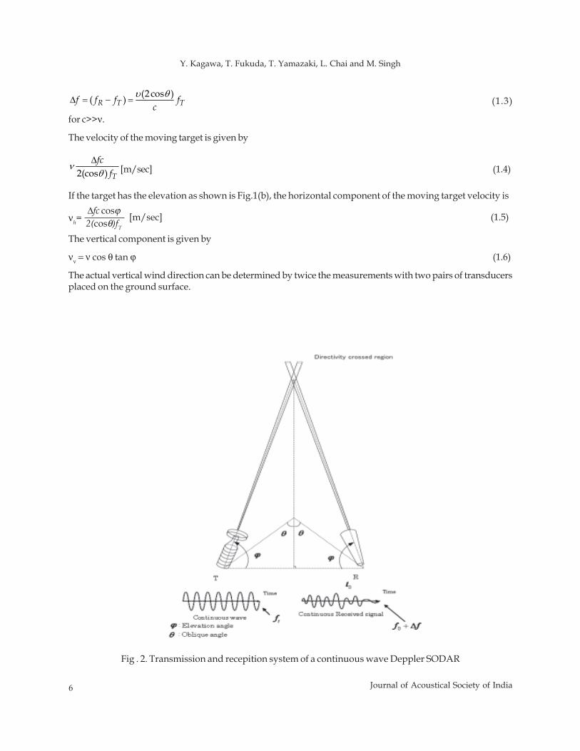
(2 cos )( )R T Tf f f fc
υ θΔ = − = (1.3)
for c>>ν.
The velocity of the moving target is given by
2(cos ) T
fcf
νθ
Δ[m/sec] (1.4)
If the target has the elevation as shown is Fig.1(b), the horizontal component of the moving target velocity is
[m/sec] (1.5)
The vertical component is given by
νν = ν cos θ tan ϕ (1.6)
The actual vertical wind direction can be determined by twice the measurements with two pairs of transducersplaced on the ground surface.
Fig . 2. Transmission and recepition system of a continuous wave Deppler SODAR
Δfc cosϕ2(cosθ)fT
νh=
Continuous Wave Doppler SODAR for Mid-range Wind Velocity Profiling
7Journal of Acoustical Society of India
3. EXPERIMENTAL SYSTEM FOR VERIFICATION
Figure 2 shows the arrangement of a pair of the transducers, the transmitter and the receiver. The space can bescanned by varying the transducers’ directions. The transducers must provide very sharp directivity so thatthe moving target velocity at the crossed region of the two directivities can be measured as the result of thefrequency shift of the received signal.
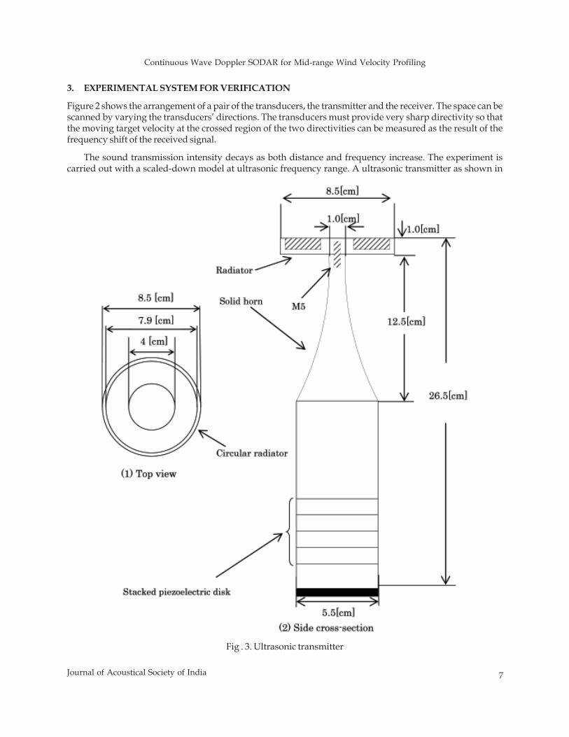
The sound transmission intensity decays as both distance and frequency increase. The experiment iscarried out with a scaled-down model at ultrasonic frequency range. A ultrasonic transmitter as shown in
Fig . 3. Ultrasonic transmitter
8 Journal of Acoustical Society of India
Y. Kagawa, T. Fukuda, T. Yamazaki, L. Chai and M. Singh
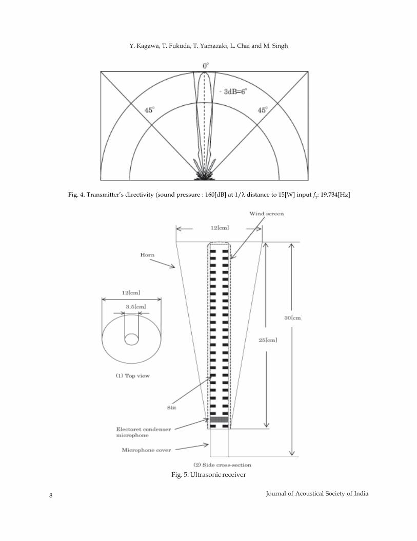
Fig. 4. Transmitter’s directivity (sound pressure : 160[dB] at 1/λ distance to 15[W] input fT: 19.734[Hz]
Fig. 5. Ultrasonic receiver
Continuous Wave Doppler SODAR for Mid-range Wind Velocity Profiling
9Journal of Acoustical Society of India
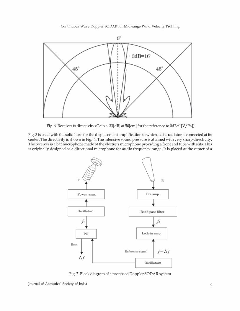
Fig. 6. Receiver fs directivity (Gain :- 33[dB] at 50[cm] for the reference to 0dB=1[V/Pa])
Fig. 3 is used with the solid horn for the displacement amplification to which a disc radiator is connected at itscenter. The directivity is shown in Fig. 4. The intensive sound pressure is attained with very sharp directivity.The receiver is a bar microphone made of the electrets microphone providing a front end tube with slits. Thisis originally designed as a directional microphone for audio frequency range. It is placed at the center of a
Fig. 7. Block diagram of a proposed Doppler SODAR system
10 Journal of Acoustical Society of India
Y. Kagawa, T. Fukuda, T. Yamazaki, L. Chai and M. Singh
conical horn as shown in Fig. 5. The directivity shown in Fig. 6 is reasonable for our purpose. The receiver cancover the range of the frequency shift, though the frequency characteristic is not given.
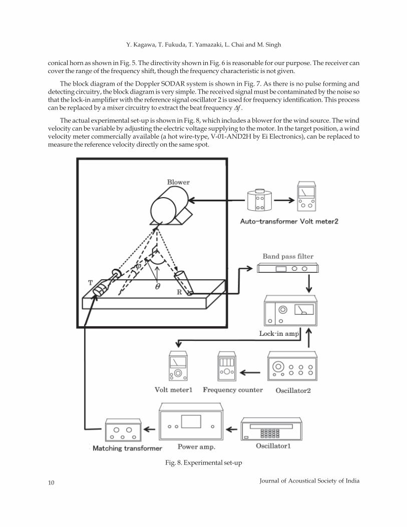
The block diagram of the Doppler SODAR system is shown in Fig. 7. As there is no pulse forming anddetecting circuitry, the block diagram is very simple. The received signal must be contaminated by the noise sothat the lock-in amplifier with the reference signal oscillator 2 is used for frequency identification. This processcan be replaced by a mixer circuitry to extract the beat frequency Δf .
The actual experimental set-up is shown in Fig. 8, which includes a blower for the wind source. The windvelocity can be variable by adjusting the electric voltage supplying to the motor. In the target position, a windvelocity meter commercially available (a hot wire-type, V-01-AND2H by Ei Electronics), can be replaced tomeasure the reference velocity directly on the same spot.
Fig. 8. Experimental set-up
Continuous Wave Doppler SODAR for Mid-range Wind Velocity Profiling
11Journal of Acoustical Society of India
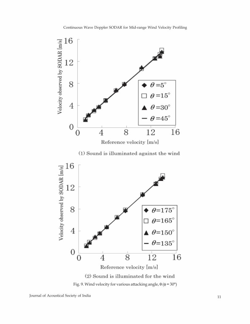
Fig. 9. Wind velocity for various attacking angle, θ (φ = 30°)
12 Journal of Acoustical Society of India
Y. Kagawa, T. Fukuda, T. Yamazaki, L. Chai and M. Singh
A target position is directed to a certain point in front of the blower fs outlet. The wind velocity is calculatedfrom the frequency shift for various attacking angle (θ) with elevation angle (φ) fixed.
Figure 9 shows the results, in which the measured velocity is compared with the reference velocity, whichare along the line 45•‹inclined regardless the attacking angle. Due to the limitation of the experimental space,the distance from the transducers to the target position is in the range of a few meters. The velocity is measurableover the adjustable range of the blower, say 0.5-15[m/sec].
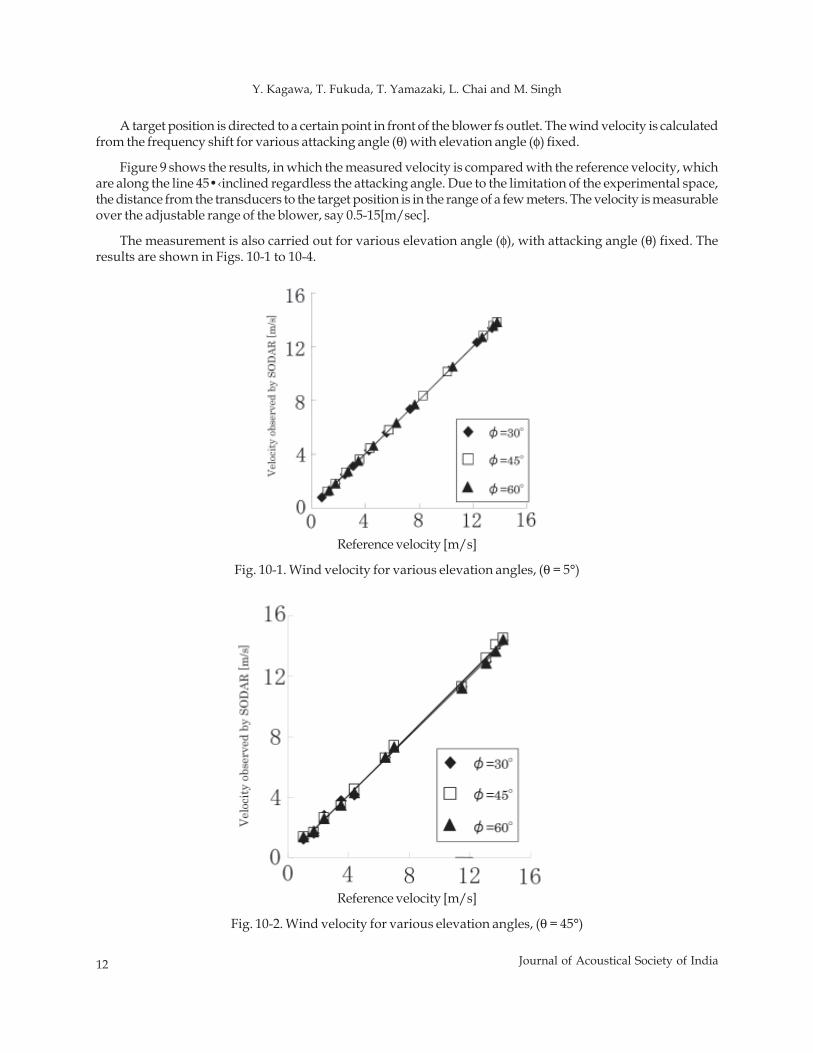
The measurement is also carried out for various elevation angle (φ), with attacking angle (θ) fixed. Theresults are shown in Figs. 10-1 to 10-4.
Reference velocity [m/s]
Fig. 10-2. Wind velocity for various elevation angles, (θ = 45°)
Reference velocity [m/s]
Fig. 10-1. Wind velocity for various elevation angles, (θ = 5°)
Continuous Wave Doppler SODAR for Mid-range Wind Velocity Profiling
13Journal of Acoustical Society of India
Reference velocity [m/s]
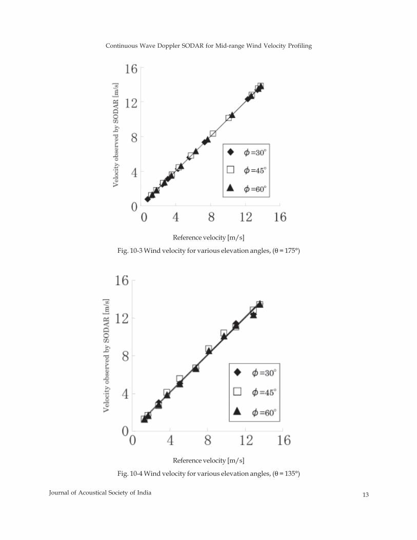
Fig. 10-3 Wind velocity for various elevation angles, (θ = 175°)
Reference velocity [m/s]
Fig. 10-4 Wind velocity for various elevation angles, (θ = 135°)
14 Journal of Acoustical Society of India
Y. Kagawa, T. Fukuda, T. Yamazaki, L. Chai and M. Singh
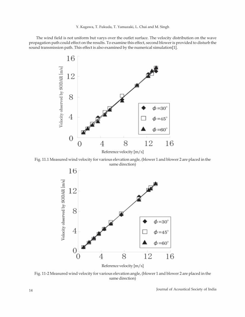
The wind field is not uniform but varys over the outlet surface. The velocity distribution on the wavepropagation path could effect on the results. To examine this effect, second blower is provided to disturb thesound transmission path. This effect is also examined by the numerical simulation[1].
Reference velocity [m/s]
Fig. 11-2 Measured wind velocity for various elevation angle, (blower 1 and blower 2 are placed in thesame direction)
Reference velocity [m/s]
Fig. 11.1 Measured wind velocity for various elevation angle, (blower 1 and blower 2 are placed in thesame direction)
Continuous Wave Doppler SODAR for Mid-range Wind Velocity Profiling
15Journal of Acoustical Society of India
Reference velocity [m/s]
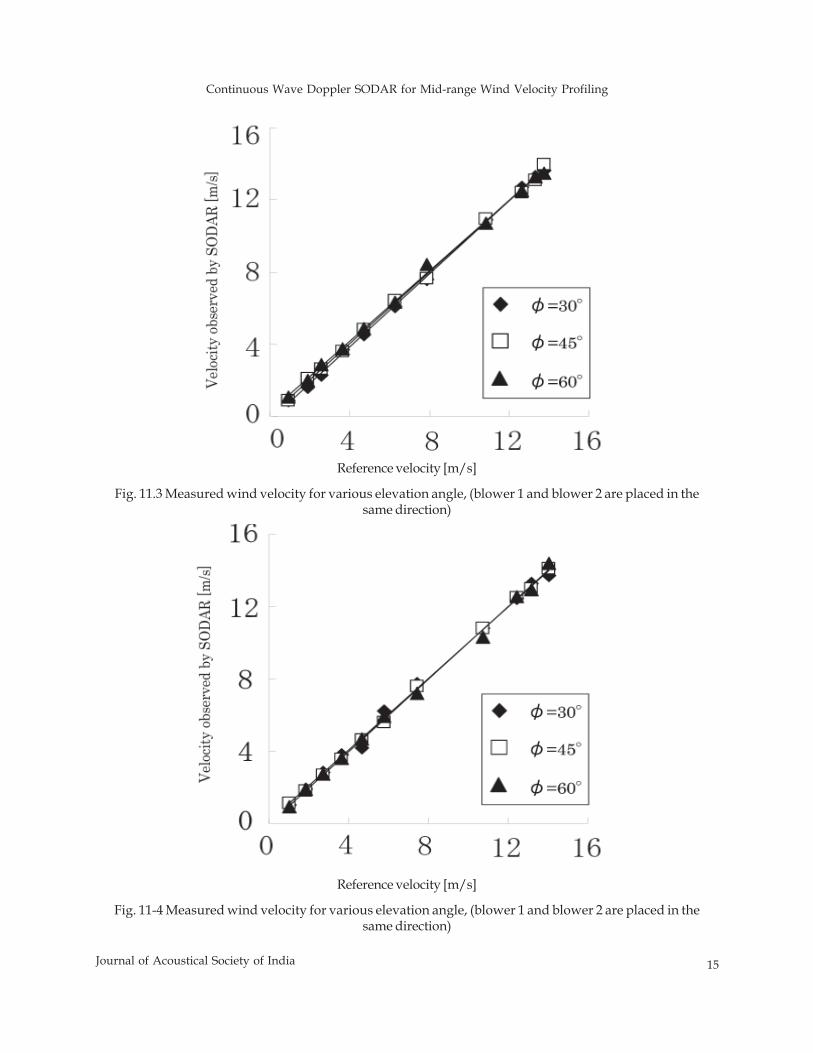
Fig. 11-4 Measured wind velocity for various elevation angle, (blower 1 and blower 2 are placed in thesame direction)
Reference velocity [m/s]
Fig. 11.3 Measured wind velocity for various elevation angle, (blower 1 and blower 2 are placed in thesame direction)
16 Journal of Acoustical Society of India
Y. Kagawa, T. Fukuda, T. Yamazaki, L. Chai and M. Singh
The second blower’s wind direction can be switched reversely. Figs. 11-1 to 11-4 shows this case. Themeasured velocity agrees with the reference velocity regardless the elevation angle φ and the direction of thedisturbing wind, whose velocity is about 4[m/sec] fixed, which could be interpreted as the interference noise.
As shown in Figs. 11-1 and 11-3, some influence is visible near the lower end or for the low wind velocity.This may degrade the measurement accuracy. It is however possible to measure the velocity as low as 1m [m/sec] with the accuracy of less than a few percents.
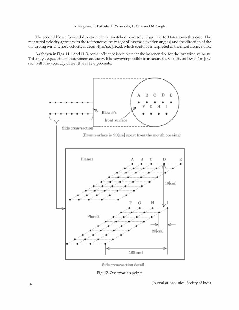
Fig. 12. Observation points
Continuous Wave Doppler SODAR for Mid-range Wind Velocity Profiling
17Journal of Acoustical Society of India
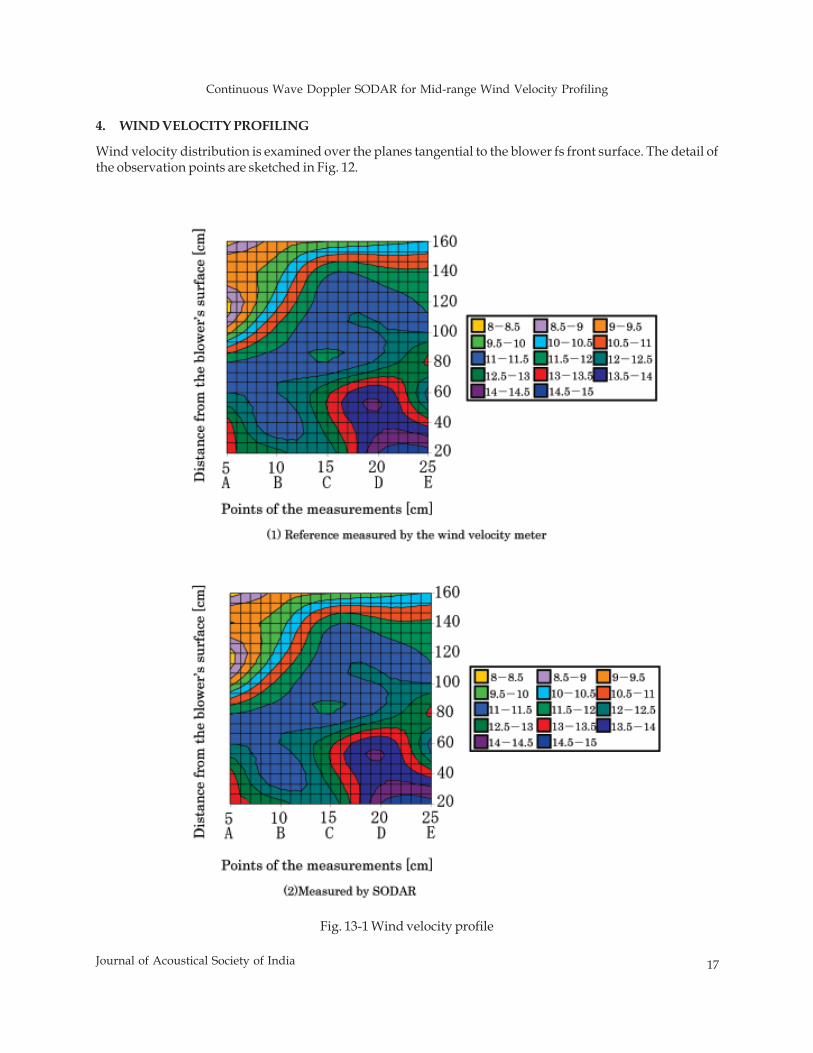
4. WIND VELOCITY PROFILING
Wind velocity distribution is examined over the planes tangential to the blower fs front surface. The detail ofthe observation points are sketched in Fig. 12.
Fig. 13-1 Wind velocity profile
18 Journal of Acoustical Society of India
Y. Kagawa, T. Fukuda, T. Yamazaki, L. Chai and M. Singh
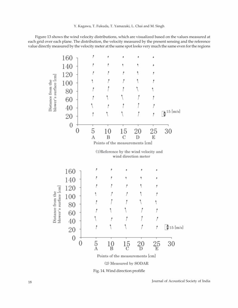
Figure 13 shows the wind velocity distributions, which are visualized based on the values measured ateach grid over each plane. The distribution, the velocity measured by the present sensing and the referencevalue directly measured by the velocity meter at the same spot looks very much the same even for the regions
Fig. 14. Wind direction profifle

Continuous Wave Doppler SODAR for Mid-range Wind Velocity Profiling
19Journal of Acoustical Society of India
where the wind velocity is very low. This validates the usefulness of the present measuring approach. Thevelocity direction can be obtained by the measurements with two pairs of the transducers as discussed inSection II-2. The wind directions are not vertical to the mouth surface as the blower fs wind direction is likelyto bend.
Figure 14 shows the results. The wind strength and direction are indicated by the length and direction ofthe arrow at each point. The arrows remotely sensed and the reference arrows directly measured at the samespots. This again validates the present technique.
5. CONCLUDING REMARKS
The Doppler SODAR using continuous wave emanation is proposed for measuring the wind velocity inmid-range space, aiming at the evaluation of the wind turbine electric generator site selection. The transmitterand the receiver with sharp directivity are carefully selected for the scaled-down model experiment. The windvelocity including its direction can be measured by a system experimentally set-up. The measured velocitydistributions at various surfaces are compared with the reference measured value by the velocity meter. Thegood agreement is established regardless the attacking and elevation angles for shooting the target. Thisvalidates the proposed technique and makes profiling the wind distribution possible. The present paperdemonstrates our experience with the experiment. The system is yet at the stage of a prototype, but scaling-upto the practical system for 100m range can easily be achievable by choosing a suitable frequency, if necessary.
6. REFERENCES
[1] L. CHAI, T. FUKUDA, K. YAMAZAKI and Y. KAGAWA, 2008. Continuous sound wave Doppler SODARto short range wind velocity detection, Proc. of 2008 Asia Simulation Conference, Beijing China 10-12.
[2] Y.KAGAWA, T.TUCHYA, T.HARA and T.TSUJI, 2001. Discrete Huygens’ modeling simulation of soundwave propagation in velocity varying environments, Journal of Sound and Vibration, 246 (3), p 419-439.
[3] S.P. SINGAL and B.S. GERA, 1982. Acoustic remote sensing of the boundary layer, Proc. Indian Acad.Sci. (Engg.Sci.) 5, Pt.2, p131-157.
[4] R.L. COULTER and M.A. KALLISTRATOVA, 1999. The role of acoustic sounding in a high-technologyera, Meteorology and Atmospheric physics, 71, p 3-13.
[5] R.M. KHANNA and S.K. AGGARWAL, 1994. Doppler SODAR and measurement of atmosphericmeasurement, IETE Technical Review, 11, No. 4, p 231-237.
[6] N. Lin, W. Luu, K. Sasaki and Y. Hara, 2003. Investigating wind evaluation by use of a mini DopplerSODAR, Proc. Japan Mechanical Society, 69(B), No. 688, p2598-2605.
[7] T. SHU, 2004. Ultrasonic cardiac diagnosis, Proc. Of Niigata School of Medicine and Welfare Society, 4,No.1, p103-111.
[8] T. OHTSUKA and K. SEGA, 1991. Intensive ultrasonic sound source for air with a staggered circular discradiator, J. Acous. Soc. Japan, 47, No. 4, p478-483.
Journal of AcousticalSociety of India (JASI)
A quarterly publication of the Acoustical Society of India
Volume 40, Number 1, January 2013
EDITORIAL
Ship Noise Reduction Approach
Mahavir Singh ............................................................................... 2
ARTICLES
Continuous Wave Doppler SODAR for Mid- range WindVelocity ProfilingY. Kagawa, T. Fukuda, T. Yamazaki, L. Chai and M. Singh............ 3
Using Directivity of Radiated Sound for Noise ControlApplicationsGyanishankar Sharma, Abhijit Sarkar and N. Ganesan.................. 20
Wave Theory Approach for Developing the MathematicalModel of the Right Angled JointV.H. Patil and D.N. Manik............................................................... 28
Noise pollution in Wards of a Hospital inTiruchirapalli CityV. Bhanumathy, R. Geetha and M. Sangeetha................................. 34
Preliminary Study on Automotive Horn Sound QualityB. Venkatesham, N. Pradeep, Goutham and Jongdae Kim.............. 40
Speech Intelligibligy in School Class Rooms -A Casestudy of Schools in an Indian TownG. Muthu Shoba Mohan................................................................... 46
Speech Rhythm in Individuals with StutteringM. Santosh, Priyanka Parakh and V. Sahana................................... 51
Search for Spectral Cues of Emotion in Hindustani MusicAnirban Patranabis, Kaushik Banerjee, Ranjan Sengupta,Nityananda Dey and Dipak Ghosh................................................... 56
Comparing Acoustic Parameters of Conversational andClear Speech during Reading in Kannada SpeakingIndividuals with Parkinson's DiseaseLakshmi Venkatesh and Ritu Mary Mathew........................................ 61
INFORMATION
Executive Council of Acoustical Society of India 66
Information for Authors Inside back cover
JASI
MAHAVIR SINGH Chief Editor
OMKAR SHARMA Managing Editor
TRINATH KAR Associate Scientific Editor
Yudhishter KumarAnil Kumar NainNaveen Garg Assistant Editors
EDITORIAL BOARD
M L Munjal IISc Banglore, India
S Narayanan IIT Chennai, India
V Rajendran KSRCT Erode, India
R J M Craik HWU Edinburg, UK
Trevor R T Nightingle NRC Ottawa, Canada
B V A Rao VIT Vellore, India
N Tandon IIT Delhi, India
P Narang NMI Lindfield, Australia
E S R Rajagopal IISc Banglore, India
A L Vyas IIT Delhi, India
V Bhujanga Rao NSTL Vizag, India
Yukio Kagawa NU Chiba, Japan
S Datta LU Loughborough, UK
Sonoko Kuwano OU Osaka, Japan
K K Pujara IIT Delhi (Ex.), India
A R Mohanty IIT Kharagpur, India
Ashok Kumar NPL New Delhi, India
V Mohanan NPL New Delhi, India
EDITOR’S SPACE
Ship Noise Reduction Approach
ISociety for Promotion of Nature Tourism and Sports (SPORTS), Indian Register of Shipping (IRS) has performeda literature study focusing on noise from ships in port and the possibilities for noise reduction. As a part ofthe study it has been established that a ship that is in agreement with the external noise limits imposed by theinternational maritime organization, IMO, when the ship at berth, potentially can have a significant impactwith respect to noise in the surroundings. A calculation example is presented where it is shown that a shipwhich fulfils the IMO noise limits can have a diesel generator exhaust sound power of 107 dB(A). The IMOnoise guiding limits for residential, city areas in the time period 22-07 is 40 dB(A). By applying the mostsimple noise propagation model it is demonstrated that if the sound power is 107 dB(A) and the noise limitis 40 dB(A), the ship should be berthed more than 600 m away in order not to exceed the noise limit. Anexcerpt of the unattenuated sound powers of some marine diesel engine exhausts and ventilation fans havebeen presented and found to be quite significant in light of the environmental noise requirements. I.e. thesound power of the engine exhausts vary between 135 to 142 dB(A) and of the ventilation fans between 81 to110 dB(A). Noise measurements of secondary noise sources such as reefers, cooling containers, show that thesound power of a single reefer is in the range of 90 dB(A). Each time the number of reefers is doubled thesound power increases by 3 dB. Therefore the noise from reefers can be significant. Standard measures forreducing noise from the major external sources onboard ships have been presented including special noisereducing measures. Some of the presented possible noise reducing measures is listed below:
• Standard silencers on the diesel generator exhaust i.e. reflection type, absorption type and combinationtype silencers.
• Utilizing the main engine exhaust silencer during port stay for the diesel generator exhaust by reroutingthe exhaust.
• On shore power supply
• Standard methods for reducing noise from ventilation systems onboard a ship including adding mineralwool to fan rooms, cylindrical silencers, baffle silencers and noise reducing louvers.
A cost ranking of the different noise reducing measures has been laid out. The cost ranking is based onwhether the installation of the noise reducing measure is considered to be cumbersome and time consuming.This is if the installation can be carried out during regular port stay or should be performed on a shipyard. Forexample installing new silencers in a diesel generator exhaust stack is a major structural change and isperformed at a shipyard which is considered to be costly. Whereas, installing mineral wool in a fan 10 roomis simple and can be carried out by the ship's crew or a contractor during port stay. A noise reducing measureon this scale is therefore considered less costly.
Mahavir Singh
28 Journal of Acoustical Society of India
V.H. Patil and D.N. Manik
ABSTRACT
In this study, vibrational energy distribution within the audible frequency range is considered betweentwo plates. The two plates are connected to form a welded joint (line connection), riveted and boltedjoint (point connection). The mathematical model for the joints is developed using a spring anddashpot model. The wave approach is used to develop the mathematical model of the coupled plate.The bending wave transmission and reflection efficiencies are determined. The limiting value of highstiffness joint is determined, which represents the weld joint like a rigid joint. The bolt and rivet jointsare modelled, with spring dashpot in only one direction and in another direction the joint is consideredas rigid. After studying the stiffness effect, the mathematical model is updated to include damping atthe joint. The damping has smoothening effect on these efficiencies.
1. INTRODUCTION
Joints are an important part of any complex structure. The waves propagating from one component to otherpass through these joints. The joint has its own stiffness and damping, which particularly attenuates theincident wave and then transmits the rest to the other connected component. Leung and Pinnington1 appliedwave theory to a right angled joint with compliance. They have found the transmission and reflectioncoefficients for the joints. The stiffness and damping at the joint are the major factors which influence energytransfer between the coupled systems. Cremer2 and others have studied the attenuation of an incident wavethrough a joint. Ungar3 has given detailed classification of the damping present in a system, which isresponsible for the energy loss. Yoshimura and Okushima4 developed a method to identify the quantitativevalues of the rigidity and damping coefficients at the joint surface by interactive use of theoretical simulationand experiment. Mead5 worked on aircraft structures having riveted and bolted joints.
2. JOINT MODEL
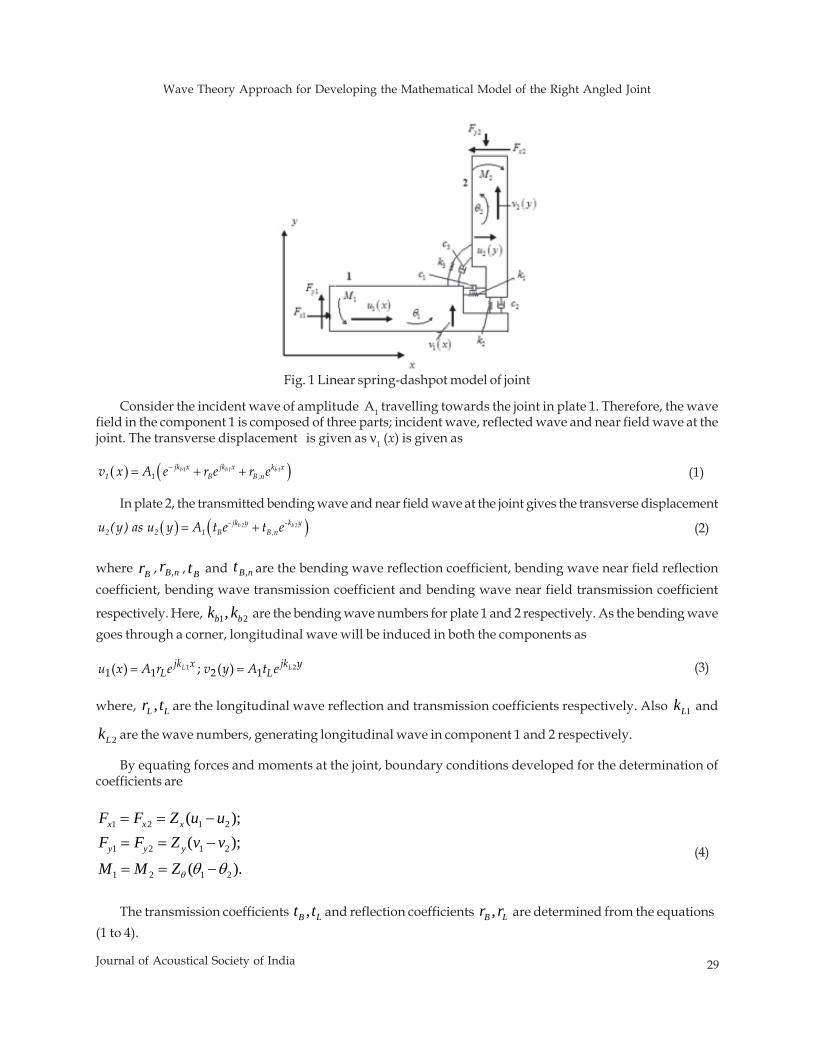
Figure (1) shows the right angle joint model with spring dashpot attached. For the cases of a joint with springsin all three degrees of freedom, wave approach is used to analyse the joint. In the Fig. (1) k2 , k2 are linearstiffness and k3 is rotational stiffness. Similarly, c1, c2 and c3 are the viscous dampers. The plate 1 is in x-z planeand plate 2 is in y-z plane. Both the plates are symmetric about the z axis, in z plane. The coordinate system istaken at the mid of the both plates in z plane and at the joint location. The coordinate system represents x=0,y=0, z=0 at the joint.
Journal of Acoustical Society of India : Vol. 40, No. 1, 2013 (pp. 28-33)
Wave Theory Approach for Developing theMathematical Model of the Right Angled Joint
V.H. Patil and D.N. ManikDepartment of Mechanical Engineering
Indian Institute of Technology, Bombay-400 076
[Received: 13.11.2012; Revised: 28.11.2012; Accepted: 08.01.2013]
© 2013 Acoustical Society of India
Wave Theory Approach for Developing the Mathematical Model of the Right Angled Joint
29Journal of Acoustical Society of India
Consider the incident wave of amplitude A1 travelling towards the joint in plate 1. Therefore, the wavefield in the component 1 is composed of three parts; incident wave, reflected wave and near field wave at thejoint. The transverse displacement is given as ν1 (x) is given as
( ) ( )−= + +b1 b1 b1jk x jk x k x1 1 B B,nv x A e r e r e (1)
In plate 2, the transmitted bending wave and near field wave at the joint gives the transverse displacement
( ) ( )= +b 2 b 2- jk y -k y2 2 1 B B,nu (y) as u y A t e t e (2)
where Br , nBr , , Bt and nBt , are the bending wave reflection coefficient, bending wave near field reflectioncoefficient, bending wave transmission coefficient and bending wave near field transmission coefficient
respectively. Here, 1 2,b bk k are the bending wave numbers for plate 1 and 2 respectively. As the bending wavegoes through a corner, longitudinal wave will be induced in both the components as
1 21 1 2 1( ) ; ( )L Ljk x jk yL Lu x A r e v y A t e= = (3)
where, ,L Lr t are the longitudinal wave reflection and transmission coefficients respectively. Also 1Lk and
2Lk are the wave numbers, generating longitudinal wave in component 1 and 2 respectively.
By equating forces and moments at the joint, boundary conditions developed for the determination ofcoefficients are
1 2 1 2
1 2 1 2
1 2 1 2
( );( );
( ).θ θ θ
= = −= = −
= = −
x x x
y y y
F F Z u uF F Z v v
M M Z(4)
The transmission coefficients ,B Lt t and reflection coefficients ,B Lr r are determined from the equations(1 to 4).
Fig. 1 Linear spring-dashpot model of joint
30 Journal of Acoustical Society of India
V.H. Patil and D.N. Manik
2 2 1 1 2 2
2 2 1 1 2 2
[(1 )( ) 2] [(1 )( ) 2][1 ( )][(1 )( ) 2] [1 ( )][2 (1 )( )]
β β βψβ β β
− + − + + + + += −
+ + + + + + + +B Bj Z j Z j Zr tj Z j Z j Z (5)
1 1 2 2 1 1 2 22[ ] 2 [1 ( )( )]β β β β+ + + − − + +=B
Z Z j Z ZtD (6)
where
1 1 2 2 1 1 2 2
1 1 2 2 1 1 2 2
3 1 1 2 2 1 1 2 2
{ 1 2( ) ( ) (1 )( )( )}{ 1 ( ) 2( ) (1 )( )( )}
{ ( )( ) 2 (1 )( ) (1 )( )}.
β β β βψ β β β βψ β β β β
= − + − + − + − + + ++ − + − + − + − + + ++ − + + + − − + − − +
D X j Z Z j Z Zj Z Z j Z Z
Z Z Z j j Z j Z (7)
where
( )
1 2 2 1 1 2 1 1 2 2 1 1 2 2
22 2
3 3 1 2 2 2 1 1 3 1 1 2 121 1
( ) ( ); ( ) ( ); ( ) ; ( ) ;
( ) ; ; ; ; ;θ θ
β β ω ω
ω ψ
= = = + = +
= + = = = = =
B L B L x y
bB x B y B B B
b
m C m C m C m C Z k j c Z k j c
k BZ k j c Z m C Z Z m C Z Z B C Z X k kk B
The efficiencies for the transmitted and reflected bending waves and longitudinal waves are
2 2;τ ψ ρ= =B B B BX t r (8)
2.1 Weld Joint (Rigid Joint)
The weld joint mathematical model is obtained by setting 1 2 3, ,k k k to infinity in Eqs. (5) to (8). Therefore,
dimensionless terms 1 2 3, ,Z Z Z become zero.
2.2 Bolt/Rivet Joint (Joint with compliance in only one direction).
Similarly, for the bolt/rivet joint mathematical model is obtained by setting 1 21,X ψ β β β= = = = and
1 3 1 2 1 20, , .Z Z u u θ θ= = = = in Eqs. (5) to (8).
3. RESULTS
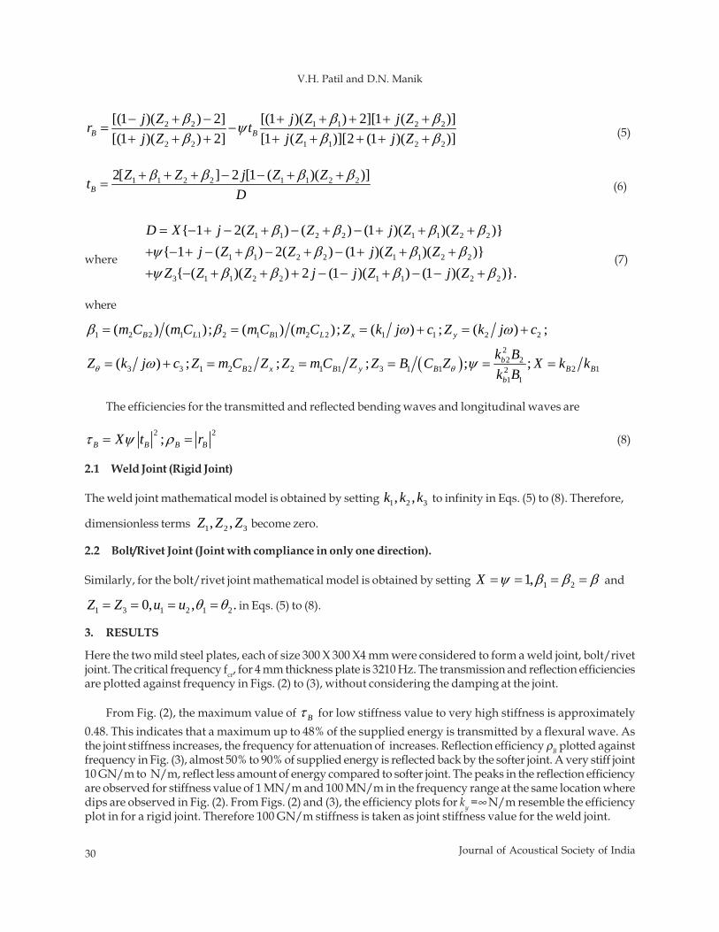
Here the two mild steel plates, each of size 300 X 300 X4 mm were considered to form a weld joint, bolt/rivetjoint. The critical frequency fcr, for 4 mm thickness plate is 3210 Hz. The transmission and reflection efficienciesare plotted against frequency in Figs. (2) to (3), without considering the damping at the joint.
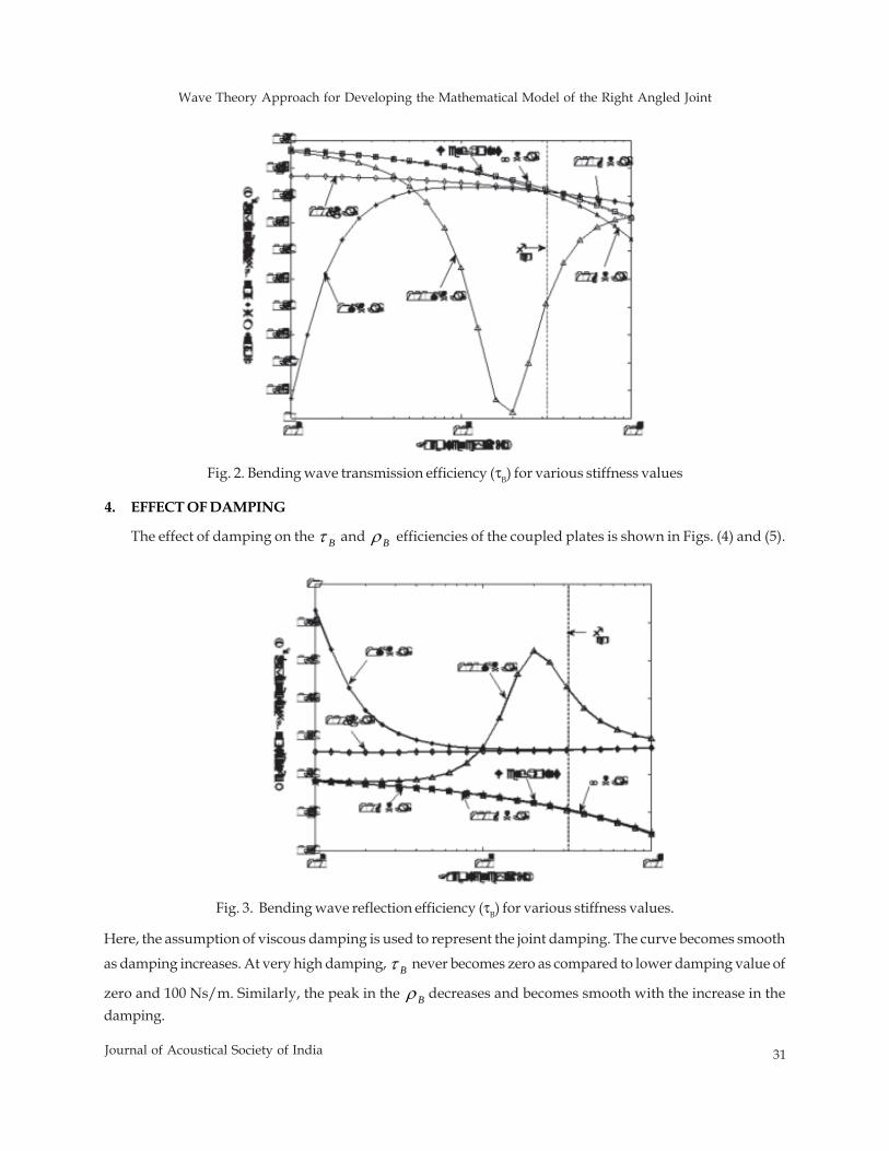
From Fig. (2), the maximum value of Bτ for low stiffness value to very high stiffness is approximately0.48. This indicates that a maximum up to 48% of the supplied energy is transmitted by a flexural wave. Asthe joint stiffness increases, the frequency for attenuation of increases. Reflection efficiency ρB plotted againstfrequency in Fig. (3), almost 50% to 90% of supplied energy is reflected back by the softer joint. A very stiff joint10 GN/m to N/m, reflect less amount of energy compared to softer joint. The peaks in the reflection efficiencyare observed for stiffness value of 1 MN/m and 100 MN/m in the frequency range at the same location wheredips are observed in Fig. (2). From Figs. (2) and (3), the efficiency plots for ky =∞ N/m resemble the efficiencyplot in for a rigid joint. Therefore 100 GN/m stiffness is taken as joint stiffness value for the weld joint.
Wave Theory Approach for Developing the Mathematical Model of the Right Angled Joint
31Journal of Acoustical Society of India
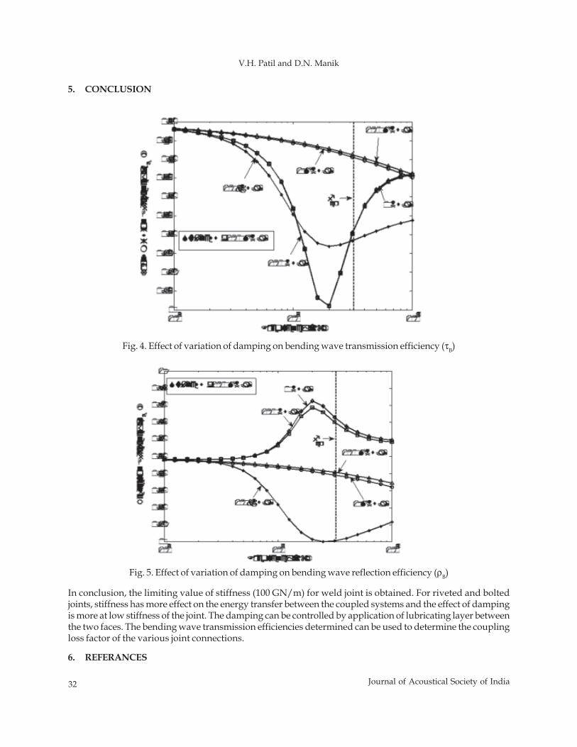
4. EFFECT OF DAMPING
The effect of damping on the Bτ and Bρ efficiencies of the coupled plates is shown in Figs. (4) and (5).
Here, the assumption of viscous damping is used to represent the joint damping. The curve becomes smooth
as damping increases. At very high damping, Bτ never becomes zero as compared to lower damping value of
zero and 100 Ns/m. Similarly, the peak in the Bρ decreases and becomes smooth with the increase in thedamping.
Fig. 2. Bending wave transmission efficiency (τB) for various stiffness values
Fig. 3. Bending wave reflection efficiency (τB) for various stiffness values.
32 Journal of Acoustical Society of India
V.H. Patil and D.N. Manik
5. CONCLUSION
In conclusion, the limiting value of stiffness (100 GN/m) for weld joint is obtained. For riveted and boltedjoints, stiffness has more effect on the energy transfer between the coupled systems and the effect of dampingis more at low stiffness of the joint. The damping can be controlled by application of lubricating layer betweenthe two faces. The bending wave transmission efficiencies determined can be used to determine the couplingloss factor of the various joint connections.
6. REFERANCES
Fig. 4. Effect of variation of damping on bending wave transmission efficiency (τB)
Fig. 5. Effect of variation of damping on bending wave reflection efficiency (ρB)

Wave Theory Approach for Developing the Mathematical Model of the Right Angled Joint
33Journal of Acoustical Society of India
[1] LEUNG, R. and PINNINGTON, R. Wave propagations through right angled joints with compliance –flexural incident wave, Journal of Sound and Vibration, 142 (1), 31-46,(1990).
[2] CREMER, L., HECKL, M. and UNGAR, E.E. Structure-Borne Sound, Berlin: Springer-Verlag, (1987).[3] UNGAR, E.E. The status of engineering knowledge concerning the damping of built- up structures,
Journal of Sound and Vibration, 26(1), 141-154, (1973).[4] YOSHIMURA, M. and OKUSHIMA, K. Measurement of dynamic rigidity and damping property for
simplified joint models and simulation by computer, Annals of CIRP 25, 193-198, (1977).[5] MEAD, D. J. The damping, stiffness a fatigue properties of joints and configuration representative of
aircraft structures, WADC-University of Minnesota Conference Acoustical Fatigue, 235-261, (1961).
20 Journal of Acoustical Society of India
Gyanishankar Sharma, Abhijit Sarkar and N. Ganesan
Using Directivity of Radiated Sound for Noise ControlApplications
Gyanishankar Sharma, Abhijit Sarkar* and N. GanesanDepartment of Mechanical Engineering, Indian Institute of Technology Madras
Chennai-600 036 (TN)*e-mail: [email protected]
ABSTRACT
In this paper a directivity based technique to control the noise radiated from vibrating plate in a baffleis presented. A novel concept of local noise control is explored by controlling the directivity patternfor the cases where global noise control is difficult to attain. Finite element simulation is done incommercial software ANSYS to obtain the displacement response. The obtained displacement responseis validated by deriving an analytical formula for response using mode summation technique. In themode summation procedure modes of the unloaded plate is used as a basis for determining theresponse of the mass loaded plate. This is accomplished by considering the effect of attached pointmass as frequency dependent force. The surface velocity is calculated from displacement responsewhich is used in a Rayleigh integral based calculation to arrive at sound pressure at a location andhence the directivity pattern. Control on directivity pattern is achieved by attaching discrete mass atdifferent locations over the plate. Passive technique for noise and vibration control is known to havea poor performance for global control in low and medium frequency region. Hence control on thedirectivity could be a useful technique for local noise control for low and medium frequency vibration.
1. INTRODUCTION
Noise control from vibro-acoustic sources has been a widely studied topic in the engineering community [1].Passive and active measures are used to control noise. The passive control methods are broadly classified as(1) source control - wherein efforts are made to directly reduce the source of noise viz. vibration levels, flowripples, etc. (2) transfer path control – wherein efforts are made to reduce the transmission of the generatednoise to the receiver without affecting the source. Reactive mufflers are one of the best examples in this casewherein the sound generated at the source is reflected back. Passive techniques for noise and vibration controlworks well for high frequency vibration whereas, active techniques spans low and medium frequency vibration.Active control techniques are costly, difficult to implement and works efficiently only for narrow frequencybands.
Noise control as we understand could be of two types i.e. global and local. In global noise control aim is toreduce noise at all the locations over the source. On the contrary in is local noise control the aim is to minimizenoise at a specified receiver location. In this work, we attempt to investigate the possibility of controllingdirectivity as an additional technique for noise control.
In several applications there are instances where the objective of the noise control engineer is to minimizethe audible noise at specific locations. For example, in automotive applications the target is to reduce the noiseat the driver and passenger ear location. It is acceptable to achieve this target even at the cost of increasing
Journal of Acoustical Society of India : Vol. 40, No. 1, 2013 (pp. 20-27)
[Received: 16.11.2012; Revised: 21.12.2012; Accepted: 07.01.2013]
© 2013 Acoustical Society of India
Using directivity of radiated sound for noise control applications
21Journal of Acoustical Society of India
sound levels at locations away from the passengers. Thus, we attempt to explore the possibility of redistributingthe available acoustic energy in different directions such that the noise levels at the specific locations of interestare reduced at the cost of increased noise levels at other locations. Similarly, the concept of directivity controlfor local noise control could be utilized in aerospace application to direct the radiated sound in upwarddirection so as to minimize the sound levels in the nearby buildings while takeoff and landing. This conceptcan have industrial application as well to direct the machinery noise away from direction of workers and tomake workplace acceptable.
Chatillon [2] studied the influence of source directivity in noise levels inside an industrial hall throughsimulation and experiment. Noise level was observed to be changed by 4 dB as the source directivity changes.Zhang [3] observed different horizontal and vertical directivity pattern of railway noise through measurement.Though in the above works aim was not to control the directivity pattern, there are many literature in which theaim is to control directivity for different applications. Juhez et al. [4] developed an acoustic transducer systemfor long distance echo-ranging application. Directivity controlled piezo-electric transducer for soundreproduction was developed by Be’dard and Berry [5]. Seo and Kim [6] studied directional radiation pattern instructural acoustic coupled system. Three typical directivity patterns i.e. steered, focused and omnidirected arepresented.
Voluminous literature is available on the study of the vibration response and acoustic radiation from massloaded structures [7, 8, 9]. There was no literature found for acoustic directivity control from vibrating structuresusing passive techniques such as lumped mass addition.
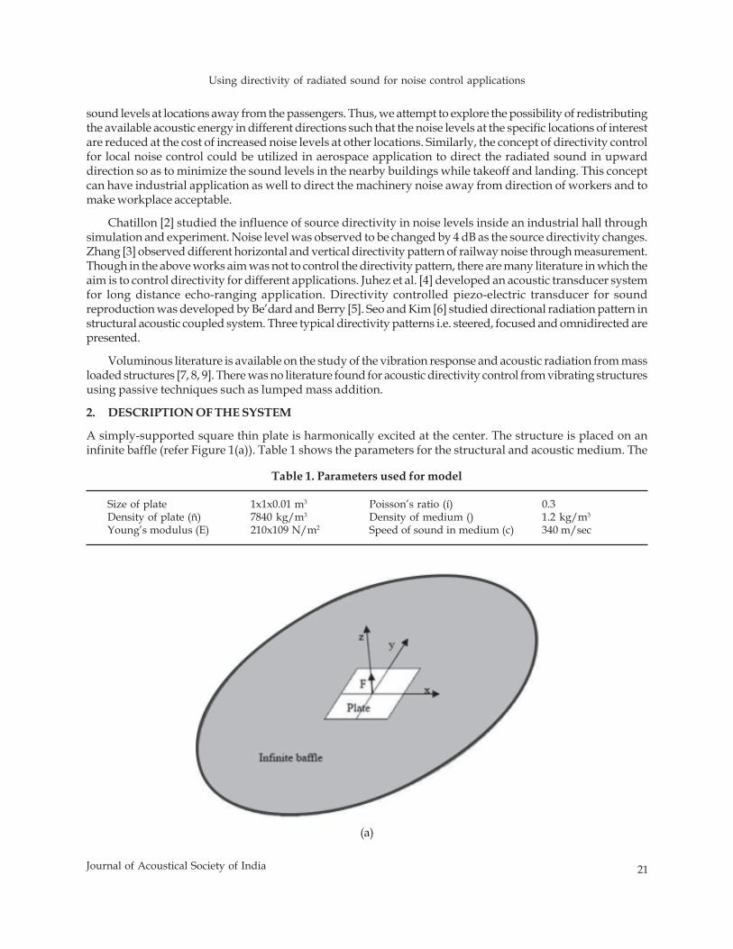
2. DESCRIPTION OF THE SYSTEM
A simply-supported square thin plate is harmonically excited at the center. The structure is placed on aninfinite baffle (refer Figure 1(a)). Table 1 shows the parameters for the structural and acoustic medium. The
Table 1. Parameters used for model
Size of plate 1x1x0.01 m3 Poisson’s ratio (í) 0.3Density of plate (ñ) 7840 kg/m3 Density of medium () 1.2 kg/m3
Young’s modulus (E) 210x109 N/m2 Speed of sound in medium (c) 340 m/sec
(a)
22 Journal of Acoustical Society of India
Gyanishankar Sharma, Abhijit Sarkar and N. Ganesan
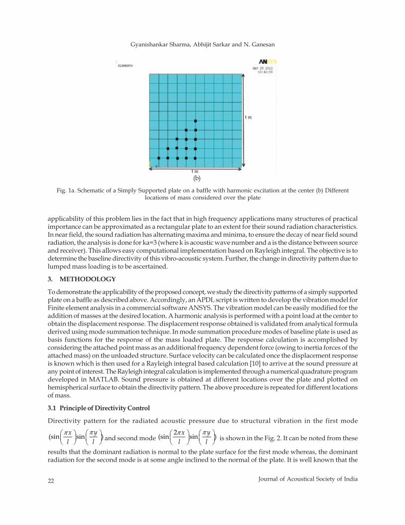
applicability of this problem lies in the fact that in high frequency applications many structures of practicalimportance can be approximated as a rectangular plate to an extent for their sound radiation characteristics.In near field, the sound radiation has alternating maxima and minima, to ensure the decay of near field soundradiation, the analysis is done for ka=3 (where k is acoustic wave number and a is the distance between sourceand receiver). This allows easy computational implementation based on Rayleigh integral. The objective is todetermine the baseline directivity of this vibro-acoustic system. Further, the change in directivity pattern due tolumped mass loading is to be ascertained.
3. METHODOLOGY
To demonstrate the applicability of the proposed concept, we study the directivity patterns of a simply supportedplate on a baffle as described above. Accordingly, an APDL script is written to develop the vibration model forFinite element analysis in a commercial software ANSYS. The vibration model can be easily modified for theaddition of masses at the desired location. A harmonic analysis is performed with a point load at the center toobtain the displacement response. The displacement response obtained is validated from analytical formuladerived using mode summation technique. In mode summation procedure modes of baseline plate is used asbasis functions for the response of the mass loaded plate. The response calculation is accomplished byconsidering the attached point mass as an additional frequency dependent force (owing to inertia forces of theattached mass) on the unloaded structure. Surface velocity can be calculated once the displacement responseis known which is then used for a Rayleigh integral based calculation [10] to arrive at the sound pressure atany point of interest. The Rayleigh integral calculation is implemented through a numerical quadrature programdeveloped in MATLAB. Sound pressure is obtained at different locations over the plate and plotted onhemispherical surface to obtain the directivity pattern. The above procedure is repeated for different locationsof mass.
3.1 Principle of Directivity Control
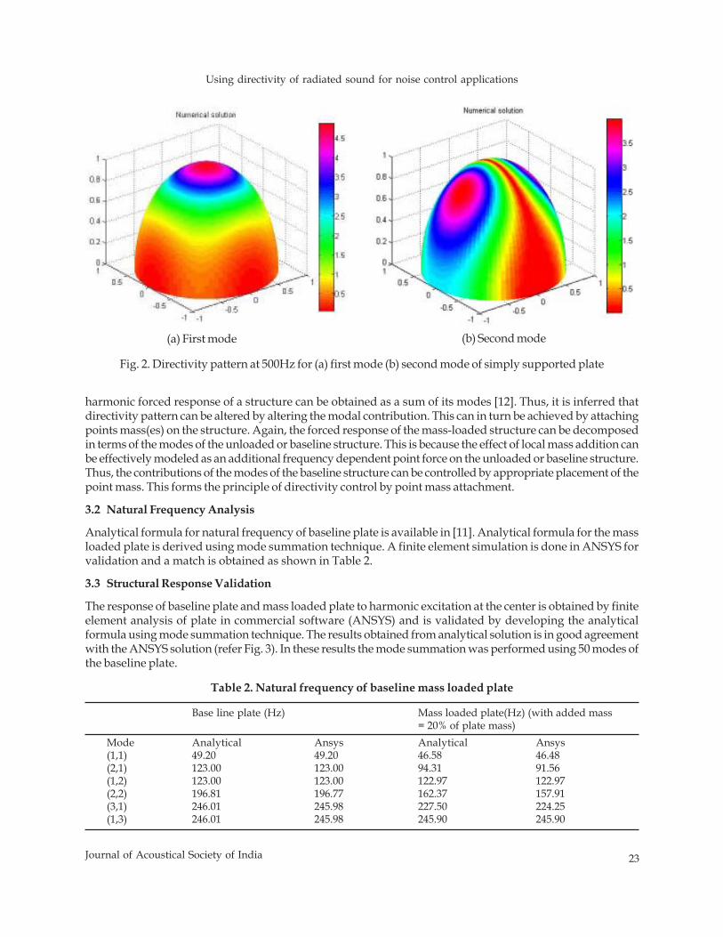
Directivity pattern for the radiated acoustic pressure due to structural vibration in the first mode
(sin sin )yxl l
ππ ⎛ ⎞⎛ ⎞⎜ ⎟ ⎜ ⎟⎝ ⎠ ⎝ ⎠
and second mode 2(sin sin )yx
l lππ ⎛ ⎞⎛ ⎞
⎜ ⎟ ⎜ ⎟⎝ ⎠ ⎝ ⎠ is shown in the Fig. 2. It can be noted from these
results that the dominant radiation is normal to the plate surface for the first mode whereas, the dominantradiation for the second mode is at some angle inclined to the normal of the plate. It is well known that the
Fig. 1a. Schematic of a Simply Supported plate on a baffle with harmonic excitation at the center (b) Differentlocations of mass considered over the plate
(b)
Using directivity of radiated sound for noise control applications
23Journal of Acoustical Society of India
harmonic forced response of a structure can be obtained as a sum of its modes [12]. Thus, it is inferred thatdirectivity pattern can be altered by altering the modal contribution. This can in turn be achieved by attachingpoints mass(es) on the structure. Again, the forced response of the mass-loaded structure can be decomposedin terms of the modes of the unloaded or baseline structure. This is because the effect of local mass addition canbe effectively modeled as an additional frequency dependent point force on the unloaded or baseline structure.Thus, the contributions of the modes of the baseline structure can be controlled by appropriate placement of thepoint mass. This forms the principle of directivity control by point mass attachment.
3.2 Natural Frequency Analysis
Analytical formula for natural frequency of baseline plate is available in [11]. Analytical formula for the massloaded plate is derived using mode summation technique. A finite element simulation is done in ANSYS forvalidation and a match is obtained as shown in Table 2.
3.3 Structural Response Validation
The response of baseline plate and mass loaded plate to harmonic excitation at the center is obtained by finiteelement analysis of plate in commercial software (ANSYS) and is validated by developing the analyticalformula using mode summation technique. The results obtained from analytical solution is in good agreementwith the ANSYS solution (refer Fig. 3). In these results the mode summation was performed using 50 modes ofthe baseline plate.
Table 2. Natural frequency of baseline mass loaded plate
Base line plate (Hz) Mass loaded plate(Hz) (with added mass= 20% of plate mass)
Mode Analytical Ansys Analytical Ansys(1,1) 49.20 49.20 46.58 46.48(2,1) 123.00 123.00 94.31 91.56(1,2) 123.00 123.00 122.97 122.97(2,2) 196.81 196.77 162.37 157.91(3,1) 246.01 245.98 227.50 224.25(1,3) 246.01 245.98 245.90 245.90
(b) Second mode
Fig. 2. Directivity pattern at 500Hz for (a) first mode (b) second mode of simply supported plate
(a) First mode
24 Journal of Acoustical Society of India
Gyanishankar Sharma, Abhijit Sarkar and N. Ganesan
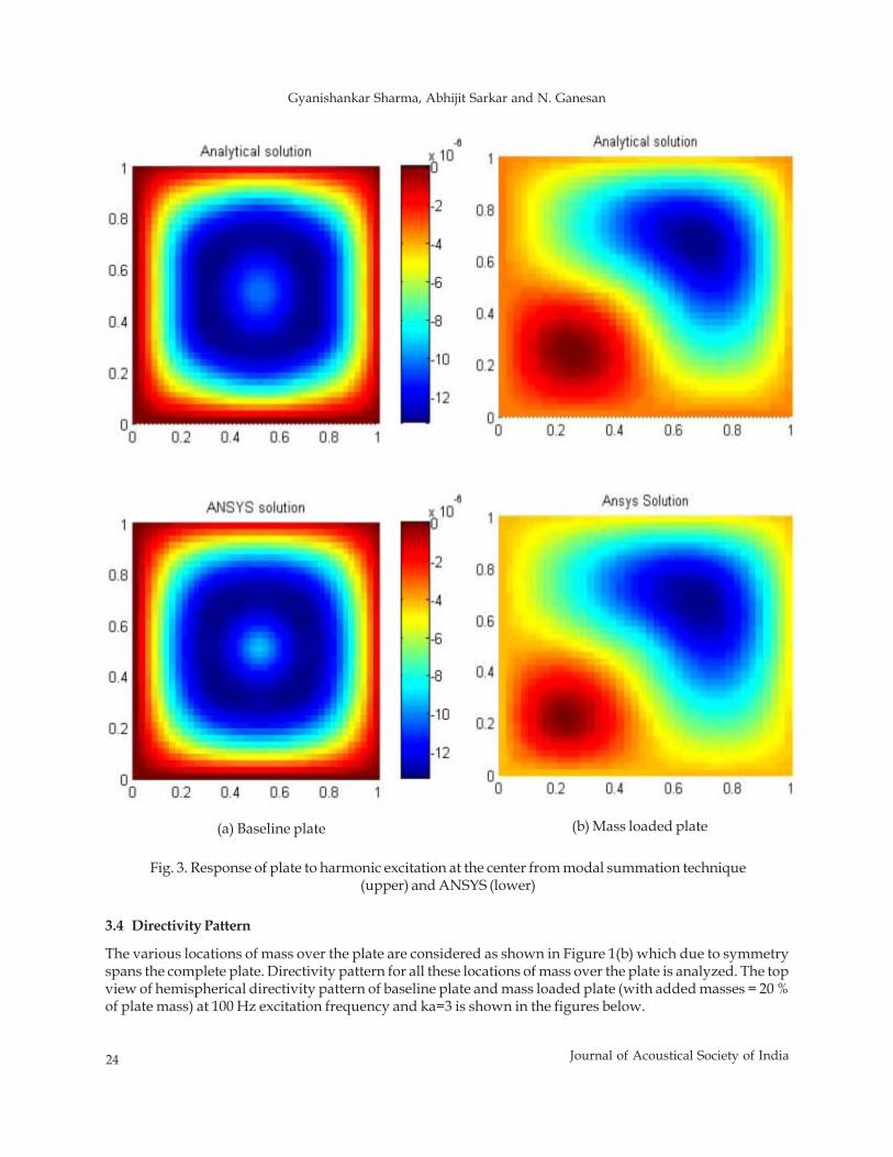
Fig. 3. Response of plate to harmonic excitation at the center from modal summation technique(upper) and ANSYS (lower)
3.4 Directivity Pattern
The various locations of mass over the plate are considered as shown in Figure 1(b) which due to symmetryspans the complete plate. Directivity pattern for all these locations of mass over the plate is analyzed. The topview of hemispherical directivity pattern of baseline plate and mass loaded plate (with added masses = 20 %of plate mass) at 100 Hz excitation frequency and ka=3 is shown in the figures below.
(a) Baseline plate (b) Mass loaded plate
Using directivity of radiated sound for noise control applications
25Journal of Acoustical Society of India
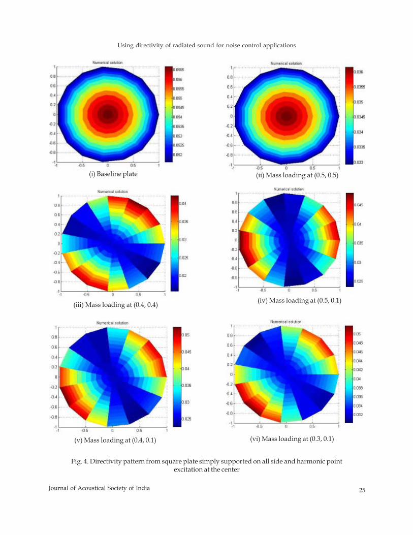
Fig. 4. Directivity pattern from square plate simply supported on all side and harmonic pointexcitation at the center
(i) Baseline plate (ii) Mass loading at (0.5, 0.5)
(iii) Mass loading at (0.4, 0.4) (iv) Mass loading at (0.5, 0.1)
(v) Mass loading at (0.4, 0.1) (vi) Mass loading at (0.3, 0.1)
26 Journal of Acoustical Society of India
Gyanishankar Sharma, Abhijit Sarkar and N. Ganesan
4. DISCUSSION
On analyzing the above results of directivity pattern, it is seen that the directivity pattern of baseline plate canbe altered by attaching additional mass. The location and magnitude of mass addition plays an important rolein controlling the directivity pattern so as to reduce noise at different planes over the plate.
It is seen that when mass location is same as that of forcing the sound pressure is reduced at all the locationwhereas, directivity pattern is unaltered (refer Figure 4(ii)). This is due to decrease in forcing which results indecrease in vibration.
In the following we present a representative analysis of directivity pattern of baseline plate and massloaded plate (0.4, 0.4). To give the vibration response of the plate as a single number for quantitative analysis,we calculated the root mean square value of displacement over the plate. This is in consonance with radiationefficiency analysis in acoustics [10]. The RMS value of displacement response of the mass-loaded plate iscalculated to be 1.74 times that of the baseline plate. Hence, the vibration is increased due to mass addition. Thereason could be explained as we are adding mass on stiffness controlled region. The total sound energy
radiated 2
0(using the formula )
2A
pE dAcρ
= ∫ for the baseline plate and mass loaded plate is computed to
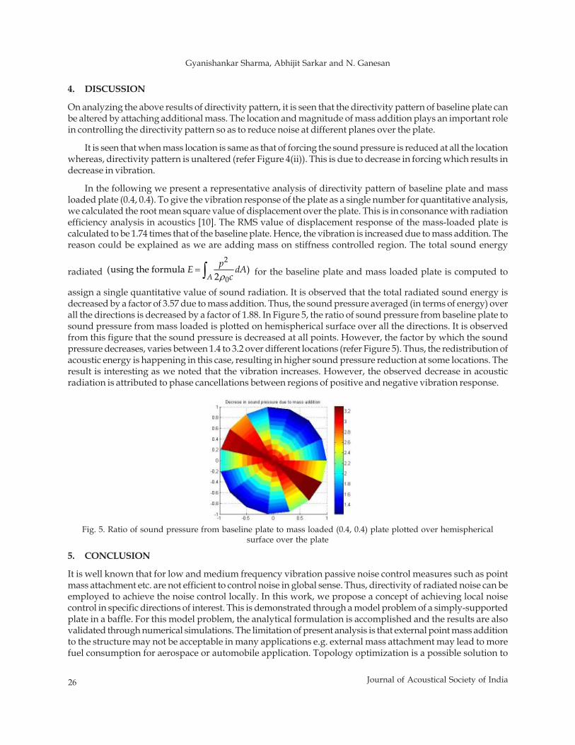
assign a single quantitative value of sound radiation. It is observed that the total radiated sound energy isdecreased by a factor of 3.57 due to mass addition. Thus, the sound pressure averaged (in terms of energy) overall the directions is decreased by a factor of 1.88. In Figure 5, the ratio of sound pressure from baseline plate tosound pressure from mass loaded is plotted on hemispherical surface over all the directions. It is observedfrom this figure that the sound pressure is decreased at all points. However, the factor by which the soundpressure decreases, varies between 1.4 to 3.2 over different locations (refer Figure 5). Thus, the redistribution ofacoustic energy is happening in this case, resulting in higher sound pressure reduction at some locations. Theresult is interesting as we noted that the vibration increases. However, the observed decrease in acousticradiation is attributed to phase cancellations between regions of positive and negative vibration response.
5. CONCLUSION
It is well known that for low and medium frequency vibration passive noise control measures such as pointmass attachment etc. are not efficient to control noise in global sense. Thus, directivity of radiated noise can beemployed to achieve the noise control locally. In this work, we propose a concept of achieving local noisecontrol in specific directions of interest. This is demonstrated through a model problem of a simply-supportedplate in a baffle. For this model problem, the analytical formulation is accomplished and the results are alsovalidated through numerical simulations. The limitation of present analysis is that external point mass additionto the structure may not be acceptable in many applications e.g. external mass attachment may lead to morefuel consumption for aerospace or automobile application. Topology optimization is a possible solution to
Fig. 5. Ratio of sound pressure from baseline plate to mass loaded (0.4, 0.4) plate plotted over hemisphericalsurface over the plate
Using directivity of radiated sound for noise control applications
27Journal of Acoustical Society of India
above limitation where one can actually remove some mass over the plate to control directivity. The externalpoint mass can also be embedded in flat plate itself by thinking of functionally graded material to create thedensity difference. As future work similar demonstrations need to be carried on for more complicated structuressuch as curved shells, built-up strctures, composites, etc. In this work we have demonstrated the concept for aspecific model problem i.e. fixed dimension steel plate radiating noise into air. As a future work, the resultsobtained can be generalized by appropriate non-dimensionalization. A numerical algorithm to find optimallocation(s) and magnitude of mass is also planned as future work.
6. REFERENCES
[1] D.A. BIES and C.H. HANSEN, 2003. Engineering Noise Control: Theory and practice, Spon press.[2] J. CHATILLON, 2007. Influence of source directivity on noise levels in industrial halls: Simulation and
experiments, Applied Acoustics, 68 (682).[3] X. ZHANG, 2010. The directivity of railway noise at different speeds, Journal of Sound and Vibration, 329
(5273).[4] J. A. GALLEGO-JUHEZ, G. RODNGUEZ, J.L. S. EMETENO, P. T. SANZ and J. C. LHZARO, 1993. An
acoustic transducer system for long-distance ranging applications in air, Sensors and Actuators A, 37(397).
[5] M. BE’DARD AND A. BERRY, 2008. Development of a directivity-controlled piezoelectric transducer forsound reproduction, Journal of Sound and Vibration, 311 (1271).
[6] H.S. SEO and Y.H. KIM, 2005. Directional radiation pattern in structural-acoustic coupled system, J.Acoust. Soc. Am., 118 (92).
[7] A.E. EKIMOV and A.V. LEBEDEV, 1996. Experimental Study of Local Mass Influence on Sound RadiationFrom a Thin Limited Cylindrical Shell, Applied Acoustics, 48 (47).
[8] S. LI AND X. LI, 2008. The effects of distributed masses on acoustic radiation behaviour of plates, AppliedAcoustics, 69 (272).
[9] J.S. WU and S.S. LUO, 1997. Use of analytical numerical combined method in the free vibration analysisof a rectangular plate with any number of point masses and translational springs, Journal of Sound andVibration, 200 (179).
40 Journal of Acoustical Society of India
B. Venkatesham, N. Pradeep, Goutham and Jongdae Kim
Preliminary Study on Automotive Horn Sound Quality
B. Venkatesham1*, N. Pradeep2, Goutham2 and Jongdae Kim2
1Department of Mechanical Engineering, Indian Institute of Technology Hyderabad-502 0252Electronics Engineering Department, Hyundai Motor India Engineering Pvt. Ltd, Hyderabad-500 084
*e-mail: [email protected]
ABSTRACT
Sound Quality (SQ) is a parameter that provides product differentiator in a competitive market.Automotive horn sound design is a compromise between the need to generate warning signals andalso customized sounds for different manufacturers. Customized sound for a product will provideuniqueness to the manufacturer brand image. The sound quality study of automotive horn is a multi-disciplinary problem. The knowledge of electro-acoustic, musical acoustics and statistics will helpthe designers for providing optimized sound quality products.
The aim of the current investigation is to develop a methodology for studying automotive horn soundquality. It has been discussed the methodology of recording horn sounds for Jury listening test. It hasbeen prepared Jury listening Questionnaire. The recorded sounds are analyzed to calculate differentobjective parameters like loudness, sharpness, roughness, fluctuation of strength and tonality. Relativesensory pleasantness index considers as an aurally adequate psycho-acoustic index to explainpleasantness as the global behavior of horn sound. This value has been calculated from objectiveparameters.
1. INTRODUCTION
Human brain interprets the source of cause and provides instruction to react. It acts like a processor. Thisstudy will be a part of Psycho-acoustic study. Psycho-acoustic study is a science to read out human perceptionand acoustics. Every working product can create a specific sound. This sound may be pleasant or unpleasantbased on human perception. Some sounds are generated for warning purposes. The purposes of these soundsare alert people and grab attention of people. These sounds convey some information. For example, alarmsound, ambulance siren sound, Factory siren sound, Police vehicle siren sound, and vehicle horn sound etc.The focus of the current study is vehicle horn sound. Vehicle horn sound is one of the major noise sources inurban noise pollution. People use horn very frequently countries like India. The major reasons for honkingmight be
The automotive horn sound is more impulsive in nature and creates more annoyance to listeners. Sound
Journal of Acoustical Society of India : Vol. 40, No. 1, 2013 (pp.40-45)
[Received: 15.11.2012; Revised: 24.12.2012; Accepted: 11.01.2013]
Traffic indiscipline Low confidence in driving Vehicle Overtaking (i.e., not following lane system)Cross-Junctions People walking on the road Blind turns & Hair-pin turnsHurriedness in people Animals crossing road Genuine Warning signalHabitual
Quality of Horn is necessary for reducing traffic noise annoyance.
© 2013 Acoustical Society of India
Preliminary Study on Automotive Horn Sound Quality
41Journal of Acoustical Society of India
Most of the automotive manufacturers are interested to create uniqueness to their Vehicle horn sound andshould be more pleasant to listeners with proper warning. This motivates for a current study of AutomotiveHorn Sound Quality.
Sound Quality (SQ) study includes subjective test or Jury test and objective test. The purpose of subjectivetest is to collect human perception of sound. Objective test data can be used to calculate Sound Quality (SQ)metrics like loudness, sharpness, fluctuation of strength, Roughness and tonality etc., based on empiricalequations. These two tests have independent results. The relation between these results can be establishedwith a proper analysis. Existing literature related to automotive horn sound is in the references [1-4].
Guillaume Lemaitre [1-3] etc., from France studied extensively on the sound quality of car horns. Theyhave discussed about the perceived quality of car horn sounds within a psycho-acoustical frame work. Theystudied timbre of car horns similar to the timbre of musical sounds. Their second paper provides insights intothe design of new sounds suitable for European environment. Hai Ann ThiPhan [4] etc., From Japan conductedcross-cultural experiments between Vietnamese and Japanese to understand the annoyance from road trafficnoise with horn sounds.
2. METHOD
The purpose of subjective test is to capture human perception about different sounds. This test can be conductedwith actual product sounds in the field. It may not be possible to conduct test all times due to limitation ofresources and complex interaction with other sounds. An alternative approach is to develop a procedure in thelaboratory.
The main focus of the current study is as follows:
i) Psycho-acoustic analysis of horn sound data to estimate objective parameters,
ii) A subjective test to identify subjective parameters, and
iii) Data analysis to correlate subjective parameters with objective parameters.
It has been developed test setup for recording of horn sound. The recorded sound samples have been usedin subjective test and objective test. Instrumentation, Mounting frame fabrication and test recording proceduredetails has been considered in test setup preparation. The subjective test has been conducted with recordedsound samples.
Objective data calculate SQ metrics and psycho-acoustic indices. Psycho-acoustic indices provide a globaldescription of sound in terms SQ Quantities. The relations used in calculation of objective parameters areempirical in nature. Relative sensory pleasantness index considered as an aurally adequate indices forautomotive horn sound.
2.1 Experimental Test Setup
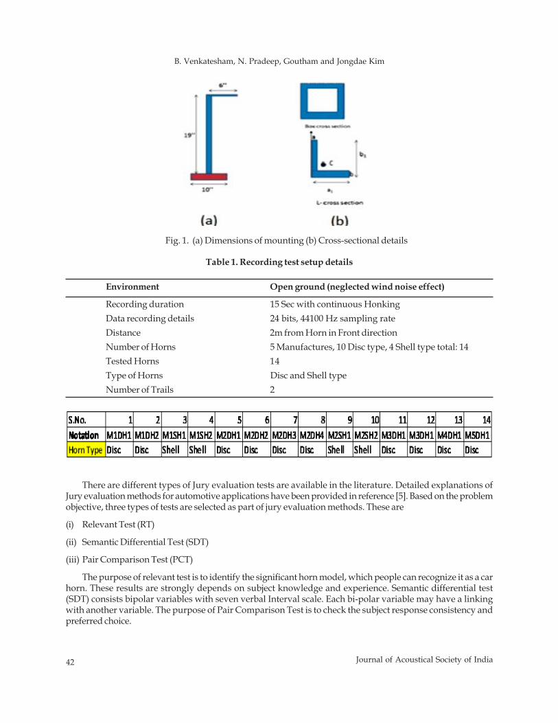
The laboratory test setup development for recording horn sounds has been discussed in this paper. BinauralHead Set (BHS) instrument used to record horn sounds. Figure 1 shows the mounting frame dimensions withCross-sections. These dimensions are estimated based on Horn sound standard and also the actual mountingposition of Horn in a car. Different holes are provided on the horizontal arm of mounting frame to mount thehornin different locations. The mounting location is not changed in the current study.Table 1 shows thesummary of horn sound sample recording test conditions.2.2 Experimental Test Setup
The subjective test consists of three major tasks. First one is a preparation of sound samples forlistening with proper instrumentation; the second one is jury evaluation methods and the last oneis jury evaluation questionnaire.
42 Journal of Acoustical Society of India
B. Venkatesham, N. Pradeep, Goutham and Jongdae Kim
There are different types of Jury evaluation tests are available in the literature. Detailed explanations ofJury evaluation methods for automotive applications have been provided in reference [5]. Based on the problemobjective, three types of tests are selected as part of jury evaluation methods. These are
(i) Relevant Test (RT)
(ii) Semantic Differential Test (SDT)
(iii) Pair Comparison Test (PCT)
The purpose of relevant test is to identify the significant horn model, which people can recognize it as a carhorn. These results are strongly depends on subject knowledge and experience. Semantic differential test(SDT) consists bipolar variables with seven verbal Interval scale. Each bi-polar variable may have a linkingwith another variable. The purpose of Pair Comparison Test is to check the subject response consistency andpreferred choice.
a
Table 1. Recording test setup details
b
Environment Open ground (neglected wind noise effect)
Recording duration 15 Sec with continuous HonkingData recording details 24 bits, 44100 Hz sampling rateDistance 2m from Horn in Front directionNumber of Horns 5 Manufactures, 10 Disc type, 4 Shell type total: 14Tested Horns 14Type of Horns Disc and Shell typeNumber of Trails 2
Fig. 1. (a) Dimensions of mounting (b) Cross-sectional details
Preliminary Study on Automotive Horn Sound Quality
43Journal of Acoustical Society of India
2.3 Objective Data Analysis
Major psycho-acoustic metrics are Loudness, specific loudness, roughness, sharpness, and fluctuations ofstrength defined or calculated based on application. Each metric represents one type of sound behavior butglobal representation is possible with psycho-acoustic indices. For example, relative sensory pleasantness isa function of loudness, roughness, sharpness and tonality. It is used to describe global behavior of most of thesound quality applications. Even Horn Sound Quality also described with relative sensory pleasantnessindex. These indices are monaural (i.e., Calculations are conducted for each ear signal without combiningsignals). It generates two separate values for left and right channels.
Fastl [6] provides the detailed information about psycho-acoustic metrics and psycho-acoustic indiceswith formulas etc., Developed MATLAB [7] code based on these formulas to calculate objective data parametersfor all recorded sound samples.
3. RESULTS AND DISCUSSION
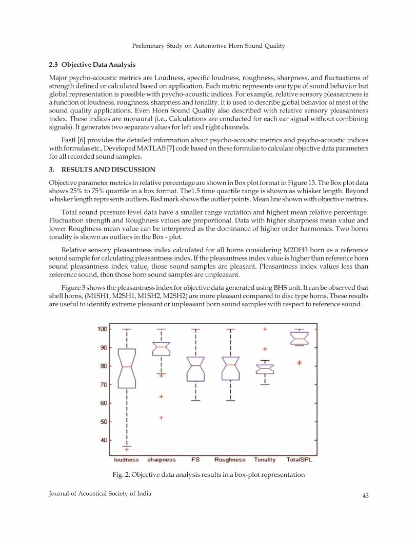
Objective parameter metrics in relative percentage are shown in Box plot format in Figure 13. The Box plot datashows 25% to 75% quartile in a box format. The1.5 time quartile range is shown as whisker length. Beyondwhisker length represents outliers. Red mark shows the outlier points. Mean line shown with objective metrics.
Total sound pressure level data have a smaller range variation and highest mean relative percentage.Fluctuation strength and Roughness values are proportional. Data with higher sharpness mean value andlower Roughness mean value can be interpreted as the dominance of higher order harmonics. Two hornstonality is shown as outliers in the Box - plot.
Relative sensory pleasantness index calculated for all horns considering M2DH3 horn as a referencesound sample for calculating pleasantness index. If the pleasantness index value is higher than reference hornsound pleasantness index value, those sound samples are pleasant. Pleasantness index values less thanreference sound, then those horn sound samples are unpleasant.
Figure 3 shows the pleasantness index for objective data generated using BHS unit. It can be observed thatshell horns, (M1SH1, M2SH1, M1SH2, M2SH2) are more pleasant compared to disc type horns. These resultsare useful to identify extreme pleasant or unpleasant horn sound samples with respect to reference sound.
Fig. 2. Objective data analysis results in a box-plot representation
44 Journal of Acoustical Society of India
B. Venkatesham, N. Pradeep, Goutham and Jongdae Kim
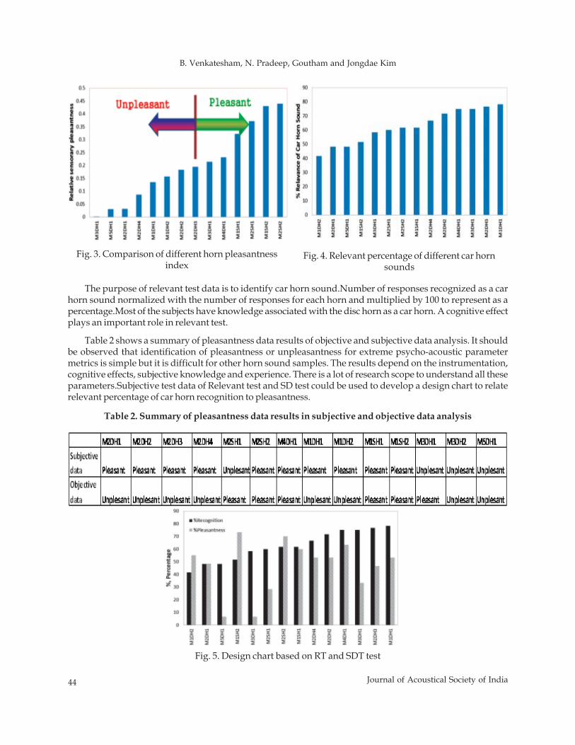
The purpose of relevant test data is to identify car horn sound.Number of responses recognized as a carhorn sound normalized with the number of responses for each horn and multiplied by 100 to represent as apercentage.Most of the subjects have knowledge associated with the disc horn as a car horn. A cognitive effectplays an important role in relevant test.
Table 2 shows a summary of pleasantness data results of objective and subjective data analysis. It shouldbe observed that identification of pleasantness or unpleasantness for extreme psycho-acoustic parametermetrics is simple but it is difficult for other horn sound samples. The results depend on the instrumentation,cognitive effects, subjective knowledge and experience. There is a lot of research scope to understand all theseparameters.Subjective test data of Relevant test and SD test could be used to develop a design chart to relaterelevant percentage of car horn recognition to pleasantness.
Table 2. Summary of pleasantness data results in subjective and objective data analysis
Fig. 3. Comparison of different horn pleasantnessindex
Fig. 4. Relevant percentage of different car hornsounds
Fig. 5. Design chart based on RT and SDT test
Preliminary Study on Automotive Horn Sound Quality
45Journal of Acoustical Society of India
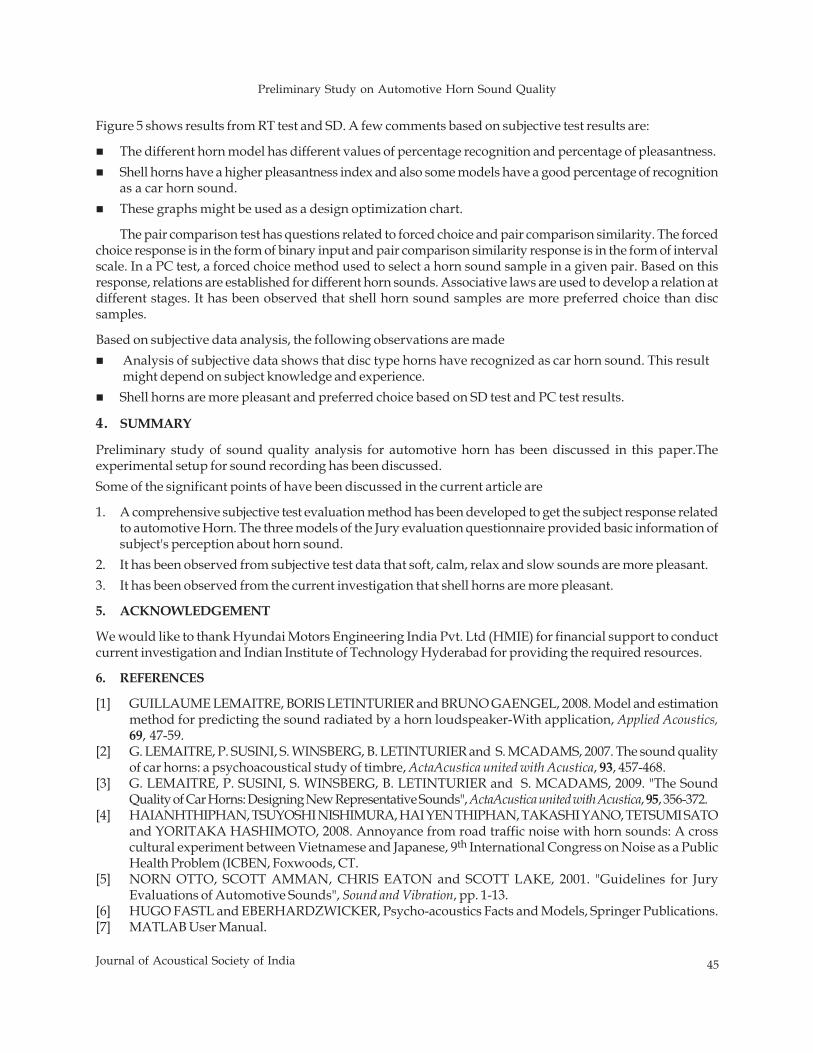
Figure 5 shows results from RT test and SD. A few comments based on subjective test results are:
The different horn model has different values of percentage recognition and percentage of pleasantness.Shell horns have a higher pleasantness index and also some models have a good percentage of recognitionas a car horn sound.These graphs might be used as a design optimization chart.
The pair comparison test has questions related to forced choice and pair comparison similarity. The forcedchoice response is in the form of binary input and pair comparison similarity response is in the form of intervalscale. In a PC test, a forced choice method used to select a horn sound sample in a given pair. Based on thisresponse, relations are established for different horn sounds. Associative laws are used to develop a relation atdifferent stages. It has been observed that shell horn sound samples are more preferred choice than discsamples.
Based on subjective data analysis, the following observations are madeAnalysis of subjective data shows that disc type horns have recognized as car horn sound. This resultmight depend on subject knowledge and experience.Shell horns are more pleasant and preferred choice based on SD test and PC test results.
4. SUMMARY
Preliminary study of sound quality analysis for automotive horn has been discussed in this paper.Theexperimental setup for sound recording has been discussed.Some of the significant points of have been discussed in the current article are
1. A comprehensive subjective test evaluation method has been developed to get the subject response relatedto automotive Horn. The three models of the Jury evaluation questionnaire provided basic information ofsubject's perception about horn sound.
2. It has been observed from subjective test data that soft, calm, relax and slow sounds are more pleasant.3. It has been observed from the current investigation that shell horns are more pleasant.
5. ACKNOWLEDGEMENT
We would like to thank Hyundai Motors Engineering India Pvt. Ltd (HMIE) for financial support to conductcurrent investigation and Indian Institute of Technology Hyderabad for providing the required resources.
6. REFERENCES
[1] GUILLAUME LEMAITRE, BORIS LETINTURIER and BRUNO GAENGEL, 2008. Model and estimationmethod for predicting the sound radiated by a horn loudspeaker-With application, Applied Acoustics,69, 47-59.
[2] G. LEMAITRE, P. SUSINI, S. WINSBERG, B. LETINTURIER and S. MCADAMS, 2007. The sound qualityof car horns: a psychoacoustical study of timbre, ActaAcustica united with Acustica, 93, 457-468.
[3] G. LEMAITRE, P. SUSINI, S. WINSBERG, B. LETINTURIER and S. MCADAMS, 2009. "The SoundQuality of Car Horns: Designing New Representative Sounds", ActaAcustica united with Acustica, 95, 356-372.
[4] HAIANHTHIPHAN, TSUYOSHI NISHIMURA, HAI YEN THIPHAN, TAKASHI YANO, TETSUMI SATOand YORITAKA HASHIMOTO, 2008. Annoyance from road traffic noise with horn sounds: A crosscultural experiment between Vietnamese and Japanese, 9th International Congress on Noise as a PublicHealth Problem (ICBEN, Foxwoods, CT.
[5] NORN OTTO, SCOTT AMMAN, CHRIS EATON and SCOTT LAKE, 2001. "Guidelines for JuryEvaluations of Automotive Sounds", Sound and Vibration, pp. 1-13.
[6] HUGO FASTL and EBERHARDZWICKER, Psycho-acoustics Facts and Models, Springer Publications.[7] MATLAB User Manual.

34 Journal of Acoustical Society of India
V. Bhanumathy, R. Geetha and M. Sangeetha
ABSTRACT
Environmental noise present in hospitals is a common stressor and is recognized as a serious healthhazard for patients, doctors and medical care workers. The aim of the work is to assess the existingnoise levels in a 112 bed hospital situated in the heart of Tiruchirapalli city. The plan of the studywas to measure the variations of noise in various wards of the hospital and appraise the mainsources of noise. Noise levels in 12 places , 6 inside the wards and 6 outside the wards weremeasured at two and a half hour intervals over a period of 12 hours. The equivalent sound level andpeak sound pressure levels were monitored by a digital sound level meter Quest suite professional2900, during a week in May 2012. The highest mean Leq(A) was 67.7 dB(A) and maximum noise levelwas 80.6 dB(A) during the measurement time in female ward and the lowest mean Leq(A) 62.1 dB(A)and minimum 55.8dB(A) in the general ward. Maximum noise levels were recordrd in the receptionoutside the wards of the hospital.The observed noise levels exceeded the recommended CPCB &WHO guidelines for hospitals. It is found that ward structures, location and various activities likeconversation of patients, nurses , visitors and traffic resulted in different levels of noise in differentwards. The study concludes that noise is a problem in the city hospital where the study was undertaken.
1. INTRODUCTION
Hospitals are extremely noisy, and noise levels in most hospitals far exceed recommended guidelines. Manystudies have revealed that extended exposure to noise pollution may cause auditory and non-auditorydisorders, such as temporary or permanent hearing loss, sleep disruption(Freedman et al.,), cardiovasculardysfunction, speech interference and mental health distortion(Ising and Kruppa). Conversation amongpatients, staff and visitors, sounds of doors, carts, phones, beepers, movement of hospital equipment etc.,make up the “Sound environment” which is a risk to healthcare. Whether by accident or incident, theaccumulation of noise and unwanted distraction add up to a negative healthcare experience. The UnitedStates Environmental Protection Agency (USEPA) recommended a guideline value for continuous backgroundnoise as 45 dB(A) during the day and 35 dB(A) at night in patients’ room. The International Noise Controland the World Health Organizations (WHO) have recommended that noise levels in hospital areas should be35-40 dB in the day time and 30-40dB(A) in the evening.. In India, noise around hospitals is around 85 dB(A)in major cities(The Hindu Dec 10, 2010). The present study was undertaken to assess noise levels, patternsand sources on wards in a 112 bed room hospital at the heart of Thiruchirapalli city.
2. MATERIALS AND METHODS
The study was conducted after obtaining institutional ethical clearance at the 112 bedded hospital with
Journal of Acoustical Society of India : Vol. 40, No. 1, 2013 (pp. 34-39)
Noise pollution in Wards of a Hospital inTiruchirapalli City
V. Bhanumathy, R. Geetha and M. SangeethaDepartment of physics, Seethalakshmi Ramaswami College, Tiruchirapalli
[Received: 18.11.2012; Revised: 28.11.2012; Accepted: 08.01.2013]
© 2013 Acoustical Society of India
Noise pollution in Wards of a Hospital in Tiruchirapalli City
35Journal of Acoustical Society of India
a bed occupancy rate of 85% and a daily attendance of about 350 outpatients. The hospital is located in acommercial area at the heart of Tiruchirapalli city housing many shopping complexes with hectic activityfrom morning 7a.m to evening 9p.m.Many two wheelers and automobiles ply near the hospital and traffichold up is a frequent event. Impatient drivers honk their horns unmindful of the presence of a big hospital.Sound levels in 12 places inside the hospital were recorded using a Digital Sound Level Meter (Quest suiteProfessional 2900) in dB (A) units, representing the sound level measured with the A-Weighting network.The instrument incorporates a type-1 microphone and records sound ranging from 50-110 dB(A). Fast modewas used to record the readings. The Sound Level Meter was placed at body level for measurements. Thereadings were taken throughout the day at five minute interval between successive recordings. Observationswere done in one week during the morning 7.30-10.00 a.m., forenoon 10.30-1.00 p.m., afternoon 1.30-4.00p.m., and evening 4.30-7.00 p.m. The parameter used in the discussion of noise pollution is the equivalentcontinuous noise level (Leq) expressed in dB(A) which is the mean rate at which energy is received by thehuman ear during the period monitored. The other variables obtained were the maximum (Lmax) and minimum(Lmin) at each place. The data were tabulated using Microsoft excel 2010 and descriptive statistics carried outusing the statistical package SPSS for windows, version 14.0.
3. RESULTS AND DISCUSSION
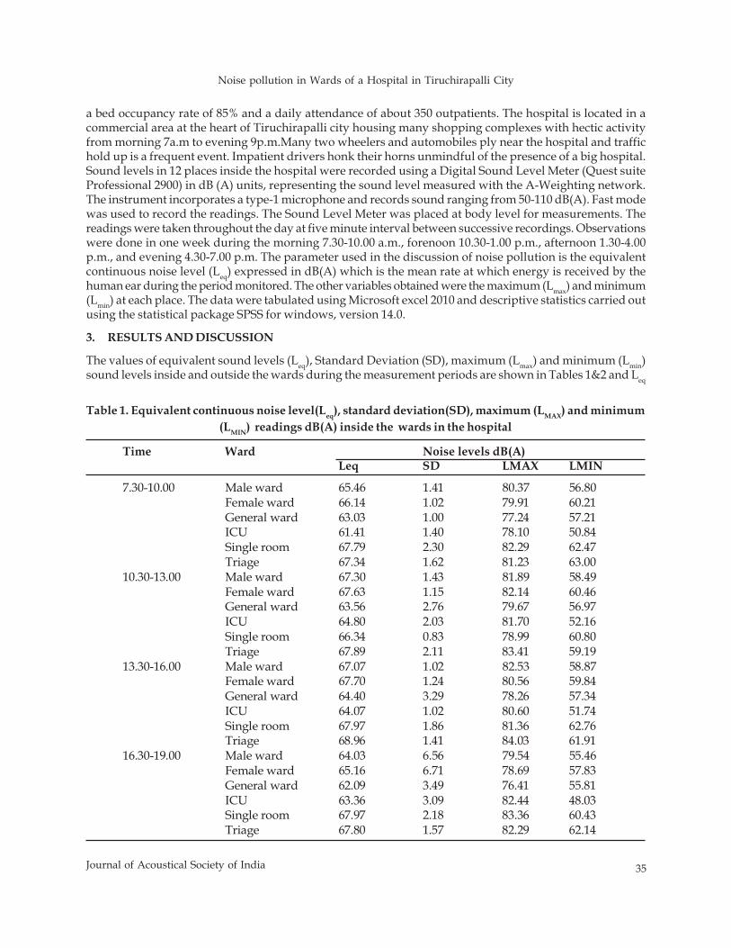
The values of equivalent sound levels (Leq), Standard Deviation (SD), maximum (Lmax) and minimum (Lmin)sound levels inside and outside the wards during the measurement periods are shown in Tables 1&2 and Leq
Time Ward Noise levels dB(A)Leq SD LMAX LMIN
7.30-10.00 Male ward 65.46 1.41 80.37 56.80Female ward 66.14 1.02 79.91 60.21General ward 63.03 1.00 77.24 57.21ICU 61.41 1.40 78.10 50.84Single room 67.79 2.30 82.29 62.47Triage 67.34 1.62 81.23 63.00
10.30-13.00 Male ward 67.30 1.43 81.89 58.49Female ward 67.63 1.15 82.14 60.46General ward 63.56 2.76 79.67 56.97ICU 64.80 2.03 81.70 52.16Single room 66.34 0.83 78.99 60.80Triage 67.89 2.11 83.41 59.19
13.30-16.00 Male ward 67.07 1.02 82.53 58.87Female ward 67.70 1.24 80.56 59.84General ward 64.40 3.29 78.26 57.34ICU 64.07 1.02 80.60 51.74Single room 67.97 1.86 81.36 62.76Triage 68.96 1.41 84.03 61.91
16.30-19.00 Male ward 64.03 6.56 79.54 55.46Female ward 65.16 6.71 78.69 57.83General ward 62.09 3.49 76.41 55.81ICU 63.36 3.09 82.44 48.03Single room 67.97 2.18 83.36 60.43Triage 67.80 1.57 82.29 62.14
Table 1. Equivalent continuous noise level(Leq), standard deviation(SD), maximum (LMAX) and minimum(LMIN) readings dB(A) inside the wards in the hospital
36 Journal of Acoustical Society of India
V. Bhanumathy, R. Geetha and M. Sangeetha
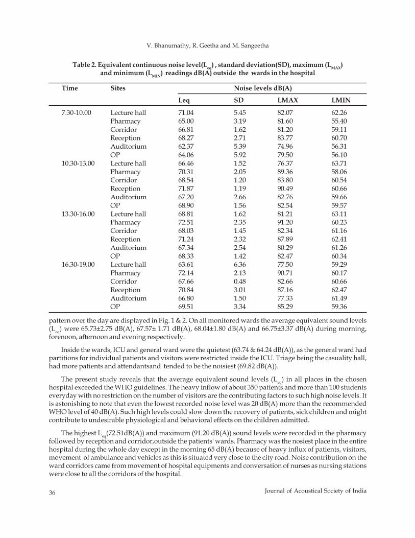
pattern over the day are displayed in Fig. 1 & 2. On all monitored wards the average equivalent sound levels(Leq) were 65.73±2.75 dB(A), 67.57± 1.71 dB(A), 68.04±1.80 dB(A) and 66.75±3.37 dB(A) during morning,forenoon, afternoon and evening respectively.
Inside the wards, ICU and general ward were the quietest (63.74 & 64.24 dB(A)), as the general ward hadpartitions for individual patients and visitors were restricted inside the ICU. Triage being the casuality hall,had more patients and attendantsand tended to be the noisiest (69.82 dB(A)).
The present study reveals that the average equivalent sound levels (Leq) in all places in the chosenhospital exceeded the WHO guidelines. The heavy inflow of about 350 patients and more than 100 studentseveryday with no restriction on the number of visitors are the contributing factors to such high noise levels. Itis astonishing to note that even the lowest recorded noise level was 20 dB(A) more than the recommendedWHO level of 40 dB(A). Such high levels could slow down the recovery of patients, sick children and mightcontribute to undesirable physiological and behavioral effects on the children admitted.
The highest Leq(72.51dB(A)) and maximum (91.20 dB(A)) sound levels were recorded in the pharmacyfollowed by reception and corridor,outside the patients' wards. Pharmacy was the nosiest place in the entirehospital during the whole day except in the morning 65 dB(A) because of heavy influx of patients, visitors,movement of ambulance and vehicles as this is situated very close to the city road. Noise contribution on theward corridors came from movement of hospital equipments and conversation of nurses as nursing stationswere close to all the corridors of the hospital.
Time Sites Noise levels dB(A)
Leq SD LMAX LMIN
7.30-10.00 Lecture hall 71.04 5.45 82.07 62.26Pharmacy 65.00 3.19 81.60 55.40Corridor 66.81 1.62 81.20 59.11Reception 68.27 2.71 83.77 60.70Auditorium 62.37 5.39 74.96 56.31OP 64.06 5.92 79.50 56.10
10.30-13.00 Lecture hall 66.46 1.52 76.37 63.71Pharmacy 70.31 2.05 89.36 58.06Corridor 68.54 1.20 83.80 60.54Reception 71.87 1.19 90.49 60.66Auditorium 67.20 2.66 82.76 59.66OP 68.90 1.56 82.54 59.57
13.30-16.00 Lecture hall 68.81 1.62 81.21 63.11Pharmacy 72.51 2.35 91.20 60.23Corridor 68.03 1.45 82.34 61.16Reception 71.24 2.32 87.89 62.41Auditorium 67.34 2.54 80.29 61.26OP 68.33 1.42 82.47 60.34
16.30-19.00 Lecture hall 63.61 6.36 77.50 59.29Pharmacy 72.14 2.13 90.71 60.17Corridor 67.66 0.48 82.66 60.66Reception 70.84 3.01 87.16 62.47Auditorium 66.80 1.50 77.33 61.49OP 69.51 3.34 85.29 59.36
Table 2. Equivalent continuous noise level(Leq) , standard deviation(SD), maximum (LMAX)and minimum (LMIN) readings dB(A) outside the wards in the hospital
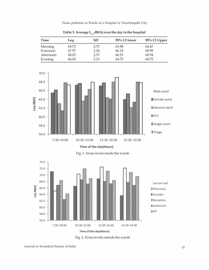
Noise pollution in Wards of a Hospital in Tiruchirapalli City
37Journal of Acoustical Society of India
Fig. 2. Noise levels outside the wards
Table 3. Average Leq dB(A) over the day in the hospital
Time Leq SD 95% CI lower 95% CI Upper
Morning 65.73 2.75 63.98 64.47Forenoon 67.57 2.24 66.14 68.99Afternoon 68.03 2.37 66.53 69.54Evening 66.02 3.15 64.75 68.75
Fig. 1. Noise levels inside the wards
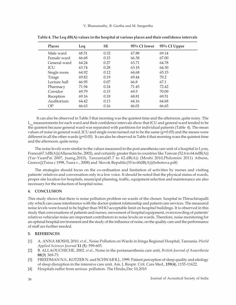
38 Journal of Acoustical Society of India
V. Bhanumathy, R. Geetha and M. Sangeetha
Places Leq SE 95% CI lower 95% CI Upper
Male ward 68.51 0.32 67.88 69.14Female ward 66.68 0.15 66.38 67.00General ward 64.24 0.27 63.71 64.78ICU 63.74 0.28 63.18 64.30Single room 64.92 0.12 64.68 65.15Triage 69.82 0.19 69.44 70.2Lecture hall 66.95 0.07 66.8 67.1Pharmacy 71.94 0.24 71.45 72.42Corridor 69.79 0.15 69.5 70.09Reception 69.16 0.18 68.81 69.51Auditorium 64.42 0.13 64.16 64.68OP 66.63 0.16 66.01 66.65
Table 4. The Leq dB(A) values in the hospital at various places and their confidence intervals
It can also be observed in Table 3 that morning was the quietest time and the afternoon ,quite noisy. TheLeq measurements for each ward and their confidence intervals show that ICU and general ward tended to bethe quietest because general ward was separated with partitions for individual patients (Table 4). The meanvalues of noise in general ward, ICU and single room turned out to be the same (p>0.05) and the means weredifferent in all the other wards (p<0.05) It can also be observed in Table 4 that morning wass the quietest timeand the afternoon ,quite noisy.
The noise levels were similar to the values measured in the post anesthesia care unit of a hospital in Lyon,France(67.1dB(A))(Allaouchiche, 2002), and certainly greater than in countries like Taiwan (52.6 to 64.6dB(A))(Yar-YuanPai 2007, Juang,2010), Tanzania(45.7 to 62.dB(A)) (Moshi 2010,Philomini 2011) Athens,Greece()(Tsiou c 1998, Tsara v., 2008) and Slovok Republic(35 to 60dB(A))(Sobotova.pdf)
The strategies should focus on the co-ordination and limitation of activities by nurses and visitingpatients' relatives and conversation only in a low voice. It should be noted that the physical status of wards,proper site location for hospitals, municipal planning, traffic, equipment selection and maintenance are alsonecessary for the reduction of hospital noise.
4. CONCLUSION
This study shows that there is noise pollution problem on wards of the chosen hospital in Thiruchirapallicity which can cause interference with the doctor-patient relationship and patient care services. The measurednoise levels were found to be higher than WHO acceptable limit on hospital buildings. It is observed in thisstudy that conversations of patients and nurses, movement of hospital equipment, overcrowding of patients'relatives vehicular noise are important contributors to noise levels on wards. Therefore, noise monitoring foran optimal hospital environment and the study of the influence of noise, on the quality care and the performanceof staff are further needed.
5. REFERENCES
[1] A. ANNA MOSHI, 2010. et al., Noise Pollution on Wards in Iringa Regional Hospital, Tanzania. WorldApplied Sciences Journal 11 (5): 599-603.
[2] B. ALLAOUCHICHE, 2002. et al., Noise in the postanaesthesia care unit, British Journal of Anaesthesia88(3) 369-73.
[3] FREEDMAN N.S., KOTZER N. and SCHWAB R.J., 1999. Patient perception of sleep quality and etiologyof sleep disruption in the intensive care unit. Am. J. Respir. Crit. Care Med., 159(4), 1155-11622.
[4] Hospitals suffer from serious pollution- The Hindu,Dec 10,2010

Noise pollution in Wards of a Hospital in Tiruchirapalli City
39Journal of Acoustical Society of India
[5] ISING, H. and B. KRUPPA, 2004. Health effects caused by Noise: Evidence in the Literature from thepast 25 years. Noise Health, 22: 5-13.
[6] D.F. JUANG; 1C.H. LEE; 1T. YANG; 2M.C. CHANG, 2010. Noise pollution and its effects on medicalcare workers and patients Environ. Sci. Tech., 7 (4), 705-716, Autumn.
[7] KULWA M. PHILIMONI, 2011. et al., Noise Pollution on Wards in Bunda District Hospital in LakeVictoria Zone, Tanzania. International Journal Of Environmental Sciences 1, No 5.
[8] SABOTOVA et.al., The acoustical environment and health risk in hospitals http://isee.ehc.ro/past_celadna/session3/11_sobotova.pdf.
[9] TSARA V, NENA E, SERASLI E, VASILEIADIS V, MATAMIS D and CHRISTAKI P., 2008. Noise levelsin Greek hospitals. Noise Health 10:110-2.
[10] TSIOU C, EFTYMIATOS D, 1998. et al., Noise sources and levels in the Evgenidion Hospital intensivecare unit. Intensive Care Med. Aug; 24 (8):845-7.
[11] WHO guidelines for Community Noise, World Health Organisation (WHO), 2010. <http://whqlibdoc.who.int/hq/2010>
[12] YAR-YUAN PAI, 2007. International Journal of Occupation Safety Ergon; Vol 13: 83-90.
Speech Rhythm in Individuals with Stuttering
51Journal of Acoustical Society of India
ABSTRACT
The objective of this study was to investigate speech rhythm in persons who stutter. Ten adults whostutter and ten age and gender matched controls participated in the study. Participants in both thegroups were native speakers of Kannada. Five sentences were constructed in Kannada and theparticipants were asked to read out these sentences. Using Praat software, two kinds of rhythmmetrics were calculated- pairwise variability indices and interval measures. Pairwise variabilityindices include normalized Pairwise Variability Index for vocalic intervals (nPVI - V) and raw PairwiseVariability Index for consonantal intervals (rPVI - C). Interval measures include percentage of vocalicintervals, standard deviation of the vocalic and consonantal intervals, and coefficient of variables forvocalic and consonantal intervals. Significant difference (p < 0.05) between the two groups waspresent for all the interval measures except coefficient of variables for vocalic intervals. However,there was no significant difference (p > 0.05) between the groups for Pairwise variability measures(nPVI - V and rPVI - C). The durational differences between the successive stressed and unstressedsegments are taken into consideration in pairwise variability indices. The findings of the presentstudy indicate that few measures of speech rhythm are deviant in persons who stutter while theothers indicate that they follow the same rhythm pattern.
1. INTRODUCTION
Stuttering is a developmental disorder of speech generally characterized by repetitions, prolongations andsilent blocks. It is estimated that 1% of the world's population stutters. Stuttering usually starts between 2 and4 years of age and in 50% of the children, condition persists. Although stuttering is one of the extensivelyresearched topics in the field of speech pathology, till today, its cause remains unknown. Previously, severalattempts have been made to understand the underlying mechanisms behind stuttering. Numerous studieshave shown timing irregularities in stutterers' fluent speech and report that stutterers have longer voice onsettimes (VOT), longer voice initiation times (VIT), longer voice termination times (VTT), and longer voweldurations (Agnello, 1975; Agnello, Wingate, and Wendell, 1974 among others) than nonstutterers. However,few other studies (Cullinan and Springer, 1980; McFarlane and Shipley, 1981; Venkatagiri, 1982) did not findany timing abnormalities when compared to nonstutterers. One reason for the differences in the results may bedifferent response modes employed (phonatory gestures, phonation of speech-like sounds, phonation of words,etc.) and differences in the severity of stuttering.
Many other studies have investigated the regularities in the timing of speech and non-speech events. Somestudies have found stutterers to be more variable than fluent peers (Boutsen, Brutten, & Watts, 2000), but othershave found no differences between groups (Max and Yudman, 2003; Zelaznik, Smith, and Franz, 1994). Mostof these studies have investigated the temporal patterning or rhythm at the segmental level. Although stutteringis disorder in the rhythm of speech, to date, surprisingly no study has been attempted quantifying speech
Journal of Acoustical Society of India : Vol. 40, No. 1, 2013 (pp.51-55)
© 2013 Acoustical Society of India
Speech Rhythm in Individuals with Stuttering
M. Santosh, Priyanka Parakh and V. SahanaAll India Institute of Speech and Hearing, Manasagangothri, Mysore-570 006
[Received: 14.12.2012; Revised: 29.12.2012; Accepted: 05.01.2013]
52 Journal of Acoustical Society of India
M. Santosh, Priyanka Parakh and V. Sahana
rhythm in sentence level in stuttering individuals. One reason for this could be difficulty with the quantificationof speech rhythm.
Over the years, studies in the speech rhythm have mainly focused on classifying languages based on theisochrony principle. Isochrony principle states that languages can be either stress-timed or syllable timed. Athird type of rhythm, mora timed was also proposed by Ladefoged (1975).Traditionally languages were classifiedinto different rhythmic classes based on perception. However, with the development of quantification measureslike pairwise variability index (PVI), more work is done at the production level. Pairwise variability index (PVI)calculates the pattering of successive vocalic and intervocalic (or consonantal) intervals showing how onelinguistic unit differs from its neighbor. Two measures are derived using PVI; normalized pairwise variabilityindex (nPVI) and raw pairwise variability index (rPVI). Both these measures help in computing the variabilityof successive measurements. Both these measures have been successfully used to classify different languagesas stressed-timed, syllable timed or mora-timed. As these durational measures can be used to quantify variabilityin successive acoustic phonetic intervals, it will be interesting to see if stutterers differ from their fluent peers onthese different measures of durational variability. Such evidence will fill remaining gaps in the field's knowledgeand help us understanding the mechanisms underlying stuttering. Hence, the aim of this study was toinvestigate (1) whether stutterers differ from nonstutterers on the measures of speech rhythm
2. METHOD
2.1 Subjects
Ten male adults with stuttering (AWS) in the age range of 17 - 30 (mean age - 21.27 years) years and ten age andgender matched controls (AWNS) (mean age - 20.9 years) participated in the study. Participants in both thegroups were native speakers of Kannada. Adults who stuttered reported to have developmental stuttering andno history of other neurological, psychological and communication problems.
2.2 Procedure
Three tasks were recorded from each participant. First was reading standardized 300- word reading passagein Kannada. Second task was conversation between the second author and client. Third task was reading fivesentences. First two tasks were used to calculate severity of stuttering and third task for measurement ofrhythm. Participants were given set of sentences, and were instructed to silently read and rehearse. Once theywere well versed with the material, recording of these sentences was done. They were instructed to read thesentences in their normal loudness and comfortable rate. They were asked to read the same sentences if theymade any mistake while reading the sentences. The control participants also read the same set of sentences inthe manner described above.
2.3 Analysis
First, the recorded sentences were edited by removing the silences between the words (Grabe & Low, 2002) andalso omitting the disfluencies in AWS. Using wideband spectrogram, vocalic and consonantal intervals weremeasured for all edited sentences. The duration between the onset and the offset of the vowel or cluster ofvowels was considered as the vocalic duration. Similarly, the duration between the onset and the offset of theconsonant or a cluster of consonants was taken as the consonantal duration. The rules that governed thesegmentation of the sounds were based on former studies on rhythm analysis and acoustic analysis (e.g.,Peterson & Lehiste, 1967). The boundary between the vocalic and the consonantal interval was indicted by asignificant drop in the amplitude and a break in the second formant structure. The identification of consonantboundaries was made easy by the cues obtained from the spectrogram which was associated to the manner ofproduction of that sound. Apart from this standard criterion, a few other factors were considered to obtainconsistency in the measurements. As it is difficult to determine the boundaries of approximants reliably, theywere taken as a part of vocalic interval (White & Mattys, 2007). Pre- vocalic glides were included in theconsonantal duration and the post vocalic glides were included in the vocalic duration (Ramus et al., 1999).Aspiration following the stop release was taken in the consonant duration (White & Mattys, 2007). Eventhough there was significant lengthening noticed in the phrase final position, it was not excluded from the
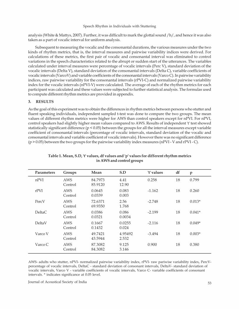
Speech Rhythm in Individuals with Stuttering
53Journal of Acoustical Society of India
analysis (White & Mattys, 2007). Further, it was difficult to mark the glottal sound /h/, and hence it was alsotaken as a part of vocalic interval for uniform analysis.
Subsequent to measuring the vocalic and the consonantal durations, the various measures under the twokinds of rhythm metrics, that is, the interval measures and pairwise variability indices were derived. Forcalculations of these metrics, the first pair of vocalic and consonantal interval was eliminated to controlvariations in the speech characteristics related to the abrupt or sudden start of the utterances. The variablescalculated under interval measures were percentage of vocalic intervals (Perc V), standard deviation of thevocalic intervals (Delta V), standard deviation of the consonantal intervals (Delta C), variable coefficients ofvocalic intervals (VarcoV) and variable coefficients of the consonantal intervals (Varco C). In pairwise variabilityindices, raw pairwise variability for the consonantal intervals (rPVI-C) and normalized pairwise variabilityindex for the vocalic intervals (nPVI-V) were calculated. The average of each of the rhythm metrics for eachparticipant was calculated and these values were subjected to further statistical analysis. The formulas usedto compute different rhythm metrics are provided in appendix.
3. RESULTS
As the goal of this experiment was to obtain the differences in rhythm metrics between persons who stutter andfluent speaking individuals, independent sampled t-test was done to compare the two groups. The meanvalues of different rhythm metrics were higher for AWS than control speakers except for nPVI. For nPVI,control speakers had slightly higher mean values compared to AWS. Results of independent 't' test showedstatistically significant difference (p < 0.05) between the groups for all the interval measures except variablecoefficient of consonantal intervals (percentage of vocalic intervals, standard deviation of the vocalic andconsonantal intervals and variable coefficient of vocalic intervals). However there was no significant difference(p > 0.05) between the two groups for the pairwise variability index measures (nPVI - V and rPVI - C).
Parameters Groups Mean S.D 't' values df p
nPVI AWS 84.7973 4.41 0.258 18 0.799Control 85.9120 12.90
rPVI AWS 0.0645 0.083 -1.162 18 0.260Control 0.0339 0.003
PercV AWS 72.6371 2.56 -2.748 18 0.013*Control 69.9350 1.768
DeltaC AWS 0.0386 0.086 -2.199 18 0.041*Control 0.0321 0.0034
DeltaV AWS 0.1667 0.0255 -2.116 18 0.049*Control 0.1432 0.024
Varco V AWS 49.7421 4.95492 -3.494 18 0.003*Control 43.5944 2.532
Varco C AWS 87.3082 9.125 0.900 18 0.380Control 84.3082 3.146
AWS- adults who stutter, nPVI- normalized pairwise variability index, rPVI- raw pariwise variability index, PercV-percentage of vocalic intervals, DeltaC - standard deviation of consonant intervals, DeltaV- standard deviation ofvocalic intervals, Varco V - variable coefficients of vocalic intervals, Varco C- variable coefficients of consonantintervals. * indicates significance at 0.05 level.
Table 1. Mean, S.D, 't' values, df values and 'p' values for different rhythm metricsin AWS and control groups
54 Journal of Acoustical Society of India
M. Santosh, Priyanka Parakh and V. Sahana
4. DISCUSSION
Here in our study, we investigated the sensitivity of pairwise variability indices and few other additionalinterval measures in differentiating speech rhythm of AWS and control speakers. Results showed significantdifference between two groups only for selected interval measures (PercV, Delta V, Delta C, Varco V). Resultshighlight that selected rhythm metrics can be objectively used to document the rhythm abnormalities in peoplewho stutter. However, there was no significant difference between the two groups for PVI measures. Thedurational differences between the successive vocalic and intervocalic segments are considered in pairwisevariability index. Pairwise variability index (PVI) calculates the pattering of successive vocalic and intervocalic(or consonantal) intervals showing how one linguistic unit differs from its neighbor (Low, 1998). The values ofPVI indices of AWS were similar to control participants. This suggests AWS are indistinguishable from controlparticipants if we measure their rhythm using PVI. The results support similar observations for non-speechsounds (Max & Yudman, 2003) and suggest that individuals who stutter are not deficient with their isochronousrhythm timing if we document using PVI measures.5. CONCLUSION
This study documents the rhythm abnormalities in persons with stuttering. As there is a mixed literatureregarding the notion of stuttering as a disorder of speech rhythm and timing abnormalities, the findings of thepresent study also is similar, i.e., a few measures indicating that the speech rhythm characteristics are deviantin persons with stuttering while the others indicating that they follow the same rhythm pattern. The resultshave positive implications for speech language pathologists. Selected activities can be taken up to teachrhythm to patients with aprosodia considering the fact that one knows the type of rhythm in that language.6. APPENDIX : FORMULAES USED
1. Normalized pair - wise variability index of Vocalic interval (nPVI-V):nPVI-V = 100*(k=1Σ m-1 | (dk - dk+1)/(dk + dk+1)/2|)/(m-1)
2. Raw pair - wise variability index of the Consonantal interval (rPVI-C):rPVI-C = (k=1Σ m-1 |dk - dk+1|)/(m-1)
3. Percentage of Vocalic interval: %V =ΣV/Σ (V + C)4. Delta C: Δ C = Standard deviation of C5. Delta V:Δ V = Standard deviation of V6. Variable coefficient of consonantal Interval (VarcoC): VarcoC = Δ C/Average C7. Variable coefficient of Vocalic Interval (VarcoV): VarcoV = Δ V/Average VAbbreviations index:m = total number of intervalsd = duration of "kth" intervalV = duration of vocalic intervalC = duration of consonant interval
7. REFERENCES
[1] J. AGNELLO, 1975. Voice onset and voice termination features of stutterers. In: L. M. Webster and L. C. Furst(Eds.), Vocal tract dynamics and dysfluency. New York: Speech and Hearing institute.
[2] J. AGNELLO, M.E. WINGATE and M. WENDELL, 1974. Voice onset and termination times of children andadult stutterers. Journal of the Acoustical Society of America, 56,p. S62.
[3] F.R. BOUTSEN, G.J. BRUTTEN and CR. WATTS, 2000. Timing and intensity variability in the metronomicspeech of stuttering and nonstuttering speakers. Journal of Speech, Language and Hearing Research, 43, 513-520.
[4] W.L. CULLINAN and M.T. SPRINGER, 1980. Voice initiation and termination times in stuttering andnon stuttering children. Journal of Speech and Hearing Research, 23, 344 - 360.

Speech Rhythm in Individuals with Stuttering
55Journal of Acoustical Society of India
[5] E. GRABE and E.L. LOW, 2002. Durational variability in speech and the rhythm class hypothesis. In N.Warner, & C. Gussenhoven (Eds.), Papers in laboratory phonology 7 (pp. 515-546). Berlin: Mouton deGruyter.
[6] P. LADEFOGED, 1975. A course in Phonetics. New York: Harcourt Brace Jovanovich.[7] L. MAX and E.M. YUDMAN, 2003. Accuracy and variability of isochronous rhythm timing across motor
systems in stuttering versus non - stuttering individuals. Journal of Speech, Language, and Hearing Research,46, 146-163.
[8] S.C. MCFARLANE and K.G. SHIPLEY, 1981. Latency of vocalization onset for stutterers and non -stutterers under conditions of auditory and visual cueing. Journal of Speech and Hearing Disorders, 46, 307- 312.
[9] G.E. PETERSON and I. LEHISTE, 1960. Duration of syllable nuclei in English. Journal of the AcousticalSociety of America, 32, 693-703.
[10] F. RAMUS, M. NESPOR and J. MEHLER, 1999. Correlates of linguistic rhythm in speech signal. Cognition,73, 265-292.
[11] H.S. VENKATAGIRI, 1982. Reaction time for "s" and "z" in stutterers and non - stutterers: A test ofdiscoordination hypothesis. Journal of Communication Disorders, 15, 55 - 62.
[12] L. WHITE and S.L. MATTYS, 2007. Calibrating rhythm: First language and second language studies.Journal of Phonetics, 35, 501 - 525.
[13] H.N. ZELAZNIK, A. SMITH and E.A. FRANZ, 1997. Differences in bimanual coordination associatedwith stuttering. Acta Psychologica, 96, 229-243.

46 Journal of Acoustical Society of India
G. Muthu Shoba Mohan
1. INTRODUCTION
The chief function of a school classroom is instruction, and instruction comes and likely will continue tocome, by word-of-mouth and listening. The school classrooms are established to promote learning, which isby speaking and listening. In elementary school classrooms, most learning involves listening to the teacherand to each other. Therefore, acoustics is one of the most important physical properties that determine howwell the school classroom building can serve its primary function. Thus the exclusion of noise and reverberationare indispensable in adapting classroom to the function of oral instruction in elementary school classrooms.
2. SCHOOLS IN INDIAN TOWN
Despite the existence of guidelines for school and classroom noise, and a body of research on the effects ofnoise on children and teachers in the classroom, there is relatively less information on noise levels outside theclassrooms and its influence within the classrooms (Dockrell and Shield 2002). The acoustics of schoolclassrooms in India are also influenced by climatic factors. In a warm-humid climate, where air-conditioningand tightly closed enclosures for the classrooms are not in practice the noise inside classrooms is highlyinfluenced by the external noise as the windows and doors are kept open.
The Speech Intelligibility is influenced by the background-noise, reverberation time and the distancefrom the source to the listener. In the classrooms of the warm-humid climate regions the possibility of increasedbackground noise in the classrooms due to the intrusion of noise through the open windows and doors alongwith the noise from fans remains higher than that in the enclosed classrooms. As the background noise is afundamental parameter for determining the intelligibility in classrooms, the assessment of speech intelligibilityin such classrooms becomes necessary. It is necessary to assess how far the typical Indian classrooms satisfythe requirement of better learning environment for school children.
3. SPEECH INTELLIGIBILITY IN CLASSROOMS
Speech Intelligibility (SI), which quantifies the quality of verbal communication, is a major concern regardingthe acoustical characteristics of classrooms. SI is the percentage of speech material presented to an averagelistener which is correctly transmitted from a speaker to a listener . Non-optimal classroom design, acousticalconditions and SI can result in impaired verbal communication between a teacher and a student, withdetrimental effects on learning. Both Bradley (2007) and Hodgson (2002) have carried out experimental andtheoretical studies to investigate the relationship between background-noise, Reverberation Time and SpeechIntelligibility in the classroom.
4. STUDY AREA
The schools evaluated are from an educationally advanced town Nagercoil located in the southern part ofIndia, in the Kanyakumari District, which is one of the 32 districts in the state of Tamilnadu, having 808schools out of which 522 are primary and middle schools with about 190,000 students . The locations of theschools in relation to noise sources vary; some are adjacent to busy roads, others are set back from the road,
Journal of Acoustical Society of India : Vol. 40, No. 1, 2013 (pp. 46-50)
Speech Intelligibligy in School Class Rooms-A Case study of Schools in an Indian Town
G. Muthu Shoba MohanMohamed Sathak School of Architecture, Kilakarai
[Received: 13.11.2012; Revised: 29.11.2012; Accepted: 17.01.2013]
© 2013 Acoustical Society of India
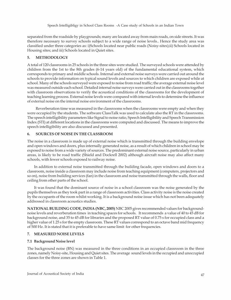
Speech Intelligibligy in School Class Rooms -A Case study of Schools in an Indian Town
47Journal of Acoustical Society of India
separated from the roadside by playgrounds; many are located away from main roads, on side streets. It wastherefore necessary to survey schools subject to a wide range of noise levels.. Hence the study area wasclassified under three categories as: i)Schools located near public roads (Noisy-sites);ii) Schools located inHousing sites; and iii) Schools located in Quiet sites.
5. METHODOLOGY
A total of 120 classrooms in 25 schools in the three sites were studied. The surveyed schools were attended bychildren from the 1st to the 8th grades (6-14 years old) of the fundamental educational system, whichcorresponds to primary and middle schools. Internal and external noise surveys were carried out around theschools to provide information on typical sound levels and sources to which children are exposed while atschool. Many of the schools surveyed were exposed to noise from road traffic; the average external noise levelwas measured outside each school. Detailed internal noise surveys were carried out in the classrooms togetherwith classroom observations to verify the acoustical conditions of the classrooms for the development ofteaching learning process. External noise levels were compared with internal levels to determine the influenceof external noise on the internal noise environment of the classrooms.
Reverberation time was measured in the classrooms when the classrooms were empty and when theywere occupied by the students. The software ClassTalk was used to calculate also the RT in the classrooms.The speech intelligibility parameters like Signal to noise ratio, Speech Intelligibility and Speech TransmissionIndex (STI) at different locations in the classrooms were computed and discussed. The means to improve thespeech intelligibility are also discussed and presented.
6. SOURCES OF NOISE IN THE CLASSROOM
The noise in a classroom is made up of external noise which is transmitted through the building envelopeand open windows and doors, plus internally generated noise, as a result of which children in school may beexposed to noise from a wide variety of sources. The predominant external noise source, particularly in urbanareas, is likely to be road traffic (Shield and Dockrell 2002) although aircraft noise may also affect manyschools, with fewer schools exposed to railway noise.
In addition to external noise transmitted through the building facade, open windows and doors to aclassroom, noise inside a classroom may include noise from teaching equipment (computers, projectors andso on), noise from building services (fan) in the classroom and noise transmitted through the walls, floor andceiling from other parts of the school.
It was found that the dominant source of noise in a school classroom was the noise generated by thepupils themselves as they took part in a range of classroom activities. Class activity noise is the noise createdby the occupants of the room whilst working. It is a background noise issue which has not been adequatelyaddressed in classroom acoustics studies.
NATIONAL BUILDING CODE, INDIA (NBC, 2005) NBC 2005 gives recommended values for background-noise levels and reverberation times in teaching spaces for schools. It recommends a value of 40 to 45 dB forbackground noise, and 35 to 45 dB for libraries and the proposed RT value of 0.75 s for occupied class and ahigher value of 1.25 s for the empty classroom. These RT values correspond to an octave band mid frequencyof 500 Hz. It is stated that it is preferable to have same limit for other frequencies.
7. MEASURED NOISE LEVELS
7.1 Background Noise level
The background noise (BN) was measured in the three conditions in an occupied classroom in the threezones, namely Noisy-site, Housing and Quiet sites. The average sound levels in the occupied and unoccupiedclasses for the three zones are shown in Table 1.
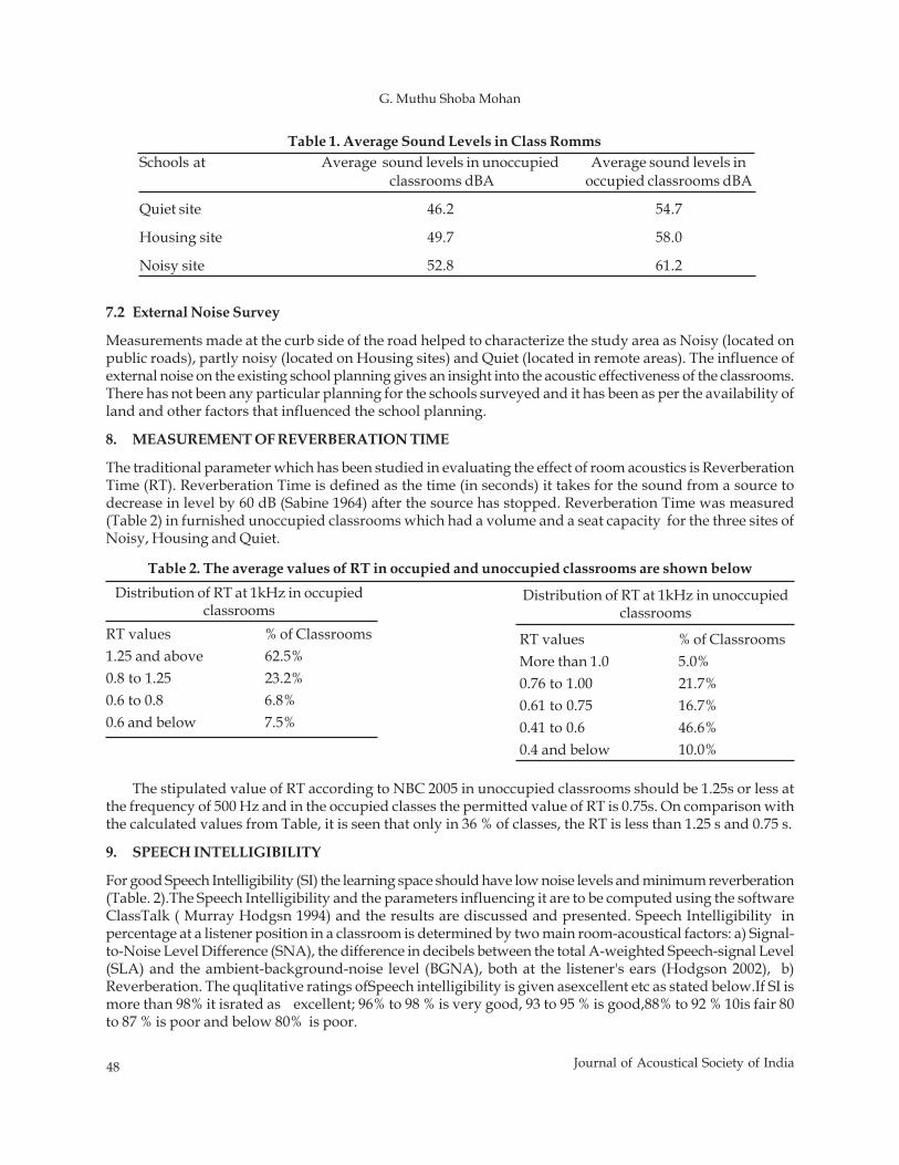
48 Journal of Acoustical Society of India
G. Muthu Shoba Mohan
Schools at Average sound levels in unoccupied Average sound levels in classrooms dBA occupied classrooms dBA
Quiet site 46.2 54.7
Housing site 49.7 58.0
Noisy site 52.8 61.2
Table 1. Average Sound Levels in Class Romms
7.2 External Noise Survey
Measurements made at the curb side of the road helped to characterize the study area as Noisy (located onpublic roads), partly noisy (located on Housing sites) and Quiet (located in remote areas). The influence ofexternal noise on the existing school planning gives an insight into the acoustic effectiveness of the classrooms.There has not been any particular planning for the schools surveyed and it has been as per the availability ofland and other factors that influenced the school planning.
8. MEASUREMENT OF REVERBERATION TIME
The traditional parameter which has been studied in evaluating the effect of room acoustics is ReverberationTime (RT). Reverberation Time is defined as the time (in seconds) it takes for the sound from a source todecrease in level by 60 dB (Sabine 1964) after the source has stopped. Reverberation Time was measured(Table 2) in furnished unoccupied classrooms which had a volume and a seat capacity for the three sites ofNoisy, Housing and Quiet.
RT values % of Classrooms1.25 and above 62.5%0.8 to 1.25 23.2%0.6 to 0.8 6.8%0.6 and below 7.5%
RT values % of ClassroomsMore than 1.0 5.0%0.76 to 1.00 21.7%0.61 to 0.75 16.7%0.41 to 0.6 46.6%0.4 and below 10.0%
Distribution of RT at 1kHz in occupiedclassrooms
Distribution of RT at 1kHz in unoccupiedclassrooms
Table 2. The average values of RT in occupied and unoccupied classrooms are shown below
The stipulated value of RT according to NBC 2005 in unoccupied classrooms should be 1.25s or less atthe frequency of 500 Hz and in the occupied classes the permitted value of RT is 0.75s. On comparison withthe calculated values from Table, it is seen that only in 36 % of classes, the RT is less than 1.25 s and 0.75 s.
9. SPEECH INTELLIGIBILITY
For good Speech Intelligibility (SI) the learning space should have low noise levels and minimum reverberation(Table. 2).The Speech Intelligibility and the parameters influencing it are to be computed using the softwareClassTalk ( Murray Hodgsn 1994) and the results are discussed and presented. Speech Intelligibility inpercentage at a listener position in a classroom is determined by two main room-acoustical factors: a) Signal-to-Noise Level Difference (SNA), the difference in decibels between the total A-weighted Speech-signal Level(SLA) and the ambient-background-noise level (BGNA), both at the listener's ears (Hodgson 2002), b)Reverberation. The quqlitative ratings ofSpeech intelligibility is given asexcellent etc as stated below.If SI ismore than 98% it israted as excellent; 96% to 98 % is very good, 93 to 95 % is good,88% to 92 % 10is fair 80to 87 % is poor and below 80% is poor.
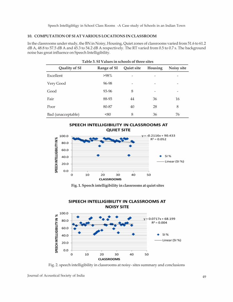
Speech Intelligibligy in School Class Rooms -A Case study of Schools in an Indian Town
49Journal of Acoustical Society of India
10. COMPUTATION OF SI AT VARIOUS LOCATIONS IN CLASSROOM
In the classrooms under study, the BN in Noisy, Housing, Quiet zones of classrooms varied from 51.6 to 61.2dB A, 48.8 to 57.5 dB A and 45.3 to 54.2 dB A respectively. The RT varied from 0.5 to 0.7 s. The backgroundnoise has great influence on Speech Intelligibility.
Quality of SI Range of SI Quiet site Housing Noisy site
Excellent >98% - - -
Very Good 96-98 - - -
Good 93-96 8 - -
Fair 88-93 44 36 16
Poor 80-87 40 28 8
Bad (unacceptable) <80 8 36 76
Table 3. SI Values in schools of three sites
Fig. 1. Speech intelligibility in classrooms at quiet sites
Fig. 2. speech intelligibility in classrooms at noisy- sites summary and conclusions
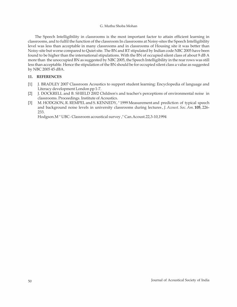
50 Journal of Acoustical Society of India
G. Muthu Shoba Mohan
The Speech Intelligibility in classrooms is the most important factor to attain efficient learning inclassrooms, and to fulfil the function of the classroom In classrooms at Noisy-sites the Speech Intelligibilitylevel was less than acceptable in many classrooms and in classrooms of Housing site it was better thanNoisy-site but worse compared to Quiet site. The BN and RT stipulated by Indian code NBC 2005 have beenfound to be higher than the international stipulations. With the BN of occupied silent class of about 9 dB Amore than the unoccupied BN as suggested by NBC 2005, the Speech Intelligibility in the rear rows was stillless than acceptable. Hence the stipulation of the BN should be for occupied silent class a value as suggestedby NBC 2005 45 dBA.
11. REFERENCES
[1] J. BRADLEY 2007 Classroom Acoustics to support student learning: Encyclopedia of language andLiteracy development London pp 1-7.
[2] J. DOCKRELL and B. SHIELD 2002 Children's and teacher's perceptions of environmental noise inclassrooms. Proceedings. Institute of Acoustics.
[3] M. HODGSON, R. REMPEL and S. KENNEDY, " 1999 Measurement and prediction of typical speechand background noise levels in university classrooms during lectures , J. Acoust. Soc. Am. 105, 226-233.Hodgson.M " UBC- Classroom acoustical survey ," Can.Acoust.22,3-10,1994
Comparing Acoustic Parameters of Conversational and Clear Speech ....... Individuals with Parkinson Disease
61Journal of Acoustical Society of India
ABSTRACT
The current study compared acoustic parameters of reading samples produced in clear speech andconversational speech conditions by individuals with Parkinson's disease (PD), grouped into threegroups of PD (early, middle and late PD) depending on disease progression. A listener judgementtask validated that instructions given to persons with PD to speak clearly indeed resulted in differencesin speech production with a large proportion of listener's judgments indicating a preference for clearspeech condition in comparison to conversational speech condition. Acoustic analysis of readingpassages demonstrated significantly increased standard deviation of Fo, standard deviation ofintensity as well as greater duration (reduced articulatory rate) in the clear speech condition incomparison to conversational reading. Further differences among the three groups of participantswith PD in acoustic parameters reveal trade-off's in the acoustic measures possibly reflectingdifferences in physiological capacities with the progression of the disease.
1. INTRODUCTION
Hypokinetic dysarthria associated with Parkinson's disease (PD) is considered to be a perceptuallydistinguishable motor speech disorder associated with basal ganglia control circuit pathology, characterizedby a progressive loss of dopamine in the brain. Clinical characterization of hypokinetic dysarthria emphasizesin rank order; monopitch, reduced stress, monoloudness, imprecise consonants, inappropriate silences,short rushes, harsh voice, continuous breathiness, pitch level disturbances, and variable rate [1]. Few studiesof speakers with dysarthria have shown that clear speech can have an important effect on intelligibility [2].Clear speech includes speaking in a deliberate manner, characterized by exaggerated articulation, reducedrate, and increased loudness relative to habitual speech. A recent study examining the acoustic characteristicsof clear speech by individuals who have hypokinetic dysarthria due to PD suggested that such an interventionmay have the potential to improve intelligibility for some speakers with dysarthria [3]. Acoustic analysisrevealed that group of individuals with PD did use some of the clear speech strategies, as indicated bysignificantly decreased articulation rate, increased mean fundamental frequency (MeanFo) and standarddeviation of speaking fundamental frequency (Fo-SD) in clear speech condition in comparison toconversational speech condition during reading and monologue [3]. Studies are necessary to describeproduction features of clear speech in individuals with dysarthria, so that those production changes that hasgreatest impact on intelligibility can be emphasized in intervention.
Journal of Acoustical Society of India : Vol. 40, No. 1, 2013 (pp. 61-65)
Comparing Acoustic Parameters of Conversational andClear Speech during Reading in Kannada Speaking
Individuals with Parkinson's Disease
Lakshmi Venkatesh and Ritu Mary MathewDr. S.R. Chandrasekhar Institute of Speech & Hearing, Bangalore
[Received: 18.12.2012; Revised: 29.12.2012; Accepted: 10.01.2013]
© 2013 Acoustical Society of India
62 Journal of Acoustical Society of India
Lakshmi Venkatesh and Ritu Mary Mathew
There is increasing evidence that acoustic/perceptual features that characterize the conversational-to-clear speech transformation may vary across languages [4]. There is some research emerging on acoustic andperceptual characterization of properties of clear speech in Indian languages. For example, clear speech inKannada was characterized by longer vowel durations and decreased speaking rate, higher mean values ofpitch, increased amplitude in spectra of consonants and fricative [5]. Research on clear speech andconversational speech in individuals with dysarthria speaking different languages would determine languagespecific acoustic/perceptual features as well as provide additional support for benefit if any of clear speechover conversational speech. The purpose of this study was to evaluate the differences in clear speech andconversational speech conditions in a reading task among individuals with dysarthria due to PD usingacoustic analysis and perceptual judgements.
2. METHOD
A total of 13 speakers with hypokinetic dysarthria due to PD (10 Male & 3 Female; Mean age 61.23 years;mean disease duration; 7.38 years) participated in the study. Participants were grouped into three groups ofPD depending on the Hoehn-Yahr Scale of disease progression such that there were four participants each inthe early and middle stages and five participants in the late stages of the development of PD. The severity ofdysarthria increased with stage. Participants were native Kannada speakers who were able to read and writeKannada. Participants with evident linguistic disturbances were excluded from the study.
Stimuli comprised of a standard reading passage in Kannada. Participants were asked to read in twospeaking styles; conversational speech condition and clear speech condition. For the conversational style,the talkers were instructed to read the passage as they would normally speak to someone familiar. For theclear speaking style, the talkers were instructed to read the passage as clearly and precisely as possible as ifthe experimenter was having trouble hearing them, or in understanding the language or as if there was noisein the background. Both speaking conditions were elicited through the use of instructions, and the participants'speech was audio-recorded as they read the passage.
Acoustic analysis of reading passage was performed by means of a commercially available software(Motor Speech Profile/ Computerized Speech Lab CSL 4300; Kay Elemetrics Corp., USA) which allowedauditory playback of marked segments. The initiation and termination of the reading passage was marked bymeans of cursors, thereby eliminating the background noise from the sample. Voiced period marks wereplaced throughout the sample. Acoustic measurements included mean fundamental frequency (meanFo),standard deviation of fundamental frequency (SD-Fo), mean intensity (mean-Int) and standard deviation ofintensity (SD-Int), measured across the entire length of the passage. In addition, the total time taken to read theentire passage was also noted. Speech samples comprising of reading passage in both speaking stylesproduced by participants were given to listeners for comparison to indicate their preference for either of thestyles or none in terms of ease of understanding and clarity of speech.
3. RESULTS AND DISCUSSION
3.1 Perceptual Judgments
As seen from Table 1, listeners indicated that clear speech was better in terms of ease of understanding andclarity of speech in comparison to the conversational speech for the task of reading passage. Out of the total130 responses, 92 listener judgments (70.77%) showed a preference for clear speech. A small number oflistener judgments 13 (10%) indicated preference for conversational speech condition over clear speech. 24(18.46%) judgments reported no preference or suggested that both conditions were perceived similar in termsof ease of understanding and clarity. 67.5% (27) and 62.5 % (25) of the listener judgements were for clearspeech condition in the early and middle PD groups respectively.
An increased number of preferences for clear speech (80%) observed in the speech of participants withsevere dysarthria associated with the late stage of PD in comparison to early and middle stages of PDsuggested that clear speech instructions resulted in changes in speech production among these participantswhich were detected by listeners to contribute to ease of understanding and clarity in light of increasedseverity of speech deficits.
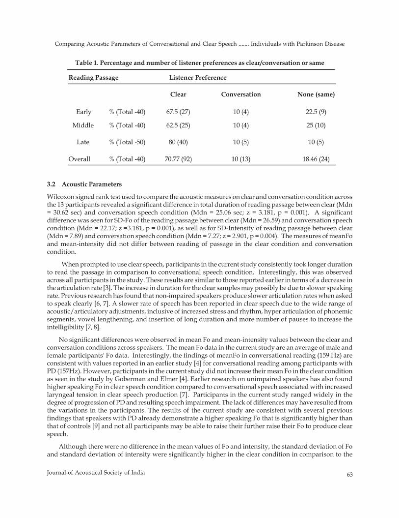
Comparing Acoustic Parameters of Conversational and Clear Speech ....... Individuals with Parkinson Disease
63Journal of Acoustical Society of India
Reading Passage Listener Preference
Clear Conversation None (same)
Early % (Total -40) 67.5 (27) 10 (4) 22.5 (9)
Middle % (Total -40) 62.5 (25) 10 (4) 25 (10)
Late % (Total -50) 80 (40) 10 (5) 10 (5)
Overall % (Total -40) 70.77 (92) 10 (13) 18.46 (24)
Table 1. Percentage and number of listener preferences as clear/conversation or same
3.2 Acoustic Parameters
Wilcoxon signed rank test used to compare the acoustic measures on clear and conversation condition acrossthe 13 participants revealed a significant difference in total duration of reading passage between clear (Mdn= 30.62 sec) and conversation speech condition (Mdn = 25.06 sec; z = 3.181, p = 0.001). A significantdifference was seen for SD-Fo of the reading passage between clear (Mdn = 26.59) and conversation speechcondition (Mdn = 22.17; z =3.181, p = 0.001), as well as for SD-Intensity of reading passage between clear(Mdn = 7.89) and conversation speech condition (Mdn = 7.27; z = 2.901, p = 0.004). The measures of meanFoand mean-intensity did not differ between reading of passage in the clear condition and conversationcondition.
When prompted to use clear speech, participants in the current study consistently took longer durationto read the passage in comparison to conversational speech condition. Interestingly, this was observedacross all participants in the study. These results are similar to those reported earlier in terms of a decrease inthe articulation rate [3]. The increase in duration for the clear samples may possibly be due to slower speakingrate. Previous research has found that non-impaired speakers produce slower articulation rates when askedto speak clearly [6, 7]. A slower rate of speech has been reported in clear speech due to the wide range ofacoustic/articulatory adjustments, inclusive of increased stress and rhythm, hyper articulation of phonemicsegments, vowel lengthening, and insertion of long duration and more number of pauses to increase theintelligibility [7, 8].
No significant differences were observed in mean Fo and mean-intensity values between the clear andconversation conditions across speakers. The mean Fo data in the current study are an average of male andfemale participants' Fo data. Interestingly, the findings of meanFo in conversational reading (159 Hz) areconsistent with values reported in an earlier study [4] for conversational reading among participants withPD (157Hz). However, participants in the current study did not increase their mean Fo in the clear conditionas seen in the study by Goberman and Elmer [4]. Earlier research on unimpaired speakers has also foundhigher speaking Fo in clear speech condition compared to conversational speech associated with increasedlaryngeal tension in clear speech production [7]. Participants in the current study ranged widely in thedegree of progression of PD and resulting speech impairment. The lack of differences may have resulted fromthe variations in the participants. The results of the current study are consistent with several previousfindings that speakers with PD already demonstrate a higher speaking Fo that is significantly higher thanthat of controls [9] and not all participants may be able to raise their further raise their Fo to produce clearspeech.
Although there were no difference in the mean values of Fo and intensity, the standard deviation of Foand standard deviation of intensity were significantly higher in the clear condition in comparison to the
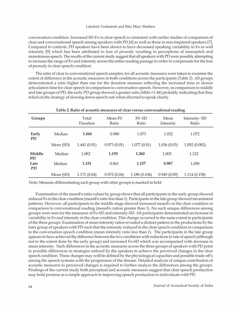
64 Journal of Acoustical Society of India
Lakshmi Venkatesh and Ritu Mary Mathew
conversation condition. Increased SD-Fo in clear speech is consistent with earlier studies of comparison ofclear and conversational speech among speakers with PD [4] as well as those in non-impaired speakers [7].Compared to controls, PD speakers have been shown to have decreased speaking variability in Fo as wellintensity [9] which has been attributed to loss of prosody resulting in perceptions of monopitch andmonotonous speech. The results of the current study suggest that all speakers with PD were possibly attemptingto increase the range of Fo and intensity across the entire reading passage in order to compensate for the lossof prosody in clear speech condition.
The ratio of clear to conversational speech samples, for all acoustic measures were taken to examine theextent of difference in the acoustic measures in both conditions across the participants (Table 2). All groupsdemonstrated a ratio higher than one for the duration measure reflecting the increased time or slowerarticulation time for clear speech in comparison to conversation speech. However, in comparison to middleand late groups of PD, the early PD group showed a greater ratio (Mdn =1.44) probably indicating that theyrelied on the strategy of slowing down speech rate when directed to speak clearly.
Groups Total Duration
Mean F0 Ratio
F0- SD Ratio
Mean Intensity
Intensity- SD Ratio
Early PD
Median 1.444 0.980 1.073 1.032 1.072
Mean (SD) 1.441 (0.01) 0.973 (0.01) 1.077 (0.01) 1.036 (0.03) 1.092 (0.082)
Middle PD
Median 1.082 1.159 1.260 1.003 1.122
Late PD
Median 1.151 0.961 1.157 0.987 1.090
Mean (SD) 1.171 (0.04) 0.972 (0.04) 1.188 (0.104) 0.945 (0.09) 1.114 (0.158)
Table 2. Ratio of acoustic measures of clear versus conversational reading
Note: Measure differentiating each group with other groups is marked in bold
Examination of the meanFo ratio values by group shows that all participants in the early group showedreduced Fo in the clear condition (meanFo ratio less than 1). Participants in the late group showed inconsistentpatterns. However, all participants in the middle stage showed increased meanFo in the clear condition incomparison to conversational reading (meanFo ration greater than 1). No such unique differences amonggroups were seen for the measures of Fo-SD and intensity-SD. All participants demonstrated an increase invariability in Fo and intensity in the clear condition. This change occurred to the same extent in participantsof the three groups. Examination of mean intensity ratios revealed a distinct pattern in the productions by thelater group of speakers with PD such that the intensity reduced in the clear speech condition in comparisonto the conversation speech condition (mean intensity ratio less than 1). The participants in the late groupappears to have achieved the difference between the two conditions with reductions in rate of speech (althoughnot to the extent done by the early group) and increased Fo-SD which was accompanied with decrease inmean intensity. Such differences in the acoustic measures across the three groups of speakers with PD pointto possible differences in strategies utilized by the speakers to achieve the perceived changes in the clearspeech condition. These changes may well be defined by the physiological capacities and possible trade-off'samong the speech systems with the progression of the disease. Detailed analysis of unique contribution ofacoustic measures to perceived changes is required to further analyze the differences among the groups.Findings of the current study both perceptual and acoustic measures suggest that clear speech productionmay hold promise as a simple approach to improving speech production in individuals with PD.
Comparing Acoustic Parameters of Conversational and Clear Speech ....... Individuals with Parkinson Disease
65Journal of Acoustical Society of India
4. REFERENCES
[1] J.R. DUFFY, 2005. Motor speech disorders. Substrates, Differential diagnosis and Management. Mosby.[2] D.R. BEUKELMAN, S. FAGER, C.ULLMAN, E. HANSON and J.A. LOGEMANN, 2002.Impact of
speech supplementation and clear speech and the intelligibility and speaking rate of speakers withtraumatic brain injury. Journal of Medical Speech Language Pathology, 10 (4), 237.
[3] A.M. GOBERMAN and L.W.ELMER, 2004. Acoustic analysis of clear versus conversational speech inindividuals with Parkinson disease. Journal of Communication Disorders, 38, 215.
[4] R. SMILJANIC, and A.R.BRADLOW, 2005. Production and perception of clear speech in Croatian andEnglish. Journal of Acoustical Society of America, 118, 1677-1688.
[5] P. KUMAR, 2008. Comparing Acoustic Parameters of Conversational and Clear Speech in Kannada.Unpublished Master Dissertation, Mangalore University, Mangalore, India.
[6] A.R.BRADLOW, N.KRAUS and E.HAYES, 2003. Speaking clearly for children with learning disabilities:Sentence perception in noise. Journal of Speech Language, and Hearing Research, 46, 80-97.
[7] M.A.PICHENY, N. I.DURLACH, and L.D.BRAIDA, 1986. Speaking clearly for the hard of hearing II:Acoustics of clear and conversational speech. Journal of Speech and Hearing Research, 29, 434-446.
[8] R.M. UCHANSKI, S. S.CHOI, L. D.BRAIDA, C.REED, and N. I. DURLACH, 1996. Speaking clearly forthe hard of hearing. IV: Further studies of the role of speaking rate. Journal of Speech and Hearing Research,39, 494–509.
[9] E.J. METTER, and W.R. HANSON, 1986. Clinical and acoustical variability in hypokinetic dysarthria.Journal of Communication Disorder, 19, 347.
56 Journal of Acoustical Society of India
Anirban Patranabis, Kaushik Banerjee, Ranjan Sengupta, Nityananda Dey and Dipak Ghosh
ABSTRACT
The foremost element of Hindustani Music (HM) is Rasa - the finest emotional behavior, outcomesfrom a perfect rendition of any raga that touches the hearts of world music lovers. In this work weattempt to find out the spectral cues of emotion in six ragas. As per literature and research findings,out of these six ragas three are of positive emotion (arousal) and rest three are of negative emotion(valence). Keeping this as standard, our objective is to find out the spectral cues of emotion from thesung signals in these six ragas. Features that communicate emotion are extracted from the music asa function of time. Our study agrees with the fact that emotion is a time varying quantity.
1. INTRODUCTION
Most of us feel that music is closely related to emotion or that music expresses emotions and/or can elicitemotional responses in the listeners. Every known human society is characterized by making music from theirvery beginnings. One fascinating possibility is that, although different cultures may differ in how they makemusic and may have developed different instruments and vocal techniques, we may all perceive music in avery similar way. That is, there may be considerable agreement in what emotion we associate with a specificmusical performance [1].
In HM, the artist aims at expressing the rasa (emotional flavour) associated with the ragas. There is a wellestablished system of ragas and talas (rhythms) that form its edifice. Ragas can be described a melodic frameworkwith specific tones with a well defined ascending (aroha) and descending (avroha) structure as well as uniquephrases (pakkad). Each raga in the HM is conventionally assigned to a corresponding rasa (emotion) and isalso known to consistently evoke more than one emotion. As per treatise, nature of raga depends on Vadi-Samvadi and combination of notes (chalan) and that could create more than one Rasa from a single raga.Earlier study indicates that the following parameters are related to the emotional expression of music: pitch orF0 (i.e., the strongest cycle component of a waveform), intensity or loudness, attack or the rapidity of tone onset,tempo or the velocity of music, articulation or the proportion of sound-to-silence, timing or rhythm variation,timbre or high-frequency energy of an instrument/singers formant [1].
In this work we have taken the aalap part of six ragas (eliciting contrasting emotions- joy and sorrow),each of 1min duration, played by an eminent sitar player for analysis. These ragas chosen for analysis areDarbari Kannada, Adana and Mian-ki Malhar and Chayanat, Jayjayanti and Basant. The first three are underthe category of pathos or Karuna and the last three expresses the mode of joy/romanticism. It is expected thatthe associated emotion with these ragas should be within the sound clips and therefore analysis of the soundspectra of each clip might reveal the spectral cues of the associated emotions. Here we did a study to find thespectral cues of emotion from the analysis of the raga clips.
Journal of Acoustical Society of India : Vol. 40, No. 1, 2013 (pp.56-60)
© 2013 Acoustical Society of India
Search for Spectral Cues of Emotion in Hindustani Music
Anirban Patranabis1, Kaushik Banerjee1, Ranjan Sengupta1,Nityananda Dey2 and Dipak Ghosh1
1C.V. Raman Centre for Physics and Music, Jadavpur University, Kolkata-700 0322ITC Sangeet Research Academy, Tollygunge, Kolkata-700 040
[Received: 16.12.2012; Revised: 30.12.2012; Accepted: 07.01.2013]
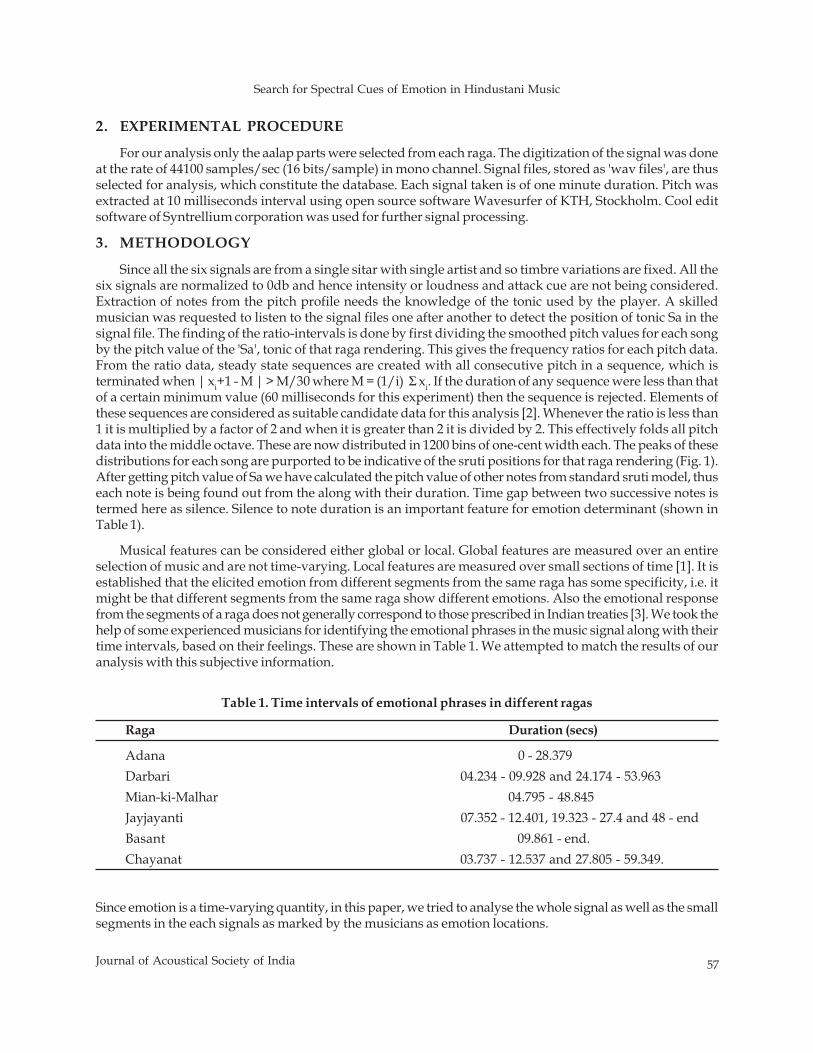
Search for Spectral Cues of Emotion in Hindustani Music
57Journal of Acoustical Society of India
2. EXPERIMENTAL PROCEDURE
For our analysis only the aalap parts were selected from each raga. The digitization of the signal was doneat the rate of 44100 samples/sec (16 bits/sample) in mono channel. Signal files, stored as 'wav files', are thusselected for analysis, which constitute the database. Each signal taken is of one minute duration. Pitch wasextracted at 10 milliseconds interval using open source software Wavesurfer of KTH, Stockholm. Cool editsoftware of Syntrellium corporation was used for further signal processing.
3. METHODOLOGY
Since all the six signals are from a single sitar with single artist and so timbre variations are fixed. All thesix signals are normalized to 0db and hence intensity or loudness and attack cue are not being considered.Extraction of notes from the pitch profile needs the knowledge of the tonic used by the player. A skilledmusician was requested to listen to the signal files one after another to detect the position of tonic Sa in thesignal file. The finding of the ratio-intervals is done by first dividing the smoothed pitch values for each songby the pitch value of the 'Sa', tonic of that raga rendering. This gives the frequency ratios for each pitch data.From the ratio data, steady state sequences are created with all consecutive pitch in a sequence, which isterminated when | xi+1 - M | > M/30 where M = (1/i) Σ xi. If the duration of any sequence were less than thatof a certain minimum value (60 milliseconds for this experiment) then the sequence is rejected. Elements ofthese sequences are considered as suitable candidate data for this analysis [2]. Whenever the ratio is less than1 it is multiplied by a factor of 2 and when it is greater than 2 it is divided by 2. This effectively folds all pitchdata into the middle octave. These are now distributed in 1200 bins of one-cent width each. The peaks of thesedistributions for each song are purported to be indicative of the sruti positions for that raga rendering (Fig. 1).After getting pitch value of Sa we have calculated the pitch value of other notes from standard sruti model, thuseach note is being found out from the along with their duration. Time gap between two successive notes istermed here as silence. Silence to note duration is an important feature for emotion determinant (shown inTable 1).
Musical features can be considered either global or local. Global features are measured over an entireselection of music and are not time-varying. Local features are measured over small sections of time [1]. It isestablished that the elicited emotion from different segments from the same raga has some specificity, i.e. itmight be that different segments from the same raga show different emotions. Also the emotional responsefrom the segments of a raga does not generally correspond to those prescribed in Indian treaties [3]. We took thehelp of some experienced musicians for identifying the emotional phrases in the music signal along with theirtime intervals, based on their feelings. These are shown in Table 1. We attempted to match the results of ouranalysis with this subjective information.
Since emotion is a time-varying quantity, in this paper, we tried to analyse the whole signal as well as the smallsegments in the each signals as marked by the musicians as emotion locations.
Table 1. Time intervals of emotional phrases in different ragas
Raga Duration (secs)
Adana 0 - 28.379Darbari 04.234 - 09.928 and 24.174 - 53.963Mian-ki-Malhar 04.795 - 48.845Jayjayanti 07.352 - 12.401, 19.323 - 27.4 and 48 - endBasant 09.861 - end.Chayanat 03.737 - 12.537 and 27.805 - 59.349.
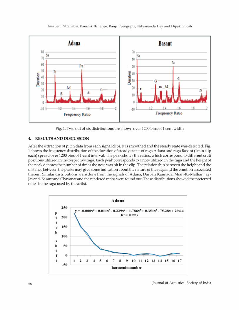
58 Journal of Acoustical Society of India
Anirban Patranabis, Kaushik Banerjee, Ranjan Sengupta, Nityananda Dey and Dipak Ghosh
4. RESULTS AND DISCUSSION
After the extraction of pitch data from each signal clips, it is smoothed and the steady state was detected. Fig.1 shows the frequency distribution of the duration of steady states of raga Adana and raga Basant (1min clipeach) spread over 1200 bins of 1-cent interval. The peak shows the ratios, which correspond to different srutipositions utilized in the respective raga. Each peak corresponds to a note utilized in the raga and the height ofthe peak denotes the number of times the note was hit in the clip. The relationship between the height and thedistance between the peaks may give some indication about the nature of the raga and the emotion associatedtherein. Similar distributions were done from the signals of Adana, Darbari Kannada, Mian-Ki-Malhar, Jay-Jayanti, Basant and Chayanat and the rendered ratios were found out. These distributions showed the preferrednotes in the raga used by the artist.
Fig. 1. Two out of six distributions are shown over 1200 bins of 1 cent width
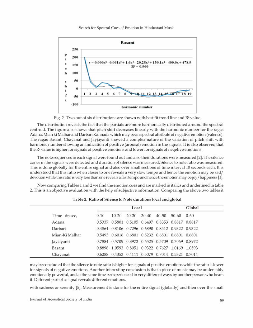
Search for Spectral Cues of Emotion in Hindustani Music
59Journal of Acoustical Society of India
The distribution reveals the fact that the partials are more harmonically distributed around the spectralcentroid. The figure also shows that pitch shift decreases linearly with the harmonic number for the ragasAdana, Mian ki Malhar and Darbari Kannada which may be an spectral attribute of negative emotion (valence).The ragas Basant, Chayanat and Jayjayanti showed a complex nature of the variation of pitch shift withharmonic number showing an indication of positive (arousal) emotion in the signals. It is also observed thatthe R2 value is higher for signals of positive emotions and lower for signals of negetive emotions.
The note sequences in each signal were found out and also their durations were measured [2]. The silencezones in the signals were detected and duration of silence was measured. Silence to note ratio was measured.This is done globally for the entire signal and also over small sections of time interval 10 seconds each. It isunderstood that this ratio when closer to one reveals a very slow tempo and hence the emotion may be sad/devotion while this ratio is very less than one reveals a fast tempo and hence the emotion may be joy/happiness [1].
Now comparing Tables 1 and 2 we find the emotion cues and are marked in italics and underlined in table2. This is an objective evaluation with the help of subjective information. Comparing the above two tables it
may be concluded that the silence to note ratio is higher for signals of positive emotions while the ratio is lowerfor signals of negative emotions. Another interesting conclusion is that a piece of music may be undeniablyemotionally powerful, and at the same time be experienced in very different ways by another person who hearsit. Different part of a signal reveals different emotions.
with sadness or serenity [5]. Measurement is done for the entire signal (globally) and then over the small
Fig. 2. Two out of six distributions are shown with best fit trend line and R2 value
Table 2. Ratio of Silence to Note durations local and global
Local Global
Time→in sec, 0-10 10-20 20-30 30-40 40-50 50-60 0-60Adana 0.5337 0.5801 0.5105 0.6497 0.8353 0.8817 0.8817Darbari 0.4864 0.8106 0.7296 0.6890 0.8512 0.9322 0.9322Mian-Ki Malhar 0.5493 0.6016 0.6801 0.5232 0.6801 0.6801 0.6801Jayjayanti 0.7884 0.5709 0.8972 0.6525 0.5709 0.7069 0.8972Basant 0.8898 1.0593 0.8051 0.9322 0.7627 1.0169 1.0593Chayanat 0.6288 0.4353 0.4111 0.5079 0.7014 0.5321 0.7014
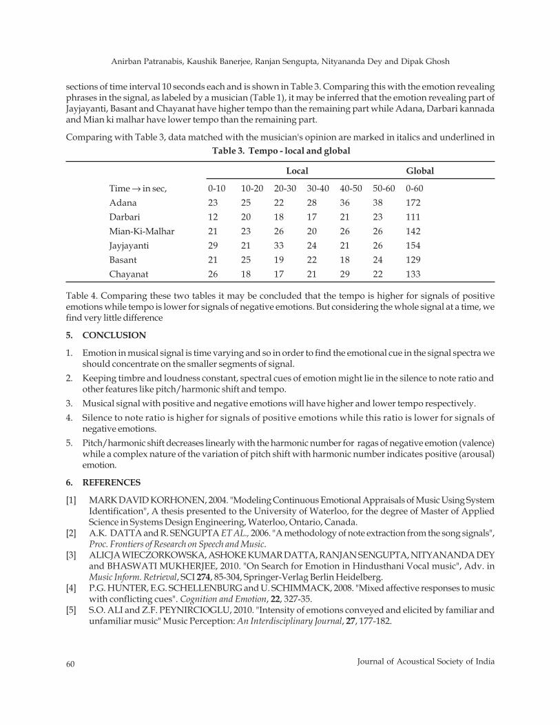
60 Journal of Acoustical Society of India
Anirban Patranabis, Kaushik Banerjee, Ranjan Sengupta, Nityananda Dey and Dipak Ghosh
sections of time interval 10 seconds each and is shown in Table 3. Comparing this with the emotion revealingphrases in the signal, as labeled by a musician (Table 1), it may be inferred that the emotion revealing part ofJayjayanti, Basant and Chayanat have higher tempo than the remaining part while Adana, Darbari kannadaand Mian ki malhar have lower tempo than the remaining part.
Comparing with Table 3, data matched with the musician's opinion are marked in italics and underlined in Table 3. Tempo - local and global
Local Global
Time → in sec, 0-10 10-20 20-30 30-40 40-50 50-60 0-60Adana 23 25 22 28 36 38 172Darbari 12 20 18 17 21 23 111Mian-Ki-Malhar 21 23 26 20 26 26 142Jayjayanti 29 21 33 24 21 26 154Basant 21 25 19 22 18 24 129Chayanat 26 18 17 21 29 22 133
Table 4. Comparing these two tables it may be concluded that the tempo is higher for signals of positiveemotions while tempo is lower for signals of negative emotions. But considering the whole signal at a time, wefind very little difference
5. CONCLUSION
1. Emotion in musical signal is time varying and so in order to find the emotional cue in the signal spectra weshould concentrate on the smaller segments of signal.
2. Keeping timbre and loudness constant, spectral cues of emotion might lie in the silence to note ratio andother features like pitch/harmonic shift and tempo.
3. Musical signal with positive and negative emotions will have higher and lower tempo respectively.4. Silence to note ratio is higher for signals of positive emotions while this ratio is lower for signals of
negative emotions.5. Pitch/harmonic shift decreases linearly with the harmonic number for ragas of negative emotion (valence)
while a complex nature of the variation of pitch shift with harmonic number indicates positive (arousal)emotion.
6. REFERENCES
[1] MARK DAVID KORHONEN, 2004. "Modeling Continuous Emotional Appraisals of Music Using SystemIdentification", A thesis presented to the University of Waterloo, for the degree of Master of AppliedScience in Systems Design Engineering, Waterloo, Ontario, Canada.
[2] A.K. DATTA and R. SENGUPTA ET AL., 2006. "A methodology of note extraction from the song signals",Proc. Frontiers of Research on Speech and Music.
[3] ALICJA WIECZORKOWSKA, ASHOKE KUMAR DATTA, RANJAN SENGUPTA, NITYANANDA DEYand BHASWATI MUKHERJEE, 2010. "On Search for Emotion in Hindusthani Vocal music", Adv. inMusic Inform. Retrieval, SCI 274, 85-304, Springer-Verlag Berlin Heidelberg.
[4] P.G. HUNTER, E.G. SCHELLENBURG and U. SCHIMMACK, 2008. "Mixed affective responses to musicwith conflicting cues". Cognition and Emotion, 22, 327-35.
[5] S.O. ALI and Z.F. PEYNIRCIOGLU, 2010. "Intensity of emotions conveyed and elicited by familiar andunfamiliar music" Music Perception: An Interdisciplinary Journal, 27, 177-182.
INFORMATION FOR AUTHORS
ARTICLES The Journal of Acoustical Society of India (JASI) is a refereed publication published quarterly by the Acoustical Society of India(ASI). JASI includes refereed articles, technical notes, letters-to-the-editor, book review and announcements of general interest toreaders.
Articles may be theoretical or experimental in nature. But those which combine theoretical and experimental approaches tosolve acoustics problems are particularly welcome. Technical notes, letters-to-the-editor and announcements may also be submitted.Articles must not have been published previously in other engineering or scientific journals. Articles in the following are particularlyencouraged: applied acoustics, acoustical materials, active noise & vibration control, bioacoustics, communication acousticsincluding speech, computational acoustics, electro-acoustics and audio engineering, environmental acoustics, musical acoustics,non-linear acoustics, noise, physical acoustics, physiological and psychological acoustics, quieter technologies, room and buildingacoustics, structural acoustics and vibration, ultrasonics, underwater acoustics.
Authors whose articles are accepted for publication must transfer copyright of their articles to the ASI. This transfer involvespublication only and does not in any way alter the author's traditional right regarding his/her articles.
PREPARATION OF MANUSCRIPTS All manuscripts are refereed by at least two referees and are reviewed by the Publication Committee (all editors) beforeacceptance. Manuscripts of articles and technical notes should be submitted for review electronically to the Chief Editor by e-mailor by express mail on a disc. JASI maintains a high standard in the reviewing process and only accept papers of high quality. Onacceptance, revised articles of all authors should be submitted to the Chief Editor by e-mail or by express mail. Text of the manuscript should be double-spaced on A4 size paper, subdivided by main headings-typed in upper and lowercase flush centre, with one line of space above and below and sub-headings within a section-typed in upper and lower caseunderstood, flush left, followed by a period. Sub-sub headings should be italic. Articles should be written so that readers indifferent fields of acoustics can understand them easily. Manuscripts are only published if not normally exceeding twenty double-spaced text pages. If figures and illustrations are included then normally they should be restricted to no more than twelve-fifteen. The first page of manuscripts should include on separate lines, the title of article, the names, of authors, affiliations andmailing addresses of authors in upper and lowers case. Do not include the author's title, position or degrees. Give an adequatepost office address including pin or other postal code and the name of the city. An abstract of not more than 200 words shouldbe included with each article. References should be numbered consecutively throughout the article with the number appearing asa superscript at the end of the sentence unless such placement causes ambiguity. The references should be grouped together,double spaced at the end of the article on a separate page. Footnotes are discouraged. Abbreviations and special terms must bedefined if used.
EQUATIONS Mathematical expressions should be typewritten as completely as possible. Equation should be numbered consecutivelythroughout the body of the article at the right hand margin in parentheses. Use letters and numbers for any equations in anappendix: Appendix A: (A1, (A2), etc. Equation numbers in the running text should be enclosed in parentheses, i.e., Eq. (1), Eqs.(1a) and (2a). Figures should be referred to as Fig. 1, Fig. 2, etc. Reference to table is in full: Table 1, Table 2, etc. Metric units shouldbe used: the preferred from of metric unit is the System International (SI).
REFERENCES The order and style of information differs slightly between periodical and book references and between published and unpublishedreferences, depending on the available publication entries. A few examples are shown below.
Periodicals:[1] S.R. Pride and M.W. Haartsen, 1996. Electroseismic wave properties, J. Acoust. Soc. Am., 100 (3), 1301-1315.[2] S.-H. Kim and I. Lee, 1996. Aeroelastic analysis of a flexible airfoil with free play non-linearity, J. Sound Vib., 193 (4), 823-846.
Books:[1] E.S. Skudzryk, 1968. Simple and Comlex Vibratory Systems, the Pennsylvania State University Press, London.[2] E.H. Dowell, 1975. Aeroelasticity of plates and shells, Nordhoff, Leyden.
Others:[1] J.N. Yang and A. Akbarpour, 1987. Technical Report NCEER-87-0007, Instantaneous Optimal Control Law For Tall
Buildings Under Seismic Excitations.
SUMISSIONS All materials from authors should be submitted in electronic form to the JASI Chief Editor: Dr Mahavir Singh, Acoustics,Ultrasonics & Vibration Section, CSIR-National Physical Laboratory, Dr. K. S. Krishnan Road, New Delhi-110 012 (email:[email protected] Tel: +91-11-4560.8317, Fax: +91-11-4560.9310). For the item to be published in a given issue of a journal,the manuscript must reach the Chief Editor at least twelve week before the publication date.
SUMISSION OF ACCEPTED MANUSCRIPT On acceptance, revised articles should be submitted in electronic form to the JASI Chief Editor ([email protected]).
Acoustical Society of India(Regn. No. 65-1971)
Executive Council (2010 - 2014)
President : Dr V Rajendran[KSRCT, Tiruchengode; [email protected]; +91-99 94 13 03 03]
Vice President : NS Naidu[NSTL, Vizag; [email protected]; +91-94 90 75 05 82]
General Secretary : PVS Ganesh Kumar[NSTL, Vizag; [email protected]; +91-98 66 40 08 94]
Jt. Secretary : Dr K Trinadh[NSTL, Vizag; [email protected]; +91-97 04 71 95 00]
Treasurer : Prof AV Sharma[AU, Vizag; [email protected]; +91-94 90 43 17 26]
Chief Editor : Dr Mahavir Singh[CSIR-NPL, New Delhi; [email protected]; +91-98 71 69 33 46]
Council Members : Dr SV Ranga Nayakulu[VITAE, Hyderabad; [email protected]; +91-98 66 53 26 13]
Dr I Johnson[SJ College, Trichy; [email protected]; +91-94 42 90 48 20]
Dr Rajiv K Upadhayay[Govt PG College, Rishikesh; [email protected]; +91-94 12 97 28 90]
Dr S Shekhar[Oxford College, Trichy; [email protected]; +91-99 94 92 00 30]
Dr V Bhujanga Rao[Past President; NSTL, Vizag; [email protected]; +91-98 66 44 10 74]
Co-opted Members : Rajshekhar Uchil[Josts, Bangalore; [email protected]; +91-98 80 17 08 95]
Dr NK Narayanan[CIT, Kozhikode; [email protected]; +91-94 46 95 58 30]

ISSN 0973-3302
Volume 40 Number 1 January 2013
A Quarterly Publication of the JASI
http://www.acousticsindia.org
OCIS E TL YA OCI FT S INU DO IAC A
AA A ~Ae ekr xk/ tk s h ku re
JOURNAL OF
ACOUSTI CAL SOCIETY
OF INDIA

Journal of AcousticalSociety of India
The Refereed Journal of the Acoustical Society of India (JASI)JASI
CHIEF EDITOR:Mahavir SinghAcoustics, Ultrasonics & Vibration SectionCSIR-National Physical LaboratoryDr. KS Krishnan RoadNew Delhi 110 012Tel: +91.11.4560.8317Fax: +91.11.4560.9310E-mail: [email protected]
ASSOCIATE SCIENTIFIC EDITOR:Applied Acoustics
Trinath KarControl Component India Pvt. Ltd6th Floor, Warp TowerPlot # 13, 14, &15SJR i-Park, EPIP Zone, Phase 1Whitefield Road, Bangalore 560066
The Journal of Acoustical Society of India is a refereed journal of the Acoustical Society of India (ASI). The ASI is anon-profit national society founded in 31st July, 1971. The primary objective of the society is to advance the science ofacoustics by creating an organization that is responsive to the needs of scientists and engineers concerned with acousticsproblems all around the world.
Manuscripts of articles, technical notes and letter to the editor should be submitted to the Chief Editor. Copies ofarticles on specific topics listed above should also be submitted to the respective Associate Scientific Editor. Manuscriptsare refereed by at least two referees and are reviewed by Publication Committee (all editors) before acceptance. Onacceptance, revised articles with the text and figures scanned as separate files on a diskette should be submitted to theEditor by express mail. Manuscripts of articles must be prepared in strict accordance with the author instructions.
All information concerning subscription, new books, journals, conferences, etc. should be submitted to Chief Editor:
Acoustics, Ultrasonics & Vibration Section, CSIR-National Physical Laboratory, Dr. KS Krishnan Road, New Delhi 110 012, Tel: +91.11.4560.8317, Fax: +91.11.4560.9310, e-mail: [email protected]
Annual subscription price including mail postage is Rs. 2000/= for institutions, companies and libraries and Rs. 2000/=for individuals who are not ASI members. The Journal of Acoustical Society of India will be sent to ASI members freeof any extra charge. Requests for specimen copies and claims for missing issues as well as address changes should besent to the Editorial Office:
Acoustics, Ultrasonics & Vibration Section, CSIR-National Physical Laboratory, Dr. KS Krishnan Road, New Delhi 110 012, Tel: +91.11.4560.8317, Fax: +91.11.4560.9310, e-mail: [email protected]
The journal and all articles and illustrations published herein are protected by copyright. No part of this journal may betranslated, reproduced, stored in a retrieval system, or transmitted, in any form or by any means, electronic, mechanical,photocopying, microfilming, recording or otherwise, without written permission of the publisher.
Copyright © 2007, Acoustical Society of IndiaISSN 0973-330
Editorial Office:
MANAGING EDITOROmkar Sharma
ASSISTANT EDITORSYudhisther KumarAnil Kumar NainNaveen Garg
Acoustics, Ultrasonics & Vibration SectionCSIR-National Physical LaboratoryDr. KS Krishnan RoadNew Delhi 110 012Tel: +91.11. 4560.8317asFax: +91.11.4560.9310E-mail: [email protected]
Printed at Alpha Printers, BG-2/38C, Paschim Vihar, New Delhi-110063 Tel.: 9811848335. JASI is sent to ASI membersfree of charge.
Journal of AcousticalSociety of India (JASI)
A quarterly publication of the Acoustical Society of India
Volume 40, Number 2, April 2013
JASI
MAHAVIR SINGH Chief Editor
OMKAR SHARMA Managing Editor
TRINATH KAR Associate Scientific Editor
Yudhishter KumarAnil Kumar NainNaveen Garg Assistant Editors
EDITORIAL BOARD
M L Munjal IISc Banglore, India
S Narayanan IIT Chennai, India
V Rajendran KSRCT Erode, India
R J M Craik HWU Edinburg, UK
Trevor R T Nightingle NRC Ottawa, Canada
B V A Rao VIT Vellore, India
N Tandon IIT Delhi, India
P Narang NMI Lindfield, Australia
E S R Rajagopal IISc Banglore, India
A L Vyas IIT Delhi, India
V Bhujanga Rao NSTL Vizag, India
Yukio Kagawa NU Chiba, Japan
S Datta LU Loughborough, UK
Sonoko Kuwano OU Osaka, Japan
K K Pujara IIT Delhi (Ex.), India
A R Mohanty IIT Kharagpur, India
Ashok Kumar NPL New Delhi, India
V Mohanan NPL New Delhi, India
EDITORIAL
Basic Factors of Noise Control
Mahavir Singh ............................................................................... 68
ARTICLES
Methods for Estimating the Accurate Values of SoundAbsorption MeasurementsMahavir Singh and Dharam Pal Singh.......................................... 69
Free Field Acoustic Radiation of Composite Plates withSurface Bonded PFC Using RME TechniquePartha Bhattacharya and Atanu Sahu........................................... 77
Shape Reconstruction of Underwater Objects fromAcoustic ReturnsT. Ratna Mani, Raj Kumar and O. Vijay Kumar........................... 91
Noise Control of a Hand Drill Using Hybrid MufflerR. Praveena, Gyanadutta Swain and B. Venkatesham.................. 108
Genetic Algorithm Based Neural Network for Classificationof Rolling Element Bearing ConditionG.S. Vijay, Srinivasa P. Pai and N.S. Sriram................................ 116
Localization of Low Flying Aircraft Based on Its AcousticSignatureA. Saravanakumar, S. Arunkumar and K. Senthilkumar............. 121
Absorption Studies of Aniline and EstersK. Sathi Reddy, D. Shanmukhi Jyothi and D. Linga Reddy........... 131
Interaction Study of Pyridine and Acetone at 313.15 KPrashant Dabrase, R.A. Patil and B.M. Suryavanshi.......................... 137
INFORMATION
Executive Council of Acoustical Society of India 143
Information for Authors Inside back cover

EDITOR’S SPACE
Basic Factors of Noise Control
ISound is a pervasive phenomenon and such factors as the high density of new residential construction andthe use of high powered equipment in modern lightweight construction systems are leading to higher noiselevels in our homes, our work spaces and generally everywhere in our cities. In fact, surveys done in theUnited States report that the noise level of major cities is rising at the rate of approximately one decibel peryear. We can no longer ignore the trend.
While the general field of noise control is quite broad, the Insight program was limited to noise controlin buildings; however, the principles of noise control are the same regardless of the environment beingconsidered.
Inadequate noise control has often made a restaurant meal an unpleasant experience. High noise levelsin the workplace are distracting and irritating, possibly resulting in higher absenteeism and loss ofproductivity. Inadequate acoustical privacy is common in office buildings. Conference rooms, despite the factthat their primary purpose is speech communication, are often excessively reverberant and noisy, making itdifficult to understand speech from people only a short distance away. Most schools, churches, gymnasiumsand swimming pools, as they now exist, could benefit from an acoustical tune-up, improving the quality oftheir indoor environment and their revenue-earning potential.
A recent survey in Vancouver found about 40% of the tenants in several multi-family dwelling projectsdissatisfied with the degree of acoustical privacy in their homes. This was the major problem as far as thetenants were concerned, and it is a major complaint in many of our new apartment and condominiumprojects.
Elsewhere, in a large hotel in India, the acoustical engineers were overruled by the project designers; inorder to save some Rs. 3.7 Crores they provided bedrooms with single glazing and operable sashes forventilation. When the hotel came into service, most of the rooms had so much traffic noise penetrating, thatthey were unusable for sleeping. To rectify the situation, the hotel had to install double glazing and airconditioning at a cost of Rs. 9.6 Crores, not including the loss of revenue and general disturbance during therepair work.
Such errors are inexcusable, given that the knowledge exists to design and build quality acousticalenvironments.
The essence of this Insight program is a discussion of the principles of noise control in buildings. Thefundamentals of sound are explained in the first paper, followed by the criteria and methods to control noisewithin rooms, in the second paper. The third paper examines the issue of noise reduction across walls, floors,windows and doors, and the last paper deals with acoustics of buildings, with an emphasis on machine andplumbing noises and the annoying problem of flanking noise.
Mahavir Singh
Methods for Estimating the Accurate Values of Sound Absorption Measurements
69Journal of Acoustical Society of India
Methods for Estimating the Accurate Values ofSound Absorption Measurements
Mahavir Singh* and Dharam Pal SinghAcoustics, Ultrasonics & Vibration (AUV) Section,
Apex Level Standards & Industrial Metrology Division,CSIR-National Physical Laboratory, Dr. K. S. Krishnan Road, New Delhi -110 012
*e-mail: [email protected]
ABSTRACT
In order to check that the reverberation chamber measurement of absorption coefficient was consistent,a short run of repeatability measurements were carried out as per standard procedure. The standardISO/IEC 17025:2005 on the competence of testing and calibration laboratories requires that theselaboratories shall apply procedures for estimating the accurate values of their measurement results.One of the possibilities is to evaluate the accurate values, taking into account all components thatcontribute significant value to the final result. In case of the sound absorption coefficient value,carried out according to the standard EN ISO 354:2003, the overall value is first of all influenced bythe reverberation times T1, T2 and the power attenuation coefficients m1 and m2, calculated accordingto the ISO 9613-1 standard and representing the climatic conditions in the reverberation room. Inspite of very little difference between the values m1 and m2 representing the change of climatic conditionsusually, it is the case in laboratory, exponential form of the coefficient's function causes that theaccurate value of measurement results increase with frequency very fast. Particularly for the highfrequencies, the accurate values of measurements are so important that the evaluation of the soundabsorption coefficient is practically not possible.
1. INTRODUCTION
However there is at present no wholly accepted calculations of repeatability and standard error in reverberationchamber absorption coefficient and the data quoted in the literature varies widely. Figure 1 shows a typical RTspectrum for the empty room, along with the IS 8225 minimum curve for the particular room volume of 257 m3
and surface area of 244 m2.
Because of lack of uncertainty evaluation based on inter-laboratory validation approach, it has to becarried out by the laboratory itself. Using the general methods specified in GUM[1], first of all we need toestablish a relationship between the mesurand Y and other quantities X1, X2,...Xn (input values) through afunction f, called the measurement equation
Y = f(X1, X2,.........................Xn) (1)
Such equation must express not only the physical relation from which we can obtain the value of mesurandY but also it should be accompanied by a quantitative statement of its uncertainty which arises from theuncertainties of the input values of directly measured quantities x1, x2 ...xn being the estimates of X1, X 2, ....Xn.
In general, uncertainty components (each of them - represented by estimated standard deviation, termedstandard uncertainty and noted u(xi) or, shortly, ui) are categorized according to the method used to evaluate
Journal of Acoustical Society of India : Vol. 40, No. 2, 2013 (pp.69-76)
[Received: 21.01.2013; Revised: 02.04.2013; Accepted: 10.04.2013]
© 2013 Acoustical Society of India
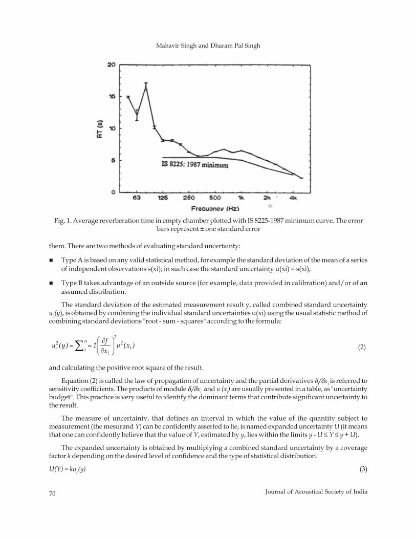
70 Journal of Acoustical Society of India
Mahavir Singh and Dharam Pal Singh
them. There are two methods of evaluating standard uncertainty:
Type A is based on any valid statistical method, for example the standard deviation of the mean of a seriesof independent observations s(xi); in such case the standard uncertainty u(xi) = s(xi),
Type B takes advantage of an outside source (for example, data provided in calibration) and/or of anassumed distribution.
The standard deviation of the estimated measurement result y, called combined standard uncertaintyuc(y), is obtained by combining the individual standard uncertainties u(xi) using the usual statistic method ofcombining standard deviations "root - sum - squares" according to the formula:
⎛ ⎞∂
= = ⎜ ⎟∂⎝ ⎠∑
2n2 2
c ii i
fu (y) 1 u (x )
x (2)
and calculating the positive root square of the result.
Equation (2) is called the law of propagation of uncertainty and the partial derivatives δf/δxi is referred tosensitivity coefficients. The products of module δf/δxi and u (xi) are usually presented in a table, as "uncertaintybudget". This practice is very useful to identify the dominant terms that contribute significant uncertainty tothe result.
The measure of uncertainty, that defines an interval in which the value of the quantity subject tomeasurement (the mesurand Y) can be confidently asserted to lie, is named expanded uncertainty U (it meansthat one can confidently believe that the value of Y, estimated by y, lies within the limits y - U ≤ Y ≤ y + U).
The expanded uncertainty is obtained by multiplying a combined standard uncertainty by a coveragefactor k depending on the desired level of confidence and the type of statistical distribution.
U(Y) = kuc(y) (3)
Fig. 1. Average reverberation time in empty chamber plotted with IS 8225-1987 minimum curve. The errorbars represent ± one standard error
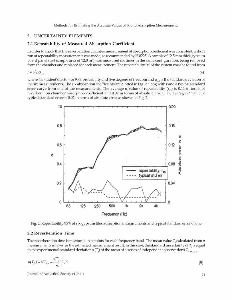
Methods for Estimating the Accurate Values of Sound Absorption Measurements
71Journal of Acoustical Society of India
2. UNCERTAINTY ELEMENTS
2.1 Repeatability of Measured Absorption Coefficient
In order to check that the reverberation chamber measurement of absorption coefficient was consistent, a shortrun of repeatability measurements was made, as recommended by IS 8225. A sample of 12.5 mm thick gypsumboard panel (test sample area of 12.8 m2) was measured six times in the same configuration, being removedfrom the chamber and replaced for each measurement. The repeatability "r" of the system was the found from
r = t√2.σn-1 (4)
where t is student's factor for 95% probability and five degrees of freedom and σn-1 is the standard deviation ofthe six measurements. The six absorption coefficients are plotted in Fig. 2 along with r and a typical standarderror curve from one of the measurements. The average α value of repeatability (r95) is 0.11 in terms ofreverberation chamber absorption coefficient and 0.02 in terms of absolute error. The average ?? value oftypical standard error is 0.02 in terms of absolute error as shown in Fig. 2.
2.2 Reverberation Time
The reverberation time is measured in n points for each frequency band. The mean value Tf calculated from nmeasurements is taken as the estimated measurement result. In this case, the standard uncertainty of Tf is equalto the experimental standard deviation s (Tf) of the mean of a series of independent observations Tf, i=1,....n.
= = f ,if f
s(T )u(T ) s(T ) ,S
n (5)
Fig. 2. Repeatability 95% of six gypsum tiles absorption measurements and typical standard error of one

72 Journal of Acoustical Society of India
Mahavir Singh and Dharam Pal Singh
Student's - t distribution with n freedom degrees is assumed.
2.3 Area of Sample
Assuming the rectangular distribution of estimated measurement result, with the boundary of ± 0.005 m2, thestandard uncertainty of sample's area amounts to
= =2
20.005mu(S) 0.0029m3 (6)
2.4 Volume of Room
Assuming the rectangular distribution of estimated measurement result, with the boundary of resolution ± 0.5m3, the standard uncertainty of room volume amounts to
= =3
30.5mu(S) 0.2887m3 (7)
2.5 Environment Factors
The measurement equations for the environmental factors like temperature, atmospheric pressure and relativehumidity assume the form:
e = e0+δe1+δe2+δe3+δe4 (8)
where,
e0 the reading value of the environmental factor in a room,δe1 the dispersion of sensor indications,δe2 the resolution of sensor indications,δe3 the error of sensor indications,δe4 the uncertainty of indication error.
The standard uncertainty of dispersion δe1 is calculated on the basis of the estimated standard deviationof m series of n measurements.
∂ = i 11
S ( e )u( e )n (9)
where,
Si(e1) the experimental standard deviation of ith series equal to
=∑=
mi 1 1 1,iS ( e )
Si( e1)m
(10)
The standard uncertainty of resolution δe2 is evaluated with the assumption of rectangular distributionwith the boundary of resolution supposed, respectively, as b = ± 0.05 °C, ± 0.05 kPa or ± 0.05%.
δ =2bu( e )3 (11)
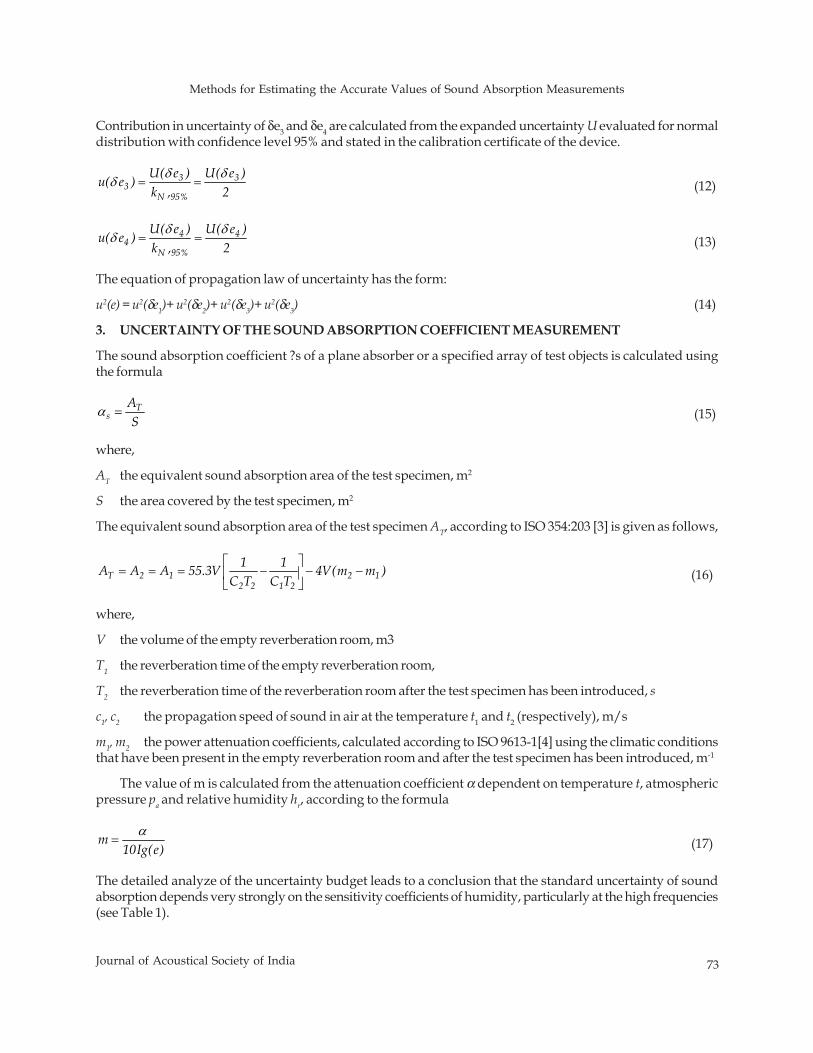
Methods for Estimating the Accurate Values of Sound Absorption Measurements
73Journal of Acoustical Society of India
Contribution in uncertainty of δe3 and δe4 are calculated from the expanded uncertainty U evaluated for normaldistribution with confidence level 95% and stated in the calibration certificate of the device.
δ δδ = =3 3
3N 95%
U( e ) U( e )u( e )k , 2 (12)
δ δδ = =4 4
4N 95%
U( e ) U( e )u( e )k , 2 (13)
The equation of propagation law of uncertainty has the form:
u2(e) = u2(δe1)+ u2(δe2)+ u2(δe3)+ u2(δe3) (14)
3. UNCERTAINTY OF THE SOUND ABSORPTION COEFFICIENT MEASUREMENT
The sound absorption coefficient ?s of a plane absorber or a specified array of test objects is calculated usingthe formula
Ts
AS
α = (15)
where,
AT the equivalent sound absorption area of the test specimen, m2
S the area covered by the test specimen, m2
The equivalent sound absorption area of the test specimen AT, according to ISO 354:203 [3] is given as follows,
⎡ ⎤= = = − − −⎢ ⎥
⎣ ⎦T 2 1 2 1
2 2 1 2
1 1A A A 55.3V 4V(m m )C T C T (16)
where,
V the volume of the empty reverberation room, m3
T1 the reverberation time of the empty reverberation room,
T2 the reverberation time of the reverberation room after the test specimen has been introduced, s
c1, c2 the propagation speed of sound in air at the temperature t1 and t2 (respectively), m/s
m1, m2 the power attenuation coefficients, calculated according to ISO 9613-1[4] using the climatic conditionsthat have been present in the empty reverberation room and after the test specimen has been introduced, m-1
The value of m is calculated from the attenuation coefficient α dependent on temperature t, atmosphericpressure pa and relative humidity hr, according to the formula
α=m
10Ig(e) (17)
The detailed analyze of the uncertainty budget leads to a conclusion that the standard uncertainty of soundabsorption depends very strongly on the sensitivity coefficients of humidity, particularly at the high frequencies(see Table 1).
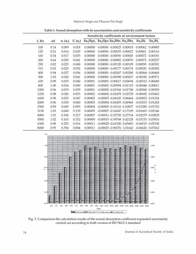
74 Journal of Acoustical Society of India
Mahavir Singh and Dharam Pal Singh
Table 1. Sound absorption with its uncertainties and sensitivity coefficients
f, Hz αS u ( )c Sα U ( )αS
Sensitivity coefficients of environment factorsδα δS 1/ pa δα δS/ pa δα δS 1/ hr δα δS 2/ hr δα δS 1/ t δα δS 2/ t
100 0.14 0.009 0.018 0.00000 0.00000 -0.00023 0.00018 0.00062 0.00085125 0.31 0.014 0.029 0.00000 0.00000 -0.00035 0.00027 0.00061 0.00116160 0.54 0.017 0.035 0.00000 0.00000 -0.00056 0.00045 0.00072 0.00181200 0.64 0.020 0.041 0.00000 0.00000 -0.00082 0.00070 0.00072 0.00227250 0.82 0.023 0.048 0.00000 0.00000 -0.00120 0.00109 0.00059 0.00301315 0.92 0.025 0.052 0.00000 0.00000 -0.00177 0.00174 0.00020 0.00382400 0.94 0.027 0.056 0.00000 0.00000 -0.00267 0.00280 -0.00064 0.00468500 1.02 0.020 0.041 0.00000 0.00000 -0.00398 0.00437 -0.00182 0.00571630 0.99 0.019 0.040 0.00001 -0.00001 -0.00617 0.00694 -0.00312 0.00680800 1.00 0.024 0.049 0.00001 -0.00001 -0.00994 0.01119 -0.00448 0.008111000 0.96 0.019 0.039 0.00001 -0.00002 -0.01568 0.01748 -0.00568 0.009291250 0.98 0.026 0.053 0.00002 -0.00002 -0.02478 0.02729 -0.00692 0.010621600 0.98 0.023 0.047 0.00002 -0.00003 -0.04105 0.04464 -0.00852 0.012242000 0.96 0.030 0.060 0.00003 -0.00004 -0.06455 0.06960 -0.01033 0.014182500 0.99 0.045 0.093 0.00004 -0,00005 -0.10116 0.10837 -0.01285 0.017023150 1.03 0.068 0.139 0.00005 -0.00007 -0.16047 0.17109 -0.01665 0.021464000 1.01 0.106 0.217 0.00007 -0.00011 -0.25730 0.27334 -0.02279 0.028295000 1.02 0.163 0.332 0.00009 -0.00015 -0.39768 0.42128 -0.03153 0.038166300 0.98 0.253 0.516 0.00011 -0.00020 -0.61920 0.65403 -0.04515 0.053388000 0.95 0.394 0.804 0.00011 -0.00023 -0.96576 1.01642 -0.06626 0.07662
Fig. 3. Comparison the calculation results of the sound absorption coefficient expanded uncertaintycarried out according to both version of ISO 9613-1 standard
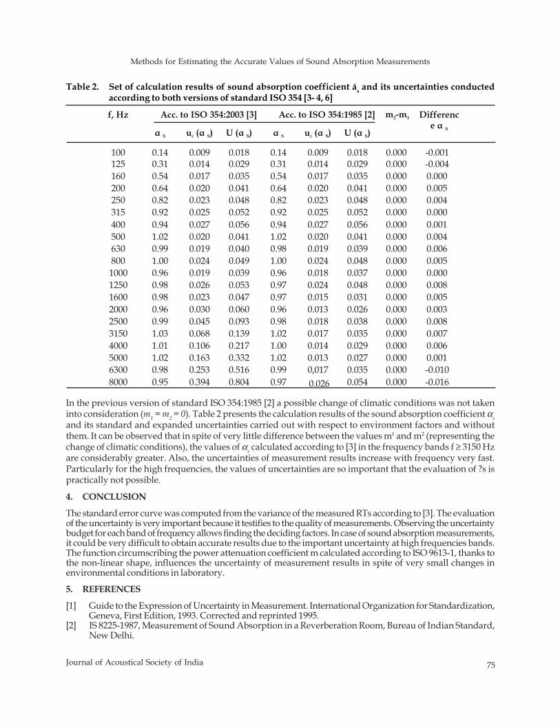
Methods for Estimating the Accurate Values of Sound Absorption Measurements
75Journal of Acoustical Society of India
f, Hz Acc. to ISO 354:2003 [3] Acc. to ISO 354:1985 [2] m -m2 1 Difference α Sα S u ( )c Sα U ( )α S α S u ( )c Sα U ( )α S
100 0.14 0.009 0.018 0.14 0.009 0.018 0.000 -0.001125 0.31 0.014 0.029 0.31 0.014 0.029 0.000 -0.004160 0.54 0.017 0.035 0.54 0.017 0.035 0.000 0.000200 0.64 0.020 0.041 0.64 0.020 0.041 0.000 0.005250 0.82 0.023 0.048 0.82 0.023 0.048 0.000 0.004315 0.92 0.025 0.052 0.92 0.025 0.052 0.000 0.000400 0.94 0.027 0.056 0.94 0.027 0.056 0.000 0.001500 1.02 0.020 0.041 1.02 0.020 0.041 0.000 0.004630 0.99 0.019 0.040 0.98 0.019 0.039 0.000 0.006800 1.00 0.024 0.049 1.00 0.024 0.048 0.000 0.0051000 0.96 0.019 0.039 0.96 0.018 0.037 0.000 0.0001250 0.98 0.026 0.053 0.97 0.024 0.048 0.000 0.0081600 0.98 0.023 0.047 0.97 0.015 0.031 0.000 0.0052000 0.96 0.030 0.060 0.96 0.013 0.026 0.000 0.0032500 0.99 0.045 0.093 0.98 0.018 0.038 0.000 0.0083150 1.03 0.068 0.139 1.02 0.017 0.035 0.000 0.0074000 1.01 0.106 0.217 1.00 0.014 0.029 0.000 0.0065000 1.02 0.163 0.332 1.02 0.013 0.027 0.000 0.0016300 0.98 0.253 0.516 0.99 0,017 0.035 0.000 -0.0108000 0.95 0.394 0.804 0.97 0.026 0.054 0.000 -0.016
Table 2. Set of calculation results of sound absorption coefficient ás and its uncertainties conductedaccording to both versions of standard ISO 354 [3- 4, 6]
In the previous version of standard ISO 354:1985 [2] a possible change of climatic conditions was not takeninto consideration (m1 = m2 = 0). Table 2 presents the calculation results of the sound absorption coefficient αsand its standard and expanded uncertainties carried out with respect to environment factors and withoutthem. It can be observed that in spite of very little difference between the values m1 and m2 (representing thechange of climatic conditions), the values of αs calculated according to [3] in the frequency bands f ≥ 3150 Hzare considerably greater. Also, the uncertainties of measurement results increase with frequency very fast.Particularly for the high frequencies, the values of uncertainties are so important that the evaluation of ?s ispractically not possible.
4. CONCLUSION
The standard error curve was computed from the variance of the measured RTs according to [3]. The evaluationof the uncertainty is very important because it testifies to the quality of measurements. Observing the uncertaintybudget for each band of frequency allows finding the deciding factors. In case of sound absorption measurements,it could be very difficult to obtain accurate results due to the important uncertainty at high frequencies bands.The function circumscribing the power attenuation coefficient m calculated according to ISO 9613-1, thanks tothe non-linear shape, influences the uncertainty of measurement results in spite of very small changes inenvironmental conditions in laboratory.
5. REFERENCES
[1] Guide to the Expression of Uncertainty in Measurement. International Organization for Standardization,Geneva, First Edition, 1993. Corrected and reprinted 1995.
[2] IS 8225-1987, Measurement of Sound Absorption in a Reverberation Room, Bureau of Indian Standard,New Delhi.

76 Journal of Acoustical Society of India
Mahavir Singh and Dharam Pal Singh
[3] MAHAVIR SINGH, OMKAR SHARMA and V. MOHANAN, 2004. Repeatability and standard error inreverberation chamber absorption coefficient, ICA2004 (Fr2.B1.4), pp. 3393-3396.
[4] EN ISO 354:1985, Acoustics - Measurement of sound absorption in a reverberation room.[5] EN ISO 354:2003, Acoustics - Measurement of sound absorption in a reverberation room.[6] ISO 9613-1:1993, Acoustics - Attenuation of sound during propagation outdoors - Part 1: Calculation of
the absorption of sound by the atmosphere.
Free Field Acoustic Radiation of Composite Plates with Surface Bonded PFC Using RME Technique
77Journal of Acoustical Society of India
ABSTRACT
In the present work an attempt is made to develop a mathematical model based on Helmoltz Integral equationand Finite Element methodology to estimate radiated sound from a vibrating baffled composite plate in to thefree field. Radiation Mode Expansion (RME) technique is implemented to estimate the radiated sound.Subsequently, it is attempted to reduce the radiated sound by introducing surface bonded IDE-PFC actuators.The model is developed in a MATLAB environment and results are obtained for various locations of IDE-PFCpatch actuators.
1. INTRODUCTION
Sound attenuation is usually achieved by means of energy absorbing materials placed on the surface of theradiating structure. This technique works quite well for sounds at medium and high frequencies but is veryinefficient at low frequencies because the thickness of the absorbing material necessarily increases withdecreasing frequency. It has been reported by Kaczmarska and Augustynska [1] that the addition of soundproofing material used for the sound insulation ability of ‘soundproof’ cabins averages typically 30-50 dB forfrequencies above 500 Hz, but only 0-19 dB for frequencies below 500 Hz. Active noise control is an alternativeto this ‘passive’ strategy where destructive interference is used to reduce the sound pressure field.
A more advanced form of this technique is based on altering the vibrations of a noisy structure such thatit radiates very little sound. This alteration is achieved by introducing discrete force actuators. Active StructuralAcoustic Control or simply ASAC is one such ‘active’ strategy and in the present work the focus is ondeveloping an ASAC strategy for vibrating laminated composite plate radiating sound into the free field.
A vibrating structure that is surrounded by an acoustic medium causes pressure perturbations in themedium, which are experienced as sound. An arbitrarily shaped vibrating structure consists of infinitenumber of natural mode shapes associated with its natural frequencies. If the vibration mode shape patternof a simply supported plate structure resting on an infinite baffle is studied, it can be seen that the fundamentalmode shape exhibit a dome shaped pattern, whereas the second mode is represented by a sine wave in themajor axis and a sine along minor axis. The fluid immediately next to the plate reacts differently for eachmode shape. The fundamental mode displaces the fluid outward virtually in phase over the entire surface.On the other hand for the second mode the fluid sloshes back and forth between each oscillating trough of thesine wave. The vibration of the plate in its first mode transports the fluid in front of the plate farther away,
Journal of Acoustical Society of India : Vol. 40, No. 2, 2013 (pp. 77-90)
Free Field Acoustic Radiation of Composite Plates withSurface Bonded PFC Using RME Technique
Partha Bhattacharya1 and Atanu Sahu2*1Department of Civil Engineering, Jadavpur University, Kolkata 700 032 (W.B.), India
German Aerospace Center (DLR), 38108 Braunschweig, Germany2 Institute of Composite Structures & Adaptive Systems, German Aerospace Center (DLR),
Lilienthalplatz7, 38108 Braunschweig, Germany*e-mail: [email protected]
[Received: 16.11.2012; Revised: 24.01.2013; Accepted: 27.02.2013]
© 2013 Acoustical S India
78 Journal of Acoustical Society of India
Partha Bhattacharya and Atanu Sahu
whereas, the net fluid motion due to the second mode remains transverse and never propagates far from theplanar surface [Bevan [2]]. However the structural mode shapes do not radiate independently. In fact, thestrong dependence on inter-modal coupling between structural modes affects the radiated sound power suchthat reducing dominant structural modes may have little affect on the radiated power.
Apart from identifying structural mode shapes, researchers developed the concept of surface velocityfilters or acoustic radiation filters. Acoustic radiation filters describe the radiated power in terms of discretesurface velocities and the surface radiation resistance as shown by Cunefare [3]. This concept can be termedas modal approach for characterizing acoustic radiation from vibrating structures. It must be noted that theterm ‘modal’ here refers to acoustic radiation modes and are independent of structural vibration modes orshould not be confused with acoustic cavity modes. Borgiotti and Jones [4] first introduced a modalrepresentation using Singular Value Decomposition (SVD) to represent radiation efficiencies and singularvelocity patterns. Baumann, Saunders and Robertshaw [5] implemented feedback control by using radiationfilters in frequency weighted cost functions to minimize the most efficient radiation modes. Elliot and Johnson[6] implemented feed forward control of beams and plates using radiation filters. Gibbs et al. [7] developed aRadiation Modal Expansion (RME) technique, exploiting the acoustic radiation bounding properties, therebyreducing computation effort for real time digital signal processing applications. Bhattacharya et al. [8] in theirwork had shown that the bounding properties of the acoustic radiation modes are very much dependent onthe size and geometry of the vibrating structure.
In the present work an attempt is made first to estimate the radiated sound power from a baffled platesubjected to mechanical excitations and thereafter introducing surface bonded Piezo Fiber Composite patcheswith Inter-digitated Electrode (IDE-PFC) to observe the changes in the radiated energy behaviour of the sameplate. The mathematical model is presented in the next section.
2. MATHEMATICAL BASIS
2.1 Acoustic Model
Acoustic wave propagation through a homogeneous elastic fluid such as air is described by the well-knownwave equation. In the case of harmonic time dependence, this equation reduces to Helmholtz differentialequation, which is as follows,
∇ + = − ωρ2 20p(r) k p(r) i q(r) (1)
where p(r) is the complex acoustic pressure amplitude at location 'r' and q(r) is the external sound source. TheHelmholtz differential equation can be rewritten in an integral form called the Helmholtz integral equation.In the present work the analysis is restricted to a flat plate like structure. The schematic of the structure isgiven in Fig. 1. When it is assumed that the structure is placed in a baffle, the Helmholtz integral equationreduces to Rayleigh second integral [9] given by,
− −ωρ=
π −∫sik r r
0n s
sS
i ep(r) v (r ) dS2 r r (2)
The Rayleigh integral is solved with a primitive numerical scheme. The plate is divided into 'N' rectangularelements of equal size, which are small compared to the acoustic wavelength. It is assumed that the normalvelocity is constant across each element. That makes each element behave like an elemental radiator or pistonthat moves with constant harmonic velocity. For this discretization, the Rayleigh integral can also be writtenas =f f np Z v (3)
where pf is the vector with pressures in a set of field points, vn is the vector with normal surface velocities of theelemental radiators, and Zf is a frequency dependent transfer matrix, whose elements are given by,
Free Field Acoustic Radiation of Composite Plates with Surface Bonded PFC Using RME Technique
79Journal of Acoustical Society of India
ijikr0 e
f ijij
i S e(Z )2 r
−ωρ=
π (4)
where, Se is the surface area of the elemental radiator and rij denotes the radial distance between the radiatingpoint and the measuring point.
For the same discretization, the expression for the sound power reduces to the summation:
Hen
SW Re(v p)2
= (5)
where, p is the vector with surface pressures, evaluated at the same points on the surface as vn.
With the substitution of p = Zvn, the sound power 'W' can be obtained in terms of discrete number of velocitymeasurements as, H
n nW v Rv= (6)
In this equation R = (Se/2)Re(Z) is the so called radiation resistance matrix.
This matrix R can be written as,
21 1N
21 1N
122 20 e
120
N1
N1
sin(kr ) sin(kr )1kr kr
sin(kr ) 1S krR4 c
sin(kr ) 1kr
⎡ ⎤⎢ ⎥⎢ ⎥⎢ ⎥
ω ρ ⎢ ⎥= ⎢ ⎥π ⎢ ⎥⎢ ⎥⎢ ⎥⎢ ⎥⎣ ⎦
L
M
M O M
K L
(7)
As is seen in Eq. (7), the matrix R is a function of frequency and for online control, it becomes computationallyexpensive to estimate 'R' at various frequencies. RME technique as described by Gibbs et al.[5] in their paperhelps one to circumvent this problem and the same is implemented in this paper as well.
2.2 IDE - PFC Model
In case of IDE-PFC patches (actuator), the electric field along the length of the patch between two consecutiveelectrode fingers is assumed to be linearly distributed with alternate electrodes being suitably grounded. It isassumed that there is a perfect bond between the piezo layer and the elastic substrate (no-slip condition).
In the present development only d33 actuation induced by the interdigitated electrode is considered andhence only E3 field (along axis 3) is taken in the modeling. Therefore, the electric field can be expressed in the
form, 3
0{E} 0
E
⎧ ⎫⎪ ⎪= ⎨ ⎬⎪ ⎪⎩ ⎭
(8)
Following the formulation for PFC with IDE as given by Azzouz et al. [9] , the electric field is related to theelectric potential as,
80 Journal of Acoustical Society of India
Partha Bhattacharya and Atanu Sahu
{ }31 11
3np np
np
1 - 0E h
E - - - - -E 10 -
h
⎡ ⎤⎢ ⎥⎧ ⎫ ⎧ ⎫φ⎢ ⎥⎪ ⎪ ⎪ ⎪⎢ ⎥= = −⎨ ⎬ ⎨ ⎬⎢ ⎥⎪ ⎪ ⎪ ⎪φ⎢ ⎥⎩ ⎭ ⎩ ⎭⎢ ⎥⎣ ⎦
(9)
In general h1, h2,,…, hnp are the spacing of interdigitated electrode for 1, 2,…, np piezoelectric layer,though in the present case only one piezoelectric actuator layer is considered.
The PFCs are composite materials comprising of uniaxially aligned active piezoceramic fibers and amatrix phase and therefore the effective fibrous volume comes into play. So, the right hand side of Eq. (9) is tobe suitably multiplied with fiber volume fraction.
The electro-mechanical coupling relationship is developed by assuming a uniform voltage distributedover the entire piezo-element and therefore following Eq. (9) the electric field within the IDE-PFC actuatorpatch is,
{ } { }a a
ide
1E [B ]h φ= − φ (10)
where,[Bφ] is a unit matrix and hide is the spacing of IDE.
3. SOLUTION METHODOLOGY
The flat plate like structure considered for the present study is first discretized using four-node isoparametricfinite element whereby each element is considered as an elemental radiator (piston). For the m x n discretizedstructure, the radiation resistance matrix is then developed. As shown by Cunefare [1], the radiation modesand the corresponding radiation efficiencies are then obtained by carrying out a Singular Value Decomposition(SVD) on the matrix R. On carrying out the SVD, the efficiency of the radiation modes are arranged in thedecreasing order of importance and one obtains the corresponding eigen vector representing the radiationmode shapes. Because the radiation matrix, R depends upon the frequency, the singular value decompositionmust be performed at all the frequency steps. As a result the radiation efficiency and the radiation mode shapealso is a function of frequency. The radiation efficiency plots as well as the radiation mode shapes are stored.
In the next phase of the work, a free vibration analysis is carried out on the same structure and thestructural mode shapes along with the corresponding frequencies are obtained. Thereafter, a response analysisis performed on the structure following Eq. (11).
[ ]{ } [ ]{ } { } { }m elM x K x F F+ = +&& (11)
where, {Fm} is the mechanical load vector and {Fel} is the electrical load vector generated by the surface bondedIDE – PFC patches and subjected to electrical voltage. On carrying out the response analysis one can obtainthe surface velocities with and without the control voltages and finally one can obtain the radiated soundpower from the vibrating plate from Eq. (6).
4. RESULTS & DISCUSSION
As has been already mentioned, the present work is an attempt to estimate the radiating sound power from avibrating laminated composite plate structure in the free field with and without using surface bonded IDE-PFC actuators in presence of the mechanical loading. In order to achieve the objective, a rectangular platewith surface bonded IDE-PFC patches (Fig. 3) is considered as the test structure. The material and geometricproperties of the host structure and the actuator are given as follows;
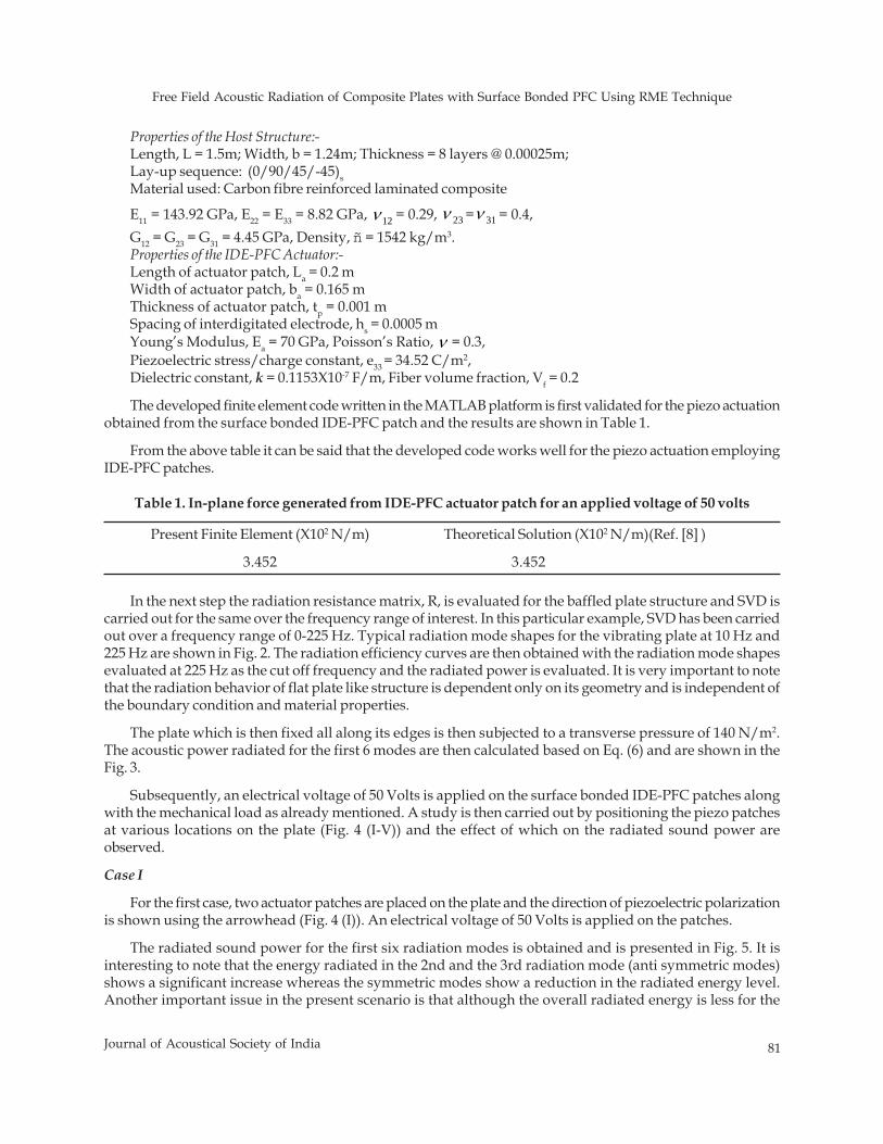
Free Field Acoustic Radiation of Composite Plates with Surface Bonded PFC Using RME Technique
81Journal of Acoustical Society of India
Properties of the Host Structure:-Length, L = 1.5m; Width, b = 1.24m; Thickness = 8 layers @ 0.00025m;Lay-up sequence: (0/90/45/-45)sMaterial used: Carbon fibre reinforced laminated composite
E11 = 143.92 GPa, E22 = E33 = 8.82 GPa, 12ν = 0.29, 23ν = 31ν = 0.4,G12 = G23 = G31 = 4.45 GPa, Density, ñ = 1542 kg/m3.Properties of the IDE-PFC Actuator:-Length of actuator patch, La = 0.2 mWidth of actuator patch, ba = 0.165 mThickness of actuator patch, tp = 0.001 mSpacing of interdigitated electrode, hs = 0.0005 mYoung’s Modulus, Ea = 70 GPa, Poisson’s Ratio, ν = 0.3,Piezoelectric stress/charge constant, e33 = 34.52 C/m2,Dielectric constant, k = 0.1153X10⁻⁷ F/m, Fiber volume fraction, Vf = 0.2
The developed finite element code written in the MATLAB platform is first validated for the piezo actuationobtained from the surface bonded IDE-PFC patch and the results are shown in Table 1.
From the above table it can be said that the developed code works well for the piezo actuation employingIDE-PFC patches.
Present Finite Element (X102 N/m) Theoretical Solution (X102 N/m)(Ref. [8] )
3.452 3.452
Table 1. In-plane force generated from IDE-PFC actuator patch for an applied voltage of 50 volts
In the next step the radiation resistance matrix, R, is evaluated for the baffled plate structure and SVD iscarried out for the same over the frequency range of interest. In this particular example, SVD has been carriedout over a frequency range of 0-225 Hz. Typical radiation mode shapes for the vibrating plate at 10 Hz and225 Hz are shown in Fig. 2. The radiation efficiency curves are then obtained with the radiation mode shapesevaluated at 225 Hz as the cut off frequency and the radiated power is evaluated. It is very important to notethat the radiation behavior of flat plate like structure is dependent only on its geometry and is independent ofthe boundary condition and material properties.
The plate which is then fixed all along its edges is then subjected to a transverse pressure of 140 N/m2.The acoustic power radiated for the first 6 modes are then calculated based on Eq. (6) and are shown in theFig. 3.
Subsequently, an electrical voltage of 50 Volts is applied on the surface bonded IDE-PFC patches alongwith the mechanical load as already mentioned. A study is then carried out by positioning the piezo patchesat various locations on the plate (Fig. 4 (I-V)) and the effect of which on the radiated sound power areobserved.
Case I
For the first case, two actuator patches are placed on the plate and the direction of piezoelectric polarizationis shown using the arrowhead (Fig. 4 (I)). An electrical voltage of 50 Volts is applied on the patches.
The radiated sound power for the first six radiation modes is obtained and is presented in Fig. 5. It isinteresting to note that the energy radiated in the 2nd and the 3rd radiation mode (anti symmetric modes)shows a significant increase whereas the symmetric modes show a reduction in the radiated energy level.Another important issue in the present scenario is that although the overall radiated energy is less for the
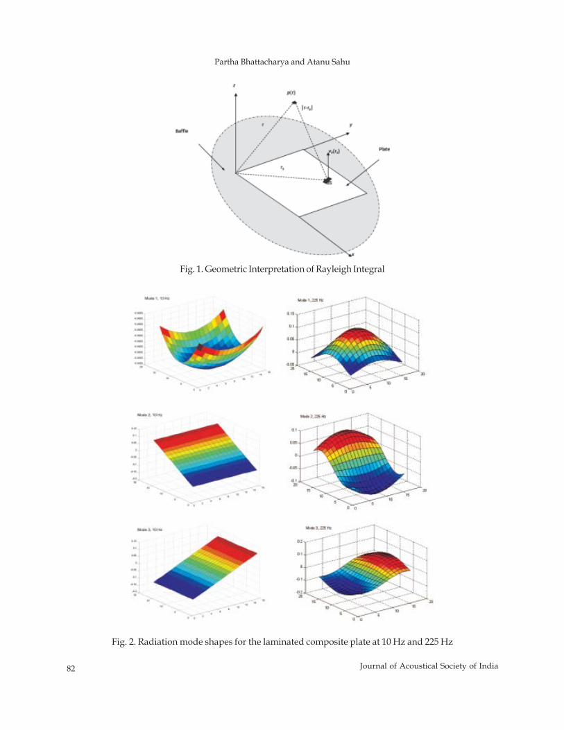
82 Journal of Acoustical Society of India
Partha Bhattacharya and Atanu Sahu
Fig. 1. Geometric Interpretation of Rayleigh Integral
Fig. 2. Radiation mode shapes for the laminated composite plate at 10 Hz and 225 Hz
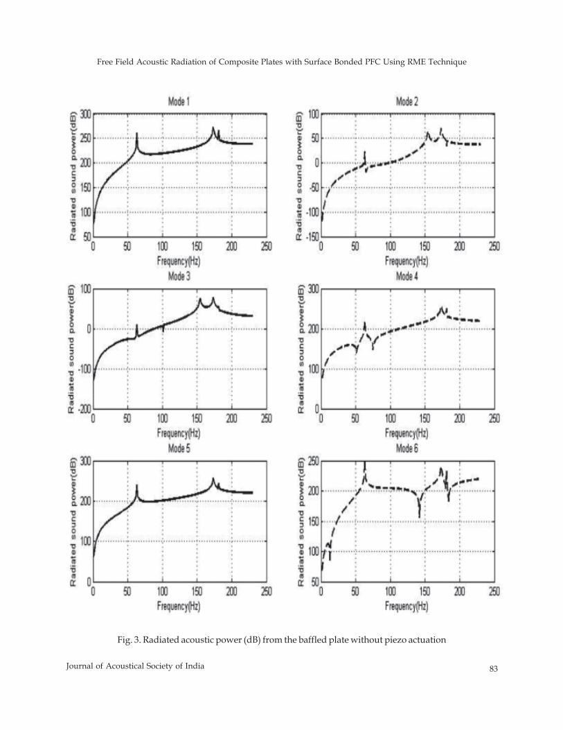
Free Field Acoustic Radiation of Composite Plates with Surface Bonded PFC Using RME Technique
83Journal of Acoustical Society of India
Fig. 3. Radiated acoustic power (dB) from the baffled plate without piezo actuation
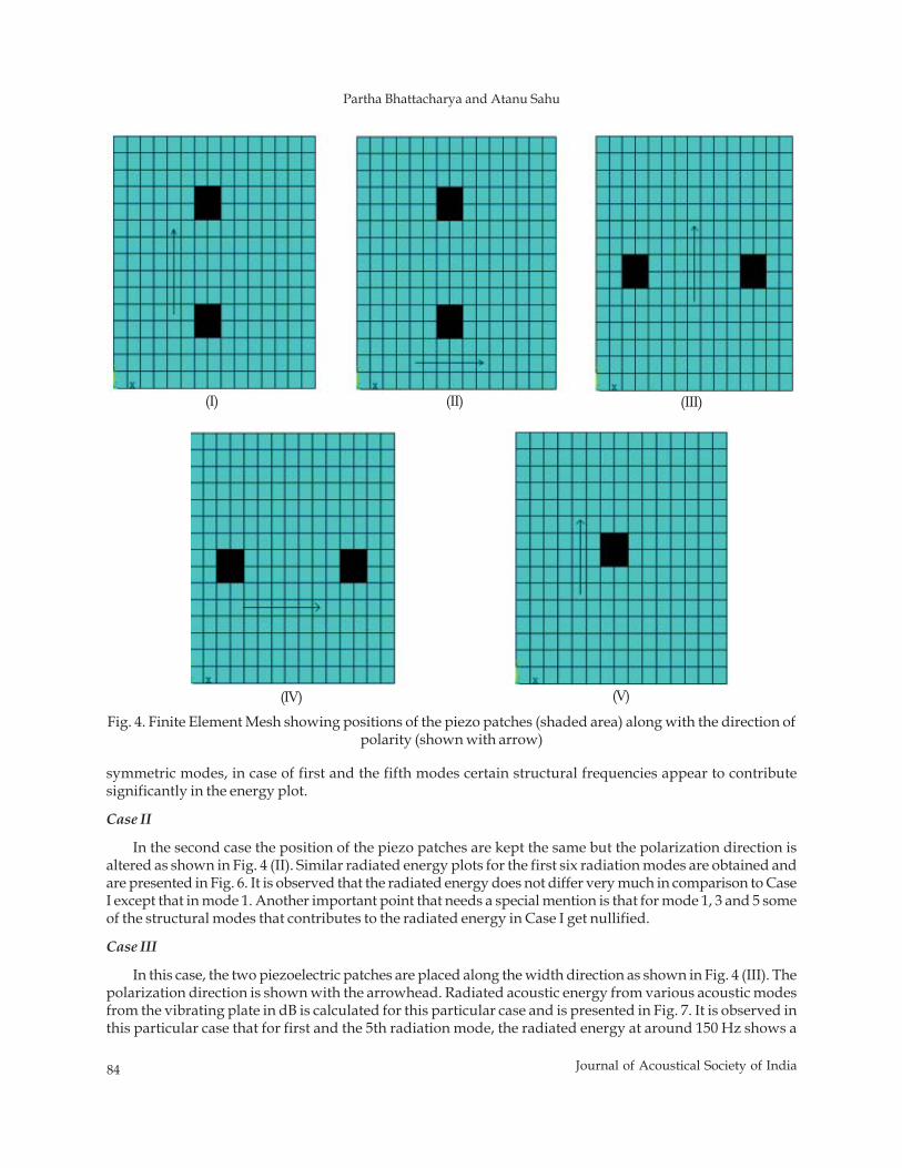
84 Journal of Acoustical Society of India
Partha Bhattacharya and Atanu Sahu
(I) (II) (III)
symmetric modes, in case of first and the fifth modes certain structural frequencies appear to contributesignificantly in the energy plot.
Case II
In the second case the position of the piezo patches are kept the same but the polarization direction isaltered as shown in Fig. 4 (II). Similar radiated energy plots for the first six radiation modes are obtained andare presented in Fig. 6. It is observed that the radiated energy does not differ very much in comparison to CaseI except that in mode 1. Another important point that needs a special mention is that for mode 1, 3 and 5 someof the structural modes that contributes to the radiated energy in Case I get nullified.
Case III
In this case, the two piezoelectric patches are placed along the width direction as shown in Fig. 4 (III). Thepolarization direction is shown with the arrowhead. Radiated acoustic energy from various acoustic modesfrom the vibrating plate in dB is calculated for this particular case and is presented in Fig. 7. It is observed inthis particular case that for first and the 5th radiation mode, the radiated energy at around 150 Hz shows a
Fig. 4. Finite Element Mesh showing positions of the piezo patches (shaded area) along with the direction ofpolarity (shown with arrow)
(V)(IV)
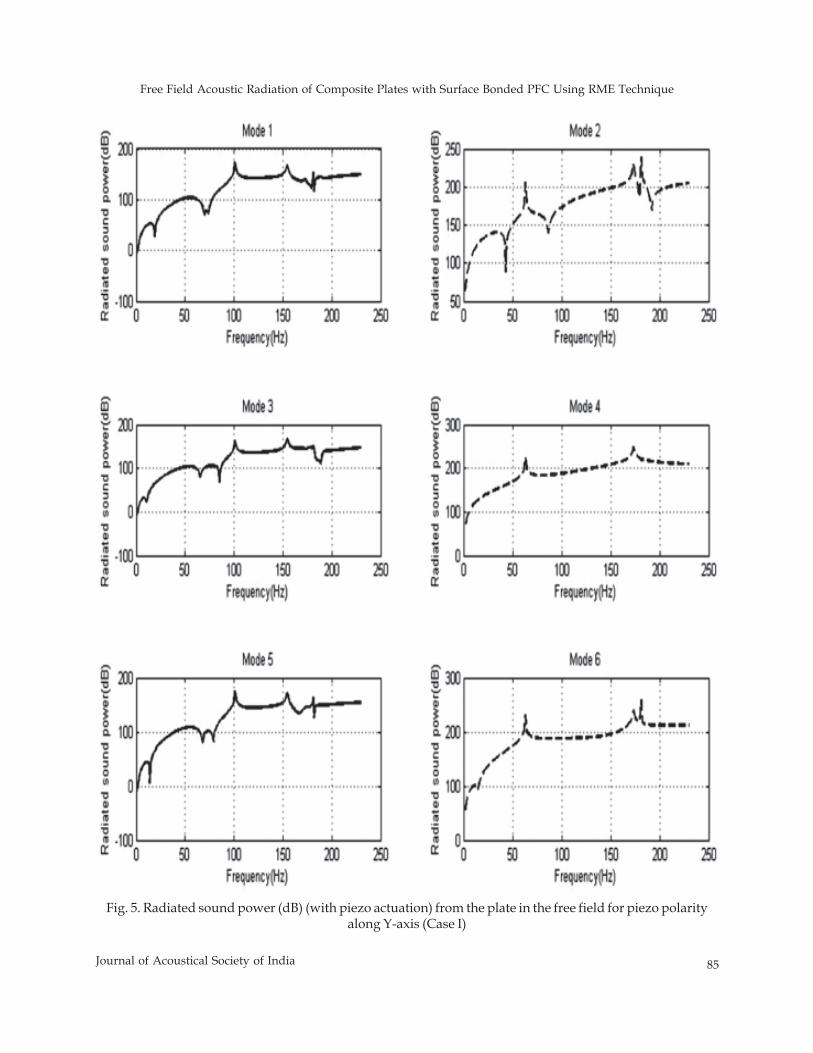
Free Field Acoustic Radiation of Composite Plates with Surface Bonded PFC Using RME Technique
85Journal of Acoustical Society of India
Fig. 5. Radiated sound power (dB) (with piezo actuation) from the plate in the free field for piezo polarityalong Y-axis (Case I)
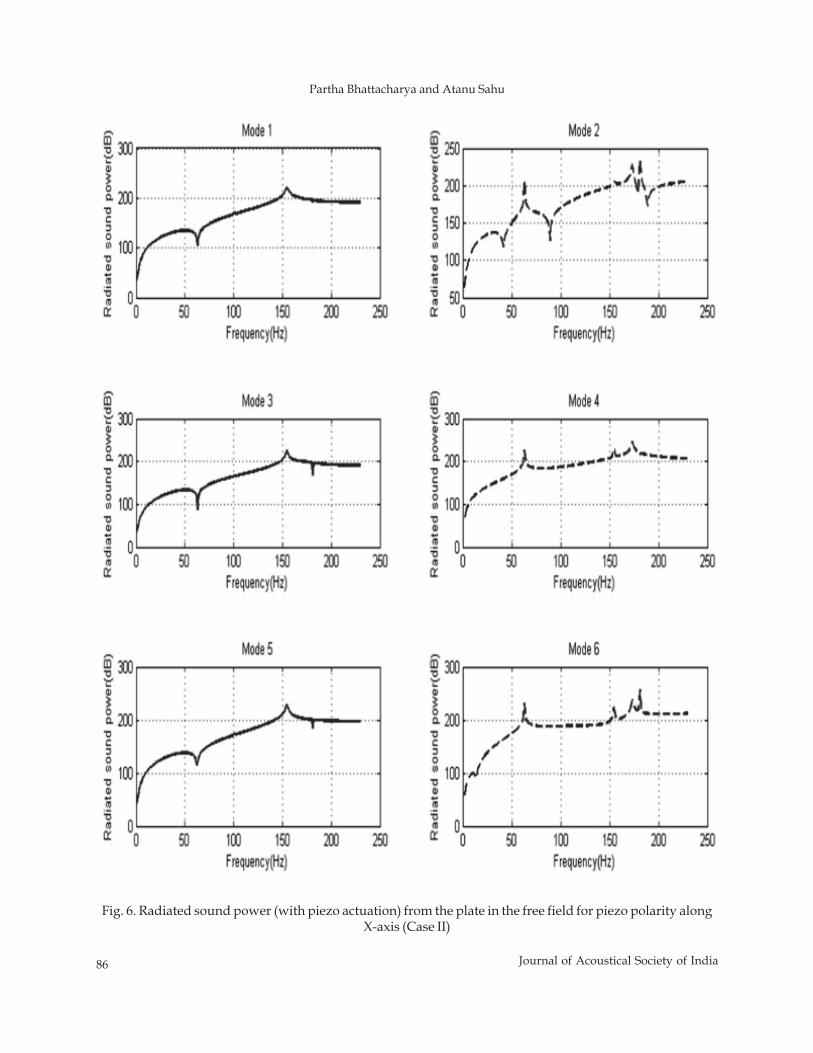
86 Journal of Acoustical Society of India
Partha Bhattacharya and Atanu Sahu
Fig. 6. Radiated sound power (with piezo actuation) from the plate in the free field for piezo polarity alongX-axis (Case II)
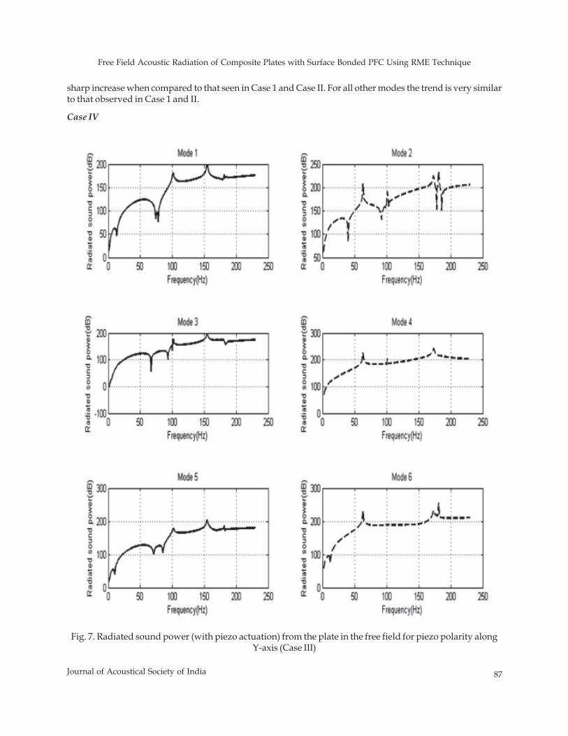
Free Field Acoustic Radiation of Composite Plates with Surface Bonded PFC Using RME Technique
87Journal of Acoustical Society of India
sharp increase when compared to that seen in Case 1 and Case II. For all other modes the trend is very similarto that observed in Case 1 and II.
Case IV
Fig. 7. Radiated sound power (with piezo actuation) from the plate in the free field for piezo polarity alongY-axis (Case III)
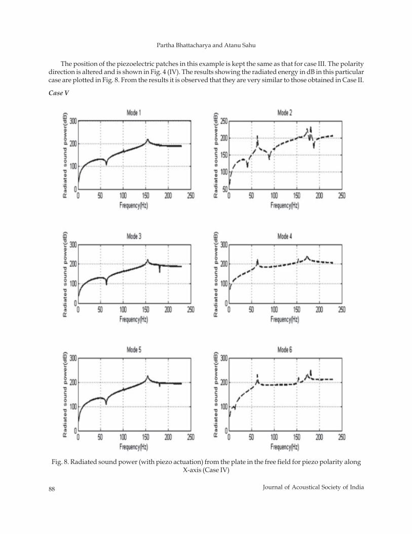
88 Journal of Acoustical Society of India
Partha Bhattacharya and Atanu Sahu
The position of the piezoelectric patches in this example is kept the same as that for case III. The polaritydirection is altered and is shown in Fig. 4 (IV). The results showing the radiated energy in dB in this particularcase are plotted in Fig. 8. From the results it is observed that they are very similar to those obtained in Case II.
Case V
Fig. 8. Radiated sound power (with piezo actuation) from the plate in the free field for piezo polarity alongX-axis (Case IV)
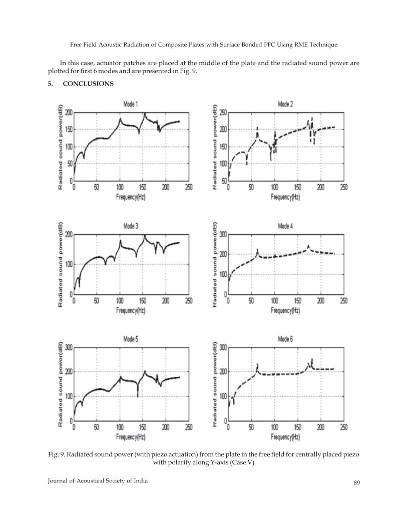
Free Field Acoustic Radiation of Composite Plates with Surface Bonded PFC Using RME Technique
89Journal of Acoustical Society of India
In this case, actuator patches are placed at the middle of the plate and the radiated sound power areplotted for first 6 modes and are presented in Fig. 9.
5. CONCLUSIONS
Fig. 9. Radiated sound power (with piezo actuation) from the plate in the free field for centrally placed piezowith polarity along Y-axis (Case V)
90 Journal of Acoustical Society of India
Partha Bhattacharya and Atanu Sahu
In the present work, Rayleigh's integral approach to the solution of the Helmholtz's Equation is carriedout and Radiation Modal Expansion method is implemented to calculate the radiation efficiency and theradiation mode shapes of the vibrating composite plate structure. Thereafter, a finite element model based onLagrange's equation for the laminated plate bonded with IDE-PFC patch actuator is developed. Radiationenergy for the vibrating structure with and without the piezo patches are the evaluated for various piezolocation and piezo polarity.
It is generally observed that with the introduction of the piezo patches, the radiated energy associatedwith the first, fifth and the sixth radiation mode, which are pumping modes and are symmetric in nature,show a reasonable reduction. On the contrary, in the second and the third radiation mode, the bare platewhich hardly contributes to any radiation energy starts pumping a significant energy into the free field oncethe piezoelectric patches are actuated.
The position and the polarity of the piezo patches also affect the radiated energy from the baffled plate byinfluencing the structural modes. From the obtained results it can be concluded that the positioning of thepiezo patches on the vibrating plate has got a significant role in the overall sound radiation. In the future it isplanned to do an optimization study to properly identify the piezo position and also the polarity directionsuch that the radiated sound power can be minimized effectively.
6. ACKNOWLEDGEMENT
The authors wish to acknowledge the Department of Science and Technology (DST), India for providingthe necessary support under the DST-PURSE scheme.
7. REFERENCES
[1] A. KACZMARSKA and D. AUGUSTYNSKA, 1992. Study of sound insulation of control cabins inindustry in the low frequency range J. Low Frequency Noise Vib., 11, 42–46.
[2] J.S. BEVAN, 2001. Technical Report NASA/CR-2001-211265, Piezoceramic Actuator Placement forAcoustic Control of Panels,.
[3] K.A. CUNEFARE, 1991. The minimum multimodal radiation efficiency of baffled finite beams, J. Acoust.Soc. Am., 90, 2521–2529.
[4] G.V. BORGIOTTI and K.E. JONES, 1994. Frequency independence property of radiation spatial filters,J. Acoust. Soc. Am., 96, 3516–3524.
[5] W.T. BAUMANN, W.R. SAUNDERS and H.H. ROBERTSHAW, 1991. Active Suppression of AcousticRadiation from Impulsively Excited Structures, J. Acoust. Soc. Am., 90(6), 3202-3208.
[6] S.J. ELLIOTT and M.E. JOHNSON, 1993. Radiation modes and the active control of sound power, J.Acoust. Soc. Am., 94, 2194–2204.
[7] G.P. GIBBS, R.L. CLARK, D.E. COX and J.S. VIPPERMAN, 2000. Radiation modal expansion: Applicationto active structural acoustic control, J. Acoust. Soc. Am., 107, 332 – 339.
[8] P. BHATTACHARYA, M. ROSE and O. HEINTZE, 2009. 9th International Conference on VibrationsProblems, IIT Kharagpur, India, 19-22 January, Active structural acoustic control of laminated Platesusing RME technique.
[9] F.J. FAHY, 2001. Foundations of Engineering Acoustics, Academic Press.[10] A.A. BENT, 1997. PhD Thesis, MIT, Active Fiber composites for Structural Actuation.[11] M.S. AZZOUZ, C. MEI, J.S. BEVAN and J.J. RO, 2001. Finite Element Modeling of MFC/AFC actuators
and performance of MFC, J. of Intel. Mat. Sys. and Struct., 12, 601-612.
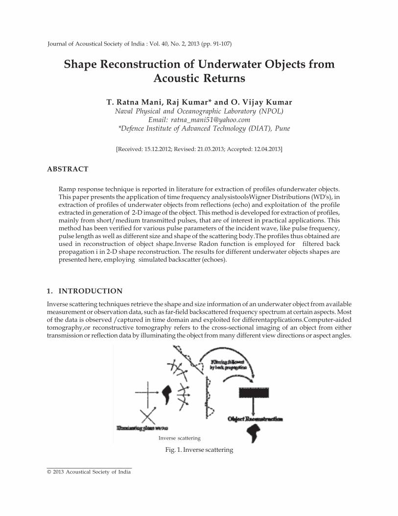
Shape Reconstruction of Underwater Objects from Acoustic Returns
91Journal of Acoustical Society of India
Shape Reconstruction of Underwater Objects fromAcoustic Returns
T. Ratna Mani, Raj Kumar* and O. Vijay KumarNaval Physical and Oceanographic Laboratory (NPOL)
Email: [email protected] *Defence Institute of Advanced Technology (DIAT), Pune
[Received: 15.12.2012; Revised: 21.03.2013; Accepted: 12.04.2013]
ABSTRACT
Ramp response technique is reported in literature for extraction of profiles ofunderwater objects.This paper presents the application of time frequency analysistoolsWigner Distributions (WD's), inextraction of profiles of underwater objects from reflections (echo) and exploitation of the profileextracted in generation of 2-D image of the object. This method is developed for extraction of profiles,mainly from short/medium transmitted pulses, that are of interest in practical applications. Thismethod has been verified for various pulse parameters of the incident wave, like pulse frequency,pulse length as well as different size and shape of the scattering body.The profiles thus obtained areused in reconstruction of object shape.Inverse Radon function is employed for filtered backpropagation i in 2-D shape reconstruction. The results for different underwater objects shapes arepresented here, employing simulated backscatter (echoes).
1. INTRODUCTION
Inverse scattering techniques retrieve the shape and size information of an underwater object from availablemeasurement or observation data, such as far-field backscattered frequency spectrum at certain aspects. Mostof the data is observed /captured in time domain and exploited for differentapplications.Computer-aidedtomography,or reconstructive tomography refers to the cross-sectional imaging of an object from eithertransmission or reflection data by illuminating the object from many different view directions or aspect angles.
Journal of Acoustical Society of India : Vol. 40, No. 2, 2013 (pp. 91-107)
Inverse scattering
Fig. 1. Inverse scattering
© 2013 Acoustical Society of India
92 Journal of Acoustical Society of India
T. Ratna Mani, Raj Kumar and O. Vijay Kumar
In ocean tomography, underwater objects are imaged by reflection tomography. Reconstructive acoustictomography reconstructs an image of the objectfrom projections recorded at all aspect angles.The transformationof object functionto image is done by single dimension projection views of the object. The sonartransducer ismoved from point to point around the entire circumference of acircle so as to view the object from all possibleaspect angles, thus compilinga complete set of projections over 3600 of aspect angle viewing. Theimagerepresents a 2-D map of the 3-D acoustic reflectivity function when projectedon the imaging plane.Similarto X-ray absorption tomography the tomographic imagingsonar, the poor resolution is overcome by viewingthe object at many aspect angles θ, enabling the reconstruction of a high-resolution image ofthe object .In bi-static sonar ,the image can be obtained by fewer no of projections. This is based on obtaining the object profilesin few multiple angles and thenapplying limiting surface technique iteratively to obtain the 3D image. In boththe cases the profile functions /object functions have to be obtained for reconstruction of the image. In General,the profile function is obtained based on impulse/ wideband input. However, in practice the sonar transducersare narrowband and the sound propagating in underwater media also has certain response. In addition therequirement of operations also imposes certain minimum duration for the transmission pulse. The velocity ofsound in this media 1500 meters/second (approximately) also has certain effects on the received data. Henceto obtain the images pulse, compression has to be carried out, or profile function has to e obtained by processingthe received data.
The forward scattering is found for given incidentacoustic waves and the physical properties ofthe objectby simulation or observation data. For generation of back scatter from the object, exact analytic solutions [1, 2]can be derived and used for objects of simplegeometries, such as sphere, infinite cylinder,and spheroid, whileapproximate methods areoften used for objects of more general shapes.The most popular method for inversescattering for underwater objects is the ramp response technique. This is basedon twice integrating the impulseresponseobtained from the underwater object. X.M.Zhang et al. [2] developed a numerical method to obtain theramp response for underwater objects in acoustic field, that requires limited data infrequency domain.Theconcept of impulse response technique isfirst introduced by E.M. Kennaugh [8] and applied to electromagneticscattering problems,based on the physical optics approximation.The impulse response of an object wasinterpretedas the second derivative of the profile function.The profile function is defined as the crosssectionalarea along the direction of the incidentwave. Consequently, by integrating the impulseresponse twice, it wasfound that the rampresponse of the object is proportional to itsprofile function [4]. The ramp responsetechniquehas been utilized in electromagneticscattering for profile reconstruction [1]. Thistechnique has alsobeen applied in acousticwave filed for solving inverse problems, likeunderwater acoustical imaging and non-destructiveevaluation methods.The methods based on impulse responsetechniques have limited practicalapplications asthe wide band returns from the underwaterbody are highly influenced by the media. Thepracticalsignals have limited bandwidth,generally very narrowband due to the limitationsof the projectors/sensors. Inaddition, the pulsewidths used is based on certain criteria andvaries from short pulse to medium pulse.Theramp response technique cannot be applied forthis type of signals. However, as the profilefunction is thecross sectional area along thedirection of propagation, the reflected wave canbe interpreted as sum of discretisedwavesreturning from the scattering body, and can beconsidered as time series data, with timevarying frequencycontent. Time series datahave been traditionally analysed in either thetime or the frequency domains.Forsignals with time-varying frequencycontent, the combined time-frequency (TF)representations, based on theCohen class of (generalized) Wigner Distributions (WD's) offer a powerful analysis tool. Using them, it ispossibleto: 1) trace the time-evolution of theresonance features usually present in a standardSonar Cross Section (SCS),or in a Radar Cross Section (RCS) and 2) extract target information that may be difficult to even notice inanordinary SCS or RCS In the underwaterapplications. The time frequency techniques aregenerally used to gettime and frequencylocalisation of the signal. This information isvaluable in frequency estimation of signals,anddetection and classification of targets.Application of time frequency analysis forscattering/inversescattering is not much reportedin literature. Time-frequency analysis can becarried out, on the reflected signal,for theprofile function extraction. The instantaneousamplitude correspond to the cross section of thescatteringbody , that is The profile function is the timeseries of amplitude at discrete time intervals,can be obtained fromsumming the energy fromall frequency bins corresponding to each time step. This technique is applied to
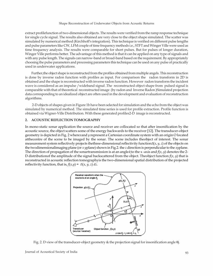
Shape Reconstruction of Underwater Objects from Acoustic Returns
93Journal of Acoustical Society of India
extract profilefunction of two-dimensional objects. The results were verified from the ramp response techniquefor single cycle signal. The results also obtained are very close to the object shape simulated. The scatter wassimulated by numerical method (Kirchhoff's integration). This technique is verified on different pulse lengthsand pulse parameters like CW, LFM couple of time frequency methods i.e., STFT and Winger Ville were used astime frequency analysis. The results were comparable for short pulses. But for pulses of longer duration,Winger Ville performs better. The advantage of this method is that it can be applied on any type of signals andwith any pulse length. The signals can narrow-band or broad-band based on the requirement. By appropriatelychoosing the pulse parameters and processing parameters this technique can be used on any pulse of practicallyused in underwater applications.
Further,the object shape is reconstructed from the profiles obtained from multiple angels. This reconstructionis done by inverse radon function with profiles as input. For comparison the radon transform in 2D isobtained and the shape is reconstructed with inverse radon function. However radon transform the incidentwave is considered as an impulse /wideband signal .The reconstructed object shape from pulsed signal iscomparable with that of theoretical reconstructed image (by radon and Inverse Radon )Simulated projectiondata corresponding to an idealized object are often used in the development and evaluation of reconstructionalgorithms.
2-D objects of shapes given in Figure 1b have been selected for simulation and the echo from the object wassimulated by numerical method. The simulated time series is used for profile extraction. Profile function isobtained via Wigner-Ville Distribution. With these generated profiles2-D image is reconstructed.
2. ACOUSTIC REFLECTION TOMOGRAPHY
In mono-static sonar application the source and receiver are collocated so that after insonification by theacoustic source, the object scatters some of the energy backwards to the receiver [12]. The transducer-objectgeometry is depicted in Fig. 2 wherexand y represent a Cartesian coordinate system with an origin O locatedatthecentre of the scene to be imaged by the sonar. The scene includes theobject of interest. The sonarmeasurement system reflectively projects thethree-dimensional reflectivity functionñ(x, y, z) of the objects onthe twodimensionalimaging plane (or x yplane) shown in Fig.2. the z direction is perpendicular to the xyplane.The direction of propagation of the sonartransmission is at an angleèjto the x -axis and f(x, y) denotes the 2-D distributionof the amplitude of the signal backscattered from the object. Theobject function f(x, y) that isreconstructed in acoustic reflection tomographyis the two-dimensional spatial distribution of the projectedreflectivity function, that is, f(x,y) = ñ(x, y, z) dz.
Fig. 2. D view of the transducer-object geometry & the projection signal for insonification angle θj.
94 Journal of Acoustical Society of India
T. Ratna Mani, Raj Kumar and O. Vijay Kumar
In Fig. 2, the sonar transducer and the object are widely separated sothat a planar wave front projected on theimaging (or xyplane) plane canbe represented by the straight line AB, which is defined mathematically bytheequation xcosèj+ y sinèj= si. Here si is the perpendicular distance ofthe line from the origin O. The two-waypropagation time for the wave frontAB is given by ti = t0 + 2(si/c), where c is the speed of sound propagationinthe underwater medium. The distance of the origin from the transduceris R0 = (ct0)/2. As the signalsbackscattered from all of the points alonga wave front are in phase, the total signal received at time ti is foundbyadding the backscattered signals f(x,y)for values of x and y along the line xcosèj+ y sinèj= si. This can berepresented mathematically as
g (si.θj) = ∫ f (x,y) ds1 (1)
where ∫ f (..) ds1 denotes integration along the line xcosèj+ y sinèj= siThe integral in Equation (1) is referred toas a wave front integral. The set of wave front integrals g(si.èj) where - <si< , forms the function g(si.èj) thatdefines the projection of f(x,y)for the angle j . Reconstructive acoustic tomography reconstructs an image of theobject from projections recorded at all aspect angles. The object function f(x,y)is reconstructed from the inverseof the integral equation given by
g (si.θj) = ∫ f (x,y) ds1
= ∫ f (sicosθj-s1sinθj, sisinθj - s1cosθj) ds1
Here, the coordinate pair (si, s1) represents the rotation of the coordinatepair f (x, y) through an angle, that isx = sicosθj-s1sinθj y = sisinθj + s1cosθj
The 2-D function g(si.èj) represents the Radon transform of Using the inverse Radon transform orother suitable reconstruction algorithm, an image of the object that is represented by the two-dimensionaldistribution can be recovered from the projections recorded at all aspect angles j , where 0< j<2ð. Theinversion is given by,f (x,y)=R-1g(si.qj)
WhereR-1 {.}denotes the inverse Radon transform operator.
However in underwater applications the velocity of the sound is nearly 1500mt/sec. Due to this slowspeed the returns from different range cells do overlap for signals of finite pulse width. Hence with the limitedbandwidth of the transmitted pulse the wave front integral is different from that of impulse transmission.The backscattered signal may be considered as sum of wave front integrals with different phases.The phasedifference of wave fronts corresponds to time difference corresponding to different range cells .Hence theprofile function has to be obtained by pulse compression corresponding to each range cell.
3. PROFILE FUNCTION
Ramp Response Technique:When an incident pulse pt represented by a delta function in time (t) encountersan object in a homogeneous, isotropic Medium, the phenomenon of wave diffraction or scattering occurs. Theincident pulse is scattered in all directions. The waveform scattered in a direction opposite to the direction ofincidence is called the backscattered impulse response. The ramp response is defined as a time-domainbackscattered signal at a distant observation point in response to an incident ramp signal. The ramp signalis a function defined to be the second integral of the incident impulse function. In practice, the projector-hydrophone system is inverseused for the ramp response measurement. The projector generates an acousticpulse and sends it out, while the hydrophone is used to receive the backscattered impulse response.Consequently, the backscattered impulse response is integrated twice with respect to time to yield rampresponse. As we only need the backscattered signals, the projector and hydrophone should be set together:PR(t) = ∫ t (∫ PI(t)dt’) dtwhere, c represents the sound velocity in the water and A (ct/2)is the area of cross section of the object
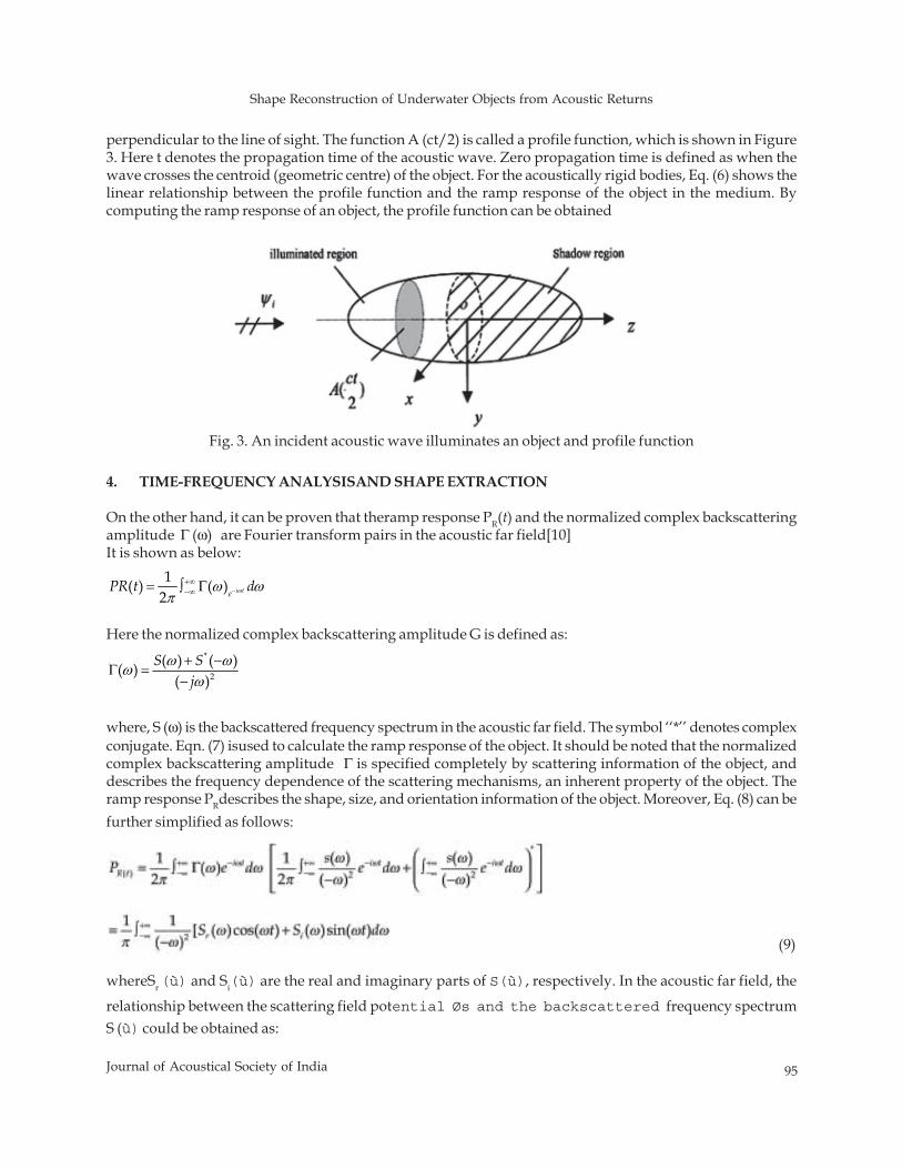
Shape Reconstruction of Underwater Objects from Acoustic Returns
95Journal of Acoustical Society of India
perpendicular to the line of sight. The function A (ct/2) is called a profile function, which is shown in Figure3. Here t denotes the propagation time of the acoustic wave. Zero propagation time is defined as when thewave crosses the centroid (geometric centre) of the object. For the acoustically rigid bodies, Eq. (6) shows thelinear relationship between the profile function and the ramp response of the object in the medium. Bycomputing the ramp response of an object, the profile function can be obtained
4. TIME-FREQUENCY ANALYSISAND SHAPE EXTRACTION
On the other hand, it can be proven that theramp response PR(t) and the normalized complex backscatteringamplitude Γ (ω) are Fourier transform pairs in the acoustic far field[10]It is shown as below:
1( ) ( )2 i tePR t dωω ωπ
−+∞−∞= ∫ Γ
Here the normalized complex backscattering amplitude G is defined as:*
2( ) ( )( )
( )S S
jω ωω
ω+ −
Γ =−
where, S (ω) is the backscattered frequency spectrum in the acoustic far field. The symbol ‘‘*’’ denotes complexconjugate. Eqn. (7) isused to calculate the ramp response of the object. It should be noted that the normalizedcomplex backscattering amplitude Γ is specified completely by scattering information of the object, anddescribes the frequency dependence of the scattering mechanisms, an inherent property of the object. Theramp response PRdescribes the shape, size, and orientation information of the object. Moreover, Eq. (8) can befurther simplified as follows:
(9)
whereSr (ù) and Si(ù) are the real and imaginary parts of S(ù), respectively. In the acoustic far field, the
relationship between the scattering field potential Øs and the backscattered frequency spectrumS (ù) could be obtained as:
Fig. 3. An incident acoustic wave illuminates an object and profile function
96 Journal of Acoustical Society of India
T. Ratna Mani, Raj Kumar and O. Vijay Kumar
(10)
Now, 1) to obtain the profile function (ramp response) for the band limited signal, the integral in the equationmay be restricted to the signal bandwidth. 2) The integral, corresponding frequency components is obtainedat discreet time instances. This method of profile function extraction is suitable for practical applications ofband-limited signals. However this requires back scattered signal to be represented/converted to timefrequency representation. Profile function can be obtained by forming the integral of amplitude of all thefrequency components for the corresponding time instances. However this may have some smearing/broadening effect on the profile function due to band limiting of the signal and can be compensated in imagereconstruction. Two Time-Frequency methods for this application that have been used and compared areSTFT and Wigner -Ville distributions. The Fourier Transform decomposes a signal into its constituent frequencycomponents. Looking at the Fourier spectrum we can identify the frequencies. However, we cannot identifytheir temporal localization. Time Frequency Distributions (TFDs) map a one-dimensional signal into a two-dimensional function of time and frequency, and describe how the spectral content of the signal changes withtime. From a strict mathematical point of view, we want to have a joint distribution, which will give us thefraction of the total energy of the signal at time t and frequency ?; i.e., we look for the function P(t, ?). The aimof time-frequency analysis is to come up with appropriate candidates for P(t, ?).TFD are appropriate tools fornon-stationary signal analysis, synthesis, and processing. Different types of time frequency distribution havebeen developed for that purpose. Two early forms of time-frequency analyses are: the Short-Time FourierTransform (STFT), used to generate the spectrogram (SP) [Koenig, Dunn and Lacy, 1946; Allen, and Rabiner,1977], and the Wigner-Ville distribution (WVD) [ClaasenandMecklenbrauker, 1980]. Studies of the well knownlinear TFD Short-Time Fourier Transform (STFT) have been published by Nawad and Quatieri, [1988], andAllen [1977] among others. The time-frequency distribution ideally describes how the energy is distributed,and allows us to estimate the fraction of the total energy of the signal at time t and at frequency ?. The abovestatement states that the energy should be positive. In order to achieve fine simultaneous time-frequencyresolution in a non-stationary time series, we must deal with the uncertainty principle [Williams, Brown andHero, 1991]. The uncertainty principle restricts us from achieving arbitrarily fine resolution simultaneouslyin both the time and the frequency domain. The condition to satisfy in the uncertainty principle is given by theinequality ΔωΔt ≥ 1/2, wherethe selection of Δt (time resolution) and Δω (frequency resolution) parameters isnot arbitrary. A trade-off between them should be considered in order to reach the desired "good" resolution.Next, an overview and a brief description of the advantages/limitations of the Spectrogram (SP), the Wigner-Ville (WVD), are presented.
4.1 Short-Time Fourier Transform (STFT)
In order to introduce time-dependency in the Fourier transform, a simple and intuitive solution consists inpre-windowing the signal x(u) around a particular time t, calculating its Fourier transform, and doing that foreach time instant t. The resulting transform, called the short-time Fourier transform (STFT, or short-timespectrum), is
2*2 ( , , ) ( ) ( ) j uF t h x u h u t e duπνν −+∞
−∞= ∫ − (11)
where h(t) is a short time analysis windowlocalized around t = 0 and v = 0.The STFT can beconsidered as the result of passing the signal x(u) through a bandpassfilter whose frequency response isH(î” v), and is therefore deduced from a mother filter H(î) by a translation of v. So the STFT is similar to abank of band-pass filters with constant bandwidth. The spectrogram is better able to resolve temporal evolutionof frequency content, buthas a trade-off in time resolution versus frequency resolution in accordance with theuncertainty principle. To overcome this restriction, several classes of Time-Frequency representations havebeen proposed, including wavelet methods and quadratic time-frequency distributions such as the Wigner-Ville distribution.
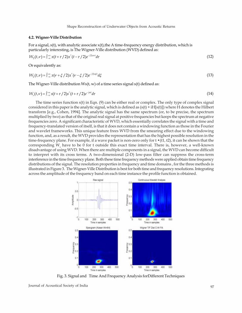
Shape Reconstruction of Underwater Objects from Acoustic Returns
97Journal of Acoustical Society of India
4.2. Wigner-Ville Distribution
For a signal, s(t), with analytic associate x(t),the A time-frequency energy distribution, which isparticularly interesting, is The Wigner-Ville distribution (WVD) defined as:
* 22 ( , ) ( /2) ( /2) J tW t x t x t e dπνν τ τ τ+∞ −
−∞= ∫ + − (12)
Or equivalently as:
* 22 ( , ) ( /2) ( /2) J tW t x x e dπξν ν ξ ν ξ ξ+∞ −
−∞= ∫ + − (13)
The Wigner-Ville distribution Ws(t, w) of a time series signal s(t) defined as:
*( , ) ( /2) ( /2) j tsW t s t s t e dων τ τ τ−+∞
−∞= ∫ + + (14)
The time series function s(t) in Eqn. (9) can be either real or complex. The only type of complex signalconsidered in this paper is the analytic signal, which is defined as (s(t) + iH[s(t)]) where H denotes the Hilberttransform [e.g., Cohen, 1994]. The analytic signal has the same spectrum (or, to be precise, the spectrummultiplied by two) as that of the original real signal at positive frequencies but keeps the spectrum at negativefrequencies zero. A significant characteristic of WVD, which essentially correlates the signal with a time andfrequency-translated version of itself, is that it does not contain a windowing function as those in the Fourierand wavelet frameworks. This unique feature frees WVD from the smearing effect due to the windowingfunction, and, as a result, the WVD provides the representation that has the highest possible resolution in thetime-frequency plane. For example, if a wave packet is non-zero only for t •(t1, t2), it can be shown that thecorresponding Ws have to be 0 for t outside this exact time interval. There is, however, a well-knowndisadvantage of using WVD. When there are multiple components in a signal, the WVD can become difficultto interpret with its cross terms. A two-dimensional (2-D) low-pass filter can suppress the cross-terminterference in the time frequency plane. Both these time frequency methods were applied obtain time frequencydistributions of the signal. The resolution properties in frequency and time domains , for the three methods isillustrated in Figure 3. The Wigner-Ville Distribution is best for both time and frequency resolutions. Integratingacross the amplitude of the frequency band on each time instance the profile function is obtained.
Fig. 3. Signal and Time And Frequency Analysis forDifferent Techniques
98 Journal of Acoustical Society of India
T. Ratna Mani, Raj Kumar and O. Vijay Kumar
5. PULSE COMPRESSION ANDRECONSTRUCTION OF THE OBJECT SHAPE( 2-D)
The back scatter is simulated for different objects, as time series for different view angles, for the same pulsewidth and pulse frequency. The time series mapped to time frequency domain by Wigner-Ville distribution(WVD) for each view angle.
*2 ( , ) ( /2) ( /2) j tW t w s t s t e dωτ τ τ−+∞
−∞= ∫ + −
From the two dimensional time -frequency mapping, profile function corresponding to time is obtainedby, integrating the amplitude of each frequency component over the frequency band, for each time instance.Thisleads to pulse compression. The pulse is compressed by a factor CF, where CF=PW/t for PW is pulse widthand t is sample time.
The profile function is PR(t) is
( )1 ( )
2i t
R tP e dω ωω ω ω
π+ −−= ∫ Γ
*
2( ) ( )( )
( )S S
jω ωω
ω+ −
Γ =−
The profile functions are obtained by for all aspect angles for reconstruction of image. The set of profileforms the radon transform of the object in terms of reflection tomography .Therefore set of profilesat all aspectangles j , where 0<j > 2are obtained. This set can be transformed by any back projection operator. The inverseRadon transform is employed in image reconstruction. An image of the object that is represented by the two-dimensional distribution f(x,y),has been recovered from the projections recorded at all aspect angles j.Thetheoretical radon transform is also computed for comparison with that obtained via time frequency tools ,forpulsed wave form .
6. RESULTS AND DISCUSSION
The 2D view of underwater object is employed in simulation of back scatter illustrated along with results foreach object.
The forward scatter of object hasbeen simulated by numerical method [9] for single cycle, multiple cyclesand for different frequencies. The refection coefficient is assumed to be uniform and equal to unity. The profilefunction was obtained by using ramp response technique via time frequency analysis [2]. The shape/contourobtained of results obtained using profile function [2] is very close to the object shape/contour simulated bynumerical method. Several shapes were used in simulations for different pulse parameters, size of the objects,as well as different sizes of the spatial grid and sampling frequencies. The parameters used in simulation arei.e., frequency; 25 KHz, transmitter angle è1 = 95and receiver angle è2 = 95. The other parameters as takenlike size of the body 10 × 1 meters and sound velocity = 1500 meters/sec. Rectangular body is defined as thebasic shape and another rectangle/triangle is either added or subtracted to obtain the shape. The forwardscatter of object has been simulated by numerical method for different cycles and for different frequencies. Theparameters like placement of the alteration (P.S), width of theshape for modification (w), and alteration type(a+ or a–) are described along with the result.The results in general conforms that for Pulsed signal the profilefunction can be obtained by time frequency tools , by pulse compression . If the pulse is close to impulseequivalent then profile obtained by ramp response is better .However result from WVD is also sufficientlyclose to object shape and efficiently used in object recognition /classification.
6.1 Profile Function via Time Frequency Analysis
Figures 5 to 7 indicates the time seriesgenerated and profile function extracted formono static case. Figure 4a,depicts time series from simulation for P.S = 200, w = 10, type = a– and No. of cycles = 3. Figure 4b and 4c
Shape Reconstruction of Underwater Objects from Acoustic Returns
99Journal of Acoustical Society of India
denotes the corresponding profile functions extracted from time series generated in Figure 3a. By rampresponse technique (4b), and Wigner Vile technique (4c). The parameters used in simulation are i.e., frequency;25 KHz, transmitter angle è1 = 950and receiver angle è2 = 950. The other parameters as taken like No. of cycles= 3; No. of finite elements; 500 × 50, Element type as rectangular, size of the bodyas 10 × 1 meters and soundvelocity = 1500 meters/sec. In Figure 4a exhibits the time series from simulation for P.S = 1000, w = 20 type =a– and at P.S = 3000, w = 20 type = a– and No. of cycles = 20. The No. of finite elements is set as 4000 x500.
In Fig. 5a exhibits the time series from simulation for P.S = 1000, w =20 type = a- and at P.S = 3000, w =20type = a- and No. Of cycles = 20.for a bi-static reception, with incidence at 95 and receiver at 40.The No. offinite elements is set as 4000 x500. The profile function extracted from Fig. 5a by ramp response technique(6b), by STFT technique (6c), and Wigner vile technique (5d) is shown in Figs. 5b, 5c, and 5d.
In Fig. 6a exhibits the time series from simulation for P.S = 1000, w =20 type = a- and at P.S = 3000, w =20type = a- and No. Of cycles = 80.for a bi-static reception, with incidence at 90 and receiver at 80. The No. offinite elements is set as 4000 x500. The profile function extracted from Fig. 6a by ramp response technique(6b), by STFT technique (6c), and Wigner vile technique (6d) is shown in Figs. 6b, 6c, and 6d.
From results, it is clear that the computational technique can be used on any shape of the object. However,the profile extraction function most suited on impulse incidence may not suitable for wide pulses, and for allpractical applications the pulse does have finite pulse width. From the above results, it is also observed thatshorter pulse gives the better definition than wide pulse.For practical applications the ramp response methodmay not suitable for profile extraction .Methods based on time- frequency distribution /analysis presentedhere for extraction of profile function are more suitable for most practical applications. Out of the methodspresented the Wigner Ville is better than the other methods, due to its inherent auto correlation property. Thismethod is also better suited for noise added signals i.e. in practical environment. Profile functions from manyangles are used on reconstruction of the object image. The set of profile functions are transformed to image byInverse-Radon transform.
6.2 Image Reconstruction
The results for reconstruction of simulated objects by two methods are depicted below. Three object shapesare simulated .The object function/profile functions are obtained for different angles via pulse compressionvia WVD. 2D images are reconstructed by applying the Inverse-radon function. The ideal profile functionswere also obtained by Radon transform. The image from this also is reconstructed by ideal I-radon transform.
The results obtained for shape reconstruction for both the cases for different are presented from figure 7to figure 9.The ‘..’ in Figure(..x) Indicates the figure number. In the results ,Figure(..) is 2D shape of the objectsemployed in simulation of backscatter. The transmission pulse used in simulation is 20 cycles. The profilefunctions obtained for all angles is plotted in figure (..a). The theoretical radon transform for the image isdepicted in figure(..b) . The reconstructed image of the object via inverse radon is in figure (..c).The radontransform obtained forpulse via WVD is presented in figure (..d).The reconstructed image of the object by thepulse compressed time series by applying WVD processing technique and further back propagated andreconstructed image is in depicted in figure (..e).In case of third object is frame with uniform reflection coefficient.
The shape reconstructed is fairly close to the original shape through WVD is better than obtained bytheoretical radon. This may be due to filtering process involved in pulse compression .i.e integration of thefrequency components of the WVD output. Post processing the image obtained shall improve the quality ofthe image. The last object simulated is a structure that is, the general acoustic reflecting surface of a mine typeof object. The results here are quite comparable to that of ideal impulse imaging.
7. CONCLUSION
The shape reconstructed is fairly close to the original shape. This is can be efficiently used in objectrecognition and classification. The method proposed i.e. Application of WVD in profile function extractiontherefore can beeffectively used in obtaining the shapereconstruction of underwater objects. .Forall practical
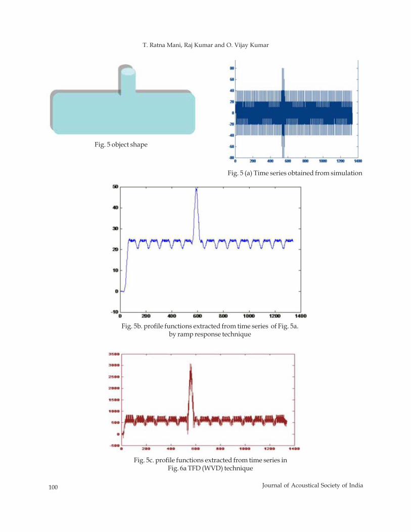
100 Journal of Acoustical Society of India
T. Ratna Mani, Raj Kumar and O. Vijay Kumar
Fig. 5 object shape
Fig. 5 (a) Time series obtained from simulation
Fig. 5b. profile functions extracted from time series of Fig. 5a.by ramp response technique
Fig. 5c. profile functions extracted from time series inFig. 6a TFD (WVD) technique
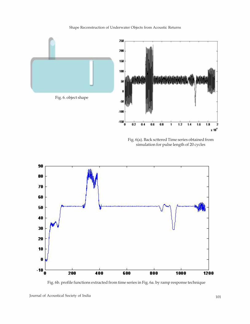
Shape Reconstruction of Underwater Objects from Acoustic Returns
101Journal of Acoustical Society of India
Fig. 6. object shape
Fig. 6(a). Back scttered Time series obtained fromsimulation for pulse length of 20 cycles
Fig. 6b. profile functions extracted from time series in Fig. 6a. by ramp response technique
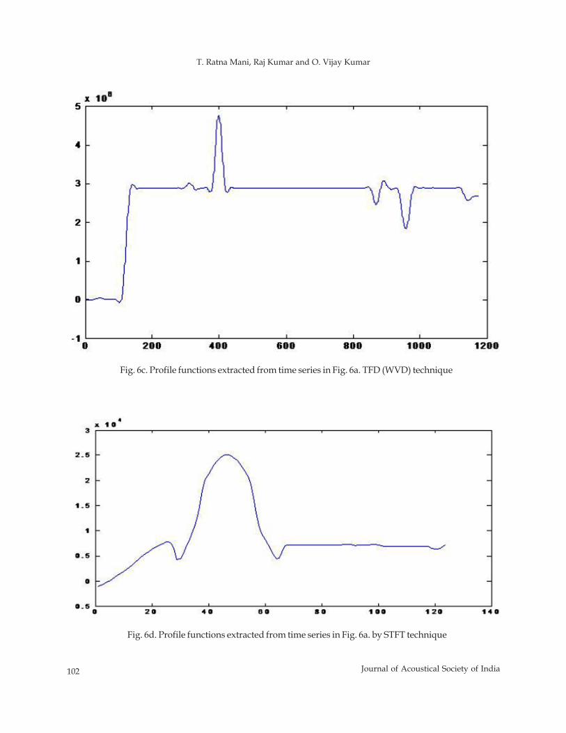
102 Journal of Acoustical Society of India
T. Ratna Mani, Raj Kumar and O. Vijay Kumar
Fig. 6c. Profile functions extracted from time series in Fig. 6a. TFD (WVD) technique
Fig. 6d. Profile functions extracted from time series in Fig. 6a. by STFT technique
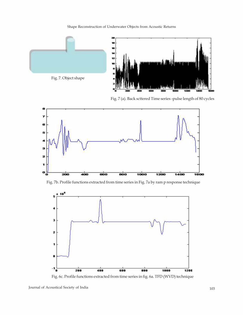
Shape Reconstruction of Underwater Objects from Acoustic Returns
103Journal of Acoustical Society of India
Fig. 7. Object shape
Fig. 7 (a). Back scttered Time series -pulse length of 80 cycles
Fig. 7b. Profile functions extracted from time series in Fig. 7a by ram p response technique
Fig. 6c. Profile functions extracted from time series in fig. 6a. TFD (WVD) technique
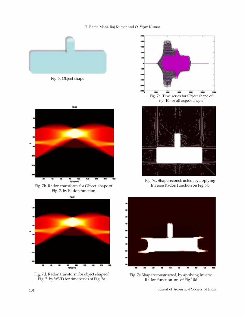
104 Journal of Acoustical Society of India
T. Ratna Mani, Raj Kumar and O. Vijay Kumar
Fig. 7. Object shape
Fig. 7a. Time series for Object shape offig. 10 for all aspect angels
Fig. 7c. Shapereconstructed, by applyingInverse Radon function on Fig. 7bFig. 7b. Radon transform for Object shape of
Fig. 7. by Radon function
Fig. 7d. Radon transform for object shapeofFig. 7. by WVD for time series of Fig. 7a
Fig. 7e.Shapereconstructed, by applying InverseRadon function on of Fig 10d
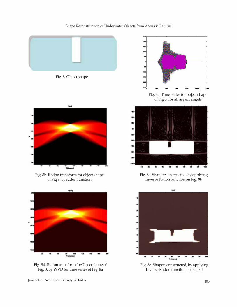
Shape Reconstruction of Underwater Objects from Acoustic Returns
105Journal of Acoustical Society of India
Fig. 8. Object shape
Fig. 8a. Time series for object shapeof Fig 8. for all aspect angels
Fig. 8b. Radon transform for object shapeof Fig 8. by radon function
Fig. 8c. Shapereconstructed, by applyingInverse Radon function on Fig. 8b
Fig. 8d. Radon transform forObject shape ofFig. 8. by WVD for time series of Fig. 8a
Fig. 8e. Shapereconstructed, by applyingInverse Radon function on Fig 8d
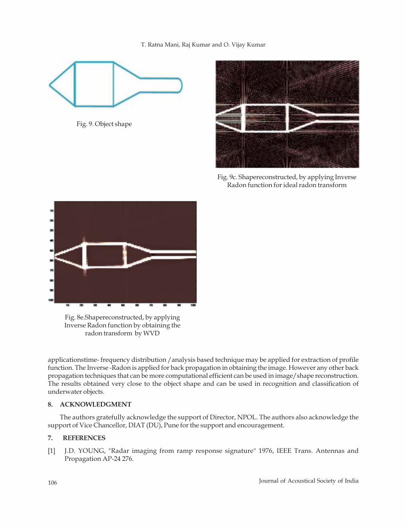
106 Journal of Acoustical Society of India
T. Ratna Mani, Raj Kumar and O. Vijay Kumar
applicationstime- frequency distribution /analysis based technique may be applied for extraction of profilefunction. The Inverse -Radon is applied for back propagation in obtaining the image. However any other backpropagation techniques that can be more computational efficient can be used in image/shape reconstruction.The results obtained very close to the object shape and can be used in recognition and classification ofunderwater objects.
8. ACKNOWLEDGMENT
The authors gratefully acknowledge the support of Director, NPOL. The authors also acknowledge thesupport of Vice Chancellor, DIAT (DU), Pune for the support and encouragement.
7. REFERENCES
[1] J.D. YOUNG, "Radar imaging from ramp response signature" 1976, IEEE Trans. Antennas andPropagation AP-24 276.
Fig. 9. Object shape
Fig. 9c. Shapereconstructed, by applying InverseRadon function for ideal radon transform
Fig. 8e.Shapereconstructed, by applyingInverse Radon function by obtaining the
radon transform by WVD
Shape Reconstruction of Underwater Objects from Acoustic Returns
107Journal of Acoustical Society of India
[2] X.M. ZHANG, W. LI and G. R. LIU, 2002 "A new technique in ramp response for acoustic imaging ofunderwater objects", Applied Acoustics 63.
[3] WELLI ,G.R. LIU, size X. M. Zhang" 2004 Size identification of underwater objects from back scatteringsignals of arbitrary looking angles", Journal of Computational Acoustics, Vol. 12, No. 3.
[4] WEL LI ,G.R. LIU, V.K. VARADAN, " 2004 Acoustical imaging of underwater objects using the bi -staticramp response signals", Smart materials and structure, Vol-13.
[5] P.C. WATERMAN, "New formulation of acoustic scattering", Journal. Acoustic. Soc. Am. 45 (1969)[6] B. BOASHASH, 2003 "Time Frequency Signal Analysis and Processing: A Comprehensive Reference,"
ELSEVIER.[7] CARLOS I HUERTA-LOPEZ, YONGJUNE SHIN, EDWARD J POWERS and JOSE M ROESSET " 2000
Time-Frequency Analysis Of Earthquake Records", 12WCEE.[9] E.M. KENNAUGH and D.L. MOFFATT," 1965 Transient and impulse response approximations",
Proceedings, IEEE.[10] T. RATNA MANI, RAJ KUMAR and O.VIJAY KUMAR," 2013 Numerical Computational Technique for
Scattering from Underwater Objects", Defence Science Journal, Vol. 63, No. 1, January.[11] T. RATNA MANI, RAJ KUMAR and O.VIJAYKUMAR ," 2011 Application of Time Frequency Analysis
Methods in Inverse Scattering ",Proceedings of SYMPOL.[12] BRIAN G. FERGUSON and RON J. WYBER, 2005 Application of acoustic reflection tomography to
sonar imaging, J. Acoust. Soc. Am. 117 (5), May.
108 Journal of Acoustical Society of India
R. Praveena, Gyanadutta Swain and B. Venkatesham
ABSTRACT
Extensive use of flexible hand tools in workshops and domestic applications are common. Thesetools are designed for multipurpose and low cost. This requirement makes designer to choose acompact and integrated system. So, it involves lot of challenges to design a quieter product. Thispaper emphasises in reducing the noise levels of a hand drill. The performance and noisecharacteristics of instrument are tested experimentally, followed by some analytical calculations onvarious subassemblies of the product to find out the dominant noise source. Experimental resultsshow that fan is the major noise source and this characteristic is being observed at high frequencyregion. After conducting parametric studies a suitable hybrid muffler of short length is mounted onthe instrument to reduce the noise levels to a considerable value. The concept of noise reduction isverified with the prototype of a muffler by measuring its insertion loss.
1. INTRODUCTION
Acoustic noise problems exist in wide variety of applications.Sound pressure levels depend on the part of thetotal mechanical or electrical energy transformed into acoustical energy. All noise control regulation actsemphasize in developing a quieter product. In the noise management data sheets for electric drills, bydepartment of commerce, government of western Australia it is mentioned that the quietest form of hand drillis the cordless variety that produces about 78 dB (A) and a normal hand drill produces about 90 dB (A) to 94dB (A) and hammer hand drills produce in excess of 100 dB (A) [1].The Internal components of hand drillsuch as fan, gear arrangement, motor and bearing act as various sources for noise which produce high soundpressure levels that can cause noise induced hearing loss if a person is exposed to it for a longer timeduration.
2. DESCRIPTION OF HAND DRILL
A hand drill consists of an electric motor that rotates a replaceable drill bit to make holes in wood, plastic, ormetal. Various components such as motor, bearing and fan are mounted on a single rotating shaft. A geararrangement connects the output shaft with the input shaft for speed reduction. Chuck is mounted on theoutput shaft where drill bit is mounted. Figure 1 shows different components of a typical hand drill.
3. METHODOLOGY FOR QUIETER DESIGN
Methodology that must be followed to determine the best solution for quieter product involves the followingsteps 1) Identification of potential noise sources, 2) Analysis of noise sources and noise generation mechanism,3) Source Ranking, 4) Noise propagation and 5) Develop noise control measures for themajor sources basedon noise propagation mechanism.
Journal of Acoustical Society of India : Vol. 40, No. 2, 2013 (pp. 108-115)
Noise Control of a Hand Drill Using Hybrid Muffler
R. Praveena, Gyanadutta Swain and B. Venkatesham*Indian Institute of Technology Hyderabad, Yeddumailaram-502 205 (A.P.)
*e-mail: [email protected]
[Received: 05.04.2013; Revised: 25.04.2013; Accepted: 29.04.2013]
© 2013 Acoustical Society of India
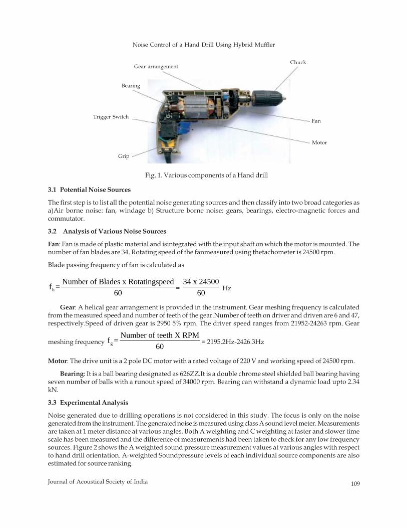
Noise Control of a Hand Drill Using Hybrid Muffler
109Journal of Acoustical Society of India
3.1 Potential Noise Sources
The first step is to list all the potential noise generating sources and then classify into two broad categories asa)Air borne noise: fan, windage b) Structure borne noise: gears, bearings, electro-magnetic forces andcommutator.
3.2 Analysis of Various Noise Sources
Fan: Fan is made of plastic material and isintegrated with the input shaft on which the motor is mounted. Thenumber of fan blades are 34. Rotating speed of the fanmeasured using thetachometer is 24500 rpm.
Blade passing frequency of fan is calculated as
bNumber of Blades x Rotatingspeedf =
60 = 34 x 24500
60 Hz
Gear: A helical gear arrangement is provided in the instrument. Gear meshing frequency is calculatedfrom the measured speed and number of teeth of the gear.Number of teeth on driver and driven are 6 and 47,respectively.Speed of driven gear is 2950 5% rpm. The driver speed ranges from 21952-24263 rpm. Gear
meshing frequency gNumber of teeth X RPMf =
60 = 2195.2Hz-2426.3Hz
Motor: The drive unit is a 2 pole DC motor with a rated voltage of 220 V and working speed of 24500 rpm.
Bearing: It is a ball bearing designated as 626ZZ.It is a double chrome steel shielded ball bearing havingseven number of balls with a runout speed of 34000 rpm. Bearing can withstand a dynamic load upto 2.34kN.
3.3 Experimental Analysis
Noise generated due to drilling operations is not considered in this study. The focus is only on the noisegenerated from the instrument. The generated noise is measured using class A sound level meter. Measurementsare taken at 1 meter distance at various angles. Both A weighting and C weighting at faster and slower timescale has been measured and the difference of measurements had been taken to check for any low frequencysources. Figure 2 shows the A weighted sound pressure measurement values at various angles with respectto hand drill orientation. A-weighted Soundpressure levels of each individual source components are alsoestimated for source ranking.
Fig. 1. Various components of a Hand drill
Gear arrangement
Bearing
Trigger Switch
Grip
Chuck
Fan
Motor
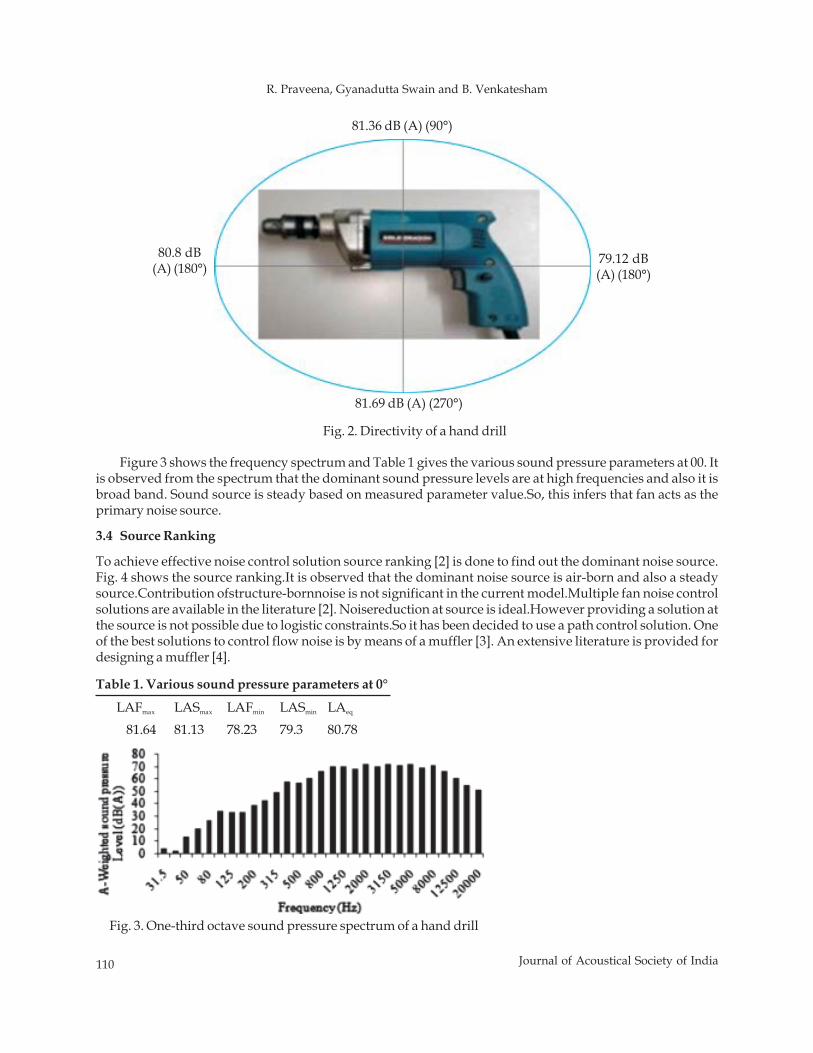
110 Journal of Acoustical Society of India
R. Praveena, Gyanadutta Swain and B. Venkatesham
81.36 dB (A) (90°)
79.12 dB(A) (180°)
80.8 dB(A) (180°)
81.69 dB (A) (270°)
Fig. 2. Directivity of a hand drill
Figure 3 shows the frequency spectrum and Table 1 gives the various sound pressure parameters at 00. Itis observed from the spectrum that the dominant sound pressure levels are at high frequencies and also it isbroad band. Sound source is steady based on measured parameter value.So, this infers that fan acts as theprimary noise source.
3.4 Source Ranking
To achieve effective noise control solution source ranking [2] is done to find out the dominant noise source.Fig. 4 shows the source ranking.It is observed that the dominant noise source is air-born and also a steadysource.Contribution ofstructure-bornnoise is not significant in the current model.Multiple fan noise controlsolutions are available in the literature [2]. Noisereduction at source is ideal.However providing a solution atthe source is not possible due to logistic constraints.So it has been decided to use a path control solution. Oneof the best solutions to control flow noise is by means of a muffler [3]. An extensive literature is provided fordesigning a muffler [4].
LAFmax LASmax LAFmin LASmin LAeq
81.64 81.13 78.23 79.3 80.78
Table 1. Various sound pressure parameters at 0°
Fig. 3. One-third octave sound pressure spectrum of a hand drill
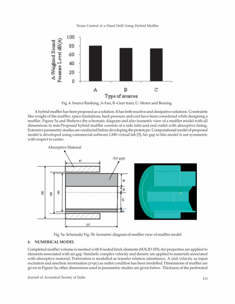
Noise Control of a Hand Drill Using Hybrid Muffler
111Journal of Acoustical Society of India
Fig. 4. Source Ranking, A-Fan, B -Gear train, C- Motor and Bearing
A hybrid muffler has been proposed as a solution. It has both reactive and dissipative solutions. Constraintslike weight of the muffler, space limitations, back pressure and cost have been considered while designing amuffler. Figure 5a and 5bshows the schematic diagram and also isometric view of a muffler model with alldimensions in mm.Proposed hybrid muffler consists of a side inlet and end outlet with absorptive lining.Extensive parametric studies are conducted before developing the prototype. Computational model of proposedmodel is developed using commercial software LMS virtual lab [5].Air gap in this model is not symmetricwith respect to centre.
Fig. 5a. Schematic Fig. 5b. Isometric diagram of muffler view of muffler model
Air gap
Absorptive Material
4. NUMERICAL MODEL
Completed muffler volume is meshed with 8 noded brick elements (SOLID 185).Air properties are applied toelements associated with air gap. Similarly complex velocity and density are applied to materials associatedwith absorptive material. Perforation is modelled as transfer relation admittance. A unit velocity as inputexcitation and anechoic termination (z=ρc) as outlet condition has been modelled. Dimensions of muffler aregiven in Figure 5a; other dimensions used in parametric studies are given below. Thickness of the perforated
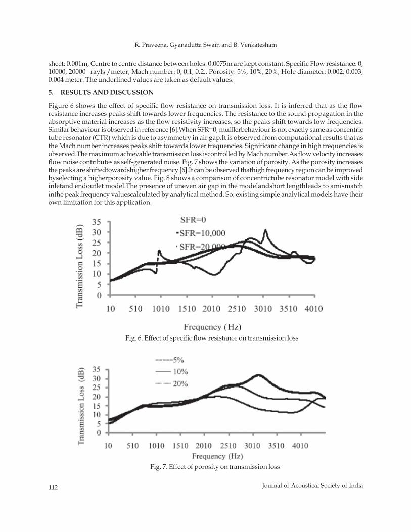
112 Journal of Acoustical Society of India
R. Praveena, Gyanadutta Swain and B. Venkatesham
sheet: 0.001m, Centre to centre distance between holes: 0.0075m are kept constant. Specific Flow resistance: 0,10000, 20000 rayls /meter, Mach number: 0, 0.1, 0.2., Porosity: 5%, 10%, 20%, Hole diameter: 0.002, 0.003,0.004 meter. The underlined values are taken as default values.
5. RESULTS AND DISCUSSION
Figure 6 shows the effect of specific flow resistance on transmission loss. It is inferred that as the flowresistance increases peaks shift towards lower frequencies. The resistance to the sound propagation in theabsorptive material increases as the flow resistivity increases, so the peaks shift towards low frequencies.Similar behaviour is observed in reference [6].When SFR=0, mufflerbehaviour is not exactly same as concentrictube resonator (CTR) which is due to asymmetry in air gap.It is observed from computational results that asthe Mach number increases peaks shift towards lower frequencies. Significant change in high frequencies isobserved.The maximum achievable transmission loss iscontrolled by Mach number.As flow velocity increasesflow noise contributes as self-generated noise. Fig. 7 shows the variation of porosity. As the porosity increasesthe peaks are shiftedtowardshigher frequency [6].It can be observed thathigh frequency region can be improvedbyselecting a higherporosity value. Fig. 8 shows a comparison of concentrictube resonator model with sideinletand endoutlet model.The presence of uneven air gap in the modelandshort lengthleads to amismatchinthe peak frequency valuescalculated by analytical method. So, existing simple analytical models have theirown limitation for this application.
Fig. 6. Effect of specific flow resistance on transmission loss
Fig. 7. Effect of porosity on transmission loss
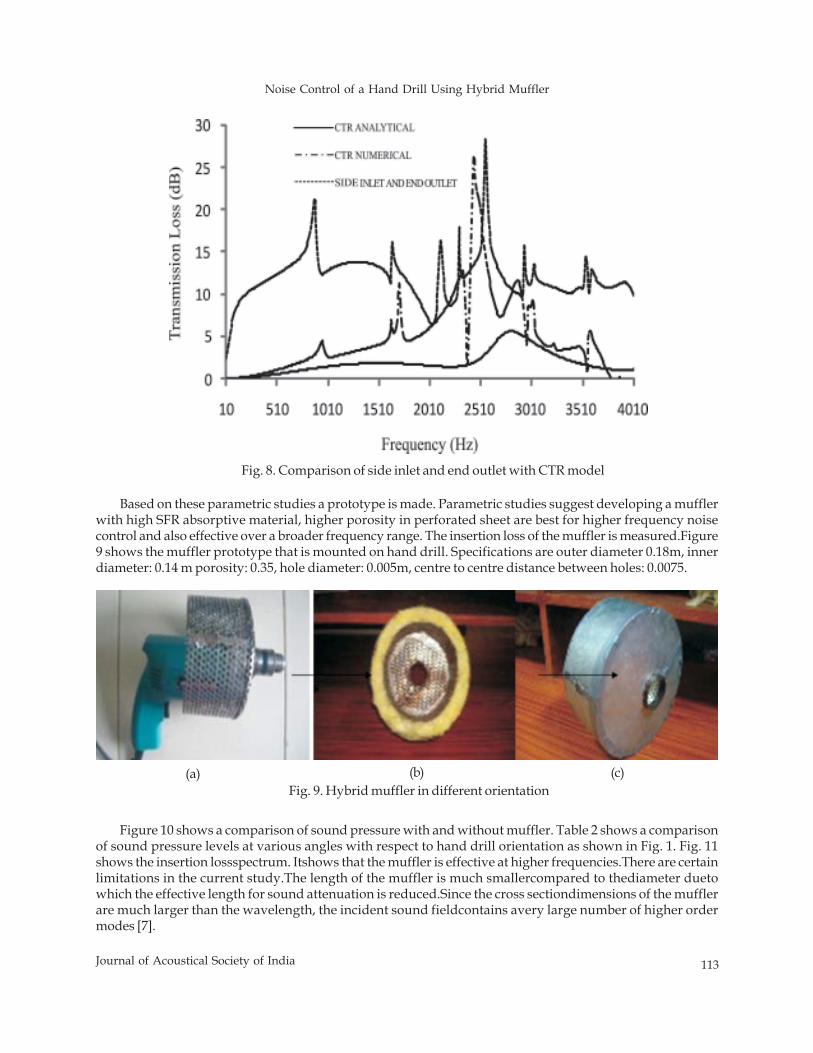
Noise Control of a Hand Drill Using Hybrid Muffler
113Journal of Acoustical Society of India
Fig. 8. Comparison of side inlet and end outlet with CTR model
Based on these parametric studies a prototype is made. Parametric studies suggest developing a mufflerwith high SFR absorptive material, higher porosity in perforated sheet are best for higher frequency noisecontrol and also effective over a broader frequency range. The insertion loss of the muffler is measured.Figure9 shows the muffler prototype that is mounted on hand drill. Specifications are outer diameter 0.18m, innerdiameter: 0.14 m porosity: 0.35, hole diameter: 0.005m, centre to centre distance between holes: 0.0075.
Figure 10 shows a comparison of sound pressure with and without muffler. Table 2 shows a comparisonof sound pressure levels at various angles with respect to hand drill orientation as shown in Fig. 1. Fig. 11shows the insertion lossspectrum. Itshows that the muffler is effective at higher frequencies.There are certainlimitations in the current study.The length of the muffler is much smallercompared to thediameter duetowhich the effective length for sound attenuation is reduced.Since the cross sectiondimensions of the mufflerare much larger than the wavelength, the incident sound fieldcontains avery large number of higher ordermodes [7].
(a) (b) (c)Fig. 9. Hybrid muffler in different orientation
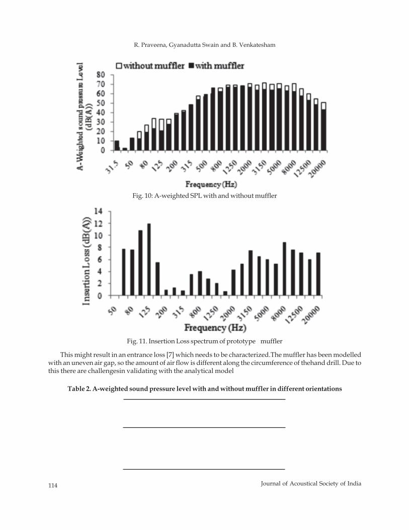
114 Journal of Acoustical Society of India
R. Praveena, Gyanadutta Swain and B. Venkatesham
Fig. 10: A-weighted SPL with and without muffler
Fig. 11. Insertion Loss spectrum of prototype muffler
This might result in an entrance loss [7] which needs to be characterized.The muffler has been modelledwith an uneven air gap, so the amount of air flow is different along the circumference of thehand drill. Due tothis there are challengesin validating with the analytical model
Table 2. A-weighted sound pressure level with and without muffler in different orientations

Noise Control of a Hand Drill Using Hybrid Muffler
115Journal of Acoustical Society of India
6. SUMMARY
Noise sources in the hand drill machine have been identified based on acoustical and vibration measurementand fan has been identifiedas the major noise source.This is done based on the concept of source ranking.Apassive noise control technique has been proposedin the form of a hybrid muffler to control fan noise. Aprototype has been prepared based on extensive parametric study using numerical models.An attempt hasbeen made to reduce the sound from the hand drillby using muffler concept. This concept helped to getinsertion loss of 4-5 dB (A).This paper described the complete noise control approach by integratinganalytical,computational and experimental methods.Similar approach can be extended to other industrialproducts.This model can be further improved with an even air gap mufflerby optimising themufflerdimensionswith considerable back pressure and thereby achieving more reduction in noise levels.
7. REFERENCES
[1] Noise management data sheets http://www.commerce.wa.gov.au/worksafe/content/safety_topics/noise/Further_information/Electrical_drills.html
[2] DAVID A. BIES and COLIN H. HANSEN, 2009. Engineering Noise Control Theory and practice,Taylor& Francis.
[3] H.S. KIM, J.S. HONG, D.G. SOHN and J.E. OH, Development of an Active Muffler System for ReducingExhaust Noise and Flow Restriction in a Heavy Vehicle, Department of Mechanical Engineering, Instituteof Noise Control Engineering,Auburn University.
[4] M.L. MUNJAL, 1987. Acoustics of Ducts and Mufflers, John Wiley.[5] LMS Virtual lab Rev -10, User's manual.[6] M.L. MUNJAL and B. VENKATESHAM, 2000. Analysis and design of an annular air gap lined duct for
hot exhaust systems, Proceedings of the IUTAM Symposium on Designing for Quietness, Kluwer Publications,Holland.
[7] IstvanL.Ver, Leo L. Beranek. Noise and vibration control engineering principles and applications 2006,John Wiley & Sons.
116 Journal of Acoustical Society of India
G.S. Vijay, Srinivasa P. Pai and N.S. Sriram
© 2013 Acoustical Society of India
ABSTRACT
In this paper, the performance of Multi Layer Perceptron Neural Network (MLPNN) based on featuresselected using Fisher's Criterion (FC) and Genetic Algorithm (GA) has been compared for rollingelement bearing condition classification. Vibration signals have been acquired from four conditions(normal bearing, bearing with defect on inner race, bearing with defect on outer race and bearingwith defect on ball element) of a deep groove ball bearing (6205) from a customized bearing test rigunder different conditions of load and speed. Several statistical features in time domain and frequencydomain were extracted from denoised vibration signal. GA was also used to optimize the learningrate, momentum factor and number of neurons in the hidden layer. MLPNN based on GA has beenfound to perform better than that based on features selected using FC, thereby helping in effectiveclassification of rolling element bearing condition.
1. INTRODUCTION
Rolling element bearings (REBs) are widely used in industrial and domestic applications. In industrialapplications, these bearings are considered as critical mechanical components and a defect in such a bearing,if not detected in time can cause malfunction and may lead to catastrophic failure of the machinery [1].Different methods are available for detection and diagnosis of bearing defects. They can be broadly classifiedas vibration and acoustic measurements, temperature and wear debris analysis. One of the commonly usedtechniques for bearing fault detection is vibration measurement [1, 2]. The vibration signals measured can beanalysed in time domain, frequency domain or time-frequency domain. Vibration signals collected from rollingelement bearings have lot of noise because of varying compliance and presence of defects [1]. The REB vibrationsignals due to defects alone are weak, compared to the harmonics of the resonant frequency of the system(noise). There is a need to remove or reduce this noise and extract dominant features in order to perform faultdiagnostics. Conventional noise reduction or signal pre-processing techniques like Adaptive Noise Cancellation(ANC) and High Frequency Resonance Technique (HFRT) or envelope technique need information aboutresonant frequencies of the rolling element bearing system [2]. Also the bearing vibration signals are not reallycyclostationary (they are rather pseudo cyclostationary) [3, 4]. Wavelet based denoising is increasingly beingused in condition monitoring applications, in order to increase the data's reliability and improve accuracy ofsignal analysis and to increase the signal-to-noise ratio (SNR) [4]. Wavelet transform due to its sparsity,locality and multi-resolution nature has emerged as an effective tool for denoising. The Artificial NeuralNetwork (ANN) has been widely used in fault diagnostics [2]. Different architectures have been studied inbearing fault diagnostics. Multi Layer Perceptron Neural Network (MLPNN) with back propagation is one of
Journal of Acoustical Society of India : Vol. 40, No. 2, 2013 (pp.116-120)
Genetic Algorithm Based Neural Network forClassification of Rolling Element Bearing Condition
G.S. Vijay1*, Srinivasa P. Pai2 and N.S. Sriram3
1Department of Mechanical and Manufacturing Engineering, MIT, Manipal (Karnataka)2Department of Mechanical Engineering, NMAMIT, Nitte (Karnataka)3Department of Mechanical Engineering, VVIET, Mysore (Karnataka)
*e-mail: [email protected]
[Received: 15.12.2012; Revised: 19.01.2013; Accepted: 22.02.2013]
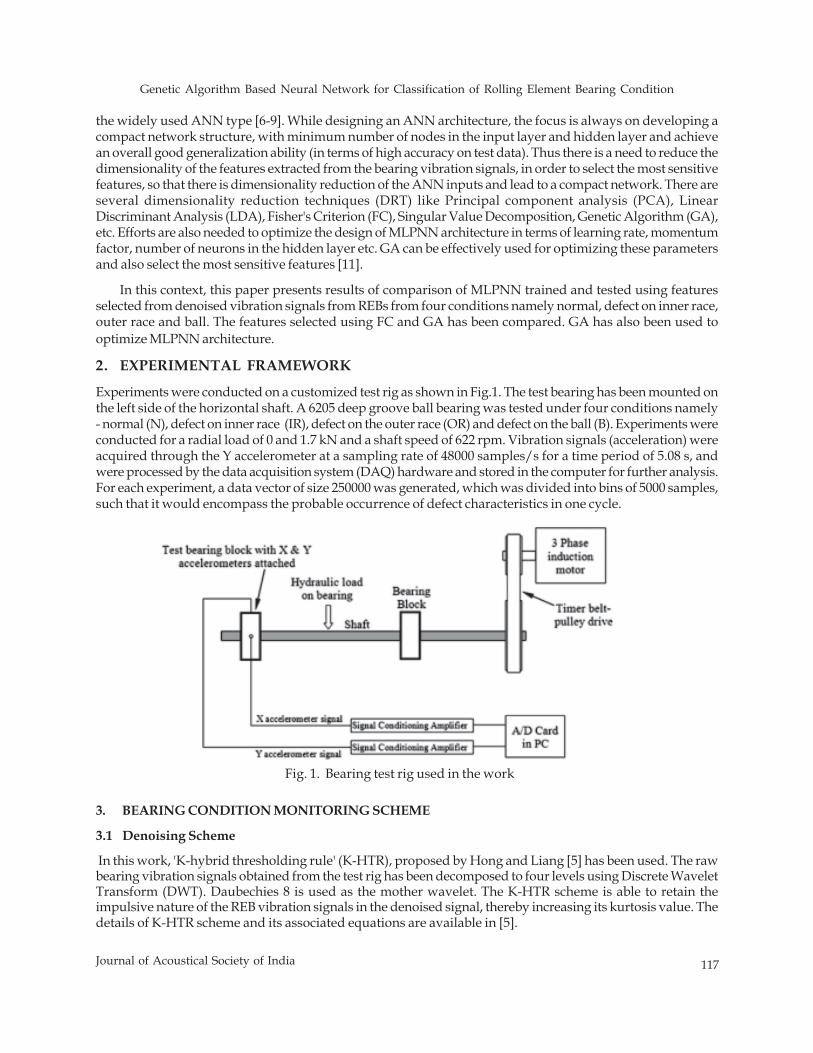
Genetic Algorithm Based Neural Network for Classification of Rolling Element Bearing Condition
117Journal of Acoustical Society of India
the widely used ANN type [6-9]. While designing an ANN architecture, the focus is always on developing acompact network structure, with minimum number of nodes in the input layer and hidden layer and achievean overall good generalization ability (in terms of high accuracy on test data). Thus there is a need to reduce thedimensionality of the features extracted from the bearing vibration signals, in order to select the most sensitivefeatures, so that there is dimensionality reduction of the ANN inputs and lead to a compact network. There areseveral dimensionality reduction techniques (DRT) like Principal component analysis (PCA), LinearDiscriminant Analysis (LDA), Fisher's Criterion (FC), Singular Value Decomposition, Genetic Algorithm (GA),etc. Efforts are also needed to optimize the design of MLPNN architecture in terms of learning rate, momentumfactor, number of neurons in the hidden layer etc. GA can be effectively used for optimizing these parametersand also select the most sensitive features [11].
In this context, this paper presents results of comparison of MLPNN trained and tested using featuresselected from denoised vibration signals from REBs from four conditions namely normal, defect on inner race,outer race and ball. The features selected using FC and GA has been compared. GA has also been used tooptimize MLPNN architecture.
2. EXPERIMENTAL FRAMEWORK
Experiments were conducted on a customized test rig as shown in Fig.1. The test bearing has been mounted onthe left side of the horizontal shaft. A 6205 deep groove ball bearing was tested under four conditions namely- normal (N), defect on inner race (IR), defect on the outer race (OR) and defect on the ball (B). Experiments wereconducted for a radial load of 0 and 1.7 kN and a shaft speed of 622 rpm. Vibration signals (acceleration) wereacquired through the Y accelerometer at a sampling rate of 48000 samples/s for a time period of 5.08 s, andwere processed by the data acquisition system (DAQ) hardware and stored in the computer for further analysis.For each experiment, a data vector of size 250000 was generated, which was divided into bins of 5000 samples,such that it would encompass the probable occurrence of defect characteristics in one cycle.
3. BEARING CONDITION MONITORING SCHEME
3.1 Denoising Scheme
In this work, 'K-hybrid thresholding rule' (K-HTR), proposed by Hong and Liang [5] has been used. The rawbearing vibration signals obtained from the test rig has been decomposed to four levels using Discrete WaveletTransform (DWT). Daubechies 8 is used as the mother wavelet. The K-HTR scheme is able to retain theimpulsive nature of the REB vibration signals in the denoised signal, thereby increasing its kurtosis value. Thedetails of K-HTR scheme and its associated equations are available in [5].
Fig. 1. Bearing test rig used in the work
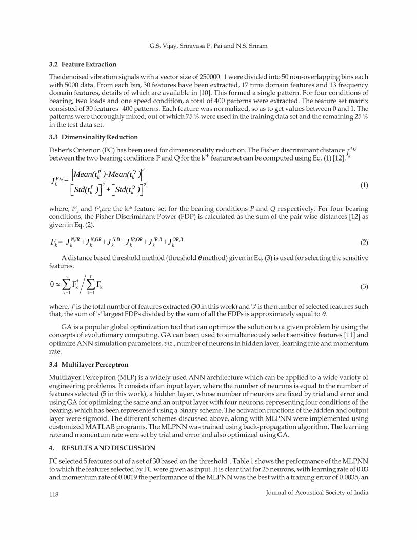
118 Journal of Acoustical Society of India
G.S. Vijay, Srinivasa P. Pai and N.S. Sriram
3.2 Feature Extraction
The denoised vibration signals with a vector size of 250000 1 were divided into 50 non-overlapping bins eachwith 5000 data. From each bin, 30 features have been extracted, 17 time domain features and 13 frequencydomain features, details of which are available in [10]. This formed a single pattern. For four conditions ofbearing, two loads and one speed condition, a total of 400 patterns were extracted. The feature set matrixconsisted of 30 features 400 patterns. Each feature was normalized, so as to get values between 0 and 1. Thepatterns were thoroughly mixed, out of which 75 % were used in the training data set and the remaining 25 %in the test data set.
3.3 Dimensinality Reduction
Fisher's Criterion (FC) has been used for dimensionality reduction. The Fisher discriminant distancebetween the two bearing conditions P and Q for the kth feature set can be computed using Eq. (1) [12].
⎡ ⎤ ⎡ ⎤⎣ ⎦ ⎣ ⎦
2P Qk kP,Q
k 2 2P Qk k
Mean(t )-Mean(t )J =
Std(t ) + Std(t ) (1)
where, tPk and tQ
kare the kth feature set for the bearing conditions P and Q respectively. For four bearingconditions, the Fisher Discriminant Power (FDP) is calculated as the sum of the pair wise distances [12] asgiven in Eq. (2).
N,IR N,OR N,B IR,OR IR,B OR,Bk k k k k k kF = J +J +J +J +J +J (2)
A distance based threshold method (threshold θ method) given in Eq. (3) is used for selecting the sensitivefeatures.
s f*k k
k=1 k=1θ F F≈∑ ∑ (3)
where, 'f' is the total number of features extracted (30 in this work) and 's' is the number of selected features suchthat, the sum of 's' largest FDPs divided by the sum of all the FDPs is approximately equal to θ.
GA is a popular global optimization tool that can optimize the solution to a given problem by using theconcepts of evolutionary computing. GA can been used to simultaneously select sensitive features [11] andoptimize ANN simulation parameters, viz., number of neurons in hidden layer, learning rate and momentumrate.
3.4 Multilayer Perceptron
Multilayer Perceptron (MLP) is a widely used ANN architecture which can be applied to a wide variety ofengineering problems. It consists of an input layer, where the number of neurons is equal to the number offeatures selected (5 in this work), a hidden layer, whose number of neurons are fixed by trial and error andusing GA for optimizing the same and an output layer with four neurons, representing four conditions of thebearing, which has been represented using a binary scheme. The activation functions of the hidden and outputlayer were sigmoid. The different schemes discussed above, along with MLPNN were implemented usingcustomized MATLAB programs. The MLPNN was trained using back-propagation algorithm. The learningrate and momentum rate were set by trial and error and also optimized using GA.
4. RESULTS AND DISCUSSION
FC selected 5 features out of a set of 30 based on the threshold . Table 1 shows the performance of the MLPNNto which the features selected by FC were given as input. It is clear that for 25 neurons, with learning rate of 0.03and momentum rate of 0.0019 the performance of the MLPNN was the best with a training error of 0.0035, an
JP,Qk
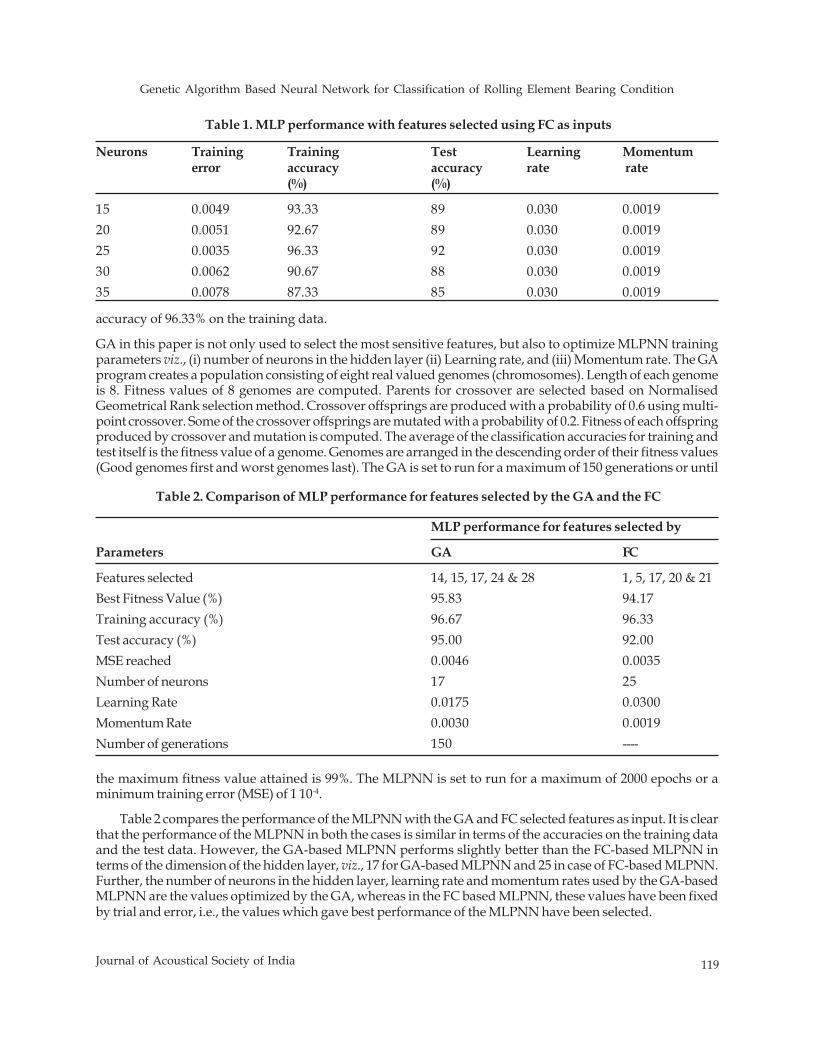
Genetic Algorithm Based Neural Network for Classification of Rolling Element Bearing Condition
119Journal of Acoustical Society of India
accuracy of 96.33% on the training data.
GA in this paper is not only used to select the most sensitive features, but also to optimize MLPNN trainingparameters viz., (i) number of neurons in the hidden layer (ii) Learning rate, and (iii) Momentum rate. The GAprogram creates a population consisting of eight real valued genomes (chromosomes). Length of each genomeis 8. Fitness values of 8 genomes are computed. Parents for crossover are selected based on NormalisedGeometrical Rank selection method. Crossover offsprings are produced with a probability of 0.6 using multi-point crossover. Some of the crossover offsprings are mutated with a probability of 0.2. Fitness of each offspringproduced by crossover and mutation is computed. The average of the classification accuracies for training andtest itself is the fitness value of a genome. Genomes are arranged in the descending order of their fitness values(Good genomes first and worst genomes last). The GA is set to run for a maximum of 150 generations or until
Table 2. Comparison of MLP performance for features selected by the GA and the FC
MLP performance for features selected by
Parameters GA FC
Features selected 14, 15, 17, 24 & 28 1, 5, 17, 20 & 21Best Fitness Value (%) 95.83 94.17Training accuracy (%) 96.67 96.33Test accuracy (%) 95.00 92.00MSE reached 0.0046 0.0035Number of neurons 17 25Learning Rate 0.0175 0.0300Momentum Rate 0.0030 0.0019Number of generations 150 ----
the maximum fitness value attained is 99%. The MLPNN is set to run for a maximum of 2000 epochs or aminimum training error (MSE) of 1 10-4.
Table 2 compares the performance of the MLPNN with the GA and FC selected features as input. It is clearthat the performance of the MLPNN in both the cases is similar in terms of the accuracies on the training dataand the test data. However, the GA-based MLPNN performs slightly better than the FC-based MLPNN interms of the dimension of the hidden layer, viz., 17 for GA-based MLPNN and 25 in case of FC-based MLPNN.Further, the number of neurons in the hidden layer, learning rate and momentum rates used by the GA-basedMLPNN are the values optimized by the GA, whereas in the FC based MLPNN, these values have been fixedby trial and error, i.e., the values which gave best performance of the MLPNN have been selected.
Table 1. MLP performance with features selected using FC as inputs
Neurons Training Training Test Learning Momentumerror accuracy accuracy rate rate
(%) (%)
15 0.0049 93.33 89 0.030 0.001920 0.0051 92.67 89 0.030 0.001925 0.0035 96.33 92 0.030 0.001930 0.0062 90.67 88 0.030 0.001935 0.0078 87.33 85 0.030 0.0019
120 Journal of Acoustical Society of India
G.S. Vijay, Srinivasa P. Pai and N.S. Sriram
5. CONCLUSION
In this paper, the MLPNN has been used for classification of REB based on features selected using FC andusing GA. GA has also been used to optimize the MLPNN architecture in terms of number of neurons in thehidden layer and simulation parameters viz., learning and momentum rate. GA-based selection of the inputfeatures takes much longer time as it depends on the performance of the MLPNN for computing the fitnessvalue, whereas the FC-based selection of input features is faster as it is independent of the performance of theMLPNN. MLPNN based on GA gave a comparable performance with that using features selected using FC.Hence MLPNN using GA can be effectively used to classify REB condition.6. REFERENCES
[1] N. TANDON and A. CHOUDHURY, 1999. A review of vibration and acoustic measurement methods forthe detection of defects in rolling element bearings, Tribology International, 32, 469-480.
[2] M.S. PATIL, JOSE MATHEW and P.K. KUMAR RAJENDRA, 2008. Bearing signature analysis as amedium for fault detection: A review, Journal of Tribology, 130, 014001.1 - 014001.7.
[3] ROBERT B. RANDALL and JEROME ANTONI, 2011. Rolling element bearing diagnostics-A tutorial,Mechanical Systems and Signal Processing, 25, 485-520.
[4] Z. K. PENG and F. L. CHU, 2004. Application of the wavelet transform in machine condition monitoringand fault diagnostics: a review with bibliography, Mechanical Systems and Signal Processing, 18, 199-221.
[5] HOONBIN HONG and MING LIANG, 2007. K-Hybrid: A Kurtosis-Based Hybrid Thresholding Methodfor Mechanical Signal Denoising, Journal of Vibration and Acoustics, Transactions of the ASME , 129, 458-470.
[6] C. CASTEJON, O. LARA and J.C. GARCIA-PRADA, 2010. Automated diagnosis of rolling bearingsusing MRA and Neural Networks, Mechanical Systems and Signal Processing, 24, 289-299.
[7] CHUN-CHIEH WANG, YUAN KANG, PING-CHEN SHEN, YEON-PUN CHANG and YU-LIANGCHUNG, 2010. Applications of fault diagnosis in rotating machinery by using time series analysis withNeural Network, Expert Systems with Applications, 37, 1696-1702.
[8] P.K. KANKAR, C. SATISH SHARMA and S.P. HARSHA, 2011. Fault diagnosis of ball bearings usingmachine learning methods, Expert Systems with Applications, 38, 1876-1886.
[9] JAFAR ZAREI, 2012. Induction motors bearing fault detection using pattern recognition techniques,Expert Systems with Applications, 39, 68-73.
[10] G.S. VIJAY, P. SRINIVASA Pai and N. S. SRIRAM, 2011. "Bearing diagnostics - A Radial Basis FunctionNeural Network approach", Proceedings of the 24th International Congress on Condition Monitoring andDiagnostics Engineering Management, Advances in Industrial Asset Integrity Management (COMADEM 2011),Stavanger, Norway, ISBN 0-9541307-2-3, 843-854.
[11] B. SAMANTA, K.R. AL-BALUSHI and S.A. Al-ARAIMI, 2006. Artificial Neural Networks and GeneticAlgorithm for bearing fault detection, Soft Computing, 10, 264-271.
[12] G.Y. GARY and Kuo-CHUNG LIN, 2000. Wavelet packet feature extraction for vibration monitoring,IEEE Transactions on industrial electronics, 47 (3), 650-667.
Localization of Low Flying Aircraft Based on Its Acoustic Signature
121Journal of Acoustical Society of India
Localization of Low Flying Aircraft Based on ItsAcoustic Signature
A. Saravanakumar*, S. Arunkumar and K. SenthilkumarDivision of Avionics, Department of Aerospace Engineering, Madras Institute of Technology
Campus, Anna University. Chennai-600 044 (Tamil Nadu)*e-mail: [email protected]
ABSTRACT
An aircraft generates an acoustic impulse that propagates outwards from the source. The position ofthe source and hence the trajectory can be estimated by measuring the relative time of arrival of theimpulse at a number of spatially distributed sensors. The time difference for the acoustic wave frontto arrive at two spatially separated sensors is estimated by cross correlating the digitized outputs ofthe sensors. The time delay estimate is used to calculate the source bearing and the position of thesource is found using triangulation technique using the bearings from two widely separated receivingnodes. The flight parameter of the aircraft is obtained by Cepstrum method using acoustic Multipathdelays. The signal emitted by an UAV arrives at a stationary sensor located above a flat ground via adirect path and a ground-reflected path. The difference in the times of arrival of the direct path andground-reflected path signal components is known as the Multipath delay. A model is developed topredict the variation with time and Cepstrum method is formulated to estimate the motion parameterslike speed and altitude of the aircraft.
1. INTRODUCTION
Acoustic techniques have been widely used in variety of fields. An aircraft which is an acoustic source producessound that can be received by placing sensors on the ground that captures the sound waves propagatedthrough the air. Acoustic sensors are used widely because of their passiveness, affordability, robustness, andcompatibility. Ground sensors are often deployed in remote areas for surveillance and early warning purposes[1]. Due to the high levels of acoustic energy radiated by the propulsion systems of aircraft and by the enginesof vehicles, it is possible to detect these sources using passive acoustic sensors mounted close to the ground.Here described a technique that utilizes the Lloyd's mirror effect [2] of the radiated sound to estimate the speed,altitude of a low-flying aircraft by using only a single sensor. The localization of acoustic source is usuallydone with sensor array in which the output of each sensor is a scalar corresponding to the acoustic pressure.For linear trajectory, we consider a different approach for solving this problem using Acoustic Vector Sensorwhose output is a vector corresponding to the acoustic pressure and acoustic particle velocity. The mainadvantage of these vector sensors over traditional scalar sensors is that they make use of more availableacoustic information, hence they should outperform sensor array in accuracy of localization [6]. An array ofsensors has been used to find the non linear trajectory as it will be a convenient way to find the trajectory of anaircraft.
2. EXPERIMENTAL PROCEDURE
2.1 Multipath Propagation
In a Multipath propagation environment, two or more attenuated and delayed replicas of the same radiated
Journal of Acoustical Society of India : Vol. 40, No. 2, 2013 (pp. 121-130)
[Received: 21.02.2013; Revised: 25.03.2013; Accepted: 27.04.2013]
© 2013 Acoustical Society of India
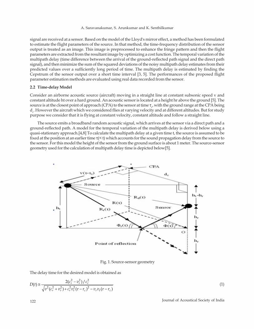
122 Journal of Acoustical Society of India
A. Saravanakumar, S. Arunkumar and K. Senthilkumar
signal are received at a sensor. Based on the model of the Lloyd's mirror effect, a method has been formulatedto estimate the flight parameters of the source. In that method, the time-frequency distribution of the sensoroutput is treated as an image. This image is preprocessed to enhance the fringe pattern and then the flightparameters are extracted from the resultant image by optimizing a cost function. The temporal variation of themultipath delay (time difference between the arrival of the ground-reflected path signal and the direct pathsignal), and then minimize the sum of the squared deviations of the noisy multipath delay estimates from theirpredicted values over a sufficiently long period of time. The multipath delay is estimated by finding theCepstrum of the sensor output over a short time interval [3, 5]. The performances of the proposed flightparameter estimation methods are evaluated using real data recorded from the sensor.
2.2 Time-delay Model
Consider an airborne acoustic source (aircraft) moving in a straight line at constant subsonic speed v andconstant altitude ht over a hard ground. An acoustic sensor is located at a height hr above the ground [5]. Thesource is at the closest point of approach (CPA) to the sensor at time τc, with the ground range at the CPA beingdc. However the aircraft which we considered flies at varying velocity and at different altitudes. But for studypurpose we consider that it is flying at constant velocity, constant altitude and follow a straight line.
The source emits a broadband random acoustic signal, which arrives at the sensor via a direct path and aground-reflected path. A model for the temporal variation of the multipath delay is derived below using aquasi-stationary approach.[4,8] To calculate the multipath delay at a given time t, the source is assumed to befixed at the position at an earlier time τ(< t) which accounts for the sound propagation delay from the source tothe sensor. For this model the height of the sensor from the ground surface is about 1 meter. The source-sensorgeometry used for the calculation of multipath delay time is depicted below[5].
Fig. 1. Source-sensor geometry
The delay time for the desired model is obtained as
r r r
r r r t c r t c
c v cD tv c v c v v v
2 2 2
2 2 2 2 2 2
2( )/( )( ) ( ) ( )τ τ τ τ
−≅
+ + − − −(1)
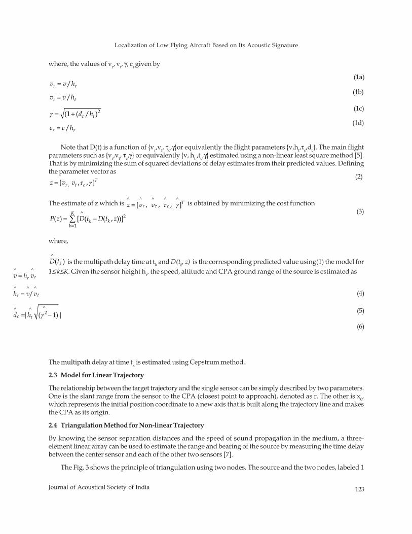
Localization of Low Flying Aircraft Based on Its Acoustic Signature
123Journal of Acoustical Society of India
where, the values of vr, vt, γ, cr given by
=
=
= +
=
2
/
/
(1 ( / )
/
r r
t t
c t
r r
v v h
v v h
d h
c c h
γ
Note that D(t) is a function of {vr,vt, τc,γ}or equivalently the flight parameters {v,ht,τc,dc}. The main flightparameters such as {vr,vt, τc,γ} or equivalently {v, ht ,tc,γ} estimated using a non-linear least square method [5].That is by minimizing the sum of squared deviations of delay estimates from their predicted values. Definingthe parameter vector as
The estimate of z which is Tr cz v v
^ ^ ^ ^ ^[ , , , ]τ τ γ= is obtained by minimizing the cost function
where,
kD t^
( ) is the multipath delay time at tk and D(tk, z) is the corresponding predicted value using(1) the model for1≤ k≤K. Given the sensor height hr, the speed, altitude and CPA ground range of the source is estimated as=
=
= −
^ ^
^ ^ ^
^^ ^ 2
/
| ( 1)|
rr
t t
c t
v h v
h v v
d h γ
The multipath delay at time tk is estimated using Cepstrum method.
2.3 Model for Linear Trajectory
The relationship between the target trajectory and the single sensor can be simply described by two parameters.One is the slant range from the sensor to the CPA (closest point to approach), denoted as r. The other is x0,which represents the initial position coordinate to a new axis that is built along the trajectory line and makesthe CPA as its origin.
2.4 Triangulation Method for Non-linear Trajectory
By knowing the sensor separation distances and the speed of sound propagation in the medium, a three-element linear array can be used to estimate the range and bearing of the source by measuring the time delaybetween the center sensor and each of the other two sensors [7].
The Fig. 3 shows the principle of triangulation using two nodes. The source and the two nodes, labeled 1
(1a)
(1b)
(1c)
(1d)
(2)Tr t cz v v,[ , , ]τ γ=
Kk k
kP z D t D t z
^ 2
1( ) [ ( ( , ))]
== −∑
(3)
(4)
(5)
(6)
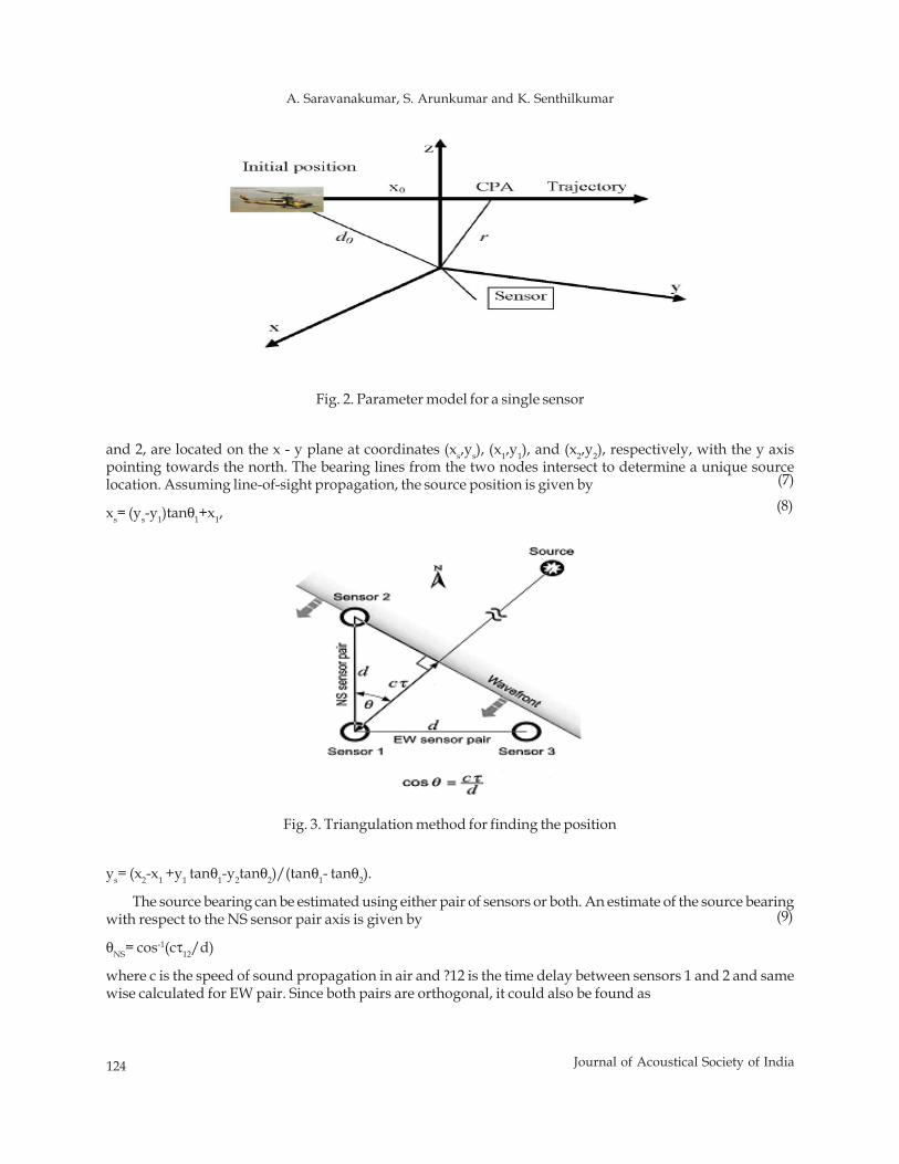
124 Journal of Acoustical Society of India
A. Saravanakumar, S. Arunkumar and K. Senthilkumar
and 2, are located on the x - y plane at coordinates (xs,ys), (x1,y1), and (x2,y2), respectively, with the y axispointing towards the north. The bearing lines from the two nodes intersect to determine a unique sourcelocation. Assuming line-of-sight propagation, the source position is given by
xs= (ys-y1)tanθ1+x1,
Fig. 2. Parameter model for a single sensor
(7)
(8)
Fig. 3. Triangulation method for finding the position
ys= (x2-x1 +y1 tanθ1-y2tanθ2)/(tanθ1- tanθ2).
The source bearing can be estimated using either pair of sensors or both. An estimate of the source bearingwith respect to the NS sensor pair axis is given by
θNS= cos-1(cτ12/d)
where c is the speed of sound propagation in air and ?12 is the time delay between sensors 1 and 2 and samewise calculated for EW pair. Since both pairs are orthogonal, it could also be found as
(9)
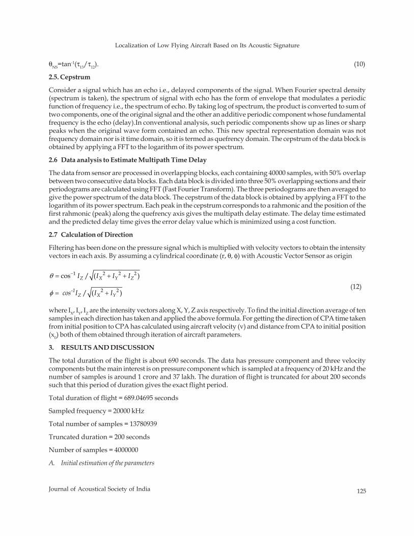
Localization of Low Flying Aircraft Based on Its Acoustic Signature
125Journal of Acoustical Society of India
θNS=tan-1(τ13/τ12). (10)
2.5. Cepstrum
Consider a signal which has an echo i.e., delayed components of the signal. When Fourier spectral density(spectrum is taken), the spectrum of signal with echo has the form of envelope that modulates a periodicfunction of frequency i.e., the spectrum of echo. By taking log of spectrum, the product is converted to sum oftwo components, one of the original signal and the other an additive periodic component whose fundamentalfrequency is the echo (delay).In conventional analysis, such periodic components show up as lines or sharppeaks when the original wave form contained an echo. This new spectral representation domain was notfrequency domain nor is it time domain, so it is termed as quefrency domain. The cepstrum of the data block isobtained by applying a FFT to the logarithm of its power spectrum.
2.6 Data analysis to Estimate Multipath Time Delay
The data from sensor are processed in overlapping blocks, each containing 40000 samples, with 50% overlapbetween two consecutive data blocks. Each data block is divided into three 50% overlapping sections and theirperiodograms are calculated using FFT (Fast Fourier Transform). The three periodograms are then averaged togive the power spectrum of the data block. The cepstrum of the data block is obtained by applying a FFT to thelogarithm of its power spectrum. Each peak in the cepstrum corresponds to a rahmonic and the position of thefirst rahmonic (peak) along the quefrency axis gives the multipath delay estimate. The delay time estimatedand the predicted delay time gives the error delay value which is minimized using a cost function.
2.7 Calculation of Direction
Filtering has been done on the pressure signal which is multiplied with velocity vectors to obtain the intensityvectors in each axis. By assuming a cylindrical coordinate (r, θ, φ) with Acoustic Vector Sensor as origin
Z X Y Z
-1Z X Y
I I I I
cos I I I
1 2 2 2
2 2
cos / ( )
/ ( )
θ
φ
−= + +
= + (12)
where IX, IY, IZ are the intensity vectors along X, Y, Z axis respectively. To find the initial direction average of tensamples in each direction has taken and applied the above formula. For getting the direction of CPA time takenfrom initial position to CPA has calculated using aircraft velocity (v) and distance from CPA to initial position(x0) both of them obtained through iteration of aircraft parameters.
3. RESULTS AND DISCUSSION
The total duration of the flight is about 690 seconds. The data has pressure component and three velocitycomponents but the main interest is on pressure component which is sampled at a frequency of 20 kHz and thenumber of samples is around 1 crore and 37 lakh. The duration of flight is truncated for about 200 secondssuch that this period of duration gives the exact flight period.
Total duration of flight = 689.04695 seconds
Sampled frequency = 20000 kHz
Total number of samples = 13780939
Truncated duration = 200 seconds
Number of samples = 4000000
A. Initial estimation of the parameters
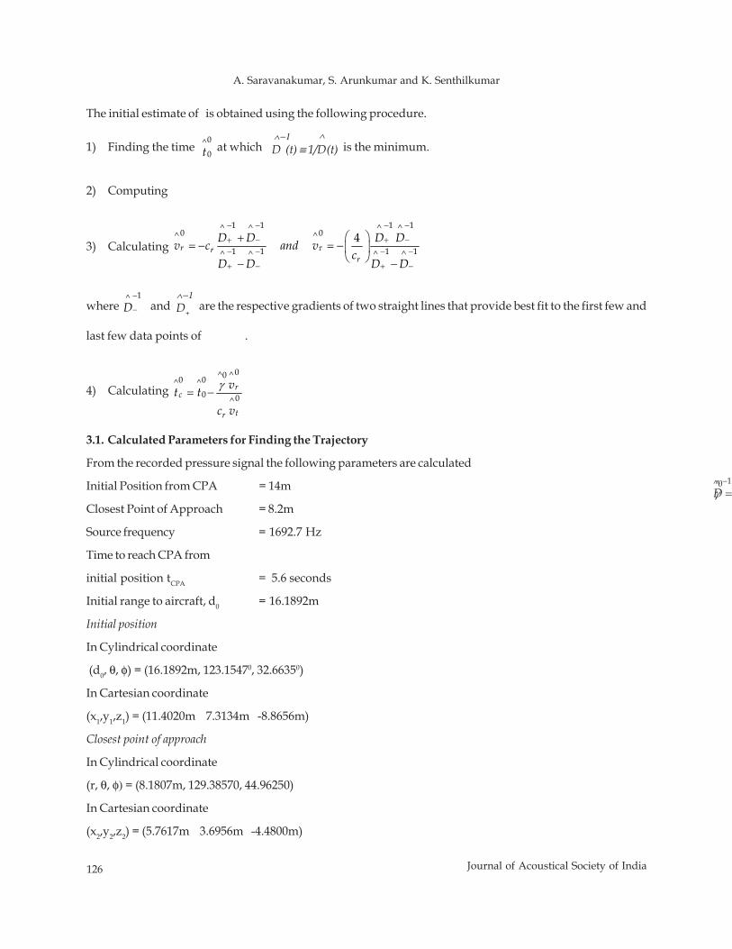
126 Journal of Acoustical Society of India
A. Saravanakumar, S. Arunkumar and K. Senthilkumar
The initial estimate of is obtained using the following procedure.
1) Finding the time t0^0
at which is the minimum.
2) Computing
^0γ =
3) Calculating r rr
D D D Dv c and v c
D D D D
1 1 1 1^ ^ ^ ^0 0^ ^
1 1 1 1^ ^ ^ ^
4τ
− − − −
+ − + −− − − −
+ − + −
⎛ ⎞+= − = −⎜ ⎟
⎝ ⎠− −
where D1^ −
− and are the respective gradients of two straight lines that provide best fit to the first few and
last few data points of
−1^D
.
4) Calculating rc
tr
vt tc v
0^0 ^0 0^ ^0 0^
γ= −
3.1. Calculated Parameters for Finding the Trajectory
From the recorded pressure signal the following parameters are calculated
Initial Position from CPA = 14m
Closest Point of Approach = 8.2m
Source frequency = 1692.7 Hz
Time to reach CPA from
initial position tCPA = 5.6 seconds
Initial range to aircraft, d0 = 16.1892m
Initial position
In Cylindrical coordinate
(d0, θ, φ) = (16.1892m, 123.15470, 32.66350)
In Cartesian coordinate
(x1,y1,z1) = (11.4020m 7.3134m -8.8656m)
Closest point of approach
In Cylindrical coordinate
(r, θ, φ) = (8.1807m, 129.38570, 44.96250)
In Cartesian coordinate
(x2,y2,z2) = (5.7617m 3.6956m -4.4800m)
∧−1D (t) ≡ 1/D(t)
∧
∧−1D+
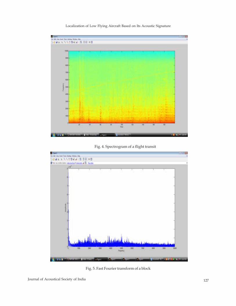
Localization of Low Flying Aircraft Based on Its Acoustic Signature
127Journal of Acoustical Society of India
Fig. 4. Spectrogram of a flight transit
Fig. 5. Fast Fourier transform of a block
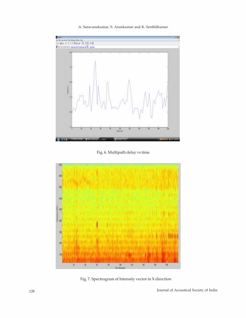
128 Journal of Acoustical Society of India
A. Saravanakumar, S. Arunkumar and K. Senthilkumar
Fig. 7. Spectrogram of Intensity vector in X direction
Fig. 6. Multipath delay vs time
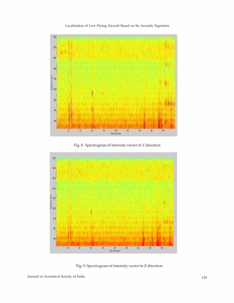
Localization of Low Flying Aircraft Based on Its Acoustic Signature
129Journal of Acoustical Society of India
Fig. 8. Spectrogram of Intensity vector in Y direction
Fig. 9. Spectrogram of intensity vector in Z direction
130 Journal of Acoustical Society of India
A. Saravanakumar, S. Arunkumar and K. Senthilkumar
The multipath delay is calculated for different values of time. The maximum multipath delay is found to be1.1 ms which occurs at 22nd second. This delay value is used to calculate the delay inverse from which theinitial estimation of the parameters is found. The estimated values of velocity and Altitude using Cepstrum are35 m/s and 15 m respectively.
Based on the Cartesian coordinates obtained for initial position and CPA, trajectory has been plotted.
4. CONCLUSION AND FUTURE WORKS
In this work, flight parameters such as velocity, altitude and straight line trajectory of an aircraft are estimatedusing a single Acoustic Vector Sensor on the assumption that aircraft following a straight line trajectory. Thismethod exploits the both the scalar as well as vector properties of sound signal for trajectory estimation.Cepstrum algorithm is used to calculate the four flight parameters with the pressure signal obtained. from asingle AVS. The pressure signal along with velocity vectors are filtered and multiplied to get the intensityvectors. By making use of intensity vectors direction has been found out. Non linear trajectory of the source isfound by triangulation method and it is in progress.
5. REFERENCES
[1] H.E. DEBREE, JELMER WIND, ERIC DRUYVESTEYN and HENK TE KULVE, 2010, "MultipurposeAcoustic Vector Sensors for Battlefield Acoustics - A passive sensor to detect multi events that can beused on multiple platforms", NATO Symposium DAMA, Norway.
[2] K.W.LO, S.W. PERRY and B.G. FERGUSON, 2002, "Aircraft flight parameter estimation using acousticalLloyd's mirror effect", IEEE Transactions on Aerospace & Electronics Systems , 38 (1).
[3] DAI HONGYAN ZOU and HONGXING, 2007, "Aircraft motion parameter estimation via Multipathtime-delay using a single ground based passive acoustic sensor". Journal of electronics.
[4] TAOWANG and QUNWAN, 2007. "Motive Parameters Estimation Using Narrow-band PassiveAcoustical Measurements". IEEE Transactions of Aerospace and Electronic Systems.
[5] KAM W.LO, BRIAN G.FERGUSON, YUJINGA and LAIN MAGUER, 2003. "Aircraft Flight parameterEstimation using Acoustic Multipath delay". IEEE Transactions of Aerospace and Electronic Systems, 39 (1).
[6] S. SADASIVAN, HE DEBREE and TOM BASTEN, 2009. "Acoustic Vector Sensor based IntensityMeasurements for Passive Localization of Small Aircraft", Journal of Acoustical Society of India, 36(1) 8-13.
[7] BRIAN G. FERGUSON, LIONEL G. CRISWICK and KAM W LO, 2002. "Locating far-field Impulsivesound sources in air by triangulation", Acoustical Society of America.
[8] KAM W. LO and B.G. FERGUSON, 2000. "Broadband Passive Acoustic Technique for Target MotionParameter Estimation", IEEE Transactions of Aerospace and Electronic Systems.
Absorption Studies of Aniline and Esters
131Journal of Acoustical Society of India
ABSTRACT
Ultrasonic velocity(v), density(ρ),viscosity(η) for binary mixtures of Aniline with Methyl Acetate,Ethyl Acetate, Amyl Acetate have been measured at room temperature of 300.15K over entirevolume component percentage range. The ultrasonic velocity (v) is measured with Pulse Echo Overlaptechnique at a frequency of 2MHz. The density (ρ) measurements have been carried out by 10mlspecific gravity bottle. The viscosity (η) measurements have been carried out by using Canon-FenskeViscometer with an accuracy of ±0.3% . Attenuation Coefficient (α) is measured using a CathodeRay Oscilloscope for a transmitted pulse and nth echo. Relaxation times (τ), Absorptivity (A) arecomputed using measured data of ultrasonic velocity (v), density (ρ), viscosity (η).
1. INTRODUCTION
Ultrasonic is a useful tool to know the nature of molecular interaction in pure, binary and ternary liquids.But no sufficient data is available in the binary mixture of Aniline in Methyl Acetate, Ethyl Acetate, AmylAcetate. Ultrasonic method found extensive application [1-2] in characterizing the various aspects of thephysico-chemical behavior of liquid mixtures such as molecular interaction and association. Molecularassociation and complex formation in liquid mixtures through ultrasonic velocity measurements have beenstudied by Reddy and Naidu [3]. Ultrasonic velocity of a liquid is related to binding forces between atomsand molecules. The sound velocity in liquid mixtures is known to be a quantity which depends on concentrationin a variety of manners according to the nature of each component liquid. Accurate measurements of ultrasonicvelocity deliver the information about the physical and chemical behavior of solutions and liquid mixtures.
In a material scattering and absorption are produced by various dynamical interactions which typicallyarise from enharmonic force between the atoms, the presence of free charge carriers, cycling to localized spinstates and the presence of impurities [4]. When acoustic waves are propagated through a liquid, dissipationof acoustic energy that is associated with changes in the molecular structure of the medium results from thefinite time, which is required for these changes to take place. Ultrasonic velocity has been a subject of activeinterest during the recent years [5-7]. Nomoto and co researchers made successful attempt to evaluate thesound velocity in binary mixtures. In the present communication we focus on the ultrasonic behavior ofliquid mixtures at 300.15K temperature with Aniline as the base and few esters Methyl Acetate, Ethyl Acetateand Amyl Acetate as mixtures.
2. EXPERIMENTAL
The samples are taken for the present study are of Analar reagent grade and procured from Sd.FineChemicals Limited,Bombay,India. The liquids are thoroughly distilled to remove the dissolved impurities
Journal of Acoustical Society of India : Vol. 40, No. 2, 2013 (pp. 131-136)
Absorption Studies of Aniline and Esters
K. Sathi Reddy, D. Shanmukhi Jyothi* and D. Linga ReddyDepartment of Physics, College of Natural Science, Arba Minch University, Ethopia
Dept of Physics, Sardar Patel College, Secunderabad-500 025, (AP)Dept of Physics, UCS, Osmania University, Hyderabad -500 007, (AP)
*e-mail: [email protected]
[Received: 16.01.2013; Revised: 17.03.2013; Accepted: 26.04.2013]
© 2013 Acoustical Society of India
132 Journal of Acoustical Society of India
K. Sathi Reddy, D. Shanmukhi Jyothi and D. Linga Reddy
using standard chemical procedures like steam distillation. Liquids practically are immiscible with water,volatile in steam and possessing a high boiling point.
By taking two liquids in separate burettes, and with Job's variation method of continuous variation hasbeen used to prepare the mixtures of required proportions.
The ultrasonic velocity measurements are made with the help of microprocessor based ultrasonic PulseEcho Overlap technique (model UX4400M) with built in time Velocity and thickness measuring feature witha frequency of 2MHz. supplied by Roop Telesonic Ultrasonic Ltd,Bombay,India. The internal circuit of(ULTRASONIX4400M) is designed with full solid state version. Further outstanding stability of operation isensured by dynamic use of integrated circuit and PCB mounted gold switches. It has special memory featureswhich enable one to enter testing procedures like angle and type of transducer for permanent storage anddirect digital read out of Ultrasonic velocity up to an accuracy of ±1m/s.
The Pulse Echo Overlap (PEO) method is very versatile and highly accurate technique for measuring thevelocity of the ultrasonic waves in materials of liquids and solids structures. A highly absolute accuracy isobtained from this system, since the method is capable of accurately measuring from any cycle of one echo tothe corresponding cycle of the next echo. The PEO method is able to handle diffraction (beam spreading) andphase correction properly, so that absolute accuracy of the PEO method may exceed the accuracy of most ofthe other methods. However, precision of some other methods is better than PEO method. The PEO methodmay operate either with transducer bonded to the specimen or directly with RF bursts. On the negative side,because of transducer effects, the leading cycles of successive echoes are attenuated and trailing cycles areburst up, so that great care has to be taken to obtain proper cycle for cycle match.In view of the aboveadvantages and accuracy of the system the PEO technique has been adopted for measuring velocity andattenuation.
The densities of all the mixtures have been determined with 10ml. specific gravity bottle and mass (m) ofa given volume of the liquid is determined by using a single pan opto- electrical balance. The results of thedensities are accurate to ±0.5%.
The internal circuit of pulse echo overlap system is designed with fully solid state version, which allowsimmediate calculation of the ultrasonic wave velocity as given in the following equation.
v = 2l / t
where l is the liquid length and t is the time interval.
The long ultrasonic waves are passed through the binary mixture. They are reflected from the reflectorface and received by the same transducer, which now acts as a receiver. The transmitted pulse and thereceived echoes are seen in the CRO screen. Once, the echo pattern is achieved on the screen of the CRO, thepattern is adjusted to a suitable height. The transmitted pulse height is measured in mv/cm and noted as 'a0'on the screen. The height of first echo is noted as 'a1' and second echo as 'ao' and so on. The path length isnoted using the micrometer attached to the reflector and is noted as 2l.
∴∴∴∴∴ The attenuation coefficient (á) is calculated as á =1/2 loge (a0/an) nepers/unit length.where ao → amplitude of transmitted pulse. an → amplitude of nth echo.
The absorptivity is measured by dividing á by the square of the frequency (2MHZ) of the ultrasonicwave propagated into the liquid media, i.e Absorptivity, A = á/fWhere f is the frequency of the ultrasonic wave propagated.
The coefficient ofabsolute viscosity (ç) has been determined using a Cannon- Fenske Viscometer. Theresults of viscosities are accurate to ± 0.3%.
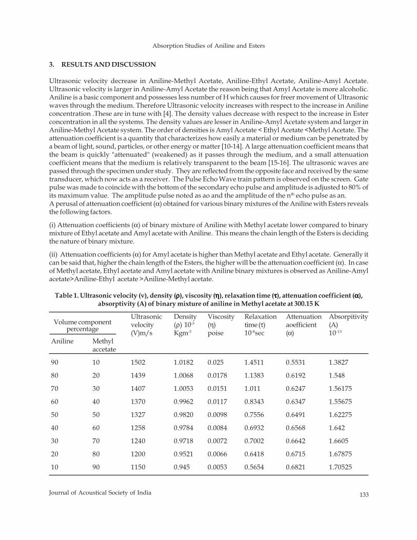
Absorption Studies of Aniline and Esters
133Journal of Acoustical Society of India
3. RESULTS AND DISCUSSION
Ultrasonic velocity decrease in Aniline-Methyl Acetate, Aniline-Ethyl Acetate, Aniline-Amyl Acetate.Ultrasonic velocity is larger in Aniline-Amyl Acetate the reason being that Amyl Acetate is more alcoholic.Aniline is a basic component and possesses less number of H which causes for freer movement of Ultrasonicwaves through the medium. Therefore Ultrasonic velocity increases with respect to the increase in Anilineconcentration .These are in tune with [4]. The density values decrease with respect to the increase in Esterconcentration in all the systems. The density values are lesser in Aniline-Amyl Acetate system and larger inAniline-Methyl Acetate system. The order of densities is Amyl Acetate < Ethyl Acetate <Methyl Acetate. Theattenuation coefficient is a quantity that characterizes how easily a material or medium can be penetrated bya beam of light, sound, particles, or other energy or matter [10-14]. A large attenuation coefficient means thatthe beam is quickly "attenuated" (weakened) as it passes through the medium, and a small attenuationcoefficient means that the medium is relatively transparent to the beam [15-16]. The ultrasonic waves arepassed through the specimen under study. They are reflected from the opposite face and received by the sametransducer, which now acts as a receiver. The Pulse Echo Wave train pattern is observed on the screen. Gatepulse was made to coincide with the bottom of the secondary echo pulse and amplitude is adjusted to 80% ofits maximum value. The amplitude pulse noted as ao and the amplitude of the nth echo pulse as an.A perusal of attenuation coefficient (α) obtained for various binary mixtures of the Aniline with Esters revealsthe following factors.
(i) Attenuation coefficients (α) of binary mixture of Aniline with Methyl acetate lower compared to binarymixture of Ethyl acetate and Amyl acetate with Aniline. This means the chain length of the Esters is decidingthe nature of binary mixture.
(ii) Attenuation coefficients (α) for Amyl acetate is higher than Methyl acetate and Ethyl acetate. Generally itcan be said that, higher the chain length of the Esters, the higher will be the attenuation coefficient (α). In caseof Methyl acetate, Ethyl acetate and Amyl acetate with Aniline binary mixtures is observed as Aniline-Amylacetate>Aniline-Ethyl acetate >Aniline-Methyl acetate.
Ultrasonic Density Viscosity Relaxation Attenuation Absorpitivityvelocity (ρ) 10-3 (η) time (τ) aoefficient (A)(V)m/s Kgm-3 poise 10-8sec (α) 10-13
Aniline Methylaccetate
90 10 1502 1.0182 0.025 1.4511 0.5531 1.3827
80 20 1439 1.0068 0.0178 1.1383 0.6192 1.548
70 30 1407 1.0053 0.0151 1.011 0.6247 1.56175
60 40 1370 0.9962 0.0117 0.8343 0.6347 1.55675
50 50 1327 0.9820 0.0098 0.7556 0.6491 1.62275
40 60 1258 0.9784 0.0084 0.6932 0.6568 1.642
30 70 1240 0.9718 0.0072 0.7002 0.6642 1.6605
20 80 1200 0.9521 0.0066 0.6418 0.6715 1.67875
10 90 1150 0.945 0.0053 0.5654 0.6821 1.70525
Volume componentpercentage
Table 1. Ultrasonic velocity (v), density (ρρρρρ), viscosity (ηηηηη), relaxation time (τττττ), attenuation coefficient (ααααα),absorptivity (A) of binary mixture of aniline in Methyl acetate at 300.15 K
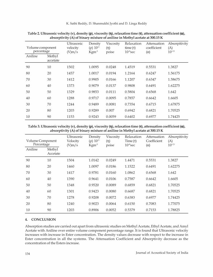
134 Journal of Acoustical Society of India
K. Sathi Reddy, D. Shanmukhi Jyothi and D. Linga Reddy
4. CONCLUSION
Absorption studies are carried out apart from ultrasonic studies on Methyl Acetate, Ethyl Acetate, and AmylAcetate with Aniline over entire volume component percentage range. It is found that Ultrasonic velocityincreases with increase in Ester concentration. The density values decrease with respect to the increase inEster concentration in all the systems. The Attenuation Coefficient and Absorptivity decrease as theconcentration of the Esters increase.
Ultrasonic Density Viscosity Relaxation Attenuation Absorpitivityvelocity (ρ) 10-3 (η) time (τ) coefficient (A)(V)m/s Kgm-3 poise 10-8sec (α) 10-13
Aniline Methylaccetate
90 10 1502 1.0095 0.0248 1.4519 0.5531 1.3827
80 20 1457 1.0017 0.0194 1.2164 0.6247 1.56175
70 30 1412 0.9905 0.0166 1.1207 0.6347 1.58675
60 40 1373 0.9079 0.0137 0.9808 0.6491 1.62275
50 50 1329 0.9853 0.0111 0.5804 0.6568 1.642
40 60 1288 0.9717 0.0095 0.7857 0.6642 1.6605
30 70 1244 0.9489 0.0081 0.7354 0.6715 1.67875
20 80 1203 0.9289 0.007 0.6942 0.6821 1.70525
10 90 1153 0.9243 0.0059 0.6402 0.6977 1.74425
Volume componentpercentage
Table 2. Ultrasonic velocity (v), density (ρρρρρ), viscosity (ηηηηη), relaxation time (τττττ), attenuation coefficient (ααααα),absorptivity (A) of binary mixture of aniline in Methyl acetate at 300.15 K
Ultrasonic Density Viscosity Relaxation Attenuation AbsorpitivityVelocity (ρ) 10-3 (η) Time (τ) Coefficient (A)(V)m/s Kgm-3 poise 10-8sec (α) 10-13
Aniline MethylAccetate
90 10 1504 1.0142 0.0249 1.4471 0.5531 1.3827
80 20 1460 1.0097 0.0186 1.1522 0.6491 1.62275
70 30 1417 0.9781 0.0160 1.0862 0.6568 1.642
60 40 1390 0.9641 0.0106 0.7587 0.6642 1.6605
50 50 1348 0.9520 0.0089 0.6859 0.6821 1.70525
40 60 1301 0.9423 0.0080 0.6687 0.6821 1.70525
30 70 1278 0.9208 0.0072 0.6383 0.6977 1.74425
20 80 1240 0.9023 0.0064 0.6150 0.7083 1.77075
10 90 1203 0.8906 0.0052 0.5379 0.7153 1.78825
Volume ComponentPercentage
Table 3. Ultrasonic velocity (v), density (ρρρρρ), viscosity (ηηηηη), relaxation time (τττττ), attenuation coefficient (ααααα),absorptivity (A) of binary mixture of aniline in Methyl acetate at 300.15 K
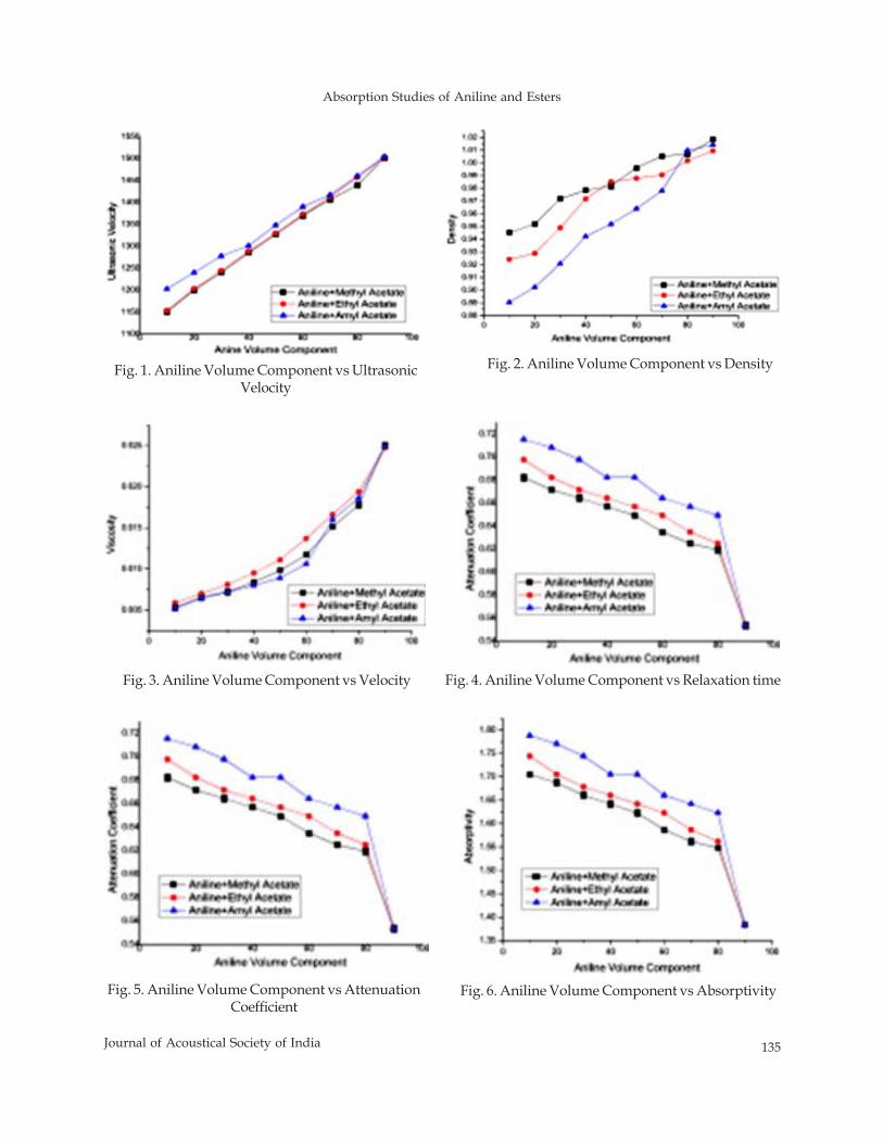
Absorption Studies of Aniline and Esters
135Journal of Acoustical Society of India
Fig. 5. Aniline Volume Component vs AttenuationCoefficient
Fig. 6. Aniline Volume Component vs Absorptivity
Fig. 4. Aniline Volume Component vs Relaxation timeFig. 3. Aniline Volume Component vs Velocity
Fig. 2. Aniline Volume Component vs DensityFig. 1. Aniline Volume Component vs UltrasonicVelocity
136 Journal of Acoustical Society of India
K. Sathi Reddy, D. Shanmukhi Jyothi and D. Linga Reddy
5. REFERENCES[1] H. EYRINGAND and J.O. HIRSCHFELDER, 1937 J.Phy.chem, 41, 249.[2] R.J. FORT and W.R. MOORE,1979 Trans, Faraday Society 61, 687.[3] K. SUBRAMANYAM REDDY and P.R. NAIDU, 1979 Aust. J. Chem 32, 687.[4] K. SATHI REDDY and D. LINGA REDDY, 2007 Journal of Ultrasonics.[5] B. Ravinder Reddy and D. Linga Reddy, Ind.J.Pure and Appl.Phy.37, (1999)56.[6] N. JAYA KUMAR, KARUNANIDHI and V. APPAN, 1999 Ind.J.Pure and Appl. Phy.36, 76[7] S.V. Ranganayakulu, C. Sreenivas Reddy and D. Linga Reddy, 2003 J. Acoustical Society of India 31, 295.[8] H. EYRING and J.F. KINCAID, 1938 J. Chem. Phy. 6, 67.[9] V.K. SYAL, KUMARI, U. CHAUHAN, S. CHAUHAN, M.S. SUD and S.P. SINGH, 1992 Indian J. Pure and
Appl. Phy.[10] S. RAJAGOPALAN, 1988 Acoustica, 66, 63.[11] K.S. REDDY and P.R. NAIDU, 1985 J. Chem. Liq.15, 147.[12] C. BACHEM and Z. PHYSIK 1936 101, 565.[13] G.V. REDDY and R.P. SINGH, 1970 Acustica 23, 31.[14] S.C. BHATT, R.S. RAWAT and B.S. SEMWAL, 1999 J. Acoust. Soc. India, 27, 297.[15] J. PRAKASH and B. RAI, 1987 Acoustica, 64, 226.[16] O. NOMOTO 1953 et al, J. Phy. Soc. Japan 8 4.
Interaction Study of Pyridine and Acetone at 313.15 K
137Journal of Acoustical Society of India
Interaction Study of Pyridine and Acetone at 313.15 K
Prashant Dabrase1*, R.A. Patil2 and B.M. Suryavanshi3
1Bhalerao Science College, Saoner-441 1072S.S.S.K.R.Innani Mahavidyalaya, Karanja-444 105
3Dept. of Physics, Government Institute of Science, Nagpur-440 001 (M.S.)*e-mail: [email protected]
ABSTRACT
The Ultrasonic velocities (υ), density (ρ) and viscosity (η) measurements of pure & binary liquidmixtures of Pyridine and Acetone have been carried out at temperature 313.15 K to evaluate the otherthermo dynamical parameters with their excess values such as adiabatic compressibility (βα), freelength (Lf), acoustical impedance (Z), free volume (Vf), internal pressure (πi) and the excess values, υE,βα
E, LfE, ZE, Vf
E and πiE over the entire range of composition. The results thus obtained are discussed
for molecular interaction. The non linearity observed in the plots of these ultrasonic parameters andtheir excess values with the composition range indicates presence of the intermolecular interactionbetween the components of the unlike molecules of the mixture. The nature of excess values of thecompressibility βα
E, free length LfE , acoustical impedance ZE, free volume Vf
E and internal pressureπi
E conforms about the existence of the molecular association between the components of the mixture.
1. INTRODUCTION
Ultrasonic studies have always played an important role in understanding the nature of intermolecularinteraction in pure liquid and liquid mixtures. They find application in several industrial and technologicalprocesses. Because the Ultrasonic velocity is highly sensitive to molecular structures [1-4] and Ultrasonicinvestigations of liquid mixtures consisting of polar and non polar components are of highly importance inunderstanding the physical nature and strength of molecular interaction in the liquid mixtures [5]. For thebetter understanding of the physical and chemical properties and the inter-molecular interactions between themolecules of the mixture, ultrasonic velocity with density and the viscosity are measured at differentconcentration. The ultrasonic velocity of liquid is basically related to the bonding forces between the atomsand molecules, it helps to understand the nature of molecular interactions in pure and binary mixtures of theliquids [6-8]. Pyridine is an important liquid used currently in the extraction process for coal to analyze itscompounds and in the manufacture of vitamin B6 and other drugs. These liquid mixtures are of interest toorganic chemists to know about the type of bond and number of each molecule in the pyridine complex [9, 10].
In the present study the ultrasonic velocity, density and viscosity measurements have been carried out forpure acetone and pyridine and their binary mixtures for various concentrations at 313.15K. The variations ofdifferent ultrasonic parameters and their excess values with concentration of binary liquid mixtures are studiedto understand molecular interaction between unlike molecules of the mixtures.
2. EXPERIMENTAL
The binary mixtures of various concentrations in mole fraction of the liquids Acetone and Pyridine wereprepared at room temperature by obtaining the AR grade liquids with purity of 99.5% commercially and used
Journal of Acoustical Society of India : Vol. 40, No. 2, 2013 (pp.137-142)
[Received: 18.01.2013; Revised: 22.03.2013; Accepted: 28.04.2013]
© 2013 Acoustical Society of India
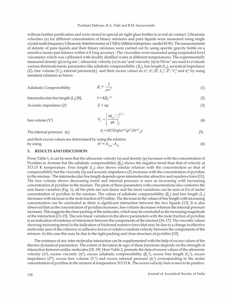
138 Journal of Acoustical Society of India
Prashant Dabrase, R.A. Patil and B.M. Suryavanshi
without further purification and were stored in special air tight glass bottles to avoid air contact. Ultrasonicvelocities (υ) for different concentration of binary mixtures and pure liquids were measured using singlecrystal multi frequency Ultrasonic Interferometer at 1 MHz (Mittal enterprises- model M-81). The measurementsof density of pure liquids and their binary mixtures were carried out by using specific gravity bottle on asensitive mono-pan balance within ± 0.1mg accuracy. The viscosities were measured using suspended levelviscometer which was calibrated with doubly distilled water at different temperatures. The experimentallymeasured density (ρ) in kg ms-1, ultrasonic velocity (υ) in ms-1and viscosity (η) in NS m-2 are used to evaluatevarious thermodynamic parameters like adiabatic compressibility ( βα), free length (Lf), acoustical impedance(Z), free volume (Vf), internal pressure(πi) and their excess values as υE, ηE, βE, Lf
E, ZE, VfE and πi
E by usingstandard relations as below.
Adiabatic Compressibility a 2
1= βρν (1)
Intermolecular free length (Lf) [8], f = Kβα1/2 (2)
Acoustic impedance (Z) Z = υρ (3)
free volume (Vf)
3 / 2ef f
f
MV
k
ν
η⎡ ⎤
= ⎢ ⎥⎢ ⎥⎣ ⎦
(4)
The internal pressure (πi) (5)
and their excess values are determined by using the relationby using AE = Aexp -Aid (6)
3. RESULTS AND DISCUSSION
From Table 1, it can be seen that the ultrasonic velocity (υ) and density (ρ) increases with the concentration ofPyridine in Acetone but the adiabatic compressibility (βα) shows the negative trend than that of velocity at313.15 K temperature. Free length (Lf) also shows similar relation with the concentration as that ofcompressibility but the viscosity (η) and acoustic impedance (Z) increases with the concentration of pyridinein the mixture. The intermolecular free length depends upon intermolecular attractive and repulsive force [11].The free volume shows decreasing trend and internal pressure is seen as increasing with increasingconcentration of pyridine in the mixture. The plots of these parameters with concentrations also conforms thenon linear variation (Fig. 1), all the plots are non linear and the most variations can be seen at 0.6 of molarconcentration of pyridine in the mixture. The values of adiabatic compressibility (βα) and free length (Lf)decreases with increase in the mole fraction of Pyridine. The decrease in the values of free length with increasingconcentration can be concluded as there is significant interaction between the two liquids [12]. It is alsoobserved that as the concentration of pyridine increases, free volume decreases whereas the internal pressureincreases. This suggests the close packing of the molecules, which may be concluded as the increasing magnitudeof the interaction [13-15]. The non linear variation in the above parameters with the mole fraction of pyridineis an indication of existence of interaction between the components of the mixture [16, 17]. The viscosity valuesshowing increasing trend is the indication of frictional resistive force that may be due to a change in effectivemolecular area of the cohesive or adhesive forces or relative random velocity between the components of themixture. In this case this may be due to the tight packing and close structure of pyridine [10].
The existence of any inter molecular interaction can be supplemented with the help of excess values of thethermo dynamical parameters. The extent of deviation & sign of these functions depends on the strength ofinteraction between unlike molecules [18, 19]. Here Table 2, presents the data of excess values of the ultrasonicvelocity (υE), excess viscosity (ηE), excess adiabatic compressibility (βα
E), excess free length (LfE), excess
impedance (ZE), excess free volume (VfE) and excess internal pressure (πi
E) corresponding to the molarconcentration of pyridine in the mixture at temperature 313.15 K. The excess velocity here is seen to be positive.
πi = bRT(kη/n)1/2(ρ2/3/M7/6eff)
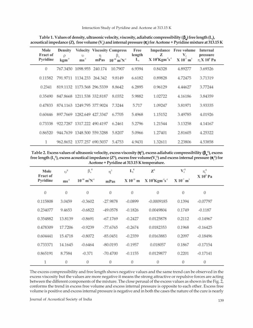
Interaction Study of Pyridine and Acetone at 313.15 K
139Journal of Acoustical Society of India
The excess compressibility and free length shows negative values and the same trend can be observed in theexcess viscosity but the values are more negative it means the strong attractive or repulsive forces are actingbetween the different components of the mixture. The close perusal of the excess values as shown in the Fig. 2,conforms the trend in excess free volume and excess internal pressure is opposite to each other. Excess freevolume is positive and excess internal pressure is negative and in both the cases the nature of the cure is nearly
Table 2. Excess values of ultrasonic velocity, excess viscosity (ηηηηηE), excess adiabatic compressibility (βββββαααααE), excess
free length (LfE), excess acoustical impedance (ZE), excess free volume(Vf
E) and excess internal pressure (πππππiE) for
Acetone + Pyridine at 313.15 K temperature.
Table 1. Values of density, ultrasonic velocity, viscosity, adiabatic compressibility ( βββββααααα) free length (Lf),acoustical impedance (Z), free volume (Vf) and internal pressure (πππππi) for Acetone + Pyridine mixture at 313.15 K
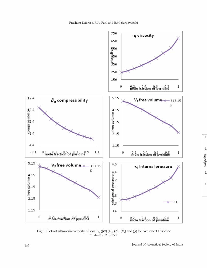
140 Journal of Acoustical Society of India
Prashant Dabrase, R.A. Patil and B.M. Suryavanshi
Fig. 1. Plots of ultrasonic velocity, viscosity, (βα) (Lf), (Z), (Vf) and (πi) for Acetone + Pyridinemixture at 313.15 K
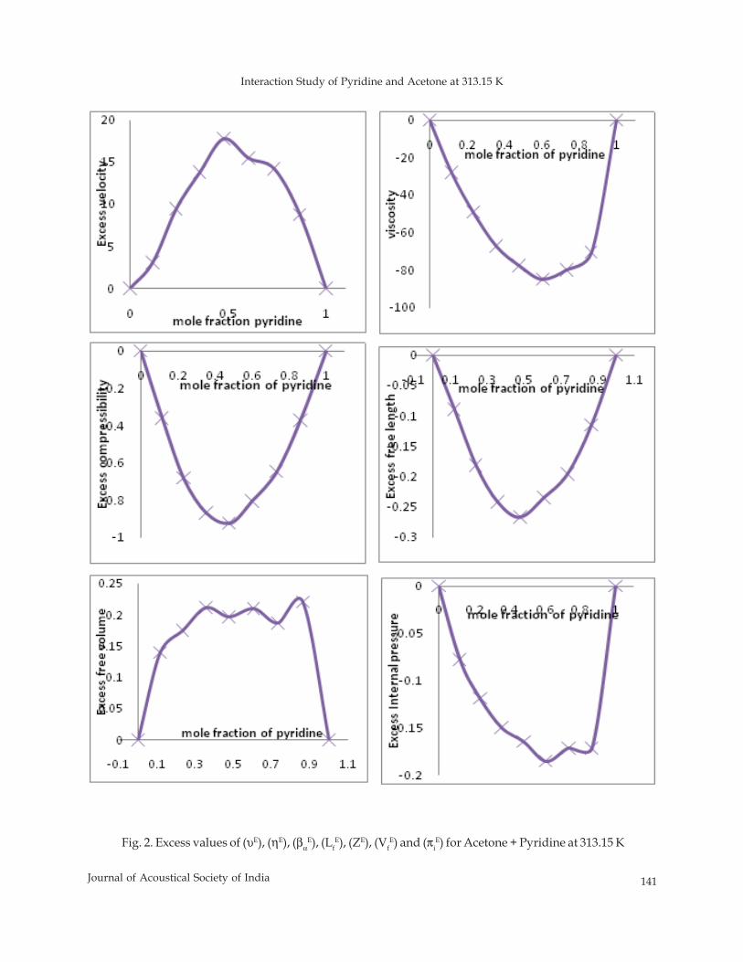
Interaction Study of Pyridine and Acetone at 313.15 K
141Journal of Acoustical Society of India
Fig. 2. Excess values of (υE), (ηE), (βαE), (Lf
E), (ZE), (VfE) and (πi
E) for Acetone + Pyridine at 313.15 K
142 Journal of Acoustical Society of India
Prashant Dabrase, R.A. Patil and B.M. Suryavanshi
flat showing the existence of interaction between the different components of the mixture for all theconcentrations of the pyridine in the mixture.
The sign of excess free length plays a vital role in assessing compactness due to molecular interactionthrough dipole-dipole interaction [20, 21] leading to more compact structure making which enhances excessfree length to have negative values. Graphs of excess adiabatic compressibility (βαE) and excess free length (Lf
E)are negative which indicates the strong molecular interaction between the components of the mixture. Thedeviation of excess impedance (ZE) is found to be positive. The excess ultrasonic velocity (υE) for the binarymixture is positive. The positive deviation and non-linear dependence suggests the presence of strong interactionbetween the components of mixture [22, 23].
4. CONCLUSION
From the present study it can be concluded that the results are very basic in nature and indicates that the nonlinear variation of the all the parameters measured at 313.15 K for the mixture of Pyridine in the Acetoneindicates existence of interaction between the different molecules of the compounds in the mixture. The non-linearity of the curve is common for all compositions. The negative values of excess compressibility (βα
E),excess viscosity (ηE), excess free length (Lf
E) & excess internal pressure (πiE) and the positive values of excess
ultrasonic velocity (υE), excess acoustic impedance (ZE) and excess free volume (VfE) for the different combinations
of the liquids in the mixture shows the presence of strong dispersive interaction between the components ofmolecule in the mixture. The excess values of thermodynamic parameters are sensitive to the molecularassociation present in the liquid mixture. The interaction is strong from 0.2 to 0.8 of concentration of thePyridine in the mixture.5. REFERENCES
[1] H. EYRING and J.F. KINCAID, 1938. J. Chem. Phys., 6, 220-229.[2] K.S. PITZER, 1995. Thermodynamics, 3rd edition (Mc.Graw-Hill book Co, NY.[3] A.N. KANNAPAN, S. THIRUMAM and R. PALANI, 2009. J. Phys. Science, 20(2), 97-108[4] V.A. TABHANE, S. GHOSH and S. AGRAWAL, 1900. J. Pure and Appl. Ultrasonic, 21, p. 122.[5] R.J. FORT and W.R. MOORE, 1966. Trans. Farady Society, 62, p. 1112.[6] V. SRINIVASULU and P.R. NAIDU, 1995. J. Pure and Appl. Ultrasonic, 17, 14-28.[7] K. SWAIN and P. PRIYADARSHANI, 2010. Indian J.Pure and Appl. Phys., 48, 539-542.[8] B. JACOBSON, 1952. Ultras Velo. of liquids and liquid mixtures, J. Chem. Phys., 20, 927-928.[9] P.K. GUPTA and F.B. STUMP, 2010. Indian J pure and Appl. Phys., 48, 326-333.[10] G. ARUL and L PALANIAPPAN, 2005. Indian J pure and Appl. Phys., 43, 755-758.[11] H. EYRING and J.F. KINCAID, 1938. J.Chem. Phys., 6, p. 620.[12] K. RAJGOPAL and S. CHENTHILNATH, 1981. Indian J. Pure and Appl. Phys., 19, p. 358.[13] T.S. BANIPAL, A.F. TOOR and V.K. RATTAN, 2000. Indian J. Chem., 39A, p. 809.[14] P.S. NAIDU and K. RAVINDRA PRASAD, 2002. Indian J.Pure and Appl. Phys., 40, p. 264.[15] G. ARUL and L. PALANIAPPAN, 2001. Indian J pure and Appl. Phys., 39, p. 561.[16] A.N. KANNAPPAN and V. RAJENDRAN, 1999. Indian J.Pure and Appl. Phys., 73B, p. 531.[17] A. SADASIVA RAO and B VIJAYKUMAR NAIDU, 2000. J Acoust Soc India, 28, p. 303.[18] O. REDLICH and A.T. KISTER, 1948. Ind. Eng. Chem., 40, p. 345.[19] A. ALI and A.K. NAIN, 1999. Int. Conf. Exhi. on Ultrsonics (ICEU-99), New Delhi.[20] D. ANBANANTHAN, 1979. J. Acost. Soc. of India, 7, p. 123.[21] NISHA SHARMA and B.P. SINGH, 2010. Acta Ciencia India, XXXIV P(3), p. 375.[22] M.K. PRAHARAJ ET AL., 2012. J. Chemical and Pharma. Research, 4(4), 1910-1920.[23] A.N. KANNAPPAN and V. RAJENDRAN, 1991. Indian J. Pure and Appl. Phys., 29, 465-468.[24] P.B. DABRASE, R.A. PATIL and B.M. SURYAVANSHI, 2012. Applied Ultras, Shree Publi., New Delhi,
233-241.

Acoustical Society of India(Regn. No. 65-1971)
Executive Council (2010 - 2014)
President : Dr V Rajendran[KSRCT, Tiruchengode; [email protected]; +91-99 94 13 03 03]
Vice President : NS Naidu[NSTL, Vizag; [email protected]; +91-94 90 75 05 82]
General Secretary : PVS Ganesh Kumar[NSTL, Vizag; [email protected]; +91-98 66 40 08 94]
Jt. Secretary : Dr K Trinadh[NSTL, Vizag; [email protected]; +91-97 04 71 95 00]
Treasurer : Prof AV Sharma[AU, Vizag; [email protected]; +91-94 90 43 17 26]
Chief Editor : Dr Mahavir Singh[CSIR-NPL, New Delhi; [email protected]; +91-98 71 69 33 46]
Council Members : Dr SV Ranga Nayakulu[VITAE, Hyderabad; [email protected]; +91-98 66 53 26 13]
Dr I Johnson[SJ College, Trichy; [email protected]; +91-94 42 90 48 20]
Dr Rajiv K Upadhayay[Govt PG College, Rishikesh; [email protected]; +91-94 12 97 28 90]
Dr S Shekhar[Oxford College, Trichy; [email protected]; +91-99 94 92 00 30]
Dr V Bhujanga Rao[Past President; NSTL, Vizag; [email protected]; +91-98 66 44 10 74]
Co-opted Members : Rajshekhar Uchil[Josts, Bangalore; [email protected]; +91-98 80 17 08 95]
Dr NK Narayanan[CIT, Kozhikode; [email protected]; +91-94 46 95 58 30]

INFORMATION FOR AUTHORS
ARTICLES The Journal of Acoustical Society of India (JASI) is a refereed publication published quarterly by the Acoustical Society of India(ASI). JASI includes refereed articles, technical notes, letters-to-the-editor, book review and announcements of general interest toreaders.
Articles may be theoretical or experimental in nature. But those which combine theoretical and experimental approaches tosolve acoustics problems are particularly welcome. Technical notes, letters-to-the-editor and announcements may also be submitted.Articles must not have been published previously in other engineering or scientific journals. Articles in the following are particularlyencouraged: applied acoustics, acoustical materials, active noise & vibration control, bioacoustics, communication acousticsincluding speech, computational acoustics, electro-acoustics and audio engineering, environmental acoustics, musical acoustics,non-linear acoustics, noise, physical acoustics, physiological and psychological acoustics, quieter technologies, room and buildingacoustics, structural acoustics and vibration, ultrasonics, underwater acoustics.
Authors whose articles are accepted for publication must transfer copyright of their articles to the ASI. This transfer involvespublication only and does not in any way alter the author's traditional right regarding his/her articles.
PREPARATION OF MANUSCRIPTS All manuscripts are refereed by at least two referees and are reviewed by the Publication Committee (all editors) beforeacceptance. Manuscripts of articles and technical notes should be submitted for review electronically to the Chief Editor by e-mailor by express mail on a disc. JASI maintains a high standard in the reviewing process and only accept papers of high quality. Onacceptance, revised articles of all authors should be submitted to the Chief Editor by e-mail or by express mail. Text of the manuscript should be double-spaced on A4 size paper, subdivided by main headings-typed in upper and lowercase flush centre, with one line of space above and below and sub-headings within a section-typed in upper and lower caseunderstood, flush left, followed by a period. Sub-sub headings should be italic. Articles should be written so that readers indifferent fields of acoustics can understand them easily. Manuscripts are only published if not normally exceeding twenty double-spaced text pages. If figures and illustrations are included then normally they should be restricted to no more than twelve-fifteen. The first page of manuscripts should include on separate lines, the title of article, the names, of authors, affiliations andmailing addresses of authors in upper and lowers case. Do not include the author's title, position or degrees. Give an adequatepost office address including pin or other postal code and the name of the city. An abstract of not more than 200 words shouldbe included with each article. References should be numbered consecutively throughout the article with the number appearing asa superscript at the end of the sentence unless such placement causes ambiguity. The references should be grouped together,double spaced at the end of the article on a separate page. Footnotes are discouraged. Abbreviations and special terms must bedefined if used.
EQUATIONS Mathematical expressions should be typewritten as completely as possible. Equation should be numbered consecutivelythroughout the body of the article at the right hand margin in parentheses. Use letters and numbers for any equations in anappendix: Appendix A: (A1, (A2), etc. Equation numbers in the running text should be enclosed in parentheses, i.e., Eq. (1), Eqs.(1a) and (2a). Figures should be referred to as Fig. 1, Fig. 2, etc. Reference to table is in full: Table 1, Table 2, etc. Metric units shouldbe used: the preferred from of metric unit is the System International (SI).
REFERENCES The order and style of information differs slightly between periodical and book references and between published and unpublishedreferences, depending on the available publication entries. A few examples are shown below.
Periodicals:[1] S.R. Pride and M.W. Haartsen, 1996. Electroseismic wave properties, J. Acoust. Soc. Am., 100 (3), 1301-1315.[2] S.-H. Kim and I. Lee, 1996. Aeroelastic analysis of a flexible airfoil with free play non-linearity, J. Sound Vib., 193 (4), 823-846.
Books:[1] E.S. Skudzryk, 1968. Simple and Comlex Vibratory Systems, the Pennsylvania State University Press, London.[2] E.H. Dowell, 1975. Aeroelasticity of plates and shells, Nordhoff, Leyden.
Others:[1] J.N. Yang and A. Akbarpour, 1987. Technical Report NCEER-87-0007, Instantaneous Optimal Control Law For Tall
Buildings Under Seismic Excitations.
SUMISSIONS All materials from authors should be submitted in electronic form to the JASI Chief Editor: Dr Mahavir Singh, Acoustics,Ultrasonics & Vibration Section, CSIR-National Physical Laboratory, Dr. K. S. Krishnan Road, New Delhi-110 012 (email:[email protected] Tel: +91-11-4560.8317, Fax: +91-11-4560.9310). For the item to be published in a given issue of a journal,the manuscript must reach the Chief Editor at least twelve week before the publication date.
SUMISSION OF ACCEPTED MANUSCRIPT On acceptance, revised articles should be submitted in electronic form to the JASI Chief Editor ([email protected]).

ISSN 0973-3302
Volume 40 Number 1 January 2013
A Quarterly Publication of the JASI
http://www.acousticsindia.org
OCIS E TL YA OCI FT S INU DO IAC A
AA A ~Ae ekr xk/ tk s h ku re
JOURNAL OF
ACOUSTI CAL SOCIETY
OF INDIA

Journal of AcousticalSociety of India
The Refereed Journal of the Acoustical Society of India (JASI)JASI
CHIEF EDITOR:Mahavir SinghAcoustics, Ultrasonics & Vibration SectionCSIR-National Physical LaboratoryDr. KS Krishnan RoadNew Delhi 110 012Tel: +91.11.4560.8317Fax: +91.11.4560.9310E-mail: [email protected]
ASSOCIATE SCIENTIFIC EDITOR:Applied Acoustics
Trinath KarControl Component India Pvt. Ltd6th Floor, Warp TowerPlot # 13, 14, &15SJR i-Park, EPIP Zone, Phase 1Whitefield Road, Bangalore 560066
The Journal of Acoustical Society of India is a refereed journal of the Acoustical Society of India (ASI). The ASI is anon-profit national society founded in 31st July, 1971. The primary objective of the society is to advance the science ofacoustics by creating an organization that is responsive to the needs of scientists and engineers concerned with acousticsproblems all around the world.
Manuscripts of articles, technical notes and letter to the editor should be submitted to the Chief Editor. Copies ofarticles on specific topics listed above should also be submitted to the respective Associate Scientific Editor. Manuscriptsare refereed by at least two referees and are reviewed by Publication Committee (all editors) before acceptance. Onacceptance, revised articles with the text and figures scanned as separate files on a diskette should be submitted to theEditor by express mail. Manuscripts of articles must be prepared in strict accordance with the author instructions.
All information concerning subscription, new books, journals, conferences, etc. should be submitted to Chief Editor:
Acoustics, Ultrasonics & Vibration Section, CSIR-National Physical Laboratory, Dr. KS Krishnan Road, New Delhi 110 012, Tel: +91.11.4560.8317, Fax: +91.11.4560.9310, e-mail: [email protected]
Annual subscription price including mail postage is Rs. 2000/= for institutions, companies and libraries and Rs. 2000/=for individuals who are not ASI members. The Journal of Acoustical Society of India will be sent to ASI members freeof any extra charge. Requests for specimen copies and claims for missing issues as well as address changes should besent to the Editorial Office:
Acoustics, Ultrasonics & Vibration Section, CSIR-National Physical Laboratory, Dr. KS Krishnan Road, New Delhi 110 012, Tel: +91.11.4560.8317, Fax: +91.11.4560.9310, e-mail: [email protected]
The journal and all articles and illustrations published herein are protected by copyright. No part of this journal may betranslated, reproduced, stored in a retrieval system, or transmitted, in any form or by any means, electronic, mechanical,photocopying, microfilming, recording or otherwise, without written permission of the publisher.
Copyright © 2007, Acoustical Society of IndiaISSN 0973-330
Editorial Office:
MANAGING EDITOROmkar Sharma
ASSISTANT EDITORSYudhisther KumarAnil Kumar NainNaveen Garg
Acoustics, Ultrasonics & Vibration SectionCSIR-National Physical LaboratoryDr. KS Krishnan RoadNew Delhi 110 012Tel: +91.11. 4560.8317asFax: +91.11.4560.9310E-mail: [email protected]
Printed at Alpha Printers, BG-2/38C, Paschim Vihar, New Delhi-110063 Tel.: 9811848335. JASI is sent to ASI membersfree of charge.
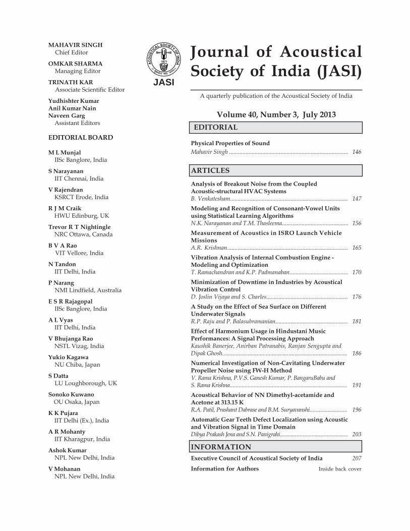
Journal of AcousticalSociety of India (JASI)
A quarterly publication of the Acoustical Society of India
Volume 40, Number 3, July 2013
JASI
MAHAVIR SINGH Chief Editor
OMKAR SHARMA Managing Editor
TRINATH KAR Associate Scientific Editor
Yudhishter KumarAnil Kumar NainNaveen Garg Assistant Editors
EDITORIAL BOARD
M L Munjal IISc Banglore, India
S Narayanan IIT Chennai, India
V Rajendran KSRCT Erode, India
R J M Craik HWU Edinburg, UK
Trevor R T Nightingle NRC Ottawa, Canada
B V A Rao VIT Vellore, India
N Tandon IIT Delhi, India
P Narang NMI Lindfield, Australia
E S R Rajagopal IISc Banglore, India
A L Vyas IIT Delhi, India
V Bhujanga Rao NSTL Vizag, India
Yukio Kagawa NU Chiba, Japan
S Datta LU Loughborough, UK
Sonoko Kuwano OU Osaka, Japan
K K Pujara IIT Delhi (Ex.), India
A R Mohanty IIT Kharagpur, India
Ashok Kumar NPL New Delhi, India
V Mohanan NPL New Delhi, India
EDITORIAL
Physical Properties of SoundMahavir Singh ............................................................................... 146
ARTICLES
Analysis of Breakout Noise from the CoupledAcoustic-structural HVAC SystemsB. Venkatesham.............................................................................. 147Modeling and Recognition of Consonant-Vowel Unitsusing Statistical Learning AlgorithmsN.K. Narayanan and T.M. Thasleema............................................ 156Measurement of Acoustics in ISRO Launch VehicleMissionsA.R. Krishnan................................................................................ 165Vibration Analysis of Internal Combustion Engine -Modeling and OptimizationT. Ramachandran and K.P. Padmanaban....................................... 170Minimization of Downtime in Industries by AcousticalVibration ControlD. Joslin Vijaya and S. Charles...................................................... 176A Study on the Effect of Sea Surface on DifferentUnderwater SignalsR.P. Raju and P. Balasubramanian................................................ 181Effect of Harmonium Usage in Hindustani MusicPerformances: A Signal Processing ApproachKaushik Banerjee, Anirban Patranabis, Ranjan Sengupta andDipak Ghosh................................................................................... 186Numerical Investigation of Non-Cavitating UnderwaterPropeller Noise using FW-H MethodV. Rama Krishna, P.V.S. Ganesh Kumar, P. BangaruBabu andS. Rama Krishna.............................................................................. 191Acoustical Behavior of NN Dimethyl-acetamide andAcetone at 313.15 KR.A. Patil, Prashant Dabrase and B.M. Suryavanshi......................... 196Automatic Gear Teeth Defect Localization using Acousticand Vibration Signal in Time DomainDibya Prakash Jena and S.N. Panigrahi............................................. 203
INFORMATIONExecutive Council of Acoustical Society of India 207
Information for Authors Inside back cover
EDITOR’S SPACE
Physical Properties of Sound
The material gives a brief introduction to some of the terms used in building acoustics and the test methodsused to characterize systems and materials. A very basic understanding of some fundamentals of acousticsand terms used in building acoustics, is all that is necessary to understand the material in this and thefollowing chapters. To emphasize the simplicity of the approach, equations are kept to a minimum.
Sound is generated by creating a disturbance of the air, which sets up a series of pressure waves fluctuatingabove and below the air's normal atmospheric pressure, much as a stone that falls in water generates expandingripples on the surface. Unlike the water waves, however, these pressure waves propagate in all directionsfrom the source of the sound. Our ears sense these pressure fluctuations, convert them to electrical impulses,and send them to our brain, where they are interpreted as sound.
There are many sources of sound in buildings: voices, human activities, external noises such as traffic,entertainment devices and machinery. They all generate small rapid variations in pressure about the staticatmospheric pressure; these propagate through the air as sound waves.
As well as travelling in air, sound can travel as vibrational waves in solids or liquids. The terms airborneand structure-borne sound are used depending on which medium the sound is travelling in at the time. Forexample, the noise from a radio set may begin as airborne sound, enter the structure of the building and travelfor some distance as structure-borne sound, and then be radiated again as airborne sound in another place.
Air pressure is usually measured in units of Pascals (Pa). Atmospheric pressure is about 100 kPa. Soundpressure is a measure of the fluctuation of the air pressure above and below normal atmospheric pressure asthe sound waves propagate past a listener.
The pressure variations in an individual sound wave are much less than the static atmospheric pressure,but the range of sound pressures encountered in acoustics is very large. The threshold of hearing is assumed tocorrespond to pressure fluctuations of 20 Micro Pascals; some individuals will have more acute hearing thanthis, some less. The threshold of pain in the ear corresponds to pressure fluctuations of about 200 Pa. Thissecond value is ten million times the first. These unwieldy numbers are converted to more convenient onesusing a logarithmic scale, the decibel scale. Sound pressure levels are expressed as a number followed by thesymbol dB. Sound level meters convert electrical signals from a microphone to sound pressure levels in dB.
Decibels are more easily related to the response of the human ear, which also responds logarithmically tosound. The response of our ears, that is, our perception of loudness, does not increase linearly with a linearincrease in sound pressure. For example, a 10 dB increase in sound pressure level would be perceived as adoubling of the loudness. In practical situations, level changes of about 3 dB are just noticeable.
It is very important to remember that decibels and similar acoustical quantities have properties differentfrom more conventional units. Sound pressure levels, for example, cannot be added together as can kilograms.The combination of two noises with average levels of 60 dB does not give a sound pressure level of 120 dB,but 63 dB.
Mahavir Singh
Analysis of Breakout Noise from the Coupled Acoustic-structural HVAC Systems
147Journal of Acoustical Society of India
Analysis of Breakout Noise from the CoupledAcoustic-structural HVAC Systems
B. VenkateshamDepartment of Mechanical Engineering
Indian Institute of Technology Hyderabad-502 025 (Andhra Pradesh)e-mail: [email protected]
ABSTRACT
Noise control in the heating, ventilation and air-conditioning (HVAC) systems is one of the criticaldesign parameters in measuring the occupant comfort. The noise generated by air-handling unitspropagates through the ducts in the axial as well as transverse direction. Noise radiated in thetransverse direction from the duct walls excited by the internal sound field is called the breakoutnoise. An analytical formulation has been discussed in order to predict the breakout noise from acavity with one or four compliant walls (plenum) and a duct with all four compliant walls byincorporating three-dimensional effects along with the acoustical and structural wave couplingphenomena.
The first step in the breakout noise prediction is to calculate the interior acoustic response andflexural vibration displacement of the compliant walls. Dynamic interaction between the internalacoustic subsystem and flexible structural subsystem has been expressed in terms of the modalcharacteristics of the uncoupled response of the acoustic and structural sub-systems. Solutions of theinhomogeneous wave equation are rearranged in terms of impedance and mobility, and the equationsdescribing the complete system are expressed in terms of matrices, which result in a compact matrixformulation.
The second step is to calculate the sound power radiated from complaint wall. The wall vibrationvelocity is a linear combination of the uncoupled flexural modes of the structural subsystem. It issubstituted into the Rayleigh integral and Kirchhoff-Helmholtz (KH) integral formulation to predictthe sound pressure radiated by the vibrating compliant wall. Sound power radiation from flexiblewalls of the plenum and duct walls has been calculated using an equivalent plate model. Analyticalresults are corroborated with numerical models.
1. INTRODUCTION
The air handling systems find application in the HVAC systems, aircraft industry, the appliances, gas turbinepower generation, etc. A basic HVAC duct setup is depicted in Figure 1 with arrows indicating flow path andnoise propagation. It consists of equipment like motor, fan or blower, and also components like plenum andduct system, to provide cool and conditioned air. Incidentally, they produce unwanted noise. Generally,sources for the unwanted noise in the air handling systems are: i) airflow velocity, ii) turbulence due to narrowand complex shaped ducts, iii) fan noise and motor noise, and iv) the motor and fan noise transmissionthrough ducts.
Journal of Acoustical Society of India : Vol. 40, No. 3, 2013 (pp. 147-155)
[Received: 22.12.2012; Revised: 10.05.2013; Accepted: 15.05.2013]
© 2013 Acoustical Society of India
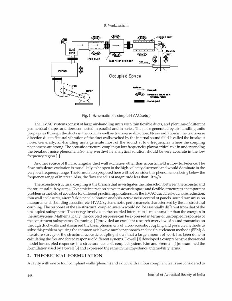
148 Journal of Acoustical Society of India
B. Venkatesham
Fig. 1. Schematic of a simple HVAC setup
The HVAC systems consist of large air-handling units with thin flexible ducts, and plenums of differentgeometrical shapes and sizes connected in parallel and in series. The noise generated by air-handling unitspropagates through the ducts in the axial as well as transverse direction. Noise radiation in the transversedirection due to flexural vibration of the duct walls excited by the internal sound field is called the breakoutnoise. Generally, air-handling units generate most of the sound at low frequencies where the couplingphenomena are strong. The acoustic-structural coupling at low frequencies plays a critical role in understandingthe breakout noise phenomena.So, any worthwhile analytical solution should be very accurate in the lowfrequency region [1].
Another source of thin rectangular duct wall excitation other than acoustic field is flow turbulence. Theflow turbulence excitation is most likely to happen in the high-velocity ductwork and would dominate in thevery low frequency range. The formulation proposed here will not consider this phenomenon, being below thefrequency range of interest. Also, the flow speed is of magnitude less than 10 m/s.
The acoustic-structural coupling is the branch that investigates the interaction between the acoustic andthe structural sub-systems. Dynamic interaction between acoustic space and flexible structure is an importantproblem in the field of acoustics for different practical applications like the HVAC duct breakout noise reduction,thin wall enclosures, aircraft skin panel vibration analysis, active noise control of panels, sound transmissionmeasurement in building acoustics, etc. HVAC systems noise performance is characterized by the air-structuralcoupling. The response of the air-structural coupled system would not be essentially different from that of theuncoupled subsystems. The energy involved in the coupled interaction is much smaller than the energies inthe subsystems. Mathematically, the coupled response can be expressed in terms of uncoupled responses ofthe constituent subsystems. Cummings [2]provided an excellent research overview of sound transmissionthrough duct walls and discussed the basic phenomena of vibro-acoustic coupling and possible methods tosolve this problem by using the common axial wave number approach and the finite element methods (FEM).Aliterature survey of the structural-acoustic coupling shows that a large amount of work has been done incalculating the free and forced response of different systems. Dowell [3] developed a comprehensive theoreticalmodel for coupled responses in a structural-acoustic coupled system. Kim and Brennan [4]re-examined theformulation used by Dowell [3] and expressed the same in the impedance and mobility terms.
2. THEORETICAL FORMULATION
A cavity with one or four compliant walls (plenum) and a duct with all four compliant walls are considered to
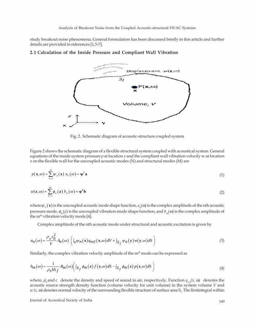
Analysis of Breakout Noise from the Coupled Acoustic-structural HVAC Systems
149Journal of Acoustical Society of India
study breakout noise phenomena. General formulation has been discussed briefly in this article and furtherdetails are provided in references [1,5-7].
2.1 Calculation of the Inside Pressure and Compliant Wall Vibration
Fig. 2. Schematic diagram of acoustic-structure coupled system
Figure 2 shows the schematic diagram of a flexible structural system coupled with acoustical system. Generalequations of the inside system pressure p at location x and the compliant wall vibration velocity w at locationz on the flexible wall for the uncoupled acoustic modes (N) and structural modes (M) are
( ) ( ) ( )N
Tn n
n 1p , aω ψ ω
=
= =∑x x ψ a (1)
( ) ( )M
m mm 1
w( , ) bω φ ω=
= =∑ Tz z φ b (2)
where ( )nψ x is the uncoupled acoustic mode shape function, an(ω) is the complex amplitude of the nth acousticpressure mode, φm(z) is the uncoupled vibration mode shape function, and bm(ω) is the complex amplitude ofthe mth vibration velocity mode [4].
Complex amplitude of the nth acoustic mode under structural and acoustic excitation is given by
( ) ( ) ( ) ( ) ( ) ( )020 , ,
ρω ω ψ ω ψ ω⎛ ⎞= +∫ ∫⎜ ⎟
⎝ ⎠f
ca A q dV w dSn n n vol nv SV
x x y y (3)
Similarly, the complex vibration velocity amplitude of the mth mode can be expressed as
( ) ( ) ( ) ( ) ( ) ( )1 , ,ω ω φ ω φ ωρ
⎛ ⎞= −∫ ∫⎜ ⎟⎝ ⎠f f
b B f dS p dSm m m mS ShSs fz z z z (4)
where, ρ0 and c denote the density and speed of sound in air, respectively. Function qνol(x, ω) denotes theacoustic source strength density function (volume velocity for unit volume) in the system volume V andw (z, ω) denotes normal velocity of the surrounding flexible structure of surface area Sf. The firstintegral within
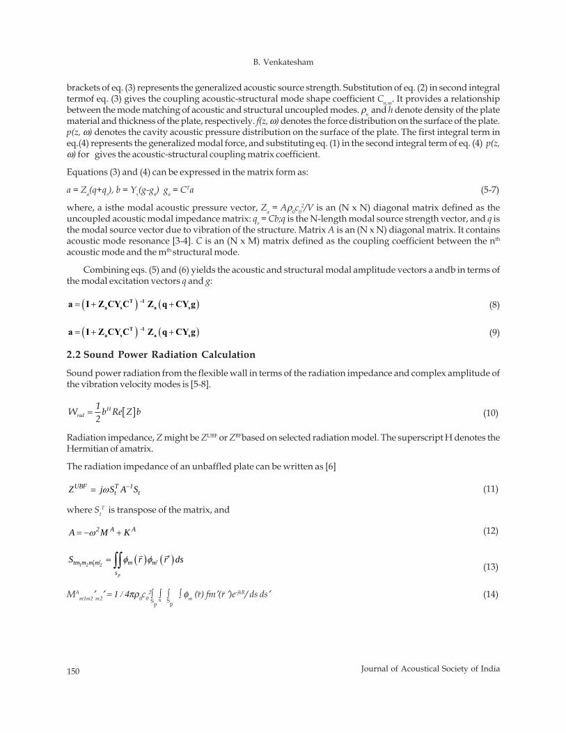
150 Journal of Acoustical Society of India
B. Venkatesham
brackets of eq. (3) represents the generalized acoustic source strength. Substitution of eq. (2) in second integraltermof eq. (3) gives the coupling acoustic-structural mode shape coefficient Cn,m. It provides a relationshipbetween the mode matching of acoustic and structural uncoupled modes. ρs and h denote density of the platematerial and thickness of the plate, respectively. f(z, ω) denotes the force distribution on the surface of the plate.p(z, ω) denotes the cavity acoustic pressure distribution on the surface of the plate. The first integral term ineq.(4) represents the generalized modal force, and substituting eq. (1) in the second integral term of eq. (4) p(z,ω) for gives the acoustic-structural coupling matrix coefficient.
Equations (3) and (4) can be expressed in the matrix form as:
a = Za(q+qs), b = Ys(g-ga) ga = CTa (5-7)
where, a isthe modal acoustic pressure vector, Za = Aρ0c02/V is an (N x N) diagonal matrix defined as the
uncoupled acoustic modal impedance matrix: qs = Cb;q is the N-length modal source strength vector, and q isthe modal source vector due to vibration of the structure. Matrix A is an (N x N) diagonal matrix. It containsacoustic mode resonance [3-4]. C is an (N x M) matrix defined as the coupling coefficient between the nth
acoustic mode and the mth structural mode.
Combining eqs. (5) and (6) yields the acoustic and structural modal amplitude vectors a andb in terms ofthe modal excitation vectors q and g:
( ) ( ) = + +T -1a s a sa I Z CY C Z q CY g (8)
( ) ( ) = + +T -1a s a sa I Z CY C Z q CY g (9)
2.2 Sound Power Radiation Calculation
Sound power radiation from the flexible wall in terms of the radiation impedance and complex amplitude ofthe vibration velocity modes is [5-8].
[ ]Hrad
1W b Re Z b2
= (10)
Radiation impedance, Z might be ZUBF or ZBFbased on selected radiation model. The superscript H denotes theHermitian of amatrix.
The radiation impedance of an unbaffled plate can be written as [6]
ω −=UBF T 1t tZ j S A S (11)
where StT is transpose of the matrix, and
ω= − +2 A AA M K (12)
( ) ( )1 2 1 2
φ φ′ ′ ′ ′= ∫∫p
tm m m m m ms
S r r dsr r
(13)
MAm1m2′m2′ = 1 / 4πρ0c0
2∫ ∫ ∫ ∫ φm (r) fm′(r ′)e-jkR/ ds ds′ (14)Sp
x Sp
−−
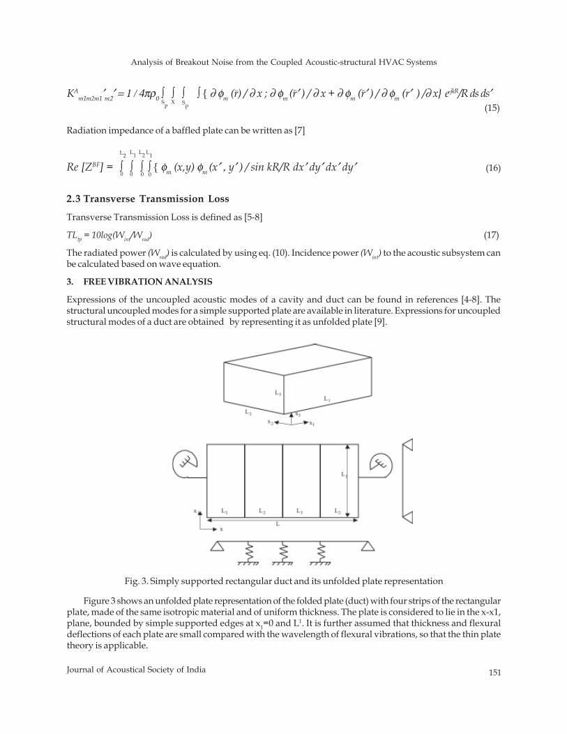
Analysis of Breakout Noise from the Coupled Acoustic-structural HVAC Systems
151Journal of Acoustical Society of India
Radiation impedance of a baffled plate can be written as [7]
Re [ZBF] = ∫ ∫ ∫ ∫ { φm (x,y) φm (x′ , y′ ) / sin kR/R dx′ dy′ dx′ dy′
2.3 Transverse Transmission Loss
Transverse Transmission Loss is defined as [5-8]
TLtp = 10log(Wint/Wrad) (17)
The radiated power (Wrad) is calculated by using eq. (10). Incidence power (Wint) to the acoustic subsystem canbe calculated based on wave equation.
3. FREE VIBRATION ANALYSIS
Expressions of the uncoupled acoustic modes of a cavity and duct can be found in references [4-8]. Thestructural uncoupled modes for a simple supported plate are available in literature. Expressions for uncoupledstructural modes of a duct are obtained by representing it as unfolded plate [9].
Figure 3 shows an unfolded plate representation of the folded plate (duct) with four strips of the rectangularplate, made of the same isotropic material and of uniform thickness. The plate is considered to lie in the x-x1,plane, bounded by simple supported edges at x1=0 and L1. It is further assumed that thickness and flexuraldeflections of each plate are small compared with the wavelength of flexural vibrations, so that the thin platetheory is applicable.
Sp
L2
X
− −−KAm1m2m1′m2′ = 1 / 4πρ0 ∫ ∫ ∫ ∫ { ∂ φm (r) / ∂ x ; ∂ φm (r′ ) / ∂ x + ∂ φm (r′ ) / ∂ φm (r′ ) /∂ x} e-jkR/R ds ds′
(15)
0 0
L1 L2 L1
0 0 (16)
Sp
Fig. 3. Simply supported rectangular duct and its unfolded plate representation
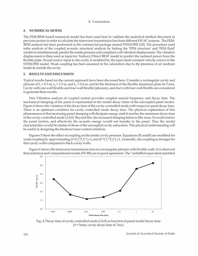
152 Journal of Acoustical Society of India
B. Venkatesham
4. NUMERICAL MODEL
The FEM-BEM based numerical model has been used here to validate the analytical method discussed inprevious section in order to calculate the transverse transmission loss from different HVAC systems. The FEM-BEM analysis has been performed in the commercial package named SYSNOISE [10]. The procedure usedinthe analysis of the coupled acoustic structural analysis by linking the 'FEM structure' and 'FEM fluid'models to simultaneously predict the inside pressure and compliant wall vibration displacement. The vibrationdisplacement is then used as input for 'Indirect/Direct BEM' model to predict the radiated power from theflexible plate. Sound source input to the cavity is modeled by the equivalent constant velocity source in theSYSNOISE model. Weak coupling has been assumed in the calculation due to the presence of air mediuminside & outside the cavity.
5. RESULTS AND DISCUSSION
Typical results based on the current approach have been discussed here. Consider a rectangular cavity andplenum of L1= 0.3 m, L2= 1.5 m, and L3 = 0.4 m, and let the thickness of the flexible aluminum plate be 5 mm.Cavity with one wall flexible and four wall flexible (plenum), and duct with four wall flexible are consideredto generate these results.
Free Vibration analysis of coupled system provides coupled natural frequency and decay time. Themechanical damping of the panel is represented in the modal decay times of the uncoupled panel modes.Figure 4 shows the variation of the decay time of the cavity-controlled mode with respect to panel decay time.There is an optimum condition for cavity controlled mode decay time. The physical explanation of thisphenomenon is that increasing panel damping will dissipate energy until it reaches the minimum decay timeof the cavity-controlled mode (1,0,0). Beyond this, the increased damping behaves like mass. It would restrictthe panel motion, and effectively the acoustic energy would not transfer to the panel. Thus the modalcharacteristics would be similar to those of the uncoupled cavity subsystem. This physical understanding willbe useful in designing the breakout noise control solutions.
Figures 5 show the effect of coupling on the inside cavity pressure. Equations (8) and(9) are modified forweak coupling by approximating (I+ZaCYsCT) ≅ I, and (I+YsCTZaC) ≅ I . Generally, the coupling is stronger forthin cavity walls compared to thick cavity walls.
Figure 6 shows the transverse transmission loss of a rectangular plenum with flexible walls. It is observedthat analytical and computational results (FE-BE) are in good agreement. The "unbaffled equivalent unfolded
Fig. 4. Decay time of cavity controlled mode (1,0,0) as function of panel modal decay time(h = 5mm, cavity decay time of 5sec)
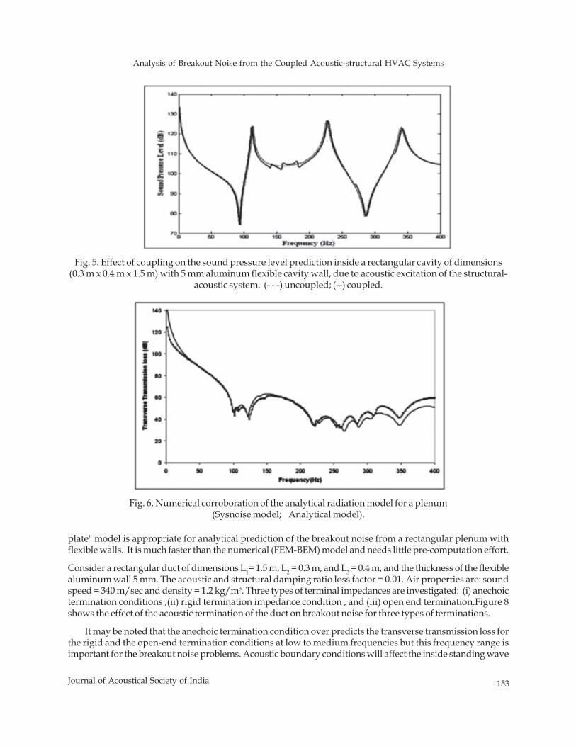
Analysis of Breakout Noise from the Coupled Acoustic-structural HVAC Systems
153Journal of Acoustical Society of India
plate" model is appropriate for analytical prediction of the breakout noise from a rectangular plenum withflexible walls. It is much faster than the numerical (FEM-BEM) model and needs little pre-computation effort.
Consider a rectangular duct of dimensions L1= 1.5 m, L2 = 0.3 m, and L3 = 0.4 m, and the thickness of the flexiblealuminum wall 5 mm. The acoustic and structural damping ratio loss factor = 0.01. Air properties are: soundspeed = 340 m/sec and density = 1.2 kg/m3. Three types of terminal impedances are investigated: (i) anechoictermination conditions ,(ii) rigid termination impedance condition , and (iii) open end termination.Figure 8shows the effect of the acoustic termination of the duct on breakout noise for three types of terminations.
It may be noted that the anechoic termination condition over predicts the transverse transmission loss forthe rigid and the open-end termination conditions at low to medium frequencies but this frequency range isimportant for the breakout noise problems. Acoustic boundary conditions will affect the inside standing wave
Fig. 5. Effect of coupling on the sound pressure level prediction inside a rectangular cavity of dimensions(0.3 m x 0.4 m x 1.5 m) with 5 mm aluminum flexible cavity wall, due to acoustic excitation of the structural-
acoustic system. (- - -) uncoupled; (--) coupled.
Fig. 6. Numerical corroboration of the analytical radiation model for a plenum(Sysnoise model; Analytical model).
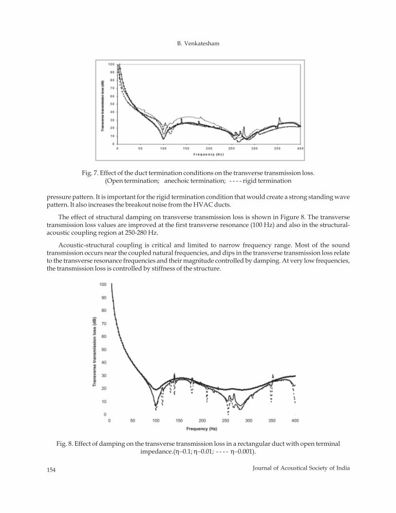
154 Journal of Acoustical Society of India
B. Venkatesham
pressure pattern. It is important for the rigid termination condition that would create a strong standing wavepattern. It also increases the breakout noise from the HVAC ducts.
The effect of structural damping on transverse transmission loss is shown in Figure 8. The transversetransmission loss values are improved at the first transverse resonance (100 Hz) and also in the structural-acoustic coupling region at 250-280 Hz.
Acoustic-structural coupling is critical and limited to narrow frequency range. Most of the soundtransmission occurs near the coupled natural frequencies, and dips in the transverse transmission loss relateto the transverse resonance frequencies and their magnitude controlled by damping. At very low frequencies,the transmission loss is controlled by stiffness of the structure.
Fig. 7. Effect of the duct termination conditions on the transverse transmission loss.(Open termination; anechoic termination; - - - - rigid termination
Fig. 8. Effect of damping on the transverse transmission loss in a rectangular duct with open terminalimpedance.(η−0.1; η−0.01; - - - - η−0.001).
Analysis of Breakout Noise from the Coupled Acoustic-structural HVAC Systems
155Journal of Acoustical Society of India
6. SUMMARY
A comprehensive theoretical model has been developed to calculate the breakout noise, based on the impedanceand mobility approach. A computationally efficient method is suggested to predict the sound power modelswith application to a cavity with one or four compliant walls and a duct with all four compliant walls. A newintuitive way has been provided to model the folded plate as "Equivalent plate model" in free vibration analysisand sound power radiation calculation.
It is worthwhile to extend the current approach to predict breakout noise from an acoustically linedrectangular duct and plenum chamber with compliant walls. Further studies are required to develop analyticalmodels in understanding the effect of stiffeners and damping (anti-drumming) on the duct breakout noise.
7. REFERENCES
[1] B. VENKATESHAM, 2008. Breakout Noise from the Coupled Acoustic-Structural HVAC Systems, PhDThesis.
[2] A. CUMMINGS, 2001. Sound transmission through duct walls, Journal of Sound and Vibration, 239 (4),731-765.
[3] E.H. DOWELL, G.F. GORMAN and D.A. SMITH, 1977. Acoustoelasticity: general theory, acoustic modesand forced response to sinusoidal excitation, including comparisons with experiment, Journal of Soundand Vibration, 52, 519-542.
[4] S.M. KIM and M.J. BRENNAN, 1999. A compact matrix formulation using the impedance and mobilityapproach for the analysis of structural-acoustic systems, Journal of Sound and Vibration, 223 (1), 97-113.
[5] B. VENKATESHAM, MAYANK TIWARI and M. L. MUNJAL, 2008. Analytical prediction of the breakoutnoise from a rectangular cavity with one compliant wall, Journal of the Acoustical Society of America, 124(5),2952-2962.
[6] B. VENKATESHAM, MAYANK TIWARI and M.L. MUNJAl, 2010. Analytical prediction of the breakoutnoise from a reactive rectangular plenum with four flexible walls, Journal of Acoustical Society of America.
[7] B. VENKATESHAM, MAYANK TIWARI and M.L. MUNJAL, 2011. Prediction of Breakout Noise from aRectangular Duct with Compliant Walls, International Journal of Acoustics and Vibration, 16 (4), 180-190.
[8] W.L. LI and H.J. GILBELING, 2000. Determination of the mutual radiation resistance of a rectangularplate and their impact on the radiated sound power, Journal of Sound and Vibration, 229.
[9] H. P. LEE, 1993. Natural frequencies and modes of cylindrical polygonal ducts, Journal of Sound andVibration, 164(1), 182-187.
[10] Sysnoise Rev. 5.6, User's Manual, LMS International, 2003.
156 Journal of Acoustical Society of India
N.K. Narayanan and T.M. Thasleema
Modeling and Recognition of Consonant-Vowel Unitsusing Statistical Learning Algorithms
N.K. Narayanan* and T.M. ThasleemaDepartment of Information Technology
Kannur University, Kannur-670 567 (Kerala)*e-mail: [email protected]
ABSTRACT
This paper investigates the use of statistical learning algorithms for the classification of MalayalamConsonant - Vowel (CV) utterances in speaker independent, noisy environments. The techniques weadopted here are k - Nearest Neighborhood (k - NN) and Support Vector Machine (SVMs) basedDecision Directed Acyclic Graph Support Vector Machine (DDAGSVM) classifiers. Three differentfeature extraction algorithms viz., Mel Frequency Cepstral Coefficients (MFCC), Normalized WaveletHybrid Feature (NWHF) and State Space Point Distribution (SSPD) parameter, are extracted toevaluate the performance of the above two classifiers. From the experimental results it is found thatthe DDAGSVM classifier is performing well compared with k-NN in additive noisy condition.
1. INTRODUCTION
In the past few decades, significant progress has been made by researchers in the area of speech and languageprocessing. In various traditional pattern recognition approaches, the statistical approach has been extensivelystudied and used in practice. More recently methods imported from statistical learning theory have beenreceiving increasing attention [1]. In the present work we are discussing two statistical pattern classifiersnamely k - Nearest Neighborhood (k - NN) and Support Vector Machine (SVM) to classify Malayalam CVspeech unit database.
The present research work is motivated by the knowledge that a little attempts were rendered for theautomatic speech recognition of CV speech unit in Indian languages like Hindi, Tamil, Bengali, Marathi etc.But very less works have been found to be reported in the literature on Malayalam CV speech unit recognition,which is the principal language of South Indian state of Kerala. Very few research attempts were reported sofar in the area of Malayalam vowel recognition. So more basic research works are essential in the area ofMalayalam CV speech unit recognition.
Malayalam is one of the major languages from Dravidian language family. Other major languages includeKannada, Tamil, Telugu, Tulu and Konkani. Malayalam is the principal language of the South Indian state ofKerala and also of the Lakshadweep Islands off the west coast of India spoken by about 36 million people.Malayalam language now contains 51 V/CV units includes 15 long and short vowel sounds and the remaining36 basic consonant sounds.
In the present work, all the experiments are carried out using 36 Malayalam CV speech unit databaseuttered by 96 different speakers. For the recognition experiments, database is divided into five different phoneticclasses based on the manner of articulation of the consonants which are given in Table 1.
Journal of Acoustical Society of India : Vol. 40, No. 3, 2013 (pp.156-164)
[Received: 16.04.2013; Revised: 29.05.2013; Accepted: 08.06.2013]
© 2013 Acoustical Society of India
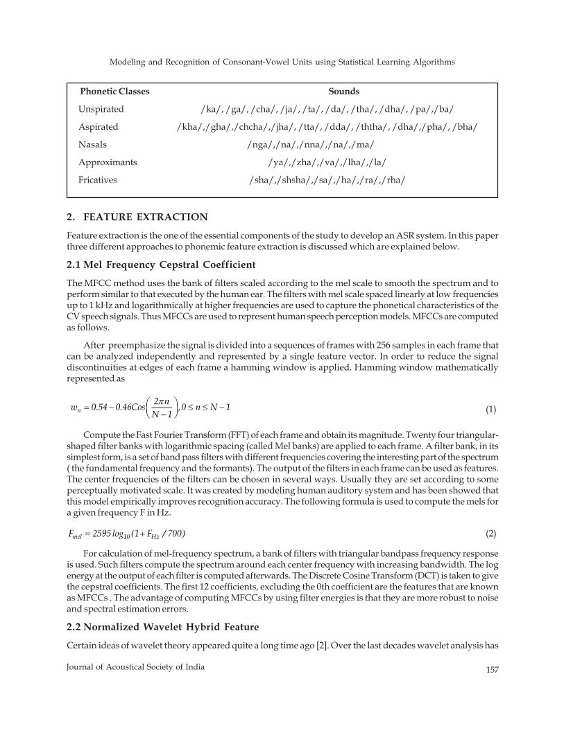
Modeling and Recognition of Consonant-Vowel Units using Statistical Learning Algorithms
157Journal of Acoustical Society of India
2. FEATURE EXTRACTION
Feature extraction is the one of the essential components of the study to develop an ASR system. In this paperthree different approaches to phonemic feature extraction is discussed which are explained below.
2.1 Mel Frequency Cepstral Coefficient
The MFCC method uses the bank of filters scaled according to the mel scale to smooth the spectrum and toperform similar to that executed by the human ear. The filters with mel scale spaced linearly at low frequenciesup to 1 kHz and logarithmically at higher frequencies are used to capture the phonetical characteristics of theCV speech signals. Thus MFCCs are used to represent human speech perception models. MFCCs are computedas follows.
After preemphasize the signal is divided into a sequences of frames with 256 samples in each frame thatcan be analyzed independently and represented by a single feature vector. In order to reduce the signaldiscontinuities at edges of each frame a hamming window is applied. Hamming window mathematicallyrepresented as
n2 nw 0.54 0.46Cos ,0 n N 1N 1π⎛ ⎞= − ≤ ≤ −⎜ ⎟−⎝ ⎠
(1)
Compute the Fast Fourier Transform (FFT) of each frame and obtain its magnitude. Twenty four triangular-shaped filter banks with logarithmic spacing (called Mel banks) are applied to each frame. A filter bank, in itssimplest form, is a set of band pass filters with different frequencies covering the interesting part of the spectrum( the fundamental frequency and the formants). The output of the filters in each frame can be used as features.The center frequencies of the filters can be chosen in several ways. Usually they are set according to someperceptually motivated scale. It was created by modeling human auditory system and has been showed thatthis model empirically improves recognition accuracy. The following formula is used to compute the mels fora given frequency F in Hz.
mel 10 HzF 2595 log (1 F / 700)= + (2)
For calculation of mel-frequency spectrum, a bank of filters with triangular bandpass frequency responseis used. Such filters compute the spectrum around each center frequency with increasing bandwidth. The logenergy at the output of each filter is computed afterwards. The Discrete Cosine Transform (DCT) is taken to givethe cepstral coefficients. The first 12 coefficients, excluding the 0th coefficient are the features that are knownas MFCCs . The advantage of computing MFCCs by using filter energies is that they are more robust to noiseand spectral estimation errors.
2.2 Normalized Wavelet Hybrid Feature
Certain ideas of wavelet theory appeared quite a long time ago [2]. Over the last decades wavelet analysis has
Phonetic Classes Sounds
Unspirated /ka/, /ga/, /cha/, /ja/, /ta/, /da/, /tha/, /dha/, /pa/,/ba/
Aspirated /kha/,/gha/,/chcha/,/jha/, /tta/, /dda/, /ththa/, /dha/,/pha/, /bha/
Nasals /nga/,/na/,/nna/,/na/,/ma/
Approximants /ya/,/zha/,/va/,/lha/,/la/
Fricatives /sha/,/shsha/,/sa/,/ha/,/ra/,/rha/
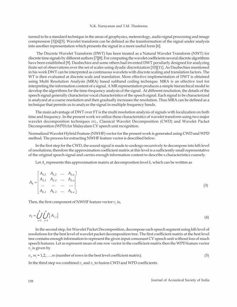
158 Journal of Acoustical Society of India
N.K. Narayanan and T.M. Thasleema
turned to be a standard technique in the areas of geophysics, meteorology, audio signal processing and imagecompression [3][4][5]. Wavelet transform can be defined as the transformation of the signal under analysisinto another representation which presents the signal in a more useful form [6].
The Discrete Wavelet Transform (DWT) has been treated as a Natural Wavelet Transform (NWT) fordiscrete time signals by different authors [7][8]. For computing the wavelet coefficients several discrete algorithmshave been established [9]. Daubechies and some others had invented DWT peculiarly designed for analyzingfinite set of observations over the set of scales using dyadic discretization [10][11]. As Daubechies mentionedin his work DWT can be interpreted as continuous wavelets with discrete scaling and translation factors. TheWT is then evaluated at discrete scale and translation. More effective implementation of DWT is obtainedusing Multi Resolution Analysis (MRA) based subband coding technique. MRA is an effective tool forinterpreting the information content of a signal. A MR representation produces a simple hierarchical model todevelop the algorithms for the time-frequency analysis of the signal. At different resolution, the details of thespeech signal generally characterize vocal characteristics of the speech signal. Each signal to be characterizedis analyzed at a coarse resolution and then gradually increases the resolution. Thus MRA can be defined as atechnique that permits us to analyze the signal in multiple frequency bands.
The main advantage of DWT over FT is the multi resolution analysis of signals with localization on bothtime and frequency. In the present work we utilize these characteristics of wavelet transform using two majorwavelet decomposition techniques viz., Classical Wavelet Decomposition (CWD) and Wavelet PacketDecomposition (WPD) for Malayalam CV speech unit recognition.
Normalized Wavelet Hybrid Feature (NWHF) vector for the present work is generated using CWD and WPDmethod. The process for extracting NWHF feature vector is described below.
In the first step for the CWD, the sound signal is made to undergo recursively to decompose into kth levelof resolutions; therefore the approximation coefficient matrix at this level is a sufficiently small representativeof the original speech signal and carries enough information content to describe s characteristics coarsely.
Let Ak represents this approximation matrix at decomposition level k, which can be written as
1,1 1,2 1,n
2,1 2,2 2,nk
k ,1 k ,2 k ,n
A A .... AA A .... A
A... ... .... ....
A A .... A
⎡ ⎤⎢ ⎥⎢ ⎥=⎢ ⎥⎢ ⎥⎣ ⎦
(3)
Then, the first component of NWHF feature vector v1 is,
{ }k n
1 i , ji 1 j 1
v A= =
=U U (4)
In the second step, for Wavelet Packet Decomposition, decompose each speech segment using kth level ofresolutions for the best level of wavelet packet decomposition tree. The first coefficient matrix at the best leveltree contains enough information to represent the given input consonant CV speech unit without loss of muchspeech features. Let m represent mean of one row vector in the coefficient matrix then the WPD feature vectorv2 is given by
v2, mi = 1,2,…..m (number of rows in the best level coefficient matrix). (5)
In the third step we combined v1 and v2 to fusion CWD and WPD coefficients.
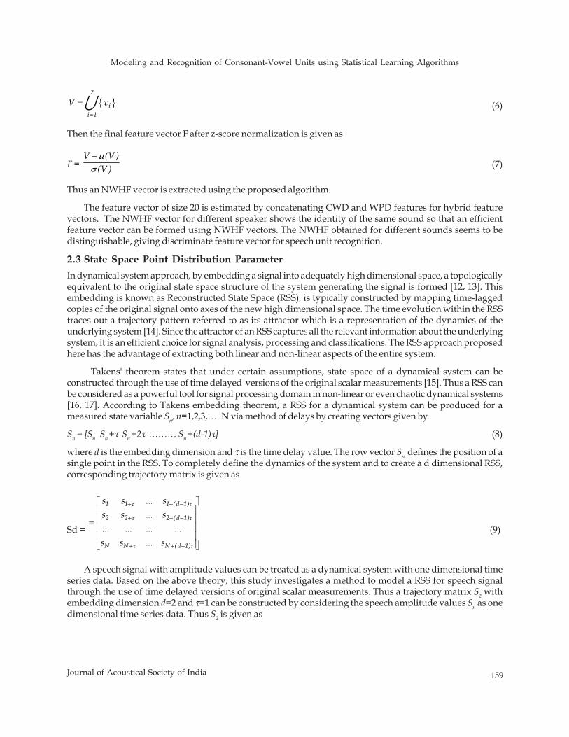
Modeling and Recognition of Consonant-Vowel Units using Statistical Learning Algorithms
159Journal of Acoustical Society of India
In dynamical system approach, by embedding a signal into adequately high dimensional space, a topologicallyequivalent to the original state space structure of the system generating the signal is formed [12, 13]. Thisembedding is known as Reconstructed State Space (RSS), is typically constructed by mapping time-laggedcopies of the original signal onto axes of the new high dimensional space. The time evolution within the RSStraces out a trajectory pattern referred to as its attractor which is a representation of the dynamics of theunderlying system [14]. Since the attractor of an RSS captures all the relevant information about the underlyingsystem, it is an efficient choice for signal analysis, processing and classifications. The RSS approach proposedhere has the advantage of extracting both linear and non-linear aspects of the entire system.
Takens' theorem states that under certain assumptions, state space of a dynamical system can beconstructed through the use of time delayed versions of the original scalar measurements [15]. Thus a RSS canbe considered as a powerful tool for signal processing domain in non-linear or even chaotic dynamical systems[16, 17]. According to Takens embedding theorem, a RSS for a dynamical system can be produced for ameasured state variable Sn, n=1,2,3,…..N via method of delays by creating vectors given by
Sn = [Sn Sn +τ Sn +2τ ……… Sn +(d-1)τ] (8)
where d is the embedding dimension and τ is the time delay value. The row vector Sn defines the position of asingle point in the RSS. To completely define the dynamics of the system and to create a d dimensional RSS,corresponding trajectory matrix is given as
Sd =
1 1 1 ( d 1)
2 2 2 ( d 1)
N N N ( d 1)
s s ... ss s ... s... ... ... ...s s ... s
τ τ
τ τ
τ τ
+ + −
+ + −
+ + −
⎡ ⎤⎢ ⎥⎢ ⎥=⎢ ⎥⎢ ⎥⎢ ⎥⎣ ⎦
(9)
A speech signal with amplitude values can be treated as a dynamical system with one dimensional timeseries data. Based on the above theory, this study investigates a method to model a RSS for speech signalthrough the use of time delayed versions of original scalar measurements. Thus a trajectory matrix S2 withembedding dimension d=2 and τ=1 can be constructed by considering the speech amplitude values Sn as onedimensional time series data. Thus S2 is given as
{ }2
ii 1
V v=
=U (6)
Then the final feature vector F after z-score normalization is given as
F = V (V )
(V )μ
σ−
(7)
Thus an NWHF vector is extracted using the proposed algorithm.
The feature vector of size 20 is estimated by concatenating CWD and WPD features for hybrid featurevectors. The NWHF vector for different speaker shows the identity of the same sound so that an efficientfeature vector can be formed using NWHF vectors. The NWHF obtained for different sounds seems to bedistinguishable, giving discriminate feature vector for speech unit recognition.
2.3 State Space Point Distribution Parameter
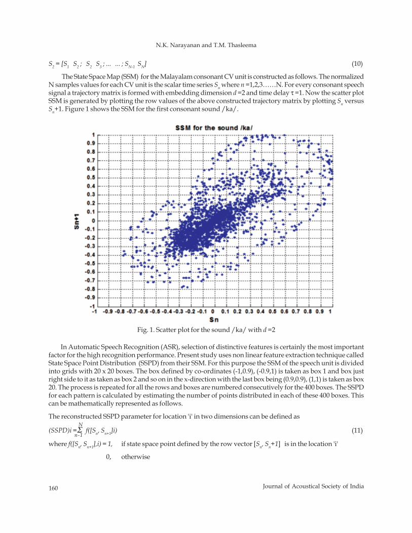
160 Journal of Acoustical Society of India
N.K. Narayanan and T.M. Thasleema
(10)
The State Space Map (SSM) for the Malayalam consonant CV unit is constructed as follows. The normalizedN samples values for each CV unit is the scalar time series Sn where n =1,2,3……N. For every consonant speechsignal a trajectory matrix is formed with embedding dimension d =2 and time delay τ =1. Now the scatter plotSSM is generated by plotting the row values of the above constructed trajectory matrix by plotting Sn versusSn+1. Figure 1 shows the SSM for the first consonant sound /ka/.
N
n-1
S2 = [S1 S2 ; S2 S3 ; ... ... ; SN-1 SN]
In Automatic Speech Recognition (ASR), selection of distinctive features is certainly the most importantfactor for the high recognition performance. Present study uses non linear feature extraction technique calledState Space Point Distribution (SSPD) from their SSM. For this purpose the SSM of the speech unit is dividedinto grids with 20 x 20 boxes. The box defined by co-ordinates (-1,0.9), (-0.9,1) is taken as box 1 and box justright side to it as taken as box 2 and so on in the x-direction with the last box being (0.9,0.9), (1,1) is taken as box20. The process is repeated for all the rows and boxes are numbered consecutively for the 400 boxes. The SSPDfor each pattern is calculated by estimating the number of points distributed in each of these 400 boxes. Thiscan be mathematically represented as follows.
The reconstructed SSPD parameter for location 'i' in two dimensions can be defined as
(SSPD)i =Σ f([Sn, Sn+1]i) (11)
where f([Sn, Sn+1],i) = 1, if state space point defined by the row vector [Sn, Sn+1] is in the location 'i'
0, otherwise
Fig. 1. Scatter plot for the sound /ka/ with d =2
Modeling and Recognition of Consonant-Vowel Units using Statistical Learning Algorithms
161Journal of Acoustical Society of India
Using this information the SSPD plot is plotted by taking the box number along x-axis and the number ofpoints in each box along y-axis. The SSPD plot for the first Malayalam CV sound /ka/ is given in Fig. 2.
The SSM and the corresponding SSPD plot obtained for different speaker shows the identity of the soundso that an efficient feature vector can be formed using SSPD. The feature vector of size 20 is estimated by takingthe average distribution of each row in the SSPD graph.
3. CLASSIFICATION
In the statistical learning approach, each pattern is represented in terms of a set of d features and can be viewedas a point in d dimensional feature space. The goal is to choose those features that allow pattern vectorsbelonging to different categories to occupy compact and disjoint regions in a d-dimensional feature space. Theeffectiveness of the representation space (feature set) is determined by how well patterns from different classescan be separated. Given a set of training patterns from each class, the objective is to establish decision boundariesin the feature space which separate patterns belonging to different classes. In the statistical decision theoreticapproach, the decision boundaries are determined by the probability distributions of the patterns belonging toeach class, which must either be specified or learned [18, 19].
3.1 k - Nearest Neighborhood
Pattern classification using distance function is an earliest concept in pattern recognition [20, 21]. Here theproximity of an unknown pattern to a class serves as a measure of its classifications. k - NN is a well knownnon - parametric classifier, where a posteriori probability is estimated from the frequency of the nearest neighborsof the unknown pattern [22]. For classifying each incoming pattern k - NN requires an appropriate value of k.A newly introduced pattern is then classified to the group where the majority of k nearest neighbor belongs[23]. Hand proposed an effective trial and error approach for identifying the value of k that incur highestrecognition accuracy [24]. Various pattern recognition studies with highest performance accuracy are alsoreported based on these classification techniques [25] .
Consider the cases of m classes ci, where i = 1,2,…….m, and a set of N samples pattern yi, i = 1,2,…..N whose
Fig. 2. SSPD plot for the sound /ka/
162 Journal of Acoustical Society of India
N.K. Narayanan and T.M. Thasleema
classification is priory known. Let x denote an arbitrary incoming pattern. The nearest neighbor classificationapproach classifies 'x' in the pattern class of its nearest neighbor in the set yi
i.e. If ⏐⏐ x-yj⏐⏐ 2 = min⏐⏐ x-y2⏐⏐2 1≤ i ≤ N then x in cj
This is 1 - NN rule since it employs only one nearest neighbor to x for classification. This can be extended byconsidering k - Nearest Neighbors to x and using a majority - rule type classifier.
3.2 Support Vector Machines
SVM is a linear algorithm with some specific properties. The basic principle of SVM in pattern recognitionapplication is to build an optimal separating hyperplane in such a way to separate two classes of pattern withmaximal margin [26]. SVM accomplish this desirable property based on the idea of Structural Risk Minimization(SRM) from statistical learning theory which shows that the error rate of a learning machine on test data (i.egeneralization error report ) is bounded by the sum of training error rate and the term that depending on theVapnik - Chervonenkis (VC) dimension of the learning system [27, 28]. By minimizing this upper bound highgeneralization performance can be obtained. For separable patterns SVM produces a value of 0 for first termand minimizes the second term. Furthermore, SVMs are quite different from other machine learning techniquesin generalization of errors which are not related to the input dimensionality of the problem, but to the marginwith which it separates data. This is the reason why SVMs can have good performance even in large numberof input problems [29] [30].
SVMs are mainly used for binary classifications. For combining the binary classification into multiclassclassification a relatively new learning architecture namely Decision Directed Acyclic Graph (DDAG) is used.For N class problem, the DDAG contains, one for each pair of classes. DDAGSVM works in a kernel inducedfeature space and uses two class maximal margin hyperplane at each decision node of the DDAG. TheDDAGSVM is considerably faster to train and evaluate comparable to other algorithms.
4. SIMULATION EXPERIMENTS AND RESULTS
All the simulation experiments are carried out using Malayalam CV speech unit database, uttered by 96different speakers. We used 8 kHz sampled speech signal which is low pass filtered to band limit to 4 kHz. Wedivide the dataset into training and test set which contains CV speech unit database, uttered by first 48speakers for training and next 48 for testing. Thus training and test set contains total of 1728 samples each. Themain objective of this article is to design a robust CV speech unit recognizer in additive noisy condition. Toperform this task each speech signal is corrupted by Additive White Gaussian Noise (AWGN) of differentSignal to Noise Ratio (SNR) levels. The recognition accuracies obtained for Malayalam CV speech database forthe five different phonetic classes at various SNR levels using MFCC, NWHF and SSPD parameters based onk-NN and DDAGSVM classifiers are tabulated in Tables 2-4, respectively.
Table 2. Recognition accuracies of 5 different phonetic classes using MFCC of different SNR values
Class Recognition Accuracy
k-NN DDAGSVM
0 dB 3 dB 10 dB 20 dB 30 dB Clean 0 dB 3 dB 10 dB 20 dB 30 dB Clean
Unaspirated 20.4 24.1 30.1 37.8 42.1 50.3 25.1 30.2 41.7 52.4 55.8 60.7Aspirated 22.5 26.9 32.5 36.1 43.7 51.8 28.6 31.6 43.2 54.2 58.1 62.2Nasals 26.9 30.2 37.3 39.2 45.9 54.8 30.7 33.8 45.9 57.1 61.5 64.9Approximant 21.6 28.7 35.9 38.1 44.4 53.9 29.2 32.6 43.2 52.5 58.3 63.4Fricatives 23.5 28.7 36.8 40.3 43.7 54.8 30.1 33.2 46.7 53.7 59.8 64.5
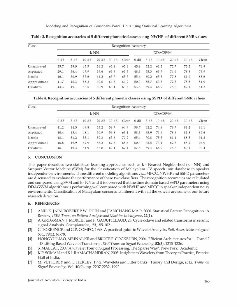
Modeling and Recognition of Consonant-Vowel Units using Statistical Learning Algorithms
163Journal of Acoustical Society of India
Class Recognition Accuracy
k-NN DDAGSVM
0 dB 3 dB 10 dB 20 dB 30 dB Clean 0 dB 3 dB 10 dB 20 dB 30 dB Clean
Unaspirated 25.7 28.9 45.5 56.2 62.4 62.6 45.8 52.2 61.2 72.7 75.2 76.8Aspirated 29.1 36.4 47.9 59.6 63.9 63.3 48.3 55.3 63.7 74.6 78.8 79.9Nasals 46.1 50.9 57.6 61.2 65.7 65.7 55.6 60.2 65.3 77.8 81.9 83.6Approximant 41.7 48.3 55.2 60.6 64.8 64.9 50.3 55.7 63.8 72.8 78.5 81.9Fricatives 43.3 49.1 56.5 60.9 63.1 63.5 53.6 59.4 66.9 78.6 82.1 84.2
Class Recognition Accuracy
k-NN DDAGSVM
0 dB 3 dB 10 dB 20 dB 30 dB Clean 0 dB 3 dB 10 dB 20 dB 30 dB Clean
Unaspirated 41.2 44.5 49.8 53.2 58.7 64.9 58.7 62.2 74.8 78.7 81.2 86.1Aspirated 40.4 43.4 48.1 50.9 56.8 63.1 58.3 65.9 71.9 78.6 81.8 85.6Nasals 48.1 51.2 53.1 59.3 63.6 70.2 65.4 70.8 75.3 81.4 88.5 94.2Approximant 46.8 49.9 52.9 58.2 62.8 68.5 60.3 65.5 73.4 82.8 88.2 93.9Fricatives 46.1 49.3 51.9 57.8 62.1 67.4 57.5 59.4 66.9 78.6 89.1 92.4
Table 3. Recognition accuracies of 5 different phonetic classes using NWHF of different SNR values
Table 4. Recognition accuracies of 5 different phonetic classes using SSPD of different SNR values
5. CONCLUSION
This paper describes two statistical learning approaches such as k - Nearest Neghborhod (k - NN) andSupport Vector Machine (SVM) for the classification of Malayalam CV speech unit database in speakerindependent environments. Three different modeling algorithms viz., MFCC, NWHF and SSPD parametersare discussed to evaluate the performance of these two classifiers. The recognition accuracies are calculatedand compared using SVM and k - NN and it is observed that the time domain based SSPD parameters usingDDAGSVM algorithms is performing well compared with NWHF and MFCC in speaker independent noisyenvironments. Classification of Malayalam consonants inherent with all the vowels are some of our futureresearch direction.
6. REFERENCES
[1] ANIL K. JAIN, ROBERT P.W. DUIN and JIANCHANG MAO, 2000. Statistical Pattern Recognition : AReview, IEEE Trans. on Pattern Analysis and Machine Intelligence, 22(1).
[2] A. GROSSMAN, J. MORLET and P. GAOUPILLAUD, 23. Cycle octave and related transforms in seismicsignal Analysis, Geoexploration, 23, 85-102.
[3] C. TORRENCE and G.P. COMPO, 1998. A practical guide to Wavelet Analysis, Bull. Amer. Meteorological.Soc., 79(1), 61-78.
[4] HONGYU LIAO, MRINAL KR and BRUCE F. COCKBURN, 2004. Efficient Architectures for 1 - D and 2- D Lifting Based Wavelet Transform, IEEE Trans. on Signal Processing, 52(5), 1315-1326.
[5] S. MALLAT, 2009.A wavelet Tour of Signal Processing, The Sparse Way", NewYork : Academic.[6] K.P. SOMAN and K.I. RAMACHANDRAN, 2005. Insight into Wavelets, from Theory to Practice, Prentice
Hall of India.[7] M. VETTERLY and C. HERLEY, 1992. Wavelets and Filter banks : Theory and Design, IEEE Trans. on
Signal Processing, Vol. 40(9), pp. 2207-2232, 1992.
164 Journal of Acoustical Society of India
N.K. Narayanan and T.M. Thasleema
[8] M.J. SHENSA, 1992. Affine Wavelets: Wedding the Atrous and mallat Algorithms, IEEE Trans. on SignalProcessing, 40, 2464-2482.
[9] S. MALLAT, 1989. Multi frequency Channel Decomposition of Images and Wavelet Models", IEEE.Trans on Acoustics, Speech and Signal Processing, 37, 2091-2110.
[10] I. DAUBECHIES, 1992. Ten Lectures on Wavelets, Philadelphia, PA: Soc. Appl. Math.[11] RONALD W. LINDSAY, DONALD B. PERCIVAL and D. ANDREW ROTHROCK, 1996. The Discrete
Wavelet Transform and the scale analysis of the surface properties of Sea Ice, IEEE Trans. on Geo Scienceand Remote Sensing, 34(3), 771-787.
[12] E. OTT, 1993. Chaos in Dynamical Systems, Cambridge University Press.[23] G. L. BAKER and J. GOLLUB, 1996. Chaotic Dynamics : An Introduction, Cambridge University Press.[14] MICHAEL T. JHONSON, RCHARD J. POVINALLi, ANDREW C. LINDGREN, JINJIN YE, XIAOLIN LIu
and Kevin Indrebo, 2005. Time Domain Isolated Phoneme Classification using Reconstructed PhaseSpace", IEEE Trans. On Speech and Audio Processing, 13(4), 458-466.
[15] F. TAKENS, 1980. Detecting Strange Attractors in Turbulence, in Proc. Dynamical Systems and Turbulence,Warwick, U.K., pp. 366-381.
[16] H. KANTZ and T. SCHREIBER, 1997. Non Linear Time Series Analysis, Cambridge University Press.[17] D. S. BROOMHEAD and G.P. KING, 1986. Extracting qualitative Dynamics from experimental data,
Physica D, pp. 217-236.[18] T.J. TOU and R.C. GONZALEZ, 1999. Pattern Recognition Principles, Addison - Wesley, London, 1974.[19] Friedmen M and Kandel A, Introduction to Pattern Recognition: Statistical, Structural, Neural and Fuzzy
Logic Approach, World Scientific.[20] T.M. COVER and P.E. HART, 1967. Nearest Neighbor Pattern Classification", IEEE trans. on Information
Theory, 13 (1), 21-27.[21] MIN-CHUN YU, 2011. Multi - Criteria ABC analysis using artificial - intelligence based classification
techniques, Elsevier - Expert Systems With Applications, 38, 3416-3421.[22] D.J. HAND, 1981. Discrimination and classification, NewYork, Wiley.[23] A.K. RAY and B. CHATTERJEE, 1984. Design of a Nearest Neighbor Classifier System for Bengali Character
Recognition, Journal of Inst. Elec. Telecom. Eng., 30, 226-229.[24] B. ZHANG and S.N. SRIHARi , 2004. Fast k - Nearest Neighbor using Cluster Based Trees, IEEE trans. on
Pattern Analysis and Machine Intelligence, 26(4), 525 - 528 .[25] F. PERNKOPF, 2005. Bayesian Network Classifiers versus selective k -NN Classifier, Pattern Recognition,
38, 1-10.[26] YING TAN and JUN WANG, 2004. A Support Vector Machine with a Hybrid Kernel and Minimal
Vapnik - Chervonenkins Dimension, IEEE Trans. On Knowledge and Data Engineering, 10(4) 385-395 .[27] VLADIMIR N. VAPNIK, 1999, An Overview of Statistical Learning Theory", IEEE Trans. On Neural Networks,
10(5), 988-999 .[28] RAVI GUPTA, ANKUSH MITTAL and KULDIP SINGH, 2008. A time Series based Feature Extraction
Approach for Prediction of Protein Structured Class, EURASIP Journal on Bioinformatics and SystemBiology.
[29] E. OSUNA, R. FREUND and F. GIROSI,1997. Training Support Vector Machines: An Application to FaceDetection, Proc. IEEE Conf.Computer Vision and Pattern Recognition, pp. 17-19.
[30] M. PONTIL and A. VERRI,1998. Support Vector Machines for 3D Object ecognition," IEEE Trans. PatternAnalysis and Machine Intelligence, 20 (6) 637-646.
Measurement of Acoustics in ISRO Launch Vehicle Missions
165Journal of Acoustical Society of India
ABSTRACT
1. INTRODUCTION
ISRO is in the process developing bigger launch vehicles to cater to future needs of heavier satellites in polarand GTO and re-entry missions. During the launch vehicle mission from lift off to satellite injection, thelaunch vehicle is subjected to acoustics and vibration fields. For a successful flight, it is important to ensurethat the acoustic levels are within design limits of the various subsystems .The acoustic environment issevere during liftoff and atmospheric phase of the flight. At liftoff, the violent and turbulent mixing of the hightemperature and high velocity exhaust of the jet with the surrounding air is the main cause of the acousticnoise. In the atmospheric flight the flight profile with the vehicle configuration determines the acousticenvironment.. The acoustic excitation induces broadband vibration responses of the vehicle structure and theget transmitted to the interior of the vehicle where sensitive assemblies are kept. The acoustic levels (SPL)normally encountered are of 120 to 170 dB during these regions.
During the development phase of the launch vehicle, large no of acoustic measurements are made tocharacterize the vehicle structure, deduce test levels for various subsystems and generate database forimprovements. A typical of 10-15 measurements are made during the development phase. A typical acousticmeasurement chain consists of an acoustic sensor, charge amplifier and digital signal processing unit.Acoustic sensor converts sound pressure level to electric charge. The common types are condenser type andMEMS based transducers. The dynamic range of these sensors are in the range of 100-180 dB SPL andbandwidth more than 10 KHz. They are rugged and operate over a wide temperature range. The chargeoutput from these sensors are converted to analog voltage using charge amplifiers and band limited to 8 KHzusing higher order switched capacitor filters. The overall telemetry available in a Launch vehicle is 2-4 Mbpsand each acoustic channel if transmitted as raw data would need 200 Kbps. Hence onboard signal processingis needed to reduced bit rate. The DSP based on board system is used to process these signal in real time andtransmit the information at reduced bandwidth. The frequency analysis is done in the 1/3 rd octave bandcovering a frequency range of 31.5 Hz to 8 KHz. The details of the sensors, interface electronics and the DSPbased processing system are explained below.
2. SENSORS
The condenser type and the MEMS type sensors are normally used in launch vehicles. Sensor 2510 from m/s Endevco was originally used in all measurements. Later it is replaced by indigenous MEMS acoustic sensorjointly developed by VSSC and CEERI ,Pilani. The endevco sensor uses Piezite as crystal material with anominal capacitance of 5000 pF .It is rugged and hermitically sealed construction and operates over a widetemperature range (up to 250deg.C).. The MEMS sensor is a bulk micro machined device, etched out of silicon
Journal of Acoustical Society of India : Vol. 40, No. 3, 2013 (pp. 165-169)
Measurement of Acoustics in ISRO Launch VehicleMissions
A.R. KrishnanAvionics Entity,VSSC, ISRO PO, Thiruvananthapuram-695 022 (Kerala)
[Received: 26.12.2012; Revised: 10.05.2013; Accepted: 15.05.2013]
© 2013 Acoustical Society of India
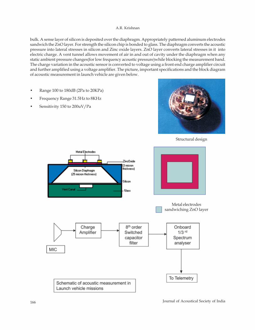
166 Journal of Acoustical Society of India
A.R. Krishnan
bulk. A sense layer of silicon is deposited over the diaphragm. Appropriately patterned aluminum electrodessandwich the ZnO layer. For strength the silicon chip is bonded to glass. The diaphragm converts the acousticpressure into lateral stresses in silicon and Zinc oxide layers. ZnO layer converts lateral stresses in it intoelectric charge. A vent tunnel allows movement of air in and out of cavity under the diaphragm when anystatic ambient pressure changes(for low frequency acoustic pressure)while blocking the measurement band.The charge variation in the acoustic sensor is converted to voltage using a front end charge amplifier circuitand further amplified using a voltage amplifier. The picture, important specifications and the block diagramof acoustic measurement in launch vehicle are given below.
• Range 100 to 180dB (2Pa to 20KPa)
• Frequency Range 31.5Hz to 8KHz
• Sensitivity 150 to 200uV/Pa
Structural design
Metal electrodessandwiching ZnO layer
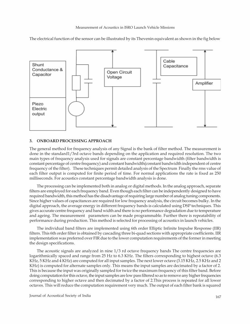
Measurement of Acoustics in ISRO Launch Vehicle Missions
167Journal of Acoustical Society of India
The electrical function of the sensor can be illustrated by its Thevenin equivalent as shown in the fig below
3. ONBOARD PROCESSING APPROACH
The general method for frequency analysis of any Signal is the bank of filter method. The measurement isdone in the standard1/3rd octave bands depending on the application and required resolution. The twomain types of frequency analysis used for signals are constant percentage bandwidth (filter bandwidth isconstant percentage of centre frequency) and constant bandwidth(constant bandwidth independent of centrefrequency of the filter). These techniques permit detailed analysis of the Spectrum Finally the rms value ofeach filter output is computed for finite period of time. For normal applications the rate is fixed as 250milliseconds. For acoustics constant percentage bandwidth analysis is done.
The processing can be implemented both in analog or digital methods. In the analog approach, separatefilters are employed for each frequency band. Even though each filter can be independently designed to haverequired bandwidth, this method has the disadvantage of requiring large number of analog tuning components.Since higher values of capacitances are required for low frequency analysis, the circuit becomes bulky. In thedigital approach, the average energy in different frequency bands is calculated using DSP techniques. Thisgives accurate centre frequency and band width and there is no performance degradation due to temperatureand ageing. The measurement parameters can be made programmable. Further there is repeatability ofperformance during production. This method is selected for processing of acoustics in launch vehicles.
The individual band filters are implemented using 6th order Elliptic Infinite Impulse Response (IIR)filters. This 6th order filter is obtained by cascading three bi-quad sections with appropriate coefficients. IIRimplementation was preferred over FIR due to the lower computation requirements of the former in meetingthe design specifications.
The acoustic signals are analyzed in nine 1/3 rd octave frequency bands The centre frequencies arelogarithmically spaced and range from 25 Hz to 6.3 KHz. The filters corresponding to highest octave (6.3KHz, 5 KHz and 4 KHz) are computed for all input samples. The next lower octave (3.15 KHz, 2.5 KHz and 2KHz) is computed for alternate samples only. This means the input samples are decimated by a factor of 2.This is because the input was originally sampled for twice the maximum frequency of this filter band. Beforedoing computation for this octave, the input samples are low pass filtered so as to remove any higher frequenciescorresponding to higher octave and then decimated by a factor of 2.This process is repeated for all loweroctaves. This will reduce the computation requirement very much. The output of each filter bank is squared
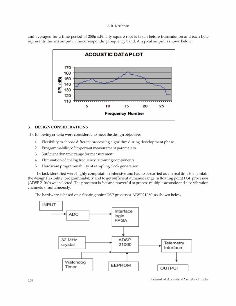
168 Journal of Acoustical Society of India
A.R. Krishnan
and averaged for a time period of 250ms.Finally square root is taken before transmission and each byterepresents the rms output in the corresponding frequency band. A typical output is shown below.
3. DESIGN CONSIDERATIONS
The following criteria were considered to meet the design objective:
1. Flexibility to choose different processing algorithm during development phase.2. Programmability of important measurement parameters.3. Sufficient dynamic range for measurement4. Elimination of analog frequency trimming components5. Hardware programmability of sampling clock generation
The task identified were highly computation intensive and had to be carried out in real time to maintainthe design flexibility, programmability and to get sufficient dynamic range, a floating point DSP processor(ADSP 21060) was selected. The processor is fast and powerful to process multiple acoustic and also vibrationchannels simultaneously.
The hardware is based on a floating point DSP processor ADSP21060 as shown below.
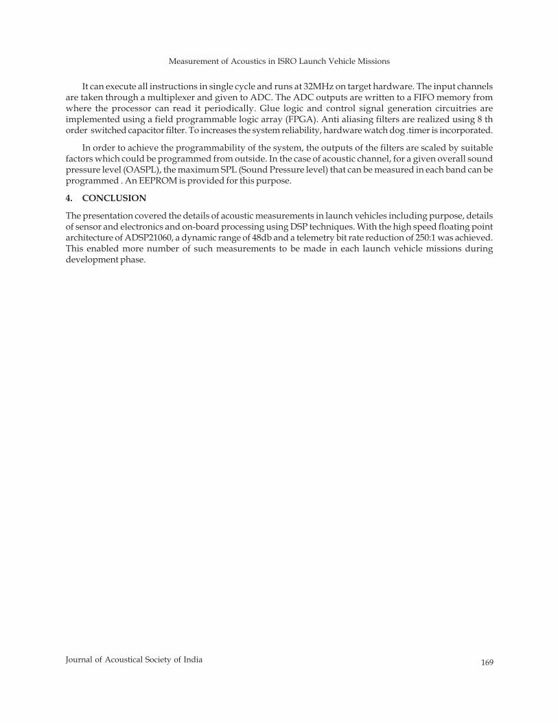
Measurement of Acoustics in ISRO Launch Vehicle Missions
169Journal of Acoustical Society of India
It can execute all instructions in single cycle and runs at 32MHz on target hardware. The input channelsare taken through a multiplexer and given to ADC. The ADC outputs are written to a FIFO memory fromwhere the processor can read it periodically. Glue logic and control signal generation circuitries areimplemented using a field programmable logic array (FPGA). Anti aliasing filters are realized using 8 thorder switched capacitor filter. To increases the system reliability, hardware watch dog .timer is incorporated.
In order to achieve the programmability of the system, the outputs of the filters are scaled by suitablefactors which could be programmed from outside. In the case of acoustic channel, for a given overall soundpressure level (OASPL), the maximum SPL (Sound Pressure level) that can be measured in each band can beprogrammed . An EEPROM is provided for this purpose.
4. CONCLUSION
The presentation covered the details of acoustic measurements in launch vehicles including purpose, detailsof sensor and electronics and on-board processing using DSP techniques. With the high speed floating pointarchitecture of ADSP21060, a dynamic range of 48db and a telemetry bit rate reduction of 250:1 was achieved.This enabled more number of such measurements to be made in each launch vehicle missions duringdevelopment phase.
170 Journal of Acoustical Society of India
T. Ramachandran and K.P. Padmanaban
ABSTRACT
There is a discrepancy in the established number of lexical tones in Manipuri, a tonal language, aswell as the terminology used to describe them. Hence, the present study attempts to describe thecharacteristics of lexical tones in Manipuri using acoustical analysis and it perception by nativespeakers. Monosyllable minimal pair words contrasting in tone were recorded from three nativespeakers of Manipuri language. Pitch values extracted for each word were used to identify differenttone contours based on the configuration of the pitch contour, initial pitch and final pitch. Resultsrevealed four pitch contours namely, level, falling, rising and falling-rising. In addition, individualdifferences were noticed in the configuration of pitch contours obtained for the same word acrossspeakers. However, for each speaker, each minimal word pair contrasting in tones were alwaysdistinguishable using pitch contour, initial pitch and final pitch of the pitch contour. The meaning ofall the words was identified correctly above chance level by four native speakers. It is possible thatnormalization of the lexical tones produced by different speakers was done by the listeners.
1. INTRODUCTION
Internal combustion (IC) engine produces intolerable vibrations during the operation, when the vibrationforces transferred to the supporting structures the reliability and the driving comfortness are much reduced.It is necessary to reduce the vibrations from the engine to the engine mounts to satisfy customer requirements.The vibration from the engine is due to the inertial and unbalanced forces of the reciprocating and rotatingcomponents in the engine. In this work a mathematical model will be developed to determine the engineinertial and unbalanced forces and the model will be solved using a computer program to determine thedisplacements and velocity at the engine supports.
Engine vibrations are caused due to the reciprocating and rotating masses of the engine. The variationsof inertial forces are due to the combustion and the compression differences of the piston cylinder arrangementduring their operation The engine inertial forces leads to the unbalanced forces of the engine and they arequiet varying with respect to speed, fuel supply and combustion characteristics of the fuel. Though thesupply and combustion of fuel is also the reasons of the vibration, they are not in the controllable sources forthe vibration. Because, they are the parameters decide the performance of an engine. To predict the vibrationoutput of an engine and to minimize the possible durability and consumer perceived quality problemsassociated with engine vibration, a robust and accurate design and simulation model is needed. Such modelshould execute quickly and requires relatively simple inputs.
Journal of Acoustical Society of India : Vol. 40, No. 3, 2013 (pp. 170-175)
Vibration Analysis of Internal Combustion Engine -Modeling and Optimization
T. Ramachandran* and K.P. PadmanabanPSNA College of Engineering & Technology, Dindigul-624 622SBM College of Engineering & Technology, Dindigul-624 005
*e-mail : [email protected]
[Received: 26.12.2012; Revised: 10.05.2013; Accepted: 15.05.2013]
© 2013 Acoustical Society of India
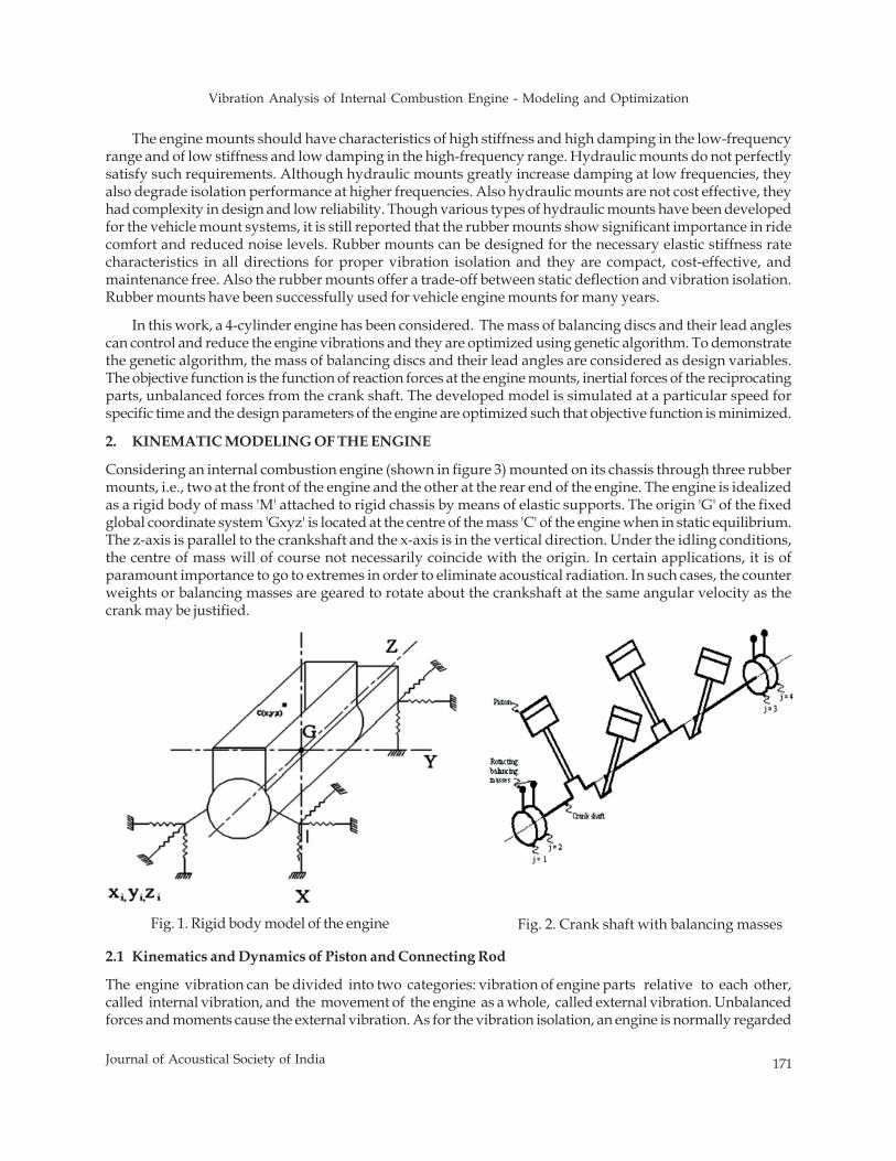
Vibration Analysis of Internal Combustion Engine - Modeling and Optimization
171Journal of Acoustical Society of India
The engine mounts should have characteristics of high stiffness and high damping in the low-frequencyrange and of low stiffness and low damping in the high-frequency range. Hydraulic mounts do not perfectlysatisfy such requirements. Although hydraulic mounts greatly increase damping at low frequencies, theyalso degrade isolation performance at higher frequencies. Also hydraulic mounts are not cost effective, theyhad complexity in design and low reliability. Though various types of hydraulic mounts have been developedfor the vehicle mount systems, it is still reported that the rubber mounts show significant importance in ridecomfort and reduced noise levels. Rubber mounts can be designed for the necessary elastic stiffness ratecharacteristics in all directions for proper vibration isolation and they are compact, cost-effective, andmaintenance free. Also the rubber mounts offer a trade-off between static deflection and vibration isolation.Rubber mounts have been successfully used for vehicle engine mounts for many years.
In this work, a 4-cylinder engine has been considered. The mass of balancing discs and their lead anglescan control and reduce the engine vibrations and they are optimized using genetic algorithm. To demonstratethe genetic algorithm, the mass of balancing discs and their lead angles are considered as design variables.The objective function is the function of reaction forces at the engine mounts, inertial forces of the reciprocatingparts, unbalanced forces from the crank shaft. The developed model is simulated at a particular speed forspecific time and the design parameters of the engine are optimized such that objective function is minimized.
2. KINEMATIC MODELING OF THE ENGINE
Considering an internal combustion engine (shown in figure 3) mounted on its chassis through three rubbermounts, i.e., two at the front of the engine and the other at the rear end of the engine. The engine is idealizedas a rigid body of mass 'M' attached to rigid chassis by means of elastic supports. The origin 'G' of the fixedglobal coordinate system 'Gxyz' is located at the centre of the mass 'C' of the engine when in static equilibrium.The z-axis is parallel to the crankshaft and the x-axis is in the vertical direction. Under the idling conditions,the centre of mass will of course not necessarily coincide with the origin. In certain applications, it is ofparamount importance to go to extremes in order to eliminate acoustical radiation. In such cases, the counterweights or balancing masses are geared to rotate about the crankshaft at the same angular velocity as thecrank may be justified.
Fig. 2. Crank shaft with balancing massesFig. 1. Rigid body model of the engine
2.1 Kinematics and Dynamics of Piston and Connecting Rod
The engine vibration can be divided into two categories: vibration of engine parts relative to each other,called internal vibration, and the movement of the engine as a whole, called external vibration. Unbalancedforces and moments cause the external vibration. As for the vibration isolation, an engine is normally regarded
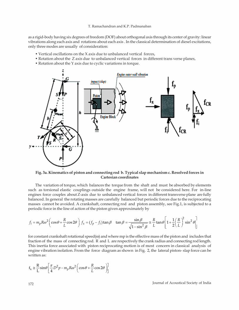
172 Journal of Acoustical Society of India
T. Ramachandran and K.P. Padmanaban
as a rigid-body having six degrees of freedom (DOF) about orthogonal axis through its center of gravity: linearvibrations along each axis and rotations about each axis . In the classical determination of diesel excitations,only three modes are usually of consideration:
• Vertical oscillations on the X axis due to unbalanced vertical forces,• Rotation about the Z axis due to unbalanced vertical forces in different trans verse planes,• Rotation about the Y axis due to cyclic variations in torque.
The variation of torque, which balances the torque from the shaft and must be absorbed by elementssuch as torsional elastic couplings outside the engine frame, will not be considered here. For in-lineengines force couples about Z-axis due to unbalanced vertical forces in different transverse plane are fullybalanced. In general the rotating masses are carefully balanced but periodic forces due to the reciprocatingmasses cannot be avoided. A crankshaft, connecting rod and piston assembly, see Fig.1, is subjected to aperiodic force in the line of action of the piston given approximately by
22 2
2sin 1cos cos 2 ( ) tan tan tan 1 sin
21 sini p x p i
R R Rf m R f f fL L L
βω θ θ β β θ θ
β
⎡ ⎤⎛ ⎞ ⎛ ⎞= + = − = ≅ +⎢ ⎥⎜ ⎟ ⎜ ⎟⎝ ⎠ ⎝ ⎠⎢ ⎥− ⎣ ⎦
for constant crankshaft rotational speed(ω) and where mp is the effective mass of the piston and includes thatfraction of the mass of connecting rod. R and L are respectively the crank radius and connecting rod length.This inertia force associated with piston reciprocating motion is of most concern in classical analysis ofengine vibration isolation. From the force diagram as shown in Fig. 2, the lateral piston- slap force can bewritten as:
2 2x
Rf sin cos cos 2 L 4 p
RD p m RL
πθ ω θ θ⎡ ⎤⎛ ⎞≅ − +⎜ ⎟⎢ ⎥⎝ ⎠⎣ ⎦
Fig. 3a. Kinematics of piston and connecting rod b. Typical slap mechanism c. Resolved forces inCartesian coordinates
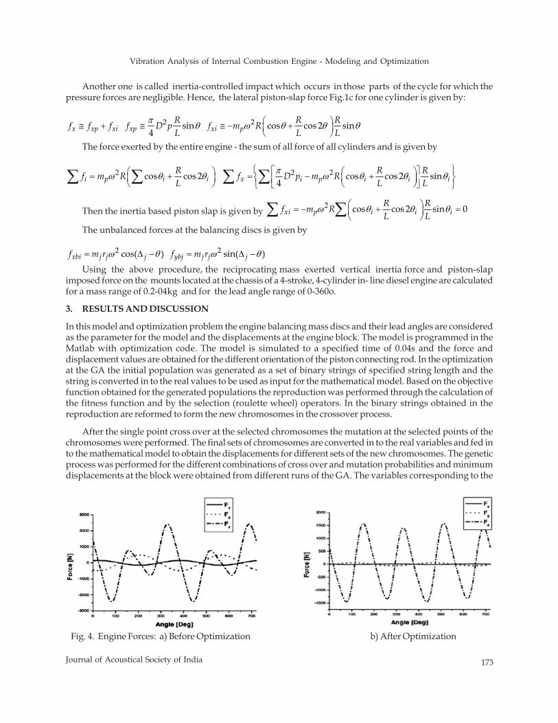
Vibration Analysis of Internal Combustion Engine - Modeling and Optimization
173Journal of Acoustical Society of India
Another one is called inertia-controlled impact which occurs in those parts of the cycle for which thepressure forces are negligible. Hence, the lateral piston-slap force Fig.1c for one cylinder is given by:
2 2 sin cos cos 2 sin4x xp xi xp xi p
R R Rf f f f D p f m RL L L
π θ ω θ θ θ⎛ ⎞≅ + ≅ ≅ − +⎜ ⎟⎝ ⎠
The force exerted by the entire engine - the sum of all force of all cylinders and is given by
2 2 2cos cos 2 cos cos 2 sin4i p i i x i p i i i
R R Rf m R f D p m RL L L
πω θ θ ω θ θ θ⎧ ⎫⎡ ⎤⎛ ⎞ ⎛ ⎞= + = − +⎨ ⎬⎜ ⎟ ⎜ ⎟⎢ ⎥⎝ ⎠ ⎝ ⎠⎣ ⎦⎩ ⎭
∑ ∑ ∑ ∑
Then the inertia based piston slap is given by 2 cos cos 2 sin 0xi p i i i
R Rf m RL L
ω θ θ θ⎛ ⎞= − + =⎜ ⎟⎝ ⎠∑ ∑
The unbalanced forces at the balancing discs is given by
2 2cos( ) sin( )xbi j j j ybj j j jf m r f m rω θ ω θ= Δ − = Δ −
Using the above procedure, the reciprocating mass exerted vertical inertia force and piston-slapimposed force on the mounts located at the chassis of a 4-stroke, 4-cylinder in- line diesel engine are calculatedfor a mass range of 0.2-04kg and for the lead angle range of 0-360o.
3. RESULTS AND DISCUSSION
In this model and optimization problem the engine balancing mass discs and their lead angles are consideredas the parameter for the model and the displacements at the engine block. The model is programmed in theMatlab with optimization code. The model is simulated to a specified time of 0.04s and the force anddisplacement values are obtained for the different orientation of the piston connecting rod. In the optimizationat the GA the initial population was generated as a set of binary strings of specified string length and thestring is converted in to the real values to be used as input for the mathematical model. Based on the objectivefunction obtained for the generated populations the reproduction was performed through the calculation ofthe fitness function and by the selection (roulette wheel) operators. In the binary strings obtained in thereproduction are reformed to form the new chromosomes in the crossover process.
After the single point cross over at the selected chromosomes the mutation at the selected points of thechromosomes were performed. The final sets of chromosomes are converted in to the real variables and fed into the mathematical model to obtain the displacements for different sets of the new chromosomes. The geneticprocess was performed for the different combinations of cross over and mutation probabilities and minimumdisplacements at the block were obtained from different runs of the GA. The variables corresponding to the
Fig. 4. Engine Forces: a) Before Optimization b) After Optimization
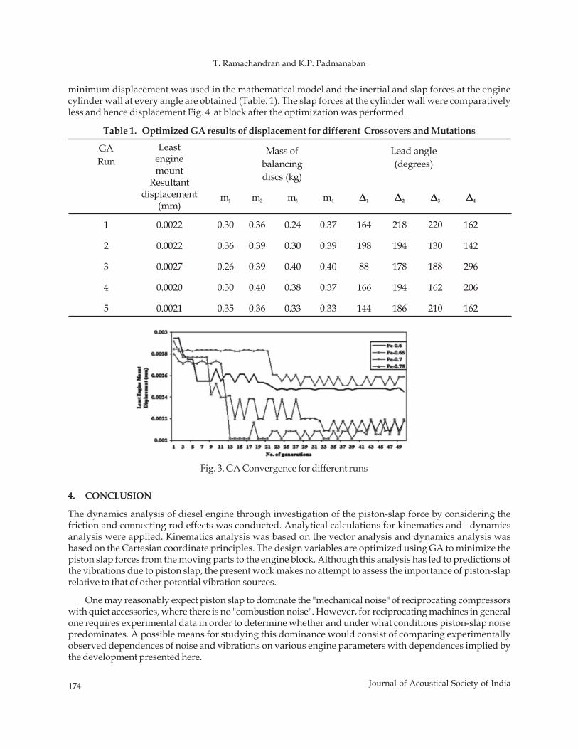
174 Journal of Acoustical Society of India
T. Ramachandran and K.P. Padmanaban
minimum displacement was used in the mathematical model and the inertial and slap forces at the enginecylinder wall at every angle are obtained (Table. 1). The slap forces at the cylinder wall were comparativelyless and hence displacement Fig. 4 at block after the optimization was performed.
GA Run
Leastenginemount
Resultant displacement
(mm)
Mass of balancingdiscs (kg)
Lead angle(degrees)
m1 m2 m3 m4 Δ1 Δ2 Δ3 Δ4
1 0.0022 0.30 0.36 0.24 0.37 164 218 220 162
2 0.0022 0.36 0.39 0.30 0.39 198 194 130 142
3 0.0027 0.26 0.39 0.40 0.40 88 178 188 296
4 0.0020 0.30 0.40 0.38 0.37 166 194 162 206
5 0.0021 0.35 0.36 0.33 0.33 144 186 210 162
Table 1. Optimized GA results of displacement for different Crossovers and Mutations
4. CONCLUSION
The dynamics analysis of diesel engine through investigation of the piston-slap force by considering thefriction and connecting rod effects was conducted. Analytical calculations for kinematics and dynamicsanalysis were applied. Kinematics analysis was based on the vector analysis and dynamics analysis wasbased on the Cartesian coordinate principles. The design variables are optimized using GA to minimize thepiston slap forces from the moving parts to the engine block. Although this analysis has led to predictions ofthe vibrations due to piston slap, the present work makes no attempt to assess the importance of piston-slaprelative to that of other potential vibration sources.
One may reasonably expect piston slap to dominate the "mechanical noise" of reciprocating compressorswith quiet accessories, where there is no "combustion noise". However, for reciprocating machines in generalone requires experimental data in order to determine whether and under what conditions piston-slap noisepredominates. A possible means for studying this dominance would consist of comparing experimentallyobserved dependences of noise and vibrations on various engine parameters with dependences implied bythe development presented here.
Fig. 3. GA Convergence for different runs
Vibration Analysis of Internal Combustion Engine - Modeling and Optimization
175Journal of Acoustical Society of India
However, it must be pointed out that the present analysis is not entirely complete, and that it may fail toconsider some parameters conceivably of considerable importance. The most important likely discrepancybetween the present analysis and reality is associated with the tacit assumptions that were made that allforces acting on the piston act through its center of gravity, and that the wrist-pin centerline passes throughthis center of gravity. Thus, rotation or cocking of the piston during its travel across the clearance space hasbeen neglected, although such rotations may have possibly marked effects on the character as well as on theseverity of the piston-slap impacts. Other shortcomings may be associated with the neglect of piston-ringfriction, of oil film cushioning, of angular accelerations of the crankshaft, of clearances at the crankshaftbearings, and of clearances and friction torques at the wrist-pin and crank-pin. However, one may entertainthe reasonable hope that these omissions are of minor importance.
5. REFERENCES
[1] ZHENG-DONG MA and NOEL C. PERKINS, 2003“An efficient multibody dynamics model for internalcombustion engine systems”, Multibody System Dynamics 10, 363-391.
[2] S. RAJENDRAN and M.V. NARASIMHAN, 1997”Effect of inertia variation due to reciprocating partsand connecting rod on coupled free vibration of crank shaft”. ASME Journal of Engineering for GasTurbine and power vol 19, 257-263.
[3] A.R. OHADI and G. MAGHSOODI, 2007“Simulation of engine vibration on non-linear hydraulic enginemounts”, ASME Journal of Vibrations and Acoustics 129, 417-42.
[4] CHUNG-HA SUH and CLIFFORD G. SMITH,”Dynamic simulation of engine mount system”. SAEPaper#971940.
[5] TETSURO BUTSUEN and MASAAKI OOKUMA, Akio Nagamatsu,”Application of direct systemidentification method for engine rigid body mount system”, SAE Paper#860551.
[6] SUDHIR KAUL, K. ANOOP DHINGRA and G. TIMOTHY HUNTER, 2007”Frame flexibility effects onengine mount optimization for vibration isolation in motor cycle”, ASME Journal of Vibrations and Acoustics129, 590-600.
[7] P. CONTI and J. BRETL, 1989“Mount stiffness and inertia properties from modal test data”, ASMEJournal of Vibrations and Acoustics-Stress and Reliability in Design 111, 134-141.
[8] J.A. SNYMAN, 1983“An improved version of the original leap frog dynamic method for unconstrainedminimization : LFOPI “, Appl. Math. Modelling 7, 216-218.
[9] NICCOLO BALDANZINI, DAVIDE CARPRIOLI and MARCO PIERINI, 2001“Designing the dynamicbehaviour of an engine suspesion system through genetic algorithm”, ASME Journal of Vibrations andAcoustics 123,480-486.
[10] E. JAMES BERNARD and M. JOHN STARKEY , “Engine mount optimization”, SAE#830257.[11] Tsuneo Tanaka, Mitsuo Iwahara, Tetsuya Sakai, “The optimization of engine vibration reduction by
simulation analysis”, SAE#962203.[12] H. ASHRAFIUON and C. NATRAJ, 1992“Dynamic Analysis of Engine-Mount Systems”, ASME J. Vibr.
Acoust. 114, 79–83.[13] H. ASHRAFIUON, 1993”Design Optimization of Aircraft Engine-Mount Systems”, ASME J. Vibr. Acoust.,
115, 463–467.[14] G. KIM and R. SINGH, 1995“A Study of Passive and Adaptive Hydraulic Engine Mount Systems With
Emphasis on Non Linear Characteristics”, J. Sound Vib., 179 (3), 427–453.[15] JUN-HWA LEE and KWANG-JOON KIM, 2005”An Efficient Technique for Design of Hydraulic Engine
Mount via Design Variable-Embedded Damping Modeling”, ASME Journal of Vibrations and Acoustics,127, 93-99.
176 Journal of Acoustical Society of India
D. Joslin Vijaya and S.Charles
ABSTRACT
Several methods can be used to monitor the condition monitoring of a machine. They are Aural,Visual, Operational variables, Temperature, Wear debris and Vibration techniques In aural methoda skilled technician, having an intimate knowledge of machines, can identify a failure simply bylistening to the sound produced by a damaged machine. Sometimes a microphone or a stroboscopeis used to hear the machine noise. The measured vibration levels can be extrapolated in order topredict whenthe vibration levels reach unacceptable values and when the machine must be servicedfully. Hence the periodic measurement of vibration characteristics of machinery and structuresbecomes very essential to ensure adequate safety margins. The occurrence of frequent resonantconditions during the operation of machinery is also avoided. By means of this the operating speedsof machinery and the productivity rate are tremendously increased which leads to the agility inmanufacturing automation. The status of the product quality and of the machine is displayed in thesimplest possible way, for example green / red light showing the status is good / bad and shortmessages in case of a bad process or machine situation.This requires fully automatic diagnosticalgorithms and also a database to tore the records and perform a statistical long-term analysis. Thetime signal, FFT-spectra, cumulative FFT-spectra etc. allows the performance of standard signalprocessing and analysis.
1. OBJECTIVES
The days when engineers , operators and maintenance staff interact only with the process automationsystem are over. Plant staff will be required to interact with the production management systems and theprocess automation systems, virtually on a simultaneous basis. Production management automation allowsoptimization of production activities, ranging from the scheduling of job orders to the traceability of finishedproducts. Computerized production management is also referred to as a "Manufacturing Execution System"(MES). One of the objectives of MES is zero breakdown. In recent years, the digital analyzers have become quitpopular for real-time signal analysis. Real-time analyzers are especially useful for machinery health monitoringsince a change in the noise can be observed at the same time the change in the machine occurs. Thus thecalculation process must not take more time than the time taken to collect the signal data.
Most of the prime movers have vibration problems due to the inherent unbalance. The unbalance may bedue to faulty design or poor manufacture. When the machine component is subjected to vibration it may fail
Journal of Acoustical Society of India : Vol. 40, No. 3, 2013 (pp.176-180)
Minimization of Downtime in Industries by AcousticalVibration Control
D. Joslin Vijaya1* and S. Charles2
1Department of Mechanical Engineering,Dhanalakshmi Srinivasan Engineering College,Perambalur-621 212
2Dhanalakshmi Srinivasan College of Engineering, Navakkarai Post, Coimbatore-641 105 *e-mail: [email protected]
[Received: 10.04.2013; Revised: 26.05..2013; Accepted: 21.06.2013]
© 2013 Acoustical Society of India
Minimization of Downtime in Industries by Acoustical Vibration Control
177Journal of Acoustical Society of India
because of material fatigue resulting from the cyclic variation of the induced stress. The vibration causes morerapid wear of machine parts such as bearings.
and gears and also creates excessive noise. In machines, vibration causes fasteners such as nuts to becomeloose. In metal cutting processes, vibration can cause chatter, which leads to a poor surface finish. Wheneverthe natural frequency of a machine or a structure coincides with the external excitation, there occurs resonance,which leads to excessive deflections and failure. Because of the devastating effects that vibrations can haveon all machines and structures, vibration testing has become a standard procedure in the design anddevelopment of most engineering systems. Many basic problems of vibrations are nonlinear. In nonlinearsystems, phenomena may occur that are theoretically impossible to solve in linear systems. Then themathematical theory of non linear vibrations were developed. The advent of high speed digital computersmade it possible to treat even complex systems.
2. METHODOLOGY ADOPTED
Sound which can be either low, soft or loud is created by vibration. When an object moves rapidly back andforth, the air molecules around it are disturbed. The disturbance moves away from the object in waves, whichis what is interpreted as sound. Often sensors like nono-power tilt, shock and vibration sensors, calibratedOEM board sensor, internal sensor systems for harsh environment. These sound waves are also measured bymeans of acoustical instruments such as sound level meters, noise dosimeter, sound calibrators, measurementmicrophones, octave band, third-octave band analyzers and signal analyzers. Spectrum or frequency analyzerscan be used for signal analysis. This is a device that analyses a signal in the frequency domain by separatingthe energy of the signal into various frequency bands. The separation of signal energy into frequency bands isaccomplished through a set of filters. The analyzers are usually classified according to the type of filteremployed. For example, if an octave band filter band is used, the spectrum analyzer is called an octave bandanalyzer. The basic component of a spectrum analyzer is the band pass filter. A band pass filter is a circuit builtby using resistors, inductors and capacitors that permits the passage of frequency components of a signal overa frequency and rejects all other frequency components of the signal. For a good band pass filter, the rippleswithin the band will be minimum and the slopes of the filter skirts will be steep to maintain the actual bandwidth. There are two types of band pass filters: the constant percent bandwidth filters and constant bandwidthfilters. Since the output impedance of transducers is not suitable for direct input into the signal analysisequipment, signal conditioners, in the form of charge or voltage amplifiers, are used to match and amplify thesignals before signal analysis. The response signal, after conditioning, is sent to an analyzer for signalprocessing. A commonly used analyzer is FFT analyzer. This receives analog voltage signals from an amplifier,filter and digitizer for computations. It computes the discrete frequency spectra and these signals are used tofind the natural frequency, damping ratios and mode shapes either in numerical or graphical form.
Many instruments are available now a days to custom sound and vibration measurement and analysissystems. The instruments are used for audio testing, acoustic measurements, environmental noise testing,vibration analysis, noise vibration and harshness measurements, noise and vibration control, machinecondition monitoring, rotating machine evaluation etc.
The MATLAB commands to detect threshold crossings are based upon the use ofthejindand interpl functionsas shown below.
% create a new vector, time shifiedby one data point
Shifidata = [data(l);data([l:length(data)-l])J;
Yofindthe time points which cross the threshold with
positive going slope.
Z=find(data>threshold&shifidata<threshold);
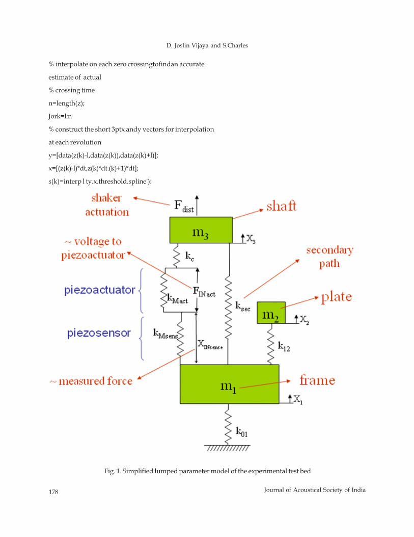
178 Journal of Acoustical Society of India
D. Joslin Vijaya and S.Charles
% interpolate on each zero crossingtofindan accurate
estimate of actual
% crossing time
n=length(z);
Jork=l:n
% construct the short 3ptx andy vectors for interpolation
at each revolution
y=[data(z(k)-l,data(z(k)),data(z(k)+l)];
x=[(z(k)-l)*dt,z(k)*dt.(k)+1)*dt];
s(k)=interp l ty.x.threshold.spline'):
Fig. 1. Simplified lumped parameter model of the experimental test bed
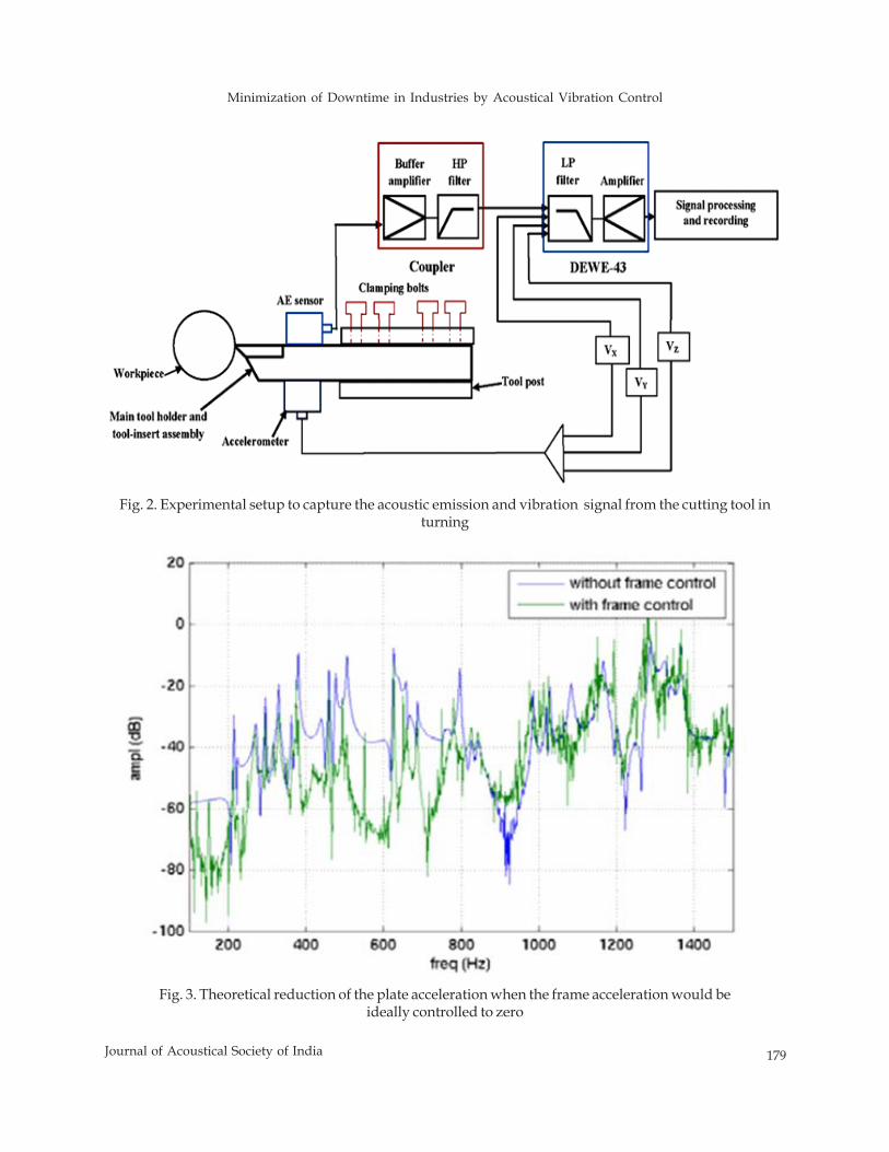
Minimization of Downtime in Industries by Acoustical Vibration Control
179Journal of Acoustical Society of India
Fig. 2. Experimental setup to capture the acoustic emission and vibration signal from the cutting tool inturning
Fig. 3. Theoretical reduction of the plate acceleration when the frame acceleration would beideally controlled to zero
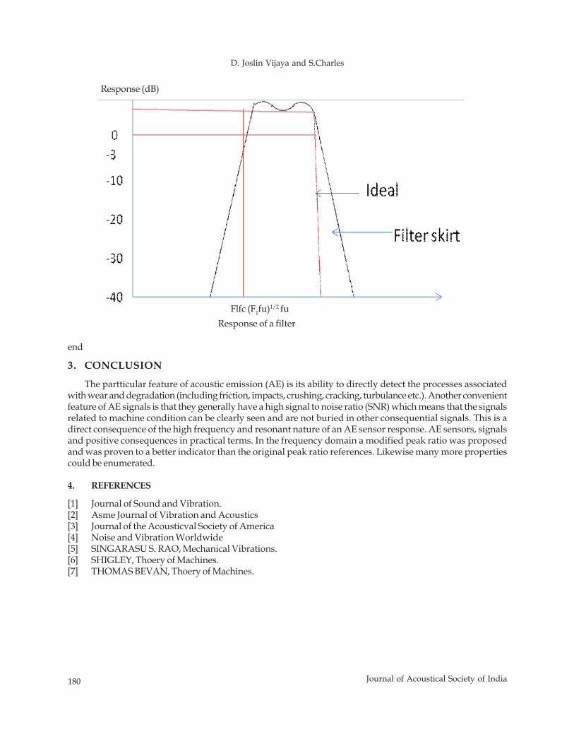
180 Journal of Acoustical Society of India
D. Joslin Vijaya and S.Charles
Response (dB)
Flfc (F1fu)1/2 fuResponse of a filter
end
3. CONCLUSION
The partticular feature of acoustic emission (AE) is its ability to directly detect the processes associatedwith wear and degradation (including friction, impacts, crushing, cracking, turbulance etc.). Another convenientfeature of AE signals is that they generally have a high signal to noise ratio (SNR) which means that the signalsrelated to machine condition can be clearly seen and are not buried in other consequential signals. This is adirect consequence of the high frequency and resonant nature of an AE sensor response. AE sensors, signalsand positive consequences in practical terms. In the frequency domain a modified peak ratio was proposedand was proven to a better indicator than the original peak ratio references. Likewise many more propertiescould be enumerated.
4. REFERENCES
[1] Journal of Sound and Vibration.[2] Asme Journal of Vibration and Acoustics[3] Journal of the Acousticval Society of America[4] Noise and Vibration Worldwide[5] SINGARASU S. RAO, Mechanical Vibrations.[6] SHIGLEY, Thoery of Machines.[7] THOMAS BEVAN, Thoery of Machines.
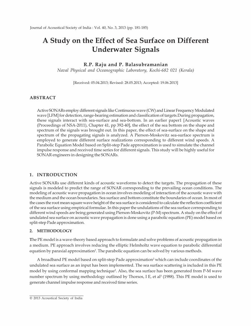
A Study on the Effect of Sea Surface on Different Underwater Signals
181Journal of Acoustical Society of India
ABSTRACT
Active SONARs employ different signals like Continuous wave (CW) and Linear Frequency Modulatedwave [LFM] for detection, range-bearing estimation and classification of targets.During propagation,these signals interact with sea-surface and sea-bottom. In an earlier paper1 [Acoustic waves(Proceedings of NSA-2011), Chapter 41, pp 392-40], the effect of the sea bottom on the shape andspectrum of the signals was brought out. In this paper, the effect of sea-surface on the shape andspectrum of the propagating signals is analyzed. A Pierson-Moskovitz sea-surface spectrum isemployed to generate different surface realizations corresponding to different wind speeds. AParabolic Equation Model based on Split-step Pade approximation is used to simulate the channelimpulse response and received time series for different signals. This study will be highly useful forSONAR engineers in designing the SONARs.
1. INTRODUCTION
Active SONARs use different kinds of acoustic waveforms to detect the targets. The propagation of thesesignals is modeled to predict the range of SONAR corresponding to the prevailing ocean conditions. Themodeling of acoustic wave propagation in ocean involves modeling of interaction of the acoustic wave withthe medium and the ocean boundaries. Sea surface and bottom constitute the boundaries of ocean. In most ofthe cases the root mean square wave height of the sea surface is considered to calculate the reflection coefficientof the sea surface using empirical formulae. In this paper the undulations of the sea surface corresponding todifferent wind speeds are being generated using Pierson-Moskovitz (P-M) spectrum. A study on the effect ofundulated sea surface on acoustic wave propagation is done using a parabolic equation (PE) model based onsplit-step Pade approximation.
2. METHODOLOGY
The PE model is a wave-theory based approach to formulate and solve problems of acoustic propagation ina medium. PE approach involves reducing the elliptic Helmholtz wave equation to parabolic differentialequation by paraxial approximation2. The parabolic equation can be solved by various methods.
A broadband PE model based on split-step Pade approximation2 which can include coordinates of theundulated sea surface as an input has been implemented. The sea surface scattering is included in this PEmodel by using conformal mapping technique2. Also, the sea surface has been generated from P-M wavenumber spectrum by using methodology outlined by Thorsos, I E, et al3 (1988). This PE model is used togenerate channel impulse response and received time series.
Journal of Acoustical Society of India : Vol. 40, No. 3, 2013 (pp. 181-185)
A Study on the Effect of Sea Surface on DifferentUnderwater Signals
R.P. Raju and P. BalasubramanianNaval Physical and Oceanographic Laboratory, Kochi-682 021 (Kerala)
[Received: 05.04.2013; Revised: 28.05.2013; Accepted: 19.06.2013]
© 2013 Acoustical Society of India
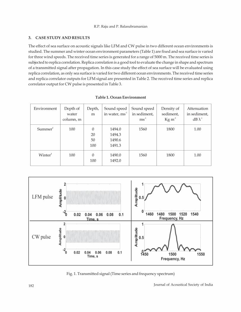
182 Journal of Acoustical Society of India
R.P. Raju and P. Balasubramanian
3. CASE STUDY AND RESULTS
The effect of sea surface on acoustic signals like LFM and CW pulse in two different ocean environments isstudied. The summer and winter ocean environment parameters (Table 1) are fixed and sea surface is variedfor three wind speeds. The received time series is generated for a range of 5000 m. The received time series issubjected to replica correlation. Replica correlation is a good tool to evaluate the change in shape and spectrumof a transmitted signal after propagation. In this case study the effect of sea surface will be evaluated usingreplica correlation, as only sea surface is varied for two different ocean environments. The received time seriesand replica correlator outputs for LFM signal are presented in Table 2. The received time series and replicacorrelator output for CW pulse is presented in Table 3.
Environment Depth of water
column, m
Depth, m
Sound speed in water, ms-1
Sound speed in sediment,
ms-1
Density of sediment,
Kg m-3
Attenuation in sediment,
dB λ-1
Summer4 100 02050100
1494.01494.31490.61491.3
1560 1800 1.00
Winter4 100 0100
1490.01492.0
1560 1800 1.00
Table 1. Ocean Environment
Fig. 1. Transmitted signal (Time series and frequency spectrum)
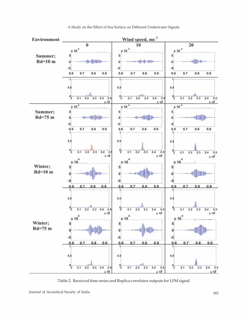
A Study on the Effect of Sea Surface on Different Underwater Signals
183Journal of Acoustical Society of India
Table 2. Received time series and Replica correlator outputs for LFM signal
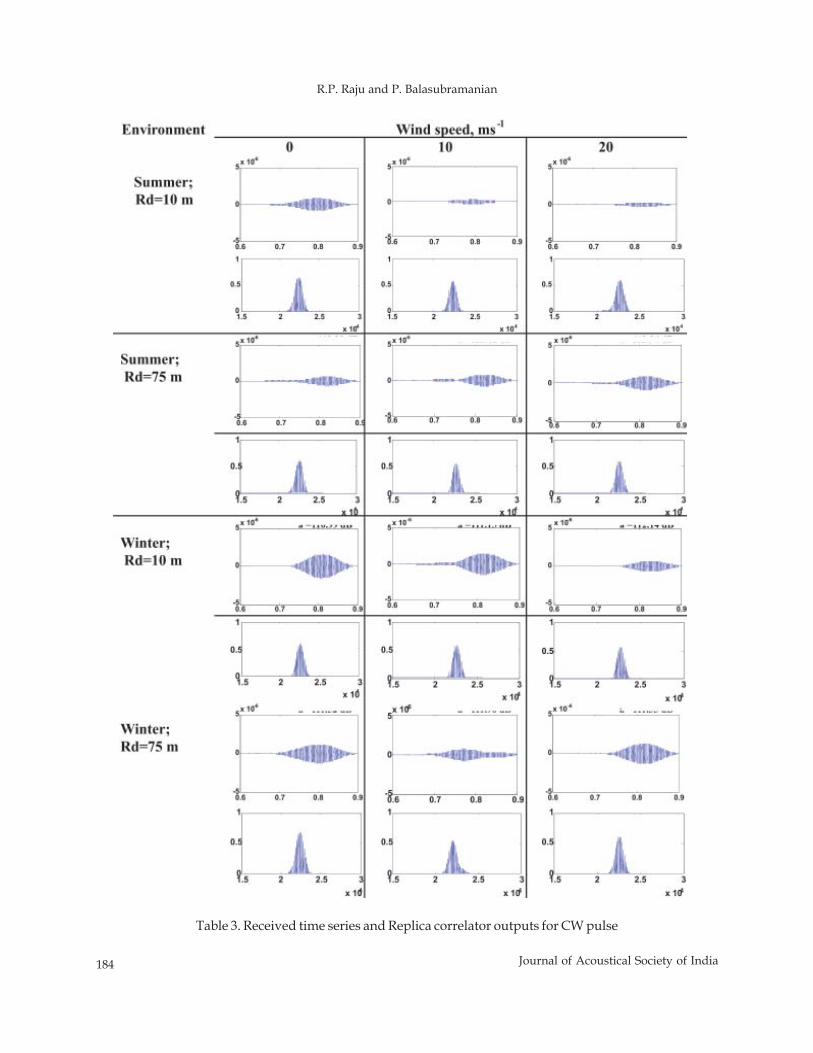
184 Journal of Acoustical Society of India
R.P. Raju and P. Balasubramanian
Table 3. Received time series and Replica correlator outputs for CW pulse
A Study on the Effect of Sea Surface on Different Underwater Signals
185Journal of Acoustical Society of India
Propagation Model used: Broadband PE Model (Split-step Pade approximation)Sea surface realization: P-M spectrum for wind speeds of 0, 10, 20 ms-1Source depth: 50 mReceiver Depth, Rd: 10 m and 75 m, Range: 5000 mWaveform: 0.1 s LFM signal with a bandwidth of 100 Hz centered at 1500 Hz. (Fig.1)0.1 s CW pulse of frequency 1500 Hz. (Fig. 1)
The plots in table 2 and 3 clearly indicate the distortion of the transmitted signal. The LFM and CWsignals are stretched to approximately 0.2 s. The replica correlator outputs in Table 2 indicate that thereceived signals at a depth of 75 m are more correlated to the transmitted LFM signal than the ones receivedat 10 m. Also, in winter environment at 10 m depth the maximum correlation value increases as the windspeed increases from 0 to 20 ms-1. The maximum correlation at 10 m receiver is very low and the pulse maynot be detected in a noise-limited environment after replica correlation. The rough sea surface leads to higherpropagation losses4 and lower pulse distortion in the given environments. In case of flat sea surface, thetrade-off is between low propagation losses and higher correlation in signals at 75 m depth. And in case of Rdat 10 m the trade-off is between high propagation losses and lower correlation in received signals.
In case of CW pulses it is observed from table 3 that there is not much change in the maximum correlationvalue (0.5-0.6) between received and transmitted signal due to change in the sea surface. But, the shape of thesignal changes after propagation.
4. CONCLUSION
A broadband PE model based on split-step Pade approximation has been implemented. The effect of seasurface on acoustic pulse is clearly shown for the cases considered. The distortion in the pulse due to one-way propagation is characterized by low correlation values. The distortion in transmitted signal has to beconsidered during the implementation of detection techniques like Replica correlation, as it fails to be effectivein realistic ocean conditions.
REFERENCES
[1] P. BALASUBRAMANIAN et al., 2011. Acoustic waves, 41, 392-401.[2] M.D. COLLINS, 1993. A split-step Pade solution for the Parabolic Equation Method”, JASA, 93, 1736-
1742.[3] E.I. THORSOS, 1990. Acoustic scattering from a “Pierson-Moskovitz” sea surface”, JASA, 88(1), 335-349.[4] D.A. MILES, et al., 2003. Forward scattering of pulses from a rough sea surface by Fourier synthesis of
parabolic equation solutions, JASA, 114(3), 1266-1280.
186 Journal of Acoustical Society of India
Kaushik Banerjee, Anirban Patranabis, Ranjan Sengupta and Dipak Ghosh
Effect of Harmonium Usage in Hindustani MusicPerformances: A Signal Processing Approach
Kaushik Banerjee, Anirban Patranabis, Ranjan Sengupta and Dipak GhoshSir C V Raman Centre for Physics and Music, Jadavpur University, Kolkata-700 032 (WB)
ABSTRACT
In this paper we attempted to find out the influence of harmonium usage (ET scale) on the ragarenderings in Hindustani music. The pitch period was extracted from 17 renderings of 12 eminentvocalists of Hindustani music, for two different ragas. Only the steady pitch periods were used foranalysis. The approach was to study the duration distribution of steady pitch states against the ratioof each note in an octave. Prominent peaks indicate preferred ratios. Attempt was made to see whetherthese ratios obey ET scale or Indian 22 sruti intervals. The result shows that most of the vocalistsfollow a mixture of both systems with a preference of any one depending on the raga.
1. INTRODUCTION
Hindustani music (HM) has had some uniqueness and so it has been highly esteemed by the rest of the world.In HM, swara (note) is conceived not merely as a sound of fixed pitch position, but as the entire tonal rangebetween itself and its previous swara. Though this interval can be theoretically divided into infinitesimalparts, the ancient musicologists believed that only a limited number, not exceeding four, sounds could bedistinctly cognized by the ear in a swara-interval. These cognizable sounds are known as Srutis and theinterval, which separated one swara from the next, was measured in terms of Srutis. Sruti was thought of bothas the least audible interval between two sounds, as well as the sounds themselves, which were separated, bysuch an interval. The total number of Srutis was fixed unambiguously at 22 in ancient, musical treatises [1].The tradition of teaching HM is an oral one. It is taught directly by the guru to the disciple, without the use oftextual material. The basics starting from voice culture to the understanding of notes and Srutis are taughtthrough direct oral communication accompanying with only tanpura. It was showed that the use of Srutisvaries with gharanas as well as with the ragas and has also a student- teacher relationship [2]. It is likely thateach gharana may have its own sense of aesthetic satisfaction of a raga and the use of Sruti may reflect these.It is also known that musicians feel that a particular note sounds better when placed relatively low for aparticular raga while it may have to be raised much higher for some other raga. For example some say thatkomal re needs to be placed high in Todi but low in Bhairav. In the later part of the British rule in India, westernmusical instrument Harmonium (using ET scale) was introduced in HM in about middle of 19th century. Theinstrument was much nourished and developed in the eastern part of Indian, especially in Kolkata [3].
This paper presents the Sruti position as revealed from the performances of contemporary and oldergeneration singers. Regarding the use of Srutis by the singers, substantive and distinctive preferences todifferent Srutis in two different ragas (Bhairav and Todi) are studied particularly in the context of the usage ofHarmonium (ET scale).
Journal of Acoustical Society of India : Vol. 40, No. 3, 2013 (pp.186-190)
[Received: 11.12.2012; Revised: 19.06.2013; Accepted: 09.05.2013]
© 2013 Acoustical Society of India
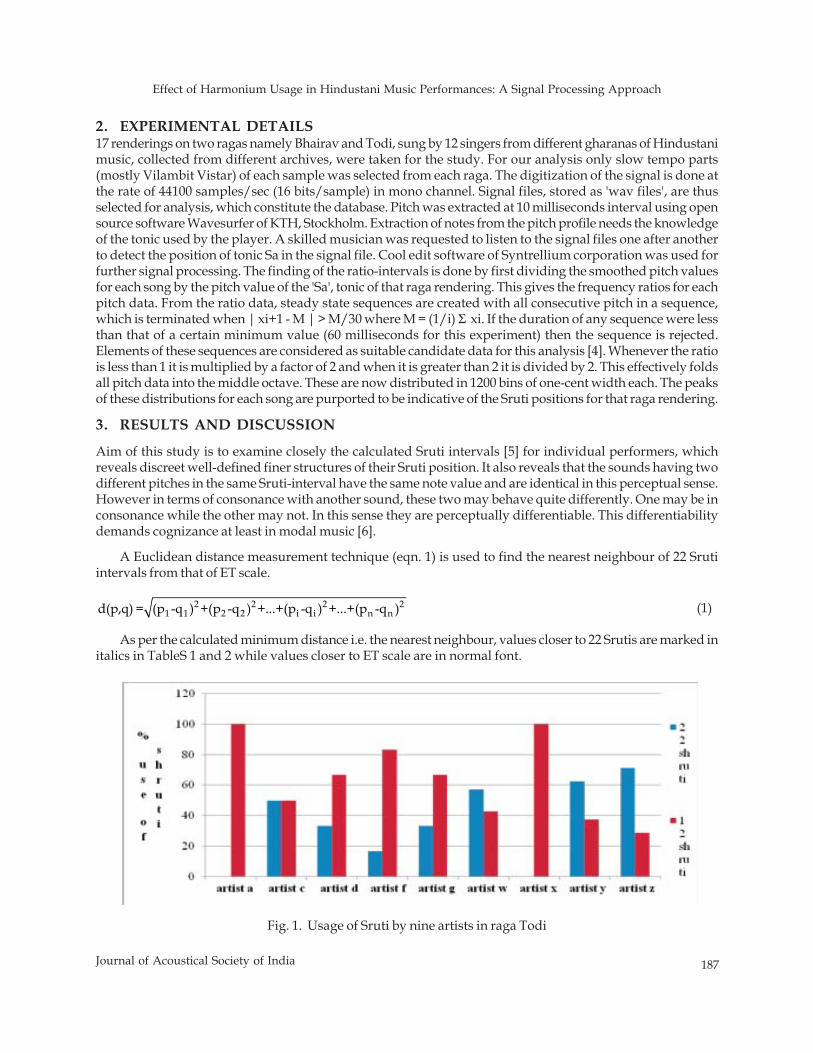
Effect of Harmonium Usage in Hindustani Music Performances: A Signal Processing Approach
187Journal of Acoustical Society of India
2. EXPERIMENTAL DETAILS17 renderings on two ragas namely Bhairav and Todi, sung by 12 singers from different gharanas of Hindustanimusic, collected from different archives, were taken for the study. For our analysis only slow tempo parts(mostly Vilambit Vistar) of each sample was selected from each raga. The digitization of the signal is done atthe rate of 44100 samples/sec (16 bits/sample) in mono channel. Signal files, stored as 'wav files', are thusselected for analysis, which constitute the database. Pitch was extracted at 10 milliseconds interval using opensource software Wavesurfer of KTH, Stockholm. Extraction of notes from the pitch profile needs the knowledgeof the tonic used by the player. A skilled musician was requested to listen to the signal files one after anotherto detect the position of tonic Sa in the signal file. Cool edit software of Syntrellium corporation was used forfurther signal processing. The finding of the ratio-intervals is done by first dividing the smoothed pitch valuesfor each song by the pitch value of the 'Sa', tonic of that raga rendering. This gives the frequency ratios for eachpitch data. From the ratio data, steady state sequences are created with all consecutive pitch in a sequence,which is terminated when | xi+1 - M | > M/30 where M = (1/i) Σ xi. If the duration of any sequence were lessthan that of a certain minimum value (60 milliseconds for this experiment) then the sequence is rejected.Elements of these sequences are considered as suitable candidate data for this analysis [4]. Whenever the ratiois less than 1 it is multiplied by a factor of 2 and when it is greater than 2 it is divided by 2. This effectively foldsall pitch data into the middle octave. These are now distributed in 1200 bins of one-cent width each. The peaksof these distributions for each song are purported to be indicative of the Sruti positions for that raga rendering.
3. RESULTS AND DISCUSSION
Aim of this study is to examine closely the calculated Sruti intervals [5] for individual performers, whichreveals discreet well-defined finer structures of their Sruti position. It also reveals that the sounds having twodifferent pitches in the same Sruti-interval have the same note value and are identical in this perceptual sense.However in terms of consonance with another sound, these two may behave quite differently. One may be inconsonance while the other may not. In this sense they are perceptually differentiable. This differentiabilitydemands cognizance at least in modal music [6].
A Euclidean distance measurement technique (eqn. 1) is used to find the nearest neighbour of 22 Srutiintervals from that of ET scale.
2 2 2 21 1 2 2 i i n nd(p,q) = (p -q ) +(p -q ) +...+(p -q ) +...+(p -q ) (1)
As per the calculated minimum distance i.e. the nearest neighbour, values closer to 22 Srutis are marked initalics in TableS 1 and 2 while values closer to ET scale are in normal font.
Fig. 1. Usage of Sruti by nine artists in raga Todi
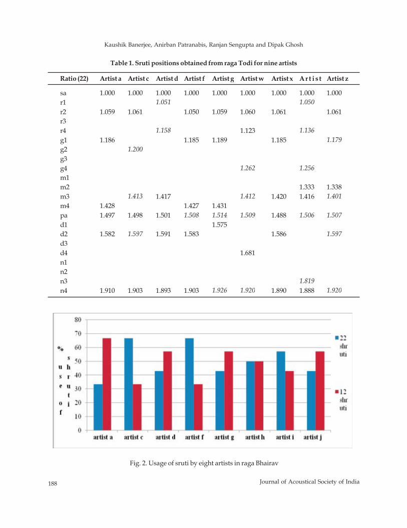
188 Journal of Acoustical Society of India
Kaushik Banerjee, Anirban Patranabis, Ranjan Sengupta and Dipak Ghosh
Table 1. Sruti positions obtained from raga Todi for nine artists
Ratio (22) Artist a Artist c Artist d Artist f Artist g Artist w Artist x A r t i s t Artist z
sa 1.000 1.000 1.000 1.000 1.000 1.000 1.000 1.000 1.000r1 1.051 1.050r2 1.059 1.061 1.050 1.059 1.060 1.061 1.061r3r4 1.158 1.123 1.136g1 1.186 1.185 1.189 1.185 1.179g2 1.200g3g4 1.262 1.256m1m2 1.333 1.338m3 1.413 1.417 1.412 1.420 1.416 1.401m4 1.428 1.427 1.431pa 1.497 1.498 1.501 1.508 1.514 1.509 1.488 1.506 1.507d1 1.575d2 1.582 1.597 1.591 1.583 1.586 1.597d3d4 1.681n1n2n3 1.819n4 1.910 1.903 1.893 1.903 1.926 1.920 1.890 1.888 1.920
Fig. 2. Usage of sruti by eight artists in raga Bhairav
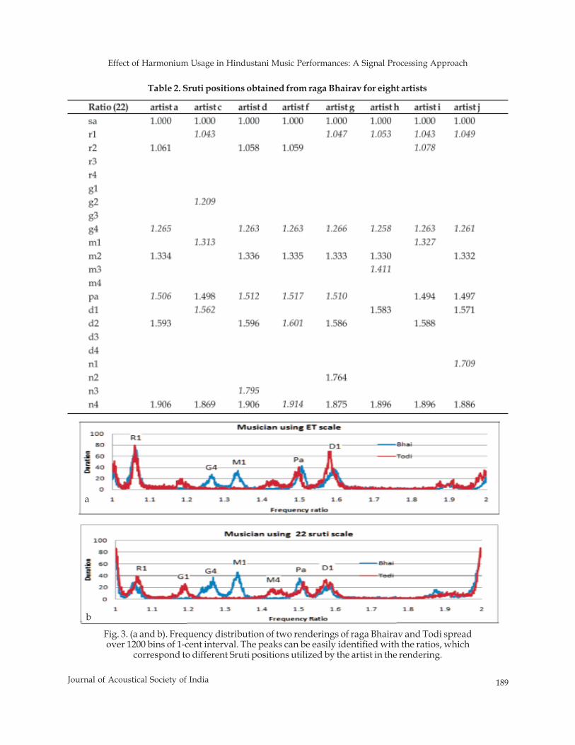
Effect of Harmonium Usage in Hindustani Music Performances: A Signal Processing Approach
189Journal of Acoustical Society of India
Fig. 3. (a and b). Frequency distribution of two renderings of raga Bhairav and Todi spreadover 1200 bins of 1-cent interval. The peaks can be easily identified with the ratios, which
correspond to different Sruti positions utilized by the artist in the rendering.
a
b
Table 2. Sruti positions obtained from raga Bhairav for eight artists

190 Journal of Acoustical Society of India
Kaushik Banerjee, Anirban Patranabis, Ranjan Sengupta and Dipak Ghosh
Usage of 22 Srutis (microtonal intervals) are perceptually distinguishable than that use of ET scale. Andaccording to some people 22 Srutis are more pleasant to listen. Possibly the frequent use of harmonium as anaccompaniment for some artists make their ratios mostly matched with the ET scale.
It is being observed from the tables and Figs. 1 and 2 that some musicians are using ET scale ratios andsome musicians are using mixed ratios both 22 srutis and ET scale.
Figure 3 (a and b) shows the frequency of occurrence of the duration of ratio of the steady pitch periods andSa (tonic) folded to middle octave and distributed over 100bins of one cent interval. Thus each peak correspondsto a note utilized by the artist in the raga. The height of the peak gives the number of times the note is sung inthe processed signal. It is being observed from the distributions that the singer (a) uses ET scale mostly and thesinger (b) uses the Indian Sruti system.
4 CONCLUSION
Influence of harmonium have enabled the vocalists of HM to deviate from the older 22 Sruti interval systemand at present most of the musicians either follow a mixed system of ET and 22 Sruti intervals or purely ETscale. There is also a preference of the system on the raga
5. REFERENCES
[1] R.K. SHRINGLY and PREM LATA SHARMA, 1989. Sangitaratnakara of Saraingadeva (vol - II) : Text &English translation. Published by - Munshiram Manoharlal Publishers Pvt. Ltd. Delhi.
[2] ASOKE KUMAR DATTA, RANJAN SENGUPTA,NITYANANDA DEY and DIPALI NAG, 2006."Experimental Analysis of Srutis from performances in Hindustani music", Monograph published byScientific Research Department, ITC Sangeet Research Academy, ISBN 81-903818-0-6.
[3] http://en.wikipedia.org/wiki/Harmonium#India[4] A.K. DATTA, 2006. "A methodology of note extraction from the song signals", Proc. Frontiers of Research
on Speech and Music.[5] A.K. DATTA and R. SENGUPTA et al., 2004. "Sruti usage by old and contemporary singers in Khyal: An
objective approach", Proc. Frontiers of Research on Speech and Music (FRSM-2004), AnnamalaiUniversity, Tamilnadu, India
[6] A.K. DATTA and R. SENGUPTA et al., 2011. "Objective analysis of srutis from the vocal performances ofHindustani Music using Clustering Algorithm", Published in EUNOMIOS - An open online journal forTheory, Analysis and Semiotics of Music, http://www.eunomios.org/.
[7] JOAN SERR`A, GOPALA K. KODURI, MARIUS MIRON and XAVIER SERRA, 2011."Assessing thetuning of sung Indian classical music", Int. Soc. for Music Information Retrieval Conf. (ISMIR), Miami,USA.
Numerical Investigation of Non-Cavitating Underwater Propeller Noise using FW-H Method
191Journal of Acoustical Society of India
ABSTRACT
The Propeller is a vital component which is subtle for the safe operation of a ship at sea. The purposeof the propeller is to produce a thrust causing to move the ship in forward direction. But it is identifiedas major noise source. The noise produced by a propeller is very much importance to warshipdesigners and military strategists for many years. A ship /Submarine noise signature of a few tens ofwatts could be sufficient to give enemy valuable information at a considerable range. Using noisesignature analysis at remote locations, it is possible not only to determine which class of vessel hasbeen located, but also if character of signature is sufficiently known to identify the particular ship.Clearly the ultimate goal of a warship designer must be to make the ship's signature vanish into thebackground noise of the sea which comprises contributions from the weather, marine life and alsoother shipping from a wide geographical area. This paper presents a numerical study on the non-cavitating noises of the underwater propeller using Computational Fluid Dynamics (CFD) Fluentsoftware.Propeller behavior is investigated for its hydrodynamic parameters and then ComputationalAcoustic Analysis (CAA) is carried out using viscous model of large eddy simulation of FfowcsWilliams-Hawkings formulation(FW-H). Here solver is chosen as pressure based, unsteadyformulation of second order implicit. Noise is predicted using time-domain acoustic analogy andfinite volume method. Sound pressure levels are predicted at different receiver positions.
1. INTRODUCTION
Sound generated by a propeller is critical in underwater detection, and is often related to the survivability ofthe vessels especially for military purposes. Marine propeller noise can be classified into cavitating and non-cavitating noise. Cavitation of the marine propeller is the most prevalent source of underwater sound inoceans and is often the dominant noise source of a single marine vehicle.However, submarines and torpedoesare usually operated deep enough under the sea to avoid cavitation. Salvatore et al. [1] presented propeller-induced noise emission is studied through a general hydro acoustics formulation based on the Ffowcs Williams-Hawkings (FW-H) equation that allows describing the acoustic pressure field generated by lifting bodies inarbitrary motion through a fluid. Chang [2] applied a finite volume CFD method in conjuction with thestandard k-? turbulence model to calculate the flow pattern and performance parameters of a DTNSRDCP4119 marine propeller in a uniform flow.
Journal of Acoustical Society of India : Vol. 40, No. 3, 2013 (pp. 191-195)
Numerical Investigation of Non-Cavitating UnderwaterPropeller Noise using FW-H Method
V. Rama Krishna1, P.V.S. Ganesh Kumar1,P. BangaruBabu2 and S. Rama Krishna3
1Naval Science and Technological Laboratory, Visakhapatnam, (AP)2National Institute of Technology (NIT), Warangal, (AP)
3G V P College of Engineering, Madhurawada, Visakhapatnam, (AP)
[Received: 15.12.2012; Revised: 22.06.2013; Accepted: 15.05.2013]
© 2013 Acoustical Society of India
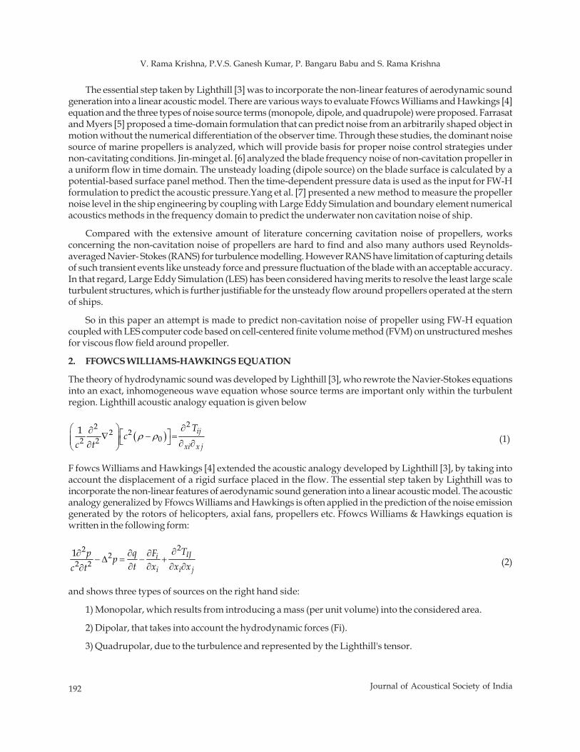
192 Journal of Acoustical Society of India
V. Rama Krishna, P.V.S. Ganesh Kumar, P. Bangaru Babu and S. Rama Krishna
The essential step taken by Lighthill [3] was to incorporate the non-linear features of aerodynamic soundgeneration into a linear acoustic model. There are various ways to evaluate Ffowcs Williams and Hawkings [4]equation and the three types of noise source terms (monopole, dipole, and quadrupole) were proposed. Farrasatand Myers [5] proposed a time-domain formulation that can predict noise from an arbitrarily shaped object inmotion without the numerical differentiation of the observer time. Through these studies, the dominant noisesource of marine propellers is analyzed, which will provide basis for proper noise control strategies undernon-cavitating conditions. Jin-minget al. [6] analyzed the blade frequency noise of non-cavitation propeller ina uniform flow in time domain. The unsteady loading (dipole source) on the blade surface is calculated by apotential-based surface panel method. Then the time-dependent pressure data is used as the input for FW-Hformulation to predict the acoustic pressure.Yang et al. [7] presented a new method to measure the propellernoise level in the ship engineering by coupling with Large Eddy Simulation and boundary element numericalacoustics methods in the frequency domain to predict the underwater non cavitation noise of ship.
Compared with the extensive amount of literature concerning cavitation noise of propellers, worksconcerning the non-cavitation noise of propellers are hard to find and also many authors used Reynolds-averaged Navier- Stokes (RANS) for turbulence modelling. However RANS have limitation of capturing detailsof such transient events like unsteady force and pressure fluctuation of the blade with an acceptable accuracy.In that regard, Large Eddy Simulation (LES) has been considered having merits to resolve the least large scaleturbulent structures, which is further justifiable for the unsteady flow around propellers operated at the sternof ships.
So in this paper an attempt is made to predict non-cavitation noise of propeller using FW-H equationcoupled with LES computer code based on cell-centered finite volume method (FVM) on unstructured meshesfor viscous flow field around propeller.
2. FFOWCS WILLIAMS-HAWKINGS EQUATION
The theory of hydrodynamic sound was developed by Lighthill [3], who rewrote the Navier-Stokes equationsinto an exact, inhomogeneous wave equation whose source terms are important only within the turbulentregion. Lighthill acoustic analogy equation is given below
( )22
2 202 2
1 ij
xi x j
Tc
c tρ ρ
∂⎛ ⎞∂ ⎡ ⎤∇ − =⎜ ⎟⎜ ⎟ ⎣ ⎦ ∂ ∂∂⎝ ⎠ (1)
F fowcs Williams and Hawkings [4] extended the acoustic analogy developed by Lighthill [3], by taking intoaccount the displacement of a rigid surface placed in the flow. The essential step taken by Lighthill was toincorporate the non-linear features of aerodynamic sound generation into a linear acoustic model. The acousticanalogy generalized by Ffowcs Williams and Hawkings is often applied in the prediction of the noise emissiongenerated by the rotors of helicopters, axial fans, propellers etc. Ffowcs Williams & Hawkings equation iswritten in the following form:
222
2 21 IJi
i i j
Tp q Fpt x x xc t
∂∂ ∂ ∂− Δ = − +
∂ ∂ ∂ ∂∂ (2)
and shows three types of sources on the right hand side:
1) Monopolar, which results from introducing a mass (per unit volume) into the considered area.
2) Dipolar, that takes into account the hydrodynamic forces (Fi).
3) Quadrupolar, due to the turbulence and represented by the Lighthill's tensor.
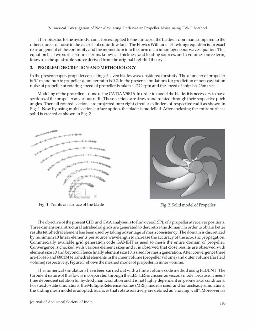
Numerical Investigation of Non-Cavitating Underwater Propeller Noise using FW-H Method
193Journal of Acoustical Society of India
The noise due to the hydrodynamic forces applied to the surface of the blades is dominant compared to theother sources of noise in the case of subsonic flow fans. The Ffowcs Williams - Hawkings equation is an exactrearrangement of the continuity and the momentum into the form of an inhomogeneous wave equation. Thisequation has two surface source terms, known as thickness and loading sources, and a volume source term,known as the quadruple source derived from the original Lighthill theory.
3. PROBLEM DESCRIPTION AND METHODOLOGY
In the present paper, propeller consisting of seven blades was considered for study. The diameter of propelleris 3.1m and hub to propeller diameter ratio is 0.2. In the present simulations for prediction of non-cavitationnoise of propeller at rotating speed of propeller is taken as 242 rpm and the speed of ship is 9.26m/sec.
Modeling of the propeller is done using CATIA V5R16. In order to model the blade, it is necessary to havesections of the propeller at various radii. These sections are drawn and rotated through their respective pitchangles. Then all rotated sections are projected onto right circular cylinders of respective radii as shown inFig. 1. Now by using multi section surface option, the blade is modelled. After enclosing the entire surfacessolid is created as shown in Fig. 2.
Fig. 1. Points on surface of the blade Fig. 2. Solid model of Propeller
The objective of the present CFD and CAA analyses is to find overall SPL of a propeller at receiver positions.Three dimensional structural tetrahedral grids are generated to descretize the domain. In order to obtain betterresults tetrahedral element has been used by taking advantage of mesh consistency. The domain is discretizedby minimum 10 linear elements per source wavelength to increase the accuracy of the acoustic propagation.Commercially available grid generation code GAMBIT is used to mesh the entire domain of propeller.Convergence is checked with various element sizes and it is observed that close results are observed withelement size 10 and beyond. Hence finally element size 10 is used for mesh generation. After convergence thereare 436445 and 680134 tetrahedral elements in the inner volume (propeller volume) and outer volume (far fieldvolume) respectively. Figure 3. shows the meshed model of propeller in inner volume.
The numerical simulations have been carried out with a finite volume code method using FLUENT. Theturbulent nature of the flow is incorporated through the LES. LES is chosen as viscous model because, it needstime dependent solution for hydrodynamic solution and it is not highly dependent on geometrical conditions.For steady-state simulations, the Multiple Reference Frames (MRF) model is used, and for unsteady simulations,the sliding mesh model is adopted. Surfaces that rotate relatively are defined as "moving wall". Moreover, as
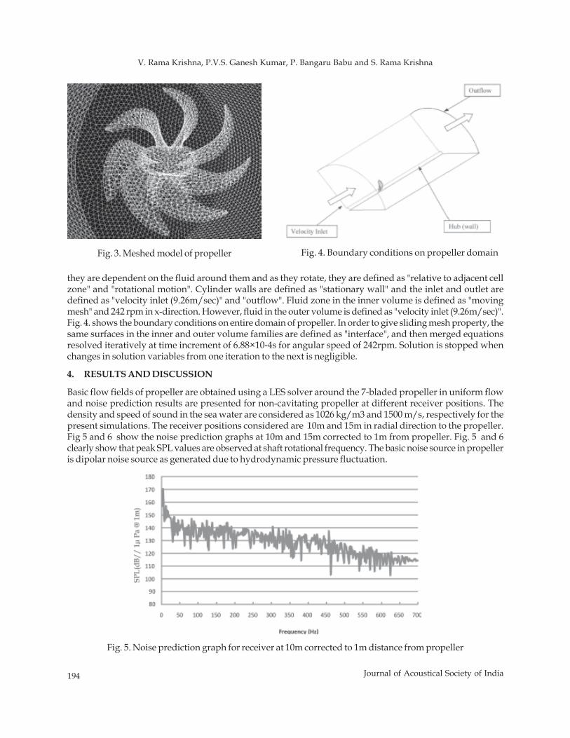
194 Journal of Acoustical Society of India
V. Rama Krishna, P.V.S. Ganesh Kumar, P. Bangaru Babu and S. Rama Krishna
they are dependent on the fluid around them and as they rotate, they are defined as "relative to adjacent cellzone" and "rotational motion". Cylinder walls are defined as "stationary wall" and the inlet and outlet aredefined as "velocity inlet (9.26m/sec)" and "outflow". Fluid zone in the inner volume is defined as "movingmesh" and 242 rpm in x-direction. However, fluid in the outer volume is defined as "velocity inlet (9.26m/sec)".Fig. 4. shows the boundary conditions on entire domain of propeller. In order to give sliding mesh property, thesame surfaces in the inner and outer volume families are defined as "interface", and then merged equationsresolved iteratively at time increment of 6.88×10⁻⁴s for angular speed of 242rpm. Solution is stopped whenchanges in solution variables from one iteration to the next is negligible.
4. RESULTS AND DISCUSSION
Basic flow fields of propeller are obtained using a LES solver around the 7-bladed propeller in uniform flowand noise prediction results are presented for non-cavitating propeller at different receiver positions. Thedensity and speed of sound in the sea water are considered as 1026 kg/m3 and 1500 m/s, respectively for thepresent simulations. The receiver positions considered are 10m and 15m in radial direction to the propeller.Fig 5 and 6 show the noise prediction graphs at 10m and 15m corrected to 1m from propeller. Fig. 5 and 6clearly show that peak SPL values are observed at shaft rotational frequency. The basic noise source in propelleris dipolar noise source as generated due to hydrodynamic pressure fluctuation.
Fig. 4. Boundary conditions on propeller domainFig. 3. Meshed model of propeller
Fig. 5. Noise prediction graph for receiver at 10m corrected to 1m distance from propeller
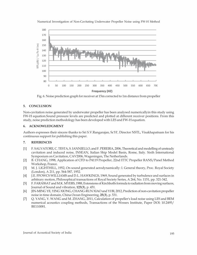
Numerical Investigation of Non-Cavitating Underwater Propeller Noise using FW-H Method
195Journal of Acoustical Society of India
Fig. 6. Noise prediction graph for receiver at 15m corrected to 1m distance from propeller
5. CONCLUSION
Non-cavitation noise generated by underwater propeller has been analysed numericallyin this study usingFW-H equation.Sound pressure levels are predicted and plotted at different receiver positions. From thisstudy, noise prediction methodology has been developed with LES and FW-H equation.
6. ACKNOWLEDGMENT
Authors expresses their sincere thanks to Sri S.V.Rangarajan, Sc'H', Director NSTL, Visakhapatnam for hiscontinuous support for publishing this paper.
7. REFERENCES
[1] F. SALVATORE, C. TESTA, S. IANNIELLO, and F. PEREIRA, 2006, Theoretical and modelling of unsteadycavitation and induced noise, INSEAN, Italian Ship Model Basin, Rome, Italy. Sixth InternationalSymposium on Cavitation, CAV2006, Wageningen, The Netherlands.
[2] B. CHANG, 1998, Application of CFD to P4119 Propeller, 22nd ITTC Propeller RANS/Panel MethodWorkshop, France.
[3] M. J. LIGHTHILL, 1952, On sound generated aerodynamically: I. General theory, Proc. Royal Society(London), A 211, pp. 564-587, 1952.
[4] J.E. FFOWCS WILLIAMS and D.L. HAWKINGS, 1969, Sound generated by turbulence and surfaces inarbitrary motion, Philosophical transactions of Royal Society Series, A 264, No. 1151, pp. 321-342.
[5] F. FARASSAT and M.K. MYERS, 1988, Extensions of Kirchhoffs formula to radiation from moving surfaces,Journal of Sound and vibration, 123(3), p. 451.
[6] JIN-MING YE, YING XIONG, CHANG-RUN XIAO and YI BI, 2012, Prediction of non-cavitation propellernoise in time domain, China Ocean Engineering, 25(3), p. 531.
[7] Q. YANG, Y. WANG and M. ZHANG, 2011, Calculation of propeller's load noise using LES and BEMnumerical acoustics coupling methods, Transactions of the Wessex Institute, Paper DOI: 10.2495/BE110081.
196 Journal of Acoustical Society of India
R.A. Patil, Prashant Dabrase and B.M. Suryavanshi
© 2013 Acoustical Society of India
ABSTRACT
The measurements of Ultrasonic velocities (υ), density (ρ) and viscosity (η) of pure & binary liquidmixtures of Acetone and N-N dimethyl acetamide have been carried out over the entire range ofcomposition at temperature 313.15K to evaluate the other thermo dynamical parameters with theirexcess values such as adiabatic compressibility (βα), free length (Lf), free volume (Vf), internal pressure(πi) and their excess values, υE, βα
E, LfE, Vf
E and πiE. The results thus obtained are discussed for molecular
interaction with varying composition of binary system. The non linearity found in all the plots ofthese ultrasonic parameters and their excess values with the composition range indicates presence ofthe intermolecular interaction between the components of the unlike molecules of the mixture. Thenature of excess values of the βα, Lf, Vf and πi conforms about the existence of the molecular associationbetween the components of the mixture.
1. INTRODUCTION
There are many physical methods which play an important role in determining molecular structure & molecularproperties of different materials. In recent years the advances in the ultrasonic technique has become a powerfultool in evaluating information about the physical and chemical behavior of molecules of the liquids [1-4]. Theultrasonic studies of the liquids are most preferred in many fields such as pharmaceutical industry, biomedicalresearch, automobile industry, chemical industry, water research & scattering spectroscopy, etc.[5]. Theinformation of density (ρ), ultrasonic velocity (υ) and viscosity (η) of the pure liquids and their mixtures playsvery important role in different applications that include surface facilities, pipeline systems & mass transferoperations.
Here in the present study the ultrasonic velocity, density and viscosity measurements have been carriedout for determination of ultrasonic parameters such as compressibility (βα), molecular free length (Lf), freevolume (Vf) and internal pressure (πi) and their excess values (υE, βα
E, LfE, Vf
E and πiE.) for the different composition
range of NN-Dimethyl acetamide in acetone at the temperature 313.15K. The variations of these parameterswith concentration of binary liquid mixtures are studied to understand molecular interaction between unlikemolecules of the mixtures.
2. EXPERIMENTAL
The binary mixtures of the chemicals Acetone and NN- dimethyl acetamide for different range of compositionwere prepared at room temperature and kept in a special airtight glass bottles to avoid air contact. The chemicals
Journal of Acoustical Society of India : Vol. 40, No. 3, 2013 (pp.196-202)
Acoustical Behavior of NN Dimethyl-acetamide andAcetone at 313.15 K
R.A. Patil1*, Prashant Dabrase2 and B.M. Suryavanshi3
1S.S.S.K.R.Innani Mahavidyalaya, Karanja-444 1052Bhalerao Science College, Saoner-441 107
3Department of Physics, Government Institute of Science, Nagpur-440 001 (MS)*e-mail: [email protected]
[Received: 18.12.2012; Revised: 24.06.2013; Accepted: 18.05.2013]
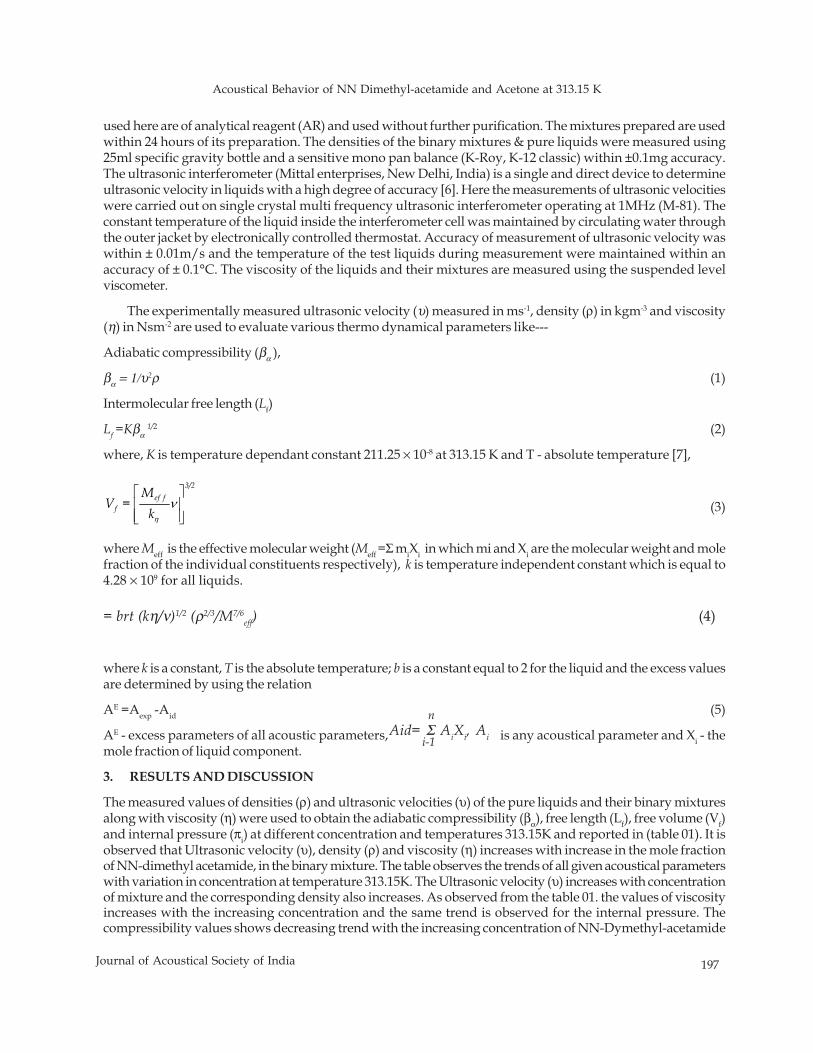
Acoustical Behavior of NN Dimethyl-acetamide and Acetone at 313.15 K
197Journal of Acoustical Society of India
used here are of analytical reagent (AR) and used without further purification. The mixtures prepared are usedwithin 24 hours of its preparation. The densities of the binary mixtures & pure liquids were measured using25ml specific gravity bottle and a sensitive mono pan balance (K-Roy, K-12 classic) within ±0.1mg accuracy.The ultrasonic interferometer (Mittal enterprises, New Delhi, India) is a single and direct device to determineultrasonic velocity in liquids with a high degree of accuracy [6]. Here the measurements of ultrasonic velocitieswere carried out on single crystal multi frequency ultrasonic interferometer operating at 1MHz (M-81). Theconstant temperature of the liquid inside the interferometer cell was maintained by circulating water throughthe outer jacket by electronically controlled thermostat. Accuracy of measurement of ultrasonic velocity waswithin ± 0.01m/s and the temperature of the test liquids during measurement were maintained within anaccuracy of ± 0.1°C. The viscosity of the liquids and their mixtures are measured using the suspended levelviscometer.
The experimentally measured ultrasonic velocity (υ) measured in ms-1, density (ρ) in kgm-3 and viscosity(η) in Nsm-2 are used to evaluate various thermo dynamical parameters like---
Adiabatic compressibility (βα ),
βα = 1/υ2ρ (1)
Intermolecular free length (Lf)
Lf =Kβα 1/2 (2)
where, K is temperature dependant constant 211.25 × 10⁻⁸ at 313.15 K and T - absolute temperature [7],
3/2ef f
f
MV =
kην
⎡ ⎤⎢ ⎥⎢ ⎥⎣ ⎦
(3)
where Meff is the effective molecular weight (Meff =Σ miXi in which mi and Xi are the molecular weight and molefraction of the individual constituents respectively), k is temperature independent constant which is equal to4.28 × 109 for all liquids.
= brt (kη/ν)1/2 (ρ2/3/M7/6eff) (4)
where k is a constant, T is the absolute temperature; b is a constant equal to 2 for the liquid and the excess valuesare determined by using the relation
AE =Aexp -Aid (5)
AE - excess parameters of all acoustic parameters, is any acoustical parameter and Xi - themole fraction of liquid component.
3. RESULTS AND DISCUSSION
The measured values of densities (ρ) and ultrasonic velocities (υ) of the pure liquids and their binary mixturesalong with viscosity (η) were used to obtain the adiabatic compressibility (βα), free length (Lf), free volume (Vf)and internal pressure (πi) at different concentration and temperatures 313.15K and reported in (table 01). It isobserved that Ultrasonic velocity (υ), density (ρ) and viscosity (η) increases with increase in the mole fractionof NN-dimethyl acetamide, in the binary mixture. The table observes the trends of all given acoustical parameterswith variation in concentration at temperature 313.15K. The Ultrasonic velocity (υ) increases with concentrationof mixture and the corresponding density also increases. As observed from the table 01. the values of viscosityincreases with the increasing concentration and the same trend is observed for the internal pressure. Thecompressibility values shows decreasing trend with the increasing concentration of NN-Dymethyl-acetamide
Aid= Σ AiXi, Ai
n
i-1
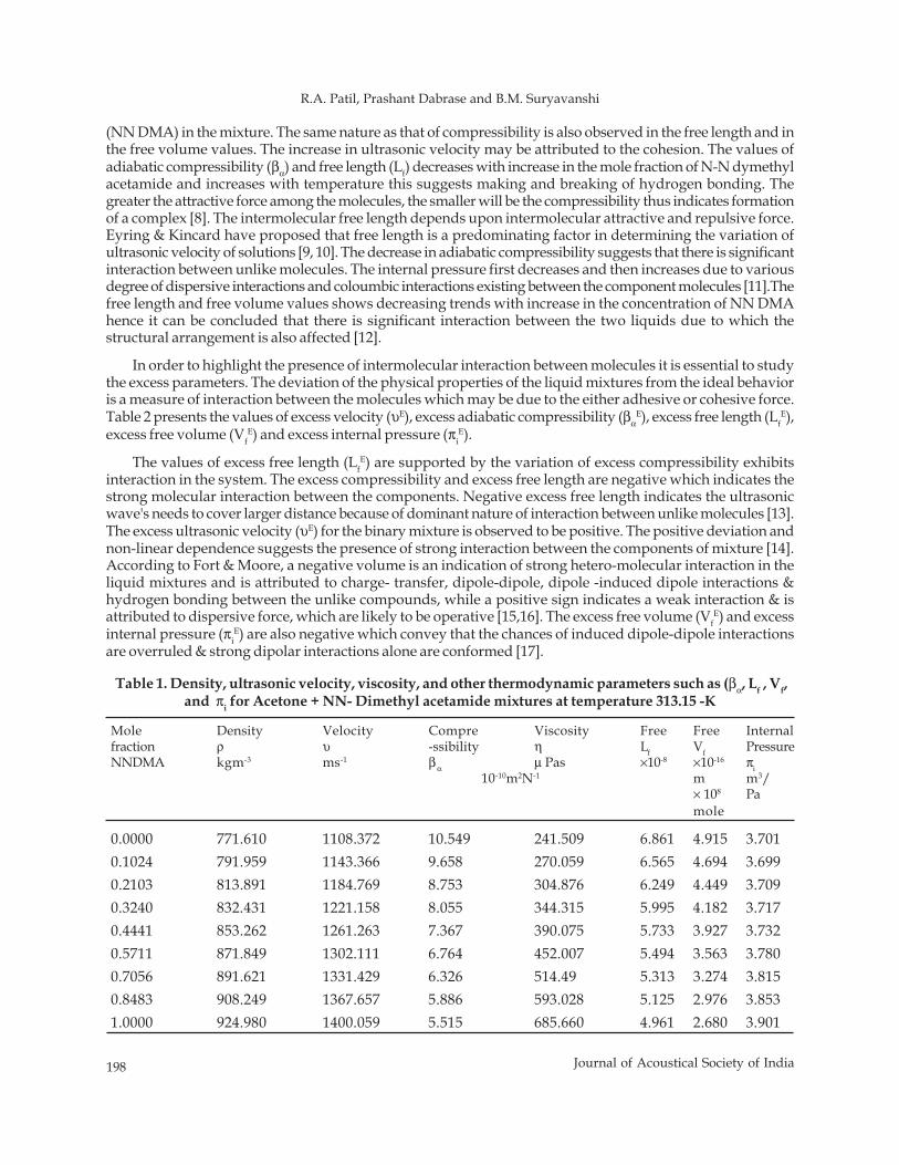
198 Journal of Acoustical Society of India
R.A. Patil, Prashant Dabrase and B.M. Suryavanshi
(NN DMA) in the mixture. The same nature as that of compressibility is also observed in the free length and inthe free volume values. The increase in ultrasonic velocity may be attributed to the cohesion. The values ofadiabatic compressibility (βα) and free length (Lf) decreases with increase in the mole fraction of N-N dymethylacetamide and increases with temperature this suggests making and breaking of hydrogen bonding. Thegreater the attractive force among the molecules, the smaller will be the compressibility thus indicates formationof a complex [8]. The intermolecular free length depends upon intermolecular attractive and repulsive force.Eyring & Kincard have proposed that free length is a predominating factor in determining the variation ofultrasonic velocity of solutions [9, 10]. The decrease in adiabatic compressibility suggests that there is significantinteraction between unlike molecules. The internal pressure first decreases and then increases due to variousdegree of dispersive interactions and coloumbic interactions existing between the component molecules [11].Thefree length and free volume values shows decreasing trends with increase in the concentration of NN DMAhence it can be concluded that there is significant interaction between the two liquids due to which thestructural arrangement is also affected [12].
In order to highlight the presence of intermolecular interaction between molecules it is essential to studythe excess parameters. The deviation of the physical properties of the liquid mixtures from the ideal behavioris a measure of interaction between the molecules which may be due to the either adhesive or cohesive force.Table 2 presents the values of excess velocity (υE), excess adiabatic compressibility (βα
E), excess free length (LfE),
excess free volume (VfE) and excess internal pressure (πi
E).
The values of excess free length (LfE) are supported by the variation of excess compressibility exhibits
interaction in the system. The excess compressibility and excess free length are negative which indicates thestrong molecular interaction between the components. Negative excess free length indicates the ultrasonicwave's needs to cover larger distance because of dominant nature of interaction between unlike molecules [13].The excess ultrasonic velocity (υE) for the binary mixture is observed to be positive. The positive deviation andnon-linear dependence suggests the presence of strong interaction between the components of mixture [14].According to Fort & Moore, a negative volume is an indication of strong hetero-molecular interaction in theliquid mixtures and is attributed to charge- transfer, dipole-dipole, dipole -induced dipole interactions &hydrogen bonding between the unlike compounds, while a positive sign indicates a weak interaction & isattributed to dispersive force, which are likely to be operative [15,16]. The excess free volume (Vf
E) and excessinternal pressure (πi
E) are also negative which convey that the chances of induced dipole-dipole interactionsare overruled & strong dipolar interactions alone are conformed [17].
Table 1. Density, ultrasonic velocity, viscosity, and other thermodynamic parameters such as (βα, Lf , Vf,and πi for Acetone + NN- Dimethyl acetamide mixtures at temperature 313.15 -K
Mole Density Velocity Compre Viscosity Free Free Internalfraction ρ υ -ssibility η Lf Vf PressureNNDMA kgm-3 ms-1 βα μ Pas ×10-8 ×10-16 πi
10-10m2N-1 m m3/× 108 Pamole
0.0000 771.610 1108.372 10.549 241.509 6.861 4.915 3.7010.1024 791.959 1143.366 9.658 270.059 6.565 4.694 3.6990.2103 813.891 1184.769 8.753 304.876 6.249 4.449 3.7090.3240 832.431 1221.158 8.055 344.315 5.995 4.182 3.7170.4441 853.262 1261.263 7.367 390.075 5.733 3.927 3.7320.5711 871.849 1302.111 6.764 452.007 5.494 3.563 3.7800.7056 891.621 1331.429 6.326 514.49 5.313 3.274 3.8150.8483 908.249 1367.657 5.886 593.028 5.125 2.976 3.8531.0000 924.980 1400.059 5.515 685.660 4.961 2.680 3.901
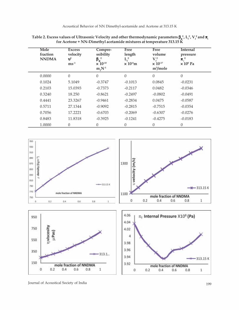
Acoustical Behavior of NN Dimethyl-acetamide and Acetone at 313.15 K
199Journal of Acoustical Society of India
Table 2. Excess values of Ultrasonic Velocity and other thermodynamic parameters βββββαααααE, Lf
E, VfE and πππππi
for Acetone + NN-Dimethyl acetamide mixtures at temperature 313.15 K
Mole Excess Compre- Free Free Internalfraction velocity ssibility length volume pressureNNDMA υυυυυE βββββ ααααα
E LfE Vf
E πππππ iE
ms-1 ××××× 10-10 ××××× 10-8m ××××× 10-17 ××××× 108 Pam2N-1 m3/mole
0.0000 0 0 0 0 00.1024 5.1049 -0.3747 -0.1013 0.0845 -0.02310.2103 15.0393 -0.7373 -0.2117 0.0482 -0.03460.3240 18.250 -0.8621 -0.2497 -0.0802 -0.04910.4441 23.3267 -0.9461 -0.2834 0.0475 -0.05870.5711 27.1344 -0.9092 -0.2815 -0.7515 -0.03540.7056 17.2221 -0.6703 -0.2069 -0.6307 -0.02760.8483 11.8318 -0.3925 -0.1241 -0.4275 -0.01831.0000 0 0 0 0 0
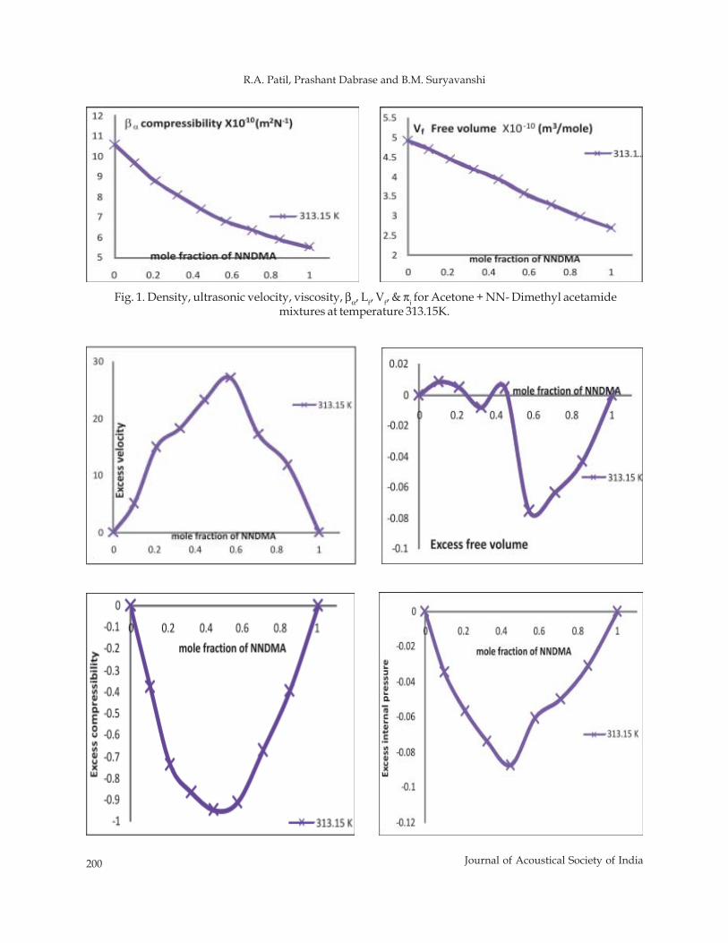
200 Journal of Acoustical Society of India
R.A. Patil, Prashant Dabrase and B.M. Suryavanshi
Fig. 1. Density, ultrasonic velocity, viscosity, βα, Lf, Vf, & πi for Acetone + NN- Dimethyl acetamidemixtures at temperature 313.15K.
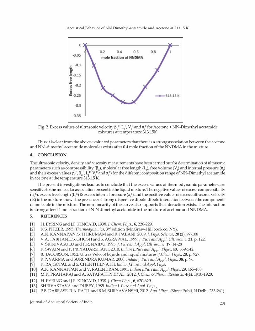
Acoustical Behavior of NN Dimethyl-acetamide and Acetone at 313.15 K
201Journal of Acoustical Society of India
Thus it is clear from the above evaluated parameters that there is a strong association between the acetoneand NN -dimethyl acetamide molecules exists after 0.4 mole fraction of the NNDMA in the mixture.
4. CONCLUSION
The ultrasonic velocity, density and viscosity measurements have been carried out for determination of ultrasonicparameters such as compressibility (βα), molecular free length (Lf), free volume (Vf) and internal pressure (πi)and their excess values (υE, βα
E, LfE, Vf
E and πiE) for the different composition range of NN-Dimethyl acetamide
in acetone at the temperature 313.15 K.The present investigations lead us to conclude that the excess values of thermodynamic parameters are
sensitive to the molecular association present in the liquid mixture. The negative values of excess compressibility(βα
E), excess free length (LfE) & excess internal pressure (πi
E) and the positive values of excess ultrasonic velocity( E) in the mixture shows the presence of strong dispersive dipole-dipole interaction between the componentsof molecule in the mixture. The non-linearity of the curve also supports the interaction exists. The interactionis strong after 0.4 mole fraction of N-N dimethyl acetamide in the mixture of acetone and NNDMA.5. REFERENCES
[1] H. EYRING and J.F. KINCAID, 1938. J. Chem. Phys., 6, 220-229.[2] K.S. PITZER, 1995. Thermodynamics, 3rd edition (Mc.Graw-Hill book co, NY).[3] A.N. KANNAPAN, S. THIRUMAM and R. PALANI, 2009. J. Phys. Science, 20 (2), 97-108[4] V.A. TABHANE, S. GHOSH and S. AGRAWAL, 1999. J. Pure and Appl. Ultrasonic, 21, p. 122.[5] V. SRINIVASULU and P.R. NAIDU, 1995. J. Pure and Appl. Ultrasonic, 17, 14-28[6] K. SWAIN and P. PRIYADARSHANI, 2010. Indian J.Pure and Appl. Phys., 48, 539-542.[7] B. JACOBSON, 1952. Ultras Velo. of liquids and liquid mixtures, J.Chem.Phys., 20, p. 927.[8] R.P. VARMA and SURENDRA KUMAR, 2000. Indian J. Pure and Appl. Phys., 38, p. 96.[9] K. RAJGOPAL and S. CHENTHILNATH, Indian J.Pure and Appl. Phys.[10] A.N. KANNAPPAN and V. RAJENDRAN, 1991. Indian J.Pure and Appl. Phys., 29, 465-468.[11] M.K. PRAHARAJ and A. SATAPATHY ET AL., 2012. J. Chem & Pharm. Research, 4(4), 1910-1920.[12] H. EYRING and J.F. KINCAID, 1938. J. Chem.Phys., 6, 620-629.[13] SHRIVASTAVA and DUBEY, 1985. Indian J. Pure and Appl. Phys.,[14] P.B. DABRASE, R.A. PATIL and B.M. SURYAVANSHI, 2012. App. Ultra., (Shree Publi, N Delhi, 233-241).
Fig. 2. Excess values of ultrasonic velocity βαE, Lf
E, VfE and πi
E for Acetone + NN-Dimethyl acetamidemixtures at temperature 313.15K

202 Journal of Acoustical Society of India
R.A. Patil, Prashant Dabrase and B.M. Suryavanshi
[15] R.T. FORT and W.R. MOORE, 1966. Trans. Farad. Soc., 62, p. 1112.[16] MOH. A. WAHAB ET AL., 2002. Bull. Korean Chem. Soc., 23 (7), 953-956.[17] S. SOUNDHARAM, 2010. Acta Ciencia India, XXXII (2), p. 285.[18] ALKA TADLKAR, PRAVINA PAWAR and GBICHILE, 2011. J. Chem. Pharm. Research, 3(3), 165-168.
Automatic Gear Teeth Defect Localization using Acoustic and Vibration Signal in Time Domain
203Journal of Acoustical Society of India
ABSTRACT
In present work a customized gear mesh test setup is prepared. The acoustic and vibration signalsare captured by introducing seeded defects in gear teeth. The bursts have been observed in timedomain signals with presence of defects and are focused in analysis. A signal processing scheme isproposed for automatic defect identification and localization of the fault in time domain. Towardsthis, the proposed scheme initially denoises the signals to improve the sharpness of the burst. TheDiscrete Wavelet Transform (DWT) has been shown suitable in enhancing the peak of the signalburst. The time frequency information of denoised signals are computed by implementing ComplexMorlet Wavelet Transform (CMWT). Furthermore, the instantaneous power spectrum is computed byintegrating coefficients in time domain. A multi scale based wavelet peak detection technique is usedto extract the peaks of the spectrum in time domain. The proposed technique has been evaluated andvalidated with captured acoustic and vibration signals. Experimental investigations reveal that theproposed technique can be implemented in real-time condition monitoring and fault diagnosis ofgear systems.
1. INTRODUCTION
Gear system is a prime component of rotating machines, power transmissions, automobiles etc. Fault diagnosisand condition monitoring of such system is highly desired for predictive maintenance purpose. The feature ofthe amplitude modulated-frequency modulated gearbox fault signal usually cannot be directly extracted. Liand Liang have implemented the time-frequency analysis to diagnose gear box fault [1]. In recent years, Li et al.investigated mechanical fault diagnosis based on redundant second generation wavelet packet transform,neighborhood rough set and support vector machine. Wang et al. have investigated rotary system fault usingdual-tree complex wavelet transform [3]. Moreover, one can find many literatures on implementation of DWT,CWT and DCT in non-stationary signal processing [4]. Rafiee et al. reported the importance on mother waveletin wavelet transform in fault diagnosis [5].
From literature, one can find many reports on implementation of various techniques of signal processingbut there is no single robust method to localize the signal burst (acoustic and vibration) in time domain tocorroborate the defect in gear or bearing. In present work, a signal processing method is proposed based uponContinuous Morlet Wavelet Transform (CMWT) of the denoised signal followed by peak detection of theinstantaneous power spectrum generated from scalogram.
2. PROPOSED TECHNIQUE
It is quite natural, that some time defect signature is carried by wider signal burst depends upon type of signal
Journal of Acoustical Society of India : Vol. 40, No. 3, 2013 (pp.203-206)
Automatic Gear Teeth Defect Localization using Acousticand Vibration Signal in Time Domain
Dibya Prakash Jena and S.N. Panigrahi*School of Mechanical Science, Indian Institute of Technology Bhubaneswar
*e-mail: [email protected]
[Received: 20.12.2012; Revised: 28.06.2013; Accepted: 22.05.2013]
© 2013 Acoustical Society of India
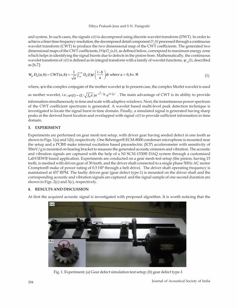
204 Journal of Acoustical Society of India
Dibya Prakash Jena and S N. Panigrahi
and system. In such cases, the signals x(t) is decomposed using discrete wavelet transform (DWT). In order toachieve a finer time frequency resolution, the decomposed detail component Dn(t) processed through a continuouswavelet transform (CWT) to produce the two dimensional map of the CWT coefficients. The generated twodimensional maps of the CWT coefficients, Wψ Dn(a,b), as defined below, correspond to maximum energy zonewhich helps in identifying the signal bursts due to defects in the piston-bore. Mathematically, the continuouswavelet transform of x(t) is defined as its integral transform with a family of wavelet functions, ψ ab(t), describedas [6,7]:
-1 -( , ) ( , ) ( ) 0,ψ ψ+∞
∞⎛ ⎞= = > ∈ℜ⎜ ⎟⎝ ⎠
∫ &n nt bW D a b CWT a b D t dt where a baa (1)
where, ψ is the complex conjugate of the mother wavelet ψ. In present case, the complex Morlet wavelet is used
as mother wavelet, i.e., 2 / 2( ) (1/ )e e πψ π −= t f f tb cbt f . The main advantage of CWT is its ability to provide
information simultaneously in time and scale with adaptive windows. Next, the instantaneous power spectrumof the CWT coefficient spectrums is generated. A wavelet based multi-level peak detection technique isinvestigated to locate the signal burst in time domain. Finally, a simulated signal is generated having sharppeaks at the derived burst location and overlapped with signal x(t) to provide sufficient information in timedomain.
3. EXPERIMENT
Experiments are performed on gear mesh test setup, with driver gear having seeded defect in one tooth asshown in Figs. 1(a) and 1(b), respectively. One Behringer® ECM-8000 condenser microphone is mounted nearthe setup and a PCB® make internal excitation based piezoelectric (ICP) accelerometer with sensitivity of50mV/g is mounted on bearing bracket to measure the generated acoustic emission and vibration. The acousticand vibration signals are captured with the help of a NI SCXI-1530® DAQ system through a customizedLabVIEW® based application. Experiments are conducted on a gear mesh test setup (the pinion, having 15teeth, is meshed with driven gear of 30 teeth, and the driver shaft connected to a single phase 50Hz AC motorCrompton® make of power rating of 0.5 HP through a belt drive). The driver shaft operating frequency ismaintained at 457 RPM. The faulty driven gear (gear defect type-1) is mounted on the driver shaft and thecorresponding acoustic and vibration signals are captured and the signal sample of one second duration areshown in Figs. 2(c) and 3(c), respectively.
4. RESULTS AND DISCUSSION
At first the acquired acoustic signal is investigated with proposed algorithm. It is worth noticing that the
Fig. 1. Experiment; (a) Gear defect simulation test setup; (b) gear defect type-1
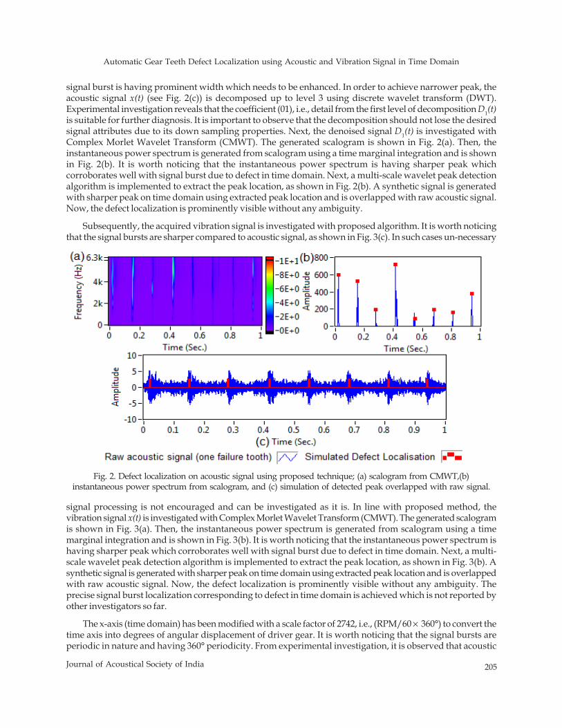
Automatic Gear Teeth Defect Localization using Acoustic and Vibration Signal in Time Domain
205Journal of Acoustical Society of India
signal burst is having prominent width which needs to be enhanced. In order to achieve narrower peak, theacoustic signal x(t) (see Fig. 2(c)) is decomposed up to level 3 using discrete wavelet transform (DWT).Experimental investigation reveals that the coefficient (01), i.e., detail from the first level of decomposition D1(t)is suitable for further diagnosis. It is important to observe that the decomposition should not lose the desiredsignal attributes due to its down sampling properties. Next, the denoised signal D1(t) is investigated withComplex Morlet Wavelet Transform (CMWT). The generated scalogram is shown in Fig. 2(a). Then, theinstantaneous power spectrum is generated from scalogram using a time marginal integration and is shownin Fig. 2(b). It is worth noticing that the instantaneous power spectrum is having sharper peak whichcorroborates well with signal burst due to defect in time domain. Next, a multi-scale wavelet peak detectionalgorithm is implemented to extract the peak location, as shown in Fig. 2(b). A synthetic signal is generatedwith sharper peak on time domain using extracted peak location and is overlapped with raw acoustic signal.Now, the defect localization is prominently visible without any ambiguity.
Subsequently, the acquired vibration signal is investigated with proposed algorithm. It is worth noticingthat the signal bursts are sharper compared to acoustic signal, as shown in Fig. 3(c). In such cases un-necessary
signal processing is not encouraged and can be investigated as it is. In line with proposed method, thevibration signal x(t) is investigated with Complex Morlet Wavelet Transform (CMWT). The generated scalogramis shown in Fig. 3(a). Then, the instantaneous power spectrum is generated from scalogram using a timemarginal integration and is shown in Fig. 3(b). It is worth noticing that the instantaneous power spectrum ishaving sharper peak which corroborates well with signal burst due to defect in time domain. Next, a multi-scale wavelet peak detection algorithm is implemented to extract the peak location, as shown in Fig. 3(b). Asynthetic signal is generated with sharper peak on time domain using extracted peak location and is overlappedwith raw acoustic signal. Now, the defect localization is prominently visible without any ambiguity. Theprecise signal burst localization corresponding to defect in time domain is achieved which is not reported byother investigators so far.
The x-axis (time domain) has been modified with a scale factor of 2742, i.e., (RPM/60 × 360°) to convert thetime axis into degrees of angular displacement of driver gear. It is worth noticing that the signal bursts areperiodic in nature and having 360° periodicity. From experimental investigation, it is observed that acoustic
Fig. 2. Defect localization on acoustic signal using proposed technique; (a) scalogram from CMWT,(b)instantaneous power spectrum from scalogram, and (c) simulation of detected peak overlapped with raw signal.
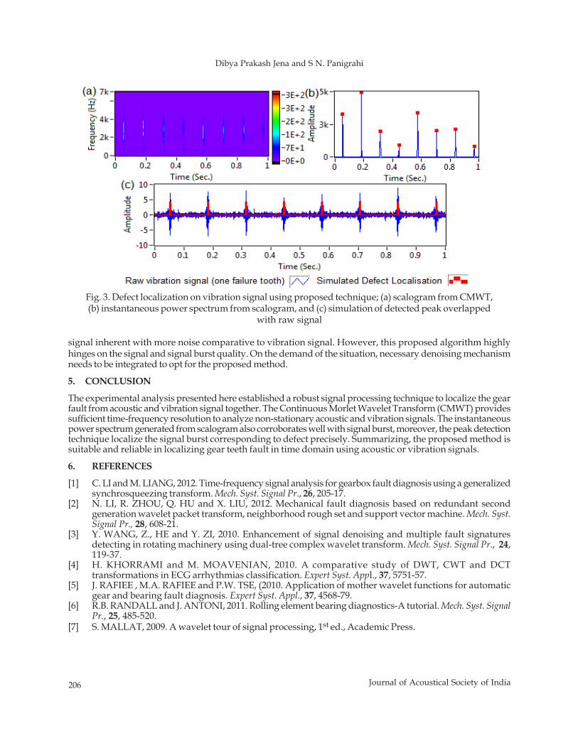
206 Journal of Acoustical Society of India
Dibya Prakash Jena and S N. Panigrahi
signal inherent with more noise comparative to vibration signal. However, this proposed algorithm highlyhinges on the signal and signal burst quality. On the demand of the situation, necessary denoising mechanismneeds to be integrated to opt for the proposed method.
5. CONCLUSION
The experimental analysis presented here established a robust signal processing technique to localize the gearfault from acoustic and vibration signal together. The Continuous Morlet Wavelet Transform (CMWT) providessufficient time-frequency resolution to analyze non-stationary acoustic and vibration signals. The instantaneouspower spectrum generated from scalogram also corroborates well with signal burst, moreover, the peak detectiontechnique localize the signal burst corresponding to defect precisely. Summarizing, the proposed method issuitable and reliable in localizing gear teeth fault in time domain using acoustic or vibration signals.
6. REFERENCES
[1] C. LI and M. LIANG, 2012. Time-frequency signal analysis for gearbox fault diagnosis using a generalizedsynchrosqueezing transform. Mech. Syst. Signal Pr., 26, 205-17.
[2] N. LI, R. ZHOU, Q. HU and X. LIU, 2012. Mechanical fault diagnosis based on redundant secondgeneration wavelet packet transform, neighborhood rough set and support vector machine. Mech. Syst.Signal Pr., 28, 608-21.
[3] Y. WANG, Z., HE and Y. ZI, 2010. Enhancement of signal denoising and multiple fault signaturesdetecting in rotating machinery using dual-tree complex wavelet transform. Mech. Syst. Signal Pr., 24,119-37.
[4] H. KHORRAMI and M. MOAVENIAN, 2010. A comparative study of DWT, CWT and DCTtransformations in ECG arrhythmias classification. Expert Syst. Appl., 37, 5751-57.
[5] J. RAFIEE , M.A. RAFIEE and P.W. TSE, (2010. Application of mother wavelet functions for automaticgear and bearing fault diagnosis. Expert Syst. Appl., 37, 4568-79.
[6] R.B. RANDALL and J. ANTONI, 2011. Rolling element bearing diagnostics-A tutorial. Mech. Syst. SignalPr., 25, 485-520.
[7] S. MALLAT, 2009. A wavelet tour of signal processing, 1st ed., Academic Press.
Fig. 3. Defect localization on vibration signal using proposed technique; (a) scalogram from CMWT,(b) instantaneous power spectrum from scalogram, and (c) simulation of detected peak overlapped
with raw signal

Acoustical Society of India(Regn. No. 65-1971)
Executive Council (2010 - 2014)
President : Dr V Rajendran[KSRCT, Tiruchengode; [email protected]; +91-99 94 13 03 03]
Vice President : NS Naidu[NSTL, Vizag; [email protected]; +91-94 90 75 05 82]
General Secretary : PVS Ganesh Kumar[NSTL, Vizag; [email protected]; +91-98 66 40 08 94]
Jt. Secretary : Dr K Trinadh[NSTL, Vizag; [email protected]; +91-97 04 71 95 00]
Treasurer : Prof AV Sharma[AU, Vizag; [email protected]; +91-94 90 43 17 26]
Chief Editor : Dr Mahavir Singh[CSIR-NPL, New Delhi; [email protected]; +91-98 71 69 33 46]
Council Members : Dr SV Ranga Nayakulu[VITAE, Hyderabad; [email protected]; +91-98 66 53 26 13]
Dr I Johnson[SJ College, Trichy; [email protected]; +91-94 42 90 48 20]
Dr Rajiv K Upadhayay[Govt PG College, Rishikesh; [email protected]; +91-94 12 97 28 90]
Dr S Shekhar[Oxford College, Trichy; [email protected]; +91-99 94 92 00 30]
Dr V Bhujanga Rao[Past President; NSTL, Vizag; [email protected]; +91-98 66 44 10 74]
Co-opted Members : Rajshekhar Uchil[Josts, Bangalore; [email protected]; +91-98 80 17 08 95]
Dr NK Narayanan[CIT, Kozhikode; [email protected]; +91-94 46 95 58 30]


INFORMATION FOR AUTHORS
ARTICLES The Journal of Acoustical Society of India (JASI) is a refereed publication published quarterly by the Acoustical Society of India(ASI). JASI includes refereed articles, technical notes, letters-to-the-editor, book review and announcements of general interest toreaders.
Articles may be theoretical or experimental in nature. But those which combine theoretical and experimental approaches tosolve acoustics problems are particularly welcome. Technical notes, letters-to-the-editor and announcements may also be submitted.Articles must not have been published previously in other engineering or scientific journals. Articles in the following are particularlyencouraged: applied acoustics, acoustical materials, active noise & vibration control, bioacoustics, communication acousticsincluding speech, computational acoustics, electro-acoustics and audio engineering, environmental acoustics, musical acoustics,non-linear acoustics, noise, physical acoustics, physiological and psychological acoustics, quieter technologies, room and buildingacoustics, structural acoustics and vibration, ultrasonics, underwater acoustics.
Authors whose articles are accepted for publication must transfer copyright of their articles to the ASI. This transfer involvespublication only and does not in any way alter the author's traditional right regarding his/her articles.
PREPARATION OF MANUSCRIPTS All manuscripts are refereed by at least two referees and are reviewed by the Publication Committee (all editors) beforeacceptance. Manuscripts of articles and technical notes should be submitted for review electronically to the Chief Editor by e-mailor by express mail on a disc. JASI maintains a high standard in the reviewing process and only accept papers of high quality. Onacceptance, revised articles of all authors should be submitted to the Chief Editor by e-mail or by express mail. Text of the manuscript should be double-spaced on A4 size paper, subdivided by main headings-typed in upper and lowercase flush centre, with one line of space above and below and sub-headings within a section-typed in upper and lower caseunderstood, flush left, followed by a period. Sub-sub headings should be italic. Articles should be written so that readers indifferent fields of acoustics can understand them easily. Manuscripts are only published if not normally exceeding twenty double-spaced text pages. If figures and illustrations are included then normally they should be restricted to no more than twelve-fifteen. The first page of manuscripts should include on separate lines, the title of article, the names, of authors, affiliations andmailing addresses of authors in upper and lowers case. Do not include the author's title, position or degrees. Give an adequatepost office address including pin or other postal code and the name of the city. An abstract of not more than 200 words shouldbe included with each article. References should be numbered consecutively throughout the article with the number appearing asa superscript at the end of the sentence unless such placement causes ambiguity. The references should be grouped together,double spaced at the end of the article on a separate page. Footnotes are discouraged. Abbreviations and special terms must bedefined if used.
EQUATIONS Mathematical expressions should be typewritten as completely as possible. Equation should be numbered consecutivelythroughout the body of the article at the right hand margin in parentheses. Use letters and numbers for any equations in anappendix: Appendix A: (A1, (A2), etc. Equation numbers in the running text should be enclosed in parentheses, i.e., Eq. (1), Eqs.(1a) and (2a). Figures should be referred to as Fig. 1, Fig. 2, etc. Reference to table is in full: Table 1, Table 2, etc. Metric units shouldbe used: the preferred from of metric unit is the System International (SI).
REFERENCES The order and style of information differs slightly between periodical and book references and between published and unpublishedreferences, depending on the available publication entries. A few examples are shown below.
Periodicals:[1] S.R. Pride and M.W. Haartsen, 1996. Electroseismic wave properties, J. Acoust. Soc. Am., 100 (3), 1301-1315.[2] S.-H. Kim and I. Lee, 1996. Aeroelastic analysis of a flexible airfoil with free play non-linearity, J. Sound Vib., 193 (4), 823-846.
Books:[1] E.S. Skudzryk, 1968. Simple and Comlex Vibratory Systems, the Pennsylvania State University Press, London.[2] E.H. Dowell, 1975. Aeroelasticity of plates and shells, Nordhoff, Leyden.
Others:[1] J.N. Yang and A. Akbarpour, 1987. Technical Report NCEER-87-0007, Instantaneous Optimal Control Law For Tall
Buildings Under Seismic Excitations.
SUMISSIONS All materials from authors should be submitted in electronic form to the JASI Chief Editor: Dr Mahavir Singh, Acoustics,Ultrasonics & Vibration Section, CSIR-National Physical Laboratory, Dr. K. S. Krishnan Road, New Delhi-110 012 (email:[email protected] Tel: +91-11-4560.8317, Fax: +91-11-4560.9310). For the item to be published in a given issue of a journal,the manuscript must reach the Chief Editor at least twelve week before the publication date.
SUMISSION OF ACCEPTED MANUSCRIPT On acceptance, revised articles should be submitted in electronic form to the JASI Chief Editor ([email protected]).
ISSN 0973-3302
Volume 40 Number 1 January 2013
A Quarterly Publication of the JASI
http://www.acousticsindia.org
OCIS E TL YA OCI FT S INU DO IAC A
AA A ~Ae ekr xk/ tk s h ku re
JOURNAL OF
ACOUSTI CAL SOCIETY
OF INDIA

Journal of AcousticalSociety of India
The Refereed Journal of the Acoustical Society of India (JASI)JASI
CHIEF EDITOR:Mahavir SinghAcoustics, Ultrasonics & Vibration SectionCSIR-National Physical LaboratoryDr. KS Krishnan RoadNew Delhi 110 012Tel: +91.11.4560.8317Fax: +91.11.4560.9310E-mail: [email protected]
ASSOCIATE SCIENTIFIC EDITOR:Applied Acoustics
Trinath KarControl Component India Pvt. Ltd6th Floor, Warp TowerPlot # 13, 14, &15SJR i-Park, EPIP Zone, Phase 1Whitefield Road, Bangalore 560066
The Journal of Acoustical Society of India is a refereed journal of the Acoustical Society of India (ASI). The ASI is anon-profit national society founded in 31st July, 1971. The primary objective of the society is to advance the science ofacoustics by creating an organization that is responsive to the needs of scientists and engineers concerned with acousticsproblems all around the world.
Manuscripts of articles, technical notes and letter to the editor should be submitted to the Chief Editor. Copies ofarticles on specific topics listed above should also be submitted to the respective Associate Scientific Editor. Manuscriptsare refereed by at least two referees and are reviewed by Publication Committee (all editors) before acceptance. Onacceptance, revised articles with the text and figures scanned as separate files on a diskette should be submitted to theEditor by express mail. Manuscripts of articles must be prepared in strict accordance with the author instructions.
All information concerning subscription, new books, journals, conferences, etc. should be submitted to Chief Editor:
Acoustics, Ultrasonics & Vibration Section, CSIR-National Physical Laboratory, Dr. KS Krishnan Road, New Delhi 110 012, Tel: +91.11.4560.8317, Fax: +91.11.4560.9310, e-mail: [email protected]
Annual subscription price including mail postage is Rs. 2000/= for institutions, companies and libraries and Rs. 2000/=for individuals who are not ASI members. The Journal of Acoustical Society of India will be sent to ASI members freeof any extra charge. Requests for specimen copies and claims for missing issues as well as address changes should besent to the Editorial Office:
Acoustics, Ultrasonics & Vibration Section, CSIR-National Physical Laboratory, Dr. KS Krishnan Road, New Delhi 110 012, Tel: +91.11.4560.8317, Fax: +91.11.4560.9310, e-mail: [email protected]
The journal and all articles and illustrations published herein are protected by copyright. No part of this journal may betranslated, reproduced, stored in a retrieval system, or transmitted, in any form or by any means, electronic, mechanical,photocopying, microfilming, recording or otherwise, without written permission of the publisher.
Copyright © 2007, Acoustical Society of IndiaISSN 0973-330
Editorial Office:
MANAGING EDITOROmkar Sharma
ASSISTANT EDITORSYudhisther KumarAnil Kumar NainNaveen Garg
Acoustics, Ultrasonics & Vibration SectionCSIR-National Physical LaboratoryDr. KS Krishnan RoadNew Delhi 110 012Tel: +91.11. 4560.8317asFax: +91.11.4560.9310E-mail: [email protected]
Printed at Alpha Printers, BG-2/38C, Paschim Vihar, New Delhi-110063 Tel.: 9811848335. JASI is sent to ASI membersfree of charge.
Journal of AcousticalSociety of India (JASI)
A quarterly publication of the Acoustical Society of India
Volume 40, Number 4, October 2013
JASI
MAHAVIR SINGH Chief Editor
OMKAR SHARMA Managing Editor
TRINATH KAR Associate Scientific Editor
Yudhishter KumarAnil Kumar NainNaveen Garg Assistant Editors
EDITORIAL BOARD
M L Munjal IISc Banglore, India
S Narayanan IIT Chennai, India
V Rajendran KSRCT Erode, India
R J M Craik HWU Edinburg, UK
Trevor R T Nightingle NRC Ottawa, Canada
B V A Rao VIT Vellore, India
N Tandon IIT Delhi, India
P Narang NMI Lindfield, Australia
E S R Rajagopal IISc Banglore, India
A L Vyas IIT Delhi, India
V Bhujanga Rao NSTL Vizag, India
Yukio Kagawa NU Chiba, Japan
S Datta LU Loughborough, UK
Sonoko Kuwano OU Osaka, Japan
K K Pujara IIT Delhi (Ex.), India
A R Mohanty IIT Kharagpur, India
Ashok Kumar NPL New Delhi, India
V Mohanan NPL New Delhi, India
EDITORIAL
Fundamental Noise Control TechniquesMahavir Singh ............................................................................... 210
ARTICLESAeroacoustics of Space Vehicles Prediction, ExperimentalDetermination and SuppressionP. Jeyajothiraj................................................................................. 211
Advancements in Acoustics - Indian ScenarioB.V.A. Rao..................................................................................... 219
Aerodynamic and Aeroacoustic Analysis of CentrifugalBlower for Noise ReductionS. Rama Krishna, Vommi Krishna, A. Rama Krishna andK. Ramji......................................................................................... 228
Optimization of Secondary Sources for Active NoiseControl in a Car Like Rigid CavityT. Ramachandran, M.C. Lenin Babu and S. Muruga Poopathy.... 233
Performance Analysis of Speckle Noise Filters forMedical Ultrasound ImagesP. Thirumoorthy and K.M. Prabusankarlal................................... 239
Ultrasonic Study of Chemical Mixture Used forPreparation of Fiber from Date Palm LeavesG. Nath, A. Sarangi and R. Paikaraay........................................... 245
Vowel Duration in the Geminate Contexts: Observationsfrom Oriya Speaking Children and AdultsVenkat Raman Prusty and Lakshmi Venkatesh............................ 250
Performance Analysis of DCT and DFT BasedSpeech CodingShijo M. Josep and P. Babu Anto...................................................... 255
Study of Molecular Interactions in Binary Mixturesthrough Ultrasonic MeasurementsS. Ponnancy and Beulah J.M. Rajkumar............................................ 261
Prcessing for Emotions Induced by HindustaniInstrumental MusicRanjan Sengupta, Anirban Patranabis, Kaushik Banerjee, TaritGuhathakurta, Samabrata Sarkar, Gautam Ganguli, Atanu Biswas,P.K. Saha and Dipak Ghosh.............................................................. 267
INFORMATIONExecutive Council of Acoustical Society of India 273
Information for Authors Inside back cover
EDITOR’S SPACE
Fundamental Noise Control Techniques
One method for controlling the sound level within a room is through dissipation of the sound energy inabsorptive materials. Sound is absorbed when a portion of the sound energy striking a surface is not reflected,but passes into the material and is converted into heat energy. Generally, higher frequencies are more easilyabsorbed than low frequencies. Materials that are good absorbers permit sound to pass through them relativelyeasily; this is why sound absorbers are generally not good sound barriers. They reduce the level of noiseinside an enclosure, because while the sound waves are being reflected from the surfaces in the room, theyinteract with the sound-absorbing materials and lose some energy each time.
However, it requires large thicknesses or many passes for the sound energy to be significantly reduced.It is important to understand the difference between sound-absorption and sound transmission loss. Materialsthat prevent the passage of sound are usually solid, fairly heavy and non-porous. A good sound absorber is15 mm of glass fiber; a good sound barrier is 150 mm of poured concrete.
Sound-absorptive materials are used to reduce the level of steady sound in a room, from a machine forexample, and to reduce the reverberance. The reverberance or liveness of a room is usually characterized byits reverberation time, the time it would take the energy of an abruptly stopped sound source to decay througha range of 60 dB. Just as sound-absorption varies with frequency, so too does reverberation time. No singlefigure rating is used to summarize reverberation time information, but the value at 500 Hz is often used forthis purpose.
Most machines generate vibration, which can be transferred to the structure of a building through themachine supports. The vibration level can be reduced by balancing the machines to reduce the forces at thesource. Transmission into the building structure can be reduced by using resilient, anti-vibration mountingsbetween the machine and the supporting structure. Common materials used as vibration isolators are rubber,cork, various types of steel springs, and glass fiber pads. The transmission of vibrational energy depends onthe resonance frequency of the machine on the resilient supports and on the energy damping in the system.The design or selection of resilient mounts is a complicated subject, best left to a competent acousticalconsultant, but it is important to know in principle where such devices should be used.
Three important measures are used in almost all noise control work. Noise shows a source placed on aresilient support inside an enclosure with high sound transmission losses and lined with sound-absorbingmaterial. If the resilient supports were omitted, the vibrational energy from the machine would pass into thebuilding structure with very little attenuation, to radiate as sound elsewhere. If the solid enclosure were notthere, the sound would pass through the sound-absorbing material with very little attenuation. If the sound-absorbing material were omitted, the reverberant sound inside the enclosure would build up and the energyloss through the enclosure would be much less than expected. All three elements should be present.
Mahavir Singh
Aeroacoustics of Space Vehicles Prediction, Experimental Determination and Suppression
211Journal of Acoustical Society of India
ABSTRACT
Aeroacoustic loading is one of important parameter in the design of space vehicle. Prediction methodsfor the estimation of aeroacoustic loading are described. Comparisons of predicted acoustic levelswith flight measurements of a typical space vehicle are given. Need for accurate determination isbrought out. Methods of accurate determination of acoustic levels are presented. Ways of suppressing/reducing the aeroacoustic loading are mentioned.
1. INTRODUCTION
Aeroacoustics is the youngest of classical mechanics branch. It can be defined as the study of “science ofsound generated aerodynamically”. Turbulence is the main source of aerodynamics sound generation. Physicalunderstanding of the origin of sound produced by turbulence was first brought out by Micheal James Lighthill [1].Success of supersonic and hypersonic commercial transport aircraft depends on meeting stringent acceptablesound level specification specified by civil aviation authorities. Besides, a reduction of 5 dB in sound levelson hypersonic aircraft increases its fatigue life by an order of magnitude. In space transportations, specificationof low sound levels in the payload bay of launch vehicles is one of the finest features for offering commerciallaunch services.
Space vehicles experience very high intensity aeroacoustic levels. Shock wave oscillation can generatelevels as high as 172 dB. Separated flow regime in boat-tail region of payload fairing induces levels ofmagnitude 160 dB. For space vehicle components, acoustic levels higher than 150 dB are dangerous. Theycan lead to (i) fatigue failure of light weight structural components, electronic circuit boards and electricalconnections, (ii) wear and deformation of bearings and (iii) malfunction of electronic components. Hence, itis essential to characterize the aeroacoustic loading at preliminary stage of the space vehicle design.
Even with the exponential growth in the computational capability and advancement in numerical schemes,it is not possible to characterize the aeroacoustic loading of space vehicle from first principle. Hence, oneneeds to resort to semi-analytical or empirical method to determine the aeroacoustic loadings and use themfor the initial design. After finalization of the space vehicle configuration, accurate aeroacoustic levels aredetermined through subscale model tests. Based on the severity of the aeroacoustic levels, proper suppression/reduction schemes are planned. These aspects are described in this paper.
2. METHODS OF ESTIMATING SPACE VEHICLE AEROACOUSTIC LOADING
2.1 Prediction of Lift-off Aeroacoustics (Jet Noise)
Journal of Acoustical Society of India : Vol. 40, No. 4, 2013 (pp. 211-218)
Aeroacoustics of Space Vehicles Prediction,Experimental Determination and Suppression
P. JeyajothirajVSSC, ISRO, Trivandrum (Kerala)e-mail: [email protected]
[Received: 09.12.2012; Revised: 29.06.2013; Accepted: 27.10.2013]
© 2013 Acoustical Society of India
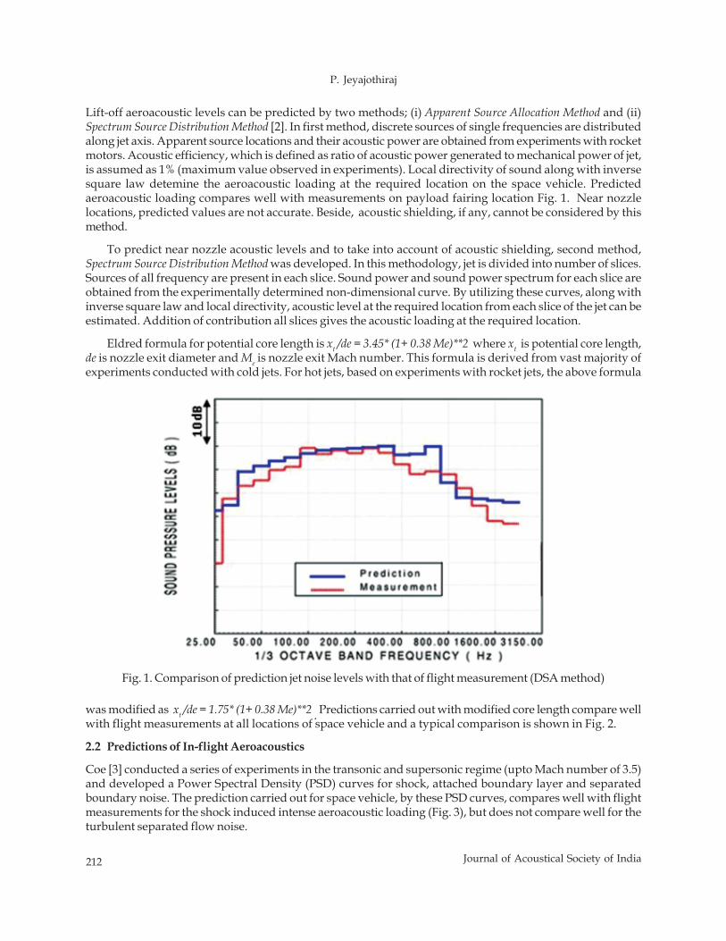
212 Journal of Acoustical Society of India
P. Jeyajothiraj
Lift-off aeroacoustic levels can be predicted by two methods; (i) Apparent Source Allocation Method and (ii)Spectrum Source Distribution Method [2]. In first method, discrete sources of single frequencies are distributedalong jet axis. Apparent source locations and their acoustic power are obtained from experiments with rocketmotors. Acoustic efficiency, which is defined as ratio of acoustic power generated to mechanical power of jet,is assumed as 1% (maximum value observed in experiments). Local directivity of sound along with inversesquare law detemine the aeroacoustic loading at the required location on the space vehicle. Predictedaeroacoustic loading compares well with measurements on payload fairing location Fig. 1. Near nozzlelocations, predicted values are not accurate. Beside, acoustic shielding, if any, cannot be considered by thismethod.
To predict near nozzle acoustic levels and to take into account of acoustic shielding, second method,Spectrum Source Distribution Method was developed. In this methodology, jet is divided into number of slices.Sources of all frequency are present in each slice. Sound power and sound power spectrum for each slice areobtained from the experimentally determined non-dimensional curve. By utilizing these curves, along withinverse square law and local directivity, acoustic level at the required location from each slice of the jet can beestimated. Addition of contribution all slices gives the acoustic loading at the required location.
Eldred formula for potential core length is xt /de = 3.45* (1+ 0.38 Me)**2 where xt is potential core length,de is nozzle exit diameter and Me is nozzle exit Mach number. This formula is derived from vast majority ofexperiments conducted with cold jets. For hot jets, based on experiments with rocket jets, the above formula
Fig. 1. Comparison of prediction jet noise levels with that of flight measurement (DSA method)
was modified as xt /de = 1.75* (1+ 0.38 Me)**2 . Predictions carried out with modified core length compare wellwith flight measurements at all locations of space vehicle and a typical comparison is shown in Fig. 2.
2.2 Predictions of In-flight Aeroacoustics
Coe [3] conducted a series of experiments in the transonic and supersonic regime (upto Mach number of 3.5)and developed a Power Spectral Density (PSD) curves for shock, attached boundary layer and separatedboundary noise. The prediction carried out for space vehicle, by these PSD curves, compares well with flightmeasurements for the shock induced intense aeroacoustic loading (Fig. 3), but does not compare well for theturbulent separated flow noise.
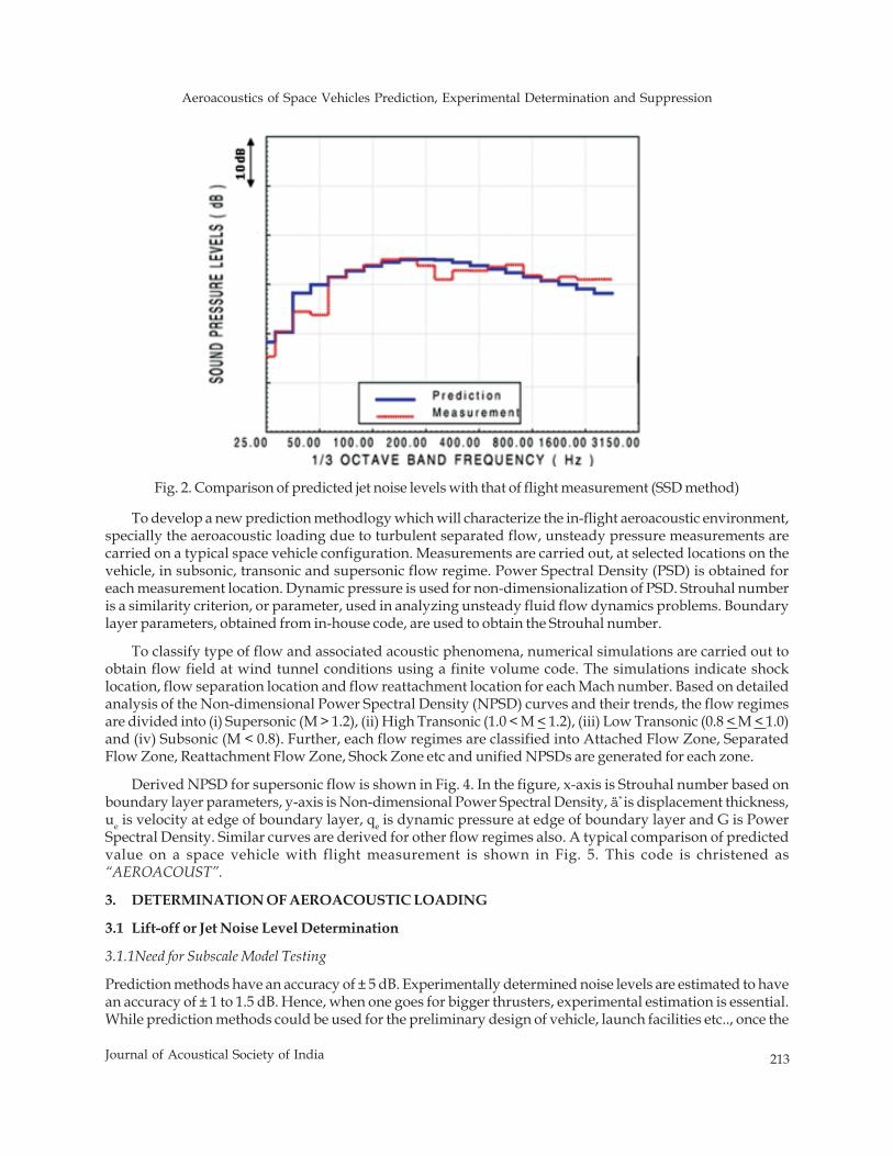
Aeroacoustics of Space Vehicles Prediction, Experimental Determination and Suppression
213Journal of Acoustical Society of India
To develop a new prediction methodlogy which will characterize the in-flight aeroacoustic environment,specially the aeroacoustic loading due to turbulent separated flow, unsteady pressure measurements arecarried on a typical space vehicle configuration. Measurements are carried out, at selected locations on thevehicle, in subsonic, transonic and supersonic flow regime. Power Spectral Density (PSD) is obtained foreach measurement location. Dynamic pressure is used for non-dimensionalization of PSD. Strouhal numberis a similarity criterion, or parameter, used in analyzing unsteady fluid flow dynamics problems. Boundarylayer parameters, obtained from in-house code, are used to obtain the Strouhal number.
To classify type of flow and associated acoustic phenomena, numerical simulations are carried out toobtain flow field at wind tunnel conditions using a finite volume code. The simulations indicate shocklocation, flow separation location and flow reattachment location for each Mach number. Based on detailedanalysis of the Non-dimensional Power Spectral Density (NPSD) curves and their trends, the flow regimesare divided into (i) Supersonic (M > 1.2), (ii) High Transonic (1.0 < M < 1.2), (iii) Low Transonic (0.8 < M < 1.0)and (iv) Subsonic (M < 0.8). Further, each flow regimes are classified into Attached Flow Zone, SeparatedFlow Zone, Reattachment Flow Zone, Shock Zone etc and unified NPSDs are generated for each zone.
Derived NPSD for supersonic flow is shown in Fig. 4. In the figure, x-axis is Strouhal number based onboundary layer parameters, y-axis is Non-dimensional Power Spectral Density, ä* is displacement thickness,ue is velocity at edge of boundary layer, qe is dynamic pressure at edge of boundary layer and G is PowerSpectral Density. Similar curves are derived for other flow regimes also. A typical comparison of predictedvalue on a space vehicle with flight measurement is shown in Fig. 5. This code is christened as“AEROACOUST”.
3. DETERMINATION OF AEROACOUSTIC LOADING
3.1 Lift-off or Jet Noise Level Determination
3.1.1Need for Subscale Model Testing
Prediction methods have an accuracy of ± 5 dB. Experimentally determined noise levels are estimated to havean accuracy of ± 1 to 1.5 dB. Hence, when one goes for bigger thrusters, experimental estimation is essential.While prediction methods could be used for the preliminary design of vehicle, launch facilities etc.., once the
Fig. 2. Comparison of predicted jet noise levels with that of flight measurement (SSD method)
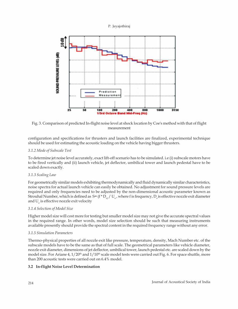
214 Journal of Acoustical Society of India
P. Jeyajothiraj
configuration and specifications for thrusters and launch facilities are finalized, experimental techniqueshould be used for estimating the acoustic loading on the vehicle having bigger thrusters.
3.1.2 Mode of Subscale Test
To determine jet noise level accurately, exact lift-off scenario has to be simulated. i.e (i) subscale motors haveto be fired vertically and (ii) launch vehicle, jet deflector, umbilical tower and launch pedestal have to bescaled down exactly.
3.1.3 Scaling Law
For geometrically similar models exhibiting thermodynamically and fluid dynamically similar characteristics,noise spectra for actual launch vehicle can easily be obtained. No adjustment for sound pressure levels arerequired and only frequencies need to be adjusted by the non-dimensional acoustic parameter known asStrouhal Number, which is defined as S= (f * De) / Ue , where f is frequency, De is effective nozzle exit diameterand Ue is effective nozzle exit velocity
3.1.4 Selection of Model Size
Higher model size will cost more for testing but smaller model size may not give the accurate spectral valuesin the required range. In other words, model size selection should be such that measuring instrumentsavailable presently should provide the spectral content in the required frequency range without any error.
3.1.5 Simulation Parameters
Thermo-physical properties of all nozzle exit like pressure, temperature, density, Mach Number etc. of thesubscale models have to be the same as that of full scale. The geometrical parameters like vehicle diameter,nozzle exit diameter, dimensions of jet deflector, umbilical tower, launch pedestal etc. are scaled down by themodel size. For Ariane 4, 1/20th and 1/10th scale model tests were carried out Fig. 6. For space shuttle, morethan 200 acoustic tests were carried out on 6.4% model.
3.2 In-flight Noise Level Determination
Fig. 3. Comparison of predicted In-flight noise level at shock location by Coe's method with that of flightmeasurement
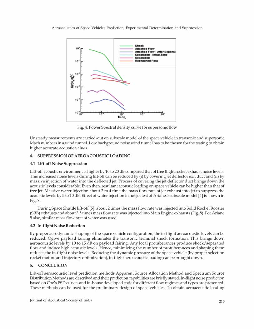
Aeroacoustics of Space Vehicles Prediction, Experimental Determination and Suppression
215Journal of Acoustical Society of India
Unsteady measurements are carried-out on subscale model of the space vehicle in transonic and supersonicMach numbers in a wind tunnel. Low background noise wind tunnel has to be chosen for the testing to obtainhigher accurate acoustic values.
4. SUPPRESSION OF AEROACOUSTIC LOADING
4.1 Lift-off Noise Suppression
Lift-off acoustic environment is higher by 10 to 20 dB compared that of free flight rocket exhaust noise levels.This increased noise levels during lift-off can be reduced by (i) by covering jet deflector exit duct and (ii) bymassive injection of water into the deflected jet. Process of covering the jet deflector duct brings down theacoustic levels considerable. Even then, resultant acoustic loading on space vehicle can be higher than that offree jet. Massive water injection about 2 to 4 time the mass flow rate of jet exhaust into jet to suppress theacoustic levels by 5 to 10 dB. Effect of water injection in hot jet test of Ariane 5 subscale model [4] is shown inFig. 7.
During Space Shuttle lift-off [5], about 2 times the mass flow rate was injected into Solid Rocket Booster(SRB) exhausts and about 3.5 times mass flow rate was injected into Main Engine exhausts (Fig. 8). For Ariane5 also, similar mass flow rate of water was used.
4.2 In-flight Noise Reduction
By proper aerodynamic shaping of the space vehicle configuration, the in-flight aeroacoustic levels can bereduced. Ogive payload fairing eliminates the transonic terminal shock formation. This brings downaeroacoustic levels by 10 to 15 dB on payload fairing. Any local protuberances produce shock/separatedflow and induce high acoustic levels. Hence, minimizing the number of protuberances and shaping themreduces the in-flight noise levels. Reducing the dynamic pressure of the space vehicle (by proper selectionrocket motors and trajectory optimization), in-flight aeroacoustic loading can be brought down.
5. CONCLUSION
Lift-off aeroacoustic level prediction methods Apparent Source Allocation Method and Spectrum SourceDistribution Methods are described and their prediction capabilities are briefly stated. In-flight noise predictionbased on Coe’s PSD curves and in-house developed code for different flow regimes and types are presented.These methods can be used for the preliminary design of space vehicles. To obtain aeroacoustic loading
Fig. 4. Power Spectral density curve for supersonic flow
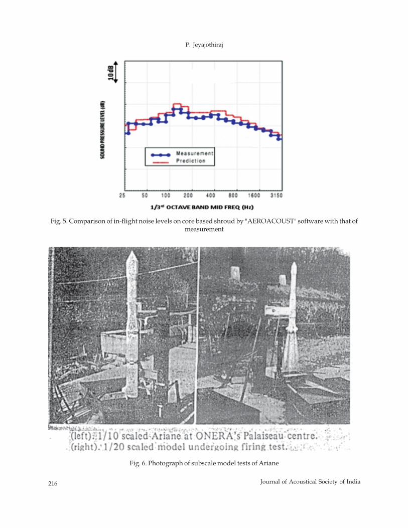
216 Journal of Acoustical Society of India
P. Jeyajothiraj
Fig. 5. Comparison of in-flight noise levels on core based shroud by "AEROACOUST" software with that ofmeasurement
Fig. 6. Photograph of subscale model tests of Ariane
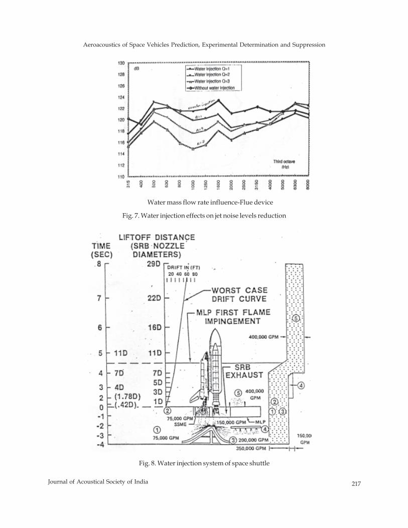
Aeroacoustics of Space Vehicles Prediction, Experimental Determination and Suppression
217Journal of Acoustical Society of India
Water mass flow rate influence-Flue device
Fig. 7. Water injection effects on jet noise levels reduction
Fig. 8. Water injection system of space shuttle
218 Journal of Acoustical Society of India
P. Jeyajothiraj
accurately, subscale model tests have to be carried out. Simulation parameters for subscale and scalingmethods are presented. Lift-off aeroacoustic levels can be reduced by covering jet deflector exit duct and bymassive water injection into deflected jets. In-flight aeroacoustic levels can be reduced by minimizing numberof protubrances and by reducing dynamic pressure encountered by space vehicle.
6. REFERENCES
[1] M.J. LIGHTHILL, 1952. Proceedings of the Royal Society of London, On Sound Generated Aerodynamically,I. General Theory, 211A(1107), 564-587.
[2] K.M. ELDRED, 1971. Acoustic Loads Generated by the Propulsion System, NASA SP-8072, Langley ResearchCenter, Virginia, United States.
[3] C.F. COE, W.J. CHYU and J.B. DODS JR, 1973. Pressure Fluctuations Underlying Attached and SeparatedSupersonic Turbulent Boundary Layers and Shock Waves”, AIAA No 73-996, Aeroacoustics Conference,Seattle, Washington.
[4] D. GELY, G. ELIAS, C. BRESSON, H. FOULTUNAND and S. RADULOVIc, 2000. Reduction of SupersonicJet Noise. Application to the Ariane 5 Launch Vehicle, AIAA 2000-2026, 6th AIAA/CEAS AeroacousticConference, Lahaina, Hawaii.
[5] M. C. COODY, H. K. PRAtt and D. E. NEWBROUGH, 1982. The Development and Verification of ShuttleOrbiter Random Vibration Test Requirements, Shock and Vibration Bulletin, 52 (2), 71–80.
Advancements in Acoustics - Indian Scenario
219Journal of Acoustical Society of India
Advancements in Acoustics - Indian Scenario
B.V.A. RaoFNAE.,Advisor (International Relations),
K L University, Vijayawada (Andhra Pradesh)
1. INTRODUCTION
The science of acoustics, one of the oldest branches of physics, embraces the design of indoor environment toachieve acceptable levels of communication, comfort and privacy for the occupants. Acoustical issues includeroom shaping, reverberation control, speech clarity and Noise control. Virtually every space demands acousticattention in order to function for its specified purpose like homes, offices, classrooms, factories, auditoriums,theaters and conference rooms.
Acoustical designing, problem solving needs technical expertise and experience in this field. It also has tobe carried out with close association with other designing agencies and giving required flexibility to aesthetics.
Acoustics is an increasingly active subject in India. The awareness for sound control is growing by theday. With the industry growing at a rapid pace combined with innovative architectural designs, challenges inthe acoustical design are increasing. In India, acoustics is a serous business today with plenty of acousticalresearch happening industrial as well as in architectural acoustics. NVIT is the criteria for modern automobiles.In addition, quieter technologies is the buzz word for all our industrial machinery.
2. INDUSTRIAL ACOUSTICS
Industrial acoustics primarily deals with noise control. With the pollution control board of India issuinggazette notification of sound levels to be emitted from machines, the design for quieter technologies is the needof the hour. Every major machine manufacturer is working towards manufacturing quieter machines. In thisprocess, there are a lot of acoustical test cells and anechoic chambers are being constructed. NVH unit hasbecome a compulsory department in big industries.
Major automotive companies in India like Tata Motor Ltd. Mahindra and Mahindra, Hero Honda, TVSMotor, Toyota Kirloskar Motors, Bajaj Auto, all have their own NVH test centres. The NVH test centres includeengine test cells, dynamometer test cells and an anechoic chamber for noise labeling. Every machinery orappliance that have to be exported must carry a label declaring the sound power levels emitted by the product.Appliances majors like the BPL, Videocon, etc also claim their own acoustical testing centres. GE BEL, GE ITC,Tatas have all invested in test cells for acoustical testing.
Many public sector companies have been involved in NVH testing. Institutions like National AerospaceLaboratories, Gas Turbine Research Establishment, Fluid Control Research Institute, Automotive ResearchAuthority of India, etc have invested in huge Test Cells and Anechoic Chambers. We have the NationalPhysical Laboratory in Delhi that has an anechoic chamber used for testing and certifying acoustical materials.IISc, the premier research institute of India has its own acoustical department with valuable research happeningin vibro-acoustics, mufflers, aero and ocean acoustics. IIT Madras contributed significantly to machine dynamicproblems and noise studies.
Journal of Acoustical Society of India : Vol. 40, No. 4, 2013 (pp.219-227)
[Received: 13.02.2013; Revised: 26.05.2013; Accepted: 27.09.2013]
© 2013 Acoustical Society of India
220 Journal of Acoustical Society of India
B.V.A. Rao
3. ARCHITECTURAL ACOUSTICS
The need for good acoustic within buildings has become a criterion. More and more people rely on acousticalconsultants for designing acoustically good spaces, be it in modern day office spaces, conference rooms,auditoriums or home theaters.
The modern day office spaces are being designed and constructed keeping acoustics as an importantcriterion. With people spending more and more time in the offices, it is important to provide them with betterwork places to improve efficiencies. There are also international guidelines for the decibel level, noise criterionwithin office spaces, which are followed by many of the MNC's setting up offices in India. Hence officeacoustical design has become a must in India. Also, with respect to Call-Centres, the design of acousticalbarriers between seats has become important.
Most of the offices have video conferencing facilities installed in their conference rooms and trainingcentres. Good acoustics with least distortions are a must and should be in these kinds of facilities.
Coming to auditorium designs. Any new auditorium being constructed has an acoustical consultant in itsdesign team. The acoustical consultant is being involved from the concept stage of the auditorium construction.Older are being completely refurbished to accommodate for good acoustics. All the universities are inclined toimprove the acoustics of their auditoriums, which have exited for a while now. Though majority of theauditoriums being constructed are for multi-purpose usage, there are a few auditoriums coming in places likeBangalore and Mysore that are being specially constructed for either drama, concerts or for speech purposes.The syndicate of Mysore University have decided to refurbish their syndicate hall to comply with the modernday standards by acoustically isolating the hall as well as providing good acoustics within the hall includingelectro acoustical facilities.
There are number of studios that have come up in India. With ever increasing television channels andradio stations, studio designing has become very important. Unlike yesteryears, companies opening upstudios are very particular about acoustical consultants being involved with their studio design. Satelliteradio station World Space recently set up 6 RJ studios in Bangalore and one in Hyderabad. The A R Rehmanstudio in Chennai can be considered as one of the best sound recording studios in India.
With the number of multiplexes growing in numbers rapidly in India, single screen theatres could behistory soon. With four to twelve auditoriums constructed adjacent to each other with common walls inbetween, the acoustical design becomes very critical and important. This apart, the multiplexes are generallysituated inside shopping malls make noise control measures inside the auditoriums even more significant.The new companies issue these certificates, only when the theatres comply with the acoustical parametersissued by these companies.
Home Theatres have become a life style statement. More and more houses insist in having a room dedicatedfor music and movies. Acoustical deign for such spaces have become popular and competitive.
Medical institutions and hospitals too are seeking acoustical consultants expertise in construction of theirAudiometric Rooms. All India Institute of Speech and Hearing in Mysore have half a dozen audiometricrooms constructed. There are independent hearing clinics with audiometric rooms that have come up in largecities.
Acoustical design is widely used in HVAC installations too. Be it for offices, theatres or auditoriums, thechiller machines noise should not be carried through the ducts. This apart, apartments and buildings situatedclose to noisy points like a busy road near an airport are seeking the services of acoustical experts for solutionfrom noise
4. ACOUSTICAL MATERIALS
One finds a wide range of companies that are manufacturing acoustical materials like tiles and barriers. There
Advancements in Acoustics - Indian Scenario
221Journal of Acoustical Society of India
are many materials like gypsum-based products, fibreglass wool based, rockwool based, mineral wool based,wood wool based, foam based and latest, polyster fibre base products. Various companies manufacture theseproducts in India who would also provide acoustical design and to name few:
♦ Noise and Heart Control System - Bangalore
♦ Acoustics India Limited - Tiruchirappalli, Tamil Nadu
♦ Sound Wizard - Pondicherry
♦ Anutone Acoustics - Bangalore
♦ Rockwell India Limited - Mumbai
♦ Jal Mistry Consultants - Mumbai
♦ Sanjay Suri Consultants - New Delhi
♦ Mikasha International - New Delhi
♦ Air Control - Chennai
♦ Parimal Mehtha Consultants - MumbaiConsiderable researching is done in these fields at Building Research Institute (Roorkee), NPL (Delhi) and
many other private industries like Beardsell, Anutone., etc.,
Classical examples of acoustic materials can be seen in the following illustrations
4.1 Acoustical Analysis Shows Temple Transforms Echoes into Sound of Nature
Mayan tombs have been analyzed and researchers have found that they were designed to produce incrediblyweird sound effects. If you stand in front of the staircase of the E1 Castillo pyramid and clap your hands, you'llhear an echo that sounds like the chirp of a bird. If you walk up the stones steps, it produces a flurry of echoesthat sounds like rain falling into a bucket. Declercq's team has shown that the height and spacing of thepyramid's steps creates like an acoustic filter that emphasizes some sound frequencies, while suppressingothers. But more detailed calculations of the acoustics shows that the echo is also influenced by other, andmore complex factors, such as the mix of frequencies of the sound source.
Rani Gumpha is the current local name given to the largest structure in a group of excavated caves nearKhandagiri, very close to Orissa's state capital, Bhubaneswar. The structure dates to about 2 to 3 century BC,the period just after Ashoka.
In Indian archaeological terms, it is a very early site, and represents an important transitional period in thecountry's history.Could this have been a theatre? Or at least, some kind of a performance space? The suggestionhas been put forward before, notably by the art historian Percy Brown and Dhiren Dash, a theatre activist fromthe region. But the general explanation (offered by the archaeological Survey India and others) has been thesewere just another set of caves set apart for meditation.
4.1.1 Physical, Underwater & Atmospheric Acoustics (includes Ultrasound & Sonars)
60 to 70% of the publications at NSA conferences belong to this category, essentially application of ultrasonicto Sensors, Sonars and Chemical activity. IIT, Delhi; NOI, Goa; NPOL, Cochin; NSTL, Vizag are some otherleading institutions.
4.1.2 Medical, Psycho & Bio Acoustics
Considerable work is going on in the field of Audiology, Cochlear implants and similar studies involvinghuman health and consequent physiological and psychological effects for both low frequency and highfrequency sounds. Good work is done at MMC, Chennai, AIIMH, New Delhi etc., They have also contributed
222 Journal of Acoustical Society of India
B.V.A. Rao
to the Mitigation of Noise Pollution and awareness of biological effects. There is a large population, whocannot understand the implications or consequences of this. After all noise is an invisible pollution, and whatthe eyes cannot see, the mind does not register it. In most of our industries, one can witness workers operatingwithout using ear muffs and getting exposed to more than 100 to 120 dBA. Most of our carpenters are easilyprone to duffness, so also drill operators.
4.2 Establishment of Bio-acoustic Analysis Facility at Wildlife Institute of India: Acoustical Studies onPycnonotus bubuls
Bioacoustics is the study of animal acoustic signals, their production and perception mechanisms. It attemptsto understand relationships between the structure of sounds and the nature of environment in which they areused. Proper documentation and recording of acoustics signals provide important base-line date for researchin the field of systematic, behaviour, and play-back tools for survey and census. Establishment of bio-acousticlaboratories and animal sound archives are the fundamental needs to initiate such studies. Acoustic signalsof Red-vented bulbul and Himalayan bulbul were recorded in their natural habitats during March 2002 toJune 2003. Both species used their own vocal repertories.
4.3 Acoustic technology by Japanese Team to Study Dolphins in Chilka
A seven-member Japanese team, led by Prof. Tamaki Ura University of Tokyo, has introduced an acoustictechnology to observe the behavoiur and eco-system of rare endangered Irrawady Dolphins in Chilka Lake.
The team in association with the Chilka Development Authority, and experts from IIT, Delhi, and WWFIndia, conducted a pilot application of the study. Dr Ura mentioned that such acoustic study using the soundpulses of a specified signal has been carried out with the support of the Japanese Ministry of Education,Culture, Sports, Science and Technology. The Chilka system, he said, would be a major step for introducingand testing a day and night automated acoustic survey system for different species of endangered marinemammals. He hinted that a more ambitious survey of the Ganges River Dolphin would be soon carried outwith the participating agencies using the new technology. Prof Ura said the pilot study carried out by the teamrevealed the presence of the Irrawady Dolphins at selected five pockets of the Chilka Lagoon. He said the teamreceived many preliminary data on the concentration of the Dolphins at four points, which would be furtheranalyzed at Tokyo to find out the underwater behaviour of the marine mammal.
The team claimed that the pilot study revealed that the Irrawady Dolphin moves at two meter per second.
4.3.1 Engineering & Machinery Acoustics (including transportation)
This is one of the largest contributors to our noise pollution in various forms including traffic covering bothsurface and air. India failed to meet global challenges in term of noise standards. Our machines produce moresound and vibration than their counterparts manufactures elsewhere. For the designers, this is the lastpriority. With more global inputs, things are getting better due to usage of suitable materials as well asmanufacturing and assembling skills. Lot of attention is being paid to this aspect now to meet the challengesby going to quieter technologies. We have noise standards, but rarely these are strictly followed. Our industryappreciates both vibrations and noise diagnostics as a strategy for CBM, but very few organizations areserious about this implementation. For the past three decades considerable awareness has gone in thisdirection, yet we have to go a long way. IIT Madras, IIT Delhi, IIPE, many of our power plants and cementplants have contributed significantly to this novel technique. Academic Research involved considered suchaspects as efficiency of sensors and instrumentation, inspection systems, and lastly economic benefits throughcost model developments. This is one of the area in which I have personally taken interest in last three decadesincluding introduction of courses like Diagnostic Maintenance in Condition Monitoring programmes. Thesewere also highlighted in number of seminars and conferences. There are both passive and active techniquesthat are being researched in this quieter effort. IITs, IISc, Space and Defence Organizations have played a majorrole.
Advancements in Acoustics - Indian Scenario
223Journal of Acoustical Society of India
4.3.2 Music, Speech and Signal Processing (Electro Acoustics)
Next to Physical Acoustics, comes this field in our country with considerable contributions. This is essentiallycontributed by our electronic specialists from TIFR, Mumbai, IISc., Bangalore, CEERI (Pilani & Delhi), AIISH(Mysore) and many other centres throughout the country. There is a small group working on Musical Acousticsin Pune. The work involves speech analysis, speech processing & speech therapy. Most of our medical unitsdealing with ENT have good audiology sections and significant contributions.
4.4 IBM India Research Lab - Speech Technologies
The design and implementation of computer systems that can cover whole range of human-like interaction byusing faces and voices is one of the challenging objectives of the Speech Group at the India Research Lab (IRL).The group aims to build state-of-the-art speech recognition/synthesis system for Indian languages and improvethe existing techniques in general. IRL is currently pursuing activities in the areas of:
Indian Language Desktop Speech Recognition
Indian language Telephony Speech Recognition
Indian-English Text-to-speech synthesis I4.4.1 Environmental & Community Noise (Noise pollution)
This is one of the major problems in the country due to lack of knowledge and education. This is a country thatpays considerable weightage for religious, cultural and political ceremonies, where noise dominates. Noiselegislations are there, framed by both CPCB and State PCB's. But hardly people pay attention. The industry,traffic and the community all contribute together to produce the Noise Pollution. I was one of the expertmembers to draft noise standards for the Ministry of Environment. It pains me to say the whole effort has gonewaste, as no serious attention is paid at any level. Honking is anybody's business in this country, and when nohonking is heard, the person thinks nothing is coming behind him or her. Movies have been made on this forscreening in theatres, and many other steps were taken. During 1982-84, I served as Chairman for constructionnoise in Singapore introducing 5 mn standard for Leq. There was an opposition, but it was Singapore!Discipline is lacking in our country.
4.4.2 Random and Non-linear Acoustics, Jet Noise, Aero Acoustics & Chaos
These are highly specialized areas involving modern jet noises and their control (more due to aerodynamiceffect). Some work was done at IIT Madras for producing 160-180 dB noise levels to impinge on rocket modelsto study their acoustic transmissibilities. These facilities have now been created at NAL Bangalore. Significantpractical work was carried out both at IISc., Bangalore & NAL. Considerable work is being done on randomnoise, non linear acoustics and chaos theory relating to stabilities. I was involved in establishing NEF contoursfor the Meenambakkam airport in Chennai and extrapolate it to Pondicherry. This was done some 15 yearsago and still Pondicherry airport has not yet been commissioned, though the airfield was put up at an enormouscost.
Fluent announced coupling with LMS SYSNOISE for Acoustics Modeling on August 8, 2003. Lebanon,NH, USA and Leuven, Belgium Fluent Inc. and LMS International announced later the release of the worldleading Vibro-Acoustics software LMS SYSNOISE Rev 5.6, which supports import of transient data fromFLUENT 6.1, the leading computational fluid dynamic (CFD) software from Fluent. This allows resultsfrom FLUENT to be used for comprehensive computational aero-acoustics simulations within SYSNOISERev5.6, complementing FLUENT 6.1's native aero-acoustics modeling capabilities.
Computational aero-acoustics is a critical technology for engineers in virtual prototyping environments,who want to predict and compare the aero-acoustics performance of proposed designs. By usingcomputational tools to identify and rank sources of flow-induced noise, engineers are able to design fornoise reduction early in their design cycle, enabling them to produce better products, while reducing theneed for expensive physical testing, and shortening the overall time to market.

224 Journal of Acoustical Society of India
B.V.A. Rao
4.4.3 Application of Holography in Jet Acoustics Studies
Source strength distribution on a jet boundary was obtained from measurements using the principle of acousticholography. Measurements were conducted in an open field. Measurement of acoustics pressure on a cylindricaltwo dimensional contour located close to the vibrating jet boundary was used to obtain the acoustic sourcestrength distribution of the sound field on to a cylindrical surface. A jet emanating from 5mm convergentnozzle was used for the holography experiments, assuming symmetry. Experimental results were comparedwith results obtained from holography.
4.4.4 Low Frequency Sound And Physiological Effects
• In 1665, people in London heard the gun fire from English and Dutch men in the battle in North Sea.
• In 1883, volcanic eruption in Krakotoa from infrasonic waves traveled 5 times around the world.
• In 1933 Greenwood's famous novel 'Love on the Dole' mentions that 'the thump of the presses makes theworkers feel sick'.
• In 1973 the 1st International conference on Informative was held in Paris.
• In 1980 the 1st International Conference on low frequency noise. Regrettably even there is widespreadignorance as to its quantitative and subjective effects, no convenient measurement unit to describe it and nodefinitive guidelines as to extent to which it should be controlled. Unfortunately people exhibit offering levelsof individual sensitivity to low frequencies.
Tests conducted in Berlin on the effects of infrasound showed marked physiological disturbances such aselevated BP, ECG disorder and change in adrenaline. Females show earlier sensitivity than male.
Its effect on auditory systems such as NIHL and Tinnitus are well known. It has also a profound effect onnon-auditory systems such as blood pressure, perspiration, heart rate, contraction of muscles, ischemic heartdiseases, hypotension, hormonal secretions, physiological stresses, neurological disorders and epilepticseizures. Its effect on animals, sleep, foetus, visual acuity, loss of balance and whole body vibration are all wellknown.
Loudness sensation can be measured up to 1 Hz, and that produced by gasturbines in the range of 3.5 Hzhas annoying characteristics. But usually the high frequency noises acting at the same time (like pop music)from a translator radius mask, the low frequency noises and sensitivity changes.Examples of Low Frequency Noise:
• Silencing of a gas turbine test bed
• Telex rooms (around 17 Hz)
• Ventilating fan noise( 20 Hz)
• Reciprocating type air compressors( 20-31.5 Hz)
• Diesel powered transport - with its low firing and of immense power is a source for low frequency noise.Ship noise spectrum contain both infrasonic and low frequency bands. Active control techniques help here.
• Low frequency noise and wind throb in cars (especially when windows are opened) act like a HelmholtzResonator induces great SPL's.
Advancements in Acoustics - Indian Scenario
225Journal of Acoustical Society of India
• Buildings in the wind - telephone cables exposed to wind produces distinctive humming sound. Thefrequency calculated from strohaul's equation on windy days, it is difficult to manage children in schools.Some of the depression symptoms exhibited by dwellers in high buildings are noise induced.
• Distant guns - dull thud gun fire.
• Bristol hum - from gas turbines producing low frequency noise.For Control of low frequency noise, 'A' network is not suitable as it is only in the audio range. They now
recommend 'P' weighting. It falls at 12dB/octave. This has a disadvantage. Hence another weighted network'N' is used, which falls at 6dB/octave. ISO is standardizing all these and coming out with reasonable standards.
Low frequency sound due to its low extenuation, its decay rate approximates to the simple inverse squarelaw, as the long wavelengths involved causes the sound to spread in a spherical manner and covers a widearea.
5. CONCLUSION
Mayan tombs haveAcoustics in India - yes, we create enough sound, as we like to be loudly heard. But we don'tbother and we do not know even how to control it, when it is needed or parts damaged as in machinery. InArchitecture, we overdesign than needed costing significantly. In countries like Australia (Queensland) andNew Zealand, they have Ministries for Noise Abatement. In Germany, noise legislations are stringent. Noisemaps are displayed in their town halls, curtailing the sound depending on the importance of those areas, andone cannot put up any noise unit that exceeds those values. Noise maps are prepared earlier for turn keyprojects, so that industrial noise affecting communities can be controlled.
In India, we have to go a long way to reach any of those norms or standards. Public awareness is still inits infancy here and the hazards involved limitless. We have each year NSA conferences, and how much of it,stresses on these aspects and the country gets thereby benefited has not been assessed. It is a cry in thewilderness. But we are sure one day our cries will be heard by future generations and a better sense dawns inthe country.
6. ACKNOWLEDGEMENT
Many citations here have been drawn from sources earlier published in newspapers or magazines and otherliterature, which cannot be recollected. Special thanks and gratitude to all those authors. Considerable workalso has been carried out by me and my colleagues, while I worked at IIT Madras. All of them are beingacknowledged here. Appendix A gives some standards adopted. Appendix B gives the list of my involvementas consultancy projects, which will be briefly highlighted while presentation.
APPENDIX BIndustrial Consultancies in Acoustics
(By the author)
IS:2526-1963 Code of practice for acoustical design of auditoriums and conference halls.
1S:9736-1981 Glossary of terms applicable to acoustics in buildings.
IS:9000(PART 21)-1985 Basic environmental testing procedure for electronic and electrical items. AcousticNoise Test.
IS:2264-1963 Preferred frequencies for acoustical measurements.
IS:9876-1981 Guide to the measurement of airborne acoustical noise and evaluation of its effects onman.

226 Journal of Acoustical Society of India
B.V.A. Rao
IS:4954-1968 Recommendations for noise abatement in town planning.
IS:7194-1973 Specification for assessment of noise-exposure during work for hearing conservation purposes.
IS:4242-1967 Method of measurement of acoustical noise emitted by ballasts for gaseousdischarge lamps.
IS:6964-1973 Specification for octave, half-octave and third-octave band filters for analysisof sound and vibrations.
IS:10775-1984 Specification for body level hearing aids.
IS:1885(PART III/Sec 1)-1965 Electro technical vocabulary Acoustics
IS: 1885(PART III/Sec 2)-1966 Electro technical vocabulary Acoustical Electro-Acoustical System
IS: 1885(PART III/Sec 4)-1966 Electro technical vocabulary Sonics, Ultrasonic and Underwater acoustics
IS: 1885(PART III/Sec 5)-1966 Electro technical vocabulary Speech and Hearing
IS: 1885(PART III/Sec 6)-1967 Electro technical vocabulary Acoustical Instruments
IS: 1885(PART III/Sec 7)-1978 Electro technical vocabulary music
IS: 1885(PART III/Sec 8)-1974 Electro technical vocabulary Architectural Acoustics
APPENDIX BIndustrial Consultancies in Acoustics
(By the author)
1. Impact noise studies through strain measurement on reactor domes ('76)2. Dynamic characteristics of indigenous machine tools ('76)3. Effect of machinery and noise vibration on neighbourhood for large Hotel complex ('76)4. Acoustic tests on SLV 3 model - VSSC, ('77)5. Dynamic and acoustic transmissibility test on rocket models, solar panels and antenna dishes ('77)6. Acoustic tests on Solar panels and Antenna Dish for ASLV & SROSS - ISAC, Bangalore {'84}7. Noise analysis and measurement of 1.3 MW induction motor - Jyoti Ltd., Baroda, 19858. Diesel Generator vibration and noise and foundation studies - India Cements, Sankar nagar & tubeinvestments, Avadi (1986)9. Airport noise survey - Ministry of Tourism, Govt. of Pondicherry10. Development of NEF contours for the Madras Airport and its extrapolation to the proposed PondicherryAirport for aircraft noise at critical locations11. Acoustic design and treatment of community hall for CCI at Yerraguntla and Kallakurchi12. Acoustical enclosure design for the gas turbines for BHEL, through SOL Engineers, Hyderabad and manyother industries through Viprah Engineers, Coimbatore13. Evaluation of the NEF contours for the proposed airport at Pondicherry, Ministry of Tourism (1987)14. Acoustical treatment and reverberation of studies for a community hall, CCI, Yerranguntla (1987)15. Noise measurement and analysis of a 1.3 MW Induction motor for Jyoti Ltd., Baroda (1987)16. Vibration and Noise Studies on DG sets for India Cements, Sankarnagar and Tube Investments, Madras (1987)
Advancements in Acoustics - Indian Scenario
227Journal of Acoustical Society of India
17. Design of an acoustical enclosure for a pump-motor set for Beacon Weir, Madras (1987)18. Environmental noise studies from exhaust fans for Kerala Laxmi Mills, Trichur (1988)19. Refrigerator compressor noise studies for Godrej and Boyce, Bombay (1988)20. Environmental noise studies from DG sets for Hydraulics India, Madras (1988)21. Acoustic treatment for the Turf Club, Beard Sell ltd., Bangalore22. Acoustic enclosure for gas turbine for BHEL, SOL Engineers, Hyderabad23. Noise analysis of inlet silencer for coincidence effect, Anutone, Bangalore24. Noise from A/C plant for Hotel Sangam, Tanjore25. Noise from Diesel - Generator sets for number of industries and residential complexes and enclosuredesigns (Indo-American Hybrid, Ramco Systems, Raheja Complexes, etc.
26. Consultation on choice of pneumatic isolators for a anechoic tank for sonar studies -NPOL, Cochin27. Study on a non-linear vibration / noise of an aircraft gas turbine - Kaveri Engine, GTRE, Bangalore28. Design of a pneumatic isolated foundation bed for an accuracy of 0.03 - IBM, Bangalore
228 Journal of Acoustical Society of India
S. Rama Krishnaa, Vommi Krishnab, A. Rama Krishnac and K. Ramji
ABSTRACT
Centrifugal blowers, which are designed for high rotating frequencies, generate high levels of noise.Thus noise reduction is a key parameter in the design of centrifugal blowers. The objective thepresent study is to estimate the aerodynamic and aeroacoustic parameters like pressure, velocity andnoise of centrifugal blower with three different types of impellers namely forward, backward andradial by both experimental and numerical analysis. Reverse engineering method is used to get thedimensions of centrifugal blower. The modelling of the blower is performed by using Solid modellingsoftware 2010 and blower is meshed with a three dimensional tetra mesh by using HYPERMESH 9.0.Numerical analysis is performed using CFD-Fluent software package for the three types of impellers.These numerical results are compared with experimental results for validation. From the study it isobserved that backward impeller generates less noise and more discharge than forward and radialimpellers.
1. INTRODUCTION
A centrifugal blower is a roto-dynamic blower that uses a rotating impeller to increase the pressure of a fluid.With the growing importance of blowers in industries, several researches have focused their work on subject.Different problems associated with the blower like noise and vibration reduction have been received due toconcern. Son et al. [1] presented the effects of bell mouth geometries on the flow rate of centrifugal blowers werenumerically simulated using a commercial Computational Fluid Dynamics (CFD) code, Fluent. Ramesh kumaret al. [2] observed that mechanical malfunctions such as, rotor unbalance and shaft misalignment are the mostcommon causes of vibration in rotating machineries. Chen-kang and Hsieh [3] explained the performanceanalysis and optimized design of backward-curved airfoil centrifugal blower. CFD package FLUENT is usedto simulate four backward curved air foil centrifugal blowers. Kolla et al. [4] proposed to carry out a study toevaluate the effectiveness of composites in reducing noise levels of the casing. Jianfeng et al. [5] conductedexperimental study to reduce the noise of the centrifugal fan, whose impeller has equidistant forward-sweptblades. Two new impellers with different blade spacing were designed for noise reduction. Moreland et al. [6]explained the housing effect of centrifugal blower. The sound power spectrum for a centrifugal blower operatingat free delivery is characterized by enhancement at various frequencies owing to acoustical resonances in theblower housing.
Journal of Acoustical Society of India : Vol. 40, No. 4, 2013 (pp. 228-232)
Aerodynamic and Aeroacoustic Analysis of CentrifugalBlower for Noise Reduction
S. Rama Krishna1, Vommi Krishna2, A. Rama Krishna3 and K. Ramji3
1Department of Mechanical Engineering, G.V.P. College of Engineering(A),Visakhapatnam-530 041 (A.P.)
2Department of Mechanical Engineering, ANITS, Visakhapatnam (A.P.)3,4Department of Mechanical Engineering, A.U.C.E(A), Visakhapatnam (A.P.)
e-mail:[email protected]
[Received: 13.04.2013; Revised: 22.06.2013; Accepted: 24.08.2013]
© 2013 Acoustical Society of India
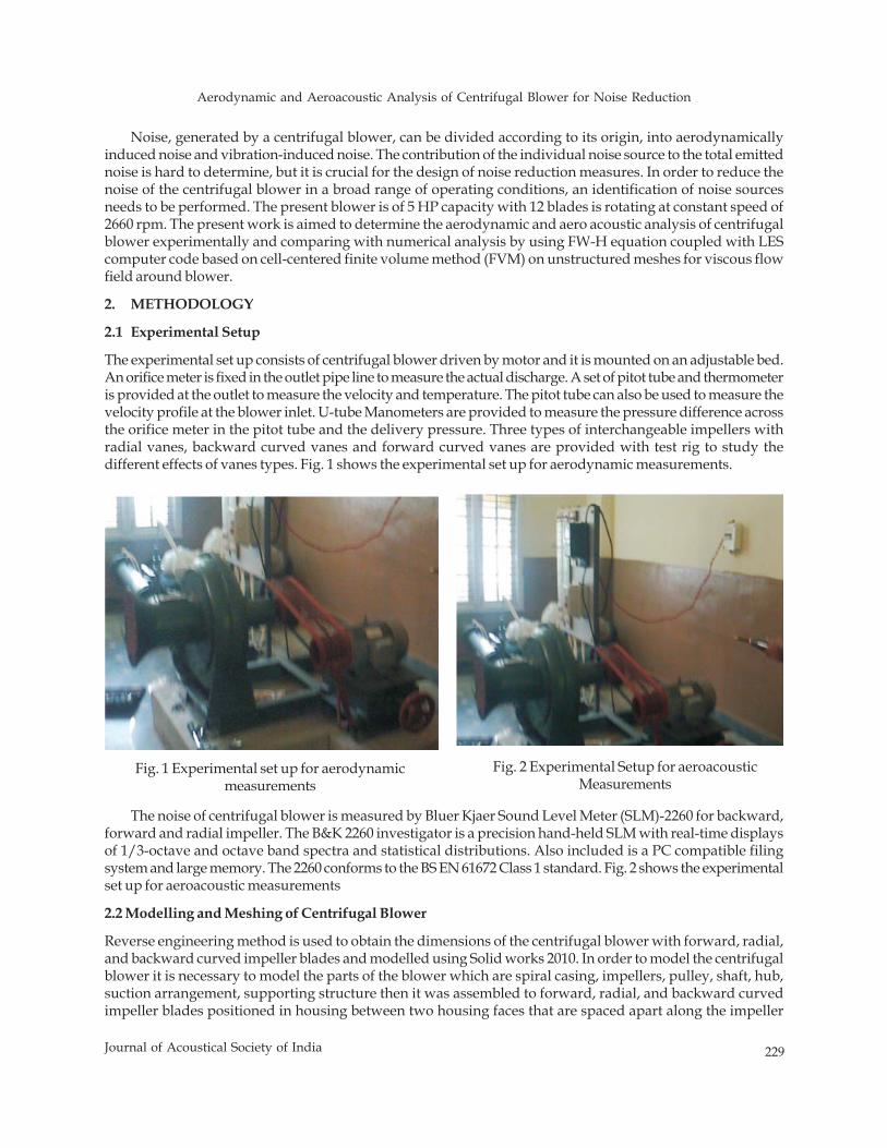
Aerodynamic and Aeroacoustic Analysis of Centrifugal Blower for Noise Reduction
229Journal of Acoustical Society of India
Noise, generated by a centrifugal blower, can be divided according to its origin, into aerodynamicallyinduced noise and vibration-induced noise. The contribution of the individual noise source to the total emittednoise is hard to determine, but it is crucial for the design of noise reduction measures. In order to reduce thenoise of the centrifugal blower in a broad range of operating conditions, an identification of noise sourcesneeds to be performed. The present blower is of 5 HP capacity with 12 blades is rotating at constant speed of2660 rpm. The present work is aimed to determine the aerodynamic and aero acoustic analysis of centrifugalblower experimentally and comparing with numerical analysis by using FW-H equation coupled with LEScomputer code based on cell-centered finite volume method (FVM) on unstructured meshes for viscous flowfield around blower.
2. METHODOLOGY
2.1 Experimental Setup
The experimental set up consists of centrifugal blower driven by motor and it is mounted on an adjustable bed.An orifice meter is fixed in the outlet pipe line to measure the actual discharge. A set of pitot tube and thermometeris provided at the outlet to measure the velocity and temperature. The pitot tube can also be used to measure thevelocity profile at the blower inlet. U-tube Manometers are provided to measure the pressure difference acrossthe orifice meter in the pitot tube and the delivery pressure. Three types of interchangeable impellers withradial vanes, backward curved vanes and forward curved vanes are provided with test rig to study thedifferent effects of vanes types. Fig. 1 shows the experimental set up for aerodynamic measurements.
The noise of centrifugal blower is measured by Bluer Kjaer Sound Level Meter (SLM)-2260 for backward,forward and radial impeller. The B&K 2260 investigator is a precision hand-held SLM with real-time displaysof 1/3-octave and octave band spectra and statistical distributions. Also included is a PC compatible filingsystem and large memory. The 2260 conforms to the BS EN 61672 Class 1 standard. Fig. 2 shows the experimentalset up for aeroacoustic measurements
2.2 Modelling and Meshing of Centrifugal Blower
Reverse engineering method is used to obtain the dimensions of the centrifugal blower with forward, radial,and backward curved impeller blades and modelled using Solid works 2010. In order to model the centrifugalblower it is necessary to model the parts of the blower which are spiral casing, impellers, pulley, shaft, hub,suction arrangement, supporting structure then it was assembled to forward, radial, and backward curvedimpeller blades positioned in housing between two housing faces that are spaced apart along the impeller
Fig. 2 Experimental Setup for aeroacousticMeasurements
Fig. 1 Experimental set up for aerodynamicmeasurements
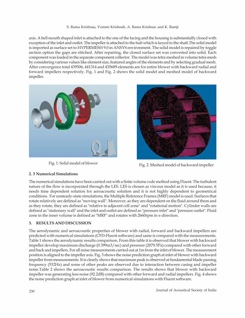
230 Journal of Acoustical Society of India
S. Rama Krishnaa, Vommi Krishnab, A. Rama Krishnac and K. Ramji
axis. A bell mouth shaped inlet is attached to the one of the facing and the housing is substantially closed withexception of the inlet and outlet. The impeller is attached to the hub which is keyed to the shaft.The solid modelis imported as surface set to HYPERMESH 9.0 in ANSYS environment. The solid model is repaired by togglesection option the gaps are stitched. After repairing, the closed surface set was converted into solid. Eachcomponent was loaded in the separate component collector. The model was tetra meshed in volume tetra meshby considering various values like element size, featured angles of the elements and by selecting gradual mesh.After convergence total 439506, 441314 and 435689 elements are for entire blower with backward radial andforward impellers respectively. Fig. 1 and Fig. 2 shows the solid model and meshed model of backwardimpeller.
Fig. 1. Solid model of blower Fig. 2. Meshed model of backward impeller
2. 3 Numerical Simulations
The numerical simulations have been carried out with a finite volume code method using Fluent. The turbulentnature of the flow is incorporated through the LES. LES is chosen as viscous model as it is used because, itneeds time dependent solution for aeroacoustic solution and it is not highly dependent to geometricalconditions. For unsteady-state simulations, the Multiple Reference Frames (MRF) model is used. Surfaces thatrotate relatively are defined as "moving wall". Moreover, as they are dependent on the fluid around them andas they rotate, they are defined as "relative to adjacent cell zone" and "rotational motion". Cylinder walls aredefined as "stationary wall" and the inlet and outlet are defined as "pressure inlet" and "pressure outlet". Fluidzone in the inner volume is defined as "MRF" and rotates with 2660rpm in x-direction.
3. RESULTS AND DISCUSSION
The aerodynamic and aeroacoustic properties of blower with radial, forward and backward impellers arepredicted with numerical simulations (CFD-Fluent software) and same is compared with the measurements.Table 1 shows the aerodynamic results comparison. From this table it is observed that blower with backwardimpeller develop maximum discharge (0.399m3/sec) and pressure (2079.5Pa) compared with other forwardand back and impellers. For all noise measurements carried out at 1m from the inlet of blower. The measurementposition is aligned to the impeller axis. Fig. 3 shows the noise prediction graph at inlet of blower with backwardimpeller from measurements. It is clearly shows that maximum peak is observed at fundamental blade passingfrequency (532Hz) and some of other peaks are observed due to interaction between casing and impellernoise.Table 2 shows the aeroacoustic results comparison. The results shows that blower with backwardimpeller was generating less noise (92.2dB) compared with other forward and radial impellers. Fig. 4 showsthe noise prediction graph at inlet of blower from numerical simulations with Fluent software.
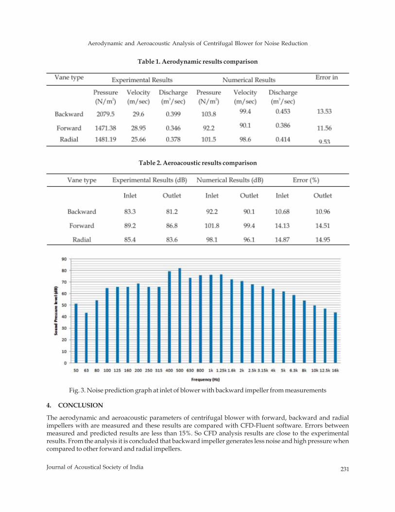
Aerodynamic and Aeroacoustic Analysis of Centrifugal Blower for Noise Reduction
231Journal of Acoustical Society of India
4. CONCLUSION
The aerodynamic and aeroacoustic parameters of centrifugal blower with forward, backward and radialimpellers with are measured and these results are compared with CFD-Fluent software. Errors betweenmeasured and predicted results are less than 15%. So CFD analysis results are close to the experimentalresults. From the analysis it is concluded that backward impeller generates less noise and high pressure whencompared to other forward and radial impellers.
Fig. 3. Noise prediction graph at inlet of blower with backward impeller from measurements
Table 1. Aerodynamic results comparison
Table 2. Aeroacoustic results comparison
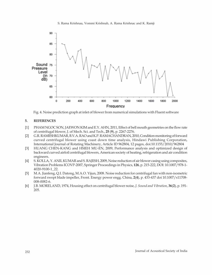
232 Journal of Acoustical Society of India
S. Rama Krishnaa, Vommi Krishnab, A. Rama Krishnac and K. Ramji
Fig. 4. Noise prediction graph at inlet of blower from numerical simulations with Fluent software
5. REFERENCES
[1] PHAM NGOC SON, JAEWON KIM and E.Y. AHN, 2011, Effect of bell mouth geometries on the flow rateof centrifugal blower, J. of Mech. Sci. and Tech., 25 (9), p. 2267-2276.
[2] G.R. RAMESHKUMAR, B.V.A. RAO and K.P. RAMACHANDRAN, 2010, Condition monitoring of forwardcurved centrifugal blower using coast down time analysis, Hindawi Publishing Corporation,International Journal of Rotating Machinery, Article ID 962804, 12 pages, doi:10.1155/2010/962804
[3] HUANG CHEN-KANG and HSIEH MU-EN, 2009, Performance analysis and optimized design ofbackward curved airfoil centrifugal blowers, American society of heating, refrigeration and air conditionengineers.
[4] S. KOLLA, Y. ANIL KUMAR and S. RAJESH, 2009, Noise reduction of air blower casing using composites,Vibration Problems ICOVP-2007, Springer Proceedings in Physics, 126, p. 215-222, DOI: 10.1007/978-1-4020-9100-1_22.
[5] M.A. Jianfeng, Q.I. Datong, M.A.O. Yijun, 2008. Noise reduction for centrifugal fan with non-isometricforward swept blade impeller, Front. Energy power engg. China, 2(4), p. 433-437 doi 10.1007/s11708-008-0082-6.
[6] J.B. MORELAND, 1974, Housing effect on centrifugal blower noise, J. Sound and Vibration, 36(2), p. 191-205.
Optimization of Secondary Sources for Active Noise Control in a Car Like Rigid Cavity
233Journal of Acoustical Society of India
ABSTRACT
In this paper genetic algorithm has been used for optimal placement of secondary sources in a three-dimensional rectangular rigid cavity for active noise control system. In this genetic algorithm amultivariable binary coding scheme along with a random initial population are used. Numericalexamples are presented to illustrate the effect of location on sound pressure level. Result shows thatthe locations obtained by genetic algorithm are very effective than arbitrary locations.
1. INTRODUCTION
The internal sound field in the enclosed cavity is significantly affected by the acoustic modal characteristics ofthe cavity, Porous material absorption efficiency is mostly apparent at high frequencies. Passive control hasthe disadvantage of minimal low frequency absorption; it can be bulky and heavy when used for low frequencies.To attenuate this low frequency noise, active noise control (ANC) system can be used in enclosed spaceswithout passive techniques. It has the specific advantage of reduction in size, volume and cost when comparedwith passive control. Nelson et al. (1987) examined the active noise control methods in harmonic enclosedsound fields. Further, the theory was verified by both numerical simulation (Bullmore et al. (1987)) andexperimentally (Elliott et al. (1987)). They considered a rectangular enclosure with rigid walls and shown thatminimizing the sum of the squared pressures at several points could lead to significant reduction in acousticpotential energy and sound pressure levels (SPL). Parkins et al. (2000) investigated active control system ofthree-dimensional enclosures based on acoustic energy density method. In their study, minimization of energyhave been carried out by sensing both the potential and kinetic energy densities, while the most popularcontrol systems of the past have relied on the potential energy density alone. Energy density control methodshown to be more effectively than pressure based measurements especially for off-resonance control. Akl andBaz (2006) investigated the effectiveness of structural acoustics of the cavity/plate system, which is lined withsmart foam.
In this work optimal location of secondary sources have been examined to enhance the reduction of thesound pressure level in a three dimensional rigid cavity as shown in Fig. 1.
2. FORMULATION
The Helmholtz equation, for a cavity of volume V, enclosed by a rigid surface for harmonic variation inacoustic pressure p is given by (eq. 1);
Journal of Acoustical Society of India : Vol. 40, No. 4, 2013 (pp. 233-238)
Optimization of Secondary Sources for Active NoiseControl in a Car Like Rigid Cavity
T. Ramachandran, M.C. Lenin Babu* and S. Muruga PoopathyDepartment of Mechanical Engineering,
PSNA College of Engineering and Technology, Dindigul-624 622*e-mail: [email protected]
[Received: 18.12.2012; Revised: 27.07.2013; Accepted: 21.09.2013]
© 2013 Acoustical Society of India
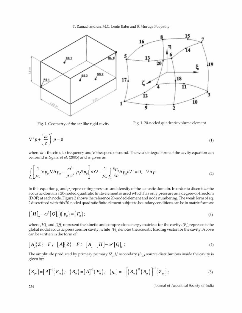
234 Journal of Acoustical Society of India
T. Ramachandran, M.C. Lenin Babu and S. Muruga Poopathy
22 0ω⎛ ⎞∇ + =⎜ ⎟
⎝ ⎠p p
c (1)
where ω is the circular frequency and 'c' the speed of sound. The weak integral form of the cavity equation canbe found in Sgard et al. (2005) and is given as
2
2
1 1 0Γ
ωδ δ Ω δ Γ δρ ρΩ
⎡ ⎤ ∂∇ ∇ − − = ∀⎢ ⎥ ∂⎣ ⎦
∫ ∫a a
aa a a a a
a a a
pp . p p p d p d , p.p c n (2)
In this equation pa and ρa representing pressure and density of the acoustic domain. In order to discretize theacoustic domain a 20-noded quadratic finite element is used which has only pressure as a degree-of-freedom(DOF) at each node. Figure 2 shows the reference 20-noded element and node numbering. The weak form of eq.2 discretized with this 20-noded quadratic finite element subject to boundary conditions can be in matrix form as:
[ ] [ ]( ){ } { }2ω− =a aa aH Q p F ; (3)
where [H]a and [Q]a represent the kinetic and compression energy matrices for the cavity, [P]a represents theglobal nodal acoustic pressures for cavity, while [F]a denotes the acoustic loading vector for the cavity. Abovecan be written in the form of:
[ ]{ } [ ]{ } [ ] [ ] [ ]2ω= = = −a
A Z F ; A Z F ; A H Q ; (4)
The amplitude produced by primary primary {Zps}/ secondary {B55} source distributions inside the cavity isgiven by:
{ } [ ] { } { } [ ] { } { } { } { } { }11 1 −− − ⎡ ⎤= = = − ⎣ ⎦
Hps ps ss ss s ss ss psZ A F ; B A F ; q B B Z ; (5)
Fig. 1. 20-noded quadratic volume element Fig. 1. Geometry of the car like rigid cavity
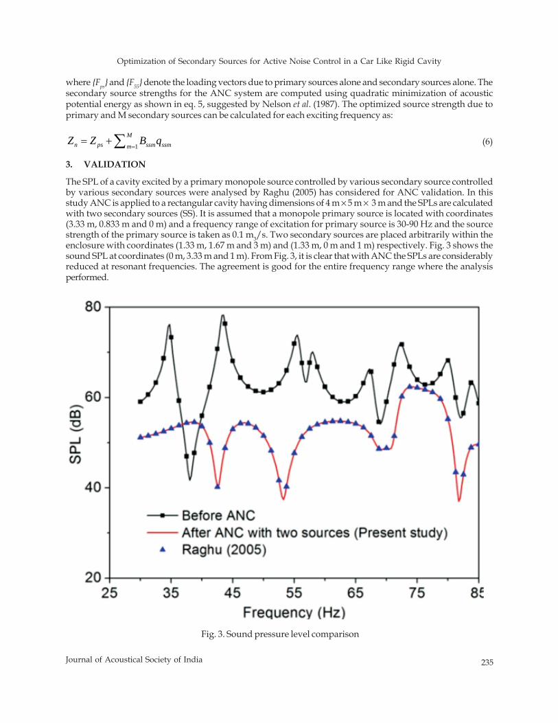
Optimization of Secondary Sources for Active Noise Control in a Car Like Rigid Cavity
235Journal of Acoustical Society of India
where {Fps} and {F55} denote the loading vectors due to primary sources alone and secondary sources alone. Thesecondary source strengths for the ANC system are computed using quadratic minimization of acousticpotential energy as shown in eq. 5, suggested by Nelson et al. (1987). The optimized source strength due toprimary and M secondary sources can be calculated for each exciting frequency as:
1== +∑M
n ps ssm ssmmZ Z B q (6)
3. VALIDATION
The SPL of a cavity excited by a primary monopole source controlled by various secondary source controlledby various secondary sources were analysed by Raghu (2005) has considered for ANC validation. In thisstudy ANC is applied to a rectangular cavity having dimensions of 4 m × 5 m × 3 m and the SPLs are calculatedwith two secondary sources (SS). It is assumed that a monopole primary source is located with coordinates(3.33 m, 0.833 m and 0 m) and a frequency range of excitation for primary source is 30-90 Hz and the sourcestrength of the primary source is taken as 0.1 m3/s. Two secondary sources are placed arbitrarily within theenclosure with coordinates (1.33 m, 1.67 m and 3 m) and (1.33 m, 0 m and 1 m) respectively. Fig. 3 shows thesound SPL at coordinates (0 m, 3.33 m and 1 m). From Fig. 3, it is clear that with ANC the SPLs are considerablyreduced at resonant frequencies. The agreement is good for the entire frequency range where the analysisperformed.
Fig. 3. Sound pressure level comparison
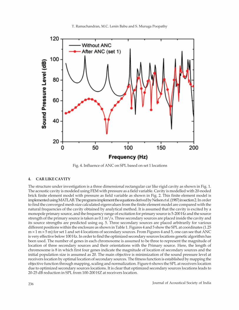
236 Journal of Acoustical Society of India
T. Ramachandran, M.C. Lenin Babu and S. Muruga Poopathy
4. CAR LIKE CAVITY
The structure under investigation is a three dimensional rectangular car like rigid cavity as shown in Fig. 1.The acoustic cavity is modeled using FEM with pressure as a field variable. Cavity is modelled with 20-nodedbrick finite element model with pressure as field variable as shown in Fig. 2. This finite element model isimplemented using MATLAB. The programs implement the equations derived by Nelson et al. (1987) in section 2. In orderto find the converged mesh size calculated eigenvalues from the finite element model are compared with thenatural frequencies of the cavity obtained by analytical method. It is assumed that the cavity is excited by amonopole primary source, and the frequency range of excitation for primary source is 5-200 Hz and the sourcestrength of the primary source is taken as 0.1 m3/s. Three secondary sources are placed inside the cavity andits source strengths are predicted using eq. 5. Three secondary sources are placed arbitrarily for variousdifferent positions within the enclosure as shown in Table 1. Figures 4 and 5 show the SPL at coordinates (1.25m × 1 m × 5 m) for set 1 and set 4 locations of secondary sources. From Figures 4 and 5, one can see that ANCis very effective below 100 Hz. In order to find the optimized secondary sources locations genetic algorithm hasbeen used. The number of genes in each chromosome is assumed to be three to represent the magnitude oflocation of three secondary sources and their orientations with the Primary source. Here, the length ofchromosome is 8 in which first four genes indicate the magnitude of location of secondary sources and theinitial population size is assumed as 20. The main objective is minimization of the sound pressure level atreceivers location by optimal location of secondary sources. The fitness function is established by mapping theobjective function through mapping, scaling and normalization. Figure 6 shows the SPL at receivers locationdue to optimized secondary sources locations. It is clear that optimized secondary sources locations leads to20-25 dB reduction in SPL from 100-200 HZ at receivers location.
Fig. 4. Influence of ANC on SPL based on set 1 locations
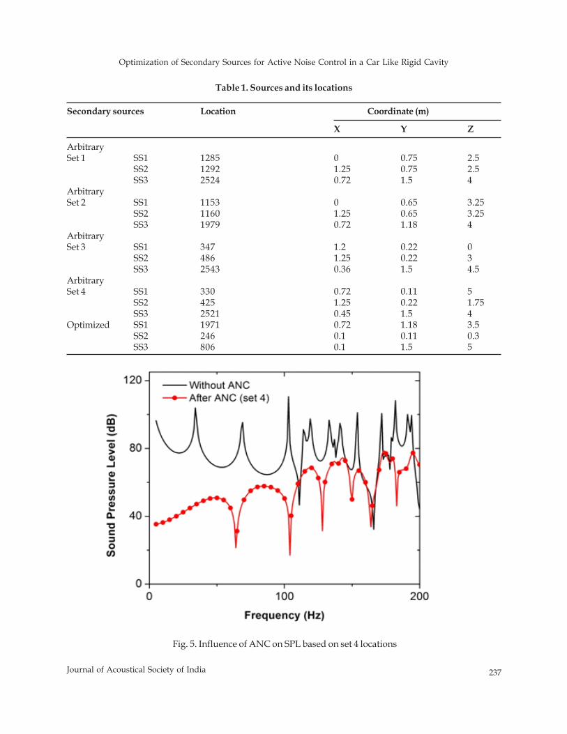
Optimization of Secondary Sources for Active Noise Control in a Car Like Rigid Cavity
237Journal of Acoustical Society of India
Table 1. Sources and its locations
Secondary sources Location Coordinate (m)
X Y Z
ArbitrarySet 1 SS1 1285 0 0.75 2.5
SS2 1292 1.25 0.75 2.5SS3 2524 0.72 1.5 4
ArbitrarySet 2 SS1 1153 0 0.65 3.25
SS2 1160 1.25 0.65 3.25SS3 1979 0.72 1.18 4
ArbitrarySet 3 SS1 347 1.2 0.22 0
SS2 486 1.25 0.22 3SS3 2543 0.36 1.5 4.5
ArbitrarySet 4 SS1 330 0.72 0.11 5
SS2 425 1.25 0.22 1.75SS3 2521 0.45 1.5 4
Optimized SS1 1971 0.72 1.18 3.5SS2 246 0.1 0.11 0.3SS3 806 0.1 1.5 5
Fig. 5. Influence of ANC on SPL based on set 4 locations
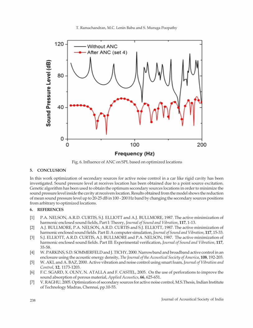
238 Journal of Acoustical Society of India
T. Ramachandran, M.C. Lenin Babu and S. Muruga Poopathy
Fig. 6. Influence of ANC on SPL based on optimized locations
5. CONCLUSION
In this work optimization of secondary sources for active noise control in a car like rigid cavity has beeninvestigated. Sound pressure level at receives location has been obtained due to a point source excitation.Genetic algorithm has been used to obtain the optimum secondary sources locations in order to minimize thesound pressure level inside the cavity at receivers location. Results obtained from the model shows the reductionof mean sound pressure level up to 20-25 dB in 100 - 200 Hz band by changing the secondary sources positionsfrom arbitrary to optimized locations.6. REFERENCES
[1] P.A. NELSON, A.R.D. CURTIS, S.J. ELLIOTT and A.J. BULLMORE, 1987. The active minimization ofharmonic enclosed sound fields, Part I: Theory, Journal of Sound and Vibration, 117, 1-13.
[2] A.J. BULLMORE, P.A. NELSON, A.R.D. CURTIS and S.J. ELLIOTT, 1987. The active minimization ofharmonic enclosed sound fields. Part II: A computer simulation, Journal of Sound and Vibration, 117, 15-33.
[3] S.J. ELLIOTT, A.R.D. CURTIS, A.J. BULLMORE and P.A. NELSON, 1987. The active minimization ofharmonic enclosed sound fields. Part III: Experimental verification, Journal of Sound and Vibration, 117,35-58.
[4] W. PARKINS, S.D. SOMMERFELD and J. TICHY, 2000. Narrowband and broadband active control in anenclosure using the acoustic energy density, The Journal of the Acoustical Society of America, 108, 192-203.
[5] W. AKL and A. BAZ, 2000. Active vibration and noise control using smart foam, Journal of Vibration andControl, 12, 1173-1203.
[6] F.C. SGARD, X. OLNY, N. ATALLA and F. CASTEL, 2005. On the use of perforations to improve thesound absorption of porous material, Applied Acoustics, 66, 625-651.
[7] V. RAGHU, 2005. Optimization of secondary sources for active noise control, M.S.Thesis, Indian Instituteof Technology Madras, Chennai, pp.10-55.
Performance Analysis of Speckle Noise Filters for Medical Ultrasound Images
239Journal of Acoustical Society of India
ABSTRACT
Ultrasound is a relatively inexpensive, noninvasive, and portable technique for imaging the internalanatomy for medical diagnosis. The Speckle noise, an inherent nature of ultrasound often contaminatesthe image, significantly degrades the quality by discriminating fine details which may contain vitalinformation and complicates the diagnostic decisions. The Speckle noise removal is the general pre-processing step for feature extraction, analysis, and recognition of ultrasound imaging. This paperanalyzes the performance of different techniques proposed for the suppression of this multiplicativenoise which is very difficult to be removed. Statistical quantity measures such as Mean Square Error(MSE), Root Mean Square Error (RMSE) and Peak Signal-to-Noise Ratio (PSNR) are used to measureand compare the quality of the enhanced images.
1. INTRODUCTION
Ultrasonic plays an important role in medical diagnosis by revealing the internal anatomy of organs to medicalpractitioners for accurate prediction of abnomabilities which may be treated if detected at the earliest [1]. Themain problem faced by them is the noise introduced due to the consequence of the coherent nature of the wavetransmitted during the ultrasonic process. These noises tend to corrupt the quality of the image and an inferiorquality image may lead to incorrect diagnosis [2]. Speckle noise affects the ultrasound images which are acomplex phenomenon, which degrades image quality with a backscattered wave appearance which originatesfrom many microscopic diffused reflections that passing through internal organs and makes it more difficultfor the observer to discriminate fine detail of the images in diagnostic examinations [3]. Suppressing thisspeckle noise from an ultrasonic image by retaining the thin and small image features is the primary step inprocessing medical ultrasonic images [4].For the early detection of cancers, such as breast cancer ,prostatecancer, lung Cancer and cervical cancer, Ultrasound imaging method is suitable to diagnose and progenies.The accurate detection of region of interest in ultrasound image is crucial.
In this paper, different methods proposed for suppressing and removing speckle noise are analyzed.Using statistical measures such as Signal-to-Noise Ratio (SNR), Peak Signal-to-Noise Ratio (PSNR), and RootMean Square Error (RMSE) the performance of the speckle filters are compared and evaluated with differentmedical images. This paper is organized as follows: Section 2 describes problems associated with noisegenerated during ultrasound process. Section 3 describes various spatial filtering techniques for denoising thespeckle noise in the ultrasound medical image. Section 4 discusses about our experimental analysis anddiscussion. Section 5 concludes this paper and provides direction for further research.
Journal of Acoustical Society of India : Vol. 40, No. 4, 2013 (pp. 239-244)
Performance Analysis of Speckle Noise Filters forMedical Ultrasound Images
P. Thirumoorthy1* and K.M. Prabusankarlal2
1Department of Electronics& Communication,Government Arts& Science College, Paramakkudi
2Department of Electronics & Communication,K.S.R. College of Arts and Science, Tiruchengode
*e-mail:[email protected]
[Received: 19.02.2013; Revised: 18.07.2013; Accepted: 22.10.2013]
© 2013 Acoustical Society of India
240 Journal of Acoustical Society of India
P. Thirumoorthy K.M. Prabusankarlal
2. PROBLEM DESCRIPTION
A digital image is defined as a two dimensional functionf(x,y), where x and y are spatial coordinates and theamplitude of f at any pair of coordinates (x,y) is called the intensity or grey level of the image [5]. The noisecontaminates the data sets collected by image sensor and the region of interest in the image is degraded, whichmakes the original image not suitable for applying image processing techniques and analysis for medicaldiagnosis. As a preprocessing step, an image enhancement technique is mandatory before image is processedand analyzed. The noise removal in the image is still a challenging problem and so an efficient filtering methodis necessary for removing noise in the images which introduces artifacts and causes blurring of the image. Thespeckle noise [6] is observed in ultrasound images where images are corrupted by a random granular patternthat delays the interpretation of the image content and reduces the chances of detection of features of interest.Noise is generally grouped into two categories viz., image data independent noise [7] and image data dependent[8] noise.
2.1 Speckle Noise
Speckle noise is a kind of data dependent noice found in the ultrasonic image is caused by errors in datatransmission [10]. The corrupted pixels by speckle noise are either set to the maximum or minimum valuewhich appears as something like a snow in image or have single bits flipped over. Speckle noise has thecharacteristic of multiplicative noise [11] and it follows a gamma distribution and is given as
1( ) .
( 1)!
gagF g e
α
∝−
∝
⎡ ⎤⎢ ⎥=⎢ ⎥∝ −⎣ ⎦
Where, variance is α2 and g is the gray level.
3. SPECKLE FILTERING TECHNIQUES
The primary goal of an image enhancement technique is to adjust the digital image so that the resultant imageis more suitable than the original image for further processing and analysis [12]. The image processingfunction in a spatial domain can be expressed as g(x,y) = T(f(x,y) ). Where, T is the transformation function,f(x,y) is the pixel value of input image, and g(x,y) is the pixel value of the processed image. Different filteringtechniques such as Median Filter [13], FIR Filter [14], DCT Filter [15] and FFT filter are used for denoising thedifferent medical images and four other filters are also proposed.
3.1 Entropy Filter
The proposed entropy filter filters image by replacing every value by the information entropy of the values inits range r neighborhood [17]. The entropy H(L) of the belief over L is defined as H(L)= - ∑τ Bel(L=l) logBel(L=l). The s denote the measurement, the change of the entropy of Bel(L) given s is defined as ΔH(L|s) :=H(L|s) -H(L). The term H(L|s) is the entropy of the belief Bel(L) after incorporating the measurements.
3.2 Range Filter
This filter uses the local-intensity subrange of pixel intensity values within a window [18]. It uses themorphological functions to determine the maximum and minimum values in the specified neighborhood anduses the padding behavior of these morphological functions, h(x) = kr
-1 (x) ∫∞−∞ ∫
∞−∞ f(ξ)sf(ξ) f(x)dξ. The sf(ξ),
f(x))measures the photometric similarity between the pixel at the neighborhood center x and that of a nearbypoint.
3.3 Standard Deviation Filter
The standard deviation filter [12] calculates the standard deviation for each group of pixels in the subimage,and assigns this value to the center pixel in the output image. The objective function of standard deviationfilter is given by
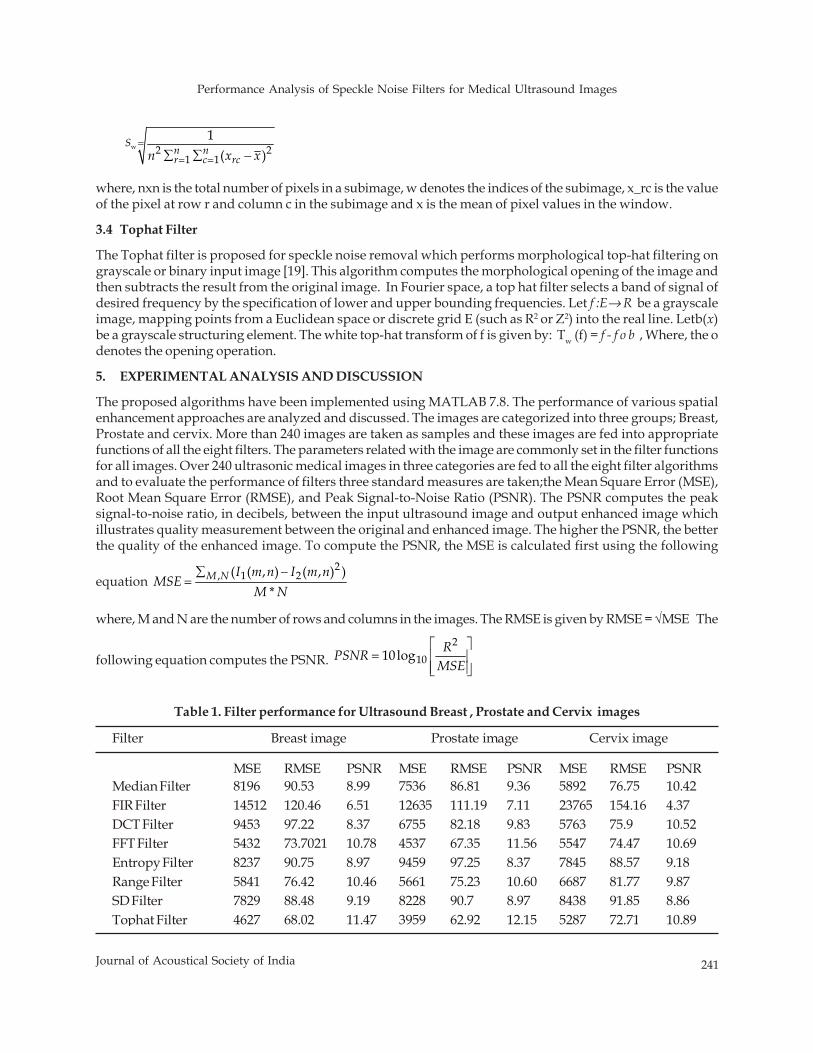
Performance Analysis of Speckle Noise Filters for Medical Ultrasound Images
241Journal of Acoustical Society of India
w 2 21 1
1( )
Sn nr c rcn x x
=
= =∑ ∑ −
where, nxn is the total number of pixels in a subimage, w denotes the indices of the subimage, x_rc is the valueof the pixel at row r and column c in the subimage and x is the mean of pixel values in the window.
3.4 Tophat Filter
The Tophat filter is proposed for speckle noise removal which performs morphological top-hat filtering ongrayscale or binary input image [19]. This algorithm computes the morphological opening of the image andthen subtracts the result from the original image. In Fourier space, a top hat filter selects a band of signal ofdesired frequency by the specification of lower and upper bounding frequencies. Let f :E→ R be a grayscaleimage, mapping points from a Euclidean space or discrete grid E (such as R2 or Z2) into the real line. Letb(x)be a grayscale structuring element. The white top-hat transform of f is given by: Tw (f) = f - f o b , Where, the odenotes the opening operation.
5. EXPERIMENTAL ANALYSIS AND DISCUSSION
The proposed algorithms have been implemented using MATLAB 7.8. The performance of various spatialenhancement approaches are analyzed and discussed. The images are categorized into three groups; Breast,Prostate and cervix. More than 240 images are taken as samples and these images are fed into appropriatefunctions of all the eight filters. The parameters related with the image are commonly set in the filter functionsfor all images. Over 240 ultrasonic medical images in three categories are fed to all the eight filter algorithmsand to evaluate the performance of filters three standard measures are taken;the Mean Square Error (MSE),Root Mean Square Error (RMSE), and Peak Signal-to-Noise Ratio (PSNR). The PSNR computes the peaksignal-to-noise ratio, in decibels, between the input ultrasound image and output enhanced image whichillustrates quality measurement between the original and enhanced image. The higher the PSNR, the betterthe quality of the enhanced image. To compute the PSNR, the MSE is calculated first using the following
equation 2
, 1 2( ( , ) ( , ) )*
M N I m n I m nMSE
M N∑ −
=
where, M and N are the number of rows and columns in the images. The RMSE is given by RMSE = √MSE The
following equation computes the PSNR. 2
1010log RPSNRMSE⎡ ⎤
= ⎢ ⎥⎢ ⎥⎣ ⎦
Filter Breast image Prostate image Cervix image
MSE RMSE PSNR MSE RMSE PSNR MSE RMSE PSNRMedian Filter 8196 90.53 8.99 7536 86.81 9.36 5892 76.75 10.42FIR Filter 14512 120.46 6.51 12635 111.19 7.11 23765 154.16 4.37DCT Filter 9453 97.22 8.37 6755 82.18 9.83 5763 75.9 10.52FFT Filter 5432 73.7021 10.78 4537 67.35 11.56 5547 74.47 10.69Entropy Filter 8237 90.75 8.97 9459 97.25 8.37 7845 88.57 9.18Range Filter 5841 76.42 10.46 5661 75.23 10.60 6687 81.77 9.87SD Filter 7829 88.48 9.19 8228 90.7 8.97 8438 91.85 8.86Tophat Filter 4627 68.02 11.47 3959 62.92 12.15 5287 72.71 10.89
Table 1. Filter performance for Ultrasound Breast , Prostate and Cervix images
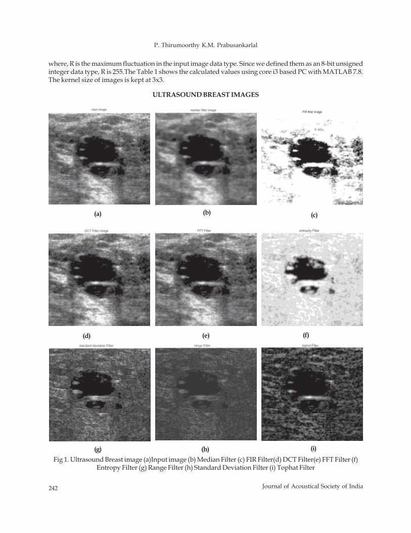
242 Journal of Acoustical Society of India
P. Thirumoorthy K.M. Prabusankarlal
ULTRASOUND BREAST IMAGES
(a) (b) (c)
(d) (e) (f)
Fig 1. Ultrasound Breast image (a)Input image (b) Median Filter (c) FIR Filter(d) DCT Filter(e) FFT Filter (f)Entropy Filter (g) Range Filter (h) Standard Deviation Filter (i) Tophat Filter
(g) (h) (i)
where, R is the maximum fluctuation in the input image data type. Since we defined them as an 8-bit unsignedinteger data type, R is 255.The Table 1 shows the calculated values using core i3 based PC with MATLAB 7.8.The kernel size of images is kept at 3x3.
Performance Analysis of Speckle Noise Filters for Medical Ultrasound Images
243Journal of Acoustical Society of India
The original ultrasound image and filtered images obtained by various filtering techniques are shown infigure 1. Medical ultrasonic images of the breast, prostate (not shown) and cervix (not shown) are filtered andtheir performance parameters are analyzed. If the value of MSE is low and the value PSNR are larger and theenhancement approach is better. The Table 1 shows the performance analysis of the different filteringtechniques we have used. It is observed from the tables in terms of high PSNR and visual observation of theenhanced image, the proposed tophat filter removes the speckle noise better than other existing and proposedapproaches.
6. CONCLUSION
The performance of noise filters are compared analyzed and evaluated using quantitative measures such asMSE, RMSE and PSNR and also in term of visual quality of the images. Some methods removed speckle noisebetter but the quality of the image too degraded. Since the finest details of the images are crucial for furtherprocessing such as edge detection and segmentation process, they have to be preserved. Very few algorithmsremoved speckle noise as well as preserved the details of the breast, prostate and cervix medical imagesduring the evaluation process, among them the tophat filter performed better than others.
7. REFERENCE
[1] YANONG ZHU, STUART WILLIAMS and REYER ZWIGGELAAR, 2006 Computer Technology inDetection and Staging of Prostate Carcinoma: A review, Medical image Analysis 10, p 178-199.
[2] S. SUDHA, G.R. SURESH and R. SUKANESH 2009 Speckle Noise Reduction in Ultrasound Images byWavelet Thresholding based on Weighted Variance, International Journal of Computer Theory andEngineering, 1, No. 1, 1793-8201
[3] HOSSEIN RABBANI, MANSUR VAFADUST and PURANG ABOLMAESUMI, 2008 Speckle NoiseReduction of Medical Ultrasound Images in Complex Wavelet Domain Using Mixture Priors, IEEEtransactions on biomedical engineering, 55, no. 9.
[4] ARPIT SINGHAL and MANDEEP SINGH, 2011 Speckle Noise Removal and Edge Detection UsingMathematical Morphology, International Journal of Soft Computing and Engineering (IJSCE) ISSN: 2231-2307, 1, 5.
[5] R.C. GONZALEZ and R. WOODS 1992 'Digital Image Processing', Addison-Wesley Publishingcompany.
[6] Image Processing Fundamentals - Statistics, "Signal to Noise Ratio", 2001.[7] YUNYI YAN and BAOLONG GUO. 2006 Application of Wavelet Neural Network (WNN) and Gradient
Descent Method (GDM) in Natural Image Denoising. Journal of Computational Information Systems, 2(2):625-631.
[8] D. ROBERT NOWAK, 1999"Wavelet based Rician noise Removal", IEEE Transaction on image processing,8, no. 10, PP 1480.
[9] A.K. JAIN, 1989 fundamental of digital image processing. Englewood cliffs, NJ Prentice-Hall.[10] MATIAS BARBER, FRANCISCO GRINGS, PABLO PERNA, MARCELA PISCITELLI, MARTIN
MAAS,CINTIA BRUSCANTINI, JULIO JACOBO-BERLLES, and HAYDEE KARSZENBAUM. 2012Speckle Noise and Soil Heterogeneities as Error Sources in a Bayesian Soil Moisture Retrieval Schemefor SAR Data. IEEE journal of selected topics in applied earth observations and remote sensing, 5, 3.
[11] K. BALA PRAKASH, R. VENU BABU and B. VENU GOPAL. 2011 Image Independent Filter for Removalof Speckle Noise. IJCSI International Journal of Computer Science Issues, 8, Issue 5, 3.
[12] K. THANGAVEL and R. MANAVALAN, 2009 Laurence Aroquiaraj. I ,Removal of Speckle Noise fromUltrasound Medical Image based on Special Filters: Comparative Study, ICGST-GVIP Journal, ISSN1687-398X, (9), Issue (III).
[13] LIM and S. JAE , 1990 Two-Dimensional Signal and Image Processing, Englewood Cliffs, NJ, PrenticeHall.
[14] N.J. FLIEGE, 1994 Multirate Digital Signal Processing: Multirate Systems, Filter Banks, Wavelets. WestSussex, England: John Wiley & Sons.

244 Journal of Acoustical Society of India
P. Thirumoorthy K.M. Prabusankarlal
[15] HAITHAM HASSANIEH, 2012 Piotr Indyk, Dina Katabi, and Eric Price, "Simple and Practical Algorithmfor Sparse Fourier Transform," ACM-SIAM Symposium on Discrete Algorithms (SODA), Kyoto, January
[16] R. SIVARANJANI, 2011 Performance Analysis of Transform based Image Compression Algorithms.CiiT International Journal of Digital Image Processing, December.
[17] R.C. GONZALEZ, R.E. WOODS and S.L. EDDINS, 2003 Digital Image Processing Using MATLAB,New Jersey, Prentice Hall, Chapter 11.
[18] C. TOMASI and R. MANDUCHI, 1998 Bilateral Filtering for Gray and Color Images. Proceedings of theIEEE International Conference on Computer Vision, Bombay, India.
[19] MING ZENG, JIANXUN LI and ZHANG PENG , 2006 The design of Top-Hat morphological filter andapplication to infrared target detection, Infrared Physics & Technology, 48, 1, 67-76.
Ultrasonic Study of Chemical Mixture Used for Preparation of Fiber from Date Palm Leaves
245Journal of Acoustical Society of India
ABSTRACT
Propagation of ultrasonic waves in chemical mixture have greater importance in study of differentacoustic parameter which are provides information about the strength of different composite materialsprepared from different agricultural wastes.Measurement of ultrasonic velocity and density atdifferent concentration of solvent mixture has been carried out at different temperature using multifrequency ultrasonic interferometer. The data obtained are used to evaluate various acousticparameters in view of identification of the presence of different interaction under prevailing conditions.The variation of ultrasonic velocity, density and other acoustic parameters with concentration underdifferent physical conditions provides information about the mechanical strength of the fiber.
1. INTRODUCTION
High intensity ultrasonic waves are generally employed in the areas of cleaning, plastic welding, machiningetc.In addition to these applications, it is observed that if a liquid mixture is subjected to irradiation of highintensity ultrasonic waves, alternate compression and expansion modes takes place which leads to change insome thermodynamic properties of the liquid mixture. As a result of which the variation in speed of ultrasonicwaves takes place which affects some of the mechanical properties of the natural fiber. Ultrasonic methods aredirectly sensitive to these changes and can be used to assess the integrity of the composite structure. Theabsorption of ultrasound in polymer composite systems is governed by local modes of motion and cooperativebecause of the existence of strong intermolecular interaction within the liquid mixture. The manner in whichthe propagation of the ultrasonic wave is affected by structure of the liquid results in parameters that can leadto the binding between the natural fibers. Variation in thermal and acoustic properties with compositionprovides added information regarding the intermolecular interactions present in a system. The sign andmagnitude of the nonlinear deviations from ideality as a function of composition and frequency may beascribed to the presence of weak or strong type of interaction between unlike molecules. The excess acousticparameters of binary mixtures have been satisfactorily used in explaining the extent of interactions betweenmixing components [1-3].The present investigation deals with two important liquids namely acetone andmethanol. Both the liquids under investigation are very useful chemicals and of industrial significance. Themixture of these liquids is used in the preparation of date palm leaf fiber.This treatment removes a certainamount of lignin, wax and oils covering the external surface of the fiber cell wall, depolymerizes cellulose andexposes the short length crystallites. This treatment has two effects on the fiber i.e. it increases surface roughnessresulting in better mechanical interlocking, and it increases the amount of cellulose exposed on the fibersurface, thus increasing the number of possible reaction sites. Date palm leaves as agricultural waste generated
Journal of Acoustical Society of India : Vol. 40, No. 4, 2013 (pp. 245-249)
Ultrasonic Study of Chemical Mixture Used forPreparation of Fiber from Date Palm Leaves
G. Nath1*, A. Sarangi1 and R. Paikaraay2
1Dept. of Physics, VSS University of Technology, Burla, Sambalpur (Odisha)2Dept. of Physics, Ravenshaw University, Cuttack (Odisha)
*e-mail:[email protected]
[Received: 29.04.2013; Revised: 25.06.2013; Accepted: 25.10.2013]
© 2013 Acoustical Society of India
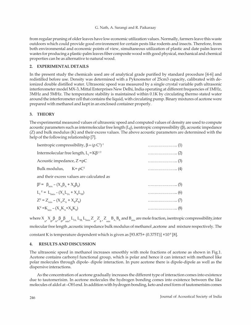
246 Journal of Acoustical Society of India
G. Nath, A. Sarangi and R. Paikaraay
from regular pruning of older leaves have low economic utilization values. Normally, farmers leave this wasteoutdoors which could provide good environment for certain pests like rodents and insects. Therefore, fromboth environmental and economic points of view, simultaneous utilization of plastic and date palm leaveswastes for producing a plastic-palm leaves fiber composite wood with good physical, mechanical and chemicalproperties can be as alternative to natural wood.
2. EXPERIMENTAL DETAILS
In the present study the chemicals used are of analytical grade purified by standard procedure [4-6] andredistilled before use. Density was determined with a Pyknometer of 25cm3 capacity, calibrated with de-ionized double distilled water. Ultrasonic speed was measured by a single crystal variable path ultrasonicinterferometer model MX-3, Mittal Enterprises New Delhi, India operating at different frequencies of 1MHz,3MHz and 5MHz. The temperature stability is maintained within 0.1K by circulating thermo stated wateraround the interferometer cell that contains the liquid, with circulating pump. Binary mixtures of acetone wereprepared with methanol and kept in an enclosed container properly.
3. THEORY
The experimental measured values of ultrasonic speed and computed values of density are used to computeacoustic parameters such as intermolecular free length (Lf), isentropic compressibility (β), acoustic impedance(Z) and bulk modulus (K) and their excess values. The above acoustic parameters are determined with thehelp of the following relationship [7].
Isentropic compressibility, β = (ρ C2)-1 ………………….. (1)
Intermolecular free length, Lf = Kβ1/2 ………………….. (2)
Acoustic impedance, Z =ρC ………………….. (3)
Bulk modulus, K= ρC2 ………………….. (4)
and their excess values are calculated as
βE = βmix – (XAβA + XBβB) ………………….. (5)
Lf E = Lfmix - (XALfA + XBLfB) ………………….. (6)
ZE = Zmix – (XAZA + XBZB) ………………….. (7)
KE =Kmix – (XAKA+XBKB) ………………….. (8)
where XA, XB,βA, βB,βmix, LfA, LfB, Lfmix ZA, ZB , Zmix
BA ,BB and Bmix are mole fraction, isentropic compressibility,inter
molecular free length ,acoustic impedance bulk modulus of methanol ,acetone and mixture respectively. The
constant K is temperature dependent which is given as [93.875+ (0.375T)] ×10-8 [8].
4. RESULTS AND DISCUSSION
The ultrasonic speed in methanol increases smoothly with mole fractions of acetone as shown in Fig.1.Acetone contains carbonyl functional group, which is polar and hence it can interact with methanol likepolar molecules through dipole- dipole interaction. In pure acetone there is dipole-dipole as well as thedispersive interactions.
As the concentration of acetone gradually increases the different type of interaction comes into existencedue to tautomerisim. In acetone molecules the hydrogen bonding comes into existence between the likemolecules of aldol at –OH end. In addition with hydrogen bonding, keto and enol form of tautomerisim comes
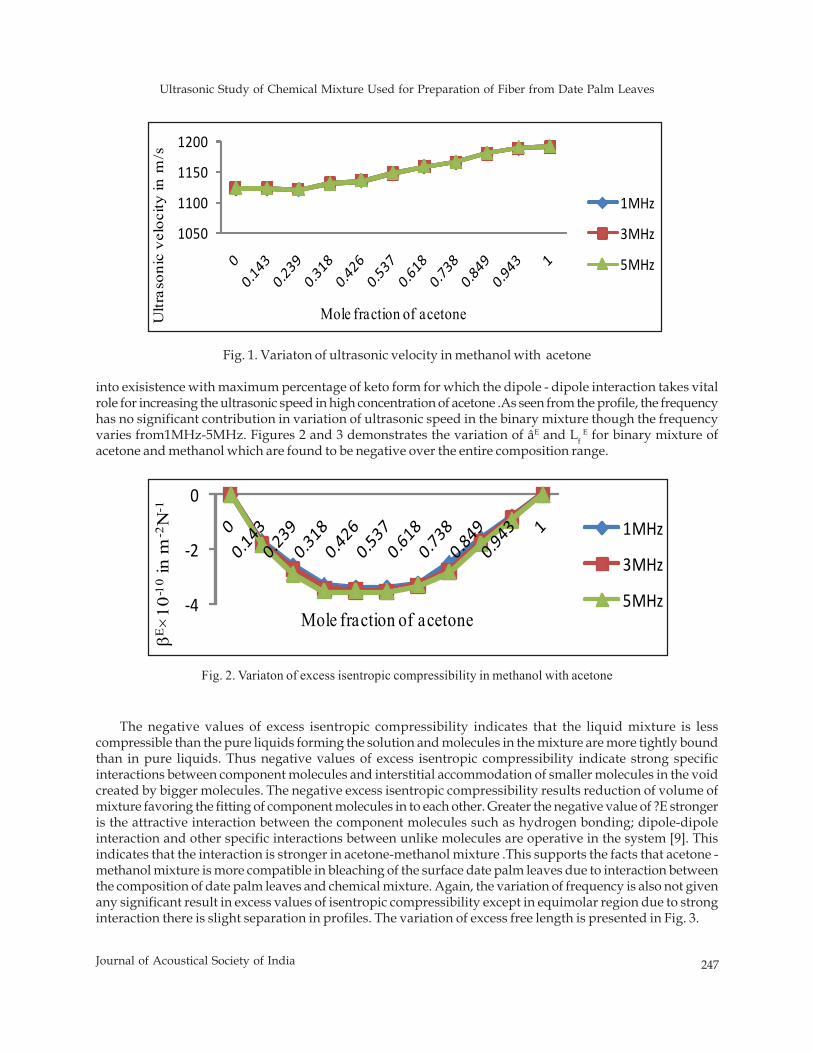
Ultrasonic Study of Chemical Mixture Used for Preparation of Fiber from Date Palm Leaves
247Journal of Acoustical Society of India
into exisistence with maximum percentage of keto form for which the dipole - dipole interaction takes vitalrole for increasing the ultrasonic speed in high concentration of acetone .As seen from the profile, the frequencyhas no significant contribution in variation of ultrasonic speed in the binary mixture though the frequencyvaries from1MHz-5MHz. Figures 2 and 3 demonstrates the variation of âE and Lf
E for binary mixture ofacetone and methanol which are found to be negative over the entire composition range.
Fig. 1. Variaton of ultrasonic velocity in methanol with acetone
The negative values of excess isentropic compressibility indicates that the liquid mixture is lesscompressible than the pure liquids forming the solution and molecules in the mixture are more tightly boundthan in pure liquids. Thus negative values of excess isentropic compressibility indicate strong specificinteractions between component molecules and interstitial accommodation of smaller molecules in the voidcreated by bigger molecules. The negative excess isentropic compressibility results reduction of volume ofmixture favoring the fitting of component molecules in to each other. Greater the negative value of ?E strongeris the attractive interaction between the component molecules such as hydrogen bonding; dipole-dipoleinteraction and other specific interactions between unlike molecules are operative in the system [9]. Thisindicates that the interaction is stronger in acetone-methanol mixture .This supports the facts that acetone -methanol mixture is more compatible in bleaching of the surface date palm leaves due to interaction betweenthe composition of date palm leaves and chemical mixture. Again, the variation of frequency is also not givenany significant result in excess values of isentropic compressibility except in equimolar region due to stronginteraction there is slight separation in profiles. The variation of excess free length is presented in Fig. 3.
1050
1100
1150
1200U
ltras
onic
vel
ocity
in m
/s
Mole fraction of acetone
1MHz
3MHz
5MHz
Fig. 2. Variaton of excess isentropic compressibility in methanol with acetone
‐4
‐2
0
βE×
10-1
0in
m-2
N-1
Mole fraction of acetone
1MHz
3MHz
5MHz
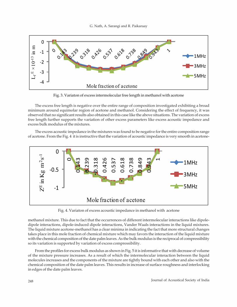
248 Journal of Acoustical Society of India
G. Nath, A. Sarangi and R. Paikaraay
The excess free length is negative over the entire range of composition investigated exhibiting a broadminimum around equimolar region of acetone and methanol. Considering the effect of frequency, it wasobserved that no significant results also obtained in this case like the above situations. The variation of excessfree length further supports the variation of other excess parameters like excess acoustic impedance andexcess bulk modulus of the mixtures.
The excess acoustic impedance in the mixtures was found to be negative for the entire composition rangeof acetone. From the Fig. 4 it is instructive that the variation of acoustic impedance is very smooth in acetone-
methanol mixture. This due to fact that the occurrences of different intermolecular interactions like dipole-dipole interactions, dipole-induced dipole interactions, Vander Waals interactions in the liquid mixtures.The liquid mixture acetone-methanol has a clear minima in indicating the fact that more structural changestakes place in this mole fraction of chemical mixture which may favors the interaction of the liquid mixturewith the chemical composition of the date palm leaves. As the bulk modulus is the reciprocal of compressibilityso its variation is supported by variation of excess compressibility.
From the profiles for excess bulk modulus as shown in Fig. 5 it is informative that with decrease of volumeof the mixture pressure increases. As a result of which the intermolecular interaction between the liquidmolecules increases and the components of the mixture are tightly bound with each other and also with thechemical composition of the date palm leaves. This results in increase of surface roughness and interlockingin edges of the date palm leaves.
Fig. 4. Variaton of excess acoustic impedance in methanol with acetone
‐1
‐0.5
0
00.14
30.23
90.31
80.42
60.53
70.61
80.73
80.84
90.94
3 1
ZE
in K
g m
2 s-1
Mole fraction of acetone
1MHz
3MHz
5MHz
‐4
‐3
‐2
‐1
0
L fE
×10-1
3in
m
Mole fraction of acetone
1MHz
3MHz
5MHz
Fig. 3. Variaton of excess intermolecular free length in methanol with acetone
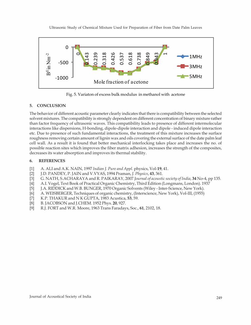
Ultrasonic Study of Chemical Mixture Used for Preparation of Fiber from Date Palm Leaves
249Journal of Acoustical Society of India
Fig. 5. Variaton of excess bulk modulus in methanol with acetone
‐1000
‐500
0
0
0.14
3
0.23
9
0.31
8
0.42
6
0.53
7
0.61
8
0.73
8
0.84
9
0.94
3 1
BEin
Nm
-2
Mole fraction of acetone
1MHz
3MHz
5MHz
5. CONCLUSION
The behavior of different acoustic parameter clearly indicates that there is compatibility between the selectedsolvent mixtures. The compatibility is strongly dependent on different concentration of binary mixture ratherthan factor frequency of ultrasonic waves. This compatibility leads to presence of different intermolecularinteractions like dispersions, H-bonding, dipole-dipole interaction and dipole - induced dipole interactionetc. Due to presence of such fundamental interactions, the treatment of this mixture increases the surfaceroughness removing certain amount of lignin wax and oils covering the external surface of the date palm leafcell wall. As a result it is found that better mechanical interlocking takes place and increases the no. ofpossible reaction sites which improves the fiber matrix adhesion, increases the strength of the composites,decreases its water absorption and improves its thermal stability.
6. REFERENCES
[1] A. ALI and A.K. NAIN, 1997 Indian J. Pure and Appl. physics, Vol-19, 41.[2] J.D. PANDEY, P. JAIN and V.VYAS, 1994 Praman, J. Physics, 43, 361.[3] G. NATH, S.ACHARAYA and R. PAIKARAY, 2007 Journal of acoustic society of India, 34 No-4, pp 135.[4] A.I. Vogel, Text Book of Practical Organic Chemistry, Third Edition (Longmans, London). 1937[5] J.A. RIDDICK and W.B. BUNGER, 1970 Organic Solvents (Wiley - Inter-Science, New York).[6] A. WEISBERGER, Techniques of organic chemistry, (Interscience, New York), Vol-III, (1955)[7] K.P. THAKUR and N K GUPTA, 1983 Acustica, 53, 59.[8] B. JACOBSON and J.CHEM. 1952 Phys. 20, 927.[9] R.J. FORT and W.R. Moore, 1963 Trans Faradays, Soc., 61, 2102, 18.
Prcessing for Emotions Induced by Hindustani Instrumental Music
267Journal of Acoustical Society of India
ABSTRACT
Music has an intriguing ability to evoke powerful emotions without having such an intrinsic link.However, establishing exactly how music communicates emotion is a topic of much debate. Thepresent study concentrates on the signal analysis of two ragas (Chayanat and Darbari Kannada)played by an eminent sitar player as well as performing listening tests and EEG analysis on naïvelisteners. An attempt was made to correlate the changes of EEG signal characteristics due to emotionwith the note sequence of the ragas.
INTRODUCTION
Western classical music which is based on harmonic relation between notes versus the melodic mode (raga)structures in the Hindustani music system (HM) within the rhythmic cycle music may demand qualitativelydifferent cognitive engagement. Each raga in the HM is conventionally assigned to a corresponding rasa/emotion is known to consistently evoke certain emotions [1]. The artist exploits ones creativity and elaboratesthe raga well within the melodic framework to bring out the rasa or the emotion. The human brain, which isone of the most complex organic systems, involves billions of interacting physiological and chemical processesthat give rise to experimentally observed neuro-electrical activity, which is called an electroencephalogram(EEG). The use of EEG signals as a vector of communication between men and machines represents one of thecurrent challenges in signal theory research. The present study concentrates on the signal analysis of the aalappart of two ragas (eliciting contrast emotions, ie, joy/romantic and sorrow/pathos) played by an eminent sitarplayer and subsequently conducting listening tests with the raga clips along with the EEG analysis to studythe emotion as processed in the brain.
1. EXPERIMENTAL DETAILS
Two ragas chosen are for our analysis are Chayanat (romantic/joy) and Darbari Kannada (pathos/sorrow).Each of these sound signals was digitized with sample rate of 44.1 kHz, 16 bit resolution and in a monochannel. From the complete playing of the ragas, segments of about 3mins and 40 seconds were taken out foranalysis for each raga. Detection of pitch was done by using the open source software package WAVESURFERof KTH, Stockholm. The tonic (Sa) was extracted from the signal by the help of a musician and then the notesequence was found out. Signals processing was performed to find out the tempo, pitch sift and note distributionof the emotion revealing part. From the sequences the phrases which contain the emotion as identified by a
Journal of Acoustical Society of India : Vol. 40, No. 4, 2013 (pp. 267-272)
Prcessing for Emotions Induced by HindustaniInstrumental Music
Ranjan Sengupta1, Anirban patranabis1, Kaushik Banerjee1, Tarit Guhathakurta1,Samabrata Sarkar1, Gautam Ganguli2, Atanu Biswas2, P.K. Saha2 and Dipak Ghosh1
1Sir C V Raman Centre for Physics and Music, Jadavpur University, Kolkata2Bangur Institute of Neuroscience, Kolkata
[Received: 25.04.2013; Revised: 28.07.2013; Accepted: 28.09.2013]
© 2013 Acoustical Society of India
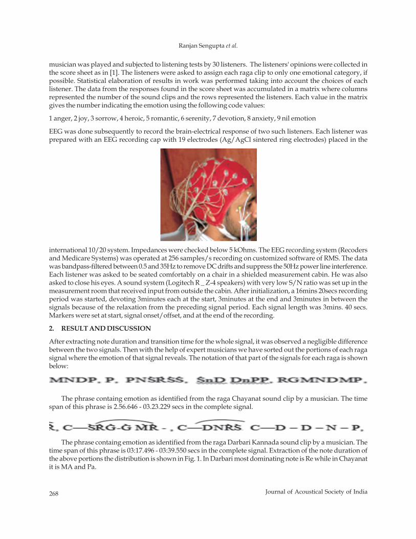
268 Journal of Acoustical Society of India
Ranjan Sengupta et al.
musician was played and subjected to listening tests by 30 listeners. The listeners' opinions were collected inthe score sheet as in [1]. The listeners were asked to assign each raga clip to only one emotional category, ifpossible. Statistical elaboration of results in work was performed taking into account the choices of eachlistener. The data from the responses found in the score sheet was accumulated in a matrix where columnsrepresented the number of the sound clips and the rows represented the listeners. Each value in the matrixgives the number indicating the emotion using the following code values:
1 anger, 2 joy, 3 sorrow, 4 heroic, 5 romantic, 6 serenity, 7 devotion, 8 anxiety, 9 nil emotion
EEG was done subsequently to record the brain-electrical response of two such listeners. Each listener wasprepared with an EEG recording cap with 19 electrodes (Ag/AgCl sintered ring electrodes) placed in the
international 10/20 system. Impedances were checked below 5 kOhms. The EEG recording system (Recodersand Medicare Systems) was operated at 256 samples/s recording on customized software of RMS. The datawas bandpass-filtered between 0.5 and 35Hz to remove DC drifts and suppress the 50Hz power line interference.Each listener was asked to be seated comfortably on a chair in a shielded measurement cabin. He was alsoasked to close his eyes. A sound system (Logitech R _ Z-4 speakers) with very low S/N ratio was set up in themeasurement room that received input from outside the cabin. After initialization, a 16mins 20secs recordingperiod was started, devoting 3minutes each at the start, 3minutes at the end and 3minutes in between thesignals because of the relaxation from the preceding signal period. Each signal length was 3mins. 40 secs.Markers were set at start, signal onset/offset, and at the end of the recording.
2. RESULT AND DISCUSSION
After extracting note duration and transition time for the whole signal, it was observed a negligible differencebetween the two signals. Then with the help of expert musicians we have sorted out the portions of each ragasignal where the emotion of that signal reveals. The notation of that part of the signals for each raga is shownbelow:
The phrase containg emotion as identified from the raga Chayanat sound clip by a musician. The timespan of this phrase is 2.56.646 - 03.23.229 secs in the complete signal.
The phrase containg emotion as identified from the raga Darbari Kannada sound clip by a musician. Thetime span of this phrase is 03:17.496 - 03:39.550 secs in the complete signal. Extraction of the note duration ofthe above portions the distribution is shown in Fig. 1. In Darbari most dominating note is Re while in Chayanatit is MA and Pa.
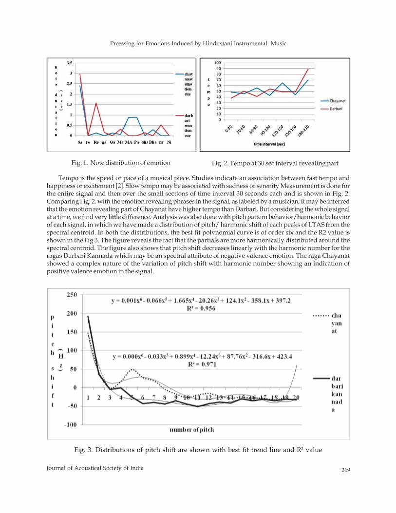
Prcessing for Emotions Induced by Hindustani Instrumental Music
269Journal of Acoustical Society of India
Tempo is the speed or pace of a musical piece. Studies indicate an association between fast tempo andhappiness or excitement [2]. Slow tempo may be associated with sadness or serenity Measurement is done forthe entire signal and then over the small sections of time interval 30 seconds each and is shown in Fig. 2.Comparing Fig. 2. with the emotion revealing phrases in the signal, as labeled by a musician, it may be inferredthat the emotion revealing part of Chayanat have higher tempo than Darbari. But considering the whole signalat a time, we find very little difference. Analysis was also done with pitch pattern behavior/harmonic behaviorof each signal, in which we have made a distribution of pitch/ harmonic shift of each peaks of LTAS from thespectral centroid. In both the distributions, the best fit polynomial curve is of order six and the R2 value isshown in the Fig 3. The figure reveals the fact that the partials are more harmonically distributed around thespectral centroid. The figure also shows that pitch shift decreases linearly with the harmonic number for theragas Darbari Kannada which may be an spectral attribute of negative valence emotion. The raga Chayanatshowed a complex nature of the variation of pitch shift with harmonic number showing an indication ofpositive valence emotion in the signal.
Fig. 1. Note distribution of emotion Fig. 2. Tempo at 30 sec interval revealing part
Fig. 3. Distributions of pitch shift are shown with best fit trend line and R2 value
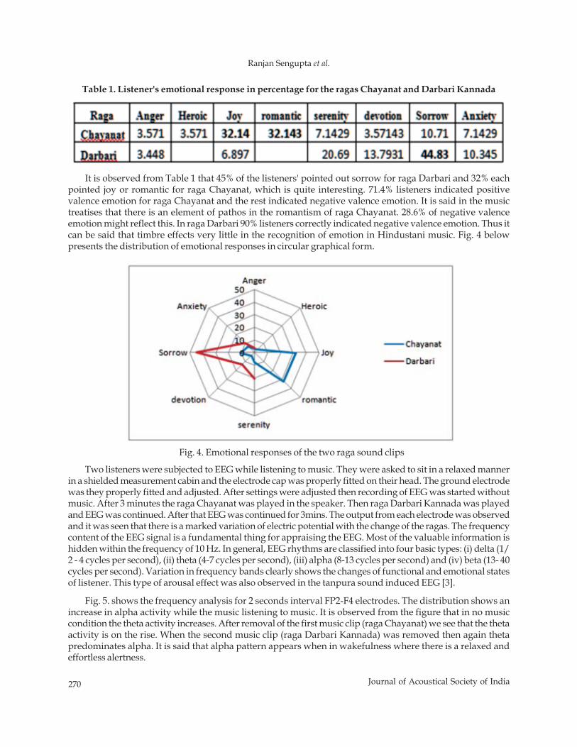
270 Journal of Acoustical Society of India
Ranjan Sengupta et al.
It is observed from Table 1 that 45% of the listeners' pointed out sorrow for raga Darbari and 32% eachpointed joy or romantic for raga Chayanat, which is quite interesting. 71.4% listeners indicated positivevalence emotion for raga Chayanat and the rest indicated negative valence emotion. It is said in the musictreatises that there is an element of pathos in the romantism of raga Chayanat. 28.6% of negative valenceemotion might reflect this. In raga Darbari 90% listeners correctly indicated negative valence emotion. Thus itcan be said that timbre effects very little in the recognition of emotion in Hindustani music. Fig. 4 belowpresents the distribution of emotional responses in circular graphical form.
Two listeners were subjected to EEG while listening to music. They were asked to sit in a relaxed mannerin a shielded measurement cabin and the electrode cap was properly fitted on their head. The ground electrodewas they properly fitted and adjusted. After settings were adjusted then recording of EEG was started withoutmusic. After 3 minutes the raga Chayanat was played in the speaker. Then raga Darbari Kannada was playedand EEG was continued. After that EEG was continued for 3mins. The output from each electrode was observedand it was seen that there is a marked variation of electric potential with the change of the ragas. The frequencycontent of the EEG signal is a fundamental thing for appraising the EEG. Most of the valuable information ishidden within the frequency of 10 Hz. In general, EEG rhythms are classified into four basic types: (i) delta (1/2 - 4 cycles per second), (ii) theta (4-7 cycles per second), (iii) alpha (8-13 cycles per second) and (iv) beta (13- 40cycles per second). Variation in frequency bands clearly shows the changes of functional and emotional statesof listener. This type of arousal effect was also observed in the tanpura sound induced EEG [3].
Fig. 5. shows the frequency analysis for 2 seconds interval FP2-F4 electrodes. The distribution shows anincrease in alpha activity while the music listening to music. It is observed from the figure that in no musiccondition the theta activity increases. After removal of the first music clip (raga Chayanat) we see that the thetaactivity is on the rise. When the second music clip (raga Darbari Kannada) was removed then again thetapredominates alpha. It is said that alpha pattern appears when in wakefulness where there is a relaxed andeffortless alertness.
Table 1. Listener's emotional response in percentage for the ragas Chayanat and Darbari Kannada
Fig. 4. Emotional responses of the two raga sound clips
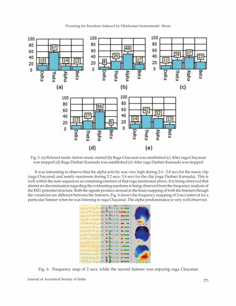
Prcessing for Emotions Induced by Hindustani Instrumental Music
271Journal of Acoustical Society of India
It was interesting to observe that the alpha activity was very high during 2.6 - 2.8 secs for the music clip(raga Chayanat) and nearly maximum during 3.2 secs- 3.4 secs for the clip (raga Darbari Kannada). This iswell within the note sequences as containing emotion of that raga mentioned above. It is being observed thatalmost no discrimination regarding the contrasting emotions is being observed from the frequency analysis ofthe EEG potential structure. Both the signals produce arousal in the brain mapping of both the listeners thoughthe variations are different between the listeners. Fig. 6 shows the frequency mapping of 2 secs interval for aparticular listener when he was listening to raga Chayanat. The alpha predominance is very well observed.
Fig. 5. (a) Relaxed mode -before music started (b) Raga Chayanat was established (c) After raga Chayanatwas stopped (d) Raga Darbari Kannada was established (e) After raga Darbari Kannada was stopped
Fig. 6. Frequency map of 2 secs. while the second listener was enjoying raga Chayanat

272 Journal of Acoustical Society of India
Ranjan Sengupta et al.
3. CONCLUSION
Emotion in music clip (raga rendering) is embedded in some specific note sequences of the clip. Arousal occursto a listener while listening to the music clip particularly when that sequence in being played. Our present EEGanalysis is unable to distinguish between contrasting emotions. As evidenced by the listening test, emotion inthe Hindustani raga music is timbre independent and mainly concentrated on the particular note sequences,note to note transitions (meends) and other ornaments. Listening test result shows that naïve listeners candistinguish between contrast emotions. More rigorous analysis of EEG data with different types of musicneeds to be done to frame a robust algorithm to have a thorough knowledge of music processing in the brain.This is our future work.
4. REFERENCES
[1] A. ALICJA WIECZORKOWSKA, ASHOKE KUMAR DATTA, RANJAN SENGUPTA, NITYANANDADEY, and BHASWATI MUKHERJEE, 2010 "On Search for Emotion in Hindusthani Vocal Music", Adv.in Music Inform. Retrieval, SCI 274, p. 285 Springer-Verlag Berlin Heidelberg.
[2] S.O. ALI and Z F PEYNIRCIOGLU, 2010 "Intensity of emotions conveyed and elicited by familiar andunfamiliar music" Music Perception: An Interdisciplinary Journal 27: 177.
[3] MATTHIAS BRAEUNIG, RANJAN SENGUPTA and ANIRBAN PATRANABIS, 2012 "On Tanpura Droneand Brain Electrical Correlates", LNCS 7172, p. 53. Springer-Verlag Berlin Heidelberg.
Performance Analysis of DCT and DFT Based Speech Coding
255Journal of Acoustical Society of India
ABSTRACT
Speech compression system focuses on reducing the amount of redundant data while preserving theintegrity of the signals. Speech compression algorithms are generally classified in to three categories.They are parametric coders, hybrid coders and transform's coders. This paper analyzes theeffectiveness of different transform technique on Indian regional language. Speech data base used forthis experiment is created in Malayalam, one of the South Indian languages. To remove insignificantcoefficient from the feature vector we apply hard thersholding technique on Discrete Cosinetransformed coefficient. Lossless run length encoding algorithms is used to encode the remainingcoefficients. Performance of this experiment is evaluated in terms of NRMSE, SNR, PSNR, MOS andpercentage of compression occurred. It has been found that Discrete Cosine Transforms (DCT) issuperior to Discrete Fourier Transforms (DFT).
1. INTRODUCTION
In information theory, data compression or source coding is the process of encoding information using feverbits than the original one. Data compression is useful because it helps to reduce consumption of expensiveresources such as memory, HDD and transmission bandwidth etc[1]. On the down side of encoding anddecoding process demands some amount of computation. The design of data compression schemes thereforeinvolves trade off among various factors including the degree of computation the amount of distortion andcomputational resource required to compress and uncompress the data [2].
Compression algorithms are classified in to lossless compression and lossy compression. Losslessalgorithms are usually exploiting statistical redundancy in the input data. Perfect reconstruction is possiblein lossless compression without any loss of fidelity. But in the case of lossy compression there are many tradeoff where by some degradation in the quality of data will occur as part of compression [3]. There is mechanismto measure the efficiency of compression without which an effectives rating of compression techniques maynot be possible. There are many parameter used to evaluate the effectiveness of data compression [4]. The mainarea of data compression is speech, image and multimedia processing.
Speech is a very unique signal by the nature due to many reasons. The most prominent factor is that thespeech is a non stationary signal. This makes the speech signal hard to analyze and model. Second factor isthat speech signal contains not only the information part but also many information like emotion, healthcondition, age and gender of speaker etc [5]. This make analyses and synthesis of speech signal more complex.There are many type of algorithms are available to process speech signal. Each one has its own merit anddemerits. So far no algorithms have 100% perfection in analyses and synthesis of speech signal. Thereforedemand for perfect algorithm is still exist in the area of compression.
Journal of Acoustical Society of India : Vol. 40, No. 4, 2013 (pp. 255-260)
Performance Analysis of DCT and DFT BasedSpeech Coding
Shijo M. Josep* and P. Babu AntoSchool of Information Science & Technology
Kannur University (Kerala)*e-mail: [email protected]
[Received: 19.04.2013; Revised: 20.07.2013; Accepted: 24.09.2013]
© 2013 Acoustical Society of India
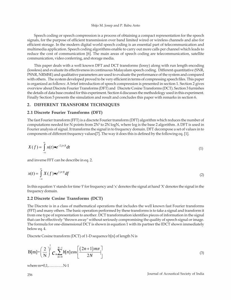
256 Journal of Acoustical Society of India
Shijo M. Josep and P. Babu Anto
Speech coding or speech compression is a process of obtaining a compact representation for the speechsignals, for the purpose of efficient transmission over band limited wired or wireless channels and also forefficient storage. In the modern digital world speech coding is an essential part of telecommunication andmultimedia application. Speech coding algorithms enable to carry out more calls per channel which leads toreduce the cost of communication [6]. The main areas of speech coding are telecommunication, satellitecommunication, video conferring, and storage media.
This paper deals with a well known DFT and DCT transforms (lossy) along with run length encoding(lossless) and evaluate its effectiveness in continuous Malayalam speech coding. Different quantitative (SNR,PSNR, NRMSE) and qualitative parameters are used to evaluate the performance of the system and comparedwith others. The system developed proved to be very efficient in terms of compressing speech files. This paperis organized as follows: A brief introduction of speech compression is presented in section 1. Section 2 givesoverview about Discrete Fourier Transforms (DFT) and Discrete Cosine Transforms (DCT). Section 3 furnishesthe details of data base created for this experiment. Section 4 discusses the methodology used in this experiment.Finally Section 5 presents the simulation and result and concludes this paper with remarks in section 6.
2. DIFFERENT TRANSFORM TECHNIQUES
2.1 Discrete Fourier Transforms (DFT)
The fast Fourier transform (FFT) is a discrete Fourier transform (DFT) algorithm which reduces the number ofcomputations needed for N points from 2N2 to 2N logN, where log is the base 2 algorithm. A DFT is used inFourier analysis of signal. It transforms the signal in to frequency domain. DFT decompose a set of values in tocomponents of different frequency values[7]. The way it does this is defined by the following eq. [1].
2( ) ( ) π∞
−
−∞
= •∫ j ftX f x t e dt (1)
and inverse FFT can be describe in eq. 2.
2( ) ( ) π∞
−∞
= •∫ j ftx t X f e df (2)
In this equation 't' stands for time 'f' for frequency and 'x' denotes the signal at hand 'X' denotes the signal in thefrequency domain.
2.2 Discrete Cosine Transforms (DCT)
The Discrete is in a class of mathematical operations that includes the well known fast Fourier transforms(FFT) and many others. The basic operation performed by these transforms is to take a signal and transform itfrom one type of representation to another. DCT transformation identifies pieces of information in the signalthat can be effectively "thrown away" without seriously compromising the quality of speech signal or image.The formula for one-dimensional DCT is shown in equation 1 with its partner the IDCT shown immediatelybelow eq. 4.
Discrete Cosine transform (DCT) of 1-D sequence b[n] of length N is
( )1
12
0
2 12B[m]= [ ]cosN 2
π−
=
+⎡ ⎤⎛ ⎞⎢ ⎥⎜ ⎟
⎝ ⎠ ⎣ ⎦∑N
mm
n mb n
Nc (3)
where m=0,1,…………N-1
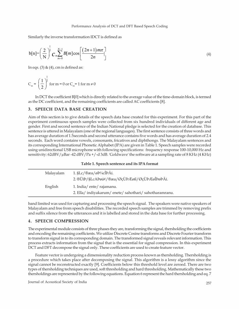
Performance Analysis of DCT and DFT Based Speech Coding
257Journal of Acoustical Society of India
Similarly the inverse transformation IDCT is defined as
( )1
12
0
2 12b[n]= [ ]cosN 2
π−
=
+⎡ ⎤⎛ ⎞⎢ ⎥⎜ ⎟
⎝ ⎠ ⎣ ⎦∑N
mm
n mB m
nc (4)
In eqs. (3) & (4), cm is defined as:
Cm =
121
2⎛ ⎞⎜ ⎟⎝ ⎠
for m = 0 or Cm= 1 for m ≠ 0
In DCT the coefficient B[0] which is directly related to the average value of the time-domain block, is termedas the DC coefficient, and the remaining coefficients are called AC coefficients [8].
3. SPEECH DATA BASE CREATION
Aim of this section is to give details of the speech data base created for this experiment. For this part of theexperiment continuous speech samples were collected from six hundred individuals of different age andgender. First and second sentence of the Indian National pledge is selected for the creation of database. Thissentence is uttered in Malayalam (one of the regional languages). The first sentence consists of three words andhas average duration of 1.5seconds and second utterance contains five words and has average duration of 2.4seconds. Each word contains vowels, consonants, fricatives and diphthongs. The Malayalam sentences andits corresponding International Phonetic Alphabet (IPA) are given in Table 1. Speech samples were recordedusing unidirectional USB microphone with following specifications: frequency response 100-10,000 Hz andsensitivity: 62dBV/μBar -42 dBV/Pa +/-d 3dB. 'Goldwave' the software at a sampling rate of 8 KHz (4 KHz)
Table 1. Speech sentence and its IPA format
Malayalam 1. §Lc/®æa/øÞ¼cÎÞÃí.2. ®ÜïÞ/§LcAÞøá¢/®æa/ØçÙÞÆøß/ØçÙÞÆøÎÞøÞÃí.
English 1. India/ ente/ rajamanu.2. Ella/ indiyakarum/ enete/ sahothari/ sahotharamranu.
band limited was used for capturing and processing the speech signal. The speakers were native speakers ofMalayalam and free from speech disabilities. The recorded speech samples are trimmed by removing prefixand suffix silence from the utterances and it is labelled and stored in the data base for further processing.
4. SPEECH COMPRESSION
The experimental module consists of three phases they are, transforming the signal, thersholding the coefficientsand encoding the remaining coefficients. We utilize Discrete Cosine transforms and Discrete Fourier transformto transform signal in to its corresponding domain. The transformed signal reveals relevant information. Thisprocess extracts information from the signal that is the essential for signal compression. In this experimentDCT and DFT decompose the signal only. These coefficients are used to create feature vector.
Feature vector is undergoing a dimensionality reduction process known as thersholding. Thersholding isa procedure which takes place after decomposing the signal. This algorithm is a lossy algorithm since thesignal cannot be reconstructed exactly [9]. Coefficients below this threshold level are zeroed. There are twotypes of thersholding techniques are used, soft thresholding and hard thresholding. Mathematically these twothersholdings are represented by the following equations. Equation 6 represent the hard thersholding and eq. 7
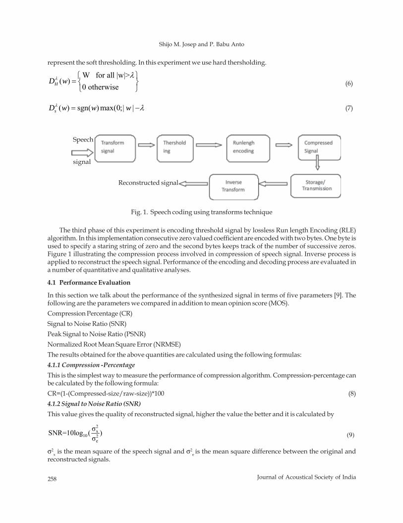
258 Journal of Acoustical Society of India
Shijo M. Josep and P. Babu Anto
represent the soft thresholding. In this experiment we use hard thersholding.
W for all |w|>( )
0 otherwiseλ λ⎧ ⎫
= ⎨ ⎬⎩ ⎭
HD w (6)
( ) sgn( ) max(0;| |λ λ= −sD w w w (7)
The third phase of this experiment is encoding threshold signal by lossless Run length Encoding (RLE)algorithm. In this implementation consecutive zero valued coefficient are encoded with two bytes. One byte isused to specify a staring string of zero and the second bytes keeps track of the number of successive zeros.Figure 1 illustrating the compression process involved in compression of speech signal. Inverse process isapplied to reconstruct the speech signal. Performance of the encoding and decoding process are evaluated ina number of quantitative and qualitative analyses.
4.1 Performance Evaluation
In this section we talk about the performance of the synthesized signal in terms of five parameters [9]. Thefollowing are the parameters we compared in addition to mean opinion score (MOS).Compression Percentage (CR)Signal to Noise Ratio (SNR)Peak Signal to Noise Ratio (PSNR)Normalized Root Mean Square Error (NRMSE)The results obtained for the above quantities are calculated using the following formulas:4.1.1 Compression -PercentageThis is the simplest way to measure the performance of compression algorithm. Compression-percentage canbe calculated by the following formula:CR=(1-(Compressed-size/raw-size))*100 (8)4.1.2 Signal to Noise Ratio (SNR)This value gives the quality of reconstructed signal, higher the value the better and it is calculated by
2x
10 2e
σSNR=10log ( )σ (9)
σ2x is the mean square of the speech signal and σ2
e is the mean square difference between the original andreconstructed signals.
Speech
signal
Reconstructed signal
Fig. 1. Speech coding using transforms technique
Performance Analysis of DCT and DFT Based Speech Coding
259Journal of Acoustical Society of India
4.1.3 Peak Signal to Noise Ratio (PSNR)This value indicates the ratio between the peak signal and noise within the reconstructed signals. Highervalue is better. PSNR is calculated by the following formula.
2
10 210 log|| ||
=−
NXPSNRx r (10)
In this equation N is the length of the reconstructed signal, X is the maximum absolute square value of thesignal x and ||x-r||2is the energy of the difference between the original and reconstructed signals.4.1.4 Normalized Root Mean Square Error (NRMSE)
( )( )
2
2
( ) ( )( ) ( )μ
−=
− X
x x n r nNRMSE
x n n (11)
x(n) is the speech signal, r(n) is the reconstructed signal, and μx(2) is the mean of the speech signal.4.1.5 Mean Opinion Score (MOS)Subjective evaluation by listeners is still a method commonly used in measuring quality of reconstructedspeech. MOS provides a numerical indication of the perceived quality of received media after compression and/ or transmission. The MOS is expressed as a single number in the range 1 to 5. Where 1 is the highestperceived quality and 5 is the lowest perceived quality. When taking subjective test, listeners focus on thedifference between the original and reconstructed signal and rate it. The MOS is generalized by averaging theresult of a set of standards, subjective tests, where a number of listeners rate reconstructed speech signals. Inour experiment the MOS rate was excellent in DCT experiment and it was good in DFT based experiment.
Table 2
Sentence 1 DFT DCT Sentence 2 DFT DCT
CP% 58.4662 80.4025 CP% 60.312 72.87SNR 1.1148 2.17112 SNR 1.00657 1.01972PSNR 4.6556 4.7269 PSNR 2.5001 3.5161NRMSE 0.16503 0.16058 NRMSE 0.0187 0.0178
Fig. 2. DFT vs. DCT Performance comparison based on first & second sentence
260 Journal of Acoustical Society of India
Shijo M. Josep and P. Babu Anto
5. RESULTS
Continuous Malayalam speech compression is implemented by different transform techniques along withthersholding and run length encoding. In these experiments the qualitative and qualitative performances aremeasured in terms of NRMSE, SNR, PSNR, Compression Percentage and MOS.
The results obtained in these experiments are tabulated in Table 2 and corresponding measures aregraphically illustrated in Fig. 2. Average measures of DFT experiments of first and second sentence are SNR is1.0606, PSNR is 3.57788, NRMSE is 0.0918 and compression percentage is 59.3891. Similarly in DCT experimentsthe obtained average values are SNR is 1.59542, PSNR is 4.1215, NRMSE is 0.08918 and compression percentageis 76.6366.
6. CONCLUSION
The main aim of speech coding is to represent speech signal with minimum number of bits for storage ortransmission. This paper discusses the efficiency of well known transform based speech coding on Indianregional language. From the stated results it is proved that, Discrete Cosine Transform (DCT) perform betterthan the DFT in Indian regional languages.
7. REFERENCES
[1] MARK NELSON and JEAN LOUP GAILLY, 2003. The Data Compression Book, 2nd Edition, BPBpublications.
[2]. KHALID SAYOOD, 2005. Introduction to Data Compression, Morgan Kaufmann Publishers 2nd edition.[3]. DAVID SALOMON, 2011. Data Compression, the Complete Reference, Springer International Edition,
4th edition.[4]. LAWRENCE RABINER and BIING HWANG JUANG, 2009. Fundamentals of Speech Recognition",
Pearson Education.[5]. THOMAS F. QUATIERI, 2012. Discrete-Time Speech Signal Processing Principle and Practice', Pearson
Publication 8th edition.[6]. K.P. SOMAN and K.I. RAMACHANDRAN, 2008. Insight in to wavelets from theory to practice", Prentice-
Hall of India Private limited, 2nd edition.[7]. G. RAJESH, A. KUMAR and K. RANJEET, 2011. Speech compression using different transform
techniques", Second IEEE International Conf. on Computer, and Communication Technology, pp. 146-151.
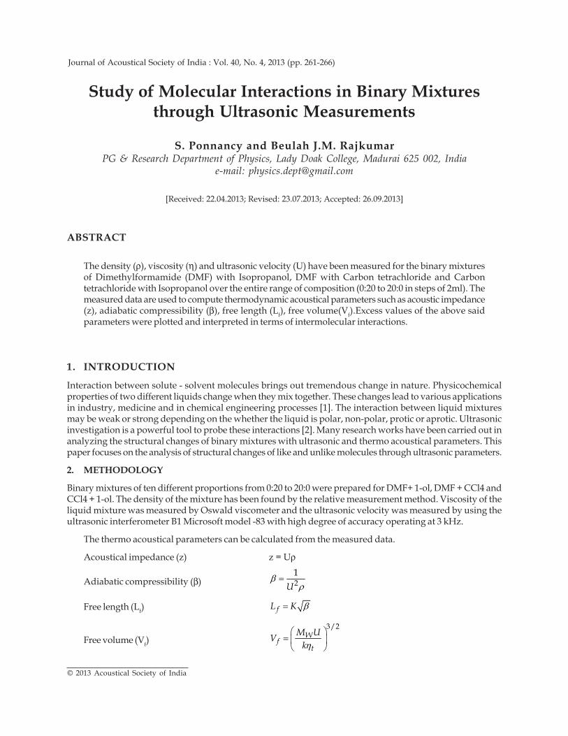
Study of Molecular Interactions in Binary Mixtures Through Ultrasonic Measurements
261Journal of Acoustical Society of India
ABSTRACT
The density (ρ), viscosity (η) and ultrasonic velocity (U) have been measured for the binary mixturesof Dimethylformamide (DMF) with Isopropanol, DMF with Carbon tetrachloride and Carbontetrachloride with Isopropanol over the entire range of composition (0:20 to 20:0 in steps of 2ml). Themeasured data are used to compute thermodynamic acoustical parameters such as acoustic impedance(z), adiabatic compressibility (β), free length (Lf), free volume(Vf).Excess values of the above saidparameters were plotted and interpreted in terms of intermolecular interactions.
1. INTRODUCTION
Interaction between solute - solvent molecules brings out tremendous change in nature. Physicochemicalproperties of two different liquids change when they mix together. These changes lead to various applicationsin industry, medicine and in chemical engineering processes [1]. The interaction between liquid mixturesmay be weak or strong depending on the whether the liquid is polar, non-polar, protic or aprotic. Ultrasonicinvestigation is a powerful tool to probe these interactions [2]. Many research works have been carried out inanalyzing the structural changes of binary mixtures with ultrasonic and thermo acoustical parameters. Thispaper focuses on the analysis of structural changes of like and unlike molecules through ultrasonic parameters.
2. METHODOLOGY
Binary mixtures of ten different proportions from 0:20 to 20:0 were prepared for DMF+ 1-ol, DMF + CCl4 andCCl4 + 1-ol. The density of the mixture has been found by the relative measurement method. Viscosity of theliquid mixture was measured by Oswald viscometer and the ultrasonic velocity was measured by using theultrasonic interferometer B1 Microsoft model -83 with high degree of accuracy operating at 3 kHz.
The thermo acoustical parameters can be calculated from the measured data.
Acoustical impedance (z) z = Uρ
Adiabatic compressibility (β) 21
Uβ
ρ=
Free length (Lf) fL K β=
Free volume (Vf)3/2
Wf
t
M UVkη
⎛ ⎞= ⎜ ⎟⎝ ⎠
Journal of Acoustical Society of India : Vol. 40, No. 4, 2013 (pp. 261-266)
Study of Molecular Interactions in Binary Mixturesthrough Ultrasonic Measurements
S. Ponnancy and Beulah J.M. RajkumarPG & Research Department of Physics, Lady Doak College, Madurai 625 002, India
e-mail: [email protected]
[Received: 22.04.2013; Revised: 23.07.2013; Accepted: 26.09.2013]
© 2013 Acoustical Society of India
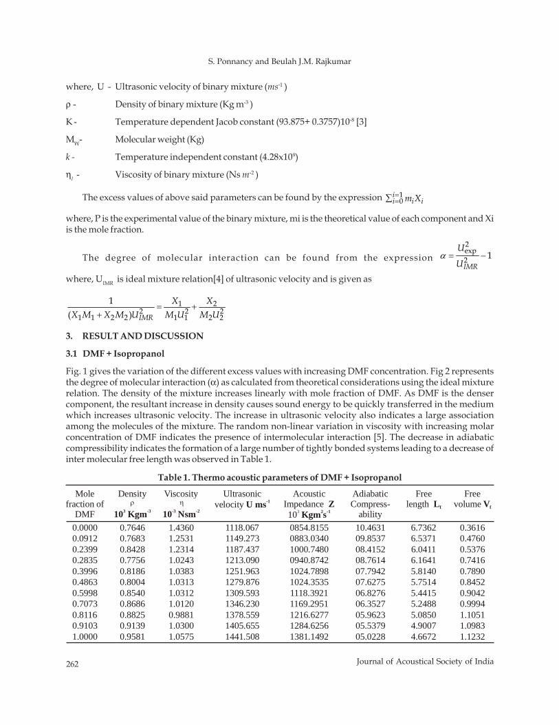
262 Journal of Acoustical Society of India
S. Ponnancy and Beulah J.M. Rajkumar
where, U - Ultrasonic velocity of binary mixture (ms-1 )
ρ - Density of binary mixture (Kg m-3 )
K - Temperature dependent Jacob constant (93.875+ 0.3757)10-8 [3]
MW- Molecular weight (Kg)
k - Temperature independent constant (4.28x10⁹)
ηl - Viscosity of binary mixture (Ns m-2 )
The excess values of above said parameters can be found by the expression 10
ii i im X==∑
where, P is the experimental value of the binary mixture, mi is the theoretical value of each component and Xiis the mole fraction.
The degree of molecular interaction can be found from the expression 2exp2 1IMR
U
Uα = −
where, UIMR is ideal mixture relation[4] of ultrasonic velocity and is given as
1 22 2 2
1 1 2 2 1 1 2 2
1( ) IMR
X XX M X M U M U M U
= ++
3. RESULT AND DISCUSSION
3.1 DMF + Isopropanol
Fig. 1 gives the variation of the different excess values with increasing DMF concentration. Fig 2 representsthe degree of molecular interaction (α) as calculated from theoretical considerations using the ideal mixturerelation. The density of the mixture increases linearly with mole fraction of DMF. As DMF is the densercomponent, the resultant increase in density causes sound energy to be quickly transferred in the mediumwhich increases ultrasonic velocity. The increase in ultrasonic velocity also indicates a large associationamong the molecules of the mixture. The random non-linear variation in viscosity with increasing molarconcentration of DMF indicates the presence of intermolecular interaction [5]. The decrease in adiabaticcompressibility indicates the formation of a large number of tightly bonded systems leading to a decrease ofinter molecular free length was observed in Table 1.
Mole fraction of
DMF
Density
10 Kgm3 -3
Viscosity
10 Nsm-3 -2
Ultrasonic velocity U ms-1
Acoustic Impedance 10
ZKgm s3 2 -1
Adiabatic Compress-
ability
Free length Lf
Free volume Vf
0.0000 0.7646 1.4360 1118.067 0854.8155 10.4631 6.7362 0.36160.0912 0.7683 1.2531 1149.273 0883.0340 09.8537 6.5371 0.47600.2399 0.8428 1.2314 1187.437 1000.7480 08.4152 6.0411 0.53760.2835 0.7756 1.0243 1213.090 0940.8742 08.7614 6.1641 0.74160.3996 0.8186 1.0383 1251.963 1024.7898 07.7942 5.8140 0.78900.4863 0.8004 1.0313 1279.876 1024.3535 07.6275 5.7514 0.84520.5998 0.8540 1.0312 1309.593 1118.3921 06.8276 5.4415 0.90420.7073 0.8686 1.0120 1346.230 1169.2951 06.3527 5.2488 0.99940.8116 0.8825 0.9881 1378.559 1216.6277 05.9623 5.0850 1.10510.9103 0.9139 1.0300 1405.655 1284.6256 05.5379 4.9007 1.09831.0000 0.9581 1.0575 1441.508 1381.1492 05.0228 4.6672 1.1232
ρ η
Table 1. Thermo acoustic parameters of DMF + Isopropanol
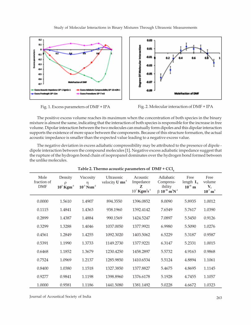
Study of Molecular Interactions in Binary Mixtures Through Ultrasonic Measurements
263Journal of Acoustical Society of India
The positive excess volume reaches its maximum when the concentration of both species in the binarymixture is almost the same, indicating that the interaction of both species is responsible for the increase in freevolume. Dipolar interaction between the two molecules can mutually form dipoles and this dipolar interactionsupports the existence of more space between the components. Because of this structure formation, the actualacoustic impedance is smaller than the expected value leading to a negative excess value.
The negative deviation in excess adiabatic compressibility may be attributed to the presence of dipole -dipole interaction between the compound molecules [1]. Negative excess adiabatic impedance suggest thatthe rupture of the hydrogen bond chain of isopropanol dominates over the hydrogen bond formed betweenthe unlike molecules.
Mole fraction of
DMF
Density ρ
10 Kgm3 -3
Viscosity η
10 Nsm-3 -2
Ultrasonic velocity U ms-1
Acoustic Impedance
10
Z
Kgm s3 2 -1
Adiabatic Compress-
ibility β 10 m N-10 2 -1
Free length L
10 mf
-11
Free volume
V10 m
f-7 3
0.0000 1.5610 1.4907 894.3550 1396.0852 8.0090 5.8935 1.0012
0.1115 1.4841 1.4363 938.1960 1392.4142 7.6549 5.7617 1.0390
0.2899 1.4387 1.4884 990.1569 1424.5247 7.0897 5.5450 0.9126
0.3299 1.3288 1.4046 1037.0050 1377.9921 6.9980 5.5090 1.0276
0.4561 1.2849 1.4255 1092.3020 1403.5062 6.5229 5.3187 0.9587
0.5391 1.1990 1.3733 1149.2730 1377.9221 6.3147 5.2331 1.0015
0.6468 1.1852 1.3679 1230.4250 1458.2897 5.5732 4.9163 0.9868
0.7524 1.0969 1.2137 1285.9850 1410.6534 5.5124 4.8894 1.1061
0.8400 1.0380 1.1518 1327.3850 1377.8827 5.4675 4.8695 1.1145
0.9277 0.9841 1.1198 1398.8960 1376.6178 5.1928 4.7455 1.1057
1.0000 0.9581 1.1186 1441.5080 1381.1492 5.0228 4.6672 1.0323
Table 2. Thermo acoustic parameters of DMF + CCl4
Fig. 1. Excess parameters of DMF + IPA Fig. 2. Molecular interaction of DMF + IPA
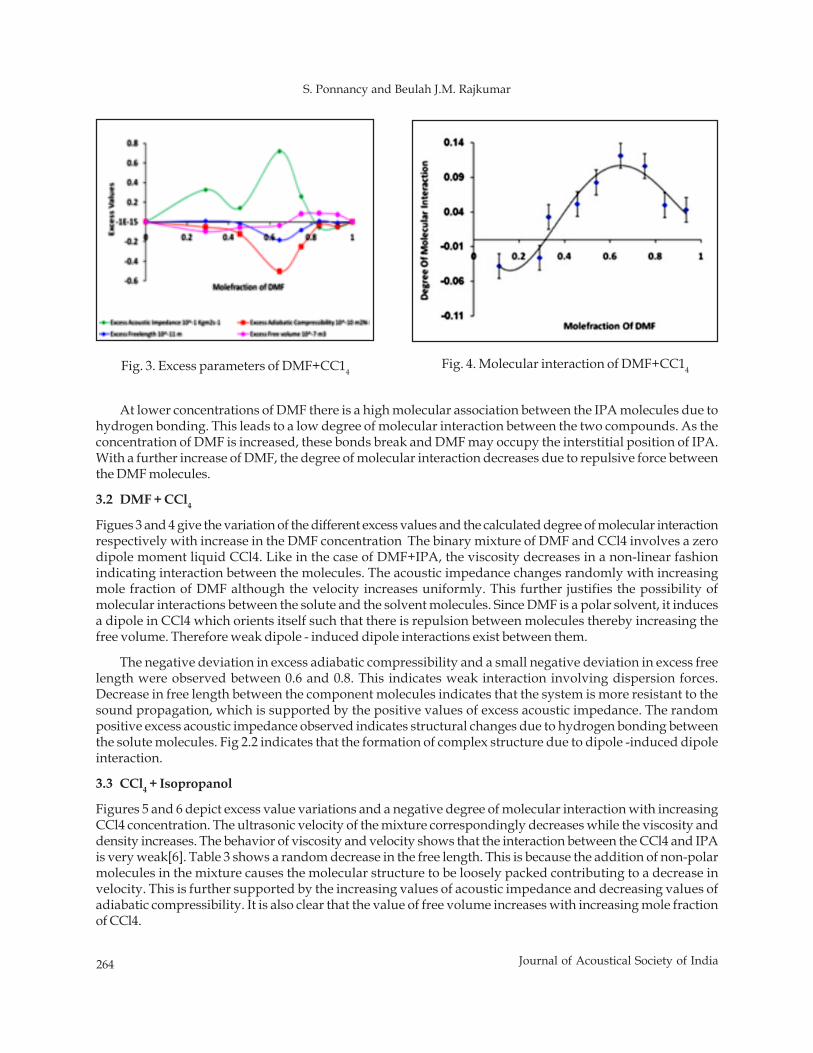
264 Journal of Acoustical Society of India
S. Ponnancy and Beulah J.M. Rajkumar
At lower concentrations of DMF there is a high molecular association between the IPA molecules due tohydrogen bonding. This leads to a low degree of molecular interaction between the two compounds. As theconcentration of DMF is increased, these bonds break and DMF may occupy the interstitial position of IPA.With a further increase of DMF, the degree of molecular interaction decreases due to repulsive force betweenthe DMF molecules.
3.2 DMF + CCl4
Figues 3 and 4 give the variation of the different excess values and the calculated degree of molecular interactionrespectively with increase in the DMF concentration The binary mixture of DMF and CCl4 involves a zerodipole moment liquid CCl4. Like in the case of DMF+IPA, the viscosity decreases in a non-linear fashionindicating interaction between the molecules. The acoustic impedance changes randomly with increasingmole fraction of DMF although the velocity increases uniformly. This further justifies the possibility ofmolecular interactions between the solute and the solvent molecules. Since DMF is a polar solvent, it inducesa dipole in CCl4 which orients itself such that there is repulsion between molecules thereby increasing thefree volume. Therefore weak dipole - induced dipole interactions exist between them.
The negative deviation in excess adiabatic compressibility and a small negative deviation in excess freelength were observed between 0.6 and 0.8. This indicates weak interaction involving dispersion forces.Decrease in free length between the component molecules indicates that the system is more resistant to thesound propagation, which is supported by the positive values of excess acoustic impedance. The randompositive excess acoustic impedance observed indicates structural changes due to hydrogen bonding betweenthe solute molecules. Fig 2.2 indicates that the formation of complex structure due to dipole -induced dipoleinteraction.
3.3 CCl4 + Isopropanol
Figures 5 and 6 depict excess value variations and a negative degree of molecular interaction with increasingCCl4 concentration. The ultrasonic velocity of the mixture correspondingly decreases while the viscosity anddensity increases. The behavior of viscosity and velocity shows that the interaction between the CCl4 and IPAis very weak[6]. Table 3 shows a random decrease in the free length. This is because the addition of non-polarmolecules in the mixture causes the molecular structure to be loosely packed contributing to a decrease invelocity. This is further supported by the increasing values of acoustic impedance and decreasing values ofadiabatic compressibility. It is also clear that the value of free volume increases with increasing mole fractionof CCl4.
Fig. 3. Excess parameters of DMF+CC14Fig. 4. Molecular interaction of DMF+CC14
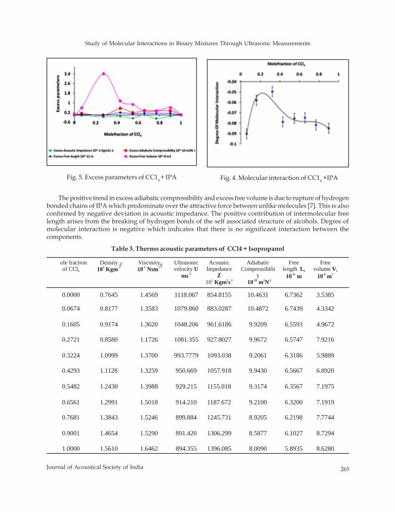
Study of Molecular Interactions in Binary Mixtures Through Ultrasonic Measurements
265Journal of Acoustical Society of India
Mole fraction of CCl4
Density 10 Kgm3 -3
Viscosity 10 Nsm-3 -2
Ultrasonic velocity U
ms-1
Acoustic Impedance
10
Z
Kgm s3 2 -1
Adiabatic Compressibilit
y 10 m N-10 2 -1
Free length L
10 mf
-11
Free volume V
10 mf
-8 3
0.0000 0.7645 1.4569 1118.067 854.8155 10.4631 6.7362 3.5385
0.0674 0.8177 1.3583 1079.860 883.0287 10.4872 6.7439 4.3342
0.1605 0.9174 1.3620 1048.206 961.6186 9.9209 6.5593 4.9672
0.2721 0.8580 1.1726 1081.355 927.8027 9.9672 6.5747 7.9216
0.3224 1.0999 1.3700 993.7779 1093.038 9.2061 6.3186 5.9889
0.4293 1.1128 1.3259 950.669 1057.918 9.9430 6.5667 6.8920
0.5482 1.2430 1.3988 929.215 1155.018 9.3174 6.3567 7.1975
0.6561 1.2991 1.5018 914.210 1187.672 9.2100 6.3200 7.1919
0.7681 1.3843 1.5246 899.884 1245.731 8.9205 6.2198 7.7744
0.9001 1.4654 1.5290 891.420 1306.299 8.5877 6.1027 8.7294
1.0000 1.5610 1.6462 894.355 1396.085 8.0090 5.8935 8.6280
ηρ
Table 3. Thermo acoustic parameters of CCl4 + Isopropanol
The positive trend in excess adiabatic compressibility and excess free volume is due to rupture of hydrogenbonded chains of IPA which predominate over the attractive force between unlike molecules [7]. This is alsoconfirmed by negative deviation in acoustic impedance. The positive contribution of intermolecular freelength arises from the breaking of hydrogen bonds of the self associated structure of alcohols. Degree ofmolecular interaction is negative which indicates that there is no significant interaction between thecomponents.
Fig. 5. Excess parameters of CC14 + IPA Fig. 4. Molecular interaction of CC14 +IPA
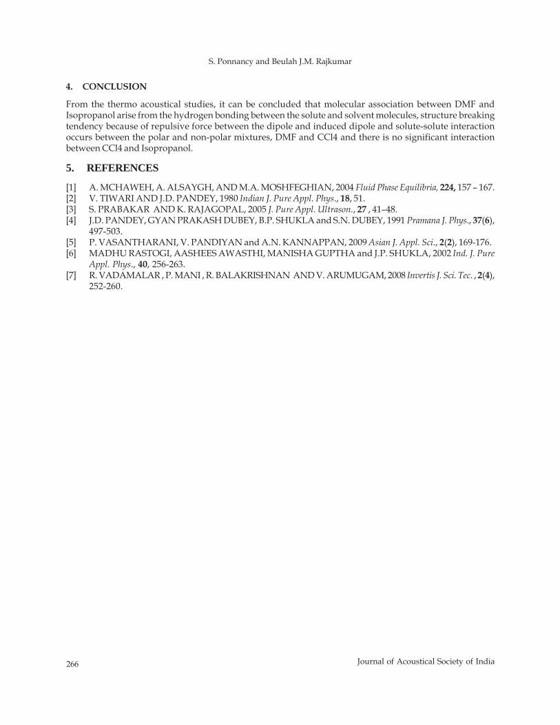
266 Journal of Acoustical Society of India
S. Ponnancy and Beulah J.M. Rajkumar
4. CONCLUSION
From the thermo acoustical studies, it can be concluded that molecular association between DMF andIsopropanol arise from the hydrogen bonding between the solute and solvent molecules, structure breakingtendency because of repulsive force between the dipole and induced dipole and solute-solute interactionoccurs between the polar and non-polar mixtures, DMF and CCl4 and there is no significant interactionbetween CCl4 and Isopropanol.
5. REFERENCES
[1] A. MCHAWEH, A. ALSAYGH, AND M.A. MOSHFEGHIAN, 2004 Fluid Phase Equilibria, 224, 157 – 167.[2] V. TIWARI AND J.D. PANDEY, 1980 Indian J. Pure Appl. Phys., 18, 51.[3] S. PRABAKAR AND K. RAJAGOPAL, 2005 J. Pure Appl. Ultrason., 27 , 41–48.[4] J.D. PANDEY, GYAN PRAKASH DUBEY, B.P. SHUKLA and S.N. DUBEY, 1991 Pramana J. Phys., 37(6),
497-503.[5] P. VASANTHARANI, V. PANDIYAN and A.N. KANNAPPAN, 2009 Asian J. Appl. Sci., 2(2), 169-176.[6] MADHU RASTOGI, AASHEES AWASTHI, MANISHA GUPTHA and J.P. SHUKLA, 2002 Ind. J. Pure
Appl. Phys., 40, 256-263.[7] R. VADAMALAR , P. MANI , R. BALAKRISHNAN AND V. ARUMUGAM, 2008 Invertis J. Sci. Tec. , 2(4),
252-260.
250 Journal of Acoustical Society of India
Venkat Raman Prusty and Lakshmi Venkatesh
ABSTRACT
Temporal characteristics of vowels in geminate contexts (phonological long vowels) were observedthrough acoustic analyses of vowels occurring in word pairs of Oriya language. Productions ofOriya speaking typical developing children in the age range of 3-14 years and young adults (25-35years) in response to recorded model were subjected to acoustic analyses to measure the duration ofvowels. Results revealed a developmental trend such that the duration of all geminate vowels differedacross the different age groups with no difference was observed between male and female participantsin each age group. Findings are discussed in terms of the age at which children's productionsreached adult like durations and comparison with duration of singleton production of vowels reportedin an earlier study.
1. INTRODUCTION
Phonemes are converted into phonetic units during the process of speech production through the realizationof different rules. Durational properties observed at the level of phonetic output are the result of both segmentaland suprasegmental factors. Variations due to intrinsic (segment specific) and extrinsic (contextual)specifications may arise from maturation, predisposition and cognitive learning. An analysis of developmentalchanges helps understanding aspects of normal maturation. Quantifying effects of language dependentfactors are helpful in identification of abnormal forms of productions in development.
Vowel length is contrastive in many languages with varied language-specific realizations of the lengthcontrast. Several languages (e.g., Sanskrit, Kannada, Japanese, Hungarian etc) from around the world makea phonemic distinction between long and short vowels. Long vowels are distinct phonemes from shortvowels leading to doubling the number of vowel phonemes in a particular language. Long vowels in Japanesefor example are analyzed as two same vowels or a vowel + the pseudo-phoneme /h/ (e.g., short /i/ and long/ii/ or /ih/). Languages such as Japanese or Finish are referred to as "Geminate vowel" languages whichallow a long vowel (a phoneme) to be analyzed as sequences of short vowels [1]. In Finnish, both consonantlength and vowel length contrasts are phonemic and are independent of each other. For example, words suchas taka /taka/ "back", takka /tak:a/ "fireplace", taakka /ta:k:a/ "burden", and so forth are different, unrelatedwords. Ladefoged defines geminates as "long consonants (or vowels) that can be analyzed as doubleconsonants (or vowels)" [2]. In several languages, gemination is not productive in the creation of phonemesand only occurs only in allophonic variation.
Gemination is contrastive in Japanese or Finnish as seen from examples above, whereas it is not contrastive
Journal of Acoustical Society of India : Vol. 40, No. 4, 2013 (pp. 250-254)
Vowel Duration in the Geminate Contexts: Observationsfrom Oriya Speaking Children and Adults
Venkat Raman Prusty1 and Lakshmi Venkatesh2
1MediCiti Institute of Medical Sciences, Ghanpur (Andhra Pradesh)2S.R. Chandrasekhar Institute of Speech & Hearing, Bangalore (Karnataka)
[Received: 17.04.2013; Revised: 18.07.2013; Accepted: 21.09.2013]
© 2013 Acoustical Society of India
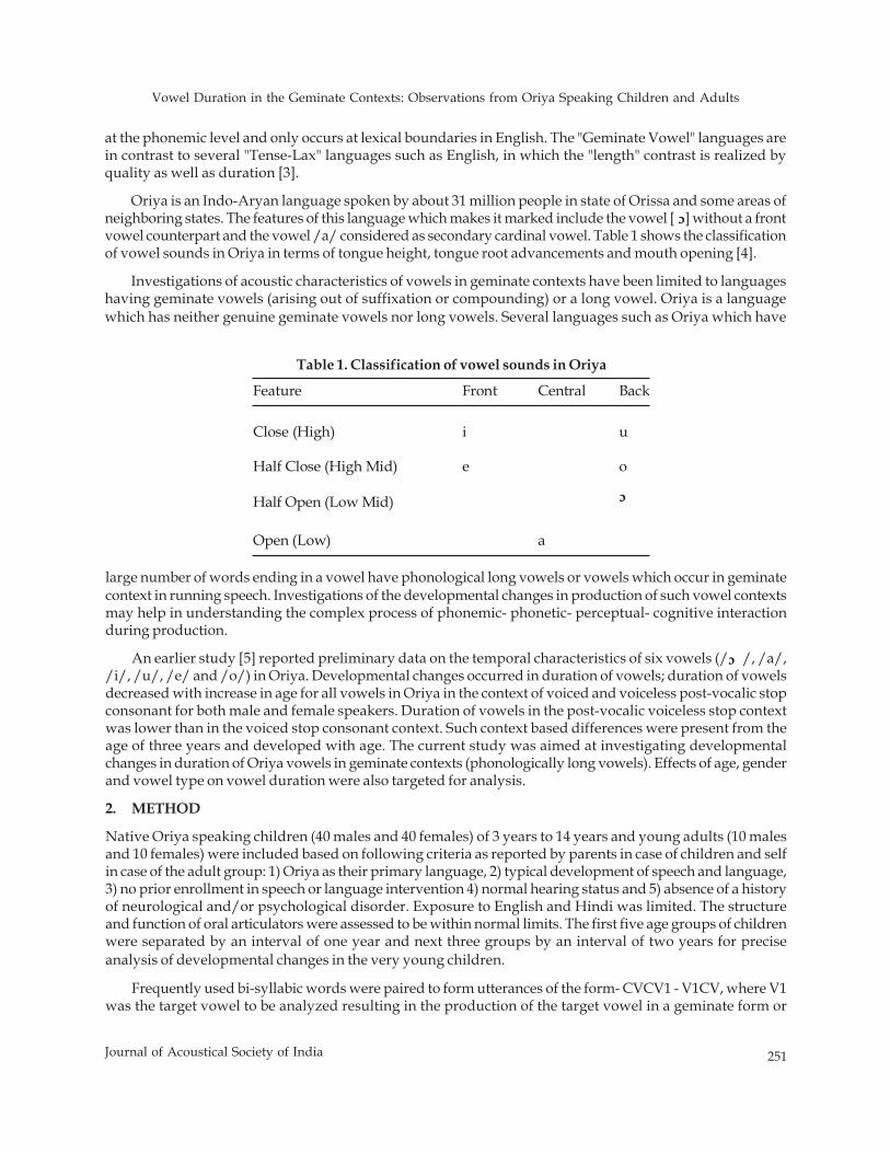
Vowel Duration in the Geminate Contexts: Observations from Oriya Speaking Children and Adults
251Journal of Acoustical Society of India
at the phonemic level and only occurs at lexical boundaries in English. The "Geminate Vowel" languages arein contrast to several "Tense-Lax" languages such as English, in which the "length" contrast is realized byquality as well as duration [3].
Oriya is an Indo-Aryan language spoken by about 31 million people in state of Orissa and some areas ofneighboring states. The features of this language which makes it marked include the vowel [ ] without a frontvowel counterpart and the vowel /a/ considered as secondary cardinal vowel. Table 1 shows the classificationof vowel sounds in Oriya in terms of tongue height, tongue root advancements and mouth opening [4].
Investigations of acoustic characteristics of vowels in geminate contexts have been limited to languageshaving geminate vowels (arising out of suffixation or compounding) or a long vowel. Oriya is a languagewhich has neither genuine geminate vowels nor long vowels. Several languages such as Oriya which have
Table 1. Classification of vowel sounds in Oriya
Feature Front Central Back
Close (High) i u
Half Close (High Mid) e o
Half Open (Low Mid) ?
Open (Low) a
large number of words ending in a vowel have phonological long vowels or vowels which occur in geminatecontext in running speech. Investigations of the developmental changes in production of such vowel contextsmay help in understanding the complex process of phonemic- phonetic- perceptual- cognitive interactionduring production.
An earlier study [5] reported preliminary data on the temporal characteristics of six vowels (/ /, /a/,/i/, /u/, /e/ and /o/) in Oriya. Developmental changes occurred in duration of vowels; duration of vowelsdecreased with increase in age for all vowels in Oriya in the context of voiced and voiceless post-vocalic stopconsonant for both male and female speakers. Duration of vowels in the post-vocalic voiceless stop contextwas lower than in the voiced stop consonant context. Such context based differences were present from theage of three years and developed with age. The current study was aimed at investigating developmentalchanges in duration of Oriya vowels in geminate contexts (phonologically long vowels). Effects of age, genderand vowel type on vowel duration were also targeted for analysis.
2. METHOD
Native Oriya speaking children (40 males and 40 females) of 3 years to 14 years and young adults (10 malesand 10 females) were included based on following criteria as reported by parents in case of children and selfin case of the adult group: 1) Oriya as their primary language, 2) typical development of speech and language,3) no prior enrollment in speech or language intervention 4) normal hearing status and 5) absence of a historyof neurological and/or psychological disorder. Exposure to English and Hindi was limited. The structureand function of oral articulators were assessed to be within normal limits. The first five age groups of childrenwere separated by an interval of one year and next three groups by an interval of two years for preciseanalysis of developmental changes in the very young children.
Frequently used bi-syllabic words were paired to form utterances of the form- CVCV1 - V1CV, where V1was the target vowel to be analyzed resulting in the production of the target vowel in a geminate form or
c
c
c
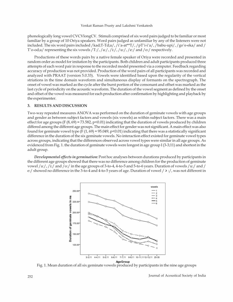
252 Journal of Acoustical Society of India
Venkat Raman Prusty and Lakshmi Venkatesh
phonologically long vowel CVCVlongCV. Stimuli comprised of six word pairs judged to be familiar or mostfamiliar by a group of 10 Oriya speakers. Word pairs judged as unfamiliar by any of the listeners were notincluded. The six word pairs included /kad;T-Td;a/, /iˆa-at**T/, /pTˆi-iˆa/, /babu-upi/, /goˆe-eka/ and /Tˆo-od;a/ representing the six vowels /T:/, /a:/, /i:/, /u:/, /e:/ and /o:/ respectively.
Productions of these words pairs by a native female speaker of Oriya were recorded and presented inrandom order as model for imitation by the participants. Both children and adult participants produced threeattempts of each word pair in response to the recorded model presented via a computer. Feedback regardingaccuracy of production was not provided. Production of the word pairs of all participants was recorded andanalyzed with PRAAT (version 5.0.33). Vowels were identified based upon the regularity of the verticalstriations in the time domain waveform and simultaneous display of formants on the spectrograph. Theonset of vowel was marked as the cycle after the burst portion of the consonant and offset was marked as thelast cycle of periodicity on the acoustic waveform. The duration of the vowel segment as defined by the onsetand offset of the vowel was measured for each production after confirmation by highlighting and playback bythe experimenter.
3. RESULTS AND DISCUSSION
Two-way repeated measures ANOVA was performed on the duration of geminate vowels with age groupsand gender as between subject factors and vowels (six vowels) as within subject factors. There was a maineffect for age groups (F (8, 69) = 73.582, p<0.01) indicating that the duration of vowels produced by childrendiffered among the different age groups. The main effect for gender was not significant. A main effect was alsofound for geminate vowel type (F (1, 69) = 95.049, p<0.01) indicating that there was a statistically significantdifference in the duration of the six geminate vowels. No interaction effect existed for geminate vowel typesacross groups, indicating that the differences observed across vowel types were similar in all age groups. Asevidenced from Fig. 1. the duration of geminate vowels were longest in age group I (3-3;11) and shortest in theadult group.
Developmental effects in germination: Post hoc analyses between durations produced by participants inthe different age groups showed that there was no difference among children for the production of geminatevowel /a:/, /i:/ and /o:/ in the age groups of 3-to-4, 4-to-5 and 5-to-6 years. Duration of vowels /u:/ and /e:/ showed no difference in the 3-to-4 and 4-to-5 years of age. Duration of vowel / :/, was not different in
Fig. 1. Mean duration of all six geminate vowels produced by participants in the nine age groups
c
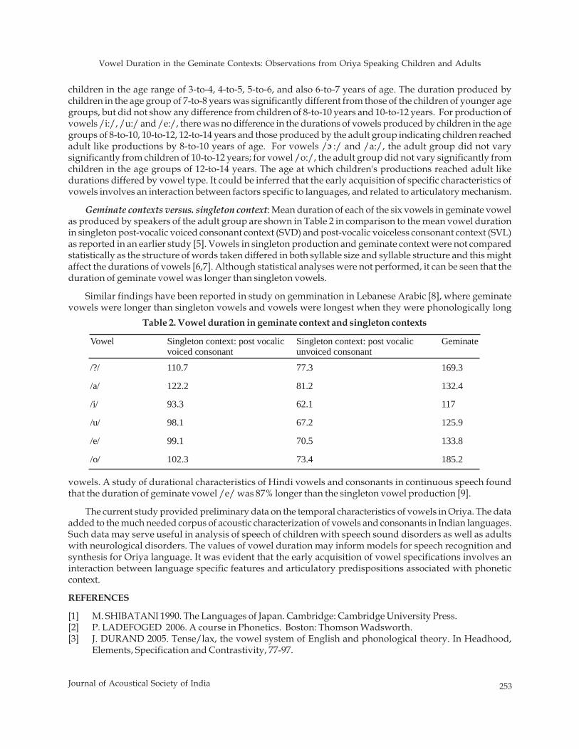
Vowel Duration in the Geminate Contexts: Observations from Oriya Speaking Children and Adults
253Journal of Acoustical Society of India
children in the age range of 3-to-4, 4-to-5, 5-to-6, and also 6-to-7 years of age. The duration produced bychildren in the age group of 7-to-8 years was significantly different from those of the children of younger agegroups, but did not show any difference from children of 8-to-10 years and 10-to-12 years. For production ofvowels /i:/, /u:/ and /e:/, there was no difference in the durations of vowels produced by children in the agegroups of 8-to-10, 10-to-12, 12-to-14 years and those produced by the adult group indicating children reachedadult like productions by 8-to-10 years of age. For vowels / :/ and /a:/, the adult group did not varysignificantly from children of 10-to-12 years; for vowel /o:/, the adult group did not vary significantly fromchildren in the age groups of 12-to-14 years. The age at which children's productions reached adult likedurations differed by vowel type. It could be inferred that the early acquisition of specific characteristics ofvowels involves an interaction between factors specific to languages, and related to articulatory mechanism.
Geminate contexts versus. singleton context: Mean duration of each of the six vowels in geminate vowelas produced by speakers of the adult group are shown in Table 2 in comparison to the mean vowel durationin singleton post-vocalic voiced consonant context (SVD) and post-vocalic voiceless consonant context (SVL)as reported in an earlier study [5]. Vowels in singleton production and geminate context were not comparedstatistically as the structure of words taken differed in both syllable size and syllable structure and this mightaffect the durations of vowels [6,7]. Although statistical analyses were not performed, it can be seen that theduration of geminate vowel was longer than singleton vowels.
Similar findings have been reported in study on gemmination in Lebanese Arabic [8], where geminatevowels were longer than singleton vowels and vowels were longest when they were phonologically long
Vowel Singleton context: post vocalic voiced consonant
Singleton context: post vocalic unvoiced consonant
Geminate
/?/ 110.7 77.3 169.3
/a/ 122.2 81.2 132.4
/i/ 93.3 62.1 117
/u/ 98.1 67.2 125.9
/e/ 99.1 70.5 133.8
/o/ 102.3 73.4 185.2
Table 2. Vowel duration in geminate context and singleton contexts
vowels. A study of durational characteristics of Hindi vowels and consonants in continuous speech foundthat the duration of geminate vowel /e/ was 87% longer than the singleton vowel production [9].
The current study provided preliminary data on the temporal characteristics of vowels in Oriya. The dataadded to the much needed corpus of acoustic characterization of vowels and consonants in Indian languages.Such data may serve useful in analysis of speech of children with speech sound disorders as well as adultswith neurological disorders. The values of vowel duration may inform models for speech recognition andsynthesis for Oriya language. It was evident that the early acquisition of vowel specifications involves aninteraction between language specific features and articulatory predispositions associated with phoneticcontext.
REFERENCES
[1] M. SHIBATANI 1990. The Languages of Japan. Cambridge: Cambridge University Press.[2] P. LADEFOGED 2006. A course in Phonetics. Boston: Thomson Wadsworth.[3] J. DURAND 2005. Tense/lax, the vowel system of English and phonological theory. In Headhood,
Elements, Specification and Contrastivity, 77-97.
c
254 Journal of Acoustical Society of India
Venkat Raman Prusty and Lakshmi Venkatesh
[4] N. RAMASWAMI 1994. Common linguistic features in Indian languages: Phonetics. Central Instituteof Indian Languages, Mysore.
[5] V.R. PRUSTY AND L. VENKATESH (in submission). Duration of vowels in Oriya: A developmentalperspective.
[6] R.K. NAGAMMA 1988. The influence of plosive consonant voicing and aspiration on duration ofvowels in Telugu and Hindi. Journal of Institution of Electronics and Telecommunication Engineers,Special Issue of JIETE on Speech Processing, New Delhi, 34, No.1.
[7] R.K. NAGAMMA 1985. Phonetic conditioning of Duration of vowels and consonants in Telugu. OsmaniaPapers in Linguistics, 11, 54-83.
[8] G. KHATTAB 2007. A phonetic study of gemination in Lebanese Arabic. Proc. 16th ICPhS, Saarbrücken,153-158.
[9] K. SAMUDRAVIJAYA 2003. Durational characteristics of Hindi phonemes in continuous speech.Technical Report, TIFR.

Acoustical Society of India(Regn. No. 65-1971)
Executive Council (2010 - 2014)
President : Dr V Rajendran[KSRCT, Tiruchengode; [email protected]; +91-99 94 13 03 03]
Vice President : NS Naidu[NSTL, Vizag; [email protected]; +91-94 90 75 05 82]
General Secretary : PVS Ganesh Kumar[NSTL, Vizag; [email protected]; +91-98 66 40 08 94]
Jt. Secretary : Dr K Trinadh[NSTL, Vizag; [email protected]; +91-97 04 71 95 00]
Treasurer : Prof AV Sharma[AU, Vizag; [email protected]; +91-94 90 43 17 26]
Chief Editor : Dr Mahavir Singh[CSIR-NPL, New Delhi; [email protected]; +91-98 71 69 33 46]
Council Members : Dr SV Ranga Nayakulu[VITAE, Hyderabad; [email protected]; +91-98 66 53 26 13]
Dr I Johnson[SJ College, Trichy; [email protected]; +91-94 42 90 48 20]
Dr Rajiv K Upadhayay[Govt PG College, Rishikesh; [email protected]; +91-94 12 97 28 90]
Dr S Shekhar[Oxford College, Trichy; [email protected]; +91-99 94 92 00 30]
Dr V Bhujanga Rao[Past President; NSTL, Vizag; [email protected]; +91-98 66 44 10 74]
Co-opted Members : Rajshekhar Uchil[Josts, Bangalore; [email protected]; +91-98 80 17 08 95]
Dr NK Narayanan[CIT, Kozhikode; [email protected]; +91-94 46 95 58 30]


INFORMATION FOR AUTHORS
ARTICLES The Journal of Acoustical Society of India (JASI) is a refereed publication published quarterly by the Acoustical Society of India(ASI). JASI includes refereed articles, technical notes, letters-to-the-editor, book review and announcements of general interest toreaders.
Articles may be theoretical or experimental in nature. But those which combine theoretical and experimental approaches tosolve acoustics problems are particularly welcome. Technical notes, letters-to-the-editor and announcements may also be submitted.Articles must not have been published previously in other engineering or scientific journals. Articles in the following are particularlyencouraged: applied acoustics, acoustical materials, active noise & vibration control, bioacoustics, communication acousticsincluding speech, computational acoustics, electro-acoustics and audio engineering, environmental acoustics, musical acoustics,non-linear acoustics, noise, physical acoustics, physiological and psychological acoustics, quieter technologies, room and buildingacoustics, structural acoustics and vibration, ultrasonics, underwater acoustics.
Authors whose articles are accepted for publication must transfer copyright of their articles to the ASI. This transfer involvespublication only and does not in any way alter the author's traditional right regarding his/her articles.
PREPARATION OF MANUSCRIPTS All manuscripts are refereed by at least two referees and are reviewed by the Publication Committee (all editors) beforeacceptance. Manuscripts of articles and technical notes should be submitted for review electronically to the Chief Editor by e-mailor by express mail on a disc. JASI maintains a high standard in the reviewing process and only accept papers of high quality. Onacceptance, revised articles of all authors should be submitted to the Chief Editor by e-mail or by express mail. Text of the manuscript should be double-spaced on A4 size paper, subdivided by main headings-typed in upper and lowercase flush centre, with one line of space above and below and sub-headings within a section-typed in upper and lower caseunderstood, flush left, followed by a period. Sub-sub headings should be italic. Articles should be written so that readers indifferent fields of acoustics can understand them easily. Manuscripts are only published if not normally exceeding twenty double-spaced text pages. If figures and illustrations are included then normally they should be restricted to no more than twelve-fifteen. The first page of manuscripts should include on separate lines, the title of article, the names, of authors, affiliations andmailing addresses of authors in upper and lowers case. Do not include the author's title, position or degrees. Give an adequatepost office address including pin or other postal code and the name of the city. An abstract of not more than 200 words shouldbe included with each article. References should be numbered consecutively throughout the article with the number appearing asa superscript at the end of the sentence unless such placement causes ambiguity. The references should be grouped together,double spaced at the end of the article on a separate page. Footnotes are discouraged. Abbreviations and special terms must bedefined if used.
EQUATIONS Mathematical expressions should be typewritten as completely as possible. Equation should be numbered consecutivelythroughout the body of the article at the right hand margin in parentheses. Use letters and numbers for any equations in anappendix: Appendix A: (A1, (A2), etc. Equation numbers in the running text should be enclosed in parentheses, i.e., Eq. (1), Eqs.(1a) and (2a). Figures should be referred to as Fig. 1, Fig. 2, etc. Reference to table is in full: Table 1, Table 2, etc. Metric units shouldbe used: the preferred from of metric unit is the System International (SI).
REFERENCES The order and style of information differs slightly between periodical and book references and between published and unpublishedreferences, depending on the available publication entries. A few examples are shown below.
Periodicals:[1] S.R. Pride and M.W. Haartsen, 1996. Electroseismic wave properties, J. Acoust. Soc. Am., 100 (3), 1301-1315.[2] S.-H. Kim and I. Lee, 1996. Aeroelastic analysis of a flexible airfoil with free play non-linearity, J. Sound Vib., 193 (4), 823-846.
Books:[1] E.S. Skudzryk, 1968. Simple and Comlex Vibratory Systems, the Pennsylvania State University Press, London.[2] E.H. Dowell, 1975. Aeroelasticity of plates and shells, Nordhoff, Leyden.
Others:[1] J.N. Yang and A. Akbarpour, 1987. Technical Report NCEER-87-0007, Instantaneous Optimal Control Law For Tall
Buildings Under Seismic Excitations.
SUMISSIONS All materials from authors should be submitted in electronic form to the JASI Chief Editor: Dr Mahavir Singh, Acoustics,Ultrasonics & Vibration Section, CSIR-National Physical Laboratory, Dr. K. S. Krishnan Road, New Delhi-110 012 (email:[email protected] Tel: +91-11-4560.8317, Fax: +91-11-4560.9310). For the item to be published in a given issue of a journal,the manuscript must reach the Chief Editor at least twelve week before the publication date.
SUMISSION OF ACCEPTED MANUSCRIPT On acceptance, revised articles should be submitted in electronic form to the JASI Chief Editor ([email protected]).


