Jumps in intensity models: investigating the performance of Ornstein-Uhlenbeck processes in credit risk modeling

Metrika (2009) 69:173–198DOI 10.1007/s00184-008-0213-4

Jumps in intensity models: investigatingthe performance of Ornstein-Uhlenbeck processesin credit risk modeling

Jessica Cariboni · Wim Schoutens

Published online: 3 December 2008© Springer-Verlag 2008

Abstract This work presents intensity-based credit risk models where the defaultintensity of the point process is modeled by an Ornstein-Uhlenbeck type processcompletely driven by jumps. Under this model we compute the default probabilityover time by linking it to the characteristic function of the integrated intensity process.In case of the Gamma and the Inverse Gaussian Ornstein-Uhlenbeck processes thisleads to a closed-form expression for the default probability and to a straightforwardestimate of credit default swaps prices. The model is calibrated to a series of real-market term structures and then used to price a digital default put option. Resultsare compared with the well known cases of Poisson and CIR dynamics. Possibleextensions of the model to the multivariate setting are finally discussed.

Keywords Ornstein-Uhlenbeck process · Credit risk · Survival probability ·Intensity-based model · Credit default swap

1 Introduction

Modern finance has put much effort in developing new models for credit risk. This isrelated both to the growth in the credit derivatives volumes traded on the market andto the possibility given to financial institutions to assess in-house their credit exposure(advanced implementation option of Basel II).

J. CariboniEuropean Commission, Joint Research Centre, 21020 Ispra, Italy

W. Schoutens (B)Department of Mathematics, K.U. Leuven, Celestijnenlaan 200B,3001 Leuven (Heverlee), Belgiume-mail: [email protected]

123

174 J. Cariboni, W. Schoutens

Credit risk models are usually classified into two categories: structural models andintensity-based models. Structural models link an event of default to the asset valueof the firm. Usually, the dynamics of the asset value is given and an event of default isdefined in terms of boundary conditions on this process. The first structural models dateback to Merton (1974) and Black and Cox (1976) but a lot of modifications/extensionscan be found in the literature (e.g., Leland 1994; Longstaff 1995; Madan et al. 1998;Cariboni and Schoutens 2006). A drawback of the structural approach is that the assetvalue is treated as a primary asset of the economy while it is usually dependent onother state variables (Madan and Unal 1998).

Intensity-based models, known also as hazard rate or reduced-form models, focusdirectly on the modeling of the default probability. The intensity-based approachdefines the time of default as the first jump-time of a counting process Mt . As a conse-quence, a central role is played by the jumps intensity rate of Mt . A standard example ofcounting process is the (homogeneous) Poisson process with constant intensity λ > 0.The corresponding default model was developed by Jarrow and Turnbull (1995). Somegeneralizations allow the default intensities to be time-dependent, leading to the so-called inhomogeneous Poisson process, or allow for stochastic default intensities. Inthis latter case, the corresponding counting process is called a Cox-process. Madanand Unal (1998) considered the case where the intensity λt is adapted to a Brownianfiltration. Duffie and Singleton (1999) developed a basic affine model, which allowsfor jumps in the hazard dynamics.

In contrast to the structural approach, under the reduced-form models default is aninaccessible stopping time. Jarrow and Protter (2004) compare structural and intensitymodels and highlight that the key distinction between them is the information setassumed to be known. Structural models suppose that the available information isthe one observed by the firm’s managers; intensity models assume the modeler’sinformation observed on the market.

From a fundamental point of view it is important to have jumps in the intensityregime or in the firm’s value price process because changes in the creditworthiness(intensity or firm’s value) are often shock driven: sudden events in reality cause impor-tant changes on the view on the company’s probability of default. Standard examplesof such dramatic changes in the regime are discovery of fraud (e.g., Parmalat), areviewing of company’s results, default of a competitor, a terroristic attack, etc.

This work introduces a new default model where the intensity of default is assumedto follow a Ornstein-Uhlenbeck (OU) process. Under this assumption, we show thatthe survival probability of the obligor can be expressed in terms of the characteris-tic function of the integrated OU process. We concentrate on two special cases, theGamma-OU and inverse Gaussian–OU (IG–OU) processes. The names refer to thestationary law of the intensity process used. In these cases a closed-form expression forthe characteristic function of the integrated process is available, leading to a straight-forward estimate of the survival probability. The Gamma case can be rephrased as aspecial case of the basic affine model introduced by Duffie and Singleton (1999).

The model abilities are tested through a calibration exercise on credit default swaps(CDS) term structures observed on the market. To this aim we consider the 125 CDSconstituting the iTraxx Europe Index. For each asset, weekly term structure data areavailable for a total of 58 market observations (i.e., covering a time period of bit more

123

Jumps in intensity models 175

than 1 year). This allows not only to investigate in depth the calibration capabilities ofthe OU-models, but also to check the stability of the processes’ parameters over time.For comparison purposes, we also calibrate intensity models based on the Poisson,inhomogeneous Poisson, and CIR dynamics, on the 7,250 CDS curves available in thedataset.

Finally, we discuss possible extensions of the model to the multivariate setting,showing that the inclusion of jumps in the intensity process allows for spanning theentire range of default correlation among assets. In our settings, dependency amongassets can be introduced either by time-changing the intensity dynamics by a commonsubordinator (Joshi and Stacey 2006) or allowing common jumps in the intensityprocesses. In the first case, we focus on the special case of the Gamma-process andderive the expression for the corresponding survival probabilities. In the second casethe dependence is introduced via the background driving Lévy process. A review ofother models for correlated defaults can be found in Elizalde (2005).

The paper is organized as follows. In the next section, we introduce the basic back-ground on Lévy processes and OU processes driven by Lévy processes, concentratingon the Gamma and Inverse Gaussian OU processes. Section 3 presents our intensitybased OU default model. We then introduce CDS and link CDS spreads to the integra-ted OU process. The last part of Sect. 3 presents the results of the calibration exercisesand show how to price a digital default put option once the models are calibrated. Thepenultimate section deals with the multivariate setting and the last section concludes.

2 Lévy processes and Ornstein-Uhlenbeck processes

2.1 Lévy processes

Supposeφ(z) is the characteristic function of a distribution. If for every positive integern, φ(z) is also the nth power of a characteristic function, we say that the distribution isinfinitely divisible. One can define for any infinitely divisible distribution a stochasticprocess, X = {Xt , t ≥ 0}, called Lévy process, which starts at zero, has independentand stationary increments and such that the distribution of an increment over [s, s + t],s, t ≥ 0, i.e., Xt+s − Xs , has (φ(z))t as characteristic function.

The function ψ(z) = logφ(z) is called the characteristic exponent and it satisfiesthe following Lévy–Khintchine formula (Bertoin 1996):

ψ(z) = iγ z − ς2

2z2 +

+∞∫

−∞(exp(izx)− 1 − izx1{|x |<1})ν(dx), (1)

where γ ∈ R, ς2 ≥ 0 and ν is a measure on R\{0} with∫ +∞−∞ (1 ∧ x2)ν(dx) < ∞.

From the Lévy-Khintchine formula, one sees that, in general, a Lévy process consistsof three independent parts: a linear deterministic part, a Brownian part, and a pure jumppart. We say that our infinitely divisible distribution has a triplet of Lévy characteristics[γ, ς2, ν(dx)]. The measure ν(dx) is called the Lévy measure of X and it dictates howthe jumps occur. Jumps of sizes in the set A occur according to a Poisson process

123


with parameter∫

A ν(dx). If ς2 = 0 and∫ +1−1 |x |ν(dx) < ∞ it follows from standard

Lévy process theory (see, for example, Bertoin 1996; Sato 1999), that the process is offinite variation. For more details about the applications of Lévy processes in financewe refer to Schoutens (2003).

2.2 OU Processes

In this section we give a brief overview of OU processes (driven by Lévy processes)which were introduced by Barndorff-Nielsen and Shephard (2001a,b, 2003) to describevolatility in finance. Further references on OU processes are Wolfe (1982), Sato andYamazato (1982), Jyrek and Vervaat (1983) and Sato et al. (1994).

An OU process y = {yt , t ≥ 0} is described by the following stochastic differentialequation:

dyt = −ϑyt dt + dzϑ t , y0 > 0, (2)

where ϑ is the arbitrary positive rate parameter and zt is a subordinator, i.e., a Lévyprocess with no Brownian component, nonnegative drift and only positive increments.z is often called background driving Lévy process (BDLP).1 As z is an increasingprocess and y0 > 0, it is clear that the process y is strictly positive. Moreover, it isbounded from below by the deterministic function y0 exp(−ϑ t).

The process y = {yt , t ≥ 0} is strictly stationary on the positive half-line, i.e.,there exists a law D, called the stationary law or the marginal law, such that yt willfollow for every t the law D, if initial y0 is chosen according to D. The process ymoves up entirely by jumps and then tails off exponentially. The fact that we have theparameter ϑ in zϑ t has to do with the separation of the stationary law from this decayparameter. In Barndorff-Nielsen and Shephard (2001a) some stochastic properties ofy are studied. Barndorff-Nielsen and Shephard established the notation that if y is anOU process with marginal law D, then we say that y is a D-OU process.

In essence, given a one-dimensional distribution D (not necessarily restricted tothe positive half line) there exists a (stationary) OU process whose marginal law is D(i.e., a D-OU process) if and only if D is self-decomposable (for definition see Sato1999). We have by standard results (Barndorff-Nielsen and Shephard 2001a) that

yt = exp(−ϑ t)y0 +t∫

0

exp(−ϑ(t − s))dzϑs

= exp(−ϑ t)y0 + exp(−ϑ t)

ϑ t∫

0

exp(s)dzs .

In the case of a D-OU process, let us denote by kD(u) the cumulant function of theself-decomposable law D and by kz(u) the cumulant function of the BDLP at time

1 Also OU processes based on a general Lévy process, not necessarily a subordinator, can be defined.However for our analysis we will only need the special case considered above.

123


t = 1, i.e., kz(u) = log E[exp(−uz1)], then both are related through the formula (see,for example, Barndorff-Nielsen 2001):

kz(u) = udkD(u)

du.

An important related process will be the integral of yt . Barndorff-Nielsen andShephard called this the integrated OU process (intOU); we will denote this processwith Y = {Yt , t ≥ 0}:

Yt =t∫

0

ysds.

A major feature of the intOU process Y is

Yt = ϑ−1 (zϑ t − yt + y0)

= ϑ−1(1 − exp(−ϑ t))y0 + ϑ−1

t∫

0

(1 − exp(−ϑ(t − s))) dzϑs .

One can show (see Barndorff-Nielsen and Shephard 2001a) that given y0,

log E[exp(iuYt )|y0] = ϑ

t∫

0

k(uϑ−1(1 − exp(−ϑ(t − s))))ds

+ iuy0ϑ−1(1 − exp(−ϑ t)),

where k(u) = kz(u) = log E[exp(−uz1)] is the cumulant function of z1.

2.2.1 The Gamma–OU process

The Gamma(a, b)–OU process has as BDLP a compound Poisson process:

zt =Nt∑

n=1

xn

where N = {Nt , t ≥ 0} is a Poisson process with intensity a (i.e., E[Nt ] = at) and{xn, n = 1, 2, . . . , Nt } is a sequence of independent identically distributed Exp(b)variables, i.e., exponentially distributed with mean 1/b. It turns out that the stationarylaw is given by a Gamma(a, b) distribution with density function

fGamma(x; a, b) = ba

Γ (a)xa−1 exp(−xb), x > 0,

123


which immediately explains the name. The Gamma–OU process has a finite numberof jumps in every compact time interval.

If yt is a Gamma–OU process, the characteristic function of the intOU processYt = ∫ t

0 ysds is given by:

φGamma−OU (u, t;ϑ, a, b, y0) = E[exp(iuYt )|y0]= exp

(iuy0

ϑ(1 − e−ϑ t )+ ϑa

iu − ϑb

(b log

(b

b − iuϑ−1(1 − e−ϑ t )

)− iut

)).

(3)

A Gamma(a, b)–OU process {yt , t ≥ 0} can be simulated at time points {t =n∆t, n = 0, 1, 2, . . .} through its BDLP. First a Poisson processes {Nt , t ≥ 0} withIntensity parameter aϑ has to be simulated at the same time points. Then we have toset:

yn∆t = exp(−ϑ∆t)y(n−1)∆t +Nn∆t∑

n=N(n−1)∆t +1

xn exp(−unϑ∆t), (4)

where {xn, n = 0, 1, . . .} are (independent) Exp(b) random numbers and {un, n =0, 1, . . .} are (independent) standard uniform random numbers. Note that the expo-nential term and the uniform random numbers un in the sum allows the jumps tohappen somewhere in between two time steps. Figure 1 (top graph) shows a path of aGamma–OU process with parameters ϑ = 4, a = 4, b = 18 and y0 = 0.08.

2.2.2 The inverse Gaussian–OU process

We start with recalling the definition of the Inverse Gaussian (IG(a, b)) law, by statingits density function:

f I G(x; a, b) = a√2π

exp(ab)x−3/2 exp(−(a2x−1 + b2x)/2), x > 0.

This IG(a, b) belongs to the class of the self-decomposable distributions and hencean IG–OU process exists. In the case of the IG(a, b)–OU process the BDLP is a sumof two independent Lévy processes z = {zt = z(1)t + z(2)t , t ≥ 0}. z(1) is an IG–Lévyprocess with parameters a/2 and b, while z(2) is of the form:

z(2)t = b−1Nt∑

n=1

v2n,

where N = {Nt , t ≥ 0} is a Poisson process with intensity parameter ab/2, i.e.,E[Nt ] = abt/2. {vn, n = 1, 2, . . . } is a sequence of independent and identicallydistributed random variables: each vn follows a normal(0, 1) law independent fromthe Poisson process N . Since the BDLP (via z(1)) jumps infinitely often in any finite

123


0 0.2 0.4 0.6 0.8 10.05

0.1

0.15

0.2

0.25

0.3

0.35

0.4

t (years)

Gamma−OU

0 0.2 0.4 0.6 0.8 10.06

0.08

0.1

0.12

0.14

0.16

0.18

0.2

t (years)

IG−OU

Fig. 1 Gamma-OU (top plot) and an inverse Gaussian–OU (bottom plot) simulated sample paths

(time) interval, also the IG–OU process jumps infinitely often in every interval. Thecumulant of the BDLP (at time 1) is given by

k(u) = −uab−1(1 + 2ub−2)−1/2.

In the IG–OU case the characteristic function of the intOU process Yt = ∫ t0 ysds

can also be given explicitly. The following expression was independently derived inNicolato and Venardos (2003) and Tompkins and Hubalek (2000):

123


φI G−OU (u, t;ϑ, a, b, y0) = E[exp(iuYt )|y0]= exp

(iuy0

ϑ(1 − exp(−ϑ t))+ 2aiu

bϑA(u, t)

), (5)

where

A(u, t) = 1 − √1 + κ(1 − exp(−ϑ t))

κ

+ 1√1 + κ

[arctanh

(√1 + κ(1 − exp(−ϑ t))√

1 + κ

)− arctanh

(1√

1 + κ

)],

κ = −2b−2iu/ϑ. (6)

In contrast to the Gamma–OU process, the IG–OU process has infinitely many jumpsin any time interval and thus cannot be simulated exactly. An approximation is obtainedby first simulating its BDLP and then applying the Euler’s scheme to the defining sto-chastic differential equation (2). Fast simulation of the BDLP is achieved by recallingthat the BDLP is the sum of two independent Lévy processes.

Figure 1 (bottom plot) shows a path of an IG–OU process with parameters ϑ = 2,a = 1.5, b = 12 and y0 = 0.08.

3 The intensity OU-model

Intensity models assume an event of default to occur at the first jump of a countingprocess M = {Mt , t ≥ 0}. The intensity rate λ = {λt , t ≥ 0}, known also as hazardrate, represents the instantaneous default probability. If we indicate with τ the defaulttime, the intensity of default is defined as:

λt = limh→0

P[τ ∈ (t, t + h]|τ > t]h

. (7)

Roughly speaking, this means that for a small time interval ∆t > 0:

P[τ ≤ t +∆t |τ > t] ≈ λt∆t.

As a consequence, the dynamics of the default intensity governs the credit quality ofthe corresponding asset. If λt is a stochastic process, Mt is called Cox process.

In our model we assume that the default intensity follows a Gamma–OU or anIG–OU process, as described in the previous section. Hence, the intensity process ismodeled by the stochastic differential equation:

dλt = −ϑλt dt + dzϑ t , λ0 > 0. (8)

As before, ϑ is the arbitrary positive rate parameter and zt is the BDLP, which weassume to be a subordinator in order to force the intensity process to be a positive

123


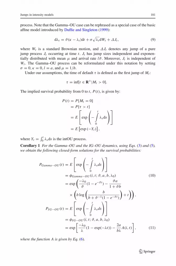
process. Note that the Gamma–OU case can be rephrased as a special case of the basicaffine model introduced by Duffie and Singleton (1999):

dλt = ϑ(κ − λt )dt + σ√λt dWt +∆Jt , (9)

where Wt is a standard Brownian motion, and ∆Jt denotes any jump of a purejump process Jt occurring at time t . Jt has jump sizes independent and exponen-tially distributed with mean µ and arrival rate lϑ . Moreover, Jt is independent ofWt . The Gamma–OU process can be reformulated under this notation by settingσ = 0, κ = 0, l = a, and µ = 1/b.

Under our assumptions, the time of default τ is defined as the first jump of Mt :

τ = inf[t ∈ R+|Mt > 0].

The implied survival probability from 0 to t , P(t), is given by:

P(t) = P[Mt = 0]= P[τ > t]

= E

⎡⎣exp

⎛⎝−

t∫

0

λsds

⎞⎠⎤⎦

= E[exp (−Yt )

],

where Yt = ∫ t0 λsds is the intOU process.

Corollary 1 For the Gamma–OU and the IG–OU dynamics, using Eqs. (3) and (5),we obtain the following closed-form solutions for the survival probabilities:

PGamma−OU (t) = E

⎡⎣exp

⎛⎝−

t∫

0

λsds

⎞⎠⎤⎦

= φGamma−OU (i, t;ϑ, a, b, λ0) (10)

= exp

(−λ0

ϑ(1 − e−ϑ t )− ϑa

1 + ϑb

×(

b log

(b

b + ϑ−1(1 − e−ϑ t )

)+ t

)),

PI G−OU (t) = E

⎡⎣exp

⎛⎝−

t∫

0

λsds

⎞⎠⎤⎦

= φI G−OU (i, t;ϑ, a, b, λ0)

= exp

[−λ0

λ(1 − exp(−λt))− 2a

bλA(i, t)

], (11)

where the function A is given by Eq. (6).

123


3.1 Calibration of the model on CDS term structures

A CDS is a derivative that provides the buyer an insurance against the default ofa company (the reference entity) on its debt. The buyer of this protection makes(continuous) predetermined payments to the seller. The payments continue until thematurity date of the contract or until default occurs, whichever is earlier. If defaultoccurs, the buyer delivers a bond on the underlying defaulting asset in exchange for itsface value. The market for CDS is well established and trading is increasing in relatedproducts like forwards and options on these CDS. For pricing techniques for theseforwards and options we refer to Hull and White (2003). In the risk-neutral world, theprice at time t = 0 of a CDS of maturity T is given by the difference of the expecteddiscounted loss payments and spread payments

C DS = (1 − R)

⎛⎝−

T∫

0

D(0, s)dP(s)

⎞⎠ − c

T∫

0

D(0, s)P(s)ds,

where R is the recovery rate and P(t) indicates the survival probability up to time t .D(0, t) is the risk-free discount factor over [0, t] such that:

D(0, t) = E

⎡⎣exp

⎛⎝

t∫

0

rsds

⎞⎠⎤⎦ , (12)

rt being the risk-free short term rate. In the numerical exercises, D(0, t)will be directlyobserved on the fixed-income market. The par spread c∗ that makes this price equalto zero is:

c∗ =(1 − R)

(− ∫ T

0 D(0, s)dP(s))

∫ T0 D(0, s)P(s)ds

. (13)

Under the Gamma-OU and IG–OU dynamics, c∗ can be computed using Eqs. (10)and (11) for the survival probability.

We calibrate our intensity OU models to the CDS term structures of the iTraxxEurope Index. Each term structure includes prices of CDS for five different times tomaturity (respectively T1 = 1y, T2 = 3y, T3 = 5y, T4 = 7y, and T5 = 10y, ymeaning years). We set for convenience T0 = 0. For each component, we considerthe complete weekly time series from the 5th of January 2005 to the 8th of February2006. This allows not only to check the calibration capabilities of the OU-models,but also to investigate the stability of their parameters over time. As specified in theprevious section, in the calibrations the discounting factor D(0, t) is taken from thefixed-income market on the corresponding day. The recovery rate for all the iTraxxEurope Index assets is fixed at R = 0.4. The integrals in Eq. (13) are estimated bycorresponding Riemann sums on a finite grid.

123


For the calibration we have to rely on a search algorithm that looks numericallyfor the minimum of a multivariate function. A typical problem in this setting is toprevent the algorithm from falling into a local minimum of the calibration function. Weinvestigate this issue further on by considering two different approaches to initialize theparameters of the multivariate functional. In the calibrations we use the Nelder–Meadsimplex (direct search) method (Kelley 1999; Lagarias et al. 1999; Schwefel 1995) tominimize the root mean square error (rmse) given by:

rmse =√√√√ ∑

CDS prices

(Market CDS price − Model CDS price)2

number of CDS prices. (14)

The same exercise could be repeated by using other direct search methods. The choicedepends on a balance between the computational cost of the search algorithm and thelikeliness of finding the true minimum. Moreover, the issue is also related with thestability of the optimal parameter over time, as detailed later on. The time required tocalibrate our OU-model to all 125 CDS term structures together for a given point intime (i.e., for a given week) is around 1 min on a standard computer station.

For comparison purposes, the capabilities of the OU model are tested by calibratingon the same term structures the following models:

1. the homogeneous Poisson (HP) model (Jarrow and Turnbull 1995), where theintensity is constant;

2. the inhomogeneous Poisson (IHP) model with piecewise constant intensity

λt = K j , Tj−1 ≤ t < Tj , j = 1, 2, . . . , 5; (15)

3. the Cox–Ingersoll–Ross (CIR) model Cox et al. (1985), where the intensity isstochastic.2

To compare the quality of the fits, we compute for each model the average relativepercentage error (arpe), which is an overall measure of the quality of fit:

arpe = 1

number of CDS prices

∑C DS

|Market CDS price − Model CDS price|Market CDS price

.

2 Under the CIR model the intensity is described by the following equation:

dλt = κ(η − λt )dt + ϑ√λt dWt

where W = {Wt , t ≥ 0} is a standard Brownian motion, η is the long-run rate of time-change, κ is the rateof mean reversion, and ϑ governs the volatility. A closed-form expression for the characteristic function ofthe integrated process is given by Cox et al. (1985):

φC I R(u, t; κ, η, ϑ, λ0) = exp(κ2ηt/ϑ2)exp(2λ0iu/(κ + γ coth(γ t/2)))

(coth(γ t/2)+ κsinh(γ t/2)/γ )2κη/ϑ2

γ =√κ2 − 2ϑ2iu.

123


Table 1 Examples of calibrated CDS term structures versus market data (in bp)

1y 3y 5y 7y 10y arpe rmse

Market 19.20 35.50 48.00 56.30 62.40

HP 44.00 44.00 44.00 44.00 44.00 30.60 34.54

IHP 19.00 35.00 48.00 56.00 62.00 – –

CIR 22.00 36.00 47.00 55.00 63.00 2.86 3.21

GOU 22.00 36.00 47.00 55.00 64.00 3.26 3.60

IGOU 19.00 36.00 48.00 55.00 63.00 1.20 1.31

The corresponding arpe and rmse are also reported

Table 2 Optimal parameters for the calibration of Zurich Insurance

Jarrow Turnbull λ = constant

λ = 0.0074

λ = piecewise constant

K1 = 0.0032, K2 = 0.0073, K3 = 0.0114, K4 = 0.0134, K5 = 0.0099

CIR dλt = κ(η − λt )dt + ϑ√λt dWt

κ = 0.0952, η = 0.0333, ϑ = 0.1966, λ0 = 0.0022

Gamma(a, b)-OU dλt = −ϑλt dt + dzϑ t , .

ϑ = 0.1963, a = 189.37, b = 10521.88, λ0 = 0.0022

I G(a, b)-OU dλt = −ϑλt dt + dzϑ t , .

ϑ = 0.3023, a = 0.1368, b = 8.588, λ0 = 0.0012

To discuss the outcomes, we first concentrate on one company, Zurich Insurance,and present the calibrations results matching market data as of 21st July 2005. Similarresults are obtained for all the other iTraxx Europe index components for each week.Figure 2 plots the calibrated term structures (top plot) and the default probabilitiesas a function of time (bottom plot) for the five models. In Tables 1 and 2 we reporton the calibration exercises for this company. In the former, market CDS prices arecompared with the prices obtained using the models. For each calibration the value ofarpe is also given. In the latter, the optimal parameters are presented.

Results highlight the complete failure of the HP model to match market data.Concerning the IHP case, the model can match perfectly the market quotes; howeverthe behavior of the term structure between two subsequent time horizons is clearlyunreliable, due to the piecewise constant assumption. The CIR, Gamma–OU andIG–OU models can all be nicely calibrated to market data. In the following we willconcentrate only on these three models and present further analysis.

For these models, we consider two different approaches for the calibrations: in thefirst the starting values of the parameters in the iterative optimization procedure areguessed at each week; we will refer to this approach as Fixed approach. In the secondapproach, the values obtained for a given week are used as initial guess for the nextweek; we will refer to this approach as Dynamic. The Fixed approach helps to avoidthat the new calibration does not persist around a minimum which might be local. Onthe other hand, initializing the values at a fixed point in the parameters’ space increases

123


0 1 2 3 4 5 6 7 8 9 100

10

20

30

40

50

60

70

Time (y)

CD

S Pr

ice

(bp)

MarketGOUIGOUCIRHPIHP

0 1 2 3 4 5 6 7 8 9 100

0.02

0.04

0.06

0.08

0.1

0.12

Time (y)

Def

ault

Prob

abili

ty

GOUIGOUCIRHPIHP

Fig. 2 Term structures (top plot) and default probabilities (bottom plot) for the five models

the probability for the parameters to be unstable over time, which is inconvenient incase of a hedging strategy. Note that this analysis pertains to the practical imperfectionsof the calibration problem and procedure. If the (global) solution to the optimizationproblem was known to exist, was unique, and could be found exactly, both the Fixedand the Dynamic approach would produce the same results.

The distributions of the arpe for the three models are plotted in Fig. 3. The histo-grams refer to the entire set of 7, 250 calibrations obtained considering all the iTraxxcomponents at each of the 58 time points. The first row refers to the CIR process, thesecond to the Gamma–OU, and the third to the IG–OU; left plots show results for the

123


0 20 40 60 80 100 120 140 1600

200

400

600

800

1000

1200

1400

1600CIR − Fixed Approach

arpe

0 50 100 150 200 2500

200

400

600

800

1000

1200

1400

1600CIR − Dynamic Approach

arpe

0 20 40 60 80 100 120 140 1600

200

400

600

800

1000

1200

1400

1600Gamma−OU − Fixed Approach

arpe0 20 40 60 80 100 120 140 160

0

200

400

600

800

1000

1200

1400

1600Gamma−OU − Dynamic Approach

arpe

0 20 40 60 80 100 120 140 1600

200

400

600

800

1000

1200

1400

1600IG−OU − Fixed Approach

arpe0 20 40 60 80 100 120 140 160

0

200

400

600

800

1000

1200

1400

1600IG−OU − Dynamic Approach

arpe

Fig. 3 Distributions of the arpe for the CIR (first row), Gamma-OU (second row) and IG–OU models.Left plots show results for the Fixed approach; right plots refer to the Dynamic approach

123


Table 3 Mean arpe and rmsefor distributions in Fig. 3

Model Fixed Dynamic

arpe rmse arpe rmse

CIR 23.04 10.56 28.01 23.54

GOU 18.76 8.47 26.40 24.35

IGOU 14.14 7.12 10.61 4.84

Fixed approach while right plots concern with the Dynamic approach. Table 3 presentsthe average values of arpe for each model. Results show that the three models can beall nicely calibrated to market observations. Model prices can better fit real data underthe Fixed approach, i.e., if the initial values for the parameters are fixed at each timestep. This is more evident for the Gamma–OU and CIR dynamics.

We further investigate our intensity models by analyzing the stability of the optimalparameters over time. For each model and each parameter we obtain a weekly timeseries of optimal values. In Fig. 4 we present the behavior of the these time series forZurich Insurance. In this figure dotted and solid lines refer to the Fixed and Dynamicapproach, respectively. The plots clearly show that the stability of the parameters ismuch enhanced under the Dynamic method. Among the models, the IG–OU is themost unstable.

To analyze the parameters behavior, we investigate the autocorrelation for eachparameter and each model. We recall that, given a discrete time series of data X ={Xt , t = 1, 2, . . . , N }, the lag-k autocorrelation is given by:

ρk = E[(

Xt − X) (

Xt+k − X)]

√E[(

Xt − X)2]

E[(

Xt+k − X)2] . (16)

Autocorrelation is thus a correlation coefficient. However, instead of correlation bet-ween two different variables, the correlation is between two values of the same variableat times ti , ti+k . Since we use autocorrelation to investigate whether there is random-ness in the optimal values of the parameters, we first consider only the lag−1 auto-correlation (i.e., k = 1). Figure 5 shows the values of the autocorrelation for lags1 − 5 for each model and each parameter. The top plot refers to the Fixed approach;the bottom plot is related to the Dynamic approach. Results show that, as expected,parameters are more correlated in the Dynamic approach , i.e., there is higher depen-dency between subsequent values. If we concentrate on the Fixed approach, whichbest fits market data, a comparison of the three models highlight that the Gamma-OUdynamics gives higher autocorrelation values. Further analysis on the behavior of themodels parameters can be found in Cariboni and Schoutens (2006).

3.2 Pricing of digital default put

The calibrated models are finally used to price a DDP with maturity T and payoff 1at default. If default occurs at any time τ < T , the owner of a DDP receives a unitpayoff. The price of such an instrument at time t = 0 is given in Schönbucher (2003):

123


5 10 15 20 25 30 35 40 45 50 550.04

0.06

0.08

0.1

0.12

0.14

0.16

0.18

t (week)

κ

Zurich Insurance, κ − CIR

FixedDynamic

5 10 15 20 25 30 35 40 45 50 550.04

0.06

0.08

0.1

0.12

0.14

0.16

0.18

0.2

t (week)

ϑ

Zurich Insurance, ϑ − Gamma−OU

FixedDynamic

5 10 15 20 25 30 35 40 45 50 550

0.1

0.2

0.3

0.4

0.5

0.6

0.7

0.8

t (week)

ϑ

Zurich Insurance, ϑ − IG−OU

FixedDynamic

5 10 15 20 25 30 35 40 45 50 550.01

0.015

0.02

0.025

0.03

0.035

0.04

t (week)

η

Zurich Insurance, η − CIRFixedDynamic

5 10 15 20 25 30 35 40 45 50 5550

100

150

200

250

300

350

t (week)

a

Zurich Insurance, a − Gamma−OU

FixedDynamic

5 10 15 20 25 30 35 40 45 50 550

10

20

30

40

50

60

t (week)

a

Zurich Insurance, a − IG−OU

FixedDynamic

5 10 15 20 25 30 35 40 45 50 550

0.05

0.1

0.15

0.2

0.25

t (week)

ϑ

Zurich Insurance, ϑ − CIR

FixedDynamic

5 10 15 20 25 30 35 40 45 50 550.2

0.4

0.6

0.8

1

1.2

1.4

1.6

1.8

2x 10

4

t (week)

b

Zurich Insurance, b − Gamma−OU

FixedDynamic

5 10 15 20 25 30 35 40 45 50 550

1000

2000

3000

4000

5000

6000

t (week)

b

Zurich Insurance, b − IG−OUFixedDynamic

5 10 15 20 25 30 35 40 45 50 551

1.5

2

2.5 x 10−3

t (week)

λ0

Zurich Insurance, λ0 − CIR

FixedDynamic

5 10 15 20 25 30 35 40 45 50 551

1.5

2

2.5x 10

−3

t (week)

λ0

Zurich Insurance, λ0 − Gamma−OU

FixedDynamic

5 10 15 20 25 30 35 40 45 50 552

4

6

8

10

12

14x 10

−4

t (week)

λ0

Zurich Insurance, λ0 − IG−OU

FixedDynamic

Fig. 4 Behavior of the optimal parameters as a function of time for for Zurich Insurance: CIR (left columnplots), Gamma-OU (central column plots), and IG–OU (right column plots)

DD P = E

⎡⎣

T∫

0

λsexp

⎛⎝−

s∫

0

(ru + λu)du

⎞⎠ ds

⎤⎦ (17)

where λu denotes the default intensity, and ru the short rate.

123


1 2 3 4 50

0.1

0.2

0.3

0.4

0.5

0.6

0.7

0.8

0.9

1

Lag

Aut

corr

elat

ion

CIR κCIR ηCIR ϑCIR λ

0GOU κGOU aGOU bGOU λ

0IGOU κIGOU aIGOU bIGOU λ

0

1 2 3 4 50

0.1

0.2

0.3

0.4

0.5

0.6

0.7

0.8

0.9

1

Lag

Aut

ocor

rela

tion

CIR κCIR ηCIR ϑCIR λ

0GOU κGOU aGOU bGOU λ

0IGOU κIGOU aIGOU bIGOU λ

0

Fig. 5 Autocorrelation behavior for each model and each parameter as a function of the first five time-lags

Once the models are calibrated, we estimate DD P using Monte Carlo simulation(sample size N = 100.000). Figure 6 plots the prices for two other components ofthe iTraxx Index AMRO (left plot) and TDC (right plot). We concentrate here on theprices obtained with CIR, Gamma–OU and IG–OU dynamics, which best fit marketdata. Despite of the similar calibration results, the DDP prices for very low (1y)and very high (10y) times to maturity can be rather different. For intermediate timehorizons some differences still exist but are less pronounced. If we focus on TDC,

123


1 2 3 4 5 6 7 8 9 100

0.2

0.4

0.6

0.8

1

1.2

1.4

1.6

1.8

2

Time (y)

Pric

e

ABN AMRO

HPIHPCIRGOUIGOU

1 2 3 4 5 6 7 8 9 100

5

10

15

20

25

30

35

40

Time (y)

Pric

e

TDC

HPINHPCIRGOUIGOU

Fig. 6 Price of the digital default put on ABN AMRO Holding (top plot) and TDC (bottom plot)

the maximum relative difference is obtained when comparing 1y prices (around 30%when comparing CIR and OU). Finally, although the calibrated CDS patterns arealmost coincident, the same order of magnitude for the relative differences in DDPprices is obtained for ABN AMRO (around 12% when comparing IG–OU and CIR).This happens because of the path-dependence of the DDP price, which is not capturedby the default probability behavior.

123


4 Moving towards a multivariate setting

Before specifying some particular directions of creating multivariate models, we firstcomment on the correlations that can be reached by using the above intensity processes.We note that the result is completely different from the diffusion case as, for example, isin detail discussed in Schönbucher (2003), because now jumps occur in the dynamics.As already indicated in Schönbucher (2003) it are exactly these jumps that allow toproduce the full spectrum of correlations. Indeed, suppose to investigate the correlationof two assets A and B to consider the extreme case where the intensity processes,λA and λB , respectively, are perfectly correlated: λA = λB = λ. We have then bystandard arguments (Schönbucher 2003) that the joint probability of default is givenby

pAB = 2p − 1 + E

⎡⎣exp

⎛⎝−2

T∫

0

λsds

⎞⎠⎤⎦ ,

where p = pA = pB is the individual default probability. Hence, the linear correlationbetween the two defaults is given by:

ρAB = pAB − p2

p(1 − p)= E[exp(−2

∫ T0 λsds)] − (1 − p)2

p(1 − p)= Var[exp(− ∫ T

0 λsds)]p(1 − p)

.

In our setting this can be rephrased in terms of characteristic functions, more precisely,

ρAB = φ(2i, T )− φ(i, T )2

φ(i, T )(1 − φ(i, T )),

where φ(u, t) is the characteristic function of the integrated OU process (Eqs. (3),(5)). In contrast to the diffusion cases, ρAB is no longer necessarily of order p, butcan span the full spectrum of correlation. Intuitively, by allowing common jumps, wehigher default correlations. In the extreme case where we allow the intensity processesto jump to infinity with a positive probability, both A and B default together.

4.1 Introducing dependence through time-changing

Based on the idea of Joshi and Stacey (2006) and Luciano and Schoutens (2006)one can introduce dependency by time-changing. We consider n assets describedby n independent individual intensity models λ(i) = {λ(i)t , t ≥ 0, i = 1, . . . , n}.The default of each asset is defined by the first jump-time of a Cox process M (i) ={M (i)

t , t ≥ 0}. We assume that the corresponding default intensities are described bythe OU model introduced in Sect. 3:

dλ(i)t = −ϑ(i)λ(i)t dt + dz(i)ϑ(i)t

, λ(i)0 > 0, i = 1, . . . , n. (18)

123


As before, ϑ(i) is the arbitrary positive rate parameter for the i th firm and z(i)t is thei th firm’s BDLP, which we assume to be a subordinator.

We introduce dependency by time-changing the individual Cox processes M (i) by acommon subordinator. A tractable choice for this subordinator is the below describedGamma process. Other choices, like the I G subordinator, are also possible.

So, let G = {Gt , t ≥ 0} be a Gamma process, i.e., a process which starts at zero,has stationary independent increments; which follows a Gamma distribution over thetime interval [s, s + t]. More precisely, G is a Lévy process (a subordinator), wherethe defining distribution of G1 is a Gamma(α, β) distribution with density function

fGamma(x;α, β) = βα

Γ (α)xα−1exp(−xβ), x > 0 (19)

and characteristic function given by

φGamma(x;α, β) = (1 − iu/β)−α. (20)

Standard Lévy process theory (see, for example, Bertoin 1996; Sato 1999; Schoutens2003) teaches us that increments over intervals of length s then are Gamma(αs, β)distributed. For normalization reasons, we will work with α = β such that E[Gt ] = t .

The time to default τ (i) of the i th firm is again defined as:

τ (i) = inf[t ∈ R+|M (i)Gt> 0]] (21)

while the implied survival probability from 0 to t , P(i)t of this firm, is given by

P(i)t = P[M (i)Gt

= 0]= P[τ (i) > Gt ]

= E

⎡⎣exp

⎛⎝−

Gt∫

0

λ(i)s ds

⎞⎠⎤⎦ (22)

= E[exp

(−Y (i)Gt

)],

where Y (i)t = ∫ t0 λ

(i)s ds is the integrated OU process of the default intensity of asset i .

In the case of a OU process, we have the following expression for the survivalprobabilities:

P(i)(t) = E[exp(−Y (i)Gt

)]

=∞∫

0

φOU (i, s)ααt

Γ (αt)sαt−1 exp(−sα)ds,

123


where φOU is the characteristic function of the intOU process. For our special casesof the Gamma–OU and IG–OU dynamics φOU is given by Eqs. (3) and (5).

4.2 Introducing dependence through the BDLP

A different way to introduce dependence is through the BDLP of the Gamma–OUprocess. The idea incorporates the fact that due to some events the intensities canjump upwards simultaneously or not. In principle one could introduce common jumpsbetween any combination of underlyers, but for practical reasons we allow individualjumps, jumps among the same sector and global jumps. We describe the model on abasket of five underlyers, call them company A, B, C, D and E; the first three belongto say Sector I and the other two (D and E) to Sector II.

We assume the following sets of independent Poisson processes, which basicallymodel all the jump times in the intensities:

– One Poisson process for each individual company. In the case of our five companies(A, B, C, D and E) we denote these processes as N (A), N (B), N (C), N (D), N (E)

and their corresponding intensity parameters as λ(A), λ(B), λ(C), λ(D), λ(E). Jumpsinto one of these processes lead to an isolated jump in the intensity process relatedto that company.

– One Poisson process for each individual sector. In the case of our two sectors wedenote these processes as N (1), N (2) and their corresponding intensity parametersas λ(1), λ(2). Jumps into one of these processes lead to an up jump in the intensityprocess of the companies in that sector.

– One Poisson process for which a jump will lead to a simultaneous up move of theintensity processes of all the companies. We denote this process by N (∗) and itscorresponding intensity parameter by λ(∗).

Furthermore, we suppose that in the case of common jumps, their sizes are inde-pendent of each other and that for each company X they follow an exponential distribu-tion, Exp(bX ). Finally, as in the univariate case, we also assume an exponential decayof each individual intensity and this with a decay parameter ϑX , X = A, B,C, D, E .

Summarizing this comes down to the following model for each individual intensityλ(X) = {λ(X)t , t ≥ 0}

dλ(X)t = −ϑXλ(X)t dt + dz(X)ϑ(X)t

, λ(X)0 > 0 (23)

where ϑX is the arbitrary positive rate parameter and z(X)ϑtis the BDLP of the company

X . This BDLP is assumed to be of the form:

z(X)t =N (X)

t∑n=1

x (X)n . (24)

where N (X)= {N (X)t , t ≥ 0} is the sum of the individual Poisson process N (X), the cor-

responding sector Poisson process (N (1) or N (2)) and the global Poisson process N (∗).

123


Because of the assumption of independence of these Poisson processes, the result N (X)

is again a Poisson process with intensity parameter λ(X) equal to the sum of the threeinvolved intensity parameters. In the case of our five companies we have:

– for company A: N (A) = N (A) + N (1) + N (∗) and λ(A) = λ(A) + λ(1) + λ(∗).– for company B: N (B) = N (B) + N (1) + N (∗) and λ(B) = λ(B) + λ(1) + λ(∗).– for company C: N (C) = N (C) + N (1) + N (∗) and λ(C) = λ(C) + λ(1) + λ(∗).– for company D: N (D) = N (D) + N (2) + N (∗) and λ(D) = λ(D) + λ(2) + λ(∗).– for company E: N (E) = N (E) + N (2) + N (∗) and λ(E) = λ(E) + λ(2) + λ(∗).

The clever reader has noticed that in the above processes and parameters, we have acontribution from the individual, the sector and the overall economy. Putting everythingtogether, we come to the conclusion that company X ’s intensity process follows aGamma–OU process as described in the univariate setting case above, but now withparameters (ϑX , aX , bX , λ

(X)0 ).

Similarly, in the IG–OU case one can opt to take as a common process the Poissonprocess in the compound Poisson part (z(2)) of the BDLP, or one can even consider totake also z(1) in common.

4.3 Multivariate calibration exercise

Next, we do a calibration exercise on a set of five CDS term structures. In order tokeep the numbers of parameters as small as possible (and still having a satisfactory fit)we opt to set the individual intensities, i.e., the one leading to just one isolated jumpin the intensity process, to zero. Also the overall global intensity, leading to a jump inevery intensity process, is set to zero; sector intensities will be non-zero. The numberof parameters is hence equal to

number of CDS × 3 + number of sectors.

This setting thus leads to a situation in which the intensity processes of companiesin the same sector always to jump together. Note that this does not mean that theywill default together; common defaults have a probability of zero. The calibrationalgorithm used again a Nelder–Mead simplex search method, was programmed inMatlab and took on an ordinary computer less than 2 min. In Table 4 and Fig. 7 onecan find the comparison of model and market prices for a calibration of a basket offive underlyers. There one also can see that we consider in total two sectors.

5 Conclusions

This work has presented an intensity-based Lévy model to price credit derivatives.An event of default is assumed to occur at the first jump-time of a Cox process.The dynamics of the default intensity is described by a Gamma or Inverse GaussianOrnstein-Uhlenbeck process. We have shown that under these hypothesis the survivalprobability can be expressed in closed-form using the characteristic function of the

123


Table 4 Results of themultivariate calibration exercise

Company Sector 1y 3y 5y 7y 10y

C1 I Market 75 154 203 225 238

Model 74 158 200 223 241

C2 II Market 5 14 25 29 36

Model 6 15 23 29 36

C3 I Market 25 65 102 117 127

Model 28 69 96 114 131

C4 I Market 15 47 75 85 95

Model 20 49 70 84 98

C5 II Market 11 20 31 36 47

Model 12 20 29 37 48

integrated Ornstein-Uhlenbeck process. This allows to estimate straightforwardly thepar spread of a credit default swap.

The capabilities of the model have been tested through a comparative calibrationexercise on the 125 credit default swaps constituting the iTraxx Europe Index. Thecalibration of the model is quite fast: in one minute a standard computer station cancalibrate the model to the complete set of the 125 CDS composing the Index. TheOrnstein-Uhlenbeck model has been compared with the homogeneous and inhomo-geneous Poisson models and with the Cox–Ingersoll–Ross dynamics. Results haveshown that while homogeneous and Inhomogeneous Poisson models fail in replica-ting real market structures, the CIR, Gamma-OU and IG–OU models can be nicelycalibrated to market data.

We have further analyzed these three models by introducing two different approa-ches for the calibration. In one case (Fixed approach) the starting values for the models’parameters are fixed at each week; in the second (Dynamic approach) the valuesobtained for a given week are used as initial guesses for the next week. Under both theapproaches we have analyzed the performance of the three models and the stability oftheir parameters. Results show that the IG–OU models slightly outperforms the othertwo in terms of calibration capabilities. However, this models lacks of parametersstability. As opposite, the Gamma–OU model nicely matches market features and itsparameters are also quite stable.

The choice between the Fixed or Dynamic approach shall be driven by the objectiveof the analysis. If the model is used within an hedging strategy, stable parameters arepreferable and the Dynamic approach provides the modeler with much appropriateresults. On the other hand, when the aim of the calibration is a spot replication ofmarket data, the Fixed approach provides the user with fits which are much closer tomarket observations.

Once the model is calibrated, we have shown how to price a digital default putand pointed out that despite of the similar calibration results, the DDP prices can berather different. The maximum relative difference in prices can be even up to 30%when comparing CIR results with the OU processes. This happens because of thepath-dependence of the DDP payoff structure, which is not captured by the defaultprobability behavior.

123


0 1 2 3 4 5 6 7 8 9 100

50

100

150

200

250A

time (y)

Par

Spre

ad (

bp)

0 1 2 3 4 5 6 7 8 9 100

20

40

60

80

100

120

140B

time (y)

Par

Spre

ad (

bp)

0 1 2 3 4 5 6 7 8 9 100

10

20

30

40

50

60

70

80

90

100C

time (y)

Par

Spre

ad (

bp)

0 1 2 3 4 5 6 7 8 9 100

5

10

15

20

25

30

35

40D

time (y)

Par

Spre

ad (

bp)

0 1 2 3 4 5 6 7 8 9 105

10

15

20

25

30

35

40

45

50E

time (y)

Par

Spre

ad (

bp)

Fig. 7 Results of the calibration exercise of the multivariate intensity model for he five CDS

123


Finally, we have discussed a possible extension of the model to multivariate setting.We have assumed that each asset is characterized by default intensity following aOrnstein-Uhlenbeck process. Dependence among default is achieved either by timechanging the corresponding Cox processes with a common subordinator or through theBDLP. In the second case we have also presented the results of a numerical examplewhere CDS term structures of five components are matched together. The obtained fitis of very good quality and opens directions for further research.

Acknowledgments The authors thank Jürgen Tistaert and Martin Baxter for their inspiring ideas andfruitful discussion. The authors also thank an anonymous referee for his useful comments. Special thanksgoes to Nomura for providing the data.

References

Barndorff-Nielsen OE (2001) Superposition of Ornstein-Uhlenbeck type processes. Theory Probab Appl45(2):175–194

Barndorff-Nielsen OE, Shephard N (2001a) Non-Gaussian Ornstein-Uhlenbeck-based models and some oftheir uses in financial economics. J Roy Stat Soc Ser B 63:167–241

Barndorff-Nielsen OE, Shephard N (2001b) Modelling by Lévy processes for financial econometrics.In: Barndorff-Nielsen OE, Mikosch T, Resnick S (eds) Lévy processes—theory and applications.Birkhäuser, Boston pp 283–318

Barndorff-Nielsen OE, Shephard N (2003) Integrated OU processes and non-Gaussian ou-based stochasticvolatility models. Scand J Stat 30(2):277–295

Bertoin J (1996) Lévy processes Cambridge tracts in mathematics 121. Cambridge University Press,Cambridge

Black F, Cox J (1976) Valuing corporate securities: some effects on bond indenture provisions. J Finance31:351–367

Cariboni J, Schoutens W (2006) Jumps in intenisty models, UCS Report 2006-01. K.U.LeuvenCox J, Ingersoll J, Ross S (1985) A theory of the term structure of interest rates. Econometrica 41:135–156Duffie D, Singleton K (1999) Modelling term structures of defaultable risky bonds. Rev Financ Stud 12:

687–720Elizalde A (2005) Default correlation in intensity models. Available at http://www.abelelizalde.comHull JC, White A (2003) The valuation of credit default swap options. J Deriv 10(3):40–50Jarrow R, Protter P (2004) Structural versus reduced form models: a new information based perspective.

J Investment Manage 2(2):1–10Jarrow R, Turnbull S (1995) Pricing derivatives on financial securities subject to credit risk. J Finance

50(1):53–86Joshi MS, Stacey AM (2006) Intensity Gamma: a new approach to pricing portfolio credit derivatives. Risk

Magazine, July Issue, pp 78–83Jyrek ZJ, Vervaat W (1983) An integral representation for selfdecomposable Banach space valued random

variables. Zeits Wahrscheinlichkeitstheorie verwandte Gebiete 62:247–262Kelley CT (1999) Iterative methods for optimisation. Society for Industrial and Applied Mathematics

(SIAM), PhiladelphiaLagarias JC, Reeds JA, Wright MH, Wright PE (1999) Convergence properties of the Nelder–Mead simplex

method in low dimension. SIAM J Optim 9(2):112–147Leland H (1994) Corporate debt value, bond covenants, and optimal capital structure. J Finance 49(4):

1213–1252Longstaff F, Schwartz E (1995) A simple approach to valuing risky fixed and floating rate debt value, bond

covenants, and optimal capital structure. J Finance 50(3):789–819Luciano E, Schoutens W (2006) A multivariate jump-driven financial asset model. Quant Finance 6(5):

385–402Madan DB, Unal H (1998) Pricing the risk of default. Rev Derivatives Res 2:121–160Madan DB, Unal H (2000) A two factor hazard rate model for pricing risky debt and term structure of credit

spreads. J Financ Quant Anal 35:43–65

123

http://www.abelelizalde.com


Madan DB, Carr P, Chang EC (1998) The variance gamma process and option pricing. Eur Finance Rev2:79–105

Merton R (1974) On the pricing of corporate debt: the risk structure of interest rates. J Finance 29:449–470Nicolato E, Venardos E (2003) Option pricing in stochastic volatility models of Ornstein-Uhlenbeck type.

Math Finance 13:445–466Sato K (1999) Lévy Processes and Infinitely Divisible Distributions. Cambridge Studies in Advanced

Mathematics 68. Cambridge University Press, CambridgeSato K, Yamazato M (1982) Stationary processes of Ornstein-Uhlenbeck type. In: Itô K, Prohorov JV (eds)

Probability theory and mathematical statistics. Lecture Notes in Mathematics, vol 1021. Springer,Berlin (1982)

Sato K, Watanabe T, Yamazato M (1994) Recurrence conditions for multidimensional processes ofOrnstein-Uhlenbeck type. J Math Soc Japan 46:245–265

Schönbucher PJ (2003) Credit derivatives pricing models. Wiley, FinanceSchoutens W (2003) Lévy processes in finance: pricing financial derivatives. Wiley, New YorkSchwefel HP (1995) Evolution and optimum seeking sixth-generation computer technology series. Wiley,

New YorkTompkins R, Hubalek F (2000) On closed form solutions for pricing options with jumping volatility,

Unpublished paper: Technical University, ViennaWolfe SJ (1982) On a continuous analogue of the stochastic difference equation ρXn+1 + Bn . Stoc Probab

Appl 12:301–312

123

Documents

Jumps in intensity models: investigating the performance of Ornstein-Uhlenbeck processes in credit risk modeling