Kineto-Elastic Analysis of a Compound Bow

KINETO-ELASTIC ANALYSIS OF A COMPOUND BOW

Ming Yang, Yuyi Lin University of Missouri Columbia, MO, USA [email protected]

Xiaoyi Jin Shanghai University of Engineering Science

Shanghai, CHINA

X Xiao

ABSTRACT This paper presents the kineto-elastic analysis of a

compound bow which in each side of the limbs has two stacked

eccentric cams connected by two inextensible cables and one

inextensible string. A large deformation cantilever beam

model was created to determine the center trajectories of the

cams. The principle of finite element method was applied to

calculate the deformation of the limbs by combining small

deflections of segmented cantilever beam elements. Another

part of this work is the construction of a quasi-static model to

simulate the draw process. The displacements of cams, cables

and string were analyzed by gradually drawing the bow string.

The required draw force as a function of draw length was

obtained, and verified by experiments. The kineto-elastic

analysis procedure described in this paper can be used later for

the optimal design of the shapes of the cams and limbs. The

modeling and simulation procedure used for combining elastic

components, flexible but inextensible string-cable components,

and rigid component in a precision dynamic model of a

mechanical system can also be applied to archery bows with

more complex configuration, and to other similar mechanical

systems.

INTRODUCTION

As one of the most important inventions in history for all

cultures, the archery bow has been a major hunting tool and

weapon from prehistoric times until the appearance of firearms

[Grayson, 2007]. Now it is still used in many fields including

the hunting, sports, and shooting practice. Different types of

bows have been invented and improved with the development

of human civilizations in thousands of years. The newest type

is compound bow (referring to Fig.1). Holless Allen [1968] of

Missouri invented the first compound bow in the 1960’s.

Improvements to compound bows continue with over 300

related patents filed since the 1960’s. Most improvements and

re-designs apparently used empirical methods. There are few

related technical and engineering analysis papers in the open

literature. Other than the obvious purpose of protecting trade

secrets, a compound bow design involves a system of stack

cams, cables and string, and two flexible limbs, creating a

challenging task for engineering analysis. Compared with

other types of bows, the main characteristics of compound

bows include storing more energy so that the arrow speed is

higher and reduced drawing force at full drawn position so that

it is easy to aim.

Among the components of the compound bow, the limbs

are considered the primary energy storage components. The

limbs can be modeled as cantilever beams with a variable force

at the free end. This force will change direction and

magnitude when the bow is used. The modeling of limbs’

deflection is the first and most basic part of the whole analytical

model. Kincy [1981] analyzed Allen’s compound bow using a

numerical approach. With a series of circular arc segments,

developed a numerical technique which approximates the

deformation of the neutral axis of the bow limb. It was

showed [Miller, 1985] that it was incorrect to claim Allen’s

original design increased arrow speed. Miller’s design used

two attached cams in the end of the limbs to increase stored

strain energy. The numerical deduction on large deflection of

cantilever beam was described in Visner’s thesis [2007]. He

used a static analysis method, a second order nonlinear

differential deflection curve equation was obtained to represent

the deformation of the free end of the beam which was assumed

weight negligible and inextensible. Then Euler’s method was

applied to solve the deflection curve equation with known

boundary conditions. A program employing the shooting

method was created to find the correct curvature at the fixed

end of the beam to obtain the deflection of beam. The

assumption of a load of constant magnitude and direction at the

end of the cantilever beam in Visner’s model limits its

applicability to any general bow design.

Early study of compound bow in our group started from a

simple design, the dual and symmetrical cam design as shown

Proceedings of the ASME 2015 International Design Engineering Technical Conferences & Computers and Information in Engineering Conference

IDETC/CIE 2015 August 2-5, 2015, Boston, Massachusetts, USA

DETC2015-46818

1 Copyright © 2015 by ASME

in Fig.1 [Lin, 2008]. Kudlacek [1977] invented this design

that uses eccentric cam elements. Two cams in the stack of

each side are not concentric, which increase the freedom in

design, and it is still in production. In Hanson’s thesis [2009],

the cam system (referring to Fig.2) is more complex than

Kudlacek’s design, and can be considered an improvement over

earlier designs. Hanson did simulations to study the

characteristics of the draw force curve using a static model.

He [2011] analyzed the kinematics of a compound bow with

concentric circles cams (Fig.3). For bow draw, the pivot point

was assumed to travel on a straight line, and the line can be

experimentally determined. Su [2009] used ABAQUS to

solve for the trajectory of the pivot point in a cam system

design as described in Fig.4, and proved the trajectory is close

to a straight line. Su [2009] shows a kinematic model and

static simulation, but the elastic model is not integrated in the

optimization program.

Fig.1 Symmetric dual disk cam design studied [Lin, 2008]

Fig.2 A different compound bow design (Buckmaster) studied

by Hanson [2009]

Fig.3 Concentric disk cam model in He’s thesis [2011]


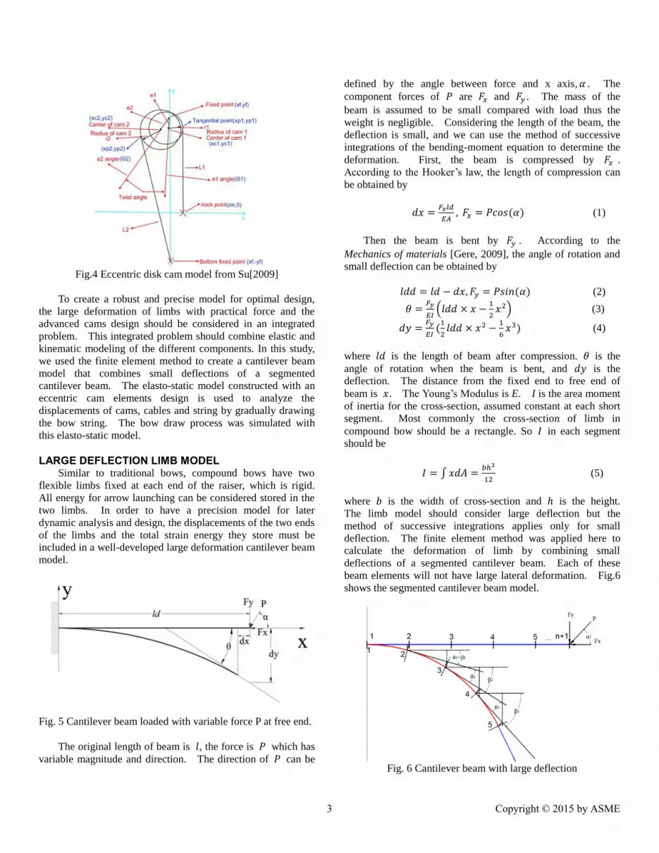
Fig.4 Eccentric disk cam model from Su[2009]

To create a robust and precise model for optimal design,

the large deformation of limbs with practical force and the

advanced cams design should be considered in an integrated

problem. This integrated problem should combine elastic and

kinematic modeling of the different components. In this study,

we used the finite element method to create a cantilever beam

model that combines small deflections of a segmented

cantilever beam. The elasto-static model constructed with an

eccentric cam elements design is used to analyze the

displacements of cams, cables and string by gradually drawing

the bow string. The bow draw process was simulated with

this elasto-static model.

LARGE DEFLECTION LIMB MODEL Similar to traditional bows, compound bows have two

flexible limbs fixed at each end of the raiser, which is rigid.

All energy for arrow launching can be considered stored in the

two limbs. In order to have a precision model for later

dynamic analysis and design, the displacements of the two ends

of the limbs and the total strain energy they store must be

included in a well-developed large deformation cantilever beam

model.

Fig. 5 Cantilever beam loaded with variable force P at free end.

The original length of beam is 𝑙, the force is 𝑃 which has

variable magnitude and direction. The direction of 𝑃 can be

defined by the angle between force and x axis,𝛼 . The

component forces of 𝑃 are 𝐹𝑥 and 𝐹𝑦 . The mass of the

beam is assumed to be small compared with load thus the

weight is negligible. Considering the length of the beam, the

deflection is small, and we can use the method of successive

integrations of the bending-moment equation to determine the

deformation. First, the beam is compressed by 𝐹𝑥 .

According to the Hooker’s law, the length of compression can

be obtained by

𝑑𝑥 =𝐹𝑥𝑙𝑑

𝐸𝐴, 𝐹𝑥 = 𝑃𝑐𝑜𝑠(𝛼) (1)

Then the beam is bent by 𝐹𝑦 . According to the

Mechanics of materials [Gere, 2009], the angle of rotation and

small deflection can be obtained by

𝑙𝑑𝑑 = 𝑙𝑑 − 𝑑𝑥, 𝐹𝑦 = 𝑃𝑠𝑖𝑛(𝛼) (2)

𝜃 =𝐹𝑦

𝐸𝐼(𝑙𝑑𝑑 × 𝑥 −

1

2𝑥2) (3)

𝑑𝑦 =𝐹𝑦

𝐸𝐼(1

2𝑙𝑑𝑑 × 𝑥2 −

1

6𝑥3) (4)

where 𝑙𝑑 is the length of beam after compression. 𝜃 is the

angle of rotation when the beam is bent, and 𝑑𝑦 is the

deflection. The distance from the fixed end to free end of

beam is 𝑥. The Young’s Modulus is E. I is the area moment

of inertia for the cross-section, assumed constant at each short

segment. Most commonly the cross-section of limb in

compound bow should be a rectangle. So 𝐼 in each segment

should be

𝐼 = ∫ 𝑥𝑑𝐴 =𝑏ℎ3

12 (5)

where 𝑏 is the width of cross-section and ℎ is the height.

The limb model should consider large deflection but the

method of successive integrations applies only for small

deflection. The finite element method was applied here to

calculate the deformation of limb by combining small

deflections of a segmented cantilever beam. Each of these

beam elements will not have large lateral deformation. Fig.6

shows the segmented cantilever beam model.

Fig. 6 Cantilever beam with large deflection

(5)


The undeformed beam is placed horizontally on the x-axis

and cut into 𝑛 segments with 𝑛 + 1 nodes. If the beam

length is 𝑙, the length of every segment is 𝑙𝑑 = 𝑙/𝑛. θ𝑖 is

the local angular deformation for one element, and β𝑖 is the

cumulative angle. For every segment, the angle of rotation

and small deflection can be determined as above; then all the

small deflections of the segmented cantilever beams are

combined to obtain the total deformation. The procedure is

shown in Fig. 7. The coordinate of node 1 is assumed as

(0, 0), therefore, all the coordinates of all nodes can be

obtained.

Fig.7 Procedure to model beam with large deflection

The node changes from number 𝑛 to 𝑛𝑎, then to 𝑛𝑏 .

(𝑥𝑓𝑛, 𝑦𝑓𝑛) is the coordinates of the node 𝑛. The coordinates of

the free end is

(𝑥𝑓𝑛+1, 𝑦𝑓𝑛+1)

= (𝑥𝑓𝑛 + 𝑙𝑑𝑑 𝑐𝑜𝑠 𝛽(𝑛 − 1) − 𝑑𝑦(𝑛) 𝑠𝑖𝑛 𝛽(𝑛 − 1) ,

𝑦𝑓𝑛 − 𝑙𝑑𝑑 𝑠𝑖𝑛 𝛽(𝑛 − 1) − 𝑑𝑦(𝑛) 𝑐𝑜𝑠 𝛽(𝑛 − 1))

(6)

And the deformation of beam is

𝑥𝑑𝑓 = 𝑙 − 𝑥𝑓𝑛+1, 𝑦𝑑𝑓 = −𝑦𝑓𝑛+1 (7)

According the analysis above, in this large deflection limb

model, the deformation in x-direction and y-direction can be

obtained from the magnitude and direction of the limb force.

CONSTRUCTION OF KINETO-STATIC MODEL The special motion of a compound bow with an elaborate

cam profile design makes the bow significant in archery. With

a set of cams, cables and limbs, this structure can be held easily

at full draw and can store more energy due to the pulley system.

In this paper, the cam profile with two eccentric circular cams

(Fig. 8) is selected for the kineto-static model.

Fig.8 Structure and kinematic diagram of a type of compound

bow studied in this work

This design has more flexible mechanical advantage and

can be produced with commercial components. The analysis

based on this design can be applied to other cam profiles.

Fig.8b shows that the bow structure is symmetric, and the angle

between limbs and the x-direction is 𝛼. So only the upper

cam needs to be analyzed, and the motion of the lower cam can

be obtained by symmetry. The motion procedure is

demonstrated by gradually drawing the bow string in Fig. 9.

The first part showed before drawing situation, the present

situation is the intermediate position, and the motion ends at the

third one. The fixed point is the end of the limb which holds

the rotation center of a cam. It is assumed that the cables and

string are inextensible, and the cam is non deformable. It is

convenient to combine previous and present situations to

analyze the displacements of cams, cables and string. The two

circular stacked cams can be separated to calculate their

motion. The bigger circle is cam1, and the smaller one is

cam2.

Fig.9 Displacement of the limbs and bow string


Fig.10 shows the analysis of cam1. The initial position

should be constructed first. The fixed point is F, the center of

cam1 is C1, and the tangent point of cable1 and cam1 is T1.

The eccentric distance from F to C1 is e1, the radius of cam1 is

r1. And the length from the tangent point to bottom fixed

point is S1. It is assumed that the original coordinate of the

fixed point is (𝑥𝑓(1), 𝑦𝑓(1)). From Fig. 10a the original

coordinate of the center of cam1 can be determined

Fig.10 Cam 1 diagram for kinematic modeling

𝑥𝑐1(1) = 𝑥𝑓(1) − 𝑒1 sin(𝑎𝑔1(1))

𝑦𝑐1(1) = 𝑦𝑓(1) − 𝑒1 cos(𝑎𝑔1(1)) (8)

𝑎𝑔1 is the angle between line F to C1 and y-axis. The

tangent point can be determined once the angle between the

cable and the y-axis is calculated. From Fig. 10b, the equation

of the cable angle is

𝑒1 cos(𝑎𝑔1(1)) + r1 sin(agcb(1)) +

𝑒1 sin(𝑎𝑔1(1))+r1 cos(agcb(1))

tan(𝑎𝑔𝑐𝑏(1))= 2𝑦𝑓(1) (9)

Solving this equation (9) to determine the angle of cable

we find:

𝑥𝑡𝑝1(1) = 𝑥𝑐1(1) − 𝑟1 𝑐𝑜𝑠(𝑎𝑔𝑐𝑏(1))

𝑦𝑡𝑝1(1) = 𝑦𝑐1(1) − 𝑟1 𝑠𝑖𝑛(𝑎𝑔𝑐𝑏(1)) (10)

Other geometry information obtained from the initial

conditions is the length from the tangent point to the bottom

fixed point:

𝑆1(1) = √(𝑥𝑡𝑝1(1) − 𝑥𝑓(1))2+ (𝑦𝑡𝑝1(1) + 𝑦𝑓(1))

2 (11)

Next is the kinematic analysis. The limb deflection is given

a constant increment 𝑑𝑙𝑡𝑦 by gradually drawing the bow

string, thus the position of cam, cable and string are calculated.

As shown in Fig. 10a, the algorithm for the next state is similar

to the algorithm for the initial one, but the deformation in the

x-direction is unknown, and a new variable (𝑟𝑜𝑎𝑔(1)) which

is the rotation of cam must be calculated first.

𝑦𝑓(2) = 𝑦𝑓(1) − 𝑑𝑙𝑡𝑦

𝑎𝑔1(2) = 𝑎𝑔1(1) + 𝑟𝑜𝑎𝑔(1)

𝑦𝑐1(2) = 𝑦𝑓(2) − 𝑒1 cos(𝑎𝑔1(2))

𝑒1 cos(𝑎𝑔1(2)) + r1 sin(agcb(2))

+𝑒1 sin(𝑎𝑔1(2)) + r1 cos(agcb(2))

tan(𝑎𝑔𝑐𝑏(2))= 2𝑦𝑓(2)

𝑦𝑡𝑝1(2) = 𝑦𝑐1(2) − 𝑟1 𝑠𝑖𝑛(𝑎𝑔𝑐𝑏(2))

𝑆1(2) = √(𝑒1 sin(𝑎𝑔1(2)) + 𝑟1𝑐𝑜𝑠(𝑎𝑔𝑐𝑏(2)))2+ (𝑦𝑡𝑝1(2) + 𝑦𝑓(2))

2

(12)

Since 𝑆1(1) = 𝑆1(2) + 𝑑𝑙𝑡𝑆1(1) , 𝑟𝑜𝑎𝑔(1) can be

solved by this equation. And from Fig. 10c, 𝑑𝑙𝑡𝑆1(1) is

solved as follows:

𝑑𝑙𝑡𝑆1(1) = 𝑟1𝑠𝑒𝑎𝑔(1)

𝑠𝑒𝑎𝑔(1) = 𝑎𝑔𝑐𝑏(2) − 𝑎𝑔𝑐𝑏(1) + 𝑟𝑜𝑎𝑔(1) (13)

The abscissa can then be calculated as:

𝑥𝑓(2) = 𝑥𝑓(1) − 𝑑𝑙𝑡𝑥 𝑥𝑐1(2) = 𝑥𝑓(2) − 𝑒1 sin(𝑎𝑔1(2))

𝑥𝑡𝑝1(2) = 𝑥𝑐1(2) − 𝑟1 𝑐𝑜𝑠(𝑎𝑔𝑐𝑏(2)) (14)

The x-direction increment of deformation (𝑑𝑙𝑡𝑥) will be

solved later. So for next 𝑛 − 1 states of cam1, the position

information can be obtained as above.

Fig.11 shows the analysis of cam2. The procedure is

similar to the analysis of cam1. The fixed point is F, the

center of circle 2 is C2, and the tangent point of string and

cam2 is T2. The nock point is Xn. The eccentric distance

from F to C2 is e2, the radius of cam2 is r2. And the length

from tangent point to nock point is S2. From Fig. 11a the

original coordinate of the center of cam2 can be determined.

Fig.11 Diagram for kinematic modeling of Cam2


𝑥𝑐2(1) = 𝑥𝑓(1) − 𝑒2 sin(𝑎𝑔2(1))

𝑦𝑐2(1) = 𝑦𝑓(1) − 𝑒2 cos(𝑎𝑔2(1)) (15)

where 𝑎𝑔2 is the angle between line F to C2 and y-axis.

The coordinates of tangent point, nock point and the

half-string length:

𝑥𝑡𝑝2(1) = 𝑥𝑐2(1) + 𝑟2

𝑦𝑡𝑝2(1) = 𝑦𝑐2(1)

𝑋𝑛(1) = 𝑥𝑡𝑝2(1)

𝑆2(1) = 𝑦𝑡𝑝2(1) (16)

The kinematic analysis shown in Fig.11a is similar to the

algorithm for the initial one (the rotation obtained for cam1).

But the x-direction deformation remains unknown. Hence we

have:

𝑦𝑓(2) = 𝑦𝑓(1) − 𝑑𝑙𝑡𝑦

𝑎𝑔2(2) = 𝑎𝑔2(1) + 𝑟𝑜𝑎𝑔(1)

𝑦𝑐2(2) = 𝑦𝑓(2) − 𝑒2 cos(𝑎𝑔2(2)) (17)

The angle between the string and the y-direction (𝑎𝑔𝑠𝑡)

needs to be determined to calculate the coordinate of the

tangent point. From Fig. 11b, the equation for 𝑎𝑔𝑠𝑡 is:

𝑟2 𝑡𝑎𝑛 (𝑎𝑔𝑠𝑡

2) +

𝑟2 𝑡𝑎𝑛 (𝑎𝑔𝑠𝑡

2) + 𝑦𝑐2

𝑐𝑜𝑠(𝑎𝑔𝑠𝑡)= 𝑟2(𝑥 + 𝑟𝑜𝑎𝑔) + 𝑆2(1)

(18)

So the ordinate of the tangent point is:

𝑦𝑡𝑝2(2) = 𝑦𝑐2(2) + 𝑟2 𝑠𝑖𝑛(𝑎𝑔𝑠𝑡(2)) (19)

The other coordinates can be calculated with the value of

𝑑𝑙𝑡𝑥.

𝑥𝑐2(2) = 𝑥𝑓(2) − 𝑒2 sin(𝑎𝑔2(2))

𝑥𝑡𝑝2(2) = 𝑥𝑐2(2) + 𝑟2 𝑐𝑜𝑠(𝑎𝑔𝑠𝑡(2))

𝑋𝑛(2) = 𝑋𝑛(1) + 𝑥𝑡𝑝2(1)tan(𝑎𝑔𝑠𝑡(2)) (20)

The position information of the next 𝑛 − 1 cam2 states

can be calculated as above. Now we need the value of 𝑑𝑙𝑡𝑥.

As discussed in the large deflection limb model, the value of

the limb force can be determined from the known direction of

the force and limb deflection. Then 𝑑𝑙𝑡𝑥 can be calculated

with the required force. First determine the direction of the

limb force.

Fig.12 Forces and moments on the cam

Fig.13 Force equilibrium diagram of the cam

Fig.12 shows the cam moment equilibrium diagram. For

the static case the moments sum to zero:

∑𝑀 = 𝑀1 + 𝑀2 = 𝐹𝑐𝑏1𝑑1 sin(𝑎𝑔𝑑1) − 𝐹𝑠𝑡𝑑2 sin(𝑎𝑔𝑑2) = 0

(21) From equation (21), the relationship between string force

and cable force is

𝐹𝑠𝑡 = 𝑘𝐹𝑐𝑏1, 𝑘 =𝑑1sin(𝑎𝑔𝑑1)

𝑑2𝑠𝑖𝑛(𝑎𝑔𝑑2) (22)

where 𝐹𝑐𝑏1 is the force of cable 1, 𝐹𝑠𝑡 is the string force, 𝑑1

is the distance from tangent point of cam1 to the fixed point,

and 𝑑2 is the distance from tangent point of cam2 to the fixed

point. The angle of 𝑑1 and cable 1 is 𝑎𝑔𝑑1 and 𝑎𝑔𝑑2 is

the angle between 𝑑2 and the string. The coefficient for

𝐹𝑐𝑏1and 𝐹𝑠𝑡 is k.

𝑑1 = √(𝑥𝑡𝑝1 − 𝑥𝑓)2 + (𝑦𝑡𝑝1 − 𝑦𝑓)2 =

√(𝑒1 𝑠𝑖𝑛(𝑎𝑔1) + 𝑟1 𝑐𝑜𝑠(𝑎𝑔𝑐𝑏))2 + (𝑦𝑡𝑝1 − 𝑦𝑓)2


𝑑2 = √(𝑥𝑡𝑝2 − 𝑥𝑓)2 + (𝑦𝑡𝑝2 − 𝑦𝑓)2 =

√(𝑟2 𝑐𝑜𝑠(𝑎𝑔𝑠𝑡) − 𝑒2 𝑠𝑖𝑛(𝑎𝑔2))2 + (𝑟2 𝑠𝑖𝑛(𝑎𝑔1) − 𝑒2𝑐𝑜𝑠 (𝑎𝑔2))2

𝑎𝑔𝑑1 = 𝑎𝑔𝑐𝑏 +𝜋

2− 𝑎𝑡𝑎𝑛

𝑦𝑓 − 𝑦𝑡𝑝1

𝑒1𝑠𝑖𝑛(𝑎𝑔1) + 𝑟1𝑐𝑜𝑠(𝑎𝑔𝑐𝑏)

𝑎𝑔𝑑2 =𝜋

2− 𝑎𝑔𝑠𝑡 + 𝑎𝑡𝑎𝑛

𝑟2𝑠𝑖𝑛(𝑎𝑔𝑠𝑡) − 𝑒2𝑐𝑜𝑠(𝑎𝑔2)

𝑟2𝑐𝑜𝑠(𝑎𝑔𝑠𝑡) − 𝑒2𝑠𝑖𝑛(𝑎𝑔2)

(23)

Fig.13 shows the cam force equilibrium diagram. The

forces must sum to zero for the static case:

∑𝐹 = 𝐹𝑐𝑏1 + 𝐹𝑐𝑏2

+ 𝐹𝑠𝑡1 + 𝐹𝑙𝑖𝑚𝑏

= 2𝐹 + 𝐹𝑠𝑡1 + 𝐹𝑙𝑖𝑚𝑏

= 0

(24)

where 𝐹𝑙𝑖𝑚𝑏 is the limb force. The angle of force 𝑃 (𝑎𝑔𝑝) is:

𝐹𝑙𝑖𝑚𝑏2 = (2𝐹)2 + (𝐹𝑠𝑡)

2 − 4𝐹𝐹𝑠𝑡cos(𝜋 − 𝑎𝑔𝑠𝑡)

𝑎𝑔𝑝 =𝜋

2−

𝐹𝑙𝑖𝑚𝑏2+(2𝐹)2−𝐹𝑠𝑡

2

4𝐹𝑙𝑖𝑚𝑏𝐹 (25)

Now, the value of limb force can be obtained from the

known y-direction deflection (𝑑𝑙𝑡𝑦) and the direction of limb

force (𝛼, 𝑎𝑔𝑝). The solution can be applied to calculate the

x-direction limb deformation (𝑑𝑙𝑡𝑥) . Then all the

displacements of cams, cables, string and limbs are solved for

the motion of this class of compound bow. Other parameters

of the bow can also be obtained. The maximum limb

deflection is 𝑀𝑎𝑥_𝐿𝑖𝑚𝑏𝐷 = 𝑑𝑙𝑡𝑦 × 𝑛. The maximum spring

force is 𝑀𝑎𝑥_𝐷𝑟𝑎𝑤𝐹 = 𝑀𝑎𝑥(𝐹𝑙𝑖𝑚𝑏). The maximum draw

force is 𝑀𝑎𝑥_𝐷𝑟𝑎𝑤𝐹 = 2 × 𝑀𝑎𝑥(𝐹𝑠𝑡) × 𝑠𝑖𝑛(𝑎𝑔𝑠𝑡) . The

let-off rate is 𝑙𝑒𝑡_𝑜𝑓𝑓 = (𝑀𝑎𝑥_𝐷𝑟𝑎𝑤𝐹 − 𝐸𝑛𝑑_𝐷𝑟𝑎𝑤𝐹)/𝑀𝑎𝑥_𝐷𝑟𝑎𝑤𝐹 × 100.

SIMULATION TO STUDY THE EFFECTS OF DESIGN VARIABLES

Simulation studies to observe the effects of design

parameter changes can be performed with a combined large

deformation elastic beam model and kinematic cam-cable

model Table 1 shows the design parameters used in this

simulation.

Table 1 List of Design Variables

Parameters symbol value

Radius of cam1 𝑟1 35(𝑚𝑚)

Radius of cam2 𝑟2 25(𝑚𝑚)

Eccentricity of cam1 𝑒1 17.5(𝑚𝑚)

Eccentricity of cam2 𝑒2 12.5(𝑚𝑚)

Angle between line FC2 and

y-axis 𝑖𝑛𝑎𝑔 10°

Angle between line FC1 and

line FC2 𝑡𝑎𝑔 10°

Angle of limb and x-axis 𝛼 𝑎𝑡𝑎𝑛(4/3)

Width of limb 𝑏 20(𝑚𝑚)

Height of limb ℎ 10(𝑚𝑚)

Length of limb 𝐿 300(𝑚𝑚)

Young’s Modulus of limb 𝐸 30(𝐺𝑃𝑎)

Fig.14. shows the deflection (y-displacement) of the limb

versus the horizontal deformation (x-displacement). The error

from using the dotted line as a linear approximation to the

actual calculated displacement is small. Intuitively if the limb

is softer, the error from a linear approximation will be larger.

Fig.14 Trajectory of pivot point of the cam

Fig.15 shows the change of limb force, cable force and

string force, as a function of the draw length. These forces are

significant in the evaluation of the bow performance. Among

the three forces displayed, if the limb force is large, usually this

is good for larger strain energy storage and faster arrow speed.

However, large limb force can result in large draw force which

is not desirable for the archer. The control of the let-off

percentage in the string force and in the design process is also

important, since this will affect how easy it is to hold and aim

the bow in the fully drawn position.

The relationship of draw force as a function of draw length

plotted is shown in Fig.16 to signify the effect of let-off. Area

under this curve is the bow input energy stored in the limbs.

Table 2 lists some numerical results of the simulation.


Fig.15 Various forces as a function of draw-length.

Fig.16 Draw force, let-off and work done by draw force in the

drawing process

Table 2 Results of simulation study

Parameters value

Maximum limb deflection 81.0032(𝑚𝑚)

Maximum limb force 722.2(𝑁)

Maximum draw force 291.5963(𝑁)

Let-off rate 22.6795(%)

Stored energy 72738.7(𝑁 ∙ 𝑚𝑚)

The kinematic and elastic analysis calculates the

displacement of compound bow, and the motion animation of

bow is shown in Fig.17 and Fig.18. This animation helps the

understanding of effects from design parameters r1 and r2.

Fig. 17 Draw force as function of r1

Fig.18 Draw force as function of r2

CONCLUSIONS Many patents related to the design and improvements of

compound bow have been issued since the invention of the

compound bow in the 1960’s. However, few published

technical papers or engineering analyses on this subject exist.

Previously unreported conclusions from our work include:

1. In an automated design or optimization system, combining

finite element analysis and kinematic analysis using

commercial software can significantly slow convergence

to a solution. To increase speed, we developed a

relatively short MATLAB program, based on the essence

of the finite element method, to do large deformation

cantilever beam analysis. The program computes the

elastic deformation of the bow limbs, where the pivots of

the stacked cams are located at the end of each limb.

Compared with the trajectory previously computed by


commercial software, the resulting trajectory seems

reasonably accurate.

2. Today’s compound bows use many different cam and

cable system designs. This paper addresses one of the

commonly used types: a dual and symmetrical cam with

an eccentric-cylindrical cam profile. This cam profile is

simple and elegant, and probably the least expensive to

manufacture. In addition to the elastic subsystem

modeling, a quasi-static kinematic model was developed

and combined into an integrated mechanical simulation

system. The kinematic part of the model analyzes the

force system acting on the stacked cams and cables, and

the string. The kinematic model provides a connection

between the variable loading for limb analysis, and draw

force (which the archer must provide).

3. Effects of cam profile design variables on the bow

performance were studied. However, optimal design of

the cam profile has not been included in this paper.

Equipped with a good elasto-kinematic model, as

described in this paper, the optimal design of cams for

minimizing draw force and maximum energy storage

should be straight forward. However, for maximizing

the arrow speed and minimizing the energy left in the bow

to reduce noise and vibration, a more complex dynamic

model, an elasto-kinetic model will be needed to analyze

for motion after the arrow is released.

ACKNOWLEDGMENTS The authors thank Mr. Yu Cheng Su, a former MS student

who started the modeling work in this subject. The authors

also thank Dr. Peter Hodges for proof reading the manuscript.

REFERENCES Allen, H. W., 1968, Archery Bow with Draw Force

Multiplying Attachments, US Patent, No.3486495.

Gere, J.M. and Goodno, B.J., 2012, Mechanics of Materials,

Cengage Learning.

Grayson, C.E., French, M., and O’Brien, M.J, 2007,

Traditional Archery from Six Continents: The C.E. Grayson

Collection, University of Missouri Press.

Hanson, A., 2009, Kinematic Analysis of Cam Profiles used

in Compound Bows, MS Thesis, University of Missouri.

He, Jiahuan, 2011, Kineto-Elasto Dynamic Modeling and

Optimal Design of Mechanical Systems—as Applied to

Compound Bow Design, MS Thesis, University of Missouri.

Kincy, M.A., 1981, A Model for Optimization of the Archer’s

Compound Bow, MS Thesis, University of Missouri-Rolla

Kooi, B.W., 1983, On the Mechanics of the Bow and Arrow,

Netherlands.

Kooi, B.W., 1991, “Archery and Mathematical Modeling,” J.

of the Society of Archer-Antiquaries, v.34, pp.21-29.

Kudlacek, D. S., 1977, Compound Archery Bow with

Eccentric Cam Elements, U.S. Pat. No.4060066.

Lin, Yuyi and Hanson, A., 2008, “Analysis and Design of a

Class of Cam Profile—as Applied to Compound Archery Bow

Machine Design and Research,” Machine Design and

Research, v.24, pp.90-94.

Marlow, W.C., 1980, Bow and Arrow Dynamics,

Perkin-Elmer Corporation, Connecticut.

Miller, L.D., 1985, Compound Archery Bow, US Patent,

No.4519374.

Su, Yu-Cheng, 2009, The Effect of the Twist Angle and the

Optimization for the Compound Bow, MAE7930 Project

Report, University of Missouri.

Visner, J.C., 2007, Analytical and Experimental Analysis of

the Large Deflection of a Cantilever Beam Subjected to a

Constant, Concentrated force, with a Constant Angle, Applied

at the Free End, MS Thesis, University of Akron.


Documents

Kineto-Elastic Analysis of a Compound Bow