Embed Size (px)
Citation preview
A Bayesian Model of Knightian Uncertainty
Nabil I. Al-Najjar∗ and Jonathan Weinstein†
First draft: December 2011This version: September 2012
Abstract
A long tradition suggests a fundamental distinction between situ-ations of risk, where true objective probabilities are known, and un-measurable uncertainties where no such probabilities are given. Thisdistinction can be captured in a Bayesian model where uncertainty isrepresented by the agent’s subjective belief over the parameter govern-ing future income streams. Whether uncertainty reduces to ordinaryrisk depends on the agent’s ability to smooth consumption. Uncer-tainty can have a major behavioral and economic impact, includingprecautionary behavior that may appear overly conservative to anoutside observer. We argue that one of the main characteristics ofuncertain beliefs is that they are not empirical, in the sense that theycannot be objectively tested to determine whether they are right orwrong. This can confound empirical methods that assume rationalexpectations.
∗ Department of Managerial Economics and Decision Sciences, Kellogg School of Man-agement, Northwestern University, Evanston IL 60208. Al-Najjar’s Research Page.† Department of Managerial Economics and Decision Sciences, Kellogg School of Man-
agement, Northwestern University, Evanston IL 60208. Weinstein’s Research Page.
Contents
1 Introduction 1
2 Risk and Uncertainty 52.1 Model and Notation . . . . . . . . . . . . . . . . . . . . . . . 52.2 Risk, Uncertainty, and the Value Function . . . . . . . . . . . 6
3 Uncertainty and Precautionary Behavior 103.1 Model . . . . . . . . . . . . . . . . . . . . . . . . . . . . . . . 103.2 Pure Risk . . . . . . . . . . . . . . . . . . . . . . . . . . . . . 113.3 Uncertainty . . . . . . . . . . . . . . . . . . . . . . . . . . . . 13
4 Empirical Implications of Uncertainty 154.1 Uncertain Beliefs are Untestable . . . . . . . . . . . . . . . . . 154.2 Inference under Uncertainty . . . . . . . . . . . . . . . . . . . 174.3 Discussion and Related Literature . . . . . . . . . . . . . . . . 21
A Appendix 24
1 Introduction
Knight (1921)’s idea of a fundamental difference between “measurable risk
and an unmeasurable uncertainty” has generated both interest and contro-
versy. Standard models in economics assume that agents use probabilities to
quantify all uncertainties regardless of their source or nature. No distinction
is drawn between actuarial and strategic risks, or between risks associated
with repetitive vs. singular events. Yet there is a compelling intuition that
some probability judgments are less ‘obvious’ or ‘objective’ than others. Bet-
ting on events like the unraveling of the European monetary union or global
warming seems qualitatively different from betting on the outcome of a coin
toss or whether it rains tomorrow. The first type of event represents, in
Knight’s words, unmeasurable uncertainties that should be treated differ-
ently from measurable risks.
This paper suggests that a Bayesian framework can capture the distinc-
tion between situations with known probabilities, or “risk,” and Knightian
uncertainty where objective probabilities are unknown.1 We illustrate the
distinction in a consumption-saving model where uncertainty is represented
by the agent’s subjective belief about the parameter governing future income.
We relate the impact of uncertainty to the agent’s ability to intertemporally
smooth consumption and show that this leads to precautionary behavior that
may appear overly conservative to an outside observer. We also point to the
potential tension between subjective uncertainty and empirical methods that
use rational expectations for econometric identification.
Consider an agent with time-separable utility over (finite or infinite) con-
sumption streams. The agent receives an i.i.d. income stream with unknown
parameter θ.2 Uncertainty is lack of knowledge represented by a prior belief
µ over θ. Uncertainty does not necessarily lead to measurable consequences
1 Keynes (1937) characterized uncertain beliefs as follows: “The sense in which I amusing the term [uncertainty] is that in which the prospect of a European war is uncertain,or the price of copper and the rate of interest twenty years hence, or the obsolescenceof a new invention, or the position of private wealth-owners in the social system in 1970.About these matters there is no scientific basis on which to form any calculable probabilitywhatever. We simply do not know.”
2 The i.i.d. assumption simplifies the analysis, but is not essential to our point. Wediscuss this point in Section 4.
1
on behavior. For example, if uncertainty is defined on consumption streams
directly, then discounted expected utility is unaffected by replacing the un-
certain belief µ by a parameter with the same marginal as µ. In this case,
uncertainty reduces to ordinary risk. The role of uncertainty is manifested
in the indirect utility the agent derives from income streams when he has
(perhaps limited) freedom to save or borrow.
We first illustrate this point in a simple setting where consumption occurs
after an initial phase of payoff accumulation. For example, a retirement
portfolio generates dividends each period, but the agent cares only about
its value at the time of retirement. Another example is a start-up that
accumulates gains and losses over a period of time, but whose value is realized
only when the entrepreneur sells the firm. In these examples, separating
consumption from payoff accumulation simplifies the calculation of indirect
utility, making the impact of uncertainty transparent and striking.
We then turn to a richer consumption-saving problem where consumption
and wealth can change as uncertainty about income resolves. Using exponen-
tial utility for tractability, we derive the evolution of consumption and show
that uncertainty results in precautionary behavior that may appear overly
conservative to an outside observer. Consumption is more volatile under
uncertainty because the agent perceives short-run income variations to be
potentially informative about his long-run income prospects. Under risk, by
contrast, all income realizations are viewed as transitory.
A Bayesian framework represents any lack of knowledge in terms of prob-
abilities. What then justifies treating uncertainty differently from other sit-
uations of imperfect information? Our main point is that the key difference
between risk and uncertainty is that uncertain beliefs are not empirical. Sec-
tion 4 introduces two arguments to support this point.
First, we formalize the intuition that the probabilities of uncertain events
are subjective opinions about which, in Keynes’ words, “there is no scientific
basis to form any calculable probability whatever.” We capture this intuition
using statistical tests that compare agents’ subjective beliefs with the actual
sequence of realized outcomes. Consider asymptotic tests for simplicity. A
natural property to require in such tests is to be free of Type I error: if
the agent knows the true probabilities, he must pass the test almost surely.
2
Proposition 4.1 says that an agent who is uncertain about the true parameter,
and who has subjective belief µ, must also believe that there is an alternative
belief µ′ 6= µ such that no Type I error free test could reject µ′ regardless of
the amount of data used. Bayesian agents assign probabilities to all events,
whether risky or uncertain. What distinguishes beliefs about uncertain events
is that they cannot be objectively tested to determine whether they are right
or wrong. By contrast, it is easy to test beliefs under risk by comparing them
with observed frequencies.
The second sense in which uncertain beliefs are not empirical concerns
the difficulty of estimating their impact using standard econometric meth-
ods. Beliefs influence decisions regardless of whether they reflect risk or
uncertainty. But since beliefs are not directly observable, econometric iden-
tification assumptions are needed to recover them from data. A standard
assumption is rational expectations which identifies beliefs with observed
empirical frequencies. While this assumption offers considerable advantages,
it also rules out subjective model-uncertainty as a factor in decisions, a point
made by Weitzman (2007) among others. In Section 4 we suggest that the
perceived failure of equilibrium models to capture Knightian uncertainty may
have more to do with the use of rational expectations in their econometric
estimation than with the Bayesian rational choice paradigm.
There is a growing interest in the economic role of Knightian uncer-
tainty.3 One motivation is the discrepancy between observed behavioral
patterns (e.g., in asset prices) and the predictions of models where agents
are assumed to know the true data generating process. Introducing uncer-
tainty about fundamentals is a natural way to bring models closer to reality.
Pastor and Veronesi (2009) survey asset pricing anomalies that could be ex-
plained with the introduction of uncertainty about fundamental parameters.
They conclude that “[m]any facts that appear baffling at first sight seem
less puzzling once we recognize that parameters are uncertain and subject to
learning.” Hansen and Sargent (2001) discuss the importance of model mis-
specification and parameter-uncertainty in macroeconomic modeling. Con-
nections to these works are discussed in greater detail in Section 4.
3 The terms parameter-uncertainty, model-uncertainty, or model mis-specification areoften used instead of what we simply call “uncertainty.”
3
Two seminal papers, Gilboa and Schmeidler (1989) and Bewley (1986),
formalize the concept of Knightian uncertainty as lack of full Bayesian belief.
In Bewley (1986), uncertainty is modeled as an incomplete ranking over acts.
Gilboa and Schmeidler (1989)’s ambiguity averse agents use a maxmin crite-
rion with respect to a set of priors to incorporate caution in their decisions.
Both approaches focus on the typical pattern of choices in static Ellsberg
experiments as a key behavioral manifestation of uncertainty.
The present paper argues that a distinction between risk and Knight-
ian uncertainty can be made within the Bayesian framework. This point of
view follows a number of authors, including Halevy and Feltkamp (2005) and
Weitzman (2007), who pursue Bayesian approaches to uncertainty. LeRoy
and Singell (1987) suggest that such approach can be traced to Knight
(1921)’s original work, noting that “Knight shared the modern view that
agents can be assumed always to act as if they have subjective probabili-
ties.” Similarly, Keynes (1937) writes that, even in situations of uncertainty,
“the necessity for action and for decision compels us [..] to behave exactly
as we should if we had [...] a series of prospective advantages and disadvan-
tages, each multiplied by its appropriate probability, waiting to be summed.”
Knight and Keynes, writing decades before modern subjective expected util-
ity theory, seemed to believe that decision making under uncertainty is not
necessarily in conflict with probabilistic reasoning.
We find it useful to distinguish Knightian uncertainty from ambiguity
aversion. We take uncertainty to mean probabilities that cannot be ob-
jectively measured, an intuition we formalize in terms of statistical tests.
Ambiguity aversion, on the other hand, refers to non-probabilistic beliefs,
exemplified by the static Ellsberg choices. Although both lead to precau-
tionary behavior, there are profound differences. In a Bayesian model, the
implications of uncertainty appear in connection with intertemporal choice
and the constraints on consumption smoothing. In static settings, such as
Ellsberg’s choices, risk and uncertainty are indistinguishable. This consistent
with Knight (1921)’s view: “when an individual instance only is at issue,
there is no difference for conduct between a measurable risk and an unmea-
surable uncertainty. The individual [...] throws his estimate of the value of
an opinion into the probability form of ‘a successes in b trials’ [...] and ‘feels’
4
toward it as toward any other probability situation.” In modern Bayesian
language, agents care only about the prizes they receive, not whether they
were the result of risk rather than uncertainty.
The outline of the rest of the paper is as follows. Section 2 introduces the
basic setup and defines the uncertainty premium. This section also introduces
a very simple model where the value function can be easily computed and
the impact of uncertainty is obvious. This simple model is related to Halevy
and Feltkamp (2005), which we discuss in some detail. Section 3 introduces
a more complete saving-consumption model and derives the stochastic laws
of consumption under risk and uncertainty. Uncertainty leads to precaution-
ary behavior and greater sensitivity to information. Section 4 discusses the
empirical implications of uncertainty. We begin with a simple argument il-
lustrating that uncertain beliefs are not testable, then discuss the potential
tension between uncertainty and rational expectations econometrics. We dis-
cuss in detail the relationship of our work to Weitzman (2007) and Cogley
and Sargent (2008).
2 Risk and Uncertainty
2.1 Model and Notation
We consider infinite horizon decision problems (finite horizon problems can
be obtained as a special case). In each period, an outcome in a finite set
S = {s1, . . . , sk} is realized. The set of infinite sequences of outcomes is
denoted S∞. We use subscripts to indicate time periods and superscripts to
indicate outcomes. For example, si is the outcome at time i while sj is the
jth outcome.
An agent has a a time-separable discounted utility for consumption streams:
U(c1, . . .) =∞∑i=1
δi u(ci), (1)
where δ ∈ [0, 1] is a discount factor and u : R → R is a concave von
Neumann-Morgenstern utility.
5
Let Θ be the set of all probability distributions θ = (θ1, . . . , θk) on S.
In this paper, a parameter is an i.i.d. distribution P θ on S∞ obtained by
independently sampling from S according to θ. We will refer to either θ or
P θ as “parameter.”4 We do not consider more general parametric models,
such as Markov processes, for tractability and expositional simplicity.
The agent’s uncertainty about θ is represented by a prior µ over Θ. Let
P µ represent the implied belief about infinite samples, defined by P µ(B) ≡∫ΘP θ(B) dµ(θ), for every event B.5 From the perspective of the agent, the
parameter θ is a random variable with distribution µ. Expectations with
respect to µ and θ are denoted Eµ, Eθ, respectively.
It will be useful to define the “average” parameter θµ
by θµ(si) = Eµθ(s
i).
For example, if si is ‘Heads’ in a coin toss, then the space of parameters is
[0,1] and µ is a distribution on [0,1]. In this case, Eµ θi is the expected value
of the probability of Heads. Although P µ and P θµ
share the same marginal
on any single coordinate, P θµ
is always independent, while P µ is independent
only when µ concentrates all its mass on a single parameter.
2.2 Risk, Uncertainty, and the Value Function
A Bayesian agent who is uncertain about the ‘true’ parameter θ represents
this lack of knowledge in terms of a prior µ. His expected utility on con-
sumption streams is:
EµEθ U(c1, . . .).
It is easy to see that this equals Eθµ U(c1, . . .), so the agent is indifferent be-
tween uncertainty about the parameter and certain knowledge of the average
parameter.6
This makes a simple but important reference point: how confident an
agent ‘feels’ about his knowledge of the true θ is irrelevant in ranking con-
4 All events in S∞ are assumed to be Borel sets. The space of probability measures onS∞ is itself endowed with the weak* topology and the Borel sigma-algebra of events. Allfunctions used in the paper are assumed measurable.
5 There is a 1-1 correspondence between Pµ and µ, yet they are different objects: theformer is a distribution on Sn, while µ is a distribution on Θ.
6 This follows from the linearity of probabilities and the time-separability of utility:∫Θ
∫Sn
∑∞i=1 δ
i u(ci) dP θ dµ =∑∞i=1 δ
iEθµ u(ci) = Eθµ U(c1, . . . , cn).
6
sumption streams. This apparent failure of the standard framework to cap-
ture uncertainty about the true probabilities may be behind the perception
that Knightian uncertainty requires a departure from probability-based rea-
soning. For instance, consider an agent A who believes that his consumption
stream will either be high forever or low forever with equal probability, vs.
an agent B who believes that each day there is an independent 50-50 draw
between high and low. Our standard utility function evaluates these as equal,
because agent B does not derive any hedging benefit from the independent
draws, but is forced to “starve” on bad days. It is more natural, though to
consider the case that some intertemporal smoothing is possible.7
While a Bayesian framework cannot distinguish risk and uncertainty in
consumption streams, this distinction is possible, indeed natural, in evaluat-
ing the indirect utility of payoff streams. To make this idea formal, define a
consumption plan c as a sequence of functions:
ci : Ri → R, i = 1, . . . ,
with the interpretation that ci is period i consumption given the payoffs
realized up to that period. The agent chooses a consumption plan from a
non-empty subset C which we interpret as the set of feasible plans. The
specification of C will vary with the problem considered.
Given a random payoff stream fi, i = 1, . . ., an agent with belief µ solves:
maxc∈C
EµEθ
∞∑i=1
δi u(ci). (2)
Let c∗(µ, f, C) be a solution to this problem. The indirect utility function is
the value V (µ, f, C) of the above problem. That is,
V (µ, f, C) = EµEθ
∞∑i=1
δi u(c∗i (f1, . . . , fi)
).
7 For example Hansen and Sargent (2001) write: “Knight (1921) distinguished riskyevents, which could be described by a probability distribution, from a worse type of igno-rance that he called uncertainty and that could not be described by a probability distri-bution. [...] A person behaving according to Savage’s axioms has a well-defined personalprobability distribution. [...] Savage’s system undermined Knight by removing the agentspossible model misspecification as a concern of the model builder.”
7
We suppress references to f and C when they are clear from the context. In
many applications, C has a recursive structure, and the impact of past payoff
realizations can be summarized by a vector of state variables.
A basic intuition is that agents prefer prospects with known probabilities
to ones where the probabilities are unknown. In fact, Knight’s original mo-
tivation was that economic profits are paid to bearing uncertainty. The first
criterion to measure the impact of uncertainty is in terms of the expected
utility improvement if the agent knew the true parameter:
Eµ V (θ)− V (µ). (3)
This term is strictly positive if V is strictly convex in θ. It captures the
value of information in helping the agent make better consumption decisions.
We examine consumption smoothing under uncertainty in greater detail in
Section 3. For now, we simply note that uncertainty has no impact when
considering preferences over consumption streams, since there is no decision
to be made. Formally, a constraint set C precludes intertemporal smoothing
if ci = f(si) for all i and s.
Proposition 2.1 If C precludes intertemporal smoothing then for every f ,
V (µ) = V (θµ).
Precluding intertemporal smoothing means that the agent consumes his en-
dowment, so indirect utility reduces to utility over consumption streams.
The agent cannot, for example, open a checking account, store consumption
goods, or put money under the proverbial mattress. In realistic economic
environments, some degree of intertemporal smoothing is possible, and un-
certainty potentially has an impact on behavior.
The second criterion to measure the impact of uncertainty is to use as a
reference point the agent’s utility under the average parameter:
V (θµ)− V (µ) (4)
and define the uncertainty premium as:
u−1(V (θ
µ, f))− u−1
(V (µ, f)
).
To illustrate these concepts, we focus on a concrete class of examples:
8
Example 1 (Deferred Consumption) There are n+1 periods and δ = 1.
The set C consists of a single consumption plan: ci = 0, i 6= n + 1 and
cn+1 =∑n
i=1 fi.
One interpretation of the utility of consumption in period n+1 is that it rep-
resents the indirect utility of consumption in subsequent periods with initial
wealth given by the lump-sum payment∑n
i=1 fi. Many important problems
fit this description, including assets that generate payoffs each period but
pay the cumulative dividend at time n+ 1.8
The separation of consumption (period n + 1) and payoff accumulation
(periods i = 1, . . . , n) makes the problem tractable. Assuming u(0) = 0,
indirect utility is simply:
V (µ) = EµEθ u(∑n
i=1 fi
).
Note that the term (3) is zero, so that criterion cannot separate risk and
uncertainty. The separation is possible under criterion (4). However, when
u is strictly concave and n > 1, the distribution of the sum∑n
i=1 fi has more
variability under the uncertain belief µ than under the i.i.d. parameter θµ.
This suggests that an agent will prefer a project with known probability θµ
to a project with uncertain probability represented by µ.
This intuition is confirmed by Halevy and Feltkamp (2005) in the case of
n = 2. They consider an agent whose utility depends on the sum f(s1)+f(s2)
of two draws from an urn with fixed but unknown composition. They show
that this creates sensitivity to uncertainty: a risk averse agent would prefer to
bet on an urn with known composition θµ
to an uncertain urn with subjective
distribution µ, so (4) holds strictly. Halevy and Feltkamp (2005)’s important
insight is that many real-world situations involve multiple draws and that
utility may depend on the sum of these draws. They suggest that agents
may develop heuristics that make them appear sensitive to uncertainty even
in one-draw experimental settings.
8 For example, a start-up company which accumulates gains and losses to its value overa period of time, but investors are paid when the company is sold or goes public. Anotherexample is a retirement portfolio that generates dividends each period, but the agent caresonly about its value at the time of retirement.
9
Halevy and Feltkamp (2005)’s study shows that analyzing even the n = 2
case can be quite involved. We gain additional intuition by considering large
n. Imagine a partnership where each partner owns (conveniently) a 1n
share
of the final value of the firm. This normalization eliminates the effect of
possible changes in risk attitude as n grows. The agent has a choice between
two projects: one with known odds θµ
and another with uncertain odds µ.
Proposition 2.2 Suppose that u is strictly concave and µ is non-degenerate.
Then for all sufficiently large n, the agent strictly prefers the project with
known odds.
This says that V(θµ)> V (µ) and the uncertainty premium is strictly posi-
tive. With large n, the intuition is simple: the law of large numbers implies
that for any θ there is high probability that the average is close to the ex-
pectation Eθf , hence the approximate equality:
Eθ u(
1n
∑∞i=1 fi
)' u
(1nEθ∑∞
i=1 fi).
The distinction between parameters and subjective beliefs about parameters
is key: while the variability implied by θ tends to average out, uncertainty is
unaffected by n. We finally note that uncertainty is irrelevant in a one-period
problem. With n = 1, P θµ
and P µ induce identical distributions on outcomes,
and are therefore indistinguishable. Our model is therefore inconsistent with
behavioral anomalies that arise in one-period choice problems.
3 Uncertainty and Precautionary Behavior
In this section we turn to a richer model where consumption decisions and
income realizations occur in each period. This standard consumption-saving
setting makes it possible to examine the theoretical and empirical implica-
tions of uncertainty in a familiar context.
3.1 Model
In each period t = 1, . . ., the agent starts with a level of wealth wt and
belief µt which represents the physical state and belief state of the system,
respectively. His consumption decision is a function of the state, ct(wt, µt).
10
The physical state evolves according to:
wt+1 = (1 + r)(wt + ft − ct), (5)
where ct is consumption in period t and r > 0 is the net return on savings.
Beliefs evolve according to Bayes rule. Note that the transition of the physical
state does not depend on beliefs, and conversely. The transitions on wealth
and beliefs define a feasible set C. The value function (indirect utility) and
the policy function are denoted V (µ,w) and c∗(µ,w).
To obtain an analytical expression for the evolution of consumption and
wealth under uncertainty, we assume that the agent has an exponential
(CARA) utility function u(x) = −e−ax and that δ = 11+r
. Our analysis
for the pure risk case is based on Caballero (1990), while the results for
uncertainty appear new. See Carroll and Kimball (2008) for a recent survey.
The optimal solution to this problem must satisfy the Euler equation:
u′(c∗t ) = Et[u′(c∗t+1)].
For the exponential utility, marginal utility is a constant multiple of the
utility level. Using this fact, and iterating expectations, we have:
u(c∗t ) = Et[u(c∗t+k)]
for every k. This implies (by taking u−1 of both sides) that consumption
today equals the certainty equivalent of consumption at any future date.
This in turn implies that the value function satisfies:9
V (µt, wt) = u(c∗t ).
3.2 Pure Risk
The evolution of consumption under risk and exponential utility is well-
known in the literature on precautionary saving. We summarize these results
for the benefit of the reader:
9 This follows from: V (µt, wt) = (1− δ)Eµt[∑∞
l=t δl−tu(c∗l )
]= (1− δ)
∑∞l=t δ
lu(c∗t ).
11
Proposition 3.1 Given any parameter θ, the optimal consumption rule is:
c∗(θ, w) =r
1 + rw + r−1CE(rf |θ) (6)
where
CE(rf |θ) ≡ u−1
(∫u(rf)dθ
)is the certainty equivalent of the random permanent impact rf on consump-
tion from the dividend implied by θ.
Furthermore, the evolution of consumption can be written
ct+1 = ct + Γ(θ) + r(ft − E[f |θ]) (7)
where Γ(θ) is the risk premium of the variable rf , defined by
Γ(θ) ≡ E(rf |θ)− CE(rf |θ) ≥ 0. (8)
Examining formula (7), we see that Γ is the drift of the consumption pro-
cess (since the last term has mean zero). Once again, Γ equals the standard
risk premium of the prospect rf . In particular, Γ is increased if the distri-
bution on f is replaced by a mean-preserving spread. It is strictly positive
as long as θ is not a point mass, since a certainty equivalent (under concave
utility) is always less than expected value. It should be interpreted as due
to “precautionary savings” since it would be absent if future dividends were
known. The term r(ft−E[f |θ]) is a mean-zero random shock to consumption
due to the wealth effect of the difference between the realized and expected
payoff.
We can also observe that, by inspection of the CARA utility form, the
term r−1CE(rf |θ) which appears in (6) is in fact the certainty equivalent
of the prospect f for an agent who has CARA utility with risk aversion of
ra rather than a. Notice that this must be larger than CE(f |θ) whenever
r < 1; an agent who is less risk averse has larger certainty equivalents. An
equivalent statement is that for r < 1:
CE(rf |θ) ≥ rCE(f |θ)
which is just the statement that there is less risk aversion at a smaller scale.
The inequality is strict whenever f takes on more than one value.
12
3.3 Uncertainty
Here we let µ be a non-trivial distribution over the parameter θ. The fol-
lowing general form, stating that adding wealth simply results in additional
interest income being consumed each period, follows intuitively from the fact
that risk attitudes under CARA are invariant to the wealth level:
Lemma 3.2
c∗(µ,w) =r
1 + rw + c∗(µ, 0).
In light of the lemma, it makes sense to use the notations
c∗(µ) ≡ c∗(µ, 0) and V (µ) ≡ V (µ, 0).
The next result shows that the value and consumption functions are con-
vex in µ; this can be interpreted to mean that given any uncertainty, resolu-
tion of this uncertainty will on average increase consumption. The last part
states further that, for a fixed marginal distribution on tomorrow’s return,
we consume less under uncertainty than under pure risk. That is, there is
additional precautionary savings due to the uncertainty about θ. To take
an extreme example, we consume more if we know our returns will be i.i.d.
50-50, 0 or 1, forever, than if we think there is a 50% chance they will be 0
forever and a 50% chance they will be 1 forever.
Proposition 3.3 For any w, V and c∗ are strictly convex in µ. That is,
letting µ1 and µ2 be any beliefs which result in distinct consumption plans,
1. V (λµ1 + (1− λ)µ2, w) < λV (µ1, w) + (1− λ)V (µ2, w);
2. c∗(λµ1 + (1− λ)µ2, w) < λc∗(µ1, w) + (1− λ)c∗(µ2, w).
Furthermore, for any µ with finite support, letting θµ
be the average of θ
under µ, if r < 1 then
V (µ) ≤ V (θµ)
with strict inequality whenever µ is not a point mass, implying also
c∗(µ) ≤ c∗(θµ).
13
The proof of the last statement makes it clear that there are two forces
at work in the preference for the risk represented by θµ
over the uncertainty
represented by µ. First, there is the value of information; it is better to have
uncertainty resolved at time 0, because it allows for superior consumption
planning. Formally, this value of information is equivalent to convexity with
respect to µ. Second, there is the hedging motive of having many independent
gambles, which is valuable when consumption can be smoothed. 10
Lemma 3.2 implies that
ct+1 = ct +r
1 + r(wt+1 − wt) + c∗(µt+1)− c∗(µt)
= ct + r(ft − c∗(µt)) + c∗(µt+1)− c∗(µt)
To interpret the evolution of consumption under uncertainty, it is useful to
write it in a way that parallels that under risk, (7). Let
Γ(µt) ≡ r(E[ft]− c∗(µt)),
and note that this reduces to (8) when µ has support θ. This term is certain
as of time t and represents an upward drift in consumption similar to what
we have seen under risk.
Rearranging terms, the evolution of consumption can be written as:
ct+1 = ct + Γ(µt) + r[ft − Eµt [ft]
]+[Eµt [c
∗(µt+1)]− c∗(µt)]
+[c∗(µt+1)− Eµt [c
∗(µt+1)]]. (9)
The first line in (9) closely resembles behavior under risk. The second line
includes a new source of upwards drift and a new mean-zero random shock
to consumption. Both terms are due to the resolution of uncertainty and
therefore absent under risk. The upward drift in consumption is due to
the resolution of uncertainty which implies less precautionary savings in the
future. This term is positive because Bayesian updating implies that µt =
Eµt [µt+1], and by Jensen’s inequality and the previous proposition, this means
that Eµt [c∗(µt+1)] ≥ c∗(µt), with strict inequality whenever µt is not a point
mass. The new source of randomness (second term in the second line) is due
10 Formally, this is concavity with respect to θ as shown in Proposition A.1.
14
to the persistent effect of the random resolution of uncertainty – that is, the
current dividend is informative about future dividends. This was not present
under risk.
4 Empirical Implications of Uncertainty
How is uncertainty different from other situations of imperfect information?
In a Bayesian setting, both “measurable risk” and an “unmeasurable uncer-
tainty” correspond to the agents’ probabilistic belief about his environment.
We will argue, however, that risk and uncertainty have sharply different em-
pirical content.
4.1 Uncertain Beliefs are Untestable
A natural intuition is that the probabilities of uncertain events are, in a
sense, subjective. They are, in Keynes’ words, events “about [which] there
is no scientific basis on which to form any calculable probability whatever.”
This has important implications for disagreement and belief heterogeneity.
One would expect most people to agree on the probability of heads in a
fair coin toss, but not on the probability of the outcome of a presidential
election or the unraveling of a monetary union. We formalize the distinction
between objective risk and subjective uncertainty in terms of statistical tests
with suitable properties. We show that objective statistical tests cannot
determine whether uncertain beliefs are right or wrong.
Consider a simple setting where only two parameters, θ1 6= θ2, are rele-
vant. Let ∆ be the set of beliefs µ with µ(θ1) + µ(θ2) = 1 and µ(θi) > 0, i =
1, 2. Interpret a function
T : {θ1, θ2} × S∞ → {0, 1}
as a statistical test, where T (θm, s∞) = 1 indicates that the infinite sequence
of observations s∞ confirms the hypothesis that the true data generating
process is θm, while T = 0 means that s∞ is inconsistent with θm. As an
idealization of what is in principle testable, consider asymptotic tests that
15
make use of the entire infinite sequence of data.11
With unlimited data, it is natural to require a test to have the following
properties:
1. T is free of Type I error on parameters:
P θm{T (θm, s∞) = 1} = 1 ∀m.
2. T identifies the true parameter:
P θm{T (θm′ , s∞) = 1} = 0 ∀m 6= m′.
A simple test with these properties is one that compares θm with the empirical
frequencies along the sequence of data. In the absence of uncertainty, such
a test can be used to objectively determine whether the belief that the true
parameter is θm is right or wrong.
This objective measurement of the correctness of beliefs is not possible
under uncertainty. To make this precise, fix a test T with the above properties
and let T : ∆×S∞ → {0, 1} be any Type I error-free extension of T (that is,
P µ{T (µ, s∞) = 1} = 1 for all µ ∈ ∆). Requiring small Type I error (or zero,
in the asymptotic limit) reflects the priority given to controlling this type of
error in statistical practice.
Proposition 4.1 Let µ, µ′ be any pair of beliefs in ∆ and T any test with
the above properties. Then
P µ{T (µ′, s∞) = 1} = P µ′{T (µ, s∞) = 1} = 1
Consider agent i who believes the economy evolves according to µi. This
agent is therefore convinced that any other agent j who disagrees with him,
µj 6= µi, must be wrong. The proposition says that this agent must also
believe that there is no Type I error-free test that can objectively determine
which belief is correct.
Proof: We have
1 = P µ′{T (µ′, s∞) = 1} = P θ1{T (µ′, s∞) = 1}µ′(θ1)+P θ2{T (µ′, s∞) = 1}µ′(θ2).
11 Footnote 12 below discusses finite tests.
16
This implies that P θ1{T (µ′, s∞) = 1} = P θ2{T (µ′, s∞) = 1} = 1. From this
it follows that:
P µ{T (µ′, s∞) = 1} = P θ1{T (µ′, s∞) = 1}µ(θ1)+P θ2{T (µ′, s∞) = 1}µ(θ2) = 1.
The other equality is proved similarly.
Parameters are objective in the sense that one can devise a powerful
statistical test that verifies the value of the true parameter. Uncertainty
about parameters, by contrast, is subjective because any unprejudiced test
of these beliefs has no power, and thus cannot be used to refute or confirm
these beliefs. Uncertainty is different from risk not because agents do not
use probabilities in making decisions, but because it is difficult to devise
objective criteria to test them.12
4.2 Inference under Uncertainty
The discussion above suggests that uncertainty is a state of beliefs whose cor-
rectness cannot be objectively tested. On the other hand, uncertain beliefs
influence decisions and can have important observable implications. For con-
creteness, we use a simple parametrized version of the consumption-saving
model to show that incorporating uncertainty in empirical studies raises spe-
cial challenges.
4.2.1 The Rational Expectations Benchmark
Empirical methods in dynamic economic models usually assume that agents
have rational expectations, i.e., beliefs coincide with the observed empirical
frequencies. In the stylized saving-consumption model of Section 3, we define
the rational expectations benchmark as an agent’s belief that coincides with
the observed empirical frequencies of the exogenous income process f .
12 A test Tn based on n observations cannot distinguish between knowing θm withcertainty and a belief µ that puts arbitrarily large weight on θm. The argument in theproposition can be modified to cover finite tests. We show this with an example: Supposethat µ(θ1) = µ(θ2) = 0.50 and Pµ{Tn(µ, s∞) = 1} ≥ 1 − ε, where ε is a small positivenumber representing Type 1 error. This says that Tn has small Type I error at µ. Usingthe same argument as the proposition, it is easy to show that Pµ{Tn(µ′, s∞) = 1} ≥ 1−2ε.
17
Take the perspective of an outside modeler (an econometrician) who com-
bines restrictions inspired by an economic model with past observations of
income realizations to estimate parameters such as θ and a. If the sequence
of observations is long enough, the modeler’s estimate, denoted θ, will be
close to the true parameter θ with high probability. Roughly, rational expec-
tations econometrics estimates the remaining model parameters by assuming
that the agent’s decisions are optimal with respect to the belief θ. These
“cross-equation restrictions” are a powerful empirical tool that eliminates
expectations as a free variable.
For our numerical example, assume that income takes just two values,
f ∈ {0, 1}, the interest rate is r = 0.01, and that the true parameter is
θ = 0.50. After a long sequence of observations, the modeler’s point estimate
θ will be close to 0.50 with high probability. Since the inference of the
econometrician is not our main concern here, assume for convenience that
his estimate is not subject to sampling error: θ = θ. The simplest way to
impose rational expectations is to assume that the agent’s belief µ puts unit
mass on the sample estimate:
µ(θ) = 1.
Rationality implies that past choices are optimal given this belief.
In this example, the hypothesis of rational expectations is a key iden-
tifying assumption that pins down beliefs to observations. This leads the
modeler to assume that consumption evolves according to the autoregressive
equation (7):
ct+1 = ct + Γ(θ) + r(ft − E[f |θ]),
where r(ft−E[f |θ]) is a mean-zero i.i.d. disturbance and Γ(θ) is a drift term.
This model has a number of concrete empirical implications that can
be tested against income and consumption data. For example, the model
predicts that the drift term is Γ(θ), where θ is estimated directly from ob-
served income. Letting α denote the coefficient in a simple linear regression
of ct+1− ct on a constant term, the model’s null hypothesis is that α = Γ(θ),
and that the residuals are generated by the i.i.d. process r(ft − E[f |θ]). In
particular, the residuals must be serially uncorrelated and homoskedastic.
18
4.2.2 Consumption under Uncertainty
The assumption that the agent’s beliefs equal the empirical distribution im-
plicitly assumes that: (1) the agent observed a long sequence of past real-
izations of the process; and (2) the agent believes that the future will be
similar to the past, in the sense that the same parameter that governed past
income will continue to govern future income. Uncertainty, in the form of a
non-degenerate µ, may represents a “belief shock” where the agent questions
the stability of the parameter governing his environment and the relevance
of past data to estimating the new parameter.
Under uncertainty, consumption evolves according to (9):
ct+1 = ct + Γ(µ) + r[ft − Eµt [ft]
]+[Eµt [c
∗(µt+1)]− c∗(µt)]
+[c∗(µt+1)− Eµt [c
∗(µt+1)]].
The belief state µt changes with the arrival of new information plays a crucial
role in the decision problem. Under risk, by contrast, beliefs are not updated
since the agent is assumed to know the true parameter θ.
Qualitatively, the introduction of uncertainty results in an additional drift
term and a new mean-zero disturbance. However, the evolution of consump-
tion itself cannot be derived analytically. To better understand the impact
of uncertainty, we simulate the model numerically. Continue to assume that
the true parameter is θ = 0.50 and that it is estimated without error by the
econometrician after observing a long sequence of income realizations. The
agent, who lacks this knowledge ex ante, quantifies his uncertainty with a
uniform prior µ over [0,1]. Note that the agent is convinced that the pa-
rameter is ‘on average’ equal to θµ
= 0.50, in the sense that he believes the
marginal on income in any period to be 50/50.
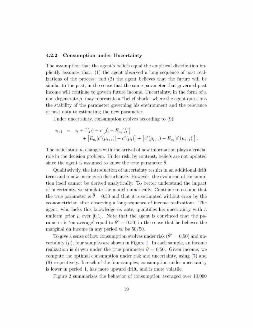
To give a sense of how consumption evolves under risk (θµ
= 0.50) and un-
certainty (µ), four samples are shown in Figure 1. In each sample, an income
realization is drawn under the true parameter θ = 0.50. Given income, we
compute the optimal consumption under risk and uncertainty, using (7) and
(9) respectively. In each of the four samples, consumption under uncertainty
is lower in period 1, has more upward drift, and is more volatile.
Figure 2 summarizes the behavior of consumption averaged over 10,000
19
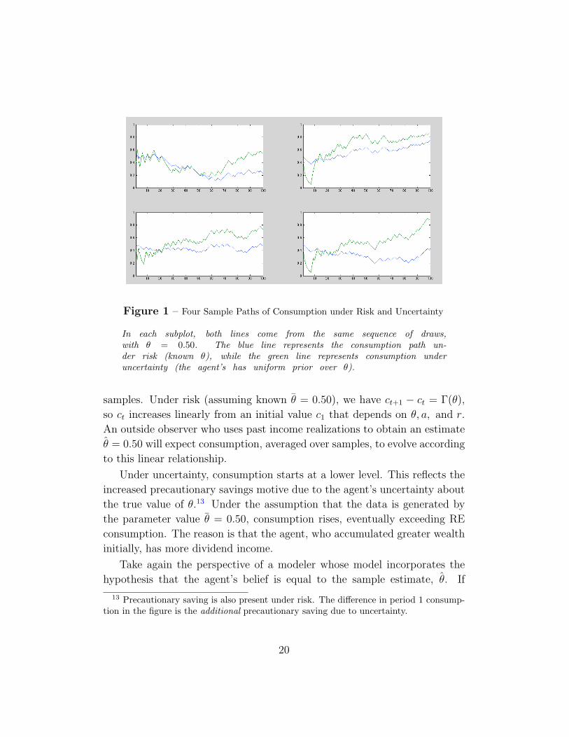
Figure 1 – Four Sample Paths of Consumption under Risk and Uncertainty
In each subplot, both lines come from the same sequence of draws,with θ = 0.50. The blue line represents the consumption path un-der risk (known θ), while the green line represents consumption underuncertainty (the agent’s has uniform prior over θ).
samples. Under risk (assuming known θ = 0.50), we have ct+1 − ct = Γ(θ),
so ct increases linearly from an initial value c1 that depends on θ, a, and r.
An outside observer who uses past income realizations to obtain an estimate
θ = 0.50 will expect consumption, averaged over samples, to evolve according
to this linear relationship.
Under uncertainty, consumption starts at a lower level. This reflects the
increased precautionary savings motive due to the agent’s uncertainty about
the true value of θ.13 Under the assumption that the data is generated by
the parameter value θ = 0.50, consumption rises, eventually exceeding RE
consumption. The reason is that the agent, who accumulated greater wealth
initially, has more dividend income.
Take again the perspective of a modeler whose model incorporates the
hypothesis that the agent’s belief is equal to the sample estimate, θ. If
13 Precautionary saving is also present under risk. The difference in period 1 consump-tion in the figure is the additional precautionary saving due to uncertainty.
20
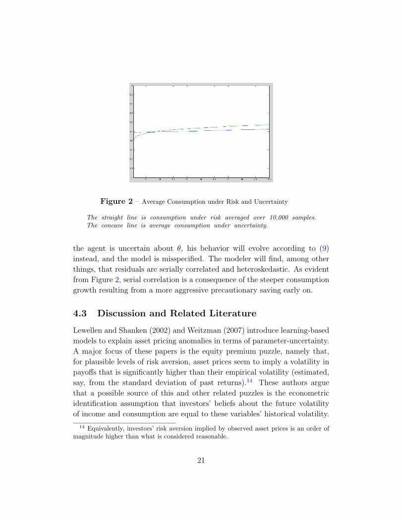
Figure 2 – Average Consumption under Risk and Uncertainty
The straight line is consumption under risk averaged over 10,000 samples.The concave line is average consumption under uncertainty.
the agent is uncertain about θ, his behavior will evolve according to (9)
instead, and the model is misspecified. The modeler will find, among other
things, that residuals are serially correlated and heteroskedastic. As evident
from Figure 2, serial correlation is a consequence of the steeper consumption
growth resulting from a more aggressive precautionary saving early on.
4.3 Discussion and Related Literature
Lewellen and Shanken (2002) and Weitzman (2007) introduce learning-based
models to explain asset pricing anomalies in terms of parameter-uncertainty.
A major focus of these papers is the equity premium puzzle, namely that,
for plausible levels of risk aversion, asset prices seem to imply a volatility in
payoffs that is significantly higher than their empirical volatility (estimated,
say, from the standard deviation of past returns).14 These authors argue
that a possible source of this and other related puzzles is the econometric
identification assumption that investors’ beliefs about the future volatility
of income and consumption are equal to these variables’ historical volatility.
14 Equivalently, investors’ risk aversion implied by observed asset prices is an order ofmagnitude higher than what is considered reasonable.
21
As noted earlier, this rational expectations assumption implicitly requires
agents to believe that the parameter generating future outcomes is the same
as the one that generated past data.
Although we do not consider asset pricing in this paper, similar effects
appear in the precautionary saving model. Under our i.i.d. assumption, pay-
offs are generated by one true parameter θ, yet an agent who does not know
its value will subjectively expect greater volatility in future income. This
uncertainty may be the result of the agent fearing that a structural change
in the income process might have occurred, shaking his confidence that the
future will be similar to the past. This uncertainty can have important con-
sequences for the behavior of endogenous variables but, as shown earlier, it
may be difficult to objectively demonstrate through statistical tests that such
uncertain beliefs are paranoid or irrational.
In Weitzman (2007)’s model, the data is generated by i.i.d. draws from
a normal distribution with known mean but unknown standard deviation.
An agent’s subjective uncertainty about the standard deviation implies that
his belief is a Student t distribution which, unlike the normal component
distributions, has a fat tail. Weitzman shows that agents’ concern about
this tail risk can lead to significant implications for asset pricing. There is a
parallel with what we do: in our model, a subjective distribution over i.i.d.
parameters is not an i.i.d. distribution, while in Weitzman’s model uncer-
tainty over standard deviations of normals implies a subjective belief that is
not itself normal. A second difference is that Weitzman does not consider
intertemporal smoothing.
There is an extensive literature on precautionary savings. That litera-
ture mainly focuses on what we call risk (agents’ beliefs coincide with the
ergodic probabilities). An important exception is Cogley and Sargent (2008)
who consider a model of precautionary savings with parameter uncertainty.
Cogley and Sargent (2008)’s main focus is on whether behavior based on
anticipated utility approximates well the full Bayesian solution in simula-
tions under power utility. They assume an income process generated by a
Markov matrix with unknown coefficients. The agent’s prior on these co-
efficients is a Dirichlet distribution, a tractable modeling assumption that
makes it easy to represent the extent to which an agent trusts his prior. The
22

uniform distribution used in our simulation reported earlier is a binomial
Dirichlet (i.e., Beta) distribution with parameters n0 = n1 = 1. As with
Cogley and Sargent (2008), we can model the agent’s uncertainty by varying
the parameter of his prior. Pure risk is then the limiting case where n0 and
n1 approach infinity. We may interpret this, as they do, that the agent has
observed a long history of the process and that he believes that the future
will look like the past. The advantage of CARA utility is that there are no
wealth effects, making the model more tractable. This allowed us to derive
equation (9) which showed clearly the relation between behavior under risk
and uncertainty in an explicit equation and proved that uncertainty causes
increased precautionary savings and increased volatility. While power utility
is considered more realistic, the differences are very minor for any modest
changes in wealth, and so we consider the ability to write down the solution
more explicitly worthwhile. Of course, we still had to solve the model nu-
merically to calculate V (µ), but the theory behind the calculation is made
much simpler by the separability of wealth in the CARA model.
23
A Appendix
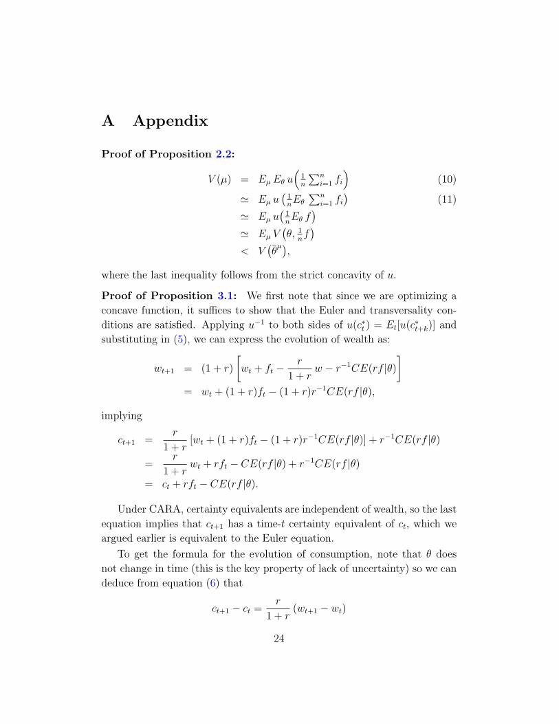
Proof of Proposition 2.2:
V (µ) = EµEθ u(
1n
∑ni=1 fi
)(10)
' Eµ u(
1nEθ∑n
i=1 fi)
(11)
' Eµ u(
1nEθ f
)' Eµ V
(θ, 1
nf)
< V(θµ),
where the last inequality follows from the strict concavity of u.
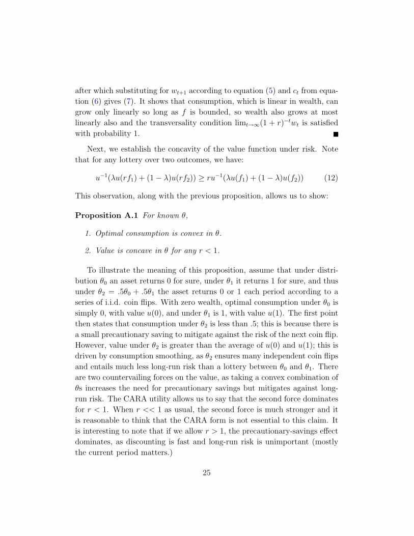
Proof of Proposition 3.1: We first note that since we are optimizing a
concave function, it suffices to show that the Euler and transversality con-
ditions are satisfied. Applying u−1 to both sides of u(c∗t ) = Et[u(c∗t+k)] and
substituting in (5), we can express the evolution of wealth as:
wt+1 = (1 + r)
[wt + ft −
r
1 + rw − r−1CE(rf |θ)
]= wt + (1 + r)ft − (1 + r)r−1CE(rf |θ),
implying
ct+1 =r
1 + r[wt + (1 + r)ft − (1 + r)r−1CE(rf |θ)] + r−1CE(rf |θ)
=r
1 + rwt + rft − CE(rf |θ) + r−1CE(rf |θ)
= ct + rft − CE(rf |θ).
Under CARA, certainty equivalents are independent of wealth, so the last
equation implies that ct+1 has a time-t certainty equivalent of ct, which we
argued earlier is equivalent to the Euler equation.
To get the formula for the evolution of consumption, note that θ does
not change in time (this is the key property of lack of uncertainty) so we can
deduce from equation (6) that
ct+1 − ct =r
1 + r(wt+1 − wt)
24
after which substituting for wt+1 according to equation (5) and ct from equa-
tion (6) gives (7). It shows that consumption, which is linear in wealth, can
grow only linearly so long as f is bounded, so wealth also grows at most
linearly also and the transversality condition limt→∞(1 + r)−twt is satisfied
with probability 1.
Next, we establish the concavity of the value function under risk. Note
that for any lottery over two outcomes, we have:
u−1(λu(rf1) + (1− λ)u(rf2)) ≥ ru−1(λu(f1) + (1− λ)u(f2)) (12)
This observation, along with the previous proposition, allows us to show:
Proposition A.1 For known θ,
1. Optimal consumption is convex in θ.
2. Value is concave in θ for any r < 1.
To illustrate the meaning of this proposition, assume that under distri-
bution θ0 an asset returns 0 for sure, under θ1 it returns 1 for sure, and thus
under θ2 = .5θ0 + .5θ1 the asset returns 0 or 1 each period according to a
series of i.i.d. coin flips. With zero wealth, optimal consumption under θ0 is
simply 0, with value u(0), and under θ1 is 1, with value u(1). The first point
then states that consumption under θ2 is less than .5; this is because there is
a small precautionary saving to mitigate against the risk of the next coin flip.
However, value under θ2 is greater than the average of u(0) and u(1); this is
driven by consumption smoothing, as θ2 ensures many independent coin flips
and entails much less long-run risk than a lottery between θ0 and θ1. There
are two countervailing forces on the value, as taking a convex combination of
θs increases the need for precautionary savings but mitigates against long-
run risk. The CARA utility allows us to say that the second force dominates
for r < 1. When r << 1 as usual, the second force is much stronger and it
is reasonable to think that the CARA form is not essential to this claim. It
is interesting to note that if we allow r > 1, the precautionary-savings effect
dominates, as discounting is fast and long-run risk is unimportant (mostly
the current period matters.)
25
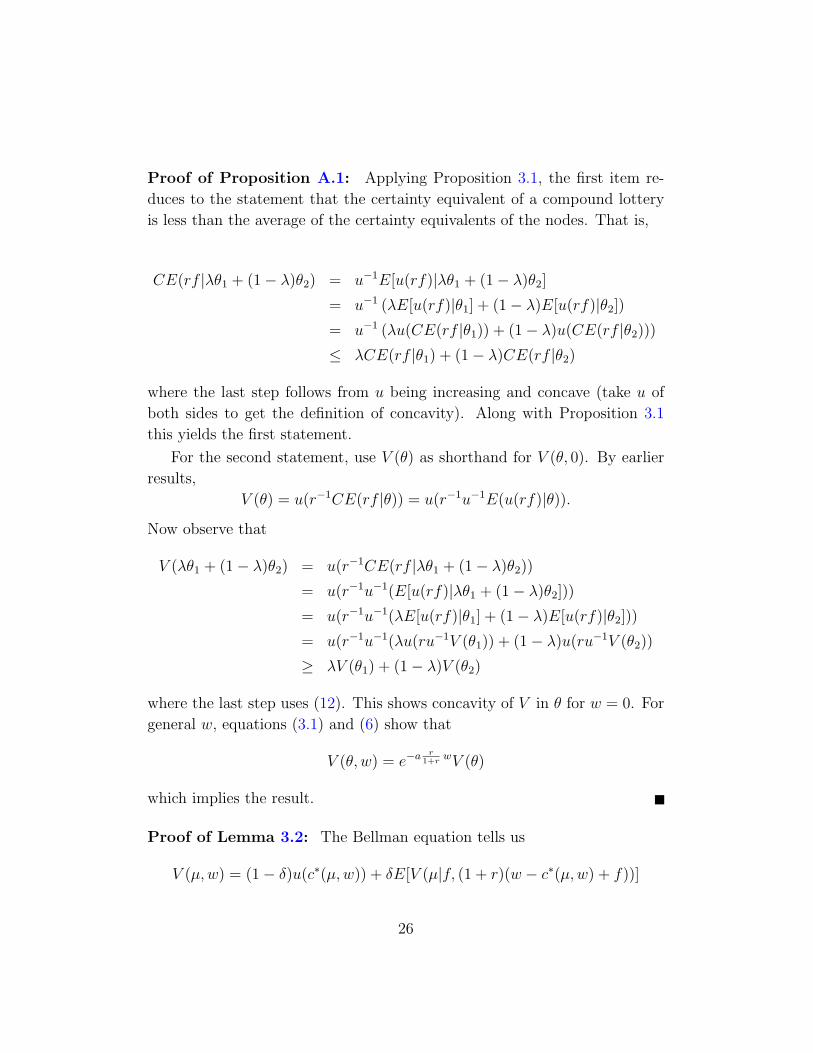
Proof of Proposition A.1: Applying Proposition 3.1, the first item re-
duces to the statement that the certainty equivalent of a compound lottery
is less than the average of the certainty equivalents of the nodes. That is,
CE(rf |λθ1 + (1− λ)θ2) = u−1E[u(rf)|λθ1 + (1− λ)θ2]
= u−1 (λE[u(rf)|θ1] + (1− λ)E[u(rf)|θ2])
= u−1 (λu(CE(rf |θ1)) + (1− λ)u(CE(rf |θ2)))
≤ λCE(rf |θ1) + (1− λ)CE(rf |θ2)
where the last step follows from u being increasing and concave (take u of
both sides to get the definition of concavity). Along with Proposition 3.1
this yields the first statement.
For the second statement, use V (θ) as shorthand for V (θ, 0). By earlier
results,
V (θ) = u(r−1CE(rf |θ)) = u(r−1u−1E(u(rf)|θ)).
Now observe that
V (λθ1 + (1− λ)θ2) = u(r−1CE(rf |λθ1 + (1− λ)θ2))
= u(r−1u−1(E[u(rf)|λθ1 + (1− λ)θ2]))
= u(r−1u−1(λE[u(rf)|θ1] + (1− λ)E[u(rf)|θ2]))
= u(r−1u−1(λu(ru−1V (θ1)) + (1− λ)u(ru−1V (θ2))
≥ λV (θ1) + (1− λ)V (θ2)
where the last step uses (12). This shows concavity of V in θ for w = 0. For
general w, equations (3.1) and (6) show that
V (θ, w) = e−ar
1+rwV (θ)
which implies the result.
Proof of Lemma 3.2: The Bellman equation tells us
V (µ,w) = (1− δ)u(c∗(µ,w)) + δE[V (µ|f, (1 + r)(w − c∗(µ,w) + f))]
26
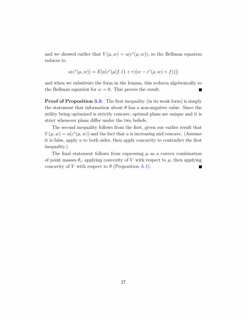
and we showed earlier that V (µ,w) = u(c∗(µ,w)), so the Bellman equation
reduces to
u(c∗(µ,w)) = E[u(c∗(µ|f, (1 + r)(w − c∗(µ,w) + f)))]
and when we substitute the form in the lemma, this reduces algebraically to
the Bellman equation for w = 0. This proves the result.
Proof of Proposition 3.3: The first inequality (in its weak form) is simply
the statement that information about θ has a non-negative value. Since the
utility being optimized is strictly concave, optimal plans are unique and it is
strict whenever plans differ under the two beliefs.
The second inequality follows from the first, given our earlier result that
V (µ,w) = u(c∗(µ,w)) and the fact that u is increasing and concave. (Assume
it is false, apply u to both sides, then apply concavity to contradict the first
inequality.)
The final statement follows from expressing µ as a convex combination
of point masses θi, applying convexity of V with respect to µ, then applying
concavity of V with respect to θ (Proposition A.1).
27
References
Bewley, T. (1986): “Knightian Decision Theory: Part I,” Cowles Founda-
tion Discussion Paper no. 807.
Caballero, R. (1990): “Consumption Puzzles and Precautionary Sav-
ings,” Journal of Monetary Economics, 25(1), 113–136.
Carroll, C., and M. Kimball (2008): “Precautionary Saving and Pre-
cautionary Wealth,” The New Palgrave Dictionary of Economics, 6, 579–
584.
Cogley, T., and T. Sargent (2008): “Anticipated Utility and Rational
Expectations as Approximiations of Bayesian Decision Making,” Interna-
tional Economic Review, 49(1), 185–221.
Gilboa, I., and D. Schmeidler (1989): “Maxmin Expected Utility with
Nonunique Prior,” J. Math. Econom., 18(2), 141–153.
Halevy, Y., and V. Feltkamp (2005): “A Bayesian Approach to Uncer-
tainty Aversion,” Review of Economic Studies, 72(2), 449–466.
Hansen, L., and T. Sargent (2001): “Acknowledging Misspecification in
Macroeconomic Theory,” Review of Economic Dynamics, 4(3), 519–535.
Keynes, J. M. (1937): “The General Theory of Employment,” The Quar-
terly Journal of Economics, 51(2), 209–223.
Knight, F. (1921): Risk, Uncertainty and Profit. Harper, New York.
LeRoy, S., and L. Singell (1987): “Knight on Risk and Uncertainty,”
The Journal of Political Economy, 95(2), 394–406.
Lewellen, J., and J. Shanken (2002): “Learning, Asset-Pricing Tests,
and Market Efficiency,” The Journal of finance, 57(3), 1113–1145.
Pastor, L., and P. Veronesi (2009): “Learning in Financial Markets,”
Annu. Rev. Financ. Econ., 1(1), 361–381.
Weitzman, M. (2007): “Subjective Expectations and Asset-Return Puz-
zles,” The American Economic Review, 97(4), 1102–1130.
28


