INSTITUTE OF AERONAUTICAL ENGINEERING(Autonomous)

Dundigal, Hyderabad - 500 043

Lab Manual:Geotechnical Engineering Laboratory

Laboratory Name(ACEB20)

Prepared by

M. Madhusudhan Reddy (IARE10881)

Department of Civill EngineeringInstitute of Aeronautical Engineering

April 10, 2022

Contents

Content iv

1 INTRODUCTION 11.1 Introduction . . . . . . . . . . . . . . . . . . . . . . . . . . . . . . . . . . . . . . . . . . 1

1.1.1 Student Responsibilities . . . . . . . . . . . . . . . . . . . . . . . . . . . . . . 11.1.2 Responsibilities of Faculty Teaching the Lab Course . . . . . . . . . . . . . 11.1.3 Laboratory In-charge Responsibilities . . . . . . . . . . . . . . . . . . . . . . 11.1.4 Course Coordinator Responsibilities . . . . . . . . . . . . . . . . . . . . . . . 2

1.2 Lab Policy and Grading . . . . . . . . . . . . . . . . . . . . . . . . . . . . . . . . . . . 21.3 Course Goals and Objectives . . . . . . . . . . . . . . . . . . . . . . . . . . . . . . . . 21.4 Use of Laboratory Instruments . . . . . . . . . . . . . . . . . . . . . . . . . . . . . . 31.5 Data Recording and Reports . . . . . . . . . . . . . . . . . . . . . . . . . . . . . . . . 3

1.5.1 The Laboratory Worksheets . . . . . . . . . . . . . . . . . . . . . . . . . . . . 31.5.2 The Laboratory Files/Reports . . . . . . . . . . . . . . . . . . . . . . . . . . 3

1.6 Conclusions . . . . . . . . . . . . . . . . . . . . . . . . . . . . . . . . . . . . . . . . . . 4

2 LAB 1–SPECIFIC GRAVITY OF SOIL SOLIDS BY PYCNOMETER METHOD 52.1 Introduction . . . . . . . . . . . . . . . . . . . . . . . . . . . . . . . . . . . . . . . . . . 52.2 Objective . . . . . . . . . . . . . . . . . . . . . . . . . . . . . . . . . . . . . . . . . . . 52.3 Equipment Needed . . . . . . . . . . . . . . . . . . . . . . . . . . . . . . . . . . . . . . 52.4 Specification . . . . . . . . . . . . . . . . . . . . . . . . . . . . . . . . . . . . . . . . . . 52.5 Procedure . . . . . . . . . . . . . . . . . . . . . . . . . . . . . . . . . . . . . . . . . . . 52.6 Theory: . . . . . . . . . . . . . . . . . . . . . . . . . . . . . . . . . . . . . . . . . . . . . 62.7 Precautions . . . . . . . . . . . . . . . . . . . . . . . . . . . . . . . . . . . . . . . . . . 62.8 Table . . . . . . . . . . . . . . . . . . . . . . . . . . . . . . . . . . . . . . . . . . . . . . 72.9 Specimen calculations: . . . . . . . . . . . . . . . . . . . . . . . . . . . . . . . . . . . . 72.10 Result: . . . . . . . . . . . . . . . . . . . . . . . . . . . . . . . . . . . . . . . . . . . . . 72.11 Verification/ Validation: . . . . . . . . . . . . . . . . . . . . . . . . . . . . . . . . . . . 72.12 Conclusion: . . . . . . . . . . . . . . . . . . . . . . . . . . . . . . . . . . . . . . . . . . 7

3 LAB 2 –SPECIFIC GRAVITY OF SOIL SOLIDS BY DENSITY BOTTLEMETHOD 83.1 Introduction . . . . . . . . . . . . . . . . . . . . . . . . . . . . . . . . . . . . . . . . . . 83.2 Objective . . . . . . . . . . . . . . . . . . . . . . . . . . . . . . . . . . . . . . . . . . . 83.3 Specification . . . . . . . . . . . . . . . . . . . . . . . . . . . . . . . . . . . . . . . . . . 83.4 Equipment . . . . . . . . . . . . . . . . . . . . . . . . . . . . . . . . . . . . . . . . . . . 83.5 Theory: . . . . . . . . . . . . . . . . . . . . . . . . . . . . . . . . . . . . . . . . . . . . . 83.6 Precautions . . . . . . . . . . . . . . . . . . . . . . . . . . . . . . . . . . . . . . . . . . 93.7 Procedure . . . . . . . . . . . . . . . . . . . . . . . . . . . . . . . . . . . . . . . . . . . 93.8 Table: . . . . . . . . . . . . . . . . . . . . . . . . . . . . . . . . . . . . . . . . . . . . . . 93.9 Specimen calculations: . . . . . . . . . . . . . . . . . . . . . . . . . . . . . . . . . . . . 103.10 Result: . . . . . . . . . . . . . . . . . . . . . . . . . . . . . . . . . . . . . . . . . . . . . 103.11 Verification/ Validation: . . . . . . . . . . . . . . . . . . . . . . . . . . . . . . . . . . . 10

i

3.12 Conclusion: . . . . . . . . . . . . . . . . . . . . . . . . . . . . . . . . . . . . . . . . . . 10

4 LAB 3–ATTERBERG’S LIMITS. 114.1 Introduction . . . . . . . . . . . . . . . . . . . . . . . . . . . . . . . . . . . . . . . . . . 11

4.1.1 Objectives . . . . . . . . . . . . . . . . . . . . . . . . . . . . . . . . . . . . . . 114.2 Prelab . . . . . . . . . . . . . . . . . . . . . . . . . . . . . . . . . . . . . . . . . . . . . 114.3 Background . . . . . . . . . . . . . . . . . . . . . . . . . . . . . . . . . . . . . . . . . . 114.4 Procedure: . . . . . . . . . . . . . . . . . . . . . . . . . . . . . . . . . . . . . . . . . . . 114.5 Probing further questions . . . . . . . . . . . . . . . . . . . . . . . . . . . . . . . . . . 134.6 Viva questions . . . . . . . . . . . . . . . . . . . . . . . . . . . . . . . . . . . . . . . . 14

5 LAB 4– WATER CONTENT OF SOIL SOLIDS BY PYCNOMETER METHOD 155.1 Introduction . . . . . . . . . . . . . . . . . . . . . . . . . . . . . . . . . . . . . . . . . . 155.2 Objectives . . . . . . . . . . . . . . . . . . . . . . . . . . . . . . . . . . . . . . . . . . . 155.3 Specifications: . . . . . . . . . . . . . . . . . . . . . . . . . . . . . . . . . . . . . . . . . 155.4 Equipment . . . . . . . . . . . . . . . . . . . . . . . . . . . . . . . . . . . . . . . . . . . 155.5 Theory: . . . . . . . . . . . . . . . . . . . . . . . . . . . . . . . . . . . . . . . . . . . . . 155.6 Procedure: . . . . . . . . . . . . . . . . . . . . . . . . . . . . . . . . . . . . . . . . . . . 165.7 Table . . . . . . . . . . . . . . . . . . . . . . . . . . . . . . . . . . . . . . . . . . . . . . 165.8 Specimen calculations: . . . . . . . . . . . . . . . . . . . . . . . . . . . . . . . . . . . . 165.9 Result: . . . . . . . . . . . . . . . . . . . . . . . . . . . . . . . . . . . . . . . . . . . . . 165.10 Verification/ Validation: . . . . . . . . . . . . . . . . . . . . . . . . . . . . . . . . . . . 165.11 Conclusion: . . . . . . . . . . . . . . . . . . . . . . . . . . . . . . . . . . . . . . . . . . 17

6 LAB 5–IN-SITU DENSITY BY CORE CUTTER METHOD 186.1 Introduction . . . . . . . . . . . . . . . . . . . . . . . . . . . . . . . . . . . . . . . . . . 186.2 Objectives . . . . . . . . . . . . . . . . . . . . . . . . . . . . . . . . . . . . . . . . . . . 186.3 Equipment . . . . . . . . . . . . . . . . . . . . . . . . . . . . . . . . . . . . . . . . . . . 186.4 Theory: . . . . . . . . . . . . . . . . . . . . . . . . . . . . . . . . . . . . . . . . . . . . . 186.5 Precautions: . . . . . . . . . . . . . . . . . . . . . . . . . . . . . . . . . . . . . . . . . . 196.6 Procedure: . . . . . . . . . . . . . . . . . . . . . . . . . . . . . . . . . . . . . . . . . . . 196.7 Observations: . . . . . . . . . . . . . . . . . . . . . . . . . . . . . . . . . . . . . . . . . 206.8 Table: . . . . . . . . . . . . . . . . . . . . . . . . . . . . . . . . . . . . . . . . . . . . . . 206.9 Specimen calculations: . . . . . . . . . . . . . . . . . . . . . . . . . . . . . . . . . . . . 206.10 Result: . . . . . . . . . . . . . . . . . . . . . . . . . . . . . . . . . . . . . . . . . . . . . 206.11 Verification/ Validation: . . . . . . . . . . . . . . . . . . . . . . . . . . . . . . . . . . . 206.12 Conclusion: . . . . . . . . . . . . . . . . . . . . . . . . . . . . . . . . . . . . . . . . . . 20

7 LAB 6– IN-SITU DENSITY BY SAND REPLACEMENT METHOD 217.1 Introduction . . . . . . . . . . . . . . . . . . . . . . . . . . . . . . . . . . . . . . . . . . 217.2 Objectives . . . . . . . . . . . . . . . . . . . . . . . . . . . . . . . . . . . . . . . . . . . 217.3 Specifications: . . . . . . . . . . . . . . . . . . . . . . . . . . . . . . . . . . . . . . . . . 217.4 Equipment . . . . . . . . . . . . . . . . . . . . . . . . . . . . . . . . . . . . . . . . . . . 217.5 Theory: . . . . . . . . . . . . . . . . . . . . . . . . . . . . . . . . . . . . . . . . . . . . . 227.6 Precautions: . . . . . . . . . . . . . . . . . . . . . . . . . . . . . . . . . . . . . . . . . . 227.7 Procedures: . . . . . . . . . . . . . . . . . . . . . . . . . . . . . . . . . . . . . . . . . . 22

8 LAB 7–GRAIN SIZE ANALYSIS 248.1 Introduction . . . . . . . . . . . . . . . . . . . . . . . . . . . . . . . . . . . . . . . . . . 248.2 Objectives . . . . . . . . . . . . . . . . . . . . . . . . . . . . . . . . . . . . . . . . . . . 248.3 Equipment . . . . . . . . . . . . . . . . . . . . . . . . . . . . . . . . . . . . . . . . . . . 248.4 Background . . . . . . . . . . . . . . . . . . . . . . . . . . . . . . . . . . . . . . . . . . 24

ii

8.5 Procedure . . . . . . . . . . . . . . . . . . . . . . . . . . . . . . . . . . . . . . . . . . . 258.6 Result . . . . . . . . . . . . . . . . . . . . . . . . . . . . . . . . . . . . . . . . . . . . . 268.7 Viva Questions . . . . . . . . . . . . . . . . . . . . . . . . . . . . . . . . . . . . . . . . 26

9 LAB 8– PERMEABILITY OF SOIL: CONSTANT AND VARIABLE HEADTEST 279.1 Introduction . . . . . . . . . . . . . . . . . . . . . . . . . . . . . . . . . . . . . . . . . . 279.2 Objective . . . . . . . . . . . . . . . . . . . . . . . . . . . . . . . . . . . . . . . . . . . 279.3 PreLab . . . . . . . . . . . . . . . . . . . . . . . . . . . . . . . . . . . . . . . . . . . . . 279.4 Procedure . . . . . . . . . . . . . . . . . . . . . . . . . . . . . . . . . . . . . . . . . . . 289.5 Result: . . . . . . . . . . . . . . . . . . . . . . . . . . . . . . . . . . . . . . . . . . . . . 289.6 Viva questions: . . . . . . . . . . . . . . . . . . . . . . . . . . . . . . . . . . . . . . . . 28

10 LAB 9-COMPACTION TEST 2910.1 Introduction . . . . . . . . . . . . . . . . . . . . . . . . . . . . . . . . . . . . . . . . . . 2910.2 Equipment . . . . . . . . . . . . . . . . . . . . . . . . . . . . . . . . . . . . . . . . . . . 29

10.2.1 Background . . . . . . . . . . . . . . . . . . . . . . . . . . . . . . . . . . . . . . 2910.3 Procedure . . . . . . . . . . . . . . . . . . . . . . . . . . . . . . . . . . . . . . . . . . . 3010.4 Observations and calculations . . . . . . . . . . . . . . . . . . . . . . . . . . . . . . . 3010.5 Viva questions . . . . . . . . . . . . . . . . . . . . . . . . . . . . . . . . . . . . . . . . 31

11 LAB 10– CALIFORNIA BEARING RATIO TEST 3211.1 Introduction . . . . . . . . . . . . . . . . . . . . . . . . . . . . . . . . . . . . . . . . . . 3211.2 Need and scope . . . . . . . . . . . . . . . . . . . . . . . . . . . . . . . . . . . . . . . . 3211.3 Equipment . . . . . . . . . . . . . . . . . . . . . . . . . . . . . . . . . . . . . . . . . . . 3211.4 Background: . . . . . . . . . . . . . . . . . . . . . . . . . . . . . . . . . . . . . . . . . . 3211.5 Preparation of test specimen . . . . . . . . . . . . . . . . . . . . . . . . . . . . . . . . 3311.6 Procedure . . . . . . . . . . . . . . . . . . . . . . . . . . . . . . . . . . . . . . . . . . . 3311.7 Observations . . . . . . . . . . . . . . . . . . . . . . . . . . . . . . . . . . . . . . . . . 3311.8 Viva questions . . . . . . . . . . . . . . . . . . . . . . . . . . . . . . . . . . . . . . . . 33

12 Lab 11– DIRECT SHEAR TEST 3412.1 Introduction . . . . . . . . . . . . . . . . . . . . . . . . . . . . . . . . . . . . . . . . . . 3412.2 Objective . . . . . . . . . . . . . . . . . . . . . . . . . . . . . . . . . . . . . . . . . . . 3412.3 Specifications: . . . . . . . . . . . . . . . . . . . . . . . . . . . . . . . . . . . . . . . . 3412.4 Equipments Required: . . . . . . . . . . . . . . . . . . . . . . . . . . . . . . . . . . . 3412.5 Theory: . . . . . . . . . . . . . . . . . . . . . . . . . . . . . . . . . . . . . . . . . . . . . 3412.6 Equation: . . . . . . . . . . . . . . . . . . . . . . . . . . . . . . . . . . . . . . . . . . . 3512.7 Precautions: . . . . . . . . . . . . . . . . . . . . . . . . . . . . . . . . . . . . . . . . . 3512.8 Procedure . . . . . . . . . . . . . . . . . . . . . . . . . . . . . . . . . . . . . . . . . . . 3512.9 Table: . . . . . . . . . . . . . . . . . . . . . . . . . . . . . . . . . . . . . . . . . . . . . 3612.10Result: . . . . . . . . . . . . . . . . . . . . . . . . . . . . . . . . . . . . . . . . . . . . . 3712.11Verification and Validation . . . . . . . . . . . . . . . . . . . . . . . . . . . . . . . . . 3712.12Conclusion: . . . . . . . . . . . . . . . . . . . . . . . . . . . . . . . . . . . . . . . . . . 3712.13Viva Questions: . . . . . . . . . . . . . . . . . . . . . . . . . . . . . . . . . . . . . . . . 37

13 Lab 12 – VANE SHEAR TEST 3913.1 Introduction . . . . . . . . . . . . . . . . . . . . . . . . . . . . . . . . . . . . . . . . . . 3913.2 Objective . . . . . . . . . . . . . . . . . . . . . . . . . . . . . . . . . . . . . . . . . . . 3913.3 Specifications: . . . . . . . . . . . . . . . . . . . . . . . . . . . . . . . . . . . . . . . . 3913.4 Equipment Required: . . . . . . . . . . . . . . . . . . . . . . . . . . . . . . . . . . . . 3913.5 Theory: . . . . . . . . . . . . . . . . . . . . . . . . . . . . . . . . . . . . . . . . . . . . 39

iii

13.6 Procedure: . . . . . . . . . . . . . . . . . . . . . . . . . . . . . . . . . . . . . . . . . . 4013.7 Observations: . . . . . . . . . . . . . . . . . . . . . . . . . . . . . . . . . . . . . . . . 4013.8 Calculations: . . . . . . . . . . . . . . . . . . . . . . . . . . . . . . . . . . . . . . . . . 4013.9 Result: . . . . . . . . . . . . . . . . . . . . . . . . . . . . . . . . . . . . . . . . . . . . . 4013.10Verification/Validations: . . . . . . . . . . . . . . . . . . . . . . . . . . . . . . . . . . 4013.11Viva Questions: . . . . . . . . . . . . . . . . . . . . . . . . . . . . . . . . . . . . . . . 40

iv

INTRODUCTION

1.1 Introduction

The Geotechnical Engineering Laboratory intends to train the students in the field of testingof soils to determine their physical, index and engineering properties. This course enablesthe students to perform the most important tests including: soil classification, compaction,permeability, direct shear testing and cyclical triaxial testing; each experiment of soil testing ispresented with brief introduction covering the important details of the experiment, the theoryand the purpose for which it is to be performed, followed by the detailed explanation of apparatusrequired, procedure and specimen calculations.

1.1.1 Student Responsibilities

The student is expected to be prepared for each lab. Lab preparation includes reading the labexperiment from the lab manual.If you have questions or problems with the preparation,contactyour lab assistant and faculty incharge but in a timely manner.Do not wait until an hour ortwo before the lab and then expect the lab assistant and faculty in charge to be immediatelyavailable.

Active participation by each student in lab activities is expected. The student is expectedto askthe lab assistant and faculty incharge any questions they may have.

A large portion of the student’s grade is determined in the comprehensive final exam, result-ing in a requirement of understanding the concepts and procedure of each lab experiment forthe successfulcompletion of the lab session. The student should remain alert and use commonsense while performinga lab experiment. They are also responsible for keeping a professional andaccurate record of the labexperiments in the lab manual wherever tables are provided. Studentsshould report any errors in the lab manual to the faculty incharge or course coordinator.

1.1.2 Responsibilities of Faculty Teaching the Lab Course

The faculty shall be completely familiar with each labprior to the laboratory. He/She shall pro-vide the students with details regarding the syllabus and safety review during the first week.Labexperiments should be checked in advance to make sure that everything is in working order.Thefaculty should demonstrate and explain the experiment and answer any questions posed by thestudents.Faculty have to supervise the students while they perform the lab experiments. Thefaculty is expected to evaluate the lab worksheets and grade them based on their practical skillsand understanding of the experiment by taking viva voce. Evaluation of work sheets has to bedone in a fair and timely manner to enable the students, for uploading them online throughtheir CMS login within the stipulated time.

1.1.3 Laboratory In-charge Responsibilities

The laboratory in-charge should ensure that the laboratory is properly equipped, i.e., thefaculty teaching the lab receive any equipment/components necessary to perform the experi-

1

ments.He/She is responsible for ensuring that all the necessary equipment for the lab is availableand in working condition. The laboratory in-charge is responsible for resolving any problemsthat are identified by the teaching faculty or the students.

1.1.4 Course Coordinator Responsibilities

The course coordinator is responsible fo rmaking any necessary corrections in course descriptionand lab manual. He/She has to ensure that it is continually updated and available to thestudents in the CMS learning Portal.

1.2 Lab Policy and Grading

The student should understand the following policy:

ATTENDANCE: Attendance is mandatory as per the academic regulations.

LAB RECORD’s: The student must:

1. Write the work sheets for the allotted experiment and keep them ready before the beginningof each lab.

2. Keep all work in preparation of and obtained during lab.

3. Perform the experiment and record the observations in the worksheets.

4. Analyze the results and get the work sheets evaluated by the faculty.

5. Upload the evaluated reports online from CMS LOGIN within the stipulated time.

Grading Policy:

The final grade of this course is awarded using the criterion detailed in the academic regulations.A large portion of the student’s grade is determined in the comprehensive final exam of the lab-oratory course (SEE PRACTICALS),resulting in a requirement of understanding the conceptsand procedure of each lab experiment for successful completion of the lab course.

Pre-Requistes and Co-Requisties:

The lab course is to be taken during the same semester as ACEB19, but receives a separategrade.

1.3 Course Goals and Objectives

The Geotechnical Engineering laboratory is designed to provide the student with the knowledgeof soil properties and its behaviour under the different loading condition with and without watercontent. In addition, the student should learn how to record experimental results effectively andpresent these results in a written report. More explicitly, the class objectives are:

1. The concept behind the soil formation, type soil and the relationships between the soilmass and volume of voids and enables the students to perform moisture content, specificgravity and atterberg limits.

2. The procedure for soil classification through grain size distribution and classification ofsoil according to IS code.

2

3. The importance of determining the permeability and enables the students to performpermeability (constant head and variable head) test; so that students can estimate groundwater flow, seepage through dams, rate of consolidation and settlement of structures.

4. IV. The behaviour of soil under different loading condition and enable the students derivethe bearing capacity, design retaining walls, evaluate the stability of slopes and embank-ments, etc.

1.4 Use of Laboratory Instruments

One of the major goals of this lab is to familiarize the student with the proper equipment andtech-niques for conducting experiments. Some understanding of the lab instruments is necessarytoavoid personal or equipment damage. By understanding the device’s purpose and following afewsimple rules, costly mistakes can be avoided.

The following rules provide a guideline for instrument protection.

1.5 Data Recording and Reports

1.5.1 The Laboratory Worksheets

Students must record their experimental values in the provided tables in this laboratory manualand reproduce the min the lab reports. Reports are integral to recording the methodologyand results of an experiment. In engineering practice, the laboratory work sheets serve as aninvaluable reference to the technique used in the lab and is essential when trying to duplicate aresult or write a report. Note that the data collected will be an accurate and permanent recordof the data obtained during the experiment and the analysis of the results. You will need thisrecord when you are ready to prepare a lab report.

1.5.2 The Laboratory Files/Reports

Record is the primary means of communicating your experience and conclusions to other pro-fessionals. In this course you will use the lab report to inform your faculty incharge about whatyou did and what you have learned from the experience. Engineering results are meaninglessunless they can be communicated to others. You will be directed by your faculty incharge toprepare a lab report on a few lab experiments during the semester.

Your laboratory record should be clear and concise. The lab record shall be typed on a wordprocessor. As a guide, use the format on the next page. Use tables, diagrams , as necessary oshow what you did, what was observed, and what conclusions you can draw from this.

Order of Lab Report Components

COVERPAGE- Cover page must include lab name and number, your name, your lab partner’sname, and the date the lab was performed.

OBJECTIVE - Clearly state the experiment objective in your own words.

EQUIPMENT USED- Indicate which equipment was used in performing the experiment.For each part of lab

� Write the lab’s part number and title in bold font. Firstly, describe the problem thatyou studied in this part, give an introduction of the theory, and explain why you did thisexperiment. Do not lift the text from the lab manual; use your own words.

3

� Secondly, describe the experimental setup and procedures. Do not follow the lab manual inlisting out individual pieces of equipment and assembly instructions. That is not relevantinformation in a lab report! Instead, describe the circuit as a whole and explain how itworks. Your description should take the form of a narrative, and include information notpresent in the manual, such as descriptions of what happened during intermediate stepsof the experiment.

� Thirdly, explain your findings. This is the most important part of your report, becausehere, you show that you understand the experiment beyond the simple level of completingit. Explain (compare expected results with those obtained). Analyze (analyze experimen-tal error).

� Finally, provide a summary of what was learned from this part of the laboratory ex-periment. If the results seem unexpected or unreliable, discuss the mand give possibleexplanation

1.6 Conclusions

The conclusion section should provide a take home message summing up what has been learnedfrom the experiment:

� Briefly restate the purpose of the experiment(the question it was seeking to answer)

� Identify the main findings (answer to the research question)

� Note the main limitations that are relevant to the interpretation of the results

� Summarise what the experiment has contributed to your understanding of the problem.

Further Probing Experiments- Advance experiments pertaining to this lab must be probedin further coming weeks

4

LAB 1–SPECIFIC GRAVITY OF SOIL SOLIDS BY PYCNOME-TER METHOD

2.1 Introduction

Specific gravity is the ratio of the mass of unit volume of soil at a stated temperature to themass of the same volume of gas-free distilled water at a stated temperature.

2.2 Objective

To determine the specific gravity of soil solids by Pycnometer bottle method.

2.3 Equipment Needed

1. Pycnometer of about 1 litre capacity

2. Weighing balance accurate to 1 g

3. Glass rod

4. De-aired distilled water etc

2.4 Specification

This test is specified in IS: 2720 (Part 4) – 1985. A soil’s specific gravity largely depends onthe density of the minerals making up the individual soil particles. However, as a general guide,some typical values for specific soil types are as follows:

� The specific gravity of the solid substance of most inorganic soils varies between 2.60 and2.80. � Tropical iron-rich laterite, as well as some lateritic soils, usually have a specific gravityof between 2.75 and 3.0 but could be higher. � Sand particles composed of quartz have a specificgravity ranging from 2.65 to 2.67. � Inorganic clays generally range from 2.70 to 2.80. � Soilswith large amounts of organic matter or porous particles (such as diatomaceous earth) havespecific gravities below 2.60. Some range as low as 2.00.

2.5 Procedure

1. Clean and dry the Pycnometer and weigh it along with the conical cap (W1 in gm).

2. Select about 300 gm of dry soil free of clods and put the same into the Pycnometer. Weighit (W2 in g) with cap and washer.

3. Fill the Pycnometer with de-aired water up-to half its height and stir the mix with a glassrod.

5

4. Add more water and stir it. Fit the screw cap and fill the Pycnometer flush with the holein the conical cap and take the weight (W3 in g).

5. Remove all the contents from the Pycnometer, clean it thoroughly and fill it with distilledwater. Weigh it (W4 in g).

6. Now use the above equation for determining G.

7. Repeat the same process for additional tests.

2.6 Theory:

Specific gravity of soil solids is defined as the weight of soil solids to weight of equal volumeof water. In effect, it tells how much heavier (or lighter) the material is than water. This testmethod covers the determination of the specific gravity of soil solids that pass 4.75 mm sieve.Equation for specific gravity, G:G= (W2-W1)/((W2-W1)-(W3-W4))

Where, W1=weight of Pycnometer in grams. W2=weight of Pycnometer + dry soil in grams.W3=weight of Pycnometer + soil+ water grams. W4=weight of Pycnometer + water grams.

Note: This method is recommended for coarse and fine grained soils

2.7 Precautions

1. Soil grains whose specific gravity is to be determined should be completely dry.

2. If on drying soil lumps are formed, they should be broken to its original size.

3. Inaccuracies in weighing and failure to completely eliminate the entrapped air are the mainsources of error. Both should be avoided.

4. While cleaning the glass jar, please be careful as there may be glass grains projecting outand it may tear the skin.

5. Make sure, you handle the glass jar and conical cap without falling on your legs or floor.

6. Hence, handle the equipment with care.

6

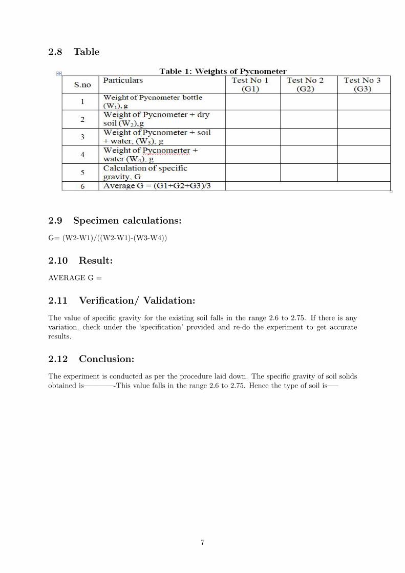
2.8 Table

2.9 Specimen calculations:

G= (W2-W1)/((W2-W1)-(W3-W4))

2.10 Result:

AVERAGE G =

2.11 Verification/ Validation:

The value of specific gravity for the existing soil falls in the range 2.6 to 2.75. If there is anyvariation, check under the ‘specification’ provided and re-do the experiment to get accurateresults.

2.12 Conclusion:

The experiment is conducted as per the procedure laid down. The specific gravity of soil solidsobtained is————-This value falls in the range 2.6 to 2.75. Hence the type of soil is—–

7

LAB 2 –SPECIFIC GRAVITY OF SOIL SOLIDS BY DENSITYBOTTLE METHOD

3.1 Introduction

Specific gravity G is defined as the ratio of the weight of an equal volume of distilled water atthat temperature, both weights taken in air.

3.2 Objective

To determine the specific gravity of soil solids by Density bottle method.

3.3 Specification

IS 2720 (Part III) – 1980 is the standard recommended to determine specific gravity of finegrained soils. The value ranges are same as the previous experiment. The average of the valuesobtained shall be taken as the specific gravity of the soil particles and shall be reported to thenearest 0.01 precision. If the two results differ by more than 0.03 the tests shall be repeated.

3.4 Equipment

1. 50 ml capacity density bottle with stopper

2. A constant temperature water bath (27°C)

3. Oven with a range of 105 to 110°C

4. Vacuum desiccators

5. Vacuum pump

6. Other accessories, such as, weighing balance accurate to 0.001 g, trays, wooden mallet,etc.

3.5 Theory:

Specific gravity of soil solids is defined as the weight of soil solids to weight of equal volume ofwater. Equation for specific gravity, G:

G= (W2-W1)/((W2-W1)-(W3-W4))

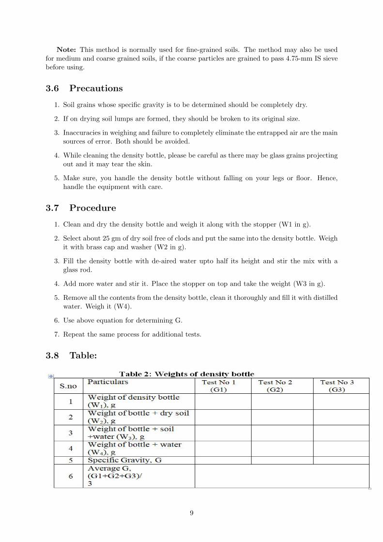
Where, W1= weight of empty bottleW2= weight of bottle + dry soilW3= weight of bottle + soil + waterW4= weight of bottle + water

8

Note: This method is normally used for fine-grained soils. The method may also be usedfor medium and coarse grained soils, if the coarse particles are grained to pass 4.75-mm IS sievebefore using.

3.6 Precautions

1. Soil grains whose specific gravity is to be determined should be completely dry.

2. If on drying soil lumps are formed, they should be broken to its original size.

3. Inaccuracies in weighing and failure to completely eliminate the entrapped air are the mainsources of error. Both should be avoided.

4. While cleaning the density bottle, please be careful as there may be glass grains projectingout and it may tear the skin.

5. Make sure, you handle the density bottle without falling on your legs or floor. Hence,handle the equipment with care.

3.7 Procedure

1. Clean and dry the density bottle and weigh it along with the stopper (W1 in g).

2. Select about 25 gm of dry soil free of clods and put the same into the density bottle. Weighit with brass cap and washer (W2 in g).

3. Fill the density bottle with de-aired water upto half its height and stir the mix with aglass rod.

4. Add more water and stir it. Place the stopper on top and take the weight (W3 in g).

5. Remove all the contents from the density bottle, clean it thoroughly and fill it with distilledwater. Weigh it (W4).

6. Use above equation for determining G.

7. Repeat the same process for additional tests.

3.8 Table:

9

3.9 Specimen calculations:

G= (W2-W1)/((W2-W1)-(W3-W4))

3.10 Result:

AVERAGE G =

3.11 Verification/ Validation:

The value of specific gravity for the existing soil falls in the range 2.6 to 2.75. If there is anyvariation, check under the ‘specification’ provided and re-do the experiment to get accurateresults.

3.12 Conclusion:

The experiment is conducted as per the procedure laid down. The specific gravity of soil solidsobtained is————-This value falls in the range 2.6 to 2.75. Hence the type of soil is—–

10

LAB 3–ATTERBERG’S LIMITS.

4.1 Introduction

This lab is performed to determine the plastic and liquid limits of a finegrained soil. The liquidlimit (LL) is arbitrarily defined as the water content, in percent, at which a pat of soil in astandard cup and cut by a groove of standard dimensions will flow together at the base of thegroove for a distance of 13 mm (1/2 in.) when subjected to 25 shocks from the cup being dropped10 mm in a standard liquid limit apparatus operated at a rate of two shocks per second. Theplastic limit (PL) is the water content, in percent, at which a soil can no longer be deformed byrolling into 3.2 mm (1/8 in.) diameter threads without crumbling.

4.1.1 Objectives

The purpose of the Atterberg Limit Lab was to calculate different properties of a certain soiltype. The Atterberg limits are a basic measure of the critical water contents of a fine-grainedsoil: its shrinkage limit, plastic limit, and liquid limit.

4.2 Prelab

� Prior to coming to lab class, complete knowledge on how to write test cases for any application

4.3 Background

Karl Terzhagi and Arthur Casagrande recognized the value of characterizing soil plasticity for usein geotechnical engineering applications in the early 1930s. Casagrande refined and standardizedthe tests, and his methods still determine the liquid limit, plastic limit, and shrinkage limit ofsoils. This blog post will define the Atterberg limits, explain the test methods, and discuss thesignificance of the limit values and calculated indexes. We will also cover lab testing equipmentused in the standard test methods.

4.4 Procedure:

Liquid Limit:

1. Take roughly 3/4 of the soil and place it into the porcelain dish. Assume that the soil waspreviously passed though a No. 40 sieve, air-dried, and then pulverized. Thoroughly mixthe soil with a small amount of distilled water until it appears as a smooth uniform paste.Cover the dish with cellophane to prevent moisture from escaping.

2. Weigh four of the empty moisture cans with their lids, and record the respective weightsand can numbers on the data sheet. .

11

3. Adjust the liquid limit apparatus by checking the height of drop of the cup. The point onthe cup that comes in contact with the base should rise to a height of 10 mm. The blockon the end of the grooving tool is 10 mm high and should be used as a gage. Practiceusing the cup and determine the correct rate to rotate the crank so that the cup dropsapproximately two times per second

4. Place a portion of the previously mixed soil into the cup of the liquid limit apparatus atthe point where the cup rests on the base. Squeeze the soil down to eliminate air pocketsand spread it into the cup to a depth of about 10 mm at its deepest point. The soil patshould form an approximately horizontal surface.

5. Use the grooving tool carefully cut a clean straight groove down the center of the cup.The tool should remain perpendicular to the surface of the cup as groove is being made.Use extreme care to prevent sliding the soil relative to the surface of the cup

6. Make sure that the base of the apparatus below the cup and the underside of the cup isclean of soil. Turn the crank of the apparatus at a rate of approximately two drops persecond and count the number of drops, N, it takes to make the two halves of the soil patcome into contact at the bottom of the groove along a distance of 13 mm (1/2 in.) If thenumber of drops exceeds 50, then go directly to step eight and do not record the numberof drops, otherwise, record the number of drops on the data sheet.

7. Take a sample, using the spatula, from edge to edge of the soil pat. The sample shouldinclude the soil on both sides of where the groove came into contact. Place the soil into amoisture can cover it. Immediately weigh the moisture can containing the soil, record itsmass, remove the lid, and place the can into the oven. Leave the moisture can in the ovenfor at least 16 hours. Place the soil remaining in the cup into the porcelain dish. Cleanand dry the cup on the apparatus and the grooving tool.

8. Remix the entire soil specimen in the porcelain dish. Add a small amount of distilledwater to increase the water content so that the number of drops required to close thegroove decrease.

9. Repeat steps six, seven, and eight for at least two additional trials producing successivelylower numbers of drops to close the groove. One of the trials shall be for a closure requiring25 to 35 drops, one for closure between 20 and 30 drops, and one trial for a closure requiring15 to 25 drops. Determine the water content from each trial by using the same methodused in the first laboratory. Remember to use the same balance for all weighing.

Plastic Limit:

1. Weigh the remaining empty moisture cans with their lids, and record the respective weightsand can numbers on the data sheet.

2. Take the remaining 1/4 of the original soil sample and add distilled water until the soil isat a consistency where it can be rolled without sticking to the hands.

3. Form the soil into an ellipsoidal mass Roll the mass between the palm or the fingers andthe glass plate Use sufficient pressure to roll the mass into a thread of uniform diameter byusing about 90 strokes per minute. (A stroke is one complete motion of the hand forwardand back to the starting position.) The thread shall be deformed so that its diameterreaches 3.2 mm (1/8 in.), taking no more than two minutes.

4. When the diameter of the thread reaches the correct diameter, break the thread into severalpieces. Knead and reform the pieces into ellipsoidal masses and re-roll them. Continuethis alternate rolling, gathering together, kneading and re-rolling until the thread crumbles

12

under the pressure required for rolling and can no longer be rolled into a 3.2 mm diameterthread.

5. Gather the portions of the crumbled thread together and place the soil into a moisturecan, then cover it. If the can does not contain at least 6 grams of soil, add soil to the canfrom the next trial (See Step 6). Immediately weigh the moisture can containing the soil,record its mass, remove the lid, and place the can into the oven. Leave the moisture canin the oven for at least 16 hours.

6. Repeat steps three, four, and five at least two more times. Determine the water contentfrom each trial by using the same method used in the first laboratory. Remember to usethe same balance for all weighing.

Analysis:Liquid Limit:

1. Calculate the water content of each of the liquid limit moisture cans after they have beenin the oven for at least 16 hours.

2. Plot the number of drops, N, (on the log scale) versus the water content (w). Draw thebest-fit straight line through the plotted points and determine the liquid limit (LL) as thewater content at 25 drops.

Plastic Limit:

1. Calculate the water content of each of the plastic limit moisture cans after they have beenin the oven for at least 16 hours.

2. Compute the average of the water contents to determine the plastic limit, PL. Check tosee if the difference between the water contents is greater than the acceptable range of tworesults (2.6).

3. Calculate the plasticity index, PI=LL-PL. Report the liquid limit, plastic limit, and plas-ticity index to the nearest whole number, omitting the percent designation.

4.5 Probing further questions

1. The liquid limit and shrinkage limit of a soil sample are 46percent and 13 percent respec-tively. On over drying, the volume of soil specimen decreases from 35 cm3 at liquid limitto 21 cm3 at shrinkage limit. The specific gravity of soil particle is ?

2. The liquid limit and plastic limit of a soil are 36percent and 28 percent respectively. Whenthe soil is dried from its state of liquid limit to dry state, the reduction in volume wasfound to be 35percent of its volume at liquid limit. The corresponding volume reductionfrom the state of plastic limit to dry state was 25 percent of its volume at Plastic limit.The shrinkage limit of soil is?

3. The Atterberg limits of a clay are 38 percent, 27 percent and 24.5 percent. Its naturalwater content is 30 percent. The clay is in. . . . . . . . . state?

4. The values of liquid limit and plasticity index for soils having common geological origin ina restricted locality usually define?

5. In a shrinkage limit test, the volume and mass of a dry soil pat are found to be 50 cm3 and88 g, respectively. The specific gravity of the soil solids is 2.71 and the density of water is1 g/cc. The shrinkage limit (in percentage, up to two decimal places) is. . . .?

13

4.6 Viva questions

1. What does an Atterberg limits test measure?

2. What is a toughness index?

3. What is the plastic limit?

4. What is the difference between liquid limit and plastic limit called?

5. Why is there 25 blows in liquid limit?

14

LAB 4– WATER CONTENT OF SOIL SOLIDS BY PYCNOME-TER METHOD

5.1 Introduction

To determine water content by this method, the value of G should have bee determined prior.

5.2 Objectives

Determination of water content of soil solids by Pycnometer method.

5.3 Specifications:

This test is done as per IS: 2720 (Part II) – 1973. This method is suitable for coarse grainedsoils from which the entrapped air can be easily removed.

5.4 Equipment

1. Pycnometer of 1000 ml capacity with a brass conical cap.

2. Balance accurate to 1 g.

3. Glass rod other accessories.

5.5 Theory:

A Pycnometer is a glass jar of about 1 liter capacity, fitted with a brass conical cap by meansof a screw type cover. The cap has a small hole of about 6mm diameter at its apex. For manysoils, the water content may be an extremely important index used for establishing the relation-ship between the way a soil behaves and its properties. The consistency of a fine-grained soillargely depends on its water content. The water content is also used in expressing the phaserelationships of air, water, and solids in a given volume of soil.Water content, w of a soil mass is defined as the ratio of mass of water in the voids to the massof solids:Water content, W% = [((W2-W1)/(W3-W4))Ö(((G-1)/G)-1)]Ö100

Where, W1= Weight of empty Pycnometer in gramsW2 = Weight of Pycnometer + wet soil in gramsW3 = Weight of Pycnometer + dry soil in gramsW4 = Weight of Pycnometer + water in grams

15

5.6 Procedure:

1. Clean and dry the Pycnometer and weigh it (W1 in g).

2. Select a mass of wet soil of about 300 gm and place the same in Pycnometer and weigh it(W2 in g).

3. Fill the Pycnometer with distilled water up-to half its height and stir the mix with a glassrod.

4. Keep on adding more water till the mix is flush with the hole in the conical cap. Dry thePycnometer outside and find the mass (W3 in g).

5. Remove the contents of PM and clean it. Fill with clean water up-to the top level of thehole in the cap weigh it (W4 in g).

6. Now use the above equation for determining water content, where, G value is taken fromExperiment No 1 (Determination of specific gravity by Pycnometer method) for thegiven soil.

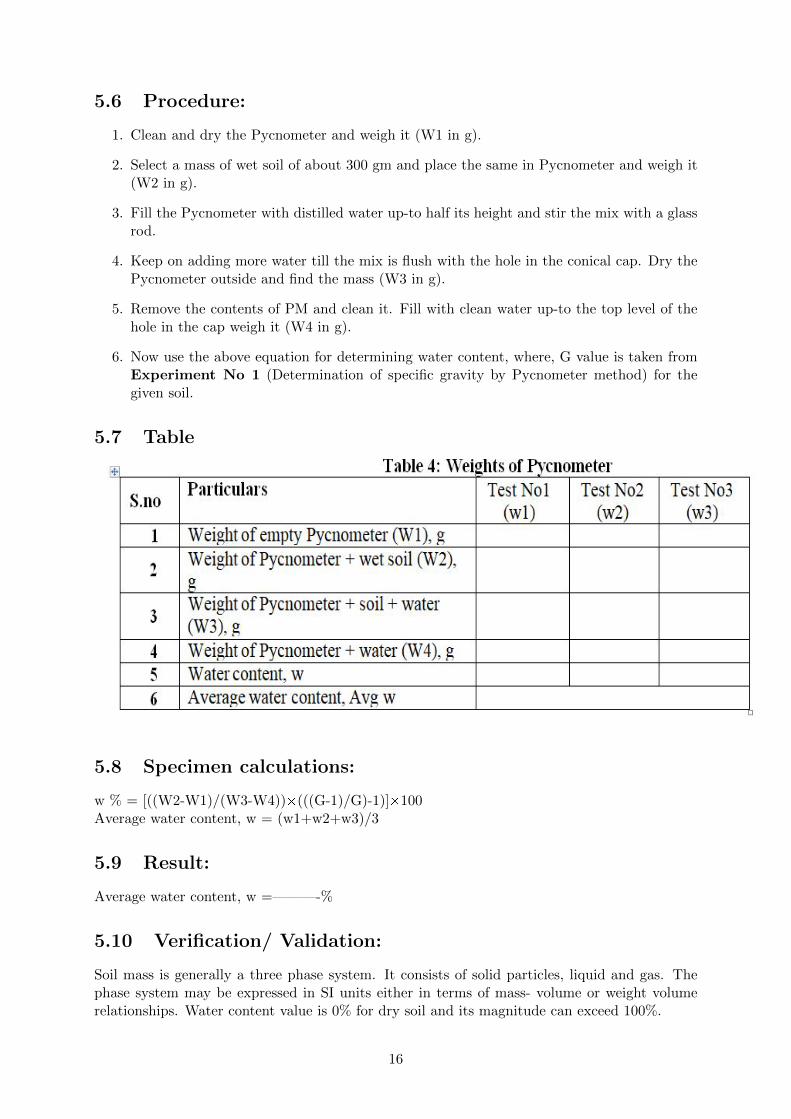
5.7 Table

5.8 Specimen calculations:

w % = [((W2-W1)/(W3-W4))Ö(((G-1)/G)-1)]Ö100Average water content, w = (w1+w2+w3)/3

5.9 Result:

Average water content, w =———-%

5.10 Verification/ Validation:

Soil mass is generally a three phase system. It consists of solid particles, liquid and gas. Thephase system may be expressed in SI units either in terms of mass- volume or weight volumerelationships. Water content value is 0% for dry soil and its magnitude can exceed 100%.

16

5.11 Conclusion:

Pycnometer method is a simple method to determine the water content of a soil. Experimentis carried out using the soil specimen collected from the college itself. All foreign matters areremoved, clods broken and water content we got for the soil specimen is——— Comparing withthe oven drying method, the value is————

17

LAB 5–IN-SITU DENSITY BY CORE CUTTER METHOD

6.1 Introduction

Core cutter method is used for finding field density of cohesive/clayey soils placed as fill. It israpid method conducted on field. It cannot be applied to coarse grained soil as the penetrationof core cutter becomes difficult due to increased resistance at the tip of core cutter leading todamage to core cutter

6.2 Objectives

To determine the field density or unit weight of soil by Core cutter method.

6.3 Equipment

1. Cylindrical core cutter, 100mm internal diameter and 130mm long.

2. Steel dolley, 25mm high and 100mm internal diameter.

3. Steel rammer mass 9kg, overall length with the foot and staff about 900mm.

4. Balance, with an accuracy of 1g.

5. Palette knife, Straight edge, steel rule etc.

6. Square metal tray – 300mm x 300mm x 40mm.

7. Trowel.

6.4 Theory:

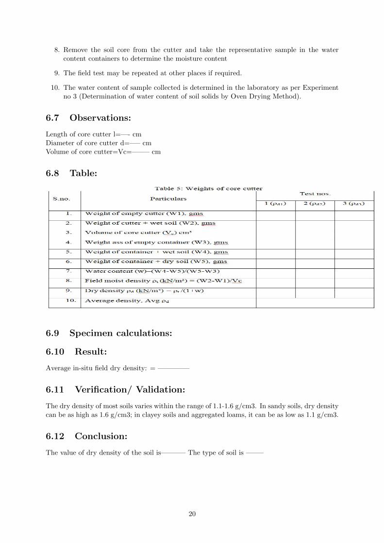
Field density is defined as weight per unit volume of soil mass in the field at in- situ conditions.In the spot adjacent to that where the field density by sand replacement method has beendetermined or planned, drive the core cutter using the dolly over the core cutter. Stop rammingwhen the dolly is just proud of the surface. Dig out the cutter containing the soil out of theground and trim off any solid extruding from its ends, so that the cutter contains a volume ofsoil equal to its internal volume which is determined from the dimensions of the cutter. Theweight of the contained soil is found and its moisture content determined. Equations are;

18

6.5 Precautions:

1. Core cutter method of determining the field density of soil is only suitable for fine grainedsoil (Silts and clay). That is, core cutter should not be used for gravels, boulders or anyhard surface. This is because collection of undisturbed soil sample from a coarse grainedsoil is difficult and hence the field properties, including unit weight, cannot be maintainedin a core sample.

2. Core cutter should be driven into the ground till the steel dolly penetrates into the groundhalf way only so as to avoid compaction of the soil in the core.

3. Before lifting the core cutter, soil around the cutter should be removed to minimize thedisturbances.

4. While lifting the cutter, no soil should drop down.

6.6 Procedure:

1. Measure the height and internal diameter of the core cutter to the nearest 0.25 mm.

2. Calculate the internal volume of the core-cutter Vc in cm³.

3. Determine the weight of the clean cutter accurate to 1 g (W1 in g).

4. Select the area in the field where the density is required to be found out. Clean and levelthe ground where the density is to be determined.

5. Place the dolley over the top of the core cutter and press the core cutter into the soil massusing the rammer. Stop the pressing when about 15mm of the dolley protrudes above thesoil surface.

6. Remove the soil surrounding the core cutter by digging using spade, up to the bottomlevel of the cutter. Lift up the cutter and remove the dolley and trim both sides of thecutter with knife and straight edge.

7. Clean the outside surface of the cutter and determine mass of the cutter with the soil (W2in g).

19

8. Remove the soil core from the cutter and take the representative sample in the watercontent containers to determine the moisture content

9. The field test may be repeated at other places if required.

10. The water content of sample collected is determined in the laboratory as per Experimentno 3 (Determination of water content of soil solids by Oven Drying Method).

6.7 Observations:

Length of core cutter l=—- cmDiameter of core cutter d=—– cmVolume of core cutter=Vc=——– cm

6.8 Table:

6.9 Specimen calculations:

6.10 Result:

Average in-situ field dry density: = ————–

6.11 Verification/ Validation:

The dry density of most soils varies within the range of 1.1-1.6 g/cm3. In sandy soils, dry densitycan be as high as 1.6 g/cm3; in clayey soils and aggregated loams, it can be as low as 1.1 g/cm3.

6.12 Conclusion:

The value of dry density of the soil is———– The type of soil is ——–

20

LAB 6– IN-SITU DENSITY BY SANDREPLACEMENTMETHOD

7.1 Introduction

Sand replacement density (SRD) tests are used to measure the in-situ density of natural orcompacted soils using sand pouring cylinders. The in-situ density is typically used for highwayor pavement design purposes to estimate the relative density of base course or subgrade materials.The in-situ density of natural soil is needed for the determination of bearing capacity of soils,for the purpose of stability analysis of slopes, for the determination of pressures on underlyingstrata for the calculation of settlement and the design of underground structures. Moreover, drydensity values are relevant both of embankment design as well as pavement design.

7.2 Objectives

To determine in-situ density of natural or compacted soil using Sand replacement method.

7.3 Specifications:

This test is done to determine the in-situ dry density of soil by core cutter method as per IS-2720-Part-28 (1975). In order to conduct the test, select uniformly graded clean sand passingthrough 600 micron IS sieve and retained on 300 micron IS sieve.

7.4 Equipment

1. Sand pouring cylinder of about 3 litre capacity (Small pouring cylinder as per IS 2720Part 28)

2. Cylindrical calibrating container 10 cm internal diameter and 15 cm depth

3. Glass plate, trays, containers for determining water content

4. Tools for making of a hole of 10 cm diameter and 15 cm deep, knife and other accessories

5. Metal container to collect excavated soil

6. Metal tray, 300mm square and 40mm deep with a hole of 100mm in diameter at the centre

7. Weighing balance

8. Moisture content cans

9. Glass plate about 450 mm/600 mm square and 10mm thick

10. Oven

11. Dessicator

21

7.5 Theory:

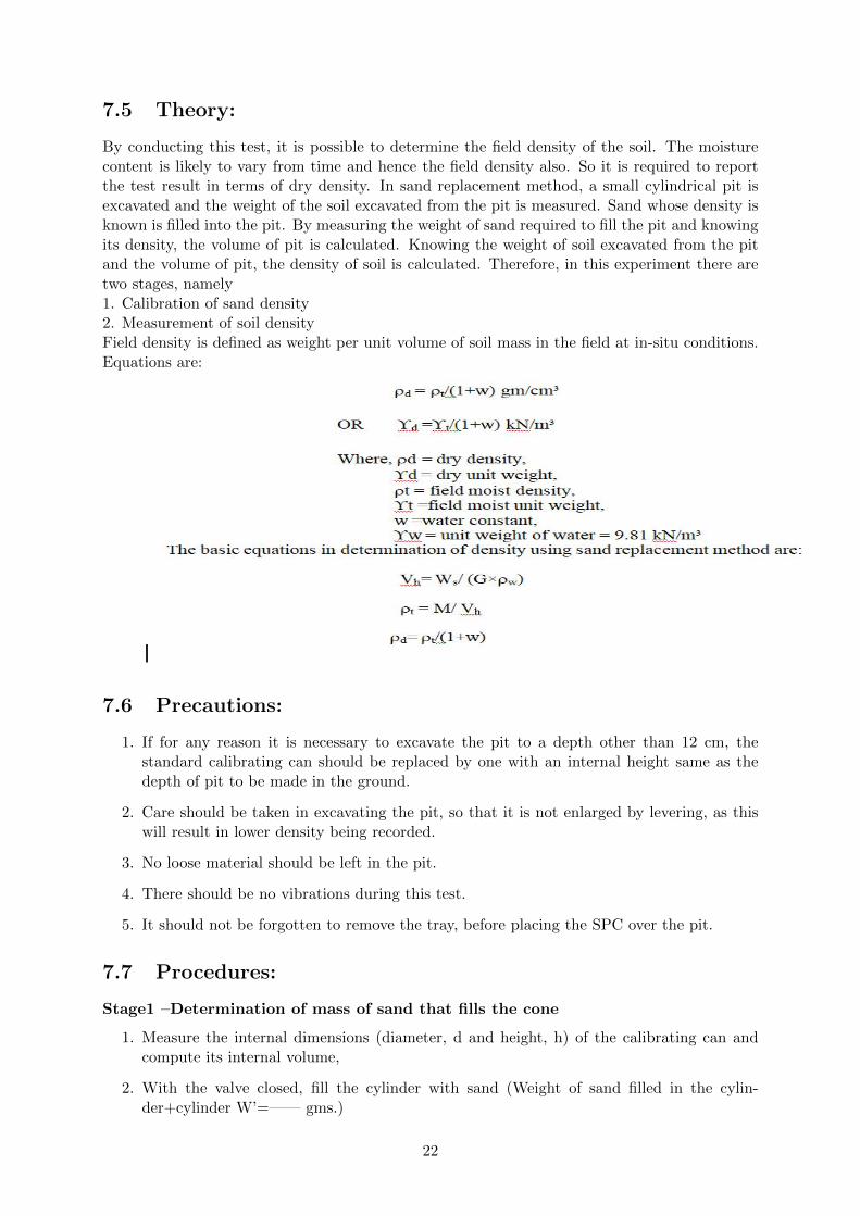
By conducting this test, it is possible to determine the field density of the soil. The moisturecontent is likely to vary from time and hence the field density also. So it is required to reportthe test result in terms of dry density. In sand replacement method, a small cylindrical pit isexcavated and the weight of the soil excavated from the pit is measured. Sand whose density isknown is filled into the pit. By measuring the weight of sand required to fill the pit and knowingits density, the volume of pit is calculated. Knowing the weight of soil excavated from the pitand the volume of pit, the density of soil is calculated. Therefore, in this experiment there aretwo stages, namely1. Calibration of sand density2. Measurement of soil densityField density is defined as weight per unit volume of soil mass in the field at in-situ conditions.Equations are:

7.6 Precautions:

1. If for any reason it is necessary to excavate the pit to a depth other than 12 cm, thestandard calibrating can should be replaced by one with an internal height same as thedepth of pit to be made in the ground.

2. Care should be taken in excavating the pit, so that it is not enlarged by levering, as thiswill result in lower density being recorded.

3. No loose material should be left in the pit.

4. There should be no vibrations during this test.

5. It should not be forgotten to remove the tray, before placing the SPC over the pit.

7.7 Procedures:

Stage1 –Determination of mass of sand that fills the cone

1. Measure the internal dimensions (diameter, d and height, h) of the calibrating can andcompute its internal volume,

2. With the valve closed, fill the cylinder with sand (Weight of sand filled in the cylin-der+cylinder W’=—— gms.)

22

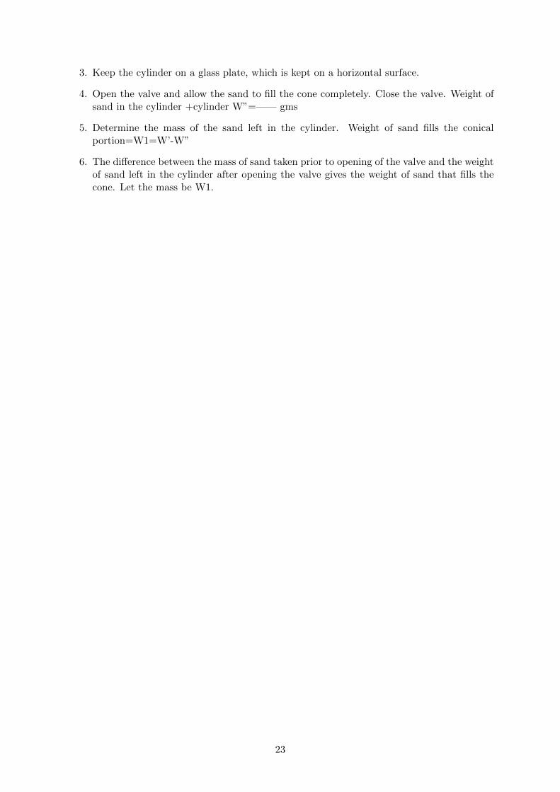
3. Keep the cylinder on a glass plate, which is kept on a horizontal surface.

4. Open the valve and allow the sand to fill the cone completely. Close the valve. Weight ofsand in the cylinder +cylinder W”=—— gms

5. Determine the mass of the sand left in the cylinder. Weight of sand fills the conicalportion=W1=W’-W”

6. The difference between the mass of sand taken prior to opening of the valve and the weightof sand left in the cylinder after opening the valve gives the weight of sand that fills thecone. Let the mass be W1.

23

LAB 7–GRAIN SIZE ANALYSIS

8.1 Introduction

Grain size analysis is a typical laboratory test conducted in the soil mechanics field. The purposeof the analysis is to derive the particle size distribution of soils. Sieve Grain Size Analysis iscapable of determining the particles’ size ranging from 0.075 mm to 100 mm.

8.2 Objectives

This test is performed to determine the percentage of different grain sizes contained within asoil. The mechanical or sieve analysis is performed to determine the distribution of the coarser,larger-sized particles, and the hydrometer method is used to determine the distribution of thefiner particles.

8.3 Equipment

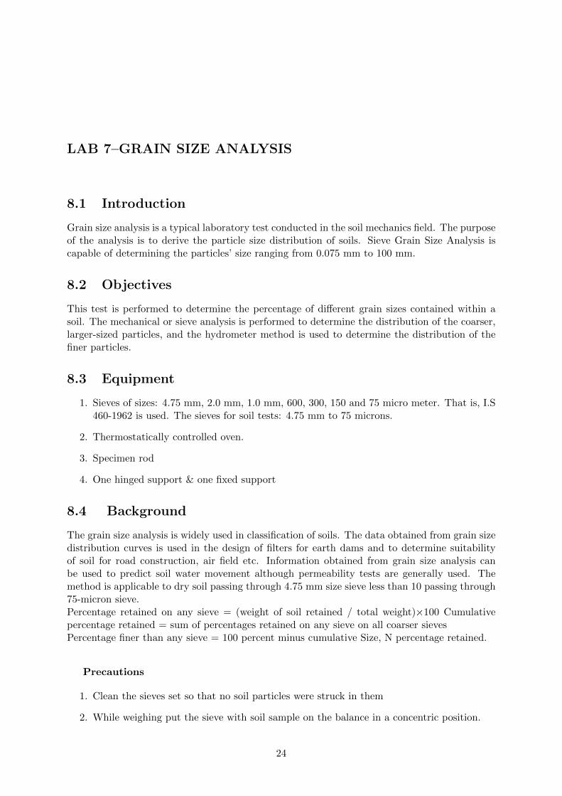
1. Sieves of sizes: 4.75 mm, 2.0 mm, 1.0 mm, 600, 300, 150 and 75 micro meter. That is, I.S460-1962 is used. The sieves for soil tests: 4.75 mm to 75 microns.

2. Thermostatically controlled oven.

3. Specimen rod

4. One hinged support & one fixed support

8.4 Background

The grain size analysis is widely used in classification of soils. The data obtained from grain sizedistribution curves is used in the design of filters for earth dams and to determine suitabilityof soil for road construction, air field etc. Information obtained from grain size analysis canbe used to predict soil water movement although permeability tests are generally used. Themethod is applicable to dry soil passing through 4.75 mm size sieve less than 10 passing through75-micron sieve.Percentage retained on any sieve = (weight of soil retained / total weight)Ö100 Cumulativepercentage retained = sum of percentages retained on any sieve on all coarser sievesPercentage finer than any sieve = 100 percent minus cumulative Size, N percentage retained.

Precautions

1. Clean the sieves set so that no soil particles were struck in them

2. While weighing put the sieve with soil sample on the balance in a concentric position.

24

3. Check the electric connection of the sieve shaker before conducting the test.

4. No particle of soil sample shall be pushed through the sieves.

8.5 Procedure

1. Take a representative sample of soil received from the field and dry it in the oven.

2. Use a known mass of dried soil with all the grains properly separated out. The maximummass of soil taken for analysis may not exceed 500 g.

3. Use a known mass of dried soil with all the grains properly separated out. The maximummass of soil taken for analysis may not exceed 500 g.

4. Make sure sieves are clean. If many soil particles are stuck in the openings try to pokethem out using brush.

5. The whole nest of sieves is given a horizontal shaking for 10 min in sieve shaker till thesoil retained on each reaches a constant value.

6. Now the column just starts buckling.

7. Till the deflection of column occurs as shown in figure mean while applied load valueapproximately coincides with the theoretical value.Determine mass of soil retained oneach sieve including that collected in the pan below.

TABULAR COLUMNThe test results obtained from a sample of soil are given below. Mass of soil taken for analysis

W = gm

25

8.6 Result

Uniformity coefficient, Cu=Coefficient of curvature, Cc=

8.7 Viva Questions

1. Define the grain size analysis and what is the silt size?

2. What is uniformity coefficient? What is the significance on computing the same?

3. What is the most basic classification of soil?

4. What are the methods of soil gradation or grain size distribution?

5. How to compute D10, D30 and D60 of soil using sieve analysis?

26

LAB 8– PERMEABILITY OF SOIL: CONSTANT AND VARI-ABLE HEAD TEST

9.1 Introduction

The constant head permeability test is a common laboratory testing method used to determinethe permeability of granular soils like sands and gravels containing little or no silt. This testingmethod is made for testing reconstituted or disturbed granular soil samples.

9.2 Objective

The objective of constant head permeability test is to determine the coefficient of permeabilityof a soil. Coefficient of permeability helps in solving issues related to: Yield of water bearingstrata. Stability of earthen dams.

9.3 PreLab

Study the Background section of this Laboratory exercise.

Constant head permeability

1. The constant head permeability test involves flow of water through a column of cylindricalsoil sample under the constant pressure difference. The test is carried out in the perme-ability cell, or permeameter, which can vary in size depending on the grain size of thetested material.

2. The soil sample has a cylindrical form with its diameter being large enough in order to berepresentative of the tested soil. As a rule of thumb, the ratio of the cell diameter to thelargest grain size diameter should be higher than 12 (Head 1982).

3. The usual size of the cell often used for testing common sands is 75 mm diamater and 260mm height between perforated plates.

4. The testing apparatus is equipped with a adjustable constant head reservoir and an outletreservoir which allows maintaining a constant head during the test. Water used for testingis de-aired water at constant temperature.

5. The permeability cell is also equipped with a loading piston that can be used to applyconstant axial stress to the sample during the test. Before starting the flow measurements,however, the soil sample is saturated

6. During the test, the amount of water flowing through the soil column is measured for giventime intervals

27

7. Knowing the height of the soil sample column L, the sample cross section A, and theconstant pressure difference delta h, the volume of passing water Q, and the time intervaldelta T, one can calculate the permeability of the sample asK=QL / (A*delta h.delta t)

Falling head permeability test The falling head permeability test is a common laboratorytesting method used to determine the permeability of fine grained soils with intermediate andlow permeability such as silts and clays. This testing method can be applied to an undisturbedsample.

9.4 Procedure

1. The falling head permeability test involves flow of water through a relatively short soilsample connected to a standpipe which provides the water head and also allows measuringthe volume of water passing through the sample.

2. The diameter of the standpipe depends on the permeability of the tested soil.

3. . The test can be carried out in a Falling Head permeability cell or in an oedometer cell.

4. Before starting the flow measurements, the soil sample is saturated and the standpipes arefilled with de-aired water to a given level.

5. The test then starts by allowing water to flow through the sample until the water in thestandpipe reaches a given lower limit.

6. The time required for the water in the standpipe to to drop from the upper to the lowerlevel is recorderd. Often, the standpipe is refilled and the test is repeated for couple oftimes.

7. The recorded time should be the same for each test within an allowable variation of about10percent (Head 1982) otherwise the test is failed.

9.5 Result:

Coefficient of Permeability of soil k=

9.6 Viva questions:

1. Is code for soil permeability test?

2. How do you measure soil permeability?

3. What are the 3 types of permeability?

4. Which soil has the highest permeability?

28

LAB 9-COMPACTION TEST

10.1 Introduction

The Proctor compaction test is a laboratory method of experimentally determining the optimalmoisture content at which a given soil type will become most dense and achieve its maximumdry density. This process is then repeated for various moisture contents and the dry densitiesare determined for each.

10.2 Equipment

1. Compaction mould 1000 ml capacity.

2. 6 kg rammer

3. Collar 60 mm hig

4. IS Sieve 4.75 mm

5. Oven

6. Weighing balance with accuracy of 1g

7. Mixing tools, spoons, trowels.

10.2.1 Background

Conduction of Proctor’s compaction test is based on the assessment of water content and drydensity relationship of a soil for a specified compactive effort. The mechanical process of den-sification through reduction of air voids in the soil mass is called compaction. The amount ofmechanical energy which is applied to the soil mass is the compactive effort. There are manymethods to compact soil in the field, and some examples include tamping, kneading, vibrationand static load compaction. This test will employ the tamping or impact compaction methodusing the type of equipment and methodology developed by R. R. Proctor in 1933, hence, thetest is also known as the Proctor test.Usually, two types of test are performed:

1. The Standard Proctor test

2. The Modified Proctor tests.

In the Standard Proctor Test, the soil is compacted by a 2.6 kg rammer falling at a distanceof 310 mm into a soil filled mould. The mould is filled with three layers of soil and each layeris subjected to 25 blows of rammer. The Modified Proctor Test is identical to the StandardProctor Test except it employs a 4.89 kg rammer falling at a distance of 450 mm and uses fiveequals of soil instead of three.

29

The bulk density in g/ml of each compacted specimen shall be calculated from the equation:Vm = (m2-m1)/Vm where, m1 = mass in g of mould and basem2 = mass in g of mould, base and soil and,Vm = Volume in ml of mouldThe dry density in g/ml of each compacted specimen shall be calculated from the equation:Vd = (100Ym)/(100+w)where, w = moisture content of soil in percent.

10.3 Procedure

1. The mould with base plate is cleaned and dried and weighed it to measure the nearest 1gm

2. Grease is applied on the mould along with base plate and collar completely.

3. About 16- 18 kg of air-dried pulverised soil is taken.

4. percent of water is added to the soil if the soil is sandy and about 8percent if the soil isclayey and mixed it thoroughly. The soil is kept in air tight container and allowed it tomature for about an hour

5. About 3 kg of the processed soil is taken and divided into approximately three equalportions.

6. One portion of the soil is put into the mould and compacted it by applying 25 number ofuniformly distributed blows.

7. The top surface of the compacted soil is scratched using spatula before filling the mouldwith second layer of soil. The soil is compacted in the similar fashion as done in for thefirst layer and scratched it.

8. The same procedure for third layer is also repeated.

9. The collar is removed and trimmed off the excess soil projecting above the mould usingstraight edge.

10. The mould is cleaned and also the base plate from outside and weighed in to the nearestgram.

11. The soil is removed from the top, middle and bottom of the case and the average of watercontent is determined.

12. About 3 percent water or a fresh portion of the processed soil is added and the steps from5 to 12 are repeated.Click Parameters at the bottom of the page.

10.4 Observations and calculations

1. Diameter of mould (D)= m

2. Height of mould (H)= cm

3. Mass of empty mould and base (in g)=

4. Mass of mould, base plate and . compacted soil (in g)=

5. Moisture content during compaction in percent=

30

6. Weight of soil (g)=

7. Volume

8. Bulk density

9. Dry density

10. Voide ratio

11. Degree of saturation

10.5 Viva questions

1. Which formula is used in constant head permeability test?

2. Why is constant head permeability test important?

3. In which type of soil constant head permeability is done?

4. What is soil permeability test?

5. What is the falling head test used for?

31

LAB 10– CALIFORNIA BEARING RATIO TEST

11.1 Introduction

This laboratory studies about The California bearing ratio (CBR) testing is an evaluation ofthe strength of a ground, base courses, and substrates.

11.2 Need and scope

The california bearing ratio test is penetration test meant for the evaluation of subgrade strengthof roads and pavements. The results obtained by these tests are used with the empirical curvesto determine the thickness of pavement and its component layers. This is the most widely usedmethod for the design of flexible pavement.This instruction sheet covers the laboratory method for the determination of C.B.R. of undis-turbed and remoulded /compacted soil specimens, both in soaked as well as unsoaked state.

11.3 Equipment

1. Cylindrical mould with inside dia 150 mm and height 175 mm, provided with a detachableextension collar 50 mm height and a detachable perforated base plate 10 mm thick.

2. Metal rammers. Weight 2.6 kg with a drop of 310 mm (or) weight 4.89 kg a drop 450 mm.

3. Weights. One annular metal weight and several slotted weights weighing 2.5 kg each, 147mm in dia, with a central hole 53 mm in diameter

4. Loading machine. With a capacity of atleast 5000 kg and equipped with a movable heador base that travels at an uniform rate of 1.25 mm/min. Complete with load indicatingdevice.

5. Metal penetration piston 50 mm dia and minimum of 100 mm in length.

6. Two dial gauges reading to 0.01 mm.

7. Sieves. 4.75 mm and 20 mm I.S. Sieves

8. Miscellaneous apparatus, such as a mixing bowl, straight edge, scales soaking tank or pan,drying oven, filter paper and containers.

11.4 Background:

The CBR test is performed by measuring the pressure required to penetrate a soil sample witha plunger of standard area. The measured pressure is then divided by the pressure required toachieve an equal penetration on a standard crushed rock material. The harder the surface, thehigher the CBR value.

32

11.5 Preparation of test specimen

Undisturbed specimenAttach the cutting edge to the mould and push it gently into the ground. Remove the soil fromthe outside of the mould which is pushed in . When the mould is full of soil, remove it fromweighing the soil with the mould or by any field method near the spot.

11.6 Procedure

1. Take about 4.5 to 5.5 kg of soil and mix thoroughly with the required water

2. Fix the extension collar and the base plate to the mould. Insert the spacer disc over thebase. Place the filter paper on the top of the spacer disc.

3. Compact the mix soil in the mould using either light compaction or heavy compaction.For light compaction, compact the soil in 3 equal layers, each layer being given 55 blowsby the 2.6 kg rammer. For heavy compaction compact the soil in 5 layers, 56 blows toeach layer by the 4.89 kg rammer.

4. Turn the mould upside down and remove the base plate and the displacer disc.

5. Weigh the mould with compacted soil and determine the bulk density and dry density

6. Put filter paper on the top of the compacted soil (collar side) and clamp the perforatedbase plate on to it.

11.7 Observations

1. Optimum water content (percentage)

2. Weight of mould + compacted specimen g

3. Weight of empty mould g

4. Weight of compacted specimen g

5. Volume of specimen cm3

6. Bulk density g/cc

7. Dry density g/cc

11.8 Viva questions

1. What is the purpose of CBR test

2. What is a good CBR test result?

3. What is CBR formula?

4. What is a good CBR?

5. What is the minimum CBR value for subgrade?

33

Lab 11– DIRECT SHEAR TEST

12.1 Introduction

In many engineering problems such as design of foundation, retaining walls, slab bridges, pipes,sheet piling, the value of the angle of internal friction and cohesion of the soil involved arerequired for the design. Direct shear test is used to predict these parameters quickly. Thelaboratory report covers the laboratory procedures for determining these values for cohesion-less soils.

12.2 Objective

To determine the shear strength of soil using the direct shear apparatus.

12.3 Specifications:

The test is conducted as per IS: 2720- 13 (1986), method of tests for soils. One kg of air drysample passing through 4.75mm IS sieve is required for this test.

12.4 Equipments Required:

Shear box apparatus consisting of

1. Shear box 60 mm square and 50 mm deep,

2. Grid plates, porous stones, etc.

3. Loading device

4. Other accessories.

12.5 Theory:

Box shear tests can be used for the following tests.1. Quick and consolidated quick tests on clay soil samples.2. Slow test on any type of soil.Only using box shear test apparatus may carry the drained or slow shear tests on sand. Asundisturbed samples of sand is not practicable to obtain, the box is filled with the sand ob-tained from the field and compacted to the required density and water content to stimulate fieldconditions as far as possible.So far clay soil is concerned the undisturbed samples may be obtained from the field. Thesample is cut to the required size and thickness of box shear test apparatus and introducedinto the apparatus. The end surfaces are properly trimmed and leveled. I9f tests on remolded

34

soils of clay samples are required; they are compacted in the mould to the required density andmoisture content.

12.6 Equation:

Coulombs equation is used for computing the shear parameters.For clay soilsS=c+ tanFor sandS= tanWhere, S = shear strength of soil in kg/cm2

c=unit cohesion in kg/cm2

= normal load applied on the surface of the specimen in kg/cm2

= angle of shearing resistance (degrees)In a Direct Shear test, the sample is sheared along a horizontal plane. This indicates that thefailure plane is horizontal. The normal stress (s) on this plane is the external vertical loaddivided by the area of the soil sample. The shear stress at failure is the external lateral loaddivided by the corrected area of soil sample. The main advantage of direct shear apparatus isits simplicity and smoothness of operation and the rapidity with which testing programmes canbe carried out. But this test has the disadvantage that lateral pressure and stresses on planesother than the plane of shear are not known during the test.

12.7 Precautions:

1. The dimensions of the shear box should be measured accurately.

2. Before allowing the sample to shear, the screw joining the two halves of the box should betaken out.

3. Rate of strain or shear displacement rate should be constant throughout the test.

4. The spacing screws after creating required spacing between two halves of the shear box,should be turned back to make them clear of the lower part.

5. For drained test, the porous stones should be saturated by boiling in water.

6. Add the self weight of the loading yoke in the vertical load.

7. Failure of the soil specimen is assumed when the proving ring dial gauge reading begins torecede after reaching its maximum or at a 20% shear displacement of the specimen length.

8. One soil specimen should be tested with not more than three normal loading conditionsas beyond this, the particle size of soil sample may change due to application of shear andnormal load.

12.8 Procedure

1. Place the sample of soil into the shear box, determine the water content and dry densityof the soil compacted.

2. Make all the necessary adjustments for applying vertical load, for measuring vertical andlateral movements and measurement of shearing force, etc.

35

3. Apply a known load on the specimen and then keep it constant during the course of thetest (for consolidation keep it for a long time without shearing, and quick tests apply theshearing without consolidation soon after placing the vertical load ). Adjust the rate ofstrain as required of the specimen.

4. Shear the specimen till failure of the specimen is noticed or the shearing resistance de-creases. Take the readings of the gauges during the shearing operation.

5. Remove the specimen from the box at the end of the test, and determine the final watercontent.

6. Repeat the tests on three or four identical specimens.

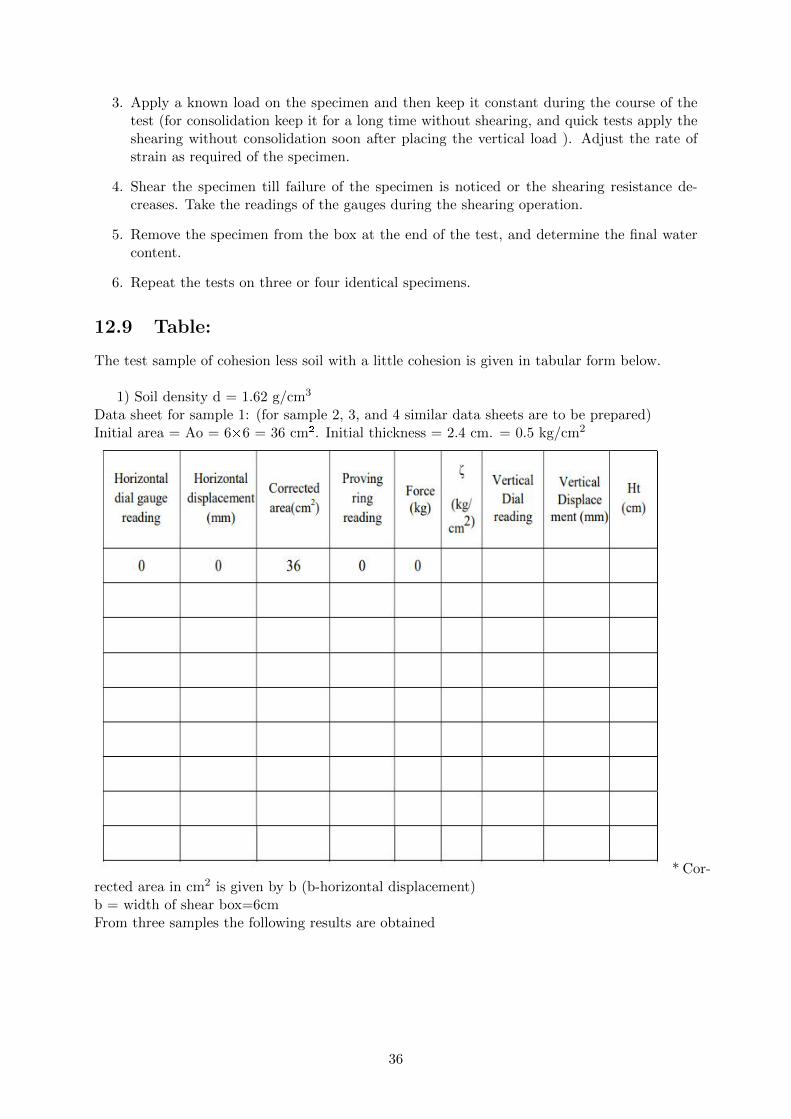
12.9 Table:

The test sample of cohesion less soil with a little cohesion is given in tabular form below.

1) Soil density d = 1.62 g/cm3

Data sheet for sample 1: (for sample 2, 3, and 4 similar data sheets are to be prepared)Initial area = Ao = 6Ö6 = 36 cm². Initial thickness = 2.4 cm. = 0.5 kg/cm2

* Cor-rected area in cm2 is given by b (b-horizontal displacement)b = width of shear box=6cmFrom three samples the following results are obtained

36

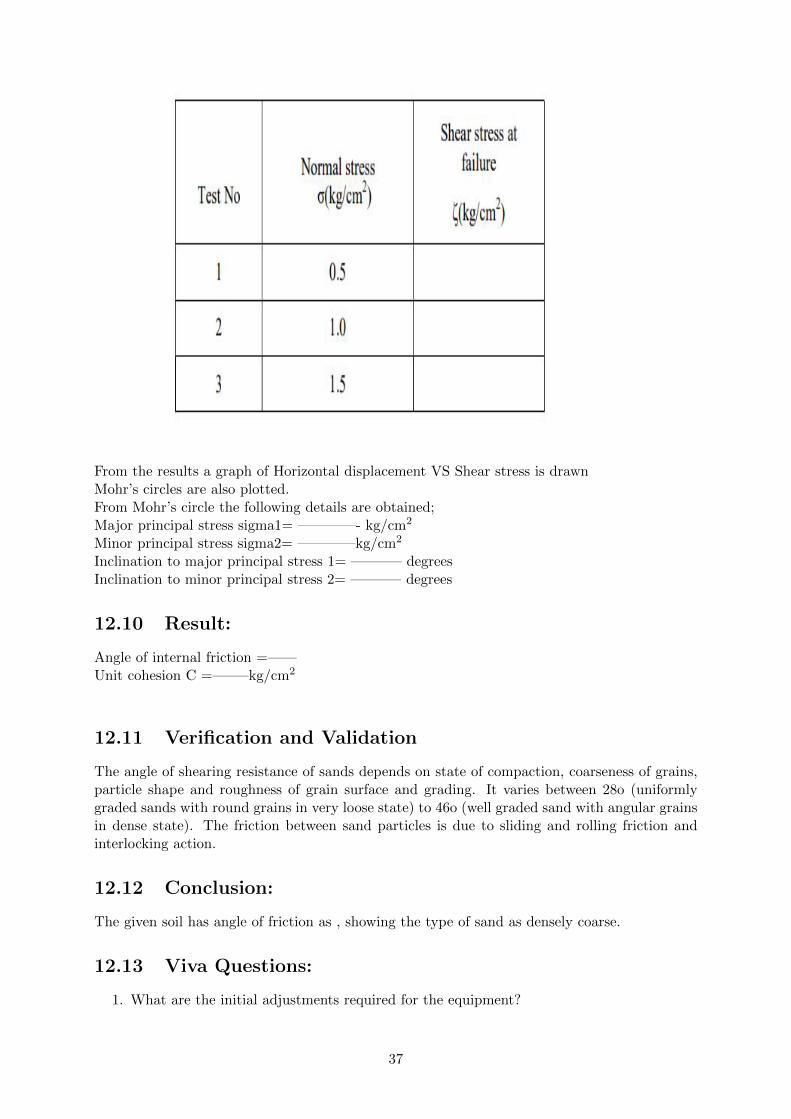
From the results a graph of Horizontal displacement VS Shear stress is drawnMohr’s circles are also plotted.From Mohr’s circle the following details are obtained;Major principal stress sigma1= ————- kg/cm2

Minor principal stress sigma2= ————kg/cm2

Inclination to major principal stress 1= ———– degreesInclination to minor principal stress 2= ———– degrees

12.10 Result:

Angle of internal friction =——Unit cohesion C =——–kg/cm2

12.11 Verification and Validation

The angle of shearing resistance of sands depends on state of compaction, coarseness of grains,particle shape and roughness of grain surface and grading. It varies between 28o (uniformlygraded sands with round grains in very loose state) to 46o (well graded sand with angular grainsin dense state). The friction between sand particles is due to sliding and rolling friction andinterlocking action.

12.12 Conclusion:

The given soil has angle of friction as , showing the type of sand as densely coarse.

12.13 Viva Questions:

1. What are the initial adjustments required for the equipment?

37

2. What is the proving ring capacity in direct shear test?

3. What are the steps taken to get accurate result?

38

Lab 12 – VANE SHEAR TEST

13.1 Introduction

The structural strength of soil is basically a problem of shear strength. Vane shear test is a usefulmethod of measuring the shear strength of clay. It is a cheaper and quicker method. The testcan also be conducted in the laboratory. The laboratory vane shear test for the measurement ofshear strength of cohesive soils, is useful for soils of low shear strength (less than 0.3 kg/cm2) forwhich triaxial or unconfined tests cannot be performed. The test gives the undrained strengthof the soil. The undisturbed and remoulded strength obtained are useful for evaluating thesensitivity of soil.

13.2 Objective

To determine Cohesion or Shear Strength of Soil.

13.3 Specifications:

The test is conducted as per IS 4434 (1978). This test is useful when the soil is soft and itswater content is nearer to liquid limit.

13.4 Equipment Required:

1. Vane shear test apparatus with accessories2. The soil sample

13.5 Theory:

The vane shear test apparatus consists of four stainless steel blades fixed at right angle to eachother and firmly attached to a high tensile steel rod. The length of the vane is usually keptequal to twice its overall width. The diameters and length of the stainless steel rod were limitedto 2.5mm and 60mm respectively. At this time, the soil fails in shear on a cylindrical surfacearound the vane. The rotation is usually continued after shearing and the torque is measured toestimate the remoulded shear strength. Vane shear test can be used as a reliable in-situ test fordetermining the shear strength of soft-sensitive clays. The vane may be regarded as a methodto be used under the following conditions.1. Where the clay is deep, normally consolidated and sensitive.2. Where only the undrained shear strength is required.It has been found that the vane gives results similar to that as obtained from unconfined com-pression tests on undisturbed samples.

39

13.6 Procedure:

1. A posthole borer is first employed to bore a hole up to a point just above the requireddepth

2. The rod is pushed or driven carefully until the vanes are embedded at the required depth.

3. At the other end of the rod just above the surface of the ground a torsion head is used toapply a horizontal torque and this is applied at a uniform speed of about 0.1 degree persecond until the soil fails, thus generating a cylinder of soil

4. The area consists of the peripheral surface of the cylinder and the two round ends.

5. The first moment of these areas divided by the applied moment gives the unit shear value.

13.7 Observations:

Force observed p= ——— kgEccentricity (lever arm) x= ——— cmTurning moment Px= ———— kg-cmLength of the vane L= ——– cmRadius of the vane blades r= ———- cm

13.8 Calculations:

Undrained Shear strength of Clay Cu=———-

13.9 Result:

Undrained Shear strength of Clay Cu = ————— kg/cm2

13.10 Verification/Validations:

Where the strength is greater than that able to be measured by the vane, i.e., the pointer reachesthe maximum value on the dial without the soil shearing, the result shall be reported in eitherof the following two ways e.g 195 + kPa or >195 kPa.

13.11 Viva Questions:

1. Is this method the direct method to determine the shear strength of soil?

2. Is it possible to determine the sensitivity of clay suing this method?

3. Is it possible to determine the sensitivity of clay suing this method?

4. What are the advantages of vane shear test?

5. What are the disadvantages of vane shear test?

40