Lab Report - Pressure Experiments - MLT 4.1 - RWTH Aachen

GUTECH

Pressure experiments Pressure Measurements in Gases and Liquids

Mohammed Omer – 000-11-0050

1/5/2014

Mohammed Omer [email protected] 000-11-0050 Gutech – LTT Lab Report

1

Table of Contents 1 Introduction ........................................................................................................................................ 2

2 Experiment 1-Calibrating a Bourdon-tube gauge ............................................................................... 2

2.1 Physical Background and theory .................................................................................................. 2

2.2 Experimental Procedure and possible errors ............................................................................... 3

3 Experiment 2 – Pressures in flowing media ........................................................................................ 4

3.1 Aim of the experiment ................................................................................................................. 4

3.2 Physical background and theory .................................................................................................. 4

3.3 Experiment 2a - Procedure and Observations ............................................................................. 6

4 Experiment 3 – Measuring dynamic pressure using a Prandl tube. ................................................... 7


4.2 Experiment 3 – Procedure and Results ........................................................................................ 7

4.3 Results and Discussion ................................................................................................................. 7

5 Experiment 4 – Mercury barometer ................................................................................................... 8

Description .......................................................................................................................................... 8

5.1 Experimental Procedure .............................................................................................................. 8

5.2 Results .......................................................................................................................................... 9

6 Experiment 5 – Piezoelectric pressure sensor .................................................................................... 9


6.2 Experimental Procedure and discussion .................................................................................... 10

7 Experiment 6 – Pirani vacuum gauge, Water jet pump and Rotary Vane pump .............................. 10

7.1 Physical background and theory ................................................................................................ 10

7.12 Water jet pump .................................................................................................................... 10

7.13 The Rotary vane pump ......................................................................................................... 11

7.14 Thermal conductivity Pirani vacuum gauge ......................................................................... 11

7.2 Experiment and Procedure ........................................................................................................ 12

8 References ......................................................................................................................................... 12

8.1 Internet ...................................................................................................................................... 12

8.2 Books .......................................................................................................................................... 13

8.3 Journals ...................................................................................................................................... 13


2

MLT – 4.1 Pressure Experiments

1 Introduction

Pressure is defined as the Force exerted per unit area (

) and its unit is Pascal [Pa]. There are two

basic types of pressures, Vacuum pressure and Gauge pressure. The Vacuum pressure is an under-

pressure that is below the atmospheric pressure and the gauge pressure is higher than the

atmospheric pressure. They are given by:-

(1)

(2)

(3)

When a flattened tube is pressurised, it tends to change to a more circular cross section. A C-shaped

metal tube is used which on getting pressurised moves in an arc motion. A needle attached to the

outer end of the tube can then point on a scale showing the pressure. For high pressure gear

reduction mechanisms can be used. This is how a Bourdon gauge works.1

2 Experiment 1-Calibrating a Bourdon-tube gauge

2.1 Physical Background and theory In this experiment a Bourdon-tube gauge is calibrated with the help of a piston manometer. The

setup is shown below:

Figure 1: Schematic of the

calibration system.


3

In this experiment the Bourdon gauge is calibrated by placing known weights on the piston and then

balancing these weights by hydraulically increasing the pressure of the oil via the hand spindle.

When a weight is placed on the piston rod, the pressure exerted by the piston is given by:

(4)

Where is the pressure exerted by the piston, is the mass of the weight placed, is the mass

of the piston rod, g is the acceleration due to gravity and is the cross-sectional area of the piston.

This pressure is transmitted through the liquid all the way to the bourdon gauge. Due to this rise

in pressure the oil in the tubes rise up and create a height difference and using this height

difference the pressure in the bourdon-gauge can be calculated by making a pressure balance:

(5)

Where is the pressure in the Bourdon gauge, is the density of the fluid in the manometer

and is height difference caused due to the difference in pressure.

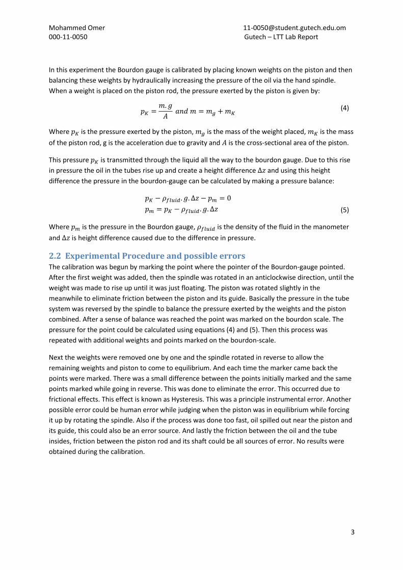
2.2 Experimental Procedure and possible errors The calibration was begun by marking the point where the pointer of the Bourdon-gauge pointed.

After the first weight was added, then the spindle was rotated in an anticlockwise direction, until the

weight was made to rise up until it was just floating. The piston was rotated slightly in the

meanwhile to eliminate friction between the piston and its guide. Basically the pressure in the tube

system was reversed by the spindle to balance the pressure exerted by the weights and the piston

combined. After a sense of balance was reached the point was marked on the bourdon scale. The

pressure for the point could be calculated using equations (4) and (5). Then this process was

repeated with additional weights and points marked on the bourdon-scale.

Next the weights were removed one by one and the spindle rotated in reverse to allow the

remaining weights and piston to come to equilibrium. And each time the marker came back the

points were marked. There was a small difference between the points initially marked and the same

points marked while going in reverse. This was done to eliminate the error. This occurred due to

frictional effects. This effect is known as Hysteresis. This was a principle instrumental error. Another

possible error could be human error while judging when the piston was in equilibrium while forcing

it up by rotating the spindle. Also if the process was done too fast, oil spilled out near the piston and

its guide, this could also be an error source. And lastly the friction between the oil and the tube

insides, friction between the piston rod and its shaft could be all sources of error. No results were

obtained during the calibration.


4

3 Experiment 2 – Pressures in flowing media

3.1 Aim of the experiment In this experiment the static pressure was measured at different points to see how the pressure

dropped or increased due to friction against the tube walls and irregularities in the tubing. In the

next experiment a demonstration was performed in a small wind tunnel of how a Prandl (pitot) tube

is used to measure dynamic pressure.

3.2 Physical background and theory

Figure 2:- Measuring the static and dynamic pressure while liquid flows out of a reservoir.

In this experiment we demonstrate how the fluid flow in a tube is connected to the Bernoulli

equation. The derivation of the Bernoulli equation is not provided here since it is long and is already

present in the script. The Bernoulli equation is directly stated here:

(6)

The static pressure is equal to the total pressure and since conditions along path 12 are

considered constant, the term

is the dynamic pressure given by . Therefore equation 6 can

also be written as :

(7)

The principle of conservation of mass through a stationary system, that is a basic for all flow or

continuity equations can be modelled here. Considering the system where we have a fluid flowing

with initial velocity through a tube with cross-sectional area and final velocity through a

cross-sectional area . The mass flow rates ̇ ̇ , therefore we can say that:-

(8)


5

According to figure.3 since is smaller

than , the velocity has to increase

to balance equation (8) because the

density is constant in an incompressible

fluid. But for our experimental setup

the tube is streamlined with a constant

cross-sectional area ( and

the water within the system is modelled

as incompressible with constant volume and so constant density ( . Therefore the speed

is constant throughout the system. If state 1 is at the reservoir and if state 2 is an arbitrary point in

the system. It can be said that the total pressure at state 1 is the sum of the total pressure

at state 2 ( ) and the loss in pressure in going from state 1 to 2 giving the following

equation:

(9)

The Bernoulli equation ignores friction in the streamlined tube, but in reality there is friction and

turbulence at the walls of the tube due to the flow of the water. In order to use the Bernoulli

equation in the frictional case, the frictional terms are taken into account in the term giving:

(10)

Here is the length of the tube, d is the diameter, is the density of the fluid, is the speed of the

fluid and is the coefficient of friction whereby is a function of the viscosity of the fluid, the tube-

wall roughness and the type of flow(turbulent or laminar). Therefore if we consider equation (10), it

can be seen that for a particular , constant tube diameter, constant fluid density and velocity. The

loss in pressure depends only on the coefficient of friction and length of the tube . For the

experimental setup 2a the expression for the total pressure becomes:

(11)

Where is the atmospheric pressure, is the change in height of the water

column in the tubes and is the fluid density.

Figure 4:- Experimental

setup to show pressure drop.

Finally applying Bernoulli’s equation to the entire pipe length the Bernoulli equation becomes:

(12)


6

Where is the total pressure of the fluid, is the static pressure,

is the dynamic

pressure and represents the pressure losses. The sum of these terms is a const.

3.3 Experiment 2a - Procedure and Observations There was a reservoir filled with water and this reservoir was connected to a streamlined tube by

thick rubber tubing that had a one way manual valve attached that could be opened to allow the

water to flow into the system and exit out to the drain. To the main tube on the top were attached

several thin vertical

transparent tubes as shown in

the figure below.

Figure 5:- Setup for measuring

drop in pressure due to

installation errors.

The experiment was begun by noting the initial height of the liquid columns and then the valve was

opened allowing water to flow through the system. Then the heights of the tubes were marked. If

there would have been no installation errors the heights of the water in the vertical tubes would

have followed the red line in figure 5. But due to the installation errors there were differences in the

heights. The Bernoulli equation (12) states that the sum of the static pressure, dynamic pressure and

pressure losses is constant. Now considering equations (11) and (12), since fluid velocity and density

are constant the static pressure must decrease along the length of the tube, and since according to

equation (8) the static pressure depends only on (change in height), if static pressure reduces the

liquid height must reduce, therefore the red line is to be seen.

In the tubes with installation errors a lower liquid height was observed. This occurred because

increased wall roughness and turbulence increased the term in equation (10), consequently

increasing the pressure loss term. And according to equation (12) with constant dynamic pressure,

increase of the pressure loss term caused the static pressure term to reduce. And in the tube with

the narrowing cross-section the fluid velocity increased, so according to equations (10) and (12)

the dynamic pressure term

and the pressure loss term (

) increased and so static

pressure had to decrease, causing a decrease in the height of the liquid column. No pressure

measurements were taken in this experiment and so no errors are discussed.


7

4 Experiment 3 – Measuring dynamic pressure using a Prandl tube. The aim of this experiment was to show how a Prandl-Pitot tube could be used to measure dynamic

pressure and how low pressures could be accurately measured using an inclined thermometer.

4.1 Physical background and theory In Figure.6.(a) below a Prandl probe is shown in which the change in height detected in the

manometer attached gives the static pressure . The other is the Pitot tube shown in Fig.6.(b),

that has an axial hole B in the tube with a manometer M attached via a hose. The height difference

in the manometer gives the total pressure . These two probes can be combined to form the

Prandl-Pitot tube shown in figure.6.(c), that on finding both the total pressure and static pressure,

subtracts them to give the dynamic pressure . This Prandl-Pitot tube was used in the

experiment to determine the dynamic pressure at different locations in a small wind tunnel.

Figure 6:- (a) Prandl proble to

measure static pressure, (b)

Pitot tube to measure total

pressure, (c) Prandl-Pitot

combination tube to measure

the dynamic pressure.

4.2 Experiment 3 – Procedure and Results There was an open end wind tunnel with a pump at the other end sucking in the air. The air flow was

made laminar with a metallic honeycomb sieve. In the centre of the tunnel was attached a Prandl-

Pitot tube that could be lowered till the bottom of the tunnel and raised to the top. There was a

scale above it which read from -4 to +4 cm. If the probe was at zero on the scale, it was in the centre

of the tunnel. The probe had an axial hole and a hole on the top. To the probe were attached two

rubber tubes that were attached to manometers. The experiment was begun by switching on the air

pump, and the readings were taken of the dynamic pressure from an inclined manometer.

The inclined manometer had different angles it could be adjusted to read higher or lower pressures.

During our readings the manometer was inclined at 15o. An inclined manometer is normally used to

measure small pressure changes. Since the dynamic pressure in the air was pretty low, this was well

suited for the job. The Prandl-Pitot tube was always aligned to the air flow. Pressure readings were

taken starting from the base of the tunnel at a level of -4.5 cm, until the centre of the tunnel. The

remaining positive probe heights were known to give the same values as on the negative heights.

4.3 Results and Discussion S.No Probe level Dynamic Pressure


8

1 -4.5 18

2 -3 31

3 -2 39

4 -1 40

5 0 40.5

Therefore it was seen that the dynamic pressure was a maximum in the centre of the wind-tunnel

and least at the ends. This was because of the higher friction and turbulence caused at the walls of

the tunnel that reduced the fluid velocity and therefore the dynamic pressure (

reduced.

Possible errors in the experiment could be human error while reading the gauge. Error could have

also occurred due to uneven placement of the manometer on the table.

5 Experiment 4 – Mercury barometer In this experiment the atmospheric pressure was obtained using a wall mounted Lambrecht Mercury

barometer.

Description The barometer consists of a reservoir of mercury at

the base along with a tube that has been evacuated

(vacuum). The vacuum allows the barometer to

measure absolute pressure. The atmospheric

pressure in the room drives the mercury up the

tube. The pressure in the room can be calculated by

measuring the height of this column of mercury

. The scale beside the column shown in

Fig.8(a),(b), gives the height of the mercury column

in mm, and the moving scale has a vernier attached

to give the estimated digit shown below in Fig.8.(d)

Figure 7:- Simplified mercury barometer

5.1 Experimental Procedure The experiment was started by aligning the scale such that the sharp bottom end of the scale was

just touching the mercury in the reservoir that it created a mirror image of itself in the form of an ‘X’

as shown in Fig.8.(c). This was done by a small rotating knob on the scale. Unlike water, mercury

forms a convex meniscus. The bottom of the vernier(nonius) scale was aligned with the top of the

meniscus. This gave the pressure reading in mm and to get the estimated digit the line on the

vernier which matched perfectly with a line on the fixed scale was noted.

The initial reading from the barometer was slightly higher than it should have been due to the

thermal expansion of mercury. The temperature affects the density of the mercury therefore the

reading had to be corrected with respect to temperature from a table. In our case the room

temperature was 210C noted from a thermometer attached to the mercury barometer, so we got a

correction factor of 2.76 from tables that had to be subtracted from the reading on the barometer.

Similarly correction readings for the height of Aachen above sea level (185m), the geographic


9

location (g=9.80665m/s2) and capillary depression were applied from tables to give the final reading.

The capillary depression was checked by measuring the height of the convex meniscus in mm.

5.2 Results Description Value

Actual reading from scale 757.3 mmHg

Add correction for temperature (21oC) -2.76

Subtract correction for geographic location (-) +0.31

Add correction for height above sea level (185m) -0.03

Subtract correction for height of meniscus (0.8mm) +0.46

Final reading of pressure in Aachen 755.28mmHg

This was compared with another barometer in the same room which read 992.2 mbars. And using

=13594kg/m3, g = 9.80665m/s2 and height of mercury as 755.28mmHg. The atmospheric

pressure was found using the formula P = and using appropriate conversion factors gives

993.9 mbar. That means the readings are pretty close.

Figure 8:- The parts of the Mercury Barometer.

6 Experiment 5 – Piezoelectric pressure sensor The aim of the experiment was to measure the pressure of a pulsating or vibrating object using a

piezoelectric pressure transducer.

6.1 Physical background and theory A piezoelectric sensor is used to measure fluctuating pressure. This is done by using a ceramic

material that has a special geometric charge distribution. Most commonly used piezoelectric

materials are Natural Quartz and Tourmaline because of their easy availability and accurate pressure

measurement. For example in SiO2 there is a charge distribution as shown in the figure below, when

a mechanical force is applied the geometric charge distribution changes whereby the negative


10

oxygen atoms come closer to the upper quartz surface making it negative and positive silicon atoms

move closer to the bottom quartz surface making it negatively charged. A charge separation is

created in the direction of applied force. This change in charge distribution is detected in the piezo

sensor and amplified using a charge amplifier to be displayed as a sinus wave on an oscilloscope.

Figure 9:- Conceptual model of polarisation

in a quartz crystal

6.2 Experimental Procedure and discussion In the experiment a piezoelectric sensor was mounted on a plastic case with wires form it being

attached to a computer that acted as the oscilloscope. First the sensor was pressed with the finger,

imitating a static pressure. This showed no signal on the computer. But when the finger was

periodically pressed on the sensor, small waves were seen. Next a tuning fork was hit on the table

and the base touched to the sensor, now a sinus wave was recorded on the screen. Therefore it was

obvious that the piezoelectric sensor is not suitable to measure static pressure but dynamic or

fluctuating pressure. No measurements were taken during the procedure so no error is discussed.

7 Experiment 6 – Pirani vacuum gauge, Water jet pump and Rotary

Vane pump

7.1 Physical background and theory

7.12 Water jet pump

A Water Jet Pump consists of a water reservoir or water source at the top and then a nozzle with a very small cross sectional area and then a diffuser as shown in Figure.10 below.

Figure 10:- Schematic of a Water jet pump.


11

As the water flows from the water source into the top of the aspirator and into the nozzle region the

decrease in cross sectional area causes an increase in the velocity of the fluid which effectively

increases the dynamic pressure. According to the laws governing fluid dynamics, a fluid's velocity

must increase as it passes through a constriction to satisfy the principle of continuity (equation .8),

while its static pressure must decrease to satisfy the principle of conservation of mechanical energy

as in equations (6) and (7). Since the sum of the potential energy, static pressure and kinetic energy

of the fluid is a constant thus any gain in kinetic energy a fluid may accrue due to its increased

velocity through a constriction is negated by a drop in pressure. This pressure drop creates a vacuum

in the suction chamber. Due to the pressure gradient created air flows into the suction chamber and

into the mixing nozzle.

7.13 The Rotary vane pump

While the water jet pump is a completely mechanical device, the rotary vane pump is a device that

uses an electric motor to run the pump and create

a vacuum.

Figure 11:- Schematic of a rotary vane pump. With

blue arrow designating inlet air and the red arrow

the exiting air.

1 – Pump housing

2 – Rotor

3 – Piston valve

4 – Spring

Source:

(http://en.wikipedia.org/wiki/File:Rotary_vane_p

ump.svg )

Figure.11 shows a schematic of a rotary vane pump. As the rotor rotates anticlockwise, the left vane

is compressed against the rotor spring antagonistically pushing the right vane out. This movement

creates a vacuum which sucks in the air shown by the blue arrows (inlet air). Then it compresses or

pushes the air through the housing shown by the green arrow. The air finally exits (shown by red

arrows) through the outlet valve. The vane pump requires oil to constantly lubricate the moving

mechanical parts and sometimes this oil can enter the tube or containers connected to the pump.

7.14 Thermal conductivity Pirani vacuum gauge

The Pirani vacuum gauge uses an electrically heated resistance wire connected in a self-balancing

Wheatstone-bridge connection with three other piezo-resistors. The element within the resistor is

constantly heated. Whenever air molecules collide with the heated element some energy is lost and

so the temperature of the resistor decreases and this changes the resistance, which is balanced by

the wheatstone bridge circuit. At this point the output signal is the change in the voltage as

shown in the figure below. This voltage reading is amplified and calibrated to show pressure

readings. Without the pump running and the gauge open to atmosphere the gauge would be

calibrated to atmospheric pressure.

http://en.wikipedia.org/wiki/File:Rotary_vane_pump.svg

http://en.wikipedia.org/wiki/File:Rotary_vane_pump.svg


12

Figure 11:- Pirani Vacuum gauge scheme.

But in case of a vacuum the air molecules

decrease so there are less collisions of air

molecules with the filament. This increases

the filament temperature and so affects its

resistance. Again the self-balancing circuit

tries to balance the resistance and the voltage difference produced is amplified and converted to

pressure readings, which can be read from the calibrated pressure indicator.

7.2 Experiment and Procedure The aim of this experiment was to compare the strength of the vacuums created by the Water jet

pump to that of a Rotary vane pump. Three different pressure gauges were used to measure the

pressures in the experiment, namely a U-tube manometer that showed the pressure in mbars, a

larger observable U-tube manometer in the centre with a scale attached that showed the change in

height and a Pirani vacuum gauge. These are all displayed in the experimental setup shown in

Figure.12. The experiment was begun by letting water flow through the water jet pump with the tap

to atmosphere open. A rise on the left column of mercury was observed, this was the water jet

pump working against the atmosphere. The height difference of the mercury gave the absolute

pressure and not the vacuum pressure of the system, in mmHg. The absolute pressure in mbars

could also be directly read from the manometer just above the jet pump. Next the atmospheric tap

was closed, and simultaneously the mercury level in the left tube was seen to rise higher. This was

now solely the vacuum pressure. The column of mercury converted to mbars would give the same

pressure as in the small manometer on the left.

The water jet pump was switched off and next the rotary vane pump was switched on along with the

atmospheric tap open. The above steps were repeated to measure the absolute pressure and then

solely the vacuum pressure. Only difference in this case was instead of the small manometer was

now a Pirani gauge on the right side as can be seen in the Figure.12 below. To compare the strength

of the two pumps, the two pumps were switched on simultaneously with the atmospheric taps

open. Then the rise in height of the mercury was seen to be on the right side of the column. This

meant that the rotary vane pump was stronger and produced a higher vacuum pressure. The

pressure registering now was the strength of the rotary vane pump over that of the water jet pump.

8 References

8.1 Internet 1. 1 – Title – SELECTECH; URL: http://www.selectech.co.za/bourdon-pressure-gauge.html Last

accessed - [15/12/2013]

2. URL:- http://www.princeton.edu/~achaney/tmve/wiki100k/docs/Bernoulli_s_principle.html -

Last accessed - [15/12/2013].

3. PDF – Title – Pressure Measurement – URL:-

www.phys.ubbcluj.ro/~anghels/teaching/.../senzori_presiune_engl.pdf Last accessed -

[16/12/2013].

http://www.selectech.co.za/bourdon-pressure-gauge.html

http://www.princeton.edu/~achaney/tmve/wiki100k/docs/Bernoulli_s_principle.html

-www.phys.ubbcluj.ro/~anghels/teaching/.../senzori_presiune_engl.pdf

-www.phys.ubbcluj.ro/~anghels/teaching/.../senzori_presiune_engl.pdf


13

8.2 Books 4. Title:- Fundamentals of Engineering Thermodynamics; 6th Edition; Author – Michael J. Moran

and Howard N. Shapiro; Publisher – John Wiley & Sons, Inc. ISBN-13 978-0471-78735-8.

8.3 Journals 1. MTL Versuch 4.1 – Druckmessung in Gasen und Flüssigkeiten; LTT – Lehrstuhl für Technische

Thermodynamik - RWTH Aachen, Germany; Amended on 7th October 2013.

Documents

Lab Report - Pressure Experiments - MLT 4.1 - RWTH Aachen