Lambda Calculus, Linear Logic and Symbolic Computation

Université Paris-Nord

Mémoire d’habilitation à diriger des recherchesSpécialité : Informatique

Lambda Calculus, Linear Logic andSymbolic Computation

Giulio Manzonetto

Présenté aux rapporteurs :Jean Goubault-Larrecq CNRS & ENS de Cachan, FranceMartin Hyland King’s College, Royaume-UniJan-Willem Klop Vrije Universiteit, Pays-Bas

afin d’être soutenu devant la commission d’examen formée de :

Henk Barendregt Radboud University, Pays-BasChristophe Fouqueré Univ. Paris-Nord, FranceMai Gehrke CNRS & Univ. Paris-Diderot, FranceJean Goubault-Larrecq CNRS & ENS de Cachan, FranceStefano Guerrini Univ. Paris-Nord, FranceMartin Hyland King’s College, Royaume-UniDelia Kesner Univ. Paris-Diderot, France

Laboratoire d’Informatique de Paris-Nord (LIPN), UMR CNRS 7030IUT de Villetaneuse et Institut Galilée - Université Paris 13 SPC

Thinking about λ-calculus. . .

Painting by Laura Fontanella, from a picture taken by Paolo Tranquilli in 2011, at the Rocky Mountains, Canada.

Short contents

Short contents · v

Contents · vi

Preface · ix

Acknowledgements · xi

Introduction · 1

Preliminaries · 6

1 The Lambda Calculus and its Type Disciplines · 7

2 The Resource Calculus and its Semantics · 29

3 Nondeterminism in the Quantitative Setting · 45

4 Factor Algebras and Symbolic Computation · 69

Conclusions · 93

Notations · 97

Bibliography · 107

Personal Bibliography · 119

Index · 123

v

Contents

Short contents v

Contents vi

Preface ix

Acknowledgements xi

Introduction 1

Preliminaries 6

1 The Lambda Calculus and its Type Disciplines 71.1 The Lambda Calculus in a Nutshell . . . . . . . . . . . . . . . . . . . . . . 81.2 Observational Equivalences . . . . . . . . . . . . . . . . . . . . . . . . . . 111.3 The Relational Semantics and its Graph Models . . . . . . . . . . . . . . . 131.4 Characterizing Fully Abstract Relational Models ofH+ . . . . . . . . . . 151.5 The ω-Rule . . . . . . . . . . . . . . . . . . . . . . . . . . . . . . . . . . . . 171.6 Simple Types and Intersection Types . . . . . . . . . . . . . . . . . . . . . 181.7 Lambda Definability and Type Inhabitation are Undecidable . . . . . . . 211.8 Uniform Intersection Types. . . . . . . . . . . . . . . . . . . . . . . . . . . 221.9 The Monotone Model over P(X) . . . . . . . . . . . . . . . . . . . . . . . 241.10 DP and IHP are Equidecidable . . . . . . . . . . . . . . . . . . . . . . . . 251.11 Raising ML to the Power of System F . . . . . . . . . . . . . . . . . . . . . 27

2 The Resource Calculus and its Semantics 292.1 Introduction . . . . . . . . . . . . . . . . . . . . . . . . . . . . . . . . . . . 302.2 The Resource Calculus . . . . . . . . . . . . . . . . . . . . . . . . . . . . . 322.3 The Taylor Expansion . . . . . . . . . . . . . . . . . . . . . . . . . . . . . . 352.4 Böhm Theorem for Resource Calculus . . . . . . . . . . . . . . . . . . . . 362.5 Differential Categories and Cartesian Closedness . . . . . . . . . . . . . . 372.6 Categorical Models of Resource Calculus . . . . . . . . . . . . . . . . . . 392.7 Relational Models of Resource Calculus . . . . . . . . . . . . . . . . . . . 412.8 Dω is Not Fully Abstract For The Resource Calculus . . . . . . . . . . . . 422.9 Adding Convergency Tests to Achieve Full Abstraction . . . . . . . . . . 43

3 Nondeterminism in the Quantitative Setting 45

vi

CONTENTS vii

3.1 Nondeterminism in a Functional Setting . . . . . . . . . . . . . . . . . . . 463.2 MRel as Quantitative Semantics of Nondeterminism . . . . . . . . . . . 473.3 Constructing Differential Categories . . . . . . . . . . . . . . . . . . . . . 523.4 A Differential Category of Games . . . . . . . . . . . . . . . . . . . . . . . 543.5 Reconstructing Categories of Games . . . . . . . . . . . . . . . . . . . . . 553.6 A Fully Abstract Model of Resource PCF . . . . . . . . . . . . . . . . . . . 563.7 The Weighted Relational Semantics . . . . . . . . . . . . . . . . . . . . . . 573.8 The CategoryR⊕ and its KleisliR⊕! . . . . . . . . . . . . . . . . . . . . . 583.9 PCFR: Nondeterministic PCF with Scalars . . . . . . . . . . . . . . . . . . 613.10 Denotational Semantics inR⊕! . . . . . . . . . . . . . . . . . . . . . . . . . 633.11 Characterizing Quantitative Properties . . . . . . . . . . . . . . . . . . . . 66

4 Factor Algebras and Symbolic Computation 694.1 Algebras and Factorizations . . . . . . . . . . . . . . . . . . . . . . . . . . 704.2 Decomposition operators . . . . . . . . . . . . . . . . . . . . . . . . . . . . 714.3 Church Algebras and Varieties . . . . . . . . . . . . . . . . . . . . . . . . 724.4 Church Algebras at Work . . . . . . . . . . . . . . . . . . . . . . . . . . . 744.5 Algebraizing Logic Through Factor Varieties . . . . . . . . . . . . . . . . 764.6 A Comparison With Decision Diagrams . . . . . . . . . . . . . . . . . . . 784.7 Multi-Valued Matrix Logics . . . . . . . . . . . . . . . . . . . . . . . . . . 794.8 Factor Algebras and Factor Varieties . . . . . . . . . . . . . . . . . . . . . 814.9 Algebraization of Multi-Valued Logics . . . . . . . . . . . . . . . . . . . . 824.10 Term Rewriting System for Factor Axioms . . . . . . . . . . . . . . . . . . 854.11 Factor Circuits and Applications to Hardware Design . . . . . . . . . . . 874.12 Symbolic Computation . . . . . . . . . . . . . . . . . . . . . . . . . . . . . 90

Conclusions 93

Notations 97

Bibliography 107

Personal Bibliography 119

Index 123

Preface

This document is a synthesis of the research I carried out in the past eight years and is partof my dossier to obtain the habilitation à diriger les recherches. My research interests lie at theinterface between computer science and mathematical logic. More precisely, my researchfocuses on the theory of programming languages, and in particular on the λ-calculus andits typed, non-deterministic and resource sensitive extensions. Most of my results havebeen obtained in collaboration with other researchers, and have been influenced by thestimulating environments where I was working. I will therefore present a quick overviewof my previous academic positions and of the research teams I was a member of.

I defended my PhD thesis on equational theories and denotational models of the un-typed λ-calculus in February 2008. After one additional year spent at the University Paris-Diderot as Attaché Temporaire d’Enseignement et de Recherche, I worked as an INRIA postdocin the Moscova project-team leaded by Jean-Jacques Lévy. Subsequently, I spent six monthsworking as a postdoc in the laboratory LIPN of the Université Paris-Nord, and one yearand a half as a member of the ICIS team, at the Radboud University of Nijmegen. In theNetherlands, I was the principal investigator of the NWO project Calmoc, and I had thehonour of working with Henk Barendregt and Mai Gehrke. During my years of postdoc,I enjoyed a priceless freedom that allowed me to work on a wide range of topics, includ-ing resource sensitive extensions of λ-calculus, several kinds of type systems, universalalgebra and categorical semantics.

In September 2011, I have been employed as a Maître de Conférences at the UniversityParis-Nord. Since then, I am a permanent member of the team Logique, calcul, raisonnementwithin the laboratory LIPN, and of the department Réseaux et Telecom, IUT de Villetaneuse.

I recently had the opportunity of supervising with Stefano Guerrini a PhD student,Domenico Ruoppolo, who defended his thesis on December 13, 2016. Ruoppolo workedon relational models of λ-calculus in connection with Morris’s original observational the-ory and the ω-rule. I also supervised a number of master students and postdocs on varioustopics related to λ-calculus and categorical semantics.

This manuscript was written during a one year délégation CNRS spent at the laboratoryIRIF of the Université Paris-Diderot. I decided to keep a separate bibliography (Page 119)containing all my articles in order to give a global view of my research.

Giulio Manzonetto,January 1, 2017, Paris

ix

Acknowledgements

Behind each of my articles there is a story made of days spent in front of a whiteboard withcolleagues and friends, calculations handwritten on paper towels at the cafeteria, scientifictrips around the world, and so on. I wish to express here my gratitude to all the peopleI had the opportunity to work with, since from each of them I learnt so many things andthey helped me to become the researcher I am today.

Heartfelt thanks to Martin Hyland, Jan-Willem Klop, and Jean Goubault-Larrecq for ac-cepting the task of reviewing this manuscript and for their attentive reading. In particular,I am grateful to Jean for bringing to my attention a strong connection between our tech-nique for algebraizing logics and the theory of binary/multi-valued decision diagrams.

I am also deeply indebted to Stefano Guerrini, who agreed to be my godfather for thishabilitation à diriger des recherches. Together with Stefano I have supervised my first PhDstudent Domenico Ruoppolo, that I wish to thank.

I express all my gratitude to the LIPN for providing all the means and the supportnecessary to work out my research, and IRIF for hosting me during a one-year déléga-tion CNRS. Thanks to all my colleagues of the University Paris-Nord and Paris-Diderotfor the friendly and stimulating environment.

A special thank, and all my love, goes to Laura, who encouraged me during allthese years, and to my unborn daughter who gave me the right stimulus to finalize thismanuscript in a reasonable amount of time.

xi

IntroductionThe purpose of this manuscript is to give an overview of the results we obtained, in col-laboration with other colleagues, from 2008 to 2016. In order to put things in perspectiveand provide some context, we also review some literature that inspired us and we explainsome of the intuitions that are behind our work.

As a matter of presentation, we have regrouped such results into four research axesthat are however deeply interconnected1.

1. The Lambda Calculus and its Type Disciplines

The λ-calculus is a foundational “idealized programming language” that has been exten-sively studied in theoretical computer science [Bar84]. When focusing on the equivalen-ces between programs, rather than on the process of computation, particular congruencescalled λ-theories become the main object of study. Certain λ-theories are particularly in-teresting because they arise as observational equivalences — this means that two programsM and N are considered equivalent whenever it is possible to plug them into any contextCL−M without noticing any difference in the global behaviour: in other words, CLMM pro-duces a result exactly when CLNM does. Therefore observational equivalences depend onthe notion of result, also called observable, we are interested in. The λ-theory H∗ is by farthe most famous and well studied observational equivalence, and it is obtained by con-sidering as observables the head normal forms, that represent sufficient stable amount ofinformation coming out of the computation [Hyl75, Wad76, Hyl76, Gou95b, DFH99, M17].

In [M9], we rather focused on the λ-theory H+ which is obtained by considering com-pletely defined β-normal forms as observables [Mor68, Lév76, CDZ87, RP04, Lév05, M21].On the syntactic side, we proved that H+ satisfies a strong form of extensionality, knownas “the ω-rule”, which has been extensively studied in the literature in connection withseveral λ-theories [IS09, Bar71, Plo74, BBKV78, IS04]. This result is somehow expected,but the proof is non trivial and brings us closer to the solution of a conjecture, formulatedby Sallé in the eighties, stating that H+ cannot be obtained just by adding the ω-rule tothe λ-theory equating all terms having the same Böhm tree. On the semantic side, we pro-vided a characterization of all relational graph models having as theory exactly H+. Thisresult was inspired by Breuvart’s PhD thesis [Bre15], where he gave sufficient and neces-sary conditions for a K-model2 to induce as theoryH∗. All previous results concerningH+

andH∗ were much weaker, since researchers were only able to provide individual modelsor identify sufficient conditions for a model to induce one of those theories.

Concerning typed λ-calculi [BDS13], we found in [M30] a perhaps unexpected connec-tion between two major undecidability results. In [Loa01], Loader studied the models ofsimply typed λ-calculus with one ground type and proved that, given the full model Fover a finite set, the question whether some element f ∈ F is λ-definable is undecida-ble. In [Urz99], Urzyczyn studied the intersection type system based on countably manyatoms and proved that it is undecidable to determine whether a type is inhabited. We haveshown that these two results of undecidability follow from each other in a natural way, byinterpreting intersection types as continuous functions logically related to elements of F .

1In particular, techniques like the Taylor expansion coming from the differential or resource calculus (Chap-ter 2) have been used for studying the untyped λ-calculus (Chapter 1) as well.

2 Using the terminology of [Ber00], Krivine’sK-models constitute a particular subclass of continuous modelsof λ-calculus. For instance, Scott’s model D∞ can be presented as a K-model.

1

2 INTRODUCTION

From this, and a result by Joly [Jol03] on λ-definability, we get that Urzyczyn’s theoremalso holds for intersection types with at most two atoms.

Concerning second order type systems, we proved in [M28] a strong normalization re-sult for MLF, an extension of ML with first-class polymorphism as in system F [Gir72]. Theproof of this result was achieved in several steps. We first focused on xMLF, the Church-style version of MLF, and showed that it can be translated into a calculus of coercions:terms are mapped into terms and instantiations into coercions. This coercion calculus canbe seen as a decorated version of system F, so that the simulation result entails strongnormalization of xMLF through the same property of system F. We then transferred theresult to all other versions of MLF using the fact that they can be compiled into xMLF andshowing that there is a bisimulation between the two.

2. The Resource Calculus and its Denotational Semantics

The λ-calculus is not resource conscious, in the sense that a λ-term can erase or duplicateits arguments an arbitrary number of times during its reduction. Inspired by the quanti-tative semantics of linear logic, Ehrhard defined the differential λ-calculus [ER03], that is anondeterministic extension of λ-calculus with a syntactic derivative operator that allows toimprove the control over the consumption of resources. Building on these insights, and in-spired by Boudol’s λ-calculus with multiplicities [Bou93], Tranquilli designed the resourcecalculus where the derivative operator is replaced by a linear application of a term to a“bag” (multiset) of resources, and reusable resources are annotated with an explicit pro-motion (·)!. Both calculi have their own interest, but they can be also used to infer proper-ties of the regular λ-calculus and of nondeterministic calculi through the Taylor expansionoriginally defined by Ehrhard and Regnier in [ER03]. The idea behind this expansion is toexpose the amount of resources possibly used by a λ-term M during its execution. This isdone by transformingM into a power series of linear terms that approximate its behaviour.

We studied the resource calculus both from a syntactic and from a semantic perspective.On the syntactic side, we have shown in [M19] that the resource calculus satisfies a semi-separability result that can be seen as a reformulation of the Böhm Theorem [Böh68].On the semantic side, starting from the work of Blute, Cockett and Seely [BCS09], weproposed the notions of Cartesian closed differential categories [M5] and linear reflex-ive objects [M18] living in such categories as models of the simply typed and of theuntyped resource calculus, respectively. These notions are general enough to encom-pass all models of resource calculus that have been individually introduced in the lit-erature [HNPR06, dC07, M3], and are equationally complete under certain hypotheses. Inparticular, the relational semantics can be seen as a Cartesian closed differential categoryand the relational graph models induce linear reflexive objects. Therefore, it is natural towonder whether the relational graph model3 Dω introduced in [M3], which we provedto be fully abstract for the regular λ-calculus [M17], is also fully abstract for the resourcecalculus. In [Bre13], Breuvart showed that this is not the case by providing an ingeniouscounterexample. However, we were able to demonstrate in [M1, M2] that Dω is actuallyfully abstract for a resource calculus extended with a convergency test mechanism firstarisen in the context of differential interaction nets [EL10].

3Notice that Dω is not Scott’s pioneering model D∞, but rather its relational version.

3

3. Nondeterminism in the Quantitative Setting

The resource calculus is intrinsically nondeterministic because a resource term needs tochoose nondeterministically how to use the different resources contained in its bags. Thisopens the way to study differential categories as models of nondeterministic languages aswell. For instance, since in the relational semantics programs are interpreted as relations,and relations are closed under arbitrary unions, it is natural to interpret nondeterministicchoice in that context as set-theoretical union. As the union of two relations is non-emptywhenever at least one of these relations is non-empty, this approach captures a notionof may-convergency: the nondeterministic choice between two terms converges if at leastone of the two terms does. In particular reflexive objects, like Dω , an interpretation of theparallel composition is also at hand and can be obtained by combining the mix-rule of linearlogic with the contraction rule, like Danos and Krivine did in [DK00]. This corresponds to anotion of must-convergency: the parallel composition between two terms converges if bothterms converge. We have shown in [M6] that Dω is an adequate model of a call-by-nameλ-calculus extended with nondeterministic choice and parallel composition, and in [M12]that this approach generalizes to the call-by-value setting. In both cases, the models thatwe found are adequate but not fully abstract — this is due to the fact that the observationalequivalence is not resource conscious while the semantics of parallel-composition is.

In order to obtain a full abstraction result, we need to consider resource sensitive ex-tensions of typed λ-calculi with constants. Keeping this purpose in mind, we designedResource PCF, a PCF-like language endowed with a linear-head reduction, and proved thatits relational semantics is fully abstract. This result is actually a consequence of a moregeneral construction we described in [M13, M14] to build a differential category from anarbitrary symmetric monoidal closed category C. The key steps are the following: wefirst perform the free sup-lattice enrichment of C and add freely countable biproducts, ifneeded, then we apply the Karoubi envelope and finally we consider the co-Kleisli cate-gory. This method is general enough to reconstruct known examples like the relationalsemantics of linear logic [Gir88] and the category of nondeterministic games defined byHarmer and McCusker in [HM99], and allows to expose their differential structure.

In [M15], we started from the consideration that the category of sets and relations can beseen as the biproduct completion of the Boolean ring of truth values. Inspired by the workdone in [M13, M14], we generalized this construction to an arbitrary continuous semiringR, producing a cpo-enriched category which is a semantics of linear logic. We have shownthat its co-Kleisli category is an adequate model of an extension of PCF, parametrizedby the continuous semiring R: terms in this extended language can be instrumented byelements ofR, leading to an operational notion of reduction weighted by values inR. Thusthe choice ofR and of how terms are instrumented allowed us to model, both operationallyand denotationally, a range of quantitative properties of program execution. For instance,we have shown that specific instances of R allow to compare programs not only withrespect to “what they can do", but also “in how many steps" or “in how many differentways" (for nondeterministic PCF) or even “with what probability" (for probabilistic PCF).

4. Factor Algebras and Symbolic Computation

Algebraic logic investigates the connections between a logic and algebraic properties ofthe corresponding class of algebras. The origin of modern algebraic logic goes back toTarski’s 1935 paper [Tar35], where he established the correspondence between classical

4 INTRODUCTION

propositional logic and cylindric algebras. Subsequently, a number of different logics werealgebraized in this way, like the intuitionistic logic and the multi-valued logics of Post,of Gödel and of Łukasiewicz. The idea is to consider a logical formula as an algebraicterm, the tautologies being those expressions that can be proven equivalent to “true”. Thisapproach is heterogeneous because for each logic one needs to find the correspondingkind of algebras, study their properties, and find ad hoc methods for proving equivalencesbetween terms using their axioms.

In the pioneering paper [M29], we proposed a unifying method for determiningwhether a propositional formula φ is a tautology. This approach is general enough tobe applicable to any multi-valued matrix logic Lwith truth values v1, . . . , vn among whichthere is a designated element t representing the truth value “verum”. The idea is to de-fine a translation mapping formulas into terms of a factor algebra. Both truth values andpropositional variables, that are static objects in the logic L, become dynamic entities afterthe translation: truth values become fresh algebraic variables ξ1, . . . , ξn that can receivesubstitutions; a propositional variable P becomes an n-ary decomposition operator fPwhose behaviour is axiomatized by three simple equations; connectives are implementedvia substitutions and logical operations on the indices of the variables ξi. Our main the-orem states that a formula φ is a tautology exactly when its translation is provable equalto ξt using the axioms of a factor variety. We then showed that this approach generalizesto the model theory of quantified matrix logics, and of first order classical logic (with orwithout equality) for which we were able to provide a completeness theorem.

The theory of decomposition operators was previously applied to study the denota-tional models of λ-calculus [M23, M25] and lattices of equational theories [M24].

PreliminariesWe fix some basic notions and notations that will be used in the rest of the manuscript.Some symbol will be overloaded, but the reader should always be able to understand itsmeaning from the context. A comprehensive table of symbols is given on Page 97.

Sets and multisets. We denote by N the set of natural numbers and by R+ the set ofpositive real numbers. Given a set A, we denote by |A| its cardinality and by P(A) itspowerset. We write A ⊆f B whenever A is a finite subset of B.

A multiset over A is a partial map a : A → N\0 and its support is its domain dom(a).For each α ∈ A, a(α) gives the multiplicity of α in a, that is the number of occurrencesof α in a. Given two multisets a1 and a2 over A, their multiset union a1 ] a2 is definedas the pointwise sum (a1 ] a2)(α) = a1(α) + a2(α). A multiset a is called finite if it hasa finite support. An infinite sequence (ai)i∈N of finite multisets over A is called quasi-finite whenever ai is non-empty for finitely many indices i. We writeMf(A) for the set ofall finite multisets over A and Mf(A)(ω) for the set of all quasi-finite sequences of finitemultisets over A.

We will systematically represent a multiset a as an unordered list [α1, α2, . . . , αi, . . . ]possibly with repetitions. In particular, the empty multiset will be represented by [].

Category theory. We generally use the notation of [Mel09] for category theory. Givena category C and two objects A,B we denote by C(A,B) or Hom(A,B) the correspondinghomset and by f, g, h, . . . its elements. We write the identity morphism on A as IdA, orsimply A. Composition is written using infix ; in diagrammatic order.

In a symmetric monoidal category (smc) C, we denote by ⊗ the tensor product and by 1its unit. When C is monoidal closed (smcc), the monoidal exponential object is denoted asA( B. We use evA,B ∈ C((A( B) ⊗ A,B) for the monoidal evaluation morphism andλ(f) ∈ C(A,B( C) for the monoidal Currying of a morphism f ∈ C(A⊗B,C).

When C is moreover ?-autonomous with respect to a dualizing object ⊥, we indicateby A⊥ the dual object A( ⊥. We will often elide the associativity and unit isomorphismsassociated with monoidal categories.

In a Cartesian category C, we write T for the terminal object and TA for the uniquemorphism in C(A,T). We useA×B to denote the product ofA andB, 〈f, g〉 for the pairingof maps f ∈ C(A,B) and g ∈ C(A,C), and π1, π2 for the corresponding projections. Inpresence of biproducts A ⊕ B, we denote by [f, g] the copairing of f ∈ C(A,C) and g ∈C(B,C) and by ι1, ι2 the corresponding injections.

When C is moreover Cartesian closed (ccc), we denote the exponential object byA→ B,the evaluation map by EvalA,B ∈ C((A→ B)×A,B) and the Currying of f ∈ C(A×B,C)by Λ(f) ∈ C(A,B → C).

Categorical semantics of linear logic. We now describe in a nutshell the categoricalsemantics of linear logic as formulated in Lafont’s thesis [Laf88], that is as Lafont categories.This is not the most general definition of a model of linear logic, but it has the advantageof being simple and general enough to encompass all the models we will use in the restof the manuscript. Our main reference for categorical models of linear logic is the surveypaper by Melliès [Mel09].

Recall that an object A of an smcc C is a comonoid if it is equipped with a multiplicationc ∈ C(A,A ⊗ A) and a unit w ∈ C(A, 1) satisfying the usual associativity and unit equa-

5

6 PRELIMINARIES

tions. A comonoid morphism f from (A1, c1,w1) to (A2, c2,w2) is defined as a morphismf ∈ C(A1, A2) such that the following two diagrams commute:

A1 A2

A1 ⊗A1 A2 ⊗A2

f

f ⊗ fc1 c2

A1 A2

1

f

w1 w2

A symmetric monoidal closed category C is a Lafont category whenever:(i) it has finite products and,

(ii) for every object A, there exists an object !A being the free commutative comonoidgenerated by A.

Condition (ii) is equivalent to ask that the forgetful functor U : C⊗ → C, where C⊗denotes the category of commutative comonoids and comonoid morphisms in C, has aright adjoint F , and that ! := F ;U is the comonad over C of this adjunction.

Unfolding this definition, one gets that for every objet A, there is an object !A endowedwith a commutative comonoid structure:

contrA ∈ C(!A, !A⊗ !A), weakA ∈ C(!A, 1),

and a morphism derA ∈ C(!A,A) satisfying the following universality property — for ev-ery commutative comonoid B and for every morphism f ∈ C(B,A) there exists a uniquecomonoid morphism f† ∈ C(B, !A) satisfying f†; derA = f . The multiplication and theunit of !A are called respectively contraction and weakening, while der is called dereliction.

Every Lafont category C is equipped with a comonad (!,der,dig) defined as follows:• the endofunctor ! sends every object A into the free commutative comonoid !A and

every morphism f ∈ C(A,B) into (derA; f)† ∈ C(!A, !B),

• the multiplication is called digging and defined as digA := (Id!A)† ∈ C(!A, !!A),

• the unit is the morphism derA ∈ C(!A,A) given above.Moreover, the functor ! is equipped with a monoidal structure turning it into a sym-

metric monoidal functor from the smc (C,⊗) to the smc (C,×): the corresponding twoisomorphisms are given by

mT := (T1)† ∈ C(1, !T), mA,B := 〈(derA⊗weakB), (weakA⊗derB)〉† ∈ C(!A⊗!B, !(A×B)).

The (co)Kleisli C! over the comonad (!,dig,der) is defined as the category having the sameobjects of C, while the homset is given by C!(A,B) := C(!A,B). The composition in C! isdenoted by ;! and defined by f ;! g := dig; !f ; g. The identities in C! are given byA := derA.

It is well known that the Kleisli category C! of a Lafont category C is Cartesian closed:indeed, the structure of cartesian smcc of C is lifted to a Cartesian closed structure in C!by the m’s isomorphisms. The exponential object A→ B is defined as !A ( B and themorphism EvalA,B ∈ C!((A→ B)×A,B) is given by

(m!A(B,A)−1; (der!A(B ⊗ !A); ev!A,B .

This defines an exponentiation since for every f ∈ C!(C×A,B) there is a unique morphismΛ(f) := λ(mC,A; f) ∈ C!(C,A→ B) satisfying Λ(f)×A = f .

1The Lambda Calculus and its Type DisciplinesIn which we show that a quarter of century after the publication of Barendregt’s bible onthe λ-calculus, there are still interesting problems to solve and new connections to find.

• Loader and Urzyczyn are Logically Related.S. Salvati, G. Manzonetto, M. Gehrke and H.P. Barendregt.Automata, Languages and Programming - 39th International Colloquium(ICALP’12), Proceedings, Part II, ed. A. Czumaj et al., Lecture Notes in ComputerScience, Volume 7392, pages 364-376, Springer, 2012.

• Relational Graph Models, Taylor Expansion and Extensionality.G. Manzonetto and D. Ruoppolo.Mathematical Foundations of Programming Semantics XIV (MFPS’14), ElectronicNotes in Theoretical Computer Science, Vol. 308, pages 245-272, 2014.

• New Results on Morris’s Observational Theory.F. Breuvart, G. Manzonetto, A. Polonsky and D. Ruoppolo.In Proceedings of Formal Structures for Computation and Deduction (FSCD 2016),LIPIcs Vol. 52, pages 15:1-15:18, 2016.

• Strong normalization of MLF via a calculus of coercions.G. Manzonetto and P. Tranquilli.Theoretical Computer Science, Volume 417, pages 74–94, 2012.

My PhD thesis mainly focused on denotational models and equational theories ofthe untyped λ-calculus. Subsequently, I broadened my scientific interests by con-sidering non-deterministic languages, resource sensitive extensions, first-order

and second-order type systems, and intersection types. However, I still think that the studyof λ-calculus remains central in theoretical computer science, as several proof techniquesoriginally developed for this system can be exported to other languages and frameworks.

In this chapter I survey the most important properties of λ-calculus, and I present someresults of mine. During my post-doc at INRIA (2010) I studied with Lévy the normalizationof system F. Together with Tranquilli, I proved a strong normalization result for MLF, afunctional programming language extending ML with first-class polymorphism.

During my postdoc in Nijmegen (2011), I worked with Barendregt and Gehrke on aconnection between the λ-definability problem of simply typed λ-calculus and the inhabi-tation problem of intersection types newly discovered by Salvati. The four of us together,proved that the two problems are equidecidable: the undecidability of the former followsfrom the undecidability of the latter, and vice versa.

In 2012, together with my PhD student Ruoppolo, I started analyzing Morris’s originalextensional observational theory both from a syntactic and from a semantic point of view.In an extended collaboration with Breuvart and Polonsky, we provided a characterizationof all relational graph models that are fully abstract for Morris’s theory. Moreover, weanswered positively the question whether such a theory satisfies the ω-rule.

7

8 CHAPTER 1. THE LAMBDA CALCULUS AND ITS TYPE DISCIPLINES

1.1 THE LAMBDA CALCULUS IN A NUTSHELL

The λ-calculus was introduced by Church around 1930 as the kernel of an investigation inthe foundation of mathematics and logic, where the notion of function instead of set wastaken as primitive. Subsequently, it became a key tool in the study of computability and,with the rise of computers, the formal basis of the functional programming paradigm.Today, the λ-calculus plays an important role as a bridge between logic and computerscience, which explains the general interest in this formalism among computer scientists.

In this section we present the main notions and results concerning the λ-calculus thatwill be useful in the rest of the manuscript. We also profit from the occasion to fix somenotations, even if we generally use the ones from Barendregt’s book [Bar84].

The syntax. A beautiful aspect of the λ-calculus is that its syntax is extremely simpleand, despite that, it is powerful enough to represent all partial computable functions. Theset Λ of λ-terms over an infinite set Var of variables is defined by the following grammar:

Λ : M,N,P,Q ::= x | λx.M | MN for all x ∈ Var.

For the sake of simplicity we consider λ-terms up to α-conversion [Bar84, Def. 2.1.11], andwe often focus on closed λ-terms, also called combinators, that are λ-terms M whose set offree variables FV(M) is empty. It should be understood that all results presented for closedλ-terms can be generalized to arbitrary terms. The set of closed λ-terms is denoted by Λo.

Concerning specific combinators, we consider fixed:

I := λx.x Ω := (λx.xx)(λx.xx) Y := λf.(λx.f(xx))(λx.f(xx))K := λxy.x K′ := λxy.y J := Y(λjxy.x(jy))

where I is the identity, K and K′ are the first and second projection, Ω is the paradigmaticlooping λ-term, and Y is Curry’s fixed point combinator. The combinator J will play acentral role in Section 1.2 in connection with the notion of “infinite η-expansions”.

Operational semantics. The main rewriting rule of the λ-calculus is the β-reduction:

(β) (λx.M)N →β MN/x

where MN/x denotes the capture-free simultaneous substitution of N for all free occur-rences of x inM . In general, the λ-calculus is an intensional language: this means that thereare different λ-terms having the same extensional behaviour. We are sometimes interestedin considering the extensional version of λ-calculus obtained by adding the η-reduction:

(η) λx.Mx→η M provided x /∈ FV(M).

We write →βη for →β ∪ →η . Given a reduction →R, the multistep R-reduction R(resp. the R-conversion =R) is defined as its transitive-reflexive (and symmetric) closure.

The first studies on the λ-calculus concerned its rewriting theory. The system wasproved to be confluent by Church and Rosser [CR36], a property which implies the unique-ness of the β-normal forms and ultimately the consistency of the calculus. Subsequently,λ-terms were investigated from the point of view of their capability of interaction with theenvironment. The question is whether, given a closed λ-term M , there is a sequence ofarguments P1, . . . , Pn ∈ Λo that are able to transform M into some other closed λ-term N :

MP1 · · ·Pn =β N (1.1)

1.1. THE LAMBDA CALCULUS IN A NUTSHELL 9

More generally, researchers undertook a quest for solutions of systems of equations be-tween closed λ-terms: M1 ~P1 =β N1 ∧ · · · ∧Mk

~Pk =β Nk. Clearly, a system of equation ofthis form is not always satisfiable and the problem of whether a system is satisfiable can bedifficult. For this reason Böhm restricted his attention to M ’s and N ’s in β-normal formsand systems having only two equations. This kind of investigations led him to the follow-ing definition of separability: two closed λ-terms M,N are called separable if there exist~P ∈ Λo such that M ~P =β K and N ~P =β K′. The first and second projections were chosenbecause they are very different β-normal forms that cannot be consistently equated.

The Böhm Theorem, which is a fundamental result in λ-calculus, states that all η-distinct β-normal forms can be separated.

Theorem 1.1.1 (Böhm Theorem [Böh68]).If M and N are two distinct βη-normal closed λ-terms, then there exist P1, . . . , Pn ∈ Λo such that:

MP1 · · ·Pn =β K and NP1 · · ·Pn =β K′

Solvability. The Böhm Theorem fits in an early tradition that tends to divide the closedλ-terms into two classes: those with normal forms, whose “values” are perfectly defined,and those without normal form which are regarded as “undefined”. In the seventies Baren-dregt realized that such a division was too discrete: there are λ-terms, like Ω, that are com-pletely undefined and therefore unable of any interaction with the environment, but thereare also λ-terms that are defined in some respects but not in others, which are neverthelesscapable of such an interaction.

To determine whether a closed λ-term M belongs to the first or the second class ofundefined terms, Barendregt identified the following test [Bar71]: M is solvable if there existP1, . . . , Pn ∈ Λo such that MP1 · · ·Pn =β I ; M is called unsolvable, otherwise. Notice thatthe equation characterizing solvability is just another instance of (1.1) where N is set to I.An important result due to Wadsworth is the fact that solvable terms can be characterizedfrom an operational point of view as those terms M having a head normal form (hnf ), that issuch that M =β λx1 . . . xn.xiM1 · · ·Mk for some n, k ≥ 0. Moreover, the hnf of M can beobtained by head reduction, that is by always contracting the redex of M in head position.

Theorem 1.1.2 (Wadsworth [Wad76]). Given M ∈ Λo, the following are equivalent:1. M is solvable,

2. M has a head normal form,

3. the head-reduction of M terminates.

Böhm trees. The study of solvability suggests a notion of separability weaker thanthe one given by Böhm: two closed λ-terms M,N are semi-separable whenever there are~P ∈ Λo such that M ~P is solvable, while N ~P is unsolvable. On the other hand, startingfrom a solvable λ-term M , one can head-reduce it to its hnf λx1 . . . xn.xiM1 · · ·Mk, andsince “λx1 . . . xn.xi” represents a stable amount of information, one can continue the head-reduction on the subterms. Clearly, if one of the Mi’s is unsolvable, that particular head-reduction will not terminate, but otherwise this gives an effective algorithm to extract fromM all the stable pieces of its (possibly infinite) output. By pushing this iteration to thelimit and using an oracle to determine whether a term is solvable, Barendregt defined atree representing the whole execution of a λ-term M , namely its Böhm tree. Formally,


BT(λx.yΩ)q

λx.y

⊥

BT(J)q

λxz0.x

λz1.z0

λz2.z1

λz3.z2...

BT(Y)q

λf.f

f

f

f...

BT(P )q

λyx.x

y

η1(x)⊥

y

η2(x)⊥ ⊥. . .

BT(Q)q

λyx.x

y

x⊥

y

x⊥ ⊥ . . .

Figure 1.1: Examples of Böhm trees. See [Bar84, Lemma 16.4.4] for the definition of P,Q.

the Böhm tree BT(M) of M is coinductively defined as follows: if M is unsolvable thenBT(M) = ⊥; otherwise, if M is solvable and its hnf is λx1 . . . xn.yM1 · · ·Mk then:

BT(M) = λx1 . . . xn.y

BT(M1) BT(Mk)· · ·

Some examples of Böhm trees are given in Figure 1.1. As we will see in Section 1.2, itis impossible to semi-separate two λ-terms having the same Böhm tree, but there are alsonon semi-separable terms having different Böhm trees.

The λ-theories are the equational theories of the λ-calculus, namely those congruenceson the set Λ containing the β-conversion. They become the main object of study whenconsidering the computational equivalence more important than the process of calculus.The set of all λ-theories, ordered by inclusion, forms a complete lattice λT of cardinality 2ℵ0

and constitutes a very rich mathematical structure as shown by Salibra in his work [LS04].When two λ-termsM,N are equated in a λ-theory T we write T `M = N orM =T N .Some λ-theories are particularly interesting for our discussion since they arise from op-

erational properties of λ-terms. For instance, the least λ-theory λ captures β-convertibility.A λ-theory is called extensional when it also includes the η-conversion, therefore the leastextensional λ-theory λη captures exactly the βη-convertibility. Certain λ-theories are calledsensible because they equate all unsolvable λ-terms. We indicate by H the least sensible λ-theory and by B the sensible λ-theory equating all λ-terms having the same Böhm tree. Thenext section is devoted to discuss in detail two sensible extensional λ-theories,H∗ andH+,that are important since they characterize observational equivalences between λ-terms.

A λ-theory may also arise from semantical considerations, that is as the theory inducedby some model. Models of λ-calculus can be defined algebraically as combinatory algebrassatisfying some additional axioms, or categorically as reflexive objects in Cartesian closedcategories. The interpretation of a λ-term M in a modelM will be denoted by JMKM. WewriteM |= M = N to indicate that the λ-terms M,N have the same interpretation inM.Every model M induces a λ-theory as follows: Th(M) = M = N | M |= M = N.Finally, we say thatM is fully abstract for the λ-theory T whenever Th(M) = T .

1.2. OBSERVATIONAL EQUIVALENCES 11

1.2 OBSERVATIONAL EQUIVALENCES

The problem of determining when two programs are equivalent is crucial in computerscience: for instance, it allows to verify that the optimizations performed by a compilerpreserve the meaning of the input program. For λ-calculi, Morris proposed to regard twoλ-terms M and N as equivalent when they are contextually equivalent with respect tosome fixed set O of observables [Mor68]. This means that one can plug either M or N intoany context CL−M without noticing any difference in the global behaviour. Formally, twoclosed λ-terms M,N are O-equivalent, written M ≡O N , if for all P1, . . . , Pk ∈ Λo:

MP1 · · ·Pk gives an observable in O exactly when NP1 · · ·Pk does.

The underlying intuition is that the terms in O represent sufficient stable amounts of in-formation coming out of the computation. The problem of working with this definition, isthat the quantification over all possible contexts is difficult to handle. Therefore, variousresearchers undertook a quest for characterizing observational equivalences both semanti-cally, by defining fully abstract denotational models, and syntactically, by comparing theirBöhm trees up to some extensional equivalence.

The λ-theory H∗. The observational equivalence obtained by considering as observa-bles the λ-terms in head normal form is by far the most famous and well studied since itenjoys many interesting properties. For instance, it corresponds to the λ-theory H∗ whichis the greatest sensible consistent λ-theory [Bar84, Lemma 16.2.4]. As shown in [Bar84,Thm. 16.2.7], two λ-terms are equivalent inH∗ exactly when their Böhm trees are equal upto denumerably many η-expansions of (possibly) infinite depth. The typical example of anη-expansion of infinite depth is given by the term J satisfying the following property:

Jx =β λz0.x(Jz0) =β λz0.x(λz1.z0(Jz1)) =β λz0.x(λz1.z0(λz2.z1(Jz2))) =β · · ·

Obviously J and I are βη-distinct, but the Böhm tree of J (depicted in Figure 1.1) is aninfinite η-expansion of the identity I, written BT(J) =η∞ BT(I). ThereforeH∗ ` I = J.

From a semantic perspective, it is now well known that H∗ is the λ-theory induced bythe pioneering model of λ-calculus D∞ introduced by Scott within the continuous seman-tics [Sco72]. This result, first reported in [Hyl76, Wad76], means that two λ-terms M,N areequivalent in H∗ exactly when their interpretations JMKD∞ and JNKD∞ coincide. In otherwords, this shows that the model D∞ is fully abstract forH∗.

Theorem 1.2.1 (Hyland [Hyl76], Wadsworth [Wad76]).Given M,N ∈ Λo, the following are equivalent

1. H∗ `M = N ,2. BT(M) =η∞ BT(N),3. D∞ |= M = N .

Subsequently, several fully abstract models for H∗ were individually introduced in othersemantics, for instance in the category of coherence spaces and stable functions [HR90], orin categories of games [DFH99]. Until recently, the most general results consisted in pro-viding sufficient conditions for models living in some class to be fully abstract [Gou95b,M17]. A substantial advance was made by Breuvart in [Bre14] where he proposed thenotion of hyperimmune model of λ-calculus, and showed that a continuous K-model (us-ing the terminology in [Ber00]) is fully abstract for H∗ exactly when it is extensional andhyperimmune, thus providing a characterization.


The λ-theory H+. Even if taking the head normal forms as observables has becomestandard for λ-calculi, it is not the only reasonable choice. In particular, when Morrisintroduced the first observational equivalence in his PhD thesis [Mor68], he consideredas observables the β-normal forms. We will denote by H+ the λ-theory corresponding tothe original Morris’s observational equivalence1. It is easy to check that the λ-theory H+

is extensional and sensible. Therefore, since H∗ is maximal among sensible theories, wecan conclude that H+ ( H∗. Despite the fact that it has been less ubiquitously studied inthe literature, also the equality inH+ has been characterized both syntactically, in terms ofBöhm trees, and semantically by providing a fully abstract model.

More precisely, Hyland proved that two λ-terms M,N are equivalent in H+ ex-actly when their Böhm trees are equal up to denumerably many η-expansions of finitedepth [Hyl75], written BT(M) =ηfin BT(N). The typical example are the λ-terms P,Qbuilt in [Bar84, §16.4] whose Böhm trees are depicted in Figure 1.1. In this figure, ηn(x)denotes the η-expansion of x having depth n, for instance η3(x) = λz1.x(λz2.z1(λz3.z2z3)).Therefore, the Böhm tree of P is such that at every level 2n the variable x is η-expanded (indepth) n times. We conclude that H+ ` P = Q because one can perform infinitely manyη-reductions of finite, but increasing, depth in BT(P ) and obtain BT(Q).

As a brief digression, notice that the existence of such λ-terms P,Q also shows thatthe λ-theory Bη generated by adding the η-equivalence to B is different form H+. Indeed,Barendregt proved in [Bar84, Lemma 16.4.3] that by performing one step of η-reduction ina λ-termM it is possible to erase from BT(M) at most one η-redex at every level. Therefore,a proof of Bη ` P = Q would require to use =η an infinite number of times, which isimpossible. As a consequence, we get that the λ-theory Bη is strictly included inH+.

A semantic characterization of Morris’s observational theory was provided by Coppo,Dezani and Zacchi in [CDZ87]. They introduced a filter modelDCDZ and proved, by adapt-ing Tait’s reducibility technique, that normalizable terms can be recognized from their se-mantics in that model — a closed λ-term is normalizable if and only if its interpretationis contained in a specific open subset (with respect to the Scott topology) of DCDZ. Byexploiting this property, and without using the characterization of H+ in terms of Böhmtrees, they were able to prove that two λ-terms are Morris equivalent exactly when theyhave the same interpretation in DCDZ. In other words, they proved that DCDZ is a fully ab-stract model ofH+. This solved negatively the conjecture stated in [Böh75, open prob. II.3]that all continuous models built as an inverse limit of a chain of projections induce themaximal theoryH∗. Summing up, the analogous of Theorem 1.2.1 holds.

Theorem 1.2.2 (Hyland [Hyl75], Coppo et Al. [CDZ87]).Given M,N ∈ Λo, the following are equivalent

1. H+ `M = N

2. BT(M) =ηfin BT(N)3. DCDZ |= M = N

As far as we know, there have been no attempts to individuate sufficient conditionsfor models living in some semantics to be fully abstract for H+. The situation seems evenworse, to the best of our knowledge DCDZ is the only model in the literature capturingMorris’s equivalence. For this reason, with our PhD student Ruoppolo, we undertook aquest for fully abstract models ofH+ within the relational semantics of λ-calculus.

1Note however that this λ-theory is denoted by TNF in Barendregt’s book [Bar84].

1.3. THE RELATIONAL SEMANTICS AND ITS GRAPH MODELS 13

1.3 THE RELATIONAL SEMANTICS AND ITS GRAPH MODELS

The relational semantics was introduced by Girard in [Gir88] as a particularly simple quanti-tative semantics of multiplicative exponential linear logic (MELL, for short). It correspondsto the category Rel of sets and relations, where the promotion ! is given by the comonadof finite multisetsMf(−). Since the intuitionistic arrow A → B can be decomposed intoa linear arrow together with the exponential modality !A ( B, a relational semantics forthe λ-calculus is also at hand. Indeed, a program P of type A→ B will be interpreted as arelation fromMf(A) to B:

JP K ⊆Mf(A)×B

The relational semantics is called quantitative because the multiplicities in the multiset keeptrack of how many times a resource is necessary during the computation. In other words,([α, α], β) ∈ JP K means that the program P needs to make two calls to its input α of type Ain order to produce the output β of type B. Besides an explicit handle of resources, theinterest of working within the relational semantics is that relational models are simplerthan, say, Scott-continuous ones because their elements are not partially ordered.

The underlying category. Formally, the relational semantics of λ-calculus is given bythe co-Kleisli category MRel of the finite multisets comonad on Rel. The category MRelcan be directly described as follows: its objects are all the sets; a morphism f : A→ B is arelation fromMf(A) to B; the composition of f : A→ B and g : A→ B is given by:

f ; g = (a1 ] · · · ] ak, γ) | (a1, β1), . . . , (ak, βk) ∈ f and ([β1, . . . , βk], γ) ∈ g.

From the ?-autonomous structure of Rel, it follows that MRel is Cartesian closed [Gir87,See89] and since the exponential object [A → B] representing the homset MRel(A,B) isthe setMf(A) × B, the category contains reflexive objects [D → D] / D. Therefore, froma categorical point of view, MRel constitutes a valid semantics of the untyped λ-calculus.

However the category MRel is not well-pointed: because of the relational nature of itscomposition, there are distinct maps f, g : A → B that coincide on all points x : 1→ A.This was considered a big issue because of a result by Koymans [Koy82] stating that re-flexive objects living in well-pointed semantics give rise to combinatory algebras that aremoreover λ-models while, without the well-pointed condition, one only obtains λ-algebras2.The difference is that any λ-model induces a λ-theory through the kernel congruence rela-tion of its interpretation function, while this might not be the case for arbitrary λ-algebras.Therefore, some researchers interested in λ-models were reluctant to work with the re-lational semantics. A first attempt of reconciling the categorical and algebraic point ofviews is the article [Sel02] where Selinger shows that also a λ-algebra can induce a λ-theory, if one considers a different notion of interpretation, called absolute in his terminol-ogy. Subsequently, together with Bucciarelli and Ehrhard, we overcame the issue in [M3]by providing a construction, different from the one proposed by Koymans but neverthe-less canonical, general enough to turn any reflexive object of a Cartesian closed categoryinto a λ-model. Nowadays the fact that the category MRel constitutes a valid semantics ofλ-calculus is unanimously accepted by the scientific community.

2The notions of λ-algebras and λ-models are two algebraic definitions of a model of λ-calculus. A λ-algebrais a combinatory algebra satisfying Curry’s axioms [Bar84, Thm. 5.2.5]. A λ-model is a λ-algebra that moreoversatisfies the Meyer-Scott axiom of “weak extensionality” [Bar84, Def. 5.2.7(ii)].


Relational graph models. Some relational models of λ-calculus were individually in-troduced in the literature [M3, HNPR06]. In 2012, together with Ruoppolo, we initiated asystematic study of the models living in the relational semantics. The aim was to providesome general methods to construct them and to study the induced λ-theories.

In [M21] we defined the class of relational graph models (rgm), that can be seen as therelational analogue of the graph models living in Scott’s continuous semantics [Ber00].

Definition 1.3.1 (Relational Graph Models). A relational graph model D = (D, i) is givenby an infinite set D and a total injection i :Mf(D)×D → D.

Intuitively, since the exponential object [D → D] of MRel is exactlyMf(D)×D, everyelement (a, α) ∈ dom(i) represents an arrow of the form a → α and the map i determineswhat arrows are identified (in an injective way) with some elements of D. In other wordsi(a, α) = β corresponds to the equality a → α = β. Since the injection i has a uniqueinverse, every rgm D univocally induces a reflexive object [D → D] / D in MRel. Noticethat the reflexive object under consideration here is D itself, while for a regular graphmodel it is of the form (P(D),⊆). As a consequence, an rgm D is extensional whenever iis bijective, while there are no extensional graph models in the continuous semantics.

The notion of rgm is general enough to encompass all previously known examples ofrelational models. For instance, we can define the relational analogues of:

• Engeler’s model [Eng81]: the rgm E , first defined in [HNPR06], has denumerablymany atoms and the inclusion map as injection;

• Coppo, Dezani and Zacchi’s model [CDZ87]: the extensional rgm D? of [M21] hasonly one atom ? and its injection is generated by the equation [?]→ ? = ?.

• Scott’s model [Sco72]: the extensional rgm Dω introduced in [M3] has only one atomε and its injection is generated by the equation []→ ε = ε.

The model Dω has been studied in [M17], where we proved that it is fully abstract for H∗.Together with Ruoppolo, we have shown in [M21] thatD? is fully abstract forH+. The factthat the λ-theory induced by E is exactly B will appear in his PhD thesis [Ruo16].

In general, when investigating the λ-theory induced by some model, the first step is toverify whether the model satisfies an approximation theorem. Approximation theoremsstate that the interpretation of a λ-term M can be calculated from the interpretations of its“finite approximants”, by taking some sort of least upper bound. The standard choice con-sists in considering as approximants of M the set App(M) of all finite subtrees of BT(M).It turns out that all relational graph models satisfies the following approximation theorem.

Theorem 1.3.2 (The Approximation Theorem for Böhm Trees [M21]).Given a relational graph model D and a closed λ-term M , we have that:

σ ∈ JMKD ⇐⇒ ∃t ∈ App(M) such that σ ∈ JtKD

As a direct consequence, the λ-theory induced by an rgm D satisfies B ⊆ Th(D). Per-haps surprisingly, it is enough to have that D is extensional to conclude thatH+ ⊆ Th(D).The latter result follows easily from a characterization of H+ given by Lévy in terms of“extensional approximants” of a Böhm tree [Lév05].

Problem 1. The λ-theories representable by relational graph models belong to the interval [B,H∗].How many distinct λ-theories can be represented by rgms? Is it possible to give a complete charac-terization of all representable λ-theories?

1.4. CHARACTERIZING FULLY ABSTRACT RELATIONAL MODELS OFH+ 15

BT(M) = λx.x

λz0.y x

x z0

BT(N) = λx.x

y λz0z′0.x

x λz2z′2.z0 λz2z

′2.z′0

λz3z′3.z′2 λz3z

′3.z′2 λz3z

′3.z′2 λz3z

′3.z′2. . .. .

. . . .. .. . . .. .

. . . .. ..

Figure 1.2: The Böhm trees of two λ-termsM,N such thatH∗ `M = N , butH+ `M 6= N .

1.4 CHARACTERIZING FULLY ABSTRACT RELATIONAL MODELS OF H+

Together with Ruoppolo, we provided sufficient conditions for an rgm D to induce as λ-theoryH+. Namely, we proved in [M21] that every extensional rgm preserving the polaritiesof the empty multiset (in a technical sense) is fully abstract for H+. In a larger collabora-tion including Breuvart and Polonsky [M9], we strengthened this result and obtained acharacterization of all relational graph models that are fully abstract forH+.

Since all extensional rgms equate at least as H+, the difficult part is to find a conditionguaranteeing that they do not equate more. In other words, we need to analyze in detailthe equations inH∗ −H+ and establish a separation result.

A new separation theorem. The crucial observation is that whenever two λ-termsM and N are equal in H∗, but not in H+, their Böhm trees are similar but there exists a(possibly virtual) position where they differ because of an infinite η-expansion of a vari-able x. Such an expansion is not always of the form BT(Jx), since J is not the only infiniteη-expansion of I. An example of this situation is depicted in Figure 1.2, where BT(M)and BT(N) differ at position 〈1〉 because of an infinite η-expansion of x that “follows thestructure” of the complete infinite binary tree.

More generally, for every computable infinite tree T , one can define a combinator JTwhose Böhm tree is an infinite η-expansion of the identity following the structure of T . Thischaracterization is complete, in the sense that all λ-definable infinite η-expansions of theidentity can be described as the Böhm tree of some JT for a suitable computable infinite T .

Thanks to a refined version of the Böhm-out technique [Böh68], we have shown thatit is always possible to extract such a difference by defining a suitable applicative context.As usual, finite η-differences can be destroyed during the process of Böhming out. Thistheorem shows that infinite η-differences can always be preserved.

Theorem 1.4.1 (Weak Separation Theorem [M9]).Let M,N ∈ Λo such that H∗ ` M = N while H+ ` M 6= N . Then, there exist P1, . . . , Pk ∈ Λosuch that, for some infinite computable tree T , we have

MP1 · · ·Pk =βη I NP1 · · ·Pk =B JT (or vice versa)

The consequences of this theorem are both semantical and syntactical. On the one sideit is central in the characterization of all relational graph models that are fully abstract forH+. On the other side it implies that the λ-theoryH+ validates the ω-rule, a result that willbe presented in Section 1.5.


Lambda-König relational models. Thanks to Theorem 1.4.1, the problem of distin-guishing all λ-terms M,N that are equal in H∗ and different in H+, boils down to dis-tinguish the identity I from all the combinators JT , where T is a computable infinite tree.To ensure that this difference is still detectable in an rgm, we introduce the notion of aλ-König model. Intuitively, an rgm D is λ-König when every computable infinite tree T hasan infinite path f (which exists by König’s lemma) witnessed by some element of D.

Definition 1.4.2. Let D be an rgm.(i) Given an infinite tree T and a function f : N→ N representing an infinite path of T , we say

that an element α ∈ D is a witness for T following f whenever:

α = a0 → · · · → af(0) → α′

and there is a witness β ∈ af(0) for the subtree of T rooted at position f(0) following thefunction k 7→ f(k + 1).

(ii) We denote by WD(T ) the set of all witnesses for T following some infinite path f .(iii) We say that D is λ-König whenever WD(T ) 6= ∅ for all infinite computable trees T .

As we will see, the set WD(T ) is inhabited by those α ∈ D such that [α] → α /∈ JJT K.We try to explain the reasons that are behind such a characterization of WD(T ).

Suppose, by the way of contradiction, that [α] → α ∈ JJT K for some α ∈ WD(T ). Bythe approximation theorem, [α] → α belongs to the interpretation of some finite approxi-mant t of BT(JT ). Now, assume that T at the root has k children T1, . . . , Tk, then JT =β

λxy1 . . . yk.x(JT1y1) · · · (JTkyk) and its approximant t is of the form λxy1 . . . yk.xt1 · · · tk for

ti ∈ App(JTiyi). From the fact that α is a witness for T following some path f we know

that α = a0 → · · · → af(0) → α′ and there is β ∈ af(0) which is a witness for Tf(0). Thedefinition of JtK is such that [α]→ α ∈ JtK implies [β]→ β ∈ Jλyf(0).tf(0)K, which in its turnentails tf(0) 6= ⊥. (The last implication follows from J⊥K = ∅.) Since this reasoning can beiterated indefinitely along the path f , at every level ` the term t should have a subtermtf(`) 6= ⊥, which is impossible because t is a finite approximant.

Proposition 1.4.3. For an rgm D, we have WD(T ) = α ∈ D | [α] → α /∈ JJT KD. Therefore,for any α ∈WD(T ), we have [α]→ α ∈ JIK − JJT K which entails that D |= I 6= JT for all T .

From this proposition and Theorem 1.4.1, we get the following result.

Theorem 1.4.4 (Breuvart et Al. [M9]).An extensional rgm D is λ-König if and only if D is fully abstract forH+.

Proof sketch. (⇒) Since D is extensional we have H+ ⊆ Th(D), we need to show thatthe other inclusion holds. By contradiction, suppose there are two closed λ-terms Mand N such that D |= M = N but H+ ` M 6= N . By maximality of H∗ we musthave H∗ ` M = N , so we can apply Theorem 1.4.1 and obtain ~P ∈ Λo such that, say,H+ ` M ~P = I and H+ ` N ~P = JT for some infinite computable tree T . By monotonicityof the interpretation, we get JIKD = JM ~P KD ⊆ JN ~P KD = JJT KD. We derive a contradictionby applying Proposition 1.4.3.

(⇐) Suppose Th(D) = H+, then D |= I 6= JT for all infinite computable tree T . As aconsequence of Proposition 1.4.3, we get that WD(T ) 6= ∅ for all such trees T .

Problem 2. Is it possible to adapt the techniques developed by Breuvart in [Bre14] to characterizeall relational graph models that are fully abstract forH∗?

1.5. THE ω-RULE 17

1.5 THE ω-RULE

λ

λη HHη

Hω Bηλω B

Bω

? • H+

H∗

During his PhD, Barendregt studied the problem whether the ω-rule is valid in λ-calculus [Bar71]. The ω-rule is defined by:

(ω) ∀P ∈ Λo.MP = NP entails M = N.

In other words, the ω-rule states that two closed λ-terms are equalexactly when they coincide on all closed arguments, it is thereforeclear that it concerns some kind of extensionality. It is easy tocheck that if a λ-theory T satisfies the ω-rule, written T ` ω, thenT is extensional. On the other hand it is non trivial to verify thatthe extensionality induced by the ω-rule is strictly stronger thanthe one corresponding to η-conversion. Indeed, the proof needsto consider Plotkin’s terms [Bar84, Def. 17.3.26], which are veryconvoluted universal generators [Bar84, Def. 8.2.7(ii)].

Given a λ-theory T , we denote by T η the smallest extensional λ-theory including T ,and by T ω its closure under the ω-rule. The picture on the side, where T is above T ′ ifT ( T ′, is taken from [Bar84, Thm. 17.4.16] and shows some known results about theλ-theories introduced in Section 1.1. Most of the inclusions follow from the definition ofsuch λ-theories, and the fact that T ⊆ T ′ entails T η ⊆ T ′η and T ω ⊆ T ′ω. In general, thedifficult part is to show that, for T ∈ λ,H,B, the inclusion T η ⊆ T ω is actually strict. Asmentioned above, the counterexample showing that λη 6` ω is based on Plotkin’s terms.We do not discuss the technique for proving H 6` ω, which is presented in [Bar84, §17.4].Here we prefer to focus on those λ-theories including B and strictly contained inH∗, sincethe fact thatH∗ ` ω clearly follows from the maximality ofH∗ among sensible theories.

We have seen that the λ-terms P,Q of Figure 1.1 are equated inH+, but different in Bη.Perhaps surprisingly, they can also be used to prove that Bη ( Bω since P =Bω Q holds.The proof uses the following interesting fact: for everyM ∈ Λo, there exists k ≥ 0 such thatMΩ · · ·Ω, k times, becomes unsolvable [Bar84, Lemma 17.4.4]. By inspecting Figure 1.1, wenotice that in BT(P ) the variable y is applied to an increasing number of Ω’s (representedby ⊥). So, when substituting some M ∈ Λo for y in BT(Py), there is a level k of the treewhere MΩ · · ·Ω becomes ⊥, thus cutting BT(PM) at level k. The same reasoning can bedone for BT(QM). Therefore BT(PM) and BT(QM) only differ because of finitely manyη-expansions. Since Bω is extensional and M is arbitrary, we conclude that Bω ` P = Q.

The question whether H+ ` ω was a longstanding open problem, which we solvedpositively in [M9]. The key point is to show that the property “M has a β-normal form,while N does not” can be preserved using a non-empty applicative context L−MP1 ~P . Thisis trivial when M,N are semi-separable, since M can be sent to the identity and N to anunsolvable term. Otherwise, it is possible to apply our Theorem 1.4.1, and send M toI and N to JT . It is easy to check that the property under consideration is stable underapplications of suitable finite η-expansions of the identity.

Theorem 1.5.1 (Breuvart et Al. [M9]). H+ satisfies the ω-rule.

Problem 3. As reported in [Bar84, Proof of Thm. 17.4.16], Sallé conjectured that the inclusionBω ⊆ H+ is actually strict. Prove Sallé’s conjecture, or show Bω = H+.


The Simply Typed λ-Calculus

∆, x : A ` x : A (var) ∆, x : A `M : B∆ ` λx.M : A→ B

(lam) ∆ `M : A→ B ∆ ` N : A∆ `MN : B (app)

Figure 1.3: The inference rules of simply typed λ-calculus. In (lam) we assume x /∈ dom(∆)

1.6 SIMPLE TYPES AND INTERSECTION TYPES

The λ-calculus can be endowed with several kinds of type systems, that allow to assignelements of a given set T of types to untyped λ-terms. A particular type system dependson two parameters: the set T of types and the inference rules of type assignment.

The simply typed λ-calculus was introduced by Church in [Chu40]. Under the Curry-Howard isomorphism, it correspond to intuitionistic logic [SU06]. The interest on thissystem among researchers has been revitalized by the recent publication of Barendregt’sbook on typed λ-calculi [BDS13].

We consider the set T0 of simple types that are built from a single atomic type 0 usingthe arrow constructor.

T0 : A,B,C ::= 0 | A→ B

The main idea is that a λ-term M gets the type A→ B when it is considered as a functionfrom terms of type A to those of type B. In this case, if N has type A, then the applicationMN is “legal” and gets type B. To assign types to open λ-terms we use type environmentsthat are partial functions from Var to T0. We denote by ∆ = x1 : A1, . . . , xn : An the typeenvironment satisfying dom(∆) = x1, . . . , xn and ∆(xi) = Ai for all xi ∈ dom(∆).

The inference rules of the simply typed λ-calculus are presented in Figure 1.3. When∆ `M : A can be derived using these rules, we say that M has type A in the environment ∆.

One of the most important features of the simply typed λ-calculus is that it enjoysnormalization. As discussed in [Gan80a], Turing first noticed that by reducing in a simplytypable λ-term M the innermost redex having highest type A, one obtains a λ-term M ′

having fewer redexes of type A. This reasoning led to a proof of weak normalization bytransfinite induction up to ω2. Subsequently, Gandy obtained a semantic proof of strongnormalization by exploiting denotational models based on strictly monotone functions.

Theorem 1.6.1 (Gandy [Gan80b]). The simply typed λ-calculus is strongly normalizable.

In [dV87], de Vrier refined Gandy’s proof by showing that it is possible to associatewith every simply typable λ-termM the exact bound of the lengths of its reductions. Otherproofs of strong normalization based on Tait’s reducibility technique appeared in the lit-erature [GLT89, Sch91]. However, none of these proofs explains what quantity actuallydecreases during the reduction. Indeed, as we think that “the maximum number of stepstowards its normal form” is not a satisfying answer, we consider the problem open.

Problem 4. Construct an “easy” assignment #(−) of (possibly transfinite) ordinals to simplytyped λ-terms in such a way that M →β N entails that #M > #N . By the fact that the ordinalsare well-ordered, this immediately shows that the system is strongly normalizing.

1.6. SIMPLE TYPES AND INTERSECTION TYPES 19

Denotational models of simply typed λ-calculus. We recall here the set-theoreticaldefinition of a model of simply typed λ-calculus.

A typed applicative structureM is given by a pair ((MA)A∈T0 , · ) where eachMA is astructure whose carrier is non-empty, and · is a function that associates to every d ∈MA→Band every e ∈ MA an element d · e inMB . We say that typed applicative structureM isextensional whenever for every d, d′ ∈ MA→B , d · e = d′ · e for all e ∈ MA entails d = d′.This is always the case whenMA→B is a set of functions and · is functional application.A typed applicative structureM is called hereditarily finite if everyMA is finite.

To interpret the free variables of M in the structureM we need a valuation ν, that is amap from Var to elements of M. A valuation ν agrees with a type environment ∆ when∆(x) = A implies ν(x) ∈ MA. Given a valuation ν and an element d ∈ M, we writeνd/x for the valuation ν′ that coincides with ν, except for x, where ν′ takes the value d.

A model M of simply typed λ-calculus is an extensional typed applicative structuresuch that the clauses below define a total interpretation function J·KM(·) which maps deriva-tions ∆ `M : A and valuations ν agreeing with ∆ to elements ofMA:

• J∆ ` x : AKMν = ν(x),

• J∆ ` NP : AKMν = J∆ ` N : B → AKMν · J∆ ` P : BKMν ,

• J∆ ` λx.N : A→ BKMν · d = J∆, x : A ` N : BKMνd/x for every d ∈MA.

When the derivation ∆ ` M : A is clear we simply write JMKMν for its interpretation.Moreover, whenever M is a closed λ-term, we simplify the notation further and writeJMKM since its interpretation is independent from the valuation.

Logical relations have been extensively used in the study of typed λ-calculi. Theyconstitute a powerful tool for establishing links between syntax and semantics, or forrelating different models. For instance, they can be used for proving Friedman’s com-pleteness theorem [Fri73], which characterizes βη-equality, and Jung-Tiuryn’s [JT93] andSieber’s [Sie92] theorems on the characterization of λ-definability. We refer the reader to[AC98, §4.5] and [BDS13, §3C] for a more detailed presentation.

For our purposes, we only need the following semantic notion of a logical relation.

Definition 1.6.2. Given two valuation modelsM,N , a logical relationR betweenM andN isa family RAA∈T0 of binary relationsRA ⊆MA×NA such that for all A,B ∈ T0, f ∈MA→Band g ∈ NA→B we have:

f RA→B g if and only if ∀h ∈MA, h′ ∈ NA [ hRA h′ ⇒ f(h)RB g(h′) ].

Given a logical relationR and f ∈MA we defineRA(f) = g ∈ NA | f RA g and, forY ⊆MA,RA(Y ) =

⋃f∈Y RA(f). Moreover, we writeR− for the inverse ofR.

It is well known that a logical relation R is univocally determined by the value of R0,and that the following fundamental lemma of logical relations holds [AC98, §4.5].

Lemma 1.6.3 (Fundamental Lemma). Let R be a logical relation betweenM and N then, forall closed λ-terms M having simple type A, we have JMKM RA JMKN .

Intersection types were introduced in the late ’70s by Coppo and Dezani [CD80]. Sub-sequently, researchers developed several type systems based on intersection types [BCD83,CDV80, RV84, CDZ87]. We refer to [BDS13, Part 3] for a survey.

We present here the system CDV defined by Coppo, Dezani and Venneri in [CDV80].


(a) The System CDV

x1 : σ1, . . . , xn : σn `∧ xi : σi(ax)

Γ `∧ M : τ → σ Γ `∧ N : τΓ `∧ MN : σ (→E)

Γ, x : σ `∧ M : τΓ `∧ λx.M : σ → τ

(→I)Γ `∧ M : σ Γ `∧ M : τ

Γ `∧ M : σ ∧ τ (∧I)Γ `∧ M : σ σ ≤ τ

Γ `∧ M : τ (≤)

(b) The Subtyping Rules

σ ≤ σ (refl) σ ∧ τ ≤ σ (inclL) σ ∧ τ ≤ τ (inclR)

(σ → τ) ∧ (σ → τ ′) ≤ σ → (τ ∧ τ ′) (→∧)

σ ≤ γ γ ≤ τσ ≤ τ (trans)

σ ≤ τ σ ≤ τ ′σ ≤ τ ∧ τ ′

(glb) σ′ ≤ σ τ ≤ τ ′σ → τ ≤ σ′ → τ ′

(→)

Figure 1.4: The intersection type system CDV and its subtyping rules.

Given a set A of atomic types, the set TA∧ of intersection types over A is generated by:

TA∧ : σ, τ ::= α | σ → τ | σ ∧ τ (for α ∈ A)

The set TA∧ is partially ordered by the subtyping relation ≤ defined in Figure 1.4(b). We

write ' for the equivalence generated by setting σ ' τ if and only if both σ ≤ τ and τ ≤ σhold. Environments Γ = x1 : τ1, . . . , xn : τn are handled as in the simply typed case. Theinference rules for deriving Γ `∧ M : σ in the system CDV are given in Figure 1.4(a). Theidea is that whenever a λ-term M has both type σ and type τ , it also gets the type σ ∧ τ .

Also this system CDV, like the simply typed λ-calculus, enjoys strong normalization. Itis however well known that there are strongly normalizable terms, like λx.xx, that are notsimply typable. On the contrary, CDV provides a characterization of normalizable λ-terms.

Theorem 1.6.4 (Coppo et Al. [CDV80]).A λ-term M is typable in CDV if and only if M is strongly normalizable.

In collaboration with Barendregt, Coppo and Dezani [BCD83] introduced a specialatomic type ω, and a subtyping rule specifying that σ ≤ ω for all types σ. As a conse-quence, all λ-terms become typable in the new system, since they can have ω as a type.

Another way to understand the language of intersection types is as a formal languagefor representing the compact elements of the domain (D,v) which they serve to define.Intuitively, the intersection types σ, τ represent compact elements d, e of D, the associationbeing bijective but order-reversing (i.e., σ ≤ τ entails e v d). The type σ → τ representsa step function, which is a compact element of D, σ ∧ τ represents the join d t e and ωrepresents ⊥. This correspondence is at the basis of the presentation of intersection typesystems as filter models. In these models the interpretation of M corresponds to the set oftypes σ such that `∧ M : σ, which is an ideal w.r.t. ≤, therefore JMK is a filter w.r.t. v.

1.7. LAMBDA DEFINABILITY AND TYPE INHABITATION ARE UNDECIDABLE 21

1.7 LAMBDA DEFINABILITY AND TYPE INHABITATION ARE UNDECIDABLE

We discuss here two apparently unrelated problems concerning the typed λ-calculi pre-sented in Section 1.6. The first one is the problem of λ-definability for the simply typedλ-calculus, while the second one is the problem of type inhabitation for the system CDV.

Definability for simply typed λ-calculus. Consider the simply typed λ-calculus onsimple types T0 with one ground type 0. A (hereditarily finite) full model of this calculus isgiven by: a collection of sets F = (FA)A∈T0 such that F0 6= ∅ is finite and FA→B = FFA

B

(that is, the set of functions from FA to FB); the map · is simply functional application.We say that an element f ∈ FA is λ-definable whenever there exists a closed λ-term M

having type A whose interpretation is f , i.e. such that JMKF = f . The following question,raised by Plotkin in [Plo73], is known as the Definability Problem:

DP: “Given an element f of any hereditarily finite full model, is f λ-definable?”

A natural restriction considered in the literature [Jol03, Loa01] is the following:

DPn: “Given an element f of Fn, is f λ-definable?”

whereFn (for n ≥ 1) denotes the unique (up to isomorphism) full model whose ground setF0 has n elements. Statman’s conjecture stating that DP is decidable [Sta82] was refuted byLoader [Loa01], who proved in 1993 (but published in 2001) that DPn is undecidable forevery n > 6. Such a result was subsequently strengthened by Joly, who showed in [Jol03]that DPn is undecidable for all n > 1.

Theorem 1.7.1 (Loader [Loa01], plus Joly [Jol03]).1. (Loader) The Definability Problem is undecidable.

2. (Loader/Joly) DPn is undecidable for every n > 6 (resp. n > 1).

Inhabitation for intersection types. Consider now the λ-calculus endowed with theintersection type system CDV based on a countable set A of atomic types. We say that atype σ ∈ T∧ is inhabited if the judgement `∧ M : σ is derivable for some closed λ-term M .

The Inhabitation Problem for this system is formulated as follows:

IHP: “Given an intersection type σ, is σ inhabited?”

We will also be interested in the following restriction of IHP:

IHPn: “Given an intersection type σ with at most n atoms, is σ inhabited?”

In 1999, Urzyczyn [Urz99] proved that IHP is undecidable for suitable intersection types,called “game types” in [BDS13, §17E], and therefore for the whole CDV. His idea was toprove that solving the inhabitation problem for a game type σ is equivalent to winning asuitable “tree game” G. An arbitrary number of atoms may be needed since, in the Turing-reduction, the actual amount of atoms in σ is determined by the tree game G.

Theorem 1.7.2 (Urzyczyn [Urz99]).1. The Inhabitation Problem for game types is undecidable.

2. The Inhabitation Problem is undecidable.


An unexpected connection. The undecidability of DP and that of IHP are major re-sults in theoretical computer science. For a thorough presentation, we refer the reader toSection 4A and Section 17E of [BDS13], respectively. Both proofs of undecidability are ob-tained by reducing these problems to well-known undecidable problems (and eventuallyto the Halting problem). However, the instruments that are used to achieve these resultsare very different — the proof by Loader proceeds by reducing DP to the two-letter wordrewriting problem, while the proof by Urzyczyn reduces (through a series of reductions)IHP to the emptiness problem for queue automata. The fact that these proofs are differentis not surprising since the two problems, at first sight, really seem unrelated.

Starting from an original idea by Salvati, and in collaboration with Barendregt andGehrke, we proved in [M30] that DP and IHP are actually Turing-equivalent, by providinga perhaps unexpected link between the two problems. More precisely, in that work wedescribe a construction that allows to obtain the following Turing-reductions3:

(i) Inhabitation Problem for game types ≤T Definability Problem,

(ii) Definability Problem ≤T Inhabitation Problem (cf. [Sal09]),

(iii) DPn ≤T IHPn (cf. [Sal09]).Therefore, by (i) and (ii) we get that the undecidability of DP and IHP follows from eachother. Moreover, by (iii) and Theorem 1.7.1(2) we conclude that IHPn is undecidablewhenever n > 1, which is a new result refining Urzyczyn’s one.

In the next sections we present the main ingredients of our constructions, while theactual undecidability results will be presented in Section 1.10.

1.8 UNIFORM INTERSECTION TYPES.

In general, a useful approach to prove that a decision problem is undecidable, is to identifya “sufficiently difficult” fragment of the problem. As mentioned earlier, Urzyczyn hasshown the undecidability of inhabitation for game types that constitute a proper subset Gof intersection types. Formally, the set of game types is given by G := A ∪ B ∪ C:

A := A∧, B := (A → A)∧, C := (D → A)∧ for D := σ ∧ τ | σ, τ ∈ (B → A)

where Y ∧ := σ1∧· · ·∧σn | σi ∈ Y for all 1 ≤ i ≤ n and Y → Z := τ → σ | τ ∈ Y, σ ∈ Z.In our case we focus on intersection types that are uniform with simple types. The idea

behind this notion, is that we want to compare the set of intersection types with a fullmodel of simply typed λ-calculus F over a set X . Therefore we need to consider the setTX∧ of intersection types having the elements of X as atomic types, and we need to stratifysuch a set following the arrow structure of the simple types.

Definition 1.8.1. The set UX(A) of intersection types uniform with A ∈ T0 is given by:

UX(0) := X∧, UX(B → C) := (UX(B)→ UX(C))∧.

It turns out that Urzyczyn’s game types are all uniform: A ⊆ UA(0), B ⊆ UA(0 → 0)and D ⊆ UA((0 → 0) → 0) thus C ⊆ UA(((0 → 0) → 0) → 0). As a consequence, theinhabitation problem for uniform intersection types over A is undecidable as well.

3Recall that if the problem P1 is undecidable and P1 ≤T P2, then also P2 is undecidable

1.8. UNIFORM INTERSECTION TYPES. 23

CDVω . To relate the uniform intersection types in CDV with the full model F , weneed an intermediate type system CDVω . The system CDVω is a variation of CDV whereintersection types are extended by adding a distinguished element ω at ground level.

The set UX∪ω(A) of intersection types with ω uniform with A will be denoted by UωX(A)and we write ωA for the type in UωX(A) defined by setting ω0 := ω and ωB→C := ωB → ωC .

The system CDVω over TA∪ω∧ , whose judgments are denoted by Γ `ω∧ M : σ, is gene-

rated by adding the following rule to the definition of ≤ in Figure 1.4:

σ ∈ UωA (A)σ ≤ ωA

(≤A)

By construction, for every A ∈ T0, the type ωA is a maximal element of UωA (A). Therefore,the system CDVω should not be confused with the usual intersection type systems with ω,where ω is a maximal element for all intersection types and can be assigned to any λ-term.

The new subtyping relation respects the stratification of uniform types, in the sense thatonly intersection types that are uniform with the same simple type A can be comparable.

Lemma 1.8.2. Let σ ∈ UωA (A) and τ ∈ UωA (A′). Then we have that σ ≤ τ entails A = A′.

Despite the fact CDVω is an intersection type system, the β-normal forms that can betyped using uniform intersection types coincide with those that are typable in the simplytyped λ-calculus. Notice that we can focus on normal forms without loss of generalitybecause both systems are strongly normalizable.

Lemma 1.8.3. For every β-normal closed λ-term M and for every σ ∈ UωA (A) we have:

`ω∧ M : σ entails `M : A.

The property above does not generalize to arbitrary closed λ-terms because, while weconsider only uniform intersection types, we do not restrict the intersection type system.In other words, non-uniform intersection types may still be used in a deduction, as shownin the following example.

Example 1.8.4. Let us consider two λ-terms M = λzy.y and N = λx.xx. It is easy to check that

`ω∧ M : ((β ∧ (β → β))→ β)→ α→ α and `ω∧ N : (β ∧ (β → β))→ β.

Therefore, in CDVω it is possible to assign MN the uniform type α ∈ UωA (0→ 0) as follows:

`ω∧ λzy.y : ((β ∧ (β → β))→ β)→ α→ α `ω∧ λx.xx : (β ∧ (β → β))→ β

`ω∧ (λzy.y)(λx.xx) : α→ α

However N is not simply typable, hence neither is MN .

Clearly every normal form M which is typable with a simple type A can be also typedwith an intersection type σ which is uniform with A. We can conclude that the type sys-tems CDV and CDVωare equivalent on normal forms in the following (strong) sense.

Lemma 1.8.5. For every β-normal closed λ-term M , and for every σ ∈ UA(A) we have:

Γ `∧ M : σ ⇐⇒ Γ `ω∧ M : σ.


1.9 THE MONOTONE MODEL OVER P(X)

It is well known that the hereditarily finite full model F contains a lot of undefinableelements (junk). For this reason it is useful to define another model S, based on monotonefunctions, which can be seen as a refinement of F . The interpretations of a λ-term in thetwo models will be subsequently related using the fundamental lemma of logical relations(Lemma 1.6.3).

Definition 1.9.1. Given a finite set X ⊆ A of atoms, the monotone model S over P(X) corre-sponds to the typed applicative structure ((SA,vA)A∈T0 , ·), were · is functional application and:

• S0 = P(X) and f v0 g if and only if f ⊆ g,• SA→B is the set of the monotone functions from SA to SB endowed with the following partial

order: f vA→B g holds if and only if for all h ∈ SA we have f(h) vB g(h).

Each SA is a finite join-semilattice, and thus a complete lattice, whose join is denotedby t and whose bottom is denoted by ⊥A.

Given f ∈ SA we write f ↑ for its upward closure in SA, that is f ↑= f ′ ∈ SA | f v f ′.As mentioned in Section 1.6, intersection types can be used to represent elements of a

filter model. Similarly, uniform intersection types over X ∪ ω correspond to elements ofthe monotone model S . The intuition is the following: at ground type, every intersectionα1 ∧ · · · ∧αk of atoms can be viewed as a set α1, . . . , αk, the type ω being represented bythe empty set; at higher levels, every arrow type σ → τ can be seen as a “step function”.

Step functions constitute the “building blocks” of monotone functions, and are definedas follows. Given f ∈ SA and g ∈ SB we write f 7→ g for the corresponding step function:

(f 7→ g)(h) =g if f vA h,⊥B otherwise.

We are now going to formalize the correspondence between uniform intersection typesand elements of the model S.

For all A ∈ T0 we define a function ιA : UωX(A) → SA by induction on A as follows.Given α ∈ X and σ, τ ∈ UωX(0) we let

ι0(α) = α, ι0(ω) = ⊥0 = ∅, ι0(σ ∧ τ) = ι0(σ) t ι0(τ)

For σ, τ ∈ UωX(A→ B) we define:

ιA→B(σ → τ) = ιA(σ) 7→ ιB(τ), ιA→B(σ ∧ τ) = ιA→B(σ) t ιA→B(τ).

Thanks to the presence of the maximal element ωA, the correspondence between Uω(A)and SA is actually very faithful. First, one can verify that for every σ ∈ Uω(A), we havethat σ ' ωA entails ιA(σ) = ⊥A. Second, one can check that for allA ∈ T0 and σ, τ ∈ Uω(A)we have that σ ≤ τ holds if and only if ιA(τ) v ιA(σ). In other words, the order betweenthe elements is reversed under the action of ι.

Theorem 1.9.2. The map ιA is an order-reversing bijection on UωX(A)/'.

The above results are related to the Stone duality for intersection types, first noticed byCoppo and Dezani in [CD80] and by Abramsky in [Abr87].

Proposition 1.9.3. LetM be a β-normal closed λ-term such that `M : A, then for all σ ∈ UωX(A)we have:

`ω∧ M : σ ⇐⇒ ιA(σ) v JMKSν

1.10. DP AND IHP ARE EQUIDECIDABLE 25

T0...

A→ B

...

0

CDVUX...

M : σ

...

X∧

⇐⇒

CDVωUωX...

M : σ

...(X∪ω)∧

∼= ι

S

P(X)

...

ι(σ)

JMK

...

I

Id

...

F

P(X)

JMK

...

Figure 1.5: Inhabitation in CDV over X reduces to definability in F over P(X).

1.10 DP AND IHP ARE EQUIDECIDABLE

IHP ≤T DP. We show that the undecidability of the Definability Problem follows fromthe undecidability of the inhabitation problem (for game types) in CDV. The reduction isobtained by linking through a suitable logical relation I the continuous model S built inthe previous section and the full model F over P(X), where X ( A is a finite set of atoms.

We consider the logical relation I generated by taking the identity at ground level. Thisactually constitutes a logical retract, in the sense that at every level A ∈ T0 we have:

(i) for all f ∈ SA there is g ∈ FA such that f IA g,

(ii) for all f, f ′ ∈ SA, g ∈ FA if f IA g and f ′ IA g then f = f ′.As a consequence we get, for every subset S ⊆ SA, that I−A (IA(S)) = S.

For every β-normal closed λ-term M having type A and every σ ∈ UX(A) we have thefollowing computable chain of equivalences:

`∧ M : σ ⇐⇒ `ω∧ M : σ, by Lemma 1.8.5,⇐⇒ JMKS ∈ ιA(σ)↑, by Proposition 1.9.3,⇐⇒ JMKF ∈ IA(ιA(σ)↑), by Lemma 1.6.3 plus condition (ii).

Suppose, by the way of contradiction, that DP is decidable. We want to decide whetherσ ∈

⋃A∈T0,X⊆fA UX(A) ⊆ G is inhabited in CDV. As CDV is strongly normalizable, we

can focus on β-normal forms. Since for a β-normal form M being typable with σ ∈ UX(A)implies being typable with A (by Lemma 1.8.3) we can focus on simply typed λ-terms.Now we can take the set X of all atoms in σ, compute the simple type A such that σ ∈UX(A), and effectively construct the finite set IA(ιA(σ)↑) ⊆ F (the full model over P(X)).If DP is decidable, then we can also decide with finitely many tests whether there is a λ-definable f ∈ IA(ιA(σ)↑). By the above equivalences, such an f exists if and only if σ isinhabited. This yields a reduction of IHP for game types (hence for uniform types) to DP.

Theorem 1.10.1 (Salvati et Al. [M30]). The undecidability of the Definability Problem follows bya reduction from the one of the Inhabitation Problem for game types, Theorem 1.7.2(1).


T0...

A→ B

...

0

...

FX

X

JMK = f J ∧ K

J0K0

...

S

P(X)

ι(ξf )

JMK

...

...

CDV UX...

M : ξf

...

X∧

⇐⇒

Figure 1.6: Definability in F over X reduces to inhabitation in CDV over X .

DP ≤T IHP. We now show that the undecidability of inhabitation in CDV follows di-rectly from the undecidability of λ-definability in the full model F over a finite set X ⊆ A.The main idea is a simple embedding of the elements of F into the uniform intersectiontypes: given f in FA we can define an intersection type ξf in UX(A) as follows:

• if A = 0, then ξf = f ,• if A = B → C, then ξf =

∧g∈FB

ξg → ξf(g).Also in this case the continuous model S over P(X) will play a key role. This time, weconsider two logical relations between the full model F and the continuous model S:

• the relation J generated by J0 = (f, F ) | f ∈ F ⊆ F0 and• the relation K generated by K0 = (f, f) | f ∈ X.

Together, they allow to capture the following property.

Lemma 1.10.2. For every f ∈ FA and g ∈ SA we have f JA g and f KA g iff ιA(ξf ) v g.

For a β-normal closed λ-termM , we have the following computable chain of equivalences:

JMKF = f ⇐⇒ f JA JMKS and f KA JMKS , by Lemma 1.6.3 (twice),⇐⇒ ιA(ξf ) v JMKS , by Lemma 1.10.2,⇐⇒ `∧ M : ξf , by Proposition 1.9.3.

Therefore f ∈ F is definable if and only if the intersection type ξf is inhabited. This yields areduction of the Definability Problem (resp. DPn) to the Inhabitation Problem (resp. IHPn).

Theorem 1.10.3 (Salvati et Al. [M30]).1. The undecidability of the Inhabitation Problem follows by a reduction from the undecidability

of the Definability Problem, Theorem 1.7.1(1).2. The undecidability of IHPn for all n > 1 follows by a reduction from the undecidability of

DPn for all n > 1, Theorem 1.7.1(2).

Problem 5. While the reduction IHP≤T DP presented in [M30] is a proper Turing reduction, DP≤T IHP is an “ordinary” (many-one, actually one-to-one) reduction, which is logically simpler.Are IHP and DP equivalent with respect to the finer structure of many-one degrees?

1.11. RAISING ML TO THE POWER OF SYSTEM F 27

1.11 RAISING ML TO THE POWER OF SYSTEM F, WHILE KEEPING NORMALIZATION

One of the most efficient techniques for assuring the “good behaviour” of a program isstatic type-checking: types are assigned to every subexpression of a program, so that consis-tency of such an assignment (which is checked at compile time) implies well-behavedness.Such an assignment may be explicit, as in C or Java, or implicit as in ML where types are in-ferred by the compiler. In this context type polymorphism allows greater flexibility, makingit possible to reuse code that works with elements of different types.

Polymorphism vs decidability. The problem of full polymorphism is that it leads toundecidable type systems: this is the case of Girard’s system F [Gir72] whose type checkinghas been proved to be undecidable by Wells [Wel94]. For this reason ML is endowed withthe so called second-class polymorphism, more restricted but allowing a type inferenceprocedure [Mil78, Mil84]. Unfortunately, the programmer is also forced to use second-classpolymorphism only. To solve this problem Le Botelan and Rémy designed MLF [LBR03]an extension of ML providing a partial type annotation mechanism with an automatic typereconstructor. This extension allows to write system F programs, which is not always pos-sible in ML, while remaining conservative: ML programs still type-check without need-ing any annotation. An important feature of MLF are principal type schemas which areobtained by employing a downward bounded quantification ∀(α ≥ σ)τ , called a flexiblequantifier. Such a type intuitively denotes that τ may be instantiated to any type τσ′/α,provided that σ′ is an instantiation of σ.

Strong normalization. As discussed in Section 1.6, one of the properties of well-behavedness that a type system can assure is strong normalization, that is the termination ofall typable programs whatever execution strategy is used. An important result is the factthat system F is strongly normalizing, which was proved by Girard in [Gir72] using hisfamous reducibility candidates. In collaboration with Tranquilli, we proved that also MLF

enjoys the strong normalization property, a problem raised in [RY10].Our proof is achieved in several steps. The starting point is xMLF [RY12], the Church-

style version of MLF: here type inference is omitted, with the aim of providing an internallanguage to which a compiler might map the surface language briefly presented above.Compared to Church-style system F, the type reduction→ι of xMLF is more complicated,and may a priori cause unexpected glitches: namely, it could cause non-termination, orblock the reduction of a β-redex. To prove that none of this happens, we define a transla-tion from xMLF into a coercion calculus Fc. Indeed, xMLF has syntactic entities (the instan-tiations) which testify an instance relation between types, and it is quite natural to regardthem as coercions. Hence our translation sends xMLF terms to Fc terms and xMLF instan-tiations to Fc coercions. The strong normalization of xMLF follows from the same propertyof Fc, which is easy to show since Fc can be seen as a decorated version of system F.

We then transfer the result from xMLF to all other versions of MLFthrough suitablebisimulation theorems.

Theorem 1.11.1 (Manzonetto, Tranquilli [M28]).The system MLF is strongly normalizable.

Note that, while the strong normalization property for β-reduction is a rather theo-retical problem, that of ι-reductions is needed to safely implement xMLF interpreters andcompilers. Moreover, we think that the coercion calculus Fc has its own interest as it mightbe used to provide an abstract characterization of coercions.

2The Resource Calculus and its Denotational SemanticsIn which we show that the theory of analytical differentiation can be fruitfully applied tothe study of λ-calculus, and opens the way to capture intensional properties of programs.

• Categorical Models for Simply Typed Resource Calculi.A. Bucciarelli, T. Ehrhard and G. Manzonetto.26th Conference on Mathematical Foundations of Programming Semantics, MFPS’10,Electronic Notes in Theoretical Computer Science, Volume 265, pages 213-230, 2010.

• Böhm’s Theorem for Resource Lambda Calculus through Taylor Expansion.G. Manzonetto and M. Pagani.Typed Lambda Calculi and Applications (TLCA’11), Lecture Notes in Computer Sci-ence, Volume 6690, pages 153-168, 2011.

• Full Abstraction for Resource Calculus with Tests.A. Bucciarelli, A. Carraro, T. Ehrhard and G. Manzonetto.In M. Bezem, editor, Computer Science Logic (CSL’11), volume 12 of Leibniz Interna-tional Proceedings in Informatics (LIPIcs), pages 97-111, Dagstuhl, Germany, 2011.

• What is a Categorical Model of the Differential and the Resource Lambda Calculi?G. Manzonetto.Mathematical Structures in Computer Science, Volume 22(3), pages 451-520, 2012.

• Full Abstraction for the Resource Lambda Calculus with Tests, through Taylor Ex-pansion. A. Bucciarelli, A. Carraro, T. Ehrhard and G. Manzonetto.Logical Methods in Computer Science, Volume 8, Issue 4, Paper 3, pp. 1-44, 2012.

In 2009, I have studied the resource calculus introduced in Tranquilli’s PhD thesis. Thestrong intuitions I acquired analyzing that calculus allowed me to better understandalso Ehrhard’s differential λ-calculus which is tightly connected.During my postdoc at the University Paris-Nord, I launched a research programme in

collaboration with Bucciarelli and Ehrhard to investigate the denotational models of re-source calculus, whose theory was still at the beginning. On the one side, starting from thenotion of a differential category, we were able to provide an abstract categorical definitionof models of the resource calculus. On the other sider we have built concrete examples ofmodels in the relational semantics of differential linear logic. Unfortunately, none of themodels introduced in this semantics turned out to be fully abstract for this calculus.

During my postdoc at the Radboud University (2010), in a larger collaboration includ-ing Carraro, we decided to extend the resource calculus with convergency tests to give thecontexts additional discriminating power. We then proved that the relational graph modelDω constitutes a fully abstract model of this extended calculus. In that period Pagani andRonchi della Rocca undertook a quest for characterizing the solvability in the resource cal-culus both in terms of a terminating reduction strategy and in terms of typability withnon-idempotent intersection types. Building on our complementary competencies, Paganiand I have formulated the analogue of the Böhm Theorem in the context of resource calcu-lus. In a joint collaboration, we proved that all extensionally distinct normal resource termshaving different Taylor expansion can be separated by a suitable applicative context.

29

30 CHAPTER 2. THE RESOURCE CALCULUS AND ITS SEMANTICS

2.1 INTRODUCTION

The λ-calculus is a very simple and powerful paradigmatic programming language but itis not resource sensitive in the sense that a program is allowed to erase its argument or du-plicate it an arbitrary number of times. This becomes a problem when the program runsin environments with bounded resources (like integrated systems) or in presence of de-pletable arguments (like quantum data that cannot be duplicated for physical reasons). Inthese contexts one would like to be able to verify at compile time the amount of resourcesneeded by a program during its execution, and to express the fact that it actually consumesits arguments. This idea of ‘resource consumption’ is central in Girard’s quantitative se-mantics of linear logic [Gir88] which establishes an analogy between linearity in the senseof computer science (programs using arguments exactly once) and algebraic linearity.

This connection found by Girard is interesting because the mainstream denotational se-mantics tends to interpret programs as partial continuous functions defined on domains.The partiality is necessary to model divergent computations, like the unsolvable terms,while the continuity takes into account the finite nature of computation — a program onlyneeds a finite piece of the input in order to produce a finite piece of the output. In themodel, this is expressed by the fact that a continuous function can be seen as the limit of asequence of compact functions, therefore the notion of approximation arising in this con-text is given by finite functions. This point of view is reflected in the syntax of λ-calculusby the theory of Böhm trees and of their finite approximants. Such an approach is howeverorthogonal to the one followed in analysis where the functions are total, defined on vectorspaces and approximated by (multi)linear maps through (iterated) differentiation.

Drawing on these insights, Ehrhard was able to conciliate these points of view by in-troducing a syntactic notion of derivative of a program in the programming languagesdiscipline. This opens the way for the application of powerful results developed in thestudy of analytical differentiation to this field of computer science. Indeed, as in analy-sis the derivative D(f) gives information on the function f (since it is a measure of howf changes as its input changes) in the theory of programming languages it is possible toinfer quantitative properties of a program P by studying its derivative.

The differential λ-calculus. In 2003, Ehrhard, in collaboration with Regnier, de-signed a resource sensitive paradigmatic programming language called the differential λ-calculus [ER03], extending the regular λ-calculus with differential and linear constructions.In this language, there are two different operators that can be used to apply a program toits argument: the usual application and a linear application. This last one defines a syntac-tic derivative operator which is an excellent candidate to increase control over programsexecuted in environments with bounded resources. Indeed, the evaluation of D(λx.M) ·N(the derivative of a program λx.M on the input N ) has a precise operational meaning: itcaptures the fact that the argument N is available for λx.M “exactly once”. Therefore, thedifferential substitution ∂M

∂x ·N forces the presence of non-determinism in the system: ifMcontains several subroutines asking for the argument N the system needs to choose non-deterministically which subroutine is actually fed with the only available copy of N . Asa consequence, the differential λ-calculus constitutes a useful framework for studying thenotions of linearity and non-determinism, and the relation between them.

2.1. INTRODUCTION 31

Approximation by Taylor expansion. As expected, iterated differentiation yields a na-tural notion of linear approximation of the ordinary application of an input to a program.This notion relates to ordinary application through the Taylor formula [ER08]:

MN =∞∑n=0

1n! (Dn(M) · (N, . . . , N︸︷︷︸

n times

))0

where 1/n! is a numerical coefficient and Dn(M) · (N, . . . , N) represent the n-th derivativeof M , which is an n-linear symmetric function, applied to n copies of N . More generally, ifone fully develops each application occurring in a program into its corresponding Taylorexpansion, one expresses the program as an infinite sum of purely “differential programs”all of which contain only linear applications and regular applications to 0. The study of therelationship between a program and its full Taylor expansion opens the way to the renewalof the theory of approximations usually based on domains and Böhm trees.

The resource calculus. In the nineties Boudol introduced the λ-calculus with multi-plicities [Bou93], an extension of call-by-value λ-calculus where arguments may come inlimited availability and are mixed together. His aim was to analyze finer notions of obser-vational equivalences, like the one given by the π-calculus via Milner’s translation [BL00].Inspired by the work of Boudol, Ehrhard and Regnier, Tranquilli introduced in his Phd the-sis the resource calculus [Tra09] and proved in [Tra11] that it corresponds to the intuitionisticminimal fragment of differential nets with promotion [ER05], exactly as λ-calculus corre-sponds to the intuitionistic minimal fragment of linear logic proof-nets [Gir87].

The resource calculus has depletable and reusable arguments that come in multisets,like in the λ-calculus with multiplicities. However, it is a call-by-name language that han-dles non-determinism via formal sums and its depletable resources are linear rather thanaffine1, like in the differential λ-calculus. In other words a termM is not applied to anotherterm N , like in the usual λ-calculus, but rather to a bag of resources:

M [L1, . . . , Lk, (M1 + · · ·+Mn)!]

where the resources Li are linear, while the promoted resources Mi are reusable. Theresource calculus is intimately related with the differential λ-calculus in the sense thatthe resource term M [L1, . . . , Lk, (M1 + · · · + Mn)!] corresponds to the differential λ-term(Dk(M) · (L1, . . . , Lk))(M1 + · · · + Mn). Under this correspondence all the summands inthe Taylor expansion of MN can be written as M [N, . . . , N ], therefore the promotion-freeresource calculus can be also seen as the target language of the Taylor expansion. For thisreason, in this chapter we will focus on Tranquilli’s resource calculus even if most of theresults could be formulated for the differential λ-calculus as well.

Outline. We start by recalling the syntax and operational semantics of resource calcu-lus and surveying the most important results. Subsequently we present an investigationon the denotational semantics of this calculus: on the one side we present Cartesian closeddifferential categories that constitute the categorical notion of model of the resource calcu-lus, on the other side we study the concrete model Dω living in the relational semantics.We conclude the chapter by showing that, even if Dω is not fully abstract for the resourcecalculus, it possible to extend the syntax of the calculus with an exception mechanism inorder to match the equality induced by this model.

1Linear resources must be used exactly once, while affine resources either zero or one times.


2.2 THE RESOURCE CALCULUS

The resource calculus was introduced in 2009 by Tranquilli [Tra09] as an alternative syntaxfor the differential λ-calculus. The calculus has three syntactic categories: resource termsthat are in functional position, bags that are in argument position and represent multisetsof resources, and finite formal sums that represent the possible results of a computation.The grammar for generating the set Λr of resource terms and the set Λb of bags is given by:

Λr: M,N,L ::= x | λx.M |MP resource termsΛb: P ::= [L1, . . . , Ln,M!] bagsN〈Λr〉: M,N ::= 0 |M |M + M sums of terms

A bag [~L,M!] is a compound object, consisting of a multiset [L1, . . . , Lk] of linear re-sources and a multiset M = M1 + · · ·+Mn, presented in additive notation, representing thereusable resources. Roughly speaking, the linear resources L1, . . . , Lk must be used exactlyonce during a reduction, while the reusable ones in M can be used ad libitum (hence, fol-lowing the linear logic notation, M is decorated with a ! superscript). We shall deal withbags as if they were multisets presented in multiplicative notation, defining union by

[ ~M,M!] · [ ~N,N!] := [ ~M, ~N, (M + N)!].

This operation is commutative, associative and has the empty bag 1 := [0!] as neutralelement. To lighten the notations we write [L1, . . . , Lk] for the bag [L1, . . . , Lk, 0!].

The α-equivalence and the set FV(M) of free variables of M are defined as in the ordi-nary λ-calculus. From now on resource terms are considered up to α-equivalence.

Adding terms and bags. Let (N,+, ·, 0, 1) be the semiring of natural numbers. Wedenote by N〈Λr〉 the free N-module generated by Λr. This amounts to say that N〈Λr〉 is theset of finite formal sums of resource terms, with 0 referring to the neutral element. Thoughin practice only sums of terms are considered, in some definitions we exploit the fact thatsums can be defined on bags as well, and we denote by N〈Λb〉 the corresponding module.

The grammar for resource terms and bags does not include any sums, but under thescope of a (·)!. As a syntactic sugar, we extend all the constructors to sums as follows:

λx.(∑iMi) :=

∑i λx.Mi,

(∑iMi)P :=

∑iMiP,

M(∑i Pi) :=

∑i MPi,

[(∑iMi)] ·P :=

∑i[Mi] ·P.

This captures the fact that all constructors except for the (·)! are (multi)linear, as expected.The intuition is that a reusable sum (M+N)! represents a resource that can be used severaltimes and each time the system can choose non-deterministically either M or N .

Observe that, in the particular case of the empty sum, we obtain

λx.0 := 0, M0 := 0, 0P := 0, [0] := 0, 0 · P := 0, [0!] = 1.

Thus 0 annihilates any resource term or bag, except when it lies under a (·)!. As an exampleof this extended (meta-)syntax, we may simply write (x1 + x2)[y1 + y2, (z1 + z2)!] instead of

x1[y1, (z1 + z2)!] + x1[y2, (z1 + z2)!] + x2[y1, (z1 + z2)!] + x2[y2, (z1 + z2)!].

This kind of meta-syntactic notation is discussed thoroughly in [ER08].

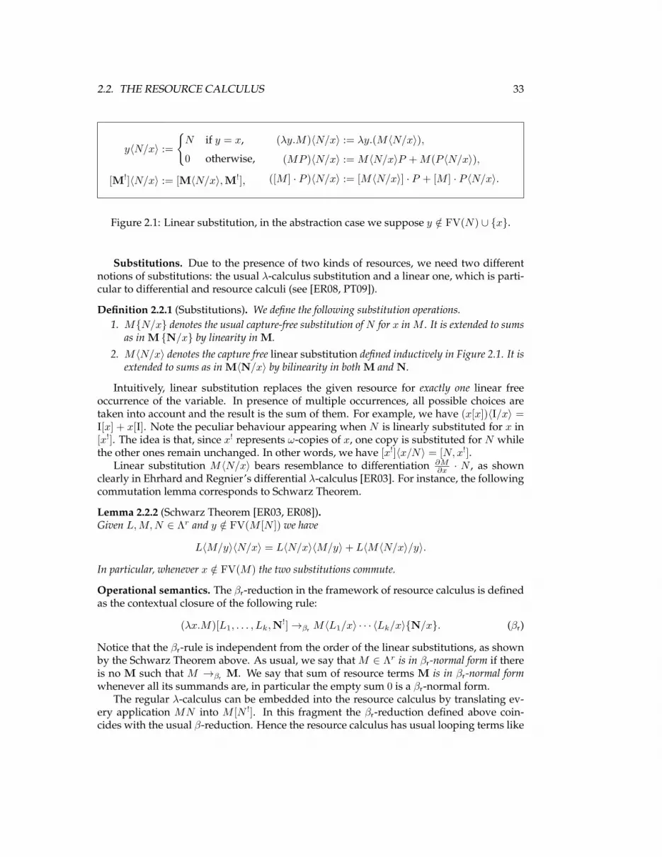
2.2. THE RESOURCE CALCULUS 33

y〈N/x〉 :=N if y = x,

0 otherwise,

[M!]〈N/x〉 := [M〈N/x〉,M!],

(λy.M)〈N/x〉 := λy.(M〈N/x〉),

(MP )〈N/x〉 := M〈N/x〉P +M(P 〈N/x〉),

([M ] · P )〈N/x〉 := [M〈N/x〉] · P + [M ] · P 〈N/x〉.

Figure 2.1: Linear substitution, in the abstraction case we suppose y /∈ FV(N) ∪ x.

Substitutions. Due to the presence of two kinds of resources, we need two differentnotions of substitutions: the usual λ-calculus substitution and a linear one, which is parti-cular to differential and resource calculi (see [ER08, PT09]).

Definition 2.2.1 (Substitutions). We define the following substitution operations.1. MN/x denotes the usual capture-free substitution of N for x in M . It is extended to sums

as in M N/x by linearity in M.2. M〈N/x〉 denotes the capture free linear substitution defined inductively in Figure 2.1. It is

extended to sums as in M〈N/x〉 by bilinearity in both M and N.

Intuitively, linear substitution replaces the given resource for exactly one linear freeoccurrence of the variable. In presence of multiple occurrences, all possible choices aretaken into account and the result is the sum of them. For example, we have (x[x])〈I/x〉 =I[x] + x[I]. Note the peculiar behaviour appearing when N is linearly substituted for x in[x!]. The idea is that, since x! represents ω-copies of x, one copy is substituted for N whilethe other ones remain unchanged. In other words, we have [x!]〈x/N〉 = [N, x!].

Linear substitution M〈N/x〉 bears resemblance to differentiation ∂M∂x · N , as shown

clearly in Ehrhard and Regnier’s differential λ-calculus [ER03]. For instance, the followingcommutation lemma corresponds to Schwarz Theorem.

Lemma 2.2.2 (Schwarz Theorem [ER03, ER08]).Given L,M,N ∈ Λr and y /∈ FV(M [N ]) we have

L〈M/y〉〈N/x〉 = L〈N/x〉〈M/y〉+ L〈M〈N/x〉/y〉.

In particular, whenever x /∈ FV(M) the two substitutions commute.

Operational semantics. The βr-reduction in the framework of resource calculus is definedas the contextual closure of the following rule:

(λx.M)[L1, . . . , Lk,N!]→βr M〈L1/x〉 · · · 〈Lk/x〉N/x. (βr)

Notice that the βr-rule is independent from the order of the linear substitutions, as shownby the Schwarz Theorem above. As usual, we say that M ∈ Λr is in βr-normal form if thereis no M such that M →βr M. We say that sum of resource terms M is in βr-normal formwhenever all its summands are, in particular the empty sum 0 is a βr-normal form.

The regular λ-calculus can be embedded into the resource calculus by translating ev-ery application MN into M [N !]. In this fragment the βr-reduction defined above coin-cides with the usual β-reduction. Hence the resource calculus has usual looping terms like


Ω := (λx.x[x!])[(λx.x[x!])!], but also terms like I1 or I[y, y] reducing to 0 because there isa mismatch between the number of linear resources needed by the functional part of theapplication and the number of resources it actually receives.

Pagani and Tranquilli proved the confluence of the resource calculus through an ap-propriate Standardization Theorem [PT09].

Theorem 2.2.3 (Confluence, Pagani and Tranquilli [PT09]).The βr-reduction is confluent on Λr.

The resource calculus is intensional. Indeed, just like in the regular λ-calculus, there aredifferent programs having the same extensional behaviour. The analogue of η-reductionfor the resource calculus is defined as the contextual closure of the following rule:

λx.M [x!]→ηr M, if x /∈ FV(M). (ηr)

Solvability has been studied by Pagani and Ronchi della Rocca in [PR10a, PR10b]. As inthe resource calculus terms appear in formal sums, various notions of solvability can arise,depending on the meaning associated with the sum. The interpretation of the + as an innerchoice operator corresponding to an angelic non-determinism arises naturally, because ofthe definition of 0 as the neutral element of the sum. However, the sum can be also seen asa parallel composition corresponding to a demonic non-determinism.

Definition 2.2.4. A closed resource term M is:• may-solvable whenever there are closed bags P1, . . . , Pn ∈ Λb such that M ~P =βr I + N,

for some N ∈ N〈Λr〉 (possibly N := 0).• must-solvable if there are closed bags P1, . . . , Pn ∈ Λb such that M ~P =βr I + · · ·+ I.

As in the formal sum of resource terms repetitions do matter, other notions of solvabil-ity may arise depending on the number of times one gets the identity I.

As in λ-calculus the solvability can be characterized in terms of head-normalization,the may-solvability of the resource calculus can be captured by “outer-normalization”.The outer-reduction →o, first defined in [PT09], corresponds to an evaluation where noreduction is made inside reusable resources. We say that a sum M of resource terms isin may-outer normal form whenever it is of the form M + N with M 6→o M′. Pagani andRonchi della Rocca proved that the may-outer normal form of M, if it exists, can be reachedby outer-reduction and that this is equivalent to ask that M is may-solvable. Inspired bythe relational semantics of λ-calculus, they also introduced a type system `m based onnon-idempotent intersection types in which a resource term M is typable if and only if itpossesses a may-outer normal form. Summing up, the following theorem holds.

Theorem 2.2.5 (Pagani, Ronchi della Rocca [PR10a, PR10b]).Given a closed resource term M , the following are equivalent:

1. M is may-solvable,2. M is reducible to a may-outer-normal form (by outer reduction),3. `m M : σ for some non-idempotent intersection type σ.

Problem 6. Is it possible to characterize the must-solvability of the resource calculus in terms ofouter-reduction and in terms of typability in a suitable type system?

A partial answer is given in [PR10a] for the fragment of Λr corresponding to the de-monic non-deterministic λ-calculus (therefore without linear resources).

2.3. THE TAYLOR EXPANSION 35

2.3 THE TAYLOR EXPANSION

The finite resource calculus is the fragment of resource calculus restricted to linear resources.In other words, every bag has the multiset of reusable resources which is empty. Theterms (resp. bags) of this fragment are called finite and their set is denoted by Λrf (resp. Λbf ).This sub-calculus is closed under βr-reduction, while ηr-reduction does not play any role.As linear resources cannot be duplicated, every reduction strictly decreases the size of aterm and the system is strongly normalizable [ER08] even if no typing is involved.

Taylor expansion of ordinary λ-terms. The Taylor expansion was originally introducedin [ER03] in the context of λ-calculus as a translation developing every application as aninfinite series of finite applications with rational coefficients. For our purposes, it is enoughto present the Taylor expansion as a map T (·) from Λ to possibly infinite sets of finiteresource terms. This simplified version corresponds to the support2 of the original Taylorexpansion. Given M ∈ Λ, the Taylor expansion T (M) of M is defined by induction as:

T (x) = x,T (λx.M) = λx.t | t ∈ T (M),T (MN) = tb | t ∈ T (M), b ∈Mf(T (N)).

The intuition is that in the λ-term MN the function M can either erase its argument Nor use it a certain amount of times during its execution. As we cannot determine thisnumber statically, we consider all possibilities henceforth the infinite set. Intuitively, theTaylor expansion T (M) can be seen as a resource sensitive version of App(M), where theapproximants keep track of the resources. Note that the resource approximants may notbe βr-normal, but are strongly normalizable, hence NFβr (T (M)) = NFβr (t) | t ∈ T (M).

The following result formalizes the intuition above.

Theorem 2.3.1 (Ehrhard and Regnier [ER08]).Given M,N ∈ Λ, we have BT(M) = BT(N) if and only if NFβr (T (M)) = NFβr (T (N)).

Taylor expansion of resource λ-terms. If in the study of usual λ-calculus we can chooseto use the Böhm trees or the Taylor expansion, depending on whether we need a grasp onresource usage, the situation is more constrained when studying the resource calculus.Indeed, at the moment, no convincing notion of Böhm tree has been developed for this cal-culus: first because one should consider forests of trees (to treat the non-determinism),second because one would have an alternation of commutative and non-commutativebranches (to treat the multisets). The resulting structure would not be easy to handle.

For this reason, in collaboration with Pagani, in [M19] we generalized the notion ofTaylor expansion to terms and bags of the resource calculus. We adopt for sets X ⊆ Λr(resp. Y,Z ⊆ Λbf ) the same abbreviations as introduced for finite sums, that is λx.X :=λx.M |M ∈ X, XZ := MP |M ∈ X,P ∈ Z and Y · Z := P1 · P2 | P1 ∈ Y, P2 ∈ Z.

Definition 2.3.2. The Taylor expansion of a resource term M ∈ Λr is the set T (M) ⊆ Λrfdefined in Figure 2.2. It is extended to sums as follows T (

∑iMi) =

⋃i T (Mi).

Problem 7. Is it possible to define a convincing notion of Böhm tree for the full resource calculus?

2I.e., the set of those finite terms appearing in the series with a non-zero coefficient.


T (x) = x, T (λx.M) = λx.T (M), T (MP ) = T (M)T (P ),

T ([M!]) =Mf(T (M)), T ([M ] · P ) = [T (M)] ·T (P ).

Figure 2.2: The Taylor expansion T (M) of a resource term M .

2.4 BÖHM THEOREM FOR RESOURCE CALCULUS

In collaboration with Pagani, we studied the separability of resource terms in [M19]. Ournotion of separability is inspired by the relational semantics of resource calculus (see §2.7).Semantically M +M is indistinguishable from M , so we assume that the + is idempotent.

The ordinary notion of separability is too strong for this calculus, as there are resourceterms like λxy.x[y!] and λxy.x[y] that cannot be separated by sending them to differentprojections, but they can be separated by sending the former to I and the latter to 0.

Definition 2.4.1 (Separability). Two closed resource termsM,N are separable if there are closedbags P1, . . . , Pk ∈ Λb such that MP1 · · ·Pk =βr I while NP1 · · ·Pk =βr 0.

Following the steps of Böhm in his pioneering work [Böh68], we focus our attention onnormal forms, which are easier to separate. However, in contrast with what happens inthe λ-calculus, there are βr-normal resource terms that cannot be separated even if they areηr-different. The typical example is given by λxyz.x[(z[y!])!] and λxyz.x[(z1+z[y, y!])!], theidea being that the ω-copies of y in the former are simulated in the latter as a erratic choicebetween zero and at least one copies. The attentive reader will notice that these terms havethe same Taylor expansion, and actually that is the reason why they cannot be separated.

Because of its infinitary nature, the property of having the same Taylor expansion looksrather semantical than syntactical. This property can be however characterized syntacti-cally by proving that T (M) = T (N) if and only if M ≡T N where ≡T is the congruencegenerated by setting [x!] = 1+[x, x!]. We let≡T

ηrbe the congruence generated by≡T ∪ =ηr .

Theorem 2.4.2 (Resource Böhm Theorem, Manzonetto and Pagani [M19]).Let M,N ∈ Λr be two closed resource terms in βr-normal form. If M 6≡T

ηrN then there are closed

bags P1, . . . , Pk ∈ Λb such that

M ~P =βr I, N ~P =βr 0. (or vice versa)

To obtain such a result we developed in [M19] a refined version of the Böhm-out tech-nique. Note that a crucial ingredient in the classic proof of the Böhm Theorem is the factthat it is possible to erase subterms in order extract from the λ-terms their structural dif-ference. This is not an easy task in Λr, because the linear resources must be consumedand cannot be erased. In this respect, our technique has some similarities with the onedeveloped to achieve the separation in the λI-calculus [Bar84, §10.5]. Moreover, since theargument of an application is a bag of resources, comparing a difference between two re-source terms may turn into comparing the differences between two multisets of terms, andthis problem presents analogies with that of separating a finite set of λ-terms [BDPR79].

2.5. DIFFERENTIAL CATEGORIES AND CARTESIAN CLOSEDNESS 37

2.5 DIFFERENTIAL CATEGORIES AND CARTESIAN CLOSEDNESS

Despite the fact that the differential λ-calculus is born from semantical considerations,namely Ehrhard’s deep analysis of coherent spaces, it took some years to provide a generalcategorical definition of its models. Inspired by Ehrhard’s work on differential λ-calculus,Blute, Cockett and Seely investigated the problem of axiomatizing a derivative operatorD(−) in the context of category theory. The authors started working in the monoidal settingand proposed a notion of monoidal differential category [BCS06]. By applying the co-Keisliconstruction, one obtains a Cartesian category having a differential operator.

Cartesian differential categories were introduced in [BCS09] to provide a direct axio-matization of the derivative operator in the Cartesian setting. The derivative of a mor-phism f : A→ B will be a morphism D(f) : A×A→ B linear in its first component.

f : A→ B

D(f) : A×A→ B(D)

In order to model differentiation in a category, we need to be able to sum its morphisms.Therefore, we consider left-additive categories, where each homset Hom(A,B) has a struc-ture of a commutative monoid and precomposition by any map preserves such a structure:

f ; (g + h) = (f ; g) + (f ;h) f ; 0 = 0.

A morphism f of a left-additive category is called additive if postcomposition by f alsopreserves the commutative monoid structure.

A left-additive category is Cartesian if it has finite products, the projections are additive,and the pairing 〈−,−〉 of additive morphisms is itself additive.

As expected, a morphism f is called linear whenever its derivative is constant, and alllinear morphisms are additive (while the converse does not hold in general).

Definition 2.5.1. A Cartesian differential category is a Cartesian left-additive category havingan operator D(−) that sends every f : A→ B into a morphism D(f) : A×A→ B and satisfying:(D1) D(f + g) = D(f) + D(g) and D(0) = 0,(D2) 〈h+ k, v〉; D(f) = 〈h, v〉; D(f) + 〈k, v〉; D(f) and 〈0, v〉; D(f) = 0,(D3) D(Id) = π1, D(π1) = π1;π1 and D(π2) = π2;π1,(D4) D(〈f, g〉) = 〈D(f),D(g)〉,(D5) D(g; f) = 〈D(g), π2; g〉; D(f),(D6) 〈〈g, 0〉, 〈h, k〉〉; D(D(f)) = 〈g, k〉; D(f),(D7) 〈〈0, h〉, 〈g, k〉〉; D(D(f)) = 〈〈0, g〉, 〈h, k〉〉; D(D(f)).

Therefore, intuitively the axiom (D1) states that the operator D(−) is linear; (D2) saysthat D(−) is additive in its first coordinate; (D3) and (D4) ask that D(−) behaves coherentlywith the product structure; (D5) is the usual chain rule; (D6) requires that D(f) is linear inits first component. (D7) states the independence of the order of “partial differentiation”.Indeed, in these categories partial derivatives are obtained from the full ones by “zeroingout” the components on which the differentiation is not required. For example, the partialderivative of a morphism f : C×A→ B on its first component C can be defined by setting

D1(f) = C × (C ×A) 〈Id,0〉×Id−−−−−−→ (C ×A)× (C ×A) D(f)−−−→ C × (C ×A)→ B.


Cartesian closed structure. In [BCS09], Blute, Cockett and Seely show that Cartesiandifferential categories are sound and complete models of a suitable term calculus. Thiscalculus has a derivative operator in the spirit of Ehrhard’s differential λ-calculus, butpossesses no λ-abstraction operator. It is therefore unlikely that these categories are wellsuited for modeling the resource calculus, that contains the whole λ-calculus as a sub-system. Indeed, in order to provide a categorical interpretation of λ-abstraction we needto have an isomorphism Hom(C × A,B) ∼= Hom(C, [A → B]) natural in both C and B,that is to say a Cartesian closed structure. However, it is not enough to have a Cartesiandifferential category which is moreover Cartesian closed to interpret the resource calculus.For this reason, in collaboration with Bucciarelli and Ehrhard, we introduced the notion of“Cartesian closed differential category” (called differential λ-category in [M5]).

The starting point is a Cartesian left-additive category C which is in addition Cartesianclosed and such that the currying Λ(−) satisfies the following axioms:

(Curry+) Λ(f+g) = Λ(f)+Λ(g) Λ(0) = 0 (Curry0)

In this case, we say that C is Cartesian closed left-additive. The axioms (Curry+) and (Curry0)are needed to ensure that currying Λ(−) is linear. From these properties, it follows that theevaluation map Eval : [A→ B]×A→ B is additive in its left component, as expected.

We ensure that the differential operator behaves correctly with respect to the Cartesianclosed structure by requiring the additional axiom (CurryD) below.

Definition 2.5.2. A Cartesian closed differential category is a Cartesian differential categorywhich is Cartesian closed left-additive and such that, for all f : C ×A→ B:

(CurryD) D(Λ(f)) = 〈π1 × 0A, π2 × IdA〉;Λ(D(f)).

In a Cartesian closed differential category it is possible to define an operator ? that canbe seen as the categorical counterpart of the linear substitution (Definition 2.2.1(2)):

f : C ×A→ B g : C → A

f ? g : C ×A→ B(?)

where f ? g = 〈〈0C×AC , π1〉; g, IdC×A〉; D(f). Intuitively, the morphism f ? g is obtained byforce-feeding the second argument A of f with one copy of the result of g. Notice that thetype is not modified because the morphism f ? g may still depend on its argument A.

Cartesian closed differential categories provide a sound model of the simply typedresource calculus, in which the sums and the elements of the bags are uniformly typed:

∆ ` 0 : A∆ `M : A ∆ `M : A

∆ `M + M : A∆ `M : A→ B ∆ ` P : A

∆ `MP : B

∆ ` 1 : A∆ ` L : A ∆ ` P : A

∆ ` [L] · P : A∆ `M : A ∆ ` P : A

∆ ` [M!] · P : A

Exploting the left-additive structure of a Cartesian closed differential category and theoperator ? above, it is not difficult to define the categorical interpretation of a judgementx1 : A1, . . . , xn : An `M : B as a morphism JMK∆ : A1 × · · · ×An → B.

Theorem 2.5.3 (Bucciarelli et Al. [M5]). Cartesian closed differential categories constitute soundmodels of the simply typed resource calculus.

2.6. CATEGORICAL MODELS OF RESOURCE CALCULUS 39

2.6 CATEGORICAL MODELS OF RESOURCE CALCULUS

The notion of Cartesian closed differential category is general enough to encompass manyexamples given in the literature, like Ehrhard’s finiteness spaces [Ehr05], Blute, Ehrhardand Tasson’s convenient categories [BET12], Kerjean and Tasson’s Mackey-completespaces [KT17], Harmer and McCusker’s category of non-deterministic games [HM99] andthe relational semantics. However, to interpret the untyped resource calculus we need re-flexive objects, while the categories presented in [Ehr05, BET12, KT17] do not possess any.

Linear reflexive objects. The resource calculus can be interpreted in a reflexive objectU of a Cartesian closed differential category provided that U satisfies some linearity con-ditions. Indeed, as the λ-abstraction of resource calculus is a linear operator, we need thatsuch a property is preserved by the morphisms performing the retraction.

Definition 2.6.1. A reflexive object U = (U, app, abs) of a Cartesian closed differential categoryis linear whenever the morphisms abs : [U → U ]→ U and app : [U → U ]→ U are linear.

The interpretation of a resource term M in a linear reflexive object U with respect to a sequence~x ⊇ FV(M) of length n is a morphism JMKU~x : Un → U defined by extending the usualcategorical interpretation of λ-terms as follows:

JM [L1, . . . , Ln,N!]KU~x = 〈Λ((· · · (Λ−(JMKU~x ; app) ? JL1KU~x ) · · · ) ? JLnKU~x ), JNKU~x 〉; Eval.

The interpretation is extended to sums by linearity: JM1+· · ·+MkKU~x = JM1KU~x+· · ·+JMkKU~x .

Theorem 2.6.2 (Manzonetto [M18]).Linear reflexive objects in differential Cartesian closed categories constitute sound models of theresource calculus.

Modeling the Taylor Expansion. Given a linear reflexive object U living in a Cartesianclosed differential category C it is interesting to check whether all resource terms havingthe same Taylor expansion get the same interpretation. As an interesting fact, this happensto be a property of the category rather than of the reflexive object under consideration.Since the definition of the Taylor expansion asks for infinite power series, we considerCartesian closed differential categories C where it is possible to add infinitely many mor-phisms. Formally, we require that for every countable set I and every family fii∈I ofmorphisms fi : A→ B there exists a morphism

∑i∈I fi ∈ Hom(A,B) and, in this case, we

say that C has countable sums.Remember that Definition 2.3.2 works under the assumption of an idempotent sum,

therefore we suppose that also our sums on the morphisms of the category is idempotent.

Definition 2.6.3. A Cartesian closed differential category models the Taylor Expansion if it hascountable sums and the following axiom holds (for every f : C ×A→ B and g : C → A):

Eval; 〈f, g〉 =∑k∈N

((· · · (Λ−(f) ? g) · · · ) ? g︸︷︷︸k times

); 〈Id, 0〉. (Taylor)

As a consequence, all models living in a category modeling the Taylor expansion equateall resource terms having the same Taylor expansion. From Theorem 2.3.1 it follows thatall λ-terms having the same Böhm trees get the same interpretation in such models.


Equational Completeness. An important result concerning λ-calculus is the equationalcompleteness theorem proved by Scott in [Sco80] and subsequently refined by Koymansin [Koy82]. The theorem states that every λ-theory T is the theory of a reflexive objectU in a Cartesian closed category C. In other words the completeness theorem guaran-tees that the definition of model of λ-calculus under consideration is general enough torepresent all λ-theories. This classical result is achieved in two steps:

(i) given a λ-theory T one proves that the set ΛT of λ-terms modulo T together with theapplication operator defined between equivalence classes constitutes a λ-modelMT(called the term model of T ) having as theory exactly T ;

(ii) by applying toMT a construction called Karoubi envelope [Kar78], which consists insplitting the idempotents, one builds a (very syntactic) Cartesian closed category CTin which the identity I is a reflexive object such that Th(I) = T .

Summing up, the idea of the proof is to find suitable λ-terms to encode the structure of thecategory (pairing, currying, evaluation, and the like) and prove that they actually define acategory with a Cartesian closed structure.

In [M18], we investigated the question whether the categorical notion of model pre-sented above is complete. Using the resource calculus, it is possible to define a syntacticCartesian closed differential category. On the one hand, the categorical operator D(−) isunproblematic since it can be easily defined in terms of linear application. On the otherhand, the encoding of categorical pairing 〈f, g〉 used by Scott is not additive. Indeed,such pairing is defined starting from Church’s encoding of the pair in λ-calculus givenby 〈f, g〉 := λx.xfg with projections π1 := K, π2 := K′. Obviously with this definition wehave 〈f1 + f2, g1 + g2〉 6= 〈f1, g1〉+ 〈f2, g2〉 since the sums do not occur in linear position3.

This problem can be circumvented by providing a different encoding of the pairing inthe resource calculus:

〈〈M,N〉〉 := λx.x[λy.M ] + λx.x[λy.y[N ]], for some y /∈ FV(M,N),

with projections π1 := λx.x1 and π2 := λx.x[I]. This encoding is inspired by the set-theoretical definition of ordered pair: intuitively the pair of M,N is the set containingM,N (the sum is representing the union) where the elements have been slightly modifiedin order to distinguish them. In our case, such a distinction consists in the number of linearresources they can receive (zero for the first component and one for the second).

With this encoding we are able to show that every equational theory T of the resourcecalculus gives rise to a category CT with a structure of differential Cartesian closed cate-gory, under the assumption that the sum is idempotent (like set-theoretical union) and thatthe Karoubi envelope splits idempotents which are linear.

Theorem 2.6.4 (Manzonetto [M18]).For all equational theories T of the resource calculus satisfying sum idempotency we have:

(i) CT is a differential Cartesian closed category,(ii) the identity I is a linear reflexive object.

Problem 8. Is it possible to prove an equational completeness theorem for categorical models of re-source calculus without assuming an idempotent sum? (See [CG16] for preliminary investigations,notice however that the authors prove completeness for another ad hoc differential calculus.)

3Recall that in λ-calculus the λ-abstraction is linear but the application is only linear in its left-component.

2.7. RELATIONAL MODELS OF RESOURCE CALCULUS 41

2.7 RELATIONAL MODELS OF RESOURCE CALCULUS

We mentioned in Section 1.3 that MRel is a Cartesian closed category. Notice that since theCartesian structure is given by the disjoint union, which will be denoted by &, there existsa Seely isomorphism betweenMf(A&B) andMf(A)×Mf(B). In particular, a morphismf : A&B → C will be systematically presented as a relation f ⊆Mf(A)×Mf(B)× C.

Cartesian differential structure. We are now going to expose the differential structureof MRel. As relations are closed under arbitrary union, every homset can be endowed witha structure (MRel(A,B),∪, ∅) of commutative monoid in such a way that precompositionby any map preserves this structure. It is easy to check that pairing preserves additivityand that currying is linear, therefore the category is Cartesian closed left-additive and hascountable sums. Moreover, given a morphism f : A→ B its derivative is given by:

D(f) = (([α], a), β) | ([α] ] a, β) ∈ f : A&A→ B.

Again, it is not difficult to check that the operator D(−) satisfies all the axioms of a Carte-sian closed differential category. Summing up, the following theorem holds.

Theorem 2.7.1 (Manzonetto [M18]).The category MRel is a Cartesian closed differential category.

Relational models of resource calculus. In the category MRel, a morphism f : A→ Bis linear when its behaviour is specified on the singleton multisets of A, that is (a, α) ∈ fentails that the multiset a is a singleton. Thus, every reflexive object U having abs and appsatisfying this property is linear. As a consequence we get that every rgm D = (D, i) islinear, since the induced retraction pair is of the following form:

• abs = ([(a, α)], a→ α) | a ∈Mf(D), α ∈ D : [D → D]→ D,

• app = ([a→ α], (a, α)) | a ∈Mf(D), α ∈ D : D → [D → D],where a → α is a notation for i(a, α) following the intuition given in Section 1.3. ByTheorem 2.6.2 rgms constitute sound models of the untyped resource calculus.

Definition 2.7.2. The interpretation of resource terms M ∈ Λr, sums of terms M ∈ N〈Λr〉 andbagsP ∈ Λb in an rgmD (with respect to a sequence ~x including their free variables) are morphismsJMKD~x , JMKD~x : D~x → D, JP KD~x : D~x →Mf(D) defined by mutual induction as follows:

• JM1 + · · ·+MkKD~x = JM1KD~x ∪ · · · ∪ JMkKD~x ,• JxiKD~x = (([], . . . , [], [α], [], . . . , []), α) | α ∈ D, where [α] stands in i-th position,• Jλy.MKD~x = (~a, b→ α) | ((~a, b), α) ∈ JMKD~x,y, where we suppose that y /∈ ~x,

• JMP KD~x = (~a1 ] ~a2, α) | ∃b ∈Mf(D) (~a1, b→ α) ∈ JMKD~x , (~a2, b) ∈ JP KD~x ,• J[L1, . . . , Lk,N!]KD~x = (]k+m

r=1 ~ar, [β1, . . . , βk+m]) | (~aj , βj) ∈ JLjKD~x , 1 ≤ j ≤ k and(~ai, βi) ∈ JNKD~x , k < i ≤ k +m,

where ~a denotes a sequence of multisets (a1, . . . , an) and, given a sequence~b = (b1, . . . , bn) havingthe same length, ~a ]~b denotes the pointwise multiset union (a1 ] b1, . . . , an ] bn).

By structural induction on M , one can verify that the analogue of Theorem 1.3.2 holds.

Theorem 2.7.3 (The Approximation Theorem for Taylor Expansion [M18]).Given a relational graph model D and a closed resource term M , we have that:

σ ∈ JMKD ⇐⇒ ∃t ∈ T (M) such that σ ∈ JtKD.


2.8 Dω IS NOT FULLY ABSTRACT FOR THE RESOURCE CALCULUS

The original relational analogue of Scott’s D∞ was defined in [M3] as part of an investiga-tion on non-well-pointed semantics of λ-calculus. The idea is to start building a family ofsets (Dn)n∈N by induction on n:

• D0 = ∅,• Dn+1 =Mf(Dn)(ω),

whereMf(A)(ω) denotes the set of infinite sequences (a0, a1, . . . , ai, . . . ) of finite multisetsofA satisfying the property ai 6= [] only for a finite number of indices i. Since the operationA 7→ Mf(A)(ω) is monotonic on sets, and sinceD0 ⊆ D1, we haveDn ⊆ Dn+1 for all n ∈ N.

The reflexive object is given by the union D =⋃n∈NDn. Indeed, to define an isomor-

phism in MRel between D and [D → D] it is enough to remark that every element α =(a0, a1, a2, . . . ) ∈ D is canonically associated with the pair (a0, (a1, a2, . . . )) ∈ Mf(D) ×Dand vice versa. It is easy to check that the reflexive object obtained by this construction isisomorphic to the rgmDω having a single atom ε and generated by the equation []→ ε = ε.Under this isomorphism the element ε corresponds to the infinite sequence ([], [], [], . . . ).

Observational equivalence. By collecting the results in the previous sections we knowthat the model Dω is extensional and equates all resource terms having the same (normalform of the) Taylor expansion. In particular, JMKDω 6= ∅ exactly when M is may-solvable.Moreover, when considered as a model of λ-calculus, Dω is fully abstract forH∗ [M17].

These considerations led us to conjecture in [M18] that the equality induced by Dω onresource terms coincides with the following observational equivalence, where we take asobservables the may-outer normal forms of [PR10b].

Definition 2.8.1 (Observational Equivalence and Preorder).Given two closed M,N ∈ Λr, we set M ≡monf N , whenever for all closed bags P1, . . . , Pn ∈ Λb:

MP1 · · ·Pn is may-solvable ⇐⇒ NP1 · · ·Pn is may-solvable

The observational preorder vmonf is defined by orienting the equivalence from left to right.

The failure of full abstraction. Breuvart, during his PhD studies, found a counterex-ample to the full abstraction of Dω for ≡monf , a result subsequently published in [Bre13].

The key idea is to exhibit a resource term A that is observationally above the identity I,but whose interpretation inDω does not contain [ε]→ ε (while, obviously, [ε]→ ε ∈ JIKDω ).Using a fixed point combinator, it is possible to define a term A such that, for all k:

A =βr Σkn=1An + A′ where An = λy1 . . . ynx.x[I[y!1] · · · [y!

n]].

Clearly, if IP1 · · ·Pn is solvable then also AP1 · · ·Pn =βr AnP1 · · ·Pn + A′P1 · · ·Pn is solv-able. On the other side, the interpretation JAKDω =

⋃n∈NJAnKDω is incomparable with the

interpretation of the identity since none of the An’s contains [ε] → ε in its semantics. Asimilar reasoning shows that A ≡monf I[I!,A!] while JAK 6= JI[I!,A!]K.

Theorem 2.8.2 (Breuvart [Bre13]).The relational model Dω of resource calculus is not fully abstract for ≡monf (nor for vmonf ).

Problem 9. Show that the relational semantics does not contain any model fully abstract for theresource calculus.

2.9. ADDING CONVERGENCY TESTS TO ACHIEVE FULL ABSTRACTION 43

2.9 ADDING CONVERGENCY TESTS TO ACHIEVE FULL ABSTRACTION

As shown by Breuvart, the applicative contexts of resource calculus are not powerfulenough to discriminate all the terms which are different in Dω . To achieve full abstrac-tion we decided, together with Bucciarelli, Carraro and Ehrhard, to endow the resourcecalculus with new constructions, to be understood as implementing a very simple excep-tion mechanism, and with a “must” parallel composition [M1]. This is part of a traditionthat consists in varying the language to fit an intended model: for instance, Plotkin neededto extend PCF with a parallel or in order to find a fully abstract continuous model [Plo77].

Convergency tests. The resource calculus with tests [M1, M2] is obtained by extendingthe syntax of resource calculus as follows:

(Λτ ) M,N,L ::= · · · | τ(Q) (Λτ ) Q,R ::= τ [L1, . . . , Lk]

where Λτ is the set of terms (which includes Λr) and Λτ is the set of (convergency) tests.Tests are “corked” multisets of terms having only two possible outcomes: either success,

which is given by the empty test τ1, or failure, given by the empty sum 0. Intuitively,the test τ [L1, . . . , Lk] represents the must-parallel composition of τ [L1] ‖ · · · ‖ τ [Lk] andtherefore it succeeds when all of its components succeed. Consequently, we will sometimesuse the notation τ [L1, . . . , Lk] ‖ τ [Lk+1, . . . , Ln] for the test τ [L1, . . . , Ln].

The operator τ(·) allows to build a term out of a test: intuitively, the term τ(Q) maybe thought of as Q preceded by an infinite sequence of dummy λ-abstractions (like a µ-abstraction of Parigot’s λµ-calculus [Par92] over un unnamed variable). Dually, the “corkconstruction” τ [L1, . . . , Lk] may be thought of as an operator applying to all its argumentsan infinite sequence of empty bags. This suggests that it is sound to reduce τ [τ(Q)] to Q.

Hence the term τ(Q) raises an exception encapsulating Q and the test τ [L1, . . . , Lk]catches the exception possibly raised by any of the Li’s and replaces Li by the multisetof terms encapsulated in that exception. The context of the exception is thrown away bythe dummy abstractions of τ and the dummy applications of τ . A test needs to catch anexception in order to succeed; for instance, τ [M ] fails as soon as M is a τ -free, closed term.

All the notions and notations of resource calculus are extended as follows.• the meta-syntax concerning sums of terms M and sums of tests Q:

τ [ΣiMi] := Σiτ [Mi], (ΣiRi) ‖ Q := ΣiRi ‖ Q, τ [ΣiRi] := Σiτ [Ri],

• the substitution MN/x (defined as expected) and the linear substitution M〈N/x〉:

τ(Q)〈N/x〉 = τ(Q〈N/x〉), τ [L1, . . . , Lk]〈N/x〉 = Σki=1τ [L1, . . . , Li〈N/x〉, . . . , Lk],

• the reduction semantics extends (βr) with the following rules:

τ [λx.M ]→τ τ [M0/x], τ [τ(Q)]→γ Q, τ(Q)[M!]→τ τ(Q), τ(Q)([L]·P )→τ 0.

In this framework the convergence of a term can be verified through suitable test-contexts.A test-context CL−M is a test having a single occurrence of its hole L−M, appearing in term-position. We write CLMM for the result of substituting M for the hole L−M in C, possiblywith capture of free variables. According with the intuition of such a test mechanism, wesay that a test Q converges, notation Q↓, if there exists a sum Q such that Qβrττγ τ [] + Q.

Definition 2.9.1. Two resource terms M,N with tests are observationally equivalent, writtenM ≡τ N , whenever ∀CL−M . CLMM↓ ⇐⇒ CLNM↓.


Interpreting the tests. At first sight, these convergency tests may seem an ad hoc syntac-tic tool with no logical content. In reality, this extension already appeared in a differentiallinear logic setting [EL10]: τ corresponds to the 0-ary tensor and τ to the 0-ary par cells.The parallel composition of tests can be obtained by combining the mix rule of linear logic,if available, with the contraction rule.

The resource calculus with tests has a natural denotational interpretation in Dω . In-deed, an element of Dω can be described as a finite tree alternating two kinds of layers:

• multiplicative layers where subtrees are indexed by natural numbers,• exponential layers where subtrees are organized as non-empty multisets.

To be more precise, `−? (negative) pairs of layers alternate with ⊗−! (positive) pairs, re-specting a strict polarity discipline very much in the spirit of Ludics [Gir03]. The emptypositive multiplicative tree corresponds to the empty tensor cell and the negative one to theempty par cell. The corresponding constructions τ , τ are therefore quite easy to interpret.

Definition 2.9.2. We extend Definition 2.7.2 by setting Jτ(Q)K~x = (~a, ε) | ~a ∈ JQK~x, whereJQK~x ⊆ D~xω represents the interpretation of a test Q with respect to a sequence ~x in Dω satisfying:

Jτ [M1, . . . ,Mk]K~x = ~a1 ] · · · ] ~ak | (~ai, ε) ∈ JMiK~x.Keeping in mind the logical interpretation of the elements ofD, we are able to associate

with each α ∈ Dω , a test-context α+L·M with a hole L·M for a term.

Definition 2.9.3. For α ∈ Dω of the form [α11, . . . , α

1k1

] → · · · → [αr1, . . . , αrkr] → ε, we define

by mutual induction a term α– and a test-context α+L·M by:• α– = λx1 . . . xr.τ(‖ri=1 ((αi1)+LxiM ‖ · · · ‖ (αiki

)+LxiM)),• α+L·M = τ [L·M[(α1

1)–, . . . , (α1k1

)–] · · · [(αr1)–, . . . , (αrkr)–]].

The test-context α+L−M and the term α– are built in such a way that Jα+LxMKx = [α]and Jα–K = α, from which it follows that Dω has the finite definability property. More-over, for all α ∈ Dω we have that α+Lα–M βrττγ ε, while α+Lβ–M βrττγ 0 for all β 6= α.From these properties and the fact that !-free terms are strongly normalizable we get:

Lemma 2.9.4. Given a closed !-free term M of resource calculus with tests, we have:

α ∈ JMK ⇐⇒ α+LMM↓As a consequence, we derive easily a full abstraction result for the promotion free frag-

ment of the resource calculus with tests. To infer the analogous result for the full calculus,we need to extend the Taylor expansion of Section 2.3 to resource terms with tests:

T (τ(Q)) = τ(Q′) | Q′ ∈ T (Q),T (τ [M1, . . . ,Mk]) = τ [M ′1, . . . ,M ′k] |M ′i ∈ T (Mi), for 1 ≤ i ≤ k.

We then exploit the fact that Dω models this kind of Taylor expansion as well as a simu-lation lemma which relates the outer-reduction of a term with the outer-reduction of itsTaylor expansion to prove that JMK = JNK if and only if M ≡τ N .

Theorem 2.9.5 (Bucciarelli et Al. [M1, M2]).The model Dω is fully abstract for the resource calculus with tests.

Problem 10. Is it possible to find a fully abstract model of the untyped resource calculus in cate-gories of games?

3Nondeterminism in the Quantitative SettingIn which we show that not only the relational semantics is well suited for modeling bothparallel composition and nondeterministic choice, but also that adding coefficients fromsemirings opens the way to capture several quantitative properties of programs.

• A Relational Semantics for Parallelism and Non-Determinism in a Functional Set-ting. A. Bucciarelli, T. Ehrhard and G. Manzonetto.Annals of Pure and Applied Logic, Vol. 163, issue 7, pp. 918-934, 2012.

• Call-By-Value Non-Determinism in a Linear Logic Type Discipline.A. Diaz-Caro, G. Manzonetto and M. Pagani.Proc. of Symposium on Logical Foundations of Computer Science 2013, Volume 7392of Lecture Notes in Computer Science, pp. 364-376, 2013.

• Constructing Differential Categories and Deconstructing Categories of Games.J. Laird, G. Manzonetto and G. McCusker.Long version. Information and Computation, Volume 222, Issue C, pp. 247-264, 2013.

• Constructing Differential Categories and Deconstructing Categories of Games.J. Laird, G. Manzonetto and G. McCusker.International Conference on Automata, Languages and Programming - Part II(ICALP 2011), Volume 6756 of LNCS, pages 186-197, 2011.

• Weighted Relational Models of Typed Lambda-Calculi.J. Laird, G. Manzonetto, G. McCusker and M. Pagani.28th Annual ACM/IEEE Symposium on Logic in Computer Science (LICS 2013), pp.301-310, 2013.

When I introduced, together with Bucciarelli and Ehrhard, the relational modelDω , we quickly realized that the semantic counterparts of may and must non-determinism were at hand. During my ATER at the University Paris-Diderot

(2008) we investigated the situation in detail and proved that Dω constitutes an adequatemodel for a λ-calculus endowed with parallel composition and nondeterministic choice.Subsequently, together with Pagani and Díaz-Caro, I showed that an analogous construc-tion can be done in the call-by-name setting, and that an element in the interpretation of aterm carries enough information to compute a bound for the number of reduction steps.

During my postdoc in Nijmegen (2011), I visited McCusker and Laird in Bath andwe started a collaboration for defining and investigating differential categories based ongames. Starting from a work of Melliès, Tabareau and Tasson we were able to provide anabstract canonical categorical construction for building differential categories, and recon-struct the relational semantics and categories of games as instances.

Subsequently (2013), in a larger collaboration including Pagani, we generalized the re-lational semantics by replacing relations from A and B with matrices indexed by A andB and populated by scalars from a continuous semiring R. This gives a weighted re-lational semantics which is an adequate model of a nondeterministic extension of PCF ,parametrized by R. Specific instances of R allow us to compare programs not only withrespect to “what they can do”, but also “in how many steps” or “in how many differentways” (for nondeterministic PCF) or even “with what probability” (for probabilistic PCF).

45

46 CHAPTER 3. NONDETERMINISM IN THE QUANTITATIVE SETTING

3.1 NONDETERMINISM IN A FUNCTIONAL SETTING

It is well known that the λ-calculus is a deterministic functional programming language.At each reduction step, one could choose nondeterministically which β-redex to contract,but the confluence of the system assures that the outcome of a program, if any, is unique.Thus, λ-terms can be thought of as specifications of sequential, deterministic processes.

Several extensions of λ-calculus with parallel and nondeterministic constructs havebeen proposed in the literature. The purpose was either to increase the expressive powerof the language, in the typed [Plo77, Pao06, Lai06] and untyped [Bou94, BL96] settings, orto study the interplay between higher-order and parallel or nondeterministic features ofthe language [Ong93, DdP96, DdP98]. When introducing nondeterminism in a functionalsetting, the same program can produce different results depending on its evaluation.

As briefly discussed in Section 2.2 (pag. 34), it becomes crucial to specify what notionof convergence is considered. Two widely used notions are:

• the may convergency: a nondeterministic choice converges if at least one of its com-ponents does. This characterizes the angelic nondeterminism;

• the must convergency: a nondeterministic choice converges whenever all its compo-nents converge. This characterizes the demonic nondeterminism.

Capturing nondeterministic behaviour in higher order languages presents a challenge forthe usual denotational models based on domains. Consider two programs P1 and P2 con-verging respectively to values v1 and v2 having incompatible denotations. What semanticvalue should take the nondeterministic program P1 +P2 that may converges either to v1 orto v2? The resulting value should be some sort of “aggregation” of v1 and v2 that could beunavailable in the domain.

The typical techniques for interpreting “multi-valued” programs, like the ones de-scribed above, consist in using models based on Plotkin’s powerdomains [Plo76]. Roughlyspeaking, a powerdomain P(D) is a domain whose elements are subsets of a domain D.The denotation of a nondeterministic program P is a set-valued function inD, that is a func-tion mapping an input d ∈ D into a set d1, . . . , dk ∈ P(D) containing all the possiblevalues produced by P starting from the input d. Similar techniques are also used for inter-preting the must nondeterminism. In this framework, both kinds of nondeterminism aremodelled by some idempotent, commutative and associative operations.

In [FM09], Faure and Miquel defined the aggregation monad as a categorical counterpartof parallel execution. Powerdomains, sets with union and multisets with multiset unionare all instances of aggregation monads (in categories of domains and of sets, respectively).In general, the notion of parallel composition is modelled by an aggregation monad that isneither idempotent, nor commutative, nor associative. There are however models of mul-tiplicative exponential linear logic, where aggregation can be interpreted by the mix rule,if available. This rule allows to “put together” any two proofs whatsoever [DK00]. Moreprecisely, parallel composition is obtained by combining the mix rule with the contractionrule. Indeed, mix can be seen as a linear morphism X ⊗ Y ( X ` Y , so that there is amorphism ?A⊗ ?A( ?A, obtained by composing the mix morphism ?A⊗ ?A( ?A` ?Awith the contraction morphism ?A ` ?A( ?A. This composite morphism defines a com-mutative algebra structure on ?A, which is used to model the “parallel composition” ofMELL proofs. Therefore, in order to obtain a categorical model of parallel λ-calculus, it issufficient to solve the equation D ∼= D → D, with an object D of shape ?A.

3.2. MREL AS QUANTITATIVE SEMANTICS OF NONDETERMINISM 47

3.2 MRel AS QUANTITATIVE SEMANTICS OF NONDETERMINISM

In the relational semantics of λ-calculus, presented in Section 1.3, a program of typeA→ Bis interpreted as a relation from Mf(A) to B. The fact that the programs are interpretedas relations rather than functions is related with the intrinsic nondeterminism of the se-mantics while the multiplicities in the multiset keep track of how many times a resourceis needed during the computation. For instance, the program P := λn.n ∗ n : N → Nimplementing the square product is interpreted in the relational semantics as follows:

JP K = ([n1, n2], k) | n1 · n2 = k.

Indeed, P uses its input n twice and each call can give as answer a different number nibecause of the nondeterminism of the system. Since relations are closed under arbitraryunions, the may nondeterminism can be interpreted directly as set-theoretical union, with-out introducing any additional powerdomain construction or aggregation monad. In theparticular case of our relational model Dω , whose construction is recalled in Section 2.8,we are considering an object satisfying the recursive equation Dω = ?A where A = (DN

ω)⊥.Hence, Dω has the commutative algebra structure discussed in Section 3.1. It is preciselythis structure that we use for interpreting parallel composition, just like Danos and Krivinedid in [DK00] for an extension of λµ-calculus with a parallel composition operation.

More concretely, given two elements σ, τ ∈ Dω we can always represent them as:

σ = a1 → · · · → an → ε τ = b1 → · · · → bn → ε

where ε is the special element of Dω satifying ε = []→ ε. Therefore, it is possible to definea merging operator σ τ = (a1 ] b1)→ · · · → (an ] bn)→ ε using mix and contraction.

As a consequence, in the model Dω , the semantic counterparts of may and must nonde-terminism are at hand: they are the set-theoretic union and the mix-based operation . Inthis framework, parallel composition is no longer idempotent: this is quite natural if weconsider each component of a parallel composition as the specification of a process whoseexecution requires the consumption of some resources.

Non-determinism in call-by-name. In [M6], together with Bucciarelli and Ehrhard,we introduced the λ+‖-calculus, an untyped λ-calculus whose terms are extended withmay nondeterministic choice and must parallel composition:

Λ+‖ : M,N,P,Q ::= x | λx.M | MN | M +N | M ‖ N

The elements of Λ+‖ are called λ+‖-terms. This calculus is endowed with a pretty standardcall-by-name operational semantics, defined in terms of head reduction→h in Figure 3.1.

The intuitive idea behind this notion of head-reduction is the following:• when a λ+‖-term of the formM1 +M2 gets in head position, either of the alternatives

may be chosen to pursue the head reduction. If either M1 or M2 converges, then alsothe global program converges.

• when a λ+‖-term of the form M1 ‖ M2 gets in head position, the head reductioncontinues the computations in parallel. In particular, if either M1 or M2 does notterminate, then also the global program diverges.

The operational value of a λ+‖-term M is therefore the set of all head-normal forms thatcan possibly be reached starting from M . Accordingly, we say that a closed λ+‖-term Mconverges whenever there is a reductionM h N1 ‖ · · · ‖ Nk where eachNi is head normal.


βh-reduction +-reductions ‖-reductions(λx.M)N →h MN/x M +N →h M

M +N →h N(M ‖ N)P →h MP ‖ NP

Contextual rules

M →h M′

λx.M →h λx.M′

N →h N′

N ‖ M →h N′ ‖ M

M →h M′

N ‖ M →h N ‖ M ′M →h M

′ M 6= λx.Q, Q1 ‖ Q2

MN →h M′N

Figure 3.1: Operational semantics of the call-by-name λ+‖-calculus (head-reduction).

The λ+‖-calculus can be interpreted in the model Dω as expected.

Definition 3.2.1. The interpretation JMKDω

~x ⊆ Mf(Dω)~x × Dω of a λ+‖-term M in Dω withrespect to a sequence of variables ~x ⊇ FV(M) extends the usual definition as follows:

• JM1 +M2KDω

~x = JM1KDω

~x ∪ JM2KDω

~x ,

• JM1 ‖M2KDω

~x = (~a ] ~b, σ τ) | (~a, σ) ∈ JM1KDω

~x , (~b, τ) ∈ JM2KDω

~x ,where ~a ] ~b is the componentwise union and denotes the mix-based operation defined previously.

By generalising Girard’s reducibility candidates to the framework of λ+‖-calculus, wewere able to prove that the model Dω is adequate. This means that the λ+‖-term M con-verges exactly when its interpretation in Dω is non-empty.

Theorem 3.2.2 (Bucciarelli et Al. [M6]).For all M ∈ Λ+‖, JMKDω 6= ∅ if and only if M h N1 ‖ · · · ‖ Nk and each Ni is head-normal.

This model is not fully abstract for the observational equivalence which is associatedwith our notion of convergency. The counterexample is very simple, just consider the iden-tity I and I ‖ I, that are observationally indistinguishable, and verify that their interpreta-tions JIKDω = [σ]→ σ | σ ∈ Dω and JI‖ IKDω = [σ, σ]→ (σ σ) | σ ∈ Dω are different.The lack of full abstraction is related with the fact that parallel composition is idempotentfrom the operational point of view, whilst it is not idempotent from the denotational one.

Notice that, until now, we have used the logical structure of the model Dω but wedid not really exploit its quantitative properties. In [dC09] de Carvalho has shown thatEngeler’s rgm E can be presented as an intersection type system, called system R, wherethe intersection is not idempotent. The lack of idempotency is the key ingredient to modelthe resource sensitiveness: while in the usual intersection type systems `M : σ ∧ τ standsfor “M can be used either as data of type σ or as data of type τ”, when the intersection isnot idempotent the meaning becomes “M will be called once as data of type σ and once asdata of type τ”. Hence, types should no longer be understood as sets of terms, but rather assets of calls to terms. Moreover, de Carvalho proved that system R, beyond characterisingconverging terms, carries information on the evaluation sequence as well — the size of aderivation tree typing a term gives a bound on the number of steps needed to reach a headnormal form. Similar results are obtained in [BL11] for a variant of system R characterisingstrong normalisation and giving a bound to the longest β-reduction sequence.


βv-reduction +-reductions ‖-reductions(λx.M)V →h MV/x M +N →h M

M +N →h N(M ‖ N)P →h MP ‖ NPV (M ‖ N)→h VM ‖ V N

Contextual rules

M →h M′

M ‖ N →h M′ ‖ N

N →h N′

M ‖ N →h M ‖ N ′M →h M

′ M 6= P ‖ QMN →h M

′N

M →h M′ M 6= P ‖ Q

VM →h VM′

Figure 3.2: Operational semantics for the call-by-value λ+‖-calculus (weak reduction).

Non-determinism in call-by-value. Together with Díaz-Caro and Pagani, we haveshown in [M12] that the approach followed in call-by-name, also works in the call-by-valuesetting [RP04]. The terms of the call-by-value λ+‖-calculus are the same as in call-by-name,but we also consider a subset V+‖ ⊆ Λ+‖ of values generated by:

V+‖ : V ::= x | λx.M

This calculus is endowed with a call-by-value operational semantics, defined in terms ofweak head reduction in Figure 3.2. The terminology “call-by-value” refers to the fact thata head-redex (λx.M)N can only be contracted when N is a value, while “weak” mans thatwe do not reduce under a λ-abstraction. In this context we say that a closed λ+‖-term Mconverges whenever there is a reduction M h V1 ‖ · · · ‖ Vn for some Vi ∈ V+‖.

In [Ehr12], Ehrhard introduced a non-idempotent intersection type system charac-terising the convergence of the deterministic call-by-value λ-calculus. This system isbased on the so-called second Girard’s translation of intuitionistic logic into linear logicA → B = !(A ( B) [Gir87, MOTW99]. In order to deal with the must nondetermi-nism, namely the parallel composition, we modify the translation by mapping the call-by-value λ-calculus into the polarised fragment of linear logic, as described by Laurentin [Lau02]. Then, our typing system is describing an object V in Rel satisfying the equa-tion V ' !V ( ?!V , where the connectives ? and ! are interpreted by the finite multisetcomonad. Following the approach used in call-by-name, the composition of the mix ruleand the contraction rule yields an operation ?!V ⊗ ?!V ( ?!V which is used to interpret theparallel composition.

To avoid a clumsy notation with multisets of multisets, we prefer to denote a !-multiset[ρ1, . . . , ρm] (the type of a computation) with the linear logic multiplicative conjunctionρ1⊗· · ·⊗ρm and a ?-multiset [σ1, . . . , σn] (the type of a parallel composition) with the multi-plicative disjunction σ1` · · ·`σn. Such a notation stresses the fact that the non-idempotentintersection type systems issued from Rel are essentially contained in the multiplicativefragment of linear logic.

The set T‖ of (parallel) types and the set C of computational types are generated by thefollowing grammar:

parallel-types T‖: σ, τ ::= σ ` τ | ρcomputational-types C: ρ, ν ::= 1 | ρ⊗ ν | ρ( σ


x : ρ `V x : ρ (ax)Γi, x : ρi `V M : σi 1 ≤ i ≤ n ≥ 0⊗ni=1Γi `V λx.M : ⊗ni=1(ρi( σi)

(I

Γ `V M : `ki=1(⊗nij=1(ρij ( σij)) Γi `V N : `ni

j=1ρij 1 ≤ i ≤ k k ≥ 1 ni ≥ 1Γ⊗ (⊗ki=1Γi) `V MN : `ki=1(`ni

j=1σij)((E)

Γ `V M : σΓ `V M +N : σ (+`)

Γ `V N : σΓ `V M +N : σ (+r)

Γ1 `V M : σ1 Γ2 `V N : σ2Γ1 ⊗ Γ2 `V M ‖ N : σ1 ` σ2

(‖I)

Figure 3.3: Type system for the call-by-value λ+‖-calculus.

For the sake of simplicity, types are considered up to associativity and commutativity ofthe tensor⊗ and the par `. The type 1, which is the only atomic type, represents the emptytensor and is therefore its neutral element (i.e. ρ⊗ 1 = ρ). Accordingly, we write⊗ni=1ρi forρ1 ⊗ · · · ⊗ ρn when n ≥ 1, and for 1 when n = 0. Similarly, when n ≥ 1, `ni=1αi stands forσ1 ` · · · ` σn. We do not allow the empty par as it would correspond to an empty sum ofterms, that would be delicate to treat operationally [AD08]. An environement Γ is handledas a total map from Var to C such that Γ(x) 6= 1 for finitely many variables x. Given twoenvironments Γ1,Γ2 their tensor product is defined by setting (Γ1⊗Γ2)(x) = Γ1(x)⊗Γ2(x).

The type system `V for the call-by-value λ+‖-calculus is presented in Figure 3.3.As mentioned above, we exploit the resource consciousness of our system for extracting

from the typing tree of a term enough information to give a bound on the length of itsreduction. In other words, we define the measure |π| of a derivation tree π as follows:

π =S

(ax) |π| = 0,

π = π1 · · · πnS

((I) |π| =∑ni=1 |πi|,

π = π0 π1 · · ·πk k ≥ 1 ni ≥ 1S

((E) |π| =∑ki=0 |πi|+ (

∑ki=1 2ni)− 1,

π = π′

S(+`) or π = π′

S(+r) |π| = |π′|+ 1,

π = π1 π2S

(‖I) |π| = |π1|+ |π2|.

When checking that the subject reduction holds we verify not only that the type of aterm is preserved along the head reduction, with the notable exception of the rules (+) thatneed to be treated more carefully, but also that the measure associated with the typing treesstrictly decreases.

Theorem 3.2.3 (Subject reduction). Let π be the derivation tree of Γ `V M : σ.• If M →h N without using +-reductions, then there is a derivation π′ of Γ `V N : σ.• If M →h N1 and M →h N2 using +-reductions, then there is a derivation π′ of either

Γ `V N1 : σ or Γ `V N2 : σ.In both cases the measure has decreased: |π′| = |π| − 1.


This gives a combinatorial proof of weak normalization for the call-by-value λ+‖-calculus. Moreover, when the type derivation is of the form `V M : 1` · · ·`1, it is possibleto prove that the associated measure provides the exact length of the reduction of M .

Theorem 3.2.4 (Díaz-Caro et Al. [M12]).Given a closed λ+‖-term M and a number k > 0, there is a typing tree π for `V M : `k1 if andonly if there are values V1, . . . , Vk and a head reduction sequenceM h V1 ‖ · · · ‖ Vk of length |π|.

As mentioned earlier and discussed thoughtfully in [PPR15], the choice of presen-ting a model through a type discipline or a categorical object satisfying the equationV ' !V ( ?!V is more a matter of taste rather than a technical decision. For instance, theinterpretation of a λ+‖-term M which is induced by our type system `V can be defined as:

JMKV = (Γ, σ) | Γ `V M : σ.

Accordingly, the interpretation of a closed term is identified with the set of its types. Theadequacy of the model V follows easily from the subject reduction (Theorem 3.2.4) and themonotonicity of the interpretation.

Corollary 3.2.5 (Adequacy).For all closed M,N ∈ Λ+‖, if JMKV ⊆ JNKV then for all closed ~P ∈ Λ+‖, we have that M ~P

converges implies that N ~P converges.

Also in this case the identity I and its parallel composition I ‖ I are operationally in-distinguishable but have different interpretations in V . However, the model V is not fullyabstract even in the deterministic case. Indeed, the call-by-value λ-calculus admits thecreation of an ogre that is capable of ‘eating’ any finite sequence of values and still con-verge, constituting therefore a top of the call-by-value observational preorder, denotedhere by vcbv. Following Boudol [Bou94], we define the ogre as follows:

O := (λxy.xx)(λxy.xx).

On the one hand we have that the ogre O converges since O → λy.O and remainsconvergent when applied to every sequence of values, by discarding them one at a time.

Lemma 3.2.6. For all closed λ+‖-terms M we have M vcbv O.

On the other hand, we have that σ ∈ JOKV if and only if σ =⊗n

i=0(1( σi) with n ≥ 0and σi ∈ JOKV for all i ≤ n. In particular, it follows that (1( 1)( (1( 1) ∈ JIKV−JOKV ,hence JIKV 6⊆ JOKV . Summing up, we have I vcbv O, but JIKV 6⊆ JOKV , therefore the modelV is not inequationally full abstraction for the call-by-value λ-calculus. To conclude thatalso the equational fully abstraction fails, one needs to find a more subtle counterexample.

Problem 11. Show that the model V introduced in [M12] (equivalently, Ehrhard’s models of[Ehr12]) is not equationally fully abstract for the call-by-value λ-calculus.

Hint: Following [EHR92], define the λ-terms:

M1 := λx.(λxyz.Ω)(x(λx.Ω)(λxy.Ω))(x(λxy.Ω)(λx.Ω))M2 := λx.(λxy.Ω)(x(λx.Ω)(λx.Ω))

Show that M1 ≡cbv M2, but JM1KV 6= JM2KV . The intuition is that the observational equi-valence satisfies a property of stability which is not satisfied by the interpretation in V .


3.3 CONSTRUCTING DIFFERENTIAL CATEGORIES

Differential categories are particularly interesting models of nondeterministic languages,as they keep track of the resource usage. However, it can be difficult to define such cat-egories by hand, because they possess a quite rich logical structure. Together with Lairdand McCusker [M13, M14], we found a general construction of models of intuitionistic li-near logic that are also differential categories. The main ingredient is the construction of acategory which possesses a comonad delivering cofree cocommutative comonoids.

The construction. Let C be a symmetric monoidal category enriched over sup-lattices,that is, over idempotent commutative monoids with all sums. Any productA×B in C is nec-essarily a biproduct, that is, it is also a coproduct and the canonical map [〈IdA, 0〉, 〈0, IdB〉] :A ⊕ B → A × B is an isomorphism. Similarly, every coproduct is a biproduct. Supposethat C has all countable biproducts, and that the monoidal structure distributes over them.We construct a differential structure on the Karoubi envelope K(C) of C, which has:

• as objects the pairs (A, f) where A is an object of C and f : A→ A is an idempotent,

• as maps (A, f)→ (B, g), those maps h : A→ B from C such that h = f ;h; g.K(C) inherits the monoidal structure, sup-lattice enrichment and biproducts from C.

First, for any object A of C, write A⊗n to denote the n-fold tensor power of A. Thesymmetric tensor power An, if it exists, is the equaliser of the diagram

(A⊗n, f⊗n) (A⊗n, f⊗n)... n! permutations

consisting of all n! permutations from A⊗n to itself.InK(C) we can readily construct symmetric tensor powers, as follows. Given an object

A of C, define ΘA,n : A⊗n → A⊗n to be the sum of the n! permutation maps. Straightfor-ward calculation establishes the following.

Lemma 3.3.1. For any object (A, f) of K(C), the following diagram is an equalizer.

(A⊗n, f⊗n) (A⊗n, f⊗n)... n! permutations(A⊗n, f⊗n; ΘA,n)

f⊗n; ΘA,n

Moreover, these equalizer diagrams are preserved by tensor products.

One consequence of this is that there are maps (A, f)m+n → (A, f)m ⊗ (A, f)n whoseunderlying maps are given by f⊗m+n; ΘA,m+n, as one might expect.

These symmetric tensor powers allow to construct a coalgebra modality onK(C) as thefree commutative comonoid. Recall that a commutative comonoid in a symmetric monoidalcategory is an object A together with maps c : A→ A⊗A and w : A→ 1 satisfying the ob-vious commutativity, associativity and unit diagrams; morphisms of comonoids are mor-phisms between the underlying objects that preserve the comonoid structure. Let K⊗(C)be the category of commutative comonoids and comonoid morphisms in K(C).

Lemma 3.3.2. The forgetful functor U : K⊗(C) → K(C) has a right adjoint, whose action onobjects takes (A, f) to the biproduct

⊕n∈N(A, f)n, which we call !(A, f).

Composing these two adjoint functors yields a comonad (!,der,dig) on K(C).

Lemma 3.3.3. The comonad (!,der,dig) is a coalgebra modality. In fact, it is a linear exponentialcomonad (also known as a storage modality).

3.3. CONSTRUCTING DIFFERENTIAL CATEGORIES 53

The fact that the cofree commutative comonoid provides a linear exponential comonadis attributed to Lafont. The construction of this comonad along the lines given above fol-lows the recipe in [MTT09], though the use of Karoubi envelope to generate a categorypossessing the required equalizers is our original contribution.

We are now in a position to construct a differential operator on K(C), making it into adifferential category. The differential operator is given by precomposition with the derivingtransformation d : (A, f)⊗ !(A, f)→ !(A, f) defined as follows.

For each n, the map f⊗n+1; ΘA,n+1 in C gives us a morphism

f⊗n+1; ΘA,n+1 : (A, f)⊗ (A, f)n → (A, f)n+1

and hence we obtain maps ∼=;πn; f⊗n+1; ΘA,n+1 : (A, f) ⊗ !(A, f) → (A, f)n+1 where∼= is the distributivity map. Tupling all these gives us a morphism (A, f) ⊗ !(A, f) →⊕

n(A, f)n+1, and finally pairing this with 0 : (A, f)⊗ !(A, f)→ I gives the required map.

Theorem 3.3.4 (Laird et Al. [M13]).Let C be a sup-lattice-enriched symmetric monoidal category with countable distributive products.Then K(C) is a sup-lattice-enriched differential category, and the Kleisli category K!(C) a cpo-enriched Cartesian differential category. If C is monoidal closed (in the sup-lattice-enriched sense)then K!(C) is a cpo-enriched Cartesian-closed differential category.

In the presentation given in [M14], we asked for n-ary sum operators Σn[f1, . . . , fn]needed to produce the symmetric tensors and a priori separated from the sums providedby commutative monoid enrichment. This is because there are models, considered in Sec-tion 3.7, in which these sums are indeed different (but related); in particular, the commu-tative monoid structure does not need to be idempotent while the n-ary sums must be.

Preliminary steps. To apply the construction above, we need a sup-lattice enrichedsymmetric monoidal category with countable distributive biproducts. Such categories canreadily be manufactured via a series of free constructions.

1) Sup-lattice enrichment. Beginning with a symmetric monoidal category C, one canconstruct its sup-lattice-completion C+ as the category with the same objects, but whosemaps A → B are sets of maps in the original category. This is a sup-lattice enrichedcategory, with joins of maps given by unions, and monoidal structure inherited from theoriginal category. The monoidal closed structure is also inherited, if it exists.

2) Biproduct completion. Given a sup-lattice-enriched symmetric monoidal category C,its biproduct completion C⊕ has as objects indexed sets Ai | i ∈ I of objects in the originalcategory, and as morphisms Ai | i ∈ I → Bj | j ∈ J matrices of morphisms, i.e., for allindices i and j, a morphismAi → Bj . Composition is (potentially infinite) matrix multipli-cation — the infinite sums required for composition are the reason we require sup-latticeenrichment. The biproduct of a set of objects is given by the disjoint union of families.

We will be interested in some categories which arise by performing these two construc-tions in sequence. Given a category C, we denote by FamRel(C) the category whoseobjects are families Ai | i ∈ I of objects of C, and whose morphisms Ai | i ∈ I → Bj |j ∈ J are given by sets of triples (i, j, f) where i ∈ I , j ∈ J and f : Ai → Bj in C. Notethat for a given i and j there might be no such triples in a morphism, or one, or many. It iseasy to check that FamRel(C) is isomorphic to the category (C+)⊕.

A simple but central example begins with the terminal category 1. FamRel(1) is thecategory Rel of sets and relations. On the image of Rel in K(Rel), ! is the finite-multisetcomonad, so we find MRel embedded in K!(Rel) as a sub-Cartesian-differential-category.


3.4 A DIFFERENTIAL CATEGORY OF GAMES

We present a category of games G⊗ introduced by Harmer and McCusker at the end of the’90s as a fully abstract model of Erratic Idealized Algol (EIA) [Har99, HM99]. EIA is a typedλ-calculus with constants, including an erratic choice operator, making it a higher-orderimperative programming language with variables in which natural numbers can be stored.We show that G⊗ is a actually a Cartesian closed differential category, which demonstratesthat this kind of categories arise naturally when modelling the nondeterminism.

Arenas, moves and sequences. An arena A is a finite bipartite forest over two sets ofmoves, MP

A and MOA with edge relation `. We say that a move is enabled by its parent in

the forest, and that root moves are initial. A QA-arena is an arena equipped with a functionlabelling each move as a question (Q) or answer (A), such that every answer is the child ofa question. We assume the standard notions of justified sequence, views, P- and O-visibilityfrom the game semantics literature (see, e.g., [McC98]). Given a justified sequence s, wesay that an answer-move occurrence a answers the question occurrence q that justifies it.A justified sequence s satisfies P-well-bracketing if, for every prefix s′a with a an answermove by P , the question that a answers is the rightmost O-question in the player view ps′q;we call this the pending question at s′. A justified sequence is complete if every question isanswered exactly once; we write comp(A) for the set of complete justified sequences of A.

Lemma 3.4.1. If s is a complete justified sequence that satisfies P-visibility (resp. O-visibility),then s satisfies P-well-bracketing (resp. O-well-bracketing).

The monoidal structure. A sequence is called well-opened if it contains exactly one ini-tial O-move. A strategy for an arena A is a set of complete sequences in which O plays first,satisfying P-visibility (and, by Lemma 3.4.1, P-well-bracketing). Given a strategy σ, wv(σ)is the set of sequences in σ that are well-opened and satisfy O-visibility. Given arenas AandB, we writeA]B for the arena arising as the disjoint union ofA andB, andA⊥ for thearena A with O and P-moves interchanged. We can define a category G in which objectsare arenas whose roots are all O-moves, and morphisms σ : A → B are strategies on thearena A⊥ ] B. Composition of strategies is the usual “parallel composition plus hiding”construction, and identities are copycat strategies. As proved in [Har99, HM99], this cate-gory is monoidal closed: disjoint union of arenas gives a tensor product, and exponentialsare given by the arenaA( B, which consists of the arenaB with a copy ofA⊥ attached be-low each initial move; duplication ofA⊥ is required to maintain the forest structure. Everyobject of G possesses a canonical comonoid structure, and the subcategory of comonoidhomomorphisms is a Cartesian closed category G⊗. These maps are those whose choice ofmove at any stage depends only on the current thread, that is, the subsequence of moveshereditarily justified by the initial O-move currently in view. It follows that such strategiesare completely determined by the well-opened plays they contain.

The differential structure of G⊗. Let s be a complete, well-opened play in A⊥ ] Bwhich contains at least one initial A-move. We say that a complete play s′ in A⊥ ]A⊥ ]Bis a derivative of s if contr; s′ = s and s′ contains one initial move in the left occurrenceof A⊥. We then define D(σ) as the strategy whose well-opened plays are

s′ ∈ comp(A⊥ ]A⊥ ]B) | s′ is a derivative of some well-opened s ∈ σ.

It is possible to verify directly that this makes G⊗ a Cartesian closed differential category,but we now show that this follows from the general constructions of Section 3.3.

3.5. RECONSTRUCTING CATEGORIES OF GAMES 55

3.5 RECONSTRUCTING CATEGORIES OF GAMES

We apply some of the constructions developed above to reconstruct the category G⊗ ofSection 3.4 and discover its differential structure as an instance.

Exhausting games. Given a finite arena A, a path is a non-repeating enumeration of allits moves, respecting the order given by the edge relation in the arena — that is, a traversalof the forest — such that the first move is by O and moves alternate polarity thereafter.Note that every move in a path has a unique justifier earlier in the path. An exhaustingstrategy on the arena A is a set of even-length paths that satisfy P-visibility. In particular, ifA has an odd number of moves, the only exhausting strategy is the empty set.

Definition 3.5.1. The category EG of exhausting games has:• finite O-rooted arenas as objects,

• exhausting strategies on A⊥ ]B as maps from A to B, with the usual composition.

The monoidal structure is given by the disjoint union of arenas. It is clear that EG issup-lattice enriched: unions of strategies are strategies, and composition preserves unions.We may therefore form its biproduct completion, to obtain the structure we require toconstruct a differential category as in Section 3.3. We write K(EG⊕) for the differentialcategory so constructed, and K!(EG⊕) for its Kleisli category, which is a Cartesian dif-ferential category. Thought EG is not monoidal closed, it has all R-exponentials, that isexponentials of the form A( R where R is the arena with a single move belonging to O.

The full subcategory of R-exponentials of K!(EG⊕) is therefore a Cartesian closed dif-ferential category that contains the original category G⊗, as we have shown in [M13].

Proposition 3.5.2. There is a full and faithful product-preserving functor from G⊗ to K!(EG⊕).

Some refined categories of games. We refine the category G⊗ by considering strategiessatisfying a notion of causal independence similar to that of Melliès [Mel06]. Let us definea relation ∼ on the paths of an arena A as the smallest equivalence such that:

s · o · p · o′ · p′ · t ∼ s · o′ · p′ · o · p · t

where o, o′ are O-moves and p, p′ are P-moves. We say that a path is safe if, whenevers = s′ · o · p · o′ · p′ · t and o justifies p′, p′ justifies o′.

A ∼-strategy σ on an arena A is a set of safe paths that is ∼-closed, that is, if s ∈ σ ands ∼ t then t ∈ σ. A ∼-strategy σ is deterministic if it is non-empty, and the longest commonprefix of any s, t ∈ σ has even length.

We define the category G∼ as the subcategory of G consisting of ∼-closed strategies.Again taking the subcategory of comonoid homomorphisms, we arrive at a Cartesianclosed differential category G⊗∼. Also in this case the category G⊗∼ can be reconstructedstarting from the category EG∼ having O-rooted arenas as objects and deterministic∼-strategies on A⊥ ]B as maps A→ B. Indeed, our construction gives us a comonad ! onK(FamRel(EG∼)) such that the Kleisli category K!(FamRel(EG∼)) is a Cartesian diffe-rential category. Also in this case EG∼ is not monoidal closed, but it has allR-exponentials,so the full subcategory of K!(FamRel(EG∼)) comprising the arenas with a single root is aCartesian closed differential category and there is a full and faithful functor from G⊗∼ intoK!(FamRel(EG∼)) which preserves the Cartesian closed differential structure.


3.6 A FULLY ABSTRACT MODEL OF RESOURCE PCF

The categories G⊗, G⊗∼ and MRel constitute sound models of Resource PCF [M13], a sim-ply typed resource calculus which incorporates the constants of PCF [Plo77], making it aprototypical resource-sensitive programming language. Its operational semantics is givenin [M13] in terms of a nondeterministic linear-head reduction. Our constructions show thateach of K!(FamRel(EG∼)), K!(BP(EG)) and K!(FamRel(1)) is a cpo-enriched differen-tial Cartesian category with enough exponentials to interpret Resource PCF; and indeedwe have identified full subcategories which are cpo-enriched Cartesian closed differentialcategories containing all the objects needed to interpret Resource PCF.

For G⊗∼ and MRel, there is more to be said. Consider those arenas for which there existsa Q/A-labelling such that every question enables a unique answer — this is a constraint onthe shapes of the trees, rather than additional structure. Write EGQA

∼ for the full subcate-gory of EG∼ consisting of such arenas, and note that G⊗∼ embeds in K!(FamRel(EGQA

∼ ))by construction: indeed, for every such arena, the set of safe paths is non-empty.

The unique functor > : EGQA∼ → 1 is full and extends through our constructions to

a full functor from K!(FamRel(EGQA∼ )) to K!(FamRel(1)). Moreover, the only idempo-

tents we make use of in the Karoubi envelope have the form∑f∈G f where G is some

group of automorphisms. In the case of Rel, these idempotents are equivalence relations,and an object (A,') inK(Rel) is isomorphic to (A/',=). The part of the Karoubi envelopethat is used in our constructions is therefore equivalent to Rel itself, with the comonad be-ing the usual finite-multiset comonad, and the Kleisli category being MRel. We obtain afull functor from G⊗∼ to MRel which preserves all the relevant structure. This is essentiallythe “time-forgetting” map of [BDER98], which is functorial because of the ∼-closure.

Theorem 3.6.1. The models of Resource PCF in G⊗∼ and MRel have the finite definability prop-erty: every finite element of the model is the denotation of some term of Resource PCF.

From this result it follows that MRel is fully abstract for Resource PCF. Note howeverthat the notion of full abstraction changes substantially for PCF-like languages because itis customary to observe the behaviour of programs at ground type. Indeed, we say that aclosed term M of type int converges, written M ⇓, if M reduces to some numeral k.

Theorem 3.6.2 (Laid et Al. [M13, M14]).The model of Resource PCF in MRel is fully abstract, that is, for any termsM andN , JMK ⊆ JNKif and only if whenever CLMM ⇓ for some context C, we also have CLNM ⇓.

Proof sketch. (⇒) By monotonicity of interpretation JMK ⊆ JNK andCLMM ⇓ entailCLNM ⇓.(⇐) Let M,N be closed terms of type A such that JMK 6⊆ JNK. There must be some a ∈JMK − JNK. By finite definability, the relation (a, 0) : A → int is the denotation of someterm x : A ` CLxM : int. Thus JCLMMK = J0K while JCLNMK = ∅, so CLMM ⇓ but CLNM 6⇓.

The above argument does not transfer to G⊗∼ because the game-semantic equivalentof (a, 0) would not in general be ∼-closed. Indeed G⊗∼ is not fully abstract, for similarreasons to the failure of full abstraction of the innocent strategy model of PCF [HO00]. Forinstance, the model contains strategies for both left-to-right and right-to-left evaluation ofthe addition function, but no σ-closed strategy (and no context) can distinguish them.

Problem 12. Provide a direct proof of the fact that every finite element of the relational semanticsis the denotation of some term of Resource PCF, and conclude that it is fully abstract.

3.7. THE WEIGHTED RELATIONAL SEMANTICS 57

3.7 THE WEIGHTED RELATIONAL SEMANTICS

We have shown that the relational semantics is quantitative in the sense that the elementsliving in the interpretation of a term M carry as information the amount of resources usedbyM during its execution. However, we have also seen that having an idempotent sum en-tails an unrecoverable loss of information, namely the number of different ways a nonde-terministic program can reduce to a certain result. In collaboration with Laird, McCuskerand Pagani, we were able to provide in [M15] a uniform denotational account of a rangeof quantitative notions, using a simple refinement of the relational model.

The underlying idea is that a relation between two sets A and B can be seen as ma-trix indexed by A and B, and populated by Boolean values. Replacing the Booleans byelements of an arbitrary continuous semiring R, we arrive at a new weighted relational se-mantics embodying some quantitative information. The weighted relational interpretationof a program M of type A→ B is an infinite matrix

JMK ∈ RMf(A)×B

whose lines are indexed by finite multisets of inputs, whose columns are indexed by thecorresponding outputs and whose entries are the coefficients from R. For instance, a pro-gram M of type bool→ bool is interpreted by a matrix of the form:

p1 q1p2 q2p3 q3p4 q4...

...

t f7→ 7→

[] 7→[t] 7→[f] 7→

[t, f] 7→...

JMK =

Like in the relational semantics the finite multisets represent the different calls needed toproduce the corresponding output, but what is the meaning of the associated scalars?

We consider PCFor, the extension of Plotkin’s PCF with a nondeterministic choice op-erator which can naturally be interpreted in our models by addition of matrices. The inter-pretation of a closed term of ground type is then a vector of scalars fromR. To understandtheir meaning, we consider a further extended language PCFR, in which terms can beinstrumented with elements of R. We demonstrate that our weighted relations correctlymodel execution in this language, and go on to use PCFR as a metalanguage for quanti-tative modelling of the execution of programs in PCFor. By varying our choice of R, andof how terms are instrumented, we show in Section 3.11 that our models can capture, forinstance, may- and must- convergence for nondeterministic programs, the probability ofconvergence; and the minimum and maximum number of reduction steps to convergence.

The models we describe in this section are in some sense the simple cousins of a rangeof models studied by Ehrhard and co-authors: finiteness spaces, Köthe spaces, as well asprobabilistic coherence spaces [Ehr05, Ehr02, DE11]. In all cases, the coherence structureserves to constrain morphisms so that the quantities in the model can remain finite. Ourmodels sacrifice this property in return for simplicity and generality.


3.8 THE CATEGORY R⊕ AND ITS KLEISLI R⊕!We show that constructions similar to the ones in Section 3.3 can be applied to build acartesian closed differential category starting from any commutative continuous semiring.

Continuous semirings have been introduced in [DK09] and are instances of continu-ous algebras (see e.g. [Gue81]). Intuitively, continuous semirings are semirings having astructure of complete partial order (cpo). Recall that a cpo is a partially ordered set (X,)having a bottom element and such that any directed subset D ⊆ X has a supremum

∨D.

Definition 3.8.1 (Continuous semiring). A continuous semiringR is a semiring

(|R|,+, · ,0,1)

equipped with a partial order such that:• (|R|,) is a cpo having 0 as bottom element,• the operators + and · are continuous.

We will often confuse R with its underlying set |R|. Since the addition is continuous,in any continuous semiringRwe can define infinite sums by directed suprema:∑

p∈Ip :=

∨F⊆fI

(∑p∈F

p

).

In particular, every continuous semiring R has a top element ∞ :=∑p∈R p satisfying

p + ∞ = ∞ for every p ∈ R. Before exhibiting the most famous examples of continuoussemiring, we fix some notations. Given a set X , we write X for X ∪ ∞ and X⊥ forX ∪ −∞, where∞, −∞ are fresh elements.

Example 3.8.2. The following semirings, endowed with the natural ordering, are continuous.1. Boolean semiring: B := (t, f,∨,∧, f, t) where f < t.2. N completed: N := (N,+, · , 0, 1,≤) where +, · are defined in the obvious way (in parti-

cular 0 · ∞ = 0 =∞ · 0). Note that for every infinite S ⊆ N we have∨S =∞.

3. Tropical semiring: T := (N,min,+,∞, 0,≥). Note that the order is reversed so that 0 isthe top element.

4. Arctic semiring: A := (N⊥,max,+,−∞, 0,≤) where max,+ are extended as usual (e.g.(−∞) +∞ = −∞).

5. R+ completed: P := (R+,+, · , 0, 1,≤).

A continuous module (M,+, 0) over a continuous semiring R is a module over R havinga structure of complete partial order such that 0 is the bottom and addition and scalarmultiplication are continuous.

The category R⊕. From now on, and until the end of the section, we consider fixedan arbitrary continuous semiringR = (|R|,0,1,+, · ,), whose product · is commutative.Notice that R can be seen as a one-object category whose morphisms are the elements ofR, whose composition is the product · , and whose identity is given by 1. Therefore, itmakes sense to consider the biproduct completionR⊕ ofR that we defined in Section 3.3.

Given a set A and α, α′ ∈ A, define the Kronecker symbol δα,α′ ∈ R which takes value 1if α = α′ and 0 if α 6= α′.

3.8. THE CATEGORYR⊕ AND ITS KLEISLIR⊕! 59

Definition 3.8.3 (The categoryR⊕).

• The objects ofR⊕ are sets and the morphisms from A to B are the matrices inRA×B .

• Identity over A is the diagonal matrix defined as IdAα,α′ := δα,α′ for all a, a′ ∈ A.

• The composition of f ∈ R⊕(A,B) and g ∈ R⊕(B,C) is the morphism f ; g given by theusual matrix composition (f ; g)α,γ :=

∑β∈B fα,β · gβ,γ for all α ∈ A, γ ∈ C.

By construction, the category R⊕ has (countable) biproducts, represented by disjointunion and indicated as ⊕. Indeed, given a (possibly infinite) set I of indices we have:⊕

i∈I Ai :=⋃i∈Ii ×Ai, πj(i,α),α′ := ιjα,(i,α′) := δ(i,α),(j,α′)

where πj (resp. ιj) stands for the canonical projection onAj (resp. injection fromAj). More-over, given fj ∈ R⊕(B,Aj) and gj ∈ R⊕(Aj , B) we have that

(〈fi〉i∈I)β,(j,α) := (fj)β,α, ([gi]i∈I)(j,α),β := (gj)α,β ,

are the unique morphisms satisfying 〈fi〉i∈I ;πj = gj and ιj ; [gi]i∈I = fj . The terminal (ac-tually null) object T is ∅. The hom-sets of R⊕ inherit from R the structure of a continuousmodule: given two sets A,B, we define for all matrices f, g ∈ RA×B and scalars p ∈ R:

0α,β := 0, (f + g)α,β := fα,β + gα,β , (pf)α,β := p · fα,β .

Moreover, we set f g if and only if fα,β gα,β for all α ∈ A, β ∈ B.The monoidal structure. We briefly present the monoidal structure of R⊕, showing

that it is a ?-autonomous category (actually, compact closed).The bifunctor ⊗ : R⊕ × R⊕ → R⊕ acts on objects like the cartesian product and on

morphisms like the Kronecker product, that is (for every f ∈ R⊕(A,B), g ∈ R⊕(C,D)):

A⊗B := A×B, (f ⊗ g)(α,γ),(β,δ) := fα,β · gγ,δ

Bifunctoriality of this operation follows from commutativity of the R-product · . The unitof the tensor is the singleton set 1 := ∗. The category R⊕ is monoidal closed: themonoidal exponential object and the monoidal evaluation are defined as:

A( B := A×B, evA,B((α,β),α′),β′ := δ(α,β),(α′,β′), λ(f)γ,(α,β) := f(γ,α),β .

The object ⊥:= ∗ is dualizing, thereforeR⊕ is ?-autonomous.Lafont exponentials. It turns out that R⊕ has all symmetric tensor powers An, so we

do not need to apply the Karoubi envelope. Indeed, for every n ∈ N and object A, theequalizer (An, eqA

n) of the symmetries of A⊗n exists and is defined by:

An :=Mn(A), eqAn

a,(α1,...,αn) := δa,[α1,...,αn],

whereMn(A) is the set of all multisets over A of cardinality n. These equalizers are pre-served by the tensor products. Hence, we can build the exponential as in as in Section 3.3:

!A :=⊕n∈N

An ∼=Mf(A), derAa,α := δa,[α],


contrAa,(a1,a2) := δa,a1]a2 , weakAa,∗ := δa,[].

Given f ∈ R⊕(A,B), its promotion is the matrix !f (∀a ∈ !A, ∀[β1, . . . , βn] ∈ !B):

!fa,[β1,...,βn] =∑

(α1,...,αn) s.t.a=[α1,...,αn]

n∏i=1

fαi,βi.

The concrete presentation of the digging is given by (∀a ∈ !A, ∀[a1, . . . , an] ∈ !!A):

digAa,[a1,...,an] = δa,a1]···]an.

This matrix is actually the digging, since it is the unique comonoid morphism satisfyingdigA; der!A = Id!A. The Seely isomorphism mA,B between !A ⊗ !B and !(A & B) maps thepair ([α1, . . . , αn], [β1, . . . , βk]) to the multiset [(1, α1), . . . , (1, αn), (2, β1), . . . , (2, βk)]. Ana-logously, the isomorphism mT between 1 and !T sends ∗ to the multiset []. We treat these bi-jections as equalities, so we still denote by (m1,m2) the corresponding element of !(A&B).

The Kleisli Category. We denote byR⊕! the Kleisli category ofR⊕ over the comonad !.The objects of R⊕! are all the sets, a morphism from A to B is a matrix in RMf(A)×B ,that is R⊕! (A,B) := R⊕(Mf(A), B). The composition of morphisms f ∈ R⊕! (A,B) andg ∈ R⊕! (B,C) is given by:

(f ;! g)a,γ :=∑

[β1,...,βn]∈!B

∑(a1,...,an) s.t.a=a1]···]an

g[β1,...,βn],γ ·n∏i=1

fai,βi .

The identity on A is given by IdAa,α := δa,[α]. For the sake of simplicity the points of A,which are the morphisms inR⊕! (T, A), will be represented as vectors inRA.

Each homsetR⊕! (A,B) inherits the structure of a continuous module overR, moreoverthe composition is continuous and post-linear, that is:

f ;! 0 = 0, f ;! (g + h) = f ;! g + f ;! h f ;! pg = p(f ;! g)

In particular, every f ∈ R⊕! (A,B) can be seen as a continuous map from RA to RB bysetting f(v) := v ;! f for all vectors v ∈ RA. This will be useful for interpreting fixed points.

The cartesian structure of R⊕ is preserved in R⊕! , therefore the product˘i∈I Ai of an

indexed family (Ai)i∈I is still the disjoint union, while the j-th projection is πja,α = δa,[(j,α)].The exponential object A→ B is given by Mf(A) × B, the evaluation morphism Eval ∈R⊕! ((A → B) & A,B) is defined as Eval(a,a′),β = δa,[(a′,β)] and the currying Λ(f) ∈R⊕! (C,A→ B) of a morphism f ∈ R⊕! (C&A,B) is given by Λ(f)a,(a′,β) = f(a,a′),β . Noticethat R⊕! is a Cartesian closed differential category, where the derivative of a morphismf : A→ B is defined as follows (for all a, a′ ∈Mf(A) and β ∈ B):

D(f)a,a′,β = δ[α],a · fa′][α],β .

Problem 13. In [Lai16], Laird has shown that it is enough to start with a complete commutativesemiring R, and still obtain fixed points in R⊕! without requiring any order-theoretic structure.These fixed points corresponding to infinite sums of finitary approximants indexed over the nestedfinite multisets, each representing a unique call-pattern for computation of the fixed point. It wouldbe interesting to see whether the commutativity can be also released, working on the premonoidalsetting, and what kind of languages it is possible to model in the coKleisli.

3.9. PCFR: NONDETERMINISTIC PCF WITH SCALARS 61

Typing Rules of PCFR

∆, x : A ` x : A∆, x : A `M : B

∆ ` λxA.M : A→ B∆ `M : A→ B ∆ ` P : A

∆ `MP : B∆ `M : A∆ ` pM : A

∆ `M : A ∆ ` P : A∆ `M or P : A ∆ ` 0 : int

∆ `M : int∆ ` pred M : int

∆ `M : int∆ ` succ M : int

∆ `M : int ∆ ` P : int ∆ ` L : int∆ ` ifz(M,P,L) : int

∆ `M : A→ A∆ ` fix(M) : A

Figure 3.4: Simple type system for PCFR.

3.9 PCFR: NONDETERMINISTIC PCF WITH SCALARS

Let PCFor be the extension of PCF [Plo77] with a nondeterministic choice operator “or”.We now present PCFR, a prototypical programming language introduced in [M15], whichextends PCFor with scalars from a continuous semiring R. In Section 3.11 we will seethat PCFR is particularly useful as a target language in which PCFor can be interpreted.Moreover, by varying such an interpretation and the semiringRwe are able to characterizesemantically several quantitative features of the nondeterministic executions in PCFor.

The language PCFR is simply typed and has constants for representing the naturalnumbers, so the set of its types contains all arrow types that are built from the groundtype int. The terms of PCFR are generated by the following grammar (where p ∈ R):

L,M,P ::= x | λxA.M |MP | fix(M) | 0 | pred M | succ M | ifz(M,P,L)|M or P | pM

Like in the language PCFor we have the simply typed λ-calculus, a fixed point operatorfix for expressing recursion, an if-then-else operator ifz(M,P,L) which tests whether thefirst argument M reduces to zero and chooses accordingly wither P or L, a Peano-stylerepresentation of natural numbers and an erratic choice operator or. Concerning naturalnumbers, for every n ∈ N, we denote by n the corresponding numeral succn(0).

Moreover, terms of PCFR can be instrumented with elements of R. Depending on thecontinuous semiring under consideration, the scalar p in pM can represent some sort ofcost, or weight or probability associated with M .

Since the language is simply typed, the type environments ∆ are handled like in thesimply typed λ-calculus (see Section 1.6). As usual, type judgements are denoted by ∆ `M : A and can be inferred using the typing rules of Figure 3.4.

The type annotation on the λ-abstraction is not strictly necessary, but it ensures theunicity of the derivation of a valid judgement.

Lemma 3.9.1. Given an environment ∆ and a term M , there exists at most one type A such that∆ `M : A, and the corresponding derivation is unique.


Reduction Rules Contextual Rules

β : (λx.M)P 1−→M [P/x]fix : fix(M) 1−→M(fix(M))

scal : pMp−→M

orl : M or P 1−→M

orr : M or P 1−→ P

pred : pred n 1−→ n− 1if0 : ifz(0, P, L) 1−→ P

ifs : ifz(n+ 1, P, L) 1−→L

Mp−→` M

′

MPp−→` M

′P

Mp−→` M

′

pred Mp−→` pred M ′

Mp−→` M

′

ifz(M,P,L) p−→` ifz(M ′, P, L)M

p−→` M′

succ Mp−→` succ M ′

Figure 3.5: The operational semantics of PCFR. In the rule pred we suppose that 0− 1 = 0.We write M

p−→` P to mean that M reduces to P using the rule (`).

The operational semantics of PCFRis defined in Figures 3.5.• The reduction rules on the left are treated as relations between terms, decorated with

a weight p ∈ R and a label ` ∈ β, fix, scal, orl, orr, pred, if0, ifs.

• The elementary reduction step (ers) Mp−→` P is the smallest relation closed under the

above reduction rules and the contextual rules.The operational semantics implements the leftmost-outermost reduction strategy. The la-bel ` is needed in the elementary reduction steps to ensure that there are two distinct re-ductions from M or M to M . When writing M

p−→ P we mean Mp−→` P for some label `.

Remark that every term has at most one redex that reduces, moreover the reduction is de-terministic except for the or-constructor. The system clearly enjoys the subject reduction.

A reduction sequence π from M to P is a finite sequence (Mipi→ Mi+1)i<k of elementary

reduction steps such that M0 = M and Mk = P . In particular, for all M , there is an emptyreduction sequence from M to itself. The set of all reduction sequences from M to P of lengthat most k is denoted by M ⇒≤k P . The set M⇒P of all reduction sequences from M to P isdefined as

⋃k∈N(M ⇒≤k P ).

We have seen that elementary reduction steps are weighted, therefore it makes sense todefine the weight of a (set of) reduction sequence(s).

Definition 3.9.2. Let M,P be two terms.• The weight of a reduction sequence π ∈ M⇒P of the form (Mi

pi→ Mi+1)i<k is definedas weight(π) :=

∏i<k pi ∈ R. In particular, the weight of the empty sequence is 1.

• The above operation is extended to a subset X ⊆M⇒P by setting

weight(X) :=∑π∈X

weight(π)

3.10. DENOTATIONAL SEMANTICS INR⊕! 63

JxiK∆~a,β = δai,[β] ·

∏j 6=i δaj ,[], JλxC .MK∆

~a,(c,β) = JMK∆,x:C(~a,c),β ,

JMP K∆~a,β =

∑a′=[α1,...,αk]

∑(~a0,...,~ak)a0]···]ak=~a

JMK∆~a0,(a′,β) ·

k∏i=1

JP K∆~ai,αi

,

J0K∆~a,n = δ0,n ·

∏i

δ[],ai, Jpred MK∆

~a,n = δn,0 · JMK∆~a,0 ] JMK∆

~a,n+1,

Jsucc MK∆~a,0 = 0, Jsucc MK∆

~a,n+1 = JMK∆~a,n,

Jifz(M,P,L)K∆~a,n =

∑(~a0,~a1) s.t. ~a0+~a1=~a

(JMK∆

~a0,0 · JP K∆~a1,n

+( ∞∑k=1

JMK∆~a0,k

)· JLK∆

~a1,n

),

JpMK∆ = pJMK∆, JM or P K∆ = JMK∆ +JP K∆, Jfix(M)K∆ =∨n∈N

fixn(JMK∆),

where fixn(ϕ) is defined by setting fix0(ϕ) := 0 and fixn+1(ϕ) := 〈ϕ,fixn(ϕ)〉 ;! Eval.

Figure 3.6: The interpretation of PCFR programs inR⊕! .

3.10 DENOTATIONAL SEMANTICS IN R⊕!Given an environment ∆ = x1 : A1, . . . , xn : An, the interpretation of ∆ ` M : B in R⊕! is amorphism JMK∆ ∈ R⊕! (A1 & · · ·&An, B) that is, up to isomorphism, a matrix

JMK∆ ∈ RMf(A1)×···×Mf(An)×B .

which is defined in Figure 3.6. When the underlying continuous semiring is not clear fromthe context we write JMKR,∆ to emphasize that JMK∆ lives in R⊕! . The continuity of Ris exploited for interpreting the fixed point operator: indeed, for every closed term M oftypeA, Jfix(M)K is the least fixed point of JMK seen as a continuous map fromRA to itself.

Proposition 3.10.1 (Soundness). For every term M which is not a normal form, we have:

JMK∆ =∑M→`

pLpJLK∆.

As a consequence, we get weight(M⇒n) JMKn for every closed termM of type int, aresult relating the denotational and operational semantics of M . The adequacy forR⊕! is astrengthening of such a result, saying that JMKn and weight(M⇒n) are actually equal. Theadequacy can be achieved following the lines of [DE11], by using suitable logical relations.More precisely, we define a relation A between vectors inRA and closed terms of type A:

f int M ⇐⇒ ∀n ∈ N, fn weight(M⇒n),f B→C M ⇐⇒ ∀g, P, g B P entails 〈f, g〉 ;! Eval C MP.

By applying the fundamental lemma of logical relations (adapted to this context) we con-clude JMK int M for all closed term M of type int.


ΦP ifz(P, succP, 0) ifz(p0, succP, 0) ifz(0, succP, 0) succP succ (p0) succ 0 := 1

succ (q1) succ 1 := 2ifz(q1, succP, 0) ifz(1, succP, 0) 0

1β

1orl

p

scal1if0

1orl

p

scalq

scal1orr

1orr

q

scal1ifs

Figure 3.7: Reduction sequences starting from ΦP , where P is the weighted nondetermin-istic numeral p0 or q1.

Theorem 3.10.2 (Adequacy, Laird et Al [M15]).For every closed term M of type int and n ∈ N we have JMKn = weight(M⇒n)

Example 3.10.3. Let us analyze the operational behaviour and denotational semantics of somespecific PCFR terms.

1. The first example we consider is the fixed point of the identity Ωint := fix(λxint.x) whichis the paradigmatic looping term of type int, indeed Ωint 1→fix (λxint.x)Ωint 1→β Ωint 1→ · · ·.Since the least fixed point of the identity is 0 we obtain JΩintK = 0, thus JM or ΩintK = JMK.It follows that, for all n ∈ N, we have Ω⇒n = ∅ and therefore weight(Ω⇒n) = 0.

2. Let us consider now the term Φ := λxint.ifz(x, succx, 0), which is of type int → int. Theoperational behaviour of Φ on numerals is easy to determine

Φ0 1→β ifz(0, 1, 0) 1→if0 1 and, for all n > 0, Φn 1→β ifz(n, n+ 1, 0) 1→ifs 0

Therefore we have that weight(Φn ⇒ k) is equal to 1 if either n = 0 and k = 1, or n > 0and k = 0. Otherwise weight(Φn ⇒ k) it is equal to 0.The reduction of Φ is more interesting when it is applied to weighted nondeterministic nu-merals, like P := p0 or q1. As shown in Figure 3.7 weights can be used to carry informationon resource consumption: for instance weight(ΦP ⇒ 1) = p2, weight(ΦP ⇒ 0) = q andweight(ΦP ⇒ 2) = p · q. The degree of the parameter p (resp. q) corresponds to the numberof times the term ΦP uses the resource p0 (resp. q1) during the reduction to a numeral.Easy calculations show that the interpretation of Φ inR⊕! is given by the following matrix

JΦKm,n =

1 if either m = [0, k] and n = k + 1or m = [k + 1] and n = 0,

0 otherwise.

3. Let Ψ := fix(λxint.(x or 0)), which is a term of type int. The reduction of Φ is

Ψ 1→fix (λxint.(x or 0))Ψ 1→β Ψ or 0

which in its turn reduces with weight 1 using the or-rules either to Ψ itself or to 0.The interpretation JΨK can be computed starting from Jλxint.(x or 0)Km,n = δm,[n] +δ(m,n),([],0) by taking the supremum for all n ∈ N of fixn(Jλxint.(x or 0)K) = J0K+ · · ·+ J0K(n times).

3.10. DENOTATIONAL SEMANTICS INR⊕! 65

Failure of Full Abstraction We now show that, for every choice of R, the model R⊕! isnot fully abstract for PCFR — it does not capture exactly the observational pre-order onterms induced byR. Let us denote by C ∆,A

B the set of PCFR contexts QL−M mapping termsM of type A in ∆, into terms QLMM of type B in the empty environment.

Definition 3.10.4 (Observational pre-order). Given ∆ `M : A and ∆ ` P : A, define

M v∆ P ⇐⇒ ∀Q ∈ C ∆,Aint ,weight(QLMM⇒0) weight(QLP M⇒0).

Let ≡∆ be the equivalence induced by v∆.

Remark that the numeral 0 chosen for testing the equality is not really significant. In-deed, from a contextQL−M such that weight(QLMM⇒0) 6weight(QLP M⇒0), one can definethe context Q′L−M := succn(QL−M) satisfying weight(Q′LMM⇒n) 6 weight(Q′LP M⇒n).

The modelR⊕! would be (inequationally) fully abstract if, for all terms M and P , we haveJMK∆ JP K∆ if and only if M v∆ P . As a corollary of the adequacy, we get the ‘only if’direction, that is the fact that JMK∆ JP K∆ entails M v∆ P . We now show that the otherimplication does not hold. Let us consider the following PCFR programs:

Ξ := λyint.∞0, Υ := λyint.(∞0 or ifz(y, 0,Ωint)). (3.1)

where Ωint is defined in Example 3.10.3 and ∞ =∑p∈R p as in Section 3.8. It is easy to

check that both terms have type int → int. By using the rules of Figure 3.6 one can easilycompute their interpretations:

• JΞK[],0 = ∞ and JΞKm,n = 0 otherwise,

• JΥK[],0 = ∞, JΥK[0],0 = 1 and JΥKm,n = 0 otherwise.Note that JΞK ≺ JΥK, indeed JΞK[0],0 = 0 ≺ 1 = JΥK[0],0. However, the two terms areobservationally equivalent — this can be proved by a standard reasoning using the logi-cal relation A to shrink the set of the contexts observing the operational behaviour of Ξand Υ. Indeed, it is possible to show that JΥK int→int Ξ holds.

Proposition 3.10.5. Υ and Ξ are observationally equivalent.

Proof. For any context QL−M ∈ C int→intint and closed term M of type int → int, we have

(λxint→int.QLxM)M 1→ QLMM. Therefore we have M v M ′ if and only if weight(LM⇒0) weight(LM ′⇒0), for every closed term L : (int→ int)→ int. From the fundamental lemmaof logical relations we get JLK(int→int)→intL, hence from JΥKint→int Ξ and Theorem 3.10.2,we obtain weight(LΥ⇒ 0) = JLΥK0 = (〈JLK, JΥK〉 ;! Eval)0 weight(LΞ⇒ 0). This givesΥ v Ξ, the converse follows from JΞK JΥK and the adequacy.

This is even a counterexample to equational full abstraction as we found two termsΞ,Υ such that JΞK 6= JΥK but Ξ ≡ Υ. Notice that Counterexample (3.1) can be rephrasedwithout using scalar multiplication as soon asR is such that ∞ =

∑n∈N 1 + · · ·+ 1. (This

is the case for all semirings in Example 3.8.2.) Indeed, under this hypothesis, the term Ψ ofExample 3.10.3(3) has the same observational and denotational semantics of ∞0.

Problem 14. Show that R⊕! is a fully abstract model for resource PCF extended with scalarsfromR. Is the model fully abstract for an Erratic Idealized Algol with scalars?


3.11 CHARACTERIZING QUANTITATIVE PROPERTIES

In this section we show how, choosing appropriate continuous semirings R, it is possibleto capture semantically several quantitative operational properties of programs.

We analyse PCFor, the restriction of PCFR obtained by forbidding the rule pM in thegrammar of PCFR given in Section 3.9, so that the weight of any reduction sequence is 1.This has a natural translation into PCFR, of course, since it is merely a restriction of thatlanguage. Here we shall see that other translations, obtained by instrumenting PCFor termswith elements of R using the pM rule, allow us to refine the semantics to various quanti-tative purposes. Thus PCFR is used as a semantic metalanguage, capable of describing arange of different quantitative models of PCFor.

May/Must Nondeterministic Convergence

The most basic behaviour to observe is whether a PCFor program (closed term of type int)M may-converges to a numeral n, that is whether there exists a reduction sequence fromM to n. For instance the term Ψ may-converges to 0, while the term Ωint does not. Toobserve such a behaviour it is enough to consider the simplest (non-trivial) continuoussemiring, that is the Boolean semiring B of Example 3.8.2(1). Theorem 3.10.2 specializes tothe following characterization of may-convergence.

Corollary 3.11.1. For every programM of PCFor, JMKBn = t if and only ifM may-converges to n.

Note that B⊕! is isomorphic to the category MRel, known as the relational semantics.Therefore, this first result is not very surprising as MRel has been proved to characterizemay-convergence for a resource sensitive extension of PCFor [M14].

Starting from the standard semiringN of Example 3.8.2(2) we already get a much finerobservation on programs. Indeed weight(M ⇒ n) becomes equal to the number of pathsin M ⇒ n. This means that N⊕! is able to compare programs depending on how manyreduction sequences lead to a certain numeral.

Corollary 3.11.2. For every program M of PCFor, JMKNn is the number of reduction sequencesfrom M to n.

For instance, we have JΨKN0 =∞ and JΦ(1 or 1)KN0 = 2, soN⊕! separates the two terms,while B⊕! gives the same interpretation to both.

The characterization of must-convergence (i.e. the convergence to a numeral n regardlessof the erratic choices taken during the evaluation) requires a more complex translation ofPCFor into PCFN , allowing detection of potentially infinite reductions. For instance, asshown in Example 3.10.3, the programs Φ1 or Ωint and Φ1 have the same interpretation forany choice ofR, but the first term is not must-convergent while the second is.

Let us consider the translation (−)Γ mapping judgments Γ `PCFor − : A into judgmentsΓ `PCFN − : A which is generated by (assuming M of type B → B and L of type B, withB = B1 → · · · → Bk → int):

(fix(M))Γ := fix(λxB .((M)Γx or λyB11 . . . λyBk

k .0)),(λxC .L)Γ := λxC .((L)Γ;x:C or λyB1

1 . . . λyBk

k .0),

where generated by means that (−)Γ commutes with all other constructors of PCFor. Fromnow on we will consider PCFor programs, so the environment will be omitted.

3.11. CHARACTERIZING QUANTITATIVE PROPERTIES 67

For all programs M,P of PCFor, we have M →` P if and only if one of the followingconditions holds:

• ` = fix and M 1→fix1→β

1→orl P,

• ` = β and M 1→β1→orl P

,

• ` /∈ fix, β and M 1→` P.

Lemma 3.11.3. For every PCFor program M , there exists a reduction sequence from M to n, forsome n ∈ N.

As a first corollary we obtain a characterization of strong convergence — a PCFor programM is strongly converging if there is no infinite reduction sequence starting from M .

Corollary 3.11.4. A PCFor program M is strongly converging if and only if∑n∈NJMKNn <∞.

For instance, (Ωint) = fix(λxint.((λxint.(x or 0))x or 0)), and∑n∈NJ(Ωint)KNn = ∞

as J(Ωint)KN0 = ∞. Finally, from Corollaries 3.11.1 and 3.11.4, we obtain the followingcharacterization of must-convergence.

Corollary 3.11.5. A PCFor program M must-converges to a numeral n if and only if∑k∈NJMKNk <∞, JMKNn > 0 and JMKNk = 0 for all k 6= n.

Probabilistic Convergence

Let us now determine the probability that a PCFor program reduces to a numeral n, sup-posing that the probability of applying orl or orr when firing an or-redex is uniformly dis-tributed. In the spirit of [DE11], this amounts to define its operational semantics througha Markov system having the terms as states, and the normal forms as absorbing states.

The Markov matrix describing such a process is given by:

RedM,P :=

1 if P = M is a normal form,1 if M →` P with ` /∈ orl, orr,1 if M →orl P and M →orr P ,0.5 if M →orl P but M 6→orr P or viceversa,0 otherwise.

Note that Red is a stochastic matrix (i.e.∑P RedM,P = 1), and that RedM,P describes

the probability of evolving from M to P in one ers. Similarly, the k-th fold matrix productRedk, which is still a stochastic matrix, gives the evolution of the system after k steps. Sincen is absorbing, RedkM,n is monotone in k and bounded by 1, so Red∞M,n := supk∈N RedkM,n

is well-defined and gives the probability that M reduces to n in finitely many elementaryreduction steps.

To capture this probabilistic feature in our semantic framework, consider the semiringP of Example 3.8.2(5) and the translation (−) : PCFor → PCFP generated by:

(M or P ) := (0.5 M) or (0.5 P ).

Note that a reduction step M →` P can be simulated by M1→` P

when ` is not anor-rule, otherwise we need two steps M 1→`

0.5−→scal P.


Lemma 3.11.6. For every programM of PCFor and n ∈ N, we have weight(M⇒n) = Red∞M,n.

As a consequence we get the following result, restating for P⊕! the adequacy theoremproved in [DE11] for the category PCoh! of probabilistic coherence spaces and entire func-tions.

Corollary 3.11.7. For every program M of PCFor, JMKPn = Red∞M,n which is the probabilitythat M reduces to n.

For example, J(Φ1)KP = JΨKP , both giving 1 on the web element 0. Notice also that,omitting the translation, JΦ1KP0 = 1 while JΨKP0 =∞.

The two models P⊕! and PCoh! share the same interpretations on probabilistic pro-grams (i.e. on the image of the translation), since there is a faithful forgetful functor fromPCoh! to P⊕! which acts like the identity on morphisms. These categories however dif-fer in a crucial property, namely the fact that PCoh! is well-pointed, while P⊕! is not (thecounterexample being given by the maps JΞK and JΥK).

Resource Analysis.

We wish now to determine the minimum number of times that a β- or a fix-redex is con-tracted during an evaluation of a PCFor program M (best case analysis), or the maximumnumber (worst case analysis). These are indeed the two most critical redexes from the pointof view of resource consumption, as their contraction may increase the size of M .

The model built from the tropical semiring T of Example 3.8.2(3) computes the bestcase analysis, through the translation (−) : PCFor → PCFT generated by:

(λxA.M) := λxA.1M, (fix(M)) := fix(1M).

Recall that in T the product is + and 1 := 0, so 1 6= 1.

Lemma 3.11.8. For all PCFor terms M,P we have M →` P if and only if either ` ∈ β, fixand M 0−→`

1→scal P or ` /∈ β, fix and in that case M 0→` P

.

Therefore, given a reduction sequence π ∈ M ⇒ n, its weight weight(π) gives thenumber of β- and fix-redexes contracted in π. Since the addition of T is min (with respectto the standard order on N), we have the following result.

Corollary 3.11.9. For every programM of PCFor, JMKTn is the minimum number of β- and fix-redexes reduced in a reduction sequence from M to n.

For the worst case analysis, consider the model built from the arctic semiringA (Exam-ple 3.8.2.4), where the addition is max, and the translation (−) : PCFor → PCFA is definedas before. An analogous reasoning gives the next corollary.

Corollary 3.11.10. For every program M of PCFor, JMKAn is the maximum number of β- andfix- redexes reduced in a reduction sequence from M to n.

For instance, we have J(Φ((λxint.x)0))KT > J(succ Ψ)KT , namely J(Φ((λxint.x)0))KT1 = 3and J(succ Ψ)KT1 = 2. On the other hand, we have J(Φ((λxint.x)0))KA < J(succ Ψ)KA, infact J(Φ((λxint.x)0))KA1 = 3 and J(succ Ψ)KA1 =∞.

4Factor Algebras and Symbolic ComputationIn which we show that the theory of decomposition operator can be fruitfully applied tothe study of λ-calculus, multi-valued matrix logics, and first-order classical logic.

• From Lambda Calculus to Universal Algebra and Back.G. Manzonetto and A. Salibra.33rd International Symposium on Mathematical Foundations of Computer Science(MFCS’08), volume 5162 of LNCS, pages 479-490, 2008.

• Lattices of Equational Theories as Church Algebras.G. Manzonetto and A. Salibra.In C. Drossos, P. Peppas, and C. Tsinakis, eds, 7th Panhellenic Logic Symposium,pages 117-121. Patras University Press, 2009.

• Applying Universal Algebra to Lambda Calculus.G. Manzonetto and A. Salibra.Special issue of Journal of Logic and Computation on Logic and Algebra, Volume 20,Number 4, pages 877-915, 2010.

• Factor Varieties and Symbolic Computation.A. Salibra, G. Manzonetto and G. Favro.ACM/IEEE Symposium on Logic in Computer Science (LICS’16), pages 738-747,New York, USA, 2016.

Universal algebra has many applications in computer science: indeed, whenever aspecification can be modelled by sets and functions, there is an algebra. However,combinatory algebras, that constitute the models of λ-calculus, were considered

algebraically pathological as they are never commutative, associative, finite or recursive.In my PhD thesis (2005-2008) and subsequently during my ATER (2008) I fruitfully

applied, in collaboration with Salibra, techniques of universal algebra based on decompo-sition operators to study models and theories of λ-calculus, thus showing that this beliefwas not well-founded. The insights gained from the analysis of combinatory algebras ledus to define the more general class of Church algebras that also encompass important al-gebraic structures like Boolean algebras, Heyting algebras and rings with unit. Churchalgebras enjoy many properties, including a Stone representation theorem having interest-ing consequences in the study of λ-calculus and of lattices of equational theories.

In 2015, Salibra has spent one month at the laboratory LIPN as an invited professor,together with his PhD student Favro. In this occasion we discovered that the theory ofdecomposition operators can also be applied to study classical logic and, mode generally,to any finite multi-valued matrix logic. We developed a uniform method for extractingthe logical content of a formula and determining whether the formula is a tautology. Wehave shown that this method can be automatized using a confluent and terminating termrewriting system, thus creating a bridge towards proof assistants and SAT-solvers. Ourapproach also suggests a new notion of logical circuit and a procedure to reduce the sat-isfiability problem of first-order logic to an equational problem in a suitable variety ofalgebras that deserve to be investigated further.

69

70 CHAPTER 4. FACTOR ALGEBRAS AND SYMBOLIC COMPUTATION

4.1 ALGEBRAS AND FACTORIZATIONS

In this technical section, we recall some concepts of universal algebra that will be useful inthe sequel. We mainly use the terminology and notations from [MMT87] and [BS81].

Algebras and varieties. An algebraic type τ is constituted by a non-empty set of functionsymbols together with their arity. We write f ∈ τn if the function symbol f ∈ τ has arity n.An algebra A of type τ , or a τ -algebra, is determined by a set A 6= ∅ together with a functionfA : An → A for every f ∈ τn. An algebra A is trivial if |A| = 1, otherwise A is proper.

A compatible equivalence relation ϕ on a τ -algebra A is called a congruence. As a matterof notation, we write aϕ b for (a, b) ∈ ϕ and [a]ϕ for the equivalence class a′ ∈ A | aϕa′.We denote by Con(A) the algebraic complete lattice of all congruences on A, ordered byinclusion. The congruences ∆ = (a, a) | a ∈ A and∇ = A×A constitute the bottom andthe top elements of Con(A), respectively. A congruence ϕ is called: trivial if it is equal to∆ or∇; consistent if it is different from∇; compact if it is finitely generated.

Given a, b ∈ A, we write ϑ(a, b) for the principal congruence generated by equating a and b,that is for the smallest congruence relating them. Given two congruences ϕ and ϑ on A,we can form their relative product by setting ϕ ϑ = (a, c) | ∃b ∈ A, aϑ bϕ c.

A class V of τ -algebras is a variety if it is closed under subalgebras, direct product andhomomorphic images. By Birkhoff theorem [Bir35] a class of algebras is variety if and onlyif it is an equational class, which means that it is axiomatizable by a set of equations.

Factorization of algebras. An algebra A is directly decomposable if there exist two non-trivial algebras B,C such that A ∼= B×C, otherwise it is called directly indecomposable.

An algebra A is a subdirect product of the algebras (Bi)i∈I , written A ≤ Πi∈IBi, ifthere exists an embedding f of A into the direct product Πi∈IBi such that the projectionπi f : A→ Bi is surjective for every i ∈ I .

Definition 4.1.1. A family (ϕi)i∈I of congruences on A is a family of complementary factorcongruences if the function

f : A→∏i∈I(A/ϕi)

defined by f(a) = (a/ϕi)i∈I is an isomorphism. When |I| = 2, we say that (ϕ1, ϕ2) is a pair ofcomplementary factor congruences.

A factor congruence is any congruence which belongs to a family of complementaryfactor congruences.

Proposition 4.1.2. A family (ϕi)i∈I of congruences on A is a family of complementary factorcongruences exactly when:

1.⋂i∈I ϕi = ∆;

2. ∀a ∈ AI , there is u ∈ A such that ai ϕi u, for all i ∈ I .

Therefore (ϕ1, ϕ2) is a pair of complementary factor congruences if and only if ϕ1∩ϕ2 =∆ and ϕ1 ϕ2 = ∇. The pair (∆,∇) corresponds to the product A ∼= A× 1, where 1 is thetrivial algebra having a singleton as carrier set; obviously 1 ∼= A/∇ and A ∼= A/∆. Theset of factor congruences of A is not, in general, a sublattice of Con(A).

We say that an algebra A is subdirectly irreducible if the lattice Con(A) has a uniqueatom; simple if Con(A) = ∆,∇. The algebra A is directly indecomposable if and onlyif it admits only the two trivial factor congruences. Any simple algebra is subdirectlyirreducible and any subdirectly irreducible algebra is directly indecomposable.

4.2. DECOMPOSITION OPERATORS 71

4.2 DECOMPOSITION OPERATORS

Factor congruences can be characterized in terms of certain algebra homomorphismscalled decomposition operators and acting on sequences. We refer the reader to [MMT87,Def. 4.32] for a thoughtful presentation.

Given a set A and a set of indices I we define an I-sequence ~x on A as a map ~x : I → A.For every index i ∈ I and element a ∈ A we denote by ~xa/i the I-sequence whichcoincides with ~x, except on i, where it takes the value a. Given a ∈ A we let aI denote theconstant sequence taking value a for all indices i ∈ I .

Definition 4.2.1.A decomposition operator on an algebra A is a function f : AI → A satisfying the followingconditions:D1 f(aI) = a, for all a ∈ A;

D2 f(f(aij)j∈I)i∈I = f(aii)i∈I ;

D3 f is an algebra homomorphism from AI to A.

Remark 4.2.2. If I is finite, then the axioms (D1)-(D3) can be expressed equationally. This willalways be the case for the decomposition operators that we consider in the following sections.

There is a bijective correspondence between families of complementary factor congru-ences and decomposition operators, and thus, between decomposition operators and fac-torizations.

Proposition 4.2.3.Any decomposition operator f : AI → A on an algebra A induces a family of complementaryfactor congruences (ϕi)i∈I where each ϕi ⊆ A×A is defined by:

a ϕi b if and only if f(aIb/i) = a.

Conversely, any family (ϕi)i∈I of complementary factor congruences induces a decomposition op-erator f on A:

f(~x) = u if and only if xi ϕi u, for all i ∈ I.

Indeed, it is possible to prove that such an element u is unique.

The Boolean product construction allows to transfer numerous fascinating propertiesof Boolean algebras into other varieties of algebras (see [BS81, Ch. IV]).

We recall that a Boolean space is a compact, Hausdorff and totally disconnected topolog-ical space, and that clopen means “open and closed”.

Definition 4.2.4.A weak Boolean product of a family (Ai)i∈I of algebras is a subdirect product A ≤ Πi∈IAi,where I can be endowed with a Boolean space topology such that:

(i) the set i ∈ I | ai = bi is open for all a, b ∈ A, and

(ii) if a, b ∈ A and N is a clopen subset of I , then the element c, defined by ci = ai for everyi ∈ N and ci = bi for every i ∈ I −N , belongs to A.

It is called a Boolean product whenever the set i ∈ I | ai = bi is clopen for all a, b ∈ A.


4.3 CHURCH ALGEBRAS AND VARIETIES

In [M23] we introduced, together with Salibra, the Church algebras, that are algebras mod-elling the “if-then-else” operator of programming languages. Perhaps surprisingly, thevariety generated by the following two identities have never been studied before.

Definition 4.3.1. A τ -algebra A is called a Church algebra if there are two constants 0, 1 ∈ Aand a ternary term ite(e, x, y) such that

ite(1, x, y) = x, ite(0, x, y) = y.

A variety V is called a Church variety if every algebra in V is a Church algebra with respect to thesame term ite(e, x, y) and constants 0, 1.

The class of Church algebra is general enough to encompass combinatory algebras,Boolean algebras, Heyting algebras, and rings with unit. For instance, in a combinatoryalgebra, the constants 1 and 0 correspond to the first and second projection respectively,so the if-then-else operator is simply defined by setting ite(e, x, y) := exy. In a Booleanalgebra we can define ite(e, x, y) := (e ∨ y) ∧ (e− ∨ x), in a Heyting algebra ite(e, x, y) :=(e ∨ y) ∧ ((e→ 0) ∨ x) and in a ring with unit ite(e, x, y) := (y + e− ey)(1− e+ ex).

Decomposition by central elements. Pierce showed that every idempotent element aof a commutative ring A induces a pair (ϑ(1, a), ϑ(a, 0)) of complementary factor congru-ences [Pie67]. In other words, the ring A can be decomposed as A ∼= A/ϑ(1, a)×A/ϑ(a, 0).Moreover, A is directly indecomposable if 0 and 1 are its unique idempotent elements.In [Vag96], Vaggione generalized idempotent elements to any algebra whose top congru-ence ∇ is compact, and called them central elements. Central elements were used, amongother things, to investigate the closure of varieties of algebras under Boolean products.In the case of Church algebras central elements admit a new equational characterization.

Definition 4.3.2. An element e of a Church algebra A is central if it satisfies:1. ite(e, x, x) = x.2. ite(e, ite(e, x, y), z) = ite(e, x, z) = ite(e, x, ite(e, y, z)).3. ite(e, f(x1, . . . , xn), f(y1, . . . , yn)) = f(ite(e, x1, y1), . . . , ite(e, xn, yn)), for every f ∈ τn.4. e = ite(e, 1, 0).

We denote by Ce(A) the set of central elements of A.

It is easy to check that all elements of a Boolean algebra are central, while an elementof a commutative ring with unit is central if and only if it is idempotent.

Every central element e induces a pair of complementary factor congruences given byϑe := ϑ(1, e) and ϑe := ϑ(e, 0). The central elements 0 and 1 are called trivial since theyinduce the trivial decomposition A ∼= A × 1. In other words, in a Church algebra, factorcongruences are internally represented as central elements. Moreover, given e ∈ Ce(A),the function fe defined by fe(x, y) = ite(e, x, y) is a decomposition operator such thatfe(1, 0) = e. Conversely, given a decomposition operator f , the element f(1, 0) is central.

Proposition 4.3.3. There is a natural bijective correspondence between central elements and de-composition operators (resp. pairs of complementary factor congruences).

Therefore a Church algebra A is directly indecomposable whenever Ce(A) = 0, 1.

4.3. CHURCH ALGEBRAS AND VARIETIES 73

Stone representation theorem for Church algebras. The central elements of a Churchalgebra constitute a Boolean algebra. Indeed, the partial ordering on the central elementsgiven by:

e ≤ d if and only if ϑe ⊆ ϑdis a Boolean ordering and the meet, join and complementation operations are internallyrepresentable. The elements 0 and 1 are respectively the bottom and top of this ordering.

Theorem 4.3.4 (Manzonetto and Salibra [M23]).Let A be a Church algebra. The algebra (Ce(A),∧,∨,− , 0, 1) of central elements of A defined by:

e ∧ d = ite(e, d, 0), e ∨ d = ite(e, 1, d), e− = ite(e, 0, 1),

is a Boolean algebra isomorphic to the Boolean algebra of factor congruences of A.

The Stone representation theorem for Church algebras follows from Theorem 4.3.4 andfrom theorems by Comer [Com71] and by Vaggione [Vag96].

In the statement of the next theorem we use the following notations. If I is a maximalideal of the Boolean algebra Ce(A), then ϕI denotes the congruence on A defined by:ϕI = ∪e∈Iϑe. Moreover, we denote by X the Boolean space of maximal ideals of Ce(A).

Theorem 4.3.5 (Stone Representation Theorem, Manzonetto and Salibra [M23]).Let A be a Church algebra. Then, for all I ∈ X the quotient algebra A/ϕI is directly indecompos-able and the function f : A→ ΠI∈X(A/ϕI), defined by

f(x) = ([x]ϕI: I ∈ X ),

gives a weak Boolean product representation of A.

When A is a Boolean algebra, we retrieve the classic Stone representation theorem forBoolean algebras. However, in general, Theorem 4.3.5 does not give a Boolean productrepresentation. This was shown in [M22] in the context of combinatory algebras.

Some Church algebras A contain a set X such that whenever we consider two disjointsubsets X1, X2 ⊆ X the elements of X1, X2 can be respectively equated with 0 and 1 with-out creating any inconsistency. As a matter of notation, given an element a ∈ A and a setY ⊆ A, we write ϑ(a, Y ) for the least congruence equating a with all the elements in Y .

Definition 4.3.6. We say that a subset X of A is an easy set1 if, for every Y ⊆ X , ϑ(1, Y ) ∨ϑ(0, X − Y ) 6= ∇ (by definition ϑ(1, ∅) = ϑ(0, ∅) = ∆).

We say that an element a is easy if a is an easy set. Thus, a is easy if the congruencesϑa and ϑa are both different from ∇. In [M23], we proved that in presence of an easy set,the congruence lattice of a Church algebras contains finite Boolean lattices as subintervals.

Theorem 4.3.7 (Manzonetto and Salibra [M23]).Let A be a Church algebra and X be an easy subset of A. Then there exists a congruence ϕ′Xsatisfying the following conditions:

1. The lattice reduct of the free Boolean algebra with a set X of generators can be embedded intothe lattice interval [ϕ′X) := ϕ ∈ Con(A) | ϕ′X ⊆ ϕ;

2. If X has finite cardinality n, then the above embedding is an isomorphism and [ϕ′X) has 22n

elements.1The terminology “easy” is borrowed from λ-calculus easy terms [Bar84, Def. 15.3.8].


4.4 CHURCH ALGEBRAS AT WORK

In this section we present some applications of the notion of Church algebra in the contextof λ-calculus to infer properties of its models and theories, and in the context of universalalgebra to characterise lattices of equational theories.

Applications to λ-calculus. Church algebras constitute a unifying framework that al-lows to study both the denotational models of λ-calculus [M22, M25] and the lattice ofλ-theories [M23]. As mentioned above, every combinatory algebra C = (C, ·,k, s) is aChurch algebra whose trivial central elements k and k′, where k′ is the combinator inter-preting the λ-term K′ in C. The representation theorem for Church algebras, instantiated tocombinatory algebras, states that the directly indecomposable combinatory algebras con-stitute the “building blocks” in the variety of combinatory algebras. It is therefore naturalto investigate the indecomposable semantics of λ-calculus, that is the class of λ-models thatare indecomposable as combinatory algebras. Together with Salibra we have shown thatthe indecomposable semantics is general enough to encompass all the main semantics.

Theorem 4.4.1 (Manzonetto and Salibra [M22]).The models living in the Scott-continuous, stable and strongly stable semantics are simple combi-natory algebras, therefore they all belong to the indecomposable semantics.

A natural problem that arises when studying a class C of models of λ-calculus is thequestion whether it is complete which means that for every λ-theory T there exists a λ-model M ∈ C such that Th(M) = T . In other words, a class C is complete wheneverall λ-theories arise as theories of some models in the class; otherwise C it is called in-complete. The completeness problem was negatively solved by Honsell and Ronchi DellaRocca for the Scott-continuous semantics [HR92], by Bastonero and Gouy for the stable se-mantics [BG99] and by Bastonero for the strongly stable semantics [Bas96]. By exploitingthe existence of easy λ-terms (like Ω), that is λ-terms that can be consistently equated withanyM ∈ Λo, we are able to provide a uniform incompleteness proof for all these semantics.The idea is to consider the λ-theories T1, T2 generated by equating Ω with K and K′ (respec-tively) and prove that Ω is a non-trivial central element in the term model of T := T1 ∩ T2.Since directly indecomposable combinatory algebras are closed under subalgebras, allmodels of T must be decomposable, and thus omitted by the indecomposable semantics.

Theorem 4.4.2 (Manzonetto and Salibra [M22]).The Scott-continuous, the stable and the strongly stable semantics are all incomplete.

We recall from Section 1.1 that the set of all λ-theories, ordered by inclusion, forms acomplete lattice λT of cardinality 2ℵ0 whose least element of is denoted by λ. The termalgebra of a λ-theory T , hereafter denoted by ΛT , has the equivalence classes of λ-termsmodulo T as elements, and the operations of application and of λ-abstractions as oper-ations on these classes. It turns out that the lattice λT of λ-theories is isomorphic to thecongruence lattice of the term algebra Λλ, which is a Church algebra. Moreover, everylattice interval [T ) = T ′ ∈ λT | T ⊆ T ′ is isomorphic to the congruence lattice of ΛT .

From the easiness of Ω and a compactness argument, it follows that the set consistingof all λ-terms Ωcn, where cn is the n-th Church numeral, is an easy set in the term algebraof λ (cf. [Bar84, Ex. 15.4.3]). More generally, if a λ-theory T is r.e., which means that itsequivalence classes [M ]T are recursively enumerable, ΛT admits an infinite easy set X .

4.4. CHURCH ALGEBRAS AT WORK 75

By Theorem 4.3.7 for every finite subset of X of cardinality k, there is a λ-theory T ′k con-taining T and such that the lattice interval [T ′k) is isomorphic to the finite Boolean latticewith 22k

elements. The λ-theory Tn in the next theorem can be defined from T ′k using thefact that every filter of a finite Boolean algebra is a Boolean lattice and the fact that the freeBoolean algebra with 22k

elements has filters of arbitrary cardinality 2n for n ≤ 2k.

Theorem 4.4.3 (Manzonetto and Salibra [M23]).For every r.e. λ-theory T and each natural number n, there exists a λ-theory Tn ⊇ T such that thelattice interval [Tn) is isomorphic to the finite Boolean lattice with 2n elements.

This is the first time that finite subintervals of λT of cardinality different from 1 areconstructed. In particular, notice that the λ-theory Tn above cannot be r.e., otherwise thelattice interval [T ) would have a continuum of elements by [Bar84, Cor. 17.1.11].

Applications to equational theories. We say that Σ is an equational theory if and only ifΣ is a set of identities closed under the rules of the equational calculus. It is well knownthat the set L(Σ) = T | Σ ⊆ T, T is an equational theory forms a lattice under inclusion.We say that a lattice L is a lattice of equational theories if and only if L is isomorphic to thelattice L(Σ) for some equational theory Σ. In 1966 A.I. Malcev [Mal68] posed the question:

which lattices can be represented as lattices of equational theories?

L(Σ) is an algebraic and coatomic lattice, possessing a compact top element; but nostronger property was known before Lampe’s discovery [Lam86] that any lattice of equa-tional theories satisfies the Zipper condition: if ∨ai : i ∈ I = 1 and a ∧ c = z then c = z.The proof uses the following representation of the lattices of equational theories, whichis due to McKenzie [McK83]: if L is a lattice of equational theories, then L is isomorphicto some congruence lattice of groupoids with right unit and right zero. The problem ofwhether any congruence lattice of groupoids with right unit and right zero is isomorphicto a lattice of equational theories, is still open (see [Lam86]). The representation of the lat-tices of equational theories by congruence lattices of monoids with one additional unaryoperation was found by Newrly [New93]. We briefly describe Newrly’s construction.

Given a countable set X = xi : i ∈ N of variables and an algebraic type τ , wedenote by TX the set of all terms over X with operation symbols from τ and by (TX , τ)the corresponding term algebra. We write End for its set of endomorphisms.

The lattice L(τ) of all equational theories of the given type τ can be described asCon(TX , τ ∪End). Newrly [New93] has shown that Con(TX , τ ∪End) = Con(TX ,+, 0, φ),where (TX ,+, 0) is a monoid and φ is unary. The operations are defined by setting 0 := x0,s + t := ts/x0, φ(xi) := xi−1 and φ(x0) := x0. In [M24] we modified Newrly’s algebra(TX ,+, 0, φ), without changing its congruence lattice, to turn it into a Church algebras.The idea is to consider the algebra C(τ) = (TX , ite, φ, 0, 1), where 0 := x0, 1 := x1, φis defined as in Newrly’s algebra and the ternary operation “ite” is defined as follows:ite(t, s, u) := tu/x0, s/x1. Newrly’s algebra is a reduct of C(τ) because s+ t = ite(t, 1, s).

In conclusion, we have for the lattice L(τ) of all equational theories of type τ :

L(τ) = Con(C(τ)).

Therefore every lattice of equational theories is isomorphic to the congruence lattice of aChurch algebra. These investigations opened the way to develop an approach to algebraiclogic based on decomposition operators, that we describe in the rest of the chapter.


4.5 ALGEBRAIZING LOGIC THROUGH FACTOR VARIETIES

Algebraic logic investigates the connections between a logic and algebraic properties ofits corresponding class of algebras. The origin of modern algebraic logic goes back toTarski’s 1935 paper [Tar35], where he introduced the Tarski-Lindenbaum algebra as a toolfor establishing the correspondence between classical propositional logic and Boolean al-gebras. In this context the tautologies coincide with those formulas equivalent to the truthvalue “true”. Subsequently, a number of different propositional logics were algebraized inthis way, the most important being the intuitionistic logic and the multi-valued logics ofGödel [Göd32], of Post [Pos21] and of Łukasiewicz [Lu20].

The problem of algebraizing predicate logics is much more complicated because of thevariable binding properties of the quantifiers. On the one hand, the algebraization of clas-sical predicate logic led Tarski to the definition of cylindric algebras [HMT85] and Halmosto the notion of polyadic Boolean algebras [Hal54]. In practice these algebras are difficultto manipulate because they are endowed with operators representing the quantifiers inthe algebraic structure and this complicates their theory. On the other hand, much workin computer science has been focused on reducing first-order logic to equational logic and,more recently, to term rewriting systems. In [McK75] McKenzie proved that for every sen-tence Φ in first-order classical logic there is an equation Φ′ in a suitable algebraic languagesuch that Φ has non-trivial models of a given cardinality κ exactly when Φ′ does. In his 1992paper [Bur92], Burris made a substantial advance by using discriminator varieties [Wer78].

A discriminator variety V is characterized by a quaternary term s that realizes theswitching function on any subdirectly irreducible member of V [BS81, Def. 7.3]:

s(a, b, c, d) =c if a = b,d otherwise.

Thanks to this switching function, Burris has shown that discriminator varieties have uni-tary unification, which is at the basis of resolution theorem provers and of the Knuth-Bendix method for finding rewriting systems. He was also able to combine McKenzie’sanalysis of satisfiability with a standard reduction of Ψ1, . . . ,Ψn |= Φ to a set of unsatis-fiable sentences in prenex normal form. Indeed, given a formula Φ and a finite set T offormulas, one can prove that T ` Φ holds by showing T |= Φ which is, in turn, equivalentto showing that Σ := T ∪ ¬Φ has no models. In [Bur92], Burris shows how to definea set E of equations in the equational logic of a given discriminator variety such that Σhas no models of cardinality greater than 1 exactly when E has no non-trivial models. Toshow that E has no non-trivial models it is enough to derive the identity x = y from E.This approach is however not applicable to propositional logic and the process of derivingx = y is not easily automatable because of the complexity of the axioms in the system.

A different approach. In [M29], together with Salibra and Favro, we developed a uni-form method for extracting the logical content of a formula: in particular, it allows to deter-mine whether a propositional formula is a tautology or a contradiction. In our approach,rather than using the switching function of discriminator varieties, we use the decomposi-tion operators characterizing the factor varieties. The definition we provide of factor varietygeneralizes not only the notion of discriminator variety, but also the one of factor varietyas it was introduced in [SLP15]. Our method is general enough to be applied to any finitemulti-valued matrix logic. The question whether it can be extended to infinite logics, likefuzzy logic [Hàj98] and probabilistic logic [Nil86], is currently under investigation.

4.5. ALGEBRAIZING LOGIC THROUGH FACTOR VARIETIES 77

As a motivating example, we consider the case of the classical propositional logic C.Our approach consists of two steps.Step 1. The first step consists in defining a translation (·)∗ sending propositional formu-

las into algebraic terms. Under this translation, the truth values f, t become fresh algebraicvariables ξf , ξt. A propositional variable P becomes a binary operator P (−,−). A proposi-tional formulas φ is translated inductively into an algebraic term φ∗ on the variables ξf , ξt.To simplify the notations we write φ∗(t0, t1) for the substitution φ∗t0/ξf , t1/ξt.

P ∗ = P (ξf , ξt);(¬φ)∗ = φ∗(ξ¬f , ξ¬t) = φ∗(ξt, ξf);

(φ ∧ ψ)∗ = ψ∗(φ∗(ξf∧f , ξf∧t), φ∗(ξt∧f , ξt∧t)) = ψ∗(φ∗(ξf , ξf), φ∗(ξf , ξt));(φ ∨ ψ)∗ = ψ∗(φ∗(ξf∨f , ξf∨t), φ∗(ξt∨f , ξt∨t)) = ψ∗(φ∗(ξf , ξt), φ∗(ξt, ξt));

(φ→ ψ)∗ = (¬φ ∨ ψ)∗ = ψ∗(φ∗(ξt, ξf), φ∗(ξt, ξt)).

Connectives are therefore implemented through substitutions and Boolean operations onthe indices of ξf , ξt. The above translation determines a congruence∼∗ on the set of propo-sitional formulas by setting φ ∼∗ ψ if and only if φ∗ = ψ∗. This defines a non-commutativeintermediate logic Cint strictly weaker than classical logic.

Step 2. To retrieve classical logic, we need to endow each P with the operational be-havior of a binary decomposition operator:

D1 P (x, x) = x;D2 P (P (x, y), P (w, z)) = P (x, z);D3 P (Q(x, y), Q(w, z)) = Q(P (x,w), P (y, z)), for every propositional variable Q.

Both truth values and propositional variables, that are static objects in the logic C, becomedynamic entities after the translation: indeed the variables ξf , ξt can receive substitutionsand the operators P (−,−) induce decompositions. We show that the propositional for-mula φ is a tautology if and only if φ∗ = ξt is provable using the axioms (D1)-(D3) above(Corollary 4.9.2). In Section 4.10, we give this process a computational flavor by showingthat, by orienting the equations from left to right and splitting (D2)-(D3) appropriately,we obtain a confluent term rewriting system. Moreover, by well-ordering the proposi-tional variables we can prevent (D3) from looping and ensure strong normalization.

This approach also suggests a new notion of circuit, described in Section 4.11, which isbased on components that we call “decomposition gates” and behave like the decomposi-tion operators of an algebra belonging to a factor variety.

Algebraization of first-order classical logic. The translation above can be also gener-alized to first-order formulas by transforming an n-ary relation symbol R into an operatorR(−1, . . . ,−n+2) of arity n + 2 (since there are two truth values), which is a decompo-sition operator in the last two coordinates. Open formulas can be therefore inductivelytranslated, as in Step 1, into algebraic terms by setting:

R(t1, . . . , tn)∗ = R(t1, . . . , tn, ξf , ξt).

Such a translation provides a bijective correspondence between first-order theories axiom-atized by universal sentences without equality and varieties of factor algebras axiomatizedby identities such as Φ∗ = ξt. In presence of equality, the situation becomes more subtle.Intuitively, the problem is that factor algebras can only capture correctly proper structures,therefore to check whether the formula Φ is actually a logical truth, one also need to verifythat its propositional translation is a tautology (see Lemma 4.7.5 below).


P1

P2

P3

f t

P3

f t

P2

P3

f t

P3

t t

Figure 4.1: The binary decision tree representing (P1 ∧ P2) ∨ P3.

4.6 A COMPARISON WITH DECISION DIAGRAMS

While reviewing an earlier version of this manuscript, Goubault-Larrecq pointed out astrong connection between our approach and the theory of binary decision diagrams, in-troduced by Lee [Lee59] and Akers [Ake78], and refined subsequently by Bryant [Bry86].We briefly describe these data structures and compare the two methods without the pre-tence of being exhaustive — as the literature on the subject is very rich, there is certainlymore to be said (see, e.g., [Bry92, Weg94]).

Binary Decision Diagrams. Every Boolean function f can be symbolically representedas a binary decision tree by performing its iterated Shannon expansion f(P1, . . . , Pn) = P1 ∧f(t, P2, . . . , Pn)∨¬P1∧f(f, P2, . . . , Pn), like in Figure 4.1. Each nonterminal node is labelledby a propositional variable P and has a left child (corresponding to the assignment P = 0)and a right one (corresponding to P = 1). The value of f is determined by following apath from the root to a terminal node, which is labelled by a Boolean value. Except for thefact that we label nonterminal vertices by decomposition operators and terminal ones byξf , ξt, our translation of Step 1 actually computes the binary decision tree of a formula.

A binary decision diagram (BDD) is a compact representation of such a tree as a directedacyclic graph, obtained by performing transformation rules to reduce its size: 1) eliminateduplicate terminals; 2) eliminate duplicate non-terminals; 3) eliminate redundant nodes.By imposing an ordering on the propositional variables occurring in the DAG, one en-sures its canonicity of the representation. A maximally reduced BDD is called a ReducedOrdered BDD (ROBDD). All these ingredients are present in our approach as well, in con-nection with the term rewriting system of Section 4.10. Indeed, the ordering on the nodesis necessary to ensure strong normalization, and the reduction rules capture the trans-formation rules of BDD’s. From this perspective, Theorem 4.10.5 gives a simple proofof the uniqueness of ROBDD representation. Generalizations of BDD’s to multi-valuedlogics, called multi-valued decisions graphs, have also been introduced [SKMB90] and stud-ied [SB96, Sas97, MD02, NS03, KZSS15] and the comparison with our method stands.

Concerning first-order classical logic, the situation is more subtle. On the one side,several techniques to simplify and Skolemize first-order sentences based on BDDs havebeen proposed [Pos92, PL92, Gou94, GP94, Gou95a]. On the other side, these works donot consider the equality relation and do not try to reduce satisfiability of a sentence toan equational problem. We leave for the future a more precise comparison of the twoapproaches in this setting.

4.7. MULTI-VALUED MATRIX LOGICS 79

Łukasiewicz Logic L–n Gödel Logic Gn Post Logic Pn

¬a = 1− a ¬a =

1 if a = 00 if a 6= 0

¬a =a− 1

n−1 if a 6= 01 if a = 0

a→ b = min(1, 1− a+ b) a→ b =

1 if a ≤ bb if a > b

Figure 4.2: Implication and negation in Łukasiewicz, Gödel and Post Logics.

4.7 MULTI-VALUED MATRIX LOGICS

A matrix logic L [Got01] is defined by specifying the logical connectives, the set of truthvalues, among which there is a “designated value” representing the traditional truth value“verum”, and the truth functions that interpret the logical connectives.

Propositional Matrix Logics. Let us consider an algebraic type τ that represents the setof logical connectives together with their arity.

Definition 4.7.1. A logical τ -matrix is a pair (V, t) where V is a finite τ -algebra and t ∈ V .

The elements of the universe V are called truth values and are denoted by v1, . . . , vp,while t is called the designated element. Given a set Pvar of propositional variables, thepropositional formulas φ of type τ are defined by induction as follows (for P ∈ Pvar, o ∈ τn):

φ, ψ ::= P | o(φ1, . . . , φn)

A truth assignment is any function I : Pvar → V . Given a propositional formula φ, itsinterpretation in V w.r.t. I is the element JφKI inductively defined by (for P ∈ Pvar, o ∈ τn):

JP KI = I(P ), Jo(φ1, . . . , φn)KI = oV(Jφ1KI , . . . , JφnKI).

A propositional formula φ is a tautology whenever JφKI = t for all truth assignments I.

Definition 4.7.2. The propositional matrix logic L induced by a logical τ -matrix (V, t) is thelogic whose semantics is defined as follows: ψ1, . . . , ψn |=L φ if and only if, for every truth assign-ment I, JφKI = t whenever JψiKI = t for all i.

There are many examples of matrix logics. The most famous is Classical Logic C, cor-responding to the algebraic type τ = ∧,∨,¬, f, t and logical matrix (2, t), where 2 is thetwo elements Boolean algebra of truth values with f < t and t is the designated element.

Łukasiewicz Logics L–n, Gödel Logics Gn and Post Logics Pn are n-valued matrix logicshaving a totally ordered set 0 < 1

n−1 < 2n−1 < · · · < n−2

n−1 < 1 of truth values, 1 asdesignated element, and join and meet defined by a∨ b = maxa, b and a∧ b = mina, b.These logics only differ for the definition of negation and implication (which is not presentin Post Logic) that is recalled in Figure 4.2.

The n-valued Gödel logics are superintuitionistic logics, which means they are logicsbetween intuitionistic and classical logics. Superintuitionistic logics form a complete latticewhose unique coatom is the 3-valued Gödel Logic G3. As shown by Gödel in [Göd32], theintuitionistic logic is not definable by a finite logical matrix.


Quantified Matrix Logics. Let us consider fixed a countably infinite set Var of indi-vidual variables, an algebraic type τ of logical connectives, a logical τ -matrix (V, t) and arelational type ν containing both function and relation symbols with arity. We write f ∈ ν(resp. R ∈ ν) to indicate that f is a function symbol (resp. R is a relation symbol) of type ν.Similarly, f ∈ νn (resp. R ∈ νn) indicates that the symbol f (resp. R) has arity n.

Terms of type ν, or ν-terms, are defined as usual from individual variables in Var andfunction symbols in ν. The set of all ν-terms will be denoted by Tν and its elements byt, t1, t2, etc. Well formed formulas are defined by the following grammar, where R ∈ νm is arelation symbol, o ∈ τn is a logical connective and t1, . . . , tm are ν-terms:

Φ,Ψ ::= R(t1, . . . , tm) | o(Φ1, . . . ,Φn) | ∀x.Φ | ∃x.Φ

A formula Φ is called: (i) a sentence if it has no free variables; (ii) open if it is quantifier-free;(iii) in prenex form if it has the shape Q1P1 . . . QnPn.Ψ where Qi ∈ ∀,∃ and Ψ is an openformula (called the matrix of Φ); (iv) universal if it is in prenex form Q1P1 . . . QnPn.Ψ andall its quantifiers Qi are universal.

Definition 4.7.3. A ν-structure S on V is given by a collection (S, gS , RS)g,R∈ν where S is aset, gS : Sk → S is a k-ary operation for any function symbol g ∈ νk and RS : Sn → V is afunction for any relation symbol R ∈ νn. We say that the structure S is proper whenever |S| > 1.

The ν-structures having as carrier set a singleton are in some sense degenerate modelsand are handled separately. We denote by Str∗ν,V the class of all proper ν-structures on V .

Given a ν-structure S on V as above, a valuation is any function ρ : Var → S. Theinterpretation JtKSρ of a term t is defined as usual. To interpret the quantifiers we assumethe set V of truth values to be a finite lattice, whose top element is the designated element t.

The interpretation of a formula Φ in S with respect to a valuation ρ is then defined induc-tively as follows (for R ∈ νm, t1 . . . , tm ∈ Tν and o ∈ τn):

JR(t1, . . . , tm)KSρ = RS(Jt1KSρ , . . . , JtmKSρ ); J∀x.ΦKSρ =∧a∈SJΦKSρa/x;

Jo(Φ1, . . . ,Φn)KSρ = oV(JΦ1KSρ , . . . , JΦnKSρ ); J∃x.ΦKSρ =∨a∈SJΦKSρa/x.

We write S |=ρ Φ whenever JΦKSρ = t. We say that a formula Φ is a logical truth if S |=ρ Φfor every structure S and valuation ρ. A class S of ν-structures is called universal if it canbe axiomatized by universal formulas.

Definition 4.7.4. The quantified matrix logic QL, induced by a logical τ -matrix (V, t) and arelational type ν, is the logic whose semantics is defined as: Ψ1, . . . ,Ψn |=QL Φ if and only if, forevery structure S and valuation ρ, JΦKSρ = t whenever JΨkKSρ = t for all k.

In order to check whether a formula Φ is true in all singleton structures it is enough toconsider its propositional translation Φp which is the propositional formula defined by:

• R(t1, . . . , tm)p = PR, where PR ∈ Pvar;• o(Φ1, . . . ,Φn)p = o(Φp

1 , . . . ,Φpn);

• (∀x.Φ)p = (∃x.Φ)p = Φp.In classical logic with equality, there exists an equality symbol which is propositionallytranslated by setting (t1 = t2)p = t.

Lemma 4.7.5. A formula Φ is true in all singleton structures if and only if its propositional trans-lation Φp is a tautology.

4.8. FACTOR ALGEBRAS AND FACTOR VARIETIES 81

4.8 FACTOR ALGEBRAS AND FACTOR VARIETIES

We present the notions of factor algebras and factor varieties as introduced in [M29].Factor algebras. We consider fixed a relational type ν and a logical τ -matrix (V, t)

where V = v1, . . . , vp. We denote by ν the smallest algebraic type containing:• a function symbol g ∈ νk for each function symbol g ∈ νk,• a function symbol fR ∈ νn+p for each relation symbol R ∈ νn,

i.e. a relation R of arity n is transformed into a function fR having p additional arguments.

Definition 4.8.1. A ν-factor algebra A = (A, gA, fAR )g,R∈ν is a ν-algebra such that, for all

fR ∈ νn+p and ~a ∈ An there exists an index i ∈ [1..p] such that:

∀ξ1 . . . ξp.fR(~a, ξ1, . . . , ξp) = ξi. (4.1)

The class FAν of all ν-factor algebras is a universal class, which means that it is closedunder subalgebras and ultraproducts. We write FA∗ν for the class of proper factor algebras.

Given a ν-factor algebra A, the algebraic reduct of A is the algebra Alg(A) = (A, gA)g∈ν .

Definition 4.8.2. We associate with every proper factor algebra A a proper structure Str(A)having the same algebraic reduct, and relations defined by (for all fR ∈ νn+p and ~a ∈ An):

RStr(A)(~a) = vk if and only if ∀ξ1, . . . , ξp.fAR (~a, ξ1, . . . , ξp) = ξk.

Conversely, we associate with every proper structure S a proper factor algebra Fa(S) having thesame algebraic reduct as S and whose functions fR (R ∈ νn) are defined as follows:

fFa(S)R (~a, ξ1, . . . , ξp) = ξk if and only if RS(~a) = vk.

In particular, we have Str(Fa(S)) = S and Fa(Str(A)) = A.

Note that the above correspondence fails on singleton structures. Let S1,S2 be twostructures over ∗ with a relation symbol R such that RS1(∗) = t but RS2(∗) 6= t. Thestructures S1 and S2 are not isomorphic, but correspond to the same trivial factor algebra.

Factor Varieties are a generalization of a discriminator variety where the set t, f ofclassical truth values is substituted by the set V and the role of the equality in the definitionof the switching term s (page 76) is played by a generic (multi-valued) relationR : An → V .

By definition, a factor variety is a variety V generated by a class of ν-factor algebras.

Proposition 4.8.3. The variety Vν generated by the class of all ν-factor algebras is axiomatized by(for fR ∈ νn+p):F1 fR(~x, ξ, . . . , ξ) = ξ;F2 fR(~x, fR(~x, ξ11, . . . , ξ1p), . . . , fR(~x, ξp1, . . . , ξpp)) = fR(~x, ξ11, . . . , ξpp);F3 fR(~x, h(ξ11, . . . , ξ1k), . . . , h(ξp1, . . . , ξpk)) = h(fR(~x, ξ11, . . . , ξp1), . . . , fR(~x, ξ1k, . . . , ξpk)),

where h ∈ νk is an arbitrary element of ν.

Let us consider an arbitrary algebra A belonging to Vν (not necessarily a factor algebra).For every fR ∈ νn+p and~a ∈ An, the p-ary map fR(~a,−, . . . ,−) is a decomposition operatoron A. By (F3), the decomposition operators fR (R ∈ ν) are closed under composition.

Given a factor variety V, we denote by Vfa the class of ν-factor algebras belongingto V. From Definition 4.8.1 and by [BS81, Ch. 5, Thm. 2.20] it follows that the class Vfa is auniversal class and every directly indecomposable algebra A ∈ V is a factor algebra.


4.9 ALGEBRAIZATION OF MULTI-VALUED LOGICS

In this section we present the approach introduced in collaboration with Salibra and Favroin the pioneering paper [M29] for the algebraization of quantified matrix logics. We willrecover the case of propositional multi-valued matrix logics as a simple instance.

Let us consider fixed a relational type ν and a logical τ -matrix (V, t), where V =v1, . . . , vp. As announced in Section 4.5, we need to define a translation (·)∗ from openν-formulas into suitable terms of type ν, that we call logical terms.

Logical terms. First, let us fix a set Ξ = ξ1, . . . , ξp of fresh algebraic variables (onefor each truth value), called logical variables. Recall that Tν stands for the set of all ν-terms(denoted by t, ti) over the set Var. The set LTν of logical terms of type ν (denoted by s, u) isgenerated by the following grammar (for ξi ∈ Ξ, fR ∈ ν and t1, . . . , tn ∈ Tν):

s, u ::= ξi | fR(t1, . . . , tn, u1, . . . , up)

Note that LTν 6⊆ Tν since ν 6= ν and neither the logical variables ξi nor the function symbolsfR can occur in t. Let s, u1, ..., up ∈ LTν , we write su1/ξ1, . . . , up/ξp for the logical termobtained by substituting simultaneously ui for each occurrence of ξi in s.

From open formulas to logical terms through substitutions. The translation (·)∗ wehave presented in Section 4.5 for classical logic, can be easily generalized to an arbitraryp-valued matrix logic L. Since the result of the translation can be very verbose, we firstintroduce some clever notation based on (hyper)matrices.

The intuitive idea is that the truth table of an n-ary logical connective o ∈ τn will berepresented as a hypermatrix M of dimension p× · · · × p (n times).

We recall that hypermatrices are k-dimensional generalizations of the usual bidimen-sional matrices. Here, we consider hypermatrices of dimension n1 × · · ·× nk over the setLTν of logical terms, that is to say functions

M : n1 × · · · × nk → LTν .

Given a hypermatrixM as above, we writeMi1...ik for the logical termM(i1, . . . , ik). A hy-permatrix M of dimension pk is called cubical. A vector v is any hypermatrix of dimensionp×1 (resp. 1×p) and its transpose is a vector of dimension 1×p (resp. p×1) denoted by vT .Given a logical term s, we write v(s) for the constant vector [s, . . . , s]T of dimension p× 1.

Let M be a cubical hypermatrix of dimension pk such that Mi1...ik ∈ LTν and let s be alogical term possibly containing ξ1, . . . , ξp as variables. The matrix multiplication Mv(s) isa hypermatrix of dimension pk−1 defined as follows:

(Mv(s))i1...ik−1 = sMi1...ik−1,1/ξ1, . . . ,Mi1...ik−1,p/ξp.

As an example, the product between a p×p-matrix and v(s) is: u11 · · · u1p...

. . ....

up1 · · · upp

s...s

=

su11/ξ1, . . . , u1p/ξp...

sup1/ξ1, . . . , upp/ξp

Hereafter, we assume that matrix multiplication associates to the left. Therefore, we simplywrite Mv1 · · · vk for ((· · · (Mv1) · · · )vk).

4.9. ALGEBRAIZATION OF MULTI-VALUED LOGICS 83

The translation. We translate inductively an open formula Φ of a quantified matrixlogic L into a logical term Φ∗ as follows:

• v∗i = ξi;

• R(~t )∗ = fR(~t, ξ1, . . . , ξp);

• o(Ψ1, . . . ,Ψn)∗ =(Mov(Ψ∗1) · · · v(Ψ∗n−1)

)T v(Ψ∗n),where Mo is the cubical hypermatrix of dimension pn defined by:

Moi1i2...in = ξk ⇐⇒ oV(vin , . . . , vi2 , vi1) = vk.

In particular, the translation of P ∈ Pvar is simply P ∗ = fP (ξ1, . . . , ξp).Note that, in the definition above, Mo has dimension pn and each v(ψ∗i ) has dimension

p×1. So Mov(Ψ∗1) · · · v(Ψ∗n−1) is a p×1-matrix and its transposed a 1×p-matrix [u1, . . . , up].By multiplying it by v(Ψ∗n) we get a 1×1-matrix, that is a term.

Moreover, we have the following substitution property:

o(Ψ1, . . . ,Ψn)∗ = Ψ∗nu1/ξ1, . . . , up/ξp. (4.2)

It is easy to check by a straightforward induction on the open formula Φ that its trans-lation Φ∗ is actually a logical term.

Note that, in the propositional case, such a translation induces a congruence ∼∗ on theset of formulas: two formulas φ and ψ are ∼∗-equivalent whenever they have the sametranslation φ∗ = ψ∗. Interestingly enough, this defines a non-commutative intermediatelogic L′ which is strictly weaker than the logic L we started from. For instance, in the caseof classical logic C, we have ¬¬φ ∼∗ φ and (φ1 ∨ φ2)∨ φ3 ∼∗ φ1 ∨ (φ2 ∨ φ3), but φ1 ∨ φ2 6∼∗φ2 ∨ φ1. This intermediate logic Cint is strictly weaker than classical logic because, forexample, we have (¬P∨P )∗ = P (P (ξt, ξf), P (ξt, ξt)) and (P∨¬P )∗ = P (P (ξt, ξt), P (ξf , ξt)),hence ¬P ∨ P 6∼∗ P ∨ ¬P .

Problem 15. What is the precise relationship between a logic L and the non-commutative inter-mediate logic L′ induced by the translation in [M29]?

Theorem 4.9.1. Let S be a proper structure and ρ : Var → S be a valuation. Then JΦKSρ = vk ifand only if Fa(S) |=ρ ∀ξ1 . . . ξp.Φ∗ = ξk.

Recall that Φp denotes the propositional translation of Φ defined at the end of Sec-tion 4.7. From Theorem 4.9.1 and Lemma 4.7.5, we obtain this corollary.

Corollary 4.9.2. A universal ν-sentence Φ is a logical truth if and only if Vν |= ∀ξ1 . . . ξp.Φ∗ = ξtand Φp is a tautology.

When the logic under consideration is without equality, a sentence Φ fails in a singletonstructure if and only if it fails in some proper structure. Therefore, in this case it is possibleto omit “and Φp is a tautology” in the statement of Corollary 4.9.2.

The algebraization of propositional logics. Propositional logic is a particular instanceof quantified logic. Indeed, the set Pvar of propositional variables can be considered as arelational type, where every P ∈ Pvar is a relation symbol of arity 0.

According to Definition 4.7.3, a structure S of type Pvar, hereafter called a propositionalstructure, is a pair (S, PS)P∈Pvar such that PS ∈ V for every P ∈ Pvar. The propositional


structure S determines the truth assignment IS : Pvar→ V defined by IS(P ) = PS . Con-versely, every truth assignment I : Pvar → V determines, for each set S, a propositionalstructure SI = (S, PSI )P∈Pvar where PSI = I(P ).

The interpretation of a propositional formula φ in a propositional structure S coin-cides with its propositional interpretation with respect to the truth assignment IS : in otherwords, JφKSρ = JφKIS for every valuation ρ : Var→ S.

We call p-factor algebra every factor algebra associated with a propositional structureaccording to Definition 4.8.2. The congruence lattice Con(A) of a p-factor algebra A coin-cides with the lattice of equivalence relations on A. As a consequence, a p-factor algebraA is directly indecomposable exactly when A is finite of prime cardinality.

We denote by Vprop the factor variety generated by all p-factor algebras.

Corollary 4.9.3 (Salibra et Al. [M29]).Let Pvar be the type of propositional variables. A propositional formula φ is a tautology if and onlyif Vprop |= ∀ξ1 . . . ξp.φ∗ = ξt.

We now apply our translation to propositional formulas of the logics presented in Sec-tion 4.7. To simplify the notations we confuse P with fP , and i with ξi. We also performsome on-the-flight application of (F1) and directly write u rather than su/ξ1, . . . , u/ξp.

Example 4.9.4. (3-valued Logics with 0 < 12 < 1) The translation of some basic formulas:

• L– 3G3P3: (P ∧Q)∗ = Q(0, P (0, 12 ,

12 ), P (0, 1

2 , 1))• L– 3G3P3: (P ∨Q)∗ = Q(P (0, 1

2 , 1), P ( 12 ,

12 , 1), 1)

• L– 3: (¬P )∗ = P (1, 12 , 0)

• G3: (¬P )∗ = P (1, 0, 0)• P3: (¬P )∗ = P (1, 0, 1

2 )• L– 3: (P → Q)∗ = Q(P (1, 1

2 , 0), P (1, 1, 12 ), 1)

• G3: (P → Q)∗ = Q(P (1, 0, 0), P (1, 1, 12 ), 1).

Example 4.9.5. The translation of P ∨ ¬P in three-valued logics:• L– 3: P (1, P ( 1

2 ,12 , 1), P (0, 1

2 , 1))• G3: P (1, P (0, 1

2 , 1), P (0, 12 , 1))

• P3: P (1, P (0, 12 , 1), P ( 1

2 ,12 , 1)).

Example 4.9.6. The Peirce law ((P → Q) → P ) → P translated in classical logic and in somethree-valued logics:

• C: P (P (Q(P (t, f), t), f), t)• L– 3: P (P (α1, α2, 0), P (β1, β2,

12 ), 1) where

– α1 = Q(P (1, 12 , 0), P (1, 1, 1

2 ), 1)– α2 = Q(P ( 1

2 , 0, 0), P ( 12 ,

12 , 0), 1

2 )– β1 = Q(P (1, 1, 1

2 ), 1, 1)– β2 = Q(P (1, 1

2 ,12 ), P (1, 1, 1

2 ), 1)• G3: P (P (γ1, 0, 0), P (δ1, δ2, 1

2 ), 1) where– γ1 = Q(P (1, 0, 0), 1, 1)– δ1 = Q(P (1, 1

2 ,12 ), 1, 1)

– δ2 = Q(P (1, 12 ,

12 ), P (1, 1, 1

2 ), 1).

4.10. TERM REWRITING SYSTEM FOR FACTOR AXIOMS 85

4.10 TERM REWRITING SYSTEM FOR FACTOR AXIOMS

We now show how to turn the equations (F1)-(F3) axiomatizing the factor variety Vν intorewriting rules. The term rewriting system that we obtain enjoys confluence and strongnormalization. Therefore, in order to check whether Vν |= Φ∗ = ξk holds it is enough tosee whether the normal form of Φ∗ is ξk.

For the sake of simplicity, we consider a propositional matrix logic L with two truthvalues t, f (therefore Ξ = ξt, ξf). All definitions and results extend easily to all p-valuedpropositional matrix logics. This method is generalizable to arbitrary quantified matrixlogics, but the actual generalization is left for future works.

We then consider a relational type ν only containing (countably many) propositionalvariables. Let us fix an enumeration (Pi)i∈N of all the propositional variables in ν. Intu-itively, this associates a priority i ∈ N with each propositional variable.

To simplify the notation, we will still denote by Pi the binary operator fPi ∈ ν.

Definition 4.10.1. The rewriting rulesR on LTν are (for i ∈ N):(F1) Pi(x, x) x;

(F `2 ) Pi(Pi(x, y), z) Pi(x, z);

(F r2 ) Pi(x, Pi(y, z)) Pi(x, z);

(F3) Pi(Pj(x, y), Pj(w, z)) Pj(Pi(x,w), Pi(y, z));

(F `3 ) Pi(Pj(x, y), z) Pj(Pi(x, z), Pi(y, z));

(F r3 ) Pi(x, Pj(y, z)) Pj(Pi(x, y), Pi(x, z));where the rules (F3), (F `3 ) and (F r3 ) only apply when i > j.

The term rewriting systemR is rather standard, except for the fact that it has infinitelymany function symbols, a property that we need to handle carefully when proving termi-nation. Note that equation (F2) of Proposition 4.8.3 is recovered in two steps:

Pi(Pi(x, y), Pi(w, z))F `2Pi(x, Pi(w, z))F r

2Pi(x, z).

Analogously, (F3) corresponds to (F `3 ) and (F r3 ), but we keep the redundant rule (F3) toavoid an unnecessary growth of the size of the terms during the reduction.

We show thatR is locally confluent and terminating , so we conclude that it is confluentby Newman’s lemma [New42]. To prove the local confluence it is enough to check that allcritical pairs are convergent.

Proposition 4.10.2. The term rewriting systemR is locally confluent.

The fact that R is terminating is non-trivial because the duplication in the rules (F ∗3 )may increase substantially the size of the term. Thanks to the condition “i > j” these rulespush the symbols with small indices towards the root and those with big indices towardthe leaves. Thus, two terms should be compared by first comparing their root symbols,and then recursively comparing their immediate subterms.

In other words, we need a lexicographic path order (lpo). We recall that lexicographicpath orders were first described by Kamin and Lévy in [KL80] (see also [BKdV03, §6.4]).


Definition 4.10.3. The lexicographic path order >lpo on terms is defined by: s >lpo u if(LPO1) u ∈ Var ∪ Ξ , u occurs in s and s 6= u, or(LPO2) s = Pi(s1, s2), u = Pj(u1, u2) and one of the following conditions holds:

(a) ∃k ∈ [1, 2], sk ≥lpo u,(b) i > j, and ∀k ∈ [1, 2], s >lpo uk,(c) i = j, (s1, s2)>lex

lpo (u1, u2) and ∀k ∈ [1, 2], s>lpouk, where >lexlpo stands for the lexico-

graphic lpo-order on pairs.

By [BKdV03, Prop. 6.4.25], the relation >lpo is a simplification order, which means that itis an order closed under contexts, under substitutions, and possesses the subterm property.

The term rewriting systemR satisfies the following property:

Lemma 4.10.4. For all rewriting rules s u ofR we have s >lpo u.

This property amounts to saying that the term rewriting system is simplifying, that iscompatible with a simplification order. In the case of finite term rewriting system, this isenough to conclude termination. As shown in [Ohl92], for infinite term rewriting systemone also need to check that the rules only introduce finitely many function symbols.

Theorem 4.10.5. The term rewriting systemR is confluent and terminating.

We denote by nf(u) the (unique) normal form of u with respect toR.

Corollary 4.10.6. A propositional formula ϕ is a tautology if and only if nf(ϕ∗) = ξt.

As an example, we apply the term rewriting system to show that the law of Peirce((P → Q) → P ) → P holds in classical logic C, but not in Gödel’s logic G3. We recall thatboth translations are given in Example 4.9.6. Without loss of generality, we assume thatthe priority of P is smaller than the priority of Q. As in Example 4.9.6, we will just write ifor ξi. In Classical Logic C we have the following reduction:

P (P (Q(P (t, f), t), f), t)F `2P (Q(P (t, f), t), t)F `

3P (P (Q(t, t), Q(f, t)), t)F `

2P (Q(t, t), t)F1 P (t, t)F1 t.

Since t is designated, the formula is a classical tautology. To compute the reduction in G3,we will use the notations γ1, δ1, δ2 introduced in Example 4.9.6, and the following facts:

1. γ1F3→ γ′1, for γ′1 = P (Q(1, 1, 1), Q(0, 1, 1), Q(0, 1, 1));

2. δ2F3→ δ′2, for δ′2 = P (Q(1, 1, 1), Q( 1

2 , 1, 1), Q( 12 ,

12 , 1)).

Therefore, in G3 we have the following reduction:

P (P (γ1, 0, 0), P (δ1, δ2, 12 ), 1)F2 P (γ1, δ2, 1)F3 P (γ′1, δ2, 1)F3 P (γ′1, δ′2, 1)F2

P (Q(1, 1, 1), δ′2, 1)F2 P (Q(1, 1, 1), Q( 12 , 1, 1), 1)F1 P (1, Q( 1

2 , 1, 1), 1)

Since P (1, Q( 12 , 1, 1), 1) is in normal form, we conclude that Peirce law is neither a tautol-

ogy nor a contradiction in G3.We end this section by remarking that the logical terms that appear during the reduc-

tion are not necessarily the translation of a logical formula. Henceforth, this process ofcalculus cannot be simulated within the logic under consideration.

Problem 16. Consider the term rewriting system R defined in [M29]. What is the complexity ofthe system? Is the optimal reduction strategy effective? What is its complexity?

4.11. FACTOR CIRCUITS AND APPLICATIONS TO HARDWARE DESIGN 87

4.11 FACTOR CIRCUITS AND APPLICATIONS TO HARDWARE DESIGN

Classical propositional logic is used as a technical tool for the analysis and the synthesisof electrical circuits built up from switches with two stable states: the voltage levels. Ana-logously, p-valued logics correspond to circuits built from similar switches with p stablestates, each representing a different truth value. This whole field of application of logic iscalled many-valued (or fuzzy) switching. We refer the reader to [Eps93] for a good intro-duction on this subject.

Our algebraic approach to multi-valued logics suggests a new notion of circuit, basedon components that we call “decomposition gates” and behave as decomposition opera-tors of an algebra A belonging to a factor variety Vν . In this section we consider A fixed.

We start by presenting the p-valued propositional case, then we instantiate it to propo-sitional classical logic and compare it with the usual Boolean circuits, finally we discussthe most general case.

A propositional decomposition gate (D-gate, for short) has:- p input ports i1, . . . , ip (one for each truth value);

- a switch s, called the selector switch;

- an output port o.The graphical representation of a D-gate is the following:

P si1ip

o

The selector switch has a particular status since it specifies which decomposition operatorfP is implemented by the gate. For instance, when A is a factor algebra then fP is aprojection πpk (that is a trivial decomposition operator) and the selector switch transformsthe D-gate into a multiplexer selecting its k-th input (thus o := ik).

D-gates can be composed using wires by connecting the output port o of a D-gate withone (or more) input port(s) ik of other D-gates. Therefore the wires transport the values ofthe algebraic variables ξ1, . . . , ξp, in other words elements of A.

The circuit obtained by composing several D-gates is called factor circuit. Since eachD-gate implements a decomposition operator of the algebra A and by (F3) decompositionoperators of A commute, by [MMT87, Ex. 4.38.15, p. 167] a factor circuit represents itself adecomposition operator on A.

Every logical term u can be easily represented as a factor circuit by following its syn-tactic tree and drawing a D-gate with selector switch Pi for each function symbol fPi

. Aformula φ is then transformed into the factor circuit corresponding to the term φ∗.

D-gates for propositional classical logic C are shown in Figure 4.4(a): to simplify thepicture, we omit the selector switch and directly label the gate with the propositional vari-able Pi, where i represents the priority of P (as in Section 4.10). A quick comparisonbetween the usual Boolean circuits and factor circuits shows the novelty of this approach(cf. Figure 4.3). In the Boolean circuits, each logical gate implements a logical connectiveo ∈ τ of arity n, so it has n input ports i1, . . . , in, and its output is obtained by applyingsuch a connective to the inputs: o(i1, . . . , in). The logical gates are connected with eachothers through wires that transport truth values. The remaining input wires are connected


logic gate AND D-gateoperation connective ∧ decomposition operator fPmeaning static (AND) dynamic (depends on P )

no. inputs arity of ∧ |V |input values propositional variables P,Q algebraic variables ξf , ξt

signals carried truth values elements of Aby the wires

output P ∧Q fP (ξf , ξt)

Figure 4.3: Comparison between a logic gate AND and a D-gate.

with propositional variables that can be seen as switches allowing to choose their truthvalues. The circuit as a whole corresponds to a Boolean expression and can be simplifiedaccordingly. Popular techniques are based, for instance, on Karnaugh maps and the resultis a circuit in sum-of-products form.

On the contrary, in factor circuits there is a unique kind of gate, the D-gate, whosebehavior depends on its selector switch. Every D-gate implements a decomposition op-erator fPi , possesses two input ports because there are two truth values, and its output isfPi(i1, i2). D-gates are connected through wires transporting elements of the ν-algebra A.The remaining input wires are connected with switches representing algebraic variables ξi.Globally, a factor circuit represents a decomposition operator built up from basic decompo-sition operators (namely, those in ν). Factor circuits can be simplified by calculating theirnormal form using the term rewriting system defined in Section 4.10 (see Figure 4.4(b)).Note that a factor circuit in normal form has a particular shape (see Figure 4.4(c)): it is abinary tree such that all the D-gates Pi1 , . . . , Pik encountered in a root-to-leaf path havestrictly increasing priority.

An interesting feature of factor circuits is that it is possible to exclude a sub-circuit byexploiting the algebraic properties of its components. Consider, for instance, the circuit inFigure 4.4(c) and suppose that we want to give ξf as first input of P2 (rather than the resultof P3(P4(x, y), P4(w, z))). Then it is enough to connect the variable ξf to all input ports ofthe gates labelled with P4 and the dashed subgraph trivializes thanks to axiom (D1).

Problem 17. What is the algebraic meaning of the “cycles” one could obtain by connecting in afactor circuit the output of a D-gate with one of its inputs?

The D-gates for quantified matrix logics are a straightforward generalization of thepropositional ones. Since an arbitrary D-gate represents a decomposition operator ofshape fR ∈ νn+p, it has n additional input parameters corresponding to the arguments ofthe relation R(P1, . . . , Pn), that is it can be drawn as follows:

Rs

P1, . . . , Pn

i1, . . . , ipo

When composing arbitrary D-gates with each other, the new arguments do not play anyrole. In other words, it is forbidden to connect the output o with an input Pk. In a factorcircuit the wires corresponding to P1, . . . , Pn will remain as pending input lines.

4.11. FACTOR CIRCUITS AND APPLICATIONS TO HARDWARE DESIGN 89

gate AND

PQ

P ∧Q P

D-gate

ξfξt P

Q

factor circuitξf

ξta) A logic gate AND, a decomposition gate P , a factor circuit implementing the classical logic formula P ∧Q.

b) Rewriting System for Factor Circuits.

AB ciao

Rewriting Rules

F1Pix x

F `2

Pixy

Piz

Pixz

Pi

Pixy

z

F r2 Pi

xz

F `3i>j

Pjxy

Piz

Pi

PiPj

x

y

z

Pj

Pixy

z

F r3i>j

Pi

PiPj

xy

z

F3i>j

Pj

PjPi

xywz

Pi

PiPj

xywz

c) Example of a factor circuit in normal form. The dashed subtree trivializes because all input portsreceive the same value ξf .

A Factor Circuit in Normal Form

P1

P2

P3

P3

P5

P5

P4

P4

P8

P7

P6

ξf

ξt

P1P1

ξt

ξf

F r2 P1

P1

P1

ξt

ξf

F1 P1ξf ξf

F1

Example of Reduction

d) A reduction showing that P1 ∧ ¬P1 is a contradiction in classical logic.

Figure 4.4: Factor circuits and decomposition gates.


4.12 SYMBOLIC COMPUTATION

Much work in computer science has been focused on reducing first-order logic to equa-tional logic and term rewriting systems. In Tarski-Givant [TG87] one has a reductionof first-order Zermelo-Fraenkel set theory to traditional equational logic by using a so-phisticated encoding into the equational logic of relation algebras. Burris and McKenzie’sreduction of first-order logic with equality to equational logic through discriminator va-rieties uses a technique which is described in [Bur92]. The new technique of reductionintroduced in [M29] and presented here is based on factor varieties and can be applied tofirst-order logic with or without equality.

Let ν be a relational type and let T ∪Φ be a finite set of first-order ν-sentences. One ofthe fundamental achievements of Gödel was to show that the semantic notion T |= Φ canbe captured by a syntactic notion T ` Φ. The usual procedure to avoid the manipulation ofquantifiers consists in observing that T |= Φ holds if and only if T ∪ ¬Φ is not satisfiableif and only if the set of sentences in T ∪¬Φ Skolemized is not satisfiable. This reduces thesyntactic level to universally quantified sentences. Such sentences are easily expressed asconjunctions of clauses (i.e., universally quantified disjunctions of atomic and/or negatedatomic formulas), so we have T |= Φ if and only if a suitable set of clauses is not satisfiable.Robinson’s resolution rule [Rob65] is complete for unsatisfiable sets of clauses, providedthat the equality is not present in the language. In presence of equality, other rules mustbe introduced like paramodulation [NR99].

Burris and McKenzie replaces all atomic subformulas of the form R(t1, . . . , tn) in theuniversally quantified sentences obtained after Skolemization, by fR(t1, . . . , tn) = t1,where fR is a new function symbol corresponding to R (This approach to encoding re-lations as functions can be found in [Ack54, p. 98]). The switching function of a suitablediscriminator variety is used to remove the logical connectives and to derive a set of equa-tions axiomatizing a new discriminator variety, which can be used to analyze T |= Φ whenwe are working with a first-order language with equality.

Reduction to equations through factor varieties.Let T = Ψ1, . . . ,Ψn be a set of first-order sentences in classical logic and Φ be a sen-

tence. Our goal is to reduce the semantical problem of checking whether T |= Φ holds toan equational problem in factor varieties. This will be achieved by executing the followingreduction procedure, and then applying Theorem 4.12.1 below.

Reduction procedure. Consider the set Σ = Ψ1, . . . ,Ψn,¬Φ.1. Convert all sentences in Σ into prenex normal form.

2. Compute the set Σσ = Ψσ1 , . . . ,Ψσ

n, (¬Φ)σ by Skolemizing the sentences obtainedin Step 1. As it is customary, we omit the universal quantifiers in the Skolemizedsentences.

3. Add to the relational type ν the new function symbols introduced by the Skolemiza-tion to obtain the new relational type µ.

4. Consider the µ-factor variety VΣ axiomatized by:

(i) the axioms (F1)-(F3);(ii) (Ψσ

1 )∗ = ξt, . . . , (Ψσn)∗ = ξt and ((¬Φ)σ)∗ = ξt;

(iii) fE(x, x, ξf , ξt) = ξt and fE(x, y, x, y) = x only if the equality symbol E is presentin the language.

4.12. SYMBOLIC COMPUTATION 91

Let us denote by Ax(VΣ) the set of these axioms.We denote by èq the deducibility in the equational calculus. We have the following com-pleteness theorem.

Theorem 4.12.1 (Completeness Theorem, Salibra et Al. [M29]).Let Φ,Ψ1, . . . ,Ψn be first-order sentences in classical logic. Then we have Ψ1, . . . ,Ψn |= Φ ifand only if Ax(VΣ) èq ∀xy(x = y) and the propositional formula (Ψ1 ∧ · · · ∧ Ψn → Φ)p is atautology.

The following examples are described in [Bur92, pp. 198-199]. The reader can comparethe simplicity of our method with respect to Burris’s and McKenzie’s reduction procedure.

Example 4.12.2. Let T be empty and Φ = ∀x(R(x) ∨ ¬R(x)).• Then ¬Φ is logically equivalent to ∃x(¬R(x) ∧R(x)).• After Skolemization we obtain the formula ¬R(c) ∧R(c).• We consider the factor variety axiomatized by the identity

fR(c, ξf , fR(c, ξt, ξf)) = ξt,

that implies ξf = ξt.• By Theorem 4.12.1 it follows that ∅ |= Φ.

Example 4.12.3. Let T be the theory axiomatized by:

a 6= b,∀x(x = a ∨ x = b), ∀xyz(R(x, y) ∧R(x, z)→ y = z),∀x∃yR(x, y), ∀xyz(R(x, z) ∧R(y, z)→ x = y).

Let Φ = ∀y∃xR(x, y) and Σ = T ∪ ¬Φ.After Skolemization of Σ we get the following Σσ :

a 6= b, x = a ∨ x = b, R(x, y) ∧R(x, z)→ y = z,R(x, g(x)), ¬R(x, c), R(x, z) ∧R(y, z)→ x = y.

The factor variety VΣ is axiomatized by:

fE(x, x, ξf , ξt) = ξt,fE(x, y, x, y) = x,fE(a, b, ξt, ξf) = ξt,fE(x, b, fE(x, a, ξf , ξt), ξt) = ξt,fR(x, z, ξf , fR(x, y, ξf , y)) = fR(x, z, ξf , fR(x, y, ξf , z)),fR(x, z, ξf , fR(y, z, ξf , x)) = fR(x, z, ξf , fR(y, z, ξf , y)),fR(x, g(x), ξf , ξt) = ξt,fR(x, c, ξt, ξf) = ξt.

Since T has no singleton models, by Theorem 4.12.1 we have that T |= Φ if and only if we canequationally prove Ax(VΣ) èq a = b.

Problem 18. Verify whether factor varieties have unitary unification, which is at the basis ofresolution theorem provers and of the Knuth-Bendix method for finding rewriting systems.

ConclusionsWe reviewed the main results obtained, jointly with other colleagues, in the last eight years.While describing these results, we individuated several interesting open problems thatare listed on Page 95 in order to provide a global view. In this section we discuss morethoroughly the research lines that we think are the most promising and worth developingin the near future.

Generalizing the weighted relational semantics further. As shown in [M13, M14,M15], and discussed in Chapter 3, several categorical constructions are available for build-ing quantitative models of the resource calculus. Some constructions give rise to categoriesof games that reveal precise intensional information about programs by interpreting themas sets of strategies, thus exposing their dynamic interaction with the environment (oppo-nent). Other ones allow to add intensional information to the semantics of a program byinterpreting it as a matrix taking values in a (continuous) commutative semiring R and,by varying the semiring, we can study different computational properties.

On the one hand, it would be interesting to combine these two approaches and definecategories of games where strategies are instrumented with scalars from semirings, andcheck whether new quantitative properties of programs can be characterized. On the otherhand, Laird recently showed in [Lai16] that the continuity condition on semirings, whichis useful to define the fixed points in the resulting category, can be dropped by consideringa different (but still canonical) construction for the fixed points. It would be interestingto verify whether the commutativity can be also dropped. In the non-commutative case,our construction give rise to pre-monoidal categories that could still have a structure richenough to model PCF-like or imperative calculi. Interesting examples of non-commutativesemirings would include semirings of formal languages, since the juxtaposition of stringsis non-commutative. This would open the way for linking denotational semantics of pro-gramming languages with the theory of formal languages and automata theory.

A different line of generalization comes from the recent work of Hyland [Hyl10, Hyl15].In these papers the author focuses on profunctors as a categorical generalization of thenotion of relations. In the profunctorial semantics objects are categories and a map from acategory C to a category D is a profunctor, that is a functor

F : Dop ×C→ Set.

In [Win13], Winskel proposes the notion of profunctors as a generalization of strategies ingames semantics. We wish to investigate whether this framework would allow to recoverall the constructions described in Chapter 3 as instances.

Algebraic approach to Multi-Valued Logics. The preliminary investigations in [M29],summarized in Chapter 4, show that our approach for algebraizing logics through factorvarieties is quite promising and deserves to be investigated further. To begin with, wewish to develop a theoretical and practical complexity analysis of our method. We haveseen that the process of checking whether, for a propositional formula φ, φ∗ = t holds, canbe automatized by defining a suitable term rewriting system. We know that such a termrewriting system is confluent and that, by labelling each operator fP with a priority level,it is possible to ensure normalization. We plan to analyze the computational complexityof such a term rewriting system. On the one side we wish to generalize some theoreticalresults [BCMT01, Hof92] that cannot be directly applied since they rely on the presence

93

94 CONCLUSIONS

of constructors in the system. On the other side we plan to define optimal reduction andlabelling strategies, to minimize the number of reduction steps. The hope is to prove thatthe optimal reduction strategy, combined with the optimal labelling, normalizes a term inpolynomial time. Notice that this does not imply that we would be able to check whethera formula is a tautology in polynomial time, which would in its turn imply P = NP. In-deed, the size of a formula may increase exponentially in the translation, and the problemof finding an optimal labelling is NP-complete [BW96] (but good heuristic algorithms areknown). We also plan to verify whether this approach extends to infinite propositional log-ics, that are logics having a infinitely many truth values. This will require to develop newtechniques for handling term rewriting systems over infinitary terms. We expect that theresulting theory will be general enough to encompass fuzzy logic [Hàj98] and probabilisticlogic [Nil86].

We have seen that our framework also suggests a new notion of logic circuits, that wecall factor circuits and are based on components called D-gates that represent decomposi-tion operators. The theory of factor circuits is still at the beginning. We plan to comparethem with the usual multi-valued circuits [Eps93] and analyze advantages and disadvan-tages of the two approaches. We will also try to answer some natural questions, like thealgebraic meaning (if any) of the “cycles” obtained by connecting the output of a gate withone of its inputs and the relationship between the classical simplification method based onKarnaugh map and the one based on our rewriting system.

We have also seen that the problem of algebraizing predicate logics is complicated be-cause of the variable binding properties of the quantifiers. Much work in computer sciencehas been focused on reducing first-order logic to equational logic. Starting from McKen-zie’s article [McK75], Burris made a substantial advance in [Bur92] by using discriminatorvarieties [Wer78]. Their works appears to have been largely overlooked by the proof as-sistants community, probably because it is not readily apparent how to manipulate theaxioms of a discriminator variety. Our approach suggests a new procedure for reducingfirst-order classical logic to equational logic based on factor varieties and depending onmuch simpler axioms that are easier to manipulate. We plan to investigate whether factorvarieties have unitary unification, which is at the basis of resolution theorem provers andof the Knuth-Bendix method for finding rewriting systems.

List of ProblemsProblem 1. The λ-theories representable by relational graph models belong to the interval [B,H∗].How many distinct λ-theories can be represented by rgms? Is it possible to give a complete charac-terization of all representable λ-theories?

Problem 2. Is it possible to adapt the techniques developed by Breuvart in [Bre14] to characterizeall relational graph models that are fully abstract forH∗?

Problem 3. As reported in [Bar84, Proof of Thm. 17.4.16], Sallé conjectured that the inclusionBω ⊆ H+ is actually strict. Prove Sallé’s conjecture, or show Bω = H+.

Problem 4. Construct an “easy” assignment #(−) of (possibly transfinite) ordinals to simplytyped λ-terms in such a way that M →β N entails that #M > #N . By the fact that the ordinalsare well-ordered, this immediately shows that the system is strongly normalizing.

Problem 5. While the reduction IHP≤T DP presented in [M30] is a proper Turing reduction, DP≤T IHP is an “ordinary” (many-one, actually one-to-one) reduction, which is logically simpler.Are IHP and DP equivalent with respect to the finer structure of many-one degrees?

Problem 6. Is it possible to characterize the must-solvability of the resource calculus in terms ofouter-reduction and in terms of typability in a suitable type system?

Problem 7. Is it possible to define a convincing notion of Böhm tree for the full resource calculus?

Problem 8. Is it possible to prove an equational completeness theorem for categorical models ofresource calculus without assuming an idempotent sum?

Problem 9. Show that the relational semantics does not contain any model fully abstract for theresource calculus.

Problem 10. Is it possible to find a fully abstract model of the untyped resource calculus in cate-gories of games?

Problem 11. Show that the model V introduced in [M12] (equivalently, Ehrhard’s models of[Ehr12]) is not equationally fully abstract for the call-by-value λ-calculus.

Problem 12. Provide a direct proof of the fact that every finite element of the relational semanticsis the denotation of some term of Resource PCF, and conclude that it is fully abstract.

Problem 13. In [Lai16], Laird has shown that it is enough to start with a complete commutativesemiring R, and still obtain fixed points in R⊕! without requiring any order-theoretic structure.These fixed points corresponding to infinite sums of finitary approximants indexed over the nestedfinite multisets, each representing a unique call-pattern for computation of the fixed point. It wouldbe interesting to see whether the commutativity can be also released, working on the premonoidalsetting, and what kind of languages it is possible to model in the coKleisli.

Problem 14. Show that R⊕! is a fully abstract model for resource PCF extended with scalarsfromR. Is the model fully abstract for an Erratic Idealized Algol with scalars?

Problem 15. What is the precise relationship between a logic L and the non-commutative inter-mediate logic L′ induced by the translation in [M29]?

95

96 CONCLUSIONS

Problem 16. Consider the term rewriting system R defined in [M29]. What is the complexity ofthe system? Is the optimal reduction strategy effective? What is its complexity?

Problem 17. What is the algebraic meaning of the “cycles” one could obtain by connecting in afactor circuit the output of a D-gate with one of its inputs?

Problem 18. Verify whether factor varieties have unitary unification, which is at the basis ofresolution theorem provers and of the Knuth-Bendix method for finding rewriting systems.

Addendum. This manuscript intends to photograph the state of the art of our researchin the day we started writing it (September 1, 2016). In the meanwhile, in collaborationwith Intrigila and Polonsky, we solved negatively Sallé’s conjecture appearing in the abovelist as Problem 3. In other words, we proved that the λ-theories Bω andH+ coincide.

NotationsSet Theory

N set of natural numbers 5R+ positive real numbers 5|A| cardinality of A 5P(A) powerset of A 5A ⊆f B A is a finite subset of B 5[] empty multiset 5a = [α1, α2, . . .] multiset whose elements are α1, α2, . . . 5a1 ] a2 multiset union of a1, a2 5Mf(A) set of all finite multisets over A 5Mf(A)(ω) set of quasi-finite N-indexed sequences ofMf(A) 5R continuous semiring 58|R| underlying set ofR 580 neutral element of the sum inR 581 neutral element of the product inR 58(|R|,) cpo associated withR 58X := X ∪ ∞ 58X⊥ := X ∪ −∞ 58∑p∈I p :=

∨F⊆fI

(∑p∈F p) 58

∞ :=∑p∈R p 58

B Boolean semiring (t, f,∨,∧, f, t) 58N N completed (N,+, · , 0, 1,≤) 58T Tropical semiring (N,min,+,∞, 0,≥) 58A Arctic semiring (N⊥,max,+,−∞, 0,≤) 58P R+ completed (R+,+, · , 0, 1,≤) 58δα,α′ Kronecker symbol 58

Category Theory

C arbitrary category 51 category with one object and one morphism 53Rel category of sets and relations 13MRel co-Kleisli ofMf(−) on Rel 13PCoh! probabilistic coherence spaces 68G category of arenas whose roots are all O-moves 54EG category of exhausting games 55EG∼ subcategory of ∼-closed strategies of EG 55G∼ subcategory of ∼-closed strategies of G 55C! co-Kleisli category of ! on C 6f ;! g diagrammatic composition in C! 6K!(C) co-Kleisli category of K(C) 52K(C) Karoubi envelope of C 52C+ sup-lattice completion of C 53C⊕ biproduct completion of C 53

97

98 NOTATIONS

C⊗ subcategory of comonoid homomorphisms of C 6FamRel(C) (C+)⊕ 53A, IdA identity on A 5A⊗B tensor product of A and B 5A⊗n n-fold tensor power of A 52An symmetric tensor power 52ΘA,n : A⊗n → A⊗n the sum of the n! permutation maps 52A( B monoidal exponential object 5ev linear evaluation morphism 5λ(f) linear Currying 5A⊥ := A( ⊥ (the dual of A) 5A×B categorical product of A and B 5T terminal object 5TA unique morphism in C(A,T) 5A&B categorical product in MRel (disjoint union) 5π1, π2 projections 5〈f, g〉 pairing of f and g 5A⊕B biproduct of A and B 5ι1, ι2 injections 5[f, g] copairing of f and g 5A→ B exponential object 5Eval evaluation morphism 5Λ(f) Currying 5contr contraction 6weak weakening 6der dereliction 6dig digging 6f† : B → !A unique comonoid morphism satisfying f†; derA = f 6mT,mA,B Seely’s isomorphisms 6D(f) derivative of f in a Cartesian category 37f ? g linear application of of f to g 38U = (U, app, abs) linear reflexive object U → U / U 39

Universal Algebra

A algebra 70τ algebraic type 70ν relational type 80τn set of n-ary function symbols in τ 70νn relational type containing n-ary relation symbols 80Σ equational theory 75L(Σ) lattice of equational theories 75Ξ set of logical variables 82ξi logical variable 82ν algebraic type associated with ν 81fR function in νn+p associated with R ∈ νn 81∆ := (a, a) | a ∈ A 70

99

∇ := A×A 70Con(A) set of congruences of A 70[a]ϕ := a′ ∈ A | aϕa′ 70ϑ(a, b) principal congruence generated by a and b 70ϕ ϑ := (a, c) | ∃b ∈ A, aϑ bϕ c 70A ∼= B A and B are isomorphic algebras 70A ≤ Πi∈IBi A is a subdirect product of (Bi)i∈I 70ite if-then-else term of a Church algebra 72s switch term of a discriminator variety 76ϑe := ϑ(1, e) 72ϑe := ϑ(e, 0). 72Ce(A) the set of central elements of A 72fe(x, y) ite(e, x, y) 72e ≤ d ⇐⇒ ϑe ⊆ ϑd 73[ϕ) interval notation for ϕ′ ∈ Con(A) | ϕ ⊆ ϕ′ 73vT transpose of the vector v 82v(s) constant vector [s, . . . , s]T 82φ ∼∗ ψ equivalence induced by (·)∗ on propositional formulas φ, ψ 83Str(A) structure associated with a factor algebra A 81Fa(S) factor algebra associated with a structure S 81Vfa class of ν-factor algebras belonging to a factor variety V 81Vprop factor variety generated by all p-factor algebras 84Ax(VΣ) set of these axioms associated with VΣ 91

Logic

L propositional logic L 79QL quantified logic 80C Classical logic 79L–n Łukasiewicz’s n-ary logic 79Gn Gödel’s n-ary logic 79Pn Post’s n-ary logic 79t, f classical Boolean values 79∧ logical and 79∨ logical or 79¬ logical not 79→ logical implication 79τ algebraic type of logical connectives 79P propositional variable 79Pvar set of propositional variables 79φ, ψ propositional formulas 79o(−1, . . . ,−n) n-ary connective o ∈ τn 79Φ,Ψ well formed formulas 80R(−1, . . . ,−m) m-ary relation R ∈ νm 80Tν set of ν-terms 80Φp propositional translation of Φ 80LTν logical terms of type ν 82

100 NOTATIONS

Games Semantics

A ]B disjoint union of the arenas A and B 54A⊥ the arena A with O and P-moves interchanged 54A( B the arena B with A⊥ attached below each initial move 54σ : A→ B strategy in A⊥ ]B 54MPA Player move in the arena A 54

MOA Opponent move in the arena A 54` edge relation 54(Q) question 54(A) answer 54psq Player’s view of s 54comp(A) set of complete justified sequences of A 54contr : A→ A ]A copycat strategy which interleaves play in the two copies

of A on the right to produce the play on the left (contraction) 54D(σ) derivative of a strategy 54A( R R-exponentials 55∼ ∼-equivalence on strategies 55

λ-calculus

Var set of variables of λ-calculus 8Λ set of λ-terms 8Λo set of closed λ-terms 8M,N,P,Q λ-terms 8MN/x capture-free substitution 8CL−M λ-calculus context with a hole L−M 11FV(M) set of free variables of M 8I := λx.x 8K := λxy.x 8K′ := λxy.y 8Ω := (λx.xx)(λx.xx) 8Y := λf.(λx.f(xx))(λx.f(xx)) 8J := Y(λjxy.x(jy)) 8JT η-expansion of I following the infinite tree T 15→β β-reduction 8→η η-reduction 8→βη :=→β ∪ →η 8R multistep R-reduction 8=R R-conversion 8BT(M) Böhm tree of M 10⊥ empty Böhm tree 10App(M) the set of all finite approximants of BT(M) 14λT the lattice of λ-theories ordered by ⊆ 10T `M = N the λ-theory T equates M and N 10M =T N the λ-theory T equates M and N 10λ smallest λ-theory 10λη smallest extensional λ-theory 10

101

H λ-theory equating all unsolvable λ-terms 10B λ-theory equating all terms with the same Böhm tree 10H+ Morris’s extensional observational λ-theory 12H∗ maximal consistent λ-theory 11T η smallest extensional λ-theory containing T 17T ω closure of T under the (ω)-rule 17T ` ω T satisfies the ω-rule 17M λ-calculus model 10JMKM interpretation of the λ-term M inM 10M |= M = N M,N have the same interpretation inM 10Th(M) := M = N | M |= M = N 10ΛT term model of T 40≡O observational equivalence where O is the set of observable 11BT(M) =η∞ BT(N) BT(M) and BT(N) are equal up to infinite η-expansions 11BT(M) =ηfin BT(N) BT(M) and BT(N) are equal up to finite η-expansions 12E relational analogue of Engeler’s model 14D∞ Scott’s original model 11Dω relational analogue of Scott’s model 14DCDZ Coppo, Dezani and Zacchi’s filter model 12Dε relational analogue of Coppo, Dezani and Zacchi’s model 14WD(T ) the set of all witnesses in D for T following some f 16

Simply typed λ-calculus

T0 set of simple types having a single ground type 0 18∆ type environment over simple types 18∆ `M : A judgement in simply typed λ-calculus 18M = ((MA)A∈T0 , · ) typed applicative structure 19J∆ `M : AKMν , JMKMν interpretation of ∆ `M : A inMwith respect to ν 19νd/x valuation such that νd/x(x) = d and νd/x(y) = ν(y) 19F = (FA)A∈T0 full model of simply typed λ-calculus 21Fn full model over a ground set of cardinality n 21S = ((SA,vA)A∈T0 , ·) monotone model of simply typed λ-calculus 24f ↑ upward closure f ′ ∈ SA | f v f ′ of f ∈ SA 24f 7→ g step function 24ιA order reversing isomorphism from UωX(A) to SA. 24R = RAA∈T0 logical relation between typed applicative structures 19RA(Y ) := ∪f∈YRA(f) 19R− inverse ofR 19I0 := (Y, Y ) | Y ∈ P(X) 25I logical retraction generated by the identity 25J0 := (f, F ) | f ∈ F ⊆ F0 26J logical relation generated by J0 26K0 := (f, f) | f ∈ X 26K logical relation generated by K0 26

102 NOTATIONS

Intersection type systems

CDV Coppo, Dezani and Venneri’s intersection type system 20CDVω uniform intersection type system with stratified top ω 23A set of atomic types 20TA∧ set of intersection types over A 20

Y → Z := τ → σ | τ ∈ Y, σ ∈ Z 22Y ∧ := σ1 ∧ · · · ∧ σn | σi ∈ Y for all 1 ≤ i ≤ n 22UX(A) set of intersection types over X uniform with A ∈ T0 22G Urzyczyn’s game types 22TA∪ω∧ intersection types over A and ω 23UωX(A) set of intersection types UX∪ω(A) with a stratified top ωA 23ωA stratified top element of uniform intersection types UωA (A) 23≤ subtyping 20Γ type environment over intersection types 20Γ `∧ M : σ judgement in CDV 20Γ `ω∧ M : σ judgement in CDVω 23

λ+‖-calculus

Λ+‖ set of nondeterminitic λ-calculus 47V+‖ values of call-by-value λ+‖-calculus 49M,N,P,Q set of λ-terms with parallel and nondeterministic choice 47M +N nondeterministic choice between M and N 47M ‖ N parallel composition of M and N 47V value 49O := (λxy.xx)(λxy.xx) 51→h one step head reduction 47h multi-step head reduction 47 mix-based merging operator on Dω 47T‖ set of parallel-types 49C set of computational-types 49Γ environment of computational types 50Γ1 ⊗ Γ2 tensor product of Γ1,Γ2 50Γ `V M : σ judgement for λ+‖-calculus with intersection types 50π derivation tree 50|π| measure of a derivation tree π 50≡cbv operational equivalence in call-by-value λ-calculus 51vcbv operational preorder in call-by-value λ-calculus 51

Resource Calculus

Λr set of resource terms 32M,N,L resource terms 32Λb set of bags 32P bag of resources 321 empty bag 32P · P ′ union of bags 32

103

N〈Λr〉 set of sums of resource terms 32M,N sum of resource terms 320 empty sum of resource terms 32P sum of bags 32MN/x capture-free substitution of N for x in M 33M〈N/x〉 capture-free linear substitution of N for x in M 33→βr βr-reduction 33→ηr ηr-reduction 34→o outer-reduction 34T (M) Taylor expansion of M 35NFβr (T (M)) = NFβr (t) | t ∈ T (M) 35Λbf set of !-free resource terms 35t !-free resource term 35b bag of !-free resource term 35≡T congruence generated by setting [x!] = 1 + [x, x!] 36≡Tηr

congruence generated by ≡T ∪ ≡ηr 36≡monf may-observational equivalence 42vmonf may-observational preorder 42Λτ set of resource terms with tests 43Q,R resource tests 43Q sum of resource tests 43Q↓ the test Q converges 43CL−M test-contexts of the resource calculus with tests 43α– resource term associated with α 43α+L−M↓ test-context associated with α 43≡τ observational equivalence of resource calculus with tests 43

PCF and its variations

PCFor PCF extended with nondeterministic choice 57Resource PCF PCF extended with nondeterminism and bags of linear and

reusable resources 56PCFR PCFor extended with scalars fromR 61C ∆,AB set of PCFR contexts mapping terms of type A in ∆, 65

into closed terms of type B 65QL−M PCFR contexts 65n numeral succn(0) 61Ωint := fix(λxint.x) 64Ψ := fix(λxint.(x or 0)) 64Φ := λxint.ifz(x, succx, 0) 64Ξ := λyint.∞0 65Υ := λyint.(∞0 or ifz(y, 0,Ωint)) 65M

p−→` P elementary reduction step 62M

p−→ P Mp−→` P for some label ` 62

π reduction sequence 62M ⇒≤k P set of reduction sequences from M to P of length ≤ k 62

104 NOTATIONS

M⇒P set of reduction sequences from M to P 62weight(π) the weight of a reduction sequence π 62A logical relation between vectors inRA and closed PCFRterms

of type A 63

v∆ observational preorder of PCFR 65≡∆ observational equivalence of PCFR 65RedM,P Markov matrix describing the reduction from M to P 67

List of Coauthors

Hendrik Pieter Barendregt . . . . . . . . . . . . . . . . . . . . . . . . . . . . . . . . . . . . . . . . . . Radboud University

Chantal Berline . . . . . . . . . . . . . . . . . . . . . . . . . . . . . . . . . . . . . . . . . . . . . . . . . Université Paris-Diderot

Flavien Breuvart . . . . . . . . . . . . . . . . . . . . . . . . . . . . . . . . . . . . . . . . . . . . . . . . . . .Université Paris-Nord

Antonio Bucciarelli . . . . . . . . . . . . . . . . . . . . . . . . . . . . . . . . . . . . . . . . . . . . . .Université Paris-Diderot

Alberto Carraro . . . . . . . . . . . . . . . . . . . . . . . . . . . . . . . . . . . . . . . . . . . . . . . . . . . . Università Ca’Foscari

Alejandro Díaz-Caro . . . . . . . . . . . . . . . . . . . . . . . . . . . . . . . . . . Universidad Nacional de Quilmes

Thomas Ehrhard . . . . . . . . . . . . . . . . . . . . . . . . . . . . . . . . . . . . . . . . . . . . . . . . Université Paris-Diderot

Giordano Favro . . . . . . . . . . . . . . . . . . . . . . . . . . . . . . . . . . . . . . . . . . . . . . . . . . . . Università Ca’Foscari

Mai Gehrke . . . . . . . . . . . . . . . . . . . . . . . . . . . . . . . . . . . . . . . . . . . . . . . . . . . . Université Paris-Diderot

James Laird . . . . . . . . . . . . . . . . . . . . . . . . . . . . . . . . . . . . . . . . . . . . . . . . . . . . . . . . . . . University of Bath

Guy McCusker . . . . . . . . . . . . . . . . . . . . . . . . . . . . . . . . . . . . . . . . . . . . . . . . . . . . . . . . University of Bath

Michele Pagani . . . . . . . . . . . . . . . . . . . . . . . . . . . . . . . . . . . . . . . . . . . . . . . . . Université Paris-Diderot

Rinus Plasmeijer . . . . . . . . . . . . . . . . . . . . . . . . . . . . . . . . . . . . . . . . . . . . . . . . . . . . Radboud University

Andrew Polonksy . . . . . . . . . . . . . . . . . . . . . . . . . . . . . . . . . . . . . . . . . . . . . . . Université Paris-Diderot

Domenico Ruoppolo . . . . . . . . . . . . . . . . . . . . . . . . . . . . . . . . . . . . . . . . . . . . . . Université Paris-Nord

Sylvain Salvati . . . . . . . . . . . . . . . . . . . . . . . . . . . . . . . . . . . . . . . . . . . . . . . . . . . . . . . . Université de Lille

Antonino Salibra . . . . . . . . . . . . . . . . . . . . . . . . . . . . . . . . . . . . . . . . . . . . . . . . . . . Università Ca’Foscari

Paolo Tranquilli . . . . . . . . . . . . . . . . . . . . . . . . . . . . . . . . . . . . . . . . . . . . . . . (ex) Università di Bologna

105

Bibliography[Abr87] S. Abramsky. Domain theory in logical form. In Proceedings, Symposium on

Logic in Computer Science, 22-25 June 1987, Ithaca, New York, USA, pages 47–53.IEEE Computer Society, 1987.

[AC98] R. Amadio and P.-L. Curien. Domains and lambda-calculi. Number 46 in Cam-bridge Tracts in Theoretical Computer Science. Cambridge University Press,1998.

[Ack54] W. Ackermann. Solvable Cases of the Decision Problem. Studies in Logic and theFoundations of Mathematics. North-Holland, 1954.

[AD08] P. Arrighi and G. Dowek. Linear-algebraic lambda-calculus: higher-order, en-codings, and confluence. In A. Voronkov, editor, Rewriting Techniques and Ap-plications, 19th International Conference, RTA 2008, Hagenberg, Austria, July 15-17, 2008, Proceedings, volume 5117 of Lecture Notes in Computer Science, pages17–31. Springer, 2008.

[Ake78] S. B. Akers. Binary Decision Diagrams. IEEE Transactions on Computers, C-27(6):509–516, 1978.

[Bar71] H. P. Barendregt. Some extensional term models for combinatory logics and λ-calculi. Ph.D. thesis, Utrecht Universiteit, the Netherlands, 1971.

[Bar84] H. P. Barendregt. The lambda-calculus, its syntax and semantics. Number 103 inStudies in Logic and the Foundations of Mathematics. North-Holland, secondedition, 1984.

[Bas96] O. Bastonero. Modèles fortement stables du λ-calcul et résultats d’incomplétude.PhD thesis, Université de Paris 7, 1996.

[BBKV78] H. P. Barendregt, J. A. Bergstra, J. W. Klop, and H. Volken. Degrees of sensiblelambda theories. Journal of Symbolic Logic, 43(1):45–55, 1978.

[BCD83] H. P. Barendregt, M. Coppo, and M. Dezani-Ciancaglini. A filter lambdamodel and the completeness of type assignment. Journal of Symbolic Logic,48:931–940, 1983.

[BCMT01] G. Bonfante, A. Cichon, J. Marion, and H. Touzet. Algorithms with polyno-mial interpretation termination proof. J. Funct. Program., 11(1):33–53, 2001.

[BCS06] R. Blute, J. Cockett, and R. Seely. Differential categories. Mathematical Struc-tures in Computer Science, 16(6):1049–1083, 2006.

[BCS09] R. Blute, J. Cockett, and R. Seely. Cartesian differential categories. Theory andApplications of Categories, 22(23):622–672, 2009.

[BDER98] P. Baillot, V. Danos, T. Ehrhard, and L. Regnier. Timeless games. In M. Nielsenand W. Thomas, editors, Computer Science Logic: 11th International Workshop,CSL ’97, Annual Conference of the EACSL, volume 1414 of Lecture Notes in Com-puter Science, pages 56–77. Springer-Verlag, 1998.

107

108 BIBLIOGRAPHY

[BDPR79] C. Böhm, M. Dezani-Ciancaglini, P. Peretti, and S. Ronchi Della Rocca. Adiscrimination algorithm inside λβ-calculus. Theoretical Computer Science,8(3):271– 291, 1979.

[BDS13] H. P. Barendregt, W. Dekkers, and R. Statman. Lambda Calculus with Types.Perspectives in logic. Cambridge University Press, 2013.

[Ber00] C. Berline. From computation to foundations via functions and application:The λ-calculus and its webbed models. Theoretical Computer Science, 249(1):81–161, 2000.

[BET12] R. Blute, T. Ehrhard, and C. Tasson. A convenient differential category. Cahiersde topologie, LIII:211–232, 2012.

[BG99] O. Bastonero and X. Gouy. Strong stability and the incompleteness of stablemodels of λ-calculus. Annals of Pure and Applied Logic, 100:247–277, 1999.

[Bir35] G. Birkhoff. On the structure of abstract algebras. In Proc. Cambridge Philos.Soc., volume 31, pages 433–454, 1935.

[BKdV03] M. Bezem, J. W. Klop, and R. de Vrijer. Term Rewriting Systems – TeReSe, vol-ume 55 of Cambridge Tracts in Theoretical Computer Science. Cambridge Univer-sity Press, 2003.

[BL96] G. Boudol and C. Laneve. The discriminating power of multiplicities in thelambda-calculus. Information and Computation, 126(1):83–102, 1996.

[BL00] G. Boudol and C. Laneve. Lambda-calculus, multiplicities, and the π-calculus.In G. D. Plotkin, C. Stirling, and M. Tofte, editors, Proof, Language, and Interac-tion, Essays in Honour of Robin Milner, pages 659–690. The MIT Press, 2000.

[BL11] A. Bernadet and S. Lengrand. Complexity of strongly normalising λ-termsvia non-idempotent intersection types. In M. Hofmann, editor, Foundationsof Software Science and Computational Structures - 14th International Conference,FOSSACS 2011, volume 6604 of Lecture Notes in Computer Science, pages 88–107. Springer, 2011.

[Bou93] G. Boudol. The lambda-calculus with multiplicities (abstract). In E. Best,editor, CONCUR ’93, 4th International Conference on Concurrency Theory,Hildesheim, Germany, August 23-26, 1993, Proceedings, volume 715 of LectureNotes in Computer Science, pages 1–6. Springer, 1993.

[Bou94] G. Boudol. Lambda-calculi for (strict) parallel functions. Information and Com-putation, 108(1):51–127, 1994.

[Bre13] F. Breuvart. The resource lambda calculus is short-sighted in its relationalmodel. In M. Hasegawa, editor, Typed Lambda Calculi and Applications, 11thInternational Conference, TLCA 2013, volume 7941 of Lecture Notes in ComputerScience, pages 93–108. Springer, 2013.

[Bre14] F. Breuvart. On the characterization of models of H∗. In T. Henzinger andD. Miller, editors, Joint Meeting CSL-LICS ’14, pages 24:1–24:10. Associationfor Computing Machinery, 2014.

BIBLIOGRAPHY 109

[Bre15] F. Breuvart. Disséquer les Sémantiques Dénotationnelles. Thèse de doctorat, Uni-versité Paris-Diderot, October 2015.

[Bry86] R. E. Bryant. Graph-Based Algorithms for Boolean Function Manipulation.IEEE Transactions on Computers, C-35(8):677–691, 1986.

[Bry92] R. E. Bryant. Symbolic boolean manipulation with ordered binary-decisiondiagrams. ACM Comput. Surv., 24(3):293–318, 1992.

[BS81] S. Burris and H. P. Sankappanavar. A course in universal algebra. Springer-Verlag, Berlin, 1981.

[Bur92] S. Burris. Discriminator varieties and symbolic computation. Journal of Sym-bolic Computation, 13(2):175 – 207, 1992.

[BW96] B. Bollig and I. Wegener. Improving the variable ordering of obdds is np-complete. IEEE Transactions on Computers, 45(9):993–1002, 1996.

[Böh68] C. Böhm. Alcune proprietà delle forme β-η-normali nel λ-K-calcolo. Pubbli-cazioni INAC, 696:1–19, 1968.

[Böh75] C. Böhm, editor. Lambda Calculus and Computer Science Theory, Proceedings ofthe Symposium Held in Rome March 25–27, 1975. Number 37 in Lecture Notesin Computer Science. Springer-Verlag, 1975.

[CD80] M. Coppo and M. Dezani-Ciancaglini. An extension of the basic functionalitytheory for the λ-calculus. Notre Dame Journal of Formal Logic, 21(4):685–693,1980.

[CDV80] M. Coppo, M. Dezani-Ciancaglini, and B. Venneri. Principal Type Schemesand Lambda-Calculus Semantics. In To H. B. Curry. Essays on CombinatoryLogic, Lambda-calculus and Formalism, pages 480–490. Academic Press, 1980.

[CDZ87] M. Coppo, M. Dezani-Ciancaglini, and M. Zacchi. Type theories, normalforms and D∞-lambda-models. Information and Computation, 72(2):85–116,1987.

[CG16] J. Cockett and J. Gallagher. Categorical models of the differential λ-calculusrevisited. Electronic Notes in Theoretical Computer Science, 325:63 – 83, 2016. TheThirty-second Conference on the Mathematical Foundations of ProgrammingSemantics (MFPS XXXII).

[Chu40] A. Church. A formulation of the simple theory of types. Journal of SymbolicLogic, 5(2):56–68, 1940.

[Com71] S. Comer. Representations by algebras of sections over Boolean spaces. PacificJournal of Mathematics, 38:29–38, 1971.

[CR36] A. Church and J. B. Rosser. Some properties of conversion. Transactions of theAmerican Mathematical Society, 39(3):472–482, 1936.

[dC07] D. de Carvalho. Sémantiques de la logique linéaire et temps de calcul. Thèse dedoctorat, Université Aix-Marseille II, 2007.

110 BIBLIOGRAPHY

[dC09] D. de Carvalho. Execution time of lambda-terms via denotational semanticsand intersection types. Technical Report, abs/0905.4251, 2009. Available athttp://arxiv.org/abs/0905.4251.

[DdP96] M. Dezani-Ciancaglini, U. de’Liguoro, and A. Piperno. Filter models forconjunctive-disjunctive lambda-calculi. Theoretical Computer Science, 170(1-2):83–128, 1996.

[DdP98] M. Dezani-Ciancaglini, U. de’Liguoro, and A. Piperno. A filter model for con-current lambda-calculus. SIAM Journal of Computing, 27(5):1376–1419, 1998.

[DE11] V. Danos and T. Ehrhard. Probabilistic coherence spaces as a model of higher-order probabilistic computation. Information and Computation, 209(6):966–991,2011.

[DFH99] P. Di Gianantonio, G. Franco, and F. Honsell. Game semantics for untypedλβη-calculus. In Typed Lambda Calculi and Applications, 4th International Con-ference, TLCA’99, volume 1581 of Lecture Notes in Computer Science, pages 114–128. Springer, 1999.

[DK00] V. Danos and J. Krivine. Disjunctive tautologies as synchronisation schemes.In P. Clote and H. Schwichtenberg, editors, Computer Science Logic, 14th An-nual Conference of the EACSL, volume 1862 of Lecture Notes in Computer Science,pages 292–301. Springer, 2000.

[DK09] M. Droste and W. Kuich. Semirings and formal power series. In M. Droste,W. Kuich, and H. Vogler, editors, Handbook of Weighted Automata, chapter 1.Springer-Verlag, 2009.

[dV87] R. de Vrijer. Exactly estimating functionals and strong normalization. Indaga-tiones Mathematicae (Proceedings), 90(4):479 – 493, 1987.

[EHR92] L. Egidi, F. Honsell, and S. Ronchi Della Rocca. Operational, denotationaland logical descriptions: a case study. Fundamenta Informaticae, 16(1):149–169,1992.

[Ehr02] T. Ehrhard. On Köthe sequence spaces and linear logic. Mathematical Structuresin Computer Science, 12:579–623, 2002.

[Ehr05] T. Ehrhard. Finiteness spaces. Mathematical Structures in Computer Science,15(4):615–646, 2005.

[Ehr12] T. Ehrhard. Collapsing non-idempotent intersection types. In P. Cégielskiand A. Durand, editors, Computer Science Logic (CSL’12) - 26th InternationalWorkshop/21st Annual Conference of the EACSL, volume 16 of LIPIcs, pages 259–273. Schloss Dagstuhl - Leibniz-Zentrum fuer Informatik, 2012.

[EL10] T. Ehrhard and O. Laurent. Interpreting a finitary pi-calculus in differentialinteraction nets. Information and Computation, 208(6):606–633, 2010.

[Eng81] E. Engeler. Algebras and combinators. Algebra Universalis, 13(3):389–392, 1981.

[Eps93] G. Epstein. Multi-valued Logic Design: an Introduction. IOP Publishing, London,1993.

http://arxiv.org/abs/0905.4251

BIBLIOGRAPHY 111

[ER03] T. Ehrhard and L. Regnier. The differential λ-calculus. Theoretical ComputerScience, 309(1):1–41, 2003.

[ER05] T. Ehrhard and L. Regnier. Differential interaction nets. Electronic Notes inTheoretical Computer Science, 123:35–74, 2005.

[ER08] T. Ehrhard and L. Regnier. Uniformity and the Taylor expansion of ordinaryλ-terms. Theoretical Computer Science, 403(2-3):347–372, 2008.

[FM09] G. Faure and A. Miquel. A categorical semantics for the parallel lambda-calculus. Research Report RR-7063, INRIA, 2009.

[Fri73] H. Friedman. Equality between functionals. In R. Parikh, editor, Logic Collo-quium: Symposium on Logic Held at Boston, 1972–73, pages 22–37, Berlin, Hei-delberg, 1973. Springer Berlin Heidelberg.

[Gan80a] R. O. Gandy. An early proof of normalization by A.M. Turing. In J. Seldin andJ. Hindley, editors, To H.B. Curry: Essays on Combinatory Logic, Lambda Calculusand Formalism, pages 453–455. Academic Press Limited, 1980.

[Gan80b] R. O. Gandy. Proofs of strong normalization. In J. Seldin and J. Hindley, edi-tors, To H.B. Curry: Essays on Combinatory Logic, Lambda Calculus and Formalism,pages 457–477. Academic Press Limited, 1980.

[Gir72] J.-Y. Girard. Interprétation Fonctionnelle et Élimination des Coupures del’Arithmétique d’Ordre Supérieur. Thèse de doctorat, Université Paris 7, 1972.

[Gir87] J.-Y. Girard. Linear logic. Theoretical Computer Science, 50:1–102, 1987.

[Gir88] J.-Y. Girard. Normal functors, power series and λ-calculus. Annals of Pure andApplied Logic, 37(2):129–177, 1988.

[Gir03] J. Girard. From foundations to ludics. Bulletin of Symbolic Logic, 9(2):131–168,2003.

[GLT89] J.-Y. Girard, Y. Lafont, and P. Taylor. Proofs and Types. Number 7 in Cambridgetracts in Theoretical Computer Science. Cambridge University Press, 1989.

[Got01] S. Gottwald. A Treatise on Many-Valued Logics, volume 9 of Studies in Logic andComputation. Research Studies Press Ltd., 2001.

[Gou94] J. Goubault. Proving with BDDs and control of information, pages 499–513.Springer Berlin Heidelberg, Berlin, Heidelberg, 1994.

[Gou95a] J. Goubault. A bdd-based simplification and skolemization procedure. LogicJournal of the IGPL, 3(6):827–855, 1995.

[Gou95b] X. Gouy. Etude des théories équationnelles et des propriétés algébriques des modèlesstables du λ-calcul. Thèse de doctorat, Université de Paris 7, 1995.

[GP94] J. Goubault and J. Posegga. Bdds and automated deduction. In Z. W. Ras andM. Zemankova, editors, Methodologies for Intelligent Systems, 8th InternationalSymposium, ISMIS ’94, Proceedings, volume 869 of Lecture Notes in ComputerScience, pages 541–550. Springer, 1994.

112 BIBLIOGRAPHY

[Gue81] I. Guessarian. Algebraic Semantics, volume 99 of Lecture Notes in Computer Sci-ence. Springer, 1981.

[Göd32] K. Gödel. Zum intuitionistischen aussagenkalkül. In Anzeiger der Akademie derWissenschaften in Wien, volume 69, pages 65–66, 1932.

[Hal54] P. R. Halmos. Polyadic Boolean algebras. Proceedings of the National Academyof Sciences USA, 40(5):296–301, 1954.

[Har99] R. Harmer. Games and full abstraction for nondeterministic languages. PhD thesis,University of London, 1999.

[HM99] R. Harmer and G. McCusker. A fully abstract game semantics for finite non-determinism. In 14th Annual IEEE Symposium on Logic in Computer Science,pages 422–430. IEEE Computer Society, 1999.

[HMT85] L. Henkin, J. D. Monk, and A. Tarski. Cylindric algebras, Part I and II. North-Holland, 1971, 1985.

[HNPR06] J. M. E. Hyland, M. Nagayama, J. Power, and G. Rosolini. A category theoreticformulation for Engeler-style models of the untyped λ-calculus. ElectronicNotes in Theoretical Computer Science, 161:43–57, 2006.

[HO00] J. M. E. Hyland and C. L. Ong. On full abstraction for PCF: I, II, and III.Information and Computation, 163(2):285–408, 2000.

[Hof92] D. Hofbauer. Termination proofs by multiset path orderings imply primi-tive recursive derivation lengths. Theoretical Computer Science, 105(1):129–140,1992.

[HR90] F. Honsell and S. Ronchi Della Rocca. Reasoning about interpretation in qual-itative lambda-models. In M. Broy and C. Jones, editors, Proceedings of Work-ing Conference on Programming Concepts and Methods – IFIP 2.2, pages 505–521.North-Holland, 1990.

[HR92] F. Honsell and S. Ronchi Della Rocca. An approximation theorem for topolog-ical lambda models and the topological incompleteness of lambda calculus.Journal of Computer and System Sciences, 45:49–75, 1992.

[Hyl75] J. M. E. Hyland. A survey of some useful partial order relations on terms ofthe λ-calculus. In Lambda-Calculus and Computer Science Theory, volume 37 ofLecture Notes in Computer Science, pages 83–95. Springer, 1975.

[Hyl10] M. Hyland. Some reasons for generalising domain theory. Mathematical Struc-tures in Computer Science, 20(2):239–265, 2010.

[Hyl15] M. Hyland. Classical lambda calculus in modern dress. Mathematical Struc-tures in Computer Science, pages 1–20, 2015.

[Hyl76] J. M. E. Hyland. A syntactic characterization of the equality in some mod-els for the λ-calculus. Journal London Mathematical Society (2), 12(3):361–370,1975/76.

[Hàj98] P. Hàjek. Metamathematics of Fuzzy Logic. Kluwer, Dordrect, 1998.

BIBLIOGRAPHY 113

[IS04] B. Intrigila and R. Statman. The omega rule is Π02-hard in the λβ-calculus.

In Symposium on Logic in Computer Science (LICS 2004), pages 202–210. IEEEComputer Society, 2004.

[IS09] B. Intrigila and R. Statman. The omega rule is Π11-complete in the λβ-calculus.

Logical Methods in Computer Science, 5(2), 2009.

[Jol03] T. Joly. Encoding of the halting problem into the monster type and appli-cations. In M. Hofmann, editor, Typed Lambda Calculi and Applications: 6thInternational Conference, TLCA 2003, pages 153–166, Berlin, Heidelberg, 2003.

[JT93] A. Jung and J. Tiuryn. A new characterization of lambda definability. In Pro-ceedings of the International Conference on Typed Lambda Calculi and Applications,TLCA ’93, pages 245–257, London, UK, UK, 1993. Springer-Verlag.

[Kar78] M. Karoubi. K-theory. Springer-Verlag, Berlin, New York, 1978.

[KL80] S. Kamin and J.-J. Levy. Two generalizations of the recursive path ordering.Technical report, University of Illinois, Urbana, Illinois, 1980.

[Koy82] C. Koymans. Models of the lambda calculus. Information and Control,52(3):306–332, 1982.

[KT17] M. Kerjean and C. Tasson. Mackey-complete spaces and power series - a topo-logical model of differential linear logic. Mathematical Structures in ComputerScience, 2017. To appear.

[KZSS15] J. Kostolny, E. Zaitseva, S. Stojkovic, and R. Stankovic. Application of Multi-valued Decision Diagrams in Computing the Direct Partial Logic Derivatives, pages41–48. Springer International Publishing, Cham, 2015.

[Laf88] Y. Lafont. Logiques, catégories et machines. PhD thesis, Université Paris 7, 1988.

[Lai06] J. Laird. Bidomains and full abstraction for countable nondeterminism. InL. Aceto and A. Ingólfsdóttir, editors, Foundations of Software Science and Com-putation Structures, 9th International Conference, FOSSACS 2006, volume 3921of Lecture Notes in Computer Science, pages 352–366. Springer, 2006.

[Lai16] J. Laird. Fixed points in quantitative semantics. In M. Grohe, E. Koskinen,and N. Shankar, editors, Proceedings of the 31st Annual ACM/IEEE Symposiumon Logic in Computer Science, LICS ’16, pages 347–356. ACM, 2016.

[Lam86] W. Lampe. A property of the lattice of equational theories. Algebra Universalis,23:61–69, 1986.

[Lau02] O. Laurent. Étude de la polarisation en logique. PhD thesis, Université de Aix-Marseille II, France, 2002.

[LBR03] D. Le Botlan and D. Rémy. MLF: raising ML to the power of system F. SIG-PLAN Notices, 38(9):27–38, 2003.

[Lee59] C. Lee. Representation of switching circuits by binary-decision programs. BellSystem Technical Journal, 38(4):985–999, 1959.

114 BIBLIOGRAPHY

[Loa01] R. Loader. The undecidability of λ-definability. In C. A. Anderson andM. Zelëny, editors, Logic, Meaning and Computation: Essays in Memory of AlonzoChurch, pages 331–342, Dordrecht, 2001. Springer Netherlands.

[LS04] S. Lusin and A. Salibra. The lattice of lambda theories. J. Log. Comput.,14(3):373–394, 2004.

[Lu20] J. Łukasiewicz. O logice tròjwartosciowej. Ruch Filozoficzny, 5:169–171, 1920.Translated in [McC67].

[Lév76] J.-J. Lévy. An algebraic interpretation of the λβk-calculus; and an applicationof a labelled λ-calculus. Theoretical Computer Science, 2(1):97–114, 1976.

[Lév05] J.-J. Lévy. Le lambda calcul - notes du cours, 2005. In French.http://pauillac.inria.fr/~levy/courses/X/M1/lambda/dea-spp/jjl.pdf.

[Mal68] A. Malcev. Some borderline problems of algebra and logic. In InternationalCongress of Mathematicians (Moscow, 1966), pages 217–231. Mir Publishers,1968.

[McC67] S. McCall. Polish Logic 1920–1939. Oxford University Press, 1967.

[McC98] G. McCusker. Games and Full Abstraction for a Functional Metalanguage withRecursive Types. Distinguished Dissertations in Computer Science. Springer-Verlag, 1998.

[McK75] R. McKenzie. On the spectra, and negative solution of the decision problemfor identities having finite nontrivial model. Journal of Symbolic Logic, 40:186–196, 1975.

[McK83] R. McKenzie. Finite forbidden lattices. In Universal algebra and lattice theory(Puebla, 1982), volume 1004 of Lecture Notes in Mathematics, pages 176–205,Berlin, 1983. Springer.

[MD02] D. M. Miller and R. Drechsler. On the construction of multiple-valued decisiondiagrams. In Proceedings 32nd IEEE International Symposium on Multiple-ValuedLogic, pages 245–253, 2002.

[Mel06] P.-A. Melliès. Asynchronous games 2: the true concurrency of innocence. The-oretical Computer Science, 358:200–228, 2006.

[Mel09] P.-A. Melliès. Categorical semantics of linear logic. Panoramas et Synthèses, 27,2009.

[Mil78] R. Milner. A theory of type polymorphism in programming. Journal of Com-puter and System, 17(3):348–375, 1978.

[Mil84] R. Milner. A proposal for standard ML. In LISP and Functional Programming,pages 184–197, 1984.

[MMT87] R. McKenzie, G. McNulty, and W. Taylor. Algebras, lattices, varieties, Volume I.Wadsworth Brooks, Monterey, California, 1987.

[Mor68] J. Morris. Lambda calculus models of programming languages. PhD thesis, MIT,1968.

http://pauillac.inria.fr/~levy/courses/X/M1/lambda/dea-spp/jjl.pdf

BIBLIOGRAPHY 115

[MOTW99] J. Maraist, M. Odersky, D. N. Turner, and P. Wadler. Call-by-name, call-by-value, call-by-need and the linear λ-calculus. Theoretical Computer Science,228(1-2):175–210, 1999.

[MTT09] P.-A. Melliès, N. Tabareau, and C. Tasson. An explicit formula for the freeexponential modality of linear logic. In S. Albers, A. Marchetti-Spaccamela,Y. Matias, S. Nikoletseas, and W. Thomas, editors, Automata, Languages andProgramming, volume 5556 of Lecture Notes in Computer Science, pages 247–260.Springer Berlin / Heidelberg, 2009.

[New42] M. Newman. On theories with a combinatorial definition of equivalence. An-nals of Mathematics, 43:223–243, 1942.

[New93] N. Newrly. Lattices of equational theories are congruence lattices of monoidswith one additional unary operation. Algebra Universalis, 30:217–220, 1993.

[Nil86] N. J. Nilsson. Probabilistic logic. Artificial Intelligence, 28(1):71–88, 1986.

[NR99] R. Nieuwenhuis and A. Rubio. Paramodulation-based theorem proving. InA. Robinson and A. Voronkov, editors, Handbook of Automated Reasoning, vol-ume I, chapter 1, pages 371–443. Elsevier, 1999.

[NS03] S. Nagayama and T. Sasao. Compact representations of logic functions usingheterogeneous mdds. In 33rd International Symposium on Multiple-Valued Logic,2003. Proceedings., pages 247–252, May 2003.

[Ohl92] E. Ohlebusch. A note on simple termination of infinite term rewriting systems.Technical report, 1992.

[Ong93] C. L. Ong. Non-determinism in a functional setting. In Proceedings of the EighthAnnual Symposium on Logic in Computer Science (LICS’93), pages 275–286. IEEEComputer Society, 1993.

[Pao06] L. Paolini. A stable programming language. Information and Computation,204(3):339–375, 2006.

[Par92] M. Parigot. λµ-calculus: an algorithmic interpretation of classical natural de-duction. In Proceedings of International Conference on Logic Programming andAutomated Reasoning, volume 624 of Lecture Notes in Computer Science, pages190–201. Springer, 1992.

[Pie67] R. Pierce. Modules over commutative regular rings. Memoirs Amer. Math. Soc.,1967.

[PL92] J. Posegga and B. Ludäscher. Towards first-order deduction based on shan-non graphs. In H. J. Ohlbach, editor, GWAI-92: Advances in Artificial Intelli-gence, 16th German Conference on Artificial Intelligence, Proceedings, volume 671of Lecture Notes in Computer Science, pages 67–75. Springer, 1992.

[Plo73] G. D. Plotkin. Lambda-definability and logical relations. Memorandum SAI–RM–4, University of Edinburgh, Edinburgh, Scotland, October 1973.

[Plo74] G. D. Plotkin. The lambda-calculus is ω-incomplete. Journal of Symbolic Logic,39(2):313–317, 1974.

116 BIBLIOGRAPHY

[Plo76] G. D. Plotkin. A powerdomain construction. SIAM Journal of Computing,5(3):452–487, 1976.

[Plo77] G. D. Plotkin. LCF considered as a programming language. Theoretical Com-puter Science, 5(3):225–255, 1977.

[Pos21] E. L. Post. Introduction to a general theory of propositions. American Journalof Mathematics, 43:163–185, 1921. Reprinted in [vH67].

[Pos92] J. Posegga. First-order shannon graphs (extended abstract). In B. Fron-höfer, R. Hähnle, and T. Käufl, editors, Workshop Theorem Proving with AnalyticTableaux and Related Methods, Lautenbach. Universität Karlsruhe, Fakultät für In-formatik, Institut für Logik, Komplexität und Deduktionssysteme, Interner Bericht8/92, March 18-20, 1992, pages 67–69, 1992.

[PPR15] L. Paolini, M. Piccolo, and S. Ronchi Della Rocca. Essential and relationalmodels. Mathematical Structures in Computer Science, FirstView:1–25, 9 2015.DOI:10.1017/S0960129515000316.

[PR10a] M. Pagani and S. Ronchi Della Rocca. Linearity, non-determinism and solv-ability. Fundamenta Informaticae, 103(1-4):173–202, 2010.

[PR10b] M. Pagani and S. Ronchi Della Rocca. Solvability in resource lambda-calculus.In Foundations of Software Science and Computation Structures, volume 6014 ofLecture Notes in Computer Science, pages 358–373. Springer, 2010.

[PT09] M. Pagani and P. Tranquilli. Parallel reduction in resource lambda-calculus.In Z. Hu, editor, Programming Languages and Systems, 7th Asian Symposium,APLAS 2009, volume 5904 of Lecture Notes in Computer Science, pages 226–242.Springer, 2009.

[Rob65] J. A. Robinson. A machine-oriented logic based on the resolution principle.Journal of the ACM, 12(1):23–41, 1965.

[RP04] S. Ronchi Della Rocca and L. Paolini. The Parametric λ-Calculus: a Metamodelfor Computation. EATCS Series. Springer, Berlin, 2004.

[Ruo16] D. Ruoppolo. Relational Graph Models and Morris’s observability. Thèse de doc-torat, Université Paris-Nord, 2016.

[RV84] S. Ronchi Della Rocca and B. Venneri. Principal type schemes for an extendedtype theory. Theoretical Computer Science, 28:151–169, 1984.

[RY10] D. Rémy and B. Yakobowski. A Church-style intermediate language for MLF.In M. Blume, N. Kobayashi, and G. Vidal, editors, Functional and Logic Pro-gramming, 10th International Symposium, FLOPS 2010, volume 6009 of LectureNotes in Computer Science, pages 24–39. Springer, 2010.

[RY12] D. Rémy and B. Yakobowski. A Church-style intermediate language for MLF.Theoretical Computer Science, 435:77–105, 2012.

[Sal09] S. Salvati. Recognizability in the simply typed lambda-calculus. In H. Ono,M. Kanazawa, and R. J. G. B. de Queiroz, editors, Logic, Language, Informationand Computation, 16th International Workshop, WoLLIC 2009, volume 5514 ofLecture Notes in Computer Science, pages 48–60. Springer, 2009.

BIBLIOGRAPHY 117

[Sas97] T. Sasao. Ternary decision diagrams. survey. In Proceedings 1997 27th Interna-tional Symposium on Multiple- Valued Logic, pages 241–250, May 1997.

[SB96] T. Sasao and J. T. Butler. A method to represent multiple-output switchingfunctions by using multi-valued decision diagrams. In Multiple-Valued Logic,1996. Proceedings., 26th International Symposium on, pages 248–254, May 1996.

[Sch91] H. Schwichtenberg. An upper bound for reduction sequences in the typedλ-calculus. Archive for Mathematical Logic, 30:405–408, 1991.

[Sco72] D. Scott. Continuous lattices. In Lawvere, editor, Toposes, Algebraic Geometryand Logic, volume 274 of Lecture Notes in Mathematics, pages 97–136. Springer,1972.

[Sco80] D. Scott. Relating theories of the lambda-calculus. In Hindley and Seldin,editors, Essays on Combinatory Logic, Lambda-Calculus, and Formalism, pages589–606. Academic Press, 1980.

[See89] R. Seely. Linear logic, ?-autonomous categories and cofree coalgebras. Con-temporary mathematics, 92, 1989.

[Sel02] P. Selinger. The lambda calculus is algebraic. Journal of Functional Program-ming, 12(6):549–566, 2002.

[Sie92] K. Sieber. Reasoning about sequential via logical relations. In Proceedings ofLondon Mathematical Society Symposium on Applications of Categories in ComputerScience, volume 177 of London Mathematical Society Lecture Notes Series. Cam-bridge University Press, 1992.

[SKMB90] A. Srinivasan, T. Kam, S. Malik, and R. K. Brayton. Algorithms for discretefunction manipulation. In IEEE/ACM International Conference on Computer-Aided Design, ICCAD 1990. Digest of Technical Papers, pages 92–95. IEEE Com-puter Society, 1990.

[SLP15] A. Salibra, A. Ledda, and F. Paoli. Factor varieties. Soft Computing, pages 1–12,2015.

[Sta82] R. Statman. Completeness, invariance and λ-definability. Journal of SymbolicLogic, 47(1):17–26, 1982.

[SU06] M. H. Sørensen and P. Urzyczyn. Lectures on the Curry-Howard Isomorphism,Volume 149 (Studies in Logic and the Foundations of Mathematics). Elsevier Sci-ence Inc., New York, NY, USA, 2006.

[Tar35] A. Tarski. Grundzüge des systemenkalküls I. Fundamenta Mathematicae,25:503–526, 1935.

[TG87] A. Tarski and S. Givant. A formalization of set theory without variables, volume 41.AMS Colloquium Publications, 1987.

[Tra09] P. Tranquilli. Nets Between Determinism and Nondeterminism. PhD thesis, Univ.Paris 7 and Univ. Roma 3, 2009.

[Tra11] P. Tranquilli. Intuitionistic differential nets and λ-calculus. Theoretical Com-puter Science, 412(20):1979–1997, 2011.

118 BIBLIOGRAPHY

[Urz99] P. Urzyczyn. The emptiness problem for intersection types. The Journal ofSymbolic Logic, 64(3):1195–1215, 1999.

[Vag96] D. Vaggione. Varieties in which the Pierce stalks are directly indecomposable.Journal of Algebra, 184:424–434, 1996.

[vH67] J. van Heijenoort, editor. From Frege to Gödel; a source book in mathematical logic,1879-1931. Harvard University Press, Cambridge, Massachusset, 1967.

[Wad76] C. Wadsworth. The relation between computational and denotational proper-ties for Scott’sD∞-models of the lambda-calculus. SIAM Journal of Computing,5(3):488–521, 1976.

[Weg94] I. Wegener. Efficient data structures for boolean functions. Discrete Mathemat-ics, 136(1-3):347–372, 1994.

[Wel94] J. B. Wells. Typability and type-checking in the second-order lambda-calculusare equivalent and undecidable. In Proceedings of the Ninth Annual Symposiumon Logic in Computer Science (LICS ’94), pages 176–185. IEEE Computer Society,1994.

[Wer78] H. Werner. Discriminator Algebras. Studien zur Algebra und ihre Anwendun-gen, Band 6, Akademie-Verlag, Berlin, 1978.

[Win13] G. Winskel. Strategies as profunctors. In F. Pfenning, editor, Foundations ofSoftware Science and Computation Structures - 16th International Conference, FOS-SACS 2013, Held as Part of the European Joint Conferences on Theory and Practice ofSoftware, ETAPS 2013, volume 7794 of Lecture Notes in Computer Science, pages418–433. Springer, 2013.

Personal Bibliography[M1] A. Bucciarelli, A. Carraro, T. Ehrhard, and G. Manzonetto. Full abstraction for re-

source calculus with tests. In M. Bezem, editor, Computer Science Logic, 25th Interna-tional Workshop / 20th Annual Conference of the EACSL, CSL 2011, volume 12 of LIPIcs,pages 97–111. Schloss Dagstuhl - Leibniz-Zentrum fuer Informatik, 2011.

[M2] A. Bucciarelli, A. Carraro, T. Ehrhard, and G. Manzonetto. Full abstraction for theresource lambda calculus with tests, through Taylor expansion. Logical Methods inComputer Science, 8(4), 2012.

[M3] A. Bucciarelli, T. Ehrhard, and G. Manzonetto. Not enough points is enough. InJ. Duparc and T. A. Henzinger, editors, Computer Science Logic, 21st InternationalWorkshop, CSL 2007, 16th Annual Conference of the EACSL, volume 4646 of LectureNotes in Computer Science, pages 298–312. Springer, 2007.

[M4] A. Bucciarelli, T. Ehrhard, and G. Manzonetto. A relational model of a parallel andnon-deterministic lambda-calculus. In Logical Foundations of Computer Science 2009,volume 5407 of Lecture Notes in Computer Science, pages 107–121, 2009.

[M5] A. Bucciarelli, T. Ehrhard, and G. Manzonetto. Categorical models for simply typedresource calculi. Electronic Notes in Theoretical Computer Science, 265:213–230, 2010.

[M6] A. Bucciarelli, T. Ehrhard, and G. Manzonetto. A relational semantics for paral-lelism and non-determinism in a functional setting. Annals of Pure and Applied Logic,163(7):918–934, 2012.

[M7] H. P. Barendregt and G. Manzonetto. Turing’s contributions to lambda calculus.In B. Cooper and J. van Leeuwen, editors, Alan Turing - His Work and Impact, pages139–143. Elsevier, 2013.

[M8] H. P. Barendregt, G. Manzonetto, and M. J. Plasmeijer. The imperative and func-tional programming paradigm. In B. Cooper and J. van Leeuwen, editors, AlanTuring - His Work and Impact, pages 121–126. Elsevier, 2013.

[M9] F. Breuvart, G. Manzonetto, A. Polonsky, and D. Ruoppolo. New results on Morris’sobservational theory: The benefits of separating the inseparable. In D. Kesner andB. Pientka, editors, 1st International Conference on Formal Structures for Computationand Deduction, FSCD 2016, volume 52 of LIPIcs, pages 15:1–15:18. Schloss Dagstuhl- Leibniz-Zentrum fuer Informatik, 2016.

[M10] C. Berline, G. Manzonetto, and A. Salibra. Lambda theories of effective lambdamodels. In J. Duparc and T. A. Henzinger, editors, Computer Science Logic, 21stInternational Workshop, CSL 2007, 16th Annual Conference of the EACSL, volume 4646of Lecture Notes in Computer Science, pages 268–282. Springer, 2007.

[M11] C. Berline, G. Manzonetto, and A. Salibra. Effective lambda-models versus recur-sively enumerable lambda-theories. Mathematical Structures in Computer Science,19(5):897–942, 2009.

[M12] A. Díaz-Caro, G. Manzonetto, and M. Pagani. Call-by-value non-determinism ina linear logic type discipline. In S. N. Artëmov and A. Nerode, editors, Logical

119

120 PERSONAL BIBLIOGRAPHY

Foundations of Computer Science, International Symposium, LFCS 2013, volume 7734 ofLecture Notes in Computer Science, pages 164–178. Springer, 2013.

[M13] J. Laird, G. Manzonetto, and G. McCusker. Constructing differential categories anddeconstructing categories of games. In L. Aceto, M. Henzinger, and J. Sgall, editors,Automata, Languages and Programming - 38th International Colloquium, ICALP 2011,Proceedings, Part II, volume 6756 of Lecture Notes in Computer Science, pages 186–197.Springer, 2011.

[M14] J. Laird, G. Manzonetto, and G. McCusker. Constructing differential categories anddeconstructing categories of games. Information and Computation, 222:247–264, 2013.

[M15] J. Laird, G. Manzonetto, G. McCusker, and M. Pagani. Weighted relational modelsof typed lambda-calculi. In 28th Annual ACM/IEEE Symposium on Logic in ComputerScience, LICS, pages 301–310. IEEE Computer Society, 2013.

[M16] G. Manzonetto. Models and theories of lambda calculus. PhD thesis, UniversitàCa’Foscari and Université Paris Diderot, 2008.

[M17] G. Manzonetto. A general class of models of H?. In R. Královic and D. Niwinski,editors, Mathematical Foundations of Computer Science 2009, 34th International Sympo-sium, MFCS 2009, volume 5734 of Lecture Notes in Computer Science, pages 574–586.Springer, 2009.

[M18] G. Manzonetto. What is a categorical model of the differential and the resourceλ-calculi? Mathematical Structures in Computer Science, 22(3):451–520, 2012.

[M19] G. Manzonetto and M. Pagani. Böhm’s theorem for resource lambda calculusthrough Taylor expansion. In C. L. Ong, editor, Typed Lambda Calculi and Appli-cations - 10th International Conference, TLCA 2011, volume 6690 of Lecture Notes inComputer Science, pages 153–168. Springer, 2011.

[M20] G. Manzonetto and A. Polonsky. On unification of lambda terms. In 22textsuper-scriptnd International Conference on Types for Proofs and Programs, TYPES, 2016.

[M21] G. Manzonetto and D. Ruoppolo. Relational graph models, Taylor expansion andextensionality. Electronic Notes in Theoretical Computer Science, 308:245–272, 2014.

[M22] G. Manzonetto and A. Salibra. Boolean algebras for lambda calculus. In 21th IEEESymposium on Logic in Computer Science (LICS 2006), pages 317–326. IEEE ComputerSociety, 2006.

[M23] G. Manzonetto and A. Salibra. From lambda-calculus to universal algebra and back.In E. Ochmanski and J. Tyszkiewicz, editors, Mathematical Foundations of ComputerScience 2008, 33rd International Symposium, MFCS 2008, volume 5162 of Lecture Notesin Computer Science, pages 479–490. Springer, 2008.

[M24] G. Manzonetto and A. Salibra. Lattices of equational theories as Church algebras. InC. Drossos, P. Peppas, and C. Tsinakis, editors, Proc. 7th Panhellenic Logic Symposium,pages 117–121. Patras University Press, 2009.

[M25] G. Manzonetto and A. Salibra. Applying universal algebra to lambda calculus.Journal of Logic and Computation, 20(4):877–915, 2010.

PERSONAL BIBLIOGRAPHY 121

[M26] G. Manzonetto and P. Tranquilli. A calculus of coercions proving the strong nor-malization of MLF. In Proc. of 5th International Workshop on Higher-Order Rewriting,pages 17–21, 2010.

[M27] G. Manzonetto and P. Tranquilli. Harnessing mlf with the power of system F.In P. Hlinený and A. Kucera, editors, Mathematical Foundations of Computer Science2010, 35th International Symposium, MFCS 2010, volume 6281 of Lecture Notes in Com-puter Science, pages 525–536. Springer, 2010.

[M28] G. Manzonetto and P. Tranquilli. Strong normalization of MLF via a calculus ofcoercions. Theoretical Computer Science, 417:74–94, 2012.

[M29] A. Salibra, G. Manzonetto, and G. Favro. Factor varieties and symbolic compu-tation. In M. Grohe, E. Koskinen, and N. Shankar, editors, Proceedings of the 31stAnnual ACM/IEEE Symposium on Logic in Computer Science, LICS ’16, pages 739–748.ACM, 2016.

[M30] S. Salvati, G. Manzonetto, M. Gehrke, and H. P. Barendregt. Loader and Urzy-czyn are logically related. In A. Czumaj, K. Mehlhorn, A. M. Pitts, and R. Watten-hofer, editors, Automata, Languages, and Programming - 39th International Colloquium,ICALP 2012, Part II, volume 7392 of Lecture Notes in Computer Science, pages 364–376.Springer, 2012.

Indexη-expansion

of finite depth, 12of infinite depth, 11

PCFR, 61terms, 61

PCFor, 61π-calculus, 31CDV, 20CDVω , 23MLF, 27λ-abstraction, 8λ-algebra –, 13λ-calculus, 8

differential –, 30model of –, 10simply typed –, 18with multiplicities, 31

λ-definable, 21λ-model, 13λ-term, 8

closed –, 8interpretation (simply typed), 19interpretation (untyped), 10relational interpretation, 13simply typable –, 18solvable –, 9unsolvable –, 9

λ-theory, 10extensional –, 10sensible –, 10

λ+‖-calculus, 47value, 49

xMLF, 27

aggregationmonad, 46

algebraτ -, 70Church –, 72directly decomposable –, 70directly indecomposable –, 70factor –, 81of type τ , 70proper –, 70simple –, 70

subdirectly irreducible –, 70term –, 74trivial –, 70

algebraic type, 70application, 8

linear –, 30arena, 54

QA-, 54arity, 70

Böhm Theorem, 9bag, 32BDD, 78biproduct, 5, 52

calculusλ-, 8λ+‖-, 47coercion –, 27resource –, 31

categoryCartesian –, 5Cartesian closed –, 5Cartesian closed differential –, 38Cartesian closed left-additive –, 38Cartesian differential –, 37composition, 5cpo enriched –, 53dual object, 5homset, 5Kleisli –, 6, 53Lafont –, 5left additive –, 37linear Currying, 5linear evaluation, 5monoidal differential –, 37of games, 11symmetric monoidal –, 5symmetric monoidal closed –, 5well-pointed –, 13

central element, 72trivial –, 72

Churchalgebra, 72numeral, 74

123

124 INDEX

circuitBoolean –, 87factor –, 87in normal form, 88

clopen, 71combinator, 8comonad, 6

exponential –, 52comonoid, 5

commutative –, 6comonoid morphism, 6completeness

equational – for Λ, 40of a semantics, 74

completionbiproduct –, 53sup-lattice –, 53

compositioninR⊕! , 60in MRel, 13in a Kleisli, 6parallel –, 43post-linear –, 60

confluence, 8confluent, 85

locally –, 85congruence, 70

compact –, 70complementary factor –s, 70consistent –, 70factor –, 70principal –, 70relative product of –s, 70trivial –, 70

connective, 79contraction, 6convergency

may –, 46must –, 46

conversion, 8α-, 8

copairing, 5Curry-Howard isomorphism, 18

Decision DiagramsBinary –, 78Binary Reduced Ordered –, 78

Multi-Valued –, 78decomposition operator, 71definability, 21dereliction, 6differentiation, 37

partial –, 37digging, 6DP, 21

easy set, 73EIA, 54element

central –, see central elementdesignated –, 79idempotent –, 72

environmentof intersection types, 20of simple types, 18tensor product of –s, 50

equationalclass, 70theory, 75

equivalenceobservational – for Λ, 11observational – for Λr, 42observational – for Λr with tests, 43observational – for Λ+‖, 51observational – for PCFR, 65Turing –, 22

Erratic Idealized Algol, 54

formulain prenex normal form, 80interpretation (predicative), 80interpretation (propositional), 79open –, 80propositional –, 79propositional translation, 80universal –, 80well formed –, 80

functionstable –, 11step –, 24switching –, 76

Fundamental Lemma of logical relations,19

INDEX 125

game type, 21gate

D–, 87decomposition –, 87

hnf, 9

IHP, 21instantiation, 27Intersection type system

CDVω , 23Barendregt-Coppo-Dezani –, 20Coppo-Dezani-Venneri –, 20

intersection types, 20

Karoubi envelope, 40, 52Kronecker

product, 59symbol, 58

latticeof λ-theories, 10of equational theories, 75sup–, 52

logicŁukasiewicz –, 79algebraic –, 76classical –, 79equational –, 76, 90Gödel –, 79intermediate –, 83Post –, 79quantified matrix –, 80superintuitionistic –, 79

logical connective, 79LPO, 85

matrix, 53hyper–, 82logical τ–, 79

matrix logicpropositional –, 79quantified –, 80

measure, 50modality

coalgebra –, 52storage –, 52

model, 10

adequate –, 48Coppo-Dezani-Zacchi –, 12Engeler –, 14filter –, 12, 20full –, 21fully abstract – forH+, 12fully abstract – forH∗, 11fully abstract – for Λr with tests, 44fully abstract – for Resource PCF, 56fully abstract – of Λ, 10hyperimmune –, 11monotone –, 24of simply typed λ-calculus, 19relational graph –, 14Scott –, 14

moveenabled, 54initial, 54

multiset, 5empty –, 5finite –, 5multiplicity of an element in a –, 5set of finite –s, 5support of a –, 5union, 5

nondeterminismangelic –, 46demonic –, 46

normal formβ-, 8head –, 9may-outer –, 34prenex –, 80

normalizationstrong –, 18, 27weak –, 18

numbernatural –, 5real –, 5

objectexponential –, 6linear reflexive –, 39reflexive –, 10terminal –, 5

observable, 11

126 INDEX

ogre, 51operational value, 47order

complete partial –, 58lexicographic path –, 85

pairing, 5paramodulation, 90partial order

complete –, 58path

safe, 55Plotkin’s terms, 17port

input –, 87output –, 87

powerdomain, 46powerset, 5Problem

Definability –, 21Inhabitation –, 21

productBoolean –, 71relative –, 70subdirect –, 70weak Boolean –, 71

projections, 5

questionpending –, 54

redexhead-, 9

reductalgebraic –, 81

reduction, 8β-, 8βr-, 33η-, 8head-, 9multistep –, 8outer –, 34Turing –, 22

relationlogical –, 19

relational semantics, 13resource

bags of –, 31depletable –, 31linear –, 32reusable –, 31, 32

resource calculussimply typed –, 38with tests, 43

resource term, 32separable –s, 36

resource PCF, 56ROBDD, 78rule

ω–, 17mix –, 46

semanticscomplete –, 74continuous –, 11operational –, 8quantitative – of linear logic, 30relational – of Λr, 41weighted relational –, 57

semi-separability, 9semiring

continuous –, 58sentence, 80separability, 9sequence

complete justified –, 54justified, 54quasi-finite –, 5set of quasi-finite –, 5

setcardinality of a –, 5

Skolemization, 90solvability

for Λ, 9for Λr, 34may –, 34must –, 34

solvablemay –, 34must –, 34

spaceBoolean –, 71coherence –, 11

stategy, 54

INDEX 127

strategyexhausting –, 55

structureν-, 80proper –, 80propositional –, 83typed applicative, see typed applica-

tive structureuniversal –, 80

substitutioncapture-free –, 8differential –, 30linear –, 33

subtyping, 20switch

function –, 76selector –, 87

systemF, 27R, 48

tautology, 79Taylor Expansion, 31

of λ-terms, 35of resource terms, 35

termλ+‖–, 47logical –, 82Plotkin –, 17resource –, see resource term

term rewriting system, 85simplifying, 86terminating, 85

testconvergency –, 43

theoremapproximation – for Taylor expan-

sion, 41Böhm –, 9completeness – for classical logic, 91equational completeness, 40equational completeness – for Λr, 40resource Böhm –, 36Schwarz –, 33Stone representation –, 73

topologyBoolean space –, 71

translationpropositional –, 80second Girard’s –, 49

treeBöhm –, 10

truthassignment, 79logical –, 80

typechecking, 27environments –, 18game –, 21ground –, 56inference, 27inhabited –, 21instance, 27intersection –, 20polymorphism, 27relational –, 80simple –, 18uniform intersection –, 22

typed applicative structure, 19extensional –, 19hereditarily finite –, 19

unitary unification, 76universal generator, 17

valuation, 19, 80values

truth –, 79variable

free –, 8logical –, 82propositional –, 79

varietydiscriminator –, 76, 90factor –, 76, 81

view, 54visibility, 54

weakening, 6well-bracketing, 54wire, 87

Zipper condition, 75

Documents

Lambda Calculus, Linear Logic and Symbolic Computation