Large-scale cloud, precipitation, and upper level features during Fronts and Atlantic Storm Track Experiment as inferred from TIROS-N Operational Vertical Sounder observations

JOURNAL OF GEOPHYSICAL RESEARCH, VOL. 106, NO. D15, PAGES 17,293-17,302, AUGUST 16, 2001

Large-scale cloud, precipitation, and upper level features during Fronts and Atlantic Storm Track Experiment as inferred from TIROS-N Operational Vertical Sounder observations

Jean-Pierre Chaboureau

Laboratoire d' A6rologie, Toulouse, France

Chantal Claud

Laboratoire de M6t6orologie Dynamique, Palaiseau, France

Jean-Pierre Cammas and Patrick J. Mascart

Laboratoire d' A6rologie, Toulouse, France

Abstract. Physical parameters retrieved from the measurements of the TIROS-N Operational Vertical Sounder aboard the National Oceanic and Atmospheric Adminis- tration satellites are used to study the large-scale cloud, precipitation, upper level features during the Fronts and Atlantic Storm Track Experiment period: the cloud top pressure, a precipitation index, and the temperature of lower stratosphere (TLS), respectively. The three dynamically consistent (i.e., temporally and spatially collocated) retrievals are able to characterize the weather regimes through their organization in locations expected from the cyclonic activity. Moreover, high-level cloud patterns, when accompanied by rain, can be discriminated with respect to TLS field. When no (or weak) warm TLS feature can be found upstream, such patterns are frontal systems. On the contrary, a warm TLS event present upstream of a rainy cloud feature suggests a baroclinic interaction. In this case, the high-level cloud pattern is associated with a large-scale baroclinic cyclone, or at least a mature low. When examining the most precipitating cases using a composite technique, the nondeveloped systems (in term of absence of high-cloud cover) are characterized by the absence of warm TLS features, grouping mostly blocking-regime cases. On the other hand, the cases that are well developed in terms of cloud cover are characterized by warm TLS patterns upstream the precipitation area. Moreover, the well-developed cases could be grouped into three families depending on the orientation of the warm TLS features: zonal, anticyclonic, and cyclonic. Only the later family, characterized by a cyclonically tilted trough, clusters the large-scale baroclinic systems that all occurred during the zonal regime. This suggests that a cyclonically tilted trough has a positive impact on the development of cyclones.

1. Introduction

Extratropical cyclones prediction remains a challenge for western European meteorology due to the difficulty to forecast damaging weather, resulting from strong winds and heavy rainfalls. Serious forecast failures associated with intense atmospheric development are often thought to be due more to localized errors in sensitive areas of the initial con-

ditions [Szunyogh et al., 1999] than to model deficiencies [Lorenz, 1990]. Some recent investigations with data assim- ilation systems find these sensitive areas in proximity to a lowered tropopause in regions of strong thermal gradients

Copyright 2001 by the American Geophysical Union.

Paper number 2000JD000150. 0148-0227/01/2000JD000150509.00

below the main concentration of potential vorticity in the upper troposphere [Langland et al., 1999; Gelaro et al., 1999].

Seen from a more theoretical perspective, an important issue is the extratropical cyclones mechanism of development, which is classically pictured by the baroclinic instability model [Charney, 1947; Eady, 1949] in which an upper level potential vorticity anomaly upstream interacts with a low-level baroclinic region [Hoskins et al., 1985]. Ex- amining the significance of upper level potential vorticity anomalies for the growth of observed cyclogenesis events was one of the many objectives of the Fronts and Atlantic Storm Track Experiment (FASTEX), which included 19 In- tensive Observing Periods (lOPs) and sampled 25 cyclone life cycles in January and February 1997 [Joly et al., 1997, 1999]. The FASTEX sample largely confirms the relevance of upper level potential vorticity anomalies in cyclone de-

17,293

17,294 CHABOUREAU ET AL.: CLOUD, PRECIPITATION, AND UPPER LEVEL FEATURES

velopment but suggests that real cyclones often have com- plex life cycles in response to multiple transient baroclinic interaction phases. In this mechanism an upper level potential vorticity anomaly approaches a low-level baroclinic region, leads to a transient phase of development, but in- stead of locking in phase with the low-level feature, departs from it in the subsequent evolution [Baehr et al., 1999] . A baroclinic development occurs as a transient response to the upper level anomaly forcing, but the distinctive phase locking of the classical baroclinic instability model is miss- ing. This mechanism is also supported by the climatological study of 14 reanalyzed winters of Ayrault and Joly [2000] which shows that the significant cyclogenesis events (deepening greater than 10 hPa per day) always involve a transient baroclinic interaction with some upper level potential vorticity anomaly.

Another novel aspect from FASTEX comes from the study of two large-scale cyclones (IOPll and IOP17) by Kucharski and Thorpe [2000], showing that barotropic energy conversion dominates the initial phase of the development of these cyclones, prior to the further baroclinic conversion. A further idealized study shows that the backward tilt (against the shear) of an upper level trough approach- ing the jet associated with a baroclinic zone serves as the most favorable situation for the barotropic growth of the trough [Kucharski and Thorpe, 2001]. Although this idealized study does not consider the change in orientation of the trough by the cyclonic flow, this emphasizes the role and the orientation of the trough.

Furthermore, the importance of the trough orientation in cyclone development has been characterized through simulations with the addition of a meridional barotropic wind shear to a baroclinic flow [e.g., Thorncroft et al., 1993; Shapiro et al., 1999]. Cyclones evolving in a non sheared environment (referred to as Life Cycle 1; LC1) are charac-

terized by backward tilted, thinning troughs being advected anticyclonically and equatorward. They develop into T-bone bent-back warm-frontal cyclones. The cyclones evolving in a cyclonically sheared environment (referred to as Life Cy- cle 2; LC2) are characterized by forward tilted, broadening troughs wrapping themselves up cyclonically and poleward and mature into classical Norwegian occluded cyclones. Re- cently, Shapiro et al. [2001] have linked these idealized simulations with life cycles over the eastern North Pacific. They have suggested that anomalies in the time-mean am- bient flow associated during E1 Nifio and La Nifia episodes lead to preferential baroclinic life cycles that mimic the idealized LC 1 and LC2 paradigms, respectively.

Up to now these climatological studies investigating the role of the upper level trough in the development of storms were based on the use of either analysis or model forecasts, yielding to examine some dynamical variables (essentially wind and temperature). The satellite observation affords us a long-time archive on storms, as seen through their signa- ture on the water budget (cloud and precipitation). In particular, the infrared and microwave data from the TIROS-N

Operational Vertical Sounder (TOVS) is useful for retrievals

of atmospheric, cloud, precipitation, and surface parameters [Smith et al., 1979]. Among them the cloud cover and the rain index allow us to select the most significant weather systems while the temperature of lower stratosphere (TLS) [Fourrid et al., 2000] characterizes the tropopause level thermal patterns.

To get suitable information on precipitation, we develop a new calibration procedure for the rain index using the microwave sounding unit (MSU) data. Section 2 presents the retrieval of the physical parameters from the TOVS data. Then we investigate the organization between the distributions of the satellite retrievals, with respect to the baroclinic interaction. This is done over the FASTEX period, helped by a large amount of earlier dynamical work done on this experiment. Section 3 describes the results, first by looking at the mean distributions, then by using Hovm611er diagrams, and finally by investigating the most intense rain events through a composite technique. In particular, we examine whether a preferential distribution of cloud field can show up within the TLS distribution and whether it could mimic one of the

life cycle paradigms cited above. Section 4 concludes the paper.

2. Retrieval of Physical Parameters From TOVS Data

The TOVS instrument flies aboard the National Oceanic

and Atmospheric Administration (NOAA) series of operational polar satellites since 1979. Observations used here are from NOAA 12, that is at 0600 and 1800 UTC over the North Atlantic. The raw TOVS data are converted into atmospheric parameters using the Improved Initialization Inversion (31) algorithm [Chddin et al., 1985; Scott et al., 1999]. This physicostatistical method, relying on pattern recognition, de- termines the following parameters: air mass type, temperature and water vapor profiles, cloud heights, amounts and types, and surface parameters (temperature and emissivity). For a full description of the method the reader is referred to Chddin et al. [1985] and Scott et al. [1999]. In the following subsections we detail the method for retrieving the temperature of lower stratosphere (TLS), the cloud top pressure, and the precipitation index. All these variables are retrieved in each 31 box with a spatial resolution of 100 km by 100 km, a compromise between the spatial resolution of the High-Resolution Infrared Radiation Sounder (HIRS) and the MSU, which are the main components of the TOVS. The characteristics of the TOVS channels used in this study are listed in Table 1.

2.1. Temperature of Lower Stratosphere

The temperature of lower stratosphere (TLS) [see Chddin et al., 1985] is used to describe the thermal structures at the tropopause level [Fourrid et al., 2000]. TLS is obtained through a combination of brightness temperatures from five TOVS channels (HIRS 2 and 3; MSU 2, 3, and 4) weighted by a set of regression coefficients. These TOVS channels are the most sensitive to the temperature around the tropopause.

CHABOUREAU ET AL.: CLOUD, PRECIPITATION, AND UPPER LEVEL FEATURES 17,295

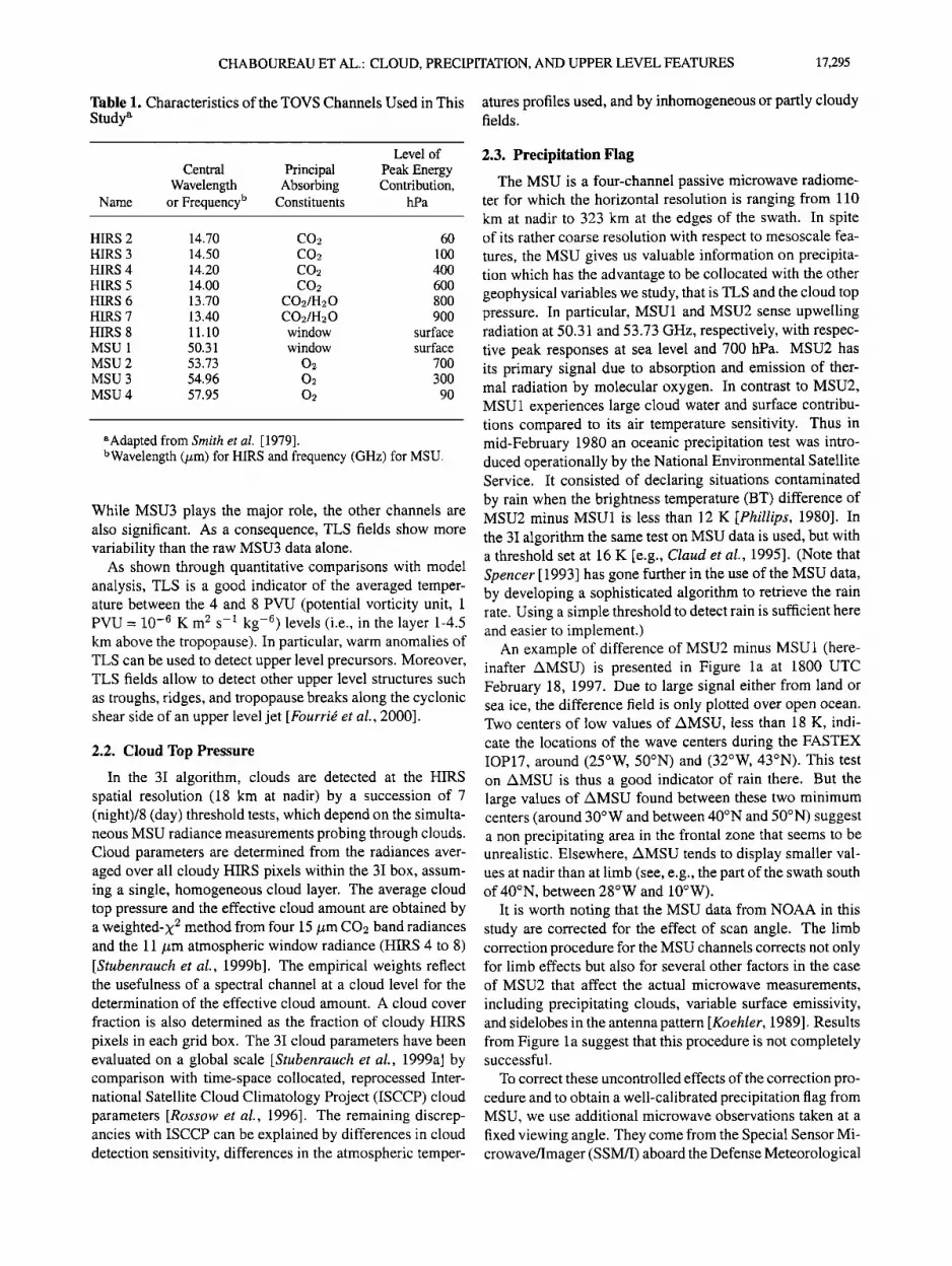
Table 1. Characteristics of the TOVS Channels Used in This

Study a atures profiles used, and by inhomogeneous or partly cloudy fields.

Nalne

Level of

Central Principal Peak Energy Wavelength Absorbing Contribution, or Frequency b Constituents hPa

HIRS 2 14.70 CO2 60 HIRS 3 14.50 CO2 100 HIRS 4 14.20 CO2 400 HIRS 5 14.00 CO2 600 HIRS 6 13.70 CO2/H20 800 HIRS 7 13.40 CO2/H20 900 HIRS 8 11.10 window surface

MSU 1 50.31 window surface

MSU 2 53.73 02 700 MSU 3 54.96 02 300 MSU 4 57.95 02 90

aAdapted from Smith et al. [1979]. bWavelength (ktm) for HIRS and frequency (GHz) for MSU.

While MSU3 plays the major role, the other channels are also significant. As a consequence, TLS fields show more variability than the raw MSU3 data alone.

As shown through quantitative comparisons with model analysis, TLS is a good indicator of the averaged temperature between the 4 and 8 PVU (potential vorticity unit, 1 PVU = 10 -6 K m 2 s -•- kg -6) levels (i.e., in the layer 1-4.5 km above the tropopause). In particular, warm anomalies of TLS can be used to detect upper level precursors. Moreover, TLS fields allow to detect other upper level structures such as troughs, ridges, and tropopause breaks along the cyclonic shear side of an upper level jet [Fourri• et al., 2000].

2.2. Cloud Top Pressure

In the 3I algorithm, clouds are detected at the HIRS spatial resolution (18 km at nadir) by a succession of 7 (night)/8 (day) threshold tests, which depend on the simulta- neous MSU radiance measurements probing through clouds. Cloud parameters are determined from the radiances averaged over all cloudy HIRS pixels within the 3I box, assum- ing a single, homogeneous cloud layer. The average cloud top pressure and the effective cloud amount are obtained by a weighted-x 2 method from four 15/•m CO2 band radiances and the 11/•m atmospheric window radiance (HIRS 4 to 8) [Stubenrauch et al., 1999b]. The empirical weights reflect the usefulness of a spectral channel at a cloud level for the determination of the effective cloud amount. A cloud cover

fraction is also determined as the fraction of cloudy HIRS pixels in each grid box. The 3I cloud parameters have been evaluated on a global scale [Stubenrauch et al., 1999a] by comparison with time-space collocated, reprocessed Inter- national Satellite Cloud Climatology Project (ISCCP) cloud parameters [Rossow et al., 1996]. The remaining discrep- ancies with ISCCP can be explained by differences in cloud detection sensitivity, differences in the atmospheric temper-

2.3. Precipitation Flag

The MSU is a four-channel passive microwave radiome- ter for which the horizontal resolution is ranging from 110 km at nadir to 323 km at the edges of the swath. In spite of its rather coarse resolution with respect to mesoscale features, the MSU gives us valuable information on precipitation which has the advantage to be collocated with the other geophysical variables we study, that is TLS and the cloud top pressure. In particular, MSU1 and MSU2 sense upwelling radiation at 50.31 and 53.73 GHz, respectively, with respec- tive peak responses at sea level and 700 hPa. MSU2 has its primary signal due to absorption and emission of thermal radiation by molecular oxygen. In contrast to MSU2, MSU1 experiences large cloud water and surface contribu- tions compared to its air temperature sensitivity. Thus in mid-February 1980 an oceanic precipitation test was intro- duced operationally by the National Environmental Satellite Service. It consisted of declaring situations contaminated by rain when the brightness temperature (BT) difference of MSU2 minus MSU! is less than !2 K [Phillips, 1980]. In the 31 algorithm the same test on MSU data is used, but with a threshold set at 16 K [e.g., Claud et al., 1995]. (Note that Spencer [ 1993] has gone further in the use of the MSU data, by developing a sophisticated algorithm to retrieve the rain rate. Using a simple threshold to detect rain is sufficient here and easier to implement.)

An example of difference of MSU2 minus MSU1 (hereinafter AMSU) is presented in Figure l a at 1800 UTC February 18, 1997. Due to large signal either from land or sea ice, the difference field is only plotted over open ocean. Two centers of low values of AMSU, less than 18 K, indicate the locations of the wave centers during the FASTEX IOP17, around (25øW, 50øN) and (32øW, 43øN). This test on AMSU is thus a good indicator of rain there. But the large values of AMSU found between these two minimum centers (around 30øW and between 40øN and 50øN) suggest a non precipitating area in the frontal zone that seems to be unrealistic. Elsewhere, AMSU tends to display smaller values at nadir than at limb (see, e.g., the part of the swath south of 40øN, between 28øW and 10øW).

It is worth noting that the MSU data from NOAA in this study are corrected for the effect of scan angle. The limb correction procedure for the MSU channels corrects not only for limb effects but also for several other factors in the case

of MSU2 that affect the actual microwave measurements,

including precipitating clouds, variable surface emissivity, and sidelobes in the antenna pattern [Koehler, 1989]. Results from Figure 1 a suggest that this procedure is not completely successful.

To correct these uncontrolled effects of the correction procedure and to obtain a well-calibrated precipitation flag from MSU, we use additional microwave observations taken at a

fixed viewing angle. They come from the Special Sensor Mi- crowave/Imager (SSM/I) aboard the Defense Meteorological


(a) AMSU (b) A37

(c) Normalized AMSU (d) Collocation between AMSU and A37

600 •ø--40 o

200 0

0 1.00

0.95 0.90

0.85 0.80

20

18

•'16 u• 14

• 12 10

2 4 6 8 1

2 4 6 8

A37=40 K

Figure 1. Maps at 1800 UTC February 18, 1997 of (a) AMSU (Kelvin), (b) A37 (Kelvin), (c) normalized AMSU (Kelvin). (d) Results, for the FASTEX period, of the collocation between AMSU and A37 according to the scan angle index of the 31 box. From top to bottom, number of samples, correlation, and correspondence of A37 = 40 K with AMSU.

Satellite Programme series. In particular, the polarization difference of the BTs at 37 GHz (vertically minus horizon- tally polarized BT; hereinafter A37) is attenuated by rain cloud and thus provides a simple and robust test to detect precipitation areas. Comparisons with ground-based radars suggest that a good indicator of rain over water in the tropics and subtropics is a A37 value less than 40 K. Higher-latitude studies should allow for larger polarization differences be- fore rain is deemed unlikely [Kummerow and Giglio, 1994]. Figure lb displays the 37 GHz BT polarization difference at 1800 UTC February 18, 1997. One can see the obvious correlation that could exist between AMSU and A37, if the limb effects on AMSU could be removed.

For this purpose the SSM/I observations have been collocated with the MSU data over the FASTEX period. The space-time window is 120 km (which roughly corresponds to the 31 box size) and 10 min (due to the high temporal variability of rain). The results of the comparison between AMSU and A37 are presented according to the scan angle index of the 31 box (Figure 1 d).

Due to the rather narrow collocation window in time, the

number of samples is limited, from less than 50 at nadir to around 600 for the larger scan angle. However, a high correlation is found between AMSU and A37, almost over 0.90

everywhere. Therefore the matching between the threshold for A37 and the equivalent one for AMSU can be taken with a high level of confidence. The lowermost part of Figure ld shows the AMSU threshold that gives the same 40 K A37 threshold. It permits us to normalize AMSU with respect to nadir. The normalized AMSU is obtained by multiplying AMSU by the fraction of the AMSU threshold correspond- ing to A37 = 40 K at nadir over the one at the scan angle of the observation.

Figure l c presents AMSU after normalization. The uncontrolled effects of the limb correction have been removed.

The normalized AMSU displays more homogeneous values between the two centers of minimal values. Also, in no-rain areas the difference between AMSU at nadir and AMSU

to the limb have been reduced. In the following we use the threshold of 12 K for the normalized AMSU that corre-


sponds to a threshold of 40 K for A37 to detect precipitation areas.

3. Results

Variables retrieved as explained in section 2 are now used to investigate the large-scale properties of cloud, precipitation and upper level features during the FASTEX period. This is done first by looking at the mean distributions, then by using Hovm611er diagrams, and finally by investigating the most intense rain events through a composite technique.

3.1. Mean Distributions

To examine the mean distribution of the retrievals, we

separate the FASTEX period into three distinct periods cor- responding to the dynamical regimes found by Joly et al. [ 1999]: a Greenland anticyclone regime from January 1 to 13, followed by a blocking regime from January 14 to Febru- ary 2, and finally a zonal regime during the rest of February. Averaged retrieval fields for the three regimes are displayed in Figure 2.

During the Greenland anticyclone regime, some maximum TLS areas, with values greater than 220 K, are located

over North America and the western Atlantic Ocean as far as

40øW (Figure 2a). Due to the correspondence between TLS and the averaged temperature between 4 and 8 PVU levels found by Fourrid et al. [2000], this suggests that, in average, the upper level jet is located to the south of the warm core of TLS, where the gradient is strong. This interpretation is in agreement with the 300 hPa wind map displayed by Joly et al. [ 1999]. The cloud top pressure varies between 550 and 750 hPa over the North Atlantic (Figure 2d). Despite this small variation, the low values of cloud top pressure over the ocean are organized as a Y rotated counterclockwise. A similar organization is found for the densities of cyclone tra- jectories for January by Baehr et al. [1999]. Indeed, the high-level clouds are largely a result of the cyclone activi- ties. The spatial variation of the normalized AMSU is small (Figure 2g).

During the blocking regime, maximum TLS areas display smaller values than for the two other regimes, with no mean values greater than 220 K (Figure 2b). The TLS pattern is also characteristically located just in the vicinity of the continents. Such an absence of the upper level jet over the ocean explains the weak organization of the mean distribution of the cloud top pressure (Figure 2e). An exception to

T!.S I Jan -• 13 9• ...... -••-•--- '- ' -'-'•:-••••.. •- •••••••. f(h) '['LS 14 dan • • Feb ••••' '••-••••-'•--•• [(e) 'F[ZS 3 Feb .* 88 Feb 9'• ••'*'••-••••••

½• • • • > - .... •-;;•' • ..... •%::•:::- --• :P: •'... :•-- :•.- x ,.'_• '. ','...'• * •',7 • • ....... •"'"•'"'•'"• '•' '••'•••••••••• - • •: v•. •.• • • ........ •5:• ' [•½•:-' • •:• F ,:•:•'. ..... : •?• :•'• .• • •, - .

(.loud 'top t ressure ½ ,tan t ..... ta• ,J?•-"• l(e) Cloud Top Pressure 14 Jan 2 Feb 9'7•/•2•'• i(f) Cloud Top Pressure 3

•4,o ' •c •o •,• .... •' '%o' •o•' '•-: ..... ;•:'>•

Figure 2. (a,b,c) Averaged fields of TLS (Kelvin), (d,e,f) cloud top pressure (hPa), and (g,h,i) normalized AMSU (Kelvin). The period of averaging is (left) from January 1 to 13, 1997, (middle) from January 14 to February 2, 1997, and (right) from February 3 to 28, 1997.


29j 3•j

. .;' .;.::'.;,:.t;.; f'½ :5•*•.;:;.;:; .:•- :...' -: ':.':"." ,--.,-.,,,%'._,%? *'"' '"'•

K•;:•Z."..:... • ......... -.- ......... ½•' ........ 70W 60W 50W 40W 30W 20W 10W 0

212 214 216 218 220

Cloud Top Pressure

' '.'"(•.'!i••

. .;-•:]:;. ½:-%., ..... .

?OW 60• 50W 40• 30W 20• 10• 0

500 550 600 650 700

Figure 3. HovmOller diagrams showing the longitude-time evolution of TLS (Kelvin), the cloud top pressure (hPa), and the normalized AMSU (Kelvin). On the left axis the scale indicates the day' j, January; f, February. On the right axis the symbols indicate the FASTEX IOPs: large-scale baroclinic cyclones are in the shadow box, end of storm track cyclones are in the clear box, comma clouds and cold-air cyclones are in italic. Solid (dashed) lines represent TLS (cloud top pressure) associated to IOPs. In the diagram related to the normalized AMSU, the boxes indicate the events examined with the composite analysis. The associated number is the class number at which the event belongs. See text related to composite for further details.

and of rank 7: there is a large decrease of the explained variance (1.30%) and the first six components represent 50.95% of the total variance.

Then the components kept are clustered using an ascend- ing hierarchical classification, which minimizes the intra- class variance: each case is then included in a class. The

key idea here, in the final step, is to generate the composite from averaging the original fields within each class, not the restricted subset of the principal components. This yields

smooth but realistic structures as illustrated below. The re- tained classification gives nine classes. Indeed, to be repre- sentative, each class should be composed of a large number of individual cases (which is hard to obtain with an initial set of 67 events). On the other hand, a too limited number of classes would smooth the variability. Thus a satis- factory compromise is obtained with nine classes. Some of them only includes a few number of cases (less than five for classes 4, 6, 7, 8, and 9) due to the short period of time ana-


Table 2. Results of the Principal Component Analysis for the First 10 Eigenvectors

Difference With the

Explained Variance Explained Variance, Summation, by the Next Rank

Rank % % %

1 19.23 19.23 9.76

2 9.48 28.71 2.85

3 6.63 35.34 0.63 4 5.99 41.33 0.87 5 5.12 46.46 0.63 6 4.49 50.95 1.30 7 3.20 54.15 0.38 8 2.82 56.97 0.41

9 2.41 59.38 0.06 10 2.35 61.74 0.11

lyzed. If a longer period would be studied, we might expect that the classes would be more populated, thus more repre- sentative. The number of the class at which each individual

rain event belongs is plotted on Figure 3, next to each rectan- gular box. The averages of the composite fields within each class are shown in Figure 4.

Only one class (class 5) is characterized by middle-level clouds covering the precipitating area (Figure 4e). More- over, the warm TLS pattern there is the weakest of all the classes. It is located to the southwest of the rainy area, that is, where no baroclinic interaction with the low levels is pos- sible. Class 5 clusters 11 frontal cases, almost all occurring during the blocking regime.

All the other classes present high-level clouds over the precipitation area, with patterns of warm TLS upstream. For all these classes this suggests a baroclinic interaction between upper and low levels. Three families of classes could be identified according to the orientation of the warm TLS field: zonal, anticyclonic, and cyclonic.

The zonal family formed by classes 4, 8, and 9 presents warm fields of TLS organized in a zonal band north of the rain area (Figures 4d, 4h, and 4i). The high-level cloud patterns are elongated along this TLS zonal band. Classes 4 and 9 are populated by fronts located between 40øN and 45øN occurring in January and February, respectively (Figures 4d and 4i). Class 8 is characterized by a cloud shield composed by clouds higher and more cyclonically curved than the two other classes (Figure 4h). Indeed, class 8 is composed of three frontal waves (lOP 16 and Lesser Observing Period (LOP) 6) that develop into cyclones as the systems cross the jet stream from the warm to the cold-air side [Baehr et al., 1999].

The anticyclonic family, that groups classes 6 and 7 (Fig- ures 4f and 4g), is characterized by a warm TLS pattern located almost everywhere in the western part of the box, and in particular, anticyclonically curved for class 7. The high- level cloud patterns are elongated downstream of this TLS band. Class 6 concerns fronts during the blocking period (Figure 4f), while class 7 accommodates two episodes of the

end of storm track IOP 6 cyclone, remaining in the warm side of the jet stream (Figure 4g). The rearward (anticyclonic) wave breaking and filamentation characterizing the LC 1 example are seen for classes 6 and 7.

The cyclonic family, which groups together classes 1, 2, and 3 (Figures 4a, 4b, and 4c), displays a warm TLS pattern tilted northwest-southeast, and quite cyclonically for classes 2 and 3 (Figures 4b and 4c). Thus the upper level structure is characterized by forward (cyclonic) trough roll up as the typical LC2. The classes are mostly populated by rain events occurring in February. Fronts are the largest events in class 1 with the rain area located around 40øN (Figure 4a). Class 2 is populated notably by some end of storm track cases (IOP 19, lOP 12, LOP1, LOP 2). Class 3 is populated notably by some large-scale baroclinic cases (lOP 9, 14, and 17) with the rain area located between 40øN and 50øN. These cases

are typical of the Norwegian cyclones that mimic the LC2 example.

Even if the period of study is limited in time, it is re- markable that the classification can discriminate rain events

both between different weather regimes and between different kinds of weather system. Thus the cyclonic family groups cases that occurred during the zonal regime, in particular all the large-scale baroclinic systems, whereas the anticyclonic family groups blocking regime cases, which are mostly frontal systems. Moreover, it is suggested that composite classes associated with blocking and zonal regimes lead to preferential baroclinic life cycles that mimic the idealized LC 1 and LC2 paradigms, respectively.

4. Conclusion

Physical parameters retrieved from TOVS measurements are used to study the large-scale cloud, precipitation, and lower stratosphere characteristics in the North Atlantic during the FASTEX period in January and February 1997. The following physical parameters are examined: temperature of lower stratosphere, cloud top pressure, and precipitation index under the guidance of the SSM/I observations.

These dynamically consistent (i.e., temporally and spatially collocated) fields are able to characterize the three weather regimes occurring during FASTEX. Thus the mean distributions of these satellite-retrieved parameters are organized in locations expected from the cyclonic activity. The Hovm611er diagrams give further details on the organization. High-level cloud patterns, when accompanied by low values of normalized AMSU, can be discriminated with respect to TLS field. When no (or weak) warm TLS feature can be found upstream, such patterns are frontal systems. On the contrary, a warm TLS event present upstream of a rainy cloud feature suggests a baroclinic interaction. In this case, the high-level cloud pattern is associated with a large-scale baroclinic cyclone, or at least a mature low.

When examining the most precipitating cases using the composite technique, the nondeveloped class (in terms of absence of high-cloud cover) is characterized by the absence of warm TLS features, grouping mostly blocking-regime cases.


(b) CLASS #2 (• e CASES) 1BOO '. -:

'-' '.4';'-' ." i•oo ;; .•-i! L:.¾:-...

-,,• .•% ......•,...:.. ,..:-....,....,.-,•......,.•....•.., .....:• .' ..... ..d.•t -•.:•..... :.....; .,..•..::.., . ......... 600

..•: •......... <.. .... . .... . .::•,...:•:x•: ...:.(';'?" . •i.:?,•: '• '•:t: 5-:•' :•i.. }: .: -. :., .,?; ;•:'..•*'.•gi•"-

- • 200 "•i':.' ß ' "-..

(h) c•ss #e (3 CASES) 800 .,.-.•'• -•r•"•.r•.• ß '•-•- .' ' "•"•-.•'•.-- •--•.. _ .•.•'?•,•'"-.' ' '.:..-::-..":'...:' '

.... ß ' :' ':' ':" •" ."•' --" ' '•5" '•;47;•:;•' •-::•':.'... ' -.:',;; ........ .., ,';

'.•-,.'•.' "-';%'.:: .'..:•f:;. ??" ½:' ': "; '•' '•:.. ';•i'.' :•..'.,".:' ;'.-')-;' '-:i?;"'. .. . , :•...,• • ..... • ...........

•, l'•,;' '• +' ¾:• •?•?•,,. ;:;•-:½•½:;•':"• • ' ....... ." • •f2, -• ' ,'•--• ./•:-• .': ',"":? .......... : ;'" '-:: ' .'•' 4.

ß .,: .• -.....;:-.•,.-•<,..•.... :.•i,:::. :.-,,x:.;-,,;•;:. <:.: •,,;• ..:•: ....... ',. ';::';::': ..";.".•:..:::'.•...".'•.,.,-?';' '" '" ........... ':;•::- ' :..;i)?:•.-

•,. ...... ..:..:..:..•.•,...... ....................... :::•.:•::4.

(C) CLASS //3 (13 CASES) .: :•.::...;-?:.'•'..;•:.:'. •--•-,:•?•. .• ........ •:•..•?•:,.-:

tzoo •..-:,.-,.. '"•' ..7'"-- '

-;•.)..::;.:i.•i•.. •:'::;-:': ?•:-:.??•:,.:.: ;•.•(" •:•. ß 0 •'" '"":" '"" ..... ' ....... • '""'

-600 - 2-' :-' .•)'" ...,:'V;• . •.. • •-•-,•::•:: . . - . .:•.. • •-•.-?,•?...., .,;.• - . '•"•

,..*•-•.,/'.•

(i) CLASS #9 (,5 CASES) •oo ......... -...., -.•-:•-'••".'• ..... <"z '•--•.•• "' .".'.:'"".':':" ':';"; •'. "' '.. ;" - 7 • • '•'-- '• •"•'"/"• '•• - - -•--•••'•

•':::,,::;;,'- ,•, :...:--.:.: .... .. •.•< ............. • • .... -.::•.- ,•' :..' ';:, :• "•:•.'.'t•"-•',.'.:.•'.:"•::f:?.:;%.":C. ::'"':" ','• ..... '.:"::'?:,•;.;•:.".: :'.:: :.':'•-.":-:/'::.'

,•oo L--, •'::?•:J•%: ':'-'::'":;•'"/:.::"Z'.:".: '-;:•;.•:.•:"":'::";".:::.:.-':.:.,:•:'-. :":: ::":::--:'. • ',':4•'":•:•,•:•:'"•,;;:.;';:• '"' •'""-. •:-•":.':'..: :•':: ..... t •.':• .... .':'.,....- ....... •- .......... .:.,'..::•...- ...... -,..'..'-' •o • ';•L--..;7'-:'•:•:-•' •/•;:. ' 7..':;-'?;;::•> :•.' .',;--.r• '-:.:".:,. :',...•.;';•

? ': :.: -..;.;;<. •: .':/-'."•,.-.,- .,:&.::....:.....,,,•.:;•.?,...., •%:•,r• -'-•"•-•.•/•4•:.'.., - ..--•... ...... .•:..•,:•:•.-•- . .•,•' -, ...... •-•

- ' • --•6•' - i 8'6• - • 2oo -6oo u ouu • •

Figure 4. Composite views of the nine classes with the precipitation area in bold solid line (normalized AMSU< 12 K), the cloud top pressure in solid lines every 100 hPa, and TLS in dashed line every 2 K. The shading indicates cloud top pressure (dark gray, pressure over 400 hPa; medium gray, pressure between 500 and 400 hPa, etc.) and the dashed patterns indicates TLS between 218 and 222 K.

On the other hand, the cases that are well developed in term of cloud cover are characterized by warm TLS patterns upstream the precipitation area. This result obtained with satellite observations confirms the finding of a previous study using model analysis [Baehr et al., 1999]. Moreover, the well- developed cases could be grouped into three families depending on the orientation of the warm TLS features: zonal, anticyclonic, and cyclonic. Only the later family, characterized by a cyclonically tilted trough, clusters-the large-scale baroclinic systems that all occurred during the zonal regime. This suggests that a cyclonically tilted trough has a positive impact on the development of cyclones.

We plan to extend such a study to a longer period of time, to look at the variability from intraseasonal to interannual time scale (using reanalyzed TOVS data over the 1979-1999 period). Moreover, similar studies for more recent periods of time will benefit from the increased spatial and spectral resolutions of the recent instruments (in particular AMSU, the Advanced MSU now on board the NOAA satellites).

Acknowledgments. This research was supported by the FASTEX-Cloud System Study Project funded by the European Commission under contract ENV4-CT97-0625. Computer re- sources were alloted by IDRIS (projects 97569, 98569, and


981076). Retrievals used here have been obtained from the Atmospheric Radiation Analysis group at LMD, through the NOAA/NASA TOVS Pathfinder (Path-B) program. The SSM/I data come from the NOAA Satellite Active Archive. Thanks are

due to the anonymous reviewers for comments on the manuscript.

References

Ayrault, F., and A. Joly, Une nouvelle typologie des d6pressions m6t6orologiques, classification des phases de maturation, C. R. Acad. Sci., Ser. IIa, 330, 167-172, 2000.

Baehr, C., B. Pouponneau, E Ayrault, and A. Joly, Dynamical char- acterization of the FASTEX cyclogenesis cases, Q. J. R. Meteo- rol. Soc., 125, 3469-3494, 1999.

Charney, J. G., The dynamics of long waves in a baroclinic westerly current, J. Meteorol., 4, 135-162, 1947.

Ch6din, A., N. A. Scott, C. Wahiche, and P. Moulinier, The Im- proved Initialization Inversion method: A high resolution physical method for temperature retrievals from the TIROS-N series, J. Clim. Appl. Meteorol., 24, 124-143, 1985.

Claud, C., K. B. Katsaros, N.M. Mognard, and N. A. Scott, Syn- ergetic satellite study of a rapidly deepening cyclone over the Norwegian Sea: 13-16 February 1989, Global Atmos. Ocean Syst., 3, 1-34, 1995.

Eady, E. T., Long-waves and cyclone waves, Tellus, 1(3), 33-52, 1949.

Fourri6, N., C. Claud, J. Donnadille, J.-P. Cammas, B. Pouponneau, and N. A. Scott, The use of TOVS observations for the identifi- cation of tropopause-level thermal anomalies, Q. J. R. Meteorol. Soc., 126, 1473-1494, 2000.

Gelaro, R., R. H. Langland, G. D. Rohaly, and T. E. Rosmond, An assessment of the singular-vector approach to targeted observing using the FASTEX dataset, Q. J. R. Meteorol. Soc., 125, 3299- 3327, 1999.

Hoskins, B. J., M. E. Mcintyre, and R. W. Robertson, On the use and significance of isentropic potential vorticity maps, Q. J. R. Meteorol. Soc., 111, 877-946, 1985.

Joly, A., et al., The Fronts and Atlantic Storm Track Experiment (FASTEX): Scientific objectives and experimental design, Bull. Am. Meteorol. Soc., 78, 1917-1940, 1997.

Joly, A., et al., Overview of the field phase of the Fronts and At- lantic Storm Track Experiment (FASTEX) project, Q. J. R. Me- teorol. Soc., 125, 3131-3163, 1999.

Koehler, T. L., Limb correction effects on TIROS-N Microwave Sounding Unit observations, J. Appl. Meteorol., 28, 807-817, 1989.

Kucharski, F., and A. J. Thorpe, Upper-level barotropic growth as a precursor to cyclogenesis during FASTEX, Q. J. R. Meteorol. Soc., 126, 3219-3232, 2000.

Kucharski, E, and A. J. Thorpe, The influence of transient upper- level barotropic growth on the development of baroclinic waves, Q. J. R. Meteorol. Soc., 127, 835-844, 2001.

Kummerow, C. D., and L. Giglio, A passive microwave technique for estimating the vertical structure of rainfall from space, I, Al- gorithm description, J. Appl. Meteorol., 33, 3-18, 1994.

Langland, R. H., R. Gelaro, G. D. Rohaly, and M. A. Shapiro, Tar- geted observations in FASTEX: Adjoint-based targeting proce- dures and data impact experiments in IOP17 and IOP18, Q. J. R. Meteorol. Soc., 125, 3241-3270, 1999.

Lorenz, E. N., Effects of analysis and model errors on routine weather forecasts, in Proceedings of ECMWF Seminars on Ten Years of Medium-Range Weather Forecasting, vol. 1, pp. 115- 128, Eur. Cent. for Medium-Range Weather Forecasts, Reading, England, 1990.

Phillips, N. A., Cloudy winter satellite retrievals over the extratropical Northern Hemisphere oceans, Mon. Weather Rev., 109, 652-659, 1980.

Rossow, W. B., A. W. Walker, D. Beuschel, and D. Roiter, Interna- tional Satellite Cloud Climatology Project (ISCCP): Description of new cloud datasets, Int. Counc. of Sci. Unions and WMO Rep. WMO/TD-No 737, 115 pp., World Climate Research Pro- gramme, Geneva, February 1996.

Scott, N. A., A. Ch6din, R. Armante, J. Francis, C. Stubenrauch, J.-P. Chaboureau, F. Chevallier, C. Claud, and F. Ch6ruy, Char- acteristics of the TOVS Pathfinder Path-B dataset, Bull. Am. Me- teorol. Soc., 80, 2679-2702, 1999.

Shapiro, M. A., H. Wemli, J.-W. Bao, J. Methven, X. Zou, J. Doyle, T. Holt, E. Donald-Grell, and P. Neiman, A planetary-scale to mesoscale perspective of the life cycles of the extratropical cyclones, in The Life Cycles of Extratropical Cyclones, edited by M. A. Shapiro and S. Gronfis, pp. 139-186, Am. Meteorol. Soc., Boston, Mass., 1999.

Shapiro, M. A., H. Wernli, N. A. Bond, and R. Langland, The influence of the 1997-1999 ENSO on extratropical baroclinic life cycles over the eastern North Pacific, Q. J. R. Meteorol. Soc., 80, 331-342, 2001.

Smith, W. L., H. M. Woolf, C. M. Hayden, D. Q. Wark, and L. M. McMillin, The TIROS-N operational vertical sounder, Bull. Am. Meteorol. Soc., 60, 1177-1187, 1979.

Spencer, R. W., Global oceanic precipitation from the MSU during 1979-91 and comparisons to other climatologies, J. Clim., 6, 1301-1326, 1993.

Stubenrauch, C. J., W. B. Rossow, F. Ch•ruy, A. Ch•din, and N. A. Scott, Clouds as seen by infrared sounders (31) and imagers (ISCCP), I, Evaluation of cloud parameters, J. Clim., 12, 2189- 2213, 1999a.

Stubenrauch, C. J., A. Ch6din, R. Armante, and N. A. Scott, Clouds as seen by infrared sounders (3I) and imagers (ISCCP), II, A new approach for cloud parameter determination in the 3I algorithms, J. Clim., 12, 221 4-2223, 1999b.

Szunyogh, I., Z. Toth, K. A. Emanuel, C. H. Bishop, C. Snyder, R. E. Morss, J. Woolen, and T. Marchok, Ensemble-based targeting experiments during FASTEX: The effect of dropsonde data from the Lear jet, Q. J. R. Meteorol. Soc., 125, 3189-3217, 1999.

Thomcroft, C. D., B. J. Hoskins, and M. E. Mcintyre, Two paradigms of baroclinic-wave life-cycle behavior, Q. J. R. Me- teorol. Soc., 119, 17-55, 1993.

J.-P. Cammas, J.-P. Chaboureau, and E J. Mascart, Laboratoire d'Adrologie, Observatoire Midi-Pyrenees, 14 av. E. Belin, 31400 Toulouse, France. ([email protected]; [email protected] mip.fr; masp @ aero.obs-mip. fr)

C. Claud, Laboratoire de M6t6orologie Dynamique, l•cole Polytechnique, 91128 Palaiseau Cedex, France. ([email protected])

(Received November 13, 2000; revised March 8, 2001; accepted March 21, 2001.)

Documents

Large-scale cloud, precipitation, and upper level features during Fronts and Atlantic Storm Track Experiment as inferred from TIROS-N Operational Vertical Sounder observations