Embed Size (px)
Citation preview
1
Large-scale ERT surveys for investigating shallow regolith
properties and architecture
Laurent Gourdol1, Rémi Clément
2, Jérôme Juilleret
1, Laurent Pfister
1, Christophe Hissler
1
1 Catchment and Eco-hydrology Research Group (CAT), Luxembourg Institute of Science and Technology (LIST), Belvaux,
L-4422, Luxembourg 5 2 REVERSAAL Research Unit, National Research Institute of Science and Technology for Environment and Agriculture
(IRSTEA), Villeurbanne, F-69626, France
Correspondence to: Laurent Gourdol ([email protected])
Abstract. Within the Critical Zone, regolith plays a key role in the fundamental hydrological function of water collection,
storage, mixing and release. Electrical Resistivity Tomography (ERT) is recognized as a remarkable tool for characterizing 10
the geometry and properties of the regolith, overcoming limitations inherent to conventional borehole-based investigations.
However, ERT measurements with a high vertical resolution remain restricted to shallow depths, essentially due to the
requirement of small electrode spacing increments (ESI). Under these circumstances, the use of ERT measurements for large
horizontal surveys remains cumbersome and time-consuming. Here we focus on the need to optimize the ESI parameter in
order to adequately characterize the subsurface fabric. We use a set of synthetic three-layered soil–saprock/saprolite–bedrock 15
models in combination with a field dataset. We demonstrate that oversized ESI can significantly affect our perception of
shallow subsurface structures by missing important layers and increasing the ill-posed inverse problem effects. More
precisely, we document how a thin surficial layer can influence inverted ERT results and cause a resistivity bias, both at the
surface and at deeper horizons. To overcome this limitation, we propose adding interpolated levels of surficial apparent
resistivity based on a limited number of ERT profiles with small ESI. We demonstrate that our protocol significantly 20
improves the accuracy of ERT profiles based on large ESI. Our protocol is time and cost efficient – especially in the case of
large-scale ERT surveys.
1 Introduction
The architecture and properties of regolith, as well as its distribution across the landscape, play a key role in how rainfall is
collected, stored and finally released to generate and shape streamflow in Critical Zone studies (Schoeneberger and Wysocki, 25
2005; Lin, 2010; Ghasemizade and Schirmer, 2013; Brooks et al., 2015). Factors such as the depth and composition of the
soil cover and the rock weathering determine water pathways, residence times in the subsurface and subsequent interactions
with surface water bodies (Freer et al., 2002; Hopp and McDonnell, 2009; Graham et al., 2010; Gabrielli et al., 2012; Lanni
et al., 2013; Ameli et al., 2016). Thus, there is a pressing need in catchment studies for precise characterizations of the
geometry and properties of regolith. 30
Hydrol. Earth Syst. Sci. Discuss., https://doi.org/10.5194/hess-2018-519Manuscript under review for journal Hydrol. Earth Syst. Sci.Discussion started: 7 December 2018c© Author(s) 2018. CC BY 4.0 License.

2
However, limited access to the subsurface is a major hurdle to acquiring this information meaning that often, even the most
basic data is missing, such as the transitions from the soil to the hard bedrock (Brooks et al., 2015). It is the complexity and
spatial variability of the subsurface that make its characterization very challenging. Conventional investigation techniques of
regolith are known to be invasive and of limited spatial representativeness – a trait causing them to be ignored in the vast
majority of catchment studies (Burt and McDonnell, 2015; Parsekian et al., 2015). 5
Fortunately, geophysical prospection techniques have received increasing attention in recent years within the hydrological
sciences community, thanks to their non-destructive character and ability to provide information on subsurface features over
large areas. These investigative tools are now recognized as being essential for accurately characterizing the subsurface and
studying water partitioning (Robinson et al., 2008; Loke et al., 2013; Binley et al., 2015; Brooks et al., 2015; Parsekian et al.,
2015; Singha, 2017). 10
Among the geophysical prospection techniques at hand, electrical resistivity tomography (ERT) is now commonly used to
characterize subsurface environments (Robinson et al., 2008; Loke et al., 2013; Singha et al., 2014; Binley et al., 2015;
Parsekian et al., 2015). This technique is based on the injection of an electrical current through a pair of electrodes and the
measurement of the resulting electrical potential between a second pair of electrodes along a line of dozens or hundreds of
electrodes stuck into the ground. Through inversion schemes, ERT data is used to generate 2D and 3D electrical resistivity 15
maps of the subsurface (Binley and Kemna, 2005).
The electrical resistivity of the subsurface provides a weighted average of the electrical properties of its mineral grains,
liquid and air (Archie, 1942; Keller and Frischknecht, 1966; Reynolds, 2011). Constitutive relationships can be used to link
electrical resistivity to several properties and states that are of major interest to hydrologists: e.g. textural properties (Tetegan
et al., 2012), porosity (Leslie and Heinse, 2013; Comte et al., 2018), hydraulic conductivity (Slater, 2007; Farzamian et al., 20
2015), water content (Brunet et al., 2010; Alamry et al., 2017) or solute concentrations (Bauer et al., 2006; Comte and
Banton, 2007). While these constitutive relationships are essential for reliable hydrological interpretations (Binley et al.,
2015), their accuracy largely depends on the resolution of the ERT images (Day-Lewis et al., 2005).
ERT has also been successfully used to characterize regolith architecture by delineating areas showing similar resistivity
patterns (Crook et al., 2008; Comte et al., 2012 ; Leopold et al., 2013; Cassidy et al., 2014; Holbrook et al., 2014; Hübner et 25
al., 2015; Uhlemann et al., 2015; Wainwright et al., 2016; Scaini et al., 2017). An increasing number of studies use
automated edge detection approaches to delineate these key interfaces within the subsurface (Nguyen, 2005; Hsu et al., 2010;
Chambers et al., 2012, 2013, 2014, 2015; Audebert et al., 2014; Ward et al., 2014; Uhlemann et al., 2015; Wainwright et al.,
2016; Scaini et al., 2017). However, it has also shown that the application of these methods can fail – even when the true
interface is sharp – because of insufficient sensitivity and accuracy in the vicinity of the interface (Chambers et al., 2013, 30
2014).
The characterization of subsurface properties and the delineation of layer boundaries should thus go hand in hand with a
suitable resolution of ERT images. Otherwise, the results can be inaccurate (Chambers et al., 2013, 2014; Clément et al.,
2009, 2014; Ward et al., 2014). Chambers et al. (2014) emphasize that using ERT to detect thin surficial layers remains
Hydrol. Earth Syst. Sci. Discuss., https://doi.org/10.5194/hess-2018-519Manuscript under review for journal Hydrol. Earth Syst. Sci.Discussion started: 7 December 2018c© Author(s) 2018. CC BY 4.0 License.

3
challenging. In many cases, the subsurface structure to be characterized is shallow and should be measured with a precise
vertical resolution, thus requiring a small electrode spacing increment (ESI) (Reynolds, 2011; Chambers et al., 2014). In
these circumstances, the use of ERT measurements for large horizontal surveys remains time-consuming. Depending on the
regolith architecture and the size of the investigated area, it is thus challenging if not impossible to balance the requirement
for a resolution suited to shallow layers (i.e. smaller ESI), against the competing need to cover the area of interest within a 5
reasonable amount of time and cost (i.e. larger ESI) (Chambers et al., 2014). Moreover, as shown by Kunetz (1960) or
Clément et al. (2009), oversizing the ESI leads not only to an inappropriate vertical resolution for thin surface layers, but
may also affect the characterization of deeper layers by causing resistivity bias in depth.
Here we ask: Which ESI should be considered to characterize the entire regolith accurately? What happens if a larger ESI is
used? What can we do if we still have to use a larger ESI due to cost and time constraints? These questions should be dealt 10
with prior to the design of fieldwork campaigns and to avoid any misinterpretation of field data. They provide the motivation
for this work, where we put the emphasis on the importance for optimizing the ESI parameter to correctly disentangle the
subsurface architecture and properties (both for the shallow part of the subsurface and for the deeper layers). Within this
work, we investigate:
1) How the ill-posed inverse problem effects relate to the ESI parameter and which is the most appropriate value for 15
accurately characterizing the entire regolith;
2) The potential for a new approach to reduce the ill-posed inverse problem effects for carrying out large-scale ERT surveys
with a large ESI by adding interpolated levels of surficial apparent resistivity based on a limited number of measurements
with a small ESI.
To this end, we investigate a set of synthetic three-layered soil–saprock/saprolite–bedrock models using a classical 20
geophysical approach based on numerical modelling. In addition, we use a field dataset to corroborate and reinforce the
numerical findings. The assessment of the ERT images obtained from these two datasets is carried out considering the
accuracy of the inverted resistivity distribution and the derived interface depths.
2 Materials and Methods
As done traditionally in geophysics for the optimization of inverse problems, we used here synthetic and real datasets to 25
assess the ill-posed inverse problem effects. While the former provide important information under controlled conditions and
a priori exact knowledge, the latter represent a field reality in terms of heterogeneity. The main stages of data processing
followed in this study and described in this section are commonly used and well-defined in several other ERT studies (e.g.
Clément at al., 2009, 2014; Audebert et al., 2014; Chambers et al., 2014; Carrière et al., 2017).
Hydrol. Earth Syst. Sci. Discuss., https://doi.org/10.5194/hess-2018-519Manuscript under review for journal Hydrol. Earth Syst. Sci.Discussion started: 7 December 2018c© Author(s) 2018. CC BY 4.0 License.

4
2.1 Synthetic resistivity dataset
2.1.1 Conceptual resistivity models
For a given geological substratum, and according to rock weathering and pedological processes, the regolith can be
partitioned into three main units (Velde and Meunier, 2008; Juilleret et al., 2016), namely, from top to bottom:
1) the solum, which is the “true soil”, where pedogenetic processes are dominant, 5
2) the subsolum, corresponding to weathered materials where the original rock structure is preserved and geogenic processes
still dominate (depending on the degree of weathering the saprock and/or saprolite can be distinguished), and
3) the hard bedrock.
Based on this three-layered subsurface conceptual model, we generated 25 one-dimensional conceptual models to investigate
different scenarios with varying resistivity and thickness contrasts. Solum and bedrock resistivity was set to 1000 ohm.m for 10
all models. The solum thickness was also set to a unique value of 0.5 m, which is also in line with the average thickness
observed in our study area (see 2.2.1). To cover a sufficiently wide range of subsurface structures and properties, the
subsolum layer was parameterized with several values of thickness (0.5, 1, 2, 4, 8 m) and resistivity (1250, 2500, 5000,
10000, 20000 ohm.m). The retained resistivity values were also chosen according to the range observed during the field
study. 15
2.1.2 Forward Modelling, ERT arrays and units of electrode spacing
To mimic resistivity measurements with the synthetic models, we simulated the electric field distribution resulting from
current injections using the electric field distribution theory (Maxwell’s equation) and the finite element method. We
performed numerical simulations using the AC/DC module of Comsol Multiphysics, complemented with a forward 3D
modelling (F3DM) Matlab script (Clément et al., 2011; Audebert et al., 2014). This script assesses automatically, for a 20
quadrupole sequence, the electric potential between the two potential electrodes, according to the intensity injected by the
two current electrodes. To achieve a realistic dataset reflecting the properties of a field survey, we applied a systematic
Gaussian noise distribution with 3% standard deviation relative error to the apparent resistivity dataset to simulate the noise
commonly recorded with the resistivity meter.
The two most commonly used ERT arrays (Carrière et al., 2017), the dipole-dipole and the Wenner-Schlumberger arrays, 25
were used to simulate apparent resistivity from the resistivity models. Their successful application in field studies is mainly
due to their surveying efficiency and sensitivity (Dahlin and Zhou, 2004). In order to assess the vertical resolution needed to
properly characterize the subsurface, simulations of apparent resistivity for both arrays were conducted using 5 different
ESIs (0.25, 0.5, 1, 2 and 4 m).
Hydrol. Earth Syst. Sci. Discuss., https://doi.org/10.5194/hess-2018-519Manuscript under review for journal Hydrol. Earth Syst. Sci.Discussion started: 7 December 2018c© Author(s) 2018. CC BY 4.0 License.
5
2.2 Field study
2.2.1 Study area description
Our experimental test site is the forested Weierbach headwater catchment, located in the Luxembourgish Ardennes Massif
(0.45 km²; Figure 1). The geological substratum of the study area is composed of Devonian metamorphic schists, phyllites
and slates. Recent studies in the Weierbach catchment have shown that its regolith plays a key role in runoff generation 5
processes (Pfister et al., 2010; Fenicia et al., 2014; Wrede et al., 2015; Martínez-Carreras et al., 2015; Martínez-Carreras et
al., 2016; Scaini et al., 2017, 2018). Hence, its characterization is of high relevance for gaining new insights into the
fundamental catchment functions of water collection, storage and release. Several soil pits and drillings were done in the
catchment in order to describe its regolith structure and mineralogical and chemical properties (Figure 1). Based on the
visual inspection of soil pits and core drillings and particle size distribution analysis and porosity measurements (Juilleret et 10
al., 2011; Wrede et al., 2015; Juilleret et al., 2016; Martínez-Carreras et al., 2016; Moragues-Quiroga et al., 2017; Scaini et
al., 2017), Figure 2a-c shows a mean schematic representation of the soil-to-substratum continuum. The three main units of
this structure are characterized as follows:
1) The solum is a stony loam soil with a mean thickness of 50 cm. The loam texture stems from a loess deposit, which was
mixed through solifluction with many schist/slate clasts native from the bedrock (coarse element content around 25%). The 15
solum has a high drainage porosity of 30% on average.
2) The subsolum has two parts. The upper subsolum (from 50 to 90 cm depth on average) is a loam to sandy-loam texture
layer with abundant schist/slate fragments. In this part, the abundance and size of rock fragments strongly increases with
increasing depth (coarse element content increases from 30% to 75%). Inversely, the drainage porosity decreases, from 30%
to 10%. The lower subsolum (from 90 to 140 cm depth on average), with the largest content of schist/slate fragments (coarse 20
element content greater than 80%), corresponds to the decomposed/broken part of the bedrock.
3) The schist/slate hard bedrock starts, on average, at a depth of 140 cm. At first, very large fractures in the hard bedrock
tend to close quickly as the depth increases. At a depth of five metres, most fractures are closed and the bedrock can be
considered fresh and almost impermeable.
Mirroring multiple weathering phases in the Luxembourgish Ardennes Massif over geological time scales (Moragues-25
Quiroba et al., 2017; Demoulin et al., 2018), cores obtained from deep drilling campaigns (Figure 2-d) reveal different
weathering degrees in the Weierbach catchment (Figure 2-e). The top of the substratum presents a high weathering degree in
the upper part of the basin (north and west of the catchment, morphologically expressed by a plateau). Elsewhere in the
catchment, bedrock weathering is less pronounced (on hillslope position and along the eastern limit). This difference also
implies contrasted surface layer properties. As observed in soil pits on the plateau, schist/slate fragments are smaller and less 30
consistent and the clay content of the matrix is higher (Figure 2-f; Regolithic Saprolite Subsolum type as per Juilleret et al.,
2016). Elsewhere, soil pits exhibit bigger and more coherent schist/slate fragments and less clay in the matrix (Figure 2-g;
Regolithic Saprock Subsolum type as per Juilleret et al., 2016).
Hydrol. Earth Syst. Sci. Discuss., https://doi.org/10.5194/hess-2018-519Manuscript under review for journal Hydrol. Earth Syst. Sci.Discussion started: 7 December 2018c© Author(s) 2018. CC BY 4.0 License.
6
2.2.2 ERT survey design, data collection and processing
For a characterization of the subsurface of the entire Weierbach catchment, we built a mesh of several large ERT profiles
using the roll-along technique (white lines drawn in Figure 1, cumulative length of about 12 km). To complete this
catchment-wide survey in a reasonable time, we chose a set-up with an ESI of 2 m. We added 12 plot scale ERT profiles of
120 electrodes each, using a smaller ESI of 0.5 m (red lines drawn in Figure 1). Their locations were chosen according to 5
prevailing local geomorphological characteristics (plateau, steep and gentle hillslope, interfluve, close to riparian zone).
These last 12 profiles are the ones that are considered in this study.
All measurements were taken with a Syscal Pro 120 (ten-channel) resistivity meter from IRIS Instruments with multicore
cables attached to 120 stainless steel rod electrodes. A pulse duration of 500 ms and a target of 50 mV for potential readings
were set as criteria for the current injection. To insure a good repeatability, stacks numbers were automatically adjusted 10
between 3 and 6 aiming for a maximum standard deviation of 3% for the repeated measurements. We retained the Wenner-
Schlumberger array for the measurements. This option offers good depth determination and spatial resolution (Dahlin and
Zhou, 2004). Despite the fact that the Wenner-Schlumberger reciprocal configuration tends to pick up more noise than the
normal configuration (Dahlin and Zhou, 2004), we decided to use it because it offers a quick data acquisition time when
using a multi-channel resistivity meter. The measurement sequence contains quadrupoles with internal electrodes separations 15
of 1 to 9 times the ESI and internal-external electrodes distances of 1 to 8 times the internal electrode separations.
An analysis of the standard deviations obtained for the repeated measurements indicated a mean value of 0.10%. Moreover,
99.4% and 99.9% of the repeated measurements fell below a standard deviation threshold of 1% and 3%, respectively. To
assess data accuracy, we measured 25% of the quadrupoles in a normal configuration (Wilkinson et al., 2012). Reciprocal
errors (defined as the percentage standard error in the average of the normal and reciprocal measurements) averaged 0.68%. 20
86.3%, 94.7% and 99.1% of the measurement pairs fell below a reciprocal error threshold of 1%, 3% and 5%, respectively.
The measurements can thus be considered both very precise and accurate. Even though the overall quality of the data was
good, a cleaning procedure was applied. First, we removed obvious apparent resistivity outliers. We then applied a filter to
remove all quadrupoles presenting a measured potential lower than 10 mV or a standard deviation of the repeated
measurement higher than 3%. After raw data processing, more than 99.5% of the original dataset remained available for each 25
of the 12 profiles.
First, all available processed apparent resistivity data were used for the inversion of each profile. Second, to match the set-up
of the catchment scale survey and document the associated loss in resolution, only quadrupoles measured with an ESI of 2 m
(or equivalent quadrupoles in terms of external electrodes distance) were considered.
2.3 Upgrading apparent resistivity datasets measured with a large ESI 30
In the event of an ERT survey carried out with a large ESI – and for which the first acquisition level (i.e. quadrupoles whose
external electrodes separation is of the smallest possible extension) does not directly give information on the resistivity of the
subsurface structure’s top layer (in our case the solum), we propose to take advantage of the correlation between this first
Hydrol. Earth Syst. Sci. Discuss., https://doi.org/10.5194/hess-2018-519Manuscript under review for journal Hydrol. Earth Syst. Sci.Discussion started: 7 December 2018c© Author(s) 2018. CC BY 4.0 License.

7
acquisition level and additional surficial apparent resistivity acquisition levels (i.e. quadrupoles with smaller external
electrodes separations) obtained from a reduced number of ERT profiles with a smaller ESI. If the top layer has a rather
constant thickness and resistivity, the correlation could then be transposed to areas where the larger ESI have been used and
where data gaps prevail in the shallow subsurface. This approach may eventually reduce the ill-posed inverse problem
effects. 5
We assess the proposed approach by applying it to the ERT profiles relying on an ESI of 2 m for both synthetic and field
datasets. The protocol for obtaining upgraded ERT datasets is as follows:
1) From the set of apparent resistivity data measured with an ESI of 2 m, we extract the first acquisition level of apparent
resistivity data (for the smallest possible external electrodes separation, i.e. 6 m). For this acquisition level, we extract – from
the set of apparent resistivity data relying on an ESI of 0.5 m – four subsets of apparent resistivity data for smaller external 10
electrodes separations of 1.5, 2.5, 3.5 and 4.5 m, respectively.
2) We use these subsets to fit four linear regressions between the apparent resistivity data for external electrodes separations
of 1.5, 2.5, 3.5 and 4.5 m respectively, and those of the first acquisition level measured with an ESI of 2 m.
3) We ultimately use the four resulting equations to upgrade each initial ERT profile, relying on an ESI of 2 m with four
levels of surficial apparent resistivity, which are interpolated from the first acquisition level of apparent resistivity data. 15
2.4 Inversion procedure
Both (synthetic and field) datasets were inverted with the same procedure. Inverse solution reconstruction of the interpreted
resistivity distribution relied on the BERT code (Boundless Electrical Resistivity Tomography; Günther and Rücker, 2016).
This code is based on the finite element-forward modelling and inversion method described in Rücker et al. (2006) and
Günther et al. (2006). The aim of the inversion process is to calculate a resistivity model that satisfies the observed apparent 20
resistivity data. A homogeneous starting model is generated with the median measured apparent resistivity, for which a
response is calculated and compared to the observed data. The starting model is then modified iteratively until an acceptable
convergence between the model response and the observed apparent resistivity is achieved. The root mean square misfit
error (Loke and Barker, 1996) and the chi² mathematical criteria (Günther et al., 2006) are used to assess the adequacy
between the model response and the observed apparent resistivity. We used the same 2D inversion settings for all apparent 25
resistivity datasets: a smooth inversion optimization method (L2-norm), a z-weight factor of 1 for generating isotropic
resistivity distribution and a regularization parameter λ of 20. To facilitate the comparison between the resulting interpreted
resistivity images, and because inversion results are to a certain degree mesh-dependent (Günther and Rücker, 2016), the
same fine mesh (whose resolution suits the smallest ESI) was used for all inversions.
2.5 Efficiency criteria for models quality assessment 30
For the synthetic dataset, we evaluate the agreement between true synthetic resistivity models and interpreted resistivity
distributions using the Nash–Sutcliffe model efficiency coefficient (NSE):
Hydrol. Earth Syst. Sci. Discuss., https://doi.org/10.5194/hess-2018-519Manuscript under review for journal Hydrol. Earth Syst. Sci.Discussion started: 7 December 2018c© Author(s) 2018. CC BY 4.0 License.
8
𝑁𝑆𝐸 = 1 −∑ (𝑂𝑖−𝑃𝑖)²𝑛𝑖=1
∑ (𝑂𝑖−�̅�)²𝑛𝑖=1
(1)
with O for observed data (true synthetic resistivity values), Ō for mean of observed data, P for predicted data (interpreted
resistivity) and n for number of data (number of meshes). Originally developed (Nash and Sutcliffe, 1970) and widely used
(Bennet et al., 2013; Hauduc, 2015; Gupta et al., 2009) for hydrological purposes, the NSE coefficient has also been applied 5
to evaluate the quality of several environmental models, such as geophysical models (Tran et al., 2016).
We compared the true interface depths with those that can be derived from inverted ERT images as an additional way to
assess the accuracy of the results. In ERT image analysis, isosurface and derivative methods are the two groups of methods
commonly used for this purpose. Here, we retained the group of derivative methods despite it being shown that these
methods can fail because of insufficient sensitivity and accuracy in the vicinity of the interface (Chambers et al., 2013, 10
2014). Indeed, derivative methods represent the most universal way to extract interfaces because their use is relevant both in
homogeneous and heterogeneous subsurface contexts (Chambers et al., 2014). Derivative methods assume that interfaces are
located where changes in image properties are at a maximum. These changes can be detected using either the first or the
second derivatives, targeting maximum gradients or zero values, respectively (Marr and Hildreth, 1980; Torreão and Amaral,
2006; Sponton and Cardelino, 2015). In this study, we used the second derivative of ERT images and targeted zero values 15
(e.g. Hsu et al., 2010) with Paraview software (Ahrens et al., 2005). To be consistent with the inverse solutions delivered by
BERT (Günther et al., 2006), we calculated the second derivative on the logarithm of resistivity. As the second derivatives of
ERT images might lead to several zero contours, we picked the most appropriate interface following contour continuity and
horizontality, and resistivity distribution and the associated gradient (first derivative). Note that we sometimes manually
manipulated the data to ensure the continuity and horizontality of the interfaces (i.e. merging several zero contours and 20
removing conflicting data).
The same accuracy criteria (NSE and interface depths derived from second derivative zero values) were used for the field
dataset of the Weierbach catchment to assess the accuracy of the inverted ERT profiles obtained from the quadrupoles
measured with an ESI of 2 m (or equivalents in terms of external electrodes distance), upgraded or not with the four surficial
interpolated levels. In this case, inverted ERT profiles, resulting from the full apparent resistivity measurements using an ESI 25
of 0.5 m, served as reference models.
3 Results
3.1 Synthetic modelling results
The 300 resistivity models resulting from the inversion of the synthetic resistivity models are provided as supporting
information (Figures S1-S12). Depending on the models, the inversion process was terminated after 1 to 11 iterations. As 30
indicated by the root mean square misfit error (average: 0.89%, range: 0.40-2.12%) and the chi² mathematical criteria
Hydrol. Earth Syst. Sci. Discuss., https://doi.org/10.5194/hess-2018-519Manuscript under review for journal Hydrol. Earth Syst. Sci.Discussion started: 7 December 2018c© Author(s) 2018. CC BY 4.0 License.

9
(average: 0.81, range: 0.16-4.11), acceptable convergence between the calculated and simulated apparent resistivity data was
achieved for all models. In 98% of all cases, the root mean square misfit error and the chi² were less than 1.5 and 2,
respectively.
3.1.1 Impact of the unit of electrode spacing on models accuracy
The visual examination of the inversion results (Figures S1 and S6) and NSE values (Tables 1-2, Figures 3-4) obtained for 5
the smallest ESI (0.25 m) indicate an overall good match of the ERT images with synthetic resistivity models serving as
benchmarks. Mean NSE values for the 25 synthetic models are equal to 0.60 and 0.61, respectively for the dipole-dipole and
the Wenner-Schlumberger arrays. As indicated by the mean NSE value of 0.55 for both the dipole-dipole and the Wenner-
Schlumberger arrays, results for an ESI of 0.5 m are slightly less positive (Table 1-2, Figures 3-4). Nonetheless, here again
the resistivity distributions obtained from inversions show a good reproduction of the synthetic resistivity models (Figures 10
S2 and S7). Regarding interface delineation, the results obtained from ERT images with ESIs of 0.25 and 0.5 m are also
good (with a slightly better accuracy when using the smallest spacing) and offer a good reproduction of the solum thickness
and depth to bedrock, as revealed by the proximity of estimates with true depths (Tables 1-2, Figures 3-4). Considering the
25 synthetic models overall, for ESIs of 0.25 and 0.5 m, the mean differences observed for the solum depth are 0.05 and 0.06
m using the dipole-dipole array and 0.02 and 0.04 m using the Wenner-Schlumberger array, respectively. For depth to 15
bedrock, for ESIs of 0.25 and 0.5 m, observed mean differences reach 0.05 and 0.19 m using the dipole-dipole array and 0.27
and 0.34 m using the Wenner-Schlumberger array, respectively. We note from the results of the two smallest ESIs that
resistivity and thickness contrasts of the synthetic resistivity models influence the accuracy of inverted models. Indeed, when
the resistivity contrast of the subsolum is too low or too high (i.e. 1250 and 20000 ohm.m), the NSE values are lower (Tables
1-2, Figures 3-4). Similarly, the NSE values also indicate slightly worse results when the subsolum is thin (i.e. 0.5 m). 20
Resistivity contrasts also affect the delineation of interfaces. We observed that an increase in the resistivity contrast induces
an overestimation effect of the interface depths (Tables 1-2, Figures 3-4). This last finding is less obvious at deeper depths to
bedrock, most probably due to the fundamental lack of resolution of ERT images at increasing depth. Moreover, the
Wenner-Schlumberger array provides lower resolution at depth than the dipole-dipole array (Dahlin and Zhou, 2004).
Although the information delivered when using an ESI of 1 m is still valid to estimate the synthetic resistivity models, its 25
accuracy is significantly weakened in comparison to that obtained with ESIs of 0.25 and 0.5 m (i.e. mean NSE values for the
25 synthetic models of 0.33 and 0.34 for the dipole-dipole and the Wenner-Schlumberger arrays, respectively; Tables 1-2,
Figures 3-4). The visual examination of the inversion results indicates an increase of local artefacts induced by the resolution
degradation (Figures S3 and S8). This degradation is mainly restricted to the lowest resistivity contrast and therefore does
not explain the general decrease in the accuracy of the results. For the strongest resistivity contrasts, the inversion process 30
leads to relatively well-defined three-layered structures. However, these are shifted in depth, in comparison to the synthetic
resistivity models (especially for the solum-subsolum interfaces; Tables 1-2, Figures 3-4). For the 25 synthetic models
overall, we observed a mean overestimation of 0.30 and 0.33 m for the solum depth using the dipole-dipole and the Wenner-
Hydrol. Earth Syst. Sci. Discuss., https://doi.org/10.5194/hess-2018-519Manuscript under review for journal Hydrol. Earth Syst. Sci.Discussion started: 7 December 2018c© Author(s) 2018. CC BY 4.0 License.
10
Schlumberger arrays, respectively. Similarly, the depths to bedrock are overestimated by an average of 0.32 and 0.54 m for
both arrays, respectively. When looking at the subsolum characteristics in detail, the deepening effect on the obtained
structure is more pronounced as the resistivity of the subsolum is higher and thicker (Tables 1-2, Figures 3-4).
Finally, mean NSE values for the 25 synthetic models obtained from ERT images using ESIs of 2 and 4 m are close to (-0.03
and 0.00 for the dipole-dipole and the Wenner-Schlumberger arrays, respectively) and less than zero (-0.20 and -0.12 for the 5
dipole-dipole and the Wenner-Schlumberger arrays, respectively). This indicates an overall performance that has not
improved, in the first case, and is even worse, in the second case, than when simply using the mean of the synthetic
resistivity models. As shown by the inversion results (Figures S4-S5 and S9-S10), several artefacts disturb the quality of
ERT images, predominantly (but not exclusively) when the resistivity contrast is low. We also observed that the distinction
between solum and subsolum is not obvious, not only when the subsolum is thin, but even more so when the contrast in 10
resistivity is low. In these cases, the NSE value is always lower than zero and, due to the badly resolved structures, interface
delineation from the second derivative of the ERT images had to be strongly supported by manual operations (Tables 1-2,
Figures 3-4). The analysis of the derived interface depths clearly shows that the precision of the interfaces is worse
(especially for an ESI of 4 m as indicated by the large standard deviations) and, even more important, their accuracy with
respect to true depths is poor (Tables 1-2, Figures 3-4). Taking into consideration all resistivity and thickness contrasts and 15
using ESIs of 2 and 4 m, the mean differences observed for the solum indicate an overall overestimation of 0.60 and 0.81 m
using the dipole-dipole array, and 0.63 and 0.75 m when using the Wenner-Schlumberger array, respectively. Looking at
subsolum characteristic differences, an overestimation of the solum depth is more pronounced as the resistivity of the
subsolum is high and it is thicker. Furthermore, for low resistivity and thin subsolum, the delimited interfaces of the solum
were often characterized by zero depth (Tables 1-2, Figures 3-4). Hence, we note a skewing of the mean difference toward 20
negative values. Concerning the depth to bedrock, its estimation is also strongly dependent on the subsolum characteristics
of the synthetic resistivity models, leading to a weak and spread correlation with true depths (Tables 1-2, Figures 3-4). In
most cases, we observed an overestimation. The overestimation increases as the contrast in resistivity in the model becomes
larger and the true depth to bedrock gets lower. Conversely, lower resistivity contrasts and deeper true depths to bedrock
lead to larger underestimated values. 25
3.1.2 Application and assessment of the proposed approach to upgrade ERT datasets
The scatter plots in Figure 5 show the correlation between the first apparent resistivity acquisition level using an ESI of 2 m
(horizontal axes) and the four selected surficial apparent resistivity levels acquired with an ESI of 0.5 m (vertical axes). As
indicated by low root mean square relative error values, the accuracy of each linear regression is good, regardless of the
array and the surficial acquisition levels. From the equations of these linear regressions, the resulting four interpolated levels 30
of surficial apparent resistivity were added to the apparent resistivity datasets using the ESI of 2 m. ERT images resulting
from the inversion of these upgraded datasets are provided in Figures S11 and S12 in the supplementary material for the
dipole-dipole and the Wenner-Schlumberger arrays, respectively. The accuracy criteria, allowing the assessment of their
Hydrol. Earth Syst. Sci. Discuss., https://doi.org/10.5194/hess-2018-519Manuscript under review for journal Hydrol. Earth Syst. Sci.Discussion started: 7 December 2018c© Author(s) 2018. CC BY 4.0 License.

11
efficiency to reproduce true synthetic models, are shown in Table 3 and Figure 6. Here again, results are fairly comparable
between the dipole-dipole and the Wenner-Schlumberger arrays.
The visual examination of the inversion results (Figures S11-S12) and NSE values obtained using the four surficial
interpolated levels indicate an overall good match between the ERT images and synthetic resistivity models (Table 3, Figure
6). Mean NSE values for the 25 synthetic models for the dipole-dipole and the Wenner-Schlumberger arrays are equal to 5
0.34 and 0.35, respectively. These values are much better than those obtained when using the standard apparent resistivity
datasets (i.e. -0.03 and 0.00 for the dipole-dipole and the Wenner-Schlumberger arrays, respectively). However, as indicated
by negative NSE values, results for the lowest subsolum resistivity contrast (i.e. 1250 ohm.m) are of poor quality (Table 3,
Figure 6), especially for the largest depth to bedrock, whose ERT images present strong resistivity artefacts (Figures S11-
S12). These poor results can be linked to the reliability of the linear regressions for models with the lowest resistivity 10
contrast. Indeed, as shown in Figure 5, regression lines cross each other at low apparent resistivity values and lead to an
unsuitable variation pattern of the apparent resistivity. Excluding these models with low resistivity contrasts leads to an
increase in the mean NSE values to 0.56 for both arrays, close to those observed for ERT images relying on an ESI of 0.5 m
(i.e, 0.59 and 0.60 for the dipole-dipole and the Wenner-Schlumberger arrays, respectively, excluding also models with the
lowest resistivity contrasts). 15
Regarding interface delineation, a strong overall improvement is also observed when adding the four surficial interpolated
levels to the apparent resistivity datasets using an ESI of 2 m (Table 3, Figure 6). The precision and accuracy of the interface
depths derived from the second derivative of the resulting ERT images are close to the values obtained from the ERT images
based on an ESI of 0.5 m. Here again, the improvement of the results is notably smaller in the case of the lowest resistivity
contrast. It is worth noting that the estimates of the largest depth to bedrock are also not satisfactory for subsolum resistivity 20
values of 2500 and 5000 ohm.m, for both arrays in the first case, and the dipole-dipole array solely in the second.
3.2 Field case study
The inversion results obtained for the 12 ERT profiles from the Weierbach catchment, with the two standard apparent
resistivity datasets and the upgraded dataset, are presented in Figure 7. Four to twelve iterations were necessary to achieve
the inversion process. In each case, an acceptable convergence between the calculated and simulated apparent resistivity data 25
was reached, as indicated by the root mean square misfit error (average: 2.54%, range: 0.94-4.82%) and the chi² criteria
(average: 1.18, range: 0.39-3.08). For each ERT profile, the median resistivity patterns as a function of depth, as well as the
median estimates of solum thickness and depth to hard bedrock derived from the second derivative of ERT images, are
provided in Figure 8.
3.2.1 Description of ERT results obtained using an ESI of 0.5 m 30
As shown in Figure 7-a and Figure 8 (blue thick lines), the variability of resistivity with depth obtained using an ESI of 0.5
m correctly reflects the Weierbach catchment subsurface structure. Overall, the observed interpreted resistivity variations are
Hydrol. Earth Syst. Sci. Discuss., https://doi.org/10.5194/hess-2018-519Manuscript under review for journal Hydrol. Earth Syst. Sci.Discussion started: 7 December 2018c© Author(s) 2018. CC BY 4.0 License.
12
similar for each of the 12 profiles. First, at a depth of less than 0.5 m, the solum has a relatively low resistivity. Then, the
resistivity curves form a sharp peak representing the subsolum, rising on average between 0.5 and 1 m depth and declining
between 1 and 1.5 m depth. In the range 1.5-5 m of the fractured bedrock, the interpreted resistivity continues to decline, but
the decay is less and less steep as the depth increases. From about 5.0 m depth, resistivity becomes relatively stable.
A clear distinction between the different stages of weathering affecting the regolith is also possible, as revealed by soil pits 5
and drillings. We are able to identify two groups of profiles (Figures 7-a and 8). Profiles P05, P06, P07, P09, P10 and P12,
located in the north and the west of the catchment, were characterized by overall lower resistivity values for each of the
subsurface layers than profiles P01, P02, P03, P04, P08 and P11, which are located on steep slopes and the eastern
catchment boundaries. For instance, the resistivity of the solum ranges from about 1500 to 2000 ohm.m for the profiles of
the first group, and from around 2000 to 3500 ohm.m for the profiles of the second group. The peak in resistivity 10
characterizing the subsolum reached values between 2000 and 4000 ohm.m for the profiles of the first group. They were are
much higher, between 5000 and 11000 ohm.m, for the second group. Finally, for the fresh bedrock pattern, the resistivity is
in the order of 100-250 ohm.m and 250-500 ohm for profiles of the first and the second groups, respectively.
Solum thickness and depth to hard bedrock derived from ERT images obtained with an ESI of 0.5 m are close to the average
estimation values obtained from intrusive investigations (i.e. 0.5 and 1.4 m, respectively; Figure 2) as shown in Figure 8 15
(blue thin dashed and dot dashed lines) and Table 4, which compiles average values and corresponding standard deviations
(averages of all ERT profiles of 0.48 m and 1.78 m, respectively). As we observed in the synthetic modelling exercise in a
similar context (mean depth of 2.01 m for 1 m thick subsolum and using the Wenner-Schlumberger array; Table 2), the depth
of the bedrock was nonetheless overestimated. Also note that profiles P01, P02, P03, P04, P08 and P11 exhibit thicker solum
overall (average value of 0.57 m), as well as deeper hard bedrock (average value of 2.06 m) than profiles P05, P06, P07, 20
P09, P10 and P12 (average values 0.40 m and 1.49 m, respectively). Again, this observation is in agreement with the
divergence observed as a function of the resistivity contrast through the modelling results.
3.2.2 Comparison of standard and upgraded ERT results obtained using an ESI of 2 m
For all 12 profiles, the scatter plots in Figure 9 show the correlation between the first apparent resistivity acquisition level
using an ESI of 2 m (horizontal axes) and the first four surficial apparent resistivity levels acquired with an ESI of 0.5 m 25
(vertical axes). Even if a decreasing accuracy from down to top apparent resistivity levels is noticeable, as indicated by
correlation coefficients and RMSE values, the four linear regressions can be qualified as robust and relevant. From the
equations of these linear regressions, the resulting four interpolated levels of surficial apparent resistivity were added to the
apparent resistivity datasets using the ESI of 2 m to build the upgraded datasets.
NSE values comparing standard ERT images obtained with an ESI of 2 m and those using an ESI of 0.5 m (Figure 7a-b) 30
clearly suggest an overall decline in geophysical information (mean NSE value of 0.136, range 0.029-0.272), resulting in a
biased picture of the subsurface. Indeed, Figure 7-b and Figure 8 (red thick lines) show that in this case, the vertical
resolution is insufficient to assess the solum resistivity pattern correctly. Due to this lack of surficial information, the
Hydrol. Earth Syst. Sci. Discuss., https://doi.org/10.5194/hess-2018-519Manuscript under review for journal Hydrol. Earth Syst. Sci.Discussion started: 7 December 2018c© Author(s) 2018. CC BY 4.0 License.

13
inversion process converges to a solution where solum and subsolum are almost merged into one single layer of intermediate
resistivity. As shown in Figure 10-a, this situation leads to a clear overall overestimation of resistivity values in the solum
and a reverse underestimation at subsolum levels. Further deep ERT images appear to still be affected since the comparison
between resistivity in the fractured bedrock also reveals a non-trivial overestimation. Resistivity values in the fresh bedrock
are more accurate, as shown by the distribution of resistivity ratios whose centre is very close to 1. 5
As shown in Figure 7-c and Figure 8 (green thick lines), the enrichment of the apparent resistivity datasets using an ESI of 2
m with the four surficial interpolated levels leads to a better solum/subsolum discrimination in the shallow part. This also
allowed a more reliable characterization of the subsurface with depth. Indeed, with the exception of the NSE value of profile
P12, which does not vary significantly, all other NSE values (Figure 7-c) indicate that this added surficial constraint is
beneficial (i.e. upgraded ERT images obtained with an ESI of 2 m better match those using an ESI of 0.5 m; mean NSE 10
value 0.353, range 0.2625-0.487). Nonetheless, overall, the inaccuracy remains considerable, as shown by similar dispersion
of resistivity ratio distributions, regardless of whether the ERT images were inverted from standard (Figure 10-a) or
upgraded (Figure 10-b) apparent resistivity datasets using an ESI of 2 m. We associate this to the small vertical resolution,
and to the loss in horizontal resolution. Nonetheless, the overall bias is lower when adding the four interpolated levels of
surficial apparent resistivity (i.e. resistivity ratio distribution more centred on the unit value, regardless of the considered 15
regolith horizon considered; Figure 10-b).
The use of standard ERT images obtained with an ESI of 2 m to determine solum thickness leads to less accurate and precise
values (see average and standard deviation values in Table 4). Most depth estimates tend towards zero because the vertical
resolution is inadequate for correctly distinguishing between solum and subsolum layers (Figure 11-a and 12-a). We can
nevertheless note that ERT images with higher resistivity contrast lead to an overall better evaluation of the solum thickness 20
(Table 4). This observation is also illustrated in Figure 12-a, where errors have a bimodal distribution with a first peak
centred on -0.5 m and a second peak centred on zero. Furthermore, we obtained less accurate and precise estimates of depth
to hard bedrock (Table 4 and the width and skew of the distribution of errors observed in Figure 12-a). As clearly shown in
Figures 8, Figure 11-a and Figure 12-a, the depth to bedrock of each profile is strongly overestimated in comparison with
depths derived from ERT images using an ESI of 0.5 m (mean overestimation of 1.33 m). Overestimation is greater for ERT 25
images with higher resistivity contrasts (Figure 11-a).
As for the accuracy of resistivity distributions, the enrichment of the apparent resistivity datasets using an ESI of 2 m with
the four surficial interpolated levels is also clearly beneficial for the delineation of interface depths. Indeed, Table 4, Figure 9
and Figure 11-b show that the values obtained for each upgraded ERT profile are closer to those derived from ERT images
produced using an ESI of 0.5 m for both solum thickness and depth to bedrock. The narrower difference distributions (Figure 30
12-b), for both solum thickness and depth to bedrock, confirms that results are more precise when adding the four
interpolated levels of surficial apparent resistivity. However, while the distribution is centred on 0 in the case of the soil
thickness, it is positively shifted for the depth to bedrock. This overestimation with respect to the depths computed when
Hydrol. Earth Syst. Sci. Discuss., https://doi.org/10.5194/hess-2018-519Manuscript under review for journal Hydrol. Earth Syst. Sci.Discussion started: 7 December 2018c© Author(s) 2018. CC BY 4.0 License.
14
using an ESI of 0.5 m, of mean value of 0.44 m, seems to affect all ERT images, regardless of their resistivity contrast (see
Table 4 and Figure 11-b).
4 Discussion
4.1 The ill-posed inverse problem effects posed by ESI parameter related choices
In this study, we choose to investigate a synthetic three-layered sequence of soil–saprock/saprolite–bedrock. This structure 5
describes the subsurface of many natural contexts, such as the Weierbach catchment. Through our modelling exercise and
the Weierbach catchment case study, we documented the ability and the limitations of ERT to correctly untangle such a
typical regolith structure according to the ESI parameter. Our results confirm that the choice of the ESI is fundamental for
obtaining accurate results, but most importantly it allows us to understand in detail from which ESI threshold, why and how
the effects of the ill-posed inverse problem significantly affect the inverted ERT images. 10
Our results indicate first, for both arrays and whatever the ESI retained, that resistivity and thickness contrasts play a key
role in the resulting inverted ERT images. In general, for lower resistivity contrasts and shallower structures, the resulting
inverted ERT images lead to relatively less well-resolved and fuzzy 3-layer structures. Moreover, mainly for the lowest
resistivity contrast, local resistivity artefacts are produced and disturb the accuracy of ERT images. At the opposite end of
the scale, the higher the resistivity contrast and the deeper the structure, the more the ERT images tend towards a sharp, well-15
defined three-layered structure in our area of interest. However, in this case, for the strongest resistivity contrasts, the
interpreted structures shift in depth, resulting in a decrease in ERT image accuracy. These relationships between resistivity
contrasts and interpreted resistivity distributions logically affect the interface depths that are extracted from the second
derivative of ERT images.
Our study also emphasizes the critical role of the ESIs. The impact of these inverse problem effects as a function of the 20
resistivity and thickness contrasts on the accuracy of the geophysical information delivered does indeed largely depend on
the ESI parameter. While these effects are rather negligible for the smallest ESIs, they increasingly deteriorate the accuracy
of the ERT images with increasing ESI values. More specifically, we observed a threshold effect at an ESI value of 0.5 m –
as a best compromise to characterize the subsurface. If a larger spacing is retained, the accuracy decreases abruptly in terms
of both resistivity distribution and interface delineation. This finding is valid for both the shallow and deeper horizons of the 25
subsurface. Observations made in the Weierbach catchment fit well this numerical finding. While the use of an ESI of 0.5 m
gave accurate results, the use of an ESI of 2 m produced biased ERT images. In both cases, the ESI of 0.5 m corresponds to
the thickness of the most surficial layer (i.e. the solum), thus suggesting that the thickness of the solum has to be taken into
consideration for the design of ERT surveys.
Indeed, considering the depth-of-investigation of collinear symmetrical four-electrode arrays using the dipole-dipole or the 30
Wenner-Schlumberger arrays (Roy and Apparao, 1971; Barker, 1989), this ESI allows a vertical resolution for the shallow
parts of the subsurface of about 0.25 m, which corresponds to half the thickness of the uppermost layer. Thus, our results
Hydrol. Earth Syst. Sci. Discuss., https://doi.org/10.5194/hess-2018-519Manuscript under review for journal Hydrol. Earth Syst. Sci.Discussion started: 7 December 2018c© Author(s) 2018. CC BY 4.0 License.

15
suggest that such a resolution is required. If a larger ESI is chosen, the more superficial apparent resistivity measurements
are too deep to accurately grasp the surface layer. This oversizing also affects the characterization of deeper layers by
causing resistivity bias in depth. This last observation supports previous findings (e.g., Kunetz, 1960; Clément et al., 2009)
and allows also a better understanding of some biases observed for deep layers in previous studies in terms of both resistivity
distribution and interface depth delineation using derivative methods (Meads et al., 2003; Hirsch et al., 2008; Chambers et 5
al., 2014).
Recently, Chambers et al. (2014) highlighted the very significant challenges in using ERT to detect thin surface layers and
suggested that a reliable resolution of surface layers with a thickness of less than one third of electrode spacing should not be
expected. This conclusion was based on the interface delineation accuracy, but not on that of the resistivity distribution.
Moreover, the use of derivative methods had failed in their case and only isosurface methods gave good results. These 10
methods, which consist of selecting a resistivity threshold value on the basis of intrusive measurements (Chambers et al.,
2013; Chambers et al., 2014; Wainwright et al. , 2016), or using statistical analysis of the ERT images (Audebert et al., 2014;
Ward et al., 2014), are indeed less dependent on the sensitivity of ERT images and have shown a greater ability than
derivative methods in several cases (Ward et al., 2014; Chambers et al., 2013; Chambers et al., 2014). The success of the
application of isosurface methods is however restricted to specific case studies, resulting from the homogeneity of targeted 15
resistivity layers which imply consistent interfaces (Chambers et al., 2013; Chambers et al., 2014; Ward et al., 2014). In
other cases, they provide poor results (Ward et al., 2014; Chambers et al., 2012). Our results are therefore not contradictory
with the findings of Chambers et al. (2014).
We ideally recommend using an ESI that is close to the thickness of the top subsurface layer in ERT surveys to mirror the
architecture and properties of the subsurface correctly. This choice is relevant to characterize not only the shallower layer, 20
but also the subsurface in its entirety – even when solely aiming for the characterization of deeper layers.
4.2 Potential and limitation of the upgrading procedure proposed in this study
The design of an ERT survey consists of a compromise between the need for high resolution for the near surface layer
(which would suggest smaller ESIs) and the need to cover the area of interest in a reasonable amount of time and to an
investigation depth that is deep enough to reconstruct the architecture of the deeper layer (which would give a preference for 25
larger ESIs; Chambers et al., 2014).
Eventually, as proposed by Dahlin and Zhou (2004), an optimized quadrupole sequence of apparent resistivity measurements
with decreasing vertical resolution and horizontal scanning in depth can reduce operational time without a drastic loss of
accuracy. However, setting up the electrodes remains time consuming and the depth of investigation may be insufficient
(e.g., ERT device with a limited number of electrodes). If the competing needs to cover the area of interest are still not 30
reached (i.e. cost and time constraints, adequate depth of investigation), a set-up with larger ESIs must be preferred, but the
accuracy of the resulting ERT images will be biased by the ill-posed inverse problem effect. An improvement of these results
is nevertheless possible by filling the lack of information in the shallow part of the subsurface. For instance, the deployment
Hydrol. Earth Syst. Sci. Discuss., https://doi.org/10.5194/hess-2018-519Manuscript under review for journal Hydrol. Earth Syst. Sci.Discussion started: 7 December 2018c© Author(s) 2018. CC BY 4.0 License.

16
of a fast-moving measurement device (Andrenelli et al., 2013; Guerrero et al., 2016) could be used in parallel to complement
the apparent resistivity dataset. Another example, as shown by Clément (2009), is the use of advanced inversion constrained
by a priori surficial information to improve the accuracy of ERT images.
Both the synthetic and the Weierbach catchment datasets demonstrated the potential for our novel upgrading procedure to
improve the accuracy of large-scale ERT surveys based on large ESIs. By adding four surficial apparent resistivity levels to 5
the standard datasets using an ESI of 2 m, we improved the vertical resolution solely in the first metre of the subsurface as
the depth of investigation curve indicates (Roy and Apparao, 1971; Barker, 1989). However, this focused upgrading led to a
better characterization overall in terms of interpreted resistivity distribution and derived interface depths, for both the
shallow and deeper horizons of the subsurface. It was this low number of additional data points that improved the solum
characterization and its transition with the subsolum, which was missing in the standard apparent resistivity datasets. 10
The main constraint of the proposed upgrading procedure is that it is only applicable if the shallower layer is relatively
homogeneous in terms of resistivity and thickness, which was the case for the synthetic models used. It is indeed this
homogeneity that induces the good correlation between the surficial apparent resistivity levels and a deeper level. In the case
of the Weierbach catchment, the solum is relatively homogeneous, as indicated by the point-scale investigations available
and the 12 plot scale ERT profiles whose locations were distributed between locations with different geomorphological 15
characteristics. It is important to note that local inconsistencies are expected in places where the shallower part of the
subsurface will not satisfy the overall solum homogeneity criteria. For instance, in the riparian zone, where solum and
subsolum have been eroded, at forest roads, where the soil has been extensively modified (road cut, ballast), or in grasslands
surrounding the catchment, where the soil does not have the same characteristics as in the forest zone, the application of the
method would most probably lead to erroneous results by inducing false inverted surficial resistivity layers. 20
A second limitation of the proposed method is pointed out by the synthetic modelling results. The proposed approach fails
and even leads to worse results if there is a low resistivity contrast between layers. Indeed, we were able to show that linear
regressions leading to the interpolated levels of surficial apparent resistivity crossed each other in this case and led to an
unsuitable variation pattern in the apparent resistivity (Figure 5). Ultimately, this causes the formation of false resistivity
layers by the inversion process (Figures S11 and S12 in the supplementary material). This problem could be solved to some 25
extent by constraining the linear regressions with respect to each other, so that they do not cross. Other improvements of the
method can be anticipated, such as a weighting procedure for the inversion of the interpolated levels of surficial apparent
resistivity levels, depending on how well they correlate.
5 Conclusions
An accurate knowledge of regolith is needed in catchment studies to better understand and predict subsurface water flow 30
paths, transit times and storage volumes. However, the characterization of the subsurface is stymied by the invasive and
“point-scale” characters of traditional investigation techniques, essentially because of time and cost constraints. ERT is one
Hydrol. Earth Syst. Sci. Discuss., https://doi.org/10.5194/hess-2018-519Manuscript under review for journal Hydrol. Earth Syst. Sci.Discussion started: 7 December 2018c© Author(s) 2018. CC BY 4.0 License.

17
of the geophysical tools at hand to overcome this limitation. This technique is now commonly used in the critical zone to
disentangle regolith properties and architecture, but its use should go hand in hand with a suitable resolution of ERT images.
In this paper, we discuss the importance of ESIs on the quality of ERT images to adequately mirror subsurface resistivity
distributions and accurately delineate interfaces. To this end, we investigated a synthetic three-layered sequence of soil–
saprock/saprolite–bedrock that mirrors the subsurface of many natural contexts in combination with a field dataset. Inversion 5
results obtained for different ESIs were compared in terms of resistivity distribution accuracy. We also inferred interface
depths from each ERT image using a derivative method and evaluated their accuracy.
Our results highlight the need to use an adapted vertical resolution to best mirror the structure of the subsurface. We found
out that the thickness of the most superficial layer must be taken into consideration when choosing the ESI. Specifically, we
demonstrated that the best compromise consists of using an ESI close to the thickness of the subsurface top layer. If a larger 10
ESI is retained, the accuracy of the results decreases rapidly in terms of both resistivity distribution and interface delineation.
Logically, our observations support previous findings and confirm that oversizing the ESIs not only leads to an inappropriate
vertical resolution for the delineation of thin surface layers, but that it also affects the characterization of deeper layers.
To overcome this limitation, we propose adding interpolated levels of surficial apparent resistivity based on a limited number
of ERT profiles with a small ESI that satisfies the thickness of the top subsurface layer. We show that our protocol 15
significantly improves the accuracy of ERT profiles based on large ESIs. Our results demonstrated that this upgrading
procedure is promising for carrying out large-scale surveys in a cost-effective and more robust way.
Acknowledgments
This work was funded by the Luxembourg National Research Fund (FNR) as part of the SOWAT
(FNR/CORE/C10/SR/799842/SOWAT) and CAOS2 (FNR/INTER/DFG/14/02/CAOS2) projects. We would like to thank 20
Cyrille Tailliez and Jean-Francois Iffly for their help during the field campaigns. We also express gratitude to T. Günther for
providing BERT2 software and supportive guidance. Data used to generate the resistivity models are archived by the
Luxembourg Institute of Science and Technology, and are available by contacting the corresponding author.
25
Hydrol. Earth Syst. Sci. Discuss., https://doi.org/10.5194/hess-2018-519Manuscript under review for journal Hydrol. Earth Syst. Sci.Discussion started: 7 December 2018c© Author(s) 2018. CC BY 4.0 License.
18
References
Ahrens, J., Geveci, B., and Law, C.: ParaView: An End-User Tool for Large Data Visualization, Visualization Handbook
2005, 717-731, 2005.
Alamry, A. S., van der Meijde, M., Noomen, M., Addink, E. A., van Benthem, R., and de Jong, S.M.: Spatial and temporal
monitoring of soil moisture using surface electrical resistivity tomography in Mediterranean soils, Catena, 157, 388-396, 5
2017.
Ameli, A. A., Amvrosiadi, N., Grabs, T., Laudon, H., Creed, I. F., McDonnell, J. J., and Bishop, K.: Hillslope permeability
architecture controls on subsurface transit time distribution and flow paths, Journal of Hydrology, 543, 17-30, 2016.
Andrenelli, M. C., Magini, S., Pellegrini, S., Perria, R., Vignozzi, N., and Costantini, E. A. C.: The use of the ARP© system
to reduce the costs of soil survey for precision viticulture, Journal of Applied Geophysics, 99, 24-34, 2013. 10
Archie, G. E.: The electrical resistivity log as an aid in determining some reservoir characteristics, Petroleum Transactions of
AIME, 146, 54-62, 1942.
Audebert, M., Clément, R., Touze-Foltz, N., Günther, T., Moreau, S., and Duquennoi, C.: Time-lapse ERT interpretation
methodology for leachate injection monitoring based on multiple inversions and a clustering strategy (MICS), Journal of
Applied Geophysics, 111, 320-333, 2014. 15
Barker, R. D.: Depth of investigation of collinear symmetrical four-electrode arrays, Geophysics, 54, 1031-1037, 1989.
Bauer, P., Supper, R., Zimmermann, S., and Kinzelbach, W.: Geoelectrical imaging of groundwater salinization in the
Okavango Delta, Botswana, Journal of Applied Geophysics, 60, 126-141, 2006.
Bennett, N. D., Croke, B. F. W., Guariso, G., Guillaume, J. H. A., Hamilton, S. H., Jakeman, A. J., Marsili-Libelli, S.,
Newham, L. T. H., Norton, J. P., Perrin, C., Pierce, S. A., Robson, B., Seppelt, R., Voinov, A. A., Fath, B. D., and 20
Andreassian, V.: Characterising performance of environmental models, Environmental Modelling & Software, 40, 1-20,
2013.
Binley, A., Hubbard, S. S., Huisman, J. A., Revil, A., Robinson, D. A., Singha, K., and Slater, L. D.: The emergence of
hydrogeophysics for improved understanding of subsurface processes over multiple scales, Water Resources Research, 51,
3837-3866, 2015. 25
Binley, A., and Kemna, A.: DC resistivity and induced polarization methods, In Hydrogeophysics, edited by Y. Rubin and
S.S. Hubbard, 129-156, Springer, New York, 2005.
Brooks, P. D., Jon Chorover, J., Fan, Y., Godsey, S. E., Maxwell, R. M., McNamara, J. P., and Tague, C.: Hydrological
partitioning in the critical zone: Recent advances and opportunities for developing transferable understanding of water cycle
dynamics, Water Resources Research, 51, 6973-6987, 2015. 30
Brunet, P., Clément, R., and Bouvier, C.: Monitoring soil water content and deficit using Electrical Resistivity Tomography
(ERT) - A case study in the Cevennes area, France, Journal of Hydrology, 380, 146-153, 2010.
Hydrol. Earth Syst. Sci. Discuss., https://doi.org/10.5194/hess-2018-519Manuscript under review for journal Hydrol. Earth Syst. Sci.Discussion started: 7 December 2018c© Author(s) 2018. CC BY 4.0 License.
19
Burt, T. P., and McDonnell, J. J.: Whither field hydrology? The need for discovery science and outrageous hydrological
hypotheses, Water Resources Research, 51, 5919-5928, 2015.
Carrière S. D., Chalikakis, K., Danquigny, C., and Torres-Rondon, L.: Using resistivity or logarithm of resistivity to
calculate depth of investigation index to assess reliability of electrical resistivity tomography, Geophysics, 82, 93-98, 2017.
Cassidy, R., Comte, J. C., Nitsche, J., Wilson, C., Flynn, R., and Ofterdinger, U.: Combining multi-scale geophysical 5
techniques for robust hydro-structural characterisation in catchments underlain by hard rock in post-glacial regions, Journal
of Hydrology, 517, 715-731, 2014.
Chambers, J. E., Wilkinson, P. B., Wardrop, D., Hameed, A., Hill, I., Jeffrey, C., Loke, M. H., Meldrum, P. I., Kuras, O.,
Cave, M., and Gunn, D. A.: Bedrock detection beneath river terrace deposits using three-dimensional electrical resistivity
tomography, Geomorphology, 177-178, 17-25, 2012. 10
Chambers, J. E., Wilkinson, P. B., Penn, S., Meldrum, P. I., Kuras, O., Loke, M. H., and Gunn, D. A.: River terrace sand and
gravel deposit reserve estimation using three-dimensional electrical resistivity tomography for bedrock surface detection,
Journal of Applied Geophysics, 93, 25-32, 2013.
Chambers, J. E., Wilkinson, P. B., Uhlemann, S., Sorensen, J. P. R., Roberts, C., Newell, A. J., Ward, W. O. C., Binley, A.,
Williams, P. J., Gooddy, D. C., Old, G., and Bai, L.: Derivation of lowland riparian wetland deposit architecture using 15
geophysical image analysis and interface detection, Water Resources Research, 50, 5886-5905, 2014.
Chambers, J. E., Meldrum, P. I., Wilkinson, P. B., Ward, W., Jackson, C., Matthews, B., Joel, P., Kuras, O., Bai, L.,
Uhlemann, S., and Gunn, D.: Spatial monitoring of groundwater drawdown and rebound associated with quarry dewatering
using automated time-lapse electrical resistivity tomography and distribution guided clustering, Engineering Geology, 193,
412-420, 2015. 20
Clément, R., Descloitres, M., Günther, T., Ribolzi, O., and Legchenko, A.: Influence of shallow infiltration on time-lapse
ERT: Experience of advanced interpretation, Comptes Rendus – Geoscience, 341, 886-898, 2009.
Clément, R., Bergeron, M., and Moreau, S.: COMSOL multiphysics modelling for measurement device of electrical
resistivity in laboratory test cell, In: Stuttgart (Ed.), European Comsol Conference, 2011.
Clément, R., Moreau, S.,Henine, H., Guérin, A., Chaumont, C., and Tournebize, J.: On the value of combining surface and 25
cross-borehole ERT measurements to study artificial tile drainage processes, Near Surface Geophysics, 12, 763-775, 2014.
Comte, J. C., and Banton, O.: Cross-validation of geo-electrical and hydrogeological models to evaluate seawater intrusion
in coastal aquifers, Geophysical Research Letters, 34, 1-5, 2007.
Comte, J. C., Cassidy, R., Nitsche, J., Ofterdinger, U., Pilatova, K., and Flynn, R.: The typology of Irish hard-rock aquifers
based on an integrated hydrogeological and geophysical approach, Hydrogeology Journal, 20, 1569-1588, 2012. 30
Comte, J. C., Ofterdinger, U., Legchenko, A., Caulfield, J., Cassidy, R., and Mezquita Gonzalez, J. A.: Catchment-scale
heterogeneity of flow and storage properties in a weathered/fractured hard rock aquifer from resistivity and magnetic
resonance surveys: implications for groundwater flow paths and the distribution of residence times, Geological Society
Special Publications, 479, 1-24, 2018.
Hydrol. Earth Syst. Sci. Discuss., https://doi.org/10.5194/hess-2018-519Manuscript under review for journal Hydrol. Earth Syst. Sci.Discussion started: 7 December 2018c© Author(s) 2018. CC BY 4.0 License.
20
Crook, N., Binley, A., Knight, R., Robinson, D. A., Zarnetske, J., and Haggerty, R.: Electrical resistivity imaging of the
architecture of substream sediments, Water Resources Research, 44, 1-11, 2008.
Dahlin, T., and Zhou, B.: A numerical comparison of 2D resistivity imaging with 10 electrode arrays, Geophysical
Prospecting, 52, 379-398, 2004.
Day-Lewis, F. D., Singha, K., and Binley, A.: Applying petrophysical models to radar travel time and electrical resistivity 5
tomograms: resolution-dependent limitations, Journal of Geophysical Research, 110, 1-17, 2005.
Demoulin, A., Barbier, F., Dekoninck, A., Verhaert, M., Ruffet, G. Dupuis, C., and Yans, J.: Erosion Surfaces in the
Ardenne–Oesling and Their Associated Kaolinic Weathering Mantle, In Landscapes and Landforms of Belgium and
Luxembourg, World Geomorphological Landscapes, edited by A. Demoulin, 63-84, Springer, Cham, 2018.
Farzamian, M., Monteiro Santos, F. A., and Khalil, M. A.: Application of EM38 and ERT methods in estimation of saturated 10
hydraulic conductivity in unsaturated soil, Journal of Applied Geophysics, 112, 175-189, 2015.
Fenicia, F., Kavetski, D., Savenije, H. H. G., Clark, M. P., Schoups, G., Pfister, L., and Freer, J.: Catchment properties,
function, and conceptual model representation: Is there a correspondence?, Hydrological Processes, 28, 2451-2467, 2014.
Freer, J., McDonnell, J. J., Beven, K. J., Peters, N. E., Burns, D. A., Hooper, R. P., Aulenbach, B., and Kendall, C.: The role
of bedrock topography on subsurface storm flow, Water Resources Research, 38, 51-516, 2002. 15
Gabrielli, C. P., McDonnell, J. J., and Jarvis, W. T.: The role of bedrock groundwater in rainfall-runoff response at hillslope
and catchment scales, Journal of Hydrology, 450-451, 117-133, 2012.
Ghasemizade, M., and Schirmer, M.: Subsurface flow contribution in the hydrological cycle: Lessons learned and challenges
ahead-a review, Environmental Earth Sciences, 69, 707-718, 2013.
Graham, C. B., Woods, R. A., and McDonnell, J. J.: Hillslope threshold response to rainfall: (1) A field based forensic 20
approach, Journal of Hydrology, 393, 65-76, 2010.
Guerrero, O., Lataste, J. F., and Marache, A.: High sampling rate measurement and data treatment for mobile investigations:
Kinematic Electrical Resistivity Tomography (KERT), Geoderma, 284, 22-33, 2016.
Günther, T., Rücker, C., and Spitzer, K.: Three-dimensional modelling and inversion of DC resistivity data incorporating
topography - II. Inversion, Geophysical Journal International, 166, 506-517, 2006. 25
Günther, T., and Rücker, C.: Boundless electrical resistivity tomography - BERT 2 - the user tutorial, www.resistivity.net,
2016.
Gupta, H. V., Kling, H., Yilmaz, K. K., and Martinez, G. F.: Decomposition of the mean squared error and NSE performance
criteria: Implications for improving hydrological modelling, Journal of Hydrology, 377, 80-91, 2009.
Hauduc, H., Neumann, M. B., Muschalla, D., Gamerith, V., Gillot, S., and Vanrolleghem, P. A.: Efficiency criteria for 30
environmental model quality assessment: A review and its application to wastewater treatment, Environmental Modelling &
Software, 68, 196-204, 2015.
Hirsch, M., Bentley, L. R., and Dietrich, P.: A comparison of electrical resistivity, ground penetrating radar and seismic
refraction results at a river terrace site, Journal of Environmental and Engineering Geophysics, 13, 325-333, 2008.
Hydrol. Earth Syst. Sci. Discuss., https://doi.org/10.5194/hess-2018-519Manuscript under review for journal Hydrol. Earth Syst. Sci.Discussion started: 7 December 2018c© Author(s) 2018. CC BY 4.0 License.
21
Holbrook, W. S., Riebe, C. S., Elwaseif, M., Hayes, J. L., Basler-Reeder, K., Harry, D. L., Malazian, A., Dosseto, A.,
Hartsough, P. C., and Hopmans, J. W.: Geophysical constraints on deep weathering and water storage potential in the
Southern Sierra Critical Zone Observatory, Earth Surface Processes and Landforms, 39, 366-380, 2014.
Hopp, L., and McDonnell, J. J.: Connectivity at the hillslope scale: Identifying interactions between storm size, bedrock
permeability, slope angle and soil depth, Journal of Hydrology, 376, 378-391, 2009. 5
Hsu, H. L., Yanites, B. J., Chen, C. C., and Chen, Y. G.: Bedrock detection using 2D electrical resistivity imaging along the
Peikang River, central Taiwan, Geomorphology, 114, 406-414, 2010.
Hübner, R., Heller, K., Günther, T., and Kleber, A.: Monitoring hillslope moisture dynamics with surface ERT for enhancing
spatial significance of hydrometric point measurements, Hydrology and Earth System Sciences, 19, 225-240, 2015.
Juilleret, J., Dondeyne, S., Vancampenhout, K., Deckers, J., and Hissler, C.: Mind the gap: A classification system for 10
integrating the subsolum into soil surveys, Geoderma, 264, 332-339, 2016.
Juilleret, J., Iffly, J. F., Pfister, L., and Hissler, C.: Remarkable Pleistocene periglacial slope deposits in Luxembourg
(Oesling): pedological implication and geosite potential, Bulletin de la Société des Naturalistes Luxembourgeois, 112, 125-
130, 2011.
Keller, G. V., and Frischknecht, F. C.: Electrical methods in geophysical prospecting, Pergamon Press, New York, 1966. 15
Krause, S., Lewandowski, J., Grimm, N. B., Hannah, D. M., Pinay, G., McDonald, K., Martí, E., Argerich, A., Pfister, L.,
Klaus, J., Battin, T., Larned, S. T., Schelker, J., Fleckenstein, J., Schmidt, C., Rivett, M. O., Watts, G., Sabater, F., Sorolla,
A., and Turk, V.: Ecohydrological interfaces as hot spots of ecosystem processes, Water Resources Research, 53, 6359-6376,
2017.
Kunetz, G.: Principles of direct current resistivity prospecting, Gebrüder Borntraeger, Geopublication Associates, Berlin, 20
Germany, 1966.
Lanni, C., McDonnell, J. J., Hopp, L., and Rigon, R.: Simulated effect of soil depth and bedrock topography on near-surface
hydrologic response and slope stability, Earth Surface Processes and Landforms, 38, 146-159, 2013.
Leopold, M., Völke, J., Huber, J., and Dethier, D.: Subsurface architecture of the boulder creek critical zone observatory
from electrical resistivity tomography, Earth Surface Processes and Landforms, 38, 1417-1431, 2013. 25
Leslie, I. N., and Heinse, R.: Characterizing soil-pipe networks with pseudo-three-dimensional resistivity tomography on
forested hillslopes with restrictive horizons, Vadose Zone Journal, 12, 1-10, 2013.
Lin, H.: Earth's Critical Zone and hydropedology: concepts, characteristics, and advances, Hydrology and Earth System
Sciences, 14, 25-45, 2010.
Loke, M. H., Chambers, J. E., Rucker, D. F., Kuras, O., and Wilkinson, P. B.: Recent developments in the direct-current 30
geoelectrical imaging method, Journal of Applied Geophysics, 95, 135-156, 2013.
Marr, D., and Hildreth, E.: Theory of edge-detection, Proceedings of the Royal Society of London, Series B: Biological
Sciences, 207, 187-217, 1980.
Hydrol. Earth Syst. Sci. Discuss., https://doi.org/10.5194/hess-2018-519Manuscript under review for journal Hydrol. Earth Syst. Sci.Discussion started: 7 December 2018c© Author(s) 2018. CC BY 4.0 License.
22
Martínez-Carreras, N., Wetzel, C. E., Frentress, J., Ector, L., McDonnell, J. J., Hoffmann, L., and Pfister, L.: Hydrological
connectivity inferred from diatom transport through the riparian-stream system, Hydrology and Earth System Sciences, 19,
3133-3151, 2015.
Martínez-Carreras, N., Hissler, C., Gourdol, L., Klaus, J., Juilleret, J., Iffly, J. F., and Pfister, L.: Storage controls on the
generation of double peak hydrographs in a forested headwater catchment, Journal of Hydrology, 543, 255-269, 2016. 5
Meads, L. N., Bentley, L. R., and Mendoza, C. A.: Application of electrical resistivity imaging to the development of a
geologic model for a proposed Edmonton landfill site, Canadian Geotechnical Journal, 40, 551-558, 2003.
Moragues-Quiroga, C., Juilleret, J., Gourdol, L., Pelt, E., Perrone, T., Aubert, A., Morvan, G., Chabaux, F., Legout, A.,
Stille, P., and Hissler, C.: Genesis and evolution of regoliths: Evidence from trace and major elements and Sr-Nd-Pb-U
isotopes, Catena, 149, 185-198, 2017. 10
Moriasi, D. N., Arnold, J. G., Van Liew, M. W., Bingner, R. L., Harmel, R. D., and Veith, T. L.: Model evaluation
guidelines for systematic quantification of accuracy in watershed simulations, Transactions of American Society of
Agricultural and Biological Engineers, 50, 885-900, 2007.
Nash, J., and Sutcliffe, J.: River flow forecasting through conceptual models part I – a discussion of principles, Journal of
Hydrology, 10, 282-290, 1970. 15
Nguyen, F., Garambois, S., Jongmans, D., Pirard, E., and Loke, M. H.: Image processing of 2D resistivity data for imaging
faults, Journal of Applied Geophysics, 57, 260-277, 2005.
Parsekian, A. D., Singha, K., Minsley, B. J., Holbrook, W. S., and Slater, L.: Multiscale geophysical imaging of the critical
zone, Reviews of Geophysics, 2015.
Pfister, L., McDonnell, J. J., Hissler, C., and Hoffmann, L.: Ground-based thermal imagery as a simple, practical tool for 20
mapping saturated area connectivity and dynamics, Hydrological Processes, 24, 3123-3132, 2010.
Reynolds, J.M.: An introduction to applied and environmental geophysics, John Wiley and Sons (2nd ed.), England, 2011.
Robinson, D. A., Binley, A., Crook, N., Day-Lewis, F. D., Ferré, T. P. A., Grauch, V. J. S., Knight, R., Knoll, M., Lakshmi,
V., Miller, R., Nyquist, J., Pellerin, L., Singha, K., and Slater, L.: Advancing process-based watershed hydrological research
using near-surface geophysics: A vision for, and review of, electrical and magnetic geophysical methods, Hydrological 25
Processes, 22 (18), 3604-3635, 2008.
Roy, A., and Apparao, A.: Depth of investigation in direct current methods, Geophysics, 36, 943-959, 1971.
Rücker, C., Günther, T., and Spitzer, K.: Three-dimensional modelling and inversion of DC resistivity data incorporating
topography I. Modelling, Geophysical Journal International, 166, 495-505, 2006.
Scaini, A., Audebert, M., Hissler, C., Fenicia, F., Gourdol, L., Pfister, L., and Beven, K. J.: Velocity and celerity dynamics at 30
plot scale inferred from artificial tracing experiments and time-lapse ERT, Journal of Hydrology, 546, 28-43, 2017.
Scaini, A., Hissler, C., Fenicia, F., Juilleret, J., Iffly, J. F., Pfister, L., and Beven, K. J.: Hillslope response to sprinkling and
natural rainfall using velocity and celerity estimates in a slate-bedrock catchment, Journal of Hydrology, 558, 366-379, 2018.
Hydrol. Earth Syst. Sci. Discuss., https://doi.org/10.5194/hess-2018-519Manuscript under review for journal Hydrol. Earth Syst. Sci.Discussion started: 7 December 2018c© Author(s) 2018. CC BY 4.0 License.
23
Schoeneberger, P. J., and Wysocki, D. A.: Hydrology of soils and deep regolith: A nexus between soil geography,
ecosystems and land management, Geoderma, 126, 117-128, 2005.
Singha, K., Day-Lewis, F. D., Johnson, T., and Slater, L. D.: Advances in interpretation of subsurface processes with time-
lapse electrical imaging, Hydrological Processes, 29 (6), 1549-1576, 2014.
Singha, K.: Geophysics Is Not a Silver Bullet, but Worth a Shot, Groundwater, 55, 149, 2017. 5
Slater, L.: Near surface electrical characterization of hydraulic conductivity: From petrophysical properties to aquifer
geometries - A review, Surveys in Geophysics, 28, 169-197, 2007.
Sponton, H., and Cardelino, J.: A Review of Classic Edge Detectors, Image Processing On Line, 5, 90-123, 2015.
Tetegan, M., Pasquier, C., Besson, A., Nicoullaud, B., Bouthier, A., Bourennane, H., Desbourdes, C., King, D., and Cousin,
I.: Field-scale estimation of the volume percentage of rock fragments in stony soils by electrical resistivity, Catena, 92, 67-10
74, 2012.
Torreão, J. R. A., and Amaral, M. S.: Efficient, recursively implemented differential operator, with application to edge
detection, Pattern Recognition Letters, 27, 987-995, 2006.
Tran, A. P., Dafflon, B., Hubbard, S. S., Kowalsky, M. B., Long, P., Tokunaga, T. K., and Williams K. H.: Quantifying
shallow subsurface water and heat dynamics using coupled hydrological-thermal-geophysical inversion, Hydrology and 15
Earth System Sciences, 20, 3477-3491, 2016.
Uhlemann, S. S., Sorensen, J. P. R., House, A. R., Wilkinson, P. B., Roberts, C., Gooddy, D. C., Binley, A. M., and
Chambers, J. E.: Integrated time-lapse geoelectrical imaging of wetland hydrological processes, Water Resources Research,
52, 1607-1625, 2015.
Velde, B., and Meunier, A.: The origin of clay minerals in soils and weathered rocks, Springer, Berlin, 406 p, 2008. 20
Wainwright, H. M., Flores Orozco, A., Bücker, M., Dafflon, B., Chen, J., Hubbard, S. S., and Williams, K. H.: Hierarchical
Bayesian method for mapping biogeochemical hot spots using induced polarization imaging, Water Resources Research, 52,
533-551, 2016.
Ward, W. O. C., Wilkinson, P. B., Chambers, J. E., Oxby, L. S., and Bai, L.: Distribution-based fuzzy clustering of electrical
resistivity tomography images for interface detection, Geophysical Journal International, 197, 310-321, 2014. 25
Wilkinson, P. B., Loke, M. H., Meldrum, P. I., Chambers, J. E., Kuras, O., Gunn, D. A., and Ogilvy, R. D.: Practical aspects
of applied optimized survey design for electrical resistivity tomography, Geophysical Journal International, 189, 428-440,
2012.
Wrede, S., Fenicia, F., Martínez-Carreras, N., Juilleret, J., Hissler, C., Krein, A., Savenije, H. H. G., Uhlenbrook, S.,
Kavetski, D., and Pfister, L.: Towards more systematic perceptual model development: a case study using 3 Luxembourgish 30
catchments, Hydrological Processes, 29, 2731-2750, 2015.
Hydrol. Earth Syst. Sci. Discuss., https://doi.org/10.5194/hess-2018-519Manuscript under review for journal Hydrol. Earth Syst. Sci.Discussion started: 7 December 2018c© Author(s) 2018. CC BY 4.0 License.
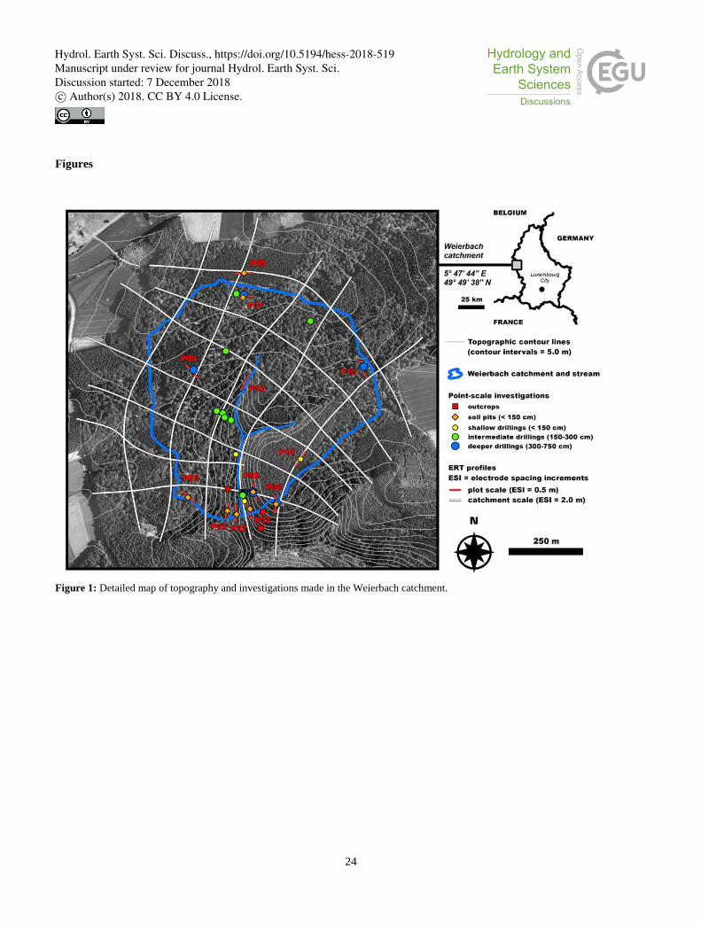
24
Figures
Figure 1: Detailed map of topography and investigations made in the Weierbach catchment.
Hydrol. Earth Syst. Sci. Discuss., https://doi.org/10.5194/hess-2018-519Manuscript under review for journal Hydrol. Earth Syst. Sci.Discussion started: 7 December 2018c© Author(s) 2018. CC BY 4.0 License.
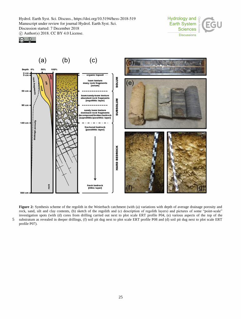
25
Figure 2: Synthesis scheme of the regolith in the Weierbach catchment (with (a) variations with depth of average drainage porosity and
rock, sand, silt and clay contents, (b) sketch of the regolith and (c) description of regolith layers) and pictures of some “point-scale”
investigation spots (with (d) cores from drilling carried out next to plot scale ERT profile P04, (e) various aspects of the top of the
substratum as revealed in deeper drillings, (f) soil pit dug next to plot scale ERT profile P08 and (d) soil pit dug next to plot scale ERT 5 profile P07).
Hydrol. Earth Syst. Sci. Discuss., https://doi.org/10.5194/hess-2018-519Manuscript under review for journal Hydrol. Earth Syst. Sci.Discussion started: 7 December 2018c© Author(s) 2018. CC BY 4.0 License.

26
Figure 3: Nash–Sutcliffe model efficiency coefficient and mean interface depths resulting from the inversion of the 25 synthetic apparent
resistivity models using the dipole-dipole array with the five different ESIs. In plots showing the estimated interface depths, thick black
lines indicate the expected values.
Hydrol. Earth Syst. Sci. Discuss., https://doi.org/10.5194/hess-2018-519Manuscript under review for journal Hydrol. Earth Syst. Sci.Discussion started: 7 December 2018c© Author(s) 2018. CC BY 4.0 License.
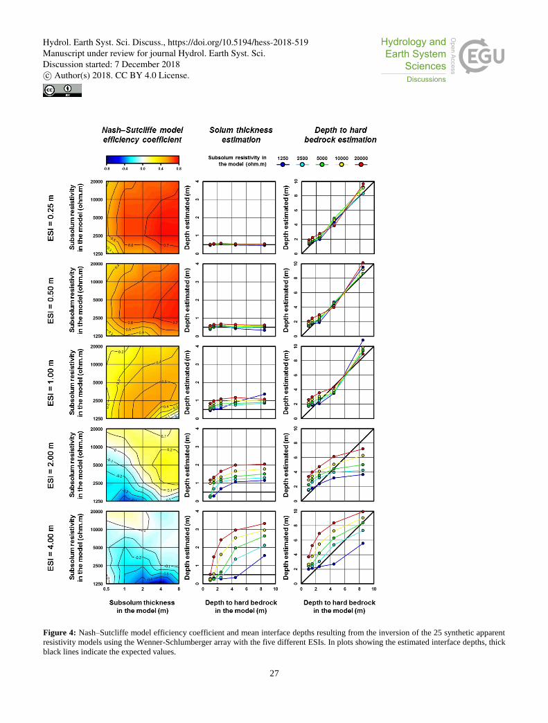
27
Figure 4: Nash–Sutcliffe model efficiency coefficient and mean interface depths resulting from the inversion of the 25 synthetic apparent
resistivity models using the Wenner-Schlumberger array with the five different ESIs. In plots showing the estimated interface depths, thick
black lines indicate the expected values.
Hydrol. Earth Syst. Sci. Discuss., https://doi.org/10.5194/hess-2018-519Manuscript under review for journal Hydrol. Earth Syst. Sci.Discussion started: 7 December 2018c© Author(s) 2018. CC BY 4.0 License.
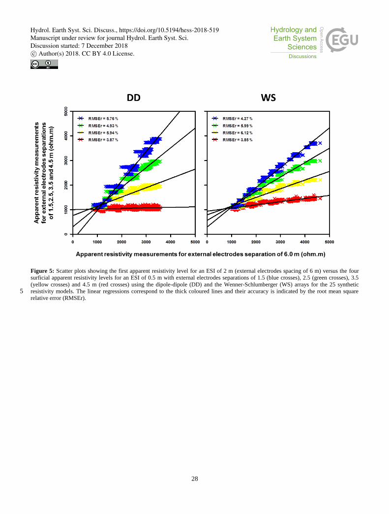
28
Figure 5: Scatter plots showing the first apparent resistivity level for an ESI of 2 m (external electrodes spacing of 6 m) versus the four
surficial apparent resistivity levels for an ESI of 0.5 m with external electrodes separations of 1.5 (blue crosses), 2.5 (green crosses), 3.5
(yellow crosses) and 4.5 m (red crosses) using the dipole-dipole (DD) and the Wenner-Schlumberger (WS) arrays for the 25 synthetic
resistivity models. The linear regressions correspond to the thick coloured lines and their accuracy is indicated by the root mean square 5 relative error (RMSEr).
Hydrol. Earth Syst. Sci. Discuss., https://doi.org/10.5194/hess-2018-519Manuscript under review for journal Hydrol. Earth Syst. Sci.Discussion started: 7 December 2018c© Author(s) 2018. CC BY 4.0 License.
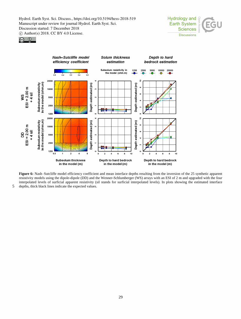
29
Figure 6: Nash–Sutcliffe model efficiency coefficient and mean interface depths resulting from the inversion of the 25 synthetic apparent
resistivity models using the dipole-dipole (DD) and the Wenner-Schlumberger (WS) arrays with an ESI of 2 m and upgraded with the four
interpolated levels of surficial apparent resistivity (sil stands for surficial interpolated levels). In plots showing the estimated interface
depths, thick black lines indicate the expected values. 5
Hydrol. Earth Syst. Sci. Discuss., https://doi.org/10.5194/hess-2018-519Manuscript under review for journal Hydrol. Earth Syst. Sci.Discussion started: 7 December 2018c© Author(s) 2018. CC BY 4.0 License.
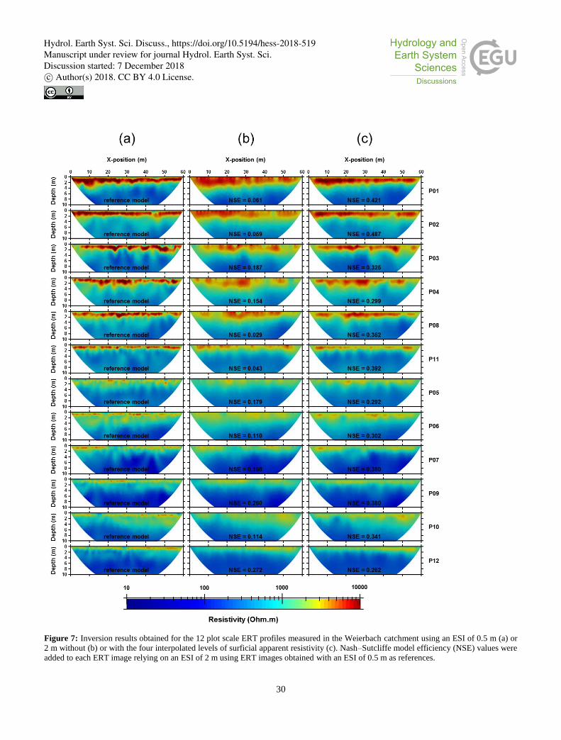
30
Figure 7: Inversion results obtained for the 12 plot scale ERT profiles measured in the Weierbach catchment using an ESI of 0.5 m (a) or
2 m without (b) or with the four interpolated levels of surficial apparent resistivity (c). Nash–Sutcliffe model efficiency (NSE) values were
added to each ERT image relying on an ESI of 2 m using ERT images obtained with an ESI of 0.5 m as references.
Hydrol. Earth Syst. Sci. Discuss., https://doi.org/10.5194/hess-2018-519Manuscript under review for journal Hydrol. Earth Syst. Sci.Discussion started: 7 December 2018c© Author(s) 2018. CC BY 4.0 License.
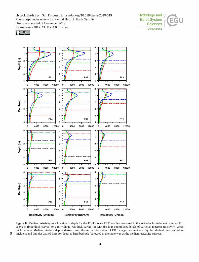
31
Figure 8: Median resistivity as a function of depth for the 12 plot scale ERT profiles measured in the Weierbach catchment using an ESI
of 0.5 m (blue thick curves) or 2 m without (red thick curves) or with the four interpolated levels of surficial apparent resistivity (green
thick curves). Median interface depths derived from the second derivative of ERT images are indicated by thin dashed lines for solum
thickness and thin dot dashed lines for depth to hard bedrock (coloured in the same way as the median resistivity curves). 5
Hydrol. Earth Syst. Sci. Discuss., https://doi.org/10.5194/hess-2018-519Manuscript under review for journal Hydrol. Earth Syst. Sci.Discussion started: 7 December 2018c© Author(s) 2018. CC BY 4.0 License.
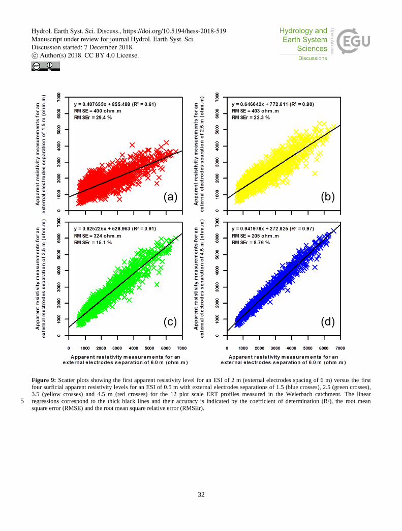
32
Figure 9: Scatter plots showing the first apparent resistivity level for an ESI of 2 m (external electrodes spacing of 6 m) versus the first
four surficial apparent resistivity levels for an ESI of 0.5 m with external electrodes separations of 1.5 (blue crosses), 2.5 (green crosses),
3.5 (yellow crosses) and 4.5 m (red crosses) for the 12 plot scale ERT profiles measured in the Weierbach catchment. The linear
regressions correspond to the thick black lines and their accuracy is indicated by the coefficient of determination (R²), the root mean 5 square error (RMSE) and the root mean square relative error (RMSEr).
Hydrol. Earth Syst. Sci. Discuss., https://doi.org/10.5194/hess-2018-519Manuscript under review for journal Hydrol. Earth Syst. Sci.Discussion started: 7 December 2018c© Author(s) 2018. CC BY 4.0 License.
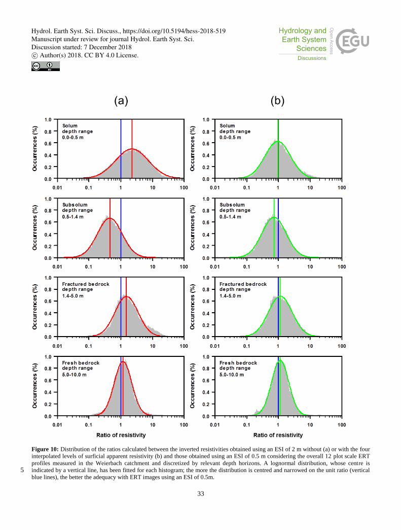
33
Figure 10: Distribution of the ratios calculated between the inverted resistivities obtained using an ESI of 2 m without (a) or with the four
interpolated levels of surficial apparent resistivity (b) and those obtained using an ESI of 0.5 m considering the overall 12 plot scale ERT
profiles measured in the Weierbach catchment and discretized by relevant depth horizons. A lognormal distribution, whose centre is
indicated by a vertical line, has been fitted for each histogram; the more the distribution is centred and narrowed on the unit ratio (vertical 5 blue lines), the better the adequacy with ERT images using an ESI of 0.5m.
Hydrol. Earth Syst. Sci. Discuss., https://doi.org/10.5194/hess-2018-519Manuscript under review for journal Hydrol. Earth Syst. Sci.Discussion started: 7 December 2018c© Author(s) 2018. CC BY 4.0 License.
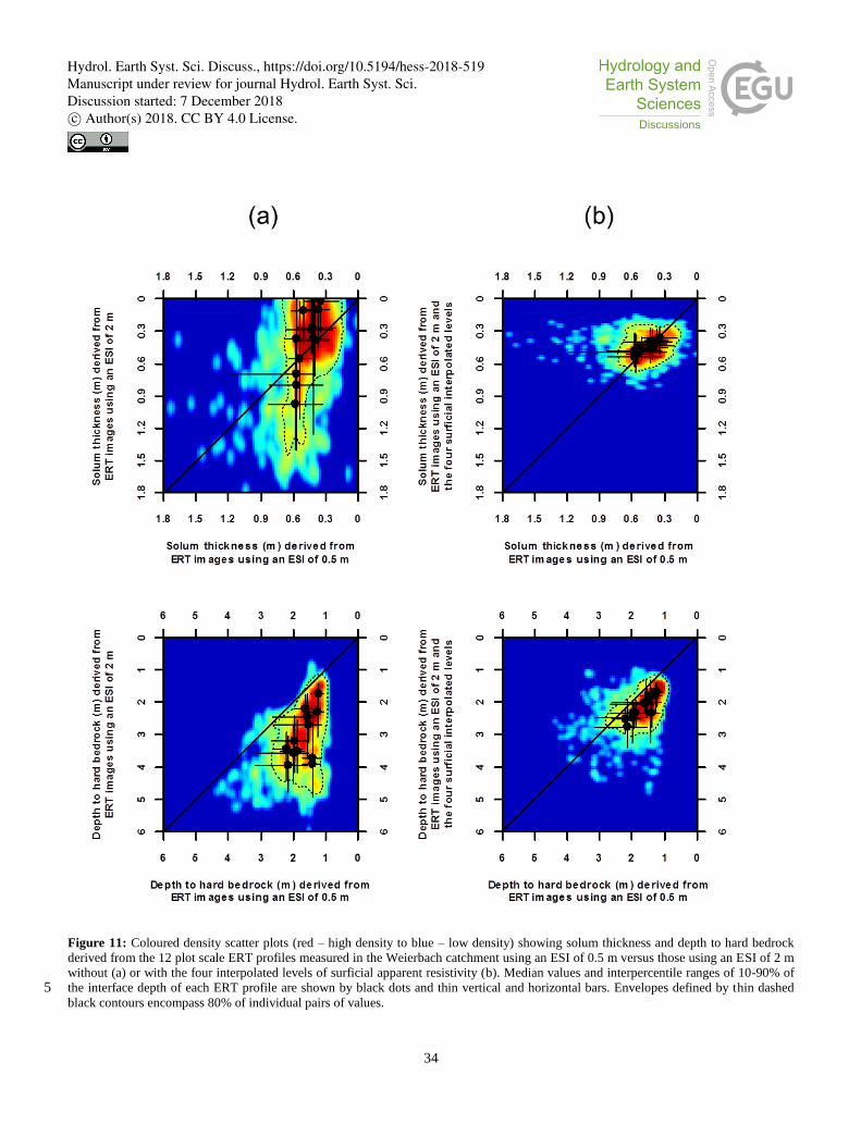
34
Figure 11: Coloured density scatter plots (red – high density to blue – low density) showing solum thickness and depth to hard bedrock
derived from the 12 plot scale ERT profiles measured in the Weierbach catchment using an ESI of 0.5 m versus those using an ESI of 2 m
without (a) or with the four interpolated levels of surficial apparent resistivity (b). Median values and interpercentile ranges of 10-90% of
the interface depth of each ERT profile are shown by black dots and thin vertical and horizontal bars. Envelopes defined by thin dashed 5 black contours encompass 80% of individual pairs of values.
Hydrol. Earth Syst. Sci. Discuss., https://doi.org/10.5194/hess-2018-519Manuscript under review for journal Hydrol. Earth Syst. Sci.Discussion started: 7 December 2018c© Author(s) 2018. CC BY 4.0 License.
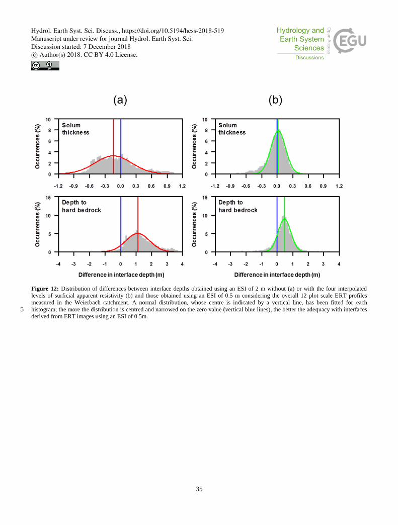
35
Figure 12: Distribution of differences between interface depths obtained using an ESI of 2 m without (a) or with the four interpolated
levels of surficial apparent resistivity (b) and those obtained using an ESI of 0.5 m considering the overall 12 plot scale ERT profiles
measured in the Weierbach catchment. A normal distribution, whose centre is indicated by a vertical line, has been fitted for each
histogram; the more the distribution is centred and narrowed on the zero value (vertical blue lines), the better the adequacy with interfaces 5 derived from ERT images using an ESI of 0.5m.
Hydrol. Earth Syst. Sci. Discuss., https://doi.org/10.5194/hess-2018-519Manuscript under review for journal Hydrol. Earth Syst. Sci.Discussion started: 7 December 2018c© Author(s) 2018. CC BY 4.0 License.

36
Tables
Table 1: Nash–Sutcliffe model efficiency coefficient (NSE) and interface depths (avg ± sd, average ± standard deviation in m; an italic value specifies that a manual operation was necessary for a proper
delineation) resulting from the inversion of the 25 synthetic apparent resistivity models (Tss, subsolum thickness in m; Rss, subsolum resistivity in ohm.m) using the dipole-dipole array with the 5 different
ESIs.
ESI = 0.25 m ESI = 0.50 m ESI = 1.00 m ESI = 2.00 m ESI = 4.00 m
Tss Rss NSE
Solum
depth
Depth to
bedrock NSE
Solum
depth
Depth to
bedrock NSE
Solum
depth
Depth to
bedrock NSE
Solum
depth
Depth to
bedrock NSE
Solum
depth
Depth to
bedrock
avg ± sd avg ± sd avg ± sd avg ± sd avg ± sd avg ± sd avg ± sd avg ± sd avg ± sd avg ± sd
0.5 1250 -0.07 0.46 ± 0.08 1.22 ± 0.15 0.36 0.44 ± 0.07 1.35 ± 0.16 0.28 0.47 ± 0.08 1.51 ± 0.19 -0.61 0.31 ± 0.32 1.62 ± 0.61 -0.27 0.30 ± 0.34 1.73 ± 1.09
0.5 2500 0.50 0.48 ± 0.05 1.31 ± 0.13 0.50 0.44 ± 0.03 1.39 ± 0.14 0.32 0.49 ± 0.04 1.58 ± 0.15 -0.27 0.21 ± 0.15 1.71 ± 0.31 -0.14 0.23 ± 0.27 1.83 ± 0.82
0.5 5000 0.53 0.51 ± 0.03 1.42 ± 0.15 0.48 0.47 ± 0.04 1.52 ± 0.15 0.29 0.56 ± 0.04 1.75 ± 0.17 -0.07 0.54 ± 0.17 2.21 ± 0.18 -0.13 0.19 ± 0.21 2.21 ± 0.37
0.5 10000 0.47 0.54 ± 0.03 1.59 ± 0.18 0.41 0.53 ± 0.04 1.72 ± 0.19 0.24 0.66 ± 0.05 2.03 ± 0.21 0.06 0.86 ± 0.11 2.77 ± 0.15 -0.09 0.24 ± 0.19 2.65 ± 0.31
0.5 20000 0.38 0.59 ± 0.03 1.81 ± 0.23 0.30 0.59 ± 0.04 1.99 ± 0.24 0.18 0.79 ± 0.06 2.36 ± 0.26 0.13 1.11 ± 0.09 3.14 ± 0.21 0.05 0.82 ± 0.34 3.77 ± 0.38
1 1250 0.42 0.56 ± 0.06 1.51 ± 0.23 0.43 0.59 ± 0.08 1.53 ± 0.18 0.44 0.53 ± 0.09 1.69 ± 0.15 -0.46 0.33 ± 0.37 1.80 ± 0.63 -0.67 0.30 ± 0.27 1.65 ± 0.80
1 2500 0.68 0.55 ± 0.03 1.59 ± 0.18 0.67 0.55 ± 0.04 1.67 ± 0.18 0.56 0.58 ± 0.04 1.85 ± 0.18 -0.10 0.65 ± 0.20 2.47 ± 0.17 -0.34 0.22 ± 0.18 2.20 ± 0.34
1 5000 0.68 0.56 ± 0.03 1.70 ± 0.20 0.65 0.57 ± 0.04 1.83 ± 0.21 0.47 0.67 ± 0.05 2.09 ± 0.21 0.03 0.91 ± 0.10 2.83 ± 0.16 -0.22 0.24 ± 0.19 2.68 ± 0.35
1 10000 0.64 0.60 ± 0.02 1.88 ± 0.23 0.56 0.61 ± 0.04 2.07 ± 0.24 0.32 0.79 ± 0.06 2.40 ± 0.27 0.08 1.12 ± 0.09 3.17 ± 0.21 -0.05 0.90 ± 0.32 3.81 ± 0.40
1 20000 0.56 0.65 ± 0.03 2.11 ± 0.26 0.41 0.66 ± 0.05 2.38 ± 0.31 0.17 0.93 ± 0.07 2.81 ± 0.26 0.10 1.35 ± 0.12 3.73 ± 0.23 0.08 1.61 ± 0.27 4.95 ± 0.28
2 1250 0.44 0.59 ± 0.09 1.97 ± 0.45 0.01 0.62 ± 0.10 1.71 ± 0.34 0.42 0.54 ± 0.09 1.84 ± 0.23 -0.31 0.77 ± 0.41 2.50 ± 0.61 -0.74 0.22 ± 0.30 1.84 ± 0.92
2 2500 0.71 0.55 ± 0.04 2.32 ± 0.37 0.63 0.59 ± 0.06 2.03 ± 0.31 0.58 0.66 ± 0.05 2.29 ± 0.25 0.16 0.94 ± 0.15 3.01 ± 0.19 -0.34 0.21 ± 0.27 3.22 ± 0.39
2 5000 0.69 0.56 ± 0.04 2.34 ± 0.28 0.63 0.59 ± 0.05 2.31 ± 0.28 0.52 0.76 ± 0.06 2.61 ± 0.25 0.19 1.16 ± 0.09 3.34 ± 0.19 -0.15 1.32 ± 0.30 4.30 ± 0.25
2 10000 0.64 0.59 ± 0.04 2.38 ± 0.30 0.58 0.63 ± 0.05 2.59 ± 0.27 0.39 0.91 ± 0.07 2.91 ± 0.23 0.13 1.39 ± 0.11 3.83 ± 0.21 -0.01 1.75 ± 0.26 5.13 ± 0.28
2 20000 0.60 0.66 ± 0.04 2.60 ± 0.30 0.53 0.67 ± 0.06 2.93 ± 0.23 0.16 1.08 ± 0.08 3.25 ± 0.27 0.04 1.63 ± 0.14 4.47 ± 0.23 0.02 2.32 ± 0.18 6.31 ± 0.47
4 1250 0.57 0.47 ± 0.09 4.11 ± 0.25 0.51 0.47 ± 0.15 3.92 ± 0.33 0.19 1.02 ± 0.24 3.09 ± 0.34 -0.08 0.95 ± 0.14 2.85 ± 0.23 -0.93 0.93 ± 0.95 3.55 ± 1.52
4 2500 0.77 0.53 ± 0.04 4.32 ± 0.16 0.75 0.51 ± 0.06 4.49 ± 0.16 0.53 0.72 ± 0.07 4.49 ± 0.43 0.22 1.13 ± 0.14 3.47 ± 0.37 -0.11 1.46 ± 0.50 5.06 ± 0.41
4 5000 0.77 0.54 ± 0.04 4.61 ± 0.16 0.74 0.54 ± 0.05 4.78 ± 0.17 0.51 0.81 ± 0.07 4.31 ± 0.59 0.24 1.33 ± 0.14 4.12 ± 0.20 0.01 1.88 ± 0.29 5.84 ± 0.39
4 10000 0.75 0.57 ± 0.04 4.78 ± 0.21 0.67 0.57 ± 0.05 5.01 ± 0.35 0.39 0.94 ± 0.07 4.14 ± 0.60 0.16 1.59 ± 0.15 4.67 ± 0.28 -0.01 2.43 ± 0.18 6.70 ± 0.48
4 20000 0.68 0.60 ± 0.04 4.92 ± 0.21 0.59 0.63 ± 0.05 4.62 ± 0.38 0.19 1.10 ± 0.08 4.40 ± 0.44 -0.08 1.88 ± 0.18 5.64 ± 0.41 -0.21 2.97 ± 0.17 8.06 ± 0.25
8 1250 0.65 0.47 ± 0.08 8.01 ± 0.19 0.54 0.40 ± 0.14 8.23 ± 0.28 -0.24 1.21 ± 0.26 8.54 ± 0.30 -0.65 1.03 ± 0.32 3.13 ± 0.42 -0.58 1.70 ± 0.67 4.85 ± 0.68
8 2500 0.80 0.52 ± 0.04 8.25 ± 0.10 0.77 0.50 ± 0.05 8.39 ± 0.12 0.44 0.85 ± 0.10 8.40 ± 0.19 0.11 1.25 ± 0.19 3.57 ± 0.29 -0.08 1.98 ± 0.55 6.08 ± 0.67
8 5000 0.78 0.54 ± 0.04 8.23 ± 0.48 0.75 0.54 ± 0.05 8.58 ± 0.14 0.52 0.84 ± 0.07 8.79 ± 0.16 0.08 1.48 ± 0.13 4.16 ± 0.28 0.01 2.38 ± 0.33 7.50 ± 0.56
8 10000 0.73 0.57 ± 0.04 7.77 ± 0.68 0.70 0.58 ± 0.05 8.61 ± 0.36 0.30 0.98 ± 0.06 9.22 ± 0.42 0.05 1.69 ± 0.13 4.82 ± 0.34 0.00 2.85 ± 0.17 8.78 ± 0.44
8 20000 0.69 0.61 ± 0.04 8.42 ± 0.30 0.66 0.62 ± 0.05 9.12 ± 0.40 0.18 1.10 ± 0.08 9.66 ± 0.31 -0.01 1.90 ± 0.18 6.61 ± 1.04 -0.17 3.25 ± 0.20 9.48 ± 0.35
5
Hydrol. Earth Syst. Sci. Discuss., https://doi.org/10.5194/hess-2018-519Manuscript under review for journal Hydrol. Earth Syst. Sci.Discussion started: 7 December 2018c© Author(s) 2018. CC BY 4.0 License.

37
Table 2: Nash–Sutcliffe model efficiency coefficient (NSE) and interface depths (avg ± sd, average ± standard deviation in m; an italic value specifies that a manual operation was necessary for a proper
delineation) resulting from the inversion of the 25 synthetic apparent resistivity models (Tss, subsolum thickness in m; Rss, subsolum resistivity in ohm.m) using the Wenner-Schlumberger array with the 5
different ESIs.
ESI = 0.25 m ESI = 0.50 m ESI = 1.00 m ESI = 2.00 m ESI = 4.00 m
Tss Rss NSE
Solum
depth
Depth to
bedrock NSE
Solum
depth
Depth to
bedrock NSE
Solum
depth
Depth to
bedrock NSE
Solum
depth
Depth to
bedrock NSE
Solum
depth
Depth to
bedrock
avg ± sd avg ± sd avg ± sd avg ± sd avg ± sd avg ± sd avg ± sd avg ± sd avg ± sd avg ± sd
0.5 1250 0.16 0.47 ± 0.06 1.30 ± 0.12 0.21 0.37 ± 0.05 1.40 ± 0.16 0.23 0.44 ± 0.09 1.69 ± 0.21 -0.24 0.28 ± 0.20 1.49 ± 0.66 0.06 0.28 ± 0.39 2.01 ± 1.33
0.5 2500 0.48 0.47 ± 0.04 1.37 ± 0.14 0.43 0.39 ± 0.04 1.45 ± 0.14 0.17 0.51 ± 0.04 1.75 ± 0.17 -0.29 0.21 ± 0.13 1.60 ± 0.29 -0.05 0.24 ± 0.32 2.43 ± 0.49
0.5 5000 0.49 0.48 ± 0.04 1.50 ± 0.15 0.45 0.44 ± 0.04 1.59 ± 0.16 0.21 0.59 ± 0.04 1.93 ± 0.19 -0.15 0.28 ± 0.20 2.28 ± 0.20 -0.09 0.18 ± 0.21 2.43 ± 0.32
0.5 10000 0.45 0.50 ± 0.04 1.67 ± 0.19 0.40 0.51 ± 0.04 1.80 ± 0.20 0.20 0.70 ± 0.05 2.22 ± 0.21 -0.01 0.98 ± 0.06 2.93 ± 0.17 -0.07 0.25 ± 0.17 2.69 ± 0.19
0.5 20000 0.37 0.52 ± 0.04 1.91 ± 0.23 0.31 0.58 ± 0.04 2.10 ± 0.24 0.18 0.83 ± 0.06 2.62 ± 0.23 0.12 1.16 ± 0.08 3.40 ± 0.20 0.07 0.52 ± 0.23 3.70 ± 0.30
1 1250 0.51 0.53 ± 0.05 1.59 ± 0.22 0.40 0.55 ± 0.08 1.68 ± 0.19 0.48 0.53 ± 0.09 1.87 ± 0.20 -0.47 0.29 ± 0.29 1.78 ± 0.64 -0.32 0.33 ± 0.31 2.15 ± 0.89
1 2500 0.69 0.53 ± 0.03 1.69 ± 0.19 0.67 0.51 ± 0.04 1.79 ± 0.19 0.47 0.60 ± 0.04 2.04 ± 0.19 -0.27 0.68 ± 0.14 2.65 ± 0.11 -0.29 0.26 ± 0.21 2.42 ± 0.32
1 5000 0.69 0.53 ± 0.03 1.79 ± 0.20 0.65 0.54 ± 0.04 1.92 ± 0.22 0.38 0.70 ± 0.05 2.27 ± 0.22 -0.08 1.01 ± 0.07 2.99 ± 0.17 -0.21 0.26 ± 0.18 2.73 ± 0.17
1 10000 0.65 0.54 ± 0.04 1.98 ± 0.23 0.55 0.59 ± 0.04 2.16 ± 0.25 0.26 0.84 ± 0.06 2.65 ± 0.22 0.05 1.17 ± 0.08 3.44 ± 0.20 -0.02 0.55 ± 0.23 3.77 ± 0.31
1 20000 0.56 0.55 ± 0.05 2.25 ± 0.26 0.43 0.65 ± 0.05 2.50 ± 0.30 0.17 0.98 ± 0.07 3.00 ± 0.24 0.15 1.31 ± 0.11 4.02 ± 0.16 0.10 1.48 ± 0.19 5.25 ± 0.40
2 1250 0.50 0.58 ± 0.07 1.98 ± 0.38 0.31 0.64 ± 0.07 1.90 ± 0.27 0.53 0.56 ± 0.10 2.08 ± 0.27 -0.38 0.69 ± 0.44 2.40 ± 0.88 -0.47 0.26 ± 0.30 2.39 ± 0.60
2 2500 0.69 0.54 ± 0.04 2.20 ± 0.29 0.67 0.57 ± 0.05 2.19 ± 0.26 0.53 0.71 ± 0.06 2.49 ± 0.25 -0.02 1.08 ± 0.09 3.23 ± 0.19 -0.29 0.35 ± 0.20 3.08 ± 0.21
2 5000 0.68 0.55 ± 0.04 2.32 ± 0.28 0.65 0.59 ± 0.05 2.40 ± 0.28 0.47 0.82 ± 0.07 2.80 ± 0.22 0.13 1.20 ± 0.08 3.60 ± 0.21 -0.10 0.64 ± 0.27 4.21 ± 0.34
2 10000 0.65 0.55 ± 0.05 2.50 ± 0.28 0.61 0.63 ± 0.05 2.68 ± 0.26 0.39 0.96 ± 0.06 3.09 ± 0.24 0.19 1.34 ± 0.11 4.12 ± 0.17 0.01 1.61 ± 0.19 5.46 ± 0.42
2 20000 0.62 0.57 ± 0.06 2.79 ± 0.23 0.57 0.68 ± 0.06 2.98 ± 0.24 0.31 1.09 ± 0.08 3.58 ± 0.27 0.10 1.64 ± 0.15 4.76 ± 0.30 0.02 2.41 ± 0.13 6.93 ± 0.44
4 1250 0.63 0.48 ± 0.06 4.34 ± 0.18 0.51 0.43 ± 0.15 4.35 ± 0.24 0.17 0.91 ± 0.37 3.50 ± 0.24 -0.07 1.06 ± 0.12 3.20 ± 0.20 -0.59 0.35 ± 0.33 2.71 ± 0.97
4 2500 0.78 0.51 ± 0.04 4.68 ± 0.20 0.73 0.50 ± 0.05 4.70 ± 0.28 0.53 0.75 ± 0.08 3.56 ± 0.32 0.19 1.21 ± 0.10 3.99 ± 0.18 -0.10 1.36 ± 0.33 5.38 ± 0.55
4 5000 0.76 0.52 ± 0.04 4.91 ± 0.23 0.70 0.53 ± 0.06 4.58 ± 0.41 0.51 0.85 ± 0.08 3.65 ± 0.29 0.27 1.36 ± 0.12 4.45 ± 0.25 -0.02 1.96 ± 0.21 6.31 ± 0.57
4 10000 0.70 0.53 ± 0.05 4.67 ± 0.47 0.64 0.58 ± 0.06 4.15 ± 0.55 0.41 1.01 ± 0.07 3.87 ± 0.24 0.19 1.66 ± 0.16 5.07 ± 0.32 -0.03 2.53 ± 0.14 7.29 ± 0.39
4 20000 0.61 0.54 ± 0.06 3.89 ± 0.49 0.57 0.65 ± 0.06 3.99 ± 0.42 0.31 1.16 ± 0.10 4.33 ± 0.29 0.04 1.99 ± 0.18 6.14 ± 0.49 -0.09 2.96 ± 0.17 8.38 ± 0.31
8 1250 0.65 0.46 ± 0.07 9.19 ± 0.33 0.53 0.34 ± 0.11 9.52 ± 0.24 -0.19 1.36 ± 0.25 10.8 ± 0.30 -0.24 1.15 ± 0.23 3.68 ± 0.33 -0.34 1.55 ± 0.59 5.57 ± 0.77
8 2500 0.78 0.51 ± 0.05 8.33 ± 0.40 0.77 0.48 ± 0.05 8.63 ± 0.25 0.48 0.86 ± 0.10 9.35 ± 0.27 0.23 1.30 ± 0.17 4.26 ± 0.28 -0.07 2.11 ± 0.39 7.33 ± 0.47
8 5000 0.75 0.52 ± 0.05 9.21 ± 0.93 0.74 0.53 ± 0.05 8.67 ± 0.26 0.50 0.90 ± 0.07 9.47 ± 0.31 0.22 1.50 ± 0.15 5.04 ± 0.31 -0.02 2.63 ± 0.17 8.41 ± 0.35
8 10000 0.73 0.54 ± 0.05 9.08 ± 0.51 0.71 0.58 ± 0.06 9.20 ± 0.37 0.46 0.98 ± 0.07 9.83 ± 0.53 0.19 1.77 ± 0.15 6.30 ± 0.59 -0.02 2.96 ± 0.16 9.08 ± 0.38
8 20000 0.69 0.54 ± 0.06 9.66 ± 0.36 0.64 0.62 ± 0.06 10.1 ± 0.50 0.40 1.07 ± 0.09 8.92 ± 1.08 0.14 2.04 ± 0.21 7.20 ± 0.48 -0.02 3.32 ± 0.18 9.93 ± 0.50
5
Hydrol. Earth Syst. Sci. Discuss., https://doi.org/10.5194/hess-2018-519Manuscript under review for journal Hydrol. Earth Syst. Sci.Discussion started: 7 December 2018c© Author(s) 2018. CC BY 4.0 License.

38
Table 3: Nash–Sutcliffe model efficiency coefficient (NSE) and interface depths (avg ± sd, average ± standard deviation in m; an italic value specifies that a manual operation was necessary for a proper
delineation) resulting from the inversion of the 25 synthetic apparent resistivity models (Tss, subsolum thickness in m; Rss, subsolum resistivity in ohm.m) using the dipole-dipole (DD) and the Wenner-
Schlumberger (WS) arrays with the ESI of 2 m upgraded with the four interpolated levels of surficial apparent resistivity (sil stands for surficial interpolated levels).
[DD] ESI = 2.00 m + 4sil [WS] ESI = 2.00 m + 4sil
Tss Rss NSE
Solum
depth
Depth to
bedrock NSE
Solum
depth
Depth to
bedrock
avg ± sd avg ± sd avg ± sd avg ± sd
0.5 1250 -0.74 0.35 ± 0.05 1.18 ± 0.10 -1.16 0.35 ± 0.05 1.23 ± 0.11
0.5 2500 0.28 0.51 ± 0.09 1.82 ± 0.12 0.34 0.47 ± 0.05 1.73 ± 0.14
0.5 5000 0.29 0.60 ± 0.05 1.91 ± 0.17 0.33 0.57 ± 0.04 1.95 ± 0.20
0.5 10000 0.29 0.59 ± 0.04 1.98 ± 0.20 0.30 0.59 ± 0.04 2.10 ± 0.23
0.5 20000 0.28 0.60 ± 0.05 2.16 ± 0.24 0.27 0.62 ± 0.05 2.29 ± 0.27
1 1250 -0.15 0.36 ± 0.04 1.26 ± 0.14 -0.38 0.37 ± 0.04 1.31 ± 0.15
1 2500 0.59 0.57 ± 0.07 2.01 ± 0.16 0.62 0.54 ± 0.05 2.02 ± 0.19
1 5000 0.59 0.59 ± 0.05 2.07 ± 0.20 0.57 0.60 ± 0.04 2.17 ± 0.23
1 10000 0.56 0.58 ± 0.05 2.21 ± 0.25 0.51 0.61 ± 0.05 2.34 ± 0.27
1 20000 0.47 0.57 ± 0.05 2.57 ± 0.29 0.43 0.62 ± 0.05 2.71 ± 0.26
2 1250 -0.05 0.38 ± 0.04 1.31 ± 0.17 -0.20 0.38 ± 0.04 1.37 ± 0.18
2 2500 0.68 0.52 ± 0.07 2.35 ± 0.25 0.69 0.54 ± 0.06 2.40 ± 0.27
2 5000 0.68 0.54 ± 0.06 2.55 ± 0.26 0.65 0.60 ± 0.05 2.63 ± 0.25
2 10000 0.68 0.53 ± 0.05 2.89 ± 0.21 0.64 0.60 ± 0.05 2.88 ± 0.22
2 20000 0.59 0.54 ± 0.05 3.53 ± 0.31 0.61 0.59 ± 0.06 3.21 ± 0.23
4 1250 -0.14 0.36 ± 0.05 3.96 ± 0.29 -0.04 0.36 ± 0.04 4.72 ± 0.32
4 2500 0.70 0.44 ± 0.05 3.90 ± 0.36 0.70 0.49 ± 0.06 3.68 ± 0.44
4 5000 0.71 0.48 ± 0.05 4.25 ± 0.38 0.66 0.54 ± 0.06 3.38 ± 0.28
4 10000 0.70 0.49 ± 0.06 4.57 ± 0.37 0.65 0.55 ± 0.06 3.84 ± 0.47
4 20000 0.65 0.52 ± 0.05 4.90 ± 0.35 0.63 0.57 ± 0.06 4.47 ± 0.49
8 1250 -1.56 0.29 ± 0.11 4.09 ± 0.15 -0.76 0.30 ± 0.06 4.65 ± 0.19
8 2500 0.48 0.34 ± 0.11 4.13 ± 0.41 0.62 0.38 ± 0.08 4.86 ± 0.46
8 5000 0.63 0.43 ± 0.08 4.42 ± 0.84 0.68 0.48 ± 0.07 7.53 ± 1.44
8 10000 0.65 0.47 ± 0.06 8.64 ± 0.63 0.68 0.51 ± 0.07 8.85 ± 0.58
8 20000 0.60 0.50 ± 0.06 8.33 ± 0.55 0.64 0.53 ± 0.06 8.97 ± 0.58
5
Hydrol. Earth Syst. Sci. Discuss., https://doi.org/10.5194/hess-2018-519Manuscript under review for journal Hydrol. Earth Syst. Sci.Discussion started: 7 December 2018c© Author(s) 2018. CC BY 4.0 License.

39
Table 4: Interface depths (avg ± sd, average ± standard deviation in m) derived from the inversion results obtained for the 12 plot scale ERT profiles measured in the Weierbach catchment using an ESI of
0.5 m or 2 m (upgraded or not with the four interpolated levels of surficial apparent resistivity; sil stands for surficial interpolated levels). Mean differences (md) in interface depths with the reference ERT
images relying on an ESI of 0.5 m were added to the standard and upgraded results obtained with an ESI of 2 m.
ESI = 0.50 m ESI = 2.00 m ESI = 2.00 m + 4sil
Profile
Solum
depth
Depth to
bedrock
Solum
depth
Depth to
bedrock
Solum
depth
Depth to
bedrock
avg ± sd avg ± sd avg ± sd [ md ] avg ± sd [ md ] avg ± sd [ md ] avg ± sd [ md ]
P01 0.59 ± 0.19 2.21 ± 0.40 0.70 ± 0.44 [0.11] 3.63 ± 0.59 [1.42] 0.52 ± 0.10 [-0.07] 2.55 ± 0.39 [0.34]
P02 0.54 ± 0.11 2.01 ± 0.46 0.59 ± 0.40 [0.05] 3.44 ± 0.55 [1.43] 0.50 ± 0.08 [-0.04] 2.39 ± 0.32 [0.38]
P03 0.69 ± 0.31 2.17 ± 0.67 0.72 ± 0.45 [0.03] 3.63 ± 0.97 [1.46] 0.50 ± 0.13 [-0.19] 2.58 ± 0.58 [0.41]
P04 0.59 ± 0.20 2.29 ± 0.68 0.90 ± 0.45 [0.31] 3.90 ± 0.73 [1.61] 0.47 ± 0.12 [-0.12] 2.74 ± 0.64 [0.45]
P08 0.52 ± 0.17 2.04 ± 0.47 0.43 ± 0.41 [-0.09] 3.28 ± 0.65 [1.24] 0.49 ± 0.12 [-0.03] 2.36 ± 0.34 [0.32]
P11 0.49 ± 0.12 1.66 ± 0.29 0.16 ± 0.16 [-0.33] 2.25 ± 0.35 [0.59] 0.46 ± 0.08 [-0.03] 2.03 ± 0.27 [0.37]
P05 0.45 ± 0.20 1.76 ± 0.61 0.26 ± 0.20 [-0.19] 2.77 ± 0.39 [1.01] 0.41 ± 0.12 [-0.04] 2.02 ± 0.38 [0.26]
P06 0.41 ± 0.11 1.42 ± 0.25 0.38 ± 0.29 [-0.03] 3.88 ± 0.73 [2.46] 0.44 ± 0.11 [0.03] 2.30 ± 0.53 [0.88]
P07 0.41 ± 0.14 1.75 ± 0.50 0.26 ± 0.26 [-0.15] 2.52 ± 0.74 [0.77] 0.41 ± 0.11 [0.00] 1.97 ± 0.45 [0.22]
P09 0.37 ± 0.08 1.28 ± 0.19 0.16 ± 0.17 [-0.21] 2.35 ± 0.54 [1.07] 0.39 ± 0.09 [0.02] 1.84 ± 0.33 [0.56]
P10 0.41 ± 0.10 1.46 ± 0.40 0.52 ± 0.48 [0.11] 3.80 ± 1.19 [2.34] 0.41 ± 0.11 [0.00] 2.11 ± 0.85 [0.65]
P12 0.34 ± 0.13 1.25 ± 0.16 0.11 ± 0.13 [-0.23] 1.82 ± 0.35 [0.57] 0.38 ± 0.09 [0.04] 1.74 ± 0.30 [0.49]
Hydrol. Earth Syst. Sci. Discuss., https://doi.org/10.5194/hess-2018-519Manuscript under review for journal Hydrol. Earth Syst. Sci.Discussion started: 7 December 2018c© Author(s) 2018. CC BY 4.0 License.


