Large-scale sandbox experiment on longitudinal effective dispersion in heterogeneous porous media

Large-scale sandbox experiment on longitudinal effective

dispersion in heterogeneous porous media

Surabhin C. Jose1 and M. Arifur Rahman

Institut fur Wasserbau, Universitat Stuttgart, Stuttgart, Germany

Olaf A. Cirpka

Swiss Federal Institute for Environmental Science and Technology, Dubendorf, Switzerland

Received 25 May 2004; revised 4 October 2004; accepted 25 October 2004; published 28 December 2004.

[1] In heterogeneous media the breakthrough curves observed at single points may differsignificantly from those integrated over a control plane. While standard macrodispersiondescribes the spread of concentration averaged over the entire cross section, effectivedispersion quantifies the average spread in the locally observed breakthrough curves. Weperform a conservative tracer test in a 14-m-long sandbox filled heterogeneously withfour types of silica sand. The filling resembles natural heterogeneities including thedistribution of facies and micro-structures within the various sand types. We usefluorescein as tracer, which we measure at 126 measurement points directly within theporous medium and at 19 levels in the outlet of the domain. We use fiber-optic probes witha point-like measurement tip for fluorescence intensity measurements. From the secondcentral temporal moments of the locally obtained breakthrough curves we computeapparent effective dispersion coefficients, and from the average over all probes within ameasurement plane we derive apparent macrodispersion coefficients. The effectivedispersion coefficient is about two thirds of the macrodispersion coefficient. Consideringthe typical length scales of the heterogeneities, the experimental findings are qualitativelyin agreement with linear stochastic theory. INDEX TERMS: 1829 Hydrology: Groundwater

hydrology; 1832 Hydrology: Groundwater transport; 1869 Hydrology: Stochastic processes; KEYWORDS:

heterogeneous porous media, temporal moments, effective dispersion, dilution, mixing, sandbox

Citation: Jose, S. C., M. A. Rahman, and O. A. Cirpka (2004), Large-scale sandbox experiment on longitudinal effective dispersion

in heterogeneous porous media, Water Resour. Res., 40, W12415, doi:10.1029/2004WR003363.

1. Introduction

[2] Over the past ten years, dilution and mixing ofcompounds in heterogeneous porous media has become atopic of significant research interest [Molz and Widdowson,1988; Kitanidis, 1994; Oya and Valocchi, 1998; Cirpka andKitanidis, 2000a, 2000b; Cirpka, 2002]. Insufficient mixinghas been addressed as possible limiting factor for reactionsbetween dissolved compounds. Numerical and theoreticalstudies have shown that, in the absence of sorption, pore-scale dispersion is the actual process leading to mixingbetween reactants [Kitanidis, 1994; Kapoor et al., 1997;Cirpka and Kitanidis, 2000b; Cirpka, 2002]. Therefore it isimportant to gain a thorough understanding of dispersivemixing.[3] Classical macrodispersion theory analyzes how the

second central spatial moments of very large, conservativeplumes increase with time due to spatial variabilityof hydraulic conductivity in heterogeneous formations.Because the ergodicity assumption holds for very largeplumes, the moments of such plumes behave like those of

the ensemble-averaged concentration, which is the commontarget of stochastic macrodispersion theory [Gelhar andAxness, 1983; Dagan, 1984]. For large plumes, a significantcontribution to the increase of second central spatialmoments is due to different parts of the tracer plume movingwith different velocity. That is, the plume gets increasinglyirregular in shape. To this process we refer as spreading.[4] For a nonsorbing compound the spatial variability of

advection controls spreading. However, if we observed twosuch compounds that initially did not occupy the same spaceand we considered advection exclusively, the mass of the twocompounds would remain in their specific, separated watervolumes moving with groundwater flow. The compoundswould never occupy the same volume, and the plumes wouldnot overlap. That is, there would be no mixing.[5] To quantify actual mixing, rather than spreading,

several parametric models have been suggested. Kitanidis[1994] introduced the dilution index, which may be visual-ized as the effective volume occupied by the solute. Kapoorand Gelhar [1994a, 1994b] analyzed the concentrationvariance, that is, the expected squared deviation betweenthe actual concentration and its expected value. A highvalue of concentration variance indicates a strong lack ofmixing. For two compounds, the segregation intensity mayquantify the difference in actual mixing and mixing pre-dicted by the application of macrodispersion coefficients[Kapoor et al., 1997].

1Now at Integrated Waste Management Centre, Cranfield University,Bedford, UK.

Copyright 2004 by the American Geophysical Union.0043-1397/04/2004WR003363

W12415

WATER RESOURCES RESEARCH, VOL. 40, W12415, doi:10.1029/2004WR003363, 2004

1 of 13

[6] For nonsorbing compounds, diffusion is the onlydriving force of dilution and mixing. Spreading enhancesdilution because it increases the plume"s surface areaacross which diffusion acts. On the pore scale, diffusionlengths are rather small, so that actual dilution catches upwith pore-scale spreading already within typical traveldistances of less than a meter [Jose and Cirpka, 2004].For heterogeneities at field scales, by contrast, a plumemay have undergone significant macrodispersion, whereasdilution has hardly started [Kitanidis, 1994].[7] Bulk-averaged quantities, such as the dilution index,

require accurate knowledge about the entire spatial concen-tration distribution. The experiments of Ursino et al. [2001a,2001b] belong to the few experimental studies wherethe necessary amount of information was accessible. Inthe temporal domain, by contrast, dense information iscommonly available in breakthrough curves. Cirpkaand Kitanidis [2000a, 2000b] expressed the lack of mixingin heterogeneous aquifers by analyzing the width ofbreakthrough curves measured at single points. WhileVanderborght and Vereecken [2001, 2002] applied stochastictheory to estimate pore-scale dispersion coefficients fromlocal breakthrough curves, Cirpka and Kitanidis [2000a]determined apparent macroscopic dispersion coefficientsrelevant for mixing from the second central momentsof single point-related breakthrough curves and macro-dispersion coefficients from all breakthrough curves mea-sured in the same observation plane. Subsequently, thedilution-related dispersion coefficients determined from theconservative tracer test were used to predict reactive mixingin the same domain [Cirpka and Kitanidis, 2000b]. In thepresent study, we will adopt the standpoint of Cirpka andKitanidis [2000a, 2000b] and characterize solute mixing bythe second central moments of point-related breakthroughcurves obtained in a large-scale sandbox experiment.[8] Traditionally, stochastic theory has dealt more

frequently with spatial than with temporal moments. First-order results for spatial moments, however, can directly betransferred to their temporal counterparts [see Rubin, 2003,chap. 9–10].Dentz et al. [2000] and Fiori and Dagan [2000]derived stochastic analytical expressions for the effectivedispersion coefficient, predicting the spread of a plume,originating from a point-like injection. These results can beused to predict the width of a breakthrough curve measured ata point because of the equivalence between spatial andtemporal moments, and because the coefficients describingthe width of a breakthrough curve measured at a point for avery wide plume are identical to those describing the widthof a breakthrough curve measured over a wide control planefor a plume originating from a point source. In numericalstudies, Cirpka [2002] showed that the longitudinal effectivedispersion coefficient for a point-like injection lead indeed tocorrect mass balances when applied to mixing-controlledreactive transport. In the present study, we will test theapplicability of the stochastic analytical expressions ofDentzet al. [2000] to real transport experiments.[9] Most of the above mentioned studies are of a

theoretical nature, or rely on numerical simulations. Thetheoretical results require rather rigorous assumptions suchas the multi-Gaussian distribution of the log-conductivityand the stationarity of the velocity field. To which extent thetheoretical results are applicable to real aquifers, deviating

from the idealized formations assumed in stochastic theory,remains open. In the present study, we want to addressthis question by performing a solute transport experiment.We study effective dispersion as quantified by the secondcentral temporal moments of point-like concentrationmeasurements. We do this using an artificial, pseudo two-dimensional, large-scale model aquifer that is filled hetero-geneously. We deliberately choose a filling that resemblesnatural sedimentary structures, including facies-like macro-heterogeneities, and microheterogeneities within the facies.Like in natural sediments, common second-order spatialstatistics cannot fully characterize the patterns in our sand-box. Nonetheless, we test whether theoretical results basedon such statistics give reasonable estimates of effectivedispersion in the experimental domain.[10] Intermediate to large-scale sandbox studies on solute

dispersion have been conducted by Silliman et al. [1998],Cirpka et al. [1999], Silliman and Zheng [2001], Barth et al.[2001], Ursino et al. [2001a, 2001b], Levy and Berkowitz[2003], Loveland et al. [2003], among others. Silliman et al.[1998] give an overview over older intermediate-scaleexperiments. In most of these studies, heterogeneities wereintroduced by blocks of different sand types, choosing eithersimple deterministic block structures or randomly generatedindicator fields. Great care was taken to make the blocksthemselves as homogeneous as possible.[11] In this study, a sandbox with dimensions 14 m �

0.13 m � 0.5 m is filled with four types of sand. Thesedimentary pattern in our sandbox resembles that in nature[Pettijohn et al., 1987]. In particular, the blocks of differentsand types have the shapes of lenses rather than rectangles,and the blocks exhibit sedimentary microstructures, such aslaminations, created by filling the box in a settling proce-dure under water. Opting for closer-to-nature conditions, wesacrifice the exact knowledge about the hydraulic structureof the domain. The latter, however, was hardly achievedeven in studies aiming at definite heterogeneous structures[Barth et al., 2001].[12] The objective of the study is to test whether the

measured temporal moments of point-related and cross-sectional averaged breakthrough curves qualitatively behavelike predicted in numerical studies [Cirpka and Kitanidis,2000a]. We also test whether the theoretical results of first-order stochastic theory for effective dispersion coefficientsby Dentz et al. [2000] are in agreement to the experimentalfindings.

2. Theory

[13] We want to analyze mixing of solutes in aquifers. Inorder to do this, we study temporal moments of soluteconcentration. In the following, we will give the definitionsof the moments, present moment-generating equations, andoutline the relation between temporal moments and mixingparameters.

2.1. Governing Equation

[14] We consider a conservative compound with aqueousphase concentration c undergoing advection and dispersion:

@c

@tþ v � rc�r � Drcð Þ ¼ 0; ð1Þ

2 of 13

W12415 JOSE ET AL.: LONGITUDINAL EFFECTIVE DISPERSION W12415

in which t is time, v denotes the spatially variable seepagevelocity vector, and D is the pore-scale dispersion tensor.The underlying flow field is in steady state. In ourexperiments, the domain contains no tracer prior toinjection:

c x; t0ð Þ ¼ 0: ð2Þ

[15] From time zero onward, the tracer is injected con-tinuously with a constant concentration cin in the inflowingwater. At the other boundaries, we restrict the normal massflux to the advective one:

n � vc� Drcð Þ ¼ n � vcin on Gin

n � Drcð Þ ¼ 0 on GnGin;ð3Þ

in which n is the unit vector normal to the boundary G, andGin is the inflow boundary section. G\Gin denotes the part ofthe boundary that is not included in Gin.

2.2. Definition of Temporal Moments

[16] Measuring the concentration at various points withinthe domain, we characterize the breakthrough curves bytheir temporal moments:

m0 xð Þ ¼Z1t¼0

c x; tð Þ dt; ð4Þ

mi xð Þ ¼Z1t¼0

tic x; tð Þdt; ð5Þ

m2c xð Þ ¼Z1t¼0

t � m1 xð Þm0 xð Þ

� �2

c x; tð Þdt ¼ m2 xð Þ � m1 xð Þð Þ2

m0 xð Þ ; ð6Þ

in which m0(x) is the zeroth temporal moment, mi(x)denotes the ith noncentral moment, and m2c(x) is the secondcentral moment.[17] In the following, we normalize all higher moments

by the zeroth moment m0(x). Also, we discuss the momentsfor a pulse-like injection of the tracer, although we apply aHeaviside boundary condition in the experiments. Becausethe advection-dispersion equation, equation (1), is linearwith respect to the concentration, we can construct thebreakthrough curve of a Dirac pulse injection from thatobserved for a Heaviside injection by taking the timederivative.

2.3. Moment-Generating Equations

[18] In the current application, the tracer is introduceduniformly over the inflow boundary. Under these condi-tions, the governing equations of the normalized first andsecond central moments for a pulse-like injection over theinflow boundary are [see Cirpka and Kitanidis, 2000a]

v � rm1 �r � Drm1ð Þ ¼ 1;m1 ¼ 0 on Gin;n � Drm1ð Þ ¼ 0 on GnGin;

ð7Þ

v � rm2c �r � Drm2cð Þ ¼ 2rm1 � Drm1ð Þ;m2c ¼ 0 on Gin;n � Drm2cð Þ ¼ 0 on GnGin:

ð8Þ

[19] In uniform flow fields, the first moment m1 increasesessentially linearly with travel distance. Depending on theboundary condition, slight deviations may be possible nearthe inflow boundary. With a uniform gradient of m1,oriented into the direction of flow, the second centralmoment m2c also increases linearly with distance. Thegradient depends on the velocity and the longitudinaldispersion coefficient. Under uniform conditions, transversedispersion has no impact on m2c.[20] In spatially variable flow fields, the distribution of the

first moment reflects the heterogeneities. In high- velocityregions, m1 increases with distance less than in low-velocityregions. This leads to a finger-like pattern of travel timecontour lines. Thus the gradient of m1 is stronger in thetransverse than in the longitudinal direction. The latter affectsthe distribution of the second central moments because thesource termrm1 � (Drm1) in the governing equation of m2c,equation (8), is the largest where old and young waters flowparallel to each other. In these regions, the source term isdominated by pore-scale transverse dispersion.

2.4. Apparent Parameters for Pulse-Like Injection

[21] To characterize transport in a heterogeneous system,we use apparent parameters which are computed from break-through curves measured by single point-like probes. Theseparameters interpret the temporal moments as if they weremeasured in a fictitious uniform medium. Assuming thatmean flow is oriented in direction x1, the apparent velocityva(x) and the apparent longitudinal dispersion coefficientDa(x) at each location are [Cirpka and Kitanidis, 2000a]

va xð Þ ¼ x1

m1 xð Þ ð9Þ

Da xð Þ ¼ x21m2c xð Þ2m3

1 xð Þ: ð10Þ

[22] It is important to keep in mind, that both va(x) andDa(x) give only a fictitious physical interpretation of thetemporal moments. va(x) and Da(x) are path-averagedquantities and must not be confused with the true localparameters v(x) and D(x). In particular, the apparent dis-persion coefficient Da(x) interprets the second centralmoment as a result of longitudinal dispersion, whereas inthe heterogeneous field, it is the transverse local dispersionthat causes m2c to grow. Nonetheless, the apparent param-eters va(x) and Da(x) may be more informative than themoments themselves, because inherent spatial trends ofthe moment distributions are removed.[23] From va(x) and Da(x), we also compute an apparent

dispersivity aa(x) and an apparent Peclet number Pea(x):

aa xð Þ ¼ Da xð Þva xð Þ ¼ x1m2c xð Þ

2m21 xð Þ

ð11Þ

Pea xð Þ ¼ x1va xð ÞDa xð Þ ¼ 2m2

1 xð Þm2c xð Þ : ð12Þ

2.5. Results From Stochastic Theory of Dispersion

[24] In stochastic theory, we consider the log-hydraulicconductivity field, and maybe other spatial parameters, as

W12415 JOSE ET AL.: LONGITUDINAL EFFECTIVE DISPERSION

3 of 13

W12415

outcome of a random space process [see Rubin, 2003].From the statistical properties of the independent parame-ters, we evaluate those of dependent quantities such asheads, velocities, concentrations and their moments. Sto-chastic dispersion theory essentially considers the expectedvalue of second central moments of concentration in spaceor time. In this context, the order of taking the expectedvalues and evaluating the moments is crucial. Standardmacrodispersion, denoted ensemble dispersion by Dentzet al. [2000a] and absolute dispersion by Andricevic andCvetkovic [1998], describes how the spatial second centralmoments of the ensemble-averaged concentration increasewith time. Since the center of gravity of the solute plumemay differ from realization to realization, the ensemble-averaged concentration distribution is much more spreadthan that in a single realization. When studying effectivedispersion [Dentz et al., 2000], denoted relative dispersionby Andricevic and Cvetkovic [1998], we first take themoments in each realization and average over all realiza-tions subsequently.[25] In the following, we consider two ensemble averages

of second central temporal moments: the expected value ofthe second central moments evaluated for each realization,hm2ci, and the second central moment of the averagedconcentration m*2c which differs from hm2ci by the varianceof first moments sm1

2 [e.g., Kitanidis, 1988; Cirpka andKitanidis, 2000a]:

m2c* x1ð Þ ¼ m2c xð Þh i þ s2m1x1ð Þ: ð13Þ

[26] hm2ci is a relative measure for mean dilution andmixing of the tracer plume, whereas m*2c also includeseffects of uncertainty in the travel time sm1

2 . In an experi-ment, it is impossible to average over many realizations,because this would require repeated filling of the domain.Here, we replace the ensemble average by the average overa large cross section. Then, hm2c(x1)i and sm1

2 (x1) are themean second central moment and the variance of thebreakthrough time observed at points within the crosssection, respectively.[27] We may estimate the expected second central

moment of the averaged concentration m*2c from theexpected one-particle variance of displacements X11 andthe variance of first moments sm1

2 at an observation pointfrom the two-particle covariance of displacements Z11 withzero initial separation by [see Rubin, 2003, chap. 9–10]

m2c* x1ð Þ ¼ 1

v1h i2X11 m1 x1ð Þh ið Þ ð14Þ

s2m1x1ð Þ ¼ 1

v1h i2Z11 m1 x1ð Þh ið Þ; ð15Þ

in which hm1(x1)i may be approximated to the first order by

m1 x1ð Þh i ¼ x1

v1h i : ð16Þ

[28] Dentz et al. [2000] derived closed form expressionsfor X11 and Z11 in second-order stationary velocity fieldsusing an Eulerian method. Fiori and Dagan [2000] came to

identical expressions in a Lagrangian framework. In thespectral domain, these expressions are

Xij tð Þ ¼ 2tDij

þZ1

2piv � sþ 4p2sTDsð Þt þ exp � 2piv � sþ 4p2sTDsð Þtð Þ � 1ð Þ2piv � sþ 4p2sTDsð Þ2

Svivj sð Þds

ð17Þ

Zij tð Þ ¼Z1

1� exp � 2piv � sþ 4p2sTDsð Þtð Þ4p2 v � sð Þ2þ16p4 sTDsð Þ2

þ 1� exp �8p2sTDstð Þ8p2sTDs 2piv � s� 4p2sTDsð Þ

!Svivj sð Þds; ð18Þ

in which s is the vector of wave numbers, D is the pore-scale dispersion tensor, i is the imaginary number, andSvivj(s) is the power (cross-) spectral density function of theseepage velocity components vi and vj which can beevaluated from the spectrum SYY(s) of the log-conductivityby [Gelhar and Axness, 1983]

Svivj sð Þ ¼ Ji �s � Js � s si

� �Jj �

s � Js � s sj

� �K2g

n2eSYY sð Þ; ð19Þ

with the mean hydraulic gradient vector J and the geometricmean of the hydraulic conductivity Kg. The log-conductiv-ity spectrum SYY(s) is the Fourier transform of thecovariance function RYY(h), here defined by

SYY sð Þ ¼Z1

RYY hð Þ exp �2pis � hð Þdh; ð20Þ

in which h is the distance vector.[29] In isotropic aquifers, the asymptotic limit of m*2c

relates to Dagan’s [1984] expression for the spatialmoments X11 by

m2c;1* xð Þ ¼ 2ls2Y x

vh i2; ð21Þ

where l is the integral scale of the aquifer heterogeneity,and sY

2 is the variance of log conductivity. The variance offirst moments, as approximated by Dentz et al. [2000] forthe two-dimensional case, can be written in the temporalform as

s2m1xð Þ ¼ 2ls2YtDT

vh i

ffiffiffiffiffiffiffiffiffiffiffiffiffiffiffiffiffiffiffiffiffiffi1þ 2px

vh itDT

s� 1

!; ð22Þ

where tDT= l2/DT is the timescale of transverse pore-scale

dispersive and DT is the transverse dispersion coefficient.Dentz et al. [2000] also derived closed form expressions forensemble and effective dispersion coefficients underanisotropic conditions.[30] In our experiments, we measure the first and

second central moments, m1(x) and m2c(x), according toequations (5) and (6), at single points. From the moments atpoints with identical travel distance x1, we evaluate thecross-sectional averages, hm1(x1)i, hm2c(x1)i and m*2c(x1),by arithmetic averaging over all probes within a crosssection. We also compute the apparent transport parameters

4 of 13


va(x) and Da(x) according to equations (9) and (10). Finally,we compare the experimental data with the results fromstochastic theory, obtained by substituting equations (17)and (18) into equations (14) and (15).

3. Experimental Setup

3.1. Materials

3.1.1. Large-Scale Sandbox[31] The experiments are performed in a sandbox of

dimensions 14 m � 0.13 m � 0.5 m (length � width �height). Figure 1 shows a sketch of the experiment setup.The box is made of standard steel. At the front side,windows with 15 mm thick glass panes provide the oppor-tunity of visual observations. Chambers of length 5 cm areadded at both the inlet and the outlet. The inlet chamber isdivided into two subchambers with equal height of 25 cm.This feature is for experiments on transverse dispersion thatare not discussed here. The outlet chamber is divided intonineteen subchambers of equal height. Stainless steel wirefabrics with a mesh size of 0.1 mm are placed in front ofeach chamber to prevent sand falling into the chambers.From the outlet chambers, the water is led to a hydraulicswitchboard. Here, each outlet chamber can be connected toone of two constant head tanks with identical water level.In order to measure the flow rate of a particular outletchamber, the latter chamber is solely connected to oneconstant-head tank, whereas all other chambers areconnected to the other constant-head tank. Then, the dis-charge is gravimetrically measured in the outflow of thefirst constant-head tank.[32] Hydraulic heads within the porous medium are

measured using groups of ten piezometers each at a distanceof approximately 1.4 m, with the first group at length 0.7 mand the final group at length 13.3 m.[33] Figure 2 shows the locations of the piezometers as

circles. At each measurement section, the piezometers areplaced at a distance of 5 cm between each other with thelowest probe at a height of 2.5 cm and the highest probe at aheight of 47.5 cm. A fine mesh is placed at the end thatconnects the piezometer tube to the sandbox in order toprevent the sand from entering the tubes.3.1.2. Heterogeneous Packing[34] The sandbox is filled heterogeneously using four

types of silica sand, the properties of which are givenin Table 1. The packing resembles natural sediments.

Figure 3b shows the distribution of the four sand types,mimicking a facies distribution. The typical length of eachlens is 3 m and its typical height is 0.08 m.[35] Before filling, the desired pattern was drawn onto the

glass pane, and the sandbox was filled to two-thirds withwater. Then, the required sand type was poured into thedomain from containers hanging from a crane. In orderto maintain uniform spreading of the falling sand, thecontainer was swayed back and forth in the longitudinaldirection of the sandbox, but within the required fillingregion. The procedure was repeated with all predefinedlenses until the whole sandbox was filled.[36] Because the sand particles settled in standing water,

the filling exhibits microheterogeneities that are similar topatterns found in natural sediments. Figure 4 shows thephoto of a 1-m-long section of the domain. The mostcommon microstructure may be addressed as lamination,but we have also found cross lamination and ripple-likestructures.[37] After filling the box with sand, the water was

drained. A bentonite layer with a height of 3 cm is providedat the top to prevent preferential flow due to setting of thesand. The sandbox is tightly covered with a metal plate withan elastomer sheet and a PVC sheet between the metal plateand the bentonite layer.[38] Prior to the tracer tests, the air filling the pore space

was displaced by carbon dioxide. Subsequently, approxi-

Figure 1. Sketch of the experimental setup: 1, storage container with tracer solution; 2, dosing pump;3, constant-head tanks; 4, piezometer board; 5, hydraulic switchboard; and 6, fluorometers and dataacquisition system.

Figure 2. Location of probes in the domain: circles,piezometers; crosses, fiber-optic probes for tracer detection.


5 of 13

W12415

mately seven pore volumes (1 pore volume is approximately360 ‘) of degassed-deionized water were passed through thesandbox at a flow rate of 50 ‘/h to completely dissolve thegas, and thereby establish fully water-saturated conditions.3.1.3. Tracer Measurement System[39] We use fluorescein at a concentration of 100 mg/‘ as

the conservative tracer. In this concentration range, thefluorescence intensity of the tracer is proportional to itsconcentration [Guilbault, 1990]. In order to prevent sorptionof fluorescein and maximize the specific fluorescenceintensity, the tracer solutions used in this study is main-tained at pH10 by adding sodium hydroxide.[40] We measure the concentration of fluorescein by

fiber-optic fluorometry [Nielsen et al., 1991; Ghodrati,1999; Jose and Cirpka, 2004]. Two probes are installed inthe inlet chambers, 19 probes in flow-through cells betweenthe outlet chambers and the hydraulic switchboard, and126 measurement locations are provided within the fillingof the sandbox. These 126 locations are arranged in groupsof 10 and 19 probes, repeating themselves at regulardistances in the sandbox (see crosses in rs and dataacquisition system in Figure 2). The first fluorescenceintensity measurement section is at 1.4 m and contains10 probes arranged vertically in equal distance. The finalsection for fluorescence intensity measurement within

the porous medium is at 12.6 m and consists also of10 probes.[41] The details of the measurement system have already

been described by Jose and Cirpka [2004]. In this context, itis important to notice that the measurement tip has areduced diameter of 2.5 mm and is pushed directly intothe porous medium, resulting in a point-like concentrationmeasurement.

3.2. Tracer Test

[42] The test is carried out under constant-flux conditionswith a flow rate of 3 ‘/h, established by the dosing pump.Before starting the experiment, the inlet chambers of thesandbox are flushed with the tracer solution in order toachieve a uniform tracer distribution in the inlet. For thispurpose, the valves at the outlet of the box are closed, andthose at the inlet opened. The tracer solution is beingpumped via the inlet chambers to the constant-head tanksat the inlet until the tracer concentration in the inlet chambershas reached a constant value. At the start of the experiment,the valves at the outlet are opened and the valves between theinlet chambers and the constant-head tank are closed. Theflushing of the inlet chamber ensures that the concentrationin the inflow exhibits a sharp step-like signal.[43] During the course of the experiment, the fluores-

cence intensity of the tracer is measured continuously at themeasurement locations mentioned above. Discharge ratesare also checked at regular intervals. The total durationof the experiment is 18 days during which approximately1300 ‘ of tracer solution is passed through the sandbox.[44] The breakthrough curves obtained from the conser-

vative tracer test are for a step input of the tracer. Asdiscussed in Section 2.2, however, our analysis of disper-sion by temporal moments is based on breakthrough curvesresulting from a pulse-like injection [Cirpka and Kitanidis,

Table 1. Grain Size and Hydraulic Conductivity of the Sand

Types Used

Sand Type Grain Size, mm Hydraulic Conductivity, m/s

Coarse sand 1.0–2.5 1.67 � 10�2

Mixed sand 0.3–1.2 4.32 � 10�3

Medium sand 0.0–3.0 9.09 � 10�4

Fine sand 0.1–0.8 5.61 � 10�4

Figure 3. Distribution of sand types and quantities of interest determined in the sandbox.

6 of 13


2000a]. Therefore we analyze the temporal derivative of thebreakthrough curves obtained from the conservative test.[45] Figure 5a shows an example of a raw breakthrough

curve. For each probe, we determine a starting point and anend point of the breakthrough curve, denoted as crosses inFigure 5. We normalize the raw breakthrough curves, so thatthe data points before the breakthrough fluctuate about zero,and those after the full breakthrough about one. Thenormalized breakthrough curves of fluorescence intensityare identical to those of concentration due to their lineardependency. As seen in Figure 5a, the measured break-through curves are prone to considerable signal noise,which leads to strongly fluctuating derivatives. Thereforewe smooth the normalized curves by convolution. Ingeneral, the convolution operation is defined as

f tð Þ ¼Zþ1

�1

a tð Þ � b t � tð Þdt; ð23Þ

in which a is the measured signal and b is the transferfunction used for smoothing. Here, we use a Gaussian filter:

b tð Þ ¼ 1

sffiffiffiffiffiffi2p

p exp � t2

2s2

� �; ð24Þ

where s is the standard deviation with a value of 1200 s forall probes. Figure 5b shows the smoothed breakthroughcurve of the raw data shown in Figure 5a.[46] Subsequently, we take the temporal derivate of the

smoothed breakthrough curves. Figure 5c shows the timederivative of the smoothed breakthrough curve plotted inFigure 5b. Because the Heaviside-related signal was alreadynormalized, the zeroth temporal moment m0 of its timederivative is unity. From the time derivatives of the break-through curves, we compute the first (m1) and second centraltemporal moments (m2c), according to equations (5) and (6).A convenient property of the convolution integral is that thefirst and second central moments of the original data and thetransfer function are additive:

m1 fð Þ ¼ m1 a tð Þð Þ þ m1 bð Þ|fflffl{zfflffl}¼0

ð25Þ

m2c fð Þ ¼ m2c a tð Þð Þ þ m2c bð Þ|fflfflffl{zfflfflffl}¼s2

: ð26Þ

It can be shown that the order of convoluting the signal andtaking the time derivative is irrelevant. Hence the temporalmoments of the original data are given from those of thefiltered data minus those of the transfer function. Forcomparison, Figure 5c includes a Gaussian curve sharingthe same zeroth, first, and second central moment as the

Figure 4. Sedimentation patterns found in the sandbox.

Figure 5. Data processing of a breakthrough curve. Onlydata between the crosses are considered. Solid lines areanalyzed signals; the dashed line is the equivalent Gaussiancurve meeting the same moments; the dotted line is the firstmoment m1.


7 of 13

W12415

time derivative of the smoothed breakthrough curve.Figure 5b includes the corresponding cumulative Gaussiandistribution function. For the breakthrough curve shown inFigure 5, like for almost all breakthrough curves, the secondcentral moment m2c of the data is much larger than thevariance s2 of the filter function. We could compute thetemporal moments, m1 and m2c, without smoothing the data.Plotting the smoothed derivatives as shown in Figure 5c,however, gives the opportunity of a visual cross check,which helps to decide upon the limits of the breakthroughcurve or even to discard a curve altogether.

4. Results

[47] From each normalized breakthrough curve measuredin the sandbox, we compute the first temporal moment m1,according to equation (5), the corresponding apparentseepage velocity va, according to equation (9), the secondcentral temporal moment m2c, according to equation (6), thecorresponding apparent dispersion coefficient Da, accordingto equation (10), and the apparent dispersivity aa, accordingto equation (11). For each travel distance, we compute thearithmetic mean of the moments and the derived quantitiesover all probes within that cross section. These averageslead to apparent parameters.

4.1. First Moments and Apparent Velocities

[48] The first normalized temporal moment m1 of abreakthrough curve is the mean travel time from theinjection to the observation point. Figure 3c shows acontour plot of the first moment in the experimentaldomain, evaluated by interpolating the probe-related values.The shape of contour lines gives a general understandingof how the tracer plume propagates through the heteroge-neously packed sandbox. The blue colored regions corre-spond to early tracer breakthrough, while the red coloredregions mark late breakthrough. The flow field may beexplained best by dividing the experimental domain intofive sections ranging from 0 to 2 m, 2 to 5 m, 5 to 10 m,10 to 12 m, and 12 to 14 m, respectively.[49] The tracer plume is introduced evenly along the

inflow boundary. In the first 2 m, it travels faster in theupper regions than at the bottom of the domain. This is dueto the presence of lowly conductive sand at the bottom.Subsequently, between 2 m and 5 m, the plume travelsfaster in the upper and lower regions of the sandbox, whilethe flow is slower in the middle. The travel time patternobserved in the region cannot be explained by the conduc-tivity of the sand in the region alone, as the travel time is anintegrative measure of the velocity and thus affected by theconductivity sampled by the plume over the entire traveldistance. Later on, until a distance of 10 m, the plume flowsfaster through the middle of the domain. Within this section,two regions with low permeability can be identified. Onelow-permeability region lies between 8 m and 9 m and islocated at the top of the experimental domain, while theother region is at the bottom of the domain between thedistances 7 m and 10 m. At about 10 m, the plumebifurcates with fast flowing arms in the upper and lowerregions of the sandbox until a distance of 12 m. The upperarm is relatively faster than the lower arm due to thepresence of low permeable sand layers at the lower sectionof the domain at 12 m. In the section between 12 m and

14 m, the flow converges toward the middle of the domainsince relatively high permeable sand layers are present inthis region. It can be seen that the flow through the upperregion between 13 m and 14 m is extremely slow.[50] As mentioned earlier, the first temporal moment in a

homogeneous porous medium increases linearly with dis-tance, while that in a heterogeneous medium exhibits devia-tions from the linear behavior. Figure 6 (top) shows thenormalized first temporal moments computed from thelocally measured breakthrough curves and their cross-sectional averages at all measurement profiles. Throughoutthe paper, cross-sectional averages are calculated by takingthe arithmetic mean of all probe-related measurements withina cross section. Figure 6 (top) includes the averaged firsttemporal moment that increases with distance, but does notgrow in a perfectly linear fashion. This may result partiallyfrom approximating the true cross-sectional average by thearithmetic mean of only a few point measurements. However,even the true cross-sectional average in a heterogeneousporous medium does not need to increase linearly. A uniformquantity in the given setup is the mean specific dischargewhich is related to the gradient of the first moment by

q1h i ¼ ne@m1

@x1

� ��1* +

; ð27Þ

Figure 6. Normalized first temporal moments and appar-ent velocities at each measurement plane as a function oftravel distance in the sandbox. (top) Locally determinedvalues and arithmetic mean of first moments m1. (bottom)Probe-related apparent velocities va(x), apparent effectivevelocity ve(x1), and apparent macroscopic velocity v*(x1).

8 of 13


in which angle brackets denote the cross-sectional average.From equation (27), it is clear that the mean gradient of thefirst moment is higher in regions with higher spatialvariability.[51] The variability in the first moments is caused by

contrasts in hydraulic conductivity. Higher variability indi-cates higher mechanical spreading and leads to enhancedmixing. As can be seen in Figure 6 (top), the sections with alarger variability in the breakthrough times were between7 m and 10 m, and near the outlet, i.e., between 12 m and14 m.[52] From the first moments of each probe, we compute

the apparent velocity va(x) for each probe according toequation (9). The spatial pattern of va(x) is essentially theinverse of that of the first temporal moments, corrected for alinear trend. Figure 6 (bottom) shows the apparent velocitiesof all probes, indicated by markers, as function of thedistance. The large variation in va(x) observed near the inletis due to the differences in the conductivities amongthe various sand types. At larger distances, va(x) becomesmore uniform because it is a path-averaged quantity, andalso because transverse pore-scale dispersion smoothesfluctuations of the first moment.[53] We consider two cross-sectional averages, a macro-

scopic velocity v*(x1) which is computed by substituting thelocal first moment in equation (9) by the cross-sectionalaverage of the first moment, and an apparent effectivevelocity ve(x1) which is the cross-sectional average ofthe locally determined apparent velocities within a mea-surement plane:

v*x1ð Þ ¼ x1

m1 xð Þh ið28Þ

ve x1ð Þ ¼ x1

m1 xð Þ

� �� v

*x1ð Þ 1þ

s2m1

m1 xð Þh i2

!: ð29Þ

[54] The second-order approximation of ve(x1) in equa-tion (29) is derived by a Taylor series expansion aboutv*(x1). Here, sm1

2 is the variance of the first moment withinthe control plane. Figure 6 (bottom) includes both v*(x1)and ve(x1) as solid and dashed lines, respectively. Theplotted values of ve(x1) are calculated directly from the dataand are not based on the approximation in equation (29). Atvery short distances, ve(x1) is significantly larger than v*(x1)because the first-moment coefficient of variation sm1

/hm1i israther high. With increasing distance, sm1

/hm1i decreases,that is, the first moment becomes in relative terms moreuniform. At large distances, both v*(x1) and ve(x1) convergeto the same asymptotic value, namely the mean specificdischarge divided by the mean porosity. The behavior ofapparent velocity is very similar to that reported by Cirpkaand Kitanidis [2000a].

4.2. Second Central Moments and ApparentDispersivities

[55] The normalized second central temporal momentsm2c, calculated from locally obtained breakthrough curves,correspond to the dilution of the plume at the respectivelocations [Cirpka and Kitanidis, 2000a; Cirpka, 2002].Being the variance of the locally observed breakthroughcurve, a high value of m2c indicates a wide breakthrough

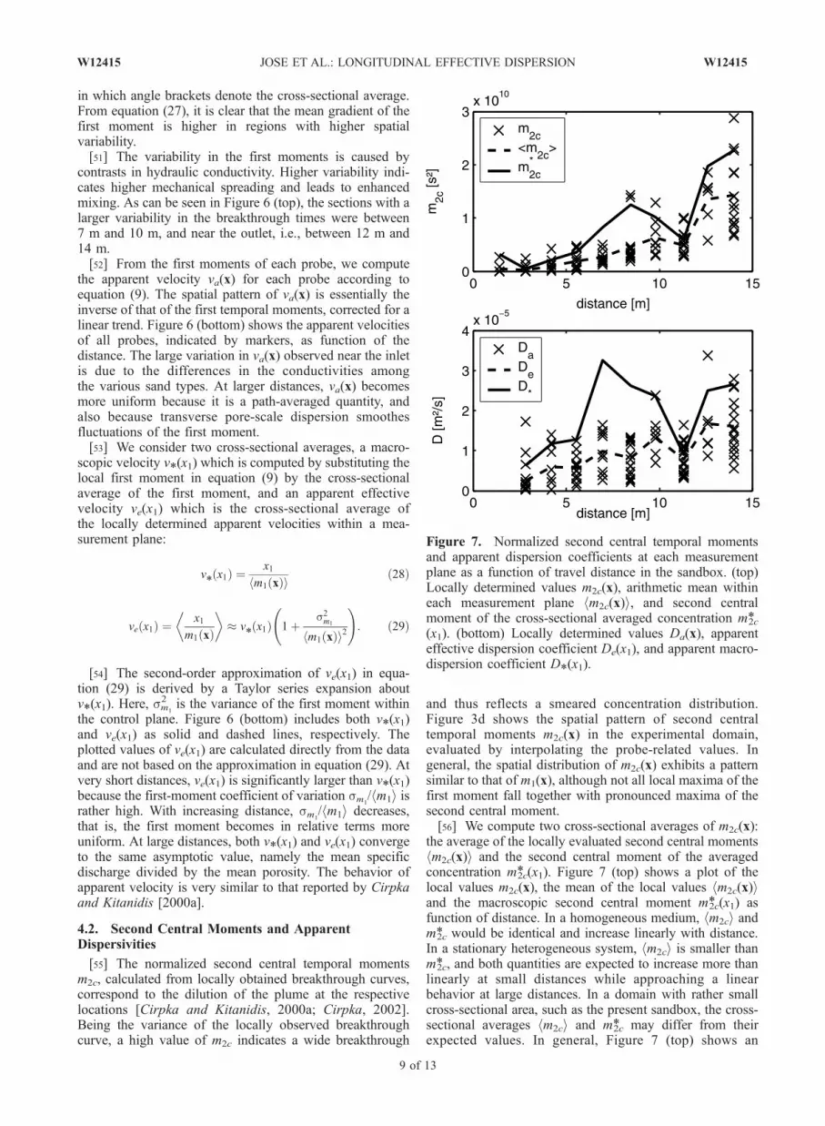
and thus reflects a smeared concentration distribution.Figure 3d shows the spatial pattern of second centraltemporal moments m2c(x) in the experimental domain,evaluated by interpolating the probe-related values. Ingeneral, the spatial distribution of m2c(x) exhibits a patternsimilar to that of m1(x), although not all local maxima of thefirst moment fall together with pronounced maxima of thesecond central moment.[56] We compute two cross-sectional averages of m2c(x):

the average of the locally evaluated second central momentshm2c(x)i and the second central moment of the averagedconcentration m*2c(x1). Figure 7 (top) shows a plot of thelocal values m2c(x), the mean of the local values hm2c(x)iand the macroscopic second central moment m*2c(x1) asfunction of distance. In a homogeneous medium, hm2ci andm*2c would be identical and increase linearly with distance.In a stationary heterogeneous system, hm2ci is smaller thanm*2c, and both quantities are expected to increase more thanlinearly at small distances while approaching a linearbehavior at large distances. In a domain with rather smallcross-sectional area, such as the present sandbox, the cross-sectional averages hm2ci and m*2c may differ from theirexpected values. In general, Figure 7 (top) shows an

Figure 7. Normalized second central temporal momentsand apparent dispersion coefficients at each measurementplane as a function of travel distance in the sandbox. (top)Locally determined values m2c(x), arithmetic mean withineach measurement plane hm2c(x)i, and second centralmoment of the cross-sectional averaged concentration m*2c(x1). (bottom) Locally determined values Da(x), apparenteffective dispersion coefficient De(x1), and apparent macro-dispersion coefficient D*(x1).


9 of 13

W12415

increase of both quantities with distance, however, m*2cdecreases between 8.4 m and 11.3 m, and hm2ci decreasesbetween 9.8 m and 11.3 m. Obviously, there is a region oflow velocity in the top of the domain between 8 m and 10 m.In this region, we find high values of the second centralmoment. Further downstream, the water that has passedthrough the low-conductivity zone flows through layers ofhigher conductivity so that the width of the plume with highm2c(x) values decreases. Lateral exchange also contributesto a smoother m2c(x) profile.[57] The macroscopic second central moment m*2c differs

significantly from the mean of the local values hm2ci inregions with high variance in first moments. This is the casebetween 7 m and 10 m, and toward the end of the domain.Between 12 m and 14 m, the large values of m*2c and hm2ciindicate strong spreading and enhanced mixing.[58] From the first and second central moments, computed

for each probe, we evaluate an apparent longitudinaldispersion coefficient Da(x) according to equation (10).Figure 3 shows a contour plot of the apparent dispersioncoefficient Da(x) in the experimental domain, evaluated byinterpolating the probe-related values. Relatively largeapparent dispersion coefficients are found mainly at tworegions in the sandbox: at the middle of the sandboxbetween 9 m and 10 m, and near the top of the sandboxbetween 12 m and 14 m. These regions may be addressed asregions with enhanced mixing.[59] Like before, we consider various cross-sectional

averages. The apparent effective dispersion coefficientDe(x1) is the cross-sectional average of the local apparentdispersion coefficients, and thus reflects the mean mixing atthe control plane. The apparent macrodispersion coefficientD*(x1) is derived from the cross-sectional averaged con-centration and its second central moment m*2c:

De x1ð Þ ¼ Da xð Þh i ¼ x21m2c xð Þ2m3

1 xð Þ

� �ð30Þ

D*x1ð Þ ¼ x21m2c* x1ð Þ

2 m1 xð Þh i3� De x1ð Þ þ

x21s2m1

x1ð Þ2 m1 xð Þh i3

: ð31Þ

[60] The apparent effective dispersion coefficient De is ameasure of mean dilution, whereas the apparent macro-dispersion coefficient D* also quantifies the combinedeffects of dilution and spreading. Figure 7 (bottom) showsthe locally determined apparent dispersion coefficientsDa(x), the apparent effective dispersion coefficient De(x1),and the apparent macrodispersion coefficient D*(x1) asfunction of travel distance. The values of D*(x1) plottedin Figure 7 (bottom) are calculated from the data without theapproximation given in equation (31).[61] The locally estimated apparent dispersion coeffi-

cients Da(x) range between 1.8 � 10�7 m2/s and 3.39 �10�5 m2/s. A general increase with distance can be observedwhich is evident in the profile of the apparent effectivedispersion coefficient De(x1). The apparent macroscopicdispersion coefficient D*(x1) is considerably higher thanDe(x1) in regions with higher variability in m1. Overall,D*(x1) is about 1.5 times larger than De(x1).[62] Plots of apparent dispersivities aa(x) and its cross-

sectional averages ae(x1) and a*(x1) (not shown) are verysimilar to those of the apparent dispersion coefficient. The

values determined at single probes range between 5.5 mmand 860 mm. The apparent effective dispersivity ae(x1)remains small (<10 cm) until a distance of approximately3 m and increases more strongly from there onward. Anasymptotic value is not reached within the experimentaldomain.[63] Regions with large contrast in hydraulic conductivity

give opportunity to enhanced mixing. We may explain thisfor the section between 10 m and 14 m (see Figure 3). In thefollowing, we explain how the distribution of materialsaffects the propagation of the tracer plume, indicated bythe travel time distribution, and leads to enhanced mixing.[64] As listed in Table 1, the coarse sand has the highest

hydraulic conductivity, followed by the mixed, medium,and fine sands. At approximately 10 m distance from theinlet, a preferential flow path starts in the coarse sand layerin the top half of the domain. Advection through the finesand layers is significantly slower. Themedium sand layer atthe bottom has a higher conductivity than the fine sand layers.However, this particular lens is blocked by fine sand furtherdownstream (12.1 – 13 m), so that the medium sandlayer mentioned is not effective as a preferential flow path.The water flowing through the coarse sand layer stays in thislayer as long as possible. At distance 12.5–13 m, most of theflow squeezes through the mixed sand layer below the coarsesand layer and finally reaches the outlet. Flow velocities in thefine sand layer directly above the preferential flow region arevery low. At the interface between coarse and fine sand layersin the top half of the domain, the strong contrast in hydraulicconductivity causes vertical gradients in the first moment.Here, transverse exchange of solutes leads to strong spreadingof the breakthrough curves as quantified by the apparentdispersion coefficient Da(x). It may be worth noting that thehot spot of mixing is located in the coarse material. Here, thepore-scale dispersion coefficient is high because of highvelocities and large grain sizes. In addition, the transversediffusion distance is smaller in high-velocity regions. That is,narrow preferential flow paths can be identified as regions ofenhanced mixing.

4.3. Apparent Parameters at the Outflow Boundary

[65] Table 2 lists the measurement accuracy of the vari-ables at the outlet (distance = 14 m) and also provides acomparison of the average moments and derived quantitieswith the moments of the averaged concentration. With 20%coefficient of variation, the first temporal moment is deter-mined the most accurate. Consequently, the velocity,derived from the first moments, varies comparably with18%. The variability of the second central temporalmoments is 45%. Among all derived quantities, the disper-sion coefficient has the highest variability followed by thePeclet number and the dispersivity. The high variability indispersion coefficient indicates that a few measurement of alocal breakthrough curve may not be sufficient to accuratelycharacterize mixing. The macroscopic dispersion coefficientat distance = 14 m is 1.66 times higher than thecorresponding effective dispersion coefficient.

4.4. Comparison With Results of LinearStochastic Theory

[66] We test the applicability of linear stochastic theory asexpressed by equations (14)–(20) to close-to-nature hetero-geneities by fitting the structural parameters of the covari-

10 of 13


ance function RYY(h) as well as the value of an isotropicpore-scale dispersion coefficient to the measured data ofm*2c and hm2ci. We assume two-dimensional flow and thenonseparable anisotropic exponential model for the covari-ance function log-conductivity fluctuations:

RYY hð Þ ¼ s2Y exp �

ffiffiffiffiffiffiffiffiffiffiffiffiffiffiffiffih21

l21

þ h22

l22

s !; ð32Þ

in which the variance of log conductivity sY2, and the two

correlation lengths l1 and l2 are the structural parameters tobe determined. In addition to the structural parameters, weestimate a scalar pore-scale dispersion coefficient D. Sinceall parameters must be positive, we estimate the logarithmof the parameters. Then, the exponent of the estimated logparameter is the geometric mean mg of the parameter, andthe exponent of the standard deviation of the log parametermay be denoted factor of variation FV of the parameter.[67] We use a Levenberg-Marquardt method with prior

information for the estimation of the log parameters. Thesingle objective function includes the squared weighteddeviation of all measured values of m*2c and hm2ci fromthe model prediction and the squared weighted deviationfrom all estimated parameters from their prior value. Theoptimization routine is written as Matlab1 script usingperiodic embedding and FFT techniques for spectral calcu-lations. The prior geometric means mg and factors ofvariation FV are given together with the fitted values inTable 3.[68] The prior variance of log conductivity sY

2 is estimatedfrom the variability in the conductivity of the sand typesused in the experiment. The prior values for the horizontaland transverse correlation lengths l1 and l2 are estimatedfrom the known general pattern of materials in the box,while we estimate the prior mean of the pore-scale disper-

sion coefficient from typical transverse dispersion coeffi-cients. The mean velocity was fixed to 3.59 � 10�5 m/s,which is the asymptotic value of v*(x1) and ve(x1) at the endof the domain.[69] The estimated parameters and their posterior factors

of variation are listed in Table 3. The logarithm of thecorrelation length in direction of flow and the log varianceof the log conductivity are strongly anticorrelated with acorrelation coefficient of �0.91, while the logarithm of thepore-scale dispersion coefficient and the logarithm of thetransverse correlation length are positively correlated with acorrelation coefficient of 0.44. Other correlations amongthe parameters are negligible. Both correlations makephysically sense. The asymptotic longitudinal dispersioncoefficient scales with the product of the longitudinalcorrelation length and the variance of log conductivity, seeequation (21). In order to distinguish between the effects ofthese two parameters, data at distances in the range ofthe correlation length or smaller are needed. The data set,however, consists mainly of measurements at largerdistances. Thus we find the strong negative correlationbetween ln(sY

2) and ln(l1). On the other hand, effectivedispersion catches up with macrodispersion with the time-scale of transverse pore-scale dispersion, tDT

= l22/D, see

equation (22). In macrodispersion, the pore-scale dispersioncoefficient D is insignificant, and the transverse correlationlength l2 has only a comparably small impact. Hence thevalues of ln(D) and ln(l2) depend mainly on the hm2ci data,and the effect of increasing ln(l2) can to a certain extent becounteracted by increasing ln(D).[70] The model fitted the experimental data except at

distances between 12 m and 14 m where measured spread-ing and mixing was stronger than predicted by the model.The results are plotted in Figure 8, where the related errorbars (standard deviation of the corresponding quantities

Table 2. Accuracy and Variability of Quantities of Interest at the

Outlet of the Domain

Variable Value Standard Deviation Coefficient of Variation

hm1i, s 4.53 � 105 8.82 � 104 0.20

hm2ci, s2 1.43 � 1010 6.40 � 109 0.45

hvai, m/s 3.20 � 10�5 5.78 � 10�6 0.18

hDai, m2/s 1.60 � 10�5 6.82 � 10�6 0.43

haai, m 0.49 0.17 0.35

hPeai 32.60 12.9 0.40

v*, m/s 3.09 � 10�5

D*, m2/s 2.66 � 10�5

a*, m 0.86

Table 3. Fitted Parameters of Linear Stochastic Theorya

Parameter

Prior Posterior

mg FV mg FV

sY2 2.4 2.72 2.45 1.43

l1, m 1.15 1.88 1.43 1.74l2, m 0.04 1.88 0.039 1.77D, m2/s 6 � 10�9 2.72 8.24 � 10�9 2.04

aFV, factor of variation (exponent of the standard deviation of the logparameter); mg, geometric mean.

Figure 8. Second central moments as function of traveldistance: comparison between fitted results of linearstochastic theory and measured data. The solid line is fittedm2c* (x1); the dashed line is fitted hm2c(x)i; crosses aremeasured m2c* (x1); and stars are measured hm2c(x)i.


11 of 13

W12415

calculated at each measurement plane) are shown togetherwith the measured data. The fitted parameters are in therange of realistic values. The estimated local dispersivitycalculated from the dispersion coefficient is 0.23 mm, whichis a typical value for transverse dispersivities of medium-size sand at the given velocity (O. A. Cirpka et al., Lengthof reactive plumes controlled by transverse dispersion,submitted to Ground Water, 2004).[71] Given the small height of the domain, the agreement

between model results and measured data is good. Stochas-tic theory yields ensemble averages. The cross-sectionalaverage applied to the data fluctuates about the ensembleaverage because the cross section is by far not large enoughto ensure ergodicity. Nonetheless, the model fit shows thecorrect overall trend with realistic model parameters. Weconclude therefore that the expressions derived for effectivedispersion and macrodispersion from stochastic theory are,in general, applicable to real systems.

5. Discussion and Conclusions

[72] For a long time, it has been known that longitudinalmacrodispersion coefficients increase strongly with traveldistance in the preasymptotic regime. This is confirmed byour data, where the apparent macrodispersivity a* reached avalue of about 60 cm toward the end of the domain. In thepresent study, the typical length of the lenses was about 3 m,and thus it cannot be expected that the asymptotic macro-dispersion coefficient is approached within the domain ofonly 14 m length. Also, the height of the domain wasrestricted to 0.5 m, which is about six times the typicalheight of the lenses. For such a shallow domain, theergodicity assumption does not hold, and one has to expectdeviations between the observed cross-sectional averagedconcentration and the expected value of concentrationaccording to stochastic theory. Other studies, like those ofBarth et al. [2001], Ursino et al. [2001a, 2001b], andSilliman and Zheng [2001], used much smaller blockspacked with the identical sand type. In these studies, theplumes sampled a more representative conductivity distri-bution. However, they were also restricted to heterogene-ities of a fairly small size.[73] Our study is focused on longitudinal effective dis-

persion, here computed as apparent coefficients from thesecond central moments of breakthrough curves measuredby point-like devices. From theoretical studies [Kitanidis,1994; Dentz et al., 2000], at first, the deviation betweenapparent macrodispersion, D*(x1), and apparent effectivedispersion, De(x1), by a factor of about 1.5 appears small.For comparison, Dentz et al. [2000, Figure 3] estimated atravel time of about 2000 days to reach a similar ratio of thetwo longitudinal dispersion coefficients in the Bordenaquifer. In our study, the difference is not that pronouncedbecause the lenses are fairly thin. It is transverse pore-scaledispersion that makes effective dispersion catch up withmacrodispersion. The smaller the transverse diffusionlength, the faster effective dispersion reaches macrodisper-sion values. We believe that the heterogeneities in oursandbox mimic rather typical sedimentary patterns. Forlenses of comparable thickness, it can thus be concludedthat incomplete dispersive mixing is significant but notstrongly pronounced. This is important for the scale up ofmixing-controlled reactive transport [Cirpka, 2002].

[74] A special feature of our domain is that the fillingexhibits microstructures mimicking natural hydrofacies.Ritzi et al. [2004] showed that the repeated occurrence ofdiscontinuities, which are typical for such structures, resultsin an exponential-like covariance function of the log-permeability. Thus the exponential model used in our studyappears appropriate. The question, whether second-orderstatistics are sufficient to predict dispersion in such systems,or whether higher-order information needs to be included,remains open. Particularly it is difficult to determine fromthe data, to which extent microheterogeneities help effectivedispersion catching up with macrodispersion. We cannotexclude that the fitted value of the pore-scale dispersioncoefficient reflects, to a certain extent, effects of the micro-structures. In additional experiments on transverse disper-sion, however, we have seen no significant increase oftransverse mixing due to the microheterogeneities (M. A.Rahman et al., Experiments on vertical transverse mixing ina large-scale heterogeneous model aquifer, submitted toJournal of Contaminant Hydrology, 2004).[75] The fit of coefficients for the first-order solution of

Dentz et al. [2000] and Fiori and Dagan [2000] leads toreasonable values, although the fit itself, due to the lackingergodicity, is not perfect. In particular, the transverse pore-scale dispersivity of 0.23 mm is in the range of valuesreported for the types of sands used in the study. In thepresent study, we have used two different approaches tointerpret the local breakthrough curves. In the first, weinterpret the locally measured breakthrough curves as ifcaused by one-dimensional transport in independent streamtubes, arriving at an apparent effective dispersivity of about40 cm toward the end of the domain [Cirpka and Kitanidis,2000a]. In the second, we account for the geostatisticalparameters of the heterogeneities. In this framework, like inthe studies of Vanderborght and Vereecken [2001, 2002],the width of the breakthrough curve is traced back to thetransverse pore-scale dispersivity of 0.23 mm. This aliasingof local transverse dispersion and macroscopic longitudinalmixing has already been reported by Cirpka and Kitanidis[2000a, 2000b]. The aliasing has direct consequences inmodel calculations. If we try to calibrate a numerical modelusing the measured breakthrough curves, we will need ratherlarge longitudinal dispersivities if we do not resolve theheterogeneities within the domain with a sufficient spatialresolution. Once we are able to resolve a certain, here notdetermined, length scale of heterogeneities, we will have toadapt the transverse dispersivity in order to meet the width ofthe breakthrough curves. Inverse modeling studies for themeasured data set, addressing these questions, are on the way.[76] In general, the experimental study demonstrates the

applicability and limitations of some mixing-related theoriesin porous media that are based on the stochastic approach.The study may be further extended to conduct reactivemixing experiments in order to check the accuracy ofeffective dispersion coefficients as measures of mixing.

[77] Acknowledgments. This work was funded by the EmmyNoether program of the Deutsche Forschungsgemeinschaft (DFG) underthe grants Ci 26/3-2 to Ci 26/3-4. The authors are grateful to WolfgangNowak helping in the programming of the data analysis routines. Theexperiments would have been impossible without the support of thetechnical staff at the research facility for subsurface remediation (VEGAS)at the Universitat Stuttgart. We thank Insa Neuweiler for carefully review-ing a draft of the manuscript.

12 of 13


ReferencesAndricevic, R., and V. Cvetkovic (1998), Relative dispersion for solute fluxin aquifers, J. Fluid Mech., 361, 145–174.

Barth, G. R., M. C. Hill, T. H. Illangasekare, and H. Rajaram (2001),Predictive modeling of flow and transport in a two-dimensional inter-mediate-scale, heterogeneous porous medium, Water Resour. Res., 37,2503–2512.

Cirpka, O. A. (2002), Choice of dispersion coefficients in reactive transportcalculations on smoothed fields, J. Contam. Hydrol., 58, 261–282.

Cirpka, O. A., and P. K. Kitanidis (2000a), Characterization of mixing anddilution in heterogeneous aquifers by means of local temporal moments,Water Resour. Res., 36, 1221–1236.

Cirpka, O. A., and P. K. Kitanidis (2000b), An advective-dispersive streamtube approach for the transfer of conservative-tracer data to reactivetransport, Water Resour. Res., 36, 1209–1220.

Cirpka, O. A., C. Windfuhr, G. Bisch, S. Granzow, H. Scholz-Muramatsu,and H. Kobus (1999), Microbial reductive dechlorination in large-scalesandbox models, J. Environ. Eng. Am. Soc. Civ. Eng., 125, 861–870.

Dagan, G. (1984), Solute transport in heterogeneous porous formations,J. Fluid Mech., 145, 151–177.

Dentz, M., H. Kinzelbach, S. Attinger, and W. Kinzelbach (2000), Temporalbehavior of a solute cloud in a heterogeneous porousmedium: 1. Point-likeinjection,Water Resour. Res., 36, 3591–3604.

Fiori, A., and G. Dagan (2000), Concentration fluctuations in aquifer trans-port: A rigorous first-order solution and applications, J. Contam. Hydrol.,45, 139–163.

Gelhar, L. W., and C. L. Axness (1983), Three dimensional stochastic anal-ysis of macrodispersion in aquifers, Water Resour. Res., 19, 161–180.

Ghodrati, M. (1999), Point measurement of solute transport processes insoil using fiber optic sensors, Soil Sci. Soc. Am. J., 63, 471–479.

Guilbault, G. G. (1990), Practical Fluorescence, 2nd ed., CRC Press, BocaRaton, Fla.

Jose, S. C., and O. A. Cirpka (2004), Measurement of mixing-controlledreactive transport in homogeneous porous media and its prediction fromconservative tracer test data, Environ. Sci. Technol., 38, 2089–2096.

Kapoor, V., and L. W. Gelhar (1994a), Transport in three-dimensionallyheterogeneous aquifers: 1. Dynamics of concentration fluctuations,WaterResour. Res., 30, 1775–1788.

Kapoor, V., and L. W. Gelhar (1994b), Transport in three-dimensionallyheterogeneous aquifers: 2. Predictions and observations of concentrationfluctuations, Water Resour. Res., 30, 1789–1801.

Kapoor, V., L. W. Gelhar, and F. Miralles-Wilhelm (1997), Bimolecularsecond-order reactions in spatially varying flows: Segregation inducedscale-dependent transformation rates, Water Resour. Res., 33, 527–536.

Kitanidis, P. K. (1988), Prediction by the method of moments of transport inheterogeneous formations, J. Hydrol., 102, 453–473.

Kitanidis, P. K. (1994), The concept of the dilution index, Water Resour.Res., 30, 2011–2026.

Levy, M., and B. Berkowitz (2003), Measurement and analysis of non-Fickian dispersion in heterogeneous porous media, J. Contam. Hydrol.,64, 203–226.

Loveland, J. P., S. Bhattacharjee, J. N. Ryan, and M. Elimelech (2003),Colloid transport in a geochemically heterogeneous porous medium:Aquifer tank experiment and modeling, J. Contam. Hydrol., 65, 161–182.

Molz, F. J., and M. A. Widdowson (1988), Internal inconsistencies indispersion-dominated models that incorporate chemical and microbialkinetics, Water Resour. Res., 24, 615–619.

Nielsen, J. M., G. F. Pinder, T. J. Kulp, and S. M. Angel (1991), Investiga-tion of dispersion in porous media using fiber-optic technology, WaterResour. Res., 27, 2743–2749.

Oya, S., and A. J. Valocchi (1998), Transport and biodegradation of solutesin stratified aquifers under enhanced in situ bioremediation conditions,Water Resour. Res., 34, 3323–3334.

Pettijohn, F. J., P. E. Potter, and R. Siever (1987), Sand and Sandstone,Springer, New York.

Ritzi, R. W., Z. X. Dai, D. F. Dominic, and Y. N. Rubin (2004), Spatialcorrelation of permeability in cross-stratified sediment with hierarchi-cal architecture, Water Resour. Res., 40, W03513, doi:10.1029/2003WR002420.

Rubin, Y. (2003), Applied Stochastic Hydrogeology, Oxford Univ. Press,New York.

Silliman, S. E., and L. Zheng (2001), Comparison of observations from alaboratory model with stochastic theory: Initial analysis of hydraulic andtracer experiments, Transp. Porous Media, 42, 85–107.

Silliman, S. E., L. Zheng, and P. Conwell (1998), The use of laboratoryexperiments for the study of conservative solute transport in heteroge-neous porous media, Hydrogeol. J., 6, 166–177.

Ursino, N., T. Gimmi, and H. Fluhler (2001a), Dilution of non-reactivetracers in variably saturated sandy structures, Adv. Water Resour., 24,877–885.

Ursino, N., T. Gimmi, and H. Fluhler (2001b), Combined effects of hetero-geneity, anisotropy, and saturation on steady state flow and transport:A laboratory sand tank experiment, Water Resour. Res., 37, 201–208.

Vanderborght, J., and H. Vereecken (2001), Analyses of locally measuredbromide breakthrough curves from a natural gradient tracer experiment atKrauthausen, J. Contam. Hydrol., 48, 23–43.

Vanderborght, J., and H. Vereecken (2002), Estimation of local scaledispersion from local breakthrough curves during a tracer test in aheterogeneous aquifer: The Lagrangian approach, J. Contam. Hydrol.,54, 141–171.

��O. A. Cirpka, Swiss Federal Institute for Environmental Science and

Technology, Uberlandstrasse 133, CH-8600 Dubendorf, Switzerland. ([email protected])

S. C. Jose, Integrated Waste Management Centre, Cranfield University,Building 61, Bedford MK43 0AL, UK. ([email protected])

M. A. Rahman, Institut fur Wasserbau, Universitat Stuttgart,Pfaffenwaldring 61, D-70569 Stuttgart, Germany. ([email protected])


13 of 13

W12415

Documents

Large-scale sandbox experiment on longitudinal effective dispersion in heterogeneous porous media