Embed Size (px)
Citation preview

Durham E-Theses
Late Holocene records of Antarctic fur Seal(Arctocephalus gazella) population variation on South
Georgia, sub Antarctic
Foster, Victoria A.
How to cite:
Foster, Victoria A. (2005) Late Holocene records of Antarctic fur Seal (Arctocephalus gazella) populationvariation on South Georgia, sub Antarctic, Durham theses, Durham University. Available at DurhamE-Theses Online: http://etheses.dur.ac.uk/3934/
Use policy
The full-text may be used and/or reproduced, and given to third parties in any format or medium, without prior permission orcharge, for personal research or study, educational, or not-for-pro�t purposes provided that:
• a full bibliographic reference is made to the original source
• a link is made to the metadata record in Durham E-Theses
• the full-text is not changed in any way
The full-text must not be sold in any format or medium without the formal permission of the copyright holders.
Please consult the full Durham E-Theses policy for further details.

Academic Support O�ce, Durham University, University O�ce, Old Elvet, Durham DH1 3HPe-mail: [email protected] Tel: +44 0191 334 6107
http://etheses.dur.ac.uk
2
Late Holocene records of Antarctic Fur Seal {Arctocephalus gazella) population
variation on South Georgia, sub Antarctic
Victoria A Foster
MSc by Research
University of Durham
Department of Geography
2005 Tbe copyright of this thesis rests with the author or the university to which it was submitted. No quotation from it, or information derived from it may be published without the prior written consent of the author or university, and any information derived from it should be acknowledged.
0? m 2007

Abstract
Late Holocene records of Antarctic Fur Seal (Arctocephalus gazelld) population
variation on South Georgia, sub Antarctic.
Foster, V. A (2005)
The Antarctic fur seal {Arctocephalus gazelld) population at South Georgia has
increased dramatically through the 20* and 21^' centuries following near extinction at
the beginning of the 20* century. This rapid increase is now causing concern as the
seals are damaging the coastal habitats of South Georgia including specially protected
areas. To assess whether this population increase is part of a natural fluctuation or due
to human induced changes in the marine ecosystem, the fur seal population has been
reconstructed through the Holocene from seal hair abundance and geochemistry.
Results firom the fur seal hair abundance record show fur seals have been present at
South Georgia for at least the past 3439 ''*C yrs BP and the population today is not
unprecedented during the late Holocene. Although previous studies have found a
correlation between fur seal populations and geochemistry, this study highlights that
this is not effective at all study sites due to the complex relationship between climate
change, catchment sediment delivery processes and seal population dynamics. At South
Georgia, Cu and Zn are found to be indicators of fiir seal activity once a threshold of
1500 hairs per 1 g of dry weight is reached.
The fiir seal hair abundance results suggest there is a link between fur seal populations
and climate change. Although the largest increases in fur seal population occur during
cooler periods, the fur seal population is primarily controlled by prey availability
(Euphausia superba), which is in turn influenced by climate change. Pre 200 yrs BP, an
increase in prey availability is associated with colder periods, which are linked to
changes in oceanography and led to a consequent increase in sea-ice extent. Post 200
yrs BP, the whaling industry has resulted in a krill surplus in the South Georgia region
elevating krill availability, causing an increase in the fur seal population (that has been
coincident with warming). Although the population has increased during the 20* and
21^' century as a result of human induced causes, this increase cannot be sustained once
the krill surplus ceases. As the population has been at similar levels previously and the
krill surplus is thought to be ending, it is concluded that the fiir seal population increase
during the 20* century is not abnormal and management of the fur seal population at
South Georgia may not be necessary.

Contents
Contents
List of figures 13
Declaration 14
Acknowledgements 15
Chapter 1 - Introduction and Aim
1.1 Research Context 20
1.2 Overall Aim 21
1.3 Specific Obj ectives 21
1.4 Mechanisms influencing fur seal populations 23
1.4.1 Natural environmental changes 23
1.4.2 Human induced changes 24
1.4.2.1 Sealing 24
1.4.2.2 Whaling 25
1.5 Summary 25
Chapter 2 - Background and Rationale
2: Background and Rationale 27
2.1 Rationale for study location 27
2.2 Study Site 28
2.2.1 South Georgia 28
2.2.2 Maiviken 31
2.2.3 Lake Catchment 35
2.2.4 Core Site 37
2.2.5 Lake processes 38
2.2.5.1 Lake inputs 39
2.2.5.2 Lake Circulation 39
2.2.5.3 Lake Outputs 39
2.2.5.1 Late Holocene Environmental Changes 40
2.3.1 South Georgia Environmental Change 43

Contents
2.3.1.1 Pre 2600 14C years BP 43
2.3.1.2 2600- 1600 14C yrs BP 43
2.3.1.3 1000 14C years BP 45
2.3.1.4 Post 200 14C years BP 46
2.3.2 Humic Lake Environmental Changes 46
2.3.2.1 General climate 49
2.3.2.2 Catchment specific environmental changes 49
2.3.3 Regional environmental change 52
2.3.3.1 2600-2000 14C yrs BP (Climate deterioration) 52
2.3.3.2 2000-1000 14C yrs BP (Warm phase) 53
2.3.3.3 1000-200 14C yrs BP (Cooling, fluctuating climate) 53
2.3.3.4 200 14C yrs BP 55
2.3.3.5 Summary 55
2.4 Historical records of climate change 56
2.4.1 1920-1940 (Cooling) 57
2.4.2 1940-1960 (Warming trend) 58
2.4.3 1960-Present day 58
2.5 Fur seal population on South Georgia 59
2.5.1 Exploitation 59
2.5.2 Post Exploitation 60
2.5.3 The Situation Today 63
2.6 Fur seal population of the Sub Antarctic Islands 64
2.7 Possible causes for the increase in fur seals 65
2.7.1 Human induced causes 66
2.7.1.1 Prey Availability 66
2.7.1.2 Predator Competition 67
2.7.2 Summary of human induced factors 67
2.7.3 Natural Environmental changes 67
2.7.3.1 Prey Availability 67
2.7.3.1.1 Climate 68
2.7.3.1.2 Competition 69
2.7.3.1.3 Swmn^ of prey ayail^^ -70
2.7.3.2 Predator competition 70
2.7.3.2.1 Sea Ice 70
2.7.3.2.2 Terrain 71

Contents
2.7.3.2.3 Summary of predator competition 72
2.7.4 Summary of factors affects fur seal populations 72
2.8 Fur seals on South Georgia and their impacts 73
2.8.1 Management of fur seals on South Georgia 77
2.9 Summary 79
Chapter 3 - Methodology
3: Methodology 81
3.1 Sediment cores 81
3.1.1 Core depth and scaling 81
3.1.2 Sedimentological and Stratigraphic core analysis 83
3.1.3 Sub sampling 83
3.2 Fur seal hair abundance 83
3.3 Development and refinement of the
Hodgson et al. (1998) technique 85
3.3.1 Final methodology 85
3.3.2 Physical separation 85
3.3.2.1 Sieving 85
3.3.2.2 Particle shape analysis 86
3.3.3 Chemical separation 86
3.3.3.1 Hydrogen peroxide (H202) 86
3.3.3.2 Fine Sieving 87
3.3.4 Identifying hairs 87
3.4 Geochemical analysis 90
3.4.1 Fur seal geochemistry 90
3.4.2 Penguin geochemistry 92
3.4.3 Geochemical hypotheses 93
3.4.3.1 Carbon 94
3.4.3.2 Nitrogen 95
3.4.3.3 Sulphur 95
3.4.3.4 Selenium 95
3.4.3.5 Zinc 95
3.4.3.6 Copper 96
3.4.3.7 Strontium 96

Contents
3.4.3.8 Cadmium 96
3.4.3.9 Sodium 97
3.4.3.10 Calcium 97
3.4.3.11 Manganese 98
3.4.4 ICP-MS hypotheses 98
3.4.4.1 Aluminium 99
3.4.4.2 Potassium 100
3.4.4.3 Titanium 100
3.4.4.4 Barium 100
3.4.4.5 Iron, Lithium, Vanadium and Chromium 100
3.4.4.6 Molybdenum 101
3.4.4.7 Thallium 101
3.4.4.8 Other elements 101
3.4.5 Geochemical summary 102
3.4.6 Methodology 103
3.4.6.1 Elemental Combustion System 103
3.4.6.2 Inductively Coupled Plasma Mass
Spectrometer (ICP-MS) 103
3.4.6.2.1 EPA 3051 Method 104
3.4.6.3 Total Organic Carbon (TOC) 104
3.4.6.4 Summary 105
3.5 Dating 105
3.5.1 Principles of radiocarbon dating 106
3.5.1.1 Radiocarbon dating methodology 106
3.5.2 210Pb and 137Cs dating 106
3.5.2.1 Principles of 21 OPb dating 107
3.5.2.2 Principles of 137Cs dating 108
3.5.2.3 Methodology for 210Pb and 137Cs dating 108
3.6 Sources and magnitude of error 108
3.6.1 Seal hair abundance 108
3.6.2 Geochemistry 109
3.6.2.1 Elemental combustion system 109
3.6.2.2 ICP-MS 110
3.7 Summary 110
6

Contents
Chapter 4 - Results
4: Results 112
4.1 Core Stratigraphy 112
4.1.1 HUM3 112
4.1.2 MAIVnC 113
4.1.3 Implications for analysis 113
4.2 Depth Scale 113
4.3 Fur seal hair abundance 113
4.3.1 Error 116
4.3.2 Summary 116
4.4 Geochemistry 117
4.4.1 Group A: Nitrogen, Carbon, Strontium, Aluminium 117
4.4.1.1 Nitrogen 117
4.4.1.2 Carbon 118
4.4.1.2.1 Total Carbon 118
4.4.1.2.2 Total Organic Carbon (TOC) 118
4.4.1.3 Strontium 119
4.4.1.4 Aluminium 119
4.4.1.5 Summary of group A 121
4.4.2 Group B: Potassium, Titanium, Barium, Iron 57 and Sodium 121
4.4.2.1 Potassium 121
4.4.2.2 Titanium 121
4.4.2.3 Barium 122
4.4.2.4 57-Iron 124
4.4.2.5 Summary of group B 124
4.4.3 Group C: Copper, Zinc, Cadmium and Lithium 125
4.4.3.1 Copper 125
4.4.3.2 Zinc 125
4.4.3.3 Cadmium 127
4A.3ALm^^m _ ^ 127
4.4.3.5 Summary of group C 128
4.4.4 Group D: Bismuth, Molybdenum, Antimony, Thallium, Boron, Beryllium
128

Contents
4.4.4.1 Bismuth 128
4.4.4.2 Molybdenum 128
4.4.4.3 Antimony 129
4.4.4.4 Thallium 129
4.4.4.5 Boron 131
4.4.4.6 Beryllium 131
4.4.4.7 Summary of group D 131
4.4.5 Group E: Selenium, Vanadium, Calcium, Chromium, Manganese, Cobalt, Iron
54 132
4.4.5.1 Selenium 132
4.4.5.2 Vanadium 132
4.4.5.3 Calcium 133
4.4.5.4 Chromium 133
4.4.5.5 Manganese 135
4.4.5.6 Cobalt 135
4.4.5.7 54-Iron 136
4.4.5.8 Summary of group E 136
4.4.6 Group F: Arsenic, Sulphur, Nickel 136
4.4.6.1 Arsenic 136
4.4.6.2 Sulphur 137
4.4.7 Summary of geochemical results 139
4.5 Dating 140
4.5.1 Radiocarbon dating 140
4.5.1.1 HUM3 82-83 cm 140
4.5.1.2 MAIV/K 50-51 cm 141
4.5.2 Radiocarbon dating results 142
4.5.3 210Pb and 137Cs dating 142
4.5.3.1 210Pb and 137Cs results 143
4.6 Summary 145
Chapter 5 - Discussion
5: Discussion 147
5.1 Age Model 147
5.1.1 Model 1 (3439 14C yrs BP only) 147

Contents
5.1.2 Model 2-(3910 14Cyrs BP only) 148
5.1.3 Model 3 - (2750 14C yrs BP) 148
5.1.4 Model 4 - 391014C yrs BP and 2750 14C yrs BP 148
5.1.5 Model 5 - 3439 14C yrs BP and 2750 14C yrs BP 149
5.1.6 Calculating the age model 149
5.2 Dating inaccuracies 150
5.2.1 21 OPb problems 150
5.2.1.1 Loss of the sediment water interface 150
5.2.1.2 Catchment Characteristics 151
5.2.1.3 Detection Limits 152
5.2.1.4 Location of the study site 152
5.2.1.5 Summary of 21 OPb problems 153
5.2.2 Radiocarbon problems 153
5.2.2.1 Seal influence 153
5.2.2.2 Contamination 155
5.2.2.3 Ice cover 155
5.2.2.4 Summary 156
5.2.3 Implications for the study 156
5.3 Assumptions 159
5.4 Late Holocene changes in fur seal populations 159
5.4.1 Fur seal hair abundance 159
5.4.2 Geochemical record 162
5.4.2.1 Group A (Carbon, Nitrogen, Strontium, Aluminium) 163
5.4.2.2 Group B (Potassium, Titanium, Barium, 57-Iron, Sodium) 165
5.4.2.3 Group C (Copper, Zinc, Cadmium, Lithium) 165
5.4.2.4 Group D (Bismuth, Molybdenvim, Antimony, Thallium, Boron,
Beryllium) 168
5.4.2.5 Group E (Selenium, Vanadium, Calcium, Chromium, Manganese,
Cobalt, 54-Iron) 168
5.4.2.6 Group F (Sulphur, Nickel, Arsenic) 171
5.4.2.6.1 Sulphur 171
5.4.2.6.2 Nickel 174
5.4.2.6.3 Arsenic 171
5.4.3 Geochemical Siimmary 173
5.5 20th - 21 St Century changes in fur seal populations 174

Contents
5.6 Environmental changes 174
5.6.1 Geochemical signature 175
5.6.1.1 Group A (Carbon, Nitrogen, Strontium, Aluminium) 175
5.6.1.2 Group B (Potassium, Titanium, Barium, 57-Iron, Sodium) 175
5.6.1.3 Group C (Copper, Zinc, Cadmium, Lithium) 176
5.6.1.4 Group D (Bismuth, Molybdenum, Antimony, Thallium, Boron,
Beryllium) 177
5.6.1.5 Group E (Selenium, Vanadium, Calcium, Chromium, Manganese,
Cobah, 54-Iron) 177
5.6.2 Climate change inferred from geochemistry 178
5.6.2.1 Summary 179
5.7 Fur seal population fluctuations relative to climate change. 181
5.7.1 Late Holocene Climate Optimum (Pre 2600 14C yrs BP) 182
5.7.2 Climate Deterioration (2600-1600 14C yrs BP) 183
5.7.3 1100-200 14C yrs BP 183
5.7.4 200 14C yrs BP-present 184
5.7.5 Summary 184
5.8 Factors controlling fur seal population changes in the late Holocene 185
5.8.1 Prey availability 185
5.8.2 Predator competition 18 8
5.8.3 Summary 189
5.9 Recent changes 190
5.10 Past studies 190
5.10.1 Hodgson et al's. (1998) study - Signy Island. 190
5.10.2 Sun et al's. (2004a) study - King George Island 191
5.11 Optimum sea ice conditions hypothesis 192
5.11.1 20th Century changes 195
Chapter 6 - Conclusions
6 Conclusions 197
6.1 Objective 1: To recoptruct^fur seaLpopulations -thrQugh the late Holoeene by
counting seal hairs from a lake on South Georgia. 197
6.2 Objective 2: To reconstruct fur seal populations indirectly using geochemical
analysis, following the method outlined by Sun et al. (2004a). 197
10

Contents
6.3 Objective 3: To determine whether the recent (20th -21st century) increases in
fur seals have exceeded the range of natural variability of past populations. 198
6.4 Objective 4: To review and assess the impact the environmental changes on
South Georgia have had upon seal populations over the same time period of the
Holocene. 198
6.5 Objective 5: To determine the factors controlling fur seal population changes at
South Georgia through the late Holocene. 199
6.6 Overall aim 200
6.7 Future change in the fur seal population at South Georgia 201
6.8 Summary 201
Chapter 7 - Limitations and further research
7 Limitations and Further Research 203
7.1 Dating 203
7.1.1 2 lOPb dating 203
7.1.2 Radiocarbon dating 203
7.2 Fur seal hair abundance 204
7.2.1 Human error 204
7.2.2 Population dynamics 204
7.3 Areas of further research 205
7.3.1 Radiocarbon dates 205
7.3.2 Dating 'old' carbon 205
7.3.3 Palaecological analysis 206
7.3.4 Additional cores 206
7.4 Continuing previous research 208
7.4.1 Sediment traps 208
7.4.2 Geochemical analysis 208
7.4.3 Wider research issues 209
7.4.3.1 210Pb and 137Cs problems 209
7.4.3.2 Isotopes in hair 209
7.4.3.3 Sea ice conditions 211
7.5 Summary 211
11

Contents
Appendix 1 213
Appendix 2 215
Appendix 3 225
References 228
12
Figures
Figures
2 Background and Rationale
2.1 South Georgia in relation to South America and the Antarctic 29
Peninsula.
2.1.1 South Georgia and surrounding islands 30
2.2 Scotia Sea region showing South Georgia and key oceanographic 30
features.
2.3 Central South Georgia 31
2.4 Location of the study site in relation to Maiviken and Grytviken. 32
2.5 Geomorphological map of the study site 1 33
2.6 Geomorphological map of the study site 2 34
2.7 Aerial view of the lake catchment 36
2.8 Vegetation cover of the lake catchment 36
2.9 Retrieving the core 37
2.10 Core site 38
2.11 A summary of climate change at South Georgia through the late 42
Holocene
2.12 Relative temperature of South Georgia through the Late Holocene. 45
2.13 A summary of environmental changes in the Maiviken catchment 48
2.14 A siimmary of sub Antarctic climate change at through the late 51
Holocene.
2.15 A high-resolution magnetic susceptibility record from the Eastern 54
Bransfield Basin, Antarctic Peninsula.
2.16 20"' century instrumental climate data from South Georgia 57
2.17 The rate of fur seal population growth through the 20" Century. 62
2.18 Sea ice distribution in the Sub Antarctic region 71
2.19 Tussock grass at South Georgia 74
2ir20 Eroded tussock grass 75
2.21 The impact of fur seals on the tussock grass of South Georgia 76
2.22 Fur seals on the beach at Maiviken 77
13

Figures
3 Methodology
3.1 Relative depths of the cores 82
3.2 Results from Hodgson et al's (1998) study 84
3.3 Fur seal hair layers 88
3.4 Fur seal hairs after preparation 89
3.5 A fur seal hair after preparation 89
3.6 Sun et al's (2004a) results 91
3.7 ^^^U decay series 107
4 Results
4.1 Fur seal hair abundance 115
4.2 Error of fiir seal hair abundance 116
4.3 Group A element concentrations relative to depth 120
4.4 Group B element concentrations relative to depth 123
4.5 Group C element concentrations relative to depth 126
4.6 Group D element concentrations relative to depth 130
4.7 Group E element concentrations relative to depth 134
4.8 Group F element concentrations relative to depth 138
4.9 ^'°Pb results 143
4.10 '"Cs results 144
5 Discussion
5.1 Sedimentation rate variation 157
5.2 Fur seal hair abundance relative to depth and time 158
5.3 Fur seal hair abundance fluctuations at South Georgia for the past 160
3439 '''C yrs BP.
5.4 Group A element concentrations relative to age 164
5.5 Group B element concentrations relative to age 166
5.6 Group C element concentrations r d age 167
5.7 Group D element concentrations relative to age 169
5.8 Group E element concentrations relative to age 170
5.9 Group F element concentrations relative to age 172
14

Figures
5.10 Summary of the catchment conditions with geochemical analysis. 180
5.11 Fur seal hair abundance fluctuations and climate changes at South 181 -182
Georgia
5.12 Sea ice extent in the sub - Antarctic region. 186 -187
5.13 Sea ice extent relative to adelie penguin populations (Smith et al. 192
1999)
5.14 The location of Signy Island and King George Island relative to 193
South Georgia.
5.15 Sea ice extent relative to climate and fur seal populations. 195
5.16 Sea ice extent relative to climate and fiir seal populations in the 196
20* century.
Tables
2 Background and Rationale
2.1 Fur seal population census data at South Georgia. 61
3 Methodology
3.1 Results of human hair in H2O2 87
3.2 The composition of seawater 92
3.3 Results from geochemical studies of penguins 93
3.4 Geochemical hypotheses 94
3.5 Element concentrations from the ICP-MS 99
3.6 Summary of geochemical elements used in analysis 102 -103
4 Results
4.1 Element Groups 117
4.2 TIG results 118
4.3 Radiocarbon results 142
15

Figures
Discussion
5.1 Age models 147
Plates
1: A fur seal {Arctocephalus gazella). 19
2: MaivikenBay 26
3: A fur seal hair 80
4: Results of the ^'°Pb and ' ^Cs analysis. 111
5: Fur seals at South Georgia 146
6: Fur seals and penguins on the beach at Maiviken 196
7: A fur seal in tussock grass 202
16

Declaration
Declaration
I certify that this thesis is the resuh of my own work and has not been submitted for any
other examination. Material from the published or unpublished work of others, which is
referred to in the thesis is credited to the author(s) in question in the text.
Statement of copyright
The copyright of this thesis rests with the author. No quotation from it should be
published without their prior written consent and information derived from it should be
acknowledged.
17

Acknowledgements
Acknowledgements
Firstly I would like to thank my two supervisors, Dr Mike Bentley and Dr Jerry Lloyd
for their continued support, advice and guidance. Secondly I would like to thank Dr
Sarah Davies and Dr Gunhild Rosqvist for giving me valuable sediment from their cores
for me to analyse, without that this thesis production would not have been possible. I
would also like to thank the following people in no particular order for their useful
advice on various aspects of the thesis: Dr Keith Reid, Dr Paddy Pomeroy; Dr Rus
Hoezel, Dr Steve Moreton and Susie Grant. Thanks must also go to the laboratory
support staff at Durham University, in particular Frank Davies for providing me with
advice and guidance in analysis of my samples. Further more, I would like to thank my
family and fHends, who have constantly reassured me, read through my draft thesis and
checked through the final document. And finally, I would like to thank Dr Dave Roberts
and Dr Dominic Hodgson for examining this thesis.
18

1: Introduction and Aim
Chapter 1
Introduction and Aim
Plate 1: Fur seal (Arctocephalus gazella)
19

1: Introduction and Aim
1 Introduction and Aim
1.1 Research Context
It is widely recognised that Antarctic fur seal (Arctocephalus gazella) populations on
the Antarctic Peninsula and surrounding Sub-Antarctic islands have rapidly increased in
the past few decades (Hodgson et al. 1998; Payne 1977). However, during the early 20*
century fur seals were almost extinct following human exploitation during the 19'''
century (Bonner 1968). It is estimated that by 1825, 1,200,000 fur seal skins had been
taken from the sub-Antarctic region (Headland 1982). The most rapid population
increase has occurred on the island of South Georgia, where the fbr seal population was
almost 3,000,000 in 1999 (ATCM 1999). Such a fast increase in fur seals is now
causing extensive changes to terrestrial and freshwater systems and in some areas
damaging Antarctic Specially Protected Areas (ASPAs) (Hodgson et al. 1998; Lewis-
Smith 1988). I f the fur seal population continues to grow at the same rate, it is possible
that the fur seal impact is likely to have a catastrophic and irreversible effect on the
Antarctic ecosystem; however, it is not yet clear i f the increase in fur seal populations is
due to climate change, recovery from exploitation or other natural variations.
With respect to climate change there is a broad scientific consensus that the warming of
the earth's climate since the 1970s is greater than any time in the last thousand years
(IPCC 2001). This has caused concern regzirding the biological and ecological changes
affecting the range and distribution of species (Croxall et al. 2002). The key to
determining the impact of climate on the Antarctic ecosystem (and specifically fur
seals) is to determine the range of natural variability in the ecosystem and to distinguish
natural changes from human perturbations (Abbott and Benninghoff 1990).
To overcome the problems distinguishing between the human impact and the impact of
natural environmental change on fur seal populations, Hodgson and Johnston (1997)
used RalaeolimnQlogy to reconstruct fur seal populations going back several centuries/
millermia, prior to human intervention. This study is based upon the theory that fur seals
moult regularly, depositing hair in terrestrial and aquatic environments. This hair is
20

1: Introduction and Aim
washed into lakes and incorporated into the lake sediments hence, providing a proxy
record of fiir seal presence.
1.2 Overall Aim
The aim of this study is to reconstruct the far seal population of South Georgia by
counting seal hairs from a South Georgia lake sequence as a proxy for fur seal
abundance combined with geochemical analysis using techniques outlined by Hodgson
et al. (1998) and Sun et al. (2004a). Comparing the fiir seal population fluctuations
during the 20* century and the late Holocene will allow the controlling factors
underlying these population fluctuations to be better understood and hence, aid
management and conservation decisions. Within this cenfral aim lie a number of
specific objectives which are outlined below.
1.3 Specific Objectives
1. To reconstruct fiir seal populations through the late Holocene by counting
seal hairs from a lake on South Georgia.
This objective seeks to assess the changes in fiir seal population, prior to, during and
since exploitation. As highlighted by Ellis-Evans (1990), long-term monitoring studies
are needed to determine the direction and rate of environmental and ecological change,
assessing the resilience of ecosystems to and their recovery from these phenomena.
Counting seal hairs in a lake sediment sequence provides a proxy for fiir seal
populations through the late Holocene and hence, allows the reconstruction of a
continuous record of fur seal populations both prior to and during human intervention.
Comparing this record with other data on environmental and ecological changes will
allow an assessment of the link between the ecosystem and environmental change.
2. To reconstruct fiir seal populations indirectly using geochemical analysis,
following the method outlined by Sun et al. (2004a).
By analysing a range of geochemical proxies it wil l be possible to not only provide an
additional proxy for the fur seal populations and help to validate the method outlined by
21

1: Introduction and Aim
Hodgson et al. (1998), but it wil l also provide prox (ies) for climate change at the site
and hence, allow comparison of the fur seal population and climatic change.
3. To determine whether recent (20* -21^' century) increases in fur seals have
exceeded the range of natural variability of past populations.
As Croxall (1992) indicates, all documented population changes of fur seals relate to
human exploitation. Using fur seal hair abundance and geochemical analysis as a proxy
for fur seal populations during the Holocene allows a record of fur seal populations
prior to the 20* century to be constructed, thereby allowing the magnitude of the 20* -
21^^ century changes in relation to changes prior to human intervention to be assessed.
The record of fiir seal populations prior to human intervention wil l help to determine
both the range of natural variability in the Antarctic ecosystem and the magnitude of
human perturbations (Abbott and Benninghoff 1990).
4. To review and assess the impact that environmental changes on South
Georgia have had upon seal populations over the Late Holocene.
Using a combination of published and instrumental climate data through the 20*
century and published proxy data through the late Holocene, this record wil l provide a
means of determining the environmental changes at South Georgia. This record wil l be
correlated with the reconstructed fur seal population data to help to determine the
impact environmental changes have had upon fiir seal population changes.
5. To determine the factors controlling fiir seal population changes at South
Georgia through the late Holocene.
Reconstructing population changes through the late Holocene allows an assessment of
factors contiolling the population variations prior to human intervention. Comparing
these changes with 20* century variations, the impact of human intervention on the fur
seal population can be assessed. This is essential to determine the appropriate
management measures required to control the population explosion.
22

1: Infroduction and Aim
1.4 Mechanisms influencing fiir seal populations
As discussed in section 1.1, there are two broad mechanisms for fiir seal population
growth; natural environmental changes and human induced changes. As human induced
changes correlate with the fur seal population data, to distinguish between these two
mechanisms there is a need to reconstruct the fur seal population through the Late
Holocene. To provide a context for the aims and objectives, these possible mechanisms
for fur seal population growth are considered briefly, before being discussed in further
detail in chapter 2.
1.4.1 Natural environmental changes
Natural envirormiental changes such as deglaciation and global warming alter the
environment and its ecosystems. It is possible that natural changes in the environment
could now be more favourable for fur seal siarvival than the early 20* century when
populations were significanfly lower than today. However, this timing also corresponds
to human intervention and so the impact of natural environmental changes may be
obscured. As Lewis-Smith (1990) indicates, the present climate warming is central to
local changes in terrestrial and marine ecosystems, directly and indirectly influencing
biological processes. For example. Laws (1977) suggests that climate warming may
produce fluctuations in food availability, which may indirectly affect changes in
predator populations such as fur seals. Other changes occur as a function of the natural
process of ecosystem development, strongly influenced by minor variations in climate
or other components of the environment. For example, as Croxall (1992) documents,
changes in krill populations correlate with major ENSO events. The magnitude and
persistence of these changes cannot be explained by natural variations in krill
demography and hence, must involve large-scale distribution changes influenced by
ocean- atmospheric processes. This variation in fur seal food supply may directly affect
the population changes. For example, on Possession Island, Guinet et al (1994)
document significant decline in fur seal pup production the year after ENSO events.
To determine whether an effect can be detected on the Southern Ocean scale, there is a
need to examine long term data on demographic parameters obtained for seabirds and
marine mammals for different breeding localities where long term monitoring
programmes are conducted. This has been done on King George Island, where Sun et al.
23

1: hitroduction and Aim
(2004a) provide a 1500-year record of seal populations and highlight that before human
influence, fur seal populations exhibited dramatic fluctuations. Comparing this record
with paleoclimatic data suggests that increases in seal populations roughly corresponded
to warm periods and decreases in population correlated with cooler periods, suggesting
that natural environmental changes, such as sea ice cover and atmospheric temperature
have historically had a large impact on seal populations. As King George Island is
located to the south of South Georgia and experiences different climate conditions, the
ecosystem is under different pressures than South Georgia, thus, it cannot be assumed
that this correlation between fur seal populations and climate wil l also occur at South
Georgia.
1.4.2 Human induced changes
Hodgson et al. 's (1998) study of Signy Island suggests there is a lack of correlation
between fur seal populations and climate during the late Holocene. This is in contrast to
Sun et al. (2004a) and Guinet et al. (1994) that state that populations have been a
similar magnitude during the late Holocene as seen today. Hodgson et al. (1998)
suggest there is a distinct correlation between a rapid decrease in fiir seal populations
and human intervention, suggesting that human intervention is the causal mechanism for
the recent 20* -21^' century changes. Evidence indicates that fur seal populations at
Signy Island are now greater than pre-exploitation levels, implying that factors that
were not present prior to exploitation have affected the population growth (Hodgson et
al. 1998). As human intervention was limited before exploitation, it is thought that
human interactions with environment are sufficient to alter the population. One of the
prime influences on the fur seal population of South Georgia has been the sealing and
whaling industries during the 18*, 19* and 20* centuries, which have been discussed in
the following terms.
1.4.2.1 Sealing
Sealing at South Georgia developed rapidly in the latter part of the 18* and early 19*
centuries (Headland 1982). Activities peaked around 1800, after this time the seal stocks
were so depleted that sealers began to exploit other islands, such as the South Shetland
Islands although the sealing on South Georgia continued at very low levels. In 1925, it
was estimated that a total of 1,200,000 fur seal skins had been taken from South
24

1: Introduction and Aim
Georgia during the sealing period and the quantity of elephant seal oil extracted was
20,000 tons (Bonner 1968). During the beginning of the 20* century the fur seal
population at South Georgia was near extinction and it was not until the 1930's the first
fur seal pups were recorded at South Georgia (Boyd 1993).
1.4.2.2 Whaling
South Georgia was the principal centre for whaling in the Southern Hemisphere fi-om its
establishment in 1906 to 1966 when stocks depleted, although restrictions had been
enforced fi-om 1906 to prevent over-exploitation (Headland 1982). The prime impact of
the whaling industry on the fur seal is thought to be the increase in abundance of krill .
Whales feed primarily on kril l ; therefore a reduction in the number of whales caused a
krill surplus (Croxall 1992). This increase in krill allowed a greater fur seal population
to be supported and led to an increase in fur seals. It is this krill surplus that is now
widely recognised as the most probable cause of the recent increase in fur seals (Doidge
and Croxall 1985; Croxall and Prince 1979; Croxall 1992; Green et al. 1989).
1.5 Summary
This dissertation is structured in the following way in order to address the aim and
objectives outlined above. Chapter two builds upon this background and outlines the
rationale for the aims and objectives discussed above. Following this, chapter 3 outlines
the methodology I used to produce the results, which are presented in chapter 4. Chapter
5 discusses the results and the imphcations these results have on my objectives. I shall
then briefly conclude the study by readdressing the overall aim in chapter 6 and then
assessing the study's limitations and potential for future work in chapter 7.
25

2: Background and Rationale
Chapter 2
Background and Rationale
Plate 2: Maiviken bay
26

2: Background and Rationale
2: Background and Rationale
This chapter outlines the background on which this study is based. Firstly I outline the
study site and the reasoning for choosing South Georgia. This is followed by a
discussion of the climate changes from proxy records through the late Holocene to use
when answering objective 4. The chapter ends on an evaluation of the size and growth
of the fur seal population in the 20* century, the possible causes for this population
growth and the impacts of this population growth.
2.1 Rationale for study location
The study uses two sediment cores from Maiviken, South Georgia, primarily because
today 95% of the world's fur seal population breeds at South Georgia and secondly, as
South Georgia has experienced the most rapid increase in 20** century fur seal
population growth throughout the Antarctic region (Croxall 1992). Such an increase in
the fur seal population at South Georgia has resulted in the collection of extensive fur
seal population census data and detailed research on the population structure and
development (Bonner 1968; Croxall and Prince 1979; Laws 1973; Payne 1977). This
record provides an important historical fur seal population record, against which the
proxy evidence derived using palaeolimnology can be compared (Laws 1973). In
addition to these factors, extensive research has been carried out on the biological
interactions of the fur seal at South Georgia. For example, Doidge and Croxall (1985)
provide evidence for the diet and energy budget of the fur seal at South Georgia, whilst
North et al. (1983) and Barlow et al. (2002) both established the primary fur seal prey
and competition. This additional biological research provides a good basis to understand
fur seal interactions with the environment hence, aiding further analysis.
It is widely implied that the human induced causes for the recent change in fur seal
populations are the sealing and whaling industries (Croxall 1992). As these activities
were generally more widespread and intensive on South Georgia, than elsewhere in the
sub Antarctic region, the impact of these activities are more easily identified. Natural
causes of the population increase are primarily thought to be climatic change {^\xn et al.
2004a). As Rosqvist et al. (1999) indicate. South Georgia is situated in a prime location
to study climatic connections between temperate and polar environments in the
Southern Hemisphere. For this reason, extensive climate reconstruction has occurred
27

2: Background and Rationale
around South Georgia allowing comparisons between fur seal population fluctuations
and climate changes to be evaluated. In addition to this. South Georgia is located on the
boundary of the temperate and polar environments therefore, it experiences large
climate fluctuations and as a consequence it is likely that the fur seal population here
wil l respond more rapidly to these changes than in other areas of the Southern Ocean
(Rosqvist et a/. 1999).
2.2 Study Site
2.2.1 South Georgia
South Georgia is an isolated island in the Southern Ocean, located at 54° S and 34° W
(see figure 2.1). The island is approximately 170 km long and ranges from 2 to 30 km
wide (Headland 1984). Surrounding the island are several smaller islands, the major one
being Bird Island off the western extremity (see figure 2.1.1).
The principal mountain chain of the island is the Allardyce Range, with the highest
peaks located towards the centre of the island, thus, providing a barrier against the
severe weather that reaches the south west of the island (Headland 1984). The climate is
governed by the island's position relative to the polar frontal zone and related
westerlies. Due to this location the climate today is cold, wet and cloudy but with no
great seasonal variation (ibid). Mean temperature is 1.8°C and mean precipitation is
1393 mm per year (Rosqvist et al. 1999). Today the polar front is approximately 250km
north of South Georgia in the eastward flowing Antarctic Circumpolar Current (ACC)
(Atkinson et al. 2001). To the west of South Georgia, the Scotia ridge deflects the ACC
northwards, looping the Southern Antarctic Circumpolar Current front (SACCF)
anticyclonically around the island before being retroflected to the east, causing a
Weddell - Scotia confluence around the eastern and northern flanks of the island (see
figure 2.2) (Meredith et al. 2005; Thorpe et al. 2002; Ward et al. 2002). These currents
are thought to have an effect on the South Georgia ecosystem through influencing the
productivity of the ocean waters (Thorpe et al. 2002).
28

2; Background and Rationale
50" W 80" W
Falkland Islands
Diego Ramirez. Cape Horn
BO°S
: Shag and Black Rocks
iaod Islands ^ South Georgia
Gierke Rocks
Polar Circfe South Orkney Islands
20" W
South Sandwich Islands
South Pole
Figure 2.1: South Georgia in relation to South America and the Antarctic Peninsula.
Source: Headland (1984: 2).
29

2: Background and Rationale
Bird Island
£ » » » • P a j M s »
Snriffi Sn«i»«f 1»U<«» " ioumonimy
SO" « * 30" J0»
-flB- eonloiirt« mMM
A'
Figure 2.1.1: South Georgia and surrounding islands. The area in the square is shown in
more detail in figure 2.3. Source: Clapperton et al. (1970)
70"W so'w 4a'w
South Island
so°s
SoUh Georgia
55»S
go's
Antan^c Perimuta
Figure 2.2: Scotia Sea region showing South Georgia and key oceanographic features.
Sub-Antarctic front (SAP), Polar Front (PF) (dashed line indicates the position of the
Polar Frontal Zone), and the Southern Antarctic Circumpolar Current Front and
Boundary (SACCF; SACCB). (Source: Murphy and Reid 2001)
30

2: Background and Rationale
2.2.2 Maiviken
Humic lake cored in this study is located in the Maiviken area of the island (see figure
2.4). Maiviken (54°15'S, 36°30'W) is the name given to a small bay in the headland
(Sappho Point) that separates Cumberland West Bay and Cumberland East Bay (see
figure 2.3) on the north eastern side of the island. The bay faces north north east, and
along its western margin are steep rock walls forming the shoulder of the glacially
scoured valley. Along its eastern and southern margins there are a number of small
lakes (Evans Lake, Humic Lake, Arch pond and Loken pond). These lakes are located
in a narrow low relief area between the bay and the high ridge forming Sappho Point.
To the south the land rises to a larger lake, Maivatn and a col that separates Maiviken
from the Bore Valley (see figure 2.4).
( »jr..
, v . »
N
30kni Scale
"I Section I 1 in figure 2.4
•1
Figure 2.3: Central South Georgia. The area in the square is the Maiviken region and is
detailed in figure 2.4. Adapted from DOS (1958)
31

2: Background and Rationale
Figure 2.4: Location of the study site in relation to Maiviken and Grytviken. Adapted
from Clapperton et al. (1970). Map courtesy of Peter Fretwell, Mapping and
Geographic Information Centre, British Antarctic Survey, 2006.
The valley was glacially scoured during the retreat of the ice cap at the last glacial
maximum, thought to have occurred c. 9700 '" C years BP (Van der Putten and
Verbruggen 2005). The relief of the valley is typical of a glacially scored landscape,
primarily knob and tarn topography (Sugden and Clapperton 1977). Glacial scouring
has formed the steep rock wall which forms the shoulder of the glacially scoured valley.
The knob and tarn topography in the valley has resulted in the formation of the
numerous lakes (Evans Lake , Humic Lake, Arch pond and Loken pond) (Sugden and
Clapperton 1977).
Evidence from peat formations and glacial features suggests that that Maiviken has been
ice free throughout the Holocene (Smith 1981) although the presence of glaciers today
and the variety of glacial geomorphology indicates that glaciers have fluctuated in the
Grytviken region following deglaciation in the early Holocene. The largest glacier in the
area is the Hamberg Glacier (see figure 2.5). Although at present it drains into Moraine
32

2: Background and Rationale
Fjord, the presence of roche moutonnees, moraines and glacial tills suggests that it has
previously been more extensive and drained into the Cumberland East Bay south of
King Edward Cove (see figures 2.5; 2.6). Further north, the Hodges Glacier (see figure
2.5) flowed south east, draining into King Edward Cove. More recently, Hayward
(1983) documents the movement of the glacier in the 20"" Century. From 1955 - 1974
the glacier retreated 5 metres, however, due to the orientation of the glacier and the
restraints of Mount Hodges, these fluctuations would affect fluvial and glacial systems
in King Edward Cove rather than Maiviken.
odges Stacier
Figure 2.5: The location of the study site relative to the geomorphology of the Thatcher
Peninsula. Black arrows indicate glacier flow following the LGM. Map courtesy of
Peter Fretwell, Mapping and Geographic Information Centre, British Antarctic Survey,
2006.
33

2: Background and Rationale
Cumberland West Ba Study Site
Cumberland East Bay
f Figure 2.6: Geomorphological map of Maiviken area. Adapted from Clapperton et al.
(1970)
To the North of the Hodges Glacier, a smaller unnamed glacier is located close to the
peak of Mt Hodges. It is possible that during colder periods this advanced into the Bore
Valley and drained into Maiviken. In addition to this, there are a number of cirques and
cirque glaciers to the east and west of the valley (see figure 2.6). These drain into
Lancetes Lake and Maivatn lake south of the study site prior to draining into Maiviken
via Maidalen. Without further analysis it is difficult to determine the extent of these
glaciers and the movement of these glaciers throughout the Holocene. However, it is
thought that glaciation did not reach Evans lake catchment described in Bimie (1990),
which is closer in proximity to the Hamberg glacier or Hodges glacier than Humic lake.
The valley where Humic lake is located been formed during a past glacial period. Due
to the altitude of the valley it is possible that due to the isostatic uplift that part of the
valley was below sea level for some of the Holocene and the lake has formed recently.
Without the reconstruction of relative sea level curves in this region this is difficult to
quantify, however, it must be considered in analysis as this wi l l have an impact upon the
depositional processes operating within the lake.
34

2: Background and Rationale
2.2.3 Lake Catchment
Lake Humic cored in this study is approximately 250 metres long and 150 metres wide,
located at low altitude (c. 15-20 m) (see figure 2.5; 2.6). The lake and its catchment are
ice and snow covered for 4-5 months of the year, but the lake is thoroughly mixed when
ice fi-ee (Moreton et al. 2004). In the lake there are 2 small islands and the water depth
reaches 3.5 metres at the deepest point. Several small streams flow into the lake fi-om a
closed catchment that measures approximately 400 metres by 300 metres and the lake
drains c. 100 m into Maiviken bay firom its NW comer. As shown in figure 2.5,
Maidalen drains the Bore Valley catchment to the south of the study site, hence, Humic
lake is closed isolated catchment and not influenced directly by processes and sediment
in the wider Maiviken area. The catchment is bounded to the east by a large ridge,
which terminates at Sappho Point (see figure 2.5). This ridge reaches a height of 1050
metres and is thought to be the shoulder of a glacially eroded valley, composed of
quatzose greywackes, volcanic greywackes, igneous intrusions and slate (Clapperton et
al. 1989). At present the ridge is a steep scree slope (see figure 2.7) and a major
sediment source for the catchment.. The remaining catchment area is knob and tarn
topography and is 100 percent vegetated, predominately with tussock grass (see figure
2.5; 2.6). The area around the lake is an areally-scoured landscape of mounds and small
hollows, which become water filled during periods of high precipitation.
35

2: Background and Rationale
bare sldffts witli orHy emtiant patchpsrpf- a l
Figure 2.7: An aerial view of the study site catchment. Source: Clapperton et al. (1990)
Figure 2.8: The view from the lake towards Grytviken Valley. The snow-covered top of
Mt Paget can be seen in the background. The figure illustrates the vegetation type and
cover of the lake catchment during the summer.
36
2: Background and Rationale
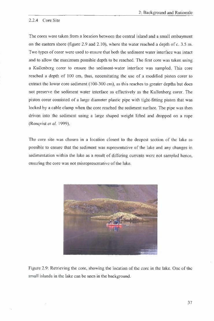
2.2.4 Core Site
The cores were taken fi-om a location between the central island and a small embayment
on the eastern shore (figure 2.9 and 2.10), where the water reached a depth of c. 3.5 m.
Two types of corer were used to ensure that both the sediment water interface was intact
and to allow the maximum possible depth to be reached. The first core was taken using
a KuUenberg corer to ensure the sediment-water interface was sampled. This core
reached a depth of 100 cm, thus, necessitating the use of a modified piston corer to
extract the lower core sediment (100-300 cm), as this reaches to greater depths but does
not preserve the sediment water interface as effectively as the KuUenberg corer. The
piston corer consisted of a large diameter plastic pipe with tight-fitting piston that was
locked by a cable clamp when the core reached the sediment surface. The pipe was then
driven into the sediment using a large shaped weight lifted and dropped on a rope
(Rosqvist a/. 1999).
The core site was chosen in a location closest to the deepest section of the lake as
possible to ensure that the sediment was representative of the lake and any changes in
sedimentation within the lake as a result of differing currents were not sampled hence,
ensuring the core was not misrepresentative of the lake.
Figure 2.9: Retrieving the core, showing the location of the core in the lake. One of the
small islands in the lake can be seen in the background.
37

2: Background and Rationale
Figure 2.10: A view of the lake used in the study, looking north across Maiviken. The
red crosses show the position of the cores. Figure 2.9 was taken looking from the right
of this picture across to the island on the far left of this picture. Source: Sugden and
Clapperton (1977)
2.2.5 Lake processes
To fully understand the processes operating at the site and therefore the mechanisms in
which the sediment has been deposited and the effects this will have upon fur seal hair
entrainment and deposition, the lake inputs, outputs and circulation must be evaluated.
These processes are key to understanding the changing processes operating within the
lake over time and the effect this may have upon the fiir seal hair record.
2.2.5.1 Lake inputs
The primary inputs into the lake are at present fluvial and slope processes which
transport precipitation and surface run off from the localised catchment. This surface
run of f is likely to transport clastic sediments from the scree slopes to the east of the
catchment (see figure 2.7). In addition to this, vegetation debris and soils become
entrained and are washed into the lake. Other elements in the catchment such as fur seal
hairs and excrement wil l also be entrained in surface run o f f and enter the lake
catchment. Furthermore, fiir seal populations wallowing in the lake wi l l entrain
sediment, fiirther increasing the inputs. Aeolian processes may also transport some
sediment from off shore winds, however, these are likely to be minimal due to the
38

2: Background and Rationale
sheltered nature of the lake and will be minor in comparison to the sediment input fi-om
fluvial and slope processes.
From the discussion in section 2.2.2, it is clear that glacial processes are not influencing
the sediment transport and input into the lake today. Although this may have been a
sediment pathway previously when glacier extent was greater, evidence presented in
section 2.2.2 suggests this is unlikely to be a major sediment source as the glaciers
draining into the Bore Valley, drain into Maivatn to the south (and upstream)of the
catchment which therefore, is likely to intercept most sediment.
The lake and catchment are snow and ice covered for approximately 4 - 5 months of the
year, although due to the relatively mild climate at South Georgia, the lake ice does not
reach a thickness where it is likely to fi-eeze to, or disturb, the lakefloor sediment. Due
to this ice and snow cover, direct sediment input is restricted during the winter period
and there is likely to be very little activity in the catchment or the lake at this time.
Snow and ice melt as the climate ameliorates in the spring and summer months
transports a rapid flux of sediment into the lake.
2.2.5.2 Lake circulation
Without sediment traps within the lake, the lake circulation and affect this will have on
sediment distribution sediment retention in the lake cannot be fully evaluated. However,
due to the sheltered location of the lake and proximity relative to glacial activity, it is
thought that lake mixing and sediment disturbance is minimal. As the lake is ice
covered for 4 -5 months of the year and the lake is too deep to permit basal freezing,
there are very few factors that would affect sediment deposition and retention in the lake
during this period. In the summer months, fiir seals wallow in the lakes, however, this is
on the surface of the lake and is unlikely to significantly affect the basal sediments. As
discussed above, the sediment cores were taken from the deepest point in the lake to
reduce any potential effect of sediment disturbance.
2.2.5.3 Lake outputs
The lake output is primarily via the outlet, which drains -100 metres to the sea. Flow in
this outlet is not rapid, suggesting sediment transport from the lake is minimal and the
majority is retained and deposited within the lake catchment. Analysis of the sediment
39

2: Background and Rationale
core and sedimentation rate will provide a greater understanding of the retention of the
sediment within the catchment.
2.3 Late Holocene Environmental Changes
This section examines Late Holocene Environmental Changes at a firstly on South
Georgia as a whole and then using this evidence associated with more site specific
reconstructions, catchment environmental changes are evaluated. Finally the
environmental changes in the Antarctic region are determined. This evaluation at
varying scales is important to fully understand the processes operating within the
catchment. Evaluating the climate changes on South Georgia with regional
environmental change can provide an indication of the changes in ocean and
atmospheric circulation in the region and help to define the causal mechanisms for such
changes (Jones et al. 2000).
The location of South Georgia 250 km south of the Polar Front, is key in
comprehending the climate of the island. This location close to the Polar frontal
boundary allows the movement of the Polar Front to be fracked and hence, records the
effect this has upon the climate connections in temperate and polar environments to be
evaluated (Van der Putten 2004; Rosqvist and Schuber 2003). Although this is
recognised as a key area of research, studies implemented at South Georgia have been
restricted primarily due to the numerous limitations of proxies in this harsh
environment. Firstly, the use of pollen assemblages as a proxy is limited as only two
genera of pollen (Gramineae and Acaena) account for 90% of the total pollen count
therefore; these species have widespread dominance (Barrow 1978; Clapperton et al.
1989; Van der Putten 2004). Very little is known about minor species as the modem
ecology is poorly known and inhospitable conditions make further research difficult
(Bimie 1990). Secondly, the wide ecological tolerance of these species restricts the
extent to which past environmental change can be reconstmcted (Barrow and Lewis-
Smith 1983; Barrow 1978). Thirdly, a large number of pollen grains are blown across
the Southem Ocean from South America and are deposited on South Georgia, hence,
what may appear as climatic change may actually only reflect changes in southem
westerlies or the influence of local topographic features on air currents and hence, the
use of pollen assemblages in environmental reconstruction at South Georgia can be
misinterpreted (Barrow and Lewis-Smith 1983).
40

2: Background and Rationale
Despite these problems in reconstructing the climate of South Georgia, it is recognised
that South Georgia has experienced a range of climatic conditions through the
Holocene. From the use of different proxies to reconstruct environmental change, it is
clear that the enviroimiental response is not uniform and often evidence is conflicting as
different proxies highlight the following different elements of environmental change.
Firstly temperature affects the climate and influences the catchment in terms of the
duration of the ice cover and the vegetation within the catchment. On South Georgia,
Van der Putten (2004) and Barrow (1983) provide an account of the relative
temperature changes on the island through the late Holocene. Secondly, precipitation
has an influence upon the climate and the catchment regime. Precipitation can influence
the vegetation cover, however, it also influences the glacial activity and greatly
influences the inputs and outputs of the lake. Precipitation has been inferred through the
late Holocene on South Georgia from pollen and macrofossil records (Barrow and
Lewis Smith 1983). Finally, glacial activity; temperature is the most influential factor
affecting glacier regime, however, fluctuations in precipitation also affect the mass
balance of the glacier, thus, a decrease in temperature may not reflect a glacial advance
i f precipitation input is insufficient (Clapperton 1990). In addition to this, a number of
glaciers on South Georgia are ^ord glaciers; these are unreliable for dating climatically
forced advances as response lags can be up to 100 years (Clapperton and Sugden 1988).
However, it is essential to understand these glacial regimes specifically on a local scale
as glacial process influence geomorphology and consequently sediment transport
processes in the catchment.
Using a combination of proxies allows the significant climate episodes to be more
clearly understood and permits response times of different systems to be recognised,
hence, reducing error and providing a more accurate picture of environmental change
(Clapperton et al. 1989). Previous studies at South Georgia have used a range of proxies
that include macrofossils (Van der Putten 2004; Taylor et al. 2001), glacier fluctuations
(Clapperton and Sugden 1988; Clapperton et al. 1989), biogenic silica (Rosqvist et al
1999), diatom assemblages (Van der Vijver 1996) and pollen assemblages (Bimie 1990;
Barrow 1978; 1983a; 1983b; 1983c) and finally radiocarbon dates from peat layers have
been used to indicate the duration of vegetation development (Van der Putten 2005,
Gordon 1987). These different proxies will be evaluated and used to reconstruct the
climate of the catchment at Maiviken, the South Georgian climate and the sub Antarctic
41

2: Background and Rationale
climate through the late Holocene. Figure 2.11 summarises the climate of South Georgia
in terms of temperature, precipitation and glacial activity from analysis of these proxy
records.
sjes\ paiejqiieo
s
s a. o
I I I
I i 11
I I
•OS.S I Q 5
o j :
51 = § 3 n ° -> ^ «>. ^ C (A « V. O ©
I t o
2 ° S 13 5
iS 0> ro O C -D
i l l i i
CD!" 3 a,
5 ^ 1 O O)
™ o E 8
2 CD
5= -
I I ro c ~ c5 - Q
- ro ro
j3 (D £ nj
"i 1 8 I I ro .s
SJB9A uoqjeooipey
Figure 2.11: A summary of the climate at South Georgia through the late Holocene.
42

2: Background and Rationale
2.3.1 South Georgia Environmental Change
It is widely agreed that in South Georgia deglaciation culminated approximately 10,000
'" C years BP, as many species of flora became established (Van der Putten 2004;
Clapperton et al. 1989; Barrow 1978). Deglaciation was followed by climate
amelioration, peaking at 5600-4800 '''C yrs BP (6350-5500 cal yrs BP) and conditions
were more conducive to plant growth than today as pollen assemblages suggest
temperatures were 0.6°C warmer than present (Bimie 1990; Clapperton 1989). During
the late Holocene, significant climate deterioration occurred around 2500 ''*C yrs BP
(2500 cal yrs BP) and again at 600 '' C yrs BP (540 cal yrs BP) (see figure 2.11)
(Clapperton and Sugden 1988; Van der Putten 2004).
2.3.1.1 Pre 2600''^C years BP
Climate changes inferred from pollen and diatom assemblages in lake sediments taken
from the Maiviken region suggest that warmer conditions persisted from 3300 ''*C yrs
BP (3500 cal yrs BP) until 2800 '"C yrs BP (2800 cal yrs BP) (Bimie 1990). This
climate amelioration and restricted ice cover is supported by evidence from microfossil
and pollen records. These records suggest a drier period from 4000 ''*C yrs BP to 2600
''*C yrs BP (4400- 2600 cal yrs BP), similar and possibly warmer than the present day
climate, often referred to as the Late Holocene Climate Optimum (Van der Putten et al.
2004; Rosqvist and Schuber 2004; Barrow 1978). This climate amelioration is further
supported by evidence from peat layers on glacial moraines to suggest that glacier
extent was restricted from 3330 '''C yrs BP to 2230 '' C yrs BP (Gordon 1987;
Clapperton et al. 1989). Although the exact timing of this change differs, a large body
of evidence suggests that the period prior to 2600 ''*C yrs (2600 cal yrs BP) was as
warm or warmer than today.
2.3.1.2 2600- 1600 "*C yrs BP
Bimie (1990) suggests that the climatic optimum began to deteriorate at 2900 '''C years
BP as the minerogenic content in the lake cores increases and from 2600 '''C years BP
the climate was wetter. This coupled with an increase in olgiotrophic bogs at 2600 '''C
43

2: Background and Rationale
years BP (2600 cal years BP), provides a broad line of evidence to suggest that the Late
Holocene Climate Optimum had ceased by 2600 ''*C years BP as the climate cooled and
precipitation increased (Van der Putten 2004; Rosqvist and Schuber 2004).
Glaciological evidence also supports this climate deterioration and increase in
precipitation as glaciers began to advance at 2200 ''*C years BP (2200 cal yrs BP)
(Rosqvist and Schuber 2004; Clapperton 1990; Clapperton and Sugden 1988). This
climatic shift is further supported by radiocarbon dates from peat layers and moraines,
which imply ice-free conditions had ceased by 2230 ''*C years BP (3500-2200 cal yrs
BP) (Gordon 1987; Van der Putten 2005)
In terms of the vegetation cover, evidence from pollen assemblages suggests that since
deglaciation, conditions have not been harsh enough to prevent the survival of the
woody herb genus Acaena (indicative of a warm, dry climate) for long periods (see
figure 2.15) (Barrow 1978). Bimie (1990) provides a pollen assemblage to suggest that
this phase (2600-1600 '''C years BP) was similar to the present day climate at South
Georgia, however, Clapperton's (1990) glaciological evidence suggests a cooling of
0.5-rC. Although the magnitude of the change is debatable, it is clear that the climate
deteriorated after 2600 '' C years BP (2600 cal yrs BP), and is thought to be 'the most
striking event in the Holocene palaeoclimatological history of South Georgia', with
major changes in atmospheric and oceanographic circulation (Van der Putten 2004:
390).
The culmination of this period of climatic deterioration is not frequently documented in
the literature and it is likely that the change was gradual. Although pollen assemblages
suggest the climate began to ameliorate at 2000 '''C years BP, the high content of silt
and clay and loss on ignition (LOI) values in lake cores suggest the climate remained
relatively cool until 1600 '''C years BP (Barrow 1978; Bimie 1990).
44

2: Background and Rationale
4000
3000
Q-CQ
$ 2000
o
1000 H
0 -»
Relatively warmer
Relabvely cooler
-10 0 10
% difference in pollen from the core top
Figure 2.12: Relative temperatures at South Georgia through the late Holocene in
comparison to the climate today. Values were calculated from pollen assemblages of
Gramineae and Acaena in Barrow (1978). Relative temperatures were calculated from
the percentage of Gramineae and Acaena today, with Gramineae indicating a warmer
climate and Acaena indicating a warmer climate than today. The scale is the difference
in percentage of Gramineae and Acaena between the sample and the percentage at the
top of the core (i.e. the climate today). For example, positive 20 indicates at that point in
the core there was 20% more Acaena than found in the top sample. A negative 20
indicates 20 more Gramineae in the sample than in the top of the core. The age of the
sample was calculated from a radiocarbon date at the base of the core.
2.3.1.3 1000'"C years BP
The next period of enviromnental change began around 1000 ''C years BP (850 cal yrs
BP) as LOI values indicate a cooling (Rosqvist and Schuber 2003). Evidence from lake
sediments suggest thaf deferidration peaked at 600 '''C years BP as minerogenic content
in the lake increased (Bimie 1990). Associated with this deterioration are glacial
fluctuations, suggesting the period from 600 ''*C years BP was particularly cold and wet
(Clapperton et al. 1989; Rosqvist and Schuber 2003). This peak in cooling is fiarther
45

2: Background and Rationale
supported by evidence from peat layers which indicates that peat growth increased from
990 '"C years BP (838 cal yrs BP) to 775 '''C years BP (686 cal yrs BP), suggesting a
warmer interval after which the climate deteriorated.
2.3.1.4 Post 200 '^C years BP
This climatic deterioration lasted until approximately 200 ''*C yrs BP (200 cal yrs BP)
when the climate ameliorated and glaciers began to advance (Clapperton et al. 1989;
Bimie 1990). Small glacier expansion occurred during the 19* century, forming
multiple moraines suggesting complex oscillations of glacier margins (Bimie 1990).
This was followed by readvances during the 1920's and glacier refreat until the late
1940's, after which all glaciers have been receding (Clapperton and Sugden 1988).
Although this record suggests marked glacier fluctuations, these fluctuations reflect
localised conditions and are dependant upon glacier type and form, thus, cannot be
solely used to evaluate climate (Hayward 1983). It is thought that climatic conditions
only significantly improved within the last 50 years, with the climate becoming warmer
and wetter (Bimie 1990). This climate amelioration is supported by the 5 metre retreat
of the Hodges glacier, south west of the catchment (see figure 2.5; 2.6) (Hayward 1983).
2.3.2 Humic Lake Environmental Changes
The catchment geology and geomorphology has evolved throughout the late Holocene
in response to local and regional climate changes. To fully understand the mechanisms
by which the fur seal hairs are incorporated into the lake sediments and the effect any
changes may have upon the entrainment and preservation of fur seal hairs in the
sediment, the differing lake inputs and depositional processes through the Holocene
must be comprehended. Although there are a variety of climatic variables affecting the
catchment, the primary factors affecting sediment transport processes can be defined as
the catchment stability and vegetation cover and hence, catchment environmental
changes wil l be evaluated under these factors.
Past studies, specifically Clapperton et al. (1989) and Bimie (1990) have used
palaeolimnology to analyse the climate of Maiviken area through the late Holocene.
Although these catchment characteristics can be determined with analysis of the core in
46

2: Background and Rationale
this study, additional proxies provide a more robust estimate of the climate changes
occurring during the late Holocene. Figure 2.13 summarises the climate changes in the
Maiviken area. Differing proxies provide evidence for differing catchment conditions.
To understand the impact this has upon sediment composition and transport
mechanisms, figure 2.13 defines the proxy records having an effect on the catchment
stability and vegetation cover to determine the processes operating within the catchment
relative to the wider climatic changes.
The summary presented in figure 2.13 considers the findings primarily by Bimie (1990)
as this paper was based on lake sediment cores in close proximity to the Humic lake
catchment and uses a multifaceted approach using sediment description, pollen and
spore analysis and microfossil analysis to determine past envirormiental change. To
supplement this record, further evidence wil l is summarised from Barrow (1983). This
record uses micropollen analysis to evaluate the vegetation changes and identify warm
and cold periods during the Late Holocene. However, as discussed in earlier sections,
this record has inherent errors related to the variability of the pollen in this region and
therefore cannot be used as a sole indicator of climate change in this region. Additional
studies (Van der Putten 2005; Rosqvist and Schuber (2003)) are also used in analysis to
provide an indication of the catchment stability or vegetation cover on South Georgia,
however, these are not site specific.
47

2: Background and Rationale
sjBaA paiBjqiieo
2"|i
1.1
o m
1 1 . i l l o : l i
§1 _ l c
I "i
f i I 8
11
i f
i f
Q 1
5 Si Q-
2 J}
c g S
>
^ J -i 181
I I I I I I . I I I !
i " 8
i s s p i l l i e S I s a -5
S o Pi E
fa *i c « 2 gj o
o g X
'S s
11 S iS a i §1
C3
c o P d
I 1 1 I 2 11
sjeaA uoqjeooipey
Figure 2.13: A summary of late Holocene environmental changes in the Maiviken
catchment.
48

2: Background and Rationale
2.3.2.1 General climate
Bimie's (1990) paper analyses a core from Lake Maivatn and Evans Lake (see figure
2.7). A date of 8657 '''C yrs BP at the base of the core indicates that the catchment of
Evans Lake has been vegetated throughout the record. From this evidence it can be
inferred that due to the close proximity of the Humic lake and the lower latitude, the
catchment has been ice free and vegetated for the majority of the late Holocene. From
this evidence it can be assumed that the catchment has remained relatively stable during
the late Holocene and there is no evidence to suggest the geology and geomorphology
of the catchment has changed dramatically since the LGM and therefore wil l not have
had a significant impact upon the fiir seal hair deposition or lake sediment dynamics.
2.3.2.2 Catchment specific environmental changes
Pre 2900 ''*C yrs BP {Pre 2600 '"Cyrs BP)
This relatively warm period documented on South Georgia (see figure 2.13) caused
increase vegetation cover and as documented in Bimie (1990) an increase in organic
input in the lake catchment. This is fiirther supported by pollen analysis which indicates
peat development prior to 2700 '''C yrs BP (Bimie 1990). Licreased vegetation cover
and a warm climate suggests a stable catchment where inputs are likely to be minimal.
Comparing this to the climate record from South Georgia, it appears this climatic
optimum ceased earlier in the catchment than in other areas on South Georgia, however,
this can be attributed to slight dating errors or the maritime location of the study site.
• 2900-2100 '''C yrs BP {Climate deterioration 2600 '"Cyrs BP)
Although changes in diatoms often reflect changes in lake chemistry rather than a
change in temperate, the presence of two new types of Diatom species in the lake record
at 2600 ''*C yrs BP coupled with a change in stratigraphy suggests a cooling (Bimie
1990). Associated with this cooling is a decline in vegetation cover, decreasing
catchment stability and increasing minerogenic inputs into the lake.
49

2: Background and Rationale
• 2100-1000 yrs BP (2600 - 1600 '"C yrs BP)
The presence of Compositae pollen at 2000 '" C yrs BP suggests a climatic warming and
associated increase in vegetation cover (Bimie 1990). Clapperton et al. (1989) indicate
that glacier expansion occurred during this period, although there are no glaciers located
in the catchment, this advance suggests an increase in precipitation and decrease in
catchment stability, hence, increasing the inputs into the lake. From this evidence, it is
likely that this period, although warmer than 2600 '''C yrs BP was not as warm as pre
2600''*C yrs BP.
• 1000 - 500''^C yrs BP
Evidence presented by Bimie (1990) suggests that by 1000 '" C yrs BP the climate began
to deteriorate. An increase in minerogenic sediment in the core indicates a decline in
organic content and a decrease in catchment stability. A peak in minerogenic content
and increase in palynomorph concentration suggests this cooling and catchment
instability peaked at 600 ''*C yrs BP. This is further supported by glaciological evidence
presented by Clapperton et al. (1989).
• 500 yrs BP - Present
From 500 '''C yrs BP to present, proxy records indicate climate amelioration, increased
vegetation cover and associated increase in catchment stability (see figure 2.13)
50

2: Background and Rationale
sjeaA pajejqiieo
0
500
860
• 13
50
~ 18
65
~ 24
85
" 31
05
Cla
pper
lon
(199
0) A
ntar
ctic
Pe
nins
ula
Ingo
lfsso
n et
al
(199
8) A
ntar
ctic
Pe
nins
ula
Jone
s et
al.
(200
0) S
igny
Is
land
Coo
ling,
in
stab
ility
Late
Hol
ocen
e cl
imat
ic o
ptim
um
Bjo
rcke
tal
(199
1a)
S. S
hetla
nd I
slan
ds
Coo
ler
drie
r co
nditio
ns
Mor
e hu
mid
gl
acie
r ex
pans
ion
ZaIe
and
Kar
len
(198
9) J
ames
R
oss
Isla
nd
Clim
atic
max
imum
Gla
cier
adva
nce
Bjo
rket
al(1
996)
Ja
mes
Ros
s Is
land
Arid
Pha
se
™ 1
§ S3 ~ ra TO 3. S c CO
Q o
111 =
S £ S S tfi ra y, y c ra (5 oi o £ > f I H
® c ra
•°5 o .s
1 1
o o o 8 in
8 o
8 8 o CO CO
sjeaA uoqjeoo\pe\i
Figure 2.14: A summary of sub Antarctic climate change through the late Holocene.
51

2: Background and Rationale
2.3.3 Regional environmental change
It is widely documented that the period from 4700 to 2000 ' C yrs BP was warmer than
today (Hodgson et al. 2004), although the exact timing of this varies across the
Antarctic region. From ice cores in Antarctica, Ciais et al. (1994), suggest that a
warmer, more stable period occurred from 4500 ''*C yrs BP. This period of climatic
optimum conditions occurs slightly later on the Antarctic Peninsula, at 4000-3000 '''C
yrs BP (4400- 3100 cal yrs BP) and is delayed fiuther on Sub- Antarctic Islands
(Ingolfsson et al. 1998). Pollen records from lake sediments on Livingston Island,
(South Shetland Islands) suggest milder, more humid conditions from 2700 '' C yrs BP
(Bjorck et al. 1991a). This period is termed the Mid Holocene Hypsithermal and it is
widely recognised that during this period, there was rapid sedimentation, high organic
productivity and increased species diversity (Hodgson et al. 2004)
2.3.3.1 2600-2000 '" C yrs BP (South Georgia climate deterioration)
Records from the Antarctic Peninsula, Antarctica and the Southern Ocean, indicate a
significant climatic shift at 2400 '" C yrs BP (2500 cal yrs BP) (Domack and Mayewski
1999). Marine records from the Antarctic Peninsula suggest that the climate
deterioration occurred at 2700 ''*C yrs BP causing reduced productivity and more
extensive and persistent sea ice (see figure 2.14) (Ingolfsson et al. 1998). This correlates
with evidence on South Shetland Island, which implies cooler conditions commenced at
2700 •''C yrs BP (2800 cal yrs BP) (Bjorck et al. 1991a). Although this shift occurred
slightly earlier in this region than on South Georgia, this may be a result of the lag time
within the system and the more northerly location of South Georgia. Although, Hodell
et al. (2001) provide a correlation of Holocene climate change at Taylor Dome, North
Atlantic and the Southern Ocean in which all the records show a significant climate shift
at 2500 '''C yrs BP (2500 cal yrs BP). This correlation throughout the Southern Ocean
indicates a significant climate change occurred at this time that was likely to be caused
by a global forcing mechanism. Domack and Mayewski (1999) identify this climate
shift in GISP2 core from Greenland, which indicates a cool episode commencing at
2500 *'*C yrs BP (2500 cal yrs BP). Evidence from Chilean records, suggest a less
humid phase occurred from 2500 ''*C yrs BP (2500 cal yrs BP), suggesting this change
in climate at 2500 ''*C yrs BP (2500 cal yrs BP) had regional implications and was
possibly a result of a regional shift in the position and sfrength of the Westerlies (Lamy
etal 2001).
52

2: Background and Rationale
The climate change widely documented to occur at 2500 ''*C yrs BP (2500 cal yrs BP) is
not evident in all the records on the Antarctic Peninsula, suggesting the forcing
mechanism for this change was of local origin. At James Ross Island, a warmer arid
phase commenced at 3000 '" C yrs BP (3100 cal yrs BP) and lasted until 1200 '' C yrs
BP (1050 cal yrs BP) (see figure 2.14) (Bjorck et al. 1996; Jones et al. 2000). This also
correlates with the Palmer Deep record that indicates that fi-om 3000-2000 cal BP
conditions were more humid than present with a reduced sea ice extent, with a
particularly warm event occurring at 2680 cal BP (Noon et al. 2003). Although this
warming is not documented in the South Georgia record or in other records fi-om the
Antarctic Peninsula, the increase in humidity does correlate with the glacier advance on
South Georgia that was delayed afl;er the onset of the climate deterioration, which Noon
et al. 2003 infer to be related to a northward shift of the Southern Westerlies.
2.3.3.2 2000-1000 yrs BP (South Georgia warm phase)
On the Antarctic Peninsula, glacier advance occurred fi-om 2000 '" C yrs BP (1850 cal
yrs BP), suggesting a change in the precipitation regime but not necessarily
deterioration (Ingolfsson et al. 1998). On the South Shetland Islands, the opposite
occurred as Bjorck et al. (1991a) document deterioration fi-om 1300-700 ''*C yrs BP
(1200-600 cal yrs BP). This is in agreement with records fi-om Antarctic ice cores,
which record an important cooling which commenced at 2000 '" C yrs BP (1850 cal yrs
BP) and culminated at 1000 '''C yrs BP (850 cal yrs BP) (Ciais et al .1994).
2.3.3.3 1000-200 '" C yrs BP (Cooling, fluctiiating climate at South Georgia)
The cooling experienced in South Georgia at 1000 '' C yrs BP (850 cal yrs BP), is also
evident in records fi-om the Antarctic Peninsula, Sub Antarctic Islands and ice core
records at Taylor Dome (Noon et al. 2003; Hodell et al. 2001). Cooling commenced
first at South Shetland Islands, as Bjorck et al. (1991b) document more continental
conditions fi-om 1500- 500 "'C yrs BP, with the coldest period starting at 1300 "*C yrs
BP (1200 cal yrs BP) and lasting until 700 ^ C yrs BP (600 cal yrs BP). On the Antarctic
Peninsula, a cooling of 0.5-rC began earlier at 1400 "'C yrs BP (1250 cal yrs BP)
(Clapperton 1990). This cooling was delayed until 1300 '' C yrs BP (1200 cal yrs BP) on
Signy Island, when a deterioration occurred following the long lasting climatic optimum
(see figure 2.14) (Jones et al. 2000).
53

2: Background and Rationale
The maximum climate deterioration at South Georgia that commenced at 600 '" C yrs
BP correlates with regional climate fluctuations. At Signy Island, a relatively warm
period ceased at 600 '''C yrs BP. This deterioration is documented earlier on James Ross
Island, commencing at 750 "'C yrs BP and lasting until 500 '''C yrs BP (Zale and Karlen
1989). However, these events are not documented on the South Shetland Islands as
maximum deterioration commenced at 1300 '''C yrs BP (1200 cal yrs BP) and ceased at
700 '"C yrs BP (600 cal yrs BP) (Bjorck et al. 1991). This fluctuation correlates with
evidence from the Antarctic Peninsula, which indicates warming, termed the Medieval
Warm Period (MWP) commencing at 1000 "*C yrs BP (850 cal yrs BP), ending at 500
'' C yrs BP with the onset of the Littie Ice Age (LIA) (see figure 2.15), documented as
the strongest of late Holocene cold and warm periods in the Antarctic Peninsula region
(Khim etal. 2002).
100 150 200
^ 10O H
1S00 (=H
200 H
h 3000
m -
Figure 2.15: A high-resolution magnetic susceptibility record from the Eastern
Bransfield Basin, Antarctic Peninsula highlighting the timing of the Little Ice Age
(LIA) and the Medieval Warm Period (MWP) in the region. Source: Khim et al. (2002:
243).
54

2: Background and Rationale
2.3.3.4 200 •''C yrs BP
Thompson et al. (1994) suggest a cooler period on the Dyer Plateau (Antarctic
Peninsula) from 1850-1930 AD when accumulation rates and dust increased in ice
cores. On Signy Island, from 1820-1880 AD a glacial advance occurred, thought to be a
response to northward displacement of the Antarctic circumpolar trough (Noon et al.
2003) . This movement of the Antarctic Circumpolar Trough correlates with the ice
readvances on South Georgia at 200 ''*C yrs BP, reaching a maximum in 1875 AD
(Bimie 1990). Peat deposits from Argentina suggest this climate deterioration also
affected the Southern Ocean and Southern South America climates (Mauquoy et al.
2004) . During the early 20* century, across the Antarctic regions glaciers advanced
until 1950, when refreat began (Clapperton and Sugden 1989; Clapperton 1990; CoUins
1976; Hayward 1983; Noon et al. 2003; Thompson 1994). This sfrong regional coupling
during the 20* century across the Antarctic Peninsula and Sub Antarctic Islands implies
a regional change in atmospheric and oceanographic circulation patterns (Noon et al.
2004).
2.3.3.5 Summary
Evidence for environmental change in the Sub Antarctic Islands and Southem Ocean
through the Holocene is conflicting as a result of the spatial interactions of the Polar
Front and Westerlies (Jones et al. 2000). Although the climate signature across the
region is varied there are some significant trends documented throughout the region,
implying that regional factors are influencing these changes. Data from the Palmer Deep
core suggests a mid Holocene climatic optimum (hypsithermal) culminated around 3360
cal yrs BP (Domack et al. 2001). Records from the Antarctic Continent (Dome C)
suggest a cooling followed this optimum from 2300 '''C yrs BP (Masson-Delmotte et al.
2004) which can be correlated with the climatic deterioration at South Georgia from
2600 ''*C yrs BP (2600 cal yrs BP) (Rosqvist and Schuber 2003). As this pronounced
cooling is documented across the Antarctic region, it suggests that a significant climate
shift of regional significance occurred at this time.
Although the period of cliniatic deterioration is punctuated with periods of warming,
there are no regional climatic frends evident in the records until approximately 1000 '' C
yrs BP (850 cal yrs BP), when a fiirther cooling occurred. Evidence from the Palmer
55

2: Background and Rationale
Deep core implies that after the mid Holocene optimum, which culminated at 2600 ''*C
yrs BP (2600 cal yrs BP) on South Georgia, climatic deterioration occurred, which
intensified at approximately 1000 '" C yrs BP (850 cal yrs BP), correlating with the
period known as the Little Ice Age from 700 cal yrs BP to 100 cal yrs BP (Domack et
al. 2001). Evidence suggests that the period of warming from 2000-1000 '''C yrs BP
(1850-850 cal yrs BP) is only documented at South Georgia. The forcing mechanism
may be of regional origin, however, as there are a variety of regional responses to a
single forcing event, it is possible that the effects on South Georgia are more
pronoimced than other areas of the Southem Ocean (Hall and Perry 2004). The onset of
enhanced cooling began at 1400 ''*C yrs BP (1250 cal yrs BP) in the Antarctic
Peninsula, 1000 "*C yrs BP (850 cal yrs BP) on James Ross Island and 600 ''*C yrs BP
on South Georgia and in the ice core record at Dome C (East Antarctica) (see figure
2.11 and 2.14). This strong coupling of the timing of climatic change in the Antarctic
region suggests that the forcing mechanism is of regional or global origin (Masson-
Delmotte et al. 2004; higolfsson et al. 1998; Bjorck et al 1996).
The sfrong similarity between ocean and terrestrial records for the past 4000 '"'C years
in the Antarctic Region suggests a sfrong coupling process is operating at this timescale
(Masson- Delmotte et al 2004). hi all records the 2600 and 600 ''*C year BP (2600 and
540 cal yrs BP) events are clear, however, there are a number of smaller climatic
changes occurring on a local level, suggesting a variety of climatic forcing mechanisms
are affecting the region (Fabres et al. 2000).
2.4 Historical records of climate change
The proxy record outiined in section 2.3 provides an indication of the climate conditions
on South Georgia prior to human intervention. This can be compared to ftir seal
population fluctuations and therefore, used to evaluate the impact of climate change on
the fiar seal population. Natural climate changes must also be assessed during the time
of human intervention to allow the impact of recent climate change on the fiir seal
population to be evaluated in comparison to the human induced changes. Although it
can be argued that human intervention has influenced climate in the recent past, this
cannot be quantified and for the purpose of this study, all climatic changes are regarded
as natural environmental changes and human induced changes are regarded as those
outlined in section 2.5.1.
56

2: Background and Rationale
There is a broad scientific consensus that the climate has warmed by 0.6 °C during the
20* century (IPCC 2001). Figure 2.16 shows the average armual temperature recorded
on South Georgia fi-om 1905. It is clear fi-om this that there has been a significant
warming trend since 1970, consistent with the Southern Ocean region and the Antarctic
continent (Weimerskirch et al. 2003; Raper et al. 1983).
3.0
4
1920 1940 1960 1980 1900 2000
Figure 2.16: Average temperature record for Gryviken, South Georgia. The smoothed
line is the running average, calculated on Sigma plot using the running average fiinction
and sampling proportion set at 0.1. Data Source: www.antarctica.ac.uk/met/READER
2.4.1 1920-1940 (Cooling)
The coldest period during the 20'*' century occurred fi-om 1923- 1939 (see figure 2.16),
when annual average temperatures were up to 1.7 °C cooler than today. This is reflected
in the glaciological record as glaciers reached their maximum advance during the late
1920's (Hayward 1983; Clapperton 1970). In conti-ast to this, Ainley et al. (2005)
establish a warming of the sea surface temperatures fi-om 1925-1946 as a result of a
positive Pacific Decadal Oscillation (PDO). Particularly warm years are thought to be
57

2: Background and Rationale
1929/30 and 1936/7 (Whitehouse et al. 1996). However, as figure 2.16 shows, although
1936/37 was a warmer year within the colder period, it was still significantly cooler
than the period from 1940-1960.
2.4.2 1940-1960 (Warming frend)
Following this cold period, figure 2.16 highlights a warming trend from 1940-1960.
During this time, McGowan et al. (1998) provide evidence for a sfrong ENSO event in
1957/58 that resulted in a warming of the oceanic temperatures, disturbing the structure
of the plankton communities in the Southem Ocean and the South Pacific. This
warming from the ENSO event is an anomaly within a negative PDO phase from 1947-
1976, causing a decline in sea surface temperatures (Ainley et al. 2005). Glacier
fluctuations at South Georgia during this warming phase showed a slow refreat until the
late 1940's and then a short rapid advance in the early 1950's, reaching a maximum in
1956 (Hayward 1983). Variability in the glacier activity during this time reflects both
the temperature regime and precipitation changes. The warming frend at South Georgia
was also occurring on the Antarctic Peninsula from the 1940's and is correlated with the
reduced frequency of winter sea ice since that time (Loeb et al. 1997).
2.4.3 1960-Present day
During the 1960's and 1970's temperatures remained relatively constant at South
Georgia. Figure 2.16 shows that from 1970 the temperature increased more rapidly than
previously during the 20* century. This is consistent with all other terrestrial and marine
records in the Southem Ocean region and suggests a regional or global forcing
mechanism influenced the climate at this time (Wiemerskirch et al. 2003). Coupled with
this increase in temperature, sea ice extent declined across the Southem Ocean region
and glaciers refreated on South Georgia (Croxall et al. 2002; Hayward 1983). This
warming is also evident from the PDO index which was sfrongly positive from 1977 to
1988, when two periodicities coincided, causing this to be the most intensive positive
regime in the 20* centiiry (Ainley et al. 2005).
From the mid 1980's, records from across the Southem Ocean region suggest the mean
temperature remained constant (Weimerskirch et al. 2003). However, it is not clear
whether this plateau occurred on South Georgia due to the incomplete data set (see
figure 2.16). The PDO index suggests a short negative (cooler) phase from 1989-91
58
2: Background and Rationale
followed by a warmer phase that has lasted from 1992 until the present day (Ainley et
al. 2005). Although this was a warming period, it is widely recognised that strong
ENSO events occurred in 1982/83 and 1997/98, causing extreme cold anomalies in the
Southem Ocean in the South Georgia region, a result of the intmsion of the Southem
Aflantic Circumpolar Current front (McGowan et al. 1998). These cold intmsions
correlate with air temperature measurements on South Georgia, implying that the
climate of South Georgia is very susceptible to ENSO events (Meredith et al. 2005).
2.5 Fur seal population on South Georgia
South Georgia was first explored in 1775 (after first sightings by Cook in 1675), with
sealing developing rapidly in the latter part of the 18* and early 19* centuries
(Headland 1982). The exploitation of fiar seals commenced in 1786 therefore, the actual
fiar seal population prior to exploitation was never documented (Headland 1984). Due to
the high competition for the seals and thus, commercial secrecy, very few sealing
expeditions following the discovery of South Georgia have been documented. The
number of seals taken from the island during the sealing epoch from documented
expeditions is also unknown as the sealers maintained secrecy about places with a large
fiir seal population in the hope that they could exploit seals in subsequent seasons
without any competition.
2.5.1 Exploitation
There are thought to have been 3 peaks in sealing activity, the first and largest
exploitation took place from 1786-1802. Records of the number of skins taken during
this time are very limited, however, some records suggest that in one season (1800/01) a
minimum of 112,000 skins were taken (Headland 1984). Following this first sealing
epoch, the Napoleonic wars prevented any sealing occurring again until 1814. During
this second sealing epoch, exploitation was not as extensive as the seal stocks of South
Georgia were depleted therefore, sealers began to exploit other islands such as the South
Shetland Islands which had previously not been discovered. This shift to other islands
reduced the pressure on South Georgian seal stocks, which were still very low, as they
had not recovered from the first period of sealing (Headland 1984). By 1822 it was
calculated that 1,200,000 fiir skins had been taken and the fiir seal population was
nearly extinct, causing the sealing to cease in 1823 (Bonner 1994). A third peak
occurred again in 1869, however, as the fiir seal population had been exploited so
59

2: Background and Rationale
extensively, the focus was predominantly upon the elephant and leopard seals rather
than the fijr seals, and very few were taken from the island (Headland 1984). Elephant
seal populations did not suffer in the way fur seal populations did, as elephant seal oil
was not as valuable therefore, it was only profitable to hunt elephant seals in areas
where they were abundant. Fur seals however, were more valuable hence, it was
profitable to take fur seals even from areas with very few seals (Headland 1982).
Although the population had reached almost extinction, small-scale hunting continued
until 1907, which is thought to be responsible for the halting recovery of the population
during the second half of the 19* Centiiry (Headland 1984).
2.5.2 Post Exploitation
Although census data has improved during the 20* century, the foraging nature of fur
seals causes data collection to be problematic hence, many data sets are only estimates
and there are no continuous records available (Payne 1977). Despite this lack of census
data, it is widely documented that the fur seal population in the Southem Ocean
increased rapidly following exploitation (Headland 1984; Hodgson et a/. 1997; Sun et al.
2004; Payne 1977; Bonner 1985). Table 2.1 and figure 2.17 show the available census
data at South Georgia.
60

2: Background and Rationale
a>
a 3 O
0)
CL
0) >
I
I c o o o
a •= (U
l « O 0) O.E a>
Q.
C o
Q. T3 P
E a>
(0 0) >-
Table 2.1: A l l the available fur seal population census data fi-om South Georgia 1930-
1999. Adapted firom Grant, S. (pers. comm.)
61

2: Background and Rationale
1e+7
1e+6 H
S 1e+3
1e+2 -
2000
— X — Pup ProducBcxi •' Total population
—-K— Population increase
Figure 2.17: A graph showing the estimated rates of fur seal population increase at
South Georgia from 1930-2000. Data is used from sources outlined in table 2.1 (note
logarithmic scale for population)
The census data for mainland South Georgia and specifically the study site (Maiviken)
is limited, however, the record for Bird Island is more extensive as the rapid increase in
ftir seals in this region caught the attention of many researchers. Table 2.1 indicates that
in 1930 the first pups were bom at Bird Island following the sealing industry (Bonner
and Walton 1985). By 1933 the population had reached 38 seals and by 1936 this had
increased to 59 (Payne 1977). From this initial census, the population documentation is
very limited until 1956, when thriving colonies were observed at Bird Island and on the
main island of South Georgia. On Bird Island, during the 1957/58 season, 5,350 pups
were counted, increasing to 11,500 in 1963/64 and 102,000 in 1976/77 (Croxall and
Prince 1979; Laws 1973). By 1963/4 the most suitable areas on Bird Island were
occupied by breeding seals, forcing nuclei of further colonies to be established on the
mainland of South Georgia (Payne 1977). During 1975/76 the population on the
62

2: Background and Rationale
mainland exceeded that of Bird Island, with over half the total pups bom on mainland
beaches, the total fiir seal population of South Georgia being estimated at 369,000 and
increasing at a rate of 16.8 % per annum (Bonner 1985; Payne 1977).
Following the rapid increase in the population from the 1930's to 1970's, Croxall and
Prince (1979) document reduced breeding success at Bird Island in 1977/78. This
decline in the fiir seal population has been correlated with a reduced krill population as
a result of a change in the water currents surrounding the island (Bonner and Walton
1985). Following this brief decline in the growth rate, the 1980's saw the population
stabilise and the rate of increase declined to 9.8% per annum as the population reached
856,000 in 1982 (Bonner 1985). By 1999, the total population was estimated to be
3,000,000 however, the rate of increase was declining with some years experiencing a
negative growth rate (Boveng et al. 1998; Hucke-Gaete et al. 2004; ATOM 1999).
Particularly significant years of decline were documented in 1991, 1994 and 1998, and
were linked to ENSO events (Reid and Croxall 2001).
As the fiir seal record is not continuous and most years are estimates, it is difficult to
determine whether the population declined briefly in some years. Although the rate of
increase has changed, the actual rate of change is difficult to determine as it is based on
a few estimates hence, the precise timing of the change cannot be correlated accurately
with climate changes and the short-term impacts on the fiir seal population cannot be
assessed.
2.5.3 The Situation Today
At South Georgia the fiir seal population expanded rapidly from initial recolonisation on
Bird Island during the early 20* century. Although the population has expanded onto
the mainland today 75% of the fiir seal population in the Southem Ocean still breed
within a 50 km radius of Bird Island (Barlow et al. 2002). The rate of increase at Bird
Island has declined as the carrying capacity has been attained on the island therefore;
the population is forced to migrate to other areas where the point of saturation has not
already been reached (Barlow et al. 2002). At Maiviken there is no fur seal census data,
however, due to proxihiity to Bird Island, it can be assumed that the population formed
as Bird Island reached its carrying capacity and hence, immigration of the fur seals took
place. Although the population of Bird Island has stabilised, evidence suggests that
63
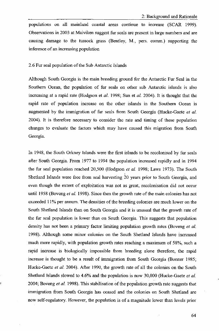
2: Background and Rationale
populations on all mainland coastal areas continue to increase (SCAR 1999).
Observations in 2003 at Maiviken suggest fur seals are present in large numbers and are
causing damage to the tussock grass (Bentiey, M. , pers. comm.) supporting the
inference of an increasing population
2.6 Fur seal population of the Sub Antarctic Islands
Although South Georgia is the main breeding ground for the Antarctic Fur Seal in the
Southem Ocean, the population of fur seals on other sub Antarctic islands is also
increasing at a rapid rate (Hodgson et al. 1998; Sun et al. 2004). It is thought that the
rapid rate of population increase on the other islands in the Southem Ocean is
augmented by the immigration of fur seals from South Georgia (Hucke-Gaete et al.
2004). It is therefore necessary to consider the rate and timing of these population
changes to evaluate the factors which may have caused this migration from South
Georgia.
In 1948, the South Orkney Islands were the first islands to be recolonised by fur seals
after South Georgia. From 1977 to 1994 the population increased rapidly and in 1994
the fur seal population reached 20,500 (Hodgson et al. 1998; Laws 1973). The South
Shetland Islands were free from seal harvesting 20 years prior to South Georgia, and
even though the extent of exploitation was not as great, recolonisation did not occur
until 1958 (Boveng et al. 1998). Since then the growth rate of the main colonies has not
exceeded 11 % per annum. The densities of the breeding colonies are much lower on the
South Shetiand Islands than on South Georgia and it is unusual that the growth rate of
the fiir seal population is lower than on South Georgia. This suggests that population
density has not been a primary factor limiting population growth rates (Boveng et al.
1998). Although some minor colonies on the South Shefland Islands have increased
much more rapidly, with population growth rates reaching a maximum of 58%, such a
rapid increase is biologically impossible from breeding alone therefore, the rapid
increase is thought to be a result of immigration from South Georgia (Bonner 1985;
Hucke-Gaete et al. 2004). After 1990, the growth rate of all the colonies on the South
Shetland Islands slowed to 4.6% and the population is now 30,000 (Hucke-Gaete et al.
2004; Boveng et al 1998). This stabilisation of the population growth rate suggests that
immigration from South Georgia has ceased and the colonies on South Shetland are
now self-regulatory. However, the population is of a magnitude lower than levels prior
64

2: Background and Rationale
to exploitation (Boveng et al. 1998). Calculating the magnitude of the South Georgia population in comparison to levels prior to exploitation will provide a key insight into the factors controlling population recovery and the impact the sealing industry has upon Antarctic ecosystems.
Other islands in the Southern Ocean, for example Marion Island and Heard Island have
experienced similar growth rates to South Georgia after exploitation (Hofineyr et al.
1997; Page et al. 2003; Guinet et al. 1994). The reestabhshment of the fiir seal
population after exploitation on these other islands was delayed in comparison to the
South Georgia and populations were not established until the mid 20* century (Page et
al. 2003). Although the rate of increase was similar to South Georgia, (growth rates
reached 17% on Marion Island) rates were not sustained for as long and today the
populations have reached maturity and the growth rates have slowed dramatically
(Hofineyr et al. 1997; Guinet et al. 1994). From this evidence, it would appear that the
South Georgia population is unique, as the high population growth rate has been
maintained for a sustained period of time.
2.7 Possible causes for the increase in fiir seals
It is widely recognised that the primary influences on population growth are the
availability of prey and predator competition (Croxall and Prince 1979; Reid et al. 1999;
Murphy and Reid 2001). As Weimerskirch et al. (2003) demonstrate, decline in food
availability at lower trophic levels may underlie the general decline of top predator
populations such as fiir seals. The primary prey of the fiar seal is krill {Euphausia
superba) therefore, factors influencing the abundance and distribution of krill are key in
determining the growth of the fiir seal population. Long-term population studies of
predators at South Georgia have shown that reductions in breeding performance occur
in years of low krill abundance (McCafferty et al. 1999; Siegel et al. 1998; Croxall
1992; Reid and Croxall 2001; Clarke and Harris 2002). Although extensive studies have
outlined the impact of fluctuations in prey availability in influencing fiir seal
populations, very little consideration has been given to the effect of predator
populations (Boyd and Murray 2001; Thomson et al. 2000). Predator populations
however, are is also a potential factor which may influence population growth and
should be considered when evaluating the possible causes of a step change in population
growth.
65

2: Background and Rationale
Although there are a number of factors that influence population growth, ultimately
these factors relate to the availability of prey and the extent of predator competition.
Factors influencing the predator competition and prey availability can be categorised in
two ways, firstly natural environmental changes and secondly human induced changes.
2.7.1 Human induced causes
Following the discovery of South Georgia in 1775, human influences have altered the
dynamics of the ecosystem and consequent predator- prey relations, which have
impacted on the fur seal population. The human influence on prey availability and
predator competition and the effect on fur seal populations are examined below.
2.7.1.1 Prey Availability
The full extent to which prey availability affects fiir seal populations is unknown as the
system is complex and there are a number of contributory factors. The primary human
induced cause of reduced prey at South Georgia is thought to be the whaling industry.
As discussed in section 1.4.2.2, South Georgia was the principal centre for whaling in
the Southern Hemisphere and this extensive whaling caused a reduction in whales and
resulted in a krill surplus and allowing a greater fur seal population to be supported
(Croxall 1992). Although this had an impact on other populations in the Southern
Ocean, for example gentoo and chinstrap penguins (Croll and Tershy 1998; Croxall et
al. 1981), fur seals are the third most important consumers of kril l , and so the impact
upon the fiir seal population was greater than the impact on these other species. The krill
surplus is now widely recognised as the most probable cause of the increase in fur seals
(Doidge and Croxall 1985; Croxall and Prince 1979; Croxall 1992; Green et al. 1989).
This is for several reasons as Croxall (1992) indicates; firsfly, the removal of the Baleen
whale reduced competition for krill within the Southern Ocean is the most significant
short-term perturbation the Southern Ocean has ever sustained. Secondly, although krill
populations are vast, their distribution is patchy and hence, wil l sustain long-term
increases in predators before limiting populations. In areas of high krill abundance,
recovery rates and reproductive performance of species are faster and better than
elsewhere.
66

2: Background and Rationale
2.7.1.2 Predator Competition
The primary hioman influence on the predator competition for the fur seal is the act of
killing the fur seal. The ending of the sealing industry and the implementation of
rational conservation measures made it illegal to kill flir seals without a permit
(Headland 1982). This reduced the number of fiir seal predators (humans)therefore,
allowing the population to recover (Lewis-Smith 1988).
2.7.2 Summary of human induced factors
It is clear that the sealing and whaling industries had a significant effect on the fur seal
population, with changes in prey availability being the most influential factor
controlling populations. For example, southern elephant seals were also exploited at
South Georgia at the end of the 19** century and the population is now stable at 300,000
(Headland 1984). The difference between these two species is their prey; fiir seal prey is
predominantly krill , however, elephant seals feed predominately on squid and hence,
did not directly benefit from the krill surplus created as a result of the whaling industry.
Although prey availability was affected by human induced changes (i.e. the sealing and
whaling industries), natural environmental changes can also have a significant impact
on krill availability and predator populations (Reid and Amould 1996).
2.7.3 Natural Enviroimiental changes
Natural environmental changes are often operating at a similar time to human induced
changes, however, as human-induced changes are often more apparent, these natural
changes are often difficult to establish or even ignored. These natural changes must also
be considered to evaluate how the fur seal population responded to changes prior to
human intervention, allowing the impact of human induced changes on the fur seal
population to be assessed. I shall now briefly examine these various natural aspects of
fiir seal population fluctuations.
2.7.3.1 Prey Availability
Although there is strong evidence in support of the krill surplus hypothesis, Reid and
Amould (1996) indicate that the distribution and abundance of krill is likely to be
67

2: Backgrovmd and Rationale
dependent on a number of oceanographic and biological characteristics, changing in
response to natural climate changes, thus, demonstrating the difficulty of attempting to
establish a single causal mechanism for the change.
2.7.3.1.1 Climate
As Weimerskirch et al. (2003) highlight, correlations of large-scale climate changes and
population sizes worldwide relate to abiotic components such as sea ice extent, sea
surface temperatures and air temperature anomalies. As these factors affect the extent of
an ecological niche, it would appear that climate change is a prime factor affecting the
ecosystems (Meredith et al. 2005). Ainley et al. (2005) indicate in the Southern Ocean,
ocean circulation and temperature is affected by Pacific Decadal Oscillation (PDO) and
to some extent North Atlantic Oscillation (NAO). These anomalies in the Southern
Ocean can cause changes in pressure systems and wind regimes that in turn affect ocean
processes. Although this can directly affect populations through determining the
temperature and hence, the ecological niche, indirectly it can also affect the population
through influencing prey availability and hence, affecting the competition for prey.
As Croxall (1992) finds, years of major unavailability of krill correlate with major
ENSO events. Studies suggest that although a reduction does not influence the adult
population, ENSO years correlate with a significantly lower fur seal pup production
(Guinet et al. 1994). ENSO events alter the ocean circulation and as the Antarctic
Circumpolar Current (ACC) is the primary mechanism transporting krill to South
Georgia any fluctuation in the ACC will have a major influence on the reproductive
success of the fiir seal and other krill-dependent predators (Clarke and Harris 2002). The
link between prey availability and ENSO events implies climatic change indirectly
affects the fiir seal population and it can be argued that the increase in the fiir seal
population correlates with recent 20** centiuy warming.
Regional warming on the Antarctic Peninsula within the last 50 years has had a
significant impact on the sea ice extent and it is now widely recognised that changes in
populations are correlated to changes in sea ice extent (Ainley et al. 2005; Curran et al.
2003 Clarke and Harris 2002; Croxall et al. 2002). For example, as McCafferty et al.
(1999) suggest, adelie penguins are inversely related to winter sea ice at Ross Island,
and hence, have increased in the past 40 years as the sea ice during this time has
declined. Alternatively Emperor penguins populations have declined over the past 50
68

2: Background and Rationale
years, suggesting a positive relationship with the sea ice conditions. Although few
studies suggest that fur seals are affected directly by ice, populations may be affected
indirectly i f ice cover influences the prey populations and competition from other
predators or predation (Croxall 1992; Croxall and Nicol 2004). It is widely recognised
that krill reproduction and survival are significantly affected by the extent and duration
of ice cover and as Loeb et al. (1997) highlight, since the 1980's regional warming
associated with reduced sea ice extent has reduced the krill abundance, thereby
diminishing the prey available for fur seal populations (Smetacek et al. 1990; Reid and
Croxall 2001).
2.7.3.1.2 Competition
Barlow et al. (2002) established that years of the lowest reproductive output by
predators at South Georgia have become more frequent in the last decade. Competition
for krill is increasing and populations are having more difficulty surviving in years of
low krill abundance. As Reid and Croxall (2001) suggest, the period of krill surplus
following the whaling industry has now ended at South Georgia and due to the decline
in krill there is now increased competition for prey between top predators. As Boyd and
Murray (2001) highlight, krill is the dominant constituent in the diet of fur seals, gentoo
penguins and macaroni penguins therefore, a change in any of these populations is
likely to impact upon the krill population and hence, indirectly affect the fur seal
population.
Extensive research has shown that other species such as Adelie penguins, gentoo
penguins, fulmars and snow petrels have been affected by climate change during the
20* cenhiry (Croxall et al. 2002). For example, Thompson et al. (2001) highlight that
fulmar populations have expanded in the past two centuries as a result of the
oceanographic changes taking place. These chEinges in population increase the
competition for krill in the Southern Ocean and therefore, reduce the population of fur
seals that can be sustained.
By contrast Barlow et al. (2002) suggest that increased competition does not affect the
fur seal population as significantiy as other populations. The decline in the krill
population of the Southern Ocean does not appear to have significantly affected the fur
seal population, however, the macaroni penguin population (also a krill predator) are
reduced. Barlow et ai (2002) suggest this may be due to the competitive advantage fur
69

2: Background and Rationale
seals have over other krill predator populations. I f this is the case, as Scheffer et al.
(2001) highlight, it is increasingly clear that competition and predation are much more
important in driving oceanic community dynamics than previously thought.
2.7.3.1.3 Summary of prey availability
It appears that although fur seals are significantly affected by prey availability, this is
not in response to increased competition for prey. In studies of the competition between
fur seals and other species (macaroni penguins), the exploitation of krill favours fur
seals (Barlow et al. 2002; Croll and Tershy 1998). Hence, a decline in fur seal prey
availability is not a result of increased competition firom other predators but from large-
scale environmental changes. Although i f the fhr seal population continues to increase,
and the krill population continues to decline, it is likely that small scale fluctuations in
krill populations are more likely to affect the fur seal population dynamics.
2.7.3.2 Predator competition
As fur seals are top predators very few studies have analysed the effect of predator
populations on the fur seals, however, as a study by Boveng et al. (1998) highlighted,
predator populations can dramatically affect fiir seal populations and this factor must be
taken into consideration when analysing past populations and possible influences on
population growth. An increase in predators, as a result of natural environmental
changes may have a negative effect on the fur seal population i f fur seals are prey for
these species. The main predator of the fur seal is the leopard seal, whose distribution is
affected by sea ice and terrain (Boveng et al. 1998)
2.7.3.2.1 Sea Ice
Boveng et al's (1998) study established that the fur seal population growth on the South
Shetland Islands is influenced by leopard seal predation. Yet this does not appear to be
the case at South Georgia as leopard seals are absent during the fur seal breeding
season. As leopard seals abmdance increases with proximity to sea ice, (sea ice is
within 200km of the South Shetland Islands during the fur seal breeding season, in
comparison to within 800km o f South Georgia) this appears to be an influential factor
(see figure 2.18) (Boveng et al. 1998). Although leopard seals do not appear to
influence the fur seal population on South Georgia today, during the late Holocene, it is
possible that sea ice extent was more extensive therefore, the leopard seals may be
70

2: Background and Rationale
within a closer proximity to the fiir seals at South Georgia, having a negative impact on
the population as observed at the South Shetland Islands today.
South Georgia
South Shetland Islands
South Orkney Islands
Weddell Sea
South America
South Fble
Bellingshausen Sea
Ross sea
55°S
Mean distribution of sea ice in February Mean distribution of sea ice in September
Figure 2.18: Mean sea ice distribution in the Antarctic region. Source: Hansom and
Gordon (1998)
2.7.3.2.2 Terrain
The terrain of the fiir seal breeding sites on the South Shetland Islands is also influential
in increasing the impact of the leopard seal on the fiir seal population. On the South
Shetland Islands, breeding sites are backed by steep rocky slopes or gentle slopes that
are more exposed to other species therefore, the fiir seals do not spend as much time on
the shore as on South Georgia hence, are more exposed to predation by the leopard seal
(Boveng et al. 1998). Climate changes such as glacial advance and retreat may have
altered the environment of South Georgia, consequently fijr seal breeding sites were not
as favourable as today, forcing the fiir seals into the ocean for longer periods and
increasing the threat of predation. Although as discussed in section 2.3.2.1, the
71

2: Background and Rationale
Maiviken area has not been glaciated since the LGM hence, this factor is unlikely to
have affected the fur seal population in the late Holocene.
2.7.3.2.3 Summary of predator competition
Although the affect of predator competition does not appear to be an issue at South
Georgia today, as Boveng et al. (1998) indicate, i f environmental factors are favourable
to leopard seals this can negatively affect the fiir seal population. Historically, the
situation at South Georgia has changed and as a result it is possible that during the
Holocene the environment of South Georgia has altered, making it more favourable to
other species that were potentially fiir seal predators.
2.4.1 Summary of natural environmental changes
It is widely accepted that climate change has a profound affect upon biotic components
of marine ecosystems, however, the direct impact upon the fur seal population is unclear
and the role of climatic variation in regulating marine populations and communities is
not well understood (McGowan et al. 1998; Weimerskirch et al 2003; Croxall and
Nicol 2004). This is due to a number of reasons; firstly interpreting the biological
response to climate change is complicated by the highly coupled nature of the
atmosphere-ice-ocean systems of the Southern Ocean; making it difficult to determine
the cause of such changes (Croxall et al. 2002). Secondly, as breeding performance
integrates measures of predator and prey behaviour over relatively long time periods
both predator and prey may respond to a number of interlinked envirormiental factors ,
generating difficulties associated in defining the primary cause of change in either
predator or prey populations (McCafferty et al. 1999). Thirdly, the biological
consequences of climatic variability of the atmosphere and ocean are largely unknown
(McGowan et al. 1998). Despite these uncertainties, research has highlighted that
marine populations do respond to climatic events and major changes have taken place in
the marine ecosystems in the past twenty years (McGowan et al. 1998).
2.7.4 Summary of factors affects fiir seal populations
Evidence suggests that the primary forcing factor influencing the fiar seal population
today is the availability of Antarctic krill . Although the abundance of krill is intimately
linked to climate variability, it has also been influenced by human induced causes. To
72

2: Background and Rationale
determine the individual impact of these differing causes, it is necessary to obtain long-
term data sets extending back prior to human intervention.
The possible long-term impacts of the growth in fur seal populations can only be fully
comprehended fi-om an appreciation of the natural change in fur seal populations and its
response to environmental change (Ellis-Evans 1990). However, due to the rapid
increase in fiar seal populations during the 20* century, smaller, annual fluctuations in
population caimot be identified and related to environmental change. Reconstructing
Antarctic fur seal populations through the Holocene wil l allow an assessment of fur seal
population fluctuations prior to human intervention and provide longer-term context
within which to assess recent changes. This wi l l then help to determine the extent
hviman induced changes have had on the population, aiding management decisions.
2.8 Fur seals on South Georgia and their impacts
One of the key reasons to determine the cause of the fiir seal population increase at
South Georgia is to evaluate the controlling factors underlying the fur seal population
fluctuations to aid management and conservation decisions. To fully determine the
potential affect future fur seal population growth may have on the environment, the
current effects of the fur seal population on the natural environment must be first
evaluated. This section wil l evaluate the impact the increasing fur seal population is
having on the environment at South Georgia.
Today the rapid increase in fur seals is altering the natural environment of South
Georgia and threatening the existence of many bird and plant species. Although this
impact is thought to be significant, the full impact of the fur seals on the terrestrial and
freshwater systems at South Georgia has not been fully assessed. However, on Signy
Island, where population recovery began approximately 20 years earlier than South
Georgia, the impact has been determined and it is thought that the fur seals are causing
irreversible damage to the environment (Lewis-Smith 1988). Although the rate of
recovery at Signy Island was more rapid than on South Georgia, today the fiir seal
populations are at similar levels on both islands.
The primary vegetation in South Georgia is tussock grass (poa flabellata), occurring on
raised beaches and other lowland areas (see figure 2.10). This tussock grass is the main
73
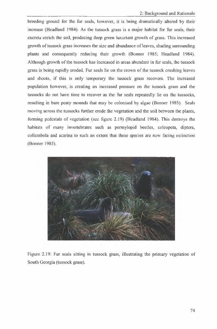
2: Background and Rationale
breeding ground for the fur seals, however, it is being dramatically altered by their
increase (Headland 1984). As the tussock grass is a major habitat for fur seals, their
excreta enrich the soil, producing deep green luxuriant growth of grass. This increased
growth of tussock grass increases the size and abundance of leaves, shading surrounding
plants and consequently reducing their growth (Bonner 1985; Headland 1984).
Although growth of the tussock has increased in areas abundant in fur seals, the tussock
grass is being rapidly eroded. Fur seals lie on the crown of the tussock crushing leaves
and shoots, i f this is only temporary the tussock grass recovers. The increased
population however, is creating an increased pressure on the tussock grass and the
tussocks do not have time to recover as the fur seals repeatedly lie on the tussocks,
resulting in bare peaty mounds that may be colonised by algae (Bonner 1985). Seals
moving across the tussocks further erode the vegetation and the soil between the plants,
forming pedestals of vegetation (see figure 2.19) (Headland 1984). This destroys the
habitats of many invertebrates such as permylopid beetles, coleopeta, diptera,
collembola and acarina to such an extent that these species are now facing extinction
(Bonner 1985).
Figure 2.19: Fur seals sitting in tussock grass, illustrating the primary vegetation of
South Georgia (tussock grass).
74

2: Background and Rationale
Figure 2.20: A fiir seal lying on a mound of tussock grass while feeding her pup. As the
population increases, the tussocks are occupied by fiir seals for longer periods, not
allowing the tussock grass to recover. Source: Bonner (1994:57)
As Croxall et al. (1990) document, other larger species are also threatened as a result of
the declining tussock grass. In the areas with most abundant seals, albatross breeding
has declined; this is thought to be because the fur seals have destroyed the albatross'
breeding habitat (tussock grass) depriving the birds of breeding and exposing them to
predation (Bonner 1985). Although there is no evidence that seals are adversely
affecting breeding success or survival, the proportion of birds being recruited into a
breeding population are avoiding areas where seals are abundant and breeding in areas
where fiir seals are absent. On Signy Island several giant petrel colonies have also been
abandoned due to fiir seal disturbance (Lewis-Smith 1990).
In several localities, extensive areas of moss carpet bog have been compacted and
recolonised by nitrophilous alga and in some areas this erosion has been so extensive
that all vegetation has been destroyed, leaving large areas of bare soil to be colonised by
Prasida crispa and other resilient algae (Headland 1984). This movement of seals and
the consequent destruction of vegetation have caused major peat and soil erosion as the
reduction in vegetation cover is exposing the soil, increasing the amount washed away
in surface run off. Removal of the soil in this marmer is also disrupting loosely attached
mosses and lichens. Such erosion is increased further in areas where seals occupy the
75

2: Background and Rationale
tussocks as the water table is at or near the surface, pools of stagnant water form
between the tussocks, further increasing the erosion of the tussock grass (see figure
2.21) (Lewis-Smith 1981).
Figure 2.21: Fur seals lying on tussock grass. As a result pools of mud have developed
among the tussocks and increasing erosion.
In addition to its erosion, the remaining soil is becoming more acidic and higher in
nitrogen levels as seal excrement alters the chemistry of the soil. Although this has
acted as a fertiliser, this has also had negative effects on the fresh water environments;
causing eutrophication, leading to the domination by few taxa and modifying the
microbiota of the freshwater system (Hawes 1990; Lewis- Smith 1990).
As the fur seal population increases, the population is expanding from its initial
breeding ground on Bird Island and the fur seals are migrating to the coastal areas on
the mainland of South Georgia. Although the greatest impact is on the passage of the fur
seals as they move from the sea to inland resting sites, population expansion means that
coastal regions are overpopulated, causing the fur seals to migrate further and further
inland, expanding the impact of fur seals. As a result of this, today slopes up to almost
200 metres altitiide are now being threatened (see figure 2.22) (Croxall and Prince 1979;
Bonner 1985; Lewis-Smith 1988). This is now causing extensive changes to terrestrial
and freshwater systems and in some areas damaging Antarctic Specially Protected
Areas (ASP As) as the composition of communities is being drastically altered (Hodgson
et al. 1998; Lewis-Smith 1990). It is estimated that fur seal induced changes on Signy
76

2: Background and Rationale
Island are the greatest and most rapid since the retreat of the Pleistocene ice sheet
(Lewis-Smith 1990).
Figure 2.22: Fur seals on the beaches of Maiviken. The vegetated slopes behind the
beach are now being eroded as the fur seal population increases.
2.8.1 Management of fiir seals on South Georgia
The sub Antarctic ecosystem is a fragile environment and recovery of this environment
is slow even to minor damage (Headland 1984). Destruction of the environment poses
important questions for conservationists and environmentalists (Lewis- Smith 1988).
Firstly should seals remain a specially protected species in accordance with Antarctic
Treaty Agreed Measures on the Conservation of Antarctic flora and fauna to permit
numbers to increase and establish a breeding population, while destroying unique
terrestrial and freshwater environments? Alternatively, should fur seal population
growth be restricted through reducing these measures whist protecting the environment
through a series of control measures? Fur seals were initially protected due to the near
extinction of the species as a consequence of the rapid human exploitation. As this
measure has been successfiil (perhaps too successfiil), should these protection measures
be lifted to allow the environment to recover and reduce the dominance of fur seals? For
example as Lewis-Smith (1988) outlines, on Bird Island, South Georgia enclosures have
been formed using electrified fencing to prevent the advancement of fur seals. This has
allowed substantial colonisation by green filamentous algae and encouraged the
regrowth of the eroded tussock grass. I f the fiir seal population continues to grow at the
77

2: Background and Rationale
same rate, it is possible this population's impact is likely to have a catastrophic and
irreversible affect on these systems.
The key to answering this dilemma, as Abbott and Benninghoff (1990) outline, is to
determine the range of natural variability in the Antarctic ecosystem and to distinguish
changes fi-om human perturbations. This can only be comprehended fi-om an
appreciation of the natural change in fur seal populations and its response to
environmental change (Ellis-Evans 1990). The increase may be a naturally occurring
fluctuation, cycle or unidirectional process, however, it may be a change in response to
artificial influences such as pollution or commercial harvesting (Croxall and Prince
1979). I f this increase in fur seals is a result of natural causes and a similar event has
happened previously, then it is likely that the fur seal populations wil l regulate naturally
and the system wil l recover and restore its equilibrium and management will not be
necessary. However, i f this is not the case and fur seal populations in the 20'*' century
exceed all historical populations, the likelihood that the equilibrium will be restored is
lower hence, necessitating management measures to prevent the loss of unique and
fragile environments.
As Croxall (1992) establishes, assessing the effects in relation to natural variability and
human induced changes is difficult for a number of reasons. Firstly, the fossil record is
limited, and gives few clues to the history of the species in relation to the varying
environments that have characterised the Antarctic. Secondly, all documented
population changes relate to human exploitation therefore, any influence of natural
causes and recovery of the ecosystem cannot be assessed. Thirdly, an important gap in
the knowledge is an understanding of how the physical environment influences the
distribution and abundance of prey, which in turn may affect the population (Croxall et
al. 1990). In addition to this, fUr seals have low reproductive and mortality rates, thus,
responses to such environmental change are slow and often hard to detect (Croxall
1992). Lastly, there are few detailed understandings of the mechanisms by which the
Southern Ocean top predator populations are regulated although some plausible
hypotheses are now emerging for a regulation by prey availability (Reid and Amould
1996, Boveng et al. 1998). As Croxall et al (2002) indicate, evidence is still limited and
these processes operating within system are only one part of the picture and other
processes triggered by mechanisms outside the system may be crucial to this
understanding.
78

2: Background and Rationale
2.9 Summary
This chapter outiines the background to the fiir seal population changes and the climate
changes through the Late Holocene. This background knowledge wil l then be applied to
the results that are presented in chapter 4. The next chapter will outline the methodology
for reconstructing the fiir seal population through the late Holocene.
79

3: Methodology
Chapter 3
Methodology
4 r
Plate 3: Fur seal hair after preparation.
80

3: Methodology
3: Methodology
The use of palaeohmnology to reconstruct fur seal populations is a relatively recent
development that has not been widely utilised and methodologies utilising this
technique are still developing. As stated in the objectives (chapter 1), this study uses the
methods outlined by Hodgson et al. (1998) to reconstruct the fur seal population from
hair abundance in sediment cores however, due to the nature of the sediment at this site,
I refined the methodology to suit the study site accordingly. Following this is
geochemical analysis which is based upon techniques employed by Sun et al. (2004a),
with alterations being made to suit the study site and the techniques available.
3.1 Sediment cores
The relative depths of the cores are shown in figure 3.1. HUM3 was extracted using a
Piston Corer to get the deeper sediment record, while MIAV/K was extracted using a
KuUenberg corer hence, ensuring the sediment water interface was intact. Cores were
transported stored in tightly sealed plastic tubing and kept cool for transportation to the
UK before being stored in a cold store.
3.1.1 Core depth and scaling
As figure 3.1 shows, the MAIV/K core extracted the top 90 cm of sediment. However,
during transportation and storage the core shrunk due to the large volume of water
present in the core during extraction. For this reason when the core was sub sampled in
the UK it was only 68 cm long. HUM3 core was taken 100cm below the surface of the
sediment to provide a deeper record and to continue the record taken from the MAIV/K
core. This core shrank by 10cm, as the volume of water in the core was not as great as
MAIV/K due to the depth of the core.
81

3: Methodology
S
i •d VI
U •B I u i3
100—
M t e l Sediment loss from shrinkage
Figure 3.1: Relative depths of the cores
The shrinkage of the cores left a gap of 32cm between cores. However, as the MAIV/K
core was extracted to a depth of 90cm, the actual amount of sediment not extracted is
only 10cm, (90-100cm below the surface of the sediment). As in both the cores, the
whole core shrank, it is unclear exactly where most of the shrinkage took place. In my
methodology I refer to samples, these are the sub samples of the core and the deepest
sub sample in the MAIV/K core is MATV/K 67-68cm. However, in the results section,
the depth of the total sediment extracted is referred to rather than the sub samples. As
MAIV/K core actually represents the top 90cm of the lake sediment, I have expanded
the depth scale to cover a total of 90cm (see equation 3.1) therefore, sub sample
MAIV/K 67-68cm represents a depth of 90cm in the lake.
82

3: Methodology
Depth in the whole core = Sub sample depth x (90/68)
Equation 3.1
Calculating the depth of the sub samples in the whole core. As 90cm is the depth within
the lake the core covers, however, 68cm is the actual length of sample left over after
shrinkage.
3.1.2 Sedimentological and Strati graphic core analysis
After extracting the core, prior to subsampling, the sedimentology of the core was
analysed using the Troels- Smith criteria. This provided a broad understanding of the
sedimentological changes within the core prior to analysis.
3.1.3 Subsampling
To provide a means of correlation, seal hair counts and geochemical analysis were
carried out at the same depths. Analysis was carried out at 8cm intervals throughout the
core and as time allowed this was increased to a 4cm resolution. A finer resolution of
2cm sampling was carried out at the top of the MATVI/K core to reconstruct the
population using the proxy technique to compare with historical far seal population
records. This was specifically so that I could compare the accuracy of the proxy
population to census data and hence, lead to more robust estimates of the actual
populations through the Holocene, when the census data was not available.
3.2 Fur seal hair abundance
Hodgson et al. (1998) outline a method to reconstruct fur seal populations using fur seal
hairs preserved in lake sediments. Fur seals have an abundance of insulating secondary
hairs, which are lost during moulting and deposited in terrestrial and aquatic
environments visited by the fiir seals hence, incorporated into the lake sediments. The
hairs remain well preserved in the lake sediments and as Hodgson and Johnston (1997)
establish, a variation in seal hair number in lake sediments can indicate fluctuations in
visiting seaLpopulations; with more abundant seal hairs reflecting a larger visiting seal
population (see figure 3.2).
83

3: Methodology
Fur seal hair abundance can used as proxy from which relative fur seal populations,
however, due to the complex differences in sediment input and output mechanisms
between lakes, this technique cannot be used to quantify the fiir seal population which
could be compared to other data sets, however, it does provide an indication of the
relative size of the fur seal population through time.
SOMB«tN>.SMth>In| 0 : M 4 M 600 I
0
IS
30
4S M
75
W
lOS
I " " I "35
" ISO
Its
I W
I M
210
22S
340
SOMB3Na.SMll (' • m M m M
" r w 73
90
IDS
m r I3S
ISO I ts
210 223 240
1 ;
I32S<AS«
1410 •^4S
l9»-f/-4S
J0HW-4S
^m^/-ss
No. Ai la iTik h r K i l kain f ' 0 200 400 6O0 100
• • i •
Whiliiit
9.0M(jii
• J 1 0
Seafagiallw S-Sbedndb.
1 3
• 1
1*73+/-4
r l»S7W-4
1961«-4
1951
19»«/-l
19114^10
lBSW-14
IU9 4/-2S
Figure 3.2: Fur seal hair abundance record from Signy Island. Source: Hodgson et al.
(1998).
Hodgson et a/'s (1998) method suggested taking a known dry weight of sample and wet
sieving the sediment through a 125|j,m sieve. Hair abundance was then expressed as
number of hairs per 1 gram of dry weight. A test of this methodology on several
samples at different intervals throughout the core did not prove successful for the
sediment from Maiviken for a number of reasons. Firstly, hairs were difficult to identify
and extract from the sediment due to the large amount of organic material, specifically
tussock grass fragments in the samples and secondly, a number of hairs were washed
through the sieve. Tests showed the proportion of hairs washed through was not
consistent throughout the core due to the different organic-minerogenic composition
throughout the core. To reduce this error, I tested a number of alternative techniques
before deciding upon a final methodology. To allow the hair abundance to be expressed
as number of hairs per 1 gram of dry weight, before any method was executed, samples
were freeze-dried. Samples were frozen at -80°C, for 48 hours before being placed in a
84

3: Methodology
fireeze drier with a vacuum of 1.030 for 16 hours. Samples were then weighed and
stored in a dessicator before being used.
3.3 Development and refinement of the Hodgson et al. (1998) technique
As the method outlined by Hodgson et al. (1998) was unsuitable for the sediment at
Maiviken, I adapted the technique to make the counting more accurate.
3.3.1 Final methodology
Before outlining the different methodologies I tested, below is a summary of the final
method used for fur seal hair extraction, refined from Hodgson etal. (1998):
1. Samples freeze dried and weighed. (Approximately 0.3-0.4 grams
(dry weight) of sediment).
2. Add 20ml of 20% hydrogen peroxide and put in a water bath for 2
hours.
3. Wash the residue back into the solution and add 45 ml of distilled
water and 5 ml of ethanol.
4. Centrifuge for 10 minutes at 4000 rpm, pour off excess water and add
more distilled water.
5. Sieve sample through 15)4,m, keeping the coarse material
6. Allow the sediment to settle and pour off the excess liquid.
Before finalising this methodology, I tried a number of different methods to separate the
hairs from the organic matter.
3.3.2 Physical separation
3.3.2.1 Sieving
Sieving the sediment through a variety of different sized sieves, larger than 125|j,m
(710|xm and 1mm), allowed the hairs to pass through the sieve hence, partly separating
the hairs from the coarser organic material. The hairs were found in both the coarse and
fine sediment and the percentage of organic material relative to the number of hairs was
not consistent in all samples. This was due to the differing sediment composition of
85

3: Methodology
samples throughout the core; in organic samples more hairs were present in the coarse
sample as the organic fi-agments trapped the hairs, hi a second test that aimed to remove
all the minerogenic matter, a finer sieve (63|im) was used however, the same problem
occurred.
3.3.2.2 Particle shape analysis
A particle shape analyser was used to see i f the hairs could be identified and counted,
therefore, reducing the problems in identifying and extracting the hairs and providing a
quick method for identifying the hairs, whilst guaranteeing that all hairs were accounted
for. However, this method proved problematic as the hairs were a similar shape to wood
and moss fibres making it difficult to distinguish between the two.
3.3.3 Chemical separation
3.3.3.1 Hydrogen peroxide (H2O2)
Hydrogen peroxide is routinely used in diatom and pollen preparation to reduce the
organic material in samples (Bimie 1990). hi this study H2O2 digestion was tested to see
i f it would separate hairs from organic (vegetation) matter. This allowed the hairs to be
more visible and reduced the problems of hair being incorporated in the organics. As
Marshall (1998) states, seal hair contains keratin, as does human hair therefore, to
ensure seal hair would not be desfroyed with the strength of the hydrogen peroxide used
in diatom and pollen preparation, different strengths were tested on human hair (see
table 3.1). The tests showed that H2O2, only affects the colour of the hair and does not
significantly affect the structure of the hair. It was inferred from this that fur seal hairs
would react in a similar manner and therefore, H2O2 was used on the sediment to reduce
the organic material in the sediment and hence, aid in identifying the hairs.
Samples from the core were placed in 20% hydrogen peroxide and left in a water bath
for 2 hours. A large amount of debris accumulated around the top of the sampling tube
and the amount varied depending upon the position in the core. Extracting some of the
material I identified fur seal hairs therefore, this residue was washed baek into the
sample. Distilled water was added and the sample was centrifiiged at 4000 rpm for 10
minutes. After checking there were only occasional very small fragments of hair in the
top of the sample, the excess water was poured off and the sample was examined.
86

3: Methodology
Additional distilled water was added to the sample to dilute the solution hence, allowing
the hairs to be more easily identified.
Time/ Concentration 20% 10% 5% 30 minutes The hair structure
appeared the same, however the colour was lighter.
Hair was not destroyed, it had just lightened, but not to the extent as 20% concentration.
As 10%, but remained darker.
1 hour Hair appeared lighter, however the structure was the same.
< Lightened.
2 hours As 1 hour but lighter.
< —^Lightened.
3 hours As 2 hours but lighter.
< Lightened
Table 3.1: Results of tests of varying H2O2 strengths on human hair
3.3.3.2 Fine Sieving
To reduce the H2O2 residue and allow the hairs to be more visible without increasing the
amount of water in each sample, the sample was sieved through a 15 [im sieve to see i f
the hairs would be retained and the cloudiness of the water reduced. Almost all the hairs
were trapped in the coarse material of the sieve. Occasional fine particles of hair were in
the fine section, however, these were all fragments of hair. As the organic material was
reduced fi-om the H2O2 the proportion of hair trapped in the sieve was the same
throughout the core hence, reducing the previous problems of differential effects
incurred during sieving. Sieving the sample also reduced its cloudiness making
identification of the hair easier. Although sieving the sediment diluted each sample
significantly, once the sample had been left to stand overnight, the hairs settled and the
excess solution was poured away.
3.3.4 Identifying hairs
Fiir seals have a dual layer of hair consisting of longer coarse guard hairs overlying a
layer of shorter, finer underhair (Bormer 1968) (see figure 3.3). Hodgson et al. (1998)
found that the hair incorporated into the sediment is primarily the underfur as it is in
greater abundance than guard hairs on the fiir seal (ratio of 40:1). Primary hairs are
87

3: Methodology
more likely to be transported through the lake without being incorporated into the
sediment therefore, the underfurs are more representative of the actual fur seal
population. Following the Hodgson et al. (1998) method, the finer underfur was counted
and coarser guard hairs were ignored. The hairs were identified using the taxonomically
distinct criteria listed in Scheffer (1964) and Bonner (1968). The criteria states the
underfur is approximately 15|i - 20|xm in diameter and reaches a maximum length of
2cm and individually the hairs are slightly waved (Scheffer 1964; Bonner 1968). The
guard hairs are significantiy longer (approximately 60nim) and coarser (125-150)xm in
diameter) and therefore, easily identified (see figure 3.3) (Bonner 1981).
Guard hairs
Undcrfur
Figure 3.3: Cross section of the fur layers of an Antarctic fur seal. Source: Bormer
(1994:23)
3.1.1 Counting
A black picking tray as used in foraminiferal analysis was used to count the hairs. This
allowed the hairs to be identified, as the H202-bleached hair was obvious against the
black background and grid squares on the tray allowed easy counting (see figures 3.4
and 3.5). A small brush was used to move the hairs around to aid counting and hairs
were identified using the criteria outlined above. Following Hodgson et al. (1998), all
counts were expressed relative to 1-gram dry weight of sediment; calculated using
equation 3.2.
88

3: Methodology
Normalised number of hairs = Total count x (1/dry weight)
Equation 3.2
Calculating the normalised number of hairs per Ig of dry weight from raw counts of a
known weight of sediment.
Figure 3.4: Fur seal hair after preparation, as seen under a low- power dissecting
microscope (magnification 4 times).
r
Figure 3.5: An individual fur seal hair separated from organic material, as seen under a
low power dissecting microscope (magnification 4 times)
89

3: Methodology
3.4 Geochemical analysis
Geochemistry has also been used to aid reconstructions of past fur seal populations (Sun
et al. 2004a). It is widely established that biological activity alters the chemistry of the
soil (Zale 1994a; Lewis- Smith 1988; Zale and Karlen 1989; Hawes 1990; Ellis- Evans
1990) and thereby provides an indication of species survival relative to time (Engstrom
and Wright 1984). Based on this theory. Sun et al. (2004a) correlate changes in fur seal
hair abundance with fluctuations in geochemistry to infer fur seal population
fluctuations at King George Island for the past 1500 years. To date this is the only study
to have used this as a means to reconstruct fiar seal populations, however, geochemistry
has been extensively used to reconstruct penguin populations and climate in the
Antarctic and Sub- Antarctic islands through the Holocene (Sun et al. 2004b; Sun et al.
2000; Zale 1994a, b; Zale and Karlen 1989).
3.4.1 Fur seal geochemistry
Sun et al. (2004a) used geochemical analysis to infer fiar seal population fluctuations
(see figure 3.6). They established that the organic matter in sediments at King George
Island was marine origin and likely to have originated from seal excrement.
Geochemical variations in sediments influenced by seal excrement are closely
associated with historical seal population changes, providing an indirect measure of
historical fiir seal populations. Reconstructions of penguin populations have correlated a
range of different elements with fur seal populations at different sites therefore, it
cannot be assumed that the elements which Sun et al. (2004a) used to reconstruct the fur
seal populations at King George Island wil l be the same at South Georgia. As Zhu et al.
(2005) indicate, the results from one study may be different to other similar studies due
to the site-specific nature of ecological and environmental factors.
90

3: Methodology
"C« l« t t»Ulho lo«y S « » l h « l r n u m b « r S ( ^ ) Stippm) F(ppm) LOI(%> TOC(%) TH(%) C o r r . " C « 9 « »
200 yr B.P,
500 yr B P.
750 yr B P.
1100 yrB.P.
— ,1400 yrB.P.
23S»7S-» _
I W»ck iwid with «*9l H»ir«[«r]»K* l i r* VMlh few h * l f » ^ D * « p 9*t mudiMh s w U b h » i r » ^ B t o c k mud w*h abuwJart h m
jCrey blac* mud enrtcned in orgai*: matter «Jh numeroia seal h a i r a ^ Black 3ilt «1th few seal haW, a rounded gravel coverii^ 15 to 16 cm
I Slack musi «Mh much «et^sort«d and rounded fine Kand, Micatlr^ marine »9<i«nentary emirwiment
Figure 3.6: Geochemical analyses used to reconstruct fiir seal populations (Sun et al.
2004a)
As Sun et al. (2004a) suggest, the primary factor influencing the geochemistry of the
sediment is the chemical composition of the seal excrement. This is enriched in Carbon
(C), Oxygen (O), Nifrogen (N) and contains traces of Calcium (Ca), Phosphorus (P),
Sulphur (S), Zinc (Zn) and Manganese (Mn) (Pomeroy, P., pers. comm.). The prime
factor controlling the chemical composition of the seal excrement is the chemical
signature of the prey, which is influenced by the Southern Ocean. As Schlesinger (1991)
indicates, the composition of the ocean (see table 3.2) is reflected in the composition of
phytoplankton. As krill feed off phytoplankton, the mineral content of krill is similar to
that of the ocean. These elements are transferred along the food chain to krill and
consequently to fur seals hence, it is likely that fluctuations in these elements will
reflect the fur seal population changes.
91
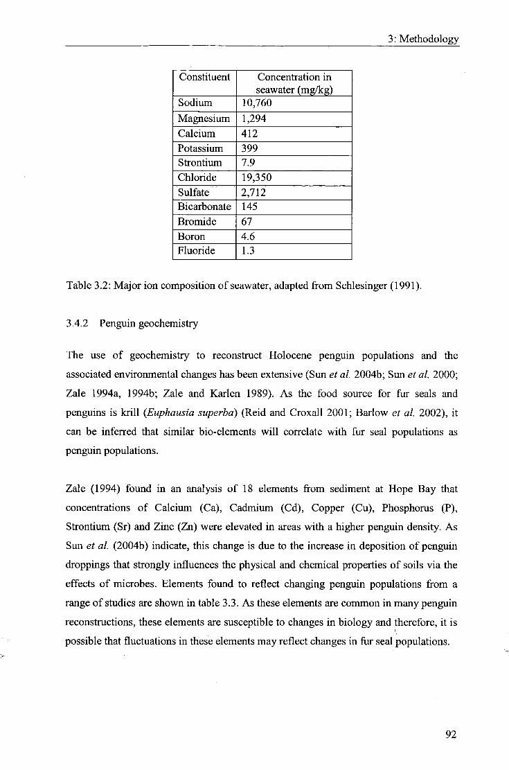
3: Methodology
Constituent Concentration in seawater (mg/kg)
Sodium 10,760 Magnesium 1,294 Calcium 412 Potassium 399 Strontium 7.9 Chloride 19,350 Sulfate 2,712 Bicarbonate 145 Bromide 67 Boron 4.6 Fluoride 1.3
Table 3.2: Major ion composition of seawater, adapted from Schlesinger (1991).
3.4.2 Penguin geochemistry
The use of geochemistry to reconstruct Holocene penguin populations and the
associated environmental changes has been extensive (Sun et al. 2004b; Sun et al. 2000;
Zale 1994a, 1994b; Zale and Karlen 1989). As the food source for fur seals and
penguins is krill {Euphausia superba) (Reid and Croxall 2001; Barlow et al. 2002), it
can be inferred that similar bio-elements wil l correlate with fur seal populations as
penguin populations.
Zale (1994) found in an analysis of 18 elements from sediment at Hope Bay that
concentrations of Calcium (Ca), Cadmium (Cd), Copper (Cu), Phosphorus (P),
Sfrontium (Sr) and Zinc (Zn) were elevated in areas with a higher penguin density. As
Sun et al. (2004b) indicate, this change is due to the increase in deposition of penguin
droppings that sfrongly influences the physical and chemical properties of soils via the
effects of microbes. Elements found to reflect changing penguin populations from a
range of studies are shown in table 3.3. As these elements are common in many penguin
reconstructions, these elements are susceptible to changes in biology and therefore, it is
possible that fluctuations in these elements may reflect changes in fur seal populations.
92

3: Methodology
Sun et al. (2004a) (Fur Seals)
Zale (1994): Hope Bay (Adelie Penguins)
Zhu et al. (2005): Barton Peninsula (Gentoo Penguins)
Sun et al. (2004b): Ardley Island (Penguin)
Sulphur (S) Calcium (Ca) Calcium (Ca) Calcium (Ca) Selenium (Se) Phosphorus (P) Phosphorus (P) Phosphorus (P) Fluorine (F) Copper (Cu) Copper (Cu) Copper (Cu) Total Nitrogen (TN) Zinc (Zn) Zinc (Zn) Zinc (Zn) Total Organic Carbon (TOC)
Sfrontium (Sr) Sfrontium (Sr) Sfrontium (Sr)
Cadmium (Cd) Sulphur (S) Sulphur (S) Selenium (Se) Selenium (Se) Fluorine (F) Fluorine (F) Barium (Ba)
Table 3.3: Element concentration increases that correlate with increases in penguin
populations compared to element concenfrations found to increase with fur seal
populations in Sun et al. (2004a).
3.4.3 Geochemical hypotheses
Due to time restrictions and the amount of sediment available, it was not possible to test
for all elements that may increase with fur seal population growth. To reduce the
number to evaluate, I used results from previous studies to hypothesize which elements
may be indicative of fur seal populations (see table 3.4).
Following Sim et al. (2004a), I tested for the following elements. Carbon, Nifrogen,
Sulphur and Selenium. Fluorine was not tested for due to restrictions on the instrument
and the limited sample size available. Analysis of the same elements as Sun et al.
(2004a) helps to determine whether these elements are indicative of fur seal populations
throughout the sub Antarctic and not restricted to King George Island. In addition to
these elements, I tested for elements that commonly correlate with penguin populations
(see table 3.4); Calcium, Copper, Zinc, Sfrontium and Cadmium. Although Phosphorous
concenfrations are a common penguin bio indicator, due to the amount of sample
available this could not be tested for. Based on the widely recognised hypothesis that
abundant ions in seawater will be passed along the food chain to fur seals, I also tested
for sodium.
93

3: Methodology
Element Method of analysis Reason for analysis
Carbon (TOC, Total organic
carbon)
Total carbon analyser,
elemental combustion system.
Sun et al. (2004)
Nitrogen (TN, total
nitrogen)
Elemental combustion system
(Costech instruments)
Sun et al. (2004)
Sulphur (S) Elemental combustion system
(Costech instruments)
Sun et al. (2004)
Selenium (Se) ICP- MS (Inductively
Coupled Plasma Mass
Spectrometer)
Sun et al. (2004)
Calcium (Ca) ICP- MS Zale (1994); Sunef al.
(2004b); Seawater
Copper (Cu) ICP- MS Zale (1994); Sun a/.
(2004b)
Zinc (Zn) ICP- MS Zale (1994); Sunet al.
(2004b)
Cadmium (Cd) ICP- MS Zale (1994)
Strontium (Sr) ICP- MS Zale (1994); Sxxnetal.
(2004b); seawater
Manganese (Mn) ICP- MS Pomeroy, P.,
(pers.com.)
Sodium (Na) ICP- MS Seawater
Table 3.4: Elements identified as possible bio indicators of fur seal presence.
Although it is possible that these elements may fluctuate with fur seal presence, there
are a number of additional factors that may cause concentrations to fluctuate and hence,
obscure the fur seal signature thus, the behaviour and environmental pathways of the
elements must first be considered.
3.4.3.1 Carbon
Carbon (CO2) is fundamental in photosynthesis and respiration hence, indicative of
organic productivity within a catchment (total organic carbon (TOC)). Carbonate rocks
are also a soxirce of Carbon therefore, concentrations may increase as weathering of
94

3: Methodology
carbonate catchments increases (total inorganic carbon (TIC)). Without determining the
difference between TOC and TIC, it is difficult to determine the source of Carbon in the
catchment. As Sun et al. (2004) highlight, TOC correlates significantiy with fur seal
hair abundance and is hence, a bio indicator of fur seal presence.
3.4.3.2 Nifrogen
As Nitrogen is an essential constituent of all organisms and represents a key nutrient, it
is expected that the concentration of Nitrogen in fur seals would be significant enough
to influence the geochemistry of the catchment (Talbot 2001). In studies of moss
communities in the Antarctic, the primary source of Nifrogen has been found to be
penguin and seal activity, suggesting that biology influences Nitrogen concentrations.
Studies of penguin populations have indicated that Nitrogen concentrations are closely
correlated with penguin populations and Nitrogen has been used as a proxy for penguin
populations (Zhu et al. 2005; Christie 1987).
3.4.3.3 Sulphur
Sun et al's (2004) study of King George Island suggests a close correlation between
Sulphur and fiir seal hair abundance. As Holmer and Storkholm (2001) indicate,
deposition of Sulphur increases in eufrophic lakes. As eufrophication is a consequence
of an increasing fur seal population, it is likely that the concentration of Sulphur
associated with the eutrophication wil l indirectiy reflect fur seal populations (Lewis-
Smith 1988).
3.4.3.4 Selenium
As Ugolini (1972) indicates, the bioavailability of Selenium in animals is determined by
other factors such as pH, redox conditions, soil texture, mineralogy and organic matter
content. As there are so many influential factors affecting the concentration of
Selenium, it is difficult to distinguish the fur seal component. However, as Selenium is
one of the elements Sun et al. (2004) found to correlate with fur seal hair abundance, it
may be a useful bio indicator of fur seal presence at South Georgia.
3.4.3.5 Zinc
As Andrews et al. (1996) establish. Zinc has a clear biological function and evidence
from previous studies suggests Zinc is highly enriched and significantly correlated to
95

3: Methodology
other biogeochemical markers (Sulphur, Calcium, Copper, Selenium, Strontium,
Barium and Flourine). As a result. Zinc has been used as a proxy for fluctuations in
penguin populations (see Sun et al 2004b; Zhu et al. 2005 and Zale 1994).
3.4.3.6 Copper
In previous biogeochemical studies. Copper has been used as an indicator for penguin
activity and is commonly correlated with Zinc and to a lesser extent Selenium (Zhu et
al 2005). Schlesinger (1991) highlight this link between Copper biological activity is
due to high concentration in phytoplankton. Copper is incorporated into sediments as
the organisms die and sink to deeper waters. Yet as Matsumoto (1993) indicates, a
major source of copper within sediments is also chemical weathering. This double usage
poses problems for interpretation however, the association of Copper with Zinc in past
analyses of bio indicators suggests that Copper concentrations are dominantly
influenced by bioactivity (Zale 1994; Zhu et al. 2005).
3.4.3.7 Sfrontium
Reimann and de Caritat (1998) indicate that the environmental paths for Strontium are
sea spray, weathering and the dissolution of calcium carbonate, suggesting very little
organic influence (AboUino et al. 2004). This implies that Strontium is more indicative
of environmental change rather than a change in organic matter. Nonetheless, Zale
(1994) and Zhu et al. (2005) suggest that Sfrontium is a bio indicator for penguins. As
penguins have a similar diet to fur seals, it would be expected that similar elements
would be present in fur seal excrement as penguin guano. Sun et al. (2004b) also came
to this conclusion as the concentration of Sfrontium in the lake sediments within close
proximity to penguin populations is elevated compared to other lake sediments in the
maritime Antarctic.
3.4.3.8 Cadmium
Research suggests that Cadmium is closely associated with Zinc however, it does not
have a biological role (Reimann and de Caritat 1998). Cadmium displays nutrient like
behaviour as it is inadvertently taken up during biological processes (Andrews et al.
1996). Due to these properties, it is likely that Cadmium is a good indicator of
biological processes. Although in previous studies. Cadmium is not commonly
96

3: Methodology
recognised commonly as a bio indicator, Zale (1994) establishes a correlation between
Cadmium and penguin activity.
3.4.3.9 Sodium
As Schlesinger (1991) highlights, Sodium is very abundant in seawater, with
concentrations reaching 10, 760 parts per million (ppm) (see table 3.2). As for seals
spend the majority of their life in the ocean, the movement of the seals onto land is
likely to increase the amount of seawater on land and hence, increase Sodium
concentrations. However, as Reimaim and de Caritat (1998) indicate, there are a number
of potential pathways for Sodium. Firstly sodium concentrations are likely to increase in
the catchment i f sea level rises and the catchment becomes submerged. Secondly, i f sea
spray increases reflecting a climatic change in wind direction and/ or strength this will
increase the concentration of Sodium in the catchment. Thirdly, Sodium is abundant in
allogenic elastics eroded from catchments therefore; it is a usefol element to assess
weathering, soil development and erosion in a catchment (Last and Smol 2001). As
Engstrom and Wright (1984) suggest, values are higher in late glacial sediments
compared to those in postglacial sediments, therefore, providing a usefol indicator of
deglaciation. As there are a number of potential sources of Sodium and concentrations
vary with a variety of processes, concentrations must be analysed in association with
other elements, to reduce the potential error in interpretation.
3.4.3.10 Calcium
A number of geochemical sfodies used to reconstruct past penguin populations have
found Calcium to be highly correlated with penguin populations (Zale 1994). However,
Ugolini (1972) suggest that Calcium concentrations are relatively low in guano layers
and therefore, perhaps not indicative of penguin or other bioactivity. Further sfodies
suggest that Calcium is a common element that occurs in most lake sediments and
ground water hence, intimately linked to the carbon and nitrogen cycles (Ito 2001). As
Engstrom and Wright (1984) highlight, the primary source of Calcium in lake sediments
are allogenic elastics eroded from catchment soils and rocks. The ratio of Na:(Na+Cl)
can be used to discriminate between rain and weathering sources and hence, an indicator
of weathering processes in the catchment (Andrews et al. 1996). As Calcium could
potentially be related to for seal activity, it is necessary to distinguish the influence of
97

3: Methodology
Calcium from other sources in the catchment before evaluating the impact fur seals have
upon the concentration.
3.4.3.11 Manganese
Studies suggest that Manganese concenfrations are elevated in fiar seal excrement and
therefore, it can be inferred that concentrations would increase with fiir seal presence
(Pomeroy, P. pers. com.). Chemical weathering is also a major source of Manganese,
hence, to distinguish whether Manganese concentrations are indicative of fur seal
presence or weathering, concentrations must correlate with fur seal hair abundance and
other bio elements, thus. Manganese cannot be used solely as a proxy for fur seal
populations (Reimann and de Caritat 1998; Matsumoto 1993).
3.4.4 ICP-MS hypotheses
Although the elements outlined in table 3.4 are the primary elements I tested for, the
ICP-MS used to test for the majority of the metals outlined above, it also provides
concentrations for a total of 29 metals from the same sample (see table 3.5). As a
consequence of this, all these elements have been analysed to firstly assess the
applicability as an indicator of fur seal presence and secondly to provide an indication
of any environmental changes at the study site.
98

3: Methodology
Analyte Symbol Mass Lithium Li 7 Beryllium Be 9 Boron B 11 Sodium* Na 23 Aluminium A l 27 Potassium K 39 Calcium* Ca 44 Titanium Ti J 48 Vanadium V 51 Chromium Cr 52 Iron Fe 54 Manganese* Mn 55 Iron Fe 57 Nickel Ni 58 Cobalt Co 59 Copper* Cu 63 Zinc* Zn 64 Arsenic As 75 Selenium* Se 82 Strontium* Sr 88 Molybdenum Mo 98 Silver Ag 107 Cadmium* Cd 114 Antimony Sb 121 Barium Ba 138 Thallium Tl 205 Lead Pb 206 Lead Pb 207 Lead Pb 208 Bismuth Bi 209
Table 3.5: Elements concentrations available from the ICP-MS (* (and bold) indicates
the elements hypothesized as indicators of fur seal presence).
Although these elements may not reflect fur seal presence, they provide an indication of
the catchment conditions through the core relative to the fur seal population, hence,
allowing the correlation between fur seal populations and changing environmental
conditions to be determined.
3.4.4.1 Aluminium
Aluminium is generally associated with an increase in groundwater influx (Abollino et
al. 2004). I f the pH in the catchment is low or high, Aluminiimi is more soluble and
99

3: Methodology
hence, concentrations increase (Itkonen et al. 1999; Andrews et al. 1996). This
alteration of pH may be associated with an increase in fur seal activity and hence, ftir
seal presence may indirectly affect the concentrations.
3.4.4.2 Potassium
An enrichment of Potassium can be a result of a number of factors including
atmospheric salts, glacial and snow melt waters, rock weathering and groundwater. As
these elements are all non- organic elements, it is unlikely that fluctuations in Potassium
wil l reflect fur seal presence in the catchment (Matsumoto 1993; Abollino et al. 2004).
3.4.4.3 Titanium
Very little is known about Titanium in lake sediments, and there are no studies to
suggest that Titanium would increase with fiir seal abundance. Titanium is very
abundant in the earths crust and geogenic dust is the main source of Titanium in the
environment, suggesting that it is not indicative of fur seal presence (Marshall and
Fairbridge 1999).
3.4.4.4 Barium
In terms of the overall geochemical cycle Barium most closely follows Strontium and
Calcium (Marshall and Fairbridge 1999). Using this theory, as Strontium has correlated
previously with fur seal abundance, it can be inferred that Ba has the potential to. There
is however, debate to the conditions causing an increase in Barium. As Marshall and
Fairbridge (1999) indicate. Barium rich areas commonly underlie zones of intense
biological activity and occur near ocean ridges. Studies of Antarctic lakes however,
suggest an increase with calcite and fluorite, implying a strong correlation with
Aluminium, Chromium, Calcium and Silicon, elements not previously found to be bio
indicators.
3.4.4.5 Iron, Lithium, Vanadium and Chromium
These elements are considered essential for biology, therefore, it is possible that these
elements may correlate with fur seal abundance, yet neither has previously been linked
to biological activity (Reimann and de Caritat 1998). Vanadium is a minor element in
lake sediments and very little work has been done on the mechanisms causing it to
100

3: Methodology
fluctuate however, the main environmental pathways for Vanadium are weathering and
geogenic dust hence, it is unlikely that concentrations wil l reflect fiir seal presence
(Reimann and Caritat 1998). The main environmental pathway for Iron is rock
weathering, therefore. Iron is likely to be more indicative of the weathering in the
catchment rather than fur seal presence (Reimann and de Caritat 1998) Although
Chromium is an essential nutrient at low concenfrations and it can potentially
accumulate in aquatic life (Reimann and de Caritat 1998), previous studies of penguin
bio elements have not found Chromium to fluctuate with the changes in biology (Zale
1994;Zhuefa/. 2005).
3.4.4.6 Molybdenum
There is debate as to how Molybdenum concenfrations fluctuate in lake sediments.
Firsfly Molybdenum is considered essential for biology but it is also a conservative
element that has little interaction with biological cycles and hence, is unlikely to
fluctuate significantly with fur seal population changes (Andrews et al. 1996).
Secondly, as Abollino et al. (2004) indicate, Molybdenum concentrations increase with
sea spray and the presence of rocks hence, reflecting an increase in weathering or
change in climate. As Molybdenum fluctuates variety of processes, it cannot be used
solely to determine fur seal population fluctuations.
3.4.4.7 Thallium
Although Thallium is considered non-essential for biology, it does have a sfrong
tendency to accumulate in aquatic life therefore, it is possible that Thallium accumulates
in krill and hence fur seals (Reimann and de Caritat 1998). However, Reimann and de
Caritat (1998) also highlight that Thallium is easily released during weathering hence,
this double source makes interpretation difficult.
3.4.4.8 Other elements
The other elements are rare elements and previous geochemical studies using
geochemistry as a proxy for past penguin and seal populations do not consider these
elements, thus, there is very little literature on how these elements may fluctuate in lake
sediments.
101

3: Methodology
3.4.5 Geochemical summary
Table 3.6 summarises the elements to be tested, the primary hypotheses for these
elements and the method of analysis.
Element Method of analysis
Hypothesis Previous Studies
Carbon (TOC; TC)
Elemental combustion system. Total c£u-bon analyser
Fundamental in respiration Sun et al. (2004a)
Nitrogen Elemental combustion system
Essential to organisms Sun et al. (2004a)
Sulphur Elemental combustion system
Increase in eutrophic lakes Sun et al. (2004a,b); Zhu et al. (2005)
Selenium ICP- MS Previous studies suggest a correlation with fur seal abundance.
Sun et al. (2004a,b); Zhu et al. (2005)
Calcium ICP- MS Seawater Zale(1994); Sun et al (2004b); Zhu et al. (2005)
Copper ICP- MS Required by phytoplankton Chemical weathering
Zale (1994); Sun et al. (2004a,b); Zhu et al. (2005)
Zinc ICP- MS Strong biological function Zale (1994); Sun et al. (2004b); Zhu et al. (2005)
Cadmium ICP- MS Nutrient like behaviour Zale (1994) Strontium ICP- MS Sea spray Zale (1994); Sun
et al. (2004b); Zhu et al (2005)
Manganese ICP- MS Pomeroy, P. (pers.com.) Sodium ICP- MS Seawater Lithium ICP- MS Essential for biology Beryllium ICP- MS Unknown Boron ICP- MS Unknown Aluminium ICP- MS Increased with groundwater Potassium ICP- MS Enriched in groundwater Titanium ICP- MS Abundant in earths crust Vanadixam ICP- MS Essential for biology Chromium ICP- MS Essential for biology Iron ICP- MS Essential for biology
Weathering is a primary environmental pathway
Nickel ICP- MS Unknown Cobalt ICP- MS Unknown Arsenic ICP- MS Unknown
102

3: Methodology
Molybdenum ICP- MS Essential for biology Silver ICP- MS Unknown Antimony ICP- MS Unknown Barium ICP- MS Follows Sr Zhu et al. (2005) Thallium ICP- MS Accumulate in aquatic life Lead ICP- MS Unknown Bismuth ICP- MS Unknown
Table 3.6: A summary of the elements tested for, the method used in analysis, possible
causes fluctuations and the use of the element in previous studies of bio indicators in the
sub Antarctic region.
3.4.6 Methodology
To prepare the samples for analysis, all samples were freeze-dried. Samples were frozen
at -80°C for 48 hours before being placed in a freeze drier with a vacuum of 1.030 mbar
for 16 hours. The samples were then ground in a ball mill at 600 rpm for 5 minutes and
stored in a dessicator before use. Table 3.6 summarises elements tested and the method
of analysis.
3.4.6.1 Elemental Combustion System
The Elemental Combustion System uses a chromatography method to test for Carbon,
Nifrogen and Sulphur. Approximately lOmg of sample was weighed out to two decimal
places. The sample was placed in a foil capsule and sealed before being combusted in
the Elemental Combustion System (Costech) for 15 minutes. A l l samples in one run
were prepared on the day the machine was run and placed in the carousel before starting
any analysis to ensure atmospheric gases would not contaminate the results. When the
element is combusted, different elements are released as gases at different times;
therefore, the concentration of these elements can be calculated (see Lewis 1997 for
further details). To ensure the calibration of the machine was correct, standards were
run at the start, end and after every 20 samples in each run.
3.4.6.2 Inductively Coupled Plasma Mass Spectrometer (ICP-MS)
Element concentrations in samples were measured using an Elan DRC, Inductively
Coupled Plasma Mass Spectrometer (IPC-MS). This technique allows a large number of
elements in a small sample size to be detected with relatively low detection limits
(Jarvis 1997). Samples were firstly freeze-dried and ball milled using the procedure
103

3: Methodology
outlined above. The samples were then digested using the EPA 3051 method before
being placed in the ICP-MS.
3.4.6.2.1 EPA 3051 Method
Approximately 250mg of dry sample was weighed out for digestion into a fluorocarbon
sample vessel. The amount of sample used varied depending upon the amount of sample
available after the other tests had been carried out therefore, in some cases only 50mg of
sample was used. To each sample 2ml of hydrogen peroxide (H2O2) was added and left
until the reactfion was finished. As the samples were particularly organic, an additional
2ml of H2O2 was added. Once the reaction stopped, 2ml of hydrochloric acid (HCL) and
9ml of nitric acid (HNO3) were added. The cap of the sample vessel was put on straight
away as there were no carbonates in the samples.
Once the reaction stopped, samples were put in a microwave (CEM MARSSX) for 10
minutes. The sample was then filtered through qualitative filter paper using dilute nitric
acid (10% v/v). After filtering, the sample was diluted 1000 times before being run
through the ICP-MS (see Jarvis 1997 for forther information). For detection of certain
elements, ammonia was used as a reaction gas. After every 20 samples, a standard was
put through the machine to ensure the calibration was correct.
3.4.6.3 Total Organic Carbon (TOC)
From the results of the elemental combustion system, the amount of total carbon (TC) in
each sample was known. To calculate the total organic carbon (TOC) content in the
sample, the amount of total inorganic carbon (TIC) was calculated and subfracted from
the total carbon (TC) concenfrations, calculated using the Elemental Combustion
System as outlined above. Although TOC could be calculated independently the TIC
method was not as time consuming and gave the same result.
Due to the limited sample sizes, there was not enough sample to test every sample for
TIC therefore, 6 samples were selected from the core based upon the TC results (e.g. a
sample from a section of high TC, low TC and average TC, ensming they were all
evenly spaced through the core). These samples were then freeze-dried and ball milled
as outlined in section 3.4.4. Between 10 and 15mg of each sample was weighed out into
a small glass capsule before being placed in the Total Carbon Analyser (TOC 1200).
104

3: Methodology
Each sample was left to react for a minimum of 240 seconds or until the reaction
stopped, hiitial tests of 2 samples (MAIV/K 50-51 and HIJM3 179-179.5) suggested
that the concenfration was very low and therefore, all the samples were run on the low
bench section of the machine, as detection limits were Ippm. Before any samples were
run a standard of NaCOs: NaHCOa (2.2061:1.748) with concentrations of lOOppm,
50ppm and lOppm was run to provide a calibration for the samples.
3.4.6.4 Summary
Using the multiproxy approach of fur seal hair abundance and geochemistry improves
the robustness of the results, reduces error and reduces the influence of local factors on
each proxy, hence, prevents the assumption that correlation is equal to causation. For
example, as Engstrom and Wright (1984) outiine, geochemical analyses can provide
evidence for climate change therefore, the geochemical record produced from my
results may be reflecting climate change or change in penguin populations rather than a
change in fur seal population. However, correlating the geochemical changes with the
fur seal hair abundance wil l provide more robust evidence for fur seal populations. This
will help to determine which chemicals reflect a change in fur seal populations and the
chemicals which can be used as a proxy in further research without using the time
consuming method of calculating the hair abundance.
3.5 Dating
To fulf i l objective 3 (To determine whether the recent (20* -21^* century) increases in
fur seals have exceeded the range of natural variability of past populations), the section
of the core that represents this time period must be found and therefore, it is necessary
that the core is dated. Further dating was also necessary to f i i l f i l objective 5 (To
determine the factors confroUing fur seal population changes at South Georgia through
the late Holocene), so the fur seal and geochemical data can be correlated with the
climate data outiined in section 2.3 and hence, allowing the factors controlling fur seal
population changes to be determined.
105

3: Methodology
3.5.1 Principles of radiocarbon dating
Radiocarbon dating is a widely used technique for accurately calculating ages up to
45,000 years BP; therefore, this technique is applicable for dating the majority of the
core. Radiocarbon dating is only accurate to at least 50 years and often error is greater
therefore, due to the dynamic changes in the 20* Century, it was necessary to use an
alternative technique for the upper part of the core hence, ^"'Pb and ' ^Cs dating
methods were used on the top section of the core.
3.5.1.1 Radiocarbon dating methodology
Three samples in the core were dated. Firstly the base of HUM3 (189-189.5 cm) was
dated to determine the time span of the whole core. This sample was sent to NERC
radiocarbon laboratories for AMS dating. The sample was firstly digested in 2M HCL at
80°C for 8 hours before being washed free from mineral acid with deionised water. The
sample was then dried under a vacuum (200 mbar) at 40°C for 16 hours before being
homogenised.
From the results of the fiir seal hair abundance and geochemical data, two additional
samples at points of significant change were selected for radiocarbon dating and sent to
BETA Analytic for AMS dating. These samples were sieved through an 180^m sieve.
The bulk sediment sample fraction greater than 180 fxm, composed of woody/plant
remains was freated as the woody/plant remains were not considered intrusive.
Following sieving, the sample was dispersed in deionised water, then washed in hot HCl
acid to eliminate carbonates and NaOH to remove secondary organic acids. This was
followed by an additional alkali wash to neutralise the solution prior to drying.
3.5.2 ^'°Pb and '"Cs dating
The sealing industry began at South Georgia in the late 18'** century and it was from this
time that rapid changes in the fur seal population took place. Determining the exact
timing of this change within the core will allow the magnitude of this fluctuation to be
compared to previous population changes and therefore, determine whether an event
such as this as happened previously. Radiocarbon dates in the 20* century can be
problematic due to the reworking of sediments, precision issues and the carbon 'bomb'
106

3: Methodology
effect during this time hence, it is widely recognised that radiocarbon dates during the
20* century are not accurate enough to provide robust dates. To provide a more accxarate
indication of the dates at the top of the core, ^ '^b and ' ^Cs dating techniques were
used.
3.5.2.1 Principles of '"Pb dating
Pb dating has been widely used to date very recent sediment sequences spanning the
past 100 to 200 years and is increasingly the backbone upon which recent sedimentation
time-scales depend upon (Walker 2005; Appleby and Oldfield 1982). The principle of
the dating method is based on the escape of radon gas from the earth into the
atmosphere and into sediments (Walker 2005). As the radon gas is an unstable isotope
^^^Rn, with a half-life of 3.8 days, it rapidly decays. This rapid decay produces a number
of daughter isotopes that decay with very short half-lives until the isotope ^'°Pb is
reached (see figure 3.7) (Olsson 1986). Measuring the ratio of ^'°Pb: '' Pb in sediments
allows the time period since the lead was deposited to be determined and hence, the rate
of accumulation can be established (Walker 2005).
238u ^ 226^^ ^ 2 2 2 ^ ^ 210p^ ^ 206p^ 4.51x10' 1602 yre 3.82 22.26
yrs days yrs
Figure 3.7: ^^*U decay series to form the daughter isotope ^'''Pb. Time beneath the
arrows indicates the half-life of each element.
Problems arise with the method as ^'°Pb accumulates in the sediments through two
different mechanisms. Firstly, ^"'Pb enters the catchment from the in wash of ^^Rn into
the lake or sediments. This is consequently incorporated into the sediment and decays to
form ^'°Pb. This is termed supported ^'°Pb. Secondly, ^'"Pb, accumulates as a result of
^^^Rn decaying prior to sediment incorporation and hence, ^'°Pb itself is washed into the
catchment. This is termed unsupported ^'°Pb (Appleby and Oldfield 1982). In dating, it
is the unsupported ^'°Pb that is used to calculate the age of the sediments as once
incorporated into the sediment it decays exponentially with time (Oldfield and Appleby
1978). The supported ^ ' ^b is calculated by the assay of the ' Ra in the sediment, arid
therefore, this provides an estimate of the amount of ^ ^Ra washed into the lake/
sediment that has not yet decayed into ^'°Pb. Subtracting the supported ^'''Pb from the
107

3: Methodology
total ^'°Pb provides the unsupported ^'°Pb used in dating the sediment (Oldfield and
Appleby 1978).
3.5.2.2 Principles o f ' "Cs dating
The concentration of ' ^Cs in lake sediments is widely used as a distinctive time-
sfratigraphic marker horizon in sediment sequences (Walker 2005). ' ^Cs concentrations
increased from the fall out of testing atomic weapons after the Second World War. This
caused a peak of '"Cs in the records in 1963 (Batterbee 1991; Olsson 1986). This
known peak in the record can be used to supplement ^'°Pb dating, providing a check for
the ^'°Pb timescale (Walker 2005).
3.5.2.3 Methodology for ^'°Pb and ' ^Cs dating
Al l samples were frozen at -80°C for 48 hours before being placed in a freeze drier with
a vacuum of 1.030 for 16 hours. The samples were then ground in a ball mill at 600 rpm
for 5 minutes and stored in a dessicator before use. Approximately 0.35 mg of sediment
was weighed into small plastic fobes before being placed in an Ortec Gamma Well
Detector (GWL series. High purity germanium, coaxial well photon detector system) for
two days. After two days, the sample was removed and the ' ^Cs and ^"^b counts were
recorded.
3.6 Sources and magnifode of error
Although the methodology outlined above attempts to minimise the error in the data, it
is not possible to folly eliminate error hence, this must highlighted and considered in
analysis.
3.6.1 Seal hair abundance
Hairs were treated to improve the ease of counting however, it is possible that some
hairs may have been lost in this process through fransferring sediment bet\veen different
vessels. As all samples were treated in the same way, this error should be systematic
through the core and hence, not affect relative abundance.
108

3: Methodology
To express the hairs per 1 g of dry weight (following Hodgson et al. 1998 method),
approximately O.lg of sediment was weighed and freated before counting. However,
multiplying the counts by a factor of 10 also increases the error by a factor of 10. To
determine the effect this error would have upon the samples, different weights of sample
(0.1, 0.2 and 0.3 g) were prepared for 2 samples through the core and counted to
evaluate the error in the scaling up process. Results suggested that the initial weight did
not alter the overall count therefore, due to the limited amount of sediment available,
O.lg of sediment was used and scaled up.
To ensure that the number of hairs counted was accurate, some samples were counted
twice to determine the counting error. Al l the samples tested showed significant
reduction in the amount of hairs when counted as second time. To ensure this error was
not specific to some samples, all samples were pounted a second time. The difference
between the two samples at all intervals throughout the core was both large and
systematic and so cast doubt on the results. To reduce any uncertainty, all the samples
were recounted a third time. The third counts were very similar to the second counts
(see appendix 1). As the first counts were a magnitude higher than the following counts,
I omitted the first counts in the results, and took an average of the second and third
counts. The anomalous first counts are thought to be a result of adapting the technique
and an incorrect identification of hairs and mistaking organic material for hairs. The
standard deviations of the second and third counts for each sample were calculated and
an average of all the standard deviations was used to calculate the average error of the
whole data set (see appendix 1).
3.6.2 Geochemistry
3.6.2.1 Elemental combustion system (Nifrogen, Carbon and Sulphur)
Each sample was tested twice and the average of the two values was taken. This ensured
that in the machine or the effect of contamination would be eliminated. For any sample
where the two values in the same run had a difference greater than 1%, the sample was
run again, imtil this error was reduced (see appendix 2). As samples were weighed to 2
decimal places, the results are expressed to 2 decimal places.
109

3: Methodology
3.6.2.2 ICP-MS
After every 20 samples, a standard was run to ensure the calibration was still correct.
The calibration of Ag was not reliable and therefore, the results of the Ag
concentrations will not be considered. As Ag has not been found previously as a bio
indicator, it was not time-efficient to run the samples again to obtain concentrations for
Ag.
3.7 Summary
This chapter has outlined the development of the methodology used to calculate fur seal
hair abundance and a methodology to determine the concentrations of elements that are
possible indicators of fur seal presence. The following chapter wil l outline the results
obtained from this methodology.
110
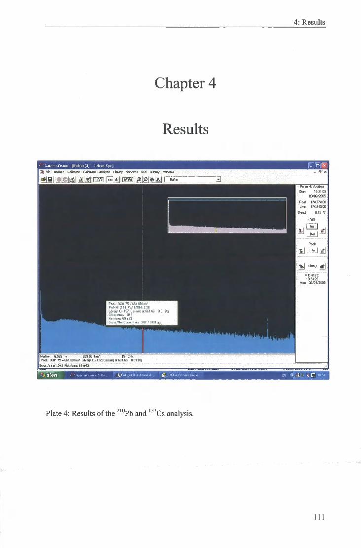
4: Results
Chapter 4
Results
' UammaVision [Ouffef(J) 3 4cni.5pcJ
Fh Acqi*> CaKlrate CaktJats Analyze Ltirary S«vlc« ROI Display Window
©N mm rm F - o m i nss Pulse Hi. A n 4 «
Sleit 16:21:03 D3/08j'2005
R e * 174,774.00 Live: 174,44aOO
Deed 0.19 «
®OBTEC 10:5423
Mon 05 /09 /2005
* : 6601.75 . 661.80keV FWHM: 2.14 FV/I1/51M: 2 Uxny. Cs-137 (Ceskm) el 681 66 ; 001 Bq Gto>!Aiea:1043 Ue) Area: 69133
s/Net Count Rale, aoi / ODO cps
Maiker 6,583 • 659.93 keV 15 Cnll Peek6E01.7S.681.80luM Lba)>:C>'137|Ce3un|etGE1 68; 001E OSS Area; 1043 Net Area: 69 « 3
1 start .iirimaVtitMi - (Biife.. FuHSM 8.0 Standard... ^ Fu •Shot 8 User's Gmde EN 1:54
Plate 4: Results of the ^"^b and ' ^Cs analysis.
I l l

4: Results
4: Results
This chapter outiines my results on which my analysis in chapter 5 is based upon.
Firstly I wil l consider factors to account for when analysing the results. This wil l be
followed by a stratigraphic and sedimentological description of the core followed by the
resuhs of the fur seal hair abundance and the geochemical analysis before the results
from the radiocarbon dating and ^'°Pb and ' ^Cs dating are addressed. Finally I consider
how the dating results can be applied to form an age model.
4.1 Core Stratigraphy
As there are two separate cores used in the study, these were analysed individually prior
to any analysis to provide a broad indication of the sedmentological changes prior to
analysis.
4.1.1 HUM3
At the base of the core, the sediment is light grey, unsaturated material. This clay is
present for 2cm, before a clean fransition to darker sediment. Using Troels- Smith
(1955) analysis, this 2cm thick basal unit can be classified as Argilla Steatodes (As).
Above the clay, the sediment is very dark, inelastic and horizontal bedding planes are
visible. In this sediment, there are fragments of primarily herbaceous material, although
there are also some small fragments of wood. The sediment is almost homogenous
throughout the core, gradually becoming darker and increasingly saturated. Throughout
the core organic fragments upto 2cm in length are visible. Very small elastics are also
noticeable giving some sub samples a grittier texture. Al l the sediment in this section of
the core can be described as Detritus Lignosis (Dl) (ibid). As noted in chapter 2, there
is the potential that the lake was previously marine due to isostatic changes following
the LGM. However, sedimentological analysis indicates there is no evidence of marine
sediments in the core hence, implying that the lake has been freshwater for at least the
past 3500 "*C yrs BP.
112

4: Results
4.1.2 M A I V n C
The sediment in the core when extracted was very satvirated and homogenous, hence, a
detailed Troels - Smith analysis was not undertaken. There were no clear stratifications
or changes in the sediment composition. The entire core was classified as Detritus
Lignosis (DL) , nigror degree 4, stratification 0, siccitas 1 and elasticitas 2.
4.1.3 Implications for analysis
As no palaeocological analysis was done on the primary transition at the base o f the
core the cause o f this change in sedimentation is unknown. However, this
sedimentological change w i l l be considered in analysis and related to the age model to
allow this transition to be analysed with proxy environmental changes and therefore,
allowing potential causes o f this change to be inferred.
4.2 Depth Scale
In this section, depths are expressed relative to the whole core as I have outlined in
section 3.1.1 (equation 3.1).
4.3 Fur seal hair abundance
Figure 4.1 shows the f i i r seal hair coimts relative to depth. A t the base o f the core the
hairs are in low abundance, fluctuating between 250 hairs to 700 hairs per 1 g o f dry
weight, but remaining relatively constant in comparison to the remainder o f the core.
The hairs remain at this level to a depth o f 243 cm, when hair abundance begins to
increase gradually fi"om 221 hairs to 2464 hairs at 191 cm. Following this increase, the
hairs remain at a relatively constant level to 139 cm. A small decrease is observed from
187 cm to 163 cm, reaching a minimum at 171 cm as hairs decrease to 687 hairs per 1 g
o f dry weight. Following this brief decline, hairs increase to 2666 at 151 cm, before
declining again to levels similar to those before the peak. From 131 cm the number o f
hairs per 1 g o f dry weight increases to 3795 at 103 cm.
After the gap in the core record a 3-point increase to 3330 hairs at 79.4 cm is observed.
Following this increase, hair abundance declines to 1705 hairs at 66.2 cm, with a small
interruption at 71.5 cm, as hairs increase again to 2913 hairs. From this minimum, hairs
113

4: Results
increase to a peak at 47.6 cm o f 5244 hairs. This increase is constant wi th the exception
o f a small decline at 55.6 cm to 1904. From this maximum, hairs rapidly decline to a
minimum o f 1805 hairs at 42.4 cm before increasing and remaining relatively constant
at 3200 hairs from 39.7 to 29.1 cm. This is followed by a one point increase to the
maximum number o f hairs for the whole core at 26.5 cm as hairs increase to 6845
before dramatically declining to 2615 hairs at 23.8 cm. Hairs then increase to a smaller
peak (5045) at 8 cm. Hairs then decline to 2665 at 5.3 cm before increasing again to
almost maximum levels at 2.6 cm as hairs reach 5541. A t the top o f the core, the
number o f hairs declines to 2718 hairs at 0 cm.
114

4: Results
a)
8000
0) 6000
o 2000 o
300
b)
5000 -1
4000 -
X3 H— o
3000 -o> T— \
0) a. 2000 -i _
'ni
o d 1000 -1000 -
0 -
300
Figure 4.1a): Fur seal hair abundance relative to depth. Note gap (between cores) at
depths 90-100 cm. b): Smoothed fur seal hair abundance results. Results were smoothed
using S i p i a Plot, running average function, wi th sampling proportions set at 0.1.
The smoothing curve was calculated using running average function in Sigma Plot. In
the fiinction running average, the sample proportion was set at 0.1, therefore, an average
115

4: Results
is calculated for the data point and the surrounding 10% o f the whole data set. As a total
o f 84 samples were tested, this is equivalent to an 8.4 point running average
4.3.1 Error
The average standard deviation for the whole core is 337.04 hairs (see appendix 1 and
figure 4.2). Error for H U M 3 core (100-289 cm) is 142.95 hairs, whereas the error for
M A T V K (0-68 cm) is slightly higher at 483.92 hairs. Compared to the number o f counts
the large fluctuations are o f a magnitude greater than the error and therefore, can be
classed as significant.
8000
m 4000
D e p t h
Figure 4.2: Fur seal hair abundance results wi th error bars. Error is calculated the
average standard deviation o f all the counts (see section 3.6 and appendix 1).
4.3.2 Summary
Figure 4.1 indicates that hair abundance has increased from the base to the top o f the
core. This increase has been accelerated with 3 step increases occurring at 250 cm, 125
cm and 66.2 cm (see figure 4.1b). Hairs are relatively low from the base o f the core until
250 cm as they begin to increase and plateau at approximately 2000 per 1 g o f dry
weight. A second significant increase is observed at a depth o f 125 cm as hairs increase
slightly too approximately 3000 per 1 g o f dry weight. The largest change through the
300
116

4: Results
core is then observed at 66.2 cm as the number o f hairs rapidly increases to
approximately 4000 hairs per 1 g o f dry weight at the top o f the core.
4.4 Geochemistry
A total o f 32 elements have been tested for within the sediments. Carbon (C), Nitrogen
(N) and Sulphur (S) concentrations were obtained using an elemental combustion
system and concentrations are expressed as percentages. The remaining elements were
analysed using an Inductively Coupled Plasma Mass Spectrometer (ICP-MS) and are
expressed in parts per bi l l ion (ppb).
The elements were grouped together wi th elements showing similar fluctuations to
improve the ease o f analysis (see table 4.1).
Group A Group B Group C Group D Group E Group F
Nitrogen (N) Potassium (K) Copper (Cu) Bismuth (Bi) Selenium (Se) Sulphur (S) Carbon (C) Titanium (Ti) Zinc (Zn) Molybdenum (Mo) Vanadium (V) Arsenic (As) Strontium (Sr) Barium (Ba) Cadmium (Cd) Antimony (Sb) Calcium (Ca) Nickel (Ni) Aluminium 57-Iron ("pe) Lithium (Li) Thallium (Tl) Chromium (Cr)
Sodium (Na) Boron (B) Manganese (Mn) BeryUium (Be) Cobalt (Co)
54 - I r o n (^^Fe)
Table 4.1: Element groups, grouped according to their fluctuations through the core.
4.4.1 Group A: Nitrogen (N), Carbon (C), Strontium (Sr), Aluminium (Al ) (figure 4.3)
4.4.1.1 Nitrogen
From the base o f the core, nitrogen concenfrations increase rapidly to a peak o f 3.64%
at 199 cm. Concentrations remain constant at this level before peaking and reaching
maximum concentrations through the whole core o f 3.72% at 179 cm. From this peak,
the percentage o f nitrogen declines slightly, fluctuating around 3% wi th a significant
decline at 175 cm as concentrations fall to 1.91%. Following this relatively stable
period, a 5-point decline to 1.61% at 131 cm occurs. After the gap in the record,
concentrations remain constant at 3.2% from 88.7 cm to the top o f the core, wi th minor
declines to approximately 2.6% at 82.1, 68.8, 59.9 and 0 cm.
117

4: Results
4.4.1.2 Carbon
Following Sun et al. (2004a), total organic carbon (TOC) is an indicator o f fur seal
populations. To obtain TOC, total carbon (TC) and total inorganic carbon (TIC) were
tested for and used to calculate the TOC (see section 3.4.6.3). The fol lowing section
presents the results o f the TC before the results o f the TIC (and hence TOC) results are
considered.
4.4.1.2.1 Total Carbon
The percentage o f Carbon in the core fluctuates in a similar manner to Nitrogen,
increasing f rom the base o f the core to a peak o f 4 1 % at 215 cm. From this peak,
concentrations decline to 37% and fluctuate at this level from 207 cm to 100 cm.
Significant declines occur at 175 cm and 131 cm as concentrations reduce to 19% and
20% respectively. From 90cm, concentrations increase to a peak o f 46% at 76.8 cm
before plateauing at 4 1 % for the remainder o f the core, wi th the exception o f a notable
3-point decline, observed at 52.9 cm, where concentrations decline to 34%.
4.4.1.2.2 Total Organic Carbon (TOC)
To calculate the TOC, the TIC was measured and subtracted from the TC, as outlined in
section 3.4.6.3. The TIC results are shown in table 4.2. In the samples tested the
percentage o f TIC in the sediment was very low (approximately 0.08%), and therefore i t
can be inferred that the majority o f the carbon is organic carbon and only a trace is
inorganic carbon.
Sample T I C (mg/kg)
% T I C
M A I V K 2-3 81.38 0.08138 M A I V K 50-51 84.9 0.0849 H U M 3 179-179.5 62.42 0.06042
Table 4.2: Results o f the TIC analysis. Results are given in mg/kg; these were converted
into percentages to correlate wi th the TC results.
The samples were only tested once and for the results to be accurate, the samples should
have been repeated. However, as the percentage o f TIC is so insignificant, the accuracy
118

4: Results
o f this is not necessary as the amount o f TIC in the sample can be termed a trace and
hence, i t can be assumed that the TC concentrations represent TOC concentrations.
4.4.1.3 Strontium
From the base o f the core, concentrations remain below detection limits (detection l imit
is 5ppb) until a rapid 3-point increase occurs at 183 cm. This increase peaks at 175 cm
as concentrations reach 45,000 ppb, a maximum concentration through the core.
Following the peak, rapid declines are observed at 147 and 139 cm as concentrations
decline to 0 ppb. Concentrations almost reach maximum levels again at 131 cm (44,000
ppb), before a 4-point decline to 28,500 ppb at 115 cm. This is followed by a small peak
at 111 cm (38,200 ppb) before another significant 3-point decline to a minimum at 100
cm. Following the gap in the record, concentrations remain relatively constant at 28,000
ppb from 90 cm to 71.5 cm. A rapid peak is observed at 68.8 cm (44,000 ppb), before a
dramatic decline at 58.2 cm to 0 ppb.
4.4.1.4 Aluminium
Concenfrations o f aluminium remain below detection limits through the base o f the core
to 183 cm, when a rapid 3-point increase begins, peaking at 20.3 ppm (parts per mill ion)
at 179 cm. This peak is followed by a small decline to 11.7 ppm at 169 cm, before
concenfrations increase again and peak at slightly lower concentrations than previously
at 159 cm. This double peak is followed by a dramatic decline at 147 cm and 139 cm as
concenfrations fal l to 0.22 ppm (218,000 ppb) and 0.10 ppm (104,000 ppb) respectively.
Concentrations rapidly increase to almost maximum concenfrations at 131 cm reaching
22.7 ppm. This peak is followed by a gradual decline to 100 cm interrupted by a small
peak at 107 cm as concentrations reach 18 ppm. Following the gap in the data, a 6-point
decline is observed to a minimum at 76.8 cm before a 3-point increase to a peak at 52
cm as concenfrations reach a maximum o f 22.9 ppm. Following this peak,
concenfrations are below detection at 44 cm before increasing and plateauing at 13 ppm
to the top o f the core. A t the very top o f the core, concenfrations increase to 19.9 ppm at
0 cm.
119

4: Results
d)
j3 a. a.
c)
a.
b)
a)
2.5e+7
2.0e+7
1.5e+7
1.0e+7
5.0e+6
0.0
50000
40000
30000
20000
10000
0
50 -1
40
30
20
10 H
0
4 -I
A ^
a. a)
• S o 6 O) Z
1
0
8000
6000 H
2000 H
50 150
Depth
200 250 300
Figure 4.3: Element concenfrations o f group A compared to fur seal hair abundance, a)
Nifrogeh; b) Carbon;!;) Strontium d) Aluminium. The siiiootli line is the smoothed
average calculated in Sigma Plot using the running average function, wi th sampling
proportion set at 0.1.
120

4: Results
4.4.1.5 Summary o f group A
This group o f elements show a dramatic increase at the base o f the core, although the
increase is delayed in the Aluminium and Strontium record, i t is o f a similar magnitude
to the increase in Carbon and Nitrogen. This rapid increase is the largest change through
the core in all o f these elements. Following the increase, although Strontium and
Aluminium fluctuate slightiy, this fluctuation is no greater than 10 ppm.
4.4.2 Group B: Potassium (K) , Titanium (Ti) , Barium (Ba), Iron 57 ("Fe) and Sodium (Na) (figure 4.4)
4.4.2.1 Potassium
From the base o f the core concentrations remain below detection limits until 207 cm, as
a rapid 7-point increase begins. Concentiations increase from 0.03ppm (33,600 ppb) at
207 cm to 6.4 ppm at 175 cm. Following this peak, concenfrations fluctuate
significantly wi th froughs at 167 cm, 155 cm and 139 cm as concentrations fa l l to
approximately 2 ppb. Maximum concenfrations occur at 131 cm (6.9 ppm) before
concentrations fall and remain constant at 4 ppm to 100 cm. After the gap in the record,
a 6-point decline is observed to a minimum at 60 cm. Concentrations peak at 68.8 cm at
4 ppm ppb before dramatically declining to 0 ppm at 58.2 cm. Concenfrations then rise
again and remain constant at 1.9 ppm to the top o f the core.
4.4.2.2 Titanium
Concenfrations remain at below detection limits from the base o f the core to 183 cm,
when concenfrations rapidly increase to a peak o f 3 ppm at 175 cm. Although the
increase is not as rapid as seen in the concenfration o f Potassium, the magnitude is
similar and peaks at the same point within the core. Following this peak, concenfrations
decline and fluctuate around 1.3 ppm, wi th the exception o f a smaller peak at 159 cm to
2.4 ppm. A dramatic decline occurs at 147 cm and 139 cm as concenfrations fal l below
detection limits. Concenfrations then increase to a niaxii i i i im o f 3.8 ppm at 131 cm.
From this maximum concenfrations decline gradually (with the exception o f a small
peak at 107cm) to 1.5 ppm at 100 cm. A t the base o f M A I V K core, concenfrations
decline continuously from 2 ppm at 90 cm to 1 ppm at 71.5 cm wi th the exception o f a
121

4: Results
small peak at 74.1 cm. From this point, concentrations plateau at 1.1 ppm to the top o f
the core, wi th the exception o f a dramatic decline to below detection limits at 58.2 cm.
4.4.2.3 Barium
The concenfration o f Barium is very similar to the fluctuations in Titanium, as
concentrations remain below detection limits from the base o f the core to 183 cm. A t
183 cm concentrations begin to increase and peak at 82,000 ppb at 175 cm. Following
this peak, concenfrations fal l and fluctuate around 40,000 ppb. A peak at 159 cm
interrupts this briefly as concentrations increase to 65,600 ppb. A dramatic decline in
concenfration is observed at 147 and 139 cm as seen in the Titanium record, before a
rapid increase at 131 cm to maximvim concenfrations through the whole core o f 91,800
ppb. Following this peak, concenfrations decline to a minimum at 115 cm o f 47,700 ppb
before a small peak o f 66,000 ppb at 107 cm. After the gap in the record, concenfrations
decline from 90 cm to 79.4 cm before increasing to 56,000 ppb at 68.8 cm. From this
point concenfrations decline to below detection limits ppb at 58.2 cm before increasing
and plateauing at 35,000 ppb to the top o f the core. A t the very top o f the core,
concentrations increase to 56,000 ppb.
122

4: Results
e)
d)
c)
b)
a)
S:
3e+B
3B+6
2e+8
2e+e
le-i-B
5e+5
0
3e*7
3e+7
2e*7
2e+7
1e+7
Se*B
0
le+S
Be*4
Be-H
4e« l
2et4
0
5et8
4e+B
3e+B
2e+6
1e+e
0
Be- a
8: 4e+6
0
8000
f t
150
Depth
Figure 4.4: Element concenfrations o f group B compared to fur seal hair abxuidance. a)
Potassium; b) Thallium; c) Barium; d) 57- fron; e) Sodium. The smooth line is the
smoothed average calculated i n Sigma Plot using the running average function, wi th
sampling proportion set at 0.1.
123

4: Results
4.4.2.4 57-Iron
^^Fe fluctuates in a similar manner to Potassium, Barium and Titanium with
concenfrations remaining at 0 ppb from the base o f the core to 183 cm and increasing
rapidly to a peak at 175 cm o f 21 ppm. This is followed by a dramatic decline to below
detection limits is seen at 147 cm and 139 cm before a rapid increase at 131 cm, as
concentrations reach the maximum within the core o f 27 ppm. ^^Fe concentrations
decline to a minimum at 123 cm before peaking at 107 cm as concenfrations reach 21
ppm. Following the gap in the record, concenfrations decline to below detection limits
at 58.2 cm before plateauing at 12 ppm from 50.3 cm to the top o f the core.
4.3.2.1 Sodium
Concenfrations again remain below detection limits through the base o f the core until
183 cm when concentrations increase to 960,000 ppb at 175 cm. Concenfrations decline
slightly to a minimum at 167 cm before peaking at 163 cm, which is followed by a
larger peak at 154 cm as concentrations reach maximum concentrations o f 2 ppm
(2,000,000 ppb). After peaking, concenfrations rapidly decline to below detection limits
at 147 cm and 139 cm, fol lowing the same frend as the other elements in the group.
Following the decline, concenfrations increase to smaller peaks o f 1 ppm (1,000,000
ppb) at 115 cm and 103 cm, peaks not observed in the other element concenfrations in
this series. After the gap in the record, concenfrations remain relatively constant from
90 cm to 74.1 cm, peaking at 68.8 cm at 1 ppm. Concenfrations then decline rapidly to
below detection at 58.2 cm, before gradually increasing to a small peak at 26.5 cm.
From this peak, concenfrations decline slightly to 18.5 cm before gradually increasing
again to 900,000 ppb at the top o f the core.
4.4.2.5 Summary o f group B
This group o f elements show a significant increase from below detection at 183 cm to a
peak at 175 cm. Following this rapid increase, concentrations decline slightiy to a
minimum at 147 and 139 cm. Concentrations then reach a maximum at 131 cm.
Following the gap in the record, a peak at 68.8 cm is observed in most element
124
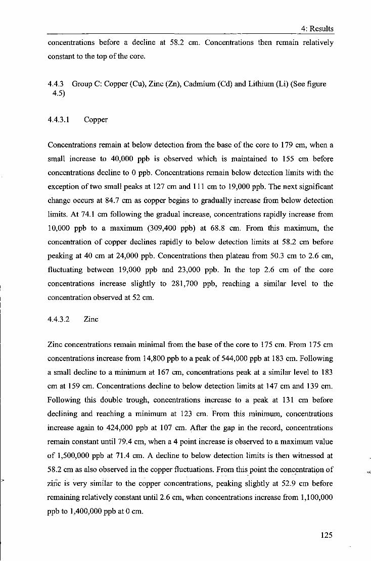
4: Results
concenfrations before a decline at 58.2 cm. Concenfrations then remain relatively
constant to the top o f the core.
4.4.3 Group C: Copper (Cu), Zinc (Zn), Cadmium (Cd) and Lithium (Li) (See figure 4.5)
4.4.3.1 Copper
Concenfrations remain at below detection from the base o f the core to 179 cm, when a
small increase to 40,000 ppb is observed which is maintained to 155 cm before
concenfrations decline to 0 ppb. Concenfrations remain below detection limits wi th the
exception o f two small peaks at 127 cm and 111 cm to 19,000 ppb. The next significant
change occurs at 84.7 cm as copper begins to gradually increase from below detection
limits. A t 74.1 cm fol lowing the gradual increase, concentrations rapidly increase from
10,000 ppb to a maximum (309,400 ppb) at 68.8 cm. From this maximum, the
concentration o f copper declines rapidly to below detection limits at 58.2 cm before
peaking at 40 cm at 24,000 ppb. Concenfrations then plateau from 50.3 cm to 2.6 cm,
fluctuating between 19,000 ppb and 23,000 ppb. In the top 2.6 cm o f the core
concenfrations increase slightly to 281,700 ppb, reaching a similar level to the
concentration observed at 52 cm.
4.4.3.2 Zinc
Zinc concenfrations remain minimal from the base o f the core to 175 cm. From 175 cm
concenfrations increase from 14,800 ppb to a peak o f 544,000 ppb at 183 cm. Following
a small decline to a minimum at 167 cm, concentrations peak at a similar level to 183
cm at 159 cm. Concenfrations decline to below detection limits at 147 cm and 139 cm.
Following this double frough, concenfrations increase to a peak at 131 cm before
declining and reaching a minimum at 123 cm. From this minimum, concenfrations
increase again to 424,000 ppb at 107 cm. After the gap in the record, concenfrations
remain constant until 79.4 cm, when a 4 point increase is observed to a maximum value
o f 1,500,000 ppb at 71.4 cm. A decline to below detection limits is then witnessed at
58.2 cm as also observed in the copper fluctuations. From this point the concenfration o f
zinc is very similar to the copper concenfrations, peaking slightly at 52.9 cm before
remaining relatively constant until 2.6 cm, when concenfrations increase from 1,100,000
ppb to 1,400,000 ppb at 0 cm.
125

4: Results
d) sooco
40000
XI 30000
=i 20000
10000
c)
X3 Q. Q.
0
10000
8000
6000
4000
2000
0
b) 1.86+6
b) 1.66+6
1.4e+6
1.26+6 Si CL 1.06+6 a. c 8.06+5 N
6.0e+6 4.0e+5
2.0e+5
00
a) 3.6e+5
a) a) 3.06+5
2.5e+6
PPb 2 0e+5
o 1.5e+5
1.0e+5
5.0e*4
0.0
8000
8000
o
hairs
p
1 4000
"5 O 2000
i D l T—
0
50 100 150
Depth
200 250 300
Figure 4.5: Element concenfrations o f group C compared to fiir seal hair abundance, a)
Copper; b) Zinc: e) Cadmium; d) LithiUin. The smooth line is the smoothed average
calculated in Sigma Plot using the running average fianction, wi th sampling proportion
set at 0.1.
126

4: Results
4.4.3.3 Cadmium
Cadmium concenfrations fluctuate to a greater extent than that observed in the Zinc and
Copper concentrations through the base o f the core. Concentrations remain at
approximately 650 ppb through the base o f the core, wi th the exception o f small peaks
at 283 cm, 275.5 cm and 251 cm as concenfrations reach 2,100 ppb, 1,477 ppb and
2,500 ppb respectively. From 183 cm to 159 cm, concentrations increase from 578 ppb
to 4,600 ppb, wi th concenfrations peaking again at 154 cm before declining to
approximately 1,000 ppb. A small peak occurs at 143 cm before concenfrations decline
to 17 ppb at 139 cm. Concenfrations remain low until 119 cm when they increase to a
peak o f 2,500 ppb at 107 cm. Following the gap in the record, concenfrations increase
from 964 ppb at 84.7 cm to a small peak at 71.4 cm before rapidly increasing from
1,500 ppb to a maximum o f 7,900 ppb at 63.5 cm. As observed in the other elements,
concenfrations then rapidly decline to below detection limits at 58.2 cm. From this
decline, concenfrations fluctuate around 1,500 ppb for the remainder o f the core.
4.4.3.4 Lithium
Lithium concenfrations are similar to the rest o f this group, as concentrations increase
from very low concenfrations at the base o f the core to 195 cm when concenfrations
increase to a peak o f 12,000 ppb at 175 cm. Although the increase begins slightly earlier
than the other element concenfrations in this group, the most significant increase
commences at 183 cm, similar to the frend observed in the rest o f the group. Following
a small decline at 167 cm, a 4-point increase to 154 cm is observed as concenfrations
peak at 24,000 ppb. Concenfrations decline to a minimum at 147 cm and 139 cm (as
observed in other records) before a small peak at 131 cm as concentrations reach 12,200
ppb. From this point concenfrations decline to 500 ppb and remain stable at this level to
100 cm. After the gap in the record, from 90 cm to 82.1 cm concenfrations remain at a
similar level as to before the gap. From 76.8 cm lithium concentrations increase and
reach a maximum at 71.5 cm as concenfrations peak at 43,600 ppb. From here
concenfrations decline and fluctuate around 5,000 ppb to the top o f the core. The
significant decline observed in the elements i n the rest o f the group at 58.2 cm is also
127

4: Results
observed in the li thium concenfrations however, this does not appear as significant as
other records as concenfrations remain relatively low though the top o f the core.
4.4.3.5 Summary o f group C
This group of elements show a general trend o f a small increase in concenfrations
commencing at 187 cm, peaking at 175 cm and again at 154 cm. Concenfrations decline
to a minimum at 139 cm, before increasing and peaking at 131 cm (copper 127 cm) and
107 cm (copper 111 cm). Following the gap in the record, concenfrations remain
relatively constant until the rapid increase to maximum concentrations at 68.8 cm
(Cadmium 63.5 cm and Lithium 71.5 cm). Following the increase, a decline to below
detection limits at 58.2 cm is observed in all concenfrations. From this rapid decline,
concenfrations plateau until 2.6 cm, where an increase is observed in all the elements.
4.4.4 Group D: Bismuth (Bi) , Molybdenum (Mo), Antimony (Sb), Thallium (Tl) , Boron (B), Beryllium (Be) (See figure 4.6)
4.4.4.1 Bismuth
Bismuth concentrations remain at below detection limits through the base o f the core to
207 cm, wi th the exception o f small peaks at 263 cm and 251 cm. Concentrations begin
to significantly increase at 199 cm, peaking at 154 cm as concenfrations reach
maximum values through the core o f 977 ppb. Concenfrations decline rapidly to below
detection limits at 147 cm and remain at this level imt i l 2.6 cm as the concenfration
increases slightly to 66 ppb.
4.4.4.2 Molybdenum
Concenfrations o f molybdenum remain below detection limits through the base o f the
core to 183 cm. From 183 cm, concentrations begin to increase to a maximum o f 40,000
ppb at 154cm. Following this peak, concenfrations rapidly decline to 1,300 ppb at 151
cm and from here remain relatively constant until 84.7 cm. From 84.7 cm, a 6-point
increase is observed to 71.5 cm as concenfrations peak at 31,800 ppb. Following this
peak, concenfrations decline to 0 ppb at 58.2 cm and then increase to plateau between
10,000 and 15,000 ppb to the top o f the core.
128

4: Results
4.4.4.3 Antimony
Concentrations at the base of the core, in contrast to the other elements are relatively
high and fluctuating, peaking at 251 cm as concentrations reach 2,800 ppb however, the
general trend is decline to a minimum of 0 ppb at 187 cm. From 167 cm the
concentration increases and peaks at 2,700 ppb at 159 cm. Following a decline at 155
cm to 401 ppb, concentrations increase again to a maximum at 154 cm of 3,300 ppb.
From this peak, concentrations rapidly decline to below detection limits at 151 cm and
remain low to 87.4 cm, concentrations increase again from below detection limits at
87.4cm to 1,400 ppb at 74.1 cm. Following this peak, concentrations decline to a
minimum of 15 ppb at 44 cm and then plateau at approximately 250 ppb to the top of
the core, where a small increase is observed at 0 cm as concentrations increase to 680
ppb.
4.4.4.4 Thallium
At the base of the core thallium concentrations remain below detection limits to 219 cm,
with the exception of a small peak at 263 cm and 227 cm. From 219 cm, concentrations
increase to a double peak at 203 cm (985 ppb) and 187 cm (1,100 ppb). After this
double peak, concentrations decline to 182 ppb at 179 cm. Following this brief fall,
concentrations increase again from 167 cm and reach a maximum of 2,700 ppb at 154
cm. From here concentrations decline to 0 ppb at 151 cm and 143 cm, peaking briefly at
147 cm at 1,500 ppb. Concentrations then peak slightly at 139 cm before declining to 60
ppb, remaining relatively constant to 84.7 cm. Concentrations increase to a peak at 71.5
cm as concentrations reach 1,000 ppb. Following the peak concentrations decline to
approximately 130 ppb where they remain constant to the top of the core. A slight
increase is observed at 58.2 cm to 329 ppb and at 0 cm as concentrations reach 425 ppb.
129

4: Results
f )
e)
d)
c)
b)
a)
^ 2000 -
1000 -
0 -
2.5B*5 -
2.09*5 -
x> t.Se+S -
8: " l.oe»5-
5 Oe»l -
0.0
3000 -
2500 -
2000 -D: 1500 -F
1000 -
500 -
I I as
50000
40000
30000
20000
10000 -
0 -
1200
1000 -I
800
SOO
400 -1
200
0
8000
8000
4000
2000
0
150
Depth
Figure 4.6: Element concentrations of group D compared to fur seal hair abvmdance. a)
Bismuth; b) Molybdenum; c) Antimony; d) Thallium; e) Boron; f) Beryllium. The
smooth line is the smoothed average calculated in Sigma Plot using the running average
function, with sampling proportion set at 0.1.
130

4: Results
4.4.4.5 Boron
Concentrations remain below detection limits through the base of the core to 223 cm.
From 223 cm, a 5-point increase occurs to a peak at 203 cm as concentrations reach
222,700 ppb, a maximum concentration for the whole core. From this peak,
concentrations decline to 9,750 ppb at 195 cm and remain at this level until 167 cm as a
second increase begins, peaking at 154 cm (207,000 ppb). Following this second peak,
concentrations decline to 0 ppb at 147 cm and 139 cm, before increasing to 20,000 ppb
and remaining at this level to 100 cm. From 88.7 cm, a 5-point increase is observed to a
peak at 74.1 cm as concentrations reach 114,000 ppb. Following the peak,
concentrations decline to below detection limits at 66.2 cm and remain at this level until
21.2 cm. From 21.2 cm, concentrations increase slightly to the top of the core, reaching
a maximum 143,000 ppb at 5.3 cm.
4.4.4.6 Beryllium
The record is not continuous however, concentrations fluctuate significantly through the
base of the core. The general trend is an increase to a maximum peak of 4,261 ppb at
154 cm. Following the peak, concentrations decline rapidly to approximately 1,000 ppb
and remain constant to the gap in the record. Following this gap, concentrations peak at
74.1 cm and 68.8 cm. The only concentrations recorded after this peak are at 39.7 cm
and 23.8 cm as concentrations reach 2,800 ppb.
4.4.4.7 Summary of group D
All the elements in this series show relatively low concentrations at the base of the core,
with the exception of Antimony, which declines fi-om the base of the core to a minimum
at 179 cm. Thallium and Boron show a peak at 203 cm. All the elements show a large
increase commencing at 179 cm and peak at maximum concentrations at 154 cm,
followed by a rapid decline. With the exception of Bismuth, an additional peak is
observed at 74.1 cm, followed by a gradual increase to the top of the core. Beryllium
shows the rapid increase at 154 cm however, the decrease fi-om this peak is not as rapid
as the other elements and the top of the core does not show the gradual increase as
observed in the other elements.
131
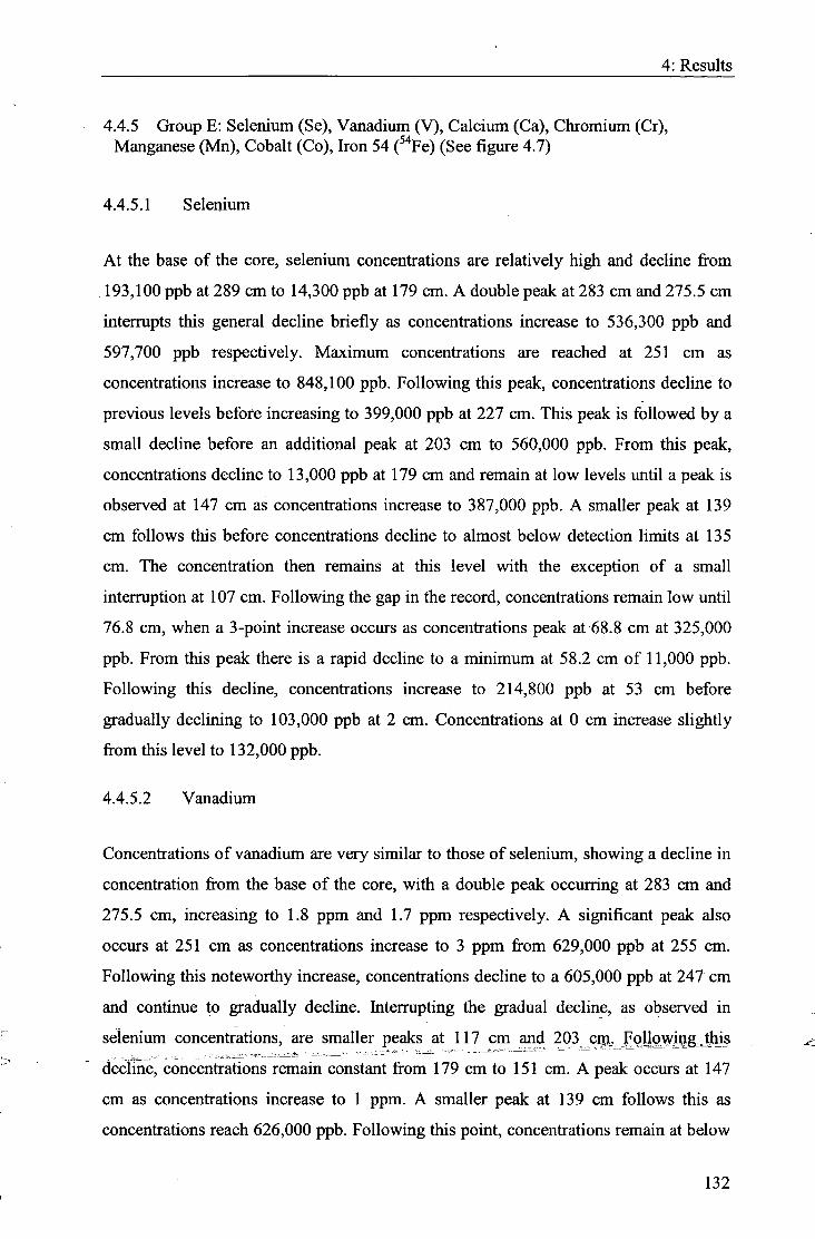
4: Results
4.4.5 Group E : Selenium (Se), Vanadiiim (V), Calcium (Ca), Chromium (Cr), Manganese (Mn), Cobalt (Co), Iron 54 ( ^ Fe) (See figure 4.7)
4.4.5.1 Selenivim
At the base of the core, selenium concentrations are relatively high and decline from
193,100 ppb at 289 cm to 14,300 ppb at 179 cm. A double peak at 283 cm and 275.5 cm
interrupts this general decline briefly as concenfrations increase to 536,300 ppb and
597,700 ppb respectively. Maximum concentrations are reached at 251 cm as
concenfrations increase to 848,100 ppb. Following this peak, concenfrations decline to
previous levels before increasing to 399,000 ppb at 227 cm. This peak is followed by a
small decline before an additional peak at 203 cm to 560,000 ppb. From this peak,
concenfrations decline to 13,000 ppb at 179 cm and remain at low levels imtil a peak is
observed at 147 cm as concenfrations increase to 387,000 ppb. A smaller peak at 139
cm follows this before concenfrations decline to almost below detection limits at 135
cm. The concenfration then remains at this level with the exception of a small
interruption at 107 cm. Following the gap in the record, concenfrations remain low until
76.8 cm, when a 3-point increase occurs as concenfrations peak at 68.8 cm at 325,000
ppb. From this peak there is a rapid decline to a minimum at 58.2 cm of 11,000 ppb.
Following this decline, concenfrations increase to 214,800 ppb at 53 cm before
gradually declining to 103,000 ppb at 2 cm. Concenfrations at 0 cm increase slightiy
from this level to 132,000 ppb.
4.4.5.2 Vanadium
Concenfrations of vanadium are very similar to those of selenium, showing a decline in
concenfration from the base of the core, with a double peak occurring at 283 cm and
275.5 cm, increasing to 1.8 ppm and 1.7 ppm respectively. A significant peak also
occurs at 251 cm as concenfrations increase to 3 ppm from 629,000 ppb at 255 cm.
Following this noteworthy increase, concenfrations decline to a 605,000 ppb at 247 cm
and continue to gradually decline, friterrupting the gradual decline, as observed in
selenium concenfrations, are smaller peaks at 117 cm and 203 cm. g ojlipving ^ ^ ^
decline, concenfrations remain constant from 179 cm to 151 cm. A peak occurs at 147
cm as concenfrations increase to 1 ppm. A smaller peak at 139 cm follows this as
concenfrations reach 626,000 ppb. Following this point, concentrations remain at below
132

4: Results
detection limits from 135 cm to 79.4 cm. At 71.5 cm maximum concentrations are
reached as the concentration increases from 0 ppb to 3 ppm. Concentrations then decline
rapidly to 0 ppb at 68.8 cm and remain at this level to 26.5 cm, when a gradual increase
is observed to the top of the core as concentrations reach 862,000 ppb.
4.4.5.3 Calcium
Calciiim shows a similar fluctuation to vanadium and selenium at the base of the core as
concentrations decline from 1,300 ppm at 289 cm to 7.2 ppm at 179 cm. The double
peak as observed in the concentration of vanadium and selenium is also evident in the
Calcium record at 283 cm and 275.5 cm. A peak at 251 cm interrupts the gradual
decline from the base of the core as concentrations increase from 1,200 ppm at 255 cm
to 6,000 ppm. Following this rapid increase, concentrations return to levels before the
increase occurred. A smaller increase is observed at 227 cm, which is followed by slight
fluctuations before a larger peak at 203 cm. From this peak, concentrations decline to
7.2 ppm at 179 cm, where concenfrations remain to 100 cm, with the exception of two
small peaks at 147 cm and 139 cm as concentrations increase to 1,300 ppm and 662
ppm respectively. From 90 cm, to the top of the core concentrations remain constant at
approximately 5 ppm.
4.4.5.4 Chromium
Chromium concentrations remain relatively constant at the base of the core at 11,000
ppb. As seen in the rest of the elements within this group, peaks are observed at 283 cm
and 275.5 cm and again at 251 cm however, this peak at 251 cm does not reach
maximum values for the whole core as shown in the rest of the elements in this group.
Following this peak at 251 cm, smaller peaks are observed at 227 cm and 203 cm. A
significant peak is also observed at 187 cm, as concenfrations increase to 50,733 ppb.
From this peak, concentrations decrease to 10,000 ppb and remain constant from 179
cm to 155 cm. At 155 cm concenfrations begin a 4-point increase to a maximum of
100,500 ppb at 147 cm. A smaller peak of 46,000 ppb at 139 cm follows this maximum
peak. At 135 cm, concenfrations decline to 14,000 ppb, which is maintained until 100
cm. From 90 cm, concenfrations decline gradually to a minimum of 150 ppb at 58.2 cm,
before then increasing to 5,500 ppb, at 55.6 cm and remaining at this level to the top of
the core.
133

4: Results
g)
f )
e)
d)
c)
b)
a)
l.2e+5 -
1.0e*5 -
S.Oe+4 -
B-0»*4 -4.00*4 -
2.0»+4 -
• 0
1.2e*S -
1.0»*5 -
8.Cte*4 -
6.0^4 -
4.(te+4 -
2.De»4 -
0-0
1.2e*5
1.0ft*5
e.0e*4
6.0e*4
4.0e*4
2.0e+4
0.0
6et9
4**9
30*9
26+9
1e*9
1et6
g 6e*S CL
2e*S
at 4000
MOO o O)
150
Deptti
Figure 4.7: Element concentrations of group E compared to fiir seal hair abundance, a)
Selenium; b) Vanadiimi; c) Calcium; d) Chromium; e) Manganese; f) Cobalt; g) 54-
Iron. The smooth line is the smoothed average calculated in Sigma Plot using the
running average function, with sampling proportion set at 0.1.
134

4: Results
4.4.5.5 Manganese
Concentrations at the base of the core are at relatively high levels and decline fi-om this
point. A double peak at 283 cm and 275.5 cm interrupts this general decline as
concentrations increase to approximately 45,000 ppb before maximum concentrations of
759,000 ppb are reached at 251 cm. Following the peak, concentrations decline rapidly
to concentrations similar to before the peak. From 231 cm, the concentration of
manganese fluctuates significantly. Significant peaks are observed at 227 cm and 203
cm, similar to the other elements in this group. An additional peak is also observed at
147 cm as concentrations increase to 448,000 ppb, yet from here the general trend is
decline. From 88.8 cm, concentrations remain at approximately 100,000 ppb.
Fluctuations in this section of the core appear insignificant in comparison to the
magnitude of changes deeper in the core. However, a small peak occurs at 68.8 cm as
concentrations increase to 158,000 ppb and a decline to below detection limits at 58.2
cm. Finally concentrations increase slightiy at 0 cm to 160,000 ppb.
4.4.5.6 Cobalt
Concentrations of cobalt at the top of the core are relatively high and although they
fluctuate significantly the general trend is one of decline. Peaks observed in the other
elements at 283 cm and 275.5 cm occur in the cobalt record however, these peaks are
not as significant as others recorded. Maximum concentrations are reached at 267.5 cm
as concentrations reach at 108,000 ppb. Following a slight decline, an additional peak
occurs at 251 cm (95,700 ppb). Slightly smaller peaks are also observed at 227 cm and
203 cm. Following this peak, concentrations rapidly decline to 1,800 ppb at 179 cm.
Concentrations remain at this level to 100 cm, interrupted slightly by a peak at 147 cm
and 139 cm. From 90 cm concentrations remain below detection limits to 76.8 cm as
concentrations increase slightly to peak at 10,000 ppb at 68.8 cm. Following this small
peak, concentrations remain relatively constant to the top of the core with the exception
of a small increase at 18.5 cm to 10,700 ppb.
135

4: Results
4.4.5.7 54-fron
Concenfrations gradually increase from the base of the core to a maximum of 146.2
ppm at 205 cm. Smaller peaks are also recorded at 283 cm, 275.5 cm and 251 cm as
observed in the other elements. From the peak at 205 cm, concentrations decline to 15.8
ppm at 179 cm and remain relatively constant until 100 cm, with a small interruption
with peaks at 147 cm and 139 cm. From 88.7 cm to the top of the core concenfrations
remain constant at approximately 14 ppm, with the exception of 58.2 cm, when
concenfrations decline to 8,000 ppb (0.008ppm).
4.4.5.8 Summary of group E
This group show a gradual decrease in concentration from the base of the core. This
decrease is interrupted in all element concenfrations with peaks at 283 cm and 275.5 cm,
followed by a larger peak at 251 cm, where maximum concenfrations are met or almost
met. Following this peak, the correlation between the elements is not as significant
however, in all the elements a peak is recorded at 147 cm and 139 cm. Following these
peaks, concenfrations fall to very low levels and remain constant to 79.4 cm. From this
point, all the elements, with the exception of Ca, Cr and " Fe peak briefly at 71.5 cm.
Following this peak, a rapid decline is observed in all the elements (with the exception
of Ca and V ) to almost below detection limits at 58.2 cm. Following this rapid decline
concentrations increase and remain relatively constant for the remainder of the core.
4.4.6 Group F: Arsenic (As), Sulphur (S), Nickel (Ni) (See figure 4.8)
These elements do not display a similar pattern to any of the element groups therefore,
they have been grouped together.
4.4.6.1 Arsenic
Maximum concentrations are reached at 283 cm as concentrations reach 16,700 ppb.
Following this peak, concenfrations decrease to 726 ppb at 279 cm and then gradually
decrease to below detection limits at 227 cm. Concenfrations remain at Oppb until 183
cm, when a rapid increase begins which peaks at 154 cm as concenfrations reach 12,600
ppb. Following this increase there is a rapid decline in concenfrations to below detection
limits at 147 cm. From this low point, concentrations increase to almost maximum
136

4: Results
concentrations at 115 cm, which is followed by a smaller peak at 107 cm. After the gap
in the record, a 4-point increase is observed to a peak at 82.1 cm at 12,500 ppb.
Concentrations then decline to approximately 7,000 ppb, as concentrations plateau to
the top of the core, with the exception of a significant decline at 58.2 cm to below
detection limits.
4.4.6.2 Sulphur
At the base of the core the sulphur content increases from 0.39% at 289 cm to 2.1% at
279 cm. Following this peak, the concentration of sulphur drops dramatically at 263 cm
to 0.48%. The sulphur concenfration then gradually increases, peaking at 259 cm and
247 cm before reaching a maximum peak of 3.075% at 227 cm. Following the peak, the
content of sulphur gradually declines to a minimum of 0.554% at 175 cm, before
increasing again and remaining relatively constant before a decline at 131 cm to 0.78%.
From this point, the percentage of sulphur increases again and peaks at 115 cm at
similar levels to the peak observed at 227 cm. Following this peak, a smaller peak is
observed at 103 cm. After the gap in the record, concentrations reach 2.41% at 90 cm
before declining to 0.82% at 82.1 cm. Concentrations gradually increase to a smaller
peak of 1.23% at 34.4 cm before a gradual decline to the top of the core.
4.3.6.1 Nickel
Nickel concentrations remain at very low levels from the base of the core to 239 cm,
when an increase in concenfration begins. The increase is gradual until a peak at 179 cm
as concentrations reach 31,700 ppb. The peak is followed by a dramatic decline to
below detection limits at 175 cm, followed by a smaller peak at 167 cm (25,300 ppb).
Concenfrations drop back to below detection limits before increasing and peaking at
maximum concenfrations of 54,900 ppb at 151 cm. Following maximum concentrations
the nickel level fluctuates, peaking at 143, 135 and 127 cm as concenfrations reach
approximately 17,000 ppb. A 4-point increase, peaking at 107 cm, follows this
fluctuation. From 88.6 to 76.8 cm the concenfrations fluctuate slighfly but remain
around the 10,000 ppb before a dramatic decline to 0 ppb at 71.5 cm. Peaks at 66.2 cm
and 55.6 cm follow this before declining back to 0 ppb from 53 cm. The concentration
of nickel remains at this level until 2.6 cm is reached and concentrations increase to
23,000 ppb.
137

4: Results
c) Boooa
50000
40000 St & 30000 z
20000
10000
b) 18000 16000 14000 12000
^ 10000 ^ 8000
8000 4000 2000
0
a)
o ^
3.5
3.0
2.5
£ 2.0
W 15
1.0
0.5
0.0
flOOO
6000
4000 H
2000
50 100 150
Depth
200 250 300
Figure 4.8: Element concentrations of group F compared to fur seal hair abundance, a)
Sulphur; b) Arsenic; c) Nickel. The smooth line is the smoothed average calculated in
Sigma Plot using the running average function, with sampling proportion set at 0.1.
138

4: Results
4.4.7 Summary of geochemical results
The most significant change through the whole core in all the element concentrations
occurs near the base of the core. Elements in groups A (Sr, Al) , B (K, Ti , Ba, ^^Fe, Na),
C (Zn, Cd, Li) and D (Bi, Mo, Sb, T l , B, Be) all show a dramatic increase in
concentrations at 183 cm. Carbon and Nitrogen are the exception to this, as the increase
in these elements begins earlier at 263 cm. The elements of group E (Se, V , Ca, Cr, Co
" Fe) decline rapidly fi-om the base of the core to very low levels at 179 cm.
The concentrations of elements in groups A and B peak at 175 cm, before declining. In
groups C and D, the increase is prolonged and concentrations do not peak until 150 cm.
The double trough observed at 147 cm and 139 cm is present in all of the element
concentrations in groups A, B, C and D (with the exception of Bi), suggesting a brief
but notable change at this point. This change also correlates with the elements
negatively correlated with depth (group E ) , as element concentrations increase to peaks
at 147 cm and 139 cm. From this point, the correlation between the element
concentrations is not as strong, suggesting smaller changes to the catchment are
occurring.
Following the decline at 147 and 139 cm and gradual increase, concentrations decline
slightly in most element groups before increasing slightly to a smaller peak. This peak
occurs in most element concentrations at 107 cm however, it does range from 111 cm
(Ti) to 103 cm (Cr). The elements in group E , negatively correlated with depth, also
peak at this point. As all element concentrations increase at this point, it suggests a brief
but significant change in the system.
After the gap in the record, a large peak is observed in all the element records. Groups
A (Sr, Al) , B (K, Ba, Na), C (Cu, Zn), E (Mn, Se) peak at 68.8 cm. Elements in group D
peak slightly earlier at 74.1 cm. Although the timing of the peak varies slightiy (fi-om
74.1 cm-63.5 cm) all elements display a significant peak at this point, with the most
dramatic peaks observed in the Zn and Cu records. Following this peak, all the elements
in groups A, B and C display a dramatic decline at 58.2 cm, as concentrations fall to
below detection limits. This decline is also observed in some elements in the other
groups (Se, Cr, Mn, Mo, Sb, As and ^''Fe) however, the magnitude is not as significant
139

4: Results
as in the other element groups. This dramatic 1-point decline in all the records suggests
a significant but very brief change has occurred in the catchment at this point. From this
point in the core there are no significant frends common across all elements. However, it
can be noted that very few significant changes in comparison to the rest of the core take
place in any elements. This implies the catchment has reached stabilisation from 58.2
cm hence, very few changes in element concentration occur.
4.5 Dating
4.5.1 Radiocarbon dating
The base of the core has been radiocarbon dated at 3439 +/- 25 yrs BP (SUERC-2303)
using Accelerator Mass Specfrometry (AMS) (Moreton et al. unpublished data). From
the results of the fur seal hair abundance record and geochemical analysis, samples were
chosen to obtain further radiocarbon dates to assist in analysis and help to correlate the
change in the fur seal hair abundance and geochemistry to climatic changes occurring
within the catchment. Samples HUM3 82-83 cm and M A I V K 50 cm were selected for
dating for reasons outlined below.
4.5.1.1 HUM3 82-83 cm
From the results of the hair abundance and geochemical analysis (See figures 4.1, 4.3,
4.4, 4.5, 4.6, 4.7 and 4.8), it is clear that a distinct change occurs at 187 cm (HUM3 87
cm) in the geochemical record and to some extent in the fur seal hair abundance record.
Using a constant sedimentation rate model derived the radiocarbon date at the base of
the core, this gives a date of approximately 2000''*C yrs BP which corresponds to a
distinct climate change at South Georgia (see figure 2.11). This point in the core appears
to be the largest change in the geochemical and fur seal hair abundance record,
therefore, it is important to get a radiocarbon date for this point to determine when it
occurred and allow correlation with other records which climate changes have been
inferred. As this is a distinct change, it is likely that sedimentation rates at this point in
the core have altered and therefore, calculating a constant sedimentation rates across
this point is likely to incur error. A date from this point will provide a pinning point
upon which a constant sedimentation rate can be used for the rest of the core. Although
a distinct change occurs at H U M 3 87 cm, after other analysis there was no sample left
140

4: Results
at this point therefore, the nearest sample was 82 cm and so this sample was submitted
to Beta Analytic for AMS dating.
4.5.1.2 M A I V / K 50-51 cm
The results of the geochemical analysis and the hair abundance record highlight a
distinct change at 66.2 cm (MAIV/K 50cm). At this point the fur seal hair abundance
begins to increase sharply to a maximum at 47 cm. The geochemical analysis also
shows a change at this point as concenfrations peak ~ 68 cm before declining to a
minimum at 58 cm (see figures 4.3 - 4.8). These rapid changes suggest that a large
catchment change is occurring at this point therefore, obtaining a date from this point
will help to establish the timing of this change and hence, allowing factors affecting fur
seal population fluctuations at this point to be inferred.
The gap between the two cores is problematic, as the amount of shrinkage between the
cores is difficult to calculate. As this sample is near the base of the M A I V / K core, this
will provide a clearer indication of the timescale missing in the combined cores and
reduce the error in calculating constant sedimentation rates. Considering the 2 cores as a
whole core, this sample is also nearer the top of the core, and therefore, it is likely that
sedimentation rates have changed from the other radiocarbon dated samples. A date at
this point in the core is useful to determine sedimentation rates and reduce the error of
calculating a constant sedimentation rate from a different core.
These radiocarbon dates will be used to date the rest of the core using a constant
sedimentation rate model. However, as figure 3.1 illustrates some of the core has shrunk
after exfraction. This coupled with the compression of sediments after deposition in the
lake means that a sedimentation rate is imlikely to be constant. Although the 3
radiocarbon dates will reduce the error, it must be noted that the fixed spatial resolution
used to sample the cores (i.e. 2 cm) will not reflect a fixed temporal resolution used for
analysis. For example the core has been sampled every 2 cm; calculating a constant
sedimentation rate, 2 cm may appear to represent 10 years however, in some sections of
the core a period of increased sedimentation rate may result in 2 cm being deposited in 5
years. During a period of l-educed sedimentation rate, 2 cm may be deposited in 20
years. Although the sampling has been done at regular intervals, there may be time
periods within the core when sedimentation rates were lower, thus, the 10 year gap
141

4: Results
expected may actually reflect a 20 year gap and hence, the detail of every 10 years may
not be seen within the record.
4.5.2 Radiocarbon dating results
The results of the Radiocarbon dating are presented in table 4.3. This presents the
sample sent for analysis, which are referenced relative to the samples within the core.
The actual depth of the sample within the cores refers to the depth of the sample when
viewed as one core, which is calculated using the equation outlined in section 3.1.1. The
radiocarbon date, as quoted from the laboratories and the conventional radiocarbon date
that is the radiocarbon date following corrections after the 13C/12C analysis to ensure
any isotopic fractionation in the sample is corrected. Finally the calibrated date is
presented.
Sample Actual depth in the core (see section
3.1.1)
Radiocarbon date 13C/12C Ratio Conventional radiocarbon date
Calibrated ages (2 Sigma calibrated
result) HUM3 200 cm. (SUERC-2303).
300 cm Not stated -29.7 o/oo 3439 +/- 25 BP 3486-3500 BP 3506-3524 BP 3555-3704 BP
HUM 3 82 cm (Beta-207757)
182 cm 3910 +/- 40 BP -26 o/oo 3890 +/- 40 BP 4420-4220 BP 4210-4170 BP
MAIVK 50 cm (Beta-208029)
66.18 cm 2750 +/- 40 BP -24.7 o/oo 2750 +/- 40 BP 2940-2770 BP
Table 4.3: Results from radiocarbon dating.
As table 4.3 indicates, the results of the radiocarbon dating show a reversal at the base
of the core. This has implications for analysis and the construction of an age model. The
possible causes for this switch and the implications for the study will be discussed in
fiarther detail in section 5.2.
4.5.3 2'°Pb and " ' C s dating
Subsamples were taken at every centimefre in the top 20 cm of the M A I V K core to
prepare for ^'°Pb and '^^Cs dating. This was based upon a radiocarbon date of 3439 '" C
yrs BP at 300cm (the base of HUM3 core). Assuming a constant sedimentation rate
from this point to the top of M A I V K core, provides a sedimentation rate of 11.8 years
per cm. Although the sedimentation rate is unlikely to have remained constant
throughout both cores, this provides a broad estimate of the sedimentation rate and
142
137,

4: Resuhs
allows the number of samples required for ^"'Pb to be estimated. The upper limit for
^'°Pb dating is 200 years therefore, testing samples estimated to be older than this is not
productive. Using this constant sedimentation rate model, 200 ''*C yrs BP is reached
after 17 cm. It is likely that sedimentation rates have increased in the past 200 years and
to take into account any compression within the core, the top 20 cm of the MAFVK core
(=26.5 cm of the total core) was tested for ^"'Pb activity. The '^^Cs peak in 1963 would
be expected at approximately 40 yrs BP which is also well within the top 20 cm of the
core.
4.5.3.1 '''Pb and'"Cs results
The ^'°Pb and '"Cs results show no activity in any of the samples in the top 20 cm (see
figure 4.9, 4.10 and appendix 3) therefore, the top of the core was dated using constant
sedimentation rates calculated fi-om the 3 radiocarbon dates. The possible reasons for
the lack of activity are discussed in section 5.1.1.
• Gamma Vis ion 6 /cm.Spc
Rto Acqiirs Caltrats CikiMe Aodyze Lbary Sirvicas ROI Display Wixkiw
HH| •|SN [w] A\ nm M^lM^in
Peak: 389 00 . 38 27 fc*l FWHM 3W FW|1/5)M:355 Lil»aiy:Pb-210(Laacnal46.54 , 0.00Bq Gross A I M 2080 NetAiea:52t112 Qrass/Nel Catt Rate. 0 01 / 0.00 cos
Peak:3e8.00.mt7keV FV,/HM:0.)0 FW|1/5|M:016 Lib(ajy:Pb-210|Lead)al46.54, 0 Gross Aiea 2072 NelArea: -186 tn7 Bross/Nel Cotnt Rale 001 7 -0 00 cpi
10.06 ke
PiisaHLAnalyn! Slat 10:07:32
08706/2005 Real 172.480.00 UvK 172.135.00
Dsad 0.20 X
ROI
^ Ddl-gl
Peak
®ORIEC 1(159.26
Mon O5ffl9/20O6
' start • •Garr.rraV 5ron-6-7cm .. -. J FliShot 8.0 Slar> lard... 6? FullShot 8 User's Gude
a)
b)
Figure 4.9: ^'°Pb and '^^Cs results, a) M A I V K 6-7 cm; b) M A I V K 1-2 cm. The label on
both the graphs indicates the position where " Pb is detected. If ^"'Pb had been present
143

4: Results
in the sample, a peak would be present at this point and the amount of '"Pb in the
sample is calculated from the net area.
Figure 4.9a ( M A I V K 6-7cm), the ^"^b count is 52+/-112. As the error on this is greater
than the actual count, the activity in the sample is below background levels.
Figure 4.9b ( M A I V K l-2cm) displays similar characteristics. The ^"^b count is -186+/-
117. As this is the top sample, this should display the greatest amount of ^'°Pb as it is
the most recent sediment however, this is not the case and hence, the sediment cannot
be dated using these results. The red band on both graphs nearest to the ^'°Pb peak
indicates where the '^'Cs peak would be if there was any activity in the sample (see
figure 4.10).
1 1 HI MM rai] \^±\ DM) rss: PuheHr Anat m Slot 18:21:03
Rut 174.77*110 Liy« 174.44a00
Dead 013 !S
lJ_HoJ tfl
a>ORTEC 10 54 23
Mon 05/09/2005
Pa GEO1.7S-ECt.80l<W FVHM:Z14 FW(1/5]M: h»y:Ci-1371C»»im)al6S1.66; insi Alex 1043 lelArHe9lS3 ran/Nat CouM Rate 001/COO qu
kMntcer 6503 .
Figure 4.10: '^^Cs results ( M A I V K 3-4 cm). The label on the graph indicates the
position of a peak if there was any '^^Cs in the sample. The label indicates that in this
sample, the amount of '^'Cs is 69+/-93; therefore there is no '^^Cs in the sample beyond
background levels. Each sample tested displayed similar characteristics and therefore
this method cannot be used to date these samples.
144

4: Results
4.6 Summary
This chapter only describes the results; results will be analysed further in the following
chapters. Chapter 5 will carefully examine the results and discuss the implications these
results have for each objective as outlined in chapter 1.
145

5: Discussion
Chapter 5
Discussion
Plate 5: Fur seals at South Georgia
146

5: Discussion
5: Discussion
Before discussing the interpretation of the fur seal hair and geochemical results, a robust
age model will be established from the Radiocarbon dates and the ^'°Pb and '"Cs
results and used as a basis for analysis.
5.1 Age Model
From the results of the radiocarbon dates, it is essential to establish an age model on
which to compare the fur seal hair abundance changes and hence, fluctuations can be
correlated to climate change. As the • '*'Pb and ' 'Cs results were inaccurate, these
caimot be used.
As table 5.1 shows, the radiocarbon dates show an apparent reversal at the base of the
core. As this is not possible, it is likely that one of the dates is inaccurate and cannot be
used. The following section discusses the implications for using each of the radiocarbon
dates and the likelihood of its accuracy. Table 5.1 presents the different age models and
the implications these models have for analysis.
HUM 3 200cm (SUERC - 2303)
HUM 3 83cm (Beta -207757)
MAIVK 50cm (Beta 208029) Basal date (14C
years BP)
Sedimentation Rate (cm/yr)
3439 3910 2750
Basal date (14C years BP) Lower
section Upper
section Model 1 • 3439 0.087 Model 2 * 6412 0.048 Model 3 • 12466 0.024 Model 4 • * 5051 0.10 0.024 Model 5 * • 3439 0.34 0.024
Table 5.1 - Different age models and the implications this has for sedimentation rate
and basal date in the core.
5.1.1 Model 1 (3439 ' C yrs BP only)
As table 5.1 shows, i f only the basal date was used to date the core, this would give a
constant sedimentation rate of 0.087cm/yr throughout the core. This is unlikely to be the
case due to the climatic changes documented in the catchment through the past 3439 ''*C
147

5: Discussion
yrs BP (see figure 2.11). Although this is possible, as there are other dates available,
using an additional date to enhance the accuracy is more favourable.
5.1.2 Model 2-(3910 "C yrs BP only)
Assuming the radiocarbon date from 187cm is correct; this would imply that the basal
date is inaccurate. Using this date as table 5.1 indicates, the basal date would be 6412
''*C yrs BP and the sedimentation rate would be 0.048 cm/ yr throughout the core. Using
an additional date is favourable as this provides an enhanced accuracy and prevents the
sedimentation rate been assumed from one constraining point. As a consequence of
these factors, this model will not be used.
5.1.3 Model 3 - (2750 •''C yrs BP)
Using the radiocarbon date fi-om the MAIVK core at 50 cm gives a very low
sedimentation rate for the entire core and would imply that the core provided a record
for the past 12466 '''C yrs BP. Given past climate reconstructions for this period, it is
thought that the catchment was still glaciated in 12466 '' C yrs BP. From analysis of the
core stratigraphy (see section 4.1) and climate reconstructions from similar lakes in the
Maiviken area, it can be inferred that the lake catchment formed following deglaciation
(Clapperton et al 1989). Using this theory, it is thought that this model is inaccurate and
will not be used.
5.1.4 Model 4 - 3910' C yrs BP and 2750 '' C yrs BP
This model uses two radiocarbon dates to enhance the accuracy of the model. Using the
dates from HUM3 82 and MAJVK 50cm implies the core provides a record for the past
5051 '''C yrs BP.
The basal date HUM3 (200cm) (SUERC -2303) is thought to be reliable as it has been
radiocarbon dated in two separate laboratories (SUERC and Prozan), each giving a very
similar date (Moreton et al. unpublished data). I f this date is correct, the HUM 3 (82Gm)
date is thought to be accurate and therefore, this model will not be used.
148

5: Discussion 5.1.5 Model 5 - 3439 "'C yrs BP and 2750 '"'C yrs BP
As the basal date HUM3 (200cm) has been dated twice by different laboratories, both
giving a similar date, it is thought that this date is accurate and hence, it can be inferred
that the date obtained at HUM 3 (83cm) is inaccurate and will not be considered in
analysis. The use of two radiocarbon dates aids in reducing error in the age model
hence, the date obtained from MATVIK (50cm) will also be used in the model.
5.1.6 Calculating the age model
The sedimentation rate was calculated using the basal date from HUM3 200 cm and the
date obtained from MAIVK 50 cm using equation 5.1. Before calculating any dates, the
samples were converted into depths as described in section 3.1.1 (equation 3.1).
(no. of years the sediment section covers) / (no. of cm covered x depth of the sample)
Equation 5.1: date for each sample in the core
Lower section of the core (66.18-300 cm)
= (3439-2750)7(300-66.18)
= 2.946 years represented by each cm of sediment
= sedimentation rate 0.34 cm/year
Upper section of the core (0-66.18 cm)
= 2750/66.18
= 41.56 years represented by each cm of sediment
= sedimentation rate 0.024 cm/ year
The top of the core cannot be accurately dated due to the problem in ' Pb and ' ^Cs
dating. Although samples for radiocarbon dates were selected from relatively equal
depths down the core, due to the age of the youngest date at the top of the core the
sampling resolution is not time sfratigraphic. However, this problem cannot be
alleviated without dating an additional sample nearer the top of the core. Although it is
unlikely that the sedimentation rate has been constant in the catchment since 2750 '''C
149

5: Discussion yrs BP, as the ^'°Pb and ' ^Cs results were unsuccessful, this is the only estimate
available.
5.2 Dating inaccuracies
The possible reasons for the inaccuracies in the dating techniques are outlined in the
following sections.
5.2.1 ^''^b problems
The results of the ^'°Pb and * Cs show no activity above background levels, therefore,
this method cannot be used as a means to date the top of the core (see figures 4.9; 4.10).
The date for the top of the core has therefore, been estimated to be zero. A constant
sedimentation rate assumed to the '''C date at 66.18 cm depth (MAIVK 50 cm) has been
used to date the top section of the core.
Although the sub Antarctic region is not an area commonly recognised as having ^"^b
and Cs dating problems, there have been no published studies on South Georgia that
have successfiilly dated lake sediments using ^^°Pb. The apparent lack of ^''^b and ' ^Cs
is difficult to explain, however, possible reasons for this are outlined below and include
the loss of the sediment-water interface, catchment characteristics, detection limits and
location of the study site.
5.2.1.1 Loss of the sediment water interface
It is possible that the sediment analysed for "'Pb and ' ^Cs is not the true core top (i.e.
sediment-water interface at the time of exfraction). If this is the case, the sediment that
appears to be at the top of the core will be older than 200 years BP and hence, all of the
^'°Pb in the sample is likely to have already decayed. Although this is feasible, it would
require a minimum of 4 cm from the top of the core to be lost (calculated on constant
sedimentation rate discussed in section 5.1.6). The use of a Kullenberg corer for the top
section of the core was designed to prevent the loss of the core top, it is possible that the
top 4cm of the sediment in the lake was lost during coring as sludge at the top of the
core.
Despite these complications, the dating model suggests the sedimentation rate in the
core has been constant for the past 2750 '''C yrs BP. Although this is the best estimate
150

5: Discussion available with the data, it is unlikely that this is the case. As figure 2.11 indicates, the
climate has changed significantly during this period and today the climate is warmer
than at 2750 '' C yrs BP hence, the sedimentation rates would be expected to be higher.
Coupling this with the compaction of deeper sediment, causes the ^'°Pb to be present in
samples deeper than 4 cm. As a consequence, all the ^'°Pb would not be lost in the
sediment water interface and all the '*^b in the core would not have decayed. The peak
of '"Cs in the sediment, used as a reference point for the ^'°Pb dating occurs in 1963
hence, i f all the ^'°Pb is depleted, it is not surprising that the peak in ' ''Cs has also been
lost.
5.2.1.2 Catchment Characteristics
The catchment of the lake may not be conducive to the accumulation of ^'°Pb fallout. It
is widely recognised in the Antarctic region, the strongest "'Pb or ' ^Cs signals are
found in large catchments which experience a focussing effect (Hodgson et al. 2004).
As section 2.2.3 and 2.2.5 discuss, the catchment is small and very localised hence,
decreasing the likelihood of any "^b or ' ^Cs accumulation.
As Appleby et al. (1995) suggest, the ^"^b flux from the atmosphere varies globally
and the fallout to Antarctica is sparse. Hardy et al. (1973) further establish that the ' ^Cs
fallout in Antarctica is a magnitude lower than fallout rates in mid latitudes of the
Northern Hemisphere. Doran et al's. (1999) study in a lake in the McMurdo Dry
Valleys, Antarctica, indicates that levels of '°Pb were high in some samples however,
counts were not sufficient in all samples to allow an age chronology to be formulated. It
was concluded that the perermial ice cover of the lake retarded the deposition of "^b
and Cs in lake sediments (Doran et al. 1999). This coupled with low fall out rates of
^'°Pb and '"Cs in Antarctica prevented the accumulation of '°Pb and '"Cs in the lake
reaching levels above backgroimd.
Humic lake is ice covered for 4-5 months of the year and as discussed in section 2.2.5
ice cover limits lake inputs hence, the pathways for ^'°Pb reaching the water column are
restricted (Doran etal. 1999). The accumulation of "'Pb and ' ^Cs in the sediment may
therefore, Se limited to only some months of tfie year and result in the accumulation of
very low levels of ^'°Pb and ' ^Cs that are not significantly above background levels and
therefore cannot be detected.
151

5: Discussion Although there have been numerous studies of ^'°Pb and '"Cs in Antarctica which
suggest that the fallout is lower than other regions, many studies have yielded sufficient
concenfrations to allow an accurate chronology to be calculated (Jones and Juggins
1995; Roberts et al. 2004). Catchments on Signy Island which experience a similar
climate to South Georgia, have yielded '°Pb results and allowed a ^'°Pb chronology to
be determined (Jones and Juggins 1995; Noon et al. 2001; Jones et al. 2000). These
catchments experience ice cover for 8-11 months of the year and are influenced by a
large population of fur seals (Noon et al. 2001) indicating that it is not the seasonal ice
cover or the influx of fur seals that is limiting the ^"¥b and ' ^Cs in the catchment.
5.2.1.3 Detection Limits
The sample size used in detection was only 0.30g, compared to the recommended Ig.
This was due to the limited sample available. As the fallout rates of '°Pb and ' ^Cs in
Antarctica are limited, this coupled with a small sample size may have resulted in any
"'Pb and ' ^Cs in the sample being below background levels and detection limits.
Analysing more sample in the detectors may reduce this problem, however, the scope of
this study did not allow this.
5.2.1.4 Location of the study site
Previous attempts to obtain a ^'°Pb chronology at South Georgia have proved
problematic and there are no published accounts of a successful ^'°Pb chronology at
South Georgia (Rosqvist, G. pers. comm.). This suggests that the lack of ^"^b and ' ^Cs
in lake sediments is a characteristic of the island rather than a result of unfavourable
specific catchment characteristics or the loss of sediment during exfraction.
Ku and Lin (1976) establish from studies across the Antarctic Convergence that
concenfrations of '^b south of the Antarctic Convergence increased to 18 dpm/lOOkg
(disintegrations per minute/ 100 kg) from 8dpm/100kg in waters to the north of the
Antarctic Convergence. The Weddell Sea region of the Southern Ocean is particularly
high in ^'°Pb waters, especially on the northern and western flanks of the gyre (Farley
and Turekain 1990). As South Georgia is located on the north west flmik of this gyre
(see figure 2.2), the large oceanic flux of *"Pb will influence the accumulafion of " Pb
in the fur seals and hence, the terrestrial accumulation of ^'°Pb on South Georgia.
However, as Shimmield et al. (1995) establish, in the Bellingshausen Sea, Antarctica
152

5: Discussion although recorded ^'°Pb activity is similar to other areas (e.g. the north east Atlantic),
there is virtually no atmospheric input of ^'^b. While the Weddell Sea surrounding
South Georgia is abundant in ^'°Pb it is possible that the source of the ^'°Pb is
atmospheric and as a consequence, terrestrial pathways for the ^'°Pb are limited. If this
is the case, sediment records will be depleted in ^'°Pb.
5.2.1.5 Summary of ^'°Pb problems
Without further research into the accuracy of the ^'°Pb detector, the potential limitations
of the small sample size and the low atmospheric ^'°Pb flux at South Georgia, it is
difficult to determine the cause of the low '''Pb concentration in the sediment.
From the evidence available, the most plausible explanation is a combination of the
small sample size, the accuracy of the detector and the location of South Georgia
relative to the atmospheric flux of '°Pb. While it is possible that the top section of the
core has been lost, the catchment characteristics are not conducive to ^*°Pb or ' ^Cs
accumulation and the sample size was inadequate. As there are no studies on South
Georgia that have found sufficient ^'°Pb to provide an age chronology, this would
suggest that the factor(s) affecting this lack of ^'°Pb are regional and not localised to the
catchment or the core used in this study.
In this study, the ^'°Pb and ' ^Cs do not provide a core top chronology and so the top of
the core is assumed to be 0 years, with a constant sedimentation rate from 0 cm to the
'"C date at 66.18 cm (MAIVK 50cm).
5.2.2 Radiocarbon problems
The three radiocarbon dates are not in age stratigraphic order (see table 4.3).
Specifically, the radiocarbon dates suggest a reversal at the base of the core of 451 years
(see figure 5.1); therefore, the middle date obtained from sample HUM3 82-83cm was
not used in the age model. Possible reasons for this reversal are outlined below.
5.2.2.1 Seafihfluence
Radiocarbon dating of the surface sediment in the lake has shown that the sediment at
the sediment-water interface has an apparent age of 426+/-37 '''C years BP (Moreton et
153
5: Discussion
al. unpublished data). Surface sediments with an apparent age are generally only found
in marine systems and this ageing of the surface sediment is known as the marine
reservoir effect. It is not commonly foimd in freshwater systems such as Humic lake,
however, it is possible that the apparent age of the sediments in Humic Lake may be a
consequence of the abundance of seals in the catchment and the influence of marine
derived faecal material on the sediments. Such an effect has been found previously in
freshwater lakes in catchments abundant in penguins (Bjorck et al. 1991a; Zale and
Karlen 1989).
It is widely recognised that sea water has a non-zero radiocarbon age: surface water
sinks to intermediate and depths without any further replenishment of '' C (Walker
2005). Fur seals and (penguins) feed predominantly off krill, which live in oceanic areas
depleted in '" C. Krill in the Weddell Sea have an apparent ''*C age of 810 +/- 120 '''C
years, therefore, the absorption of the old ''*C by the fiar seal consequently gives the fiir
seal an apparent age (Gordon and Harkness 1992). Fur seal excrement and hair washed
into the lake contain this similar level of ''*C, which dilute the level of ''*C in the lake
sediment, therefore, when sediment is radiocarbon dated it has an apparent age. In a
previous study Moreton et al. (unpubliushed data) found this ageing effect to be 426
years.
As the ageing effect is caused by fur seal influence, the magnitude will vary depending
upon the size of the fur seal population (and penguins i f present). As the fur seal
population has varied throughout the Holocene, the apparent age at the core top is
unlikely to have been constant through the Holocene. As a consequence, the age of
deeper sediment carmot be corrected by the same factor as the sediment surface.
The two dates experiencing the age reversal are located at 183 cm (3910 +/- 40 BP) and
300 cm (3439 +/- 25 BP). Assuming the radiocarbon date at 183 cm has been affected
by this marine reservoir effect and the basal date (300 cm) has not, due to the difference
in fur seal hair abundance, (fur seal hair abundance is significantly higher at 183 cm
compared to 300 cm) correcting the date obtained from 183 cm yields a date of 3464 '' C
yrs BP, which is almost identical to the basal date. However, there is 117em of sediment
separating these two dates hence, this sedimentation rate is unrealistic. Furthermore, the
correction factor of 426 years is derived from the top of the core; as figure 4.1 shows,
fur seal hair abundance is 3.5 times greater at the top of the core than at 183cm. It can
154

5: Discussion
be inferred that the fur seal population at 183 cm was only 33% that at the top of the
core and so the correction factor is likely to be significantiy less at 183cm than at the
core top. Taking this into account and a correction for the basal date, the date at 183cm
is still older than the basal date. Hence, although the seal influence is a possible factor
ageing the date, it cannot be used to fully explain the ageing of the sample.
5.2.2.2 Contamination
Radiocarbon dating depends upon the decay of the '" C in the sediment, however, it
assumes that all the material incorporated in the sediment is 'new' carbon (Walker
2005). Yet, it is possible that older material such as soil sediment or weathered carbon
bearing rocks could be washed into the lake and incorporated into the sediment (Lowe
and Walker 1997; Hodgson et al. 2004). This contaminates the ''*C in the sediment with
older '" C therefore, the date of the sediment appears older than it actually is.
Alternatively, reworking of the sediment once deposited may result in older sediment
lying above younger sediment causing in a reversal.
As Bjorck et al. (1991c) indicate, snow and ice contain old CO2 therefore, i f this melts
in the catchment it can result in the input of older carbon into the lake. As vegetation
grows in the lake it incorporates the older carbon. When such vegetation dies, this
carbon is incorporated into the sediment, producing a '" C content significantly lower
than the modem day '" C concentrations hence, the date of the sample appears older. As
contamination alters the age of the sediment, it is difficult to correlate this section of the
core with climate changes which would help determine a potential climate change in the
catchment at this time that may have caused an influx of sediment. From the age model
ouflined in section 5.1, 183 cm is dated at approximately 3000 ''*C yrs BP. Assuming
the date is correct, correlating this with climate changes on South Georgia (see figure
2.14), at 3000 ''*€ yrs BP, the climate was thought to be dry and warm, with no
evidence of any glacial activity therefore, it is iinlikely that snow and ice cover caused
an influx of old '''C which consequently aged the sediment.
5.2.2.3 Ice cover
It is widely documented that i f the ice cOver on a lake reaches the basal sediments, this
can cause sediment disturbance. Although this process is only common in lakes up to 2
mefres deep, as the lake in the study is 3.5 mefres deep, this is not affecting the basal
sediments today. During the Late Holocene, the climate has been colder than today and
155

5: Discussion
ice cover has been more extensive (see figure 2.11). Although proxy climate records
suggest that the catchment has not been influenced by glacial activity, it is possible that
the climate cooled sufficiently to cause the lake to freeze to a greater depth. If this was
the case, it is possible that during the past 3439 '''C yrs the base of the lake has been
frozen causing the reworking of the sediments.
As discussed in section 4.1, as the core sfratigraphy shows homogenous sediment
through the majority of the core, there is no indication of sediment reworking following
deposition.
5.2.2.4 Summary
As the bulk sediment sample was dated, the most plausible explanation for the reversal
of ages at the base of the core is the incorporation of older carbon as a result of sediment
reworking or the influx of older carbon from the catchment. Using the age model to
determine the climate at the time this layer of sediment was deposited, the climate
appears relatively warm and dry, hence, sedimentation is unlikely to have been
disrupted. However, the reason for using this sample was due to the dramatic change in
the geochemical record at this point. This dramatic change would suggest that a
significant shift took place in the catchment at this point, therefore, may have disrupted
the sediment or caused an inwashing of older sediment, and caused a change in the '" C
ratio. Coupled with the marine reservoir effect caused by the increase in fiir seals (as
discussed in section 5.2.2.1), may give the sediment an apparent age, hence, the
sediment appears older than the actual age it was deposited. If the samples were to be
dated again, to alleviate this issue wood and plant fragments could be exfracted and
dated separately to determine the aging effect this 'old' carbon may have upon the
sample.
5.2.3 Implications for the study
The age model as outiined in section 5.1 uses 2 radiocarbon dates to infer constant
sedimentation rate through the core. This has resulted in a significant change in
sampling resolution between the lower section of the core (6 yrs) and the upper section
of the core (110 yrs) (see figure 5.1). At the base of the core, as the sedimentation rate is
0.34cm/year, the resolution is high at ~ 6 years. The sedimentation rate in the top
section of the core is 0.024cm/ year and therefore, the sampling resolution is
156

5: Discussion significantly lower at ~ 110 years. Although the core top is unlikely to experience such
a low sedimentation rate, as the ^'°Pb and ' ^Cs dating was unsuccessful, this is the best
estimate available. This however has implications for analysis; i f the reason for the lack
of ^'°Pb and ' 'Cs in the top samples of the core is a result of loss in the sediment water
interface, recent 20'*' and 21'' century changes in the fur seal population are not
represented in this core. Assuming the core top (0 cm) is the present day, (as the
KuUenberg corer was used to ensure the sediment-water interface remained in tact) the
poor resolution at the top of the core prevents 20"' century changes being fully evaluated
as the sampling resolution (110 years) covers the entire 20' century change in the
population.
No. orhoirs pa I g ofdry weight
OytsBP
lOOOyisBP
2000 yra BP
2750 14CyrsBP
3000 yrs BP
(3890 14Cyrs BP)—
8000
3439 14C yrs BP
0.024£m/yr
O.Hem/yt
I—289cin JOOcm
66cni (50ciii) 90cm (68cni) 100cm
Figure 5.1: Sedimentation rates in the core relative to core position, radiocarbon dates
and sampling resolution.
157

5: Discussion
Figure 5.2 highlights the effect the change in sedimentation rate has on the results and
the observed frend in fur seal hair abimdance fluctuations. Plotting the fur seal hair
abundance against the age scale skews the data and causes the step changes at the base
of the core to be more pronounced. At the top of the core, due to the reduced sampling
resolution relative to age, the increase in fur seal hairs observed in the depth record is
not as distinct.
4000 H
9 ° O D)
150
Depth
250
Q. »
I I
8000 -I
6000
4000
20QD
1000 2000 3000
14 0 yrs BP
Figure 5.2: a) Fur seal hair abundance relative to depth in the core, b) Fur seal hair
abundance relative to time (as calculated using the age model outlined in section 5.1.6).
As the time - sfratigraphic resolution in the upper core is significantly lower than the
lower core, in this section, the averaging function has averaged a range of points
covering a larger time scale than m the lower core. As shown in figure 5.1, the sampling
resolution is 110 years therefore, a running average of 0.1 is equal to an average of -800
years, thus, when considering the top section of the core, I will refer to the raw data
rather than the running average. Even referring to the raw data, the sampling resolution
is too low to fully assess the changes in fur seal populations in the past 200 yrs BP. For
this reason, the changes in fur seal hair abundance relative to specific climate events
cannot be evaluated.
158

5: Discussion
5.3 Assumptions
Before analysing the results, due to the issues relating to dating the core, a number of
assumptions must be made. As outlined by Hodgson et al. (1998), fur seal hair
abundance has been used as a proxy for fur seal populations. This is based upon the
assumption that the rate of hair deposition relative to the fur seal population has been
constant through the entire core. As outlined in section 2.3.2, the climate of the Humic
lake catchment has changed throughout the core and as discussed affect the inputs into
the lake. As a consequence, this will impact upon the rate at which fur seal hairs are
enfrained in the sediment and deposited in the lake. For example, during periods of
increased ice cover, inputs into the lake are reduced; following the melt of ice, the
inputs would increase hence, increasing the flux of hairs into the lake. As a consequence
of this, the number of fur seal hairs relative to the number of fiir seal in the catchment
may not have been consistent throughout the core. Furthermore, lake circulation may
have altered, reducing the retention of the hairs within the lake sediments. For example,
in section 3.3 the hairs are described as being incorporated in organic material and
hence, making exfraction difficult. During periods of reduced organic lake content it is
possible that the sediment does not retain the hairs in the same manner as during
increased organic content, thus, the deposition of hairs relative to the fur seal population
is not constant through the core. The extent to which this has occurred is difficult to
quantify, therefore, for the purpose of this study it is assumed that the fur seal hair
abundance relative to the fur seal population is constant through the core.
5.4 Late Holocene changes in fur seal populations
As outiined in the objectives, the fur seal population can be reconstructed using fur seal
hair abundance and geochemistry. I will firstly evaluate the results of the fur seal hair
abundance method followed by the geochemical analysis. For the purpose of this study,
following Hodgson et al. (1998) and Sun et al. (2004), it is assumed that fur seal hair
abundance is directly proportional to the size of the fur seal population and hence,
provides a proxy record of the fur seal population.
5.4.1 Fur seal hair abundance
Figure 5.3 shows the fur seal hair abundance plotted using the age model described in
section 5.1. As the sedimentation rate has changed from 0.34cm/year in the lower
159

5: Discussion
section of the core to 0.024cm/ year in the upper section of the core, the resolution of
the hairs is lower at the top of the core
As shown in figure 5.3, fur seal hair abundance in Humic lake has gradually increased
through the late Holocene from at least 3439 '''C yr BP. The most dramatic increases in
the hair abundance occurs from 3300-3200 "*C yr BP and 3000-2800 '' C yr BP as the
number of hairs per Ig of dry weight of sediment increases by a factor of 2.8. A third
significant increase is observed from 2600 '''C yrs BP as the hair abundance increases
by a factor of 1.3 in 220 years. From 2400 ''*C BP, hair abundance increases gradually
to the top of the core. Figure 5.3b indicates that the fur seal hair abundance has been
constant for the past 500 years however, from the census data (see figure 2.17), it is
clear that this is not the case. This inaccuracy is primarily due to the low sampling
resolution at the top of the core.
8000
t 2000
2000
Years (14C BP)
Figure 5.3a: Fur seal hair abundance fluctuations at South Georgia for the past 3439 ''*C
years BP.
160

5: Discussion
5000
tr 3000
1000 2000
Years (14C BP)
3000
Figure 5.3b: Average fur seal hair abundance for the past 3439 ''*C years BP. The
average was calculated on Sigma Plot using running average function, sampling
proportion set at 0.1.
The most significant increase in fur seal hair abundance occurs at the base of the core as
hair abundance increase almost 10 fold, from 268 hairs per Ig of dry weight to 2575
hairs per Ig of dry weight in a period of 150 years (3294-3141 '''C yrs BP). Further
peaks in the hair abundance occur at 2000 '' C yrs BP and 1100 '" C yrs BP. The fur seal
population increases by a factor of 2.8 in 300 '" C years to peak at 2000 '' C yrs BP and
declines by a similar factor in only 200 ''*C years. This rapid increase and decrease,
prior to human intervention suggests that the fur seal population has the capacity to
fluctuate significantly (potentially doubling/halving) as a result of natural causes. An
increase in hair abundance of a similar magnitude is observed at 1100 ''*C years,
suggesting that the population increased by more than 100% in 100 years and
subsequently declined in a similar period of time. More recently from 700 '" C yrs BP,
hair abundance increased by a factor of 1.8, to a peak at 400 '''C yrs BP. From this peak,
hair abundance declined by a similar magnitude to a minimum at 200 ''*C yrs BP.
Although hair abundance fluctuates through the core, significant increases in the hair
are not sustained once a threshold of 3000 hairs per 1 g of dry weight is attained. At the
base of the core (3439-2900 '''C yrs BP) hair abundance is below 3000 hairs therefore,
the increases are sustained and the record does not indicate any declines. Although the
161

5: Discussion
abundance does increase beyond 3000 hairs per 1 g of dry weight, to a maximum of
almost 7000 hairs per 1 g of dry weight, this higher abundance in fur seal hair cannot be
sustained for periods longer than c. 200 '' C yrs BP before hair abundance dramatically
declines. This suggests that once the fiir seal population reaches a certain level it cannot
be sustained and results in a (dramatic) decline, implying that the population has been
highly variable.
During the past 2600 ''*C yrs BP there does not appear to be any factor that has caused
fur seal hair abundance to decline below 2000 hairs per Ig of dry weight. This suggests
that within the last 2600 years the population has not changed by more than a factor of
3.5 despite the population increasing from a minimum at the base of the core (3439 '''C
yrs BP).
5.4.2 Geochemical record
As discussed in section 3.4, geochemistry has been used previously to reconstruct fur
seal populations and it is expected that concentrations of similar elements will correlate
with fur seal and penguin populations as krill is their primary prey. However, the
chemical processes in each animal may differ, hence, it is possible that alternative
mechanisms may influence the concentrations of elements to a greater extent than fur
seals, hi addition to this, it must be noted that fur seals are not the sole species
influencing the geochemical signature on South Georgia. For example, although
penguin populations at the study site are not dominant today, it is possible that penguin
populations were more extensive during the late Holocene and therefore, influenced the
geochemistry of the catchment (Zale 1994). Other possible influences on the
geochemistry are the climate signature and the pressure of weathering on the catchment.
As the climate has fluctuated through the core, the climate influence on the
geochemistry is unlikely to be constant through the core and therefore, it is possible that
the fur seal signature may be obscured by this climate influence.
For the purpose of this study, as the exact signature of these other influences is
unknown, it is assumed that any correlation in geochemistry and fiir seal hair abundance
could be an indirect link to the fur seal population. A difference in results between this
study and Sun et a/'s (2004a) study may be explained by the difference in catchment
characteristics and lake composition. Taking these factors into account, I will assess
162

5: Discussion
whether the geochemical record is an indicator for fur seal presence and hence, used as
proxy for fur seal populations at South Georgia.
5.4.2.1 Group A (Carbon, Nitrogen, Strontium, Aluminixmi)
The elements in group A do not fluctuate significantly with the fur seal population (see
figure 5.4). Although previous studies have highlighted that carbon and nitrogen
fluctuate with fur seal and penguin activity (Sun et al. 2004a), this does not appear to be
the case at South Georgia. As these studies were done on different islands, the differing
catchment characteristics may influence the initial concentration of elements and
therefore, the point of saturation will alter.
The correlation in previous studies does not necessarily imply causation. Sun et al.
(2004a) correlate the fur seal population changes with climate changes and so the
catchment characteristics will also change hence, influencing element concentrations.
Although in Sun et al.'s (2004a) study, the fiir seal population is changing in response to
climate changes, it is possible that the element concentrations are changing in response
to climate changes, rather than changes in the fur seal population. On South Georgia,
although the fur seal population may influence the element concentrations, alternative
mechanisms such as an ecosystem change may be altering the element concentrations.
163

5: Discussion
2.5e+7
2.0e+7 4
V.5e+7
t.Oe+7 H
5.0e+6
3.0
50000 -1
40000
30000
2000Q
100GG
0
50 -,
40
30
20
10
0
4 -t
2 H
3000
14 C yrs BP
Figure 5.4: Element concentrations of group A compared to for seal hair abundance
relative to age. a) Nitrogen; b) Carbon; c) Strontium d) Aluminium. The smooth line is
the smoothed average calculated in Sigma Plot using the running average fonction, with
sampling proportion set at 0.1.
164

5: Discussion
5.4.2.2 Group B (Potassium, Titanium, Barium, 57-Iron, Sodium)
These elements do not reflect the fur seal hair abundance and therefore, cannot be used
as bio indicators for fur seal populations (see figure 5.5). None of the elements have
been used successfully as bio indicators previously, a point reinforced by this study. The
only element thought to be a possible indictor of fur seal abundance was sodium due to
its high concentration in seawater therefore, likely to show high in concentrations in
krill and fur seals. However, as sodium also increases with weathering, the association
of sodium with the other element concentrations in this group suggests that in this
catchment, concentrations of sodium are more closely associated with weathering than
with fur seals.
5.4.2.3 Group C (Copper, Zinc, Cadmium, Lithium)
Significant increases in the concentration of these elements correlates with the rapid
increase in fur seal hair abundance at 3100 '" C yrs BP and 2800 '''C yrs BP, with a lag
of approximately 100 years (see figure 5.6). Copper concentrations only increase for a
period of 100 years before declining back to the initial concentration. This is not
observed in the fur seal hair abundance record however, after the increase at 3000 '''C
yrs BP, the fur seal hair abundance declines slightly and remains at this lower level for
100 years. It is possible that copper is a bio indicator of fur seal presence but only once
a threshold of 1500 hairs per Ig of dry weight is exceeded. Below this level, the fiir seal
population is not significant enough to influence the concentration of copper in the
catchment. From 3000 ''*C yrs BP, the number of fur seal hairs in the catchment does
not decline below 1500 hairs, correlating with the increase in copper concentiations
which increase firom 2900 '" C yrs BP, this being consistent with the 100 year lag as
observed earlier in the record. Zinc behaves in a similar way, however, fluctuations
below the threshold of 1500 hairs are observed.
Zinc and copper are possible indicators of fur seal activity however, this is dependant
upon the size of the fur seal population as the fur seal hair abundance is relatively low
and therefore, a significant fur seal population is required before the concentration of
these elements is affected.
165

5: Discussion
a)
b)
c)
d)
e)
3e+6 -1
3e+B
2e+B H
S: 2e+B
1e+8 -
5e+5 -
0
3e+7
3e*7
Si 2e+7
8: ^. 2e+7 u- le+7
5e+6
0
1e+5
8e-M
£ a e ^
CD
DO 4e+4
2e->4
0 5e+6
4e+6
g 3e+6 H Q. P 2e+6
\ /
G
8e+B
aCDO -
3000
14 C yrs BP
Figure 5.5: Element concentrations of group B compared to for seal hair abundance,
relative to age a) Potassium; b)Thallium; c) Barium; d) 57- Iron; e) Sodium. The smooth
line is the smoothed average calculated in Sigma Plot using the rurming average
fonction, with sampling proportion set at 0.1.
166

5: Discussion
a)
b)
c)
d)
50000
40000 H
g 30000 H
n 20000
10000 -[v
0
10000
0000 -
JQ a.
6000 -
a. -a O 4000 -
2000 - V
0 -
8:
.Se+B -n
.6e+6 ^
.4e+B H
.2e+B l .0e*B H B.Oe+5
6.0e+5 H 4.0e+5 2.0e+5
3.5e+5
3.0e+5
2.5e+5
2.0e+5
1.5e+5
I.Oe+S
5.0e->4
0.0
8000
BOOO -
2CO0 -i
1000 2000
14 C yrs BP
Figure 5.6: Element concentrations of group C compared to fur seal hair abundance,
relative to age. a) Copper; b) Zinc: c) Cadmium; d) Lithium. The smooth line is the
smoothed average calculated in Sigma Plot using the running average function, with
sampling proportion set at 0.1.
167

5: Discussion
5.4.2.4 Group D (Bismuth, Molybdenum, Antimony, Thallium, Boron, Beryllium)
None of the elements in this group have previously been found to correlate with fur seal
or penguin activity and as figure 5.7 shows, it does not appear that this record fi-om
Humic Lake shows a significant correlation. As the other elements in the group are
considered non-essential to biology, it is not surprising that these element
concentrations do not correlate with an increase in fur seals (Reimann and de Caritat
1998).
5.4.2.5 Group E (Selenium, Vanadium, Calcium, Chromium, Manganese, Cobalt, 54-h:on)
The elements of group E are negatively correlated with fur seal hair abundance below
3000 hairs per Ig of dry weight. Above this threshold, these elements show no
correlation with fur seal hair abundance, suggesting additional processes are operating
in the catchment at this time, diluting the affect of fur seals on these element
concentrations (see figure 5.8). The exception to this is vanadium and to some extent
selenium, as the increase at 1100 '''C yrs BP indicates that there are other factors
influencing the concentiations of these elements in addition to fur seals. This will be
considered later in this chapter (see section 5.6).
In previous studies, selenium and calcium have been found to correlate with biological
activity, however, this does not appear to be the case in this catchment. This is likely to
be the result of catchment characteristics dominating the fluctuations of these elements
at South Georgia. Although it is possible that the size of the population in this study is
not significant enough to influence the elements, in previous studies where seal hair
abimdance was a magnitude lower, selenium concentrations were closely correlated
with fur seal hair abundance (Sun et al. 2004a). A disparity here is likely to be due to a
more dominant force than fiir seals influencing the selenium concentrations at South
Georgia and hence, the fur seal signature is obscured.
168

5: Discussion
a)
b)
c)
d)
e)
f )
4000
3000 £i D. D.
u 2000
100O
0
2,Se»5
2,08.5
X I t .5e«5
5.0e>4
0.0
3000
2500
2000
8: 1500
F 1000
500
0
4000
3000
S. Q- 2000
50000
40000
30000
20000
1200
1000
800
600
400
200
0
8000
6000
14CyrsBP
Figure 5.7: Element concentrations of group D compared to for seal hair abundance, a)
Bismuth; b) Molybdenum; c) Antimony; d) Thallium; e) Boron; f ) Beryllium. The
smooth line is the smoothed average calculated in Sigma Plot using the miming average
fonction, with sampling proportion set at 0.1.
169

5: Discussion
a)
b)
c)
d)
e)
f )
g)
1.2et5
1.0b*5
8,0e+4
6.00^4
4.0c*4
2.0e+4
0.0
1.2e*5
1.0e-»S
8.0e+4
6.0e+4
4.0S+4
2.0e*4
1.2e+5
1.0a+5
8.08+4
6.0S+4
4.0e*4
2.0e+4
0.0
7&»9
6e*9
5e+9
4e>9
3e*9
2et9
I I
1e>6
88»5
M 4<>«5
26+5
0
6000
6O0O
4O0O
2000
14 C yrs Bp
Figure 5.8: Element concentrations of group E compared to fur seal hair abundance,
relative to age. a) Selenium; b) Vanadium; c) Calcium; d) Chromium; e) Manganese; f)
Cobalt; g) 54-Iron. The smooth line is the smoothed average calculated in Sigma Plot
using the running average function, with sampling proportion set at 0.1.
170

5: Discussion
5.4.2.6 Group F (Sulphur, Nickel, Arsenic)
As the elements in group F do not correlate significantiy with each other, the elements
are considered separately.
5.4.2.6.1 Sulphur
Sun et al. (2004a) establish sulphur as a bio element for fur seals however, as figure
5.9a shows, there is very little correlation between the concentration of sulphur and fur
seal hair abundance. It is possible that the sulphur concentrations at South Georgia do
not correlate with fur seal hair abundance as concentrations do on King George Island
due to the magnitude of eutrophication. As Holmer and Storkholm (2001) indicate,
sulphur concentrations increase in eutrophic lakes. It is widely recognised that one of
the impacts of fur seal population growth is the eutrophication of lakes, as fiir seal
populations increase, eutrophication in nearby lakes also increases. At Humic Lake, this
does not appear to be the case, which is possibly a result of variable catchment
characteristics and lake processes.
5.4.2.6.2 Nickel
The nickel record is not complete therefore, any correlation with fur seal hair abundance
is difficult (see figure 5.9b). Previously nickel has not been found to be a bio indicator
and results suggest in this catchment, this is also the case, thus, it can be concluded that
nickel cannot be used as a bio indicator for fur seals.
5.4.2.6.3 Arsenic
The fluctuations in arsenic correlate significantly with fur seal hair abundance with the
exception of a peak at the base of the core. From this evidence. As concentrations
increase with fur seal hair abundance, with the exception of a peak at 3388 ''*C yrs BP.
Previously arsenic has not been found as a bio marker as arsenic is not an element
essential for biology therefore, in this case, it is unlikely that the fur seals are
influencing the concentration of arsenic. The correlation is likely to be a result of a
171

5: Discussion
change in the catchment to conditions more conducive to for seal population growth and
causing a change in the concentration in arsenic.
a)
b)
c)
a.
(D .2> a.«
is 'S '5 I ?
BOOOO -1
50000
40000
30000
20000
10000
0 -t
18000
16000 -I
14000
12000
10000
8000 -).-r=r'
6000
4000
2000
0 •
3.5
3.0
2.5
I 2.0 L
, 1.5 -
1.0 -
0.5
0.0 -J
8000
6000 -
4000 -
2000 -
14 C yrs BP
Figure 5.9: Element concentrations of group F compared to for seal hair abundance
relative to age. a) Sulphur; b) Arsenic; c) Nickel. The smooth line is the smoothed
average calculated in Sigma Plot using the running average fonction, with sampling
proportion set at 0.1.
172
5: Discussion
5.4.3 Geochemical Summary
From the results of the geochemical analysis, none of the elements correlate
significantly with the fur seal population changes and cannot be used solely as an
indicator of fur seal population variation. This conflicts with evidence from Sun et al.
(2004a) which highlighted selenium, sulphur, carbon (TOC), nitrogen (TN) and flourine
concentrations to fluctuate significantly with fur seal hair abundance (see figure 3.6).
This difference can be related to the differing catchment conditions, such as catchment
size, geology, vegetation cover and the differing magnitude of the fur seal population
between the study sites. Although some elements correlate with the fur seal population
at some points in the core, there appears to be additional factor(s) significantly
influencing the element concentrations rather than fur seals. It is possible that the fur
seal signature has been diluted at South Georgia due to more influential factors, for
example a change in weathering regimes in the catchment or an alternative biological
population (e.g. penguins). As the exact timing of these changes at the top of the core is
unknown it is difficult to determine the possible effect these additional factors may
have.
The elements most significanfly correlated with fur seal hair abundance in this study are
zinc and copper however, the concentration of these elements only increases once the
fur seal population increases beyond 1500 hairs per Ig of dry weight. Below this level,
the fur seal population may not be large enough to cause a considerable change in
concentration. Although carbon and nitrogen correlate with fur seal abundance from
3439-2700 '' C yrs BP, fi-om 2700 '''C yrs BP, carbon and nitrogen reach satiiration in
the catchment hence, very few of the fur seal hair abundance fluctuations after 2700 ''*C
yrs BP are observed in the record. Comparing these findings with previous studies of fur
seal geochemistry, it is clear that the influence of fur seals on the geochemistry of the
catchment differs significantly between catchments and therefore, the elements fi-om
one study cannot be transferred to another. As a result of this it is difficult to use the
geochemistiy to validate the Hodgson et al. (1998) method of using fur seal hair
abundance as a proxy for fur seal populations.
173

5: Discussion
5.5 2 0 ' - 2 1 ^ ' Century changes in fur seal populations
Although the fur seal population is known during the 20* century from census data,
reconstructing the population in terms of fur seal hair abundance allows a comparison to
be made between 20''' century changes and the changes in the late Holocene.
Due to the unexpectedly low resolution of the fur seal hair abundance data at the top of
the core, it is difficult to evaluate the recent changes in the fur seal hair abundance and
hence, determine whether population growth in the 20'*' and 21^' century is greater than
any time in the past 3439 ''*C yrs BP (see figure 5.1). In this discussion I will assume the
top sample (0 cm) is indicative of seal populations during the 20* century (see section
5.2.3). As figure 5.3 indicates, fur seal hair abundance has been increasing since at least
3439 '''C yrs BP, therefore, it can be argued that this recent increase is part of a longer-
term frend through the late Holocene. From figure 5.3 it is clear that a large increase in
the fiir seal hair abundance occurred at 1100 '" C yrs BP to levels greater than the
population at the top of the core, suggesting that South Georgia has the capacity to
support a larger fur seal population than recent times. The increase from 3439 ''*C yrs
BP to 2800 ''*C yrs BP is the largest increase in hair abundance in the past 3439 '" C yrs
BP and appears more significant than changes taking place towards the top of the core.
This increase follows a very low fur seal hair abundance at 3439 '" C yrs BP, from this it
can be deduced that the greatest rate of increase in fur seals occurs when the population
is near extinction. Using this theory, as the 20* century increase follows almost
extinction of the fur seal population, it can be concluded that the rapid increase
documented in the 20* and 21^' centuries is part of the natural variability of the fur seal
population, recovering from near extinction.
5.6 Environmental changes
As outlined in objective 4 (see section 1.3), this study has investigated the possible link
between the fur seal population and the changes in climate on South Georgia as outlined
in section 2.3. A second sfrand of the geochemical Jinalysis was to evaluate the impact
climate changes had on the geochemistry of the sediment. As summarised in section
5.4.3, geochemical fluctuations in the catchment do not correlate with the fur seal hair
abundance. Although geochemistry caimot be used as a proxy for fur seal populations at
Humic lake, fluctuations in the geochemistry may be occurring in response to
environmental change. The rate elements are deposited represents important
174

5: Discussion
palaeoenviroiraiental signals (Engstiom and Wright 1978), therefore, the geochemical
record can be used to provide further evidence for late Holocene environmental
changes. This data and data outiined in section 2.3 (summarized in figure 2.11, 2.13)
will be used as a basis on which to evaluate the impact of climate change on the fiir seal
population.
5.6.1 Geochemical signature
5.6.1.1 Group A (Carbon, Nitrogen, Strontium, Aluminium)
As all the carbon in the sample is organic carbon, it can be inferred that this record
provides an indication of past lake productivity (Last and Smol 2001). Assuming the
dating model is correct, the plateau of carbon and nitrogen fi-om 2700 '' C yrs BP
suggests that organic productivity in the catchment has not changed significantly from
2700 ''*C yrs BP to present. Previous studies of environmental change on South Georgia
suggest a decrease in productivity, associated with climate deterioration at 2600 ''*C yrs
BP (see figure 2.11). This disagreement in the record can be attributed the error in
dating the sediments.
Strontium and Aluminium are not commonly used as indicators of environmental
change and fluctuations in the catchment do not correlate with previous proxies used to
reconstruct climate as shown in figure 2.11.
5.6.1.2 Group B (Potassium, Titanium, Barium, 57-Iron, Sodium)
As Engstrom and Wright (1978) indicate, sodium and potassium concentrations increase
in late glacial sediments in comparison to post glacial sediments. The high
concentration of these elements fi-om 3100- 2700 ''*C yrs BP, implies sediments are
postglacial. This is in accordance with the climate shifts of South Georgia as this period
was warm and dry. Associated with this warmer period, as figure 2.11 indicates,
glaciers were retreating. Glacial retreat releases precipitation and inorganic sediment
into the catchment hence, increasing the concentration of sodium and potassium in the
catchment. Lowe and Walker (1998) also indicate sodium and potassium concentrations
increase with soil erosion. Although this period is thought to be stable, as glaciers
retreat, this releases precipitation in the catchment and hence, sediment transport
175

5: Discussion
increases, forther supporting the hypothesis that the period up to 2700 '''C yrs BP was
relatively warm.
At 2400 '''C yrs BP, the concentration of sodium declines to Oppb, suggesting an
increased stability. This closely correlates with the cooling event at 2600 *'*C yrs BP,
which may cause increased ice cover in the catchment hence, reducing and stabilising
the inputs into the lake. From this point, potassium and sodium concentrations remain
relatively constant, suggesting very few changes in the catchment stability from 2600
'" C yrs BP. As figure 2.11 indicates, although glacial flucfoations occurred post 2600
'''C yrs BP, the climate remained relatively cool and glacial flucfoations were not as
great as 2600 '''C yrs BP. The concentration of sodium and potassium is likely to have
been maintained from a constant supply of glacial t i l l from within the catchment.
5.6.1.3 Group C (Copper, Zinc, Cadmium, Lithium)
As stated in section 5.4.2.3, copper and zinc correlate with the for seal population
flucfoations hence, these elements cannot be used as indicators of climate change.
Cadmium and lithium however, do not correlate with for seal hair abundance and it is
possible that flucfoations in these elements reflect a climate signafore. The coupling of
cadmium, lithixrai, copper and zinc prior to 2700 '" C yrs BP suggests the climate was
relatively stable and the for seal population was not significant enough to alter these
element concenfrations. At 2700 '" C yrs BP a significant change in the catchment
occurred, correlating with other element groups to suggest deterioration in climate. The
lithium and cadmium concenfrations decline rapidly following this increase to suggest a
brief change as conditions returned to similar levels prior to this increase. Although the
climate records (see figure 2.11) suggest this is not the case, it is possible that following
the change at 2700 '" C yrs BP, the change in catchment conditions resulted in other
element concenfrations to increase and hence, the relative concenfration of lithium and
cadmiiim in the catchment declined. Previous sfodies suggest that cadmium and lithium
are not used extensively as indicators of climate change and hence, very little of the
climate signafore can be deduced from this record.
176

5: Discussion 5.6.1.4 Group D (Bismuth, Molybdenum, Antimony, Thallium, Boron, Beryllium)
Although these elements are not conmionly used as indicators of environmental change,
they may be used to provide an indication of catchment change. Element concentrations
peak slightly at 3000 '' C yrs BP, although this is not significant in all records, the peak
in boron is the largest in the whole record. The climate at this point (see figure 2.11)
does not appear to change dramatically, remaining warm and stable. Concentrations
remain relatively low following this peak, with the exception of a peak at 2773 '''C yrs
BP, however, this does not significantly correlate with other element groups. All the
peaks in concentrations occur pre 2773 '''C yrs BP, prior to the dramatic climate cooling
(see figure 2.11) hence, suggesting that these elements are abundant during warm
phases, as concentrations are very low or at Oppb after this time. It is possible that these
fluctuations are showing changes in the warm period, which is not widely documented
in the literature. However, very few of these elements are commonly used as
environmental indicators therefore, this cannot be substantiated without fiirther analysis.
It can be concluded that the elements in group D do not clearly reflect fiir seal
population changes or climate changes during the past 2700 ''*C yrs BP.
5.6.1.5 Group E (Selenium, Vanadium, Calcium, Chromium, Manganese, Cobalt, 54-Iron)
As Matsumoto (1993) indicates, cobalt, iron, manganese, copper and nickel are a major
source of chemical weathering. Although copper and nickel are not correlated in this
group, as I outlined in section 5.4.2.3, copper is influenced by fur seal activity therefore,
chemical weathering does not solely influence concentrations. The nickel record is
incomplete, making correlation difficult. From cobalt, iron, manganese record and the
hypothesis that these elements are a major source of chemical weathering, it can be
deduced that chemical weathering was greatest at 3439 '''C yrs BP, declining to a
minimum at 2750 ''*C yrs BP. From this point levels remain relatively constant with the
exception of a dramatic decline at 2400 '''C yrs BP.
This compares with the climate changes inferred firom other studies (see figure 2.11). At
the base of the core although the climate is warm and stable glaciers are retreating,
suggesting an increase in sediment input into the catchment. These sediments are likely
to be glacial origin and primarily minerogenic matter. The concentration of these
177
5: Discussion elements decline to a minimum at 2750 ''*C yrs BP. This decline can be correlated to
glacial expansion documented in other proxy records (see figure 2.11) occurring at
approximately 2600 ''*C yrs BP hence, restricting the inputs into the lake and the
catchment. Although the catchment has not remained glaciated for the period since 2750
'" C yrs BP, the climate has remained relatively cool and there has not been a significant
glacial retreat to release a large amount of sediment into the catchment.
5.6.2 Climate change inferred from geochemistry
Due to the resolution of the record and the dating error, it is difficult to identify climate
small climate changes within the sediment record. From the sediment record, 6 distinct
climate changes can be identified which can be correlated to the climate record (shown
in italics) as observed in figure 2.11 and 2.13.
• 3400-3100 ''*C yrs BP {Pre 2600 '"Cyrs BP)
Element concentrations are minimal, suggesting very few inputs into the lake during
this period. This correlates with the late Holocene Climate Optimum as documented in
the literature to suggest a warm, dry and stable period (Rosqvist and Schuber 2003).
Although glaciers are retreating, glacial extents are more restrained than today and
therefore, not affecting the catchment at Maiviken (Clapperton et al. 1989).
• 3100-2700 "'C yrs BP
Concentrations in elements increase, signifying an increase in weathering and sediment
flux into the lake, similar to conditions documented from palaeolimnological studies in
other lakes in the Maiviken area (see figure 2.13) (Bimie 1990; Clapperton et al. 1989).
This increase in instability can be correlated to climate deterioration, causing an
increase in weathering and instability in the catchment. This releases a large amount of
sediment into the catchment, causing element concentrations to increase.
• 2700-2300 •''C yrs BP {Climate deterioration 2600 '''Cyrs BP)
Element concentrations plateau as the catchment stabilises following a climatic cooling
and associated increase in annual ice cover in the catchment (see figure 2.11). Although
178

5: Discussion
the entire catchment is not glaciated, the cooler climate increases the ice cover on the
lake and small cirque glaciers within the catchment expand, reducing the sediment
availability in the catchment. The radiocarbon date obtained at 183cm point suggests the
sedimentation rate had decreased from 3400 ''C BP by 2750 yrs BP.
« 2310-1320 yrs BP
The slight increase in element concentrations at this stage and correlation with other
proxy climate records suggests that climate begins to ameliorate, however remains
relatively stable. Clapperton et al. (1989) suggests that glaciers are advanced, therefore,
restricting the sediment input into the catchment.
1320-770 ' X yrs BP {Cooling 1000 "'Cyrs BP)
Element concentrations in group B increase at 1320 '" C yrs BP, suggesting an increase
in weathering and sediment input into the catchment. This can be correlated to the cool
climate as documented by Rosqvist and Schuber (2003) which caused glacier
fluctuations and an increase in instability in the catchment. This instability releases
sediment (primarily glacial till) into the catchment, however this release is not as
notable as the change at 2700 ''*C yrs BP.
• 770 •''C yrs BP- Present
Element concentrations are stable at this point in the core, suggesting that the climate
has remained stable and relatively cool from 770 '''C yrs BP to present. Although
Clapperton et al. (1989) and Hayward (1983) document glacial fluctuations in the past
200 years, these fluctuations have not affected the lake catchment in this study due to its
low attitude and small catchment size.
5.6.2.1 Summary
From the results of the geochemistry and other proxy records, figure 5.10 summarises
the climate changes in the catchment.
179

5: Discussion
500
1000
1500
ra
2000 -4
2500 H
3000 -t
3500 H
4000 - I
Catchment specific clianges (Birnle
1990; Ciapperton et al 1989)
Relatively stable catctiment. Cooler
temperatures.
Glaciers retreat, Inwash Increases.
Deterioration peaks at 600 BP
Most stable period in the core, climate warm. Glaciers
continue to advance.
Catchment begins to stabilise, organic
content increases. Glaciers advance.
Cooler, environmental deterioration. Glaciers withdrawn. Increased
minerogenic input
Catchment stable, relatively warm.
Glaciers retreating. High organic input
South Georgia climate
Cool, dry climate.
Glaciers fluctuations, Inwash increases.
Deterioration peaks at 600 BP
Climate begins to ameliorate, organic content increases. Glaciers advance.
Cooler, environmental deterioration. Glaciers
remain withdrawn.
Relatively warm. Glaciers retreating.
Geochemlcal signature
Catchment stabilises and remains relatively
cool
Increase in instability in the catchment,
climate remains cool
Climate ameliorates slightly. The
catchment remains stable.
Climate cools and catchment stabilises
Increase in instability in the catchment,
climate remains warm
Warm, dry, stable catchment
No record
Summary
Catchment stabilises, however the climate remains cool
500
860
Climate ameliorates, glaciers fluctuate, however the catchment
remains stable.
1350
1865 S
2485
Warm, dry climate, catchment Is stable.
3105
4378
Figure 5.10- Summary of the climate changes occurring within the catchment from
proxy records and geochemical analysis from Humic Lake.
180
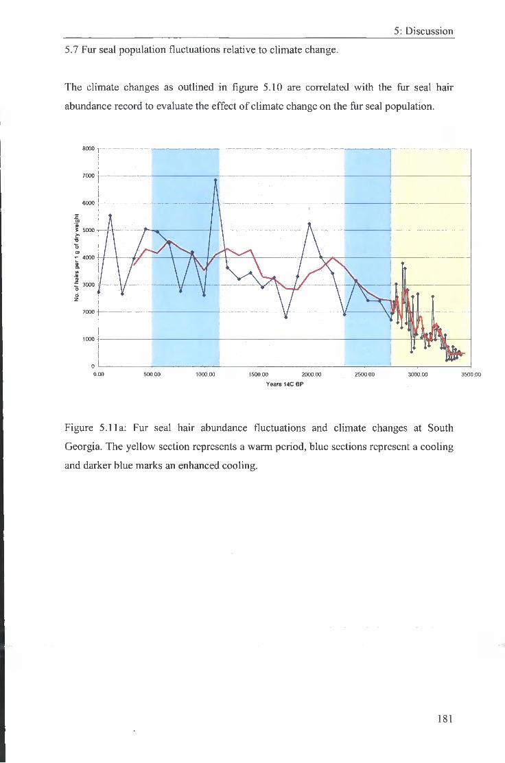
5: Discussion
5.7 Fur seal population fluctuations relative to climate change.
The climate changes as outlined in figure 5.10 are correlated with the fur seal hair
abundance record to evaluate the effect of climate change on the fur seal population.
8000
4000
1500.00 2000.00
Years 14C BP
2500.00 3000.00 3500.00
Figure 5.11a: Fur seal hair abundance fluctuations and climate changes at South
Georgia. The yellow section represents a warm period, blue sections represent a cooling
and darker blue marks an enhanced cooling.
181

5: Discussion
i f is •s-s
.Be+6
l.6e+8
1,4e+B
l.Oe+6
BOe+5
BOe+5 4 0e+5
3 5e+5
3 0e+5
2,De+5
.58+5
1000 3000
14 0 yrs BP
Figure 5.11b: Fur seal hair abundance fluctuations correlated with copper and zinc
fluctuations and climate changes at South Georgia.
5.7.1 Late Holocene Climate Optimum (Pre 2600 "*C yrs BP)
The low concentration and minimal fluctuations of elements in group A, B, C and D
suggest that the catchment was warm and stable from 3400-3100 '" C BP. This is in
agreement with other records from South Georgia that suggest a warm dry period (see
figure 2.11 and 5.10). As figure 5.11 indicates, at this time, the fiir seal population was
at a minimum for the past 3439 ''*C yrs BP, suggesting that wanner conditions are not
favourable for fiir seal population growth.
182

5: Discussion The most significant change in the geochemical record occurred at 3100 ''*C yrs BP, as
weathering and instability increased in the catchment, increasing the inputs into the lake
and hence, the rapid increase in element concenti-ations. This change at 3100 '' C yrs BP
correlates with a plateau in the far seal record, suggesting that although the population
were not negatively affected by climate change, it caused a stagnation of the population,
before then increasing again at 2900 ''*C yrs BP.
5.7.2 Climate Deterioration (2600-1600 ''C yrs BP)
It is widely documented that the warmer period ceased at 2600 '''C yrs BP, when a
significant cooling occurred (see figure 5.10). During the cooler period, an increase in
ice cover reduced the inputs into the lake causing a decline in the element
concentrations.
The fiir seal record peaks slightly at this point, as part of a longer-term tiend of increase,
suggesting that this brief glacial period was favourable for fiir seal population growth,
however, did not dramatically affect the fur seal population.
A larger increase in the fiir seal population is observed at 1980 '''C yrs BP, yet at this
point in the geochemical record there are no significant changes in any of the element
concentrations. In the climate record however, there does not appear to be a significant
climate change at this point. As figure 2.11 indicates, most climate records indicate this
was a period of cooling, sustained fi-om the widely documented climate deterioration at
2600 '" C yrs BP.
5.7.3 1100-200'^C yrs BP
The largest peak in the fiir seal population in the past 3439 ''*C years occurred at 1100
'''C yrs BP. Although this peak was brief, it is significant as the fur seal hair abundance
increases by a factor of 2 at this point. The geochemical record and other proxy records
suggest that the climate cooled and instability in the catchment increased from 1100 '" C
yrs BP and was sustained until 500 '''C yrs BP.
Although the fiir seal population increase was not sustained during this cooling period
(see figure 5.11), as I stated in section 5.4, the fur seal population cannot be sustained
above 4000 hairs per 1 g of dry weight at Humic Lake, therefore, although external
183

5: Discussion factors such as climate allow the population to increase, internal factors such as
competition for breeding ground between seals appears to limit the population.
The fur seal hair abundance remains relatively constant from 660 ''*C yrs BP, with the
general increase ceasing. There is however a notable peak at 440 '" C yrs BP. Due to the
change in sedimentation rate, and low resolution it is possible that this peak is in
response to the cooling at 600 ''*C yrs BP described by Bimie (1990).
5.7.4 200 ''*C yrs BP- present
The most recent climate record is derived primarily from historical records, rather than
proxy data. As the resolution of the core at this point is not known exactly (as outlined
in section 5.2.3), the core record caimot be used to accurately infer the fur seal hair
abundance and climate changes.
As highlighted in section 2.5 the fiir seal population during the past 200 '''C yrs BP
declined significantly and consequently increased dramatically from 1930 AD. Relating
this to climate changes (see figure 2.16) fur seal population increases broadly correlate
with climate wanning.
5.7.5 Summary
Figure 5.11 shows a summary of the fiir seal abundance record in relation to the climate
changes through the late Holocene. From 3439 '''C yrs BP, when the record began to
2700 '" C yrs BP the climate was warm, possibly warmer than today in a period known
as the late Holocene optimum. Through this period the fiir seal hair abundance in the
core gradually increases.
Although the geochemical record suggests climate deterioration conmienced earlier than
the climate record, the peak of cooling occurred from 2700 - 2400 '''C yrs BP (see
figure 5.10). The climate remained cool post 2400 '''C yrs BP however, at this point,
there is not a significant change in the fiir seal hair abundance. As figure 5.10 suggests,
this was a period of increased ice cover hence, inputs into the lake at this time were
minimal restricting inputs into the lake. The peak in fur seal hair abundance at 2000 '''C
yrs BP, suggests cooler conditions are favourable for fur seal population growth.
184

5: Discussion As figure 5.11 shows, the climate cooled from 1100 '" C yrs BP (Bimie 1990), again
correlating with an increase in the fiir seal hair abundance however, this increase is not
sustained through the cooling period as the population rapidly declines beck to previous
levels and continues to gradually increase to the top of the core.
5.8 Factors controlling fiir seal population changes in the late Holocene
During the late Holocene, although fiir seal populations have continually increased from
3439 '''C yrs BP, perhaps reflecting the recovery of the population following the
Holocene Climatic Optimum, larger peaks in the population generally correlate with
colder periods (see figure 5.11). Although the core does not extend back to the
Holocene Climatic Optimum, at 3439 ''*C yrs BP, the population was very low
suggesting that the climate conditions were not conducive to fiir seal population growth.
As the climate cooled, fiir seal population growth increases dramatically.
As discussed in chapter 2, the prime factors influencing fiir seal population growth are
prey availability and predator competition therefore, it can be inferred that at South
Georgia, as the climate cools, prey availability and predator competition become more
favourable for fiir seal population growth.
5.8.1 Prey availability
Assuming krill has been the primary prey for the fiir seal through the late Holocene, it
appears that krill availability is more favourable for fiir seals during cooler climates.
Although there is no single environmental variable found to show a reliable and
predictable relationship for distribution of krill relative to climate, broad scale
relationships have been found relating to temperature and oceanic fronts (Trathan et al.
2002).
The krill population at South Georgia is not self-sustaining, with the majority of krill
fransported to the region from the Antarctic Peninsula, South Orkney and the Weddell
Sea via the ACC (Antarctic Circumpolar Current) (Reid et at. 1999; Meredith et al.
2005; Hofinann and Murphy 2004). Variability in the krill population is thought to be a
consequence of the amount of krill that becomes enfrained within the ACC at sites
upstream of South Georgia or as a result of the spatial and temporal variability in the
transport mechanism itself (Hofinatm and Murphy 2004). The magnitude of this change
185

5: Discussion is dependant upon how much the front moves, how quickly it returns to its former
position and the time of year the movement occurs (Trathan et al. 2003). As the
atmosphere and ocean are a highly coupled system, changes in oceanography are
simultaneous with changes in terrestrial temperature hence, correlating with climate
changes. The precise movement of these oceanographic fronts through the late
Holocene is debatable and therefore, the exact movement of these fronts cannot be
accurately correlated with fur seal population changes to determine whether this
influenced the growth of the fur seal population. At present, areas of high krill
abundance are located in the area between the SACCF and the SACCB, close to the sea
ice boundary (see figure 5.12). The location of these fronts is highly variable. During
colder, glacial periods, the polar frontal zone is located further north and therefore,
increases the proximity of the SACCF in relation to South Georgia hence, the krill
fransported into the ocean waters surrounding South Georgia reduces (Thorpe et al.
2002). During warmer periods, the SACCF is located fiirther south of South Georgia,
again reducing the krill transported to South Georgia. Optimum conditions for krill
transport are debatable, however, are thought to occur in a climate between these warm
and cold exfremes.
South Georgia
South Orkney Islands Sduth
Srtetland Islands
South Amer ca
South Po e SeH/ngshaicertSea
/Amundsen Sea
Mean distribution of sea ice in February Mean distribution of sea ice in September
Figure 5.12b: Mean sea ice boundary relative to South Georgia, South Shetland and
South Orkney Islands. The section in the red box is enlarged in figure 5.12b. Adapted
from Hansom and Gordon (1998).
186

5: Discussion
60*W so°w
Southf Island
Figure 5.12b: Scotia Sea region showing South Georgia relative to key oceanographic
features which influence the distribution of krill. Sub-Antarctic front (SAF), Polar Front
(PF) (dashed line indicates the position of the Polar Frontal Zone), and the Southern
Antarctic Circumpolar Current Front and Boundary (SACCF; SACCB). (Source:
Murphy and Reid 2001)
As Murphy and Reid (2001) indicate, today krill at South Georgia are on the northern
edge of their distribution and stock relies on immigration associated with regional
current systems. As the climate changes, the krill frack shifting climate and hence, the
distribution of krill alters in relation to climate change (Walther et al. 2002). During
periods relatively cooler than today krill were more abundant and thus, the prey
availability for fiir seals increased. Alternatively, during warmer periods, the northern
extent of krill was located further south than today, thereby decreasing the prey
availability for fiir seal populations at South Georgia.
Despite this, it must be noted that, krill populations declined in 1998/99 and 2000/01,
both of these years being linked to cold anomalies the in Southern Ocean. In 2000/03
these changes are thought be the result of changes in the path of the SACCF bringing
colder water closer to South Georgia than in other years (Meredith et al. 2005). The
cold anomaly in 1998/99 is linked to the 1997/98 El Nino event and is not directiy
linked to the changes in the path of SACCF and hence, the krill distribution at South
187

5: Discussion Georgia. Although it is widely recognised that El Nino events do affect krill
distribution, the affect of this at South Georgia has not been fully quantified and will not
be considered in detail here. These different factors affecting krill distribution illustrates
how complex the system is and krill distribution cannot be solely defined as dependant
upon the SACCF. Although this has implications for analysis and must be considered,
these cold anomalies were annual events and therefore, the changes experienced during
a cooling of the magnitude at 2600 '" C yrs BP is likely to be greater than this annual
variability.
Alternative evidence suggests that patterns in sea ice distribution and abundance affect
krill productivity and recruitment (Reid et al. 1999; Murphy et al. 1998). A reduced
krill biomass is thought to be associated with periods of low ice extent. From this it can
be inferred that in a colder period, ice extent is greater and hence, is more favourable to
greater regional immigration of krill into the South Georgia area. In warmer periods, sea
ice declines and krill abundance falls hence, agreeing with the correlation found in
figure 5.11.
Smith et al. (1999) outiine a model for adelie penguin growth in relation to sea ice
distribution. Here population growth increases during conditions of moderate sea ice
cover, between extremes of excessive and insufficient ice cover. Although fiir seal
populations at South Georgia grow during colder periods, an exfreme cold situation
does not appear to have been reached during the late Holocene as the population does
not show any indication of decline during cold periods. However, this is only a
hypothesis and it is not clear how oceanography and sea ice variability are linked and
how this may affect krill distribution. Conversely, evidence presented by Hofinann and
Murphy (2004) suggests that the distribution of krill does not show any relationship
with winter sea ice distribution or fronts.
5.8.2 Predator competition
Although prey availability is a fiindamental factor affecting fiir seal population growth,
predator competition also plays an important role (see section 2.7.3.2). Sea ice extent
increases in response to oceanographic and climatic changes. Changes in sea ice as
Boveng et al. (1998) highlight, increase the abundance of leopard seals, a fiir seal
predator. During cooler periods, although prey availability increases, it is also possible
188

5: Discussion that the predator competition increases. As Boveng et al. (1998) argue, the predator
competition on the South Shetland Islands is greater than at South Georgia due to the
location of South Shetland Islands relative to the position of sea ice (see figure 5.12).
The point of optimum fur seal population growth is likely to occur when sea ice
increases and hence, increases the abundance of krill but not to such an extent to
increase leopard seals, thus, fur seals perhaps survive when sea ice extent is not at its
maximum extent but to a greater extent than today. This would explain why the fur seal
population did not notably increase during the coldest periods, as the sea ice may have
been too extensive, thereby increasing the predator competition. As the climate warmed
slightly from the maximum cold period, sea ice declined thus, decreasing the predator
competition whilst krill availability was still enhanced sufficientiy to allow population
growth.
Increased sea ice extent is also likely to bring other changes such as a variation in
species, and perhaps increasing the competition for krill. For example, as I stated in
section 2.7.3.1.1, emperor penguins are positively correlated with sea ice extent and
therefore, the increase in these species may affect the availability of krill due to the
increased competition. Alternatively, increased sea ice extent is likely to cause a decline
in some species (e.g. adelie penguins), therefore, reducing the competition for prey.
Although these factors must be considered, this change in species is unlikely to have
greatly affected the fur seal population due to the dynamic nature of ecosystems, as
although some species may be unable to survive, different species are likely to increase
with the change in conditions.
5.8.3 Summary
Fur seal populations at South Georgia appear to increase during cooler periods.
However, due to the complex interactions between the ocean and atmosphere, it is
difficult to ascertain the reasons for this increase in fur seal populations during cold
periods. Evidence from past studies suggests that the primary influence on fur seal
population growth is prey availability (krill) (see section 2.7.4). This increase in prey
availability is either a consequence of ocean currents moving northward or an increase
in sea ice or possibly (due to the highly coupled oceanographic system) a combination
of both factors. A change in oceanography alters the sea ice extent, which increases the
availability of krill and therefore, increases the prey availability for fur seals. During
189
5: Discussion warmer periods, sea ice extent decreases and the availability of krill declines. Although
to fiilly understand the reasons for the increase in fiir seal populations, krill dynamics in
relation to oceanographic changes must be understood fiirther. As I have outiined in
section 5.8.2, predator competition is a potential influential factor on the fiir seal
population growth, however, the knowledge of predator competition on South Georgia
is limited. To accurately correlate fluctuations in predator competition with fiir seal
population changes, the interactions of the predators at South Georgia must be
understood.
5.9 Recent changes
Although it is difficult to determine changes in recent fiir seal populations through the
20* century from this study, it can be stated that fiir seal populations have increased
dramatically through the late Holocene and therefore, increases noted today are not
unprecedented. Although the magnitude of change is unprecedented, the trigger for this
change does not correlate with the factors affecting population growth during the late
Holocene. As discussed in section 5.8, prior to human intervention fur seal populations
increased during cooler periods as a consequence of abundance in krill. This increase in
krill is closely correlated to an increase in sea ice extent. As the climate during the 20*
century is warming, it is expected that the fiar seal population would decline. However,
it is widely recognised that the population has increased (see figure 2.17) due to a rise in
prey availability caused by the sealing and whaling industries in the 19* Century (see
section 2.7.2). As these activities are human induced, it can be concluded that fiar seal
population changes in the 20* century are a result of human induced change, creating a
population growth of fiir seals to a greater magnitude than natural environmental
changes during the Holocene.
5.10 Past studies
Comparing these results to the study by Sun et al. (2004a) and Hodgson et al. (1998),
this conclusion does not appear to be valid at Signy Island or King George Island.
5.10.1 Hodgson et al's. (1998) study - Signy Island.
Evaluating the fiir seal population reconstruction at Signy Island with South Georgia,
there does not appear to be any significant correlation (see figure 3.2). The fiir seal
190

5: Discussion
population at Signy Island does not show any significant peaks through the past 6570
'" C yrs BP, with the exception of a rapid increase from the 1970's to the present day.
Fur seal hair abundance is also a magnitude lower here than the records at South
Georgia.
5.10.2 Sun et al's. (2004a) study - King George Island
Sun et al. (2004a) reconstruct the fiir seal population on King George Island for the past
2367 '''C yrs BP. The record of the fiir seal population (see figure 3.6) suggests that the
population increased from 1400-1100 ''*C yrs BP and 750-500 '''C yrs BP, hence,
presenting a similar picture to that of the South Georgia record (see figure 5.2).
The first peak from 1400-1100 '''C yrs BP correlates with a peak at 1100 '' C yrs BP in
the record from South Georgia (see figure 5.2). The increase at South Georgia
commences at approximately 1320 ''*C yrs BP however, due to the low resolution this is
difficult to evaluate exactly. This peak in the South Georgia record suggests that the fur
seal population increase lags the King George Island population increase by
approximately 100 years. The second peak in the record by Sun et al. (2004a), from
750-500 '''C yrs BP correlates with the peak at 440 '"C yrs BP at South Georgia. Further
suggesting population increase lags the King George Island population by
approximately 100 years. Although the record at King George Island extends back to
2300 '"C yrs BP, the evidence suggests that the fiir seal population has been present on
the island from only 1400 ''*C yrs BP (see figure 3.6), significantiy shorter than the
population at South Georgia.
The sfrong correlation between the record at King George Island and South Georgia
suggests that a regional forcing factor such as a climate change was causing a fiir seal
population increase at approximately 1100 '''C yrs BP and 500 '" C yrs BP. Although
fluctuations in both studies are similar, the reasoning for the change is conflicting. Sun
et al. (2004a) conclude that the change in fiir seal hair abundance correlates with
warmer periods whereas fluctuations at South Georgia correlate with cooler periods (see
section 5.8.3). This conflict can be explained using a model of optimum sea ice
conditions as outiined by Smith et al. (1999).
191

5: Discussion 5.11 Optimum sea ice conditions hypothesis
Smith et al. (1999) suggest krill populations are closely correlated to sea ice
distribution, therefore, are affected by climate change. From a study of adelie penguins,
the optimum level of krill availability is thought to be between two extremes of sea ice
cover; excessive and insufficient ice cover. Depending upon the location of the breeding
sites, the penguin population can increase and decrease at two different locations during
the same period of time (see figure 5.13).
'X,
mm
Figure 5.13: Conceptual model indicating the direction of Adelie penguin population
changes in relation to sea ice extent (source Smith et al. 1999). This model highlights
that in years of lower sea ice cover, populations of Adelie penguins in the Ross sea
increase, whereas they decrease in the Palmer region.
Relating this model to fiir seal populations, the population at South Georgia is near the
limit of present day sea ice extent (see figure 5.12) therefore, any decrease in
temperature increases the sea ice extent and hence, increases prey availability (Hansom
and Gordon 1998; Smith et al. 1999). Using this hypothesis, it can be inferred that due
to the positive correlation of fiir seal population and prey availability, (as discussed in
section 2.7.4) the fur seal population will increase at South Georgia during cooler
periods.
192
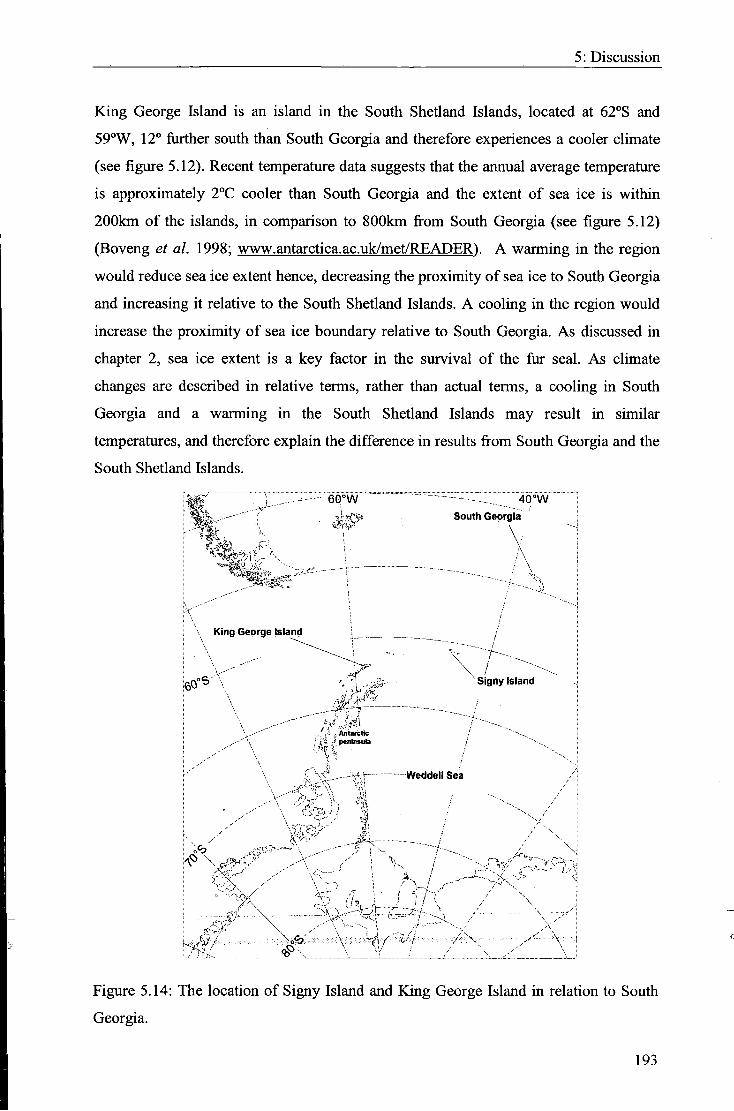
5: Discussion
BCing George Island is an island in the South Shetland Islands, located at 62°S and
59°W, 12° further south than South Georgia and therefore experiences a cooler climate
(see figure 5.12). Recent temperature data suggests that the annual average temperature
is approximately 2°C cooler than South Georgia and the extent of sea ice is within
200km of the islands, in comparison to 800km fi-om South Georgia (see figure 5.12)
(Boveng et al. 1998; www.antarctica.ac.uk/met/READER). A warming in the region
would reduce sea ice extent hence, decreasing the proximity of sea ice to South Georgia
and increasing it relative to the South Shetland Islands. A cooling in the region would
increase the proximity of sea ice boundary relative to South Georgia. As discussed in
chapter 2, sea ice extent is a key factor in the survival of the fur seal. As climate
changes are described in relative terms, rather than actual terms, a cooling in South
Georgia and a warming in the South Shetiand Islands may result in similar
temperatures, and therefore explain the difference in results from South Georgia and the
South Shetland Islands.
60°W
•^"•SSS MX -
King George Island
,A i iUre t io
40°W South Georgia
' Signy Island
Weddell Sea
=fc3t \
Figure 5.14: The location of Signy Island and King George Island in relation to South
Georgia.
193

5: Discussion
Figure 5.15 shows an adaptation of figure 5.13 to suit fur seal populations in the Sub
Antarctic Islands. Line A illustrates the situation during a warmer period (relative to
today), therefore, the number of fur seals on South Georgia decreases as the sea ice
extent reduces and prey availability declines. On King George Island, as sea ice
declines, the boundary of the sea ice extent moves closer to King George Island and
therefore, prey availability rises hence, increasing fur seal populations. During a cooler
period (relative to today) the situation is shown in line B. As sea ice extent increases at
South Georgia prey availability increases, therefore, the fur seal population at South
Georgia grows. However, the sea ice extent is too great at King George Island for
optimum levels of prey availability hence, the fur seal population decreases.
Lower
King George Island South Georgia
Sea Ice extent Higher
Figure 5.15: Conceptual model illustrating fur seal population changes in relation to sea
ice extent (adapted from Smith et al. 1999). The black line is an approximation of the
situation today, although the exact magnitude and position of the islands cannot be
determined with the available data. Line A (blue line) indicates a climate relatively
cooler than today. Line B (yellow line) indicates a climate relatively warmer than today.
Although this model may not explain all the variation in the record, it does clarify the
general trend and agrees with the conclusion that fur seal population fluctuations are
intimately related to sea ice distribution. Details in the fur seal hair abundance record
however, are not accounted for in this figure and it does not explain the greater
fluctuations in the fur seal population at King George Island compared to South
Georgia. On King George Island, fiir seal populations decline rapidly between peaks,
194

5: Discussion
whereas at South Georgia the population is continually increasing from a minimum at
the base of the core. However, larger peaks occur at South Georgia at a similar time to
those on King George Island therefore, it is possible that a larger population at South
Georgia can be sustained as a consequence of more favourable environmental
conditions and predator relationships. As a larger population can be sustained, the
climate variability does not affect the fiir seals as significantly as at King George Island
and hence, population decline is not as evident in the record.
5.11.1 20* Century changes
Although the model outlined in figure 5.15 correlates with changes in the fur seal
population during the late Holocene, it caimot be applied to 20'* century changes in the
fiir seal population as the population is increasing during a period of warming, opposite
to the trend modelled in figure 5.15. Figure 5.16 shows an adapted model of figure 5.15
to incorporate 20* century changes. The blue line shows the potential fiir seal
population during the 20* century vinder krill surplus conditions, when the potential fiir
seal population is greater. The magnitude of this is unknown and cannot be evaluated
until the fiir seal population begins to decline at South Georgia, as indicated at point A
in figure 5.16. Once this threshold has been reached and the krill availability is no
longer sufficient to sustain the fiir seal population, the fiir seal population wil l decline at
South Georgia. On King George Island however, the population may continue to
increase due to the warmer climate conditions.
The situation today is not known exactly but is located on the line between points A and
C as it is known that a krill surplus effect exists (Croxall et al. 2002). The results of the
fiir seal hair abundance suggest that the fiir seal population today is not greater than the
population during the late Holocene; therefore, it is likely that the population is located
between points B and C. Due to the resolution of the core, this is not known exactly (see
section 5.2.3) therefore, it is possible that the population today has exceeded the
optimum fiir seal capacity of the Southern Ocean prior to the krill surplus hence, the
population may be at a point between point A and B. Once point A is reached, i.e. the
krill surplus effect is no longer effective at South Georgia and it is likely that the fiir
seal population will begin to decline.
195

5: Discussion
King GeoTse Island Optimum SoulhOcoisia
Lower Sea Ice extent Higher
Figure 5.16: Conceptual model of fur seal population changes in relation to sea ice
extent and prey availability as a result of the Icrill surplus effect during the 20"' century.
The black line indicates the fur seal population in relation to sea ice conditions prior to a
krill surplus; the blue line indicates the fur seal population in relation to sea ice
conditions during a period of krill surplus.
5.11 Summary
The above discussion suggests that the fur seal populations on South Georgia, and in the
sub-Antarctic region as a whole are influenced primarily by krill availability, both
during the late Holocene and during the 20* century. However, the mechanisms causing
the change in krill availability has varied, from natural environmental change pre 200
yrs BP to human induced changes post 200 BP. The implications of this in terms of
predicting future changes and implementing management measures wil l be addressed in
the following chapter.
196

6: Conclusions
Chapter 6
Conclusions
Plate 6: Fur seals and penguins on the beach at Maiviken, South Georgia.
196

6: Conclusions
6 Conclusions
This chapter outiines the main conclusions of this thesis and is structured using the
objectives discussed in chapter 1.
6.1 Objective 1: To reconstruct fur seal populations through the late Holocene by
counting seal hairs from a lake on South Georgia.
Using fiar seal hair abundance as a proxy for fur seal populations, allows an indication
of the fluctuations and magnitude of the population through the core. From this record,
it can be inferred that the fiir seal population on South Georgia has been present for at
least the past 3439 '"C yrs BP. At the beginning of the record (3439 '" C yrs BP) the fiir
seal population at South Georgia was the lowest it has been for the past 3439 ''*C years.
From this minimum, the fiir seal hair abundance record suggests the population
increased and plateaued at a level approximately 4000 hairs per 1 g of dry weight (see
figure 5.2). Although the population increased beyond this level, peaks were brief and
only lasted c. 300 years before declining back to previous levels.
6.2 Objective 2: To reconstruct fiir seal populations indirectly using geochemical
analysis, following the method outlined by Sun et al. (2004a).
At South Georgia, none of the elements tested for can be used to reliably reconstruct the
fiir seal population during the past 3439 '' C yrs BP. Zinc and copper are the most
closely correlated to fiir seal hair abundance however, the fiir seal signature is only seen
when the population reaches a threshold of 1500 hairs per 1 g of dry weight. Other
elements such as carbon and nitrogen correlate with the fiir seal population when the
catchment is stable. However, a large catchment change occurs at approximately 3000
''*C yrs BP, increasing the concenfration of carbon and nitrogen, obscuring the fiir seal
signature in this record.
On South Georgia, the fur seal signature is not as evident in the geochemistry as in
previous studies, this can be attributed to factors such as catchment stability, vegetation
cover and seal populations. Evidence presented in this study suggests that the elements
highlighted by Sun et al. (2004a) as bio indicators for fiir seal population are not
197

6: Conclusions
transferable from one catchment to another as each catchment displays different
characteristics such as biological composition, climate conditions and lake circulation.
For example, at South Georgia, tussock grass is abundant in the catchment, and affects
the chemical composition of the lake sediments, in areas where this is not as abundant,
such as King George Island, the fur seal signature is likely to be more pronounced.
6.3 Objective 3: To determine whether the recent (20* -21^' century) increases in fur
seals have exceeded the range of natural variability of past populations.
Due to the unexpectedly low resolution in the top part of the core and the ^^^Pb/' Cs
dating problems, evaluating the 20* and 21^* century changes in the population is
difficult. In this thesis I assume that the core top is equivalent to 0 yrs BP (reasons for
this are outlined in section 5.2.3). I f this is correct then the fiir seal population during
the 20* and 21^* century does not appear to be significantly higher than at any time
during the past 3439 '' C yrs BP.
In addition to the actual size of the population, the rate of the fur seal population
increase at South Georgia during the 20* century is a cause for concern (see section
2.5). During the 20* century, the population has increased c. 10 -10^ times in 100 years
(see figure 2.17). As section 5.4 outlines, increases of a similar magnitude are observed
through the late Holocene. Figure 5.2 highlights that the fur seal population growth has
been greater than growth today at two separate points through the core. Firstly, when the
population was at a minimum, as observed at the base of the core, the population
increased 10 fold. Secondly; once the population reached a threshold (4000 hairs per Ig
of dry weight), i f it increased beyond this level, increases were dramatic but brief before
the population declined back to similar levels. Using these two hypotheses, 20* Century
increases in the fur seal population are not unprecedented through the Late Holocene
and are expected as the population is recovering from almost extinction at the begirming
of the 20* Century.
6.4 Objective 4: To review and assess the impact the environmental changes on South
Georgia have had upon seal populations over the same time period of the Holocene.
The largest peaks in fur seal population occur during periods of climate deterioration at
South Georgia (see figure 5.11). However, studies on other sub-Antarctic islands (e.g.
198

6: Conclusions
King George Island) correlate increases in fiar seal populations with warming (Sun et al.
2004a). This apparent paradox can be explained by analogy using a model correlating
penguin populations and sea ice extent as outiined by Smith et al. (1999) (see figure
5.13). From past research (see section 2.7.4), the primary controls upon the fiir seal
population are prey availability and predator competition. Prey availability is sfrongly
controlled by the distribution of sea ice. The zone of optimum sea ice conditions for
krill availability and hence, fiir seal population growth today is located between King
George Island and South Georgia. Although the oceanography of the Southern Ocean is
complex and not fially understood, the general principle is that during a cooling these
optimum conditions migrate closer to South Georgia, whereas during a warmer period,
they migrate closer to King George Island. As krill populations closely follow the sea
ice distribution, this movement of sea ice, alters the krill availability and hence, the prey
availability for fiir seals (see figure 5.15).
It is widely documented that relative to the late Holocene climate, the 20* Century was
a period of warming. Census data shows the fiar seal population has increased during
this period in contrast to the palaeo record where populations augment during cooling
periods. Using this theory, it can be inferred that the increase in 20* century fur seal
populations are not a result of natural environmental changes. As 20* century changes
in the fiar seal population are not related to natural environmental changes, the changes
must be a consequence of human-induced factors. The most likely human induced cause
is the whaling industry that resulted in a krill surplus in the Southern Ocean. This
surplus increased the krill availability for fur seals, providing the same effect as
increasing sea ice extent, leading to population growth. The effects of this on seal
populations were particularly spectacular due to the preceding exploitation of seals to
near extinction.
6.5 Objective 5: To determine the factors controlling fur seal population changes at
South Georgia through the late Holocene.
From this evidence, the primary control on the fiir seal population through the late
Holocene is prey availability. Prior to human intervention, prey availability was
controlled by sea ice distribution and hence, climatic fluctuations. During the 20*
century, although the climate conditions do not suggest an increase in prey availability
at South Georgia, human intervention caused an artificial increase. In this way this
199

6: Conclusions
study confirms the assertions by Croxall (1992) that the krill surplus has been the
primary driver for 20* century fiir seal population increases on South Georgia.
6.6 Overall aim
My aim was to reconstruct the fiir seal population of South Georgia by counting seal
hairs from a South Georgia lake sequence as a proxy for fur seal abundance combined
with geochemical analysis using techniques outiined by Hodgson et al. (1998) and Sun
et al. (2004a). Comparing the population fluctuations in 20* century and late Holocene
fiir seal populations allowed the controlling factors underlying fur seal population
fluctuations to be better understood and hence, aid management and conservation
decisions.
As figure 5.2 shows, the fiir seal population has been reconstructed from fur seal hair
abundance. The use of geochemical analysis for reconstructing the fur seal population in
this study has not proved successful and has highlighted the problems in tiansferring
geochemical signatures between catchments. Although the 20* century population
cannot be precisely compared with late Holocene population fluctuations due to the
resolution of the core, assuming that 0 cm is 0 yrs BP, the 20* century changes are not
unprecedented. The factor confrolling these fiir seal population changes through the past
3439 '''C yrs BP has been primarily prey availability, influenced by sea ice and hence,
climate changes before human intervention. As krill populations during the Late
Holocene are only estimates, the magnitude of the krill increase during the 20* century
cannot be accurately quantified, however, it is widely recognised that the krill
population has increased during the early 20* century due to the krill surplus effect.
This artificial increase in prey availability as a result of human intervention has caused a
consequent increase in the fur seal population.
In term of addressing the management issues associated with the fiir seal population at
South Georgia (see section 2.8.1), evidence from this study suggests that management
may not be necessary. The fiir seal population at South Georgia through the Holocene
was at levels as high i f not higher than the fur seal population today. Following a large
increase, the fur seal population returned back to previous levels as part of the natural
cycle. Although the actual trigger for 20*-21^' century increases in population was not
200

6: Conclusions
part of the natural cycle, there is strong evidence to suggest the mechanism by which it
occurred (prey availability) as the same.
6.7 Future change in the fur seal population at South Georgia
As the factor controlling the fur seal population (prey availability) is the same through
the late Holocene, it is clear that this increase cannot be maintained once prey
availability reaches a threshold. Once the krill surplus period ceases, the prey
availability wil l reduce and it is likely that the fur seal population wil l decline (see
figure 5.16). I predict that the fur seal population will cease to increase and the
population will plateau at a level equivalent to the deposition of ~ 4000 hairs per 1 g of
dry weight. This estimate however, is based upon evidence from past natural
environmental change and the impact of human induced changes may be more extensive
than initially thought. For example the effect of climate phenomena such as El Nino on
the fur seal population has not been assessed in this study. As Croxall et al. (2002)
highlight. El Niiio affects sea ice processes in the Southern Ocean. The effect on the
krill population is not fully understood and therefore, to comprehend factors affecting
fur seal populations, the mechanisms affecting sea ice distribution and krill distribution
must first be fully comprehended. In addition to this, human impacts on the krill
population such as the growth of krill fisheries or a change in location of the krill
fisheries wil l cause fluctuations in krill populations independent of natural long-term
climate changes (Croxall and Nicol 2004).
6.8 Summary
The fur seal population at Maiviken, South Georgia has been present for at least 3439
'''C years BP. Increases in the population are the most rapid when the population is very
low or during colder periods however, fur seal hair abundance plateaus at approximately
4000 hairs per 1 g of dry weight. Although increases are documented above 4000 hairs
per Ig of dry weight, these increases cannot be maintained for a sustained period of
time.
The primary factor influencing the fur seal population at South Georgia is prey
availability; hence, indirectly the mechanisms causing changes in prey availability
affect fur seal populations. Through the past 3439 ''C years BP there has not been a
201

6: Conclusions
time when the krill population at South Georgia has declined significantly enough to
cause extinction of the fur seal population. Prior to human intervention, prey availability
was primarily confroUed by sea ice distribution and hence, climate changes. During the
20* and 21^' century the primary factors affecting prey availability have been human
induced changes which have resulted in a krill surplus. Despite this, once such a surplus
ceases or the population reaches a threshold, the population wil l stop growing and it is
likely that the population wil l stabilise or decline.
Highlighting prey availability as the cause of fur seal population growth has improved
understanding of fur seal population fluctuations and the impact that human-induced
changes has upon these populations. Such findings can then be used to aid management
and conservation decisions. Correlating fur seal populations with sea ice distribution has
improved the understanding of the factors controlling fur seal populations; hence, past
fur seal populations could potentially now be used as an important indicator of
environmental change in the sub Antarctic region (Jouventin and Weimerskirch 1990).
202

7: Limitations and Further Research
Chapter 7
Limitations and Further Research
Plate 7: Fur seals in tussock grass
202

7: Limitations and Further Research
7 Limitations and Further Research
In light of the findings of this study as outlined in the previous chapter, it is important to
note that there are a number of limitations inherent in a study of this nature, not least
clear restiaints of time and logistics. For this reason I shall examine these limitations
below and the avenues that such shortcomings may open for fiiture research before
finally looking towards their relation to the projects overall outcomes.
7.1 Dating
7.1.1 ^'°Pb dating
As the ^'''Pb dating technique was unsuccessfiil, the top section of the core was dated
using a constant sedimentation rate calculated from radiocarbon dates deeper in the
core. This technique incurs a larger potential error in the dates at the top of the core and
therefore, the fluctuations noted in fur seal hair abundance during the 20* century
cannot be accurately determined and compared relative to the timing of the sealing and
whaling activity. As a consequence of this, the impact of human induced changes
cannot be as accurately evaluated as other studies have done (Hodgson et al. 1998).
Inaccurate dating in the top section of the core has also prevented the census data and
fiir seal hair abundance being compared and hence, the development of a transfer
fiinction which would allow the size of the fiir seal population prior to exploitation to be
quantified.
7.1.2 Radiocarbon dating
The radiocarbon dates obtained from the core show a reversal at the base of the core
(see section 5.1), as a result only two radiocarbon dates were used to date the whole
core. In addition to this, the top radiocarbon date was unexpectedly old resulting in the
resolution of the hairs in the top section of the core to be very low. Obtaining the
radiocarbon dates before calculating seal hair abundance would have allowed a greater
sampling resolution to be taken in the top section of the core and therefore, allowing the
time- stiatigraphic sampling resolution to be continuous through the core. Alternatively,
i f time had allowed, organic fragments in the sediment could have been extracted and
dated separately to determine the potential ageing effect of old carbon in the sediment.
203

7: Limitations and Further Research
Although this is dependant on fragments being present in the sediment, using this aging
factor, the dates radiocarbon obtained could have been corrected. Furthermore, as the
sedimentation rate at the top of this core was so low, an alternative core with a higher
sedimentation rate could have been used to reconstruct the fur seal population, hence,
providing a more accurate record of change during the 20* century which could be
compared to census data.
7.2 Fur seal hair abimdance
Although calculating fur seal hair abimdance provides a useful indicator of fur seal
presence, it does have its limitations that must be considered when analysing the data.
7.2.1 Human error
The method used to count fur seal hairs as this study demonstrates can incur a large
amount of error (see section 3.6) even using the same method of preparation and with
the same person counting. This presents problems in comparing the data from one site
to another and hence, developing a fransfer function which could be used to quantify the
fur seal population.
7.2.2 Population dynamics
Although using fur seal hair abundance as a proxy for fiir seal populations provides an
indication of the size of the fur seal population, the population dynamics and
interactions with the ecosystem caimot be deduced from this method thus, causing
difficulties in determining factors affecting past populations. A decline in fur seal hair
abundance implies a decline in the population however; it is possible that a decline in
fur seal hairs was a result of population migration due to a change in the localised
conditions rather than a system change such as a regional decline in krill or a climatic
change. Although this is reflected in the geochemical data, further cores from other
catchments would help to distinguish these localised changes from a large system shift
on South Georgia.
Furthermore, factors affecting the fur seal population historically may not affect the
population today due to evolution and the ability of the fur seal to adapt to differing
conditions. An example of this is a change in the prey availability; from recent research,
204

7: Limitations and Further Research
the primary prey of the fur seal at South Georgia is krill and research indicates that the
foraging behaviour of the fur seal changes to accommodate changes in prey distribution
and abundance (Green et al. 1989; Reid and Amould 1996; Boyd et al. 1994). Although
this is the case today, it is possible that past populations of fur seals were not as well
adapted, therefore, smaller more localised changes in prey abundance would have a
greater impact upon the population. Natural changes in prey availability in the past may
appear as a larger natural change than actually occurred due to the ability of the fur seal
to adapt to system changes, hence, comparing the magnitude of historical fur seal
population changes with changes today and inferring possible mechanisms for this
change has limitations.
7.3 Areas of further research
This was a time-limifed study and there are obviously a number of potential avenues
remaining for future research
7.3.1 Radiocarbon dates
Two of the radiocarbon dates were obtained after the fur seal hair abundance had been
assessed. Collecting these dates earlier in the study would have allowed the core top to
be sampled at a higher resolution based upon the age- stratigraphy rather than depth-
stratigraphy. Alternatively a core with a higher sedimentation rate at the core top could
have been analysed. A higher sampling resolution at the top of the core would have
allowed the 20* century changes in the fur seal population to be assessed to a greater
extent, therefore, allowing a more exact assessment of whether 20* century increases in
the population had occurred previously during the late Holocene.
7.3.2 Dating 'old' carbon
To determine the potential ageing effect of the carbon on the sediment, visible organic
fragments could be exfracted from the sediment and radiocarbon dated separately. This
would provide an indication whether there has been significant sediment reworking.
Using this date, it may be possible to determine the dating error and provide a better
indication as to which radiocarbon dates are more accurate.
205
7: Limitations and Further Research
7.3.3 Palaecological analysis
To provide a baseline for the radiocarbon dates and hence, provide a greater indication
of the accuracy of the dates, palaeocological analysis could be implemented at key
sediment transisitions. Although Troels - Smith analysis (see section 4.1) indicates
uniform sediment for the majority of the core, the basal section of the core could be
analysed to determine when this sediment change took place and related to other proxy
records to determine the age of this key sediment change. Determining the cause of the
sediment change would also help to evaluate the accuracy of the radiocarbon dates
obtained and hence, provide a more robust age model.
7.3.4 Additional cores
As two separate cores were used (MAIVK and HUM3), there is a gap in the record.
Although this c.lO cm gap is relatively small, the exact size is unknown. During
exfraction, the position of the cores in relation to each other was calculated however, in
the field it is difficult to measure this difference accurately. At the time of coring an
additional core was extracted from the same point, covering this gap between M A I V K
and HUM3. Using magnetic susceptibility the cores could be aligned and allow the size
of the gap to be calculated accurately. This would allow the section of the sediment to
be analysed for fiir seal hair abundance and geochemistry, hence, providing a fully
continuous record of fiir seal hair abundance for the past 3500 years.
In addition to improving the core at the single study site, additional cores could be
analysed from other sites on South Georgia. The study of additional cores would
broaden the project and allow a fiirther insight into fiir seal population dynamics
through the Holocene. Potential sites for additional cores include those that could aid an
understanding of the expansion of the seal population both altitudinally and along the
coast of South Georgia as illustrated below.
Proposed sites for additional cores:
a. Altitude
206

7: Limitations and Further Research
Lewis-Smith (1988) highUghts slopes of 200 metres altitude are now being threatened
by fur seals at South Georgia. This is a higher altitude than any time previously during
the 20* century however, it is unknown whether fur seals have reached this altitude
previously during the Holocene (pre 1900), when census data is not available. Taking
further cores fi-om higher altitudes would provide an insight as to whether this situation
occurred previously and whether the environment can recover from such an event. It
would also provide an indication of the maximum fur seal population the area can
accommodate. For example, i f the population has previously reached similar levels to
today but not gone beyond this level, it may indicate that the carrying capacity of this
location has been reached, hi order to assess the maximum level that fur seals have
reached additional study sites are needed at the altitudinal limits of the fur seal breeding
range.
b. Bird Island
Bird Island is the main breeding ground for the fur seal at South Georgia; therefore, the
impact is the most pronounced. The first pup observed on South Georgia following the
sealing and whaling industries was on Bird Island (Payne 1977). As this was the first
site, the exact timing of the recovery of the fiir seal population can be calculated.
Census data indicates that the population growth migrated fi-om Bird Island, therefore,
population growth at Maiviken was delayed and the exact timing and causal mechanism
for this growth cannot be assessed accurately. Comparing the timing of changes in fur
seal abundance at Bird Island with changes on the mainland allows the rate of the
expansion to the mainland of South Georgia to be determined hence, the optimum
carrying capacity of Bird Island can be measured to aid in management decisions.
Due to the high population of fur seals on Bird Island, the fur seal census data of Bird
Island is the most accurate and extensive for the whole of South Georgia. This detailed
census data for the 20* century allows the number of fur seals to be accurately
correlated with the fur seal hair abundance, therefore, the number of fur seals during the
Holocene can be quantatively assessed through a transfer function.
c. Latitudinal transect
207

7: Limitations and Further Research
The fur seal population has migrated from a small colony on Bird Island to the main
island. Taking cores along a transect from Bird Island to the south of the main island
and reconstructing the ftir seal population would allow the rate of migration and the
impact this has had upon the environment to be assessed. A visual assessment of the
environmental conditions at each site compared relative to the fiir seal population allows
a greater understanding of the management measures required.
7.4 Continuing previous research
7.4.1 Sediment fraps
Hodgson et al. (1998) used sediment traps in the lake to calculate the number of hairs
frapped within the lake and the amount of mixing that occurred in the lake itself In the
traps, the number of hairs collected were calculated and used to indicate the trapped hair
that would be incorporated into the sediment at different times of the year.
Although I assumed the results of this study could be applied to the lake at South
Georgia, as the results from the geochemical analysis highlight (see section 4.4.7),
different catchments display different characteristics and therefore, it is likely that the
situation as observed in the Hodgson et al. (1998) study is not representative of the lake
at South Georgia. This affects the results of the fiir seal hair abundance; firstly sediment
traps allow the mixing of the lake to be calculated, therefore, allowing the best position
for the cores to be taken and facilitating the most accurate measure of fiir seal hair
abundance. For example, the coring site in this study may be a site that is particularly
abimdant in ftir seal hairs at the time of coring due to the flow within the lake. Taking
sediment traps allows an assessment of the flow within the lake, thereby preventing a
core being taken from a site not typical of the lake or i f the core is taken in a section of
the lake that is not representative of the lake as a whole, it allows for a correction in the
results.
7.4.2 Geochemical analysis
Following Sun et al. (2004a), I used geochemical analysis to evaluate elements that
could be used as potential bio indicators of fiir seal presence. Unfortunately, due to the
shortage of sample and the restrictions on instruments, fluorine and phosphorous,
(found by Sun et al. (2004a, b) to be indicators of fur seal and penguin populations)
208
7: Limitations and Further Research
could not be tested for. Analysing the similar elements as Sun et al. (2004a), allowed
the transferability of the bio element indicators at one site to be assessed. Although this
can be done to some extent, as a number of the elements Sun et al. (2004a) tested for
were also tested for in this study, it is still possible that the elements not tested for were
the most indicative of fur seal presence. With additional time and sample size these
additional analyses could be implemented.
7.4.3 Wider research issues
The above issues are possible study areas to explore i f the time were available however,
the issues outlined below are larger and wider ranging issues beyond the scope of an
individual study but should be noted as important issues that would enhance the results
of this study.
7.4.3.1 ^'°Pb and'^^Cs problems
To date there are few palaeolimnological studies at South Georgia that have
successfully used ^"'Pb and ' ^Cs dating (see section 5.2). Unpublished data suggests
previous studies have experienced problems in detecting low concentrations of "'Pb in
lake sediments (Rosqvist, G. pers. comm.). This apparent lack of ^'°Pb may be isolated
to this particular core due to loss of sediment or the lack of sediment used for detection
(see section 5.2.1 for further explanation), but as there have been no other studies that
have dated South Georgian lake sediments using ^'°Pb and '^'Cs successfully, it appears
to be an island wide problem. To fully assess this issue, further lake cores are needed
from a variety of locations across the island. The use of a variety of detectors and sizes
of sediment samples will also help to evaluate the cause of the lack of ^'°Pb and ' ^Cs in
the core.
7.4.3.2 Isotopes in hair
It is widely recognised that carbon and nitrogen isotope signatures can be used to frace
food webs and understand palaeodiets in terrestrial and marine ecosystems (Lajtha and
Michener 1994). The isotopic composition of food and fluids ingested by animals has a
sfrong influence on*the isotopic composition of their tissues: As carbon and nitrogen
isotopes fractionate in a predictable way between each trophic level the isotopic
composition reflects the trophic position of the animal (Koch et al. 1994; Hobson et al.
1996). In this way, measuring the isotopic composition of animal tissue provides an
209

7: Limitations and Further Research
indication of their position in the food web and hence, their diet. Using this theory, it is
possible that isotopes in fiir seal hair can be used to trace palaeodiet through the Late
Holocene
Carbon is fractionated by 3 primary processes; firstly preferential loss of '^C02 during
respiration, secondly preferential uptake of '^C compounds during digestion and thirdly
metabolic fractionation during synthesis of different tissue types. This fractionation
results in an enrichment of '^C by 1.1 %o at each trophic level (Michiener and Schell
1994; Rau et al. 1983). This carbon isotopic signature can be used to determine the
marine domain in which an animal is obtaining its prey, for example, values are
higher in nearshore food webs than in offshore food webs (Kurle and Worthy 2001).
Nitrogen isotopes are also fractionated during biological processes and therefore, can be
used as a fracer for dietary analysis and to determine the frophic level of given animals
(Minagawa and Wada 1984). Faure (1986) suggests that animal tissue is enriched in '^N
relative to dietary inputs and therefore, an average enrichment of 3.0%o of '^N is
observed at each trophic step (Faure 1986; Zhao et al. 2004). This enrichment of '^N
with each trophic step allows the position of the animal in the food chain to be assessed
(Kelly 2000).
Isotopic fractionation and the assessment of frophic positions in food webs has been
used in previous studies to provide an insight into whether modem pinniped populations
change in relation to human influences on the marine ecosystem or in response to longer
oceanographic or climatic changes (Burton and Koch 1999). Previous studies of
Antarctic Seals have indicated that Weddell Seals occupy a higher trophic position than
Ross seals and are considered the top predator in the Antarctic phocid ecosystem (Zhao
et al. 2004). Calculating the isotopic composition of fiir seals and comparing the carbon
and nitrogen isotopic ratios with other seals in the region, wi l l allow the ftir seal
competition for prey to be evaluated.
As Burton et al. (1999) highlight this method of determining the trophic position of
seals can also be used to determine the cause of historic population changes. As Hobson
et al. (1996) indicate, analysis of metabolically inactive tissues such as hair, skin,
whiskers, nails and feathers reflect the diet of individuals during the period of growth.
Using this theory, the isotopic ratios in hairs through the core could be used to assess
210
7: Limitations and Further Research
the changes in the trophic relationships of the Antarctic fur seal through the Holocene.
This would provide an indication of the influence prey availability has upon the fur seal
population, which can be used to assess the impact human induced changes and natural
environmental change have had upon the 20* and 21^' century increases in populations.
7.4.3.3 Sea ice conditions
De la Mare (1997) highlights the possibility of reconstructing the sea ice boundary of
the Southern Ocean during the 20* century from whaling records. As fur seal
populations correlate with krill distribution and therefore sea ice extent, a similar
principle can be used to reconstruct sea ice extent during the late Holocene using fur
seal hair abundance records. As I have highlighted in section 5.11, with the record from
only two islands (South Georgia and King George Island), an indication of the sea ice
extent can be inferred. Reconstructing the fur seal population on a range of islands in
the sub Antarctic region would allow this to be more fully understood and therefore,
enhance understanding of the factors this affects such as productivity and oceanic
circulation. Such a move will also help to comprehend climate changes and the possible
impacts this has upon other species. For example, as Croxall et al. (2002) highlight,
adelie penguins and emperor penguins are closely related to sea ice distribution,
therefore, reconstructing sea ice distribution through the late Holocene would provide
an indication of their distribution in the Southern Ocean through the late Holocene.
7.5 Summary
Despite the limitations outlined in this chapter there are a number of important
outcomes to emerge from this study that can be taken forward in future research. As I
have discussed, dating the core restrained the scope of this study as the 20* century
changes in fur seal hair abundance could not be accurately compared to Late Holocene
population fluctuations, therefore, it cannot be accurately assessed whether 20* century
population growth is unprecedented during the late Holocene. Despite this, an important
outcome of the study is the correlation between fur seal population growth, sea ice
extent and the reliance of the fur seal population upon krill availability. From this
correlation, as fur seal populations during the 20* century are increasing during a
warming period, it can be deduced that population changes at this time are not a result
of natural environmental changes. As a result, it can be concluded that 20* century
population increases are a consequence of human induced changes, primarily a result of
211

7: Limitations and Further Research
the krill surplus. This linkage can be used to predict fiature population shifts thereby
aiding important decisions for fixture management and conservation of the Antarctic fiir
seal population both at South Georgia and the Southern Ocean.
212

Appendix
Appendix 1
Fur seal hair counts
These are the counts of fur seal hair abundance expressed as number per 1 g of dry
weight. Each sample was counted 3 times however as the first count (count a) was
significantly higher, only the second and third counts (count b and count c) are used in
analysis. Sample depth is the actual sample niimber without correction for core
shrinkage, actual depth is the depth in the core after correction for shrinkage using
equation 3.1 outlined in section 3.1.1. SD is the standard deviation of the counts for
each sample. Average SD is the average of the standard deviations for each individual
sample, which is used as the error in the data.
213
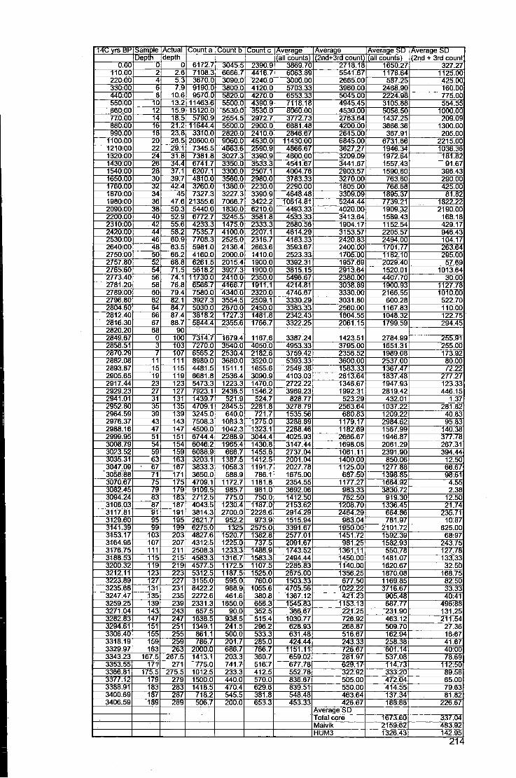
1 4 C y r s & P Sample Actual Count a Count b Count c Average Average Average SD Average SD Depth depth (all counts) (2nd+3rd count) (all counts) (2nd + 3rd count
0.00 0 0 6172.7 3045:5 2390.9 3869.70 2718.18 1650.27 327.27 110.00 2 2.6 7108.3 6666.7 4416:7 6063:89 5541.67 1178.64 1125.00 220:00 4 5.3 3670.0 3090:0 2240.0 3000.00 2665.00 587.25 425.00 330.00 6 7.9 9190.0 3800.0 4120.0 5703.33 3960.00 2468.90 160.00 440:00 8 10.6 9570.0 5820.0 4270.0 6553.33 5045.00 2224:98 775.00 550i00 10 13:2 11463.6 5500:0 4390.9 7118.18 4945.45 3105.88 554.55 660:00 12 15.9 15120.0 5530:0 3530.0 8060:00 4530.00 5058.50 1000.00 770.00 14 18.5 5790.9 2554.5 2972.7 3772.73 2763.64 1437.25 209.09 880:00 16 21.2 11644.4 5500:0 2900.0 6681.48 4200.00 3666.36 1300.00 990.00 18 23.8 3310.0 2820:0 2410.0 2846.67 2615.00 367.91 205.00
1100.00 20 26.5 20600.0 906o:o 4630;0 11430.00 6845.00 6731.66 2215.00 1210i00 22 29.1 7345.5 4663.6 2590.9 4866.67 3627.27 1946.34 1036,36 1320:00 24 31.8 7381.8 3027.3 3390,9 4600.00 3209.09 1972.64 181,82 1430:00 26 34.4 6741.7 3350.0 3533.3 4541.67 3441.67 1557.43 91.67 1540:00 28 37.1 6207.1 3300.0 2507.1 4004.76 2903:57 1590.60 396.43 1650.00 30 39.7 4810.0 3560.0 2980.0 3783.33 3270.00 763.60 290.00 1760.00 32 42.4 3260.0 1380.0 22300 2290.00 1805.00 768.68 425:00 1870:00 34 45 7327.3 3227.3 3390:9 4648.48 3309.09 1895.37 81.82 1980:00 36 47.6 21355.6 7066.7 3422.2 10614.81 5244.44 7739:21 1822.22 2090:00 38 50.3 5440.0 1830:0 6210.0 4493.33 4020.00 1909.32 2190.00 2200:00 40 52.9 6772.7 3245.5 3581.8 4533.33 3413.64 1589.43 168.18 2310:00 42 55.6 4233.3 1475.0 2333.3 2680.56 1904.17 1152.54 429.17 2420:00 44 58.2 7535.7 4100.0 2207.1 4614.29 3153.57 2205:57 946.43 2530:00 46 60.9 7708.3 2525.0 2316:7 4183.33 2420.83 2494.00 104.17 2640:00 48 63.5 5981.0 2136.4 2663.6 3593.67 2400.00 1701.77 263.64 2750:00 50 66.2 4160.0 2000.0 1410.0 2523.33 1705.00 1182.10 295.00 2757.80 52 68.8 6261.5 2015.4 1900.0 3392.31 1957.69 2029.40 57.69 2765:60 54 71.5 5618.2 3927.3 1900.0 3815.15 2913.64 1520.01 1013.64 2773.40 56 74.1 11730.0 2410:0 2350.0 5496.67 2380.00 4407.70 30.00 2781.20 58 76.8 6566.7 4166.7 1911.1 4214.81 3038.89 1900.93 1127.78 2789:00 60 79.4 7580.0 4340.0 2320:0 4746.67 3330.00 2166.55 1010.00 2796.80 62 82.1 3927.3 3554.5 2509.1 3330.29 3031.80 600.28 522.70 2804.60 64 84.7 5030.0 2670.0 2450.0 3383.33 2560.00 1167.83 110.00 2812.40 66 87.4 3818.2 1727.3 1481.8 2342.43 1604.55 1048.32 122.75 2816:30 67 88.7 5844.4 2355.6 1766.7 3322.25 2061.15 1799.59 294.45 2820.20 68 90 2849:67 0 100 7314.7 1679.4 1167.6 3387.24 1423.51 2784.99 255.91 2858.51 3 103 7270.0 3540.0 4050.0 4953.33 3795.00 1651.31 255.00 2870:29 7 107 6565.2 2530.4 2182:6 3759.42 2356.52 1989.08 173.92 2882.08 11 111 8980.0 3680.0 3520:0 5393.33 3600.00 2537.00 80.00 2893.87 15 115 4481.5 1511.1 1655.6 2549.38 1583.33 1367.47 72.22 2905.65 19 119 6681.8 2536.4 3090.9 4103.03 2813.64 1837.48 277.27 2917.44 23 123 5473.3 1223.3 1470:0 2722.22 1346.67 1947.93 123.33 2929.23 27 127 7923.1 2438.5 1546.2 3969.23 1992.31 2819.42 446.15 2941.01 31 131 1439.7 521.9 524.7 828.77 523.29 432.01 1.37 2952.80 35 135 4709.1 2845.5 2281.8 3278.79 2563.64 1037.22 281.82 2964.59 39 139 3245.0 640.0 721.7 1535.56 680:83 1209.22 40,83 2976.37 43 143 7508.3 1083.3 1275.0 3288.89 1179.17 2984.62 95.83 2988.16 47 147 4500.0 1042.3 1323.1 2288.46 1182.69 1567.99 140.38 2999.95 51 151 6744.4 2288.9 3044.4 4025.93 2666:67 1946.87 377.78 3008.79 54 154 6046.2 1965.4 1430:8 3147.44 1698:08 2061.29 267.31 3023.52 59 159 6088:9 666.7 1455.6 2737.04 1061.11 2391.90 394.44 3035.31 63 163 3203.1 1387.5 1412.5 2001.04 1400.00 850.06 12.50 3047.09 ' 67 167 3833.3 1058.3 1191.7 2027.78 1125.00 1277,88 66.67 3058.88 71 171 3650.0 588.9 786.1 1675.00 687.50 1398,85 98.61 3070.67 75 175 4709.1 1172.7 1181.8 2354.55 1177.27 1664,92 4.55 3082745 /9 179 9109:5 985.7 981.0 3692.06 983.33 3830.72 2:38 3094.24 83 183 2712.5 775.0 750.0 1412.50 762.50 919.30 12:50 3106.03 87 187 4043.5 1230.4 1187.0 2153.62 1208.70 1336.45 21.74 3117.81 91 191 3814.3 2700.0 2228.6 2914.29 2464.29 664:86 235.71 3129.60 95 195 2621.7 952.2 973:9 1515.94 963:04 781.97 10.87 3141.39 99 199 6275.0 1325 2575.0 3391.67 1950.00 2101.72 625:00 3153.17 103 203 4827:6 1520.7 1382.8 2577.01 1451.72 1592:39 68:97 3164.96 107 207 4312:5 1225.0 737.5 2091.67 981.25 1582:93 243.75 3176.75 111 211 2508.3 1233.3 1488.9 1743.52 1361.11 550.78 127.78 3188.53 115 215 4583.3 1316.7 1583.3 2494.44 1450:00 1481.07 133.33 3200.32 119 219 4577:5 1172.5 1107.5 2285.83 1140,00 1620.67 32.50 3212.11 123 223 5312:5 1187.5 1525.0 2675.00 1356.25 1870:08 168.75 3223.89 127 227 3155.0 595.0 760.0 1503.33 677.50 1169:85 82:50 3235.68 131 231 8422.2 988.9 1055.6 4705.56 1022.22 3716.67 33.33 3247.47 135 235 2272.6 461.6 380.8 1367.12 421.23 905.48 40:41 3259.25 139 239 2331.3 1650:0 656.3 1545.83 1153.13 687.77 496:88 3271.04 143 243 657.5 90.0 352.5 366.67 221.25 231.90 131,25 3282.83 147 247 1638.5 938.5 515.4 1030.77 726.92 463.12 211,54 3294.61 151 251 1349.1 241.5 296.2 628.93 268.87 509.70 27.36 3306.40 155 255 861.1 500.0 533.3 631.48 516.67 162:94 16.67 3318.19 159 259 786.7 201.7 285.0 424.44 243.33 258.38 41.67 3329.97 163 263 2000:0 686.7 766.7 1151. I t 72667 601.14 40:00 3343.23 167.5 267.5 1413.1 203.3 360.7 659.02 281.97 537.08 78.69 3353.55 171 271i 775.0 741.7 516:7 677.78 629.17 114.73 112.50 3366.81 175.5 275.5 1012.5 233.3 412.5 552.78 322.92 333:20 89.58 3377.12 179 279 1500.0 440.0 570.0 836.67 505.00 472,04 65.00 3388.91 183 283 1418.5 470.4 629.6 839.51 550.00 414:55 79.63 3400.69 187 287 718.2 545.5 381.8 548.48 463.64 137,34 81.82 3406.59 189 289 506.7 200.0 653.3 453.33 426.67 188:88 226.67
Average SD Total core 1673,60 337.04 Malvik 2159:62 483:92 HUM3 1326.43 142.95
214

Appendix
Appendix 2
Geochemical data
These are the results from the ICP-MS and Elemental combustion system. Al l counts
are expressed as ppb, with the exception of Carbon, Nifrogen and Sulphur which are
expressed as percentages. Samples with 0 ppb, were below the detection limit of the
ICP-MS of 5ppb. Sample depth is the actual sample number without correction for core
shrinkage, actual depth is the depth in the core after correction for shrinkage using
equation 3.1 outlined in section 3.1.1.
215

X
C
o CL Q.
<
CM
to ^
m
6?
^5
04 r -
kMICMICvJ CM

X
C
m
J o
- [M
SI !> CM c > CM e
n
5
; 1 - ; 1 * '
( O f
IB:
i ^
5 CO
i d
5|

>< T3 C
a.
1
1 5"
(0
3 S L
mi i X) <
2S 0 QO
9
5 *
mi
• *r I Mh
5§ . CO Q CO i CO 4 CO
3 * 3 * Isl
- to 'to
?5ii 3 * C
m m 3 n
1 03 : CO • 9
) CN C
3 c o k 3 n o t 3 COfc
is; 3 CO C
m
IB
3 o d
EE 5^
- DO ' 3 DOk
3S
5& mi. 3g
r C33k
5 o k
f t k M h t t o t o t o

X T3 C
l i s
I I 1 ^
I
53 - aa
• t > a>
) o <

X T3 C (U Q. Q.
<
O
8^
i
' atS' d
• o t V .
to
5 CO ) * - rvi
5g
- CO I- 3 )
> CM C > * C > O >
3

X
c a> Q. a. <
o
m
! c o ' I ID
' 5 M CO
- l O 5 M
•pi-
> C M K
5?S l> CO c
3 ? :
•> C3)
i s
> n i s
5 o i CD
IS;
CM
« 5^
-»M»MKMKMKM» m

RUN1 RUN 2 RUNS Average MAIVK Nitrogen Carbon Sulphur Nitrogen Carbon Sulphur Nitrogen Carbon Sulphur Nitrogen Carbon Sulphur 0-1 2.6715 38.3343 0.6935 . 2.65075 38.09985 0.71885
2.63 37.8654 0.7442 2-3i 3.0827 39.3411 3.14 44.14 0 2.8684 38.4216 0.9162 3.03 38.79 0.91
3.06 39.39 3.13 41.24 0.84 2.92 38.02 0.91 4-51 3.14 44.13 0.9268 3.14 44.41 0.91105
3.13 44.68 0.8953 6 7ii 3.1777 41.1869 3.24 42.57 0 3.18 41.92 0
3.17 41.20 3.16 42.71 1.00 8-91 3.2463 42.2222 3.02 t> lb 3.083 39.6762 1.0573 3.12 40.986625 1.0316
3.2894 42.7746 3.10 37 44 0.8014 3.0045 39.2735 1.0059 10-11i 3.1537 40.9214 3.19 38.05 3.19 39.61 0
3.1308 40.7776 3.27 38.70 12-131 3.0195 41 8/07 1.1105 2.92 38.63 1.2796 2.7425 38.1617 1.0695 2.93 38.26 1.16
3.1273 4'. 07^0 1.1611 2.75 38.74 1.2299 3.0106 37.5098 1.1344 14-15 3.1296 39.8813 3.03 36.39 2.9971 37.7844 1.1443 3.05 38.68 1.15
3.0886 39.4007 3.05 35.56 3.0077 37.6341 1.1527 16-17 3.2068 44.0397 1.1252 3.17075 43.77175 1.12775
3.1347 43.5038 1.1303 18-19il 3.1489 40.8985 3.16885 41.20165
3.1888 41.5048 20-21 i 3.1209 44.635 1.2393 3.1233 44.5742 1.20695
3.1257 44.5134 1.1746 22-2311 3.0099 38.0817 3.00715 38.03995
3.0044 37.9982 24-251 3.2074 44.0849 1.0658 3.2205 44.10795 1.02915
3.2336 44.131 0.9925 26-271 3.1771 43.9341 1.1789 3.1611 43.61025 1.23435
3.1451 43.2864 1.2898 28-291 3.1262 41 5876 2.75 40.7798 1.3302 2.8914 40.9855 0.9364 2.98 40.49845 1.143225
3.0495 40.282 3.0632 39.5667 1.2068 3.0092 39.9465 1.0995 30-31li 3.0729 43 1548 1.0103 2.6058 38.4332 1.0258 2.85895 38.3049 1.081425
3.0166 421316 1.1365 2.7405 38.1766 1.1531 32-331 3.1483 40.0146 3.1888 40.48745
3.2293 40.9603 34-35ii 3.2314 44.7247 1.0207 3.2291 45.19645 1.0623
3.2268 45.6682 1.1039 36-37i 3.1509 40.5492 3.1509 40.7653
3.1509 40.9814 38-39ii 3.0396 39.8451 3.04655 39.9029
3.0535 39.9607 40-4111 2.6376 33.8501 2.6535 34.0888
2.6694 34.3275 42-4311 3.1859 42.6644 0.9024 3.1699 42.83235 0.87895
3.1539 43.0003 0.8555 44-4511 3.1212 43.2675 1.1749 3.11655 43.09155 1.1585
3.1119 42.9156 1.1421 46-4711 3.2294 44.4446 0.9366 3.2206 44.04355 0.9092
3.2118 43.6425 0.8818 48-49ii 3.2125 43.2304 0.9582 3.2032 43.3516 0.99125
3.1939 43.4728 1.0243 50-51 3.1058 43.8372 0.9337 3.10075 43.9528 0.978
3.0957 44.0684 1.0223 52-5311 2.7744 41 61 Id 0.75 2.52 37.2601 0.9643 2.5976 «) ;-f)&j 0.7347 2.64 37.33285 0.83
2.7674 40.3605 0.8647 2.4798 37.4056 0.9114 2.6796 35.7397 0.7447 54-55 3.2511 43.6067 0.9304 3.24575 43.9295 0.9223
3.2404 44.2523 0.9142 56-571 3.1815 43.7787 0.8769 3.15845 43.2526 0.9101
3.1354 42.7265 0.9433 58 59 3.2182 46.7848 0.8027 3.2216 46.52125 0.79175
3.225 46.2577 0.7808 60 61 3.2835 46.1074 0.9703 3.2616 46.03605 0.9666
3.2397 45.9647 0.9629 62 63 2.7382 41.52-17 0.8483 3 2i' 40.3551 1.4658 2.5906 38.6528 0.877 2.65 39.2856 0.828225
2.6806 43.3459 0.766 39.6516 ri.'4952 2.5958 38.4829 0.8216 64-651 3.292 40.3551 1.4658 3.20765 40.00335 1.4805
3.1233 39.6516 1.4952 66-67 3.314 38.95 1.4579 3.2713 39.0061 1.44695
3.2286 39.0622 1.436 67-68 3.2542 37.0716 3.3153 3.18755 37.2862 2.4135

RUN 1 RUN 2 RUNS Average MAIVK Nitrogen Carbon Sulphur Nitrogen Carbon Sulphur Nitrogen Carbon Sulphur Nitrogen Carbon Sulphur
3.1209 37.5008 1.5117 HUM3 0-1 3.0848 37.7234 1.3102 3.07285 37.77735 1.26945
3.0609 37.8313 1.2287 3 4 3.0862 37.3964 1.6621 3.0997 37.17505 1.64045
3.1132 36.9537 1.6188 7 8 3.1056 38.7687 1.5613 3.2155 39.0413 1.2284 3.3801 38.87203333 1.434775
3.7167 4-1 in<n 1.7562 3.4826 38.8061 1.1932 11 12 2.6079 32.6762 1.3182 2.69555 32.6847 1.3078
2.7832 32.6932 1.2974 15 16 3.0176 36.4453 1.9011 3.06295 36.42445 1.95225
3.1083 36.4036 2.0034 19 20 3.1458 36.0681 1.6979 3.2061 35.9895 1.72565
3.2664 35.9109 1.7534 23 24 2.4504 35 1877 1.4574 2.6388 36.8312 0.9577 2.6093 36.715 1.237375
2.7388 36.6179 1.5124 2.6092 36.6959 1.022 27 28 2.2219 34.5551 1.552 2.23605 34.11865 1.3632
2.2502 33.6822 1.1744 31 32i 1.70 20.86 0.79 1.6914 20.9163 0.7786
1.68 20.98 0.77 35 36 2.43 30.69 0.83 2.4382 30.4138 0.8642
2.44 30.14 0.90 39 40i 2.81 37.08 1.02 2.79815 37.1863 1.02815
2.79 37.29 1.04 43 44 2.56 35.21 0.94 2.51065 35.15065 0.9284
2.47 35.09 0.92 47 48i 3.48 38.60 0.98 3.4647 38.70855 0.98495
3.45 38.81 0.99 51 52 2 95 41.16 2.69 40.5346 1.2545 2.76 40.60 1.28
2 78 M 2.6253 40.6684 1.3123 54 55i 3.61 45 77 1.56 2.9705 37.2564 0.7843 2.64 36.8904 0.7613 2.844475 37.0703 0.836125
3.12 If) 1.4 1.59 2.9032 37.448 0.9718 2.8642 36.6864 0.8271 59 60 2.52 28.94 1.2443 2.55 28.76065 1.2377
2.58 28.58 1.2311 63 64i 3.5247 39.3722 1.2967 2.941 38.9147 1.2999 3.24595 38.4885 1.292025
3.3943 37.526 1.2365 3.1238 38.1411 1.335 67 68 3.7173 40.1915 1.4148 2.54 34.0437 1.0828 3.3745 40.034 1.1267 3.54604 39.77458 1.33346
3.698 39.3829 3.3735 39.636 1.6896 3.5669 39.6285 1.3534 71 72i 3.2324 lb GGii-1 3.0692 37.3165 1.2803 3.110275 37.35375 1.3085
3.0863 31 28/7 3.0532 37.391 1.3367 75 76 1.9222 19.4386 0.5623 1.91755 19.3407 0.55435
1.9129 19.2428 0.5464 79 80i 3.7202 36 63 3.5587 39.6132 1.3317 3.7218 39.56955 1.363
3.9383 •M 17111 3.67 39.5259 1.3943 83 84 3.24 35.22 1.58 2.9163 35.7635 1.6073 3.0486 35.4387 1.552425
3.12 3-171 1.53 2.9181 35.3326 1.4924 87 88i 3.63 36.93 1.24 3.68 37.105 1.235
3.73 37.28 1.23 95 96i 3.0377 34.1517 1.2775 2.562 33.9272 1.2694
2.0863 33.7027 1.2613 99 100 3.6886 34.0282 1.3394 3.64745 34.13 1.29145
3.6063 34.2318 1.2435 103 104i 3.53 36.66 1.33 3.53 36.93 1.35
3.53 37.2 1.37 107 108 3.172 34.4975 1.3317 3.1309 34.4249 1.3445
3.0898 34.3523 1.3573 111 112i 2.9669 41.1335 1.1796 3.1671 40.72235 1.1568
3.3673 40.3112 1.134 115 116 3.365 41.1998 1.4339 3.36435 40.9198 1.3464
3.3637 40.6398 1.2589 119 120i 2.98 32.09 1.45 3.01 32.82 1.495
3.04 33.55 1.54 123 124 2.89 33.17 1.75 2.5887 33.2644 1.534 2.744525 33.24706667 1.58715
2.84 1.58 2.6594 33.3068 1.4846 127 128i 2.19 25.53 2.96 2.175 25.545 3.075
2.16 25.56 3.19 131 132 2.4 29.5 1.7 2.445 29.44 1.61
2.49 29.38 1.52 135 1361 1.39 17.69 1.23 1.38 17.59 1.205

RUN 1 RUN 2 RUN 3 Average MAIVK Nitrogen Carbon Sulphur Nitrogen Carbon Sulphur Nitrogen Carbon Sulphur Nitrogen Carbon Sulphur
1.37 17.49 1.18 139 140 1.39 15.59 0.74 1.39535 15.5755 0.727
1.40 15.56 0.72 143 144i 1.63 18.42 0.82 1.6453 18.5987 0.81395
1.66 18.77 0.81 147 148 2.18 24.83 1.11 2.20555 25.0876 1.1222
2.23 25.35 1.13 151 152i 1.35 14.23 0.68 1.3585 14.24355 0.6479
1.36 14.26 0.62 155 156 1.37 14.86 0.79 1.3679 14.80875 0.83295
1.36 14.76 0.87 159 160i 1.46 15.81 1.02 1.46325 15.89025 1.03335
1.47 15.97 1.05 163 163.5 0.93 11.91 O.HB 0.8622 9.6299 0.4746 0.89 9.6045 0.4821
000 10 40 ono 0.8806 9.5791 0.4896 167.5 168 0.96 12.16 1.27 0.9625 12.16705 1.291
0.96 12.18 1.31 171 171.5 1.14 13.83 0.92 1.13305 13.77085 0.9424
1.13 13.71 0.96 175.5 176 1.64 22.16 1.30 1.6908 22.4363 1.31215
1.74 22.71 1.32 179 179.5 1.70 21.22 2.08 1.68215 21.24495 2.1034
1.66 21.27 2.13 183 183.5 1.87 21.26 1.93 1.82865 21.09195 1.91575
1.78 20.93 1.90 187 187.5 1.28 16.80 2.47 0.64125 17.0535 1.73855
0.00 17.30 1.01 189-189.5 0.53 6.03 0.20 0.53 6.00425 0.3873
0.53 5.98 0.57

Appendix
Appendix 3
210t^i J 137 Pband '"'Cs results
As the ^'°Pb and ' ''Cs analysis was unsuccessful, a full set of results is not possible.
This appendix shows the actual counts of a number of different samples through the
core. I f " Pb and ' ^Cs had been present within these samples, peaks would have been
observed. Although small peaks are observed in some of the samples, these peaks are
consistent in every sample and are part of the background level. The line and the label
indicate the position where the peak in the ^'°Pb and ' ^Cs concentration would be. A l l
sample numbers are depths in the MATV/K core before taking into account shrinkage of
the core.
225

Appendix
Fie Acgu^ abitx Cdaiate Analyze Ubray Services ROI Disnby WMon
B«|B| m\»H\ j f l ^ l [ M ] R a I l)uffer|4| 1 7cm.Spc Slait mUM
01/06/2005 Htet 189339.00 Live: 169^4.00
Dead 019 X
Peak: 352-00 . 35 29 keV FWHM O10 FW11/5)M:0I6 Ltiaiy:Pll-2101lead)aHS 54: 2 Gross Area: 3753 Net Aie» 1341179 Qross/Nel CouH Rate: 0.02 / OOO cps
t | _ ! n f c j _ ^
SOHIEC 1015633
Mon 05/03/2005
Peak: 389.00 - 39.00keV FWHM aiO fW|t/51M 016 Lii»aiy:Pb-2101leadl«l4e54: 0 Gross Aiea 4080 NetA/ei «U191 Gross/Net Couil Rare: 002 / « 00 co
Marker 352 35.29 keV
Samples l-2cm and 3-4cm.
' GiUTimdVision 1? 13cm.Sp
Me Acquire Caferate Caladate Anflyze Uxaty Services ROI Display WMow
i * |B | •Isiuiil i w ] f::;_Aj nm fi>\^\Miii\ Pi i seHlAiM^ Slate 16:20-02
16/08/2005 Red 156.01452 Live: 155J3920
Dead 0 05 X
Peak: 371 00 . 3719k(!V FWHM 010 FW11/5IM 016 Lil«ary:Pb-210|Lea(i) at 46.54: 1 BrossAtea 3624 NelAtea: 74t177 Bros»/Net Coinl Rate: 0 02 / aOO cos
SORTEC 10:59:49
Hon 05/09/2005
-eak. 355.19-J4.3^ka FWHM: 1.50 FW11/5|M;1.57 Lfaar/ Pli.210 (Lead) at 46 54 : 0 00 Gross Area 1971 Nel Area 931108 Gross/Net CoM Rate 001 / 0.00 cps
Marker 352 • 34.60 k ^
start ' • '3anr ,maVi i ion-1M3 ^ FulShot 8.0 5 tand*d. . . fc? F U H ^ 8 User's Guide
Samples 19-20cmand 12-13cm.
226

Appendix
• GdmmdVisian 14 IScm.Spc
Ffc taqiie Cdbrate Calculate Analyze Ubfaiy Services ROI Display Whdow
c N I [ M ] R _ a J 0 ^ PJse Ht An^wi ilat 18:50:02
?2A)8/'2005 Real H S ^ . X Live: 149.495M
Dead O04 %
Huf(er|10) M Ibctn.Spr.
Peal. '4^;;4 'jJ= IJbUuiev R A W M : 0 1 0 F W ( 1 / 5 ) M 0 1 6 SiossAie* 1 1 9 6 NelA/ea 1 2 2 3 1 1 4 1 5ios»>TJei Couri Rate: 0 O W -0 01 cpi
!>DRIEC 11:0J.08
Mon 05/09/2005
Peak: 5 1 5 6 , 3 0 - 511 17keV F W H M : 1 . 6 7 F W | 1 / 5 | M : 2 - 3 7 Gro«Ajea 5 1 8 0 NelAiea: 1 8 5 6 1 1 6 3 Srcss/Net Cotjnt Rate O 0 2 / 0 01 cw
Matker 14.570 - 1,460,60 keV
5«o -14 -15 ^ F J 5 h o t 8 . 0 S t a n d a t d . , . ' |i> FuKtot 8 Usei's Gude EN *JtSv . 6 C 11:03
Sample 14-15cm and 10-11cm. This indicates the count at peaks, however these peaks
do not occur at the correct position for '' Pb and ' ^Cs and are fluctuations in the
background level.
227

References
References
228

References
References
Abbott, S.B. and Benninghoff, W.S. (1990) Orientation of environmental change studies to
the conservation of Antarctic ecosystems, in Kerry, K.R. and Hempel, G. (eds.) Antarctic
Ecosystems: ecological change and conservation. Springer-Verlag, Berlin.
AboUino, O., Acelo, M., Buoso, S., Gasparon, M., Green, W.J., Malandrino, M. and
Mentasti, E. (2004) Distribution of major, minor and trace elements in lake enviroimients of
Antarctica. Antarctic Science 16 (3) 277-291.
Andrews, J.E., Brimblecombe, P., Jickells, T.D. and Liss, P.S. (1996) An introduction to
environmental chemistry. Blackwell Science, pp 209.
Anelio, A. (1978) The present status of the Antarctic for seal Arctocephalus gazella at
South Shetland Islands. Polar Record 19 (119) 167-176.
Ainley, D.G., Clarke, E.D., Arrigo, K., Eraser, W.R., Kato, A., Barton, K.J. and Wilson,
P.R. (2005) Decadal- scale changes in the climate and biota of the Pacific Sector of the
Southern Ocean, 1950's-1990's. Antarctic Science 17(2) 171-182.
Appleby, P.G. and Oldfield, F. (1982) Application of lead-210 to sedimentation studies, in
Ivanovich, M. and Harmon, R.S. (eds.) Uranium-series disequilibrium: applications to
earth, marine and environmental science. Oxford Science Publications, pp 731-778.
Appleby, P.G., Jones, V.J. and Ellis-Evans, J.C. (1995) Radiometric dating of lake
sediments from Signy Island (maritime Antarctic): evidence of recent climatic changes.
Journal of Palaeolimnology 13 179-191.
229

References
ATCM (1999) Specially Protected Species in Antarctica. Working Paper 24. Agenda Item 7c), CEP Agenda Item 5b). Submitted by United Kingdom. XXII I Antarctic Treaty Consultative Meeting (Lima, Peru, 24 May - 4 June, 1999)
Atkinson, A., Whitehouse, M.J., Priddle, J., Cripps, G.C., Ward, P. and Brandon, M.A.
(2001) South Georgia, Antarctica: a productive, cold water, pelagic ecosystem. Marine
Ecology Progress Series 216 279-308.
Atkinson, A., Siegel, V., Pakhomov, E. and Rothery, P. (2004) Long-term decline in krill
stock and increase in slaps within the Southern Ocean. Nature 432 100-103.
Barlow, K.E., Boyd, I.L., Croxall, J.P., Ried, K., Staniland, LJ. and Brierley, A.S (2002)
Are penguins and seals in competition for Antarctic krill at South Georgia? Marine Biology
140 205-213.
Barrow, C.J. (1978) Postglacial pollen diagrams from South Georgia and West Falkland
Island. Journal of Biogeography 5 251-274.
Barrow, C.J and Lewis-Smith, R.I. (1983a) Palynological sfodies in South Georgia: I I two
profiles in Sphagnum Valley, Cumberland West Bay. British Antarctic Survey Bulletin 58
15-42.
Barrow, C.J. (1983b) Palynological studies in South Georgia: I I I three profiles from near
King Edward Cove, Cumberland East Bay. British Antarctic Survey Bulletin 58 43-60.
Barrow, C.J. (1983c) Palynological studies in South Georgia: IV profiles from Barff
peninsula and Annekov Island. British Antarctic Survey Bulletin 58 61-70.
Batterbee, R.W. (1991) Recent palaeolimnology and diatom- based environmental
reconstruction in Shane, L.C.K and Gushing, E.J (eds) Quaternary Landscapes. London,
Belhaven.
230

References
British Antarctic Survey and University of Aberdeen (1971) Geomorphology of the Stromness Bay Cumberland Bay Area South Georgia.
Bengtson, J.L, Perm, L.M, Harkonen, T.J and Stewart, B.S (1990) Abundance of Antarctic
ftir seals in the South Shetland Islands, Antarctica during the 1986/87 austral summer in
Kerry, K.R and Hempel, G. (eds.) Antarctic Ecosystems: ecological change and
conservation. Springer-Verlag, Berlin pp 265-270.
Bimie, J. (1990) Holocene environmental change in South Georgia: evidence from lake
sediments. Journal of Quaternary Science 5 (3) 171-187.
Bjorck, S., Hakansson, H., Zale, R., Karlen, W., and Jonsson, B.L. (1991a) A late Holocene
lake sediment sequence from Livingston Island, South Shetland Islands, with
palaeoclimatic impHcations. Antarctic Science 3 (1) 61-72.
Bjorck, S., Maimer, N. , Hjort, C, Snadgren, P., Ingolfsson, O, Wallen, B., Lewis-Smith,
R.I., and Jonsson, B.L., (1991b) Stratigraphic and palaeoclimatic studies of a 5500 year old
moss bank on Elephant Island, Antarctica. Arctic and Alpine Research 23 (4) 361-374.
Bjorck, S., Olsson, S., Ellis-Evans, C, Hakansson, H., Humlum, O. and Manuel de Lirio, J
(1996) Late Holocene palaeoclimatic records from lake sediments on James Ross Island,
Antarctica. Palaeogeography, Palaeoclimatology, Palaeoecology 121 195-220.
Bonner, N.W. (1968) The fur seal of South Georgia. British Antarctic Survey Reports no.
56. London: British Antarctic Survey pp 81.
Bonner, W.N. and Walton, D.W.H. (1985) Key Environments: Antarctica. Oxford:
Pergamon Press pp 381.
Bonner, W.N. (1981) Southern Fur Seals: Arctocephalus in Ridgeway, S.H. and Harrison,
R.J. (eds.) Handbook of Marine Mammals volume 1: The Walrus, Sea Lions, Fur Seals and
Sea Otter. Academic Press, London pp 161-208.
231

References
Bonner, W.N. (1985) Impact of fur seals on the terrestrial environmental at South Georgia
in Siegfried, W.R., Condy, P.R. and Laws, R.M. (eds) Antarctic Nutrient Cycles and Food
Webs. Springer-Verlag, Berlin pp 641-646.
Bonner, W.N. (1994) Seals and Sea Lions of the World. Blandford pp 224.
Boveng, P.L., Hiruki, L.M., Schwartz, M.K. and Bengston, J.L. (1998) Population growth
of Antarctic for seals: limitation by a top predator, the leopard seal? Ecology 79 (8) 2863-
2877.
Boyd, I.L. (1993) Pup production and distribution of breeding Antarctic for seals at South
Georgia. Antarctic Science 5(1) 17-24.
Boyd, I.L., Amould, J.P.Y., Barton, T. and Croxall, J.P. (1994) Foraging behaviour of
Antarctic fur seals during periods of contrasting prey abundance. Journal of Animal
Ecology 63 (3) 703-713.
Boyd, I.L. and Murray, A.W.A. (2001) Monitoring a marine ecosystem using responses of
upper trophic level predators. Journal of Animal Ecology 70 747-760.
Burton, R.K. and Koch, P.I. (1999) Isotopic tracking of foraging and long distance
migration in North East pacific piimipeds. Oecologia 119 578-585.
Burton, R.K., Snodgrass, J.J., Gifford- Gonzalez, D., Guilderson, T., Brown, T. and Koch,
P.L. (2001) Holocene changes in the ecology of northern for seals: insights from stable
isotopes and archaeofauna. Oecologia 128 107-115.
Christie, P. (1987) Nitrogen in 2 contrasting Antarctic bryphyte communities. Journal of
Ecology 75 73-93.
Ciais, P., Jouzel, J., Petit, J.R., Lipenkov, V. and White, J.W.C. (1994) Holocene
temperature variations inferred from six Antarctic ice cores. Annals of Glaciology 20, 427-
436.
232

References
Clapperton, C M . (1970) Geomorphology of the Stromness Bay - Cumberland Bay area, South Georgia. British Antarctic Survey Scientific Reports 70.
Clapperton, C M . and Sugden, D.E. (1988) Holocene glacier fluctuations in South America
and Antarctica. Quaternary Science Reviews 7 185-189.
Clapperton, CM. , Sugden, D.E., Bimie, J., and Wilson, M.J. (1989) Late-glacial and
Holocene glacier fluctuations and environmental change on South Georgia, Southem
Ocean. Quaternary Research 31 210-228.
Clapperton, C M . (1990) Quaternary Glaciations in the Southem Ocean and Antarctic
Peninsula area. Quatemary Science Reviews 9, 229-252.
Clarke, A. and Harris, C M . (2002) Polar Marine ecosystems: major threats and future
change. Envirorraiental Conservation 30 (1), 1-25.
Collins, N.J. (1976) The development of moss peat banks in relation to changing climate
and ice cover on Signy Island in the maritime Antarctic. British Antarctic Survey Bulletin
43 85-102.
Croll, D.A. and Tershy, B.R. (1998) Penguins, fur seals and fishing: prey requirements and
potential competition in the South Shetland Islands, Antarctica. Polar Biology 19 365-374.
Croxall, J.P. (1992) Southem Ocean environmental changes: effects on seabird, seal and
whale populations. Philosophical Transactions of the Royal Society, London B 338 319-
328
Croxall, J.P., Rootes, D.M., and Price, R.A. (1981) Increases in penguin populations at
Signy Island, South Orkney Islands. British Antarctic Survey Bulletin 54 47-56.
Croxall, J.P, Pickering, S.P.C. and Rothery, P. (1990) Influence of the increasing fur seal
population on wandering albatrosses breeding on Bird Island, South Georgia, in Kerry,
233

References
K.R. and Hempel, G. (eds.) Antarctic Ecosystems: ecological change and conservation, Springer-Verlag, Berlin
Croxall, J.P. and Nicol, S. (2004) Management of Southem Ocean fisheries: global forces
and fiiture sustainability. Antarctic Science 16 (4) 569-584.
Croxall, J. P. and Prince, P.A. (1979) Antarctic seabird and seal monitoring studies, Polar
Record 19 (123) 573-595.
Croxall, J.P., Trathan, P.N. and Murphy, E.J. (2002) Environmental change and Antarctic
Seabird populations. Science 297 1510-1514.
Curran, M.A.J., Ommen van, T.D., Morgan, V.I . , Phillips, K.L. and Palmer, A.S. (2003)
Ice core evidence for Antarctic sea ice decline since the 1950's. Science 302 1203-1206.
De la Mare, W.K. (1997) Abrupt mid-twentieth-century decline in Antarctic sea-ice extent
from whaling records. Nature 389 57-60.
Doidge, D.W. and Croxall, J.P. (1985) Diet and energy of the Antarctic fiir seal
Arctocephalus Gazella at South Georgia, in Siegfried, W.R, Condy, P.R. and Laws, R.M.
(eds.) Antarctic Nutrient Cycles and Food Webs. New York: Springer- Verlag, pp 543-550.
Domack, E.W. and Mayewski, P.A. (1999) Bi-polar ocean linkages: evidence from late-
Holocene Antarctic marine and Greenland ice-core records. Holocene 9 (2) 247-251.
Domack, E.W., Leventer, A., Dunbar, R., Taylor, F., Brachfield, S., Sjunneskog, C. (2001)
Chronology of the Palmer Deep site, Antarctic Peninsula: a Holocene palaeoenvironmental
reference for the circum-Antarctic. The Holocene 11(1)1-9.
Doran, P.T., Berger, G.W., Lyons, W.B., Wharton, R.A., Davisson, M.L., Southon, J. and
Dibb, J.E. (1999) Dating Quaternary lacustrine sediments in the McMurdo Dry Valleys,
Antarctica. Palaeogeography, Palaeoclimatology and Palaeoecology 147 223-239.
234

References
Engstrom, D.R. and Wright, H.E. (1984) Chemical stratigraphy of sediments as a record of environmental change in Haworth, E.Y and Lund, J.W.G, (eds.) Lake sediments and environmental history: studies in palaeolunnology and palaeoecology. University of Minnesota Press pp 11-67.
Ellis- Evans, J.C. (1990) Evidence for change in the chemistry of the maritime Antarctic
Heywood Lake, in Kerry, K.R and Hempel, G. (eds.) Antarctic Ecosystems: ecological
change and conservation. Springer-Verlag, Berlin pp 78-82.
Fabres, J., Calafat, A., Canals, M., Barcena, M.A. and Flores, J.A. (2000) Bransfield Basin
fine-grained sediments: late- Holocene sedimentary processes and Antarctic oceanographic
conditions. The Holocene 10(6) 703-718.
Farley, K.A. and Turekian, K.K (1990) 210-Pb in the circumpolar South Atlantic. Deep Sea
Research A. Oceanographic research papers 37 (12) 1849-1860.
Faure, G. (1986) Principles of isotope geology. New York, Wiley, pp 589.
Gordon, J.E. (1987) Radiocarbon dates from Nordenskjold glacier. South Georgia and their
implications for late Holocene glacier chronology. British Antarctic Survey Bulletin 76, 1-
5.
Green, K., Burton, H.R., Williams, R. (1989) The diet of Antarctic fur seals during the
breeding season at Heard Island. Antarctic Science 1 (4) 317-324.
Guinet, G., Jouventin, J„ Georges, J-Y. (1994) Long- term population changes of for seals
Arctocephalus Gazella and Arctocephalus Tropicalis on subantarctic Crozet and subtropical
(St Paul and Amsterdam Islands) and their possible relationship to ENSO. Antarctic
Science 6(4) 473-478.
Hall, B.L. and Perry, E.R. (2004) Variations in ice rafted detrifos on beaches in the South
Shetland Islands: a possible climate proxy. Antarctic Science 16(3) 339-344.
235
References
Hansom, J.D and Gordon, J.E (1998) Antarctic Environments and Resources, a geographical perspective. Longman.
Hardy, E.P., Krey, P.W., Volchok, H.L. (1973) Global inventory and distribution of fallout
plutonium. Nature 241 444-445.
Hayward, R.J.C. (1983) Glacier fluctuations in South Georgia, 1883-1974. British
Antarctic Survey Bulletin 52 47-61.
Hawes, I . (1990) Eutrophication and vegetation development in maritime Antarctic lakes,
in Kerry, K.R. and Hempel, G. (eds.) Antarctic Ecosystems: ecological change and
conservation. Springer-Verlag, Berlin
Headland, R.M. (1982) South Georgia: A concise account. British Antarctic Survey,
Cambridge: British Antarctic Survey, pp 28.
Headland, R.M. (1984) The Island Of South Georgia. Cambridge University Press, pp 293.
Hobson, K.A., Schell, D.M., Renouf, D. and Noseworthy, E. (1996) Stable carbon and
nitrogen isotopic fractionation between diet and tissues of captive seals: implications for
dietary reconstructions involving marine mammals. Canadian Journal of Fisheries and
Aquatic Sciences 53 528-533.
Hodell, D.A., Kanfoush, S.L., Shemesh, A., Crosta, X., Charles, D.A. and Guilderson, T.P.
(2001) Abrupt cooling of Antarctic surface waters and sea ice expansion in the Southern
Atlantic sector of the Southern Ocean at 5000 cal year BP. Quaternary Research 56, 191-
198.
Hodgson, D.A., Johnston, N.M., Caulkett, A.P., and Jones, V.J. (1998) Palaeolimnology of
Antarctic Fur Seal Arctocephalus gazella populations and implications for Antarctic
management. Biological Conservation 83(2) 145-154.
236

References
Hodgson, D.A. and Johnston, N.M. (1997) Inferring seal populations from lake sediments. Nature 387 30-31.
Hoimann, E.E. and Murphy, E.J. (2004) Advection, krill and Antarctic Marine Ecosystems,
Antarctic Science 16(4) 487-499.
Hofineyr, G.J.G., Bester, M.N. and Jonker, F.C (1997) Changes in population sizes and
distribution of fur seals at Marion Island. Polar Biology 17 150-158.
Hohner, M. and Storkholm, P. (2001) Sulphate reduction and sulphur recycling in lake
sediments: a review. Freshwater Biology 46, 431 -451.
Hucke-Gaete, R., Osman, L.P., Moreno, C.A., and Torres, D. (1994) Examining natural
population growth from near extinction: the case of the Antarctic fur seal at the South
Shetland Islands, Antarctica. Polar Biology 27 304-311
Ingolfsson, O., Hjort, C, Berkham, P.A., Bjorck, S., Colhoun, E., Goodwin, I.D., Hall, B.,
Hirakawa, K., Melles, M., Moller, P. and Prentice, M.L. (1998) Antarctic glacial history
since the Last Glacial Maximum: an overview of the record on land. Antarctic Science
10(3) 326-344
IPCC (2001) IPCC Third Assessment Report: Climate Change 2001, Cambridge University
Press pp 398
Itkonen, A., Marttila, V., Merilainen, J.J. and Salonen, V-P. (1999) 8000-year history of
palaeoproductivity in a large boreal lake. Joumal of Palaeolimnology 21 271-294.
Ito, E. (2001) Application of stable isotope techniques in Last, W.M. and Smol, J.P. (eds.)
Tracking Environmental Change using lake sediments volume 2: physical and geochemical
methods. Kulwer Academic Publishers, 351-373.
237

References
Jarvis, K.E. (1997) Inductively coupled plasma-mass spectrometry in Gill, R. (ed.) Modem Analytical Geochemistry: an introduction to quantative chemical analysis for earth, environmental and materials scientists. Longman pp 171-187.
Jones, V.J, Hodgson, D.A. and Chepstow-Lusty, A. (2000) Palaeolimnological evidence for
marked Holocene environmental changes on Signy Island, Antarctica. The Holocene 10 (1)
43-60.
Jones, V.J. and Juggins, S. (1995) The construction of a diatom-based transfer chlorophyll
a transfer function and its application at three lakes on Signy Island (maritime Antarctic)
subject to differing degrees of nutrient enrichment. Freshwater Biology 34 433-445.
Kelly, J.F. (2000) Stable isotopes of carbon and nitrogen in the study of avian and
mammalian trophic ecology. Canadian Joumal of Zoology 78 1-27.
Khim, B-0., Yoon, H.L., Kim, Y., Shin, I.C. (2001) Late Holocene stable isotope
chronology and meltwater discharge event at Maxwell and Admiralty bays. King George
Island, Antarctica. Antarctic Science 13(2) 167-173.
Koch, P.L., Fogel, M.L. and Tuross, N . (1994) Tracing the diets of fossil animals using
stable isotopes in Lajtha, K. and Michener, R.H. (eds.) Stable isotopes in ecology and
environmental science. Blackwell, pp 63-92.
Krishanaswamy, S., Lai, D., Martin, J.M. and Meybeck, M. (1971) Geochronology of lake
sediments. Earth Planetary Science Letters 11 407-414.
Ku, T-L., Lin, M-C. (1976) ^ Ra distribution in the Antarctic Ocean. Earth and Planetary
Science Letters 32, 236-248.
Kurle, C M . and Worthy, G.A.J. (2001) Stable isotope assessment of temporal and
geographic differences in feeding ecology of Northem fur seals and their prey. Oecologia
126, 254-265.
238

References
Lamy, F., Hebbeln, D., Rohl, U., and Wefer, G. (2001) Holocene rainfall variability in Southern Chile: a marine record of latitudinal shifts of the Southern Westerlies. Earth and Planetary Science Letters 185, 369-382.
Last, W.M. and Smol, J.P. (2001) An introduction to physical and geochemical methods
used in palaeolimnology in Last, W.M. and Smol, J.P. (eds) Tracking Environmental
Change using lake sediments volume 2: physical and geochemical methods. Kulwer
Academic Publishers pp 504.
Laws, R.M. (1973) Population mcrease of fur seals at South Georgia. Polar Record 16, 856-
858.
Laws, R.M. (1977a) Seals and Whales of the Southern Ocean. Philosophical transactions of
the Royal Society B 279 81-96.
Lewis, A.C. (1997) Analytical techniques in organic geochemistry in Gill, R. (ed.) Modem
Analytical Geochemistry: an introduction to quantative chemical analysis for earth,
environmental and materials scientists. Longman pp 243-273
Lewis-Smith, R.I. (1981) Types of peat and peat forming vegetation on South Georgia.
British Antarctic Survey Bulletin, 53 119-129.
Lewis- Smith, R.I. (1988) Destruction of Antarctic terrestrial ecosystems by a rapidly
increasing fur seal population. Biological Conservation 45 55-72.
Lewis- Smith, R.I. (1990) Signy Island as a paradigm of biological and environmental
change in Antarctic terrestrial ecosystems, in Kerry, K.R. and Hempel, G. (eds.) Antarctic
Ecosystems: ecological change and conservation, Springer-Verlag, Berlin pp 32-50.
Loeb, v., Siegel, V., Hohn-Hanson, O., Hewitt, R., Eraser, W., Trivelpiece, W. and
Trivelpiece, S. (1997) Effects of sea-ice extent and krill or slap dominance on Antarctic
food webs. Nature 387 (6636) 897-900.
239

References
Lowe, J.J. and Walker, M.J.C. (1997) Reconstructing Quaternary Environments. Longman
pp 446.
Marshall, W.A. (1998) Aerial transport of keratinaceous substrate and distribution of the
fungus geomyces pannorum in Antarctic soils. Microbial Ecology 36 212-219.
Marshall, CP. and Fairbridge, R.W. (1999) Encyclopaedia of Geochemistry. Kluwer
Academic Publishers, London pp 712
Masson-Delmotte, V., Stenni, B. and Jouzel, J. (2004) Common millermial-scale variability
of Antarctic and Southern Ocean temperatures during the past 5000 years reconstructed
from the EPIC A Dome C ice core. Holocene 14(2) 145-151.
Matsximoto, G.I. (1993) Geochemical features of the McMurdo Dry Valley Lakes,
Antarctica in Green, W.J. and Friedman, I.E. (eds.) Physical and Geochemical processes in
Antarctic Lakes. Antarctic Research Series 59, 95-118.
Mauquoy, D., Blaauw, M., van Geel, B., Borromei, A., Quattrocchio, M., Chambers, F.M.
and Possnert, G. (2004) Late Holocene climate changes in Tierra del Fuego based on
multiproxy analyses of peat deposits. Quaternary Research 61, 148-158.
McCafferty, D.J., Boyd, I.L., Walker, T.R. and Taylor, R.I. (1999) Can marine mammals
be used to monitor oceanographic conditions? Marine Biology 134, 387-395.
McGowan, J.A., Cayan, D.R. and Dorman, L.M. (1998) Climate-ocean variability and
ecosystem response in the north east Pacific. Science 281 (5374) 210-217.
Meredith, M.P., Brandon, M.A., Murphy, E.J., Trathan, P.N., Thorpe, S.E., Bone, D.G.,
Chemyshkov, P.P. and Sushin, V.A. (2005) Variability in hydrographic conditions to the
east and northwest of South Georgia, 1996-2001. Journal of Marine Science 53 143-167.
240

References
Michiener, R.H. and Schell, D.M. (1994) Stable isotope ratios as tracers in marine aquatic food webs in Lajtha, K. and Micliener, R.H. (eds.) Stable isotopes in ecology and environmental science. Blackwell, pp 138-157.
Minagawa, M. and Wada, E. (1984) Stepwise enrichment of '^N along food chains: further
evidence and the relation between 6 ' ^ and animal age. Geochimica et Cosmochimica Acta
48,1135-1140.
Moreton, S.G., Rosqvist, G.C., Davies, S.J. and Bentley, M.J. (2004) Radiocarbon reservoir
ages from freshwater lakes, South Georgia, sub- Antarctic: modem analogues from
particulate organic matter and surface sediments. Radiocarbon 46 (2) 621-626.
Murphy, E.J., Watkins, J.L., Raid, K., Trathan, P.N., Everson, I . , Croxall, J.P., Priddle, J.,
Brandon, M.A., Brierley, A.S. and Hofrnann, E. (1998) Interannual variability of the South
Georgia marine ecosystem: biological and physical sources of variation in the abundance of
krill. Fisheries Oceanography 7 (3/4) 381-390.
Murphy, E.J. and Reid, K. (2001) Modelling southern ocean krill population dynamics:
biological processes generating fluctuations in the South Georgia ecosystem. Marine
Ecology Progress Series 217 175-189.
Noon, P.E., Leng, M.J., and Jones, V.J. (2003) Oxygen isotope (5'^0) evidence of
Holocene hydrological changes at Signy Island, maritime Antarctica. Holocene 13(2) 251-
263.
Noon, P.E., Birks, H.J.B., Jones, V.J. and Ellis-Evans, J.C. (2001) Quantative models for
reconstructing catchment ice- extent using physical characteristics of lake sediments.
Journal of Palaeolimnology 25 375-392.
North, A.W., Croxall, J.P., and Doidge, D.W. (1983) Fish prey of the Antarctic fiir seal
Arctocephalus gazella at South Georgia. British Antarctic Survey Bulletin 61 27-37.
241

References
Oldfield, F. and Appleby, P.G. (1978) Empirical testing of 210Pb-dating models for lake sediments, in Haworth, E.Y and Lund, J.W.G, (eds.) Lake sediments and environmental history: studies in palaeolimnology and palaeoecology. University of Minnesota Press pp 93-124.
Olsson, LU. (1986) Radiometric dating, in Berglund, B.E (eds) Handbook of Holocene
Palaeoecology, Palaeohydrology. Wiley pp 273-312.
Page, B., Welling, A., Chambellant, M., Goldsworthy, S.D., Dorr, T. and van Veen, R.
(2003) Population status and breeding season chronology of Heard Island fur seals. Polar
Biology 26, 219-224.
Payne, M.R. (1977) Growth of a fur seal population. Philosophical Transactions of the
Royal Society, London B 279 67-79
Raper, S.C.B., Wigley, T.M.L., Jones, P.D., Kelly, P.M., Mayes, P.R. and Limbert, D.W.S.
(1983) Recent temperature changes in the Arctic and Antarctic. Nature 306 (5942) 458-459.
Rau, G.H., Meams, A.J., Young, D.R., Olson, R.J., Schafer, H.A. and Kaplan, LR. (1983)
Animal ' C/''*C correlates with trophic level in pelagic food webs. Ecology 64(5) 1314-
1318.
Reid, K. and Amould, J.P.Y. (1996) The diet of Antarctic fiir seals Arctocephalus Gazella
during the breeding season at South Georgia. Polar Biology 16 105-114.
Reid, K., Barlow, K.E., Croxall, J.P. and Taylor, R.L (1999) Predicting changes in the
Antarctic krill {Euphasia superba) population at South Georgia. Marine Biology 135 647-
652.
Reid, K and Croxall, J.P (2001) Environmental response of upper trophic- level predators
reveals a system change in an Antarctic marine ecosystem. Proceedings of the Royal
Society London B 268 377-384.
242

References
Reimann, C. and de Caritat, P. (1998) Chemical elements in the Environment: Factsheets for the Geochemist and Environmental Scientist. Springer pp 398.
Roberts, D., McMinn, A., Cremer, H., Gore, D.B. and Melles, M. (2004) The Holocene
evolution and palaeosalinity history of Beall Lake, Windmill Islands (East Antarctica)
using an expanded diatom based weighted averaging model. Palaeogeography,
Palaeoclimatology, Palaeoecology 208 121-140.
Rosqvist, G.C., Retti-Shati, M. and Shemesh, A. (1999) Late glacial to middle Holocene
climatic record of lacustrine biogenic silica oxygen isotopes from a Southern Ocean island.
Geology 27(11)967-970.
Rosqvist, G. C. and Schuber, P. (2003) Millennial- scale climate changes on South Georgia,
Southern Ocean. Quaternary Research 59 470-475.
Scientific Committee on Antarctic Research (SCAR) bulletin no. 135, October 1999.
Scheffer, V.B. (1964) Hair patterns in seals (Pinnipedia). Journal of Morphology 115 291-
304.
Scheffer, M., Carpenter, S., Foley, J.A., Folke, C and Walker, B. (2001) Catastrophic shifts
in ecosystems. Nature 413 (6856) 591-596.
Schlesinger, W.H. (1991) Biogeochemistry: An analysis of global change, London:
Academic Press, pp 588.
Shimmeld, G.B., Ritchie, G.D. and Fileman, T.W. (1995) The impact of marginal ice zone
processes on the distribution of ^'°Pb, ' Po and •'' Th and implications for new production
in the Bellingshausen Sea, Antarctica. Deep- Sea Research II42 (4-5) 1313-1335.
Siegel, v., Loeb, V. and Groger, J. (1998) Krill (Euphausia Superba) density, proportional
and absolute recruitment and biomass in the Elephant Island region (Antarctic Peninsula)
during period 1977-1997. Polar Biology 19 393-398.
243

References
Smetacek, V., Scharek, R., and Nothig, E-M., (1990) Seasonal and regional variation in the pelagial and its relationship to the life history cycle of krill in Kerry, K.R. and Hempel, G. (eds.) Antarctic Ecosystems: ecological change and conservation. Springer-Verlag, Berlin, pp 103-114.
Smith, R.C., Ainley, D., Baker, K., Domack, E., Emslie, S., Eraser, B., Kennett, J.,
Leventer, A., Mosley-Thompson, E., Stammerjohn, S. and Vemet, M. (1999) Marine
ecosystems sensitivity to climate change. Bioscience 49 (5) 393-404.
Sugden, D.E. and Clapperton, C M . (1977) The maximum ice extent on island groups in the
Scotia Sea, Antarctica. Quaternary Research 7 268-282.
Sun, L., Lui, X., Yin, X., Zhu, R., Xie, Z. and Wang, Y. (2004a) A 1,500 year record of
Antarctic seal populations in response to climate change. Polar Biology 27 495-501.
Sun, L., Zhu, R., Yin, X., Lui, X., Xie, Z. and Wang, Y. (2004b) A geochemical method for
the reconstruction of the occupation history of a penguin colony in the maritime Antarctic.
Polar Biology 27 670-678.
Talbot, M.R. (2001) Nitrogen Isotopes in Palaeolimnology in Last, W.M. and Smol, J.P.
(eds) Tracking Environmental Change using lake sediments volume 2: physical and
geochemical methods. Kulwer Academic Publishers pp 401-441.
Taylor, F., Whitehead, J. and Domack, E. (2001) Holocene palaeoclimate change in the
Antarctic peninsula: evidence from the diatom, sedimentary and geochemical record.
Marine Micropaleontology 41 25-43.
Thompson, L.G. (1994) Climate since AD1510 on Dyer Plateau, Antarctic Penuisula:
evidence for recent climate change. Annals of Glaciology 20 420-426.
Thompson, P.M. and OUason, J.C (2001) Lagged effects of ocean climate change on
fulmar population dynamics. Nature 413 (6854) 417-426.
244

References
Thomson, R.B., Butterworth, D.S., Boyd, I.L. and Croxall, J.P. (2000) Modelling the consequences of Antarctic krill harvesting on Antarctic fur seals. Ecological applications, 10(6) 1806-1819.
Thorpe, S., Hayward, K.J., Brandon, M.A. and Stevens, D.P. (2002) Variability of the
Southern Antarctic Circumpolar Current front north of South Georgia. Journal of Marine
Systems 37 87-105.
Trathan, P.N., Brierley, A.S., Brandon, M.A., Bone, D.G., Goss, C, Grant, S.A., Murphy,
E.J. and Watkins, J.L. (2003) Oceanographic variability and changes in Antarctic krill
(Euphausia Superba) abundance at South Georgia. Fisheries Oceanography 12 (6) 569-583.
Ugolini, F.C. (1972) Omithogenic soils of Antarctica in Llano, G.A. (ed.) Antarctic
Terrestrial Biology. Antarctic Research Series 20. American Geophysical Union, pp 181-
195.
Van der Putten, N., Stieperaere, H., Verbruggen, C. and Ochyra, R. (2004) Holocene
palaeoecology and climate history of South Georgia (sub- Antarctica) based on a
macrofossil record of bryophytes and seeds. The Holocene 14 (3) 382-392.
Van der Putten, N . and Verbruggen, C. (2005) The onset of deglaciation of Cumberland
Bay and Str0mness bay. South Georgia. Antarctic Science 17(1) 29-32.
Van der Vijver, B. and Beyens, L.(1996) Freshwater diatom communities of the Stromness
Bay area. South Georgia. Antarctic Science 8(4) 359-368.
Walker, M. (2005) Quaternary Dating Methods. Wiley pp 286.
Walther, G-R., Post, E., Convey, P., Menzel, A., Parmesan, C, Beebee, T.J.C., Fromentin,
J-M., Guldberg, O-H. and Bairlein, F. (2002) Ecological responses to recent climate
change. Nature 416 389-395.
245

References
Ward, P, Whitehouse, M., Meredith, M., Murphy, E., Shreeve, R., Korb, R., Watkins, J., Thorpe, S., Wood-Walker, R., Brierley, A., Cunningham, N., Grant, S., and Bone, D. (2002) The Southern Atlantic Circumpolar Current Front: physical and biological coupling at South Georgia. Deep Sea Research 149 2183-2202.
Weimerskirch, H., Inchaust, P., Guinet, C. and Barbraud, C. (2003) Trends in bird and seal
populations as indicators of a system shift in the Southern Ocean. Antarctic Science 15(2)
249-256.
Whitehouse, M.J., Priddle, J. and Symon, C. (1996) Seasonal and annual change in
seawater temperature, salinity, nutrient and chlorophyll a distributions aroimd South
Georgia, South Atlantic. Deep-sea Research I 43 425-443.
Zaie, R. (1994a) Changes in the size of the Hope Bay Adelie penguin rookery as inferred
from Lake Boeckella sediment. Ecography 17(4) 297-304.
Zale R. (1994b) '' C age corrections in Antarctic lake sediments inferred from
geocher ' y. Radiocarbon 36(2) 173-185.
Zale, R. and Karlen, W. (1989) Lake sediment cores from the Antarctic Peninsula and
surrounding islands. Geografiska Annaler A 71(3/4) 211-220.
Zhao, L., Castellini, M.A., Mau, T.L. and Trimble, S.J. (2004) Trophic interactions of
Antarctic seals determined by stable isotopic signatures. Polar Biology 27 368-373.
Zhu, R., Sun, L., Yin, X., Xie, Z. and Lui, X. (2005) Geochemical evidence for rapid
enlargement of a gentoo penguin colony on Barton Peninsula in the maritime Antarctic.
Antarctic Science 17(1) 11-16.
Websites
www.antarctica.ac.uk/met/READER (accessed 17th May 2005).
246