Embed Size (px)
Citation preview
ISSN 1870-9095
LATIN AMERICAN JOURNAL OF PHYSICS EDUCATION
www.journal.lapen.org.mx
Volume 2 Number 2 May 2008
A publication sponsored by Research Center on Applied Science and Advanced Technology of National Polytechnic Institute and the Latin American Physics Education Network
LATIN AMERICAN JOURNAL OF PHYSICS EDUCATION Volume 2, Number 2, May 2008
CONTENTS/CONTENIDO
Papers/Artículos Teaching-learning sequences: A comparison of learning demand analysis and educational reconstruction,
Jouni Viiri, Antti Savinainen 80-86
Learning Physics in a Virtual Environment: Is There Any?, Gerald W. Meisner, Harol Hoffman, Mike Turner 87-102
Basics Quantum Mechanics teaching in Secondary School: One Conceptual Structure based on Paths Integrals Method,
Maria de los Ángeles Fanaro, Maria Rita Otero 103-112 Prospective physics teachers’ ideas and drawings about the reflection and transmission of mechanical waves,
Rabia Tanel, Serap Kaya Sengören, Nevzat Kavcar 113-123 Effects of Cooperative Learning on Instructing Magnetism: Analysis of an Experimental Teaching Sequence,
Zafer Tanel and Mustafa Erol 124-136 How can formulation of physics problems and exercises aid students in thinking about their results?,
Josip Slisko 137-142
Weightlessness vs. absence of gravity. An illustration of a didactic approach showing accuracy and attention to fact,
J. Vila and C. J. Sierra 143-146 ¿Qué hace al buen maestro?: La visión del estudiante de ciencias físico matemáticas,
Adrián Corona Cruz 147-151 A brief history of the mathematical equivalence between the two quantum mechanics,
Carlos M. Madrid Casado 152-155 Muon lifetime measurement from muon nuclear capture process,
F. I. G. Da Silva, C. R. A. Augusto, C. E. Navia, M. B. Robba 156-161 Reactance of a Parallel RLC Circuit,
Lianxi Ma, Terry Honan, Qingli Zhao 162-164
continued/continuación
continued/continuación
LATIN AMERICAN JOURNAL OF PHYSICS EDUCATION Vol. 2, No. 2, May 2008
contents/contenido The angular momentum in the classical anisotropic Kepler problem,
Emilio Cortés 165-169 Comparación de métodos analíticos y numéricos para la solución del lanzamiento vertical de una bola en el aire,
Alejandro González y Hernández 170-179 Deducción de los primeros modelos cosmológicos,
César Mora 180-185 Geometría de equilibrio de estructuras en arco,
Emilio Cortés 186-200 Una epistemología histórica del producto vectorial: Del cuaternión al análisis vectorial
Gustavo Martínez-Sierra, Pierre Francois Benoit Poirier 201-208 Escuchando la luz: breve historia y aplicaciones del efecto fotoacústico,
E. Marín 209-215 Y Ud,... ¿cómo mide la bioenergía?,
Arnaldo González Arias 216-219 Notes/Notas
D. C. Agrawal 220 Conference Report/Reportes de Conferencias Reporte de Conferencia: AAyOF/CRAAF-1
Julio Benegas, Zulma Gangoso, César Mora 221-223 Book reviews/Revisión de libros Cambio conceptual y representacional en el aprendizaje y la enseñanza de la ciencia,
Jesús Manuel Cruz Cisneros 224-225
Announcements/Anuncios
Próximos congresos 226-231
LATIN AMERICAN JOURNAL OF PHYSICS EDUCATION
Electronic version of this journal can be downloaded free of charge from the web-resource: http://www.journal.lapen.org.mx Production and technical support Daniel Sánchez Guzmán [email protected]
EDITORIAL POLICY Latin American Journal of Physics Education is a peer-reviewed, electronic international journal for the publication of papers of instructional and cultural aspects of physics. Articles are chosen to support those involved with physics courses from introductory up to postgraduate levels.
Papers may be comprehensive reviews or reports of original investigations that make a definitive contribution to existing knowledge. The content must not have been published or accepted for publication elsewhere, and papers must not be under consideration by another journal.
This journal is published three times yearly (January, May and September), one volume per year by Centro de Investigación en Ciencia Aplicada y Tecnología Avanzada del Instituto Politécnico Nacional and The Latin American Physics Education Network (LAPEN). Manuscripts should be submitted to [email protected] or [email protected] .Further information is provided in the “Instructions to Authors” on www.journal.lapen.org.mx
Direct inquiries on editorial policy and the review process to: Cesar Mora, Editor in Chief, CICATA-IPN Av. Legaria 694, Col Irrigación, Del. Miguel Hidalgo, CP 11500 México D. F. Copyright © 2007 César Eduardo Mora Ley, Latin American Physics Education Network. (www.lapen.org.mx) ISSN 1870-9095
INTERNATIONAL ADVISORY COMMITTEE Carl Wenning, Illinois State University (USA) Diane Grayson, Andromeda Science Education (South Africa) David Sokoloff, University of Oregon (USA) Edward Redish, University of Maryland (USA) Elena Sassi, University of Naples (Italy) Freidrich Herrmann, University of Karlsruhe (Germany) Gordon Aubrecht II, Ohio State University (USA) Hiroshi Kawakatsu, Kagawa University (Japan) Jorge Barojas Weber, Universidad Nacional Autónoma de México (México) José Zamarro, University of Murcia (Spain) Laurence Viennot, Université Paris 7 (France) Marisa Michelini, University of Udine (Italy) Marco Antonio Moreira, Universidade Federal do Rio Grande do Sul (Brazil) Minella Alarcón, UNESCO (France) Pratibha Jolly, University of Delhi (India) Priscilla Laws, Dickinson College (USA) Ton Ellermeijer, AMSTEL Institute University of Amsterdam (Netherlands) Verónica Tricio, University of Burgos (Spain) Vivien Talisayon, University of the Philippines (Philippines) Zdenek Kluiber, Technical University (Czech Republic) EDITORIAL BOARD Amadeo Sosa, Ministerio de Educación y Cultura Montevideo (Uruguay) Carola Graziosi, Asociación de Profesores de Físics de Argentina (Argentina) Deise Miranda, Universidade Federal do Rio de Janeiro (Brasil) Eduardo Moltó, Instituto Superior Pedagógico José Varona (Cuba) Eduardo Montero, Escuela Superior Politécnica del Litoral (Ecuador) Josefina Barrera, Universidade do Estado do Amazonas (Brasil) Josip Slisko, Benemérita Universidad Autónoma de Puebla (México) Juan Evertsz, Universidad Pontificia Católica Maestra y Maestra, Sociedad Dominicana de Física (Rep. Dominicana) Julio Benegas, Universidad Nacional de San Luis (Argentina) Leda Roldán, Universidad de Costa Rica (Costa Rica) Manuel Reyes, Universidad Pedagógica Experimental Libertador (Venezuela) Mauricio Pietrocola Universidad de Sao Paulo (Brasil) Nelson Arias Ávila, Universidad Distrital, Bogotá (Colombia) Octavio Calzadilla, Universidad de la Habana (Cuba) Ricardo Buzzo Garrao, Pontificia Universidad Católica de Valparaíso (Chile)
EDITOR-IN-CHIEFCésar Mora, Instituto Politécnico Nacional, México.
EDITORIAL
In this issue we present contributions of colleagues from Argentina, Brazil, China, Cuba,
Spain, Finland, India, Mexico, Turkey and USA, this shows the good acceptance of the
Latin American Journal of Physics. The selected papers enclose subjects of great interest
of research on Physics Education, which are related with teaching-learning sequences, the
use of virtual laboratory, the introduction of modern physics topics in the secondary
school, the analysis of physics teachers’ ideas about reflection and transmission of
mechanical waves, the cooperative learning on magnetism and what thinking students
about their results, because it is known that a lot of text book problems are disconnected
of the reality and its pedagogical value is poor. It is important to know the student
opinions about their physics teachers in order to improve the teaching work. We think
that by means of the collection of papers here presented, the physics teachers will find
some interesting cultural aspects of physics, that later can be presented to students. The
topics included are electrical circuits, elementary particles, the classical anisotropic
Kepler problem, dynamical analysis of arch structures, measurement of the bioenergy,
and historical development of mathematical methods for physics. Also, in this issue we
present a conference report about the First Workshop on Active Learning of Optics and
Photonics and the First Conference on Active Learning of Physics (AAyOF/CRAAF-1)
held in Córdoba, Argentina, on May 12-16, 2008. We hope that this kind of workshops
can spread in Latin America to improve the learning of physics. Finally, in the
announcements section you can find information about GIREP Conference 2008, the
Latin-american meetings on Physics Education and a postdoctoral position in the
University of Calgary in Canada.
Cesar Mora
Editor in Chief
EDITORIAL
En este número presentamos contribuciones de colegas de Argentina, Brasil, China,
Cuba, España, Finlandia, India, México, USA y Turquía, esto muestra la buena
aceptación del Latin American Journal of Physics Education. Los trabajos escogidos
abarcan temas de gran interés en la investigación educativa en física, y van desde las
secuencias de enseñanza aprendizaje, el uso del laboratorio virtual, la introducción de
temas de física moderna en la escuela secundaria, el análisis de las ideas de los profesores
de física sobre la reflexión y transmisión de ondas mecánicas, el aprendizaje cooperativo
en magnetismo. También se incluye un análisis sobre la formulación de problemas de
física y lo que piensan los alumnos sobre sus resultados, es conocido que muchos
problemas propuestos en los libros de texto están muy alejados de la realidad y son de
escaso valor pedagógico. Es importante conocer las opiniones de los alumnos sobre sus
maestros de física, esto para buscar mejorar la labor docente. Consideramos que por
medio de los artículos aquí presentados los maestros de física encontrarán interesantes
aspectos culturales de la física, que después pueden ser presentados a los alumnos, la
variedad de temas van desde circuitos eléctricos, partículas elementales, el problema
clásico anisotrópico de Kepler, métodos numéricos aplicados a problemas cinemáticos,
origen de los primeros modelos cosmológicos, estudios dinámicos de estructuras en arco,
el desarrollo histórico del efecto fotoeléctrico, la medición de la bioenergía, y métodos
matemáticos de interés para la física. En este número incluimos un reporte de conferencia
sobre el Primer Taller de Aprendizaje de la Óptica y la Fotónica y la Primera Conferencia
sobre Aprendizaje de la Física realizadas en Córdoba, Argentina del 12 al 16 de mayo de
2008, se espera que estos talleres se puedan diseminar a lo largo de nuestra región para
obtener mejores resultados en el aprendizaje de la física. Finalmente, en la sección de
anuncios encontrarán información acerca de la Conferencia GIREP 2008, las reuniones
Latinoamericanas sobre Educación en Física y una plaza posdoctoral en la Universidad
de Calgaria en Canadá.
Cesar Mora
Editor en Jefe
Lat. Am. J. Phys. Educ. Vol. 2, No. 2, May 2008 80 http://www.journal.lapen.org.mx
Teaching-learning sequences: A comparison of learning demand analysis and educational reconstruction
Jouni Viiri, Antti Savinainen Department of Teacher Education, University of Jyväskylä, P.O.Box 35, FI-40014 University of Jyväskylä, Finland. E-mail: [email protected] (Received 3 January 2008; accepted 4 February 2008)
Abstract Teaching-learning sequences (TLS) for science teaching have been designed for over two decades and there is a growing interest in them amongst the science education community. Several theoretical frameworks have been utilized in designing TLSs. In this paper we outline two such frameworks: learning demand and educational reconstruction. We compare the learning demand and the educational reconstruction frameworks, present some concrete examples from two studies where these frameworks have been used, and present some general recommendations for developing TLSs. Keywords: Teaching-learning sequence, learning demand, reconstruction educational.
Resumen Las secuencia de enseñanza-aprendizaje (TLS) para la enseñanza de las ciencias han sido diseñadas por más de dos décadas y entre la comunidad de educación de las ciencias hay un creciente interés por ellas. Se han utilizado varios marcos de referencia teóricos al diseñar los TLSs. En este artículo describimos dos de tales sistemas de referencia: demanda de aprendizaje y la reconstrucción educational. Comparamos los marcos de referencia de la demanda de aprendizaje y el de reconstrucción educacional, presentamos algunos ejemplos concretos de dos estudios en donde estos marcos de referencia se han usado, y también presentamos algunas recomendaciones generales para desarrollar TLS. Palabras clave: Secuencia de Enseñanza-aprendizaje, demanda de aprendizaje, reconstrucción educacional. PACS: 01.40.Fk, 01.40.gb, 03.65.-w ISSN 1870-9095
I. INTRODUCTION
Designing teaching-learning sequences (TLS) for science teaching has been going on for over two decades and there is growing interest in it amongst the science education community. The design work done has concentrated on investigating the teaching and learning of single science topics rather than whole curricula [1]. Since the TLSs developed have dealt with single science topics content-specific knowledge is necessary in designing TLSs. General constructivist and sociocultural theories can provide general guidelines for designing TLSs but they are insufficient when designing a teaching sequence for a given topic in detail [2].
For designing TLS several theoretical frameworks have been utilized [1]. We have experience in using two such frameworks in designing teaching-learning-sequences: learning demand [3] and educational reconstruction [4].
These frameworks seem to be somewhat different as they are inspired by different learning theories. There is no systematic comparison of similarities and differences of these two frameworks in the research literature even though they are discussed to some extent in a review paper by Meheut and Psillos [1].
In this paper we first outline these frameworks and present examples from two studies where these frameworks were used. We do not outline the research questions nor the learning outcomes of these studies since they have already been published [5, 6]. Then we provide a comparison of the frameworks to help science and physics education researchers in finding suitable tools for their designing tasks. We are going to argue that these frameworks share many similarities despite their different underlying theoretical assumptions. However, they might be suitable for somewhat different purposes. We believe that this kind of reflection is important for future development of frameworks for designing TLSs.
Teaching-learning sequences: A comparison of learning demand analysis and educational reconstruction
Lat. Am. J. Phys. Educ. Vol. 2, No. 2, May 2008 81 http://www.journal.lapen.org.mx
II. LEARNING DEMAND
The learning demand approach is underpinned by a perspective on science learning which incorporates both individual and sociocultural views of learning [7]. As Leach and Scott [7] stress, the teacher plays a central role in introducing scientific ideas to the class and in guiding the classroom discourse. The teacher should be aware of and appreciate students’ everyday modes of thinking and talking about the topics (pre-instructional or alternative conceptions) which will be taught. The notion of learning demand specifies the differences between the everyday and scientific modes of thinking: it is used in identifying, at a fine-grain definition level, the learning challenges involved in specific domains of science.
In this approach, instructional design starts with an analysis of the science content to be taught. The next step is the learning demand analysis, which addresses differences between everyday and scientific ways of thinking and talking. The learning demand may be due to differences in the conceptual tools, the epistemological underpinnings of the knowledge being used, or certain ontological assumptions. A conceptual learning demand arises when students apply everyday notions (e.g. ‘motion implies force’) instead of scientific concepts (‘acceleration implies net force’) in explaining phenomena. An epistemological learning demand arises when students have difficulties in applying conceptual tools in various contexts. This type of learning demand seems to be common, since there is good evidence that student understanding tends to be context dependent (e.g. [8, 9]). An ontological learning demand is created in cases where students perceive a property of a process (e.g. heat, work, force) as a property of objects: this notion has close links to the ontological theory of conceptual change [10]. Hence, the accumulated research into students’ conceptions provides an excellent resource in identifying learning demands in various domains of science.
The overall scheme for the learning demand approach can be summarized in the following way [11]: 1. Identify the school science to be taught 2. Consider how this area is conceptualized in the
everyday reasoning of students 3. Identify the learning demand by appraising the nature
of any differences (conceptual, epistemological, ontological) between 1 and 2
4. Design a teaching sequence to address each aspect of this learning demand: • identify the teaching goals for each phase of the
sequence • plan a sequence of activities to address the
specific teaching goals • specify how these teaching activities might be
linked to appropriate forms of classroom communication.
The last point, about classroom communication, should be interpreted broadly: it includes teacher-student talk and students’ peer discussions as well as other forms of
communication such as gestures, drawings and different representations (e.g., graphical, diagrammatic and vectorial).
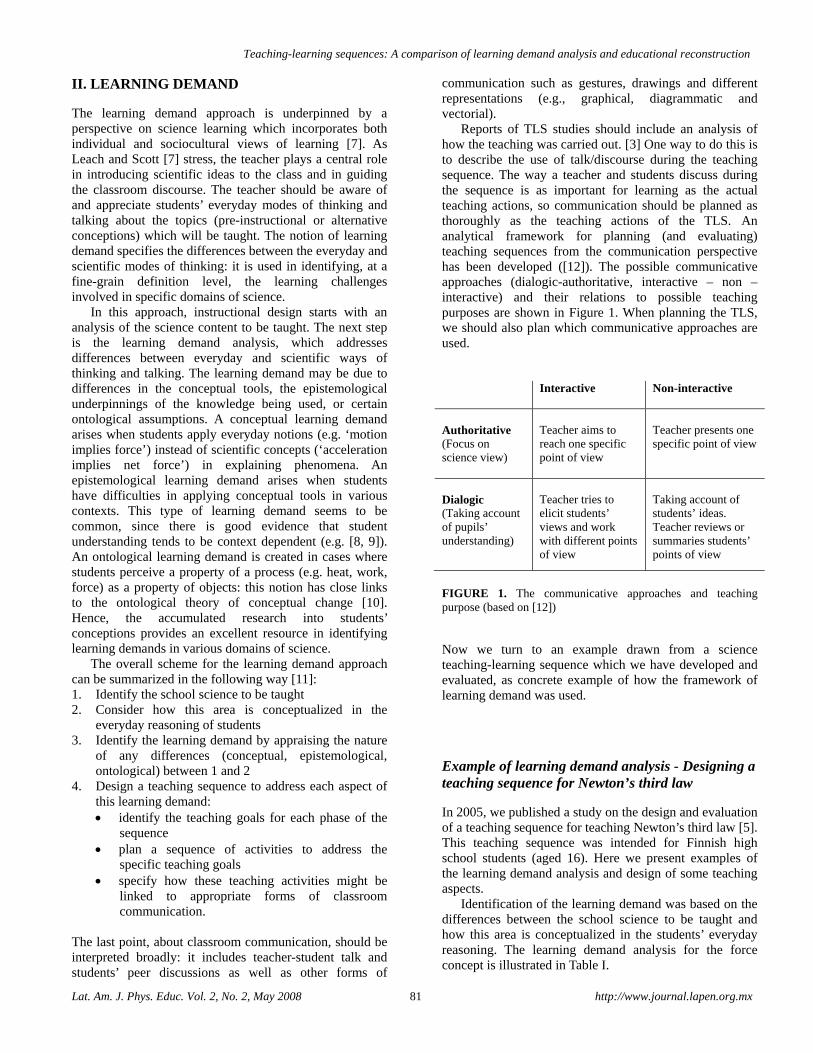
Reports of TLS studies should include an analysis of how the teaching was carried out. [3] One way to do this is to describe the use of talk/discourse during the teaching sequence. The way a teacher and students discuss during the sequence is as important for learning as the actual teaching actions, so communication should be planned as thoroughly as the teaching actions of the TLS. An analytical framework for planning (and evaluating) teaching sequences from the communication perspective has been developed ([12]). The possible communicative approaches (dialogic-authoritative, interactive – non –interactive) and their relations to possible teaching purposes are shown in Figure 1. When planning the TLS, we should also plan which communicative approaches are used.
Interactive
Non-interactive
Authoritative (Focus on science view)
Teacher aims to reach one specific point of view
Teacher presents one specific point of view
Dialogic (Taking account of pupils’ understanding)
Teacher tries to elicit students’ views and work with different points of view
Taking account of students’ ideas. Teacher reviews or summaries students’ points of view
FIGURE 1. The communicative approaches and teaching purpose (based on [12]) Now we turn to an example drawn from a science teaching-learning sequence which we have developed and evaluated, as concrete example of how the framework of learning demand was used.
Example of learning demand analysis - Designing a teaching sequence for Newton’s third law
In 2005, we published a study on the design and evaluation of a teaching sequence for teaching Newton’s third law [5]. This teaching sequence was intended for Finnish high school students (aged 16). Here we present examples of the learning demand analysis and design of some teaching aspects.
Identification of the learning demand was based on the differences between the school science to be taught and how this area is conceptualized in the students’ everyday reasoning. The learning demand analysis for the force concept is illustrated in Table I.
Jouni Viiri, Antti Savinainen
Lat. Am. J. Phys. Educ. Vol. 2, No. 2, May 2008 82 http://www.journal.lapen.org.mx
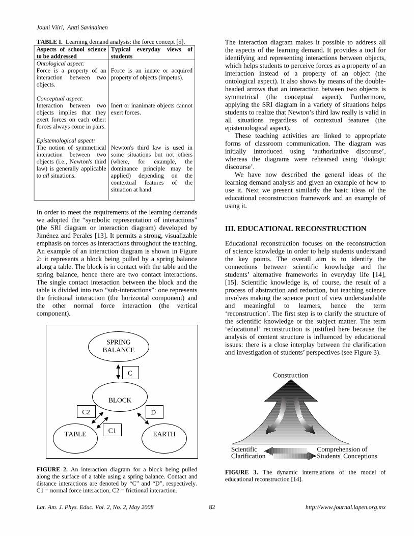
TABLE I. Learning demand analysis: the force concept [5]. Aspects of school science to be addressed
Typical everyday views of students
Ontological aspect: Force is a property of an interaction between two objects. Conceptual aspect: Interaction between two objects implies that they exert forces on each other: forces always come in pairs. Epistemological aspect: The notion of symmetrical interaction between two objects (i.e., Newton's third law) is generally applicable to all situations.
Force is an innate or acquired property of objects (impetus). Inert or inanimate objects cannot exert forces. Newton's third law is used in some situations but not others (where, for example, the dominance principle may be applied) depending on the contextual features of the situation at hand.
In order to meet the requirements of the learning demands we adopted the “symbolic representation of interactions” (the SRI diagram or interaction diagram) developed by Jiménez and Perales [13]. It permits a strong, visualizable emphasis on forces as interactions throughout the teaching. An example of an interaction diagram is shown in Figure 2: it represents a block being pulled by a spring balance along a table. The block is in contact with the table and the spring balance, hence there are two contact interactions. The single contact interaction between the block and the table is divided into two “sub-interactions”: one represents the frictional interaction (the horizontal component) and the other normal force interaction (the vertical component).
FIGURE 2. An interaction diagram for a block being pulled along the surface of a table using a spring balance. Contact and distance interactions are denoted by “C” and “D”, respectively. C1 = normal force interaction, C2 = frictional interaction.
The interaction diagram makes it possible to address all the aspects of the learning demand. It provides a tool for identifying and representing interactions between objects, which helps students to perceive forces as a property of an interaction instead of a property of an object (the ontological aspect). It also shows by means of the double-headed arrows that an interaction between two objects is symmetrical (the conceptual aspect). Furthermore, applying the SRI diagram in a variety of situations helps students to realize that Newton’s third law really is valid in all situations regardless of contextual features (the epistemological aspect).
These teaching activities are linked to appropriate forms of classroom communication. The diagram was initially introduced using ‘authoritative discourse’, whereas the diagrams were rehearsed using ‘dialogic discourse’.
We have now described the general ideas of the learning demand analysis and given an example of how to use it. Next we present similarly the basic ideas of the educational reconstruction framework and an example of using it.
III. EDUCATIONAL RECONSTRUCTION
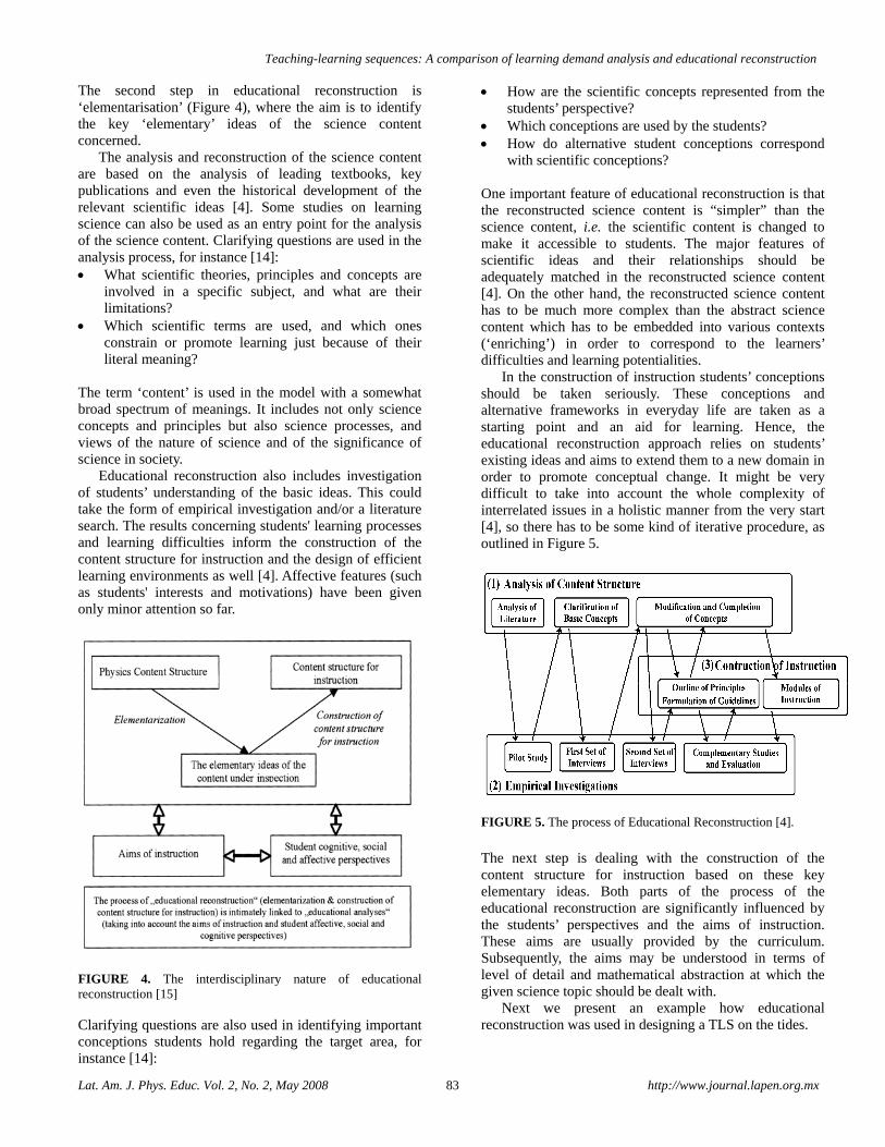
Educational reconstruction focuses on the reconstruction of science knowledge in order to help students understand the key points. The overall aim is to identify the connections between scientific knowledge and the students’ alternative frameworks in everyday life [14], [15]. Scientific knowledge is, of course, the result of a process of abstraction and reduction, but teaching science involves making the science point of view understandable and meaningful to learners, hence the term ‘reconstruction’. The first step is to clarify the structure of the scientific knowledge or the subject matter. The term ‘educational’ reconstruction is justified here because the analysis of content structure is influenced by educational issues: there is a close interplay between the clarification and investigation of students’ perspectives (see Figure 3).
Construction
ScientificClarification
Comprehension ofStudents' Conceptions
FIGURE 3. The dynamic interrelations of the model of educational reconstruction [14].
BLOCK
SPRING BALANCE
TABLE EARTH
C
D
C1
C2
Teaching-learning sequences: A comparison of learning demand analysis and educational reconstruction
Lat. Am. J. Phys. Educ. Vol. 2, No. 2, May 2008 83 http://www.journal.lapen.org.mx
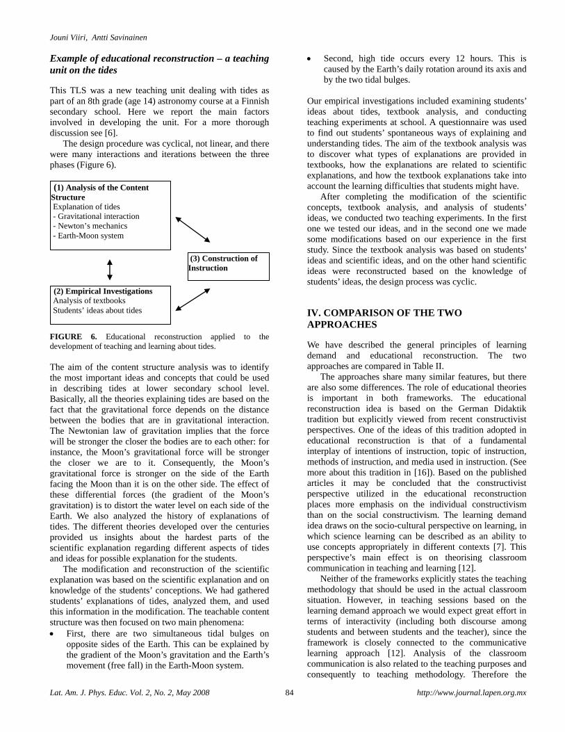
The second step in educational reconstruction is ‘elementarisation’ (Figure 4), where the aim is to identify the key ‘elementary’ ideas of the science content concerned.
The analysis and reconstruction of the science content are based on the analysis of leading textbooks, key publications and even the historical development of the relevant scientific ideas [4]. Some studies on learning science can also be used as an entry point for the analysis of the science content. Clarifying questions are used in the analysis process, for instance [14]: • What scientific theories, principles and concepts are
involved in a specific subject, and what are their limitations?
• Which scientific terms are used, and which ones constrain or promote learning just because of their literal meaning?
The term ‘content’ is used in the model with a somewhat broad spectrum of meanings. It includes not only science concepts and principles but also science processes, and views of the nature of science and of the significance of science in society.
Educational reconstruction also includes investigation of students’ understanding of the basic ideas. This could take the form of empirical investigation and/or a literature search. The results concerning students' learning processes and learning difficulties inform the construction of the content structure for instruction and the design of efficient learning environments as well [4]. Affective features (such as students' interests and motivations) have been given only minor attention so far.
FIGURE 4. The interdisciplinary nature of educational reconstruction [15] Clarifying questions are also used in identifying important conceptions students hold regarding the target area, for instance [14]:
• How are the scientific concepts represented from the students’ perspective?
• Which conceptions are used by the students? • How do alternative student conceptions correspond
with scientific conceptions?
One important feature of educational reconstruction is that the reconstructed science content is “simpler” than the science content, i.e. the scientific content is changed to make it accessible to students. The major features of scientific ideas and their relationships should be adequately matched in the reconstructed science content [4]. On the other hand, the reconstructed science content has to be much more complex than the abstract science content which has to be embedded into various contexts (‘enriching’) in order to correspond to the learners’ difficulties and learning potentialities.
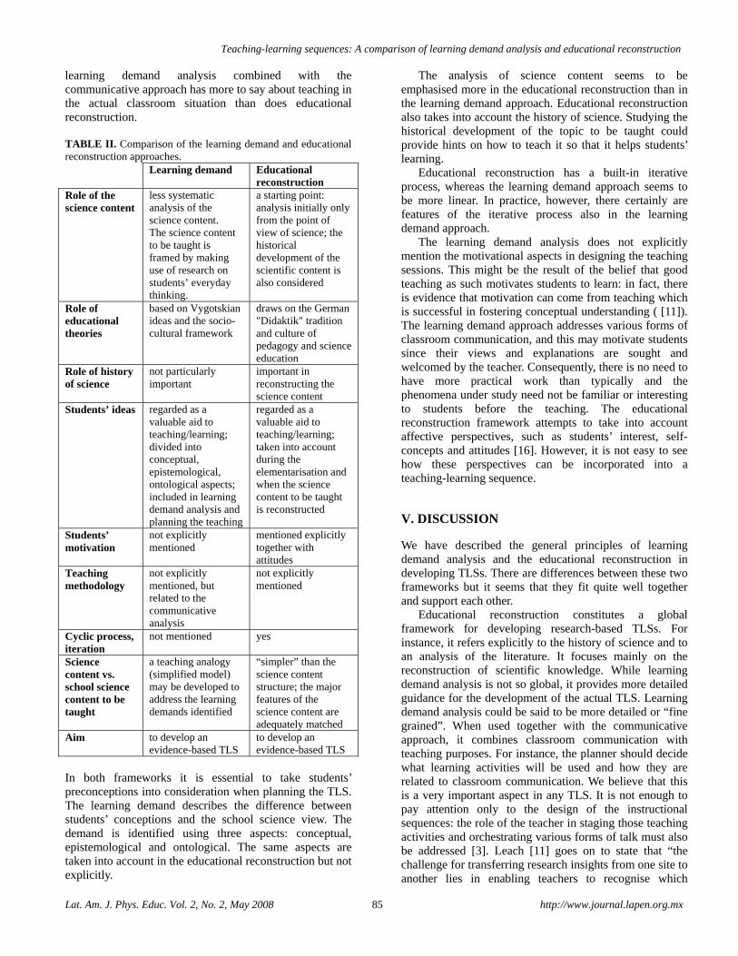
In the construction of instruction students’ conceptions should be taken seriously. These conceptions and alternative frameworks in everyday life are taken as a starting point and an aid for learning. Hence, the educational reconstruction approach relies on students’ existing ideas and aims to extend them to a new domain in order to promote conceptual change. It might be very difficult to take into account the whole complexity of interrelated issues in a holistic manner from the very start [4], so there has to be some kind of iterative procedure, as outlined in Figure 5.
FIGURE 5. The process of Educational Reconstruction [4].
The next step is dealing with the construction of the content structure for instruction based on these key elementary ideas. Both parts of the process of the educational reconstruction are significantly influenced by the students’ perspectives and the aims of instruction. These aims are usually provided by the curriculum. Subsequently, the aims may be understood in terms of level of detail and mathematical abstraction at which the given science topic should be dealt with.
Next we present an example how educational reconstruction was used in designing a TLS on the tides.
Jouni Viiri, Antti Savinainen
Lat. Am. J. Phys. Educ. Vol. 2, No. 2, May 2008 84 http://www.journal.lapen.org.mx
Example of educational reconstruction – a teaching unit on the tides
This TLS was a new teaching unit dealing with tides as part of an 8th grade (age 14) astronomy course at a Finnish secondary school. Here we report the main factors involved in developing the unit. For a more thorough discussion see [6].
The design procedure was cyclical, not linear, and there were many interactions and iterations between the three phases (Figure 6).
FIGURE 6. Educational reconstruction applied to the development of teaching and learning about tides. The aim of the content structure analysis was to identify the most important ideas and concepts that could be used in describing tides at lower secondary school level. Basically, all the theories explaining tides are based on the fact that the gravitational force depends on the distance between the bodies that are in gravitational interaction. The Newtonian law of gravitation implies that the force will be stronger the closer the bodies are to each other: for instance, the Moon’s gravitational force will be stronger the closer we are to it. Consequently, the Moon’s gravitational force is stronger on the side of the Earth facing the Moon than it is on the other side. The effect of these differential forces (the gradient of the Moon’s gravitation) is to distort the water level on each side of the Earth. We also analyzed the history of explanations of tides. The different theories developed over the centuries provided us insights about the hardest parts of the scientific explanation regarding different aspects of tides and ideas for possible explanation for the students.
The modification and reconstruction of the scientific explanation was based on the scientific explanation and on knowledge of the students’ conceptions. We had gathered students’ explanations of tides, analyzed them, and used this information in the modification. The teachable content structure was then focused on two main phenomena: • First, there are two simultaneous tidal bulges on
opposite sides of the Earth. This can be explained by the gradient of the Moon’s gravitation and the Earth’s movement (free fall) in the Earth-Moon system.
• Second, high tide occurs every 12 hours. This is caused by the Earth’s daily rotation around its axis and by the two tidal bulges.
Our empirical investigations included examining students’ ideas about tides, textbook analysis, and conducting teaching experiments at school. A questionnaire was used to find out students’ spontaneous ways of explaining and understanding tides. The aim of the textbook analysis was to discover what types of explanations are provided in textbooks, how the explanations are related to scientific explanations, and how the textbook explanations take into account the learning difficulties that students might have.
After completing the modification of the scientific concepts, textbook analysis, and analysis of students’ ideas, we conducted two teaching experiments. In the first one we tested our ideas, and in the second one we made some modifications based on our experience in the first study. Since the textbook analysis was based on students’ ideas and scientific ideas, and on the other hand scientific ideas were reconstructed based on the knowledge of students’ ideas, the design process was cyclic.
IV. COMPARISON OF THE TWO APPROACHES
We have described the general principles of learning demand and educational reconstruction. The two approaches are compared in Table II.
The approaches share many similar features, but there are also some differences. The role of educational theories is important in both frameworks. The educational reconstruction idea is based on the German Didaktik tradition but explicitly viewed from recent constructivist perspectives. One of the ideas of this tradition adopted in educational reconstruction is that of a fundamental interplay of intentions of instruction, topic of instruction, methods of instruction, and media used in instruction. (See more about this tradition in [16]). Based on the published articles it may be concluded that the constructivist perspective utilized in the educational reconstruction places more emphasis on the individual constructivism than on the social constructivism. The learning demand idea draws on the socio-cultural perspective on learning, in which science learning can be described as an ability to use concepts appropriately in different contexts [7]. This perspective’s main effect is on theorising classroom communication in teaching and learning [12].
Neither of the frameworks explicitly states the teaching methodology that should be used in the actual classroom situation. However, in teaching sessions based on the learning demand approach we would expect great effort in terms of interactivity (including both discourse among students and between students and the teacher), since the framework is closely connected to the communicative learning approach [12]. Analysis of the classroom communication is also related to the teaching purposes and consequently to teaching methodology. Therefore the
(1) Analysis of the Content Structure Explanation of tides - Gravitational interaction - Newton’s mechanics - Earth-Moon system
(2) Empirical Investigations Analysis of textbooks Students’ ideas about tides
(3) Construction of Instruction
Teaching-learning sequences: A comparison of learning demand analysis and educational reconstruction
Lat. Am. J. Phys. Educ. Vol. 2, No. 2, May 2008 85 http://www.journal.lapen.org.mx
learning demand analysis combined with the communicative approach has more to say about teaching in the actual classroom situation than does educational reconstruction.
TABLE II. Comparison of the learning demand and educational reconstruction approaches. Learning demand Educational
reconstruction Role of the science content
less systematic analysis of the science content. The science content to be taught is framed by making use of research on students’ everyday thinking.
a starting point: analysis initially only from the point of view of science; the historical development of the scientific content is also considered
Role of educational theories
based on Vygotskian ideas and the socio-cultural framework
draws on the German "Didaktik" tradition and culture of pedagogy and science education
Role of history of science
not particularly important
important in reconstructing the science content
Students’ ideas regarded as a valuable aid to teaching/learning; divided into conceptual, epistemological, ontological aspects; included in learning demand analysis and planning the teaching
regarded as a valuable aid to teaching/learning; taken into account during the elementarisation and when the science content to be taught is reconstructed
Students’ motivation
not explicitly mentioned
mentioned explicitly together with attitudes
Teaching methodology
not explicitly mentioned, but related to the communicative analysis
not explicitly mentioned
Cyclic process, iteration
not mentioned yes
Science content vs. school science content to be taught
a teaching analogy (simplified model) may be developed to address the learning demands identified
“simpler” than the science content structure; the major features of the science content are adequately matched
Aim to develop an evidence-based TLS
to develop an evidence-based TLS
In both frameworks it is essential to take students’ preconceptions into consideration when planning the TLS. The learning demand describes the difference between students’ conceptions and the school science view. The demand is identified using three aspects: conceptual, epistemological and ontological. The same aspects are taken into account in the educational reconstruction but not explicitly.
The analysis of science content seems to be emphasised more in the educational reconstruction than in the learning demand approach. Educational reconstruction also takes into account the history of science. Studying the historical development of the topic to be taught could provide hints on how to teach it so that it helps students’ learning.
Educational reconstruction has a built-in iterative process, whereas the learning demand approach seems to be more linear. In practice, however, there certainly are features of the iterative process also in the learning demand approach.
The learning demand analysis does not explicitly mention the motivational aspects in designing the teaching sessions. This might be the result of the belief that good teaching as such motivates students to learn: in fact, there is evidence that motivation can come from teaching which is successful in fostering conceptual understanding ( [11]). The learning demand approach addresses various forms of classroom communication, and this may motivate students since their views and explanations are sought and welcomed by the teacher. Consequently, there is no need to have more practical work than typically and the phenomena under study need not be familiar or interesting to students before the teaching. The educational reconstruction framework attempts to take into account affective perspectives, such as students’ interest, self-concepts and attitudes [16]. However, it is not easy to see how these perspectives can be incorporated into a teaching-learning sequence.
V. DISCUSSION
We have described the general principles of learning demand analysis and the educational reconstruction in developing TLSs. There are differences between these two frameworks but it seems that they fit quite well together and support each other.
Educational reconstruction constitutes a global framework for developing research-based TLSs. For instance, it refers explicitly to the history of science and to an analysis of the literature. It focuses mainly on the reconstruction of scientific knowledge. While learning demand analysis is not so global, it provides more detailed guidance for the development of the actual TLS. Learning demand analysis could be said to be more detailed or “fine grained”. When used together with the communicative approach, it combines classroom communication with teaching purposes. For instance, the planner should decide what learning activities will be used and how they are related to classroom communication. We believe that this is a very important aspect in any TLS. It is not enough to pay attention only to the design of the instructional sequences: the role of the teacher in staging those teaching activities and orchestrating various forms of talk must also be addressed [3]. Leach [11] goes on to state that “the challenge for transferring research insights from one site to another lies in enabling teachers to recognise which
Jouni Viiri, Antti Savinainen
Lat. Am. J. Phys. Educ. Vol. 2, No. 2, May 2008 86 http://www.journal.lapen.org.mx
features of a design are central to its rationale, and therefore should be modified with extreme caution, and which features are less critical.”
The differences mentioned – the global aspect of educational reconstruction and the fine grained detail provided by learning demand – were evident also in the examples given. Since Newton’s third law is a very specific topic, the learning demand analysis is appropriate for that case. In contrast, the tides are very many sided so educational reconstruction might be a more suitable framework for designing a TLS for this topic.
Both the frameworks discussed here stress that domain-specific research is necessary for designing effective learning experiences, for (at least) two reasons. Firstly, TLS should take into account the most common student difficulties in a given domain, since numerous studies provide evidence of common misunderstandings in many science domains [17]. Secondly, conceptual development does not follow the same routes in different science topics [18]. Also both learning demand analysis and educational reconstruction are based on the idea that content-oriented theories are a necessary complement to theoretical platforms such as constructivist and the socio-cultural approaches.
ACKNOWLEDGEMENTS
We wish to thank Reinders Duit, John Leach and Phil Scott for their helpful comments on the first draft of the paper.
REFERENCES
[1] Meheut, M. and Psillos, D., Teaching-learning sequences: aims and tools for science education research, International Journal of Science Education 16, 515-535 (2004). [2] Andersson, B and Wallin, A., On developing content-oriented theories taking biological evolution as an example, International Journal of Science Education 28, 673 – 695 (2006). [3] Leach, J. and Scott, P., Designing and evaluating science teaching sequences: an approach drawing upon the concept of learning demand and a social constructivist perspective on learning, Studies in Science Education 38, 115-142 (2002). [4] Duit, R., A model of educational reconstruction as a framework for designing and validating teaching and learning sequences. Paper presented at the meeting on research-based teaching sequences, Paris, November, (2000). [5] Savinainen, A., Scott, P. and Viiri, J., Using a bridging representation and social interactions to foster conceptual
change: Designing and evaluating an instructional sequence for Newton’s third law, Science Education 89, 175 -195 (2005). [6] Viiri, J. and Saari, H., Research based teaching unit on the tides, International Journal of Science Education 26, 463-482 (2004). [7] Leach, J. and Scott, P., Individual and sociocultural views of learning in science education, Science and Education 12, 91-113 (2003). [8] Palmer, D., The effect of context on students' reasoning about forces, International Journal of Science Education 6, 681-696 (1997). [9] Savinainen, A. and Scott, P., Using the Force Concept Inventory to monitor student learning and to plan teaching, Physics Education 37, 53-58 (2002). [10] Chi, M. T. H., Slotta, J. D. and de Leeuw, N., From things to processes: a theory of conceptual change for learning science concepts, Learning and Instruction 4, 27-43 (1994). [11] Leach, J., Contested territory: The actual and potential impact of research on teaching and learning science on students’ learning. Paper presented at the meeting of the European Science Education Research Association, Barcelona, August/September 2005. http://www.education.leeds.ac.uk/research/uploads/26.pdf Visited April 19, 2006. [12] Mortimer, E. and Scott, P. Meaning making in secondary science classrooms (Open University Press, Berkshire, 2003). [13] Jiménez, J. D. and Perales, F. J., Graphic representation of force in secondary education: analysis and alternative educational proposals, Physics Education 36, 227 – 235 (2001). [14] Kattman, U., Duit, R. and Gropengießer, H., The Model of Educational Reconstruction - Bringing together Issues of Scientific Clarification and Students' Conceptions. In (ERIDOB), 1998, Kiel, Germany: IPN – Leibniz Institute for Science Education, 253-262. [15] Duit, R., Gropengiesser, H. and Kattmann, U., Towards science education research that is relevant for improving practice: The model of educational reconstruction. In H. Fisher (ed.) Developing standards in research on science education (pp. 1–9) (Taylor & Francis group, London, 2005). [16] Duit, R., Niedderer, H. and Schecker, H. Teaching physics. In S.K. Abell & N.G. Lederman, Eds., Handbook of research on science education (pp.599-629). (Lawrence Erlbaum, Mahwah, N J, 2007). [17] Duit, R., Bibliography - STCSE Students' and teachers' conceptions and science education. <http://www.ipn.uni-kiel.de/aktuell/stcse/stcse.html> Visited August 6, 2006. [18] Vosniadou, S., Ioannides, C., Dimitrakopoulou, A. and Papademetriou, E., Designing learning environments to promote conceptual change in science, Learning and Instruction 11, 381-419 (2001).
Lat. Am. J. Phys. Educ. Vol. 2, No. 2, May 2008 87 http://www.journal.lapen.org.mx
Learning Physics in a Virtual Environment: Is There Any?
Gerald W. Meisner1, Harol Hoffman2, Mike Turner3
1UNC Greensboro. 2Science Lab Courseware. 3Providence Day School, Charlotte, NC, USA. E-mail: [email protected] (Received 4 April 2008; accepted 5 May 2008)
Abstract With nearly one in five college students taking at least one course online, with nearly every major college and university offering courses and/or programs online and with a growing number of citizens in the work place wanting and needing education in ways which fit their work and personal schedules, e-learning is becoming more important and ubiquitous each year. The supply (courses) is there in many disciplines; the demand (students and non-students) is there. The unanswered question is: How good is the product? Is learning taking place? How do we measure the learning effectiveness of online courses? Are some courses more amenable than others to e-learning? In particular, is it possible to effectively teach pedagogically sound science courses online? There is little research on many of these questions. Of interest to legislators is another important question: Is online learning cost effective? There is a paucity of data here as well, although some argue that it is possible to have e-learning which is cost effective at the margin [1, 38] provided that an instructional design model is used wherein there is no one ‘at the end of the phone’ – a model very different from that currently used in the online community. We have collected data from student use of a highly interactive, virtual physics laboratory that answers some of these questions. Data are from an introductory, algebra-based introductory physics course taken mostly by pre-professionals in health fields during the 2005-2006 academic year. Pre- and post- FCI tests were administered in the fall semester when students studied mechanics. Results show that a cadre of students taking ‘classwork’ in a virtual, highly interactive physics laboratory environment have normalized <g> gains [4] on the FCI test [12] which is greater than that of a similar cadre of students in a (physical) modified Modeling Workshop [8] laboratory environment and considerably larger than those in a lecture environment [4]. Keywords: Physics Education, Physics simulation, Virtual Physics Laboratory.
Resumen Con casi uno de cinco estudiantes universitarios tomando al menos un curso en línea, con casi todos los principales institutos y universidades que ofrecen cursos y/o programas en línea y con un número creciente de ciudadanos que desean y necesitan de educación desde su lugar de trabajo de manera que se adapten a su trabajo y horarios personales, el e-learning es cada vez más importante y omnipresente en cada año. El suministro (cursos) está ahí en muchas disciplinas, la demanda (estudiantes y no estudiantes) también está ahí. La pregunta sin respuesta es: ¿Qué tan bueno es el producto? ¿Se está consiguiendo el aprendizaje? ¿Cómo podemos medir la efectividad del aprendizaje de los cursos en línea? ¿Algunos cursos son más susceptibles que otros para el e-learning? En particular, es posible enseñar de manera efectiva pedagógicamente cursos de ciencias en línea? Hay poca investigación sobre muchas de estas cuestiones. Para los legisladores es de interés otra pregunta importante: ¿Es rentable el aprendizaje en línea? también aquí hay una escasez de datos, aunque algunos sostienen que es posible el tener al margen e-learning rentable [38, 39], siempre que exista un diseño instruccional se ha utilizado el modelo en el que no hay nadie “al final del teléfono”- un modelo muy diferente del que actualmente se utiliza en la comunidad en línea. Se han recogido datos del uso de los estudiantes de un laboratorio virtual de física, muy interactivo que responde a algunas de estas preguntas. Los datos son de un curso de física introductoria sin cálculo que la mayoría de pre-profesionales en áreas de la salud han tomado durante el año académico 2005-2006. Las pruebas de Pre- y post FCI- se administraron en el semestre de otoño cuando los alumnos estudian mecánica. Los resultados muestran que un grupo de estudiantes realizando el “trabajo de clase” en un laboratorio de física con un entorno grandemente interactivo tienen una ganancia normalizada <g> [4] en la prueba FCI [12] que es mayor que la de un grupo similar de estudiantes en un entorno de laboratorio de Taller de Modelado físico modificado [8] y considerablemente mayor que aquellos de un entorno de clases [4]. Palabras clave: Educación en Física, Simulación en Física, Laboratorio virtual de Física. PACS: 01.40.Fk, 01.50.H-, 01.50.hv, 01.50.Lc, 01.50.Qb
Gerald W. Meisner, Harol Hoffman, Mike Turner
Lat. Am. J. Phys. Educ. Vol.2, No. 2, May 2008 88 http://www.journal.lapen.org.mx
I. INTRODUCTION Research over the past 30 years [1, 2, 3] has shown that students fail to evidence deep understanding of science content and process when subjected to conventional instruction of lecture and demonstrations. Synergistic research by cognitive and physical scientists in the past several decades have given rise to successful efforts in challenging the solipsistic way in which students are being taught. Physics education research or PER [4, 5] has shown that highly interactive engagement of physics students based on pedagogy that has an element of careful guidance is critical for deep learning of physics. Transmission of information, no matter no skillfully or artfully presented, does little more that convince students that a memorization of facts and equations is the sine qua non of science in general and physics in particular. Furthermore, we now know that carefully crafted lectures, including (passive) visuals, whether in situ or a virtual space, will not help to answer in the affirmative the question posed by Hake in a recent article [6]: “Distance and Classroom Learning: Is There Any?”. The reason for these failed educational ‘experiments’ may be explained by what educational psychologists call the “curse of knowledge” [7]: ‘The more one knows, the more difficult it is, for most people, to understand how some other person could not know what we know.’ In designing the virtual learning environment, we have avoided this curse by careful use of research into misconceptions which students bring to the table and how students learn [5]. The past 20 years of PER has enabled those in this reform movement to put to rest the notion that good teaching is an ‘art’ possessed by only a select few. Rather, by examining the conclusions of this research, many in the physics community are now using highly interactive pedagogical methods which result in their students showing considerable improvement in basic and conceptual understanding of physics [4]. We have been guided by this approach in authoring our asynchronous virtual physics laboratory environments, LabPhysics. The software is modular and multi-purposed – it can be used as a platform for courses horizontally across the sciences and vertically within a specific discipline; the first course authored with the software is an introductory, college (or high school) level physics course in mechanics.
LabPhysics includes both the process and content of science – essential components for any course for students entering upon a study of the discipline. The scientific process, including detailed and highly interactive laboratory investigations, with decision-making, selection of equipment and instrumentation, data collection and analysis and the capability to make mistakes, are essential components of the experience. The process followed in LabPhysics consists of those procedures followed by bench scientists in their daily investigations in the science laboratory. The principle guiding the implementation of this process and the development of both the software architecture and the story-boarding of tutorials which comprise the LabPhysics Mechanics course is the Modeling Workshop [8] pedagogy, a highly acclaimed and
NSF-funded program. This approach is one of several in the movement to reform the teaching of physics, and leads students to investigate patterns in the physical (or realistically virtual!) world and to map them onto specific conceptual systems using various representations. It uses a variation of Karplus’ learning cycle [9, 10], which for Modeling purposes consists of exploration, model development and formulation, model deployment and finally, synthesis. Transferring conclusions from studies in cognitive psychology [11] into the learning environment enable students to use models as learning aids for both understanding and later retrieval.
Students using the Modeling approach have consistently scored significantly higher [4] on standardized ‘conceptual’ exams (the FCI [12], for example) than have students in traditional (lecture) learning situations. An instrument (Reformed Teaching Observational Protocol or RTOP [13] to quantify the extent to which research-based reforms have been implemented in a setting has recently been developed. The instrument consists of twenty-five questions worth from 0-4 points. Studies [14] show a high correlation between high scores on RTOP and student achievement (concept understanding and reasoning skills). A LabPhysics RTOP score of 81 out of 100 and the result of the study by Lawson [14] correlates well with this investigation that showed an average Hake <g> factor score of LabPhysics students nearly twice that of a control group.
In spite of evidence linking reform teaching procedures and student learning, the reform movement in physics teaching has progressed slowly beyond a committed core, for reasons having to do with inertia, lack of awareness, reward structure, physical space, equipment and teaching loads. The growth of online education further complicates the problem. There are more than 3.5 million students taking at least one online course in the United States [15], a number which is growing at a yearly rate of nearly 10 percent, or six times faster than the total number of higher education students. The growth in science courses is smaller but still robust and requires more effort and resources for implementing the highly interactive environments that are requisite for deep learning.
Without interactive online science laboratories, we lack the necessary tools for delivering high quality online science courses, for conducting essential research into human-computer interactions and interactive settings that promote and enhance learning of science concepts and model-building in online settings, and for establishing limitations on virtual training of personnel in disparate settings. Despite the proliferation of online universities, robust continual learning auxiliaries of colleges and universities, ‘open courseware,’ and laboratory simulations, there have been remarkably few sustained and successful collaborative efforts to bring together the interdisciplinary experts in technology, content area, design, and discipline-based education research needed to address the creation of effective virtual laboratories. There are, however, a plethora of approaches with somewhat different teaching objectives. One such approach, MIT’s Open CourseWare or OCW (MIT) [41], consists of video taped lectures, demonstrations, problems and small labs
Learning Physics in a Virtual Environment: Is There Any?
Lat. Am. J. Phys. Educ. Vol. 2, No. 2, May 2008 89 http://www.journal.lapen.org.mx
such as a traditional lecture-based course would have -> all on the web and open to all. OCW is suitable for those students who are adept at abstract learning in the lecture tradition, and want to go beyond the material presented at their school. OCW fills a niche for those seeking the experience of seeing lectures delivered by eminent scientists at MIT. Nonetheless, such an approach has, a fortiori, many of the problems addressed by Hake [6] – those learning problems inherent in a format based almost entirely on the delivery of information. Christian and Belloni [16], Kiselev [17] and others have authored single concept Java applets that behave as visual spread sheets, enabling the student to quickly see the effect of changing a variable in optics (e.g., object distance affecting image distance for constant converging lens focal length), mechanics (e.g., mass affecting acceleration for constant force), circuits (changing resistance for constant voltage in simple DC circuit), etc. These times - saving visuals assist students in understanding the affects in given mathematical expressions of a variable change. A more holistic approach has been employed by the University of Colorado at Boulder team [18] wherein students see a cartoon-like laboratory simulation embedded in a discussion of the phenomena to be examined. Flash animations such as these can help students visualize relevant mathematical expressions describing a physical situation. Such activities comprise one phase in the learning cycle espoused by Karplus [1], Hestenes [8] and others, and are thus valuable in the sense that they incorporate part of the cycle. The activities generally either leave a large footprint devoid of research – based pedagogy (entire courses of online lecture notes and power point presentations, both visual and oral) or they leave a small foot print based on a small component of the learning cycle (experimental simulations, applets).
Lacking was a comprehensive online approach, based on results of the physics education research community and using the best of the rapidly evolving technologies. The desired approach to online learning in the sciences, then, has to simulate, as best as possible, the entire student learning experience in a scientific setting – in a virtual science laboratory wherein students could interact with equipment, apparatus, mentor, and peers in ways that closely emulate a physical approach to learning by interactive engagement.
The approach of LabPhysics is to expose the user to all aspects of the learning cycle in her virtual laboratory immersion: engagement, exploration, explanation, elaboration and evaluation. Or, in Modeling Workshop [8] language, engage, explore, develop, deploy, and assess. It is a comprehensive approach and closely emulates best practices in the (physical) laboratory environment. The approach must adhere to the charge by Arons [19] to guide the inquiry and help students gain some insight into the practice of scientists, so that they will not leave their learning experience with little more than what Whitehead [20] described as “inert ideas”. LabPhysics courseware incorporates features unique to the online medium: (virtual) mentor, (virtual) collaborators, transparent computer-human interface and time-critical and meaningful assessment. Some of these general
requirements have recently been enumerated in more detail by Boettcher [21].
In order to answer the question: ‘Can Student Learning Take Place in an Online Environment? we must ask four preliminary questions:
i. What is the discipline? ii. How do we measure learning? iii. How can we carry out a suitable investigation? iv. Do we have a suitable instrument to carry out the
investigation? We limit ourselves to physics, and although we examine other aspects of learning, we will use the FCI test as a measure of learning accepted by many in the physics community. Learning a laboratory science should include meaningful laboratory investigations; we must create a virtual laboratory that simulates a physical one as closely as possible. Lacking haptic capabilities, we permit students to explore other laboratory activities as closely as is technologically possible and compare physical and virtual experiences as meaningfully as possible. Although the canonical double blind study is the gold standard for measuring effectiveness, such a technique is clearly not possible in this situation. Our substitute for that ideal was to have two cadres of students, each taught by the same instructor, with the same exams, homework, assigned text, semester projects and grading system, but with one cadre immersed in a physical lab and the other in a virtual lab. However, there was no existing software/instrument to use for such an investigation. We decided to create one. II. SOFTWARE Funded in part by a grant from the U.S. Department of Education (Grant No. P339B990329), we have designed and built (LabPhysics) software which has the requisite characteristics. • Architecture to enable interactive engagement, [8] based
on Modeling Pedagogy that is the sine qua non behind the scripting and guided, laboratory-based tutorials. LabPhysics tutorials emphasize the scientific process and learning cycle, thus permitting deep problem-solving analyses after the necessary model-based scaffold has been built and understood by the student. Stored data for each student permits ‘flagging’ of each student’s misconceptions [22, 5] as well as her preconceptions [22] and learning facets [23]. In addition, correlations among misconceptions with the various representations of models can provide insight into student learning [24]. A virtual tutor guides students, as would an expert modeler, in, say, Hestenes’ Modeling Workshop. Traditional ‘end of the chapter’, multiple choice and true-false can be authored and incorporated into the software.
• Procedures to assess student content understanding within the tutorial settings under varying conditions. Students are exposed to both higher-level concepts/tasks in which they deploy their developed models in novel situations, and lower level tasks such as learning how to
Gerald W. Meisner, Harol Hoffman, Mike Turner
Lat. Am. J. Phys. Educ. Vol.2, No. 2, May 2008 90 http://www.journal.lapen.org.mx
use instruments and equipment, or how to identify dependent and independent variables in an experimental investigation. Assessment and evaluation questions are being authored which go beyond the common algorithmic questions at the ‘end of the chapter’. With appropriate courseware tools for faculty and student use, online environments permit a richness in assessment not possible with ‘hard’ media. We have authored a variety of these tools which permit faculty access to instantaneous qualitative grading capabilities hitherto lacking: LabGraph, LabAnalysis, LabVector and LabMotionMap. These instruments have unique features that permit faculty to qualitatively (as well as quantitatively) grade a student’s understanding of graphs, vectors, and kinematics. As with all online developments, midcourse corrections can be easily and
quickly executed. The extensibility of the LabPhysics approach, along with authoring tools we are developing, will permit a community of developers to quickly emerge, both here and in other countries. Multiple branching forks (keyed to student responses) currently guide students of various backgrounds and educational experiences through different paths of learning.
• Administrative tools for faculty use to monitor student progress (read and insert comments in student virtual notebooks, examine patterns of online usage, etc.).
• Development tools to permit the creation of different mechanics courses, based on the needs of the end users.
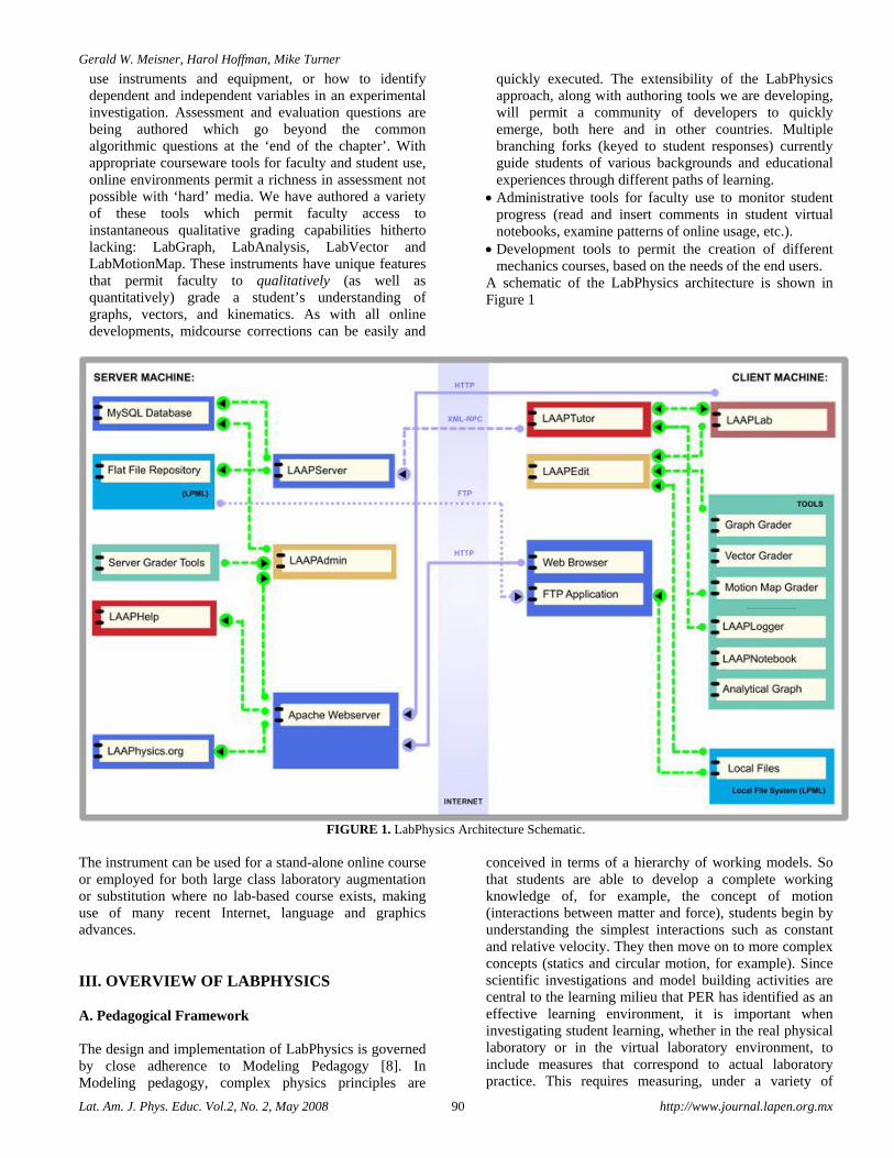
A schematic of the LabPhysics architecture is shown in Figure 1
FIGURE 1. LabPhysics Architecture Schematic.
The instrument can be used for a stand-alone online course or employed for both large class laboratory augmentation or substitution where no lab-based course exists, making use of many recent Internet, language and graphics advances. III. OVERVIEW OF LABPHYSICS A. Pedagogical Framework The design and implementation of LabPhysics is governed by close adherence to Modeling Pedagogy [8]. In Modeling pedagogy, complex physics principles are
conceived in terms of a hierarchy of working models. So that students are able to develop a complete working knowledge of, for example, the concept of motion (interactions between matter and force), students begin by understanding the simplest interactions such as constant and relative velocity. They then move on to more complex concepts (statics and circular motion, for example). Since scientific investigations and model building activities are central to the learning milieu that PER has identified as an effective learning environment, it is important when investigating student learning, whether in the real physical laboratory or in the virtual laboratory environment, to include measures that correspond to actual laboratory practice. This requires measuring, under a variety of
Learning Physics in a Virtual Environment: Is There Any?
Lat. Am. J. Phys. Educ. Vol. 2, No. 2, May 2008 91 http://www.journal.lapen.org.mx
conditions, behaviors that typify those of laboratory scientists: 1) the ability to understand and produce different representational models (verbal, graphical, diagrammatic, mathematical) of the relationships among relevant variables; 2) the ability to design and execute experiments with appropriate tools (which demands problem solving competency), and 3) the ability to transfer learning from one experimental context to another (see discussion on capstone investigation below). Student assessment practices that only measure a student’s ability to solve ‘end of chapter problems’ provide little data on these critical STEM competencies, but rather measure a valuable but limited skill - that of applying algorithms to solve specific word problems. B. Modeling Framework in a Virtual World LabPhysics has been designed to incorporate, as faithfully as possible, the fundamental components of the Modeling pedagogy classroom setting. The software package includes a series of curriculum tutorials that contain model development investigations in which students work in an open-ended online laboratory environment with ‘virtual’ peers (real peers are, of course, also possible with chat, text messaging or cell phone). A second component of each curriculum module includes a comprehensive model deployment activity, the capstone experiment, which is designed to assess student ability to transfer learning from one experimental context to another.
The LabPhysics capstone experiment helps cut the contextual strings between the model constructed by the student during the model development phase, and the specific context or circumstance in which that model was constructed. These activities expand on the development of ‘context rich’ problems from the University of Minnesota PER group [25] and of the ‘experiment problems’ from the Ohio State University PER Group [26]. Capstone experiments immerse students in a contextual and media rich virtual environment where they are forced to make decisions on how to proceed (assumptions and variable data are not pre-defined). Students must also make appropriate measurements, often designing an investigation and collecting (their own) data in order to achieve success. These tasks evaluate student understanding in a virtual environment similar to that encountered by scientists in a physical world. Student learning can be evaluated by comparing student predictions to their experimentally measured quantities, or by analyzing representations that students employ and/or events that occur in the virtual experimental environment. Student behavior also can be evaluated on the basis of each student’s overall strategy choices and the individual steps they take to reach their solution. Such evaluations go far beyond conventional assessment mechanisms [40] and are not limited by class size.
The Constant Velocity tutorial provides an example of the curriculum pedagogy. In the tutorial, the virtual mentor guides the student through the process of constructing a model of an object moving with constant velocity. The student develops this model through the two stage modeling cycle. In the model development stage, the
student empirically develops the functional relationship between position and time and learns to represent that relationship verbally (written), then diagrammatically (using motion maps), graphically (position versus time and velocity versus time), and finally, mathematically [linear relationships: x = vt + x0; v(ave) = �x/�t)]. The emphasis on the use of multiple representations of the model is designed to strengthen the student’s conceptual understanding of the model as well as to improve qualitative reasoning ability. C. LabPhysics Courseware The LabPhysics courseware permit students to: 1) conduct their own scientific investigations in a guided environment; 2) move through an introductory physics course in either a linear or nonlinear fashion at the discretion of the student or the instructor, depending on the desired learning goals; 3) move asynchronously to accommodate learning styles, differing academic strengths, work, family and health-related time constraints. Student understanding of the principles developed in each tutorial are evaluated by analyzing student responses to questions at various points in the tutorial. ‘Checkpoint’ questions within each tutorial chapter provide formative assessment, requiring students to immediately apply concepts and skills. The capstone problem appears at the end of each tutorial to provide summative assessment.
Model development in each LabPhysics tutorial begins by presenting the student with a situation ('ponderable') that establishes a need for the model. In the constant velocity tutorial, the student is asked to imagine a scenario in which s/he is a police officer who has to quickly reach an accident scene. The student knows that s/he can travel along a straight road to reach the scene but the police dispatcher needs an estimated time of arrival. This situation establishes the need in a believable setting for determining a functional relationship between position and time at constant velocity. After receiving the information from the dispatcher, the student is invited to experiment (make observations) with the police car apparatus in the virtual lab space. Model development continues through a paradigm lab activity wherein the student interacts with a system that displays all relevant aspects of the model. The student analyzes the motion of the police car moving in a straight line with a constant speed. The student observes the system, identifies and isolates measurable variables associated with the system, then collects and analyzes data to draw conclusions about the functional relationship between these variables.
Students are guided in developing their model via discussions with the virtual guide agent and virtual peers. The developed model is used for explanation, prediction, and further investigations. After the model has been developed, the student deploys it in novel situations. This includes applying the model to other objects moving with constant velocity as well as applying it to multiple objects moving with different constant velocities. These deployment activities serve two functions: 1) to separate the student’s understanding of the model from the specific context in which the model was developed, and 2) to let
Gerald W. Meisner, Harol Hoffman, Mike Turner
Lat. Am. J. Phys. Educ. Vol.2, No. 2, May 2008 92 http://www.journal.lapen.org.mx
the student experience the efficacy as well as the limitations of the model. PER has shown that this concrete approach is needed for a deep and lasting understanding of basic principles.
Insights from PER research guided the selection of technologies, the system architecture and computer-human interface issues. Conventional simulations emphasize model deployment (solve a particular problem with recently presented information) and too often are extensions of the lecture and demonstration model, a practice which research has shown to limited success in promoting student learning [27]. Within the LabPhysics virtual environment, students have the freedom to explore and then undertake a series of guided scientific investigations that lead them to construct and ultimately test their own models of physical reality.
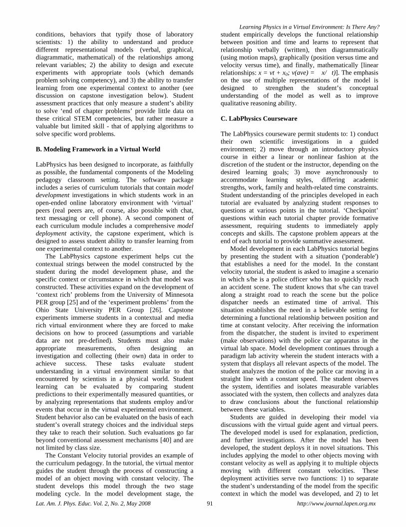
D. Courseware Components The virtual laboratory courseware currently encompasses three main components with which the end-user interacts. 1) A simulated, open-ended laboratory workspace (Figure 2) with virtual laboratory equipment and apparatus objects, the parameters of which can be modified, altered and controlled as well as misused, by the user in an experimental setting (students drag these objects from the equipment cabinet onto the lab table environment in order to set up their own experiments and collect and analyze real-time data generated within the software by standard differential equations);
FIGURE 2. Laboratory environment for constant acceleration investigations.
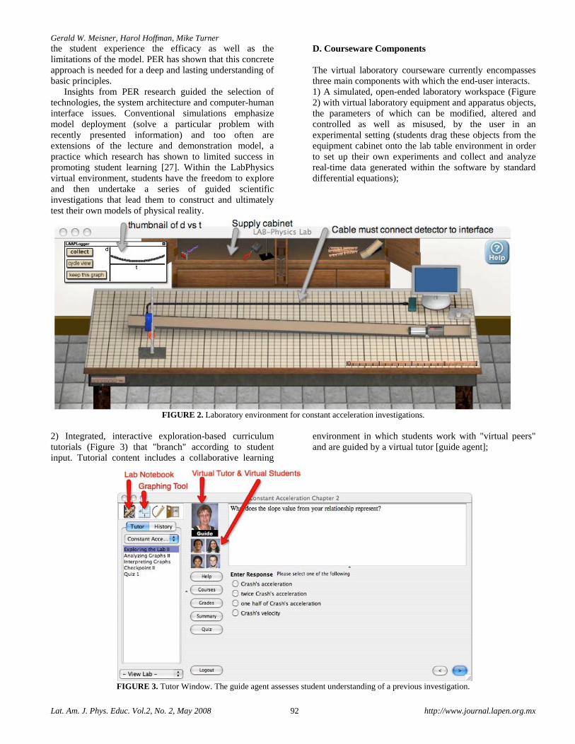
2) Integrated, interactive exploration-based curriculum tutorials (Figure 3) that "branch" according to student input. Tutorial content includes a collaborative learning
environment in which students work with "virtual peers" and are guided by a virtual tutor [guide agent];
FIGURE 3. Tutor Window. The guide agent assesses student understanding of a previous investigation.
Learning Physics in a Virtual Environment: Is There Any?
Lat. Am. J. Phys. Educ. Vol. 2, No. 2, May 2008 93 http://www.journal.lapen.org.mx
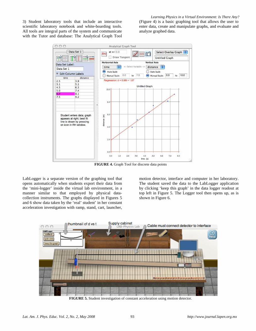
3) Student laboratory tools that include an interactive scientific laboratory notebook and white-boarding tools. All tools are integral parts of the system and communicate with the Tutor and database: The Analytical Graph Tool
(Figure 4) is a basic graphing tool that allows the user to enter data, create and manipulate graphs, and evaluate and analyze graphed data.
FIGURE 4. Graph Tool for discrete data points
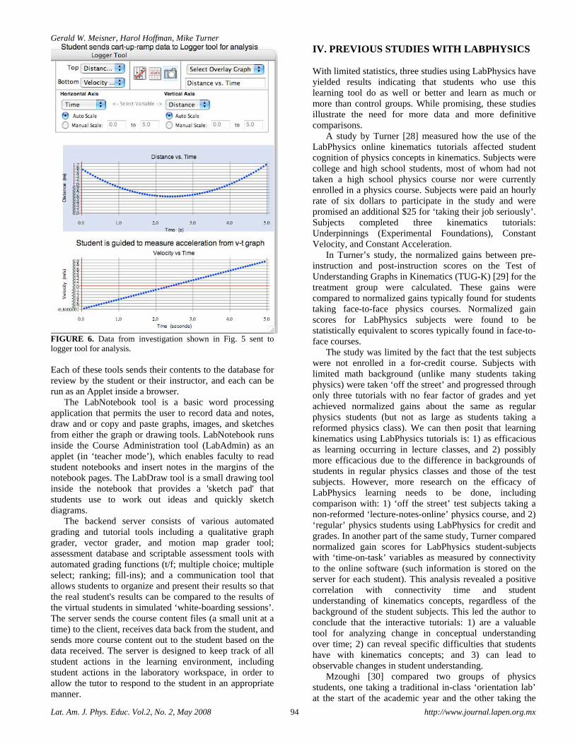
LabLogger is a separate version of the graphing tool that opens automatically when students export their data from the ‘mini-logger’ inside the virtual lab environment, in a manner similar to that employed by physical data-collection instruments. The graphs displayed in Figures 5 and 6 show data taken by the ‘real’ student’ in her constant acceleration investigation with ramp, stand, cart, launcher,
motion detector, interface and computer in her laboratory. The student saved the data to the LabLogger application by clicking ‘keep this graph’ in the data logger readout at top left in Figure 5. The Logger tool then opens up, as is shown in Figure 6.
FIGURE 5. Student investigation of constant acceleration using motion detector.
Gerald W. Meisner, Harol Hoffman, Mike Turner
Lat. Am. J. Phys. Educ. Vol.2, No. 2, May 2008 94 http://www.journal.lapen.org.mx
FIGURE 6. Data from investigation shown in Fig. 5 sent to logger tool for analysis. Each of these tools sends their contents to the database for review by the student or their instructor, and each can be run as an Applet inside a browser.
The LabNotebook tool is a basic word processing application that permits the user to record data and notes, draw and or copy and paste graphs, images, and sketches from either the graph or drawing tools. LabNotebook runs inside the Course Administration tool (LabAdmin) as an applet (in ‘teacher mode’), which enables faculty to read student notebooks and insert notes in the margins of the notebook pages. The LabDraw tool is a small drawing tool inside the notebook that provides a 'sketch pad' that students use to work out ideas and quickly sketch diagrams.
The backend server consists of various automated grading and tutorial tools including a qualitative graph grader, vector grader, and motion map grader tool; assessment database and scriptable assessment tools with automated grading functions (t/f; multiple choice; multiple select; ranking; fill-ins); and a communication tool that allows students to organize and present their results so that the real student's results can be compared to the results of the virtual students in simulated ‘white-boarding sessions’. The server sends the course content files (a small unit at a time) to the client, receives data back from the student, and sends more course content out to the student based on the data received. The server is designed to keep track of all student actions in the learning environment, including student actions in the laboratory workspace, in order to allow the tutor to respond to the student in an appropriate manner.
IV. PREVIOUS STUDIES WITH LABPHYSICS With limited statistics, three studies using LabPhysics have yielded results indicating that students who use this learning tool do as well or better and learn as much or more than control groups. While promising, these studies illustrate the need for more data and more definitive comparisons.
A study by Turner [28] measured how the use of the LabPhysics online kinematics tutorials affected student cognition of physics concepts in kinematics. Subjects were college and high school students, most of whom had not taken a high school physics course nor were currently enrolled in a physics course. Subjects were paid an hourly rate of six dollars to participate in the study and were promised an additional $25 for ‘taking their job seriously’. Subjects completed three kinematics tutorials: Underpinnings (Experimental Foundations), Constant Velocity, and Constant Acceleration.
In Turner’s study, the normalized gains between pre-instruction and post-instruction scores on the Test of Understanding Graphs in Kinematics (TUG-K) [29] for the treatment group were calculated. These gains were compared to normalized gains typically found for students taking face-to-face physics courses. Normalized gain scores for LabPhysics subjects were found to be statistically equivalent to scores typically found in face-to-face courses.
The study was limited by the fact that the test subjects were not enrolled in a for-credit course. Subjects with limited math background (unlike many students taking physics) were taken ‘off the street’ and progressed through only three tutorials with no fear factor of grades and yet achieved normalized gains about the same as regular physics students (but not as large as students taking a reformed physics class). We can then posit that learning kinematics using LabPhysics tutorials is: 1) as efficacious as learning occurring in lecture classes, and 2) possibly more efficacious due to the difference in backgrounds of students in regular physics classes and those of the test subjects. However, more research on the efficacy of LabPhysics learning needs to be done, including comparison with: 1) ‘off the street’ test subjects taking a non-reformed ‘lecture-notes-online’ physics course, and 2) ‘regular’ physics students using LabPhysics for credit and grades. In another part of the same study, Turner compared normalized gain scores for LabPhysics student-subjects with ‘time-on-task’ variables as measured by connectivity to the online software (such information is stored on the server for each student). This analysis revealed a positive correlation with connectivity time and student understanding of kinematics concepts, regardless of the background of the student subjects. This led the author to conclude that the interactive tutorials: 1) are a valuable tool for analyzing change in conceptual understanding over time; 2) can reveal specific difficulties that students have with kinematics concepts; and 3) can lead to observable changes in student understanding.
Mzoughi [30] compared two groups of physics students, one taking a traditional in-class ‘orientation lab’ at the start of the academic year and the other taking the
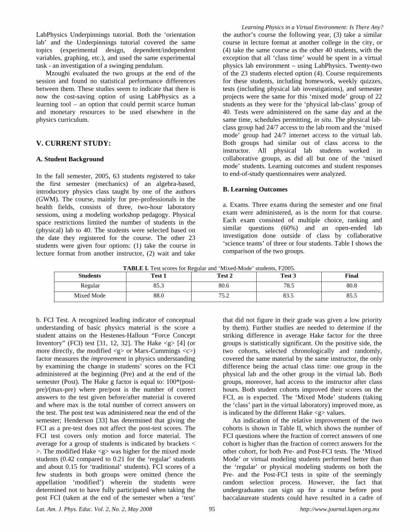
Learning Physics in a Virtual Environment: Is There Any?
Lat. Am. J. Phys. Educ. Vol. 2, No. 2, May 2008 95 http://www.journal.lapen.org.mx
LabPhysics Underpinnings tutorial. Both the ‘orientation lab’ and the Underpinnings tutorial covered the same topics (experimental design, dependent/independent variables, graphing, etc.), and used the same experimental task - an investigation of a swinging pendulum.
Mzoughi evaluated the two groups at the end of the session and found no statistical performance differences between them. These studies seem to indicate that there is now the cost-saving option of using LabPhysics as a learning tool – an option that could permit scarce human and monetary resources to be used elsewhere in the physics curriculum. V. CURRENT STUDY: A. Student Background In the fall semester, 2005, 63 students registered to take the first semester (mechanics) of an algebra-based, introductory physics class taught by one of the authors (GWM). The course, mainly for pre–professionals in the health fields, consists of three, two-hour laboratory sessions, using a modeling workshop pedagogy. Physical space restrictions limited the number of students in the (physical) lab to 40. The students were selected based on the date they registered for the course. The other 23 students were given four options: (1) take the course in lecture format from another instructor, (2) wait and take
the author’s course the following year, (3) take a similar course in lecture format at another college in the city, or (4) take the same course as the other 40 students, with the exception that all ‘class time’ would be spent in a virtual physics lab environment – using LabPhysics. Twenty-two of the 23 students elected option (4). Course requirements for these students, including homework, weekly quizzes, tests (including physical lab investigations), and semester projects were the same for this ‘mixed mode’ group of 22 students as they were for the ‘physical lab-class’ group of 40. Tests were administered on the same day and at the same time, schedules permitting, in situ. The physical lab-class group had 24/7 access to the lab room and the ‘mixed mode’ group had 24/7 internet access to the virtual lab. Both groups had similar out of class access to the instructor. All physical lab students worked in collaborative groups, as did all but one of the ‘mixed mode’ students. Learning outcomes and student responses to end-of-study questionnaires were analyzed. B. Learning Outcomes a. Exams. Three exams during the semester and one final exam were administered, as is the norm for that course. Each exam consisted of multiple choice, ranking and similar questions (60%) and an open-ended lab investigation done outside of class by collaborative ‘science teams’ of three or four students. Table I shows the comparison of the two groups.
TABLE I. Test scores for Regular and ‘Mixed-Mode’ students, F2005.
Students Test 1 Test 2 Test 3 Final
Regular 85.3 80.6 78.5 80.8
Mixed Mode 88.0 75.2 83.5 85.5
b. FCI Test. A recognized leading indicator of conceptual understanding of basic physics material is the score a student attains on the Hestenes-Halloun “Force Concept Inventory” (FCI) test [31, 12, 32]. The Hake <g> [4] (or more directly, the modified <g> or Marx-Cummings <c>) factor measures the improvement in physics understanding by examining the change in students’ scores on the FCI administered at the beginning (Pre) and at the end of the semester (Post). The Hake g factor is equal to: 100*(post-pre)/(max-pre) where pre/post is the number of correct answers to the test given before/after material is covered and where max is the total number of correct answers on the test. The post test was administered near the end of the semester; Henderson [33] has determined that giving the FCI as a pre-test does not affect the post-test scores. The FCI test covers only motion and force material. The average for a group of students is indicated by brackets < >. The modified Hake <g> was higher for the mixed mode students (0.42 compared to 0.21 for the ‘regular’ students and about 0.15 for ‘traditional’ students). FCI scores of a few students in both groups were omitted (hence the appellation ‘modified’) wherein the students were determined not to have fully participated when taking the post FCI (taken at the end of the semester when a ‘test’
that did not figure in their grade was given a low priority by them). Further studies are needed to determine if the striking difference in average Hake factor for the three groups is statistically significant. On the positive side, the two cohorts, selected chronologically and randomly, covered the same material by the same instructor, the only difference being the actual class time: one group in the physical lab and the other group in the virtual lab. Both groups, moreover, had access to the instructor after class hours. Both student cohorts improved their scores on the FCI, as is expected. The ‘Mixed Mode’ students (taking the ‘class’ part in the virtual laboratory) improved more, as is indicated by the different Hake <g> values.
An indication of the relative improvement of the two cohorts is shown in Table II, which shows the number of FCI questions where the fraction of correct answers of one cohort is higher than the fraction of correct answers for the other cohort, for both Pre- and Post-FCI tests. The ‘Mixed Mode’ or virtual modeling students performed better than the ‘regular’ or physical modeling students on both the Pre- and the Post-FCI tests in spite of the seemingly random selection process. However, the fact that undergraduates can sign up for a course before post baccalaureate students could have resulted in a cadre of
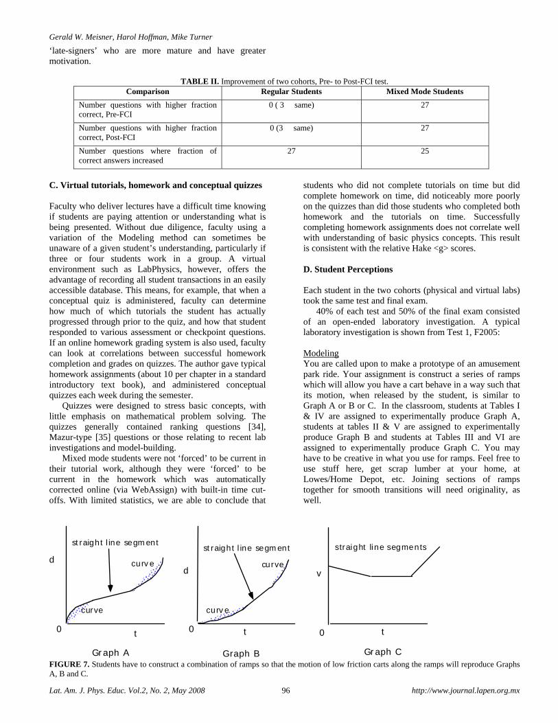
Gerald W. Meisner, Harol Hoffman, Mike Turner
Lat. Am. J. Phys. Educ. Vol.2, No. 2, May 2008 96 http://www.journal.lapen.org.mx
‘late-signers’ who are more mature and have greater motivation.
TABLE II. Improvement of two cohorts, Pre- to Post-FCI test.
Comparison Regular Students Mixed Mode Students
Number questions with higher fraction correct, Pre-FCI
0 ( 3 � same) 27
Number questions with higher fraction correct, Post-FCI
0 (3 � same) 27
Number questions where fraction of correct answers increased
27 25
C. Virtual tutorials, homework and conceptual quizzes Faculty who deliver lectures have a difficult time knowing if students are paying attention or understanding what is being presented. Without due diligence, faculty using a variation of the Modeling method can sometimes be unaware of a given student’s understanding, particularly if three or four students work in a group. A virtual environment such as LabPhysics, however, offers the advantage of recording all student transactions in an easily accessible database. This means, for example, that when a conceptual quiz is administered, faculty can determine how much of which tutorials the student has actually progressed through prior to the quiz, and how that student responded to various assessment or checkpoint questions. If an online homework grading system is also used, faculty can look at correlations between successful homework completion and grades on quizzes. The author gave typical homework assignments (about 10 per chapter in a standard introductory text book), and administered conceptual quizzes each week during the semester.
Quizzes were designed to stress basic concepts, with little emphasis on mathematical problem solving. The quizzes generally contained ranking questions [34], Mazur-type [35] questions or those relating to recent lab investigations and model-building.
Mixed mode students were not ‘forced’ to be current in their tutorial work, although they were ‘forced’ to be current in the homework which was automatically corrected online (via WebAssign) with built-in time cut-offs. With limited statistics, we are able to conclude that
students who did not complete tutorials on time but did complete homework on time, did noticeably more poorly on the quizzes than did those students who completed both homework and the tutorials on time. Successfully completing homework assignments does not correlate well with understanding of basic physics concepts. This result is consistent with the relative Hake <g> scores. D. Student Perceptions Each student in the two cohorts (physical and virtual labs) took the same test and final exam.
40% of each test and 50% of the final exam consisted of an open-ended laboratory investigation. A typical laboratory investigation is shown from Test 1, F2005: Modeling You are called upon to make a prototype of an amusement park ride. Your assignment is construct a series of ramps which will allow you have a cart behave in a way such that its motion, when released by the student, is similar to Graph A or B or C. In the classroom, students at Tables I & IV are assigned to experimentally produce Graph A, students at tables II & V are assigned to experimentally produce Graph B and students at Tables III and VI are assigned to experimentally produce Graph C. You may have to be creative in what you use for ramps. Feel free to use stuff here, get scrap lumber at your home, at Lowes/Home Depot, etc. Joining sections of ramps together for smooth transitions will need originality, as well.
d
t
d
t
v
t
Graph A Graph B Graph C
0 0 0
straight line segmentstraight line segment straight line segments
curve
curve
curve
curve
FIGURE 7. Students have to construct a combination of ramps so that the motion of low friction carts along the ramps will reproduce Graphs A, B and C.
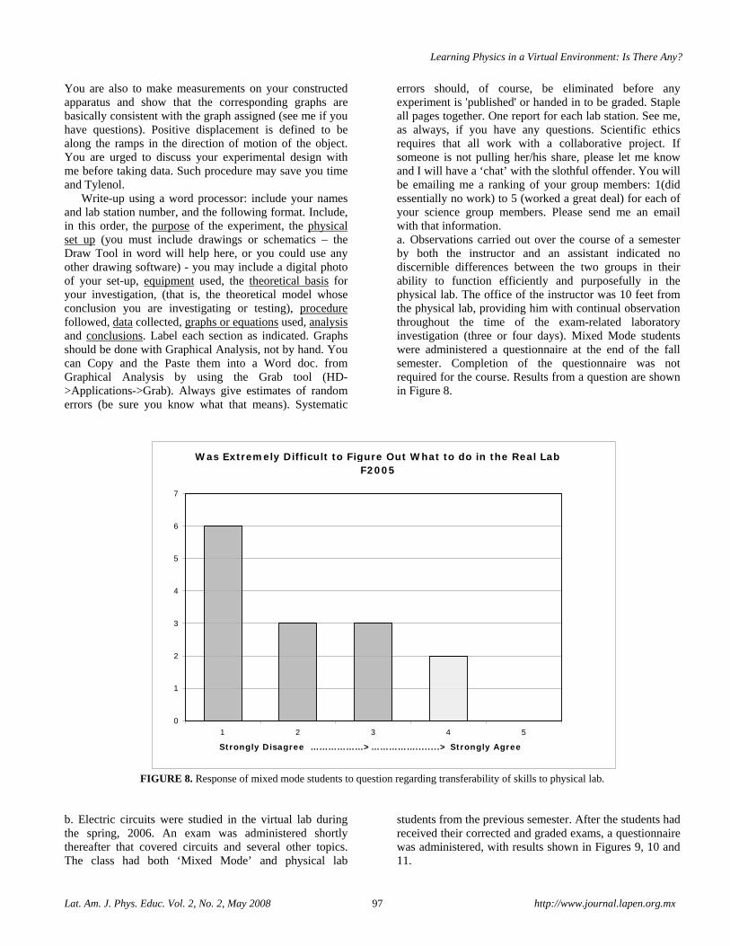
Learning Physics in a Virtual Environment: Is There Any?
Lat. Am. J. Phys. Educ. Vol. 2, No. 2, May 2008 97 http://www.journal.lapen.org.mx
You are also to make measurements on your constructed apparatus and show that the corresponding graphs are basically consistent with the graph assigned (see me if you have questions). Positive displacement is defined to be along the ramps in the direction of motion of the object. You are urged to discuss your experimental design with me before taking data. Such procedure may save you time and Tylenol.
Write-up using a word processor: include your names and lab station number, and the following format. Include, in this order, the purpose of the experiment, the physical set up (you must include drawings or schematics – the Draw Tool in word will help here, or you could use any other drawing software) - you may include a digital photo of your set-up, equipment used, the theoretical basis for your investigation, (that is, the theoretical model whose conclusion you are investigating or testing), procedure followed, data collected, graphs or equations used, analysis and conclusions. Label each section as indicated. Graphs should be done with Graphical Analysis, not by hand. You can Copy and the Paste them into a Word doc. from Graphical Analysis by using the Grab tool (HD->Applications->Grab). Always give estimates of random errors (be sure you know what that means). Systematic
errors should, of course, be eliminated before any experiment is 'published' or handed in to be graded. Staple all pages together. One report for each lab station. See me, as always, if you have any questions. Scientific ethics requires that all work with a collaborative project. If someone is not pulling her/his share, please let me know and I will have a ‘chat’ with the slothful offender. You will be emailing me a ranking of your group members: 1(did essentially no work) to 5 (worked a great deal) for each of your science group members. Please send me an email with that information. a. Observations carried out over the course of a semester by both the instructor and an assistant indicated no discernible differences between the two groups in their ability to function efficiently and purposefully in the physical lab. The office of the instructor was 10 feet from the physical lab, providing him with continual observation throughout the time of the exam-related laboratory investigation (three or four days). Mixed Mode students were administered a questionnaire at the end of the fall semester. Completion of the questionnaire was not required for the course. Results from a question are shown in Figure 8.
Was Extremely Difficult to Figure Out What to do in the Real Lab F2005
0
1
2
3
4
5
6
7
1 2 3 4 5
Strongly Disagree ………………>……………........> Strongly Agree
FIGURE 8. Response of mixed mode students to question regarding transferability of skills to physical lab.
b. Electric circuits were studied in the virtual lab during the spring, 2006. An exam was administered shortly thereafter that covered circuits and several other topics. The class had both ‘Mixed Mode’ and physical lab
students from the previous semester. After the students had received their corrected and graded exams, a questionnaire was administered, with results shown in Figures 9, 10 and 11.
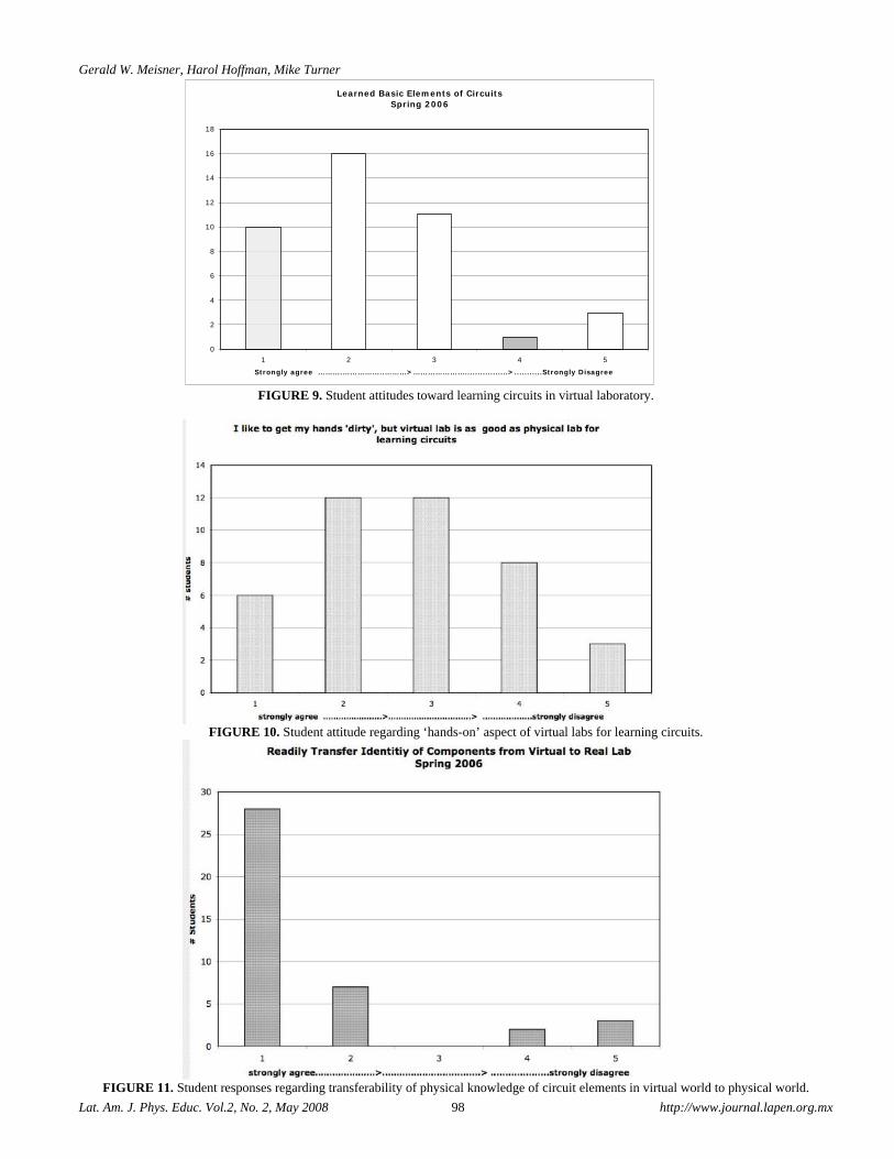
Gerald W. Meisner, Harol Hoffman, Mike Turner
Lat. Am. J. Phys. Educ. Vol.2, No. 2, May 2008 98 http://www.journal.lapen.org.mx
Learned Basic Elements of CircuitsSpring 2006
0
2
4
6
8
10
12
14
16
18
1 2 3 4 5
Strongly agree ……….……………..………>………………….................>...........Strongly Disagree
FIGURE 9. Student attitudes toward learning circuits in virtual laboratory.
FIGURE 10. Student attitude regarding ‘hands-on’ aspect of virtual labs for learning circuits.
FIGURE 11. Student responses regarding transferability of physical knowledge of circuit elements in virtual world to physical world.
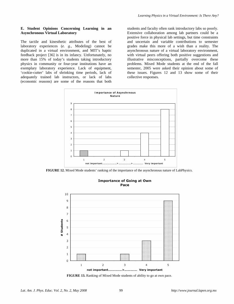
Learning Physics in a Virtual Environment: Is There Any?
Lat. Am. J. Phys. Educ. Vol. 2, No. 2, May 2008 99 http://www.journal.lapen.org.mx
E. Student Opinions Concerning Learning in an Asynchronous Virtual Laboratory The tactile and kinesthetic attributes of the best of laboratory experiences (e. g., Modeling) cannot be duplicated in a virtual environment, and MIT’s haptic feedback project [36] is in its infancy. Unfortunately, no more than 15% of today’s students taking introductory physics in community or four-year institutions have an exemplary laboratory experience. Lack of equipment, ‘cookie-cutter’ labs of shrinking time periods, lack of adequately trained lab instructors, or lack of labs (economic reasons) are some of the reasons that both
students and faculty often rank introductory labs so poorly. Extensive collaboration among lab partners could be a positive force in physical lab settings, but time constraints and uncertain and variable contributions to semester grades make this more of a wish than a reality. The asynchronous nature of a virtual laboratory environment, with virtual peers offering both positive suggestions and illustrative misconceptions, partially overcome these problems. Mixed Mode students at the end of the fall semester, 2005 were asked their opinion about some of these issues. Figures 12 and 13 show some of their collective responses.
Importance of Asynchrnous Nature
0
1
2
3
4
5
6
7
8
9
1 2 3 4 5
not important.………………>…..........…>............. Very important
FIGURE 12. Mixed Mode students’ ranking of the importance of the asynchronous nature of LabPhysics.
FIGURE 13. Ranking of Mixed Mode students of ability to go at own pace.
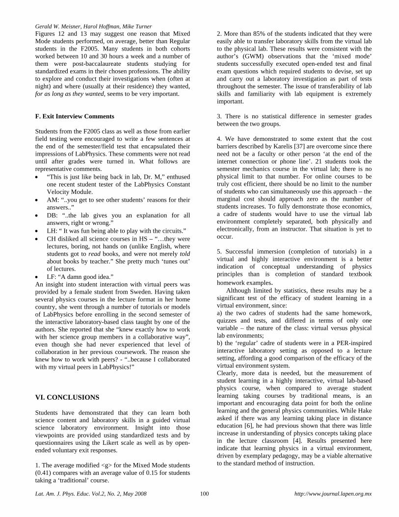
Gerald W. Meisner, Harol Hoffman, Mike Turner
Lat. Am. J. Phys. Educ. Vol.2, No. 2, May 2008 100 http://www.journal.lapen.org.mx
Figures 12 and 13 may suggest one reason that Mixed Mode students performed, on average, better than Regular students in the F2005. Many students in both cohorts worked between 10 and 30 hours a week and a number of them were post-baccalaureate students studying for standardized exams in their chosen professions. The ability to explore and conduct their investigations when (often at night) and where (usually at their residence) they wanted, for as long as they wanted, seems to be very important. F. Exit Interview Comments Students from the F2005 class as well as those from earlier field testing were encouraged to write a few sentences at the end of the semester/field test that encapsulated their impressions of LabPhysics. These comments were not read until after grades were turned in. What follows are representative comments. • “This is just like being back in lab, Dr. M,” enthused
one recent student tester of the LabPhysics Constant Velocity Module.
• AM: “..you get to see other students’ reasons for their answers..”
• DB: “..the lab gives you an explanation for all answers, right or wrong.”
• LH: “ It was fun being able to play with the circuits.” • CH disliked all science courses in HS – “…they were
lectures, boring, not hands on (unlike English, where students got to read books, and were not merely told about books by teacher.” She pretty much ‘tunes out’ of lectures.
• LF: “A damn good idea.” An insight into student interaction with virtual peers was provided by a female student from Sweden. Having taken several physics courses in the lecture format in her home country, she went through a number of tutorials or models of LabPhysics before enrolling in the second semester of the interactive laboratory-based class taught by one of the authors. She reported that she “knew exactly how to work with her science group members in a collaborative way”, even though she had never experienced that level of collaboration in her previous coursework. The reason she knew how to work with peers? - “..because I collaborated with my virtual peers in LabPhysics!” VI. CONCLUSIONS Students have demonstrated that they can learn both science content and laboratory skills in a guided virtual science laboratory environment. Insight into those viewpoints are provided using standardized tests and by questionnaires using the Likert scale as well as by open-ended voluntary exit responses. 1. The average modified <g> for the Mixed Mode students (0.41) compares with an average value of 0.15 for students taking a ‘traditional’ course.
2. More than 85% of the students indicated that they were easily able to transfer laboratory skills from the virtual lab to the physical lab. These results were consistent with the author’s (GWM) observations that the ‘mixed mode’ students successfully executed open-ended test and final exam questions which required students to devise, set up and carry out a laboratory investigation as part of tests throughout the semester. The issue of transferability of lab skills and familiarity with lab equipment is extremely important. 3. There is no statistical difference in semester grades between the two groups. 4. We have demonstrated to some extent that the cost barriers described by Karelis [37] are overcome since there need not be a faculty or other person ‘at the end of the internet connection or phone line’. 21 students took the semester mechanics course in the virtual lab; there is no physical limit to that number. For online courses to be truly cost efficient, there should be no limit to the number of students who can simultaneously use this approach – the marginal cost should approach zero as the number of students increases. To fully demonstrate those economics, a cadre of students would have to use the virtual lab environment completely separated, both physically and electronically, from an instructor. That situation is yet to occur. 5. Successful immersion (completion of tutorials) in a virtual and highly interactive environment is a better indication of conceptual understanding of physics principles than is completion of standard textbook homework examples.
Although limited by statistics, these results may be a significant test of the efficacy of student learning in a virtual environment, since: a) the two cadres of students had the same homework, quizzes and tests, and differed in terms of only one variable – the nature of the class: virtual versus physical lab environments; b) the ‘regular’ cadre of students were in a PER-inspired interactive laboratory setting as opposed to a lecture setting, affording a good comparison of the efficacy of the virtual environment system. Clearly, more data is needed, but the measurement of student learning in a highly interactive, virtual lab-based physics course, when compared to average student learning taking courses by traditional means, is an important and encouraging data point for both the online learning and the general physics communities. While Hake asked if there was any learning taking place in distance education [6], he had previous shown that there was little increase in understanding of physics concepts taking place in the lecture classroom [4]. Results presented here indicate that learning physics in a virtual environment, driven by exemplary pedagogy, may be a viable alternative to the standard method of instruction.
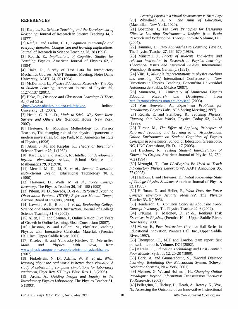
Learning Physics in a Virtual Environment: Is There Any?
Lat. Am. J. Phys. Educ. Vol. 2, No. 2, May 2008 101 http://www.journal.lapen.org.mx
REFERENCES [1] Karplus, R., Science Teaching and the Development of Reasoning, Journal of Research in Science Teaching 14, 7 (1977). [2] Reif, F. and Larkin, J. H., Cognition in scientific and everyday domains: Comparison and learning implications, Journal of Research in Science Teaching 28, 28 (1991). [3] Redish, E., Implications of Cognitive Studies for Teaching Physics, American Journal of Physics 62, 8 (1994). [4] Hake, R., Survey of Test Data for Introductory Mechanics Courses, AAPT Summer Meeting, Notre Dame University, AAPT. 24, 55 (1994). [5] McDermott, L., Physics Education Research - The Key to Student Learning, American Journal of Physics 69, 1127-1137 (2001). [6] Hake, R., Distance and Classroom Learning: Is There Any? ref 53 at <http://www.physics.indiana.edu/~hake>, Indiana University: 21 (2007). [7] Heath, C. H. a. D., Made to Stick: Why Some Ideas Survive and Others Die, (Random House, New York, 2007). [8] Hestenes, D., Modeling Methodology for Physics Teachers, The changing role of the physics department in modern universities, College Park, MD, American Institute of Physics, (1996). [9] Atkin, J. M. and Karplus, R., Theory or Invention? Science Teacher 29, 1 (1962). [10] Karplus, E. and Karplus, R., Intellectual development beyond elementary school, School Science and Mathematics 79, 9 (1970). [11] Merrill, M. D., Li, Z. et al., Second Generation Instructional Design, Educational Technology 30, 8 (1990). [12] Hestenes, D., Wells, M. et al., Force Concept Inventory, The Physics Teacher 30, 141-158 (1992). [13] Piburn, M. D., Sawada, D. et al., Reformed Teaching Observation Protocol (RTOP) Reference Manual Tempe, Arizona Board of Regents, (2000). [14] Lawson, A. E., Bloom, I. et al., Evaluating College Science and Mathematics Instruction, Journal of College Science Teaching 31, 6 (2002).- [15] Allen, I. E. and Seaman, J., Online Nation: Five Years of Growth in Online Learning, Sloan Consortium (2007). [16] Christian, W. and Belloni, M., Physlets: Teaching Physics with Interactive Curricular Material, (Prentice Hall, Inc., Upper Saddle River, 2001). [17] Kiselev, S. and Yanovsky-Kiselev, T., Interactive Math and Physics with Java, from www.physics.uoguelph.ca/applets/intro_physics/kisalev, (2007). [18] Finkelstein, N. D., Adams, W. K. et al., When learning about the real world is better done virtually: A study of substituting computer simulations for laboratory equipment, Phys. Rev. ST Phys. Educ. Res. 1, 8 (2005). [19] Arons, A., Guiding Insight and Inquiry in the Introductory Physics Laboratory, The Physics Teacher 31, 5 (1993).
[20] Whitehead, A. N., The Aims of Education, (Macmillan, New York, 1929). [21] Boettcher, J., Ten Core Principles for Designing Effective Learning Environments: Insights from Brain Research and Pedagogical Theory, Innovate Volume, DOI (2007). [22] Hammer, D., Two Approaches to Learning Physics, The Physics Teacher 27, 664-670 (1989). [23] Minstrell, J., Facets of students' knowledge and relevant instruction in Research in Physics Learning: Theoretical Issues and Empirical Studies, International Workshop, Bremen, Germany, (1991). [24] Viiri, J., Multiple Representations in physics teaching and learning, XV International Conference on New Directions in Physics Teaching, Benemérita Universidad Autónoma de Puebla, México (2007). [25] Minnesota, U., University of Minnesota Physics Education Research and Development, from http://groups.physics.umn.edu/physed/, (2008). [26] Van Heuvelen, A., Experiment Problems for Introductory Physics Labs, APS Spring Meeting (1997). [27] Redish, E. and Steinberg, R., Teaching Physics: Figuring Out What Works, Physics Today 52, 24-30 (1999). [28] Turner, M., The Effect of Applying Principles of Reformed Teaching and Learning to an Asynchronous Online Environment on Student Cognition of Physics Concepts in Kinematics, School of Education, Greensboro, NC, UNC Greensboro, Ph. D. 117 (2005). [29] Beichner, R., Testing Student Interpretation of Kinematics Graphs, American Journal of Physics 62, 750-762 (1994). [30] Mzoughi, T., Can LAAPhysics Be Used to Teach Introductory Physics Laboratory?, AAPT Announcer 35, 77 (2005). [31] Halloun, I. and Hestenes, D., Initial Knowledge State of College Physics Students, American Journal of Physics 53, (1985). [32] Huffman, D. and Heller, P., What Does the Force Concept Inventory Acually Measure?, The Physics Teacher 33, 6 (1995). [33] Henderson, C., Common Concerns About the Force Concept Inventory, The Physics Teacher 40, 6 (2002). [34] O'Kuma, T., Maloney, D. et al., Ranking Task Exercises in Physics, (Prentice Hall, Upper Saddle River, New Jersey, 2000). [35] Mazur, E., Peer Instruction, (Prentice Hall Series in Educational Innovation, Prentice Hall, Inc., Upper Saddle River, 1997). [36] Thompson, E., MIT and London team report first transatlantic touch, Volume, DOI (2002). [37] Karelis, C., Education Technology and Cost Control: Four Models, Syllabus 12, 20-28 (1999). [38] Bork, A. and Gunnarsdottir, S., Tutorial Distance Learning: Rebuilding Our Educational System, (Kluwer Academic Systems, New York, 2001). [39] Meisner, G. W. and Hoffman, H., Changing Online Paradigms: Beyond Information Transmission 'Lectures' To Research-, (2003). [40] Pellegrino, J., Hickey, D., Heath, A., Rewey, K., Vye, N., Assessing the Outcome of an Innovatifve Instructional

Gerald W. Meisner, Harol Hoffman, Mike Turner
Lat. Am. J. Phys. Educ. Vol.2, No. 2, May 2008 102 http://www.journal.lapen.org.mx
Program. Technology Report No. 91-1, The Vanderbilt Learning Technology Center. Nashville, TN, (1991).
[41] MIT. "MIT Open CourseWare." from http://ocw.mit.edu/OcwWeb/hs/home/home/index.html
__________________________________________________________________________________________________________________ *The thesis is developing in the International Doctorate in Teaching Sciences of Burgos University, Spain, in agreement with the UFRGS, Brazil. Director: Dr. Marco Antonio Moreira, Joint Directress: Dra. Maria Rita Otero.
Lat. Am. J. Phys. Educ. Vol. 2, No.2, May 2008 103 http://www.journal.lapen.org.mx
Basics Quantum Mechanics teaching in Secondary School: One Conceptual Structure based on Paths Integrals Method
Maria de los Ángeles Fanaro1, Maria Rita Otero 1,2 1NIECyT-Departamento de Formación Docente- UNCPBA-Argentina.
2CONICET-Argentina.
E-mail: [email protected], [email protected] (Received 15 January 2008; accepted 18 April 2008)
Abstract This paper integrates a doctoral thesis* to investigate the Basics Quantum Mechanics (MQ) teaching in high school. This work adopts as Conceptual Structure of Reference the Paths Integrals method of Feynman [4], and a Proposed Conceptual Structure for Teaching (PCST) [2, 3] is designed, analyzed and proposed. The PCST does not follow the historical route and it is complementary of the canonical formalism. The concepts: probability distribution, quantum system, x(t) alternative, amplitude of probability, sum of probability amplitude, action, Planck´ s constant, and classic-quantum transition were constructed with the students. The math formalism was eluded and simulation software assistance was used. Also, we are presenting results about the affective impact (PCST) in the class group. Keywords: Quantum Mechanics Teaching, Physics Didactic, Affectivity.
Resumen Este trabajo es parte de una tesis doctoral* que investiga la Enseñanza de Fundamentos de Mecánica Cuántica (MC) en la Enseñanza Media. En ella se establece como Estructura Conceptual de Referencia al método de Integrales de Trayectoria de Feynman [4], y se analiza, propone e implementa, una Estructura Conceptual Propuesta para Enseñar (ECPE) [2, 3] que no sigue la génesis histórica y es complementaria al formalismo canónico. Se pretende reconstruir con los estudiantes de nivel medio los conceptos: distribución de probabilidad, sistema cuántico, x(t) alternativas, amplitud de probabilidad, suma de amplitudes de probabilidad, acción, constante de Planck, transición clásico-cuántico, eludiendo el formalismo y con asistencia de software de simulación. En este trabajo se presentan resultados acerca del impacto afectivo de la propuesta en los estudiantes del grupo de clase que participaron de la implementación. Palabras clave: Enseñanza de la Mecánica Cuántica, Didáctica de la Física, Afectividad. PACS: 01.40.Fk, 01.40.gb, 03.65.-w ISSN 1870-9095
I. INTRODUCTION This work comprises an investigation about the Basics Quantum Mechanics (QM) teaching in the high school. The organization of the concepts does not follow a time line. The Paths Integrals method of Feynman [1] was adopted as Referential Conceptual Structure (RCS) [2, 3] that is an alternative to the canonical formalism [4]. We have designed a Proposed Conceptual Structure for teaching the foundations of Quantum Mechanics (QM) eluding the math formalism and using simulation software.
The investigation intends to analyze the viability of a proposal to study QM in the high school. We want to understand the knowledge construction process in the classroom and in each group of discussion; the adaptation of designed materials; and the interaction between the students and the teacher. In a previous publication, we presented and discussed results obtained by the students in their evaluation tests. [5]. In the present work, we are also analyzing results on the affective dimension.
In order to know students’ perceptions about the studied concepts; the results of the implemented sequence; and the students’ performance using the software, we will
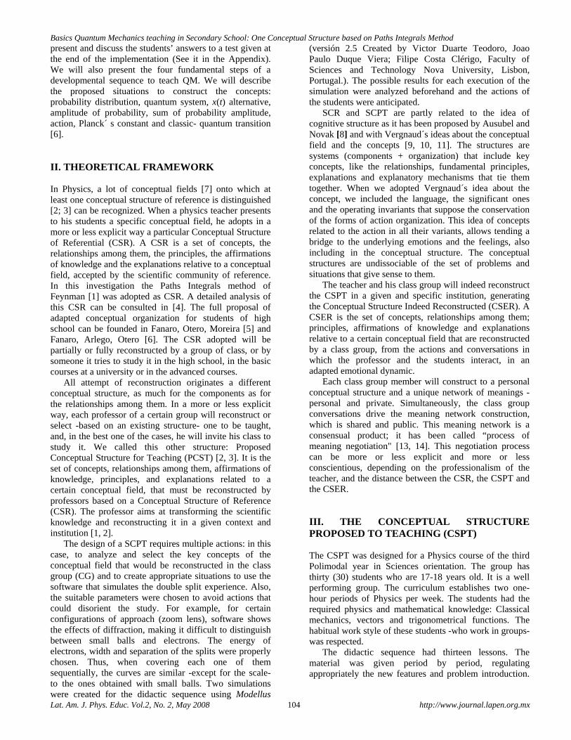
Basics Quantum Mechanics teaching in Secondary School: One Conceptual Structure based on Paths Integrals Method
Lat. Am. J. Phys. Educ. Vol.2, No. 2, May 2008 104 http://www.journal.lapen.org.mx
present and discuss the students’ answers to a test given at the end of the implementation (See it in the Appendix). We will also present the four fundamental steps of a developmental sequence to teach QM. We will describe the proposed situations to construct the concepts: probability distribution, quantum system, x(t) alternative, amplitude of probability, sum of probability amplitude, action, Planck´ s constant and classic- quantum transition [6]. II. THEORETICAL FRAMEWORK In Physics, a lot of conceptual fields [7] onto which at least one conceptual structure of reference is distinguished [2; 3] can be recognized. When a physics teacher presents to his students a specific conceptual field, he adopts in a more or less explicit way a particular Conceptual Structure of Referential (CSR). A CSR is a set of concepts, the relationships among them, the principles, the affirmations of knowledge and the explanations relative to a conceptual field, accepted by the scientific community of reference. In this investigation the Paths Integrals method of Feynman [1] was adopted as CSR. A detailed analysis of this CSR can be consulted in [4]. The full proposal of adapted conceptual organization for students of high school can be founded in Fanaro, Otero, Moreira [5] and Fanaro, Arlego, Otero [6]. The CSR adopted will be partially or fully reconstructed by a group of class, or by someone it tries to study it in the high school, in the basic courses at a university or in the advanced courses.
All attempt of reconstruction originates a different conceptual structure, as much for the components as for the relationships among them. In a more or less explicit way, each professor of a certain group will reconstruct or select -based on an existing structure- one to be taught, and, in the best one of the cases, he will invite his class to study it. We called this other structure: Proposed Conceptual Structure for Teaching (PCST) [2, 3]. It is the set of concepts, relationships among them, affirmations of knowledge, principles, and explanations related to a certain conceptual field, that must be reconstructed by professors based on a Conceptual Structure of Reference (CSR). The professor aims at transforming the scientific knowledge and reconstructing it in a given context and institution [1, 2].
The design of a SCPT requires multiple actions: in this case, to analyze and select the key concepts of the conceptual field that would be reconstructed in the class group (CG) and to create appropriate situations to use the software that simulates the double split experience. Also, the suitable parameters were chosen to avoid actions that could disorient the study. For example, for certain configurations of approach (zoom lens), software shows the effects of diffraction, making it difficult to distinguish between small balls and electrons. The energy of electrons, width and separation of the splits were properly chosen. Thus, when covering each one of them sequentially, the curves are similar -except for the scale- to the ones obtained with small balls. Two simulations were created for the didactic sequence using Modellus
(versión 2.5 Created by Victor Duarte Teodoro, Joao Paulo Duque Viera; Filipe Costa Clérigo, Faculty of Sciences and Technology Nova University, Lisbon, Portugal.). The possible results for each execution of the simulation were analyzed beforehand and the actions of the students were anticipated.
SCR and SCPT are partly related to the idea of cognitive structure as it has been proposed by Ausubel and Novak [8] and with Vergnaud´s ideas about the conceptual field and the concepts [9, 10, 11]. The structures are systems (components + organization) that include key concepts, like the relationships, fundamental principles, explanations and explanatory mechanisms that tie them together. When we adopted Vergnaud´s idea about the concept, we included the language, the significant ones and the operating invariants that suppose the conservation of the forms of action organization. This idea of concepts related to the action in all their variants, allows tending a bridge to the underlying emotions and the feelings, also including in the conceptual structure. The conceptual structures are undissociable of the set of problems and situations that give sense to them.
The teacher and his class group will indeed reconstruct the CSPT in a given and specific institution, generating the Conceptual Structure Indeed Reconstructed (CSER). A CSER is the set of concepts, relationships among them; principles, affirmations of knowledge and explanations relative to a certain conceptual field that are reconstructed by a class group, from the actions and conversations in which the professor and the students interact, in an adapted emotional dynamic.
Each class group member will construct to a personal conceptual structure and a unique network of meanings -personal and private. Simultaneously, the class group conversations drive the meaning network construction, which is shared and public. This meaning network is a consensual product; it has been called “process of meaning negotiation" [13, 14]. This negotiation process can be more or less explicit and more or less conscientious, depending on the professionalism of the teacher, and the distance between the CSR, the CSPT and the CSER. III. THE CONCEPTUAL STRUCTURE PROPOSED TO TEACHING (CSPT) The CSPT was designed for a Physics course of the third Polimodal year in Sciences orientation. The group has thirty (30) students who are 17-18 years old. It is a well performing group. The curriculum establishes two one-hour periods of Physics per week. The students had the required physics and mathematical knowledge: Classical mechanics, vectors and trigonometrical functions. The habitual work style of these students -who work in groups-was respected.
The didactic sequence had thirteen lessons. The material was given period by period, regulating appropriately the new features and problem introduction.
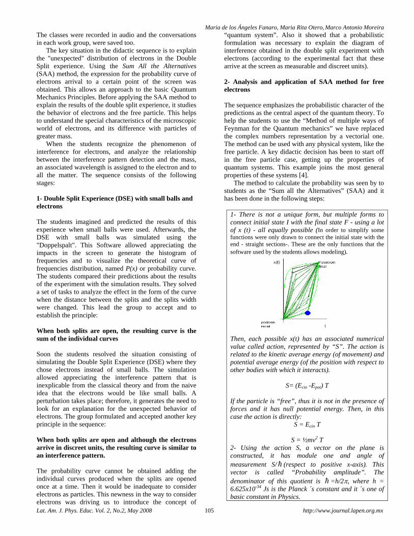
Maria de los Ángeles Fanaro, Maria Rita Otero, Marco Antonio Moreira
Lat. Am. J. Phys. Educ. Vol. 2, No.2, May 2008 105 http://www.journal.lapen.org.mx
The classes were recorded in audio and the conversations in each work group, were saved too.
The key situation in the didactic sequence is to explain the "unexpected" distribution of electrons in the Double Split experience. Using the Sum All the Alternatives (SAA) method, the expression for the probability curve of electrons arrival to a certain point of the screen was obtained. This allows an approach to the basic Quantum Mechanics Principles. Before applying the SAA method to explain the results of the double split experience, it studies the behavior of electrons and the free particle. This helps to understand the special characteristics of the microscopic world of electrons, and its difference with particles of greater mass.
When the students recognize the phenomenon of interference for electrons, and analyze the relationship between the interference pattern detection and the mass, an associated wavelength is assigned to the electron and to all the matter. The sequence consists of the following stages: 1- Double Split Experience (DSE) with small balls and electrons The students imagined and predicted the results of this experience when small balls were used. Afterwards, the DSE with small balls was simulated using the "Doppelspalt". This Software allowed appreciating the impacts in the screen to generate the histogram of frequencies and to visualize the theoretical curve of frequencies distribution, named P(x) or probability curve. The students compared their predictions about the results of the experiment with the simulation results. They solved a set of tasks to analyze the effect in the form of the curve when the distance between the splits and the splits width were changed. This lead the group to accept and to establish the principle: When both splits are open, the resulting curve is the sum of the individual curves Soon the students resolved the situation consisting of simulating the Double Split Experience (DSE) where they chose electrons instead of small balls. The simulation allowed appreciating the interference pattern that is inexplicable from the classical theory and from the naive idea that the electrons would be like small balls. A perturbation takes place; therefore, it generates the need to look for an explanation for the unexpected behavior of electrons. The group formulated and accepted another key principle in the sequence: When both splits are open and although the electrons arrive in discreet units, the resulting curve is similar to an interference pattern. The probability curve cannot be obtained adding the individual curves produced when the splits are opened once at a time. Then it would be inadequate to consider electrons as particles. This newness in the way to consider electrons was driving us to introduce the concept of
“quantum system”. Also it showed that a probabilistic formulation was necessary to explain the diagram of interference obtained in the double split experiment with electrons (according to the experimental fact that these arrive at the screen as measurable and discreet units). 2- Analysis and application of SAA method for free electrons The sequence emphasizes the probabilistic character of the predictions as the central aspect of the quantum theory. To help the students to use the “Method of multiple ways of Feynman for the Quantum mechanics” we have replaced the complex numbers representation by a vectorial one. The method can be used with any physical system, like the free particle. A key didactic decision has been to start off in the free particle case, getting up the properties of quantum systems. This example joins the most general properties of these systems [4].
The method to calculate the probability was seen by to students as the “Sum all the Alternatives” (SAA) and it has been done in the following steps:
1- There is not a unique form, but multiple forms to connect initial state I with the final state F - using a lot of x (t) - all equally possible (In order to simplify some functions were only drawn to connect the initial state with the end - straight sections-. These are the only functions that the software used by the students allows modeling).
Then, each possible x(t) has an associated numerical value called action, represented by “S”. The action is related to the kinetic average energy (of movement) and potential average energy (of the position with respect to other bodies with which it interacts).
S= (Ecin -Epot) T
If the particle is “free”, thus it is not in the presence of forces and it has null potential energy. Then, in this case the action is directly:
S = Ecin T
S = ½mv2 T 2- Using the action S, a vector on the plane is constructed, it has module one and angle of measurement S/ (respect to positive x-axis). This vector is called “Probability amplitude”. The denominator of this quotient is =h/2π, where h = 6.625x10⁻³⁴ Js is the Planck ´s constant and it ´s one of basic constant in Physics.
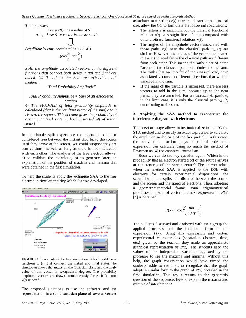
Basics Quantum Mechanics teaching in Secondary School: One Conceptual Structure based on Paths Integrals Method
Lat. Am. J. Phys. Educ. Vol.2, No. 2, May 2008 106 http://www.journal.lapen.org.mx
That is to say: Every x(t) has a value of S using these S, a vector is constructed: Amplitude Vector associated to each x(t)
)S
;S
cos( sen
3-All the amplitude associated vectors at the different functions that connect both states initial and final are added. We’ll call to the Sum vector(head to tail method):
“Total Probability Amplitude”
Total Probability Amplitude = Sum of all associated vectors
4- The MODULE of total probability amplitude is calculated (that is the resultant vector of the sum) and it rises to the square. This account gives the probability of arriving at final state F, having started off of initial state I.
In the double split experience the electrons could be considered free between the instant they leave the source until they arrive at the screen. We could suppose they are sent at time intervals as long as there is not interaction with each other. The analysis of the free electron allows: a) to validate the technique, b) to generate later, an explanation of the position of maxima and minima that were obtained in the first simulation. To help the students apply the technique SAA to the free electron, a simulation using Modellus was developed.
FIGURE 1. Screen about the first simulation. Selecting different functions x (t) that connect the initial and final states, the simulation shows the angles on the Cartesian plane and the angle value of this vector in sexagesimal degrees. The probability amplitude vectors are drawn simultaneously for each function x(t) selected. The proposed situations to use the software and the representation in a same cartesian plane of several vectors
associated to functions x(t) near and distant to the classical one, allow the GC to formulate the following conclusions: • The action S is minimum for the classical functional
relation x(t) -a straight line- if it is compared with other arbitrary functional relations x(t).
• The angles of the amplitude vectors associated with those paths x(t) near the classical path xclas(t) are similar. However, the angles of the vectors associated to the x(t) placed far to the classical path are different from each other. This means that only a set of paths “around” the classical path contributes to the sum. The paths that are too far of the classical one, have associated vectors in different directions that will be annulled in the sum.
• If the mass of the particle is increased, there are less vectors to add in the sum, because up to the near paths, they are annulled. For a macroscopic particle, in the limit case, it is only the classical path xclas(t) contributing to the sum.
3- Applying the SAA method to reconstruct the interference diagram with electrons The previous stage allows to institutionalize in the CG the STA method and to justify an exact expression to calculate the amplitude in the case of the free particle. In this case, the conventional action plays a central role; this expression can calculate using so much the method of Feynman as [4] the canonical formalism.
Soon we can do the key question again: Which is the probability that an electron started off of the source arrives at a distance x of the screen center? The answer arises when the method SAA is applied to the DSE with electrons for certain experimental dispositions: the separation of the splits, the distance between the source and the screen and the speed of electrons. Then, adopting a geometric-vectorial frame, some trigonometrical properties and sum of vectors the next expression of P(x) [4] is obtained:
⎟⎟⎠
⎞⎜⎜⎝
⎛x
T
mdxP
42cos~)( .
The students discussed and analyzed with their group the applied processes and the functional form of the expression P(x). Using this expression and certain experimental characteristics (separation distance, time, etc.) given by the teacher, they made an approximate graphical representation of P(x). The students used the values of the independent variable suggested by the professor to see the maxima and minima. Without this help, the graph construction would have turned the students aside to the first: to recognize that the graph adopts a similar form to the graph of P(x) obtained in the first simulation. This result returns to the generatrix question of the sequence: how to explain the maxima and minima of interference?
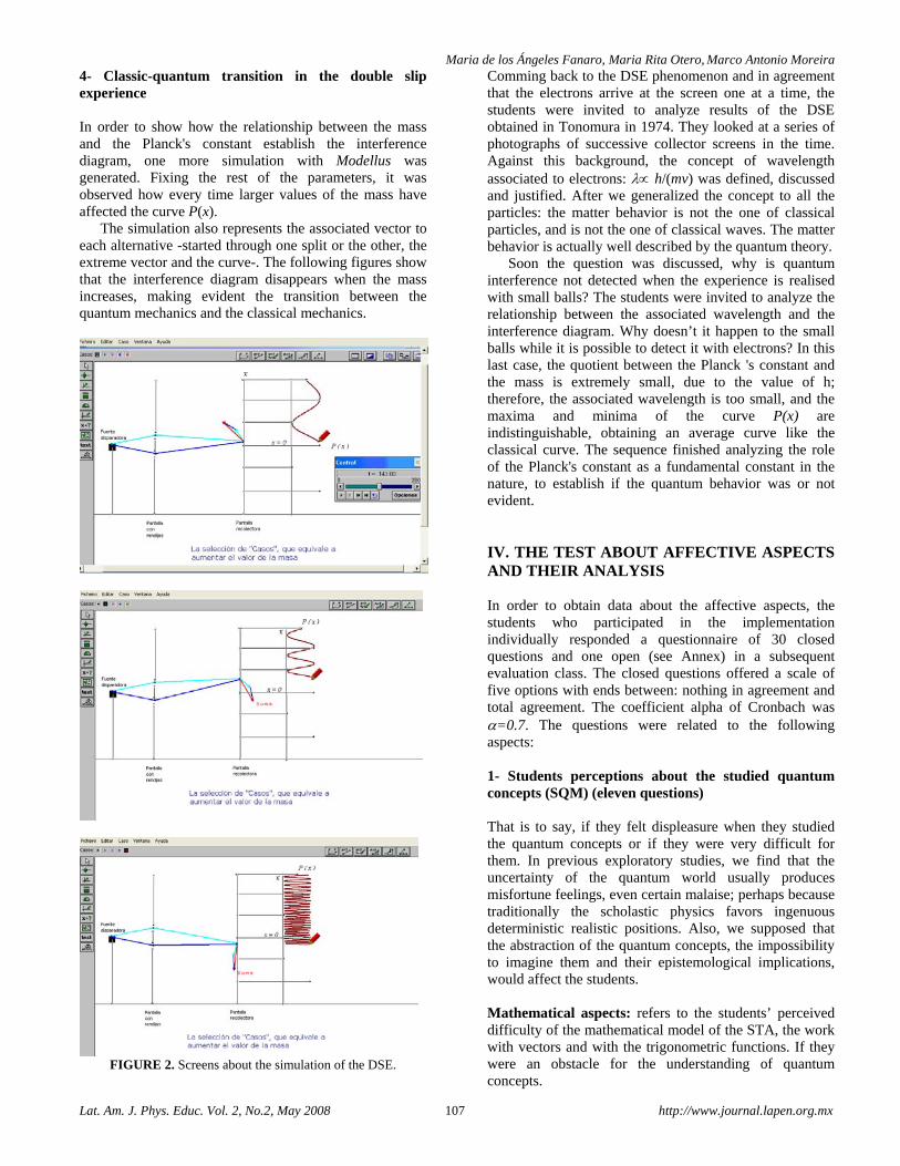
Maria de los Ángeles Fanaro, Maria Rita Otero, Marco Antonio Moreira
Lat. Am. J. Phys. Educ. Vol. 2, No.2, May 2008 107 http://www.journal.lapen.org.mx
4- Classic-quantum transition in the double slip experience In order to show how the relationship between the mass and the Planck's constant establish the interference diagram, one more simulation with Modellus was generated. Fixing the rest of the parameters, it was observed how every time larger values of the mass have affected the curve P(x).
The simulation also represents the associated vector to each alternative -started through one split or the other, the extreme vector and the curve-. The following figures show that the interference diagram disappears when the mass increases, making evident the transition between the quantum mechanics and the classical mechanics.
FIGURE 2. Screens about the simulation of the DSE.
Comming back to the DSE phenomenon and in agreement that the electrons arrive at the screen one at a time, the students were invited to analyze results of the DSE obtained in Tonomura in 1974. They looked at a series of photographs of successive collector screens in the time. Against this background, the concept of wavelength associated to electrons: λ∝ h/(mv) was defined, discussed and justified. After we generalized the concept to all the particles: the matter behavior is not the one of classical particles, and is not the one of classical waves. The matter behavior is actually well described by the quantum theory.
Soon the question was discussed, why is quantum interference not detected when the experience is realised with small balls? The students were invited to analyze the relationship between the associated wavelength and the interference diagram. Why doesn’t it happen to the small balls while it is possible to detect it with electrons? In this last case, the quotient between the Planck 's constant and the mass is extremely small, due to the value of h; therefore, the associated wavelength is too small, and the maxima and minima of the curve P(x) are indistinguishable, obtaining an average curve like the classical curve. The sequence finished analyzing the role of the Planck's constant as a fundamental constant in the nature, to establish if the quantum behavior was or not evident. IV. THE TEST ABOUT AFFECTIVE ASPECTS AND THEIR ANALYSIS In order to obtain data about the affective aspects, the students who participated in the implementation individually responded a questionnaire of 30 closed questions and one open (see Annex) in a subsequent evaluation class. The closed questions offered a scale of five options with ends between: nothing in agreement and total agreement. The coefficient alpha of Cronbach was α=0.7. The questions were related to the following aspects: 1- Students perceptions about the studied quantum concepts (SQM) (eleven questions) That is to say, if they felt displeasure when they studied the quantum concepts or if they were very difficult for them. In previous exploratory studies, we find that the uncertainty of the quantum world usually produces misfortune feelings, even certain malaise; perhaps because traditionally the scholastic physics favors ingenuous deterministic realistic positions. Also, we supposed that the abstraction of the quantum concepts, the impossibility to imagine them and their epistemological implications, would affect the students. Mathematical aspects: refers to the students’ perceived difficulty of the mathematical model of the STA, the work with vectors and with the trigonometric functions. If they were an obstacle for the understanding of quantum concepts.
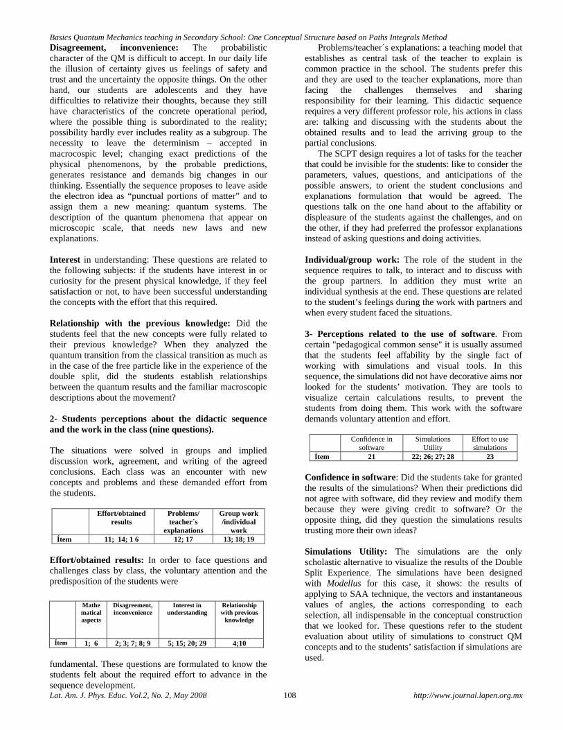
Basics Quantum Mechanics teaching in Secondary School: One Conceptual Structure based on Paths Integrals Method
Lat. Am. J. Phys. Educ. Vol.2, No. 2, May 2008 108 http://www.journal.lapen.org.mx
Disagreement, inconvenience: The probabilistic character of the QM is difficult to accept. In our daily life the illusion of certainty gives us feelings of safety and trust and the uncertainty the opposite things. On the other hand, our students are adolescents and they have difficulties to relativize their thoughts, because they still have characteristics of the concrete operational period, where the possible thing is subordinated to the reality; possibility hardly ever includes reality as a subgroup. The necessity to leave the determinism – accepted in macrocospic level; changing exact predictions of the physical phenomenons, by the probable predictions, generates resistance and demands big changes in our thinking. Essentially the sequence proposes to leave aside the electron idea as “punctual portions of matter” and to assign them a new meaning: quantum systems. The description of the quantum phenomena that appear on microscopic scale, that needs new laws and new explanations. Interest in understanding: These questions are related to the following subjects: if the students have interest in or curiosity for the present physical knowledge, if they feel satisfaction or not, to have been successful understanding the concepts with the effort that this required. Relationship with the previous knowledge: Did the students feel that the new concepts were fully related to their previous knowledge? When they analyzed the quantum transition from the classical transition as much as in the case of the free particle like in the experience of the double split, did the students establish relationships between the quantum results and the familiar macroscopic descriptions about the movement? 2- Students perceptions about the didactic sequence and the work in the class (nine questions). The situations were solved in groups and implied discussion work, agreement, and writing of the agreed conclusions. Each class was an encounter with new concepts and problems and these demanded effort from the students.
Effort/obtained results
Problems/ teacher´s
explanations
Group work /individual
work Ítem 11; 14; 1 6 12; 17 13; 18; 19
Effort/obtained results: In order to face questions and challenges class by class, the voluntary attention and the predisposition of the students were
fundamental. These questions are formulated to know the students felt about the required effort to advance in the sequence development.
Problems/teacher´s explanations: a teaching model that establishes as central task of the teacher to explain is common practice in the school. The students prefer this and they are used to the teacher explanations, more than facing the challenges themselves and sharing responsibility for their learning. This didactic sequence requires a very different professor role, his actions in class are: talking and discussing with the students about the obtained results and to lead the arriving group to the partial conclusions.
The SCPT design requires a lot of tasks for the teacher that could be invisible for the students: like to consider the parameters, values, questions, and anticipations of the possible answers, to orient the student conclusions and explanations formulation that would be agreed. The questions talk on the one hand about to the affability or displeasure of the students against the challenges, and on the other, if they had preferred the professor explanations instead of asking questions and doing activities. Individual/group work: The role of the student in the sequence requires to talk, to interact and to discuss with the group partners. In addition they must write an individual synthesis at the end. These questions are related to the student’s feelings during the work with partners and when every student faced the situations. 3- Perceptions related to the use of software. From certain "pedagogical common sense" it is usually assumed that the students feel affability by the single fact of working with simulations and visual tools. In this sequence, the simulations did not have decorative aims nor looked for the students’ motivation. They are tools to visualize certain calculations results, to prevent the students from doing them. This work with the software demands voluntary attention and effort.
Confidence in software
Simulations Utility
Effort to use simulations
Ítem 21 22; 26; 27; 28 23
Confidence in software: Did the students take for granted the results of the simulations? When their predictions did not agree with software, did they review and modify them because they were giving credit to software? Or the opposite thing, did they question the simulations results trusting more their own ideas? Simulations Utility: The simulations are the only scholastic alternative to visualize the results of the Double Split Experience. The simulations have been designed with Modellus for this case, it shows: the results of applying to SAA technique, the vectors and instantaneous values of angles, the actions corresponding to each selection, all indispensable in the conceptual construction that we looked for. These questions refer to the student evaluation about utility of simulations to construct QM concepts and to the students’ satisfaction if simulations are used.
Mathematical aspects
Disagreement, inconvenience
Interest in understanding
Relationship with previous
knowledge
Ítem 1; 6 2; 3; 7; 8; 9 5; 15; 20; 29 4;10
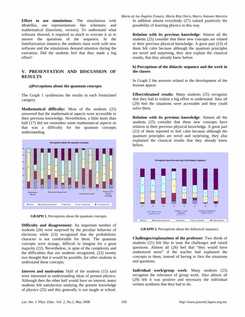
Maria de los Ángeles Fanaro, Maria Rita Otero, Marco Antonio Moreira
Lat. Am. J. Phys. Educ. Vol. 2, No.2, May 2008 109 http://www.journal.lapen.org.mx
Effort to use simulations: The simulations with Modellus, use representations like schematic and mathematical (functions, vectors). To understand what software showed, it required as much to execute it as to answer the questions of the sequence. In the familiarization instance, the students must work with new software and the simulations demand attention during the execution. Did the students feel that they made a big effort? V. PRESENTATION AND DISCUSSION OF RESULTS
a)Perceptions about the quantum concepts
The Graph 1 synthesizes the results in each formulated category Mathematical difficulty: Most of the students (25) answered that the mathematical aspects were accessible to their previous knowledge. Nevertheless, a little more than half (17) did not remember some mathematical aspects so that was a difficulty for the quantum concepts understanding.
Perceptions about the quantum concepts
22
1
7
89
6
5
3
711
9
12
14
0
12
3 3
79 9
31 0
9
4 5
0
5
10
15
20
25
30
1 6 2 3 7 8 9 5 15 20 29 4 10
Discord Something of agreement Agreement Very in agreement In total agreement
Mathematical difficulty
Difficulty and disagreement
Interest and motivation
Relation with its previous
knowledge
GRAPH 1. Perceptions about the quantum concepts. Difficulty and disagreement: An important number of students (26) were surprised by the peculiar behavior of electrons; while (23) recognized that the probabilistic character is not comfortable for them. The quantum concepts were strange, difficult to imagine for a great majority (22). Nevertheless, in spite of the complexity and the difficulties that our students recognized, (22) twenty two thought that it would be possible, for other students to understand these concepts. Interest and motivation: Half of the students (15) said were interested in understanding ideas of present physics. Although then the other half would have no interest, many students felt satisfaction studying the present knowledge of physics (25) and this generally is not taught at school.
In addition almost everybody (27) valued positively the possibility of learning physics in this way. Relation with its previous knowledge: Almost all the students (25) consider that these new concepts are related to their previous physical knowledge. A great part (23) of them felt calm because although the quantum principles are novel and surprising, they also explain the classical results, that they already knew before b) Perceptions of the didactic sequence and the work in the classes In Graph 2 the answers related to the development of the lessons appear. Effort/obtained results: Many students (25) recognize that they had to realize a big effort to understand. Also all (29) feel the situations were accessible and they could solve them. Relation with its previous knowledge: Almost all the students (25) consider that these new concepts have relation to their previous physical knowledge. A great part (23) of them reported to feel calm because although the quantum principles are novel and surprising, they also explained the classical results that they already knew before.
Perceptions about the work way in the didactic sequence
0 0 02
03
1 013
5
7
42
0 2
87
5
12
5 4
5 4
14 1114
7
6 7
6 6
79
62
15 1418 18
0
5
10
15
20
25
30
11 14 16 12 17 13 18 19
Discord Something of agreement Agreement Very in agreement In total agreement
Effort / Obtained results Questions 11,14,16
Challenges / Teacher explanations
Questions 12 17
Grupal work / Individual work Questions 13,18,19
GRAPH 2. Perceptions about the didactical sequence. Challenges/explanations of the professor: Two thirds of students (21) felt like to taste the challenges and raised questions. Almost all (26) feel that “they would have understood more” if the teacher had explained the concepts to them, instead of having to face the situations and questions. Individual work/group work: Many students (25) recognize the relevance of group work. Also almost all (29) felt it was positive and necessary the individual written synthesis that they had to do.
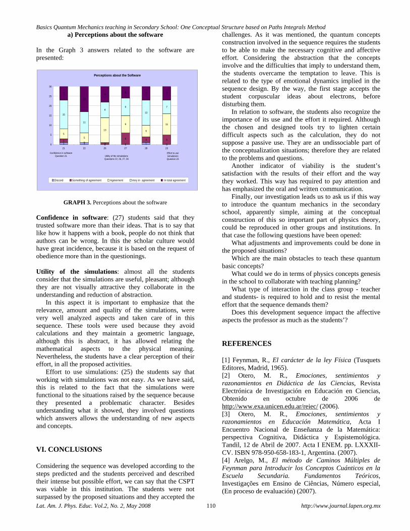
Basics Quantum Mechanics teaching in Secondary School: One Conceptual Structure based on Paths Integrals Method
Lat. Am. J. Phys. Educ. Vol.2, No. 2, May 2008 110 http://www.journal.lapen.org.mx
a) Perceptions about the software In the Graph 3 answers related to the software are presented:
Perceptions about the Software
1 1 0 0 1 02
0 1
6 3 5
55
13
9
6
11
15
11
89
13
7
7
13
86 7 7
0
5
10
15
20
25
30
21 22 26 27 28 23
Discord Something of agreement Agreement Very in agreement In total agreement
Confidence in softwareQuestion 21 Utility of the simulations
Questions 22, 26, 27, 28
Effort to use simulationsQuestion 23
GRAPH 3. Perceptions about the software Confidence in software: (27) students said that they trusted software more than their ideas. That is to say that like how it happens with a book, people do not think that authors can be wrong. In this the scholar culture would have great incidence, because it is based on the request of obedience more than in the questionings. Utility of the simulations: almost all the students consider that the simulations are useful, pleasant; although they are not visually attractive they collaborate in the understanding and reduction of abstraction.
In this aspect it is important to emphasize that the relevance, amount and quality of the simulations, were very well analyzed aspects and taken care of in this sequence. These tools were used because they avoid calculations and they maintain a geometric language, although this is abstract, it has allowed relating the mathematical aspects to the physical meaning. Nevertheless, the students have a clear perception of their effort, in all the proposed activities.
Effort to use simulations: (25) the students say that working with simulations was not easy. As we have said, this is related to the fact that the simulations were functional to the situations raised by the sequence because they presented a problematic character. Besides understanding what it showed, they involved questions which answers allows the understanding of new aspects and concepts.
VI. CONCLUSIONS Considering the sequence was developed according to the steps predicted and the students perceived and described their intense but possible effort, we can say that the CSPT was viable in this institution. The students were not surpassed by the proposed situations and they accepted the
challenges. As it was mentioned, the quantum concepts construction involved in the sequence requires the students to be able to make the necessary cognitive and affective effort. Considering the abstraction that the concepts involve and the difficulties that imply to understand them, the students overcame the temptation to leave. This is related to the type of emotional dynamics implied in the sequence design. By the way, the first stage accepts the student corpuscular ideas about electrons, before disturbing them.
In relation to software, the students also recognize the importance of its use and the effort it required. Although the chosen and designed tools try to lighten certain difficult aspects such as the calculation, they do not suppose a passive use. They are an undissociable part of the conceptualization situations; therefore they are related to the problems and questions.
Another indicator of viability is the student’s satisfaction with the results of their effort and the way they worked. This way has required to pay attention and has emphasized the oral and written communication.
Finally, our investigation leads us to ask us if this way to introduce the quantum mechanics in the secondary school, apparently simple, aiming at the conceptual construction of this so important part of physics theory, could be reproduced in other groups and institutions. In that case the following questions have been opened:
What adjustments and improvements could be done in the proposed situations?
Which are the main obstacles to teach these quantum basic concepts?
What could we do in terms of physics concepts genesis in the school to collaborate with teaching planning?
What type of interaction in the class group - teacher and students- is required to hold and to resist the mental effort that the sequence demands them?
Does this development sequence impact the affective aspects the professor as much as the students’? REFERENCES [1] Feynman, R., El carácter de la ley Física (Tusquets Editores, Madrid, 1965). [2] Otero, M. R., Emociones, sentimientos y razonamientos en Didáctica de las Ciencias, Revista Electrónica de Investigación en Educación en Ciencias, Obtenido en octubre de 2006 de http://www.exa.unicen.edu.ar/reiec/ (2006). [3] Otero, M. R., Emociones, sentimientos y razonamientos en Educación Matemática, Acta I Encuentro Nacional de Enseñanza de la Matemática: perspectiva Cognitiva, Didáctica y Espistemológica. Tandil, 12 de Abril de 2007. Acta I ENEM. pp. LXXXII-CV. ISBN 978-950-658-183-1, Argentina. (2007). [4] Arelgo, M., El método de Caminos Múltiples de Feynman para Introducir los Conceptos Cuánticos en la Escuela Secundaria. Fundamentos Teóricos, Investigações em Ensino de Ciências, Número especial, (En proceso de evaluación) (2007).
Maria de los Ángeles Fanaro, Maria Rita Otero, Marco Antonio Moreira
Lat. Am. J. Phys. Educ. Vol. 2, No.2, May 2008 111 http://www.journal.lapen.org.mx
[5] Fanaro, M., Otero, M. R., Moreira, M. A., Enseñanza de los Fundamentos de la Mecánica Cuántica en la Secundaria: Propuesta e implementación de una Estructura Conceptual, Investigações em Ensino de Ciências, Número especial. (En proceso de evaluación) (2007). [6] Fanaro, M., Arlego, M., Otero, M. R., El método de caminos múltiples de Feynman para enseñar los conceptos fundamentales de la Mecánica Quántica en la escuela secundaria, Caderno Catarinense de Ensino de Física 22, 233-260 (2007). [7] Verganud, G., La théorie des champs conceptuels, Recherches en Didactique des Mathématiques 10, 133-170 (1990). [8] Ausubel, D. P., Novak, J. D. & Hanesian, H., Psicología educativa: un punto de vista cognoscitivo, (Editorial Trillas, México, 1983). [9] Vergnaud, G. (coord.), Aprendizajes y didácticas: ¿Qué hay de nuevo?, (Edicial, Buenos Aires, 1994). [10] Vergnaud, G., Algunas ideas fundamentales de Piaget en torno a la didáctica, Revista Perspectivas 26, (1996). [11] Vergnaud, G., Sur la théorie des situations didactiques. Hommage à Guy Brousseau. La Penseé Sauvage, Édition (2005). [12]Gowin, D. B., Educating, (Cornell University Press, New York, 1981). Traducción al español: Hacia una teoría de la educación, (Ediciones Aragón, Argentina, 1985). [13] Moreira, M. A., Aprendizagem significativa crítica, Atas do III Encontro Internacional sobre Aprendizagem Significativa, 33-45 (2000). [14] Moreira, M. A., Aprendizagem significativa crítica, (Porto Alegre, Brasil, 2005). [15] Novak, J. D. & Gowin, D. B., Aprendiendo a aprender, (Alianza Editorial Martínez Roca, Madrid, 1988). APPENDIX Questionnaire A- Please, indicate your degree of agreement- with the following sentences about the Quantum mechanics concepts that we have studied. (1 disagree, 5 in total agreement) 1- The work with the vectors and the trigonometric functions necessary to understand the QM concepts was not finally complicated. 2- The probabilistic character of the QM made me feel me uncomfortable. 3- Studying the QM concepts has radically changed my previous ideas about the electrons. 4- I have learned a different Physics from the usual one, although it is based on that I already know 5- I feel satisfaction to have studied a very important and current part of physics knowledge; many students of the secondary school could never have studied it.
6- If I had remembered better my mathematical knowledge, it would have been easier to understand the new concepts. 7- I don’t believe that I have learned so difficult things that could not be understood by other students with similar characteristics. 8- I have been surprised by the strange behavior of the electrons and the microscopic world. 9- I felt the quantum world is strange and difficult to imagine. 10- I feel confident because these new concepts that I have learned allow me to explain what I knew of before. 11- Making much effort of my part, I believe that I solved the posed questions 12- I felt affability trying to resolve the questions and the proposed challenges 13- Talking with my class group was essential to understand the quantum concepts 14- Understanding the concepts has required too much effort from me. 15- I felt very motivated by the new concepts when I found out that they were concepts of today’s physics. 16- I had to make an effort to understand the QM questions proposed to answer. 17- If the teacher had explained the concepts instead of giving us activities and questions, I would have understood more. 18- Doing the personal synthesis I reflected and thought about the class work with my classmates. 19- The synthesis activities were essential to understanding and to have a global look about the studied subjects. 20- In this work I was interested in understanding the concepts proposed to be learnt. 21- I trusted the simulation results, and they made me review my calculations and my thinking if they are not in agreement with the software results showed. 22- The experience simulations were useful to understand the involved concepts. 23- Working with the simulations required much attention of my part, and was not simple.
24- If I had watched the "Dr. Quantum” video before, I would have understood everything that I understand now. 25- The “Dr. Quantum” video must be watched before; therefore it would have helped me to understand better what we studied. 26- I liked to work with the Double Split Experience simulation because it showed me the experience results that are impossible to do in the school. 27- The simulations and the video have helped me to understand the abstract quantum mechanics concepts, but without the raised questions and activities it would not have been possible. 28- The Software Modellus was not visually attractive, but without the simulation it would have been difficult to understand how the SAA technique can be used. 29- It seems important to me to have been able to study this physics part with the simulations and the video.

Basics Quantum Mechanics teaching in Secondary School: One Conceptual Structure based on Paths Integrals Method
Lat. Am. J. Phys. Educ. Vol.2, No. 2, May 2008 112 http://www.journal.lapen.org.mx
30- After we watched and we talked about “Dr. Quantum” video I thought that quantum world is strange and I have curiosity to know more about this.
B- Express freely your opinion about that you lived in these classes about QM.
Lat. Am. J. Phys. Educ. Vol.2, No. 2, May 2008 113 http://www.journal.lapen.org.mx
Prospective physics teachers’ ideas and drawings about the reflection and transmission of mechanical waves
Rabia Tanel1, Serap Kaya Sengören1, Nevzat Kavcar1 1Department of Physics Education, Education Faculty of Buca, Dokuz Eylül University, 35100, Buca, Izmir, Turkey. E-mail: [email protected] (Received 1 April 2008; accepted 16 April 2008)
Abstract It is known that most of the students have difficulties in understanding the behaviour of a mechanical wave at a boundary. Being aware of the students’ misconceptions about the subjects mentioned above can lead to the development of more effective teaching material on the topic of Vibrations and Waves. In this study, in order to reveal students’ ideas about the subject, a test containing questions with drawings has been developed. The test was applied to 147 prospective physics teachers attending a state university in Türkiye, and interviews have been carried out with 21 students. The results have shown that the students had certain misconceptions and inadequate information about the subject. In the view of the results, some suggestions were made about teaching the subject. Keywords: Physics education, Misconceptions on reflection of mechanical waves, Misconceptions on transmission of mechanical waves.
Resumen Es conocido que la mayoría de los estudiantes tienen dificultades en comprender el comportamiento de una onda mecánica en una frontera. El estar consciente de las ideas erróneas de los estudiantes sobre los temas antes mencionados puede llevar al desarrollo más eficaz de material didáctico sobre el tema de Vibraciones y Ondas. En este estudio, con el fin de revelar las ideas de los estudiantes sobre el tema, se ha desarrollado una prueba que contiene preguntas con dibujos. La prueba se aplicó a 147 futuros profesores de física que asisten a una universidad estatal en Türkiye, y las entrevistas se han llevado a cabo con 21 estudiantes. Los resultados han demostrado que los estudiantes tenían ciertas ideas erróneas e información inadecuada sobre el tema. En vista de los resultados, se hacen algunas sugerencias sobre la enseñanza de la materia Palabras clave: Physics education, Misconceptions on reflection of mechanical waves, Misconceptions on transmission of mechanical waves. PACS: 01.40.Fk, 01.40.gb, 01.40.J- ISSN 1870-9095
I. INTRODUCTION Researches indicate that students come to the science classroom with a number of naive conceptions which can inhibit the learning and understanding of certain concepts. Many of these misconceptions are widespread and have a detrimental effect on problem solving, course performance, and conceptual understanding of the material. These naive conceptions also appear to be resistant to change via traditional instructional approaches [1]. In this article, “misconception” refers to beliefs students have that contradict accepted scientific theories [2].
In order for students to change old ways of thinking, they must be willing to go through a series of conceptual changes. They must be either dissatisfied with their existing understanding, or they must be aware of contradictions and
reconcile them accurately [3]. And for this, first of all, it is necessary to be aware of the students’ ideas, to reveal the thought processes they used, and to understand how they departed from the modern scientific principles. This knowledge informs us about the difficulties that the students encounter and provide a foundation for preparing constructive and more efficient educational materials [4]. For these reasons, for many years, physics education researchers have worked on the students’ understanding about special subjects such as mechanics, electrical circuits, heat, and temperature [5].
Witmann [5, 6], Witmann, Steinberg and Redish [7], Kaya Sengören, Tanel & Kavcar [8] and Tanel, Kaya Sengören & Kavcar [9] carried out studies to determine and eliminate student’s misconceptions related to propagation and superposition of mechanical waves. Witmann [6] found
Rabia Tanel, Serap Kaya Sengören, Nevzat Kavcar
Lat. Am. J. Phys. Educ. Vol. 2, No. 2, May 2008 114 http://www.journal.lapen.org.mx
the following misconceptions about reflection of mechanical waves from a boundary such that the wave bounced as a particle, that is to say, in which side of the rope it was, it reflected in the same side, or the pulse was damped on free or constant end. Moreover, he stated that most of the students had difficulties with the subject of reflection at the free end. Ambrose [10] found that the ability to relate the relative wave speeds and widths of the transmitted and incident pulses was difficult after standard instruction at both the introductory and the advanced level. As a result of the answers obtained from the question in which students were asked to draw the shape of two connected ropes after a certain time, where the propagating velocities of the pulses on two connected ropes were given relative to each other, he found that many students: (i) had failed to recognize that reflection would occur at a junction between two regions of different wave speed and (ii) had failed to relate the widths of the incident and transmitted pulses to the wave speeds. Ambrose [10] reported that students often said that a pulse approaching a different spring with greater wave speed would be completely transmitted. These students often articulate the idea that reflection only occurs when the incident pulse experiences “resistance” at the boundary. For many students, this “resistance” occurs only when the pulse is incident on a different spring with smaller wave speed. The task of drawing the transmitted pulse was proven to be difficult for all students, including graduate students, and the most common error was to indicate that the transmitted pulse had the same width as the incident pulse.
Subjects such as the reflection and transmission of the pulse in the boundary of another medium are the main subjects of the course of vibrations and waves. The reflection and transmission events on ropes or spiral springs look like the light being reflected and refracted at the same time. Having learned the subjects which can be understood more perceptible such as the transmission, and reflection of mechanical waves without misconceptions will make the optical subjects, which will be taught later, easier to be understood. Being aware of the misconceptions about the related subjects of the physics education students, who will be the high school teachers of the future, is the preliminary step to achieve the works intended to eliminate these misconceptions. Tao and Gunstone [11] were stated that students’ conceptual change was context dependent and unstable. Palmer [12] also said that students were contextually dependent in their ideas (about gravity). Therefore, the researches related to students’ misconceptions about the subjects are needed but there are no many researches investigating students’ misconceptions about the subjects. For these reasons, it is thought that this study will be useful for following researches and it is important.
The aim of this study was to determine the physics education students’ misconceptions and the reason of these misconceptions about the transmission and reflection in another medium’s boundary. We hope and believe that this research would be useful also for the high school teachers since this is a subject taught in high school level in our country, Türkiye.
II. METHOD A. The sample The subjects of this study are a total of 147 students from the 1st, 2nd, 3rd, 4th, and 5th grade students attending Dokuz Eylül University, Education Faculty of Buca, Physics Education Department, Türkiye. B. The prepared test In this study, case study research method which is used in the qualitative research methodology had been used [13]. In order to gather information (drawings and ideas of the students) about the subjects, a test containing four questions with drawings had been developed. Actually the questions can be found in many physics books but, as we said before, there are no many researches investigating students’ ideas with using similar questions about the subjects. The authors didn’t point out the features like the reflected pulse, the transmitted pulse, the amplitude, the width and the velocity in the questions not to direct answers of the students intentionally. The prepared test was checked by three experts, and the necessary corrections were made. Then, it was tested on two students, and it was decided that the questions were not misunderstood. In the questions, students were asked to draw the required shapes and explain their answers.
In the test applied to students, there were totally four questions appropriate to the aim of the study, two of which were related to reflection on fixed and free ends, and two of which were related to reflection and transmission on another medium boundary. The students were explained that the pulses in the questions were mechanical waves with small amplitudes which were progressing on a homogeneous, smooth, and frictionless medium without dispersion [14].
The test was applied to a total number of 147 students of which 33, 34, 32, 24, and 24 were 1st, 2nd, 3rd, 4th, and 5th grade students, respectively, attending Dokuz Eylül University, Education Faculty of Buca, Physics Education Department, Türkiye. Students’ drawings were classified independently by two experts in order to maintain the validity, and the common ideas were collected in subtitles. The analyses made by the two researchers were than compared and common results were concluded. C. The interview structure It was tried to deeply understand the students’ ideas by interviewing. When the test was applied, the students were asked to write their names on their answer sheet in order to able to select the corresponding students in the subsequent interview, and to be able to interview students whose explanations were not clearly understood; the reason for this was explained to the students. Interviews were conducted with 21 students seen as required to interview with. These students were those whose explanations were not understood clearly by researchers during analysis, and those who had certain common misconceptions as determined by the researchers. The interviews were performed separately in a semi-structured interview format, by developing a common structure by two researchers [13]. During the interviews, the
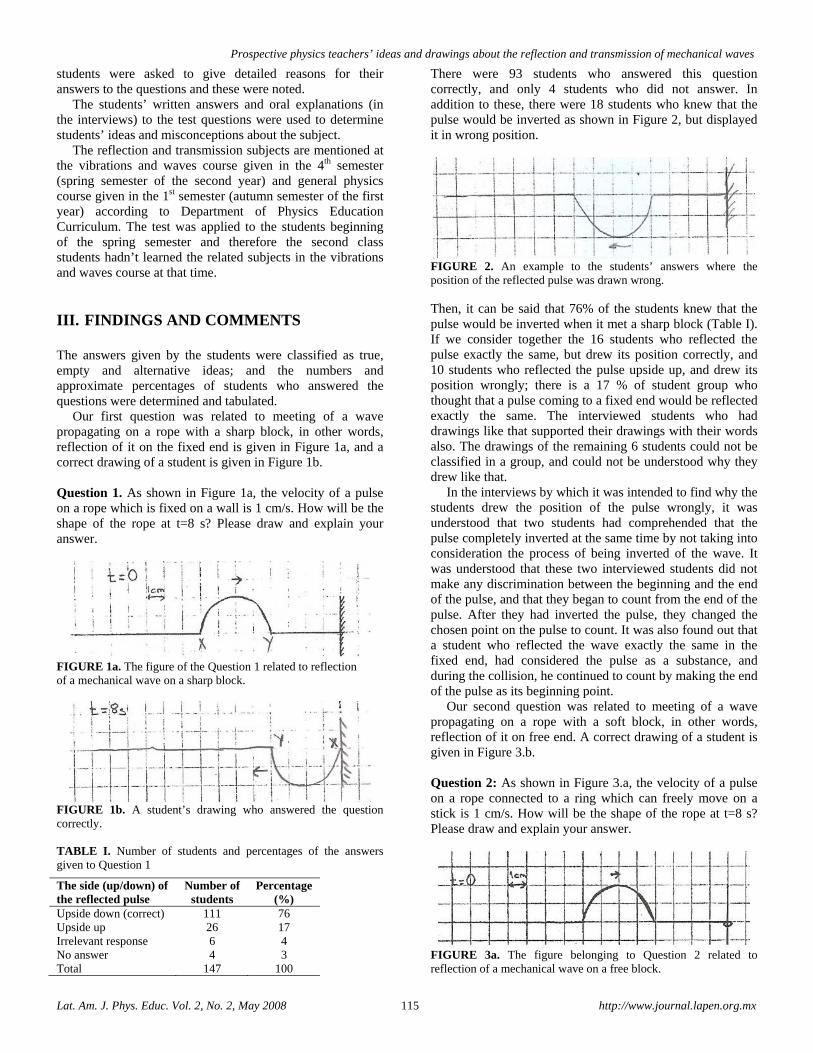
Prospective physics teachers’ ideas and drawings about the reflection and transmission of mechanical waves
Lat. Am. J. Phys. Educ. Vol. 2, No. 2, May 2008 115 http://www.journal.lapen.org.mx
students were asked to give detailed reasons for their answers to the questions and these were noted.
The students’ written answers and oral explanations (in the interviews) to the test questions were used to determine students’ ideas and misconceptions about the subject.
The reflection and transmission subjects are mentioned at the vibrations and waves course given in the 4th semester (spring semester of the second year) and general physics course given in the 1st semester (autumn semester of the first year) according to Department of Physics Education Curriculum. The test was applied to the students beginning of the spring semester and therefore the second class students hadn’t learned the related subjects in the vibrations and waves course at that time.
III. FINDINGS AND COMMENTS The answers given by the students were classified as true, empty and alternative ideas; and the numbers and approximate percentages of students who answered the questions were determined and tabulated.
Our first question was related to meeting of a wave propagating on a rope with a sharp block, in other words, reflection of it on the fixed end is given in Figure 1a, and a correct drawing of a student is given in Figure 1b. Question 1. As shown in Figure 1a, the velocity of a pulse on a rope which is fixed on a wall is 1 cm/s. How will be the shape of the rope at t=8 s? Please draw and explain your answer.
FIGURE 1a. The figure of the Question 1 related to reflection of a mechanical wave on a sharp block.
FIGURE 1b. A student’s drawing who answered the question correctly. TABLE I. Number of students and percentages of the answers given to Question 1
There were 93 students who answered this question correctly, and only 4 students who did not answer. In addition to these, there were 18 students who knew that the pulse would be inverted as shown in Figure 2, but displayed it in wrong position.
FIGURE 2. An example to the students’ answers where the position of the reflected pulse was drawn wrong. Then, it can be said that 76% of the students knew that the pulse would be inverted when it met a sharp block (Table I). If we consider together the 16 students who reflected the pulse exactly the same, but drew its position correctly, and 10 students who reflected the pulse upside up, and drew its position wrongly; there is a 17 % of student group who thought that a pulse coming to a fixed end would be reflected exactly the same. The interviewed students who had drawings like that supported their drawings with their words also. The drawings of the remaining 6 students could not be classified in a group, and could not be understood why they drew like that.
In the interviews by which it was intended to find why the students drew the position of the pulse wrongly, it was understood that two students had comprehended that the pulse completely inverted at the same time by not taking into consideration the process of being inverted of the wave. It was understood that these two interviewed students did not make any discrimination between the beginning and the end of the pulse, and that they began to count from the end of the pulse. After they had inverted the pulse, they changed the chosen point on the pulse to count. It was also found out that a student who reflected the wave exactly the same in the fixed end, had considered the pulse as a substance, and during the collision, he continued to count by making the end of the pulse as its beginning point.
Our second question was related to meeting of a wave propagating on a rope with a soft block, in other words, reflection of it on free end. A correct drawing of a student is given in Figure 3.b. Question 2: As shown in Figure 3.a, the velocity of a pulse on a rope connected to a ring which can freely move on a stick is 1 cm/s. How will be the shape of the rope at t=8 s? Please draw and explain your answer.
FIGURE 3a. The figure belonging to Question 2 related to reflection of a mechanical wave on a free block.
The side (up/down) of the reflected pulse
Number of students
Percentage (%)
Upside down (correct) 111 76 Upside up 26 17 Irrelevant response 6 4 No answer 4 3 Total 147 100
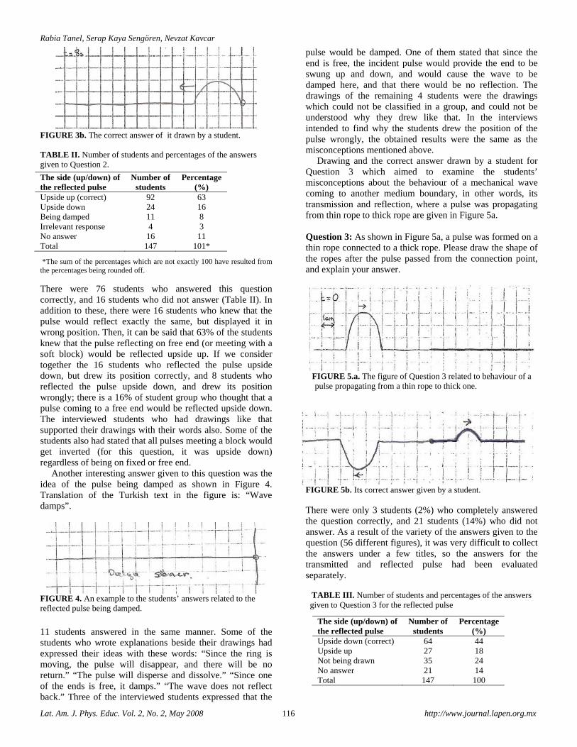
Rabia Tanel, Serap Kaya Sengören, Nevzat Kavcar
Lat. Am. J. Phys. Educ. Vol. 2, No. 2, May 2008 116 http://www.journal.lapen.org.mx
FIGURE 3b. The correct answer of it drawn by a student. TABLE II. Number of students and percentages of the answers given to Question 2.
*The sum of the percentages which are not exactly 100 have resulted from the percentages being rounded off.
There were 76 students who answered this question correctly, and 16 students who did not answer (Table II). In addition to these, there were 16 students who knew that the pulse would reflect exactly the same, but displayed it in wrong position. Then, it can be said that 63% of the students knew that the pulse reflecting on free end (or meeting with a soft block) would be reflected upside up. If we consider together the 16 students who reflected the pulse upside down, but drew its position correctly, and 8 students who reflected the pulse upside down, and drew its position wrongly; there is a 16% of student group who thought that a pulse coming to a free end would be reflected upside down. The interviewed students who had drawings like that supported their drawings with their words also. Some of the students also had stated that all pulses meeting a block would get inverted (for this question, it was upside down) regardless of being on fixed or free end.
Another interesting answer given to this question was the idea of the pulse being damped as shown in Figure 4. Translation of the Turkish text in the figure is: “Wave damps”.
FIGURE 4. An example to the students’ answers related to the reflected pulse being damped.
11 students answered in the same manner. Some of the students who wrote explanations beside their drawings had expressed their ideas with these words: “Since the ring is moving, the pulse will disappear, and there will be no return.” “The pulse will disperse and dissolve.” “Since one of the ends is free, it damps.” “The wave does not reflect back.” Three of the interviewed students expressed that the
pulse would be damped. One of them stated that since the end is free, the incident pulse would provide the end to be swung up and down, and would cause the wave to be damped here, and that there would be no reflection. The drawings of the remaining 4 students were the drawings which could not be classified in a group, and could not be understood why they drew like that. In the interviews intended to find why the students drew the position of the pulse wrongly, the obtained results were the same as the misconceptions mentioned above.
Drawing and the correct answer drawn by a student for Question 3 which aimed to examine the students’ misconceptions about the behaviour of a mechanical wave coming to another medium boundary, in other words, its transmission and reflection, where a pulse was propagating from thin rope to thick rope are given in Figure 5a. Question 3: As shown in Figure 5a, a pulse was formed on a thin rope connected to a thick rope. Please draw the shape of the ropes after the pulse passed from the connection point, and explain your answer.
FIGURE 5.a. The figure of Question 3 related to behaviour of a
pulse propagating from a thin rope to thick one.
FIGURE 5b. Its correct answer given by a student. There were only 3 students (2%) who completely answered the question correctly, and 21 students (14%) who did not answer. As a result of the variety of the answers given to the question (56 different figures), it was very difficult to collect the answers under a few titles, so the answers for the transmitted and reflected pulse had been evaluated separately.
TABLE III. Number of students and percentages of the answers
given to Question 3 for the reflected pulse
The side (up/down) of the reflected pulse
Number of students
Percentage (%)
Upside up (correct) 92 63 Upside down 24 16 Being damped 11 8 Irrelevant response 4 3 No answer 16 11 Total 147 101*
The side (up/down) of the reflected pulse
Number of students
Percentage (%)
Upside down (correct) 64 44 Upside up 27 18 Not being drawn 35 24 No answer 21 14 Total 147 100
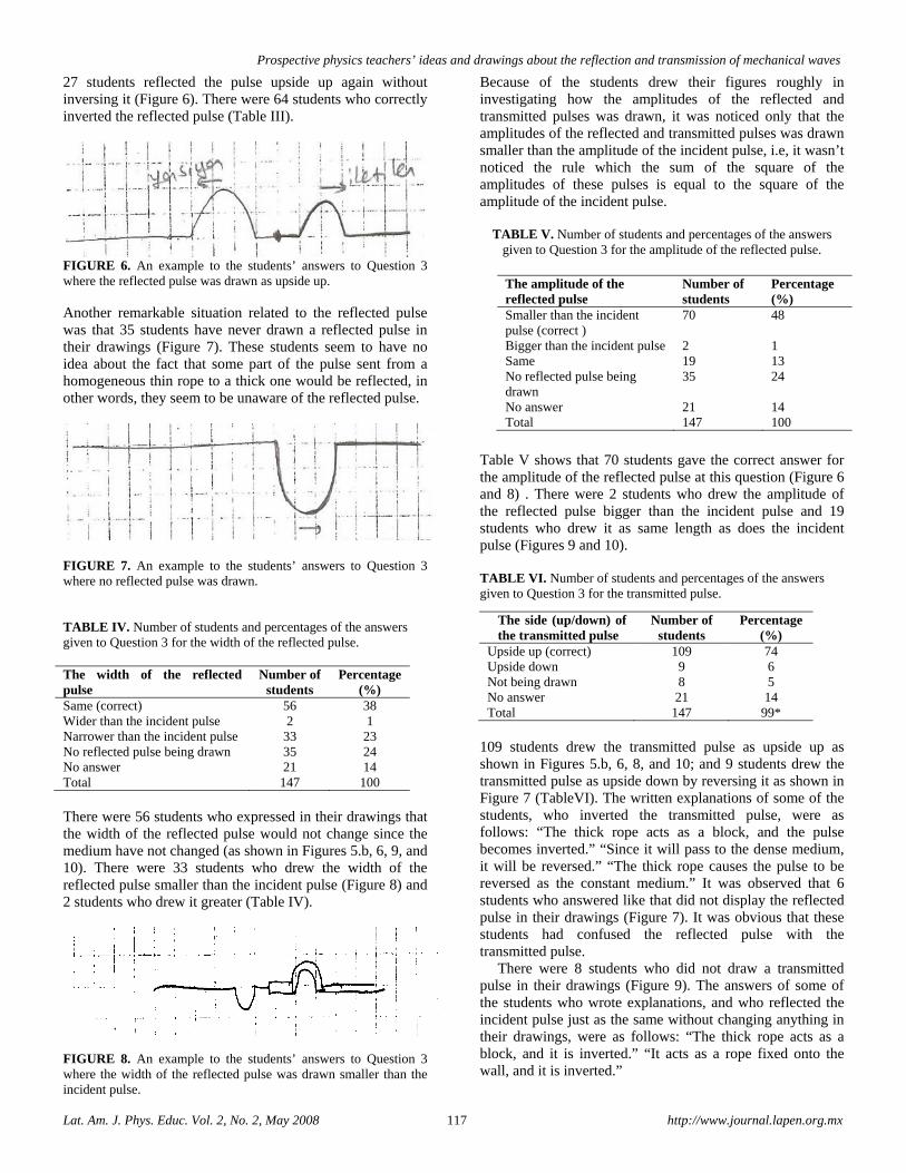
Prospective physics teachers’ ideas and drawings about the reflection and transmission of mechanical waves
Lat. Am. J. Phys. Educ. Vol. 2, No. 2, May 2008 117 http://www.journal.lapen.org.mx
27 students reflected the pulse upside up again without inversing it (Figure 6). There were 64 students who correctly inverted the reflected pulse (Table III).
FIGURE 6. An example to the students’ answers to Question 3 where the reflected pulse was drawn as upside up. Another remarkable situation related to the reflected pulse was that 35 students have never drawn a reflected pulse in their drawings (Figure 7). These students seem to have no idea about the fact that some part of the pulse sent from a homogeneous thin rope to a thick one would be reflected, in other words, they seem to be unaware of the reflected pulse.
FIGURE 7. An example to the students’ answers to Question 3 where no reflected pulse was drawn. TABLE IV. Number of students and percentages of the answers given to Question 3 for the width of the reflected pulse.
There were 56 students who expressed in their drawings that the width of the reflected pulse would not change since the medium have not changed (as shown in Figures 5.b, 6, 9, and 10). There were 33 students who drew the width of the reflected pulse smaller than the incident pulse (Figure 8) and 2 students who drew it greater (Table IV).
FIGURE 8. An example to the students’ answers to Question 3 where the width of the reflected pulse was drawn smaller than the incident pulse.
Because of the students drew their figures roughly in investigating how the amplitudes of the reflected and transmitted pulses was drawn, it was noticed only that the amplitudes of the reflected and transmitted pulses was drawn smaller than the amplitude of the incident pulse, i.e, it wasn’t noticed the rule which the sum of the square of the amplitudes of these pulses is equal to the square of the amplitude of the incident pulse.
TABLE V. Number of students and percentages of the answers
given to Question 3 for the amplitude of the reflected pulse.
Table V shows that 70 students gave the correct answer for the amplitude of the reflected pulse at this question (Figure 6 and 8) . There were 2 students who drew the amplitude of the reflected pulse bigger than the incident pulse and 19 students who drew it as same length as does the incident pulse (Figures 9 and 10).
TABLE VI. Number of students and percentages of the answers given to Question 3 for the transmitted pulse.
109 students drew the transmitted pulse as upside up as shown in Figures 5.b, 6, 8, and 10; and 9 students drew the transmitted pulse as upside down by reversing it as shown in Figure 7 (TableVI). The written explanations of some of the students, who inverted the transmitted pulse, were as follows: “The thick rope acts as a block, and the pulse becomes inverted.” “Since it will pass to the dense medium, it will be reversed.” “The thick rope causes the pulse to be reversed as the constant medium.” It was observed that 6 students who answered like that did not display the reflected pulse in their drawings (Figure 7). It was obvious that these students had confused the reflected pulse with the transmitted pulse.
There were 8 students who did not draw a transmitted pulse in their drawings (Figure 9). The answers of some of the students who wrote explanations, and who reflected the incident pulse just as the same without changing anything in their drawings, were as follows: “The thick rope acts as a block, and it is inverted.” “It acts as a rope fixed onto the wall, and it is inverted.”
The width of the reflected pulse
Number of students
Percentage (%)
Same (correct) 56 38 Wider than the incident pulse 2 1 Narrower than the incident pulse 33 23 No reflected pulse being drawn 35 24 No answer 21 14 Total 147 100
The amplitude of the reflected pulse
Number of students
Percentage (%)
Smaller than the incident pulse (correct )
70 48
Bigger than the incident pulse 2 1 Same 19 13 No reflected pulse being drawn
35 24
No answer 21 14 Total 147 100
The side (up/down) of the transmitted pulse
Number of students
Percentage (%)
Upside up (correct) 109 74 Upside down 9 6 Not being drawn 8 5 No answer 21 14 Total 147 99*
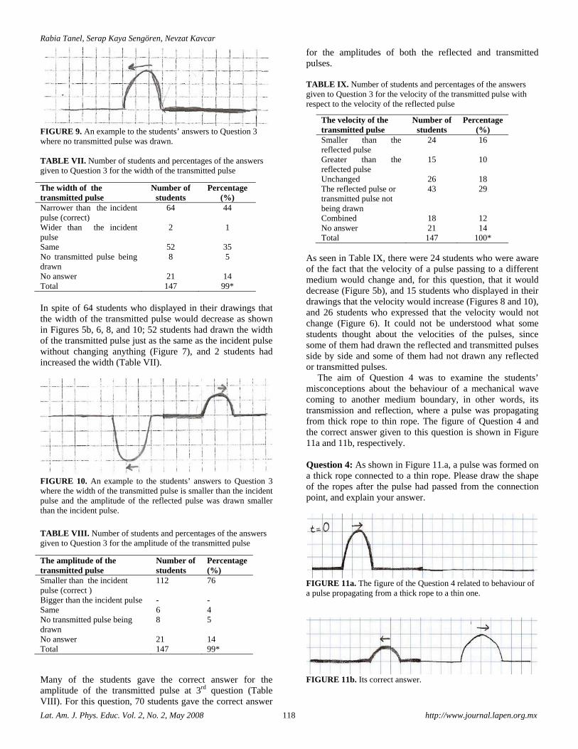
Rabia Tanel, Serap Kaya Sengören, Nevzat Kavcar
Lat. Am. J. Phys. Educ. Vol. 2, No. 2, May 2008 118 http://www.journal.lapen.org.mx
FIGURE 9. An example to the students’ answers to Question 3 where no transmitted pulse was drawn. TABLE VII. Number of students and percentages of the answers given to Question 3 for the width of the transmitted pulse
In spite of 64 students who displayed in their drawings that the width of the transmitted pulse would decrease as shown in Figures 5b, 6, 8, and 10; 52 students had drawn the width of the transmitted pulse just as the same as the incident pulse without changing anything (Figure 7), and 2 students had increased the width (Table VII).
FIGURE 10. An example to the students’ answers to Question 3 where the width of the transmitted pulse is smaller than the incident pulse and the amplitude of the reflected pulse was drawn smaller than the incident pulse.
TABLE VIII. Number of students and percentages of the answers given to Question 3 for the amplitude of the transmitted pulse
Many of the students gave the correct answer for the amplitude of the transmitted pulse at 3rd question (Table VIII). For this question, 70 students gave the correct answer
for the amplitudes of both the reflected and transmitted pulses.
TABLE IX. Number of students and percentages of the answers given to Question 3 for the velocity of the transmitted pulse with respect to the velocity of the reflected pulse
As seen in Table IX, there were 24 students who were aware of the fact that the velocity of a pulse passing to a different medium would change and, for this question, that it would decrease (Figure 5b), and 15 students who displayed in their drawings that the velocity would increase (Figures 8 and 10), and 26 students who expressed that the velocity would not change (Figure 6). It could not be understood what some students thought about the velocities of the pulses, since some of them had drawn the reflected and transmitted pulses side by side and some of them had not drawn any reflected or transmitted pulses.
The aim of Question 4 was to examine the students’ misconceptions about the behaviour of a mechanical wave coming to another medium boundary, in other words, its transmission and reflection, where a pulse was propagating from thick rope to thin rope. The figure of Question 4 and the correct answer given to this question is shown in Figure 11a and 11b, respectively. Question 4: As shown in Figure 11.a, a pulse was formed on a thick rope connected to a thin rope. Please draw the shape of the ropes after the pulse had passed from the connection point, and explain your answer.
FIGURE 11a. The figure of the Question 4 related to behaviour of a pulse propagating from a thick rope to a thin one.
FIGURE 11b. Its correct answer.
The width of the transmitted pulse
Number of students
Percentage (%)
Narrower than the incident pulse (correct)
64 44
Wider than the incident pulse
2 1
Same 52 35 No transmitted pulse being drawn
8 5
No answer 21 14 Total 147 99*
The amplitude of the transmitted pulse
Number of students
Percentage (%)
Smaller than the incident pulse (correct )
112 76
Bigger than the incident pulse - - Same 6 4 No transmitted pulse being drawn
8 5
No answer 21 14 Total 147 99*
The velocity of the transmitted pulse
Number of students
Percentage (%)
Smaller than the reflected pulse
24 16
Greater than the reflected pulse
15 10
Unchanged 26 18 The reflected pulse or transmitted pulse not being drawn
43 29
Combined 18 12 No answer 21 14 Total 147 100*
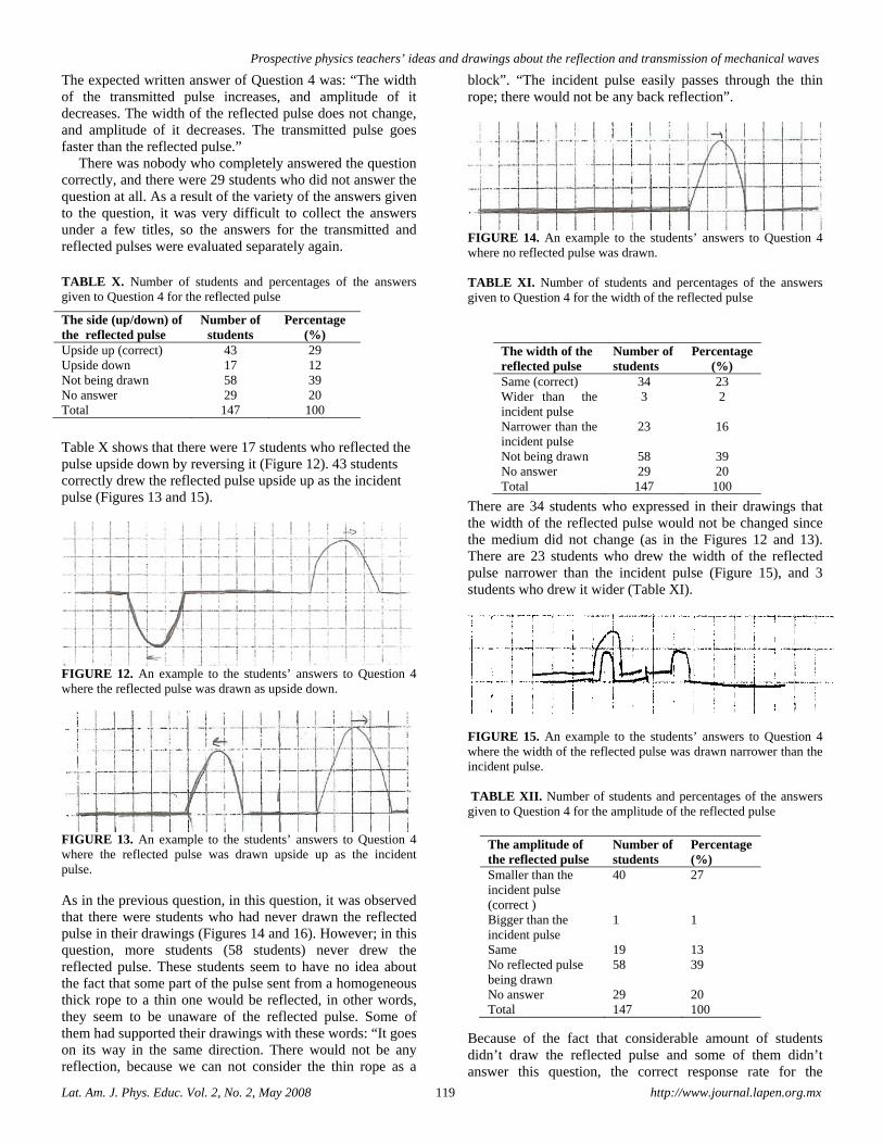
Prospective physics teachers’ ideas and drawings about the reflection and transmission of mechanical waves
Lat. Am. J. Phys. Educ. Vol. 2, No. 2, May 2008 119 http://www.journal.lapen.org.mx
The expected written answer of Question 4 was: “The width of the transmitted pulse increases, and amplitude of it decreases. The width of the reflected pulse does not change, and amplitude of it decreases. The transmitted pulse goes faster than the reflected pulse.”
There was nobody who completely answered the question correctly, and there were 29 students who did not answer the question at all. As a result of the variety of the answers given to the question, it was very difficult to collect the answers under a few titles, so the answers for the transmitted and reflected pulses were evaluated separately again.
TABLE X. Number of students and percentages of the answers given to Question 4 for the reflected pulse
Table X shows that there were 17 students who reflected the pulse upside down by reversing it (Figure 12). 43 students correctly drew the reflected pulse upside up as the incident pulse (Figures 13 and 15).
FIGURE 12. An example to the students’ answers to Question 4 where the reflected pulse was drawn as upside down.
FIGURE 13. An example to the students’ answers to Question 4 where the reflected pulse was drawn upside up as the incident pulse. As in the previous question, in this question, it was observed that there were students who had never drawn the reflected pulse in their drawings (Figures 14 and 16). However; in this question, more students (58 students) never drew the reflected pulse. These students seem to have no idea about the fact that some part of the pulse sent from a homogeneous thick rope to a thin one would be reflected, in other words, they seem to be unaware of the reflected pulse. Some of them had supported their drawings with these words: “It goes on its way in the same direction. There would not be any reflection, because we can not consider the thin rope as a
block”. “The incident pulse easily passes through the thin rope; there would not be any back reflection”.
FIGURE 14. An example to the students’ answers to Question 4 where no reflected pulse was drawn. TABLE XI. Number of students and percentages of the answers given to Question 4 for the width of the reflected pulse
There are 34 students who expressed in their drawings that the width of the reflected pulse would not be changed since the medium did not change (as in the Figures 12 and 13). There are 23 students who drew the width of the reflected pulse narrower than the incident pulse (Figure 15), and 3 students who drew it wider (Table XI).
FIGURE 15. An example to the students’ answers to Question 4 where the width of the reflected pulse was drawn narrower than the incident pulse. TABLE XII. Number of students and percentages of the answers given to Question 4 for the amplitude of the reflected pulse
Because of the fact that considerable amount of students didn’t draw the reflected pulse and some of them didn’t answer this question, the correct response rate for the
The side (up/down) of the reflected pulse
Number of students
Percentage (%)
Upside up (correct) 43 29 Upside down 17 12 Not being drawn 58 39 No answer 29 20 Total 147 100
The width of the reflected pulse
Number of students
Percentage (%)
Same (correct) 34 23 Wider than the incident pulse
3 2
Narrower than the incident pulse
23 16
Not being drawn 58 39 No answer 29 20 Total 147 100
The amplitude of the reflected pulse
Number of students
Percentage (%)
Smaller than the incident pulse (correct )
40 27
Bigger than the incident pulse
1 1
Same 19 13 No reflected pulse being drawn
58 39
No answer 29 20 Total 147 100
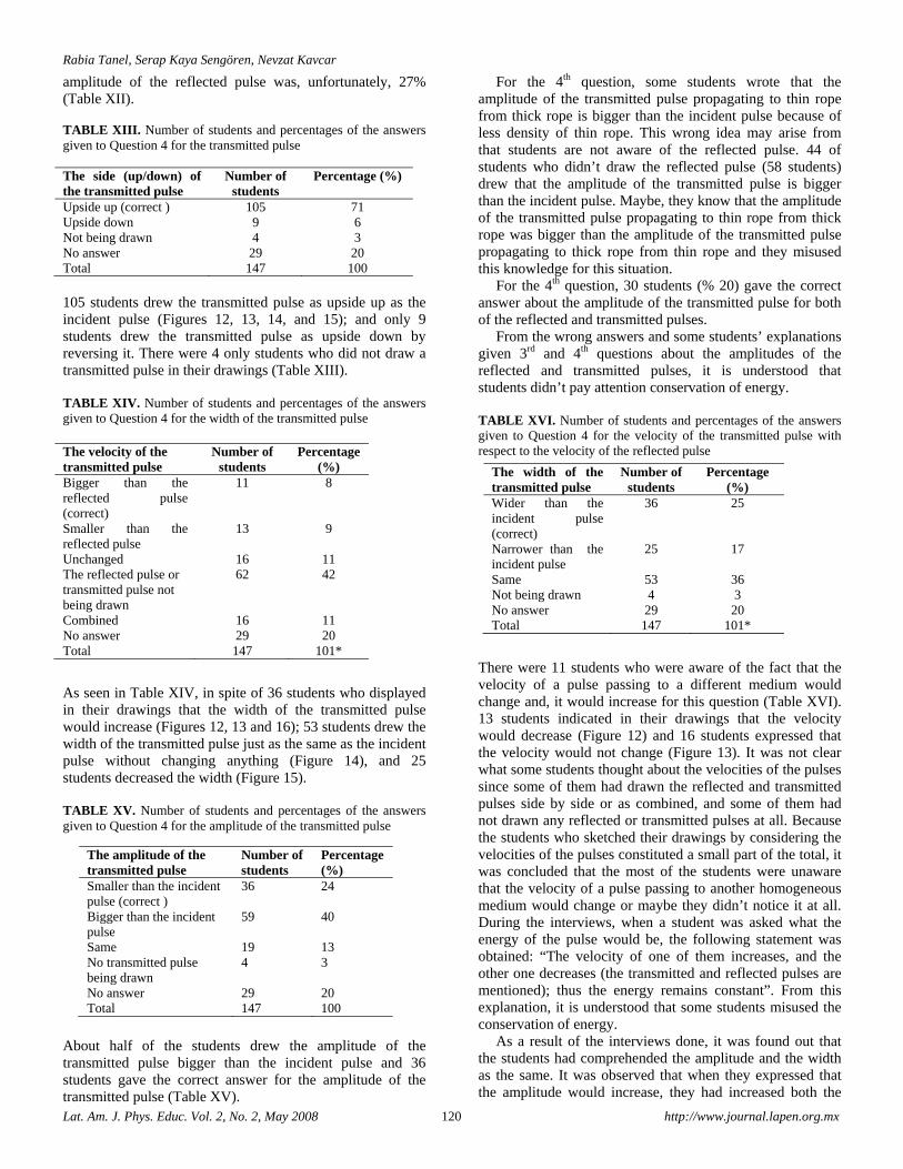
Rabia Tanel, Serap Kaya Sengören, Nevzat Kavcar
Lat. Am. J. Phys. Educ. Vol. 2, No. 2, May 2008 120 http://www.journal.lapen.org.mx
amplitude of the reflected pulse was, unfortunately, 27% (Table XII). TABLE XIII. Number of students and percentages of the answers given to Question 4 for the transmitted pulse
105 students drew the transmitted pulse as upside up as the incident pulse (Figures 12, 13, 14, and 15); and only 9 students drew the transmitted pulse as upside down by reversing it. There were 4 only students who did not draw a transmitted pulse in their drawings (Table XIII). TABLE XIV. Number of students and percentages of the answers given to Question 4 for the width of the transmitted pulse
As seen in Table XIV, in spite of 36 students who displayed in their drawings that the width of the transmitted pulse would increase (Figures 12, 13 and 16); 53 students drew the width of the transmitted pulse just as the same as the incident pulse without changing anything (Figure 14), and 25 students decreased the width (Figure 15).
TABLE XV. Number of students and percentages of the answers given to Question 4 for the amplitude of the transmitted pulse
About half of the students drew the amplitude of the transmitted pulse bigger than the incident pulse and 36 students gave the correct answer for the amplitude of the transmitted pulse (Table XV).
For the 4th question, some students wrote that the amplitude of the transmitted pulse propagating to thin rope from thick rope is bigger than the incident pulse because of less density of thin rope. This wrong idea may arise from that students are not aware of the reflected pulse. 44 of students who didn’t draw the reflected pulse (58 students) drew that the amplitude of the transmitted pulse is bigger than the incident pulse. Maybe, they know that the amplitude of the transmitted pulse propagating to thin rope from thick rope was bigger than the amplitude of the transmitted pulse propagating to thick rope from thin rope and they misused this knowledge for this situation.
For the 4th question, 30 students (% 20) gave the correct answer about the amplitude of the transmitted pulse for both of the reflected and transmitted pulses.
From the wrong answers and some students’ explanations given 3rd and 4th questions about the amplitudes of the reflected and transmitted pulses, it is understood that students didn’t pay attention conservation of energy.
TABLE XVI. Number of students and percentages of the answers given to Question 4 for the velocity of the transmitted pulse with respect to the velocity of the reflected pulse
There were 11 students who were aware of the fact that the velocity of a pulse passing to a different medium would change and, it would increase for this question (Table XVI). 13 students indicated in their drawings that the velocity would decrease (Figure 12) and 16 students expressed that the velocity would not change (Figure 13). It was not clear what some students thought about the velocities of the pulses since some of them had drawn the reflected and transmitted pulses side by side or as combined, and some of them had not drawn any reflected or transmitted pulses at all. Because the students who sketched their drawings by considering the velocities of the pulses constituted a small part of the total, it was concluded that the most of the students were unaware that the velocity of a pulse passing to another homogeneous medium would change or maybe they didn’t notice it at all. During the interviews, when a student was asked what the energy of the pulse would be, the following statement was obtained: “The velocity of one of them increases, and the other one decreases (the transmitted and reflected pulses are mentioned); thus the energy remains constant”. From this explanation, it is understood that some students misused the conservation of energy.
As a result of the interviews done, it was found out that the students had comprehended the amplitude and the width as the same. It was observed that when they expressed that the amplitude would increase, they had increased both the
The side (up/down) of the transmitted pulse
Number of students
Percentage (%)
Upside up (correct ) 105 71 Upside down 9 6 Not being drawn 4 3 No answer 29 20 Total 147 100
The velocity of the transmitted pulse
Number of students
Percentage (%)
Bigger than the reflected pulse (correct)
11 8
Smaller than the reflected pulse
13 9
Unchanged 16 11 The reflected pulse or transmitted pulse not being drawn
62 42
Combined 16 11 No answer 29 20 Total 147 101*
The amplitude of the transmitted pulse
Number of students
Percentage (%)
Smaller than the incident pulse (correct )
36 24
Bigger than the incident pulse
59 40
Same 19 13 No transmitted pulse being drawn
4 3
No answer 29 20 Total 147 100
The width of the transmitted pulse
Number of students
Percentage (%)
Wider than the incident pulse (correct)
36 25
Narrower than the incident pulse
25 17
Same 53 36 Not being drawn 4 3 No answer 29 20 Total 147 101*
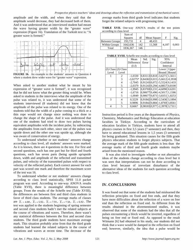
Prospective physics teachers’ ideas and drawings about the reflection and transmission of mechanical waves
Lat. Am. J. Phys. Educ. Vol. 2, No. 2, May 2008 121 http://www.journal.lapen.org.mx
amplitude and the width, and when they said that the amplitude would decrease, they had decreased both of them. And it was understood that an interviewed student had meant the wave having greater width by the “greater wave” expression (Figure 16). Translation of the Turkish text is: “A greater wave is formed.”
FIGURE 16. An example to the students’ answers to Question 4 where a student drew wider wave for “greater wave” expression.
When asked to another student what he meant by his expression of “greater wave is formed”, it was recognized that he did not know what the greater thing would be. When asked to students in the interviews what the amplitude of the pulse was related to, it was understood that some of the students interviewed (8 students) did not know that the amplitude of the pulse was related to its energy. One of the students told that the width of a pulse coming to a thick or a thin rope would not change since nothing was done to change the shape of the pulse. And it was understood that one of the students had tried to draw two pulses having equivalent amplitudes with the incident pulse, by subtracting the amplitudes from each other, since one of the pulses was upside down and the other one was upside up, although she was aware of conservation of energy.
To understand whether or not students’ answers change according to class level, all students’ answers were marked. As it is known, there are 4 questions in the test. For first and second questions, each has one part but for third and fourth questions, each has seven parts (being upside up/upside down, width and amplitude of the reflected and transmitted pulses, and velocity of the transmitted pulses with respect to velocity of the reflected pulse). Each correct answer for each part was scored one mark and therefore the maximum score of the test was 16.
To understand whether or not students’ answers change according to class level statistically, SPSS 11.0 packet program was used. According to one-way ANOVA results (Table XVII), there is meaningful difference between groups. From the results of the Scheffe test (Table XVIII), the differences are between first and third class students in favor of third class students. The average marks of classes are 1 4.88X = , 2 5.92X = , 3 7.91X = , 4 7.58X = , 5 6.92X = . The test was applied to the students beginning of spring semester and second class students hadn’t met the related subjects at the course of vibrations and waves. Therefore, there wasn’t any statistical difference between the first and second class students. The third grade students have maximum average mark. This situation probably arise from that the third grade students had learned the related subjects in the course of vibrations and waves at recent time. The decrease of the
average marks from third grade level indicates that students forget the related subjects with progressing time.
TABLE XVII. One-way ANOVA results of the test points according to class level
Sum of Squares
df
Mean Square
F
Sig.
Between Groups 193,731 4 48,433 4,187 0,003 Within Groups 1642,636 142 11,568
Total 1836,367 146
TABLE XVIII. Scheffe test results according to class level
Mean Difference
(I-J)
Std. Error
Sig. 95% Confidence
Interval (I) Class
Level (J) Class
Level Lower
BoundUpper Bound
1 2 3 4 5
-1,0330 -3,0275* -2,7045 -2,0379
0,83113 0,84382 0,91243 0,91243
0,8180,0150,0720,294
-3,6271-5,6612-5,5524-4,8857
1,5611-0,39380,14330,8100
2 3 4 5
-1,9945 -1,6716 -1,0049
0,83769 0,90677 0,90677
0,2310,4960,873
-4,6090-4,5017-3,8351
0,62011,15861,8253
3 4 5
0,3229 0,9896
0,91842 0,91842
0,9980,884
-2,5436-1,8769
3,18943,8561
4 5 0,6667 0,98183 0,977 -2,3978 3,7311
Instruction period is five years at the departments of Physics, Chemistry, Mathematics and Biology Education at education faculties in Türkiye. According to the curriculum of education faculties in Türkiye, students have to attend all physics courses in first 3,5 years (7 semester) and then, they have to attend educational lessons in 1,5 years (3 semester) for being graduated. This situation causes for the fifth grade physics education students to forget physics subjects. That the average mark of the fifth grade students is less than the average marks of third and fourth grade students maybe arised from the mentioned reason.
It was also tried to investigate whether or not alternative ideas of the students change according to class level but it was seen that interpretations can not be done according to class level because of irrevelant disturbance of the alternative ideas of the students for each question according to class level.
IV. CONCLUSIONS It was found out that some of the students had mislearned the reflection principles on fixed and free ends, and that they have more difficulties about the reflection of a wave on free end than the reflection on fixed end. As different from the results obtained in the aforementioned studies, it was observed that some of the students had the idea that all the pulses encountering a block would be inverted, regardless of being on free end or fixed end. As opposed to the result Witmann [6] had obtained in his study, our students did not think that a wave would be damped in the reflection on fixed end; however, similarly, the idea that a pulse would be
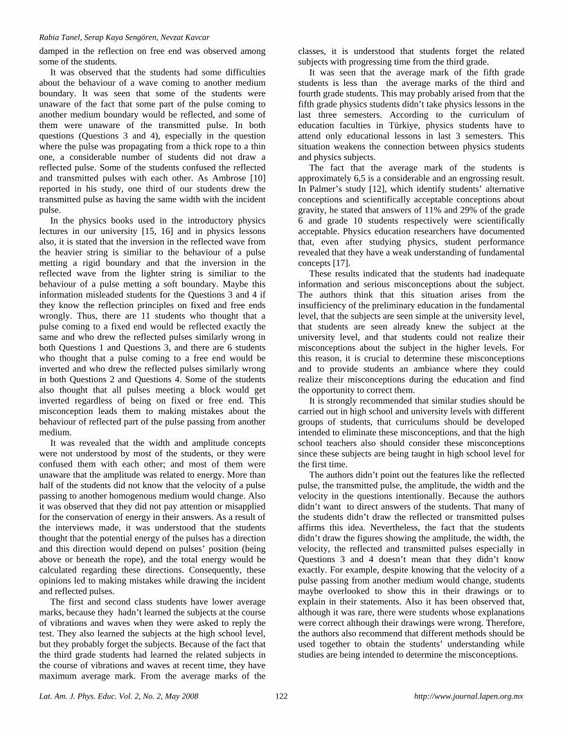
Rabia Tanel, Serap Kaya Sengören, Nevzat Kavcar
Lat. Am. J. Phys. Educ. Vol. 2, No. 2, May 2008 122 http://www.journal.lapen.org.mx
damped in the reflection on free end was observed among some of the students.
It was observed that the students had some difficulties about the behaviour of a wave coming to another medium boundary. It was seen that some of the students were unaware of the fact that some part of the pulse coming to another medium boundary would be reflected, and some of them were unaware of the transmitted pulse. In both questions (Questions 3 and 4), especially in the question where the pulse was propagating from a thick rope to a thin one, a considerable number of students did not draw a reflected pulse. Some of the students confused the reflected and transmitted pulses with each other. As Ambrose [10] reported in his study, one third of our students drew the transmitted pulse as having the same width with the incident pulse.
In the physics books used in the introductory physics lectures in our university [15, 16] and in physics lessons also, it is stated that the inversion in the reflected wave from the heavier string is similiar to the behaviour of a pulse metting a rigid boundary and that the inversion in the reflected wave from the lighter string is similiar to the behaviour of a pulse metting a soft boundary. Maybe this information misleaded students for the Questions 3 and 4 if they know the reflection principles on fixed and free ends wrongly. Thus, there are 11 students who thought that a pulse coming to a fixed end would be reflected exactly the same and who drew the reflected pulses similarly wrong in both Questions 1 and Questions 3, and there are 6 students who thought that a pulse coming to a free end would be inverted and who drew the reflected pulses similarly wrong in both Questions 2 and Questions 4. Some of the students also thought that all pulses meeting a block would get inverted regardless of being on fixed or free end. This misconception leads them to making mistakes about the behaviour of reflected part of the pulse passing from another medium.
It was revealed that the width and amplitude concepts were not understood by most of the students, or they were confused them with each other; and most of them were unaware that the amplitude was related to energy. More than half of the students did not know that the velocity of a pulse passing to another homogenous medium would change. Also it was observed that they did not pay attention or misapplied for the conservation of energy in their answers. As a result of the interviews made, it was understood that the students thought that the potential energy of the pulses has a direction and this direction would depend on pulses’ position (being above or beneath the rope), and the total energy would be calculated regarding these directions. Consequently, these opinions led to making mistakes while drawing the incident and reflected pulses.
The first and second class students have lower average marks, because they hadn’t learned the subjects at the course of vibrations and waves when they were asked to reply the test. They also learned the subjects at the high school level, but they probably forget the subjects. Because of the fact that the third grade students had learned the related subjects in the course of vibrations and waves at recent time, they have maximum average mark. From the average marks of the
classes, it is understood that students forget the related subjects with progressing time from the third grade.
It was seen that the average mark of the fifth grade students is less than the average marks of the third and fourth grade students. This may probably arised from that the fifth grade physics students didn’t take physics lessons in the last three semesters. According to the curriculum of education faculties in Türkiye, physics students have to attend only educational lessons in last 3 semesters. This situation weakens the connection between physics students and physics subjects.
The fact that the average mark of the students is approximately 6,5 is a considerable and an engrossing result. In Palmer’s study [12], which identify students’ alternative conceptions and scientifically acceptable conceptions about gravity, he stated that answers of 11% and 29% of the grade 6 and grade 10 students respectively were scientifically acceptable. Physics education researchers have documented that, even after studying physics, student performance revealed that they have a weak understanding of fundamental concepts [17].
These results indicated that the students had inadequate information and serious misconceptions about the subject. The authors think that this situation arises from the insufficiency of the preliminary education in the fundamental level, that the subjects are seen simple at the university level, that students are seen already knew the subject at the university level, and that students could not realize their misconceptions about the subject in the higher levels. For this reason, it is crucial to determine these misconceptions and to provide students an ambiance where they could realize their misconceptions during the education and find the opportunity to correct them.
It is strongly recommended that similar studies should be carried out in high school and university levels with different groups of students, that curriculums should be developed intended to eliminate these misconceptions, and that the high school teachers also should consider these misconceptions since these subjects are being taught in high school level for the first time.
The authors didn’t point out the features like the reflected pulse, the transmitted pulse, the amplitude, the width and the velocity in the questions intentionally. Because the authors didn’t want to direct answers of the students. That many of the students didn’t draw the reflected or transmitted pulses affirms this idea. Nevertheless, the fact that the students didn’t draw the figures showing the amplitude, the width, the velocity, the reflected and transmitted pulses especially in Questions 3 and 4 doesn’t mean that they didn’t know exactly. For example, despite knowing that the velocity of a pulse passing from another medium would change, students maybe overlooked to show this in their drawings or to explain in their statements. Also it has been observed that, although it was rare, there were students whose explanations were correct although their drawings were wrong. Therefore, the authors also recommend that different methods should be used together to obtain the students’ understanding while studies are being intended to determine the misconceptions.
Prospective physics teachers’ ideas and drawings about the reflection and transmission of mechanical waves
Lat. Am. J. Phys. Educ. Vol. 2, No. 2, May 2008 123 http://www.journal.lapen.org.mx
REFERENCES
[1] Brown, D. E., Using examples and analogies to remediate misconceptions in physics: Factors influencing conceptual change, Journal of Research in Science Teaching 29, 17-34 (1992). [2] Eryilmaz, A., Effects of conceptual assignments and conceptual change discussions on students’ misconceptions and achievement regarding force and motion, Journal of Research in Science Teaching 39, 1001-1015 (2002). [3] Meyer, D. K., Recognizing and changing students’ misconceptions, College Teaching 41, 104-110 (1993). [4] Wheatley, G. H., Constructivist perspectives on science and mathematical learning, Sci. Educ. 75, 9-21 (1991). [5] Witmann, M. C., The object coordination class applied to wavepulses: Analysing student reasoning in wave physics, International Journal of Science Education 24, 97-118 (2002). [6] Witmann, M. C., “Making sense of how students come to an understanding of physics: An example from mechanical waves” Ph.D. dissertation, University of Maryland College Park, 1998, avalaible in proquest digital dissertations. UMI No: AAT 9921649. [7] Witmann, M. C., Steinberg, R. N., and Redish, E. F., Making sense of how students make sense of mechanical waves, The Physics Teacher 37, 15-21 (1999). [8] Kaya �engören, S., Tanel, R. and Kavcar, N., Drawings and ideas of physics teacher candidates relating to the superposition principle on a continuous rope, Physics Education 41, 453-461 (2006).
[9]Tanel, R., Kaya Sengören, S., and Kavcar, N., The Effect of Using the Cooperative Learning Strategies on Students’ Conceptual Change for the Subject of Mechanical Waves, AIP Conf. Proc. 899, 846 (2007). [10] Ambrose, B. S., “Investigation of student understanding of the wave-like properties of light and matter” Ph.D. dissertation, University of Washington, 1999, avalaible in proquest digital dissertations. UMI No: AAT 9924069. [11] Tao, P. K. and Gunstone, R. F., The procees of conceptual change in force and motion during computer-supported physics instruction Journal of Research in Science Teaching 36, 859-882 (1999). [12] Palmer, D., Students’ alternative conceptions and scientifically acceptable conceptions about gravity, International Journal of Science Education 23, 691-706 (2001). [13] Ekiz, D., Egitimde Arastirma Yöntem ve Metodlarina Giris, (Ani Yayincilik, 2003), p.43 and p.62. [14] Crawford, F. S., Dalgalar, Berkeley Fizik Dersleri -3, (Bilim Yayinlari, 1996). [15] Fishbane, P. M., Gasiorowicz, S. and Thornton, S. T., Temel Fizik, Cilt I, (Arkadas Yayinevi, 2003). [16] Serway, R. A., Physics for Scientists and Engineers with Modern Physics, (Saunders Golden Sunburst Series, 1990). [17] Hossain, K., “Developing and validating performance assessment tasks for concepts of geometrical optics” Ph.D. dissertation, State University of Newyork at Buffalo, 2001, avalaible in proquest digital dissertations. UMI No: AAT 3010832.
Lat. Am. J. Phys. Educ. Vol.2, No. 2, May 2008 124 http://www.journal.lapen.org.mx
Effects of Cooperative Learning on Instructing Magnetism: Analysis of an Experimental Teaching Sequence
Zafer Tanel and Mustafa Erol Buca Education Faculty, Department of Physics Education, Dokuz Eylul University,35150, Izmir,TURKEY. E-mail: [email protected] (Received 11 April 2008; accepted 30 April 2008)
Abstract This paper describes methods and the results of a work designed to analyze effectiveness of an experimental teaching sequence on the topic of magnetism. Cooperative learning techniques were employed to experimental group and conventional teaching method was used for control group throughout the teaching sequence. Sampling of the study consists of 19-20 years old 100 students at a state university in �zmir, Turkey. Levels of pre-knowledge acquired by the students were evaluated by means of a self-developed “Magnetism Topics Achievement Scale (MTAS)” and the progress and retention were determined by the same scale. A clear significant difference, as a conclusion, was detected in favor of the experimental group indicating the success of the cooperative learning teaching sequence. Additionally, personal compositions were administered to extract information about the students’ views on the overall actual teaching techniques and methods. Keywords: Cooperative learning, Teaching magnetism, Physics education.
Resumen Este artículo describe los métodos y resultados de un trabajo diseñado para analizar la eficacia de una secuencia de enseñanza experimental sobre el tema de magnetismo. Se emplearon técnicas de aprendizaje cooperativo con un grupo experimental y se utilizó el método de enseñanza convencional con un grupo de control en toda la secuencia de enseñanza. La toma de muestra del estudio consta de 100 estudiantes de 19-20 años de edad en una Universidad estatal en �zmir, Turquía. Los niveles de pre-conocimientos adquiridos por los estudiantes fueron evaluados por medio de una auto desarrollada “Escala de Logros en Temas de Magnetismo (MTAS)” y el progreso y la retención fueron determinados por la misma escala. Como una conclusión, se detectó una clara diferencia significativa a favor del grupo experimental indicando el éxito de la secuencia de enseñanza de aprendizaje cooperativo. Adicionalmente, se administraron composiciones personales para conseguir información sobre las opiniones de los estudiantes sobre el conjunto real de métodos y técnicas de enseñanza. Palabras clave: Aprendizaje cooperativo, Enseñanza del magnetismo, Educación en Física. PACS: 01.40.Fk, 01.40.gb, 01.40.Ha, 01.40.Di ISSN 1870-9095
I. INTRODUCTION Lecturing is the most common method of instruction in the tertiary levels of education [1]. However, research results of many researchers who focus on teaching various topics of university physics indicated that conventional teaching hardly improves the teaching of principle concepts of physics [2]. Similarly, experiences in this field suggested that even physics education conveyed by a well-prepared presentation do not give effective results through understanding principal concepts [3]. In debates concerning how to increase the learning of physical concepts, many researchers claimed that students need to take part in social interaction [4]. In addition, it was underlined that while teaching physics, it is necessary to use methods which utilize instructional activities that students can think of what they are doing and think of the
applications they are carrying out [5]. It is also essential to allow students reflecting their own ideas and prepare an environment giving them a chance to discuss their learning with other students and their teachers [6]. Cooperative learning can be shown as a sample of education of this kind [3] and this method can easily be adapted to the current structure of physics education [5]. On the other hand, Johnson and Johnson [7] indicate that if cooperative learning is used more widely and more frequently, students would learn to be more scientific and come to feel better about themselves as science students. Benefits of cooperative learning, which is defined as “involving three or more children who work together in a group in order to maximize their own and each other’s learning” by Johnson, Johnson and Holubec [8], on academic and social gains of students were indicated by various studies [4, 9, 10, 11, 12, 13, 14, 15, 16].
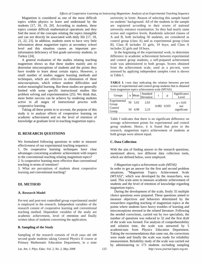
Effects of Cooperative Learning on Instructing Magnetism: Analysis of an Experimental Teaching Sequence
Lat. Am. J. Phys. Educ. Vol. 2, No. 2, May 2008 125 http://www.journal.lapen.org.mx
Magnetism is considered as one of the most difficult topics within physics to learn and understand by the students [17, 18, 19, 20]. According to students, these topics contain difficult mathematical operations and they find the most of the concepts relating the topics intangible and can not directly be associated with daily life [17, 18, 21, 22, 23]. In addition, students seem to have very little information about magnetism topics at secondary school level and this situation causes an important pre-information deficiency of first grade university students, in Turkey [24].
A general evaluation of the studies relating teaching magnetism shows us that these studies mainly aim to determine misconceptions of students and the points they have trouble to learn about certain topics. However, a small number of studies suggest learning methods and techniques, which are effective in elimination of these misconceptions, which reduce student difficulties and realize meaningful learning. But these studies are generally limited with some specific instructional studies like problem solving and experimentation [25]. We think that, more better success can be achieve by rendering students active in all stages of instructional process with cooperative learning.
Taking all these points in to account, the purpose of this study is to analyze effects of cooperative learning on academic achievement and on the level of retention of knowledge at graduate level in teaching magnetism topics. II. RESEARCH QUESTIONS We formulated following questions in order to measure effectiveness of our experimental teaching sequence: 1. Do cooperative learning techniques have clear advantages concerning academic achievement with respect to the conventional teaching relating magnetism topics? 2. Is cooperative learning more effective than conventional teaching in terms of retention? 3. What are perceptions of students about cooperative learning and conventional teaching? III. METHOD A. Research Model Pre-test and post-test controlled group experimental model is employed in the research. Independent variables of the research consist of cooperative learning and conventional teaching method. Dependent variables of the study are academic achievement, level of retention and finally written ideas of students concerning the application.
B. Sampling of the Study Sampling of the research consists of 19-20 years old 100 second grade students taking General Physics II course at Primary Mathematic Education Department, in a state
university in Izmir. Reason of selecting this sample based on students’ background. All of the students in the sample are registered according to their scores of national university entrance examination. So they had nearly same scores and cognitive levels. Randomly selected classes of A and B, both including 50 students, are considered as control group (class A) and as experimental group (class B). Class B includes 31 girls, 19 boys; and Class A includes 32 girls and 18 boys.
In the beginning of the experimental work, to determine difference in academic achievement between experimental and control group students, a self-prepared achievement scale was administered to both groups. Scores obtained from the achievement scale, used as a pre-test, were assessed by applying independent samples t-test is shown in Table I. TABLE I. t-test data indicating the relation between pre-test scores of experimental and control group students that is obtained from magnetism topics achievement scale (MTAS).
Table I indicates that there is no significant difference on average achievement points for experimental and control group students. Hence, it is found that prior to the research, magnetism topics achievement of students at both groups were almost equal.
C. Data Collection With the aim of finding answer to the research questions, mentioned above, two different data collection tools, which are defined below, were employed.
I-Magnetism topics achievement scale (MTAS)
In order to get an answer for the first and second problem situations, “Magnetism Topics Achievement Scale (MTAS)”, which was developed by the researchers, was used. This scale aims to measure academic achievement of students and the level of retention of knowledge regarding magnetism topics.
During the development of the scale, firstly 35 multiple choice questions were prepared. These questions aimed to measure objectives and behaviors determined by the researchers regarding teaching of magnetism topics at the points where students have heavy troubles of learning and misconceptions stressed in the related literature. Following the needed corrections, carried out by two specialists, the number of questions was reduced to 32 and the first draft of the scale was formed. For analysis of comprehensibility and solution time, the scale was answered by 5 academicians from Physics Education Department. Taking the recommendations that came out, the corrections were made and finally the scale was ready for reliability measurement. Reliability study of the scale was carried out by administering to 173 students excluding sampling
Groups n Mean Standard Deviation
t p Significance
Level Experimental Group
50 5,02 2,63 0,082 0,935
p > 0,05 not
significant Control Group
50 4,98 2,23
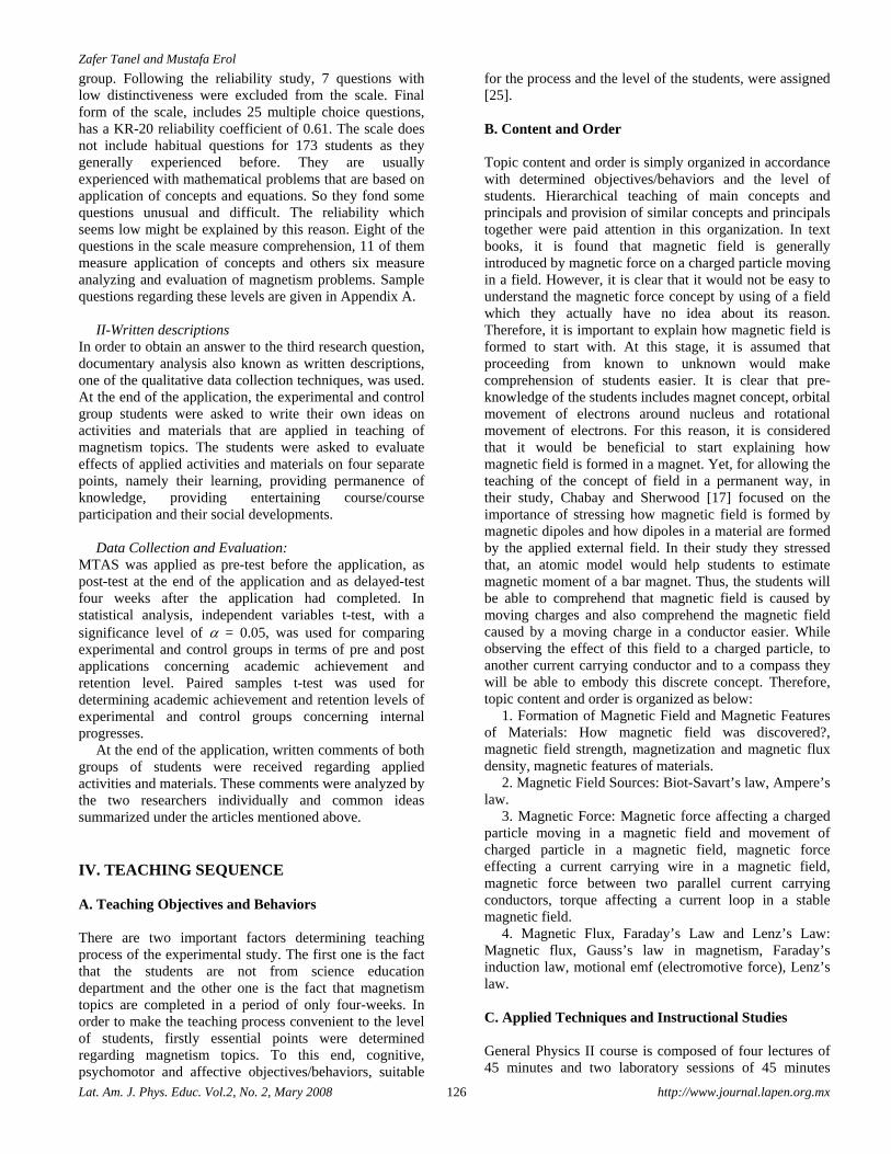
Zafer Tanel and Mustafa Erol
Lat. Am. J. Phys. Educ. Vol.2, No. 2, Mary 2008 126 http://www.journal.lapen.org.mx
group. Following the reliability study, 7 questions with low distinctiveness were excluded from the scale. Final form of the scale, includes 25 multiple choice questions, has a KR-20 reliability coefficient of 0.61. The scale does not include habitual questions for 173 students as they generally experienced before. They are usually experienced with mathematical problems that are based on application of concepts and equations. So they fond some questions unusual and difficult. The reliability which seems low might be explained by this reason. Eight of the questions in the scale measure comprehension, 11 of them measure application of concepts and others six measure analyzing and evaluation of magnetism problems. Sample questions regarding these levels are given in Appendix A.
II-Written descriptions
In order to obtain an answer to the third research question, documentary analysis also known as written descriptions, one of the qualitative data collection techniques, was used. At the end of the application, the experimental and control group students were asked to write their own ideas on activities and materials that are applied in teaching of magnetism topics. The students were asked to evaluate effects of applied activities and materials on four separate points, namely their learning, providing permanence of knowledge, providing entertaining course/course participation and their social developments.
Data Collection and Evaluation:
MTAS was applied as pre-test before the application, as post-test at the end of the application and as delayed-test four weeks after the application had completed. In statistical analysis, independent variables t-test, with a significance level of α = 0.05, was used for comparing experimental and control groups in terms of pre and post applications concerning academic achievement and retention level. Paired samples t-test was used for determining academic achievement and retention levels of experimental and control groups concerning internal progresses.
At the end of the application, written comments of both groups of students were received regarding applied activities and materials. These comments were analyzed by the two researchers individually and common ideas summarized under the articles mentioned above. IV. TEACHING SEQUENCE A. Teaching Objectives and Behaviors There are two important factors determining teaching process of the experimental study. The first one is the fact that the students are not from science education department and the other one is the fact that magnetism topics are completed in a period of only four-weeks. In order to make the teaching process convenient to the level of students, firstly essential points were determined regarding magnetism topics. To this end, cognitive, psychomotor and affective objectives/behaviors, suitable
for the process and the level of the students, were assigned [25].
B. Content and Order Topic content and order is simply organized in accordance with determined objectives/behaviors and the level of students. Hierarchical teaching of main concepts and principals and provision of similar concepts and principals together were paid attention in this organization. In text books, it is found that magnetic field is generally introduced by magnetic force on a charged particle moving in a field. However, it is clear that it would not be easy to understand the magnetic force concept by using of a field which they actually have no idea about its reason. Therefore, it is important to explain how magnetic field is formed to start with. At this stage, it is assumed that proceeding from known to unknown would make comprehension of students easier. It is clear that pre-knowledge of the students includes magnet concept, orbital movement of electrons around nucleus and rotational movement of electrons. For this reason, it is considered that it would be beneficial to start explaining how magnetic field is formed in a magnet. Yet, for allowing the teaching of the concept of field in a permanent way, in their study, Chabay and Sherwood [17] focused on the importance of stressing how magnetic field is formed by magnetic dipoles and how dipoles in a material are formed by the applied external field. In their study they stressed that, an atomic model would help students to estimate magnetic moment of a bar magnet. Thus, the students will be able to comprehend that magnetic field is caused by moving charges and also comprehend the magnetic field caused by a moving charge in a conductor easier. While observing the effect of this field to a charged particle, to another current carrying conductor and to a compass they will be able to embody this discrete concept. Therefore, topic content and order is organized as below:
1. Formation of Magnetic Field and Magnetic Features of Materials: How magnetic field was discovered?, magnetic field strength, magnetization and magnetic flux density, magnetic features of materials.
2. Magnetic Field Sources: Biot-Savart’s law, Ampere’s law.
3. Magnetic Force: Magnetic force affecting a charged particle moving in a magnetic field and movement of charged particle in a magnetic field, magnetic force effecting a current carrying wire in a magnetic field, magnetic force between two parallel current carrying conductors, torque affecting a current loop in a stable magnetic field.
4. Magnetic Flux, Faraday’s Law and Lenz’s Law: Magnetic flux, Gauss’s law in magnetism, Faraday’s induction law, motional emf (electromotive force), Lenz’s law.
C. Applied Techniques and Instructional Studies General Physics II course is composed of four lectures of 45 minutes and two laboratory sessions of 45 minutes
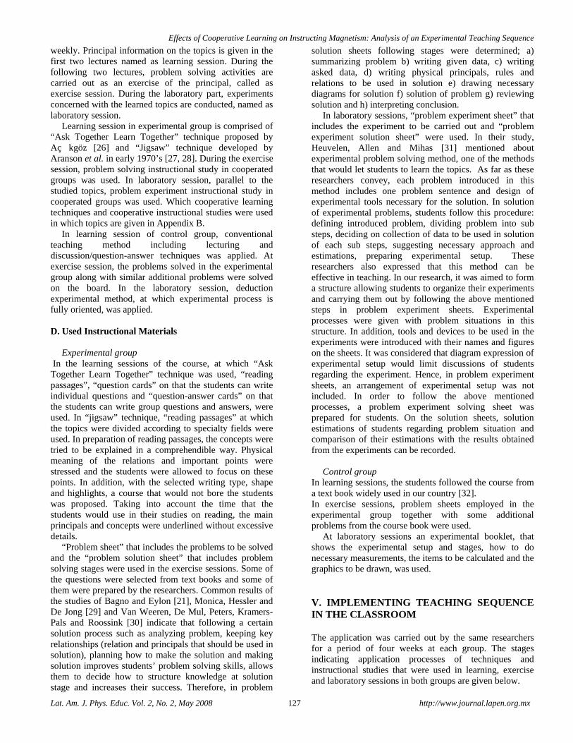
Effects of Cooperative Learning on Instructing Magnetism: Analysis of an Experimental Teaching Sequence
Lat. Am. J. Phys. Educ. Vol. 2, No. 2, May 2008 127 http://www.journal.lapen.org.mx
weekly. Principal information on the topics is given in the first two lectures named as learning session. During the following two lectures, problem solving activities are carried out as an exercise of the principal, called as exercise session. During the laboratory part, experiments concerned with the learned topics are conducted, named as laboratory session.
Learning session in experimental group is comprised of “Ask Together Learn Together” technique proposed by Aç�kgöz [26] and “Jigsaw” technique developed by Aranson et al. in early 1970’s [27, 28]. During the exercise session, problem solving instructional study in cooperated groups was used. In laboratory session, parallel to the studied topics, problem experiment instructional study in cooperated groups was used. Which cooperative learning techniques and cooperative instructional studies were used in which topics are given in Appendix B.
In learning session of control group, conventional teaching method including lecturing and discussion/question-answer techniques was applied. At exercise session, the problems solved in the experimental group along with similar additional problems were solved on the board. In the laboratory session, deduction experimental method, at which experimental process is fully oriented, was applied. D. Used Instructional Materials
Experimental group In the learning sessions of the course, at which “Ask Together Learn Together” technique was used, “reading passages”, “question cards” on that the students can write individual questions and “question-answer cards” on that the students can write group questions and answers, were used. In “jigsaw” technique, “reading passages” at which the topics were divided according to specialty fields were used. In preparation of reading passages, the concepts were tried to be explained in a comprehendible way. Physical meaning of the relations and important points were stressed and the students were allowed to focus on these points. In addition, with the selected writing type, shape and highlights, a course that would not bore the students was proposed. Taking into account the time that the students would use in their studies on reading, the main principals and concepts were underlined without excessive details.
“Problem sheet” that includes the problems to be solved and the “problem solution sheet” that includes problem solving stages were used in the exercise sessions. Some of the questions were selected from text books and some of them were prepared by the researchers. Common results of the studies of Bagno and Eylon [21], Monica, Hessler and De Jong [29] and Van Weeren, De Mul, Peters, Kramers-Pals and Roossink [30] indicate that following a certain solution process such as analyzing problem, keeping key relationships (relation and principals that should be used in solution), planning how to make the solution and making solution improves students’ problem solving skills, allows them to decide how to structure knowledge at solution stage and increases their success. Therefore, in problem
solution sheets following stages were determined; a) summarizing problem b) writing given data, c) writing asked data, d) writing physical principals, rules and relations to be used in solution e) drawing necessary diagrams for solution f) solution of problem g) reviewing solution and h) interpreting conclusion.
In laboratory sessions, “problem experiment sheet” that includes the experiment to be carried out and “problem experiment solution sheet” were used. In their study, Heuvelen, Allen and Mihas [31] mentioned about experimental problem solving method, one of the methods that would let students to learn the topics. As far as these researchers convey, each problem introduced in this method includes one problem sentence and design of experimental tools necessary for the solution. In solution of experimental problems, students follow this procedure: defining introduced problem, dividing problem into sub steps, deciding on collection of data to be used in solution of each sub steps, suggesting necessary approach and estimations, preparing experimental setup. These researchers also expressed that this method can be effective in teaching. In our research, it was aimed to form a structure allowing students to organize their experiments and carrying them out by following the above mentioned steps in problem experiment sheets. Experimental processes were given with problem situations in this structure. In addition, tools and devices to be used in the experiments were introduced with their names and figures on the sheets. It was considered that diagram expression of experimental setup would limit discussions of students regarding the experiment. Hence, in problem experiment sheets, an arrangement of experimental setup was not included. In order to follow the above mentioned processes, a problem experiment solving sheet was prepared for students. On the solution sheets, solution estimations of students regarding problem situation and comparison of their estimations with the results obtained from the experiments can be recorded.
Control group
In learning sessions, the students followed the course from a text book widely used in our country [32]. In exercise sessions, problem sheets employed in the experimental group together with some additional problems from the course book were used.
At laboratory sessions an experimental booklet, that shows the experimental setup and stages, how to do necessary measurements, the items to be calculated and the graphics to be drawn, was used. V. IMPLEMENTING TEACHING SEQUENCE IN THE CLASSROOM The application was carried out by the same researchers for a period of four weeks at each group. The stages indicating application processes of techniques and instructional studies that were used in learning, exercise and laboratory sessions in both groups are given below.
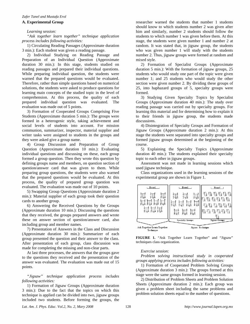
Zafer Tanel and Mustafa Erol
Lat. Am. J. Phys. Educ. Vol.2, No. 2, Mary 2008 128 http://www.journal.lapen.org.mx
A. Experimental Group Learning session: “Ask together learn together” technique application
process includes following activities: 1) Circulating Reading Passages (Approximate duration
3 min.): Each student was given a reading passage. 2) Individual Studying on Reading Passage and
Preparation of an Individual Question (Approximate duration 30 min.): In this stage, students studied on reading passages and prepared their individual questions. While preparing individual question, the students were warned that the prepared questions would be evaluated. Therefore, rather than simple questions based on numerical solutions, the students were asked to produce questions for learning main concepts of the studied topic in the level of comprehension. At this process, the quality of each prepared individual question was evaluated. The evaluation was made out of 5 points.
3) Formation of Cooperated Groups Comprising Five Students (Approximate duration 5 min.): The groups were formed in a heterogenic style, taking achievement and social levels of students into account. For mission communion, summarizer, inspector, material supplier and writer tasks were assigned to students in the groups and they were asked give a group name.
4) Group Discussion and Preparation of Group Question (Approximate duration 10 min.): Evaluating individual questions and discussing on these, each group formed a group question. Then they wrote this question by defining groups name and members, on question section of question/answer card that was given to them. While preparing group questions, the students were also warned that the prepared questions would be evaluated. At this process, the quality of prepared group question was evaluated. The evaluation was made out of 10 points.
5) Swapping Group Questions (Approximate duration 2 min.): Material supplier of each group took their question cards to another group.
6) Answering the Received Questions by the Groups (Approximate duration 10 min.): Discussing the questions that they received, the groups prepared answers and wrote these on answer section of question/answer card, also including group and member names.
7) Presentation of Answers in the Class and Discussion (Approximate duration 30 min.): Summarizer of each group presented the question and their answer to the class. After presentation of each group, class discussion was made for completing the missing and non-clear parts.
At last three processes, the answers that the groups gave to the questions they received and the presentation of the answer was evaluated. The evaluation was made out of 15 points.
“Jigsaw” technique application process includes
following activities: 1) Formation of Jigsaw Groups (Approximate duration
3 min.): Due to the fact that the topics on which this technique is applied can be divided into two, jigsaw groups included two students. Before forming the groups, the
researcher warned the students that number 1 students should know to which students number 2 was given after him and similarly, number 2 students should follow the students to which number 1 was given before them. At this stage, the students were given number 1 and number 2 at random. It was stated that, in jigsaw group, the students who was given number 1 will study with the students number 2. Thus, jigsaw groups were formed at random and mixed style.
2) Formation of Specialist Groups (Approximate duration 5 min.): With the formation of jigsaw groups, 25 students who would study one part of the topic were given number 1; and 25 students who would study the other section were given number 2. By dividing these groups of 25, into haphazard groups of 5, specialty groups were formed.
3) Studying Given Specialty Topics by Specialist Groups (Approximate duration 40 min.): The study over reading passage was carried out by specialty groups. For learning this material and for determining how to explain it to their friends in jigsaw group, the students made discussions.
4) Disintegration of Specialty Groups and Formation of Jigsaw Groups (Approximate duration 2 min.): At this stage the students were separated into specialty groups and formed jigsaw groups determined at the beginning of the course.
5) Explaining the Specialty Topics (Approximate duration 40 min.): The students explained their specialty topic to each other in jigsaw groups.
Assessment was not made in learning sessions which used jigsaw technique.
Class organizations used in the learning sessions of the experimental group are shown in Figure 1.
FIGURE 1. “Ask Together Learn Together” and “Jigsaw” techniques class organization.
Exercise session: Problem solving instructional study in cooperated
groups applying process includes following activities: 1) Formation of Cooperated Problem Solving Groups
(Approximate duration 3 min.): The groups formed at this stage were the same groups formed in learning session.
2) Distribution of Problem Sheets and Problem Solution Sheets (Approximate duration 2 min.): Each group was given a problem sheet including the same problems and problem solution sheets equal to the number of questions.
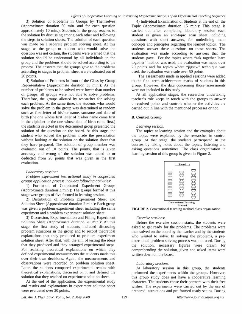
Effects of Cooperative Learning on Instructing Magnetism: Analysis of an Experimental Teaching Sequence
Lat. Am. J. Phys. Educ. Vol. 2, No. 2, May 2008 129 http://www.journal.lapen.org.mx
3) Solution of Problems in Groups by Themselves (Approximate duration 50 min. and for each question approximately 10 min.): Students in the group reaches to the solution by discussing among each other and following the steps in solution sheets. The solution of each question was made on a separate problem solving sheet. At this stage, as the group or student who would solve the question was not certain, the students were warned that the solution should be understood by all individuals in the group and the problems should be solved according to the process. The answers that the groups gave to the problems according to stages in problem sheet were evaluated out of 20 points.
4) Solution of Problems in front of the Class by Group Representative (Approximate duration 35 min.): As the number of problems to be solved were lower than number of groups, all groups were not able to solve problems. Therefore, the groups allotted by researcher for solving each problem. At the same time, the students who would solve the problem in the group was determined at random such as first letter of his/her name, surname and date of birth (the one whose first letter of his/her name came first in the alphabet or the one whose date of birth came first.) the students selected in the determined group presented the solution of the question on the board. At this stage, the student who solved the problem made the presentation without looking at the solution on the solution sheet that they have prepared. The solution of group member was evaluated out of 10 points. The points, that is given accuracy and wrong of the solution was added to or deducted from 20 points that was given in the first evaluation.
Laboratory session: Problem experiment instructional study in cooperated
groups application process includes following activities: 1) Formation of Cooperated Experiment Groups
(Approximate duration 3 min.): The groups formed at this stage were groups of five formed in learning session.
2) Distribution of Problem Experiment Sheet and Solution Sheet (Approximate duration 2 min.): Each group was given a problem experiment sheet including the same experiment and a problem experiment solution sheet.
3) Discussion, Experimentation and Filling Experiment Solution Sheet (Approximate duration 70 min.): At this stage, the first study of students included discussing problem situations in the group and to record theoretical explanations that they produced to problem experiment solution sheet. After that, with the aim of testing the ideas that they produced and they arranged experimental steps. For realizing theoretical explanations on which they defined experimental measurements the students made this over their own decisions. Again, the measurements and observations were recorded on problem solution sheet. Later, the students compared experimental results with theoretical explanations, discussed on it and defined the solution that they reached on experiment solution sheet.
At the end of the application, the experimental study and results and explanations in experiment solution sheet were evaluated over 30 points.
4) Individual Examination of Students at the end of the Topic (Approximate duration 15 min.): This stage is carried out after completing laboratory session each student is given an end-topic scan sheet including questions with short answers, for underlining main concepts and principles regarding the learned topics. The students answer these questions on these sheets. The evaluation was made according to answers that the students gave. For the topics where “ask together learn together” method was used, the evaluation was made over 20 points and for topics where “jigsaw” technique was used, the evaluation was made over 50 points.
The assessments made in applied sessions were added to the final term achievement marks of students in this group. However, the data concerning those assessments were not included in this study.
At all application stages, the researcher undertaking teacher’s role keeps in touch with the groups to answer unresolved points and controls whether the activities are carried out in line with the mentioned processes or not.
B. Control Group
Learning session: The topics at learning session and the examples about
the topics were explained by the researcher in control group. At that stage, the students participated in the courses by taking notes about the topics, listening and asking questions sometimes. The class organization in learning session of this group is given in Figure 2.
FIGURE 2. Conventional teaching method class organization.
Exercise sessions: Before the exercise session starts, the students were
asked to get ready for the problems. The problems were then solved on the board by the teacher and by the students who wanted to solve. In solving the problems, a pre-determined problem solving process was not used. During the solution, necessary figures were drawn for comprehending the solution, given and asked items were written down on the board.
Laboratory sessions: At laboratory session in this group, the students
performed the experiments within the groups. However, this group study does not have a cooperative learning character. The students chose their partners with their free wishes. The experiments were carried out by the use of prepared instructions and pre-formed ready setups. During
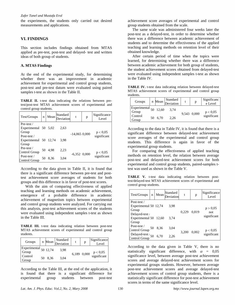
Zafer Tanel and Mustafa Erol
Lat. Am. J. Phys. Educ. Vol.2, No. 2, Mary 2008 130 http://www.journal.lapen.org.mx
the experiments, the students only carried out desired measurements and applications.
VI. FINDINGS
This section includes findings obtained from MTAS applied as pre-test, post-test and delayed- test and written ideas of both group of students. A. MTAS Findings At the end of the experimental study, for determining whether there was an improvement in academic achievement for experimental and control group students, post-test and pre-test datum were evaluated using paired samples t-test as shown in the Table II. TABLE II. t-test data indicating the relations between pre-test/post-test MTAS achievement scores of experimental and control group students.
According to the data given in Table II, it is found that there is a significant difference between pre-test and post-test achievement score averages of students for both groups and this difference is in favor of post-test scores.
With the aim of comparing effectiveness of applied teaching and learning methods on academic achievement, emergence of a probable difference in academic achievement of magnetism topics between experimental and control group students were analyzed. For carrying out this analysis, post-test achievement scores of the students were evaluated using independent samples t-test as shown in the Table III.
TABLE III. t-test data indicating relation between post-test MTAS achievement scores of experimental and control group students.
According to the Table III, at the end of the application, it is found that there is a significant difference for experimental group students between post-test
achievement score averages of experimental and control group students obtained from the scale.
The same scale was administered four weeks later the post-test as a delayed-test, in order to determine whether there was a difference between academic achievement of students and to determine the effectiveness of the applied teaching and learning methods on retention level of their obtained knowledge.
After certain period of time when the topics were learned, for determining whether there was a difference between academic achievement for both group of students, the student achievement scores obtained from delayed-test were evaluated using independent samples t-test as shown in the Table IV.
TABLE IV. t-test data indicating relation between delayed-test MTAS achievement scores of experimental and control group students.
According to the data in Table IV, it is found that there is a significant difference between delayed-test achievement score averages of the experimental and control group students. This difference is again in favor of the experimental group students.
For comparing the effectiveness of applied teaching methods on retention level, the relation between average post-test and delayed-test achievement scores for both experimental and control group students, paired-samples t-test was used as shown in the Table V. TABLE V. t-test data indicating relation between post-test/delayed-test MTAS achievement scores of experimental and control group students.
According to the data given in Table V, there is no statistically significant difference, with α = 0,05 significance level, between average post-test achievement scores and average delayed-test achievement scores for experimental groups students. However, between average post-test achievement scores and average delayed-test achievement scores of control group students, there is a statistically significant difference for post-test achievement scores in terms of the same significance level.
Test/Groups n Mean Standard Deviation
t p Significance
Level
Pre-test / Experimental Group
50 5,02 2,63
-14,065 0,000 p < 0,05 significant Post-test /
Experimental Group
50 12,74 3,98
Pre-test / Control Group
50 4,98 2,23 -6,352 0,000 p < 0,05
significant Post-test / Control Group
50 8,36 3,04
Groups n Mean Standard Deviation
t p Significance
Level Experimental Group
50 12,74 3,98 6,189 0,000 p < 0,05
significant Control Group
50 8,36 3,04
Groups n Mean Standard Deviation
t p Significanc
e Level Experimental Group
50 12,60 3,74 9,543 0,000 p < 0,05
significant Control Group
50 6,70 2,26
Test/Groups n MeanStandard Deviation
t p Significance
Level
Post-test / Experimental Group
50 12,74 3,98
0,229 0,819 p > 0,05
not significant
Delayed-test /Experimental Group
50 12,60 3,74
Post-test / Control Group
50 8,36 3,04 3,200 0,002 p < 0,05
significant Delayed-test /Control Group
50 6,70 2,26
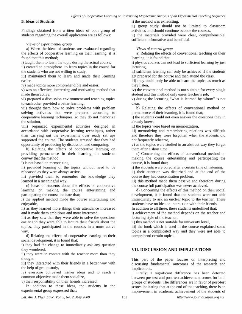
Effects of Cooperative Learning on Instructing Magnetism: Analysis of an Experimental Teaching Sequence
Lat. Am. J. Phys. Educ. Vol. 2, No. 2, May 2008 131 http://www.journal.lapen.org.mx
B. Ideas of Students Findings obtained from written ideas of both group of students regarding the overall application are as follows:
Views of experimental group a) When the ideas of students are evaluated regarding
the effects of cooperative learning on their learning, it is found that this method; i) taught them to learn the topic during the actual course, ii) created an atmosphere to learn topics in the course for the students who are not willing to study, iii) maintained them to learn and made their learning easier, iv) made topics more comprehendible and easier, v) was an effective, interesting and motivating method that made them active, vi) prepared a discussion environment and teaching topics to each other provided a better learning, vii) thought them how to solve problems with problem solving activities that were prepared according to cooperative learning techniques, so they do not memorize the solution, viii) organized experimental activities designed in accordance with cooperative learning techniques, rather than carrying out the experiments over ready set ups supported the course. The students stressed that they had opportunity of producing by discussion and comparing.
b) Relating the effects of cooperative learning on providing permanence in their learning the students convey that the method; i) is not based on memorizing, ii) provided learning of the topics without need to be rehearsed as they were always active iii) provided them to remember the knowledge they learned in a meaningful way,
c) Ideas of students about the effects of cooperative learning on making the course entertaining and participating the course indicate that; i) the applied method made the course entertaining and enjoyable, ii) as they learned more things their attendance increased and it made them ambitious and more interested, iii) as they saw that they were able to solve the questions easier and they were able to lecture their friends about the topics, they participated in the courses in a more active way.
d) Relating the effects of cooperative learning on their social development, it is found that; i) they had the change to immediately ask any question they wondered, ii) they were in contact with the teacher more than they thought, iii) they interacted with their friends in a better way with the help of group study, iv) everyone conveyed his/her ideas and to reach a common objective made them socialize, v) their responsibility on their friends increased.
In addition to these ideas, the students in the experimental group expressed that;
i) the method was exhausting, ii) group study should not be limited to classroom activities and should continue outside the courses, ii) the materials provided were clear, comprehensible, sufficient informative and beneficial.
Views of control group a) Relating the effects of conventional teaching on their
learning, it is found that; i) physics courses can not lead to sufficient learning by just lecturing, ii) sufficient learning can only be achieved if the students get prepared for the course and then attend the class, iii) they could only be able to learn the topics as much as they listen, iv) the conventional method is not suitable for every single student and this method only eases teacher’s job, v) during the lecturing “what is learned by whom” is not clear.
b) Relating the effects of conventional method on permanence of their learning, it is found that; i) the students could not even answer the questions they in already knew, ii) the topics were based on memorization, iii) memorizing and remembering relations was difficult and therefore they were forgotten when the students did not frequently rehearse, v) as the topics were studied in an abstract way they forget them after a short time
c) Concerning the effects of conventional method on making the course entertaining and participating the course, it is found that; i) the students were bored after a certain time of listening, ii) their attention was disturbed and at the end of the course they had concentration problem, iii) this method made them passive and therefore during the course full participation was never achieved.
d) Concerning the effects of this method on their social development, it is found that the students were not able immediately to ask an unclear topic to the teacher. These students have no idea on interaction with their friends. In addition to all these, these students underlined that; i) achievement of the method depends on the teacher and lecturing style of the teacher, ii) this method is not suitable for university level, iii) the book which is used in the course explained some topics in a complicated way and they were not able to comprehend certain topics.
VII. DISCUSSION AND IMPLICATIONS This part of the paper focuses on interpreting and discussing fundamental outcomes of the research and implications.
Firstly, a significant difference has been detected between pre-test and post-test achievement scores for both groups of students. The differences are in favor of post-test scores indicating that at the end of the teaching, there is an improvement in academic achievement of the students of
Zafer Tanel and Mustafa Erol
Lat. Am. J. Phys. Educ. Vol.2, No. 2, Mary 2008 132 http://www.journal.lapen.org.mx
both groups. However, when the post-test achievement scores of both groups were compared, it is found that experimental group students taught by cooperative learning techniques are more successful than control group students. At this point, it is found that cooperative learning increased magnetism topics academic achievement of students to a higher level when compared to conventional teaching method. This result obtained for magnetism topics is in agreement with the results of other studies [4, 9, 10, 11, 14, 15, 16]. After analyzing the effects of cooperative learning on retention level of the knowledge, while no significant change is observed in knowledge of experimental group, it is found that there is a significant regression in knowledge of control group students. This suggests that cooperative learning is more effective in remembering learned knowledge than conventional method.
Based on ideas of students, it can be noted that cooperative learning provides a better learning environment with discussions while learning magnetism topics and helps students to learn in an easily, effective and meaningful way. Other studies concerned with cooperative learning also support these results [33, 34, 35]. Interaction of students with each other when solving problems, deciding on a solution by discussing with each other and evaluating different views provide them a better understanding atmosphere as pointed out by other studies [35, 36, 37]. Similar effects appear in conducting experiments in cooperated groups and learned information is not immediately forgotten indicating the effectiveness of this method.
In both learning and exercise sessions, passiveness in control group turns the students into passive listeners and after a short time they begin to lose concentration from the course with their distracted attentions. In laboratory sessions, students perform experiments without fully thinking on it and making any comments. It is thought that this situation causes the students not to learn and realize what they have learned. Therefore, students in this case chose to memorize rather than trying to understand.
Our experiences during the application show that despite the unwillingness of control group students, experimental group students spend greater efforts and enjoyed the application very much. This experience of them also influenced their ideas about having an entertaining course and having higher course participation. It is clear that, these techniques that were applied in experimental group made the physics course, to which non-science students attended with unwillingness, entertaining and enjoyable as mentioned in other studies regarding cooperative learning [3, 11, 34, 38] and increased the interest of the students to the topic thus provided a higher participation.
Experimental group students noted that this method made the sequence very tiring. Even if it seems like a negative criticism made by the students, it is evaluated as a positive and beneficial situation by the researchers. This shows that the method forces students to study more and gains an effective studying habit.
The ideas of students suggested that cooperative learning techniques improve social abilities of the students. As Nattiv, Winitzky and Dricky [39] express in their research, students are engaged in a higher rate of interaction with their friends when cooperative learning techniques used. Similar improvement is observed in the interaction between teacher and students, this situation also results in improvement of interpersonal communication skills [16]. In addition, it is thought that the students have undertaken the responsibility of other members in cooperative groups and attachment of importance to the ideas of others improved their responsibility and democracy understanding. Improvement on social development together with responsibility and democracy understanding indicate that these techniques can be suitable in achieving affective objectives. Achieving affective objectives is one of the most important deficiencies and it is assumed that a sufficient environment for affective development cannot be provided with conventional teaching.
Considering the selected teaching materials, the ideas of students indicate that these materials should be prepared as appropriate as possible to their levels also clear and comprehensible. Even though the use of course books are widespread, sometimes course books may not be convenient to the level of students. In their study, Bagno and Eylon [21] noted that some deficiencies in content and organization of course books may cause a difficulty in learning related topics. It is therefore important to compile various sources and organize topics, on which students have problems, at a level that students can easily understand. This should be paid attention especially in activities where the students learn by themselves. Boxtel et al. [4] suggest that using course books results in a negative effect on students’ interaction in terms of detailed studying and raising views in cooperative learning. The researchers also underline that students sometimes waste time while analyzing the course books and this prevents them communicating to each other and discuss.
The other important point of this work is carrying out this study in an education faculty. The teacher candidates are introduced different techniques and learned by their own experience. During the application, it is observed that some students found the method beneficial and noted that they would use cooperative learning in the future on-service. Therefore, it is clearly understood that introducing such methods to science and physics teacher candidates helps them in their professional life.
In application stage, for preventing experimental study influenced by undesired variables, the reading passages used in experimental group were handed to the students at the beginning of learning sessions. However, the students noted that receiving reading passages before the beginning of the sessions would be more beneficial. Therefore, it is suggested that giving reading passages before they attended the course would pave the way for teacher and students.
The other point students underlined is that assigning project works outside the school and providing
Effects of Cooperative Learning on Instructing Magnetism: Analysis of an Experimental Teaching Sequence
Lat. Am. J. Phys. Educ. Vol. 2, No. 2, May 2008 133 http://www.journal.lapen.org.mx
cooperation to realize this can be achieved to a higher efficiency level.
Prior to experimental study, the materials and techniques were applied as a pilot study to similar students who received education in the same department and arrangements regarding the deficient parts were rearranged according to reactions and results. It is thought that, this pre-application work increased the achievement of the experimental study. Hence, it is strongly recommended to appliers to use these techniques continuingly for reaching to the best results.
In addition, in teaching of magnetism topics the use of other effective teaching methods and techniques and comparing their results with present ones can indicate how to teach these topics in the most effective way. Accordingly, the magnetism topics can be among the interesting topics, rather than the topics that the students dread.
Another point which was not directly dealt with in the study is the analyzing the effects of laboratory studies carried out by cooperative learning activities on psychomotor development of students. It is thought that, the experiments that the students carry out by designing the related tools and devices themselves can improve their skills. The researchers at this point suggest that further research ought to be carried out on improving psychomotor objectives through the cooperative learning and this would greatly contribute to teaching physics. ACKNOWLEDGEMENT This study was supported by a project grant with a number of 04.KB.EGT.010 by University of Dokuz Eylul, �zmir, Turkey. REFERENCES [1] Banerjee, A. C. and Vidyapati, T. J., Effect of lecture and cooperative learning strategies on achievement in chemistry in undergraduate classes, International Journal of Science Education 19, 903-910 (1997). [2] Crouch, C. H. and Mazur, E., Peer instruction: Ten years of experience and results, American Journal of Physics 69, 970 – 977 (2001). [3] Mills, D., McKittrick, B., Mulhall, P. and Feteris, S., CUP: Cooperative learning that works, Physics Education 34, 11-16 (1999). [4] Boxtel, C., Linden, J. and Kanselaar, G., The use of textbooks as a tool during collaborative physics learning, The Journal of Experimental Education 69, 57-76 (2000). [5] Samiullah, M., Effect of in-class student-student interaction on the learning of physics in a college physics course, American Journal of Physics 63, 944-950 (1995). [6] Saglam, M. and Millar, R., Upper high school students’ understanding of electromagnetism, International Journal of Science Education 28, 543-566 (2006).
[7] Johnson, D. W. and Johnson, R. T., Learning Together and Alone, 2nd ed. (Prentice-Hall, Englewood Cliffs, N J, 1987). [8] Johnson, D. W., Johnson, R. T. and Holubec, E. J., Cooperation in the Classroom (Interaction Book, Edina, MN, 1993). [9] Balfakih, N. M. A., The effectiveness of student team-achievement division (STAD) for teaching high school chemistry in the United Arab Emirates, International Journal of Science Education 25, 605–624 (2003). [10] Daubenmire, P. L., “A longitudinal investigation of student learning in general chemistry with the guided inquiry approach”, Dissertation Abstracts International, 65, 880A. (UMI No. 3124889), 2004. [11] Johnson, D. W., Johnson, R. T. and Smith, K. A., Cooperative learning returns to college what evidence is there that it works?, Change 30, 26-35 (1998). [12] Jones, R. M. and Steinbrink, J. E., Using cooperative groups in science teaching, School Science and Mathematics 89, 541- 551 (1989). [13] Jordan, D. and Le Metaias, J., Social skilling through cooperative learning, Educational Research 39, 3-21 (1997). [14] Kagan, S., Kagan, M. and Kagan, L., Science: Reaching standarts through Cooperative learning. Providing for all learners in general education classrooms (Kagan Publishing, San Clemente, 2000). [15] Merebah, S. A. A., “Cooperative learning in science: A comparative study in Saudi Arabia”, Dissertation Abstracts International 48, 892A. (UMI No. 8715226), 1987. [16] Towns, M. H. and Grant, E. R., ‘I believe I will go out of this class actually knowing something’: Cooperative learning activities in physical chemistry, Journal of Research in Science Teaching 34, 819-835 (1997). [17] Chabay, R. and Sherwood, B., Restructuring the introductory electricity and magnetism course, American Journal of Physics 74, 329-336 (2006). [18] Houldin, J. E., The teaching of electromagnetism at university level, Physics Education 9, 9-12 (1974). [19] Loftus, M., Students ideas about electromagnetism, School Science Review 77, 93-94 (1996). [20] Yigit, N., Akdeniz, A. R. and Kurt, S., Fizik ogretiminde calisma yapraklarinin gelistirilmesi, Paper presented at Yeni Binyilin Basinda Turkiye’de Fen Bilimleri Egitimi Sempozyumu, Istanbul: Maltepe University, 2001. [21] Bagno, E. and Eylon, B. S., From problem solving to a knowledge structure: An example from the domain of electromagnetism, American Journal of Physics 65, 726-736 (1997). [22] Kocakulah, M. S., “A study of the development of Turkish first year university students’ understanding of electromagnetism and the implications for instruction” Unpublished doctorate thesis, The University of Leeds, School of Education, Leeds, UK, 1999. [23] Raduta, C., General students’ misconceptions related to electricity and magnetism, <http://arxiv.org/ftp/physics/papers/0503/0503132.pdf>, visited in October 13, 2005.
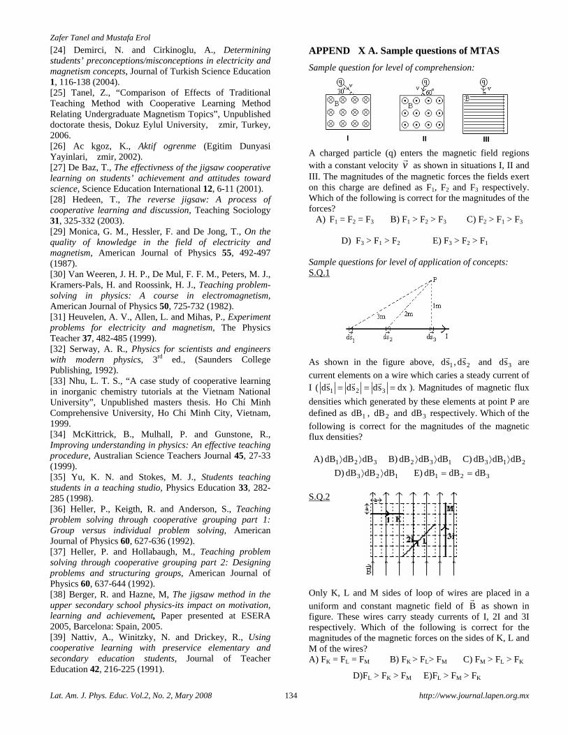
Zafer Tanel and Mustafa Erol
Lat. Am. J. Phys. Educ. Vol.2, No. 2, Mary 2008 134 http://www.journal.lapen.org.mx
[24] Demirci, N. and Cirkinoglu, A., Determining students’ preconceptions/misconceptions in electricity and magnetism concepts, Journal of Turkish Science Education 1, 116-138 (2004). [25] Tanel, Z., “Comparison of Effects of Traditional Teaching Method with Cooperative Learning Method Relating Undergraduate Magnetism Topics”, Unpublished doctorate thesis, Dokuz Eylul University, �zmir, Turkey, 2006. [26] Ac�kgoz, K., Aktif ogrenme (Egitim Dunyasi Yayinlari, �zmir, 2002). [27] De Baz, T., The effectivness of the jigsaw cooperative learning on students’ achievement and attitudes toward science, Science Education International 12, 6-11 (2001). [28] Hedeen, T., The reverse jigsaw: A process of cooperative learning and discussion, Teaching Sociology 31, 325-332 (2003). [29] Monica, G. M., Hessler, F. and De Jong, T., On the quality of knowledge in the field of electricity and magnetism, American Journal of Physics 55, 492-497 (1987). [30] Van Weeren, J. H. P., De Mul, F. F. M., Peters, M. J., Kramers-Pals, H. and Roossink, H. J., Teaching problem-solving in physics: A course in electromagnetism, American Journal of Physics 50, 725-732 (1982). [31] Heuvelen, A. V., Allen, L. and Mihas, P., Experiment problems for electricity and magnetism, The Physics Teacher 37, 482-485 (1999). [32] Serway, A. R., Physics for scientists and engineers with modern physics, 3rd ed., (Saunders College Publishing, 1992). [33] Nhu, L. T. S., “A case study of cooperative learning in inorganic chemistry tutorials at the Vietnam National University”, Unpublished masters thesis. Ho Chi Minh Comprehensive University, Ho Chi Minh City, Vietnam, 1999. [34] McKittrick, B., Mulhall, P. and Gunstone, R., Improving understanding in physics: An effective teaching procedure, Australian Science Teachers Journal 45, 27-33 (1999). [35] Yu, K. N. and Stokes, M. J., Students teaching students in a teaching studio, Physics Education 33, 282- 285 (1998). [36] Heller, P., Keigth, R. and Anderson, S., Teaching problem solving through cooperative grouping part 1: Group versus individual problem solving, American Journal of Physics 60, 627-636 (1992). [37] Heller, P. and Hollabaugh, M., Teaching problem solving through cooperative grouping part 2: Designing problems and structuring groups, American Journal of Physics 60, 637-644 (1992). [38] Berger, R. and Hazne, M, The jigsaw method in the upper secondary school physics-its impact on motivation, learning and achievement, Paper presented at ESERA 2005, Barcelona: Spain, 2005. [39] Nattiv, A., Winitzky, N. and Drickey, R., Using cooperative learning with preservice elementary and secondary education students, Journal of Teacher Education 42, 216-225 (1991).
APPEND�X A. Sample questions of MTAS
Sample question for level of comprehension: A charged particle (q) enters the magnetic field regions with a constant velocity v as shown in situations I, II and III. The magnitudes of the magnetic forces the fields exert on this charge are defined as F1, F2 and F3 respectively. Which of the following is correct for the magnitudes of the forces? A) F1 = F2 = F3 B) F1 > F2 > F3 C) F2 > F1 > F3
D) F3 > F1 > F2 E) F3 > F2 > F1 Sample questions for level of application of concepts: S.Q.1
As shown in the figure above, 321 sdandsd,sd are
current elements on a wire which caries a steady current of I ( dxsdsdsd 321 === ). Magnitudes of magnetic flux
densities which generated by these elements at point P are defined as 1dB , 2dB and 3dB respectively. Which of the
following is correct for the magnitudes of the magnetic flux densities? A) 321 dBdBdB ⟩⟩ B) 132 dBdBdB ⟩⟩ C) 213 dBdBdB ⟩⟩
D) 123 dBdBdB ⟩⟩ E) 321 dBdBdB ==
S.Q.2 Only K, L and M sides of loop of wires are placed in a
uniform and constant magnetic field of B as shown in figure. These wires carry steady currents of I, 2I and 3I respectively. Which of the following is correct for the magnitudes of the magnetic forces on the sides of K, L and M of the wires? A) FK = FL = FM B) FK > FL> FM C) FM > FL > FK
D)FL > FK > FM E)FL > FM > FK
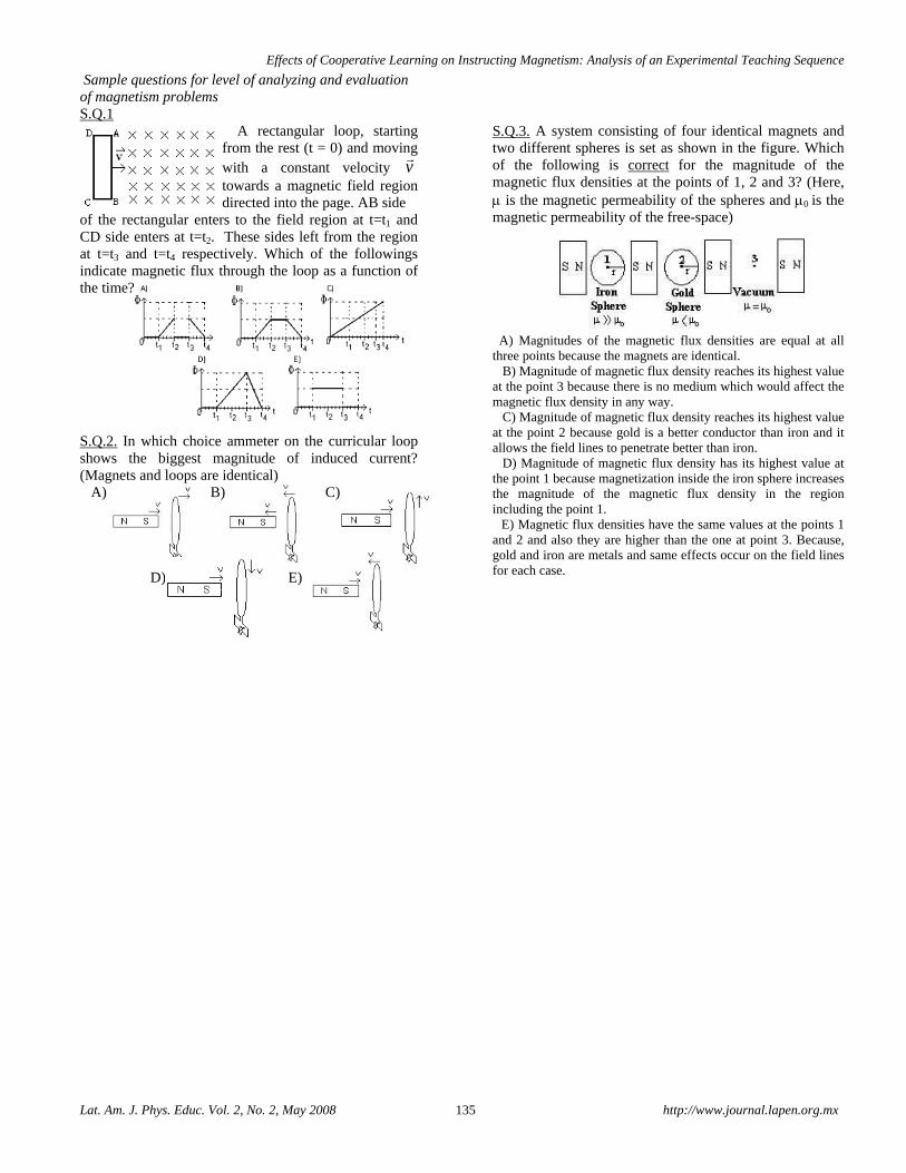
Effects of Cooperative Learning on Instructing Magnetism: Analysis of an Experimental Teaching Sequence
Lat. Am. J. Phys. Educ. Vol. 2, No. 2, May 2008 135 http://www.journal.lapen.org.mx
Sample questions for level of analyzing and evaluation of magnetism problems S.Q.1
A rectangular loop, starting from the rest (t = 0) and moving with a constant velocity v towards a magnetic field region directed into the page. AB side
of the rectangular enters to the field region at t=t1 and CD side enters at t=t2. These sides left from the region at t=t3 and t=t4 respectively. Which of the followings indicate magnetic flux through the loop as a function of the time? S.Q.2. In which choice ammeter on the curricular loop shows the biggest magnitude of induced current? (Magnets and loops are identical) A) B) C) D) E)
S.Q.3. A system consisting of four identical magnets and two different spheres is set as shown in the figure. Which of the following is correct for the magnitude of the magnetic flux densities at the points of 1, 2 and 3? (Here, μ is the magnetic permeability of the spheres and μ0 is the magnetic permeability of the free-space) A) Magnitudes of the magnetic flux densities are equal at all three points because the magnets are identical. B) Magnitude of magnetic flux density reaches its highest value at the point 3 because there is no medium which would affect the magnetic flux density in any way. C) Magnitude of magnetic flux density reaches its highest value at the point 2 because gold is a better conductor than iron and it allows the field lines to penetrate better than iron. D) Magnitude of magnetic flux density has its highest value at the point 1 because magnetization inside the iron sphere increases the magnitude of the magnetic flux density in the region including the point 1.
E) Magnetic flux densities have the same values at the points 1 and 2 and also they are higher than the one at point 3. Because, gold and iron are metals and same effects occur on the field lines for each case.
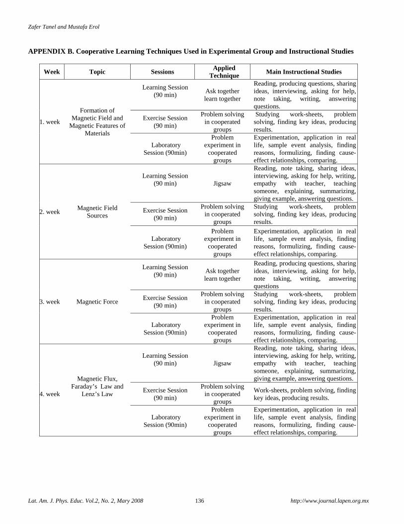
Zafer Tanel and Mustafa Erol
Lat. Am. J. Phys. Educ. Vol.2, No. 2, Mary 2008 136 http://www.journal.lapen.org.mx
APPENDIX B. Cooperative Learning Techniques Used in Experimental Group and Instructional Studies
Week Topic Sessions Applied
Technique Main Instructional Studies
1. week
Formation of Magnetic Field and
Magnetic Features of Materials
Learning Session (90 min)
Ask together learn together
Reading, producing questions, sharing ideas, interviewing, asking for help, note taking, writing, answering questions.
Exercise Session (90 min)
Problem solving in cooperated
groups
Studying work-sheets, problem solving, finding key ideas, producing results.
Laboratory Session (90min)
Problem experiment in
cooperated groups
Experimentation, application in real life, sample event analysis, finding reasons, formulizing, finding cause-effect relationships, comparing.
2. week Magnetic Field
Sources
Learning Session (90 min)
Jigsaw
Reading, note taking, sharing ideas, interviewing, asking for help, writing, empathy with teacher, teaching someone, explaining, summarizing, giving example, answering questions.
Exercise Session (90 min)
Problem solving in cooperated
groups
Studying work-sheets, problem solving, finding key ideas, producing results.
Laboratory Session (90min)
Problem experiment in
cooperated groups
Experimentation, application in real life, sample event analysis, finding reasons, formulizing, finding cause-effect relationships, comparing.
3. week Magnetic Force
Learning Session (90 min)
Ask together learn together
Reading, producing questions, sharing ideas, interviewing, asking for help, note taking, writing, answering questions
Exercise Session (90 min)
Problem solving in cooperated
groups
Studying work-sheets, problem solving, finding key ideas, producing results.
Laboratory Session (90min)
Problem experiment in
cooperated groups
Experimentation, application in real life, sample event analysis, finding reasons, formulizing, finding cause-effect relationships, comparing.
4. week
Magnetic Flux, Faraday’s Law and
Lenz’s Law
Learning Session (90 min)
Jigsaw
Reading, note taking, sharing ideas, interviewing, asking for help, writing, empathy with teacher, teaching someone, explaining, summarizing, giving example, answering questions.
Exercise Session (90 min)
Problem solving in cooperated
groups
Work-sheets, problem solving, finding key ideas, producing results.
Laboratory Session (90min)
Problem experiment in
cooperated groups
Experimentation, application in real life, sample event analysis, finding reasons, formulizing, finding cause-effect relationships, comparing.
Lat. Am. J. Phys. Educ. Vol. 2, No.2, May 2008 137 http://www.journal.lapen.org.mx
How can formulation of physics problems and exercises aid students in thinking about their results?
Josip Slisko Facultad de Ciencias Físico Matemáticas, Benemérita Universidad Autónoma de Puebla, México.
E-mail: [email protected] (Received 15 April 2008, accepted 8 May 2008)
Abstract It has recently became common that the authors of the physics textbooks describe, in general terms, the most important steps students have to follow in order to solve problems. The last step is usually a recommendation to “think about the result” in order to find out if it is reasonable. Nevertheless, the standard formulation of exercises is such that “thinking about the result” is likely to be left out or, in the best scenario, it can be used only to fix students’ careless math errors. In fact, it seems that the physics textbook authors have on their minds precisely this role for the “thinking about the result”. Even in the cases when the physical evaluation of the mathematically correct results is required explicitly, the students might not have the knowledge necessary to evaluate it in an appropriate way. In this article, a better way to formulate physics exercises is proposed. In such a formulation the evaluation of the result cannot be avoided. Keywords: Physics problem solving, steps of expert, critical thinking, textbook errors, design of physics problem.
Resumen Recientemente se volvió común que los autores de los libros de texto describan, en términos generales, los más importantes pasos que los estudiantes tienen que seguir para resolver problemas. El último paso es usualmente una recomendación “piensa sobre el resultado” con el fin de determinar si es sensato. Sin embargo, la formulación estándar de los ejercicios es tal que es probable que el “pensamiento sobre el resultado” se omite o, en el mejor caso, se usa solamente para arreglar los errores matemáticos que los estudiantes hacen por descuido. De hecho, parece que los autores de libros de texto de física tienen en su mente precisamente este papel del “pensamiento sobre el resultado”. Incluso, en los casos en que se requiere explícitamente la evolución física de los resultados que son matemáticamente correctos, puede ser que los estudiantes no tengan el conocimiento necesario para evaluarlos de manera apropiada. En este artículo, se propone una mejor manera de formular ejercicios de física. En tal formulación la evolución de los resultados no se puede evitar. Palabras clave: resolución de problemas de física, pasos del experto, pensamiento crítico, errores en los libros de texto, diseño de problemas de física. PACS01.40.-d, 01.40.Jp, 01.50-i ISSN 1870-9095
I. TWO STANDARD RECOMMENDATIONS FOR THINKING ABOUT THE RESULTS: CHECKING MATH OR PHYSICS? Problem solving, as an important part of physics teaching and learning, has received in the last few decades the deserved attention of the research community [1]. The most important result of this research has been the astonishing difference between experts and novice problem solving strategies. As a pedagogical consequence, it recently became common that physics textbooks provide a summary of problem-solving steps which seem to be in resonance with the ones used by experts. Usually the last
step is an explicit recommendation of thinking about the meaning of the results obtained in the calculations performed. Roughly speaking, these recommendations fall in two different categories.
Students should have some kind of ready-to-use knowledge in order to judge the validity of the results (three different versions of this type of recommendation are given in the Table I).
Students have to estimate the order of magnitude in order to judge the mathematical validity of the result (two different wordings of this recommendation can be found in the Table II).
Josip Slisko
Lat. Am. J. Phys. Educ. Vol.2, No. 2, May 2008 138 http://www.journal.lapen.org.mx
TABLE I. Recommendations to activate ready-to-use knowledge in order to judge the validity of the results.
“…When you arrive at a number, think about it. Does it make sense? If you find that it takes 3 min to drive from New York City to Los Angeles, you have probably made a mistake” [2].
“… Consider whether the result is reasonable. That is, does the answer have an appropriate magnitude? (This means is it “in the right ball park.”) For example, if a person’s calculated mass turns out to be 2.30 x 10² kg, the result should be questioned, since 230 kg corresponds to a weight of 506 lbs” [3].
“After you have finished your calculations, always check whether the answer is plausible. For instance, if your calculation yields the result that a diver jumping off a cliff hits water at 3000 km/h, then somebody has made a mistake somewhere!” [4].
TABLE II. Recommendations to carry out order-of-magnitude estimation in order to judge the validity of the results.
“Think carefully about the result you obtain: Is it reasonable? Does it make sense according to your own intuition and experience? A good check is to do a rough estimate using only powers on ten…” [5].
“As a final check, you should consider whether your answer is reasonable.
Does your result have the proper order of magnitude? You may even carry out a quick order-of-magnitude estimate as a way to confirming your work” [6].
No one doubts that both of these recommendations are very useful in eliminating the negative effects of careless errors in algebraic manipulations or incorrect formula usage. Therefore, it is worthwhile to explicitly ask students to use them and make them an important part of problem-solving sessions, homework and exams.
Nevertheless, the first type or recommendation could only be used in a small fraction of standard exercises. While it is likely that students will know that the “3-
minute travel time between New York and Los Angeles”, “230 kg mass for a human” and “3000 km/h diver’s speed” are not feasible in the real world, for many physical situations used in numerical exercises the corresponding real-world facts are simple not part of students’ knowledge. Two situations in which the reasonable value of the gravitational force is beyond students’ knowledge base are presented in the Table III.
TABLE III. Which real-world knowledge is useful to judge if the results are reasonable?
“Two students sitting in adjacent seats in a lecture room have weights of 600 N and 700 N. Assume that Newton’s law of gravitation can be applied to these students and find the gravitational force that one student exerts on the other when they are separated by 0.5 m” [7].
“Two supertankers, each with a mass of 7 x 10⁸ kg, are separated by a distance of 2 km. What is the gravitational force that each exerts on the other. Treat them as particles” [8].
Comment: Students are not asked to examine if the results are reasonable or to compare them with a known force in order to have some experience and knowledge about the size of the gravitational force between humans or men-made objects like supertankers. In addition, the applicability of the law of gravitation is, explicitly or implicitly, suggested.
When students don’t have at their disposal the necessary real-world knowledge to judge directly the feasibility of the result, they can only use the second type of recommendation and make an order-of-magnitude estimation.
If such estimation agrees with their prior calculations, is the result feasible? Unfortunately, in some cases it is not. Textbook authors and teachers also make errors, supposing physical situations which are not very likely to happen (or are even impossible) in the real world [9, 10, 11, 12, 13].
Although useful in eliminating students’ math errors, the above recommendations are not effective against the more serious errors made by physics textbooks authors or teachers in regard to physical feasibility of problem situations.
This is true because students, like authors and teachers themselves, may lack the real-world knowledge which directly contradicts the result. In addition, an order-of-magnitude calculation is essentially a tactic to rapidly check the numerical results of mathematical steps involved and cannot judge the feasibility of the situation supposed. One cannot stress enough that the mathematical correctness of the results has little or nothing to do with its physical feasibility. Namely, student should know that some mathematically possible situations and results are physically impossible due the real-world restrictions.
With the standard design of numerical exercises and only the type of recommendations discussed above, the students are not likely to practice and develop strategies
How can formulation of physics problems and exercises aid students in thinking about their results?
Lat. Am. J. Phys. Educ. Vol. 2, No.1, January 2008 139 http://www.journal.lapen.org.mx
of critical thinking, proudly announced as one of the most important objectives of physics teaching. II. SHOULD STUDENTS DEAL WITH “WRONG ANSWERS” IN NUMERICAL EXERCISES? Detecting unfeasible physical situations, implied by carelessly assigned “bad numbers” to some physical quantities, isn’t an easy task with clear solution. Taking into account that many authors, reviewers and teachers are highly-qualified physicists, if it were a trivial task, there would be no such errors in physics textbooks. It is frequently impossible to detect an unfeasible physical situation, supposed as a “context” for calculations, without using some, apparently unrelated concepts. A good example of how nontrivially it is to carry out such a task is to examine the feasibility of the situation “two bodies charged with 1 C at 1 m distance”, frequently used in physics textbooks as one of exercise for the application of Coulomb’s law “application” [10]. In order to show that such a situation is impossible in the real world, one should know facts about electrical strength of air, cold emission and the electrical stress the metals can sustain.
There are authors who think that students should not be given the problems and exercises whose results are, strictly speaking, incorrect. For instance, Blickensderfer [14] argued that some questions, likely to be found in typical textbooks for introductory-level physics courses, have wrong answers because they are usually answered within overly simplified mathematical models.
He suggests that a more appropriate approach in introductory courses would be to change numerical data in order to fit better supposed simple formulas rather than to
use more advanced physical and mathematical models (reserved for upper-division part of curriculum).
Other authors, the present one included, have quite the opposite opinion and would rather answer the question in the subtitle with “yes”. For instance, Urone made use of this idea in a unique way. In his college-physics textbook, he stressed the importance that students deal with clearly stated “unreasonable result problems”:
“Unreasonable result problems are unique to this text. They are designed to further emphasize that properly applied physics must describe nature accurately and it is not simply the process of solving equations. For example, if the heat generated by metabolizing an average day’s food is retained, a person’s body temperature will rise to a lethal level. Thus, physics correctly applied produces in this case a result that is never observed –the student must recognize that the premise of complete heat retention is at fault. These problems are clearly labeled and are found at the very end of the end-of-chapter problems– all other problems in the text produce reasonable results and often contain discussion to emphasize that physics must fit nature. Taken with the careful accuracy of the text and the discussions at the end of worked examples, unreasonable result problems can help students examine the concepts of a problem as well as the mechanics of solving it” [15]..
“... Problems with unreasonable results are included to give practice in assessing whether nature is being accurately described, and to trace the source of difficulty if it is not. This is very much like the process followed in original research when physical principles as well as faulty premises are tested” [16].
One example of Urone’s “unreasonable result problem”, related to the law of gravitation, is given in the Table IV.
TABLE IV. A mountain with too big mass. “A mountain 10.0 km from a person exerts a gravitational force on him equal to 2.00 % of his weight. (a) Calculate the mass of the mountain. (b) Compare the mountain’s mass with that of the entire earth. (c) What is unreasonable about these results? (d) Which premises are unreasonable or inconsistent? (Note that accurate gravitational measurements can easily detect the effect of nearby mountains and variations in local geology.)” [15, Problem 8.43, p. 217]. Answers (a) 2.94 x 10¹⁷ kg (b) 4.92 x 10⁻⁸ of the earth’s mass (c) the mass of the mountain and its fraction to the earth’s mass are too great. (d) The gravitational force assumed to be exerted by the mountain is too great [15, AN-2].
Although this type of problems is a step in right direction, students still might lack the skills necessary to arrive at the conclusion that the implied mass of the mountain and its fraction to the Earth’s mass are too great. If they have to accept blindly the answer, provided by Urone, without being able to reconstruct it or grasp the essence of the reasoning it is based on, the chance for becoming critical thinker is lost forever.
One way to improve this type of problems is to provide students with some hints or guidance in order that they can conclude by themselves what is wrong with the problem in
question. This is the approach I used in the critical-thinking rubrics of my secondary-school physics textbooks, named “No creas todo lo que lees” (“Don’t believe everything you read”) [17, 18].
In the case of the too-massive-mountain exercise, one tactic might be to ask students: what the value of the supposed gravitational force would be if the person were at a distance 1 km from the mountain? According to the law of gravitation, when distance is ten times smaller, the force would be 100 times bigger. In this situation the force would be quite unreasonable twice the person’s weight. As
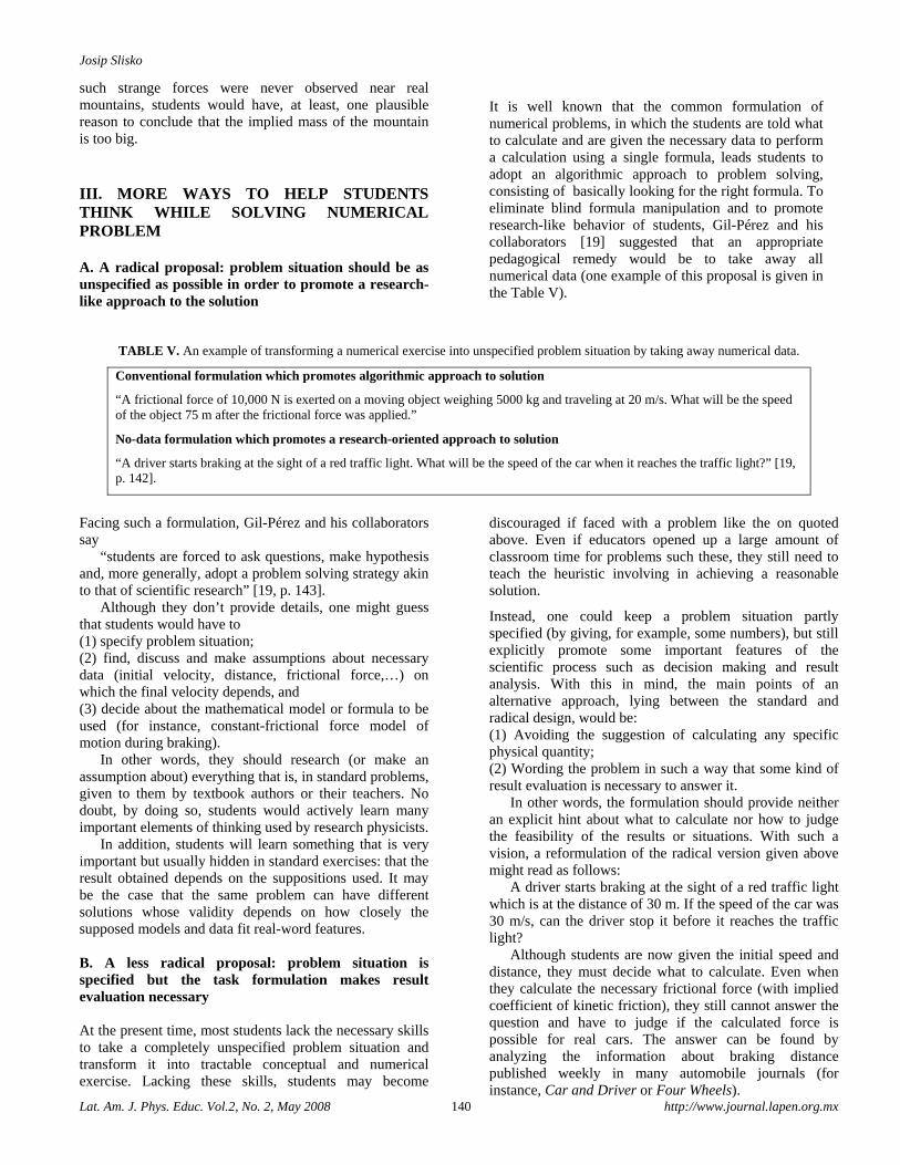
Josip Slisko
Lat. Am. J. Phys. Educ. Vol.2, No. 2, May 2008 140 http://www.journal.lapen.org.mx
such strange forces were never observed near real mountains, students would have, at least, one plausible reason to conclude that the implied mass of the mountain is too big. III. MORE WAYS TO HELP STUDENTS THINK WHILE SOLVING NUMERICAL PROBLEM A. A radical proposal: problem situation should be as unspecified as possible in order to promote a research-like approach to the solution
It is well known that the common formulation of numerical problems, in which the students are told what to calculate and are given the necessary data to perform a calculation using a single formula, leads students to adopt an algorithmic approach to problem solving, consisting of basically looking for the right formula. To eliminate blind formula manipulation and to promote research-like behavior of students, Gil-Pérez and his collaborators [19] suggested that an appropriate pedagogical remedy would be to take away all numerical data (one example of this proposal is given in the Table V).
TABLE V. An example of transforming a numerical exercise into unspecified problem situation by taking away numerical data.
Conventional formulation which promotes algorithmic approach to solution
“A frictional force of 10,000 N is exerted on a moving object weighing 5000 kg and traveling at 20 m/s. What will be the speed of the object 75 m after the frictional force was applied.”
No-data formulation which promotes a research-oriented approach to solution
“A driver starts braking at the sight of a red traffic light. What will be the speed of the car when it reaches the traffic light?” [19, p. 142].
Facing such a formulation, Gil-Pérez and his collaborators say
“students are forced to ask questions, make hypothesis and, more generally, adopt a problem solving strategy akin to that of scientific research” [19, p. 143].
Although they don’t provide details, one might guess that students would have to (1) specify problem situation; (2) find, discuss and make assumptions about necessary data (initial velocity, distance, frictional force,…) on which the final velocity depends, and (3) decide about the mathematical model or formula to be used (for instance, constant-frictional force model of motion during braking).
In other words, they should research (or make an assumption about) everything that is, in standard problems, given to them by textbook authors or their teachers. No doubt, by doing so, students would actively learn many important elements of thinking used by research physicists.
In addition, students will learn something that is very important but usually hidden in standard exercises: that the result obtained depends on the suppositions used. It may be the case that the same problem can have different solutions whose validity depends on how closely the supposed models and data fit real-word features.
B. A less radical proposal: problem situation is specified but the task formulation makes result evaluation necessary At the present time, most students lack the necessary skills to take a completely unspecified problem situation and transform it into tractable conceptual and numerical exercise. Lacking these skills, students may become
discouraged if faced with a problem like the on quoted above. Even if educators opened up a large amount of classroom time for problems such these, they still need to teach the heuristic involving in achieving a reasonable solution.
Instead, one could keep a problem situation partly specified (by giving, for example, some numbers), but still explicitly promote some important features of the scientific process such as decision making and result analysis. With this in mind, the main points of an alternative approach, lying between the standard and radical design, would be: (1) Avoiding the suggestion of calculating any specific physical quantity; (2) Wording the problem in such a way that some kind of result evaluation is necessary to answer it.
In other words, the formulation should provide neither an explicit hint about what to calculate nor how to judge the feasibility of the results or situations. With such a vision, a reformulation of the radical version given above might read as follows:
A driver starts braking at the sight of a red traffic light which is at the distance of 30 m. If the speed of the car was 30 m/s, can the driver stop it before it reaches the traffic light?
Although students are now given the initial speed and distance, they must decide what to calculate. Even when they calculate the necessary frictional force (with implied coefficient of kinetic friction), they still cannot answer the question and have to judge if the calculated force is possible for real cars. The answer can be found by analyzing the information about braking distance published weekly in many automobile journals (for instance, Car and Driver or Four Wheels).
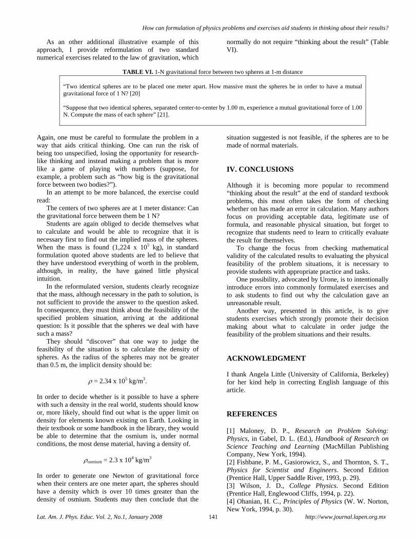
How can formulation of physics problems and exercises aid students in thinking about their results?
Lat. Am. J. Phys. Educ. Vol. 2, No.1, January 2008 141 http://www.journal.lapen.org.mx
As an other additional illustrative example of this approach, I provide reformulation of two standard numerical exercises related to the law of gravitation, which
normally do not require “thinking about the result” (Table VI).
TABLE VI. 1-N gravitational force between two spheres at 1-m distance
“Two identical spheres are to be placed one meter apart. How massive must the spheres be in order to have a mutual gravitational force of 1 N? [20] “Suppose that two identical spheres, separated center-to-center by 1.00 m, experience a mutual gravitational force of 1.00 N. Compute the mass of each sphere” [21].
Again, one must be careful to formulate the problem in a way that aids critical thinking. One can run the risk of being too unspecified, losing the opportunity for research-like thinking and instead making a problem that is more like a game of playing with numbers (suppose, for example, a problem such as “how big is the gravitational force between two bodies?”).
In an attempt to be more balanced, the exercise could read:
The centers of two spheres are at 1 meter distance: Can the gravitational force between them be 1 N?
Students are again obliged to decide themselves what to calculate and would be able to recognize that it is necessary first to find out the implied mass of the spheres. When the mass is found (1,224 x 105 kg), in standard formulation quoted above students are led to believe that they have understood everything of worth in the problem, although, in reality, the have gained little physical intuition.
In the reformulated version, students clearly recognize that the mass, although necessary in the path to solution, is not sufficient to provide the answer to the question asked. In consequence, they must think about the feasibility of the specified problem situation, arriving at the additional question: Is it possible that the spheres we deal with have such a mass?
They should “discover” that one way to judge the feasibility of the situation is to calculate the density of spheres. As the radius of the spheres may not be greater than 0.5 m, the implicit density should be:
ρ = 2.34 x 10⁵ kg/m3.
In order to decide whether is it possible to have a sphere with such a density in the real world, students should know or, more likely, should find out what is the upper limit on density for elements known existing on Earth. Looking in their textbook or some handbook in the library, they would be able to determine that the osmium is, under normal conditions, the most dense material, having a density of.
ρosmium = 2.3 x 10⁴ kg/m3 In order to generate one Newton of gravitational force when their centers are one meter apart, the spheres should have a density which is over 10 times greater than the density of osmium. Students may then conclude that the
situation suggested is not feasible, if the spheres are to be made of normal materials. IV. CONCLUSIONS Although it is becoming more popular to recommend “thinking about the result” at the end of standard textbook problems, this most often takes the form of checking whether on has made an error in calculation. Many authors focus on providing acceptable data, legitimate use of formula, and reasonable physical situation, but forget to recognize that students need to learn to critically evaluate the result for themselves.
To change the focus from checking mathematical validity of the calculated results to evaluating the physical feasibility of the problem situations, it is necessary to provide students with appropriate practice and tasks.
One possibility, advocated by Urone, is to intentionally introduce errors into commonly formulated exercises and to ask students to find out why the calculation gave an unreasonable result.
Another way, presented in this article, is to give students exercises which strongly promote their decision making about what to calculate in order judge the feasibility of the problem situations and their results. ACKNOWLEDGMENT I thank Angela Little (University of California, Berkeley) for her kind help in correcting English language of this article.
REFERENCES [1] Maloney, D. P., Research on Problem Solving: Physics, in Gabel, D. L. (Ed.), Handbook of Research on Science Teaching and Learning (MacMillan Publishing Company, New York, 1994). [2] Fishbane, P. M., Gasiorowicz, S., and Thornton, S. T., Physics for Scientist and Engineers. Second Edition (Prentice Hall, Upper Saddle River, 1993, p. 29). [3] Wilson, J. D., College Physics. Second Edition (Prentice Hall, Englewood Cliffs, 1994, p. 22). [4] Ohanian, H. C., Principles of Physics (W. W. Norton, New York, 1994, p. 30).

Josip Slisko
Lat. Am. J. Phys. Educ. Vol.2, No. 2, May 2008 142 http://www.journal.lapen.org.mx
[5] Giancoli, D. C., Physics,.Principles and Applications. Fifth Edition (Prentice Hall, Upper Saddle River, 1998, p. 29). [6] Jones, E., and Childers, R., Contemporary College Physics. Third Edition (WCB/McGraw-Hill, Boston, 1999, p. 20). [7] Serway, R. A. and Faughn, J. S., College Physics. Third Edition (Saunders College Publishing, Fort Worth, 1992, p. 202, Problem 43). [8] Ohanian, H. C., Principles of Physics (W. W. Norton, New York, 1994, p. 179, Problem 1). [9] Slisko, J., The limitless world of textbook mistakes, The Physics Teacher 33, 318, (1995). [10] Slisko, J. and Krokhin, A., Physics or Reality? F = k (1C)(1C)/(1 m)
2, The Physics Teacher, 33, 210 – 212,
(1995). [11] Slisko, J., Errores comunes en problemas numéricos de la física escolar, Didáctica de las Ciencias Experimentales y Sociales 14, 87 – 98, (2000). [12] Slisko, J., Errores en los libros de texto de física: ¿Cómo convertir estos obstáculos de aprendizaje en oportunidades para el desarrollo del pensamiento crítico?, in Flores, F. and Aguirre M. E. (Eds.), Educación en física. Incursiones en su investigación. (Plaza y Valdes Editores, México, D. F., 2003) pp. 79 – 120.
[13] Slisko, J., Electric charge of humans: should students buy what the textbooks sell? Physics Education 41, 114–116 (2006). [14] Blickensderfer, R., What’s wrong with this question?, The Physics Teacher 36, 524 - 525 (1998). [15] Urone, P., College Physics (Brooks/Cole Publishing Company, Pacific Grove, CA, 1998, p. XI). [16] Urone, P., College Physics (Brooks/Cole Publishing Company, Pacific Grove, CA, 1998, p. 217. [17] Slisko, J., Física 1. El encanto de pensar (Pearson Educación, Naucalpan de Juérez, México, 2002). [18] Slisko, J., Física 2. El encanto de pensar (Pearson Educación, Naucalpan de Juérez, México, 2003). [19] Gil-Pérez, D., Dumas-Carré, A., Caillot, M., and Martínez-Torregrosa, J., Paper and pencil problem solving in the physical sciences as a research activity, Studies in Science Education 18, 137 – 151 (1990). [20] Culver, R., Facets of Physics. A Conceptual Approach (West Publishing Company, (St. Paul, 1993, Problem 2, p. 143). [21] Hecht, E., Physics: Algebra / Trig. Second Edition (Brooks / Cole Publishing Company, Pacific Grove, CA, 1997, Problem 27, p. 171).
Lat. Am. J. Phys. Educ. Vol. 2, No. 2, May 2008 143 http://www.journal.lapen.org.mx
Weightlessness vs. absence of gravity. An illustration of a didactic approach showing accuracy and attention to fact
J. Vila1 and C. J. Sierra2 1University of the Basque Country, Spain
2“Los Peñascales” Secondary School, Madrid, Spain E-mail: [email protected] (Received 2 March 2008, accepted 28 April 2008)
Abstract Earth force and weight force are two of the magnitudes that are most used in mechanics and in our daily life. These two terms are commonly confused or taken as the same and this may lead to erroneous conclusions, as for example in relation to weightlessness. The following paper is a didactic approach that explains these concepts with great precision on the basis of their respective interaction and the three laws of Newton in relation to mechanical movement. It has been used with teachers and with groups of students, and very good results has been obtained. Keywords: Weight and the frequent confusion to the term gravitational force, weightlessness, absence of gravity.
Resumen Fuerza gravitatoria y fuerza peso son dos de las magnitudes más usadas en mecánica y en la vida diaria. Estos dos términos son generalmente confundidos o tomados como el mismo, y esto puede llevarnos a conclusiones erróneas como por ejemplo con la impesantez. El siguiente artículo es una aproximación didáctica para explicar estos conceptos con gran precisión en base a su respectiva interacción y la tercera ley de Newton en relación con el movimiento mecánico. Esto ha sido usado con profesores y con grupos de estudiantes, obteniéndose muy buenos resultados. Palabras clave: Peso y la frecuente confusión con el término fuerza gravitacional, impesantez, ingravidez. PACS: 01.40.Fk, 01.40.gb, 01.40.gf, 01.50.My ISSN 1870-9095
I. INTRODUCTION The accuracy of the concept ‘weight’ of an object and the frequent confusion that exists in relation to the term ‘gravitational force’ or simply ‘earth force’ is of great interest from a theoretical and pedagogical viewpoint.
The fact that, in systems of inertia, the numerical value of these two forces coincides can be considered an excuse, but it is still a conceptual error which should be eradicated in modern teaching.
Normally, we hear, read and even receive explanation, about, for instance, that an astronaut realised work in his ship to study the influence of the absence of gravity (on micro-gravity) in so on to experiment [4, 10]. It does not matter which, a newspaper, cultural television program, a technical magazine. Even in test books in all this items we find this kind of affirmation. Speaking of absence of gravity when we are facing the contradiction of long distances inferior at 400 km. From our planet, this in astronomical terms means “just across the street”. Anyone can check, for that distance, is the acceleration gravity g = 8.7 m/s2. If you put in account that Earth surface is g = 9.8 m/s2, why 8.7 m/s2 suppose to speak of “absence of gravity” on “microgravity”? [4].
Is unbelievable that the beginning of XXI century, with the extraordinary exit of the scientific work the idea of absence of gravity is still being used, for this matter the necessity of using several kind of tricks such as, apparent weigh, oven-weigh, and other frivolities trying to explain what happen in and elevator, on during “a hole” in a flying trip, in a “Russian mountain” and in others gravity attraction. We believe for all this reasons that is very important to explain to you the real difference between absence of gravity and weightlessness [6, 8].
We propose to study two faces of the matter: in the first place we must try you clean the point of what try knowing of the weigh of a body. The concept of a weigh of a body is very imprecise, even for the teaching. We used it normally as a synonymous of mass, “I weigh 80 kg”; and some other time as a measurement of volume “pour 25 cm3 more of water weigh”. This is totally considered the name or equivalent (in quality and quantity) at the gravity force and/on at the property of each body in itself. In several occasions it is used with “density”. In consequence and in the first place, we are to define what wigh are [7]. In second place, we are to realise a very simple experiment with a soda – can and elastic band and some water. We can sea affect the items (springs, rubber band and containers). How even, it exist the planetary interaction. Between the previous ideas during the experiment, it is necessary to invent some forces (not produced for interactions) or to confuse the weight with that of the gravity. But the proper
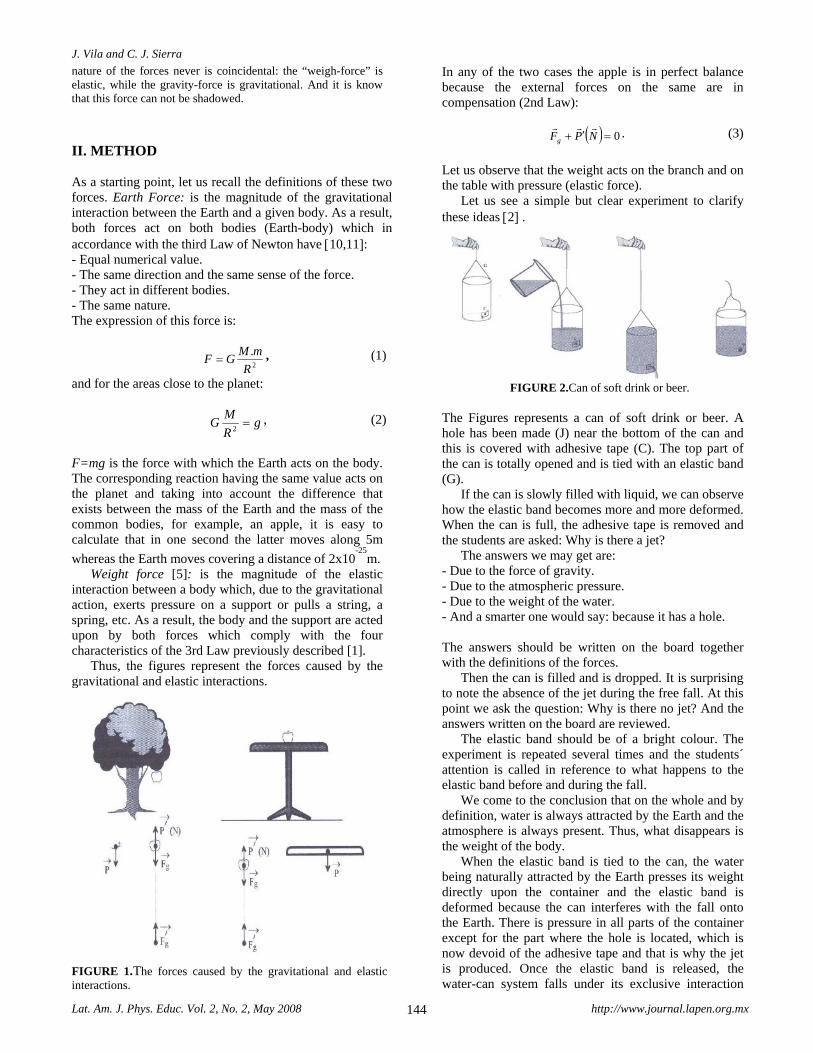
J. Vila and C. J. Sierra
Lat. Am. J. Phys. Educ. Vol. 2, No. 2, May 2008 144 http://www.journal.lapen.org.mx
nature of the forces never is coincidental: the “weigh-force” is elastic, while the gravity-force is gravitational. And it is know that this force can not be shadowed.
II. METHOD As a starting point, let us recall the definitions of these two forces. Earth Force: is the magnitude of the gravitational interaction between the Earth and a given body. As a result, both forces act on both bodies (Earth-body) which in accordance with the third Law of Newton have [10,11]: - Equal numerical value. - The same direction and the same sense of the force. - They act in different bodies. - The same nature. The expression of this force is:
2
.
R
mMGF = , (1)
and for the areas close to the planet:
gR
MG =
2, (2)
F=mg is the force with which the Earth acts on the body. The corresponding reaction having the same value acts on the planet and taking into account the difference that exists between the mass of the Earth and the mass of the common bodies, for example, an apple, it is easy to calculate that in one second the latter moves along 5m
whereas the Earth moves covering a distance of 2x10-25
m. Weight force [5]: is the magnitude of the elastic
interaction between a body which, due to the gravitational action, exerts pressure on a support or pulls a string, a spring, etc. As a result, the body and the support are acted upon by both forces which comply with the four characteristics of the 3rd Law previously described [1].
Thus, the figures represent the forces caused by the gravitational and elastic interactions.
FIGURE 1.The forces caused by the gravitational and elastic interactions.
In any of the two cases the apple is in perfect balance because the external forces on the same are in compensation (2nd Law):
( ) 0=′+ NPFg. (3)
Let us observe that the weight acts on the branch and on the table with pressure (elastic force).
Let us see a simple but clear experiment to clarify these ideas [2] .
FIGURE 2.Can of soft drink or beer.
The Figures represents a can of soft drink or beer. A hole has been made (J) near the bottom of the can and this is covered with adhesive tape (C). The top part of the can is totally opened and is tied with an elastic band (G).
If the can is slowly filled with liquid, we can observe how the elastic band becomes more and more deformed. When the can is full, the adhesive tape is removed and the students are asked: Why is there a jet?
The answers we may get are: - Due to the force of gravity. - Due to the atmospheric pressure. - Due to the weight of the water. - And a smarter one would say: because it has a hole. The answers should be written on the board together with the definitions of the forces.
Then the can is filled and is dropped. It is surprising to note the absence of the jet during the free fall. At this point we ask the question: Why is there no jet? And the answers written on the board are reviewed.
The elastic band should be of a bright colour. The experiment is repeated several times and the students´ attention is called in reference to what happens to the elastic band before and during the fall.
We come to the conclusion that on the whole and by definition, water is always attracted by the Earth and the atmosphere is always present. Thus, what disappears is the weight of the body.
When the elastic band is tied to the can, the water being naturally attracted by the Earth presses its weight directly upon the container and the elastic band is deformed because the can interferes with the fall onto the Earth. There is pressure in all parts of the container except for the part where the hole is located, which is now devoid of the adhesive tape and that is why the jet is produced. Once the elastic band is released, the water-can system falls under its exclusive interaction
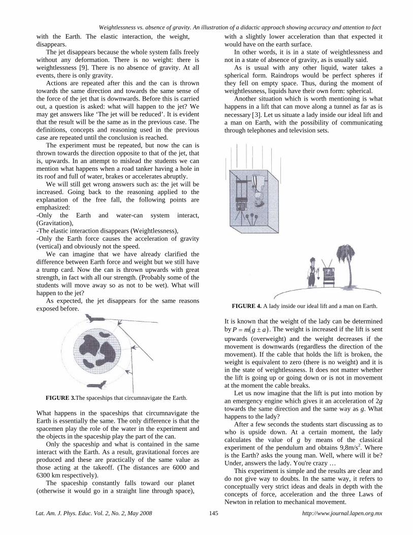
Weightlessness vs. absence of gravity. An illustration of a didactic approach showing accuracy and attention to fact
Lat. Am. J. Phys. Educ. Vol. 2, No. 2, May 2008 145 http://www.journal.lapen.org.mx
with the Earth. The elastic interaction, the weight, disappears.
The jet disappears because the whole system falls freely without any deformation. There is no weight: there is weightlessness [9]. There is no absence of gravity. At all events, there is only gravity.
Actions are repeated after this and the can is thrown towards the same direction and towards the same sense of the force of the jet that is downwards. Before this is carried out, a question is asked: what will happen to the jet? We may get answers like ‘The jet will be reduced’. It is evident that the result will be the same as in the previous case. The definitions, concepts and reasoning used in the previous case are repeated until the conclusion is reached.
The experiment must be repeated, but now the can is thrown towards the direction opposite to that of the jet, that is, upwards. In an attempt to mislead the students we can mention what happens when a road tanker having a hole in its roof and full of water, brakes or accelerates abruptly.
We will still get wrong answers such as: the jet will be increased. Going back to the reasoning applied to the explanation of the free fall, the following points are emphasized: -Only the Earth and water-can system interact, (Gravitation), -The elastic interaction disappears (Weightlessness), -Only the Earth force causes the acceleration of gravity (vertical) and obviously not the speed.
We can imagine that we have already clarified the difference between Earth force and weight but we still have a trump card. Now the can is thrown upwards with great strength, in fact with all our strength. (Probably some of the students will move away so as not to be wet). What will happen to the jet?
As expected, the jet disappears for the same reasons exposed before.
FIGURE 3.The spaceships that circumnavigate the Earth.
What happens in the spaceships that circumnavigate the Earth is essentially the same. The only difference is that the spacemen play the role of the water in the experiment and the objects in the spaceship play the part of the can.
Only the spaceship and what is contained in the same interact with the Earth. As a result, gravitational forces are produced and these are practically of the same value as those acting at the takeoff. (The distances are 6000 and 6300 km respectively).
The spaceship constantly falls toward our planet (otherwise it would go in a straight line through space),
with a slightly lower acceleration than that expected it would have on the earth surface.
In other words, it is in a state of weightlessness and not in a state of absence of gravity, as is usually said.
As is usual with any other liquid, water takes a spherical form. Raindrops would be perfect spheres if they fell on empty space. Thus, during the moment of weightlessness, liquids have their own form: spherical.
Another situation which is worth mentioning is what happens in a lift that can move along a tunnel as far as is necessary [3]. Let us situate a lady inside our ideal lift and a man on Earth, with the possibility of communicating through telephones and television sets.
FIGURE 4. A lady inside our ideal lift and a man on Earth.
It is known that the weight of the lady can be determined by ( )agmP ±= . The weight is increased if the lift is sent
upwards (overweight) and the weight decreases if the movement is downwards (regardless the direction of the movement). If the cable that holds the lift is broken, the weight is equivalent to zero (there is no weight) and it is in the state of weightlessness. It does not matter whether the lift is going up or going down or is not in movement at the moment the cable breaks.
Let us now imagine that the lift is put into motion by an emergency engine which gives it an acceleration of 2g towards the same direction and the same way as g. What happens to the lady?
After a few seconds the students start discussing as to who is upside down. At a certain moment, the lady calculates the value of g by means of the classical experiment of the pendulum and obtains 9,8m/s2. Where is the Earth? asks the young man. Well, where will it be? Under, answers the lady. You're crazy …
This experiment is simple and the results are clear and do not give way to doubts. In the same way, it refers to conceptually very strict ideas and deals in depth with the concepts of force, acceleration and the three Laws of Newton in relation to mechanical movement.
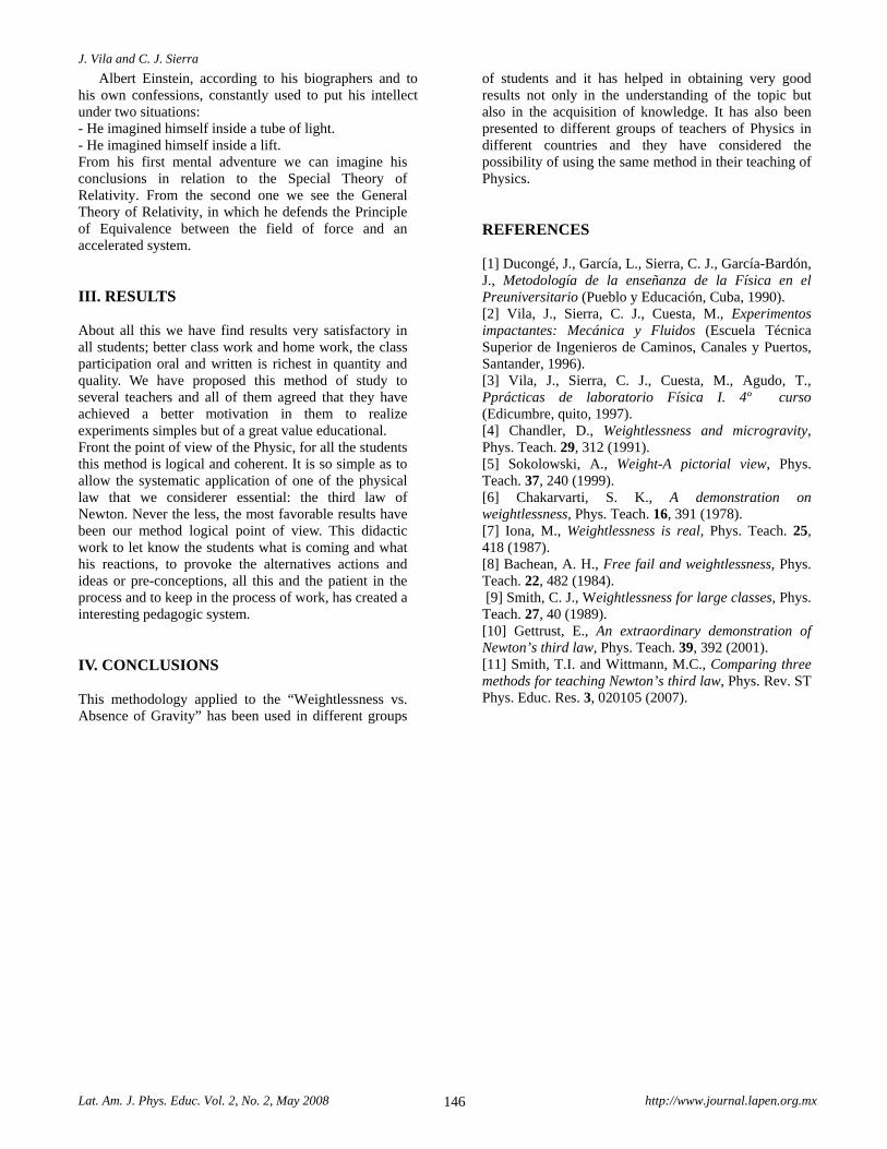
J. Vila and C. J. Sierra
Lat. Am. J. Phys. Educ. Vol. 2, No. 2, May 2008 146 http://www.journal.lapen.org.mx
Albert Einstein, according to his biographers and to his own confessions, constantly used to put his intellect under two situations: - He imagined himself inside a tube of light. - He imagined himself inside a lift. From his first mental adventure we can imagine his conclusions in relation to the Special Theory of Relativity. From the second one we see the General Theory of Relativity, in which he defends the Principle of Equivalence between the field of force and an accelerated system. III. RESULTS About all this we have find results very satisfactory in all students; better class work and home work, the class participation oral and written is richest in quantity and quality. We have proposed this method of study to several teachers and all of them agreed that they have achieved a better motivation in them to realize experiments simples but of a great value educational. Front the point of view of the Physic, for all the students this method is logical and coherent. It is so simple as to allow the systematic application of one of the physical law that we considerer essential: the third law of Newton. Never the less, the most favorable results have been our method logical point of view. This didactic work to let know the students what is coming and what his reactions, to provoke the alternatives actions and ideas or pre-conceptions, all this and the patient in the process and to keep in the process of work, has created a interesting pedagogic system. IV. CONCLUSIONS This methodology applied to the “Weightlessness vs. Absence of Gravity” has been used in different groups
of students and it has helped in obtaining very good results not only in the understanding of the topic but also in the acquisition of knowledge. It has also been presented to different groups of teachers of Physics in different countries and they have considered the possibility of using the same method in their teaching of Physics. REFERENCES [1] Ducongé, J., García, L., Sierra, C. J., García-Bardón, J., Metodología de la enseñanza de la Física en el Preuniversitario (Pueblo y Educación, Cuba, 1990). [2] Vila, J., Sierra, C. J., Cuesta, M., Experimentos impactantes: Mecánica y Fluidos (Escuela Técnica Superior de Ingenieros de Caminos, Canales y Puertos, Santander, 1996). [3] Vila, J., Sierra, C. J., Cuesta, M., Agudo, T., Pprácticas de laboratorio Física I. 4º curso (Edicumbre, quito, 1997). [4] Chandler, D., Weightlessness and microgravity, Phys. Teach. 29, 312 (1991). [5] Sokolowski, A., Weight-A pictorial view, Phys. Teach. 37, 240 (1999). [6] Chakarvarti, S. K., A demonstration on weightlessness, Phys. Teach. 16, 391 (1978). [7] Iona, M., Weightlessness is real, Phys. Teach. 25, 418 (1987). [8] Bachean, A. H., Free fail and weightlessness, Phys. Teach. 22, 482 (1984). [9] Smith, C. J., Weightlessness for large classes, Phys. Teach. 27, 40 (1989). [10] Gettrust, E., An extraordinary demonstration of Newton’s third law, Phys. Teach. 39, 392 (2001). [11] Smith, T.I. and Wittmann, M.C., Comparing three methods for teaching Newton’s third law, Phys. Rev. ST Phys. Educ. Res. 3, 020105 (2007).
Lat. Am. J. Phys. Educ. Vol. 2, No. 2, May 2008 147 http://www.journal.lapen.org.mx
¿Qué hace al buen maestro?: La visión del estudiante de ciencias físico matemáticas
Adrián Corona Cruz Facultad de Ciencias Físico Matemáticas, Benemérita Universidad Autónoma de Puebla, México.
E-mail: [email protected] (Recibido el 9 de Febrero de 2008; Aceptado el 30 Abril de 2008)
Resumen
Esta investigación se ha realizado con la finalidad de encontrar respuesta a la pregunta: ¿qué idea tienen los estudiantes del maestro? Se creyó importante saber cuál es la visión que los estudiantes tienen sobre un “buen maestro”, y, lo más importante, que la comunidad académica la reconozca. Para conocer el perfil que los estudiantes de la Facultad de Ciencias Físico Matemáticas (FCFM) de la Benemérita Universidad Autónoma de Puebla (BUAP) relacionan con un buen maestro, se aplicó una encuesta cualitativa y se analizó la opinión de 65 estudiantes que habían cursado por lo menos ocho materias en la facultad. Los resultados, en lo general, muestran las preferencias entre los aspectos académicos y sociales que los estudiantes tienen de quienes consideraron como buenos maestros. Éstos están en resonancia con los resultados reportados por estudios equivalentes. Palabras clave: Buen maestro, social, académico, docente, enseñanza.
Abstract This research was carried out with the aim to find out the answer to the question: what idea do students have about the teacher? It was believed important to know what was the vision which students have about a “good teacher” and, even the most important, to make the academic community recognize that vision. In order to know the profile which the students of the School of Physical and Mathematical Sciences of the Autonomous University of Puebla relate with a good teacher, a set of qualitative questions was applied and the views of 65 students, who have taken at least 8 courses at the School, were analyzed. In general, the results show the preferences between academic and social aspects which students have about those who they consider as good teachers. These results are in resonance with the results reported in other equivalent studies. Key words: Good teacher, social, academic, educational, teaching. PACS: 01.40.-d, 01.40.Jp, 01.50-i ISSN 1870-9095
I. INTRODUCCIÓN En la búsqueda de la respuesta a la pregunta: ¿Qué constituye la buena enseñanza? Traina [1] exploró las autobiografías de prominentes americanos (en las áreas sociales, económicas, geográficas, religiosas, etc.) de los siglos XIX y XX (125 casos); a la pregunta: ¿qué es lo que ellos citaron sobre los maestros que valoraron durante sus experiencias educativas? El resultado más notable fue la consistente descripción del buen y memorable maestro. Había fundamentalmente tres características que se describieron en un grado asombroso: a) la competencia en la materia, b) la preocupación profunda por los estudiantes y su éxito, y c) su carácter distintivo. Estos atributos eran evidentes sin tener en cuenta el nivel de educación o la materia que enseñaron [1].
Derivado de las experiencias durante su educación, los estudiantes consideran que hay un hueco entre la retórica y la práctica docente. Los buenos maestros, dicen ellos, cierran el hueco, pero el problema es que no hay suficientes buenos maestros [2].
A la práctica docente del maestro se han asociado diferentes tareas: La de instructor de conocimientos; facilitador (motivador, estimulador); mediador del proceso de aprendizaje; innovador en cuanto a estrategias y metodologías didácticas; consejero en el aula y fuera de ella; entre otros. Además, el maestro debe estar comprometido con su actualización y el desarrollo de sus habilidades. No obstante se encuentra que hay docentes que muestran inconsistencias pedagógicas, sociales y un bajo dominio en los conocimientos asociados a su labor docente. II. ¿QUÉ CARACTERIZA A UN BUEN MAESTRO? Al parecer es complicado intentar hacer un listado de conceptos y actitudes que caracterice al “buen maestro”, debido a la cantidad de variables implicadas; sin embargo, se puede “intentar” identificar las características que los propios estudiantes tienen de los que consideran actúan como “buenos maestros”. Podría pensarse que para los estudiantes, un buen maestro es quien enseña “bien”; que
Adrián Corona Cruz
Lat. Am. J. Phys. Educ. Vol. 2, No. 2, May 2008 148 http://www.journal.lapen.org.mx
una buena enseñanza se caracteriza por los valores del docente; una clase que siempre se desarrolla en el entero silencio se puede considerar que se debe a un buen maestro. Un maestro cuyos estudiantes logran en sus exámenes buenos resultados, podría verse como un buen maestro. El maestro que permite entrar y salir de la clase podría verse por algunos estudiantes como un buen maestro. Aquel maestro que realiza grandes y complejos desarrollos matemáticos, puede ser considerado un buen maestro. Ante esta variedad de valores y su subjetividad, ésta investigación tuvo como objetivo, cualificar o en su caso cuantificar al buen maestro, explorando las ideas de los estudiantes.
La pregunta ¿qué define al buen maestro?, se remonta a los años 30´s; se cuestionó a directores, maestros y estudiantes, para identificar las cualidades más importantes del buen maestro; se reportaron resultados de un estudio en que se pidió a estudiantes de primaria y secundaria que brevemente escribieran sobre 'el buen maestro' y 'el peor maestro'; se realizaron un conjunto de observaciones estructuradas para identificar factores asociados con la buena enseñanza [3]. Fundamentalmente se identificaron dos estilos contrastantes de enseñanza que denominaron como: directa e indirecta; a) la enseñanza directa se caracteriza por la confianza generada en el aula, su actitud crítica, autoridad y dirección; b) la indirecta se caracteriza por la confianza que genera al hacer preguntas, reconocer las ideas de los estudiantes, enaltecer y estimular, encontrando que los estudiantes de maestros indirectos aprenden más y tienen mejores actitudes hacia el aprendizaje que los estudiantes de maestros directos.
Rosenshine y Furst [3] identificaron cinco características del maestro eficaz consistentemente asociadas con los logros de los estudiantes; 1) el entusiasmo, 2) la instrucción metódica, 3) la claridad; la claridad-o la falta de ella, por ejemplo: aclarar preguntas de los estudiantes, la frecuencia con que los estudiantes responden a las preguntas del maestro sin que el maestro tenga que impartir información adicional, anular palabras vagas (algunos, muchos, por supuesto) durante la exposición, 4) la variedad en la enseñanza; característica que se refiere al uso de diferentes materiales instruccionales, pruebas variando el nivel cognoscitivo del discurso en el aula, 5) característica relacionada con las oportunidades a los estudiantes para aprender los contenidos, o la habilidad del maestro para realizar actividades normalmente enfocadas en los tipos de aprendizaje cognoscitivo.
Bob Kibble considera que los docentes calificados como buenos maestros, son aquellos que utilizan varias estrategias para lograr que los estudiantes en general los describan como aquellos que: _ “me escuchan”, _ “me hacen sentir importante”, _ “disponen de su tiempo para explicarme las cosas”, entre otros [4]. III. MARCO TEÓRICO Las acciones del docente en el aula, se analizan considerando los principios filosóficos y teóricas en las
que están basadas las nuevas formas educativas, "constructivismo" [5], caracterizado por la suposición "el conocimiento no se transmite directamente de uno a otro, se construye activamente por el estudiante" [6]. La base de éstas formas de enseñanza, para muchos, se toma de referencia la teoría de Piagetiana, (von Glasersfeld) [5], donde los estudiantes podrían asimilar sus nuevas experiencias en lo que ya saben, o podrían acomodar sus ideas para incorporar la nueva información. Otra base del constructivismo se debe al trabajo de L. S. Vygotsky [6]. La idea básica considera que el aprendizaje es un fenómeno socio-lingüístico, donde el discurso en el aula se vuelve un enfoque de mayor atención.
Además, se considera que los estudiantes llegan a las aulas con una variedad de puntos de vista y preconcepciones que ellos han adquirido tanto de los contextos socioculturales como en las aulas. Bajo este marco de referencia, los principios de la instrucción efectiva planteadas por Hennann Astleitner [7], en lo referente a la relación maestro-estudiante-aula sirven de marco para interpretar las ideas basadas en las experiencias que los estudiantes manifiestan a la pregunta, motivo de éste trabajo:
• Al estudiante se le debe dar la posibilidad para reflexionar sobre su aprendizaje, presentándole contenidos y tareas organizadas y claras, variando los métodos instruccionales, estableciendo un buen clima social-emocional entre los estudiantes y el maestro y una instrucción en la que los estudiantes y maestros tengan tiempo para pensar y hacer preguntas. • La instrucción motiva a los estudiantes si la atención se despierta, la relevancia de los contenidos se muestra, la confianza en sí mismo se fortalece, y la satisfacción con los resultados de aprendizaje se logra. Respeto a la emoción, la instrucción debe disminuir los sentimientos negativos (sobre todo el miedo, envidia, y enojo) y debe aumentar los sentimientos positivos (sobre toda la simpatía y placer). • La instrucción y el logro en la evaluación son especialmente efectivos, cuando ayudan al estudiante a encontrar y aumentar sus fortalezas personales y, los direcciona para superar sus debilidades personales. Además, el logro en la instrucción y evaluación deben ser basadas en el individuo. • El interés como motivación a una cierta materia, puede estimularse por métodos instruccionales diferentes. Los estudiantes encuentran el interés cuando ellos piensan que son parte importante de un desarrollo o un grupo. El interés también puede aumentarse cuando los estudiantes experimentan la competencia (basado en el éxito) • La simpatía y alegría representan sentimientos positivos de los estudiantes. Las relaciones entre ellos, se logra instalando interacciones sensibles, estableciendo estructuras de aprendizaje cooperativas, estableciendo oportunidades de aprendizaje abiertas, etc. • El temor, envidia, y enojo son sentimientos negativos que a menudo ocurren durante la instrucción; aceptar los errores como oportunidades para aprendizaje; inducir la relajación en el aula; ser crítico pero sostener
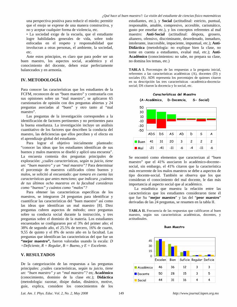
¿Qué hace al buen maestro?: La visión del estudiante de ciencias físico matemáticas
Lat. Am. J. Phys. Educ. Vol. 2, No. 2, May 2008 149 http://www.journal.lapen.org.mx
una perspectiva positiva para reducir el miedo; permitir que el enojo se exprese de una manera constructiva, y no y aceptar cualquier forma de violencia, etc. • La sociedad exige de la escuela, que el estudiante logre habilidades generales de vida, sobre todo enfocadas en el respeto y responsabilidad que involucran a otras personas, el ambiente, la sociedad, etc. Ante estos principios, es claro que para poder ser un
buen maestro, los aspectos social, académico y el conocimiento del docente, deben estar perfectamente balanceados y en armonía. IV. METODOLOGÍA Para conocer las características que los estudiantes de la FCFM, reconocen de un “buen maestro” y contrastarla con sus opiniones sobre un “mal maestro”, se aplicaron 65 cuestionarios de opinión con dos preguntas abiertas y 24 preguntas asociadas al “buen” y otro tanto al “mal maestro”.
Las preguntas de la investigación corresponden a la identificación de factores pertinentes y no pertinentes para la buena enseñanza. La investigación incluye un análisis cuantitativo de los factores que describen la conducta del maestro, las deficiencias que ellos perciben y el efecto en el aprendizaje global del estudiante.
Para lograr el objetivo inicialmente planteado: “conocer las ideas que los estudiantes identifican de sus buenos y malos maestros se diseñó y aplicó una encuesta”. La encuesta contenía dos preguntas principales de exploración: ¿cuáles características, según tu juicio, tiene un: “buen maestro” y un “mal maestro”? Para determinar el porcentaje de maestros calificados cómo buenos y malos, se solicitó al encuestado: que tomara en cuenta las características que antes menciono; que indicara ¿cuántos de tus últimos ocho maestros en la facultad consideras como “buenos” y cuántos como “malos”?
Para obtener las características específicas de los maestros, se integraron 24 preguntas para identificar y cuantificar las características del "buen maestro" así como las ideas que identifican un mal maestro [8]. Diez preguntas cubren aspectos de método; once preguntas sobre su conducta social durante la instrucción, y tres preguntas sobre el dominio de la materia. Los estudiantes encuestados se configuraron por el 3% del primer año; el 38% de segundo año, el 25.5% de tercero, 16% de cuarto, 9,55 de quinto y el 8% de sexto año en la facultad. Las preguntas que identifican las características del que fue un “mejor maestro”, fueron valoradas usando la escala: D =Deficiente, R = Regular, B = Bueno, y E = Excelente. V. RESULTADOS De la categorización de las respuestas a las preguntas principales: ¿cuáles características, según tu juicio, tiene un: “buen maestro” y un “mal maestro”? en; Académico (conocimiento, dominio de la clase etc.); Didáctica (metodología: razonar, disipe dudas, dinámico, motive, guíe, explica, considere los conocimientos de los
estudiantes, etc.), y Social (actitudinal: estricto, puntual, responsable, amable, compresivo, accesible, carismático, gusto por enseñar etc.), y los conceptos referentes al mal maestro: Anti-Social (actitudinal: déspota, grosero, altanero, ofensivo, discriminante, desordenado, inmaduro, intolerante, inaccesible, impaciente, impuntual, etc.); Anti-Didáctica (metodología: no explique bien la clase, no tome en cuenta a estudiantes, evalué mal, etc.); Anti-Académico (conocimientos: no sabe, no prepara su clase, no domina los temas, etc.) TABLA I. Porcentajes de las respuestas a la pregunta inicial, referentes a las características académicas (A), docentes (D) y sociales (S). ADS representa los porcentajes de quienes citaron en su descripción las tres características –académica-docencia-social; DS citaron la docencia y lo social, etc.
Características del Maestro(A-Académico, D-Docencia, S- Social)
-50-30-10103050
Buen 41 31 20 3 2 2 2
Mal -21 -41 -11 -6 -4 -11 -6
ADS DS AS AD D S A
Se encontró como elementos que caracterizan al “buen maestro” que el 41% asociaron lo académico-docente–social, sin embargo, el 41% citaron que la característica más recurrente de los malos maestros se debe a aspectos de tipo docente-social. También se observa que los que consideran el conocimiento del mal docente, le dan más importancia al aspecto social que al académico.
La estadística que muestra la relación entre las características que los estudiantes consideraron tiene él que fue Su “mejor maestro” y las del “peor maestro” derivadas de las 24 preguntas, se resumen en la tabla II.
TABLA II. Frecuencia de las respuestas que calificaron al buen maestro, según sus características académicas, docentes, y actitudinales.
Buen Maestro
0
1530
45
Académico 46 36 12 3 3
Docente 50 28 15 3 5
Social 44 31 16 4 4
Excelen Bien Suficie Regular Deficie
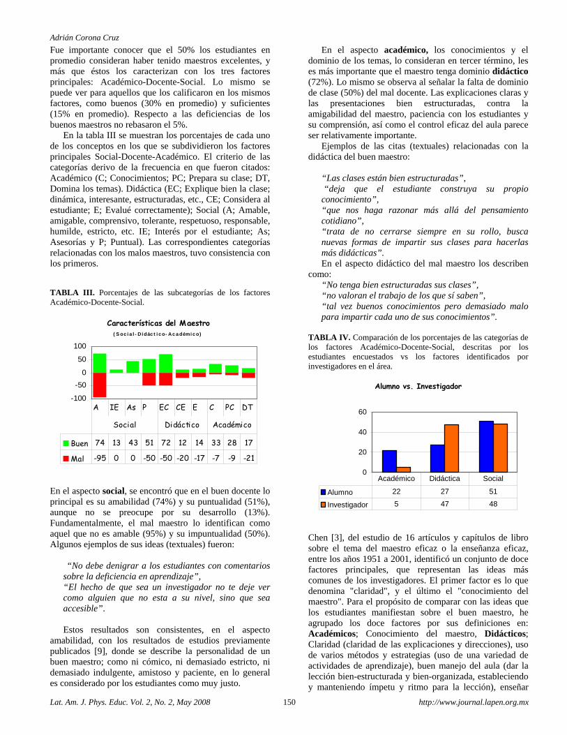
Adrián Corona Cruz
Lat. Am. J. Phys. Educ. Vol. 2, No. 2, May 2008 150 http://www.journal.lapen.org.mx
Fue importante conocer que el 50% los estudiantes en promedio consideran haber tenido maestros excelentes, y más que éstos los caracterizan con los tres factores principales: Académico-Docente-Social. Lo mismo se puede ver para aquellos que los calificaron en los mismos factores, como buenos (30% en promedio) y suficientes (15% en promedio). Respecto a las deficiencias de los buenos maestros no rebasaron el 5%.
En la tabla III se muestran los porcentajes de cada uno de los conceptos en los que se subdividieron los factores principales Social-Docente-Académico. El criterio de las categorías derivo de la frecuencia en que fueron citados: Académico (C; Conocimientos; PC; Prepara su clase; DT, Domina los temas). Didáctica (EC; Explique bien la clase; dinámica, interesante, estructuradas, etc., CE; Considera al estudiante; E; Evalué correctamente); Social (A; Amable, amigable, comprensivo, tolerante, respetuoso, responsable, humilde, estricto, etc. IE; Interés por el estudiante; As; Asesorías y P; Puntual). Las correspondientes categorías relacionadas con los malos maestros, tuvo consistencia con los primeros. TABLA III. Porcentajes de las subcategorías de los factores Académico-Docente-Social.
Características del Maestro( S oc i a l - D i dác t i c o- Ac a démi c o)
-100
-500
50
100
Buen 74 13 43 51 72 12 14 33 28 17
Mal -95 0 0 -50 -50 -20 -17 -7 -9 -21
A IE As P EC CE E C PC DT
Social Didáctico Académico
En el aspecto social, se encontró que en el buen docente lo principal es su amabilidad (74%) y su puntualidad (51%), aunque no se preocupe por su desarrollo (13%). Fundamentalmente, el mal maestro lo identifican como aquel que no es amable (95%) y su impuntualidad (50%). Algunos ejemplos de sus ideas (textuales) fueron:
“No debe denigrar a los estudiantes con comentarios
sobre la deficiencia en aprendizaje”, “El hecho de que sea un investigador no te deje ver como alguien que no esta a su nivel, sino que sea accesible”. Estos resultados son consistentes, en el aspecto
amabilidad, con los resultados de estudios previamente publicados [9], donde se describe la personalidad de un buen maestro; como ni cómico, ni demasiado estricto, ni demasiado indulgente, amistoso y paciente, en lo general es considerado por los estudiantes como muy justo.
En el aspecto académico, los conocimientos y el dominio de los temas, lo consideran en tercer término, les es más importante que el maestro tenga dominio didáctico (72%). Lo mismo se observa al señalar la falta de dominio de clase (50%) del mal docente. Las explicaciones claras y las presentaciones bien estructuradas, contra la amigabilidad del maestro, paciencia con los estudiantes y su comprensión, así como el control eficaz del aula parece ser relativamente importante.
Ejemplos de las citas (textuales) relacionadas con la didáctica del buen maestro:
“Las clases están bien estructuradas”, “deja que el estudiante construya su propio conocimiento”, “que nos haga razonar más allá del pensamiento cotidiano”, “trata de no cerrarse siempre en su rollo, busca nuevas formas de impartir sus clases para hacerlas más didácticas”. En el aspecto didáctico del mal maestro los describen
como: “No tenga bien estructuradas sus clases”, “no valoran el trabajo de los que sí saben”, “tal vez buenos conocimientos pero demasiado malo para impartir cada uno de sus conocimientos”.
TABLA IV. Comparación de los porcentajes de las categorías de los factores Académico-Docente-Social, descritas por los estudiantes encuestados vs los factores identificados por investigadores en el área.
Alumno vs. Investigador
0
20
40
60
Alumno 22 27 51
Investigador 5 47 48
Académico Didáctica Social
Chen [3], del estudio de 16 artículos y capítulos de libro sobre el tema del maestro eficaz o la enseñanza eficaz, entre los años 1951 a 2001, identificó un conjunto de doce factores principales, que representan las ideas más comunes de los investigadores. El primer factor es lo que denomina "claridad", y el último el "conocimiento del maestro". Para el propósito de comparar con las ideas que los estudiantes manifiestan sobre el buen maestro, he agrupado los doce factores por sus definiciones en: Académicos; Conocimiento del maestro, Didácticos; Claridad (claridad de las explicaciones y direcciones), uso de varios métodos y estrategias (uso de una variedad de actividades de aprendizaje), buen manejo del aula (dar la lección bien-estructurada y bien-organizada, estableciendo y manteniendo ímpetu y ritmo para la lección), enseñar
¿Qué hace al buen maestro?: La visión del estudiante de ciencias físico matemáticas
Lat. Am. J. Phys. Educ. Vol. 2, No. 2, May 2008 151 http://www.journal.lapen.org.mx
para entender (alentando la participación del estudiante y consiguiendo involucrar a todos los estudiantes), y Social; dejar tarea, buena personalidad, buena atmósfera de clase, que inspire y cree interés por el estudiante, alta expectativa, entusiasmo. En la tabla IV, se muestran los porcentajes de ideas asociadas a los estudiantes, comparadas con los porcentajes de factores citados en los trabajos considerados por Chen [3].
Aparte de encontrar acuerdo sobre el comportamiento social del docente, es trascendente identificar que mientras los investigadores sobre la enseñanza eficaz consideran la didáctica como importante (47%), para los estudiantes es más relevante que el docente conozca su materia (22%).
IV CONCLUSIONES Las ideas que los estudiantes de la Facultad de Ciencias Físico Matemáticas (FCFM) de la Benemérita Universidad Autónoma de Puebla (BUAP) tienen de lo que consideran un buen maestro, fundamentalmente se basa en sus habilidades académicas, docentes y sociales y lo cumplen el 65% de la planta académica. Este resultado es del orden del reportado de una universidad pública (60%) con una población encuestada de mil doscientos estudiantes, donde se hace la comparación con lo que piensan estudiantes de una universidad privada (42%), aunque en su interpretación se considera que el porcentaje puede estar afectado por la falta de libertad al contestar la encuesta [10].
Respecto a las características principales de los maestros considerados como malos (35%) fue su actitud y puntualidad. Considerados los resultados reportados [2, 8, 10] no sorprendió su gran correlación Mi conclusión, la hago coincidir con la idea de Kibble [4]; las características de la buena enseñanza es equivalente al concepto de buen maestro; se basa en las calidad humana: la habilidad para escuchar, ser humilde aceptando que se aprende de los estudiantes, la capacidad para crear un ambiente social que activa el pensamiento y su comunicando y finalmente reconocer que todo lo que pasa en el aula, es el trabajo de aprendices aprendiendo y maestros sólo apoyando. También, espero que los resultados del presente documento, sean un indicador de lo que debemos optimizar y lo que debemos corregir en nuestra labor docente de nuestra facultad.
REFERENCIAS [1] Canestrari, A. S., & Marlowe, B. A., Educational foundations: An anthology of critical readings. Thousand Oaks, CA: Sage. http://www.sagepub.com/upmdata/6057_Chapter_4_Marlowe_I_Proof_2.pdf, (2004). [2] Malcolm S., What makes a ‘Good Teacher’?: The Views of Boys, A conference paper presented at Challenging Futures? Changing Agendas in Teacher Education, University of New England Armidale NSW (2002). [3] Xiaoduan Ch., Characteristics of Effective Teaching and Reform of Teacher Education: Some Considerations Based on Literature Survey. College of Educational Science, Shaanxi Normal University, Xi’an, Shaanxi, P. R. China. , http://k1.ioe.ac.uk/May2006/Papers/XiaoduanChen%20_Paper.doc, (2006). [4] Kibble, B., What makes a good teacher, Phys. Educ. 38, 340-342 (2003). [5] von Glasersfeld, E., Cognition, construction of knowledge, and teaching, Synthese, Springer Netherlands, 80, 121-140 (1989). [6] Driver, R., Asako, H., Leach, J., Mortimer, E. & Scott, P., Constructing scientific knowledge in the classroom, Educational Researcher, 23, 5-12 (1994). [7] Hermann A., Principles of Effective Instruction - General Standards for Teachers and Instructional Designers, Journal of Instructional Psychology, 32 3-8 (2005). [8] Loveland, K. A., Student Evaluation of Teaching (SET) in Web-based Classes: Preliminary Findings and a Call for Further Research, The Journal of Educators Online, 4, 1-18 (2007). [9] Bettina G-F. & Alois G., Students' Evaluation of Teachers and Instructional Quality – Analysis of Relevant Factors Based on Empirical Evaluation Research, Assessment & Evaluation in Higher Education, 28, 229–238 (2003). [10] Esquivias M. y González A., Estudio de Universidades Mexicanas sobre el Perfil Docente. 4º Congreso Internacional, Docencia Universitaria e innovación, Barcelona España, http://eprints.upc.es/cidui_2006/pujades/comunicaciones_completas/doc151.doc, (2006).
Lat. Am. J. Phys. Educ. Vol. 2, No. 2, May 2008 152 http://www.journal.lapen.org.mx
A brief history of the mathematical equivalence between the two quantum mechanics
Carlos M. Madrid Casado1, 2 1Departamento de Matemáticas, IES Lázaro Cárdenas, Collado Villalba, Madrid, España. 2Departamento de Lógica y Filosofía de la Ciencia, Facultad de Filosofía, Universidad Complutense, Madrid, España.
E-mail: [email protected] (Received 29 December 2007; aceppted 4 March 2008)
Abstract The aim of this paper is to give a brief account of the development of the mathematical equivalence of quantum mechanics. In order to deal with atomic systems, Heisenberg developed matrix mechanics in 1925. Some time later, in the winter of 1926, Schrödinger established his wave mechanics. In the spring of 1926, quantum physicists had two theoretical models that allowed them to predict the same behaviour of the quantum systems, but both of them were very different. Schrödinger thought that the empirical equivalence could be explained by means of a proof of mathematical equivalence. Keywords: Matrix mechanics, wave mechanics, mathematical equivalence.
Resumen El objetivo de este artículo es ofrecer una breve reseña del desarrollo de la equivalencia matemática de las mecánicas cuánticas. Para tratar con los sistemas atómicos, Heisenberg desarrolló la mecánica matricial en 1925. Algún tiempo después, en el invierno de 1926, Schrödinger estableció su mecánica ondulatoria. En la primavera de 1926, los físicos cuánticos disponían de dos modelos teóricos que les permitían predecir el mismo comportamiento de los sistemas cuánticos, pero ambos eran muy diferentes. Schrödinger pensó que la equivalencia empírica podría ser explicada mediante una prueba de equivalencia matemática. Palabras clave: Mecánica matricial, mecánica ondulatoria, equivalencia matemática. PACS: 01.65.+g, 01.70.+w, 03.65.Ca. ISSN 1870-9095
I. INTRODUCTION Quantum physics grew out from attempts to understand the strange behaviour of atomic systems, which were capable of assuming discrete energy changes only. The heroic origin of quantum theory dates from December 14th, 1900. The dramatis personae of the prehistory of quantum theory (1900-1924) includes the names of Max Planck, Albert Einstein or Niels Bohr. However, old quantum physics was a bridge over troubled waters: each problem had to be solved first within the classical physics realm, and only then the solution could be translated –by means of diverse computation rules (for instance: the Correspondence Principle of Bohr)– into a meaningful statement in quantum physics. These rules revealed a dismaying state of affairs in 1924. In words of Bohr, Kramers & Slater [1]:
“At the present state of science it does not seem possible to avoid the formal character of the quantum theory which is shown by the fact that the interpretation of atomic phenomena does not involve a description of
the mechanism of the discontinuous processes, which in the quantum theory of spectra are designated as transitions between stationary states of the atom.”
Quantum physicists became more and more convinced that a radical change on the foundations of physics was necessary, that is to say: a new kind of mechanics which they called quantum mechanics. II. MATRIX MECHANICS In 1925 Werner Heisenberg developed matrix mechanics (MM) in his paper Über quantentheoretische Umdeutung kinematischer und mechanischer Beziehungen [2], although he did not even know what a matrix was, as Max Born and Pascual Jordan pointed out.
Heisenberg aimed at constructing a quantum-mechanical formalism corresponding as closely as possible to that of classical mechanics. Thus he considered the classical equation of motion
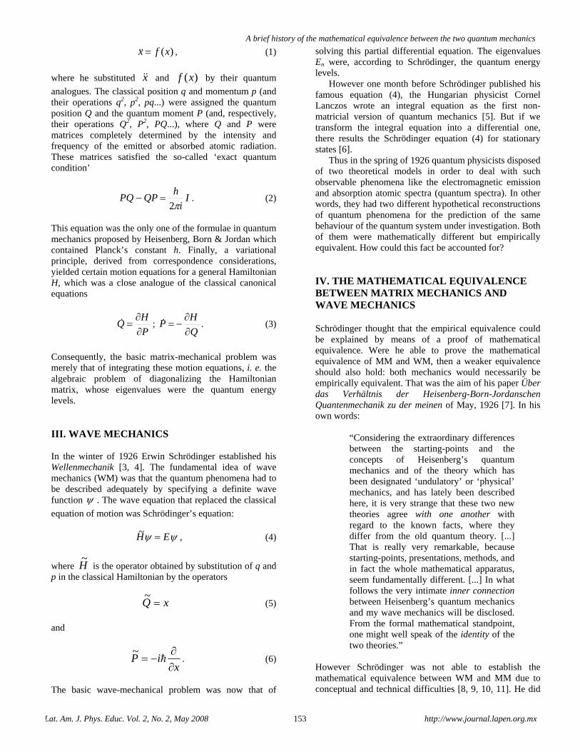
A brief history of the mathematical equivalence between the two quantum mechanics
Lat. Am. J. Phys. Educ. Vol. 2, No. 2, May 2008 153 http://www.journal.lapen.org.mx
)(xfx = , (1)
where he substituted x and )(xf by their quantum
analogues. The classical position q and momentum p (and their operations q2, p2, pq...) were assigned the quantum position Q and the quantum moment P (and, respectively, their operations Q2, P2, PQ...), where Q and P were matrices completely determined by the intensity and frequency of the emitted or absorbed atomic radiation. These matrices satisfied the so-called ‘exact quantum condition’
Ii
hQPPQ
π2=− . (2)
This equation was the only one of the formulae in quantum mechanics proposed by Heisenberg, Born & Jordan which contained Planck’s constant h. Finally, a variational principle, derived from correspondence considerations, yielded certain motion equations for a general Hamiltonian H, which was a close analogue of the classical canonical equations
P
HQ
∂∂
= ; Q
HP
∂∂
−= . (3)
Consequently, the basic matrix-mechanical problem was merely that of integrating these motion equations, i. e. the algebraic problem of diagonalizing the Hamiltonian matrix, whose eigenvalues were the quantum energy levels.
III. WAVE MECHANICS In the winter of 1926 Erwin Schrödinger established his Wellenmechanik [3, 4]. The fundamental idea of wave mechanics (WM) was that the quantum phenomena had to be described adequately by specifying a definite wave function ψ . The wave equation that replaced the classical
equation of motion was Schrödinger’s equation:
ψψ EH =~ , (4)
where H~
is the operator obtained by substitution of q and p in the classical Hamiltonian by the operators
xQ =~
(5)
and
x
iP∂∂
−=~
. (6)
The basic wave-mechanical problem was now that of
solving this partial differential equation. The eigenvalues En were, according to Schrödinger, the quantum energy levels.
However one month before Schrödinger published his famous equation (4), the Hungarian physicist Cornel Lanczos wrote an integral equation as the first non-matricial version of quantum mechanics [5]. But if we transform the integral equation into a differential one, there results the Schrödinger equation (4) for stationary states [6].
Thus in the spring of 1926 quantum physicists disposed of two theoretical models in order to deal with such observable phenomena like the electromagnetic emission and absorption atomic spectra (quantum spectra). In other words, they had two different hypothetical reconstructions of quantum phenomena for the prediction of the same behaviour of the quantum system under investigation. Both of them were mathematically different but empirically equivalent. How could this fact be accounted for?
IV. THE MATHEMATICAL EQUIVALENCE BETWEEN MATRIX MECHANICS AND WAVE MECHANICS Schrödinger thought that the empirical equivalence could be explained by means of a proof of mathematical equivalence. Were he able to prove the mathematical equivalence of MM and WM, then a weaker equivalence should also hold: both mechanics would necessarily be empirically equivalent. That was the aim of his paper Über das Verhältnis der Heisenberg-Born-Jordanschen Quantenmechanik zu der meinen of May, 1926 [7]. In his own words:
“Considering the extraordinary differences between the starting-points and the concepts of Heisenberg’s quantum mechanics and of the theory which has been designated ‘undulatory’ or ‘physical’ mechanics, and has lately been described here, it is very strange that these two new theories agree with one another with regard to the known facts, where they differ from the old quantum theory. [...] That is really very remarkable, because starting-points, presentations, methods, and in fact the whole mathematical apparatus, seem fundamentally different. [...] In what follows the very intimate inner connection between Heisenberg’s quantum mechanics and my wave mechanics will be disclosed. From the formal mathematical standpoint, one might well speak of the identity of the two theories.”
However Schrödinger was not able to establish the mathematical equivalence between WM and MM due to conceptual and technical difficulties [8, 9, 10, 11]. He did
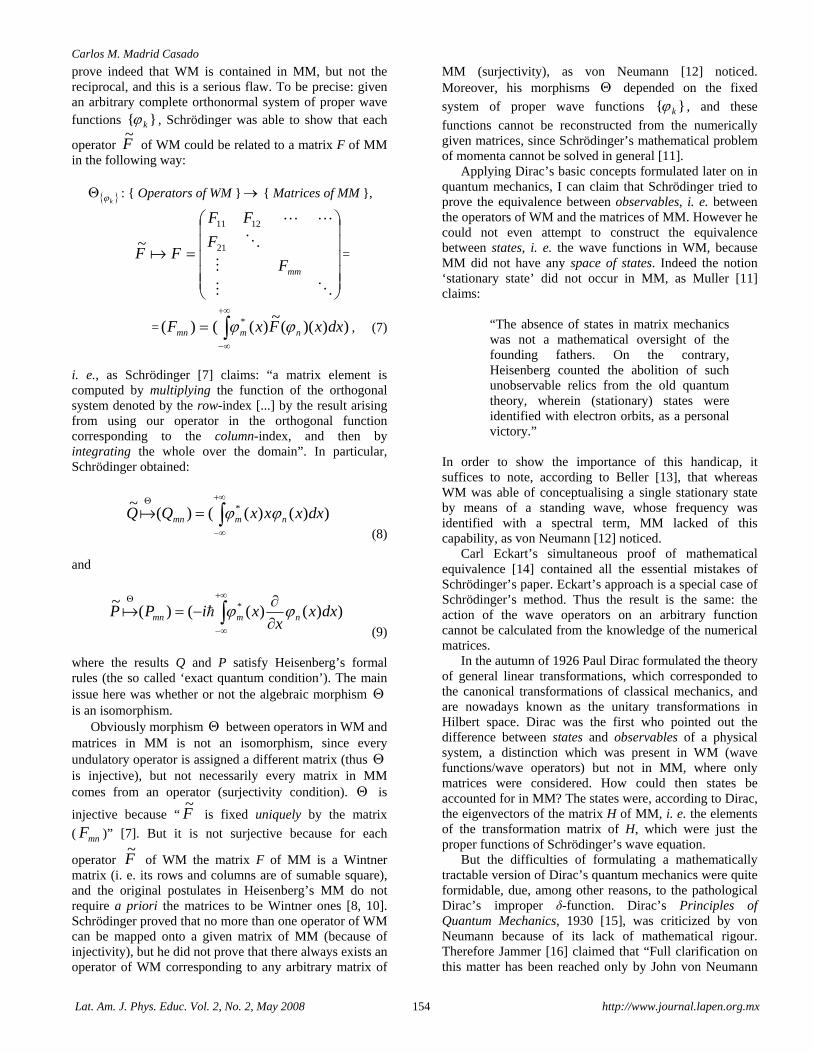
Carlos M. Madrid Casado
Lat. Am. J. Phys. Educ. Vol. 2, No. 2, May 2008 154 http://www.journal.lapen.org.mx
prove indeed that WM is contained in MM, but not the reciprocal, and this is a serious flaw. To be precise: given an arbitrary complete orthonormal system of proper wave functions }{ kϕ , Schrödinger was able to show that each
operator F~
of WM could be related to a matrix F of MM in the following way:
{ }kϕΘ : { Operators of WM }→ { Matrices of MM },
⎟⎟⎟⎟⎟
⎠
⎞
⎜⎜⎜⎜⎜
⎝
⎛
=mmF
F
FF
FF 21
1211
~=
= )))((~
)(()( *∫+∞
∞−
= dxxFxF nmmn ϕϕ , (7)
i. e., as Schrödinger [7] claims: “a matrix element is computed by multiplying the function of the orthogonal system denoted by the row-index [...] by the result arising from using our operator in the orthogonal function corresponding to the column-index, and then by integrating the whole over the domain”. In particular, Schrödinger obtained:
))()(()(~ *∫
+∞
∞−
Θ
= dxxxxQQ nmmn ϕϕ (8)
and
))()(()(~ *∫
+∞
∞−
Θ
∂∂
−= dxxx
xiPP nmmn ϕϕ (9)
where the results Q and P satisfy Heisenberg’s formal rules (the so called ‘exact quantum condition’). The main issue here was whether or not the algebraic morphism Θ is an isomorphism.
Obviously morphism Θ between operators in WM and matrices in MM is not an isomorphism, since every undulatory operator is assigned a different matrix (thus Θ is injective), but not necessarily every matrix in MM comes from an operator (surjectivity condition). Θ is
injective because “ F~
is fixed uniquely by the matrix
( mnF )” [7]. But it is not surjective because for each
operator F~
of WM the matrix F of MM is a Wintner matrix (i. e. its rows and columns are of sumable square), and the original postulates in Heisenberg’s MM do not require a priori the matrices to be Wintner ones [8, 10]. Schrödinger proved that no more than one operator of WM can be mapped onto a given matrix of MM (because of injectivity), but he did not prove that there always exists an operator of WM corresponding to any arbitrary matrix of
MM (surjectivity), as von Neumann [12] noticed. Moreover, his morphisms Θ depended on the fixed
system of proper wave functions }{ kϕ , and these
functions cannot be reconstructed from the numerically given matrices, since Schrödinger’s mathematical problem of momenta cannot be solved in general [11].
Applying Dirac’s basic concepts formulated later on in quantum mechanics, I can claim that Schrödinger tried to prove the equivalence between observables, i. e. between the operators of WM and the matrices of MM. However he could not even attempt to construct the equivalence between states, i. e. the wave functions in WM, because MM did not have any space of states. Indeed the notion ‘stationary state’ did not occur in MM, as Muller [11] claims:
“The absence of states in matrix mechanics was not a mathematical oversight of the founding fathers. On the contrary, Heisenberg counted the abolition of such unobservable relics from the old quantum theory, wherein (stationary) states were identified with electron orbits, as a personal victory.”
In order to show the importance of this handicap, it suffices to note, according to Beller [13], that whereas WM was able of conceptualising a single stationary state by means of a standing wave, whose frequency was identified with a spectral term, MM lacked of this capability, as von Neumann [12] noticed.
Carl Eckart’s simultaneous proof of mathematical equivalence [14] contained all the essential mistakes of Schrödinger’s paper. Eckart’s approach is a special case of Schrödinger’s method. Thus the result is the same: the action of the wave operators on an arbitrary function cannot be calculated from the knowledge of the numerical matrices.
In the autumn of 1926 Paul Dirac formulated the theory of general linear transformations, which corresponded to the canonical transformations of classical mechanics, and are nowadays known as the unitary transformations in Hilbert space. Dirac was the first who pointed out the difference between states and observables of a physical system, a distinction which was present in WM (wave functions/wave operators) but not in MM, where only matrices were considered. How could then states be accounted for in MM? The states were, according to Dirac, the eigenvectors of the matrix H of MM, i. e. the elements of the transformation matrix of H, which were just the proper functions of Schrödinger’s wave equation.
But the difficulties of formulating a mathematically tractable version of Dirac’s quantum mechanics were quite formidable, due, among other reasons, to the pathological Dirac’s improper δ-function. Dirac’s Principles of Quantum Mechanics, 1930 [15], was criticized by von Neumann because of its lack of mathematical rigour. Therefore Jammer [16] claimed that “Full clarification on this matter has been reached only by John von Neumann
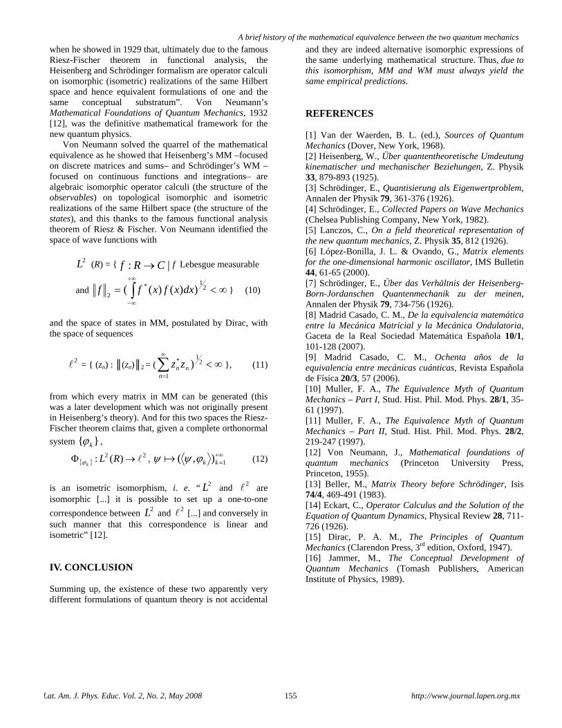
A brief history of the mathematical equivalence between the two quantum mechanics
Lat. Am. J. Phys. Educ. Vol. 2, No. 2, May 2008 155 http://www.journal.lapen.org.mx
when he showed in 1929 that, ultimately due to the famous Riesz-Fischer theorem in functional analysis, the Heisenberg and Schrödinger formalism are operator calculi on isomorphic (isometric) realizations of the same Hilbert space and hence equivalent formulations of one and the same conceptual substratum”. Von Neumann’s Mathematical Foundations of Quantum Mechanics, 1932 [12], was the definitive mathematical framework for the new quantum physics.
Von Neumann solved the quarrel of the mathematical equivalence as he showed that Heisenberg’s MM –focused on discrete matrices and sums– and Schrödinger’s WM –focused on continuous functions and integrations– are algebraic isomorphic operator calculi (the structure of the observables) on topological isomorphic and isometric realizations of the same Hilbert space (the structure of the states), and this thanks to the famous functional analysis theorem of Riesz & Fischer. Von Neumann identified the space of wave functions with
2L (R) = { |: CRf → f Lebesgue measurable
and ∫+∞
∞−
∞<= 21*
2))()(( dxxfxff } (10)
and the space of states in MM, postulated by Dirac, with the space of sequences
2 = { (zn) : ║(zn)║2 = ( 21
1
* )∑∞
=nnn zz ∞< }, (11)
from which every matrix in MM can be generated (this was a later development which was not originally present in Heisenberg’s theory). And for this two spaces the Riesz-Fischer theorem claims that, given a complete orthonormal
system }{ kϕ ,
{ }22 )(: →Φ RL
kϕ, +∞
=1),( kkϕψψ (12)
is an isometric isomorphism, i. e. “ 2L and 2 are isomorphic [...] it is possible to set up a one-to-one
correspondence between 2L and 2 [...] and conversely in such manner that this correspondence is linear and isometric” [12]. IV. CONCLUSION
Summing up, the existence of these two apparently very different formulations of quantum theory is not accidental
and they are indeed alternative isomorphic expressions of the same underlying mathematical structure. Thus, due to this isomorphism, MM and WM must always yield the same empirical predictions. REFERENCES [1] Van der Waerden, B. L. (ed.), Sources of Quantum Mechanics (Dover, New York, 1968). [2] Heisenberg, W., Über quantentheoretische Umdeutung kinematischer und mechanischer Beziehungen, Z. Physik 33, 879-893 (1925). [3] Schrödinger, E., Quantisierung als Eigenwertproblem, Annalen der Physik 79, 361-376 (1926). [4] Schrödinger, E., Collected Papers on Wave Mechanics (Chelsea Publishing Company, New York, 1982). [5] Lanczos, C., On a field theoretical representation of the new quantum mechanics, Z. Physik 35, 812 (1926). [6] López-Bonilla, J. L. & Ovando, G., Matrix elements for the one-dimensional harmonic oscillator, IMS Bulletin 44, 61-65 (2000). [7] Schrödinger, E., Über das Verhältnis der Heisenberg-Born-Jordanschen Quantenmechanik zu der meinen, Annalen der Physik 79, 734-756 (1926). [8] Madrid Casado, C. M., De la equivalencia matemática entre la Mecánica Matricial y la Mecánica Ondulatoria, Gaceta de la Real Sociedad Matemática Española 10/1, 101-128 (2007). [9] Madrid Casado, C. M., Ochenta años de la equivalencia entre mecánicas cuánticas, Revista Española de Física 20/3, 57 (2006). [10] Muller, F. A., The Equivalence Myth of Quantum Mechanics – Part I, Stud. Hist. Phil. Mod. Phys. 28/1, 35-61 (1997). [11] Muller, F. A., The Equivalence Myth of Quantum Mechanics – Part II, Stud. Hist. Phil. Mod. Phys. 28/2, 219-247 (1997). [12] Von Neumann, J., Mathematical foundations of quantum mechanics (Princeton University Press, Princeton, 1955). [13] Beller, M., Matrix Theory before Schrödinger, Isis 74/4, 469-491 (1983). [14] Eckart, C., Operator Calculus and the Solution of the Equation of Quantum Dynamics, Physical Review 28, 711-726 (1926). [15] Dirac, P. A. M., The Principles of Quantum Mechanics (Clarendon Press, 3rd edition, Oxford, 1947). [16] Jammer, M., The Conceptual Development of Quantum Mechanics (Tomash Publishers, American Institute of Physics, 1989).
Lat. Am. J. Phys. Educ. Vol. 2, No. 2, May 2008 156 http://www.journal.lapen.org.mx
Muon lifetime measurement from muon nuclear capture process
F. I. G. Da Silva, C. R. A. Augusto, C. E. Navia, M. B. Robba
Instituto de Física, Universidade Federal Fluminense, 24210-346, Niterói RJ. Brazil E-mail: [email protected] (Received 26 February 2008, accepted 7 April 2008)
Abstract We report the results from a search for cosmic muon decay through muon nuclear capture process measured at sea level by the Tupi muon telescope. The method denominated “frozen images” has been used and it requires a relatively small active volume, such as a plastic scintillator with its outlying system, a photomultiplier with its power supply. The data acquisition system is constituted on the basis of a 100 MHz oscilloscope with trigger and stop. The method of frozen images allows us to separate the two (ordinary and radiative) muon decay modes in the data set. The muon lifetime as well as the branching ratio for the radiative muon decay are obtained in this survey. They are in relative agreement with the results reported by the Data Particle Group. Keywords: Cosmic Rays, Particle Physics, Particle detectors teaching.
Resumen Reportamos los resultados de una búsqueda para el decaimiento de muones cósmicos mediante el proceso de captura nuclear de muones medidos al nivel del mar mediante el telescopio de muón Tupi. Se ha utilizado el método denominado “imágenes congeladas” que requiere de un pequeño volumen relativamente activo, tal como un scintillator plástico con su sistema periférico, un fotomultiplicador con su fuente de poder. El sistema de adquisición de datos está constituido mediante un osciloscopio de 100 MHz con disparador y con pausa. El método de imágenes congeladas nos permite separar los dos modos de decaimiento del muón (ordinario y radiativo) en el conjunto de datos. En esta revisión son obtenidos el tiempo de vida del muón así como también la razón de ramificación para el decaimiento radiativo del muón. Esto coincide relativamente con los resultados reportados por el Grupo de Datos de Partículas. Palabras clave: Rayos Cósmicos, Física de Partículas, Enseñanza de detectores de partículas. PACS: 13.30.Ce, 01.50.Pa, 13.85.Tp ISSN 1870-9095
I. INTRODUCTION The fundamental constituent of the matter consists of two categories: hadrons and leptons. The hadrons are defined as the particles that interact through strong interaction and they are constituted by quarks.
Quarks are bounded up into hadrons, forming the baryons (semi-integer spin) such as protons and neutrons and the mesons (integer spin) such as the pions and kaons. The other fundamental constituent of matter is the leptons. Leptons include the electrons, the muons and their associated neutrinos, as the electrons, the muons can carry a positive or negative electric charge (μ+ or μ-). Muons are produced in the atmosphere by cosmic-ray induced air showers, and because they are quite penetrating, they can reach the ground, enter the laboratory through the walls or roof of the building, and be detected with a suitable apparatus.
Muons were first detected and investigated by Bruno Rossi in the 1930s and 1940s [1] and in 1947 by Neddermeyer and Anderson [2] in surveys on cosmic rays. The mass of the muons was estimated in ∼ 200 times the mass of the electron. Initially the muon particle was associated with the Yukawa particle postulate in 1935, the Yukawa’s mesotron (later denominated as π meson), a force carrier of the strong interaction. But, it was demonstrated in 1947 that the muon did not interact through the strong interaction. Consequently, the muons could not be the Yukawa π meson. The discovery of the Yukawa’s particle, the π meson was made in 1947 by Lattes, Ochianilli, and Powel [3] in the cosmic rays using emulsion techniques. Around one year later Lattes at Chacaltaya-Bolivia (5200 m above sea level) obtained the first experimental evidence of the π → μ decay [4].
The search for muon nuclear capture process (μ- N → e- N, where N is a nucleus capturing a muon) was initially
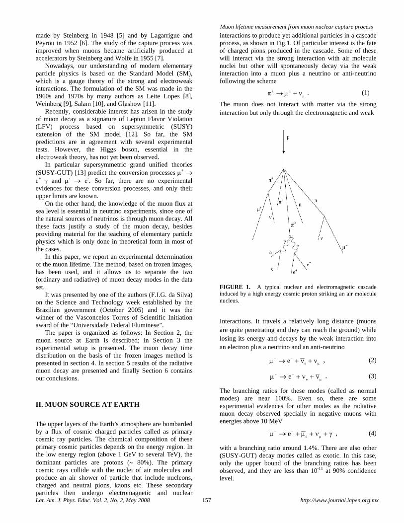
Muon lifetime measurement from muon nuclear capture process
Lat. Am. J. Phys. Educ. Vol. 2, No. 2, May 2008 157 http://www.journal.lapen.org.mx
made by Steinberg in 1948 [5] and by Lagarrigue and Peyrou in 1952 [6]. The study of the capture process was improved when muons became artificially produced at accelerators by Steinberg and Wolfe in 1955 [7].
Nowadays, our understanding of modern elementary particle physics is based on the Standard Model (SM), which is a gauge theory of the strong and electroweak interactions. The formulation of the SM was made in the 1960s and 1970s by many authors as Leite Lopes [8], Weinberg [9], Salam [10], and Glashow [11].
Recently, considerable interest has arisen in the study of muon decay as a signature of Lepton Flavor Violation (LFV) process based on supersymmetric (SUSY) extension of the SM model [12]. So far, the SM predictions are in agreement with several experimental tests. However, the Higgs boson, essential in the electroweak theory, has not yet been observed.
In particular supersymmetric grand unified theories (SUSY-GUT) [13] predict the conversion processes μ+ → e+ γ and μ- → e-. So far, there are no experimental evidences for these conversion processes, and only their upper limits are known.
On the other hand, the knowledge of the muon flux at sea level is essential in neutrino experiments, since one of the natural sources of neutrinos is through muon decay. All these facts justify a study of the muon decay, besides providing material for the teaching of elementary particle physics which is only done in theoretical form in most of the cases.
In this paper, we report an experimental determination of the muon lifetime. The method, based on frozen images, has been used, and it allows us to separate the two (ordinary and radiative) of muon decay modes in the data set.
It was presented by one of the authors (F.I.G. da Silva) on the Science and Technology week established by the Brazilian government (October 2005) and it was the winner of the Vasconcelos Torres of Scientific Initiation award of the “Universidade Federal Fluminese”.
The paper is organized as follows: In Section 2, the muon source at Earth is described; in Section 3 the experimental setup is presented. The muon decay time distribution on the basis of the frozen images method is presented in section 4. In section 5 results of the radiative muon decay are presented and finally Section 6 contains our conclusions. II. MUON SOURCE AT EARTH
The upper layers of the Earth’s atmosphere are bombarded by a flux of cosmic charged particles called as primary cosmic ray particles. The chemical composition of these primary cosmic particles depends on the energy region. In the low energy region (above 1 GeV to several TeV), the dominant particles are protons (∼ 80%). The primary cosmic rays collide with the nuclei of air molecules and produce an air shower of particle that include nucleons, charged and neutral pions, kaons etc. These secondary particles then undergo electromagnetic and nuclear
interactions to produce yet additional particles in a cascade process, as shown in Fig.1. Of particular interest is the fate of charged pions produced in the cascade. Some of these will interact via the strong interaction with air molecule nuclei but other will spontaneously decay via the weak interaction into a muon plus a neutrino or anti-neutrino following the scheme
μ±± ν+μ→π . (1)
The muon does not interact with matter via the strong interaction but only through the electromagnetic and weak
FIGURE 1. A typical nuclear and electromagnetic cascade induced by a high energy cosmic proton striking an air molecule nucleus.
Interactions. It travels a relatively long distance (muons are quite penetrating and they can reach the ground) while losing its energy and decays by the weak interaction into an electron plus a neutrino and an anti-neutrino
μ−− ν+ν+→μ ee , (2)
μ++ ν+ν+→μ ee . (3)
The branching ratios for these modes (called as normal modes) are near 100%. Even so, there are some experimental evidences for other modes as the radiative muon decay observed specially in negative muons with energies above 10 MeV
γ+ν+μ+→μ μ−−
ee , (4)
with a branching ratio around 1.4%. There are also other (SUSY-GUT) decay modes called as exotic. In this case, only the upper bound of the branching ratios has been observed, and they are less than 10-11 at 90% confidence level.
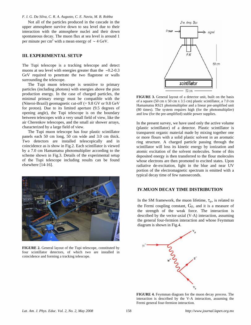
F. I. G. Da Silva, C. R. A. Augusto, C. E. Navia, M. B. Robba
Lat. Am. J. Phys. Educ. Vol. 2, No. 2, May 2008 158 http://www.journal.lapen.org.mx
Not all of the particles produced in the cascade in the upper atmosphere survive down to sea level due to their interaction with the atmosphere nuclei and their down spontaneous decay. The muon flux at sea level is around 1 per minute per cm2 with a mean energy of ∼ 4 GeV. III. EXPERIMENTAL SETUP The Tupi telescope is a tracking telescope and detect muons at sea level with energies greater than the ∼0.2-0.3 GeV required to penetrate the two flagstone or walls surrounding the telescope.
The Tupi muon telescope is sensitive to primary particles (including photons) with energies above the pion production energy. In the case of charged particles, the minimal primary energy must be compatible with the (Niteroi-Brazil) geomagnetic cut-off (= 9.8 GV or 9.8 GeV for proton). Due to its limited aperture (9.5 degrees of opening angle), the Tupi telescope is on the boundary between telescopes with a very small field of view, like the air Cherenkov telescopes, and the small air shower arrays, characterized by a large field of view.
The Tupi muon telescope has four plastic scintillator panels each 50 cm long, 50 cm wide and 3.0 cm thick. Two detectors are installed telescopically and in coincidence as is show in Fig.2. Each scintillator is viewed by a 7.0 cm Hamamatsu photomultiplier according to the scheme shown in Fig.3. Details of the experimental setup of the Tupi telescope including results can be found elsewhere [14-16].
FIGURE 2. General layout of the Tupi telescope, constituted by four scintillator detectors, of which two are installed in coincidence and forming a tracking telescope.
FIGURE 3. General layout of a detector unit, built on the basis of a square (50 cm x 50 cm x 3.5 cm) plastic scintillator, a 7.0 cm Hamamatsu RS21 photomultiplier and a linear pre-amplified unit (80 times). The system requires high (for the photomultiplier) and low (for the pre-amplified) stable power supplies. In the present survey, we have used only the active volume (plastic scintillator) of a detector. Plastic scintillator is transparent organic material made by mixing together one or more flours with a solid plastic solvent in an aromatic ring structure. A charged particle passing through the scintillator will loss its kinetic energy by ionization and atomic excitation of the solvent molecules. Some of this deposited energy is then transferred to the flour molecules whose electrons are then promoted to excited states. Upon radiative de-excitation, light in the blue and near UV portion of the electromagnetic spectrum is emitted with a typical decay time of few nanoseconds. IV.MUON DECAY TIME DISTRIBUTION
In the SM framework, the muon lifetime, τμ, is related to the Fermi coupling constant, GF, and it is a measure of the strength of the weak force. The interaction is described by the vector-axial (V-A) interaction, assuming the general four-fermion interaction and whose Feymman diagram is shown in Fig.4.
FIGURE 4. Feymman diagram for the muon decay process. The interaction is described by the V-A interaction, assuming the Fermi general four-fermion interaction.
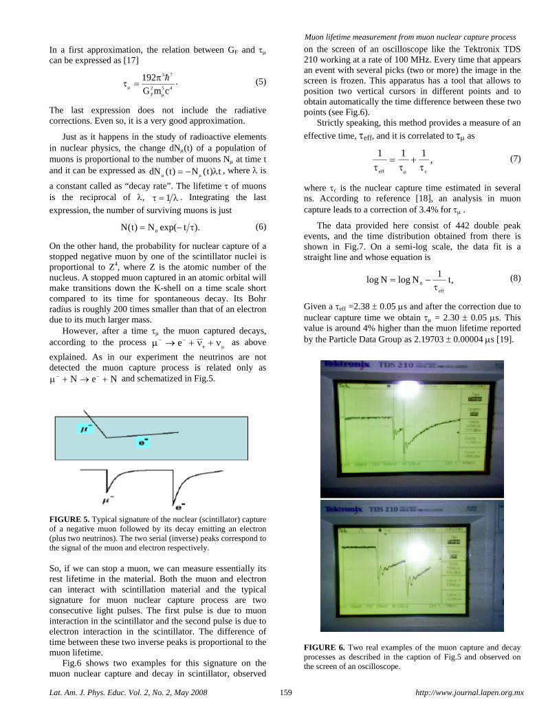
Muon lifetime measurement from muon nuclear capture process
Lat. Am. J. Phys. Educ. Vol. 2, No. 2, May 2008 159 http://www.journal.lapen.org.mx
In a first approximation, the relation between GF and τμ can be expressed as [17]
452
F
73
cmG
192
μ
μ
π=τ . (5)
The last expression does not include the radiative corrections. Even so, it is a very good approximation.
Just as it happens in the study of radioactive elements in nuclear physics, the change dNμ(t) of a population of muons is proportional to the number of muons Nμ at time t and it can be expressed as t)t(N)t(dN λ−= μμ
, where λ is
a constant called as “decay rate”. The lifetime τ of muons is the reciprocal of λ, λ=τ 1 . Integrating the last
expression, the number of surviving muons is just
).texp(N)t(N 0 τ−= (6)
On the other hand, the probability for nuclear capture of a stopped negative muon by one of the scintillator nuclei is proportional to Z4, where Z is the atomic number of the nucleus. A stopped muon captured in an atomic orbital will make transitions down the K-shell on a time scale short compared to its time for spontaneous decay. Its Bohr radius is roughly 200 times smaller than that of an electron due to its much larger mass.
However, after a time τμ the muon captured decays, according to the process
μ−− ν+ν+→μ ee as above
explained. As in our experiment the neutrinos are not detected the muon capture process is related only as
NeN +→+μ −− and schematized in Fig.5.
FIGURE 5. Typical signature of the nuclear (scintillator) capture of a negative muon followed by its decay emitting an electron (plus two neutrinos). The two serial (inverse) peaks correspond to the signal of the muon and electron respectively. So, if we can stop a muon, we can measure essentially its rest lifetime in the material. Both the muon and electron can interact with scintillation material and the typical signature for muon nuclear capture process are two consecutive light pulses. The first pulse is due to muon interaction in the scintillator and the second pulse is due to electron interaction in the scintillator. The difference of time between these two inverse peaks is proportional to the muon lifetime.
Fig.6 shows two examples for this signature on the muon nuclear capture and decay in scintillator, observed
on the screen of an oscilloscope like the Tektronix TDS 210 working at a rate of 100 MHz. Every time that appears an event with several picks (two or more) the image in the screen is frozen. This apparatus has a tool that allows to position two vertical cursors in different points and to obtain automatically the time difference between these two points (see Fig.6).
Strictly speaking, this method provides a measure of an
effective time, τeff, and it is correlated to τμ as
,111
ceff τ+
τ=
τ μ
(7)
where τc is the nuclear capture time estimated in several ns. According to reference [18], an analysis in muon capture leads to a correction of 3.4% for τμ .
The data provided here consist of 442 double peak events, and the time distribution obtained from there is shown in Fig.7. On a semi-log scale, the data fit is a straight line and whose equation is
,t1
NlogNlogeff
0 τ−= (8)
Given a τeff =2.38 ± 0.05 μs and after the correction due to nuclear capture time we obtain τμ = 2.30 ± 0.05 μs. This value is around 4% higher than the muon lifetime reported by the Particle Data Group as 2.19703 ± 0.00004 μs [19].
FIGURE 6. Two real examples of the muon capture and decay processes as described in the caption of Fig.5 and observed on the screen of an oscilloscope.
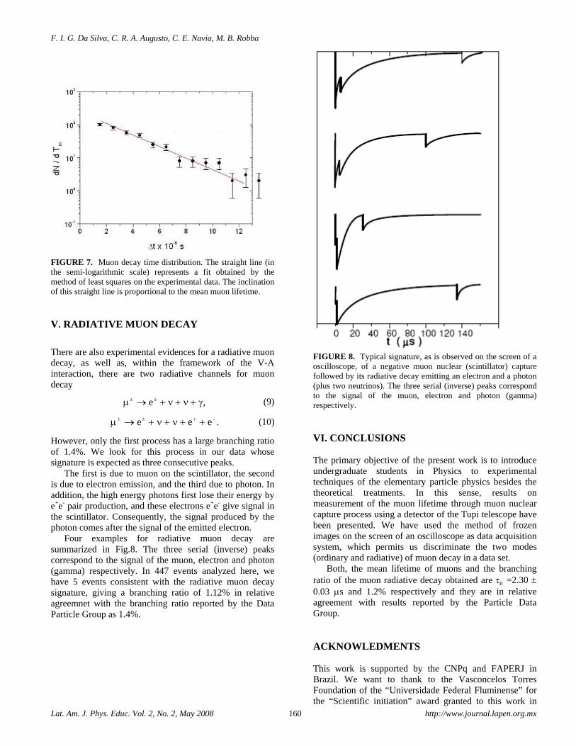
F. I. G. Da Silva, C. R. A. Augusto, C. E. Navia, M. B. Robba
Lat. Am. J. Phys. Educ. Vol. 2, No. 2, May 2008 160 http://www.journal.lapen.org.mx
FIGURE 7. Muon decay time distribution. The straight line (in the semi-logarithmic scale) represents a fit obtained by the method of least squares on the experimental data. The inclination of this straight line is proportional to the mean muon lifetime. V. RADIATIVE MUON DECAY
There are also experimental evidences for a radiative muon decay, as well as, within the framework of the V-A interaction, there are two radiative channels for muon decay
,e γ+ν+ν+→μ ±± (9)
.eee −+±± ++ν+ν+→μ (10)
However, only the first process has a large branching ratio of 1.4%. We look for this process in our data whose signature is expected as three consecutive peaks.
The first is due to muon on the scintillator, the second is due to electron emission, and the third due to photon. In addition, the high energy photons first lose their energy by e+e- pair production, and these electrons e+e- give signal in the scintillator. Consequently, the signal produced by the photon comes after the signal of the emitted electron.
Four examples for radiative muon decay are summarized in Fig.8. The three serial (inverse) peaks correspond to the signal of the muon, electron and photon (gamma) respectively. In 447 events analyzed here, we have 5 events consistent with the radiative muon decay signature, giving a branching ratio of 1.12% in relative agreemnet with the branching ratio reported by the Data Particle Group as 1.4%.
FIGURE 8. Typical signature, as is observed on the screen of a oscilloscope, of a negative muon nuclear (scintillator) capture followed by its radiative decay emitting an electron and a photon (plus two neutrinos). The three serial (inverse) peaks correspond to the signal of the muon, electron and photon (gamma) respectively. VI. CONCLUSIONS The primary objective of the present work is to introduce undergraduate students in Physics to experimental techniques of the elementary particle physics besides the theoretical treatments. In this sense, results on measurement of the muon lifetime through muon nuclear capture process using a detector of the Tupi telescope have been presented. We have used the method of frozen images on the screen of an oscilloscope as data acquisition system, which permits us discriminate the two modes (ordinary and radiative) of muon decay in a data set.
Both, the mean lifetime of muons and the branching ratio of the muon radiative decay obtained are τμ =2.30 ± 0.03 μs and 1.2% respectively and they are in relative agreement with results reported by the Particle Data Group. ACKNOWLEDMENTS This work is supported by the CNPq and FAPERJ in Brazil. We want to thank to the Vasconcelos Torres Foundation of the “Universidade Federal Fluminense” for the “Scientific initiation” award granted to this work in

Muon lifetime measurement from muon nuclear capture process
Lat. Am. J. Phys. Educ. Vol. 2, No. 2, May 2008 161 http://www.journal.lapen.org.mx
2005. We are grateful to the K. H. Tsui for reading the manuscript. REFERENCES [1] Rossi, B., High Energy Particles (Prentice-Hall, Inc. New York, 1955). [2] Neddemeyer, S. H. and Anderson, C. D., Phys. Rev. 51, 884 (1937). [3] Lattes, C. M. G., Occhialini, G. P. S. and Powell, C. F., Nature 160, 453 (1949). [4] Lattes, C. M. G., Occhialini, G. P. S and Powell, C. F. , A determination of the ratio of the masses of pi-meson and mu-meson by the method of grain-counting, Proceedings of The Physical Society 61, 173-183 (1948). [5] Steinberg, J., Phys. Rev. 74, 500 (1948). [6] Lagarrigue, A. and Peyrou, C., Acad. Sci. Paris 234, 873 (1952). [7] Steinerg, J. and Whole, H. B., Phys. Rev. 100, 1490 (1955).
[8] Leite Lopes, J., Nucl. Phys. 8, 234 (1958). [9] Weinberg, S., Phys. Rev. Lett. 19, 1264 (1967). [10] Salam, A., Elementary Particle Theory, p.367 (Almquist and Wiksells, Stockholm, 1969). [11] Glashow, S. L. et al., Phys. Rev. D 2, 1285 (1970). [12] Nilles, H. P., Phys. Rep. 110, 1 (1984). [13] Barbieri, R. and Hall, L. J., Phys., Lett. B 228, 212 (1994). [14] Navia, C. E., Augusto, C. R. A., Robba, M. B., Malheiro, M. and Shigueoka, H., Ap. J, 621, 1137 (2005). [15] Augusto, C. R. A. Navia, C. E. and Robba, M. B., Phys. Rev. D 71, 103011 (2005). [16] Navia, C. E., Augusto, C. R. A., Tsui, K. H. and Robba, M. B., Phys. Rev. D 72, 103001 (2005). [17] Konishita, T. and Sirlin, A., Phys. Rev. 113, 1652 (1959). [18] Galviati, C. and Beacon, J., Phys. Rev. C 72, 025807 (2005). [19] Particle Data Group, J. of Phys. G, 33, 33 (2006).
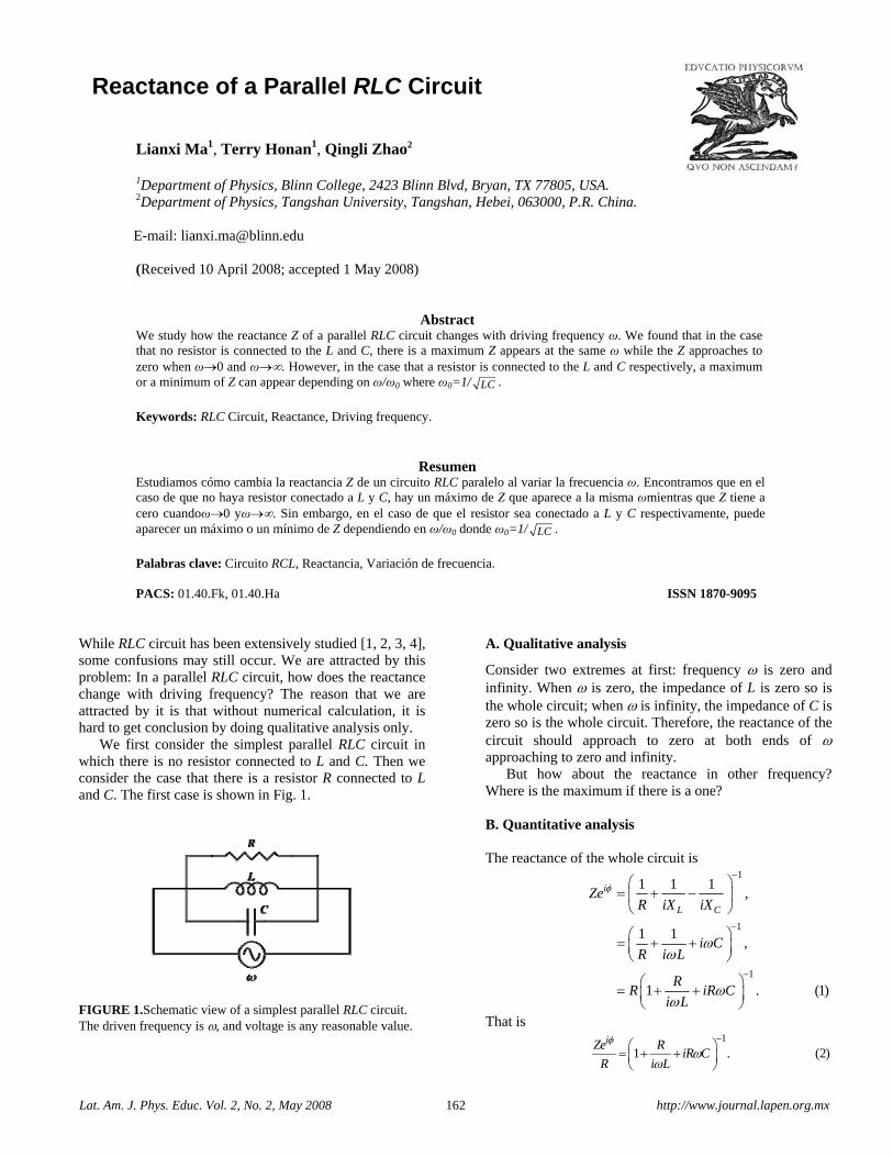
Lat. Am. J. Phys. Educ. Vol. 2, No. 2, May 2008 162 http://www.journal.lapen.org.mx
Reactance of a Parallel RLC Circuit
Lianxi Ma1, Terry Honan1, Qingli Zhao2
1Department of Physics, Blinn College, 2423 Blinn Blvd, Bryan, TX 77805, USA. 2Department of Physics, Tangshan University, Tangshan, Hebei, 063000, P.R. China. E-mail: [email protected] (Received 10 April 2008; accepted 1 May 2008)
Abstract We study how the reactance Z of a parallel RLC circuit changes with driving frequency ω. We found that in the case that no resistor is connected to the L and C, there is a maximum Z appears at the same ω while the Z approaches to zero when ω→0 and ω→∞. However, in the case that a resistor is connected to the L and C respectively, a maximum or a minimum of Z can appear depending on ω/ω0 where ω0=1/ LC .
Keywords: RLC Circuit, Reactance, Driving frequency.
Resumen Estudiamos cómo cambia la reactancia Z de un circuito RLC paralelo al variar la frecuencia ω. Encontramos que en el caso de que no haya resistor conectado a L y C, hay un máximo de Z que aparece a la misma ωmientras que Z tiene a cero cuandoω→0 yω→∞. Sin embargo, en el caso de que el resistor sea conectado a L y C respectivamente, puede aparecer un máximo o un mínimo de Z dependiendo en ω/ω0 donde ω0=1/ LC . Palabras clave: Circuito RCL, Reactancia, Variación de frecuencia. PACS: 01.40.Fk, 01.40.Ha ISSN 1870-9095
While RLC circuit has been extensively studied [1, 2, 3, 4], some confusions may still occur. We are attracted by this problem: In a parallel RLC circuit, how does the reactance change with driving frequency? The reason that we are attracted by it is that without numerical calculation, it is hard to get conclusion by doing qualitative analysis only.
We first consider the simplest parallel RLC circuit in which there is no resistor connected to L and C. Then we consider the case that there is a resistor R connected to L and C. The first case is shown in Fig. 1.
FIGURE 1.Schematic view of a simplest parallel RLC circuit. The driven frequency is ω, and voltage is any reasonable value.
A. Qualitative analysis
Consider two extremes at first: frequency ω is zero and infinity. When ω is zero, the impedance of L is zero so is the whole circuit; when ω is infinity, the impedance of C is zero so is the whole circuit. Therefore, the reactance of the circuit should approach to zero at both ends of ω approaching to zero and infinity.
But how about the reactance in other frequency? Where is the maximum if there is a one? B. Quantitative analysis The reactance of the whole circuit is
1
1
1
1 1 1,
1 1,
1 . (1)
i
L C
ZeR iX iX
i CR i L
RR iR C
i L
φ
ωω
ωω
−
−
−
⎛ ⎞= + −⎜ ⎟
⎝ ⎠
⎛ ⎞= + +⎜ ⎟⎝ ⎠
⎛ ⎞= + +⎜ ⎟⎝ ⎠
That is 1
1 . (2)iZe R
iR CR i L
φω
ω
−⎛ ⎞= + +⎜ ⎟⎝ ⎠
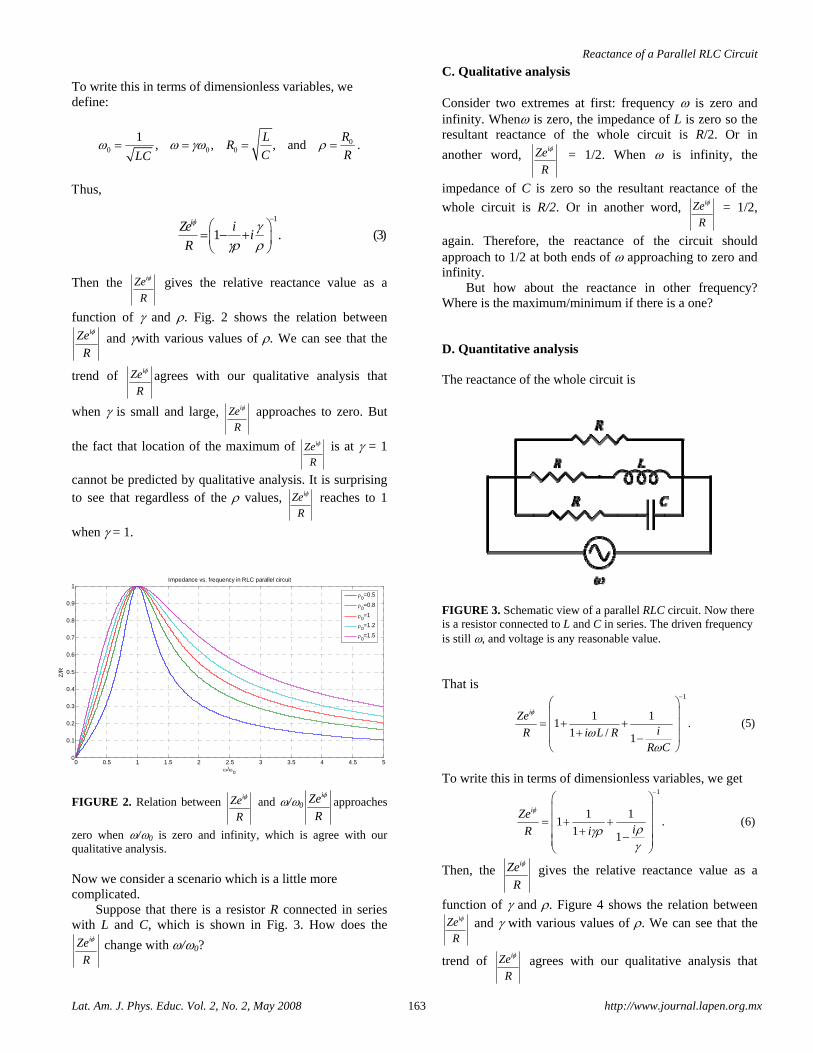
Reactance of a Parallel RLC Circuit
Lat. Am. J. Phys. Educ. Vol. 2, No. 2, May 2008 163 http://www.journal.lapen.org.mx
To write this in terms of dimensionless variables, we define:
00 0 0
1, , , and .
RLR
C RLCω ω γω ρ= = = =
Τhus,
1
1 . (3)iZe i
iR
φ γγρ ρ
−⎛ ⎞
= − +⎜ ⎟⎝ ⎠
Then the iZe
R
φ gives the relative reactance value as a
function of γ and ρ. Fig. 2 shows the relation between iZe
R
φ and γwith various values of ρ. We can see that the
trend of iZe
R
φ agrees with our qualitative analysis that
when γ is small and large, iZe
R
φ approaches to zero. But
the fact that location of the maximum of iZe
R
φ is at γ = 1
cannot be predicted by qualitative analysis. It is surprising to see that regardless of the ρ values, iZe
R
φ reaches to 1
when γ = 1.
0 0.5 1 1.5 2 2.5 3 3.5 4 4.5 50
0.1
0.2
0.3
0.4
0.5
0.6
0.7
0.8
0.9
1
ω/ω0
Z/R
Impedance vs. frequency in RLC parallel circuit
ρ0=0.5
ρ0=0.8
ρ0=1
ρ0=1.2
ρ0=1.5
FIGURE 2. Relation between
iZe
R
φ and ω/ω0
iZe
R
φapproaches
zero when ω/ω0 is zero and infinity, which is agree with our qualitative analysis. Now we consider a scenario which is a little more complicated.
Suppose that there is a resistor R connected in series with L and C, which is shown in Fig. 3. How does the
iZe
R
φ change with ω/ω0?
C. Qualitative analysis Consider two extremes at first: frequency ω is zero and infinity. Whenω is zero, the impedance of L is zero so the resultant reactance of the whole circuit is R/2. Or in
another word, iZe
R
φ = 1/2. When ω is infinity, the
impedance of C is zero so the resultant reactance of the
whole circuit is R/2. Or in another word, iZe
R
φ = 1/2,
again. Therefore, the reactance of the circuit should approach to 1/2 at both ends of ω approaching to zero and infinity.
But how about the reactance in other frequency? Where is the maximum/minimum if there is a one? D. Quantitative analysis The reactance of the whole circuit is
FIGURE 3. Schematic view of a parallel RLC circuit. Now there is a resistor connected to L and C in series. The driven frequency is still ω, and voltage is any reasonable value.
That is
1
1 11 . (5)
1 / 1
iZeiR i L R
R C
φ
ωω
−⎛ ⎞⎜ ⎟
= + +⎜ ⎟+⎜ ⎟−⎝ ⎠
To write this in terms of dimensionless variables, we get
1
1 11 . (6)
1 1
iZeiR i
φ
ργργ
−⎛ ⎞⎜ ⎟⎜ ⎟= + +
+⎜ ⎟−⎜ ⎟⎝ ⎠
Then, the iZe
R
φ gives the relative reactance value as a
function of γ and ρ. Figure 4 shows the relation between iZe
R
φ and γ with various values of ρ. We can see that the
trend of iZe
R
φ agrees with our qualitative analysis that
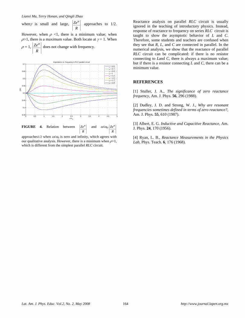
Lianxi Ma, Terry Honan, and Qingli Zhao
Lat. Am. J. Phys. Educ. Vol.2, No. 2, May 2008 164 http://www.journal.lapen.org.mx
whenγ is small and large, iZe
R
φ approaches to 1/2.
However, when ρ <1, there is a minimum value; when ρ>1, there is a maximum value. Both locate at γ = 1. When
ρ = 1, iZe
R
φ does not change with frequency.
0 0.5 1 1.5 2 2.5 3 3.5 4 4.5 50.35
0.4
0.45
0.5
0.55
0.6
0.65
0.7
ω/ω0
Z/R
Impedance vs. frequency in RLC parallel circuit
ρ = 0.5ρ = 0.7ρ = 0.9ρ = 1ρ = 1.2ρ = 1.5ρ = 1.7ρ = 1.9
FIGURE 4. Relation between iZe
R
φ and ω/ω0.iZe
R
φ
approaches1/2 when ω/ω0 is zero and infinity, which agrees with our qualitative analysis. However, there is a minimum when ρ>1, which is different from the simplest parallel RLC circuit.
Reactance analysis on parallel RLC circuit is usually ignored in the teaching of introductory physics. Instead, response of reactance to frequency on series RLC circuit is taught to show the asymptotic behavior of L and C. Therefore, some students and teachers are confused when they see that R, L, and C are connected in parallel. In the numerical analysis, we show that the reactance of parallel RLC circuit can be complicated: if there is no resistor connecting to Land C, there is always a maximum value; but if there is a resistor connecting L and C, there can be a minimum value. REFERENCES [1] Stuller, J. A., The significance of zero reactance frequency, Am. J. Phys. 56, 296 (1988). [2] Dudley, J. D. and Strong, W. J., Why are resonant frequencies sometimes defined in terms of zero reactance?, Am. J. Phys. 55, 610 (1987). [3] Albert, E. G. Inductive and Capacitive Reactance, Am. J. Phys. 24, 170 (1956). [4] Ryan, L. B., Reactance Measurements in the Physics Lab, Phys. Teach. 6, 176 (1968).
Lat. Am. J. Phys. Educ. Vol. 2, No. 2, May 2008 165 http://www.journal.lapen.org.mx
The angular momentum in the classical anisotropic Kepler problem
Emilio Cortés 1Departamento de Física, Universidad Autónoma Metropolitana Iztapalapa,
Apdo. Postal 55-534 .México D. F. 09340, México.
E-mail: [email protected]
(Received 7 February 2008; accepted 14 April 2008)
Abstract The behavior of the angular momentum of the two dimensional Anisotropic Kepler Problem (AKP) is addressed. We
find here ourselves, from the point of view of physics didactics, with a classical mechanics ``simple" problem that
should be carefully analyzed from the outset. Taking into account that the angular momentum varies with time due to
an ``inertial torque", we are still allowed to restrict the problem to a two dimensional motion, and then, being the
angular momentum in this restricted case, a one-dimensional variable, we study how its behavior can describe the
dynamics of this chaotic system. The approach to this problem through the angular momentum, to our knowledge, has
not been reported in the literature. We investigate, from a numerical solution of the equations of motion, different
features of this quantity and obtain a return plot for the angular momentum, as well as some phase space diagrams for
the torque vs. angular momentum, for different values of the anisotropy parameter, by using a Poincare surface section.
Keywords: anisotropic Kepler problem, chaos.
Resumen
En el presente trabajo estudiamos el comportamiento del momento angular en el problema de Kepler anisotrópico
(AKP) en dos dimensiones. Nos encontramos aquí, desde el punto de vista de la didáctica de la física, con un problema
``sencillo" de la mecánica clásica, que debe ser analizado con cuidado desde el principio. Tomando en cuenta que el
momento angular varía con el tiempo debido a una ``torca inercial", es aun posible restringir el problema a un
movimiento en dos dimensiones, y de esta manera, siendo el momento angular en este caso restringido una variable
unidimensional, analizamos cómo su comportamiento puede describir la dinámica de este sistema caótico. El enfoque
de este problema a través del momento angular, hasta donde sabemos, no ha sido reportado en la literatura. A partir de
una solución numérica de las ecuaciones, se investigan diferentes características de esta variable y obtenemos una
``gráfica de retorno" para el momento angular, así como algunos diagramas de espacio fase de la torca contra momento
angular, para diferentes valores del parámetro de anisotropía, utilizando una superficie sección de Poincare.
Palabras clave: Problema de Kepler anisotrópico, caos.
PACS: 45, 05.45 Pq, 01.40.Fk ISSN 1870-9095
I. INTRODUCTION
The anisotropic Kepler problem (AKP) originated in the
description of an electron close to a donor impurity in a
Silicon or Germanium semiconductor [1], inspired the
classical AKP, and this Hamiltonian system was one of the
first “simple” systems for which the chaos was rigorously
proved [2, 3]. It has also been used to study the interplay
between classical and quantum mechanics [3]. In fact, as
Gutzwiller [4] pointed out, the quantum mechanical
systems whose classical behavior is chaotic reveal
significant differences in the character of their wave
functions, the distribution of their energy levels, among
other properties. Most of the analysis of the AKP has been
done from numerical calculations for the trajectory, both in
the coordinates space and in the phase space. There are
also mathematical treatments of the classical AKP [5, 6, 7].
II. THE HAMILTONIAN
The Hamiltonian of the AKP can be reduced from three to
two degrees of freedom, by taking into account the
symmetry around an axis, and appropriate initial
conditions1.
It is expressed in the form
2 2 2 2
= ( / 2 ) ( / 2 ) / ,x y
H p p G x yµ ν+ − + (1)
where µ and ν are the elements of the mass tensor, which
means the existence of different mass parameter for each
axis. Here it is not considered a centrifugal potential,
which stabilizes the trajectories and in which case the hard
1In the non-restricted case the motion will be in general, in the
three dimensional space. This is due to the fact that the angular
momentum is not conserved.
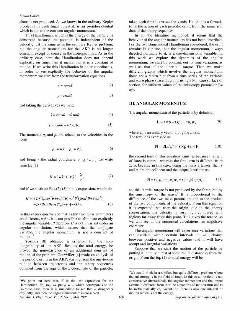
Emilio Cortés
Lat. Am. J. Phys. Educ. Vol. 2, No. 2, May 2008 166 http://www.journal.lapen.org.mx
chaos is not produced. As we know, in the ordinary Kepler
problem this centrifugal potential, is an pseudo-potential
which is due to the constant angular momentum.
This Hamiltonian, which is the energy of the particle, is
conserved because the potential is independent of the
velocity, just the same as in the ordinary Kepler problem,
but the angular momentum for the AKP is no longer
constant, except of course in the isotropic limit. As in the
ordinary case, here the Hamiltonian does not depend
explicitly on time, then it means that it is a constant of
motion. If we write this Hamiltonian in polar coordinates,
in order to see explicitly the behavior of the angular
momentum we start from the transformation equations
= ,x rcosθ (2)
= ,y rsinθ (3)
and taking the derivatives we write
= ,x rcos r sinθ θ θ− && & (4)
= .y rsin r cosθ θ θ+ && & (5)
The momenta px and py are related to the velocities in the
form
= , = ,x yp x p yµ ν& & (6)
and being r the radial coordinate, r= 2 2 ,x y+ we write
from Eq.(1)
2 21 12 2
= ,G
H x yr
µ ν+ −& &
(7)
and if we sustitute Eqs.(2)-(5) in this expression, we obtain
2 2 2 2 2 2 2=1/ 2[ ( ) ( )H r cos sin r sin cosµ θ ν θ θ µ θ ν+ + +&&
2 ( )] / .rr sin cos G rθ θ θ µ ν− − −&& (8)
In this expression we see that as the two mass parameters
are different, µ ≠ ν, it is not possible to eliminate explicitly
the angular variable, θ therefore H is not invariant under an
angular translation, which means that the conjugate
variable, the angular momentum, is not a constant of
motion. 2
Yoshida [8] obtained a criterion for the non-
integrability of the AKP. Besides the total energy, he
proved the non-existence of an additional constant of
motion of the problem. Gutzwiller [4] made an analysis of
the periodic orbits in the AKP, starting from the one-to-one
relation between trajectories and the binary sequences
obtained from the sign of the x coordinate of the particle,
2We point out here that, if in the last expression for the
Hamiltonian, Eq. (8), we put µ = ν, which corresponds to the
isotropic case, then it is immediate to see that θ disappears
explicitly, and then the angular momentum is conserved.
taken each time it crosses the x axis. He obtains a formula
to fit the action of each periodic orbit, from the numerical
data of the binary sequences.
In all the literature mentioned, it seems that the
behavior of the angular momentum has not been described.
For the two-dimensional Hamiltonian considered, the orbit
remains in a plane, then the angular momentum, always
directed normally to it, is a one-dimensional variable. In
this work we explore the dynamics of the angular
momentum, we start by pointing out its time variation, as
well as that of the “inertial” torque. Then we make
different graphs which involve the angular momentum;
those are a return plot from a time series of the variable
and some phase space diagrams using a Poincare surface of
section, for different values of the anisotropy parameter ζ =
µ/ν.
III. ANGULAR MOMENTUM
The angular momentum of the particle is by definition
= = ( ) ,zL r p ey x
xp yp× − (9)
where ez is an unitary vector along the z axis.
The torque is expressed as
= / = ,N L v p r Fd dt × + × (10)
the second term of this equation vanishes because the field
of force is central, whereas the first term is different from
zero, because in this case, being the mass a tensor, then v
and p are not collinear and the torque is written as
= ( ) = ( )z zN e ex y y x x yv p v p v vν µ− − , (11)
so, this inertial torque is not produced by the force, but by
the anisotropy of the mass.3 It is proportional to the
difference of the two mass parameters and to the product
of the two components of the velocity. From this equation
it is expected that near the origin, due to the energy
conservation, the velocity is very high compared with
regions far away from this point. This gives the torque, as
we will see in the numerical calculations, an impulsive
character.
The angular momentum will experience variations that
can oscillate within certain intervals, it will change
between positive and negative values and it will have
abrupt and irregular variations.
Suppose that we start the motion of the particle by
putting it initially at rest at some radial distance r0 from the
origin. From the Eq. (1) its total energy will be
3We could think in a similar, but quite different problem where
the anisotropy is in the field of force. In this case the field is not
conservative (irrotational), the angular momentum and the torque
assume a different form, but the equations of motion turn out to
be mathematically equivalent. So, there is also one integral of
motion which is not the energy.
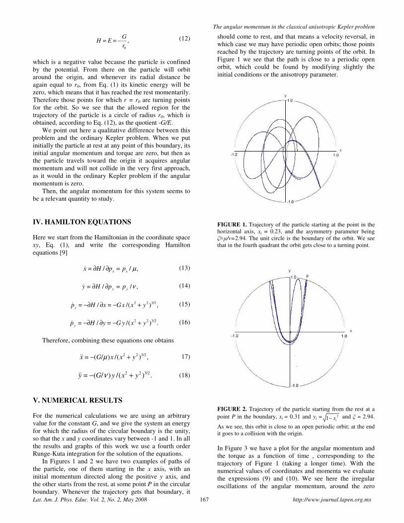
The angular momentum in the classical anisotropic Kepler problem
Lat. Am. J. Phys. Educ. Vol. 2, No. 2, May 2008 167 http://www.journal.lapen.org.mx
0
= = ,G
H Er
− (12)
which is a negative value because the particle is confined
by the potential. From there on the particle will orbit
around the origin, and whenever its radial distance be
again equal to r0, from Eq. (1) its kinetic energy will be
zero, which means that it has reached the rest momentarily.
Therefore those points for which r = r0 are turning points
for the orbit. So we see that the allowed region for the
trajectory of the particle is a circle of radius r0, which is
obtained, according to Eq. (12), as the quotient -G/E.
We point out here a qualitative difference between this
problem and the ordinary Kepler problem. When we put
initially the particle at rest at any point of this boundary, its
initial angular momentum and torque are zero, but then as
the particle travels toward the origin it acquires angular
momentum and will not collide in the very first approach,
as it would in the ordinary Kepler problem if the angular
momentum is zero.
Then, the angular momentum for this system seems to
be a relevant quantity to study.
IV. HAMILTON EQUATIONS
Here we start from the Hamiltonian in the coordinate space
xy, Eq. (1), and write the corresponding Hamilton
equations [9]
= / = / ,x x
x H p p µ∂ ∂& (13)
= / = / ,y yy H p p ν∂ ∂& (14)
2 2 3/2= / = /( ) ,xp H x Gx x y−∂ ∂ − +& (15)
2 2 3/2= / = /( ) .
yp H y G y x y−∂ ∂ − +& (16)
Therefore, combining these equations one obtains
2 2 3/2= ( / ) /( ) ,x G x x yµ− +&& 17)
2 2 3/2= ( / ) /( ) .y G y x yν− +&& (18)
V. NUMERICAL RESULTS
For the numerical calculations we are using an arbitrary
value for the constant G, and we give the system an energy
for which the radius of the circular boundary is the unity,
so that the x and y coordinates vary between -1 and 1. In all
the results and graphs of this work we use a fourth order
Runge-Kuta integration for the solution of the equations.
In Figures 1 and 2 we have two examples of paths of
the particle, one of them starting in the x axis, with an
initial momentum directed along the positive y axis, and
the other starts from the rest, at some point P in the circular
boundary. Whenever the trajectory gets that boundary, it
should come to rest, and that means a velocity reversal, in
which case we may have periodic open orbits; those points
reached by the trajectory are turning points of the orbit. In
Figure 1 we see that the path is close to a periodic open
orbit, which could be found by modifying slightly the
initial conditions or the anisotropy parameter.
FIGURE 1. Trajectory of the particle starting at the point in the
horizontal axis, xi = 0.23, and the asymmetry parameter being
ζ≡µ/ν=2.94. The unit circle is the boundary of the orbit. We see
that in the fourth quadrant the orbit gets close to a turning point.
FIGURE 2. Trajectory of the particle starting from the rest at a
point P in the boundary, xi = 0.31 and yi = 21 ix− and ξ = 2.94.
As we see, this orbit is close to an open periodic orbit; at the end
it goes to a collision with the origin.
In Figure 3 we have a plot for the angular momentum and
the torque as a function of time , corresponding to the
trajectory of Figure 1 (taking a longer time). With the
numerical values of coordinates and momenta we evaluate
the expressions (9) and (10). We see here the irregular
oscillations of the angular momentum, around the zero
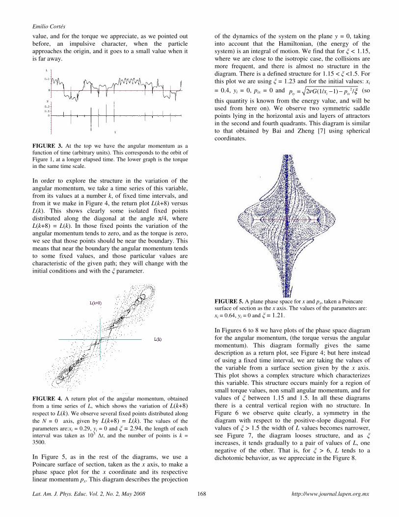
Emilio Cortés
Lat. Am. J. Phys. Educ. Vol. 2, No. 2, May 2008 168 http://www.journal.lapen.org.mx
value, and for the torque we appreciate, as we pointed out
before, an impulsive character, when the particle
approaches the origin, and it goes to a small value when it
is far away.
FIGURE 3. At the top we have the angular momentum as a
function of time (arbitrary units). This corresponds to the orbit of
Figure 1, at a longer elapsed time. The lower graph is the torque
in the same time scale.
In order to explore the structure in the variation of the
angular momentum, we take a time series of this variable,
from its values at a number k, of fixed time intervals, and
from it we make in Figure 4, the return plot L(k+8) versus
L(k). This shows clearly some isolated fixed points
distributed along the diagonal at the angle π/4, where
L(k+8) = L(k). In those fixed points the variation of the
angular momentum tends to zero, and as the torque is zero,
we see that those points should be near the boundary. This
means that near the boundary the angular momentum tends
to some fixed values, and those particular values are
characteristic of the given path; they will change with the
initial conditions and with the ξ parameter.
FIGURE 4. A return plot of the angular momentum, obtained
from a time series of L, which shows the variation of L(k+8)
respect to L(k). We observe several fixed points distributed along
the N = 0 axis, given by L(k+8) = L(k). The values of the
parameters are:xi = 0.29, yi = 0 and ξ = 2.94, the length of each
interval was taken as 103 ∆t, and the number of points is k =
3500.
In Figure 5, as in the rest of the diagrams, we use a
Poincare surface of section, taken as the x axis, to make a
phase space plot for the x coordinate and its respective
linear momentum px. This diagram describes the projection
of the dynamics of the system on the plane y = 0, taking
into account that the Hamiltonian, (the energy of the
system) is an integral of motion. We find that for ξ < 1.15,
where we are close to the isotropic case, the collisions are
more frequent, and there is almost no structure in the
diagram. There is a defined structure for 1.15 < ξ <1.5. For
this plot we are using ξ = 1.23 and for the initial values: xi
= 0.4, yi = 0, pix = 0 and 2= 2 (1/ 1) /iy i ix
p G x pν ξ− − (so
this quantity is known from the energy value, and will be
used from here on). We observe two symmetric saddle
points lying in the horizontal axis and layers of attractors
in the second and fourth quadrants. This diagram is similar
to that obtained by Bai and Zheng [7] using spherical
coordinates.
FIGURE 5. A plane phase space for x and px, taken a Poincare
surface of section as the x axis. The values of the parameters are:
xi = 0.64, yi = 0 and ξ = 1.21.
In Figures 6 to 8 we have plots of the phase space diagram
for the angular momentum, (the torque versus the angular
momentum). This diagram formally gives the same
description as a return plot, see Figure 4; but here instead
of using a fixed time interval, we are taking the values of
the variable from a surface section given by the x axis.
This plot shows a complex structure which characterizes
this variable. This structure occurs mainly for a region of
small torque values, non small angular momentum, and for
values of ξ between 1.15 and 1.5. In all these diagrams
there is a central vertical region with no structure. In
Figure 6 we observe quite clearly, a symmetry in the
diagram with respect to the positive-slope diagonal. For
values of ξ > 1.5 the width of L values becomes narrower,
see Figure 7, the diagram looses structure, and as ξ
increases, it tends gradually to a pair of values of L, one
negative of the other. That is, for ξ > 6, L tends to a
dichotomic behavior, as we appreciate in the Figure 8.
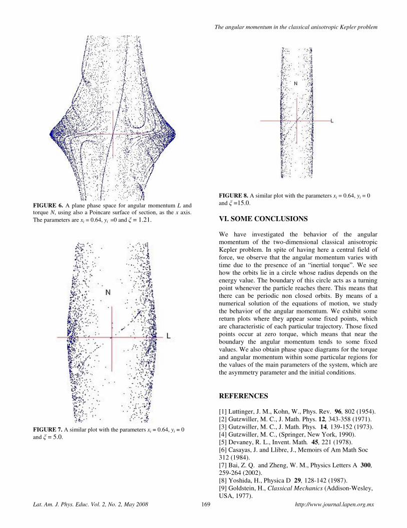
The angular momentum in the classical anisotropic Kepler problem
Lat. Am. J. Phys. Educ. Vol. 2, No. 2, May 2008 169 http://www.journal.lapen.org.mx
FIGURE 6. A plane phase space for angular momentum L and
torque N, using also a Poincare surface of section, as the x axis.
The parameters are xi = 0.64, yi =0 and ξ = 1.21.
FIGURE 7. A similar plot with the parameters xi = 0.64, yi = 0
and ξ = 5.0.
FIGURE 8. A similar plot with the parameters xi = 0.64, yi = 0
and ξ =15.0.
VI. SOME CONCLUSIONS
We have investigated the behavior of the angular
momentum of the two-dimensional classical anisotropic
Kepler problem. In spite of having here a central field of
force, we observe that the angular momentum varies with
time due to the presence of an “inertial torque”. We see
how the orbits lie in a circle whose radius depends on the
energy value. The boundary of this circle acts as a turning
point whenever the particle reaches there. This means that
there can be periodic non closed orbits. By means of a
numerical solution of the equations of motion, we study
the behavior of the angular momentum. We exhibit some
return plots where they appear some fixed points, which
are characteristic of each particular trajectory. Those fixed
points occur at zero torque, which means that near the
boundary the angular momentum tends to some fixed
values. We also obtain phase space diagrams for the torque
and angular momentum within some particular regions for
the values of the main parameters of the system, which are
the asymmetry parameter and the initial conditions.
REFERENCES
[1] Luttinger, J. M., Kohn, W., Phys. Rev. 96, 802 (1954).
[2] Gutzwiller, M. C., J. Math. Phys. 12, 343-358 (1971).
[3] Gutzwiller, M. C., J. Math. Phys. 14, 139-152 (1973).
[4] Gutzwiller, M. C., (Springer, New York, 1990).
[5] Devaney, R. L., Invent. Math. 45, 221 (1978).
[6] Casayas, J. and Llibre, J., Memoirs of Am Math Soc
312 (1984).
[7] Bai, Z. Q. and Zheng, W. M., Physics Letters A 300,
259-264 (2002).
[8] Yoshida, H., Physica D 29, 128-142 (1987).
[9] Goldstein, H., Classical Mechanics (Addison-Wesley,
USA, 1977).
Lat. Am. J. Phys. Educ. Vol. 2, No. 2, May 2008 170 http://www.journal.lapen.org.mx
Comparación de métodos analíticos y numéricos para la solución del lanzamiento vertical de una bola en el aire
Alejandro González y Hernández Facultad de Ciencias, Universidad Nacional Autónoma de México
E-mail: [email protected] (Recibido el 4 de Febrero de 2008; aceptado el 29 de Abril de 2008)
Resumen La ecuación de movimiento para el lanzamiento de una bola vertical en el aire tiene una solución analítica que necesita del cálculo diferencial e integral para su obtención. Sin embargo, los estudiantes del primer año de una licenciatura de física tienen dificultades en aplicar el cálculo para la solución analítica de la ecuación de movimiento, por esto se piensa en utilizar soluciones numéricas. Estas soluciones corresponden a ecuaciones algebraicas que se resuelven por métodos numéricos comprensibles a los estudiantes, pero en general, no son incluidas en la mayoría de los libros de texto y frecuentemente se piensa de ellas como inexactas, explicando la preferencia de los métodos analíticos sobre los numéricos. Por este motivo, aquí se comparan la solución analítica con las numéricas para el tiro vertical en el aire, con el fin de analizar las diferencias entre ellas y establecer criterios que permitan discutir estas diferencias. Palabras claves: Dinámica newtoniana, métodos analíticos, métodos numéricos, ecuación de movimiento, fuerza de resistencia del aire.
Abstract The equation of motion for a vertical launching of a ball in the air has analytic solution that needs of the differential and integral calculus for their obtaining. However, the first year-old students of a physics major have difficulties in applying the calculation for the analytic solution of the movement equation and for this reason it is thought of using numerical solutions. These solutions correspond to algebraic equations that are solved for numerical methods comprehensible to the students, but in general, they are not included in most of the text books and frequently it is thought of them as inexact, explaining the preference of the analytic methods on the numerical ones. For this reason, the analytic solution is compared with the numerical ones for the vertical shot in the air, with the purpose of analyzing the differences among them and to settle down approaches that allow the discussions of these differences. Palabras clave: Newtonian dynamics, analytic methods, numerical methods, equation of motion, air resistance. PACS: 01.50.H, 02.30.Hq, 02.60.-x, 02.60.Cb, 45.20.D-, 45.50.Dd
I. INTRODUCCIÓN En numerosos estudios empíricos se ha reportado que los estudiantes tienen dificultades para entender la Dinámica Newtoniana [1], y diferentes innovaciones se han desarrollado y propuestos en Física Educativa para tratar de mejorar la comprensión de los estudiantes de este tipo de fenómenos de la Física [2]. La Física Computacional se ha incorporado al estudio de la Física actual y se ha colocado intermedia entre la enseñanza de la teoría y la experimentación de los cursos tradicionales, por lo que en los cursos de introducción de la Mecánica a nivel universitario se recomienda incorporar tópicos contemporáneos de Mecánica lineal y no lineal [3] que incluyan la modelación y la simulación por computadora y la introducción de nuevas representaciones gráficas y simbólicas de los fenómenos físicos para ayudar a los estudiantes en el desarrollo de un adecuado entendimiento de estos temas. En este caso, es necesario añadir al
desarrollo de las habilidades de razonamiento científico y experimental, las habilidades en la creación computación [4], para la modelación, el análisis y la solución de sistemas dinámicos.
La modelación [5] y la simulación [6] de sistemas dinámicos [7] se han estado introduciendo en el currículo de los cursos de física introductoria en los últimos años, lo que hace imprescindible que el estudiante desarrolle habilidades científicas para relacionar un conjunto de objetos conceptuales útiles en el planteamiento y la solución de los sistemas dinámicos, en especial, de la Mecánica Newtoniana fundamentados por la segunda Ley de Newton que es el primer ejemplo de ecuación de movimiento que se introdujo en la Física.
La ecuación de movimiento de Newton es una ecuación diferencial de segundo orden que se puede resolver mediante métodos analíticos o métodos numéricos. Los métodos analíticos frecuentemente utilizan el cálculo diferencial e integral para resolver la ecuación
Comparación de métodos analíticos y numéricos para la solución del lanzamiento vertical de una bola en el aire
Lat. Am. J. Phys. Educ. Vol. 2, No. 2, May 2008 171 http://journal.lapen.org.mx
de movimiento de Newton, como en el caso del lanzamiento vertical de una bola en el aire, con lo que se obtienen expresiones matemáticas para determinar la posición, la velocidad y la aceleración del cuerpo en movimiento para cada instante de tiempo. En contraparte, las soluciones de la ecuación de movimiento por métodos numéricos, expresa la posición, la velocidad y la aceleración del cuerpo en movimiento de forma numérica en tiempos que difieren unos de otros en Δt. La comparación de ambos tipos de métodos se puede hacer para valores discretos de t, de tal manera que la discrepancia entre ellos se puede cuantificar.
A menudo las soluciones analíticas aparecen en los libros de texto de cursos de introducción de física a nivel universitario, pero no necesariamente los métodos de cálculo utilizados. La dificultad de aplicar los métodos analíticos para resolver la ecuación de movimiento de Newton radica en que los estudiantes de física de primer año en una licenciatura científica tienen problemas para aplicar sus conocimientos de cálculo a la física [8]. El lanzamiento vertical de una bola en el aire, es un problema típico de este tipo, cuya solución numérica simplificada aparece en algunos libros de texto, pero no así la solución analítica.
La organización de este trabajo es la siguiente, en la sección II se plantea la ecuación de movimiento para el tiro vertical en el aire y su solución analítica. En la sección III, se discuten los métodos numéricos de: Euler, Euler-Cromer, Medio Punto, Euler-Richardson y Leap Frog, en la Sección IV se trata el error global, en la sección V se desarrollan los cómputos numéricos con Mathematica, luego en la sección VI se hace la comparación del método analítico con los métodos numéricos y finalmente en la sección VII se establecen las conclusiones.
II. DINÁMICA DEL LANZAMIENTO VERTICAL. SOLUCIÓN ANALÍTICA La ecuación de movimiento de una bola que se lanza verticalmente hacia arriba sujeta a la fuerza de gravedad y a la fuerza de resistencia del aire es [9].
d a
dv 1m mg C S v v ,
dt 2ρ= − − (1)
siendo m la masa de la bola, g la aceleración de la gravedad, Cd el coeficiente de forma del cuerpo, S la sección transversal del cuerpo perpendicular a la velocidad, ρa la densidad del aire y v la velocidad de la bola.
El valor absoluto de la velocidad v en el lanzamiento vertical de la bola da la posibilidad de separar el movimiento en dos movimientos verticales en línea recta. Si el movimiento es hacia arriba (v >0), entonces
21,
2 d a
dvm mg C S v
dtρ= − − (2)
y si el movimiento es hacia abajo (v<0), entonces
21.
2 d a
dvm mg C S v
dtρ= − + (3)
La solución de la ecuación (2) se obtiene mediante la integral
v t
2v0 0
dvg dt ,
1 v / gA= −
+∫ ∫ (4)
y la solución de la ecuación (3) mediante la integral
M
v t
20 t
dvg dt ,
1 v / gA= −
−∫ ∫ (5)
donde A=2m/Cd ρ a , v0 la velocidad inicial hacia arriba y tM el tiempo en que la pelota alcanza su máxima altura. Ambas integrales se resuelven respectivamente, para la velocidad de la pelota, expresando v como función del tiempo, de la siguiente manera.
1 0vgv gA tan t tan ,
A gA−
⎛ ⎞⎛ ⎞= − +⎜ ⎟⎜ ⎟⎜ ⎟⎜ ⎟⎝ ⎠⎝ ⎠
(6)
para 0 ≤ t ≤ tM , y
( )M
gv gA tanh t t ,
A
⎛ ⎞= − − −⎜ ⎟⎜ ⎟
⎝ ⎠ (7)
para t ≥ tM.
La altura de ascenso se obtiene a partir de la integral
y t
1 0
0 0
vgdy gA tan t tan dt ,
A gA−
⎛ ⎞⎛ ⎞= − +⎜ ⎟⎜ ⎟⎜ ⎟⎜ ⎟⎝ ⎠⎝ ⎠
∫ ∫ (8)
y la de descenso, mediante la integral
( )M M
y t
M
y t
gdy gA tanh t t dt .
A
⎛ ⎞= − − −⎜ ⎟⎜ ⎟
⎝ ⎠∫ ∫ (9)
Al resolver ambas integrales para y, se obtienen respectivamente la altura de ascenso y descenso
1 0
1 0
vgcos t tan
A gAy A ln ,
vcos tan
gA
−
−
⎡ ⎤⎛ ⎞− +⎢ ⎥⎜ ⎟⎜ ⎟⎢ ⎥⎝ ⎠⎣ ⎦=
⎡ ⎤⎛ ⎞⎢ ⎥⎜ ⎟⎜ ⎟⎢ ⎥⎝ ⎠⎣ ⎦
(10)
para 0 ≤ t ≤ tM, y
Alejandro González y Hernández
Lat. Am. J. Phys. Educ. Vol. 2, No. 2, May 2008 172 http://www.journal.lapen.org.mx
( )M M
gy y A ln cosh t t ,
A
⎛ ⎞⎛ ⎞= − − −⎜ ⎟⎜ ⎟⎜ ⎟⎜ ⎟⎝ ⎠⎝ ⎠
(11)
para t ≥ tM y yM la altura máxima.
El tiempo máximo de ascenso tM se obtiene haciendo v = 0 en la ecuación (6), obteniéndose
M
1
0vAt tan .
g gA
−⎛ ⎞
= ⎜ ⎟⎜ ⎟⎝ ⎠
(12)
La altura máxima yM se obtiene sustituyendo el valor de tM en la ecuación (10) y el tiempo de descenso Δt se obtiene de la ecuación (11) para y = 0, dando por resultado
1 Mycosh ( e / A )T ,
g
A
Δ−
= (13)
de tal manera que el tiempo total tT de vuelo esta dado por
tT = tM + ΔT . (14) III. MÉTODOS NUMÉRICOS Diversos métodos numéricos pueden ser aplicados para resolver la ecuación de movimiento de la ecuación (1), los más simple son el método de Euler o los métodos que se derivan de este método. A. Fórmula de la derivada El principio del método de Euler se basa en la evaluación de las primeras derivadas de las ecuaciones de movimiento de Newton, que de manera general pueden escribirse como [10].
m
)t,v,r(F
dt
)t(vd= ; )t(v
dt
)t(rd= . (15)
La definición de derivada es
t
)t(f)tt(flim)t('f
0t Δ−Δ+
=→Δ
, (16)
y la diferencia entre f’(t) y el cociente
t
)t(f)tt(f
t
f
Δ−Δ+
=ΔΔ para una Δt finita, determina la
discrepancia entre este cociente y la derivada. Para evaluar esta discrepancia, se hace uso de la
expansión de Taylor, que se puede expresar de la siguiente manera
2tf ( t t ) f ( t ) tf '( t ) f "( t ) ... ,
2
ΔΔ Δ+ = + + + (17)
o también
2tf ( t t ) f ( t ) tf '( t ) f "( ) ,
2
ΔΔ Δ ζ+ = + + (18)
Donde ζ es un valor entre t y t + Δt.
El despeje de f’(t) de esta ecuación, da por resultado que
f ( t t ) f ( t ) 1f '( t ) tf "( ) .
t 2
Δ Δ ζΔ
+ −= − (19)
En esta expresión, que se conoce como derivada por la derecha, el último término da el error de truncamiento al evaluar la derivada solamente por el cociente Δf/Δt.
Otra forma común de escribir esta última expresión es
)t(Ot
)t(f)tt(f)t('f Δ+
Δ−Δ+
= , (20)
en donde se ha especificado el error de truncamiento por su orden en Δt, que en este caso es lineal en Δt. La notación O(Δt) indica el orden del error que se comete al no calcular la derivada sino sólo una aproximación de ella B. Método de Euler para el lanzamiento vertical Las ecuaciones de movimiento en la ecuación (15) aplicadas al movimiento de lanzamiento vertical de una pelota, se expresan de la siguiente forma
v( ) F(v, )( ( )) ,
d t ta v t
dt m= = (21)
y( )
v( ) ,d t
tdt
= (22)
con
( ( )) .v v
a v t gA
= − − (23)
Aplicando la expresión derivada de la ecuación (20) para estas ecuaciones, se tienen las siguientes aproximaciones
( ) ( )( ) ( ( )) ,
v t t v tO t a v t
t
+ Δ −+ Δ =
Δ (24)
( ) ( )
( ) ( ) ,y t t y t
O t v tt
+ Δ −+ Δ =
Δ (25)
o bien
2v( t t ) v( t ) ta( v( t )) O( t ) ,Δ Δ Δ+ = + + (26)
Comparación de métodos analíticos y numéricos para la solución del lanzamiento vertical de una bola en el aire
Lat. Am. J. Phys. Educ. Vol. 2, No. 2, May 2008 173 http://journal.lapen.org.mx
2( ) ( ) ( ) ( ) ,y t t y t tv t O t+ Δ = + Δ + Δ (27)
donde Δt O(t) = O(Δt2). Estas ecuaciones son conocidas como el método de Euler, que en la práctica se aplican eliminando el error de truncamiento, las cuales se expresan en su forma abreviada de la siguiente manera kk1k tavv Δ+=+ , (28)
kk1k tvyy Δ+=+ . (29)
Las condiciones iniciales en t=0, con y(0) = y0 y v(0) = v0 , sirven para calcular a0= a(v0) e inicializar el método numérico con k = 0, para obtener los valores de y1 y de v1. Usando estos valores en lugar de los valores y0 y v0, se obtienen los valores para k=2, y repitiendo este método para k+1 a partir de k, en el método de Euler, se va obteniendo iterativamente la posición del movimiento y la velocidad de la pelota en tiempos discretos separados unos de otros por el intervalo Δt. El programador decide el tiempo final en donde detener este proceso. C. Método de Euler-Cromer El método de Euler-Cramer [3] es una modificación simple del método de Euler, en donde se utiliza la velocidad actualizada en la ecuación de la posición
kk1k tavv Δ+=+ , (30)
1kk1k tvyy ++ Δ+= . (31)
El error de truncamiento todavía es del orden de O(Δt2) tanto en la ecuación de la velocidad, como en la ecuación de la posición. D. Métodos de Medio Punto El método de Medio Punto I [3] puede usar en la ecuación de la posición, la velocidad promedio de las dos velocidades al principio y al final del intervalo de tiempo, esto es
kk1k tavv Δ+=+ , (32)
2
vvtyy k1k
k1k+
Δ+= ++ . (33)
Donde al usar la ecuación (32) en la ecuación (33), se obtiene
2kkk1k ta
2
1tvyy Δ+Δ+=+ . (34)
El error de truncamiento sigue siendo del orden de O(Δt2) en la ecuación de la velocidad, pero para la posición ahora es del orden de O(Δt3).
En el libro de Physics: Foundations and Applications, Vol. I de Eisberg [11] se utiliza el método de Medio Punto II, que consiste en iniciar el método determinando la velocidad en un intervalo de tiempo de Δt/2 en lugar de Δt, esto es
1/ 2 0 0
tv v a( v )
2
Δ= + , (35)
y utilizando este valor medio de la velocidad en la ecuación de posición, se tiene
1 0 1/ 2y y tv= + Δ . (36)
De esta manera, el valor de la velocidad v1, se calcula como
1 0 1/ 2v v ta( v )= + Δ . (37)
A partir de estos cálculos, el método sigue aplicándose en intervalos de Δt, pero con la ventaja de poder calcular valores al final del intervalo de Δt y valores intermedios a este intervalo. Así, la iteración continúa para k ≠ 0, como
k 1/ 2 k 1/ 2 kv v ta( v )+ −= + Δ , (38)
k 1 k k 1 / 2y y tv ,+ += + Δ (39)
k 1 k k 1/ 2v v ta( v )+ += + Δ . (40)
El error de truncamiento para las posiciones sigue siendo del orden de O(Δt2), pero para las velocidades el error de truncamiento es del orden de O(Δt3). E. Método de Euler-Richardson El método de Euler-Richardson [12], es un método de medio punto, en donde la iteración se comienza con un intervalo de tiempo Δt/2 en lugar de Δt. De tal manera que
k 1 / 2 k k
tv v a .
2+
Δ= + (41)
El error de truncamiento se reduce a un orden de O(Δt2/2). Con el valor de la velocidad en la ecuación (41), se
calcula
k 1 / 2 k 1 / 2a a( v ) .+ += (42)
Y finalmente, utilizando los valores obtenidos en (41) y (42), se calculan los valores en el intervalo Δt, esto es
k 1 k k 1/ 2v v ta ,+ += + Δ (43)
k 1 k k 1/ 2y y tv+ += + Δ , (44)
donde el error de truncamiento se reduce a un orden de O(Δt3).
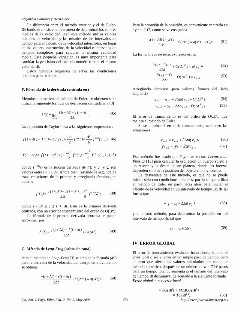
Alejandro González y Hernández
Lat. Am. J. Phys. Educ. Vol. 2, No. 2, May 2008 174 http://www.journal.lapen.org.mx
La diferencia entre el método anterior y el de Euler-Richardson consiste en la manera de determinar los valores medios de la velocidad. Así, este método utiliza valores iniciales de velocidad y las mitades de los intervalos de tiempo para el cálculo de la velocidad intermedia, en lugar de los valores intermedios de la velocidad e intervalos de tiempos completos para calcular la misma velocidad media. Esta pequeña variación es muy importante para cambiar la precisión del método numérico para el mismo valor de Δt.
Estos métodos requieren de saber las condiciones iniciales para su inicio.
F. Fórmula de la derivada centrada en t Métodos alternativos al método de Euler, se obtienen si se utiliza la siguiente fórmula de derivación centrada en t [3]
0
( ) ( )'( ) .
2limt
f t t f t tf t
tΔ →
+ Δ − − Δ=
Δ (45)
La expansión de Taylor lleva a las siguientes expresiones
2 3( 3 )t t
f ( t t ) f ( t ) tf '( t ) f "( t ) f ( ) ,2 6
Δ ΔΔ Δ ζ ++ = + + + 46)
2 3
( 3 )t tf ( t t ) f ( t ) tf '( t ) f "( t ) f ( ) ,
2 6
Δ ΔΔ Δ ζ −− = − + − (47)
donde f (3)(t) es la tercera derivada de f(t) y ζ+ y ζ- son valores entre t y t ± Δt. Ahora bien, restando la segunda de estas ecuaciones de la primera y arreglando términos, se obtiene
2( 3 )f ( t t ) f ( t t ) t
f '( t ) f ( ) ,2 t 6
Δ Δ Δ ζΔ
+ − −= − (48)
donde t - Δt ≤ ζ ≤ t + Δt. Esta es la primera derivada centrada, con un error de truncamiento del orden de O(Δt2).
La fórmula de la primera derivada centrada se puede aproximar por
2( ) ( )
'( ) ( ) .2
f t t f t tf t O t
t
+ Δ − − Δ= + Δ
Δ (49)
G. Método de Leap-Frog (saltos de rana) Para el método de Leap-Frog [3] se emplea la fórmula (49) para la derivada de la velocidad del cuerpo en movimiento, se obtiene
2( ) ( )( ) ( ( )) .
2
v t t v t tO t a v t
t
+ Δ − − Δ+ Δ =
Δ (50)
Para la ecuación de la posición, es conveniente centrarla en t y t + 2ΔT, como se ve enseguida
2y( t 2 t ) y( t )O( t ) a( v( t t )) .
2 t
Δ Δ ΔΔ
+ −+ = + (51)
La forma breve de estas expresiones, es
)v(a)t(Ot2
vvk
21k1k =Δ+Δ− −+ , (52)
1k2k2k v)t(O
t2
yy+
+ =Δ+Δ− . (53)
Arreglando términos para valores futuros del lado izquierdo )t(O)v(ta2vv 3
k1k1k Δ+Δ+= −+ , (54)
)t(Otv2yy 31kk2k Δ+Δ+= ++ . (55)
El error de truncamiento es del orden de O(Δt3), que mejora el método de Euler.
Si se elimina el error de truncamiento, se tienen las ecuaciones
)v(ta2vv k1k1k Δ+= −+ , (56)
1kk2k tv2yy ++ Δ+= . (57)
Este método fue usado por Feynman en sus Lectures on Physics [13] para calcular la oscilación un cuerpo sujeto a un resorte y la órbita de un planeta, donde las fuerzas dependen solo de la posición del objeto en movimiento.
La desventaja de este método, es que no se puede iniciar sólo con condiciones iniciales, por lo se que utiliza el método de Euler un paso hacia atrás para iniciar el cálculo de la velocidad en un intervalo de tiempo Δt, de tal forma que
)v(tavv 001 Δ−=− , (58)
y el mismo método, para determinar la posición en el intervalo de tiempo Δt, tal que
001 tvyy Δ+= . (59)
IV. ERROR GLOBAL El error de truncamiento, evaluado hasta ahora, ha sido el error local o sea el error en un simple paso de tiempo, pero el error que afecta los valores calculados por cualquier método numérico, después de un número de n = T/Δt pasos para un tiempo total T, aumenta si el tamaño del intervalo de tiempo Δt disminuye, de acuerdo a la siguiente fórmula Error global = n x error local = nO(Δti) = (T/Δt)O(Δtn) = TO(Δti-1). (60)
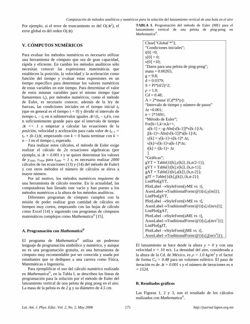
Comparación de métodos analíticos y numéricos para la solución del lanzamiento vertical de una bola en el aire
Lat. Am. J. Phys. Educ. Vol. 2, No. 2, May 2008 175 http://journal.lapen.org.mx
Por ejemplo, si el error de truncamiento es del O(Δt2), el error global es del orden O(Δt). V. CÓMPUTOS NUMÉRICOS Para evaluar los métodos numéricos es necesario utilizar una herramienta de cómputo que sea de gran capacidad, rápida y eficiente. En cambio los métodos analíticos sólo necesitan conocer las expresiones matemáticas que establecen la posición, la velocidad y la aceleración como función del tiempo y evaluar estas expresiones en un tiempo específico para determinar los valores numéricos de estas variables en este tiempo. Para determinar el valor de estos mismas variables para el mismo tiempo (que llamaremos tn), por métodos numéricos, como el método de Euler, es necesario conocer, además de la ley de fuerzas, las condiciones iniciales en el tiempo inicial t0 (que en general es el tiempo t = 0) y dividir el intervalo de tiempo tn – t0 en n subintervalos iguales Δt=(tn – t0)/n, con n suficientemente grande para que el intervalo de tiempo Δt << 1 y empezar a calcular las ecuaciones de la posición, velocidad y aceleración para cada valor de tk+1 = t0 + (k-1)Δt, empezando con k = 0 hasta terminar con k = n – 1 en el tiempo tn esperado.
Para realizar estos cálculos, el método de Euler exige realizar el cálculo de 2n ecuaciones algebraicas (por ejemplo, si Δt = 0.001 s y se quiere determinar los valores de y1000, v1000 para t1000 = 1 s, es necesario realizar 2000 cálculos de las ecuaciones (13) y (14) del método de Euler) y con otros métodos el número de cálculos se eleva a mayor número.
Por tal motivo, los métodos numéricos requieren de una herramienta de cálculo enorme. En la actualidad, las computadoras han llenado este vacío y han puesto a los métodos numéricos a la altura de los métodos analíticos.
Diferentes programas de cómputo cumplen con la misión de poder realizar gran cantidad de cálculos en tiempos muy cortos, empezando con las hojas de cálculo como Excel [14] y siguiendo con programas de cómputos matemáticos complejos como Mathematica® [15].
A. Programación con Mathematica® El programa de Mathematica® utiliza un poderoso lenguaje de programación simbólico y numérico, y aunque no es una programación gratuita, es una herramienta de cómputo muy recomendable por ser conocida y usada por estudiantes que se dediquen a una carrera como Física, Matemáticas o Ingeniería.
Para ejemplificar el uso del cálculo numérico realizado en Mathematica®, en la Tabla I, se describen las líneas de programación para la solución por el método de Euler del lanzamiento vertical de una pelota de ping pong en el aire. La masa de la pelota es de 2 g y su diámetro de 4.5 cm.
TABLA I. Programación del método de Euler (ME) para el lanzamiento vertical de una pelota de ping-pong en Mathematica®.
Clear["Global`*"]; "Condiciones iniciales"; t[0] =0; y[0] = 0; v[0] =10; "Datos para una pelota de ping-pong"; masa = 0.00265; g = 9.8; d = 0.0379; S = Pi*(d/2)^2; ρ = 1.0; Cd = 0.48; A = 2*masa/ (Cd*S*ρ); “Intervalo de tiempo y número de pasos” Δt =0.001; n = 2*1691; “Método de Euler”; For[k=1,k<n,k++, a[k-1] = -g-Abs[v[k-1]]*v[k-1]/A; j[k-1]=-Abs[v[k-1]]*a[k-1]/A; y[k] = y[k-1]+v[k-1]* Δt; v[k]=v[k-1]+a[k-1]*Δt; t[k] = t[k-1]+ Δt ] “Gráficas”; gYT = Table[{t[k],y[k]},{k,n/2-1}]; gVT = Table[{t[k],v[k]},{k,n-1}]; gAT = Table[{t[k],a[k]},{k,n-2}]; gJT = Table[{t[k],j[k]},{k,n-2}]; ListPlot[gYT, PlotLabel →StyleForm[yME vs t], AxesLabel→TraditionalForm/@{t[s],y[m]}]; ListPlot[gVT, PlotLabel →StyleForm[vME vs t], AxesLabel→TraditionalForm/@{t[s],v[m/s]}]; ListPlot[gAT, PlotLabel →StyleForm[aME vs t], AxesLabel→TraditionalForm/@{t[s],a[m/s2]}]; ListPlot[gJT, PlotLabel →StyleForm[jME vs t], AxesLabel→TraditionalForm/@{t[s],j[m/s3]}];
El lanzamiento se hace desde la altura y = 0 y con una velocidad v = 10 m/s. La densidad del aire, considerada a la altura de la Cd. de México, es ρ = 1.0 kg/m3 y el factor de forma Cd = 0.48 para un volumen esférico. El paso de iteración es de Δt = 0.001 s y el número de iteraciones es n = 1524.
B. Resultados gráficos Las Figuras 1, 2 y 3, son el resultado de los cálculos realizados con Mathematica®.
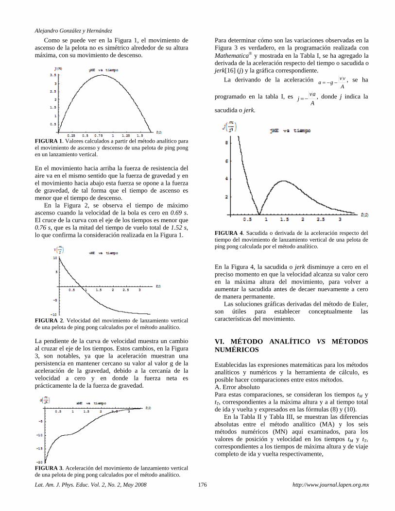
Alejandro González y Hernández
Lat. Am. J. Phys. Educ. Vol. 2, No. 2, May 2008 176 http://www.journal.lapen.org.mx
Como se puede ver en la Figura 1, el movimiento de ascenso de la pelota no es simétrico alrededor de su altura máxima, con su movimiento de descenso.
FIGURA 1. Valores calculados a partir del método analítico para el movimiento de ascenso y descenso de una pelota de ping pong en un lanzamiento vertical. En el movimiento hacia arriba la fuerza de resistencia del aire va en el mismo sentido que la fuerza de gravedad y en el movimiento hacia abajo esta fuerza se opone a la fuerza de gravedad, de tal forma que el tiempo de ascenso es menor que el tiempo de descenso.
En la Figura 2, se observa el tiempo de máximo ascenso cuando la velocidad de la bola es cero en 0.69 s. El cruce de la curva con el eje de los tiempos es menor que 0.76 s, que es la mitad del tiempo de vuelo total de 1.52 s, lo que confirma la consideración realizada en la Figura 1.
FIGURA 2. Velocidad del movimiento de lanzamiento vertical de una pelota de ping pong calculados por el método analítico. La pendiente de la curva de velocidad muestra un cambio al cruzar el eje de los tiempos. Estos cambios, en la Figura 3, son notables, ya que la aceleración muestran una persistencia en mantener cercano su valor al valor g de la aceleración de la gravedad, debido a la cercanía de la velocidad a cero y en donde la fuerza neta es prácticamente la de la fuerza de gravedad.
FIGURA 3. Aceleración del movimiento de lanzamiento vertical de una pelota de ping pong calculados por el método analítico.
Para determinar cómo son las variaciones observadas en la Figura 3 es verdadero, en la programación realizada con Mathematica® y mostrada en la Tabla I, se ha agregado la derivada de la aceleración respecto del tiempo o sacudida o jerk[16] (j) y la gráfica correspondiente.
La derivando de la aceleración A
vvga −−= , se ha
programado en la tabla I, es A
avj −= , donde j indica la
sacudida o jerk.
FIGURA 4. Sacudida o derivada de la aceleración respecto del tiempo del movimiento de lanzamiento vertical de una pelota de ping pong calculada por el método analítico. En la Figura 4, la sacudida o jerk disminuye a cero en el preciso momento en que la velocidad alcanza su valor cero en la máxima altura del movimiento, para volver a aumentar la sacudida antes de decaer nuevamente a cero de manera permanente.
Las soluciones gráficas derivadas del método de Euler, son útiles para establecer conceptualmente las características del movimiento. VI. MÉTODO ANALÍTICO VS MÉTODOS NUMÉRICOS Establecidas las expresiones matemáticas para los métodos analíticos y numéricos y la herramienta de cálculo, es posible hacer comparaciones entre estos métodos. A. Error absoluto Para estas comparaciones, se consideran los tiempos tM y tT, correspondientes a la máxima altura y a al tiempo total de ida y vuelta y expresados en las fórmulas (8) y (10).
En la Tabla II y Tabla III, se muestran las diferencias absolutas entre el método analítico (MA) y los seis métodos numéricos (MN) aquí examinados, para los valores de posición y velocidad en los tiempos tM y tT, correspondientes a los tiempos de máxima altura y de viaje completo de ida y vuelta respectivamente,
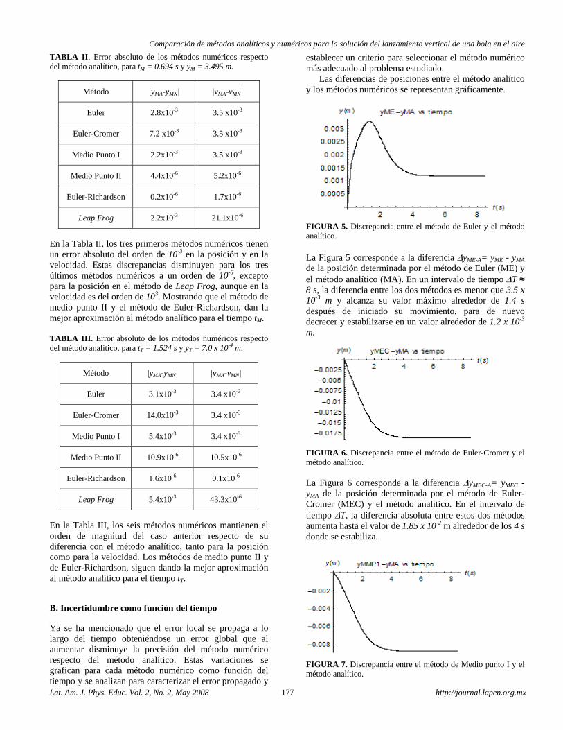
Comparación de métodos analíticos y numéricos para la solución del lanzamiento vertical de una bola en el aire
Lat. Am. J. Phys. Educ. Vol. 2, No. 2, May 2008 177 http://journal.lapen.org.mx
TABLA II. Error absoluto de los métodos numéricos respecto del método analítico, para tM = 0.694 s y yM = 3.495 m.
Método |yMA-yMN| |vMA-vMN|
Euler 2.8x10⁻³ 3.5 x10⁻³
Euler-Cromer 7.2 x10⁻³ 3.5 x10⁻³
Medio Punto I 2.2x10⁻³ 3.5 x10⁻³
Medio Punto II 4.4x10⁻⁶ 5.2x10⁻⁶
Euler-Richardson 0.2x10⁻⁶ 1.7x10⁻⁶
Leap Frog 2.2x10⁻³ 21.1x10⁻⁶
En la Tabla II, los tres primeros métodos numéricos tienen un error absoluto del orden de 10-3 en la posición y en la velocidad. Estas discrepancias disminuyen para los tres últimos métodos numéricos a un orden de 10-6, excepto para la posición en el método de Leap Frog, aunque en la velocidad es del orden de 103. Mostrando que el método de medio punto II y el método de Euler-Richardson, dan la mejor aproximación al método analítico para el tiempo tM. TABLA III. Error absoluto de los métodos numéricos respecto del método analítico, para tT = 1.524 s y yT = 7.0 x 10⁻⁴ m.
Método |yMA-yMN| |vMA-vMN|
Euler 3.1x10⁻³ 3.4 x10⁻³
Euler-Cromer 14.0x10⁻³ 3.4 x10⁻³
Medio Punto I 5.4x10⁻³ 3.4 x10⁻³
Medio Punto II 10.9x10⁻⁶ 10.5x10⁻⁶
Euler-Richardson 1.6x10⁻⁶ 0.1x10⁻⁶
Leap Frog 5.4x10⁻³ 43.3x10⁻⁶
En la Tabla III, los seis métodos numéricos mantienen el orden de magnitud del caso anterior respecto de su diferencia con el método analítico, tanto para la posición como para la velocidad. Los métodos de medio punto II y de Euler-Richardson, siguen dando la mejor aproximación al método analítico para el tiempo tT. B. Incertidumbre como función del tiempo Ya se ha mencionado que el error local se propaga a lo largo del tiempo obteniéndose un error global que al aumentar disminuye la precisión del método numérico respecto del método analítico. Estas variaciones se grafican para cada método numérico como función del tiempo y se analizan para caracterizar el error propagado y
establecer un criterio para seleccionar el método numérico más adecuado al problema estudiado.
Las diferencias de posiciones entre el método analítico y los métodos numéricos se representan gráficamente.
FIGURA 5. Discrepancia entre el método de Euler y el método analítico. La Figura 5 corresponde a la diferencia ΔyME-A= yME - yMA de la posición determinada por el método de Euler (ME) y el método analítico (MA). En un intervalo de tiempo ΔT ≈ 8 s, la diferencia entre los dos métodos es menor que 3.5 x 10⁻³ m y alcanza su valor máximo alrededor de 1.4 s después de iniciado su movimiento, para de nuevo decrecer y estabilizarse en un valor alrededor de 1.2 x 10⁻³ m.
FIGURA 6. Discrepancia entre el método de Euler-Cromer y el método analítico. La Figura 6 corresponde a la diferencia ΔyMEC-A= yMEC - yMA de la posición determinada por el método de Euler-Cromer (MEC) y el método analítico. En el intervalo de tiempo ΔT, la diferencia absoluta entre estos dos métodos aumenta hasta el valor de 1.85 x 10⁻² m alrededor de los 4 s donde se estabiliza.
FIGURA 7. Discrepancia entre el método de Medio punto I y el método analítico.
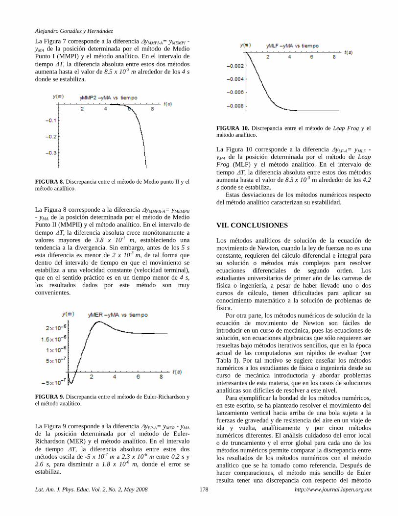
Alejandro González y Hernández
Lat. Am. J. Phys. Educ. Vol. 2, No. 2, May 2008 178 http://www.journal.lapen.org.mx
La Figura 7 corresponde a la diferencia ΔyMMPI-A= yMEMPI - yMA de la posición determinada por el método de Medio Punto I (MMPI) y el método analítico. En el intervalo de tiempo ΔT, la diferencia absoluta entre estos dos métodos aumenta hasta el valor de 8.5 x 10⁻³ m alrededor de los 4 s donde se estabiliza.
FIGURA 8. Discrepancia entre el método de Medio punto II y el método analítico. La Figura 8 corresponde a la diferencia ΔyMMPII-A= yMEMPII - yMA de la posición determinada por el método de Medio Punto II (MMPII) y el método analítico. En el intervalo de tiempo ΔT, la diferencia absoluta crece monótonamente a valores mayores de 3.8 x 10⁻¹ m, estableciendo una tendencia a la divergencia. Sin embargo, antes de los 5 s esta diferencia es menor de 2 x 10⁻³ m, de tal forma que dentro del intervalo de tiempo en que el movimiento se estabiliza a una velocidad constante (velocidad terminal), que en el sentido práctico es en un tiempo menor de 4 s, los resultados dados por este método son muy convenientes.
FIGURA 9. Discrepancia entre el método de Euler-Richardson y el método analítico. La Figura 9 corresponde a la diferencia ΔyER-A= yMER - yMA de la posición determinada por el método de Euler-Richardson (MER) y el método analítico. En el intervalo de tiempo ΔT, la diferencia absoluta entre estos dos métodos oscila de -5 x 10⁻⁷ m a 2.3 x 10⁻⁶ m entre 0.2 s y 2.6 s, para disminuir a 1.8 x 10⁻⁶ m, donde el error se estabiliza.
FIGURA 10. Discrepancia entre el método de Leap Frog y el método analítico. La Figura 10 corresponde a la diferencia ΔyLF-A= yMLF - yMA de la posición determinada por el método de Leap Frog (MLF) y el método analítico. En el intervalo de tiempo ΔT, la diferencia absoluta entre estos dos métodos aumenta hasta el valor de 8.5 x 10⁻³ m alrededor de los 4.2 s donde se estabiliza.
Estas desviaciones de los métodos numéricos respecto del método analítico caracterizan su estabilidad. VII. CONCLUSIONES Los métodos analíticos de solución de la ecuación de movimiento de Newton, cuando la ley de fuerzas no es una constante, requieren del cálculo diferencial e integral para su solución o métodos más complejos para resolver ecuaciones diferenciales de segundo orden. Los estudiantes universitarios de primer año de las carreras de física o ingeniería, a pesar de haber llevado uno o dos cursos de cálculo, tienen dificultades para aplicar su conocimiento matemático a la solución de problemas de física.
Por otra parte, los métodos numéricos de solución de la ecuación de movimiento de Newton son fáciles de introducir en un curso de mecánica, pues las ecuaciones de solución, son ecuaciones algebraicas que sólo requieren ser resueltas bajo métodos iterativos sencillos, que en la época actual de las computadoras son rápidos de evaluar (ver Tabla I). Por tal motivo se sugiere enseñar los métodos numéricos a los estudiantes de física o ingeniería desde su curso de mecánica introductoria y abordar problemas interesantes de esta materia, que en los casos de soluciones analíticas son difíciles de resolver a este nivel.
Para ejemplificar la bondad de los métodos numéricos, en este escrito, se ha planteado resolver el movimiento del lanzamiento vertical hacia arriba de una bola sujeta a la fuerzas de gravedad y de resistencia del aire en un viaje de ida y vuelta, analíticamente y por cinco métodos numéricos diferentes. El análisis cuidadoso del error local o de truncamiento y el error global para cada uno de los métodos numéricos permite comparar la discrepancia entre los resultados de los métodos numéricos con el método analítico que se ha tomado como referencia. Después de hacer comparaciones, el método más sencillo de Euler resulta tener una discrepancia con respecto del método
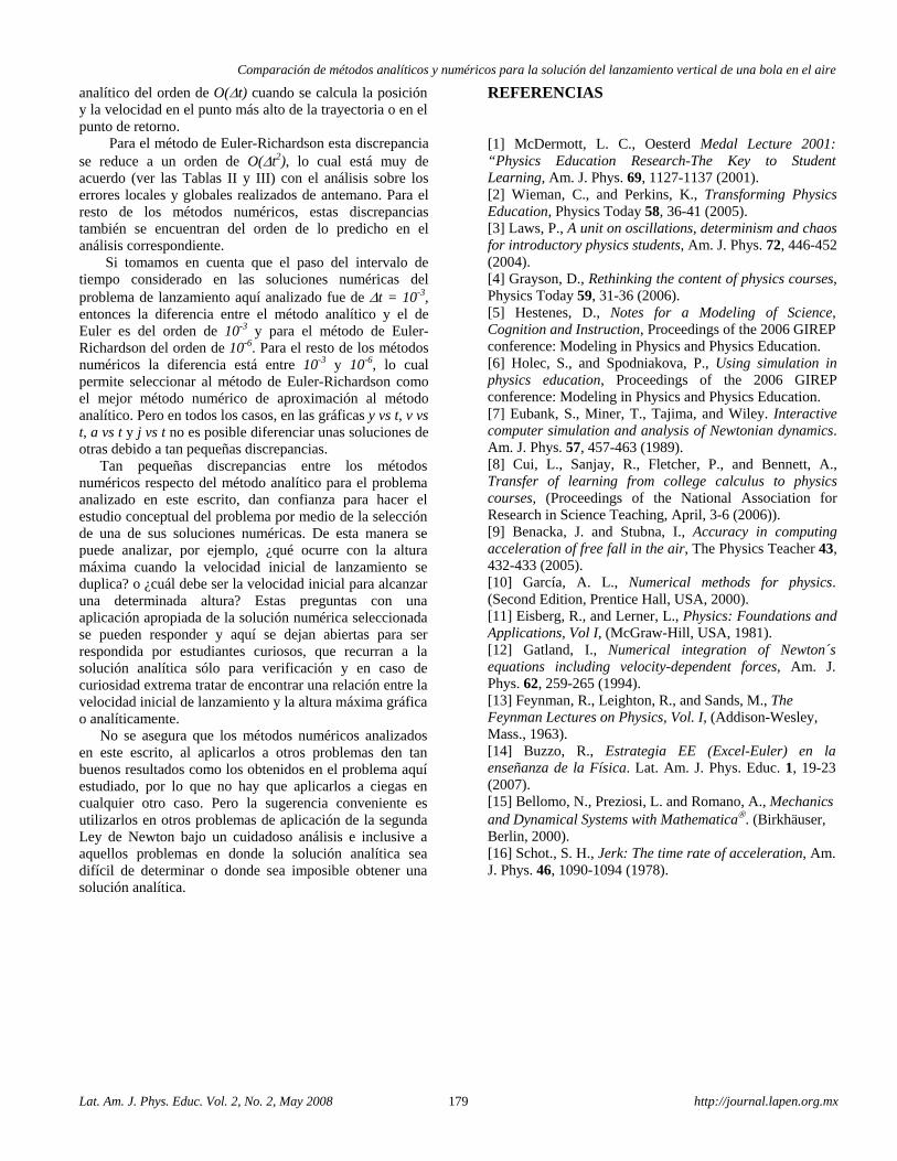
Comparación de métodos analíticos y numéricos para la solución del lanzamiento vertical de una bola en el aire
Lat. Am. J. Phys. Educ. Vol. 2, No. 2, May 2008 179 http://journal.lapen.org.mx
analítico del orden de O(Δt) cuando se calcula la posición y la velocidad en el punto más alto de la trayectoria o en el punto de retorno.
Para el método de Euler-Richardson esta discrepancia se reduce a un orden de O(Δt2), lo cual está muy de acuerdo (ver las Tablas II y III) con el análisis sobre los errores locales y globales realizados de antemano. Para el resto de los métodos numéricos, estas discrepancias también se encuentran del orden de lo predicho en el análisis correspondiente.
Si tomamos en cuenta que el paso del intervalo de tiempo considerado en las soluciones numéricas del problema de lanzamiento aquí analizado fue de Δt = 10-3, entonces la diferencia entre el método analítico y el de Euler es del orden de 10-3 y para el método de Euler-Richardson del orden de 10-6. Para el resto de los métodos numéricos la diferencia está entre 10-3 y 10-6, lo cual permite seleccionar al método de Euler-Richardson como el mejor método numérico de aproximación al método analítico. Pero en todos los casos, en las gráficas y vs t, v vs t, a vs t y j vs t no es posible diferenciar unas soluciones de otras debido a tan pequeñas discrepancias.
Tan pequeñas discrepancias entre los métodos numéricos respecto del método analítico para el problema analizado en este escrito, dan confianza para hacer el estudio conceptual del problema por medio de la selección de una de sus soluciones numéricas. De esta manera se puede analizar, por ejemplo, ¿qué ocurre con la altura máxima cuando la velocidad inicial de lanzamiento se duplica? o ¿cuál debe ser la velocidad inicial para alcanzar una determinada altura? Estas preguntas con una aplicación apropiada de la solución numérica seleccionada se pueden responder y aquí se dejan abiertas para ser respondida por estudiantes curiosos, que recurran a la solución analítica sólo para verificación y en caso de curiosidad extrema tratar de encontrar una relación entre la velocidad inicial de lanzamiento y la altura máxima gráfica o analíticamente.
No se asegura que los métodos numéricos analizados en este escrito, al aplicarlos a otros problemas den tan buenos resultados como los obtenidos en el problema aquí estudiado, por lo que no hay que aplicarlos a ciegas en cualquier otro caso. Pero la sugerencia conveniente es utilizarlos en otros problemas de aplicación de la segunda Ley de Newton bajo un cuidadoso análisis e inclusive a aquellos problemas en donde la solución analítica sea difícil de determinar o donde sea imposible obtener una solución analítica.
REFERENCIAS [1] McDermott, L. C., Oesterd Medal Lecture 2001: “Physics Education Research-The Key to Student Learning, Am. J. Phys. 69, 1127-1137 (2001). [2] Wieman, C., and Perkins, K., Transforming Physics Education, Physics Today 58, 36-41 (2005). [3] Laws, P., A unit on oscillations, determinism and chaos for introductory physics students, Am. J. Phys. 72, 446-452 (2004). [4] Grayson, D., Rethinking the content of physics courses, Physics Today 59, 31-36 (2006). [5] Hestenes, D., Notes for a Modeling of Science, Cognition and Instruction, Proceedings of the 2006 GIREP conference: Modeling in Physics and Physics Education. [6] Holec, S., and Spodniakova, P., Using simulation in physics education, Proceedings of the 2006 GIREP conference: Modeling in Physics and Physics Education. [7] Eubank, S., Miner, T., Tajima, and Wiley. Interactive computer simulation and analysis of Newtonian dynamics. Am. J. Phys. 57, 457-463 (1989). [8] Cui, L., Sanjay, R., Fletcher, P., and Bennett, A., Transfer of learning from college calculus to physics courses, (Proceedings of the National Association for Research in Science Teaching, April, 3-6 (2006)). [9] Benacka, J. and Stubna, I., Accuracy in computing acceleration of free fall in the air, The Physics Teacher 43, 432-433 (2005). [10] García, A. L., Numerical methods for physics. (Second Edition, Prentice Hall, USA, 2000). [11] Eisberg, R., and Lerner, L., Physics: Foundations and Applications, Vol I, (McGraw-Hill, USA, 1981). [12] Gatland, I., Numerical integration of Newton´s equations including velocity-dependent forces, Am. J. Phys. 62, 259-265 (1994). [13] Feynman, R., Leighton, R., and Sands, M., The Feynman Lectures on Physics, Vol. I, (Addison-Wesley, Mass., 1963). [14] Buzzo, R., Estrategia EE (Excel-Euler) en la enseñanza de la Física. Lat. Am. J. Phys. Educ. 1, 19-23 (2007). [15] Bellomo, N., Preziosi, L. and Romano, A., Mechanics and Dynamical Systems with Mathematica®. (Birkhäuser, Berlin, 2000). [16] Schot., S. H., Jerk: The time rate of acceleration, Am. J. Phys. 46, 1090-1094 (1978).
Lat. Am. J. Phys. Educ. Vol.2, No. 2, May 2008 180 http://www.journal.lapen.org.mx
Deducción de los primeros modelos cosmológicos
César Mora Centro de Investigación en Ciencia Aplicada y Tecnología Avanzada del Instituto Politécnico Nacional, Av. Legaria 694, Col. Irrigación, Del. Miguel Hidalgo, C. P. 11500, México D. F. E-mail: [email protected] (Recibido el 16 de Enero de 2008; aceptado el 3 de Abril de 2008)
Resumen Este artículo describe cómo se han fundamentado algunos de los primeros modelos cosmológicos clásicos, también discutimos los errores que aún persisten en la actualidad en algunos libros de texto básicos y avanzados. Discutimos los rudimentos de la cosmología Newtoniana y su conexión con la relatividad general. Palabras clave: Modelos cosmológicos, dinámica del Universo, cosmología Newtoniana.
Abstract This paper describes some formulations of the first classical cosmological models, also we discuss mistakes which nowadays are present in basic and advanced text books. We discuss the fundamentals of Newtonian cosmology and its connection with general relativity. Keywords: Cosmological models, dynamics of the Universe. PACS: 01.55.+b, 01.30.-y, 95.10.-a, 98.80.-k ISSN 1870-9095
I. INTRODUCCIÓN Los temas relacionados con el origen del universo son de actualidad en la física teórica [1] y también son de interés pedagógico [2]. En los últimos años se han realizado algunos estudios sobre cosmología básica para estudiantes preuniversitarios con el fin de proporcionar las herramientas básicas para comprender la descripción clásica y cuántica de nuestro universo [3, 4, 5, 6]. La cosmología Newtoniana se deriva de la dinámica, la gravitación y el principio cosmológico, esto es, que el Universo sea homogéneo e isotrópico, y puede reproducir los modelos cosmológicos de la relatividad general y los modelos evolutivos del big-bang. La descripción del Universo en expansión fue introducido por Milne y McCrea en 1934 [7], y aplicaron la gravedad Newtoniana a una distribución esférica uniforme de masa, ignorando la masa en el exterior de la esfera con el supuesto de que también es una distribución esférica y que se anula al permitir que el radio de la esfera llegue a ser arbitrariamente muy grande. Luego, utilizaron el principio de equivalencia, estableciendo que las fuerzas gravitacionales y de inercia producen efectos indistinguibles, y se requiere para que este Universo sea conforme con el principio cosmológico, pero esto lleva el análisis a la relatividad general. En este artículo consideramos la deducción de la cosmología Newtoniana realizada por Lemons [8] quien ha señalado que la cosmología Newtoniana estándar realmente es no Newtoniana. En su deducción utiliza el principio dado por Newton del sistema de referencia de las estrellas fijas,
estando distribuidas uniformemente en todos los puntos del cielo, cancelando sus tirones con las atracciones opuestas. El cual es un argumento de simetría. Newton creía que el Universo era estacionario pero también infinito y uniforme. El desarrollo de Lemons muestra que la cosmología de Newton lleva a modelos evolutivos y que describen al Universo en curso en equilibrio neutro.
Una consecuencia interesante del principio de simetría de Newton en la cosmología Newtoniana es que se requiere de la introducción de un término cosmológico para la ecuación de campo clásico de la gravedad, esto en contraste con la constante cosmológica introducida por Einsten.
El artículo está organizado como sigue, el la sección II
mostramos los rudimentos físicos para modelar matemáticamente nuestro Universo, se muestra el modelo cosmológico de Einstein, el de De Sitter y el de Friedmann, en la sección III mencionamos algunos errores sobre la deducción de los primeros modelos cosmológicos, en la sección IV tratamos sobre la fundamentación de la cosmología Newtoniana, y finalmente en la sección V mostramos nuestras conclusiones. II. MODELANDO EL UNIVERSO Para describir el Universo en el que vivimos tenemos que enfocaremos a la distribución de la materia a gran escala y al movimiento de la misma. Para ello, se considera una
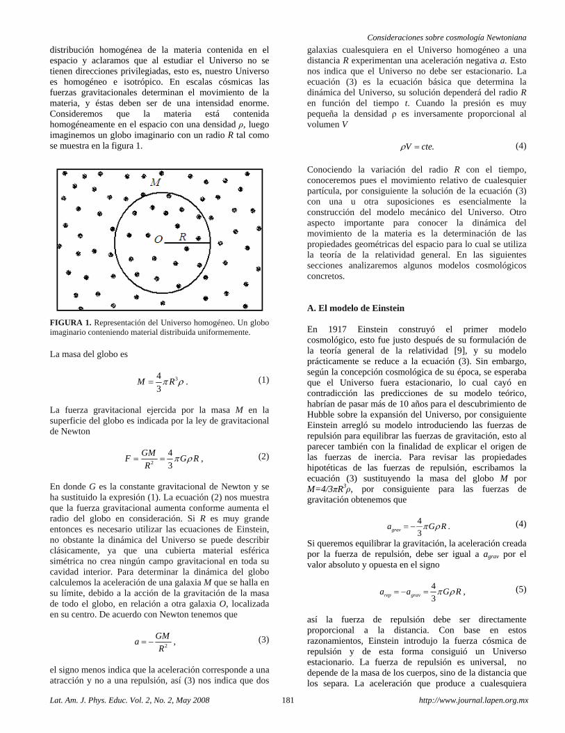
Consideraciones sobre cosmología Newtoniana
Lat. Am. J. Phys. Educ. Vol. 2, No. 2, May 2008 181 http://www.journal.lapen.org.mx
distribución homogénea de la materia contenida en el espacio y aclaramos que al estudiar el Universo no se tienen direcciones privilegiadas, esto es, nuestro Universo es homogéneo e isotrópico. En escalas cósmicas las fuerzas gravitacionales determinan el movimiento de la materia, y éstas deben ser de una intensidad enorme. Consideremos que la materia está contenida homogéneamente en el espacio con una densidad ρ, luego imaginemos un globo imaginario con un radio R tal como se muestra en la figura 1.
FIGURA 1. Representación del Universo homogéneo. Un globo imaginario conteniendo material distribuida uniformemente.
La masa del globo es
34.
3M Rπ ρ= (1)
La fuerza gravitacional ejercida por la masa M en la superficie del globo es indicada por la ley de gravitacional de Newton
2
4,
3
GMF G R
Rπ ρ= = (2)
En donde G es la constante gravitacional de Newton y se ha sustituido la expresión (1). La ecuación (2) nos muestra que la fuerza gravitacional aumenta conforme aumenta el radio del globo en consideración. Si R es muy grande entonces es necesario utilizar las ecuaciones de Einstein, no obstante la dinámica del Universo se puede describir clásicamente, ya que una cubierta material esférica simétrica no crea ningún campo gravitacional en toda su cavidad interior. Para determinar la dinámica del globo calculemos la aceleración de una galaxia M que se halla en su límite, debido a la acción de la gravitación de la masa de todo el globo, en relación a otra galaxia O, localizada en su centro. De acuerdo con Newton tenemos que
2,
GMa
R= − (3)
el signo menos indica que la aceleración corresponde a una atracción y no a una repulsión, así (3) nos indica que dos
galaxias cualesquiera en el Universo homogéneo a una distancia R experimentan una aceleración negativa a. Esto nos indica que el Universo no debe ser estacionario. La ecuación (3) es la ecuación básica que determina la dinámica del Universo, su solución dependerá del radio R en función del tiempo t. Cuando la presión es muy pequeña la densidad ρ es inversamente proporcional al volumen V
.V cteρ = (4)
Conociendo la variación del radio R con el tiempo, conoceremos pues el movimiento relativo de cualesquier partícula, por consiguiente la solución de la ecuación (3) con una u otra suposiciones es esencialmente la construcción del modelo mecánico del Universo. Otro aspecto importante para conocer la dinámica del movimiento de la materia es la determinación de las propiedades geométricas del espacio para lo cual se utiliza la teoría de la relatividad general. En las siguientes secciones analizaremos algunos modelos cosmológicos concretos. A. El modelo de Einstein
En 1917 Einstein construyó el primer modelo cosmológico, esto fue justo después de su formulación de la teoría general de la relatividad [9], y su modelo prácticamente se reduce a la ecuación (3). Sin embargo, según la concepción cosmológica de su época, se esperaba que el Universo fuera estacionario, lo cual cayó en contradicción las predicciones de su modelo teórico, habrían de pasar más de 10 años para el descubrimiento de Hubble sobre la expansión del Universo, por consiguiente Einstein arregló su modelo introduciendo las fuerzas de repulsión para equilibrar las fuerzas de gravitación, esto al parecer también con la finalidad de explicar el origen de las fuerzas de inercia. Para revisar las propiedades hipotéticas de las fuerzas de repulsión, escribamos la ecuación (3) sustituyendo la masa del globo M por M=4/3πR3ρ, por consiguiente para las fuerzas de gravitación obtenemos que
4.
3grava G Rπ ρ= − (4)
Si queremos equilibrar la gravitación, la aceleración creada por la fuerza de repulsión, debe ser igual a agrav por el valor absoluto y opuesta en el signo
4,
3rep grava a G Rπ ρ= − = (5)
así la fuerza de repulsión debe ser directamente proporcional a la distancia. Con base en estos razonamientos, Einstein introdujo la fuerza cósmica de repulsión y de esta forma consiguió un Universo estacionario. La fuerza de repulsión es universal, no depende de la masa de los cuerpos, sino de la distancia que los separa. La aceleración que produce a cualesquiera
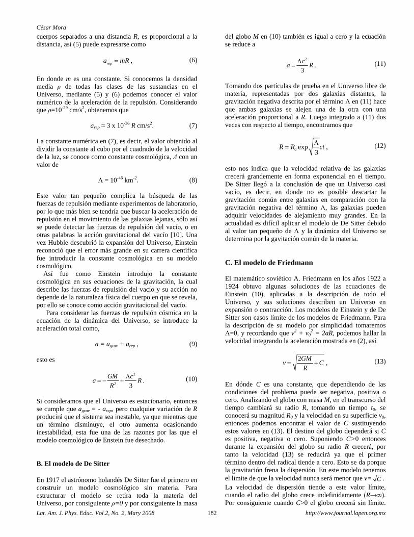
César Mora
Lat. Am. J. Phys. Educ. Vol.2, No. 2, Mary 2008 182 http://www.journal.lapen.org.mx
cuerpos separados a una distancia R, es proporcional a la distancia, así (5) puede expresarse como
,repa mR= (6)
En donde m es una constante. Si conocemos la densidad media ρ de todas las clases de las sustancias en el Universo, mediante (5) y (6) podemos conocer el valor numérico de la aceleración de la repulsión. Considerando que ρ=10-29 cm/s2, obtenemos que
arep ≈ 3 x 10-36 R cm/s2. (7) La constante numérica en (7), es decir, el valor obtenido al dividir la constante al cubo por el cuadrado de la velocidad de la luz, se conoce como constante cosmológica, Λ con un valor de
Λ = 10-46 km-2. (8) Este valor tan pequeño complica la búsqueda de las fuerzas de repulsión mediante experimentos de laboratorio, por lo que más bien se tendría que buscar la aceleración de repulsión en el movimiento de las galaxias lejanas, sólo así se puede detectar las fuerzas de repulsión del vacío, o en otras palabras la acción gravitacional del vacío [10]. Una vez Hubble descubrió la expansión del Universo, Einstein reconoció que el error más grande en su carrera científica fue introducir la constante cosmológica en su modelo cosmológico. Así fue como Einstein introdujo la constante cosmológica en sus ecuaciones de la gravitación, la cual describe las fuerzas de repulsión del vacío y su acción no depende de la naturaleza física del cuerpo en que se revela, por ello se conoce como acción gravitacional del vacío.
Para considerar las fuerzas de repulsión cósmica en la ecuación de la dinámica del Universo, se introduce la aceleración total como,
a = agrav + arep , (9) esto es
2
2.
3
GM ca R
R
Λ= − + (10)
Si consideramos que el Universo es estacionario, entonces se cumple que agrav = - arep, pero cualquier variación de R producirá que el sistema sea inestable, ya que mientras que un término disminuye, el otro aumenta ocasionando inestabilidad, esta fue una de las razones por las que el modelo cosmológico de Enstein fue desechado. B. El modelo de De Sitter En 1917 el astrónomo holandés De Sitter fue el primero en construir un modelo cosmológico sin materia. Para estructurar el modelo se retira toda la materia del Universo, por consiguiente ρ=0 y por consiguiente la masa
del globo M en (10) también es igual a cero y la ecuación se reduce a
2
.3
ca R
Λ= (11)
Tomando dos partículas de prueba en el Universo libre de materia, representadas por dos galaxias distantes, la gravitación negativa descrita por el término Λ en (11) hace que ambas galaxias se alejen una de la otra con una aceleración proporcional a R. Luego integrado a (11) dos veces con respecto al tiempo, encontramos que
0 exp ,3
R R ctΛ
= (12)
esto nos indica que la velocidad relativa de las galaxias crecerá grandemente en forma exponencial en el tiempo. De Sitter llegó a la conclusión de que un Universo casi vacío, es decir, en donde no es posible descartar la gravitación común entre galaxias en comparación con la gravitación negativa del término Λ, las galaxias pueden adquirir velocidades de alejamiento muy grandes. En la actualidad es difícil aplicar el modelo de De Sitter debido al valor tan pequeño de Λ y la dinámica del Universo se determina por la gavitación común de la materia. C. El modelo de Friedmann El matemático soviético A. Friedmann en los años 1922 a 1924 obtuvo algunas soluciones de las ecuaciones de Einstein (10), aplicadas a la descripción de todo el Universo, y sus soluciones describen un Universo en expansión o contracción. Los modelos de Einstein y de De Sitter son casos límite de los modelos de Friedmann. Para la descripción de su modelo por simplicidad tomaremos Λ=0, y recordando que v2 + v0
2 = 2aR, podemos hallar la velocidad integrando la aceleración mostrada en (2), así
2,
GMv C
R= + (13)
En dónde C es una constante, que dependiendo de las condiciones del problema puede ser negativa, positiva o cero. Analizando el globo con masa M, en el transcurso del tiempo cambiará su radio R, tomando un tiempo t0, se conocerá su magnitud R0 y la velocidad en su superficie v0, entonces podemos encontrar el valor de C sustituyendo estos valores en (13). El destino del globo dependerá si C es positiva, negativa o cero. Suponiendo C>0 entonces durante la expansión del globo su radio R crecerá, por tanto la velocidad (13) se reducirá ya que el primer término dentro del radical tiende a cero. Esto se da porque la gravitación frena la dispersión. En este modelo tenemos el límite de que la velocidad nunca será menor que v= C . La velocidad de dispersión tiende a este valor límite, cuando el radio del globo crece indefinidamente (R→∞). Por consiguiente cuando C>0 el globo crecerá sin límite.
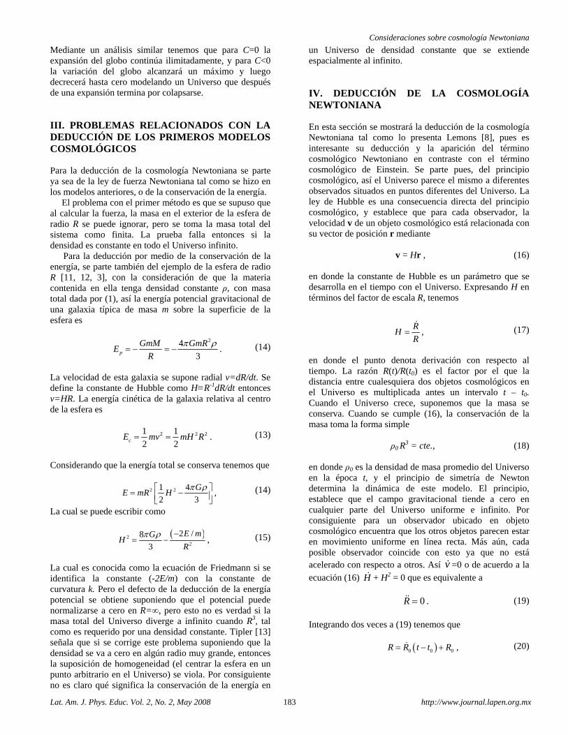
Consideraciones sobre cosmología Newtoniana
Lat. Am. J. Phys. Educ. Vol. 2, No. 2, May 2008 183 http://www.journal.lapen.org.mx
Mediante un análisis similar tenemos que para C=0 la expansión del globo continúa ilimitadamente, y para C<0 la variación del globo alcanzará un máximo y luego decrecerá hasta cero modelando un Universo que después de una expansión termina por colapsarse. III. PROBLEMAS RELACIONADOS CON LA DEDUCCIÓN DE LOS PRIMEROS MODELOS COSMOLÓGICOS Para la deducción de la cosmología Newtoniana se parte ya sea de la ley de fuerza Newtoniana tal como se hizo en los modelos anteriores, o de la conservación de la energía. El problema con el primer método es que se supuso que al calcular la fuerza, la masa en el exterior de la esfera de radio R se puede ignorar, pero se toma la masa total del sistema como finita. La prueba falla entonces si la densidad es constante en todo el Universo infinito.
Para la deducción por medio de la conservación de la energía, se parte también del ejemplo de la esfera de radio R [11, 12, 3], con la consideración de que la materia contenida en ella tenga densidad constante ρ, con masa total dada por (1), así la energía potencial gravitacional de una galaxia típica de masa m sobre la superficie de la esfera es
24.
3p
GmM GmRE
R
π ρ= − = − (14)
La velocidad de esta galaxia se supone radial v=dR/dt. Se define la constante de Hubble como H≡R-1dR/dt entonces v=HR. La energía cinética de la galaxia relativa al centro de la esfera es
2 2 21 1.
2 2cE mv mH R= = (13)
Considerando que la energía total se conserva tenemos que
2 21 4,
2 3
GE mR H
π ρ⎡ ⎤= −⎢ ⎥⎣ ⎦ (14)
La cual se puede escribir como
( )22
2 /8,
3
E mGH
R
π ρ −= − (15)
La cual es conocida como la ecuación de Friedmann si se identifica la constante (-2E/m) con la constante de curvatura k. Pero el defecto de la deducción de la energía potencial se obtiene suponiendo que el potencial puede normalizarse a cero en R=∞, pero esto no es verdad si la masa total del Universo diverge a infinito cuando R3, tal como es requerido por una densidad constante. Tipler [13] señala que si se corrige este problema suponiendo que la densidad se va a cero en algún radio muy grande, entonces la suposición de homogeneidad (el centrar la esfera en un punto arbitrario en el Universo) se viola. Por consiguiente no es claro qué significa la conservación de la energía en
un Universo de densidad constante que se extiende espacialmente al infinito. IV. DEDUCCIÓN DE LA COSMOLOGÍA NEWTONIANA En esta sección se mostrará la deducción de la cosmología Newtoniana tal como lo presenta Lemons [8], pues es interesante su deducción y la aparición del término cosmológico Newtoniano en contraste con el término cosmológico de Einstein. Se parte pues, del principio cosmológico, así el Universo parece el mismo a diferentes observados situados en puntos diferentes del Universo. La ley de Hubble es una consecuencia directa del principio cosmológico, y establece que para cada observador, la velocidad v de un objeto cosmológico está relacionada con su vector de posición r mediante
v = Hr , (16) en donde la constante de Hubble es un parámetro que se desarrolla en el tiempo con el Universo. Expresando H en términos del factor de escala R, tenemos
,R
HR
= (17)
en donde el punto denota derivación con respecto al tiempo. La razón R(t)/R(t0) es el factor por el que la distancia entre cualesquiera dos objetos cosmológicos en el Universo es multiplicada antes un intervalo t – t0. Cuando el Universo crece, suponemos que la masa se conserva. Cuando se cumple (16), la conservación de la masa toma la forma simple
ρ0 R3 = cte., (18)
en donde ρ0 es la densidad de masa promedio del Universo en la época t, y el principio de simetría de Newton determina la dinámica de este modelo. El principio, establece que el campo gravitacional tiende a cero en cualquier parte del Universo uniforme e infinito. Por consiguiente para un observador ubicado en objeto cosmológico encuentra que los otros objetos parecen estar en movimiento uniforme en línea recta. Más aún, cada posible observador coincide con esto ya que no está acelerado con respecto a otros. Así v =0 o de acuerdo a la
ecuación (16) H + H2 = 0 que es equivalente a
0 .R = (19)
Integrando dos veces a (19) tenemos que
( )0 0 0 ,R R t t R= − + (20)
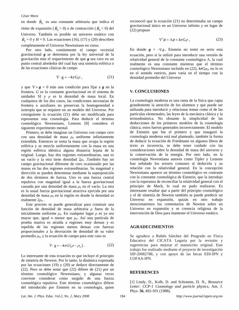
César Mora
Lat. Am. J. Phys. Educ. Vol.2, No. 2, Mary 2008 184 http://www.journal.lapen.org.mx
en donde 0R es una constante arbitraria que indica el
ritmo de expansión (0R > 0) o de contracción (
0R < 0) del
Universo. También es posible un universo estático con
0R = 0 y H = 0. Las ecuaciones (16), (17) y (20) describen
completamente el Universo Newtoniano en curso. Por otro lado, comúnmente el campo vectorial gravitacional g se determina por la ley universal de la gravitación más el requerimiento de que g sea cero en un punto central alrededor del cual hay una simetría esférica o de las ecuaciones clásicas de campo
g 4 ,Gπ ρ∇ ⋅ = − (21)
y que ∇× g = 0 más una condición para fijar a g en la frontera. G es la constante gravitacional en el sistema de unidades SI y ρ es la densidad de masa local. En cualquiera de los dos casos, las condiciones necesarias de frontera o auxiliares no preservan la homogeneidad e isotropía que se requiere en un modelo del Universo. Por consiguiente la ecuación (21) debe ser modificada para representar esta cosmología. Para deducir el término cosmológico Newtoniano, Lemons [8] considera el siguiente experimento mental. Primero, se debe imaginar un Universo con campo cero con una densidad de masa ρ0 uniforme infinitamente extendida. Entonces se toma la masa que ocupa la región esférica y se mezcla uniformemente con la masa en una región esférica idéntica alguna distancia lejana de la original. Luego, hay dos regiones extraordinarias, una es un vacío y la otra tiene densidad 2ρ0 .También hay un campo gravitacional diferente de cero ocasionado por las masas en las dos regiones extraordinarias. Su magnitud y dirección se pueden determinar mediante la superposición de dos términos de fuerza. Uno es una fuerza central repulsiva con magnitud igual a la fuerza gravitacional causada por una densidad de masa ρ0 en el vacío. La otra es la usual fuerza gravitacional atractiva ejercida por una densidad de masa ρ0 en la región en donde la densidad es realmente 2ρ0 . Este proceso se puede generalizar para construir una función de densidad de masa arbitraria ρ fuera de la inicialmente uniforme ρ0. En cualquier lugar ρ es ya sea mayor que, igual o menor que ρ0. Así una partícula de prueba masiva es atraída a regiones muy densas y es repelida de las regiones menos densas con fuerzas proporcionales a la desviación de densidad de su valor promedio ρ0, y la ecuación de campo para este caso es
( )0g 4 .Gπ ρ ρ∇ ⋅ = − − (22)
Lo interesante de esta ecuación es que incluye el principio de simetría de Newton. Por lo tanto, la dinámica expresada por las ecuaciones (19) y (20) se deduce directamente de (22). Pero se debe notar que (22) difiere de (21) por un término cosmológico Newtoniano, y algunas veces conviene considerar como surgido de una fuerza cosmológica repulsiva. Este término cosmológico difiere del introducido por Einstein en su cosmología, quien
reconoció que la ecuación (21) no determinaba un campo gravitacional único en un Universo infinito y en lugar de (22) propuso
2 4 ,Gφ φ π ρ∇ = Λ + (23)
En donde g = - φ∇ . Einstein no tomó en serio esta
ecuación, pero si la utilizó para introducir una versión de relatividad general de la constante cosmológica Λ, la cual realmente es una constante mientras que el término cosmológico Newtoniano incluido en (22), 4πGρ0, no lo es en el sentido estricto, pues varía en el tiempo con la densidad promedio del Universo V. CONCLUSIONES La cosmología moderna es una rama de la física que capta grandemente la atención de los alumnos y que puede ser utilizada para introducir y relacionar temas como el de las partículas elementales, las leyes de la mecánica clásica y la termodinámica. No obstante la simplicidad de las deducciones de los primeros modelos de la cosmología clásica, estos fueron generados incorrectamente. El modelo de Einstein que fue el primero y que inauguró la cosmología moderna está mal planteado, también la forma de deducir la ecuación de Friedmann en algunos libros de texto es incorrecta, se debe tener cuidado con las consideraciones sobre la densidad de masa del universo y la conservación de la energía. Por otro lado, en la cosmología Newtoniana autores como Tipler y Lemons han señalado los errores comunes al deducirla y su relación con la relatividad general. En la concepción Newtoniana aparece un término cosmológico en contraste con la constante cosmológica de Einstein, que la introdujo con la esperanza de reconciliar la relatividad general con el principio de Mach, lo cual no pudo realizarse. Es interesante resaltar que a partir del principio cosmológico y el de simetría de Newton también se puede predecir un Universo en expansión, quizás en otro trabajo mencionaremos los comentarios de Newton sobre un Universo en expansión y se creencia religiosa de la intervención de Dios para mantener el Universo estático. AGRADECIMIENTOS Se agradece a Rubén Sánchez del Posgrado en Física Educativa del CICATA Legaria por la revisión y sugerencias para mejorar el manuscrito original. Este trabajo fue realizado mediante el proyecto de investigación SIP-20082788, y con apoyo de las becas EDI-IPN y COFAA-IPN. REFERENCES [1] Lindy, D., Kolb, D. and Schramm, D. N., Resource Letter: CCP-1 Cosmology and particle physics, Am. J. Phys. 56, 492-501 (1988).

Consideraciones sobre cosmología Newtoniana
Lat. Am. J. Phys. Educ. Vol. 2, No. 2, May 2008 185 http://www.journal.lapen.org.mx
[2] AAPT, American Association of Physics Teachers statement on the teaching of evolution and cosmology, Am. J. Phys. 68, 11 (2000). [3] García-Salcedo, R. y Moreno C., Descripción de la evolución del Universo: una presentación para alumnos preuniversitarios, Lat. Am. J. Phys. Educ. 1, 95-100 (2007). [4] Jordan, T. F., Cosmology calculations almost without general relativity, Am. J. Phys. 73, 653-662 (2005). [5] Akridge, R., A simple cosmology: General relativity not required, Am. J. Phys. 69, 195-200 (2001). [6] Sales, J. A., Note on solving for the dynamics of the Universe, Am. J. Phys. 69, 1245-1247 (2001). [7] McCrea, W. H. and Milne, E. A., Q. J. Math. 5, 73 (1934).
[8] Lemons, D. S., A Newtonian cosmology Newton World understand, Am. J. Phys. 56, 502-504 (1998). [9] Einstein, A., “Cosmological Considerations on the General Theory of Relativity”, in The Principle of Relativity, edited by Sommerfeld, A. (Dover, New York, 1923) pp. 175-188. [10] Novikov, I., Cómo explotó el Universo, (Editorial Mir, Moscú, 1990). [11] Weinberg, S., The First Three Minutes: A Modern View of the Origin of the Universe, (Fontana/Collins, Glasgow, 1977). [12] Silk, J., The Big Bang: The Creation and Evolution of The Universe, (Freeman, San Francisco, 1980). [13] Tipler, F. J., Rigorous Newtonian cosmology, Am. J. Phys. 64, 1311-1315 (1996).
Lat. Am. J. Phys. Educ. Vol. 2, No. 2, May 2008 186 http://www.journal.lapen.org.mx
Geometría de equilibrio de estructuras en arco
Emilio Cortés Departamento de Física, Universidad Autónoma Metropolitana, Iztapalapa Apdo. Postal 55-534, México D.F., 09340 México
E-mail: [email protected]
(Recibido el 29 de Febrero de 2008; aceptado el 31 de Marzo de 2008)
Resumen El estudio de la estática de cuerpos continuos es un tópico que cobra especial interés cuando la geometría juega un papel crucial y la solución intuitiva no se da en forma evidente. En este trabajo se analizan estructuras de arco en una dimensión, o eje curvo, cuando se someten a su propio peso o bien a una cierta carga dada. Se parte de los principios fundamentales del equilibrio de fuerzas y se obtienen fórmulas generales para el cálculo de momentos (torcas) flexionantes así como fuerzas cortantes y de compresión, para estructuras con geometrías específicas. Por otro lado, se plantea el problema de encontrar la forma geométrica del arco que lleve al equilibrio de la estructura, bajo las condiciones de carga elegidas. Este estudio, que puede ubicarse dentro de la física aplicada, no pretende tener una cobertura ni un enfoque ingenieril de las estructuras en arco. Consideramos que este trabajo aporta varios elementos didácticos sobre principios físicos fundamentales que, traducidos al lenguaje del análisis vectorial y del cálculo, nos llevan a resultados físicos y geométricos interesantes, tanto por su aplicación como por su posible contribución al mejor entendimiento de los conceptos y la herramienta de análisis empleados. Palabras clave: Física educativa, enseñanza de la mecánica, equilibrio y geometría.
Abstract The study of statics of continuous bodies kindles special interest when the geometry plays a crucial role and the intuitive guess is not very evident. Here we analyze arc structures in one dimension, or curve axis, when they are subjected to its own weight or to a certain given load. We start from the fundamental principles of equilibrium of forces and obtain general expressions for the bending moments (torques) as well as shear and compression forces in the structures. In the other hand, we go to the problem of how to find the arc geometry which yields equilibrium, under prescribed conditions. This study which can belong to applied physics, does not intend to have an engineering point of view neither a broad coverage, about the arc structures. We consider that this work contains didactic elements of fundamental physical principles, which, translated to the language of vector analysis and calculus, brings us to physical and geometric results that can be interesting both, for its applications as well as for its possible contribution to the understanding of concepts and analysis used. Keywords: Educational physics, mechanics teaching, equilibrium and geometry. PACS: 01.40.-d, 01.40.Fk, 01.40.Jp, 01.55. +b.
I. INTRODUCCIÓN
El arco es un elemento estructural en la arquitectura y en la ingeniería civil, que lleva a cabo como funciones cubrir claros, soportar cargas, así como constituir un elemento estético. Una amplia gama de formas geométricas de arcos han sido construidos desde la antigüedad [1]. Los romanos usaron el arco semicircular en puentes, acueductos y arquitectura de gran escala; este tipo de arco consistía en la unión de bloques de tabique o piedra, dispuestos en forma circular. En estas estructuras los bloques se mantenían en su posición debido a su geometría y a la fuerza de compresión que actúa a lo largo del eje del arco. Los principios geométricos jugaron un papel muy importante en el diseño de arcos estructurales a través de la historia, especialmente en tiempos anteriores al conocimiento de las leyes físicas [2]. Otros diseños de arcos han pasado a la historia, los que fueron concebidos
más por su forma estética que por su funcionalidad [1]. Tal es el caso del arco de herradura en las mezquitas árabes, el arco gótico de la Edad Media, así como el arco falso en los templos mayas. Además de estas formas continuas, se han diseñado arcos en forma de estructuras poligonales, cuya construcción en algunos casos ofrece ventajas prácticas.
Los arcos modernos son hechos de acero, concreto y madera laminada y se construyen en una variedad de combinaciones de elementos estructurales, donde algunos de estos elementos trabajan a compresión y otros a tensión.
Dentro de los campos de la ingeniería civil y de materiales, el diseño de estructuras en arco en una dimensión o eje curvo (o bien cascarones en dos dimensiones), encierra un gran interés, tanto por sus aplicaciones, como por el análisis teórico del equilibrio y la estabilidad de este tipo de estructuras. En la literatura sobre el campo [3, 4] encontramos que existen, estructuras
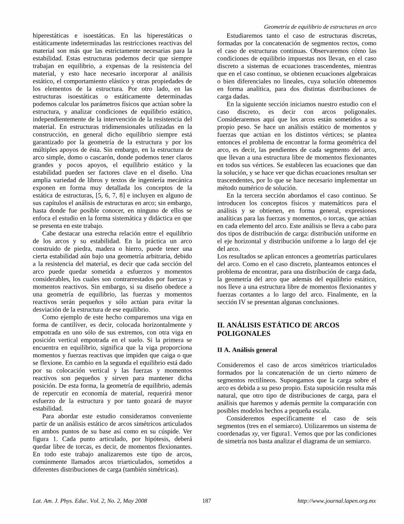
Geometría de equilibrio de estructuras en arco
Lat. Am. J. Phys. Educ. Vol. 2, No. 2, May 2008 187 http://www.journal.lapen.org.mx
hiperestáticas e isoestáticas. En las hiperestáticas o estáticamente indeterminadas las restricciones reactivas del material son más que las estrictamente necesarias para la estabilidad. Estas estructuras podemos decir que siempre trabajan en equilibrio, a expensas de la resistencia del material, y esto hace necesario incorporar al análisis estático, el comportamiento elástico y otras propiedades de los elementos de la estructura. Por otro lado, en las estructuras isoestáticas o estáticamente determinadas podemos calcular los parámetros físicos que actúan sobre la estructura, y analizar condiciones de equilibrio estático, independientemente de la intervención de la resistencia del material. En estructuras tridimensionales utilizadas en la construcción, en general dicho equilibrio siempre está garantizado por la geometría de la estructura y por los múltiples apoyos de ésta. Sin embargo, en la estructura de arco simple, domo o cascarón, donde podemos tener claros grandes y pocos apoyos, el equilibrio estático y la estabilidad pueden ser factores clave en el diseño. Una amplia variedad de libros y textos de ingeniería mecánica exponen en forma muy detallada los conceptos de la estática de estructuras, [5, 6, 7, 8] e incluyen en alguno de sus capítulos el análisis de estructuras en arco; sin embargo, hasta donde fue posible conocer, en ninguno de ellos se enfoca el estudio en la forma sistemática y didáctica en que se presenta en este trabajo.
Cabe destacar una estrecha relación entre el equilibrio de los arcos y su estabilidad. En la práctica un arco construido de piedra, madera o hierro, puede tener una cierta estabilidad aún bajo una geometría arbitraria, debido a la resistencia del material, es decir que cada sección del arco puede quedar sometida a esfuerzos y momentos considerables, los cuales son contrarrestados por fuerzas y momentos reactivos. Sin embargo, si su diseño obedece a una geometría de equilibrio, las fuerzas y momentos reactivos serán pequeños y sólo actúan para evitar la desviación de la estructura de ese equilibrio.
Como ejemplo de este hecho comparemos una viga en forma de cantilíver, es decir, colocada horizontalmente y empotrada en uno sólo de sus extremos, con otra viga en posición vertical empotrada en el suelo. Si la primera se encuentra en equilibrio, significa que la viga proporciona momentos y fuerzas reactivas que impiden que caiga o que se flexione. En cambio en la segunda el equilibrio está dado por su colocación vertical y las fuerzas y momentos reactivos son pequeños y sirven para mantener dicha posición. De esta forma, la geometría de equilibrio, además de repercutir en economía de material, requerirá menor esfuerzo de la estructura y por tanto gozará de mayor estabilidad.
Para abordar este estudio consideramos conveniente partir de un análisis estático de arcos simétricos articulados en ambos puntos de su base así como en su cúspide. Ver figura 1. Cada punto articulado, por hipótesis, deberá quedar libre de torcas, es decir, de momentos flexionantes. En todo este trabajo analizaremos este tipo de arcos, comúnmente llamados arcos triarticulados, sometidos a diferentes distribuciones de carga (también simétricas).
Estudiaremos tanto el caso de estructuras discretas, formadas por la concatenación de segmentos rectos, como el caso de estructuras continuas. Observaremos cómo las condiciones de equilibrio impuestas nos llevan, en el caso discreto a sistemas de ecuaciones trascendentes, mientras que en el caso continuo, se obtienen ecuaciones algebraicas o bien diferenciales no lineales, cuya solución obtenemos en forma analítica, para dos distintas distribuciones de carga dadas.
En la siguiente sección iniciamos nuestro estudio con el caso discreto, es decir con arcos poligonales. Consideraremos aquí que los arcos están sometidos a su propio peso. Se hace un análisis estático de momentos y fuerzas que actúan en los distintos vértices; se plantea entonces el problema de encontrar la forma geométrica del arco, es decir, las pendientes de cada segmento del arco, que llevan a una estructura libre de momentos flexionantes en todos sus vértices. Se establecen las ecuaciones que dan la solución, y se hace ver que dichas ecuaciones resultan ser trascendentes, por lo que se hace necesario implementar un método numérico de solución.
En la tercera sección abordamos el caso continuo. Se introducen los conceptos físicos y matemáticos para el análisis y se obtienen, en forma general, expresiones analíticas para las fuerzas y momentos, o torcas, que actúan en cada elemento del arco. Este análisis se lleva a cabo para dos tipos de distribución de carga: distribución uniforme en el eje horizontal y distribución uniforme a lo largo del eje del arco. Los resultados se aplican entonces a geometrías particulares del arco. Como en el caso discreto, planteamos entonces el problema de encontrar, para una distribución de carga dada, la geometría del arco que además del equilibrio estático, nos lleve a una estructura libre de momentos flexionantes y fuerzas cortantes a lo largo del arco. Finalmente, en la sección IV se presentan algunas conclusiones. II. ANÁLISIS ESTÁTICO DE ARCOS POLIGONALES II A. Análisis general Consideremos el caso de arcos simétricos triarticulados formados por la concatenación de un cierto número de segmentos rectilíneos. Supongamos que la carga sobre el arco es debida a su peso propio. Esta suposición resulta más natural, que otro tipo de distribuciones de carga, para el análisis que haremos y además permite la comparación con posibles modelos hechos a pequeña escala.
Consideremos específicamente el caso de seis segmentos (tres en el semiarco). Utilizaremos un sistema de coordenadas xy, ver figura1. Vemos que por las condiciones de simetría nos basta analizar el diagrama de un semiarco.
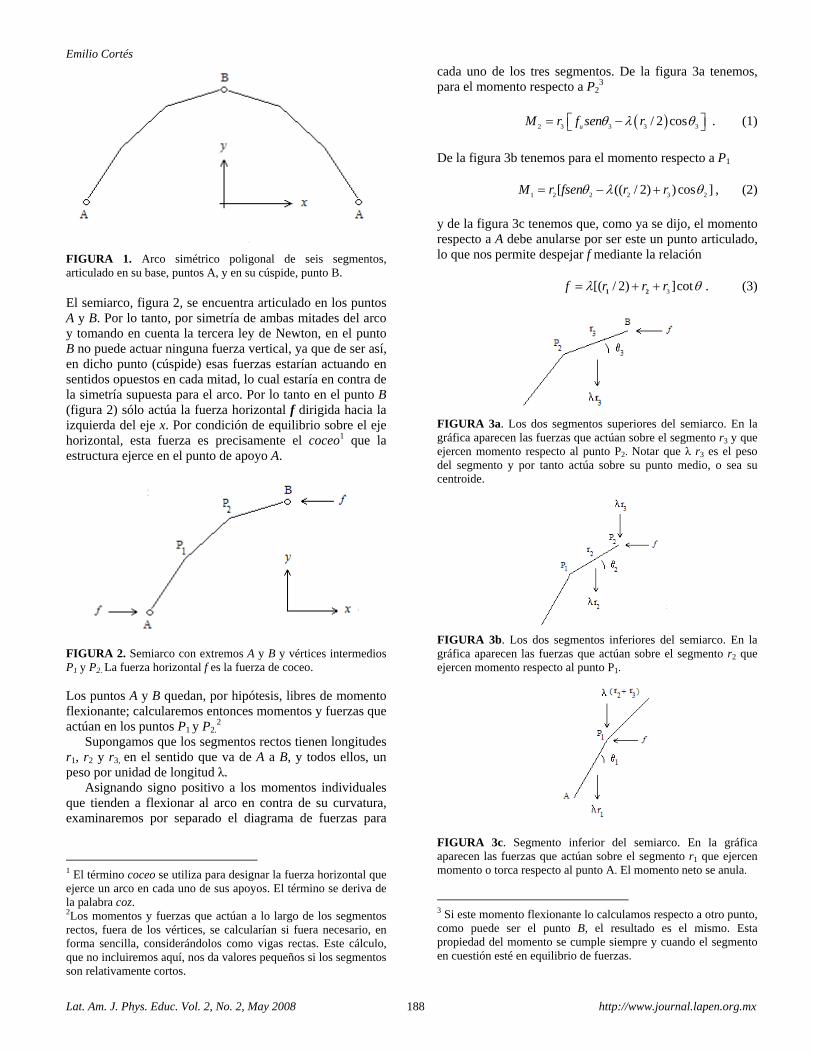
Emilio Cortés
Lat. Am. J. Phys. Educ. Vol. 2, No. 2, May 2008 188 http://www.journal.lapen.org.mx
FIGURA 1. Arco simétrico poligonal de seis segmentos, articulado en su base, puntos A, y en su cúspide, punto B. El semiarco, figura 2, se encuentra articulado en los puntos A y B. Por lo tanto, por simetría de ambas mitades del arco y tomando en cuenta la tercera ley de Newton, en el punto B no puede actuar ninguna fuerza vertical, ya que de ser así, en dicho punto (cúspide) esas fuerzas estarían actuando en sentidos opuestos en cada mitad, lo cual estaría en contra de la simetría supuesta para el arco. Por lo tanto en el punto B (figura 2) sólo actúa la fuerza horizontal f dirigida hacia la izquierda del eje x. Por condición de equilibrio sobre el eje horizontal, esta fuerza es precisamente el coceo1 que la estructura ejerce en el punto de apoyo A.
FIGURA 2. Semiarco con extremos A y B y vértices intermedios P1 y P2. La fuerza horizontal f es la fuerza de coceo. Los puntos A y B quedan, por hipótesis, libres de momento flexionante; calcularemos entonces momentos y fuerzas que actúan en los puntos P1 y P2.
2 Supongamos que los segmentos rectos tienen longitudes
r1, r2 y r3, en el sentido que va de A a B, y todos ellos, un peso por unidad de longitud λ.
Asignando signo positivo a los momentos individuales que tienden a flexionar al arco en contra de su curvatura, examinaremos por separado el diagrama de fuerzas para
1 El término coceo se utiliza para designar la fuerza horizontal que ejerce un arco en cada uno de sus apoyos. El término se deriva de la palabra coz. 2Los momentos y fuerzas que actúan a lo largo de los segmentos rectos, fuera de los vértices, se calcularían si fuera necesario, en forma sencilla, considerándolos como vigas rectas. Este cálculo, que no incluiremos aquí, nos da valores pequeños si los segmentos son relativamente cortos.
cada uno de los tres segmentos. De la figura 3a tenemos, para el momento respecto a P2
3
( )2 3 3 3 3/ 2 cosuM r f sen rθ λ θ= −⎡ ⎤⎣ ⎦ . (1)
De la figura 3b tenemos para el momento respecto a P1
1 2 2 2 3 2[ (( / 2) ) cos ]M r fsen r rθ λ θ= − + , (2)
y de la figura 3c tenemos que, como ya se dijo, el momento respecto a A debe anularse por ser este un punto articulado, lo que nos permite despejar f mediante la relación
3[( / 2) ]cotf r r rλ θ= + +1 2 . (3)
FIGURA 3a. Los dos segmentos superiores del semiarco. En la gráfica aparecen las fuerzas que actúan sobre el segmento r3 y que ejercen momento respecto al punto P2. Notar que λ r3 es el peso del segmento y por tanto actúa sobre su punto medio, o sea su centroide.
FIGURA 3b. Los dos segmentos inferiores del semiarco. En la gráfica aparecen las fuerzas que actúan sobre el segmento r2 que ejercen momento respecto al punto P1.
FIGURA 3c. Segmento inferior del semiarco. En la gráfica aparecen las fuerzas que actúan sobre el segmento r1 que ejercen momento o torca respecto al punto A. El momento neto se anula.
3 Si este momento flexionante lo calculamos respecto a otro punto, como puede ser el punto B, el resultado es el mismo. Esta propiedad del momento se cumple siempre y cuando el segmento en cuestión esté en equilibrio de fuerzas.
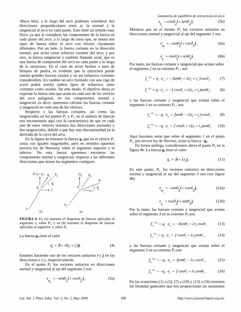
Geometría de equilibrio de estructuras en arco
Lat. Am. J. Phys. Educ. Vol. 2, No. 2, May 2008 189 http://www.journal.lapen.org.mx
Ahora bien, a lo largo del arco podemos considerar dos direcciones perpendiculares entre sí, la normal y la tangencial al arco en cada punto. Esto tiene un sentido muy físico ya que al considerar las componentes de la fuerza en cada punto del arco, a lo largo de estos ejes, se tienen dos tipos de fuerza sobre el arco con efectos claramente diferentes. Por un lado, la fuerza cortante en la dirección normal, que actúa como esfuerzo cortante del arco, y por otro, la fuerza tangencial o también llamada axial, que es una fuerza de compresión del arco en cada punto a lo largo de la estructura. En el caso de arcos hechos a base de bloques de piedra, es evidente que la estructura puede resistir grandes fuerzas axiales y no así esfuerzos cortantes considerables. En cambio un arco formado con una viga de acero podrá resistir ambos tipos de esfuerzos, tanto cortantes como axiales. De este modo, el objetivo ahora es expresar la fuerza neta que actúa en cada uno de los vértices del arco poligonal, en sus componentes normal y tangencial, es decir, queremos calcular las fuerzas cortante y tangencial en cada uno de los vértices.
Respecto a las fuerzas cortantes, así como las tangenciales en los puntos P1 y P2, en el análisis de fuerzas nos encontramos aquí con la característica de que en cada uno de estos vértices tenemos dos direcciones normales y dos tangenciales, debido a que hay una discontinuidad en la derivada de la curva del arco.
En la figura 4a tenemos la fuerza q1 que en el vértice P1
actúa con iguales magnitudes, pero en sentidos opuestos (tercera ley de Newton), sobre el segmento superior y el inferior. De esta fuerza queremos encontrar las componentes normal y tangencial, respecto a las diferentes direcciones que tienen los segmentos contiguos.
FIGURA 4. En (a) tenemos el diagrama de fuerzas aplicadas al segmento 2, sobre P1, y en (b) tenemos el diagrama de fuerzas aplicadas al segmento 3, sobre P2. La fuerza q1 tiene el valor
1q f r rλ= + +2 3i ( )j . (4)
Estamos haciendo uso de los vectores unitarios i y j en las direcciones x y y, respectivamente.
En el punto P1 los vectores unitarios en direcciones normal y tangencial al eje del segmento 2 son
2
cos2 2
e senn
θ θ= − +i j , (5a)
2
cos2 2
e sent
θ θ= +i j . (5b)
Mientras que en el mismo P1 los vectores unitarios en direcciones normal y tangencial al eje del segmento 1 son
1
cos1 1
e senn
θ θ= − +i j , (6a)
1
cos1 1
e sent
θ θ= +i j . (6b)
Por tanto, las fuerzas cortante y tangencial que actúan sobre el segmento 2 en su extremo P1 , son
1
2
( )
1 2 2 2cosP
c nf q e fsen (r r )θ λ θ= ⋅ = − + +2 3 , (7)
1
2
( )
1 2 2 2cos ( )P
t tf q e f r r senθ λ θ= ⋅ = − + +2 3 , (8)
y las fuerzas cortante y tangencial que actúan sobre el segmento 1 en su extremo P1 , son
1
1
( )
1 1 1( ) cosP
nf q e fsen r rθ λ θ= − ⋅ = − +1c 2 3 , (9)
1
1
( )
1 1 1cos ( )P
tf q e f r r senθ λ θ= − ⋅ = + +1t 2 3 . (10)
Aquí hacemos notar que sobre el segmento 1 en el punto P1, por tercera ley de Newton, actúa la fuerza –q1.
En forma análoga, consideramos ahora el punto P2 en la figura 4b. La fuerza q2 tiene el valor
2q f rλ= + 3i j . (11)
En este punto, P2, los vectores unitarios en direcciones normal y tangencial al eje del segmento 3 son (ver figura 4b)
3
cos3 3
e senn
θ θ= − +i j , (12a)
3
cos3 3
e sent
θ θ= +i j . (12b)
Por lo tanto, las fuerzas cortante y tangencial que actúan sobre el segmento 3 en su extremo P2 son
2
3
( )
2 3 cosP
nf q e fsen rθ λ θ= ⋅ = − +3c 3 , (13)
2
3
( )
2 3 3cosP
tf q e f r senθ λ θ= ⋅ = +3t 3 , (14)
y las fuerzas cortante y tangencial que actúan sobre el segmento 2 en su extremo P2 son
2
2
( )
2 2 2cosP
nf q e fsen rθ λ θ= − ⋅ = −2c 3 , (15)
2
2
( )
2 2 2cosP
tf q e f r senθ λ θ= − ⋅ = +2t 3 . (16)
En las ecuaciones (1) a (3), (7) a (10) y (13) a (16) tenemos las fórmulas generales que nos proporcionan los momentos
Emilio Cortés
Lat. Am. J. Phys. Educ. Vol. 2, No. 2, May 2008 190 http://www.journal.lapen.org.mx
flexionantes, fuerzas tangenciales , cortantes y de coceo en el arco poligonal simétrico sometido a su peso propio, todo esto en términos de los valores de los parámetros que son la densidad lineal de los segmentos, sus longitudes y los ángulos que forman cada uno con la horizontal. A continuación consideramos las condiciones de equilibrio del arco poligonal. Es decir, queremos determinar si existe una geometría de nuestro arco poligonal para la cual, además del equilibrio de fuerzas ya considerado aquí, el momento flexionante en los vértices intermedios, P1 y P2 se anule. II B. Arco poligonal en equilibrio La condición de equilibrio que buscamos significa físicamente el encontrar una geometría en la que en el arco considerado aquí de siete vértices, aun cuando todos ellos estuvieran articulados, tendría una estructura que se mantendría en pie, al estar sometida exclusivamente a su propio peso.
Supongamos que queremos diseñar un arco poligonal simétrico de seis segmentos idénticos de longitud r. (Si los segmentos se consideran con longitudes diferentes, por parejas, las expresiones serían un poco menos compactas y los resultados no serían mucho más ilustrativos).
Supongamos además que los segmentos tienen todos una densidad lineal λ y que el claro y la flecha (ancho y altura) del semiarco son valores dados, a y b, respectivamente. Nos planteamos el problema de encontrar los parámetros geométricos del arco, para los cuales se anule el momento flexionante en los vértices intermedios P1 y P2. Es decir, para las condiciones señaladas, necesitamos determinar el valor de cuatro parámetros: la longitud r y los ángulos de elevación de los tres segmentos, θ1, θ2 y θ3. O bien, si r es dato entonces la flecha queda por determinarse. Para esto tomamos las ecuaciones (1) a (3); haciendo cero los momentos M1 y M2 obtenemos las tres igualdades
( ) 31/ 2 cotf rλ θ= , (17)
2(3 / 2) cotf rλ θ= , (18)
1(5 / 2) cotf rλ θ= , (19)
(ésta última se obtiene de la ecuación (3)). De estas tres expresiones para f despejamos tanθ2 y tanθ1 en términos de tanθ3, y obtenemos las siguientes relaciones entre las pendientes de los tres segmentos de cada semiarco:
tan 3tanθ θ=2 3 , (20)
1 3tan 5 tanθ θ= . (21)
Hacemos notar aquí la tendencia que nos da este resultado que relaciona las pendientes de los segmentos a medida que los tomamos de arriba hacia abajo. Está claro que si
hubiéramos considerado cuatro segmentos, en lugar de tres, en cada semiarco, la pendiente del cuarto arco hacia abajo sería 7 veces el valor de la pendiente del primero, y así sucesivamente para un número aún mayor se segmentos. Esta relación es una condición de equilibrio del arco.
Agregamos a éstas, dos relaciones que vienen de las características geométricas del arco ya establecidas:
cos cos cosa r θ θ θ= + +1 2 3( ) , (22)
( )b r sen sen senθ θ θ= + +1 2 3 . (23)
Obtenemos así en las ecuaciones (20) a (23), cuatro ecuaciones trascendentes en las incógnitas r, θ1, θ2 y θ3. La solución de este sistema sólo puede obtenerse en forma numérica ya que se trata de ecuaciones trascendentes. Esta solución puede obtenerse en forma sencilla en un programa de computadora. La idea es partir de un cierto valor para uno de los ángulos, digamos θ3, que puede ser cero, y entonces ir incrementando en una magnitud muy pequeña dicho valor hasta que las igualdades (20) a (23) se cumplan. Para esta estructura en equilibrio, podemos calcular las fuerzas cortantes que actúan en ambos extremos de cada segmento rectilíneo. Por otro lado, combinando las ecuaciones (9) con (19), (7) con (18), (13) con (17) y (15) con (18) obtenemos un resultado interesante que se resume en esta forma: “la fuerza cortante es la misma en ambos extremos de cada segmento” y tiene el valor
( 2) cosf rλ θ=c(i) i i/ , (24)
donde i es un índice que, en este caso, va de 1 a 3 y representa a cada uno de los tres segmentos. Con la salvedad de que en el extremo superior del segmento 3 (la parte más alta del arco) no hay fuerza cortante. Es interesante notar que bajo esta situación de equilibrio, en lo que respecta a la fuerza cortante, cada uno de los extremos de cada segmento trabaja como lo hace una viga recta horizontal, con apoyos verticales en sus extremos.
Consideremos los siguientes ejemplos numéricos. Supongamos que disponemos de 6 barras rectas cada una con una longitud r = 1.5 m. y una densidad lineal de masa de λ = 1 kg/m. Supongamos que las barras se unen por medio de bisagras formando una cadena, y que en cada extremo de la cadena también hay una bisagra la cual se fijará a una superficie horizontal, como se muestra en la figura 1. Ahora bien, queremos colocar los extremos del arco a dos distancias diferentes uno del otro: en un caso a 8 m y en otro a 6 m. Al colocar esta cadena formando un arco simétrico queremos saber cuál es la posición de equilibrio en la que el arco puede permanecer. Esta geometría queda determinada por los tres ángulos θ1, θ2 y θ3 y la flecha o altura b del arco. Notar que a es la mitad del claro y es en este caso un dato del problema.
Resolviendo numéricamente las ecuaciones (20)-(23) por medio de un programa de computadora, y evaluando las expresiones (17) y (24) obtenemos lo siguiente:
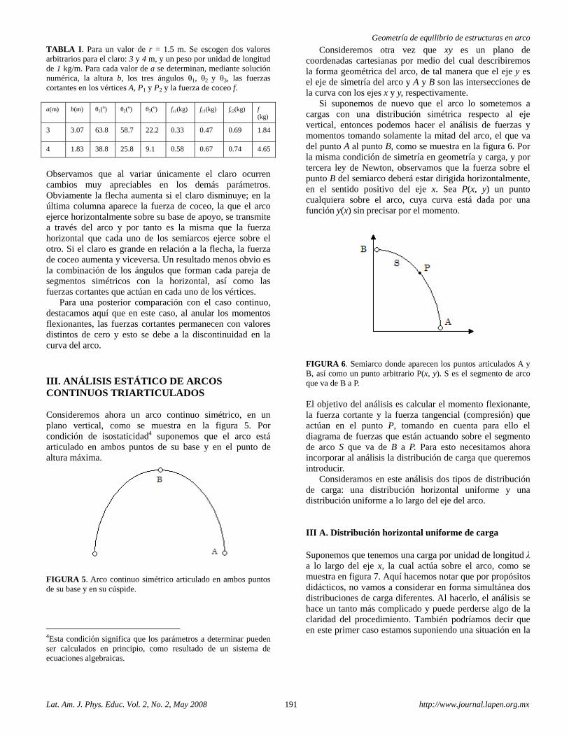
Geometría de equilibrio de estructuras en arco
Lat. Am. J. Phys. Educ. Vol. 2, No. 2, May 2008 191 http://www.journal.lapen.org.mx
TABLA I. Para un valor de r = 1.5 m. Se escogen dos valores arbitrarios para el claro: 3 y 4 m, y un peso por unidad de longitud de 1 kg/m. Para cada valor de a se determinan, mediante solución numérica, la altura b, los tres ángulos θ1, θ2 y θ3, las fuerzas cortantes en los vértices A, P1 y P2 y la fuerza de coceo f. a(m) b(m) θ1(
o) θ2(o) θ3(
o) fc1(kg) fc1(kg) fc2(kg) f
(kg)
3 3.07 63.8 58.7 22.2 0.33 0.47 0.69 1.84
4 1.83 38.8 25.8 9.1 0.58 0.67 0.74 4.65
Observamos que al variar únicamente el claro ocurren cambios muy apreciables en los demás parámetros. Obviamente la flecha aumenta si el claro disminuye; en la última columna aparece la fuerza de coceo, la que el arco ejerce horizontalmente sobre su base de apoyo, se transmite a través del arco y por tanto es la misma que la fuerza horizontal que cada uno de los semiarcos ejerce sobre el otro. Si el claro es grande en relación a la flecha, la fuerza de coceo aumenta y viceversa. Un resultado menos obvio es la combinación de los ángulos que forman cada pareja de segmentos simétricos con la horizontal, así como las fuerzas cortantes que actúan en cada uno de los vértices.
Para una posterior comparación con el caso continuo, destacamos aquí que en este caso, al anular los momentos flexionantes, las fuerzas cortantes permanecen con valores distintos de cero y esto se debe a la discontinuidad en la curva del arco. III. ANÁLISIS ESTÁTICO DE ARCOS CONTINUOS TRIARTICULADOS Consideremos ahora un arco continuo simétrico, en un plano vertical, como se muestra en la figura 5. Por condición de isostaticidad4 suponemos que el arco está articulado en ambos puntos de su base y en el punto de altura máxima.
FIGURA 5. Arco continuo simétrico articulado en ambos puntos de su base y en su cúspide.
4Esta condición significa que los parámetros a determinar pueden ser calculados en principio, como resultado de un sistema de ecuaciones algebraicas.
Consideremos otra vez que xy es un plano de coordenadas cartesianas por medio del cual describiremos la forma geométrica del arco, de tal manera que el eje y es el eje de simetría del arco y A y B son las intersecciones de la curva con los ejes x y y, respectivamente.
Si suponemos de nuevo que el arco lo sometemos a cargas con una distribución simétrica respecto al eje vertical, entonces podemos hacer el análisis de fuerzas y momentos tomando solamente la mitad del arco, el que va del punto A al punto B, como se muestra en la figura 6. Por la misma condición de simetría en geometría y carga, y por tercera ley de Newton, observamos que la fuerza sobre el punto B del semiarco deberá estar dirigida horizontalmente, en el sentido positivo del eje x. Sea P(x, y) un punto cualquiera sobre el arco, cuya curva está dada por una función y(x) sin precisar por el momento.
FIGURA 6. Semiarco donde aparecen los puntos articulados A y B, así como un punto arbitrario P(x, y). S es el segmento de arco que va de B a P. El objetivo del análisis es calcular el momento flexionante, la fuerza cortante y la fuerza tangencial (compresión) que actúan en el punto P, tomando en cuenta para ello el diagrama de fuerzas que están actuando sobre el segmento de arco S que va de B a P. Para esto necesitamos ahora incorporar al análisis la distribución de carga que queremos introducir.
Consideramos en este análisis dos tipos de distribución de carga: una distribución horizontal uniforme y una distribución uniforme a lo largo del eje del arco. III A. Distribución horizontal uniforme de carga Suponemos que tenemos una carga por unidad de longitud λ a lo largo del eje x, la cual actúa sobre el arco, como se muestra en figura 7. Aquí hacemos notar que por propósitos didácticos, no vamos a considerar en forma simultánea dos distribuciones de carga diferentes. Al hacerlo, el análisis se hace un tanto más complicado y puede perderse algo de la claridad del procedimiento. También podríamos decir que en este primer caso estamos suponiendo una situación en la
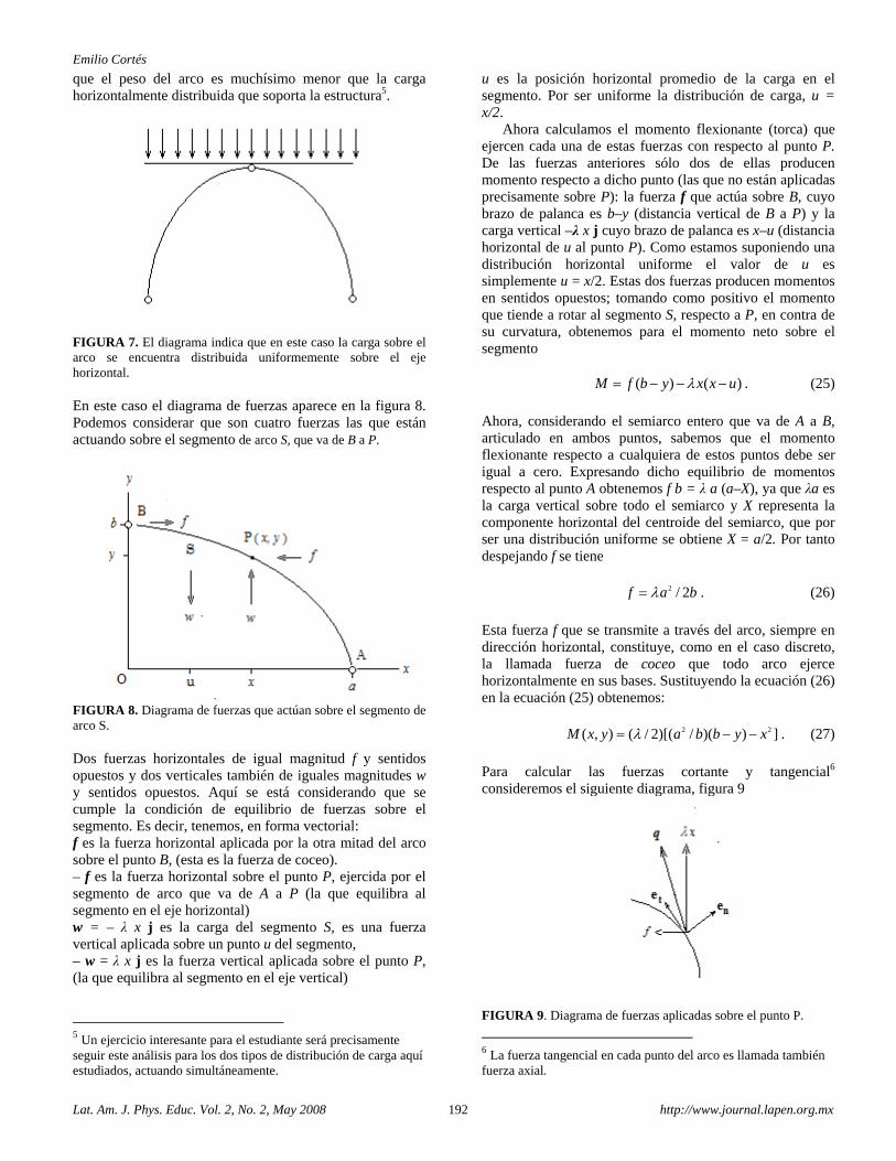
Emilio Cortés
Lat. Am. J. Phys. Educ. Vol. 2, No. 2, May 2008 192 http://www.journal.lapen.org.mx
que el peso del arco es muchísimo menor que la carga horizontalmente distribuida que soporta la estructura5.
FIGURA 7. El diagrama indica que en este caso la carga sobre el arco se encuentra distribuida uniformemente sobre el eje horizontal. En este caso el diagrama de fuerzas aparece en la figura 8. Podemos considerar que son cuatro fuerzas las que están actuando sobre el segmento de arco S, que va de B a P.
FIGURA 8. Diagrama de fuerzas que actúan sobre el segmento de arco S. Dos fuerzas horizontales de igual magnitud f y sentidos opuestos y dos verticales también de iguales magnitudes w y sentidos opuestos. Aquí se está considerando que se cumple la condición de equilibrio de fuerzas sobre el segmento. Es decir, tenemos, en forma vectorial: f es la fuerza horizontal aplicada por la otra mitad del arco sobre el punto B, (esta es la fuerza de coceo). – f es la fuerza horizontal sobre el punto P, ejercida por el segmento de arco que va de A a P (la que equilibra al segmento en el eje horizontal) w = – λ x j es la carga del segmento S, es una fuerza vertical aplicada sobre un punto u del segmento, – w = λ x j es la fuerza vertical aplicada sobre el punto P, (la que equilibra al segmento en el eje vertical)
5 Un ejercicio interesante para el estudiante será precisamente seguir este análisis para los dos tipos de distribución de carga aquí estudiados, actuando simultáneamente.
u es la posición horizontal promedio de la carga en el segmento. Por ser uniforme la distribución de carga, u = x/2.
Ahora calculamos el momento flexionante (torca) que ejercen cada una de estas fuerzas con respecto al punto P. De las fuerzas anteriores sólo dos de ellas producen momento respecto a dicho punto (las que no están aplicadas precisamente sobre P): la fuerza f que actúa sobre B, cuyo brazo de palanca es b–y (distancia vertical de B a P) y la carga vertical –λ x j cuyo brazo de palanca es x–u (distancia horizontal de u al punto P). Como estamos suponiendo una distribución horizontal uniforme el valor de u es simplemente u = x/2. Estas dos fuerzas producen momentos en sentidos opuestos; tomando como positivo el momento que tiende a rotar al segmento S, respecto a P, en contra de su curvatura, obtenemos para el momento neto sobre el segmento
( ) ( )M f b y x x uλ= − − − . (25)
Ahora, considerando el semiarco entero que va de A a B, articulado en ambos puntos, sabemos que el momento flexionante respecto a cualquiera de estos puntos debe ser igual a cero. Expresando dicho equilibrio de momentos respecto al punto A obtenemos f b = λ a (a–X), ya que λa es la carga vertical sobre todo el semiarco y X representa la componente horizontal del centroide del semiarco, que por ser una distribución uniforme se obtiene X = a/2. Por tanto despejando f se tiene
2 / 2f a bλ= . (26)
Esta fuerza f que se transmite a través del arco, siempre en dirección horizontal, constituye, como en el caso discreto, la llamada fuerza de coceo que todo arco ejerce horizontalmente en sus bases. Sustituyendo la ecuación (26) en la ecuación (25) obtenemos:
2 2( , ) ( / 2)[( / )( ) ]M x y a b b y xλ= − − . (27)
Para calcular las fuerzas cortante y tangencial6 consideremos el siguiente diagrama, figura 9
FIGURA 9. Diagrama de fuerzas aplicadas sobre el punto P.
6 La fuerza tangencial en cada punto del arco es llamada también fuerza axial.
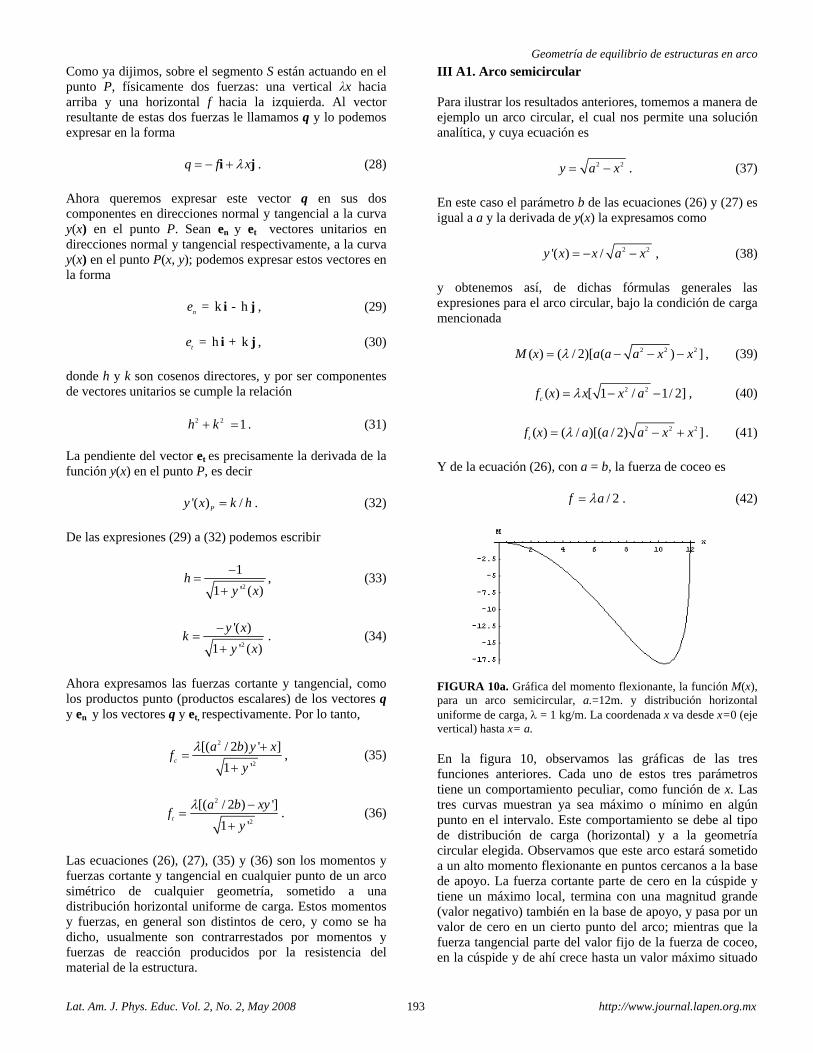
Geometría de equilibrio de estructuras en arco
Lat. Am. J. Phys. Educ. Vol. 2, No. 2, May 2008 193 http://www.journal.lapen.org.mx
Como ya dijimos, sobre el segmento S están actuando en el punto P, físicamente dos fuerzas: una vertical λx hacia arriba y una horizontal f hacia la izquierda. Al vector resultante de estas dos fuerzas le llamamos q y lo podemos expresar en la forma
q f xλ= − +i j . (28)
Ahora queremos expresar este vector q en sus dos componentes en direcciones normal y tangencial a la curva y(x) en el punto P. Sean en y et vectores unitarios en direcciones normal y tangencial respectivamente, a la curva y(x) en el punto P(x, y); podemos expresar estos vectores en la forma
= k - hne i j , (29)
= h + kte i j , (30)
donde h y k son cosenos directores, y por ser componentes de vectores unitarios se cumple la relación
2 2 1h k+ = . (31) La pendiente del vector et es precisamente la derivada de la función y(x) en el punto P, es decir
'( ) /Py x k h= . (32)
De las expresiones (29) a (32) podemos escribir
2
1
1 ' ( )h
y x
−=
+, (33)
2
'( )
1 ' ( )
y xk
y x
−=
+. (34)
Ahora expresamos las fuerzas cortante y tangencial, como los productos punto (productos escalares) de los vectores q y en y los vectores q y et, respectivamente. Por lo tanto,
2
2
[( / 2 ) ' ]
1 'c
a b y xf
y
λ +=
+, (35)
2
2
[( / 2 ) ']
1 't
a b xyf
y
λ −=
+. (36)
Las ecuaciones (26), (27), (35) y (36) son los momentos y fuerzas cortante y tangencial en cualquier punto de un arco simétrico de cualquier geometría, sometido a una distribución horizontal uniforme de carga. Estos momentos y fuerzas, en general son distintos de cero, y como se ha dicho, usualmente son contrarrestados por momentos y fuerzas de reacción producidos por la resistencia del material de la estructura.
III A1. Arco semicircular Para ilustrar los resultados anteriores, tomemos a manera de ejemplo un arco circular, el cual nos permite una solución analítica, y cuya ecuación es
2 2y a x= − . (37)
En este caso el parámetro b de las ecuaciones (26) y (27) es igual a a y la derivada de y(x) la expresamos como
2 2'( ) /y x x a x= − − , (38)
y obtenemos así, de dichas fórmulas generales las expresiones para el arco circular, bajo la condición de carga mencionada
2 2 2( ) ( / 2)[ ( ) ]M x a a a x xλ= − − − , (39)
2 2( ) [ 1 / 1/ 2]cf x x x aλ= − − , (40)
2 2 2( ) ( / )[( / 2) ]tf x a a a x xλ= − + . (41)
Y de la ecuación (26), con a = b, la fuerza de coceo es
/ 2f aλ= . (42)
FIGURA 10a. Gráfica del momento flexionante, la función M(x), para un arco semicircular, a.=12m. y distribución horizontal uniforme de carga, λ = 1 kg/m. La coordenada x va desde x=0 (eje vertical) hasta x= a. En la figura 10, observamos las gráficas de las tres funciones anteriores. Cada uno de estos tres parámetros tiene un comportamiento peculiar, como función de x. Las tres curvas muestran ya sea máximo o mínimo en algún punto en el intervalo. Este comportamiento se debe al tipo de distribución de carga (horizontal) y a la geometría circular elegida. Observamos que este arco estará sometido a un alto momento flexionante en puntos cercanos a la base de apoyo. La fuerza cortante parte de cero en la cúspide y tiene un máximo local, termina con una magnitud grande (valor negativo) también en la base de apoyo, y pasa por un valor de cero en un cierto punto del arco; mientras que la fuerza tangencial parte del valor fijo de la fuerza de coceo, en la cúspide y de ahí crece hasta un valor máximo situado
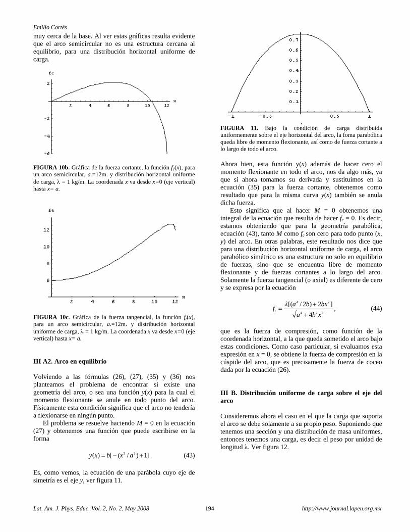
Emilio Cortés
Lat. Am. J. Phys. Educ. Vol. 2, No. 2, May 2008 194 http://www.journal.lapen.org.mx
muy cerca de la base. Al ver estas gráficas resulta evidente que el arco semicircular no es una estructura cercana al equilibrio, para una distribución horizontal uniforme de carga.
FIGURA 10b. Gráfica de la fuerza cortante, la función fc(x), para un arco semicircular, a.=12m. y distribución horizontal uniforme de carga, λ = 1 kg/m. La coordenada x va desde x=0 (eje vertical) hasta x= a.
FIGURA 10c. Gráfica de la fuerza tangencial, la función ft(x), para un arco semicircular, a.=12m. y distribución horizontal uniforme de carga, λ = 1 kg/m. La coordenada x va desde x=0 (eje vertical) hasta x= a. III A2. Arco en equilibrio Volviendo a las fórmulas (26), (27), (35) y (36) nos planteamos el problema de encontrar si existe una geometría del arco, o sea una función y(x) para la cual el momento flexionante se anule en todo punto del arco. Físicamente esta condición significa que el arco no tendería a flexionarse en ningún punto.
El problema se resuelve haciendo M = 0 en la ecuación (27) y obtenemos una función que puede escribirse en la forma
2 2( ) [ ( / ) 1]y x b x a= − + . (43)
Es, como vemos, la ecuación de una parábola cuyo eje de simetría es el eje y, ver figura 11.
FIGURA 11. Bajo la condición de carga distribuida uniformemente sobre el eje horizontal del arco, la foma parabólica queda libre de momento flexionante, así como de fuerza cortante a lo largo de todo el arco. Ahora bien, esta función y(x) además de hacer cero el momento flexionante en todo el arco, nos da algo más, ya que si ahora tomamos su derivada y sustituimos en la ecuación (35) para la fuerza cortante, obtenemos como resultado que para la misma curva y(x) también se anula dicha fuerza.
Esto significa que al hacer M = 0 obtenemos una integral de la ecuación que resulta de hacer fc = 0. Es decir, estamos obteniendo que para la geometría parabólica, ecuación (43), tanto M como fc son cero para todo punto (x, y) del arco. En otras palabras, este resultado nos dice que para una distribución horizontal uniforme de carga, el arco parabólico simétrico es una estructura no solo en equilibrio de fuerzas, sino que se encuentra libre de momento flexionante y de fuerzas cortantes a lo largo del arco. Solamente la fuerza tangencial (o axial) es diferente de cero y se expresa por la ecuación
4 2
4 2 2
[( / 2 ) 2 ]
4t
a b bxf
a b x
λ +=
+, (44)
que es la fuerza de compresión, como función de la coordenada horizontal, a la que queda sometido el arco bajo estas condiciones. Como caso particular, si evaluamos esta expresión en x = 0, se obtiene la fuerza de compresión en la cúspide del arco, que es precisamente la fuerza de coceo dada por la ecuación (26). III B. Distribución uniforme de carga sobre el eje del arco Consideremos ahora el caso en el que la carga que soporta el arco se debe solamente a su propio peso. Suponiendo que tenemos una sección y una distribución de masa uniformes, entonces tenemos una carga, es decir el peso por unidad de longitud λ. Ver figura 12.
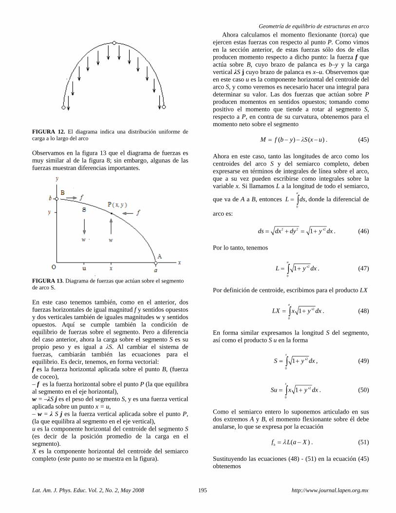
Geometría de equilibrio de estructuras en arco
Lat. Am. J. Phys. Educ. Vol. 2, No. 2, May 2008 195 http://www.journal.lapen.org.mx
FIGURA 12. El diagrama indica una distribución uniforme de carga a lo largo del arco Observamos en la figura 13 que el diagrama de fuerzas es muy similar al de la figura 8; sin embargo, algunas de las fuerzas muestran diferencias importantes.
FIGURA 13. Diagrama de fuerzas que actúan sobre el segmento de arco S. En este caso tenemos también, como en el anterior, dos fuerzas horizontales de igual magnitud f y sentidos opuestos y dos verticales también de iguales magnitudes w y sentidos opuestos. Aquí se cumple también la condición de equilibrio de fuerzas sobre el segmento. Pero a diferencia del caso anterior, ahora la carga sobre el segmento S es su propio peso y es igual a λS. Al cambiar el sistema de fuerzas, cambiarán también las ecuaciones para el equilibrio. Es decir, tenemos, en forma vectorial: f es la fuerza horizontal aplicada sobre el punto B, (fuerza de coceo), – f es la fuerza horizontal sobre el punto P (la que equilibra al segmento en el eje horizontal), w = –λS j es el peso del segmento S, y es una fuerza vertical aplicada sobre un punto x = u, – w = λ S j es la fuerza vertical aplicada sobre el punto P, (la que equilibra al segmento en el eje vertical), u es la componente horizontal del centroide del segmento S (es decir de la posición promedio de la carga en el segmento). X es la componente horizontal del centroide del semiarco completo (este punto no se muestra en la figura).
Ahora calculamos el momento flexionante (torca) que ejercen estas fuerzas con respecto al punto P. Como vimos en la sección anterior, de estas fuerzas sólo dos de ellas producen momento respecto a dicho punto: la fuerza f que actúa sobre B, cuyo brazo de palanca es b–y y la carga vertical λS j cuyo brazo de palanca es x–u. Observemos que en este caso u es la componente horizontal del centroide del arco S, y como veremos es necesario hacer una integral para determinar su valor. Las dos fuerzas que actúan sobre P producen momentos en sentidos opuestos; tomando como positivo el momento que tiende a rotar al segmento S, respecto a P, en contra de su curvatura, obtenemos para el momento neto sobre el segmento
( ) ( )M f b y λS x u= − − − . (45)
Ahora en este caso, tanto las longitudes de arco como los centroides del arco S y del semiarco completo, deben expresarse en términos de integrales de línea sobre el arco, que a su vez pueden escribirse como integrales sobre la variable x. Si llamamos L a la longitud de todo el semiarco,
que va de A a B, entonces 0
,a
L ds= ∫ donde la diferencial de
arco es:
2 2 21 'ds dx dy y dx= + = + . (46)
Por lo tanto, tenemos
2
0
1 'a
L y dx= +∫ . (47)
Por definición de centroide, escribimos para el producto LX
2
0
1 'a
LX x y dx= +∫ . (48)
En forma similar expresamos la longitud S del segmento, así como el producto S u en la forma
2
0
1 'x
S y dx= +∫ , (49)
2
0
1 'x
Su x y dx= +∫ . (50)
Como el semiarco entero lo suponemos articulado en sus dos extremos A y B, el momento flexionante sobre él debe anularse, lo que se expresa por la ecuación
( )bf L a Xλ= − . (51)
Sustituyendo las ecuaciones (48) - (51) en la ecuación (45) obtenemos
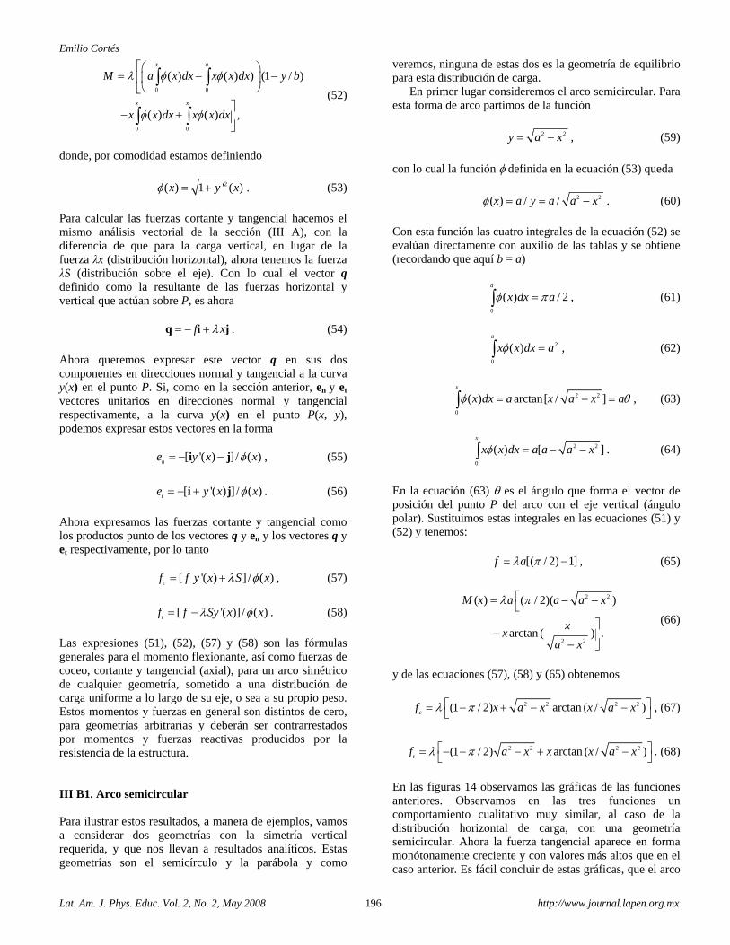
Emilio Cortés
Lat. Am. J. Phys. Educ. Vol. 2, No. 2, May 2008 196 http://www.journal.lapen.org.mx
0 0
0 0
( ) ( ) ) (1 / )
( ) ( ) ,
x a
x x
M a x dx x x dx y b
x x dx x x dx
λ φ φ
φ φ
⎡⎛ ⎞= − −⎢⎜ ⎟
⎝ ⎠⎣⎤
− + ⎥⎦
∫ ∫
∫ ∫ (52)
donde, por comodidad estamos definiendo
2( ) 1 ' ( )x y xφ = + . (53)
Para calcular las fuerzas cortante y tangencial hacemos el mismo análisis vectorial de la sección (III A), con la diferencia de que para la carga vertical, en lugar de la fuerza λx (distribución horizontal), ahora tenemos la fuerza λS (distribución sobre el eje). Con lo cual el vector q definido como la resultante de las fuerzas horizontal y vertical que actúan sobre P, es ahora
f xλ= − +q i j . (54)
Ahora queremos expresar este vector q en sus dos componentes en direcciones normal y tangencial a la curva y(x) en el punto P. Si, como en la sección anterior, en y et vectores unitarios en direcciones normal y tangencial respectivamente, a la curva y(x) en el punto P(x, y), podemos expresar estos vectores en la forma
[ '( ) ] / ( )ne y x xφ= − −i j , (55)
[ '( ) ] / ( )te y x xφ= − +i j . (56)
Ahora expresamos las fuerzas cortante y tangencial como los productos punto de los vectores q y en y los vectores q y et respectivamente, por lo tanto
[ '( ) ] / ( )cf f y x S xλ φ= + , (57)
[ '( )] / ( )tf f Sy x xλ φ= − . (58)
Las expresiones (51), (52), (57) y (58) son las fórmulas generales para el momento flexionante, así como fuerzas de coceo, cortante y tangencial (axial), para un arco simétrico de cualquier geometría, sometido a una distribución de carga uniforme a lo largo de su eje, o sea a su propio peso. Estos momentos y fuerzas en general son distintos de cero, para geometrías arbitrarias y deberán ser contrarrestados por momentos y fuerzas reactivas producidos por la resistencia de la estructura. III B1. Arco semicircular Para ilustrar estos resultados, a manera de ejemplos, vamos a considerar dos geometrías con la simetría vertical requerida, y que nos llevan a resultados analíticos. Estas geometrías son el semicírculo y la parábola y como
veremos, ninguna de estas dos es la geometría de equilibrio para esta distribución de carga.
En primer lugar consideremos el arco semicircular. Para esta forma de arco partimos de la función
2 2y a x= − , (59)
con lo cual la función φ definida en la ecuación (53) queda
2 2( ) / /x a y a a xφ = = − . (60)
Con esta función las cuatro integrales de la ecuación (52) se evalúan directamente con auxilio de las tablas y se obtiene (recordando que aquí b = a)
0
( ) / 2a
x dx aφ π=∫ , (61)
2
0
( )a
x x dx aφ =∫ , (62)
2 2
0
( ) arctan[ / ]x
x dx a x a x aφ θ= − =∫ , (63)
2 2
0
( ) [ ]x
x x dx a a a xφ = − −∫ . (64)
En la ecuación (63) θ es el ángulo que forma el vector de posición del punto P del arco con el eje vertical (ángulo polar). Sustituimos estas integrales en las ecuaciones (51) y (52) y tenemos:
[( / 2) 1]f aλ π= − , (65)
2 2
2 2
( ) ( / 2)( )
arctan ( ) .
M x a a a x
xx
a x
λ π⎡= − −⎣⎤
− ⎥− ⎦
(66)
y de las ecuaciones (57), (58) y (65) obtenemos
2 2 2 2(1 / 2) arctan ( / )cf x a x x a xλ π⎡ ⎤= − + − −⎣ ⎦ , (67)
2 2 2 2(1 / 2) arctan ( / )tf a x x x a xλ π⎡ ⎤= − − − + −⎣ ⎦ . (68)
En las figuras 14 observamos las gráficas de las funciones anteriores. Observamos en las tres funciones un comportamiento cualitativo muy similar, al caso de la distribución horizontal de carga, con una geometría semicircular. Ahora la fuerza tangencial aparece en forma monótonamente creciente y con valores más altos que en el caso anterior. Es fácil concluir de estas gráficas, que el arco
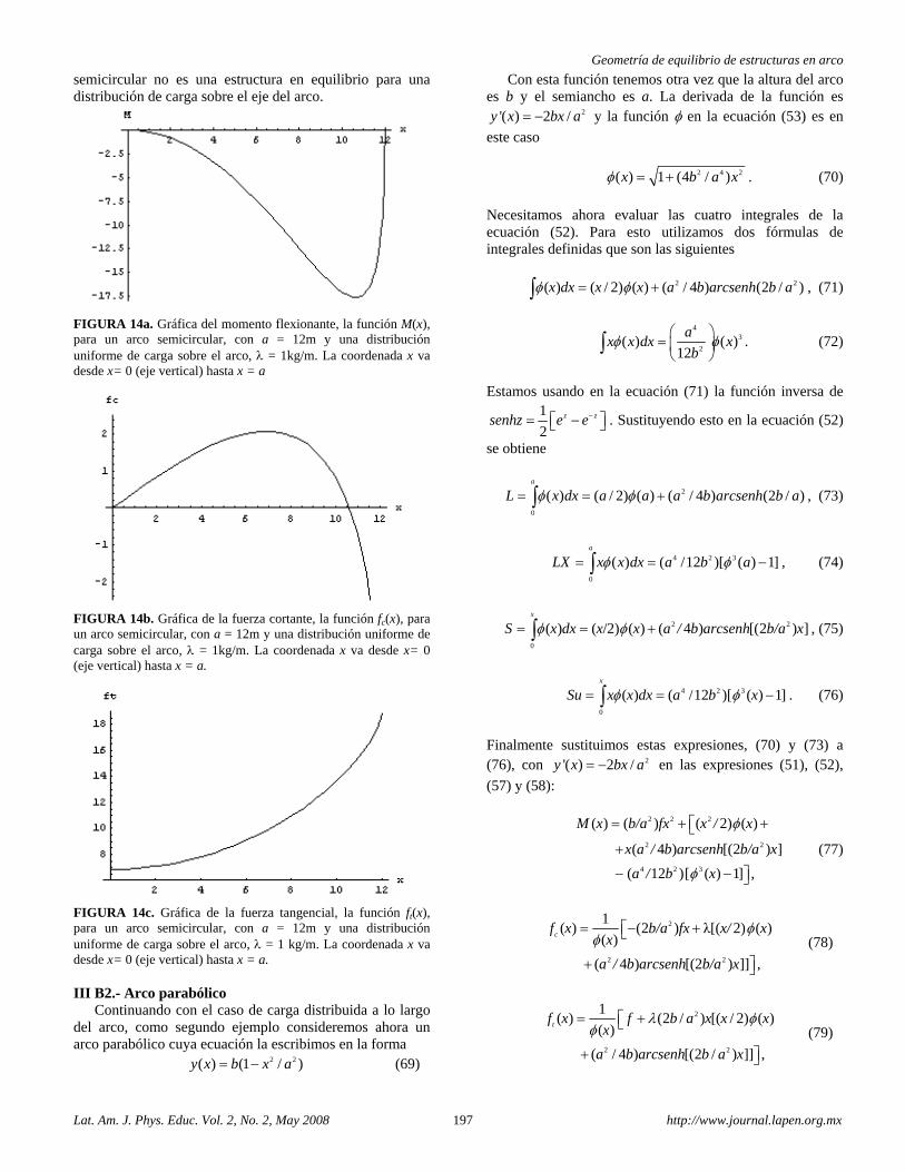
Geometría de equilibrio de estructuras en arco
Lat. Am. J. Phys. Educ. Vol. 2, No. 2, May 2008 197 http://www.journal.lapen.org.mx
semicircular no es una estructura en equilibrio para una distribución de carga sobre el eje del arco.
FIGURA 14a. Gráfica del momento flexionante, la función M(x), para un arco semicircular, con a = 12m y una distribución uniforme de carga sobre el arco, λ = 1kg/m. La coordenada x va desde x= 0 (eje vertical) hasta x = a
FIGURA 14b. Gráfica de la fuerza cortante, la función fc(x), para un arco semicircular, con a = 12m y una distribución uniforme de carga sobre el arco, λ = 1kg/m. La coordenada x va desde x= 0 (eje vertical) hasta x = a.
FIGURA 14c. Gráfica de la fuerza tangencial, la función ft(x), para un arco semicircular, con a = 12m y una distribución uniforme de carga sobre el arco, λ = 1 kg/m. La coordenada x va desde x= 0 (eje vertical) hasta x = a. III B2.- Arco parabólico
Continuando con el caso de carga distribuida a lo largo del arco, como segundo ejemplo consideremos ahora un arco parabólico cuya ecuación la escribimos en la forma
2 2( ) (1 / )y x b x a= − (69)
Con esta función tenemos otra vez que la altura del arco es b y el semiancho es a. La derivada de la función es
2'( ) 2 /y x bx a= − y la función φ en la ecuación (53) es en
este caso
2 4 2( ) 1 (4 / )x b a xφ = + . (70)
Necesitamos ahora evaluar las cuatro integrales de la ecuación (52). Para esto utilizamos dos fórmulas de integrales definidas que son las siguientes
2 2( ) ( / 2) ( ) ( / 4 ) (2 / )x dx x x a b arcsenh b aφ φ= +∫ , (71)
4
3
2( ) ( )
12
ax x dx x
bφ φ⎛ ⎞
= ⎜ ⎟⎝ ⎠∫ . (72)
Estamos usando en la ecuación (71) la función inversa de
1
2z zsenhz e e−= −⎡ ⎤⎣ ⎦ . Sustituyendo esto en la ecuación (52)
se obtiene
2
0
( ) ( / 2) ( ) ( / 4 ) (2 / )a
L x dx a a a b arcsenh b aφ φ= = +∫ , (73)
4 2 3
0
( ) ( /12 )[ ( ) 1]a
LX x x dx a b aφ φ= = −∫ , (74)
2 2
0
( ) ( /2) ( ) ( 4 ) [(2 ) ]x
S x dx x x a / b arcsenh b/a xφ φ= = +∫ , (75)
4 2 3
0
( ) ( /12 )[ ( ) 1]x
Su x x dx a b xφ φ= = −∫ . (76)
Finalmente sustituimos estas expresiones, (70) y (73) a (76), con 2'( ) 2 /y x bx a= − en las expresiones (51), (52),
(57) y (58):
2 2 2
2 2
4 2 3
( ) ( ) ( 2) ( )
( 4 ) [(2 ) ]
( 12 )[ ( ) 1] ,
M x b/a fx x / x
x a / b arcsenh b/a x
a / b x
φ
φ
= + +⎡⎣+
− − ⎤⎦
(77)
2
2 2
1( ) (2 ) λ[( 2) ( )
( )
( 4 ) [(2 ) ]] ,
cf x b/a fx x/ xx
a / b arcsenh b/a x
φφ
= − +⎡⎣
+ ⎤⎦
(78)
2
2 2
1( ) (2 / ) [( / 2) ( )
( )
( / 4 ) [(2 / ) ]] ,
tf x f b a x x xx
a b arcsenh b a x
λ φφ
= +⎡⎣
+ ⎤⎦
(79)
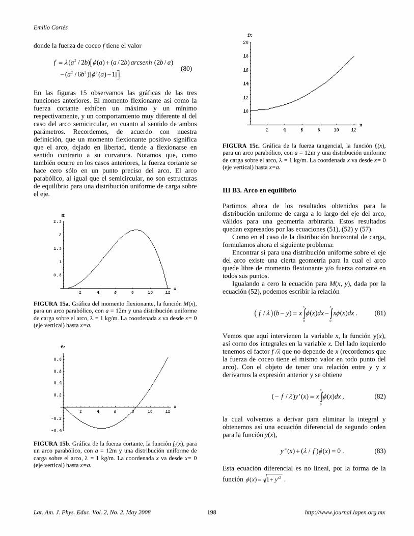
Emilio Cortés
Lat. Am. J. Phys. Educ. Vol. 2, No. 2, May 2008 198 http://www.journal.lapen.org.mx
donde la fuerza de coceo f tiene el valor
[2
2 2 3
( / 2 ) ( ) ( / 2 ) (2 / )
( / 6 )[ ( ) 1] .
f a b a a b arcsenh b a
a b a
λ φ
φ
= +
− − ⎤⎦ (80)
En las figuras 15 observamos las gráficas de las tres funciones anteriores. El momento flexionante así como la fuerza cortante exhiben un máximo y un mínimo respectivamente, y un comportamiento muy diferente al del caso del arco semicircular, en cuanto al sentido de ambos parámetros. Recordemos, de acuerdo con nuestra definición, que un momento flexionante positivo significa que el arco, dejado en libertad, tiende a flexionarse en sentido contrario a su curvatura. Notamos que, como también ocurre en los casos anteriores, la fuerza cortante se hace cero sólo en un punto preciso del arco. El arco parabólico, al igual que el semicircular, no son estructuras de equilibrio para una distribución uniforme de carga sobre el eje.
FIGURA 15a. Gráfica del momento flexionante, la función M(x), para un arco parabólico, con a = 12m y una distribución uniforme de carga sobre el arco, λ = 1 kg/m. La coordenada x va desde x= 0 (eje vertical) hasta x=a.
FIGURA 15b. Gráfica de la fuerza cortante, la función fc(x), para un arco parabólico, con a = 12m y una distribución uniforme de carga sobre el arco, λ = 1 kg/m. La coordenada x va desde x= 0 (eje vertical) hasta x=a.
FIGURA 15c. Gráfica de la fuerza tangencial, la función ft(x), para un arco parabólico, con a = 12m y una distribución uniforme de carga sobre el arco, λ = 1 kg/m. La coordenada x va desde x= 0 (eje vertical) hasta x=a. III B3. Arco en equilibrio Partimos ahora de los resultados obtenidos para la distribución uniforme de carga a lo largo del eje del arco, válidos para una geometría arbitraria. Estos resultados quedan expresados por las ecuaciones (51), (52) y (57).
Como en el caso de la distribución horizontal de carga, formulamos ahora el siguiente problema:
Encontrar si para una distribución uniforme sobre el eje del arco existe una cierta geometría para la cual el arco quede libre de momento flexionante y/o fuerza cortante en todos sus puntos.
Igualando a cero la ecuación para M(x, y), dada por la ecuación (52), podemos escribir la relación
( )0 0
/ ( ) ( ) ( )x x
f b y x x dx x x dxλ φ φ− = −∫ ∫ . (81)
Vemos que aquí intervienen la variable x, la función y(x), así como dos integrales en la variable x. Del lado izquierdo tenemos el factor f /λ que no depende de x (recordemos que la fuerza de coceo tiene el mismo valor en todo punto del arco). Con el objeto de tener una relación entre y y x derivamos la expresión anterior y se obtiene
0
( / ) ' ( ) ( )x
f y x x x dxλ φ− = ∫ , (82)
la cual volvemos a derivar para eliminar la integral y obtenemos así una ecuación diferencial de segundo orden para la función y(x),
'' ( ) ( / ) ( ) 0y x f xλ φ+ = . (83)
Esta ecuación diferencial es no lineal, por la forma de la
función 2'1)( yx +=φ .
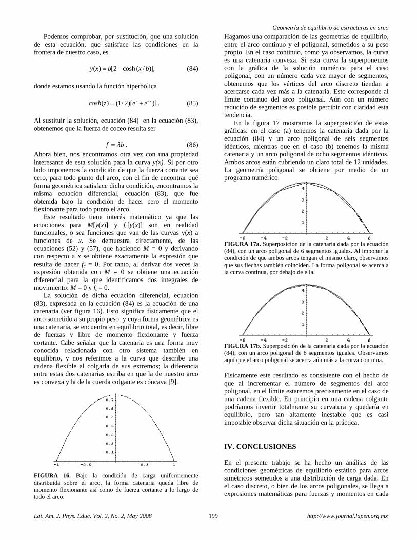
Geometría de equilibrio de estructuras en arco
Lat. Am. J. Phys. Educ. Vol. 2, No. 2, May 2008 199 http://www.journal.lapen.org.mx
Podemos comprobar, por sustitución, que una solución de esta ecuación, que satisface las condiciones en la frontera de nuestro caso, es
( ) [2 cosh ( / )],y x b x b= − (84)
donde estamos usando la función hiperbólica
( ) (1/ 2)[ )]z zcosh z e e−= + . (85)
Al sustituir la solución, ecuación (84) en la ecuación (83), obtenemos que la fuerza de coceo resulta ser
f bλ= . (86)
Ahora bien, nos encontramos otra vez con una propiedad interesante de esta solución para la curva y(x). Si por otro lado imponemos la condición de que la fuerza cortante sea cero, para todo punto del arco, con el fin de encontrar qué forma geométrica satisface dicha condición, encontramos la misma ecuación diferencial, ecuación (83), que fue obtenida bajo la condición de hacer cero el momento flexionante para todo punto el arco.
Este resultado tiene interés matemático ya que las ecuaciones para M[y(x)] y fc[y(x)] son en realidad funcionales, o sea funciones que van de las curvas y(x) a funciones de x. Se demuestra directamente, de las ecuaciones (52) y (57), que haciendo M = 0 y derivando con respecto a x se obtiene exactamente la expresión que resulta de hacer fc = 0. Por tanto, al derivar dos veces la expresión obtenida con M = 0 se obtiene una ecuación diferencial para la que identificamos dos integrales de movimiento: M = 0 y fc = 0.
La solución de dicha ecuación diferencial, ecuación (83), expresada en la ecuación (84) es la ecuación de una catenaria (ver figura 16). Esto significa físicamente que el arco sometido a su propio peso y cuya forma geométrica es una catenaria, se encuentra en equilibrio total, es decir, libre de fuerzas y libre de momento flexionante y fuerza cortante. Cabe señalar que la catenaria es una forma muy conocida relacionada con otro sistema también en equilibrio, y nos referimos a la curva que describe una cadena flexible al colgarla de sus extremos; la diferencia entre estas dos catenarias estriba en que la de nuestro arco es convexa y la de la cuerda colgante es cóncava [9].
FIGURA 16. Bajo la condición de carga uniformemente distribuida sobre el arco, la forma catenaria queda libre de momento flexionante así como de fuerza cortante a lo largo de todo el arco.
Hagamos una comparación de las geometrías de equilibrio, entre el arco continuo y el poligonal, sometidos a su peso propio. En el caso continuo, como ya observamos, la curva es una catenaria convexa. Si esta curva la superponemos con la gráfica de la solución numérica para el caso poligonal, con un número cada vez mayor de segmentos, obtenemos que los vértices del arco discreto tiendan a acercarse cada vez más a la catenaria. Esto corresponde al límite continuo del arco poligonal. Aún con un número reducido de segmentos es posible percibir con claridad esta tendencia.
En la figura 17 mostramos la superposición de estas gráficas: en el caso (a) tenemos la catenaria dada por la ecuación (84) y un arco poligonal de seis segmentos idénticos, mientras que en el caso (b) tenemos la misma catenaria y un arco poligonal de ocho segmentos idénticos. Ambos arcos están cubriendo un claro total de 12 unidades. La geometría poligonal se obtiene por medio de un programa numérico.
FIGURA 17a. Superposición de la catenaria dada por la ecuación (84), con un arco poligonal de 6 segmentos iguales. Al imponer la condición de que ambos arcos tengan el mismo claro, observamos que sus flechas también coinciden. La forma poligonal se acerca a la curva continua, por debajo de ella.
FIGURA 17b. Superposición de la catenaria dada por la ecuación (84), con un arco poligonal de 8 segmentos iguales. Observamos aquí que el arco poligonal se acerca aún más a la curva continua. Físicamente este resultado es consistente con el hecho de que al incrementar el número de segmentos del arco poligonal, en el límite estaremos precisamente en el caso de una cadena flexible. En principio en una cadena colgante podríamos invertir totalmente su curvatura y quedaría en equilibrio, pero tan altamente inestable que es casi imposible observar dicha situación en la práctica. IV. CONCLUSIONES En el presente trabajo se ha hecho un análisis de las condiciones geométricas de equilibrio estático para arcos simétricos sometidos a una distribución de carga dada. En el caso discreto, o bien de los arcos poligonales, se llega a expresiones matemáticas para fuerzas y momentos en cada
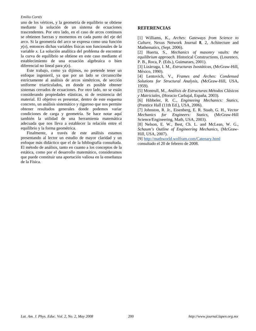
Emilio Cortés
Lat. Am. J. Phys. Educ. Vol. 2, No. 2, May 2008 200 http://www.journal.lapen.org.mx
uno de los vértices, y la geometría de equilibrio se obtiene mediante la solución de un sistema de ecuaciones trascendentes. Por otro lado, en el caso de arcos continuos se obtienen fuerzas y momentos en cada punto del eje del arco. Si la geometría del arco se expresa como una función y(x), entonces dichas variables físicas son funcionales de la variable x. La solución analítica del problema de encontrar la curva de equilibrio se obtiene en este caso mediante el establecimiento de una ecuación algebraica o bien diferencial no lineal para y(x).
Este trabajo, como ya dijimos, no pretende tener un enfoque ingenieril, ya que por un lado se circunscribe estrictamente al análisis de arcos simétricos, de sección uniforme triarticulados, en donde es posible obtener sistemas cerrados de ecuaciones. Por otro lado, no se están considerando propiedades elásticas, ni de resistencia del material. El objetivo es presentar, dentro de este esquema concreto, un análisis sistemático y riguroso que nos permite obtener resultados generales donde podemos variar condiciones de carga y geometría. Se hace notar aquí también la utilidad de una herramienta matemática adecuada que nos lleva a establecer la relación entre el equilibrio y la forma geométrica.
Finalmente, a través de este análisis estamos presentando al lector un estudio de mayor claridad y un enfoque más didáctico que el de la bibliografía consultada. El método de análisis, tanto en cuanto a los conceptos de la estática, como por el desarrollo matemático, consideramos que puede constituir una aportación valiosa en la enseñanza de la Física.
REFERENCIAS [1] Williams, K., Arches: Gateways from Science to Culture, Nexus Network Journal 8, 2, Achitecture and Mathematics, (Sept. 2006). [2] Huerta, S., Mechanics of masonry vaults: the equilibrium approach. Historical Constructions, (Lourenco, P. B., Roca, P. (Eds.), Guimaraes, 2001). [3] Lizárraga, I. M., Estructuras Isostáticas, (McGraw-Hill, México, 1990). [4] Lentovich, V., Frames and Arches: Condensed Solutions for Structural Analysis, (McGraw-Hill, USA, 1959). [5] Montrull, M., Análisis de Estructuras:Métodos Clásicos y Matriciales, (Horacio Carbajal, España, 2003). [6] Hibbeler, R. C., Engineeing Mechanics: Statics, (Prentice Hall (11th Ed.), USA, 2006). [7] Johnston, R. Jr., Eisenberg, E. R. Staab, G. H., Vector Mechanics for Engineers: Statics, (McGraw-Hill Science/Engineering, Math, USA, 2003). [8] Nelson, E. W., Best, Ch. L. and McLean, W. G., Schaum’s Outline of Engineering Mechanics, (McGraw-Hill, USA, 2007). [9] http://mathworld.wolfram.com/Catenary.html consultado el 20 de febrero de 2008.
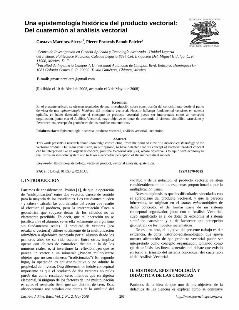
Lat. Am. J. Phys. Educ. Vol. 2, No. 2, May 2008 201 http://www.journal.lapen.org.mx
Una epistemología histórica del producto vectorial: Del cuaternión al análisis vectorial
Gustavo Martínez-Sierra1, Pierre Francois Benoit Poirier2
1Centro de Investigación en Ciencia Aplicada y Tecnología Avanzada - Unidad Legaria del Instituto Politécnico Nacional. Calzada Legaria #694 Col. Irrigación Del. Miguel Hidalgo, C. P. 11500, México, D. F. 2Facultad de Ingeniería Campus I, Universidad Autónoma de Chiapas. Blvd. Belisario Domínguez km 1081 Colonia Centro C. P. 29020. Tuxtla Gutiérrez, Chiapas, México. E-mail: [email protected]
(Recibido el 10 de Abril de 2008, aceptado el 3 de Mayo de 2008)
Resumen En el presente artículo se ofrecen resultados de una investigación sobre construcción del conocimiento desde el punto de vista de una epistemología histórica del producto vectorial. Nuestro hallazgo fundamental consiste, en nuestra opinión, en haber detectado que el concepto de producto vectorial puede ser interpretado como un concepto organizador, junto con el Análisis Vectorial, cuyo objetivo es dotar de economía al sistema simbólico cartesiano y favorecer una percepción geométrica de los modelos matemáticos. Palabras clave: Epistemología-histórica, producto vectorial, análisis vectorial, cuaternión.
Abstract This work presents a research about knowledge construction, from the point of view of a historic-epistemology of the vectorial product. Our main conclusion, in our opinion, to have detected that the concept of vectorial product concept can be interpreted like an organizer concept, joint the Vectorial Analysis, whose objective is to equip with economy to the Cartesian symbolic system and to favor a geometric perception of the mathematical models. Keywords: Historic-epistemology, vectorial product, vectorial analysis, quaternion. PACS: 01.40.gf, 01.65.+g, 02.10.Ud ISSN 1870-9095
I. INTRODUCCION Partimos de consideración, Poirier [1], de que la operación de “multiplicación” entre dos vectores carece de sentido para la mayoría de los estudiantes. Los estudiantes pueden - y saben - calcular las coordenadas del vector que resulte al efectuar el producto, pero la interpretación física o geométrica que subyace detrás de los cálculos no es claramente percibida. Es decir, que tal operación no se justifica ante el alumno, ve en ella solamente un algoritmo sin fundamentos reales. El producto de vectores (sea escalar o vectorial) difiere totalmente de la multiplicación aritmética o algebraica manejado por el alumno desde los primeros años de su vida escolar. Entre otros, implica operar con objetos de naturaleza distinta a la de los números reales; o, si invertimos la reflexión: ¿en qué se parece un vector a un número? ¿Pueden multiplicarse objetos que no son números “tradicionales”? En segundo lugar, la operación es anti-conmutativa y no admite la propiedad del inverso. Otra diferencia de índole conceptual importante es que el producto de dos vectores no nulos puede dar como resultado cero, mientras que en álgebra elemental, si ninguno de los factores de una multiplicación es cero, el resultado tiene que ser distinto de cero. Esas observaciones nos señalan que detrás de la similitud del
vocablo y de la notación, el producto vectorial se aleja considerablemente de los esquemas proporcionados por la multiplicación usual.
Nuestra hipótesis es que las dificultades vinculadas con el aprendizaje del producto vectorial, y que le parecen inherentes, se originan en el status epistemológico de dicho concepto: el de formar parte de un sistema conceptual organizador, junto con el Análisis Vectorial, cuyo significado es el de dotar de economía al sistema simbólico cartesiano y el de favorecer una percepción geométrica de los modelos matemáticos.
De esta manera, el objetivo del presente trabajo es dar evidencia, de corte histórico-epistemológico, que apoya nuestra afirmación de que producto vectorial puede ser interpretado como concepto organizador, tomando como eje de análisis las líneas generales del debate que existió en torno al tránsito del sistema conceptual del cuaternión al del Análisis Vectorial. II. HISTORIA, EPISTEMOLOGÍA Y DIDÁCTICA DE LAS CIENCIAS Partimos de la idea de que uno de los objetivos de la didáctica de las ciencias es explicar cómo se construye
Gustavo Martínez-Sierra y Pierre Francois Benoit Poirier
Lat. Am. J. Phys. Educ. Vol. 2, No. 2, May 2008 202 http://www.journal.lapen.org.mx
conocimiento científico en situación escolar. De ahí nuestro interés en el estudio de los procesos de construcción de conocimiento y de los fenómenos que se suscitan al seno del sistema didáctico (el conocimiento, la institución-profesor y el alumno) y del contexto sociocultural que lo rodea. Nuestra aproximación sistémica, [2] y [3], permite tratar los fenómenos de construcción y de difusión del conocimiento desde una perspectiva múltiple, al incorporar el estudio de las interacciones entre la epistemología del saber, su dimensión sociocultural, los procesos cognitivos asociados y los mecanismos de institucionalización a través de la enseñanza.
En otras palabras, se considera que al menos cuatro grandes dimensiones interdependientes son las que condicionan/determinan la construcción y la difusión del conocimiento: las dimensiones cognitivas, didácticas, epistemológicas y sociales. Estas últimas condicionan/determinan, a su vez, las tres primeras. La dimensión didáctica atiende a aquellas circunstancias propias del funcionamiento de los diferentes sistemas didácticos y de enseñanza. La dimensión cognitiva se ocupa de las circunstancias que son relativas al funcionamiento y la actividad mental de las personas. La dimensión epistemológica se aboca a aquellas circunstancias que son propias de la naturaleza y significados del saber matemático. La dimensión social atiende a las circunstancias conformadas por las normativas y valoraciones sociales del saber y la manera en como éstas influyen en las demás dimensiones.
Un punto esencial de nuestro acercamiento consiste en problematizar el conocimiento. Desde nuestro punto de vista los conocimientos no son objetos que el profesor proporciona al alumno, el cual a su vez los recibe, si no que se les considera como objetos evolutivos y cambiantes en función del entorno sociocultural en donde tienen origen. Desde este punto de vista el conocimiento se vuelve la piedra angular del conjunto de relaciones didácticas que se tejan alrededor de la enseñanza de un concepto o un sistema conceptual. Entendemos, entonces, que los procesos didácticos no se resumen en una relación bilateral entre el docente y el estudiante o entre la enseñanza y el aprendizaje, sino que se establecen como producto de encuentros múltiples alrededor de y con el conocimiento.
Desde el punto de vista anterior, y de acuerdo con Artigue [4], el análisis epistemológico de un conocimiento de referencia es una tarea indispensable para el que busca comprender los fenómenos didácticos relativos a éste. Así, un análisis histórico-epistemológico tiene por objetivo entender su naturaleza, su significado y sentido al determinar las causas que posibilitaron su aparición, de identificar las diferentes etapas de su construcción en el ámbito científico, así como las condiciones de sus transformaciones sucesivas hasta llegar en el aula como objeto de enseñanza (esto dicho en el sentido de la transposición didáctica por Chevallard [5]). De ahí nuestro desplazamiento hacia la epistemología histórica para atender preguntas alrededor de procesos de construcción de conocimiento: ¿Cómo y por qué surge históricamente
un conocimiento? ¿Cómo se vincula con los saberes ya existentes? ¿Cómo se integra en una estructura más amplia para a su vez propiciar nuevos descubrimientos?
Nuestra acepción de epistemología histórica se toma en el sentido de Bachelard [6]. Al respecto, Bachelard hace una distinción entre el trabajo del historiador de la ciencia y el del epistemólogo: mientras el primero debe considerar las ideas como hechos, el segundo debe considerar los hechos como ideas e insertarlos en un sistema de pensamiento. “Un fait mal interprété par une époque reste un fait pour l’historien. C’est au gré de l’épistémologue, un obstacle ou une contre pensée” [6].
No sobra señalar que las situaciones de desarrollo histórico de un concepto no son directamente transferibles al salón de clase. En primer lugar, está el factor del tiempo: no se puede recrear en unas horas o unos semestres una génesis que, históricamente, se extiende sobre varias decenas de años y hasta varios siglos. Luego están presentes las restricciones cognitivas: la organización del saber que se enseña no sigue en su conjunto la progresión histórica del saber erudito. Por fin, las diferencias en los aspectos sociales, psicológicos e institucionales son tales que la construcción escolar que se realiza en el salón de clase no puede presentar sino una semejanza alejada con el proceso histórico. En realidad, lo que se busca en el análisis histórico, no es tanto la enumeración y la definición del papel de las diferentes etapas de la evolución de un concepto, sino la determinación de las condiciones que permiten pasar de una etapa a otra o, al contrario, determinar los aspectos que actuaron como obstáculo en este pasaje. III. UNA EPISTEMOLOGÍA HISTÓRICA DEL PRODUCTO VECTORIAL La génesis del producto vectorial es inseparable, y al mismo tiempo explicativa, de la aparición del Análisis Vectorial. Según Crowe [7], esta creación corresponde, por lo menos en sus inicios, al encuentro entre dos tradiciones matemáticas. La primera concierne la noción de número y cantidad y su desarrollo a través de la historia, desde los naturales a los irracionales transcendentales, pasando por la inclusión de los complejos y de los “hipercomplejos”, así como de las operaciones algebraicas que permiten trabajar con esos números. La segunda consiste en la búsqueda de la representación de la realidad física por medio de conceptos matemáticos. Para Dorier [8], el análisis vectorial nace de “une profonde réflexión dialectique entre intuition géometrique et calcul algébrique”.
En el marco de lo señalado anteriormente, el análisis histórico-epistemológico que desarrollamos nos permite dar cuenta tres etapas que históricamente corresponden a una epistemología del producto vectorial: 1) Hamilton y los cuaterniones, 2) La defensa y crítica del cálculo de cuaterniones, y 3) Del cuaternión al análisis vectorial moderno. A continuación los detalles del análisis.
Una epistemología histórica del producto vectorial: Del cuaternión al análisis vectorial
Lat. Am. J. Phys. Educ. Vol. 2, No. 2, May 2008 203 http://www.journal.lapen.org.mx
A. Hamilton y los cuaterniones A partir del éxito de la representación geométrica de los números complejos, que posibilitan en cierta medida un Cálculo geométrico en el plano, lo que busca Hamilton es extender esta idea, eso es, busca una manera de modelar matemáticamente los fenómenos observados en el mundo tridimensional que sea más intuitiva que el análisis cartesiano. En este sentido, su motivación inicial no está muy alejada de aquellos que utilizaron la ley del paralelogramo para sumar cantidades vectoriales. Aunque después Hamilton se encierre en la construcción de un sistema puramente matemático, podemos decir que el cuaternión nace indirectamente de la voluntad de una interpretación matemática del mundo real. Dos obstáculos se pusieron en su camino: el primero, y claro está que Hamilton no podía saberlo, es que no existe álgebra de números tridimensional, sino de hipercomplejos cuadridimensional. El segundo es el principio de permanencia que tuvo que rebasar para admitir una multiplicación no conmutativa. El resultado de su investigación es el cuaternión, objeto híbrido con una parte escalar y una parte vectorial geométrica. La presencia junta de estas dos partes dificulta considerablemente la interpretación de este número.
La expresión matemática que corresponde a lo que actualmente conocemos como producto vectorial y que encontramos en la parte vectorial del cuaternión resultante de la multiplicación de dos vectores no surge por azar, sino que aparece como consecuencia lógica de una operación algebraica definida entre números cuadridimensionales. Lo que norma el modo operativo son las "fórmulas fundamentales”, son ellas que al ser activadas producen el resultado mencionado. En otros términos, la parte imaginaria, o vectorial, del cuaternión producto se desprende de leyes que el mismo Hamilton definió para que pueda funcionar su sistema. A.1 El descubrimiento de los cuaterniones El primer artículo de Hamilton cuyo tema es puramente matemático apareció en 1833. En él, establece una correspondencia entre números complejos y pares ordenados de reales. Esa idea será para él un leitmotiv y aparece regularmente en sus artículos mientras desarrolla su teoría de las funciones conjugadas, o de los pares algebraicos. Así, en 1837, Hamilton [9] escribe: “In the
theory of single numbers, the symbol 1− is absurd, and denotes an impossible extraction, or a merely imaginary number; but in the theory of couples, the same symbol
1− is significant, and denotes a possible extraction, or a real couple, namely (...) the principal square root of the couple (-1, 0). Therefore, (...) for any couple ( )21 , aa
whatever, ( ) 1, 2121 −+= aaaa . ” Su centro de interés en los años que siguen se enfoca
en la búsqueda de una generalización de los principios descritos en el artículo al espacio de dimensión 3, es decir a una “theory of triplets”. Su acercamiento a la
problemática es múltiple: a veces lo estudia bajo el ángulo algebraico, a veces desde un punto de vista geométrico. Es esta última aproximación, al examinar las propiedades geométricas de la multiplicación de los números complejos, que le va a proporcionar la clave para su descubrimiento de los cuaterniones.
La multiplicación entre dos números complejos se basa sobre el producto de las longitudes de cada vector y el ángulo que forman entre ellos. Hamilton, al querer extender esas ideas al espacio tridimensional, se da cuenta que la consideración del ángulo entre los vectores no es suficiente, sino que hay que tomar en cuenta también el plano en el cual se inscribe el ángulo, es decir la rotación que permite obtener una dirección a partir de la otra. Ahora bien, una rotación en el espacio esta determinada por un ángulo de naturaleza unidimensional y una dirección de naturaleza bidimensional. Dicho de otro modo, mientras que en el plano complejo, la multiplicación requiere de la longitud (objeto unidimensional) y de un ángulo, o sea un total de dos dimensiones, la multiplicación en el espacio necesita de cuatro dimensiones, tres procedentes de la rotación y una debida a la longitud. Ese análisis va llevar a Hamilton a abandonar progresivamente la idea de construir un “cálculo geométrico” basándose en la noción de terna, pues se convence poco a poco que el elemento que permitirá dicha construcción es el cuádruplo.
Además, la composición de dos rotaciones en el espacio no es conmutativa, al contrario de lo que ocurre en la geometría plana. De hecho, se sabía desde hace mucho tiempo que la función resultante de la composición de dos funciones no es la misma según el orden de composición. No constituye por lo tanto un ejemplo de no conmutatividad, no se viola el principio de permanencia. Sin embargo, la consideración de la rotación en una operación algebraica conduce finalmente a la renuncia a la conmutatividad en el producto de los cuádruplos.
La teoría de los cuaterniones, nombre dado por Hamilton a sus números cuatro-dimensionales, se publica en 1844. Con este sistema, se crea un cálculo que respeta el conjunto de reglas prescritas por el principio de permanencia con la sola excepción de la conmutatividad de la multiplicación. Es de notar en particular que la asociatividad de la multiplicación o la inambigüedad de la división son mantenidas. Pronto, las aplicaciones del cuaternión en física darán otra justificación, saber en cuanto a la utilidad, a la aparición de tal cálculo como “cálculo geométrico”. A.2 Los cuaterniones Los cuaterniones son números hipercomplejos que se escriben bajo la forma, q = w + ix + jy + kz, en dónde w, x, y, y z son números reales. Hamilton [11] escribe “has been induced to call the trinomial expression itself, as well as the line which it represents, a vector." Por lo tanto, contienen dos partes distintas: el primer término, w, llamado escalar, y una parte imaginaria ix + jy + kz, que puede representarse como un segmento con una dirección en el espacio. Hamilton [10] escribe que i, j, k son “a
Gustavo Martínez-Sierra y Pierre Francois Benoit Poirier
Lat. Am. J. Phys. Educ. Vol. 2, No. 2, May 2008 204 http://www.journal.lapen.org.mx
system of three different imaginary quantities” dirigidos a lo largo de los ejes x, y, z respectivamente. Además, esas unidades obedecen a las "fórmulas fundamentales”: i2 = j2 = k2 = -ijk = -1; ij = -ji = k; jk = -kj = i; ik =-ki = j.
Hamilton está consciente de la dificultad de dar una interpretación geométrica a la parte escalar del cuaternión, mientras que la parte vectorial (o imaginaria) puede ser representada fácilmente. Pues, al contrario de lo que pasa con los números complejos, no indica una distancia con respecto a un eje de rotación. Escribe [11], en un artículo mandado a la Academia Real Irlandesa, en 1844: “A quaternion may thus be said to consist generally of a real part and a vector. The fixing a special attention on this last part, or element, of a quaternion, by giving it a special name, and denoting it in many calculations by a single and special sign, appears to the author to have been an improvement in his method of dealing with the subject (...) Regarded from a geometrical point of view, this algebraically imaginary part of a quaternion has thus so natural and simple a signification or representation in space, that the difficulty is transferred to the algebraically real part; and we are tempted to ask what this last can denote in geometry or what in space might have suggested it.”
La presencia de esta parte real y su falta de significado constituye el eslabón débil de la teoría y es el punto que recibirá más críticas. El propio Hamilton siente que esas dos partes no tienen implícitamente el mismo estatuto, que son de naturaleza diferente, no solamente por la interpretación geométrica que posibilitan –o no–, sino también por las aplicaciones que permiten; por lo tanto establece la necesidad de hacer una distinción entre las dos partes del número, pues estima [12] que “the separation of the real and imaginary parts of a quaternion is an operation of such frequency occurrence, and may be regarded as so fundamental in this theory”. Introduce la notación siguiente, para designar un cuaternión:
Q = Sca.Q + Vect.Q = S.Q + V.Q = SQ + VQ. Y con el afán de ilustrar – al mismo tiempo que justificar – la utilización de esta simbología, propone aplicarla a la multiplicación de dos cuaterniones α y α’ con parte real igual a 0, esto es, si tenemos α =xi + yj + zk y α’= x’i + y’j + z’k, y tomando en cuenta las operaciones fundamentales, entonces:
)'''('. zzyyxxS ++−=αα ;
)''()''()''('. yxxykxzzxjzyyziV −+−+−=αα .
Constatamos que la parte real del cuaternión resultante es igual al opuesto del producto escalar actual, mientras que su parte imaginaria corresponde al producto vectorial moderno. Es decir que la multiplicación de estos vectores conlleva a los dos productos entre vectores que hoy en día se utilizan, y cuya interpretación física es conocida (trabajo de un fuerza, momento de una fuerza). De hecho, Hamilton y Tait utilizarán de manera recurrente esta escritura en casos en donde hoy se usaría el producto punto
o el producto escalar. Por ejemplo, Hamilton demuestra que V.αα’=0 equivale al paralelismo de α y α’. B. Defensa y crítica del cálculo de los cuaterniones Al representar un objeto geométrico por un símbolo y operar sobre este símbolo, Hamilton marca en cierta medida el principio del análisis vectorial moderno. Sin embargo, queda el problema latente de la significación de la yuxtaposición en un mismo número de una parte real que no tiene interpretación geométrica con otra, la parte imaginaria, que sí tiene una. ¿Tiene que eliminarse entonces la parte real para sólo considerar la parte geométrica? ¿Cómo dar sentido a esa parte real? Ese tipo de preguntas son las que van a surgir con la difusión de la teoría de los cuaterniones, las que van a dirigir el debate acerca de su uso y dividir la comunidad científica, principalmente en Inglaterra. Numerosos científicos intervinieron en el debate, pero en el marco de nuestro trabajo, nos limitaremos a examinar el punto de vista de solamente algunos de ellos, los más representativos en cuanto a su acercamiento al incipiente análisis vectorial: P. G. Tait, quien es en cierta medida el continuador de la obra de Hamilton sobre los cuaterniones, J. Gibbs e Heavyside quienes crearon los métodos vectoriales modernos y J. C. Maxwell, quien por su crítica al cuaternión constituye un puente entre ellos. B.1 Tait: el abogado de los cuaterniones El principal defensor del uso de los cuaterniones es P.G. Tait y es él quien se va encargar de difundir el trabajo de Hamilton. En un libro intitulado Elementary treatise on quaternion [13], cuya primera edición es de 1867, desarrolla toda la teoría en vista de sus aplicaciones en física de una manera mucho más clara de lo que hacía Hamilton. El primer capítulo se llama “vectors and their composition”, es decir, se enfoca en el cuaternión sin su parte real. Trata de las operaciones elementales entre vectores (adición, multiplicación escalar, diferenciación de vectores con respecto a una variable escalar) y en este sentido, presenta muchas similitudes con el capítulo equivalente de un libro actual de cálculo vectorial. En el segundo capítulo, “Productos y cociente de vectores” explica los principios de la multiplicación de los cuaterniones. Establece, por ejemplo, que para dos cuaterniones α y β se tiene “ βααβ SS = ” y “ βααβ VV −= ”
(lo que corresponde a la conmutatividad del producto escalar y la anti-conmutatividad del producto cruz respectivamente).
En los dos capítulos siguientes, demuestra propiedades de los cuaterniones. Podemos leer así θβααβ cosTTS −= y
ηθβααβ .senTTV = en donde T es el símbolo que indica la
longitud del vector y η un vector unitario perpendicular a α y β. Luego, desarrolla aplicaciones de la teoría en el campo de la geometría y de la física notablemente a través el uso del operador ∇ . Para dar un ejemplo, en la
Una epistemología histórica del producto vectorial: Del cuaternión al análisis vectorial
Lat. Am. J. Phys. Educ. Vol. 2, No. 2, May 2008 205 http://www.journal.lapen.org.mx
simbología utilizada por Tait el equilibrio de un sólido se escribe ∑ = 0αδβS .
Es claro que muchos de los elementos del análisis vectorial moderno están presentes en esta obra: suma vectorial, multiplicación escalar, producto punto y producto vectorial, propiedades de ∇, etc. Sin embargo, la forma de presentarlo, la necesidad de considerar únicamente una de las dos partes del cuaternión, sea la parte real o sea la parte imaginaria, la ausencia de representación geométrica de la parte real, el problema de dar una interpretación física a un número cuadri-dimensional dificultan el acceso a esa teoría. Por lo tanto, no es de extrañarse que otros científicos, como Maxwell, van a verter críticas a dicha teoría, reconociendo que si bien indica un camino interesante en búsqueda de un cálculo geométrico intrínseco, no es lo suficientemente satisfactoria en términos operativos y en cuanto a los significados que se puede dar a los dos partes del cuaternión reunidas en un mismo ente. B.2 Maxwell: aceptación de los vectores, rechazo de los cuaterniones En los preliminares de la segunda edición de A Treatise of Electricity and Magnetism de Maxwell [14] podemos leer “But for many purposes in physical reasoning, as distinguished from calculation, it is desirable to avoid explicitly introducing the Cartesian coordinates and to fix the mind at once on a point of space instead of its three coordinates and on the magnitude and direction instead of its three components. This mode of contemplating geometrical and physical quantities is more primitive and more natural than the other, although the ideas connected with it did not receive their full development till Hamilton made the next great step in dealing with space, by the invention of his Calculus of Quaternions. (…) As the methods of Descartes are still the most familiar to students of science, and as they are really the most useful for purposes of calculations, we shall express all our results in the Cartesian form. I am convinced, however, that the introduction of the ideas, as distinguished from the operations and methods of Quaternions, will be of great use to us in the study of all parts of our subject, and especially in electrodynamics where we have to deal with a number of physical quantities, the relations of which to each other can be expressed far more simply by a few words of Hamilton’s, than by the ordinary equations. (…) 11. One of the most important features of Hamilton’s method is the division of quantities into Scalars and Vectors”.
Así, para Maxwell, lo importante en la teoría de los cuaterniones es la idea que representan, esto es, una concepción geométrica del cálculo, y no tanto los métodos utilizados para trabajar con ellos. Maxwell reivindica, para la física, el viejo deseo leibniziano de poder aprehender a un problema a través de su visualización geométrica y el poder operar directamente sobre la cantidad geométrica (dirección con longitud), haciendo abstracción de las coordenadas cartesianas. En este aspecto, con la creación
de los vectores, el método de los cuaterniones propone un acercamiento que permite considerar la cantidad física en su globalidad durante los cálculos. Es de precisar que de ninguna manera constituye – así por lo menos lo percibe Maxwell – una herramienta para ahorrar el esfuerzo del pensamiento. Pero aunque significa un progreso en el sentido hacia un cálculo de situación, el método queda insatisfactorio en términos operativos y Maxwell prefiere proponer todas sus demostraciones por medio del cálculo cartesiano. Sin embargo, con el fin de ilustrar las ventajas que podría representar un cálculo intrínseco sobre cantidades vectoriales, no solamente en términos de medio para analizar y resolver un problema, sino también, más prosaicamente, en cuestión de simplificación de escritura, propone utilizar el lenguaje de los cuaterniones en algunos casos.
En la mayor parte de las veces, este uso se restringe a la transcripción del resultado obtenido por medio del análisis cartesiano en una forma vectorial, al final de una sección. Por ejemplo, en los últimos incisos de la parte preliminar, Maxwell [14] enuncia el teorema de Stokes de esta forma: “Theorem IV: A line integral taken round a close curve may be expressed in terms of a surface integral taken over a surface bounded by the curve”. Sigue la demostración que lleva a la ecuación cartesiana:
dsds
dzZ
ds
dyY
ds
dxXdSnml )()( ++=++ ∫∫∫ ςηξ .
Luego, introduce el operador ∇ y a través del uso de la notación de los cuaterniones, propone una nueva escritura de la ecuación anterior:
∫∫ ∫=∇ ρσσ dSUvdsS .. ,
en donde ds es un elemento de superficie, ρd un elemento
de longitud y Uv un vector unitario en la dirección normal.
Maxwell hace hincapié regularmente a lo largo del tratado (principalmente en el segundo tomo) sobre la utilidad de un acercamiento de índole geométrica en cuanto a la forma de abordar el problema y a la economía de escritura que este implica. Escribe [14], después de una demostración acerca de la fuerza de Ampère: “The reasoning therefore may be presented in a much more condensed and appropriate form by the use of the ideas and language of the mathematical method specially adapted to the expressions of such geometrical relations – the Cuaternións of Hamilton”
No es sorprendente, entonces, constatar que Maxwell utiliza ampliamente las cantidades vectoriales, por una parte para insistir sobre la naturaleza de la cantidad representada (caracterizada como teniendo una dirección espacial a partir de un punto dado, y una magnitud), por otra en un esfuerzo de abreviación. Así encontramos [14], en el cuerpo explicativo del texto, sentencias del tipo: “The
three vectors, the magnetization F, the magnetic force S
and the magnetic induction B are connected by the vector equation: B = S+ 4πF”.
A pesar de las ventajas presentadas por un enfoque vectorial derivado de los cuaterniones, el manejo directo de este último conlleva dificultades intrínsecas; como las
Gustavo Martínez-Sierra y Pierre Francois Benoit Poirier
Lat. Am. J. Phys. Educ. Vol. 2, No. 2, May 2008 206 http://www.journal.lapen.org.mx
que aparecen en la última sección del capítulo “General equations of the electromagnetic Field ”, la cual se intitula “Quaternion Expressions for the Electromagnetic Equations” y al principio de la cual Maxwell [14] reitera: “In this treatise, we have endeavored to avoid any process demanding from the reader a knowledge of the Calculus of Quaternions. At the same time we have not scrupled to introduce the idea of a vector when it was necessary to do so”. A continuación rescribe todas las ecuaciones del electromagnetismo en una notación vectorial. Por ejemplo, las ecuaciones que definen las componentes (a, b, c) de la inducción magnética, dadas por:
dz
dG
dy
dHa −= ,
dx
dH
dz
dFb −= ,
dy
dF
dx
dGc −= ,
se cambian en: B = V ∇ U en donde U representa el momento electromagnético “and V indicate that the vector part of the result of this operation is to be taken”. La última frase es importante y representa en cierta forma la mayor crítica que Maxwell dirige al Cálculo desarrollado por Hamilton, eso es la existencia en la constitución del cuaternión de dos partes no homogéneas, una parte escalar y una parte vectorial (geométrica). De ahí su aceptación de las ideas vinculadas con esa teoría pero su rechazo de sus métodos de cálculo. De hecho, Maxwell utiliza de manera repetitiva la noción de vector, efectúa las operaciones básicas (suma, multiplicación escalar,...) pero nunca realiza una multiplicación completa en términos de cuaternión. Toma ya sea la parte escalar del producto, ya sea la parte vectorial, pero nunca considera el resultado en su globalidad.
Esta actitud se refleja también en su acercamiento al operador ∇ pues al considerar el producto ∇σ, escribe [14]: “The scalar part is:
)(dz
dZ
dy
dY
dx
dXS −+−=∇σ ,
and the vector part is:
)()()(dy
dX
dx
dYk
dx
dZ
dz
dXj
dz
dY
dy
dZiV −+−+−=∇σ ,
para luego proponer llamarlas convergencia (hoy en día, esa operación se llama divergencia – término acuñado por William Clifford – y da como resultado el negativo de la convergencia de Maxwell) y versión de σ respectivamente, por la interpretación física que tienen estas dos operaciones. O sea que la parte real y la parte imaginaria de un cuaternión adquieren un sentido si se les considera de manera separada, pero no la yuxtaposición de los dos en un mismo ente matemático.
Como resumen de esta sección, podemos decir que la teoría de los cuaterniones constituye un paso intermedio entre un cálculo geométrico plano (representado por los complejos) y el análisis vectorial actual. Permite simplificar la escritura, permite en ciertas condiciones una interpretación geométrica del problema y su multiplicación desemboca en dos productos con sentido en física. Pero la presencia de dos partes en el mismo número dificulta el manejo directo del cuaternión. Así, Maxwell no duda en utilizar la notación vectorial en la medida que su uso no deja lugar a problemas de interpretación, eso es, cuando la
ecuación es homogénea (suma de vectores, multiplicación escalar). Utilizando únicamente vectores, el problema proviene de la multiplicación, pues el producto de dos vectores da un cuaternión. Maxwell no rompe el estatuto de la multiplicación para trabajar con un álgebra de vectores estructurado por la existencia de dos productos. Sigue considerando esos dos productos como parte de un sólo producto general. C. Del cuaternión al análisis vectorial moderno C.1 La transición: Clifford
Al parecer, el primero en querer hacer la transición del análisis cuaterniónal al análisis vectorial es W. K. Clifford. En un texto intitulado Elements of Dynamics publicado en 1878, un año antes de su muerte, dedica una sección al producto de dos vectores¨. De acuerdo con Crowe [7] Clifford escribe: “We are thus led to two different kinds of product of two vectors ab, ac; a vector product, which may be written V.ab.ac, and which is the area of the parallelogram of which they are two sides, being both regarded as steps; and a scalar product, which may be written S.ab.ac, and which is the volume traced out by an area represented by one, when made to take the step representind by the other”.
Para Clifford, el uso de métodos vectoriales en dinámica revela ser de gran interés aunque se da cuenta de que el producto de vectores en las formas definidas por la multiplicación de cuaterniones es de uso limitado. Prefiere entonces construir un álgebra de vectores –en cuanto a la multiplicación– sobre bases distintas. Así, las consideraciones que utiliza para establecer sus productos son geométricas. Al interpretar el área de un paralelogramo como generada por el movimiento de vector ab sobre un vector ac, define el producto vectorial, cuyo resultado es un vector de longitud (ab.ac)senbac y cuya dirección depende del sentido de recorrido. Por otro lado, el examen de un volumen construido entorno de la translación de ab (el cual representa ahora una área) a lo largo de ac, determina el segundo producto, el producto escalar, como la magnitud (ab.ac)cosbac. Esas dos multiplicaciones son evidentemente equivalentes a las que se obtienen con el cuaternión (de hecho, no es totalmente un azar si la notaciones empleadas son similares), pero, y es la gran diferencia con Maxwell, Clifford se deshace del poco atrayente manejo del cuaternión para considerar los productos de dos vectores de manera separada, lo que no hacían los científicos anteriores quienes veían en ellos las dos partes de un mismo y único producto. C.2 El nacimiento del análisis moderno De acuerdo con Crowe [7] en una carta escrita en 1888 y destinada a Victor Schlegel, Gibbs explica las razones de su acercamiento al cálculo vectorial: “I saw, that although the methods were called quaternionic the idea of the quaternion was quite foreign to the subject. In regard to the products of vectors, I saw that there were two important functions (or product) called the vector part &
Una epistemología histórica del producto vectorial: Del cuaternión al análisis vectorial
Lat. Am. J. Phys. Educ. Vol. 2, No. 2, May 2008 207 http://www.journal.lapen.org.mx
the scalar part of the product, but that the union of the two to form what was called the whole product did not advance the theory as an instrument of geom. investigation. Again with respect to the operator ∇ as supplied as a vector I saw that the vector part & the scalar part of the result represented important operations, but the union (generally to be separated afterwards) did not seem a valuable idea.” Reconocemos aquí, expresada de manera explícita, los críticas que Maxwell dirigía hacia los métodos del cálculo de cuaternión, lo que no es sorprendente ya que Gibbs descubrió los cuaterniones a través de la lectura del Treatise of Electricity and Magnetism.
En 1881, se imprime el libro (en edición privada) Elements of vector analysis, el cual inicialmente estaba destinado por Gibbs a sus estudiantes. En él, ordena y presenta su cálculo vectorial. Al estudiar la composición del libro, uno no puede omitir notar el parecido con un libro de texto actual (por la menos en lo relevante a la teoría, pues el texto de Gibbs no presenta graficas ni propone ejercicios). El primero de los dos capítulos se intitula “Concerning the algebra of vector”; empieza con las definiciones de escalar, vector y análisis vectorial. Gibbs [15] propone entonces sus dos productos, el producto escalar (direct product) y el producto cruz (skew product). Este último está definido de la siguiente manera: “14 Def.- The skew product of α and β (written αXβ) is a vector function of α and β. Its magnitude is obtained by multiplying the product of the magnitude of α and β by the sin of the angle made by their directions. Its direction is at right angles to α and β, and on that side of the plane containing α and β (supposed drown from a common origin) on which a rotation from α to β through an arc of less than 180° appears counter-clockwise”
La definición es muy parecida a la que da Clifford, es decir en términos geométricos antes que cartesianos. Por lo demás, la notación utilizada sigue la tradición de la teoría del cuaternión: por ejemplo, los vectores son designados
por medio de letras griegas, o por BA (cuando Tait escribe AB). Las analogías con el primer capítulo del libro “Treatise on quaternions” de Tait son de hecho numerosas. Para ofrecer dos comparaciones, Gibbs escribe
αββα ×−=× , o bien γαββγαγβα ).().(][ −=××
cuando en Tait, las mismas propiedades se leen respectivamente: βααβ VV −= y αγβαβγβγα SSVV −= .
El segundo capítulo Gibbs [15] desarrolla los métodos vectorial acerca del operador ∇. Tres años después, en 1884, Gibbs agrega dos capítulos a su libro, en los cuales se extiende sobre la noción de función vectorial. Desde nuestro punto de vista el mérito principal de Gibbs – en lo que se refiere al cálculo vectorial – reside ante todo en haber escogido una notación clara y significativa, sigue en vigor hoy en día. Su producto escalar por ejemplo corresponde a la suma de los productos de las componentes, lo que permite relacionarlo sin problema de interpretación con la noción de magnitud.
Así, como lo subraya Crowe [7], Gibbs tuvo la capacidad de percibir cuáles eran los ajustes en la teoría de los cuaterniones que se tenían que hacer para obtener un
sistema de cálculo geométrico que no solamente sea coherente, sino más satisfactorio en su uso.
De manera independiente a Gibbs, Heaviside va a desarrollar un sistema vectorial idéntico al que se utiliza hoy en día, excepto por la notación. Temprano en sus escritos – a partir de 1882 – se pronuncia a favor de un acercamiento a la física (en particular al electromagnetismo) bajo la forma de la cantidades vectoriales. Pero rechaza la teoría del cuaternión, pues según Heaviside [16]: “A quaternion is neither a scalar, nor a vector, but a sort of combination of both. It has no physical representatives, but is a highly abstract mathematical concept”
El principal defecto de los quaterniones consiste en su ausencia de significado físico, problema ya señalado por Maxwell y Gibss (de acuerdo con Crowe [7]): “Quaternionics was in its vectorial aspects antiphisical and unnatural, and did not harmonise with common scalar mathamaticas. So I dropped out the cuaternion altogether, and kept to pure scalars and vectors, using a very simple vectorial algebra in my papers from 1888 onward.”
Heaviside, en sus primeros escritos utiliza su cálculo vectorial sin realmente presentarlo. De hecho, su introducción al vector se realiza por medio de la definición del rotacional, sin que sea necesario hablar de multiplicación de vectores. Por lo tanto, muchas de sus demostraciones quedan en forma cartesiana o son puramente cualitativas. En 1885, Heaviside define los productos vectoriales, por medio de consideraciones físicas sobre la inducción y la fuerza eléctrica. Escribe
EVC ε= , lo que conocemos como EC ×= ε . En otro artículo del mismo año, presenta –en dos
páginas– su sistema vectorial, al definir la suma vectorial, el producto escalar, el producto vectorial y el operador ∇. Su notación es muy parecida a la que utilizaron Hamilton y Tait, por ejemplo representa el producto vectorial de la forma (en donde podemos observar la persistencia de la letra V para simbolizar la operación):
VAB = i(A2B3 – B2A3) + j (A3B1 – B1A3) + k(A1B2 –
B1A2) = - VBA. Al enterarse de los trabajos de Gibbs, Heaviside, si bien está de acuerdo con el enfoque vectorial propuesto, critica la notación utilizada por estimar la suya más sencilla. Heaviside será el primero en escribir las ecuaciones de Maxwell en la forma sintética con la cual se conocen hoy en día. En un artículo sobre los flujos de energía en los campos electromagnéticos publicado en 1892, Heaviside [17] resume su posición con respeto a su sistema vectorial de la manera siguiente: “Its rests enterily upon a few definitions, and may be regarded (from one point of few) as a systematically abbreviated Cartesian method of investigation, and be understood and practically used by any one accustomed to Cartesians, without any study of the difficult science of Quaternions. It is simply the elements of quaternions without the quaternions, with the notation simplified to the uttermost, and with the very inconvenient minus sign before scalar products done away with”
Gustavo Martínez-Sierra y Pierre Francois Benoit Poirier
Lat. Am. J. Phys. Educ. Vol. 2, No. 2, May 2008 208 http://www.journal.lapen.org.mx
Las observaciones realizadas alrededor del trabajo de Gibbs pueden también aplicarse al de Heaviside. Su sistema vectorial no propone un método realmente novedoso, sino que se deriva de una simplificación de la teoría de los cuaterniones. Claro está que al igual que Gibbs, tuvo el mérito de reconocer en dónde y cómo se debía modificarla para obtener un sistema mucho más práctico.
Conviene agregar que la diferencia entre los sistemas presentados por Gibbs y Heaviside no se reduce a una cuestión de notación, sino en la dirección a donde llevan su creación. Físico ante todo, Heaviside desarrolla su sistema en función de lo que necesita y al aplicar su cálculo vectorial al campo de la electricidad y del magnetismo, ilustra de cierta manera la potencia de su acercamiento. Su sistema le interesa únicamente en vista de sus representaciones interpretativas en aplicaciones prácticas; de hecho, ellas son el origen de su creación como lo atestigua por ejemplo su primera presentación del producto vectorial. Por su lado, Gibbs tiene un acercamiento más formal que lo induce a realizar una presentación más estructurada de su sistema y lo conduce a buscar demostrar nuevos teoremas por medio del análisis vectorial. Esta perspectiva, que se tradujo por la realización de un opúsculo de vocación didáctica puede explicar por qué fue su sistema de notación y no el de Heaviside el que perduró hasta hoy. IV. CONCLUSIONES En este artículo, se ha presentado los resultados de un estudio que da cuenta de una epistemología histórica del producto vectorial. Éste estudio permite dar cuenta sobre tres etapas que históricamente corresponden a una epistemología del producto vectorial: 1) Hamilton y los cuaterniones, 2) La defensa y crítica del cálculo de cuaterniones, y 3) Del cuaternión al análisis vectorial moderno.
Con respecto a la primera etapa podemos concluir que la invención de los cuaterniones, atribuido a Hamilton, son el antecedente directo del producto vectorial; siendo éstos, en primera instancia, el intento por dotar a los vectores (o puntos) en el espacio de tres dimensiones de estructura multiplicativa. La segunda etapa, es caracterizada por la existencia de un debate entre la pertinencia de los cuaterniones como parte del sistema simbólico para representar los modelos matemáticos de tipo vectorial. Finalmente, la tercera etapa, se percibe la adaptación plena de la noción de producto vectorial admitiendo la pertinencia de aceptar dos tipos de producto: el escalar y el vectorial.
Es a partir del análisis de esta tercera etapa, en donde se desprende que el producto vectorial puede ser interpretado como concepto organizador, en el sentido de que el producto vectorial, junto con el Análisis Vectorial, tiene por objetivo el de dotar de economía al sistema simbólico cartesiano y el de favorecer una percepción geométrica de los modelos matemáticos.
En general, consideramos que nuestra investigación aporta evidencia para aumentar nuestro conocimiento respecto a la construcción histórica de los sistemas simbólicos matemáticos que son la base de nuestra interpretación de la realidad física. BIBLIOGRAFÍA [1] Poirier, P., Un acercamiento epistemológico al producto vectorial desde la perspectiva de la convención matemática (Tesis de Maestría no publicada. Universidad Autónoma de Chiapas, México, 2007) [2] Cantoral, R. & Farfán, R. M., La sensibilité à la contradiction: logarithmes de nombres négatifs et origine de la variable complexe, Recherches en Didactique des Mathématiques 24, 137 - 168 (2004). [3] Cantoral, R., Farfán, R. M., Lezama, J., Martínez-Sierra, G., Socioepistemología y representación: algunos ejemplos, Revista Latinoamericana de Investigación en Matemática Educativa. (Special Issue on Semiotics, Culture and Mathematical Thinking. L. Radford & D'Amore, B. (Guess Editors)), 27 - 46, 2006). [4] Artigue M., Epistémologie et didactique, Recherche en didactique des Mathématiques 10, 241-286 (1991). [5] Chevallard, Y., La transposition didactique, (Editions La pensée sauvage, Grenoble, 1991). [6] Bachelard, G., La formation de l’esprit scientifique, (Vrin, Paris, 1938). [7] Crowe, M. J., A history of vector analysis: the evolution of the idea of a vectorial system. (Dover Publications, Inc, USA, 1985). [8] Dorier, J.–L., Recherche en histoire et en didactique des mathématiques sur l’algèbre Linéaire. Perspectives théoriques sur leur interactions, Les cahiers du laboratoire Leibniz N°12. Grenoble, IMAG, (2000). [9] Hamilton, W. R., Theory of conjugate functions, or Algebraic couples; with a preliminary and elementary essay on Algebra as the science of pure Time, Proceedings of the Royal Irish Academy, 293 – 422 (1837). [10] Hamilton, W. R., On a new species of imaginary quantities connected with a theory of quaternions, Proceedings of the Royal Irish Academy 2, 424-434 (1844). [11] Hamilton, W. R., On quaternions, Proceedings of the Royal Irish Academy 3, 1-16 (1847). [12] Hamilton, W. R., On quaternions, Philosophical magazine, (London, 1844). [13] Tait, P. G., Traité élémentaire des quaternions (2 Vol.), (Gauthier-Villars Editeurs, Paris, 1882). [14] Maxwell, J. C., A treatise on electricity and magnetism, (Oxford Press, London, 1873). [15] Gibbs, J. W., The scientific Papers of J. W. Gibbs, (Dover Publications Inc., USA, 1961). [16] Heaviside, O., Electromagnetic theory (Vol. 1). (reprint of 1893 ed.) (Nueva York, 1925). [17] Heaviside O., On the forces, stresses and fluxes of energy in the electromagnetic fields, Transactions of the royal society of London, 423-484 (1892).
Lat. Am. J. Phys. Educ. Vol. 2, No. 2, May 2008 209 http://www.journal.lapen.org.mx
Escuchando la luz: breve historia y aplicaciones del efecto fotoacústico
E. Marín Centro de Investigación en Ciencia Aplicada y Tecnología Avanzada del Instituto Politécnico Nacional Legaria 694, Col. Irrigación, C. P. 11500, México D. F., México Email: [email protected] , [email protected] (Recibido 31 de Enero de 2008; aceptado 3 de marzo de 2008)
Resumen Se presentan cuestiones históricas relacionadas con el descubrimiento del efecto fotoacústico, su interpretación y aplicaciones, con el animo de dar a conocer a profesores involucrados en la enseñanza de las ciencias un episodio poco conocido de la historia de la física y una técnica que hoy en día se ha incorporado al gran arsenal de herramientas existentes para escudriñar la naturaleza y resolver algunos problemas cruciales relacionados con nuestra interacción con el medioambiente. Palabras clave: Historia de la ciencia, fotoacústica, espectroscopía.
Abstract We describe some historical details related to the discovery of the photoacoustic effect, its interpretation and applications, with the aim to present to professors and teachers involved in sciences education a little known episode of the history of physics and a technique that nowadays has been incorporated to the great arsenal of existing tools to the study of nature and to solve some crucial problems related to our interaction with the environment. Keywords: Historia de la ciencia, Fotoacústica, espectroscopía. PACS: 01.65.+g, 43.58.Kr, 43.35.Ud ISSN 1870-9095
I. INTRODUCCIÓN Hace más de 100 años Alexander Graham Bell (1847-1922) [1] descubrió que una señal acústica puede producirse iluminando con radiación modulada periódicamente una muestra colocada en una celda cerrada. En la actualidad las técnicas basadas en ese fenómeno tienen muchas aplicaciones.
El Efecto Fotoacústico (FA) es interesante desde el punto de vista pedagógico por diversas razones: Su historia demuestra una vez más1 cómo un descubrimiento aparentemente sin aplicaciones en determinado momento histórico puede ser re-descubierto muchos años después y dar lugar a aplicaciones excitantes. Por otra parte, su
1 Otro ejemplo tiene que ver con los orígenes de la espectroscopía cuantitativa, o espectrometría (una de ellas es la espectroscopía FA) que se remontan a los trabajos de Lambert (1760) y Beer (1852) que condujeron a la hoy muy conocida Ley de Lambert-Beer que relaciona la absorbancia de una sustancia a una longitud de onda particular con la concentración de especies absorbentes en la muestra. La realización práctica no tuvo lugar hasta muchos años después en que se inventaron fuentes de luz y detectores apropiados.
descripción involucra diferentes tipos de ondas, como electromagnéticas, acústicas y térmicas, ofreciendo una oportunidad para compararlas y contrastar sus peculiaridades, así como de sintetizar conocimientos provenientes de diferentes ramas de la Física para entender el efecto y utilizarlo de manera práctica. Los mecanismos físicos involucrados pueden ser tratados cualitativamente, a un nivel elemental, o cuantitativamente en cursos avanzados, una vez que los estudiantes hayan tenido una introducción a las ecuaciones diferenciales y en derivadas parciales.
El objetivo de este artículo es proponer una manera sencilla de explicar en qué consiste el efecto FA, así como hacer una síntesis de la historia de su descubrimiento y mencionar algunas de sus aplicaciones, haciendo énfasis en aquellas relacionadas con la solución de problemas ambientales, un asunto de gran importancia hoy en día. II. ¿PODEMOS ESCUCHAR LA LUZ? UN EXPERIMENTO CASERO Intente realizar el siguiente experimento (varios experimentos “de cocina” parecidos son descritos en las Refs. [2, 3, 4, 5]). Tome un estetoscopio, de los que
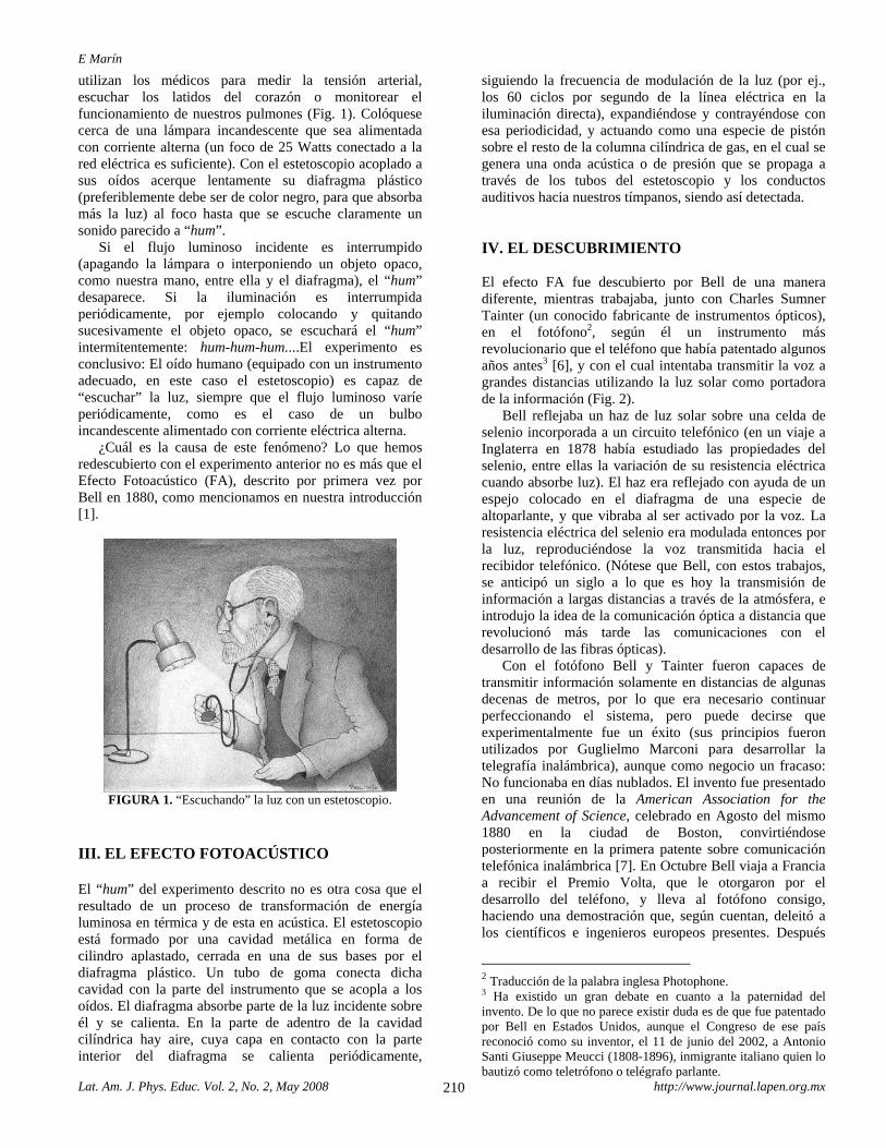
E Marín
Lat. Am. J. Phys. Educ. Vol. 2, No. 2, May 2008 210 http://www.journal.lapen.org.mx
utilizan los médicos para medir la tensión arterial, escuchar los latidos del corazón o monitorear el funcionamiento de nuestros pulmones (Fig. 1). Colóquese cerca de una lámpara incandescente que sea alimentada con corriente alterna (un foco de 25 Watts conectado a la red eléctrica es suficiente). Con el estetoscopio acoplado a sus oídos acerque lentamente su diafragma plástico (preferiblemente debe ser de color negro, para que absorba más la luz) al foco hasta que se escuche claramente un sonido parecido a “hum”.
Si el flujo luminoso incidente es interrumpido (apagando la lámpara o interponiendo un objeto opaco, como nuestra mano, entre ella y el diafragma), el “hum” desaparece. Si la iluminación es interrumpida periódicamente, por ejemplo colocando y quitando sucesivamente el objeto opaco, se escuchará el “hum” intermitentemente: hum-hum-hum....El experimento es conclusivo: El oído humano (equipado con un instrumento adecuado, en este caso el estetoscopio) es capaz de “escuchar” la luz, siempre que el flujo luminoso varíe periódicamente, como es el caso de un bulbo incandescente alimentado con corriente eléctrica alterna.
¿Cuál es la causa de este fenómeno? Lo que hemos redescubierto con el experimento anterior no es más que el Efecto Fotoacústico (FA), descrito por primera vez por Bell en 1880, como mencionamos en nuestra introducción [1].
FIGURA 1. “Escuchando” la luz con un estetoscopio.
III. EL EFECTO FOTOACÚSTICO El “hum” del experimento descrito no es otra cosa que el resultado de un proceso de transformación de energía luminosa en térmica y de esta en acústica. El estetoscopio está formado por una cavidad metálica en forma de cilindro aplastado, cerrada en una de sus bases por el diafragma plástico. Un tubo de goma conecta dicha cavidad con la parte del instrumento que se acopla a los oídos. El diafragma absorbe parte de la luz incidente sobre él y se calienta. En la parte de adentro de la cavidad cilíndrica hay aire, cuya capa en contacto con la parte interior del diafragma se calienta periódicamente,
siguiendo la frecuencia de modulación de la luz (por ej., los 60 ciclos por segundo de la línea eléctrica en la iluminación directa), expandiéndose y contrayéndose con esa periodicidad, y actuando como una especie de pistón sobre el resto de la columna cilíndrica de gas, en el cual se genera una onda acústica o de presión que se propaga a través de los tubos del estetoscopio y los conductos auditivos hacia nuestros tímpanos, siendo así detectada. IV. EL DESCUBRIMIENTO El efecto FA fue descubierto por Bell de una manera diferente, mientras trabajaba, junto con Charles Sumner Tainter (un conocido fabricante de instrumentos ópticos), en el fotófono2, según él un instrumento más revolucionario que el teléfono que había patentado algunos años antes3 [6], y con el cual intentaba transmitir la voz a grandes distancias utilizando la luz solar como portadora de la información (Fig. 2).
Bell reflejaba un haz de luz solar sobre una celda de selenio incorporada a un circuito telefónico (en un viaje a Inglaterra en 1878 había estudiado las propiedades del selenio, entre ellas la variación de su resistencia eléctrica cuando absorbe luz). El haz era reflejado con ayuda de un espejo colocado en el diafragma de una especie de altoparlante, y que vibraba al ser activado por la voz. La resistencia eléctrica del selenio era modulada entonces por la luz, reproduciéndose la voz transmitida hacia el recibidor telefónico. (Nótese que Bell, con estos trabajos, se anticipó un siglo a lo que es hoy la transmisión de información a largas distancias a través de la atmósfera, e introdujo la idea de la comunicación óptica a distancia que revolucionó más tarde las comunicaciones con el desarrollo de las fibras ópticas).
Con el fotófono Bell y Tainter fueron capaces de transmitir información solamente en distancias de algunas decenas de metros, por lo que era necesario continuar perfeccionando el sistema, pero puede decirse que experimentalmente fue un éxito (sus principios fueron utilizados por Guglielmo Marconi para desarrollar la telegrafía inalámbrica), aunque como negocio un fracaso: No funcionaba en días nublados. El invento fue presentado en una reunión de la American Association for the Advancement of Science, celebrado en Agosto del mismo 1880 en la ciudad de Boston, convirtiéndose posteriormente en la primera patente sobre comunicación telefónica inalámbrica [7]. En Octubre Bell viaja a Francia a recibir el Premio Volta, que le otorgaron por el desarrollo del teléfono, y lleva al fotófono consigo, haciendo una demostración que, según cuentan, deleitó a los científicos e ingenieros europeos presentes. Después
2 Traducción de la palabra inglesa Photophone. 3 Ha existido un gran debate en cuanto a la paternidad del invento. De lo que no parece existir duda es de que fue patentado por Bell en Estados Unidos, aunque el Congreso de ese país reconoció como su inventor, el 11 de junio del 2002, a Antonio Santi Giuseppe Meucci (1808-1896), inmigrante italiano quien lo bautizó como teletrófono o telégrafo parlante.
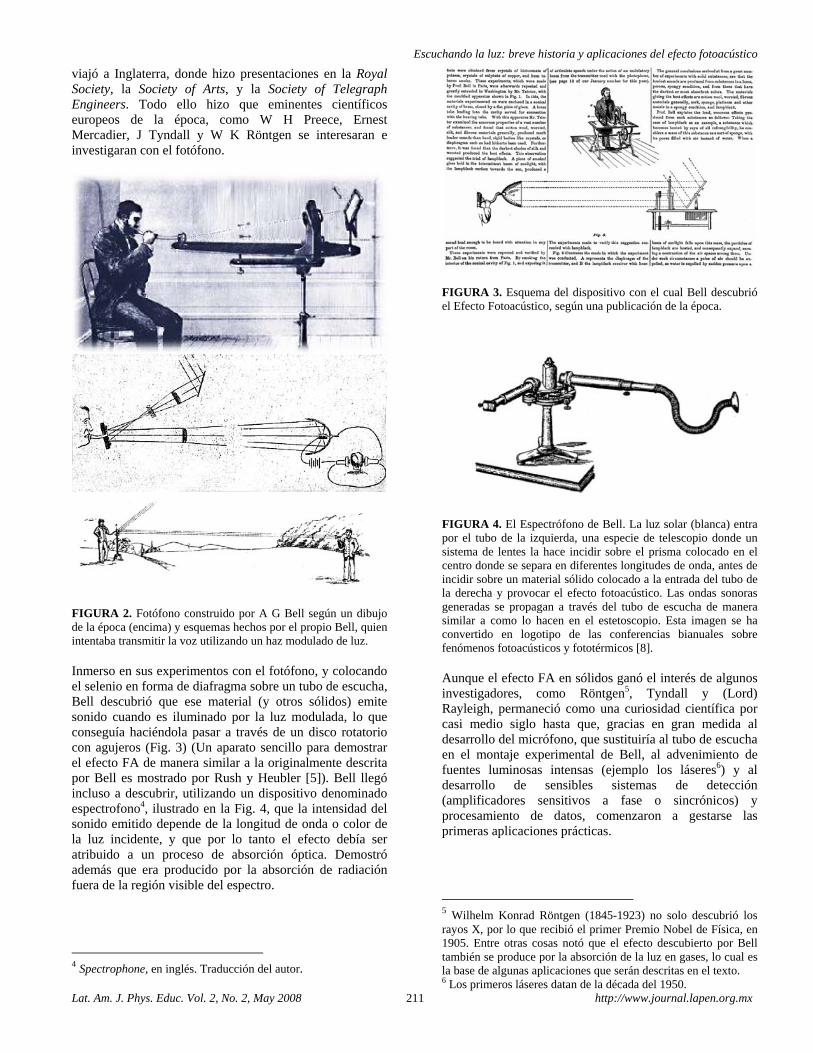
Escuchando la luz: breve historia y aplicaciones del efecto fotoacústico
Lat. Am. J. Phys. Educ. Vol. 2, No. 2, May 2008 211 http://www.journal.lapen.org.mx
viajó a Inglaterra, donde hizo presentaciones en la Royal Society, la Society of Arts, y la Society of Telegraph Engineers. Todo ello hizo que eminentes científicos europeos de la época, como W H Preece, Ernest Mercadier, J Tyndall y W K Röntgen se interesaran e investigaran con el fotófono.
FIGURA 2. Fotófono construido por A G Bell según un dibujo de la época (encima) y esquemas hechos por el propio Bell, quien intentaba transmitir la voz utilizando un haz modulado de luz.
Inmerso en sus experimentos con el fotófono, y colocando el selenio en forma de diafragma sobre un tubo de escucha, Bell descubrió que ese material (y otros sólidos) emite sonido cuando es iluminado por la luz modulada, lo que conseguía haciéndola pasar a través de un disco rotatorio con agujeros (Fig. 3) (Un aparato sencillo para demostrar el efecto FA de manera similar a la originalmente descrita por Bell es mostrado por Rush y Heubler [5]). Bell llegó incluso a descubrir, utilizando un dispositivo denominado espectrofono4, ilustrado en la Fig. 4, que la intensidad del sonido emitido depende de la longitud de onda o color de la luz incidente, y que por lo tanto el efecto debía ser atribuido a un proceso de absorción óptica. Demostró además que era producido por la absorción de radiación fuera de la región visible del espectro.
4 Spectrophone, en inglés. Traducción del autor.
FIGURA 3. Esquema del dispositivo con el cual Bell descubrió el Efecto Fotoacústico, según una publicación de la época.
FIGURA 4. El Espectrófono de Bell. La luz solar (blanca) entra por el tubo de la izquierda, una especie de telescopio donde un sistema de lentes la hace incidir sobre el prisma colocado en el centro donde se separa en diferentes longitudes de onda, antes de incidir sobre un material sólido colocado a la entrada del tubo de la derecha y provocar el efecto fotoacústico. Las ondas sonoras generadas se propagan a través del tubo de escucha de manera similar a como lo hacen en el estetoscopio. Esta imagen se ha convertido en logotipo de las conferencias bianuales sobre fenómenos fotoacústicos y fototérmicos [8].
Aunque el efecto FA en sólidos ganó el interés de algunos investigadores, como Röntgen5, Tyndall y (Lord) Rayleigh, permaneció como una curiosidad científica por casi medio siglo hasta que, gracias en gran medida al desarrollo del micrófono, que sustituiría al tubo de escucha en el montaje experimental de Bell, al advenimiento de fuentes luminosas intensas (ejemplo los láseres6) y al desarrollo de sensibles sistemas de detección (amplificadores sensitivos a fase o sincrónicos) y procesamiento de datos, comenzaron a gestarse las primeras aplicaciones prácticas.
5 Wilhelm Konrad Röntgen (1845-1923) no solo descubrió los rayos X, por lo que recibió el primer Premio Nobel de Física, en 1905. Entre otras cosas notó que el efecto descubierto por Bell también se produce por la absorción de la luz en gases, lo cual es la base de algunas aplicaciones que serán descritas en el texto. 6 Los primeros láseres datan de la década del 1950.
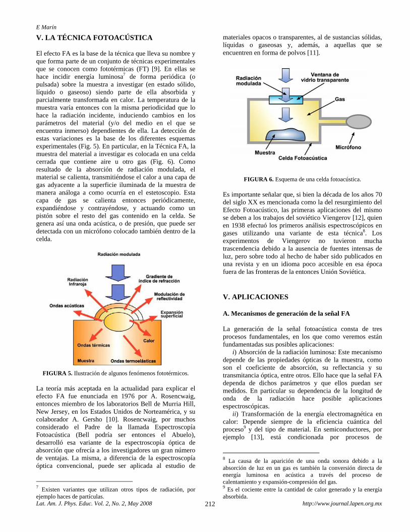
E Marín
Lat. Am. J. Phys. Educ. Vol. 2, No. 2, May 2008 212 http://www.journal.lapen.org.mx
V. LA TÉCNICA FOTOACÚSTICA El efecto FA es la base de la técnica que lleva su nombre y que forma parte de un conjunto de técnicas experimentales que se conocen como fototérmicas (FT) [9]. En ellas se hace incidir energía luminosa7 de forma periódica (o pulsada) sobre la muestra a investigar (en estado sólido, líquido o gaseoso) siendo parte de ella absorbida y parcialmente transformada en calor. La temperatura de la muestra varía entonces con la misma periodicidad que lo hace la radiación incidente, induciendo cambios en los parámetros del material (y/o del medio en el que se encuentra inmerso) dependientes de ella. La detección de estas variaciones es la base de los diferentes esquemas experimentales (Fig. 5). En particular, en la Técnica FA, la muestra del material a investigar es colocada en una celda cerrada que contiene aire u otro gas (Fig. 6). Como resultado de la absorción de radiación modulada, el material se calienta, transmitiéndose el calor a una capa de gas adyacente a la superficie iluminada de la muestra de manera análoga a como ocurría en el estetoscopio. Esta capa de gas se calienta entonces periódicamente, expandiéndose y contrayéndose, y actuando como un pistón sobre el resto del gas contenido en la celda. Se genera así una onda acústica, o de presión, que puede ser detectada con un micrófono colocado también dentro de la celda.
Expansión superficial
FIGURA 5. Ilustración de algunos fenómenos fototérmicos.
La teoría más aceptada en la actualidad para explicar el efecto FA fue enunciada en 1976 por A. Rosencwaig, entonces miembro de los laboratorios Bell de Murria Hill, New Jersey, en los Estados Unidos de Norteamérica, y su colaborador A. Gersho [10]. Rosencwaig, por muchos considerado el Padre de la llamada Espectroscopía Fotoacústica (Bell podría ser entonces el Abuelo), desarrolló esa variante de la espectroscopía óptica de absorción que ofrecía a los investigadores un gran número de ventajas. La misma, a diferencia de la espectroscopía óptica convencional, puede ser aplicada al estudio de
7 Existen variantes que utilizan otros tipos de radiación, por ejemplo haces de partículas.
materiales opacos o transparentes, al de sustancias sólidas, líquidas o gaseosas y, además, a aquellas que se encuentren en forma de polvos [11].
FIGURA 6. Esquema de una celda fotoacústica.
Es importante señalar que, si bien la década de los años 70 del siglo XX es mencionada como la del resurgimiento del Efecto Fotoacústico, las primeras aplicaciones del mismo se deben a los trabajos del soviético Viengerov [12], quien en 1938 efectuó los primeros análisis espectroscópicos en gases utilizando una variante de esta técnica8. Los experimentos de Viengerov no tuvieron mucha trascendencia debido a la ausencia de fuentes intensas de luz, pero sobre todo al hecho de haber sido publicados en una revista y en un idioma poco accesible en esa época fuera de las fronteras de la entonces Unión Soviética. V. APLICACIONES A. Mecanismos de generación de la señal FA La generación de la señal fotoacústica consta de tres procesos fundamentales, en los que como veremos están fundamentadas sus posibles aplicaciones:
i) Absorción de la radiación luminosa: Este mecanismo depende de las propiedades ópticas de la muestra, como son el coeficiente de absorción, su reflectancia y su transmitancia óptica, entre otros. Ello hace que la señal FA dependa de dichos parámetros y que ellos puedan ser medidos. En particular su dependencia de la longitud de onda de la radiación hace posible aplicaciones espectroscópicas.
ii) Transformación de la energía electromagnética en calor: Depende siempre de la eficiencia cuántica del proceso9 y del tipo de material. En semiconductores, por ejemplo [13], está condicionada por procesos de
8 La causa de la aparición de una onda sonora debido a la absorción de luz en un gas es también la conversión directa de energía luminosa en acústica a través del proceso de calentamiento y expansión-compresión del gas. 9 Es el cociente entre la cantidad de calor generado y la energía absorbida.
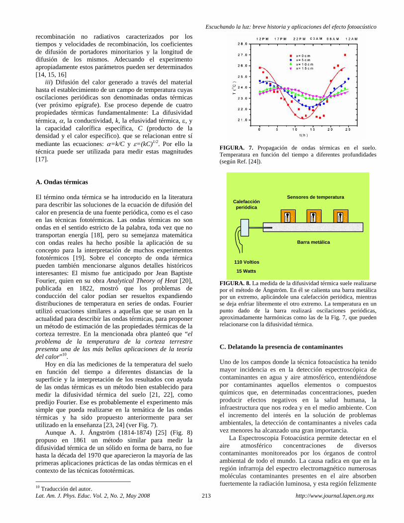
Escuchando la luz: breve historia y aplicaciones del efecto fotoacústico
Lat. Am. J. Phys. Educ. Vol. 2, No. 2, May 2008 213 http://www.journal.lapen.org.mx
recombinación no radiativos caracterizados por los tiempos y velocidades de recombinación, los coeficientes de difusión de portadores minoritarios y la longitud de difusión de los mismos. Adecuando el experimento apropiadamente estos parámetros pueden ser determinados [14, 15, 16]
iii) Difusión del calor generado a través del material hasta el establecimiento de un campo de temperatura cuyas oscilaciones periódicas son denominadas ondas térmicas (ver próximo epígrafe). Ese proceso depende de cuatro propiedades térmicas fundamentalmente: La difusividad térmica, α, la conductividad, k, la efusividad térmica, ε, y la capacidad calorífica específica, C (producto de la densidad y el calor específico). que se relacionan entre sí mediante las ecuaciones: α=k/C y ε=(kC)1/2. Por ello la técnica puede ser utilizada para medir estas magnitudes [17]. A. Ondas térmicas El término onda térmica se ha introducido en la literatura para describir las soluciones de la ecuación de difusión del calor en presencia de una fuente periódica, como es el caso en las técnicas fototérmicas. Las ondas térmicas no son ondas en el sentido estricto de la palabra, toda vez que no transportan energía [18], pero su semejanza matemática con ondas reales ha hecho posible la aplicación de su concepto para la interpretación de muchos experimentos fototérmicos [19]. Sobre el concepto de onda térmica pueden también mencionarse algunos detalles históricos interesantes: El mismo fue anticipado por Jean Baptiste Fourier, quien en su obra Analytical Theory of Heat [20], publicada en 1822, mostró que los problemas de conducción del calor podían ser resueltos expandiendo distribuciones de temperatura en series de ondas. Fourier utilizó ecuaciones similares a aquellas que se usan en la actualidad para describir las ondas térmicas, para proponer un método de estimación de las propiedades térmicas de la corteza terrestre. En la mencionada obra planteó que “el problema de la temperatura de la corteza terrestre presenta una de las más bellas aplicaciones de la teoría del calor”10.
Hoy en día las mediciones de la temperatura del suelo en función del tiempo a diferentes distancias de la superficie y la interpretación de los resultados con ayuda de las ondas térmicas es un método bien establecido para medir la difusividad térmica del suelo [21, 22], como predijo Fourier. Ese es probablemente el experimento más simple que pueda realizarse en la temática de las ondas térmicas y ha sido propuesto anteriormente para ser utilizado en la enseñanza [23, 24] (ver Fig. 7).
Aunque A. J. Ángström (1814-1874) [25] (Fig. 8) propuso en 1861 un método similar para medir la difusividad térmica de un sólido en forma de barra, no fue hasta la década del 1970 que aparecieron la mayoría de las primeras aplicaciones prácticas de las ondas térmicas en el contexto de las técnicas fototérmicas.
10 Traducción del autor.
FIGURA. 7. Propagación de ondas térmicas en el suelo. Temperatura en función del tiempo a diferentes profundidades (según Ref. [24]).
110 Voltios
15 Watts
Sensores de temperatura
Barra metálica
Calefacciónperiódica
FIGURA. 8. La medida de la difusividad térmica suele realizarse por el método de Ängström. En él se calienta una barra metálica por un extremo, aplicándole una calefacción periódica, mientras se deja enfriar libremente el otro extremo. La temperatura en un punto dado de la barra realizará oscilaciones periódicas, aproximadamente harmónicas como las de la Fig. 7, que pueden relacionarse con la difusividad térmica. C. Delatando la presencia de contaminantes Uno de los campos donde la técnica fotoacústica ha tenido mayor incidencia es en la detección espectroscópica de contaminantes en agua y aire atmosférico, entendiéndose por contaminantes aquellos elementos o compuestos químicos que, en determinadas concentraciones, pueden producir efectos negativos en la salud humana, la infraestructura que nos rodea y en el medio ambiente. Con el incremento del interés en la solución de problemas ambientales, la detección de contaminantes a niveles cada vez menores ha alcanzado una gran importancia.
La Espectroscopia Fotoacústica permite detectar en el aire atmosférico concentraciones de diversos contaminantes monitoreados por los órganos de control ambiental de todo el mundo. La causa radica en que en la región infrarroja del espectro electromagnético numerosas moléculas contaminantes presentes en el aire absorben fuertemente la radiación luminosa, y esta región felizmente
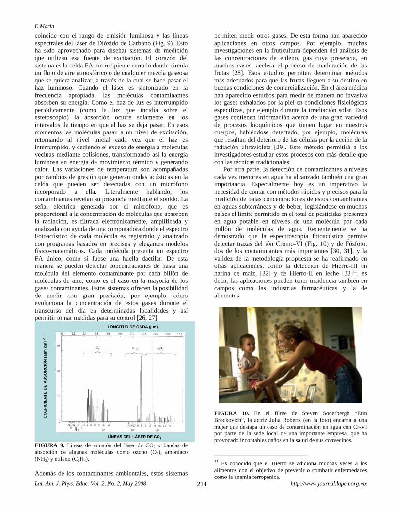
E Marín
Lat. Am. J. Phys. Educ. Vol. 2, No. 2, May 2008 214 http://www.journal.lapen.org.mx
coincide con el rango de emisión luminosa y las líneas espectrales del láser de Dióxido de Carbono (Fig. 9). Esto ha sido aprovechado para diseñar sistemas de medición que utilizan esa fuente de excitación. El corazón del sistema es la celda FA, un recipiente cerrado donde circula un flujo de aire atmosférico o de cualquier mezcla gaseosa que se quiera analizar, a través de la cual se hace pasar el haz luminoso. Cuando el láser es sintonizado en la frecuencia apropiada, las moléculas contaminantes absorben su energía. Como el haz de luz es interrumpido periódicamente (como la luz que incidía sobre el estetoscopio) la absorción ocurre solamente en los intervalos de tiempo en que el haz se deja pasar. En esos momentos las moléculas pasan a un nivel de excitación, retornando al nivel inicial cada vez que el haz es interrumpido, y cediendo el exceso de energía a moléculas vecinas mediante colisiones, transformando así la energía luminosa en energía de movimiento térmico y generando calor. Las variaciones de temperatura son acompañadas por cambios de presión que generan ondas acústicas en la celda que pueden ser detectadas con un micrófono incorporado a ella. Literalmente hablando, los contaminantes revelan su presencia mediante el sonido. La señal eléctrica generada por el micrófono, que es proporcional a la concentración de moléculas que absorben la radiación, es filtrada electrónicamente, amplificada y analizada con ayuda de una computadora donde el espectro Fotoacústico de cada molécula es registrado y analizado con programas basados en precisos y elegantes modelos físico-matemáticos. Cada molécula presenta un espectro FA único, como si fuese una huella dactilar. De esta manera se pueden detectar concentraciones de hasta una molécula del elemento contaminante por cada billón de moléculas de aire, como es el caso en la mayoría de los gases contaminantes. Estos sistemas ofrecen la posibilidad de medir con gran precisión, por ejemplo, cómo evoluciona la concentración de estos gases durante el transcurso del día en determinadas localidades y así permitir tomar medidas para su control [26, 27].
CO
EFIC
IEN
TE D
E A
BSO
RC
IÓN
(atm
cm) -1
LÍNEAS DEL LÁSER DE CO2
LONGITUD DE ONDA (μm)
FIGURA 9. Líneas de emisión del láser de CO2 y bandas de absorción de algunas moléculas como ozono (O3), amoniaco (NH3) y etileno (C2H4). Además de los contaminantes ambientales, estos sistemas
permiten medir otros gases. De esta forma han aparecido aplicaciones en otros campos. Por ejemplo, muchas investigaciones en la fruticultura dependen del análisis de las concentraciones de etileno, gas cuya presencia, en muchos casos, acelera el proceso de maduración de las frutas [28]. Esos estudios permiten determinar métodos más adecuados para que las frutas lleguen a su destino en buenas condiciones de comercialización. En el área médica han aparecido estudios para medir de manera no invasiva los gases exhalados por la piel en condiciones fisiológicas específicas, por ejemplo durante la irradiación solar. Esos gases contienen información acerca de una gran variedad de procesos bioquímicos que tienen lugar en nuestros cuerpos, habiéndose detectado, por ejemplo, moléculas que resultan del deterioro de las células por la acción de la radiación ultravioleta [29]. Este método permitirá a los investigadores estudiar estos procesos con más detalle que con las técnicas tradicionales.
Por otra parte, la detección de contaminantes a niveles cada vez menores en agua ha alcanzado también una gran importancia. Especialmente hoy es un imperativo la necesidad de contar con métodos rápidos y precisos para la medición de bajas concentraciones de estos contaminantes en aguas subterráneas y de beber, legislándose en muchos países el límite permitido en el total de pesticidas presentes en agua potable en niveles de una molécula por cada millón de moléculas de agua. Recientemente se ha demostrado que la espectroscopía fotoacústica permite detectar trazas del ión Cromo-VI (Fig. 10) y de Fósforo, dos de los contaminantes más importantes [30, 31], y la validez de la metodología propuesta se ha reafirmado en otras aplicaciones, como la detección de Hierro-III en harina de maíz, [32] y de Hierro-II en leche [33]11, es decir, las aplicaciones pueden tener incidencia también en campos como las industrias farmacéuticas y la de alimentos.
FIGURA 10. En el filme de Steven Soderbergh “Erin Brockovich”, la actriz Julia Roberts (en la foto) encarna a una mujer que destapa un caso de contaminación en agua con Cr-VI por parte de la sede local de una importante empresa, que ha provocado incontables daños en la salud de sus convecinos.
11 Es conocido que el Hierro se adiciona muchas veces a los alimentos con el objetivo de prevenir o combatir enfermedades como la anemia ferropénica.
Escuchando la luz: breve historia y aplicaciones del efecto fotoacústico
Lat. Am. J. Phys. Educ. Vol. 2, No. 2, May 2008 215 http://www.journal.lapen.org.mx
VII. CONCLUSIONES Las técnicas fototérmicas han alcanzado un gran desarrollo desde el redescubrimiento del efecto fotoacústico y sus primeras aplicaciones en la década del 1970. Sin embargo, aún son desconocidas para muchas personas. Por ello resulta importante dar a conocer sus principios fundamentales, la historia de su desarrollo y sus potencialidades, a profesores y estudiantes de ciencias e ingenierías y a aquellos involucrados en la enseñanza de la historia de las ciencias, con el objetivo de que estos aspectos puedan ser incorporados en algunos cursos y diseminados entre una audiencia más amplia. Las referencias [9-11, 18, 19] pueden ser un buen punto de partida para profundizar en el tema.
Aunque hemos limitado la exposición de las aplicaciones al campo de la espectroscopía y específicamente a su uso en la detección de contaminantes en sistemas ambientales, muchas otras demuestran que podemos, escuchando la luz, detectar la actividad de diferentes elementos químicos en diversos sistemas físicos y biológicos, cuya presencia en muchos casos puede resultar indeseable. Escuchando la luz se pueden medir, además, diferentes propiedades de los materiales, como las ópticas, que regulan cómo es absorbida la luz de diferentes colores, o las térmicas, que describen por qué un cuerpo se calienta más o por qué conduce mejor el calor que otro. Pero referirse a ellas podría ser tema de otros trabajos. AGRADECIMIENTOS El autor agradece a Y. Marín-Gutiérrez por proporcionarle la Fig. 1. Este trabajo ha sido apoyado parcialmente por el IPN a través de COFAA y del proyecto de investigación SIP 20070490. REFERENCIAS [1] Bell, A. G., Am. J. of Sci. 20, 305 (1880). [2] Campbell, C. y Laherrere, J., Sci. Am. 78, 278, (1998). [3] Euler, M., Niemann, K. y Müller, A., The Physics Teacher 38, 356 (Septiembre 2000). [4] Euler, M., The Physics Teacher 39, 406 (2001). [5] Rush, W. F. y Heubler, E., Am. J. Phys. 50, 669, 1982. [6] Bell, A. G., Telephone United States Patent No. 174, 465, (1876). [7] Bell, A. G. y Tainter, S., Photophone United State Patent No. 235, 496, (1880). [8] http://www.icppp.org/links.htm. [9] Almond, D. P. y Patel, P. M., Photothermal Science and Techniques en Physics and its Applications, 10 Dobbsand, E. R. y Palmer, S. B. (Eds), (Chapman and Hall, London, 1996). [10] Rosencwaig, A. y Gersho, A., J. of Appl. Phys. 47, 64 (1976). [11] Rosencwaig, A., Physics Today 28, 23 (1975)
[12] Viengerov, M. L., Dokl. Akad. Nauk. SSSR 19, 687 (1938) [13] Mandelis, A. (Ed.) Photoacoustic and Thermal Wave Phenomena in Semiconductors (Elsevier, 1987). [14] Marín, E., Vargas, H., Díaz, P. y Riech, I., Phys. Stat. Sol.(A) 179, 387 (2000). [15] Marín, E., Riech, I., Díaz, P., Alvarado-Gil, J. J., Baquero, R., Mendoza-Alvarez, J. G., Vargas, H., Cruz-Orea, A. y Vargas, M., J. Appl. Phys. 83, 2604 (1998). [16] Riech, I., Gomez-Herrera, M. L., Díaz, P., Mendoza-Alvarez, J. G, Herrera-Pérez, J. L. y Marín, E., Applied Physics Letters 79, 964 (2001). [17] Vargas, H. y Miranda, L. C. M., Physics Reports 161, 43 (1980). [18] Salazar, A., Eur. J. Phys. 27, 1 (2006). [19] Marin, E., European Journal of Physics 28, 429 (2007). [20] Fourier, J. B. J., Analytical theory of Heat, traducida por Freeman, A. (Encyclopedia Britannica, Inc., Chicago: 1952) [21] Hanks, R. J., Applied soil physics. Soil water and temperature applications, 2nd ed., (Springer-Verlag, New York, 1992). [22] Fuhrer, O. Inverse Heat Conduction In Soils A New Approach Towards Recovering Soil Moisture From Temperature Records Diploma Thesis Climate Research ETH, Zurich ETH Zurich, Dept. Physics March 2000. http://iacweb.ethz.ch/staff/fuhrer/publ/dipl/ [23] McIntosh, G. y Sharratt, B. S., The Phys. Teach. 39 458 (2001). [24] Marín, E., Jean-Baptiste, E. y Hernández, M., Revista Mexicana de Física E52, 21 (2006). [25] Ångström, A. J., Ann. Physik. Lpz. 114, 513, (1861). [26] Sigrist, M. W. In “Air Monitoring by Spectroscopyc Techniques” Sigrist, M. W. (Ed.) (Wiley, New York, 163, 1994). [27] de Vries, H. S. M., “Non-intrusive fruit and plant analysis by laser photothermal measurements of ethylene emission” In “Modern methods of plant analysis” Linskend, H. F. y Jackson, J. F. (Eds) (Springer-Verlag, Heidelberg, 1995). [28] Voesenek, L, A, C, J., M Banga, J, H, G, M,, Rijnders, E. J. W., Visser, F. J. M., Harrent, Brailsford, R. W., Jacksont, M. B. y Blom, C. W. P. M., Annals of Botany 79 (Supplement A): 57 (1997). [29] Harren, F. J. M. y Reuss, J., Encyclopaedia of Applied Physics, Trigg, G. L. (Ed.), (Weinheim, 1997). [29] Lima, J. A. P., Marin, E., Cardoso, S. L., da Silva, M. G., Sthel, M., Costa, C. G. S., Mariano, A., Rezende, C. E., Ovalle, R. C., Susuki, M. S. y Vargas, H., Int. J. of Envirom. Anal. Chem. 76, 331 (2000). [30] Delgado-Vasallo, O., Valdés, A. C., Marín, E., Lima, J. A. P., da Silva, M. G., Sthel, M. S., Vargas, H. y Cardoso, S. L., Meas. Sc. Technol. 11, 412 (2000). [31] Delgado-Vasallo, O., Peña, J., San Martín Martínez,
E., Calderón, A., Peña-Rodríguez, G., Jaime Fonseca, M. R. y Marín, E. Anal. Sciences 19, 599 (2003). [32] Cardoso, S. L., Dias, C. M. F., Lima, J. A. P., Massunaga, M. S. O., da Silva, M. G. y Vargas, H., Rev. Sci. Instrum. 74, 712 (2003).
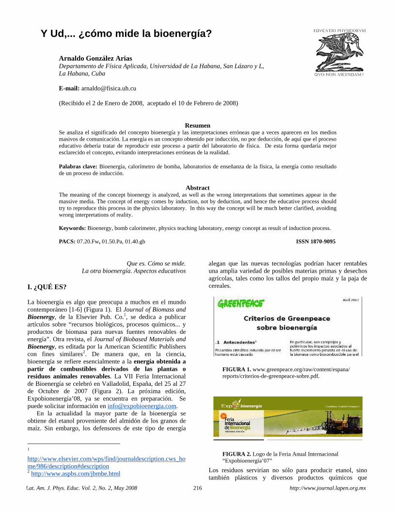
Lat. Am. J. Phys. Educ. Vol. 2, No. 2, May 2008 216 http://www.journal.lapen.org.mx
Y Ud,... ¿cómo mide la bioenergía?
Arnaldo González Arias Departamento de Física Aplicada, Universidad de La Habana, San Lázaro y L, La Habana, Cuba E-mail: [email protected] (Recibido el 2 de Enero de 2008, aceptado el 10 de Febrero de 2008)
Resumen Se analiza el significado del concepto bioenergía y las interpretaciones erróneas que a veces aparecen en los medios masivos de comunicación. La energía es un concepto obtenido por inducción, no por deducción, de aquí que el proceso educativo debería tratar de reproducir este proceso a partir del laboratorio de física. De esta forma quedaría mejor esclarecido el concepto, evitando interpretaciones erróneas de la realidad. Palabras clave: Bioenergía, calorímetro de bomba, laboratorios de enseñanza de la física, la energía como resultado de un proceso de inducción.
Abstract The meaning of the concept bioenergy is analyzed, as well as the wrong interpretations that sometimes appear in the massive media. The concept of energy comes by induction, not by deduction, and hence the educative process should try to reproduce this process in the physics laboratory. In this way the concept will be much better clarified, avoiding wrong interpretations of reality. Keywords: Bioenergy, bomb calorimeter, physics teaching laboratory, energy concept as result of induction process. PACS: 07.20.Fw, 01.50.Pa, 01.40.gb ISSN 1870-9095
Que es. Cómo se mide. La otra bioenergía. Aspectos educativos
I. ¿QUÉ ES?
La bioenergía es algo que preocupa a muchos en el mundo contemporáneo [1-6] (Figura 1). El Journal of Biomass and Bioenergy, de la Elsevier Pub. Co.1, se dedica a publicar artículos sobre “recursos biológicos, procesos químicos... y productos de biomasa para nuevas fuentes renovables de energía”. Otra revista, el Journal of Biobased Materials and Bioenergy, es editada por la American Scientific Publishers con fines similares2. De manera que, en la ciencia, bioenergía se refiere esencialmente a la energía obtenida a partir de combustibles derivados de las plantas o residuos animales renovables. La VII Feria Internacional de Bioenergía se celebró en Valladolid, España, del 25 al 27 de Octubre de 2007 (Figura 2). La próxima edición, Expobionenergía’08, ya se encuentra en preparación. Se puede solicitar información en [email protected].
En la actualidad la mayor parte de la bioenergía se obtiene del etanol proveniente del almidón de los granos de maíz. Sin embargo, los defensores de este tipo de energía
1 http://www.elsevier.com/wps/find/journaldescription.cws_home/986/description#description 2 http://www.aspbs.com/jbmbe.html
alegan que las nuevas tecnologías podrían hacer rentables una amplia variedad de posibles materias primas y desechos agrícolas, tales como los tallos del propio maíz y la paja de cereales.
Los residuos servirían no sólo para producir etanol, sino también plásticos y diversos productos químicos que
FIGURA 2. Logo de la Feria Anual Internacional “Expobioenergía’07”
FIGURA 1. www.greenpeace.org/raw/content/espana/ reports/criterios-de-greenpeace-sobre.pdf.
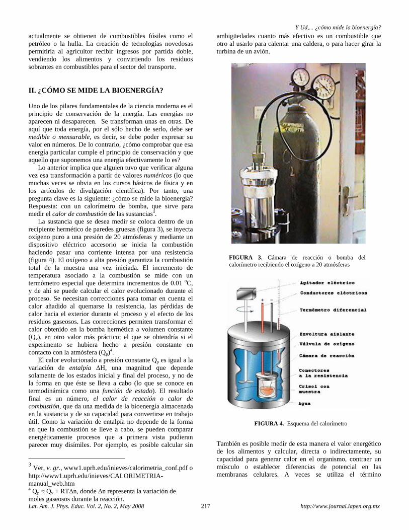
Y Ud,... ¿cómo mide la bioenergía?
Lat. Am. J. Phys. Educ. Vol. 2, No. 2, May 2008 217 http://www.journal.lapen.org.mx
actualmente se obtienen de combustibles fósiles como el petróleo o la hulla. La creación de tecnologías novedosas permitiría al agricultor recibir ingresos por partida doble, vendiendo los alimentos y convirtiendo los residuos sobrantes en combustibles para el sector del transporte.
II. ¿CÓMO SE MIDE LA BIOENERGÍA?
Uno de los pilares fundamentales de la ciencia moderna es el principio de conservación de la energía. Las energías no aparecen ni desaparecen. Se transforman unas en otras. De aquí que toda energía, por el sólo hecho de serlo, debe ser medible o mensurable, es decir, se debe poder expresar su valor en números. De lo contrario, ¿cómo comprobar que esa energía particular cumple el principio de conservación y que aquello que suponemos una energía efectivamente lo es?
Lo anterior implica que alguien tuvo que verificar alguna vez esa transformación a partir de valores numéricos (lo que muchas veces se obvia en los cursos básicos de física y en los artículos de divulgación científica). Por tanto, una pregunta clave es la siguiente: ¿cómo se mide la bioenergía? Respuesta: con un calorímetro de bomba, que sirve para medir el calor de combustión de las sustancias3.
La sustancia que se desea medir se coloca dentro de un recipiente hermético de paredes gruesas (figura 3), se inyecta oxígeno puro a una presión de 20 atmósferas y mediante un dispositivo eléctrico accesorio se inicia la combustión haciendo pasar una corriente intensa por una resistencia (figura 4). El oxígeno a alta presión garantiza la combustión total de la muestra una vez iniciada. El incremento de temperatura asociado a la combustión se mide con un termómetro especial que determina incrementos de 0.01 oC, y de ahí se puede calcular el calor evolucionado durante el proceso. Se necesitan correcciones para tomar en cuenta el calor añadido al quemarse la resistencia, las pérdidas de calor hacia el exterior durante el proceso y el efecto de los residuos gaseosos. Las correcciones permiten transformar el calor obtenido en la bomba hermética a volumen constante (Qv), en otro valor más práctico; el que se obtendría si el experimento se hubiera hecho a presión constante en contacto con la atmósfera (Qp)
4. El calor evolucionado a presión constante Qp es igual a la
variación de entalpía ΔH, una magnitud que depende solamente de los estados inicial y final del proceso, y no de la forma en que éste se lleva a cabo (lo que se conoce en termodinámica como una función de estado). El resultado final es un número, el calor de reacción o calor de combustión, que da una medida de la bioenergía almacenada en la sustancia y de su capacidad para convertirse en trabajo útil. Como la variación de entalpía no depende de la forma en que la combustión se lleve a cabo, se pueden comparar energéticamente procesos que a primera vista pudieran parecer muy disímiles. Por ejemplo, es posible calcular sin
3 Ver, v. gr., www1.uprh.edu/inieves/calorimetria_conf.pdf o http://www1.uprh.edu/inieves/CALORIMETRIA-manual_web.htm 4 Qp ≈ Qv + RTΔn, donde Δn representa la variación de moles gaseosos durante la reacción.
ambigüedades cuanto más efectivo es un combustible que otro al usarlo para calentar una caldera, o para hacer girar la turbina de un avión.
También es posible medir de esta manera el valor energético de los alimentos y calcular, directa o indirectamente, su capacidad para generar calor en el organismo, contraer un músculo o establecer diferencias de potencial en las membranas celulares. A veces se utiliza el término
FIGURA 4. Esquema del calorímetro
FIGURA 3. Cámara de reacción o bomba del calorímetro recibiendo el oxígeno a 20 atmósferas
Arnaldo González Arias
Lat. Am. J. Phys. Educ. Vol.2, No. 2, May 2008 218 http://www.journal.lapen.org.mx
bioenergética para designar el estudio de estos procesos5, que en realidad no se refieren a la bioenergía como tal, sino a la forma en que la energía proveniente de los alimentos, y almacenada en las células, se transforma en energía mecánica, eléctrica, o de otro tipo. El contenido bioenergético de los alimentos es bien conocido; en valor aproximado:
Hidratos de carbono ~ 17 kJ/g Proteínas ~ 17,5 kJ/g Grasas ~ 39 kJ/g
En el organismo, sólo un 20% se aprovecha en trabajo muscular. El resto se disipa en forma de calor.
III. LA OTRA BIOENERGIA En la pseudociencia6 es usual encontrar una sutil apropiación de términos científicos conocidos para designar supuestos objetos o fenómenos cuya existencia ni siquiera está comprobada. De esa forma se trata de dar apariencia científica a lo que no lo es, presentando las creencias como supuestas evidencias. Y no siempre se hace a propósito o conscientemente, sino más bien por desconocimiento acerca de la ciencia y su metodología. Se crea de esta manera una especie de subcultura marginal que pretende ser ciencia sin aplicar sus métodos.
Así, en determinados círculos pseudocientíficos bioenergía designa un “algo” diferente al concepto explicado en la sección anterior. Este “algo” es una imaginaria “energía” cuya existencia se asume o postula, pero que ni los mismos que la postulan saben bien lo que es. Se considera asociada exclusivamente a la vida y a los seres vivos, de forma que cuando la planta o la persona mueren, la tal “bioenergía” desaparece. No es una forma de energía que la ciencia pueda reconocer porque, por más que Ud. busque y rebusque, resulta imposible encontrar una definición concreta o una descripción clara de como se mide ese “algo”.
Por ejemplo, en uno de estos sitios “bioenergéticos” se puede leer: "Una metodología práctica y sencilla para seleccionar los alimentos midiendo su campo bioenergético, asegurando la adquisición de un alimento fresco, de gran sabor y que aporta energía vital (prana) a nuestro organismo".7 Pero cuando Ud. escribe a la dirección de contacto -como hizo el autor- preguntando donde se puede obtener información acerca de como se mide el tal campo bioenergético, recibe la callada por respuesta.8
Además, si la tal “energía” desaparece cuando la vida se extingue, evidentemente no puede cumplir el principio de conservación. Y si no desaparece... ¿adonde va? ¿Se disipa en el medio ambiente? ¿Se convierte en calor? ¿Es tan sutil que no se puede medir o detectar?
5 Enciclopedia Encarta 2007 6 Pseudociencia: falsa ciencia 7 http://www.bioenergetica.cl/seleccion-
alimentos.php?id_familia=alimentos 8 Lo mismo sucede con la energía vital, concepto similar
del hinduismo, indefinido, no medible, asociado sólo a lo vivo, no cumple el principio de conservación, etc.
Si no se puede detectar, ¿como sabe Ud. que está ahí? De aquí que cuando alguna sociedad bioenergética9
intenta describir las propiedades de “su” bioenergía, no es difícil encontrar afinidades con el misticismo, el alma, el espíritu u otros conceptos religiosos, –aunque las terminologías utilizadas no sean las mismas que comunmente emplea la religión. Esto último, según los que conocen del tema, además de no ser ciencia, es pésima teología.
IV ASPECTOS EDUCATIVOS La transformación de la energía no se deduce a partir de otro principio ni es un postulado teórico, es un resultado inducido10 de la evidencia experimental. De aquí que el proceso docente-educativo debería de alguna forma tratar de reproducir este proceso de inducción, haciendo énfasis en las prácticas experimentales que ilustren las transformaciones de energía con valores numéricos.
Parece ser que la falta de preparación en el tema energético, tanto en la enseñanza media como en la universitaria, ha sido y es un excelente caldo de cultivo para que prolifere la pseudociencia. La imprecisión se agrava drásticamente cuando hay escasez de recursos para las prácticas del laboratorio docente. No le queda al alumno otra posibilidad que imaginar la realidad -si puede y como pueda- obteniendo así una visión deformada de la ciencia y del método científico.
V. CONCLUSIONES El concepto general de energía proviene de la inducción; no se deduce de ningún lugar. De aquí que las formas de enseñanza adecuadas deberían estar acordes al proceso mediante el cual fue obtenido el concepto. Por tanto, parece razonable concluir que sería conveniente introducir en los laboratorios de física la medición de energías particulares (como la bioenergía) antes de llegar al concepto general de energía -o al menos, programar tales mediciones en actividades paralelas-. Tal proceder debería ser válido para cualquier nivel de enseñanza donde se mencione la energía.
Y en cuanto a la concepción errónea de bioenergía que muchas veces aparece en los medios masivos de comunicación, en realidad resulta fácil separar lo ilusorio de la realidad física. Cuando alguien le argumente sobre estos temas, pregunte:
Y cuando la vida cesa... ¿adonde va la bioenergía? O mejor aún: Y Ud,... ¿cómo mide la bioenergía?
9 Hay muchísimos sitios en la WEB que tratan este tema, usualmente asociados a “terapias” de dudosa efectividad. 10 Inducción: en el campo de la lógica, proceso en el que se razona desde lo particular hasta lo general, al contrario de la deducción.

Y Ud,... ¿cómo mide la bioenergía?
Lat. Am. J. Phys. Educ. Vol. 2, No. 2, May 2008 219 http://www.journal.lapen.org.mx
REFERENCIAS
[1] Shapouri, H., Duffield, J., Mcaloon, A. J. The 2001 Net Energy Balance of Corn-Ethanol. Proceedings of the Conference on Agriculture As a Producer and Consumer of Energy, Arlington, VA., June 24-25 (2004). [2] Farrell, A. E., Plevin, R. J., Turner, B. T., Jones, A. D., O’Hare, M., Kammen, D. M. Ethanol can contribute to energy and environmental goals. Science 311: 506-508 (2006). [3] Dias de Oliveira, M. E., Vaughan, B.E. & Rykiel, Jr. E. J.
Ethanol as fuel: energy, carbon dioxide balances, and ecological footprint. Bioscience 55, 593-602 (2005). [4] Pearce, F. 2005. Forests paying the price forbio-fuels. New Scientist 19th November Greenpeace (2006). [5] Farrell, A. E., Plevin, R. J., Turner, B. T., Jones, A. D., O’Hare, M., Kammen, D. M. Ethanolcan contribute to energy and environmental goals, Science 311, 506-508 (2006). [6] Gray, K. A., Zhao, L. & Emptage, M. Bioethanol. Current Opinion in Chemical Biology 10, 141-146 (2006).

Lat. Am. J. Phys. Educ. Vol. 2, No. 2, May 2008 220 http://www.journal.lapen.org.mx
NOTES D. C. Agrawal Department of Farm Engineering, Banaras Hindu University, Varanasi 221005, India E-mail: [email protected]
As mentioned by Hamdan, Chamaa and Lopez-Bonilla [1] the Dirac’s wave equation still has many features which have not been fully understood. One such feature concerning the beta matrix is discussed below: In the Dirac free particle [2] Hamiltonian H = cα.p + β mc2, the first term is related purely with the motion of the particle while the second term describes the properties purely at rest. In the first term the linear momentum p is dotted with σ (because α =ρσ) which is essentially the inherent spin operator whose classical analog is rotatory angular momentum. A similar analogy should also hold for the second term i.e., the mass m which is inertia for the linear motion should be multiplied by an inherent property representing the inertia for rotatory motion. Hence it may be proposed that β essentially measures moment of inertia Io of the particle and the suggested relation between them could be Io = β (ħ2 /mc2). This is
plausible because both β and Io should be Hermitian operators with positive (negative) eigenvalues corresponding to particle (antiparticle). Starting with this idea the following speculations can be made. (i) Just as a conservation law holds for L + S we expect the sum, Io + m x an appropriate operator, to be conserved. (ii) Since β commutes with σ hence Io should be independent of the spinning of the particle and the expression Io ω = ħ S would define the classical analog of angular frequency. REFERENCES [1] Hamdan N., Chamaa A. and Lopez-Bonilla J., On the relativistic concept of the Dirac’s electron spin, Lat. Am. J. Phys. Educ. 2, 65-70 (2008). [2] Leonard I. Schiff, Quantum Mechanics (McGraw-Hill, Tokyo, 1955) p. 323.
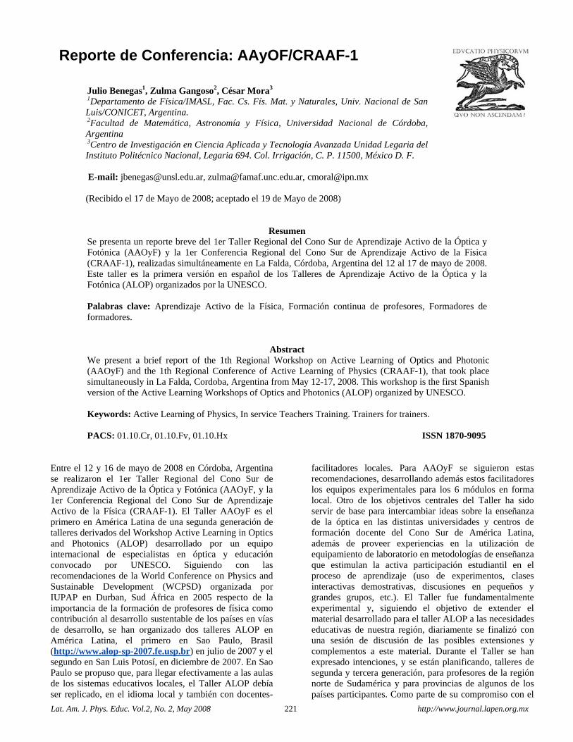
Lat. Am. J. Phys. Educ. Vol.2, No. 2, May 2008 221 http://www.journal.lapen.org.mx
Reporte de Conferencia: AAyOF/CRAAF-1
Julio Benegas1, Zulma Gangoso2, César Mora3 1Departamento de Física/IMASL, Fac. Cs. Fís. Mat. y Naturales, Univ. Nacional de San Luis/CONICET, Argentina. 2Facultad de Matemática, Astronomía y Física, Universidad Nacional de Córdoba, Argentina 3Centro de Investigación en Ciencia Aplicada y Tecnología Avanzada Unidad Legaria del Instituto Politécnico Nacional, Legaria 694. Col. Irrigación, C. P. 11500, México D. F. E-mail: [email protected], [email protected], [email protected] (Recibido el 17 de Mayo de 2008; aceptado el 19 de Mayo de 2008)
Resumen Se presenta un reporte breve del 1er Taller Regional del Cono Sur de Aprendizaje Activo de la Óptica y Fotónica (AAOyF) y la 1er Conferencia Regional del Cono Sur de Aprendizaje Activo de la Física (CRAAF-1), realizadas simultáneamente en La Falda, Córdoba, Argentina del 12 al 17 de mayo de 2008. Este taller es la primera versión en español de los Talleres de Aprendizaje Activo de la Óptica y la Fotónica (ALOP) organizados por la UNESCO. Palabras clave: Aprendizaje Activo de la Física, Formación continua de profesores, Formadores de formadores.
Abstract We present a brief report of the 1th Regional Workshop on Active Learning of Optics and Photonic (AAOyF) and the 1th Regional Conference of Active Learning of Physics (CRAAF-1), that took place simultaneously in La Falda, Cordoba, Argentina from May 12-17, 2008. This workshop is the first Spanish version of the Active Learning Workshops of Optics and Photonics (ALOP) organized by UNESCO. Keywords: Active Learning of Physics, In service Teachers Training. Trainers for trainers. PACS: 01.10.Cr, 01.10.Fv, 01.10.Hx ISSN 1870-9095
Entre el 12 y 16 de mayo de 2008 en Córdoba, Argentina se realizaron el 1er Taller Regional del Cono Sur de Aprendizaje Activo de la Óptica y Fotónica (AAOyF, y la 1er Conferencia Regional del Cono Sur de Aprendizaje Activo de la Física (CRAAF-1). El Taller AAOyF es el primero en América Latina de una segunda generación de talleres derivados del Workshop Active Learning in Optics and Photonics (ALOP) desarrollado por un equipo internacional de especialistas en óptica y educación convocado por UNESCO. Siguiendo con las recomendaciones de la World Conference on Physics and Sustainable Development (WCPSD) organizada por IUPAP en Durban, Sud África en 2005 respecto de la importancia de la formación de profesores de física como contribución al desarrollo sustentable de los países en vías de desarrollo, se han organizado dos talleres ALOP en América Latina, el primero en Sao Paulo, Brasil (http://www.alop-sp-2007.fe.usp.br) en julio de 2007 y el segundo en San Luis Potosí, en diciembre de 2007. En Sao Paulo se propuso que, para llegar efectivamente a las aulas de los sistemas educativos locales, el Taller ALOP debía ser replicado, en el idioma local y también con docentes-
facilitadores locales. Para AAOyF se siguieron estas recomendaciones, desarrollando además estos facilitadores los equipos experimentales para los 6 módulos en forma local. Otro de los objetivos centrales del Taller ha sido servir de base para intercambiar ideas sobre la enseñanza de la óptica en las distintas universidades y centros de formación docente del Cono Sur de América Latina, además de proveer experiencias en la utilización de equipamiento de laboratorio en metodologías de enseñanza que estimulan la activa participación estudiantil en el proceso de aprendizaje (uso de experimentos, clases interactivas demostrativas, discusiones en pequeños y grandes grupos, etc.). El Taller fue fundamentalmente experimental y, siguiendo el objetivo de extender el material desarrollado para el taller ALOP a las necesidades educativas de nuestra región, diariamente se finalizó con una sesión de discusión de las posibles extensiones y complementos a este material. Durante el Taller se han expresado intenciones, y se están planificando, talleres de segunda y tercera generación, para profesores de la región norte de Sudamérica y para provincias de algunos de los países participantes. Como parte de su compromiso con el
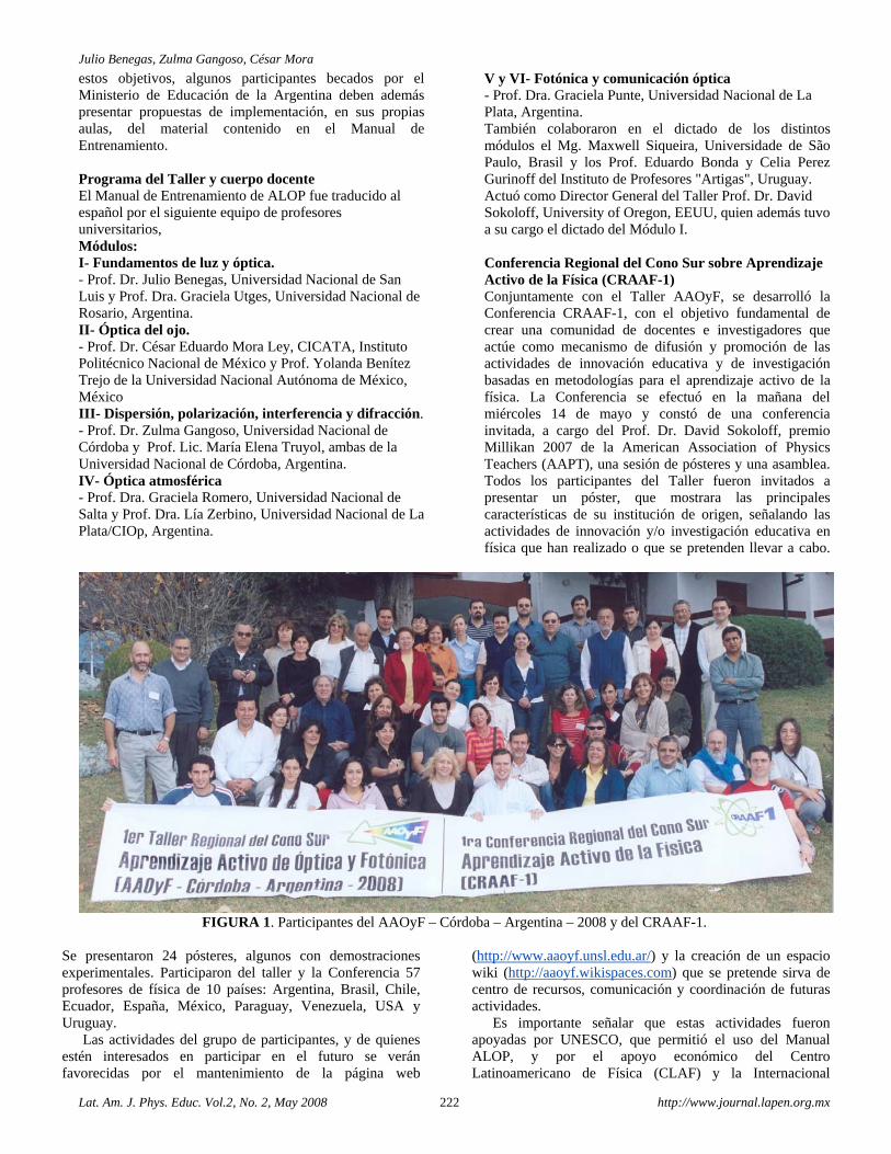
Julio Benegas, Zulma Gangoso, César Mora
Lat. Am. J. Phys. Educ. Vol.2, No. 2, May 2008 222 http://www.journal.lapen.org.mx
estos objetivos, algunos participantes becados por el Ministerio de Educación de la Argentina deben además presentar propuestas de implementación, en sus propias aulas, del material contenido en el Manual de Entrenamiento. Programa del Taller y cuerpo docente El Manual de Entrenamiento de ALOP fue traducido al español por el siguiente equipo de profesores universitarios, Módulos: I- Fundamentos de luz y óptica. - Prof. Dr. Julio Benegas, Universidad Nacional de San Luis y Prof. Dra. Graciela Utges, Universidad Nacional de Rosario, Argentina. II- Óptica del ojo. - Prof. Dr. César Eduardo Mora Ley, CICATA, Instituto Politécnico Nacional de México y Prof. Yolanda Benítez Trejo de la Universidad Nacional Autónoma de México, México III- Dispersión, polarización, interferencia y difracción. - Prof. Dr. Zulma Gangoso, Universidad Nacional de Córdoba y Prof. Lic. María Elena Truyol, ambas de la Universidad Nacional de Córdoba, Argentina. IV- Óptica atmosférica - Prof. Dra. Graciela Romero, Universidad Nacional de Salta y Prof. Dra. Lía Zerbino, Universidad Nacional de La Plata/CIOp, Argentina.
V y VI- Fotónica y comunicación óptica - Prof. Dra. Graciela Punte, Universidad Nacional de La Plata, Argentina. También colaboraron en el dictado de los distintos módulos el Mg. Maxwell Siqueira, Universidade de São Paulo, Brasil y los Prof. Eduardo Bonda y Celia Perez Gurinoff del Instituto de Profesores "Artigas", Uruguay. Actuó como Director General del Taller Prof. Dr. David Sokoloff, University of Oregon, EEUU, quien además tuvo a su cargo el dictado del Módulo I. Conferencia Regional del Cono Sur sobre Aprendizaje Activo de la Física (CRAAF-1) Conjuntamente con el Taller AAOyF, se desarrolló la Conferencia CRAAF-1, con el objetivo fundamental de crear una comunidad de docentes e investigadores que actúe como mecanismo de difusión y promoción de las actividades de innovación educativa y de investigación basadas en metodologías para el aprendizaje activo de la física. La Conferencia se efectuó en la mañana del miércoles 14 de mayo y constó de una conferencia invitada, a cargo del Prof. Dr. David Sokoloff, premio Millikan 2007 de la American Association of Physics Teachers (AAPT), una sesión de pósteres y una asamblea. Todos los participantes del Taller fueron invitados a presentar un póster, que mostrara las principales características de su institución de origen, señalando las actividades de innovación y/o investigación educativa en física que han realizado o que se pretenden llevar a cabo.
FIGURA 1. Participantes del AAOyF – Córdoba – Argentina – 2008 y del CRAAF-1.
Se presentaron 24 pósteres, algunos con demostraciones experimentales. Participaron del taller y la Conferencia 57 profesores de física de 10 países: Argentina, Brasil, Chile, Ecuador, España, México, Paraguay, Venezuela, USA y Uruguay.
Las actividades del grupo de participantes, y de quienes estén interesados en participar en el futuro se verán favorecidas por el mantenimiento de la página web
(http://www.aaoyf.unsl.edu.ar/) y la creación de un espacio wiki (http://aaoyf.wikispaces.com) que se pretende sirva de centro de recursos, comunicación y coordinación de futuras actividades.
Es importante señalar que estas actividades fueron apoyadas por UNESCO, que permitió el uso del Manual ALOP, y por el apoyo económico del Centro Latinoamericano de Física (CLAF) y la Internacional

Reporte de Conferencia: AAOyF/CRAAF-1
Lat. Am. J. Phys. Educ. Vol.2, No. 2, May 2008 223 http://www.journal.lapen.org.mx
Society of Optical Engineering (SPIE). La organización recibió un importante apoyo del Ministerio de Educación de la República Argentina, a través del Instituto Nacional de Formación Docente y de la Secretaría de Políticas Universitarias de la Nación, así como a través de las Universidades Nacionales de San Luis y de Córdoba, LAPEN y la Federación Iberoamericana de Sociedades de Física de (FEIASOFI) apoyaron estas actividades.
La Universidades Nacional de Córdoba, San Luis y Rosario concedieron becas “de servicio” a estudiantes de profesorados de física que además de asistir al Taller y Conferencia colaboraron activamente en tareas administrativas. http://www.aaoyf.unsl.edu.ar/
Lat. Am. J. Phys. Educ. Vol. 2, No. 2, May 2008 224 http://www.journal.lapen.org.mx
BOOK REVIEWS Jesús Manuel Cruz Cisneros, Colegio de Ciencias y Humanidades de la Universidad Nacional Autónoma de México, México, D. F. E-mail: [email protected]
Cambio conceptual y representacional en el aprendizaje y la enseñanza de la ciencia.
Juan Ignacio Pozo, Fernando Flores (Coord). 311 pp., editado por A. Machado Libros, S. A., Madrid, 2007. ISBN: 978-84-7774-152-7.
En el libro mencionado se presentan reflexiones sobre el cambio conceptual y representacional en los referente a perspectivas epistemológicas, cognitivas y evolutivas, en su segunda parte se refiere al cambio conceptual y representacional en el aprendizaje y la enseñanza de la Biología. La parte III toca aspectos sobre el cambio conceptual y representacional en el aprendizaje de la Química y finalmente, en la parte IV se abordan formas de considerar al cambio conceptual y representacional en las estrategias de enseñanza.
Los autores muestran en si introducción una perspectiva sobre el propósito del libro así como los diferentes puntos de vista de otros investigadores que constituyen una amplia reflexión sobre el cambio conceptual y representacional tanto en el aspecto teórico como el de su aplicación a la educación.
En la propia introducción los autores manifiestan que la intención del libro es la de aportar elementos de reflexión desde diferentes puntos de vista, y está organizado en tres grandes ejes, el epistemológico, el psicológico y el educativo.
La primera parte corresponde al cambio conceptual y representacional: perspectivas epistemológicas, cognitivas y evolutivas, en esta parte se han agrupado trabajos con una orientación teórica y reflexiva sobre aspectos epistemológicos, como es el caso de Flores y Valdés en donde se hacen reflexiones alrededor de los aportes epistemológicos de las representaciones así como su transformación, y el trabajo de Romo, M. (Psicología de la creatividad) quien hace un recorrido de los enfoques epistemológicos y las propuestas de cambio conceptual. Las reflexiones sobre los aspectos psicológicos se encuentran en la aportación de Rodríguez Moneo con el análisis de los aspectos motivacionales y sus implicaciones en los procesos de cambio conceptual y de Pozo que ofrece una visión integrada y evolutiva de la re descripción representacional, además de una perspectiva compleja desde los tres ejes que estructuran este libro La perspectiva evolutiva del cambio conceptual y representacional se aborda en el capítulo 6 de Martí y García-Mila, quienes describen la función de las representaciones externas en el proceso de construcción del conocimiento. Pérez Echeverría, Pecharromán y
Postigo dan cuenta también de los procesos involucrados en la elaboración de conceptos matemáticos mediante las representaciones externas.
El cambio conceptual y representacional en el aprendizaje y la enseñanza de la biología abordaron tres estudios diversos aspectos y formas de analizar lo que ocurre en los procesos en los procesos de transformación conceptual en este dominio. En el primero de ellos Frixione muestra los cambios de representación,- organización celular o fibrilar – que han ocurrido en el desarrollo de la biología, mientras Coutinho, Niño y Mortiner presentan una investigación con estudiantes universitarios de los perfiles conceptuales y sus transformaciones en torno al conceptos de vida. En el capítulo 10 de López Manjón, Postigo y León-Sánchez describe los procesos de cambio representacional sobre el sistema circulatorio en estudiantes y profesores de bachillerato.
La tercera parte “El cambio conceptual y representacional es el aprendizaje y la enseñanza de la Química” es similar al anterior, de modo que los trabajos están centrados sobre un tema: la estructura de la materia. En el capítulo 11, Gallegos y Garritz hacen un análisis de las representaciones múltiples sobre ésta temática en estudiantes universitarios, proponiendo estudiarlos en forma de perfiles conceptuales.
En el capítulo 12 de Gómez-Crespo, Pozo y Gutiérrez se abordan también los perfiles conceptuales y se muestran los procesos de cambio en estudiantes del nivel medio superior en cuanto a sus representaciones sobre la materia. En el capítulo 13 de Garrtiz y Trinidad-Velasco se estudia el tema de la perspectiva del cambio conceptual en los profesores de Química a través de su conocimiento pedagógico sobre cómo abordar ésta temática con sus alumnos.
La cuarta parte “el cambio conceptual y representacional en las estrategias de enseñanza” muestra tres análisis y reflexiones diferentes sobre las formas de considerar en la educación el cambio conceptual y representacional. Así, en el capítulo 14 Gallegos, García y Calderón ofrecen un análisis sobre diversas estrategias de enseñanza y sus relaciones con las teorías de cambio conceptual, así como elementos para que los profesores puedan percibir las orientaciones que, en este sentido, tienen diversas propuestas didácticas.
Aleixandre en el capítulo 15 presenta cómo es posible trabajar un proceso de transformación conceptual con los alumnos, partiendo de una teoría del cambio conceptual y llevándola a la práctica mediante procesos de razonamiento y argumentación con los estudiantes. Finalmente, el capítulo 16 de Pesoa de Carvalho y

Jesús Manuel Cruz Cisneros
Lat. Am. J. Phys. Educ. Vol. 2, No. 2, May 2008 225 http://www.journal.lapen.org.mx
Varone, con el que se cierra el libro, ofrece un análisis sobre las posibilidades educativas de lograr esos cambios conceptuales y representacionales, concibiéndolo como un proceso de “aculturación” en los alumnos a través de la formación docente, que retoma muchos de los aspectos mencionados en los capítulos precedentes.
Los autores expresan que la pluralidad conceptual y representacional es una riqueza, pero también la
convicción de que necesitamos un diálogo o una traducción entre las diversas concepciones y teorías que estudian el cambio conceptual y representacional, e incluso desde los diversos enfoques o miradas que aquí se recogen, la visión epistemológica, psicológica y educativa. Este libro es el fruto de ese diálogo pero quiere sobre todo generar la expectativa de nuevos diálogos y encuentros.
Lat. Am. J. Phys. Educ. Vol. 2, No. 2, May 2008 226 http://www.journal.lapen.org.mx
ANNOUNCEMENTS
AAPT 2008 SUMMER MEETING
Physics From the Ground Up July 19-23
Edmonton, Alberta
The American Association of Physics Teachers' (AAPT) National Meeting presents a unique opportunity to take part in a variety of events that are based on physics education and the principles that AAPT represents. Enjoy a variety of sessions and activities including internationally known physics speakers, committee meetings, awards, workshops on various facets of physics teaching, presentations, poster sessions, and most of all, over 1,000 physics teachers. AAPT also hosts a broad range of physics equipment suppliers, resources, and booksellers in our large exhibit hall. AAPT's meeting gives you a chance to exchange ideas, network with colleagues, and gain professional development. We hope that you will join us in Edmonton for the 2008 National Summer Meeting.
More information:
www.aapt.org
+++++++++++++++++++++++++++++++++++++
GIREP 2008 INTERNATIONAL CONFERENCE
and MPTL 13th Workshop
Multimedia in Physics Teaching and Learning University of Cyprus 18 - 22 August, 2008
The GIREP conference is one of the main international event in the field of Physics Education. Conferences are held every two years bringing together participants from all over the world, ready to share their experiences and research work in an interesting and rewarding domain.
This year, the Learning in Science Group, University of Cyprus hosts the GIREP-MPTL joint meeting. The theme of the conference Physics Curriculum Design, Development and Validation, highlights an aspect of great relevance to recent innovation efforts in Physics Education: research-based curriculum design as a mechanism for unifying different approaches to enhance our knowledge of learning processes and explore the role of context, designed or circumstantial, in Physics learning and instruction.
Girep Board
Ton Ellermeijer President University of Amsterdam, Netherlands e-mail: [email protected] Michele D'Anna Vice-president Alta Scuola Pedagogica, Switzerland e-mail: [email protected] Ian Lawrence Vice-president University of Birmingham, UK email: [email protected] Gorazd Planinsic Secretary University of Ljubljana Faculty of Mathematics and Physics Jadranska 19, SI-1000 Ljubljana, Slovenia e-mail: [email protected]
Rosa Maria Sperandeo-Mineo Treasurer Universita di Palermo, Viale delle Scienze (Edificio 18), 90128 PALERMO, Italy e-mail: [email protected]
International Scientific Committee
Constantinos P. Constantinou Conference President, Cyprus Theodora Kyratsi Conference Manager, Cyprus Zacharias Zacharia, Cyprus Cesar Eduardo Mora, Mexico Dean Zollman, USA Gorazd Planinsic, Slovenia Helmut Kuehnelt, Austria Ian Lawrence, UK Leopold Mathelitsch, Austria Manfred Euler, Germany
Lat. Am. J. Phys. Educ. Vol. 2, No. 2, May 2008 227 http://www.journal.lapen.org.mx
Marisa Michelini, Italy Michele D'Anna, Switzerland Prathiba Jolly, India Robert Sporken, Belgium Rosa Maria Sperandeo-Mineo, Italy Ton Ellermeijer, The Netherlands Vivian Talisayon, Phillippines
More information:
http://www.ucy.ac.cy/girep2008/
+++++++++++++++++++++++++++++++++++++++++
“XVIII Encuentro Nacional de
Profesores de Física”, “IX Encuentro
Internacional de Educación en Física”
PAYSANDÚ- URUGUAY
Setiembre de 2008
http://apfu.fisica.edu.uy/encuentros/XVIIIpaysandu/paysa
ndu.html
+++++++++++++++++++++++++++++++++++++++++
Noveno Simposio de Investigación en Educación en Física, SIEF 9
Facultad de Ciencias Exactas, Ingeniería y Agrimensura de la Universidad Nacional de Rosario, Argentina, 29 y 31 de octubre de 2008 http://www.fceia.unr.edu.ar/fceia/sief9/PAGINA_WEB/index.htm Los Simposios de Investigación en Educación en Física (SIEF) son eventos bienales promovidos por la Asociación de Profesores de Física de la Argentina – APFA. El propósito general de los mismos es ofrecer un ámbito de comunicación, debate y reflexión sobre la educación en física y la didáctica de las ciencias como campo de investigación.
El Simposio permitirá reunir a investigadores, profesores y todos aquellos interesados en la enseñanza de las ciencias para compartir sus producciones y experiencias. Si bien el eje es la educación en Física, todos
los aportes relacionados con la enseñanza de las ciencias naturales o las matemáticas son bienvenidos.
A través de la presentación y discusión de trabajos, desarrollo de mesas redondas y conferencias, y conformación de grupos de discusión, se analizarán y debatirán cuestiones relevantes que contribuyan a mejorar la educación en ciencias en todos los niveles educativos y consolidar el área de investigación en enseñanza de las ciencias. Las sesiones del Simposio se desarrollarán con las siguientes modalidades: Comunicaciones orales: presentación y discusión de trabajos agrupados por ejes temáticos afines. Comunicaciones murales: presentación de trabajos en posters, que estarán expuestos durante todo el evento. Se desarrollarán sesiones de discusión de murales agrupados según ejes temáticos. Mesas redondas: Sesiones organizadas con la finalidad de debatir temas de actualidad y controversia. Conferencias a cargo de especialistas invitados. Presentación de tesis de posgrado, informes de avance, proyectos de trabajo de grupos noveles: Se dispondrá de una sesión especial para estas presentaciones. Instancias de reflexión para la elaboración de recomendaciones.
ASAMBLEA APFA Durante el Simposio se realizará la asamblea anual de la Asociación de Profesores de Física de la Argentina. +++++++++++++++++++++++++++++++++++++++++
PRIMER CONGRESO INTERNACIONAL
SOBRE ENSEÑANZA EN FÍSICA
del 19 al 21 de Noviembre de 2008, ESPOL (Campus Gustavo Galindo)
Guayaquil-Ecuador http://www.icf.espol.edu.ec/Congreso/index.php
ANTECEDENTES
La Escuela Superior Politécnica del Litoral (ESPOL) es una institución de educación superior, sin fines de lucro, autónoma en lo académico, científico, técnico, administrativo, financiero y económico, con capacidad para auto-regularse, buscar la verdad y formular propuestas para el desarrollo humano, sin más restricciones que las señaladas en la constitución y las leyes.
Las actividades académicas y de investigación las desarrolla en 6 campus: Gustavo Galindo, Las Peñas, CENAIM, Santa Elena, Daule y Samborondón.
El campus Gustavo Galindo tiene una extensión de 724 hectáreas, está ubicado en el km 30.5 de la vía Perimetral (Guayaquil), es el asiento de la administración central y de
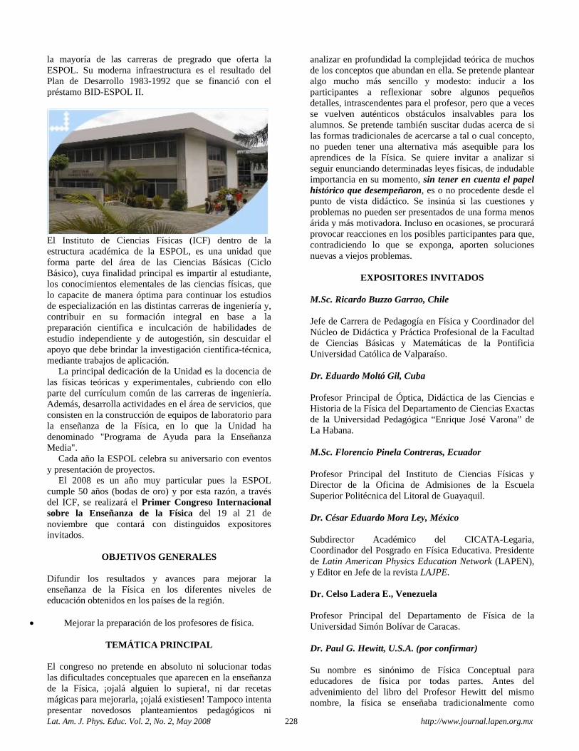
Lat. Am. J. Phys. Educ. Vol. 2, No. 2, May 2008 228 http://www.journal.lapen.org.mx
la mayoría de las carreras de pregrado que oferta la ESPOL. Su moderna infraestructura es el resultado del Plan de Desarrollo 1983-1992 que se financió con el préstamo BID-ESPOL II.
El Instituto de Ciencias Físicas (ICF) dentro de la estructura académica de la ESPOL, es una unidad que forma parte del área de las Ciencias Básicas (Ciclo Básico), cuya finalidad principal es impartir al estudiante, los conocimientos elementales de las ciencias físicas, que lo capacite de manera óptima para continuar los estudios de especialización en las distintas carreras de ingeniería y, contribuir en su formación integral en base a la preparación científica e inculcación de habilidades de estudio independiente y de autogestión, sin descuidar el apoyo que debe brindar la investigación científica-técnica, mediante trabajos de aplicación.
La principal dedicación de la Unidad es la docencia de las físicas teóricas y experimentales, cubriendo con ello parte del currículum común de las carreras de ingeniería. Además, desarrolla actividades en el área de servicios, que consisten en la construcción de equipos de laboratorio para la enseñanza de la Física, en lo que la Unidad ha denominado "Programa de Ayuda para la Enseñanza Media".
Cada año la ESPOL celebra su aniversario con eventos y presentación de proyectos.
El 2008 es un año muy particular pues la ESPOL cumple 50 años (bodas de oro) y por esta razón, a través del ICF, se realizará el Primer Congreso Internacional sobre la Enseñanza de la Física del 19 al 21 de noviembre que contará con distinguidos expositores invitados.
OBJETIVOS GENERALES
Difundir los resultados y avances para mejorar la enseñanza de la Física en los diferentes niveles de educación obtenidos en los países de la región.
• Mejorar la preparación de los profesores de física.
TEMÁTICA PRINCIPAL El congreso no pretende en absoluto ni solucionar todas las dificultades conceptuales que aparecen en la enseñanza de la Física, ¡ojalá alguien lo supiera!, ni dar recetas mágicas para mejorarla, ¡ojalá existiesen! Tampoco intenta presentar novedosos planteamientos pedagógicos ni
analizar en profundidad la complejidad teórica de muchos de los conceptos que abundan en ella. Se pretende plantear algo mucho más sencillo y modesto: inducir a los participantes a reflexionar sobre algunos pequeños detalles, intrascendentes para el profesor, pero que a veces se vuelven auténticos obstáculos insalvables para los alumnos. Se pretende también suscitar dudas acerca de si las formas tradicionales de acercarse a tal o cual concepto, no pueden tener una alternativa más asequible para los aprendices de la Física. Se quiere invitar a analizar si seguir enunciando determinadas leyes físicas, de indudable importancia en su momento, sin tener en cuenta el papel histórico que desempeñaron, es o no procedente desde el punto de vista didáctico. Se insinúa si las cuestiones y problemas no pueden ser presentados de una forma menos árida y más motivadora. Incluso en ocasiones, se procurará provocar reacciones en los posibles participantes para que, contradiciendo lo que se exponga, aporten soluciones nuevas a viejos problemas.
EXPOSITORES INVITADOS M.Sc. Ricardo Buzzo Garrao, Chile Jefe de Carrera de Pedagogía en Física y Coordinador del Núcleo de Didáctica y Práctica Profesional de la Facultad de Ciencias Básicas y Matemáticas de la Pontificia Universidad Católica de Valparaíso. Dr. Eduardo Moltó Gil, Cuba Profesor Principal de Óptica, Didáctica de las Ciencias e Historia de la Física del Departamento de Ciencias Exactas de la Universidad Pedagógica “Enrique José Varona” de La Habana. M.Sc. Florencio Pinela Contreras, Ecuador Profesor Principal del Instituto de Ciencias Físicas y Director de la Oficina de Admisiones de la Escuela Superior Politécnica del Litoral de Guayaquil. Dr. César Eduardo Mora Ley, México Subdirector Académico del CICATA-Legaria, Coordinador del Posgrado en Física Educativa. Presidente de Latin American Physics Education Network (LAPEN), y Editor en Jefe de la revista LAJPE. Dr. Celso Ladera E., Venezuela Profesor Principal del Departamento de Física de la Universidad Simón Bolívar de Caracas. Dr. Paul G. Hewitt, U.S.A. (por confirmar) Su nombre es sinónimo de Física Conceptual para educadores de física por todas partes. Antes del advenimiento del libro del Profesor Hewitt del mismo nombre, la física se enseñaba tradicionalmente como
Lat. Am. J. Phys. Educ. Vol. 2, No. 2, May 2008 229 http://www.journal.lapen.org.mx
matemáticas aplicadas adaptada a estudiantes con altas matemáticas y aptitudes para la ciencia. El acercamiento conceptual de Hewitt cambió todo esto. Traduciendo los conceptos centrales de física del lenguaje matemático al lenguaje común, y explicando física en lugar de proclamar física, y a través del empleo extenso de analogías como un instrumento de enseñanza, Hewitt sacó la física de la corriente principal educativa. Su texto ha cambiado el modo que se enseña la física tanto a los estudiantes de ciencias como a los que no siguen ciencias.
En reconocimiento a los logros de Hewitt, la Asociación americana de Profesores de Física lo honró en 1982 con su Premio Millikan, el premio más prestigioso para contribuciones excepcionales a la enseñanza de la física.
Hewitt es en este momento es columnista para The Physics Teacher, la revista mensual de la Asociación Americana de Profesores de Física. Dr. Eric Mazur, U.S.A. (por confirmar) Es un físico prominente y educador en Harvard University. Mazur es conocido por su trabajo en la óptica experimental ultrarrápida y la física de materia condensada y es un líder nacional e internacional en la educación de ciencias. Diseñó una estrategia instruccional para enseñar la llamada instrucción por pares. Publicó un libro sobre la Instrucción por Pares llamada: Manual del Usuario que proporciona detalles sobre esta estrategia. En el 2006 fue seleccionado como uno de los 75 físicos americanos más excepcionales por la Asociación Americana de Profesores de Física CONFERENCIAS DURANTE EL EVENTO (POR CONFIRMAR) • Uso de las TIC’s en la Enseñanza de la Física • Uso de la Metodología Indagatoria en la Enseñanza de la Física • Diseño de una malla curricular para Profesores de Física, basada en competencias • Formación Inicial y Formación Continua de Profesores de Física • La Ciencia en la Actualidad y su Reflejo en la Enseñanza de la Física • LAPEN y la formación de profesores de física
PRESENTACIÓN DE TRABAJOS Los asistentes que deseen presentar sus trabajos, deberán enviarlos hasta el 30 de septiembre. Los resúmenes contendrán: título, autor o autores, institución y descripción de los aspectos fundamentales del trabajo (media página, como máximo, escrita en cualquiera de las versiones de Word para Windows. Tamaño del papel: Carta, 279,4 × 215,9 mm. Letra: Arial 12 puntos. Márgenes: 3 cm. Interlineado: sencillo).
Los trabajos no excederán de 25 páginas con las mismas normas del resumen. Para las presentaciones de los trabajos en talleres los ponentes contarán con 15 minutos. La exposición de los trabajos en ponencias estará sujeta a la selección que haga el Comité Científico del Congreso.
Los trabajos aceptados y el programa oficial serán publicados el 15 octubre.
PROGRAMA GENERAL
Inscripciones 18 de noviembre Apertura 19 de noviembre Actividades científicas del Congreso 19 al 21 de noviembre Clausura 21 de noviembre
CUOTA DE INSCRIPCIÓN AL CONGRESO
Participantes: 100.00 USD Incluye: • Registro y Credencial. • Traslados al congreso (entrada y salida en horarios específicos) durante los tres días del evento. • Participación en las actividades científicas, certificado de asistencia y certificado de autor o coautor por cada trabajo presentado. • Refrigerios y almuerzos durante los tres días del evento. • Portafolio con la documentación del evento. • Programa cultural (cargo adicional de $30 para acompañantes) Un cargo extra de 20% será aplicado a los participantes que se registren luego del 30 de septiembre. La cuota de inscripción debe abonarse de 14h00 a 19h00 el 18 de noviembre en el momento de la acreditación.
LUGAR DE INSCRIPCIÓN: Escuela Superior Politécnica del Litoral Campus Las Peñas (Malecón Simón Bolívar y Loja) Oficina de Admisiones
LUGAR DE CONFERENCIAS: Escuela Superior Politécnica del Litoral Campus Gustavo Galindo (km 30.5 Vía Perimetral) Auditorio de la Facultad de Ingeniería Eléctrica y Computación (FIEC)
CONTACTO PARA MÁS DETALLES DEL CONGRESO
M.Sc. Eduardo Montero Carpio [email protected] Tel: 593 97547512
Lat. Am. J. Phys. Educ. Vol. 2, No. 2, May 2008 230 http://www.journal.lapen.org.mx
VIII TALLER INTERNACIONAL SOBRE
ENSEÑANZA DE LA FÍSICA EN LA
INGENIERÍA EFING'08 1 - 5 Diciembre de 2008
La Habana, Cuba http://www.cujae.edu.cu/eventos/convencion/sitios/efing/index.htm El Departamento de Física del Instituto Superior Politécnico “José Antonio Echeverría” (ISPJAE), se complace en convocar a los profesores de Física y otras Ciencias Básicas afines a las Ciencias Técnicas así como a investigadores en el campo de la Física Aplicada en la Ingeniería, a participar en el VIII Taller Internacional sobre la Enseñanza de la Física en la Ingeniería (EFING´08) que se celebrará entre los días 1 y 5 de Diciembre del 2008 en el Palacio de las Convenciones en La Habana, Cuba.
OBJETIVOS
• Analizar y fundamentar el papel que desempeñan las tecnologías de la Informática y las Comunicaciones aplicadas a la Física en la formación de ingenieros . • Debatir y divulgar los trabajos científicos más avanzados en el campo de la Enseñanza de la Física en la Ingeniería y en la Didáctica de la Física para su aprendizaje a distancia y en otras formas semipresenciales. • Propiciar la concertación de proyectos conjuntos de investigación y desarrollo entre los participantes, así como la firma de cartas de intención y convenios entre las instituciones representadas en el evento. Temáticas principales • Nuevas Tecnologías en la enseñanza de la Física. • Entornos virtuales para el aprendizaje de la Física. • Didáctica de la Física y didáctica del postgrado en Física Aplicada. • Diseño curricular en la Física para Ingenieros. • Nuevas tendencias pedagógicas en la enseñanza de la Física en Ingeniería. • Interrelación de la Física con otras ciencias básicas y técnicas. • Laboratorios docentes de Física en Ingeniería. • Automática y Electrónica en el Proceso de Enseñanza-aprendizaje. • Taller de Tesis en Maestrías y Doctorados.
COMITÉ ORGANIZADOR
Presidente: Dr. Juan J. Llovera González (ISPJAE, Cuba) Vicepresidentes: Dr. Hilario Falcón Tanda (ISPJAE, Cuba) Dr. Juan Antonio Alejo Díaz (ISPJAE, Cuba) MSc. Justo Ortega Breto (ISPJAE, Cuba) Lic. Carlos Osaba Rodríguez (ISPJAE, Cuba) Secretario Ejecutivo: Dr. Rolando Serra Toledo (ISPJAE, Cuba)
FORMATOS PARA LOS RESÚMENES, ARTÍCULOS Y POSTERS
PRESENTACIÓN DE RESÚMENES
Los interesados en la presentación de ponencias deberán enviar su resumen en español e inglés al evento (según las referencias) con un máximo de 250 palabras
El formato de presentación de los Resúmenes será en letra Arial 10 a simple espacio con las siguientes especificaciones: margen superior primera página 5cm; resto de las páginas; 2,5cm, margen inferior y laterales: 2,5cm.
El resumen debe incluir información referente a: Título del trabajo, autores, institución, evento, temática, dirección postal y electrónica, teléfono y Fax, todo en letra Arial tamaño 12.
Tamaño de hoja 8½” x 11” (21,59 cm x 27,94 cm), elaborado con procesador de texto Word, versión 6.0 o posterior.
Para observar el formato adecuado para los resúmenes puede descargar los documentos con las normas: Los resúmenes y trabajos deben ser enviados por correo electrónico.
Debe indicar al final del resumen la modalidad en que desea presentar el trabajo.
FORMATO DE ARTÍCULOS
Las ponencias deberán ser en español o inglés con una extensión máxima de 10 cuartillas (incluyendo figuras y tablas).
Tamaño de hoja 8½” x 11” (21,59 cm x 27,94 cm), elaborado con procesador de texto Word, versión 6.0 o posterior.
Para observar el formato adecuado para los trabajos puede descargar los documentos con las normas: Los trabajos deben ser enviados por correo electrónico
FORMATO DE LOS CARTELES (POSTERS)
Deben tener como máximo 1m de ancho por 1,50 m de alto. La presentación de un trabajo en esta modalidad no excluye la entrega del mismo en el formato solicitado para los resúmenes y artículos para su publicación en las Memorias del Evento. PREFERIBLEMENTE deben ser enviados como un anexo (attachment) por correo electrónico a: [email protected] [email protected]
FECHAS LÍMITES
Envío de resúmenes: Hasta el 30 de Junio 2008. Información de aceptación: Hasta el 15 de Julio 2008. Envío de presentaciones completas: Hasta el 15 de Septiembre 2008. Aceptación final para publicación: Hasta el 15 de Octubre 2008. Realización del EFING 2008: Del 1 al 5 de Diciembre 2008.
Lat. Am. J. Phys. Educ. Vol. 2, No. 2, May 2008 231 http://www.journal.lapen.org.mx
INFORMACIÓN:
Fuera de estas fechas, puede garantizarse su participación en el evento, pero no así la publicación del trabajo y la modalidad en que lo quiere presentar. El comité organizador, en función de la calidad de los trabajos presentados, podrá hacer las gestiones con la Sociedad Cubana de Física, para que valore la inclusión de estos trabajos en las publicaciones de su revista. Los trabajos recomendados por el comité de arbitraje serán publicados en una de las siguientes revistas: • Revista Cubana de Física. • Revista Avanzada Pedagógica. Cuotas de inscripción Las cuotas de inscripción para las diferentes categorías se ajustan a las referidas en la promoción de la Convención.
Delegado 180.00 CUC Estudiante 80.00 CUC
Acompañante 70.00 CUC
Derechos que se adquieren con la cuota de inscripción Para los delegados: • Credencial y materiales de trabajo del evento. • Memorias del evento, en formato electrónico (CD) con su correspondiente código ISBN. • Participación en todas las actividades del evento. • Certificado de ponente o participante. • Brindis de bienvenida y actividad de despedida. • Otras actividades de tipo cultural ofrecidas por el comité organizador
CONTACTO
Los interesados en participar en el evento pueden dirigir sus comunicaciones o solicitudes de información por cualquiera de las siguientes vías: Dirección postal: Dpto. de Física, Fac. de Ingeniería Eléctrica, ISPJAE. Ave. 114 No. 11901, e/ 119 y 127. Apdo. Postal 6028, Marianao . Ciudad de La Habana, CP-19390. Cuba. Teléfonos: (537) 266-3736, (537) 266 3734, Fax: (537) 267-2964, 267-1574 e-mail: [email protected] Prof. Dr. Juan José Llovera González (Presidente del comité organizador) [email protected] Prof. Dr. Rolando Serra Toledo (Secretario ejecutivo) [email protected]
Postdoctoral Fellowship Physics Education
University of Calgary Department of Physics and Astronomy
Applications are invited for a Postdoctoral Fellow position in Physics Education Research in the Department of Physics and Astronomy at the University of Calgary in Calgary, Alberta, Canada (www.ucalgary.ca). This is a two-year position and is available immediately, although start dates no later than September 1st 2008 will be considered. The position will be focused on the development, implementation, and efficacy evaluation of labatorial exercises in 1st year service courses in Mechanics, Electromagnetism, and Thermodynamics. Labatorials are the University of Calgary implementation of some of the ideas commonly associated with Studio Physics. These two hour weekly small group sessions utilize mini-laboratories, computational exercises, and demonstration-based tutorials to complement student learning in clicker-based, large-section, lecture sessions. The candidate selected for this position is expected to be involved in the instruction of these courses, as well as working with other faculty and graduate students on labatorial development and assessment, including publication of the results of these pedagogical implementations.
Applicants must have teaching experience and an interest in physics education. Experience in the field of Physics Education Research would be an asset. The University of Calgary is locating in the City of Calgary, Alberta, Canada (www.tourismcalgary.com), a vibrant metropolis of a million people located in the foothills of the Canadian Rocky Mountains.
The University of Calgary is a broadly-based institution of 28000 students spread over 16 different faculties. The Department of Physics and Astronomy (www.ucalgary.ca/phas/) is a mid-sized Canadian physics department with nearly 30 faculty members, about 80 graduate students and roughly 130 undergraduate physics and astrophysics majors. Each year, the Department teaches over 3000 students in our physics and astronomy service courses.
The Faculty of Science at the University of Calgary is home to the newly-formed RAISE (Research And Instruction in Science Education), a multi-disciplinary group of scholars committed to quality university education in the sciences.
Complete applications, including cover letter, curriculum vitae, teaching dossier, and the names and contact information (including e-mail address) for three references, should be sent to: Dr. Robert I. Thompson, P. Phys. Undergraduate Program Director and Assistant Head Department of Physics and Astronomy, University of Calgary, 2500 University Drive NW, Calgary, Alberta, Canada, T2N 1N4 email: [email protected] tel. (403) 220-5407, fax: (403) 210-8974