Lattice Boltzmann Modeling of Advection-Diffusion-Reaction Equations: Pattern Formation Under Uniform Differential Advection

Commun. Comput. Phys.doi: 10.4208/cicp.441011.270112s

Vol. 13, No. 3, pp. 741-756March 2013

Lattice Boltzmann Modeling of

Advection-Diffusion-Reaction Equations: Pattern

Formation Under Uniform Differential Advection

S. G. Ayodele1,∗, D. Raabe1 and F. Varnik1,2

1 Max-Planck Institut fur, Eisenforschung, Max-Planck Straße 1, 40237, Dusseldorf,Germany.2 Interdisciplinary Center for Advanced Materials Simulation, Ruhr University Bochum,Stiepeler Straße 129, 44780 Bochum, Germany.

Received 31 October 2011; Accepted (in revised version) 27 January 2012

Available online 29 August 2012

Abstract. A lattice Boltzmann model for the study of advection-diffusion-reaction(ADR) problems is proposed. Via multiscale expansion analysis, we derive from theLB model the resulting macroscopic equations. It is shown that a linear equilibriumdistribution is sufficient to produce ADR equations within error terms of the order ofthe Mach number squared. Furthermore, we study spatially varying structures arisingfrom the interaction of advective transport with a cubic autocatalytic reaction-diffusionprocess under an imposed uniform flow. While advecting all the present species leadsto trivial translation of the Turing patterns, differential advection leads to flow inducedinstability characterized with traveling stripes with a velocity dependent wave vectorparallel to the flow direction. Predictions from a linear stability analysis of the modelequations are found to be in line with these observations.

AMS subject classifications: 76R05, 76R50, 92C15, 80A32

Key words: Advective transport, differential advection, Turing patterns, linear stability, latticeBoltzmann.

1 Introduction

Spatially and/or temporally varying structures have been observed in a variety of phys-ical [1, 2], chemical [3–5] and biological [6–11] systems operating far from equilibrium.In chemical and biological systems for instance, the macroscopic reaction-diffusion (RD)equations have been proposed as models for morphogenesis [12], pattern formation [6,7]and self-organization [13, 14]. This class of equations usually includes the following two

∗Corresponding author. Email addresses: [email protected] (S. G. Ayodele), [email protected] (D. Raabe),[email protected] (F. Varnik)

http://www.global-sci.com/ 741 c©2013 Global-Science Press

742 S. G. Ayodele, D. Raabe and F. Varnik / Commun. Comput. Phys., 13 (2013), pp. 741-756

features: (i) a nonlinear reaction between chemical species describing local productionor consumption of the species and (ii) the diffusive transport of these species due todensity gradients. The properties of structures that arise from this class of systems aredetermined by the intrinsic transport parameters of the system such as the diffusion co-efficient and reaction constants. However, the presence of an external influence such asadvection may lead to qualitative changes in the system’s behavior and to the emergenceof new non-equilibrium structures. This is very important in the experimental investi-gations of the diffusive chemical instability in gel reactors where the perturbative effectof the feeding flows is not fully suppressed or in tubular reactors where spatiotemporalbehaviors might also be of interest. Attempts to understand the role played by advectionin spatio-temporal organization of RD systems have led to the discovery of the flow dis-tributed structures (FDS) or flow distributed oscillations (FDO). In this case excitable RDsystems with fixed or periodically forced inflow boundary, are known to develop station-ary [15, 16] and traveling waves [17, 18] depending on the boundary-forcing frequency.Patterns of these type are known to occur even when the Turing instability condition ofunequal diffusion coefficient is not satisfied.

A closely related problem to the boundary forced structures which have received lessstudy in 2D is the interactions between advective fields and a pre-existing sharp chem-ical gradients produced by reaction-diffusion processes. This means the interaction ofalready existing instabilities with the instability caused by advection. This interactioncan give rise to complex patterns in both chemical and biological systems [19, 20]. Inthis work we consider the interaction of a uniform flow field with the Turing instability.As a prominent example of an autocatalytic reaction-diffusion pattern forming systemwe choose the Gray-Scott model [23]. This model has some generic features which canmake it adaptable to study some realistic situations such as vegetative patterns, combus-tion and cell division [21, 22]. We propose a Lattice Boltzmann (LB) method for solvingthe ADR equations arising from the interaction of the advective fields with the Turingpatterns. The LB simulation of the ADR equations shows that while advecting all thespecies leads to trivial translation of the Turing patterns, differential advection of thespecies leads to an additional flow induced instability characterized by traveling stripeswith a velocity dependent wave vector parallel to the flow direction. These observationsare in line with the predictions from linear stability analysis carried out on the modelequations. The article is organized as follows. In the next section, we present the modelequations. In Section 3 we address the framework adopted for the Lattice Boltzmannmodeling of the model equations. The results obtained from the linear stability analysisand numerical simulations are discussed in Section 4. At the end of the same section, weconclude the discussion with a summary of our results.

2 The model equations

In this section we present the governing equations for the Gray-Scott advection-diffusion-reaction (ADR) model. The original Gray-Scott reaction-diffusion model describes the ki-

S. G. Ayodele, D. Raabe and F. Varnik / Commun. Comput. Phys., 13 (2013), pp. 741-756 743

netics of a simple autocatalytic reaction in an un-stirred homogeneous flow reactor [23].The reactor is confined in a narrow space between two porous walls in contact with areservoir. Substance A whose density is kept fixed at Ao in the reservoir outside of thereactor is supplied through the walls into the reactor with the volumetric flow rate perunit volume k f . Inside the reactor, A undergoes an autocatalytic reaction with an inter-mediate species B at a rate k1. The species B then undergoes a decay reaction to an inertproduct C at a rate k2. The product C and excess reactants A and B are then removedfrom the reactor at the same flow rate per unit volume k f . The basic reaction steps aresummarized as follows

A+2Bk1−→3B, (2.1a)

Bk2−→C. (2.1b)

The reaction in Eq. (2.1a) is the cubic autocatalytic reaction in which two molecules ofspecies B produce three molecules of B through interaction with the species A. The pres-ence of B stimulates further production of itself, while the presence of A controls theproduction of B. Substance A is sometimes called the inhibitor and B the activator. Byconstantly feeding the reactor with a uniform flow of species A while at the same timeremoving the product and excess reactants, far from equilibrium conditions can be main-tained. Note that inside the reactor the two species A and B are assumed to interact onlythrough the non-linear autocatalytic reaction in Eq. (2.1a). In particular, interaction termsdue to cross diffusion between the species are neglected. This assumption is physicallyjustified as pattern forming systems often occur in the form of dilute solutions. Followingthis assumption, the equations of chemical kinetics which describe the above situationsand include the spatio-temporal variations of the concentrations of A and B in the reactortake the following form:

∂A

∂t= k f (A0−A)−k1B2A+DA∇

2 A, (2.2a)

∂B

∂t=−

(

k f +k2

)

B+k1B2A+DB∇2B, (2.2b)

where A and B are the density of species A and B respectively, A0 is the density of Ain the reservoir, while DA and DB are the diffusion coefficients of species A and B re-spectively. To account for the effect of an imposed flow, one simply adds a term due toadvection to the Gray-Scott reaction-diffusion Eqs. (2.2a) and (2.2b). However, note thatthe two dimensional reaction-diffusion model described above contains a constant feedflow term (k f A0) perpendicular to the reaction surface. This feed flow term constantlyreplenishes species A on the reaction surface and thus species A is therefore sometimesreferred to as the substrate. But in a variety of technical settings or Tubular flow reactorsthe external field that drives the system enters from one end and the idea of modelingadvection by driving species A and B with flow velocity u parallel to the surface is phys-ically justified. In the case of the velocity field considered here, an incompressible flow


with divergence free velocity field, the advection-diffusion-reaction (ADR) describing thetransport of species A and B can then be written as:

∂A

∂t= k f (A0−A)−k1B2A+DA∇

2 A−u·∇A, (2.3a)

∂B

∂t=−

(

k f +k2

)

B+k1B2A+DB∇2B−δu·∇B, (2.3b)

where the parameter δ is the ratio of the advective rates of the two species or the differen-tial advection parameter. The absence and presence of differential advection is modeledwith the parameter δ=1 and δ 6=1 respectively. Here we focus on the situations with δ=1and δ=0.

In order to proceed with the analysis of Eq. (2.3), it is important to reduce the numberof parameters and introduce variables in the form of time and length scales that repre-sent the physical processes acting in the system. We therefore introduce concentrationscales (A0,B0), time scales (τA = 1/k f , τB = 1/(k f +k2)), length scales (lA = (DAτA)

1/2,

lB =(DBτB)1/2) and velocity scale uA = lA/τA such that:

t=t

τA, A=

A

A0, B=

B

B0, (x,y)=

1

lA(x,y), u=

u

uA, B0=(k f /k1)

1/2. (2.4)

Using the above relations in Eq. (2.3) we arrive at the non-dimensional equations as:

∂A

∂t=(

1− A)

− B2A+∇2 A−u·∇A, (2.5a)

1

τ

∂B

∂t=−B+ηB2A+

1

ε2∇2B−

δ

τu·∇B, (2.5b)

where the parameter

η=A0(k1k f )

1/2

(k f +k2), τ=τA/τB, ε= lA/lB=

√

τADA/τBDB. (2.6)

Eqs. (2.5a) and (2.5b) have three simple equilibrium solutions which correspond to aspatially homogeneous situation with no fluid flow (u=0). The first solution is the trivialhomogeneous solution Be=0, Ae=1. This state exist for all system parameters. The othertwo solutions exist provided that η>2. These are given by:

A±e =

η±√

η2−4

2η, B±

e =η∓

√

η2−4

2. (2.7)

In equilibrium, the system can be found in any of these states and any external activationor perturbation added to these states would either grow far from the equilibrium stateto a patterned state or decays back towards the equilibrium. The nature of the timeevolution from equilibrium depends on the systems transport parameters.


3 Lattice Boltzmann modeling

Lattice Boltzmann schemes have been used to study the advection, diffusion and reactionof a scalar field in reactive chemical transport processes [24–26]. In this work we intro-duce the framework adopted for modeling advection-diffusion-reaction in domains withno-flux boundary condition. In general, the lattice Boltzmann method [27–30] can beregarded as a mesoscopic particle based numerical approach allowing to solve fluid dy-namical equations in a certain approximation, which (within, e.g. the so called diffusivescaling, i.e. by choosing ∆t=∆x2) becomes exact as the grid resolution is progressivelyincreased. The density of the fluid at each lattice site is accounted for by a one particleprobability distribution fi(x,t), where x is the lattice site, t is the time and the subscripti represents one of the finite velocity vectors ei at each lattice node. The number anddirection of the velocities are chosen such that the resulting lattice is symmetric so as toeasily reproduce the isotropy of the fluid [31]. During each time step, particles streamalong each velocity vector ei to a neighboring lattice site and collide locally, conservingmass and momentum in the process.

In order to use this method to simulate the ADR equations, we introduce a multi-species distribution function fi,j where the subscript j runs over the number of speciesj= 1,··· ,ns. As stated above, here, we assume that the diffusion of a given species doesnot depend on the concentration of other species. In other words, the species in ourmodel do not interact among each other, except through the chemical reaction term. Thisassumption is physically justified since many pattern forming systems are studied in theform of dilute solutions. At higher concentrations, however, the mutual interactions ofdifferent species shall be taken into account [32, 33]. The species field fi,j is advectedwith the imposed flow velocity u and does not have any effect on the velocity field (pas-sive tracer limit). The chemical reaction is modeled by including a source term, Rj, inthe collision step. The LB-BGK equation governing propagation, collision of the density(concentration) distribution of the passive tracers is given as:

fi,j(x+ei,t+1)− fi,j(x,t)=f

eqi,j (x,t)− fi,j(x,t)

τj+wiRj, (3.1)

where τs is the relaxation time for species s and feqi,j is the equilibrium distribution func-

tion expanded up to the linear order in velocity as feqi,j (x,t)=wiρj

[

1+(ei ·u)/c2s

]

. As will

be shown below, the expansion to linear order is sufficient to recover the ADR equationconsidered in this study. In the expression for the equilibrium distribution, cs is the soundspeed on the lattice and wi is a set of weights normalized to unity. The weights wi in theequilibrium distribution depend on the number of velocities used for the lattice. In thiswork, we have used the two dimensional nine velocity (D2Q9) model, with the soundspeed cs given as c2

s = c2/3, where c=∆x/∆t is the lattice speeds. The lattice weights and


number of velocities for the D2Q9 is given as

wi=

4/9, ei =(0, 0), i=0;

1/9, ei =(±1, 0), (0,±1), i=1,··· ,4;

1/36, ei =(±1,±1), i=5,··· ,8.

(3.2)

The source term Rj represents the rate of change of density of the species, j, with re-gard to reaction kinetics. The exact form of the relation between the reaction rate Rj andthe density (concentration) of each species depends on the type of reaction being mod-eled. In this work, for species A, the reaction term is taken as R1 = k f (A0−A)−k1B2A

and for species B, R2=−(

k f +k2

)

B+k1B2A. The density of the species j, is computed by

taking the zeroth moment of the distribution function, i.e. A=∑Ni=0 fi,1 and B=∑

Ni=0 fi,2,

where N=8 in the present D2Q9 model. The corresponding macroscopic ADR equationcan be recovered from the LB Eq. (3.1) by performing a multiscale Chapman-Enskog ex-pansion. We present a brief outline of the derivation and discuss the contribution of theerror terms to the ADR equations in the following section.

3.1 Chapman-Enskog procedure for the derivation of ADR equation

In this section, we derive the macroscopic ADR equation from the lattice Boltzmann equa-tion;

fi,j(x+ei∆t,∆t+t)− fi,j(x,t)=f


τj+∆twiRj. (3.3)

By performing a Taylor series expansion of the left hand side of Eq. (3.3), a partial differ-ential term can be written in place of the finite difference term as

∞

∑n=1

∆tn

n!(∂t+eiα∂xα)

n fi,j(x,t)=f


τj+∆twiRj. (3.4)

The distribution functions, time derivative, spatial derivative and the reaction term Rj

are expanded in terms of a smallness parameter, ǫ, as [34, 35]

fi,j = f(0)i,j +ǫ f

(1)i,j +ǫ2 f

(2)i,j +ǫ3 f

(3)i,j +O(ǫ4), (3.5a)

∂t =ǫ∂(1)t +ǫ2∂

(2)t , (3.5b)

∂xα =ǫ∂(1)xα , (3.5c)

Rj =ǫ2R(2)j +ǫ3R

(3)j +O(ǫ4). (3.5d)

A natural interpretation of the parameter ǫ is the so called Knudsen number, the ratio ofthe fluids mean free path to a characteristic dimension for variations of the macroscopic


velocity field. Inserting Eqs. (3.5a), (3.5b), (3.5c) and (3.5d) in Eq. (3.4), one obtains

[

∆t(ǫ∂(1)t +ǫ2∂

(2)t +ǫeiα∂

(1)xα )+

∆t2

2(ǫ2∂

(1)t ∂

(1)t +2ǫ2eiα∂

(1)t ∂

(1)xα +ǫ2eiαeiβ∂

(1)xα ∂

(1)xβ

+2ǫ3eiα∂(2)t ∂

(1)xα

+ 2ǫ3∂(2)t ∂

(1)t +2ǫ4∂

(2)t ∂

(2)t

]

( f(0)i,j +ǫ f

(1)i,j +ǫ2 f

(2)i,j +O(ǫ3))

=1

τj

(

feqi,j (x,t)−( f

(0)i,j +ǫ f

(1)i,j +ǫ2 f

(2)i,j +ǫ3 f

(3)i,j +O(ǫ4))

)

+∆twi(ǫR(1)j +ǫ2R

(2)j +ǫ3R

(3)j +O(ǫ4)). (3.6)

Grouping terms of the same order in ǫ yields the following successive approximations

O(ǫ0) : f(0)i,j = f

eqi,j , (3.7)

O(ǫ1) : ∆t(

∂(1)t +eiα∂

(1)xα

)

f(0)i,j =−

1

τjf(1)i,j , (3.8)

O(ǫ2) : ∆t(

∂(2)t f

(0)i,j +

(

∂(1)t +eiα∂

(1)xα

)

f(1)i,j

)

+∆t2

2

(

∂(1)2

t +2eiα∂(1)t ∂

(1)xα +eiαeiβ∂

(1)xα ∂

(1)xβ

)

f(0)i,j

=−1

τjf(2)i,j +∆twiR

(2)j , (3.9)

O(ǫ3) : ∆t(

∂(3)t f

(0)i,j +∂

(2)t f

(1)i,j +

(

∂(1)t +eiα∂

(1)xα

)

f(2)i,j

)

d+∆t2

2

(

∂(1)1

t +2eiα∂(1)t ∂

(1)xα

+eiαeiβ∂(1)xα ∂

(1)xβ

)

f(1)i,j +∆t2∂

(2)t

(

∂(1)t +eiα∂

(1)xα

)

f(0)i,j +

∆t3

6

(

∂(1)t +eiα∂

(1)xα

)3f(0)i,j

=−1

τjf(3)i,j +∆twiR

(3)j . (3.10)

Putting the expression for f(1)i,j from Eq. (3.8) into Eq. (3.9) yields

1

τjf(2)i =−∆t∂

(2)t f

(0)i,j +∆t2

(

τj−1

2

)

(

∂(1)t +eiα∂

(1)xα

)2f(0)i,j +∆twiR

(2)j . (3.11)

In Eq. (3.10), we insert the expression for f(1)i,j and f

(2)i,j from Eqs. (3.8) and (3.9) and obtain

1

τjf(3)i,j =−∆t∂

(3)t f

(0)i,j +∆t2(2τj−1)

(

∂(1)t +eiα∂

(1)xα

)

∂(2)t f

(0)i,j −∆t3

(

τ2j −τj+

1

6

)

(

∂(1)t

+eiα∂(1)xα

)3f(0)i,j −τs∆t2

(

∂(1)t +eiα∂

(1)xα

)

wiR(2)j +∆twiR

(3)j . (3.12)

Next, we take the moments of the distribution functions in Eqs. (3.8), (3.11) and (3.12).Note that, since mass is conserved upon collision, only the equilibrium distribution func-

tion contributes to the local values of the mass. In other words, ∑Ni=0 f

(k)i,j =0, for all higher


order corrections, k> 0, and all species, j. For the purpose of comparison, we considerhere two different equilibrium distribution, the linearized form

f(0)i,j =ρjwi

(

1+eiαuα/c2s

)

, (3.13)

and the quadratic form

f(0)i,j =ρjwi

(

1+1

c2s

eiαuα+uαuβ

2c2s

(

eiαeiβ

c2s

−δαβ

))

. (3.14)

Starting with the linear equilibrium distribution, the zeroth, first and second momentsare given as:

∑i

f(0)i,j =ρj, ∑

i

f(0)i,j eiα=ρjuα, ∑

i

f(0)i,j eiαeiβ=ρjc

2s . (3.15)

Taking ∑i of Eq. (3.8) and using Eq. (3.15), yields

∂(1)t ρj+∂

(1)xα (ρjuα)=0. (3.16)

Again, taking ∑i of Eq. (3.11) and using Eqs. (3.15) and (3.16) yields

∂(2)t ρj =∆t

(

τj−1

2

)

(

∂(1)t ∂

(1)xα ρjuα+c2

s ∂(1)xα ∂

(1)xα ρj

)

+∆tR(2)j . (3.17)

Adding together Eq. (3.16) ×ǫ and Eq. (3.17) ×ǫ2 leads to

∂tρj+∂xα(ρjuα)=∆t

(

τj−1

2

)

(

c2s ∂2

xαρj+Rj+∂t∂xα ρjuα

)

. (3.18)

Comparing Eq. (3.17) with the ADR equations, the diffusion coefficient can be taken asDs= c2

s ∆t(

τj−1/2)

and we can rewrite Eq. (3.18) as

∂tρj+∂xα(ρjuα)=Dj∂2xα

ρj+Rj+Dj

c2s

∂t∂xα ρjuα, (3.19)

with an error term E1=Dj/c2s ∂t∂xα ρjuα.

Alternatively, using the quadratic equilibrium distribution in Eq. (3.17) and followingthe above procedure, one obtains

∂tρj+∂xα(ρjuα)=Dj∂2xα

ρj+Rj+Dj

c2s

(

∂t∂xα(ρjuα)+∂xα ∂xβ(ρjuαuβ)

)

, (3.20)

where the error term is now identified to be E2=Dj/c2s

(

∂t∂xα(ρjuα)+∂xα ∂xβ(ρjuαuβ)

)

.We remark that, in the both cases of the equilibrium distributions considered, the

ADR equations are recovered at O(ǫ2). The contribution to the error term from the reac-tion rate kinetics only enters the equations at O(ǫ3). Indeed, after a little bit of algebra,one finds that a term of O(u2/c2

s ), due to spurious diffusion, is always present whetheror not terms of O(u2) are included in the local equilibrium distribution [36,37]. This termcan however be neglected provided that u2/c2

s ≪1 [37]. This condition is easily satisfiedin our simulations.


4 Results and discussion

In this section, we discuss the results obtained from the numerical simulation of the Tur-ing patterns under the imposed flow. We first begin with the linear stability analysis ofthe ADR equations, and then test some of the predictions of the linear stability analysisby performing numerical simulations.

4.1 Linear stability of the advection-diffusion-reaction equations

The dimensionless ADR equation is written as

∂A

∂t=(

1− A)

− B2A+∇2A−u·∇A, (4.1a)

1

τ

∂B

∂t=−B+ηB2A+

1

ε2∇2B−

δ

τu·∇B. (4.1b)

To determine the conditions for pattern formation, we add to the equilibrium states inEq. (2.7), spatially inhomogeneous perturbations of the form (δA, δB)=(ΦA, ΦB)e

αt+iq·r,where the perturbations have a growth rate α, amplitudes (ΦA, ΦB) and wave vectorq=(qcosθ, qsinθ). The wave vector is assumed to make an angle θ with the direction ofthe flow in the (x,y) plane. The concentration of species A and B can then be written as

A= Ae+ΦAeαteiq·r, B= Be+ΦBeαteiq·r . (4.2)

Inserting this ansatz in the kinetic Eqs.(4.1a) and (4.1b) we obtain

α

[

ΦA

ΦB

]

=

τ

(

2ηA±e B±

e −1−q2

ε2−

iqδucosθ

τ

)

τηB±2

e

−2A±e B±

e −(q2+ B±2

e +1+iqucosθ)

[

ΦA

ΦB

]

. (4.3)

We consider the non-trivial states (A±e , B±

e ). From Eq. (2.7) the equilibrium states can be

written as A±e =1/ηB±

e and B±2

e +1=ηB±e . Substituting these relations in matrix equation

(4.3) we arrive at the eigenvalue equation

|M−αI|Φ=0, (4.4)

where I is the unit matrix and the matrix M in this case is given as:

M=

τ

(

1−q2

ε2−

iqδucosθ

τ

)

τηB±e

−2

η−(q2+ηB±

e +iqucosθ)

. (4.5)


The trace and determinant of matrix M can be written as

trM=−q2(

1+τ

ε2

)

−iqu(1+δ)cosθ+(τ−ηB±e ), (4.6a)

|M|=τq4

ε2+iq3

(

τu

ε2+u

)

+ q2

(

τηB±e

ε2−τ−u2

)

+iqu(ηB±e −τ)+τ(ηB±

e −2). (4.6b)

This can be re-written in a more shorthand notation as

trM= a+ib, |M|= c+id (4.7)

where the parameters a, b, c and d are given as

a=−q2(

1+τ

ε2

)

+(τ−ηB±e ), b=−qu(1+δ)cosθ, (4.8a)

c=τq4

ε2+ q2

(

τηB±e

ε2−τ−δu2cos2 θ

)

+τ(ηB±e −2), (4.8b)

d= ucosθ(

q3(τ/ε2+δ)+ q(δηB±e −τ)

)

. (4.8c)

The dispersion relation obtained from the solution of Eq. (4.4) is written as:

α2−αtrM+|M|=0. (4.9)

The eigenvalues α are the characteristic solution of the polynomial equation (4.9). Thiscan be written in terms of shorthand notation as:

α1,2=1

2

(

(a+ib)±√

(a2−b2−4c)+i(2ab−4d)

)

. (4.10)

Evaluating the complex term in the square root by separating the solution into thereal and imaginary part one obtains the eigenvalue solutions as

Re[α]=a

2±

1

2

√

r+(a2−b2−4c)

2, Im[α]=

b

2±

1

2

√

r−(a2−b2−4c)

2, (4.11)

where r=√

(a2−b2−4c)2+(2ab−4d)2.Instability in the system sets in when Re[α(q)]> 0 for some wave numbers q. The

type of instability depends on whether this occurs for q=0 (Hopf instability) or for q 6=0(corresponding to a Turing instability if, in addition, Im[α(q)]=0). In this work, we focusonly on the effect of advection by a uniform flow on the Turing instability. In the absenceof flow, the Turing instability in this system sets in when ǫ> ηB±

e . In the following, werestrict the discussion to two cases of uniform advection, associated with two values ofthe parameter δ in Eq. (2.3). First, we consider the trivial – but for test purposes stillinteresting – case of δ=1, i.e., the advection of all concentration fields with the flow. Dueto Galilean invariance, we expect here a trivial transport of existing patterns with the flow


0 1 2 3 4 5

q~-2

-1

0

1

Re(

α)

0 1 2 3 4 5

q~-2

-1

0

1

Re(

α)

ε2 = 9ε2 = 17ε2 = 22

qc q

c

(a) (b)

δ = 1 δ = 0

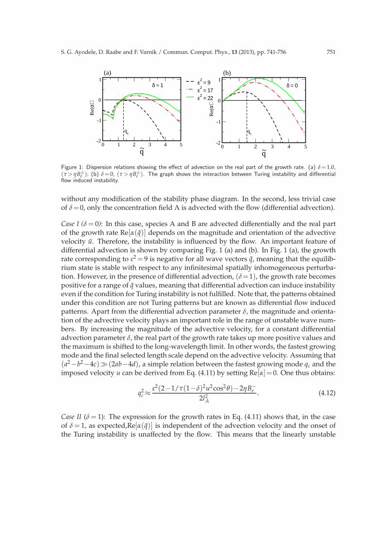
Figure 1: Dispersion relations showing the effect of advection on the real part of the growth rate. (a) δ=1.0,(τ> ηB±

e ); (b) δ= 0, (τ > ηB±e ). The graph shows the interaction between Turing instability and differential

flow induced instability.

without any modification of the stability phase diagram. In the second, less trivial caseof δ=0, only the concentration field A is advected with the flow (differential advection).

Case I (δ= 0): In this case, species A and B are advected differentially and the real partof the growth rate Re[α(q)] depends on the magnitude and orientation of the advectivevelocity u. Therefore, the instability is influenced by the flow. An important feature ofdifferential advection is shown by comparing Fig. 1 (a) and (b). In Fig. 1 (a), the growthrate corresponding to ε2 = 9 is negative for all wave vectors q, meaning that the equilib-rium state is stable with respect to any infinitesimal spatially inhomogeneous perturba-tion. However, in the presence of differential advection, (δ=1), the growth rate becomespositive for a range of q values, meaning that differential advection can induce instabilityeven if the condition for Turing instability is not fulfilled. Note that, the patterns obtainedunder this condition are not Turing patterns but are known as differential flow inducedpatterns. Apart from the differential advection parameter δ, the magnitude and orienta-tion of the advective velocity plays an important role in the range of unstable wave num-bers. By increasing the magnitude of the advective velocity, for a constant differentialadvection parameter δ, the real part of the growth rate takes up more positive values andthe maximum is shifted to the long-wavelength limit. In other words, the fastest growingmode and the final selected length scale depend on the advective velocity. Assuming that(a2−b2−4c)≫ (2ab−4d), a simple relation between the fastest growing mode qc and theimposed velocity u can be derived from Eq. (4.11) by setting Re[α]=0. One thus obtains:

q2c ≈

ε2(2−1/τ(1−δ)2u2cos2 θ)−2ηB−e

2l2A

. (4.12)

Case II (δ= 1): The expression for the growth rates in Eq. (4.11) shows that, in the caseof δ= 1, as expected,Re[α(q)] is independent of the advection velocity and the onset ofthe Turing instability is unaffected by the flow. This means that the linearly unstable


modes are the same as that in the absence of the flow. This fact is confirmed by ournumerical simulation as shown in the following discussions. The fastest growing modeqc or the mode with the maximum linear growth rate α can be obtained from Eq. (4.11)by differentiating α with respect to q2. In this case, this is written as:

q2c =

1

l2A

ε2−ηB−e

2. (4.13)

As expected, the wave length of the patterns is also independent of the velocity. Theimaginary part of α for δ= 1 obtained from Eq. (4.11) is given as Im[α]=−qucosθ. Thismeans that the unstable modes moves with the imposed velocity u. Thus, in a constantuniform velocity field u the result is just a translational motion of the original Turingpatterns.

4.2 Numerical simulation

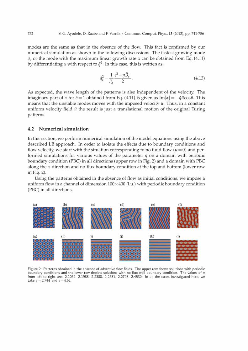
In this section, we perform numerical simulation of the model equations using the abovedescribed LB approach. In order to isolate the effects due to boundary conditions andflow velocity, we start with the situation corresponding to no fluid flow (u=0) and per-formed simulations for various values of the parameter η on a domain with periodicboundary condition (PBC) in all directions (upper row in Fig. 2) and a domain with PBCalong the x-direction and no-flux boundary condition at the top and bottom (lower rowin Fig. 2).

Using the patterns obtained in the absence of flow as initial conditions, we impose auniform flow in a channel of dimension 100×400 (l.u.) with periodic boundary condition(PBC) in all directions.

��

��

Figure 2: Patterns obtained in the absence of advective flow fields. The upper row shows solutions with periodicboundary conditions and the lower row depicts solutions with no-flux wall boundary condition. The values of ηfrom left to right are: 2.1052, 2.1988, 2.2388, 2.2531, 2.2798, 2.4530. In all the cases investigated here, wetake τ=2.744 and ε=4.62.


��

��

��

��

�

�

��

��

�

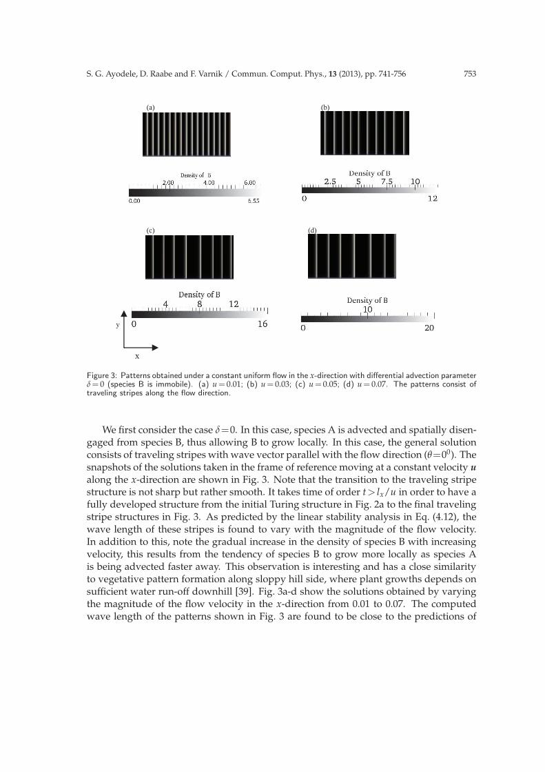
Figure 3: Patterns obtained under a constant uniform flow in the x-direction with differential advection parameterδ= 0 (species B is immobile). (a) u= 0.01; (b) u= 0.03; (c) u= 0.05; (d) u= 0.07. The patterns consist oftraveling stripes along the flow direction.

We first consider the case δ=0. In this case, species A is advected and spatially disen-gaged from species B, thus allowing B to grow locally. In this case, the general solutionconsists of traveling stripes with wave vector parallel with the flow direction (θ=00). Thesnapshots of the solutions taken in the frame of reference moving at a constant velocity u

along the x-direction are shown in Fig. 3. Note that the transition to the traveling stripestructure is not sharp but rather smooth. It takes time of order t> lx/u in order to have afully developed structure from the initial Turing structure in Fig. 2a to the final travelingstripe structures in Fig. 3. As predicted by the linear stability analysis in Eq. (4.12), thewave length of these stripes is found to vary with the magnitude of the flow velocity.In addition to this, note the gradual increase in the density of species B with increasingvelocity, this results from the tendency of species B to grow more locally as species Ais being advected faster away. This observation is interesting and has a close similarityto vegetative pattern formation along sloppy hill side, where plant growths depends onsufficient water run-off downhill [39]. Fig. 3a-d show the solutions obtained by varyingthe magnitude of the flow velocity in the x-direction from 0.01 to 0.07. The computedwave length of the patterns shown in Fig. 3 are found to be close to the predictions of


0.02 0.04 0.06 0.08u [Lattice units]

0

0.005

0.01

0.015

0.02

∆qc [L

attic

e un

its]

TheorySimulation

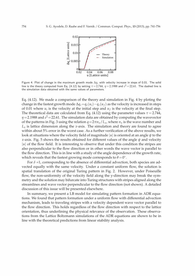
Figure 4: Plot of change in the maximum growth mode ∆qc with velocity increase in steps of 0.01. The solid

line is the theory computed from Eq. (4.12) by setting τ=2.744, η=2.1988 and ε2=22.61. The dashed line isthe simulation data obtained with the same values of parameters.

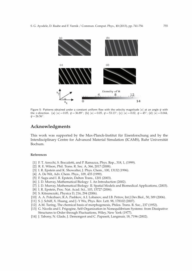
Eq. (4.12). We made a comparison of the theory and simulation in Fig. 4 by ploting thechange in the fastest growth mode ∆qc=qc(ui)−qc(u f ) as the velocity is increased in stepsof 0.01 where ui is the velocity at the initial step and u f is the velocity at the final step.The theoretical data are calculated from Eq. (4.12) using the parameter values τ= 2.744,η=2.1988 and ε2=22.61. The simulation data are obtained by computing the wavevectorof the patterns in Fig. 3 using the relation q=2πnx/Lx, where nx is the wave number andLx is lattice dimension along the x-axis. The simulation and theory are found to agreewithin about 5% error in the worst case. As a further verification of the above results, welook at situations where the velocity field of magnitude |u| is oriented at an angle ψ to thex-axis. Fig. 5 shows the results obtained for different values of the angle ψ and velocity|u| of the flow field. It is interesting to observe that under this condition the stripes arealso perpendicular to the flow direction or in other words the wave vector is parallel tothe flow direction. This is in line with a study of the angle dependence of the growth rate,which reveals that the fastest growing mode corresponds to θ=0◦.

For δ =1, corresponding to the absence of differential advection, both species are ad-vected equally with the same velocity. Under a constant uniform flow, the solution isspatial translation of the original Turing pattern in Fig. 2. However, under Poiseuilleflow, the non-uniformity of the velocity field along the y-direction may break the sym-metry and the solution may bifurcate into Turing structures with stripes aligned along thestreamlines and wave vector perpendicular to the flow direction (not shown). A detaileddiscussion of this issue will be presented elsewhere.

In summary, we present a LB model for simulating pattern formation in ADR equa-tions. We found that pattern formation under a uniform flow with differential advectionmechanism, leads to traveling stripes with a velocity dependent wave vector parallel tothe flow direction. This holds regardless of the flow direction with respect to the latticeorientation, thus underlining the physical relevance of the observation. These observa-tions from the Lattice Boltzmann simulations of the ADR equations are shown to be inline with the theoretical predictions from linear stability analysis.


��

��

�

��

�

Figure 5: Patterns obtained under a constant uniform flow with the velocity magnitude |u| at an angle ψ withthe x-direction. (a) |u|= 0.05, ψ= 36.89◦; (b) |u|= 0.05, ψ= 53.13◦; (c) |u|= 0.02, ψ= 45◦; (d) |u|= 0.044,ψ=26.56◦.

Acknowledgments

This work was supported by the Max-Planck-Institut fur Eisenforschung and by theInterdisciplinary Centre for Advanced Material Simulation (ICAMS), Ruhr UniversitatBochum.

References

[1] F. T. Arecchi, S. Boccaletti, and P. Ramazza, Phys. Rep., 318, 1, (1999).[2] R. E. Wilson, Phil. Trans. R. Soc. A, 366, 2017 (2008).[3] I. R. Epstein and K. Showalter, J. Phys. Chem., 100, 13132 (1996).[4] A. De Wit, Adv. Chem. Phys., 109, 435 (1999).[5] F. Sagu and I. R. Epstein, Dalton Trans., 1201 (2003).[6] J. D. Murray, Mathematical Biology: I. An Introduction (2002).[7] J. D. Murray, Mathematical Biology: II. Spatial Models and Biomedical Applications, (2003).[8] I. R. Epstein, Proc. Nat. Acad. Sci., 103, 15727 (2006).[9] S. Kitsunezaki, Physica D, 216, 294 (2006).

[10] A. A. Polezhaev, R.A. Pashkov, A.I. Lobanov, and I.B. Petrov, Int.J.Dev.Biol., 50, 309 (2006).[11] S. J. Schiff, X. Huang, and J.-Y Wu, Phys. Rev. Lett. 98, 178102 (2007).[12] A.M. Turing, The chemical basis of morphogenesis, Philos. Trans. R. Soc., 237 (1952).[13] G. Nicolis and I. Prigogine, Self-Organization in Nonequilibrium Systems: from Dissipative

Structures to Order through Fluctuations, Wiley, New York (1977).[14] J. Tabony, N. Glade, J. Demongeot and C. Papaseit, Langmuir, 18, 7196 (2002).


[15] P. Andresen, M. Bache, E. Mosekilde, G. Dewel, and P. Borckmanns, Phys. Rev. E 60, 297(1999).

[16] M. Kærn and M. Menzinger, Phys. Rev. E 60, R3471 (1999).[17] M. Kærn, M. Menzinger, and A. Hunding, J. Theor. Biol. 207, 473 (2000).[18] M. Kærn, M. Menzinger, R. Satnoianu, and A. Hunding, Faraday Discuss. 120, 295 (2002).[19] P.W. Boyd et al., Nature 407, 695 (2000).[20] A.P. Martin, Prog. Oceanography 57, 125 (2003).[21] P.A. Bachmann, P.L. Luisi, and J. Lang, Nature, 357, 57 (1992).[22] M. A. Bedau, J. S. McCaskill, N. H. Packard, S. Rasmussen, C. Adami, D. G. Green, Artificial

Life, 6, 363 (2000).[23] J.E. Pearson, Science 261, 189 (1993).[24] E.G. Flekkoy, Phys. Rev. E 47, 4247 (1993).[25] A. Xu, G. Gonnella, and A. Lamura Phys. Rev. E 67, 056105 (2003).[26] S. G. Ayodele, F. Varnik, and D. Raabe, Phys. Rev. E 83, 016702 (2011).[27] G. R. McNamara and G. Zanetti, Phys. Rev. Lett. 61, 2332 (1988).[28] F. Higuera, S. Succi, and R. Benzi, Europhys. Lett. 9, 345 (1989).[29] Y. Qian, D. d’Humieres, and P. Lallemand, Europhys. Lett. 17, 479 (1992).[30] S. Succi, The Lattice Boltzmann Equation: for Fluid Dynamics and Beyond, Oxford Univer-

sity Press, (2001).[31] R. Rubinstein, and L.S. Luo, Phys. Rev. E 77, 036709 (2008).[32] S. Arcidiacono, I. V. Karlin, J. Mantzaras, and C. E. Frouzakis, Phys. Rev. E 76, 046703 (2007).[33] S. Arcidiacono, J. Mantzaras, and I. V. Karlin, Phys. Rev. E 78, 046711 (2008).[34] S. Chapman and T. G. Cowling, “The Mathematical Theory of Non-uniform Gases,“ 3rd ed.,

Cambridge University press, Cambridge (1970).[35] D. A. Wolf-Gladrow, ”Lattice-Gas Cellular Automata and lattice Boltzmann Models“, Lec-

ture Notes in Mathematics 1725, Springer-Verlag, Berlin/Heidelberg (2000).[36] B. Chopard, J.L. Falcone, and J. Latt, Eur. Phys. J. Special Topics 171, 245 (2009).[37] H.-B Huang, X.-Y Lu and M. C. Sukop, J. Phys. A: Math. Theor. 44, 055001 (2011).[38] M. Beck, A. Ghazaryan and B. Sandstede. J. Differential Equations 246, 4371 (2009).[39] J. A. Sherratt, Proc. R. Soc. A, 467, 3272 (2011).

Documents

Lattice Boltzmann Modeling of Advection-Diffusion-Reaction Equations: Pattern Formation Under Uniform Differential Advection