Embed Size (px)
Citation preview
Expert Systems With Applications 75 (2017) 94–108
Contents lists available at ScienceDirect
Expert Systems With Applications
journal homepage: www.elsevier.com/locate/eswa
Learning style Identifier: Improving the precision of learning style
identification through computational intelligence algorithms
Jason Bernard
a , ∗, Ting-Wen Chang
b , Elvira Popescu
c , Sabine Graf a
a School of Computing and Information Systems, Athabasca University, 1200 10011-109 Street, Edmonton, AB T5J3S8, Canada b Smart Learning Institute, Beijing Normal University, China, 19 Xinjiekou Outer Street, Haidian, Beijing, 10 0870 0875, China c Faculty of Automation, Computers and Electronics, University of Craiova, Strada Alexandru Ioan Cuza 13, Craiova 200585, Romania
a r t i c l e i n f o
Article history:
Received 11 November 2016
Revised 3 January 2017
Accepted 24 January 2017
Available online 24 January 2017
Keywords:
Intelligent tutoring systems
Distance education and telelearning
Interactive learning environments
Computational intelligence
a b s t r a c t
Identifying students’ learning styles has several benefits such as making students aware of their strengths
and weaknesses when it comes to learning and the possibility to personalize their learning environment
to their learning styles. While there exist learning style questionnaires for identifying a student’s learn-
ing style, such questionnaires have several disadvantages and therefore, research has been conducted on
automatically identifying learning styles from students’ behavior in a learning environment. Current ap-
proaches to automatically identify learning styles have an average precision between 66% and 77%, which
shows the need for improvements in order to use such automatic approaches reliably in learning en-
vironments. In this paper, four computational intelligence algorithms (artificial neural network, genetic
algorithm, ant colony system and particle swarm optimization) have been investigated with respect to
their potential to improve the precision of automatic learning style identification. Each algorithm was
evaluated with data from 75 students. The artificial neural network shows the most promising results
with an average precision of 80.7%, followed by particle swarm optimization with an average precision of
79.1%. Improving the precision of automatic learning style identification allows more students to benefit
from more accurate information about their learning styles as well as more accurate personalization to-
wards accommodating their learning styles in a learning environment. Furthermore, teachers can have a
better understanding of their students and be able to provide more appropriate interventions.
© 2017 Elsevier Ltd. All rights reserved.
a
i
t
q
d
n
A
a
q
a
c
f
s
C
&
1. Introduction
Learning styles describe the preferences a student has for how
material is presented, how to work with material and how to inter-
nalize information ( Felder & Soloman, 20 0 0 ). Knowing a student’s
learning styles can help in several ways to improve the learning
process. For example, personalizing content to the learning styles
of students has been found to be beneficial to learning in several
ways such as improving satisfaction ( Popescu, 2010 ), learning out-
comes ( Bajraktarevic, Hall, & Fullick, 2003 ), and reducing the time
needed to learn ( Graf, Chung, Liu, & Kinshuk, 2009 ). Students may
also be enlightened by understanding their own learning styles
( Felder & Spurlin, 2005 ). This enlightenment on their strengths
and weaknesses allows them to make better choices when self-
regulating their learning. Furthermore, teachers can benefit from
knowing students’ learning styles as they can then provide more
∗ Corresponding author.
E-mail addresses: [email protected] (J. Bernard), [email protected]
(T.-W. Chang), [email protected] (E. Popescu), [email protected]
(S. Graf).
K
Ö
a
g
t
http://dx.doi.org/10.1016/j.eswa.2017.01.021
0957-4174/© 2017 Elsevier Ltd. All rights reserved.
ppropriate interventions based on an individual student’s learn-
ng styles.
In order to identify students’ learning styles, dedicated ques-
ionnaires can be used. Although typically valid and reliable, such
uestionnaires have notable drawbacks. First, they take the stu-
ent away from the actual learning task. Second, such question-
aires may sometimes misidentify students due to several factors.
student’s perceived importance of the questionnaire can lead to
misidentification of their learning styles as they may answer the
uestions very quickly without much thought. Further, students’
nswers may be biased by personal misconceptions or from per-
eived expectations. To overcome these drawbacks, research has
ocused on automatic approaches that identify students’ learning
tyles from their behavior in a learning system (e.g., Carmona,
astillo, & Millán, 2008; Cha et al., 2006; Dorça, Lima, Fernandes,
Lopes, 2013; García, Amandi, Schiaffino, & Campo, 2007; Graf,
inshuk, & Liu, 2009; Latham, Crockett, McLean, & Edmonds, 2012;
zpolat & Akar, 2009; Villaverde, Godoy, & Amandi, 2006 ). Such an
utomatic approach reduces intrusiveness by working in the back-
round as the student uses the learning system. Furthermore, au-
omatic approaches are not influenced by students’ perceived im-
J. Bernard et al. / Expert Systems With Applications 75 (2017) 94–108 95
p
s
a
n
u
p
a
i
L
r
a
T
h
s
2
s
l
r
p
i
a
c
t
r
d
2
t
a
2
m
b
a
b
i
l
e
t
t
n
d
b
i
e
t
t
p
l
l
i
(
c
c
t
p
f
e
w
r
a
i
i
t
(
m
c
p
G
c
m
s
s
t
&
s
t
d
l
l
fi
c
t
a
t
d
i
H
i
m
c
n
A
i
c
d
t
F
a
q
(
b
P
s
v
l
d
d
o
t
s
s
s
i
t
d
f
d
m
n
l
i
u
“
ortance, preconceptions or expectations with respect to learning
tyles as only their actual behaviors are considered.
As the current automatic approaches yield results between 66%
nd 77% average precision at identifying learning styles, there is a
eed for improvement before such approaches can be effectively
sed. The goal of this research is to investigate the use of com-
utational intelligence (CI) algorithms to improve the precision of
utomatic approaches to identify learning styles. In this paper, we
ntroduce four approaches to identify learning styles (LSID-ANN,
SID-GA, L SID-ACS and L SID-PSO), each using a different CI algo-
ithm (i.e., artificial neural network (ANN), genetic algorithm (GA),
nt colony system (ACS), and particle swarm optimization (PSO)).
hese approaches are designed to work in any learning system and
ave been evaluated with real data from the learning management
ystem Moodle.
The remainder of this paper is structured as follows. Section
provides background information on learning styles and de-
cribes related works on automatic approaches used to identify
earning styles. Section 3 provides an overview of the CI algo-
ithms used in this research. Section 4 describes the four pro-
osed approaches and how the CI algorithms were adapted to
dentify learning styles. Section 5 presents the evaluation of the
pproaches. This includes the performance metrics used, the pro-
ess for optimizing the control parameters and examining overfit-
ing reduction strategies, and the results and observations on the
esults. Finally, Section 6 concludes this work and suggests future
irections to be taken.
. Related work
This section starts with providing some background informa-
ion on learning styles. Furthermore, related works on automatic
pproaches for identifying learning styles are presented.
.1. Learning styles
Individual students learn in different ways (e.g., Felder & Solo-
an, 20 0 0; Kolb, 1971 ). For example, some students may learn
est while working in groups, while others learn best working
lone. Another example is that some students may prefer to learn
y doing something while others prefer to read and reflect about
t. Learning styles are not just about a preference for a particu-
ar type of activity, but rather describe the entirety of the prefer-
nces a student has for how learning material is presented, how
hey process information and how they internalize the informa-
ion ( Felder & Soloman, 20 0 0 ). While there is not a single defi-
ition for learning styles, some of the more popular definitions in-
icate that learning styles are “a description of the attitudes and
ehaviors which determine an individual’s preferred way of learn-
ng” ( Honey & Mumford, 1992 ), “characteristic strengths and pref-
rences in the ways they (learners) take in and process informa-
ion” ( Felder, 1996 ) and “a complex manner in which, and condi-
ions under which, learners most efficiently and most effectively
erceive, process, store, and recall what they are attempting to
earn” ( James & Gardner, 1995 ). Based on different definitions of
earning styles, different learning style models have been proposed,
ncluding, for example, those by Felder and Silverman (1988), Kolb
1981), Pask (1976) and Honey and Mumford (1992) .
As already mentioned, the knowledge about and the identifi-
ation of learning styles can benefit learners in many ways and
an significantly help in improving the learning process. However,
here also has been some critique on learning styles. For exam-
le, a criticism of learning styles is that using learning styles in a
ace-to-face environment requires an impractical effort f or teach-
rs ( Coffield, Moseley, Hall, & Ecclestone, 2004a ). In a classroom
ith many students and therefore, many different learning styles
epresented, there is no possibility that a teacher could adapt to
nd consider each student’s individual learning style. Solving that
ssue by splitting classrooms by learning styles is also logistically
mpractical in large scales ( Coffield et al., 2004a ). However, with
he increase in online education and the use of learning systems
Dahlstrom, Walker, & Dziuban, 2013 ) this criticism becomes less
eaningful as it has already been shown that learning systems
an adapt to individual students’ learning styles and that such ap-
roach benefits learners ( Bajraktarevic et al., 2003; Popescu, 2010 ;
raf, Chung et al., 2009 ). Furthermore, even those who raise these
riticisms agree that identification of learning styles is useful as a
eans of self-awareness for students ( Coffield et al., 2004a ). When
tudents know their own learning styles it allows them to use their
trengths to their advantage to succeed at learning and understand
heir weaknesses when they struggle ( Coffield et al., 2004a; Felder
Spurlin, 2005 ). Another point of criticism is the method for mea-
uring learning styles. Most often, learning styles are identified
hrough questionnaires. Such questionnaires have some general
rawbacks, including that they make certain assumptions about
earners that may not be true. For example, it is assumed that
earners are motivated to fill out such questionnaires, that they will
ll out the questionnaire truthfully (without the influence of per-
eived expectations) and that they actually know how they prefer
o learn. In addition, questionnaires have the drawback that they
re typically filled out only once and if learning styles change over
ime, then the results of these questionnaires would become out-
ated. Furthermore, some currently available questionnaires have
ssues with respect to validity and reliability. Coffield, Moseley,
all, and Ecclestone (2004b) argued that from the 13 major learn-
ng style models they have identified and studied, only three of the
odels are close to being considered valid and reliable. Given this
ritic on the current method of measuring learning styles, it is only
atural to investigate other approaches to identify learning styles.
s such, automatic approaches, where data from students’ behav-
ors within a learning system are used, seem ideal as they over-
ome most of the drawbacks of questionnaires. Such approaches
o not rely on any assumptions with respect to students’ motiva-
ion and attitudes, as they are purely based on student behavior.
urthermore, such approaches can use data over a period of time
nd therefore, update information on students’ learning styles fre-
uently, ensuring that this information never gets outdated.
For this research, the Felder-Silverman learning styles model
FSLSM) (1988) has been selected for several reasons. The FSLSM
rings together different elements from the models by Kolb (1981),
ask (1976) and Myers-Briggs (1962) . The FSLSM uses four dimen-
ions: active / reflective (A/R), sensing / intuitive (S/I), visual /
erbal (V/V) and sequential / global (S/G), allowing the students’
earning styles to be described in great detail. The A/R dimension
escribes a preference for processing information, with active stu-
ents preferring to learn by doing, experimentation and collab-
ration, while reflective students preferring to think and absorb
he information alone or in small groups. The S/I dimension de-
cribes how students prefer to gather information. Students with a
ensing preference tend to gather information by the use of their
enses, i.e. interacting with the real world. Students with an intu-
tive learning style tend to prefer to gather information indirectly,
hrough the use of speculation or imagination. The V/V dimension
escribes the input preference of the student. Visual students pre-
er materials such as graphs, charts or videos, while verbal stu-
ents prefer words whether written or spoken. Lastly, the S/G di-
ension describes how students prefer to have information orga-
ized. Sequential students prefer information to be provided in a
inear (serial) fashion and tend to make small steps through learn-
ng material. Global students tend to make larger leaps from non-
nderstanding to understanding and tend to require seeing the
big picture” before understanding a topic. Another reason for se-
96 J. Bernard et al. / Expert Systems With Applications 75 (2017) 94–108
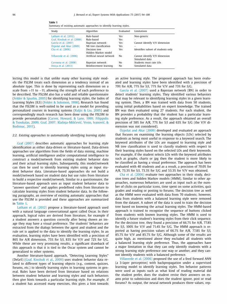
Table 1
Summary of existing automatic approaches to identify learning styles.
Study Algorithm Evaluated Limitations
Latham et al. (2012) Rule-based Yes Non-generic
Graf, Kinshuk et al. (2009) Rule-based Yes –
García et al. (2007) Bayesian network Yes Cannot identify V/V dimension
Özpolat and Akar (2009) NB tree classification Yes –
Cha et al. (2006) Decision tree Yes Identifies subset of students only
Hidden Markov model
Villaverde et al. (2006) Artificial neural network No Cannot identify V/V dimension
Simulated data
Carmona et al. (2008) Bayesian network No Students must rate LOs
Dorça et al. (2013) Reinforcement learning No Simulated data
a
a
7
d
t
i
u
B
B
i
p
m
t
s
k
N
t
F
s
b
e
A
s
p
b
g
a
d
f
t
a
f
i
F
f
p
8
q
a
a
s
n
(
l
w
t
a
f
lecting this model is that unlike many other learning style mod-
els the FSLSM treats each dimension as a tendency instead of an
absolute type. This is done by representing each dimension on a
scale from + 11 to −11, allowing the strength of each preference to
be described. The FSLSM also has a valid and reliable questionnaire
( Felder & Spurlin, 2005 ) for identifying learning styles, the Index of
Learning Styles (ILS) ( Felder & Solomon, 1998 ). Research has found
that the FSLSM is well-suited to be used as a model for providing
personalized courses in learning systems ( Kuljis & Liu, 2005 ) and
correspondingly much research has been done using the FSLSM to
provide personalization ( Carver, Howard, & Lane, 1999; Filippidis
& Tsoukalas, 2009; Graf, 2007; Klašnja-Mili ́cevi ́c, Vesin, Ivanovi ́c, &
Budimac, 2011 ).
2.2. Existing approaches to automatically identifying learning styles
Graf (2007) describes automatic approaches for learning style
identification as either data-driven or literature-based. Data-driven
approaches use algorithms from the fields of data mining, machine
learning, artificial intelligence and/or computational intelligence to
construct a model/network from existing student behavior data
and their actual learning styles. Subsequently, this model/network
can then be used to identify learning styles using as input stu-
dent behavior data. Literature-based approaches do not build a
model/network based on student data but use rules from literature
to build a respective model/network. Similar to a questionnaire, the
literature-based approach uses as input student behavior data to
“answer questions” and applies predefined rules from literature to
calculate learning styles from student behavior data. In the follow-
ing paragraphs, an overview of existing automatic approaches that
use the FSLSM is provided and these approaches are summarized
in Table 1 .
Latham et al. (2012) propose a literature-based approach used
with a natural language conversational agent called Oscar. In their
approach, logical rules are derived from literature, for example if
a student answers a question correctly after being shown an im-
age they may have a visual preference. The students’ behaviors are
extracted from the dialogs between the agent and student and the
rule set is applied to the data to identify the learning styles. In an
evaluation, learning styles have been identified with a precision of
86% for A/R dimension, 75% for S/I, 83% for V/V and 72% for S/G.
While these are very promising results, a significant drawback of
this approach is that it is tied to the Oscar system and cannot be
generalized to other systems.
Another literature-based approach, “Detecting Learning Styles”
(DeLeS) ( Graf, Kinshuk et al., 2009 ) uses student behavior data re-
lated to different types of learning objects (e.g., content, quizzes,
forums, etc.) to identify learning styles in learning systems in gen-
eral. Rules have been derived from literature based on relations
between student behavior and learning styles and such behaviors
then give hints towards a particular learning style. For example, if
a student has accessed many exercises, this gives a hint towards
n active learning style. The proposed approach has been evalu-
ted and learning styles have been identified with a precision of
9% for A/R, 77% for S/I, 77% for V/V and 73% for S/G.
García et al. (2007) used a Bayesian network (BN) in order to
etect students’ learning styles. They identified various behaviors
hat may be relevant to identifying learning styles in a given learn-
ng system. Then, a BN was trained with data from 50 students,
sing initial probabilities based on expert knowledge. The trained
N was then evaluated using 27 students. For each student, the
N provides a probability that the student has a particular learn-
ng style preference. As a result, the approach obtained an overall
recision of 58% for A/R, 77% for S/I and 63% for S/G (the V/V di-
ension was not considered).
Özpolat and Akar (2009) developed and evaluated an approach
hat focuses on examining the learning objects (LOs) selected by
tudents as being most useful in response to a keyword search. The
eyword attributes of the LOs are mapped to learning style and
B tree classification is used to classify students with respect to
heir learning styles based on the selected LOs and their keywords.
or example, if the student selects LOs with the keyword attributes
uch as graphs, charts or jpg then the student is more likely to
e classified as having a visual preference. The approach has been
valuated with 40 students and as a result, a precision of 70.0% for
/R, 73.3% for S/I, 73.3% for S/G and 53.3% for V/V was obtained.
Cha et al. (2006) evaluate two approaches in their study, deci-
ion trees and hidden Markov models (HMM). Similar to other ap-
roaches, numerous behaviors are used as input such as the num-
er of clicks on particular icons, time spent on some activities, quiz
rades and reading or posting to forums. The decision tree as well
s the HMM were evaluated with data from 70 students; however,
ata from students with a balanced learning style were removed
rom the dataset. A subset of the data is used to train the decision
ree based on knowing the actual learning styles. The HMM-based
pproach is trained to recognize the sequence of buttons clicked
rom students with known learning styles. The HMM is used to
dentify a future student’s learning styles from their click sequence.
or the decision tree, they found a precision of 66.7% for A/R, 77.8%
or S/I, 100% for V/V and 71.4% for S/G. The HMM approach is re-
orted as having precision values of 66.7% for A/R, 77.8% for S/I,
5.7% for V/V and 85.7% for S/G. Although some of the results are
uite high, as mentioned above they excluded all students with
balanced learning style preference. Thus, the approaches have
major limitation in that they can only identify students with a
trong learning style preference one way or another, and they can-
ot identify students with a balanced preference.
Villaverde et al. (2006) proposed the use of a feed forward ANN
a 3-layer perceptron) with backpropagation under a supervised
earning model to identify learning styles. Ten behavior patterns
ere used as inputs such as what kind of reading material did
he student prefer, does the student revise their answers on ex-
ms prior to submission and does the student ignore, post or read
orums? As output, the neural network produces three values, rep-
J. Bernard et al. / Expert Systems With Applications 75 (2017) 94–108 97
r
d
a
t
a
L
F
L
c
b
m
b
d
p
a
B
t
a
l
o
t
e
t
r
T
a
w
t
s
p
i
p
s
L
w
h
f
m
e
f
r
h
s
s
w
3
t
a
t
i
g
r
t
t
s
(
S
r
3
b
a
w
w
i
c
u
h
h
p
i
t
t
r
A
l
a
p
t
u
k
t
i
o
o
t
A
w
a
v
i
t
b
e
d
c
t
t
c
3
1
l
t
o
d
t
a
N
I
u
r
s
fi
h
t
s
m
c
esenting the learning styles on three of the four learning style
imensions of the FSLSM. In an evaluation with simulated data,
n average precision of 69.3% across the three dimensions was ob-
ained. LSID-ANN is similar to this approach in that they both use
3-layer perceptron with behavior patterns as inputs; however,
SID-ANN is expected to provide better results for two reasons.
irst, since a separate ANN is built for each FSLSM dimension each
SID-ANN is able to be more specialized and therefore more pre-
ise. Second, since Cha et al. (2006 ) used a single ANN, all of the
ehavior patterns are used as inputs for all three learning style di-
ensions they considered; however, it is likely that some of the
ehavior patterns were not relevant for some of the learning style
imensions. For each LSID-ANN only those behavior patterns ex-
ected to be relevant for each learning style dimension are used
s inputs.
Carmona et al. (2008) also explored the use of a dynamic
ayesian network to identify learning styles. To LOs in the system
hey associated five learning style relevant attributes: format (im-
ge, text, etc.), resource type (exercise, example, etc.), interactivity
evel (very low to very high), interactivity type (active, expositive
r mixed) and semantic density (very low to very high). Each of
he attributes is mapped to one or more FSLSM dimension(s). Ev-
ry time a student selected a LOs, they would be asked to rate
he usefulness of the material from 1 to 4. After rating the LO, the
ating is used as evidence to adjust the belief state of the network.
he drawback to this approach, when compared to other automatic
pproaches, is that it requires input from the student instead of
orking solely on their behaviors. This is potentially intrusive for
he student and there is no guarantee that the student will rate
olely based on how it appealed to their learning styles. This ap-
roach was also not evaluated.
Dorça et al. (2013) presented an approach for identifying learn-
ng styles using reinforcement learning (Q-learning). In this ap-
roach, LOs in the system were associated to particular learning
tyles based on expert knowledge. The student is then presented
Os to achieve a learning goal followed by an assessment on how
ell they learned the material. The probability that the student
as particular learning styles is then reinforced based on the per-
ormance assessment and how well the learning styles of the LO
atch the student’s current predicted learning styles. Three differ-
nt strategies are considered towards reinforcement, either rein-
orcing for high performance only, low performance only (inverse
einforcement) or both. So, for example, with a reinforcement with
igh performance strategy if the student performs well on an as-
essment it is more likely the student has the learning styles as-
ociated with the presented LO. The approach was only evaluated
ith simulated data.
. Background on algorithms
Since many related works use classification algorithms for iden-
ifying learning styles, in this research we propose the use of an
rtificial neural network (ANN). An ANN is a universal approxima-
or ( Hornik, Stinchcombe, & White, 1990 ) and so it is reasoned that
t may be a very suitable algorithm for identifying learning styles,
iven the typically small amount of data available in this line of
esearch. In addition to ANNs, this research evaluates the use of
hree optimization algorithms: genetic algorithm, ant colony sys-
em and particle swarm optimization. These algorithms have been
elected due to their wide-spread use to solve similar problems
Pothiya, Ngamroo, & Kongprawechnon, 2010; Robinson & Rahmat-
amii, 2004; Yao, 1999 ). In the following subsections, each algo-
ithm is described in more detail.
.1. Artificial neural network (ANN)
ANNs ( Basheer & Hajmeer, 20 0 0; Mitchell, 1997 ) are inspired
y neurons in a brain. As such, they are described as a graph of
rtificial neurons. There are different ways these can be connected,
ith feed forward networks being the most commonly used ones,
here circular connections are not permitted. ANNs are configured
nto layers, distinguishing between a single and multi-layer per-
eptron, where the latter is more common. One common config-
ration of a multi-layer perceptron consists of three layers: input,
idden and output. In this configuration, each neuron in each layer
as a weighted connection (neural link) from each neuron in the
receding layer. Each input neuron has a single connection to an
nput variable. A sigmoid function (e.g., tanh) is used to calculate
he strength (output) of the neuron. The input to the sigmoid func-
ion is the sum of each input multiplied by the weight of the neu-
al link between the neurons. In this research, our approach, LSID-
NN, uses the commonly used configuration of a feed forward 3-
ayer perceptron.
To evaluate the ANNs outputs, one of two learning strategies
re typically used: supervised or unsupervised learning. With su-
ervised learning, the correct answer for the sample is known, so
hat the output can be directly compared with the answer. With
nsupervised learning the correct answer for the sample is un-
nown. Unsupervised learning is generally used for finding clus-
ers or other structures in data. LSID-ANN uses a supervised learn-
ng strategy since training data include the actual learning styles
f students.
Lastly, there are numerous techniques for training an ANN. One
f the most commonly used training algorithms is back propaga-
ion, which is also used for LSID-ANN. Using back propagation, the
NN is traversed in reverse along each neural link, adjusting the
eights and thresholds by calculating a weight modification ( �W )
s a sigmoid function of the error between the output and actual
alues. The weight modification is further multiplied by a learn-
ng rate ( η > 0) which helps control the size of the steps to take
o keep the ANN from oscillating over the optimum. Training may
e further optimized by adding momentum ( m ≥ 0) which aids in
scaping local optima. Lastly, two training modes are possible: in-
ividual and ensemble. In individual training the weight modifi-
ation is applied after the sample is run, whereas with ensemble
raining they are summed and applied at the end of the genera-
ion. The back propagation algorithm then runs until a termination
ondition is reached.
.2. Genetic algorithm (GA)
A genetic algorithm (GA) ( Grefenstette, 1986; Srinivas & Patnaik,
994 ) is an optimization algorithm that utilizes concepts from evo-
utionary biology to solve optimization problems. In biology, when
wo individuals produce offspring, they intermix their genes. If one
ffspring is more fit than others, it will tend to survive and pro-
uce offspring of its own and so propagate its parents’ genes. In
his way, over time, increasingly fit offspring are evolved. With GA,
population of P genomes is produced. Each genome consists of
genes and each gene represents a component of the solution.
n each generation, pairs of genomes are selected from the pop-
lation favoring genomes with higher fitness (e.g., by using the
oulette wheel technique where the chance of each genome being
elected is equal to its fitness divided by the sum of all genomes’
tness values). A crossover process is conducted where each pair
as some genes selected and swapped between them (based on
he crossover weight); thereby, producing two new genomes (off-
pring). This crossover operation allows the genetic algorithm to
ake leaps far from its current position, making it useful for es-
aping local optima. Then each offspring can be mutated by se-
98 J. Bernard et al. / Expert Systems With Applications 75 (2017) 94–108
S
τ
τ
3
i
u
a
s
t
l
c
p
j
e
i
2
u
(
g
c
t
t
g
H
i
v
t
e
s
v
a
p
f
(
o
n
V
4
a
p
i
i
a
p
a
a
a
b
h
d
lecting some of its genes and changing them to a random value
(based on the mutation weight). Mutation ensures that gene diver-
sity does not stagnate by injecting new values into the genomes.
Finally, the new population is built from a mix of the genomes and
their offspring, depending on their fitness values. With the selec-
tion of a new population, a new generation starts.
The functioning of the GA is controlled by three parameters and
a termination condition. The parameters are: population size ( P ),
crossover weight ( C ) and mutation weight ( M ). The population size
dictates the number of genomes in the population. The crossover
weight determines the likelihood that any particular gene will be
used for crossover; a high crossover weight encourages exploration
but can disrupt good combinations of genes. The mutation weight
determines the likelihood that a gene will be mutated, ensuring
that particular gene values do not persist forever. The termination
condition tells the GA when to stop processing.
3.3. Ant colony system (ACS)
ACS ( Dorigo & Gambardella, 1997b ) is one of several algorithms
collectively referred to as ant colony optimization. These algo-
rithms are inspired by the way ants share information while for-
aging for food. In such scenario, ants lay pheromone trails to food
sources, thereby indirectly communicating to the other ants about
the path to the food. With ACS, a graph is built where each node
represents a part of a solution to the problem and the whole path
through the graph represents a solution. Each link from one node
to another has a problem specific inherent desirability (local qual-
ity) and may also have pheromone laid upon it. The overall qual-
ity ( Q ) of a link is a function of the local quality ( l ) and amount
of pheromones ( τ ) on the link, with two parameters ( α ≥ 0 and
β ≥ 0) weighting the local quality and amount of pheromones re-
spectively (shown in Formula (1) ).
To start the algorithm, a colony (population) of P artificial ants
is created and they are set to traverse the graph in the following
manner. Each ant is placed at a starting node, and depending on
the problem this may be a fixed node or selected in some fash-
ion, for example, randomly. The ant then chooses a link to follow
by a pseudorandom proportional rule described as follows. A ran-
dom value from 0 to 1 is selected and if this value is less than the
exploitation parameter (0 ≤ q 0 ≤ 1) then the link with the highest
quality ( Q ) is selected. Otherwise the link is selected by roulette
wheel technique (shown in Formula (2) ), where the chance of se-
lection is equal to the quality of the link divided by the total qual-
ity of all links from that node. Optionally, the list of nodes to be
considered under the pseudorandom proportional rule can include
only nodes that are from a candidate list, which is a pre-generated
static list of preferred choices from each node. Typically, a tabu list
is maintained for each ant so that it does not return to a previ-
ously visited node. If the ant cannot move to any node, then it is
considered stuck and depending on the problem this may mean
the solution is complete or invalid. In order to encourage explo-
ration, as an ant traverses a link, it consumes a portion (0 ≤ τ 0 ≤ 1)
of the pheromone (shown in Formula (3) ). This makes it less likely
that ants which follow will take the same path. Once all of the
ants have completed traversing the graph, a portion of pheromones
(0 ≤ ρ ≤ 1) from each link in the graph is evaporated causing the
colony to forget a little and so encourages exploration (shown in
Formula (4) ). Furthermore, the global best path or the iteration
best path has pheromones laid on each link of the path as a func-
tion of the fitness of the solution. Subsequently, a new generation
starts with ants starting again to move through the graph, until a
termination condition is fulfilled.
Q = l α × τβ (1)
n =
Q ( l n , τn ) ∑ n x =1 Q ( l x , τx )
(2)
= ( 1 − τ0 ) × τ ′ (3)
= ( 1 − ρ) × τ ′ (4)
.4. Particle swarm optimization (PSO)
PSO ( Eberhart & Kennedy, 1995 ) is an optimization algorithm
nspired by flocking movements in nature, such as birds. PSO is
sed where the solution space to a problem can be represented
s a hyperspace or hypershape. The position of a particle repre-
ents a candidate solution to the problem being solved. Each of
he coordinates in the position represents a component of the so-
ution although how the coordinates are decoded is problem spe-
ific. PSO uses search by social intelligence as the population of
articles share information as they fly through the space and ad-
ust their trajectories to focus on promising areas.
PSO has the following control parameters: population size, in-
rtia, particle best acceleration, global best acceleration and max-
mum velocity which are described as follows ( Clerc & Kennedy,
002; Eberhart & Kennedy, 1995; Shi & Eberhart, 1998 ). The pop-
lation size is the number of particles in the swarm. Inertia
0 ≤ w ≤ 1) keeps the particle moving in the same direction it is
oing and so higher values promote global exploration. The parti-
le is encouraged to turn from its current position ( X curr ) towards
he particle best position so far ( X pbest ) and the global best posi-
ion ( X gbest ) based on the particle best acceleration (0 ≤ c1 ≤ 1 ) and
lobal best acceleration (0 < c2 ≤ 1 ) ( Eberhart & Kennedy, 1995 ).
igher acceleration rates promote exploitation of the most promis-
ng areas found so far. The maximum velocity ( Vmax ) helps to pre-
ent the particles from exploring too far from promising areas, al-
hough if it is set too low the particles may not be able to explore
nough space to find the best promising areas.
To use PSO, a population of particles is created and placed in-
ide the hyperspace (or hypershape) with an initial position and
elocity. In each generation, each particle’s position is updated by
velocity vector calculated using Formula (5) where V 0 is the
article’s current velocity and rand 1 and rand 2 are random values
rom 0 to 1. After each generation, the particle best position so far
X pbest ) and the global best position ( X gbest ) may be updated based
n found solutions and a new generation is started, until a termi-
ation condition is reached.
= w × V 0 + ran d 1 × c1 ×(X curr − X pbest
)+ ran d 2 × c2 ×
(X curr − X gbest
)(5)
. Learning styles identifiers
In this section, four Learning Styles Identifier (LSID) approaches
re introduced, each using a different CI algorithm. These ap-
roaches aim at investigating the suitability of CI algorithms for
mproving the precision of identifying learning styles. Furthermore,
t was a requirement that these approaches would be applicable
nd useful for any learning system rather than being specific to a
articular system.
In order to ensure that the LSID approaches are generalizable
nd applicable for any learning system, it was key to base the
pproaches on generic behavior patterns that can be collected in
ny learning system. After a literature review, we found that the
ehavior patterns used in DeLeS ( Graf, Kinshuk et al., 2009 ) are
ighly suitable for our approaches. These behavior patterns were
esigned to be generic and focus on elements that are available
J. Bernard et al. / Expert Systems With Applications 75 (2017) 94–108 99
Table 2
Relevant behavior patterns for each FSLSM dimension ( Graf, Kinshuk et al., 2009 ).
Active/Reflective Sensing/Intuitive Visual/Verbal Sequential/Global
content_stay ( −) content_stay ( −) content_visit ( −) outline_stay ( −)
content_visit ( −) content_visit ( −) forum_post ( −) outline_visit ( −)
example_stay ( −) example_stay ( + ) forum_stay ( −) question_detail ( + )
exercise_stay ( + ) example_visit ( + ) forum_visit ( −) question_develop ( −)
exercise_visit ( + ) exercise_visit ( + ) question_graphics ( + ) question_interpret ( −)
forum_post ( + ) question_concepts ( −) question_text ( −) question_overview ( −)
forum_visit ( −) question_details ( + ) navigation_overview_stay ( −)
outline_stay ( −) question_develop ( −) navigation_overview_visit ( −)
quiz_stay_results ( −) question_facts ( + ) navigation_skip ( −)
self_assess_stay ( −) quiz_revisions ( + )
self_assess_twice_wrong ( + ) quiz_results_stay ( + )
self_assess_visit ( + ) self_assess_stay ( + )
self_assess_visit ( + )
i
e
h
p
p
u
t
s
f
p
g
P
l
i
m
o
a
a
c
(
v
s
i
b
d
l
i
l
t
b
i
i
l
s
d
o
i
a
4
S
t
s
s
p
c
b
l
u
c
4
t
t
w
1
a
e
b
v
V
o
a
u
t
t
t
t
c
a
s
t
s
6
i
f
b
t
a
s
f
o
w
l
h
A
p
p
a
t
t
T
o
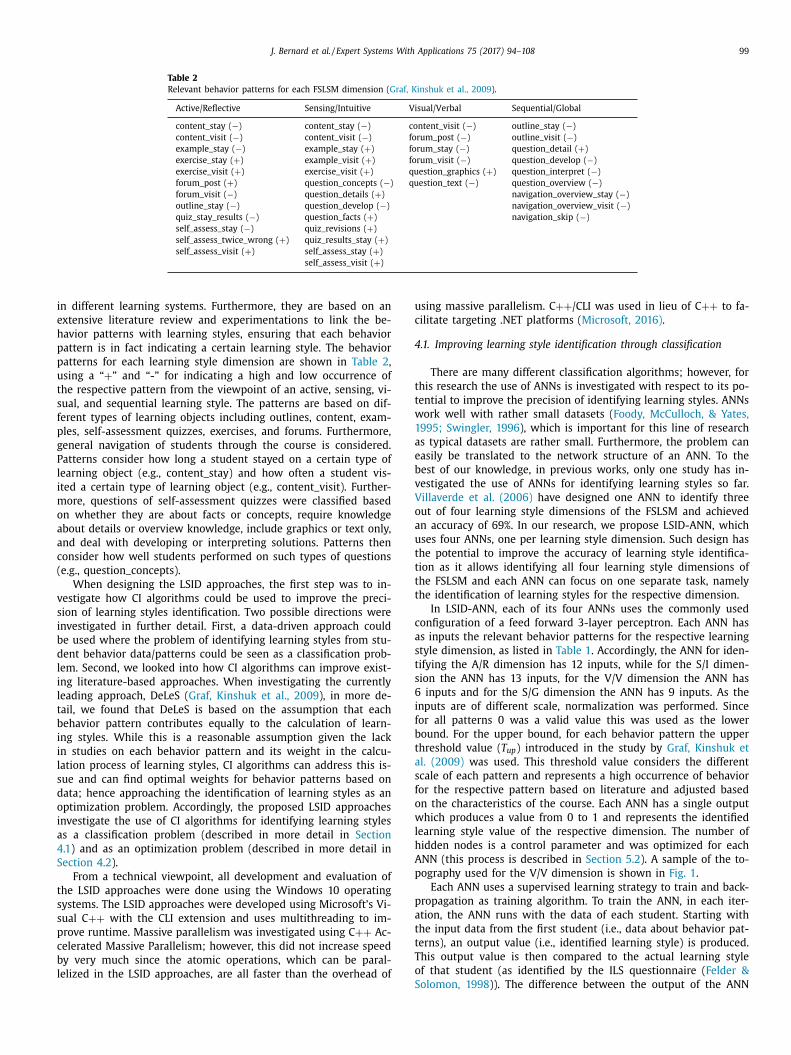
n different learning systems. Furthermore, they are based on an
xtensive literature review and experimentations to link the be-
avior patterns with learning styles, ensuring that each behavior
attern is in fact indicating a certain learning style. The behavior
atterns for each learning style dimension are shown in Table 2 ,
sing a “+ ” and “-” for indicating a high and low occurrence of
he respective pattern from the viewpoint of an active, sensing, vi-
ual, and sequential learning style. The patterns are based on dif-
erent types of learning objects including outlines, content, exam-
les, self-assessment quizzes, exercises, and forums. Furthermore,
eneral navigation of students through the course is considered.
atterns consider how long a student stayed on a certain type of
earning object (e.g., content_stay) and how often a student vis-
ted a certain type of learning object (e.g., content_visit). Further-
ore, questions of self-assessment quizzes were classified based
n whether they are about facts or concepts, require knowledge
bout details or overview knowledge, include graphics or text only,
nd deal with developing or interpreting solutions. Patterns then
onsider how well students performed on such types of questions
e.g., question_concepts).
When designing the LSID approaches, the first step was to in-
estigate how CI algorithms could be used to improve the preci-
ion of learning styles identification. Two possible directions were
nvestigated in further detail. First, a data-driven approach could
e used where the problem of identifying learning styles from stu-
ent behavior data/patterns could be seen as a classification prob-
em. Second, we looked into how CI algorithms can improve exist-
ng literature-based approaches. When investigating the currently
eading approach, DeLeS ( Graf, Kinshuk et al., 2009 ), in more de-
ail, we found that DeLeS is based on the assumption that each
ehavior pattern contributes equally to the calculation of learn-
ng styles. While this is a reasonable assumption given the lack
n studies on each behavior pattern and its weight in the calcu-
ation process of learning styles, CI algorithms can address this is-
ue and can find optimal weights for behavior patterns based on
ata; hence approaching the identification of learning styles as an
ptimization problem. Accordingly, the proposed LSID approaches
nvestigate the use of CI algorithms for identifying learning styles
s a classification problem (described in more detail in Section
.1 ) and as an optimization problem (described in more detail in
ection 4.2 ).
From a technical viewpoint, all development and evaluation of
he LSID approaches were done using the Windows 10 operating
ystems. The LSID approaches were developed using Microsoft’s Vi-
ual C ++ with the CLI extension and uses multithreading to im-
rove runtime. Massive parallelism was investigated using C ++ Ac-
elerated Massive Parallelism; however, this did not increase speed
y very much since the atomic operations, which can be paral-
elized in the LSID approaches, are all faster than the overhead of
Ssing massive parallelism. C ++ /CLI was used in lieu of C ++ to fa-
ilitate targeting .NET platforms ( Microsoft, 2016) .
.1. Improving learning style identification through classification
There are many different classification algorithms; however, for
his research the use of ANNs is investigated with respect to its po-
ential to improve the precision of identifying learning styles. ANNs
ork well with rather small datasets ( Foody, McCulloch, & Yates,
995; Swingler, 1996 ), which is important for this line of research
s typical datasets are rather small. Furthermore, the problem can
asily be translated to the network structure of an ANN. To the
est of our knowledge, in previous works, only one study has in-
estigated the use of ANNs for identifying learning styles so far.
illaverde et al. (2006) have designed one ANN to identify three
ut of four learning style dimensions of the FSLSM and achieved
n accuracy of 69%. In our research, we propose LSID-ANN, which
ses four ANNs, one per learning style dimension. Such design has
he potential to improve the accuracy of learning style identifica-
ion as it allows identifying all four learning style dimensions of
he FSLSM and each ANN can focus on one separate task, namely
he identification of learning styles for the respective dimension.
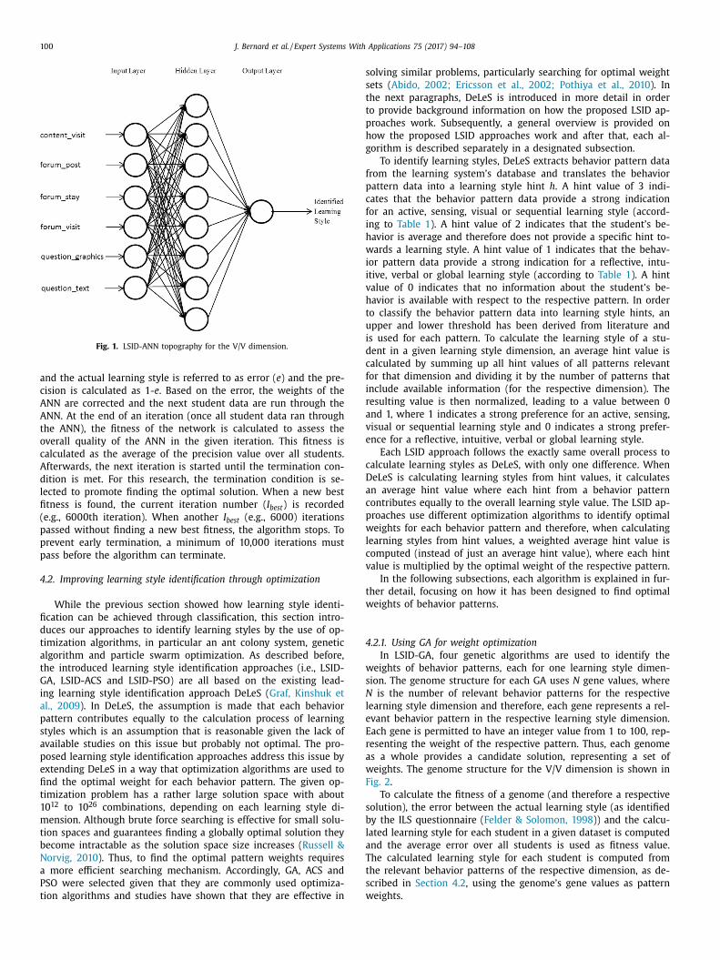
In LSID-ANN, each of its four ANNs uses the commonly used
onfiguration of a feed forward 3-layer perceptron. Each ANN has
s inputs the relevant behavior patterns for the respective learning
tyle dimension, as listed in Table 1 . Accordingly, the ANN for iden-
ifying the A/R dimension has 12 inputs, while for the S/I dimen-
ion the ANN has 13 inputs, for the V/V dimension the ANN has
inputs and for the S/G dimension the ANN has 9 inputs. As the
nputs are of different scale, normalization was performed. Since
or all patterns 0 was a valid value this was used as the lower
ound. For the upper bound, for each behavior pattern the upper
hreshold value ( T up ) introduced in the study by Graf, Kinshuk et
l. (2009) was used. This threshold value considers the different
cale of each pattern and represents a high occurrence of behavior
or the respective pattern based on literature and adjusted based
n the characteristics of the course. Each ANN has a single output
hich produces a value from 0 to 1 and represents the identified
earning style value of the respective dimension. The number of
idden nodes is a control parameter and was optimized for each
NN (this process is described in Section 5.2 ). A sample of the to-
ography used for the V/V dimension is shown in Fig. 1 .
Each ANN uses a supervised learning strategy to train and back-
ropagation as training algorithm. To train the ANN, in each iter-
tion, the ANN runs with the data of each student. Starting with
he input data from the first student (i.e., data about behavior pat-
erns), an output value (i.e., identified learning style) is produced.
his output value is then compared to the actual learning style
f that student (as identified by the ILS questionnaire ( Felder &
olomon, 1998 )). The difference between the output of the ANN
100 J. Bernard et al. / Expert Systems With Applications 75 (2017) 94–108
Fig. 1. LSID-ANN topography for the V/V dimension.
s
s
t
t
p
h
g
f
p
c
f
i
h
w
i
i
v
h
t
u
i
d
c
f
i
r
a
v
e
c
D
a
c
p
w
l
c
v
t
w
4
w
s
N
l
e
E
r
a
w
F
s
b
l
a
T
t
s
w
and the actual learning style is referred to as error ( e ) and the pre-
cision is calculated as 1- e . Based on the error, the weights of the
ANN are corrected and the next student data are run through the
ANN. At the end of an iteration (once all student data ran through
the ANN), the fitness of the network is calculated to assess the
overall quality of the ANN in the given iteration. This fitness is
calculated as the average of the precision value over all students.
Afterwards, the next iteration is started until the termination con-
dition is met. For this research, the termination condition is se-
lected to promote finding the optimal solution. When a new best
fitness is found, the current iteration number ( I best ) is recorded
(e.g., 60 0 0th iteration). When another I best (e.g., 60 0 0) iterations
passed without finding a new best fitness, the algorithm stops. To
prevent early termination, a minimum of 10,0 0 0 iterations must
pass before the algorithm can terminate.
4.2. Improving learning style identification through optimization
While the previous section showed how learning style identi-
fication can be achieved through classification, this section intro-
duces our approaches to identify learning styles by the use of op-
timization algorithms, in particular an ant colony system, genetic
algorithm and particle swarm optimization. As described before,
the introduced learning style identification approaches (i.e., LSID-
GA, LSID-ACS and LSID-PSO) are all based on the existing lead-
ing learning style identification approach DeLeS ( Graf, Kinshuk et
al., 2009 ). In DeLeS, the assumption is made that each behavior
pattern contributes equally to the calculation process of learning
styles which is an assumption that is reasonable given the lack of
available studies on this issue but probably not optimal. The pro-
posed learning style identification approaches address this issue by
extending DeLeS in a way that optimization algorithms are used to
find the optimal weight for each behavior pattern. The given op-
timization problem has a rather large solution space with about
10 12 to 10 26 combinations, depending on each learning style di-
mension. Although brute force searching is effective for small solu-
tion spaces and guarantees finding a globally optimal solution they
become intractable as the solution space size increases ( Russell &
Norvig, 2010 ). Thus, to find the optimal pattern weights requires
a more efficient searching mechanism. Accordingly, GA, ACS and
PSO were selected given that they are commonly used optimiza-
tion algorithms and studies have shown that they are effective in
olving similar problems, particularly searching for optimal weight
ets ( Abido, 2002; Ericsson et al., 2002; Pothiya et al., 2010 ). In
he next paragraphs, DeLeS is introduced in more detail in order
o provide background information on how the proposed LSID ap-
roaches work. Subsequently, a general overview is provided on
ow the proposed LSID approaches work and after that, each al-
orithm is described separately in a designated subsection.
To identify learning styles, DeLeS extracts behavior pattern data
rom the learning system’s database and translates the behavior
attern data into a learning style hint h . A hint value of 3 indi-
ates that the behavior pattern data provide a strong indication
or an active, sensing, visual or sequential learning style (accord-
ng to Table 1 ). A hint value of 2 indicates that the student’s be-
avior is average and therefore does not provide a specific hint to-
ards a learning style. A hint value of 1 indicates that the behav-
or pattern data provide a strong indication for a reflective, intu-
tive, verbal or global learning style (according to Table 1 ). A hint
alue of 0 indicates that no information about the student’s be-
avior is available with respect to the respective pattern. In order
o classify the behavior pattern data into learning style hints, an
pper and lower threshold has been derived from literature and
s used for each pattern. To calculate the learning style of a stu-
ent in a given learning style dimension, an average hint value is
alculated by summing up all hint values of all patterns relevant
or that dimension and dividing it by the number of patterns that
nclude available information (for the respective dimension). The
esulting value is then normalized, leading to a value between 0
nd 1, where 1 indicates a strong preference for an active, sensing,
isual or sequential learning style and 0 indicates a strong prefer-
nce for a reflective, intuitive, verbal or global learning style.
Each LSID approach follows the exactly same overall process to
alculate learning styles as DeLeS, with only one difference. When
eLeS is calculating learning styles from hint values, it calculates
n average hint value where each hint from a behavior pattern
ontributes equally to the overall learning style value. The LSID ap-
roaches use different optimization algorithms to identify optimal
eights for each behavior pattern and therefore, when calculating
earning styles from hint values, a weighted average hint value is
omputed (instead of just an average hint value), where each hint
alue is multiplied by the optimal weight of the respective pattern.
In the following subsections, each algorithm is explained in fur-
her detail, focusing on how it has been designed to find optimal
eights of behavior patterns.
.2.1. Using GA for weight optimization
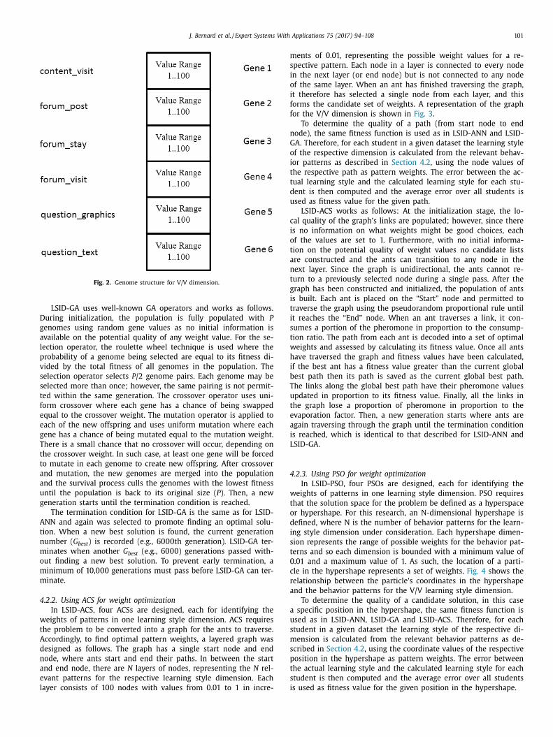
In LSID-GA, four genetic algorithms are used to identify the
eights of behavior patterns, each for one learning style dimen-
ion. The genome structure for each GA uses N gene values, where
is the number of relevant behavior patterns for the respective
earning style dimension and therefore, each gene represents a rel-
vant behavior pattern in the respective learning style dimension.
ach gene is permitted to have an integer value from 1 to 100, rep-
esenting the weight of the respective pattern. Thus, each genome
s a whole provides a candidate solution, representing a set of
eights. The genome structure for the V/V dimension is shown in
ig. 2 .
To calculate the fitness of a genome (and therefore a respective
olution), the error between the actual learning style (as identified
y the ILS questionnaire ( Felder & Solomon, 1998 )) and the calcu-
ated learning style for each student in a given dataset is computed
nd the average error over all students is used as fitness value.
he calculated learning style for each student is computed from
he relevant behavior patterns of the respective dimension, as de-
cribed in Section 4.2 , using the genome’s gene values as pattern
eights.
J. Bernard et al. / Expert Systems With Applications 75 (2017) 94–108 101
Fig. 2. Genome structure for V/V dimension.
D
g
a
l
p
v
s
s
t
f
e
e
g
T
t
t
a
a
u
g
A
t
n
m
o
m
m
4
w
t
A
d
n
a
e
l
m
s
i
o
i
f
f
n
G
o
i
t
t
d
u
c
i
o
t
a
n
t
g
i
t
i
s
t
w
h
i
b
T
u
t
e
a
i
L
4
w
t
o
d
i
s
t
0
c
r
a
a
u
s
m
s
p
t
s
i
LSID-GA uses well-known GA operators and works as follows.
uring initialization, the population is fully populated with P
enomes using random gene values as no initial information is
vailable on the potential quality of any weight value. For the se-
ection operator, the roulette wheel technique is used where the
robability of a genome being selected are equal to its fitness di-
ided by the total fitness of all genomes in the population. The
election operator selects P /2 genome pairs. Each genome may be
elected more than once; however, the same pairing is not permit-
ed within the same generation. The crossover operator uses uni-
orm crossover where each gene has a chance of being swapped
qual to the crossover weight. The mutation operator is applied to
ach of the new offspring and uses uniform mutation where each
ene has a chance of being mutated equal to the mutation weight.
here is a small chance that no crossover will occur, depending on
he crossover weight. In such case, at least one gene will be forced
o mutate in each genome to create new offspring. After crossover
nd mutation, the new genomes are merged into the population
nd the survival process culls the genomes with the lowest fitness
ntil the population is back to its original size ( P ). Then, a new
eneration starts until the termination condition is reached.
The termination condition for LSID-GA is the same as for LSID-
NN and again was selected to promote finding an optimal solu-
ion. When a new best solution is found, the current generation
umber ( G best ) is recorded (e.g., 60 0 0th generation). LSID-GA ter-
inates when another G best (e.g., 60 0 0) generations passed with-
ut finding a new best solution. To prevent early termination, a
inimum of 10,0 0 0 generations must pass before LSID-GA can ter-
inate.
.2.2. Using ACS for weight optimization
In LSID-ACS, four ACSs are designed, each for identifying the
eights of patterns in one learning style dimension. ACS requires
he problem to be converted into a graph for the ants to traverse.
ccordingly, to find optimal pattern weights, a layered graph was
esigned as follows. The graph has a single start node and end
ode, where ants start and end their paths. In between the start
nd end node, there are N layers of nodes, representing the N rel-
vant patterns for the respective learning style dimension. Each
ayer consists of 100 nodes with values from 0.01 to 1 in incre-
ents of 0.01, representing the possible weight values for a re-
pective pattern. Each node in a layer is connected to every node
n the next layer (or end node) but is not connected to any node
f the same layer. When an ant has finished traversing the graph,
t therefore has selected a single node from each layer, and this
orms the candidate set of weights. A representation of the graph
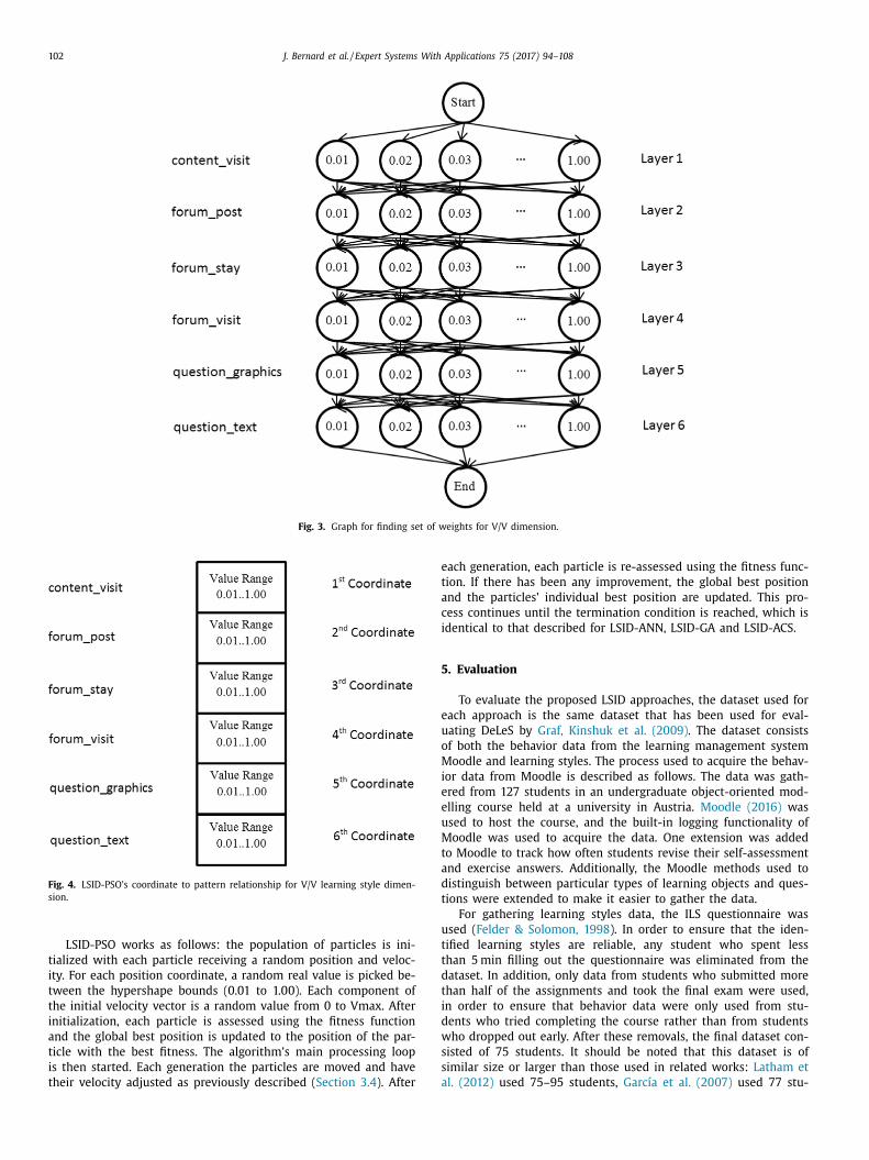
or the V/V dimension is shown in Fig. 3 .
To determine the quality of a path (from start node to end
ode), the same fitness function is used as in LSID-ANN and LSID-
A. Therefore, for each student in a given dataset the learning style
f the respective dimension is calculated from the relevant behav-
or patterns as described in Section 4.2 , using the node values of
he respective path as pattern weights. The error between the ac-
ual learning style and the calculated learning style for each stu-
ent is then computed and the average error over all students is
sed as fitness value for the given path.
LSID-ACS works as follows: At the initialization stage, the lo-
al quality of the graph’s links are populated; however, since there
s no information on what weights might be good choices, each
f the values are set to 1. Furthermore, with no initial informa-
ion on the potential quality of weight values no candidate lists
re constructed and the ants can transition to any node in the
ext layer. Since the graph is unidirectional, the ants cannot re-
urn to a previously selected node during a single pass. After the
raph has been constructed and initialized, the population of ants
s built. Each ant is placed on the “Start” node and permitted to
raverse the graph using the pseudorandom proportional rule until
t reaches the “End” node. When an ant traverses a link, it con-
umes a portion of the pheromone in proportion to the consump-
ion ratio. The path from each ant is decoded into a set of optimal
eights and assessed by calculating its fitness value. Once all ants
ave traversed the graph and fitness values have been calculated,
f the best ant has a fitness value greater than the current global
est path then its path is saved as the current global best path.
he links along the global best path have their pheromone values
pdated in proportion to its fitness value. Finally, all the links in
he graph lose a proportion of pheromone in proportion to the
vaporation factor. Then, a new generation starts where ants are
gain traversing through the graph until the termination condition
s reached, which is identical to that described for LSID-ANN and
SID-GA.
.2.3. Using PSO for weight optimization
In LSID-PSO, four PSOs are designed, each for identifying the
eights of patterns in one learning style dimension. PSO requires
hat the solution space for the problem be defined as a hyperspace
r hypershape. For this research, an N-dimensional hypershape is
efined, where N is the number of behavior patterns for the learn-
ng style dimension under consideration. Each hypershape dimen-
ion represents the range of possible weights for the behavior pat-
erns and so each dimension is bounded with a minimum value of
.01 and a maximum value of 1. As such, the location of a parti-
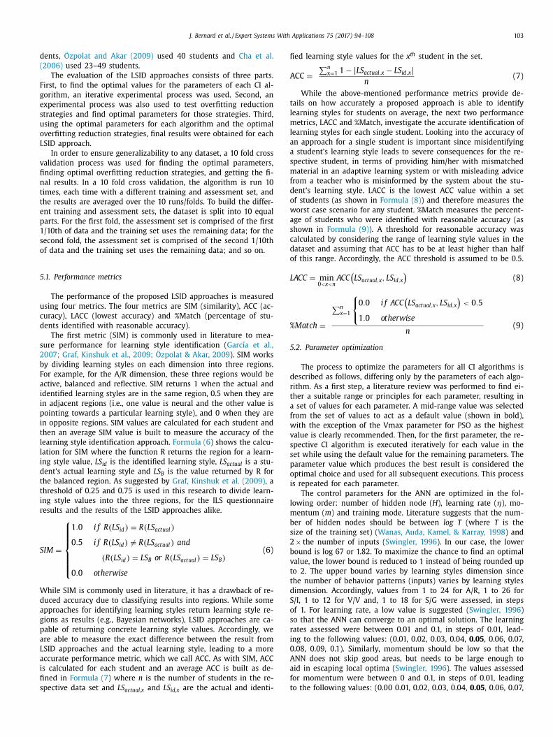
le in the hypershape represents a set of weights. Fig. 4 shows the
elationship between the particle’s coordinates in the hypershape
nd the behavior patterns for the V/V learning style dimension.
To determine the quality of a candidate solution, in this case
specific position in the hypershape, the same fitness function is
sed as in LSID-ANN, LSID-GA and LSID-ACS. Therefore, for each
tudent in a given dataset the learning style of the respective di-
ension is calculated from the relevant behavior patterns as de-
cribed in Section 4.2 , using the coordinate values of the respective
osition in the hypershape as pattern weights. The error between
he actual learning style and the calculated learning style for each
tudent is then computed and the average error over all students
s used as fitness value for the given position in the hypershape.
102 J. Bernard et al. / Expert Systems With Applications 75 (2017) 94–108
Fig. 3. Graph for finding set of weights for V/V dimension.
Fig. 4. LSID-PSO’s coordinate to pattern relationship for V/V learning style dimen-
sion.
e
t
a
c
i
5
e
u
o
M
i
e
e
u
M
t
a
d
t
u
t
t
d
t
i
d
w
s
s
a
LSID-PSO works as follows: the population of particles is ini-
tialized with each particle receiving a random position and veloc-
ity. For each position coordinate, a random real value is picked be-
tween the hypershape bounds (0.01 to 1.00). Each component of
the initial velocity vector is a random value from 0 to Vmax. After
initialization, each particle is assessed using the fitness function
and the global best position is updated to the position of the par-
ticle with the best fitness. The algorithm’s main processing loop
is then started. Each generation the particles are moved and have
their velocity adjusted as previously described ( Section 3.4 ). After
ach generation, each particle is re-assessed using the fitness func-
ion. If there has been any improvement, the global best position
nd the particles’ individual best position are updated. This pro-
ess continues until the termination condition is reached, which is
dentical to that described for LSID-ANN, LSID-GA and LSID-ACS.
. Evaluation
To evaluate the proposed LSID approaches, the dataset used for
ach approach is the same dataset that has been used for eval-
ating DeLeS by Graf, Kinshuk et al. (2009) . The dataset consists
f both the behavior data from the learning management system
oodle and learning styles. The process used to acquire the behav-
or data from Moodle is described as follows. The data was gath-
red from 127 students in an undergraduate object-oriented mod-
lling course held at a university in Austria. Moodle (2016) was
sed to host the course, and the built-in logging functionality of
oodle was used to acquire the data. One extension was added
o Moodle to track how often students revise their self-assessment
nd exercise answers. Additionally, the Moodle methods used to
istinguish between particular types of learning objects and ques-
ions were extended to make it easier to gather the data.
For gathering learning styles data, the ILS questionnaire was
sed ( Felder & Solomon, 1998 ). In order to ensure that the iden-
ified learning styles are reliable, any student who spent less
han 5 min filling out the questionnaire was eliminated from the
ataset. In addition, only data from students who submitted more
han half of the assignments and took the final exam were used,
n order to ensure that behavior data were only used from stu-
ents who tried completing the course rather than from students
ho dropped out early. After these removals, the final dataset con-
isted of 75 students. It should be noted that this dataset is of
imilar size or larger than those used in related works: Latham et
l. (2012) used 75–95 students, García et al. (2007) used 77 stu-
J. Bernard et al. / Expert Systems With Applications 75 (2017) 94–108 103
d
(
F
g
e
s
u
o
L
v
fi
n
t
t
e
p
1
s
o
5
u
c
d
s
2
b
F
a
i
i
p
i
t
l
l
i
d
t
t
i
r
S
W
d
a
g
p
a
L
a
i
fi
s
fi
A
t
l
m
l
a
a
s
m
f
d
o
w
a
s
c
d
o
L
%
5
d
r
t
a
f
w
v
s
s
p
o
i
l
m
b
s
2
b
v
t
t
d
S
o
s
r
i
0
A
a
f
t
ents, Özpolat and Akar (2009) used 40 students and Cha et al.
2006) used 23–49 students.
The evaluation of the LSID approaches consists of three parts.
irst, to find the optimal values for the parameters of each CI al-
orithm, an iterative experimental process was used. Second, an
xperimental process was also used to test overfitting reduction
trategies and find optimal parameters for those strategies. Third,
sing the optimal parameters for each algorithm and the optimal
verfitting reduction strategies, final results were obtained for each
SID approach.
In order to ensure generalizability to any dataset, a 10 fold cross
alidation process was used for finding the optimal parameters,
nding optimal overfitting reduction strategies, and getting the fi-
al results. In a 10 fold cross validation, the algorithm is run 10
imes, each time with a different training and assessment set, and
he results are averaged over the 10 runs/folds. To build the differ-
nt training and assessment sets, the dataset is split into 10 equal
arts. For the first fold, the assessment set is comprised of the first
/10th of data and the training set uses the remaining data; for the
econd fold, the assessment set is comprised of the second 1/10th
f data and the training set uses the remaining data; and so on.
.1. Performance metrics
The performance of the proposed LSID approaches is measured
sing four metrics. The four metrics are SIM (similarity), ACC (ac-
uracy), LACC (lowest accuracy) and %Match (percentage of stu-
ents identified with reasonable accuracy).
The first metric (SIM) is commonly used in literature to mea-
ure performance for learning style identification ( García et al.,
0 07; Graf, Kinshuk et al., 20 09; Özpolat & Akar, 20 09 ). SIM works
y dividing learning styles on each dimension into three regions.
or example, for the A/R dimension, these three regions would be
ctive, balanced and reflective. SIM returns 1 when the actual and
dentified learning styles are in the same region, 0.5 when they are
n adjacent regions (i.e., one value is neural and the other value is
ointing towards a particular learning style), and 0 when they are
n opposite regions. SIM values are calculated for each student and
hen an average SIM value is built to measure the accuracy of the
earning style identification approach. Formula (6 ) shows the calcu-
ation for SIM where the function R returns the region for a learn-
ng style value, LS id is the identified learning style, LS actual is a stu-
ent’s actual learning style and LS B is the value returned by R for
he balanced region. As suggested by Graf, Kinshuk et al. (2009) , a
hreshold of 0.25 and 0.75 is used in this research to divide learn-
ng style values into the three regions, for the ILS questionnaire
esults and the results of the LSID approaches alike.
IM =
⎧ ⎪ ⎪ ⎪ ⎪ ⎨
⎪ ⎪ ⎪ ⎪ ⎩
1 . 0 i f R ( L S id ) = R ( L S actual )
0 . 5 i f R ( L S id ) � = R ( L S actual ) and
( R ( L S id ) = L S B or R ( L S actual ) = L S B )
0 . 0 otherwise
(6)
hile SIM is commonly used in literature, it has a drawback of re-
uced accuracy due to classifying results into regions. While some
pproaches for identifying learning styles return learning style re-
ions as results (e.g., Bayesian networks), LSID approaches are ca-
able of returning concrete learning style values. Accordingly, we
re able to measure the exact difference between the result from
SID approaches and the actual learning style, leading to a more
ccurate performance metric, which we call ACC. As with SIM, ACC
s calculated for each student and an average ACC is built as de-
ned in Formula (7 ) where n is the number of students in the re-
pective data set and LS actual,x and LS id,x are the actual and identi-
ed learning style values for the x th student in the set.
CC =
∑ n x=1 1 − | L S actual,x − L S id,x |
n
(7)
While the above-mentioned performance metrics provide de-
ails on how accurately a proposed approach is able to identify
earning styles for students on average, the next two performance
etrics, LACC and %Match, investigate the accurate identification of
earning styles for each single student. Looking into the accuracy of
n approach for a single student is important since misidentifying
student’s learning style leads to severe consequences for the re-
pective student, in terms of providing him/her with mismatched
aterial in an adaptive learning system or with misleading advice
rom a teacher who is misinformed by the system about the stu-
ent’s learning style. LACC is the lowest ACC value within a set
f students (as shown in Formula (8) ) and therefore measures the
orst case scenario for any student. %Match measures the percent-
ge of students who were identified with reasonable accuracy (as
hown in Formula (9) ). A threshold for reasonable accuracy was
alculated by considering the range of learning style values in the
ataset and assuming that ACC has to be at least higher than half
f this range. Accordingly, the ACC threshold is assumed to be 0.5.
ACC = min
0 <x<n ACC
(L S actual,x , L S id,x
)(8)
Match =
∑ n x =1
{
0 . 0 i f AC C (L S actual,x , L S id,x
)< 0 . 5
1 . 0 otherwise
n
(9)
.2. Parameter optimization
The process to optimize the parameters for all CI algorithms is
escribed as follows, differing only by the parameters of each algo-
ithm. As a first step, a literature review was performed to find ei-
her a suitable range or principles for each parameter, resulting in
set of values for each parameter. A mid-range value was selected
rom the set of values to act as a default value (shown in bold),
ith the exception of the Vmax parameter for PSO as the highest
alue is clearly recommended. Then, for the first parameter, the re-
pective CI algorithm is executed iteratively for each value in the
et while using the default value for the remaining parameters. The
arameter value which produces the best result is considered the
ptimal choice and used for all subsequent executions. This process
s repeated for each parameter.
The control parameters for the ANN are optimized in the fol-
owing order: number of hidden node ( H ), learning rate ( η), mo-
entum ( m ) and training mode. Literature suggests that the num-
er of hidden nodes should be between log T (where T is the
ize of the training set) ( Wanas, Auda, Kamel, & Karray, 1998 ) and
× the number of inputs ( Swingler, 1996 ). In our case, the lower
ound is log 67 or 1.82. To maximize the chance to find an optimal
alue, the lower bound is reduced to 1 instead of being rounded up
o 2. The upper bound varies by learning styles dimension since
he number of behavior patterns (inputs) varies by learning styles
imension. Accordingly, values from 1 to 24 for A/R, 1 to 26 for
/I, 1 to 12 for V/V and, 1 to 18 for S/G were assessed, in steps
f 1. For learning rate, a low value is suggested ( Swingler, 1996 )
o that the ANN can converge to an optimal solution. The learning
ates assessed were between 0.01 and 0.1, in steps of 0.01, lead-
ng to the following values: (0.01, 0.02, 0.03, 0.04, 0.05 , 0.06, 0.07,
.08, 0.09, 0.1). Similarly, momentum should be low so that the
NN does not skip good areas, but needs to be large enough to
id in escaping local optima ( Swingler, 1996 ). The values assessed
or momentum were between 0 and 0.1, in steps of 0.01, leading
o the following values: (0.00 0.01, 0.02, 0.03, 0.04, 0.05 , 0.06, 0.07,
104 J. Bernard et al. / Expert Systems With Applications 75 (2017) 94–108
Table 3
LSID-ANN optimal parameter settings.
Number of
hidden nodes
Learning rate Momentum Training mode
A / R 1 0 .08 0 .10 Individual
S / I 5 0 .06 0 .09 Individual
V / V 8 0 .08 0 .06 Individual
S / G 2 0 .07 0 .01 Individual
Table 4
LSID-GA optimal parameter settings.
Population Crossover weight Mutation weight
A / R 200 0 .80 0 .03
S / I 100 0 .90 0 .03
V / V 100 0 .80 0 .03
S / G 400 0 .70 0 .04
Table 5
LSID – ACS optimal parameter settings.
Population Exploitation Evaporation ratio Consumption ratio
A / R 100 0 .00 0 .80 0 .20
S / I 200 0 .00 0 .80 0 .20
V / V 50 0 .00 0 .90 0 .05
S / G 200 0 .00 0 .50 0 .20
i
u
(
t
m
t
w
T
(
v
l
q
b
c
0
c
s
v
o
1
a
a
r
i
T
t
0
0
b
a
i
p
t
a
m
e
(
a
X
s
V
t
s
a
t
u
0
0
a
5
t
a
f
0.08, 0.09, 0.1). Both individual and ensemble training modes are
assessed for LSID-ANN with individual used as the default. The op-
timal parameters for LSID-ANN are shown in Table 3 .
The control parameters optimized for the GA are: population
size ( P ), crossover weight ( C ) and mutation weight ( M ). In gen-
eral, for larger populations it is suggested to use lower crossover
and mutation weights and vice versa ( Grefenstette, 1986; Srinivas
& Patnaik, 1994 ); however, since no firm relationship is known be-
tween these parameters a variety of configurations has been as-
sessed. Grefenstette (1986) recommends either very low or very
high populations. His work examined up to 160 genomes (but
does not recommend this as a strict upper limit). Therefore, we
expanded on this upper limit to 400 in order to maximize the
chances of finding an optimal setting. This results in a set of pop-
ulation values of (25, 50, 100, 150, 200, 400). The crossover weight
is recommended to be above 0.6 ( Grefenstette, 1986; Srinivas &
Patnaik, 1994 ), therefore the set of values assessed was (0.6, 0.7,
0.8 , 0.9). Mutation weight is recommended to be between 0.05
and 0.01 ( Grefenstette, 1986 ) or even between 0.05 and 0.0 0 01
( Srinivas & Patnaik, 1994 ). Accordingly, the set of values assessed
was (0.0 0 01, 0.0 01, 0.01, 0.02, 0.03, 0.04, 0.05). The optimal param-
eters for LSID-GA are shown in Table 4 .
The following parameters are optimized for the ACS: popula-
tion size ( P ), local quality weight ( α), pheromone weight ( β), ex-
ploitation parameter ( q 0 ), evaporation ratio ( ρ), and consumption
ratio ( τ 0 ) ( Dorigo & Gambardella, 1997b ). For the population size,
Stutzle et al. (2011) examined values up to 400 and found that val-
ues above 100 generally performed poorly; however, Dorigo and
Birattari (2010) state that the optimal population size is prob-
lem dependent. Therefore, the maximum value for population was
slightly expanded to 200 to maximize the chance of optimization
giving the set (25, 50, 100, 200). As discussed previously, there is
no local information available to determine the inherent quality for
any particular pattern weight. Therefore, the local information for
all links is set to 1. This means that an ant’s decision is only based
on the amount of pheromone on a link and therefore, there is no
need to optimize α and β parameters, so both are set to 1. In addi-
tion, the lack of local information significantly changes the way ex-
ploitation works in the pseudorandom proportional rule. Normally,
when exploiting an ant takes the link ( l ) with the highest overall
quality (see Formula (1) ) ( Dorigo & Gambardella, 1997a ) which is
a function of local information and pheromone. For this problem,
as the local information is always 1, the ant will take the link with
the highest pheromone. Since this is such a significant change to
the pseudorandom proportional rule, the exploitation parameter is
also evaluated as off ( q 0 = 0). In general, the exploitation param-
eter is preferred to be high so that the ants will use previously
found good solutions ( Dorigo & Gambardella, 1997b ) and accord-
ngly, the exploitation parameter is assessed with the set of val-
es (0.0, 0.5, 0.6, 0.7 , 0.8, 0.9). When evaluated by Stutzle et al.
2011) , it was found that for the evaporation ratio values higher
han 0.6 performed best with slightly lower values performing not
uch worse. Since Dorigo and Gambardella (1997a) suggested that
he evaporation ratio may be problem specific, the set of values
as expanded to include 0.5 giving the set (0.5, 0.6, 0.7 , 0.8, 0.9).
he consumption ratio parameter is recommended to be 0 < τ 0 ≤ 1
Dorigo & Birattari, 2010 ). Initially, the intent was to evaluate the
alues from 0.1 to 1.0 in increments of 0.1; however, for this prob-
em, values above 0.3 were found to reduce pheromone trails very
uickly to near zero thereby suggesting that low values may be
est, and therefore, two values lower than 0.1 were added. So, the
onsumption ratio values assessed were (0.01, 0.05, 0.10, 0.20, 0.30,
.40, 0.50 , 0.60, 0.70, 0.80, 0.90). The optimal parameter values
omputed for LSID-ACS are shown in Table 5 .
The following parameters are optimized for PSO: population
ize ( P ), acceleration rates ( c1 and c2 ), inertia ( w ) and maximum
elocity ( VMax ). In much of the research on PSO, a population size
f 100 or less is used ( Clerc & Kennedy, 2002; Eberhart & Kennedy,
995; Shi & Eberhart, 1998 ); however, this is not recommended as
n absolute maximum and so was expanded to 400 resulting in
set of values to be assessed of (25, 50, 75, 10 0, 20 0, 40 0). The
ecommendation is that acceleration rates should be found exper-
mentally as they are problem specific ( Clerc & Kennedy, 2002 ).
he range of values for the individual acceleration rate ( c1 ) is 0
o 1 ( Clerc & Kennedy, 2002 ) and so the values assessed were (0.0,
.25, 0.5 , 0.75, 1.0). The global acceleration rate ( c2 ) should satisfy
< c2 ≤ 1 ( Clerc & Kennedy, 2002 ), 0.0 is excluded as the global
est position must always be considered, and so the set of values
ssessed were (0.25, 0.5 , 0.75, 1.0). The recommended range for
nertia is 0.9 to 1.2 ( Shi & Eberhart, 1998 ); however, this was ex-
anded slightly to allow for a greater chance of optimization giving
he set of values of (0.75, 0.9, 1.0 , 1.1, 1.2). For bounded problems,
good initial value for the maximum velocity ( Vmax ) is recom-
ended to be set equal to the extent of the bounds ( Xmax ), how-
ver, a trial-and-error process is recommended to refine the value
Shi & Eberhart, 1998 ). The bounds for the problem in this research
re the minimum (0.01) and maximum (1.0) weights, giving an
max = 0.99. Therefore, the default value for Vmax is set to 0.99 in-
tead of a mid-range value. There is no reason to assess a value of
max > Xmax as this has the same effect as Vmax = Xmax. If a par-
icle has a velocity ( v ) such that v ≥ Xmax, it simply hits the hyper-
hape boundary. However, there is a reason to assess Vmax ≤ Xmax
s this promotes exploitation of promising areas by preventing par-
icles from flying away from them too quickly. The set of Vmax val-
es was found by iteratively multiplying Xmax by the values (0.05,
.1, 0.25, 0.5 and 1.0) giving a set of value for Vmax of (0.0495,
.099, 0.2475, 0.495, 0.990 ). The optimal parameters for LSID-PSO
re shown in Table 6 .
.3. Overfitting reduction strategies
With CI algorithms, overfitting is a common problem where
he solution is fit to noise in the training data and is not gener-
lizable to other data. Such overfitting reduces the quality of the
ound solution (i.e., reduces the precision of learning styles iden-
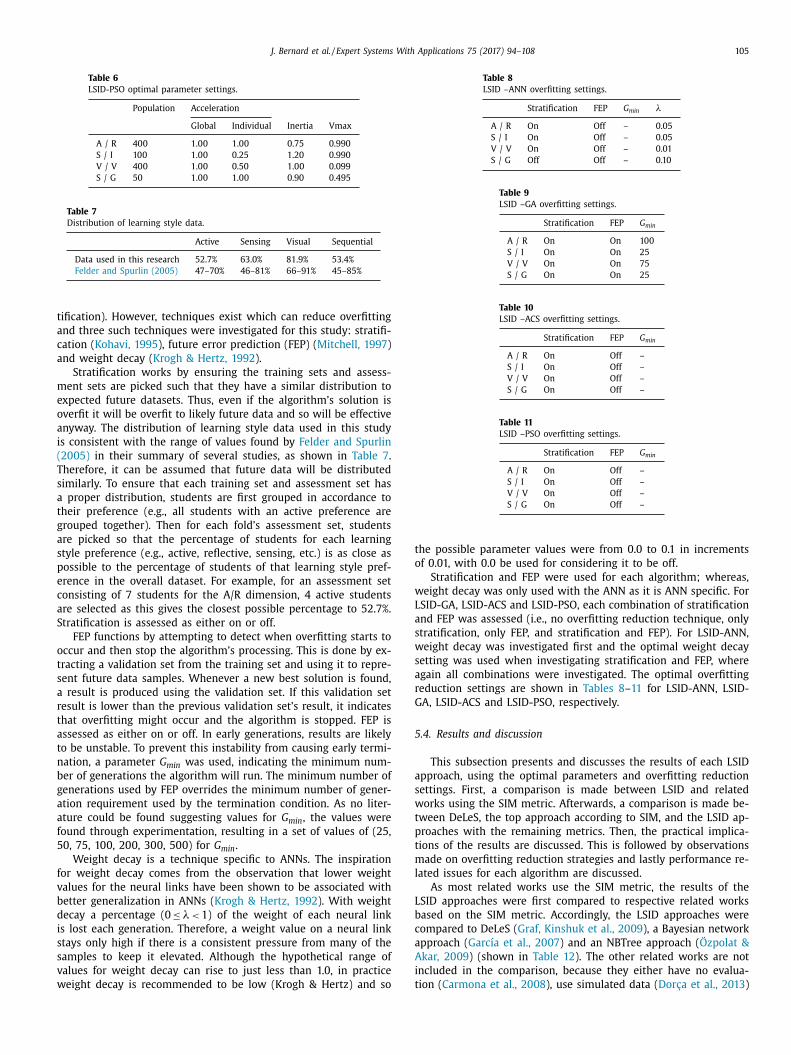
J. Bernard et al. / Expert Systems With Applications 75 (2017) 94–108 105
Table 6
LSID-PSO optimal parameter settings.
Population Acceleration
Global Individual Inertia Vmax
A / R 400 1 .00 1 .00 0 .75 0 .990
S / I 100 1 .00 0 .25 1 .20 0 .990
V / V 400 1 .00 0 .50 1 .00 0 .099
S / G 50 1 .00 1 .00 0 .90 0 .495
Table 7
Distribution of learning style data.
Active Sensing Visual Sequential
Data used in this research 52 .7% 63 .0% 81 .9% 53 .4%
Felder and Spurlin (2005) 47–70% 46–81% 66–91% 45–85%
t
a
c
a
m
e
o
a
i
(
T
s
a
t
g
a
s
p
e
c
a
S
o
t
s
a
r
t
a
t
n
b
g
a
a
f
5
f
v
b
d
i
s
s
v
w
Table 8
LSID –ANN overfitting settings.
Stratification FEP G min λ
A / R On Off – 0 .05
S / I On Off – 0 .05
V / V On Off – 0 .01
S / G Off Off – 0 .10
Table 9
LSID –GA overfitting settings.
Stratification FEP G min
A / R On On 100
S / I On On 25
V / V On On 75
S / G On On 25
Table 10
LSID –ACS overfitting settings.
Stratification FEP G min
A / R On Off –
S / I On Off –
V / V On Off –
S / G On Off –
Table 11
LSID –PSO overfitting settings.
Stratification FEP G min
A / R On Off –
S / I On Off –
V / V On Off –
S / G On Off –
t
o
w
L
a
s
w
s
a
r
G
5
a
s
w
t
p
t
m
l
L
b
c
a
A
i
t
ification). However, techniques exist which can reduce overfitting
nd three such techniques were investigated for this study: stratifi-
ation ( Kohavi, 1995 ), future error prediction (FEP) ( Mitchell, 1997 )
nd weight decay ( Krogh & Hertz, 1992 ).
Stratification works by ensuring the training sets and assess-
ent sets are picked such that they have a similar distribution to
xpected future datasets. Thus, even if the algorithm’s solution is
verfit it will be overfit to likely future data and so will be effective
nyway. The distribution of learning style data used in this study
s consistent with the range of values found by Felder and Spurlin
2005) in their summary of several studies, as shown in Table 7 .
herefore, it can be assumed that future data will be distributed
imilarly. To ensure that each training set and assessment set has
proper distribution, students are first grouped in accordance to
heir preference (e.g., all students with an active preference are
rouped together). Then for each fold’s assessment set, students
re picked so that the percentage of students for each learning
tyle preference (e.g., active, reflective, sensing, etc.) is as close as
ossible to the percentage of students of that learning style pref-
rence in the overall dataset. For example, for an assessment set
onsisting of 7 students for the A/R dimension, 4 active students
re selected as this gives the closest possible percentage to 52.7%.
tratification is assessed as either on or off.
FEP functions by attempting to detect when overfitting starts to
ccur and then stop the algorithm’s processing. This is done by ex-
racting a validation set from the training set and using it to repre-
ent future data samples. Whenever a new best solution is found,
result is produced using the validation set. If this validation set
esult is lower than the previous validation set’s result, it indicates
hat overfitting might occur and the algorithm is stopped. FEP is
ssessed as either on or off. In early generations, results are likely
o be unstable. To prevent this instability from causing early termi-
ation, a parameter G min was used, indicating the minimum num-
er of generations the algorithm will run. The minimum number of
enerations used by FEP overrides the minimum number of gener-
tion requirement used by the termination condition. As no liter-
ture could be found suggesting values for G min , the values were
ound through experimentation, resulting in a set of values of (25,
0, 75, 100, 200, 300, 500) for G min .
Weight decay is a technique specific to ANNs. The inspiration
or weight decay comes from the observation that lower weight
alues for the neural links have been shown to be associated with
etter generalization in ANNs ( Krogh & Hertz, 1992 ). With weight
ecay a percentage (0 ≤ λ< 1) of the weight of each neural link
s lost each generation. Therefore, a weight value on a neural link
tays only high if there is a consistent pressure from many of the
amples to keep it elevated. Although the hypothetical range of
alues for weight decay can rise to just less than 1.0, in practice
eight decay is recommended to be low (Krogh & Hertz) and so
he possible parameter values were from 0.0 to 0.1 in increments
f 0.01, with 0.0 be used for considering it to be off.
Stratification and FEP were used for each algorithm; whereas,
eight decay was only used with the ANN as it is ANN specific. For
SID-GA, L SID-ACS and L SID-PSO, each combination of stratification
nd FEP was assessed (i.e., no overfitting reduction technique, only
tratification, only FEP, and stratification and FEP). For LSID-ANN,
eight decay was investigated first and the optimal weight decay
etting was used when investigating stratification and FEP, where
gain all combinations were investigated. The optimal overfitting
eduction settings are shown in Tables 8 –11 for L SID-ANN, L SID-
A, LSID-ACS and LSID-PSO, respectively.
.4. Results and discussion
This subsection presents and discusses the results of each LSID
pproach, using the optimal parameters and overfitting reduction
ettings. First, a comparison is made between LSID and related
orks using the SIM metric. Afterwards, a comparison is made be-
ween DeLeS, the top approach according to SIM, and the LSID ap-
roaches with the remaining metrics. Then, the practical implica-
ions of the results are discussed. This is followed by observations
ade on overfitting reduction strategies and lastly performance re-
ated issues for each algorithm are discussed.
As most related works use the SIM metric, the results of the
SID approaches were first compared to respective related works
ased on the SIM metric. Accordingly, the LSID approaches were
ompared to DeLeS ( Graf, Kinshuk et al., 2009 ), a Bayesian network
pproach ( García et al., 2007 ) and an NBTree approach ( Özpolat &
kar, 2009 ) (shown in Table 12 ). The other related works are not
ncluded in the comparison, because they either have no evalua-
ion ( Carmona et al., 2008 ), use simulated data ( Dorça et al., 2013 )
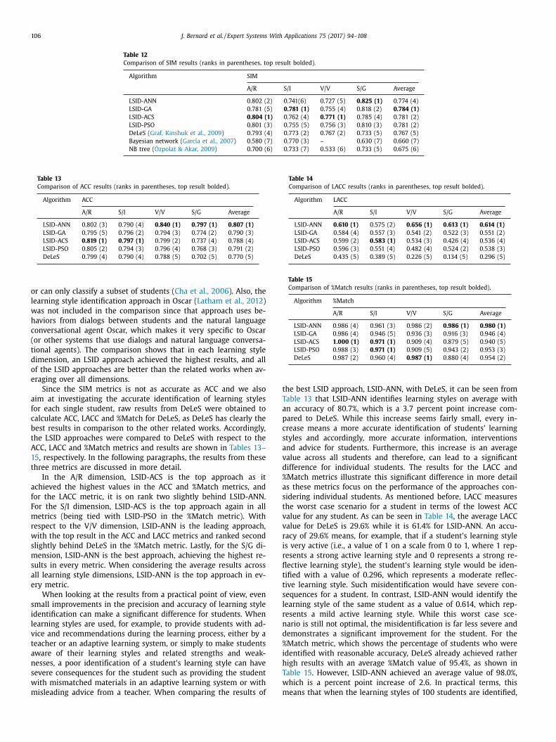
106 J. Bernard et al. / Expert Systems With Applications 75 (2017) 94–108
Table 12
Comparison of SIM results (ranks in parentheses, top result bolded).
Algorithm SIM
A/R S/I V/V S/G Average
LSID-ANN 0 .802 (2) 0 .741(6) 0 .727 (5) 0 .825 (1) 0 .774 (4)
LSID-GA 0 .781 (5) 0 .781 (1) 0 .755 (4) 0 .818 (2) 0 .784 (1)
LSID-ACS 0 .804 (1) 0 .762 (4) 0 .771 (1) 0 .785 (4) 0 .781 (2)
LSID-PSO 0 .801 (3) 0 .755 (5) 0 .756 (3) 0 .810 (3) 0 .781 (2)
DeLeS ( Graf, Kinshuk et al., 2009 ) 0 .793 (4) 0 .773 (2) 0 .767 (2) 0 .733 (5) 0 .767 (5)
Bayesian network ( García et al., 2007 ) 0 .580 (7) 0 .770 (3) – 0 .630 (7) 0 .660 (7)
NB tree ( Özpolat & Akar, 2009 ) 0 .700 (6) 0 .733 (7) 0 .533 (6) 0 .733 (5) 0 .675 (6)
Table 13
Comparison of ACC results (ranks in parentheses, top result bolded).
Algorithm ACC
A/R S/I V/V S/G Average
LSID-ANN 0 .802 (3) 0 .790 (4) 0 .840 (1) 0 .797 (1) 0 .807 (1)
LSID-GA 0 .795 (5) 0 .796 (2) 0 .794 (3) 0 .774 (2) 0 .790 (3)
LSID-ACS 0 .819 (1) 0 .797 (1) 0 .799 (2) 0 .737 (4) 0 .788 (4)
LSID-PSO 0 .805 (2) 0 .794 (3) 0 .796 (4) 0 .768 (3) 0 .791 (2)
DeLeS 0 .799 (4) 0 .790 (4) 0 .788 (5) 0 .702 (5) 0 .770 (5)
Table 14
Comparison of LACC results (ranks in parentheses, top result bolded).
Algorithm LACC
A/R S/I V/V S/G Average
LSID-ANN 0 .610 (1) 0 .575 (2) 0 .656 (1) 0 .613 (1) 0 .614 (1)
LSID-GA 0 .584 (4) 0 .557 (3) 0 .541 (2) 0 .522 (3) 0 .551 (2)
LSID-ACS 0 .599 (2) 0 .583 (1) 0 .534 (3) 0 .426 (4) 0 .536 (4)
LSID-PSO 0 .596 (3) 0 .551 (4) 0 .482 (4) 0 .524 (2) 0 .538 (3)
DeLeS 0 .435 (5) 0 .389 (5) 0 .226 (5) 0 .134 (5) 0 .296 (5)
Table 15
Comparison of %Match results (ranks in parentheses, top result bolded).
Algorithm %Match
A/R S/I V/V S/G Average
LSID-ANN 0 .986 (4) 0 .961 (3) 0 .986 (2) 0 .986 (1) 0 .980 (1)
LSID-GA 0 .986 (4) 0 .946 (5) 0 .936 (3) 0 .916 (3) 0 .946 (4)
LSID-ACS 1 .0 0 0 (1) 0 .971 (1) 0 .909 (4) 0 .879 (5) 0 .940 (5)
LSID-PSO 0 .988 (3) 0 .971 (1) 0 .909 (5) 0 .943 (2) 0 .953 (3)
DeLeS 0 .987 (2) 0 .960 (4) 0 .987 (1) 0 .880 (4) 0 .954 (2)
t
T
a
p
c
s
a
v
d
%
a
s
t
v
v
r
i
r
fl
t
t
s
l
r
n
d
%
i
h
T
w
m
or can only classify a subset of students ( Cha et al., 2006 ). Also, the
learning style identification approach in Oscar ( Latham et al., 2012 )
was not included in the comparison since that approach uses be-
haviors from dialogs between students and the natural language
conversational agent Oscar, which makes it very specific to Oscar
(or other systems that use dialogs and natural language conversa-
tional agents). The comparison shows that in each learning style
dimension, an LSID approach achieved the highest results, and all
of the LSID approaches are better than the related works when av-
eraging over all dimensions.
Since the SIM metrics is not as accurate as ACC and we also
aim at investigating the accurate identification of learning styles
for each single student, raw results from DeLeS were obtained to
calculate ACC, LACC and %Match for DeLeS, as DeLeS has clearly the
best results in comparison to the other related works. Accordingly,
the LSID approaches were compared to DeLeS with respect to the
ACC, LACC and %Match metrics and results are shown in Tables 13–
15 , respectively. In the following paragraphs, the results from these
three metrics are discussed in more detail.
In the A/R dimension, LSID-ACS is the top approach as it
achieved the highest values in the ACC and %Match metrics, and
for the LACC metric, it is on rank two slightly behind LSID-ANN.
For the S/I dimension, LSID-ACS is the top approach again in all
metrics (being tied with LSID-PSO in the %Match metric). With
respect to the V/V dimension, LSID-ANN is the leading approach,
with the top result in the ACC and LACC metrics and ranked second
slightly behind DeLeS in the %Match metric. Lastly, for the S/G di-
mension, LSID-ANN is the best approach, achieving the highest re-
sults in every metric. When considering the average results across
all learning style dimensions, LSID-ANN is the top approach in ev-
ery metric.
When looking at the results from a practical point of view, even
small improvements in the precision and accuracy of learning style
identification can make a significant difference for students. When
learning styles are used, for example, to provide students with ad-
vice and recommendations during the learning process, either by a
teacher or an adaptive learning system, or simply to make students
aware of their learning styles and related strengths and weak-
nesses, a poor identification of a student’s learning style can have
severe consequences for the student such as providing the student
with mismatched materials in an adaptive learning system or with
misleading advice from a teacher. When comparing the results of
he best L SID approach, L SID-ANN, with DeLeS, it can be seen from
able 13 that LSID-ANN identifies learning styles on average with
n accuracy of 80.7%, which is a 3.7 percent point increase com-
ared to DeLeS. While this increase seems fairly small, every in-
rease means a more accurate identification of students’ learning
tyles and accordingly, more accurate information, interventions
nd advice for students. Furthermore, this increase is an average
alue across all students and therefore, can lead to a significant
ifference for individual students. The results for the LACC and
Match metrics illustrate this significant difference in more detail
s these metrics focus on the performance of the approaches con-
idering individual students. As mentioned before, LACC measures
he worst case scenario for a student in terms of the lowest ACC
alue for any student. As can be seen in Table 14 , the average LACC
alue for DeLeS is 29.6% while it is 61.4% for LSID-ANN. An accu-
acy of 29.6% means, for example, that if a student’s learning style
s very active (i.e., a value of 1 on a scale from 0 to 1, where 1 rep-
esents a strong active learning style and 0 represents a strong re-
ective learning style), the student’s learning style would be iden-
ified with a value of 0.296, which represents a moderate reflec-
ive learning style. Such misidentification would have severe con-
equences for a student. In contrast, LSID-ANN would identify the
earning style of the same student as a value of 0.614, which rep-
esents a mild active learning style. While this worst case sce-
ario is still not optimal, the misidentification is far less severe and
emonstrates a significant improvement for the student. For the
Match metric, which shows the percentage of students who were
dentified with reasonable accuracy, DeLeS already achieved rather
igh results with an average %Match value of 95.4%, as shown in
able 15 . However, LSID-ANN achieved an average value of 98.0%,
hich is a percent point increase of 2.6. In practical terms, this
eans that when the learning styles of 100 students are identified,
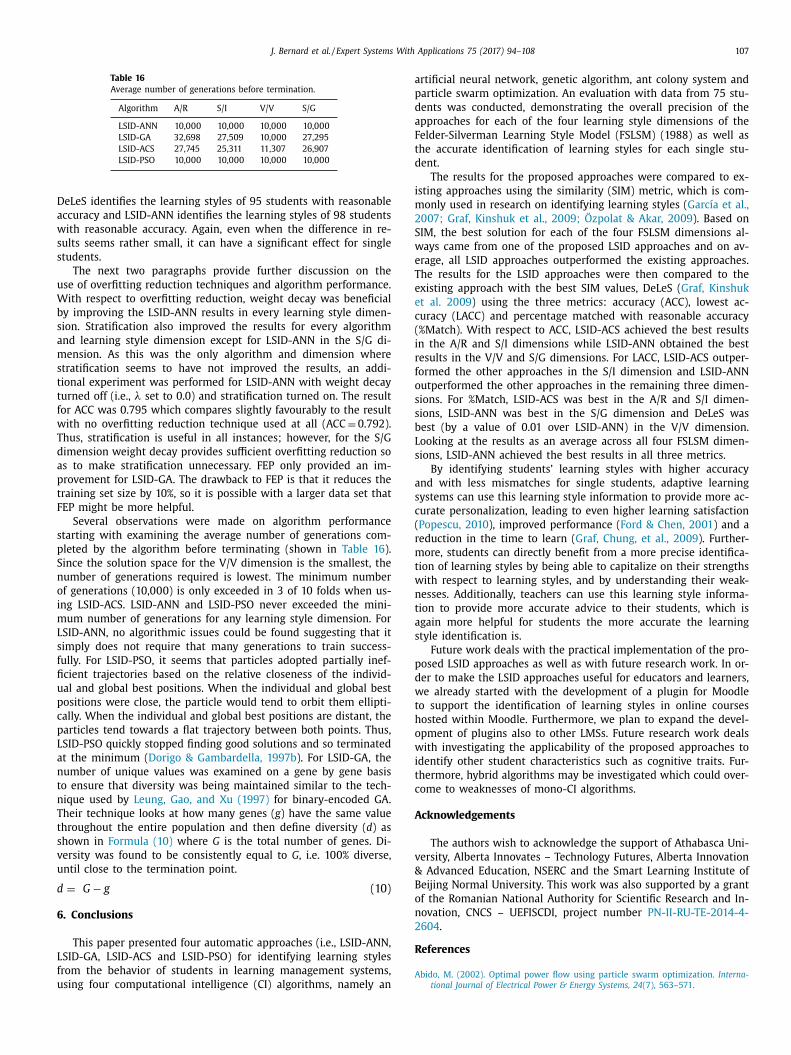
J. Bernard et al. / Expert Systems With Applications 75 (2017) 94–108 107
Table 16
Average number of generations before termination.
Algorithm A/R S/I V/V S/G
LSID-ANN 10 ,0 0 0 10 ,0 0 0 10 ,0 0 0 10 ,0 0 0
LSID-GA 32 ,698 27 ,509 10 ,0 0 0 27 ,295
LSID-ACS 27 ,745 25 ,311 11 ,307 26 ,907
LSID-PSO 10 ,0 0 0 10 ,0 0 0 10 ,0 0 0 10 ,0 0 0
D
a
w
s
s
u
W
b
s
a
m
s
t
t
f
w
T
d
a
p
t
F
s
p
S
n
o
i
m
L
s
f
fi
u
p
c
p
L
a
n
t
n
T
t
s
v
u
d
6
L
f
u
a
p
d
a
F
t
d
i
m
2
S
w
e
T
e
e
c
(
i
r
f
o
s
s
b
L
s
a
s
c
(
r
m
t
w
n
t
a
s
p
d
w
t
h
o
w
i
t
c
A
v
&
B
o
n
2
R
A
eLeS identifies the learning styles of 95 students with reasonable
ccuracy and LSID-ANN identifies the learning styles of 98 students
ith reasonable accuracy. Again, even when the difference in re-
ults seems rather small, it can have a significant effect for single
tudents.
The next two paragraphs provide further discussion on the
se of overfitting reduction techniques and algorithm performance.
ith respect to overfitting reduction, weight decay was beneficial
y improving the LSID-ANN results in every learning style dimen-
ion. Stratification also improved the results for every algorithm
nd learning style dimension except for LSID-ANN in the S/G di-
ension. As this was the only algorithm and dimension where
tratification seems to have not improved the results, an addi-
ional experiment was performed for LSID-ANN with weight decay
urned off (i.e., λ set to 0.0) and stratification turned on. The result
or ACC was 0.795 which compares slightly favourably to the result
ith no overfitting reduction technique used at all (ACC = 0.792).
hus, stratification is useful in all instances; however, for the S/G
imension weight decay provides sufficient overfitting reduction so
s to make stratification unnecessary. FEP only provided an im-
rovement for LSID-GA. The drawback to FEP is that it reduces the
raining set size by 10%, so it is possible with a larger data set that
EP might be more helpful.
Several observations were made on algorithm performance
tarting with examining the average number of generations com-
leted by the algorithm before terminating (shown in Table 16 ).
ince the solution space for the V/V dimension is the smallest, the
umber of generations required is lowest. The minimum number
f generations (10,0 0 0) is only exceeded in 3 of 10 folds when us-
ng L SID-ACS. L SID-ANN and L SID-PSO never exceeded the mini-
um number of generations for any learning style dimension. For
SID-ANN, no algorithmic issues could be found suggesting that it
imply does not require that many generations to train success-
ully. For LSID-PSO, it seems that particles adopted partially inef-
cient trajectories based on the relative closeness of the individ-
al and global best positions. When the individual and global best
ositions were close, the particle would tend to orbit them ellipti-
ally. When the individual and global best positions are distant, the
articles tend towards a flat trajectory between both points. Thus,
SID-PSO quickly stopped finding good solutions and so terminated
t the minimum ( Dorigo & Gambardella, 1997b ). For LSID-GA, the
umber of unique values was examined on a gene by gene basis
o ensure that diversity was being maintained similar to the tech-
ique used by Leung, Gao, and Xu (1997) for binary-encoded GA.
heir technique looks at how many genes ( g ) have the same value
hroughout the entire population and then define diversity ( d ) as
hown in Formula (10) where G is the total number of genes. Di-
ersity was found to be consistently equal to G , i.e. 100% diverse,
ntil close to the termination point.
= G − g (10)
. Conclusions
This paper presented four automatic approaches (i.e., LSID-ANN,
SID-GA, L SID-ACS and L SID-PSO) for identifying learning styles
rom the behavior of students in learning management systems,
sing four computational intelligence (CI) algorithms, namely an
rtificial neural network, genetic algorithm, ant colony system and
article swarm optimization. An evaluation with data from 75 stu-
ents was conducted, demonstrating the overall precision of the
pproaches for each of the four learning style dimensions of the
elder-Silverman Learning Style Model (FSLSM) (1988) as well as
he accurate identification of learning styles for each single stu-
ent.
The results for the proposed approaches were compared to ex-
sting approaches using the similarity (SIM) metric, which is com-
only used in research on identifying learning styles ( García et al.,
007; Graf, Kinshuk et al., 2009; Özpolat & Akar, 2009 ). Based on
IM, the best solution for each of the four FSLSM dimensions al-
ays came from one of the proposed LSID approaches and on av-
rage, all LSID approaches outperformed the existing approaches.
he results for the LSID approaches were then compared to the
xisting approach with the best SIM values, DeLeS ( Graf, Kinshuk
t al. 2009 ) using the three metrics: accuracy (ACC), lowest ac-
uracy (LACC) and percentage matched with reasonable accuracy
%Match). With respect to ACC, LSID-ACS achieved the best results
n the A/R and S/I dimensions while LSID-ANN obtained the best
esults in the V/V and S/G dimensions. For LACC, LSID-ACS outper-
ormed the other approaches in the S/I dimension and LSID-ANN
utperformed the other approaches in the remaining three dimen-
ions. For %Match, LSID-ACS was best in the A/R and S/I dimen-
ions, LSID-ANN was best in the S/G dimension and DeLeS was
est (by a value of 0.01 over LSID-ANN) in the V/V dimension.
ooking at the results as an average across all four FSLSM dimen-
ions, LSID-ANN achieved the best results in all three metrics.
By identifying students’ learning styles with higher accuracy
nd with less mismatches for single students, adaptive learning
ystems can use this learning style information to provide more ac-
urate personalization, leading to even higher learning satisfaction
Popescu, 2010 ), improved performance ( Ford & Chen, 2001 ) and a
eduction in the time to learn ( Graf, Chung, et al., 2009 ). Further-
ore, students can directly benefit from a more precise identifica-
ion of learning styles by being able to capitalize on their strengths
ith respect to learning styles, and by understanding their weak-
esses. Additionally, teachers can use this learning style informa-
ion to provide more accurate advice to their students, which is
gain more helpful for students the more accurate the learning
tyle identification is.
Future work deals with the practical implementation of the pro-
osed LSID approaches as well as with future research work. In or-
er to make the LSID approaches useful for educators and learners,
e already started with the development of a plugin for Moodle
o support the identification of learning styles in online courses
osted within Moodle. Furthermore, we plan to expand the devel-
pment of plugins also to other LMSs. Future research work deals
ith investigating the applicability of the proposed approaches to
dentify other student characteristics such as cognitive traits. Fur-
hermore, hybrid algorithms may be investigated which could over-
ome to weaknesses of mono-CI algorithms.
cknowledgements
The authors wish to acknowledge the support of Athabasca Uni-
ersity, Alberta Innovates – Technology Futures, Alberta Innovation
Advanced Education, NSERC and the Smart Learning Institute of
eijing Normal University. This work was also supported by a grant
f the Romanian National Authority for Scientific Research and In-
ovation, CNCS – UEFISCDI, project number PN-II-RU-TE-2014-4-
604 .
eferences
bido, M. (2002). Optimal power flow using particle swarm optimization. Interna-
tional Journal of Electrical Power & Energy Systems, 24 (7), 563–571 .
108 J. Bernard et al. / Expert Systems With Applications 75 (2017) 94–108
G
H
H
J
K
K
K
K
L
M
M
M
Ö
P
P
P
R
S
S
S
V
W
Y
Bajraktarevic, N. , Hall, W. , & Fullick, P. (2003). Incorporating learning styles in hy-permedia environment: Empirical evaluation. In Proceedings of the workshop on
adaptive hypermedia and adaptive web-based systems (pp. 41–52). June 22 2003 . Basheer, I. A. , & Hajmeer, M. (20 0 0). Artificial neural networks: fundamentals, com-
puting, design, and application. Journal of Microbiological Methods, 43 (1), 3–31 . Carmona, C. , Castillo, G. , & Millán, E. (2008). Designing a dynamic Bayesian network
for modeling students’ learning styles. In Proceedings of 8th international confer-ence on advanced learning technologies (pp. 346–350). IEEE. July 2008 .
Carver, C. A., Jr , Howard, R. A. , & Lane, W. D. (1999). Enhancing student learning
through hypermedia courseware and incorporation of student learning styles.IEEE Transactions on Education, 42 (1), 33–38 .
Cha, H. J. , Kim, Y. S. , Park, S. H. , Yoon, T. B. , Jung, Y. M. , & Lee, J.-H. (2006). Learn-ing styles diagnosis based on user interface behaviors for the customization of
learning interfaces in an intelligent tutoring system. In Proceedings of the 8th in-ternational conference on intelligent tutoring systems, Berlin, June 26-30 2006: Vol.
4053 (pp. 513–524). Berlin Heidelberg: Springer .
Clerc, M. , & Kennedy, J. (2002). The particle swarm-explosion, stability, and conver-gence in a Mmultidimensional complex space. IEEE Transactions on Evolutionary
Computation, 6 (1), 58–73 . Coffield, F. , Moseley, D. , Hall, E. , & Ecclestone, K. (2004a). Learning styles and ped-
agogy in post-16 learning: A systematic and critical review . London: Learning &Skills Research Centre .
Coffield, F. J. , Moseley, D. V. , Hall, E. , & Ecclestone, K. (2004b). Learning styles: What
research has to say to practice . London: Learning & Skills Research Centre . Dahlstrom, E. , Walker, J. D. , & Dziuban, C. (2013). Ecar study of undergraduate stu-
dents and information technology . Boulder, CO: Educause Center for Applied Re-search .
Dorça, F. A. , Lima, L. V. , Fernandes, M. A. , & Lopes, C. R. (2013). Comparing strate-gies for Mmodeling students learning styles through reinforcement learning in
adaptive and intelligent educational systems: An experimental analysis. Expert
Systems with Applications, 40 (6), 2092–2101 . Dorigo, M. , & Birattari, M. (2010). Ant colony optimization. In In Encyclopedia of
machine learning (pp. 36–39). New York, NY: Springer . Dorigo, M. , & Gambardella, L. M. (1997a). Ant colonies for the travelling salesman
problem. BioSystems, 43 (2), 73–81 . Dorigo, M. , & Gambardella, L. M. (1997b). Ant colony system: A cooperative learning
approach to the traveling salesman problem. IEEE Transactions on Evolutionary
Computation, 1 (1), 53–66 . Eberhart, R. C. , & Kennedy, J. (1995). A new optimizer using particle swarm theory.
In Proceedings of the sixth international symposium on micro machine and humanscience (pp. 39–43). October 4-6 1995 .
Ericsson, M. , Resende, M. G. C. , & Pardalos, P. M. (2002). A genetic algorithm for theweight setting problem in Ospf routing. Journal of Combinatorial Optimization,
6 (3), 299–333 .
Felder, R. M. (1996). Matters of style. ASEE Prism, 6 (4), 18–23 . Felder, R. M. , & Silverman, L. K. (1988). Learning and teaching styles in engineering
education. Engineering Education, 78 (7), 674–681 . Felder, R. M., & Soloman, B. A. (20 0 0). Learning s tyles and s trategies Retrieved Oc-
tober 7th 2016 from https:// www.dal.ca/ content/ dam/ dalhousie/ pdf/ management/Faculty% 20% 26% 20Staff/LEARNING% 20STYLES% 20AND% 20STRATEGIES.pdf .
Felder, R. M., & Solomon, B. A. (1998). Index of l earning s tyles Retrieved October 7th2016 from http:// www.engr.ncsu.edu/ learningstyles/ ilsweb.html .
Felder, R. M. , & Spurlin, J. (2005). Applications, reliability and validity of the index
of learning styles. International Journal of Engineering Education, 21 (1), 103–112 . Filippidis, S. K. , & Tsoukalas, I. A. (2009). On the use of adaptive instructional im-
ages based on the sequential–global dimension of the Felder–Silverman learningstyle theory. Interactive Learning Environments, 17 (2), 135–150 .
Foody, G. M. , McCulloch, M. B. , & Yates, W. B. (1995). The effect of training set sizeand composition on artificial neural network classification. International Journal
of Remote Sensing, 16 (9), 1707–1723 .
Ford, N. , & Chen, S. (2001). Matching/Mismatching revisited: An empirical studyof learning and teaching styles. British Journal of Educational Technology, 32 (1),
5–22 . García, P. , Amandi, A. , Schiaffino, S. , & Campo, M. (2007). Evaluating Bayesian net-
works’ precision for detecting students’ learning styles. Computers & Education,49 (3), 794–808 .
Graf, S. (2007). Adaptivity in learning management systems focussing on learning
styles . Vienna University of Technology . Graf, S. , Chung, H. L. , Liu, T.-C. , & Kinshuk (2009). Investigations about the ef-
fects and effectiveness of adaptivity for students with different learning styles.In Proceedings of 9th international conference on advanced learning technologies
(pp. 415–419). Latvia: IEEE. July 200 .
raf, S. , Kinshuk , & Liu, T.-C. (2009). Supporting teachers in identifying students’learning styles in learning management systems: An automatic student mod-
elling approach. Educational Technology & Society, 12 (4), 3–14 . Grefenstette, J. J. (1986). Optimization of control parameters for genetic algorithms.
IEEE Transactions on Systems, Man and Cybernetics, 16 (1), 122–128 . oney, P. , & Mumford, A. (1992). The manual of learning styles (3rd ed.). Maidenhead .
ornik, K. , Stinchcombe, M. , & White, H. (1990). Universal approximation of anunknown mapping and its derivatives using multilayer feedforward networks.
Neural Networks, 3 (5), 551–560 .
ames, W. B. , & Gardner, D. L. (1995). Learning styles: Implications for distancelearning. New Directions for Adult and Continuing Education , (67), 19–31 1995 .
Klašnja-Mili ́cevi ́c, A. , Vesin, B. , Ivanovi ́c, M. , & Budimac, Z. (2011). E-Learning per-sonalization based on hybrid recommendation strategy and learning style iden-
tification. Computers & Education, 56 (3), 885–899 . ohavi, R. (1995). A study of cross-validation and bootstrap for accuracy estimation
and model selection. In Proceedings of the 14th international joint conference on
artificial intelligence (pp. 1137–1145). Morgan Kaufmann Publishers Inc. August1995 .
olb, D. A. (1971). Individual learning styles and the learning process . Cambridge, MA:Sloan School of Management, Massachusetts Institute of Technology .
Kolb, D. A. (1981). Learning styles and disciplinary differences. In Chickering andAssociates (Ed.), The modern american college (pp. 232–255). San Franciso, CA:
Jossey-Bass .
rogh, A. , & Hertz, J. A. (1992). A simple weight decay can improve generalization.Advances in Neural Information Processing Systems, 4 , 950–957 .
uljis, J. , & Liu, F. (2005). A comparison of learning style theories on the suitabilityfor elearning. In Proceedings of the IASTED conference on web technologies, appli-
cations and services (pp. 191–197). ACTA Press. July 17-19 2005 . atham, A. , Crockett, K. , McLean, D. , & Edmonds, B. (2012). A conversational intelli-
gent tutoring system to automatically predict learning styles. Computers & Edu-
cation, 59 (1), 95–109 . Leung, Y. , Gao, Y. , & Xu, Z.-B. (1997). Degree of population diversity-a perspective
on premature convergence in genetic algorithms and its Markov chain analysis.IEEE Transactions on Neural Networks, 8 (5), 1165–1176 .
icrosoft. (2016). Net p rogramming with C ++ /CLI Retrieved October 7th, 2016, fromhttps:// msdn.microsoft.com/ en-us/ library/ 68td296t.aspx .
Mitchell, T. (1997). Machine learning : Vol. 45. Burr Ridge, IL: McGraw Hill .
oodle. (2016). Moodle Retrieved December 1st, 2016, from http://www.moodle.org.yers-Briggs, I. (1962). The Myers-Briggs type indicator: Manual . Palo Alto, CA: Con-
sulting Psychologists Press . zpolat, E. , & Akar, G. B. (2009). Automatic detection of learning styles for an
e-learning system. Computers & Education, 53 (2), 355–367 . ask, G. (1976). Styles and strategies of learning. British Journal of Educational Psy-
chology, 46 (2), 128–148 .
opescu, E. (2010). Adaptation provisioning with respect to learning styles in a we-b-based educational system: An experimental study. Journal of Computer Assisted
Learning, 26 (4), 243–257 . othiya, S. , Ngamroo, I. , & Kongprawechnon, W. (2010). Ant colony optimisation for
economic dispatch problem with non-smooth cost functions. International Jour-nal of Electrical Power & Energy Systems, 32 (5), 478–487 .
Robinson, J. , & Rahmat-Samii, Y. (2004). Particle swarm optimization in electromag-netics. IEEE Transactions on Antennas and Propagation, 52 (2), 397–407 .
ussell, S. J. , & Norvig, P. (2010). Artificial intelligence: A modern approach : Vol. 3.
Upper Saddle River: Prentice Hall . Shi, Y. , & Eberhart, R. C. (1998). Parameter selection in particle swarm optimiza-
tion. In Proceedings of the 7th annual conferences on evolutionary programming(pp. 591–600). Springer. March 25-27 .
rinivas, M. , & Patnaik, L. M. (1994). Genetic algorithms: A survey. Computer, 27 (6),17–26 .
tutzle, T. , Lopez-Ibanez, M. , Pellegrini, P. , Maur, M. , Montes de Oca, M. , Birattari, M. ,
et al. (2011). Parameter adaptation in ant colony optimization. In Autonomoussearch (pp. 191–215). Berlin: Springer .
wingler, K. (1996). Applying neural networks: A practical guide . San Franciso, CA:Morgan Kaufmann .
illaverde, J. E. , Godoy, D. , & Amandi, A. (2006). Learning styles’ recognition ine-learning environments with feed-forward neural networks. Journal of Com-
puter Assisted Learning, 22 (3), 197–206 .
anas, N. , Auda, G. , Kamel, M, S. , & Karray, F. (1998). On the optimal number ofhidden nodes in a neural network. In Proceedings of IEEE canadian conference on
electrical and computer engineering (pp. 918–921). IEEE. May 1998 . ao, X. (1999). Evolving artificial neural networks. Proceedings of the IEEE, 87 (9),
1423–1447 .


