Embed Size (px)
Citation preview
Learning to Visually Predict Terrain Properties for Planetary Rovers
by
Christopher A. Brooks
Bachelor of Science in Engineering and Applied Science
California Institute of Technology, 2000
Master of Science in Mechanical Engineering
Massachusetts Institute of Technology, 2004
Submitted to the Department of Mechanical Engineering in Partial Fulfillment of the
Requirements for the Degree of
Doctor of Philosophy in Mechanical Engineering
at the
Massachusetts Institute of Technology
June 2009
© 2009 Massachusetts Institute of Technology. All rights reserved.
Signature of Author:
Department of Mechanical Engineering
May 7, 2009
Certified by:
Karl Iagnemma
Principal Research Scientist
Thesis Supervisor
Accepted by:
David Hardt
Professor of Mechanical Engineering
Graduate Officer, Department of Mechanical Engineering

Learning to Visually Predict Terrain Properties for Planetary Rovers
by
Christopher A. Brooks
Submitted to the Department of Mechanical Engineering
on May 7, 2009, in partial fulfillment of the requirements for the degree of
Doctor of Philosophy in Mechanical Engineering
Abstract
For future planetary exploration missions, improvements in autonomous rover
mobility have the potential to increase scientific data return by providing safe access to
geologically interesting sites that lie in rugged terrain, far from landing areas. This thesis
presents an algorithmic framework designed to improve rover-based terrain sensing, a
critical component of any autonomous mobility system operating in rough terrain.
Specifically, this thesis addresses the problem of predicting the mechanical properties of
distant terrain. A self-supervised learning framework is proposed that enables a robotic
system to learn predictions of mechanical properties of distant terrain, based on
measurements of mechanical properties of similar terrain that has been previously
traversed.
The proposed framework relies on three distinct algorithms. A mechanical terrain
characterization algorithm is proposed that computes upper and lower bounds on the net
traction force available at a patch of terrain, via a constrained optimization framework.
Both model-based and sensor-based constraints are employed. A terrain classification
method is proposed that exploits features from proprioceptive sensor data, and employs
either a supervised support vector machine (SVM) or unsupervised k-means classifier to
assign class labels to terrain patches that the rover has traversed. A second terrain
classification method is proposed that exploits features from exteroceptive sensor data
(e.g. color and texture), and is automatically trained in a self-supervised manner, based
on the outputs of the proprioceptive terrain classifier. The algorithm includes a method
for distinguishing novel terrain from previously observed terrain. The outputs of these
three algorithms are merged to yield a map of the surrounding terrain that is annotated
with the expected achievable net traction force. Such a map would be useful for path
planning purposes.
The algorithms proposed in this thesis have been experimentally validated in an
outdoor, Mars-analog environment. The proprioceptive terrain classifier demonstrated
92% accuracy in labeling three distinct terrain classes. The exteroceptive terrain classifier
that relies on self-supervised training was shown to be approximately as accurate as a
similar, human-supervised classifier, with both achieving 94% correct classification rates
on identical data sets. The algorithm for detection of novel terrain demonstrated 89%
accuracy in detecting novel terrain in this same environment. In laboratory tests, the
mechanical terrain characterization algorithm predicted the lower bound of the net
available traction force with an average margin of 21% of the wheel load.
Thesis Supervisor: Karl Iagnemma
Principal Research Scientist


Acknowledgements 5
Acknowledgements
I would like to thank my adviser and the rest of my Ph.D. committee for their guidance
and support of my research and this thesis. Their advice has greatly improved the quality
of this work.
I would like to thank all of the people who helped me with my experiments with
the TORTOISE rover. Maria Tanner, Matt Carvey, Shingo Shimoda, Ibrahim Halatci,
and Marcos Berrios all contributed to the construction and assembly of the rover. I
gratefully appreciate everyone who helped me in taking the rover to test sites around MIT
and Gloucester, including Shingo Shimoda, Ibrahim Halatci, Chris Ward, Steve Peters,
Sterling Anderson, Jon Brooks, and Artie Moffa. I hope you don’t hold it against me that
“a day at the beach” always seemed to coincide with frigid temperatures. Except one
gorgeous day in January.
For the experiments with the FSRL Wheel-Terrain Testbed, I have Shinwoo Kang
to thank.
I would also like to thank all of the other members of the Field and Space
Robotics Laboratory for making all of my hours in the lab more enjoyable, and my family
and friends who made my time outside the lab something to look forward to. Most
especially, I would like to thank my wife, Corinne, for her unending support and
encouragement.
This work was supported by the National Aeronautics and Space Administration through
the Mars Technology Program, and by the US Army Research Office.
6 Table of Contents
Table of Contents
List of Figures ..................................................................................................................... 8
List of Tables..................................................................................................................... 11
Chapter 1 Introduction ...................................................................................................... 13
1.1 Problem Statement and Motivation......................................................................... 13
1.2 Purpose of this Thesis and Scenario Description .................................................... 17
1.3 Background and Literature Review......................................................................... 19
1.3.1 Mobility-related Terrain Sensing ..................................................................... 19
1.3.2 Terrain Classification ....................................................................................... 23
1.3.3 Machine Learning ............................................................................................ 24
1.3.4 Mobility Prediction .......................................................................................... 26
1.4 Approach Overview ................................................................................................ 27
1.4.1 Learning From Experience............................................................................... 28
1.4.2 Terrain Representation and Terminology ........................................................ 29
1.4.3 Self-Supervised Classification Framework and Algorithmic Components ..... 33
1.5 Contribution of this Thesis...................................................................................... 37
1.6 Outline of this Thesis .............................................................................................. 37
Chapter 2 Proprioceptive Terrain Classification............................................................... 39
2.1 Vibration-Based Terrain Classification................................................................... 39
2.1.1 Introduction ...................................................................................................... 39
2.1.2 Approach .......................................................................................................... 40
2.1.3 Experiment Details........................................................................................... 42
2.1.4 Results .............................................................................................................. 46
2.1.5 Conclusions ...................................................................................................... 48
2.2 Proprioceptive Terrain Clustering........................................................................... 49
2.2.1 Introduction ...................................................................................................... 49
2.2.2 Approach .......................................................................................................... 52
2.2.3 Experiment Details........................................................................................... 56
2.2.4 Results .............................................................................................................. 59
2.2.5 Conclusions ...................................................................................................... 61
Chapter 3 Exteroceptive Terrain Classification ................................................................ 63
3.1 Visual Terrain Classification................................................................................... 64
3.1.1 Introduction ...................................................................................................... 64
3.1.2 Approach .......................................................................................................... 65
3.1.3 Experiment Details........................................................................................... 73
3.1.4 Results .............................................................................................................. 77
3.1.5 Conclusions ...................................................................................................... 80
3.2 Visual Detection of Novel Terrain .......................................................................... 80
3.2.1 Introduction ...................................................................................................... 80
3.2.2 Approach .......................................................................................................... 82
3.2.3 Experiment Details........................................................................................... 92
3.2.4 Results .............................................................................................................. 94
3.2.5 Conclusions ...................................................................................................... 98
Table of Contents 7
Chapter 4 Mechanical Terrain Characterization ............................................................. 100
4.1 Introduction ........................................................................................................... 100
4.2 Approach ............................................................................................................... 102
4.2.1 Traversability Metric...................................................................................... 102
4.2.2 Terrain Sensing .............................................................................................. 105
4.2.3 Terrain Models ............................................................................................... 107
4.2.4 Optimization Framework Description............................................................ 111
4.3 Experiment Details................................................................................................ 120
4.3.1 FSRL Wheel-Terrain Interaction Testbed Experiments................................. 120
4.3.2 TORTOISE Experiments on Wingaersheek Beach ....................................... 123
4.4 Results ................................................................................................................... 126
4.4.1 FSRL Wheel-Terrain Interaction Testbed...................................................... 126
4.4.2 TORTOISE Rover on Wingaersheek Beach.................................................. 131
4.5 Conclusions ........................................................................................................... 133
Chapter 5 Self-Supervised Classification........................................................................ 135
5.1 Experimental Validation of Self-Supervised Classification Framework .............. 136
5.1.1 Introduction .................................................................................................... 136
5.1.2 Self-Supervised Classification Approaches ................................................... 138
5.1.3 Experiment Details......................................................................................... 145
5.1.4 Results ............................................................................................................ 148
5.1.5 Conclusions .................................................................................................... 158
5.2 Self-Supervised Terrain Learning System for Novel Environments .................... 158
5.2.1 Introduction .................................................................................................... 158
5.2.2 Terrain Learning System Framework and Algorithmic Components............ 159
5.2.3 Experiment Details......................................................................................... 163
5.2.4 Results ............................................................................................................ 164
5.2.5 Conclusions .................................................................................................... 169
Chapter 6 Conclusions and Suggestions for Future Work .............................................. 170
6.1 Contributions of this Thesis .................................................................................. 170
6.2 Suggestions for Future Work ................................................................................ 172
References ....................................................................................................................... 174
Appendix A TORTOISE Rover Description .................................................................. 181
Appendix B Wingaersheek Beach Description............................................................... 189
B.1 Sample Stereo Camera Images ............................................................................. 193
Appendix C Wheel-Terrain Interaction Testbed Description ......................................... 198
Appendix D Support Vector Machine Background and Optimizations.......................... 202
D.1 C-Support Vector Classification .......................................................................... 202
D.2 One-Class Support Vector Machine..................................................................... 203
D.3 Kernel Functions .................................................................................................. 204
D.4 Optimizations for Linear and Polynomial Kernels............................................... 205
Appendix E MATLAB Feature Extraction Code............................................................ 208
E.1 Vibration Feature Extraction ................................................................................ 208
E.2 Terrain Geometry Feature Extraction ................................................................... 209
8 List of Figures
List of Figures Figure 1-1. Deep tracks in Purgatory Dune left by MER Opportunity (Image courtesy
NASA/JPL-Caltech).................................................................................................. 15
Figure 1-2. Artist concept of Mars Science Laboratory, left, compared to Mars
Exploration Rover, right (Image courtesy NASA/JPL-Caltech)............................... 18
Figure 1-3. Schematic of proposed self-supervised classification framework.................. 28
Figure 1-4. Sample overhead view showing regular grid of terrain patches in front of
rover .......................................................................................................................... 30
Figure 1-5. Sample terrain map showing data associated with terrain patches in front of
rover (overhead view) ............................................................................................... 33
Figure 1-6. Information flow for self-supervised classification framework ..................... 34
Figure 1-7. Information flow for classification using exteroceptive terrain classifier...... 36
Figure 2-1. Photo of TORTOISE, showing location of local sensor suite........................ 43
Figure 2-2. TORTOISE’s local sensor suite, with vibration sensor and belly-mounted
camera ....................................................................................................................... 44
Figure 2-3. TORTOISE on Wingaersheek Beach, showing terrain classes...................... 45
Figure 2-4. ROC curve for vibration-based terrain classifier............................................ 47
Figure 2-5. Vibration signals for three terrain classes plotted against first four principal
components................................................................................................................ 50
Figure 2-6. Scatter plot of three terrain classes illustrating overlap of statistics of time-
windowed torque signal ............................................................................................ 51
Figure 2-7. Scatter plot of torque signals from three terrain classes with induced wheel
slip ............................................................................................................................. 52
Figure 2-8. TORTOISE’s local sensor suite, with torque sensor and belly-mounted
camera ....................................................................................................................... 57
Figure 3-1. Information flow for exteroceptive terrain classifier...................................... 63
Figure 3-2. TORTOISE, showing location of stereo camera pair..................................... 74
Figure 3-3. Sample image from stereo camera ................................................................. 75
Figure 3-4. TORTOISE on Wingaersheek Beach, showing terrain classes...................... 76
Figure 3-5. Representative ROC curves for visual terrain classifier................................. 78
Figure 3-6. ROC curves for baseline approaches and two-class classification approach for
all data sets with rock as novel class ......................................................................... 95
Figure 3-7. ROC curves for baseline approaches and two-class classification approach for
all data sets with beach grass as novel class.............................................................. 96
Figure 4-1. Wheel forces, torque, and sinkage................................................................ 103
Figure 4-2. Wheel forces on flat terrain (a) and slopes (b) ............................................. 104
Figure 4-3. Nondimensionalized drawbar pull (DP/W) as a function of slip for four
terrains..................................................................................................................... 105
Figure 4-4. Absolute sinkage (a) vs. relative sinkage (b)................................................ 106
Figure 4-5. Contact Region model .................................................................................. 107
Figure 4-6. Bekker terrain model .................................................................................... 109
Figure 4-7. Locations of concentrated stresses for lower bound ((a) or (b)), and upper
bound ((c) or (d))..................................................................................................... 114
Figure 4-8. FSRL wheel-terrain interaction testbed........................................................ 121
Figure 4-9. FSRL wheel-terrain interaction testbed wheel with sensors ........................ 122
List of Figures 9
Figure 4-10. Photo of TORTOISE, showing location of local sensor suite.................... 124
Figure 4-11. TORTOISE’s local sensor suite, with torque sensor and belly-mounted
camera ..................................................................................................................... 124
Figure 4-12. Testbed results for Contact Region Model with Absolute Sinkage (CRAS)
................................................................................................................................. 126
Figure 4-13. Testbed results for Bekker Model with Relative Sinkage (BRS)............... 128
Figure 4-14. Testbed results for Bekker Model with Absolute Sinkage (BAS) ............. 129
Figure 4-15. Comparison of testbed results for all approaches....................................... 130
Figure 4-16. TORTOISE results for Bekker Model with Absolute Sinkage .................. 132
Figure 5-1. Schematic of self-supervised classification, (a) vibration-supervised training
of visual classifier, (b) prediction using visual classifier ........................................ 138
Figure 5-2. Information flow in self-supervised classification framework during (a)
training and (b) classification.................................................................................. 139
Figure 5-3. Information during training phase using local training approach ................ 142
Figure 5-4. Sample image from belly-mounted camera.................................................. 142
Figure 5-5. Illustration of visual information being recalled in remote training approach
................................................................................................................................. 143
Figure 5-6. TORTOISE, showing location of stereo camera pair................................... 145
Figure 5-7. TORTOISE on Wingaersheek Beach, showing terrain classes.................... 147
Figure 5-8. ROC curves for self-supervised classifier using local training .................... 150
Figure 5-9. ROC curves for manually trained classifier ................................................. 151
Figure 5-10. ROC curves for self-supervised classifier using remote training............... 155
Figure 5-11. Information flow for self-supervised classification framework ................. 159
Figure 5-12. Terrain learning system results, at t = 5.0 sec, distance traveled = 0.13 m, (a)
3-D view, (b) plan view showing terrain classes .................................................... 165
Figure 5-13. Terrain learning system results, at t = 129.0 sec, distance traveled = 3.4 m,
(a) 3-D view, (b) plan view showing terrain classes ............................................... 166
Figure 5-14. Terrain learning system results, at t = 226.5 sec, distance traveled = 6.02 m,
(a) 3-D view, (b) plan view showing classes .......................................................... 168
Figure A-1. Photo of TORTOISE, showing location of stereo camera pair ................... 181
Figure A-2. Torque sensor mounted on TORTOISE ...................................................... 183
Figure A-3. Vibration sensor mounted on TORTOISE .................................................. 184
Figure A-4. Belly-mounted camera on TORTOISE ....................................................... 184
Figure A-5. Rover communications schematic ............................................................... 186
Figure B-1. TORTOISE on Wingaersheek Beach, looking northeast towards Annisquam
lighthouse. Mats of beach grass lie between TORTOISE and the rock outcrops. .. 189
Figure B-2. TORTOISE on Wingaersheek Beach, looking southeast towards Goose
Cove. A long stretch of sand with occasional mats of beach grass lies between the
rover and the distant rock outcrop........................................................................... 190
Figure B-3. TORTOISE (distant) on Wingaersheek Beach, looking northwest. A band of
small, loose stones divides sections of washboard-textured sand between the camera
and TORTOISE....................................................................................................... 191
Figure B-4. Chris Ward and TORTOISE on Wingaersheek Beach, looking southwest.
Large mats of dark beach grass lie over the sand between the camera and
TORTOISE.............................................................................................................. 192
Figure B-5. TORTOISE on Wingaersheek Beach, showing terrain classes ................... 193
10 List of Figures
Figure B-6. Sample image from Image Set 1 (Nov 30, 2006, Run 2)............................. 194
Figure B-7. Sample image from Image Set 2 (Dec 7, 2006, Run 4) ............................... 194
Figure B-8. Sample image from Image Set 3 (Dec 7, 2006, Run 5) ............................... 195
Figure B-9. Sample image from Image Set 4 (Dec 7, 2006, Run 6) ............................... 195
Figure B-10. Sample image from Image Set 5 (Dec 14, 2006, Run 1) ........................... 196
Figure B-11. Sample image from Image Set 6 (Dec 14, 2006, Run 2) ........................... 196
Figure B-12. Sample image from terrain learning system for novel environments image
set (Oct 30, 2007, Run 5) ........................................................................................ 197
Figure C-1. Wheel-terrain interaction testbed, with dimensions .................................... 198
Figure C-2. Black wheel assembly on wheel-terrain interaction testbed........................ 200
List of Tables 11
List of Tables Table 2-1. Pseudocode for k-Means Clustering Algorithm............................................... 56
Table 2-2. Performance of Proprioceptive Terrain Clustering Algorithm........................ 60
Table 3-1. Performance of Visual Terrain Classifier ........................................................ 79
Table 3-2. Comparison of Novel Terrain Detection Approaches ..................................... 97
Table 4-1. Bekker Model Parameters.............................................................................. 110
Table 4-2. Ranges for Bekker Parameters ...................................................................... 111
Table 4-3. Optimization Parameters for Bekker Model with Relative Sinkage.............. 117
Table 4-4. Optimization Parameters for Bekker Model with Absolute Sinkage ............ 119
Table 4-5. Summary of Testbed Results ......................................................................... 131
Table 5-1. Comparison of Self-Supervised Classification Using Local Training to
Manually Supervised Classification........................................................................ 152
Table 5-2. Comparison of Self-Supervised Classification Using Remote Training to
Manually Supervised Classification........................................................................ 156
Table 5-3. Class Labels and Associated DP/W Ranges .................................................. 161
Table A-1. TORTOISE Dimensions ............................................................................... 182
Table A-2. TORTOISE Motors and Transmissions........................................................ 183
Table A-3. TORTOISE Sensors...................................................................................... 184
Table A-4. TORTOISE PC104 System Components ..................................................... 187
Table C-1. Specifications for Black Plastic Wheel Assembly........................................ 200
Table C-2. Wheel-Terrain Interaction Testbed Carriage Drive Specifications............... 201
Table D-1. Kernel Types and Corresponding Equations ................................................ 205
Table E-1. Vibration Feature Extraction Code................................................................ 209
Table E-2. Terrain Geometry Feature Extraction Code .................................................. 209


13
Chapter
1 Chapter 1 Introduction
1.1 Problem Statement and Motivation
The ability for humans to explore the surface of other planets using mobile robots
(“rovers”) is fundamentally dependent on the autonomous mobility capabilities of these
robots. Because targets of scientific interest such as craters, ravines, and cliffs present
dangers to landing, planetary rovers must land at safe locations and travel long distances
to reach these targets (NASA/JPL, 2007). Close teleoperational supervision of robots is
not desirable because limited communication with operators on Earth places significant
restrictions on the distance a rover can travel during a mission lifetime—for each
downlink/uplink cycle of roughly 24 hours (Mishkin & Laubach, 2006), the rover cannot
safely travel beyond the distance it can image with its cameras, which has been as little as
15 meters or less in dune fields observed by the Mars Exploration Rovers (NASA/JPL,
2005). Thus, advances in robot autonomy will lead to payoffs in terms of scientific data
return from locations that were previously unreachable, since it will allow rovers to travel
longer distances with limited human supervision.
One current limitation to autonomous mobility is the rover’s inability to
autonomously identify terrain regions that can be safely traversed. Existing path planning
14 Chapter 1. Introduction
algorithms can generate a route to a target that avoids known obstacles only if they are
given an accurate map of the ease of traversability of the surrounding terrain (Nilsson,
1982; Stentz, 1994; Goldberg, Maimone, & Matthies, 2002). Unknown hazards have the
potential to immobilize the rover, delaying or permanently preventing completion of the
mission. Thus, autonomous navigation is generally restricted to environments which
operators have previously determined to be relatively benign. The ability to
autonomously detect possible hazards from a safe distance would enable safe
autonomous travel in previously unexplored rough terrain.
While geometric1 hazards, such as large rocks or cliffs, can be sensed remotely
using range sensing techniques (Talukder et al., 2002), little research has addressed
remote sensing of non-geometric hazards, such as loosely packed soil or sandy slopes.
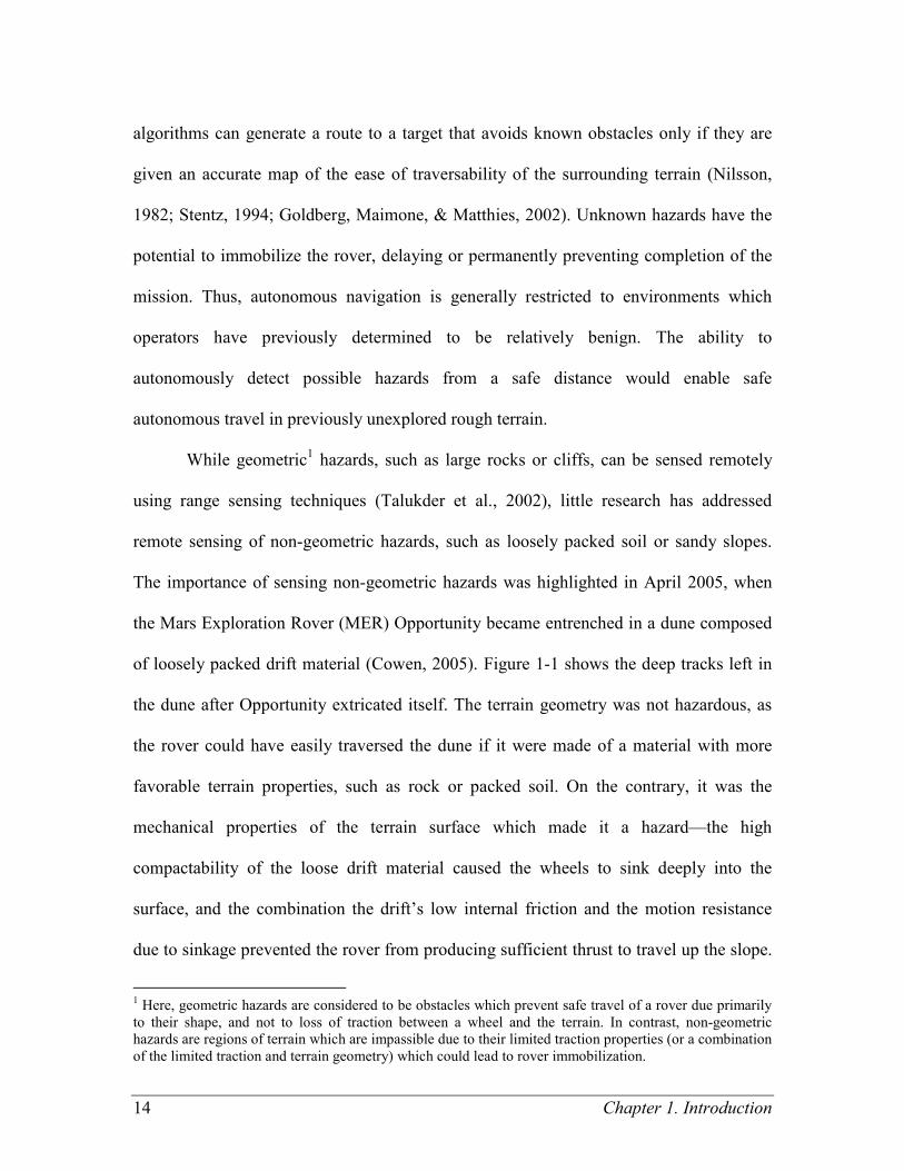
The importance of sensing non-geometric hazards was highlighted in April 2005, when
the Mars Exploration Rover (MER) Opportunity became entrenched in a dune composed
of loosely packed drift material (Cowen, 2005). Figure 1-1 shows the deep tracks left in
the dune after Opportunity extricated itself. The terrain geometry was not hazardous, as
the rover could have easily traversed the dune if it were made of a material with more
favorable terrain properties, such as rock or packed soil. On the contrary, it was the
mechanical properties of the terrain surface which made it a hazard—the high
compactability of the loose drift material caused the wheels to sink deeply into the
surface, and the combination the drift’s low internal friction and the motion resistance
due to sinkage prevented the rover from producing sufficient thrust to travel up the slope.
1 Here, geometric hazards are considered to be obstacles which prevent safe travel of a rover due primarily
to their shape, and not to loss of traction between a wheel and the terrain. In contrast, non-geometric
hazards are regions of terrain which are impassible due to their limited traction properties (or a combination
of the limited traction and terrain geometry) which could lead to rover immobilization.
15
Opportunity’s progress was delayed for more than a month while engineers worked to
extricate it.
Figure 1-1. Deep tracks in Purgatory Dune left by MER Opportunity
(Image courtesy NASA/JPL-Caltech)
Since non-geometric hazards are highly dependent on wheel-terrain interaction
properties, methods for characterizing such hazards have focused on measuring aspects of
that interaction. Examples include wheel sinkage measurement (Brooks, Iagnemma, &
Dubowsky, 2006; Wilcox, 1994), parametric soil characterization (Iagnemma, Kang,
Shibly, & Dubowsky, 2004), wheel slip detection (Reina, Ojeda, Milella, & Borenstein,
2006), and explicit traversability estimation (Kang, 2003). These methods rely on

16 Chapter 1. Introduction
proprioceptive2 terrain sensing, which characterizes only the terrain immediately under
the rover wheel, so it is of limited use for predictive hazard avoidance.
Where researchers have addressed terrain sensing using exteroceptive sensors,
such as cameras or LIDAR sensors, it has typically been assumed that the visual
appearances of terrain classes of interest are known a priori (Angelova, Matthies,
Helmick, & Perona, 2007a; Wellington, Courville, & Stentz, 2005). Although (Kim, Sun,
Oh, Rehg, & Bobick, 2006) describes an approach for distinguishing traversable from
non-traversable terrain where the terrain class appearances are learned, their work focuses
on the detection of geometric hazards. No research has addressed the detection of non-
geometric hazards using exteroceptive sensors, where the visual appearance of the terrain
classes is not known a priori.
In summary, autonomous planetary rover mobility is significantly affected by the
mechanical properties of terrain, which to date have been identified only for terrain
physically contacted by the rover or for terrain classes known a priori. In environments
where the visual appearances of terrain classes are not known a priori, no framework
exists for autonomously predicting the mechanical properties of distant terrain, such that
these properties can be used for autonomous navigation and hazard avoidance. Such an
approach would greatly increase a rover’s ability to autonomously navigate to distant
sites of scientific interest.
2 Proprioceptive sensors measure the internal state of the rover, and therefore sense terrain through its
interaction with the rover. In this work, wheel torque, wheel speed, and wheel sinkage are considered to be
measured by proprioceptive sensors.

17
1.2 Purpose of this Thesis and Scenario Description
The purpose of this thesis is to develop a framework and the underlying
algorithmic components to enable a planetary rover to accurately predict mechanical
properties of distant terrain, by learning from its experience in traversing similar terrain.
In particular, this work is concerned with 1) the estimation of mechanical properties
relevant to robotic mobility prediction, and with 2) associating these mechanical
properties with visual features, such that the mechanical properties can be reliably
identified from a distance of several meters. To minimize the time between terrain
sensing and terrain property prediction, emphasis will be placed on using algorithms that
are computationally inexpensive, such that they can be executed in seconds or minutes on
COTS hardware.
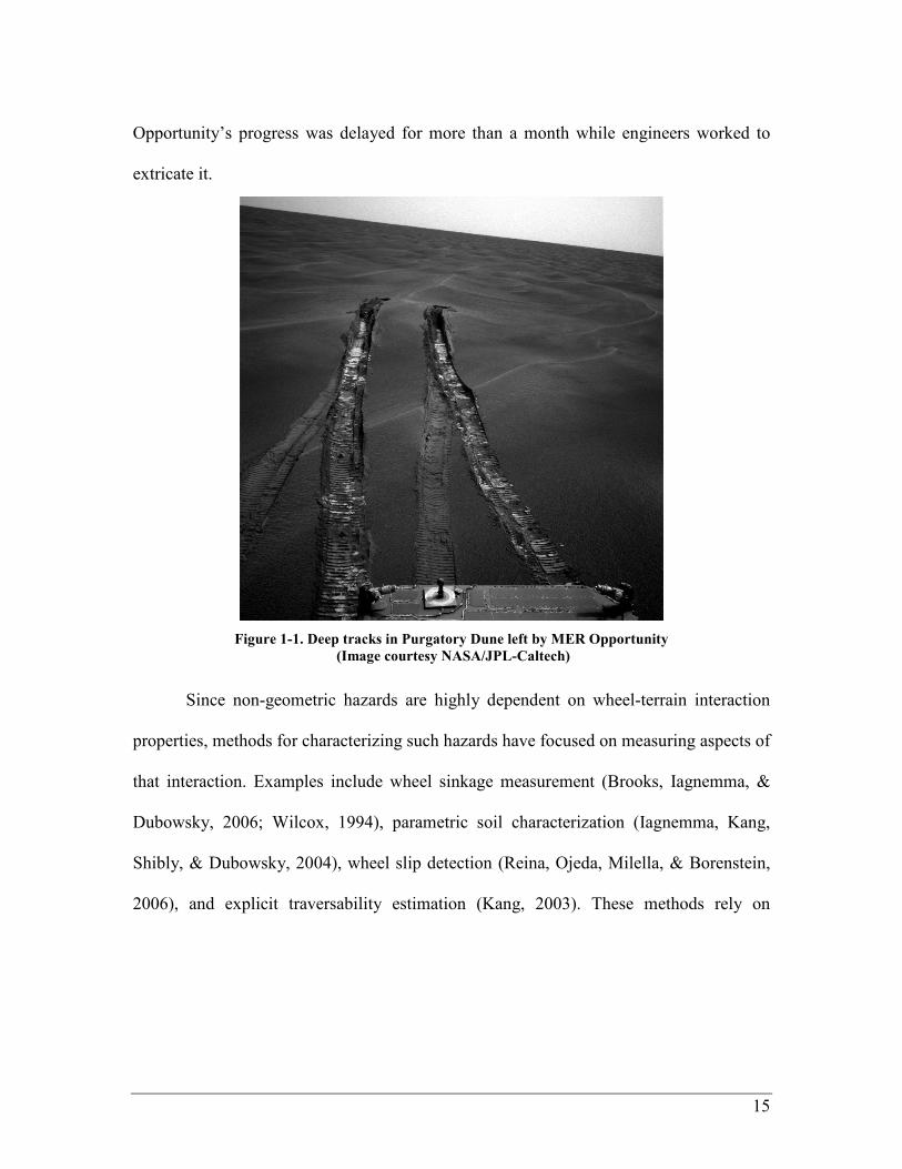
The scenario assumed for this work is one of planetary exploration, loosely
modeled on the sensing, mobility, and predicted environment of the Mars Science
Laboratory (MSL) mission, a large, six-wheeled rover scheduled for launch to Mars in
2011 (J. Johnson, 2008; NASA/JPL, 2008b). (Figure 1-2 shows an artist’s concept of the
MSL on Mars.) In this scenario, communication delays of 8 to 40 minutes (round-trip)
and a communication bandwidth of approximately 7.5 MB per day necessitate the use of
autonomous navigation to reach targets of interest at least 20 km away3. (For comparison,
Opportunity and Spirit, which have been on Mars for nearly 5 years, are only now on the
verge of having traveled 20 km combined (NASA/JPL, 2008a).) The challenge of terrain
sensing is eased by the fact that the environment can be considered as static—any
obstacles will remain stationary—and the robot is slow-moving, traveling at a speed of 5
3 Twenty kilometers is the predicted length of the landing ellipse for MSL.
18 Chapter 1. Introduction
to 15 cm per second. However computation is limited,4 and a very high cost of failure
requires that any approach tend to minimize risk of failure.
Figure 1-2. Artist concept of Mars Science Laboratory, left, compared to Mars Exploration Rover,
right (Image courtesy NASA/JPL-Caltech)
In this thesis it is assumed that the rover will be able to measure wheel torque,
sinkage of a rigid wheel into deformable terrain, and vibrations in the rover suspension
arising from wheel-terrain interaction. Wheel torque can either be measured with a
dedicated torque sensor, or estimated from motor current and wheel speed using a
Kalman filter. Wheel sinkage can be measured visually based on images containing the
rover wheels as in (Brooks et al., 2006), or the relative wheel sinkage between two
positions on the rover path can be calculated as in (Wilcox, 1994). It should be noted that
wheel torque and sinkage measurement can be implemented with no additional hardware
beyond that planned for MSL. Rover suspension vibration can be sensed using an
inexpensive contact microphone or accelerometer.
4 MSL has a radiation-hardened version of IBM’s PowerPC 750 running at 200 MHz (Bajracharya,
Maimone, & Helmick, 2008). For reference, the PowerPC G3 line of Macintosh desktop computers based
around the PowerPC 750 were sold between November, 1997 and July, 2001.
19
It is also assumed that the rover will be equipped with a stereo pair of mast-
mounted cameras to sense the color and geometry of terrains from 1 meter to 20 meters
away. This sensing is currently planned for inclusion on MSL as a pair of monochrome
cameras with filter wheels. The last assumption is that the rover will be able to measure
its speed relative to the terrain. This is currently implemented on the Mars Exploration
Rovers via a visual odometry algorithm (Maimone, A. Johnson, Cheng, Willson, &
Matthies, 2006).
1.3 Background and Literature Review
This thesis draws on techniques from the machine learning and machine vision
fields, as well as research in terrain parameter estimation and mobility prediction. While
most previous works in robotic terrain estimation have addressed only a subset of these
research areas, some recent works have presented coherent approaches to mobility-
related terrain sensing. These works will be described in the first subsection. Other
subsections address previous work related to the algorithmic components of this thesis,
including terrain recognition, machine learning, and mobility prediction.
1.3.1 Mobility-related Terrain Sensing
Terrain sensing is a broad field addressing the interpretation of sensor data to
yield information about a terrain region. Here, mobility-related terrain sensing refers to
approaches for associating sensor data with vehicle mobility. Some approaches operate
on data from only proprioceptive sensors (e.g. vibration or wheel sinkage data), and thus
address the rover’s mobility on the terrain immediately beneath the rover’s wheels. Other
20 Chapter 1. Introduction
approaches operate on data from exteroceptive sensors (e.g. vision or LIDAR data), and
are used to predict the mobility properties of terrain several rover lengths away.
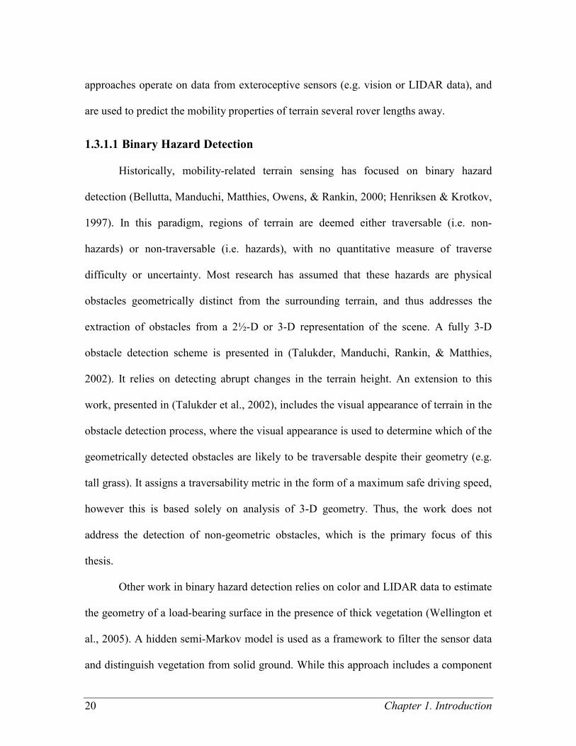
1.3.1.1 Binary Hazard Detection
Historically, mobility-related terrain sensing has focused on binary hazard
detection (Bellutta, Manduchi, Matthies, Owens, & Rankin, 2000; Henriksen & Krotkov,
1997). In this paradigm, regions of terrain are deemed either traversable (i.e. non-
hazards) or non-traversable (i.e. hazards), with no quantitative measure of traverse
difficulty or uncertainty. Most research has assumed that these hazards are physical
obstacles geometrically distinct from the surrounding terrain, and thus addresses the
extraction of obstacles from a 2½-D or 3-D representation of the scene. A fully 3-D
obstacle detection scheme is presented in (Talukder, Manduchi, Rankin, & Matthies,
2002). It relies on detecting abrupt changes in the terrain height. An extension to this
work, presented in (Talukder et al., 2002), includes the visual appearance of terrain in the
obstacle detection process, where the visual appearance is used to determine which of the
geometrically detected obstacles are likely to be traversable despite their geometry (e.g.
tall grass). It assigns a traversability metric in the form of a maximum safe driving speed,
however this is based solely on analysis of 3-D geometry. Thus, the work does not
address the detection of non-geometric obstacles, which is the primary focus of this
thesis.
Other work in binary hazard detection relies on color and LIDAR data to estimate
the geometry of a load-bearing surface in the presence of thick vegetation (Wellington et
al., 2005). A hidden semi-Markov model is used as a framework to filter the sensor data
and distinguish vegetation from solid ground. While this approach includes a component
21
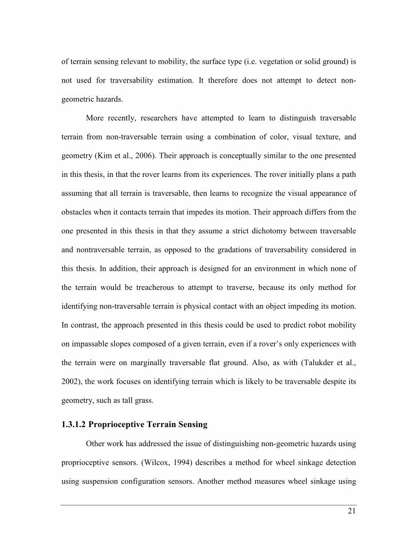
of terrain sensing relevant to mobility, the surface type (i.e. vegetation or solid ground) is
not used for traversability estimation. It therefore does not attempt to detect non-
geometric hazards.
More recently, researchers have attempted to learn to distinguish traversable
terrain from non-traversable terrain using a combination of color, visual texture, and
geometry (Kim et al., 2006). Their approach is conceptually similar to the one presented
in this thesis, in that the rover learns from its experiences. The rover initially plans a path
assuming that all terrain is traversable, then learns to recognize the visual appearance of
obstacles when it contacts terrain that impedes its motion. Their approach differs from the
one presented in this thesis in that they assume a strict dichotomy between traversable
and nontraversable terrain, as opposed to the gradations of traversability considered in
this thesis. In addition, their approach is designed for an environment in which none of
the terrain would be treacherous to attempt to traverse, because its only method for
identifying non-traversable terrain is physical contact with an object impeding its motion.
In contrast, the approach presented in this thesis could be used to predict robot mobility
on impassable slopes composed of a given terrain, even if a rover’s only experiences with
the terrain were on marginally traversable flat ground. Also, as with (Talukder et al.,
2002), the work focuses on identifying terrain which is likely to be traversable despite its
geometry, such as tall grass.
1.3.1.2 Proprioceptive Terrain Sensing
Other work has addressed the issue of distinguishing non-geometric hazards using
proprioceptive sensors. (Wilcox, 1994) describes a method for wheel sinkage detection
using suspension configuration sensors. Another method measures wheel sinkage using
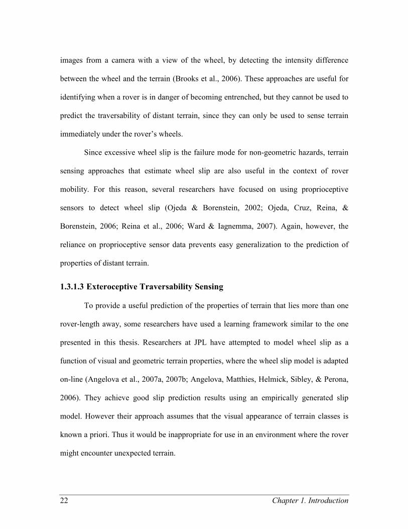
22 Chapter 1. Introduction
images from a camera with a view of the wheel, by detecting the intensity difference
between the wheel and the terrain (Brooks et al., 2006). These approaches are useful for
identifying when a rover is in danger of becoming entrenched, but they cannot be used to
predict the traversability of distant terrain, since they can only be used to sense terrain
immediately under the rover’s wheels.
Since excessive wheel slip is the failure mode for non-geometric hazards, terrain
sensing approaches that estimate wheel slip are also useful in the context of rover
mobility. For this reason, several researchers have focused on using proprioceptive
sensors to detect wheel slip (Ojeda & Borenstein, 2002; Ojeda, Cruz, Reina, &
Borenstein, 2006; Reina et al., 2006; Ward & Iagnemma, 2007). Again, however, the
reliance on proprioceptive sensor data prevents easy generalization to the prediction of
properties of distant terrain.
1.3.1.3 Exteroceptive Traversability Sensing
To provide a useful prediction of the properties of terrain that lies more than one
rover-length away, some researchers have used a learning framework similar to the one
presented in this thesis. Researchers at JPL have attempted to model wheel slip as a
function of visual and geometric terrain properties, where the wheel slip model is adapted
on-line (Angelova et al., 2007a, 2007b; Angelova, Matthies, Helmick, Sibley, & Perona,
2006). They achieve good slip prediction results using an empirically generated slip
model. However their approach assumes that the visual appearance of terrain classes is
known a priori. Thus it would be inappropriate for use in an environment where the rover
might encounter unexpected terrain.
23
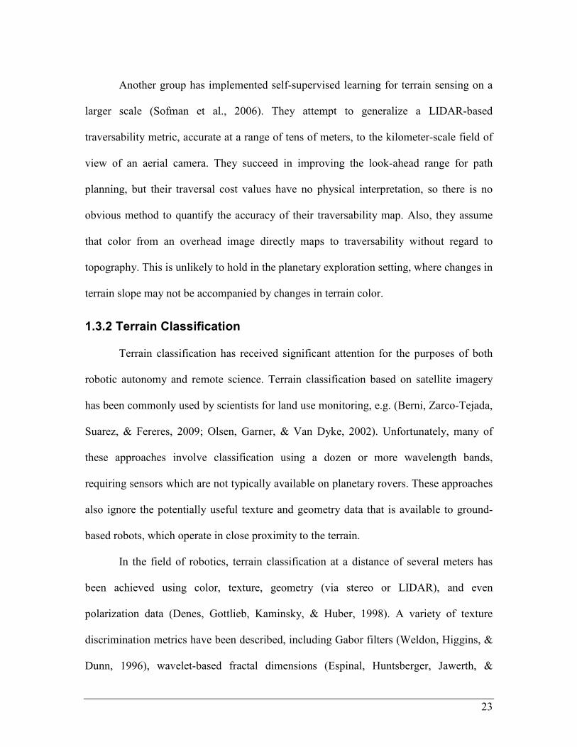
Another group has implemented self-supervised learning for terrain sensing on a
larger scale (Sofman et al., 2006). They attempt to generalize a LIDAR-based
traversability metric, accurate at a range of tens of meters, to the kilometer-scale field of
view of an aerial camera. They succeed in improving the look-ahead range for path
planning, but their traversal cost values have no physical interpretation, so there is no
obvious method to quantify the accuracy of their traversability map. Also, they assume
that color from an overhead image directly maps to traversability without regard to
topography. This is unlikely to hold in the planetary exploration setting, where changes in
terrain slope may not be accompanied by changes in terrain color.
1.3.2 Terrain Classification
Terrain classification has received significant attention for the purposes of both
robotic autonomy and remote science. Terrain classification based on satellite imagery
has been commonly used by scientists for land use monitoring, e.g. (Berni, Zarco-Tejada,
Suarez, & Fereres, 2009; Olsen, Garner, & Van Dyke, 2002). Unfortunately, many of
these approaches involve classification using a dozen or more wavelength bands,
requiring sensors which are not typically available on planetary rovers. These approaches
also ignore the potentially useful texture and geometry data that is available to ground-
based robots, which operate in close proximity to the terrain.
In the field of robotics, terrain classification at a distance of several meters has
been achieved using color, texture, geometry (via stereo or LIDAR), and even
polarization data (Denes, Gottlieb, Kaminsky, & Huber, 1998). A variety of texture
discrimination metrics have been described, including Gabor filters (Weldon, Higgins, &
Dunn, 1996), wavelet-based fractal dimensions (Espinal, Huntsberger, Jawerth, &

24 Chapter 1. Introduction
Kubota, 1998), and receptive fields inspired by the human visual system (Balas, 2006;
Malik & Perona, 1990). Various approaches for combining color, texture, and geometry
have been proposed including naïve Bayes fusion (Shi & Manduchi, 2003), neural
networks (Rasmussen, 2002), meta-classifier fusion (Halatci, Brooks, & Iagnemma,
2008), and semi-supervised fusion (Manduchi, 1999). These approaches are typically
used in a supervised fashion, where the number and appearance of classes is known a
priori. While (Rasmussen, 2002) addresses the classification problem in the context of
road detection, most approaches make no attempt to associate traversability with the
classification result. It should be noted that the work in this thesis relies on the visual
classifier developed by Halatci, so Section 1.1 closely follows the approach presented in
(Halatci, 2006; Halatci et al., 2008).
A limited amount of work has been performed in the area of classification based
on proprioceptive terrain sensors such as accelerometers. Such an approach was proposed
in (Iagnemma & Dubowsky, 2002), and a functional algorithm was presented in (Brooks
& Iagnemma, 2005). A similar algorithm, intended for high-speed ground vehicles, was
presented in (DuPont, Roberts, Selekwa, C. Moore, & Collins, 2005; Sadhukhan, 2004).
These approaches are useful in classifying the terrain in contact with the rover’s wheels,
and the approach of Brooks & Iagnemma is described in Section 2.1 for this purpose.
However due to its reliance on proprioceptive sensor data, this algorithm cannot be
applied directly to classify terrain not in contact with the rover.
1.3.3 Machine Learning
The terrain classification and clustering approaches presented in this thesis take
advantage of work in the field of machine learning. While both classification and
25
clustering have been studied extensively, only a small subset of the previously developed
approaches are appropriate for use in a learning framework operating in a time-
constrained scenario, and these will be described below.
For classification, support vector machines (SVM) have received significant
attention due to the speed at which they can be trained as well as their success in
classifying data from a wide variety of datasets (Schölkopf, 2000; Vapnik, 2000). Recent
work has provided strict bounds on the classification error rate, given the error rate over
the training data (Rakhlin, Mukherjee, & Poggio, 2006). An implementation of an SVM
has also been developed for online applications, where training data is presented as a
sequence rather than as a single batch (Kivinen, Smola, & Williamson, 2004). It is not
appropriate for this thesis, however, because it relies on the conditional independence of
sequential training examples—a poor assumption in the scenario considered here. SVM
classifiers can be implemented with linear or polynomial kernels, which can reduce both
training and classification time in situations when there is a large number of training
examples. Details related to reducing the SVM classification time are presented in
Appendix D, and SVMs are used extensively in this thesis.
Clustering, as opposed to classification, is a machine learning technique
appropriate for situations when the classes are not known a priori, or when labeled
training data is not available. It is the task of dividing unlabeled points into “clusters” of
similar points. Traditional methods of clustering include the well-known k-means method
as well as linkage-based methods derived from graph theory (Bishop, 1995; Brandes,
Gaertler, & Wagner, 2003). These methods all rely heavily on the features used to
26 Chapter 1. Introduction
represent the data. They have not previously been applied to traversability-related terrain
segmentation.
Another area of machine learning related to this research is that of novelty
detection. Novelty detection is the task of classifying a point as “same” or “different” as
compared to the training data, where there are no explicit examples of what is “different.”
This has occasionally been referred to as “one-class classification,” and a one-class
variant of the SVM classifier has been proposed (Schölkopf, Platt, Shawe-Taylor, Smola,
& Williamson, 2001). Another approach is to model the distribution of the training data,
for example using a mixture of Gaussians (MoG) model, and to label a new point as
“different” if the modeled density at that point is lower than some threshold. A theoretical
analysis of single-class classification strategies was presented in (El-Yaniv & Nisenson,
2007), and this analysis was the inspiration for the approach presented in 1.1. These
novelty detection approaches have not previously been applied to terrain identification.
1.3.4 Mobility Prediction
An important aspect of mobility prediction is modeling the interaction between a
wheel and the terrain. (Bekker, 1969) is the authoritative work in this field, describing
measurable mechanical properties of deformable terrain and defining the relationship
between these properties and the net forces and torques acting between the wheel and
terrain. Similar work by Wong and Reece differs only in the role of wheel width in the
force and torque equations (Wong, 2001; Wong & Reece, 1967). Both of these
approaches require the use of dedicated equipment to measure the terrain properties.
To enable parametric terrain modeling in scenarios without dedicated equipment,
Iagnemma proposed an approach for estimating terrain parameters using measurements
27
of the net forces and torques on a wheel (Iagnemma, Shibly, & Dubowsky, 2002;
Iagnemma et al., 2004). It was demonstrated that a Kalman filter could be used to
estimate the coefficients of a reduced-order Bekker model during a rover traverse.
However the estimated terrain properties were not used to predict a measure of
traversability of terrain. Kang extended that work and proposed a nondimensionalized
drawbar pull—the drag force that would be required to hold the vehicle stationary—as a
traversability metric (Kang, 2003; Iagnemma, Kang, Brooks, & Dubowsky, 2003). Kang
proposed an approximate equation for drawbar pull as a function of wheel sinkage, wheel
torque and vertical load.
Other researchers have attempted to quantify traversability in other ways. In
(Seraji, 1999) a traversability index based on fuzzy logic was calculated as a function of
terrain slope, rock size, and rock concentration. Another approach, the T-transformation,
calculated a traversability index based on terrain slope and geometric roughness of the
terrain (Ye & Borenstein, 2004). Neither of these approaches considered the mechanical
properties of the terrain, making them incompatible with the notion of non-geometric
hazards presented in this thesis.
1.4 Approach Overview
In order to appreciate the relationship between the algorithmic components
developed in this thesis, it is useful to understand how they are integrated in an online
terrain sensing framework. This section presents the concept of learning from experience,
defines the terrain representation and terminology that will be used throughout the thesis,
and then describes how each of the algorithmic components fit into the overall self-
supervised learning framework.

28 Chapter 1. Introduction
1.4.1 Learning From Experience
As described in 1.2, the purpose of this thesis is to allow a rover to learn the
relationship between mechanical terrain properties and terrain appearance, to enable it to
predict the mechanical properties of distant terrain. Figure 1-3 illustrates the three stages
of this learning process.
Figure 1-3. Schematic of proposed self-supervised classification framework
Initially, the rover has no knowledge of the relationship between the terrain
appearance and its mechanical properties. From a given position, it is assumed that a
29
rover can sense the appearance of terrain using cameras (Figure 1-3(a)), but cannot yet
predict its ability to traverse this terrain.
Figure 1-3(b) shows the rover after it has driven onto a patch of terrain that it
previously sensed with its cameras. Using proprioceptive sensors (e.g. vibration sensors
or torque sensors), the rover can sense the interaction between the rover wheels and
terrain, and thus characterize the mechanical terrain properties which affect the mobility
of the rover.
Once the rover has sensed the appearance of a patch of terrain and characterized
its effect on rover mobility, it associates the features related to appearance with mobility
properties. From this association, the rover can sense the appearance of terrain it has not
yet traversed and predict that effect that terrain may have on the rover (Figure 1-3(c)).
Thus, the rover has learned to predict the mobility properties of distant terrain from its
experiences traversing terrain with a similar appearance.
1.4.2 Terrain Representation and Terminology
To avoid ambiguity in the description of the self-supervised classification
framework and its algorithmic components, it is necessary to establish terminology to
describe the terrain and the rover’s sensors. This section introduces terminology for
terrain patches, mechanical terrain properties, terrain classes, proprioceptive and
exteroceptive sensors, and the terrain map.
Terrain Patch
In this thesis, terrain around a rover is divided into a regular grid of 20 cm by 20
cm terrain patches, whose locations are fixed in inertial space. Each patch is identified by
30 Chapter 1. Introduction
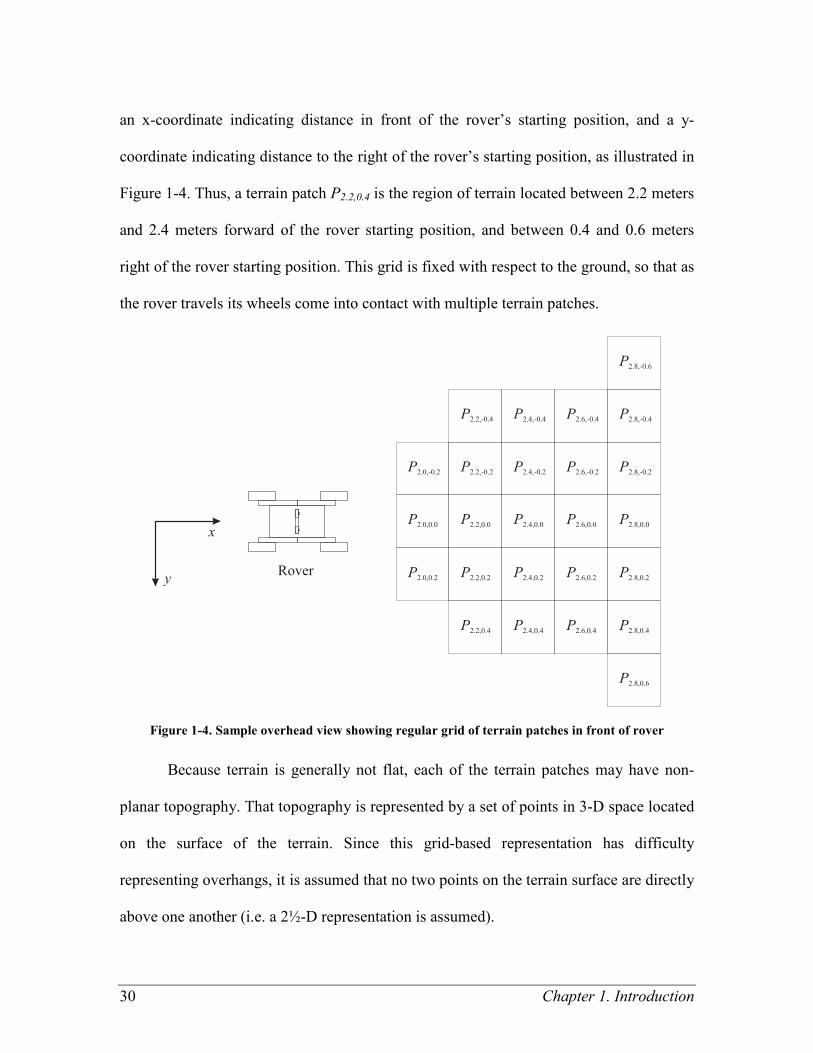
an x-coordinate indicating distance in front of the rover’s starting position, and a y-
coordinate indicating distance to the right of the rover’s starting position, as illustrated in
Figure 1-4. Thus, a terrain patch P2.2,0.4 is the region of terrain located between 2.2 meters
and 2.4 meters forward of the rover starting position, and between 0.4 and 0.6 meters
right of the rover starting position. This grid is fixed with respect to the ground, so that as
the rover travels its wheels come into contact with multiple terrain patches.
Figure 1-4. Sample overhead view showing regular grid of terrain patches in front of rover
Because terrain is generally not flat, each of the terrain patches may have non-
planar topography. That topography is represented by a set of points in 3-D space located
on the surface of the terrain. Since this grid-based representation has difficulty
representing overhangs, it is assumed that no two points on the terrain surface are directly
above one another (i.e. a 2½-D representation is assumed).
31
Mechanical Terrain Properties
For this thesis, mechanical terrain properties are measurable quantities that can be
used to describe the forces and torques between a rover wheel and the terrain. For
example, one mechanical terrain property is the maximum thrust force that a rover wheel
could exert when in contact with a terrain patch. Here, the primary interest is in
mechanical terrain properties that are useful in determining whether a terrain patch may
be traversed safely.
Terrain Class
It is assumed that each terrain patch Px,y can be uniquely associated with a terrain
class (e.g. “sand,” “rock,” and “beach grass”). A terrain class is a categorization for a
terrain patch based on its mechanical properties: a terrain patch Px1,y1 associated with
terrain class “sand” will react differently to forces applied by the rover’s wheel than
would a terrain patch Px2,y2 associated with terrain class “rock.” In this thesis, terrain
classes are categorizations of the mechanical properties of the terrain without regard to its
topography. Thus, patches Px1,y1 and Px2,y2 may be associated with the same terrain class
even if Px1,y1 is nearly flat and Px2,y2 has a steep slope.
It should be noted that terrain classes may be defined by human supervisors based
on prior knowledge of the rover’s environment, or they may be discovered by the rover
through unsupervised learning (i.e. clustering). Human-defined terrain classes typically
have some clear semantic interpretation: “sand,” “rock,” and “beach grass” are all easily
understood. Terrain chasses discovered through clustering are not associated with
semantic labels, so interpretation of the distinctions between classes may be more
difficult.
32 Chapter 1. Introduction
Proprioceptive and Exteroceptive Sensors
Various sensors are used by the rover to sense its environment. These sensors are
either exteroceptive or proprioceptive. Exteroceptive sensors, such as cameras, are able to
directly sense features related to terrain. Proprioceptive sensors, such as wheel torque
sensors or vibration sensors, are able to sense features related to the terrain only through
the physical interaction between the rover wheels and terrain.
Because proprioceptive sensors function by measuring characteristics of wheel-
terrain interaction, they are restricted to sensing terrain in direct contact with a rover
wheel. In this thesis, sensor data is denoted S, with indices specifying the sensor and the
time at which the sensor reading was recorded, for example Storque,t=0. Given the position
of the rover, it is trivial to identify the terrain patch Px,y with which proprioceptive sensor
data Storque,t=0 is associated.
Exteroceptive sensors can sense features related to terrain not in contact with the
rover, and thus sensor data associated with multiple terrain patches may be sensed
simultaneously. For example, an image Scamera,t taken at time t can contain pixels
associated with multiple terrain patches. To identify the terrain patch associated with a
given pixel Scamera,t,i,j located at row i and column j, the (stereo-derived) range data
associated with that pixel (Srange,t,i,j) is needed, as well as the rover’s position and
orientation at time t.
Terrain Map
A terrain map is a rover’s internal representation of the surrounding terrain around
it. For this thesis, that representation includes the topography of each terrain patch that
has been previously sensed, as well as the associated terrain class and mechanical terrain
33
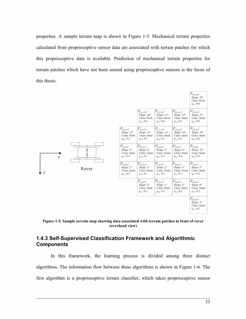
properties. A sample terrain map is shown in Figure 1-5. Mechanical terrain properties
calculated from proprioceptive sensor data are associated with terrain patches for which
this proprioceptive data is available. Prediction of mechanical terrain properties for
terrain patches which have not been sensed using proprioceptive sensors is the focus of
this thesis.
Figure 1-5. Sample terrain map showing data associated with terrain patches in front of rover
(overhead view)
1.4.3 Self-Supervised Classification Framework and Algorithmic Components
In this framework, the learning process is divided among three distinct
algorithms. The information flow between these algorithms is shown in Figure 1-6. The
first algorithm is a proprioceptive terrain classifier, which takes proprioceptive sensor
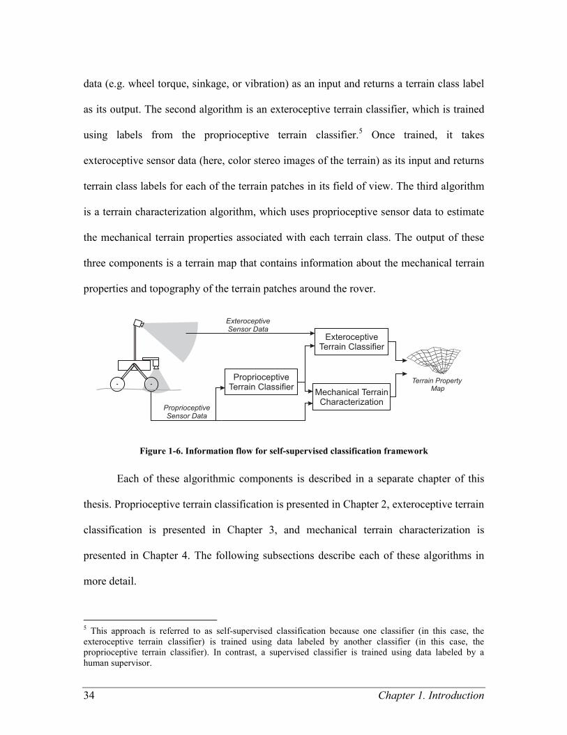
34 Chapter 1. Introduction
data (e.g. wheel torque, sinkage, or vibration) as an input and returns a terrain class label
as its output. The second algorithm is an exteroceptive terrain classifier, which is trained
using labels from the proprioceptive terrain classifier.5 Once trained, it takes
exteroceptive sensor data (here, color stereo images of the terrain) as its input and returns
terrain class labels for each of the terrain patches in its field of view. The third algorithm
is a terrain characterization algorithm, which uses proprioceptive sensor data to estimate
the mechanical terrain properties associated with each terrain class. The output of these
three components is a terrain map that contains information about the mechanical terrain
properties and topography of the terrain patches around the rover.
Figure 1-6. Information flow for self-supervised classification framework
Each of these algorithmic components is described in a separate chapter of this
thesis. Proprioceptive terrain classification is presented in Chapter 2, exteroceptive terrain
classification is presented in Chapter 3, and mechanical terrain characterization is
presented in Chapter 4. The following subsections describe each of these algorithms in
more detail.
5 This approach is referred to as self-supervised classification because one classifier (in this case, the
exteroceptive terrain classifier) is trained using data labeled by another classifier (in this case, the
proprioceptive terrain classifier). In contrast, a supervised classifier is trained using data labeled by a
human supervisor.
35
1.4.3.1 Proprioceptive Terrain Classification
The purpose of proprioceptive terrain classification is to classify terrain patches
based on proprioceptive sensor data, such that terrain patches with similar mechanical
properties are associated with the same terrain class, and terrain patches with
significantly different mechanical properties are associated with different terrain classes.
There are a number of potential approaches for accomplishing this task. This thesis
presents three distinct approaches.
The first approach, presented in 2.1, relies on training of a supervised classifier to
identify terrain classes based on proprioceptive sensor data, where these terrain classes
are defined by a human supervisor during training. This requires a priori knowledge of
the terrain classes in the rover’s environment, and hand labeling of training data.
The second approach, investigated in 2.1, relies on unsupervised clustering to
group terrain patches into classes based on proprioceptive sensor data. This approach
eliminates the need for hand labeling of data. However, the terrain clusters are not
associated with meaningful labels, so interpretations of the distinctions between terrain
classes may be difficult. Also, this approach may require more clustered terrain classes to
adequately represent the terrain compared to the first approach.
In the third approach, briefly addressed in 1.1, terrain patches are classified based
on the mechanical terrain properties identified by the mechanical terrain characterization
algorithm. Here, terrain classes are defined a priori to correspond to a range of
mechanical terrain properties. This requires that the mechanical terrain characterization
algorithm be executed frequently to accumulate training data for the exteroceptive terrain
classifier, which may be more computationally expensive than either of the first two
36 Chapter 1. Introduction
approaches due to the nonlinear optimizations involved in computing the mechanical
terrain properties.
1.4.3.2 Exteroceptive Terrain Classifier
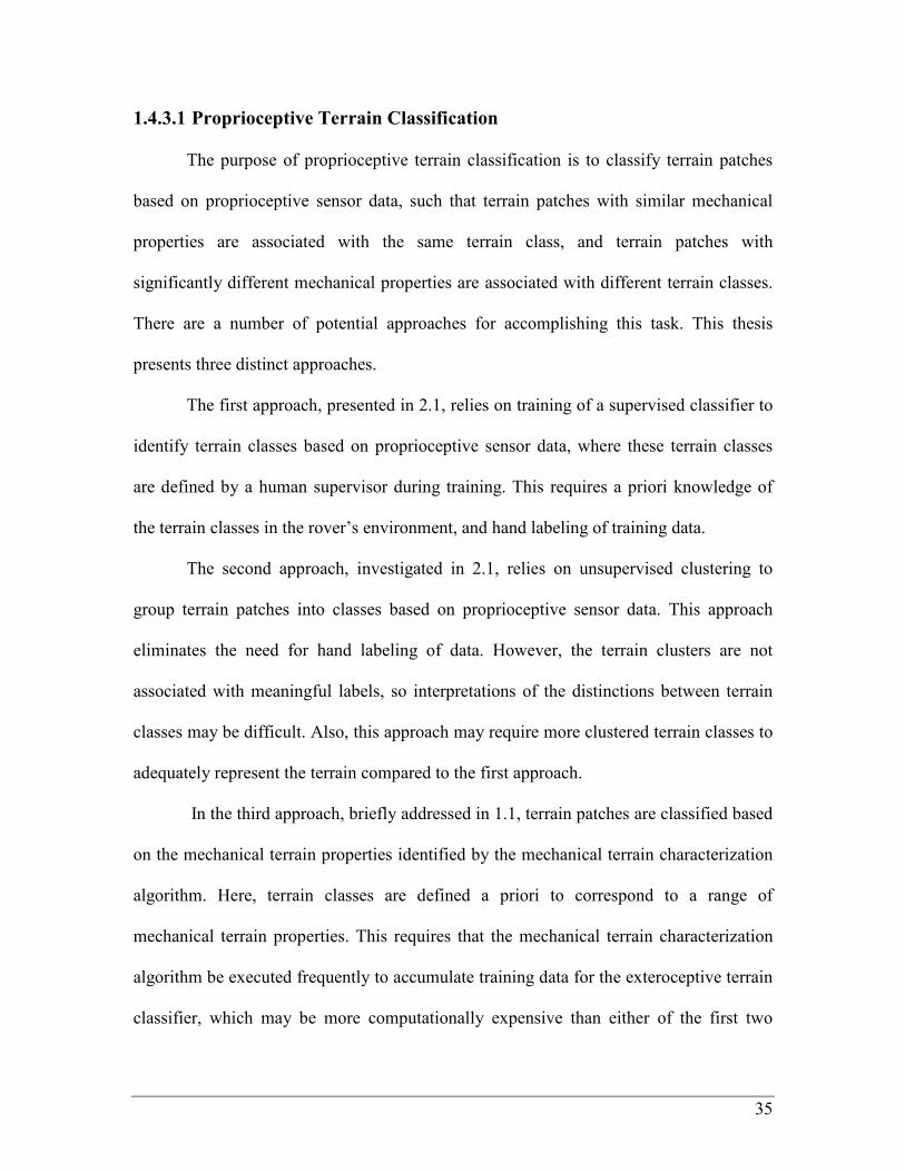
The purpose of exteroceptive terrain classification is to classify terrain patches
based on features derived from exteroceptive sensor data—in this case, color, visual
texture, and topography. The approach proposed in this thesis is to use a two-stage
classification process, as shown in Figure 1-7. First, a novel terrain detection stage
identifies whether the terrain patch belongs to a known class. If the patch belongs to one
of the known classes, the known terrain classifier is invoked. Otherwise, the patch is
labeled as “unrecognized” in the terrain class map. The exteroceptive terrain
classification algorithm is presented in Chapter 3.
Figure 1-7. Information flow for classification using exteroceptive terrain classifier
1.4.3.3 Mechanical Terrain Characterization
The purpose of mechanical terrain characterization is to use proprioceptive sensor
data to identify mechanical properties associated with a terrain patch. The approach
presented in this thesis establishes bounds on the net traction force available at a given
terrain patch. This approach is described in Chapter 4.

37
1.5 Contribution of this Thesis
The contribution of this thesis is the development and analysis of a self-
supervised learning framework and component algorithms. This framework enables a
planetary rover to accurately predict mechanical properties of terrain at a distance by
learning from experiences gained during traverses of similar terrain. This work includes
the development and validation of
• a self-supervised learning framework,
• supervised and unsupervised proprioceptive terrain classification algorithms,
• an exteroceptive novel terrain detection algorithm capable of identifying
terrain patches not belonging to known terrain classes, and
• a mechanical terrain characterization algorithm capable of identifying bounds
on the net traction force available at a given terrain patch.
1.6 Outline of this Thesis
This thesis is organized into six chapters, with five appendices. This chapter is the
introduction, describing the motivation and related work and providing an overview of
the approach.
Chapters 2, 3, and 4 present the development and validation of the algorithmic
components used within the self-supervised learning framework. Chapter 2 addresses
proprioceptive terrain classification, and presents two distinct approaches for classifying
terrain patches based on proprioceptive sensor data. Chapter 3 addresses exteroceptive
terrain classification, and presents methods for terrain classification and for identification
of novel terrain (i.e. terrain patches that are not associated with any known class).
38 Chapter 1. Introduction
Chapter 4 addresses mechanical terrain characterization, and presents a method for
identifying bounds on the net traction force available at a terrain patch.
Chapter 5 presents the development and experimental validation of the self-
supervised framework itself, including a detailed description of how the algorithms from
Chapters 2, 3, and 4 are employed in a terrain learning system suitable for novel
environments. Chapter 6 presents conclusions and describes potential avenues for future
research.
The five appendices present additional information related to the work presented
in the thesis body. The first three appendices describe the experiments used to validate
the algorithms described in this thesis. Appendix A contains details related to the four-
wheeled rover, TORTOISE, that was used as a test platform for each of the algorithms.
Appendix B contains details and images from the Wingaersheek Beach experimental test
site. Appendix C contains details related to the wheel-terrain interaction testbed, the
laboratory platform used to validate the mechanical terrain characterization approach.
Appendix D presents general information on support vector machines and describes
numerical optimization techniques that were used to speed up the classification process.
Appendix E presents Matlab code to extract classification features from raw sensor data.
2.1 Vibration-Based Terrain Classification 39
Chapter
2 Chapter 2 Proprioceptive Terrain Classification
Proprioceptive terrain classification is the process of assigning class labels to
terrain patches based on features derived from proprioceptive sensor data. Since the
terrain classes are associated with mechanical properties, mechanically similar terrain
patches should be assigned the same class label, while mechanically distinct terrain
patches should be assigned different class labels.
This chapter presents two approaches for proprioceptive terrain classification. The
first approach, presented in 2.1, uses a supervised classifier that has been trained by a
human operator to classify vibration data. The second approach, presented in 2.1, uses an
unsupervised clustering algorithm to group terrain patches into classes based on wheel
torque.
2.1 Vibration-Based Terrain Classification
2.1.1 Introduction
This section (2.1) presents a method for classifying terrain patches based on
vibrations induced in the rover structure by wheel-terrain interaction. Because
mechanically distinct terrains induce distinct vibrations, features derived from these
vibrations can be used to distinguish between them. This presents a means for
40 Chapter 2. Proprioceptive Terrain Classification
classification that is independent of the terrain patch’s visual appearance and is thus
inherently robust to changes in lighting conditions. The approach presented in this section
relies on measurement of vibrations using an accelerometer mounted on the rover
structure, representation of those vibrations in terms of the log-scaled power spectral
density, and classification of the resulting features using a support vector machine (SVM)
classifier. It uses a supervised classification framework, which relies on labeled vibration
training data collected for each of the terrain classes during an offline learning phase.
Vibration-based terrain classification was suggested in 2002 by Iagnemma and
Dubowsky as a novel sensing mode for classifying terrain for hazard detection
(Iagnemma & Dubowsky, 2002). Other researchers demonstrated vibration-based terrain
classification for a high-speed vehicle, but the accuracy deteriorated at low speeds (i.e.
under 50 cm/s) where vibration amplitudes were reduced (DuPont et al., 2005;
Sadhukhan, 2004; Weiss, Frohlich, & Zell, 2006). Thus, it would not be applicable to
planetary rovers, whose speeds are expected to be under 15 cm/s.
The approach presented here for vibration-based terrain classification was initially
developed in (Brooks, 2004) and (Brooks & Iagnemma, 2005), using a Fisher linear
discriminant for classification. This section proposes an improved approach that employs
an SVM classifier. It also describes experimental results from the Wingaersheek Beach
environment. This is the same environment on which the complete self-supervised
classification framework is experimentally validated in Chapter 5.
2.1.2 Approach
The vibration-based terrain classification algorithm presented here takes a signal-
recognition approach to classifying terrain patches based on vibration signals. As such, it

2.1 Vibration-Based Terrain Classification 41
learns to classify vibrations during an offline training phase in which it is presented with
hand-labeled vibration signals. This is in contrast to an approach which might use a solid
mechanics model to analytically predict how the rover structure will vibrate in response
to interaction with terrain.
2.1.2.1 Description of Vibration Features
This algorithm represents each 1-second segment of vibration data as a vector of
frequency-domain features. These features are calculated as follows. Given a time series
of vibration signals v=[Svib,t=t0,…,Svib,t=t0+1-1/Fs] sampled at a frequency Fs, the first step is
to compute the power spectral density (PSD), using Welch’s method (Welch, 1967).
Welch’s method averages calculations of the power spectral density over eight
subwindows to yield a 1025-element vector p, where the ith element, pi, is the estimate of
the power spectral density at a frequency of 2048/)1( −iFs . Thus, p is a time-shift-
invariant representation of the vibration. To reduce the dominating effect of high-
magnitude elements of p, these magnitudes are log-scaled to yield a vector p :
( ) 1025,...,1logˆ == iii pp .6 (2-1)
The vibration feature vector f, is the set of elements from p which correspond to a
frequency range of interest between Fmin and Fmax:
( )1/2048/2048,...,1ˆ)/2048( +−== + sminsminFFii FFFFi
sminpf . (2-2)
Sample Matlab code for this feature extraction process is presented in Table E-1 in
Appendix E.
6 This logarithmic scaling also has the advantage of representing time-domain convolution with vector
addition. Thus, the log-scaled PSD of the convolution of two signals is equal to the sum of their log-scaled
PSDs.
42 Chapter 2. Proprioceptive Terrain Classification
For this work, vibrations are sampled at 44.1 kHz, which results in a spacing of
21.5 Hz between frequencies in the PSD estimate. The frequency range of interest is from
0 to 12 kHz. This yields a 558 element vibration feature vector (log-scaled PSD
magnitudes) associated with each vibration segment.
2.1.2.2 Classifier Description
An SVM classifier was implemented to classify the vibration features using the
open-source library LIBSVM (Chang & C. Lin, 2005, 2008). A Gaussian radial basis
function (RBF) was used as the SVM kernel function, with parameters optimized by
cross-validation over a set of vibration data not used for testing. (The optimized
parameters were C=100 and γ=5*10-5
.) The LIBSVM option to return predicted class
likelihood was enabled.
During the offline training phase, the SVM was trained to recognize distinct
terrain classes using vibration features calculated from traverses of the rover over terrain
patches corresponding to each of the known terrain classes. In the online terrain
classification process, vibration features associated with unlabeled terrain patches were
calculated and these features were fed into the SVM for classification.
2.1.3 Experiment Details
The performance of the vibration-based terrain classifier was studied using data
from experiments with the Field and Space Robotics Laboratory (FSRL) Technology
Testbed Rover, TORTOISE, in an outdoor beach environment.
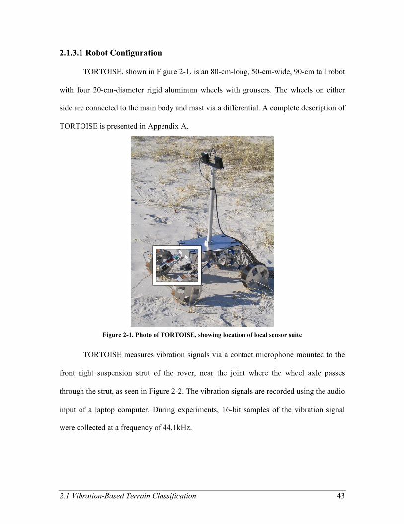
2.1 Vibration-Based Terrain Classification 43
2.1.3.1 Robot Configuration
TORTOISE, shown in Figure 2-1, is an 80-cm-long, 50-cm-wide, 90-cm tall robot
with four 20-cm-diameter rigid aluminum wheels with grousers. The wheels on either
side are connected to the main body and mast via a differential. A complete description of
TORTOISE is presented in Appendix A.
Figure 2-1. Photo of TORTOISE, showing location of local sensor suite
TORTOISE measures vibration signals via a contact microphone mounted to the
front right suspension strut of the rover, near the joint where the wheel axle passes
through the strut, as seen in Figure 2-2. The vibration signals are recorded using the audio
input of a laptop computer. During experiments, 16-bit samples of the vibration signal
were collected at a frequency of 44.1kHz.
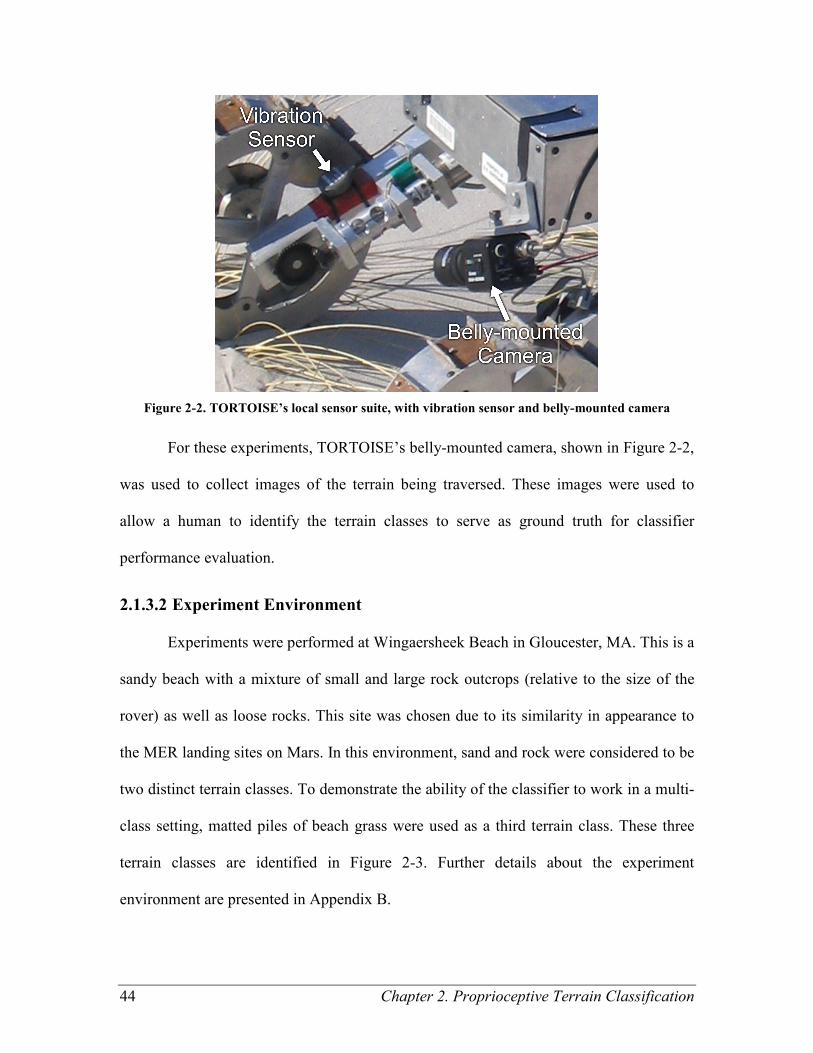
44 Chapter 2. Proprioceptive Terrain Classification
Figure 2-2. TORTOISE’s local sensor suite, with vibration sensor and belly-mounted camera
For these experiments, TORTOISE’s belly-mounted camera, shown in Figure 2-2,
was used to collect images of the terrain being traversed. These images were used to
allow a human to identify the terrain classes to serve as ground truth for classifier
performance evaluation.
2.1.3.2 Experiment Environment
Experiments were performed at Wingaersheek Beach in Gloucester, MA. This is a
sandy beach with a mixture of small and large rock outcrops (relative to the size of the
rover) as well as loose rocks. This site was chosen due to its similarity in appearance to
the MER landing sites on Mars. In this environment, sand and rock were considered to be
two distinct terrain classes. To demonstrate the ability of the classifier to work in a multi-
class setting, matted piles of beach grass were used as a third terrain class. These three
terrain classes are identified in Figure 2-3. Further details about the experiment
environment are presented in Appendix B.
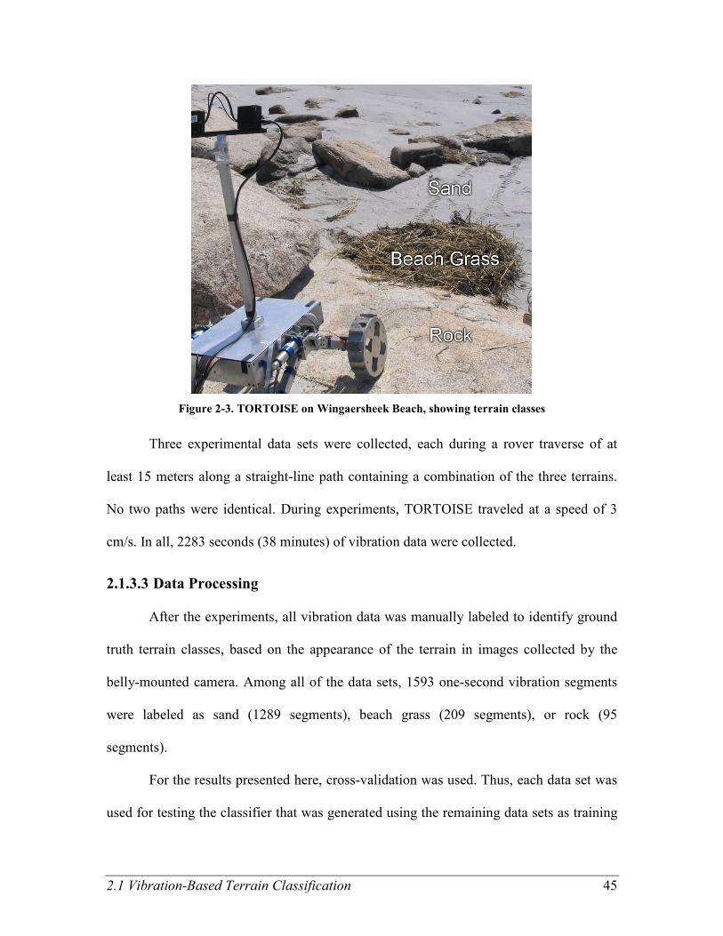
2.1 Vibration-Based Terrain Classification 45
Figure 2-3. TORTOISE on Wingaersheek Beach, showing terrain classes
Three experimental data sets were collected, each during a rover traverse of at
least 15 meters along a straight-line path containing a combination of the three terrains.
No two paths were identical. During experiments, TORTOISE traveled at a speed of 3
cm/s. In all, 2283 seconds (38 minutes) of vibration data were collected.
2.1.3.3 Data Processing
After the experiments, all vibration data was manually labeled to identify ground
truth terrain classes, based on the appearance of the terrain in images collected by the
belly-mounted camera. Among all of the data sets, 1593 one-second vibration segments
were labeled as sand (1289 segments), beach grass (209 segments), or rock (95
segments).
For the results presented here, cross-validation was used. Thus, each data set was
used for testing the classifier that was generated using the remaining data sets as training

46 Chapter 2. Proprioceptive Terrain Classification
data. Due to the reduced amount of training data, cross-validation is expected to under-
predict the performance of a classifier generated using all three labeled data sets (Kohavi,
1995).
2.1.4 Results
The performance of the vibration-based terrain classifier was assessed by
comparison to the hand-identified class labels (i.e., ground truth) using a receiver
operating characteristic (ROC) curve, shown in Figure 2-4. Here the horizontal axis
indicates the percentage of false positives (%FP) (e.g., instances when sand or beach
grass were falsely identified as rock) and the vertical axis indicates the percentage of true
positives (%TP) (e.g., instances when rock was correctly identified as rock). Each terrain
class forms a curve on the plot, as the threshold for leaving terrain patches “unclassified”
is adjusted. The end point of the curves represents the situation in which none of the
terrain patches are left unclassified. Any combination of points on these curves can be
achieved through proper selection of the threshold.
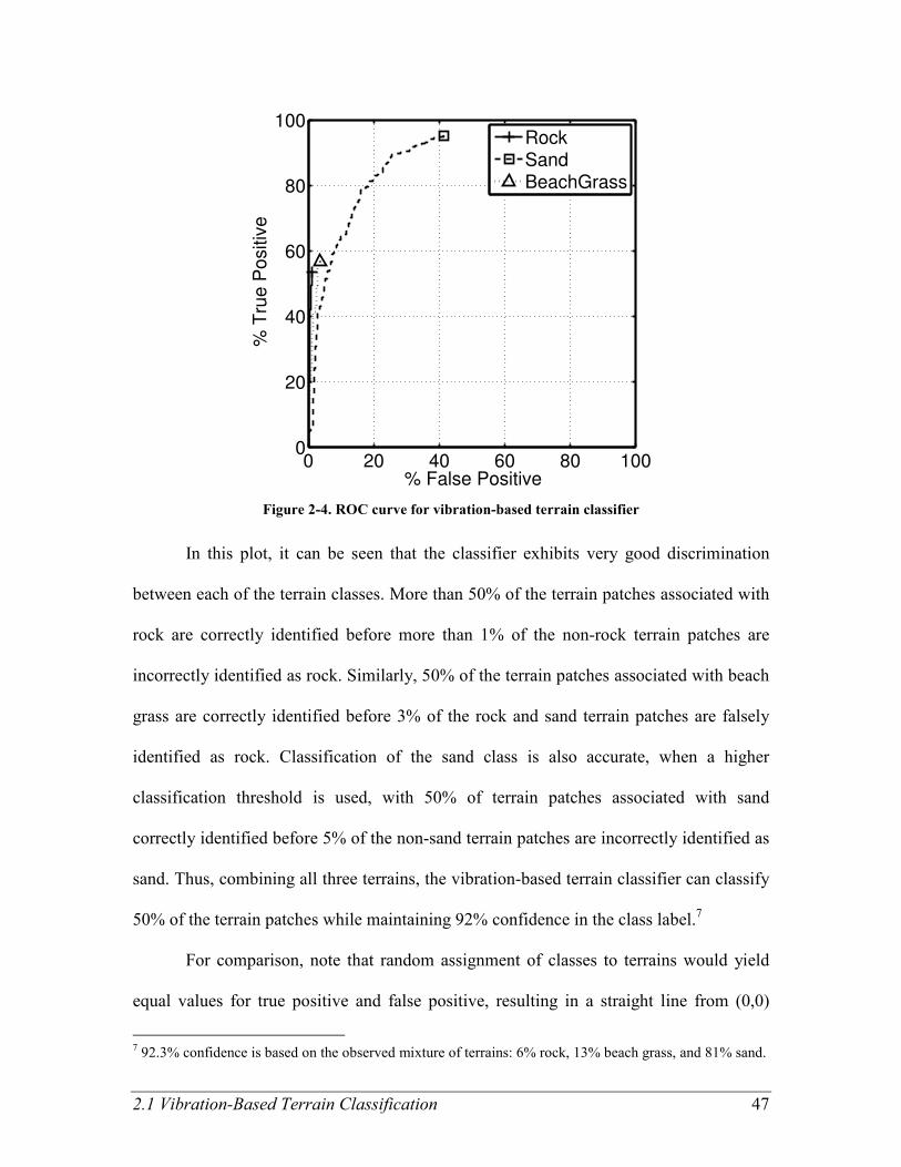
2.1 Vibration-Based Terrain Classification 47
0 20 40 60 80 1000
20
40
60
80
100
% False Positive
% T
rue
Po
sitiv
e
RockSandBeachGrass
Figure 2-4. ROC curve for vibration-based terrain classifier
In this plot, it can be seen that the classifier exhibits very good discrimination
between each of the terrain classes. More than 50% of the terrain patches associated with
rock are correctly identified before more than 1% of the non-rock terrain patches are
incorrectly identified as rock. Similarly, 50% of the terrain patches associated with beach
grass are correctly identified before 3% of the rock and sand terrain patches are falsely
identified as rock. Classification of the sand class is also accurate, when a higher
classification threshold is used, with 50% of terrain patches associated with sand
correctly identified before 5% of the non-sand terrain patches are incorrectly identified as
sand. Thus, combining all three terrains, the vibration-based terrain classifier can classify
50% of the terrain patches while maintaining 92% confidence in the class label.7
For comparison, note that random assignment of classes to terrains would yield
equal values for true positive and false positive, resulting in a straight line from (0,0)
7 92.3% confidence is based on the observed mixture of terrains: 6% rock, 13% beach grass, and 81% sand.
48 Chapter 2. Proprioceptive Terrain Classification
towards (100,100). By definition, random assignment into three classes yields only a 33%
confidence in the class label.
It should be noted that the low true positive detection rates for rock and beach
grass with all terrain patches labeled—54% and 57%, respectively—reflects the fact that
there were fewer examples of these terrain classes in the training data than there were for
sand. This implicitly gives these two terrain classes a lower prior probability in the final
classification. Thus, while they are correctly identified less often than sand, they have a
correspondingly lower false positive rate. If a detection rate higher than that shown in
Figure 2-4 is desired, more training examples can be provided, or a higher weight can be
placed on the existing examples when training the SVM.
2.1.5 Conclusions
In this section an approach has been presented for classifying terrain based on
proprioceptive sensor data. It uses a supervised classification framework to distinguish
terrain classes based on frequency-domain vibration features, where a human provides
class labels during a training process.
The performance of this classification approach is measured by the relationship
between the true positive rate and false positive rate for each terrain class. The balance
between the fraction of terrain patches labeled and the confidence of the labeling can be
adjusted by a threshold on the classification.
Experiments were performed with a four-wheeled rover, TORTOISE, in an
outdoor beach environment, with three distinct terrain classes. Classification results from
more than 1500 vibration segments demonstrate the ability of this approach to effectively

2.1 Vibration-Based Terrain Classification 49
distinguish these three terrain classes. These results should be seen as an extension to the
results presented in (Brooks, 2004) and (Brooks & Iagnemma, 2005).
The proposed algorithm is robust to variations in terrain appearance and lighting
as it classifies terrain based solely on wheel-terrain interaction. As such, it presents a
method for autonomous assignment of terrain patches to terrain classes, even when
terrain appearance or lighting are not known a priori. It is in this role that the vibration-
based terrain classification algorithm fits into the self-supervised classification
framework presented in Chapter 5.
2.2 Proprioceptive Terrain Clustering
2.2.1 Introduction
In situations when terrain classes are not known in advance, supervised
classification such as the vibration-based approach presented in 2.1 is infeasible. In such
situations, unsupervised clustering can be used to separate terrain patches into distinct
classes. This section presents a method for autonomously clustering terrain patches based
on proprioceptive sensor data, thus establishing a set of classes that can be assigned to
other terrain patches the rover encounters. Note that while these clusters (i.e.
autonomously generated classes) do not necessarily correspond to the classes a human
observer would identify, it will be shown that this approach can be used to successfully
divide a set of terrain patches into mechanically distinct classes.
There are many possible approaches to clustering terrain patches into distinct
classes, and several were investigated over the course of this research. Autonomous
clustering based on the terrain patches’ visual appearance (using the visual features
described in 3.1.2) was studied briefly, but it was observed that the human-identified
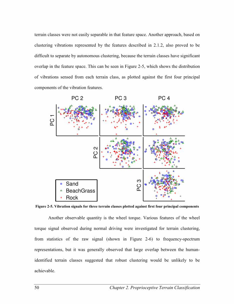
50 Chapter 2. Proprioceptive Terrain Classification
terrain classes were not easily separable in that feature space. Another approach, based on
clustering vibrations represented by the features described in 2.1.2, also proved to be
difficult to separate by autonomous clustering, because the terrain classes have significant
overlap in the feature space. This can be seen in Figure 2-5, which shows the distribution
of vibrations sensed from each terrain class, as plotted against the first four principal
components of the vibration features.
PC 2
PC
1
PC 3 PC 4
PC
2
PC
3Sand
BeachGrass
Rock
Figure 2-5. Vibration signals for three terrain classes plotted against first four principal components
Another observable quantity is the wheel torque. Various features of the wheel
torque signal observed during normal driving were investigated for terrain clustering,
from statistics of the raw signal (shown in Figure 2-6) to frequency-spectrum
representations, but it was generally observed that large overlap between the human-
identified terrain classes suggested that robust clustering would be unlikely to be
achievable.
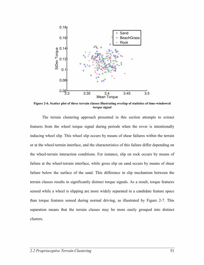
2.2 Proprioceptive Terrain Clustering 51
3.3 3.35 3.4 3.45 3.50.06
0.08
0.1
0.12
0.14
0.16
0.18
Mean Torque
StD
ev T
orq
ue
Sand
BeachGrass
Rock
Figure 2-6. Scatter plot of three terrain classes illustrating overlap of statistics of time-windowed
torque signal
The terrain clustering approach presented in this section attempts to extract
features from the wheel torque signal during periods when the rover is intentionally
inducing wheel slip. This wheel slip occurs by means of shear failures within the terrain
or at the wheel-terrain interface, and the characteristics of this failure differ depending on
the wheel-terrain interaction conditions. For instance, slip on rock occurs by means of
failure at the wheel-terrain interface, while gross slip on sand occurs by means of shear
failure below the surface of the sand. This difference in slip mechanism between the
terrain classes results in significantly distinct torque signals. As a result, torque features
sensed while a wheel is slipping are more widely separated in a candidate feature space
than torque features sensed during normal driving, as illustrated by Figure 2-7. This
separation means that the terrain classes may be more easily grouped into distinct
clusters.
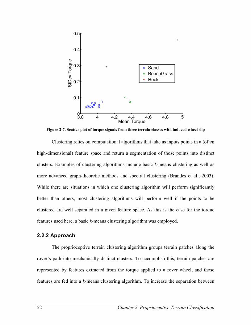
52 Chapter 2. Proprioceptive Terrain Classification
3.8 4 4.2 4.4 4.6 4.8 50
0.1
0.2
0.3
0.4
0.5
Mean Torque
StD
ev T
orq
ue
Sand
BeachGrass
Rock
Figure 2-7. Scatter plot of torque signals from three terrain classes with induced wheel slip
Clustering relies on computational algorithms that take as inputs points in a (often
high-dimensional) feature space and return a segmentation of those points into distinct
clusters. Examples of clustering algorithms include basic k-means clustering as well as
more advanced graph-theoretic methods and spectral clustering (Brandes et al., 2003).
While there are situations in which one clustering algorithm will perform significantly
better than others, most clustering algorithms will perform well if the points to be
clustered are well separated in a given feature space. As this is the case for the torque
features used here, a basic k-means clustering algorithm was employed.
2.2.2 Approach
The proprioceptive terrain clustering algorithm groups terrain patches along the
rover’s path into mechanically distinct clusters. To accomplish this, terrain patches are
represented by features extracted from the torque applied to a rover wheel, and those
features are fed into a k-means clustering algorithm. To increase the separation between
2.2 Proprioceptive Terrain Clustering 53
mechanically distinct terrain classes, the wheel torques are sensed while the rover
intentionally induces slip between the wheel and the terrain.
2.2.2.1 Rover Wheel Slip Behaviors
To emphasize the difference between mechanically distinct terrains, wheel torque
is sensed with the wheel slipping relative to the soil. By ensuring that the wheel is
slipping, the torque is usually dictated by the wheel-terrain interaction conditions rather
than the feedback control algorithm maintaining the wheel’s speed. Two separate rover
behaviors for inducing wheel slip were studied. The performance of segmentation using
these behaviors is presented in 2.2.4.
The first slip-inducing behavior is termed “Incremental Slip” and is presented as
Behavior 1 below. Here, after a period of normal driving, the rover drives the right front
wheel faster than the other wheels. Since the rover body remains moving at
(approximately) the longitudinal speed of the remaining wheels, wheel slip is induced
under the faster-rotating wheel. Initially, the slip ratio8 commanded is 33%. At
t=3 seconds, the rover body speed is decreased, increasing the slip ratio to 50%. At
t=6 seconds, the rover body is slowed down further, increasing the slip ratio to 67%. At
t=9 seconds, the rover resumes normal driving. The process repeats while the rover
traverses the terrain, allowing torque data to be collected at three distinct slip ratios.
8 The slip ratio is defined as 1 – (vx / ω r), where vx is the forward velocity of the wheel, ω is the angular
velocity, and r is the wheel radius.

54 Chapter 2. Proprioceptive Terrain Classification
Behavior 1. Incremental Slip
1. Normal Driving – 11 seconds
Drive all wheels at 3 cm/s
2. 33% Slip – 3 seconds
Drive right-front wheel at 4.5 cm/s and other wheels at 3 cm/s
3. 50% Slip – 3 seconds
Drive right-front wheel at 4.5 cm/s and other wheels at 2.25 cm/s
4. 67% Slip – 3 seconds
Drive right-front wheel at 4.5 cm/s and other wheels at 1.5 cm/s
5. Repeat
Note that the “Incremental Slip” results presented in 2.2.4 reflect clustering of
wheel torque signals recorded during the second half of the 67% slip state. The 67% slip
state was selected because the separation between terrain features was observed to be
largest in the high-slip state. Additionally it was observed that by the second half of each
slip state, the torque signals tended to have reached steady state or a limit cycle.
The second slip-inducing behavior is termed “Stop and Spin” and is presented as
Behavior 2 below. Here, after a period of normal driving, the rover brakes all four wheels
to bring the rover to a full stop. It then spins only the right front wheel, thus inducing
100% slip. The “Stop and Spin” results presented in 2.2.4 reflect clustering of wheel
torque signals recorded during the second half of the spin state.
Behavior 2. Stop and Spin
1. Normal Driving – 10 seconds
Drive all wheels at 3 cm/s
2. Stop – 1 second
Brake all wheels
3. Spin – 4 seconds
Drive right-front wheel at 3 cm/s and brake other wheels
4. Repeat
2.2.2.2 Torque Features
While the rover’s right-front wheel is slipping, the torque is recorded at a
sampling frequency Fs of 26.7 Hz, yielding a time series ],...,[10 ,, ttorquettorque SS=τ . From

2.2 Proprioceptive Terrain Clustering 55
the torque signals recorded in each high-slip state—either 67% slip or spin, depending on
the behavior—a single set of five features is extracted. For the state starting at time t0 and
ending at time t1, these features are
1) mean torque, τµ (N m):
( )
∑+−
+
−=
−=
1
12
01
01
01
2
1 ttF
ttFi
i
s
s
s
ttF
ττµ ,
(2-3)
2) standard deviation of torque, τσ (N m):
( )( )
2/1
1
12
2
01
01
0112
1
−
−
−= ∑
+−
+
−=
ttF
ttFi
i
s
s
s
ttF
ττ τ µσ , (2-4)
3) maximum torque, τ (N m):
( )i
ttFtt
Fi ss
τ
−
−∈
=01
01 ,...,2
maxτ ,
(2-5)
4) minimum torque, τ (N m):
( )i
ttFtt
Fi ss
τ
−
−∈
=01
01 ,...,2
minτ ,
(2-6)
5) difference between maximum and minimum torque, τr (N m):
ττ −=τr . (2-7)
This set of five features is combined into a vector, ],,,,[ τττf rττσµ= , and passed to the
clustering algorithm.
2.2.2.3 Clustering Algorithm
The torque features associated with all of the high-slip states from a single rover
traverse of 15 to 20 meters are passed to the clustering algorithm.9 Because the terrain
9 In practice, the clustering algorithm could be run every few meters of a traverse, with the clustering
results analyzed to see whether the new clusters are significantly better than the previous clusters.
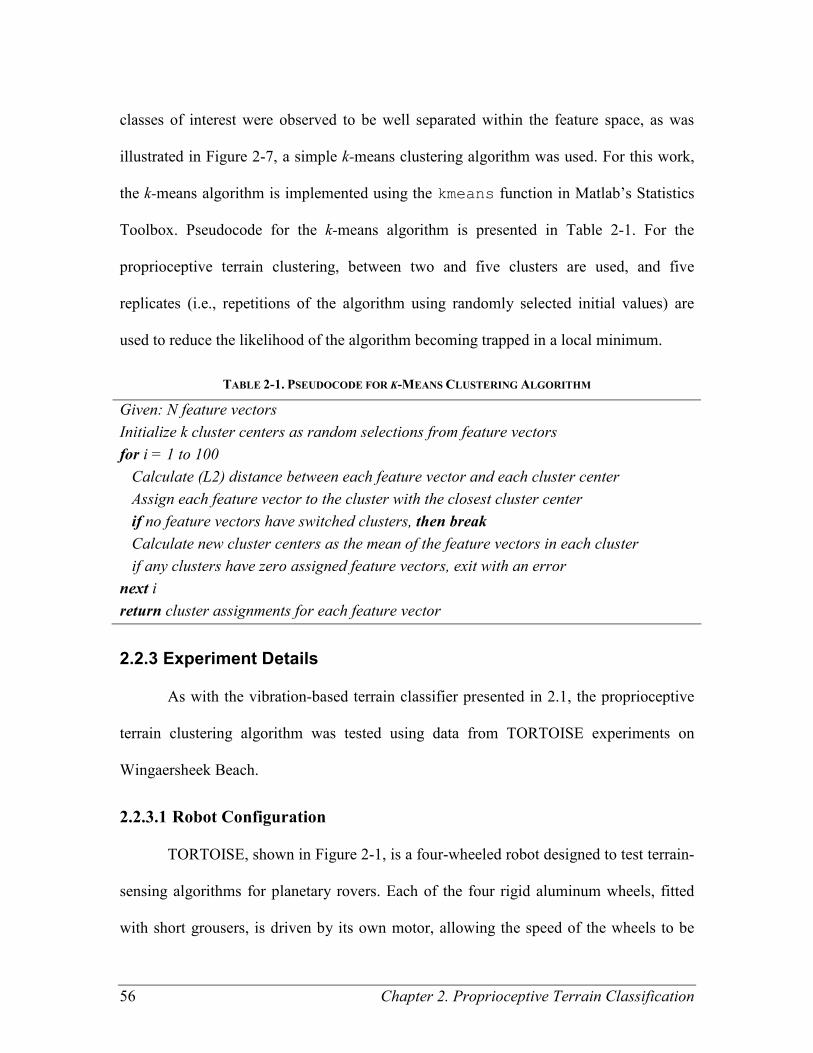
56 Chapter 2. Proprioceptive Terrain Classification
classes of interest were observed to be well separated within the feature space, as was
illustrated in Figure 2-7, a simple k-means clustering algorithm was used. For this work,
the k-means algorithm is implemented using the kmeans function in Matlab’s Statistics
Toolbox. Pseudocode for the k-means algorithm is presented in Table 2-1. For the
proprioceptive terrain clustering, between two and five clusters are used, and five
replicates (i.e., repetitions of the algorithm using randomly selected initial values) are
used to reduce the likelihood of the algorithm becoming trapped in a local minimum.
TABLE 2-1. PSEUDOCODE FOR K-MEANS CLUSTERING ALGORITHM
Given: N feature vectors
Initialize k cluster centers as random selections from feature vectors
for i = 1 to 100
Calculate (L2) distance between each feature vector and each cluster center
Assign each feature vector to the cluster with the closest cluster center
if no feature vectors have switched clusters, then break
Calculate new cluster centers as the mean of the feature vectors in each cluster
if any clusters have zero assigned feature vectors, exit with an error
next i
return cluster assignments for each feature vector
2.2.3 Experiment Details
As with the vibration-based terrain classifier presented in 2.1, the proprioceptive
terrain clustering algorithm was tested using data from TORTOISE experiments on
Wingaersheek Beach.
2.2.3.1 Robot Configuration
TORTOISE, shown in Figure 2-1, is a four-wheeled robot designed to test terrain-
sensing algorithms for planetary rovers. Each of the four rigid aluminum wheels, fitted
with short grousers, is driven by its own motor, allowing the speed of the wheels to be
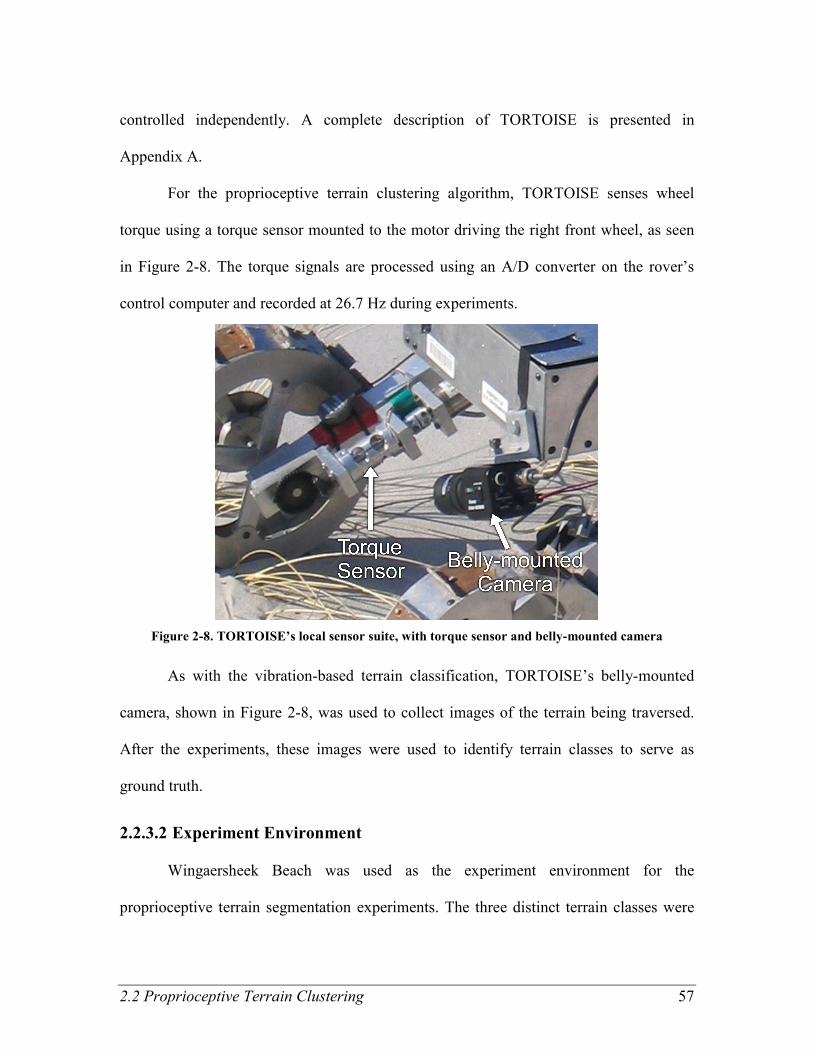
2.2 Proprioceptive Terrain Clustering 57
controlled independently. A complete description of TORTOISE is presented in
Appendix A.
For the proprioceptive terrain clustering algorithm, TORTOISE senses wheel
torque using a torque sensor mounted to the motor driving the right front wheel, as seen
in Figure 2-8. The torque signals are processed using an A/D converter on the rover’s
control computer and recorded at 26.7 Hz during experiments.
Figure 2-8. TORTOISE’s local sensor suite, with torque sensor and belly-mounted camera
As with the vibration-based terrain classification, TORTOISE’s belly-mounted
camera, shown in Figure 2-8, was used to collect images of the terrain being traversed.
After the experiments, these images were used to identify terrain classes to serve as
ground truth.
2.2.3.2 Experiment Environment
Wingaersheek Beach was used as the experiment environment for the
proprioceptive terrain segmentation experiments. The three distinct terrain classes were

58 Chapter 2. Proprioceptive Terrain Classification
sand, rock, and beach grass. These terrain classes are identified in Figure 2-3. Full details
about the experiment environment are presented in Appendix B.
Sixteen experimental data sets were collected, each set corresponding to a rover
traverse along a straight-line path containing a combination of the three terrains. No two
paths were identical. For seven of the data sets, the rover executed Behavior 1
(“Incremental Slip”) described in 2.2.2, totaling 101 slip cycles. For the other nine data
sets, the rover executed Behavior 2 (“Stop and Spin”), totaling 237 spin cycles.
2.2.3.3 Data Processing
After the data was collected, all of the terrain traversed by the rover was manually
labeled, using images from the belly-mounted camera to identify the ground truth terrain
class. Of the “incremental slip” data sets, 55 of the slip cycles had the right front wheel in
contact with sand, 13 with beach grass, and 5 with rock. Of the “stop and spin” data sets,
164 of the cycles had the right front wheel in contact with sand, 12 with beach grass, and
11 with rock. Cycles in which the terrain in contact with the right front wheel is unclear
were not labeled.
For each of the data sets, torque feature vectors associated with all cycles (labeled
and unlabeled) were passed to the clustering algorithm. Thus, the clustering algorithm
clustered the torque features from each data set without using any information from the
other data sets, and the performance of the clustering was evaluated separately for each
data set. The robustness of the algorithm was assessed by comparing the clustering
performance across all data sets.

2.2 Proprioceptive Terrain Clustering 59
2.2.4 Results
The results of experimental torque data clustering are presented in Table 2-2.
Here, algorithm performance is measured by its ability to separate the three human-
labeled terrain classes (i.e. sand, rock, and beach grass). Specifically, the “maximum
classification accuracy” metric is the largest fraction of terrain that can be classified
correctly, subject to the limitation that all terrain within the same cluster must be assigned
the same class label. This metric has the benefit of being insensitive to arbitrary ordering
of the clusters, and it does not penalize a clustering algorithm that is able to detect finer
distinctions than the hand-labeled classes. It should be noted, however, that even the
worst clustering approach will achieve a maximum classification accuracy equal to the
fraction of terrain belonging to the most common class. (This means that if 85% of the
terrain is sand, even randomly assigned clusters will have a maximum classification
accuracy of at least 85%.) This baseline accuracy is noted in the top row of the table. The
percentages listed are the mean of the performances observed across all data sets. The
numbers in brackets indicate 95% confidence intervals for the mean.
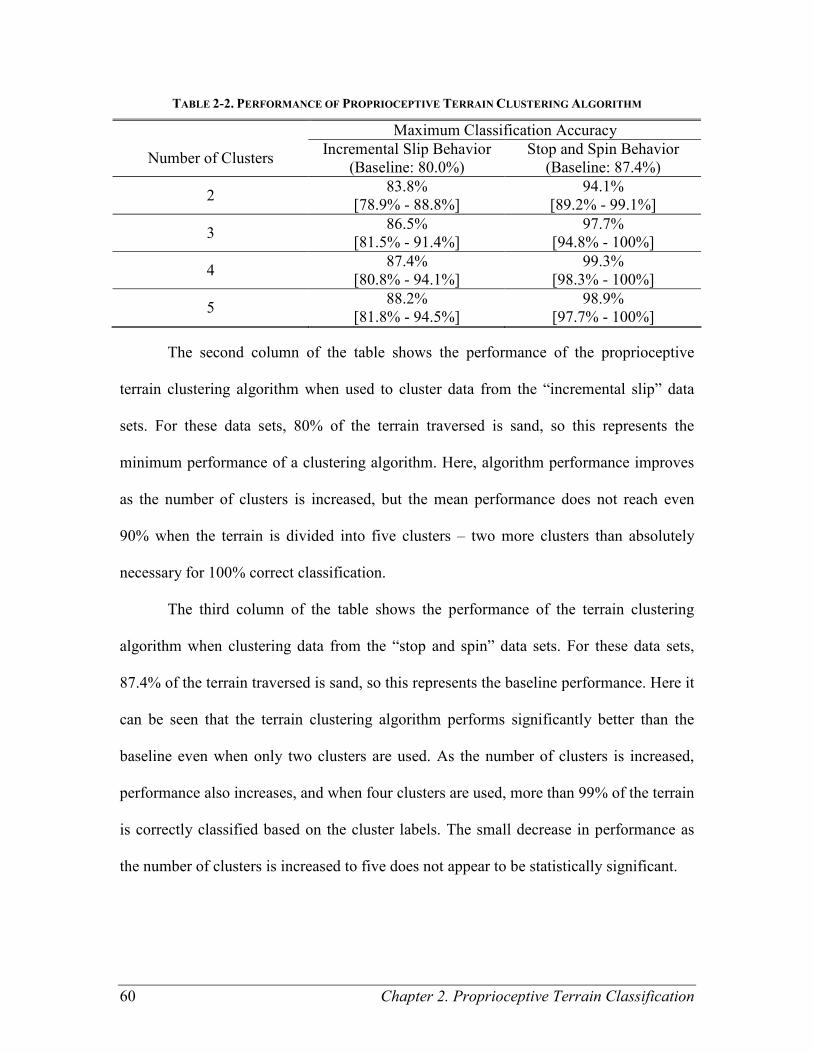
60 Chapter 2. Proprioceptive Terrain Classification
TABLE 2-2. PERFORMANCE OF PROPRIOCEPTIVE TERRAIN CLUSTERING ALGORITHM
Maximum Classification Accuracy
Number of Clusters Incremental Slip Behavior
(Baseline: 80.0%)
Stop and Spin Behavior
(Baseline: 87.4%)
2 83.8%
[78.9% - 88.8%]
94.1%
[89.2% - 99.1%]
3 86.5%
[81.5% - 91.4%]
97.7%
[94.8% - 100%]
4 87.4%
[80.8% - 94.1%]
99.3%
[98.3% - 100%]
5 88.2%
[81.8% - 94.5%]
98.9%
[97.7% - 100%]
The second column of the table shows the performance of the proprioceptive
terrain clustering algorithm when used to cluster data from the “incremental slip” data
sets. For these data sets, 80% of the terrain traversed is sand, so this represents the
minimum performance of a clustering algorithm. Here, algorithm performance improves
as the number of clusters is increased, but the mean performance does not reach even
90% when the terrain is divided into five clusters – two more clusters than absolutely
necessary for 100% correct classification.
The third column of the table shows the performance of the terrain clustering
algorithm when clustering data from the “stop and spin” data sets. For these data sets,
87.4% of the terrain traversed is sand, so this represents the baseline performance. Here it
can be seen that the terrain clustering algorithm performs significantly better than the
baseline even when only two clusters are used. As the number of clusters is increased,
performance also increases, and when four clusters are used, more than 99% of the terrain
is correctly classified based on the cluster labels. The small decrease in performance as
the number of clusters is increased to five does not appear to be statistically significant.

2.2 Proprioceptive Terrain Clustering 61
2.2.5 Conclusions
Section 1.1 has presented a second algorithm for separating terrain into classes
based on proprioceptive sensor data. It uses unsupervised clustering to divide terrain into
clusters, where the terrain is represented by features of the wheel torque signal. By
operating on the wheel torque signal recorded while the wheel is slipping relative to the
terrain, this clustering approach groups terrains based on properties affecting the
mechanical interaction between the wheel and the terrain. This approach is inherently
insensitive to the terrain appearance.
This approach was validated using data collected during experiments with a four-
wheeled rover in a natural beach environment with three distinct terrain classes. By
comparing the output terrain clusters to human-identified terrain classes, the performance
of the clustering algorithm can be assessed. Clustering results were compared for two
behaviors by which the rover can induce wheel slip. The results demonstrate that
clustering of torque data collected during the “stop and spin” behavior is more robust
than that of the “incremental slip” behavior. This difference is likely due to the rolling
contact in the "incremental slip" behavior disengaging the wheel from the terrain at load-
bearing points before the failure threshold was reached, thereby masking the difference in
material properties within the terrains. This decrease in maximum torque is particularly
evident when the wheel is spinning on rock. The robustness of the clustering of the “stop
and spin” data sets was observed to be very good.
As with the vibration-based terrain classification algorithm, the proprioceptive
terrain clustering algorithm serves as a method for assigning labels to terrain based on
features derived from wheel terrain interaction. Whereas vibration-based terrain

62 Chapter 2. Proprioceptive Terrain Classification
classification is appropriate for situations when representative terrain vibrations may be
hand-labeled during a training phase, proprioceptive terrain clustering is appropriate for
completely autonomous situations, when human supervision is unavailable. By robustly
separating the terrain patches into mechanically distinct clusters using proprioceptive
sensor data, this algorithm fits into the self-supervised classification framework (Chapter
5) as a proprioceptive terrain classifier.
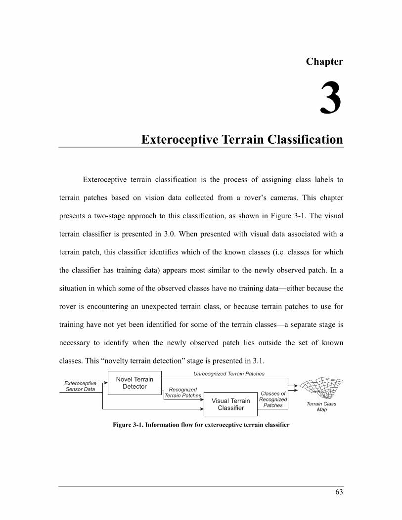
63
Chapter
3 Chapter 3 Exteroceptive Terrain Classification
Exteroceptive terrain classification is the process of assigning class labels to
terrain patches based on vision data collected from a rover’s cameras. This chapter
presents a two-stage approach to this classification, as shown in Figure 3-1. The visual
terrain classifier is presented in 3.0. When presented with visual data associated with a
terrain patch, this classifier identifies which of the known classes (i.e. classes for which
the classifier has training data) appears most similar to the newly observed patch. In a
situation in which some of the observed classes have no training data—either because the
rover is encountering an unexpected terrain class, or because terrain patches to use for
training have not yet been identified for some of the terrain classes—a separate stage is
necessary to identify when the newly observed patch lies outside the set of known
classes. This “novelty terrain detection” stage is presented in 3.1.
Figure 3-1. Information flow for exteroceptive terrain classifier
64 Chapter 3. Exteroceptive Terrain Classification
3.1 Visual Terrain Classification
3.1.1 Introduction
Classification of terrain using visual features is an area that has received
significant previous attention, from scientists studying land use (Olsen et al., 2002) to
engineers designing navigation systems for autonomous robots (Rasmussen, 2002). In
this thesis, the visual terrain classification approach of Halatci is followed closely
(Halatci, 2006; Halatci et al., 2008). This approach represents the appearance of a terrain
patch via color, visual texture, and geometric feature vectors. For each of these three
sensing modes, a SVM classifier is used to estimate likelihoods of the terrain patch
belonging to each of the known terrain classes. The three sensing modes are then
combined using naïve Bayes fusion to estimate the combined class likelihoods. The
terrain patch is classified as belonging to the terrain class with the highest likelihood.
Much of the development of the algorithm presented in this section (1.1) was
performed by Halacti for his Master’s thesis, though both the visual texture and
geometric features have small modifications from that presented in (Halatci et al., 2008).
The algorithm description is included here as it is a critical component of the self-
supervised classification system, and the visual features used in this classifier form the
foundation of the novel terrain detection approach presented in 1.1. This section will also
present detailed results for visual classification of terrains in the Wingaersheek Beach
environment, for direct comparison to the self-supervised classification results in Chapter
5.
3.1 Visual Terrain Classification 65
3.1.2 Approach
Here, exteroceptive terrain classification operates by extracting visual features
from terrain observed using a stereo pair of color cameras. Separate SVM classifiers for
each sensing mode—color, visual texture, and range—are used to predict the likelihood
that a particular terrain patch belongs to any given terrain class. The resulting class
likelihoods are combined using naïve Bayes fusion to yield a combined class assignment.
3.1.2.1 Visual Features
The appearance of a terrain patch is represented as a set of feature vectors derived
from the color, visual texture, and geometry of the terrain. These features are all extracted
from color images collected using a stereo pair.
3.1.2.1.1 Color
Color data is directly available from the cameras as red, green, and blue (RGB)
intensities. However, the illumination intensity affects all three values in a raw RGB
representation, which can lead to poor classification results. To reduce the effect of the
overall illumination level, a modified hue, saturation, and value (HSV) representation of
color is used as in (Sofman et al., 2006). In this approach, hue (an angle) is represented as
two values—sin(hue) and cos(hue)—to eliminate the artificial discontinuity at 2π. Thus,
color is represented as a 4-element vector: [sin(hue), cos(hue), saturation, value].
3.1.2.1.2 Visual Texture
Visual texture is a measure of the local spatial variation in the intensity of an
image. Researchers have proposed many metrics for visual texture, such as Gabor filters
and local energy methods (Bouman & Liu, 1991; Reed & du Buf, 1993). The work in this

66 Chapter 3. Exteroceptive Terrain Classification
thesis uses a wavelet-based approach, similar to the one demonstrated in (Espinal et al.,
1998). Here, a grayscale image is decomposed with the Haar wavelet (Strang, 1993).
Three scales of wavelets are used, each scale having horizontal, diagonal, and vertical
wavelets, corresponding to estimating the derivative of the intensity in the horizontal,
diagonal, and vertical directions at each length scale. The scales used are 2, 4, and 8
pixels. Because this process is sensitive to local changes in intensity, the magnitudes of
the wavelet coefficients are then averaged over windows of 11, 9, and 7 wavelets. Thus,
visual texture is represented by a 9-element vector, composed of the window-averaged
horizontal, diagonal, and vertical wavelet coefficients at each scale.
The visual texture features are calculated using the following procedure. First, the
640 pixel × 480 pixel color image I (with all ]1,0[,, ∈colorjiI ) is converted to a grayscale
image G using Matlab’s rgb2gray function, such that
,114.0587.02989.0 ,,,,,,, bluejigreenjiredjiji IIIG ++= (3-1)
for i=1,…,480 and j=1,…,640.10
Texture based on the grayscale image is calculated
using the Haar wavelet. Here, the low-pass wavelet l is [0.25, 0.5, 0.25], and the high-
pass wavelet h is [-0.5, 0, 0.5]. Using these wavelets four images are calculated, each of
which has half the resolution of G: A1, which has the low-pass wavelet applied in both
the horizontal and vertical directions, as
====
=== ∑∑
= =−+−+
;320,1240,...,1or 320,...,1240,10
319,...,2239,...,23
1
3
1
22,22,
jiji
jiGll1A
m n
njminmji (3-2)
10
The constants in Equation (3-1) were specified within the rgb2gray function.

3.1 Visual Terrain Classification 67
V1, which has the low-pass wavelet applied in the horizontal direction, and the high-pass
wavelet applied in the vertical direction, as
====
=== ∑∑
= =−+−+
;320,1240,...,1or 320,...,1240,10
319,...,2239,...,23
1
3
1
22,22,
jiji
jiGlh1V
m n
njminmji (3-3)
H1, which has the high-pass wavelet applied in the horizontal direction and the low-pass
wavelet applied in the vertical direction, as
====
=== ∑∑
= =−+−+
;320,1240,...,1or 320,...,1240,10
319,...,2239,...,23
1
3
1
22,22,
jiji
jiGhl1H
m n
njminmji (3-4)
and D1, which has the high-pass wavelet applied in both directions, as
====
=== ∑∑
= =−+−+
.320,1240,...,1or 320,...,1240,10
319,...,2239,...,23
1
3
1
22,22,
jiji
jiGhh1D
m n
njminmji (3-5)
Here H1, D1, and V1 contain directional derivative information at the 2-pixel scale, and
A1 contains a low-pass-filtered version of the grayscale image at ½ of the original
dimensions.
To calculate the directional derivatives at the 4-pixel scale, the wavelets are
applied to A1. A2 has the low-pass wavelet applied in both horizontal and vertical
directions:
====
=== ∑∑
= =−+−+
.160,1120,...,1or 160,...,1120,10
159,...,2119,...,23
1
3
1
22,22,
jiji
ji1All2A
m n
njminmji (3-6)
V2 has the low-pass wavelet applied in the horizontal direction and the high-pass wavelet
applied in the vertical direction:
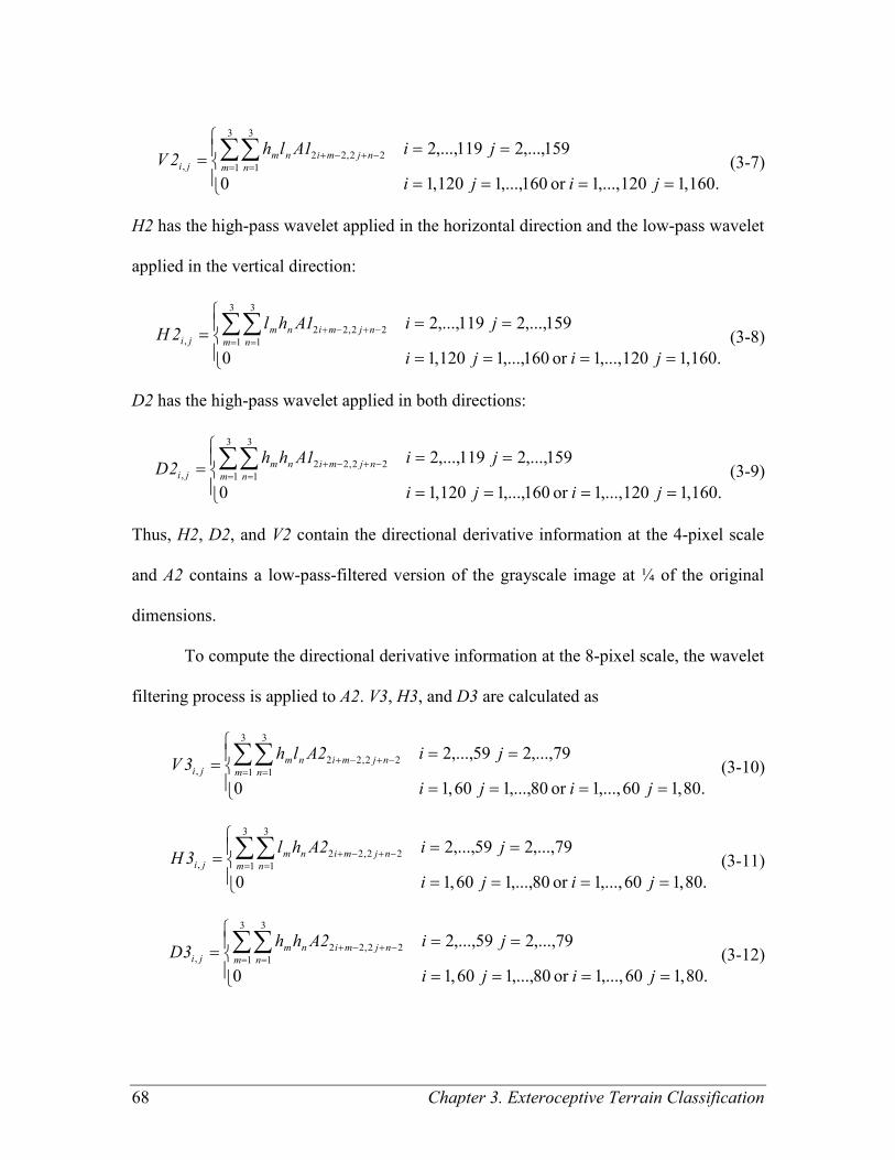
68 Chapter 3. Exteroceptive Terrain Classification
====
=== ∑∑
= =−+−+
.160,1120,...,1or 160,...,1120,10
159,...,2119,...,23
1
3
1
22,22,
jiji
ji1Alh2V
m n
njminmji (3-7)
H2 has the high-pass wavelet applied in the horizontal direction and the low-pass wavelet
applied in the vertical direction:
====
=== ∑∑
= =−+−+
.160,1120,...,1or 160,...,1120,10
159,...,2119,...,23
1
3
1
22,22,
jiji
ji1Ahl2H
m n
njminmji (3-8)
D2 has the high-pass wavelet applied in both directions:
====
=== ∑∑
= =−+−+
.160,1120,...,1or 160,...,1120,10
159,...,2119,...,23
1
3
1
22,22,
jiji
ji1Ahh2D
m n
njminmji (3-9)
Thus, H2, D2, and V2 contain the directional derivative information at the 4-pixel scale
and A2 contains a low-pass-filtered version of the grayscale image at ¼ of the original
dimensions.
To compute the directional derivative information at the 8-pixel scale, the wavelet
filtering process is applied to A2. V3, H3, and D3 are calculated as
====
=== ∑∑
= =−+−+
.80,160,...,1or 80,...,160,10
79,...,259,...,23
1
3
1
22,22,
jiji
ji2Alh3V
m n
njminmji (3-10)
====
=== ∑∑
= =−+−+
.80,160,...,1or 80,...,160,10
79,...,259,...,23
1
3
1
22,22,
jiji
ji2Ahl3H
m n
njminmji (3-11)
====
=== ∑∑
= =−+−+
.80,160,...,1or 80,...,160,10
79,...,259,...,23
1
3
1
22,22,
jiji
ji2Ahh3D
m n
njminmji (3-12)
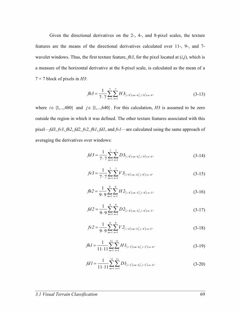
3.1 Visual Terrain Classification 69
Given the directional derivatives on the 2-, 4-, and 8-pixel scales, the texture
features are the means of the directional derivatives calculated over 11-, 9-, and 7-
wavelet windows. Thus, the first texture feature, fh3, for the pixel located at (i,j), which is
a measure of the horizontal derivative at the 8-pixel scale, is calculated as the mean of a
7 × 7 block of pixels in H3:
.
77
1 7
1
7
1
48/,48/∑∑= =
−+−+⋅=
m n
njmi3H3fh (3-13)
where }480,...,1{∈i and }640,...,1{∈j . For this calculation, H3 is assumed to be zero
outside the region in which it was defined. The other texture features associated with this
pixel—fd3, fv3, fh2, fd2, fv2, fh1, fd1, and fv1—are calculated using the same approach of
averaging the derivatives over windows:
.
77
1 7
1
7
1
48/,48/∑∑= =
−+−+⋅=
m n
njmi3D3fd (3-14)
.
77
1 7
1
7
1
48/,48/∑∑= =
−+−+⋅=
m n
njmi3V3fv (3-15)
.
99
1 9
1
9
1
54/,54/∑∑= =
−+−+⋅=
m n
njmi2H2fh (3-16)
.
99
1 9
1
9
1
54/,54/∑∑= =
−+−+⋅=
m n
njmi2D2fd (3-17)
.
99
1 9
1
9
1
54/,54/∑∑= =
−+−+⋅=
m n
njmi2V2fv (3-18)
.
1111
1 11
1
11
1
62/,62/∑∑= =
−+−+⋅=
m n
njmi1H1fh (3-19)
.
1111
1 11
1
11
1
62/,62/∑∑= =
−+−+⋅=
m n
njmi1D1fd (3-20)
70 Chapter 3. Exteroceptive Terrain Classification
.
1111
1 11
1
11
1
62/,62/∑∑= =
−+−+⋅=
m n
njmi1V1fv (3-21)
Thus, the texture feature vector for the pixel located at (i,j) is the 9-element vector [fh3,
fd3, fv3, fh2, fd2, fv2, fh1, fd1, fv1].
3.1.2.1.3 Geometry
Terrain geometry is available through stereo image processing. The raw output of
a stereo processing algorithm is a cloud of range data points. Here the points are divided
into a grid of 20-cm by 20-cm terrain patches projected onto a horizontal plane. The
geometric features are statistics calculated from the elevation of points associated with
each terrain patch. When calculating the features, the n points associated with a given
terrain patch are represented as a n × 3 matrix denoting each point’s position in the
[forward, right, down] coordinate frame with its origin at the rover’s starting position:
P = {p1,…,pn}T.
The first element of the geometric feature vector is the average slope of the
terrain, defined as the angle φ between the least-squares-fit plane and the horizontal
plane, in radians. To calculate φ, the first step is to calculate the 3 × 3 covariance matrix,
C:
}3,2,1{3,2,1for ,
111
1 1
,,
1
,,, ∈=
−
−= ∑ ∑∑
= ==
jinnn
n
k
n
l
jljk
n
l
ilikji PPPPC . (3-22)
The minimum eigenvalue s of C and its corresponding eigenvector u can be calculated
using singular value decomposition, such that
.,1whereminarg},{13,
ssss
uuCuuuu
==⋅=×ℜ∈ℜ∈
(3-23)
Since u is a unit vector normal to the least-squares-fit plane, φ can be calculated as
3.1 Visual Terrain Classification 71
( ),ˆarccosφ zu ⋅= (3-24)
where z is a unit vector pointing down.
The second element is the mean-squared deviation from that plane along its
normal, 2σ⊥ . Here, this value is the same as the minimum singular value of the covariance
matrix, so
s=⊥
2σ . (3-25)
The third element is the variance in the height of the range data points, 2σ z ,
calculated as
.ˆ
1ˆ
1σ
1
2
2 ∑ ∑=
⋅−⋅=n
k
kkznn
zpzp (3-26)
The fourth element is the height difference between the highest and lowest points
within the patch, rz:
( ) ( )zpzp ˆminˆmax ⋅−⋅= kkzr . (3-27)
Thus, the geometry of each patch is represented as a 4-element vector: [φ, 2σ⊥ ,
2σ z , rz]. These features were chosen based on the work of Halatci who used a similar
feature set for classification of terrain in images collected by the Mars Exploration
Rovers (Halatci et al., 2008). The Matlab code (Mathworks, 2005) for this terrain
geometry feature extraction process is presented in Table E-2 in Appendix E.
3.1.2.2 Classifier Description
The visual terrain classifier uses a support vector machine classifier, implemented
using the open-source library LIBSVM (Chang & C. Lin, 2005, 2008), as was used for
the vibration-based terrain classifier presented in 2.1. For visual classification, linear or
72 Chapter 3. Exteroceptive Terrain Classification
low-order polynomial kernels are appropriate, because optimizations can allow for very
fast classification (see Appendix D for details). Here, a linear kernel is used, with the cost
factor C optimized by cross-validation over a subset of images used for training. (For this
work the optimized value was C=10. The option to return class likelihoods was enabled.)
It has been previously demonstrated that a straightforward approach of
concatenating the color, visual texture, and geometric features into a single feature vector
can yield poor classification results (Halatci et al., 2008), so a naïve Bayes fusion
approach is used here. This approach assumes that color, visual texture, and geometric
features are conditionally independent given the terrain class. Thus, the likelihood of a
terrain patch belonging to a terrain class is the product of the class likelihoods for each
sensing mode, e.g. as
).|()|()|(
),,|(
geometrySandPtextureSandPcolorSandP
geometrytexturecolorSandP
⋅⋅= (3-28)
Note that since there may be many pixels observed in each terrain patch, the
overall estimate of the class likelihood, based on the pixels’ color data, is taken as the
geometric mean of the class likelihoods of the individual pixels. Thus, where the SVM
yields the likelihood of a terrain class for each pixel based on its color—e.g. P(Sand |
color(pixel1))—the color-based class likelihood is calculated as
( )∏=
=
=n
i
n
i
n
pixelcolorSandP
pixelcolorpixelcolorSandPcolorSandP
1
/1
1
.)(|(
))(),...,(|()|(
(3-29)
The same approach is used to calculate the class likelihood for visual texture:
( )∏=
=
=n
i
n
i
n
pixeltextureSandP
pixeltexturepixeltextureSandPtextureSandP
1
/1
1
.)(|(
))(),...,(|()|(
(3-30)
3.1 Visual Terrain Classification 73
In this supervised classification framework, hand-labeled feature vectors
associated with each of the classes are used for SVM training. In the naïve Bayes fusion
approach, separate SVM models are trained to classify color, visual texture, and
geometry features. For this work 400 color feature vectors associated with each of the
terrain classes is used to train the color SVM model. Visual texture and geometry SVM
models are trained in the same manner.
3.1.3 Experiment Details
As with the local terrain classifiers, the visual terrain classifier was
experimentally validated using data collected during experiments with the FSRL
Technology Testbed Rover, TORTOISE, in an outdoor beach environment.
3.1.3.1 Robot Configuration
TORTOISE, shown in Figure 3-2, is an 80-cm-long, 50-cm-wide robot with four
rigid aluminum wheels with grousers. The wheels on either side are connected to the
main body with a differential, such that the pitch angle of the main body is the average of
the pitch angles of the left and right wheel pairs. A complete description of TORTOISE is
presented in Appendix A.
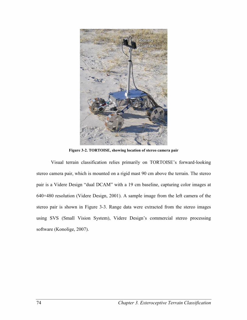
74 Chapter 3. Exteroceptive Terrain Classification
Figure 3-2. TORTOISE, showing location of stereo camera pair
Visual terrain classification relies primarily on TORTOISE’s forward-looking
stereo camera pair, which is mounted on a rigid mast 90 cm above the terrain. The stereo
pair is a Videre Design “dual DCAM” with a 19 cm baseline, capturing color images at
640×480 resolution (Videre Design, 2001). A sample image from the left camera of the
stereo pair is shown in Figure 3-3. Range data were extracted from the stereo images
using SVS (Small Vision System), Videre Design’s commercial stereo processing
software (Konolige, 2007).
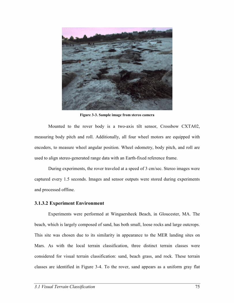
3.1 Visual Terrain Classification 75
Figure 3-3. Sample image from stereo camera
Mounted to the rover body is a two-axis tilt sensor, Crossbow CXTA02,
measuring body pitch and roll. Additionally, all four wheel motors are equipped with
encoders, to measure wheel angular position. Wheel odometry, body pitch, and roll are
used to align stereo-generated range data with an Earth-fixed reference frame.
During experiments, the rover traveled at a speed of 3 cm/sec. Stereo images were
captured every 1.5 seconds. Images and sensor outputs were stored during experiments
and processed offline.
3.1.3.2 Experiment Environment
Experiments were performed at Wingaersheek Beach, in Gloucester, MA. The
beach, which is largely composed of sand, has both small, loose rocks and large outcrops.
This site was chosen due to its similarity in appearance to the MER landing sites on
Mars. As with the local terrain classification, three distinct terrain classes were
considered for visual terrain classification: sand, beach grass, and rock. These terrain
classes are identified in Figure 3-4. To the rover, sand appears as a uniform gray flat
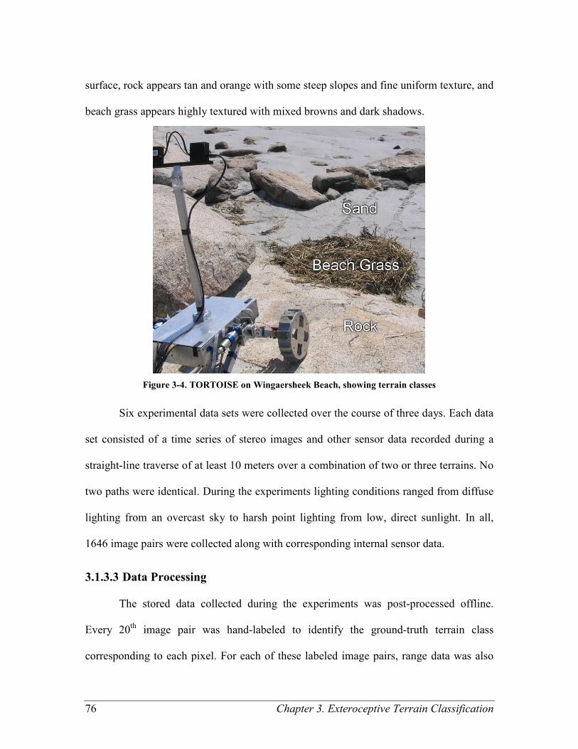
76 Chapter 3. Exteroceptive Terrain Classification
surface, rock appears tan and orange with some steep slopes and fine uniform texture, and
beach grass appears highly textured with mixed browns and dark shadows.
Figure 3-4. TORTOISE on Wingaersheek Beach, showing terrain classes
Six experimental data sets were collected over the course of three days. Each data
set consisted of a time series of stereo images and other sensor data recorded during a
straight-line traverse of at least 10 meters over a combination of two or three terrains. No
two paths were identical. During the experiments lighting conditions ranged from diffuse
lighting from an overcast sky to harsh point lighting from low, direct sunlight. In all,
1646 image pairs were collected along with corresponding internal sensor data.
3.1.3.3 Data Processing
The stored data collected during the experiments was post-processed offline.
Every 20th
image pair was hand-labeled to identify the ground-truth terrain class
corresponding to each pixel. For each of these labeled image pairs, range data was also

3.1 Visual Terrain Classification 77
calculated. By combining the labels with the range data, ground-truth terrain classes were
identified for each 20-cm by 20-cm terrain cell. For each of the six data sets, between 10
and 27 image pairs were hand labeled. The first two or three image pairs from each data
set were used for training the classifiers, with the remaining images used for testing. Note
that separate classifiers were trained and tested for each data set.
3.1.4 Results
The accuracy of the visual terrain classifier was assessed for each of the data sets
described in 3.1.3. Figure 3-5 shows the receiver operating characteristic (ROC) curves
for a representative data set. Here the horizontal axis indicates the false positive
percentage (%FP) and the vertical axis indicates the true positive percentage (%TP). Each
terrain forms a curve on the plot as the threshold for leaving terrain “unclassified” is
adjusted. The end point of the curves represents the case in which none of the terrain is
left unclassified. Any combination of points on these curves can be achieved through
proper selection of the threshold. Note that the scale of the x-axis is magnified to allow
the curves to be easily seen.
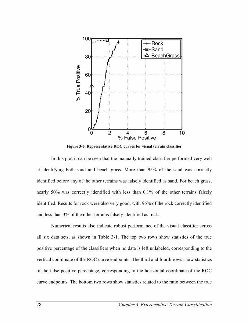
78 Chapter 3. Exteroceptive Terrain Classification
0 2 4 6 8 100
20
40
60
80
100
% False Positive
% T
rue P
ositiv
e
RockSandBeachGrass
Figure 3-5. Representative ROC curves for visual terrain classifier
In this plot it can be seen that the manually trained classifier performed very well
at identifying both sand and beach grass. More than 95% of the sand was correctly
identified before any of the other terrains was falsely identified as sand. For beach grass,
nearly 50% was correctly identified with less than 0.1% of the other terrains falsely
identified. Results for rock were also very good, with 96% of the rock correctly identified
and less than 3% of the other terrains falsely identified as rock.
Numerical results also indicate robust performance of the visual classifier across
all six data sets, as shown in Table 3-1. The top two rows show statistics of the true
positive percentage of the classifiers when no data is left unlabeled, corresponding to the
vertical coordinate of the ROC curve endpoints. The third and fourth rows show statistics
of the false positive percentage, corresponding to the horizontal coordinate of the ROC
curve endpoints. The bottom two rows show statistics related to the ratio between the true
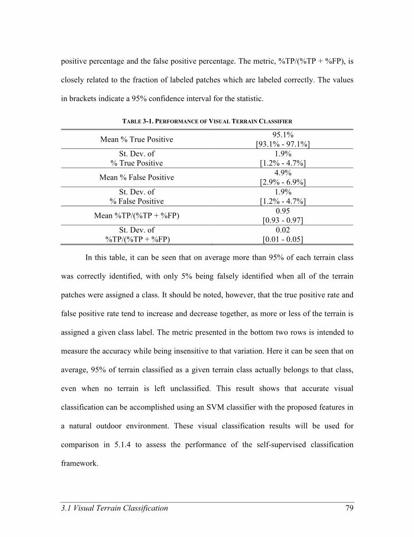
3.1 Visual Terrain Classification 79
positive percentage and the false positive percentage. The metric, %TP/(%TP + %FP), is
closely related to the fraction of labeled patches which are labeled correctly. The values
in brackets indicate a 95% confidence interval for the statistic.
TABLE 3-1. PERFORMANCE OF VISUAL TERRAIN CLASSIFIER
Mean % True Positive 95.1%
[93.1% - 97.1%]
St. Dev. of
% True Positive
1.9%
[1.2% - 4.7%]
Mean % False Positive 4.9%
[2.9% - 6.9%]
St. Dev. of
% False Positive
1.9%
[1.2% - 4.7%]
Mean %TP/(%TP + %FP) 0.95
[0.93 - 0.97]
St. Dev. of
%TP/(%TP + %FP)
0.02
[0.01 - 0.05]
In this table, it can be seen that on average more than 95% of each terrain class
was correctly identified, with only 5% being falsely identified when all of the terrain
patches were assigned a class. It should be noted, however, that the true positive rate and
false positive rate tend to increase and decrease together, as more or less of the terrain is
assigned a given class label. The metric presented in the bottom two rows is intended to
measure the accuracy while being insensitive to that variation. Here it can be seen that on
average, 95% of terrain classified as a given terrain class actually belongs to that class,
even when no terrain is left unclassified. This result shows that accurate visual
classification can be accomplished using an SVM classifier with the proposed features in
a natural outdoor environment. These visual classification results will be used for
comparison in 5.1.4 to assess the performance of the self-supervised classification
framework.
80 Chapter 3. Exteroceptive Terrain Classification
3.1.5 Conclusions
Section 1.1 has presented a method for classifying terrain based on visual
features. In this approach, a supervised framework is used to classify terrain based on
color, visual texture, and geometry, with the multiple sensory modes combined using
naïve Bayes fusion.
This approach was applied to experimental data collected with a four-wheeled
rover in an outdoor beach environment. Classification accuracy was assessed by
comparing the classifier results to hand-labeled ground truth data. These results
demonstrate that this visual classification approach can be used to accurately classify
natural outdoor terrain in real-world conditions.
This visual terrain classifier is appropriate for use in scenarios in which labeled
examples of all terrain classes are available for training. As described in the introduction
to this chapter, it can also be used as a component of a more general vision system,
capable of classifying terrain in the presence of unexpected terrain classes. The results
presented in this section are also useful as a baseline for comparison to the self-
supervised classification results presented in Chapter 5.
3.2 Visual Detection of Novel Terrain
3.2.1 Introduction
In the planetary exploration scenario, situations often occur when a robot
encounters a terrain patch belonging to a class it wasn’t trained to recognize. A traditional
supervised visual classifier like the one described in 1.1 would assume that the terrain
patch belonged to one of the known classes, then make an incorrect class prediction. For
instance, if a classifier has only learned to recognize safely traversable terrain classes, it

3.2 Visual Detection of Novel Terrain 81
would predict that all terrain patches are traversable, potentially jeopardizing the safety of
the robot. If the novel terrain represented something of scientific interest, failure to
identify it could result in a missed scientific opportunity. The purpose of the novel terrain
detection algorithm is to identify terrain patches that lie outside the set of known classes
and thus represent a previously unobserved class. This would allow appropriate caution
or interest to be taken by the rover.
The goal of a novel terrain detection algorithm is to distinguish between terrain
patches belonging to a set of a priori known terrain classes and terrain patches belonging
to an unknown “novel” class. This section presents an approach for detection of novel
terrain using color stereo imagery. It employs the same color, visual texture, and range-
derived geometric data features described in 1.1 as features for classification.
The innovation of this approach is the use of a two-class classifier for novelty
detection. While novelty detection algorithms have been developed for scenarios in
which the only available training data is associated with the known classes, this approach
is intended for scenarios in which an additional set of unlabeled data is also available for
training. In the planetary exploration scenario, terrain patches associated with the known
terrain classes may be identified autonomously using the proprioceptive terrain
classification techniques described in Chapter 2. This approach takes advantage of the
availability of unlabeled visual data11
to improve the accuracy of novel terrain detection.
The use of unlabeled data was inspired by the work of (El-Yaniv & Nisenson, 2007) on
optimal single-class classification strategies. Because no hand-labeling of visual data is
11
Here, unlabeled visual data can be visual data associated with any terrain patch that hasn’t been
autonomously classified using other sensors. If proprioceptive sensors are used for this autonomous
classification, then visual data of terrain patches not sensed proprioceptively are unlabeled.
82 Chapter 3. Exteroceptive Terrain Classification
required, this approach is appropriate for detection of novel terrain without a human in
the loop.
Section 3.1.2 describes the two-class classification approach to novelty detection,
as well as two baseline approaches which will be used for performance comparison.
Section 3.2.3 gives details about the experiments conducted to analyze the performance
of the proposed approach, and section 3.2.4 presents the results of those experiments.
Section 3.2.5 presents conclusions and suggests directions for future research.
3.2.2 Approach
As described in the introduction, the goal of novel terrain detection is to
distinguish between terrain patches belonging to a set of a priori known terrain classes
and terrain patches belonging to an unknown “novel” class. This problem is distinct from
traditional two-class classification problems because labeled examples of the novel class
do not exist. Previously proposed approaches to novelty detection, such as those based on
a one-class SVM (Schölkopf, 2000) or distribution modeling (Bishop, 1995), are trained
using only labeled examples of known terrain classes. In the scenario considered here,
however, it is assumed that information is available about both the a priori known classes
and a “world” class, which is a mixture of both known and unknown classes. This
situation arises when only a subset of the terrain patches observed by the robot are
associated with known terrain classes.
For example, this occurs when terrain is labeled as “known” only after the robot
has come into physical contact with it, or when it is labeled based on exteroceptive sensor

3.2 Visual Detection of Novel Terrain 83
data12
available for only a small fraction of the observed terrain. The two-class
classification approach presented here uses a SVM classifier trained to distinguish known
classes from the world class, thereby implicitly identifying the novel class. For
comparison, baseline approaches based on a one-class SVM and a distribution model are
also presented in section 3.2.2.3.
3.2.2.1 Theoretical Justification
Justification for the proposed approach to novelty detection is based on a
comparison of an optimal novelty detector and an optimal two-class classifier in the
scenario when the probability density functions of all classes are known. This analysis
shows that the novelty detector and a two-class classifier can identify the same regions
associated with the novel and known classes.
In the following analysis, it is assumed that the world class, W, represents a
mixture of all of the terrains in the environment. W is composed of two disjoint classes: A
(known terrain), and B (novel terrain). Any patch of terrain will belong to A or B, but not
both. In this hypothetical scenario, it is assumed that the probability density functions
associated with A and B are known. Here p(x|A) and p(x|B) represent the probability
density of a feature vector x occurring given that it is associated with terrain class A or B,
respectively.
In this scenario, the goal of novelty detection is to identify the region of the
feature space containing the largest fraction of B, while containing only a specified
fraction (r) of A, ideally zero. Thus, the novelty detection problem is posed as
12
The thermal emission spectrometer carried by the Mars Exploration Rovers represents one such
exteroceptive sensor, since each observation represents only a 20 mrad field of view (20 cm at a range of
10 m).

84 Chapter 3. Exteroceptive Terrain Classification
( ) ( ) p s.t. pmaxarg*
rdAdBND == ∫∫SS
SxxxxS ,
(3-31)
where S is a region of the feature space, and SND* is the region of the feature space
identified as novel. Note that r is the rate of false positives—instances when known
terrain is incorrectly identified as novel. In principle r can be set to zero, but if there
exists some x where both p(x|A)>0 and p(x|B)>0, increasing r will have the benefit of
increasing the detection rate of novel terrain, which may be desirable. The solution to the
novelty detection problem is
( ) ( ){ }BtAND xxxS pp:* ≤= , (3-32)
where t is found such that
( ) .p*
rdA
ND
=∫S
xx (3-33)
Here t is a monotonic function of r. This solution can be understood intuitively by
contradiction. If there is some region outside SND* where )|p()|p( BtA xx < , then the
fraction of B in SND* could be increased by changing SND
*. SND
* is unique as long as there
is no region of measure greater than zero where )|p()|p( BtA xx = .
In practice, there is no way to explicitly estimate the distribution of the novel
class, so p(x|B) cannot be used directly. Instead, we assume that it is possible to estimate
p(x|W), the probability density of the world class, which is given as
( ) ( ) ( )BAW xxx p)1(pp αα −+= . (3-34)
Here α is unknown, representing the fraction of A in W (i.e., the fraction of the rover’s
environment made up of known terrain). Using p(x|W), the A vs. W two-class
classification problem can be written as

3.2 Visual Detection of Novel Terrain 85
( ) ( ) p1pminarg
*
−+= ∫∫
SSS
xxxxS dWcdAc WAW , (3-35)
where the region SW* is the region of the feature space classified as the world class. Here
cA is the cost of misclassifying A as W, and cW is the cost of misclassifying W as A.
Equation (3-35) is the problem that traditional two class classifiers attempt to solve
without explicit definitions of p(x|A) and p(x|W). The solution to this two-class
classification problem in terms of p(x|A) and p(x|W) is
( ) ( )
≤= Wc
cA
A
W
W xxxS pp:*
. (3-36)
Written in terms of p(x|A) and p(x|B), this becomes
( ) ( ) ( )
−
−≤= B
cc
cA
wA
W
W xxxS p1
p:*
αα
. (3-37)
Thus it can be seen that SND* and SW
* are both defined as regions where p(x|A) is less than
some factor multiplied by p(x|B). Without knowledge of α or p(x|B), cA and cW can be
found from (3-36) such that
( ) p*
rdA
W
=∫S
xx . (3-38)
With these values of cA and cW, SND* and SW
* are identical. Thus, it follows that a two-
class classifier distinguishing the known class, A, from the world class, W, can be used
for detection of the novel class, B.
3.2.2.2 Detailed Approach
The proposed two-class classification approach employs a support vector machine
to classify terrain based on visual features. This section describes the visual features, the
classification algorithm, and the training process.

86 Chapter 3. Exteroceptive Terrain Classification
3.2.2.2.1 Visual Features
The representation of the terrain color, visual texture, and geometric features is
identical to that described for the visual classifier in 3.1.2.1, and their description is
repeated here for completeness. These features are all extracted from color images
collected using a stereo pair.
Color data is directly available from the cameras as red, green, and blue (RGB)
intensities. However, the illumination intensity affects all three values in a raw RGB
representation, which can lead to poor classification results. To reduce the effect of the
overall illumination level, a modified hue, saturation, and value (HSV) representation of
color is used as in (Sofman et al., 2006). In this approach, hue (an angle) is represented as
two values—sin(hue) and cos(hue)—to eliminate the artificial discontinuity at 2π. Thus,
color is represented as a 4-element vector: [sin(hue), cos(hue), saturation, value].
Visual texture is a measure of the local spatial variation in the intensity of an
image. Researchers have proposed many metrics for visual texture, such as Gabor filters
and local energy methods (Bouman & Liu, 1991; Reed & du Buf, 1993). The work in this
thesis uses a wavelet-based approach, similar to the one demonstrated in (Espinal et al.,
1998). Here, a grayscale image is decomposed with the Haar wavelet (Strang, 1993).
Three scales of wavelets are used, each scale having horizontal, diagonal, and vertical
wavelets, corresponding to estimating the derivative of the intensity in the horizontal,
diagonal, and vertical directions at each length scale. The scales used are 2, 4, and 8
pixels. Because this process is sensitive to local changes in intensity, the magnitudes of
the wavelet coefficients are then averaged over windows of 11, 9, and 7 wavelets. Thus,
visual texture is represented by a 9-element vector, composed of the window-averaged

3.2 Visual Detection of Novel Terrain 87
horizontal, diagonal, and vertical wavelet coefficients at each scale. The process of
calculating these visual texture coefficients from an image is presented in 3.1.2.1.2.
Terrain geometry is available through stereo image processing. The raw output of
a stereo processing algorithm is a cloud of range data points. Here, the points are divided
into a grid of 20-cm by 20-cm terrain patches projected onto a horizontal plane. The
geometric features are statistics calculated from the elevation of points associated with
each terrain patch. Here, the n points associated with a given terrain patch are represented
as a n × 3 matrix denoting each point’s position in the [forward, right, down] coordinate
frame with its origin at the rover’s starting position: {p1,…,pn}T. The first element of the
geometric feature vector is the average slope of the terrain, defined as the angle φ
between the least-squares-fit plane and the horizontal plane, in radians. The second
element is the mean-squared deviation from that plane along its normal, 2σ⊥ . The third
element is the variance in the height of the range data points, 2σ z . The fourth element is
the height difference between the highest and lowest points within the patch, rz. Thus, the
geometry of each patch is represented as a 4-element vector: [φ, 2σ⊥ , 2σ z , rz]. These
features were chosen based on the work of Halatci who used a similar feature set for
classification of terrain in images collected by the Mars Exploration Rovers (Halatci et
al., 2008). Equations showing how these features can be calculated from the matrix of
points is presented in 3.1.2.1.3.
For the two-class classification approach, the visual features associated with
color, visual texture, and geometry are concatenated into a single feature vector for each
pixel. This combined feature vector has 17 elements. The first four elements of the
combined feature vector are the color features associated with the pixel. The next nine
88 Chapter 3. Exteroceptive Terrain Classification
elements of the combined feature vector are the texture features associated with the pixel.
The last four elements of the combined feature vector are the geometry features
associated with the terrain patch to which the pixel corresponds. Note that while the color
and visual texture features are distinct for each pixel, the geometric feature vectors are
identical for all pixels in the same terrain patch.
3.2.2.2.2 Classification Algorithm
As with the previously presented classifiers, the support vector machine was
implemented using the open-source library LIBSVM (Chang & C. Lin, 2005, 2008). For
novelty detection, a Gaussian radial basis function (RBF) kernel13
was used, with
parameters optimized by cross-validation over a subset of the images used for training.
(The optimized parameters were C=1, γ=1, and cW/ cA =0.05.)
Terrain classification was performed on the same grid of 20-cm by 20-cm terrain
patches used for the geometric feature extraction. Multiple pixels in an image can
correspond to the same terrain patch, and the concatenated color-texture-geometry feature
vector associated with each pixel is classified separately by the support vector machine.
The classification result for a patch is calculated by a majority vote of the individual pixel
classification results. Thus, for each pixel (i, j) associated with a patch P, the support
vector machine yields a predicted terrain class Ci,j, and the terrain class CP associated
with terrain patch P, is calculated as
( )∑=Pji
jiC
P CCisequalCin ),(
,,maxarg . (3-39)
13
The radial basis function kernel and other kernels are described in detail in Appendix D.
3.2 Visual Detection of Novel Terrain 89
3.2.2.2.3 Classifier Training
Training of the two-class classifier requires two sets of data: one set which
represents terrain of known classes, and one set of unlabeled data which represents terrain
of all (known and unknown) classes. Four hundred pixels are used to represent the known
class for training, and two thousand pixels are used to represent the world class for
training. The feature vectors associated with these pixels are used to train the two-class
SVM. These values (400 known pixels and 2000 world pixels) were selected to balance
the competing requirements of computation cost and classification accuracy.14
3.2.2.3 Baseline Approaches
To assess the performance of the proposed two-class classification approach to
detection of novel terrain, it was compared to two existing approaches: one-class SVM
and mixture-of-Gaussians distribution modeling.
3.2.2.3.1 One-Class SVM Approach
The one-class SVM, described in (Schölkopf et al., 2001), is a classification
framework designed to segment a feature space into “same” and “different” classes.
While a traditional two-class SVM operates by finding the hyperplane with the largest
margin separating two classes in a Hilbert space, the one-class SVM operates by finding
the hyperplane with the largest margin separating the “same” class from the origin in that
Hilbert space.
As with the proposed two-class SVM novelty detector, the one-class SVM was
implemented using LIBSVM. Again, a Gaussian RBF kernel was used. Parameters of the
14
Analysis of the performance of the proposed novelty detection approach with more or fewer training
points suggested that further increasing the number of training points might increase the accuracy of
novelty detection, though this would increase the computational cost.
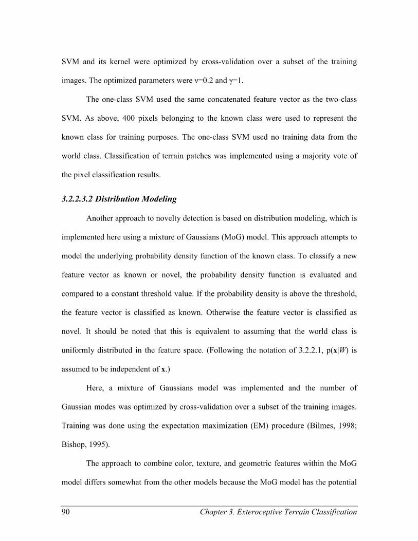
90 Chapter 3. Exteroceptive Terrain Classification
SVM and its kernel were optimized by cross-validation over a subset of the training
images. The optimized parameters were ν=0.2 and γ=1.
The one-class SVM used the same concatenated feature vector as the two-class
SVM. As above, 400 pixels belonging to the known class were used to represent the
known class for training purposes. The one-class SVM used no training data from the
world class. Classification of terrain patches was implemented using a majority vote of
the pixel classification results.
3.2.2.3.2 Distribution Modeling
Another approach to novelty detection is based on distribution modeling, which is
implemented here using a mixture of Gaussians (MoG) model. This approach attempts to
model the underlying probability density function of the known class. To classify a new
feature vector as known or novel, the probability density function is evaluated and
compared to a constant threshold value. If the probability density is above the threshold,
the feature vector is classified as known. Otherwise the feature vector is classified as
novel. It should be noted that this is equivalent to assuming that the world class is
uniformly distributed in the feature space. (Following the notation of 3.2.2.1, p(x|W) is
assumed to be independent of x.)
Here, a mixture of Gaussians model was implemented and the number of
Gaussian modes was optimized by cross-validation over a subset of the training images.
Training was done using the expectation maximization (EM) procedure (Bilmes, 1998;
Bishop, 1995).
The approach to combine color, texture, and geometric features within the MoG
model differs somewhat from the other models because the MoG model has the potential
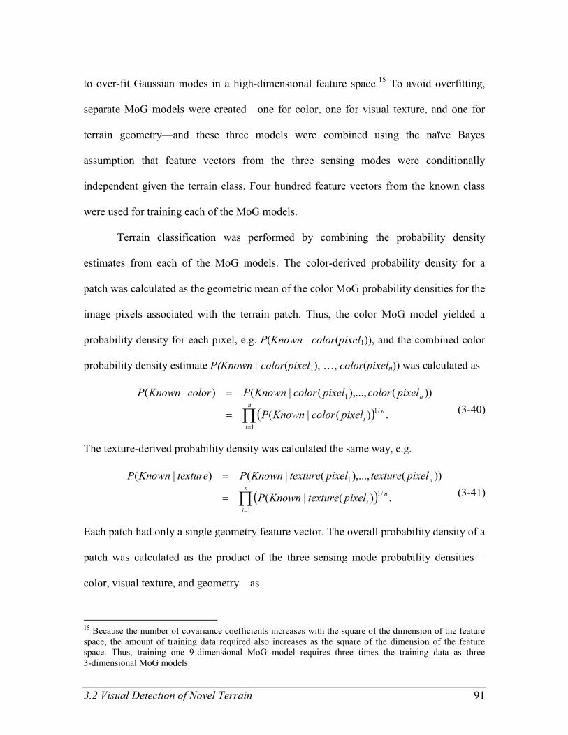
3.2 Visual Detection of Novel Terrain 91
to over-fit Gaussian modes in a high-dimensional feature space.15
To avoid overfitting,
separate MoG models were created—one for color, one for visual texture, and one for
terrain geometry—and these three models were combined using the naïve Bayes
assumption that feature vectors from the three sensing modes were conditionally
independent given the terrain class. Four hundred feature vectors from the known class
were used for training each of the MoG models.
Terrain classification was performed by combining the probability density
estimates from each of the MoG models. The color-derived probability density for a
patch was calculated as the geometric mean of the color MoG probability densities for the
image pixels associated with the terrain patch. Thus, the color MoG model yielded a
probability density for each pixel, e.g. P(Known | color(pixel1)), and the combined color
probability density estimate P(Known | color(pixel1), …, color(pixeln)) was calculated as
( )∏=
=
=n
i
n
i
n
pixelcolorKnownP
pixelcolorpixelcolorKnownPcolorKnownP
1
/1
1
.)(|(
))(),...,(|()|(
(3-40)
The texture-derived probability density was calculated the same way, e.g.
( )∏=
=
=n
i
n
i
n
pixeltextureKnownP
pixeltexturepixeltextureKnownPtextureKnownP
1
/1
1
.)(|(
))(),...,(|()|(
(3-41)
Each patch had only a single geometry feature vector. The overall probability density of a
patch was calculated as the product of the three sensing mode probability densities—
color, visual texture, and geometry—as
15
Because the number of covariance coefficients increases with the square of the dimension of the feature
space, the amount of training data required also increases as the square of the dimension of the feature
space. Thus, training one 9-dimensional MoG model requires three times the training data as three
3-dimensional MoG models.
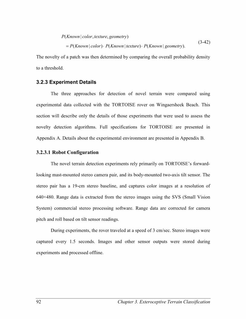
92 Chapter 3. Exteroceptive Terrain Classification
).|()|()|(
),,|(
geometryKnownPtextureKnownPcolorKnownP
geometrytexturecolorKnownP
⋅⋅= (3-42)
The novelty of a patch was then determined by comparing the overall probability density
to a threshold.
3.2.3 Experiment Details
The three approaches for detection of novel terrain were compared using
experimental data collected with the TORTOISE rover on Wingaersheek Beach. This
section will describe only the details of those experiments that were used to assess the
novelty detection algorithms. Full specifications for TORTOISE are presented in
Appendix A. Details about the experimental environment are presented in Appendix B.
3.2.3.1 Robot Configuration
The novel terrain detection experiments rely primarily on TORTOISE’s forward-
looking mast-mounted stereo camera pair, and its body-mounted two-axis tilt sensor. The
stereo pair has a 19-cm stereo baseline, and captures color images at a resolution of
640×480. Range data is extracted from the stereo images using the SVS (Small Vision
System) commercial stereo processing software. Range data are corrected for camera
pitch and roll based on tilt sensor readings.
During experiments, the rover traveled at a speed of 3 cm/sec. Stereo images were
captured every 1.5 seconds. Images and other sensor outputs were stored during
experiments and processed offline.
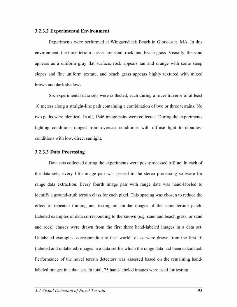
3.2 Visual Detection of Novel Terrain 93
3.2.3.2 Experimental Environment
Experiments were performed at Wingaersheek Beach in Gloucester, MA. In this
environment, the three terrain classes are sand, rock, and beach grass. Visually, the sand
appears as a uniform gray flat surface, rock appears tan and orange with some steep
slopes and fine uniform texture, and beach grass appears highly textured with mixed
brown and dark shadows.
Six experimental data sets were collected, each during a rover traverse of at least
10 meters along a straight-line path containing a combination of two or three terrains. No
two paths were identical. In all, 1646 image pairs were collected. During the experiments
lighting conditions ranged from overcast conditions with diffuse light to cloudless
conditions with low, direct sunlight.
3.2.3.3 Data Processing
Data sets collected during the experiments were post-processed offline. In each of
the data sets, every fifth image pair was passed to the stereo processing software for
range data extraction. Every fourth image pair with range data was hand-labeled to
identify a ground-truth terrain class for each pixel. This spacing was chosen to reduce the
effect of repeated training and testing on similar images of the same terrain patch.
Labeled examples of data corresponding to the known (e.g. sand and beach grass, or sand
and rock) classes were drawn from the first three hand-labeled images in a data set.
Unlabeled examples, corresponding to the “world” class, were drawn from the first 10
(labeled and unlabeled) images in a data set for which the range data had been calculated.
Performance of the novel terrain detectors was assessed based on the remaining hand-
labeled images in a data set. In total, 75 hand-labeled images were used for testing.

94 Chapter 3. Exteroceptive Terrain Classification
3.2.4 Results
The performance of the two-class classification approach was compared to that of
the baseline approaches for each test set. Figure 3-6 shows the ROC curve of the results
for each approach across all of the data sets. For this figure, the rock class was used as the
novel class.16
Thus, the labeled training data was drawn only from the sand and beach
grass classes. Here the vertical axis indicates the percentage of true novel detection
(%TN) (i.e., the fraction of rock terrain patches which were correctly identified as novel),
and the horizontal axis indicates the percentage of false novel detection (%FN) (i.e., the
fraction of sand or beach grass terrain patches which were incorrectly identified as
novel). Each detection approach forms a curve on the plot, since both %TN and %FN are
functions of the novelty detection threshold. Note that random assignment of terrain as
novel would tend to yield a diagonal line from (0,0) to (100,100). Better performance is
indicated by proximity of a curve to the upper-left corner of the plot.
16
In the Wingaersheek Beach data sets all three terrain classes were known a priori. To simulate the
presence of novel terrain, terrain patches corresponding to one of the classes—in this case, the rock class—
were intentionally removed from the set of labeled training examples.
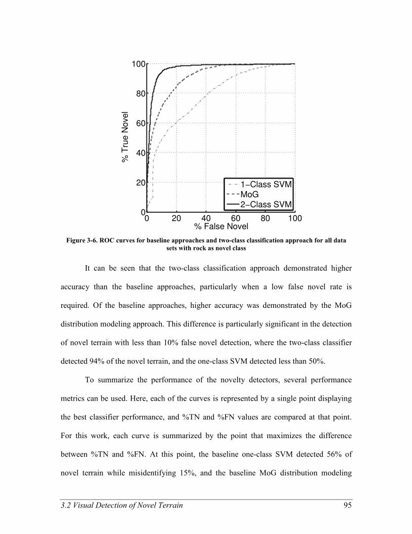
3.2 Visual Detection of Novel Terrain 95
0 20 40 60 80 1000
20
40
60
80
100
% False Novel
% T
rue N
ovel
1−Class SVMMoG2−Class SVM
Figure 3-6. ROC curves for baseline approaches and two-class classification approach for all data
sets with rock as novel class
It can be seen that the two-class classification approach demonstrated higher
accuracy than the baseline approaches, particularly when a low false novel rate is
required. Of the baseline approaches, higher accuracy was demonstrated by the MoG
distribution modeling approach. This difference is particularly significant in the detection
of novel terrain with less than 10% false novel detection, where the two-class classifier
detected 94% of the novel terrain, and the one-class SVM detected less than 50%.
To summarize the performance of the novelty detectors, several performance
metrics can be used. Here, each of the curves is represented by a single point displaying
the best classifier performance, and %TN and %FN values are compared at that point.
For this work, each curve is summarized by the point that maximizes the difference
between %TN and %FN. At this point, the baseline one-class SVM detected 56% of
novel terrain while misidentifying 15%, and the baseline MoG distribution modeling
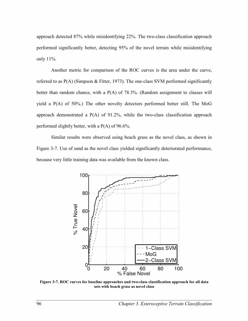
96 Chapter 3. Exteroceptive Terrain Classification
approach detected 87% while misidentifying 22%. The two-class classification approach
performed significantly better, detecting 95% of the novel terrain while misidentifying
only 11%.
Another metric for comparison of the ROC curves is the area under the curve,
referred to as P(A) (Simpson & Fitter, 1973). The one-class SVM performed significantly
better than random chance, with a P(A) of 78.3%. (Random assignment to classes will
yield a P(A) of 50%.) The other novelty detectors performed better still. The MoG
approach demonstrated a P(A) of 91.2%, while the two-class classification approach
performed slightly better, with a P(A) of 96.6%.
Similar results were observed using beach grass as the novel class, as shown in
Figure 3-7. Use of sand as the novel class yielded significantly deteriorated performance,
because very little training data was available from the known class.
0 20 40 60 80 1000
20
40
60
80
100
% False Novel
% T
rue N
ovel
1−Class SVMMoG2−Class SVM
Figure 3-7. ROC curves for baseline approaches and two-class classification approach for all data
sets with beach grass as novel class
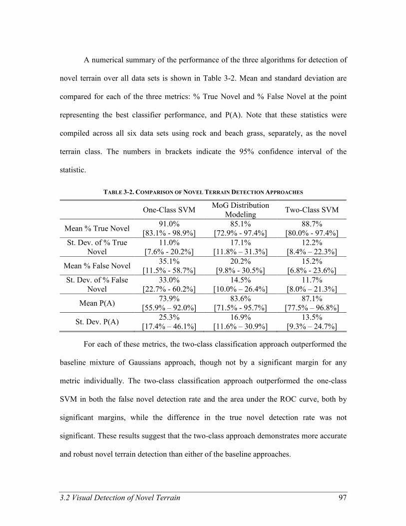
3.2 Visual Detection of Novel Terrain 97
A numerical summary of the performance of the three algorithms for detection of
novel terrain over all data sets is shown in Table 3-2. Mean and standard deviation are
compared for each of the three metrics: % True Novel and % False Novel at the point
representing the best classifier performance, and P(A). Note that these statistics were
compiled across all six data sets using rock and beach grass, separately, as the novel
terrain class. The numbers in brackets indicate the 95% confidence interval of the
statistic.
TABLE 3-2. COMPARISON OF NOVEL TERRAIN DETECTION APPROACHES
One-Class SVM MoG Distribution
Modeling Two-Class SVM
Mean % True Novel 91.0%
[83.1% - 98.9%]
85.1%
[72.9% - 97.4%]
88.7%
[80.0% - 97.4%]
St. Dev. of % True
Novel
11.0%
[7.6% - 20.2%]
17.1%
[11.8% – 31.3%]
12.2%
[8.4% – 22.3%]
Mean % False Novel 35.1%
[11.5% - 58.7%]
20.2%
[9.8% - 30.5%]
15.2%
[6.8% - 23.6%]
St. Dev. of % False
Novel
33.0%
[22.7% - 60.2%]
14.5%
[10.0% – 26.4%]
11.7%
[8.0% – 21.3%]
Mean P(A) 73.9%
[55.9% – 92.0%]
83.6%
[71.5% - 95.7%]
87.1%
[77.5% – 96.8%]
St. Dev. P(A) 25.3%
[17.4% – 46.1%]
16.9%
[11.6% – 30.9%]
13.5%
[9.3% – 24.7%]
For each of these metrics, the two-class classification approach outperformed the
baseline mixture of Gaussians approach, though not by a significant margin for any
metric individually. The two-class classification approach outperformed the one-class
SVM in both the false novel detection rate and the area under the ROC curve, both by
significant margins, while the difference in the true novel detection rate was not
significant. These results suggest that the two-class approach demonstrates more accurate
and robust novel terrain detection than either of the baseline approaches.
98 Chapter 3. Exteroceptive Terrain Classification
Computation time for classification using the two-class approach on a desktop
computer ranged from 12-70 seconds for a 640×480 image. Computation time varied
based on the complexity of the boundary between the known and novel classes (as
measured by the number of support vectors), and the fraction of the image with valid
range data.
3.2.5 Conclusions
This section has presented a two-class classification approach to novel terrain
detection. This approach uses samples of visual data from unlabeled images to represent
the world class for use in training a novel terrain detection algorithm. A theoretical
analysis showed the fundamental similarities between two-class classification and
novelty detection. Using experimental data from the TORTOISE rover on Wingaersheek
Beach, the two-class classification approach was compared to two baseline approaches
for novelty detection which use only data from known terrain classes during training. The
results suggests that the two-class classification approach achieves a higher accuracy than
the baseline approaches while reducing variability between data sets.
3.2.5.1 Future work
For a robot in rough terrain, the computational cost of novel terrain detection can
be significant, with the current approach taking 12-70 seconds per image on a modern
desktop computer. Computation time could likely be reduced by an order of magnitude or
more by replacing the Gaussian kernel of the SVM with a polynomial kernel.
Mathematical details of optimizing a SVM for use with a polynomial kernel are presented
in Appendix D.

3.2 Visual Detection of Novel Terrain 99
Additionally, this two-class classification approach to novelty detection is not
restricted to the use of a SVM classification algorithm. Other two-class classification
algorithms, including those based on regularized least squares regression or Bayesian
logistic regression, may be used in the place of the SVM. Further experimental studies
would be necessary to determine whether one classification algorithm performs
significantly better than any other when used for novelty detection.
100 Chapter 4. Mechanical Terrain Characterization
Chapter
4 Chapter 4 Mechanical Terrain Characterization
The purpose of mechanical terrain characterization is to identify mechanical
properties associated with a particular terrain class from proprioceptive sensor data. In
this thesis, the mechanical properties of interest are measurable quantities that describe
the forces and torques acting between a rover wheel and the terrain. The mechanical
terrain characterization approach presented in this chapter establishes minimum and
maximum bounds on the net traction force available at a given terrain patch based on
observed rover wheel torque and sinkage when wheel slip is induced.
4.1 Introduction
Understanding the physical interaction between a planetary rover and the terrain it
is traversing is critical to predicting whether that terrain can be traversed safely. Some
types of terrain (e.g. loosely packed sand) are treacherous to traverse on even shallow
slopes, as significant wheel sinkage may occur, leading to high motion resistance and
rover entrapment. Other terrain types (e.g., textured rock) present a solid footing on
which a rover might safely climb steep slopes. The purpose of mechanical terrain
characterization is to measure mechanical terrain properties that can be used to determine
whether a terrain patch may be safely traversed. This chapter is focused on the
101
characterization of deformable terrain under a rigid wheel, a scenario in which excessive
wheel slip could result in the wheel becoming trapped.
Previous researchers have taken various approaches to characterizing deformable
terrain. Bekker, Wong, and Reece developed parametric models for normal and shear
stress on wheels in deformable terrain that can be used to calculate the net forces and
torques on wheels (Bekker, 1969; Wong, 2001; Wong & Reece, 1967). In their models,
terrain is characterized by eight parameters. Measuring these parameters requires
dedicated equipment to apply normal and shear forces and measure the corresponding
displacements. Iagnemma developed an approach to measure the parameters of a
reduced-order Bekker model without dedicated terrain sensing equipment, by measuring
wheel torque and sinkage during a rover traverse (Iagnemma et al., 2002; Iagnemma et
al., 2004). Kang extended that work and proposed a nondimensionalized metric based on
drawbar pull—the drag force that would be required to hold the vehicle stationary—as a
traversability metric (Iagnemma et al., 2003; Kang, 2003). This metric, the drawbar pull
divided by the vertical load, represents the available net traction force as a fraction of the
weight on a wheel. Analyzing simulations over a variety of terrains Kang found an
approximate equation for drawbar pull as a function of wheel sinkage, wheel torque and
vertical load. However, while Kang’s predictions of drawbar pull accurately approximate
the predictions of the Bekker model when averaged over many terrains, he provided no
guarantees about the error of any single drawbar pull prediction.
In the field of planetary exploration, overly optimistic predictions related to the
traversability of terrain can lead to catastrophic failure. This chapter presents a novel,
optimization-based method for predicting strict upper and lower bounds on Kang’s
102 Chapter 4. Mechanical Terrain Characterization
traversability metric for a terrain patch, such that if the terrain model assumptions are
correct, the traversability metric is guaranteed to fall between the bounds. By providing
bounds on the traversability metric, this approach serves as a method for characterizing
terrain traversability in potentially high-risk scenarios.
4.2 Approach
The terrain characterization approach proposed here attempts to find upper and
lower bounds on Kang’s nondimensionalized drawbar pull traversability metric for a
given patch of terrain, without requiring that drawbar pull be measured directly. This is
accomplished by using constrained optimization to combine a terrain model with
observed wheel-terrain interaction measurements, specifically wheel torque and sinkage.
Section 4.2.1 describes the nondimensionalized drawbar pull measure which is used as
the traversability metric, section 4.2.2 describes the specific attributes of terrain
interaction being sensed, section 4.2.3 describes the wheel-terrain interaction models, and
section 4.2.4 describes the optimization method as it applies to each model.
4.2.1 Traversability Metric
The traversability metric used here for terrain characterization is the
nondimensionalized drawbar pull, DP/W, which is a measure of the net available traction
force between the wheel and the terrain. The net traction force can be modeled via
lumped forces acting on a single, rigid wheel, as shown in Figure 4-1. In this figure, the
wheel is traveling from left to right and rotating clockwise. Forces and torques on the
axle are shown, assuming the wheel to be in equilibrium. Here, W is the vertical load on
the wheel (including its own weight), T is the torque exerted on the wheel by a drive
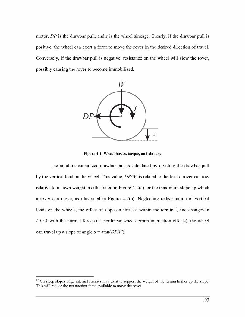
103
motor, DP is the drawbar pull, and z is the wheel sinkage. Clearly, if the drawbar pull is
positive, the wheel can exert a force to move the rover in the desired direction of travel.
Conversely, if the drawbar pull is negative, resistance on the wheel will slow the rover,
possibly causing the rover to become immobilized.
Figure 4-1. Wheel forces, torque, and sinkage
The nondimensionalized drawbar pull is calculated by dividing the drawbar pull
by the vertical load on the wheel. This value, DP/W, is related to the load a rover can tow
relative to its own weight, as illustrated in Figure 4-2(a), or the maximum slope up which
a rover can move, as illustrated in Figure 4-2(b). Neglecting redistribution of vertical
loads on the wheels, the effect of slope on stresses within the terrain17
, and changes in
DP/W with the normal force (i.e. nonlinear wheel-terrain interaction effects), the wheel
can travel up a slope of angle α = atan(DP/W).
17
On steep slopes large internal stresses may exist to support the weight of the terrain higher up the slope.
This will reduce the net traction force available to move the rover.
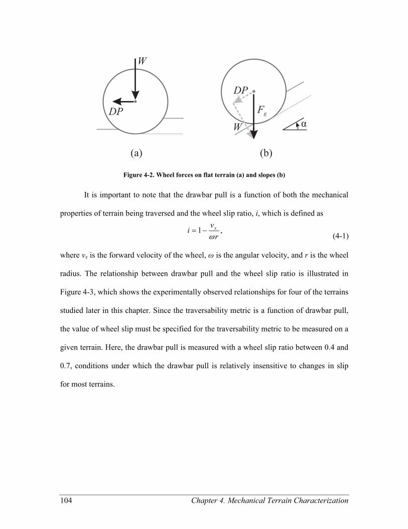
104 Chapter 4. Mechanical Terrain Characterization
Figure 4-2. Wheel forces on flat terrain (a) and slopes (b)
It is important to note that the drawbar pull is a function of both the mechanical
properties of terrain being traversed and the wheel slip ratio, i, which is defined as
r
vi x
ω−= 1 ,
(4-1)
where vx is the forward velocity of the wheel, ω is the angular velocity, and r is the wheel
radius. The relationship between drawbar pull and the wheel slip ratio is illustrated in
Figure 4-3, which shows the experimentally observed relationships for four of the terrains
studied later in this chapter. Since the traversability metric is a function of drawbar pull,
the value of wheel slip must be specified for the traversability metric to be measured on a
given terrain. Here, the drawbar pull is measured with a wheel slip ratio between 0.4 and
0.7, conditions under which the drawbar pull is relatively insensitive to changes in slip
for most terrains.
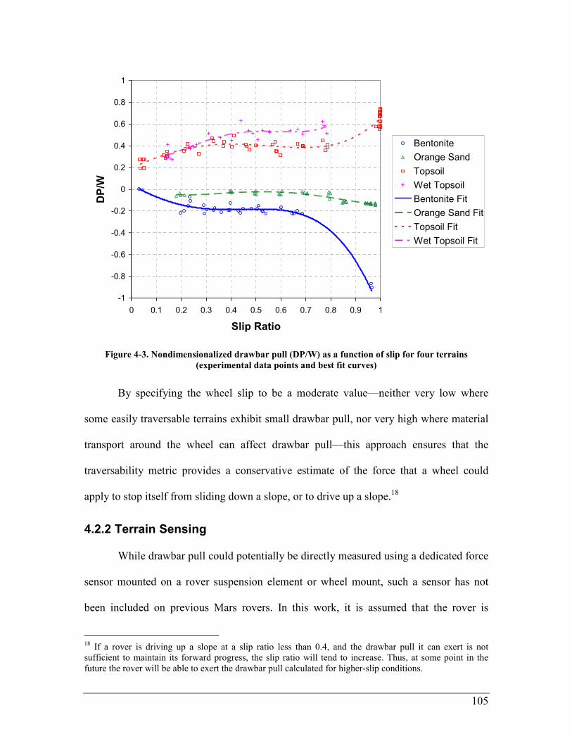
105
-1
-0.8
-0.6
-0.4
-0.2
0
0.2
0.4
0.6
0.8
1
0 0.1 0.2 0.3 0.4 0.5 0.6 0.7 0.8 0.9 1
Slip Ratio
DP/W
Bentonite
Orange Sand
Topsoil
Wet Topsoil
Bentonite Fit
Orange Sand Fit
Topsoil Fit
Wet Topsoil Fit
Figure 4-3. Nondimensionalized drawbar pull (DP/W) as a function of slip for four terrains
(experimental data points and best fit curves)
By specifying the wheel slip to be a moderate value—neither very low where
some easily traversable terrains exhibit small drawbar pull, nor very high where material
transport around the wheel can affect drawbar pull—this approach ensures that the
traversability metric provides a conservative estimate of the force that a wheel could
apply to stop itself from sliding down a slope, or to drive up a slope.18
4.2.2 Terrain Sensing
While drawbar pull could potentially be directly measured using a dedicated force
sensor mounted on a rover suspension element or wheel mount, such a sensor has not
been included on previous Mars rovers. In this work, it is assumed that the rover is
18
If a rover is driving up a slope at a slip ratio less than 0.4, and the drawbar pull it can exert is not
sufficient to maintain its forward progress, the slip ratio will tend to increase. Thus, at some point in the
future the rover will be able to exert the drawbar pull calculated for higher-slip conditions.

106 Chapter 4. Mechanical Terrain Characterization
equipped with a torque sensor on (at least) one driven wheel. The ability to measure
wheel sinkage is also assumed.
Here two different sinkage measurement capabilities are considered: absolute and
relative sinkage measurement, illustrated in Figure 4-4. Absolute sinkage measurement
refers to the ability to measure the distance between the undisturbed soil surface and the
lowest point on the wheel, at a single (specified) wheel slip ratio, as illustrated in Figure
4-4(a). This measurement could be attained using a camera with a view of the side of the
wheel, or by a dedicated sinkage sensor (Brooks et al., 2006; Reina et al., 2006).
Figure 4-4. Absolute sinkage (a) vs. relative sinkage (b)
The alternative to absolute sinkage measurement is relative sinkage measurement,
which is the ability to measure the difference in the vertical position of the wheel at two
different slip ratios, as illustrated in Figure 4-4(b). On flat terrain, this could be
accomplished using only proprioceptive sensors that measure the suspension
configuration, as in (Wilcox, 1994).
Since the drawbar pull is evaluated under slip conditions, wheel torque and
sinkage must be measured while the wheel is slipping. Here, wheel slip is induced by
driving one wheel faster than the others, as in the behaviors presented in 2.2.2.

107
4.2.3 Terrain Models
A terrain model is used to relate observed wheel sinkage and torque to a predicted
drawbar pull. Here two different terrain models are presented: a contact region model,
which can describe most plausible interaction states with rigid or deformable terrain; and
a Bekker model, which closely approximates the behavior of many real-world deformable
terrains. Results for both these models will be shown in 4.4.
4.2.3.1 Contact Region Model
The contact region model described here is a highly nonrestrictive model for
wheel terrain interaction. This model is depicted in Figure 4-5. Given an angle θ from the
vertical, wheel terrain interaction forces are modeled as a normal stress distribution σ(θ)
and a tangential stress distribution τ(θ) that act within a contact region between θ1 and θ2.
The only constraint on the stresses is that they must be non-negative—that is, the soil
cannot apply tension, and the tangential stress must always oppose the net applied wheel
torque.
Figure 4-5. Contact Region model
To compute the net forces applied to the wheel by the terrain, these stresses are
integrated over the contact region:
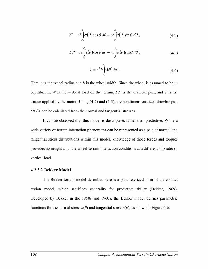
108 Chapter 4. Mechanical Terrain Characterization
( ) ( )∫∫ +=
1
2
1
2
sincos
θ
θ
θ
θ
θθθτθθθσ dbrdbrW , (4-2)
( ) ( )∫∫ −=
1
2
1
2
sincos
θ
θ
θ
θ
θθθσθθθτ dbrdbrDP , (4-3)
( )∫=
1
2
2
θ
θ
θθτ dbrT . (4-4)
Here, r is the wheel radius and b is the wheel width. Since the wheel is assumed to be in
equilibrium, W is the vertical load on the terrain, DP is the drawbar pull, and T is the
torque applied by the motor. Using (4-2) and (4-3), the nondimensionalized drawbar pull
DP/W can be calculated from the normal and tangential stresses.
It can be observed that this model is descriptive, rather than predictive. While a
wide variety of terrain interaction phenomena can be represented as a pair of normal and
tangential stress distributions within this model, knowledge of those forces and torques
provides no insight as to the wheel-terrain interaction conditions at a different slip ratio or
vertical load.
4.2.3.2 Bekker Model
The Bekker terrain model described here is a parameterized form of the contact
region model, which sacrifices generality for predictive ability (Bekker, 1969).
Developed by Bekker in the 1950s and 1960s, the Bekker model defines parametric
functions for the normal stress σ(θ) and tangential stress τ(θ), as shown in Figure 4-6.

109
Figure 4-6. Bekker terrain model
The equation describing the normal stress function is as follows:
( ) ( )( )nc rrkb
k1
* coscos θθθθσ φ −
+= , (4-5)
using
( ) ( )
≤−−
−−
≥=
m
m
m
m
θθθθθθθθ
θ
θθθθθ
for
for
2
2
1
1
* , (4-6)
( ) 121 θθ iccm += , (4-7)
and the equation describing the shear stress equation is as follows:
( ) ( )( ) ( )
−−+=K
jc
θφθσθτ exp1tan , (4-8)
using
( ) ( )( )( )θθθθθ sinsin1 11 −−−−= irj . (4-9)
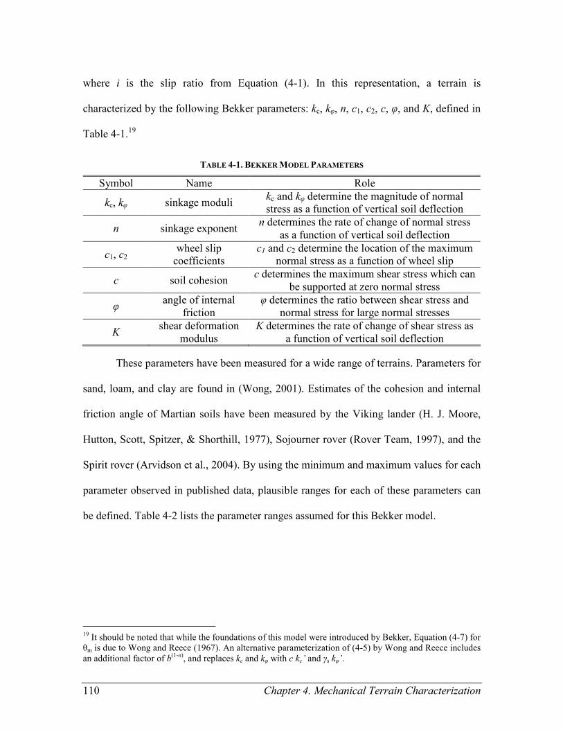
110 Chapter 4. Mechanical Terrain Characterization
where i is the slip ratio from Equation (4-1). In this representation, a terrain is
characterized by the following Bekker parameters: kc, kφ, n, c1, c2, c, φ, and K, defined in
Table 4-1.19
TABLE 4-1. BEKKER MODEL PARAMETERS
Symbol Name Role
kc, kφ sinkage moduli kc and kφ determine the magnitude of normal
stress as a function of vertical soil deflection
n sinkage exponent n determines the rate of change of normal stress
as a function of vertical soil deflection
c1, c2 wheel slip
coefficients
c1 and c2 determine the location of the maximum
normal stress as a function of wheel slip
c soil cohesion c determines the maximum shear stress which can
be supported at zero normal stress
φ angle of internal
friction
φ determines the ratio between shear stress and
normal stress for large normal stresses
K shear deformation
modulus
K determines the rate of change of shear stress as
a function of vertical soil deflection
These parameters have been measured for a wide range of terrains. Parameters for
sand, loam, and clay are found in (Wong, 2001). Estimates of the cohesion and internal
friction angle of Martian soils have been measured by the Viking lander (H. J. Moore,
Hutton, Scott, Spitzer, & Shorthill, 1977), Sojourner rover (Rover Team, 1997), and the
Spirit rover (Arvidson et al., 2004). By using the minimum and maximum values for each
parameter observed in published data, plausible ranges for each of these parameters can
be defined. Table 4-2 lists the parameter ranges assumed for this Bekker model.
19
It should be noted that while the foundations of this model were introduced by Bekker, Equation (4-7) for
θm is due to Wong and Reece (1967). An alternative parameterization of (4-5) by Wong and Reece includes
an additional factor of b(1-n)
, and replaces kc and kφ with c kc’ and γs kφ’.
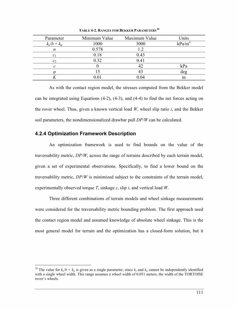
111
TABLE 4-2. RANGES FOR BEKKER PARAMETERS 20
Parameter Minimum Value Maximum Value Units
kc/b + kφ 1000 3000 kPa/mn
n 0.578 1.2
c1 0.18 0.43
c2 0.32 0.41
c 0 42 kPa
φ 15 43 deg
K 0.01 0.04 m
As with the contact region model, the stresses computed from the Bekker model
can be integrated using Equations (4-2), (4-3), and (4-4) to find the net forces acting on
the rover wheel. Thus, given a known vertical load W, wheel slip ratio i, and the Bekker
soil parameters, the nondimensionalized drawbar pull DP/W can be calculated.
4.2.4 Optimization Framework Description
An optimization framework is used to find bounds on the value of the
traversability metric, DP/W, across the range of terrains described by each terrain model,
given a set of experimental observations. Specifically, to find a lower bound on the
traversability metric, DP/W is minimized subject to the constraints of the terrain model,
experimentally observed torque T, sinkage z, slip i, and vertical load W.
Three different combinations of terrain models and wheel sinkage measurements
were considered for the traversability metric bounding problem. The first approach used
the contact region model and assumed knowledge of absolute wheel sinkage. This is the
most general model for terrain and the optimization has a closed-form solution, but it
20
The value for kc/b + kφ is given as a single parameter, since kc and kφ cannot be independently identified
with a single wheel width. This range assumes a wheel width of 0.051 meters, the width of the TORTOISE
rover’s wheels.
112 Chapter 4. Mechanical Terrain Characterization
requires measurement of absolute wheel sinkage, which might not be possible in practical
scenarios.21
The second approach uses a Bekker terrain model and assumes knowledge of
relative wheel sinkage. This is a more restrictive model of the terrain compared to the
contact region model, but it is capable of predicting behavior at different slip conditions
and requires measurement of only the relative sinkage.
The third approach uses a Bekker terrain model and assumes knowledge of
absolute wheel sinkage. This again uses a relatively restrictive model and requires
measurement of absolute sinkage, but has the potential for prediction of tighter bounds on
the traversability metric compared to the other two approaches.
The following sections describe the optimization of each of the three approaches.
4.2.4.1 Contact Region Model with Absolute Sinkage
Due to the simplicity of the contact region model, upper and lower bounds on
DP/W can be written explicitly, assuming the absolute sinkage is known. Here the
optimization problems for the lower and upper bounds are posed as
21
Measurement of absolute sinkage can be accomplished as in (Brooks et al., 2006), but this approach
requires the presence of a camera with a view of the side of the wheel, sufficient illumination, and visual
contrast between the wheel rim and the terrain. Guaranteeing sufficient illumination would require the
addition of a light source to the rover. Other methods of measuring absolute wheel sinkage may require
additional hardware, such as laser or sonar range sensors.
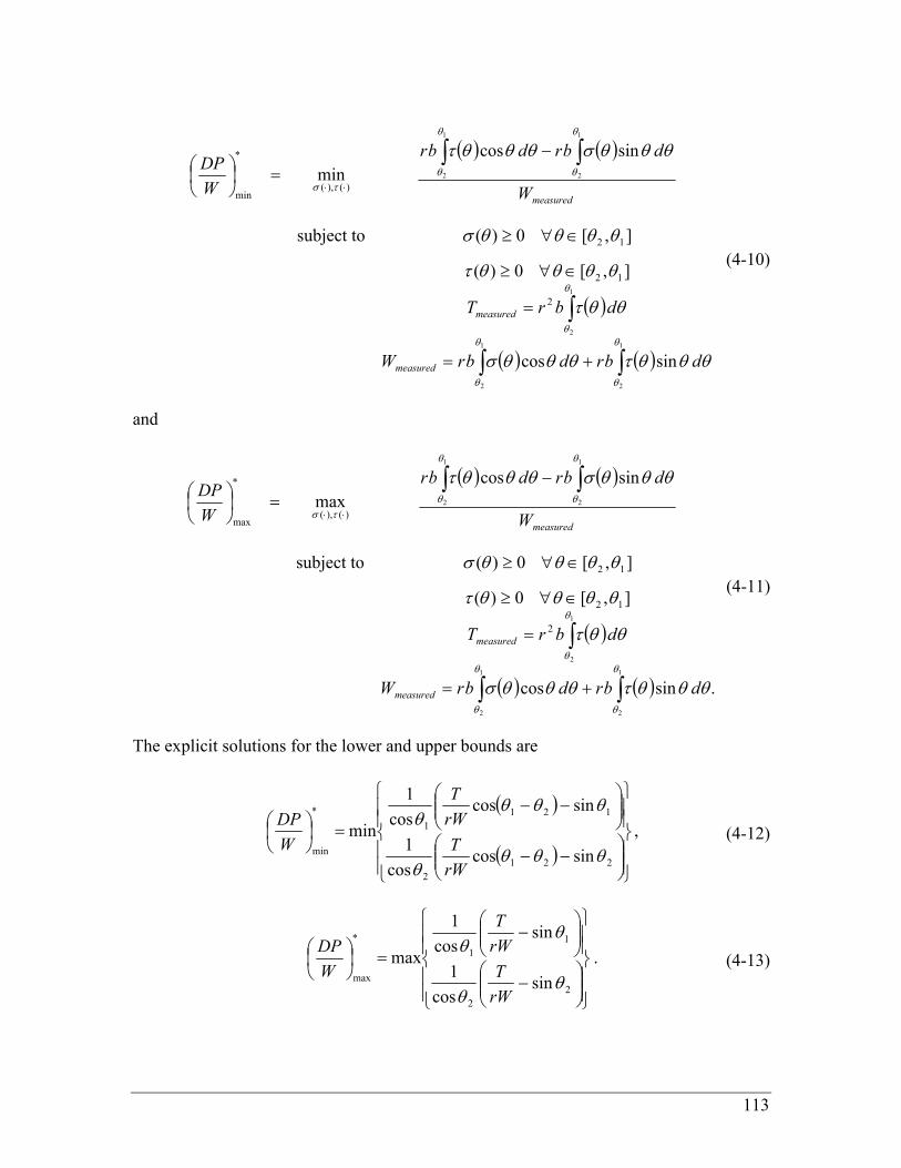
113
( ) ( )
( )
( ) ( )∫∫
∫
∫∫
+=
=
∈∀≥
∈∀≥
−=
⋅⋅
1
2
1
2
1
2
1
2
1
2
sincos
],[0)(
],[0)(subject to
sincos
min
2
12
12
)(),(
*
min
θ
θ
θ
θ
θ
θ
θ
θ
θ
θτσ
θθθτθθθσ
θθτ
θθθθτ
θθθθσ
θθθσθθθτ
dbrdbrW
dbrT
W
dbrdbr
W
DP
measured
measured
measured
(4-10)
and
( ) ( )
( )
( ) ( ) .sincos
],[0)(
],[0)(subject to
sincos
max
1
2
1
2
1
2
1
2
1
2
2
12
12
)(),(
*
max
∫∫
∫
∫∫
+=
=
∈∀≥
∈∀≥
−=
⋅⋅
θ
θ
θ
θ
θ
θ
θ
θ
θ
θτσ
θθθτθθθσ
θθτ
θθθθτ
θθθθσ
θθθσθθθτ
dbrdbrW
dbrT
W
dbrdbr
W
DP
measured
measured
measured
(4-11)
The explicit solutions for the lower and upper bounds are
( )
( )
−−
−−
=
221
2
121
1
*
min sincoscos
1
sincoscos
1
min
θθθθ
θθθθ
Wr
T
Wr
T
W
DP, (4-12)
−
−
=
2
2
1
1
*
max sincos
1
sincos
1
max
θθ
θθ
Wr
T
Wr
T
W
DP. (4-13)
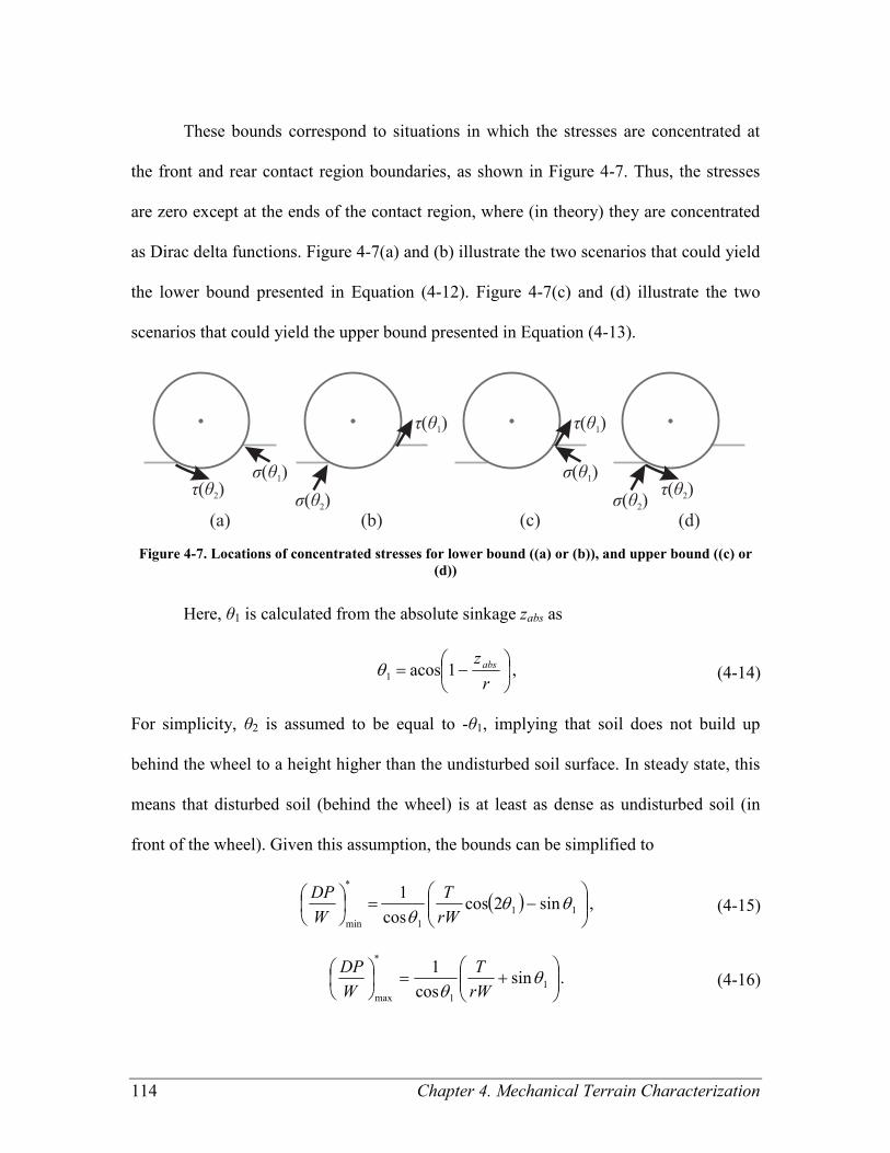
114 Chapter 4. Mechanical Terrain Characterization
These bounds correspond to situations in which the stresses are concentrated at
the front and rear contact region boundaries, as shown in Figure 4-7. Thus, the stresses
are zero except at the ends of the contact region, where (in theory) they are concentrated
as Dirac delta functions. Figure 4-7(a) and (b) illustrate the two scenarios that could yield
the lower bound presented in Equation (4-12). Figure 4-7(c) and (d) illustrate the two
scenarios that could yield the upper bound presented in Equation (4-13).
Figure 4-7. Locations of concentrated stresses for lower bound ((a) or (b)), and upper bound ((c) or
(d))
Here, θ1 is calculated from the absolute sinkage zabs as
−=
r
zabs1acos1θ , (4-14)
For simplicity, θ2 is assumed to be equal to -θ1, implying that soil does not build up
behind the wheel to a height higher than the undisturbed soil surface. In steady state, this
means that disturbed soil (behind the wheel) is at least as dense as undisturbed soil (in
front of the wheel). Given this assumption, the bounds can be simplified to
( )
−=
11
1
*
min
sin2coscos
1θθ
θ Wr
T
W
DP, (4-15)
+=
1
1
*
max
sincos
1θ
θ Wr
T
W
DP. (4-16)

115
4.2.4.2 Bekker Model with Relative Sinkage
The complexity of the stress functions in the Bekker model prohibit derivation of
an explicit solution for DP/W bounds, so numerical optimization is used to find the
minimum and maximum DP/W. Constrained optimization is implemented using
sequential quadratic programming (SQP) using the Matlab fmincon function
(Mathworks, 2005). Specifically, DP/W as calculated using Equations (4-2) and (4-3) is
minimized (or maximized) over the parameters defined in Table 4-3. The optimization
problem to find the lower bound is posed as the following minimization:
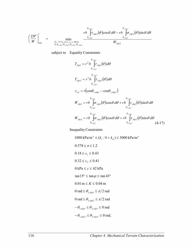
116 Chapter 4. Mechanical Terrain Characterization
( ) ( )
( )
( )
( )
( ) ( )
( ) ( )
rad, 0
rad 0
rad 2rad 0
rad 2rad 0
m 04.0m 01.0
43tantan15tan
kPa 42kPa 0
41.032.0
43.018.0
2.1578.0
kPa/m 3000)/(kPa/m 1000
sConstraint Inequality
sincos
sincos
coscos
sConstraintEquality subject to
sincos
min
2,22,1
1,21,1
2,1
1,1
2
1
222
111
2
2
2
1
2
1
2
22
,,,,
,tan,,,,),/(
*
min
2,1
2,2
1,1
1,2
2,21,22,11,1
21
≤≤−
≤≤−
≤≤
≤≤
≤≤
°≤≤°
≤≤
≤≤
≤≤
≤≤
≤+≤
+=
+=
−=
=
=
−
=
∫∫
∫∫
∫
∫
∫∫+
slipslip
slipslip
slip
slip
n
c
n
slipslipslip
slipslipslip
1,slip21,slip1rel
slipslip
slipslip
slip
slipslip
K
cccnkbk
K
c
c
c
n
kbk
dbrdbrW
dbrdbrW
rz
dbrT
dbrT
W
dbrdbr
W
DP
1,slip2
2,slip2
1,slip2
2,slip2
1,slip1
2,slip1
1,slip1
2,slip1
slip
slip
slip
slip
1,slip2
2,slip2
1,slip2
2,slip2
slipslipslipslip
c
θθ
θθ
πθ
πθ
ϕ
θθθτθθθσ
θθθτθθθσ
θθ
θθτ
θθτ
θθθσθθθτ
ϕ
θ
θ
θ
θ
θ
θ
θ
θ
θ
θ
θ
θ
θ
θ
θ
θ
θθθθϕϕ
(4-17)
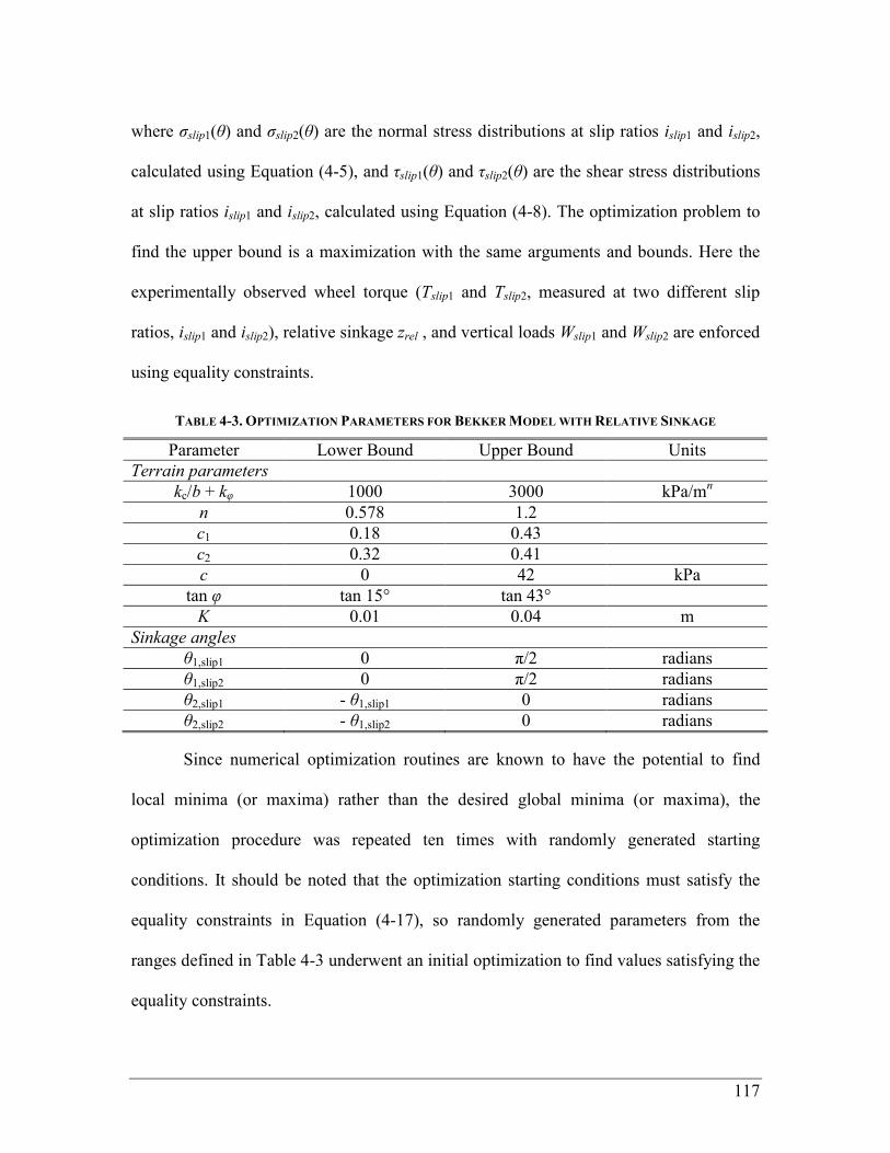
117
where σslip1(θ) and σslip2(θ) are the normal stress distributions at slip ratios islip1 and islip2,
calculated using Equation (4-5), and τslip1(θ) and τslip2(θ) are the shear stress distributions
at slip ratios islip1 and islip2, calculated using Equation (4-8). The optimization problem to
find the upper bound is a maximization with the same arguments and bounds. Here the
experimentally observed wheel torque (Tslip1 and Tslip2, measured at two different slip
ratios, islip1 and islip2), relative sinkage zrel , and vertical loads Wslip1 and Wslip2 are enforced
using equality constraints.
TABLE 4-3. OPTIMIZATION PARAMETERS FOR BEKKER MODEL WITH RELATIVE SINKAGE
Parameter Lower Bound Upper Bound Units
Terrain parameters
kc/b + kφ 1000 3000 kPa/mn
n 0.578 1.2
c1 0.18 0.43
c2 0.32 0.41
c 0 42 kPa
tan φ tan 15° tan 43°
K 0.01 0.04 m
Sinkage angles
θ1,slip1 0 π/2 radians
θ1,slip2 0 π/2 radians
θ2,slip1 - θ1,slip1 0 radians
θ2,slip2 - θ1,slip2 0 radians
Since numerical optimization routines are known to have the potential to find
local minima (or maxima) rather than the desired global minima (or maxima), the
optimization procedure was repeated ten times with randomly generated starting
conditions. It should be noted that the optimization starting conditions must satisfy the
equality constraints in Equation (4-17), so randomly generated parameters from the
ranges defined in Table 4-3 underwent an initial optimization to find values satisfying the
equality constraints.
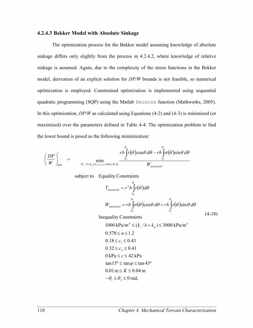
118 Chapter 4. Mechanical Terrain Characterization
4.2.4.3 Bekker Model with Absolute Sinkage
The optimization process for the Bekker model assuming knowledge of absolute
sinkage differs only slightly from the process in 4.2.4.2, where knowledge of relative
sinkage is assumed. Again, due to the complexity of the stress functions in the Bekker
model, derivation of an explicit solution for DP/W bounds is not feasible, so numerical
optimization is employed. Constrained optimization is implemented using sequential
quadratic programming (SQP) using the Matlab fmincon function (Mathworks, 2005).
In this optimization, DP/W as calculated using Equations (4-2) and (4-3) is minimized (or
maximized) over the parameters defined in Table 4-4. The optimization problem to find
the lower bound is posed as the following minimization:
( ) ( )
( )
( ) ( )
rad, 0
m 04.0m 01.0
43tantan15tan
kPa 42kPa 0
41.032.0
43.018.0
2.1578.0
kPa/m 3000)/(kPa/m 1000
sConstraint Inequality
sincos
sConstraintEquality subject to
sincos
min
21
2
1
2
,,tan,,,,),/(
*
min
1
2
221
≤≤−
≤≤
°≤≤°
≤≤
≤≤
≤≤
≤≤
≤+≤
+=
=
−=
∫∫
∫
∫∫+
θθ
ϕ
θθθτθθθσ
θθτ
θθθσθθθτ
ϕ
θ
θ
θ
θ
θ
θ
θ
θ
θ
θ
θϕϕ
K
c
c
c
n
kbk
dbrdbrW
dbrT
W
dbrdbr
W
DP
n
c
n
measured
measured
measuredKcccnkbk
1
2
1
2
1
2
1
2
c
(4-18)
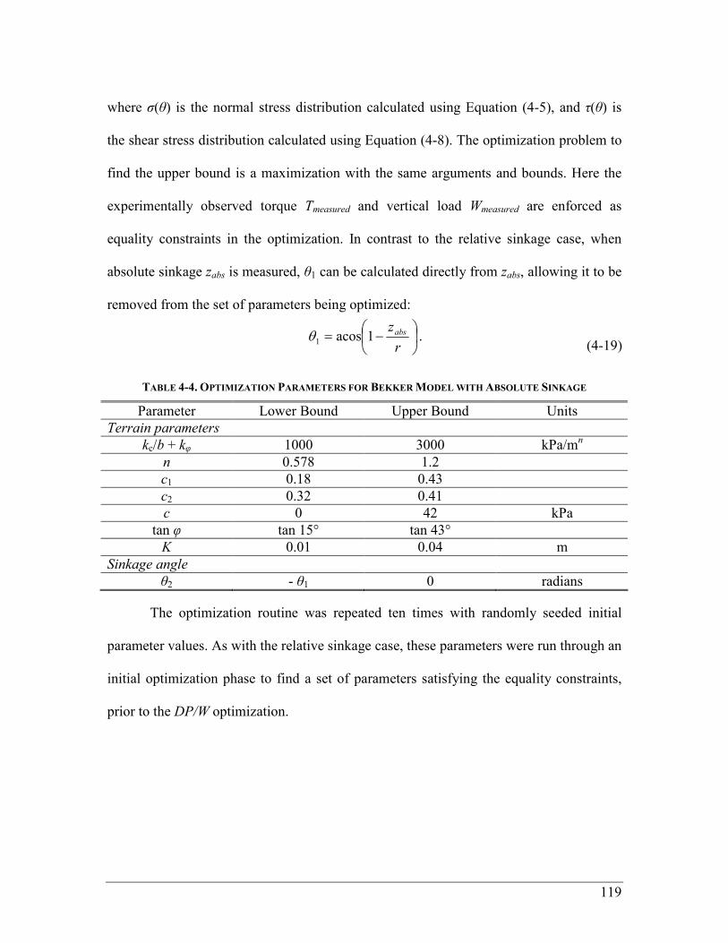
119
where σ(θ) is the normal stress distribution calculated using Equation (4-5), and τ(θ) is
the shear stress distribution calculated using Equation (4-8). The optimization problem to
find the upper bound is a maximization with the same arguments and bounds. Here the
experimentally observed torque Tmeasured and vertical load Wmeasured are enforced as
equality constraints in the optimization. In contrast to the relative sinkage case, when
absolute sinkage zabs is measured, θ1 can be calculated directly from zabs, allowing it to be
removed from the set of parameters being optimized:
−=
r
zabs1acos1θ . (4-19)
TABLE 4-4. OPTIMIZATION PARAMETERS FOR BEKKER MODEL WITH ABSOLUTE SINKAGE
Parameter Lower Bound Upper Bound Units
Terrain parameters
kc/b + kφ 1000 3000 kPa/mn
n 0.578 1.2
c1 0.18 0.43
c2 0.32 0.41
c 0 42 kPa
tan φ tan 15° tan 43°
K 0.01 0.04 m
Sinkage angle
θ2 - θ1 0 radians
The optimization routine was repeated ten times with randomly seeded initial
parameter values. As with the relative sinkage case, these parameters were run through an
initial optimization phase to find a set of parameters satisfying the equality constraints,
prior to the DP/W optimization.
120 Chapter 4. Mechanical Terrain Characterization
4.3 Experiment Details
The mechanical terrain characterization approaches were validated using data
from laboratory experiments with the FSRL wheel-terrain interaction testbed. Additional
experiments with the TORTOISE rover on Wingaersheek Beach were also conducted.
4.3.1 FSRL Wheel-Terrain Interaction Testbed Experiments
Initial validation of the mechanical terrain characterization approaches was done
on data collected during experiments with the FSRL wheel-terrain interaction testbed,
using five distinct terrains. These experiments were conducted by Shinwoo Kang for
research presented in (Kang, 2003). The analysis of the data presented here represents
work completed for this thesis.
The FSRL wheel-terrain interaction testbed, shown in Figure 4-8 and described in
detail in Appendix C, is an apparatus designed to measure forces on a rigid wheel driven
over terrain. It consists of a driven wheel mounted on an undriven vertical axis. The
wheel-axis assembly is mounted on a driven carriage, so that the wheel forward velocity
and angular velocity can be controlled independently. These testbed experiments were
conducted using a rigid black plastic wheel 4.8 cm wide and 20 cm in diameter. Sand is
bonded to the outside of the wheel to improve traction.
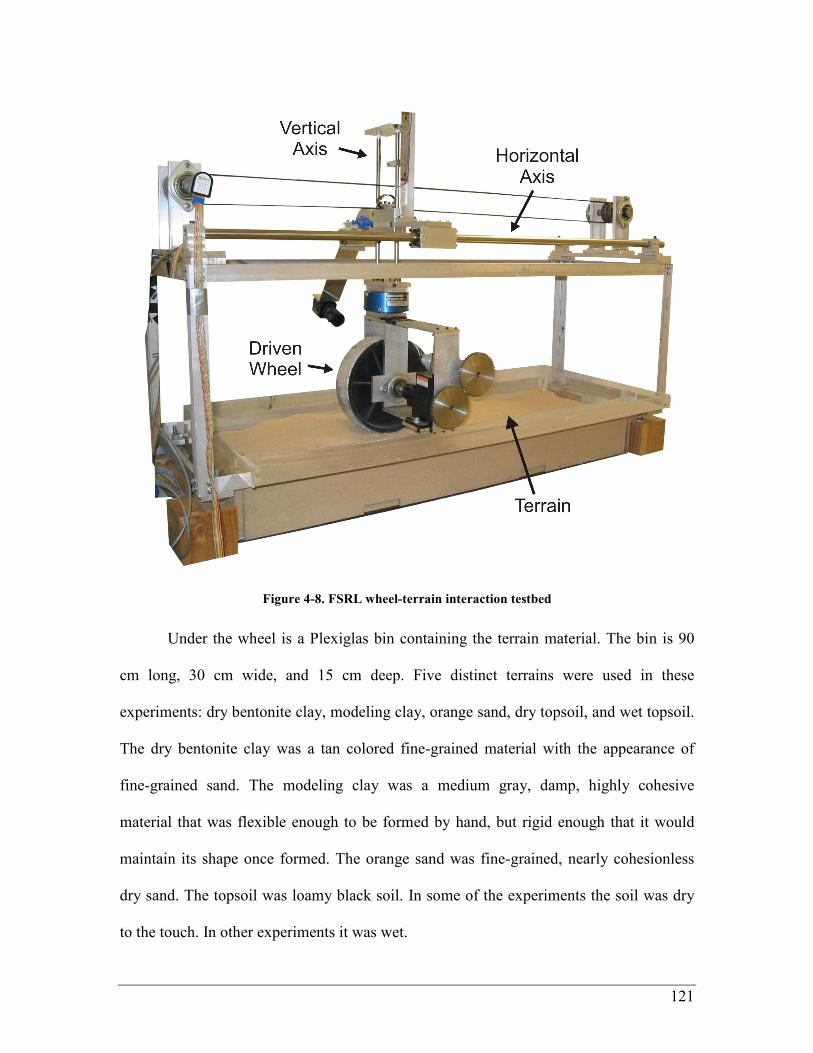
121
Figure 4-8. FSRL wheel-terrain interaction testbed
Under the wheel is a Plexiglas bin containing the terrain material. The bin is 90
cm long, 30 cm wide, and 15 cm deep. Five distinct terrains were used in these
experiments: dry bentonite clay, modeling clay, orange sand, dry topsoil, and wet topsoil.
The dry bentonite clay was a tan colored fine-grained material with the appearance of
fine-grained sand. The modeling clay was a medium gray, damp, highly cohesive
material that was flexible enough to be formed by hand, but rigid enough that it would
maintain its shape once formed. The orange sand was fine-grained, nearly cohesionless
dry sand. The topsoil was loamy black soil. In some of the experiments the soil was dry
to the touch. In other experiments it was wet.
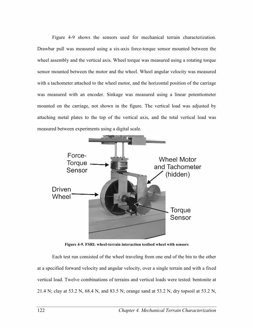
122 Chapter 4. Mechanical Terrain Characterization
Figure 4-9 shows the sensors used for mechanical terrain characterization.
Drawbar pull was measured using a six-axis force-torque sensor mounted between the
wheel assembly and the vertical axis. Wheel torque was measured using a rotating torque
sensor mounted between the motor and the wheel. Wheel angular velocity was measured
with a tachometer attached to the wheel motor, and the horizontal position of the carriage
was measured with an encoder. Sinkage was measured using a linear potentiometer
mounted on the carriage, not shown in the figure. The vertical load was adjusted by
attaching metal plates to the top of the vertical axis, and the total vertical load was
measured between experiments using a digital scale.
Figure 4-9. FSRL wheel-terrain interaction testbed wheel with sensors
Each test run consisted of the wheel traveling from one end of the bin to the other
at a specified forward velocity and angular velocity, over a single terrain and with a fixed
vertical load. Twelve combinations of terrains and vertical loads were tested: bentonite at
21.4 N; clay at 53.2 N, 68.4 N, and 83.5 N; orange sand at 53.2 N, dry topsoil at 53.2 N,
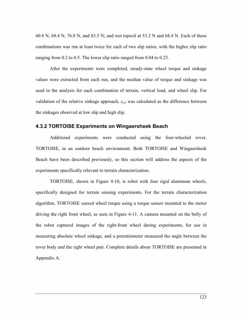
123
60.8 N, 68.4 N, 76.0 N, and 83.5 N; and wet topsoil at 53.2 N and 68.4 N. Each of these
combinations was run at least twice for each of two slip ratios, with the higher slip ratio
ranging from 0.2 to 0.5. The lower slip ratio ranged from 0.04 to 0.23.
After the experiments were completed, steady-state wheel torque and sinkage
values were extracted from each run, and the median value of torque and sinkage was
used in the analysis for each combination of terrain, vertical load, and wheel slip. For
validation of the relative sinkage approach, zrel was calculated as the difference between
the sinkages observed at low slip and high slip.
4.3.2 TORTOISE Experiments on Wingaersheek Beach
Additional experiments were conducted using the four-wheeled rover,
TORTOISE, in an outdoor beach environment. Both TORTOISE and Wingaersheek
Beach have been described previously, so this section will address the aspects of the
experiments specifically relevant to terrain characterization.
TORTOISE, shown in Figure 4-10, is robot with four rigid aluminum wheels,
specifically designed for terrain sensing experiments. For the terrain characterization
algorithm, TORTOISE sensed wheel torque using a torque sensor mounted to the motor
driving the right front wheel, as seen in Figure 4-11. A camera mounted on the belly of
the robot captured images of the right-front wheel during experiments, for use in
measuring absolute wheel sinkage, and a potentiometer measured the angle between the
rover body and the right wheel pair. Complete details about TORTOISE are presented in
Appendix A.
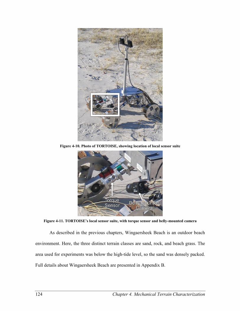
124 Chapter 4. Mechanical Terrain Characterization
Figure 4-10. Photo of TORTOISE, showing location of local sensor suite
Figure 4-11. TORTOISE’s local sensor suite, with torque sensor and belly-mounted camera
As described in the previous chapters, Wingaersheek Beach is an outdoor beach
environment. Here, the three distinct terrain classes are sand, rock, and beach grass. The
area used for experiments was below the high-tide level, so the sand was densely packed.
Full details about Wingaersheek Beach are presented in Appendix B.
125
To induce wheel slip, the “Incremental Slip” behavior described in 2.2.2 was
implemented. Here, the rover drives normally for 11 seconds, then (at t=0 seconds) starts
to spin the right-front wheel faster than the other wheels. Since the rover body remains
moving at the speed of the other three wheels, this causes the right-front wheel to slip
relative to the terrain, at a slip ratio of 33%. At t=3 seconds, the other three wheels are
slowed down, reducing the rover body speed and increasing the slip ratio to 50%. At
t=6 seconds, the other three wheels are slowed down further, increasing the slip ratio to
67%. At t=9 seconds, the rover resumes normal driving. The process then repeats.
For mechanical terrain characterization, analysis was performed using wheel
torque recorded during the second half of the 50% slip stage. The 50% slip stage was
selected because 50% slip is close to the range of slip ratios studied on the wheel-terrain
interaction testbed. The second half of the stage was used to allow the wheel sinkage and
torque to reach their steady state values.
Data from a single rover traverse of 11 meters over all three terrain classes was
collected. Absolute wheel sinkage was measured using the images from the belly-
mounted camera by hand-labeling the wheel rim and wheel-terrain interface. Images from
the belly-mounted camera were also used to identify the terrain being traversed at any
instant. Wheel sinkage and torque were passed to the optimization algorithm to determine
bounds on the normalized drawbar pull, DP/W. No measurement of the drawbar pull was
made, so assessment of the accuracy of the bounds relies on consistency between the
predicted bounds and the known terrain classes.
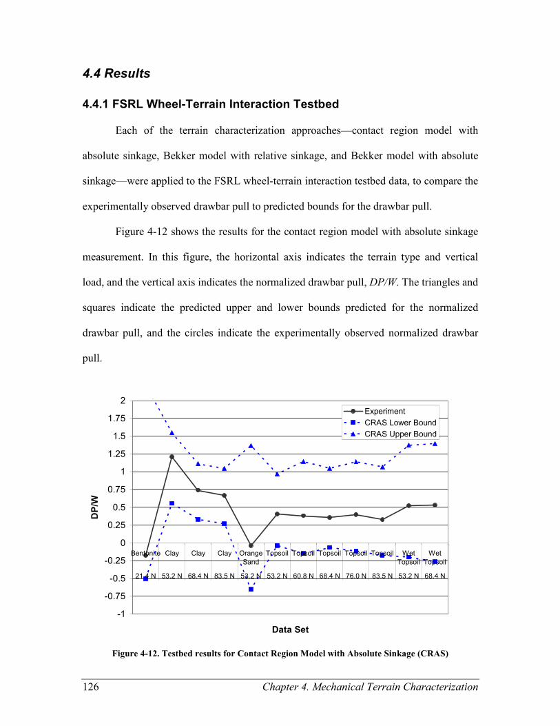
126 Chapter 4. Mechanical Terrain Characterization
4.4 Results
4.4.1 FSRL Wheel-Terrain Interaction Testbed
Each of the terrain characterization approaches—contact region model with
absolute sinkage, Bekker model with relative sinkage, and Bekker model with absolute
sinkage—were applied to the FSRL wheel-terrain interaction testbed data, to compare the
experimentally observed drawbar pull to predicted bounds for the drawbar pull.
Figure 4-12 shows the results for the contact region model with absolute sinkage
measurement. In this figure, the horizontal axis indicates the terrain type and vertical
load, and the vertical axis indicates the normalized drawbar pull, DP/W. The triangles and
squares indicate the predicted upper and lower bounds predicted for the normalized
drawbar pull, and the circles indicate the experimentally observed normalized drawbar
pull.
-1
-0.75
-0.5
-0.25
0
0.25
0.5
0.75
1
1.25
1.5
1.75
2
Bentonite Clay Clay Clay Orange
Sand
Topsoil Topsoil Topsoil Topsoil Topsoil Wet
Topsoil
Wet
Topsoil
21.4 N 53.2 N 68.4 N 83.5 N 53.2 N 53.2 N 60.8 N 68.4 N 76.0 N 83.5 N 53.2 N 68.4 N
Data Set
DP/W
Experiment
CRAS Lower Bound
CRAS Upper Bound
Figure 4-12. Testbed results for Contact Region Model with Absolute Sinkage (CRAS)

127
In this figure it can be seen that this approach is consistently correct with respect
to its bounds: none of the observed drawbar pull values fall outside the predicted bounds.
However these bounds are quite loose, with an average margin22
of 0.84 between the
observed value and the upper bound, and an average margin of 0.53 between the
observed value and the lower bound. Thus they are likely to be marginally helpful in
confidently identifying terrain that can be safely traversed. For example, although wet
topsoil is relatively easy to traverse (with a measured DP/W of just over 0.5), the bounds
cannot confidently predict that it would be at all traversable, since the predicted lower
bound is less than zero.
Figure 4-13 shows results for the Bekker model with relative sinkage measured.
Here the predicted bounds are significantly tighter. With this approach, the average
margin between the measured value of DP/W and the upper bound was 0.10, and the
average margin between the measured value and the lower bound was 0.43. In one case
(clay at 53.2 N) the optimization predicted an upper bound which fell below the
measured value of DP/W. However, while this small underestimation may lead the rover
to underestimate the safety of traversing this terrain, a pessimistic error such as this
would not put the rover in danger. In another case (bentonite at 21.4 N) the optimization
algorithm was unable to find any combination of parameters that yielded the observed
wheel sinkage and torque. This suggests that the model may not accurately represent the
relationship between slip, sinkage, and torque in that terrain. Overall, the results are good,
with tight upper bounds. While the looseness of the lower bounds is somewhat improved
22
The average margin was calculated as the average of the absolute values of the differences between the
measured DP/W and the bound.
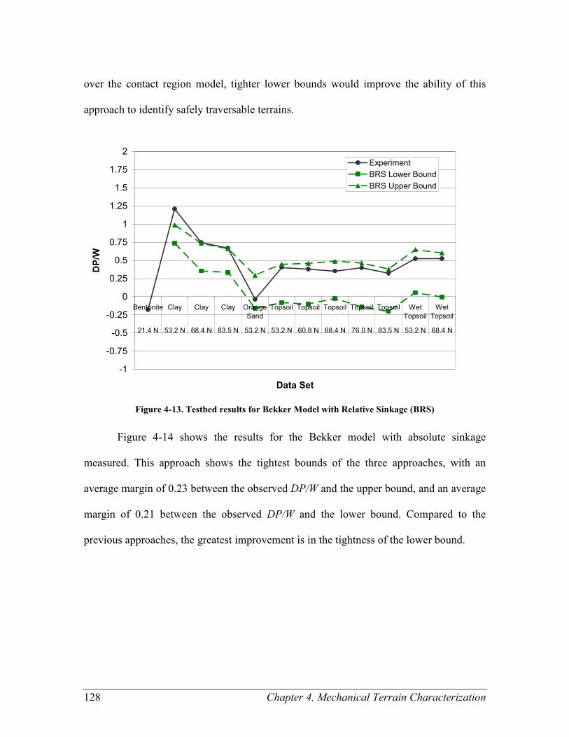
128 Chapter 4. Mechanical Terrain Characterization
over the contact region model, tighter lower bounds would improve the ability of this
approach to identify safely traversable terrains.
-1
-0.75
-0.5
-0.25
0
0.25
0.5
0.75
1
1.25
1.5
1.75
2
Bentonite Clay Clay Clay Orange
Sand
Topsoil Topsoil Topsoil Topsoil Topsoil Wet
Topsoil
Wet
Topsoil
21.4 N 53.2 N 68.4 N 83.5 N 53.2 N 53.2 N 60.8 N 68.4 N 76.0 N 83.5 N 53.2 N 68.4 N
Data Set
DP/W
Experiment
BRS Lower Bound
BRS Upper Bound
Figure 4-13. Testbed results for Bekker Model with Relative Sinkage (BRS)
Figure 4-14 shows the results for the Bekker model with absolute sinkage
measured. This approach shows the tightest bounds of the three approaches, with an
average margin of 0.23 between the observed DP/W and the upper bound, and an average
margin of 0.21 between the observed DP/W and the lower bound. Compared to the
previous approaches, the greatest improvement is in the tightness of the lower bound.
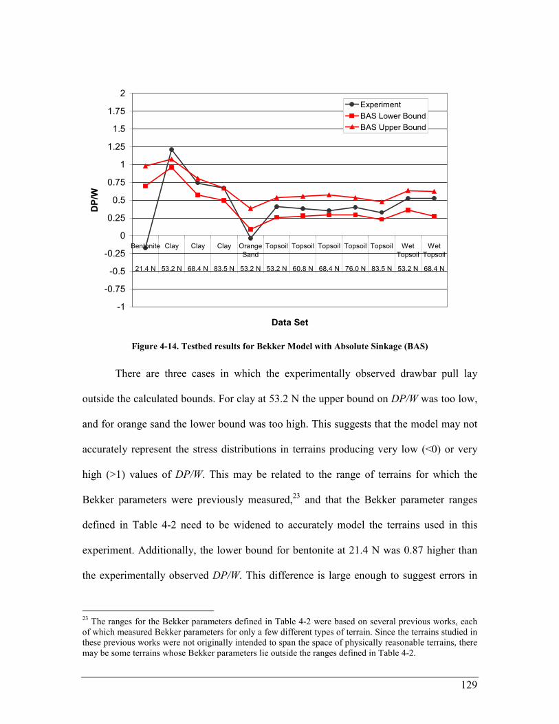
129
-1
-0.75
-0.5
-0.25
0
0.25
0.5
0.75
1
1.25
1.5
1.75
2
Bentonite Clay Clay Clay Orange
Sand
Topsoil Topsoil Topsoil Topsoil Topsoil Wet
Topsoil
Wet
Topsoil
21.4 N 53.2 N 68.4 N 83.5 N 53.2 N 53.2 N 60.8 N 68.4 N 76.0 N 83.5 N 53.2 N 68.4 N
Data Set
DP/W
Experiment
BAS Lower Bound
BAS Upper Bound
Figure 4-14. Testbed results for Bekker Model with Absolute Sinkage (BAS)
There are three cases in which the experimentally observed drawbar pull lay
outside the calculated bounds. For clay at 53.2 N the upper bound on DP/W was too low,
and for orange sand the lower bound was too high. This suggests that the model may not
accurately represent the stress distributions in terrains producing very low (<0) or very
high (>1) values of DP/W. This may be related to the range of terrains for which the
Bekker parameters were previously measured,23
and that the Bekker parameter ranges
defined in Table 4-2 need to be widened to accurately model the terrains used in this
experiment. Additionally, the lower bound for bentonite at 21.4 N was 0.87 higher than
the experimentally observed DP/W. This difference is large enough to suggest errors in
23
The ranges for the Bekker parameters defined in Table 4-2 were based on several previous works, each
of which measured Bekker parameters for only a few different types of terrain. Since the terrains studied in
these previous works were not originally intended to span the space of physically reasonable terrains, there
may be some terrains whose Bekker parameters lie outside the ranges defined in Table 4-2.
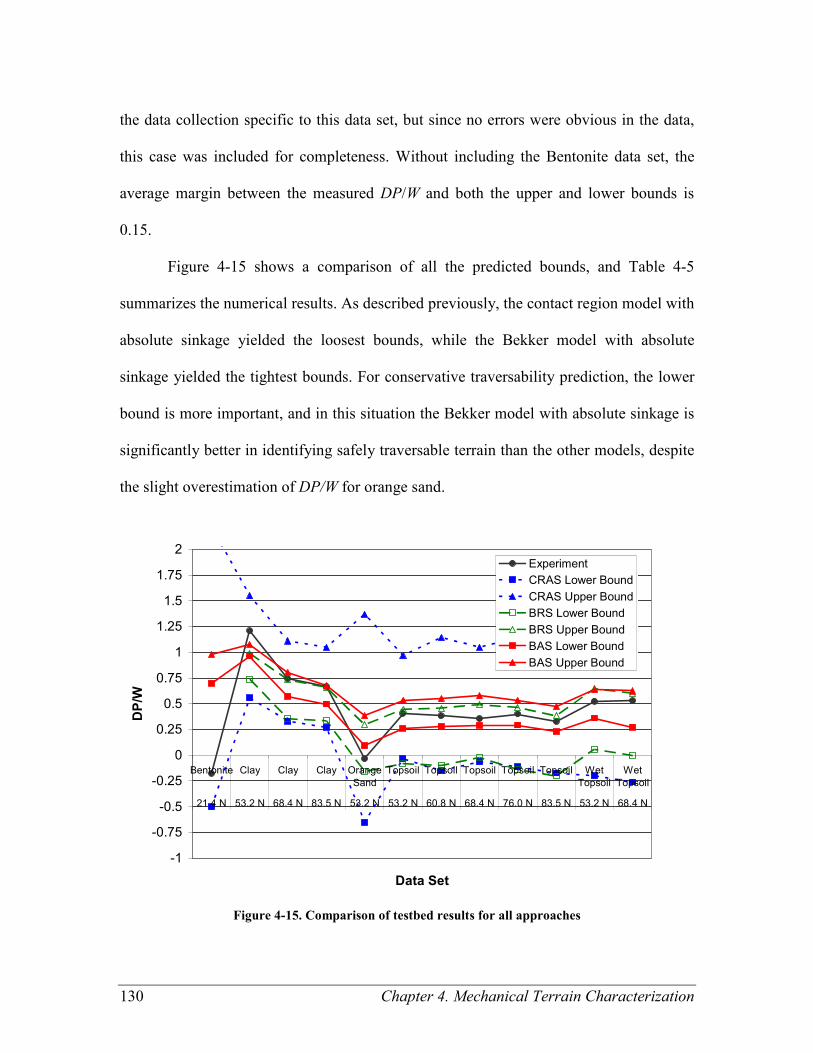
130 Chapter 4. Mechanical Terrain Characterization
the data collection specific to this data set, but since no errors were obvious in the data,
this case was included for completeness. Without including the Bentonite data set, the
average margin between the measured DP/W and both the upper and lower bounds is
0.15.
Figure 4-15 shows a comparison of all the predicted bounds, and Table 4-5
summarizes the numerical results. As described previously, the contact region model with
absolute sinkage yielded the loosest bounds, while the Bekker model with absolute
sinkage yielded the tightest bounds. For conservative traversability prediction, the lower
bound is more important, and in this situation the Bekker model with absolute sinkage is
significantly better in identifying safely traversable terrain than the other models, despite
the slight overestimation of DP/W for orange sand.
-1
-0.75
-0.5
-0.25
0
0.25
0.5
0.75
1
1.25
1.5
1.75
2
Bentonite Clay Clay Clay Orange
Sand
Topsoil Topsoil Topsoil Topsoil Topsoil Wet
Topsoil
Wet
Topsoil
21.4 N 53.2 N 68.4 N 83.5 N 53.2 N 53.2 N 60.8 N 68.4 N 76.0 N 83.5 N 53.2 N 68.4 N
Data Set
DP/W
Experiment
CRAS Lower Bound
CRAS Upper Bound
BRS Lower Bound
BRS Upper Bound
BAS Lower Bound
BAS Upper Bound
Figure 4-15. Comparison of testbed results for all approaches
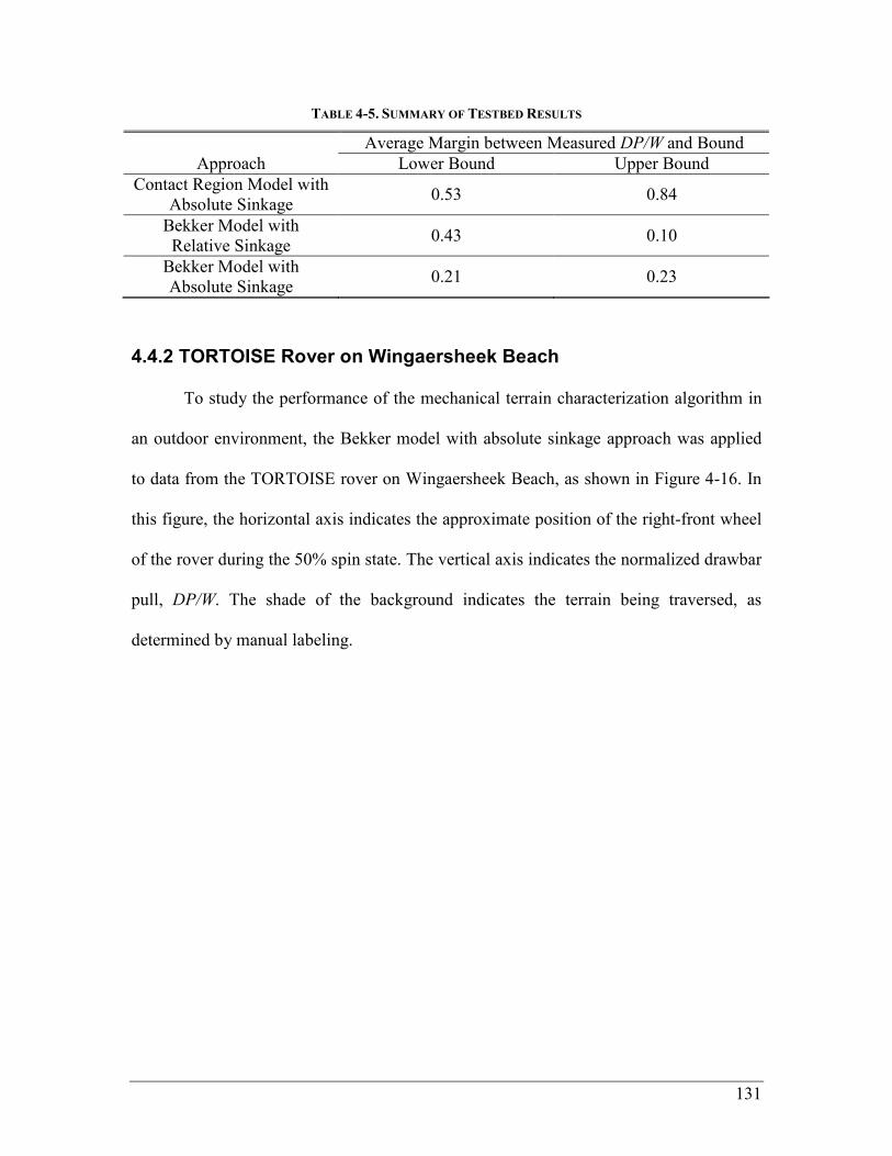
131
TABLE 4-5. SUMMARY OF TESTBED RESULTS
Average Margin between Measured DP/W and Bound
Approach Lower Bound Upper Bound
Contact Region Model with
Absolute Sinkage 0.53 0.84
Bekker Model with
Relative Sinkage 0.43 0.10
Bekker Model with
Absolute Sinkage 0.21 0.23
4.4.2 TORTOISE Rover on Wingaersheek Beach
To study the performance of the mechanical terrain characterization algorithm in
an outdoor environment, the Bekker model with absolute sinkage approach was applied
to data from the TORTOISE rover on Wingaersheek Beach, as shown in Figure 4-16. In
this figure, the horizontal axis indicates the approximate position of the right-front wheel
of the rover during the 50% spin state. The vertical axis indicates the normalized drawbar
pull, DP/W. The shade of the background indicates the terrain being traversed, as
determined by manual labeling.
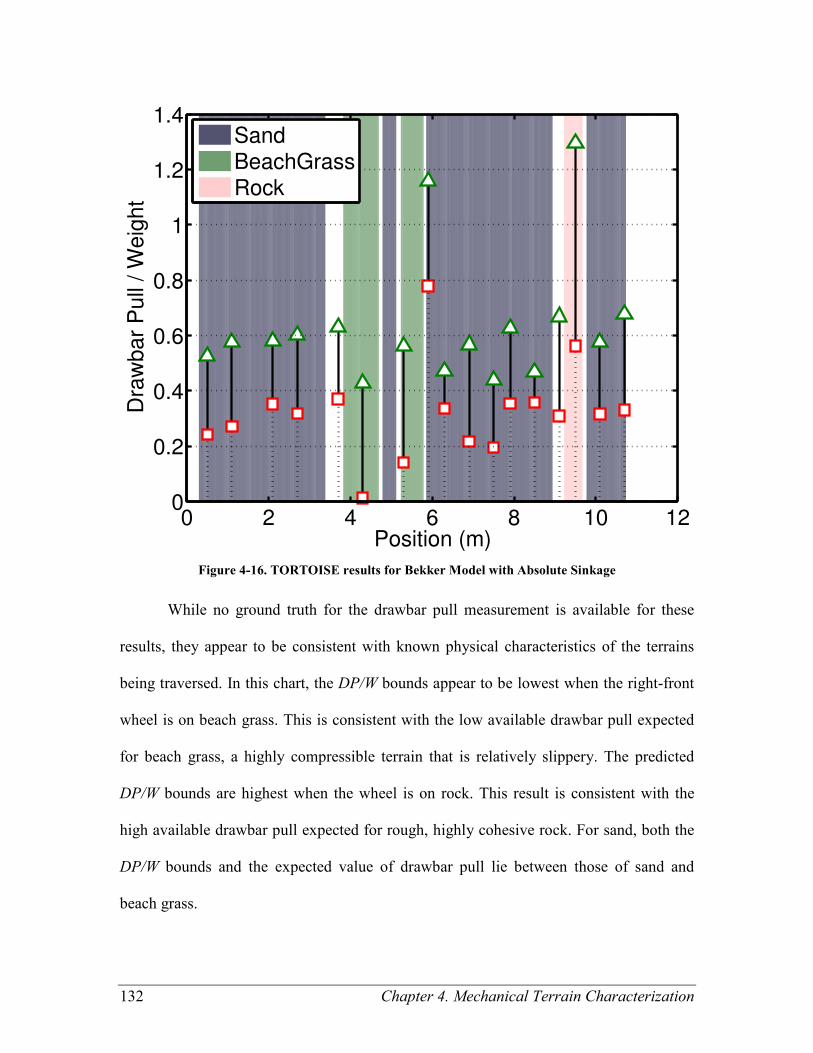
132 Chapter 4. Mechanical Terrain Characterization
Position (m)
Dra
wbar
Pull
/ W
eig
ht
0 2 4 6 8 10 120
0.2
0.4
0.6
0.8
1
1.2
1.4SandBeachGrassRock
Figure 4-16. TORTOISE results for Bekker Model with Absolute Sinkage
While no ground truth for the drawbar pull measurement is available for these
results, they appear to be consistent with known physical characteristics of the terrains
being traversed. In this chart, the DP/W bounds appear to be lowest when the right-front
wheel is on beach grass. This is consistent with the low available drawbar pull expected
for beach grass, a highly compressible terrain that is relatively slippery. The predicted
DP/W bounds are highest when the wheel is on rock. This result is consistent with the
high available drawbar pull expected for rough, highly cohesive rock. For sand, both the
DP/W bounds and the expected value of drawbar pull lie between those of sand and
beach grass.
133
4.5 Conclusions
This chapter has presented an approach for evaluating terrain traversability which
is appropriate for situations when a high degree of confidence is required. This approach
uses an optimization framework to find upper and lower bounds on the normalized
drawbar pull subject to observed wheel sinkage and torque. It uses two general terrain
models, and presents three distinct model/measurement pairs. The normalized drawbar
pull is guaranteed to lie between the bounds if the terrain is accurately represented by the
model.
Using data from the FSRL wheel-terrain interaction testbed with five different
terrains and six different vertical loads, the three methods were compared. The tightest
bounds were achieved using the Bekker model with absolute sinkage, which
demonstrated good consistency with experimentally observed drawbar-pull. This drawbar
pull bounding method was also applied to data from a four-wheeled rover in a natural
environment, and the associated drawbar pull predictions appear to be consistent with
known physical characteristics of the terrains being traversed.
This technique for terrain characterization is likely to be useful in situations where
a conservative estimate of wheel thrust is desired but cannot be measured directly. As a
proprioceptive terrain sensing technique, it can be used for terrain clustering (by simple
binning of the predicted lower bound), or it can be used as a component of a larger
system, such as the self-supervised terrain classification approach presented in Chapter 5.
4.5.1.1 Future Work
Future work in the area of terrain characterization has the potential to further
improve the ability of a rover to predict terrain traversability. Because the approach of

134 Chapter 4. Mechanical Terrain Characterization
measuring relative sinkage is particularly sensitive to the relationship between sinkage
and slip ratio, use of a more accurate model for slip-sinkage24
behavior might improve
the bounds for the relative sinkage measurement approach significantly. Additionally,
experiments on sloped terrain would be valuable to determine how much the slope of the
terrain affects the net traction force.
24
Slip-sinkage is the mechanism by which a wheel that is slipping relative to the terrain exhibits higher
sinkage than a wheel that is rolling without slip. Slip-sinkage behavior was observed in experiments by
Hegedus (1963), and mathematical models were described by Bekker (1969, pp. 139-140) and by Steiner
(1978).

135
Chapter
5 Chapter 5 Self-Supervised Classification
In this thesis, a self-supervised classification framework is proposed which allows
measurements of mechanical properties of local terrain to be generalized to yield
predictions about mechanical properties of distant terrain. The self-supervised
classification framework uses the algorithmic components presented in Chapters 2, 3, and
4.
This chapter presents two instantiations of the self-supervised classification
framework. The first instantiation, presented in Section 1.1, uses a supervised
proprioceptive terrain classifier to identify human-defined terrain classes associated with
proprioceptively sensed terrain patches. Because the exteroceptive terrain classifier learns
to identify terrain patches in the distance that correspond with the human-defined terrain
classes, this instantiation is used to experimentally validate the self-supervised
classification framework, Thus the results of exteroceptive terrain classification can be
directly compared to ground truth (i.e. hand-labeled terrain classes observed in stereo
camera images). However, because human supervision is required to train the
proprioceptive terrain classifier, this instantiation is not appropriate for implementation in
novel environments where some of the terrain classes may not be known a priori.
136 Chapter 5. Self-Supervised Classification
The second instantiation, presented in Section 1.1, is designed for scenarios in
which no a priori knowledge of the terrain classes is available. In this instantiation,
terrain classes are defined to correspond to ranges of a traversability metric, and thus
exteroceptive terrain class predictions are used to predict the traversability of distant
terrain. This instantiation is demonstrated using experimental data.
5.1 Experimental Validation of Self-Supervised Classification Framework
5.1.1 Introduction
Traditional methods for sensing non-geometric hazards, such as wheel sinkage
measurement and wheel slip detection, are typically dependent on proprioceptive sensing
of wheel-terrain interaction, and thus are limited to characterizing terrain patches in
physical contact with the rover. This implies that a rover could not recognize a potentially
hazardous situation until it has at least one wheel in contact with the hazard. To allow for
predictive non-geometric hazard avoidance, remote detection of non-geometric hazards is
needed. The self-supervised classification framework presented here provides a method
for generalizing information gained from proprioceptive sensors to yield information
about distant terrain.
Here, “self-supervised” refers to automatic training of the remote terrain
classifier. Whereas in a traditional (i.e. manually) supervised classifier a human provides
labeled training examples for each class of interest, in a self-supervised framework
another classification algorithm identifies these training examples. In the context of this
thesis, proprioceptive sensors are used to identify terrain patches associated with the
terrain classes of interest, and visual features associated with these terrain patches are

5.1 Experimental Validation of Self-Supervised Classification Framework 137
used to train a visual classifier. This visual classifier then identifies instances of these
terrain classes in a distant scene.
In the self-supervised framework presented in this section, local terrain patches
are classified based on the vibration signature in the rover structure caused by wheel
terrain interaction, and distant terrain patches are classified based on stereo imagery as
belonging to one of the terrain classes of interest. Note that visual data used for training
can be gathered either 1) from a camera with a view of the terrain under the rover wheels,
or 2) from stored imagery from a camera with a view of the terrain in front of the rover.
In the latter scenario, odometry-based position estimation is used to identify where the
currently sensed terrain patch appears in the stored images.
To assess the performance of self-supervised classification in these two scenarios,
experiments were performed using the four-wheeled TORTOISE rover in an outdoor
beach environment. The accuracy of the self-supervised approach in classifying terrain
was compared to that of the traditional “manually supervised” classifier presented in 1.1.
Results demonstrate the viability of the self-supervised classification framework.
Section 5.1.2 describes the self-supervised classification approaches. Section
5.1.3 presents detailed information about the experiments, and Section 5.1.4 presents the
results of the experiments. Section 5.1.5 presents the conclusions drawn from these
results and suggests directions for future research.

138 Chapter 5. Self-Supervised Classification
5.1.2 Self-Supervised Classification Approaches
5.1.2.1 Overview
The self-supervised learning process has two stages: the training stage and the
classification stage. In the training stage, the proprioceptive terrain classifier—in this
instantiation a supervised vibration-based terrain classifier—identifies terrain class labels
for proprioceptively sensed terrain patches, as illustrated in Figure 5-1(a). These labels,
along with visual features associated with the labeled terrain patches, are used to train the
visual terrain classifier. In the classification stage, illustrated in Figure 5-1(b), the visual
terrain classifier is used to predict terrain classes associated with distant terrain patches.
Figure 5-1. Schematic of self-supervised classification, (a) vibration-supervised training of visual
classifier, (b) prediction using visual classifier
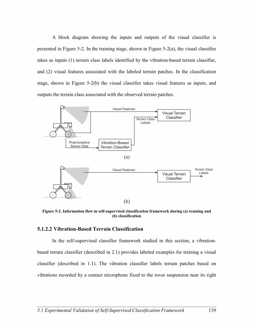
5.1 Experimental Validation of Self-Supervised Classification Framework 139
A block diagram showing the inputs and outputs of the visual classifier is
presented in Figure 5-2. In the training stage, shown in Figure 5-2(a), the visual classifier
takes as inputs (1) terrain class labels identified by the vibration-based terrain classifier,
and (2) visual features associated with the labeled terrain patches. In the classification
stage, shown in Figure 5-2(b) the visual classifier takes visual features as inputs, and
outputs the terrain class associated with the observed terrain patches.
Figure 5-2. Information flow in self-supervised classification framework during (a) training and
(b) classification
5.1.2.2 Vibration-Based Terrain Classification
In the self-supervised classifier framework studied in this section, a vibration-
based terrain classifier (described in 2.1) provides labeled examples for training a visual
classifier (described in 1.1). The vibration classifier labels terrain patches based on
vibrations recorded by a contact microphone fixed to the rover suspension near its right

140 Chapter 5. Self-Supervised Classification
front wheel. Here it fills the role of the “supervisory” classifier, because it supervises the
labeling of training data.
The vibration-based terrain classifier represents vibrations as log-scaled power
spectral densities computed over a 1-second window. The 558-element representation is
classified using a support vector machine (SVM) that has been trained using human-
labeled vibration data. Full details on this classifier are presented in 2.1.
It should be noted that in the self-supervised classification framework, care must
be taken to ensure the accuracy of the supervisory classifier. This is necessary to prevent
incorrect labels from corrupting the training of the visual classifier. In this work,
accuracy is guaranteed by combining multiple separate vibration-based class predictions
for each terrain patch. Thus, the vibration-based terrain classifier identifies a terrain class
based on each 1-second segment of vibration data. Since the rover travels at a slow speed,
multiple vibration segments correspond to the same terrain patch, and each of them is
classified independently. If any of these terrain class assignments disagree, no training
data from that terrain patch is used for training the visual classifier.
5.1.2.3 Vision-Based Terrain Classification
The vision-based classifier in this self-supervised framework has been presented
in 1.1. This classifier is intended to classify distant terrain patches based on visual
features derived from color stereo images. As described in 1.1, color stereo cameras yield
color, visual texture, and geometry classification features. Features associated with each
of these sensing modes are classified using separate support vector machines, and the
resulting class likelihoods are combined using naïve Bayes fusion. It should be noted that
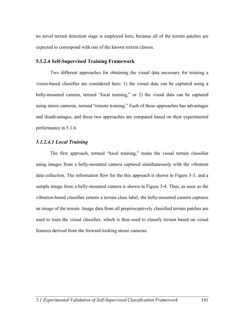
5.1 Experimental Validation of Self-Supervised Classification Framework 141
no novel terrain detection stage is employed here, because all of the terrain patches are
expected to correspond with one of the known terrain classes.
5.1.2.4 Self-Supervised Training Framework
Two different approaches for obtaining the visual data necessary for training a
vision-based classifier are considered here: 1) the visual data can be captured using a
belly-mounted camera, termed “local training,” or 2) the visual data can be captured
using stereo cameras, termed “remote training.” Each of these approaches has advantages
and disadvantages, and these two approaches are compared based on their experimental
performance in 5.1.4.
5.1.2.4.1 Local Training
The first approach, termed “local training,” trains the visual terrain classifier
using images from a belly-mounted camera captured simultaneously with the vibration
data collection. The information flow for the this approach is shown in Figure 5-3, and a
sample image from a belly-mounted camera is shown in Figure 5-4. Thus, as soon as the
vibration-based classifier returns a terrain class label, the belly-mounted camera captures
an image of the terrain. Image data from all proprioceptively classified terrain patches are
used to train the visual classifier, which is then used to classify terrain based on visual
features derived from the forward-looking stereo cameras.
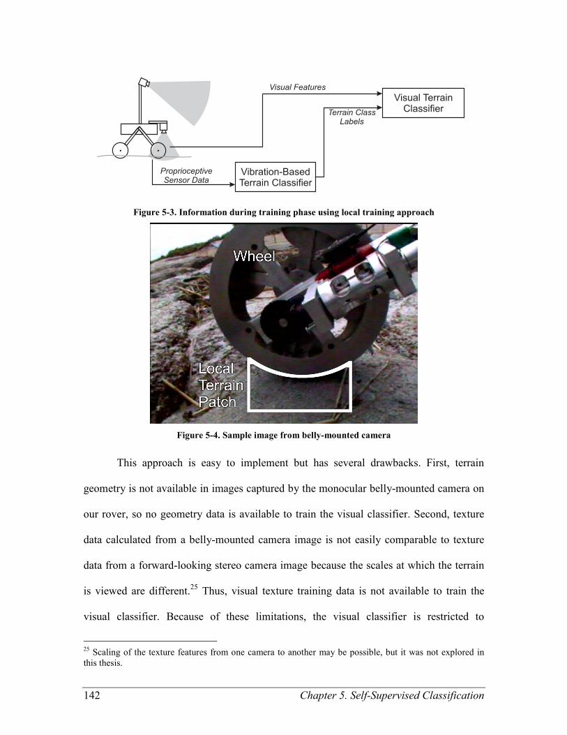
142 Chapter 5. Self-Supervised Classification
Figure 5-3. Information during training phase using local training approach
Figure 5-4. Sample image from belly-mounted camera
This approach is easy to implement but has several drawbacks. First, terrain
geometry is not available in images captured by the monocular belly-mounted camera on
our rover, so no geometry data is available to train the visual classifier. Second, texture
data calculated from a belly-mounted camera image is not easily comparable to texture
data from a forward-looking stereo camera image because the scales at which the terrain
is viewed are different.25
Thus, visual texture training data is not available to train the
visual classifier. Because of these limitations, the visual classifier is restricted to
25
Scaling of the texture features from one camera to another may be possible, but it was not explored in
this thesis.
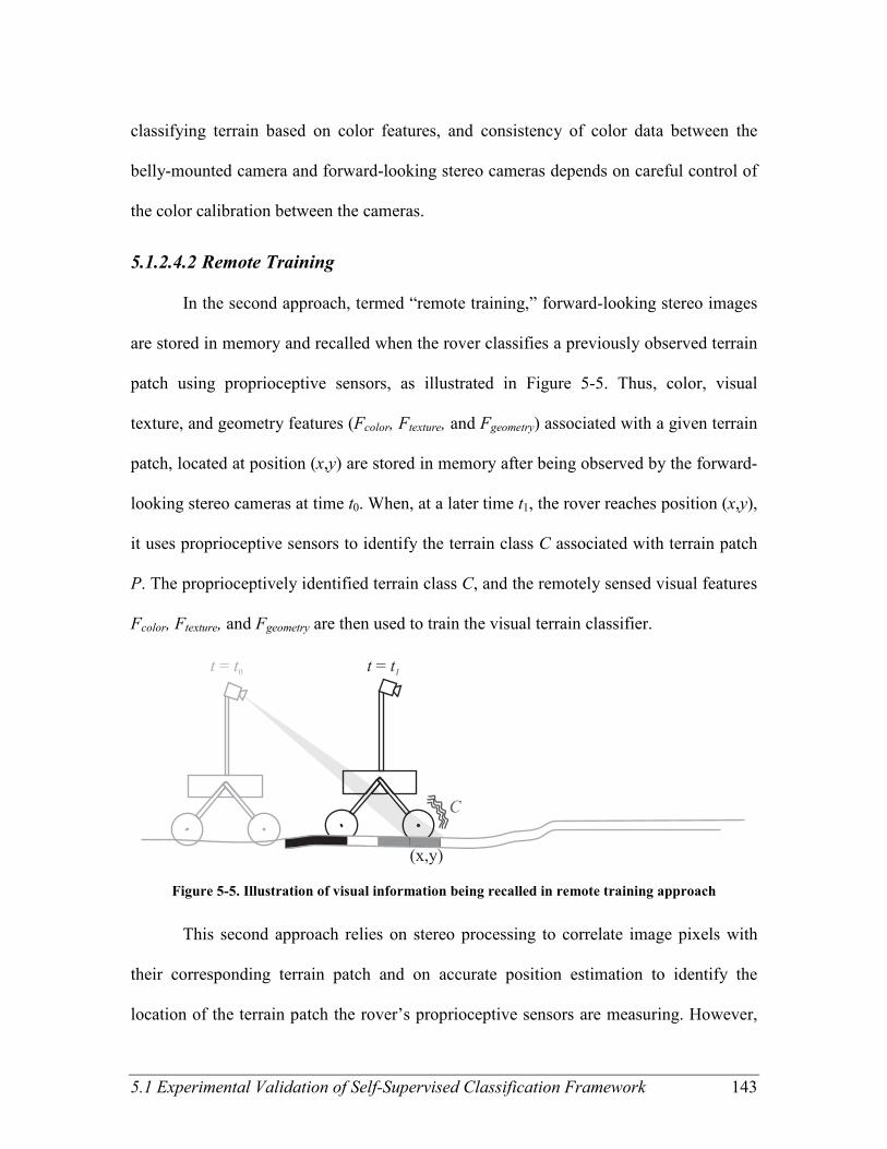
5.1 Experimental Validation of Self-Supervised Classification Framework 143
classifying terrain based on color features, and consistency of color data between the
belly-mounted camera and forward-looking stereo cameras depends on careful control of
the color calibration between the cameras.
5.1.2.4.2 Remote Training
In the second approach, termed “remote training,” forward-looking stereo images
are stored in memory and recalled when the rover classifies a previously observed terrain
patch using proprioceptive sensors, as illustrated in Figure 5-5. Thus, color, visual
texture, and geometry features (Fcolor, Ftexture, and Fgeometry) associated with a given terrain
patch, located at position (x,y) are stored in memory after being observed by the forward-
looking stereo cameras at time t0. When, at a later time t1, the rover reaches position (x,y),
it uses proprioceptive sensors to identify the terrain class C associated with terrain patch
P. The proprioceptively identified terrain class C, and the remotely sensed visual features
Fcolor, Ftexture, and Fgeometry are then used to train the visual terrain classifier.
Figure 5-5. Illustration of visual information being recalled in remote training approach
This second approach relies on stereo processing to correlate image pixels with
their corresponding terrain patch and on accurate position estimation to identify the
location of the terrain patch the rover’s proprioceptive sensors are measuring. However,
144 Chapter 5. Self-Supervised Classification
this approach does not depend on accurate color calibration between multiple cameras,
and texture and geometric data are readily available for use in training the visual
classifier.
5.1.2.4.3 Local and Remote Training
In both self-supervised classification approaches, training data is accumulated as
the rover travels, and the training data for each terrain class is stored in memory. To limit
the training time for the visual classifier, each terrain class is limited to a maximum of
400 sets of features26
—some of the older data is discarded if new data arrives that would
exceed that maximum.27
Visual terrain classification is implemented on a patch level;
each terrain patch is classified via naïve Bayes fusion of the color, visual texture, and
geometric features sensed for pixels corresponding to that patch.
It should be noted that the decision to use a support vector machine for the self-
supervised visual classifier is particularly important, because there is a non-negligible
chance that some of the training data may be incorrectly labeled. A boosting algorithm
such as AdaBoost (Freund & Schapire, 1997) would be particularly inappropriate,
because it would tend to assign excessively high importance to misclassified training
data.
26
It was observed in experimental analysis that 400 sets of features per terrain class represented a good
balance between computation cost and classification accuracy. 27
The number of new feature sets added to the training data is the number of new feature sets sensed, up to
the maximum of (1) 400 minus the number of old sets of features, (2) 400 divided by the number of terrain
patches represented in the training data, and (3) four (representing 1% of 400). If adding this many new
feature sets would increase the training data beyond the 400 sets of features, older feature sets are discarded
randomly to decrease the number to 400 feature sets. Randomly discarding older features has the effect of
providing an exponentially decreasing likelihood that a feature from an older data set will be maintained,
thus allowing the visual terrain classifier to adapt to slow changes in illumination, while not being
excessively sensitive to the appearance of the most recently added terrain patches.
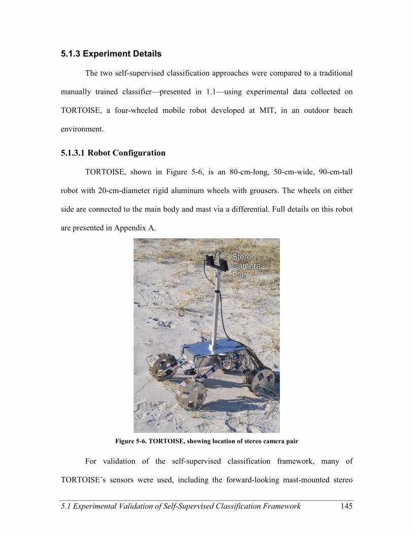
5.1 Experimental Validation of Self-Supervised Classification Framework 145
5.1.3 Experiment Details
The two self-supervised classification approaches were compared to a traditional
manually trained classifier—presented in 1.1—using experimental data collected on
TORTOISE, a four-wheeled mobile robot developed at MIT, in an outdoor beach
environment.
5.1.3.1 Robot Configuration
TORTOISE, shown in Figure 5-6, is an 80-cm-long, 50-cm-wide, 90-cm-tall
robot with 20-cm-diameter rigid aluminum wheels with grousers. The wheels on either
side are connected to the main body and mast via a differential. Full details on this robot
are presented in Appendix A.
Figure 5-6. TORTOISE, showing location of stereo camera pair
For validation of the self-supervised classification framework, many of
TORTOISE’s sensors were used, including the forward-looking mast-mounted stereo
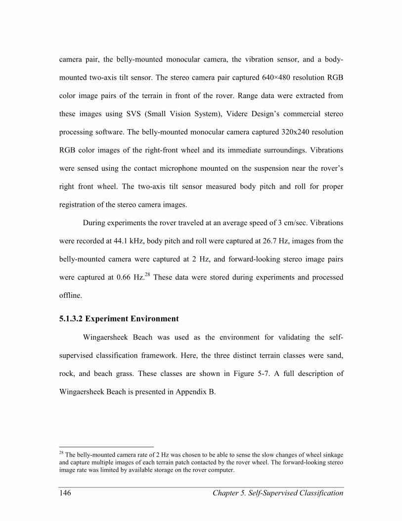
146 Chapter 5. Self-Supervised Classification
camera pair, the belly-mounted monocular camera, the vibration sensor, and a body-
mounted two-axis tilt sensor. The stereo camera pair captured 640×480 resolution RGB
color image pairs of the terrain in front of the rover. Range data were extracted from
these images using SVS (Small Vision System), Videre Design’s commercial stereo
processing software. The belly-mounted monocular camera captured 320x240 resolution
RGB color images of the right-front wheel and its immediate surroundings. Vibrations
were sensed using the contact microphone mounted on the suspension near the rover’s
right front wheel. The two-axis tilt sensor measured body pitch and roll for proper
registration of the stereo camera images.
During experiments the rover traveled at an average speed of 3 cm/sec. Vibrations
were recorded at 44.1 kHz, body pitch and roll were captured at 26.7 Hz, images from the
belly-mounted camera were captured at 2 Hz, and forward-looking stereo image pairs
were captured at 0.66 Hz.28
These data were stored during experiments and processed
offline.
5.1.3.2 Experiment Environment
Wingaersheek Beach was used as the environment for validating the self-
supervised classification framework. Here, the three distinct terrain classes were sand,
rock, and beach grass. These classes are shown in Figure 5-7. A full description of
Wingaersheek Beach is presented in Appendix B.
28
The belly-mounted camera rate of 2 Hz was chosen to be able to sense the slow changes of wheel sinkage
and capture multiple images of each terrain patch contacted by the rover wheel. The forward-looking stereo
image rate was limited by available storage on the rover computer.

5.1 Experimental Validation of Self-Supervised Classification Framework 147
Figure 5-7. TORTOISE on Wingaersheek Beach, showing terrain classes
Six experimental data sets were used in this analysis. Each data set was collected
during a single rover traverse of 10 to 35 meters along a straight-line path containing a
combination of two or three terrains. No two paths were identical. These experiments
were conducted over the course of three days. During experiments the lighting varied
from uniform diffuse light from an overcast sky to harsh direct light from the sun low in
the sky.
5.1.3.3 Data Processing
After the experiments were complete, stored data was processed offline. Range
data were calculated for every fifth stereo image pair.29
Every 20th
stereo image pair30
was labeled by hand to identify the ground-truth terrain class corresponding to each pixel.
By combining the labels with the range data, ground truth terrain classes were identified
29
Every fifth image pair was chosen to reduce the computation time for range data calculation and to
reduce repeated training and testing on the same image patches viewed from nearly identical positions. 30
Every 20th
image pair was chosen to provide at least 10 labeled stereo image pairs in each data set.

148 Chapter 5. Self-Supervised Classification
for each 20-cm by 20-cm terrain patch. For each of the six data sets, between 10 and 28
stereo image pairs were labeled. Additionally, every image from the belly-mounted
camera was labeled to identify the ground truth terrain class under the rover’s right-front
wheel.
For the baseline manually supervised classifier, the first two stereo image pairs
with ground truth labels were used to train a visual classifier for each data set. Four
hundred data features for each sensing mode from each class were used for training the
classifier. The remaining hand-labeled images from that data set were used for testing.
Across all six data sets, 93 image pairs were used for assessing the accuracy of the visual
classifiers.
For self-supervised classification, a separate vibration-based classifier was trained
for each data set, using hand-labeled vibration data from the other data sets. This
vibration-based classifier was then used to provide labels for the entire rover traverse. At
the end of the traverse, the self-supervised visual classifier was trained using 400 features
from each sensing mode for each class. The accuracy of the self-supervised classifier was
tested using the same stereo test images as were used for testing the baseline manually
supervised classifier.
5.1.4 Results
5.1.4.1 Approach 1: Local Training
The first approach for self-supervised training of a visual terrain classifier uses
images from a monocular belly-mounted camera as training data, with labels provided by
a vibration-based classifier. Since geometry information is not available from the belly-

5.1 Experimental Validation of Self-Supervised Classification Framework 149
mounted camera and visual texture is not easily comparable between the belly-mounted
camera and the stereo cameras (due to the difference in observation distance), color
information is used exclusively.
Figure 5-8 shows the receiver operating characteristic (ROC) curves for the
locally trained self-supervised visual classifier. This plot shows classification accuracy as
measured using the 26 test images from one data set. Here, the horizontal axis indicates
the percentage of false positives (%FP) and the vertical axis indicates the percentage of
true positives (%TP). Note that the scale of the horizontal axis is much larger than that of
the vertical axis, to allow the curves to be seen more easily. Each curve on the plot
represents a single terrain, since both %TP and %FP are functions of the threshold for
leaving terrain unclassified. The end point of each curve represents the point at which
none of the terrain is left unclassified. Random assignment of terrain patches to classes
would tend to yield a diagonal line along which the true positive percentage equals the
false positive percentage.
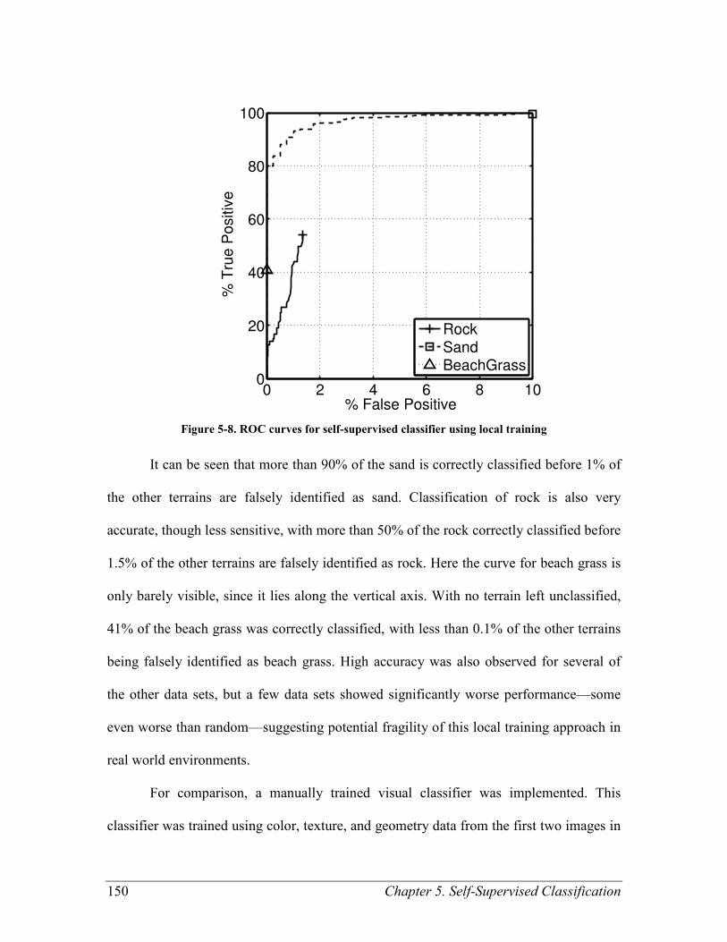
150 Chapter 5. Self-Supervised Classification
0 2 4 6 8 100
20
40
60
80
100
% False Positive
% T
rue
Po
sitiv
e
RockSandBeachGrass
Figure 5-8. ROC curves for self-supervised classifier using local training
It can be seen that more than 90% of the sand is correctly classified before 1% of
the other terrains are falsely identified as sand. Classification of rock is also very
accurate, though less sensitive, with more than 50% of the rock correctly classified before
1.5% of the other terrains are falsely identified as rock. Here the curve for beach grass is
only barely visible, since it lies along the vertical axis. With no terrain left unclassified,
41% of the beach grass was correctly classified, with less than 0.1% of the other terrains
being falsely identified as beach grass. High accuracy was also observed for several of
the other data sets, but a few data sets showed significantly worse performance—some
even worse than random—suggesting potential fragility of this local training approach in
real world environments.
For comparison, a manually trained visual classifier was implemented. This
classifier was trained using color, texture, and geometry data from the first two images in
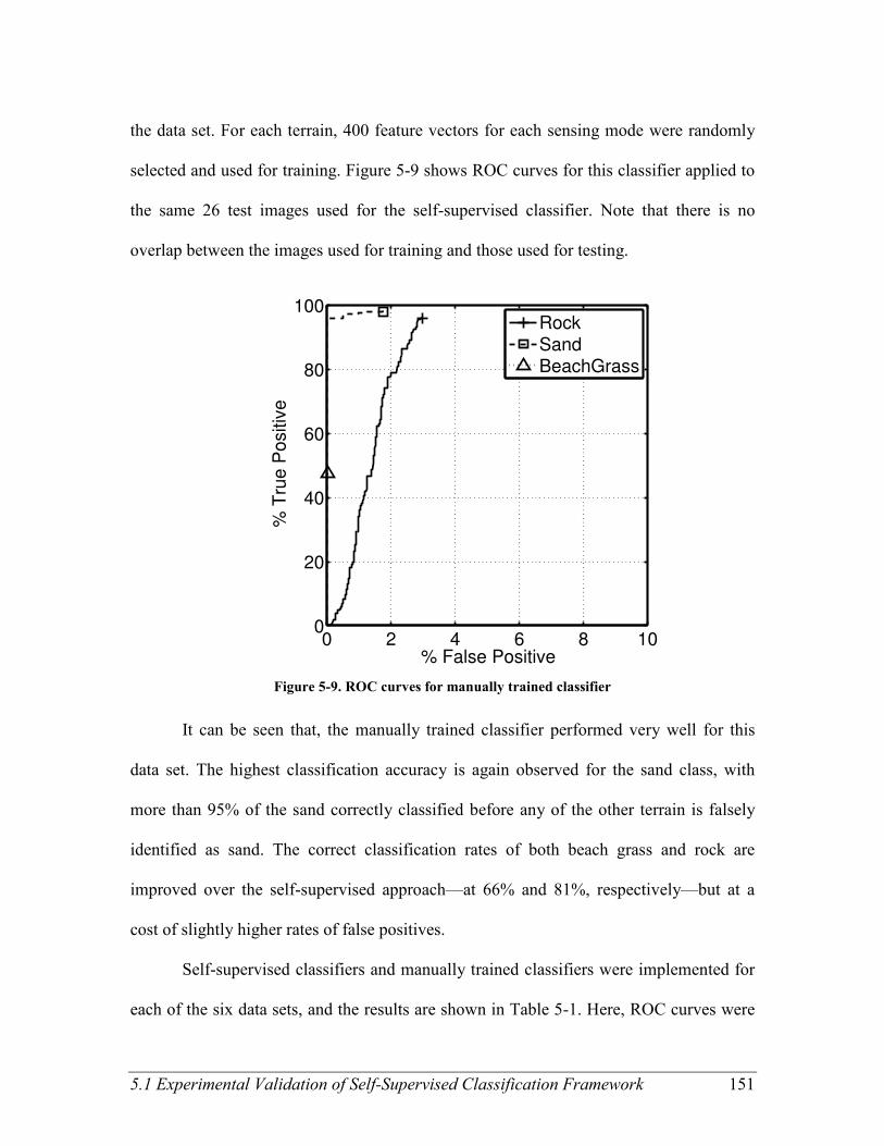
5.1 Experimental Validation of Self-Supervised Classification Framework 151
the data set. For each terrain, 400 feature vectors for each sensing mode were randomly
selected and used for training. Figure 5-9 shows ROC curves for this classifier applied to
the same 26 test images used for the self-supervised classifier. Note that there is no
overlap between the images used for training and those used for testing.
0 2 4 6 8 100
20
40
60
80
100
% False Positive
% T
rue P
ositiv
e
RockSandBeachGrass
Figure 5-9. ROC curves for manually trained classifier
It can be seen that, the manually trained classifier performed very well for this
data set. The highest classification accuracy is again observed for the sand class, with
more than 95% of the sand correctly classified before any of the other terrain is falsely
identified as sand. The correct classification rates of both beach grass and rock are
improved over the self-supervised approach—at 66% and 81%, respectively—but at a
cost of slightly higher rates of false positives.
Self-supervised classifiers and manually trained classifiers were implemented for
each of the six data sets, and the results are shown in Table 5-1. Here, ROC curves were
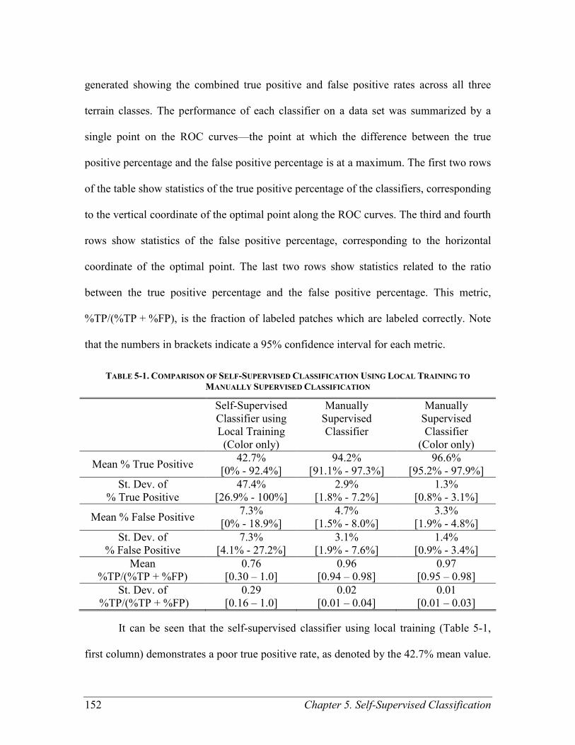
152 Chapter 5. Self-Supervised Classification
generated showing the combined true positive and false positive rates across all three
terrain classes. The performance of each classifier on a data set was summarized by a
single point on the ROC curves—the point at which the difference between the true
positive percentage and the false positive percentage is at a maximum. The first two rows
of the table show statistics of the true positive percentage of the classifiers, corresponding
to the vertical coordinate of the optimal point along the ROC curves. The third and fourth
rows show statistics of the false positive percentage, corresponding to the horizontal
coordinate of the optimal point. The last two rows show statistics related to the ratio
between the true positive percentage and the false positive percentage. This metric,
%TP/(%TP + %FP), is the fraction of labeled patches which are labeled correctly. Note
that the numbers in brackets indicate a 95% confidence interval for each metric.
TABLE 5-1. COMPARISON OF SELF-SUPERVISED CLASSIFICATION USING LOCAL TRAINING TO
MANUALLY SUPERVISED CLASSIFICATION
Self-Supervised
Classifier using
Local Training
(Color only)
Manually
Supervised
Classifier
Manually
Supervised
Classifier
(Color only)
Mean % True Positive 42.7%
[0% - 92.4%]
94.2%
[91.1% - 97.3%]
96.6%
[95.2% - 97.9%]
St. Dev. of
% True Positive
47.4%
[26.9% - 100%]
2.9%
[1.8% - 7.2%]
1.3%
[0.8% - 3.1%]
Mean % False Positive 7.3%
[0% - 18.9%]
4.7%
[1.5% - 8.0%]
3.3%
[1.9% - 4.8%]
St. Dev. of
% False Positive
7.3%
[4.1% - 27.2%]
3.1%
[1.9% - 7.6%]
1.4%
[0.9% - 3.4%]
Mean
%TP/(%TP + %FP)
0.76
[0.30 – 1.0]
0.96
[0.94 – 0.98]
0.97
[0.95 – 0.98]
St. Dev. of
%TP/(%TP + %FP)
0.29
[0.16 – 1.0]
0.02
[0.01 – 0.04]
0.01
[0.01 – 0.03]
It can be seen that the self-supervised classifier using local training (Table 5-1,
first column) demonstrates a poor true positive rate, as denoted by the 42.7% mean value.

5.1 Experimental Validation of Self-Supervised Classification Framework 153
The false positive rate is low—7.4% on average—but the other classifiers demonstrated
significantly lower false positive rates, especially as compared to their true positive rates
as indicated by the %TP/(%TP + %FP) metric. The manually supervised classifier
demonstrates better performance than the self-supervised classifier using local training in
each of the metrics. Most of these differences were statistically significant. It should be
noted that there were several runs for which the self-supervised classifier using local
training performed nearly as well as the manually supervised classifier, but its average
performance was degraded by runs in which it performed significantly worse, suggesting
that the self-supervised classification approach using local training suffers from poor
robustness, possibly due to shadows on the terrain observed by the belly-mounted
camera.
To analyze whether the difference between these classifiers was due to the use of
texture and geometric features31
, an additional manually trained classifier was
implemented using only color data. Results from that classifier are shown in the third
column of Table 5-1. These results show that the manually supervised classifier using
only the color feature is significantly more robust than the self-supervised classifier.
Thus, other factors, such as miscalibration between cameras used for training and
cameras used for testing, are likely to be the cause of the poor performance of the locally
trained self-supervised classifier.
It should be noted that while the manually supervised classifier based solely on
color seems to perform slightly better for these data sets, this difference does not appear
31
Recall that the self-supervised classifier using local training employed only color features, whereas the
manually supervised classifier employed color, visual texture, and geometry features.

154 Chapter 5. Self-Supervised Classification
to be significant. In previous work this difference has favored the manually supervised
classifier using color, texture, and range data (Halatci et al., 2008).
5.1.4.2 Approach 2: Remote Training
The second approach to self-supervised training of a visual classifier is to store in
memory the appearance of a terrain patch (as measured by the forward-looking stereo
pair) and recall the appearance when the rover comes into contact with that terrain patch.
Stereo-derived range estimation is used to associate pixels with terrain patches, and
wheel odometry-based position estimation associates the rover’s position at a later time
with the terrain patch. Since this approach uses the same cameras for collecting both
training data and test data, color, texture, and geometry data are all available for training,
and the potential for color miscalibration is eliminated.
Figure 5-10 shows ROC curves for the self-supervised terrain classifier based on
remote training for the same 26 images used for the results shown in Figure 5-8 and
Figure 5-9. The remotely trained self-supervised visual classifier demonstrates accurate
terrain classification on this data set. More than 80% of both sand and beach grass are
correctly classified before 1% of the other terrains are misclassified as either. While the
classification of rock has a low false positive rate—less than 1.5%—the classifier is less
successful at detecting rock than the other terrains. Just under 25% of the rock was
correctly classified for this data set.
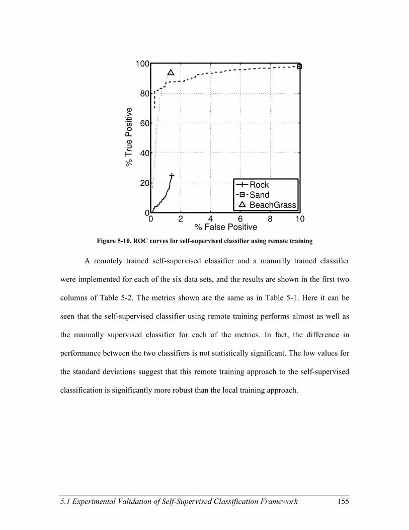
5.1 Experimental Validation of Self-Supervised Classification Framework 155
0 2 4 6 8 100
20
40
60
80
100
% False Positive
% T
rue P
ositiv
e
RockSandBeachGrass
Figure 5-10. ROC curves for self-supervised classifier using remote training
A remotely trained self-supervised classifier and a manually trained classifier
were implemented for each of the six data sets, and the results are shown in the first two
columns of Table 5-2. The metrics shown are the same as in Table 5-1. Here it can be
seen that the self-supervised classifier using remote training performs almost as well as
the manually supervised classifier for each of the metrics. In fact, the difference in
performance between the two classifiers is not statistically significant. The low values for
the standard deviations suggest that this remote training approach to the self-supervised
classification is significantly more robust than the local training approach.
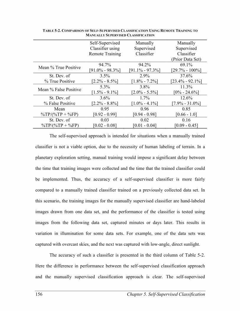
156 Chapter 5. Self-Supervised Classification
TABLE 5-2. COMPARISON OF SELF-SUPERVISED CLASSIFICATION USING REMOTE TRAINING TO
MANUALLY SUPERVISED CLASSIFICATION
Self-Supervised
Classifier using
Remote Training
Manually
Supervised
Classifier
Manually
Supervised
Classifier
(Prior Data Set)
Mean % True Positive 94.7%
[91.0% - 98.3%]
94.2%
[91.1% - 97.3%]
69.1%
[29.7% - 100%]
St. Dev. of
% True Positive
3.5%
[2.2% - 8.5%]
2.9%
[1.8% - 7.2%]
37.6%
[23.4% - 92.1%]
Mean % False Positive 5.3%
[1.5% - 9.1%]
3.8%
[2.0% - 5.5%]
11.3%
[0% - 24.6%]
St. Dev. of
% False Positive
3.6%
[2.2% - 8.8%]
1.7%
[1.0% - 4.1%]
12.6%
[7.9% - 31.0%]
Mean
%TP/(%TP + %FP)
0.95
[0.92 - 0.99]
0.96
[0.94 - 0.98]
0.85
[0.66 - 1.0]
St. Dev. of
%TP/(%TP + %FP)
0.03
[0.02 - 0.08]
0.02
[0.01 - 0.04]
0.16
[0.09 - 0.45]
The self-supervised approach is intended for situations when a manually trained
classifier is not a viable option, due to the necessity of human labeling of terrain. In a
planetary exploration setting, manual training would impose a significant delay between
the time that training images were collected and the time that the trained classifier could
be implemented. Thus, the accuracy of a self-supervised classifier is more fairly
compared to a manually trained classifier trained on a previously collected data set. In
this scenario, the training images for the manually supervised classifier are hand-labeled
images drawn from one data set, and the performance of the classifier is tested using
images from the following data set, captured minutes or days later. This results in
variation in illumination for some data sets. For example, one of the data sets was
captured with overcast skies, and the next was captured with low-angle, direct sunlight.
The accuracy of such a classifier is presented in the third column of Table 5-2.
Here the difference in performance between the self-supervised classification approach
and the manually supervised classification approach is clear. The self-supervised
5.1 Experimental Validation of Self-Supervised Classification Framework 157
classification approach yields better true positive classification, a lower false positive
rate, and higher overall classification accuracy, as compared to the manually supervised
classifier when training delay is added.
5.1.4.3 Computation time
To enable real time operation, an effort was made to limit the computational
complexity of training and testing of these classifiers, so the most computationally
intensive tasks were stereo data extraction and texture feature computation. Extraction of
geometric features from a 3-D point cloud takes an average of 5 seconds per image using
a Matlab script on a Pentium 4 1.8 GHz desktop computer. Texture feature extraction
takes 17.3 sec, using an unoptimized Matlab script. A C-code implementation would be
expected to run much faster.
Because it doesn’t rely on stereo data or texture feature extraction, the locally
trained classifier can be trained very quickly. Training takes 1.7 seconds on a Pentium 4
1.8 GHz desktop using the LIBSVM library. Color-based classification takes only 0.7
seconds for a full 640×480 image. Classifying terrain patches requires that stereo data be
computed to identify which pixel belongs to which patch; once that data is computed,
each patch took an average of 0.01 seconds to classify in Matlab, with an average of 400
patches per image.
The remotely trained classifier took slightly less time to train, at 1.5 seconds on
average, because some of the terrains had fewer than 400 training data points.
Classification was slower for the remotely trained classifier, at 4.1 seconds per image,
due to the use of texture and geometry data.
158 Chapter 5. Self-Supervised Classification
5.1.5 Conclusions
In this section, two self-supervised classification approaches were presented. Both
approaches train a visual classifier using terrain class labels identified locally using a
vibration-based terrain classifier. The first approach uses images from a belly-mounted
camera as training data. It was shown to have excellent performance in classifying terrain
for some data sets, but experimentally observed results were inconsistent. The second
approach uses the recalled appearance of a terrain patch to provide training data for a
visual classifier. This approach was shown to perform as well as a manually supervised
classifier trained using the same data set, and was shown to perform significantly better
than the manually supervised classifier when a delay due to manual training is
considered.
While these results support the use of autonomous labeling to train a visual
classifier, the vibration-based terrain classifier used to perform the labeling requires its
own manually supervised training. Thus it is not a truly unsupervised approach suitable
for application to novel environments where no a priori knowledge is available.
5.2 Self-Supervised Terrain Learning System for Novel Environments
5.2.1 Introduction
For scenarios in which no a priori information about the terrain is available, a
completely unsupervised terrain learning system can be assembled using the self-
supervised classification framework and component algorithms developed and validated
earlier in this thesis. As with the self-supervised learning system validated in 1.1, this
terrain learning system learns to identify instances of a terrain class in the distance based
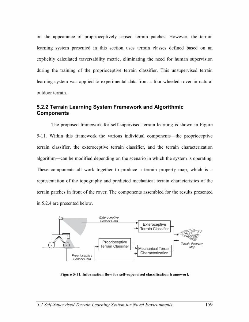
5.2 Self-Supervised Terrain Learning System for Novel Environments 159
on the appearance of proprioceptively sensed terrain patches. However, the terrain
learning system presented in this section uses terrain classes defined based on an
explicitly calculated traversability metric, eliminating the need for human supervision
during the training of the proprioceptive terrain classifier. This unsupervised terrain
learning system was applied to experimental data from a four-wheeled rover in natural
outdoor terrain.
5.2.2 Terrain Learning System Framework and Algorithmic Components
The proposed framework for self-supervised terrain learning is shown in Figure
5-11. Within this framework the various individual components—the proprioceptive
terrain classifier, the exteroceptive terrain classifier, and the terrain characterization
algorithm—can be modified depending on the scenario in which the system is operating.
These components all work together to produce a terrain property map, which is a
representation of the topography and predicted mechanical terrain characteristics of the
terrain patches in front of the rover. The components assembled for the results presented
in 5.2.4 are presented below.
Figure 5-11. Information flow for self-supervised classification framework

160 Chapter 5. Self-Supervised Classification
5.2.2.1 Self-Supervised Learning Approach
As described in 1.1, there are multiple potential approaches to self-supervised
learning. Based on the experimental results, the “remote training” approach was chosen
for implementation in this terrain learning system. In this approach, images from
forward-looking stereo cameras are stored in memory. When the proprioceptive terrain
classifier identifies the class associated with a terrain patch, the terrain patch’s
appearance is recalled to use in training the exteroceptive terrain classifier. This approach
relies heavily on the accuracy of stereo processing and rover position estimation to
properly associate the image data with the class labels, but it was shown using
experimental data to yield more robust classification than the “local training” approach.
5.2.2.2 Proprioceptive Terrain Classifier
The proprioceptive terrain classification component for the terrain learning
system is derived from the mechanical terrain characterization work presented in Chapter
4. In this algorithm the local terrain is divided into classes based on the minimum bound
for the net traction force, sensed during the 67% slip stage of the “Incremental Slip”
behavior described in 2.2.2. (Vibration-based terrain classification, presented in 2.1, was
not used because it requires use of a priori knowledge of the terrain classes and human-
supervised labeling of vibration data. Torque-based terrain clustering, presented in 1.1,
was not used because it didn’t perform well in the experiments with the “Incremental
Slip” behavior, and experiments with moderate values of slip are required for the
mechanical terrain characterization algorithm.)
Here, for every local terrain patch with associated slip data, DP/W bounds were
calculated using the Bekker model with absolute sinkage described in 4.2.4.3. Five terrain
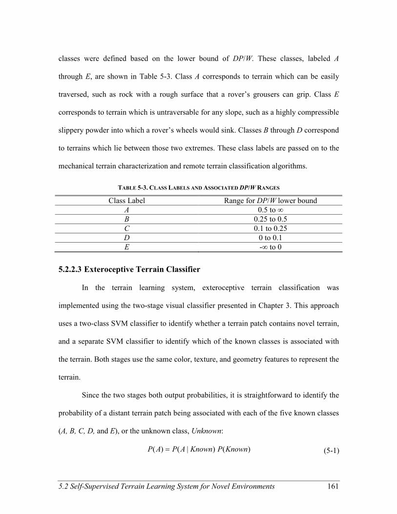
5.2 Self-Supervised Terrain Learning System for Novel Environments 161
classes were defined based on the lower bound of DP/W. These classes, labeled A
through E, are shown in Table 5-3. Class A corresponds to terrain which can be easily
traversed, such as rock with a rough surface that a rover’s grousers can grip. Class E
corresponds to terrain which is untraversable for any slope, such as a highly compressible
slippery powder into which a rover’s wheels would sink. Classes B through D correspond
to terrains which lie between those two extremes. These class labels are passed on to the
mechanical terrain characterization and remote terrain classification algorithms.
TABLE 5-3. CLASS LABELS AND ASSOCIATED DP/W RANGES
Class Label Range for DP/W lower bound
A 0.5 to ∞
B 0.25 to 0.5
C 0.1 to 0.25
D 0 to 0.1
E -∞ to 0
5.2.2.3 Exteroceptive Terrain Classifier
In the terrain learning system, exteroceptive terrain classification was
implemented using the two-stage visual classifier presented in Chapter 3. This approach
uses a two-class SVM classifier to identify whether a terrain patch contains novel terrain,
and a separate SVM classifier to identify which of the known classes is associated with
the terrain. Both stages use the same color, texture, and geometry features to represent the
terrain.
Since the two stages both output probabilities, it is straightforward to identify the
probability of a distant terrain patch being associated with each of the five known classes
(A, B, C, D, and E), or the unknown class, Unknown:
)()|()( KnownPKnownAPAP = (5-1)
162 Chapter 5. Self-Supervised Classification
and
)()( NovelPUnknownP = , (5-2)
where P(Known) and P(Novel) are outputs of the novel terrain detector, and P(A|Known)
is one of the outputs of the known terrain classifier. Thus, the remote terrain classifier
calculates the probability of each terrain cell belonging to each terrain class: [P(A), P(B),
P(C), P(D), P(E), P(Unknown)].
5.2.2.4 Terrain Characterization
In the instantiation of the terrain learning system described here, the terrain
classes identified by the proprioceptive terrain classifier are defined by their mechanical
characteristics, so a separate terrain characterization stage is redundant.
5.2.2.5 Class/Property Fusion
The last important step in producing the terrain property map is to combine the
outputs of the remote terrain classifier with the output of the terrain characterization
algorithm. To make the terrain property map easier to interpret, it is desirable to have
only a single number represent the terrain traversability in each patch. For this terrain
learning system, that number is a conservative estimate for the net traction force, DP/W.
Here that conservative estimate of DP/W is defined as the highest value for which
there is at least an 80% probability that the true value would be higher. This can be
calculated from the ranges of lower DP/W bounds associated with the classes (Table 5-3)
and the class probabilities from the remote terrain classifier. For example, given the
probabilities P(A) = 50%, P(B) = 25%, P(C) = 6%, P(D) = 10%, P(E) = 4%, P(Unknown)
= 5%, a conservative estimate of DP/W for the associated terrain cell would be 0.1 (i.e.
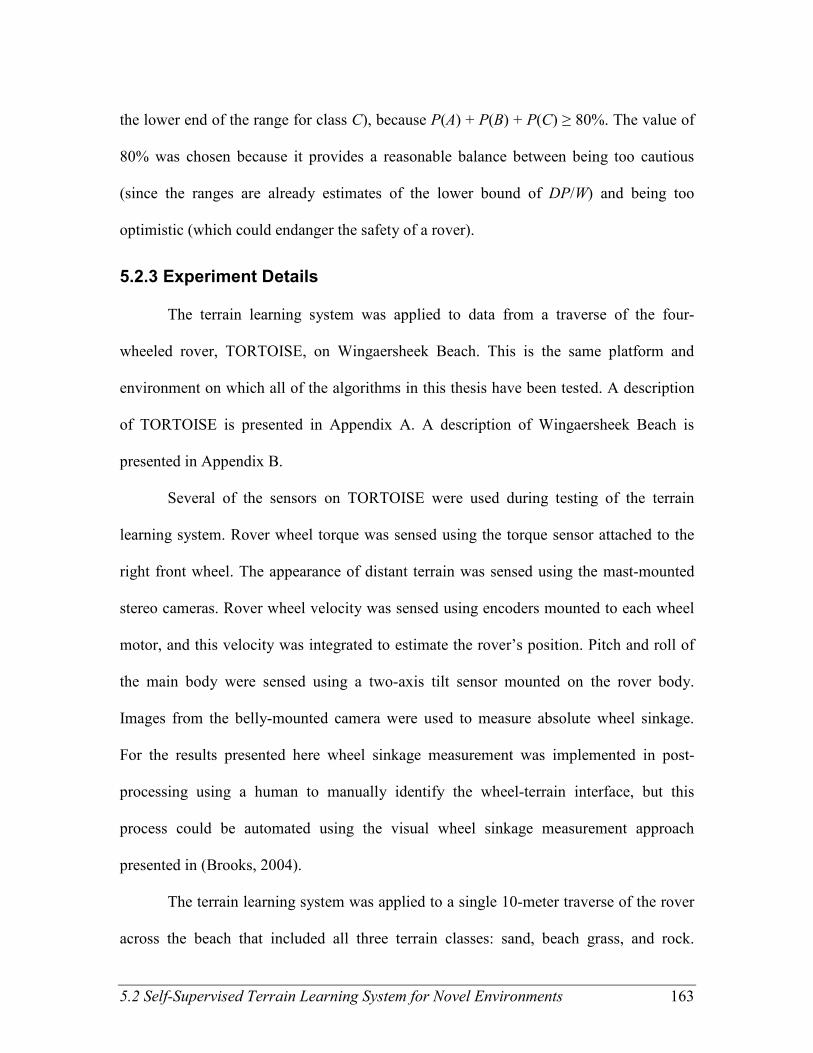
5.2 Self-Supervised Terrain Learning System for Novel Environments 163
the lower end of the range for class C), because P(A) + P(B) + P(C) ≥ 80%. The value of
80% was chosen because it provides a reasonable balance between being too cautious
(since the ranges are already estimates of the lower bound of DP/W) and being too
optimistic (which could endanger the safety of a rover).
5.2.3 Experiment Details
The terrain learning system was applied to data from a traverse of the four-
wheeled rover, TORTOISE, on Wingaersheek Beach. This is the same platform and
environment on which all of the algorithms in this thesis have been tested. A description
of TORTOISE is presented in Appendix A. A description of Wingaersheek Beach is
presented in Appendix B.
Several of the sensors on TORTOISE were used during testing of the terrain
learning system. Rover wheel torque was sensed using the torque sensor attached to the
right front wheel. The appearance of distant terrain was sensed using the mast-mounted
stereo cameras. Rover wheel velocity was sensed using encoders mounted to each wheel
motor, and this velocity was integrated to estimate the rover’s position. Pitch and roll of
the main body were sensed using a two-axis tilt sensor mounted on the rover body.
Images from the belly-mounted camera were used to measure absolute wheel sinkage.
For the results presented here wheel sinkage measurement was implemented in post-
processing using a human to manually identify the wheel-terrain interface, but this
process could be automated using the visual wheel sinkage measurement approach
presented in (Brooks, 2004).
The terrain learning system was applied to a single 10-meter traverse of the rover
across the beach that included all three terrain classes: sand, beach grass, and rock.

164 Chapter 5. Self-Supervised Classification
During the traverse, the rover performed the “Incremental Slip” behavior described in
2.2.2, and all data was stored so that it could be passed to an offline implementation of
the sensing system.
5.2.4 Results
The output of the terrain learning system is a prediction of a lower bound of net
drawbar pull for each terrain patch as predicted using each stereo image. This is most
easily viewed as a video, but still frames are shown in Figure 5-12, Figure 5-13, and
Figure 5-14.
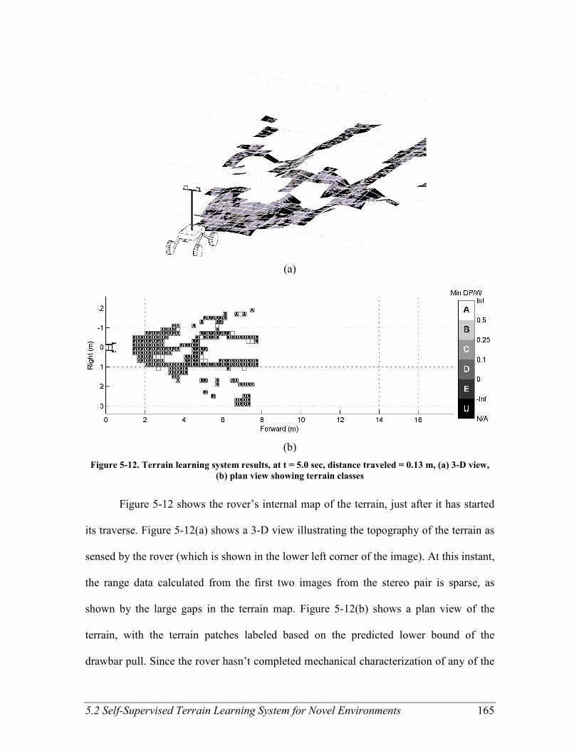
5.2 Self-Supervised Terrain Learning System for Novel Environments 165
(a)
(b)
Figure 5-12. Terrain learning system results, at t = 5.0 sec, distance traveled = 0.13 m, (a) 3-D view,
(b) plan view showing terrain classes
Figure 5-12 shows the rover’s internal map of the terrain, just after it has started
its traverse. Figure 5-12(a) shows a 3-D view illustrating the topography of the terrain as
sensed by the rover (which is shown in the lower left corner of the image). At this instant,
the range data calculated from the first two images from the stereo pair is sparse, as
shown by the large gaps in the terrain map. Figure 5-12(b) shows a plan view of the
terrain, with the terrain patches labeled based on the predicted lower bound of the
drawbar pull. Since the rover hasn’t completed mechanical characterization of any of the
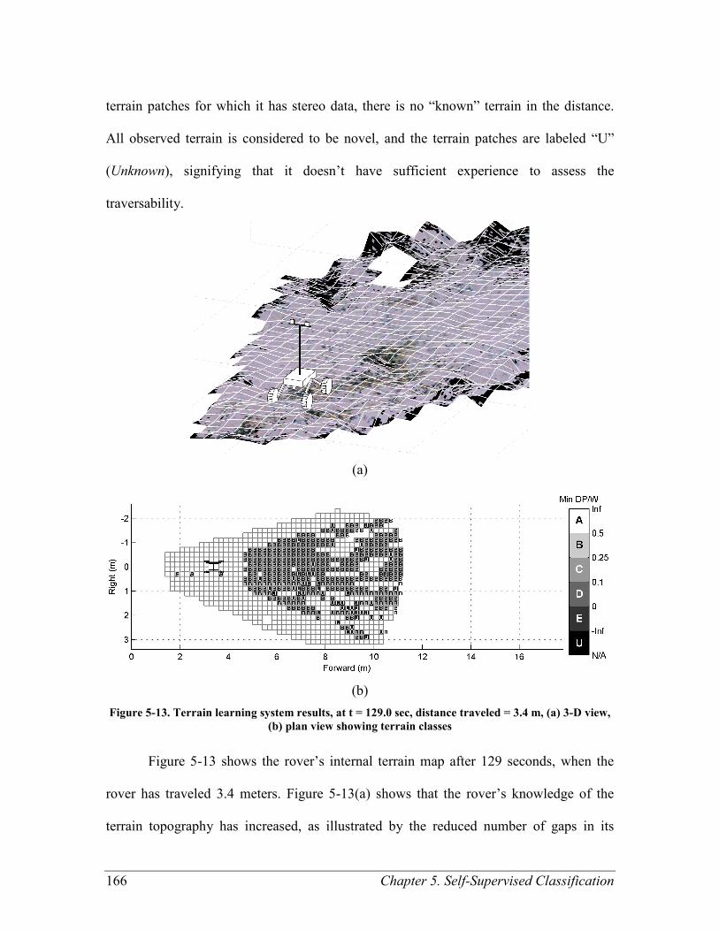
166 Chapter 5. Self-Supervised Classification
terrain patches for which it has stereo data, there is no “known” terrain in the distance.
All observed terrain is considered to be novel, and the terrain patches are labeled “U”
(Unknown), signifying that it doesn’t have sufficient experience to assess the
traversability.
(a)
(b)
Figure 5-13. Terrain learning system results, at t = 129.0 sec, distance traveled = 3.4 m, (a) 3-D view,
(b) plan view showing terrain classes
Figure 5-13 shows the rover’s internal terrain map after 129 seconds, when the
rover has traveled 3.4 meters. Figure 5-13(a) shows that the rover’s knowledge of the
terrain topography has increased, as illustrated by the reduced number of gaps in its

5.2 Self-Supervised Terrain Learning System for Novel Environments 167
internal representation of the terrain. Figure 5-13(b) shows that the rover has identified
the minimum net traction force for three terrain patches with associated stereo data.
These are illustrated in the figure by the three labeled terrain patches at 1.9m, 2.5m, and
3.7m. (Here, terrain patches which have been characterized through physical interaction
are labeled with italicized letters.) Since these three patches all fall into class B
(representing a lower bound of DP/W between 0.25 and 0.5 from Table 5-3), all of the
recognized (i.e. not novel) terrain in the distance is predicted to fall into that range.
Terrain that is sufficiently different from the terrain the rover has driven over is still
labeled “U,” with unknown traversability properties.
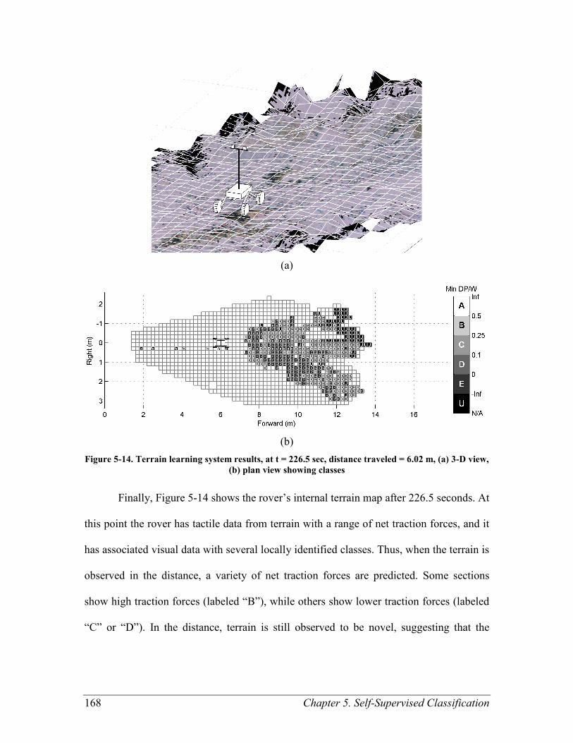
168 Chapter 5. Self-Supervised Classification
(a)
(b)
Figure 5-14. Terrain learning system results, at t = 226.5 sec, distance traveled = 6.02 m, (a) 3-D view,
(b) plan view showing classes
Finally, Figure 5-14 shows the rover’s internal terrain map after 226.5 seconds. At
this point the rover has tactile data from terrain with a range of net traction forces, and it
has associated visual data with several locally identified classes. Thus, when the terrain is
observed in the distance, a variety of net traction forces are predicted. Some sections
show high traction forces (labeled “B”), while others show lower traction forces (labeled
“C” or “D”). In the distance, terrain is still observed to be novel, suggesting that the

5.2 Self-Supervised Terrain Learning System for Novel Environments 169
terrain in the distance may have a significantly different appearance than the terrains
previously traversed.
5.2.5 Conclusions
This section has presented a terrain learning system for novel environments that is
capable of learning from experience to visually recognize terrain and predict a lower
bound on the net traction force. This system employs a self-supervised learning approach
that uses the recalled appearance of terrain from stored images to train a visual classifier.
Proprioceptive terrain classification is accomplished by grouping terrain patches based on
the mechanically sensed lower bound on the net traction force. Exteroceptive
classification is accomplished using a two-stage visual classifier capable of recognizing
novel terrain.
Results from the application of this complete terrain sensing system to an
experimental data set yields reasonable results, however no ground truth is available to
confirm the accuracy of the net traction force predictions. It is expected that the
capabilities for visual recognition of the traction forces would continue to improve over
significantly longer traverses. Future work is needed to establish how the tightness of the
predicted traversability bounds will change over longer traverses.
170 Chapter 6. Conclusions and Suggestions for Future Work
Chapter
6 Chapter 6 Conclusions and Suggestions for Future Work
6.1 Contributions of this Thesis
This thesis has presented a framework of algorithms to enable a planetary rover to
accurately predict mechanical properties of terrain at a distance by learning from
experiences gained during traverses of similar terrain. This has been accomplished
through the use of a self-supervised learning framework, which provides a coherent
architecture in which local terrain classification, remote terrain classification, and
mechanical terrain characterization can be combined.
In Chapter 2, two distinct approaches were presented for classification of terrain
based on proprioceptive sensor data. The first section presented a method for vibration-
based terrain classification using a support vector machine (SVM). It is suitable for a
supervised scenario, i.e. when labeled vibration training data is available. The second
section presented a novel method for segmenting terrain based on the wheel torque
sensed during high wheel slip ratio conditions. This approach is suitable for an
unsupervised scenario, i.e. when the terrain classes are not known a priori. A comparison
of experimental results using this approach showed that higher induced wheel slip ratios
improve segmentation accuracy. Both local classification approaches were validated
171
using experimental data from a four-wheeled rover in a beach environment. These local
terrain characterization approaches are viable methods for distinguishing terrain using
features from proprioceptive sensors, making them inherently insensitive to changes in
illumination.
Chapter 3 addressed exteroceptive classification of terrain. The first section
described a SVM-based visual classifier, modeled on the approach of Halatci (Halatci,
2006; Halatci et al., 2008). It presented new experimental results for this classification
approach. The second section addressed a specific shortcoming of a supervised classifier:
recognizing when new observations are not associated with any of the trained classes.
This section introduced a new approach to detection of novel terrain. This approach was
specifically targeted to the self-supervised classification scenario in which a large
quantity of unclassified training data is available. Data from rover experiments in a beach
environment were used to validate this novelty detection approach. A two-stage visual
classification system combining these two algorithms can both accurately classify terrain
and detect terrain not belonging to the set of trained classes.
Chapter 4 addressed the issue of how to characterize terrain. It presented a method
to calculate bounds on the net traction force based on observed wheel torque and sinkage
under induced wheel slip conditions. Three different approaches were explored using data
from laboratory experiments with a wheel-terrain interaction test platform, and the most
promising approach was applied to experimental data from a four-wheeled rover on
Wingaersheek Beach. This approach yields a physically meaningful metric for
representing the traversability of terrain that is appropriate for situations when caution is
required.
172 Chapter 6. Conclusions and Suggestions for Future Work
In Chapter 5, the self-supervised classification framework itself was studied. The
first section compared two sources for training data for the visual classifier, based on
classification performance on experimental data from Wingaersheek Beach. The second
section presented a terrain learning system for novel environments, which combined
proprioceptive classification, exteroceptive classification, and mechanical terrain sensing
in a single system and applied it to experiment data from the TORTOISE rover on
Wingaersheek Beach. Thus, the terrain learning system, in which each component was
independently validated, was demonstrated.
6.2 Suggestions for Future Work
There are several areas in which this work could be extended. Where a suggestion
applies only to a particular component, the suggestion has been included in the section in
which the component is described. The suggestions described here can be divided into
experimental extensions, computational extensions, and algorithmic extensions.
Experimental extensions are additional experiments that could be implemented
without changing the terrain sensing algorithms. The easiest extension to accomplish
would be to use the same robot platform and demonstrate that this terrain learning system
(and each of its subcomponents) will work in a variety of unique environments. This
should be straightforward in any environment that can be modeled as a height field;
changes in the terrain representation would be required for it to operate in a fully 3-D
environment. Applying this terrain sensing algorithm to a different platform, such as a
high-speed UGV or a human-driven automobile, might also be promising.
Computational extensions would include changes in some of the underlying code
which should reduce computation time without affecting the algorithm accuracy. For

173
example, all of the classification in this work is done using support vector machines. In
situations when a linear or low-order polynomial kernel is used, the standard
classification code can be significantly streamlined, which would enable faster
classification. The overall approach for these optimizations are presented in Appendix D.
There are likely to be optimizations along the same lines for reducing the time necessary
for training the SVM classifier.
Algorithmic extensions would include changing some of the larger components of
this sensing system. For example, computing the texture feature of the visual classifier is
currently one of the slowest steps. If some other texture feature is easier to compute or
yields better discrimination, it might be worthwhile to implement. Other changes which
might be made include replacing the SVM with another classifier; Bayesian logistic
regression is currently in favor. Another classification replacement to consider is the
regularized least squares (RLS), which is likely to have a closed form solution for
incremental training.
174 References
References Angelova, A., Matthies, L., Helmick, D., & Perona, P. (2007a). Learning and prediction
of slip from visual information. Journal of Field Robotics, 24(3), 205-231. doi:
10.1002/rob.20179.
Angelova, A., Matthies, L., Helmick, D., & Perona, P. (2007b). Learning slip behavior
using automatic mechanical supervision. In Proceedings of the 2007 IEEE
International Conference on Robotics and Automation (ICRA '07) (pp. 1741-
1748). Rome, Italy. doi: 10.1109/ROBOT.2007.363574.
Angelova, A., Matthies, L., Helmick, D., Sibley, G., & Perona, P. (2006). Learning to
predict slip for ground robots. In Proceedings of the 2006 IEEE International
Conference on Robotics and Automation (ICRA '06) (pp. 3324-3331). Orlando,
FL.
Arvidson, R. E., Anderson, R. C., Bartlett, P., Bell, J. F., Blaney, D., Christensen, P. R.,
et al. (2004). Localization and Physical Properties Experiments Conducted by
Spirit at Gusev Crater. Science, 305(5685), 821-824. doi:
10.1126/science.1099922.
Bajracharya, M., Maimone, M. W., & Helmick, D. (2008). Autonomy for Mars Rovers:
Past, Present, and Future. Computer, 41(12), 44-50. doi: 10.1109/MC.2008.479.
Balas, B. J. (2006). Texture synthesis and perception: Using computational models to
study texture representations in the human visual system. Vision Research, 46(3),
299-309. doi: 10.1016/j.visres.2005.04.013 .
Bekker, M. G. (1969). Introduction to Terrain-Vehicle Systems. Ann Arbor: University of
Michigan Press.
Bellutta, P., Manduchi, R., Matthies, L., Owens, K., & Rankin, A. (2000). Terrain
perception for DEMO III. In Proceedings of the 2000 IEEE Intelligent Vehicles
Symposium (IV 2000) (pp. 326-331). Dearborn, MI. doi:
10.1109/IVS.2000.898363.
Berni, J. A. J., Zarco-Tejada, P. J., Suarez, L., & Fereres, E. (2009). Thermal and
Narrowband Multispectral Remote Sensing for Vegetation Monitoring From an
Unmanned Aerial Vehicle. IEEE Transactions on Geoscience and Remote
Sensing, 47(3), 722-738. doi: 10.1109/TGRS.2008.2010457.
Bilmes, J. (1998). A Gentle Tutorial of the EM Algorithm and its Application to
Parameter Estimation for Gaussian Mixture and Hidden Markov Models.
Technical Report, Berkeley, CA: International Computer Science Institute.
Retrieved November 21, 2008, from
http://ssli.ee.washington.edu/people/bilmes/mypapers/em.pdf.
Bishop, C. M. (1995). Neural Networks for Pattern Recognition. Oxford, England:
Clarendon Press.
References 175
Bouman, C., & Liu, B. (1991). Multiple resolution segmentation of textured images.
IEEE Transactions on Pattern Analysis and Machine Intelligence, 13(2), 99-113.
doi: 10.1109/34.67641.
Brandes, U., Gaertler, M., & Wagner, D. (2003). Experiments on Graph Clustering
Algorithms. In Algorithms - ESA 2003, Lecture Notes in Computer Science (Vol.
2832, pp. 568-579). Springer Berlin / Heidelberg. Retrieved November 12, 2008,
from http://www.springerlink.com/content/cv8tbjmrhdflau3r.
Brooks, C. (2004). Terrain Identification Methods for Planetary Exploration Rovers.
Thesis (S.M.), Massachusetts Institute of Technology. Retrieved from
http://dspace.mit.edu/handle/1721.1/30303.
Brooks, C., & Iagnemma, K. (2005). Vibration-based terrain classification for planetary
exploration rovers. IEEE Transactions on Robotics, 21(6), 1185-1191. doi:
10.1109/TRO.2005.855994.
Brooks, C., Iagnemma, K., & Dubowsky, S. (2006). Visual wheel sinkage measurement
for planetary rover mobility characterization. Autonomous Robots, 21(1), 55-64.
doi: 10.1007/s10514-006-7230-9.
Chang, C., & Lin, C. (2005). LIBSVM: a library for support vector machines (Version
2.81) [Computer software]. Retrieved from
http://www.csie.ntu.edu.tw/~cjlin/libsvm.
Chang, C., & Lin, C. (2008, October 29). LIBSVM: a Library for Support Vector
Machines. Retrieved November 20, 2008, from
http://www.csie.ntu.edu.tw/~cjlin/papers/libsvm.pdf.
Cowen, R. (2005). Opportunity Rolls out of Purgatory. Science News, 167(26), 413.
Denes, L. J., Gottlieb, M. S., Kaminsky, B., & Huber, D. F. (1998). Spectropolarimetric
imaging for object recognition. In 26th AIPR Workshop: Exploiting New Image
Sources and Sensors (Vol. 3240, pp. 8-18). Washington, DC: SPIE. doi:
10.1117/12.300052.
DuPont, E., Roberts, R., Selekwa, M., Moore, C., & Collins, E. (2005). Online Terrain
Classification for Mobile Robots. In Proceedings of the 2005 ASME International
Mechanical Engineering Congress and Exposition (IMECE2005) (p. 81659).
Orlando, FL.
El-Yaniv, R., & Nisenson, M. (2007). Optimal Single-Class Classification Strategies. In
B. Schölkopf, J. Platt, & T. Hoffman (Eds.), Advances in Neural Information
Processing Systems (NIPS) 19 (p. 377―384). Cambridge, MA: MIT Press.
Retrieved from http://eprints.pascal-network.org/archive/00002663/.
Espinal, F., Huntsberger, T. L., Jawerth, B. D., & Kubota, T. (1998). Wavelet-based
fractal signature analysis for automatic target recognition. Optical Engineering,
37(1), 166-174. doi: 10.1117/1.601844.
Freund, Y., & Schapire, R. E. (1997). A Decision-Theoretic Generalization of On-Line
Learning and an Application to Boosting. Journal of Computer and System
Sciences, 55(1), 119-139. doi: 10.1006/jcss.1997.1504.
176 References
Goldberg, S., Maimone, M. W., & Matthies, L. (2002). Stereo vision and rover
navigation software for planetary exploration. In Proceedings of the 2002 IEEE
Aerospace Conference (Vol. 5, pp. 2025-2036). Big Sky, Montana.
Halatci, I. (2006). Vision-Based Terrain Classification and Classifier Fusion for
Planetary Exploration Rovers. Thesis (S.M.), Massachusetts Institute of
Technology. Retrieved from http://dspace.mit.edu/handle/1721.1/38271.
Halatci, I., Brooks, C., & Iagnemma, K. (2008). A Study of Visual and Tactile Terrain
Classification and Classifier Fusion for Planetary Exploration Rovers. Robotica,
26(6), 767-779. doi: 10.1017/S0263574708004360.
Hegedus, E. (1963). Pressure Distribution and Slip-Sinkage Relationship Under Driven
Rigid Wheels. Technical Report, Warren, MI: Army Tank-Automotive Center,
Land Locomotion Lab.
Henriksen, L., & Krotkov, E. (1997). Natural Terrain Hazard Detection with a Laser
Rangefinder. In Proceedings of the 1997 IEEE International Conference on
Robotics and Automation (ICRA '97) (Vol. 2, pp. 968-973). Albuquerque, NM.
doi: 10.1109/ROBOT.1997.614260.
Iagnemma, K., & Dubowsky, S. (2002). Terrain estimation for high-speed rough-terrain
autonomous vehicle navigation. In Proceedings of SPIE Conference on
Unmanned Ground Vehicle Technology IV (Vol. 4715, pp. 256-266). Orlando,
FL: SPIE. doi: 10.1117/12.474457.
Iagnemma, K., Kang, S., Brooks, C., & Dubowsky, S. (2003). Multi-Sensor Terrain
Estimation for Planetary Rovers. In Proceedings of the 7th International
Symposium on Artificial Intelligence, Robotics and Automation in Space, i-
SAIRAS. Nara, Japan. Retrieved November 17, 2008, from
http://citeseerx.ist.psu.edu/viewdoc/summary?doi=10.1.1.8.3791.
Iagnemma, K., Kang, S., Shibly, H., & Dubowsky, S. (2004). Online terrain parameter
estimation for wheeled mobile robots with application to planetary rovers. IEEE
Transactions on Robotics, 20(5), 921-927. doi: 10.1109/TRO.2004.829462.
Iagnemma, K., Shibly, H., & Dubowsky, S. (2002). On-line terrain parameter estimation
for planetary rovers. In Proceedings of the 2002 IEEE International Conference
on Robotics and Automation (ICRA '02) (Vol. 3, pp. 3142-3147). Washington,
DC. doi: 10.1109/ROBOT.2002.1013710.
Johnson, J. (2008, December 5). NASA delays Mars rover launch to 2011. The Los
Angeles Times. Retrieved December 5, 2008, from
http://www.latimes.com/news/printedition/asection/la-sci-mars5-
2008dec05,0,5658120.story.
Kang, S. (2003). Terrain Parameter Estimation and Traversability Assessment for
Mobile Robots. Thesis (S.M.), Massachusetts Institute of Technology.
Kim, D., Sun, J., Oh, S. M., Rehg, J. M., & Bobick, A. F. (2006). Traversability
classification using unsupervised on-line visual learning for outdoor robot
navigation. In Proceedings of the 2006 IEEE International Conference on
Robotics and Automation (ICRA '06) (pp. 518-525). Orlando, FL.
References 177
Kivinen, J., Smola, A. J., & Williamson, R. C. (2004). Online learning with kernels.
IEEE Transactions on Signal Processing, 52(8), 2165-2176. doi:
10.1109/TSP.2004.830991.
Kohavi, R. (1995). A study of cross-validation and bootstrap for accuracy estimation and
model selection. In Proceedings of the International Joint Conference on
Artificial Intelligence (IJCAI-95) (pp. 1137-1143). Montreal, Canada: Morgan
Kaufmann. Retrieved February 11, 2009, from
http://robotics.stanford.edu/%7Eronnyk/accEst.pdf.
Konolige, K. (2007). SVS: Small Vision System (Version 4.4d) [Computer software].
Menlo Park, CA: SRI International. Retrieved November 20, 2008, from
http://www.videredesign.com/vision/svs.htm.
Maimone, M. W., Johnson, A., Cheng, Y., Willson, R., & Matthies, L. (2006).
Autonomous Navigation Results from the Mars Exploration Rover (MER)
Mission. In Experimental Robotics IX, Springer Tracts in Advanced Robotics
(Vol. 21, pp. 3-13). Springer Berlin / Heidelberg. Retrieved April 16, 2009, from
http://dx.doi.org/10.1007/11552246_1.
Malik, J., & Perona, P. (1990). Preattentive texture discrimination with early vision
mechanisms. Journal of the Optical Society of America A, 7(5), 923-932. doi:
10.1364/JOSAA.7.000923.
Manduchi, R. (1999). Bayesian fusion of color and texture segmentations. In Proceedings
of the Seventh IEEE International Conference on Computer Vision, 1999. (Vol. 2,
pp. 956-962). Kerkyra, Greece. doi: 10.1109/ICCV.1999.790351.
Mathworks. (2005). Matlab (Version 7.1) with Optimization Toolbox (Version 3.0.3)
[Computer software]. Natick, MA.
Mishkin, A., & Laubach, S. (2006). From Prime to Extended Mission: Evolution of the
MER Tactical Uplink Process. In Proceedings of SpaceOps 2006 Conference (pp.
AIAA-2006-5689). Rome, Italy: American Institute of Aeronautics and
Astronautics.
Moore, H. J., Hutton, R. E., Scott, R. F., Spitzer, C. R., & Shorthill, R. W. (1977).
Surface materials of the Viking landing sites. Journal of Geophysical Research,
82(28), 4497-4523. doi: 10.1029/JS082i028p04497.
NASA/JPL. (2005, July 12). JPL.NASA.GOV: Pushing Away from Purgatory, Mars
Exploration Rover Image Release. NASA Jet Propulsion Laboratory. Retrieved
March 6, 2009, from http://www.jpl.nasa.gov/missions/mer/images-
print.cfm?id=1709.
NASA/JPL. (2007). MSL Landing Site Selection - User's Guide to Engineering
Constraints. Version 4.5. The Mars Science Laboratory Project. Jet Propulsion
Laboratory, California Institute of Technology. Retrieved March 5, 2009, from
http://webgis.wr.usgs.gov/msl/docs/MSL_Eng_User_Guide_v4.5.1.pdf.
NASA/JPL. (2008a, October). Mars Exploration Rover Mission: Where Are the Rovers
Now? Retrieved November 7, 2008, from
http://marsrovers.jpl.nasa.gov/mission/traverse_maps.html.
178 References
NASA/JPL. (2008b, December 4). Next NASA Mars Mission Rescheduled for 2011.
NASA Jet Propulsion Laboratory. Retrieved December 5, 2008, from
http://www.jpl.nasa.gov/news/news.cfm?release=2008-226.
Nilsson, N. J. (1982). Principles of Artificial Intelligence (p. 476). New York, N.Y.:
Springer-Verlag.
Ojeda, L., & Borenstein, J. (2002). FLEXnav: fuzzy logic expert rule-based position
estimation for mobile robots on rugged terrain. In Proceedings of the 2002 IEEE
International Conference on Robotics and Automation (ICRA '02) (Vol. 1, pp.
317-322). Washington, DC. doi: 10.1109/ROBOT.2002.1013380.
Ojeda, L., Cruz, D., Reina, G., & Borenstein, J. (2006). Current-Based Slippage
Detection and Odometry Correction for Mobile Robots and Planetary Rovers.
IEEE Transactions on Robotics, 22(2), 366-378. doi: 10.1109/TRO.2005.862480.
Olsen, R., Garner, J., & Van Dyke, E. (2002). Terrain classification in urban wetlands
with high-spatial-resolution multispectral imagery. In Proceedings of SPIE
Conference on Sensors, Systems, and Next-Generation Satellites VI (Vol. 4881,
pp. 686-691). Agia Pelagia, Crete, Greece: SPIE. doi: 10.1117/12.465161.
Rakhlin, A., Mukherjee, S., & Poggio, T. (2006). Stability Results in Learning Theory.
Analysis and Applications, 3(4), 397-419.
Rasmussen, C. (2002). Combining laser range, color, and texture cues for autonomous
road following. In Proceedings of the 2002 IEEE International Conference on
Robotics and Automation (ICRA '02) (Vol. 4, pp. 4320-4325). Washington, DC.
doi: 10.1109/ROBOT.2002.1014439.
Reed, T. R., & du Buf, J. M. H. (1993). A review of recent texture segmentation and
feature extraction techniques. CVGIP: Image Understanding, 57(3), 359-372. doi:
10.1006/ciun.1993.1024 .
Reina, G., Ojeda, L., Milella, A., & Borenstein, J. (2006). Wheel slippage and sinkage
detection for planetary rovers. IEEE/ASME Transactions on Mechatronics, 11(2),
185-195. doi: 10.1109/TMECH.2006.871095.
Rover Team. (1997). Characterization of the Martian Surface Deposits by the Mars
Pathfinder Rover, Sojourner. Science, 278(5344), 1765-1768. doi:
10.1126/science.278.5344.1765.
Sadhukhan, D. (2004). Autonomous Ground Vehicle Terrain Classification Using
Internal Sensors. Thesis (M.S.), Florida State University. Retrieved from
http://etd.lib.fsu.edu/theses/available/etd-04092004-171647.
Schölkopf, B. (2000). Statistical Learning and Kernel Methods. Technical Report,
Microsoft Research. Retrieved November 12, 2008, from
ftp://ftp.research.microsoft.com/pub/tr/tr-2000-23.pdf.
Schölkopf, B., Platt, J., Shawe-Taylor, J., Smola, A. J., & Williamson, R. C. (2001).
Estimating the Support of a High-Dimensional Distribution. Neural Computation,
13(7), 1443-1471. doi: 10.1162/089976601750264965.
References 179
Seraji, H. (1999). Traversability index: a new concept for planetary rovers. In
Proceedings of the 1999 IEEE International Conference on Robotics and
Automation (ICRA '99) (Vol. 3, pp. 2006-2013). Detroit, MI. doi:
10.1109/ROBOT.1999.770402.
Shi, X., & Manduchi, R. (2003). A Study on Bayes Feature Fusion for Image
Classification. In Proceedings of the Conference on Computer Vision and Pattern
Recognition Workshop, 2003 (CVPRW '03) (Vol. 8, p. 95). Madison, WI. doi:
10.1109/CVPRW.2003.10090.
Simpson, A. J., & Fitter, M. J. (1973). What is the best index of detectability?
Psychological Bulletin, 80(6), 481-488. doi: 10.1037/h0035203.
Sofman, B., Lin, E., Bagnell, J. A., Cole, J., Vandapel, N., & Stentz, A. (2006).
Improving robot navigation through self-supervised online learning. Journal of
Field Robotics, 23(11-12), 1059-1075. doi: 10.1002/rob.20169.
Steiner, M. (1978). Analyse Der Triebkraft-Schlupfkurve Von Feifen Berechnung Aus
Den Verlustanteilen Und Den Spannungsverteilungen (An Analysis of the
Traction Slip Curve of Tires Calculated from the Loss Factors and the Stress
Distribution). In Proceedings of the 6th International Conference of the Society
for Terrain Vehicle Systems (Vol. 2, pp. 555-586). Vienna, Austria: University of
Toronto Press.
Stentz, A. (1994). The D* Algorithm for Real-Time Planning of Optimal Traverses (p.
34). Technical Report, Pittsburgh, PA: The Robotics Institute, Carnegie Mellon
University. Retrieved November 5, 2008, from
http://www.ri.cmu.edu/pubs/pub_356.html.
Strang, G. (1993). Wavelet Transforms Versus Fourier Transforms. Bulletin of the
American Mathematical Society, 28(2), 288-305. doi: 10.1090/S0273-0979-1993-
00390-2.
Talukder, A., Manduchi, R., Castano, R., Owens, K., Matthies, L., Castano, A., et al.
(2002). Autonomous terrain characterisation and modelling for dynamic control
of unmanned vehicles. In Proceedings of the 2002 IEEE/RSJ International
Conference on Intelligent Robots and System (Vol. 1, pp. 708-713). Lausanne,
Switzerland. doi: 10.1109/IRDS.2002.1041474.
Talukder, A., Manduchi, R., Rankin, A., & Matthies, L. (2002). Fast and reliable obstacle
detection and segmentation for cross-country navigation. In Proceedings of the
2002 IEEE Intelligent Vehicle Symposium (Vol. 2, pp. 610-618). France.
Vapnik, V. (2000). The Nature of Statistical Learning Theory. Statistics for engineering
and information science (2nd ed., p. 314). New York: Springer.
Videre Design. (2001). STH-DCAM Stereo Head User's Manual, Rev. 2. Retrieved
February 13, 2009, from http://www.videredesign.com/docs/sthdcam.pdf.
Ward, C., & Iagnemma, K. (2007). Classification-Based Wheel Slip Detection and
Detector Fusion for Outdoor Mobile Robots. In Proceedings of the 2007 IEEE
International Conference on Robotics and Automation (ICRA '07) (pp. 2730-
2735). Rome, Italy. doi: 10.1109/ROBOT.2007.363878.
180 References
Weiss, C., Frohlich, H., & Zell, A. (2006). Vibration-based Terrain Classification Using
Support Vector Machines. In Proceedings of the 2006 IEEE/RSJ International
Conference on Intelligent Robots and Systems (pp. 4429-4434). Beijing, China.
doi: 10.1109/IROS.2006.282076.
Welch, P. D. (1967). The use of fast Fourier transform for the estimation of power
spectra: A method based on time averaging over short, modified periodograms.
IEEE Transactions on Audio and Electroacoustics, 15(2), 70-73.
Weldon, T. P., Higgins, W. E., & Dunn, D. F. (1996). Efficient Gabor filter design for
texture segmentation. Pattern Recognition, 29(12), 2005-2015. doi:
10.1016/S0031-3203(96)00047-7 .
Wellington, C., Courville, A., & Stentz, A. (2005). Interacting Markov Random Fields
for Simultaneous Terrain Modeling and Obstacle Detection. In Proceedings of
Robotics: Science and Systems (pp. 1-8). Cambridge, MA: MIT Press.
Wilcox, B. H. (1994). Non-geometric hazard detection for a Mars microrover. In
Proceedings of the Conference on Intelligent Robotics in Field, Factory, Service,
and Space (CIRFFSS '94), NASA Conference Publication (Vol. 2, p. 675).
Houston, TX, USA: Publ by NASA, Washington, DC, USA.
Wong, J. (2001). Theory of Ground Vehicles (3rd ed.). New York: John Wiley.
Wong, J., & Reece, A. R. (1967). Prediction of rigid wheel performance based on the
analysis of soil-wheel stresses part I. Performance of driven rigid wheels. Journal
of Terramechanics, 4(1), 81-98. doi: 10.1016/0022-4898(67)90105-X.
Ye, C., & Borenstein, J. (2004). T-transformation: traversability analysis for navigation
on rugged terrain. In Proceedings of the SPIE Defense and Security Symposium,
Unmanned Ground Vehicle Technology VI (Vol. 5422, pp. 473-483). Orlando,
FL: SPIE. doi: 10.1117/12.542576.
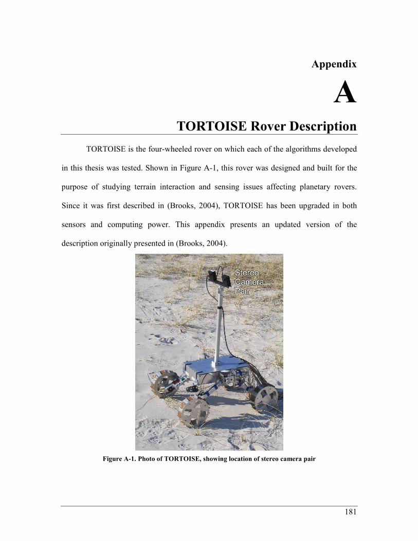
181
Appendix
A Appendix A TORTOISE Rover Description
TORTOISE is the four-wheeled rover on which each of the algorithms developed
in this thesis was tested. Shown in Figure A-1, this rover was designed and built for the
purpose of studying terrain interaction and sensing issues affecting planetary rovers.
Since it was first described in (Brooks, 2004), TORTOISE has been upgraded in both
sensors and computing power. This appendix presents an updated version of the
description originally presented in (Brooks, 2004).
Figure A-1. Photo of TORTOISE, showing location of stereo camera pair
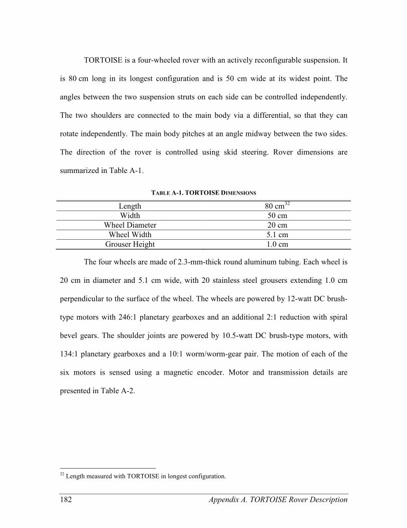
182 Appendix A. TORTOISE Rover Description
TORTOISE is a four-wheeled rover with an actively reconfigurable suspension. It
is 80 cm long in its longest configuration and is 50 cm wide at its widest point. The
angles between the two suspension struts on each side can be controlled independently.
The two shoulders are connected to the main body via a differential, so that they can
rotate independently. The main body pitches at an angle midway between the two sides.
The direction of the rover is controlled using skid steering. Rover dimensions are
summarized in Table A-1.
TABLE A-1. TORTOISE DIMENSIONS
Length 80 cm32
Width 50 cm
Wheel Diameter 20 cm
Wheel Width 5.1 cm
Grouser Height 1.0 cm
The four wheels are made of 2.3-mm-thick round aluminum tubing. Each wheel is
20 cm in diameter and 5.1 cm wide, with 20 stainless steel grousers extending 1.0 cm
perpendicular to the surface of the wheel. The wheels are powered by 12-watt DC brush-
type motors with 246:1 planetary gearboxes and an additional 2:1 reduction with spiral
bevel gears. The shoulder joints are powered by 10.5-watt DC brush-type motors, with
134:1 planetary gearboxes and a 10:1 worm/worm-gear pair. The motion of each of the
six motors is sensed using a magnetic encoder. Motor and transmission details are
presented in Table A-2.
32
Length measured with TORTOISE in longest configuration.
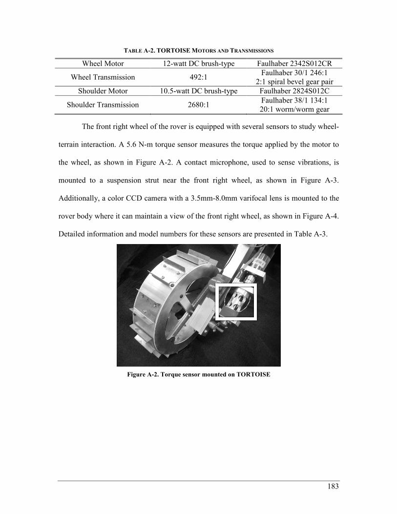
183
TABLE A-2. TORTOISE MOTORS AND TRANSMISSIONS
Wheel Motor 12-watt DC brush-type Faulhaber 2342S012CR
Wheel Transmission 492:1 Faulhaber 30/1 246:1
2:1 spiral bevel gear pair
Shoulder Motor 10.5-watt DC brush-type Faulhaber 2824S012C
Shoulder Transmission 2680:1 Faulhaber 38/1 134:1
20:1 worm/worm gear
The front right wheel of the rover is equipped with several sensors to study wheel-
terrain interaction. A 5.6 N-m torque sensor measures the torque applied by the motor to
the wheel, as shown in Figure A-2. A contact microphone, used to sense vibrations, is
mounted to a suspension strut near the front right wheel, as shown in Figure A-3.
Additionally, a color CCD camera with a 3.5mm-8.0mm varifocal lens is mounted to the
rover body where it can maintain a view of the front right wheel, as shown in Figure A-4.
Detailed information and model numbers for these sensors are presented in Table A-3.
Figure A-2. Torque sensor mounted on TORTOISE
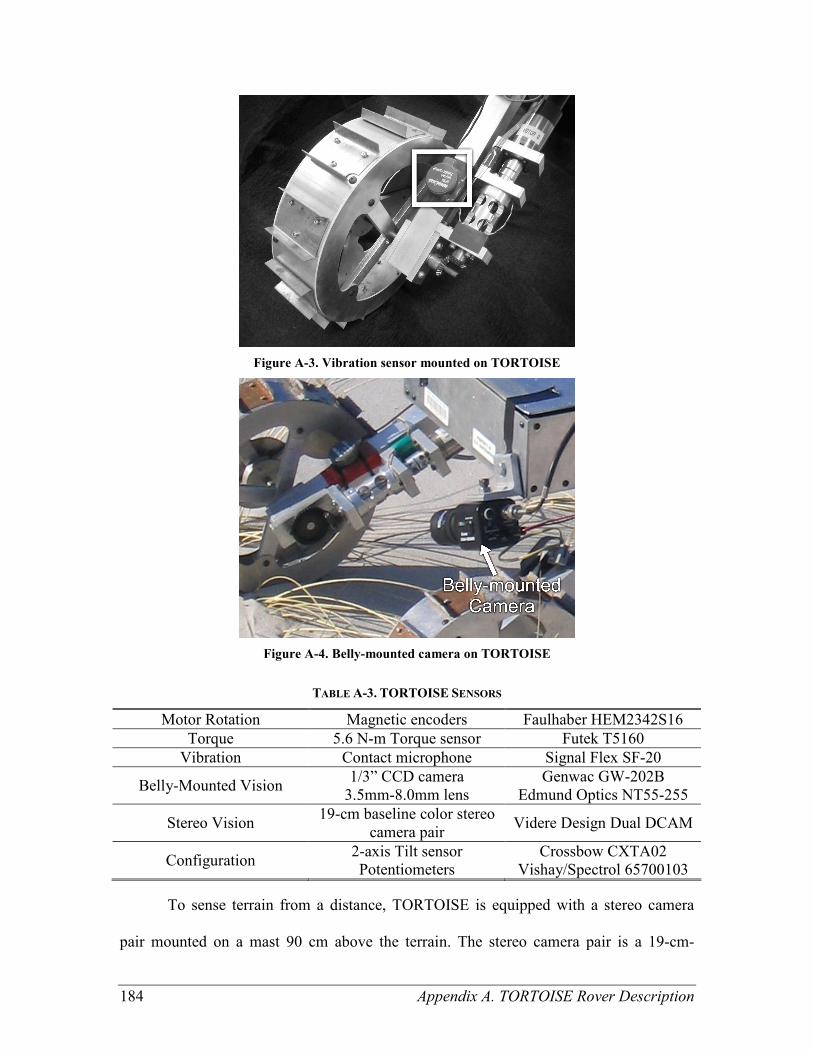
184 Appendix A. TORTOISE Rover Description
Figure A-3. Vibration sensor mounted on TORTOISE
Figure A-4. Belly-mounted camera on TORTOISE
TABLE A-3. TORTOISE SENSORS
Motor Rotation Magnetic encoders Faulhaber HEM2342S16
Torque 5.6 N-m Torque sensor Futek T5160
Vibration Contact microphone Signal Flex SF-20
Belly-Mounted Vision 1/3” CCD camera
3.5mm-8.0mm lens
Genwac GW-202B
Edmund Optics NT55-255
Stereo Vision 19-cm baseline color stereo
camera pair Videre Design Dual DCAM
Configuration 2-axis Tilt sensor
Potentiometers
Crossbow CXTA02
Vishay/Spectrol 65700103
To sense terrain from a distance, TORTOISE is equipped with a stereo camera
pair mounted on a mast 90 cm above the terrain. The stereo camera pair is a 19-cm-

185
baseline Videre Design “dual DCAM” capable of capturing color images at 640×480
resolution. Range data were extracted from the stereo images using SVS (Small Vision
System), Videre Design’s commercial stereo processing software. The accuracy of the
range estimation is sufficient to assign pixels to 20-cm by 20-cm terrain cells up to a
distance of 8 meters.
The rover is also outfitted with sensors to estimate its attitude and suspension
configuration. A two-axis tilt sensor measures the pitch and roll of the rover body. The
angles of the two shoulder joints are measured with potentiometers, as is the angle
between the right shoulder and the body. Model numbers for all sensors are shown in
Table A-3.
All feedback control and data sampling is done on computers attached to the rover
via a tether. Motor power is sent to the rover via this tether and sensory signals are
returned the same way. Motor control is implemented on an off-board PC104 computer.
Sampling of wheel torque and rover configuration is done by the same PC104 system,
and images from the stereo camera pair are captured via a FireWire (IEEE 1394)
connection to the PC104 system. Image capture from the belly-mounted camera and
vibration signal recording is done on a tethered laptop computer. Figure A-5 shows a
schematic of the rover communications.
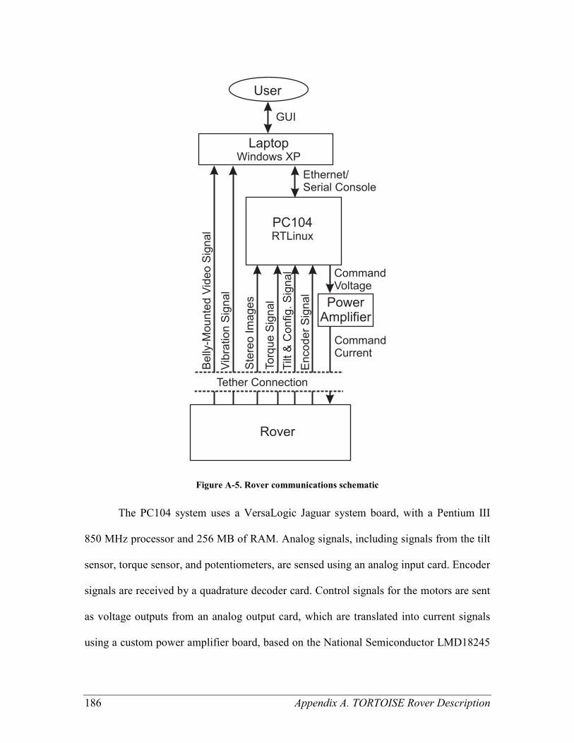
186 Appendix A. TORTOISE Rover Description
Figure A-5. Rover communications schematic
The PC104 system uses a VersaLogic Jaguar system board, with a Pentium III
850 MHz processor and 256 MB of RAM. Analog signals, including signals from the tilt
sensor, torque sensor, and potentiometers, are sensed using an analog input card. Encoder
signals are received by a quadrature decoder card. Control signals for the motors are sent
as voltage outputs from an analog output card, which are translated into current signals
using a custom power amplifier board, based on the National Semiconductor LMD18245
187
full-bridge motor driver. The current signals are sent to the motor via the tether. Stereo
camera images are received on a FireWire (IEEE 1394) card. The PC104 is also equipped
with a sound card to receive vibration signals and a frame grabber to receive imagery
from the belly-mounted camera, but use of these cards was never implemented. Model
numbers for the components of the PC104 system are presented in Table A-4.
TABLE A-4. TORTOISE PC104 SYSTEM COMPONENTS
CPU Board (PC104+) VersaLogic Jaguar (Pentium III 850 MHz)
RAM Crucial 256MB PC133 SDRAM
Hard Drive 6 GB 2.5” Internal Hard Drive
Analog Input, Digital I/O Diamond Systems Diamond MM-AT
Quadrature Decoder Microcomputer Systems MSI-P400
Analog Output Diamond Systems Ruby MM-4XT
FireWire Advanced Digital Logic MSMW104+
Sound Card Diamond Systems Crystal-MM-HP-5
Video Frame Grabber (NTSC) Parvus FG104
The PC104 system runs Linux with an RTLinux microkernel for real-time control
and data sampling. The control and sampling software was developed specifically for this
rover. Stereo image capture was implemented using the libraries provided with the SVS
software. User interaction with the PC104 system is done over a connection to the laptop
computer, either using a 100BASE-TX Ethernet connection using SSH (preferentially) or
using a serial console connection.
The laptop computer, a PC running Windows XP, interacts with the PC104
system, the belly-mounted camera, and the vibration sensor. It connects to the PC104
system using either an Ethernet crossover cable or a null modem serial cable. It connects
to the belly-mounted camera with a USB video capture box (ProVideo model PV321CE).
The connection to the vibration sensor is via a standard audio cable which plugs into the
laptop’s microphone port.

188 Appendix A. TORTOISE Rover Description
The entire system is run using battery power so that it can be taken to remote
locations where electrical outlets are unavailable. Power to the PC104 is provided by a
12V motorcycle battery, regulated to 5V and 3.3V with a DC/DC converter. Power to the
motors is provided by two 12V motorcycle batteries and passed on to the motors by the
power amplifier board. Power for the laptop is provided by onboard batteries.
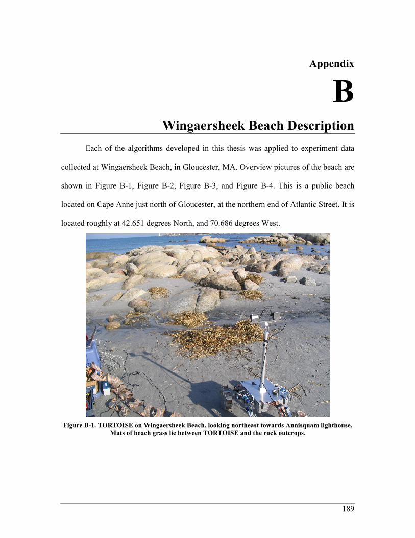
189
Appendix
B Appendix B Wingaersheek Beach Description
Each of the algorithms developed in this thesis was applied to experiment data
collected at Wingaersheek Beach, in Gloucester, MA. Overview pictures of the beach are
shown in Figure B-1, Figure B-2, Figure B-3, and Figure B-4. This is a public beach
located on Cape Anne just north of Gloucester, at the northern end of Atlantic Street. It is
located roughly at 42.651 degrees North, and 70.686 degrees West.
Figure B-1. TORTOISE on Wingaersheek Beach, looking northeast towards Annisquam lighthouse.
Mats of beach grass lie between TORTOISE and the rock outcrops.
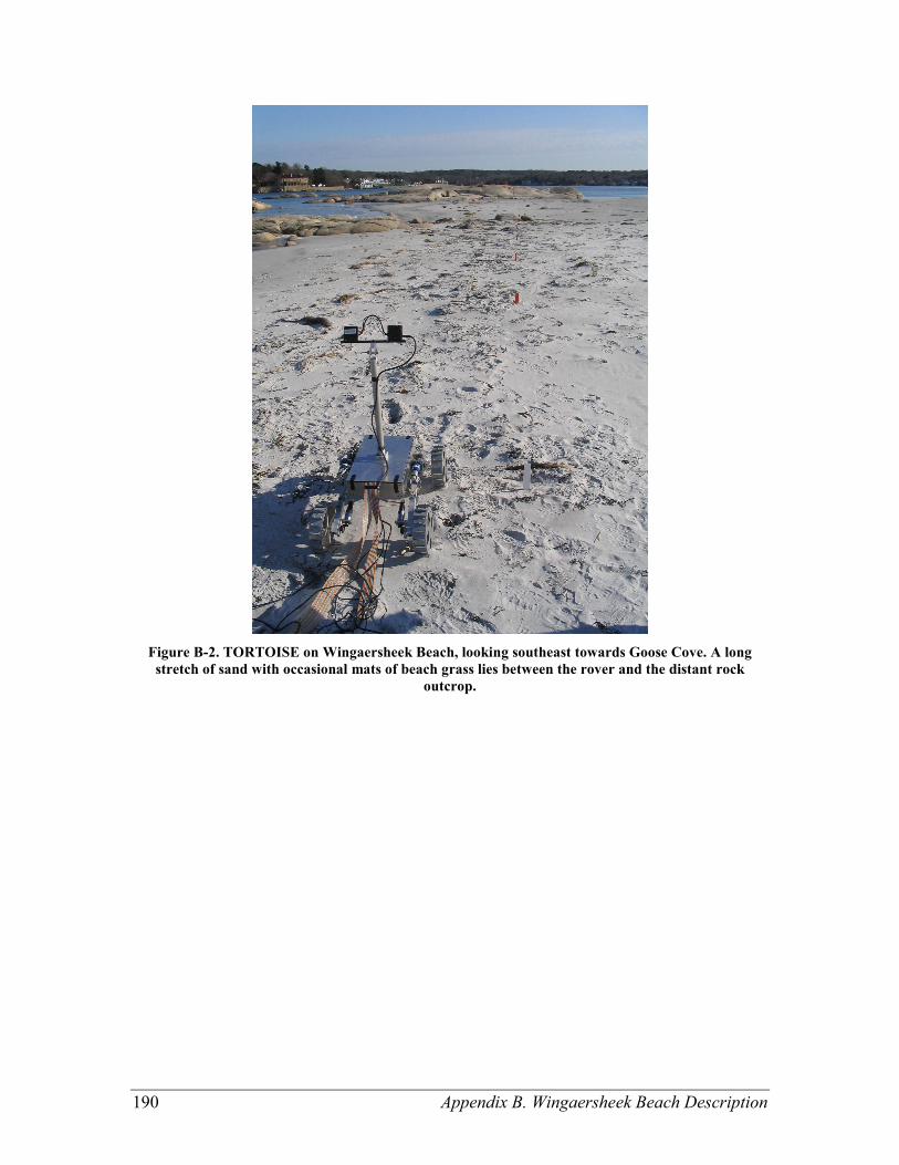
190 Appendix B. Wingaersheek Beach Description
Figure B-2. TORTOISE on Wingaersheek Beach, looking southeast towards Goose Cove. A long
stretch of sand with occasional mats of beach grass lies between the rover and the distant rock
outcrop.
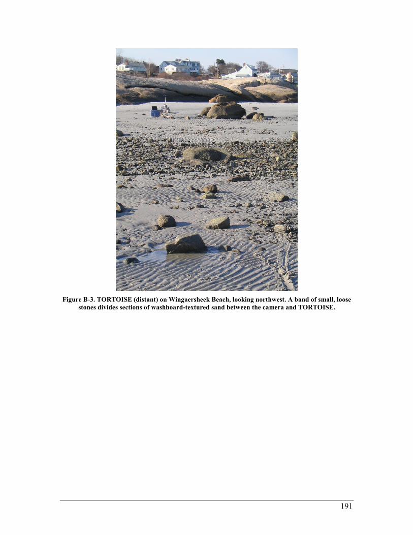
191
Figure B-3. TORTOISE (distant) on Wingaersheek Beach, looking northwest. A band of small, loose
stones divides sections of washboard-textured sand between the camera and TORTOISE.
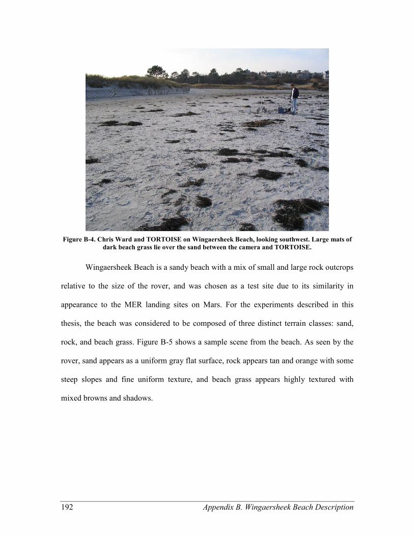
192 Appendix B. Wingaersheek Beach Description
Figure B-4. Chris Ward and TORTOISE on Wingaersheek Beach, looking southwest. Large mats of
dark beach grass lie over the sand between the camera and TORTOISE.
Wingaersheek Beach is a sandy beach with a mix of small and large rock outcrops
relative to the size of the rover, and was chosen as a test site due to its similarity in
appearance to the MER landing sites on Mars. For the experiments described in this
thesis, the beach was considered to be composed of three distinct terrain classes: sand,
rock, and beach grass. Figure B-5 shows a sample scene from the beach. As seen by the
rover, sand appears as a uniform gray flat surface, rock appears tan and orange with some
steep slopes and fine uniform texture, and beach grass appears highly textured with
mixed browns and shadows.
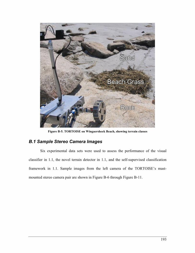
193
Figure B-5. TORTOISE on Wingaersheek Beach, showing terrain classes
B.1 Sample Stereo Camera Images
Six experimental data sets were used to assess the performance of the visual
classifier in 1.1, the novel terrain detector in 1.1, and the self-supervised classification
framework in 1.1. Sample images from the left camera of the TORTOISE’s mast-
mounted stereo camera pair are shown in Figure B-6 through Figure B-11.
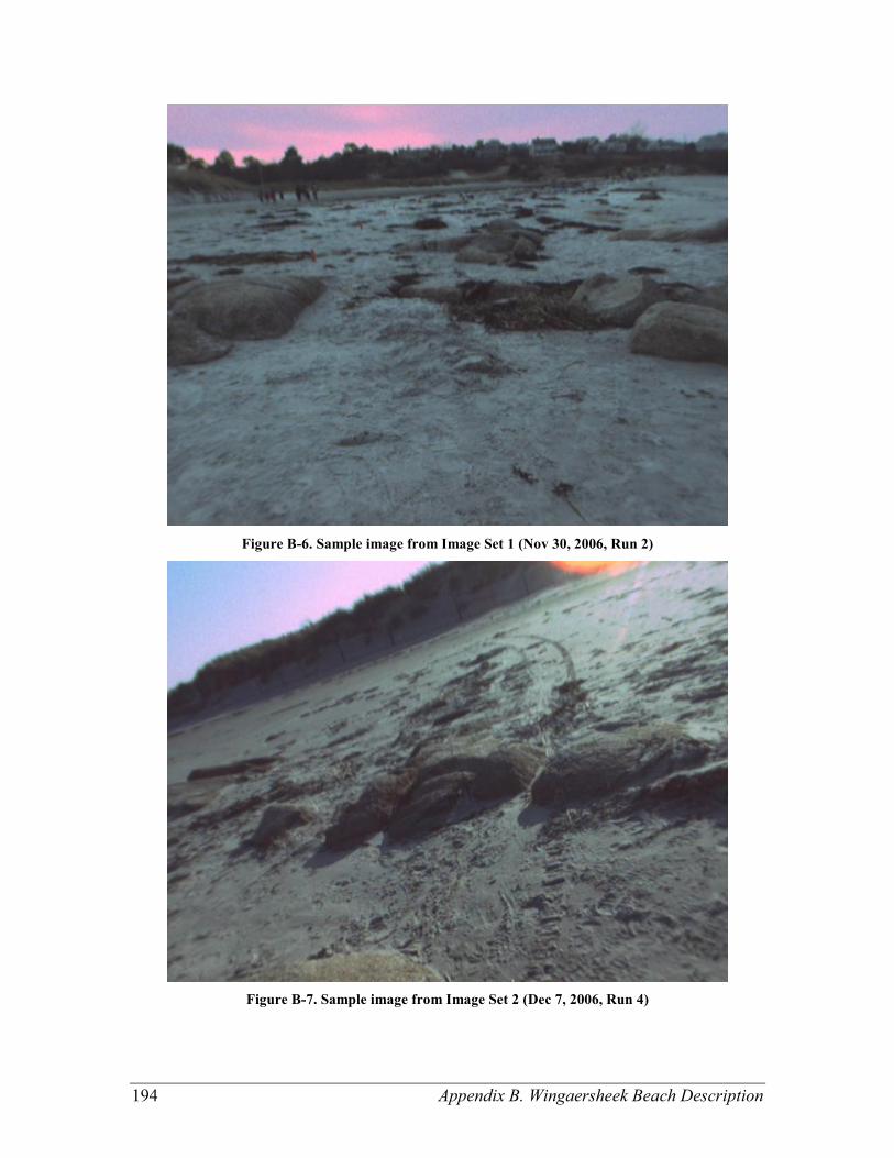
194 Appendix B. Wingaersheek Beach Description
Figure B-6. Sample image from Image Set 1 (Nov 30, 2006, Run 2)
Figure B-7. Sample image from Image Set 2 (Dec 7, 2006, Run 4)
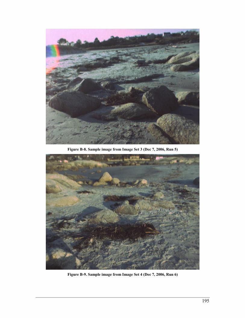
195
Figure B-8. Sample image from Image Set 3 (Dec 7, 2006, Run 5)
Figure B-9. Sample image from Image Set 4 (Dec 7, 2006, Run 6)
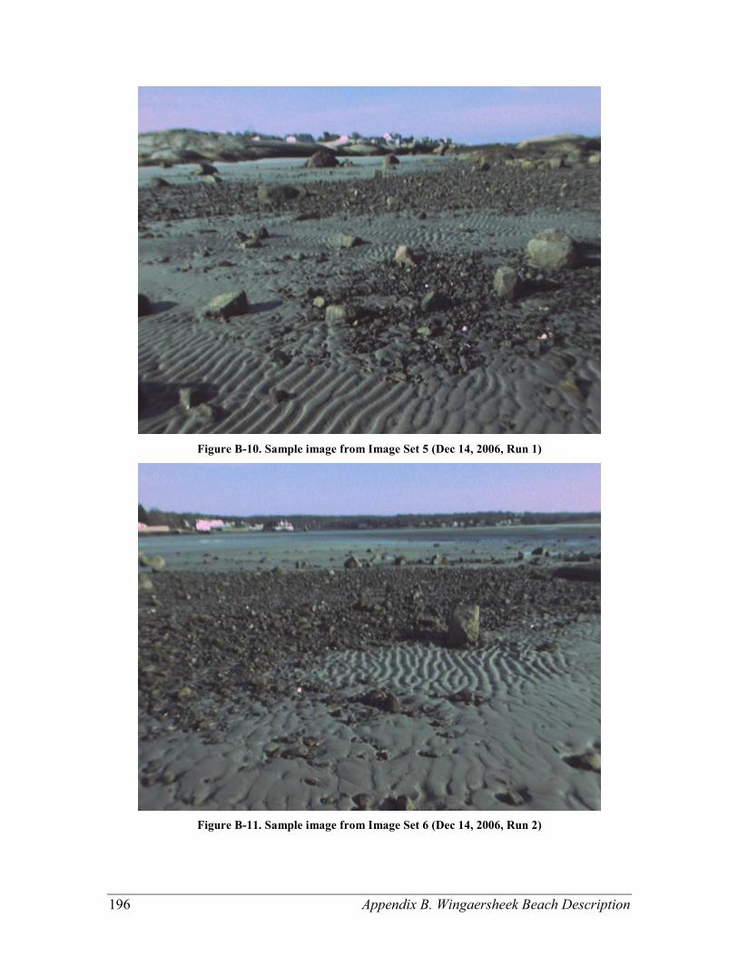
196 Appendix B. Wingaersheek Beach Description
Figure B-10. Sample image from Image Set 5 (Dec 14, 2006, Run 1)
Figure B-11. Sample image from Image Set 6 (Dec 14, 2006, Run 2)
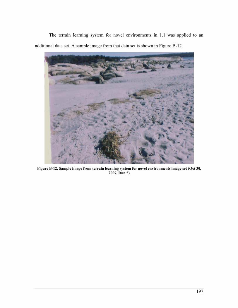
197
The terrain learning system for novel environments in 1.1 was applied to an
additional data set. A sample image from that data set is shown in Figure B-12.
Figure B-12. Sample image from terrain learning system for novel environments image set (Oct 30,
2007, Run 5)
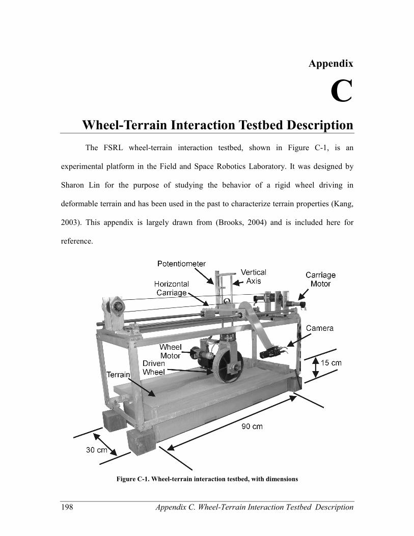
198 Appendix C. Wheel-Terrain Interaction Testbed Description
Appendix
C Appendix C Wheel-Terrain Interaction Testbed Description
The FSRL wheel-terrain interaction testbed, shown in Figure C-1, is an
experimental platform in the Field and Space Robotics Laboratory. It was designed by
Sharon Lin for the purpose of studying the behavior of a rigid wheel driving in
deformable terrain and has been used in the past to characterize terrain properties (Kang,
2003). This appendix is largely drawn from (Brooks, 2004) and is included here for
reference.
Figure C-1. Wheel-terrain interaction testbed, with dimensions

199
The testbed consists of a driven wheel mounted on an undriven vertical axis. The
wheel-axis assembly is mounted on a frame such that the wheel’s forward velocity and
angular velocity can be controlled independently. The testbed can be fitted with a number
of different wheel assemblies, each assembly containing both a motor and a wheel. For
the results presented in this thesis, tests were conducted using the black plastic wheel
assembly.
The black plastic wheel assembly, shown in Figure C-2, consists of a wheel, a
motor, and a torque sensor. The wheel is 4.8 cm wide and 20 cm in diameter. Sand is
bonded to the outside of the wheel to improve traction. The motor applying torque to the
wheel is a 14.5-watt DC brush-type motor. It is mounted with a 246:1 transmission, and
has a tachometer to measure angular velocity. The maximum linear velocity of the
outside of the wheel is 15 cm/sec. Motor torque is measured using a rotating torque
sensor with a working range of 7 N-m, mounted between the motor and the wheel. A six-
axis force-torque sensor is mounted between this wheel assembly and the frame, so that
all of the forces and torques applied by the wheel on the terrain can be sensed. Table C-1
provides detailed information about this wheel assembly including component model
numbers.
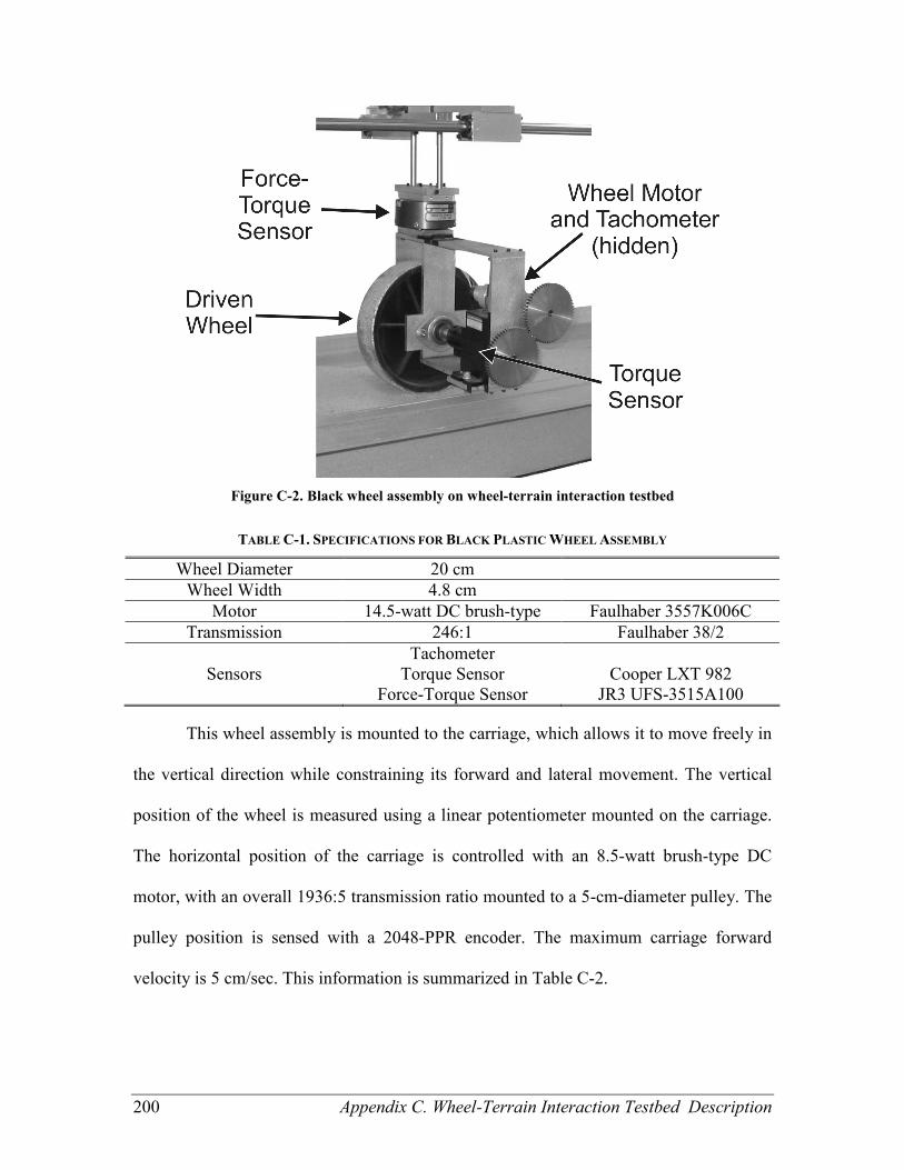
200 Appendix C. Wheel-Terrain Interaction Testbed Description
Figure C-2. Black wheel assembly on wheel-terrain interaction testbed
TABLE C-1. SPECIFICATIONS FOR BLACK PLASTIC WHEEL ASSEMBLY
Wheel Diameter 20 cm
Wheel Width 4.8 cm
Motor 14.5-watt DC brush-type Faulhaber 3557K006C
Transmission 246:1 Faulhaber 38/2
Sensors
Tachometer
Torque Sensor
Force-Torque Sensor
Cooper LXT 982
JR3 UFS-3515A100
This wheel assembly is mounted to the carriage, which allows it to move freely in
the vertical direction while constraining its forward and lateral movement. The vertical
position of the wheel is measured using a linear potentiometer mounted on the carriage.
The horizontal position of the carriage is controlled with an 8.5-watt brush-type DC
motor, with an overall 1936:5 transmission ratio mounted to a 5-cm-diameter pulley. The
pulley position is sensed with a 2048-PPR encoder. The maximum carriage forward
velocity is 5 cm/sec. This information is summarized in Table C-2.
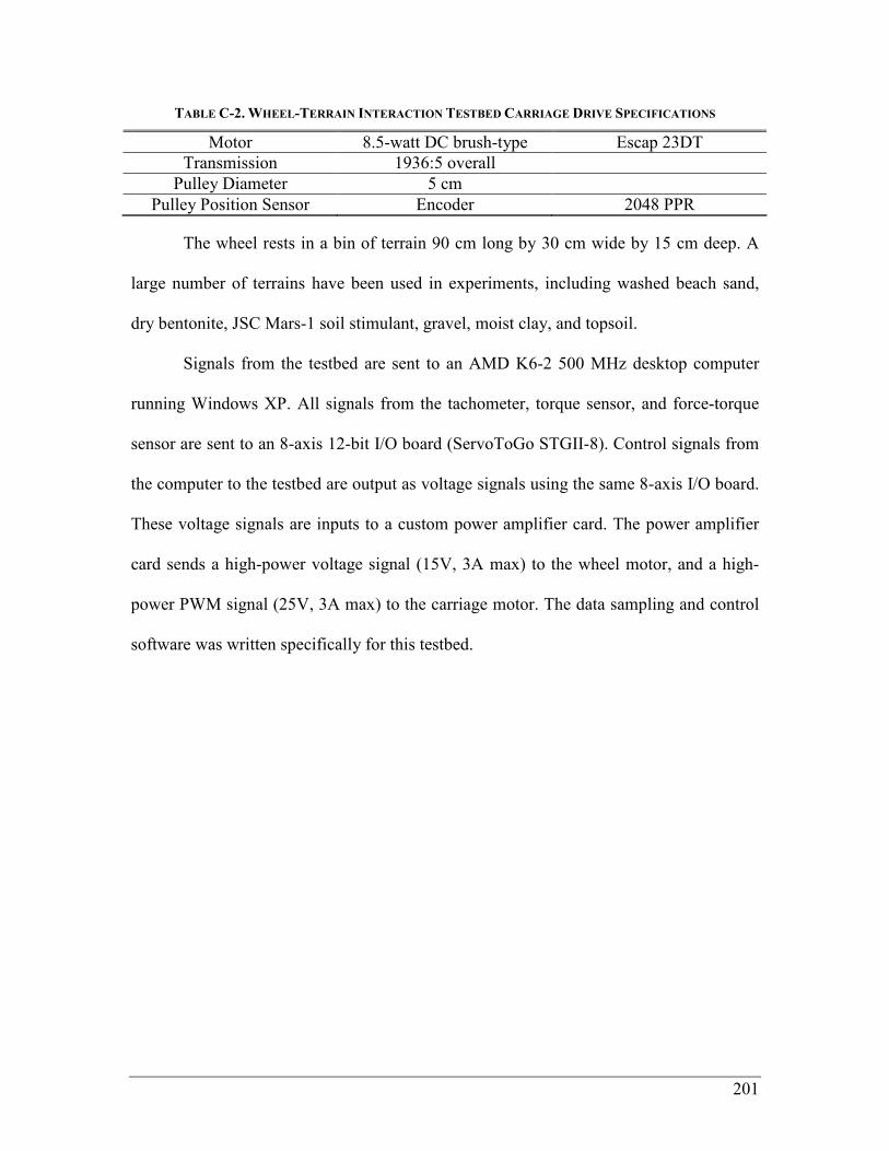
201
TABLE C-2. WHEEL-TERRAIN INTERACTION TESTBED CARRIAGE DRIVE SPECIFICATIONS
Motor 8.5-watt DC brush-type Escap 23DT
Transmission 1936:5 overall
Pulley Diameter 5 cm
Pulley Position Sensor Encoder 2048 PPR
The wheel rests in a bin of terrain 90 cm long by 30 cm wide by 15 cm deep. A
large number of terrains have been used in experiments, including washed beach sand,
dry bentonite, JSC Mars-1 soil stimulant, gravel, moist clay, and topsoil.
Signals from the testbed are sent to an AMD K6-2 500 MHz desktop computer
running Windows XP. All signals from the tachometer, torque sensor, and force-torque
sensor are sent to an 8-axis 12-bit I/O board (ServoToGo STGII-8). Control signals from
the computer to the testbed are output as voltage signals using the same 8-axis I/O board.
These voltage signals are inputs to a custom power amplifier card. The power amplifier
card sends a high-power voltage signal (15V, 3A max) to the wheel motor, and a high-
power PWM signal (25V, 3A max) to the carriage motor. The data sampling and control
software was written specifically for this testbed.
202 Appendix D. Support Vector Machine Background and Optimizations
Appendix
D Appendix D Support Vector Machine Background and
Optimizations
The support vector machine (SVM) classifiers presented in this thesis were
implemented using the open-source library LIBSVM (Chang & C. Lin, 2005, 2008). This
appendix is intended to define the mathematical formulations used in this library. C-
support vector classification is the more traditional formulation of an SVM, and is
presented in D.1. This is the formulation used for vibration-based terrain classification in
2.1 and visual classification in 1.1. The one-class SVM, presented in D.2, is an extension
to the SVM framework which can distinguish “similar” features from “different.” It is
used as one of the baseline approaches to novelty detection in 1.1. Both of these
classifiers use kernel functions for regularization, and the formulations of these kernel
functions are presented in D.3. Finally, as mentioned in the main body of this thesis, there
are some optimizations which can improve the speed of classification. These
optimizations are presented in D.4.
D.1 C-Support Vector Classification
The C-support vector classifier is used for most of the two-class classification
presented in this thesis. Here, it is assumed that labeled training data is available in the
form of vectors lin
i ,,1, K=ℜ∈x and labels { }1,1 −∈iy . Note that n is the dimension of
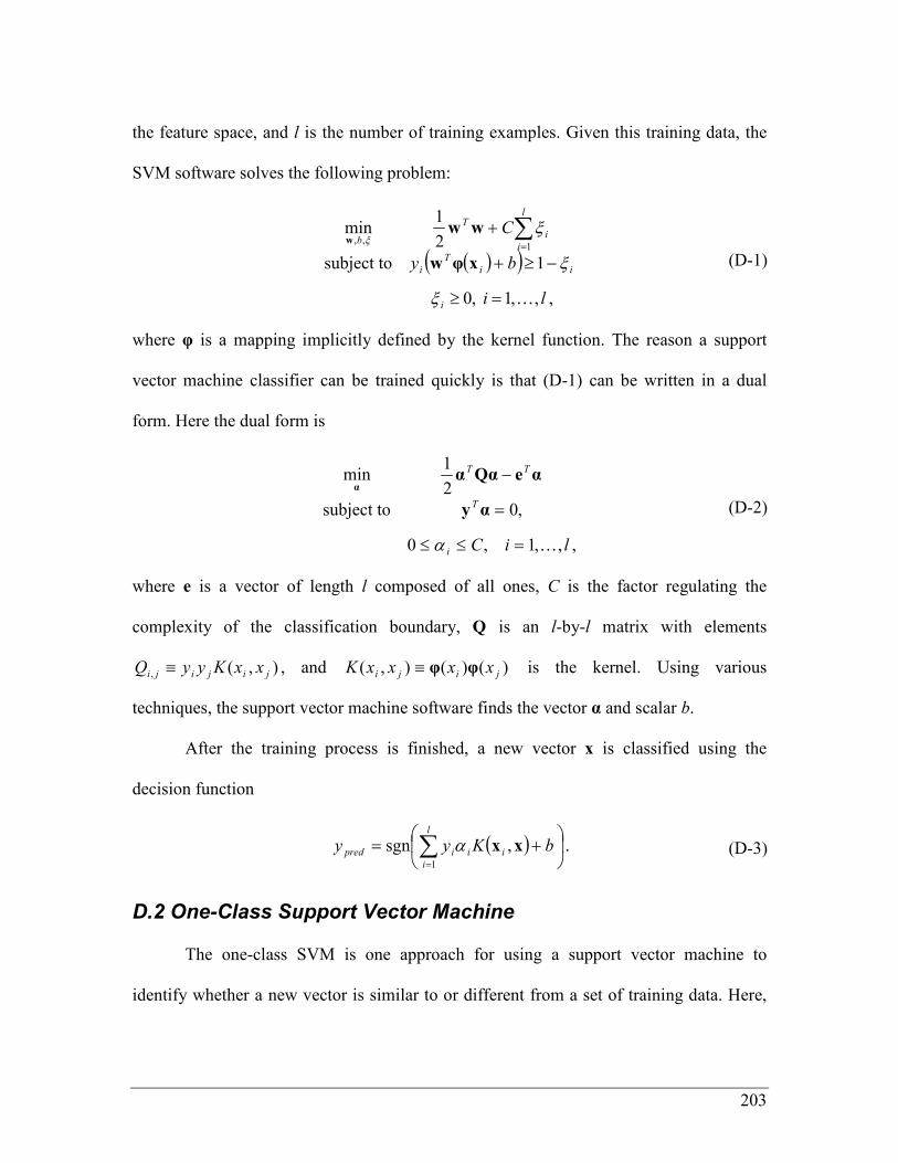
203
the feature space, and l is the number of training examples. Given this training data, the
SVM software solves the following problem:
( )( ),,,1,0
1subject to
2
1min
1,,
li
by
C
i
ii
T
i
l
i
i
T
b
K=≥
−≥+
+ ∑=
ξ
ξ
ξξ
xφw
www
(D-1)
where φ is a mapping implicitly defined by the kernel function. The reason a support
vector machine classifier can be trained quickly is that (D-1) can be written in a dual
form. Here the dual form is
,,,1,0
,0subject to
2
1min
liCi
T
TT
K=≤≤
=
−
α
αy
αeαQαα
(D-2)
where e is a vector of length l composed of all ones, C is the factor regulating the
complexity of the classification boundary, Q is an l-by-l matrix with elements
),(, jijiji xxKyyQ ≡ , and )()(),( jiji xxxxK φφ≡ is the kernel. Using various
techniques, the support vector machine software finds the vector α and scalar b.
After the training process is finished, a new vector x is classified using the
decision function
( )
+= ∑
=
l
i
iiipred bKyy1
,sgn xxα . (D-3)
D.2 One-Class Support Vector Machine
The one-class SVM is one approach for using a support vector machine to
identify whether a new vector is similar to or different from a set of training data. Here,

204 Appendix D. Support Vector Machine Background and Optimizations
training vectors lin
i ,,1, K=ℜ∈x are provided without labels, and the problem solved
by the SVM is
( )
,,,1,0
subject to
1
2
1min
1,,
li
l
i
ii
T
l
i
i
T
K=≥
−≥
+− ∑=
ξ
ξρ
ξν
ρρξ
xφw
www
(D-4)
where ]1,0(∈ν is the factor regulating the complexity of the classifier, and φ is a
mapping implicitly defined by the kernel function. For this problem, the dual formulation
solved by LIBSVM is
,
,,,1,0subject to
2
1min
l
liC
T
i
T
ν
α
=
=≤≤
αe
αQαα
K (D-5)
where e is a vector of length l composed of all ones, Q is an l-by-l matrix with elements
),(, jijiji xxKyyQ ≡ , and )()(),( jiji xxxxK φφ≡ is the kernel. LIBSVM thus solves for
the vector α and the scalar ρ.
After training, a new vector x is considered to be similar to the training data if
ypred > 0 in the decision function
( )
−= ∑
=
l
i
iipred Ky1
,sgn ρα xx . (D-6)
D.3 Kernel Functions
One of the main choices to be made when using a SVM is which kernel function
to use. LIBSVM provides the option to choose between four different kernels: linear,
polynomial, radial basis function (RBF) and sigmoid. The formulations for these kernels
are presented in Table D-1. In this table, γ, r, and d are kernel parameters.
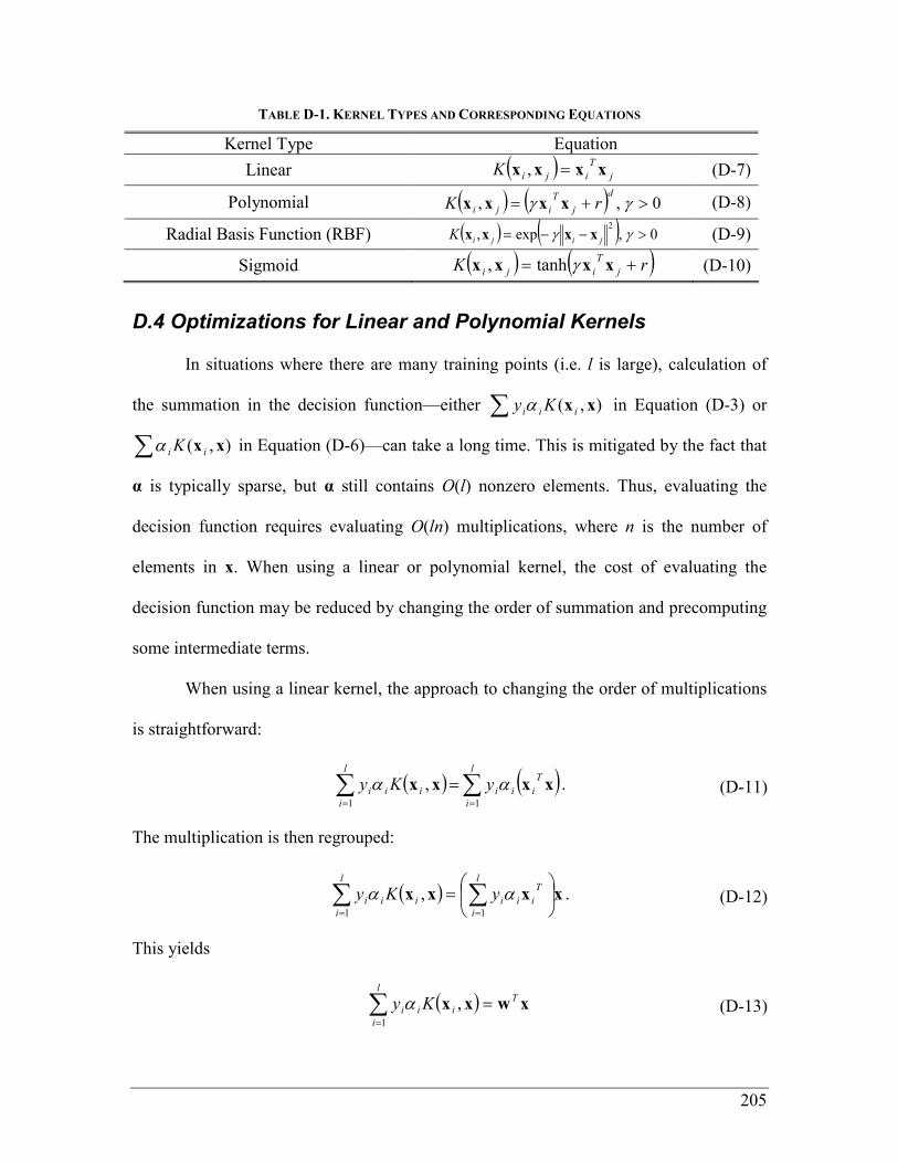
205
TABLE D-1. KERNEL TYPES AND CORRESPONDING EQUATIONS
Kernel Type Equation
Linear ( )j
T
ijiK xxxx =, (D-7)
Polynomial ( ) ( ) 0,, >+= γγd
j
T
iji rK xxxx (D-8)
Radial Basis Function (RBF) ( ) ( ) 0,exp,2
>−−= γγ jijiK xxxx (D-9)
Sigmoid ( ) ( )rK j
T
iji += xxxx γtanh, (D-10)
D.4 Optimizations for Linear and Polynomial Kernels
In situations where there are many training points (i.e. l is large), calculation of
the summation in the decision function—either ∑ ),( xx iii Ky α in Equation (D-3) or
∑ ),( xx ii Kα in Equation (D-6)—can take a long time. This is mitigated by the fact that
α is typically sparse, but α still contains O(l) nonzero elements. Thus, evaluating the
decision function requires evaluating O(ln) multiplications, where n is the number of
elements in x. When using a linear or polynomial kernel, the cost of evaluating the
decision function may be reduced by changing the order of summation and precomputing
some intermediate terms.
When using a linear kernel, the approach to changing the order of multiplications
is straightforward:
( ) ( )∑∑==
=l
i
T
iii
l
i
iii yKy11
, xxxx αα . (D-11)
The multiplication is then regrouped:
( ) xxxx
= ∑∑
==
l
i
T
iii
l
i
iii yKy11
, αα . (D-12)
This yields
( ) xwxxT
l
i
iii Ky =∑=1
,α (D-13)
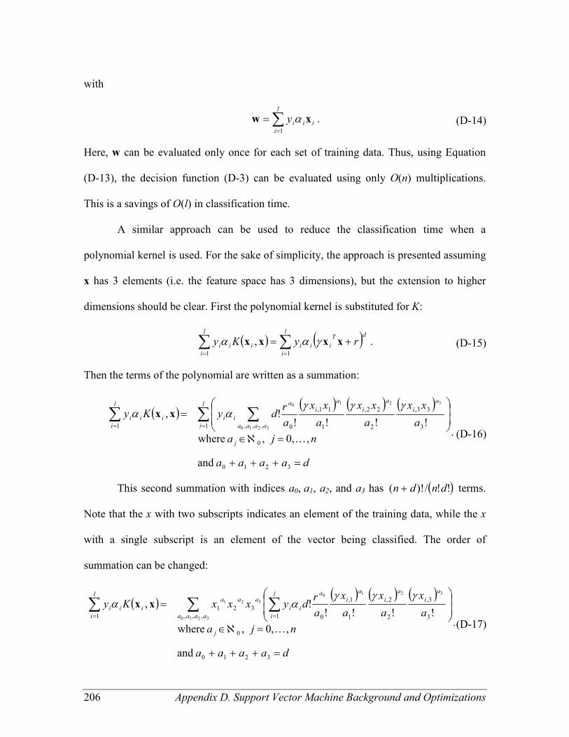
206 Appendix D. Support Vector Machine Background and Optimizations
with
∑=
=l
i
iiiy1
xw α . (D-14)
Here, w can be evaluated only once for each set of training data. Thus, using Equation
(D-13), the decision function (D-3) can be evaluated using only O(n) multiplications.
This is a savings of O(l) in classification time.
A similar approach can be used to reduce the classification time when a
polynomial kernel is used. For the sake of simplicity, the approach is presented assuming
x has 3 elements (i.e. the feature space has 3 dimensions), but the extension to higher
dimensions should be clear. First the polynomial kernel is substituted for K:
( ) ( )∑∑==
+=l
i
dT
iii
l
i
iii ryKy11
, xxxx γαα . (D-15)
Then the terms of the polynomial are written as a summation:
( )
( ) ( ) ( )
daaaa
nja
a
xx
a
xx
a
xx
a
rdyKy
j
l
i aaaa
a
i
a
i
a
ia
ii
l
i
iii
=+++
=ℵ∈
= ∑ ∑∑
==
3210
0
1 ,,, 3
33,
2
22,
1
11,
01
and
,,0 , where
!!!!!,
3210
3210
K
γγγαα xx
. (D-16)
This second summation with indices a0, a1, a2, and a3 has ( )!!/)!( dndn + terms.
Note that the x with two subscripts indicates an element of the training data, while the x
with a single subscript is an element of the vector being classified. The order of
summation can be changed:
( )
( ) ( ) ( )
daaaa
nja
a
x
a
x
a
x
a
rdyxxxKy
j
aaaa
l
i
a
i
a
i
a
ia
ii
aaal
i
iii
=+++
=ℵ∈
= ∑ ∑∑
==
3210
0
,,, 1 3
3,
2
2,
1
1,
0
321
1
and
,,0 , where
!!!!!,
3210
3210
321
K
γγγαα xx
.(D-17)
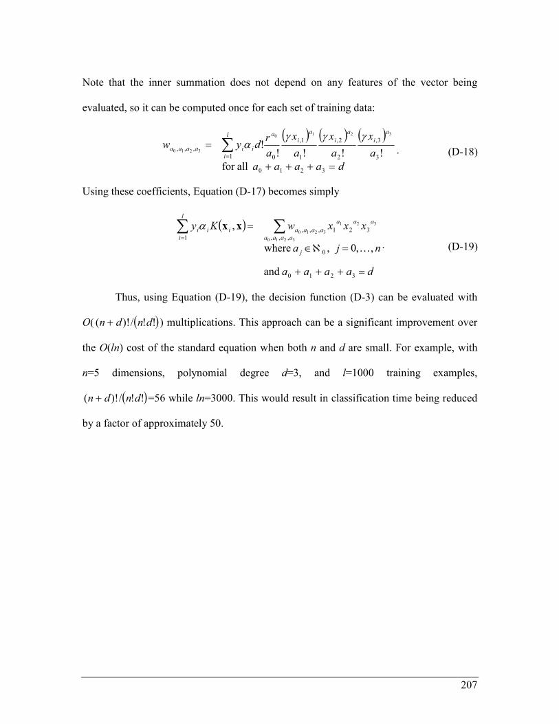
207
Note that the inner summation does not depend on any features of the vector being
evaluated, so it can be computed once for each set of training data:
( ) ( ) ( )
daaaa
a
x
a
x
a
x
a
rdyw
l
i
a
i
a
i
a
ia
iiaaaa
=+++
= ∑=
3210
1 3
3,
2
2,
1
1,
0
,,,
allfor
!!!!!
3210
3210
γγγα
. (D-18)
Using these coefficients, Equation (D-17) becomes simply
( )
daaaa
nja
xxxwKy
j
aaaa
aaa
aaaa
l
i
iii
=+++
=ℵ∈
= ∑∑=
3210
0
,,,
321,,,
1
and
,,0 , where
,3210
321
3210
K
xxα
. (D-19)
Thus, using Equation (D-19), the decision function (D-3) can be evaluated with
O( ( )!!/)!( dndn + ) multiplications. This approach can be a significant improvement over
the O(ln) cost of the standard equation when both n and d are small. For example, with
n=5 dimensions, polynomial degree d=3, and l=1000 training examples,
( )!!/)!( dndn + =56 while ln=3000. This would result in classification time being reduced
by a factor of approximately 50.

208 Appendix E. MATLAB Feature Extraction Code
Appendix
E Appendix E MATLAB Feature Extraction Code
The algorithms developed in this thesis were implemented as Matlab scripts
(Mathworks, 2005). This appendix presents short Matlab functions which can be used to
extract classification features from raw sensor data.
E.1 Vibration Feature Extraction
Table E-1 presents Matlab code for the feature extraction used in the vibration-
based terrain classifier in 2.1. This function takes as an input the time series of
accelerometer values, and returns the log-scaled power spectral density features as its
output.
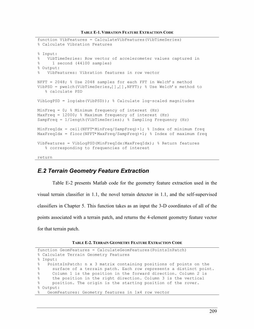
209
TABLE E-1. VIBRATION FEATURE EXTRACTION CODE
function VibFeatures = CalculateVibFeatures(VibTimeSeries)
% Calculate Vibration Features
% Input:
% VibTimeSeries: Row vector of accelerometer values captured in
% 1 second (44100 samples)
% Output:
% VibFeatures: Vibration features in row vector
NFFT = 2048; % Use 2048 samples for each FFT in Welch’s method
VibPSD = pwelch(VibTimeSeries,[],[],NFFT); % Use Welch’s method to
% calculate PSD
VibLogPSD = log(abs(VibPSD)); % Calculate log-scaled magnitudes
MinFreq = 0; % Minimum frequency of interest (Hz)
MaxFreq = 12000; % Maximum frequency of interest (Hz)
SampFreq = 1/length(VibTimeSeries); % Sampling Frequency (Hz)
MinFreqIdx = ceil(NFFT*MinFreq/SampFreq)+1; % Index of minimum freq
MaxFreqIdx = floor(NFFT*MaxFreq/SampFreq)+1; % Index of maximum freq
VibFeatures = VibLogPSD(MinFreqIdx:MaxFreqIdx); % Return features
% corresponding to frequencies of interest
return
E.2 Terrain Geometry Feature Extraction
Table E-2 presents Matlab code for the geometry feature extraction used in the
visual terrain classifier in 1.1, the novel terrain detector in 1.1, and the self-supervised
classifiers in Chapter 5. This function takes as an input the 3-D coordinates of all of the
points associated with a terrain patch, and returns the 4-element geometry feature vector
for that terrain patch.
TABLE E-2. TERRAIN GEOMETRY FEATURE EXTRACTION CODE
function GeomFeatures = CalculateGeomFeatures(PointsInPatch)
% Calculate Terrain Geometry Features
% Input:
% PointsInPatch: n x 3 matrix containing positions of points on the
% surface of a terrain patch. Each row represents a distinct point.
% Column 1 is the position in the forward direction. Column 2 is
% the position in the right direction. Column 3 is the vertical
% position. The origin is the starting position of the rover.
% Output:
% GeomFeatures: Geometry features in 1x4 row vector
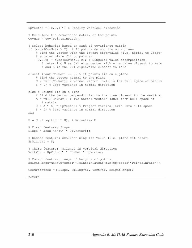
210 Appendix E. MATLAB Feature Extraction Code
UpVector = [0,0,1]’; % Specify vertical direction
% Calculate the covariance matrix of the points
CovMat = cov(PointsInPatch);
% Select behavior based on rank of covariance matrix
if (rank(CovMat) > 2) % If points do not lie on a plane
% Find the vector with the lowest eigenvalue (i.e. normal to least-
% squares plane fit to points)
[U,S,V] = svds(CovMat,1,0); % Singular value decomposition,
% returning U as 3x1 eigenvector with eigenvalue closest to zero
% and S is the 1x1 eigenvalue closest to zero
elseif (rank(CovMat) == 2) % If points lie on a plane
% Find the vector normal to the plane
U = null(CovMat); % Normal vector (3x1) is the null space of matrix
S = 0; % Zero variance in normal direction
else % Points lie on a line
% Find the vector perpendicular to the line closest to the vertical
A = null(CovMat); % Two normal vectors (3x2) form null space of
% matrix
U = A * A’ * UpVector; % Project vertical axis into null space
S = 0; % Zero variance in normal direction
end
U = U ./ sqrt(U’ * U); % Normalize U
% First feature: Slope
Slope = acos(abs(U’ * UpVector));
% Second feature: Smallest Singular Value (i.e. plane fit error)
SmSingVal = S;
% Third feature: variance in vertical direction
VertVar = UpVector’ * CovMat * UpVector;
% Fourth feature: range of heights of points
HeightRange=max(UpVector’*PointsInPatch)–min(UpVector’*PointsInPatch);
GeomFeatures = [Slope, SmSingVal, VertVar, HeightRange];
return


