Least Distance Smart neighboring Search (LDSNS)

over Wireless Sensor Networks

Abdul Razaque, Member IEEE,Khaled .M. Elleithy, Senior member IEEE

arazaque@bridgeport.eduelleithy@bridgeport.edu

Wireless and Mobile Communication (WMC) Laboratory

Computer Science and Engineering Department, University of Bridgeport, Bridgeport, CT 06604

Abstract: - In this paper, we introduce a novel least distance

smart neighboring search (LDSNS) to determine the

mostefficient path at one-hop distance over WSNs. LDSNS

helps to reduce the energy consumption and speeds up

scheduling for delivery of data. It provides cross layering

support and linking MAC layer with network layer to reduce

the amount of control messages. LDSNS is a robust and

efficient approach that isbased on single-hop communication

mechanism. To validate the strength of LDSNS, we

incorporate LDSN in Boarder Node Medium AccessControl

(BN-MAC) protocol [ 15] to determine the list of neighboring

sensor nodes and choosing best 1-hop efficient search to avoid

collision and reducing energy consumption.

Evaluation of LDSNS is conducted using network simulator-2

(ns2).The performance of LDSNS is compared with minimum

energy accumulative routing problem (MEAR) [12],

asynchronous quorum-based wakeup scheduling scheme

(AQWSS) [14] and Minimum Energy Relay Routing (MERR)

[13]. Simulation results show that LDSNS is highly energy

efficient and faster as compared with MEAR, AQWSS and

MERR. It saves 24% to 62% energy resources and

improves12% to 21% search at 1-hop neighboring nodes.

Keywords: LDSNS, Wireless sensor network, Energy

consumption, MAC layer.

1. INTRODUCTION

WSNs is one of the prominent research areas in recent years.

Unlike traditional networks, WSNs are particularlyusedin

physical environments to develop high degree of perceptibility

[6]. It is one of the rapidly growing fields with attractive

features to use in several application areas[2], [3]. WSNs are

considered as low-cost and easy to set up [4]. The advent of

WSN has improved progress in surveillance and monitoring

systems, home automation devices, earthquake and disaster

applications etc. [1] & [5].

WSNsfaceseveral design and performance issues such as

waste of energy in idle listening, overhearing, extra control

messaging, emitting and congestion. In addition, experiencing

several performance impairing factors such as scalability,

mobility, lack of robustness, uniformity etc. The energy

consumption is considered as one of the major apprehensions

[7] that stimulates challenges for industrial and academic

sectors. Therefore, proper energy handling is one of the key

skills to preserve energy [9].

The radio is the main power consuming section of sensor in

WSNs that can be handled by introducing robust MAC

protocols. Thus, an efficient MAC protocol improves WSN

lifetime. In addition, MAC protocol has capability to handle

the issue of sharing the wireless channel and reduces the

collisions in order to improve throughput.

Several MAC protocols have been proposed to reduce energy

consumption and to providefaster delivery of data but

problemis not fully yet resolved. Two types of mechanisms

are used to support scheduling and routing the data: single hop

and multiple-hop.

According to some protocols, a node takes a part in data union

and consumes more energy. Since, the transmission of power

is quadratically proportional tothe distance, multi-hop

approach consumes less energy than one hop communication,

but it creates more overhead on the network and it also

experiences severe problem when routes are broken.

Furthermore, joining of new node and leaving of working

node reduce the throughput and consumes sufficient amount

of energy [10].In this regard, one-hop communication is

efficient and more reliable.

An energy-efficient minimum transmission energy

consumption (MTEC) protocol is proposedto reduce the

energy consumption and increase throughput during data

transmissions. METC has also discussed that MAC protocol

can dynamicallyadjust the size of contention window on basis

of successful ratios of data transmissions using cross-layer

protocol [8]. MEAR developed heuristic approach to

determine an energy efficient wave-path and compared with

traditional shortest path algorithm.The authors urgedthat the

existing shortest path algorithm has shortcoming of optimal

relaying strategy and channel propagation. MEAR also filsto

decide which node should contribute in transmission schedule

and the order of nodes to transmit and their transmission

power [12].

AQWSS [14] introduced a set of asynchronous quorum-based

wakeup scheduling mechanism to provide a better trade-off

between average delay and energy consumption for neighbor

discovery under variable environments.

MERR is introduced for linear sensor topology to consume

less energy based on optimal transmission distance [13]. All of

the discussed techniques tryto reduce the energy consumption

but from other side, they increased the overhead of network.

Keeping these factors in mind, we introduce LDSNS approach

to support BN-MAC protocol to reduce energy consumption

and speed up the delivery of data without putting any extra

overhead of control packets on network. The reminder of

paper is organized as: section 2, explains the Least Distance

Smart Neighboring Search (LDSNS). Section 3, simulation

and analysis of result are discussed and thepaper is concluded

in section 4.

2. LEAST DISTANCE SMART NEIGHBORING SEARCH

(LDSNS)

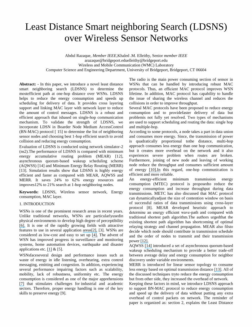
In LDSNS, any node monitors the channel after every 500 ms.

ifgain of channel is less than set threshold value, it shows that

there is no activity on medium from its neighbor nodes;

resulting that the node decides to sleep again.When a

transmitter wants to communicate, it first sends short preamble

to alertone hop neighboring nodes for sending the data. When

the targeted receiversenses short preamble, it wakes up and

responds with an acknowledgment (ACK) to transmitter. After

the transmitter gets ACK,it starts to send the data packets.

Pictorial illustration of the protocol is given in Figure 1.

SP SPSP

RE-

ACK

DATA

TRANSMIT

SHORT PREAMBLE WITH

WITHOUT TARGET ADDRESS

TX

(LDSNS)

RX

(LDSNS)

RX

S- W

SE-

ACK

DATA

RECEIVE ABP

ENERGY AND TIME

SAVE AT TX & RX

ABP

AUTOMATIC

BUFFER PACKET

SE-

ACK

SENDER EARLY

ACKNOWLEDGEMENT

RE-

ACK

SHORT

WAKE UP

RECEIVER EARLY

ACKNOWLEDGEMENT

RX

S-W

RX WAKE

UP TIME

TIME

TIME

Figure 1: Mechanism of LDSNS to communicate with 1-hop neighbor nodes

Let us prove this idea by using Lemmas and definitions. The

least distance smart neighboring search is based on 1-hop

distance and route discovery. The designed WSN consists of

different regions. The node which communicates within

region that maintains local connectivity, whereas node that

communicates out of region and schedules within region is

called boarder node (BN). Let us assume that directed graph D

= (V, A), consisting of the set of sensor nodes V. The set of

edges are called arcs that are A ⊆ V2. It helps to differentiate

between 1-hop destination and more than 1-hop destination

nodes. The digraph distance between nodes is simply the

number of shortest path between them [12]. We assign a name

to each sensor node in V. A local route discovery method is

based on relay scheme that works as follows.

For any destination node in „V‟specified by name „v‟, the

scheme targets the 1-hop destination nodes „u‟ on basis of

stored information in routing table regarding the shortest path

1-hop destination node. Each 1-hop destination node delivers

the shortest path to its predecessor during exchange of control

message.Finally destination „v‟ is acquired with efficient path.

We apply method [8] for estimation of global technology of

sensors by dividing nodes into routable boundaries and

extracting adjacency associations between these boundaries.

The objective of creating each boundary is to make the

topology simpler, so that the searching process works

efficiently within the boundaries. For a number of sensor

nodes „V‟ and communication digraph „D‟.

We pretend that D is connected, thus we just consider

connected components autonomously. Therefore,u:((u, v) ∈ A)

can be denoted for hop count of neighboring search between

„u‟, „v‟ in communication digraph.

Definition 1. Let P(x, y) denote set of paths from „x‟ to‟ y‟

for 1-hop neighbor nodes in direct graph (Dg). Hence, S (x, y)

is the distance (S) between two neighbor nodes x, y in Dg,

which shows shortest path from node „x‟ to „y‟. It can be

computed as:

𝑆 = 𝑥, 𝑦 = 𝐿𝑚𝑖𝑛 𝑝 ∈ 𝑝 ∈ 𝑃 𝑥, 𝑦 1

Where

Lmin: Minimum length from one node to other node.

p: path value

If Dg (x, y) = ∅ then Dg (x, y) = ∞.

Therefore,

Dg(x, Ѐ) between node „x‟ and subset of nodes Ѐ ⊆ E that is

defined as:

𝐷𝑔 = 𝑥, É = min𝐷𝑔 𝑥, 𝑦 & 𝑦 ∈ É (2)

Thus, Ẋ, Ѐ ⊆ E, be the distance between two neighbor nodes

that can be computed as:

min 𝐷𝑔 𝑥, É & 𝑥 ∈ É (3)

Thus, we can add random infinitesimal for unique path.

Definition 2. For a digraph D = (V1, V2), be the set of 1-hop

destination nodes for vertex „v‟ that is explained as:

𝜆 − 𝐷 𝑣 = { 𝑢 ∶ 𝑢. 𝑣 ∈ 𝑉2}, and beyond of 1-hop

destination nodes are explained as:

𝜆 + 𝐷 𝑣 = { 𝑢 ∶ 𝑢. 𝑣 ∈ 𝑉2},

Where,

λ: Total number of neighboring nodes

D(v): Pair of one hop neighboring nodes

v: Value of link between two neighboring nodes

V1: Vertex of node

V2: Vertex of neighbor node

We describe 1-hop destination nodes of a vertex „V1„as union

with set of 1-hop destination nodesvertex „V2‟. If the distance

exceeds more than 1-hop destination nodes, it can be

expressed as:

𝐷𝑡 𝑣 = 𝜆 + 𝐷 𝑣 𝑈 𝜆 − 𝐷 𝑣 4

The range and out of range distance can be found as:

𝐷𝑟𝑎𝑛𝑔𝑒 𝑣 = 𝜆 + 𝐷 𝑣 5

Above equation (5) shows that node is within range.

𝐷𝑂𝑢𝑡𝑟𝑎𝑛𝑔𝑒 𝑣 = 𝜆 − 𝐷 𝑣 6

Equation (6) shows that node is out of range.

From equation (5) and (6), we deduce that

𝐷𝑟𝑎𝑛𝑔𝑒 𝑣 ≠ 𝐷𝑜𝑢𝑡𝑟𝑎𝑛𝑔𝑒 𝑣

We may again exclude subscript if digraph Dg = (V1, V2) is

clear from context. The weighted graphs also get association

of assorted length, cost and strength. We only focus on edge-

weighted graph that is opposite to node-weighted graphs. We

also need to restrict edge weights to 1 that yield an un-

weighted graph.

Consider digraph Dg = (V1, V2) and its subset for boundary of

regions R ⊂ V1, explain boundary B (v) of a node. Therefore,

v ∈ R and whose nearest region is „v‟.

Thus, boundary of all regions can be expressed as follows:

𝐵 𝑣 = 𝑢 ∈ 𝑉1 ∀w ∈ R, λ u, v ≤ 𝜆 𝑢, 𝑣 } (7)

Lemma 1. Let simple path 𝑃 = (𝑑, 𝑎1 , 𝑎1 , . . . , 𝑎𝑒−1)that

connects tworegion nodes d= a1 and t= 𝑎𝑒with „e‟ edges and

path of length is „p'. The related boundary path „p*‟ has

maximum length in boundary dual graph𝐵𝑔∗ such as L(P*) ≤ e

.L(P*).

Proof: The path includes e-1 that is used for more than 1-hop

destination nodes and „e‟ edges that pass through e +1 multi-

hop in the same region. The most of regions e+1 are intrusive

regions, it means that original path does not go directly to

those nodes but shortest path does. The L (P) in original graph

is sum of edge weights that can be defined as:

L P = d s, t = w(𝑎𝑖 , 𝑎2

𝑒−1

𝑖=0

+ 1 ) (8)

Equation (8) shows the creation of path from transmitter to

receiver. „e‟ is an edge between two nodes of boundaries on

path P* that is bounded as follows:

𝑃∗ = 𝑑∗𝑁𝑏𝑜𝑢 𝑎𝑖 , 𝑁𝑏𝑜𝑢 𝑎𝑖 + 1 ≤ 𝑁𝑏𝑜𝑢 𝑎𝑖 , 𝑎𝑖

+ 𝑊 𝑎𝑖 , 𝑎𝑖 + 1

+ 𝑑 ( 𝑎𝑖 + 1 , 𝑁𝑏𝑜𝑢 𝑎𝑖 + 1 )] (9)

Nbou : Node in region

d*: Connecting two region nodes

Let us assume that„s‟and„t‟be two nodes of region that could

be source and target nodes, and defined as follows:

𝑑(𝑎𝑖 , 𝑁𝑏𝑜𝑢 𝑎𝑖 ≤ 𝑑 𝑁𝑏𝑜𝑢 𝑠, 𝑎𝑖 ∗ 𝑑 (𝑎𝑖𝑁𝑏𝑜𝑢 𝑎𝑖 ≤ 𝑑 𝑡, 𝑎𝑖 = 𝑑( 𝑁𝑏𝑜𝑢 𝑎𝑖 , 𝑎𝑖 )

It yields:

𝑃∗ ≤ 𝑑∗ 𝑠, 𝑡 = 𝑑∗ (𝑠, 𝑁𝑏𝑜𝑢 𝑎𝑖 [𝑑 (

𝑒−2

𝑖=1

𝑁𝑏𝑜𝑢 𝑎𝑖 , 𝑎𝑖

+ 𝑤 (𝑎𝑖 , 𝑎𝑖+1 + 𝑑 𝑎𝑖 + 𝑁𝑏𝑜𝑢 𝑎𝑖 + 1)𝑖+1

+ 𝑑∗ 𝑁𝑏𝑜𝑢 𝑎𝑒 − 1 , 𝑡

≤ 𝑤 𝑠, 𝑎𝑖 + 𝑑 𝑎𝑖 , 𝑁𝑏𝑜𝑢 𝑎𝑖 (10)

[𝑑 (𝑁𝑏𝑜𝑢

𝑒−2

𝑖=1

𝑎𝑖 , 𝑎𝑖) + 𝑑 (𝑎𝑖

+ 1, 𝑁𝑏𝑜𝑢 𝑎1 + 1 )] 𝑑(𝑎𝑖

𝑒−2

𝑖=1

, 𝑎𝑖+1)

+ 𝑑 (𝑁𝑏𝑜𝑢 (𝑎𝑒 − 1), (𝑎𝑒 − 1, 𝑡)

≤ (𝑠, 𝑡) + 𝑑(𝑠, 𝑎𝑖

𝑒−2

𝑖=1

) + (𝑎𝑒 , 𝑡) (11)

Simplifying the equation (11), we get as:

L P = e. L(P) (12)

From equation (12), we see that Bound is observed to be tight

because constructions exist.

For example, If any choice for m >λ> 0, thus edge graph

weights of graph for two nodes of regions can be described as:

𝑑(𝑎𝑖 , 𝑁𝑏𝑜𝑢 (𝑎𝑖 = 𝑚 − λ, w 𝑎𝑖 , 𝑎𝑖 + 1 = λ (13)

And

𝑊 𝑠, 𝑎𝑖 = 𝑊 𝑎𝑒−1, 𝑡 = 𝑚 (14)

Since 2m + (e-2) λ is the length of path and 2m +(e-2) λ 2(e-

1)*(e- λ) is the length of whole region.

Therefore, the worst case for „λ‟ can be written as:

λ → 0, and ratio can be shown as follows:

𝐿𝑃∗

𝐿 𝑃 → e 15

If region nodes are available on shortest path, thus maximum

expansion will be shorter than number of edges on shortest

path. We hereby prove that maximum expansion is

proportional to largest gap between region nodes on path.

Lemma 2. For any node u ∈ B (v), the shortest path from

node u to v is completely included in B (v).

Proof: If lemma were incorrect, there would exist 𝑤 ≠𝐵(𝑣)on the shortest path from node ‟u‟ to destination node

„v‟.

Therefore,

𝜆 𝑤, 𝑦 < 𝜆 𝑤, 𝑢

And such that:

𝜆 𝑥, 𝑦 ≤ 𝜆 𝑥, 𝑤 + 𝜆 𝑤, 𝑣 < 𝜆 𝑥, 𝑤 + 𝜆 𝑤, 𝑢 = 𝜆 𝑥, 𝑢 16

This statement contradicts with hypothesis, such as 𝑥 ∈ 𝐵 𝑢 ;

thus lemma must be correct. One inference of this lemma is

connection of boundary cells on spanning graph. Region cells

are dirichlet, connecting all points of sensor field. Region has

simple topology in all dimensions that is stronger point of

connectivity. The simpler topology helps to make subsets of

sensor fields, when sensor filed experiences large holes. Thus,

edges u1, u2 є B (v).

Lemma 3: For node in each region of WSN calculates

maximum cost for all one-hop neighboring nodes for selection

of lowest cost path.

Proof: Let „x1‟ be node, which calculates the cost for each 1-

hop neighboring nodes „x2‟

Here, „Tcost‟ is total cost for all 1-hop neighbor nodes and

„Scost‟ is the cost for one neighbor node, which can be

calculated as follows.

𝑇𝑐𝑜𝑠𝑡 = 𝑆𝑐𝑜𝑠𝑡 𝑥1 + 𝑆𝑐𝑜𝑠𝑡 𝑥2 + 𝐿𝑒𝑣𝑒𝑙 𝑥1 , 𝑥2 17

We set value zero to Tcost(x1) because „x1‟ is initiating node

that calculates the path cost that will be starting point. Energy

Level is used to calculate transmitting and receiving cost of

node with remaining energy of nodes. Nodes with value of

high cost are discarded and the cost of each 1- hop neighbor

node is saved into routing forwarding table (RFT).

Thus, „x2‟ calculates the minimum cost distance „D‟ for

reaching at 1-hop destination node with RFT using following

formula.

𝑆𝑐𝑜𝑠𝑡 𝑥1 = 𝐷𝑥1

𝑘

𝑘∈𝑅𝐹𝑇

, 𝑥2 ∗ 𝑇𝑐𝑜𝑠𝑡 18

It is proved that minimum cost for establishing path from „x1‟

to „x2‟ is set in RFT of „x1‟.

3. SIMULATION AND ANALYSIS OF RESULT

The Realistic environment of WSNs use low power radios

with stochastic link and high asymmetrical communication

range. The simulation results could be different from expected

realistic results.We simulate LDSNS, MEAR, AQWSS and

MERR using NS 2.35-RC7. For simulation, we have designed

WSN that consists of different regions. Each region has

boarder node (BN) that forwards the collected information of

its region to BN of next region. We have simulated different

realistic scenarios:mobileand static. The main goal of

contribution is to reduce energy consumption and

supportingfaster search at one hop neighbor nodes.

The simulation scenario consists of 140 nodes with

transmission radius of 30 meters. The Bluetooth enabled

(BT)sensor nodes are uniformly and randomly placed in

geographical area of 300 * 300 square meters. Area is divided

into 75m x 75m different regions. The initial energy of nodes

is set 40 Joules. The bandwidth of node is 50 Kb/Sec and

maximum power consumption for each sensor is set 16 Mw.

Sensing and idle modes 12 mW and 0.5 mW respectively but

in our case, there is no idle mode. Sensors either go to active

or sleep mode. Each sensor is capable of broadcasting the data

at 10 power intensity ranging from -20 dBm to 12 dBm.

Total simulation time is 35 minutes and set 30 seconds

pause time for initialization of phase at start of simulation.

During this phase, only BN remains active and remaining

sensors of all regions go into power saving mode

automatically. The results demonstrate an average of 10

simulation runs. The energy consumption pertaining with

different radio modes and simulation parameters are summed

up in Table 1.

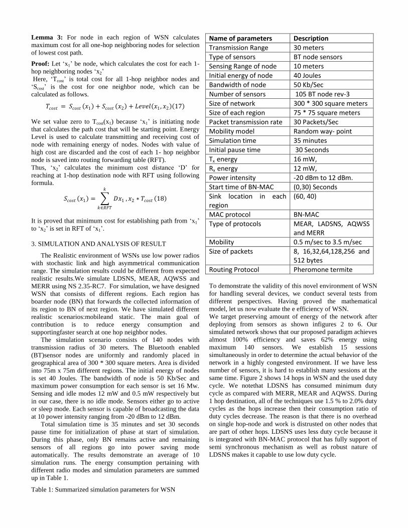
Table 1: Summarized simulation parameters for WSN

Name of parameters Description

Transmission Range 30 meters

Type of sensors BT node sensors

Sensing Range of node 10 meters

Initial energy of node 40 Joules

Bandwidth of node 50 Kb/Sec

Number of sensors 105 BT node rev-3

Size of network 300 * 300 square meters

Size of each region 75 * 75 square meters

Packet transmission rate 30 Packets/Sec

Mobility model Random way- point

Simulation time 35 minutes

Initial pause time 30 Seconds

Tx energy 16 mW,

Rx energy 12 mW,

Power intensity -20 dBm to 12 dBm.

Start time of BN-MAC (0,30) Seconds

Sink location in each region

(60, 40)

MAC protocol BN-MAC

Type of protocols MEAR, LADSNS, AQWSS and MERR

Mobility 0.5 m/sec to 3.5 m/sec

Size of packets 8, 16,32,64,128,256 and 512 bytes

Routing Protocol Pheromone termite

To demonstrate the validity of this novel environment of WSN

for handling several devices, we conduct several tests from

different perspectives. Having proved the mathematical

model, let us now evaluate the e efficiency of WSN.

We target preserving amount of energy of the network after

deploying from sensors as shown infigures 2 to 6. Our

simulated network shows that our proposed paradigm achieves

almost 100% efficiency and saves 62% energy using

maximum 140 sensors. We establish 15 sessions

simultaneously in order to determine the actual behavior of the

network in a highly congested environment. If we have less

number of sensors, it is hard to establish many sessions at the

same time. Figure 2 shows 14 hops in WSN and the used duty

cycle. We notethat LDSNS has consumed minimum duty

cycle as compared with MERR, MEAR and AQWSS. During

1 hop destination, all of the techniques use 1.5 % to 2.0% duty

cycles as the hops increase then their consumption ratio of

duty cycles decrease. The reason is that there is no overhead

on single hop-node and work is distrusted on other nodes that

are part of other hops. LDSNS uses less duty cycle because it

is integrated with BN-MAC protocol that has fully support of

semi synchronous mechanism as well as robust nature of

LDSNS makes it capable to use low duty cycle.

2

0.5

11

.52

.02

.5

0

NUMBER OF HOPS

DU

TY

CY

CL

E (

%)

LDSNS

MEAR

MERR

0 4 6 8 10 12 14

AQWSS

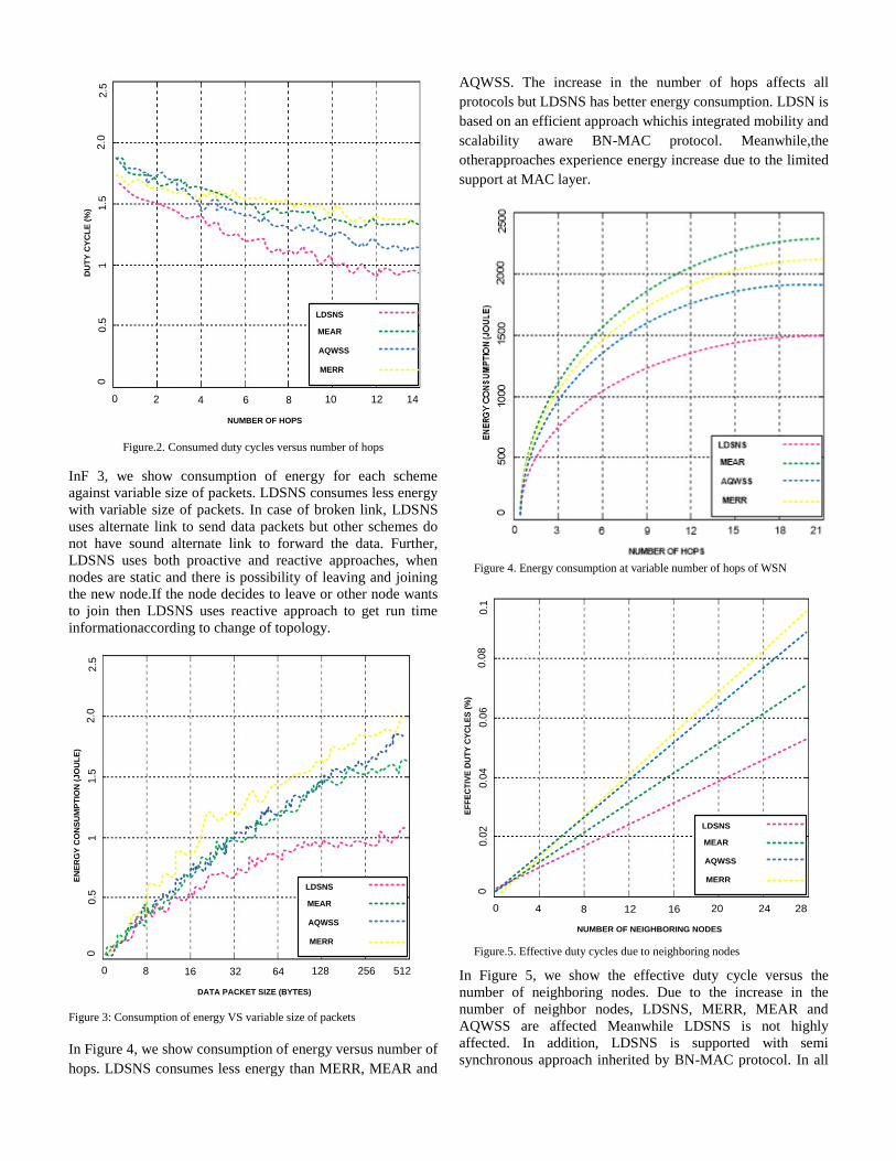
Figure.2. Consumed duty cycles versus number of hops

InF 3, we show consumption of energy for each scheme

against variable size of packets. LDSNS consumes less energy

with variable size of packets. In case of broken link, LDSNS

uses alternate link to send data packets but other schemes do

not have sound alternate link to forward the data. Further,

LDSNS uses both proactive and reactive approaches, when

nodes are static and there is possibility of leaving and joining

the new node.If the node decides to leave or other node wants

to join then LDSNS uses reactive approach to get run time

informationaccording to change of topology.

8

0.5

11

.52

.02

.5

0

DATA PACKET SIZE (BYTES)

EN

ER

GY

CO

NS

UM

PT

ION

(J

OU

LE

)

LDSNS

MEAR

MERR

0 16 32 64 128 256 512

AQWSS

Figure 3: Consumption of energy VS variable size of packets

In Figure 4, we show consumption of energy versus number of

hops. LDSNS consumes less energy than MERR, MEAR and

AQWSS. The increase in the number of hops affects all

protocols but LDSNS has better energy consumption. LDSN is

based on an efficient approach whichis integrated mobility and

scalability aware BN-MAC protocol. Meanwhile,the

otherapproaches experience energy increase due to the limited

support at MAC layer.

Figure 4. Energy consumption at variable number of hops of WSN

4

0.0

20

.04

0.0

60

.08

0.1

0

NUMBER OF NEIGHBORING NODES

EF

FE

CT

IVE

DU

TY

CY

CL

ES

(%

)

LDSNS

MEAR

MERR

0 8 12 16 20 24 28

AQWSS

Figure.5. Effective duty cycles due to neighboring nodes

In Figure 5, we show the effective duty cycle versus the

number of neighboring nodes. Due to the increase in the

number of neighbor nodes, LDSNS, MERR, MEAR and

AQWSS are affected Meanwhile LDSNS is not highly

affected. In addition, LDSNS is supported with semi

synchronous approach inherited by BN-MAC protocol. In all

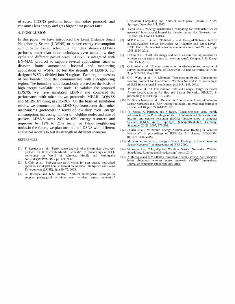
of cases, LDSNS performs better than other protocols and

consumes less energy and gets higher data packet rates.

4. CONCLUSION

In this paper, we have introduced the Least Distance Smart

Neighboring Search (LDSNS) to reduce energy consumption

and provide faster scheduling for data delivery.LDSNS

performs better than other techniques even under low duty

cycle and different packet sizes. LDSNS is integrated with

BN-MAC protocol to support several applications such as

disaster, home automation, hospital and monitoring

applications of WSNs. To test the strength of LDSNS, our

designed WSNis divided into N-regions. Each region consists

of one boarder node that communicates with a neighboring

region. The boundary node israndomly elected on the basis of

high energy available inthe node. To validate the proposed

LDSNS, we have simulated LDSNS and compared its

performance with other known protocols: MEAR, AQWSS

and MERR by using ns2.35-RC7. On the basis of simulation

results, we demonstrate thatLDSNSperformsbetter than other

mechanisms (protocols) in terms of low duty cycle, energy

consumption, increasing number of neighbor nodes and size of

packets. LDSNS saves 24% to 62% energy resources and

improves by 12% to 21% search at 1-hop neighboring

nodes.In the future, we plan tocombine LDSNS with different

analytical models to test its strength in different scenarios. REFERENCES

[1] F. Restuccia et al., “Performance analysis of a hierarchical discovery protocol for WSNs with Mobile Elements”, In proceedings of IEEE

conference on World of Wireless, Mobile and Multimedia

Networks(WOWMOM), pp. 1-9, 2012.

[2] J. Chin et al., “Soft-appliances: A vision for user created networked appliances in digital homes. Journal on Ambient Intelligence and Smart Environments (JAISE), 1(1):69–75, 2009.

[3] A. Razaque and K.M.Elleithy,” Ambient Intelligence Paradigm to support pedagogical activities over wireless sensor networks,”

Ubiquitous Computing and Ambient Intelligence (UCAmI), ACM/ Springer, December 3-5, 2012.

[4] T.Zhu et al., “Energy-synchronized computing for sustainable sensor networks” International Journal for Elsevier on Ad Hoc Networks, vol. 11, no.4, pp. 1392-1404,2013.

[5] M.D.Francesco et al., “Reliability and Energy-Efficiency inIEEE 802.15.4/ZigBee Sensor Networks: An Adaptive and Cross-Layer”, IEEE Trans. On selected areas in communications, vol.29, no.8, pp. 1508-1524, 2011.

[6] Debraj et al., “EAR: An energy and activity-aware routing protocol for wireless sensor networks in smart environments”, Comput. J. 55(12),pp. 1492-1506, 2012.

[7] G Anastasi et al., “Energy conservation in wireless sensor networks: A survey. International journal of Elsevier on Ad Hoc Networks, vol 7, no. 3,pp. 537–568, May 2009.

[8] C-C. Weng et al., “A Minimum Transmission Energy Consumption Routing Protocol for User-Centric Wireless Networks” In proceedings of IEEE International SI conference, pp.1143-1148, 2011.

[9] P Tarrio et al., “A Transmission Rate and Energy Design for Power Aware Localization in Ad Hoc and Sensor Networks. PIMRC”, In proceedings of IEEE,pp. 1-5, 2007.

[10] D. Bhattacharyya et al., “Review: A Comparative Study of Wireless Sensor Networks and Their Routing Protocols”, International Journal of sensors, vol.10, pp.10506-10523, 2010.

[11] Y. Zhang, K. Partridge and J. Reich, ”Localizing tags using mobile infrastructure”, In Proceedings of the 3rd International Symposium on location and context awareness (LoCA). Lecture notes in computer Science (LNCS 4718). Springer, (Oberpfaffenhofen, Germany, September 20-21, 2007, 279-296.

[12] J.Chen et al., “Minimum Energy Accumulative Routing in Wireless Networks”, In proceedings of IEEE for 24th Annual INFOCOM, pp.1875-1886, 2005.

[13] M. Zimmerling et al., Energy-Efficient Routing in Linear Wireless Sensor Networks”, In proceedings of IEEE 2009.

[14] Shouwen Lai, “Duty-Cycled Wireless Sensor Networks: Wakeup Scheduling, Routing, and Broadcasting” thesis, 2010.

[15] A. Razaque and K.M.Elleithy, “Automatic energy saving (AES) modelto boost ubiquitous wireless sensor networks (WSNs)“ International Journal of computers and technology 2013.