Embed Size (px)
Citation preview
CENG 5030Energy Efficient Computing
Lecture 05: Quantization
Bei Yu
(Latest update: February 10, 2021)
Spring 2021
1 / 25

Overview
Overview
Non-differentiable Quantization
Differentiable Quantization
Reading List
2 / 25

Overview
Overview
Non-differentiable Quantization
Differentiable Quantization
Reading List
3 / 25
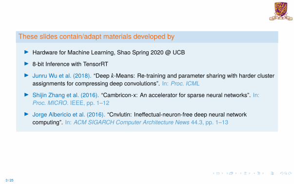
These slides contain/adapt materials developed by
I Hardware for Machine Learning, Shao Spring 2020 @ UCB
I 8-bit Inference with TensorRT
I Junru Wu et al. (2018). “Deep k-Means: Re-training and parameter sharing with harder clusterassignments for compressing deep convolutions”. In: Proc. ICML
I Shijin Zhang et al. (2016). “Cambricon-x: An accelerator for sparse neural networks”. In:Proc. MICRO. IEEE, pp. 1–12
I Jorge Albericio et al. (2016). “Cnvlutin: Ineffectual-neuron-free deep neural networkcomputing”. In: ACM SIGARCH Computer Architecture News 44.3, pp. 1–13
3 / 25
Scientific Notation
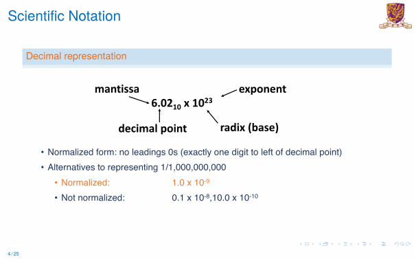
Decimal representation
Shao Spring 2020 © UCBHardware for Machine Learning 8
Scientific Notation (in Decimal)
• Normalized form: no leadings 0s (exactly one digit to left of decimal point)• Alternatives to representing 1/1,000,000,000
• Normalized: 1.0 x 10⁻⁹
• Not normalized: 0.1 x 10-8,10.0 x 10-10
6.0210 x 10²³
radix (base)decimal point
mantissa exponent
4 / 25
Scientific Notation
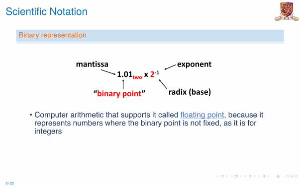
Binary representation
Shao Spring 2020 © UCBHardware for Machine Learning 9
Scientific Notation (in Binary)
• Computer arithmetic that supports it called floating point, because it represents numbers where the binary point is not fixed, as it is for integers
1.01two x 2-1
radix (base)“binary point”
exponentmantissa
5 / 25
Normalized Form
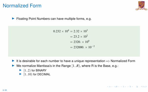
I Floating Point Numbers can have multiple forms, e.g.
0.232× 104 = 2.32× 103
= 23.2× 102
= 2320.× 100
= 232000.× 10−2
I It is desirable for each number to have a unique representation => Normalized FormI We normalize Mantissa’s in the Range [1..R), where R is the Base, e.g.:
I [1..2) for BINARYI [1..10) for DECIMAL
6 / 25
Floating-Point Representation
Shao Spring 2020 © UCBHardware for Machine Learning 10
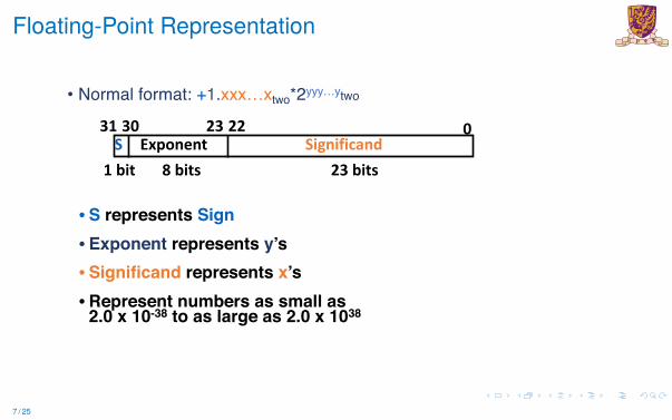
Floating-Point Representation• Normal format: +1.xxx…xtwo*2yyy…ytwo
031S Exponent30 23 22
Significand1 bit 8 bits 23 bits
• S represents Sign• Exponent represents y’s• Significand represents x’s• Represent numbers as small as
2.0 x 10-38 to as large as 2.0 x 1038
7 / 25
Floating-Point Representation (FP32)
Shao Spring 2020 © UCBHardware for Machine Learning 11
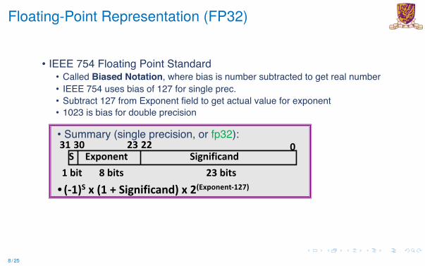
Floating-Point Representation (fp32)• IEEE 754 Floating Point Standard
• Called Biased Notation, where bias is number subtracted to get real number• IEEE 754 uses bias of 127 for single prec.• Subtract 127 from Exponent field to get actual value for exponent• 1023 is bias for double precision
• Summary (single precision, or fp32):031
S Exponent30 23 22
Significand1 bit 8 bits 23 bits• (-1)S x (1 + Significand) x 2(Exponent-127)
8 / 25
Floating-Point Representation (FP16)
Shao Spring 2020 © UCBHardware for Machine Learning 12
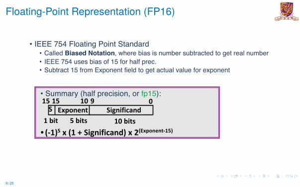
Floating-Point Representation (fp16)• IEEE 754 Floating Point Standard • Called Biased Notation, where bias is number subtracted to get real number• IEEE 754 uses bias of 15 for half prec.• Subtract 15 from Exponent field to get actual value for exponent
• Summary (half precision, or fp15):015
S Exponent15 10 9
Significand1 bit 5 bits 10 bits• (-1)S x (1 + Significand) x 2(Exponent-15)
9 / 25
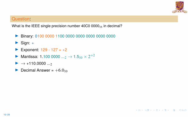
Question:What is the IEEE single precision number 40C0 000016 in decimal?
I Binary: 0100 0000 1100 0000 0000 0000 0000 0000I Sign: +I Exponent: 129 - 127 = +2I Mantissa: 1.100 0000 ...2 → 1.510 × 2+2
I → +110.0000 ...2I Decimal Answer = +6.010
10 / 25
Question:What is the IEEE single precision number 40C0 000016 in decimal?
I Binary: 0100 0000 1100 0000 0000 0000 0000 0000I Sign: +I Exponent: 129 - 127 = +2I Mantissa: 1.100 0000 ...2 → 1.510 × 2+2
I → +110.0000 ...2I Decimal Answer = +6.010
10 / 25

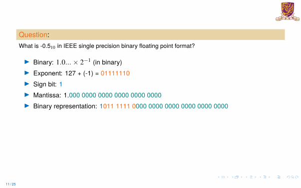
Question:What is -0.510 in IEEE single precision binary floating point format?
I Binary: 1.0...× 2−1 (in binary)I Exponent: 127 + (-1) = 01111110I Sign bit: 1I Mantissa: 1.000 0000 0000 0000 0000 0000I Binary representation: 1011 1111 0000 0000 0000 0000 0000 0000
11 / 25
Question:What is -0.510 in IEEE single precision binary floating point format?
I Binary: 1.0...× 2−1 (in binary)I Exponent: 127 + (-1) = 01111110I Sign bit: 1I Mantissa: 1.000 0000 0000 0000 0000 0000I Binary representation: 1011 1111 0000 0000 0000 0000 0000 0000
11 / 25
Fixed-Point Arithmetic
Shao Spring 2020 © UCBHardware for Machine Learning 14
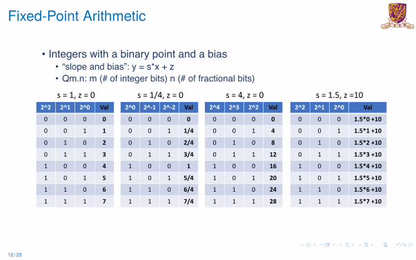
Fixed-Point Arithmetic• Integers with a binary point and a bias
• “slope and bias”: y = s*x + z• Qm.n: m (# of integer bits) n (# of fractional bits)
2^2 2^1 2^0 Val
0 0 0 00 0 1 1
0 1 0 2
0 1 1 31 0 0 4
1 0 1 51 1 0 6
1 1 1 7
2^0 2^-1 2^-2 Val
0 0 0 00 0 1 1/4
0 1 0 2/4
0 1 1 3/41 0 0 1
1 0 1 5/41 1 0 6/4
1 1 1 7/4
2^4 2^3 2^2 Val
0 0 0 00 0 1 4
0 1 0 8
0 1 1 121 0 0 16
1 0 1 201 1 0 24
1 1 1 28
2^2 2^1 2^0 Val
0 0 0 1.5*0 +100 0 1 1.5*1 +10
0 1 0 1.5*2 +10
0 1 1 1.5*3 +101 0 0 1.5*4 +10
1 0 1 1.5*5 +101 1 0 1.5*6 +10
1 1 1 1.5*7 +10
s = 1, z = 0 s = 1/4, z = 0 s = 4, z = 0 s = 1.5, z =10
Shao Spring 2020 © UCBHardware for Machine Learning 14
Fixed-Point Arithmetic• Integers with a binary point and a bias
• “slope and bias”: y = s*x + z• Qm.n: m (# of integer bits) n (# of fractional bits)
2^2 2^1 2^0 Val
0 0 0 00 0 1 1
0 1 0 2
0 1 1 31 0 0 4
1 0 1 51 1 0 6
1 1 1 7
2^0 2^-1 2^-2 Val
0 0 0 00 0 1 1/4
0 1 0 2/4
0 1 1 3/41 0 0 1
1 0 1 5/41 1 0 6/4
1 1 1 7/4
2^4 2^3 2^2 Val
0 0 0 00 0 1 4
0 1 0 8
0 1 1 121 0 0 16
1 0 1 201 1 0 24
1 1 1 28
2^2 2^1 2^0 Val
0 0 0 1.5*0 +100 0 1 1.5*1 +10
0 1 0 1.5*2 +10
0 1 1 1.5*3 +101 0 0 1.5*4 +10
1 0 1 1.5*5 +101 1 0 1.5*6 +10
1 1 1 1.5*7 +10
s = 1, z = 0 s = 1/4, z = 0 s = 4, z = 0 s = 1.5, z =10
12 / 25
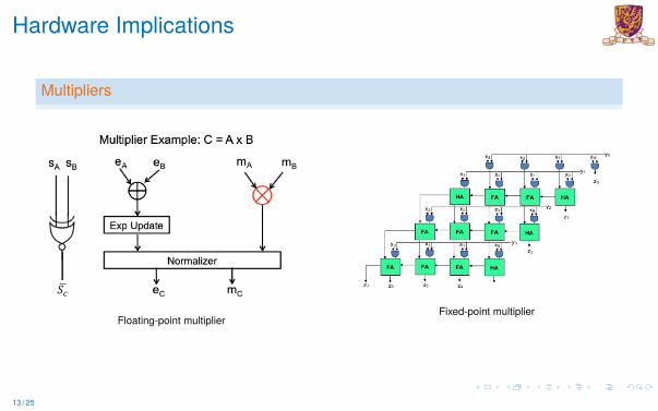
Hardware Implications
Multipliers
Shao Spring 2020 © UCBHardware for Machine Learning 16
Hardware Implications
Fixed-Point Multiplier Floating-Point Multiplier
!"#
Floating-point multiplier
Shao Spring 2020 © UCBHardware for Machine Learning 16
Hardware Implications
Fixed-Point Multiplier Floating-Point Multiplier
!"#
Fixed-point multiplier
13 / 25
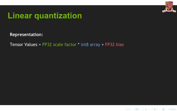
Linear quantization
Representation:
Tensor Values = FP32 scale factor * int8 array + FP32 bias
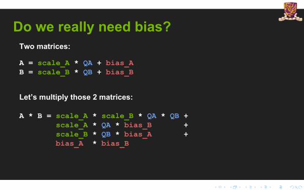
Do we really need bias?Two matrices:
A = scale_A * QA + bias_AB = scale_B * QB + bias_B
Let’s multiply those 2 matrices:
A * B = scale_A * scale_B * QA * QB + scale_A * QA * bias_B + scale_B * QB * bias_A + bias_A * bias_B
Do we really need bias?Two matrices:
A = scale_A * QA + bias_AB = scale_B * QB + bias_B
Let’s multiply those 2 matrices:
A * B = scale_A * scale_B * QA * QB + scale_A * QA * bias_B + scale_B * QB * bias_A + bias_A * bias_B
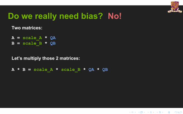
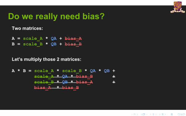
Do we really need bias? No!Two matrices:
A = scale_A * QAB = scale_B * QB
Let’s multiply those 2 matrices:
A * B = scale_A * scale_B * QA * QB
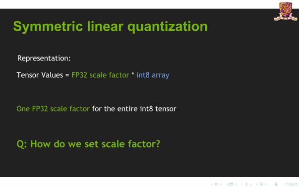
Symmetric linear quantization
Representation:
Tensor Values = FP32 scale factor * int8 array
One FP32 scale factor for the entire int8 tensor
Q: How do we set scale factor?
18
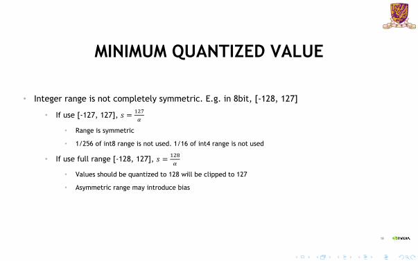
MINIMUM QUANTIZED VALUE
• Integer range is not completely symmetric. E.g. in 8bit, [-128, 127]
• If use [-127, 127], 𝑠 = 127𝛼
• Range is symmetric
• 1/256 of int8 range is not used. 1/16 of int4 range is not used
• If use full range [-128, 127], 𝑠 = 128𝛼
• Values should be quantized to 128 will be clipped to 127
• Asymmetric range may introduce bias

19
EXAMPLE OF QUANTIZATION BIAS
𝐴 = −2.2 −1.1 1.1 2.2 , 𝐵 =0.50.30.30.5
, 𝐴𝐵 = 0
8bit scale quantization, use [-128, 127]. sA=128/2.2, sB=128/0.5
−128 −64 64 127 ∗1277777127
= −127
Dequantize -127 will get -0.00853. A small bias is introduced towards -∞
Bias introduced when int values are in [-128, 127]
20
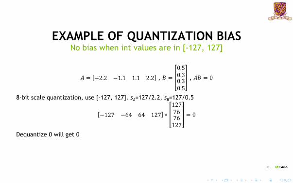
EXAMPLE OF QUANTIZATION BIAS
𝐴 = −2.2 −1.1 1.1 2.2 , 𝐵 =0.50.30.30.5
, 𝐴𝐵 = 0
8-bit scale quantization, use [-127, 127]. sA=127/2.2, sB=127/0.5
−127 −64 64 127 ∗1277676127
= 0
Dequantize 0 will get 0
No bias when int values are in [-127, 127]
21
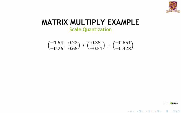
MATRIX MULTIPLY EXAMPLEScale Quantization
−1.54 0.22−0.26 0.65 ∗ 0.35
−0.51 = −0.651−0.423
22
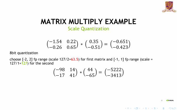
MATRIX MULTIPLY EXAMPLEScale Quantization
−1.54 0.22−0.26 0.65 ∗ 0.35
−0.51 = −0.651−0.423
8bit quantization
choose [-2, 2] fp range (scale 127/2=63.5) for first matrix and [-1, 1] fp range (scale = 127/1=127) for the second
−98 14−17 41 ∗ 44
−65 = −5222−3413
23
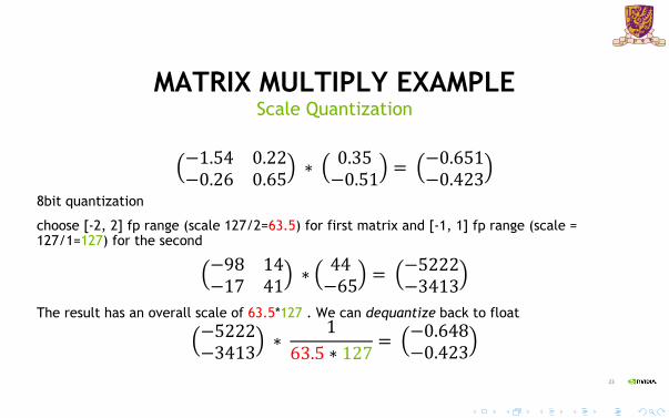
MATRIX MULTIPLY EXAMPLEScale Quantization
−1.54 0.22−0.26 0.65 ∗ 0.35
−0.51 = −0.651−0.423
8bit quantization
choose [-2, 2] fp range (scale 127/2=63.5) for first matrix and [-1, 1] fp range (scale = 127/1=127) for the second
−98 14−17 41 ∗ 44
−65 = −5222−3413
The result has an overall scale of 63.5*127 . We can dequantize back to float−5222−3413 ∗
163.5 ∗ 127
= −0.648−0.423
24
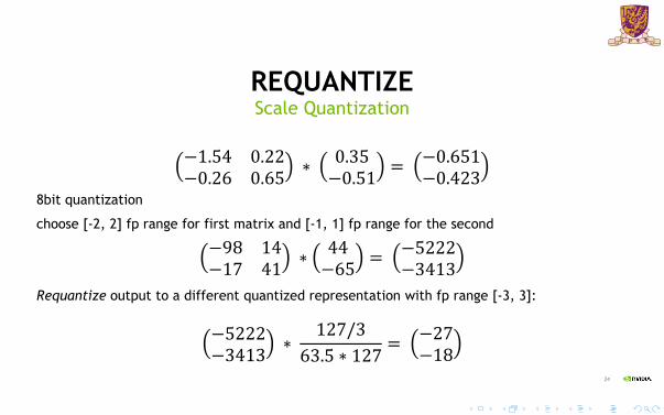
REQUANTIZEScale Quantization
−1.54 0.22−0.26 0.65 ∗ 0.35
−0.51 = −0.651−0.423
8bit quantization
choose [-2, 2] fp range for first matrix and [-1, 1] fp range for the second
−98 14−17 41 ∗ 44
−65 = −5222−3413
Requantize output to a different quantized representation with fp range [-3, 3]:
−5222−3413 ∗
127/363.5 ∗ 127
= −27−18

Overview
Overview
Non-differentiable Quantization
Differentiable Quantization
Reading List
14 / 25
Greedy Layer-wise Quantization1
Quantization flow
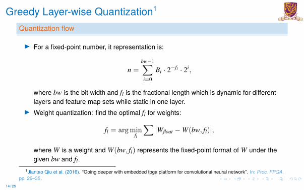
I For a fixed-point number, it representation is:
n =
bw−1∑
i=0Bi · 2−fl · 2i,
where bw is the bit width and fl is the fractional length which is dynamic for differentlayers and feature map sets while static in one layer.
I Weight quantization: find the optimal fl for weights:
fl = argminfl
∑|Wfloat −W(bw, fl)|,
where W is a weight and W(bw, fl) represents the fixed-point format of W under thegiven bw and fl.
1Jiantao Qiu et al. (2016). “Going deeper with embedded fpga platform for convolutional neural network”. In: Proc. FPGA,pp. 26–35.
14 / 25
Greedy Layer-wise Quantization
Quantization flow
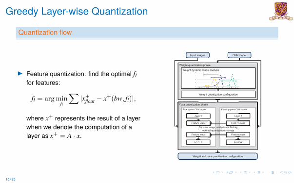
I Feature quantization: find the optimal flfor features:
fl = argminfl
∑|x+float − x+(bw, fl)|,
where x+ represents the result of a layerwhen we denote the computation of alayer as x+ = A · x.
Table 2: The Memory footprint, Computation Complexities,and Performance of the VGG16 model and its SVD version.
Network FC6# of total # of Top-5weights operations accuracy
VGG16 25088!4096 138.36M 30.94G 88.00%VGG16-SVD 25088!500 + 500!4096 50.18M 30.76G 87.96%
For pooling layers and FC layers, the time complexities are
CTimePooling = O(nin · r · c), (5)
CTimeFC = O(nin · nout). (6)
For pooling layers, nout equals to nin since each input featuremap is pooled to a corresponding output feature map, and thus thecomplexity is linear to either input or output feature map number.
Space complexity refers to the memory footprint. For a CONVlayer, there are nin !nout convolution kernels, and each kernel hask2 weights. Consequently, the space complexity for a CONV layeris
CSpaceCONV = O(nin · nout · k2). (7)
FC layer actually applies a multiplication to the input feature vec-tor, and thus the complexity for FC layer is measure by the size forthe parameter matrix, which is shown in Equation 8:
CSpaceFC = O(nin · nout) (8)
No space is needed for pooling layers since it has no weight.The distribution of demanded operations and weight numbers in
the inference process of state-of-the-art CNN models are shown inFigure 2. The measured operations consist of multiplications, adds,and non-linear functions.
As shown in Figure 2 (a), the operations of CONV layers com-pose most of the total operations of CNN models, and thus thetime complexity of CONV layers is much higher than that of FClayers. Consequently, for CONV layers, more attention should bepaid to accelerate convolution operations.
For space complexity, the situation is quite different. As shownin Figure 2 (b), FC layers contribute to most of the weights. S-ince each weight in FC layers is used only once in one inferenceprocess, leaves no chance for reuse, the limited bandwidth cansignificantly degrade the performance since loading those weightsmay take quite long time.
Since FC layers contribute to most of memory footprint, it isnecessary to reduce weights of FC layers while maintaining com-parable accuracy. In this paper, SVD is adopted for acceleratingFC layers. Considering an FC layer fout = Wf in + b, the weightmatrix W can be decomposed as W " UdSdVd = W1W2, inwhich Sd is a diagonal matrix. By choosing the first d singularvalues in SVD, i.e. the rank of matrix Ud, Sd, and Vd, both timeand space complexity can be reduced to O(d · nin + d · nout) fromO(nin · nout). Since accuracy loss may be minute even when dis much smaller than nin and nout, considerable reduction of timeconsumption and memory footprint can be achieved.
The effectiveness of SVD is proved by the results in Table 2.By applying SVD to the parameter matrix of the FC6 layer andchoosing first 500 singular values, the number of weights in FC6layers is reduced to 14.6 million from 103 million, which achievesa compression rate at 7.04!. However, the number of operationsdoes not decrease much since the FC layer contributes little to totaloperations. The SVD only introduces 0.04% accuracy loss.
5. DATA QUANTIZATIONUsing short fixed-point numbers instead of long floating-point
numbers is efficient for implementations on the FPGA and can sig-nificantly reduce memory footprint and bandwidth requirements. Ashorter bit width is always wanted, but it may lead to a severe ac-curacy loss. Though fixed-point numbers have been widely used inCNN accelerator designs, there is no comprehensive investigation
Input images
Data quantization phase
Fixed-point CNN model
CNN model
Floating-point CNN model
Weight and data quantization configuration
Layer 1
Feature maps
Layer N
Layer 1
Feature maps
Layer N
Feature maps Feature maps
CNN model
yer 1
e maps
Data quantization
Fixed-point CNN
Laye
Featuree maure
Layer Layer
aturee ma
uantiz
… …Dynamic range analysis and findingoptimal quantization strategy
Weight quantization phase
Weight dynamic range analysis
Weight quantization configuration
namic range analysis
zation
Figure 3: The dynamic-precision data quantization flow.
on different quantization strategies and the trade-off between the bitlength of fixed-point numbers and the accuracy. In this section, wepropose a dynamic-precision data quantization flow and compare itwith widely used static-precision quantization strategies.
5.1 Quantization FlowFor a fixed-point number, its value can be expressed as
n =
bw!1!
i=0
Bi · 2!fl · 2i, (9)
where bw is the bit width and fl is the fractional length whichcan be negative. To convert floating-point numbers into fixed-pointones while achieving the highest accuracy, we propose a dynamic-precision data quantization strategy and an automatic workflow, asshown in Figure 3. Unlike previous static-precision quantization s-trategies, in the proposed data quantization flow, fl is dynamic fordifferent layers and feature map sets while static in one layerto minimize the truncation error of each layer. The proposedquantization flow mainly consists of two phases: the weight quan-tization phase and the data quantization phase.
The weight quantization phase aims to find the optimal fl forweights in one layer, as shown in Equation 10:
fl = argminfl
!|Wfloat # W (bw, fl)|, (10)
where W is a weight and W (bw, fl) represents the fixed-point for-mat of W under the given bw and fl. In this phase, the dynamicranges of weights in each layer is analyzed first. After that, the fl
is initialized to avoid data overflow. Furthermore, we search for theoptimal fl in the adjacent domains of the initial fl.
The data quantization phase aims to find the optimal fl for aset of feature maps between two layers. In this phase, the inter-mediate data of the fixed-point CNN model and the floating-pointCNN model are compared layer by layer using a greedy algorithmto reduce the accuracy loss. For each layer, the optimization targetis shown in Equation 11:
fl = argminfl
!|x+
float # x+(bw, fl)|. (11)
In Equation 11, x+ represents the result of a layer when we denotethe computation of a layer as x+ = A · x. It should be noted, foreither CONV layer or FC layer, the direct result x+ has longer bitwidth than the given standard. Consequently, truncation is neededwhen optimizing fl selection. Finally, the entire data quantizationconfiguration is generated.
29
15 / 25
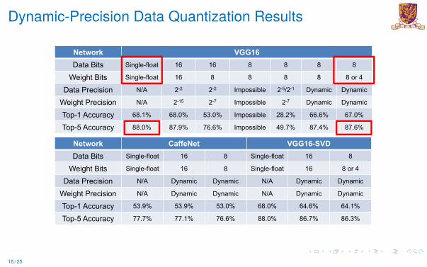
Dynamic-Precision Data Quantization Results� '\QDPLF�3UHFLVLRQ�'DWD�4XDQWL]DWLRQ�5HVXOWV �6LPXODWLRQ�UHVXOWV�
ϭϴ
'DWD�4XDQWL]DWLRQ
1HWZRUN &DIIH1HW 9**���69''DWD %LWV 6LQJOH�IORDW �� � 6LQJOH�IORDW �� �
:HLJKW�%LWV 6LQJOH�IORDW �� � 6LQJOH�IORDW �� ��RU��
'DWD�3UHFLVLRQ 1�$ '\QDPLF '\QDPLF 1�$ '\QDPLF '\QDPLF
:HLJKW�3UHFLVLRQ 1�$ '\QDPLF '\QDPLF 1�$ '\QDPLF '\QDPLF
7RS���$FFXUDF\ ����� ����� ����� ����� ����� �����
7RS�� $FFXUDF\ ����� ����� ����� ����� ����� �����
1HWZRUN 9**��'DWD %LWV 6LQJOH�IORDW �� �� � � � �
:HLJKW�%LWV 6LQJOH�IORDW �� � � � � ��RU��
'DWD�3UHFLVLRQ 1�$ ��� ��� ,PSRVVLEOH ������� '\QDPLF '\QDPLF
:HLJKW�3UHFLVLRQ 1�$ ���� ��� ,PSRVVLEOH ��� '\QDPLF '\QDPLF
7RS���$FFXUDF\ ����� ����� ����� ,PSRVVLEOH ����� ����� �����
7RS�� $FFXUDF\ ����� ����� ����� ,PSRVVLEOH ����� ����� �����
16 / 25
Industrial Implementations – Nvidia TensorRT
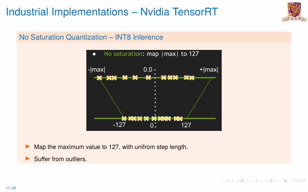
No Saturation Quantization – INT8 Inference
Quantization
● No saturation: map |max| to 127 ● Saturate above |threshold| to 127
0.0 +|max|-|max|
0-127 127
● Significant accuracy loss, in general
0.0 +|T|-|T|
0-127 127
● Weights: no accuracy improvement● Activations: improved accuracy● Which |threshold| is optimal?
I Map the maximum value to 127, with unifrom step length.
I Suffer from outliers.
17 / 25
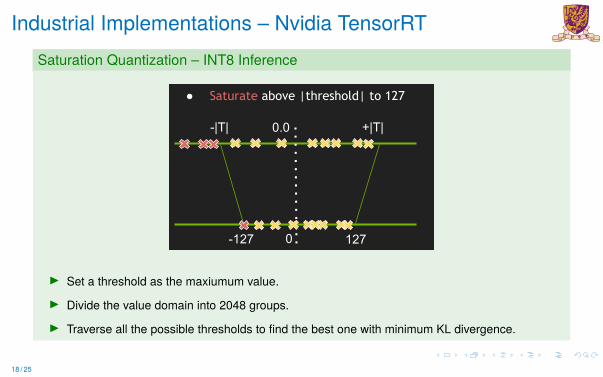
Industrial Implementations – Nvidia TensorRTSaturation Quantization – INT8 Inference
Quantization
● No saturation: map |max| to 127 ● Saturate above |threshold| to 127
0.0 +|max|-|max|
0-127 127
● Significant accuracy loss, in general
0.0 +|T|-|T|
0-127 127
● Weights: no accuracy improvement● Activations: improved accuracy● Which |threshold| is optimal?
I Set a threshold as the maxiumum value.
I Divide the value domain into 2048 groups.
I Traverse all the possible thresholds to find the best one with minimum KL divergence.
18 / 25
Industrial Implementations – Nvidia TensorRT
Relative Entropy of two encodings
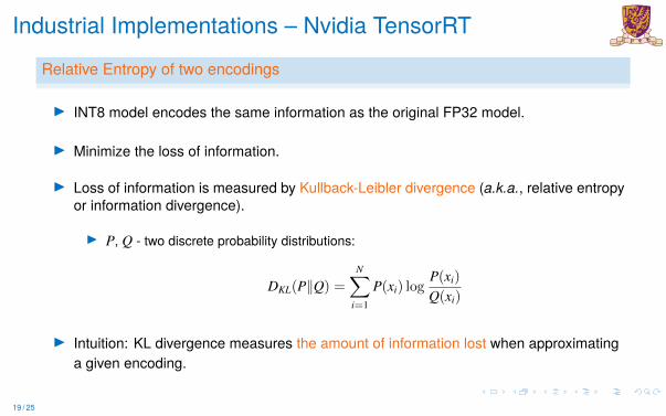
I INT8 model encodes the same information as the original FP32 model.
I Minimize the loss of information.
I Loss of information is measured by Kullback-Leibler divergence (a.k.a., relative entropyor information divergence).
I P, Q - two discrete probability distributions:
DKL(P‖Q) =N∑
i=1
P(xi) logP(xi)Q(xi)
I Intuition: KL divergence measures the amount of information lost when approximatinga given encoding.
19 / 25

Overview
Overview
Non-differentiable Quantization
Differentiable Quantization
Reading List
20 / 25
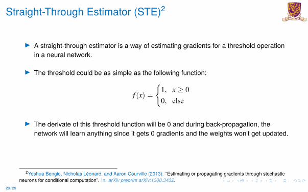
Straight-Through Estimator (STE)2
I A straight-through estimator is a way of estimating gradients for a threshold operationin a neural network.
I The threshold could be as simple as the following function:
f (x) =
{1, x ≥ 00, else
I The derivate of this threshold function will be 0 and during back-propagation, thenetwork will learn anything since it gets 0 gradients and the weights won’t get updated.
2Yoshua Bengio, Nicholas Léonard, and Aaron Courville (2013). “Estimating or propagating gradients through stochasticneurons for conditional computation”. In: arXiv preprint arXiv:1308.3432.
20 / 25
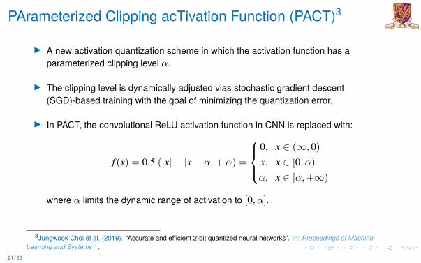
PArameterized Clipping acTivation Function (PACT)3
I A new activation quantization scheme in which the activation function has aparameterized clipping level α.
I The clipping level is dynamically adjusted vias stochastic gradient descent(SGD)-based training with the goal of minimizing the quantization error.
I In PACT, the convolutional ReLU activation function in CNN is replaced with:
f (x) = 0.5 (|x| − |x− α|+ α) =
0, x ∈ (∞, 0)x, x ∈ [0, α)α, x ∈ [α,+∞)
where α limits the dynamic range of activation to [0, α].
3Jungwook Choi et al. (2019). “Accurate and efficient 2-bit quantized neural networks”. In: Proceedings of MachineLearning and Systems 1.
21 / 25
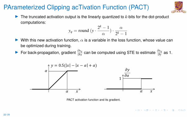
PArameterized Clipping acTivation Function (PACT)I The truncated activation output is the linearly quantized to k-bits for the dot-product
computations:
yq = round (y · 2k − 1α
) · α
2k − 1I With this new activation function, α is a variable in the loss function, whose value can
be optimized during training.I For back-propagation, gradient ∂yq∂α can be computed using STE to estimate ∂yq
∂y as 1.
Accurate and Efficient 2-bit Quantized Neural Networks
back-propagation, gradient @yq
@↵ can be computed using theStraight-Through Estimator (STE) (Bengio et al., 2013) toestimate @yq
@y as 1. Thus,
@yq
@↵=
@yq
@y
@y
@↵=
(0, x 2 (�1,↵)
1, x 2 [↵, +1)(3)
The larger the ↵, the more the parameterized clipping func-tion resembles ReLU. To avoid large quantization errors dueto a wide dynamic range, we include a L2-regularizer for ↵in the loss function. Figure 2(b) illustrates how the valueof ↵ changes during full-precision training of CIFAR10ResNet20 starting with an initial value of 10 and using theL2-regularizer. It can be observed that ↵ converges to thevalues much smaller than the initial value after epochs oftraining, thereby limiting the dynamic range of activationsand reducing the quantization error. We empirically foundthat ↵ per layer was easier to train than ↵ per-channel.
!
!
" = 0.5( ( − ( − ! + !)
(
1
!
-"-!
(
(a) (b)
Valu
e of
.
epoch
Figure 2. (a) PACT activation function and its gradient. The dy-namic range of activation after PACT is bounded by ↵, thus it ismore robust to quantization. (b) Evolution of the trainable clippingparameter ↵ during training of CIFAR10 ResNet20.
3.3 Analysis
3.3.1 PACT is as Expressive as ReLU
When used as an activation function of the neural network,PACT is as expressive as ReLU. This is because the clippingparameter introduced in PACT, ↵, allows flexibility in ad-justing the dynamic range of activation for each layer, thusit can cover large dynamic range as needed. We demonstratein the simple example below that PACT can reach the samesolution as ReLU via SGD.Lemma 3.1. Consider a single-neuron network with PACT;x = w · a, y = PACT(x), where a is input and w is weight.This network can be trained with SGD to find the output thenetwork with ReLU would achieve.
Proof. Consider a sample of training data (a, y⇤). For thepurpose of illustration, consider mean-square-error (MSE)as the cost function: L = 0.5 · (y⇤ � y)2.
If x ↵, then clearly the network with PACT behaves thesame as the network with ReLU.
If x > ↵, then y = ↵ and @y@↵ = 1 from (1). Thus,
@L
@↵=
@L
@y· @y
@↵=
@L
@y(4)
Therefore, when ↵ is updated by SGD,
↵new = ↵� ⌘@L
@↵= ↵� ⌘
@L
@y(5)
where ⌘ is a learning rate. Note that during this update, theweight is not updated as @L
@w = @L@y · @y
@x (= 0) · a = 0.
From the MSE cost function, @L@y = (y � y⇤). Therefore, if
y⇤ > x, ↵ is increased for each update of (5) until ↵ � x,then the PACT network behaves the same as the ReLUnetwork.
Interestingly, if y⇤ y or y < y⇤ < x, ↵ is decreased orincreased to converge to y⇤. Note that in this case, ReLUwould pass erroneous output x to increase cost function,which needs to be fixed by updating w with @L
@w . PACT, onthe other hand, ignores this erroneous output by directlyadapting the dynamic range to match the target output y⇤.In this way, the PACT network can be trained to produceoutput which converges to the same target that the ReLUnetwork would achieve via SGD.
In general, @L@↵ =
Pi
@L@yi
, and PACT considers all the out-put neurons together to change the dynamic range. Thereare two options: (1) if output xi is not clipped, then thenetwork is trained via back-propagation of gradient to up-date weight, (2) if output xi is clipped, then ↵ is increasedor decreased based on how close the overall output is tothe target. Hence, there exist configurations under whichSGD leads to a solution that the network with ReLU wouldachieve. Figure 3 demonstrates that CIFAR10 ResNet20with PACT converges almost identical to the network withReLU.
(a) (b)
Trai
n er
ror
Trai
n er
ror
Trai
n er
ror
Trai
n er
ror
Valid
atio
n er
ror
Trai
n er
ror
epoch epoch
Figure 3. (a) Training error and (b) validation error of PACT forCIFAR10 ResNet20. Note that the convergence curve of PACTclosely follow ReLU.
PACT activation function and its gradient.
22 / 25
Better Gradients
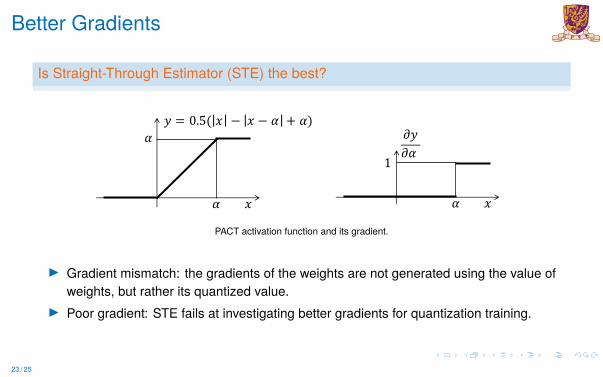
Is Straight-Through Estimator (STE) the best?
Accurate and Efficient 2-bit Quantized Neural Networks
back-propagation, gradient @yq
@↵ can be computed using theStraight-Through Estimator (STE) (Bengio et al., 2013) toestimate @yq
@y as 1. Thus,
@yq
@↵=
@yq
@y
@y
@↵=
(0, x 2 (�1,↵)
1, x 2 [↵, +1)(3)
The larger the ↵, the more the parameterized clipping func-tion resembles ReLU. To avoid large quantization errors dueto a wide dynamic range, we include a L2-regularizer for ↵in the loss function. Figure 2(b) illustrates how the valueof ↵ changes during full-precision training of CIFAR10ResNet20 starting with an initial value of 10 and using theL2-regularizer. It can be observed that ↵ converges to thevalues much smaller than the initial value after epochs oftraining, thereby limiting the dynamic range of activationsand reducing the quantization error. We empirically foundthat ↵ per layer was easier to train than ↵ per-channel.
!
!
" = 0.5( ( − ( − ! + !)
(
1
!
-"-!
(
(a) (b)
Valu
e of
.
epoch
Figure 2. (a) PACT activation function and its gradient. The dy-namic range of activation after PACT is bounded by ↵, thus it ismore robust to quantization. (b) Evolution of the trainable clippingparameter ↵ during training of CIFAR10 ResNet20.
3.3 Analysis
3.3.1 PACT is as Expressive as ReLU
When used as an activation function of the neural network,PACT is as expressive as ReLU. This is because the clippingparameter introduced in PACT, ↵, allows flexibility in ad-justing the dynamic range of activation for each layer, thusit can cover large dynamic range as needed. We demonstratein the simple example below that PACT can reach the samesolution as ReLU via SGD.Lemma 3.1. Consider a single-neuron network with PACT;x = w · a, y = PACT(x), where a is input and w is weight.This network can be trained with SGD to find the output thenetwork with ReLU would achieve.
Proof. Consider a sample of training data (a, y⇤). For thepurpose of illustration, consider mean-square-error (MSE)as the cost function: L = 0.5 · (y⇤ � y)2.
If x ↵, then clearly the network with PACT behaves thesame as the network with ReLU.
If x > ↵, then y = ↵ and @y@↵ = 1 from (1). Thus,
@L
@↵=
@L
@y· @y
@↵=
@L
@y(4)
Therefore, when ↵ is updated by SGD,
↵new = ↵� ⌘@L
@↵= ↵� ⌘
@L
@y(5)
where ⌘ is a learning rate. Note that during this update, theweight is not updated as @L
@w = @L@y · @y
@x (= 0) · a = 0.
From the MSE cost function, @L@y = (y � y⇤). Therefore, if
y⇤ > x, ↵ is increased for each update of (5) until ↵ � x,then the PACT network behaves the same as the ReLUnetwork.
Interestingly, if y⇤ y or y < y⇤ < x, ↵ is decreased orincreased to converge to y⇤. Note that in this case, ReLUwould pass erroneous output x to increase cost function,which needs to be fixed by updating w with @L
@w . PACT, onthe other hand, ignores this erroneous output by directlyadapting the dynamic range to match the target output y⇤.In this way, the PACT network can be trained to produceoutput which converges to the same target that the ReLUnetwork would achieve via SGD.
In general, @L@↵ =
Pi
@L@yi
, and PACT considers all the out-put neurons together to change the dynamic range. Thereare two options: (1) if output xi is not clipped, then thenetwork is trained via back-propagation of gradient to up-date weight, (2) if output xi is clipped, then ↵ is increasedor decreased based on how close the overall output is tothe target. Hence, there exist configurations under whichSGD leads to a solution that the network with ReLU wouldachieve. Figure 3 demonstrates that CIFAR10 ResNet20with PACT converges almost identical to the network withReLU.
(a) (b)
Trai
n er
ror
Trai
n er
ror
Trai
n er
ror
Trai
n er
ror
Valid
atio
n er
ror
Trai
n er
ror
epoch epoch
Figure 3. (a) Training error and (b) validation error of PACT forCIFAR10 ResNet20. Note that the convergence curve of PACTclosely follow ReLU.
PACT activation function and its gradient.
I Gradient mismatch: the gradients of the weights are not generated using the value ofweights, but rather its quantized value.
I Poor gradient: STE fails at investigating better gradients for quantization training.
23 / 25
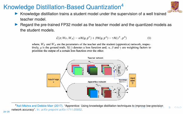
Knowledge Distillation-Based Quantization4I Knowledge distillation trains a student model under the supervision of a well trained
teacher model.I Regard the pre-trained FP32 model as the teacher model and the quantized models as
the student models.
4Asit Mishra and Debbie Marr (2017). “Apprentice: Using knowledge distillation techniques to improve low-precisionnetwork accuracy”. In: arXiv preprint arXiv:1711.05852.
24 / 25

Overview
Overview
Non-differentiable Quantization
Differentiable Quantization
Reading List
25 / 25
Further Reading List
I Darryl Lin, Sachin Talathi, and Sreekanth Annapureddy (2016). “Fixed pointquantization of deep convolutional networks”. In: Proc. ICML, pp. 2849–2858
I Soroosh Khoram and Jing Li (2018). “Adaptive quantization of neural networks”. In:Proc. ICLR
I Jan Achterhold et al. (2018). “Variational network quantization”. In: Proc. ICLRI Antonio Polino, Razvan Pascanu, and Dan Alistarh (2018). “Model compression via
distillation and quantization”. In: arXiv preprint arXiv:1802.05668I Yue Yu, Jiaxiang Wu, and Longbo Huang (2019). “Double quantization for
communication-efficient distributed optimization”. In: Proc. NIPS, pp. 4438–4449I Markus Nagel et al. (2019). “Data-free quantization through weight equalization and
bias correction”. In: Proc. ICCV, pp. 1325–1334
25 / 25


