Embed Size (px)
Citation preview

arX
iv:g
r-qc
/040
7095
v1 2
6 Ju
l 200
4
Lectures on Mathematical Cosmology
Hans-Jurgen Schmidt
Universitat Potsdam, Institut fur Mathematik, Am Neuen Palais 10
D-14469 Potsdam, Germany, E-mail: [email protected]
http://www.physik.fu-berlin.de/˜hjschmi
c©2004, H.-J. Schmidt

CONTENTS 3
Contents
1 Preface 7
2 Changes of the Bianchi type 9
2.1 Introduction to generalized Bianchi models . . . . . . . . . . . 9
2.2 Spaces possessing homogeneous slices . . . . . . . . . . . . . . 11
2.3 Continuous changes of the Bianchi type . . . . . . . . . . . . . 13
2.4 Physical conditions . . . . . . . . . . . . . . . . . . . . . . . . 16
3 Inhomogeneous models with flat slices 19
3.1 Models with flat slices . . . . . . . . . . . . . . . . . . . . . . 20
3.2 Energy inequalities and perfect fluid models . . . . . . . . . . 22
3.3 A simple singularity theorem . . . . . . . . . . . . . . . . . . . 26
4 Properties of curvature invariants 31
4.1 The space of 3–dimensional Riemannian manifolds . . . . . . . 31
4.2 Why do all the invariants of a gravitational wave vanish? . . . 35
4.2.1 Preliminaries . . . . . . . . . . . . . . . . . . . . . . . 36
4.2.2 Gravitational waves . . . . . . . . . . . . . . . . . . . . 39
4.2.3 Topological properties . . . . . . . . . . . . . . . . . . 41
4.3 Spacetimes which cannot be distinguished by invariants . . . . 43
5 Surface layers and relativistic surface tensions 45
5.1 Introduction to surface layers . . . . . . . . . . . . . . . . . . 45
5.2 Non-relativistic surface tensions . . . . . . . . . . . . . . . . . 47
5.3 Mean curvature in curved spacetime . . . . . . . . . . . . . . . 49
5.4 Equation of motion for the surface layer . . . . . . . . . . . . 51
5.5 Notation, distributions and mean curvature . . . . . . . . . . 52

4 CONTENTS
6 The massive scalar field in a Friedmann universe 57
6.1 Some closed-form approximations . . . . . . . . . . . . . . . . 59
6.2 The qualitative behaviour . . . . . . . . . . . . . . . . . . . . 62
6.2.1 Existence of a maximum . . . . . . . . . . . . . . . . . 63
6.2.2 The space of solutions . . . . . . . . . . . . . . . . . . 63
6.2.3 From one extremum to the next . . . . . . . . . . . . . 64
6.2.4 The periodic solutions . . . . . . . . . . . . . . . . . . 66
6.2.5 The aperiodic perpetually oscillating solutions . . . . . 67
6.3 Problems with die probability measure . . . . . . . . . . . . . 70
6.3.1 The spatially flat Friedmann model . . . . . . . . . . . 70
6.3.2 The Bianchi-type I model . . . . . . . . . . . . . . . . 71
6.3.3 The closed Friedmann model . . . . . . . . . . . . . . . 72
6.4 Discussion of the inflationary phase . . . . . . . . . . . . . . . 73
7 The superspace of Riemannian metrics 75
7.1 The superspace . . . . . . . . . . . . . . . . . . . . . . . . . . 75
7.2 Coordinates in superspace . . . . . . . . . . . . . . . . . . . . 76
7.3 Metric in superspace . . . . . . . . . . . . . . . . . . . . . . . 77
7.4 Signature of the superspace metric . . . . . . . . . . . . . . . 79
7.5 Supercurvature and superdeterminant . . . . . . . . . . . . . . 81
7.6 Gravity and quantum cosmology . . . . . . . . . . . . . . . . . 83
7.7 The Wheeler-DeWitt equation . . . . . . . . . . . . . . . . . . 85
8 Scalar fields and f(R) for cosmology 87
8.1 Introduction to scalar fields . . . . . . . . . . . . . . . . . . . 87
8.2 The Higgs field . . . . . . . . . . . . . . . . . . . . . . . . . . 89
8.3 The non-linear gravitational Lagrangian . . . . . . . . . . . . 90
8.3.1 Calculation of the ground states . . . . . . . . . . . . . 92

CONTENTS 5
8.3.2 Definition of the masses . . . . . . . . . . . . . . . . . 93
8.4 The cosmological model . . . . . . . . . . . . . . . . . . . . . 94
8.4.1 The field equation . . . . . . . . . . . . . . . . . . . . . 94
8.4.2 The masses . . . . . . . . . . . . . . . . . . . . . . . . 95
8.4.3 The Friedmann model . . . . . . . . . . . . . . . . . . 96
8.5 The generalized Bicknell theorem . . . . . . . . . . . . . . . . 100
8.6 On Ellis’ programme within homogeneous world models . . . . 104
8.6.1 Ellis’ programme . . . . . . . . . . . . . . . . . . . . . 104
8.6.2 The massive scalar field in a Bianchi-type I model . . . 106
8.6.3 The generalized equivalence . . . . . . . . . . . . . . . 110
8.6.4 The fourth-order gravity model . . . . . . . . . . . . . 111
9 Models with De Sitter and power–law inflation 113
9.1 Differential–geometrical properties . . . . . . . . . . . . . . . . 114
9.2 Scale–invariant field equations . . . . . . . . . . . . . . . . . . 115
9.3 Cosmological Friedmann models . . . . . . . . . . . . . . . . . 116
9.3.1 The closed and open models . . . . . . . . . . . . . . . 117
9.3.2 The spatially flat model . . . . . . . . . . . . . . . . . 119
9.4 Discussion of power-law inflation . . . . . . . . . . . . . . . . 120
9.5 The cosmic no hair theorem . . . . . . . . . . . . . . . . . . . 121
9.5.1 Introduction to no hair theorems . . . . . . . . . . . . 122
9.5.2 Definition of an asymptotic de Sitter spacetime . . . . 130
9.5.3 Lagrangian F (R,2R,22R, . . . ,2kR) . . . . . . . . . . 134
9.5.4 No hair theorems for higher-order gravity . . . . . . . . 135
9.5.5 Diagonalizability of Bianchi models . . . . . . . . . . . 138
9.5.6 Discussion of no hair theorems . . . . . . . . . . . . . . 141
6 CONTENTS
10 Solutions of the Bach-Einstein equation 145
10.1 Introduction to the Bach equation . . . . . . . . . . . . . . . . 145
10.2 Notations and field equations . . . . . . . . . . . . . . . . . . 147
10.3 Linearizations . . . . . . . . . . . . . . . . . . . . . . . . . . . 149
10.4 Non-standard analysis . . . . . . . . . . . . . . . . . . . . . . 151
10.5 Discussion – Einstein’s particle programme . . . . . . . . . . . 154
10.6 Non-trivial solutions of the Bach equation exist . . . . . . . . 156
11 The Newtonian limit of non-linear gravity 159
11.1 The Newtonian limit of 4th-order gravity . . . . . . . . . . . . 159
11.2 Introduction to higher-order gravity . . . . . . . . . . . . . . . 164
11.3 Lagrangian and field equation . . . . . . . . . . . . . . . . . . 165
11.4 Newtonian limit in higher-order gravity . . . . . . . . . . . . . 166
11.5 Discussion of the weak-field limit . . . . . . . . . . . . . . . . 170
11.6 A homogeneous sphere . . . . . . . . . . . . . . . . . . . . . . 172
12 Cosmic strings and gravitational waves 175
12.1 Introduction to cosmic strings . . . . . . . . . . . . . . . . . . 175
12.2 The main formulae . . . . . . . . . . . . . . . . . . . . . . . . 176
12.3 The string in a Friedmann model . . . . . . . . . . . . . . . . 178
12.3.1 The open string . . . . . . . . . . . . . . . . . . . . . . 179
12.3.2 The closed string . . . . . . . . . . . . . . . . . . . . . 181
12.4 The string in an anisotropic Kasner background . . . . . . . . 182
12.5 The string in a gravitational wave . . . . . . . . . . . . . . . . 183
13 Bibliography 187
7
1 Preface
We present mathematical details of several cosmological models, whereby the
topological and the geometrical background will be emphasized.
This book arose from lectures I read as advanced courses in the following
universities: 1990 at TU Berlin, 1991 in Munster, 1993 - 1996 and 2002, 2003
in Potsdam, 1999 and 2000 in Salerno, and 2001 at FU Berlin.
The reader is assumed to be acquainted with basic knowledge on general
relativity, e.g. by knowing Stephani’s book [250]. As a rule, the deduction is
made so explicit, that one should be able to follow the details without further
background knowledge. The intention is to present a piece of mathematical
physics related to cosmology to fill the gap between standard textbooks like
MTW1, LL2, or Weinberg3, on the one hand and to the current research
literature on the other. I hope that this will become useful for both students
and researchers who are interested in cosmology, mathematical physics or
differential geometry.
To the reference list: If more than one source is given in one item, then a dot
is put between them. If, however, two versions of the same source are given,
then a semicolon is put between them. The gr-qc number in the reference
list refers to the number in the preprint archive
http://xxx.lanl.gov/find/
and the numbers in italics given at the end of an item show the pages where
this item is mentioned. This way, the Bibliography simultaneously serves as
1C. Misner, K. Thorne, J. Wheeler Gravitation, Freeman, San Francisco 1973
2L. Landau, E. Lifschitz Field Theory, Nauka, Moscow 1973
3S. Weinberg Gravitation and Cosmology, J. Wiley, New York 1972
8 1 PREFACE
author index.
Parts of this book4 are composed from revised versions of papers of mine
published earlier in research journals. They are reprinted with the kind
permissions of the copyright owners: Akademie-Verlag Berlin for Astron.
Nachr. and Plenum Press New York for Gen. Rel. Grav. The details about
the originals can also be seen in
http://www.physik.fu-berlin.de/˜hjschmi
I thank the following colleagues: Luca Amendola, Michael Bachmann, H.
Baumgartel, W. Benz, Claudia Bernutat, Ulrich Bleyer, A. Borde, H.-H.
v. Borzeszkowski, Salvatore Capozziello, G. Dautcourt, Vladimir Dzhunu-
shaliev, Mauro Francaviglia, T. Friedrich, V. Frolov, H. Goenner, Stefan
Gottlober, V. Gurovich, Graham Hall, F. Hehl, Olaf Heinrich, Alan Held, L.
Herrera, Rainer John, U. Kasper, Jerzy Kijowski, Hagen Kleinert, B. Klotzek,
Sabine Kluske, O. Kowalski, Andrzej Krasinski, W. Kuhnel, W. Kundt, K.
Lake, K. Leichtweiss, D.-E. Liebscher, Malcolm MacCallum, W. Mai, R.
Mansouri, V. Melnikov, P. Michor, Salvatore Mignemi, Volker Muller, S.
Nikcevic, I. Novikov, F. Paiva, Axel Pelster, V. Perlick, K. Peters, Ines
Quandt, L. Querella, M. Rainer, J. Reichert, Stefan Reuter, W. Rinow,
M. Sanchez, R. Schimming, M. Schulz, E. Schmutzer, U. Semmelmann, I.
Shapiro, A. Starobinsky, P. Teyssandier, H.-J. Treder, H. Tuschik, L. Van-
hecke and A. Zhuk for valuable comments, and my wife Renate for patience
and support.
Hans-Jurgen Schmidt, Potsdam, July 2004
4The details are mentioned at the corresponding places.

9
2 Cosmological models with changes of the
Bianchi type
We investigate such cosmological models which instead of the usual spatial
homogeneity property only fulfil the condition that in a certain synchronized
system of reference all spacelike sections t = const. are homogeneous mani-
folds.
This allows time-dependent changes of the Bianchi type. Discussing
differential-geometrical theorems it is shown which of them are permitted.
Besides the trivial case of changing into type I there exist some possible
changes between other types. However, physical reasons like energy inequal-
ities partially exclude them.
2.1 Introduction to generalized Bianchi models
Recently, besides the known Bianchi models, there are investigated certain
classes of inhomogeneous cosmological models. This is done to get a better
representation of the really existent inhomogeneities, cf. e.g. Bergmann [23],
Carmeli [51], Collins [55], Spero [240], Szekeres [251] and Wainwright [265].
We consider, similar as in Collins [55], such inhomogeneous models V4
which in a certain synchronized system of reference possess homogeneous
sections t = const., called V3(t). This is analogous to the generalization of
the concept of spherical symmetry in Krasinski [136], cf. also [137].
In this chapter, which is based on [200], we especially investigate which
time-dependent changes of the Bianchi type are possible. Thereby we im-
pose, besides the twice continuous differentiability, a physically reasonable

10 2 CHANGES OF THE BIANCHI TYPE
condition: the energy inequality,
T00 ≥ |Tαβ| , (2.1)
holds in each Lorentz frame.
We begin with some globally topological properties of spacetime: Under
the physical condition (2.1) the topology of the sections V3(t) is, according
to Lee [142], independent of t. Hence, the Kantowski-Sachs models, with
underlying topology S2 × R or S2 × S1 and the models of Bianchi type IX
with underlying topology S3 or continuous images of it as SO(3) may not
change, because all other types are represented by the R3-topology, factorized
with reference to a discrete subgroup of the group of motions. But the
remaining types can all be represented in R3-topology itself; therefore we do
not get any further global restrictions. All homogeneous models, the above
mentioned Kantowski-Sachs model being excluded, possess simply transitive
groups of motion. If the isometry group G has dimension ≥ 4, then this
statement means: G possesses a 3-dimensional simply-transitive subgroup
acting transitively on the V3(t). Hence we do not specialize if we deal only
with locally simply-transitive groups of motions. We consequently do not
consider here trivial changes of the Bianchi type, e. g. from type III to type
VIII by means of an intermediate on which a group of motions possessing
transitive subgroups of both types acts.
Next, we consider the easily tractable case of a change to type I: For each
type M there one can find a manifold V4 such that for each t ≤ 0 the section
V3(t) is flat and for each t > 0 it belongs to type M. Indeed, one has simply
to use for every V3(t) such a representative of type M that their curvature
vanishes as t → 0+. Choosing exponentially decreasing curvature one can

2.2 Spaces possessing homogeneous slices 11
obtain an arbitrarily high differentiable class for the metric, e. g.
ds2 = −dt2 + dr2 + h2 · (dψ2 + sin2 ψdφ2) , (2.2)
where
h =
r for t ≤ 0
exp(t−2) · sinh2 (r · exp(−t−2)) else .(2.3)
This is a C∞-metric whose slices V3(t) belong to type I for t ≤ 0 and to
type V for t > 0. In t = 0, of course, it cannot be an analytical one. The
limiting slice belongs necessarily to type I by continuity reasons. Applying
this fact twice it becomes obvious that by the help of a flat intermediate of
finite extension or only by a single flat slice, all Bianchi types can be matched
together. However, if one does not want to use such a flat intermediate the
transitions of one Bianchi type to another become a non-trivial problem. It
is shown from the purely differential-geometrical as well as from the physical
points of view, sections 2.3 and 2.4 respectively, which types can be matched
together immediately without a flat intermediate. To this end we collect the
following preliminaries.
2.2 Spaces possessing homogeneous slices
As one knows, in cosmology the homogeneity principle is expressed by the
fact that to a spacetime V4 there exists a group of motions acting transitively
on the spacelike hypersurfaces V3(t) of a slicing of V4. Then the metric is
given by
ds2 = −dt2 + gab(t)ωaωb (2.4)
where the gab(t) are positively definite and ωa are the basic 1-forms corre-
sponding to a certain Bianchi type; for details see e.g. [134]. If the ωa are

12 2 CHANGES OF THE BIANCHI TYPE
related to a holonomic basis xi, using type-dependent functions Aai (xj), one
can write:
ωa = Aai dxi . (2.5)
For the spaces considered here we have however: there is a synchronized
system of reference such that the slices t = const. are homogeneous spaces
V3(t). In this system of reference the metric is given by
ds2 = −dt2 + gijdxidxj (2.6)
where gij(xi, t) are twice continuously differentiable and homogeneous for
constant t. Hence it is a generalization of eqs. (2.4) and (2.5). This is a
genuine generalization because there is only posed the condition g0α = −δ0αon the composition of the homogeneous slices V3(t) to a V4. This means in
each slice only the first fundamental form gij is homogeneous; but in the
contrary to homogeneous models, the second fundamental form Γ0ab need
not have this property. Therefore, also the curvature scalar (4)R, and with it
the distribution of matter, need not be constant within a V3(t).
Now let t be fixed. Then one can find coordinates xit(xj, t) in V3(t) such
that according to eqs. (2.4) and (2.5) the inner metric gets the form
gab(t)ωat ω
bt where ωat = Aai (x
it) dx
it . (2.7)
Transforming this into the original coordinates xi one obtains for the metric
of the full V4
g0α = −δ0α , gij = gab(t)Aak(x
it) A
bl (x
it) x
kt,i x
lt,j . (2.8)

2.3 Continuous changes of the Bianchi type 13
If the Bianchi type changes with time one has to take such an ansatz5 like
eqs. (2.2), (2.3) for each interval of constant type separately; between them
one has to secure a C2-joining. An example of such an inhomogeneous model
is, cf. Ellis 1967 [70]
ds2 = −dt2 + t−2/3 [t+ C(x)]2 dx2 + t4/3(dy2 + dz2) . (2.9)
The slices t = const. are flat, but only for constant C it belongs to Bianchi
type I, cf. also [99] for such a model. Later, see eq. (3.19), we will present a
more general model.
2.3 Continuous changes of the Bianchi type
Using the usual homogeneity property the same group of motions acts on
each slice V3(t). Hence the Bianchi type is independent of time by definition.
But this fails to be the case for the spaces considered here. However, we
can deduce the following: completing ∂/∂t to an anholonomic basis which
is connected with Killing vectors in each V3(t) one obtains for the structure
constants associated to the commutators of the basis:
C0αβ = 0 ; Ci
jk(t) depends continuously on time . (2.10)
Note: These structure constants are calculated as follows: Without loss of
generality let xit(0, 0, 0, t) = 0. At this point ∂/∂xit and ∂/∂xi are taken as
initial values for Killing vectors within V3(t). The structure constants ob-
tained by these Killing vectors are denoted by Cijk(t) and Ci
jk(t) respectively,
where Cijk(t) are the canonical ones. Between them it holds at (0, 0, 0, t):
xit,jCjkl = Ci
mnxmt,kx
nt,l . (2.11)
5The word “ansatz” (setting) stems from the German noun “der Ansatz”; that word
stems from the German verb “setzen” (to set).

14 2 CHANGES OF THE BIANCHI TYPE
Using only the usual canonical structure constants then of course no type
is changeable continuously. To answer the question which Bianchi types may
change continuously we consider all sets of structure constants Cijk being
antisymmetric in jk and fulfilling the Jacobi identity. Let CS be such a
set belonging to type S. Then we have according to eq. (2.10): Type R is
changeable continuously into type S, symbolically expressed by the validity
of R → S, if and only if to each CS there exists a sequence C(n)R such that
one has
limn→∞
C(n)R = CS . (2.12)
The limit has to be understood componentwise.
It holds that R → S if and only if there are a CS and a sequence C(n)R such
that eq. (2.12) is fulfilled. The equivalence of both statements is shown by
means of simultaneous rotations of the basis. In practice one takes as CS the
canonical structure constants and investigates for which types R there can
be found corresponding sequences C(n)R : the components of CS are subjected
to a perturbation not exceeding ε and their Bianchi types are calculated.
Finally one looks which types appear for all ε > 0. Thereby one profits, e.g.,
from the statement that the dimension of the image space of the Lie algebra,
which equals 0 for type I, . . . , and equals 3 for types VIII and IX, cannot
increase during such changes; see [189] and [210] for more details about these
Lie algebras.
One obtains the following diagram. The validity of R → S and S →T implies the validity of R → T, hence the diagram must be continued
transitively. The statement VI∞ → IV expresses the facts that there exists
a sequence
C(n)VIh
→ CIV (2.13)

2.3 Continuous changes of the Bianchi type 15
and that in each such a sequence the parameter h must necessarily tend to
infinity.
Further VIh → II holds for every h. Both statements hold analogously
for type VIIh. In MacCallum [146] a similar diagram is shown, but there it
is only investigated which changes appear if some of the canonical structure
constants are vanishing. So e.g., the different transitions from type VIh to
types II and IV are not contained in it.
?
?
?
-
-
I V
IV
VI∞VI0VIII
VII∞VII0IX
II
Fig. 1, taken from [200]

16 2 CHANGES OF THE BIANCHI TYPE
To complete the answer to the question posed above it must be added: To
each transition shown in the diagram, there one can indeed find a spacetime
V4 in which it is realized. Let f(t) be a C∞-function with f(t) = 0 for t ≤ 0
and f(t) > 0 else. Then, e.g.,
ds2 = −dt2 + dx2 + e2x dy2 + e2x (dz + x f(t) dy)2 (2.14)
is a C∞-metric whose slices V3(t) belong to type V and IV for t ≤ 0 and
t > 0 respectively. Presumably it is typical that in a neighbourhood of t = 0
the curvature becomes singular at spatial infinity; this is at least the case
for metric (2.14). And, for the transition R → S the limiting slice be1ongs
necessarily to type S.
2.4 Physical conditions
To obtain physically reasonable spacetimes one has at least to secure the
validity of an energy inequality like (2.1), T00 ≥ |Tαβ | in each Lorentz frame.
Without this requirement the transition II → I is possible. We prove that
the requirement T00 ≥ 0 alone is sufficient to forbid this transition. To this
end let V4 be a manifold which in a certain synchronized system of reference
possesses a flat slice V3(0), and for all t > 0 has Bianchi type II-slices V3(t).
Using the notations of eq. (2.11) we have: C123 = −C1
32 = 1 are the only
non-vanishing canonical structure constants of Bianchi type II. With the
exception A12 = −x3 we have Aai = δai .
By the help of eq. (2.11) one can calculate the structure constants Cijk(t).
The flat-slice condition is equivalent to
limt→0
Cijk(t) = 0 . (2.15)

2.4 Physical conditions 17
First we consider the special case xit = ai(t) · xi (no sum), i. e. extensions of
the coordinate axes. It holds xit,j = δij ai (no sum). The only non-vanishing
Cijk(t) are C1
23 = −C132 = a(t), where a = a2 · a3/a1. Then eq. (2.15) reads
lim t→0 a(t) = 0. The coefficients gab(t) have to be chosen such that the gij,
according to eq. (2.8), remain positive definite and twice continuously differ-
entiable. Let (3)R be the scalar curvature within the slices. (3)R > 0 appears
only in Bianchi type IX and in the Kantowski-Sachs models. But changes
from these types are just the cases already excluded by global considerations.
Inserting gij into the Einstein equation by means of the Gauss-Codazzi the-
orem one obtains
κT00 = R00 −1
2g00
(4)R =1
2(3)R +
1
4g−1 ·H , g = det gij , (2.16)
(3)R being the scalar curvature within the slices, hence
(3)R ≤ 0 and H = g11[g22,0g33,0 − (g23,0)2]
− 2 · g12[g33,0g12,0 − g13,0g23,0] + cyclic perm . (2.17)
In our case H is a quadratic polynomial in x3 whose quadratic coefficient
reads
−g11[g11g33 − (g13)2] ·
[
∂a(t)
∂t
]2
. (2.18)
Hence, for sufficiently large values x3 and values t with ∂a/∂t 6= 0 we have
H < 0, and therefore T00 < 0.
Secondly we hint at another special case, namely rotations of the coordi-
nate axes against each other, e.g.
x1t = x1 cosω + x2 sinω , x2
t = x2 cosω − x1 sinω , x3t = x3, ω = ω(t) .

18 2 CHANGES OF THE BIANCHI TYPE
There one obtains in analogy to eq. (2.18) a negative T00. Concerning the
general case we have: loosely speaking, each diffeomorphism is a composite
of such extensions and rotations. Hence, for each II → I-transition one would
obtain points with negative T00.
Hence, the energy condition is a genuine restriction to the possible tran-
sitions of the Bianchi types. Concerning the other transitions we remark:
equations (2.16), (2.17) keep valid, and the remaining work is to examine the
signs of the corresponding expressions H . Presumably one always obtains
points with negative H , i.e., also under this weakened homogeneity presump-
tions the Bianchi types of the spacelike hypersurfaces at different distances
from the singularity must coincide.

19
3 Inhomogeneous cosmological models with
flat slices
A family of cosmological models is considered which in a certain synchronized
system of reference possess flat slices t = const. They are generated from the
Einstein-De Sitter universe by a suitable transformation. Under physically
reasonable presumptions these transformed models fulfil certain energy con-
ditions. In Wainwright [265] a class of inhomogeneous cosmological models
is considered which have the following property: there exists a synchronized
system of reference of such a kind that the slices t = const. are homogeneous
manifolds.
Here we consider a special family of such models which possess flat slices.
Following [201], we use the transformation formalism developed in chapter
2. In Krasinski [137], e.g. in Fig. 2.1., it is shown how this approach fits
into other classes of cosmological solutions of the Einstein field equation.
Additionally, we require that these transformations leave two coordinates
unchanged; this implies the existence of a 2-dimensional Abelian group of
motions. A similar requirement is posed in [265], too.
Starting from a Friedmann universe, we investigate whether the energy
inequalities are fulfilled in the transformed model, too. In general this fails
to be the case, but starting from the Einstein-De Sitter universe [68], cf.
also Tolman [256], and requiring perfect fluid for the transformed model, the
energy inequalities in the initial model imply their validity in the transformed
model. A new review on exact solutions can be found in [26], and a new proof
of Birkhoff’s theorem is given in [226].

20 3 INHOMOGENEOUS MODELS WITH FLAT SLICES
3.1 Models with flat slices
The transformation formalism of chapter 2 restricted to Bianchi type I reads
as follows: using the same notations eq. (2.5), we have Aai = δai , ωa = dxa
and
ds2 = −dt2 + gab(t)dxadxb (3.1)
as the initial hypersurface-homogeneous model instead of eq. (2.4). Now let
us consider the time-dependent transformation xat (xi, t), where for each t it
has to be a diffeomorphism of R3. Then one obtains in place of eq. (2.8)
g0α = −δ0α, gij = gab(t)xat,ix
bt,j (3.2)
as the transformed model. It is no restriction to insert gab(t) = δab in eq.
(3.1), i.e. to start from Minkowski spacetime. In the following we consider
only transformations which leave two coordinates unchanged, i.e., now writ-
ing t, x, y, z instead of x0, . . . x3 resp., we restrict to transformations which
read as follows
xt(x, t) , yt = y , zt = z . (3.3)
These transformations we shall call x-transformations.
Using x-transformations, the Killing vectors ∂/∂y and ∂/∂z of the initial
model remain Killing vectors. They form a 2-dimensional Abelian group of
motions. All others, including the rotation z(∂/∂y)−y(∂/∂z), may fail to re-
main Killing vectors. On the contrary to the general case, the x-transformed
models depend genuinely on the initial ones. In the following, the spatially
flat Friedmann universe with power-law behaviour of the cosmic scale factor
shall be used as initial model, i.e.
gab(t) = δabK2(t) with K(t) = tτ . (3.4)

3.1 Models with flat slices 21
Together with eq. (3.1) one obtains from the Einstein field equation
κµ = κT00 = 3τ 2/t2 , p = T 22 = αµ with α =
2
3τ− 1 ; (3.5)
where µ is the energy density and p is the pressure.
Now, inserting eq. (3.4) in eq. (3.1) and transforming to eq. (3.2) with
restriction eq. (3.3) one obtains for the metric of the x-transformed model
g11 = t2τ · (xt,1)2 ≡ t2τ · h(x, t) , g22 = g33 = t2τ , gαβ = ηαβ else . (3.6)
Here, ηαβ = diag(−1, 1, 1, 1) is the metric of the flat Minkowski spacetime.
This metric (3.6) belongs to the so-called Szekeres class, cf. [251]. Defining
a(x, t) by
g11 = e2a(x,t) , (3.7)
a coordinate transformation x(x) yields a(x, 1) = 0. If v = a0 t, then we have
a(x, t) =∫ t
1v(x, t) · t−1dt , (3.8)
v(x, t) being an arbitrary twice continuously differentiable function which
may be singular at t = 0 and t = ∞. The initial model is included by setting
xt = x, hence a = τ ln t, v = τ .
For τ 6= 0 different functions v correspond to the same model only if
they are connected by a translation into x-direction. Inserting eq. (3.6)
with eq. (3.7) and eq. (3.8) into the Einstein field equation one obtains the
energy-momentum tensor
κT00 = (τ 2 + 2vτ)/t2 ,
κT 11 = (2τ − 3τ 2)/t2 ,
κT 22 = κT 3
3 = −v,0t−1 + (τ − τ 2 − vτ − v2 + v)/t2 ,

22 3 INHOMOGENEOUS MODELS WITH FLAT SLICES
κTαβ = 0 else , and
κT = κT αα = −2v,0t−1 − 2(3τ 2 − 2τ + 2vτ + v2 − v)/t2 . (3.9)
The question, in which cases equation (3.6) gives a usual hypersurface-
homogeneous model, can be answered as follows: metric (3.6) is a Fried-
mann universe, if and only if h,0 = 0. For this case it is isometric to the
initial model. Metric (3.6) is a hypersurface-homogeneous model, if and only
if functions A and B exist for which holds h(x, t) = A(x) · B(t). Because of
h > 0 this is equivalent to h,01 · h = h,0 · h,1. In this case it is a Bianchi type
I model.
3.2 Energy inequalities and perfect fluid models
In this section it shall be discussed, in which manner the geometrically de-
fined models described by eqs. (3.6), (3.7), (3.8) and (3.9) fulfil some energy
conditions. Here we impose the following conditions: each observer measures
non-negative energy density, time- or lightlike energy flow and spacelike ten-
sions which are not greater than the energy density. In our coordinate system
these conditions are expressed by the following inequalities
T00 ≥ |T 11 | , (3.10)
T00 ≥ |T 22 | , (3.11)
and T ≤ 0 . (3.12)
For the initial model this means τ = 0 or τ ≥ 1/2, i.e. Minkowski spacetime
or −1 < α ≤ 1/3. For the limiting case α = −1 one gets the de Sitter
spacetime in the original model (3.5) which does not have the assumed power-
law behaviour for the scale factor. Using the energy-momentum tensor eq.
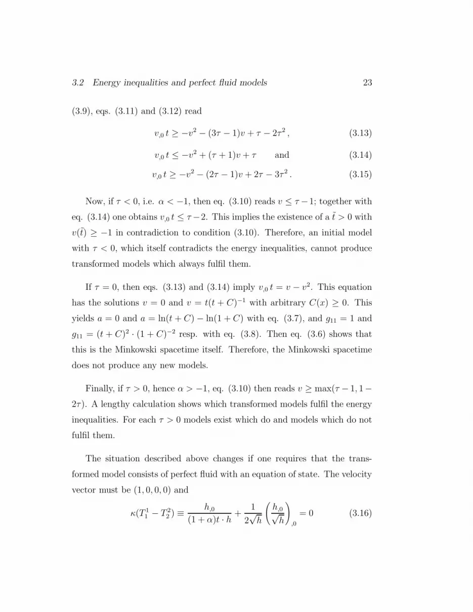
3.2 Energy inequalities and perfect fluid models 23
(3.9), eqs. (3.11) and (3.12) read
v,0 t ≥ −v2 − (3τ − 1)v + τ − 2τ 2 , (3.13)
v,0 t ≤ −v2 + (τ + 1)v + τ and (3.14)
v,0 t ≥ −v2 − (2τ − 1)v + 2τ − 3τ 2 . (3.15)
Now, if τ < 0, i.e. α < −1, then eq. (3.10) reads v ≤ τ −1; together with
eq. (3.14) one obtains v,0 t ≤ τ−2. This implies the existence of a t > 0 with
v(t) ≥ −1 in contradiction to condition (3.10). Therefore, an initial model
with τ < 0, which itself contradicts the energy inequalities, cannot produce
transformed models which always fulfil them.
If τ = 0, then eqs. (3.13) and (3.14) imply v,0 t = v − v2. This equation
has the solutions v = 0 and v = t(t + C)−1 with arbitrary C(x) ≥ 0. This
yields a = 0 and a = ln(t + C) − ln(1 + C) with eq. (3.7), and g11 = 1 and
g11 = (t + C)2 · (1 + C)−2 resp. with eq. (3.8). Then eq. (3.6) shows that
this is the Minkowski spacetime itself. Therefore, the Minkowski spacetime
does not produce any new models.
Finally, if τ > 0, hence α > −1, eq. (3.10) then reads v ≥ max(τ − 1, 1−2τ). A lengthy calculation shows which transformed models fulfil the energy
inequalities. For each τ > 0 models exist which do and models which do not
fulfil them.
The situation described above changes if one requires that the trans-
formed model consists of perfect fluid with an equation of state. The velocity
vector must be (1, 0, 0, 0) and
κ(T 11 − T 2
2 ) ≡ h,0(1 + α)t · h +
1
2√h
(
h,0√h
)
,0
= 0 (3.16)

24 3 INHOMOGENEOUS MODELS WITH FLAT SLICES
must be fulfilled. Eq. (3.16) expresses the condition that the pressure has to
be isotropic. T 22 = T 3
3 is fulfilled anyhow due to our assumption eq. (3.3).
If f = h,0h−1/2, then eq. (3.16) reads
f
(1 + α)t+f,02
= 0 ,
hence f,0f−1 does not depend on x, therefore f,01 · f = f,0 · f,1, and we can
use the ansatz f = a(t) · b(x). Inserting this into eq. (3.16), one obtains
h =[
b(x) · t(α−1)(α+1) + c(x)]2, where c(x) =
√
h(x, 0) (3.17)
with arbitrary non-negative functions b and c fulfilling b(x)+ c(x) > 0 for all
x. For energy density and pressure we then obtain
κµ =4
3(1 + α)2t2− 4(1 − α) · b
3(1 + α)2t(bt+ ct2/(1+α)),
κp =4α
3(1 + α)2t2. (3.18)
An equation of state means that p uniquely depends on µ. This takes
place if and only if α = 0 or b/c = const. The latter is equivalent to the
hypersurface-homogeneity of the model and is of lower interest here. For
α = 0 the initial model is the dust-filled Einstein-De Sitter model [68].
With eq. (3.18) we obtain p = 0 and µ ≥ 0 and may formulate: If the
Einstein-De Sitter universe is x-transformed into a perfect fluid model, then
this model also contains dust and fulfils the energy conditions.
These models have the following form: inserting eq. (3.17) with α = 0
into eq. (3.6) we get a dust-filled model
ds2 = −dt2 + t4/3 [ b(x)/t+ c(x) ]2 dx2 + dy2 + dz2 (3.19)
3.2 Energy inequalities and perfect fluid models 25
with arbitrary b, c as before. A subcase of eq. (3.19) is contained in Szekeres
[251] as case (iii), but the parameter ε used there may now be non-constant.
For b = 1, eq. (3.19) reduces to eq. (2.9). Of course, locally one can achieve
a constant b by a transformation x = x(x), but, e.g. changes in the sign of b
then are not covered. As an illustration we give two examples of this model
eq. (3.19):
1. If b = 1, c > 0, then
κµ =4c
3t(1 + ct), (3.20)
hence the density contrast at two different values x1, x2 reads
µ1
µ2
=c2c1
· 1 + c1t
1 + c2t(3.21)
and tends to 1 as t→ ∞. This shows that one needs additional presumptions
if one wants to prove an amplification of initial density fluctuations.
2. If b = 1, c = 0, then eq. (3.19) is the axially symmetric Kasner vacuum
solution. If now c differs from zero in the neighbourhoods of two values x1,
x2, then the model is built up from two thin dust slices and Kasner-like
vacuum outside them. The invariant distance of the slices is
At−1/3 +Bt2/3 (3.22)
with certain positive constants A and B. In [225] it is argued that the in-
variant distance along spacelike geodesics need not coincide with what we
measure as spatial distance. The distinction comes from the fact, that a
geodesic within a prescribed spacelike hypersurface need not coincide with
a spacelike geodesic in spacetime. This eq. (3.22) looks like gravitational
repulsion, because the distance has a minimum at a positive value. But the

26 3 INHOMOGENEOUS MODELS WITH FLAT SLICES
t−1/3-term is due to the participation of the slices in cosmological expansion
and the remaining t2/3-term is due to an attractive gravitational force in
parabolic motion. A more detailed discussion of this behaviour eq. (3.22) is
given in Griffiths [99]: he argues, “however inhomogeneous the mass distri-
bution, matter on each plane of symmetry has no net attraction to matter
on other planes.”
The transformation of a hypersurface-homogeneous cosmological model
considered here preserves all inner properties, expressed by the first funda-
mental form, of the slices t = const., and also preserves the property that t
is a synchronized time, but may change all other outer properties, which are
expressed by the second fundamental form. The investigations of section 3.2
show that energy conditions are preserved under very special presumptions
only.
One may consider these transformations as a guide in the search for new
exact solutions of Einstein’s field equation. The new models are close to the
initial hypersurface-homogeneous ones, if the transformation is close to the
identical one. Thus, one can perturb a Bianchi model with exact solutions
without use of any approximations.
3.3 A simple singularity theorem
What do we exactly know about solutions when no exact solution, in the sense
of “solution in closed form”, is available? In which sense these solutions have
a singularity? Here we make some remarks to these questions, see [228].
In [221], the following simple type of singularity theorems was discussed:
The coordinates t, x, y, z shall cover all the reals, and a(t) shall be an

3.3 A simple singularity theorem 27
arbitrary strictly positive monotonously increasing smooth function defined
for all real values t, where “smooth” denotes “C∞-differentiable”. Then it
holds:
The Riemannian space defined by
ds2 = dt2 + a2(t)(dx2 + dy2 + dz2) (3.23)
is geodesically complete. This fact is well-known and easy to prove; however,
on the other hand, for the same class of functions a(t) it holds:
The spacetime defined by
ds2 = dt2 − a2(t)(dx2 + dy2 + dz2) (3.24)
is lightlike geodesically complete if and only if
∫ 0
−∞a(t) dt = ∞ (3.25)
is fulfilled. The proof is straightforwardly done by considering lightlike
geodesics in the x − t−plane. So, one directly concludes that the state-
ments do not depend on the number n of spatial dimensions, only n > 0 is
used, and the formulation for n = 3 was chosen as the most interesting case.
Moreover, this statement remains valid if we replace “lightlike geodesically
complete” by “lightlike and timelike geodesically complete”.
Further recent results on singularity theorems are reviewed in Senovilla
[233]. This review and most of the research concentrated mainly on the 4–
dimensional Einstein theory. Probably, the majority of arguments can be
taken over to the higher–dimensional Einstein equation without change, but
this has not yet worked out up to now. And singularity theorems for F (R)-
gravity are known up to now only for very special cases only.

28 3 INHOMOGENEOUS MODELS WITH FLAT SLICES
The most frequently used F (R)-Lagrangian is
L =
(
R
2− l2
12R2
) √−g where l > 0 , (3.26)
here we discuss the non–tachyonic case only. From this Lagrangian one gets
a fourth-order field equation; only very few closed-form solutions, “exact
solutions”, are known. However, for the class of spatially flat Friedmann
models, the set of solutions is qualitatively completely described, but not in
closed form, in [163]. We call them “rigorous solutions”.
One of them, often called “Starobinsky inflation”, can be approximated
with
a(t) = exp(− t2
12l2) (3.27)
This approximation is valid in the region t ≪ −l. However, this solution
does not fulfil the above integral condition. Therefore, Starobinsky inflation
does not represent a lightlike geodesically complete cosmological model as
has been frequently stated in the literature.
To prevent a further misinterpretation let me reformulate this result as
follows: Inspite of the fact that the Starobinsky model is regular, in the
sense that a(t) > 0 for arbitrary values of synchronized time t, every past–
directed lightlike geodesic terminates in a curvature singularity, i.e., |R| −→∞, at a finite value of its affine parameter. Therefore, the model is not only
geodesically incomplete in the coordinates chosen, moreover, it also fails to
be a subspace of a complete one.
In contrast to this one can say: the spatially flat Friedmann model with
a(t) = exp(Ht), H being a positive constant, is the inflationary de Sitter
spacetime. According to the above integral condition, it is also incomplete.

3.3 A simple singularity theorem 29
However, contrary to the Starobinsky model, it is a subspace of a complete
spacetime, namely of the the de Sitter spacetime represented as a closed
Friedmann model.
The application of conformal transformations represents one of the most
powerful methods to transform different theories into each other. In many
cases this related theories to each other which have been originally considered
to be independent ones. The most often discussed question in this context is
“which of these metrics is the physical one”, but one can, of course, use such
conformal relations also as a simple mathematical tool to find exact solutions
without the necessity of answering this question. However, concerning a con-
formal transformation of singularity theorems one must be cautious, because
typically, near a singularity in one of the theories, the conformal factor di-
verges, and then the conformally transformed metric need not be singular
there.
Finally, let me again mention the distinct properties of the Euclidean and
the Lorentzian signature: Smooth connected complete Riemannian spaces are
geodesically connected. However, smooth connected complete spacetimes,
e.g. the de Sitter space–time, need not be geodesically connected, see for
instance Sanchez [196]. The topological origin of this distinction is the same
as the distinction between the two above statements: for the positive definite
signature case one uses the compactness of the rotation group, whereas in the
indefinite case the noncompactness of the Lorentz group has to be observed
[227].

31
4 Properties of curvature invariants
In section 4.1, which is an extended version of [223] we answer the follow-
ing question: Let λ, µ, ν be arbitrary real numbers. Does there exist a
3-dimensional homogeneous Riemannian manifold whose eigenvalues of the
Ricci tensor are just λ, µ and ν?
In section 4.2 we discuss, following [224], why all the curvature invariants
of a gravitational wave vanish.
In section 4.3 we present the example [222] that it may be possible that
non–isometric spacetimes with non–vanishing curvature scalar cannot be dis-
tinguished by curvature invariants.
4.1 The space of 3–dimensional homogeneous Rieman-
nian manifolds
The curvature of a 3–manifold is completely determined by the Ricci tensor,
and the Ricci tensor of a homogeneous manifold has constant eigenvalues.
However, it is essential to observe, that, nevertheless, the constancy of all
three eigenvalues of the Ricci tensor of a 3-manifold does not imply the
manifold to be locally homogeneous, see [132] for examples.
Assume λ, µ, ν to be arbitrary real numbers. First question: Does there
exist a 3-dimensional homogeneous Riemannian manifold whose eigenvalues
of the Ricci tensor are just λ, µ and ν? Second question: If it exists, is
it uniquely determined, at least locally up to isometries? The answer to
these questions does not alter if we replace “homogeneous” by “locally ho-
mogeneous”. In principle, they could have been answered by the year 1905

32 4 PROPERTIES OF CURVATURE INVARIANTS
already. But in fact, it was not given until 1995: the first of these problems
have been solved independently by Kowalski and Nikcevic [133] on the one
hand, and by Rainer and Schmidt [189], on the other hand; the second one
is solved several times, e.g. in [189]. Curiously enough, the expected answer
“Yes” turns out to be wrong.
Of course, both answers [133] and [189] are equivalent. But the formu-
lations are so different, that it is useful to compare them here. In [133] one
defines
ρ1 = maxλ, µ, ν , ρ3 = minλ, µ, ν (4.1)
and
ρ2 = λ+ µ+ ν − ρ1 − ρ3 (4.2)
and formulates the conditions as inequalities between the ρi.
In [189] the formulation uses curvature invariants. First step: one ob-
serves that the answer does not alter, if one multiplies λ, µ, ν with the same
positive constant. Note: this fails to be the case if we take a negative con-
stant. Second step: we take curvature invariants which do not alter by this
multiplication, i.e. we look for suitable homothetic invariants. Third step:
we formulate the answer by use of the homothetic invariants.
First step: this can be achieved by a homothetic transformation of the
metric, i.e., by a conformal transformation with constant conformal factor.
Then one excludes the trivial case λ = µ = ν = 0. Note: It is due to the
positive definiteness of the metric that λ = µ = ν = 0 implies the flatness of
the space.
Second step:
R = λ+ µ+ ν , N = λ2 + µ2 + ν2 (4.3)

4.1 The space of 3–dimensional Riemannian manifolds 33
are two curvature invariants with N > 0, and
R = R/√N (4.4)
is a homothetic invariant. For defining a second homothetic invariant we
introduce the trace-free part of the Ricci tensor
Sij = Rij −R
3gij (4.5)
and its invariant
S = Sji Skj S
ik . (4.6)
The desired second homothetic invariant reads
S = S/√N3 . (4.7)
Of course, one can also directly define R and S as functions of λ, µ and ν,
then S is the cubic polynomial,
S =(
(2λ− µ− ν)3 + (2µ− ν − λ)3 + (2ν − λ− ν)3)
/27 , (4.8)
see [189] for details. Remark: the inequalities S > 0 and ρ2 < (ρ1 + ρ3)/2
are equivalent.
Third step: The answer is “yes” if and only if one of the following condi-
tions (4.9) till (4.14) are fulfilled:
N = 0 , flat space (4.9)
R2 = 3 and S = 0 , non-flat spaces of constant curvature (4.10)
R2 = 2 and 9RS = −1 , real line times constant curvature space (4.11)
R2 = 1 and 9RS = 2 (4.12)
18S > R(9 − 5R2) , equivalent to λµν > 0 (4.13)
−√
3 < R < −√
2 and 0 < S ≤(
3 − R2)2 6 − 5R2
18R3. (4.14)
34 4 PROPERTIES OF CURVATURE INVARIANTS
Remarks: 1. In [133] the last of the four inequalities (4.14) is more elegantly
written as
ρ2 ≥ρ2
1 + ρ23
ρ1 + ρ3
. (4.15)
2. There exists a one–parameter set of Bianchi-type VI manifolds, with
parameter a where 0 < a < 1, having ρ1 = −a−a2, ρ2 = −1−a2, ρ3 = −1−a;they represent the case where in (4.14) the fourth inequality is fulfilled with
“=”.
Now we turn to the second question: Let the 3 numbers λ, µ, ν be given
such that a homogeneous 3-space exists having these 3 numbers as its eigen-
values of the Ricci tensor; is this 3-space locally uniquely determined? The
first part of the answer is trivial:
If λ = µ = ν, then “yes”, it is the space of constant curvature. The second
part of the answer is only slightly more involved: If λ, µ and ν represent 3
different numbers, then the 3 eigendirections of the Ricci tensor are uniquely
determined, and then we can also prove: “yes”. The third part is really
surprising: If
R = 1 and S =2
9(4.16)
then the answer is “no”, otherwise “yes”.
Clearly, eq. (4.16) represents a subcase of (4.12). What is the peculiarity
with the values (4.16) of the homothetic invariants? They belong to Bianchi
type IX, have one single and one double eigenvalue, and with these values,
a one-parameter set of examples with 3-dimensional isometry group, and
another example with a 4-dimensional isometry group exist.

4.2 Why do all the invariants of a gravitational wave vanish? 35
4.2 Why do all the curvature invariants of a gravita-
tional wave vanish?
We prove the theorem valid for Pseudo-Riemannian manifolds Vn: “Let x ∈Vn be a fixed point of a homothetic motion which is not an isometry then
all curvature invariants vanish at x.” and get the Corollary: “All curvature
invariants of the plane wave metric
ds2 = 2 du dv + a2(u) dw2 + b2(u) dz2 (4.17)
identically vanish.”
Analysing the proof we see: The fact that for definite signature flatness
can be characterized by the vanishing of a curvature invariant, essentially
rests on the compactness of the rotation group SO(n). For Lorentz signature,
however, one has the non-compact Lorentz group SO(3, 1) instead of it.
A further and independent proof of the corollary uses the fact, that the
Geroch limit does not lead to a Hausdorff topology, so a sequence of gravita-
tional waves can converge to the flat spacetime, even if each element of the
sequence is the same pp-wave.
The energy of the gravitational field, especially of gravitational waves,
within General Relativity was subject of controversies from the very be-
ginning, see Einstein [66]. Global considerations - e.g. by considering the
far-field of asymptotically flat spacetimes - soon led to satisfactory answers.
Local considerations became fruitful if a system of reference is prescribed e.g.
by choosing a timelike vector field. If, however, no system of reference is pre-
ferred then it is not a priori clear whether one can constructively distinguish

36 4 PROPERTIES OF CURVATURE INVARIANTS
flat spacetime from a gravitational wave. This is connected with the gener-
ally known fact, that for a pp-wave, see e.g. Stephani [250] especially section
15.3. and [65] all curvature invariants vanish, cf. Hawking and Ellis [107]
and Jordan et al. [123], but on the other hand: in the absence of matter or
reference systems - only curvature invariants are locally constructively mea-
surable. See also the sentence “R. Penrose has pointed out, in plane-wave
solutions the scalar polynomials are all zero but the Riemann tensor does not
vanish.” taken from page 260 of [107]. At page 97 of [123] it is mentioned
that for a pp-wave all curvature invariants constructed from
Rijkl;i1...ir (4.18)
by products and traces do vanish.
It is the aim of this section to explain the topological origin of this strange
property.
4.2.1 Preliminaries
Let Vn be a C∞-Pseudo-Riemannian manifold of arbitrary signature with
dimension n > 1. The metric and the Riemann tensor have components gij
and Rijlm resp. The covariant derivative with respect to the coordinate xm
is denoted by “;m” and is performed with the Christoffel affinity Γilm. We
define
I is called a generalized curvature invariant of order k if it is a scalar with
dependence
I = I(gij, Rijlm, . . . , Rijlm;i1... ik) . (4.19)

4.2 Why do all the invariants of a gravitational wave vanish? 37
By specialization we get the usual Definition: I is called a curvature invariant
of order k if it is a generalized curvature invariant of order k which depends
continuously on all its arguments. The domain of dependence is requested
to contain the flat space, and
I(gij, 0, . . . 0) ≡ 0 . (4.20)
Examples: Let
I0 = sign(n∑
i,j,l,m=1
|Rijlm|) , (4.21)
where the sign function is defined by sign(0) = 0 and sign(x) = 1 for x > 0.
Then I0 is a generalized curvature invariant of order 0, but it fails to be a
curvature invariant. It holds: Vn is flat if and only if I0 ≡ 0. Let further
I1 = RijlmRijlm (4.22)
which is a curvature invariant of order 0. If the metric has definite signature
or if n = 2 then it holds: Vn is flat if and only if I1 ≡ 0. Proof: For definite
signature I0 = sign(I1); for n = 2, I1 ≡ 0 implies R ≡ 0, hence flatness.
q.e.d.
For all other cases, however, the vanishing of I1 does not imply flatness.
Moreover, there does not exist another curvature invariant serving for this
purpose, it holds:
For dimension n ≥ 3, arbitrary order k and indefinite metric it holds: To
each curvature invariant I of order k there exists a non-flat Vn with I ≡ 0.
Proof: Let n = 3. We use
ds2 = 2 du dv ± a2(u) dw2 (4.23)

38 4 PROPERTIES OF CURVATURE INVARIANTS
with a positive non-linear function a(u). The “±” covers the two possible
indefinite signatures for n = 3. The Ricci tensor is Rij = Rmimj and has
with u = x1
R11 = − 1
a· d
2a
du2(4.24)
and therefore, eq. (4.23) represents a non-flat metric. Now let n > 3. We use
the Cartesian product of eq. (4.23) with a flat space of dimension n− 3 and
arbitrary signature. So we have for each n ≥ 3 and each indefinite signature
an example of a non-flat Vn. It remains to show that for all these examples,
all curvature invariants of order k vanish. It suffices to prove that at the
origin of the coordinate system, because at all other points it can be shown
by translations of all coordinates accompanied by a redefinition of a(u) to
a(u − u0). Let I be a curvature invariant of order k. Independent of the
dimension, i.e., how many flat spaces are multiplied to metric eq. (4.23), one
gets for the case considered here that
I = I(a(0)(u), a(1)(u), . . . , a(k+2)(u)) (4.25)
where a(0)(u) = a(u), a(m+1)(u) = ddua(m)(u), and
I(a(0)(u), 0, . . . , 0) = 0 . (4.26)
This is valid because each
Rijlm;i1... ip (4.27)
continuously depends on a(0)(u), a(1)(u), . . . , a(p+2)(u) and on nothing else;
and for a = const., metric (4.23) represents a flat space.
Now we apply a coordinate transformation: Let ε > 0 be fixed, we replace
u by u · ε and v by v/ε. This represents a Lorentz boost in the u− v−plane.

4.2 Why do all the invariants of a gravitational wave vanish? 39
Metric eq. (4.23) remains form-invariant by this rotation, only a(u) has to
be replaced by a(u · ε). At u = 0 we have
I = I(a(0)(0), a(1)(0), . . . , a(k+2)(0)) (4.28)
which must be equal to
Iε = I(a(0)(0), ε · a(1)(0), . . . , εk+2 · a(k+2)(0)) (4.29)
because I is a scalar. By continuity and by the fact that flat space belongs
to the domain of dependence of I, we have
limε→0
Iε = 0 . (4.30)
All values Iε with ε > 0 coincide, and so I = 0. q.e.d.
4.2.2 Gravitational waves
New results on gravitational waves can be found in [72], and [84]. A pp-
wave is a plane-fronted gravitational wave with parallel rays, see [77]. It is
a non-flat solution of Einstein’s vacuum equation Rij = 0 possessing a non-
vanishing covariantly constant vector; this vector is then automatically a null
vector. The simplest type of pp-waves can be represented similar as metric
eq. (4.23)
ds2 = 2 du dv + a2(u) dw2 + b2(u) dz2 , (4.31)
where
b · d2a
du2+ a · d
2b
du2= 0 . (4.32)
This metric represents flat spacetime if and only if both a and b are linear
functions. Using the arguments of subsection 4.2.1 one sees that all curvature
invariants this metric identically vanish. Here we present a second proof of

40 4 PROPERTIES OF CURVATURE INVARIANTS
that statement which has the advantage to put the problem into a more
general framework and to increase the class of spacetimes covered, e.g. to
the waves
ds2 = dx2 + dy2 + 2du dv +H(x, y, u)du2 (4.33)
Hall [102] considers fixed points of homothetic motions, which cannot exist
in compact spacetimes, and shows that any plane wave, not only vacuum
plane waves, admits, for each x, a homothetic vector field which vanishes at
x. It holds
Let x ∈ Vn be a fixed point of a homothetic motion which is not an
isometry then all curvature invariants vanish at x.
Proof: The existence of a homethetic motion which is not an isometry
means that Vn is selfsimilar. Let the underlying differentiable manifold be
equipped with two metrics gij and
gij = e2Cgij (4.34)
where C is a non-vanishing constant. The corresponding Riemannian mani-
folds are denoted by Vn and Vn resp. By assumption, there exists an isometry
from Vn to Vn leaving x fixed. Let I be a curvature invariant. I can be rep-
resented as continuous function which vanishes if all the arguments do of
finitely many of the elementary invariants. The elementary invariants are
such products of factors gij with factors of type
Rijlm;i1... ip (4.35)
which lead to a scalar, i.e., all indices are traced out. Let J be such an
elementary invariant. By construction we have J(x) = eqCJ(x) with a non-
vanishing natural q, which depends on the type of J . Therefore, J(x) = 0.
q.e.d.

4.2 Why do all the invariants of a gravitational wave vanish? 41
From this it follows: All curvature invariants of metric (4.17) identically
vanish. This statement refers not only to the 14 independent elementary
invariants of order 0, see Harvey [104] and Lake 1993 [140] for a list of them,
but for arbitrary order.
Proof: We have to show that for each point x, there exists a homothetic
motion with fixed point x which is not an isometry. But this is trivially done
by suitable linear coordinate transformations of v, w, and z. q.e.d.
4.2.3 Topological properties
Sometimes it is discussed that the properties of spacetime which can be lo-
cally and constructively, i.e., by rods and clocks, measured are not only the
curvature invariants but primarily the projections of the curvature tensor
and its covariant derivatives to an orthonormal tetrad, called 4-bein.6 The
continuity presumption expresses the fact that a small deformation of space-
time should also lead to a correspondingly small change of the result of the
measurement. To prevent a preferred system of reference one can construct
curvature invariants like
I2 = inf∑
i,j,l,m
|Rijlm| (4.36)
where the infimum, here the same as the minimum, is taken over all orthonor-
mal tetrads. From the first glance one could believe that I2 ≡ 0 if and only
if the space is flat. But for indefinite signature this would contradict the
result of subsection 4.2.1. What is the reason? For definite signature the
infimum is to be taken about the rotation group SO(4), or O(4) if one allows
6The German word “das Bein” denotes both “bone” and “leg”, here it is used in the
second sense.

42 4 PROPERTIES OF CURVATURE INVARIANTS
orientation-reversing systems; this group is compact. One knows: A positive
continuous function over a compactum possesses a positive infimum. So, if
one of the Rijlm differs from zero, then I2 > 0 at that point. For Lorentz sig-
nature, however, the infimum is to be taken about the non-compact Lorentz
group SO(3, 1) and so Rijlm 6= 0 does not imply I2 6= 0.
Another topological argument, which underlies our subsection 4.2.1, is
connected with the Geroch limit of spacetimes [86], we use the version of
[210]. Theorem 3.1 of reference [210] reads:
1: For local Riemannian manifolds with definite signature, Geroch’s limit
defines a Hausdorff topology.
2: For indefinite signature this topology is not even T1.
Explanation: A topology is Hausdorff if each generalized Moore - Smith
sequence possesses at most one limit, and it is T1 if each constant sequence
possesses at most one limit. The main example is a sequence, where each
element of the sequence is the same pp-wave, and the sequence possesses two
limits: flat spacetime and that pp-wave. Here the reason is: Only for definite
signature, geodetic ε-balls form a neighbourhood basis for the topology.
Final remarks: The change from Euclidean to Lorentzian signature of a
Pseudo-Riemannian space is much more than a purely algebraic duality - an
impression which is sometimes given by writing an imaginary time coordi-
nate: One looses all the nice properties which follow from the compactness of
the rotation group. Lake 1993 [140] pointed out that also for the Robinson-
Trautman vacuum solutions of Petrov type III all 14 curvature invariants
vanish.

4.3 Spacetimes which cannot be distinguished by invariants 43
4.3 On spacetimes which cannot be distinguished by
curvature invariants
For a positive C∞–function a(u) let
ds2 =1
z2
[
2 du dv − a2(u) dy2 − dz2]
. (4.37)
In the region z > 0, ds2 represents the anti-de Sitter spacetime if and only if
a(u) is linear in u. Now, let d2a/du2 < 0 and
φ :=1√κ
∫
(
−1
a
d2a
du2
)1/2
du . (4.38)
Then
2φ = φ,i φ,i = 0 (4.39)
and
Rij − R
2gij = Λ gij + κTij (4.40)
with Λ = −3 and Tij = φ,i φ,j. So (ds2, φ) represents a solution of Einstein’s
equation with negative cosmological constant Λ and a minimally coupled
massless scalar field φ.
Let I be a curvature invariant of order k, i.e., I is a scalar
I = I (gij , Rijlm, . . . , Rijlm;i1... ik) (4.41)
depending continuously on all its arguments. Then for the metric ds2, I does
not depend on the function a(u).
This seems to be the first example that non–isometric spacetimes with
non–vanishing curvature scalar cannot be distinguished by curvature invari-
ants. The proof essentially uses the non–compactness of the Lorentz group

44 4 PROPERTIES OF CURVATURE INVARIANTS
SO(3, 1), here of the boosts u → u λ, v → v/λ. One can see this also in the
representation theory in comparison with the representations of the compact
rotation group SO(4).
Let v ∈ R4 be a vector and g ∈ SO(4) such that g(v) ↑↑ v, then g(v) = v.
In Minkowski spacetime M4, however, there exist vectors v ∈M4 and a h ∈SO(3, 1) with h(v) ↑↑ v and h(v) 6= v. This is the reason why the null frame
components of the curvature tensor called Cartan “scalars” are not always
curvature scalars, see [224]. Further new results on curvature invariants are
given in [28], [184] and [188]. Limits of spacetimes are considered in [176]
and [230].
45
5 Surface layers and relativistic surface ten-
sions
For a thin shell, the intrinsic 3-pressure will be shown to be analogous to
−A, where A is the classical surface tension: First, interior and exterior
Schwarzschild solutions will be matched together such that the surface layer
generated at the common boundary has no gravitational mass; then its intrin-
sic 3-pressure represents a surface tension fulfilling Kelvin’s relation between
mean curvature and pressure difference in the Newtonian limit. Second, after
a suitable definition of mean curvature, the general relativistic analogue to
Kelvin’s relation will be proven to be contained in the equation of motion of
the surface layer.
5.1 Introduction to surface layers
In general relativity, an energy-momentum tensor concentrated on a timelike
hypersurface is called a surface layer. Via Einstein’s equations it is related
to non-spurious jumps of the Christoffel affinities or equivalently to jumps
of the second fundamental tensor. In [141], [178], [60], [117], [177] and [138]
there have been given algorithms for their calculating, and in [141], [117],
and [38], [63], [202], [260], [79] and [140] the spherically symmetric case was
of a special interest. The discussion of disklike layers as models for accretion
disks was initiated in [160] and [264], and [143] contains surface layers as
sources of the Kerr geometry.
A surface layer has no component in the normal direction, otherwise the
delta-like character would be destroyed. Hence, an ideal fluid with non-
vanishing pressure cannot be concentrated on an arbitrarily thin region and

46 5 SURFACE LAYERS AND RELATIVISTIC SURFACE TENSIONS
therefore in most cases, the layer is considered to be composed of dust. Ad-
ditionally, an intrinsic 3-pressure is taken into account in [67], where for a
spherically symmetric configuration each shell r = const. is thought to be
composed of identical particles moving on circular orbits without a preferred
direction, and the tangential pressure, which is analogous to the intrinsic
3-pressure, is due to particle collisions, whereas a radial pressure does not
appear. See also [202], [140], and [151], where the equation of motion for a
spherically symmetric layer has been discussed.
Such an intrinsic 3-pressure as well as surface tensions are both of the
physical dimension “force per unit length.” There the question arises whether
an intrinsic 3-pressure of a surface layer may be related to a surface tension,
and this chapter will deal with just this question. Then a general relativistic
formulation of thermodynamics can be completed by equations for surface
tensions to answer, e.g., the question how long a drop, say, a liquid comet,
remains connected while falling towards a compact object. The only paper
concerned with such questions seems to be [135]. There the influence of
surface tensions on the propagation of gravitational waves has been calculated
by perturbation methods, yielding a possibly measurable effect. For the
background knowledge cf. [118] or [170] for relativistic thermodynamics and
[174] for non-relativistic surface tensions.
This chapter, which is based on [203], proceeds as follows: Section 5.2
contains Kelvin’s relation for non-relativistic surface tensions and discusses
the matching of the interior to the exterior Schwarzschild solution such that
a surface tension appears, and compares with Kelvin’s relation in the New-
tonian limit, calculations are found in the appendices, sections 5.5, 5.5 and
5.5. Sections 5.3 and 5.4 are devoted to the non-spherically symmetric case.

5.2 Non-relativistic surface tensions 47
Section 5.3 contains a suitable definition of mean curvature and section 5.4
deduces Kelvin’s relation from the equation of motion of the surface layer
without any weak field assumptions.
5.2 Non-relativistic surface tensions
Imagine a drop of some liquid moving in vacuo. Its equilibrium configuration
is a spherical one, and Kelvin’s relation [255] between surface tension A,
pressure difference ∆P , i.e. outer minus inner pressure, and mean curvature
H , where H = 1/R for a sphere of radius R, reads
∆P = −2HA . (5.1)
A is a material-dependent constant. Equation (5.1) means, an energy A ·∆Fis needed to increase the surface area by ∆F . This supports our description
of −A as a kind of intrinsic pressure. But of course, it is a quite different
physical process: Pressure, say, of an ideal gas, can be explained by collisions
of freely moving particles, whereas the microphysical explanation of surface
tensions requires the determination of the intermolecular potential, which
looks like
Φ(r) = −µr−6 +Ne−r/ρ (5.2)
with certain constants µ, N , and ρ; see Ono [174]. In this context the surface
has a thickness of about 10−7 cm but in most cases this thickness may be
neglected.
In addition, for a non-spherically symmetric surface, the mean curvature
H in equation eq. (5.1) may be obtained from the principal curvature radii
R1, R2 by means of the relation
H =1
2R1+
1
2R2. (5.3)

48 5 SURFACE LAYERS AND RELATIVISTIC SURFACE TENSIONS
Now the drop shall be composed of an incompressible liquid. For a general
relativistic description we have to take the interior Schwarzschild solution
ds2 = −[
3
2(1 − rg/r0)
1/2 − 1
2(1 − rgr
2/r30)
1/2]2
dt2
+dr2
1 − rgr2/r30
+ r2dΩ2 where dΩ2 = dψ2 + sin2 ψdϕ2 , (5.4)
whose energy-momentum tensor represents ideal fluid with energy density
µ = 3rg/κr30 and pressure
p(r) = µ · (1 − rgr2/r3
0)1/2 − (1 − rg/r0)
1/2
3(1 − rg/r0)1/2 − (1 − rgr2/r30)
1/2. (5.5)
One has p(r0) = 0, and therefore usually 0 ≤ r ≤ r0 is considered. But now
we require only a non-vanishing pressure at the inner surface and take eq.
(5.4) for values r with 0 ≤ r ≤ R and a fixed R < r0 only.
The gravitational mass of the inner region equals
M = µ · 4πR3/3 = rg(R/r0)3/2 (5.6)
where we assumed unit such that G = c = 1. The outer region shall be
empty and therefore we have to insert the Schwarzschild solution for r ≥ R.
Neglecting the gravitational mass of the boundary Σ ⊂ V4 which is defined
by r−R = 0, just M of equation (5.6) has to be used as the mass parameter
of the exterior Schwarzschild metric. Then only delta-like tensions appear
at Σ, and ∆P = −p(R) < 0. The vanishing of the gravitational mass is
required to single out the properties of an intrinsic 3-pressure. In general, a
surface layer is composed of both parts, not at least to ensure the validity of
the energy condition T00 ≥ |Tik| which holds for all known types of matter.
On Σ, the energy-momentum tensor is
T ki = τki · δΣ (5.7)

5.3 Mean curvature in curved spacetime 49
the non-vanishing components of which are
τ 22 = τ 3
3 = −p(R)R/2(1 − 2M/R)1/2 (5.8)
cf. section 5.5.
The δΣ distribution is defined such that for all smooth scalar functions f
the invariant integrals are related by∫
Σf d(3)x =
∫
V4
f · δΣ d(4)x . (5.9)
For a more detailed discussion of distribution-valued tensors in curved space-
time, cf. [252]. The fact that all components τα0 in eq. (5.7) vanish reflects
the non-existence of a delta-like gravitational mass on Σ.
Now consider the Newtonian limit M/R ≪ 1; then the mean curvature
becomes again H = 1/R, and together with eq. (5.8) Kelvin’s relation eq.
(5.1) is just equivalent to
τ 22 = τ 3
3 = −A[1 +O(M/R)] . (5.10)
Therefore: At least for static spherically symmetric configurations and weak
fields a delta-like negative tangential pressure coincides with the classical
surface tension.
In the next two sections we investigate to what extent these presumptions
are necessary.
5.3 Mean curvature in curved spacetime
To obtain a general relativistic analogue to Kelvin’s relation eq. (5.1) we have
to define the mean curvature H of the timelike hypersurface Σ contained in
a spacetime V4 such that for weak fields just the usual mean curvature arises.

50 5 SURFACE LAYERS AND RELATIVISTIC SURFACE TENSIONS
To get the configuration we have in mind, we make the ansatz
ταβ = −A(gαβ + uαuβ) uαuα = −1 (5.11)
with A > 0. Thereby again the gravitational mass of Σ will be neglected.
Now the mean curvature shall be defined. But there is a problem: In general,
there does not exist a surface S ⊂ Σ which can serve as “boundary at a fixed
moment” for which we are to determine the mean curvature. To circumvent
this problem we start considering the special case
uα‖β = uβ‖α . (5.12)
Then there exists a scalar t on Σ such that uα = t‖α, and the surface S ⊂ Σ
defined by t = 0 may be called “boundary at a fixed moment.” Now S has to
be embedded into a “space at a fixed moment”: We take intervals of geodesics
starting from points of S in the normal direction ni and the opposite one.
The union V3 of these geodetic segments will be called “space at a fixed
moment,” and S ⊂ V3 is simply a two-surface in a three-dimensional positive
definite Riemannian manifold, for which mean curvature has a definite sense:
Let vα, wα be the principal curvature directions inside S and R1, R2 the
corresponding principal curvature radii, then equation (5.3) applies to obtain
H .
Of course, vαwα = 0 holds, and vαvα = wαwα = 1 shall be attained.
Then, inserting the second fundamental tensor cf. section 5.5, this becomes
equivalent to
H =1
2(vαvα + wαwα)kαβ =
1
2(gαβ + uαuβ)kαβ . (5.13)
But this latter relation makes sense without any reference to condition eq.
(5.12). Therefore, we define eq. (5.13) to be the general relativistic analogue

5.4 Equation of motion for the surface layer 51
to the mean curvature of a surface. For the case H+ 6= H− we take their
arithmetic mean
H = (H+ +H−)/2 , (5.14)
and then we obtain from eqs. (5.11) and (5.13)
−2HA =1
2
(
k+αβ + k−αβ
)
ταβ . (5.15)
This choice can be accepted noting that in the Newtonian limit
|H+ −H−| ≪ |H+ +H−| (5.16)
anyhow. To compare this with Kelvin’s relation we have to relate the right-
hand side of equation (5.15) to the pressure difference ∆P at Σ. To this end
we investigate the equation of motion for the surface layer.
5.4 Equation of motion for the surface layer
The equation of motion, T ki;k = 0, contains products of δ distributions and
θ-step functions, where θ(x) = 1 for x ≥ 0, and θ(x) = 0 else, at points where
Γijk has a jump discontinuity. These products require special care; cf. [53]
for a discussion of his point. But defining θ · δ = 12δ we obtain, cf. section
5.5
∆P ≡ ∆ninkT ik =
1
2
(
k+αβ + k−αβ
)
ταβ and (5.17)
∆T 1α ≡ ∆nie
kαT
ik = −τβα‖β . (5.18)
From equation (5.18) we see the following: The equation τβα‖β = 0 holds only
under the additional presumption that the regular, i.e., not delta-like, part
of T 1α has no jump on Σ.

52 5 SURFACE LAYERS AND RELATIVISTIC SURFACE TENSIONS
This condition is fulfilled e.g., presuming Σ to be such a boundary that
the regular energy flow does not cross it and the four-velocity is parallel to
Σ in both V+ and V−. This we will presume in the following. Then ∆P
is indeed the difference of the pressures on both sides, and together with
equations (5.15) and (5.17) we obtain exactly Kelvin’s relation eq. (5.1).
That means, it is the definition of mean curvature used here that enables us
to generalize Kelvin’s formula to general relativity. Furthermore, O(M/R)
of equation (5.10) vanishes.
Finally we want to discuss the equation τβα‖β = 0. Transvection with uα
and δαγ + uαuγ yields
uα‖α = 0 and uαuγ‖α + (lnA)‖α(δαγ + uαuγ) = 0 (5.19)
respectively. But A is a constant here, and therefore uα is an expansion-free
geodesic vector field in Σ. But observe that the uα lines are geodesics in V4
under additional presumptions only.
Here, we have only considered a phenomenological theory of surface ten-
sions, and, of course, a more detailed theory has to include intermolecular
forces. But on that phenomenological level equations (5.11) and (5.19) to-
gether with Kelvin’s relation eq. (5.1), which has been shown to follow from
the equation of motion, and A = const as a solely temperature-dependent
equation of state complete the usual general relativistic Cauchy problem for
a thermodynamical system by including surface tensions.
5.5 Notation, distributions and mean curvature
To make the equations better readable, some conventions and formulas shall
be given. Let ξα, α = 0, 2, 3, be coordinates in Σ and xi, i = 0, 1, 2, 3,

5.5 Notation, distributions and mean curvature 53
those for V4. The embedding Σ ⊂ V4 is performed by functions xi(ξα) whose
derivatives
eiα = ∂xi/∂ξα ≡ xi,α (5.20)
form a triad field in Σ. Σ divides, at least locally, V4 into two connected
components, V+ and V−, and the normal ni, defined by
nini = 1 , nie
iα = 0 (5.21)
is chosen into the V+ direction, which can be thought being the outer region.
Possibly V+ and V− are endowed with different coordinates xi+, xi− and met-
rics gik+ and gik−, respectively. For this case all subsequent formulas had to
be indexed with +/−, and only the inner metric of Σ, its first fundamental
tensor
gαβ = eiαekβ gik (5.22)
has to be the same in both cases. As usual, we require gik to be C2-
differentiable except for jumps of gij,k at Σ. Covariant derivatives within
V4 and Σ will be denoted by ; and ‖ respectively.
The second fundamental tensor k±αβ on both sides of Σ is defined by
k±αβ =(
eiαekβni;k
)±=(
eiα;kekβni
)±(5.23)
and the difference, ∆kαβ = k+αβ − k−αβ , ∆k = gαβ∆kαβ, enters the energy-
momentum tensor via equation (5.7) and the relation
τ ik ≡ eiαekβτ
αβ , where κταβ = gαβ∆k − ∆kαβ (5.24)
cf. e.g., [117]. From equation (5.21) and the Lanczos equation (5.24) one
obtains niτik = 0, i.e., indeed the absence of a delta-like energy flow in the
normal direction.

54 5 SURFACE LAYERS AND RELATIVISTIC SURFACE TENSIONS
Now take a special coordinate system: xα = ξα, and the x1 lines are
geodesics starting from Σ into ni direction with natural parameter x1. Then
the line element of V4 reads
ds2 = −(
dx1)2
+ gαβdxαdxβ (5.25)
and the only jumps of Γijk are
Γ±1αβ = −k±1
αβ = −1
2g±αβ,1 .
The most natural definition of θ · δ is 12δ being equivalent to the choice
Γijk =1
2
(
Γ+ijk + Γ−i
jk
)
on Σ . (5.26)
But cf. Dautcourt 1963 [60] for another choice of Γijk with the consequence
that T ki;k 6= 0 at Σ.
Now the δ part of the equation T k1;k = 0 reads
∆T 11 ≡ T 1
+1 − T 1−1 =
1
2
(
k+αβ + k−αβ
)
ταβ . (5.27)
Analogously one obtains for the other components
∆T 1α = −τβα‖β . (5.28)
Reintroducing the original coordinate system, the left-hand sides of equa-
tions (5.27) and (5.28) have to be replaced by ∆P1 = ∆ninkT ik and ∆Pα =
∆niekαT
ik, respectively; cf. [151]. Thereby, ∆Pi is the difference of the energy
flows on both sides of Σ.
To deduce equation eq. (5.8) we take proper time ξ0 and angular coordi-
nates ψ = ξ2 and ϕ = ξ3. Then, inside Σ,
ds2 = −(
dξ0)2
+R2dΩ2 . (5.29)

5.5 Notation, distributions and mean curvature 55
Using equation (5.23) and the exterior Schwarzschild solution one obtains
k+αβ the non-vanishing components of which are
k+00 = −M/R2(l − 2M/R)1/2 , k+
22 = R(1 − 2M/R)1/2 (5.30)
and
k+33 = k+
22 sin2 ψ (5.31)
because of spherical symmetry. To avoid long calculations with the metric
(5.4) one can proceed as follows. By construction, τ00 = 0, and together with
equation (5.24) and the spherical symmetry k−22 = k+22, k
−33 = k+
33 follows.
From equation (5.27), equation (5.8) follows then immediately without the
necessity of determining the actual value of k−00.
And to be independent of the discussions connected with equation (5.26),
we deduce equation (5.27) another way. First, independent of surface layers,
for an arbitrary timelike hypersurface and a coordinate system such that eq.
(5.25) holds, we have
κT11 =1
2
(
(3)R + k2 − kαβkαβ)
(5.32)
where (3)R is the curvature scalar within that surface. Now turn to a surface
layer with k+αβ 6= k−αβ. Then equation (5.32) splits into a “+” and a “−”
equation, having in common solely (3)R. Inserting all this into equation
(5.24), one obtains
1
2
(
k+αβ + k−αβ
)
ταβ =1
2κ
(
k+αβ + k−αβ
) (
gαβ∆k − ∆kαβ)
=1
2κ
[
(k+)2 − (k−)2 − k+αβk
+αβ + k−αβk−αβ
]
= T+11 − T−
11 (5.33)
i.e., just equation (5.27).

57
6 The massive scalar field in a closed Fried-
mann universe
For the minimally coupled scalar field in Einstein’s theory of gravitation we
look for the space of solutions within the class of closed Friedmann universe
models. We prove D ≥ 1, where D is the dimension of the set of solutions
which can be integrated up to t → ∞. D > 0 was conjectured by Page in
1984 [175]. We discuss concepts like “the probability of the appearance of a
sufficiently long inflationary phase” and argue that it is primarily a proba-
bility measure µ in the space V of solutions and not in the space of initial
conditions, which has to be applied. The measure µ is naturally defined for
Bianchi-type I cosmological models because V is a compact cube. The prob-
lems with the closed Friedmann model, which led to controversial claims in
the literature, will be shown to originate from the fact that V has a compli-
cated non-compact non-Hausdorff Geroch topology: no natural definition of
µ can be given. We conclude: the present state of our universe can be ex-
plained by models of the type discussed, but thereby the anthropic principle
cannot be fully circumvented. We consider a closed Friedmann cosmological
model,
ds2 = gijdxidxj = dt2 − a2(t)[dr2 + sin2 r(dψ2 + sin2 ψdχ2)] , (6.1)
with the cosmic scale factor a(t). We apply Einstein’s General Relativity
Theory and take a minimally coupled scalar field φ without self-interaction
as source, i.e., the Lagrangian is
L =R
16πG+
1
2gij∇iφ∇jφ− 1
2m2φ2 . (6.2)
In this chapter we assume units such that h = c = 1; R is the scalar curvature,
G Newton’s constant, and m the mass of the scalar field. The variational

58 6 THE MASSIVE SCALAR FIELD IN A FRIEDMANN UNIVERSE
derivative δL/δφ = 0 yields the field equation for the scalar field
(m2 + 2)φ = 0 , 2 ≡ gij∇i∇j (6.3)
where 2 denotes the covariant D’Alembertian. The variation of the La-
grangian with respect to the metric
δL√
−detgkl/δgij = 0 (6.4)
yields Einstein’s field equation
Rij −R
2gij = 8πGTij , Tij ≡ ∇iφ∇jφ− 1
2
(
∇kφ∇kφ−m2φ2)
gij , (6.5)
with Ricci tensor Rij . It is the aim of this chapter, which is based on [215],
to present some rigorous results about the space V of solutions of eqs. (6.3),
(6.5) with metric (6.1). This is done in sections 6.1, 6.2 and 6.3. We discuss
them in the context of cosmology in section 6.4: the probability of the ap-
pearance of a sufficiently long inflationary phase and the anthropic principle.
Schrodinger [234] already dealt with the massive scalar field in the closed
Friedmann universe in 1938, but there the back-reaction of the scalar field on
the evolution of the cosmic scale factor had been neglected. 35 years later the
model enjoyed a renewed interest, especially as a semi-classical description
of quantum effects, cf. e.g. Fulling and Parker [82], [83], Starobinsky [243],
Barrow and Matzner [14], Gottlober [92] and Hawking and Luttrell [108].
One intriguing property - the possibility of a bounce, i.e., a positive local
minimum of the cosmic scale factor - made it interesting in connection with
a possible avoidance of a big bang singularity a(t) → 0. The existence of
periodic solutions (φ(t), a(t)) of eqs. (6.1), (6.3) and (6.5) became clear in
1984 by independent work of Hawking [106] and Gottlober and Schmidt [96].

6.1 Some closed-form approximations 59
The existence of an inflationary phase, which is defined by
|dh/dt| ≪ h2 , where h = d(ln a)/dt (6.6)
is the Hubble parameter, in the cosmic evolution is discussed in many papers
to that model, cf e.g. Belinsky et al. [20], [21], Gottlober and Muller [93] and
Page 1987 [175]. Soon it became clear that the satisfactory results obtained
for the spatially flat model – the existence of a naturally defined measure in
the space of solutions and with this measure the very large probability to
have sufficient inflation – cannot be generalized to the closed model easily.
We shall turn to that point in section 6.4.
6.1 Some closed-form approximations
We consider the system (6.3), (6.5) with metric (6.1). Sometimes, one takes
it as an additional assumption that φ depends on the coordinate t only, but
it holds, cf. Turner [258]: the spatial homogeneity of metric (6.1) already
implies this property. Proof: For i 6= j we have Rij = gij = 0 and, therefore
we get ∇iφ∇jφ = 0. This means, locally φ depends on one coordinate xi
only. Supposed i 6= 0, then gijTij − 2T00 = m2φ2. The l.h.s. depends on
t only. For m 6= 0 this is already a contradiction. For m = 0 we have
Rij = ∇iφ∇jφ, which is a contradiction to the spatial isotropy of Rij , q.e.d.
We always require a(t) > 0, for otherwise the metric (6.1) is degenerated,
leading to a “big bang”. Inserting metric (6.1), eqs. (6.3), (6.5) reduce to
d2φ/dt2 + 3hdφ/dt+m2φ = 0 (6.7)
and
3(
h2 + a−2)
= 4πG [m2φ2 + (dφ/dt)2] . (6.8)

60 6 THE MASSIVE SCALAR FIELD IN A FRIEDMANN UNIVERSE
Eq. (6.8) is the 00-component of eq. (6.5), the other components are a conse-
quence of it. To get the analogous equations for the spatially flat Friedmann
model, the l.h.s. of eq. (6.8) has to be replaced by 3h2.
For the massless case m = 0 representing stiff matter, i.e., pressure equals
energy density, eqs. (6.7), (6.8) can be integrated in closed form. First,
for the spatially flat model, we get solution eq. (3.4) with τ = 1/3, i.e.
a(t) = t1/3; this means α = 1 in eq. (3.5). Second, for the closed model, let
ψ = dφ/dt, then eq. (6.7) implies ψa3 = const. Inserting this into eq. (6.8),
we get
da/dt = ±√
L4/a4 − 1 (6.9)
with a constant L > 0 and 0 < a ≤ L. We get a(t) via the inverted function
up to a t translation from the following equation
±t =1
2L arcsin(a/L) − a
2
√
1 − a2/L2 . (6.10)
The minimally coupled massless scalar field in Einstein’s theory is confor-
mally equivalent to the theory of gravity following from the Lagrangian
L = R2, cf. Bicknell [29], or [245] and [16]. Details of this Bicknell the-
orem are presented in chapter 8, especially section 8.5.
For a≪ L we have from eq. (6.10) a ∼ t1/3 and φ = φ0+φ1 ln t. The limit
L → ∞ is, only locally of course, the limit from the closed to the spatially
flat Friedmann model. Thus we recover, as it must be the case, τ = 1/3 given
above. Eq. (6.10) shows that the function a(t) has a maximum at a = L.
a(t) > 0 is fulfilled for a t-interval of length ∆t = πL/2 only, and there is
no bounce. In which range can one except the massless case to be a good
approximation for the massive case? To this end we perform the following

6.1 Some closed-form approximations 61
substitutions:
t = t/ε , a = a/ε , m = mε , φ = φ . (6.11)
They do not change the differential equations. Therefore, to get a solution
a(t) with a maximum amax = ε ≪ 1 for m fixed, we can transform to a
solution with amax = 1, m = εm≪ m and apply solutions a(
t)
with m = 0
as a good approximation. Then a(t) > 0 is fulfilled for a t-interval of length
∆t ≈ πamax/2 only. This is in quite good agreement with the estimate in eq.
(22) of Page 1984 [175]. But in the contrary to the massless case it holds:
to each ε > 0 there exist bouncing solutions which possess a local maximum
amax = ε.
Let henceforth be m > 0. Then we use√
4πG/3 · φ instead of φ as scalar
field and take units such m = 1. With a dot denoting d/dt we finally get
from eqs. (6.7), (6.8)
φ+ 3h φ+ φ = 0 , h2 + a−2 = φ2 + φ2 . (6.12)
φ→ −φ is a Z2-gauge transformation, where Z2 denotes the two-point group.
Derivating eq. (6.12) we can express φ and φ as follows
φ = ±√
2 + 2a2 + aa /√
3a2 , φ = ±√
1 + a2 − aa /√
3a2 . (6.13)
Inserting eq. (6.13) into eq. (6.12) we get
a2d3a
dt3= 4a(1 + a2) − 3aaa± 2a
√2 + 2a2 + aa
√1 + a2 − aa . (6.14)
On the r.h.s. we have “ + ” if φφ > 0 and “ − ” otherwise. At all points t,
where one of the roots becomes zero, “+” and “−” have to be interchanged.

62 6 THE MASSIVE SCALAR FIELD IN A FRIEDMANN UNIVERSE
To get the temporal behaviour for very large values a ≫ 1 but small values
|h|, we make the ansatz
a(t) = 1/ε+ εA(t) , ε > 0 , ε ≈ 0 . (6.15)
In lowest order of ε we get from eq. (6.14)
d3A
dt3= ± 2
√
2 + A√
1 − A . (6.16)
An additive constant toA(t) can be absorbed by a redefinition of ε, eq. (6.15),
so we require A(0) = 0. After a suitable translation of t, each solution of eq.
(6.16) can be represented as
A(t) = αt− t2/4 +3
8sin(2t) , |α| ≤ π/4 . (6.17)
α = π/4 and α = −π/4 represent the same solution, so we have a S1 space of
solutions. Here, Sn denotes the n-dimensional sphere. a(t) > 0 is fulfilled for
A(t) > −1/ε2, i.e. |t| < 2/ε only. In dependence of the value α, A(t) has one
or two maxima and, accordingly, null or one minimum. The corresponding
intervals for α meet at two points, α ≈ 0 and |α| ≈ π/4, where one maximum
and one horizontal turning point
a = a = 0,d3a
dt36= 0 (6.18)
exist.
6.2 The qualitative behaviour
Eqs. (6.12) represent a regular system: at t = 0 we prescribe a0, sgn a0, φ0,
φ0 fulfilling
a20
(
φ20 + φ2
0
)
≤ 1 (6.19)
6.2 The qualitative behaviour 63
and then all higher derivatives can be obtained by differentiating:
|a| =√
a2(φ2 + φ2) − 1 , φ = −3aφ/a− φ , (6.20)
the r.h.s. being smooth functions. It follows
d/dt(
h2 + a−2)
= −6h(dφ/dt)2 . (6.21)
6.2.1 Existence of a maximum
The existence of a local maximum for each solution a(t) already follows from
the “closed universe recollapse conjecture”, but we shall prove it for our
model as follows: if we start integrating with h ≥ 0; otherwise, t → −tserves to reach that; then h2 + a−2 is a monotonously decreasing function as
long as h ≥ 0 holds, because h φ = 0 holds at isolated points t only, cf. eq.
(6.21). We want to show that after a finite time, h changes its sign giving rise
to a local maximum of a(t). If this is not the case after a short time, then we
have after a long time h ≪ 1, a ≫ 1, and eqs. (6.15), (6.17) become a good
approximation to the exact solution. The approximate solution (6.15), (6.17)
has already shown to possess a local quadratic maximum and this property is
a stable one within C2-perturbations. So the exact solution has a maximum,
too, q.e.d.
6.2.2 The space of solutions
We denote the space of solutions for eqs. (6.1), (6.12) by V and endow it
with Geroch’s topology from 1969, see [86] and subsection 6.3.3 for further
details. Applying the result of subsection 6.2.1, V can be constructed as
follows: the set of solutions will not be diminished if we start integrating

64 6 THE MASSIVE SCALAR FIELD IN A FRIEDMANN UNIVERSE
with a0 = 0. We prescribe
f = a−10 and g = (1 − a0a0) · sgn(φ0φ0) , (6.22)
then all other values are fixed. f and g are restricted by f > 0; |g| ≤ 3,
where g = 3 and g = −3 describe the same solution. Therefore
V = (R× S1)/Q , (6.23)
where R denotes the real line, considered as topological space, and Q is
an equivalence relation defined as follows: Some solutions a(t) have more
than one, but at most countably many, extremal points, but each extremum
defines one point in R× S1; these are just the points being Q-equivalent.
Considering eqs. (6.12), (6.22) in more details, we get the following: for
|g| < 1 we have a minimum and for |g| > 1 a maximum for a(t).
d3a0
dt3> 0 (6.24)
holds for 0 < g < 3. a(t) is an even function for g = 0 and g = ±3 only. For
g = 0 it is a symmetric minimum of a(t) and φ is even, too. For g = ±3 it is
a symmetric maximum of a(t) and φ is odd. For |g| = 1 one has a horizontal
turning point for a(t). Time reversal t→ −t leads to g → −g.
6.2.3 From one extremum to the next
To prove our result, D ≥ 1, where D is the dimension of the set of solutions
which can be integrated up to t → ∞, we need a better knowledge of the
equivalence relation Q. To this end we define a map
p : R× S1 → R× S1 (6.25)
6.2 The qualitative behaviour 65
as follows: For x = (f, g) we start integrating at t = 0. Let
t1 = mint|t > 0, a(t) = 0 . (6.26)
For t1 <∞ we define
p(x) = x = (f , g) = (f(t1), g(t1)) (6.27)
and otherwise p is not defined. In words: p maps the initial conditions from
one extremal point of a(t) to the next one. It holds: p is injective and xQy if
and only if there exists an integer m such that pm(x) = y. Let Vm ⊂ R× S1
be that subspace for which pm is defined. Then the inclusion
(f, g)| − 1 < g ≤ 1 ⊂ V1 (6.28)
means: a minimum is always followed by a maximum; |g| < 1 implies |g| ≥ 1.
V2 6= ∅ follows from the end of section 6.1. For x = (f, g) we define −x =
(f, −g). With this notation it holds, see the end of subsection 6.2.2,
pm(Vm) = V−m = −Vm , (6.29)
and for x ∈ V we have
pm (−pm(x)) = −x and p−m (Vm ∩ V−m) = V2m . (6.30)
A horizontal turning point can be continuously deformed to a pair of extrema;
such points give rise to discontinuities of the function p, but for a suitably
defined non-constant integer power m the function pm is a continuous one. If
x ∈ V1\int(V1) where int denotes the topological interior, then a(t) possesses
a horizontal turning point. To elucidate the contents of these sentences we
give an example:

66 6 THE MASSIVE SCALAR FIELD IN A FRIEDMANN UNIVERSE
For very small values f and f we may apply eqs. (6.15), (6.17) to calculate
the function pm. In the approximation used, no more than 3 extremal points
appear, so we have to consider
pm , m ∈ −2, −1, 0, 1, 2 (6.31)
only. f and f approximately coincide, so we concentrate on the function
g(g). The necessary power m is sketched at the curve. To come from m to
−m, the curve has to he reflected at the line g = g. Time reversal can be
achieved, if it is reflected at g = −g. V1 is the interval −1 < g ≤ 2.8853. The
jump discontinuity of p at g = 1 and the boundary value g = 2.8853 . . . are
both connected with horizontal turning points g, g = ±1. The shape of the
function g(g) for m = 1 can be obtained by calculating the extrema of A(t)
eq. (6.17) in dependence of α and then applying eq. (6.22). For m 6= 1 one
applies eq. (6.30).
6.2.4 The periodic solutions
The periodic solutions a(t) are characterized by the fixed points of some pm,
m ≥ 2, whereas p itself has no fixed points. The notation pm means, that
the map p, eqs. (6.25), (6.27), will be applied m times. The existence of
the fixed points can be proved as follows: we start integrating at t = 0 with
a symmetric minimum, g = 0, of a(t) and count the number m of zeros of
φ(t) in the time interval 0 < t < t2, where a(t2) is the first 1ocal maximum
of a(t). The number m depends on f = 1/a0 and has jump discontinuities
only at points where φ(t2) = 0. For initial values f = fk, where the number
m jumps from k to k + 1, the function a(t) is symmetric about t = t2. But
a function, which is symmetric about two different points, is a periodic one.
We call periodic solutions obtained by this procedure, periodic solutions of

6.2 The qualitative behaviour 67
the first type, they represent fixed points of the map p2. Page 1984 [175]
gives the numerically obtained result:
f1 = 1/a0 with a0 = 0.76207 . . . (6.32)
That fk exists also for very large values k can be seen as follows: take solution
eqs. (6.15), (6.17) with a very small value ε and insert it into eq. (6.13); we
roughly get m = 1/επ.
Fixed points of p4, which are not fixed points of p2, are called periodic
solutions of the second type. They can be constructed as follows: we start
with g = 0 but f 6= fk and count the number n of zeros of φ(t) in the interval
0 < t < t3, where a(t3) > 0 is next local minimum of a(t). For f ≈ fk, t3
is defined by continuity reasons. For f = f l, the number n jumps from l to
l + 1, and we have a periodic solution. Numerical evaluations yield
f 1 = 1/a0 , a0 = 0.74720 . . . (6.33)
The existence of f l for very large values l is again ensured by solution (6.15),
(6.17).
6.2.5 The aperiodic perpetually oscillating solutions
Now we look at the solutions in the neighbourhood of the periodic ones. Let
x0 = (fk, 0) ∈ V2 be one of the fixed points of p2 representing a periodic
solution of the first type; a0(t), the corresponding solution has no horizontal
turning points. Therefore, the function p is smooth at x0. Let us denote the
circle with boundary of radius ε around x0 by K(ε). By continuity reasons
there exists an ε > 0 such thatK(ε) ⊂ int(V2∩V−2) and the first two extrema
of the functions a(t) corresponding to points of K(ε) are either maxima or
68 6 THE MASSIVE SCALAR FIELD IN A FRIEDMANN UNIVERSE
minima. Let R0 = K(ε) and for n ≥ 1
Rn := R0 ∩ p2 (Rn−1) ; R−n := R0 ∩ p−2 (R1−n) . (6.34)
By assumption, p±2 is defined in R0, so Rm is a well-defined compact set
with x0 ∈ intRm for each integer m. It holds
Rn+1 ⊂ Rn , R−n = −Rn (6.35)
and
Rn = x|p2m(x) ∈ R0 for m = 0, . . . n . (6.36)
Then the set
R∞ :=∞⋂
n=0
Rn (6.37)
is a non-empty compact set with x0 ∈ R∞. In words: Rn represents the set
of all these solutions which have n different maxima. R∞ then corresponds
to the set of solutions possessing infinitely many maxima. For each x ∈ R∞,
the corresponding solution a(t) can be integrated up to t → ∞. The last
statement follows from the fact that the time from one extremum to the next
is bounded from below by a positive number within the compact set R0, i.e.,
an infinite number of extrema can be covered only by an infinite amount of
time. Analogous statements hold for R−∞ = −R∞ and t→ −∞.
Let us fix an integer m ≥ 1. We start integrating at xδ := (fk, δ) ∈ R0,
0 < δ ≤ ε.
δ(m) := maxδ|δ ≤ ε, p2k(xδ) ∈ R0 for k = 0, . . .m (6.38)
exists because of compactness, i.e., xδ(m) ∈ Rm and there is an integer k(m) ≤m such that
y(m) := p2k(m)(
xδ(m)
)
∈ δR0 , (6.39)

6.2 The qualitative behaviour 69
δR0 being the boundary of R0.
j(m) :=
1 , if k(m) < m/2
0 otherwise .(6.40)
The sequence
(y(m), j(m)) ⊂ S1 × Z2 (6.41)
possesses a converging subsequence with
y(∞) := limi→∞
y(mi) , j(∞) := limi→∞
j(mi) . (6.42)
Now let us start integrating from y(∞) forward in time for j(∞) = 1 and
backwards in time for j(∞) = 0. We consider only the case j(∞) = 1, the
other case will be solved by t → −t. For each I with mi > 2m we have
y(mi) ∈ Rm, therefore, y(∞) ∈ Rm for all m, i.e., y(∞) ∈ R∞. y(∞) ∈ δR0
and for all n ≥ 1, p2n (y(∞)) ∈ R0.
By continuously diminishing ε we get a one-parameter set of solutions
aε(t), which can be integrated up to t → ∞. To this end remember that
one solution a(t) is represented by at most countably many points of R0.
Supposed aε(t) is a periodic function. By construction this solution has a
symmetric minimum and there exist only countably many such solutions. Let
the set M of solutions be defined as follows: M = a(t)|a(0) is a minimum
parametrized by a point of R0, a(t1) is the next minimum, and 0 ≤ t ≤ t1;then we get M = [amin, amax] with amin > 0, amax < ∞, and for each ε
and each t ≥ 0 it holds amin ≤ aε(t) ≤ amax. So we have proven: in each
neighbourhood of the periodic solutions of the first type there exists a set
of Hausdorff dimension D ≥ 1 of uniformly bounded aperiodic perpetually
oscillating solutions which can be integrated up to t→ ∞.
70 6 THE MASSIVE SCALAR FIELD IN A FRIEDMANN UNIVERSE
6.3 Problems with die probability measure
To give concepts like “the probability p of the appearance of a sufficiently
long inflationary phase” a concrete meaning, we have to define a probability
measure µ in the space V of solutions. Let us suppose we can find a hy-
persurface H in the space G of initial conditions such that each solution is
characterized by exactly one point of H . Then V and H are homeomorphic
and we need not to make a distinction between them. Let us further suppose
that H ⊂ G is defined by a suitably chosen physical quantity ψ to take the
Planckian value. Then we are justified to call H the quantum boundary. By
construction, H divides G into two connected components; ψ ≤ ψPl defines
the classical region. All classical trajectories start their evolution at H and
remain in the classical region forever.
Let us remember the situation for the spatially flat Friedmann model
Belinsky et al. [20] subsection 6.3.1, and for the Bianchi type I model, Lukash
and Schmidt [145] subsection 6.3.2, before we discuss the closed Friedmann
model in subsection 6.3.3.
6.3.1 The spatially flat Friedmann model
For this case, eq. (6.21) reduces to hh = −3hφ2, i.e., each solution crosses
the surface h = hPl exactly once, the only exception is the flat Minkowski
spacetime h ≡ 0. Reason: For φ 6= 0 we get h < 0. The corresponding
physical quantity
ψ = h2 = φ2 + φ2 (6.43)
is the energy density. The space of non-flat spatially flat Friedmann models
is topologically S1, and equipartition of initial conditions gives a natural

6.3 Problems with die probability measure 71
probability measure there. With this definition it turned out that for m ≪mPl it holds
p ≈ 1 − 8m/mPl , (6.44)
cf. e.g. Muller and Schmidt [163], i.e., inflation becomes quite probable.
If, on the other hand, equipartition is taken at some h0 ≪ hPlm/mPl then
inflation is quite improbable. The total space V of solutions has Geroch
topology αS1, i.e., V = S1 ∪ α, and the space itself is the only neighbour-
hood around the added point α which corresponds to h ≡ 0, because each
solution is asymptotically flat for t→ ∞.
6.3.2 The Bianchi-type I model
With the metric
ds2 = dt2 − e2α[e2(s+√
3r)dx2 + e2(s−√
3r)dy2 + e−4sdz2], h = α (6.45)
the analogue to eq. (6.43) is
ψ = h2 = φ2 + φ2 + r2 + s2 , (6.46)
and h = hPl defines a sphere S3 in eq. (6.46). Here all solutions cross this
sphere exactly once, even the flat Minkowski spacetime: it is represented as
(0 0 1)-Kasner solution α, so the space of solutions is V = S3/Q, where Q
is a 12-fold cover of S3 composed of the Z2-gauge transformation φ → −φand of the six permutations of the three spatial axes. Eq. (6.46) induces a
natural probability measure on the space ψ = ψPl by equipartition, and the
equivalence relation Q does not essentially influence this. As in subsection
6.3.1, α ∈ V has only one neighbourhood: V itself. Up to this exception,
V is topologically a 3-dimensional cube with boundary. One diagonal line

72 6 THE MASSIVE SCALAR FIELD IN A FRIEDMANN UNIVERSE
through it represents the Kasner solution φ ≡ 0. The boundary δV of V has
topology S2 and represents the axially symmetric solutions and one great
circle of it the isotropic ones. As usual, the solutions with higher symmetry
form the boundary of the space of solutions. p turns out to be the same as in
subsection 6.3.1 and how ψ eq. (6.46) can be invariantly defined, is discussed
in [145].
6.3.3 The closed Friedmann model
Now we come to the analogous questions concerning the closed Friedmann
model. Before defining a measure, one should have a topology in a set. I
feel it should be a variant of Geroch [86]. The Geroch topology, cf. [210],
is defined as follows: let xi = (ai(t), φi(t)) be a sequence of solutions and
x = (a(t), φ(t)) a further solution. Then xi → x in Geroch’s topology, if there
exist suitable gauge and coordinate transformations after which ai(t) → a(t)
and φi(t) → φ(t) converge uniformly together with all their derivatives in
the interval t ∈ [−ε, ε] for some ε > 0. Because of the validity of the field
equations, “with all their derivatives” may be substituted by “with their first
derivatives”.
With this definition one gets just the same space V as in subsection 6.2.2,
eq. (6.23). The existence of aperiodic perpetually oscillating solutions, which
go right across the region of astrophysical interest subsection 6.2.5 shows
that for a subset of dimension D ≥ 1 of R×S1, Q identifies countably many
points. All these points lie in a compact neighbourhood of the corresponding
periodic point (fk, 0) and possess therefore at least one accumulation point
z. At these points z, V has a highly non-Euclidean topology. Further, V
has a non-compact non-Hausdorff topology. So there is no chance to define a

6.4 Discussion of the inflationary phase 73
probability measure in a natural way and no possibility to define a continuous
hypersurface in the space of initial conditions which each trajectory crosses
exactly once.
6.4 Discussion of the inflationary phase
Supposed, we had obtained a result of the type: “Each solution a(t) has at
least one but at most seven local maxima.” Then one could define — up to
a factor 7 = O(1) — a probability measure. So it is just the existence of
the perpetually bouncing aperiodic solutions which gives the problems. We
conclude: it is not a lack of mathematical knowledge but an inherent property
of the closed Friedmann model which hinders to generalize the convincing
results obtained for the spatially flat model. So it is no wonder that different
trials led to controversial results, cf. Belinsky et al. [20], [21] and Page 1987
[175]. One of these results reads “inflationary and non-inflationary solutions
have both infinite measure”, hence, nothing is clear.
Let us now discuss the results of Starobinsky [243] and Barrow and
Matzner [14] concerning the probability of a bounce. They have obtained
a very low probability to get a bounce, but they used equipartition at some
h0 ≪ hPlm/mPl. As seen in subsection 6.3.1 for the spatially flat Fried-
mann model concerning inflation, this low probability does not hinder to get
a considerable large probability if equipartition is applied at h = hPl. We
conclude, the probability of bouncing solutions is not a well-defined concept
up to now. Well-defined is, on the other hand, some type of conditional
probability. If we suppose that some fixed value a, say 1028 cm or so, and
there some fixed value h, say 50 km/sec · Mpc or so, appear within the
cosmic evolution, then the remaining degree of freedom is just the phase of

74 6 THE MASSIVE SCALAR FIELD IN A FRIEDMANN UNIVERSE
the scalar field, which is the compact set S1 as configuration space. But this
solves not all problems, because the perpetually bouncing solutions discussed
in subsection 6.2.5 cross this range of astrophysical interest infinitely often.
Calculating conditional probabilities instead of absolute probabilities, and, if
this condition is related to our own human existence, then we have already
applied the anthropic principle. Cf. similar opinions in Singh and Padman-
abhan [238] concerning the so far proposed explanations of the smallness of
the cosmological constant.
The massive scalar field in a closed Friedmann model with Einstein’s the-
ory of gravity cannot explain the long inflationary stage of cosmic evolution
as an absolutely probable event and so some type of an anthropic principle
has to be applied; see the well-balanced monograph by Barrow and Tipler
[17] to this theme. We have discussed the solutions for the minimally coupled
scalar field, but many results for the conformally coupled one are similar, see
e.g. Turner and Widrow [259]; this fact in turn can be explained by the ex-
istence of a conformal transformation relating between them, see [213]. The
problems in the case of defining a probability measure in the set of not neces-
sarily spatially flat Friedmann models are also discussed in Madsen and Ellis
[149]. They conclude that inflation need not to solve the flatness problem.
The Gibbons-Hawking-Stewart approach [89] gives approximately the same
probability measure as the equipartition of initial conditions used here. The
Wheeler-de Witt equation for the massive scalar field in a closed Friedmann
universe model is also discussed by Calzetta [46]. Possibly, this approach is
the route out of the problems mentioned here.

75
7 The metric in the superspace of Rieman-
nian metrics
The space of all Riemannian metrics is infinite-dimensional. Nevertheless a
great deal of usual Riemannian geometry can be carried over. The superspace
of all Riemannian metrics shall be endowed with a class of Riemannian met-
rics; their curvature and invariance properties are discussed. Just one of this
class has the property to bring the Lagrangian of General Relativity into the
form of a classical particle’s motion. The signature of the superspace metric
depends on the signature of the original metric in a non-trivial manner, we
derive the corresponding formula. Our approach, which is based on [217], is
a local one: the essence is a metric in the space of all symmetric rank-two
tensors, and then the space becomes a warped product of the real line with
an Einstein space.
7.1 The superspace
Let n ≥ 2, n be the dimension of the basic Riemannian spaces. Let M be
an n-dimensional differentiable manifold with an atlas x of coordinates xi,
i = 1, . . . , n. The signature s shall be fixed; s is the number of negative
eigenvalues of the metric. Let V be the space of all Riemannian metrics
gij(x) in M with signature s, related to the coordinates xi.
This implies that isometric metrics in M are different points in V in
general. The V is called superspace, its points are the Riemannian metrics.
The tangent space in V is the vector space
T = hij(x)|x ∈M, hij = hji , (7.1)

76 7 THE SUPERSPACE OF RIEMANNIAN METRICS
the space of all symmetric tensor fields of rank 2. All considerations are local
ones, so we may have in mind one single fixed coordinate system in M .
7.2 Coordinates in superspace
Coordinates should possess one contravariant index, so we need a transfor-
mation of the type
yA = µAijgij(x) (7.2)
such that the yA are the coordinates for V . To have a defined one–to–one
correspondence between the index pairs (i, j) and the index A we require
A = 1, . . . N = n(n + 1)/2 , (7.3)
and A = 1, . . .N corresponds to the pairs
(1, 1), (2, 2), . . . (n, n), (1, 2), (2, 3), . . . (n− 1, n), (1, 3),
. . . (n− 2, n), . . . (1, n) (7.4)
consecutively. (i, j) and (j, i) correspond to the same A. We make the
ansatz
µAij = µAij =
b for i 6= j
c for i = j
0 if (i, j) does not correspond to A
(7.5)
with certain real numbers b and c to be fixed later and require the usual
inversion relations
µAijµBij = δAB and µAijµAkl = δ(ik δ
j)l . (7.6)
Bracketed indices are to be symmetrized, which is necessary because of sym-
metry of the metric gij. Inserting ansatz (7.5) into eq. (7.6) gives c2 = 1,

7.3 Metric in superspace 77
b2 = 1/2. Changing the sign of b or c only changes the sign of the coordinates,
so we may put
c = 1, b = 1/√
2 . (7.7)
The object µAij is analogous to the Pauli spin matrices relating two spinorial
indices to one vector index.
7.3 Metric in superspace
The metric in the superspace shall be denoted by HAB, it holds
HAB = HBA (7.8)
and the transformed metric is
Gijkl = HABµAijµBkl , HAB = µAijµBklG
ijkl . (7.9)
From eqs. (7.5) and (7.8) it follows that
Gijkl = Gjikl = Gklij . (7.10)
The inverse to HAB is HAB, and we define
Gijkl = HABµAijµBkl (7.11)
which has the same symmetries as eq. (7.10). We require Gijkl to be a tensor
and use only the metric gij(x) to define it.
Then the ansatz
Gijkl = z gi(k gl)j + α gij gkl (7.12)
Gijkl = v gi(k gl)j + β gij gkl (7.13)

78 7 THE SUPERSPACE OF RIEMANNIAN METRICS
where v, z, α and β are constants, is the most general one to fulfil the
symmetries eq. (7.10). One should mention that also curvature-dependent
constants could have heen introduced.
The requirement that HAB is the inverse to HAB leads via eqs. (7.9) and
(7.11) to
GijklGklmp = δ
(mi δ
p)j . (7.14)
The requirement that Gijkl is a tensor can be justified as follows: Let a curve
yA(t), 0 < t < 1 in V be given, then its length is
σ =∫ 1
0
(
HABdyA
dt
dyB
dt
)1/2
dt (7.15)
i.e., with eqs. (7.2) and (7.9)
σ =∫ 1
0
(
Gijkl dgijdt
dgkldt
)1/2
dt . (7.16)
A coordinate transformation in M : xi → εxi changes gij → ε−2gij.
We now require that σ shall not be changed by such a transformation.
Then α and z are constant real numbers. Inserting eqs. (7.12) and (7.13)
into eq. (7.14) gives v z = 1, hence z 6= 0. By a constant rescaling we get
v = z = 1 (7.17)
and then eqs. (7.12), (7.13) and (7.14) yield the conditions
α 6= −1
n, β =
−α1 + αn
. (7.18)
So we have got a one-parameter set of metrics in V .
Eq. (7.18) fulfils the following duality relation: with
f(α) = −α/(1 + αn) , (7.19)

7.4 Signature of the superspace metric 79
the equation f(f(α)) = α holds for all α 6= −1/n.
Inserting eq. (7.17) into eqs. (7.12) and (7.13), we finally get for the
superspace metric
Gijkl = gi(k gl)j + α gij gkl and
Gijkl = gi(k gl)j + β gij gkl . (7.20)
It holds: For α = −1/n, the metric HAB is not invertible.
Indirect proof: Gijkl depends continuously on α, so it must be the case
with the inverse. But
limα→−1/n
applied to Gijkl gives no finite result. Contradiction.
7.4 Signature of the superspace metric
Let S be the superspace signature, i.e., the number of negative eigenvalues
of the superspace metric HAB. S depends on α and s, but α = −1/n is
excluded. For convenience we define
Θ =
0, α > −1/n
1, α < −1/n(7.21)
From continuity reasons it follows that S is a function of Θ and s: S =
S(Θ, s). If we transform gij → −gij i.e., s→ n−s, then HAB is not changed,
i.e.,
S(Θ, s) = S(Θ, n− s) . (7.22)
We transform gij to diagonal form as follows
g11 = g22 = . . . = gss = −1, gij = δij otherwise . (7.23)

80 7 THE SUPERSPACE OF RIEMANNIAN METRICS
Let us now give the signature for Θ = 0. To calculate S(0, s) we may put
α = 0 and get with eqs. (7.9), (7.12) and (7.17)
HAB = µAij µBkl gik gjl (7.24)
which is a diagonal matrix. It holds H11 = . . . = Hnn = 1 and the other
diagonal components are ±1. A full estimate gives in agreement with eq.
(7.22)
S(0, s) = s(n− s) . (7.25)
Now, we look for the signature for Θ = 1. To calculate S(1, s) we may
put α = −1 and get
HAB = µAij µBkl(
gik gjl − gij gkl)
. (7.26)
For A ≤ n < B, HAB = 0, i.e., the matrix HAB is composed of two blocks.
For A, B ≤ n we get
HAB =
0 for A = B
1 for A 6= B(7.27)
a matrix which has the (n − 1)-fold eigenvalue 1 and the single eigenvalue
1 − n. For A,B > n we have the same result as for the case α = 0, i.e., we
get S(1, s) = 1 + s(n− s).
Result: The signature of the superspace metric is
S = Θ + s(n− s) . (7.28)

7.5 Supercurvature and superdeterminant 81
7.5 Supercurvature and superdeterminant
We use exactly the same formulae as for finite-dimensional Riemannian ge-
ometry to define Christoffel affinities ΓABC and Riemann tensor RABCD in su-
perspace. We even omit the prefix “super” in the following. Using eq. (7.5)
we write all equations with indices i, j = 1, . . . n.
Then each pair of covariant indices i, j corresponds to one contravariant
index A. The following formulae appear:
∂gij
∂gkm= −gi(k gm)j (7.29)
Γijklmp = −1
2gi(kgl)(mgp)j − αgijgk(mgp)l − 1
2gj(kgl)(mgp)i (7.30)
and, surprisingly independent of α we get
Γklmpij = −δ(k(i g
l)(m δp)j) . (7.31)
Consequently, also Riemann- and Ricci tensor do not depend on α:
Rklmpijrs =
1
2
(
δ(k(r g
l)(mgp)(i δj)s) − δ
(k(r g
l)(igj)(m δp)s)
)
. (7.32)
Summing over r = m and s = p we get
Rklij =1
4
(
gijgkl − ngk(igj)l)
. (7.33)
The Ricci tensor has one eigenvalue 0. Proof: It is not invertible because
it is proportional to the metric for the degenerated case α = −1/n, cf. eq.
(7.20) in section 7.3.
The co–contravariant Ricci tensor reads
Rijkl = GklmpR
mpij =1
4
(
gijgkl − nδ(ik δ
j)l
)
, (7.34)
82 7 THE SUPERSPACE OF RIEMANNIAN METRICS
and the curvature scalar is
R = −1
8n(n− 1)(n+ 2) . (7.35)
The eigenvector to the eigenvalue 0 of the Ricci tensor is gij. All other eigen-
values equal −n/4, and the corresponding eigenvectors can be parametrized
by the symmetric traceless matrices, i.e. the multiplicity of the eigenvalue
−n/4 is (n − 1)(n + 2)/2. This is another view to the well-known split of
metric perturbations into conformal transformations, i.e., one bulk degree of
freedom on the one hand, and the remaining volume-preserving degrees of
freedom on the other.
We define the superdeterminant
H = detHAB . (7.36)
H is a function of g, α and n which becomes zero for α = −1/n, cf. section
7.3. We use eqs. (7.9) and (7.20) to look in more details for the explicit value
of H . Though we assume n ≥ 2, here the formal calculation for n = 1 makes
sense; it leads to
H = H11 = G1111 = g11g11 + αg11g11 = (1 + α)g−2 . (7.37)
Let us return to the general case n ≥ 2. Multiplication of gij with ε gives
g → εng, HAB → ε−2HAB and H → ε−n(n+1)H .
So we get in an intermediate step
H = H1 g−n−1 (7.38)
where H1 is the value of H for g = 1. H1 depends on α and n only. To
calculate H1 we put gij = δij and get via Hij = δij + α, HAi = 0 for A > n,

7.6 Gravity and quantum cosmology 83
and HAB = δAB for A,B > n finally
H1 = 1 + αn . (7.39)
This result is in agreement with the n = 1-calculation eq. (7.37) and also
with the fact that α = −1/n gives H = 0.
7.6 Gravity and quantum cosmology
Now, we come to the main application: The action for gravity shall be ex-
pressed by the metric of superspace. The purpose is to explain the math-
ematical background of quantum cosmology, see [9], [59], [73], [101], [126],
[148], [158], [179], [182] and [198] for new papers on that topic.
We start from the metric
ds2 = dt2 − gij dxi dxj (7.40)
i, j = 1, . . . n with positive definite gij and x0 = t. We define the second
fundamental form Kij by
Kij =1
2gij,0 . (7.41)
The Einstein action for metric (7.40) is
I = −∫ 1
2∗R
√g dn+1x (7.42)
where g = det gij and ∗R is the (n + 1)-dimensional curvature scalar for eq.
(7.40). Indices at Kij will be shifted with gij, and K = Kii . With eq. (7.41)
we get
(K√g),0 = (K,0 +K2)
√g . (7.43)

84 7 THE SUPERSPACE OF RIEMANNIAN METRICS
This divergence can be added to the integrand of eq. (7.42) without changing
the field equations. It serves to cancel the term K,0 of I. So we get
I =∫ 1
2
(
KijKij −K2 +R)√
g dn+1x (7.44)
where R is the n-dimensional curvature scalar for gij .
Applying eq. (7.20), we now make the ansatz for the kinetic energy
W =1
2GijmpKijKmp =
1
2
(
KijKij + αK2)
. (7.45)
Comparing eq. (7.45) with eq. (7.44) we see that for α = −1
I =∫ (
W +R
2
)√g dn+1x (7.46)
holds.
Surprisingly, this value for α does not depend on n. Because of n ≥ 2
this value α gives a regular superspace metric. For n = 1, eq. (7.42) is a
divergence, and α = −1 does not give an invertible superspace metric. This
is another form of the result that Einstein gravity does not lead to a local
field equation in 1+1-dimensional spacetime.
Using the µAij and the notations zA = µAij gij / 2 and vA = dzA/dt we
get from eqs. (7.45) and (7.46)
I =∫
1
2
(
HABvAvB +R(zA)
)√g dn+1x (7.47)
i.e., the action has the classical form of kinetic plus potential energy. The
signature of the metric HAB is S = 1. This can be seen from eqs. (7.21) and
(7.28).

7.7 The Wheeler-DeWitt equation 85
7.7 The Wheeler-DeWitt equation
In eq. (7.47), Einstein gravity is given in a form to allow canonical quantiza-
tion: The momentum vA is replaced by −i∂/∂zA in units where h = 1, and
then the Wheeler-DeWitt equation for the world function ψ(zA) appears as
Hamiltonian constraint in form of a wave equation:
(
2 − R(zA))
ψ = 0 . (7.48)
After early attempts in [7], the Wheeler - DeWitt equation has often been
discussed, especially for cosmology, see e.g. [30], [89], [100] and [103]. Besides
curvature, matter fields can be inserted as potential, too. It is remarkable
that exactly for Lorentz and for Euclidean signatures in eq. (7.40), i.e.,
positive and negative definite gij respectively, the usual D’Alembert operator
with S = 1 in eq. (7.48) appears. For other signatures in eq. (7.40), eq.
(7.48) has at least two timelike axes.

87
8 Comparison of scalar fields and f(R) for
cosmology
Following [209], we generalize the well-known analogies between m2φ2 and
R+R2 theories to include the self-interaction λφ4-term for the scalar field. It
turns out to be the R+R3 Lagrangian which gives an appropriate model for
it. Considering a spatially flat Friedmann cosmological model, common and
different properties of these models are discussed, e.g., by linearizing around
a ground state the masses of the corresponding spin 0-parts coincide. Then
we prove a general conformal equivalence theorem between a Lagrangian
L = L(R), L′L′′ 6= 0, and a minimally coupled scalar field in a general
potential in section 8.5. This theorem was independently deduced by several
persons, and it is now known as Bicknell theorem [29]. In the final section 8.6,
which is based on [212] we discuss Ellis’ programme, on which length scale
the Einstein field equation is valid, on microscipic or on cosmic distances?
8.1 Introduction to scalar fields
For the gravitational Lagrangian
L = (R/2 + βR2)/8πG , (8.1)
where β is some free but constant parameter, the value
R = Rcrit = −1/4β (8.2)
is the critical value of the curvature scalar, cf. Nariai [169] and Schmidt
[206], [207]. It is defined by
∂L/∂R = 0 . (8.3)

88 8 SCALAR FIELDS AND F (R) FOR COSMOLOGY
In regions where
R/Rcrit < 1 (8.4)
holds, we can define
ψ = ln(1 − R/Rcrit) (8.5)
and
gij = (1 −R/Rcrit) gij . (8.6)
In units where 8πG = 1 we now obtain from the Lagrangian eq. (8.1) via
the conformal transformation eq. (8.6) the transformed Lagrangian
L = R/2 − 3gijψ;iψ;j/4 −(
1 − e−ψ)2/16β (8.7)
being equivalent to L, cf. Whitt [270]; see [207] for the version of this equiv-
alence used here.
For β < 0, i.e., the absence of tachyons in L eq. (8.1), we have massive
gravitons of mass
m0 = (−12β)−1/2 (8.8)
in L, cf. Stelle [248]. For the weak field limit, the potential in eq. (8.7)
can be simplified to be ψ2/(16 · β), i.e., we have got a minimally coupled
scalar field whose mass is also m0. The superfluous factor 3/2 in eq. (8.7)
can be absorbed by a redefinition of ψ. Therefore, it is not astonishing, that
all results concerning the weak field limit for both R + R2-gravity without
tachyons and Einstein gravity with a minimally coupled massive scalar field
exactly coincide. Of course, one cannot expect this coincidence to hold for
the non-linear region, too, but it is interesting to observe which properties
hold there also.

8.2 The Higgs field 89
We give only one example here: we consider a cosmological model of the
spatially flat Friedmann type, start integrating at the quantum boundary,
which is obtained by
RijklRijkl
on the one hand, and T00 on the other hand, to have Planckian values, with
uniformly distributed initial conditions and look whether or not an inflation-
ary phase of the expansion appears. In both cases we get the following result:
The probability p to have sufficient inflation is about p = 1 −√λm0/mPl,
i.e., p = 99.992% if we take m0 = 10−5mPl from GUT and λ = 64, where eλ
is the linear multiplication factor of inflation. Cf. Belinsky et al. [19] for the
scalar field and Schmidt [207] for R +R2, respectively.
From Quantum field theory, however, instead of the massive scalar field,
a Higgs field with self-interaction turns out to he a better candidate for
describing effects of the early universe. One of the advances of the latter
is its possibility to describe a spontaneous breakdown of symmetry. In the
following, we try to look for a purely geometric model for this Higgs field
which is analogous to the above mentioned type where L = R+R2 modelled
a massive scalar field.
8.2 The Higgs field
For the massive scalar Field φ we have the mater Lagrangian
Lm = −(
φ;iφ;i −m2φ2
)
/2 , (8.9)
and for the Higgs field to be discussed now,
Lλ = −(
φ;iφ;i + µ2φ2 − λφ4/12
)
/2 . (8.10)

90 8 SCALAR FIELDS AND F (R) FOR COSMOLOGY
The ground states are defined by φ = const. and ∂L/∂φ = 0. This means
φ = 0 for the scalar field, and the three ground states φ = φ0 = 0, and
φ = φ± = ±√
6µ2/λ (8.11)
for the Higgs field.
The expression(
∂2L/∂φ2)1/2
(8.12)
represents the effective mass at these points. This gives the value m for the
scalar field eq. (8.9), so justifying the notation. Further, eq. (8.12) give mass
i µ at φ = 0 and√
2µ at φ = φ± for the Higgs field eq. (8.10). The imaginary
value of the mass at the ground state φ = 0 shows the instability met there,
and in the particle picture, this gives rise to a tachyon.
To have a vanishing Lagrangian at the ground state φ± eq. (8.11) we add
a constant
Λ = −3µ4/2λ (8.13)
to the Lagrangian eq. (8.10). The final Lagrangian reads
L = R/2 + Lλ + Λ (8.14)
with Lλ eq. (8.10) and Λ eq. (8.13).
8.3 The non-linear gravitational Lagrangian
Preliminarily we direct the attention to the following fact: on the one hand,
for Lagrangians (8.9), (8.10) and (8.14) the transformation φ→ −φ is a pure
gauge transformation, it does not change any invariant or geometric objects.
On the other hand,
Rijkl → −Rijkl (8.15)

8.3 The non-linear gravitational Lagrangian 91
or simpler
R → −R (8.16)
is a gauge transformation at the linearized level only: taking
gik = ηik + εhik , (8.17)
where
ηik = diag(1,−1,−1,−1) , (8.18)
then ε → −ε implies curvature inversion eq. (8.15) To be strict at the
linearized level in ε. On the other hand, the curvature inversion eq. (8.15),
and even its simpler version eq. (8.16), fails to hold quadratic in ε. This
corresponds to fact that the ε2-term in eq. (8.7), which corresponds to the
ψ3-term in the development of L in powers of ψ, is the first one to break the
ψ → −ψ symmetry in eq. (8.7).
In fact, the potential is essentially(
1 − e(−x))2. (8.19)
Calculating this to Order = 14, the mapleresult reads
x2 − x3 +7
12x4 − 1
4x5 +
31
360x6 − 1
40x7 +
127
20160x8 − 17
12096x9 +
73
259200x10 − 31
604800x11 +
2047
239500800x12 − 1
760320x13 + O(x14) (8.20)
Now, let us introduce the general non-linear Lagrangian L = L(R) which
we at the moment only assume to be an analytical function of R. The ground
states are defined by R = const., i.e.,
L′Rik − gikL/2 = 0 . (8.21)
Here, L′ = ∂L/∂R.

92 8 SCALAR FIELDS AND F (R) FOR COSMOLOGY
8.3.1 Calculation of the ground states
From eq. (8.21) one immediately sees that ∂L/∂R = 0 defines critical values
of the curvature scalar. For these values R = Rcrit it holds: For L(Rcrit) 6= 0
no such ground state exists, and for L(Rcrit) = 0, we have only one equation
R = Rcrit to be solved with 10 arbitrary functions gik. We call these ground
states degenerated ones. For L = R2, Rcrit = 0, this has been discussed by
Buchdahl [43]. Now, let us concentrate on the case ∂L/∂R 6= 0. Then Rij is
proportional to gij with a constant proportionality factor, i.e., each ground
state is an Einstein space
Rij = Rgij/4 , (8.22)
with a prescribed constant value R. Inserting eq. (8.22) into eq. (8.21) we
get as condition for ground states
RL′ = 2L . (8.23)
As an example, let L be a third order polynomial
L = Λ +R/2 + βR2 + λR3/12 . (8.24)
We consider only Lagrangians with a positive linear term as we wish to
reestablish Einstein gravity in the Λ → 0 weak field limit, and β < 0 to
exclude tachyons there.
We now solve eq. (8.23) for the Lagrangian eq. (8.24). For λ = 0 we have,
independently of β, the only ground state R = −4Λ. It is a degenerated one
if and only if βΛ = 1/16. That implies that for usual R + R2 gravity eq.
(8.1), i.e. λ = Λ = 0, we get R = 0 as the only ground state; it is a
non-degenerated one.

8.3 The non-linear gravitational Lagrangian 93
Now, let λ 6= 0 and Λ = 0. To get non-trivial ground states we need the
additional assumption λ > 0. Then, besides R = 0, the ground states are
R = R± = ±√
6/λ (8.25)
being quite analogous to the ground states eq. (8.11) of the Higgs field
eq. (8.10). The ground state R = 0 is not degenerated. Of course, this
statement is independent of λ and holds true, as one knows, for λ = 0. To
exclude tachyons, we require β < 0, then R− is not degenerated and R+
is degenerated if and only if β = −√
6/λ. The case λΛ 6= 0 will not be
considered here.
8.3.2 Definition of the masses
For the usual R + R2 theory eq. (8.1), the mass is calculated at the level
of the linearized theory. Then the equivalence to the Einstein field equation
with a scalar field applies, and we use eqs. (8.12) and (8.2) to calculate
m0 = (Rcrit/3)1/2 = (−12β)−1/2 . (8.26)
Thus, we recover the value eq. (8.8). But how to define the graviton’s masses
for the Lagrangian eq. (8.24)? To give such a definition a profound meaning
one should do the following: linearize the full vacuum field equation around
the ground state, preferably de Sitter- or anti-de Sitter spacetime, respec-
tively, decompose its solutions with respect to a suitably chosen orthonormal
system, which is a kind of higher spherical harmonics, and look for the prop-
erties of its single modes. For L eq. (8.1) this procedure just gave m0.
A little less complicated way to look at this mass problem is to consider
a spatially flat Friedmann cosmological model and to calculate the frequency

94 8 SCALAR FIELDS AND F (R) FOR COSMOLOGY
with which the scale factor oscillates around the ground state, from which
the mass m0 turned out to be the graviton’s mass for L eq. (8.1), too.
Keep in mind, 1. that all things concerning a linearization around flat
vacuous spacetime do not depend on the parameter λ neither for the Higgs
field nor for the L(R) model, and 2. that a field redefinition R→ R∗ +R± is
not possible like φ→ φ∗ + φ± because curvature remains absolutely present.
8.4 The cosmological model
Now we take as Lagrangian eq. (8.24) and as line element
ds2 = dt2 − a2(t)(dx2 + dy2 + dz2) . (8.27)
The dot denotes d/dt and h = a/a. We have
R = −6h− 12h2 , (8.28)
and the field equation will be obtained as follows.
8.4.1 The field equation
For L = L(R) the variation
δ(
L√−g
)
/δgij = 0 (8.29)
gives with L′ = ∂L/∂R the following fourth-order gravitational field equation
L′Rij − gijL/2 + gij2L′ − L′
;ij = 0 , (8.30)
cf. e.g., Novotny (1985) [172]; see also the ideas presented by Kerner [125].
It holds
L′;ij = L′′R;ij + L′′′R;iR;j . (8.31)

8.4 The cosmological model 95
With eq. (8.31), the trace of eq. (8.30) reads
L′R− 2L+ 3L′′2R + 3L′′′R;kR
;k = 0 , (8.32)
i.e., with L eq. (8.24)
−2Λ − R/2 + λR3/12 + 6β2R +3λ
2(R2R +R;kR
;k) = 0 . (8.33)
Inserting eqs. (8.27), (8.28) and (8.31) into the 00-component of eq. (8.30)
we get the equation
0 = h2/2 − Λ/6 − 6β(2hh− h2 + 6h2h)
+3λ(h+ 2h2)(6hh+ 19h2h− 2h2 − 2h4) . (8.34)
The remaining components are a consequence of this one.
8.4.2 The masses
Linearizing the trace equation (8.32) around the flat spacetime, hence Λ = 0,
gives independently of λ of course, R = 12β2R, and the oscillations around
the flat spacetime indeed correspond to a mass m0 = (−12β)−1/2. This once
again confirms the evaluation eq. (8.8).
Now, let us linearize around the ground states eq. (8.25) by inserting
Λ = 0 and R = ±√
6/λ+ Z into eq. (8.32). It gives
Z =(
−6β ∓√
27λ/2)
2Z , (8.35)
and, correspondingly, comparing eq. (8.35) with the equation (2 + m±)Z =
0, we get
m± =(
6β ±√
27λ/2)−1/2
. (8.36)

96 8 SCALAR FIELDS AND F (R) FOR COSMOLOGY
For β ≪ −√λ, m± is imaginary, and its absolute value differs by a factor
√2 from m0. This is quite analogous to the λφ4-theory, cf. section 8.2.
Therefore, we concentrate on discussing this range of parameters.
For the ground state for Λ 6= 0, λ = 0 we get with R = −4Λ + Z just
Z = 12β2Z, i.e., mass m0 eq. (8.8) just as in the case λ = Λ = 0.
Let us generalize this estimate to L = L(R); according to eq. (8.23),
R = R0 = const. is a ground state if
L′(R0)R0 = 2L(R0) (8.37)
holds. It is degenerated if L′(R0) = 0. Now, we linearize around R = R0:
R = R0 +Z. For L′′(R0) = 0, only Z = 0 solves the linearized equation, and
R = R0 is a singular solution. For L′′(R0) 6= 0 we get the mass
m =(
R0/3 − L′(R0)/3L′′(R0)
)1/2(8.38)
meaning the absence of tachyons for real values m. Eq. (8.38) is the analogue
to eq. (8.12) for the general Lagrangian L(R).
8.4.3 The Friedmann model
Here we only consider the spatially flat Friedmann model eq. (8.27). There-
fore, we can discuss only de Sitter stages with R < 0, especially the ground
state R+ eq. (8.25) representing an anti-de Sitter spacetime does not enter
our discussion, but R− does.
Now, let Λ = 0. Solutions of eq. (8.34) with constant values h are h = 0
representing flat spacetime and in the case that λ > 0 also
h =1
4√
24λ(8.39)

8.4 The cosmological model 97
representing the de Sitter spacetime. These are the non-degenerated ground
states R = 0 and R = R− = −√
6/λ, respectively. Eq. (8.34) can be written
as
0 = h2(1 − 24λh4)/2 + hh(
1/m20 + 18λ(h+ 2h2)
)
−6λh3 + h2(45λh2 − 1/2m20) + 3h2h(1/m2
0 + 36λh2) . (8.40)
First, let us consider the singular curve defined by the vanishing of the coef-
ficient of h in eq. (8.40) in the h − h-phase plane. It is, besides h = 0, the
curve
h = −2h2 − 1/18λm20 (8.41)
i.e., just the curve
R = 1/3λm20 = −4β/λ (8.42)
which is defined by L′′ = 0, cf. eq. (8.32). This value coincides with R+ if
β = −√
3λ/8, this value we need not discuss here. Points of the curve eq.
(8.41) fulfil eq. (8.40) for
h = ± 1 / 18λm30
√3√
1 − 1/18λm40 (8.43)
only, which is not real because of λ≪ m40. Therefore, the space of solutions
is composed of at least two connected components.
Second, for h = 0 we have h = 0 or
h = −1/12λm2 . (8.44)
From the field equation we get: h = h = 0 implies hh ≥ 0, i.e. h does not
change its sign. We know such a behaviour already from the calculations in

98 8 SCALAR FIELDS AND F (R) FOR COSMOLOGY
[163], where the same model with λ = 0 was discussed. In a neighbourhood
of eq. (8.44) we can make the ansatz
h = −t/12λm20 +
∞∑
n=2
an tn (8.45)
which has solutions with arbitrary values a2. This means: one can change
from expansion to subsequent recontraction, but only through the “eye of
a needle” eq. (8.44). On the other hand, a local minimum of the scale
factor never appears. Further, eq. (8.44) does not belong to the connected
component of flat spacetime.
But we are especially interested in the latter one, and therefore, we restrict
to the subset h > h( eq. (8.41)) and need only to discuss expanding solutions
h ≥ 0. Inserting h = 0,
h = h(24λh4 − l)/(2/m20 + 72λh2) (8.46)
turns out, i.e., h > 0 for h > 1/ 4√
24λ only. All other points in the h−h phase
plane are regular ones, and one can write dh/dh ≡ h/h = F (h, h) which can
be calculated by eq. (8.40).
For a concrete discussion let λ ≈ 102l4Pl and m0 = 10−5mPl. Then both
conditions β ≪ −√λ and |R−| < l−2
Pl are fulfilled. Now the qualitative be-
haviour of the solutions can be summarized: There exist two special solutions
which approximate the ground state R− for t → −∞. All other solutions
have a past singularity h→ ∞. Two other special solutions approximate the
ground state R− for t → +∞. Further solutions have a future singularity
h→ ∞, and all other solutions have a power-like behaviour for t→ ∞, a(t)
oscillates around the classical dust model a(t) ∼ t2/3. But if we restrict the

8.4 The cosmological model 99
initial conditions to lie in a small neighbourhood of the unstable ground state
R−, only one of the following three cases appears:
1. Immediately one goes with increasing values h to a singularity.
2. As a special case: one goes back to the de Sitter stage R−.
3. The only interesting one: One starts with a finite lPl-valued inflationary
era, goes over to a GUT-valued second inflation and ends with a power-like
Friedmann behaviour.
In the last case to be considered here, let λ = 0, Λ > 0 and β < 0. The
analogue to eq. (8.40) then reads
0 = h2/2 − Λ/6 + (2hh− h2 + 6h2h)/2m20 . (8.47)
Here, always h 6= 0 holds, we consider only expanding solutions h > 0. For
h = 0 we have
h = (Λm20/3 −m2
0h2)/2h . (8.48)
For h = 0 we have h > m20/6 and
h = (Λ/3 + h2/m20)
1/2(1 + 6h/m20)
−1/2 . (8.49)
Using the methods of [163], where the case Λ = 0 has been discussed, we
obtain the following result: All solutions approach the de Sitter phase h2 =
Λ/3 as t→ ∞. There exists one special solution approaching h = −m20/6 for
h → ∞, and all solutions have a past singularity h → ∞. For a sufficiently
small value Λ we have again two different inflationary eras in most of all
models.

100 8 SCALAR FIELDS AND F (R) FOR COSMOLOGY
8.5 The generalized Bicknell theorem
In this section we derive a general equivalence theorem between a non-linear
Lagrangian L(R) and a minimally coupled scalar field φ with a general po-
tential with Einstein’s theory. Instead of φ we take
ψ =√
2/3 φ . (8.50)
This is done to avoid square roots in the exponents. Then the Lagrangian
for the scalar field reads
L = R/2 − 3gijψ;iψ;j/4 + V (ψ) . (8.51)
At ground states ψ = ψ0, defined by ∂V/∂ψ = 0 the effective mass is
m =√
2/3√
∂2V/∂ψ2 , (8.52)
cf. eqs. (8.12) and (8.50). The variation 0 = δL/δψ gives
0 = ∂V/∂ψ + 3 gij∇i∇j ψ/2 (8.53)
and Einstein’s equation is
Eij = κTij (8.54)
with
κTij = 3ψ;iψ;j/2 + gij
(
V (ψ) − 3
4gabψ;aψ;b
)
. (8.55)
Now, let
gij = eψgij . (8.56)
The conformal transformation eq. (8.56) shall be inserted into eqs. (8.53),
(8.54) and eq. (8.55). One obtains from eq. (8.53) with
ψ;k := gikψ;i
2ψ + ψ;kψ;k = −2(eψ∂V/∂ψ)/3 (8.57)

8.5 The generalized Bicknell theorem 101
and from eqs. (8.54), (8.55)
Eij = ψ;ij + ψ;iψ;j + gij(
eψV (ψ) − 2ψ − ψ;aψ;a)
. (8.58)
Its trace reads
−R = 4eψV (ψ) − 32ψ − 3ψ;aψ;a . (8.59)
Comparing with eq. (8.57) one obtains
R = R(ψ) = −2e−ψ∂(
e2ψV (ψ))
/∂ψ . (8.60)
Now, let us presume ∂R/∂ψ 6= 0, then eq. (8.60) can be inverted as
ψ = F (R) . (8.61)
In the last step, eq. (8.61) shall be inserted into eqs. (8.57), (8.58), (8.59).
Because of
F (R);ij = ∂F/∂R · R;ij + ∂2F/∂R2 · R;iR;j (8.62)
and ∂F/∂R 6= 0, eq. (8.58) is a fourth-order equation for the metric gij . We
try to find a Lagrangian L = L(R) such that the equation δL√−g/δgij = 0
becomes just eq. (8.58). For L′ = ∂L/∂R 6= 0, eq. (8.30) can be solved to
be
Eij = −gijR/2 + gijL/2L′ − gij2L
′/L′ − L′;ij/L
′ . (8.63)
We compare the coefficients of the R;ij terms in eqs. (8.58) and (8.63), this
gives
∂F/∂R = L′′/L′ , hence
L(R) = µ∫ R
R0
eF (x)dx+ Λ0 (8.64)
with suitable constants Λ0, µ, and R0, µ 6= 0. We fix them as follows: We
are interested in a neighbourhood of R = R0 and require L′(R0) = 1/2.
102 8 SCALAR FIELDS AND F (R) FOR COSMOLOGY
Otherwise L should be multiplied by a constant factor. Further, a constant
translation of ψ can be used to obtain F (R0) = 0, hence µ = 1/2, L(R0) =
Λ0, and
L′(R0) = ∂F/∂R(R0)/2 6= 0 . (8.65)
With eq. (8.64) being fulfilled, the traceless parts of eqs. (8.58) and (8.64)
identically coincide. Furthermore, we have
2L′/L′ = 2F + F ;iF;i (8.66)
and it suffices to test the validity of the relation
eF V (F (R)) = −R/2 + L/2L′ . (8.67)
It holds
2L′ = eF , i.e.,
e2FV (F (R)) = L− ReF/2 . (8.68)
At R = R0, this relation reads V (0) = Λ0 − R0/2. Applying ∂/∂R to eq.
(8.68) gives just eq. (8.57), and, by the way, V ′(0) = R0/2 − 2Λ0. In sum,
L(R) = V (0) +R0/2 +∫ R
R0
eF (x)dx/2 , (8.69)
where F (x) is defined via F (R0) = 0,
ψ = F(
−2e−ψ∂(e2ψV (ψ))/∂ψ)
. (8.70)
Now, let us go the other direction: Let L = L(R) be given such that at
R = R0, L′L′′ 6= 0. By a constant change of L let L′(R0) = 1/2. Define

8.5 The generalized Bicknell theorem 103
Λ0 = L(R0), ψ = F (R) = ln(2L′(R)) and consider the inverted function
R = F−1(ψ). Then
V (ψ) = (Λ0 −R0/2)e−2ψ − e−2ψ∫ ψ
0ex F−1(x)dx/2 (8.71)
is the potential ensuring the above mentioned conformal equivalence. This
procedure is possible at all R-intervals where L′ L′′ 6= 0 holds. For analytical
functions L(R), this inequality can be violated for discrete values R only, or
one has simply a linear function L(R) being Einstein gravity with Λ-term.
Eq. (8.71) is given here in the form published in [209]. Later it turned
out that this integral can be evaluated in closed form as follows:
V (ψ) = L(F−1(ψ)) · e−2ψ − 1
2F−1(ψ) · e−ψ . (8.72)
Examples: 1. Let L = Λ +R2, R0 = 1/4, then 4R = eψ and
V (ψ) = Λe−2ψ − 1/16 . (8.73)
For Λ = 0, this is proven in Bicknell [29] and Starobinsky and Schmidt [245].
2. Let L = Λ +R/2 + βR2 + λR3/12, R0 = 0, hence β 6= 0 is necessary.
We get
eψ − 1 = 4βR+ λR2/2 and
V (ψ) = Λe−2ψ +
2βλ−1e−2ψ(
eψ − 1 − 16β2(3λ)−1((1 + λ(eψ − l)/8β2)3/2 − 1))
. (8.74)
The limit λ→ 0 in eq. (8.74) is possible and leads to
V (ψ) = Λe−2ψ − (1 − e−ψ)2/16β , (8.75)

104 8 SCALAR FIELDS AND F (R) FOR COSMOLOGY
so we get for Λ = 0 again the potential from eq. (8.7).
Now, let R0 be a non-degenerated ground state, hence
L(R) = Λ0 + (R −R0)/2 + L′′(R0)(R− R0)2/2 + . . . (8.76)
with L′′(R0) 6= 0 and Λ0 = R0/4, cf. subsection 8.3.1. Using eq. (8.71) we
get V ′(0) = 0 and
V ′′(0) = R0/2 − 1 /(4L′′(R0)) . (8.77)
Inserting this into eq. (8.52) we exactly reproduce eq. (8.38). This fact once
again confirms the estimate eq. (8.38) and, moreover, shows it to be a true
analogue to eq. (8.12). To understand this coincidence one should note that
at ground states, the conformal factor becomes a constant = 1.
8.6 On Ellis’ programme within homogeneous world
models
For the non-tachyonic curvature squared action we show that the expanding
Bianchi-type I models tend to the dust-filled Einstein-de Sitter model for
t tending to infinity if the metric is averaged over the typical oscillation
period. Applying a conformal equivalence between curvature squared action
and a minimally coupled scalar field, which holds for all dimensions > 2,
the problem is solved by discussing a massive scalar field in an anisotropic
cosmological model.
8.6.1 Ellis’ programme
Ellis [70] has asked in 1984 on which length scale the Einstein field equation
is valid. On laboratory or on cosmic distances? Here we extend this question
to cover microscopic scales, too. This is a real problem as one knows:

8.6 On Ellis’ programme within homogeneous world models 105
1. An averaging procedure does not commute with a non-linear differential
operator as the Einstein tensor is.
2. Einstein’s theory is well tested at large distances ≫ 1 cm.
3. The ultraviolet divergencies of Einstein gravity can be removed by adding
curvature squared terms to the action, see Weinberg [267]; this is a micro-
scopic phenomenon and forces to prefer a curvature squared action already
on the level of classical field theory, as we are concerned here.
Now, we propose a synthesis of 1., 2., and 3. as follows: microscopically,
we take
Lg = (R/2 − l2R2)/8πG (8.78)
the minus sign before the R2-term shows that we consider the non-tachyonic
case only. By an averaging procedure we get Einstein gravity on large scales
≫ l ≈ 10−28 cm. As we are dealing with homogeneous cosmological mod-
els, the average is taken over the time coordinate only: We will show: the
curvature squared contribution represents effectively dust in the asymptotic
region t→ ∞. For spatially flat Friedmann models this was already proven in
Muller and Schmidt [163], here we generalize to models with less symmetry.
In the present paper we consider only the vacuum case
δLg
√
− det gij δgkl = 0 , (8.79)
and therefore, we interpret the effectively obtained dust as invisible gravitat-
ing matter necessary to get a spatially flat universe.
We conjecture that additional matter contributions, that means usual
dust plus radiation, do not alter the result qualitatively. The general ex-
pectation for Lagrangian eq. (8.78) is the following: starting at die Planck

106 8 SCALAR FIELDS AND F (R) FOR COSMOLOGY
era
RijklRijkl ≈ 10131 cm−4 , (8.80)
the R2-term is dominant, the inflationary de Sitter phase is an attractor; its
appearance becomes very probable, see [207] and [245]; the R-term in eq.
(8.78) yields a parametric decay of the value of R and one turns over to the
region t→ ∞ where R2 gives just dust in the mean.
In Carfora and Marzuori [50] another approach to Ellis’ programme was
initiated: a smoothing out of die spatially closed 3-geometry in the direction
of die spatial Ricci-tensor leads to different values of mean mass density
before and after the smoothing out procedure.
8.6.2 The massive scalar field in a Bianchi-type I model
Consider a minimally coupled scalar field φ in a potential V (φ), where 8πG =
1 is assumed,
L = R/2 − 1
2φ;iφ
;i + V (φ) . (8.81)
We suppose V (φ) to be a C3-function and V (0) = 0 to be a local quadratic
minimum of the potential V , i.e., V ′(0) = 0, V ′′(0) = m2, m > 0. To describe
the asymptotic behaviour φ→ 0 as t→ ∞ it suffices to use V (φ) = m2φ2/2
because the higher order terms do not affect it. This statement can be proved
as follows: For each ε > 0, ε < m, there exists a φ0 > 0 such that for all φ
with |φ| < φ0 it holds
(m− ε)2φ2 ≤ 2V (φ) ≤ (m+ ε)2φ2 . (8.82)
Then all further development is enclosed by inequalities with m± ε, ε → 0.

8.6 On Ellis’ programme within homogeneous world models 107
Here, we concentrate on a cosmological model of Bianchi-type I. In Misner
parametrization it can be written as
ds2 = dt2 − e2α[e2(s+√
3r)dx2 + e2(s−√
3r)dy2 + e−4sdz2] . (8.83)
The functions φ, α, r, s depend on t only. α = dα/dt = h is the Hubble
parameter and η = u/h, u = (r2 + s2)1/2 the anisotropy parameters. It holds
0 ≤ η ≤ 1, η = 0 represents the isotropic model, and η = 1 gives φ ≡ 0,
therefore, we consider only the case 0 < η < 1 in the following. h = 0
is possible for Minkowski spacetime only, and the time arrow is defined by
h > 0, i.e., we restrict to expanding solutions.
In Lukash and Schmidt [145] it was shown that all such solutions tend
to Minkowski spacetime for t → ∞. More detailed: At t = 0, let α = r =
s = 0 by a coordinate transformation. Then for each prescribed quadruple
(r, s, φ, φ) at t = 0 the integration of the relevant system up to t → ∞ is
possible with r, s, φ, φ, h, h tending to zero in that limit. The relevant
equations are
(φ2 + φ2 + u2)1/2 = h (8.84)
φ+ 3hφ+ φ = 0 (8.85)
r = Cre−3α , s = Cse
−3α . (8.86)
We put the mass m = 1; Cr, Cs are constants. Now, we consider this
limit in more details. Up to now the following is known: For the isotropic
models u ≡ 0, eα = a one knows that the asymptotic behaviour is given
by oscillations around a ∼ t2/3 i.e., we get the Einstein-de Sitter model
in the mean, and the effective equation of state is that of dust, cf. e.g.
Starobinsky [243]. In Gottlober 1977 [92] this is generalized to a special class
108 8 SCALAR FIELDS AND F (R) FOR COSMOLOGY
of inhomogeneous, nearly isotropic models. After averaging over space and
oscillation period one gets as effective equation of state
p ∼ ρ/a2 (8.87)
i.e., also dust in the limit t→ ∞.
The question for the Bianchi-type I model is now: does one get the energy-
momentum tensor of an ideal fluid in the mean, or will there appear a strongly
anisotropic pressure? The first question to be answered is about the averaging
procedure: From eq. (8.85) and the fact that h → 0 as t → ∞ one gets a
fixed oscillation period: let t = tn be the n-th local extremum of φ(t), then
limn→∞
tn+1 − tn = π . (8.88)
Therefore, we average the metric about this period of time. Let us denote
r(tn) by rn, . . . For a fixed finite time it is ambiguous how to perform this
average, but in the limit t → ∞ one can describe the system by adiabatic
or parametric deviations from pure φ ∼ cos t-oscillations, and the averaging
procedure consists of constructing monotonous smooth curves α(t) fulfilling
α(tn) = αn, . . . , and the effective energy-momentum tensor is obtained from
eq. (8.78) with α = α(t), . . . using the Einstein equation.
Derivating eq. (8.84) one gets with eq. (8.85)
0 ≥ h = 3φ2 − 3h2 ≥ −3h2 (8.89)
and therefore,
hn ≥ hn+1 > hn − 3πh2n . (8.90)
Let
h ≥ 1
3π(n+ n0)(8.91)

8.6 On Ellis’ programme within homogeneous world models 109
be valid for one value n = n1 then, by induction, this holds true also for all
larger values n, i.e.,
h(t) ≥ 1
3(t+ t0)(8.92)
for some t0, let t0 = 0 subsequently. Derivating eq. (8.86) we get with eq.
(8.84)
η = −3η(1 − η2)h · φ2
φ2 + φ2. (8.93)
The last factor can be substituted by its mean value, which equals 1/2. From
eq. (8.92) one can see that for initial conditions 0 < η < 1 as we met here, eq.
(8.93) leads to η → 0 as t → ∞. Knowing this, we can perform a stronger
estimate for h, because in the mean, h = −3h2/2, i.e., in the leading order
we have h(t) = 2/3t and, using eq. (8.93), we get
η = −η/t , η = η0/t . (8.94)
Remember: the inflationary era diminishes η exponentially with increasing
time, but here we consider only the asymptotic region. In sum we get for
metric (8.83)
eα = t2/3 , r = −Cr/t , s = −Cs/t . (8.95)
Inserting eq. (8.95) into eq. (8.83) we get, via the Einstein equation, a
diagonal energy-momentum tensor with ρ = T00 = 4/3t2 and pressure of the
order (C2r + C2
s )/t4. The effective equation of state is p ∼ ρ/t2 ∼ ρ/a3, i.e.,
also dust in the limit t → ∞ as eq. (8.87). From the details of the paper
[145] one can see that for almost all models the end of the inflationary stage
is just the beginning of the Einstein-de Sitter stage. A similar result occurs
if not the metric, but ρ and p will be averaged, cf. Gottlober [92].
Result: For the minimally coupled scalar field in a potential V which
has a single quadratic minimum at V = 0 all expanding Bianchi-type I

110 8 SCALAR FIELDS AND F (R) FOR COSMOLOGY
cosmological solutions tend to the Einstein-de Sitter model for t→ ∞ if the
metric is averaged over the oscillation period.
8.6.3 The generalized equivalence
Some types of a conformal equivalence theorem between fourth-order gravity
and minimally coupled scalar fields are obtained in [209], [211]. This theo-
rem was also independently obtained by Ferraris [76], see also Jakubiec and
Kijowski [120], Goenner [90]. All of them are restricted to 4-dimensional
spacetimes. On the other hand, both R2-terms and scalar fields have been
discussed for higher-dimensional spacetimes, cf. e.g. Ishihara [116].
Therefore, it is worth mentioning that this conformal equivalence theorem
can be formulated for arbitrary dimensions n > 2: Let
L = R/2 − 1
2gijφ|iφ|j + V (φ) (8.96)
and
gij = eλφgij , λ =2
(n− 1)(n− 2)(8.97)
be the conformally transformed metric. Then the solutions of the variation
of eq. (8.96) are transformed by eq. (8.97) to the solutions of the variation
of L = L(R), where
R = −2eλφ(
nV
n− 2+ µ
dV
dφ
)
, µ =
√
n− 1
n− 2(8.98)
is supposed to be locally, i.e. near R = R0, invertible as
φ = F (R) , F (R0) = 0 , F ′(R0) 6= 0
L(R) =1
2R0 + V (0) +
1
2
∫ R
R0
eF (x)/µdx . (8.99)

8.6 On Ellis’ programme within homogeneous world models 111
The inverse direction is possible provided L′(R) · L′′(R) 6= 0, cf. [209], [211]
for details with n = 4. Other cosmological models with higher dimensions
are in [32], [119], and [190]. Two-dimensional models are discussed in [154]
and [229].
8.6.4 The fourth-order gravity model
Now we come to the question posed in the introduction: Let L(R) be a
C3-function fulfilling L(0) = 0, L′(0) · L′′(0) < 0. Then we can write
L(R) =R
2+ βR2 +O(R3) , β < 0 . (8.100)
We consider the Bianchi-type I vacuum solutions which start in a neigh-
bourhood of the Minkowski spacetime and ask for the behaviour as t → ∞.
Applying the equivalence theorem cited in subsection 8.6.3 we arrive at the
models discussed in subsection 8.6.2, and this is applicable for |R | being
small enough. The conformal factor depends on t only, and therefore, the
space of Bianchi-type I models will not be leaved, and we can formulate the
following: In a neighbourhood of Minkowski spacetime, all Bianchi-type I
models which represent a stationary point of the action eq. (8.100), can be
integrated up to t → ∞ or −∞, let it be +∞. One singular solution is the
Kasner solution and all other solutions undergo isotropization and have an
averaged equation of state p = 0 for t→ ∞.
Let us conclude: Anderson [6] discussed the possibility that curvature
squared terms give an effective contribution to the energy density of a Fried-
mann model. This could explain the discrepancy between the observed mean
mass density of about 1/10 the critical one and the predicted one, from infla-
tionary cosmology, nearly the critical one. Here, we have shown that also for
112 8 SCALAR FIELDS AND F (R) FOR COSMOLOGY
a large initial anisotropy the oscillating curvature squared contributions give
just dust in the mean and not an equally large anisotropic pressure as one
could have expected. The next step would be to look for a generalization of
this fact to inhomogeneous cosmological models. Further fourth-order grav-
ity models can be seen in [11], [48], [49], [61], [74], [110], [111], [115], [124],
[128], [139], [193], [214] and [246]. Another approach to averaging procedures,
i.e., to Ellis’ programme, is due to Zalaletdinov [275].

113
9 Friedmann models with de Sitter
and power–law inflation
Following [216], we consider the spatially flat Friedmann model
ds2 = dt2 − a2(t)(dx2 + dy2 + dz2) . (9.1)
For a ≈ tp, especially, if p ≥ 1, this is called power-law inflation. For the
Lagrangian
L = Rm with p = −(m− 1)(2m− 1)/(m− 2) (9.2)
power-law inflation is an exact solution, as it is for Einstein gravity with a
minimally coupled scalar field Φ in an exponential potential
V (Φ) = exp(µΦ) (9.3)
and also for the higher-dimensional Einstein equation with a special Kaluza-
Klein ansatz. The synchronized coordinates are not adapted to allow a
closed-form solution, so we write
ds2 = a2(
Q2(a) da2 − dx2 − dy2 − dz2)
. (9.4)
The general solutions reads
Q(a) = (ab + C)f/b (9.5)
with free integration constant C, where C = 0 gives exact power-law inflation,
and m-dependent values b and f :
f = −2 + 1/p , b = (4m− 5)/(m− 1) . (9.6)
Further, special solutions for the closed and open Friedmann model are found.

114 9 MODELS WITH DE SITTER AND POWER–LAW INFLATION
The de Sitter spacetime
ds2 = dt2 − e2Ht(dx2 + dy2 + dz2) , H 6= 0 (9.7)
is the spacetime being mainly discussed to represent the inflationary phase
of cosmic evolution. However, a spacetime defined by
ds2 = dt2 − |t|2p(dx2 + dy2 + dz2) , p 6= 0 (9.8)
enjoys increasing interest for these discussions, too. Especially, eq. (9.8) with
p ≥ 1, t > 0 is called power-law inflation; and with p < 0, t < 0 it is called
polar inflation.
We summarize some differential-geometrical properties of both de Sitter
and power-law/polar inflation in section 9.1 and show, from which kind of
scale-invariant field equations they arise in section 9.2; we give the complete
set of solutions for the spatially flat and special solutions for the closed and
open Friedmann models in closed form for field equations following from the
Lagrangian L = Rm in section 9.3, and discuss the results in section 9.4
under the point of view that power-law inflation is an attractor solution of
the corresponding field equations.
9.1 Differential–geometrical properties
Eq. (9.8) defines a self-similar spacetime: if we multiply the metric ds2 by
an arbitrary positive constant a2, then the resulting ds2 = a2ds2 is isometric
to ds2. Proof: We perform a coordinate transformation t = at, x = b(a, p)x
. . . On the other hand, the de Sitter spacetime eq. (9.7) is not self-similar,
because it has a constant non-vanishing curvature scalar.

9.2 Scale–invariant field equations 115
Power-law inflation is intrinsically time-oriented. Proof: The gradient of
the curvature scalar defines a temporal orientation. On the other hand, the
expanding (H > 0) and the contracting (H < 0) de Sitter spacetime can be
transformed into each other by a coordinate transformation, because both of
them can be transformed to the closed Friedmann universe with scale factor
cosh(Ht), which is an even function of t. This property is connected with
the fact that eq. (9.8) gives a global description, whereas eq. (9.7) gives only
a proper subset of the full de Sitter spacetime.
For p→ ∞, eq. (9.8) tends to eq. (9.7). Such a statement has to be taken
with care, even for the case with real functions. Even more carefully one has
to deal with spacetimes. The most often used limit — the Geroch-limit [86]
of spacetimes — has the property that a symmetry, here we take it to be
self-similarity, of all the elements of the sequence must also be a symmetry
of the limit.
From this it follows that the Geroch limit of spacetimes eq. (9.8) with
p→ ∞ cannot be unique, moreover, it is just the one-parameter set eq. (9.7)
parametrized by arbitrary values H > 0.
9.2 Scale–invariant field equations
A gravitational field equation is called scale-invariant, if to each solution
ds2 and to each positive constant c2 the resulting homothetically equivalent
metric ds2 = c2ds2 is also a solution. One example of such field equations is
that one following from eq. (9.2). Moreover, no Lagrangian L = L(R) gives
rise to a scale-invariant field equation which is not yet covered by eq. (9.2)
already.
116 9 MODELS WITH DE SITTER AND POWER–LAW INFLATION
Secondly, for
L = R/16πG− 1
2gijΦ,iΦ,j + V0 exp(µΦ) , (9.9)
we assume 8πG = 1 henceforth, the homothetic transformation has to be
accompanied by a suitable translation of Φ to ensure scale-invariance. For
µ 6= 0, the value of V0 can be normalized to 1, 0 or −1.
A third example is the following: for the Kaluza-Klein ansatz eq. (9.10)
the N -dimensional Einstein equation RAB = 0 is scale-invariant. We take
the ansatz as
dS2 = ds2(xi) +W (xi)dτ 2(xα) , (9.10)
where i, j = 0, . . . 3; α, β = 4, . . .N − 1; A,B = 0 . . . N − 1, and restrict
to the warped product of the (N − 4)-dimensional internal space dτ 2 with
4–dimensional spacetime ds2.
Let us consider the limits m → ∞ and m → 0 of eq. (9.2). One gets
L = exp(R/R0) and L = ln(R/R0), respectively. Both of them give rise to
a field equation which is not scale-invariant: a homothetic transformation
changes also the reference value R0. For the second case this means a change
of the cosmological constant. So we have a similar result as before: the limits
exist, but they are not unique.
9.3 Cosmological Friedmann models
We consider the closed and open model in subsection 9.3.1. and the spatially
flat model in subsection 9.3.2.

9.3 Cosmological Friedmann models 117
9.3.1 The closed and open models
Let us start with the closed model. We restrict ourselves to a region where one
has expansion, so we may use the cosmic scale factor as timelike coordinate:
ds2 = a2(
Q2(a) da2 − dσ2)
, Q(a) > 0 , (9.11)
where dσ2, defined by
dσ2 = dr2 + sin2 rdΩ2 , dΩ2 = dθ2 + sin2 θdψ2 (9.12)
is the positively curved 3-space of constant curvature. It holds: if the 00-
component of the field equation, here: eq. (9.15) below, is fulfilled, then
all other components are fulfilled, too. Such a statement holds true for all
Friedmann models and “almost all sensible field theories”. With ansatz eqs.
(9.11), (9.12) we get via
R00 = 3(a−4Q−2 + a−3Q−3dQ/da) (9.13)
and
R = 6(a−3Q−3dQ/da− a−2) (9.14)
the result: the field equation following from the Lagrangian (9.2) is fulfilled
for metric (9.11), (9.12), if and only if
mRR00 − R2/2 + 3m(m− 1)Q−2a−3dR/da = 0 (9.15)
holds. For m = 1, which represents Einstein’s theory, no solution exists.
For all other values m, eqs. (9.13), (9.14) and (9.15) lead to a second order
equation for Q(a).
We look now for solutions with vanishing R 00 , i.e., with eq. (9.13) we
get
Q = C/a , C = const. > 0 . (9.16)

118 9 MODELS WITH DE SITTER AND POWER–LAW INFLATION
By the way, metric (9.11), (9.12) is self-similar if and only if eq. (9.16) holds.
From eqs. (9.14), (9.16) we get
R = D/a2 , D = −6(l + 1/C2) . (9.17)
We insert eqs. (9.16), (9.17) into eq. (9.15) and get
C = (2m2 − 2m− 1)1/2 , (9.18)
which fulfils eq. (9.16) if
m > (1 +√
3)/2 or m < (1 −√
3)/2 (9.19)
holds. Inserting eq. (9.16) and eq. (9.18) into eq. (9.11) and introducing
synchronized coordinates we get as a result: if eq. (9.19) holds, then
ds2 = dt2 − t2dσ2/(2m2 − 2m− 1) (9.20)
is a solution of the fourth-order field equation following from Lagrangian
(9.2). It is a self-similar solution, and no other self–similar solution describing
a closed Friedmann model exists.
For the open Friedmann model all things are analogous, one gets for
(1 −√
3)/2 < m < (1 +√
3)/2 (9.21)
and with sinh r instead of sin r in eq. (9.12) the only self-similar open
solution, which is flat for m ∈ 0, 1,
ds2 = dt2 − t2dσ2/(−2m2 + 2m+ 1) . (9.22)

9.3 Cosmological Friedmann models 119
9.3.2 The spatially flat model
The field equation for the spatially flat model can be deduced from that
one of a closed model by a limiting procedure as follows: we insert the
transformation r → εr, a → a/ε, Q → Qε2 and apply the limit ε → 0
afterwards. One gets via
limε→0
sin(εr) = r (9.23)
the metric
ds2 = a2(
Q2(a)da2 − dx2 − dy2 − dz2)
(9.24)
with unchanged eqs. (9.13) and (9.15), whereas eq. (9.14) yields
R = 6a−3Q−3dQ/da . (9.25)
The trivial solutions are the flat Minkowski spacetime and the model with
constant value of Q, i.e., R = 0, a valid solution for m > 1 only, which has
the geometry of Friedmann’s radiation model.
Now, we consider only regions with non-vanishing curvature scalar. For
the next step we apply the fact that the spatially flat model has one symme-
try more than the closed one: the spatial part of the metric is self-similar.
In the coordinates eq. (9.24) this means that each solution Q(a) may be
multiplied by an arbitrary constant. To cancel this arbitrariness, we define
a new function
P (a) = d(lnQ)/da . (9.26)
We insert eqs. (9.13), (9.25) into eq. (9.15), and then eq. (9.26) into the
resulting second order equation for Q. We get the first order equation for P
0 = m(m− 1)dP/da+ (m− 1)(1 − 2m)P 2 +m(4 − 3m)P/a . (9.27)

120 9 MODELS WITH DE SITTER AND POWER–LAW INFLATION
As it must be the case, for m = 0, 1, only P = 0 is a solution. For m = 1/2,
P ∼ a5 and Q = exp(c a6) , (9.28)
where c denotes an integration constant. For the other values m we define
z = aP as new dependent and t = ln a as new independent variable. Eq.
(9.27) then becomes
0 = dz/dt+ gz2 − bz , g = l/m− 2 , b = (4m− 5)/(m− 1) . (9.29)
For m = 5/4 we get
z = −5/(6t−c) , i.e., P = −5/(6a ln(a/c)) , Q = (ln(a/c))−5/6 . (9.30)
For the other values we get
z = f/(exp(−bt + c) − 1) , f = −b/g , P = f/(eca1−b − a)
Q = (±ab + c)1/g . (9.31)
For m → 1/2 we get b → 6 and 1/g → ∞; for m → 5/4 we get b → 0 and
1/g → −5/6, so the two special cases could also have been obtained by a
limiting procedure from eq. (9.31).
Metric (9.24) with eq. (9.31) can be explicitly written in synchronized
coordinates for special examples only, see e.g. Burd and Barrow [45].
9.4 Discussion of power-law inflation
We have considered scale–invariant field equations. The three examples men-
tioned in section 9.2 can be transformed into each other by a conformal trans-
formation of the four–dimensional spacetime metric. The parameters of eqs.

9.5 The cosmic no hair theorem 121
(9.2) and (9.9) are related by√
3µ =√
2(2−m)/(m−1), cf. [214], a similar
relation exists to the internal dimension in eq. (9.10), one has
m = 1 + 1/
1 +√
3 [1 + 2/(N − 4)]±1/2
, (9.32)
for details see [31]. The necessary conformal factor is a suitable power of the
curvature scalar eq. (9.2). A further conformal transformation in addition
with the field redefinition θ = tanh Φ leads to the conformally coupled scalar
field θ in the potential
(1 + θ)2+µ (1 − θ)2−µ , (9.33)
the conformal factor being cosh4 Φ, cf. [213]. So, equations stemming from
quite different physical foundations are seen to be equivalent. We have looked
at them from the point of view of self-simi1ar solutions and of limiting pro-
cesses changing the type of symmetry.
The general solution for the spatially flat Friedmann models in fourth-
order gravity eq. (9.2), eqs. (9.24), (9.31) can be written for small c in
synchronized coordinates as follows
ds2 = dt2 − a2(t)(dx2 + dy2 + dz2) , a(t) = tp(1 + εt−bp +O(ε2)) . (9.34)
ε = 0 gives exact power-law inflation with p = (m − 1)(2m − 1)/(2 − m)
and b = (4m − 5)/(m − 1). We see: in the range 1 < m < 2, power-law
inflation is an attractor solution within the set of spatially flat Friedmann
models for m ≥ 5/4 only, because otherwise b would become negative. The
generalization to polar inflation with m > 2 and p < 0 is similar.
9.5 The cosmic no hair theorem
Following [129], we now discuss the cosmic no hair theorem, which tells under
which circumstances the de Sitter spacetime represents an attractor solution

122 9 MODELS WITH DE SITTER AND POWER–LAW INFLATION
within the set of other nearby solutions. This property ensures the inflation-
ary model to be a typical solution. The notion “cosmic no hair theorem” is
chosen because of its analogous properties to the “no hair theorem” for black
holes, for which one can cf. [194].
After a general introduction we restrict our consideration to spatially flat
Friedmann models. In this section, we choose gravitational Lagrangians
R2kR
√−g (9.35)
and linear combinations of them. They are motivated from trials how to
overcome the non–renormalizability [248] of Einstein’s theory of gravity. Re-
sults are: For arbitrary k, i.e., for arbitrarily large order 2k + 4 of the field
equation, one can always find examples where the attractor property takes
place. Such examples necessarily need a non-vanishing R2-term. The main
formulas do not depend on the dimension, so one gets similar results also for
1+1-dimensional gravity and for Kaluza-Klein cosmology.
9.5.1 Introduction to no hair theorems
Over the years, the notion “no hair conjecture” drifted to “no hair theo-
rem” without possessing a generally accepted formulation or even a complete
proof. Several trials have been made to formulate and prove it at least for
certain special cases. They all have the overall structure: “For a geometri-
cally defined class of spacetimes and physically motivated properties of the
energy-momentum tensor, all the solutions of the gravitational field equation
asymptotically converge to a space of constant curvature.”
The paper Weyl [269] is cited in [13] with the phrase: “The behaviour
of every world satisfying certain natural homogeneity conditions in the large

9.5 The cosmic no hair theorem 123
follows the de Sitter solution asymptotically.” to be the first published ver-
sion of the no hair conjecture. Barrow and Gotz [13] apply the formulation:
“All ever-expanding universes with Λ > 0 approach the de Sitter spacetime
locally.” The first proof of the stability of the de Sitter solution, in this case
within the steady-state theory, is due to Hoyle and Narlikar 1963 [112].
The probability of inflation is large if the no hair theorem is valid, cf. Alt-
shuler [1]. Peter, Polarski, Starobinsky [181] and Kofman, Linde, Starobinsky
[130] compared the double–inflationary models with cosmological observa-
tions. Brauer, Rendall, Reula [40] discussed the no hair conjecture within
Newtonian cosmological models. Hubner and Ehlers [113] and Burd [44]
considered inflation in an open Friedmann universe and have noted that in-
flationary models need not to be spatially flat.
Gibbons and Hawking 1977 [88] have found two of the earliest strict
results on the no hair conjecture for Einstein’s theory, cf. also Hawking,
Moss [109] and Demianski [62]. Barrow 1986 [12] gave examples that the no
hair conjecture fails if the energy condition is relaxed and points out, that
this is necessary to solve the graceful exit problem. He uses the formulation of
the no hair conjecture “in the presence of an effective cosmological constant,
stemming e.g. from viscosity, the de Sitter spacetime is a stable asymptotic
solution”.
Usually, energy inequalities are presumed for formulating the no hair
conjecture. Nakao et al. [168] found some cases where it remains valid also
for negative Abbott-Deser mass. The latter goes over to the well-known
ADM-mass [7] for Λ −→ 0. In Murphy [165], viscosity terms as source are
considered to get a singularity-free cosmological model. In the eighties, these

124 9 MODELS WITH DE SITTER AND POWER–LAW INFLATION
non-singular models with viscosity where reinterpreted as inflationary ones,
cf. Oleak [173].
In the three papers [186], Prigogine et al. developed a phenomenological
model of particle and entropy creation. It allows particle creation from space-
time curvature, but the inverse procedure, i.e. particle decay into spacetime
curvature is forbidden. This breaks the t −→ −t-invariance of the model.
Within that model, the expanding de Sitter spacetime is an attractor solu-
tion independently of the initial fluctuations; this means, only the expanding
de Sitter solution is thermodynamically possible.
Vilenkin 1992 [262] and Borde [33], [34] discussed future-eternal inflating
universe models; they must have a singularity if the condition D: “There is
at least one point p such that for some point q to the future of p the volume
of the difference of the pasts of p and q is finite” is fulfilled. Mondaini and
Vilar [157] have considered recollapse and the no hair conjecture in closed
higher-dimensional Friedmann models.
In Shiromizu et al. [237], Shibata et al. [235] and Chiba, Maeda [52]
the following argument is given: If the matter distribution is too clumpy,
then a large number of small black holes appears. Then one should look for
an inflationary scenario where these black holes are harmless. They cannot
clump together to one giant black hole because of the exponential expansion
of the universe; this explains the existing upper bound of the mass of black
holes in the quasi-de Sitter model: above
Mcrit =1
3√
Λ(9.36)
there do not exist horizons; this restriction is called cosmic hoop conjecture.
The paper [52] from 1994 is entitled “Cosmic hoop conjecture?”, and that

9.5 The cosmic no hair theorem 125
conjecture is formulated as: when an apparent horizon forms in a gravita-
tional collapse, the matter must be sufficiently compactified such that the
circumference C satisfies the condition
C < 4πM < 4πMcrit , (9.37)
where M is the Abbott–Deser mass of the collapsed body.
Xu, Li and Liu [272] proved the instability of the anti-de Sitter spacetime
against gravitational waves and dust matter perturbations in 1994. Coley and
Tavakol [54] discussed the robustness of the cosmic no hair conjecture under
using the concept of the structural stability. Sirousse-Zia [239] considered
the Bianchi type IX model in Einstein’s theory with a positive Λ-term and
got an asymptotic isotropization of the mixmaster model. She uses methods
of Belinsky et al. [22]. Muller [162] used L = R2 and discussed the power-
asymptotes of Bianchi models. Barrow and Sirousse-Zia [16] discussed the
mixmaster R2-model and the question, under which conditions the Bianchi
type IX model becomes asymptotic de Sitter. In Yokoyama, Maeda [273]
and Cotsakis et al. [57] the no hair conjecture for Bianchi type IX models
and Einstein’s theory with a cosmological term are discussed; they get R2−inflation in anisotropic universe models and typically, an initial anisotropy
helps to enhance inflation. They got some recollapsing solutions besides those
converging to the de Sitter solution. In Spindel [241] also general Bianchi
type I models in general dimensions are considered.
Breizman et al. 1970 [41] considered
L = R + αR4/3 (9.38)
to get a singularity-free model, the solutions are of a quasi de Sitter type.
The papers Barrow [12] from 1987, Pollock [185], Muller et al. [164] and

126 9 MODELS WITH DE SITTER AND POWER–LAW INFLATION
Mijic et al. [155] consider the no hair conjecture for R2 models, they use
the formulation “asymptotical de Sitter, at least on patch”. The restriction
“on patch” is not strictly defined but refers to a kind of local validity of the
statement, e.g., in a region being covered by one single synchronized system
of reference in which the spatial curvature is non-positive and the energy
conditions are fulfilled. The Starobinsky model is one of those which does
not need an additional inflaton field to get the desired quasi de Sitter stage.
One should observe a notational change: Originally,
L = R + aR2 lnR (9.39)
was called Starobinsky model, whereas
L = R + aR2 (9.40)
got the name “improved Starobinsky model” - but now the latter carries sim-
ply the name “Starobinsky model”, see e.g. Starobinsky 1983 [244], Hwang
[114], Gottlober et al. [95] and Amendola et al. [3] and [4]. For the infla-
tionary phase, both versions are quite similar. A further result of the papers
[12] and [185] is that by the addition of a cosmological term, the Starobinsky
model leads naturally to double inflation. Let us comment this result: It is
correct, but one should add that this is got at the price of getting a “graceful
exit problem”, by this phrase there is meant the problem of how to finish the
inflationary phase dynamically - in the Starobinsky model this problem is
automatically solved by the fact that the quasi de Sitter phase is a transient
attractor only.
The papers Maeda [150], Maeda et al. [152] and Barrow, Saich [15] discuss
the no hair conjecture within R2-models and found inflation as a transient

9.5 The cosmic no hair theorem 127
attractor in fourth-order gravity. The papers Feldman [75], Rogers, Isaacson
[192] and [220] discuss the stability of inflation in R2-gravity. The papers
Bicak, Podolsky [27], Cotsakis, Flessas [58], Borzeszkowski, Treder [36] and
Contreras et al. [56] discuss generalized cosmic no hair theorems for quasi
exponential expansion.
In Starobinsky 1983 [244] the no hair theorem for Einstein’s theory with
a positive Λ-term is tackled by using a power series expansion as ansatz to
describe a general spacetime. This includes a definition of an asymptotic de
Sitter spacetime even for inhomogeneous models. However, the convergence
of the sequence is not rigorously proven. In [245], the ansatz [244] was gen-
eralized to consider also the cosmic no hair theorem for L = R2. Shiromizu
et al. [237] discussed an inflationary inhomogeneous scenario and mentioned
the open problem how to define asymptotic de Sitter spacetimes.
Jensen, Stein-Schabes [122] consider the no hair theorem for a special
class of inhomogeneous models and give partial proofs. Morris [161] considers
inhomogeneous models for R+R2-cosmology. In Calzetta, Sakellariadou [47]
inflation in inhomogeneous but spherically symmetric cosmological models
is obtained only if the Cauchy data are homogeneous over several horizon
lengths. The analogous problem is considered in Nakao et al. [166], [167];
in Shinkai, Maeda [236] also the inclusion of colliding plane gravitational
waves is considered, they give a numerical support of the no hair conjecture
by concentrating on the dynamics of gravitational waves. Berkin [24] gets
as further result, that for L = f(R), a diagonal Bianchi metric is always
possible. Barrow and Sirousse-Zia [16] and Spindel [241] also worked on
the diagonalization problem. They apply the diagonalization condition of
MacCallum et al. [146], [147].

128 9 MODELS WITH DE SITTER AND POWER–LAW INFLATION
Kottler 1918 [131] found the spherically symmetric vacuum solution for
Einstein’s theory with Λ-term
ds2 = A(r)dt2 − dr2
A(r)− r2(dθ2 + sin2 θ dφ2) (9.41)
with
A(r) = 1 − 2m
r− Λ
3r2 . (9.42)
At the horizon A(r) = 0 the Killing vector changes its sign and one gets
by interchanging the coordinates t and r the corresponding Kantowski-Sachs
model. The cosmic no hair conjecture within Kantowski-Sachs models and
Λ > 0 is discussed by Moniz [159]. To get a theory renormalizable to one-
loop order one needs at least curvature squared terms in the Lagrangian,
and they lead to a fourth-order theory, Stelle [248]. But there exist several
further motivations to consider fourth-order theories; to get an overview for
early papers on fourth–order gravity see e.g. [199].
Let us now discuss sixth–order equations. Stelle [248] 1977 considers
mainly fourth-order R2-models; in the introduction he mentioned that in the
next order, terms like
R3 +Rij;kRij;k (9.43)
become admissible, but the pure R3-term is not admissible. The paper Buch-
dahl 1951 [42] deals with Lagrangians of arbitrarily high order. Its results
are applied in [218], Quandt et al. [187], and Battaglia Mayer et al. [18] to
general Lagrangians F (R,2). In the paper Vilkovisky [263], the Sacharov-
approach was generalized. The original idea of A. Sakharov [195] from 1967,
see the commented reprint from 2000, was to define higher order curvature
corrections to the Einstein action to get a kind of elasticity of the vacuum.
Then the usual breakdown of measurements at the Planck length, such a

9.5 The cosmic no hair theorem 129
short de Broglie wave length corresponds to such a large mass which makes
the measuring apparatus to a black hole, is softened.
Vilkovisky [263] discusses the effective gravitational action in the form
Rf(2)R, where
f(2) =∫
1
2 − xρ(x)dx . (9.44)
Martin and Mazzitelli [153] discuss the non-local Lagrangian R 12R as con-
formal anomaly in two dimensions. Treder 1991 [257] used higher-order La-
grangians, especially R2-terms, and he mentioned that for
R +R,iR,kgik (9.45)
a sixth-order field equation appears. Remark: This Lagrangian leads to the
same field equation as R−R2R. Lu and Wise [144] consider the gravitational
Lagrangian as a sequence S = S0 + S1 + S2 + . . . ordered with respect to
physical dimension. So, S0 = R and S1 sums up the R2-terms. Kirsten et
al. [127] consider the effective Lagrangian for self-interacting scalar fields; in
the renormalized action, the term
2R
c+R(9.46)
appears. Wands [266] classifies Lagrangians of the type F (R,Φ)2R and
mentions that not all of them can be conformally transformed to Einstein’s
theory. Amendola [2] considers the Lagrangian Φ22R, Gottlober et al. [97]
the Lagrangian R2R, Gottlober et al. [94] and Schmidt [219] discuss double
inflation from Φ and R2-terms. Besides R2R, Berkin [24] and Berkin, Maeda
[25] consider the de Sitter spacetime as attractor solution for field equations
where the variational derivative of the term CijklCijkl is included.

130 9 MODELS WITH DE SITTER AND POWER–LAW INFLATION
This section is organized as follows: subsection 9.5.2 compares several
possible definitions of an asymptotic de Sitter spacetime. Subsection 9.5.3
deals with the Lagrangian and corresponding field equations for higher–order
gravity, and 9.5.4 gives the no hair theorem for it. In subsection 9.5.5, we
determine under which circumstances the Bianchi models in higher–order
gravity can be written in diagonal form without loss of generality, and in
subsection 9.5.6 we discuss and summarize the results.
9.5.2 Definition of an asymptotic de Sitter spacetime
In this subsection we want to compare some possible definitions of an asymp-
totic de Sitter spacetime. To this end let us consider the metric
ds2 = dt2 − e2α(t)n∑
i=1
d(xi)2 (9.47)
which is the spatially flat Friedmann model in n spatial dimensions. We
consider all values n ≥ 1, but then concentrate on the usual case n = 3. The
Hubble parameter is
H = α ≡ dα
dt. (9.48)
We get
R00 = −n(
dH
dt+H2
)
, R = −2nH − n(n+ 1)H2 . (9.49)
Then it holds: The following 4 conditions for metric (9.47) are equivalent.
1: The spacetime is flat. 2: It holds R = R00 = 0. 3: The curvature
invariant RijRij vanishes. 4: Either α = const. or
n = 1 and α = ln |t− t0| + const. (9.50)
For the last case with n = 1 one has to observe that
ds2 = dt2 − (t− t0)2dx2 (9.51)

9.5 The cosmic no hair theorem 131
represents flat spacetime in polar coordinates. For the proof we use the
identity
RijRij = (R00)
2 +1
n(R− R00)
2 . (9.52)
An analogous characterization is valid for the de Sitter spacetime. The
following 4 conditions for metric (9.47) are equivalent. 1: It is a non–flat
spacetime of constant curvature. 2: R00 = R/(n + 1) = const. 6= 0. 3:
(n + 1)RijRij = R2 = const. 6= 0. 4: Either H = const. 6= 0 or
n = 1 and(
ds2 = dt2 − sin2(λt)dx2 or ds2 = dt2 − sinh2(λt)dx2)
. (9.53)
For n = 1, the de Sitter spacetime and anti-de Sitter spacetime differ by the
factor −1 in front of the metric only. For n > 1, only the de Sitter spacetime,
having R < 0, is covered, because the anti-de Sitter spacetime cannot be
represented as spatially flat Friedmann model. Our result shows that within
the class of spatially flat Friedmann models, a characterization of the de
Sitter spacetime using polynomial curvature invariants only, is possible.
Next, let us look for isometries leaving the form of the metric (9.47)
invariant. Besides spatial isometries, the map α→ α defined by
α(t) = c+ α(±t+ t0), c, t0 = const. (9.54)
leads to an isometric spacetime. The simplest expressions being invariant by
such a transformation are H2 and H . We take α as dimensionless, then H is
an inverse time and H an inverse time squared. Let H 6= 0 in the following.
The expression
ε := HH−2 (9.55)
is the simplest dimensionless quantity defined for the spatially flat Friedmann
models and being invariant with respect to this transformation. Let n > 1 in
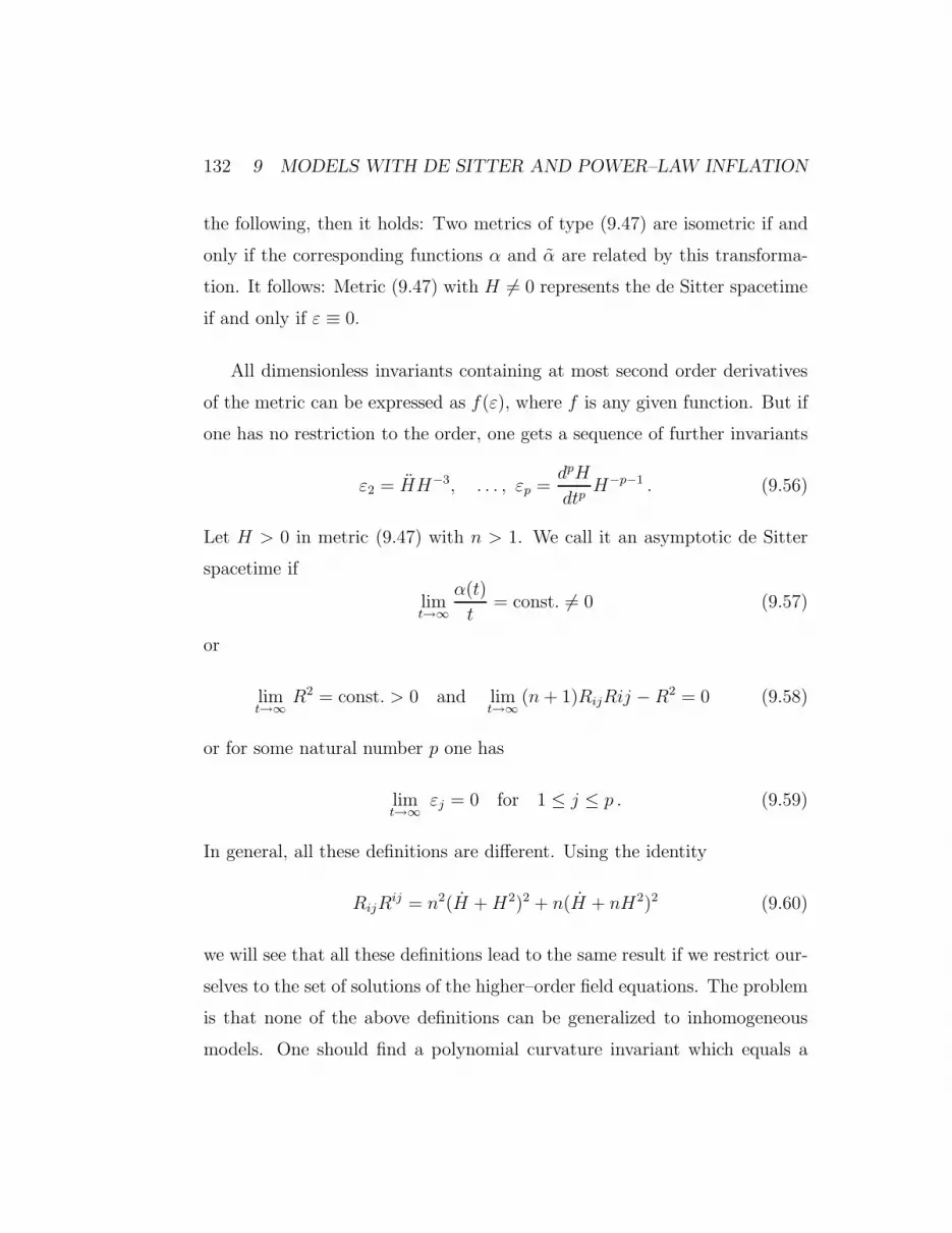
132 9 MODELS WITH DE SITTER AND POWER–LAW INFLATION
the following, then it holds: Two metrics of type (9.47) are isometric if and
only if the corresponding functions α and α are related by this transforma-
tion. It follows: Metric (9.47) with H 6= 0 represents the de Sitter spacetime
if and only if ε ≡ 0.
All dimensionless invariants containing at most second order derivatives
of the metric can be expressed as f(ε), where f is any given function. But if
one has no restriction to the order, one gets a sequence of further invariants
ε2 = HH−3, . . . , εp =dpH
dtpH−p−1 . (9.56)
Let H > 0 in metric (9.47) with n > 1. We call it an asymptotic de Sitter
spacetime if
limt→∞
α(t)
t= const. 6= 0 (9.57)
or
limt→∞
R2 = const. > 0 and limt→∞
(n+ 1)RijRij − R2 = 0 (9.58)
or for some natural number p one has
limt→∞
εj = 0 for 1 ≤ j ≤ p . (9.59)
In general, all these definitions are different. Using the identity
RijRij = n2(H +H2)2 + n(H + nH2)2 (9.60)
we will see that all these definitions lead to the same result if we restrict our-
selves to the set of solutions of the higher–order field equations. The problem
is that none of the above definitions can be generalized to inhomogeneous
models. One should find a polynomial curvature invariant which equals a

9.5 The cosmic no hair theorem 133
positive constant if and only if the spacetime is locally the de Sitter space-
time. To our knowledge, such an invariant cannot be found in the literature,
but also the non–existence of such an invariant has not been proven up to
now. For the anti-de Sitter spacetime, a partial result is given in section 4.3.
This situation is quite different for the positive definite case: For signature
(+ + ++) and Sij = Rij − R4gij it holds:
I ≡ (R− R0)2 + CijklC
ijkl + SijSij = 0 (9.61)
if and only if the V4 is a space of constant curvature R0. So I −→ 0 is a
suitable definition of an asymptotic space of constant curvature. One possi-
bility exists, however, for the Lorentz signature case, if one allows additional
structure as follows: An ideal fluid has an energy–momentum tensor
Tij = (ρ+ p)uiuj − pgij (9.62)
where ui is a continuous vector field with uiui ≡ 1. For matter with equation
of state ρ = −p, the equation T ij;j ≡ 0 implies p = const., and so every
solution of Einstein’s theory with such matter is isometric to a vacuum so-
lution of Einstein’s theory with a cosmological term. The inverse statement,
however, is valid only locally:
Given a vacuum solution of Einstein’s theory with a Λ–term, one has
to find continuous timelike unit vector fields which need not to exist from
topological reasons. And if they exist, they are not at all unique. So, it
becomes possible to define an invariant J which vanishes if and only if the
spacetime is de Sitter by transvecting the curvature tensor with uiuj and/or
gij and suitable linear and quadratic combinations of such terms. Then time
t becomes defined by the streamlines of the vector ui. If one defines the

134 9 MODELS WITH DE SITTER AND POWER–LAW INFLATION
asymptotic de Sitter spacetime by J −→ 0 as t −→ ∞, then it turns out,
that this definition is not independent of the vector field ui.
9.5.3 Lagrangian F (R,2R,22R, . . . ,2kR)
Let us consider the Lagrangian density L given by
L = F (R,2R,22R, . . . ,2kR)√−g (9.63)
where R is the curvature scalar, 2 the D’Alembertian and gij the metric
of a Pseudo-Riemannian VD of dimension D ≥ 2 and arbitrary signature;
g = −| det gij|. The main application will be D = 4 and metric signature
(+ − −−). F is supposed to be a sufficiently smooth function of its argu-
ments, preferably a polynomial. Buchdahl [42] already dealt with such kind
of Lagrangians in 1951, but then it became quiet of them for decades.
The variational derivative of L with respect to the metric yields the tensor
P ij = − 1√−gδL
δgij(9.64)
The components of this tensor read
Pij = GRij − 1
2Fgij − G;ij + gij2G + Xij (9.65)
where the semicolon denotes the covariant derivative, Rij the Ricci tensor,
and
Xij =k∑
A=1
1
2gij[FA(2A−1R);m];m − FA(;i[2
A−1R];j) (9.66)
having the round symmetrization brackets in its last term. For k = 0, i.e.
F = F (R), a case considered in subsection 9.5.4, the tensor Xij identically
vanishes. It remains to define the expressions FA, A = 0, . . . , k .
Fk =∂F
∂2kR(9.67)

9.5 The cosmic no hair theorem 135
and for A = k − 1, . . . , 0
FA = 2FA+1 +∂F
∂2AR(9.68)
and finally G = F0. The brackets are essential, for any scalar Φ it holds
2(Φ;i) − (2Φ);i = R ji Φ;j (9.69)
Inserting Φ = 2mR into this equation, one gets identities to be applied in
the sequel without further notice. The covariant form of energy-momentum
conservation reads
P ij;i ≡ 0 (9.70)
and Pij identically vanishes if and only if F is a divergence, i.e., locally there
can be found a vector vi such that F = vi;i holds. Remark: Even for com-
pact manifolds without boundary the restriction “locally” is unavoidable, for
example, let D = 2 and V2 be the Riemannian two-sphere S2 with arbitrary
positive definite metric. R is a divergence, but there do not exist continuous
vector fields vi fulfilling R = vi;i on the whole S2. Example: for m,n ≥ 0
it holds
2mR 2
nR − R 2m+nR = divergence . (9.71)
So, the terms 2mR 2
nR with naturals m and n can be restricted to the case
m = 0 without loss of generality.
9.5.4 No hair theorems for higher-order gravity
For n > 1, the n+ 1-dimensional de Sitter spacetime is an attractor solution
for the field equation derived from the Lagrangian
R(n+1)/2 . (9.72)

136 9 MODELS WITH DE SITTER AND POWER–LAW INFLATION
It is not an attractor solution for the Lagrangian R2kR and k > 0. There
exist combinations of coefficients ci, such that the de Sitter spacetime is
an attractor solution for the field equation derived from the more general
Lagrangian
L = c0R(n+1)/2 +
m∑
k=0
ck R2kR . (9.73)
Idea of Proof: Concerning fourth-order gravity this method was previously
applied e.g. by Barrow 1986 [12]. The de Sitter spacetime is an exact solution
for the field equation, if and only if 2RG = (n+ 1)F . If we make the ansatz
α(t) = 1 + β(t) (9.74)
we get the linearized field equation 0 = β + nβ for the Lagrangian Rn+1
2 .
For the Lagrangian L = R2kR we get the linearized field equation 2
kR =
(2kR),0. For the characteristic polynomial we get a recursive formula such
that the next order is received from the previous one by multiplying with
· x · (x + n). We get the roots x1 = −n − 1, x2 = −n (k-fold), x3 = 0
(k-fold) and x4 = +1. Because of the last root the de Sitter spacetime is not
an attractor solution. For the Lagrangian (9.73) we get the characteristic
polynomial
P (x) = x(x+ n)
[
c0 +m∑
k=1
ckxk−1(x+ n)k−1(x− 1)(x+ n+ 1)
]
(9.75)
for the linearized field equation. The transformation z = x2 + nx + n2
4
gives a polynomial Q(z) which can be solved explicitly. So one can find
those combinations of the coefficients such that the de Sitter spacetime is an
attractor solution.
It turned out that all the variants of the definition of an asymptotic de
Sitter solution given in subsection 9.5.2 lead to the same class of solutions,

9.5 The cosmic no hair theorem 137
i.e., the validity of the theorems written below does not depend on which
of the variants of definition of an asymptotic de Sitter spacetime listed is
applied. For the 6th–order case we can summarize as follows: Let
L = R2 + c1 R 2R (9.76)
and
LE = R − l2
6L (9.77)
with length l > 0. Then the following statements are equivalent.
1. The Newtonian limit of LE is well–behaved, and the potential φ consists
of terms e−αr/r with α ≥ 0 only.
2. The de Sitter spacetime with H = 1/l is an attractor solution for L
in the set of spatially flat Friedmann models, and this can already be seen
from the linearized field equation.
3. The coefficient c1 ≥ 0, and the graceful exit problem is solved for the
quasi de Sitter phase H ≤ 1/l of LE.
4. l2 = l20 + l21 such that l2 c1 = l20 l21 has a solution with 0 ≤ l0 < l1.
5. 0 ≤ c1 < l2/4.
A formulation which includes also the marginally well-behaved cases reads
as follows: Let L and LE as in the previous result, then the following state-
ments are equivalent:
1. The Newtonian limit of LE is well–behaved, for the potential φ we
allow 1/r and terms like
P (r)
re−αr with α > 0 (9.78)

138 9 MODELS WITH DE SITTER AND POWER–LAW INFLATION
and a polynomial P .
2. The de Sitter spacetime with H = 1/l cannot be ruled out to be an
attractor solution for L in the set of spatially flat Friedmann models if one
considers the linearized field equation only.
3. LE is tachyonic–free.
4. l2 = l20 + l21 with l2 c1 = l20 l21 has a solution with 0 ≤ l0 ≤ l1.
5. For the coefficients we have 0 ≤ c1 ≤ l2
4.
Of course, it would be interesting what happens in the region where the
linearized equation does not suffice to decide.
9.5.5 Diagonalizability of Bianchi models
A Bianchi model can always be written as
ds2 = dt2 − gαβ(t)σασβ (9.79)
where gαβ is positive definite and σα are the characterizing one-forms. It
holds
dσγ = −1
2Cγαβσ
α ∧ σβ (9.80)
with structure constants Cγαβ of the corresponding Bianchi type. It belongs
to class A if Cβαβ = 0. The Abelian group, Bianchi type I, and the rotation
group, Bianchi type IX, both belong to class A. In most cases, the gαβ are
written in diagonal form; it is a non-trivial problem to decide under which
circumstances this can be done without loss of generality. For Einstein’s
theory, this problem is solved. One of its results reads: If a Bianchi model
of class A, except Bianchi types I and II, has a diagonal energy-momentum
tensor, then the metric gαβ(t) can be chosen in diagonal form. Here, the

9.5 The cosmic no hair theorem 139
energy-momentum tensor is called diagonal, if it is diagonal in the basis
(dt, σ1, σ2, σ3).
This result rests of course on Einstein’s theory and cannot be directly
applied to higher-order gravity. For fourth-order gravity following from a
Lagrangian L = f(R) considered in an interval of R-values where
df
dR· d2f
dR26= 0 (9.81)
one can do the following: The application of the conformal equivalence the-
orem, cf. e.g. [29] or [218], is possible, the conformal factor depends on t
only, so the diagonal form of metric does not change. The conformal pic-
ture gives Einstein’s theory with a minimally coupled scalar field as source;
the energy-momentum tensor is automatically diagonal. So, in this class of
fourth-order theories of gravity, we can apply the above cited theorem of
MacCallum et al. [146], [147], where the initial-value formulation of General
Relativity is applied. As example we formulate: All solutions of Bianchi
type IX of fourth-order gravity following from L = R2 considered in a region
where R 6= 0 can be written in diagonal form. Consequently, the ansatz used
by Barrow and Sirousse-Zia [16] for this problem is already the most general
one, cf. Spindel [241].
For fourth-order gravity of a more complicated structure, however, things
are more involved; example: Let
L = R + aR2 + bCijklCijkl (9.82)
with ab 6= 0. Then there exist Bianchi type IX models which cannot be
written in diagonal form. This is a non-trivial statement because its proof
needs a careful analysis of the correspondingly allowed initial values in the
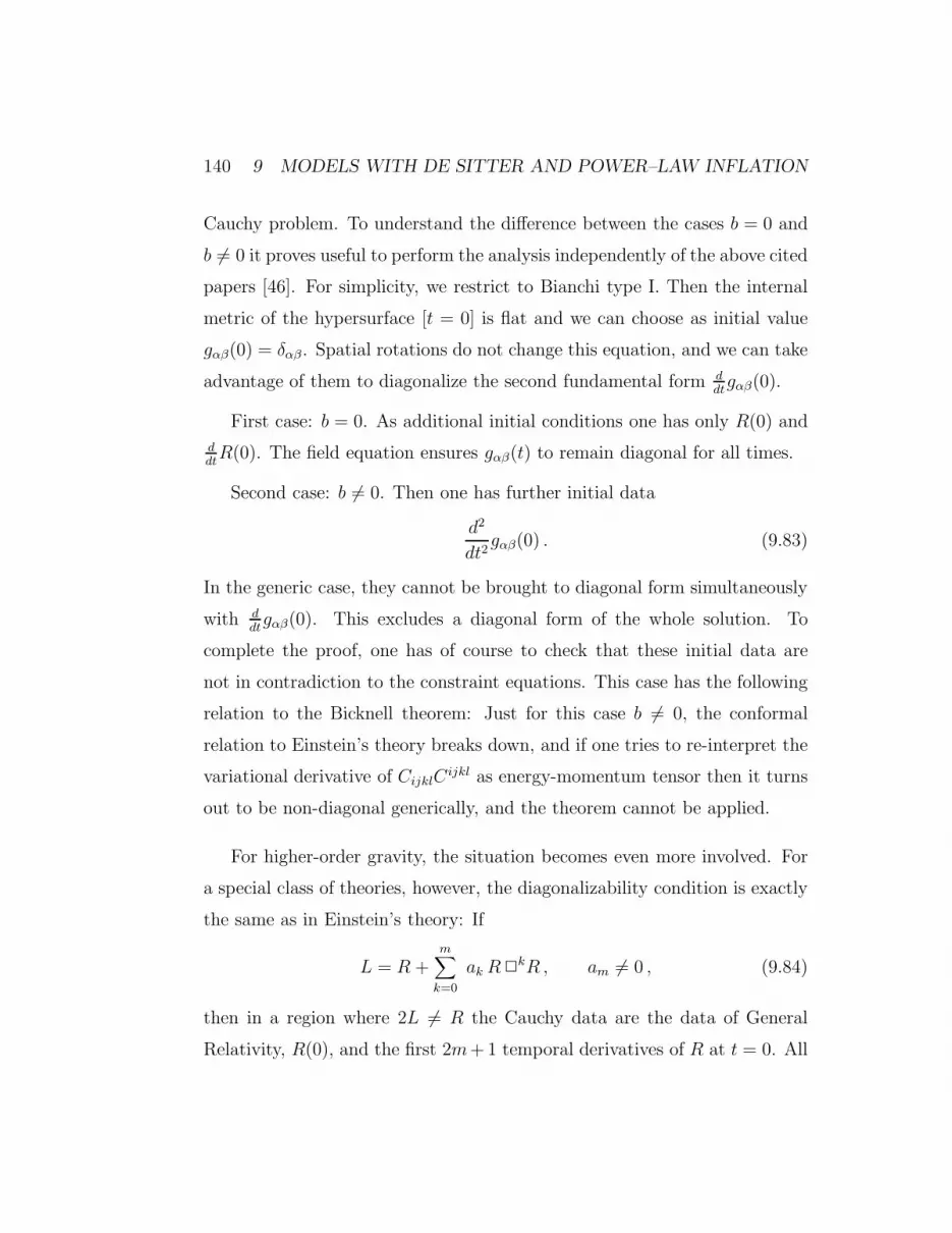
140 9 MODELS WITH DE SITTER AND POWER–LAW INFLATION
Cauchy problem. To understand the difference between the cases b = 0 and
b 6= 0 it proves useful to perform the analysis independently of the above cited
papers [46]. For simplicity, we restrict to Bianchi type I. Then the internal
metric of the hypersurface [t = 0] is flat and we can choose as initial value
gαβ(0) = δαβ . Spatial rotations do not change this equation, and we can take
advantage of them to diagonalize the second fundamental form ddtgαβ(0).
First case: b = 0. As additional initial conditions one has only R(0) and
ddtR(0). The field equation ensures gαβ(t) to remain diagonal for all times.
Second case: b 6= 0. Then one has further initial data
d2
dt2gαβ(0) . (9.83)
In the generic case, they cannot be brought to diagonal form simultaneously
with ddtgαβ(0). This excludes a diagonal form of the whole solution. To
complete the proof, one has of course to check that these initial data are
not in contradiction to the constraint equations. This case has the following
relation to the Bicknell theorem: Just for this case b 6= 0, the conformal
relation to Einstein’s theory breaks down, and if one tries to re-interpret the
variational derivative of CijklCijkl as energy-momentum tensor then it turns
out to be non-diagonal generically, and the theorem cannot be applied.
For higher-order gravity, the situation becomes even more involved. For
a special class of theories, however, the diagonalizability condition is exactly
the same as in Einstein’s theory: If
L = R +m∑
k=0
ak R2kR , am 6= 0 , (9.84)
then in a region where 2L 6= R the Cauchy data are the data of General
Relativity, R(0), and the first 2m+ 1 temporal derivatives of R at t = 0. All
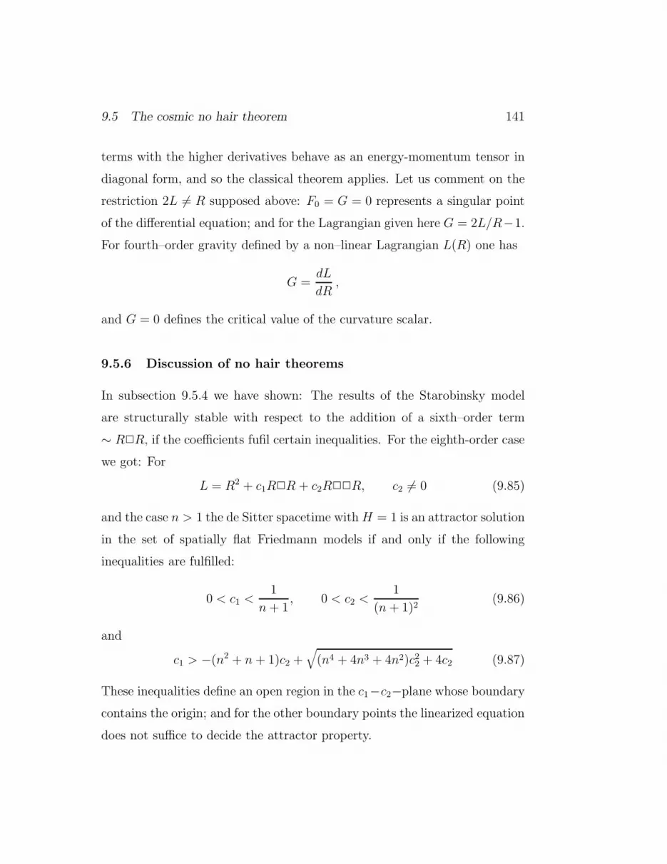
9.5 The cosmic no hair theorem 141
terms with the higher derivatives behave as an energy-momentum tensor in
diagonal form, and so the classical theorem applies. Let us comment on the
restriction 2L 6= R supposed above: F0 = G = 0 represents a singular point
of the differential equation; and for the Lagrangian given here G = 2L/R−1.
For fourth–order gravity defined by a non–linear Lagrangian L(R) one has
G =dL
dR,
and G = 0 defines the critical value of the curvature scalar.
9.5.6 Discussion of no hair theorems
In subsection 9.5.4 we have shown: The results of the Starobinsky model
are structurally stable with respect to the addition of a sixth–order term
∼ R2R, if the coefficients fufil certain inequalities. For the eighth-order case
we got: For
L = R2 + c1R2R + c2R22R, c2 6= 0 (9.85)
and the case n > 1 the de Sitter spacetime withH = 1 is an attractor solution
in the set of spatially flat Friedmann models if and only if the following
inequalities are fulfilled:
0 < c1 <1
n+ 1, 0 < c2 <
1
(n+ 1)2(9.86)
and
c1 > −(n2 + n + 1)c2 +√
(n4 + 4n3 + 4n2)c22 + 4c2 (9.87)
These inequalities define an open region in the c1−c2−plane whose boundary
contains the origin; and for the other boundary points the linearized equation
does not suffice to decide the attractor property.

142 9 MODELS WITH DE SITTER AND POWER–LAW INFLATION
This situation shall be called “semi–attractor” for simplicity. In a gen-
eral context this notion is used to describe a situation where all Lyapunov
coefficients have non-positive real parts and at least one of them is purely
imaginary.
In contrary to the 6th–order case, here we do not have a one–to–one
correspondence, but a non–void open intersection with that parameter set
having the Newtonian limit for LE well–behaved.
To find out, whether another de Sitter spacetime with an arbitrary Hubble
parameter H > 0 is an attractor solution for the eighth–order field equation
following from the above Lagrangian, one should remember that H has the
physical dimension of an inverted time, c1 is a time squared, c2 is a time to
power 4. So, we have to replace c1 by c1H2 and c2 by c2H
4 in the above
dimensionless inequalities to get the correct conditions. Example:
0 < c1H2 <
1
4.
Let us summarize: Here for a theory of gravity of order higher than four
the Newtonian limit and the attractor property of the de Sitter spacetime are
systematically compared. It should be noted that the details of the theory
sensibly depend on the numerical values of the corresponding coefficients. So,
no general overall result about this class of theories is ever to be expected.
The facts, contradicting each other from the first glance, field equations of
higher than second order follow from quantum gravity considerations Mirz-
abekian et al. [156] on the one hand but such equations are known to be
unstable in general and are therefore unphysical on the other hand, have now

9.5 The cosmic no hair theorem 143
considered in more details: It depends on the special circumstances whether
such theories are unstable.
We have found out that for the class of theories considered here, one of
the typical indicators of instability - cosmological runaway–solutions - need
not to exist, even for an arbitrarily high order of the field equation. It is
an additional satisfactory result that this takes place in the same range of
parameters where the Newtonian limit is well behaved.

145
10 Solutions of the Bach-Einstein equation
For field equations of 4th order, following from a Lagrangian “Ricci scalar
plus Weyl scalar”, it is shown using methods of non-standard analysis that
in a neighbourhood of Minkowski spacetime there do not exist regular static
spherically symmetric solutions. With that, besides the known local expan-
sions about r = 0 and r = ∞ respectively, a global statement on the existence
of such solutions is given, see [205]. Then, this result will be discussed in
connection with Einstein’s particle programme. Finally, in section 10.6 it will
be shown, that cosmological Bianchi type I solutions of the Bach equation
exist which fail to be conformally related to an Einstein space.
10.1 Introduction to the Bach equation
General Relativity Theory starts from the Einstein-Hilbert Lagrangian
LEH = R/2κ (10.1)
with the Ricci scalar R which leads to the Einstein vacuum field equation
Rki = 0 being of second order in the metrical tensor gik. Its validity is proven
with high accuracy in spacetime regions where the curvature is small only.
Therefore, the additional presence of a term being quadratic in the curvature
is not excluded by the standard weak field experiments.
Lagrangians with squared curvature have already been discussed by Weyl
in 1919 [268], by Bach in 1921 [8] and Einstein in 1921. They were guided by
ideas about conformal invariance, and Einstein [66] proposed to look seriously
to such alternatives. In Bach [8], the Lagrangian LW with the the Weyl scalar
C,
LW = C/2κ , with C =1
2· CijklCijkl (10.2)

146 10 SOLUTIONS OF THE BACH-EINSTEIN EQUATION
was of special interest. Then it became quiet of them for a couple of decades
because of the brilliant results of General Relativity but not at least because
of mathematical difficulties.
Later, new interest in such equations arose with arguments coming from
quantum gravity, cf. e.g. [257], Borzeszkowski, Treder, Yourgrau [37], Stelle
[249], Fiedler, Schimming [78]. In the large set of possible quadratic modifi-
cations a linear combination
L = LEH + l2LW (10.3)
enjoyed a special interest, cf. e.g. Treder 1977 [257]. The coupling constant
l has to be a length for dimensional reasons and it has to be a small one to
avoid conflicts with observations: One often takes it to be the Heisenberg
length, which is the Compton wave length of the proton, = 1.3 · 10−18 cm
or the Planck length = 1.6 · 10−33 cm.
In this chapter we consider the Lagrangian L eq. (10.3) in connection
with Einstein’s particle programme, see Einstein, Pauli 1943 [69]: One asks
for spherically symmetric singularity-free asymptotically flat solutions of the
vacuum field equations which shall be interpreted as particles, but this cannot
be fulfilled within General Relativity itself; it is still a hope, cf. [35], to realize
it in such 4th order field equations.
Two partial answers have already been given: Stelle [249] has shown the
gravitationa1 potential of the linearized equations to be
Φ(r) = −m/r + exp(−r/l)c/r for r ≪ l ; (10.4)
he also gave an expansion series about r = 0, and Fiedler, Schimming [78]
proved its convergence and smoothness in a certain neighbourhood of r = 0,
but said nothing about the convergence radius of this expansion.

10.2 Notations and field equations 147
Now we want to join these two local expansions. To this end we write
down the field equations in different but equivalent versions section 10.2,
calculate some linearizations section 10.3 and prove the statement of the
summary in section 10.4 which will be followed by a discussion of Einstein’s
particle programme in section 10.5.
10.2 Notations and field equations
We start from a spacetime metric with signature (+−−−), the Riemann and
Ricci tensor being defined by Rijkl = Γi jl,k − . . ., Rik = Rj
ijk respectively.
The Weyl tensor Cijkl is the traceless part of the Riemann tensor and the
Weyl scalar is given by 2C = CijklCijkl. Light velocity is taken to be 1 and
G = κ/8π is Newton’s constant; g = det gij.
Then we consider the Lagrangian
L =√−gL =
√−g(R + l2C)/2κ+ Lmat , (10.5)
where Lmat is the matter Lagrangian. For writing down the corresponding
field equation it is convenient to introduce the Bach tensor Bij , cf. Bach [8]
and Wunsch [271], beforehand.
1
2Bij =
κ δ(√−g LW)√−g δ gij = Ca b
ij ;ba +1
2Ca b
ij Rba . (10.6)
It holds Bii = 0, Bj
i;j = 0, Bij = Bji, and Bij is conformally invariant
of weight -1. Variation of eq. (10.5) with respect to gij leads to the field
equation
Rij −1
2gijR + l2Bij = κTij . (10.7)
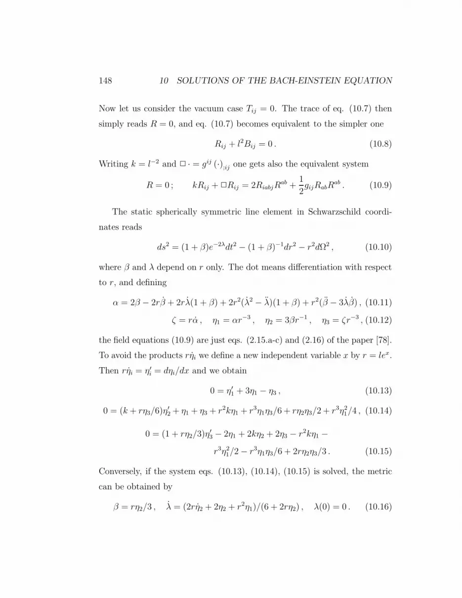
148 10 SOLUTIONS OF THE BACH-EINSTEIN EQUATION
Now let us consider the vacuum case Tij = 0. The trace of eq. (10.7) then
simply reads R = 0, and eq. (10.7) becomes equivalent to the simpler one
Rij + l2Bij = 0 . (10.8)
Writing k = l−2 and 2 · = gij (·);ij one gets also the equivalent system
R = 0 ; kRij + 2Rij = 2RiabjRab +
1
2gijRabR
ab . (10.9)
The static spherically symmetric line element in Schwarzschild coordi-
nates reads
ds2 = (1 + β)e−2λdt2 − (1 + β)−1dr2 − r2dΩ2 , (10.10)
where β and λ depend on r only. The dot means differentiation with respect
to r, and defining
α = 2β − 2rβ + 2rλ(1 + β) + 2r2(λ2 − λ)(1 + β) + r2(β − 3λβ) , (10.11)
ζ = rα , η1 = αr−3 , η2 = 3βr−1 , η3 = ζr−3 , (10.12)
the field equations (10.9) are just eqs. (2.15.a-c) and (2.16) of the paper [78].
To avoid the products rηi we define a new independent variable x by r = lex.
Then rηi = η′i = dηi/dx and we obtain
0 = η′1 + 3η1 − η3 , (10.13)
0 = (k + rη3/6)η′2 + η1 + η3 + r2kη1 + r3η1η3/6 + rη2η3/2 + r3η21/4 , (10.14)
0 = (1 + rη2/3)η′3 − 2η1 + 2kη2 + 2η3 − r2kη1 −
r3η21/2 − r3η1η3/6 + 2rη2η3/3 . (10.15)
Conversely, if the system eqs. (10.13), (10.14), (10.15) is solved, the metric
can be obtained by
β = rη2/3 , λ = (2rη2 + 2η2 + r2η1)/(6 + 2rη2) , λ(0) = 0 . (10.16)

10.3 Linearizations 149
10.3 Linearizations
Now we make some approximations to obtain the rough behaviour of the
solutions. First, for r → ∞, Stelle [249] has shown the following: Lineariza-
tion about Minkowski spacetime leads, using our notations eqs. (10.4) and
(10.10), to λ = 0 and β = 2Φ, where powers of Φ are neglected and the term
exp(r/l)/r in Φ must he suppressed because of asymptotical flatness.
That means, loosely speaking, the right hand side of eq. (10.9) will be
neglected. Connected with this one may doubt the relevance of the term
cr−1e−r/l in eq. (10.4) for m 6= 0 and r → ∞, because it is small compared
with the neglected terms. Further, a finite Φ(0) requires c = m in eq. (10.4).
Then Φ is just the Bopp-Podolsky potential stemming from 4th order elec-
trodynamics, and it were Pechlaner and Sexl [180] who proposed this form
as representing a gravitational potential. Now we have
Φ(r) = m (exp(−r/l) − 1) /r = −m/l + rm/(2l2) + . . . , (10.17)
but also this finite potential gives rise to a singularity: For one of the curva-
ture invariants we get RijRij ≈ m2/r4 as r → 0, that means, the linearization
makes no sense for this region. From this one can already expect that in a
neighbourhood of Minkowski spacetime no regular solutions exist.
Second, for r → 0, in [78] it is shown that there exists a one-parameter
family of solutions being singularity-free and analytical in a neighbourhood
of r = 0. The parameter will be called ε and can be defined as follows:
neglecting the terms with r in the system eqs. (10.13), (10.14), (10.15)
one obtains a linear system with constant coefficients possessing just a one-
parameter family of solutions being regular at r = 0; it reads
η1 = εk2r , η2 = −5εkr , η3 = 4εk2r . (10.18)

150 10 SOLUTIONS OF THE BACH-EINSTEIN EQUATION
The factors kn are chosen such that ε becomes dimensionless. Now one
can take eq. (10.18) as the first term of a power series ηi = Σn a(n)i rn ,
and inserting this ansatz into that system, one iteratively obtains the coeffi-
cients a(n)i . For n even, a
(n)i vanishes: The r3-terms are k3(ε/14 + 10ε2/21),
−k2(ε/2 − 10ε2/3) and k3(3ε/7 + 20ε2/7) respectively. Furthermore, the
r2n−1-term is always a suitable power of k times a polynomial in ε of the
order ≤ n.
Up to the r2-terms the corresponding metric (10.10) reads
ds2 = (1 + 5kεr2/3)dt2 − (1 + 5kεr2/3)dr2 − r2dΩ2 . (10.19)
Third, we look for a linearization which holds uniformly for 0 ≤ r < ∞.
A glance at eqs. (10.16) and (10.10) shows that ηi = 0 gives Minkowski
spacetime, and therefore we neglect terms containing products of ηi in the
system. In other words, instead of the linearization used before we addition-
ally retain the term r2η1. Then we proceed as follows: from eqs. (10.13) and
(10.15) we obtain
η3 = η′1 + 3η1 and (10.20)
η2 =−η′1 − 5η1 + (e2x − 4)η1 + l3e3xη1(η1 + η′1/6)
2k + lex(η′1 + 5η1 + 6η1)/3. (10.21)
Inserting eqs. (10.20), (10.21) into eq. (10.14) one obtains a third order
equation for η1 only whose linearization reads
0 = η′′′1 + 5η′′1 + η′1(2 − e2x) − η1(8 + 4e2x) . (10.22)
In Schmidt and Muller [231] the same vacuum field equations were discussed
for axially symmetric Bianchi type I models. They possess a four-parameter
group of isometries, too, and the essential field equation is also a third order

10.4 Non-standard analysis 151
equation for one function. The difference is that in the present case spherical
symmetry implies an explicit coordinate dependence.
The solution of eq. (10.22) which is bounded for x→ −∞ reads
η1 = γ ·[
(3e−4x + e−2x) sinh ex − 3e−3x cosh ex]
. (10.23)
A second solution is η1 = −12mr−4 leading to the Schwarzschild solution,
this solution solves both the full and the linearized equations in accordance
with the fact that it makes zero both sides of eq. (10.9), and the third one can
be obtained from them up to quadrature by usual methods. A comparison
of eq. (10.23) with eq. (10.18) gives γ = 15εl−3.
Now we insert this η1 into eqs. (10.21), (10.16) and neglect again powers
of η1; then the metric reads
β = 5ε[
lr−1 sinh(rl−1) − cosh(rl−1)]
,
λ =5ε
2l·∫ r
0
[
(l2z−2 − 1) sinh(zl−1) − lz−1 cosh(zl−1)]
dz . (10.24)
This linearization has, in contrary to eqs. (10.4) and (10.18), the following
property: to each r0 > 0 and ∆ > 0 there exists an δ > 0 such that for
−δ < ε < δ the relative error of the linearized solution (10.24) does not
exceed ∆ uniformly on the interval 0 ≤ r ≤ r0.
10.4 Non-standard analysis
In this section we will prove that in a neighbourhood of Minkowski spacetime
there do not exist any solutions. “Neighbourhood of Minkowski spacetime”
is in general a concept requiring additional explanations because of the large
number of different topologies discussed in literature. To make the above

152 10 SOLUTIONS OF THE BACH-EINSTEIN EQUATION
statement sufficiently strong we apply a quite weak topology here: given a
δ > 0 then all spacetimes being diffeomorphic to Minkowski spacetime and
fulfilling |RijRij | < δk2 form a neighbourhood about Minkowski spacetime.
In eq. (10.19) we have at r = 0, independently of higher order terms in r,
RijRij = 100k2ε2/3 and R00 = 5kε . (10.25)
Therefore it holds: the one-parameter family of solutions being regular at
r = 0 is invariantly characterized by the real parameter ε, and a necessary
condition for it to be within a neighbourhood of Minkowski spacetime is that
ε lies in a neighbourhood of 0.
Now we suppose ε to be an infinitesimal number, i.e., a positive number
which is smaller than any positive real number. The mathematical theory
dealing with such infinitesimals is called non-standard analysis, cf. Robin-
son [191]. The clue is that one can handle non-standard numbers like real
numbers. Further we need the so-called Permanence principle, which is also
called the Robinson lemma: Let A(ε) be an internal statement holding for
all infinitesimals ε. Then there exists a positive standard real δ > 0 such
that A(ε) holds for all ε with 0 < ε < δ. The presumption “internal” says,
roughly speaking, that in the formulation of A(.) the words “standard” and
“infinitesimal” do not appear.
This permanence principle shall be applied as follows: A(ε) is the state-
ment: “Take eq. (10.18) as initial condition for eqs. (10.13), (10.14), (10.15)
and calculate the corresponding metric (10.10), (10.16). Then there exists
an r0 ≤ l such that RijRij ≥ k2 at r = r0.” Remark: At this point it is not
essential whether r0 is a standard or an infinitely large non-standard number.

10.4 Non-standard analysis 153
Proof of A(ε) for infinitesimals ε with ε 6= 0: the difference of eq. (10.24)
in relation to the exact solution is of the order ε2, i.e. the relative error
is infinitesimally small. For increasing r, |β| becomes arbitrary large, i.e.
(1 + β)−1 becomes small and RijRij increases to arbitrarily large values, cf.
eq. (10.24). Now take r0 such that with metric (10.10), (10.24) RijRij ≥ 2k2
holds. Then, for the exact solution, RijRij ≥ k2 holds at r = r0, because
their difference was shown to be infinitesimally small.
Now the permanence principle tells us that there exists a positive standard
real δ > 0 such that for all ε with 0 < |ε| < δ the corresponding exact solution
has a point r0 such that at r = r0 the inequality RijRij ≥ k2 holds. But
“RijRij < k2” is another necessary condition for a solution to lie within a
neighbourhood of Minkowski spacetime. Remark: Supposed this r0 is an
infinitely large non-standard number, then by continuity arguments also a
standard finite number with the same property exists.
The statement is proved, but we have learned nothing about the actual
value of the number δ. Here, numerical calculations may help. They were
performed as follows: the power series for the functions ηi were calculated
up to the r6-term, then these functions taken at x = −4 i.e. r = 0.018 l
were used as initial conditions for a Runge–Kutta integration. We got the
following result: firstly, for ε = ±10−5 and r ≤ 10 l, the relative difference
between the linearized solution eq. (10.23) and the numerical one is less than
2 per thousand. Secondly, for 0 < |ε| ≤ 1 the behaviour “β → −∞ · sgnε”
is confirmed. That means, the statement made above keeps valid at least
for δ = 1. Remark: For large values ε the power series for the ηi converge
very slowly, and therefore other methods would be necessary to decide about
asymptotical flatness.

154 10 SOLUTIONS OF THE BACH-EINSTEIN EQUATION
10.5 Discussion – Einstein’s particle programme
Fourth-order gravitational field equations could be taken as a field theoretical
model of ordinary matter, the energy–momentum tensor of which is defined
by
κT ∗ij = Rij −
1
2gijR . (10.26)
For our case one obtains at r = 0 that T ∗ij represents an ideal fluid with the
equation of state p∗ = µ∗/3 and, cf. eq. (10.25),
µ∗(0) = 5kεκ−1 = 5ε/8πGl2 . (10.27)
Inserting |ε| ≥ 1 and l ≤ 1.3 · 10−13 cm into eq. (10.27), we obtain
|µ∗(0)| ≥ 1.5 · 1053 g cm−3 . (10.28)
Therefore it holds: if there exists a non-trivial static spherically symmetric
asymptotically flat singularity-free solution of eq. (10.8) at all, then the corre-
sponding particle would be a very massive one: its phenomenological energy
density exceeds that of a neutron star by at least 40 orders of magnitude.
The resulting statement can be understood as follows: For a small cur-
vature the 4th order corrections to Einstein’s equations are small, too, and
the situation should not be very different from that one we know from Ein-
stein’s theory. Now we want to refer to a problem concerning Schwarzschild
coordinates: the transition from a general static spherically symmetric line
element to Schwarzschild coordinates is possible only in the case that the
function “invariant surface of the sphere r = const. in dependence on its
invariant radius” has not any stationary point. Here two standpoints are
possible: either one takes this as a natural condition for a reasonable particle
model or one allows coordinate singularities in eq. (10.10) like “β ≥ −1,

10.5 Discussion – Einstein’s particle programme 155
and β = −1 at single points” which require a special care. For β < −1 one
would obtain a cosmological model of Kantowski-Sachs type. Eqs. (10.5) till
(10.16) remain unchanged for this case. The discussion made above is not
influenced by this.
The statement on the existence of solutions can be strengthened as fol-
lows: Fiedler and Schimming [78] proved that the solutions are analytical in
a neighbourhood of r = 0. Further, the differential equation is an analytical
one and, therefore, in the subspace of singularity-free solutions they remain
so in the limit r → ∞. Then, there exists only a finite or countably infinite
set of values εn such that the corresponding solution becomes asymptotically
flat; the question, whether this set is empty or not, shall be subject of further
investigation. Furthermore, the εn have no finite accumulation point. That
means, there exists at most a discrete spectrum of solutions.
With respect to this fact, we remark the following: as one knows, Ein-
stein’s theory is a covariant one. But besides this symmetry, it is homotheti-
cally invariant, too. That means, if ds2 is changed to e2χds2 with constant χ,
then the tensor Rij − 12gijR remains unchanged, whereas the scalars R and
C will be divided by e2χ and e4χ respectively. From this it follows: with one
solution of Einstein’s vacuum equation one obtains by homothetic invariance
just a one-parameter class of solutions. On the other hand, the sum R+ l2C
has not such a symmetry and, therefore, one should not expect that a one-
parameter family of solutions globally exists, and this is just in the scope of
the particle programme where a definite particle’s mass is wanted.

156 10 SOLUTIONS OF THE BACH-EINSTEIN EQUATION
10.6 Non-trivial solutions of the Bach equation exist
Following [204], we show that solutions of the Bach equation exist which are
not conformal Einstein spaces. In connection with fourth-order gravitational
field equations, cf. e.g. Weyl 1921 [268], [37] where the breaking of conformal
invariance was discussed, the original Bach equation,
Bij = 0 , (10.29)
enjoys current interest, see e.g. [64], [71] and [91]. Eq. (10.29) stems from a
Lagrangian
L =1
2
√−g CijklCijkl , (10.30)
and variation gives, cf. Bach 1921 [8],
1√−g δL/δgij = Bij = 2Ca b
ij ;ba + Ca bij Rba . (10.31)
An Einstein space, defined by
Rij = λ gij , (10.32)
is always a solution of the Bach equation (10.29). But eq. (10.29) is confor-
mally invariant, and therefore, each metric, which is conformally related to
an Einstein space, fulfils eq. (10.29), too. We call such solutions trivial ones.
Now the question arises whether non-trivial solutions of the Bach equation
eq. (10.29) do or do not exist. In this section we will give an affirmative
answer. As a by-product, some conditions will be given under which only
trivial solutions exist. Observe that eq. (10.29) is conformally invariant
whereas eq. (10.32) is not. Therefore, a simple counting of degrees of freedom
does not suffice.

10.6 Non-trivial solutions of the Bach equation exist 157
Because the full set of solutions of eq. (10.29) is not easy to describe, let
us consider some homogeneous cosmological models. Of course, we have to
consider anisotropic ones, because all Friedmann models are trivial solutions
of eq. (10.29). Here, we concentrate on the diagonal Bianchi type I models
ds2 = dt2 − a2i
(
dxi)2
(10.33)
with Hubble parameters hi = a−1i dai/dt, h = Σhi and anisotropy parameters
mi = hi − h/3. The Einstein spaces of this kind are described in [134] eq.
(11.52), for λ = 0 it is just the Kasner metric ai = tpi, Σpi = Σp2i = 1.
All these solutions have the property that the quotient of two anisotropy
parameters, mi/mj , which equals (3pi − 1)/(3pj − 1) for the Kasner metric,
is independent of t, and this property is a conformally invariant one. Fur-
thermore, it holds: A solution of eqs. (10.29), (10.33) is a trivial one, if and
only if the quotients mi/mj are constants.
Restricting now to axially symmetric Bianchi type I models, i.e., metric
(10.33) with h1 = h2, the identity Σmi = 0 implies m1/m2 = 1, m3/m1 =
m3/m2 = −2 , i.e., each axially symmetric Bianchi type I solution of eq.
(10.29) is conformally related to an Einstein space. Analogously, all static
spherically symmetric solutions of eq. (10.29) are trivial ones, cf. [77].
Finally, the existence of a solution of eqs. (10.29), (10.33) with a non-
constant m1/m2 will be shown. For the sake of simplicity we use the gauge
condition h = 0, which is possible because of the conformal invariance of
eq. (10.29). Then the 00 component and the 11 component of eq. (10.29)
are sufficient to determine the unknown functions h1 and h2; h3 = −h1 − h2
follows from the gauge condition. Defining r = (h21 + h1h2 + h2
2)1/2 and

158 10 SOLUTIONS OF THE BACH-EINSTEIN EQUATION
p = h1/r, eq. (10.29) is equivalent to the system
3d2(pr)/dt2 = 8pr3 + 4c, c = const., p2 ≤ 4/3 , (10.34)
9(dp/dt)2r4 = [2rd2r/dt2 − (dr/dt)2 − 4r4](4r2 − 3p2r2) . (10.35)
As one can see, solutions with a non-constant p exist, i.e., m1/m2 is not
constant for this case.
Result: Each solution of the system eqs. (10.33), (10.34), (10.35) with
dp/dt 6= 0 represents a non-trivial solution of the Bach equation (10.29).

159
11 The Newtonian limit of non-linear gravity
In this chapter, the weak-field slow-motion limit of fourth and higher-order
gravity will be deduced. Here we follow [208] for the fourth-order case and
[187] for the general case. More explicitly: we consider the Newtonian limit
of the theory based on the Lagrangian
L =
(
R +p∑
k=0
ak R2kR
)√−g . (11.1)
The gravitational potential of a point mass turns out to be a combination
of Newtonian and Yukawa terms. For fourth-order and sixth-order gravity,
p = 0 and p = 1 respectively, the coefficients are calculated explicitly. For
general p one gets the potential to be
Φ = m/r
(
1 +p∑
i=0
ci exp(−r/li))
(11.2)
with certain coefficients ci fulfilling the relation
p∑
i=0
ci = 1/3 . (11.3)
Therefore, the potential is always unbounded near the origin, see also [10].
11.1 The Newtonian limit of 4th-order gravity
Let us consider the gravitational theory defined by the Lagrangian
Lg = (8πG)−1(
R/2 + (αRijRij + βR2)l2
)
. (11.4)
G is Newton’s constant, l a coupling length and α and β numerical param-
eters. Rij and R are the Ricci tensor and its trace. Introducing the matter
Lagrangian Lm and varying Lg + Lm one obtains the field equation
Eij + αHij + βGij = 8πGTij . (11.5)

160 11 THE NEWTONIAN LIMIT OF NON-LINEAR GRAVITY
For α = β = 0 this reduces to General Relativity Theory. The explicit
expressions Hij and Gij can be found in sections 8.4 and 10.2, see also Stelle
[249].
In a well-defined sense, the weak-field slow-motion limit of Einstein’s the-
ory is just Newton’s theory, cf. Dautcourt 1964 [60]. In the following, we
consider the analogous problem for fourth-order gravity eqs. (11.4), (11.5).
In some cases, the Newtonian limit of the theory defined by eq. (11.5) has
already been deduced in the literature: For the special case α = 0 see Pech-
laner and Sexl [180] or Polijevktov-Nikoladze [183]. For the case α+ 2β = 0
see Havas [105] or Jankiewicz [121], and for α + 3β = 0 see Borzeszkowski,
Treder and Yourgrau [37]. Cf. also Anandan [5], where torsion has been
taken into account.
The slow-motion limit can be equivalently described as the limit c→ ∞,
where c is the velocity of light. In this sense we have to take the limit G→ 0
while G · c and l remain constants. Then the energy-momentum tensor Tij
reduces to the rest mass density ρ:
Tij = δ0i δ
0j ρ , (11.6)
x0 = t being the time coordinate. The metric can be written as
ds2 = (1 − 2φ)dt2 − (1 + 2ψ)(dx2 + dy2 + dz2) . (11.7)
Now eqs. (11.6) and (11.7) will be inserted into eq. (11.5). In our approach,
products and time derivatives of φ and ψ can be neglected, i.e.,
R = 4∆ψ − 2∆φ , where ∆f = f,xx + f,yy + f,zz . (11.8)
Further R00 = −∆φ, H00 = −2∆R00 − ∆R and G00 = −4∆R, where l = 1.

11.1 The Newtonian limit of 4th-order gravity 161
Then it holds: The validity of the 00-component and of the trace of eq.
(11.5),
R00 − R/2 + αH00 + βG00 = 8πGρ (11.9)
and
−R− 4(α+ 3β)∆R = 8πGρ , (11.10)
imply the validity of the full eq. (11.5).
Now, let us discuss eqs. (11.9) and (11.10) in more details: Eq. (11.9)
reads
−∆φ−R/2 + α(2∆∆φ− ∆R) − 4β∆R = 8πGρ . (11.11)
Subtracting one half of eq. (11.10) yields
−∆φ+ 2α∆∆φ+ (α + 2β)∆R = 4πGρ . (11.12)
For α + 2β = 0 one obtains
−(1 − 2α∆)∆φ = 4πGρ (11.13)
and then ψ = φ is a solution of eqs. (11.9), (11.10). For all other cases the
equations for φ and ψ do not decouple immediately, but, to get equations
comparable with Poisson’s equation we apply ∆ to eq. (11.10) and continue
as follows.
For α + 3β = 0 one gets from eq. (11.12)
−(1 − 2α∆)∆φ = 4πG(1 + 2α∆/3)ρ . (11.14)
The ∆-operator applied to the source term in eq. (11.14) is only due to the
application of ∆ to the trace, the original equations (11.9), (11.10) contain
only ρ itself.
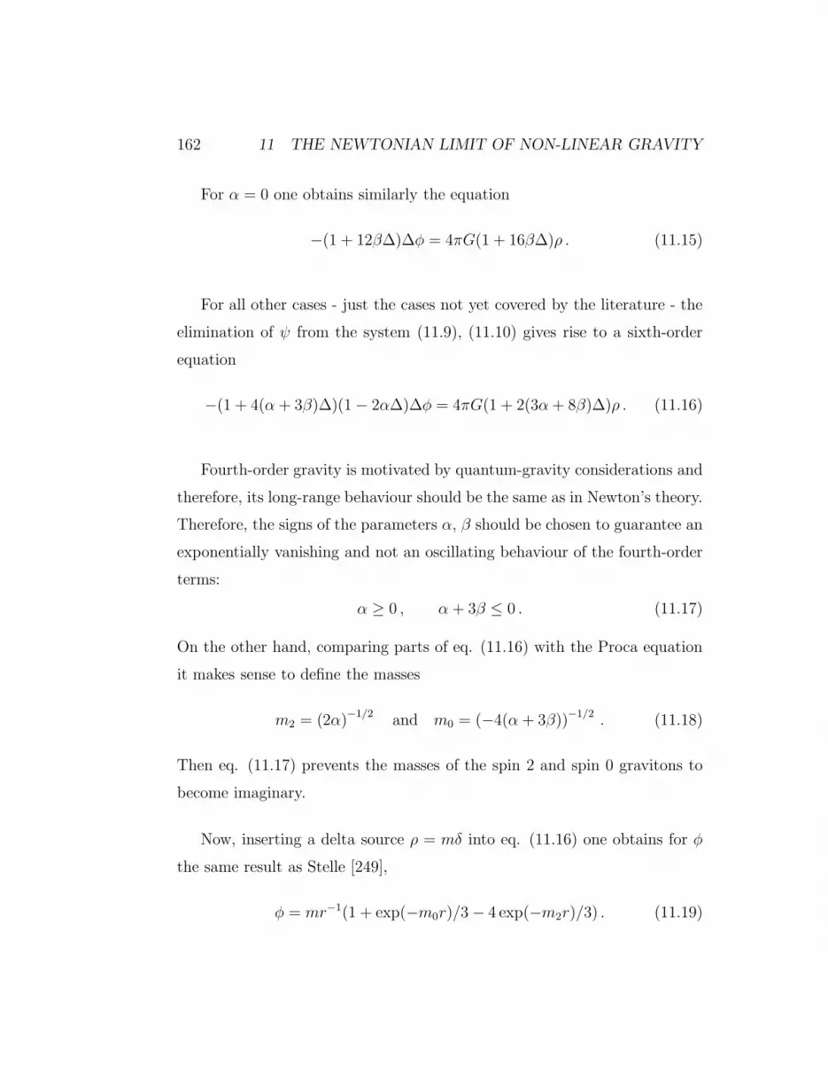
162 11 THE NEWTONIAN LIMIT OF NON-LINEAR GRAVITY
For α = 0 one obtains similarly the equation
−(1 + 12β∆)∆φ = 4πG(1 + 16β∆)ρ . (11.15)
For all other cases - just the cases not yet covered by the literature - the
elimination of ψ from the system (11.9), (11.10) gives rise to a sixth-order
equation
−(1 + 4(α + 3β)∆)(1 − 2α∆)∆φ = 4πG(1 + 2(3α+ 8β)∆)ρ . (11.16)
Fourth-order gravity is motivated by quantum-gravity considerations and
therefore, its long-range behaviour should be the same as in Newton’s theory.
Therefore, the signs of the parameters α, β should be chosen to guarantee an
exponentially vanishing and not an oscillating behaviour of the fourth-order
terms:
α ≥ 0 , α + 3β ≤ 0 . (11.17)
On the other hand, comparing parts of eq. (11.16) with the Proca equation
it makes sense to define the masses
m2 = (2α)−1/2 and m0 = (−4(α + 3β))−1/2 . (11.18)
Then eq. (11.17) prevents the masses of the spin 2 and spin 0 gravitons to
become imaginary.
Now, inserting a delta source ρ = mδ into eq. (11.16) one obtains for φ
the same result as Stelle [249],
φ = mr−1(1 + exp(−m0r)/3 − 4 exp(−m2r)/3) . (11.19)

11.1 The Newtonian limit of 4th-order gravity 163
To obtain the metric completely one has also to calculate ψ. It reads
ψ = mr−1(1 − exp(−m0r)/3 − 2 exp(−m2r)/3) . (11.20)
For finite values m0 and m2 these are both bounded functions, also for r → 0.
In the limits α→ 0, i.e. m2 → ∞, and α+ 3β → 0, i.e. m0 → ∞, the terms
with m0 and m2 in eqs. (11.19) and (11.20) simply vanish. For these cases
φ and ψ become unbounded as r → 0.
Inserting eqs. (11.19) and (11.20) into the metric (11.7), the behaviour
of the geodesics shall be studied. First, for an estimation of the sign of the
gravitational force we take a test particle at rest and look whether it starts
falling towards the centre or not. The result is: for m0 ≤ 2m2, gravitation
is always attractive, and for m0 > 2m2 it is attractive for large but repelling
for small distances. The intermediate case m0 = 2m2, i.e., 3α + 8β = 0, is
already known to be a special one from eq. (11.16).
Next, let us study the perihelion advance for distorted circle-like orbits.
Besides the general relativistic perihelion advance, which vanishes in the
Newtonian limit, we have an additional one of the following behaviour: for
r → 0 and r → ∞ it vanishes and for r ≈ 1/m0 and r ≈ 1/m2 it has local
maxima, i.e., resonances.
Finally, it should be mentioned that the gravitational field of an extended
body can be obtained by integrating eqs. (11.19) and (11.20). For a spheri-
cally symmetric body the far field is also of the type
mr−1(
1 + a exp(−m0r) + b exp(−m2r))
, (11.21)
and the factors a and b carry information about the mass distribution inside
the body.

164 11 THE NEWTONIAN LIMIT OF NON-LINEAR GRAVITY
11.2 Introduction to higher-order gravity
One-loop quantum corrections to the Einstein equation can be described by
curvature-squared terms and lead to fourth-order gravitational field equa-
tions; their Newtonian limit is described by a potential “Newton + one
Yukawa term”, cf. e.g. Stelle [249] and Teyssandier [253]. A Yukawa poten-
tial has the form exp(−r/l)/r and was originally used by Yukawa [274] to
describe the meson field.
Higher-loop quantum corrections to the Einstein equation are expected
to contain terms of the type R2kR in the Lagrangian, which leads to a grav-
itational field equation of order 2k + 4, cf. [97]. Some preliminary results to
this type of equations are already due to Buchdahl [42]. For k = 1, the cos-
mological consequences of the corresponding sixth-order field equations are
discussed by Berkin and Maeda [25], and by Gottlober, Muller and Schmidt
[94].
In the present chapter we deduce the Newtonian limit following from this
higher order field equation. The Newtonian limit of General Relativity The-
ory is the usual Newtonian theory, cf. e.g. Dautcourt 1964 [60] or Stephani
[250]. From the general structure of the linearized higher-order field equa-
tion, cf. [218], one can expect that for this higher-order gravity the far field
of the point mass in the Newtonian limit is the Newtonian potential plus a
sum of different Yukawa terms. And just this form is that one discussed in
connection with the fifth force, cf. [85], [242] and [197]. Here we are inter-
ested in the details of this connection between higher-order gravity and the
lengths and coefficients in the corresponding Yukawa terms.

11.3 Lagrangian and field equation 165
11.3 Lagrangian and field equation
Let us start with the Lagrangian
L =
(
R +p∑
k=0
ak R2kR
)
· √−g , ap 6= 0 . (11.22)
In our considerations we will assume that for the gravitational constant G and
for the speed of light c it holds G = c = 1. This only means a special choice of
units. In eq. (11.22), R denotes the curvature scalar, 2 the D’Alembertian,
and g the determinant of the metric. Consequently, the coefficient ak has the
dimension “length to the power 2k + 2”.
The starting point for the deduction of the field equation is the principle
of minimal action. A necessary condition for it is the stationarity of the
action:
− δLδgij
= 8π T ij√−g , (11.23)
where T ij denotes the energy-momentum tensor. The explicit equations for
P ij √−g = − δLδgij
(11.24)
are given in [218]. Here we only need the linearized field equation. It reads,
cf. [97]
P ij ≡ Rij − R
2gij + 2
p∑
k=0
ak[gij2k+1R− 2
kR ; ij] = 8πT ij , (11.25)
and for the trace it holds:
gij · P ij = −n− 1
2R + 2n
p∑
k=0
ak[gij2k+1R] = 8πT . (11.26)
n is the number of spatial dimensions; the most important application is of
cause n = 3. From now on we put n = 3.

166 11 THE NEWTONIAN LIMIT OF NON-LINEAR GRAVITY
11.4 The Newtonian limit in higher-order gravity
The Newtonian limit is the weak-field static approximation. So we use the
linearized field equation and insert a static metric and an energy-momentum
tensor
Tij = δ0i δ0
j ρ , ρ ≥ 0 (11.27)
into eq. (11.25).
Without proof we mention that the metric can be brought into spatially
conformally flat form, and so we may use
gij = ηij + fij ,
ηij = diag(1, −1, −1, −1) and
fij = diag(−2Φ, −2Ψ, −2Ψ, −2Ψ) . (11.28)
Then the metric equals
ds2 = (1 − 2Φ)dt2 − (1 + 2Ψ)(dx2 + dy2 + dz2) , (11.29)
where Φ and Ψ depend on x, y and z. Linearization means that the metric
gij has only a small difference to ηij ; quadratic expressions in fij and its
partial derivatives are neglected. We especially consider the case of a point
mass. In this case it holds: Φ = Φ(r), Ψ = Ψ(r), with
r =√
x2 + y2 + z2 , (11.30)
because of spherical symmetry and ρ = mδ. Using these properties, we
deduce the field equation and discuss the existence of solutions of the above
mentioned type.
At first we make some helpful general considerations: The functions Φ
and Ψ are determined by eq. (11.25) for i = j = 0 and the trace of eq.

11.4 Newtonian limit in higher-order gravity 167
(11.25). If these two equations hold, then all other component-equations are
automatically satisfied. For the 00-equation we need R00:
R00 = −∆Φ . (11.31)
Here, the Laplacian is given is as usual by
∆ =∂2
∂x2+
∂2
∂y2+
∂2
∂z2. (11.32)
For the inverse metric we get
gij = diag (1/(1 − 2Φ), −1/(1 + 2Ψ), −1/(1 + 2Ψ), −1/(1 + 2Ψ)) (11.33)
and 1/(1− 2Φ) = 1 + 2Φ + h(Φ), where h(Φ) is quadratic in Φ and vanishes
after linearization. So we get
gij = ηij − f ij . (11.34)
In our coordinate system, f ij equals fij for all i, j. For the curvature scalar
we get
R = 2(2∆Ψ − ∆Φ) . (11.35)
Moreover, we need expressions of the type 2k R. 2R is defined by 2R =
R ; ij gij, where “;” denotes the covariant derivative. Remarks: Because of
linearization we may replace the covariant derivative with the partial one.
So we get
2k R = ( 1)k 2(−∆k+1Φ + 2∆k+1Ψ) (11.36)
and after some calculus
−8πρ = ∆Φ + ∆Ψ . (11.37)
We use eq. (11.37) to eliminate Ψ from the system. So we get an equation
relating Φ and ρ = mδ.
−4π
(
ρ+ 8p∑
k=0
ak(−1)k∆k+1 ρ
)
= ∆Φ + 6p∑
k=0
ak(−1)k∆k+2Φ . (11.38)

168 11 THE NEWTONIAN LIMIT OF NON-LINEAR GRAVITY
In spherical coordinates it holds
∆Φ =2
rΦ , r + Φ , rr , (11.39)
because Φ depends on the radial coordinate r only.
We apply the following lemma: In the sense of distributions it holds
∆(
1
re−r/l
)
=1
rl2e−r/l − 4πδ . (11.40)
Now we are ready to solve the whole problem. We assume
Φ =m
r
(
1 +q∑
i=0
ci exp(−r/li))
, li > 0 . (11.41)
Without loss of generality we may assume li 6= lj for i 6= j. Then eq. (11.38)
together with that lemma yield
8πp∑
k=0
ak(−1)k∆k+1 δ =q∑
i=0
(
citi
+ 6p∑
k=0
ak(−1)kci
tk+2i
)
1
rl2e−r/li
−4πq∑
i=0
(
ci + 6p∑
k=0
ak(−1)kci
tk+1i
)
δ
+24 πp∑
k=0
p∑
j=k
p∑
i=0
ciaj(−1)j+1 1
tj−ki
∆k+1δ (11.42)
where ti = l2i ; therefore also ti 6= tj for i 6= j. This equation is equivalent
to the system
q∑
i=0
ci = 1/3 , (11.43)
q∑
i=0
citsi
= 0 , s = 1, . . . p (11.44)
tp+1i + 6
p∑
k=0
ak(−1)ktp−ki = 0 , i = 0, . . . q . (11.45)

11.4 Newtonian limit in higher-order gravity 169
From eq. (11.45) we see that the values ti represent q + 1 different solutions
of one polynomial. This polynominal has the degree p+ 1. Therefore q ≤ p.
Now we use eqs. (11.43) and (11.44) . They can be written in matrix
form as
1 . . . 1
1/t0 . . . 1/tq
. . .
1/tp0 . . . 1/tpq
·
c0
c1
. . .
cq
=
1/3
0
. . .
0
(11.46)
Here, the first q + 1 rows form a regular matrix, the Vandermonde matrix.
Therefore, we get
1/tji =q∑
k=0
λjk / tki j = q + 1, . . . p (11.47)
with certain coefficients λjk i.e., the remaining rows depend on the first q+1
ones. If λj0 6= 0 then the system has no solution. So λj0 = 0 for all q + 1 ≤j ≤ p. But for q < p we would get
1/tqi =q∑
k=1
λq+1 k / tk−1i (11.48)
and this is a contradiction to the above stated regularity. Therefore p equals
q. The polynomial in (14) may be written as
6 ·
1 1/t0 . . . 1/tp0
. . .
1 1/tp . . . 1/tpp
·
a0
. . .
(−1)pap
=
−t0. . .
−τp
(11.49)
This matrix is again a Vandermonde one, i.e., there exists always a unique
solution (a0, . . . ap), which are the coefficients of the quantum corrections to
the Einstein equation, such that the Newtonian limit of the corresponding

170 11 THE NEWTONIAN LIMIT OF NON-LINEAR GRAVITY
gravitational field equation is a sum of Newtonian and Yukawa potential with
prescribed lengths li. A more explicit form of the solution is given in section
11.6.
11.5 Discussion of the weak-field limit
Let us give some special examples of the deduced formulas of the Newtonian
limit of the theory described by the Lagrangian (11.22). If all the ai vanish
we get of course the usual Newton theory
Φ =m
r, ∆Φ = −4πδ . (11.50)
Φ and Ψ refer to the metric according to eq. (11.29). For p = 0 we get for
a0 < 0
Φ =m
r
[
1 +1
3e−r/
√−6a0
]
(11.51)
cf. [249] and
Ψ =m
r
[
1 − 1
3e−r/
√−6a0
]
(11.52)
cf. [208]. For a0 > 0 no Newtonian limit exists.
For p = 1, i.e., the theory following from sixth-order gravity
L =(
R + a0R2 + a1R2R
)√−g , (11.53)
we get, see [187]
Φ =m
r
[
1 + c0e−r/l0 + c1e
−r/l1]
(11.54)
and
Ψ =m
r
[
1 − c0e−r/l0 − c1e
−r/l1]
(11.55)
where
c0,1 =1
6∓ a0
2√
9a20 + 6a1
(11.56)

11.5 Discussion of the weak-field limit 171
and
l0,1 =
√
−3a0 ±√
9a20 + 6a1 . (11.57)
This result is similar in structure but has different coefficients as in fourth-
order gravity with included square of the Weyl tensor in the Lagrangian.
The Newtonian limit for the degenerated case l0 = l1 can be obtained by
a limiting procedure as follows: As we already know a0 < 0, we can choose
the length unit such that a0 = −1/3. The limiting case 9a20 + 6a1 → 0 may
be expressed by a1 = −1/6 + ε2. After linearization in ε we get:
li = 1 ±√
3/2 ε ci = 1/6 ± 1/(6√
6ε) (11.58)
and applying the limit ε → 0 to the corresponding fields Φ and Ψ we get
Φ = m/r1 + (1/3 + r/6)e−r
Ψ = m/r1 − (1/3 + r/6)e−r . (11.59)
For the general case p > 1, the potential is a complicated expression, but
some properties are explicitly known, these hold also for p = 0, 1. One gets
Φ = m/r
(
1 +p∑
i=0
ci exp(−r/li))
(11.60)
and
Ψ = m/r
(
1 −p∑
i=0
ci exp(−r/li))
(11.61)
where∑
ci = 1/3;∑
means∑pi=0 and li and ci are, up to permutation of
indices, uniquely determined by the Lagrangian.
There exist some inequalities between the coefficients ai, which must be
fulfilled in order to get a physically acceptable Newtonian limit. By this
phrase we mean that besides the above conditions, additionally the fields Φ

172 11 THE NEWTONIAN LIMIT OF NON-LINEAR GRAVITY
and Ψ vanish for r → ∞ and that the derivatives dΦ/dr and dΨ/dr behave
like O(1/r2). These inequalities express essentially the fact that the li are
real, positive, and different from each other. The last of these three conditions
can be weakened by allowing the ci to be polynomials in r instead of being
constants, cf. the example with p = 1 calculated above.
The equality∑
ci = 1/3 means that the gravitational potential is un-
bounded and behaves, up to a factor 4/3, like the Newtonian potential for
r ≈ 0. The equation Φ + Ψ = 2m/r enables us to rewrite the metric as
ds2 = (1 − 2θ)[
(1 − 2m/r)dt2 − (1 + 2m/r)(dx2 + dy2 + dz2)]
, (11.62)
which is the conformally transformed linearized Schwarzschild metric with
the conformal factor 1 − 2θ, where
θ =m
r
∑
cie−r/li (11.63)
can be expressed as functional of the curvature scalar, this is the linearized
version of the conformal transformation theorem, cf. [218]. For an arbitrary
matter configuration the gravitational potential can be obtained by the usual
integration procedure.
11.6 A homogeneous sphere
For general p and characteristic lengths li fulfilling 0 < l0 < l1 < . . . < lp we
write the Lagrangian as
L = R − R
6
[
(l20 + . . .+ l2p)R + (l20l21 + l20l
22 . . .+ l2p−1l
2p)2R+
(l20l21l
22 + . . .+ l2p−2l
2p−1l
2p)2
2R + . . .+ l20 · l21 · . . . · l2p2pR]
(11.64)

11.6 A homogeneous sphere 173
the coefficients in front of 2iR in this formula read
∑
0≤j0<j1<...<ji≤p
i∏
m=0
l2jm . (11.65)
Using this form of the Lagrangian, the gravitational potential of a point mass
reads
Φ =m
r
1 +1
3
p∑
i=0
(−1)i+1∏
j 6=i| l
2j
l2i− 1|−1 e−r/li
, (11.66)
Ψ =m
r
1 − 1
3
p∑
i=0
(−1)i+1∏
j 6=i| l
2j
l2i− 1|−1 e−r/li
. (11.67)
For a homogeneous sphere of radius r0 and mass m we get
Φ =m
r
[
1 +1
r30
p∑
i=0
e−r/li l2i ci(r0 cosh(r0/li) − li sinh(r0/li))
]
, (11.68)
where
ci = (−1)i+1∏
j 6=i| l
2j
l2i− 1|−1 . (11.69)

175
12 Cosmic strings and gravitational waves
We consider strings with the Nambu action as extremal surfaces in a given
spacetime, thus, we ignore their back reaction. Especially, we look for strings
sharing one symmetry with the underlying spacetime. If this is a non-null
symmetry the problem of determining the motion of the string can be dimen-
sionally reduced. Following [232], we get exact solutions for the following
cases: straight and circle-like strings in a Friedmann background, straight
strings in an anisotropic Kasner background, different types of strings in the
metric of a gravitational wave. The solutions will be discussed.
12.1 Introduction to cosmic strings
To give detailed arguments for considering strings means carrying coals to
Newcastle. So we only list the main points: A string is, generally speaking,
an object possessing a two-dimensional world surface, which is also called
a world sheet, in contrast to a point particle possessing a one-dimensional
world line, cf. the review article by Vilenkin [261]. In details we have
1. One considers strings with the Nambu action in a D-dimensional
flat spacetime. The theory can be consistently quantized for D = 26 only:
otherwise the light cone quantization leads to a breakdown of Lorentz co-
variance, cf. Green, Schwarz and Witten [98]. But we consider a classical
non-quantized theory only and require D = 4 henceforth.
2. Cosmic strings are one-dimensional topological defects in gauge field
theories. They have a large mass and can be seeds for larger objects by
accretion processes, cf. Zeldovich [276].
3. One looks for solutions of the Einstein equation with distribution-

176 12 COSMIC STRINGS AND GRAVITATIONAL WAVES
valued energy-momentum tensor whose support is a two-dimensional sub-
manifold of indefinite signature. The equation of state is pz = −µ and the
solution is called cosmic string. These are good candidates for the origin of
structure, especially for the formation of galaxies, in the early universe.
4. If one looks for strings according to 2. or 3. in a given spacetime,
i.e., with negligible back reaction of the string onto spacetime geometry, one
arrives at the Nambu action, too, see Nielsen and Olesen [171] for 2. and
Geroch and Traschen [87] for 3. In other words, cosmic strings are extremal,
maximal or minimal in dependence of the boundary conditions, surfaces of
indefinite signature in a given spacetime. This approach is justified if the
diameter of the string is small compared with the curvature radius of the
underlying manifold and if for the string tension α′ ≪ 1/G holds; we use
units with c = 1. Normally, one thinks in orders of magnitude Gα′ = 10−6±2,
see Brandenberger [39]. In other words, the string is supposed to possess a
mass per unit length of 1022±2 g/cm, if the phase transition is supposed to
be at the GUT-scale, see Frolov and Serebriany [80].
In [81], a stationary string in the Kerr-Newman metric has been consid-
ered. We use the method developed there and apply it to other cases. In
this chapter we shall adopt the 4. approach and try to give some geometric
insights into the motion of a string. To this end we give a sample of closed-
form solutions for a special class of string solutions: strings which share a
spacelike or timelike isometry with the underlying background metric.
12.2 The main formulae
The string is a two-dimensional extremal surface of indefinite signature. Let
us take coordinates (τ, σ) = (yA), A = 0, 1 within the string and coordinates

12.2 The main formulae 177
(xi), i = 0, 1, 2, 3 for the spacetime V4 with the metric gij. The string is
given by specifying the four functions xi(yA). The signature for the metric
gij is (+ −−−). The tangents to the string are
eiA = ∂xi/∂yA (12.1)
and induce the metric
hAB = eiAejB gij (12.2)
at the string world sheet. The signature of the string is required to be (+−),
thus
h ≡ det hAB < 0 . (12.3)
The action to be varied is
I =1
2α′
∫ ∫ √−h dσdτ . (12.4)
Instead of writing down the full equations we specialize to the case we are in-
terested here: we require that an isometry for both the underlying spacetime
and the string exists. Let ki be a non-null hypersurface-orthogonal Killing
vector field, i.e.,
kiki 6= 0, k[ikj;k] = 0, k(i;j) = 0 . (12.5)
Then there exist coordinates xi (x0 = t) such
ds2 = g00dt2 + gαβdx
αdxβ . (12.6)
α, β = 1, 2, 3, the gij do not depend on t, ki = ∂/∂t. The sign of g00 is
determined by the condition g00 kiki > 0: for timelike ki we have g00 > 0
and for spacelike ki we have g00 < 0. The requirement that ki is also an
isometry of the string gives us the possibility to specify the functions xi(yA)
to be t = τ , xα depends on σ only. Then we get
ei0 = (1, 0, 0, 0) , ei1 = (0, dxα/dσ) (12.7)

178 12 COSMIC STRINGS AND GRAVITATIONAL WAVES
and h01 = 0, h00 = g00,
h11 = gαβ dxα/dσ dxβ/dσ ,
I =1
2α′
∫ ∫
√
−g00 gαβ dxα/dσ dxβ/dσ dσdτ . (12.8)
The integrand does not depend on τ , so we can omit the τ integration.
Therefore, extremizing eq. (12.8) is the same as solving the geodesic equation
for the auxiliary metric fαβ of a V3 defined by
fαβ = −g00gαβ . (12.9)
Remarks: 1. If ki is not hypersurface-orthogonal then we get contains terms
with g0α, and one has to add g0αg0β to the r.h.s. of the definition of fαβ.
2. The dimensional reduction is not fully trivial: the geodesic equation for
metric fαβ corresponds to compare the strings in eq. (12.8) with other strings
sharing the same isometry induced by ki, whereas the Nambu action has to
be compared with all other strings, too. But writing down all full equations
or counting the degrees of freedom one can see that at our circumstances no
difference appears.
3. For a timelike ki, fαβ is positive definite, and the condition h < 0
is automatically fulfilled. On the other hand, for a spacelike ki, fαβ is of
signature (+ − −), and the validity of h < 0 requires the vector dxα/dσ to
be timelike, i.e., the root in eq. (12.8) has to be real.
12.3 The string in a Friedmann model
Now we specify the underlying V4 to be a spatially flat Friedmann model
ds2 = dt2 − a2(t)(dx2 + dy2 + dz2) . (12.10)

12.3 The string in a Friedmann model 179
12.3.1 The open string
First we use the spacelike Killing vector ∂/∂x of metric (12.10). We have
in mind an infinitely long straight string moving through the expanding uni-
verse. We apply the formalism deduced in the previous section and get the
following result: we write metric (12.10) in the form
ds2 = −a2dx2 + dt2 − a2(dy2 + dz2) . (12.11)
The metric fαβ then reads
ds2(3) = a2dt2 − a4(dy2 + dz2) . (12.12)
Without loss of generality the string is situated at z = 0 and moves into the
y-direction according to
ds2(3) = a2dt2 − a4dy2
t+1
a
da
dtt2 + 2
da
dtay2 = 0 with · = d/dλ
a4y = M
a2t2 − a4y2 = 1
y(t) = M∫
dt
a(t)√
a4(t) +M2(12.13)
where M is an integration constant. The natural distance of the string from
the origin is
s(t) = a(t) · y(t) . (12.14)
1. Example. Let a(t) = tn, n ≥ 0 then for t ≫ 1, cf. Stein-Schabes and
Burd [247],
y(t) ≈Mt1−3n , s(t) ≈Mt1−2n for n 6= 1/3 (12.15)
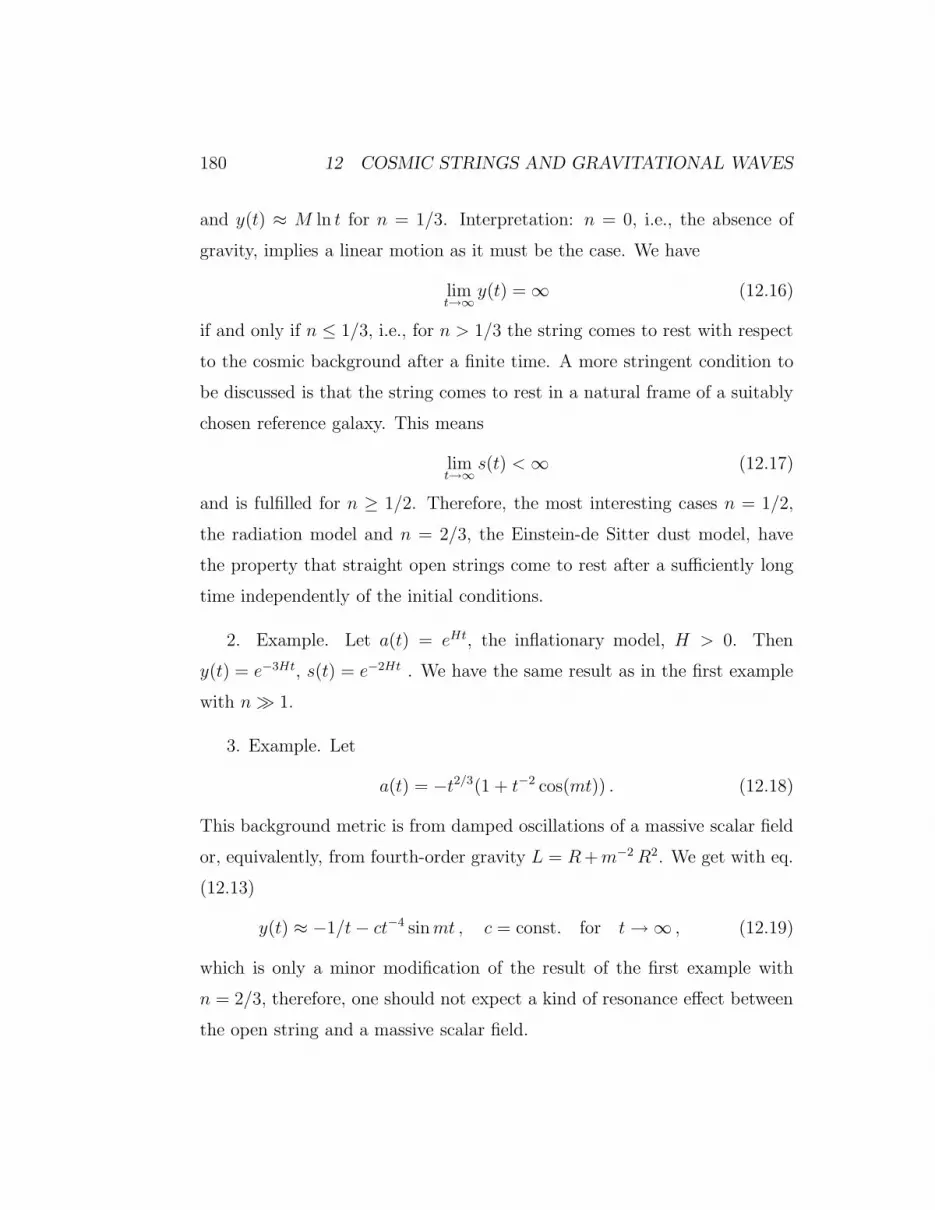
180 12 COSMIC STRINGS AND GRAVITATIONAL WAVES
and y(t) ≈ M ln t for n = 1/3. Interpretation: n = 0, i.e., the absence of
gravity, implies a linear motion as it must be the case. We have
limt→∞
y(t) = ∞ (12.16)
if and only if n ≤ 1/3, i.e., for n > 1/3 the string comes to rest with respect
to the cosmic background after a finite time. A more stringent condition to
be discussed is that the string comes to rest in a natural frame of a suitably
chosen reference galaxy. This means
limt→∞
s(t) <∞ (12.17)
and is fulfilled for n ≥ 1/2. Therefore, the most interesting cases n = 1/2,
the radiation model and n = 2/3, the Einstein-de Sitter dust model, have
the property that straight open strings come to rest after a sufficiently long
time independently of the initial conditions.
2. Example. Let a(t) = eHt, the inflationary model, H > 0. Then
y(t) = e−3Ht, s(t) = e−2Ht . We have the same result as in the first example
with n≫ 1.
3. Example. Let
a(t) = −t2/3(1 + t−2 cos(mt)) . (12.18)
This background metric is from damped oscillations of a massive scalar field
or, equivalently, from fourth-order gravity L = R+m−2R2. We get with eq.
(12.13)
y(t) ≈ −1/t− ct−4 sinmt , c = const. for t→ ∞ , (12.19)
which is only a minor modification of the result of the first example with
n = 2/3, therefore, one should not expect a kind of resonance effect between
the open string and a massive scalar field.

12.3 The string in a Friedmann model 181
12.3.2 The closed string
We insert dy2 + dz2 = dr2 + r2dΦ2 into metric (12.10) and use the spacelike
Killing vector ∂/∂Φ: its trajectories are circles, so we have in mind a closed
string with radius r moving and oscillating in the expanding universe. The
corresponding geodesic equation leads to
d
dλ(−a4r2r) − a2rt2 + a4r(x2 + r2) = 0 , (12.20)
d
dλ(a4r2x) = 0 , (12.21)
t2 − a2(x2 + r2) =1
a2r2, (12.22)
where the dot denotes d/dλ, λ is the natural parameter along the geodesic.
We are mainly interested in solutions not moving into the x-direction, to
understand the oscillating behaviour. Inserting x = 0 into this system of 3
equations and using the fact that always t 6= 0 holds, this system can be
brought into the form
r · r′′a3 − 2rr′a4a′ − r′2a3 + 3rr′a2a′ + a = 0 , (12.23)
where the dash denotes d/dt.
4. Example. Let a = 1, i.e., we have the flat Minkowski spacetime. Then
this equation reduces to
rr′′ = r′2 − 1 . (12.24)
The solution reads
r(t) = r0 cos((t− t0)/r0) , r′ = − sin((t− t0)/r0) . (12.25)
This is the oscillating solution for closed strings. At points t where r = 0,
we have |r′| = 1. These points are the often discussed cusp points of the

182 12 COSMIC STRINGS AND GRAVITATIONAL WAVES
string, where the interior string metric becomes singular and the motion
approximates the velocity of light, cf. Thompson [254].
Let us compare eq. (12.24) with the analogous equation for a positive
definite back-ground metric. It reads
rr′′ = r′2 + 1 (12.26)
and has solutions with cosh instead of cos. This is the usual minimal
surface taken up e.g. by a soap-bubble spanned between two circles.
5. Example. Let a(t) = tn, then we have to solve
rr′′t2n − 2nrr′3t4n−1 − r′2t2n + 3nrr′t2n−1 + 1 = 0 . (12.27)
This equation governs the radial motion of a circle-like closed string in a
Friedmann background. The solutions can be hardly obtained by analytic
methods.
12.4 The string in an anisotropic Kasner background
Now we take as background metric
ds2 = dt2 − a2(t)dx2 − b2(t)dy2 − c2(t)dz2 (12.28)
and ∂/∂x as Killing vector. Astonishingly, the anisotropy has only a minor
influence on the motion of the string, so we get mainly the same formulae as
in the isotropic case: the geodesic equations are
d
dλ(a2b2y) = 0 hence a2b2y = M1 (12.29)
d
dλ(a2c2z) = 0 hence a2c2z = M2 (12.30)
a2t2 − a2c2z2 = 1 (12.31)

12.5 The string in a gravitational wave 183
and can be integrated to yield for M1M2 6= 0
y(r) =∫
(
a2b2
M21
+M2
2
M21
· b2
c2+ 1
)−1/2dt
b(t). (12.32)
The equation for z(t) can be obtained from this equation by interchanging
b↔ c and M1 ↔ M2.
For the Kasner metric we have a = tp, b = tq, c = tr, p + q + r =
p2 + q2 + r2 = 1. We get
y(r) =∫
dt
tq√t2(p+q) + t2(q−r) + 1
. (12.33)
The behaviour for t → ∞ in dependence of the values p, q, r can be seen
from this equation.
12.5 The string in a gravitational wave
As background metric we use the plane-wave ansatz
ds2 = 2dudv + p2(u)dy2 + q2(u)dz2 . (12.34)
This metric represents a solution of Einstein’s vacuum equation if
q d2p/du2 + p d2q/du2 = 0 . (12.35)
Let us take ∂/∂y as Killing vector. Then the geodesic equations for the
auxiliary metric are
d
dλ(p2u) = 0 hence p2u = M1 6= 0 , (12.36)
d
dλ(p2q2z) = 0 hence p2q2z = M2 , (12.37)
−2p2uv − p2q2z2 = 1 . (12.38)

184 12 COSMIC STRINGS AND GRAVITATIONAL WAVES
If we take u as new independent variable, which is possible because of u 6= 0,
we get the solutions
z(u) =M2
M1
∫
du′
q2(u′),
v(u) =−M2
2
2M21
∫
(
1
q2(u′)− p2(u′)
)
du′ . (12.39)
As an example let us take
p(u) = sin u , q(u) = sinh u (12.40)
which produces a vacuum solution. With this choice of p and q we get
z(u) = M coth u , v(u) = −M2(4 cothu+ sin 2u− 2u)/8 . (12.41)
Another Killing vector of the plane wave is ∂/∂v, but it is a null Killing
vector and so the reduction used above does not work. But there exists a
further non-null Killing vector of this plane wave: It reads
ki = (0, y,H, 0), where H = −∫
p−2du . (12.42)
By a coordinate transformation
u = t y = w · e−G G(u) =∫
du
p2H
z = k v = x+1
2He−2G(w2 − 1) (12.43)
we get the form
ds2 = e−2Gp2dw2 + 2dxdt+e−2G
p2H2dt2 + q2dk2 (12.44)
and have to solve the equations
d
dλ
(
p2q2e−2Gk)
= 0 ,d
dλ
(
p2e−2Gt)
= 0 ,
−p2q2e−2Gk2 − 1
H2e−4Gt2 − 2p2e−2Gxt = 1 . (12.45)

12.5 The string in a gravitational wave 185
For the special case k = 0 one has finally
x(t) = −1
2
∫
e−2G
(
p2
M22
+1
H2p2
)
dt . (12.46)
Let us suppose a spatially flat Friedmann model eq. (12.10) with scale
factor a(t) = tn, and n = 2/3, representing the Einstein-de Sitter dust model,
or n = 1/2, representing the radiation model. There we consider an open
string which is only a little bit curved such that the approximation of a
straight string is applicable. At time t = t0 > 0 we can prescribe place and
initial velocity v0 of the string arbitrarily and get for t→ ∞ the behaviour
s(t) ≈ const +M(v0)t1−2n (12.47)
where s denotes the natural distance from the origin. That means, for the
cases n = 2/3 and = 1/2 we are interested in, the string comes to rest for
large values t at a finite distance from the origin.
We compare this result with the analogous motion of a point-particle in
the same background: in the same approximation we get
s(t) ≈ const +M(v0)t1−n , (12.48)
i.e., |s| → ∞ as t → ∞, a totally other type of motion. It should be
mentioned that in the absence of gravity, i.e., n = 0, both motions are of the
same type, but otherwise not.
The remaining calculations above indicate that the interaction of the
motion of the string with scalar field oscillations, with anisotropy, and with
gravitational waves is quite weak, we did not find any type of resonance
effects.
187
13 Bibliography
[1] Altshuler, B.: 1990, Class. Quant. Grav. 7, 189. 123
[2] Amendola, L.: 1993, Phys. Lett. B 301, 175. 1999, Phys. Rev. D 60,043501. 129
[3] Amendola, L., Battaglia Mayer, A., Capozziello, S., Gottlober, S.,Muller, V., Occhionero, F., Schmidt, H.-J.: 1993, Class. Quant. Grav.10, L43. 126
[4] Amendola, L., Capozziello, S., Litterio, M., Occhionero, F.: 1992,Phys. Rev. D 45, 417. 126
[5] Anandan, J.: 1983, in: Hu, N., ed., Proc. 3. Marcel Grossmann Meeting
B, Amsterdam NHPC, 941. 160
[6] Anderson, P.: 1986, Phys. Lett. B 169, 31. 111
[7] Arnowitt, R., Deser, S., Misner, C.: 1962, in: Witten, E., ed., Gravi-
tation, an introduction to current research, Wiley New York. 123
[8] Bach, R.: 1921, Math. Zeitschr. 9, 110. 145, 147, 156
[9] Bachmann, M., Schmidt, H.-J.: 2000, Phys. Rev. D 62, 043515; gr-qc/9912068. 83
[10] Barabash, O., Shtanov, Y.: 1999, Phys. Rev. D 60, 064008; astro-ph/9904144. 159
[11] Barraco, D., Hamity, V.: 2000, Phys. Rev. D 62, 044027. 1999, Gen.Relat. Grav. 31, 213. 112
[12] Barrow, J.: 1986, Phys. Lett. B 180, 335. 1987, Phys. Lett. B 187, 12.123, 125, 126, 136
[13] Barrow, J., Gotz, G.: 1989, Class. Quant. Grav. 6, 1253. 122, 123
[14] Barrow, J., Matzner, R.: 1980, Phys. Rev. D 21, 336. 59, 74
[15] Barrow, J., Saich, P.: 1990, Phys. Lett. B 249, 406. 126

188
[16] Barrow, J., Sirousse-Zia, H.: 1989, Phys. Rev. D 39, 2187. Erratum1990, D 41, 1362. 61, 125, 127, 139
[17] Barrow, J., Tipler, F.: 1988, The anthropic cosmological principle,Cambridge University Press. 75
[18] Battaglia Mayer, A., Schmidt, H.-J.: 1993, Class. Quant. Grav. 10,2441. 128
[19] Belinsky, V., Grishchuk, L., Khalatnikov, I., Zeldovich, Y.: 1985, Phys.Lett. B 155, 232. 89
[20] Belinsky, V., Grishchuk, L., Zeldovich, Y., Khalatnikov, I.: 1985, Zh.Eksp. Teor. Fiz. 89, 346. 71, 74
[21] Belinsky, V., Khalatnikov, I.: 1987, Zh. Eksp. Teor. Fiz. 93, 784. 59,
74
[22] Belinsky, V., Lifshitz, E., Khalatnikov, I.: 1972, Sov. Phys. JETP 35,838. 59, 125 7
[23] Bergmann, O.: 1981, Phys. Lett. A 82, 383. 9
[24] Berkin, A.: 1990, Phys. Rev. D 42, 1016. 1991, Phys. Rev. D 44, 1020.127, 129
[25] Berkin, A., Maeda, K.: 1990, Phys. Lett. B 245, 348. 1991, Phys. Rev.D 44, 1691. 129, 164
[26] Bicak, J: 2000, Lect. Notes Phys. 540, 1-126; gr-qc/0004016. 19
[27] Bicak, J., Podolsky, J.: 1992, in: Abstracts Conf. Gen. Relat. 13,Cordoba, 12. 1995, Phys. Rev. D 52, 887. 127
[28] Bicak, J., Pravda, V.: 1998, Class. Quant. Grav. 15, 1539. 44
[29] Bicknell, G.: 1974, J. Phys. A 7, 341. 1061. 61, 87, 103, 139
[30] Bleyer, U., Liebscher, D.-E., Schmidt, H.-J., Zhuk, A.: 1990, Wiss.Zeitschr. d. Univ. Jena, Naturwiss. Reihe 39, 20. 85
7The authors are in alphabetical order of the original Russian language version.

189
[31] Bleyer, U., Schmidt, H.-J.: 1990, Int. J. Mod. Phys. A 5 (1990) 4671.121
[32] Bojowald, M., Kastrup, H., Schramm, F., Strobl, T.: 2000, Phys. Rev.D 62 (2000) 044026. 111
[33] Borde, A.: 1994, Phys. Rev. D 50, 3692. 124
[34] Borde, A., Vilenkin, A.: 1994, Phys. Rev. Lett. 72, 3305. 124
[35] Borzeszkowski, H. v.: 1981, Ann. Phys. (Leipz.) 38, 239. 146
[36] Borzeszkowski, H. v., Treder, H.-J.: 1994, Found. Phys. 24, 949. 127
[37] Borzeszkowski, H. v., Treder, H.-J., Yourgrau, W.: 1978, Ann. Phys.(Leipz.) 35, 471. 146, 156, 160
[38] Boulware, D.: 1973, Phys. Rev. D 8, 2363. 45
[39] Brandenberger, R.: 1987, Int. J. Mod. Phys. A 2, 77. 176
[40] Brauer, U., Rendall, A., Reula, O.: 1994, Class. Quant. Grav. 11, 2283.123
[41] Breizman, B., Gurovich, V., Sokolov, V.: 1970, Zh. Eksp. Teor. Fiz.59, 288. 125
[42] Buchdahl, H.: 1951, Acta Math. 85, 63. 128, 134, 164
[43] Buchdahl, H.: 1962, Nuovo Cim. 23, 141. 92
[44] Burd, A.: 1993, Class. Quant. Grav. 10, 1495. 123
[45] Burd, A., Barrow, J.: 1988, Nucl. Phys. B 308, 929. 122
[46] Calzetta, E.: 1989, Class. Quant. Grav. 6, L227. 76, 140
[47] Calzetta, E., Sakellariadou, M.: 1992, Phys. Rev. D 45, 2802. 127
[48] Campanelli, M., Lousto, C.: 1996, Phys. Rev. D 54, 3854. 112
[49] Capozziello, S., Lambiase, G.: 2000, Gen. Relat. Grav. 32, 295. 673.112
[50] Carfora, M., Marzuoli, A.: 1984, Phys. Rev. Lett. 53, 2445. 106

190
[51] Carmeli, M., Charach, C. : 1980, Phys. Lett. A 75, 333. 9
[52] Chiba, T., Maeda, K.: 1994, Phys. Rev. D 50, 4903. 124
[53] Cohen, M., Cohen, J.: 1971, in: Kuper, C., ed., Relativity and Gravi-
tation, Gordon and Breach New York, 99. 51
[54] Coley, A., Tavakol, R.: 1992, Gen. Relat. Grav. 24, 835. 125
[55] Collins, C., Szafron, D.: 1981, J. Math. Phys. 22, 543. 9
[56] Contreras, C., Herrera, R., del Campo, S.: 1995, Phys. Rev. D 52,4349. 127
[57] Cotsakis, S., Demaret, J., De Rop, Y., Querella, L.: 1993, Phys. Rev.D 48, 4595. 125
[58] Cotsakis, S., Flessas, G.: 1993, Phys. Lett. B 319, 69. 127
[59] Coule, D.: 2000, Phys. Rev. D 62, 124010; gr-qc/0007037. 1995, Class.Quant. Grav. 12, 455; gr-qc/9408026. 83
[60] Dautcourt, G. : 1963, Math. Nachr. 27, 277. 1964, Acta Phys. Polon.25, 637. 45, 54, 164
[61] Demaret, J., Querella, L., Scheen, C.: 1999, Class. Quant. Grav. 16,749. Demaret, J., Querella, L.: 1995, Class. Quant. Grav. 12, 3085.112
[62] Demianski, M.: 1984, Nature 307, 140. 123
[63] Denisov, V. I.: 1972, J. Exp. Teor. Phys. 62, 1990. 45
[64] Dzhunushaliev, V., Schmidt, H.-J.: 2000, J. Math. Phys. 41, 3007;gr-qc/9908049. 156
[65] Ehlers, J., Kundt, W.: 1962, in: Witten, E., ed., Gravitation, an in-
troduction to current research, Wiley New York, 49. 36
[66] Einstein, A.: 1914, Sitzungsber. Akad. d. Wiss. Berlin, 1030. 1916,Sitzungsber. Akad. d. Wiss. Berlin, 688. 1918, Sitzungsber. Akad. d.Wiss. Berlin, 154. 1921, Sitzungsber. Akad. d. Wiss. Berlin, 261. 35,
145

191
[67] Einstein, A.: 1939, Ann. Math. 40, 922. 46
[68] Einstein, A., De Sitter, W.: 1932, Proc. Nat. Acad. Sci. 18, 213. 19,
24
[69] Einstein, A., Pauli, W.: 1943, Ann. Math. 44, 131. 146
[70] Ellis, G.: 1984, Ann. Rev. Astron. Astrophys. 22, 157. Ellis, G.: 1967,J. Math. Phys. 8, 1171. 13, 104
[71] Esteban, E., Kazanas, D.: 2001, Gen. Relat. Grav. 33, 1281. 156
[72] Fabris, J., Pelinson, A., Shapiro, I.: 2001, Nucl. Phys. B 597, 539;hep-th/0009197. 39
[73] Fabris, J., Reuter, S.: 2000, Gen. Relat. Grav. 32, 1345. 83
[74] Faraoni, V., Gunzig, E., Nardone, P.: 1999, Fund. Cosmic Physics 20,121; gr-qc/9811047. 112
[75] Feldman, H.: 1990, Phys. Lett. B 249, 200. 127
[76] Ferraris, M.: 1986, in: Fabbri, R., Modugno, M., eds., VI Conv. Naz.
Rel. Gen. e Fisica della Grav., Pitagora Edit. Bologna, 127. 110
[77] Fiedler, B., Schimming, R.: 1980, Rep. Math. Phys. 17, 15. 39
[78] Fiedler, B., Schimming, R.: 1983, Astron. Nachr. 304, 221. 146, 148,
149, 155
[79] Frehland, E.: 1972, Ann. Phys. (Leipz.) 28, 91. 45
[80] Frolov, V., Serebriany, E.: 1987, Phys. Rev. D 35, 3779. 176
[81] Frolov, V., Skarzhinsky, V., Zelnikov, A., Heinrich, O.: 1988, PreprintPotsdam-Babelsberg, PRE-ZIAP 88-14. 176
[82] Fulling, S.: 1973, Phys. Rev. D 7, 2850. 58
[83] Fulling, S., Parker, L.: 1974, Ann. Phys. NY 87, 176. 58
[84] Gemelli, G.: 1997, Gen. Relat. Grav. 29, 1163. 39
[85] Gerbal, D., Sirousse-Zia, H.: 1989, C. R. Acad. Sci. Paris 309, 353.165
192
[86] Geroch, R.: 1969, Commun. Math. Phys. 13, 180. 42, 64, 73, 115
[87] Geroch, R., Traschen, J.: 1987, Phys. Rev. D 36, 1017. 176
[88] Gibbons, G. and Hawking, S.: 1977, Phys. Rev. D 15, 2738. 123
[89] Gibbons, G., Hawking, S., Stewart, J.: 1987, Nucl. Phys. B 281, 736.85
[90] Goenner, H.: 1987, in: MacCallum, M., ed., Proc. 11th Int. Conf. Gen.
Rel. Grav., Cambridge University Press, 262. 110
[91] Gorbatenko, M., Pushkin, A., Schmidt, H.-J.: 2002, Gen. Relat. Grav.34, in press; gr-qc/0106025. 156
[92] Gottlober, S.: 1984, Ann. Phys. (Leipz.) 41, 45. 1984, Astron. Nachr.305, 1. 1987, Astrophys. Space Sc. 132, 191.59, 107, 109
[93] Gottlober, S., Muller, V.: 1987, Class. Quant. Grav. 4, 1427. 59
[94] Gottlober, S., Muller, V., Schmidt, H.-J.: 1991, Astron. Nachr. 312,291. 129, 164
[95] Gottlober, S., Muller, V., Schmidt, H.-J., Starobinsky, A.: 1992, Int.J. Mod. Phys. D 1, 257. 126
[96] Gottlober, S., Schmidt, H.-J.: 1984, Potsdamer Forschungen B 43, 117.59
[97] Gottlober, S., Schmidt, H.-J, Starobinsky, A.: 1990, Class. QuantumGrav. 7, 893. 129, 164, 165
[98] Green, M., Schwarz, J., Witten, E.: 1987, Superstring theory, Cam-bridge University Press. 175
[99] Griffiths, J.: 1995, Gen. Relat. Grav. 27, 905. 13, 26
[100] Grishchuk, L., Sidorov, J.: 1988, in: Markov, M., ed., Proc. 4. Sem.
Quantum Gravity Moscow, WSPC Singapore, 700. 85
[101] Gurovich, V., Schmidt, H.-J., Tokareva, I.: 2001, Gen. Relat. Grav.33, 591; gr-qc/0007046. 83

193
[102] Hall, G.: 1988, Gen. Relat. Grav. 20, 671. 1990, J. Math. Phys. 31,1198. 1991, Diff. Geom. Appl. 1, 35. 40
[103] Halliwell, J., Hawking, S.: 1985, in: Markov, M., ed., Proc. 3. Sem.
Quantum Gravity Moscow, WSPC Singapore, 509. 85
[104] Harvey, A.: 1990, Class. Quant. Grav. 7, 715. 41
[105] Havas, P.: 1977, Gen. Relat. Grav. 8, 631. 160
[106] Hawking, S.: 1984, Nucl. Phys. B 239, 257. 1984, in: De Witt, B.,Stora, R., eds., Relativity, Groups, and Topology II, North Holland PCAmsterdam. 59
[107] Hawking, S., Ellis, G.: 1973, The large scale structure of space-time,Cambridge University Press. 36
[108] Hawking, S., Luttrell, J.: 1984, Nucl. Phys. B 247, 250. 59
[109] Hawking, S., Moss, I.: 1982, Phys. Lett. B 110, 35. 123
[110] Hehl, F., McCrea, J., Mielke, E., Ne’eman, Y.: 1995, Phys. Repts. 258,1. 112
[111] Hindawi, A., Ovrut, B., Waldram, D.: 1996, Phys. Rev. D 53, 5583.112
[112] Hoyle, F., Narlikar, J.: 1963, Proc. R. Soc. Lond. A 273, 1. 123
[113] Hubner, P., Ehlers, J.: 1991, Class. Quant. Grav. 8, 333. 123
[114] Hwang, J.: 1991, Class. Quant. Grav. 8, L133. 126
[115] Hwang, J., Noh, H.: 2001, Phys. Lett. B 506, 13. 112
[116] Ishihara, R.: 1986, Phys. Lett. B 179, 217. 112
[117] Israel, W.: 1966, Nuovo Cim. B 44, 1. 45, 54
[118] Israel, W., Stewart, J.: 1980, in: Held, A., ed., General Relativity and
Gravitation II, Plenum New York, 491. 46
[119] Ivashchuk, V., Melnikov, V.: 1995, Grav. Cosmol. 1, 133; hep-th/9503223. 111

194
[120] Jakubiec, A., Kijowski, J.: 1988, Phys. Rev. D 37, 1406. 1989, J. Math.Phys. 30, 1073. 110
[121] Jankiewicz, C.: 1981, Acta Phys. Polon. 13, 859. 160
[122] Jensen, L., Stein-Schabes, J.: 1987, Phys. Rev. D 35, 1146. 127
[123] Jordan, P., Ehlers, J., Kundt, W.: 1960, Abh. Akad. Wiss. Mainz,Math./Nat. Kl. 2, 21. 36
[124] Kao, W.: 2000, Phys. Rev. D 61, 047501. 112
[125] Kerner, R.: 1982, Gen. Relat. Grav. 14, 453. 94
[126] Kiefer, C.: 2001, in: Janke, W., Pelster, A., Schmidt, H.-J., Bachmann,M., eds., Fluctuating paths and fields, WSPC Singapore, 729. 83
[127] Kirsten, K., Cognola, G., Vanzo, L.: 1993, Phys. Rev. D 48, 2813. 129
[128] Kleinert, H., Schmidt, H.-J.: 2000, Cosmology with curvature–saturated
gravitational lagrangian R/√
1 + l4R2, Preprint gr-qc/0006074. 112
[129] Kluske, S., Schmidt, H.-J.: 1996, Astron. Nachr. 317, 337; gr-qc/9503021. 121
[130] Kofman, L., Linde, A., Starobinsky, A.: 1996, Phys. Rev. Lett. 76,1011. 123
[131] Kottler, F.: 1918, Ann. Phys. (Leipz.) 56, 410. 128
[132] Kowalski, O.: 1993, Nagoya Math. J. 132, 1. 31
[133] Kowalski, O.,. Nikcevic, S.: 1995, On Ricci eigenvalues of locally ho-
mogeneous Riemannian 3–manifolds, preprint. 32
[134] Kramer, D., Stephani, H., Herlt, E., MacCallum, M.: 1980, Exact
solutions of Einstein’s field equations, Verl. d. Wiss. Berlin. 11
[135] Krasilnikov, V. A., Pavlov, V. I.: 1972, Vestnik Univ. Moskau 27, 235.46
[136] Krasinski, A.: 1980, Proc. Conf. General Relativity GR 9 Jena, 44. 9

195
[137] Krasinski, A.: 1997, Inhomogeneous Cosmological Models, CambridgeUniversity Press. 9, 19
[138] Kuchar, K.: 1968, Czech. J. Phys. B 18, 435. 45
[139] Kung, J.: 1996, Phys. Rev. D 53, 3017. 112
[140] Lake, K.: 1979, Phys. Rev. D 19, 2847. 1981, Lett. Nuovo Cim. 30,186. 1993, J. Math. Phys. 34, 5900. 41, 42, 45, 46
[141] Lanczos, K.: 1924, Ann. Phys. (Leipz.) 74, 518. 45
[142] Lee, C. W.: 1978, Proc. R. Soc. Lond. A 364, 295. 10
[143] Lopez, C.: 1981, Nuovo Cim. B 66, 17. 45
[144] Lu, M. and Wise, M.: 1993, Phys. Rev. D 47, R3095. 129
[145] Lukash, V. N., Schmidt, H.-J.: 1988, Astron. Nachr. 309, 25. 71, 72,
107, 109
[146] MacCallum, M.: 1971, Commun. Math. Phys. 20, 57. 1972, Phys. Lett.A 40, 385. 15, 127, 139
[147] MacCallum, M., Stewart, J., Schmidt, B.: 1970, Commun. Math. Phys.17, 343. 127, 139
[148] Macias, A.: 1999, Gen. Relat. Grav. 31, 653. 83
[149] Madsen, M., Ellis, G.: 1988, Mon. Not. R. Astron. Soc. 234, 67. 76
[150] Maeda, K.: 1988, Phys. Rev. D 37, 858. 1989, Phys. Rev. D 39, 3159.126
[151] Maeda, K., Sato, H.: 1983, Progr. Theor. Phys. 70, 772. 46, 54
[152] Maeda, K., Stein-Schabes, J., Futamase, T.: 1989, Phys. Rev. D 39,2848. 126
[153] Martin, G., Mazzitelli, F.: 1994, Phys. Rev. D 50, R613. 129
[154] Mignemi, S.: 1996, Ann. Phys. NY 245 (1996) 23. 111
[155] Mijic, M., Stein-Schabes, J.: 1988, Phys. Lett. B 203, 353. 126

196
[156] Mirzabekian, A., Vilkovisky, G., Zhytnikov, V.: 1996, Phys. Lett. B369, 215. 142
[157] Mondaini, R., Vilar, L.: 1993, Int. J. Mod. Phys. D 2, 477. 124
[158] Mongan, T.: 2001, Gen. Relat. Grav. 33, 1415. 83
[159] Moniz, P.: 1993, Phys. Rev. D 47, 4315. 128
[160] Morgan, L., Morgan, T.: 1970, Phys. Rev. D 2, 2756. 45
[161] Morris, M.: 1989, Phys. Rev. D 39, 1511. 127
[162] Muller, V.: 1986, Ann. Phys. (Leipz.) 43, 67. 125
[163] Muller, V., Schmidt, H.-J.: 1985, Gen. Relat. Grav. 17, 769. 1989,Gen. Relat. Grav. 21, 489. 28, 71, 98, 99, 105
[164] Muller, V., Schmidt, H.-J., Starobinsky, A.: 1988, Phys. Lett. B 202,198. 125
[165] Murphy, G.: 1973, Phys. Rev. D 8, 4231. 123
[166] Nakao, K., Nakamura, T., Oohara, K., Maeda, K.: 1991, Phys. Rev. D43, 1788. 127
[167] Nakao, K., Maeda, K., Nakamura, T., Oohara, K.: 1993, Phys. Rev. D47, 3194 (1993). 127
[168] Nakao, K., Shiromizu, T., Maeda, K.: 1994, Class. Quant. Grav. 11,2059. 123
[169] Nariai, H.: 1973, Progr. Theor. Phys. 49, 165. 1974, Progr. Theor.Phys. 51, 613. 87
[170] Neugebauer, G.: 1980, Relativistische Thermodynamik, Akad.-Verl.Berlin. 46
[171] Nielsen, H., Olesen, P.: 1973, Nucl. Phys. B 61, 45. 176
[172] Novotny, J.: 1984, Coll. J. Bolyai Math. Soc. Diff. Geom. Debrecen 46,959. 94

197
[173] Oleak, H.: 1974, Astron. Nachr. 295, 107. 1987, Ann. Phys. (Leipz.)44, 74. 124
[174] Ono, S., Kondo, S.: 1960, in: Flugge, S., ed., Handbuch der Physik 10,Springer Berlin, 134. 46, 47
[175] Page, D.: 1984, Class. Quant. Grav. 1, 417. 1987, Phys. Rev. D 36,1607. 57, 59, 61, 67, 74
[176] Paiva, F., Reboucas, M., Hall, G., MacCallum, M.: 1998, Class. Quant.Grav. 15, 1031. 44
[177] Papapetrou, A., Hamoui, A.: 1968, Ann. Inst. H. Poincare A 9, 179.45
[178] Papapetrou, A., Treder, H.-J.: 1959, Math. Nachr. 20, 53. 45
[179] Parker, L., Raval, A.: 1999, Phys. Rev. D 60 063512. 83
[180] Pechlaner, E., Sexl, R.: 1966, Commun. Math. Phys. 2, 165. 149, 160
[181] Peter, P., Polarski, D., Starobinsky, A.: 1994, Phys. Rev. D 50, 4827.123
[182] Pimentel, L.: 2001, Gen. Relat. Grav. 33, 781; gr-qc/0009046. 83
[183] Polijevktov-Nikoladze, N.: 1967, J. Exp. Teor. Fiziki 52, 1360. 160
[184] Pollney, D., Skea, J., D’Inverno, R.: 2000, Class. Quant. Grav. 17,2885. 44
[185] Pollock, M.: 1987, Phys. Lett. B 192, 59. 125, 126
[186] Prigogine, I., Geheniau, J., Gunzig, E., Nardone, P.: 1988, Proc. Nat.Acad. Sci. 85, 7428. 1989, Gen. Relat. Grav. 21, 767. 1989, Int. J.Theor. Phys. 28, 927. 124
[187] Quandt, I., Schmidt, H.-J.: 1991, Astron. Nachr. 312, 97; gr-qc/0109005. 128, 159, 171
[188] Rainer, M.: 1995, Grav. Cosmol. 1, 121. 1995, Int. J. Mod. Phys. D 4,397. 44

198
[189] Rainer, M., Schmidt, H.-J.: 1995, Gen. Relat. Grav. 27, 1265; gr-qc/9507013. 14, 32, 33, 34
[190] Rainer, M., Zhuk, A.: 2000, Gen. Relat. Grav. 32, 79. 111
[191] Robinson, A.: 1966, Non-standard analysis, North Holland Amster-dam. 152
[192] Rogers, B., Isaacson, J.: 1991, Nucl. Phys. B 364, 381. 1992, Nucl.Phys. B 368, 415. 127
[193] Romero, C., Tavakol, R., Zalaletdinov, R.: 1996, Gen. Relat. Grav. 28,365. 112
[194] Saa, A.: 1996, J. Math. Phys. 37, 2346. 122
[195] Sakharov, A.: 2000, Gen. Relat. Grav. 32, 365; 1967, Dokl. Akad. NaukSSSR 177, 70. 128
[196] Sanchez, M.: 1998, Gen. Relat. Grav. 30, 915. 29
[197] Sanders, R. : 1984, Astron. Astrophys. 136, L21. 1986, Astrophys. J.154, 135. 165
[198] Sanyal, A., Modak, B.: 2001, Phys. Rev. D 63, 064021; gr-qc/0107001.83
[199] Schimming, R., Schmidt, H.-J.: 1990, NTM-Schriftenr. Geschichte derNaturwiss., Technik, Medizin 27, 41. 128
[200] Schmidt, H.-J.: 1982, Astron. Nachr. 303, 227; gr-qc/0105104. 9, 15
[201] Schmidt, H.-J.: 1982, Astron. Nachr. 303, 283; gr-qc/0105105. 19
[202] Schmidt, H.-J.: 1983, in: Bertotti, B., ed., Contributed Papers Conf.
General Relativity GR10 Padova 1, 339. 45, 46
[203] Schmidt, H.-J.: 1984, Gen. Relat. Grav. 16, 1053; gr-qc/0105106. 46
[204] Schmidt, H.-J.: 1984, Ann. Phys. (Leipz.) 41, 435; gr-qc/0105108. 156
[205] Schmidt, H.-J.: 1985, Astron. Nachr. 306, 67; gr-qc/0105107. 145

199
[206] Schmidt, H.-J.: 1986, Conf. General Relativity GR 11 Stockholm, 117.87
[207] Schmidt, H.-J.: 1986, Physikalische Konsequenzen von Feldgleichun-
gen vierter Ordnung bei der Beschreibung des fruhen Universums und
isolierter Gravitationsfelder, Thesis B, Akad. d. Wiss. Berlin; 2nd ed.:1994, Tectum-Verlag Marburg. 87, 88, 89, 106
[208] Schmidt, H.-J.: 1986, Astron. Nachr. 307, 339; gr-qc/0106037. 159,
170
[209] Schmidt, H.-J.: 1987, Astron. Nachr. 308, 183; gr-qc/0106035. 87, 103,
110
[210] Schmidt, H.-J.: 1987, J. Math. Phys. 28, 1928. Addendum: 1988, J.Math. Phys. 29, 1264. 14, 42, 73
[211] Schmidt, H.-J.: 1988, Class. Quant. Grav. 5, 233. 110
[212] Schmidt, H.-J.: 1988, Astron. Nachr. 309, 307; gr-qc/0106036. 87
[213] Schmidt, H.-J.: 1988, Phys. Lett. B 214, 519. 75, 121
[214] Schmidt, H.-J.: 1989, Class. Quant. Grav. 6, 557. 1994, Phys. Rev. D50, 5452; gr-qc/0109006. 1995, Phys. Rev. D 52, 6198; gr-qc/0106034.112
[215] Schmidt, H.-J.: 1990, Astron. Nachr. 311, 99; gr-qc/0108087. 58
[216] Schmidt, H.-J.: 1990, Astron. Nachr. 311, 165; gr-qc/0109004. 113
[217] Schmidt, H.-J.: 1990, in: Janyska, J., Krupka, D., eds., Proc. Conf.
Brno, Diff. Geom. Appl., WSPC Singapore, 405; gr-qc/0109001. 77
[218] Schmidt, H.-J.: 1990, Class. Quantum Grav. 7, 1023. 128, 139, 164,
165, 172
[219] Schmidt, H.-J.: 1992, in: Sato, H., Nakamura, T., eds., Proc. Sixth
Marcel Grossmann Meeting on General Relativity Kyoto, WSPC Sin-gapore, 92. 129
[220] Schmidt, H.-J.: 1993, Gen. Relat. Grav. 25, 87. Erratum 25, 863. 127

200
[221] Schmidt, H.-J.: 1994, Phys. Rev. D 49, 6354. Erratum: 1996, Phys.Rev. D 54, 7906; gr-qc/9404038. 27
[222] Schmidt, H.-J.: 1995, Abstr. Conf. General Relativity GR 14 Florence;gr-qc/0109007. 31
[223] Schmidt, H.-J.: 1996, in: Janyska, J., Kolar, I., Slovak, J., eds., Proc.
Conf. Brno Diff. Geom. Appl., 119; gr-qc/0109008. 31
[224] Schmidt, H.-J.: 1996, in: Sardanashvily, G., ed., New frontiers in grav-
itation, Hadronic Press Palm Harbor, 337; gr-qc/9404037. 31, 44
[225] Schmidt, H.-J.: 1996, Gen. Relat. Grav. 28, 899; gr-qc/9512006. 25
[226] Schmidt, H.-J.: 1997, Grav. Cosmol. 3, 185; gr-qc/9709071. 19
[227] Schmidt, H.-J.: 1998, Int. J. Theor. Phys. 37, 691; gr-qc/9512007. 29
[228] Schmidt, H.-J.: 1998, in: Rainer, M., Schmidt, H.-J., eds., Current top-
ics in mathematical cosmology, WSPC Singapore, 288; gr-qc/9808060.1993, Fortschr. Phys. 41, 179. 27
[229] Schmidt, H.-J.: 1999, Gen. Relat. Grav. 31, 1187; gr-qc/9905051. 111
[230] Schmidt, H.-J: 2000, Ann. Phys. (Leipz.) 9, SI-158. gr-qc/9905103. 44
[231] Schmidt, H.-J., Muller, V.: 1985, Gen. Relat. Grav. 17, 971. 150
[232] Schmidt, H.-J., Semmelmann, U.: 1989, Astron. Nachr. 310, 103; gr-qc/0106089. 175
[233] Senovilla, J.: 1998, Gen. Relat. Grav. 30, 701. 27
[234] Schrodinger, E.: 1938, Comment. Vatican. Acad. 2, 321. 1956, Expand-
ing Universes, Cambridge University Press. 58
[235] Shibata, M., Nakao, K., Nakamura, T., Maeda, K.: 1994, Phys. Rev.D 50, 708. 124
[236] Shinkai, H., Maeda, K.: 1993, Phys. Rev. D 48, 3910. 1994, Phys. Rev.D 49, 6367. 127
[237] Shiromizu, T., Nakao, K., Kodama, H., Maeda, K.: 1993, Phys. Rev.D 47, R3099. 124, 127

201
[238] Singh, T., Padmanabhan, T.: 1988, Int. J. Mod. Phys. A 3, 1593. 75
[239] Sirousse-Zia, H.: 1982, Gen. Relat. Grav. 14, 751. 125
[240] Spero, A., Baierlein, R.: 1978, J. Math. Phys. 19, 1324. 9
[241] Spindel, P.: 1994, Int. J. Mod. Phys. D 3, 273. 125, 127, 139
[242] Stacey, F., Tuck, G., Holding, S., Maher, A., Morris, D.: 1981, Phys.Rev. D 23, 1683. 165
[243] Starobinsky, A.: 1978, Pis’ma Astron. Zh. 4, 155. 58, 74, 107
[244] Starobinsky, A.: 1983, Sov. Phys. JETP Lett. 37, 66. 126, 127
[245] Starobinsky, A., Schmidt, H.-J.: 1987, Class. Quant. Grav. 4, 695. 61,
103, 106, 127
[246] Starobinsky, A., Tsujikawa, S., Yokoyama, J: 2001, Cosmological per-
turbations from multi-field inflation in generalized Einstein theories,astro-ph/0107555; Nucl. Phys. B in press. 112
[247] Stein-Schabes, J., Burd, A.: 1988, Phys. Rev. D 37, 1401. 179
[248] Stelle, K.: 1977, Phys. Rev. D 16, 953. 90, 122, 128
[249] Stelle, K.: 1978, Gen. Relat. Grav. 9, 353. 146, 149, 160, 163, 164,
170
[250] Stephani, H.: 1982, General Relativity, Cambridge University Press. 7,
36, 164
[251] Szekeres, P.: 1975, Commun. Math. Phys. 41, 55. 9, 21, 25
[252] Taub, A.: 1980, J. Math. Phys. 21, 1423. 49
[253] Teyssandier, P.: 1989, Class. Quant. Grav. 6, 219. 164
[254] Thompson, J.: 1988, Phys. Rev. D 37, 283. 182
[255] Thomson, W. (Lord Kelvin): 1858, Proc. R. Soc. London 9, 255. 47
[256] Tolman, R. C.: 1934, Relativity Thermodynamics and Cosmology,Clarendon Press Oxford. 19

202
[257] Treder, H.-J.: 1975, Ann. Phys. (Leipz.) 32, 383. 1977, in: Brauer, W.,ed., 75 Jahre Quantentheorie, Akad.-Verl. Berlin, 279. 1991, Found.Phys. 21, 283. 129, 146
[258] Turner, M.: 1983, Phys. Rev. D 28, 1243. 59
[259] Turner, M., Widrow, L.: 1988, Phys. Rev. D 37, 3428. 75
[260] Urbandtke, H.: 1972, Acta Physica Austriaca 35, 1. 45
[261] Vilenkin, A.: 1985, Phys. Rep. 121, 263. 175
[262] Vilenkin, A.: 1992, Phys. Rev. D 46, 2355. 124
[263] Vilkovisky, G.: 1992, Class. Quant. Grav. 9, 895. 128, 129
[264] Voorhees, B.: 1972, Phys. Rev. D 5, 2413. 45
[265] Wainwright, J.: 1981, J. Phys. A 14, 1131. 9, 19
[266] Wands, D.: 1994, Class. Quant. Grav. 11, 269. 129
[267] Weinberg, S.: 1979, in: Hawking, S., Israel, W., eds., General Relativ-
ity, Cambridge University Press., 790. 105
[268] Weyl, H.: 1919, Ann. Phys. (Leipz.) 59, 101. 1921, Raum, Zeit, Ma-
terie, Springer Berlin. 145, 156
[269] Weyl, H.: 1927, Handbuch der Philosophie, chapter “Philosophie derMathematik und Naturwissenschaft”, Oldenburg. 122
[270] Whitt, B.: 1984, Phys. Lett. B 145, 176. 88
[271] Wunsch, V.: 1976, Math. Nachr. 73, 37. 147
[272] Xu, J., Li, L., Liu, L.: 1994, Phys. Rev. D 50, 4886. 125
[273] Yokoyama, J. and Maeda, K.: 1990, Phys. Rev. D 41, 1047. 125
[274] Yukawa, H.: 1935, Proc. Math. Phys. Soc. Japan 17, 48. 164
[275] Zalaletdinov, R.: 1996, Gen. Relat. Grav. 28, 953. 112
[276] Zeldovich, Y.: 1980, Mon. Not. R. Astron. Soc. 192, 663. 175


