Embed Size (px)
Citation preview
Statistical Methods forSurvival Data Analysis

Statistical Methods forSurvival Data Analysis
Third Edition
ELISA T. LEEJOHN WENYU WANGDepartment of Biostatistics and Epidemiology andCenter for American Indian Health ResearchCollege of Public HealthUniversity of Oklahoma Health Sciences CenterOklahoma City, Oklahoma
A JOHN WILEY & SONS, INC., PUBLICATION
Copyright � 2003 by John Wiley & Sons, Inc. All rights reserved.
Published by John Wiley & Sons, Inc., Hoboken, New Jersey.Published simultaneously in Canada.
No part of this publication may be reproduced, stored in a retrieval system, or transmitted in anyform or by any means, electronic, mechanical, photocopying, recording, scanning, or otherwise,except as permitted under Section 107 or 108 of the 1976 United States Copyright Act,without either the prior written permission of the Publisher, or authorization through payment ofthe appropriate per-copy fee to the Copyright Clearance Center, Inc., 222 Rosewood Drive,Danvers, MA 01923, 978-750-8400, fax 978-750-4470, or on the web at www.copyright.com.Requests to the Publisher for permission should be addressed to the Permissions Department,John Wiley & Sons, Inc., 111 River Street, Hoboken, NJ 07030, (201) 748-6011, fax (201) 748-6008,e-mail: permreq�wiley.com.
Limit of Liability/Disclaimer of Warranty: While the publisher and author have used their bestefforts in preparing this book, they make no representations or warranties with respect to theaccuracy or completeness of the contents of this book and specifically disclaim any impliedwarranties of merchantability or fitness for a particular purpose. No warranty may be created orextended by sales representatives or written sales materials. The advice and strategies containedherein may not be suitable for your situation You should consult with a professional whereappropriate. Neither the publisher nor author shall be liable for any loss of profit or any othercommercial damages, including but not limited to special, incidental, consequential, or otherdamages.
For general information on our other products and services please contact our Customer CareDepartment within the U.S. at 877-762-2974, outside the U.S. at 317-572-3993 or fax 317-572-4002.
Wiley also publishes its books in a variety of electronic formats. Some content that appears inprint, however, may not be available in electronic format.
Library of Congress Cataloging-in-Publication Data:
Lee, Elisa T.Statistical methods for survival data analysis.--3rd ed./Elisa T. Lee and John Wenyu Wang.
p. cm.--(Wiley series in probability and statistics)Includes bibliographical references and index.ISBN 0-471-36997-7 (cloth : alk. paper)1. Medicine--Research--Statistical methods. 2. Failure time data analysis. 3.
Prognosis--Statistical methods. I. Wang, John Wenyu. II. Title. III. Series.
R853.S7 L43 2003610�.72--dc21 2002027025
Printed in the United States of America.
10 9 8 7 6 5 4 3 2 1
To the memory of our parents
Mr. Chi-Lan Tan and Mrs. Hwei-Chi Lee Tan(E.T.L.)
Mr. Beijun Zhang and Mrs. Xiangyi Wang(J.W.W.)

Contents
Preface xi
1 Introduction
1.1 Preliminaries, 1
1.2 Censored Data, 1
1.3 Scope of the Book, 5
Bibliographical Remarks, 7
2 Functions of Survival Time 8
2.1 Definitions, 8
2.2 Relationships of the Survival Functions, 15
Bibliographical Remarks, 17
Exercises, 17
3 Examples of Survival Data Analysis 19
3.1 Example 3.1: Comparison of Two Treatments and ThreeDiets, 19
3.2 Example 3.2: Comparison of Two Survival PatternsUsing Life Tables, 26
3.3 Example 3.3: Fitting Survival Distributions to RemissionData, 29
3.4 Example 3.4: Relative Mortality and Identification ofPrognostic Factors, 32
3.5 Example 3.5: Identification of Risk Factors, 40
Bibliographical Remarks, 47
Exercises, 47
vii
4 Nonparametric Methods of Estimating Survival Functions 64
4.1 Product-Limit Estimates of Survivorship Function, 65
4.2 Life-Table Analysis, 77
4.3 Relative, Five-Year, and Corrected Survival Rates, 94
4.4 Standardized Rates and Ratios, 97
Bibliographical Remarks, 102
Exercises, 102
5 Nonparametric Methods for Comparing Survival Distributions 106
5.1 Comparison of Two Survival Distributions, 106
5.2 Mantel—Haenszel Test, 121
5.3 Comparison of K (K � 2) Samples, 125Bibliographical Remarks, 131
Exercises, 131
6 Some Well-Known Parametric Survival Distributionsand Their Applications 134
6.1 Exponential Distribution, 134
6.2 Weibull Distribution, 138
6.3 Lognormal Distribution, 143
6.4 Gamma and Generalized Gamma Distributions, 148
6.5 Log-Logistic Distribution, 154
6.6 Other Survival Distributions, 155
Bibliographical Remarks, 160
Exercises, 160
7 Estimation Procedures for Parametric Survival Distributionswithout Covariates 162
7.1 General Maximum Likelihood Estimation Procedure, 162
7.2 Exponential Distribution, 166
7.3 Weibull Distribution, 178
7.4 Lognormal Distribution, 180
7.5 Standard and Generalized Gamma Distributions, 188
7.6 Log-Logistic Distribution, 195
7.7 Other Parametric Survival Distributions, 196
Bibliographical Remarks, 196
Exercises, 197
viii
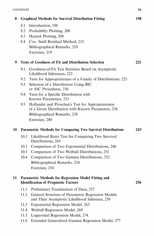
8 Graphical Methods for Survival Distribution Fitting 198
8.1 Introduction, 198
8.2 Probability Plotting, 200
8.3 Hazard Plotting, 209
8.4 Cox—Snell Residual Method, 215
Bibliographical Remarks, 219
Exercises, 219
9 Tests of Goodness of Fit and Distribution Selection 221
9.1 Goodness-of-Fit Test Statistics Based on AsymptoticLikelihood Inferences, 222
9.2 Tests for Appropriateness of a Family of Distributions, 225
9.3 Selection of a Distribution Using BICor AIC Procedures, 230
9.4 Tests for a Specific Distribution withKnown Parameters, 233
9.5 Hollander and Proschan’s Test for Appropriatenessof a Given Distribution with Known Parameters, 236
Bibliographical Remarks, 238
Exercises, 240
10 Parametric Methods for Comparing Two Survival Distributions 243
10.1 Likelihood Ratio Test for Comparing Two SurvivalDistributions, 243
10.2 Comparison of Two Exponential Distributions, 246
10.3 Comparison of Two Weibull Distributions, 251
10.4 Comparison of Two Gamma Distributions, 252
Bibliographical Remarks, 254
Exercises, 254
11 Parametric Methods for Regression Model Fitting andIdentification of Prognostic Factors 256
11.1 Preliminary Examination of Data, 257
11.2 General Structure of Parametric Regression Modelsand Their Asymptotic Likelihood Inference, 259
11.3 Exponential Regression Model, 263
11.4 Weibull Regression Model, 269
11.5 Lognormal Regression Model, 274
11.6 Extended Generalized Gamma Regression Model, 277
ix
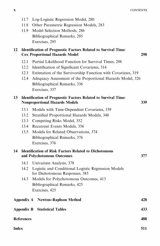
11.7 Log-Logistic Regression Model, 280
11.8 Other Parametric Regression Models, 283
11.9 Model Selection Methods, 286
Bibliographical Remarks, 295
Exercises, 295
12 Identification of Prognostic Factors Related to Survival Time:Cox Proportional Hazards Model 298
12.1 Partial Likelihood Function for Survival Times, 298
12.2 Identification of Significant Covariates, 314
12.3 Estimation of the Survivorship Function with Covariates, 319
12.4 Adequacy Assessment of the Proportional Hazards Model, 326
Bibliographical Remarks, 336
Exercises, 337
13 Identification of Prognostic Factors Related to Survival Time:Nonproportional Hazards Models 339
13.1 Models with Time-Dependent Covariates, 339
13.2 Stratified Proportional Hazards Models, 348
13.3 Competing Risks Model, 352
13.4 Recurrent Events Models, 356
13.5 Models for Related Observations, 374
Bibliographical Remarks, 376
Exercises, 376
14 Identification of Risk Factors Related to Dichotomousand Polychotomous Outcomes 377
14.1 Univariate Analysis, 378
14.2 Logistic and Conditional Logistic Regression Modelsfor Dichotomous Responses, 385
14.3 Models for Polychotomous Outcomes, 413
Bibliographical Remarks, 425
Exercises, 425
Appendix A Newton--Raphson Method 428
Appendix B Statistical Tables 433
References 488
Index 511
x
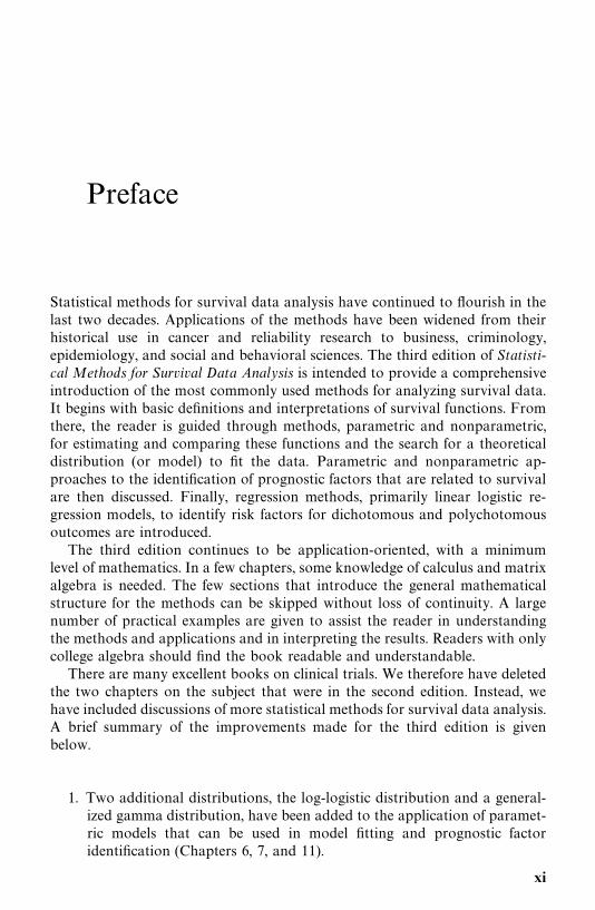
Preface
Statistical methods for survival data analysis have continued to flourish in thelast two decades. Applications of the methods have been widened from theirhistorical use in cancer and reliability research to business, criminology,epidemiology, and social and behavioral sciences. The third edition of Statisti-cal Methods for Survival Data Analysis is intended to provide a comprehensiveintroduction of the most commonly used methods for analyzing survival data.It begins with basic definitions and interpretations of survival functions. Fromthere, the reader is guided through methods, parametric and nonparametric,for estimating and comparing these functions and the search for a theoreticaldistribution (or model) to fit the data. Parametric and nonparametric ap-proaches to the identification of prognostic factors that are related to survivalare then discussed. Finally, regression methods, primarily linear logistic re-gression models, to identify risk factors for dichotomous and polychotomousoutcomes are introduced.The third edition continues to be application-oriented, with a minimum
level of mathematics. In a few chapters, some knowledge of calculus and matrixalgebra is needed. The few sections that introduce the general mathematicalstructure for the methods can be skipped without loss of continuity. A largenumber of practical examples are given to assist the reader in understandingthe methods and applications and in interpreting the results. Readers with onlycollege algebra should find the book readable and understandable.There are many excellent books on clinical trials. We therefore have deleted
the two chapters on the subject that were in the second edition. Instead, wehave included discussions of more statistical methods for survival data analysis.A brief summary of the improvements made for the third edition is givenbelow.
1. Two additional distributions, the log-logistic distribution and a general-ized gamma distribution, have been added to the application of paramet-ric models that can be used in model fitting and prognostic factoridentification (Chapters 6, 7, and 11).
xi
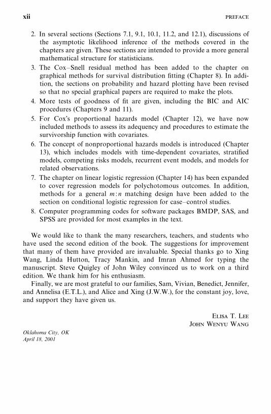
2. In several sections (Sections 7.1, 9.1, 10.1, 11.2, and 12.1), discussions ofthe asymptotic likelihood inference of the methods covered in thechapters are given. These sections are intended to provide a more generalmathematical structure for statisticians.
3. The Cox—Snell residual method has been added to the chapter ongraphical methods for survival distribution fitting (Chapter 8). In addi-tion, the sections on probability and hazard plotting have been revisedso that no special graphical papers are required to make the plots.
4. More tests of goodness of fit are given, including the BIC and AICprocedures (Chapters 9 and 11).
5. For Cox’s proportional hazards model (Chapter 12), we have nowincluded methods to assess its adequency and procedures to estimate thesurvivorship function with covariates.
6. The concept of nonproportional hazards models is introduced (Chapter13), which includes models with time-dependent covariates, stratifiedmodels, competing risks models, recurrent event models, and models forrelated observations.
7. The chapter on linear logistic regression (Chapter 14) has been expandedto cover regression models for polychotomous outcomes. In addition,methods for a general m : n matching design have been added to thesection on conditional logistic regression for case—control studies.
8. Computer programming codes for software packages BMDP, SAS, andSPSS are provided for most examples in the text.
We would like to thank the many researchers, teachers, and students whohave used the second edition of the book. The suggestions for improvementthat many of them have provided are invaluable. Special thanks go to XingWang, Linda Hutton, Tracy Mankin, and Imran Ahmed for typing themanuscript. Steve Quigley of John Wiley convinced us to work on a thirdedition. We thank him for his enthusiasm.Finally, we are most grateful to our families, Sam, Vivian, Benedict, Jennifer,
and Annelisa (E.T.L.), and Alice and Xing (J.W.W.), for the constant joy, love,and support they have given us.
E T. LJ W W
Oklahoma City, OKApril 18, 2001
xii
CHAPTER 1
Introduction
1.1 PRELIMINARIES
This book is for biomedical researchers, epidemiologists, consulting statisti-cians, students taking a first course on survival data analysis, and othersinterested in survival time study. It deals with statistical methods for analyzingsurvival data derived from laboratory studies of animals, clinical and epi-demiologic studies of humans, and other appropriate applications.
Survival time can be defined broadly as the time to the occurrence of a givenevent. This event can be the development of a disease, response to a treatment,relapse, or death. Therefore, survival time can be tumor-free time, the time fromthe start of treatment to response, length of remission, and time to death.Survival data can include survival time, response to a given treatment, andpatient characteristics related to response, survival, and the development of adisease. The study of survival data has focused on predicting the probability ofresponse, survival, or mean lifetime, comparing the survival distributions ofexperimental animals or of human patients and the identification of risk and/orprognostic factors related to response, survival, and the development of adisease. In this book, special consideration is given to the study of survival datain biomedical sciences, although all the methods are suitable for applicationsin industrial reliability, social sciences, and business. Examples of survival datain these fields are the lifetime of electronic devices, components, or systems(reliability engineering); felons’ time to parole (criminology); duration of firstmarriage (sociology); length of newspaper or magazine subscription (market-ing); and worker’s compensation claims (insurance) and their various influenc-ing risk or prognostic factors.
1.2 CENSORED DATA
Many researchers consider survival data analysis to be merely the applicationof two conventional statistical methods to a special type of problem: parametricif the distribution of survival times is known to be normal and nonparametric
1
if the distribution is unknown. This assumption would be true if the survivaltimes of all the subjects were exact and known; however, some survival timesare not. Further, the survival distribution is often skewed, or far from beingnormal. Thus there is a need for new statistical techniques. One of the mostimportant developments is due to a special feature of survival data in the lifesciences that occurs when some subjects in the study have not experienced theevent of interest at the end of the study or time of analysis. For example, somepatients may still be alive or disease-free at the end of the study period. Theexact survival times of these subjects are unknown. These are called censoredobservations or censored times and can also occur when people are lost tofollow-up after a period of study. When these are not censored observations,the set of survival times is complete. There are three types of censoring.
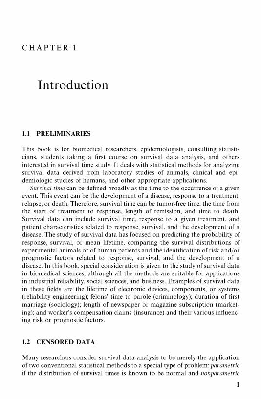
Type I CensoringAnimal studies usually start with a fixed number of animals, to which thetreatment or treatments is given. Because of time and/or cost limitations, theresearcher often cannot wait for the death of all the animals. One option is toobserve for a fixed period of time, say six months, after which the survivinganimals are sacrificed. Survival times recorded for the animals that died duringthe study period are the times from the start of the experiment to their death.These are called exact or uncensored observations. The survival times of thesacrificed animals are not known exactly but are recorded as at least the lengthof the study period. These are called censored observations. Some animals couldbe lost or die accidentally. Their survival times, from the start of experimentto loss or death, are also censored observations. In type I censoring, if there areno accidental losses, all censored observations equal the length of the studyperiod.
For example, suppose that six rats have been exposed to carcinogens byinjecting tumor cells into their foot pads. The times to develop a tumor of agiven size are observed. The investigator decides to terminate the experimentafter 30 weeks. Figure 1.1 is a plot of the development times of the tumors.Rats A, B, and D developed tumors after 10, 15, and 25 weeks, respectively.Rats C and E did not develop tumors by the end of the study; their tumor-freetimes are thus 30-plus weeks. Rat F died accidentally without tumors after 19weeks of observation. The survival data (tumor-free times) are 10, 15, 30�, 25,30�, and 19� weeks. (The plus indicates a censored observation.)
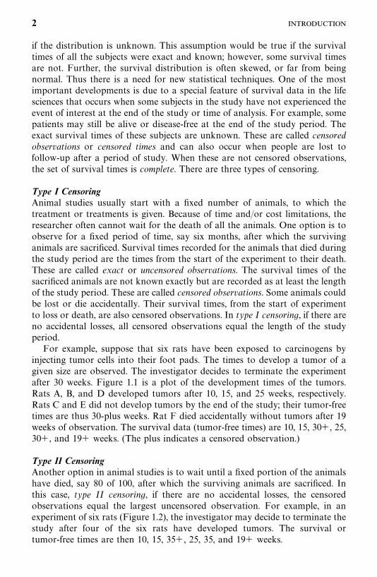
Type II CensoringAnother option in animal studies is to wait until a fixed portion of the animalshave died, say 80 of 100, after which the surviving animals are sacrificed. Inthis case, type II censoring, if there are no accidental losses, the censoredobservations equal the largest uncensored observation. For example, in anexperiment of six rats (Figure 1.2), the investigator may decide to terminate thestudy after four of the six rats have developed tumors. The survival ortumor-free times are then 10, 15, 35�, 25, 35, and 19� weeks.
2
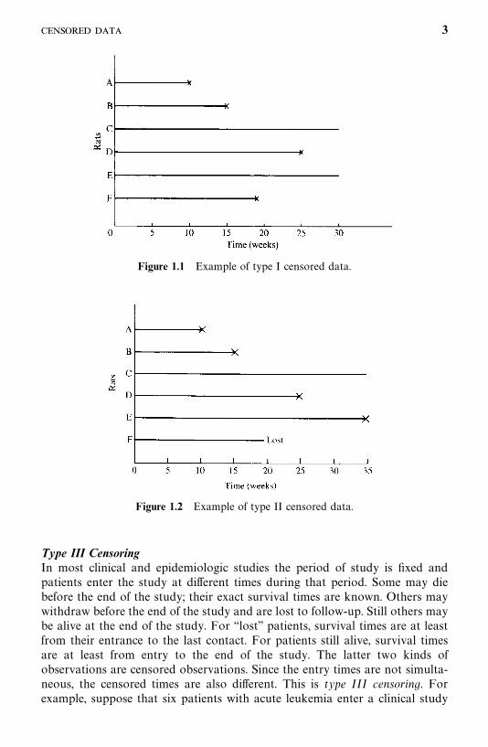
Figure 1.1 Example of type I censored data.
Figure 1.2 Example of type II censored data.
Type III CensoringIn most clinical and epidemiologic studies the period of study is fixed andpatients enter the study at different times during that period. Some may diebefore the end of the study; their exact survival times are known. Others maywithdraw before the end of the study and are lost to follow-up. Still others maybe alive at the end of the study. For ‘‘lost’’ patients, survival times are at leastfrom their entrance to the last contact. For patients still alive, survival timesare at least from entry to the end of the study. The latter two kinds ofobservations are censored observations. Since the entry times are not simulta-neous, the censored times are also different. This is type III censoring. Forexample, suppose that six patients with acute leukemia enter a clinical study
3
Figure 1.3 Example of type III censored data.
during a total study period of one year. Suppose also that all six respond totreatment and achieve remission. The remission times are plotted in Figure 1.3.Patients A, C, and E achieve remission at the beginning of the second, fourth,and ninth months, and relapse after four, six, and three months, respectively.Patient B achieves remission at the beginning of the third month but is lost tofollow-up four months later; the remission duration is thus at least fourmonths. Patients D and F achieve remission at the beginning of the fifth andtenth months, respectively, and are still in remission at the end of the study;their remission times are thus at least eight and three months. The respectiveremission times of the six patients are 4, 4�, 6, 8�, 3, and 3� months.
Type I and type II censored observations are also called singly censoreddata, and type III, progressively censored data, by Cohen (1965). Anothercommonly used name for type III censoring is random censoring. All of thesetypes of censoring are right censoring or censoring to the right. There are alsoleft censoring and interval censoring cases. L eft censoring occurs when it isknown that the event of interest occurred prior to a certain time t, but the exacttime of occurrence is unknown. For example, an epidemiologist wishes to knowthe age at diagnosis in a follow-up study of diabetic retinopathy. At the time ofthe examination, a 50-year-old participant was found to have already develop-ed retinopathy, but there is no record of the exact time at which initial evidencewas found. Thus the age at examination (i.e., 50) is a left-censored observation.It means that the age of diagnosis for this patient is at most 50 years.
Interval censoring occurs when the event of interest is known to haveoccurred between times a and b. For example, if medical records indicate thatat age 45, the patient in the example above did not have retinopathy, his ageat diagnosis is between 45 and 50 years.
We will study descriptive and analytic methods for complete, singly cen-sored, and progressively censored survival data using numerical and graphical
4
techniques. Analytic methods discussed include parametric and nonparametric.Parametric approaches are used either when a suitable model or distributionis fitted to the data or when a distribution can be assumed for the populationfrom which the sample is drawn. Commonly used survival distributions are theexponential, Weibull, lognormal, and gamma. If a survival distribution is foundto fit the data properly, the survival pattern can then be described by theparameters in a compact way. Statistical inference can be based on thedistribution chosen. If the search for an appropriate model or distribution istoo time consuming or not economical or no theoretical distribution adequate-ly fits the data, nonparametric methods, which are generally easy to apply,should be considered.
1.3 SCOPE OF THE BOOK
This book is divided into four parts.Part I (Chapters 1, 2, and 3) defines survival functions and gives examples
of survival data analysis. Survival distribution is most commonly described bythree functions: the survivorship function (also called the cumulative survivalrate or survival function), the probability density function, and the hazardfunction (hazard rate or age-specific rate). In Chapter 2 we define these threefunctions and their equivalence relationships. Chapter 3 illustrates survivaldata analysis with five examples taken from actual research situations. Clinicaland laboratory data are systematically analyzed in progressive steps and theresults are interpreted. Section and chapter numbers are given for quickreference. The actual calculations are given as examples or left as exercises inthe chapters where the methods are discussed. Four sets of data are providedin the exercise section for the reader to analyze. These data are referred to inthe various chapters.
In Part II (Chapters 4 and 5) we introduce some of the most widely usednonparametric methods for estimating and comparing survival distributions.Chapter 4 deals with the nonparametric methods for estimating the threesurvival functions: the Kaplan and Meier product-limit (PL) estimate and thelife-table technique (population life tables and clinical life tables). Also coveredis standardization of rates by direct and indirect methods, including thestandardized mortality ratio. Chapter 5 is devoted to nonparametric tech-niques for comparing survival distributions. A common practice is to comparethe survival experiences of two or more groups differing in their treatment orin a given characteristic. Several nonparametric tests are described.
Part III (Chapters 6 to 10) introduces the parametric approach to survivaldata analysis. Although nonparametric methods play an important role insurvival studies, parametric techniques cannot be ignored. In Chapter 6 weintroduce and discuss the exponential, Weibull, lognormal, gamma, andlog-logistic survival distributions. Practical applications of these distributionstaken from the literature are included.
5
An important part of survival data analysis is model or distribution fitting.Once an appropriate statistical model for survival time has been constructedand its parameters estimated, its information can help predict survival, developoptimal treatment regimens, plan future clinical or laboratory studies, and soon. The graphical technique is a simple informal way to select a statisticalmodel and estimate its parameters. When a statistical distribution is found tofit the data well, the parameters can be estimated by analytical methods. InChapter 7 we discuss analytical estimation procedures for survival distribu-tions. Most of the estimation procedures are based on the maximum likelihoodmethod. Mathematical derivations are omitted; only formulas for the estimatesand examples are given. In Chapter 8 we introduce three kinds of graphicalmethods: probability plotting, hazard plotting, and the Cox—Snell residualmethod for survival distribution fitting. In Chapter 9 we discuss several testsof goodness of fit and distribution selection. In Chapter 10 we describe severalparametric methods for comparing survival distributions.
A topic that has received increasing attention is the identification ofprognostic factors related to survival time. For example, who is likely tosurvive longest after mastectomy, and what are the most important factors thatinfluence that survival? Another subject important to both biomedical re-searchers and epidemiologists is identification of the risk factors related to thedevelopment of a given disease and the response to a given treatment. Whatare the factors most closely related to the development of a given disease? Whois more likely to develop lung cancer, diabetes, or coronary disease? In manydiseases, such as cancer, patients who respond to treatment have a betterprognosis than patients who do not. The question, then, relates to what thefactors are that influence response. Who is more likely to respond to treatmentand thus perhaps survive longer?
Part IV (Chapters 11 to 14) deals with prognostic/risk factors and survivaltimes. In Chapter 11 we introduce parametric methods for identifying impor-tant prognostic factors. Chapters 12 and 13 cover, respectively, the Coxproportional hazards model and several nonproportional hazards models forthe identification of prognostic factors. In the final chapter, Chapter 14, weintroduce the linear logistic regression model for binary outcome variables andits extension to handle polychotomous outcomes.
In Appendix A we describe a numerical procedure for solving nonlinearequations, the Newton—Raphson method. This method is suggested in Chap-ters 7, 11, 12, and 13. Appendix B comprises a number of statistical tables.
Most nonparametric techniques discussed here are easy to understand andsimple to apply. Parametric methods require an understanding of survivaldistributions. Unfortunately, most of survival distributions are not simple.Readers without calculus may find it difficult to apply them on their own.However, if the main purpose is not model fitting, most parametric techniquescan be substituted for by their nonparametric competitors. In fact, a largepercentage of survival studies in clinical or epidemiological journals areanalyzed by nonparametric methods. Researchers not interested in survival
6

model fitting should read the chapters and sections on nonparametric methods.Computer programs for survival data analysis are available in several commer-cially available software packages: for example, BMDP, SAS, and SPSS. Thesecomputer programs are referred to in various chapters when applicable.Computer programming codes are given for many of the examples.
Bibliographical Remarks
Cross and Clark (1975) was the first book to discuss parametric models andnonparametric and graphical techniques for both complete and censoredsurvival data. Since then, several other books have been published in additionto the first edition of this book (Lee, 1980, 1992). Elandt-Johnson and Johnson(1980) discuss extensively the construction of life tables, model fitting, compet-ing risk, and mathematical models of biological processes of disease pro-gression and aging. Kalbfleisch and Prentice (1980) focus on regressionproblems with survival data, particularly Cox’s proportional hazards model.Miller (1981) covers a number of parametric and nonparametric methods forsurvival analysis. Cox and Oakes (1984) also cover the topic concisely with anemphasis on the examination of explanatory variables.
Nelson (1982) provides a good discussion of parametric, nonparametric, andgraphical methods. The book is more suited for industrial reliability engineersthan for biomedical researchers, as are Hahn and Shapiro (1967) and Mann etal. (1974). In addition, Lawless (1982) gives a broad coverage of the area withapplications in engineering and biomedical sciences.
More recent publications include Marubini and Valsecchi (1994), Klein-baum (1995), Klein and Moeschberger (1997), and Hosmer and Lemeshow(1999). Most of these books take a more rigorous mathematical approach andrequire knowledge of mathematical statistics.
7
C H A P T E R 2
Functions of Survival Time
Survival time data measure the time to a certain event, such as failure, death,response, relapse, the development of a given disease, parole, or divorce. Thesetimes are subject to random variations, and like any random variables, form adistribution. The distribution of survival times is usually described or charac-terized by three functions: (1) the survivorship function, (2) the probabilitydensity function, and (3) the hazard function. These three functions aremathematically equivalent — if one of them is given, the other two can bederived.
In practice, the three functions can be used to illustrate different aspects ofthe data. A basic problem in survival data analysis is to estimate from thesampled data one or more of these three functions and to draw inferencesabout the survival pattern in the population. In Section 2.1 we define the threefunctions and in Section 2.2, discuss the equivalence relationship among thethree functions.
2.1 DEFINITIONS
Let T denote the survival time. The distribution of T can be characterized bythree equivalent functions.
Survivorship Function (or Survival Function)This function, denoted by S(t), is defined as the probability that an individualsurvives longer than t:
S(t) �P (an individual survives longer than t)
�P(T � t ) (2.1.1)
From the definition of the cumulative distribution function F(t) of T,
S(t) � 1-P (an individual fails before t)
� 1 � F(t) (2.1.2)
8
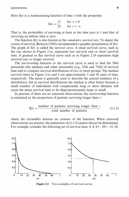
Figure 2.1 Two examples of survival curves.
Here S(t) is a nonincreasing function of time t with the properties
S(t) ��1 for t� 0
0 for t� �
That is, the probability of surviving at least at the time zero is 1 and that ofsurviving an infinite time is zero.
The function S(t) is also known as the cumulative survival rate. To depict thecourse of survival, Berkson (1942) recommended a graphic presentation of S(t).The graph of S(t) is called the survival curve. A steep survival curve, such asthe one shown in Figure 2.1a, represents low survival rate or short survivaltime. A gradual or flat survival curve such as in Figure 2.1b represents highsurvival rate or longer survival.
The survivorship function or the survival curve is used to find the 50thpercentile (the median) and other percentiles (e.g., 25th and 75th) of survivaltime and to compare survival distributions of two or more groups. The mediansurvival times in Figure 2.1a and b are approximately 5 and 36 units of time,respectively. The mean is generally used to describe the central tendency of adistribution, but in survival distributions the median is often better because asmall number of individuals with exceptionally long or short lifetimes willcause the mean survival time to be disproportionately large or small.
In practice, if there are no censored observations, the survivorship functionis estimated as the proportion of patients surviving longer than t :
S� (t) �number of patients surviving longer than t
total number of patients(2.1.3)
where the circumflex denotes an estimate of the function. When censoredobservations are present, the numerator of (2.1.3) cannot always be determined.For example, consider the following set of survival data: 4, 6, 6�, 10�, 15, 20.
9
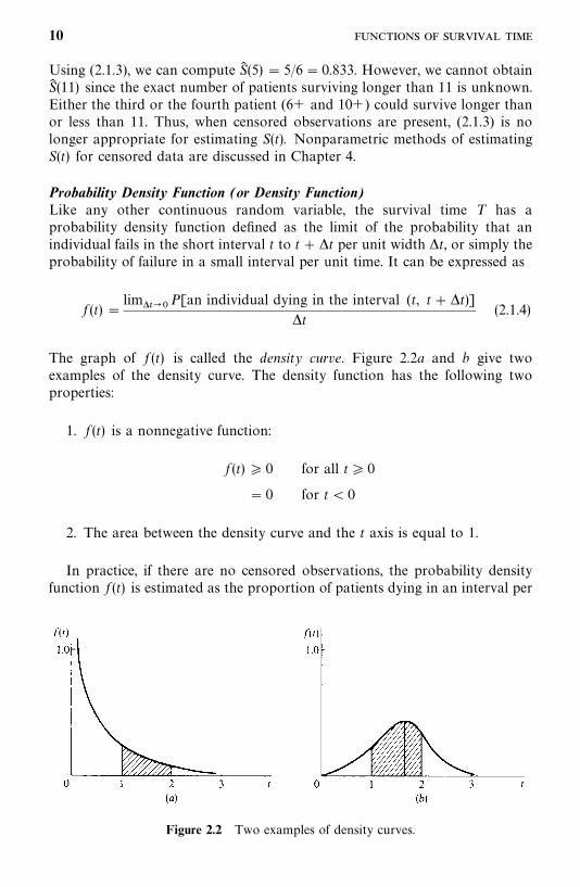
Figure 2.2 Two examples of density curves.
Using (2.1.3), we can compute S� (5) � 5/6 � 0.833. However, we cannot obtainS� (11) since the exact number of patients surviving longer than 11 is unknown.Either the third or the fourth patient (6� and 10�) could survive longer thanor less than 11. Thus, when censored observations are present, (2.1.3) is nolonger appropriate for estimating S(t). Nonparametric methods of estimatingS(t) for censored data are discussed in Chapter 4.
Probability Density Function (or Density Function)Like any other continuous random variable, the survival time T has aprobability density function defined as the limit of the probability that anindividual fails in the short interval t to t� �t per unit width �t, or simply theprobability of failure in a small interval per unit time. It can be expressed as
f (t) �lim����
P[an individual dying in the interval (t, t��t)]�t
(2.1.4)
The graph of f (t) is called the density curve. Figure 2.2a and b give twoexamples of the density curve. The density function has the following twoproperties:
1. f (t) is a nonnegative function:
f (t) � 0 for all t� 0
� 0 for t� 0
2. The area between the density curve and the t axis is equal to 1.
In practice, if there are no censored observations, the probability densityfunction f (t) is estimated as the proportion of patients dying in an interval per
10
unit width:
f� (t) �number of patients dying in the interval beginning at time t
(total number of patients)�(interval width)(2.1.5)
Similar to the estimation of S(t), when censored observations are present,(2.1.5) is not applicable. We discuss an appropriate method in Chapter 4.
The proportion of individuals that fail in any time interval and the peaks ofhigh frequency of failure can be found from the density function. The densitycurve in Figure 2.2a gives a pattern of high failure rate at the beginning of thestudy and decreasing failure rate as time increases. In Figure 2.2b, the peak ofhigh failure frequency occurs at approximately 1.7 units of time. The propor-tion of individuals that fail between 1 and 2 units of time is equal to the shadedarea between the density curve and the axis. The density function is also knownas the unconditional failure rate.
Hazard FunctionThe hazard function h(t) of survival time T gives the conditional failure rate.This is defined as the probability of failure during a very small time interval,assuming that the individual has survived to the beginning of the interval, oras the limit of the probability that an individual fails in a very short interval,t��t, given that the individual has survived to time t:
h(t) �
lim����P �
an individual fails in the time interval (t, t��t)given the individual has survived to t �
�t(2.1.6)
The hazard function can also be defined in terms of the cumulativedistribution function F(t) and the probability density function f (t):
h(t) �f (t)
1 �F(t)(2.1.7)
The hazard function is also known as the instantaneous failure rate, force ofmortality, conditional mortality rate, and age-specific failure rate. If t in (2.1.6)is age, it is a measure of the proneness to failure as a function of the age of theindividual in the sense that the quantity �th(t) is the expected proportion ofage t individuals who will fail in the short time interval t��t. The hazardfunction thus gives the risk of failure per unit time during the aging process. Itplays an important role in survival data analysis.
In practice, when there are no censored observations the hazard function isestimated as the proportion of patients dying in an interval per unit time, given
11
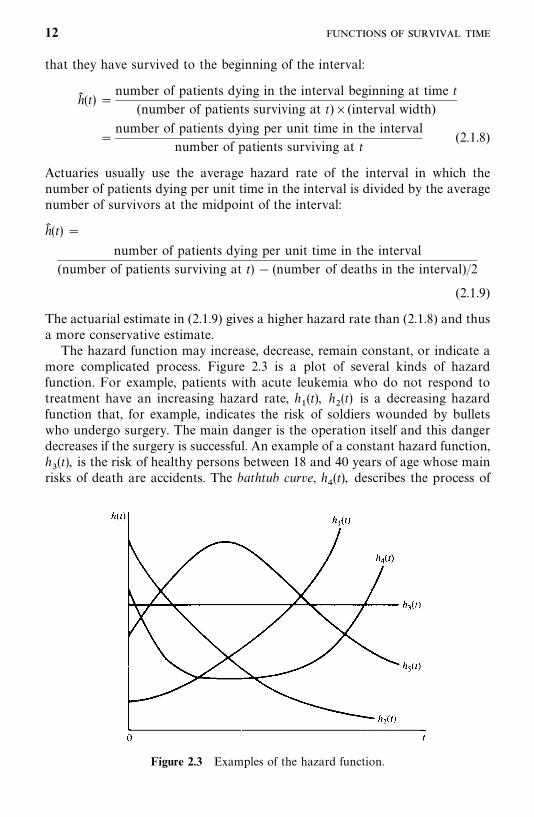
Figure 2.3 Examples of the hazard function.
that they have survived to the beginning of the interval:
h� (t) �number of patients dying in the interval beginning at time t
(number of patients surviving at t)�(interval width)
�number of patients dying per unit time in the interval
number of patients surviving at t(2.1.8)
Actuaries usually use the average hazard rate of the interval in which thenumber of patients dying per unit time in the interval is divided by the averagenumber of survivors at the midpoint of the interval:
h� (t) �
number of patients dying per unit time in the interval
(number of patients surviving at t) � (number of deaths in the interval)/2
(2.1.9)
The actuarial estimate in (2.1.9) gives a higher hazard rate than (2.1.8) and thusa more conservative estimate.
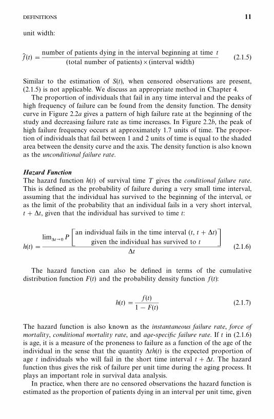
The hazard function may increase, decrease, remain constant, or indicate amore complicated process. Figure 2.3 is a plot of several kinds of hazardfunction. For example, patients with acute leukemia who do not respond totreatment have an increasing hazard rate, h
�(t), h
�(t) is a decreasing hazard
function that, for example, indicates the risk of soldiers wounded by bulletswho undergo surgery. The main danger is the operation itself and this dangerdecreases if the surgery is successful. An example of a constant hazard function,h�(t), is the risk of healthy persons between 18 and 40 years of age whose main
risks of death are accidents. The bathtub curve, h�(t), describes the process of
12
Table 2.1 Survival Data and Estimated Survival Functions of 40 Myeloma Patients
Number of PatientsSurviving at Number of Patients
Survival Time Beginning of Dying int (months) Interval Interval S� (t) f� (t) h� (t)
0—5 40 5 1.000 0.025 0.0275—10 35 7 0.875 0.035 0.044
10—15 28 6 0.700 0.030 0.04815—20 22 4 0.550 0.020 0.04020—25 18 5 0.450 0.025 0.06525—30 13 4 0.325 0.020 0.07230—35 9 4 0.225 0.020 0.11435—40 5 0 0.125 0.000 0.00040—45 5 2 0.125 0.010 0.10045—50 3 1 0.075 0.005 0.080�50 2 2 0.050 — —
human life. During an initial period, the risk is high (high infant mortality).Subsequently, h(t) stays approximately constant until a certain time, afterwhich it increases because of wear-out failures. Finally, patients with tubercu-losis have risks that increase initially, then decrease after treatment. Such anincreasing, then decreasing hazard function is described by h
(t).
The cumulative hazard function is defined as
H(t) ���
�
h(x) dx (2.1.10)
It will be shown in Section 2.2 that
H(t) ��logS(t) (2.1.11)
Thus, at t� 0, S(t) � 1, H(t) � 0, and at t��, S(t) � 0, H(t) ��. Thecumulative hazard function can be any value between zero and infinity. All logfunctions in this book are natural logs (base e) unless otherwise indicated.
The following example illustrates how these functions can be estimated froma complete sample of grouped survival times without censored observations.
Example 2.1 The first three columns of Table 2.1 give the survival data of40 patients with myeloma. The survival times are grouped into intervals of fivemonths. The estimated survivorship function, density function, and hazardfunction are also given, with the corresponding graphs plotted in Figure2.4a—c.
13
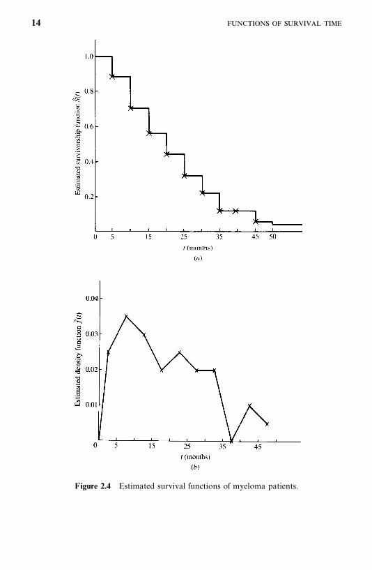
Figure 2.4 Estimated survival functions of myeloma patients.
14
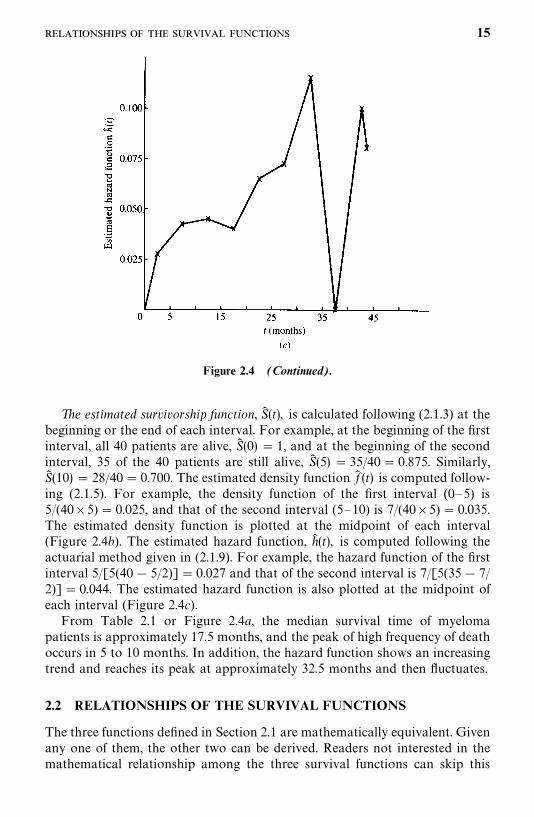
Figure 2.4 (Continued).
The estimated survivorship function, S� (t), is calculated following (2.1.3) at thebeginning or the end of each interval. For example, at the beginning of the firstinterval, all 40 patients are alive, S� (0) � 1, and at the beginning of the secondinterval, 35 of the 40 patients are still alive, S� (5) � 35/40 � 0.875. Similarly,S� (10) � 28/40 � 0.700. The estimated density function f� (t) is computed follow-ing (2.1.5). For example, the density function of the first interval (0—5) is5/(40�5) � 0.025, and that of the second interval (5—10) is 7/(40�5) � 0.035.The estimated density function is plotted at the midpoint of each interval(Figure 2.4b). The estimated hazard function, h� (t), is computed following theactuarial method given in (2.1.9). For example, the hazard function of the firstinterval 5/[5(40 � 5/2)] � 0.027 and that of the second interval is 7/[5(35 � 7/2)] � 0.044. The estimated hazard function is also plotted at the midpoint ofeach interval (Figure 2.4c).
From Table 2.1 or Figure 2.4a, the median survival time of myelomapatients is approximately 17.5 months, and the peak of high frequency of deathoccurs in 5 to 10 months. In addition, the hazard function shows an increasingtrend and reaches its peak at approximately 32.5 months and then fluctuates.
2.2 RELATIONSHIPS OF THE SURVIVAL FUNCTIONS
The three functions defined in Section 2.1 are mathematically equivalent. Givenany one of them, the other two can be derived. Readers not interested in themathematical relationship among the three survival functions can skip this
15
section without loss of continuity.
1. From (2.1.2) and (2.1.7),
h(t) �f (t)
S(t)(2.2.1)
This relationship can also be derived from (2.1.6) using basic definitions ofconditional probabilities.
2. Since the probability density function is the derivative of the cumulativedistribution function,
f (t) �d
dt[1 �S(t)] ��S�(t) (2.2.2)
3. Substituting (2.2.2) into (2.2.1) yields
h(t) ��S�(t)S(t)
��d
dtlogS(t) (2.2.3)
4. Integrating (2.2.3) from zero to t and using S(0) � 1, we have
���
�
h(x) dx� logS(t)
or
H(t) ��logS(t)or
S(t) � exp[�H(t)] � exp�� ��
�
h(x) dx� (2.2.4)
5. From (2.2.1) and (2.2.4) we obtain
f (t) � h(t) exp[�H(t)] (2.2.5)
Hence, if f (t) is known, the survivorship function can be obtained from thebasic relationship between f (t), F(t), and (2.1.2). The hazard function can thenbe determined from (2.2.1). If S(t) is known, f (t) and h(t) can be determinedfrom (2.2.2) and (2.2.1), respectively, or h(t) can be derived first from (2.2.3) andthen f (t) from (2.2.1). If h(t) is given, S(t) and f (t) can be obtained, respectively,from (2.2.4) and (2.2.5). Thus, given any one of the three survival functions, theother two can easily be derived. The following example illustrates theseequivalence relationships.
16
Example 2.2 Suppose that the survival time of a population has thefollowing density function:
f (t) � e� t� 0
Using the definition of the cumulative distribution function,
F(t) ���
�
f (x) dx���
�
e� dx��e� ��
�
� 1 � e�
From (2.1.2) we obtain the survivorship function
S(t) � e�
The hazard function can then be obtained from (2.2.1):
h(t) �e�
e�� 1
A complete treatment of this distribution is given in Section 6.1.
Bibliographical Remarks
The three survival functions and their equivalents are discussed in every textcited in the Bibliographical Remarks in Chapter 1.
EXERCISES
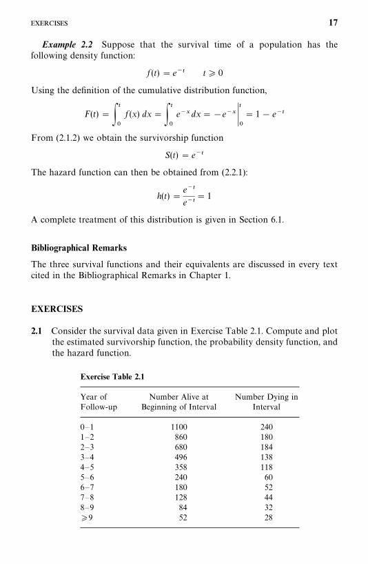
2.1 Consider the survival data given in Exercise Table 2.1. Compute and plotthe estimated survivorship function, the probability density function, andthe hazard function.
Exercise Table 2.1
Year of Number Alive at Number Dying inFollow-up Beginning of Interval Interval
0—1 1100 2401—2 860 1802—3 680 1843—4 496 1384—5 358 1185—6 240 606—7 180 527—8 128 448—9 84 32�9 52 28
17
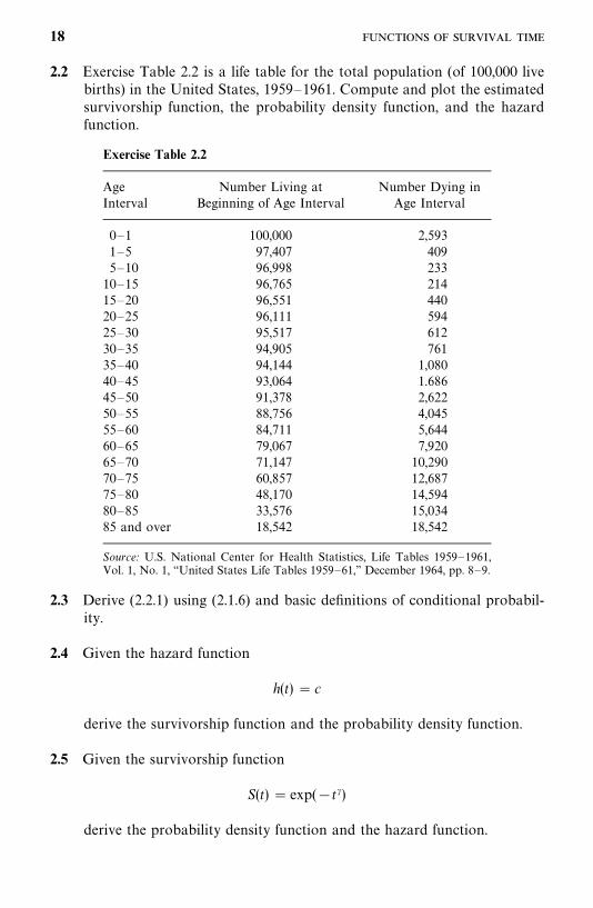
2.2 Exercise Table 2.2 is a life table for the total population (of 100,000 livebirths) in the United States, 1959—1961. Compute and plot the estimatedsurvivorship function, the probability density function, and the hazardfunction.
Exercise Table 2.2
Age Number Living at Number Dying inInterval Beginning of Age Interval Age Interval
0—1 100,000 2,5931—5 97,407 4095—10 96,998 233
10—15 96,765 21415—20 96,551 44020—25 96,111 59425—30 95,517 61230—35 94,905 76135—40 94,144 1,08040—45 93,064 1.68645—50 91,378 2,62250—55 88,756 4,04555—60 84,711 5,64460—65 79,067 7,92065—70 71,147 10,29070—75 60,857 12,68775—80 48,170 14,59480—85 33,576 15,03485 and over 18,542 18,542
Source: U.S. National Center for Health Statistics, Life Tables 1959—1961,Vol. 1, No. 1, ‘‘United States Life Tables 1959—61,’’ December 1964, pp. 8—9.
2.3 Derive (2.2.1) using (2.1.6) and basic definitions of conditional probabil-ity.
2.4 Given the hazard function
h(t) � c
derive the survivorship function and the probability density function.
2.5 Given the survivorship function
S(t) � exp(�t�)
derive the probability density function and the hazard function.
18
CHAPTER 3
Examples of Survival Data Analysis
The investigator who has assembled a large amount of data must decide whatto do with it and what it indicates. In this chapter we take several sets ofsurvival data from actual research situations and analyze them. In Example 3.1we analyze two sets of data obtained, respectively, from two and threetreatment groups to compare the treatment’s abilities to prolong life. Example3.2 is an example of the life-table technique for large samples. Example 3.3 givesremission data from two treatments; the investigator seeks a well-knowndistribution for the remission patterns to compare the two groups. In Example3.4 we study survival data and several other patient characteristics to identifyimportant prognostic factors; the patient characteristics are analyzed individ-ually and simultaneously for their prognostic values. In Example 3.5 weintroduce a case in which the interest is to identify risk factors in thedevelopment of a given disease. Four sets of real data are presented in theexercises so that the reader can plan analysis.
3.1 EXAMPLE 3.1: COMPARISON OF TWO TREATMENTSAND THREE DIETS
3.1.1 Comparison of Two Treatments
Thirty melanoma patients (stages 2 to 4) were studied to compare theimmunotherapies BCG (Bacillus Calmette-Guerin) and Corynebacterium par-vum for their abilities to prolong remission duration and survival time. The age,gender, disease stage, treatment received, remission duration, and survival timeare given in Table 3.1. All the patients were resected before treatment beganand thus had no evidence of melanoma at the time of first treatment.
The usual objective with this type of data is to determine the length ofremission and survival and to compare the distributions of remission andsurvival time in each group. Before comparing the remission and survival
19
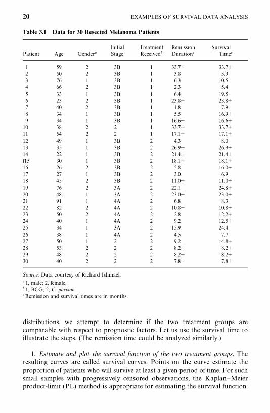
Table 3.1 Data for 30 Resected Melanoma Patients
Initial Treatment Remission SurvivalPatient Age Gender� Stage Received� Duration� Time�
1 59 2 3B 1 33.7� 33.7�2 50 2 3B 1 3.8 3.93 76 1 3B 1 6.3 10.54 66 2 3B 1 2.3 5.45 33 1 3B 1 6.4 19.56 23 2 3B 1 23.8� 23.8�7 40 2 3B 1 1.8 7.98 34 1 3B 1 5.5 16.9�9 34 1 3B 1 16.6� 16.6�
10 38 2 2 1 33.7� 33.7�11 54 2 2 1 17.1� 17.1�12 49 1 3B 2 4.3 8.013 35 1 3B 2 26.9� 26.9�14 22 1 3B 2 21.4� 21.4�f15 30 1 3B 2 18.1� 18.1�16 26 2 3B 2 5.8 16.0�17 27 1 3B 2 3.0 6.918 45 2 3B 2 11.0� 11.0�19 76 2 3A 2 22.1 24.8�20 48 1 3A 2 23.0� 23.0�21 91 1 4A 2 6.8 8.322 82 2 4A 2 10.8� 10.8�23 50 2 4A 2 2.8 12.2�24 40 1 4A 2 9.2 12.5�25 34 1 3A 2 15.9 24.426 38 1 4A 2 4.5 7.727 50 1 2 2 9.2 14.8�28 53 2 2 2 8.2� 8.2�29 48 2 2 2 8.2� 8.2�30 40 2 2 2 7.8� 7.8�
Source: Data courtesy of Richard Ishmael.
� 1, male; 2, female.� 1, BCG; 2, C. parvum.�Remission and survival times are in months.
distributions, we attempt to determine if the two treatment groups arecomparable with respect to prognostic factors. Let us use the survival time toillustrate the steps. (The remission time could be analyzed similarly.)
1. Estimate and plot the survival function of the two treatment groups. Theresulting curves are called survival curves. Points on the curve estimate theproportion of patients who will survive at least a given period of time. For suchsmall samples with progressively censored observations, the Kaplan—Meierproduct-limit (PL) method is appropriate for estimating the survival function.
20 EXAMPLES OF SURVIVAL DATA ANALYSIS
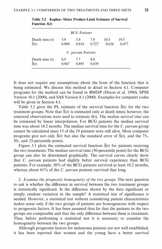
Table 3.2 Kaplan--Meier Product-Limit Estimate of SurvivalFunction S(t)
BCG Patients
Death time (t) 3.9 5.4 7.9 10.5 19.5S� (t) 0.909 0.818 0.727 0.636 0.477
C. parvum Patients
Death time (t) 6.9 7.7 8.0S� (t) 0.947 0.895 0.839
It does not require any assumptions about the form of the function that isbeing estimated. We discuss this method in detail in Section 4.1. Computerprograms for the method can be found in BMDP (Dixon et al. 1990), SPSSVersion 10.1 (2000), and SAS Version 8.1 (2000). Examples for computer codeswill be given in Section 4.1.
Table 3.2 gives the PL estimate of the survival function S� (t) for the twotreatment groups. Note that S� (t) is estimated only at death times; however, thecensored observations were used to estimate S(t). The median survival time canbe estimated by linear interpolation. For BCG patients the median survivaltime was about 18.2 months. The median survival time for the C. parvum groupcannot be calculated since 15 of the 19 patients were still alive. Most computerprograms give not only S� (t) but also the standard error of S� (t), and the 75-,50-, and 25-percentile points.
Figure 3.1 plots the estimated survival function S� (t) for patients receivingthe two treatments: The median survival time (50-percentile point) for the BCGgroup can also be determined graphically. The survival curves clearly showthat C. parvum patients had slightly better survival experience than BCGpatients. For example, 50% of the BCG patients survived at least 18.2 months,whereas about 61% of the C. parvum patients survived that long.
2. Examine the prognostic homogeneity of the two groups. The next questionto ask is whether the difference in survival between the two treatment groupsis statistically significant. Is the difference shown by the data significant orsimply random variation in the sample? A statistical test of significance isneeded. However, a statistical test without considering patient characteristicsmakes sense only if the two groups of patients are homogeneous with respectto prognostic factors. It has been assumed thus far that the patients in the twogroups are comparable and that the only difference between them is treatment.Thus, before performing a statistical test it is necessary to examine thehomogeneity between the two groups.
Although prognostic factors for melanoma patients are not well established,it has been reported that women and the young have a better survival
EXAMPLE 3.1: COMPARISON OF TWO TREATMENTS AND THREE DIETS 21
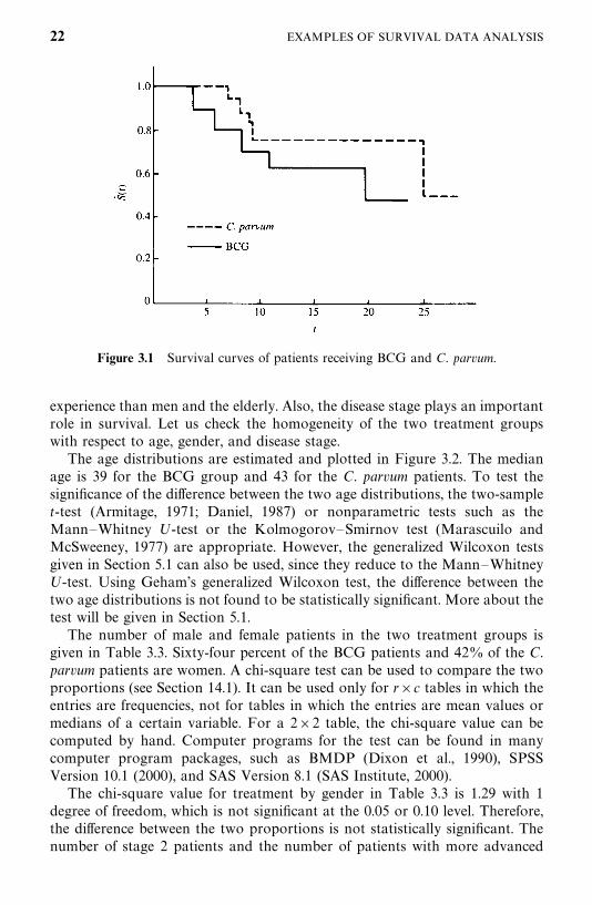
Figure 3.1 Survival curves of patients receiving BCG and C. parvum.
experience than men and the elderly. Also, the disease stage plays an importantrole in survival. Let us check the homogeneity of the two treatment groupswith respect to age, gender, and disease stage.
The age distributions are estimated and plotted in Figure 3.2. The medianage is 39 for the BCG group and 43 for the C. parvum patients. To test thesignificance of the difference between the two age distributions, the two-samplet-test (Armitage, 1971; Daniel, 1987) or nonparametric tests such as theMann—Whitney U-test or the Kolmogorov—Smirnov test (Marascuilo andMcSweeney, 1977) are appropriate. However, the generalized Wilcoxon testsgiven in Section 5.1 can also be used, since they reduce to the Mann—WhitneyU-test. Using Geham’s generalized Wilcoxon test, the difference between thetwo age distributions is not found to be statistically significant. More about thetest will be given in Section 5.1.
The number of male and female patients in the two treatment groups isgiven in Table 3.3. Sixty-four percent of the BCG patients and 42% of the C.parvum patients are women. A chi-square test can be used to compare the twoproportions (see Section 14.1). It can be used only for r�c tables in which theentries are frequencies, not for tables in which the entries are mean values ormedians of a certain variable. For a 2�2 table, the chi-square value can becomputed by hand. Computer programs for the test can be found in manycomputer program packages, such as BMDP (Dixon et al., 1990), SPSSVersion 10.1 (2000), and SAS Version 8.1 (SAS Institute, 2000).
The chi-square value for treatment by gender in Table 3.3 is 1.29 with 1degree of freedom, which is not significant at the 0.05 or 0.10 level. Therefore,the difference between the two proportions is not statistically significant. Thenumber of stage 2 patients and the number of patients with more advanced
22 EXAMPLES OF SURVIVAL DATA ANALYSIS
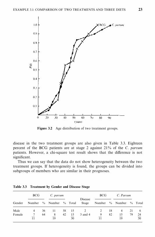
Figure 3.2 Age distribution of two treatment groups.
Table 3.3 Treatment by Gender and Disease Stage
BCG C. parvum BCG C. ParvumDisease
Gender Number % Number % Total Stage Number % Number % Total
Male 4 36 11 58 15 2 2 18 4 21 6Female 7 64 8 42 15 3 and 4 9 82 15 79 24
— — — — — —11 19 30 11 19 30
disease in the two treatment groups are also given in Table 3.3. Eighteenpercent of the BCG patients are at stage 2 against 21% of the C. parvumpatients. However, a chi-square test result shows that the difference is notsignificant.
Thus we can say that the data do not show heterogeneity between the twotreatment groups. If heterogeneity is found, the groups can be divided intosubgroups of members who are similar in their prognoses.
EXAMPLE 3.1: COMPARISON OF TWO TREATMENTS AND THREE DIETS 23
3. Compare the two survival distributions. There are several parametric andnonparametric tests to compare two survival distributions. They are describedin Chapters 5 and 10. Since we have no information of the survival distributionthat the data follow, we would continue to use nonparametric methods tocompare the two survival distributions. The four tests described in Sections5.1.1 to 5.1.4 are suitable. The performance of these tests is discussed at the endof Section 5.1. We chose Gehan’s generalized Wilcoxon test here to demon-strate the analysis procedure only because of its simplicity of calculation.
In testing the significance of the difference between two survival distribu-tions, the hypothesis is that the survival distribution of the BCG patients is thesame as that of the C. parvum patients. Let S
�(t) and S
�(t) be the survival
function of the BCG and C. parvum groups, respectively. The null hypothesis is
H�: S
�(t) � S
�(t)
The alternative hypothesis chosen is two-sided:
H�: S
�(t) � S
�(t)
since we have no prior information concerning the superiority of either of thetwo treatments. The slight difference between the two estimated survival curvescould be due to random variation. The one-sided alternative H
�:S
�(t) �S
�(t)
should be considered inappropriate.Using Gehan’s generalized Wilcoxon test, the difference in survival distribu-
tion of the two treatment groups is found to be insignificant (p� 0.33).Therefore, we do not reject the null hypothesis that the two survival distribu-tions are equal. Although our conclusion is that the data do not provideenough evidence to reject the hypothesis, ‘‘not to reject the null hypothesis’’does not automatically mean ‘‘to accept the null hypothesis.’’ The differencebetween the two statements is that the error probability of the latter statementis usually much larger than that of the former.
3.1.2 Comparison of Three Diets
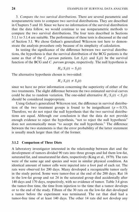
A laboratory investigator interested in the relationship between diet and thedevelopment of tumors divided 90 rats into three groups and fed them low-fat,saturated fat, and unsaturated fat diets, respectively (King et al., 1979). The ratswere of the same age and species and were in similar physical condition. Anidentical amount of tumor cells were injected into a foot pad of each rat. Therats were observed for 200 days. Many developed a recognizable tumor earlyin the study period. Some were tumor-free at the end of the 200 days. Rat 16in the low-fat group and rat 24 in the saturated group died accidentally after140 days and 170 days, respectively, with no evidence of tumor. Table 3.4 givesthe tumor-free time, the time from injection to the time that a tumor developsor to the end of the study. Fifteen of the 30 rats on the low-fat diet developeda tumor before the experiment was terminated. The rat that died had atumor-free time of at least 140 days. The other 14 rats did not develop any
24 EXAMPLES OF SURVIVAL DATA ANALYSIS
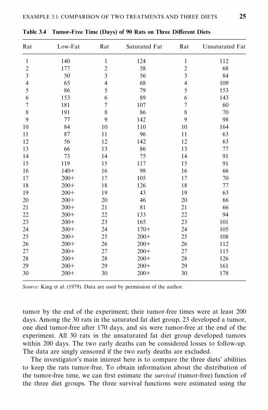
Table 3.4 Tumor-Free Time (Days) of 90 Rats on Three Different Diets
Rat Low-Fat Rat Saturated Fat Rat Unsaturated Fat
1 140 1 124 1 1122 177 2 58 2 683 50 3 56 3 844 65 4 68 4 1095 86 5 79 5 1536 153 6 89 6 1437 181 7 107 7 608 191 8 86 8 709 77 9 142 9 98
10 84 10 110 10 16411 87 11 96 11 6312 56 12 142 12 6313 66 13 86 13 7714 73 14 75 14 9115 119 15 117 15 9116 140� 16 98 16 6617 200� 17 105 17 7018 200� 18 126 18 7719 200� 19 43 19 6320 200� 20 46 20 6621 200� 21 81 21 6622 200� 22 133 22 9423 200� 23 165 23 10124 200� 24 170� 24 10525 200� 25 200� 25 10826 200� 26 200� 26 11227 200� 27 200� 27 11528 200� 28 200� 28 12629 200� 29 200� 29 16130 200� 30 200� 30 178
Source: King et al. (1979). Data are used by permission of the author.
tumor by the end of the experiment; their tumor-free times were at least 200days. Among the 30 rats in the saturated fat diet group, 23 developed a tumor,one died tumor-free after 170 days, and six were tumor-free at the end of theexperiment. All 30 rats in the unsaturated fat diet group developed tumorswithin 200 days. The two early deaths can be considered losses to follow-up.The data are singly censored if the two early deaths are excluded.
The investigator’s main interest here is to compare the three diets’ abilitiesto keep the rats tumor-free. To obtain information about the distribution ofthe tumor-free time, we can first estimate the survival (tumor-free) function ofthe three diet groups. The three survival functions were estimated using the
EXAMPLE 3.1: COMPARISON OF TWO TREATMENTS AND THREE DIETS 25
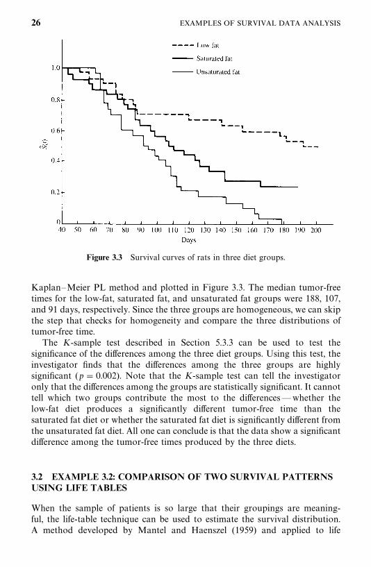
Figure 3.3 Survival curves of rats in three diet groups.
Kaplan—Meier PL method and plotted in Figure 3.3. The median tumor-freetimes for the low-fat, saturated fat, and unsaturated fat groups were 188, 107,and 91 days, respectively. Since the three groups are homogeneous, we can skipthe step that checks for homogeneity and compare the three distributions oftumor-free time.
The K-sample test described in Section 5.3.3 can be used to test thesignificance of the differences among the three diet groups. Using this test, theinvestigator finds that the differences among the three groups are highlysignificant (p� 0.002). Note that the K-sample test can tell the investigatoronly that the differences among the groups are statistically significant. It cannottell which two groups contribute the most to the differences—whether thelow-fat diet produces a significantly different tumor-free time than thesaturated fat diet or whether the saturated fat diet is significantly different fromthe unsaturated fat diet. All one can conclude is that the data show a significantdifference among the tumor-free times produced by the three diets.
3.2 EXAMPLE 3.2: COMPARISON OF TWO SURVIVAL PATTERNSUSING LIFE TABLES
When the sample of patients is so large that their groupings are meaning-ful, the life-table technique can be used to estimate the survival distribution.A method developed by Mantel and Haenszel (1959) and applied to life
26 EXAMPLES OF SURVIVAL DATA ANALYSIS
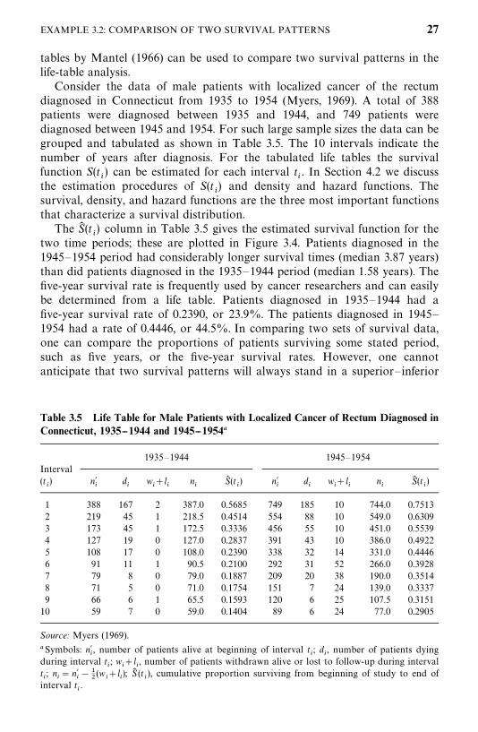
Table 3.5 Life Table for Male Patients with Localized Cancer of Rectum Diagnosed inConnecticut, 1935--1944 and 1945--1954�
1935—1944 1945—1954Interval(t�) n�
�d�
w��l
�n�
S� (t�) n�
�d�
w��l
�n�
S� (t�)
1 388 167 2 387.0 0.5685 749 185 10 744.0 0.75132 219 45 1 218.5 0.4514 554 88 10 549.0 0.63093 173 45 1 172.5 0.3336 456 55 10 451.0 0.55394 127 19 0 127.0 0.2837 391 43 10 386.0 0.49225 108 17 0 108.0 0.2390 338 32 14 331.0 0.44466 91 11 1 90.5 0.2100 292 31 52 266.0 0.39287 79 8 0 79.0 0.1887 209 20 38 190.0 0.35148 71 5 0 71.0 0.1754 151 7 24 139.0 0.33379 66 6 1 65.5 0.1593 120 6 25 107.5 0.3151
10 59 7 0 59.0 0.1404 89 6 24 77.0 0.2905
Source: Myers (1969).
�Symbols: n��, number of patients alive at beginning of interval t
�; d
�, number of patients dying
during interval t�; w
��l
�, number of patients withdrawn alive or lost to follow-up during interval
t�; n
�� n�
���
�(w
��l
�); S� (t
�), cumulative proportion surviving from beginning of study to end of
interval t�.
tables by Mantel (1966) can be used to compare two survival patterns in thelife-table analysis.
Consider the data of male patients with localized cancer of the rectumdiagnosed in Connecticut from 1935 to 1954 (Myers, 1969). A total of 388patients were diagnosed between 1935 and 1944, and 749 patients werediagnosed between 1945 and 1954. For such large sample sizes the data can begrouped and tabulated as shown in Table 3.5. The 10 intervals indicate thenumber of years after diagnosis. For the tabulated life tables the survivalfunction S(t
�) can be estimated for each interval t
�. In Section 4.2 we discuss
the estimation procedures of S(t�) and density and hazard functions. The
survival, density, and hazard functions are the three most important functionsthat characterize a survival distribution.
The S� (t�) column in Table 3.5 gives the estimated survival function for the
two time periods; these are plotted in Figure 3.4. Patients diagnosed in the1945—1954 period had considerably longer survival times (median 3.87 years)than did patients diagnosed in the 1935—1944 period (median 1.58 years). Thefive-year survival rate is frequently used by cancer researchers and can easilybe determined from a life table. Patients diagnosed in 1935—1944 had afive-year survival rate of 0.2390, or 23.9%. The patients diagnosed in 1945—1954 had a rate of 0.4446, or 44.5%. In comparing two sets of survival data,one can compare the proportions of patients surviving some stated period,such as five years, or the five-year survival rates. However, one cannotanticipate that two survival patterns will always stand in a superior— inferior
EXAMPLE 3.2: COMPARISON OF TWO SURVIVAL PATTERNS 27
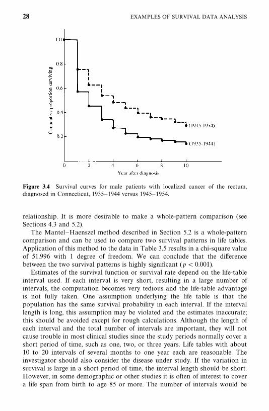
Figure 3.4 Survival curves for male patients with localized cancer of the rectum,diagnosed in Connecticut, 1935—1944 versus 1945—1954.
relationship. It is more desirable to make a whole-pattern comparison (seeSections 4.3 and 5.2).
The Mantel—Haenszel method described in Section 5.2 is a whole-patterncomparison and can be used to compare two survival patterns in life tables.Application of this method to the data in Table 3.5 results in a chi-square valueof 51.996 with 1 degree of freedom. We can conclude that the differencebetween the two survival patterns is highly significant (p� 0.001).
Estimates of the survival function or survival rate depend on the life-tableinterval used. If each interval is very short, resulting in a large number ofintervals, the computation becomes very tedious and the life-table advantageis not fully taken. One assumption underlying the life table is that thepopulation has the same survival probability in each interval. If the intervallength is long, this assumption may be violated and the estimates inaccurate;this should be avoided except for rough calculations. Although the length ofeach interval and the total number of intervals are important, they will notcause trouble in most clinical studies since the study periods normally cover ashort period of time, such as one, two, or three years. Life tables with about10 to 20 intervals of several months to one year each are reasonable. Theinvestigator should also consider the disease under study. If the variation insurvival is large in a short period of time, the interval length should be short.However, in some demographic or other studies it is often of interest to covera life span from birth to age 85 or more. The number of intervals would be
28 EXAMPLES OF SURVIVAL DATA ANALYSIS
very large if short intervals were used. In this case five-year intervals aresufficient to take into account the important variations in survival rateestimates (Shryock et al., 1971).
3.3 EXAMPLE 3.3: FITTING SURVIVAL DISTRIBUTIONS TOREMISSION DATA
The remission times of 42 patients with acute leukemia were reported byFreireich et al. (1963) in a clinical trial undertaken to assess the ability of6-mercaptopurine (6-MP) to maintain remission.� Each patient was ran-domized to receive 6-MP or a placebo. The study was terminated after oneyear. The following remission times, in weeks, were recorded:
6-MP (21 patients): 6, 6, 6, 7, 10, 13, 16, 22, 23, 6�, 9�, 10�, 11�, 17�,19�, 20�, 25�, 32�, 32�, 34�, 35�
Placebo (21 patients): 1, 1, 2, 2, 3, 4, 4, 5, 5, 8, 8, 8, 8, 11, 11, 12, 12, 15, 17,22, 23
Suppose that we are interested in a distribution to describe the remission timesof these patients but that no information is available as to which distributionwill fit. We need to find a distribution that fits the data well. If we can find one,the remission experience can then be described by the properties of thedistribution, and the remission time of new patients can be predicted. Paramet-ric tests can be used to compare the effectiveness of the two treatments, butsince there are a large number of well-known functions and distributions tochoose from, the search becomes an art as much as a scientific task.
The simplest and most efficient tool is the graph. Probability plotting canbe done for complete data; for data that include censored observations, hazardplotting and the Cox—Snell method are more appropriate. It is not difficult touse the computer to generate these plots. Detailed discussions of probabilityplotting and hazard plotting are presented in Chapter 8. In both probabilityand hazard plotting, a linear configuration indicates that the distribution fitswell and its parameters can be estimated from the graph.
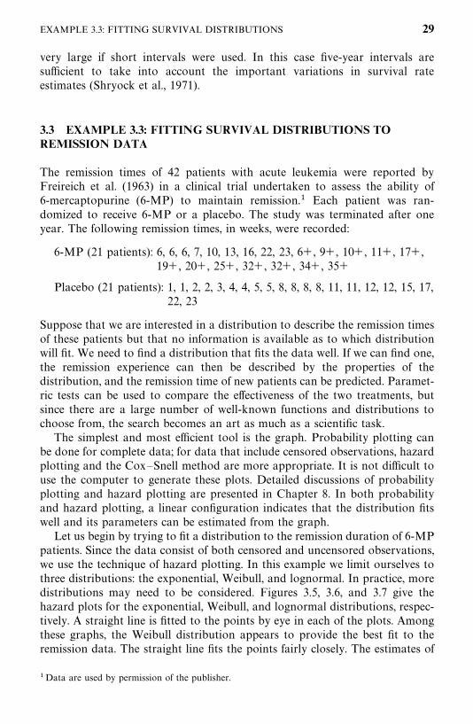
Let us begin by trying to fit a distribution to the remission duration of 6-MPpatients. Since the data consist of both censored and uncensored observations,we use the technique of hazard plotting. In this example we limit ourselves tothree distributions: the exponential, Weibull, and lognormal. In practice, moredistributions may need to be considered. Figures 3.5, 3.6, and 3.7 give thehazard plots for the exponential, Weibull, and lognormal distributions, respec-tively. A straight line is fitted to the points by eye in each of the plots. Amongthese graphs, the Weibull distribution appears to provide the best fit to theremission data. The straight line fits the points fairly closely. The estimates of
�Data are used by permission of the publisher.
EXAMPLE 3.3: FITTING SURVIVAL DISTRIBUTIONS 29
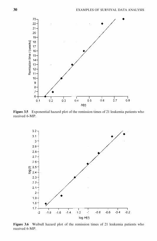
Figure 3.5 Exponential hazard plot of the remission times of 21 leukemia patients whoreceived 6-MP.
Figure 3.6 Weibull hazard plot of the remission times of 21 leukemia patients whoreceived 6-MP.
30 EXAMPLES OF SURVIVAL DATA ANALYSIS
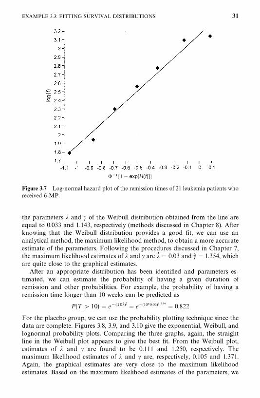
����1� exp[H(t)]�
Figure 3.7 Log-normal hazard plot of the remission times of 21 leukemia patients whoreceived 6-MP.
the parameters � and � of the Weibull distribution obtained from the line areequal to 0.033 and 1.143, respectively (methods discussed in Chapter 8). Afterknowing that the Weibull distribution provides a good fit, we can use ananalytical method, the maximum likelihood method, to obtain a more accurateestimate of the parameters. Following the procedures discussed in Chapter 7,the maximum likelihood estimates of � and � are �� � 0.03 and � � 1.354, whichare quite close to the graphical estimates.
After an appropriate distribution has been identified and parameters es-timated, we can estimate the probability of having a given duration ofremission and other probabilities. For example, the probability of having aremission time longer than 10 weeks can be predicted as
P(T 10) � e������ �� � e�(10*0.03)��� � 0.822
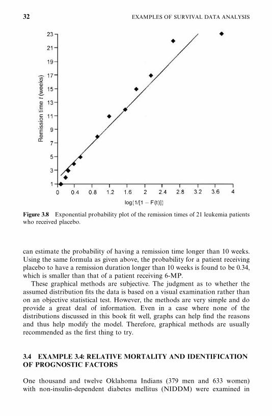
For the placebo group, we can use the probability plotting technique since thedata are complete. Figures 3.8, 3.9, and 3.10 give the exponential, Weibull, andlognormal probability plots. Comparing the three graphs, again, the straightline in the Weibull plot appears to give the best fit. From the Weibull plot,estimates of � and � are found to be 0.111 and 1.250, respectively. Themaximum likelihood estimates of � and � are, respectively, 0.105 and 1.371.Again, the graphical estimates are very close to the maximum likelihoodestimates. Based on the maximum likelihood estimates of the parameters, we
EXAMPLE 3.3: FITTING SURVIVAL DISTRIBUTIONS 31
log�1/[1�F(t )]�
Figure 3.8 Exponential probability plot of the remission times of 21 leukemia patientswho received placebo.
can estimate the probability of having a remission time longer than 10 weeks.Using the same formula as given above, the probability for a patient receivingplacebo to have a remission duration longer than 10 weeks is found to be 0.34,which is smaller than that of a patient receiving 6-MP.
These graphical methods are subjective. The judgment as to whether theassumed distribution fits the data is based on a visual examination rather thanon an objective statistical test. However, the methods are very simple and doprovide a great deal of information. Even in a case where none of thedistributions discussed in this book fit well, graphs can help find the reasonsand thus help modify the model. Therefore, graphical methods are usuallyrecommended as the first thing to try.
3.4 EXAMPLE 3.4: RELATIVE MORTALITY AND IDENTIFICATIONOF PROGNOSTIC FACTORS
One thousand and twelve Oklahoma Indians (379 men and 633 women)with non-insulin-dependent diabetes mellitus (NIDDM) were examined in
32 EXAMPLES OF SURVIVAL DATA ANALYSIS
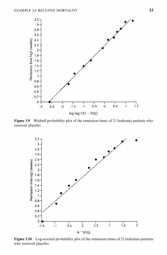
log log�1/[1� F(t)]�
Figure 3.9 Weibull probability plot of the remission times of 21 leukemia patients whoreceived placebo.
���(F(t))
Figure 3.10 Log-normal probability plot of the remission times of 21 leukemia patientswho received placebo.
EXAMPLE 3.4: RELATIVE MORTALITY 33
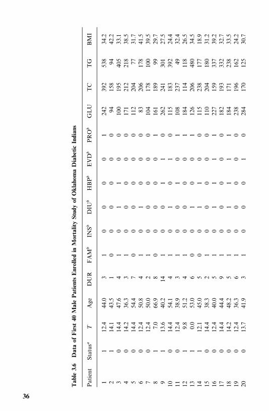
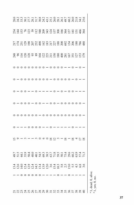
1972—1980 and a mortality follow-up study was conducted in 1986—1989 (Leeet al., 1993). The mean [standard deviation (SD)] age and duration of diabetesat baseline examination were 52 (11) and 7 (6) years. The average duration offollow-up was 10 (SD 4) years. As of December 31, 1989, 548 patients werealive, 452 (187 men and 265 women) were dead, and 12 could not be traced.Table 3.6 gives the survival time in years (T ) of the first 40 male patients alongwith 12 potential prognostic factors: age, duration of diabetes (DUR) in years,family history of diabetes (FAM), use of insulin within one year of diagnosis(INS), use of diuretics (DIU), hypertension (HBP), retinopathy (EVD), pro-teinuria (PRO), fasting plasma glucose (GLU) in milligrams per deciliter,cholesterol (TC) in milligrams per deciliter, triglyceride (TG) in milligrams perdeciliter, and body mass index (BMI), which is defined as weight in kilogramsdivided by height in meters squared.
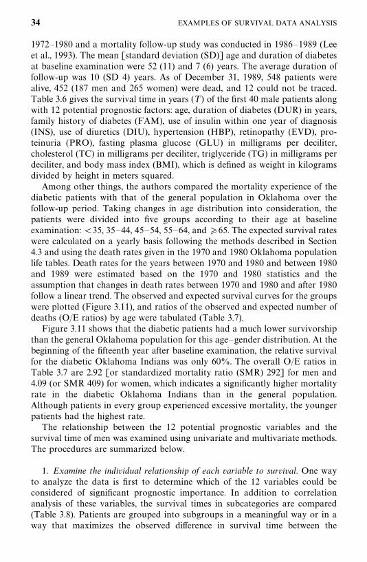
Among other things, the authors compared the mortality experience of thediabetic patients with that of the general population in Oklahoma over thefollow-up period. Taking changes in age distribution into consideration, thepatients were divided into five groups according to their age at baselineexamination: �35, 35—44, 45—54, 55—64, and �65. The expected survival rateswere calculated on a yearly basis following the methods described in Section4.3 and using the death rates given in the 1970 and 1980 Oklahoma populationlife tables. Death rates for the years between 1970 and 1980 and between 1980and 1989 were estimated based on the 1970 and 1980 statistics and theassumption that changes in death rates between 1970 and 1980 and after 1980follow a linear trend. The observed and expected survival curves for the groupswere plotted (Figure 3.11), and ratios of the observed and expected number ofdeaths (O/E ratios) by age were tabulated (Table 3.7).
Figure 3.11 shows that the diabetic patients had a much lower survivorshipthan the general Oklahoma population for this age—gender distribution. At thebeginning of the fifteenth year after baseline examination, the relative survivalfor the diabetic Oklahoma Indians was only 60%. The overall O/E ratios inTable 3.7 are 2.92 [or standardized mortality ratio (SMR) 292] for men and4.09 (or SMR 409) for women, which indicates a significantly higher mortalityrate in the diabetic Oklahoma Indians than in the general population.Although patients in every group experienced excessive mortality, the youngerpatients had the highest rate.
The relationship between the 12 potential prognostic variables and thesurvival time of men was examined using univariate and multivariate methods.The procedures are summarized below.
1. Examine the individual relationship of each variable to survival. One wayto analyze the data is first to determine which of the 12 variables could beconsidered of significant prognostic importance. In addition to correlationanalysis of these variables, the survival times in subcategories are compared(Table 3.8). Patients are grouped into subgroups in a meaningful way or in away that maximizes the observed difference in survival time between the
34 EXAMPLES OF SURVIVAL DATA ANALYSIS
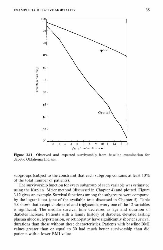
Figure 3.11 Observed and expected survivorship from baseline examination fordabetic Oklahoma Indians.
subgroups (subject to the constraint that each subgroup contains at least 10%of the total number of patients).
The survivorship function for every subgroup of each variable was estimatedusing the Kaplan—Meier method (discussed in Chapter 4) and plotted. Figure3.12 gives an example. Survival functions among the subgroups were comparedby the logrank test (one of the available tests discussed in Chapter 5). Table3.8 shows that except cholesterol and triglyceride, every one of the 12 variablesis significant. The median survival time decreases as age and duration ofdiabetes increase. Patients with a family history of diabetes, elevated fastingplasma glucose, hypertension, or retinopathy have significantly shorter survivaldurations than those without these characteristics. Patients with baseline BMIvalues greater than or equal to 30 had much better survivorship than didpatients with a lower BMI value.
EXAMPLE 3.4: RELATIVE MORTALITY 35
Tab
le3.6
Dataof
First
40M
alePatientsEnr
olledin
Mor
talitySt
udyof
Oklah
omaDiabe
ticIndian
s
Patient
Status�
TAge
DUR
FAM
�IN
S�
DIU
�HBP�
EVD
�PRO
�GLU
TC
TG
BM
I
11
12.4
44.0
31
00
00
124
239
253
834
.22
114
.143
.51
00
00
00
9415
894
42.2
30
14.4
47.6
41
01
10
010
019
540
533
.14
014
.236
.33
10
00
00
171
212
218
38.5
50
14.4
54.4
70
00
00
011
220
477
31.7
60
12.4
50.8
41
01
00
083
206
178
41.5
70
12.4
50.0
21
00
00
010
417
810
039
.58
17.0
66.9
80
00
00
116
118
999
29.7
91
13.6
40.2
141
00
11
026
224
130
127
.510
014
.454
.14
10
10
10
115
183
392
24.4
110
12.4
38.9
31
00
10
110
823
749
32.4
121
9.8
51.2
41
00
00
118
411
411
826
.513
10.0
53.0
60
01
00
112
620
648
034
.514
112
.145
.05
00
11
00
115
238
177
18.9
150
14.4
38.3
21
00
00
011
020
418
031
.216
012
.440
.05
10
11
11
227
159
337
39.2
170
14.4
44.4
91
00
00
018
219
333
232
.718
014
.248
.25
10
11
11
184
171
238
33.5
190
12.4
36.3
61
00
00
023
819
616
224
.220
013
.741
.93
10
00
10
284
170
125
30.7
36
211
13.4
49.7
150
00
00
024
821
723
428
.022
112
.651
.59
10
11
10
9617
414
424
.223
014
.044
.11
10
00
00
116
251
153
33.3
240
12.4
35.9
31
00
00
012
012
976
30.1
250
12.9
50.4
10
00
10
012
819
012
327
.726
012
.448
.01
00
11
00
9520
759
28.1
270
14.5
40.1
30
00
00
089
252
112
31.7
280
13.4
54.5
00
10
10
010
449
054
030
.829
113
.969
.36
10
11
00
122
162
209
24.2
301
12.0
38.5
01
01
10
122
518
334
343
.131
13.6
63.7
180
00
11
021
121
712
425
.132
115
.471
.812
10
00
00
150
227
137
26.0
330
10.3
59.5
31
01
10
018
018
830
828
.134
15.8
50.1
11
00
00
040
020
016
626
.135
12.5
75.4
181
00
10
128
169
236
449
.736
015
.029
.61
10
00
01
167
154
157
60.2
371
5.5
60.2
180
00
01
035
120
614
126
.038
14.5
63.9
41
00
10
112
718
013
121
.839
16.8
57.4
171
00
11
015
378
646
634
.140
13.6
71.3
181
11
11
117
948
836
425
.6
�1,
dead
;0,
alive.
�1,
yes;
0,no.
37
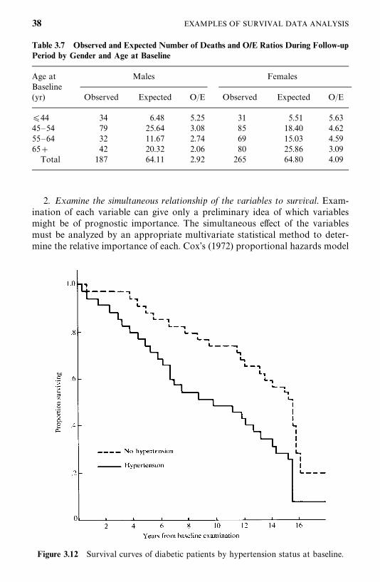
Figure 3.12 Survival curves of diabetic patients by hypertension status at baseline.
Table 3.7 Observed and Expected Number of Deaths and O/E Ratios During Follow-upPeriod by Gender and Age at Baseline
Age at Males FemalesBaseline(yr) Observed Expected O/E Observed Expected O/E
�44 34 6.48 5.25 31 5.51 5.6345—54 79 25.64 3.08 85 18.40 4.6255—64 32 11.67 2.74 69 15.03 4.5965� 42 20.32 2.06 80 25.86 3.09
Total 187 64.11 2.92 265 64.80 4.09
2. Examine the simultaneous relationship of the variables to survival. Exam-ination of each variable can give only a preliminary idea of which variablesmight be of prognostic importance. The simultaneous effect of the variablesmust be analyzed by an appropriate multivariate statistical method to deter-mine the relative importance of each. Cox’s (1972) proportional hazards model
38 EXAMPLES OF SURVIVAL DATA ANALYSIS
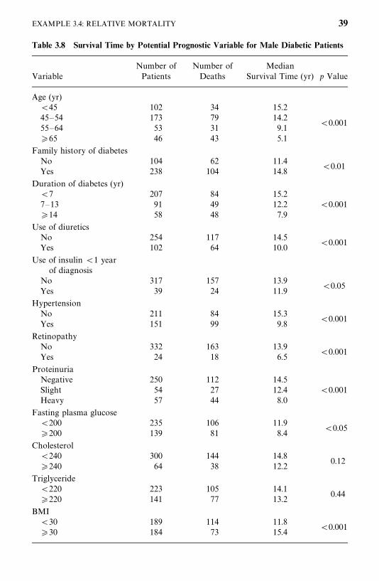
Table 3.8 Survival Time by Potential Prognostic Variable for Male Diabetic Patients
Number of Number of MedianVariable Patients Deaths Survival Time (yr) p Value
Age (yr)�45 102 34 15.245—54 173 79 14.2 �0.00155—64 53 31 9.1�65 46 43 5.1
Family history of diabetesNo 104 62 11.4 �0.01Yes 238 104 14.8
Duration of diabetes (yr)�7 207 84 15.27—13 91 49 12.2 �0.001�14 58 48 7.9
Use of diureticsNo 254 117 14.5 �0.001Yes 102 64 10.0
Use of insulin �1 yearof diagnosis
No 317 157 13.9 �0.05Yes 39 24 11.9
HypertensionNo 211 84 15.3 �0.001Yes 151 99 9.8
RetinopathyNo 332 163 13.9 �0.001Yes 24 18 6.5
ProteinuriaNegative 250 112 14.5Slight 54 27 12.4 �0.001Heavy 57 44 8.0
Fasting plasma glucose�200 235 106 11.9 �0.05�200 139 81 8.4
Cholesterol�240 300 144 14.8
0.12�240 64 38 12.2
Triglyceride�220 223 105 14.1
0.44�220 141 77 13.2
BMI�30 189 114 11.8 �0.001�30 184 73 15.4
EXAMPLE 3.4: RELATIVE MORTALITY 39
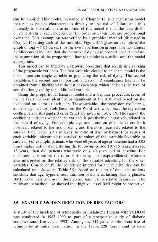
can be applied. This model, presented in Chapter 12, is a regression modelthat relates patient characteristics directly to the risk of failure and thusindirectly to survival. The assumption of this model is that the hazards fordifferent strata of each independent (or prognostic) variable are proportionalover time. This assumption was verified by a graphical method (discussed inChapter 12) using each of the variables. Figure 3.13 gives an example of thegraph of log[�S(t)] versus t for the two hypertension groups. The two almostparallel curves indicate that the hazards of dying are proportional. Therefore,the assumption of the proportional hazards model is satisfied and the modelappropriate.
This model can be fitted by a stepwise procedure that results in a rankingof the prognostic variables. The first variable selected to enter the model is themost important single variable in predicting the risk of dying. The secondvariable is the second most important, and so on. A significance level can beobtained from a likelihood ratio test at each step, which indicates the level ofcontribution given by the additional variable.
Using the proportional hazards model and a stepwise procedure, seven ofthe 12 variables were identified as significant at the 0.05 level based on thelikelihood ratio test at each step. These variables, the regression coefficients,and the significance levels based on the Ward test, which uses the regressioncoefficient and its standard error (S.E.) are given in Table 3.9. The sign of thecoefficient indicates whether the variable is positively or negatively related tothe hazard of dying. For example, age and duration of diabetes are bothpositively related to the risk of dying and therefore negatively related to thesurvival time. Table 3.9 also gives the ratio of risk (or hazard) for values ofeach variable unfavorable to survival to values of that variable favorable tosurvival. For example, patients who were 60 years of age at baseline had a 3.05times higher risk of dying during the follow-up period (10—16 years, average13 years) than did patients who were only 40 years old at baseline. Fordichotomous variables, the ratio of risk is equal to exp(coefficient), which isalso interpreted as the relative risk of the variable adjusting for the othervariables. Consequently, the confidence interval for the relative risk can becalculated (not shown in Table 3.9). Based on this set of data, the authorsconclude that age, hypertension, duration of diabetes, fasting plasma glucose,BMI, proteinuria, and use of diuretics are significantly related to survival. Themultivariate method also showed that high values of BMI might be protective.
3.5 EXAMPLE 3.5: IDENTIFICATION OF RISK FACTORS
A study of the incidence of retinopathy in Oklahoma Indians with NIDDMwas conducted in 1987—1990 as part of a prospective study of diabeticcomplications (Lee et al., 1992). Among the 312 patients who were free ofretinopathy at initial examination in the 1970s, 228 were found to have
40 EXAMPLES OF SURVIVAL DATA ANALYSIS
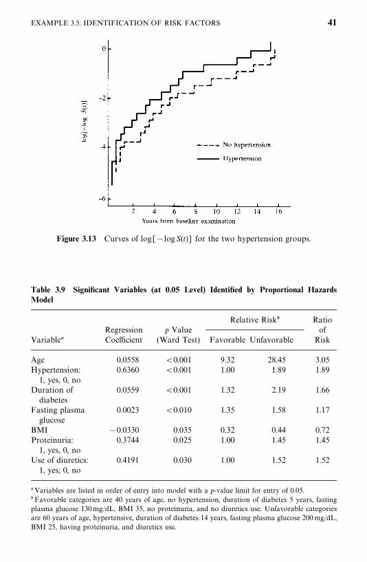
Figure 3.13 Curves of log[�logS(t)] for the two hypertension groups.
Table 3.9 Significant Variables (at 0.05 Level) Identified by Proportional HazardsModel
Relative Risk� RatioRegression p Value of
Variable� Coefficient (Ward Test) Favorable Unfavorable Risk
Age 0.0558 �0.001 9.32 28.45 3.05Hypertension: 0.6360 �0.001 1.00 1.89 1.89
1, yes, 0, noDuration of 0.0559 �0.001 1.32 2.19 1.66
diabetesFasting plasma 0.0023 �0.010 1.35 1.58 1.17
glucoseBMI �0.0330 0.035 0.32 0.44 0.72Proteinuria: 0.3744 0.025 1.00 1.45 1.45
1, yes, 0, noUse of diuretics: 0.4191 0.030 1.00 1.52 1.52
1, yes; 0, no
�Variables are listed in order of entry into model with a p-value limit for entry of 0.05.�Favorable categories are 40 years of age, no hypertension, duration of diabetes 5 years, fastingplasma glucose 130mg/dL, BMI 35, no proteinuria, and no diuretics use. Unfavorable categoriesare 60 years of age, hypertensive, duration of diabetes 14 years, fasting plasma glucose 200mg/dL,BMI 25, having proteinuria, and diuretics use.
EXAMPLE 3.5: IDENTIFICATION OF RISK FACTORS 41
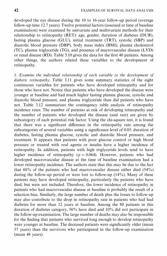
developed the eye disease during the 10 to 16-year follow-up period (averagefollow-up time 12.7 years). Twelve potential factors (assessed at time of baselineexamination) were examined by univariate and multivariate methods for theirrelationship to retinopathy (RET): age, gender, duration of diabetes (DUR),fasting plasma glucose (GLU), initial treatment (TRT), systolic (SBP) anddiastolic blood pressure (DBP), body mass index (BMI), plasma cholesterol(TC), plasma triglyceride (TG), and presence of macrovascular disease (LVD)or renal disease (RD). Table 3.10 gives the data for the first 40 patients. Amongother things, the authors related these variables to the development ofretinopathy.
1. Examine the individual relationship of each variable to the development ofdiabetic retinopathy. Table 3.11 gives some summary statistics of the eightcontinuous variables for patients who have developed retinopathy and forthose who have not. Notice that patients who have developed the disease wereyounger at baseline and had much higher fasting plasma glucose, systolic anddiastolic blood pressure, and plasma triglyceride than did patients who havenot. Table 3.12 summarizes the contingency table analysis of retinopathyincidence rates. The number of patients at risk of developing retinopathy andthe number of patients who developed the disease (and rate) are given bysubcategory of each potential risk factor. Using the chi-square test, it is foundthat there was a significant difference in the retinopathy rate among thesubcategories of several variables using a significance level of 0.05: duration ofdiabetes, fasting plasma glucose, systolic and diastolic blood pressure, andtreatment. It appears that patients with poor glucose control or high bloodpressure or treated with oral agents or insulin have a higher incidence ofretinopathy. In addition, patients with high triglyceride levels tend to havehigher incidence of retinopathy (p� 0.064). However, patients who haddeveloped macrovascular disease at the time of baseline examination had alower retinopathy incidence. The authors state that this may be due to the factthat 68% of the patients who had macrovascular disease either died (54%)during the follow-up period or were lost to follow-up (14%). Many of thesepatients may have developed retinopathy, particularly the patients who havedied, but were not included. Therefore, the lower incidence of retinopathy inpatients who had macrovascular disease at baseline is probably the result of aselection bias. Similarly, the large number of death plus the losses to follow-upmay also contribute to the drop in retinopathy rate in patients who had haddiabetes for more than 12 years at baseline. Among the 80 patients in thisduration of diabetes category, 56% have died and 10% did not participate inthe follow-up examination. The large number of deaths may also be responsiblefor the finding that patients who survived long enough to develop retinopathywere younger at baseline. The deceased patients were significantly older (mean57 years) than the survivors who participated in the follow-up examination(mean 48 years).
42 EXAMPLES OF SURVIVAL DATA ANALYSIS
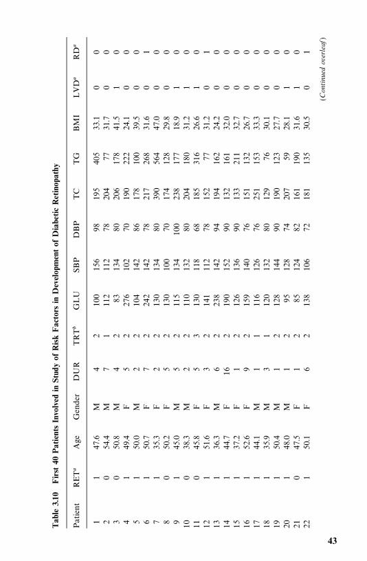
Tab
le3.10
First
40PatientsIn
volved
inStudy
ofRisk
Fac
tors
inDevelop
men
tof
Diabe
ticRetinop
athy
Patient
RET�
Age
Gen
der
DUR
TRT�
GLU
SBP
DBP
TC
TG
BM
ILVD
�RD
�
11
47.6
M4
210
015
698
195
405
33.1
00
20
54.4
M7
111
211
278
204
7731
.70
03
050
.8M
42
8313
480
206
178
41.5
10
41
49.4
F5
227
610
270
190
222
24.1
00
51
50.0
M2
210
414
286
178
100
39.5
00
61
50.7
F7
224
214
278
217
268
31.6
01
71
35.3
F2
213
013
480
390
564
47.0
00
80
50.2
F5
213
010
070
174
128
29.8
00
91
45.0
M5
211
513
410
023
817
718
.91
010
038
.3M
22
110
132
8020
418
031
.21
011
045
.8F
53
130
118
6818
531
626
.61
012
151
.6F
32
141
112
7815
277
31.2
01
131
36.3
M6
223
814
294
194
162
24.2
00
141
44.7
F16
219
015
290
132
161
32.0
00
151
37.2
F1
212
613
690
133
211
32.7
00
161
52.6
F9
215
914
076
151
132
26.7
00
171
44.1
M1
111
612
676
251
153
33.3
00
181
35.9
M3
112
013
280
129
7630
.10
019
150
.4M
12
128
144
9019
012
327
.70
020
148
.0M
12
9512
874
207
5928
.11
021
047
.5F
12
8512
482
161
190
31.6
10
221
50.1
F6
213
810
672
181
135
30.5
01
(Continued
overleaf
)
43
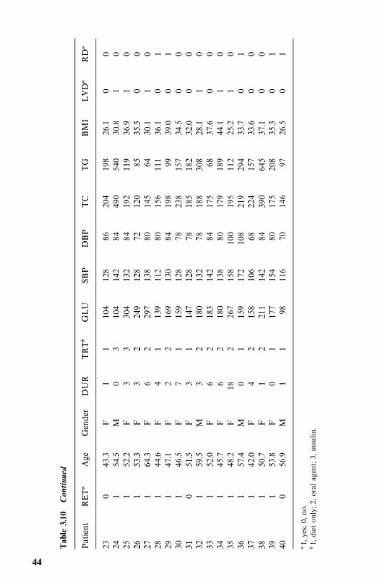
Tab
le3.10
Con
tinu
ed
Patient
RET�
Age
Gen
der
DUR
TRT�
GLU
SBP
DBP
TC
TG
BM
ILVD
�RD
�
230
43.3
F1
110
412
886
204
198
26.1
00
241
54.5
M0
310
414
284
490
540
30.8
10
251
52.2
F3
330
413
284
192
119
36.9
10
261
53.3
F3
224
912
872
120
8535
.50
027
164
.3F
62
297
138
8014
564
30.1
10
281
44.6
F4
113
911
280
156
111
36.1
01
291
47.1
F2
216
913
084
198
9939
.00
130
146
.5F
71
159
128
7823
815
734
.50
031
051
.5F
31
147
128
7818
518
232
.00
032
159
.5M
32
180
132
7818
830
828
.11
033
152
.0F
62
183
142
8417
568
37.6
00
341
45.7
F6
218
013
880
179
189
44.1
10
351
48.2
F18
226
715
810
019
511
225
.21
036
157
.4M
01
159
172
108
219
294
33.7
01
371
42.0
F4
215
810
668
224
157
33.6
00
381
50.7
F1
221
114
284
390
645
37.1
00
391
53.8
F0
117
715
480
175
208
35.3
01
400
56.9
M1
198
116
7014
697
26.5
01
�1,
yes;
0,no.
�1,
diet
only;2,
oral
agen
t;3,
insu
lin.
44
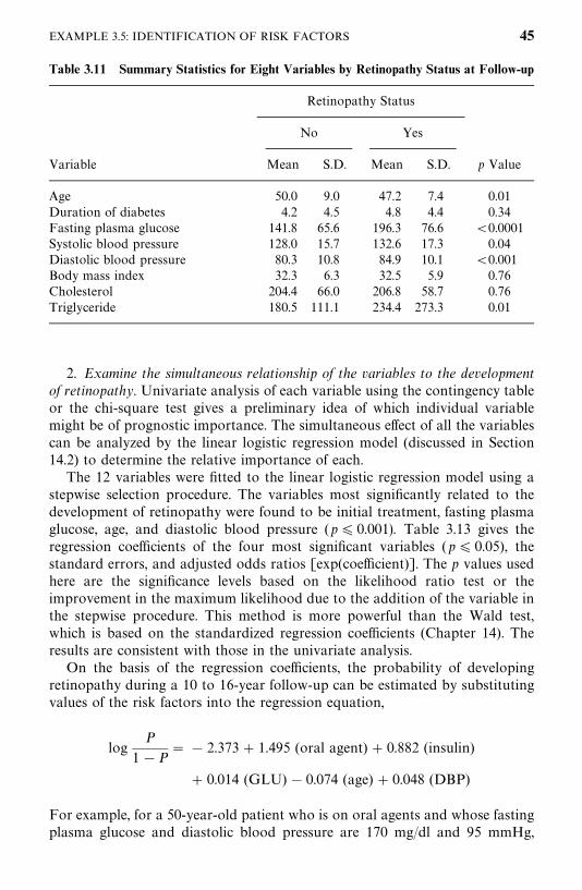
Table 3.11 Summary Statistics for Eight Variables by Retinopathy Status at Follow-up
Retinopathy Status
No Yes
Variable Mean S.D. Mean S.D. p Value
Age 50.0 9.0 47.2 7.4 0.01Duration of diabetes 4.2 4.5 4.8 4.4 0.34Fasting plasma glucose 141.8 65.6 196.3 76.6 �0.0001Systolic blood pressure 128.0 15.7 132.6 17.3 0.04Diastolic blood pressure 80.3 10.8 84.9 10.1 �0.001Body mass index 32.3 6.3 32.5 5.9 0.76Cholesterol 204.4 66.0 206.8 58.7 0.76Triglyceride 180.5 111.1 234.4 273.3 0.01
2. Examine the simultaneous relationship of the variables to the developmentof retinopathy. Univariate analysis of each variable using the contingency tableor the chi-square test gives a preliminary idea of which individual variablemight be of prognostic importance. The simultaneous effect of all the variablescan be analyzed by the linear logistic regression model (discussed in Section14.2) to determine the relative importance of each.
The 12 variables were fitted to the linear logistic regression model using astepwise selection procedure. The variables most significantly related to thedevelopment of retinopathy were found to be initial treatment, fasting plasmaglucose, age, and diastolic blood pressure (p� 0.001). Table 3.13 gives theregression coefficients of the four most significant variables (p� 0.05), thestandard errors, and adjusted odds ratios [exp(coefficient)]. The p values usedhere are the significance levels based on the likelihood ratio test or theimprovement in the maximum likelihood due to the addition of the variable inthe stepwise procedure. This method is more powerful than the Wald test,which is based on the standardized regression coefficients (Chapter 14). Theresults are consistent with those in the univariate analysis.
On the basis of the regression coefficients, the probability of developingretinopathy during a 10 to 16-year follow-up can be estimated by substitutingvalues of the risk factors into the regression equation,
logP
1�P� � 2.373� 1.495 (oral agent) � 0.882 (insulin)
� 0.014 (GLU) � 0.074 (age) � 0.048 (DBP)
For example, for a 50-year-old patient who is on oral agents and whose fastingplasma glucose and diastolic blood pressure are 170 mg/dl and 95 mmHg,
EXAMPLE 3.5: IDENTIFICATION OF RISK FACTORS 45
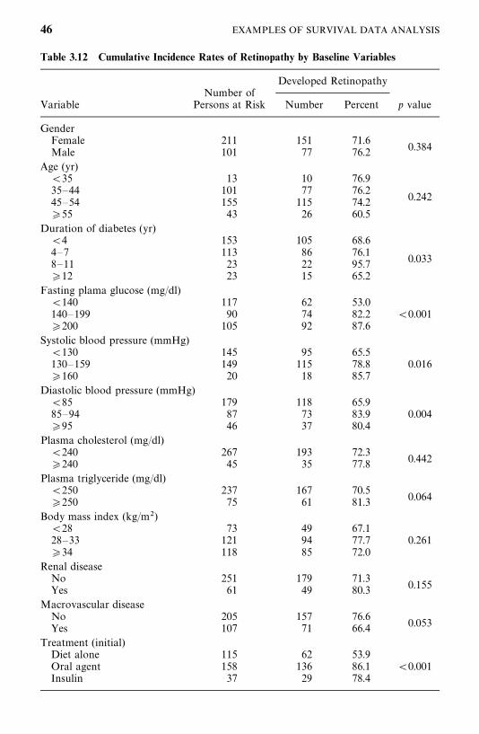
Table 3.12 Cumulative Incidence Rates of Retinopathy by Baseline Variables
Developed RetinopathyNumber of
Variable Persons at Risk Number Percent p value
GenderFemale 211 151 71.6
0.384Male 101 77 76.2Age (yr)
�35 13 10 76.935—44 101 77 76.2
0.24245—54 155 115 74.2�55 43 26 60.5
Duration of diabetes (yr)�4 153 105 68.64—7 113 86 76.1
0.0338—11 23 22 95.7�12 23 15 65.2
Fasting plama glucose (mg/dl)�140 117 62 53.0140—199 90 74 82.2 �0.001�200 105 92 87.6
Systolic blood pressure (mmHg)�130 145 95 65.5130—159 149 115 78.8 0.016�160 20 18 85.7
Diastolic blood pressure (mmHg)�85 179 118 65.985—94 87 73 83.9 0.004�95 46 37 80.4
Plasma cholesterol (mg/dl)�240 267 193 72.3
0.442�240 45 35 77.8Plasma triglyceride (mg/dl)
�250 237 167 70.50.064�250 75 61 81.3
Body mass index (kg/m�)�28 73 49 67.128—33 121 94 77.7 0.261�34 118 85 72.0
Renal diseaseNo 251 179 71.3
0.155Yes 61 49 80.3Macrovascular disease
No 205 157 76.60.053Yes 107 71 66.4
Treatment (initial)Diet alone 115 62 53.9Oral agent 158 136 86.1 �0.001Insulin 37 29 78.4
46 EXAMPLES OF SURVIVAL DATA ANALYSIS
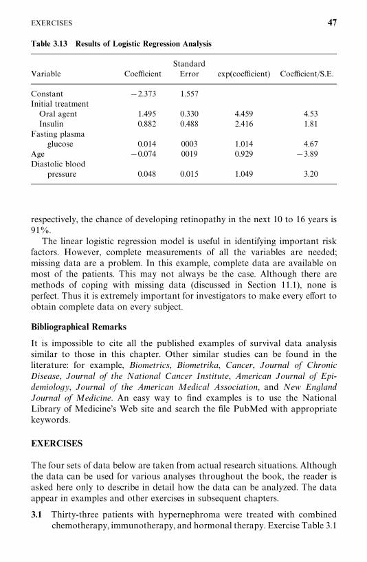
Table 3.13 Results of Logistic Regression Analysis
StandardVariable Coefficient Error exp(coefficient) Coefficient/S.E.
Constant �2.373 1.557Initial treatment
Oral agent 1.495 0.330 4.459 4.53Insulin 0.882 0.488 2.416 1.81
Fasting plasma0.014 0003 1.014 4.67glucose
Age �0.074 0019 0.929 �3.89Diastolic blood
0.048 0.015 1.049 3.20pressure
respectively, the chance of developing retinopathy in the next 10 to 16 years is91%.
The linear logistic regression model is useful in identifying important riskfactors. However, complete measurements of all the variables are needed;missing data are a problem. In this example, complete data are available onmost of the patients. This may not always be the case. Although there aremethods of coping with missing data (discussed in Section 11.1), none isperfect. Thus it is extremely important for investigators to make every effort toobtain complete data on every subject.
Bibliographical Remarks
It is impossible to cite all the published examples of survival data analysissimilar to those in this chapter. Other similar studies can be found in theliterature: for example, Biometrics, Biometrika, Cancer, Journal of ChronicDisease, Journal of the National Cancer Institute, American Journal of Epi-demiology, Journal of the American Medical Association, and New EnglandJournal of Medicine. An easy way to find examples is to use the NationalLibrary of Medicine’s Web site and search the file PubMed with appropriatekeywords.
EXERCISES
The four sets of data below are taken from actual research situations. Althoughthe data can be used for various analyses throughout the book, the reader isasked here only to describe in detail how the data can be analyzed. The dataappear in examples and other exercises in subsequent chapters.
3.1 Thirty-three patients with hypernephroma were treated with combinedchemotherapy, immunotherapy, and hormonal therapy. Exercise Table 3.1
EXERCISES 47
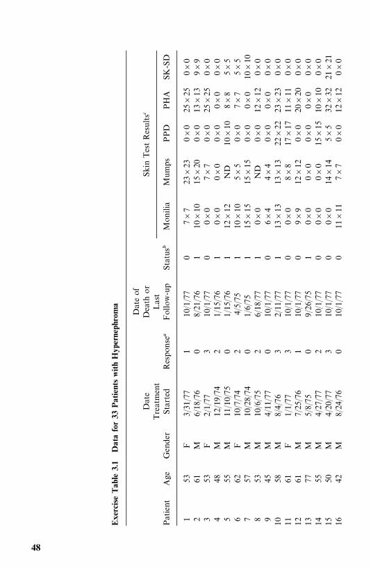
Exe
rciseTab
le3.1
Datafor33
PatientswithHyp
erne
phro
ma
Dateof
Date
Dea
thor
Skin
TestResults�
Treatmen
tLast
Patient
Age
Gen
der
Started
Respon
se�
Follow-u
pStatus�
Mon
ilia
Mumps
PPD
PHA
SK-SD
153
F3/31
/77
110
/1/77
07�
723
�23
0�0
25�
250�
02
61M
6/18
/76
08/21
/76
110
�10
15�
200�
013
�13
9�9
353
F2/1/77
310
/1/77
00�
07�
70�
025
�25
0�0
448
M12
/19/74
21/15
/76
10�
00�
00�
00�
00�
05
55M
11/10/75
01/15
/76
112
�12
ND
10�
108�
85�
56
62F
10/7/74
24/5/75
110
�10
5�5
0�0
7�7
5�5
757
M10
/28/74
01/6/75
115
�15
15�
150�
00�
010
�10
853
M10
/6/75
26/18
/77
10�
0ND
0�0
12�
120�
09
45M
4/11
/77
010
/1/77
06�
44�
40�
00�
00�
010
58M
8/4/76
32/11
/77
113
�13
13�
1322
�22
23�
230�
011
61F
1/1/77
310
/1/77
00�
08�
817
�17
11�
110�
012
61M
7/25
/76
110
/1/77
09�
912
�12
0�0
20�
200�
013
77M
5/8/75
09/26
/75
10�
00�
00�
00�
00�
014
55M
4/27
/77
210
/1/77
00�
00�
015
�15
10�
100�
015
50M
4/20
/77
310
/1/77
00�
014
�14
5�5
32�
3221
�21
1642
M8/24
/76
010
/1/77
011
�11
7�7
0�0
12�
120�
0
48
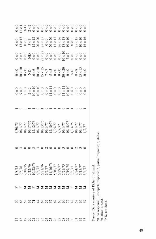
1750
F1/8/75
06/30
/75
10�
00�
00�
00�
00�
018
66F
9/8/76
310
/1/77
09�
910
�10
6�6
15�
1511
�11
1958
M2/18
/75
010
/1/77
00�
00�
00�
00�
0ND
2062
M5/12
/76
010
/17/76
12�
2ND
ND
3�3
2�2
2171
F10
/22/76
312
/12/76
110
�10
6�6
0�0
12�
120�
022
44M
6/6/77
310
/1/77
010
�10
10�
100�
020
�20
0�0
2369
M6/21
/76
010
/13/76
10�
015
�15
25�
2525
�25
0�0
2456
M6/7/77
210
/1/77
00�
07�
70�
00�
00�
025
57M
11/16/76
012
/10/76
111
�11
5�5
0�0
20�
200�
026
69M
5/10
/77
07/25
/77
10�
00�
00�
015
�15
0�0
2760
M6/29
/77
07/7/77
10�
00�
00�
026
�26
0�0
2860
M7/21
/75
310
/1/77
011
�11
20�
2010
�10
18�
180�
029
72M
7/19
/75
010
/18/75
110
�10
0�0
7�7
10�
100�
030
42F
3/3/75
04/23
/75
10�
0ND
0�0
0�0
0�0
3157
M2/24
/77
210
/1/77
05�
58�
80�
025
�15
0�0
3266
M6/15
/77
310
/1/77
00�
015
�15
0�0
10�
100�
033
59M
3/4/77
04/2/77
10�
00�
00�
016
�16
0�0
Source:Dataco
urtesyofRicha
rdIshmae
l.
�0,
noresp
ons
e;1,
completeresp
ons
e;2,
par
tial
resp
onse;3
,stab
le.
�0,
alive;
1,dea
d.�N
D,n
otdon
e.
49
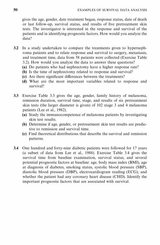
gives the age, gender, date treatment began, response status, date of deathor last follow-up, survival status, and results of five pretreatment skintests. The investigator is interested in the response and survival of thepatients and in identifying prognostic factors. How would you analyze thedata?
3.2 In a study undertaken to compare the treatments given to hyperneph-roma patients and to relate response and survival to surgery, metastasis,and treatment time, data from 58 patients were collected (Exercise Table3.2). How would you analyze the data to answer these questions?(a) Do patients who had nephrectomy have a higher response rate?(b) Is the time of nephrectomy related to response and survival?(c) Are there significant differences between the treatments?(d) What are the most important variables related to response and
survival?
3.3 Exercise Table 3.3 gives the age, gender, family history of melanoma,remission duration, survival time, stage, and results of six pretreatmentskin tests (the larger diameter is given) of 102 stage 3 and 4 melanomapatients (Lee et al., 1982).(a) Study the immunocompetence of melanoma patients by investigating
skin test results.(b) Determine if age, gender, or pretreatment skin test results are predic-
tive to remission and survival time.(c) Find theoretical distributions that describe the survival and remission
patterns.
3.4 One hundred and forty-nine diabetic patients were followed for 17 years(a subset of data from Lee et al., 1988). Exercise Table 3.4 gives thesurvival time from baseline examination, survival status, and severalpotential prognostic factors at baseline: age, body mass index (BMI), ageat diagnosis of diabetes, smoking status, systolic blood pressure (SBP),diastolic blood pressure (DBP), electrocardiogram reading (ECG), andwhether the patient had any coronary heart disease (CHD). Identify theimportant prognostic factors that are associated with survival.
50 EXAMPLES OF SURVIVAL DATA ANALYSIS
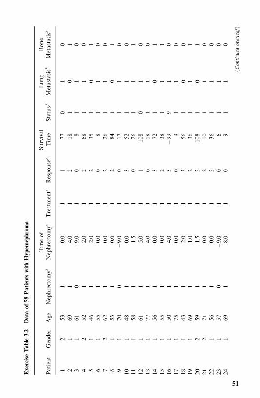
Exe
rciseTab
le3.2
Dataof
58PatientswithHyp
erne
phro
ma
Tim
eof
Surv
ival
Lung
Bone
Patient
Gen
der
Age
Nep
hrectom
y�Nep
hrectomy�
Treatmen
t�Respons
e�Tim
eStatu
s�M
etas
tasis�
Metas
tasis�
12
531
0.0
11
770
10
21
691
4.0
12
181
01
31
610
�9.0
10
81
10
42
521
2.0
12
681
10
51
461
2.0
12
351
01
61
551
0.0
10
81
10
72
621
0.0
12
261
10
81
531
0.0
12
841
01
91
700
�9.0
10
171
10
101
481
0.0
13
521
10
111
581
1.5
10
261
11
121
611
5.0
11
108
01
013
177
14.0
10
181
10
141
561
0.0
13
721
01
151
551
0.0
12
381
11
161
501
4.0
13
�99
91
017
175
10.0
10
91
10
181
431
2.0
13
561
00
191
691
1.0
12
361
11
202
591
1.5
12
108
10
121
271
10.0
12
101
10
221
561
0.0
12
361
10
231
570
�9.0
10
61
10
241
691
8.0
10
91
10
(Continued
overleaf
)
51
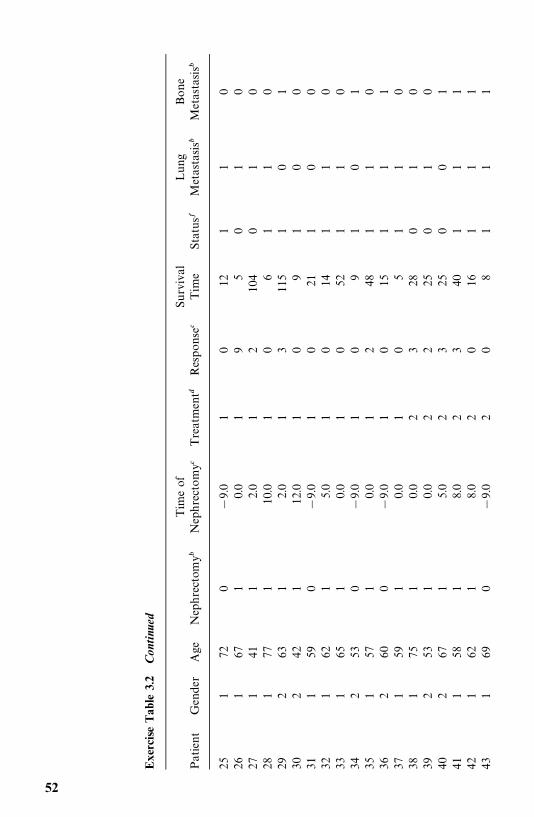
Exe
rciseTab
le3.2
Con
tinu
ed
Tim
eof
Surv
ival
Lung
Bone
Patient
Gen
der
Age
Nep
hrectom
y�Nep
hrectomy�
Treatmen
t�Respons
e�Tim
eStatu
s�M
etas
tasis�
Metas
tasis�
251
720
�9.0
10
121
10
261
671
0.0
19
50
10
271
411
2.0
12
104
01
028
177
110
.01
06
11
029
263
12.0
13
115
10
130
242
112
.01
09
10
031
159
0�
9.0
10
211
00
321
621
5.0
10
141
10
331
651
0.0
10
521
10
342
530
�9.0
10
91
01
351
571
0.0
12
481
10
362
600
�9.0
10
151
11
371
591
0.0
10
51
10
381
751
0.0
23
280
10
392
531
0.0
22
250
10
402
671
5.0
23
250
01
411
581
8.0
23
401
11
421
621
8.0
20
161
11
431
690
�9.0
20
81
11
52
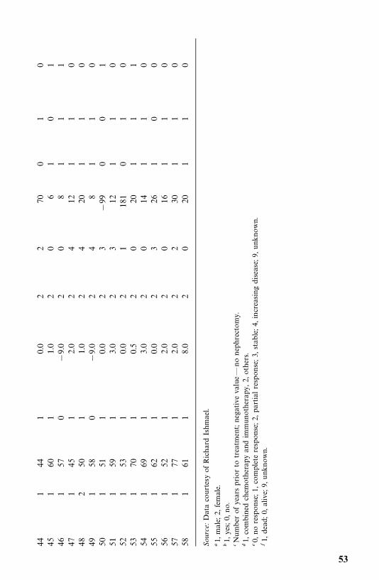
441
441
0.0
22
700
10
451
601
1.0
20
61
01
461
570
�9.0
20
81
11
471
451
2.0
24
121
10
482
501
1.0
24
201
10
491
580
�9.0
24
81
10
501
511
0.0
23
�99
00
151
159
13.0
23
121
10
521
531
0.0
21
181
01
053
170
10.5
20
201
11
541
691
3.0
20
141
10
551
621
0.0
23
261
00
561
521
2.0
20
161
10
571
771
2.0
22
301
10
581
611
8.0
20
201
10
Source:Dataco
urtesy
ofRichar
dIshm
ael.
�1,
male;
2,female.
�1,
yes;
0,no.
�Number
ofye
arsprior
totrea
tmen
t;ne
gative
value—
nonep
hrecto
my.
�1,
combined
chem
oth
erap
yan
dim
mun
otherap
y,2,
others.
�0,
noresp
ons
e;1,
complete
resp
onse;2
,pa
rtialresp
onse;3,
stab
le;4,
increa
singdiseas
e;9,
unk
nown.
�1,
dead
;0,
alive;
9,unk
nown.
53
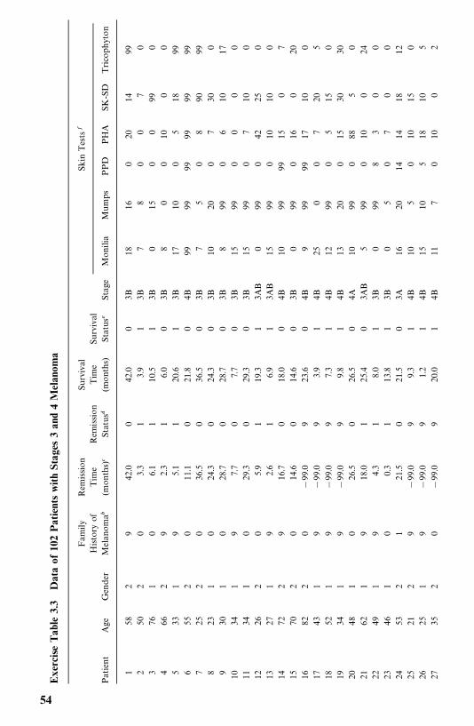
Exe
rciseTab
le3.3
Dataof
102PatientswithSt
ages
3an
d4M
elan
oma
Fam
ilyRem
ission
Surv
ival
Skin
Tests
�
Histo
ryof
Tim
eRem
ission
Tim
eSu
rvival
Patient
Age
Gen
der
Melan
oma�
(mon
ths)
�St
atus
�(m
onth
s)Statu
s�St
age
Mon
ilia
Mum
psPPD
PHA
SK-S
DTrico
phyton
158
29
42.0
042
.00
3B18
160
2014
992
502
03.3
13.9
13B
78
00
70
376
10
6.1
110
.51
3B0
150
099
04
662
92.3
16.0
03B
80
010
00
533
19
5.1
120
.61
3B17
100
518
996
552
011
.10
21.8
04B
9999
9999
9999
725
20
36.5
036
.50
3B7
50
890
998
231
024
.30
24.3
03B
1020
07
300
930
10
28.7
028
.70
3B8
990
610
1710
341
97.7
07.7
03B
1599
00
00
1134
10
29.3
029
.30
3B15
990
710
012
262
05.9
119
.31
3AB
099
042
250
1327
19
2.6
16.9
13A
B15
990
1010
014
722
916
.70
18.0
04B
1099
9915
07
1570
20
14.6
014
.60
3B0
990
160
2016
822
0�
99.0
923
.60
4B9
9999
1710
017
431
9�
99.0
93.9
14B
250
07
205
1852
19
�99
.09
7.3
14B
1299
05
150
1934
19
�99
.09
9.8
14B
1320
015
3030
2048
10
26.5
026
.50
4A10
990
885
021
621
918
.01
25.4
03A
B5
990
100
2422
491
94.3
18.0
13B
099
83
00
2346
10
0.3
113
.81
3B0
50
70
024
532
121
.50
21.5
03A
1620
1414
1812
2521
29
�99
.09
9.3
14B
105
010
150
2625
19
�99
.09
1.2
14B
1510
518
105
2735
20
�99
.09
20.0
14B
117
010
02
54
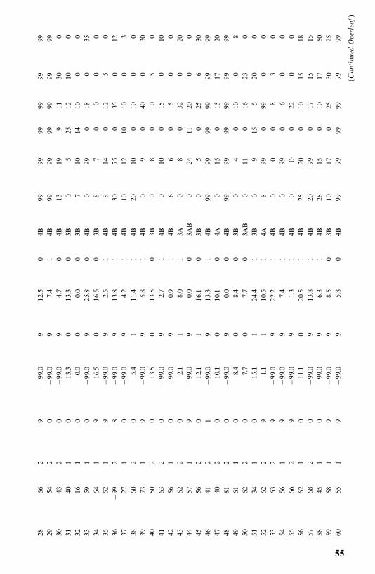
2866
29
�99
.09
12.5
04B
9999
9999
9999
2954
20
�99
.09
7.4
14B
9999
9999
9999
3043
20
�99
.09
4.7
04B
1319
911
300
3140
10
13.3
013
.30
3B0
525
1210
032
161
00.0
00.0
03B
710
1410
00
3359
10
�99
.09
25.8
04B
099
018
035
3464
19
16.5
016
.50
3B8
70
00
035
521
9�
99.0
92.5
14B
914
012
50
36�
992
8�
99.0
913
.81
4B30
750
350
1237
271
0�
99.0
94.2
14B
1012
1010
03
3860
20
5.4
111
.41
4B20
100
100
039
731
9�
99.0
95.8
14B
09
040
030
4050
20
13.5
013
.50
3B0
80
105
041
632
0�
99.0
92.7
14B
010
015
010
4256
10
�99
.09
0.9
14B
66
015
00
4362
20
2.1
18.0
13A
08
032
020
4457
19
�99
.09
0.0
03A
B0
2411
200
045
562
012
.11
16.1
03B
05
025
630
4641
21
�99
.09
13.3
14B
9999
9999
9999
4740
20
10.1
010
.10
4A0
150
1517
2048
812
0�
99.0
90.0
04B
9999
9999
9999
4961
10
8.4
08.4
03B
04
010
08
5062
20
7.7
07.7
03A
B0
110
1623
051
341
015
.11
24.4
13B
09
155
200
5262
29
1.1
110
.51
4A8
990
990
053
632
9�
99.0
922
.21
4B0
00
83
054
561
9�
99.0
97.4
14B
099
06
00
5566
29
�99
.09
1.3
14B
00·
022
00
5662
10
11.1
020
.51
4B25
200
1015
1857
682
0�
99.0
913
.81
4B20
990
1715
1558
451
0�
99.0
96.3
14B
2815
010
1750
5958
19
�99
.09
8.5
03B
1017
025
3025
6055
19
�99
.09
5.8
04B
9999
9999
9999
(Continued
Overleaf)
55
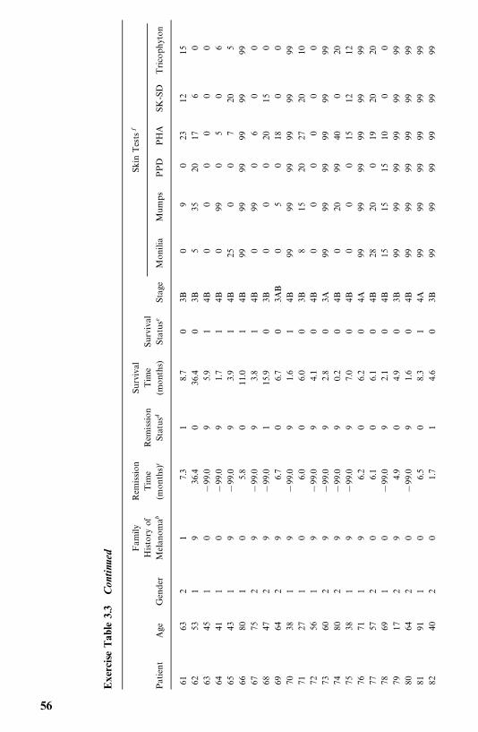
Exe
rciseTab
le3.3
Con
tinu
ed
Fam
ilyRem
ission
Surv
ival
Skin
Tests
�
Histo
ryof
Tim
eRem
ission
Tim
eSu
rvival
Patient
Age
Gen
der
Melan
oma�
(mon
ths)
�St
atus
�(m
onth
s)Statu
s�St
age
Mon
ilia
Mum
psPPD
PHA
SK-S
DTrico
phyton
6163
21
7.3
18.7
03B
09
023
1215
6253
19
36.4
036
.40
3B5
3520
176
063
451
0�
99.0
95.9
14B
00
00
00
6441
10
�99
.09
1.7
14B
099
05
06
6543
19
�99
.09
3.9
14B
250
07
205
6680
10
5.8
011
.01
4B99
9999
9999
9967
752
9�
99.0
93.8
14B
099
06
00
6847
29
�99
.01
15.9
03B
00
020
150
6964
29
6.7
06.7
03A
B0
50
180
070
381
9�
99.0
91.6
14B
9999
9999
9999
7127
10
6.0
06.0
03B
815
2027
2010
7256
19
�99
.09
4.1
04B
00
00
00
7360
29
�99
.09
2.8
03A
9999
9999
9999
7480
29
�99
.09
0.2
04B
020
9940
020
7538
19
�99
.09
7.0
04B
00
015
1212
7671
19
6.2
06.2
04A
9999
9999
9999
7757
20
6.1
06.1
04B
2820
019
2020
7869
10
�99
.09
2.1
04B
1515
1510
00
7917
29
4.9
04.9
03B
9999
9999
9999
8064
20
�99
.09
1.6
04B
9999
9999
9999
8191
10
6.5
08.3
14A
9999
9999
9999
8240
20
1.7
14.6
03B
9999
9999
9999
56
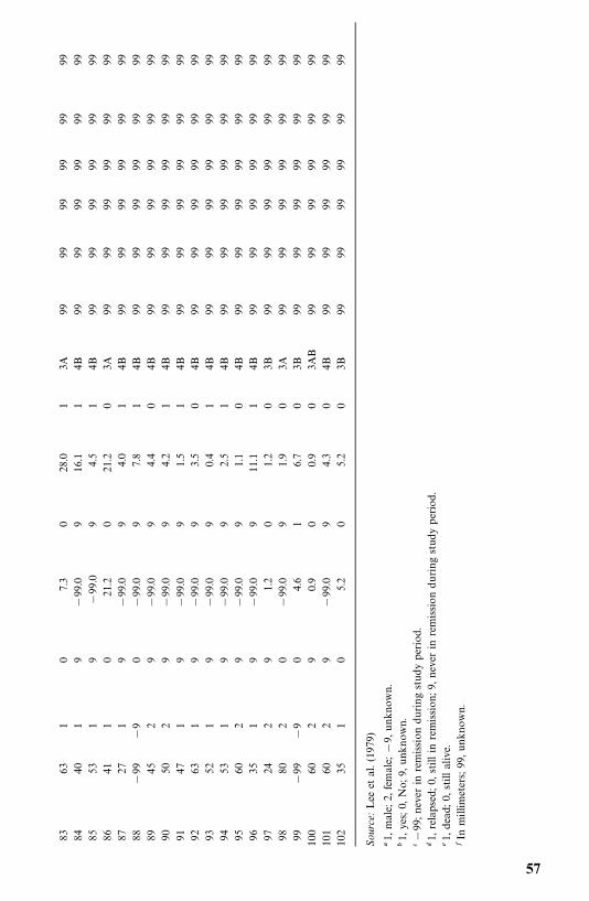
8363
10
7.3
028
.01
3A99
9999
9999
9984
401
9�
99.0
916
.11
4B99
9999
9999
9985
531
9�
99.0
94.5
14B
9999
9999
9999
8641
10
21.2
021
.20
3A99
9999
9999
9987
271
9�
99.0
94.0
14B
9999
9999
9999
88�
99�
90
�99
.09
7.8
14B
9999
9999
9999
8945
29
�99
.09
4.4
04B
9999
9999
9999
9050
29
�99
.09
4.2
14B
9999
9999
9999
9147
19
�99
.09
1.5
14B
9999
9999
9999
9263
19
�99
.09
3.5
04B
9999
9999
9999
9352
19
�99
.09
0.4
14B
9999
9999
9999
9453
19
�99
.09
2.5
14B
9999
9999
9999
9560
29
�99
.09
1.1
04B
9999
9999
9999
9635
19
�99
.09
11.1
14B
9999
9999
9999
9724
29
1.2
01.2
03B
9999
9999
9999
9880
20
�99
.09
1.9
03A
9999
9999
9999
99�
99�
90
4.6
16.7
03B
9999
9999
9999
100
602
90.9
00.9
03A
B99
9999
9999
9910
160
29
�99
.09
4.3
04B
9999
9999
9999
102
351
05.2
05.2
03B
9999
9999
9999
Source:
Lee
etal.(19
79)
�1,
male;
2,female;
�9,
unk
nown.
�1,
yes;
0,No;
9,un
know
n.��
99;n
ever
inremissiondu
ringstudype
riod.
�1,
relaps
ed;0
,stillin
remission
;9,n
ever
inremission
during
stud
yperiod.
�1,
dea
d;0
,stillalive.
�In
millim
eters;
99,u
nknown.
57
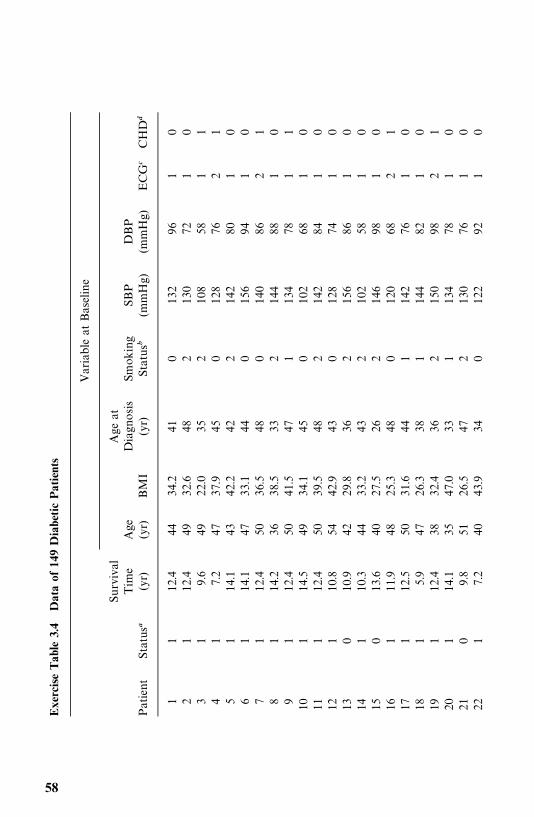
Exe
rciseTab
le3.4
Dataof
149Diabe
ticPatients
Var
iable
atBas
eline
Surv
ival
Age
atTim
eAge
Diagn
osis
Smok
ing
SBP
DBP
Patient
Status�
(yr)
(yr)
BM
I(yr)
Status�
(mmHg)
(mmHg)
ECG
�CHD
�
11
12.4
4434
.241
013
296
10
21
12.4
4932
.648
213
072
10
31
9.6
4922
.035
210
858
11
41
7.2
4737
.945
012
876
21
51
14.1
4342
.242
214
280
10
61
14.1
4733
.144
015
694
10
71
12.4
5036
.548
014
086
21
81
14.2
3638
.533
214
488
10
91
12.4
5041
.547
113
478
11
101
14.5
4934
.145
010
268
10
111
12.4
5039
.548
214
284
10
121
10.8
5442
.943
012
874
10
130
10.9
4229
.836
215
686
10
141
10.3
4433
.243
210
258
10
150
13.6
4027
.526
214
698
10
161
11.9
4825
.348
012
068
21
171
12.5
5031
.644
114
276
10
181
5.9
4726
.338
114
482
10
191
12.4
3832
.436
215
098
21
201
14.1
3547
.033
113
478
10
210
9.8
5126
.547
213
076
10
221
7.2
4043
.934
012
292
10
58
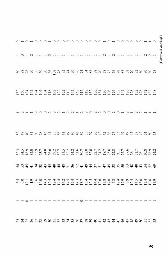
231
3.5
5432
.352
113
280
10
241
0.0
5334
.547
215
088
31
250
12.1
4518
.940
113
498
10
261
1.9
4132
.031
114
290
21
271
8.6
3433
.930
212
466
10
281
14.0
3823
.728
010
260
10
291
14.3
4324
.843
013
480
10
301
12.4
4526
.641
211
866
21
311
12.4
4039
.235
219
210
81
032
114
.444
32.7
362
122
781
033
114
.248
33.5
431
122
921
034
114
.551
32.2
492
112
741
035
112
.436
24.2
302
142
901
036
114
.352
31.6
481
152
961
037
013
.741
30.7
392
112
741
038
113
.449
28.0
352
118
841
039
112
.544
32.0
290
152
881
040
114
.437
32.7
362
136
881
041
112
.651
24.2
422
134
901
042
113
.847
18.7
420
130
782
143
114
.045
25.6
360
108
721
044
16.8
3822
.827
212
666
21
451
12.4
3530
.133
013
278
10
461
12.9
5027
.749
114
488
10
471
8.9
5327
.649
212
668
10
481
12.4
4828
.147
112
870
10
491
14.5
4031
.737
213
282
10
501
13.0
4326
.142
212
880
10
511
13.4
5430
.854
114
280
21
521
10.6
5236
.950
113
280
21
531
13.9
6924
.263
114
878
10
(Continued
overleaf
)
59
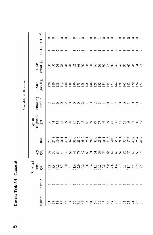
Exe
rciseTab
le3.4
Con
tinu
ed
Var
iable
atBas
eline
Surv
ival
Age
atTim
eAge
Diagn
osis
Smok
ing
SBP
DBP
Patient
Status�
(yr)
(yr)
BM
I(yr)
Status�
(mmHg)
(mmHg)
ECG
�CHD
�
541
16.9
3827
.526
217
010
01
055
13.6
5027
.344
114
090
10
561
10.2
6430
.158
013
876
21
571
15.7
4436
.141
011
278
10
581
12.0
3843
.139
214
078
10
590
6.7
6234
.658
013
878
31
601
11.6
4739
.045
013
082
10
610
2.0
7828
.777
017
886
21
621
10.2
4928
.243
215
880
10
631
3.6
6325
.146
116
888
31
641
15.4
7126
.059
014
688
10
651
11.3
5132
.049
212
876
10
661
10.3
5928
.157
113
276
11
671
5.8
5026
.149
115
480
10
680
8.0
6645
.349
015
492
10
691
14.6
4230
.041
112
280
10
701
11.4
4035
.736
214
476
21
711
7.2
6728
.161
017
896
10
721
5.5
8632
.961
016
260
10
731
11.1
5237
.646
114
280
10
741
16.5
4243
.437
012
076
10
751
10.9
6025
.460
012
464
10
761
2.5
7549
.757
117
482
21
60
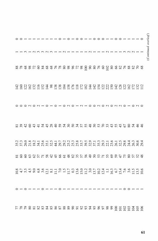
770
10.8
8135
.281
014
288
10
781
4.7
6037
.339
016
078
10
790
5.5
6026
.042
012
268
31
801
4.5
6321
.860
216
298
11
811
9.0
6218
.243
013
272
21
821
6.8
5734
.141
211
660
31
830
3.6
7125
.654
115
284
31
841
12.1
5835
.145
014
468
21
851
8.1
4232
.528
198
683
186
111
.145
44.1
400
138
761
187
07.0
6629
.759
113
878
10
881
1.5
6129
.254
018
480
21
891
11.7
4825
.230
215
898
10
901
0.3
8225
.350
017
696
11
911
13.6
3525
.834
111
872
10
921
15.0
5733
.757
217
298
10
931
11.2
5639
.555
118
210
01
194
13.0
4932
.948
014
490
21
951
13.7
5037
.150
014
280
10
961
10.2
5335
.353
215
476
10
971
12.4
7129
.370
012
260
10
981
1.1
5522
.133
222
210
22
199
116
.369
23.6
430
150
801
110
01
6.7
5926
.155
214
266
10
101
115
.447
32.5
452
128
821
010
20
7.6
7529
.867
012
276
31
103
03.6
8024
.480
116
288
21
104
111
.557
26.3
540
172
822
110
51
13.5
5230
.846
213
270
11
106
110
.648
29.4
460
112
681
0
(Continued
overleaf
)
61
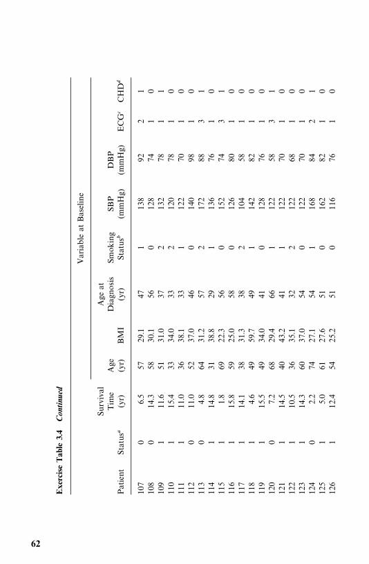
Exe
rciseTab
le3.4
Con
tinu
ed
Var
iable
atBas
eline
Surv
ival
Age
atTim
eAge
Diagn
osis
Smok
ing
SBP
DBP
Patient
Status�
(yr)
(yr)
BM
I(yr)
Status�
(mmHg)
(mmHg)
ECG
�CHD
�
107
06.5
5729
.147
113
892
21
108
014
.358
30.1
560
128
741
010
91
11.6
5131
.037
213
278
11
110
115
.433
34.0
332
120
781
011
11
11.0
3638
.133
112
270
10
112
011
.052
37.0
460
140
981
011
30
4.8
6431
.257
217
288
31
114
114
.831
38.8
291
136
761
011
51
1.8
6922
.356
015
274
31
116
115
.859
25.0
580
126
801
011
71
14.1
3831
.338
210
458
10
118
14.6
4959
.749
114
282
10
119
115
.549
34.0
410
128
761
012
00
7.2
6829
.466
112
258
31
121
114
.540
43.2
411
122
701
012
21
10.5
3635
.132
212
268
10
123
114
.360
37.0
540
122
701
012
40
2.2
7427
.154
116
884
21
125
15.0
6127
.651
016
282
10
126
112
.454
25.2
510
116
761
0
62
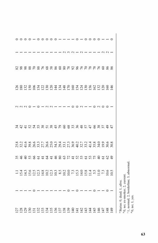
127
11.1
3525
.834
212
682
10
128
115
.446
32.2
422
180
981
012
91
14.3
4041
.641
213
298
10
130
115
.653
39.8
520
150
881
013
10
12.5
6626
.654
110
670
11
132
112
.361
33.3
550
154
881
013
31
14.8
4127
.738
112
276
10
134
110
.264
26.6
512
130
681
013
51
12.3
4125
.038
212
058
10
136
110
.346
54.3
451
144
861
013
71
8.5
8029
.479
113
460
11
138
110
.263
33.1
601
148
802
113
90
10.0
7227
.368
117
078
31
140
17.3
4136
.933
016
092
21
141
015
.352
40.2
360
154
961
014
21
14.0
5332
.748
212
476
21
143
115
.861
33.2
571
130
701
014
41
11.4
5341
.447
115
678
10
145
05.5
7535
.866
016
278
10
146
111
.040
34.0
382
132
761
014
71
7.3
6119
.937
012
060
21
148
010
.662
30.6
490
160
862
114
91
10.5
4930
.847
114
686
10
�Statu
s:0,
dea
d;1
,alive.
�0,
no;e
x-sm
oker;2
,cu
rren
t.�1
,no
rmal;2,
bord
erlin
e;3,
abnor
mal.
�0,
no;1
,ye
s.
63
CHAPTER 4
Nonparametric Methods ofEstimating Survival Functions
In this chapter we discuss methods of estimating the three survival (survivor-ship, density, and hazard) functions for censored data. Unfortunately, thesimple method of Example 2.1 cannot be applied if some of the patients arealive at the time of analysis and therefore their exact survival times areunknown. Nonparametric or distribution-free methods are quite easy tounderstand and apply. They are less efficient than parametric methods whensurvival times follow a theoretical distribution and more efficient when nosuitable theoretical distributions are known. Therefore, we suggest usingnonparametric methods to analyze survival data before attempting to fit atheoretical distribution. If the main objective is to find a model for the data,estimates obtained by nonparametric methods and graphs can be helpful inchoosing a distribution.Of the three survival functions, survivorship or its graphical presentation,
the survival curve, is the most widely used. Section 4.1 introduces theproduct-limit (PL) method of estimating the survivorship function developedby Kaplan and Meier (1958). With the increased availability of computers, thismethod is applicable to small, moderate, and large samples. However, if thedata have already been grouped into intervals, or the sample size is very large,say in the thousands, or the interest is in a large population, it may be moreconvenient to perform a life-table analysis. Section 4.2 is devoted to thediscussion of population and clinical life tables. The PL estimates and life-tableestimates of the survivorship function are essentially the same. Many authorsuse the term life-table estimates for the PL estimates. The only difference is thatthe PL estimate is based on individual survival times, whereas in the life-tablemethod, survival times are grouped into intervals. The PL estimate can beconsidered as a special case of the life-table estimate where each intervalcontains only one observation.
64
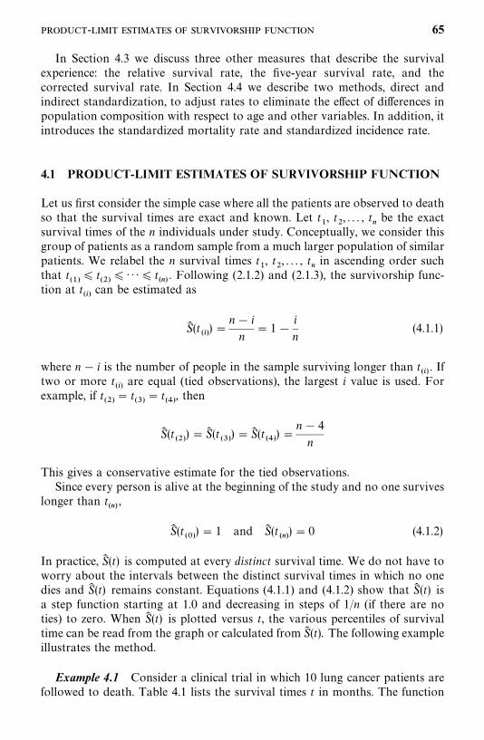
In Section 4.3 we discuss three other measures that describe the survivalexperience: the relative survival rate, the five-year survival rate, and thecorrected survival rate. In Section 4.4 we describe two methods, direct andindirect standardization, to adjust rates to eliminate the effect of differences inpopulation composition with respect to age and other variables. In addition, itintroduces the standardized mortality rate and standardized incidence rate.
4.1 PRODUCT-LIMIT ESTIMATES OF SURVIVORSHIP FUNCTION
Let us first consider the simple case where all the patients are observed to deathso that the survival times are exact and known. Let t
�, t
�, . . . , t
�be the exact
survival times of the n individuals under study. Conceptually, we consider thisgroup of patients as a random sample from a much larger population of similarpatients. We relabel the n survival times t
�, t
�, . . . , t
�in ascending order such
that t���
� t���
� · · ·� t���. Following (2.1.2) and (2.1.3), the survivorship func-
tion at t���can be estimated as
S� (t���)�
n� i
n� 1�
i
n(4.1.1)
where n� i is the number of people in the sample surviving longer than t���. If
two or more t���are equal (tied observations), the largest i value is used. For
example, if t���
� t���
� t���, then
S� (t���)� S� (t
���)� S� (t
���)�
n� 4
n
This gives a conservative estimate for the tied observations.Since every person is alive at the beginning of the study and no one survives
longer than t���,
S� (t��)� 1 and S� (t
���)� 0 (4.1.2)
In practice, S� (t) is computed at every distinct survival time. We do not have toworry about the intervals between the distinct survival times in which no onedies and S� (t) remains constant. Equations (4.1.1) and (4.1.2) show that S� (t) isa step function starting at 1.0 and decreasing in steps of 1/n (if there are noties) to zero. When S� (t) is plotted versus t, the various percentiles of survivaltime can be read from the graph or calculated from S� (t). The following exampleillustrates the method.
Example 4.1 Consider a clinical trial in which 10 lung cancer patients arefollowed to death. Table 4.1 lists the survival times t in months. The function
- 65
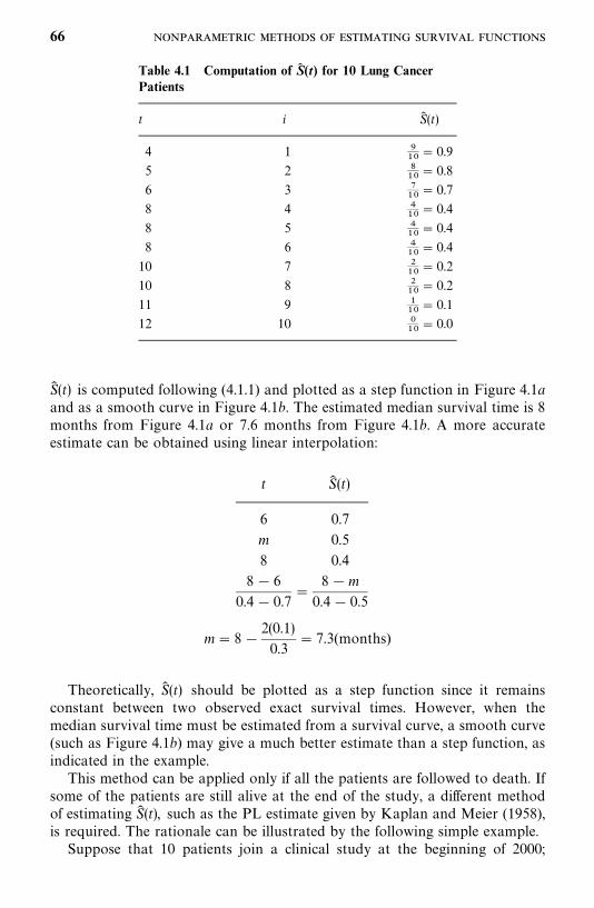
Table 4.1 Computation of S� (t) for 10 Lung CancerPatients
t i S� (t)
4 1 �
� 0.9
5 2 ��
� 0.8
6 3 ��
� 0.7
8 4 ��
� 0.4
8 5 ��
� 0.4
8 6 ��
� 0.4
10 7 ��
� 0.2
10 8 ��
� 0.2
11 9 ��
� 0.1
12 10 �
� 0.0
S� (t) is computed following (4.1.1) and plotted as a step function in Figure 4.1aand as a smooth curve in Figure 4.1b. The estimated median survival time is 8months from Figure 4.1a or 7.6 months from Figure 4.1b. A more accurateestimate can be obtained using linear interpolation:
t S� (t)
6 0.7
m 0.5
8 0.4
8� 6
0.4� 0.7�
8�m
0.4� 0.5
m� 8�2(0.1)
0.3� 7.3(months)
Theoretically, S� (t) should be plotted as a step function since it remainsconstant between two observed exact survival times. However, when themedian survival time must be estimated from a survival curve, a smooth curve(such as Figure 4.1b) may give a much better estimate than a step function, asindicated in the example.This method can be applied only if all the patients are followed to death. If
some of the patients are still alive at the end of the study, a different methodof estimating S� (t), such as the PL estimate given by Kaplan and Meier (1958),is required. The rationale can be illustrated by the following simple example.Suppose that 10 patients join a clinical study at the beginning of 2000;
66
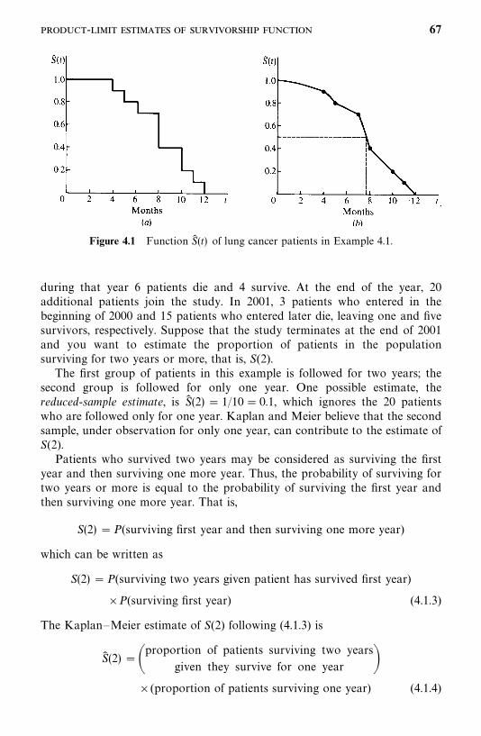
Figure 4.1 Function S� (t) of lung cancer patients in Example 4.1.
during that year 6 patients die and 4 survive. At the end of the year, 20additional patients join the study. In 2001, 3 patients who entered in thebeginning of 2000 and 15 patients who entered later die, leaving one and fivesurvivors, respectively. Suppose that the study terminates at the end of 2001and you want to estimate the proportion of patients in the populationsurviving for two years or more, that is, S(2).The first group of patients in this example is followed for two years; the
second group is followed for only one year. One possible estimate, thereduced-sample estimate, is S� (2) � 1/10� 0.1, which ignores the 20 patientswho are followed only for one year. Kaplan and Meier believe that the secondsample, under observation for only one year, can contribute to the estimate ofS(2).Patients who survived two years may be considered as surviving the first
year and then surviving one more year. Thus, the probability of surviving fortwo years or more is equal to the probability of surviving the first year andthen surviving one more year. That is,
S(2) �P(surviving first year and then surviving one more year)
which can be written as
S(2) �P(surviving two years given patient has survived first year)
�P(surviving first year) (4.1.3)
The Kaplan—Meier estimate of S(2) following (4.1.3) is
S� (2) ��proportion of patients surviving two years
given they survive for one year ��(proportion of patients surviving one year) (4.1.4)
- 67
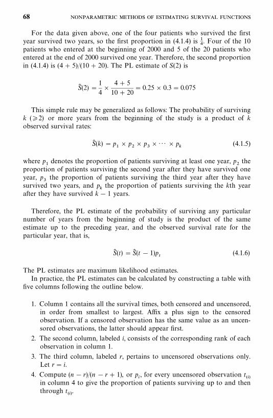
For the data given above, one of the four patients who survived the firstyear survived two years, so the first proportion in (4.1.4) is �
�. Four of the 10
patients who entered at the beginning of 2000 and 5 of the 20 patients whoentered at the end of 2000 survived one year. Therefore, the second proportionin (4.1.4) is (4 5)/(10 20). The PL estimate of S(2) is
S� (2) �1
4�
4 5
10 20� 0.25� 0.3� 0.075
This simple rule may be generalized as follows: The probability of survivingk (�2) or more years from the beginning of the study is a product of kobserved survival rates:
S� (k) � p�� p
�� p
�� · · · � p
�(4.1.5)
where p�denotes the proportion of patients surviving at least one year, p
�the
proportion of patients surviving the second year after they have survived oneyear, p
�the proportion of patients surviving the third year after they have
survived two years, and p�the proportion of patients surviving the kth year
after they have survived k� 1 years.
Therefore, the PL estimate of the probability of surviving any particularnumber of years from the beginning of study is the product of the sameestimate up to the preceding year, and the observed survival rate for theparticular year, that is,
S� (t) � S� (t � 1)p�
(4.1.6)
The PL estimates are maximum likelihood estimates.In practice, the PL estimates can be calculated by constructing a table with
five columns following the outline below.
1. Column 1 contains all the survival times, both censored and uncensored,in order from smallest to largest. Affix a plus sign to the censoredobservation. If a censored observation has the same value as an uncen-sored observations, the latter should appear first.
2. The second column, labeled i, consists of the corresponding rank of eachobservation in column 1.
3. The third column, labeled r, pertains to uncensored observations only.Let r� i.
4. Compute (n � r)/(n � r 1), or p�, for every uncensored observation t
���in column 4 to give the proportion of patients surviving up to and thenthrough t
���.
68
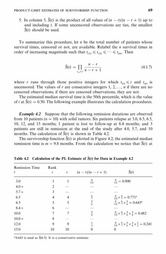
Table 4.2 Calculation of the PL Estimate of S� (t) for Data in Example 4.2
Remission Time Rankt i r (n � r)/(n � r 1) S� (t)
3.0 1 1 �
�
� 0.900
4.0 2 — — —
5.7 3 — — —
6.5 4 4 ��
�
���� 0.771�
6.5 5 5 ��
�
�����
�� 0.643�
8.4 6 — — —
10.0 7 7 ��
�
�����
���
�� 0.482
10.0 8 — — —
12.0 9 9 ��
�
�����
���
���
�� 0.241
15.0 10 10 0 0
� 0.643 is used as S� (6.5). It is a conservative estimate.
5. In column 5, S� (t) is the product of all values of (n � r)/(n � r 1) up toand including t. If some uncensored observations are ties, the smallestS� (t) should be used.
To summarize this procedure, let n be the total number of patients whosesurvival times, censored or not, are available. Relabel the n survival times inorder of increasing magnitude such that t
���� t
���� · · ·� t
���. Then
S� (t) � �t���
�t
n� r
n� r 1(4.1.7)
where r runs through those positive integers for which t���
� t and t���is
uncensored. The values of r are consecutive integers 1, 2, . . . , n if there are nocensored observations; if there are censored observations, they are not.The estimated median survival time is the 50th percentile, which is the value
of t at S� (t) � 0.50. The following example illustrates the calculation procedures.
Example 4.2 Suppose that the following remission durations are observedfrom 10 patients (n� 10) with solid tumors. Six patients relapse at 3.0, 6.5, 6.5,10, 12, and 15 months; 1 patient is lost to follow-up at 8.4 months; and 3patients are still in remission at the end of the study after 4.0, 5.7, and 10months. The calculation of S� (t) is shown in Table 4.2.The survivorship function S� (t) is plotted in Figure 4.2; the estimated median
remission time is m� 9.8 months. From the calculation we notice that S� (t) at
- 69
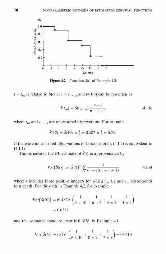
Figure 4.2 Function S� (t) of Example 4.2.
t� t���is related to S� (t) at t� t
�����and (4.1.6) can be rewritten as
S� (t���)�S� (t
�����)
n� i
n� i 1(4.1.8)
where t���and t
�����are uncensored observations. For example,
S� (12) �S� (10) � ��� 0.482� �
�� 0.241
If there are no censored observations or losses before t, (4.1.7) is equivalent to(4.1.1).The variance of the PL estimate of S� (t) is approximated by
Var[S� (t)] � [S� (t)]� ��
1
(n � r )(n � r 1)(4.1.9)
where r includes those positive integers for which t���
� t and t���corresponds
to a death. For the data in Example 4.2, for example,
Var[S� (10)] � (0.482)� �1
9� 10
1
6� 7
1
5� 6
1
3� 4�� 0.0352
and the estimated standard error is 0.1876. In Example 4.1,
Var[S� (6)] � (0.7)� �1
9� 10
1
8� 9
1
7� 8�� 0.0210
70
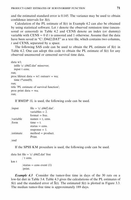
and the estimated standard error is 0.145. The variance may be used to obtainconfidence intervals for S(t).Calculation of the PL estimate of S(t) in Example 4.2 can also be obtained
by using statistical software. Let t denote the observed remission time (uncen-sored or censored) in Table 4.2 and CENS denote an index (or dummy)variable with CENS� 0 if t is censored and 1 otherwise. Assume that the datahave been saved in ‘‘C:�D4d2.DAT’’ as a text file, which contains two columns,t and CENS, separated by a space.The following SAS code can be used to obtain the PL estimate of S(t) in
Table 4.2. One can adopt this code to obtain the PL estimate of S(t) for anyobserved uncensored or censored survival time data.
data w1;infile ‘c:�d4d2.dat’ missover;input t cens;
run;proc lifetest data�w1 outsurv�wa;time t*cens(0);
run;title ’PL estimate of survival function’;proc print data�wa;run;
If BMDP 1L is used, the following code can be used.
/input file� ‘c:�d4d2.dat’.variables� 2.format� free.
/variable names� t, cens./form time� t.
status� cens.response� 1.
/estimate method�product.Print.
/end
If the SPSS KM procedure is used, the following code can be used.
data list file� ‘c:�d4d2.dat’ free/ t cens.
km t/status� cens event (1)/print.
Example 4.3 Consider the tumor-free time in days of the 30 rats on alow-fat diet in Table 3.4. Table 4.3 gives the calculations of the PL estimates ofS(t) and the standard error of S� (t). The estimated S(t) is plotted in Figure 3.3.The median tumor-free time is approximately 189 days.
- 71
Tab
le4.
3C
alcu
lation
ofS�(t)an
dSt
anda
rdErr
orof
S�(t)fo
r30
Rat
son
aLow
-Fat
Die
tin
Tab
le3.
4
Rat
Tumor-free
Number
Timet
ir
n�
r
n�
r 1
S�(t)
StandardErrorofS�(t)
350
11
� �� �
�0.967
�(0.967
)��
1
29�30����
��0.033
1256
22
�� �0.967�
�� ��0.933
�(0.933
)��
1
29�30
1
28�29����
��0.046
465
33
�� ��0.933�
�� ���0.900
�(0.900
)��
1
29�30
1
28�29
1
27�28����
��0.055
1366
44
�� ��0.900�
�� ���0.867
0.062
1473
55
�� ��0.833
0.068
977
66
�� ��0.800
0.073
1084
77
�� ��0.767
0.077
586
88
�� ��0.733
0.081
1187
99
�� ��0.700
0.084
15119
1010
� ��0.667
0.086
1140
1111
� �0.633
0.088
16140
12—
——
72

6153
1313
�� ��0.633�
�� ���0.598
0.090
2177
1414
�� ��0.598�
�� ���0.563
0.091
7181
1515
�� ��0.528
0.092
8191
1616
�� ��0.493
0.092
17200
17—
——
—
18200
18—
——
—
19200
19—
——
—
20200
20—
——
—
21200
21—
——
—
22200
22—
——
—
23200
23—
——
—
24200
24—
——
—
25200
25—
——
—
26200
26—
——
—
27200
27—
——
—
28200
28—
——
—
29200
29—
——
—
30200
30—
——
—
73

The mean survival time � can be shown to equal the area under theestimated survivorship function. To estimate �, we can use
�� ���
S� (t) dt
that is, �� is equal to the area under the estimated survivorship function. Thus,if the times to death are ordered as t���� t���� · · ·� t��� (if there are muncensored observations) and t��� is the largest observation of all n observa-tions [i.e., t���� t
���when t
���is an uncensored observation], � can be estimated
as
�� � 1.000t��� S� (t���)(t��� � t���) S� (t���)(t��� � t���) · · ·
S� (t�����)(t��� � t�����) (4.1.10)
which is the sum of the areas of the rectangles under the survival curve formedby the uncensored observations. Consider the data in Example 4.2: m� 6,t���� 3.0, t���� 6.5, t���� 6.5, t���� 10, t���� 12, and t���� 15. The meansurvival time is estimated using (4.1.10) as
�� � 1.000� 3.0 0.900(6.5� 3.0) 0.643(10� 6.5)
0.482(12� 10) 0.241(15� 12)
� 3.000 3.150 2.251 0.964 0.723
� 10.088 months
However, if the largest observation in the data is censored and is used ast��� in (4.10), � so obtained may be a low estimate. In such cases, Irwin (1949)suggests that instead of estimating the mean survival time, one should choosea time limit L and estimate the ‘‘mean survival time limited to a time L ,’’ say����, by using L for t��� in (4.1.10). For example, if in Example 4.2 the largest
observation is censored, that is, 15 , and if we let L � 16, then
�����
� 3.000 3.150; 2.251 0.964 0.241(16� 12)
� 10.329 months
which is the mean survival time limited to 16 months.The variance of �� is estimated by
Var(�� )���
A��
(n � r)(n � r 1)(4.1.11)
where r runs through those integers for which t�corresponds to a death, and
74
A�is the area under the curve S� (t) to the right of t
���. The kth A
�in terms of
the m uncensored observations is
S� (t���)(t���� � k���) S� (t����)(t���� � t����) · · · S� (t�����)(t��� � t�����)
(4.1.12)
If there are no censored observations, (4.1.10) reduces to the sample meant � t
�/n, and (4.1.11) reduces to
Var(�� ) �Var(t )�� (t
�� t )�n�
(4.1.13)
which is not an unbiased estimate. Kaplan and Meier suggest that (4.1.11) and(4.1.13) be multiplied by m/(m � 1) and n/(n � 1), respectively, to correct thebias.Consider the survival times in Example 4.1: The sample mean is t ��� � 8.2
months and the estimated variance of �� , by (4.1.13), is 0.616. If the factorn/(n � 1)� 10/9 is multiplied, the estimated variance of � becomes 0.684.To compute the variance of �� in Example 4.2, we first compute the five A
�’s:
A�, A
�, A
�, A
�, and A
. The first A
�is
A��S� (t���)(t��� � t���) S� (t���)(t��� � t���) · · · S� (t���)(t��� � t���)
� 3.150 2.251 0.964 0.723� 7.088
The second A�is
A��S� (t���)(t��� � t���) · · · S� (t���)(t��� � t���)
� 2.251 0.964 0.723� 3.938
The third, fourth, and fifth A�’s are, respectively,
A�� 2.251 0.964 0.723� 3.938
A�� 0.964 0.723� 1.687
A� 0.723
Thus,
Var� (�� )�(7.088)�9� 10
(3.938)�6� 7
(3.928)�5� 6
(1.687)�3� 4
(0.723)�1� 2
� 1.942
The estimated standard error of �� is 1.394. If the factor m/(m � 1)� 6/5 isincluded, these results become 2.330 and 1.526, respectively.The Kaplan—Meier method provides very useful estimates of survival
probabilities and graphical presentation of survival distribution. It is the most
- 75
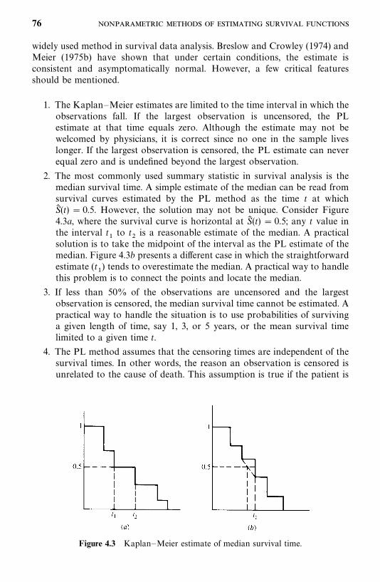
Figure 4.3 Kaplan—Meier estimate of median survival time.
widely used method in survival data analysis. Breslow and Crowley (1974) andMeier (1975b) have shown that under certain conditions, the estimate isconsistent and asymptomatically normal. However, a few critical featuresshould be mentioned.
1. The Kaplan—Meier estimates are limited to the time interval in which theobservations fall. If the largest observation is uncensored, the PLestimate at that time equals zero. Although the estimate may not bewelcomed by physicians, it is correct since no one in the sample liveslonger. If the largest observation is censored, the PL estimate can neverequal zero and is undefined beyond the largest observation.
2. The most commonly used summary statistic in survival analysis is themedian survival time. A simple estimate of the median can be read fromsurvival curves estimated by the PL method as the time t at whichS� (t) � 0.5. However, the solution may not be unique. Consider Figure4.3a, where the survival curve is horizontal at S� (t) � 0.5; any t value inthe interval t
�to t
�is a reasonable estimate of the median. A practical
solution is to take the midpoint of the interval as the PL estimate of themedian. Figure 4.3b presents a different case in which the straightforwardestimate (t
�) tends to overestimate the median. A practical way to handle
this problem is to connect the points and locate the median.
3. If less than 50% of the observations are uncensored and the largestobservation is censored, the median survival time cannot be estimated. Apractical way to handle the situation is to use probabilities of survivinga given length of time, say 1, 3, or 5 years, or the mean survival timelimited to a given time t.
4. The PL method assumes that the censoring times are independent of thesurvival times. In other words, the reason an observation is censored isunrelated to the cause of death. This assumption is true if the patient is
76
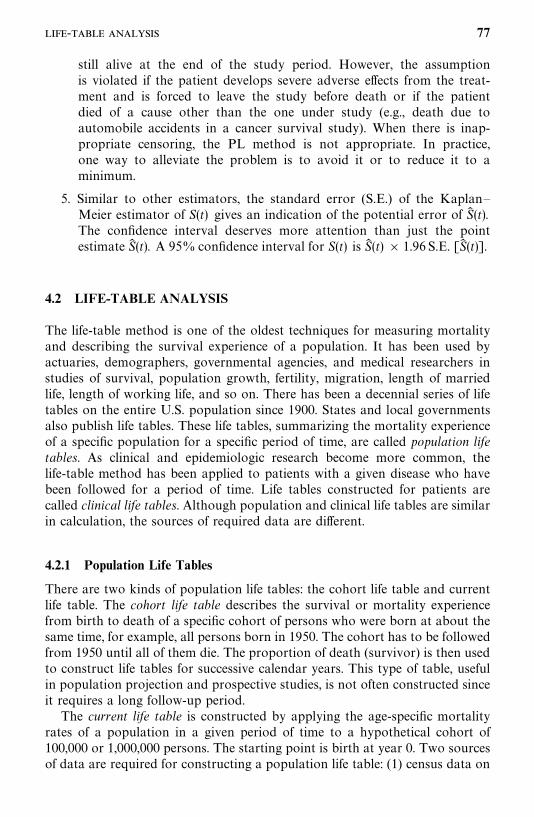
still alive at the end of the study period. However, the assumptionis violated if the patient develops severe adverse effects from the treat-ment and is forced to leave the study before death or if the patientdied of a cause other than the one under study (e.g., death due toautomobile accidents in a cancer survival study). When there is inap-propriate censoring, the PL method is not appropriate. In practice,one way to alleviate the problem is to avoid it or to reduce it to aminimum.
5. Similar to other estimators, the standard error (S.E.) of the Kaplan—Meier estimator of S(t) gives an indication of the potential error of S� (t).The confidence interval deserves more attention than just the pointestimate S� (t). A 95% confidence interval for S(t) is S� (t) � 1.96 S.E. [S� (t)].
4.2 LIFE-TABLE ANALYSIS
The life-table method is one of the oldest techniques for measuring mortalityand describing the survival experience of a population. It has been used byactuaries, demographers, governmental agencies, and medical researchers instudies of survival, population growth, fertility, migration, length of marriedlife, length of working life, and so on. There has been a decennial series of lifetables on the entire U.S. population since 1900. States and local governmentsalso publish life tables. These life tables, summarizing the mortality experienceof a specific population for a specific period of time, are called population lifetables. As clinical and epidemiologic research become more common, thelife-table method has been applied to patients with a given disease who havebeen followed for a period of time. Life tables constructed for patients arecalled clinical life tables. Although population and clinical life tables are similarin calculation, the sources of required data are different.
4.2.1 Population Life Tables
There are two kinds of population life tables: the cohort life table and currentlife table. The cohort life table describes the survival or mortality experiencefrom birth to death of a specific cohort of persons who were born at about thesame time, for example, all persons born in 1950. The cohort has to be followedfrom 1950 until all of them die. The proportion of death (survivor) is then usedto construct life tables for successive calendar years. This type of table, usefulin population projection and prospective studies, is not often constructed sinceit requires a long follow-up period.The current life table is constructed by applying the age-specific mortality
rates of a population in a given period of time to a hypothetical cohort of100,000 or 1,000,000 persons. The starting point is birth at year 0. Two sourcesof data are required for constructing a population life table: (1) census data on
- 77
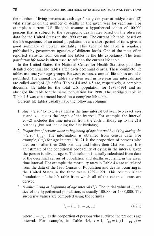
the number of living persons at each age for a given year at midyear and (2)vital statistics on the number of deaths in the given year for each age. Forexample, a current U.S. life table assumes a hypothetical cohort of 100,000persons that is subject to the age-specific death rates based on the observeddata for the United States in the 1990 census. The current life table, based onthe life experience of an actual population over a short period of time, gives agood summary of current mortality. This type of life table is regularlypublished by government agencies of different levels. One of the most oftenreported statistics from current life tables is the life expectancy. The termpopulation life table is often used to refer to the current life table.In the United States, the National Center for Health Statistics publishes
detailed decennial life tables after each decennial census. These complete lifetables use one-year age groups. Between censuses, annual life tables are alsopublished. The annual life tables are often seen in five-year age intervals andare called abridged life tables. Tables 4.4 and 4.5 are, respectively, a completedecennial life table for the total U.S. population for 1989—1991 and anabridged life table for the same population for 1998. The abridged table inTable 4.5 was constructed based on a complete life table.Current life tables usually have the following columns:
1. Age interval [x to x t). This is the time interval between two exact agesx and x t; t is the length of the interval. For example, the interval20—21 includes the time interval from the 20th birthday up to the 21stbirthday (but not including the 21st birthday).
2. Proportion of persons alive at beginning of age interval but dying during theinterval (
�q). The information is obtained from census data. For
example, (�q) for age interval 20—21 is the proportion of persons who
died on or after their 20th birthday and before their 21st birthday. It isan estimate of the conditional probability of dying in the interval giventhe person is alive at age x. This column is usually calculated from dataof the decennial census of population and deaths occurring in the giventime interval. For example, the mortality rates in Table 4.4 are calculatedfrom the data of the 1990 Census of Population and deaths occurring inthe United States in the three years 1989—1991. This column is thefoundation of the life table from which all of the other columns arederived.
3. Number living at beginning of age interval (l). The initial value of l
, the
size of the hypothetical population, is usually 100,000 or 1,000,000. Thesuccessive values are computed using the formula
l� l
��(1�
�q��
) (4.2.1)
where 1��q��
is the proportion of persons who survived the previous ageinterval. For example, in Table 4.4, t� 1, l
�� l
�(1�
�q�)�
78
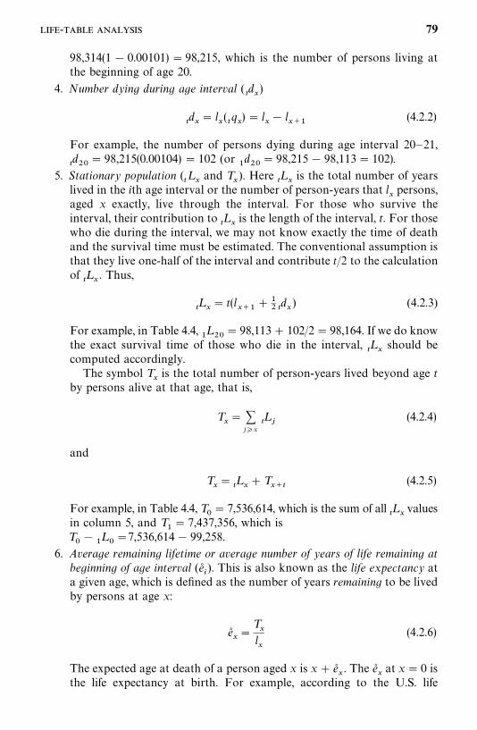
98,314(1� 0.00101)� 98,215, which is the number of persons living atthe beginning of age 20.
4. Number dying during age interval (�d)
�d� l
(�q)� l
� l
�(4.2.2)
For example, the number of persons dying during age interval 20—21,
�d�
� 98,215(0.00104)� 102 (or�d�
� 98,215� 98,113� 102).
5. Stationary population (�Land T
). Here
�Lis the total number of years
lived in the ith age interval or the number of person-years that lpersons,
aged x exactly, live through the interval. For those who survive theinterval, their contribution to
�Lis the length of the interval, t. For those
who die during the interval, we may not know exactly the time of deathand the survival time must be estimated. The conventional assumption isthat they live one-half of the interval and contribute t/2 to the calculationof
�L. Thus,
�L� t(l
� �
� �d) (4.2.3)
For example, in Table 4.4,�L�
� 98,113 102/2� 98,164. If we do knowthe exact survival time of those who die in the interval,
�Lshould be
computed accordingly.The symbol T
is the total number of person-years lived beyond age t
by persons alive at that age, that is,
T� �
j�x �L�
(4.2.4)
and
T�
�L T
�(4.2.5)
For example, in Table 4.4, T�7,536,614, which is the sum of all
�Lvalues
in column 5, and T�� 7,437,356, which is
T�
�L�7,536,614� 99,258.
6. Average remaining lifetime or average number of years of life remaining atbeginning of age interval (e�
�). This is also known as the life expectancy at
a given age, which is defined as the number of years remaining to be livedby persons at age x:
e��
Tl
(4.2.6)
The expected age at death of a person aged x is x e�. The e�
at x� 0 is
the life expectancy at birth. For example, according to the U.S. life
- 79
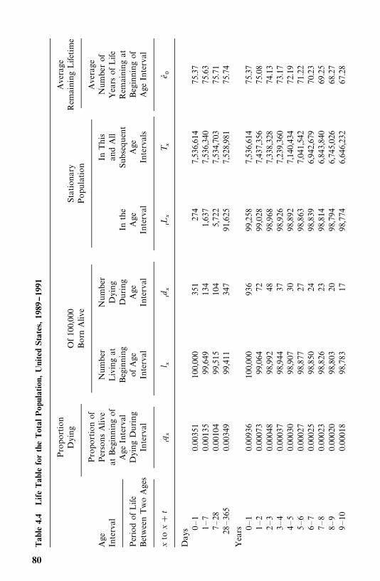
Tab
le4.
4Life
Tab
lefo
rth
eTot
alPop
ulat
ion,
Uni
ted
Stat
es,19
89--19
91
Proportion
Of100,000
Stationary
Average
Dying
BornAlive
Population
RemainingLifetime
Proportionof
Average
Age
PersonsAlive
Number
Number
InThis
Numberof
Interval
atBeginningof
Livingat
Dying
andAll
YearsofLife
AgeInterval
Beginning
During
Inthe
Subsequent
Remainingat
PeriodofLife
DyingDuring
ofAge
Age
Age
Age
Beginningof
BetweenTwoAges
Interval
Interval
Interval
Interval
Intervals
AgeInterval
xto
x
t�q
l
�d
�L
T
e�
Days 0—1
0.00351
100,000
351
274
7,536,614
75.37
1—7
0.00135
99,649
134
1,637
7,536,340
75.63
7—28
0.00104
99,515
104
5,722
7,534,703
75.71
28—365
0.00349
99,411
347
91,625
7,528,981
75.74
Years 0—1
0.00936
100,000
936
99,258
7,536,614
75.37
1—2
0.00073
99,064
7299,028
7,437,356
75.08
2—3
0.00048
98,992
4898,968
7,338,328
74.13
3—4
0.00037
98,944
3798,926
7,239,360
73.17
4—5
0.00030
98,907
3098,892
7,140,434
72.19
5—6
0.00027
98,877
2798,863
7,041,542
71.22
6—7
0.00025
98,850
2498,839
6,942,679
70.23
7—8
0.00023
98,826
2398,814
6,843,840
69.25
8—9
0.00020
98,803
2098,794
6,745,026
68.27
9—10
0.00018
98,783
1798,774
6,646,232
67.28
80
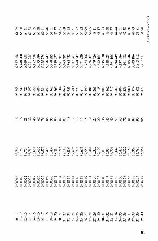
10—11
0.00016
98,766
1698,758
6,547,458
66.29
11—12
0.00016
98,750
1698,742
6,448,700
65.30
12—13
0.00022
98,734
2198,723
6,349,958
64.31
13—14
0.00032
98,713
3298,697
6,251,235
63.33
14—15
0.00047
98,681
4698,658
6,152,538
62.35
15—16
0.00063
98,635
6298,604
6,053,880
61.38
16—17
0.00077
98,573
7698,534
5,955,276
60.41
17—18
0.00089
98,497
8898,453
5,856,742
59.46
18—19
0.00096
98,409
9598,362
5,758,289
58.51
19—20
0.00101
98,314
9998,265
5,659,927
57.57
20—21
0.00104
98,215
102
98,164
5,561,662
56.63
21—22
0.00109
98,113
107
98,060
5,463,498
55.69
22—23
0.00112
98,006
110
97,951
5,365,438
54.75
23—24
0.00114
97,896
112
97,840
5,267,487
53.81
24—25
0.00116
97,784
113
97,727
5,169,647
52.87
25—26
0.00117
97,671
115
97,614
5,071,920
51.93
26—27
0.00119
97,556
115
97,499
4,974,306
50.99
27—28
0.00121
97,441
119
97,381
4,876,807
50.05
28—29
0.00126
97,322
123
97,261
4,779,426
49.11
29—30
0.00133
97,199
129
97,135
4,682,165
48.17
30—31
0.00140
97,070
136
97,002
4,585,030
47.23
31—32
0.00147
96,934
143
96,862
4,488,028
46.30
32—33
0.00154
96,791
149
96,717
4,391,166
45.37
33—34
0.00162
96,642
157
96,563
4,294,449
44.44
34—35
0.00170
96,485
163
96,404
4,197,886
43.51
35—36
0.00178
96,322
172
96,236
4,101,482
42.58
36—37
0.00188
96,150
181
96,060
4,005,246
41.66
37—38
0.00198
95,969
189
95,874
3,909,186
40.73
38—39
0.00207
95,780
199
95,681
3,813,312
39.81
39—40
0.00217
95,581
208
95,477
3,717,631
38.90
(Continued
overleaf)
81
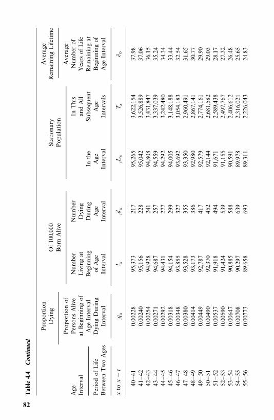
Tab
le4.
4C
onti
nued
Proportion
Of100,000
Stationary
Average
Dying
BornAlive
Population
RemainingLifetime
Proportionof
Average
Age
PersonsAlive
Number
Number
InThis
Numberof
Interval
atBeginningof
Livingat
Dying
andAll
YearsofLife
AgeInterval
Beginning
During
Inthe
Subsequent
Remainingat
PeriodofLife
DyingDuring
ofAge
Age
Age
Age
Beginningof
BetweenTwoAges
Interval
Interval
Interval
Interval
Intervals
AgeInterval
xto
x
t�q
l
�d
�L
T
e�
40—41
0.00228
95,373
217
95,265
3,622,154
37.98
41—42
0.00240
95,156
228
95,042
3,526,889
37.06
42—43
0.00254
94,928
241
94,808
3,431,847
36.15
43—44
0.00271
94,687
257
94,559
3,337,039
35.24
44—45
0.00292
94,431
277
94,292
3,242,480
34.34
45—46
0.00318
94,154
299
94,005
3,148,188
33.44
46—47
0.00348
93,855
327
93,692
3,054,183
32.54
47—48
0.00380
93,528
355
93,350
2,960,491
31.65
48—49
0.00414
93,173
386
92,980
2,867,141
30.77
49—50
0.00449
92,787
417
92,579
2,774,161
29.90
50—51
0.00490
92,370
452
92,144
2,681,582
29.03
51—52
0.00537
91,918
494
91,671
2,589,438
28.17
52—53
0.00590
91,424
539
91,155
2,497,767
27.32
53—54
0.00647
90,885
588
90,591
2,406,612
26.48
54—55
0.00708
90.297
639
89.978
2,316,021
25.65
55—56
0.00773
89,658
693
89,311
2,226,043
24.83
82
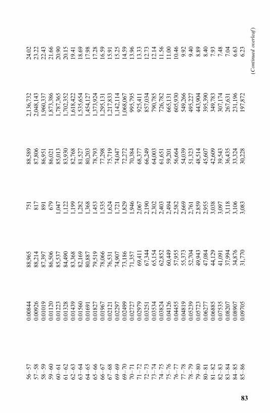
56—57
0.00844
88,965
751
88,589
2,136,732
24.02
57—58
0.00926
88,214
817
87,806
2,048,143
23.22
58—59
0.01019
87,397
891
86,951
1,960,337
22.43
59—60
0.01120
86,506
679
86,021
1,873,386
21.66
60—61
0.01223
85,537
1,047
85,013
1,787,365
20.90
61—62
0.01328
84,490
1,122
83,930
1,702,352
20.15
62—63
0.01439
83,368
1,199
82,768
1,618,422
19.41
63—64
0.01560
82,169
1,282
81,527
1,535,654
18.69
64—65
0.01691
80,887
1,368
80,203
1,454,127
17.98
65—66
0.01827
79,519
1.453
78,793
1,373,924
17.28
66—67
0.01967
78,066
1,535
77,298
1,295,131
16.59
67—68
0.02121
76,531
1,624
75,719
1,217,833
15.91
69—69
0.02297
74,907
1,721
74,047
1,142,114
15.25
69—70
0.02499
73,186
1,829
72,272
1,068,067
14.59
70—71
0.02727
71,357
1,946
70,384
995,795
13.96
71—72
0.02979
69,411
2,067
68,377
925,411
13.33
72—73
0.03251
67,344
2,190
66,249
857,034
12.73
73—74
0.03534
65,154
2,302
64,003
790,785
12.14
74—75
0.03824
62,852
2,403
61,651
726,782
11.56
75—76
0.04126
60,449
2,494
59,201
665,131
11.00
76—77
0.04455
57,955
2,582
56,664
605,930
10.46
77—78
0.04819
55,373
2,669
54,039
549,266
9.92
78—79
0.05239
52,704
2,761
51,323
495,227
9.40
79—80
0.05723
49,943
2.859
48,514
443,904
8.89
80—81
0.06277
47,084
2,955
45,607
395,390
8.40
81—82
0.06885
44,129
3,038
42,609
349,783
7.93
82—83
0.07535
41,091
3,097
39,543
307,174
7.48
83—84
0.08207
37,994
3,118
36,435
267,631
7.04
84—85
0.08907
34,876
3,106
33,324
231,196
6.63
85—86
0.09705
31,770
3,083
30,228
197,872
6.23
(Continued
overleaf)
83
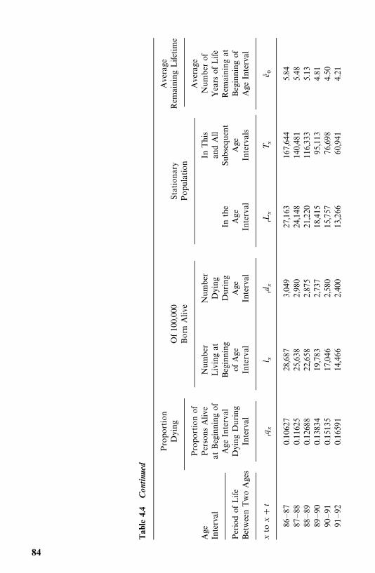
Tab
le4.
4C
onti
nued
Proportion
Of100,000
Stationary
Average
Dying
BornAlive
Population
RemainingLifetime
Proportionof
Average
Age
PersonsAlive
Number
Number
InThis
Numberof
Interval
atBeginningof
Livingat
Dying
andAll
YearsofLife
AgeInterval
Beginning
During
Inthe
Subsequent
Remainingat
PeriodofLife
DyingDuring
ofAge
Age
Age
Age
Beginningof
BetweenTwoAges
Interval
Interval
Interval
Interval
Intervals
AgeInterval
xto
x
t�q
l
�d
�L
T
e�
86—87
0.10627
28,687
3,049
27,163
167,644
5.84
87—88
0.11625
25,638
2,980
24,148
140,481
5.48
88—89
0.12688
22,658
2,875
21,220
116,333
5.13
89—90
0.13834
19,783
2,737
18,415
95,113
4.81
90—91
0.15135
17,046
2,580
15,757
76,698
4.50
91—92
0.16591
14,466
2,400
13,266
60,941
4.21
84
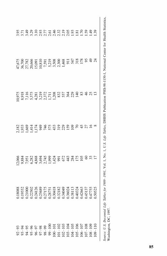
92—93
0.18088
12,066
2,182
10,975
47,675
3.95
93—94
0.19552
9,884
1,933
8,918
36,700
3.71
94—95
0.21000
7,951
1,669
7,116
27,782
3.49
95—96
0.22502
6,282
1,414
5,575
20,666
3.29
96—97
0.24126
4,868
1,174
4,281
15,091
3.10
97—98
0.25689
3,694
949
3,219
10,810
2.93
98—99
0.27175
2,745
746
2,372
7,591
2.77
99—100
0.28751
1,999
575
1,711
5,219
2.61
100—101
0.30418
1,424
433
1,208
3,508
2.46
101—102
0.32182
991
319
832
2,300
2.32
102—103
0.34049
672
229
557
1,468
2.19
103—104
0.36024
443
159
364
911
2.05
104—105
0.38113
284
109
229
547
1.93
105—106
0.40324
175
70140
318
1.81
106—107
0.42663
105
4583
178
1.70
107—108
0.45137
6027
4695
1.59
108—109
0.47755
3316
2549
1.49
109—110
0.50525
178
1324
1.39
Source:U.S.Decennial
LifeTa
bles
for
1989
—19
91,Vol.1,No.1,
U.S.Life
Tables,DHHSPublicationPHS-98-1150-1,NationalCenterforHealthStatistics,
Washington,DC,1997.
85
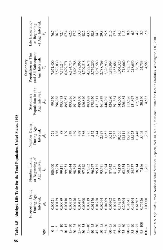
Tab
le4.
5A
brid
ged
Life
Tab
lefo
rth
eTot
alPop
ulat
ion,
Uni
ted
Stat
es,19
98
Stationary
ProportionDying
NumberLiving
NumberDying
Stationary
PopulationinThis
LifeExpectancy
DuringAge
atBeginningof
DuringAge
Populationinthe
andAllSubsequent
atBeginning
Interval,
AgeInterval,
Interval,
AgeInterval,
AgeIntervals,
ofAgeInterval,
Age
�q
l �d
�L
T
e�
0—1
0.00721
100,000
721
99,370
7,671,400
76.7
1—5
0.00139
99,279
138
396,786
7,572,030
76.3
5—10
0.00089
99,141
88495,473
7,175,244
72.4
10—15
0.00110
99,053
109
495,057
6,679,771
67.4
15—20
0.00353
98,944
349
493,926
6,184,714
62.5
20—25
0.00476
98,595
469
491,820
5,690,788
57.7
25—30
0.00487
98,126
478
489,450
5,198,968
53.0
30—35
0.00600
97,648
586
486,840
4,709,518
48.2
35—40
0.00819
97,062
795
483,428
4,222,678
43.5
40—45
0.01176
96,267
1,132
478,670
3,739,250
38.8
45—50
0.01728
95,135
1,644
471,811
3,260,580
34.3
50—55
0.02564
93,491
2,397
461,839
2,788,769
29.8
55—60
0.04009
91,094
3,652
446,966
2,326,930
25.5
60—65
0.06302
87,442
5,511
424,280
1,879,964
21.5
65—70
0.09437
81,931
7,732
391,364
1,455,684
17.8
70—75
0.14239
74,199
10,565
345,660
1,064,320
14.3
75—80
0.20604
63,634
13,111
286,484
718,660
11.3
80—85
0.31641
50,523
15,986
213,526
432,176
8.6
85—90
0.46104
34,537
15,923
131,897
218,650
6.3
90—95
0.61502
18,614
11,448
62,020
86,753
4.7
95—100
0.75426
7,166
5,405
20,150
24,733
3.5
100
1.00000
1,761
1,761
4,583
4,583
2.6
Source:U.S.Life
Tables,
1998.NationalVitalStatisticsReports,Vol.48,No.18,NationalCenterforHealthStatistics,Washington,DC,2001.
86
table for 1989—1991 the life expectancy at birth is 75.37 years and that atage 40 is 37.98 years. This means that according to the mortality rates of1989—1991 newborns are expected to live 75.37 years and those at age 40are expected to live another 37.98 years. The life expectancy of apopulation is a general indication of the capability of prolonging life. Itis used to identify trends and to compare longevity. Table 4.5 shows thataccording to the mortality rates of 1998, the newborns and those at age40 are expected to live 76.7 and 38.8 years, respectively. The overall lifeexpectancy indicates an improvement in longevity in the United Statesover the time period.
Population life tables can be constructed for various subgroups. Forexample, there are published life tables by gender, race, cause of death, as wellas those which eliminate certain causes of death.
4.2.2 Clinical Life Tables
The actuarial life table method has been applied to clinical data for manydecades. Berkson and Gage (1950) and Cutler and Ederer (1958) give alife-table method for estimating the survivorship function; Gehan (1969)provides methods for estimating all three functions (survivorship, density, andhazard).The life-table method requires a fairly large number of observations, so that
survival times can be grouped into intervals. Similar to the PL estimate, thelife-table method incorporates all survival information accumulated up to thetermination of the study. For example, in computing a five-year survival rateof breast cancer patients, one need not restrict oneself only to those patientswho have entered on study for five or more years. Patients who have enteredfor four, three, two, and even one year contribute useful information to theevaluation of five-year survival. In this way, the life-table technique usesincomplete data such as losses to follow-up and persons withdrawn alive aswell as complete death data.Table 4.6 shows the format of the clinical life table. The columns are
described below.
1. Interval [t� t
��). The first column gives the intervals into which the
survival times and times to loss or withdrawal are distributed. Theinterval is from t
�up to but not including t
��, i� 1, . . . , s. The last
interval has an infinite length. These intervals are assumed to be fixed.
2. Midpoint (t��
). The midpoint of each interval, designated t��, i� 1, . . . ,
s� 1, is included for convenience in plotting the hazard and probabilitydensity functions. Both functions are plotted as t
��.
3. Width (b�). The width of each interval, b
�� t
��� t
�, i� 1, . . . , , s� 1,
is needed for calculation of the hazard and density functions. The width
- 87
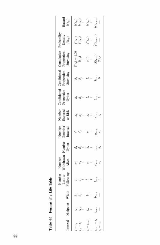
Tab
le4.
6For
mat
ofa
Life
Tab
le
Number
Number
Number
Number
ConditionalConditionalCumulative
Probability
Lostto
WithdrawnNumber
Entering
Exposed
Proportion
Proportion
Proportion
Density
Hazard
Interval
Midpoint
Width
Follow-up
Alive
Dying
Interval
toRisk
Dying
Surviving
Surviving
f(t �
�)h�(t �
�)
t�t �
t ��
b �l �
w�
d �n� �
n �q� �
p� �S�(t �)
�1.00
f�(t �
�)h�(t �
�)t �
�t �
t ��
b �l �
w�
d �n� �
n �q� �
p� �S�(t �)
f�(t �
�)h�(t �
�)�
��
��
��
��
��
��
t ��t �
�t �
�b �
l �w
�d �
n� �n �
q� �p� �
s�(t �)
f�(t �
�)h�(t �
�)�
��
��
��
��
��
��
t ����
t �t �
����
b ���
l ���
w��
�d ��
�n� ��
�n ��
�q� ��
�p� ��
�S�(t ��
�)f�(t �
���
�)h�(t �
����)
t ���
——
l �w�
d �n� �
n �1
0S�(t �)
——
88
of the last interval, b�, is theoretically infinite; no estimate of the hazard or
density function can be obtained for this interval.
4. Number lost to follow-up (l�). This is the number of people who are lost
to observation and whose survival status is thus unknown in the ithinterval (i� 1, . . . , s).
5. Number withdrawn alive (w�). People withdrawn alive in the ith interval
are those known to be alive at the closing date of the study. The survivaltime recorded for such persons is the length of time from entrance tothe closing date of the study.
6. Number dying (d�). This is the number of people who die in the ith
interval. The survival time of these people is the time from entrance todeath.
7. Number entering the ith interval (n��). The number of people entering the
first interval n��is the total sample size. Other entries are determined
from n��� n�
���� l
����w
���� d
���. That is, the number of persons
entering the ith interval is equal to the number studied at the beginningof the preceding interval minus those who are lost to follow-up,withdrawn alive, or have died in the preceding interval.
8. Number exposed to risk (n�). This is the number of people who are
exposed to risk in the ith interval and is defined as n�� n�
���
�(l� w
�).
It is assumed that the times to loss or withdrawal are approximatelyuniformly distributed in the interval. Therefore, people lost or with-drawn in the interval are exposed to risk of death for one-half theinterval. If there are no losses or withdrawals, n
�� n�
�.
9. Conditional proportion dying (q��). This is defined as q
�� d
�/n
�for
i� 1, . . . , s� 1, and q��� 1. It is an estimate of the conditional
probability of death in the ith interval given exposure to the risk ofdeath in the ith interval.
10. Conditional proportion surviving (q��). This is given by p�
�� 1� q�
�, which
is an estimate of the conditional probability of surviving in the ithinterval.
11. Cumulative proportion surviving [S� (t�)]. This is an estimate of the
survivorship function at time t�; it is often referred to as the cumulative
survival rate. For i� 1, S�� (t��)� 1 and for i� 2, . . . , s, S� (t
�)�
p����
S� (t���). It is the usual life-table estimate and is based on the fact
that surviving to the start of the ith interval means surviving to the startof and then through the (i� 1)th interval.
12. Estimated probability density function [ f� (t�)]. This is defined as the
probability of dying in the ith interval per unit width. Thus, a naturalestimate at the midpoint of the interval is
f� (t�)�
S� (t�)�S� (t
���)
b�
�S� (t
�)q�
�b�
i� 1, . . . , s� 1 (4.2.7)
- 89
13. Hazard function [h� (t��)]. The hazard function for the ith interval,
estimated at the midpoint, is
h� (t��)�
d�
b�(n
���
�d�)�
2q��
b�(1 p�
�)
i� 1, . . . , s� 1 (4.2.8)
It is the number of deaths per unit time in the interval divided bythe average number of survivors at the midpoint of the interval.That is, h� (t
��) is derived from f� (t
��)/S� (t
��) and S� (t
��)��
�[S� (t
��)
S� (t�)] since S(t
�) is defined as the probability of surviving at the
beginning, not the midpoint, of the ith interval:
h� (t��)�
f� (t��)
S� (t��)�
S� (t�)q�
�/b
���S� (t
�)( p�
� 1)
(4.2.9)
which reduces to (4.2.8).Sacher (1956) derives an estimate of the hazard function by assuming
that hazard is constant within an interval but varies among intervals.His estimate is
h� (t��)�
�log p��
b�
(4.2.10)
In a Monte Carlo study, Gehan and Siddiqui (1973) show that (4.2.9) isless biased than (4.2.10).
The large-sample approximate variances of the estimated survival functions,S� (t
�), f� (t
��), and h� (t
��) in the ith interval are
Var[S� (t�)]� [S� (t
�)]�
�������
q��
n�p��
(4.2.11)
Var[ f� (t��)]�
[S� (t�)q�
�]�
b�
��������
q��
n�p��
p��
n�q��� (4.2.12)
and
Var[h� (t��)]�
[h� (t��)]�
n�q���1��
1
2h� (t
��)b
���
� (4.2.13)
Equation (4.2.11) is given by Greenwood (1926); Gehan (1969) derived (4.2.12)and (4.2.13). These may be used to obtain approximate confidence intervals forthe various survival functions.The graph of S� (t
�) can be used to find an estimate of the median. Or let
(t�, t
��) be the interval such that S� (t
�)� 0.5 and S� (t
��) 0.5. Then the
90
median survival time t�can be estimated by linear interpolation:
t��
� t� [S� (t
�)� 0.5]b
�S� (t
�)�S� (t
��)� t
�
S� (t�)� 0.5
f� (t��)
(4.2.14)
where f� (t��
) is defined in (4.2.7).Another interesting measure that can be obtained from the life table is the
median remaining lifetime at time t�, denoted by t
��(i), i� 1, . . . , s� 1. If at t
�the proportion of individual survival is S� (t
�), the proportion of individual
survival at t��(i) is �
�S� (t
�). That is, one-half of the people who are alive at time
t�are expected to be alive at time t
��(i) . Let (t
�, t
��) be the interval in which
��S� (t
�) falls; that is, S� (t
�)� �
�S� (t
�) and S� (t
��) �
�S� (t
�). Then an estimate of t
��(i)
is
t���(i) � (t
�� t
�)
b�[S� (t
�)��
�S� (t
�)]
S� (t�)�S� (t
��)
(4.2.15)
Here S� (t�) is the estimated proportion surviving beyond the lower limit of the
interval containing the median.The variance of t
��(i) is approximately
Var[t���(i )]�
[S� (t�)]�
4n�[ f� (t
��)]�
(4.2.16)
Example 4.4 The following survival data for 2418 males with anginapectoris, originally reported by Parker et al. (1946), were also included inGehan’s (1969) paper. Survival time is computed from time of diagnosis inyears. The life table uses 16 intervals of one year. Table 4.7 gives estimates ofthe various survival functions, the median remaining lifetime, and theirstandard errors. The survivorship function, S� (t), is plotted at t and the hazardand density functions, h� (t) and f� (t), are plotted at the midpoint of the interval(Figure 4.4).The graph of the estimated hazard function shows that the death rate is
highest in the first year after diagnosis. From the end of the first year to thebeginning of the tenth year, the death rate remains relatively constant,fluctuating between 0.09 and 0.12. The hazard rate is generally higher after thetenth year. Hence, the prognosis for a patient who has survived one year isbetter than that for a newly diagnosed patient if factors such as age, gender,and race are not considered. A similar interpretation is reached by examiningthe estimated median remaining lifetimes. Initially, the estimated medianremaining lifetime is 5.33 years. It reaches a peak of 6.34 years at the beginningof the second year after diagnosis and then decreases. The median survivaltime, either read from the survival curve or using (4.2.14), is 5.33 years and thefive-year survival rate is 0.5193 with a standard error of 0.0103.
- 91
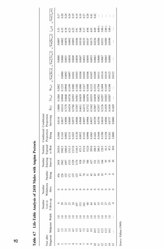
Tab
le4.
7Life-
Tab
leA
naly
sis
of24
18M
ales
with
Ang
ina
Pec
toris
Number
Number
Number
Number
ConditionalConditional
Yearafter
Lostto
Withdrawn
Number
Entering
Exposed
Proportion
Proportion
DiagnosisMidpointWidth
Follow-up
Alive
Dying
Interval
toRisk
Dying
Surviving
S�(t �)
f�(t �
�)h�(t �
�)�Var[S
�(t�)]
�Var[f�(t �
�)]
�Var[h�(t
��)]
t� ��(i)
�Var[t
� ��(i)]
00.5
1.0
00
456
2418
2418.0
0.1886
0.8114
1.0000
0.1886
0.2082
—0.0080
0.0097
5.33
0.17
11.5
1.0
390
226
1962
1942.5
0.1163
0.8837
0.8114
0.0944
0.1235
0.0080
0.0060
0.0082
6.35
0.20
22.5
1.0
220
152
1697
1686.0
0.0902
0.9098
0.7170
0.0646
0.0944
0.0092
0.0051
0.0076
6.34
0.24
33.5
1.0
230
171
1523
1511.5
0.1131
0.8869
0.6524
0.0738
0.1199
0.0097
0.0054
0.0092
6.23
0.24
44.5
1.0
240
135
1329
1317.0
0.1025
0.8975
0.5786
0.0593
0.1080
0.0101
0.0049
0.0093
6.22
0.19
55.5
1.0
107
0125
1170
1116.5
0.1120
0.8880
0.5193
0.0581
0.1186
0.0103
0.0050
0.0106
5.91
0.18
66.5
1.0
133
083
938
871.5
0.0952
0.9048
0.4611
0.0439
0.1000
0.0104
0.0047
0.0110
5.60
0.19
77.5
1.0
102
074
722
671.0
0.1103
0.8897
0.4172
0.0460
0.1167
0.0105
0.0052
0.0135
5.17
0.27
88.5
1.0
680
51546
512.0
0.0996
0.9904
0.3712
0.0370
0.1048
0.0106
0.0050
0.0147
4.94
0.28
99.5
1.0
640
42427
395.0
0.1063
0.8937
0.3342
0.0355
0.1123
0.0107
0.0053
0.0173
4.83
0.41
1010.5
1.0
450
43321
298.5
0.1441
0.8559
0.2987
0.0430
0.1552
0.0109
0.0063
0.0236
4.69
0.42
1111.5
1.0
530
34233
206.5
0.1646
0.8354
0.2557
0.0421
0.1794
0.0111
0.0068
0.0306
4.00
—
1212.5
1.0
330
18146
129.5
0.1390
0.8610
0.2136
0.0297
0.1494
0.0114
0.0067
0.0351
3.00
—
1313.5
1.0
270
995
81.5
0.1104
0.8896
0.1839
0.0203
0.1169
0.0118
0.0065
0.0389
2.00
—
1414.5
1.0
230
659
47.5
0.1263
0.8737
0.1636
0.0207
0.1348
0.0123
0.0080
0.0549
1.00
—
15—
—0
00
3030.0
1.0000
0.0000
0.1429
——
0.0133
——
——
Source:Gehan
(1969).
92
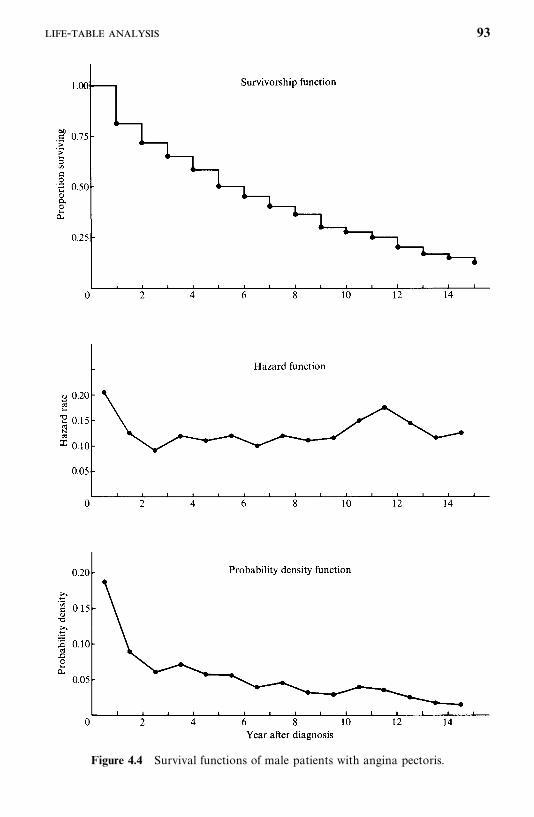
Figure 4.4 Survival functions of male patients with angina pectoris.
- 93
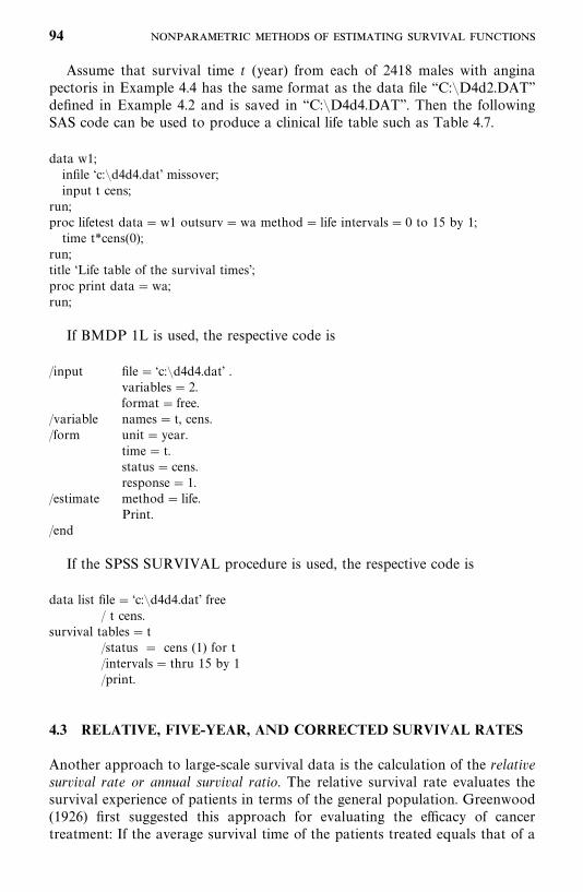
Assume that survival time t (year) from each of 2418 males with anginapectoris in Example 4.4 has the same format as the data file ‘‘C:�D4d2.DAT’’defined in Example 4.2 and is saved in ‘‘C:�D4d4.DAT’’. Then the followingSAS code can be used to produce a clinical life table such as Table 4.7.
data w1;infile ‘c:�d4d4.dat’ missover;input t cens;
run;proc lifetest data�w1 outsurv�wa method� life intervals� 0 to 15 by 1;time t*cens(0);
run;title ‘Life table of the survival times’;proc print data�wa;run;
If BMDP 1L is used, the respective code is
/input file� ‘c:�d4d4.dat’ .variables� 2.format� free.
/variable names� t, cens./form unit� year.
time� t.status� cens.response� 1.
/estimate method� life.Print.
/end
If the SPSS SURVIVAL procedure is used, the respective code is
data list file� ‘c:�d4d4.dat’ free/ t cens.
survival tables� t/status � cens (1) for t/intervals� thru 15 by 1/print.
4.3 RELATIVE, FIVE-YEAR, AND CORRECTED SURVIVAL RATES
Another approach to large-scale survival data is the calculation of the relativesurvival rate or annual survival ratio. The relative survival rate evaluates thesurvival experience of patients in terms of the general population. Greenwood(1926) first suggested this approach for evaluating the efficacy of cancertreatment: If the average survival time of the patients treated equals that of a
94
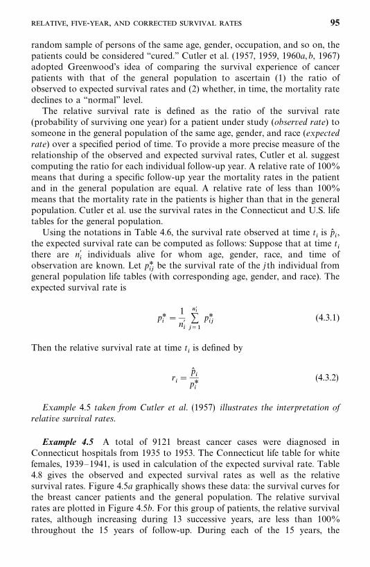
random sample of persons of the same age, gender, occupation, and so on, thepatients could be considered ‘‘cured.’’ Cutler et al. (1957, 1959, 1960a, b, 1967)adopted Greenwood’s idea of comparing the survival experience of cancerpatients with that of the general population to ascertain (1) the ratio ofobserved to expected survival rates and (2) whether, in time, the mortality ratedeclines to a ‘‘normal’’ level.The relative survival rate is defined as the ratio of the survival rate
(probability of surviving one year) for a patient under study (observed rate) tosomeone in the general population of the same age, gender, and race (expectedrate) over a specified period of time. To provide a more precise measure of therelationship of the observed and expected survival rates, Cutler et al. suggestcomputing the ratio for each individual follow-up year. A relative rate of 100%means that during a specific follow-up year the mortality rates in the patientand in the general population are equal. A relative rate of less than 100%means that the mortality rate in the patients is higher than that in the generalpopulation. Cutler et al. use the survival rates in the Connecticut and U.S. lifetables for the general population.Using the notations in Table 4.6, the survival rate observed at time t
�is p�
�,
the expected survival rate can be computed as follows: Suppose that at time t�
there are n��individuals alive for whom age, gender, race, and time of
observation are known. Let p*��be the survival rate of the j th individual from
general population life tables (with corresponding age, gender, and race). Theexpected survival rate is
p*��1
n��
����
���
p*��
(4.3.1)
Then the relative survival rate at time t�is defined by
r��
p��
p*�
(4.3.2)
Example 4.5 taken from Cutler et al. (1957) illustrates the interpretation ofrelative survival rates.
Example 4.5 A total of 9121 breast cancer cases were diagnosed inConnecticut hospitals from 1935 to 1953. The Connecticut life table for whitefemales, 1939—1941, is used in calculation of the expected survival rate. Table4.8 gives the observed and expected survival rates as well as the relativesurvival rates. Figure 4.5a graphically shows these data: the survival curves forthe breast cancer patients and the general population. The relative survivalrates are plotted in Figure 4.5b. For this group of patients, the relative survivalrates, although increasing during 13 successive years, are less than 100%throughout the 15 years of follow-up. During each of the 15 years, the
, -, 95
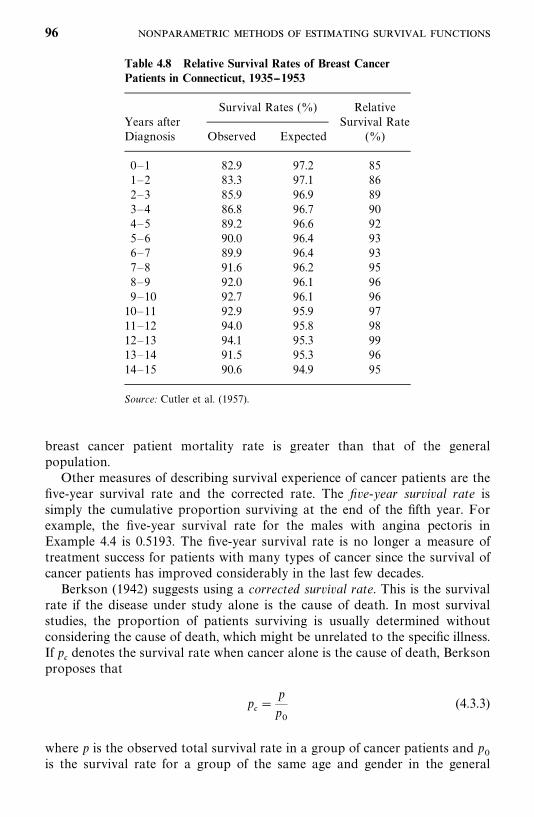
Table 4.8 Relative Survival Rates of Breast CancerPatients in Connecticut, 1935--1953
Survival Rates (%) RelativeYears after Survival RateDiagnosis Observed Expected (%)
0—1 82.9 97.2 851—2 83.3 97.1 862—3 85.9 96.9 893—4 86.8 96.7 904—5 89.2 96.6 925—6 90.0 96.4 936—7 89.9 96.4 937—8 91.6 96.2 958—9 92.0 96.1 969—10 92.7 96.1 9610—11 92.9 95.9 9711—12 94.0 95.8 9812—13 94.1 95.3 9913—14 91.5 95.3 9614—15 90.6 94.9 95
Source: Cutler et al. (1957).
breast cancer patient mortality rate is greater than that of the generalpopulation.Other measures of describing survival experience of cancer patients are the
five-year survival rate and the corrected rate. The five-year survival rate issimply the cumulative proportion surviving at the end of the fifth year. Forexample, the five-year survival rate for the males with angina pectoris inExample 4.4 is 0.5193. The five-year survival rate is no longer a measure oftreatment success for patients with many types of cancer since the survival ofcancer patients has improved considerably in the last few decades.Berkson (1942) suggests using a corrected survival rate. This is the survival
rate if the disease under study alone is the cause of death. In most survivalstudies, the proportion of patients surviving is usually determined withoutconsidering the cause of death, which might be unrelated to the specific illness.If p
denotes the survival rate when cancer alone is the cause of death, Berkson
proposes that
p �
p
p
(4.3.3)
where p is the observed total survival rate in a group of cancer patients and p
is the survival rate for a group of the same age and gender in the general
96
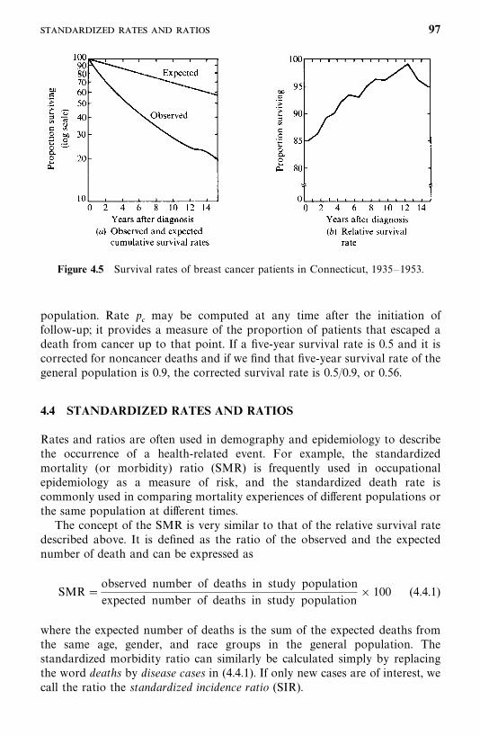
Figure 4.5 Survival rates of breast cancer patients in Connecticut, 1935—1953.
population. Rate p may be computed at any time after the initiation of
follow-up; it provides a measure of the proportion of patients that escaped adeath from cancer up to that point. If a five-year survival rate is 0.5 and it iscorrected for noncancer deaths and if we find that five-year survival rate of thegeneral population is 0.9, the corrected survival rate is 0.5/0.9, or 0.56.
4.4 STANDARDIZED RATES AND RATIOS
Rates and ratios are often used in demography and epidemiology to describethe occurrence of a health-related event. For example, the standardizedmortality (or morbidity) ratio (SMR) is frequently used in occupationalepidemiology as a measure of risk, and the standardized death rate iscommonly used in comparing mortality experiences of different populations orthe same population at different times.The concept of the SMR is very similar to that of the relative survival rate
described above. It is defined as the ratio of the observed and the expectednumber of death and can be expressed as
SMR�observed number of deaths in study population
expected number of deaths in study population� 100 (4.4.1)
where the expected number of deaths is the sum of the expected deaths fromthe same age, gender, and race groups in the general population. Thestandardized morbidity ratio can similarly be calculated simply by replacingthe word deaths by disease cases in (4.4.1). If only new cases are of interest, wecall the ratio the standardized incidence ratio (SIR).
97
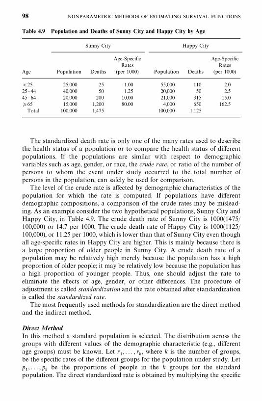
Table 4.9 Population and Deaths of Sunny City and Happy City by Age
Sunny City Happy City
Age-Specific Age-SpecificRates Rates
Age Population Deaths (per 1000) Population Deaths (per 1000)
25 25,000 25 1.00 55,000 110 2.025—44 40,000 50 1.25 20,000 50 2.545—64 20,000 200 10.00 21,000 315 15.0�65 15,000 1,200 80.00 4,000 650 162.5Total 100,000 1,475 100,000 1,125
The standardized death rate is only one of the many rates used to describethe health status of a population or to compare the health status of differentpopulations. If the populations are similar with respect to demographicvariables such as age, gender, or race, the crude rate, or ratio of the number ofpersons to whom the event under study occurred to the total number ofpersons in the population, can safely be used for comparison.The level of the crude rate is affected by demographic characteristics of the
population for which the rate is computed. If populations have differentdemographic compositions, a comparison of the crude rates may be mislead-ing. As an example consider the two hypothetical populations, Sunny City andHappy City, in Table 4.9. The crude death rate of Sunny City is 1000(1475/100,000) or 14.7 per 1000. The crude death rate of Happy City is 1000(1125/100,000), or 11.25 per 1000, which is lower than that of Sunny City even thoughall age-specific rates in Happy City are higher. This is mainly because there isa large proportion of older people in Sunny City. A crude death rate of apopulation may be relatively high merely because the population has a highproportion of older people; it may be relatively low because the population hasa high proportion of younger people. Thus, one should adjust the rate toeliminate the effects of age, gender, or other differences. The procedure ofadjustment is called standardization and the rate obtained after standardizationis called the standardized rate.The most frequently used methods for standardization are the direct method
and the indirect method.
Direct MethodIn this method a standard population is selected. The distribution across thegroups with different values of the demographic characteristic (e.g., differentage groups) must be known. Let r
�, . . . , r
�, where k is the number of groups,
be the specific rates of the different groups for the population under study. Letp�, . . . , p
�be the proportions of people in the k groups for the standard
population. The direct standardized rate is obtained by multiplying the specific
98
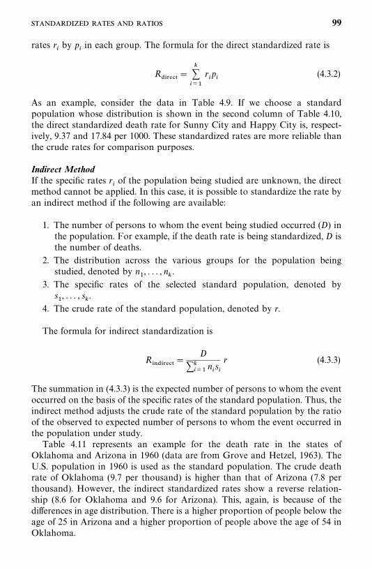
rates r�by p
�in each group. The formula for the direct standardized rate is
R������
������
r�p�
(4.3.2)
As an example, consider the data in Table 4.9. If we choose a standardpopulation whose distribution is shown in the second column of Table 4.10,the direct standardized death rate for Sunny City and Happy City is, respect-ively, 9.37 and 17.84 per 1000. These standardized rates are more reliable thanthe crude rates for comparison purposes.
Indirect MethodIf the specific rates r
�of the population being studied are unknown, the direct
method cannot be applied. In this case, it is possible to standardize the rate byan indirect method if the following are available:
1. The number of persons to whom the event being studied occurred (D) inthe population. For example, if the death rate is being standardized, D isthe number of deaths.
2. The distribution across the various groups for the population beingstudied, denoted by n
�, . . . , n
�.
3. The specific rates of the selected standard population, denoted bys�, . . . , s
�.
4. The crude rate of the standard population, denoted by r.
The formula for indirect standardization is
R��������
�D
�����
n�s�
r (4.3.3)
The summation in (4.3.3) is the expected number of persons to whom the eventoccurred on the basis of the specific rates of the standard population. Thus, theindirect method adjusts the crude rate of the standard population by the ratioof the observed to expected number of persons to whom the event occurred inthe population under study.Table 4.11 represents an example for the death rate in the states of
Oklahoma and Arizona in 1960 (data are from Grove and Hetzel, 1963). TheU.S. population in 1960 is used as the standard population. The crude deathrate of Oklahoma (9.7 per thousand) is higher than that of Arizona (7.8 perthousand). However, the indirect standardized rates show a reverse relation-ship (8.6 for Oklahoma and 9.6 for Arizona). This, again, is because of thedifferences in age distribution. There is a higher proportion of people below theage of 25 in Arizona and a higher proportion of people above the age of 54 inOklahoma.
99
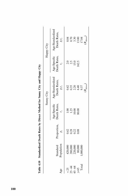
Tab
le4.
10St
anda
rdiz
edD
eath
Rat
esby
Direc
tM
etho
dfo
rSu
nny
City
and
Hap
pyC
ity
SunnyCity
HappyCity
Age-Specific
Age-Standardized
Age-Specific
Age-Standardized
Standard
Proportion,
DeathRates,
DeathRates,
DeathRates,
DeathRates,
Age
Population
p �r �
p �r�
r �p �r
�
25
420,000
0.42
1.00
0.42
2.0
0.84
25—44
280,000
0.28
1.25
0.35
2.5
0.70
45—64
220,000
0.22
10.00
2.20
15.0
3.30
�65
80,000
0.08
80.00
6.40
162.5
13.00
Total
1,000,000
9.37
17.84
(R������)
(R������)
100
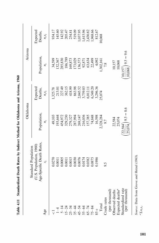
Tab
le4.
11St
anda
rdiz
edD
eath
Rat
esby
Indi
rect
Met
hod
for
Okl
ahom
aan
dA
rizo
na,19
60
Oklahoma
Arizona
StandardPopulation
(U.S.Population,1960
)Expected
Expected
Age-SpecificDeathRates,
Population,
Deaths,
Population,
Deaths,
Age
s �n �
n �s�
n �n �s
�
1
0.0270
49,103
1,325.78
34,599
934.17
1—4
0.0011
193,644
213.01
132,367
145.60
5—14
0.0005
454,972
227.49
285,830
142.92
15—24
0.0011
329,230
362.15
186,789
205.47
25—34
0.0015
279,327
418.99
169,873
254.81
35—44
0.0030
287,994
863.98
173,029
519.09
45—54
0.0076
269,147
2,045.52
136,573
1,037.95
55—64
0.0174
216,036
3,759.03
92,871
1,615.96
65—74
0.0382
157,385
6,012.11
63,634
2,430.82
75—84
0.0875
74,848
6,549.20
22,499
1,968.66
85
0.1986
16,598
3,296.36
4,092
812.67
Total
2,328,284
25,074
1,302,161
10,068
Cruderates
9.5
9.7
7.8
(perthousand
)Observeddeaths
22,584
10,157
Expecteddeaths�
25,074
10,068
Standardizedrate
�22,584
25,074�9.5
�8.6
�10,157
10,068�9.5
�9.6
(perthousand
)
Source:Datafrom
GroveandHetzel
(1963).
�n �s
�.
101
Results for the adjusted rates depend on the standard population selected.Hence, this selection should be done carefully. When discussing death rate byage, Shryock et al. (1971) suggest that a population with similar age distribu-tion to the various populations under study be selected as a standard. If thedeath rate of two populations is being compared, it is best to use the averageof the two distributions as a standard.It should be remembered that specific rates are still the most accurate and
essential indicators of the variations among populations. No matter whichmethod is used, standardized rates are meaningful only when compared withsimilarly computed rates. Kitagawa (1964) also criticizes the standardized ratebecause if the specific rates vary in different ways between the two populationsbeing compared, standardization will not indicate the differences and some-times will even mask the differences. Nevertheless, if the specific rates are notavailable, if a single rate for a population is desired, or if the demographiccomposition of the population being compared is different, the standardizedrate is useful.
Bibliographical Remarks
Kaplan and Meier’s (1958) PL method is the most commonly used techniquefor estimating the survivorship function for samples of small and moderate size.However, with the aid of a computer, it is not difficult to use the method forlarge sample sizes.Berkson (1942), Berkson and Gage (1950), Cutler and Ederer (1958), and
Gehan (1969) have written classic reports on life-table analysis. Peto et al.(1976) published an excellent review of some statistical methods related toclinical trials. The term life-table analysis that they use includes the PL method.Other references on life tables are, for example, Armitage (1971), Shryock et al.(1971), Kuzma (1967), Chiang (1968), Gross and Clark (1975), and Elandt-Johnson and Johnson (1980).Relative survival rates and corrected survival rates have been used by Cutler
and co-workers in a series of survival studies on cancer patients in Connecticutin the 1950s and 1960s (Cutler et al., 1957, 1959, 1960a, b, 1967; Ederer et al.,1961). Discussions of SMR, standardized rates, and related topics can be foundin many standard epidemiology textbooks: for example, Mausner and Kramer(1985), Kahn (1983), Kelsey et al. (1986), Shryock et al. (1971), Chiang (1961),and Mantel and Stark (1968).
EXERCISES
4.1 Consider the survival time of the 30 melanoma patients in Table 3.1.(a) Compute and plot the PL estimates of the survivorship functions
S� (t) of the two treatment groups and check your results with Table3.2 and Figure 3.1.
102
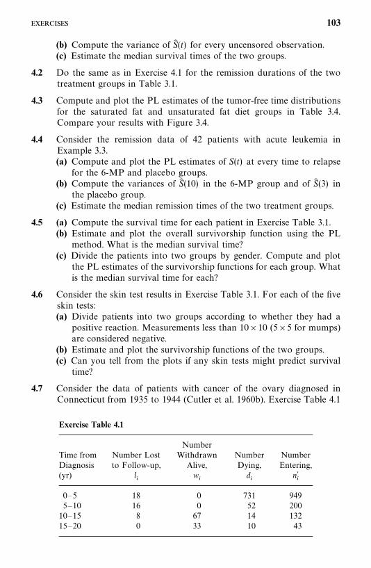
Exercise Table 4.1
NumberTime from Number Lost Withdrawn Number NumberDiagnosis to Follow-up, Alive, Dying, Entering,(yr) l
�w�
d�
n��
0—5 18 0 731 9495—10 16 0 52 20010—15 8 67 14 13215—20 0 33 10 43
(b) Compute the variance of S� (t) for every uncensored observation.(c) Estimate the median survival times of the two groups.
4.2 Do the same as in Exercise 4.1 for the remission durations of the twotreatment groups in Table 3.1.
4.3 Compute and plot the PL estimates of the tumor-free time distributionsfor the saturated fat and unsaturated fat diet groups in Table 3.4.Compare your results with Figure 3.4.
4.4 Consider the remission data of 42 patients with acute leukemia inExample 3.3.(a) Compute and plot the PL estimates of S(t) at every time to relapse
for the 6-MP and placebo groups.(b) Compute the variances of S� (10) in the 6-MP group and of S� (3) in
the placebo group.(c) Estimate the median remission times of the two treatment groups.
4.5 (a) Compute the survival time for each patient in Exercise Table 3.1.(b) Estimate and plot the overall survivorship function using the PL
method. What is the median survival time?(c) Divide the patients into two groups by gender. Compute and plot
the PL estimates of the survivorship functions for each group. Whatis the median survival time for each?
4.6 Consider the skin test results in Exercise Table 3.1. For each of the fiveskin tests:(a) Divide patients into two groups according to whether they had a
positive reaction. Measurements less than 10�10 (5�5 for mumps)are considered negative.
(b) Estimate and plot the survivorship functions of the two groups.(c) Can you tell from the plots if any skin tests might predict survival
time?
4.7 Consider the data of patients with cancer of the ovary diagnosed inConnecticut from 1935 to 1944 (Cutler et al. 1960b). Exercise Table 4.1
103
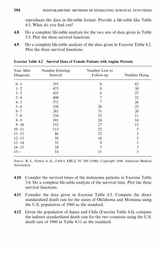
Exercise Table 4.2 Survival Data of Female Patients with Angina Pectoris
Year After Number Entering Number Lost toDiagnosis Interval Follow-up Number Dying
0—1 555 0 821—2 473 8 302—3 435 8 273—4 400 7 224—5 371 7 265—6 338 28 256—7 285 31 207—8 234 32 118—9 191 24 149—10 153 27 1310—11 113 22 511—12 86 23 512—13 58 18 513—14 35 9 214—15 24 7 315 14 11 3
Source: R. L. Parker et al., JAMA, 131(2), 95—100 (1946). Copyright 1946. American MedicalAssociation.
reproduces the data in life-table format. Provide a life-table like Table4.5. What do you find out?
4.8 Do a complete life-table analysis for the two sets of data given in Table3.5. Plot the three survival functions.
4.9 Do a complete life-table analysis of the data given in Exercise Table 4.2.Plot the three survival functions.
4.10 Consider the survival times of the melanoma patients in Exercise Table3.4. Do a complete life-table analysis of the survival time. Plot the threesurvival functions.
4.11 Consider the data given in Exercise Table 4.3. Compute the directstandardized death rate for the states of Oklahoma and Montana usingthe U.S. population of 1960 as the standard.
4.12 Given the population of Japan and Chile (Exercise Table 4.4), computethe indirect standardized death rate for the two countries using the U.S.death rate of 1960 in Table 4.11 as the standard.
104
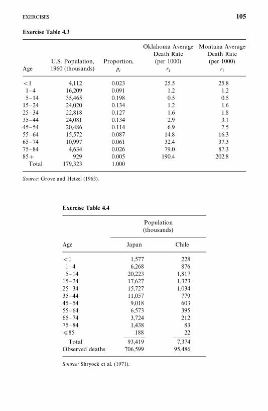
Exercise Table 4.3
Oklahoma Average Montana AverageDeath Rate Death Rate
U.S. Population, Proportion, (per 1000) (per 1000)Age 1960 (thousands) p
�r�
r�
1 4,112 0.023 25.5 25.81—4 16,209 0.091 1.2 1.25—14 35,465 0.198 0.5 0.515—24 24,020 0.134 1.2 1.625—34 22,818 0.127 1.6 1.835—44 24,081 0.134 2.9 3.145—54 20,486 0.114 6.9 7.555—64 15,572 0.087 14.8 16.365—74 10,997 0.061 32.4 37.375—84 4,634 0.026 79.0 87.385 929 0.005 190.4 202.8Total 179,323 1.000
Source: Grove and Hetzel (1963).
Exercise Table 4.4
Population(thousands)
Age Japan Chile
1 1,577 2281—4 6,268 8765—14 20,223 1,81715—24 17,627 1,32325—34 15,727 1,03435—44 11,057 77945—54 9,018 60355—64 6,573 39565—74 3,724 21275—84 1,438 83�85 188 22
———— ———Total 93,419 7,374
Observed deaths 706,599 95,486
Source: Shryock et al. (1971).
105
C H A P T E R 5
Nonparametric Methods forComparing Survival Distributions
The problem of comparing survival distributions arises often in biomedicalresearch. A laboratory researcher may want to compare the tumor-free timesof two or more groups of rats exposed to carcinogens. A diabetologist maywish to compare the retinopathy-free times of two groups of diabetic patients.A clinical oncologist may be interested in comparing the ability of two or moretreatments to prolong life or maintain health. Almost invariably, the disease-free or survival times of the different groups vary. These differences can beillustrated by drawing graphs of the estimated survivorship functions, but thatgives only a rough idea of the difference between the distributions. It does notreveal whether the differences are significant or merely chance variations. Astatistical test is necessary.
In Section 5.1 we introduce five nonparametric tests that can be used fordata with and without censored observations. Section 5.2 is devoted to theMantel—Haenszel test, which is particularly useful in stratified analysis, amethod commonly used to take account of possible confounding variables. InSection 5.3 we discuss the problem of comparing three or more survivaldistributions with or without censoring.
5.1 COMPARISON OF TWO SURVIVAL DISTRIBUTIONS
Suppose that there are n�
and n�
patients who receive treatments 1 and 2,respectively. Let x
�, . . . , x
��be the r
�failure observations and x�
����, . . . , x�
��the
n�� r
�censored observations in group 1. In group 2, let y
�, . . . , y
��be the r
�failure observations and y�
����, . . . , y�
��the n
�� r
�censored observations. That
is, at the end of the study n�� r
�patients who received treatment 1 and
n�� r
�patients who received treatment 2 are still alive. Suppose that the
observations in group 1 are samples from a distribution with survivorshipfunction S
�(t) and the observations in group 2 are samples from a distribution
106
with survivorship function S�(t). Then null hypothesis to consider is
H�
:S�(t) �S
�(t) (treatments 1 and 2 are equally effective)
against the alternative
H�: S
�(t) �S
�(t) (treatment 1 more effective than 2)
or
H�: S
�(t) �S
�(t) (treatment 2 more effective than 1)
or
H�: S
�(t) �S
�(t) (treatments 1 and 2 not equally effective)
When there are no censored observations, standard nonparametric tests canbe used to compare two survival distributions. For example, the Wilcoxon(1945) test or the Mann—Whitney (1947) U-test can test the equality of twoindependent populations, and the sign test can be used for paired (or depend-ent) samples (Marascuilo and McSweeney, 1977). In the following we introducefive nonparametric tests: Gehan’s generalized Wilcoxon test (Gehan, 1965a,b),the Cox—Mantel test (Cox 1959, 1972; Mantel, 1966), the logrank test (Petoand Peto, 1972), Peto and Peto’s generalized Wilcoxon test (1972), and Cox’sF-test (1964). All the tests are designed to handle censored data; data withoutcensored observations can be considered a special case.
5.1.1 Gehan’s Generalized Wilcoxon Test
In Gehan’s generalized Wilcoxon test every observation x�
or x��
in group 1 iscompared with every observation y
�or y�
�in group 2 and a score U
��is given
to the result of every comparison. For the purpose of illustration, let us assumethat the alternative hypothesis is H
�: S
�(t) �S
�(t), that is, treatment 1 is more
effective than treatment 2.Define
U��� �
�1 if x�� y
�or x�
�� y
�0 if x
�� y
�or x�
�� y
�or y�
��x
�or (x�
�, y�
�)
�1 if x�� y
�or x
�� y�
�
and calculate the test statistic
W �������
������
U��
(5.1.1)
where the sum is over all n�n�
comparisons. Hence, there is a contribution to
107
the test statistic W for every comparison where both observations are failures(except for ties) and for every comparison where a censored observation isequal to or larger than a failure. The calculation of W is laborious when n
�and n
�are large. Mantel (1967) shows that it can be calculated in an alternative
way by assigning a score to each observation based on its relative ranking. InGehan’s computation each observation in sample 1 is compared with each insample 2. If the two samples are combined into a single pooled sample ofn�� n
�observations, it is the same as comparing each observation with the
remaining n�� n
�� 1. Let U
�, i� 1, . . . , n
�� n
�, be the number of remaining
n�� n
�� 1 observations that the ith is definitely greater than minus the
number that it is definitely less than. The n�� n
�U
�’s define a finite population
with mean 0 and it is true that Gehan’s
W �������
U�
(5.1.2)
where summation is over the U�
of sample 1 only. From either (5.1.1) or (5.1.2),it is clear that W would be a large positive number if H
�is true. Mantel also
suggests that the permutational variance of W be used instead of the morecomplicated variance formula derived by Gehan. The permutational distribu-tion of W can be obtained by considering all�
�n�� n
�n���
(n�� n
�)!
n�! n
�!
ways of selecting n�
of the U�
at random. The test statistic W under H�
can beconsidered approximately normally distributed with mean 0 and variance�
Var(W ) �
n�n�
���������
U��
(n�� n
�)(n
�� n
�� 1)
(5.1.3)
Since W is discrete, an appropriate continuity correction of 1 is ordinarily usedwhen there are neither ties nor censored observations. Otherwise, a continuitycorrection of 0.5 would probably be appropriate.
Since W has an asymptotically normal distribution with mean zero andvariance in (5.1.3), Z�W/�Var(W ) has standard normal distribution. Therejection regions are Z�Z� for H
�, and Z� �Z� for H
�, and �Z��Z�� for
H�
where P(Z �Z� �H�) � �.
� n! is read n factorial: n! � n(n � 1)(n � 2) � 3.2.1.� This is called the permutational variance because it is obtained by considering the per mutationaldistribution of all (n
�� n
�)!/n
�! n
�!W ’s
108
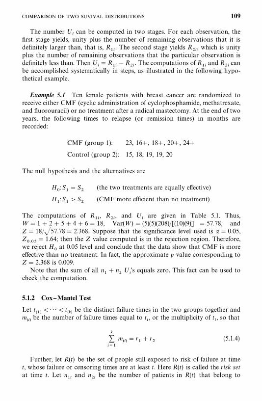
The number U�
can be computed in two stages. For each observation, thefirst stage yields, unity plus the number of remaining observations that it isdefinitely larger than, that is, R
��. The second stage yields R
��, which is unity
plus the number of remaining observations that the particular observation isdefinitely less than. Then U
��R
���R
��. The computations of R
��and R
��can
be accomplished systematically in steps, as illustrated in the following hypo-thetical example.
Example 5.1 Ten female patients with breast cancer are randomized toreceive either CMF (cyclic administration of cyclophosphamide, methatrexate,and fluorouracil) or no treatment after a radical mastectomy. At the end of twoyears, the following times to relapse (or remission times) in months arerecorded:
CMF (group 1): 23, 16�, 18�, 20�, 24�
Control (group 2): 15, 18, 19, 19, 20
The null hypothesis and the alternatives are
H�: S
�� S
�(the two treatments are equally effective)
H�: S
�� S
�(CMF more efficient than no treatment)
The computations of R��
, R��
, and U�
are given in Table 5.1. Thus,W � 1 � 2 � 5 � 4 � 6 � 18, Var(W ) � (5)(5)(208)/[(10)(9)] � 57.78, andZ� 18/�57.78� 2.368. Suppose that the significance level used is �� 0.05,Z
���� 1.64; then the Z value computed is in the rejection region. Therefore,
we reject H�
at 0.05 level and conclude that the data show that CMF is moreeffective than no treatment. In fact, the approximate p value corresponding toZ� 2.368 is 0.009.
Note that the sum of all n�� n
�U
�’s equals zero. This fact can be used to
check the computation.
5.1.2 Cox--Mantel Test
Let t��
� · · ·� t��
be the distinct failure times in the two groups together andm
�� be the number of failure times equal to t
�, or the multiplicity of t
�, so that
�����
m��
� r�� r
�(5.1.4)
Further, let R(t) be the set of people still exposed to risk of failure at timet, whose failure or censoring times are at least t. Here R(t) is called the risk setat time t. Let n
��and n
��be the number of patients in R(t) that belong to
109
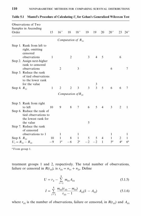
Table 5.1 Mantel’s Procedure of Calculating Ui for Gehan’s Generalized Wilcoxon Test
Observations of TwoSamples in AscendingOrder 15 16� 18 18� 19 19 20 20� 23 24�
Computation of R��
Step 1. Rank from left toright, omittingcensoredobservations 1 2 3 4 5 6
Step 2. Assign next-higherrank to censoredobservations 2 3 6 7
Step 3. Reduce the rankof tied observationsto the lower rankfor the value 3
Step 4. R��
1 2 2 3 3 3 5 6 6 7
Computation ofR��
Step 5. Rank from rightto left 10 9 8 7 6 5 4 3 2 1
Step 6. Reduce the rank oftied observations tothe lowest rank forthe value 5
Step 7. Reduce the rankof censoredobservations to 1 1 1 1 1
Step 8. R��
10 1 8 1 5 5 4 1 2 1U
��R
���R
���9 1� �6 2� �2 �2 1 5� 4� 6�
� From group 1.
treatment groups 1 and 2, respectively. The total number of observations,failure or censored in R(t
�� ), is r
�� � n
��� n
��. Define
U� r��
�����
m�� A
�� (5.1.5)
I������
m��
(r��
�m��
)
r��
� 1A
�� (1 �A
�� ) (5.1.6)
where r��
is the number of observations, failure or censored, in R(t��
) and A��
110
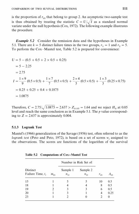
Table 5.2 Computations of Cox--Mantel Test
Number in Risk Set of:
Distinct Sample 1 Sample 2Failure Time, t
�m
�� n��
n��
r��
A��
15 1 5 5 10 0.518 1 4 4 8 0.519 2 3 3 6 0.520 1 3 1 4 0.2523 1 2 0 2 0
is the proportion of r��
that belong to group 2. An asymptotic two-sample test
is thus obtained by treating the statistic C�U/�I as a standard normalvariate under the null hypothesis (Cox, 1972). The following example illustratesthe procedure.
Example 5.2 Consider the remission data and the hypotheses in Example5.1. There are k� 5 distinct failure times in the two groups, r
�� 1 and r
�� 5.
To perform the Cox—Mantel test, Table 5.2 is prepared for convenience:
U� 5 � (0.5 � 0.5 � 2 � 0.5 � 0.25)
� 5 � 2.25
� 2.75
I�1�9
9(0.5�0.5) �
1�7
7(0.5�0.5) �
2�4
5(0.5�0.5) �
1�3
3(0.25�0.75)
� 0.25 � 0.25 � 0.4 � 0.1875
� 1.0875
Therefore, C� 2.75/�1.0875 � 2.637 �Z���
� 1.64 and we reject H�
at 0.05level and reach the same conclusion as in Example 5.1. The p value correspond-ing to Z� 2.637 is approximately 0.004.
5.1.3 Logrank Test
Mantel’s (1966) generalization of the Savage (1956) test, often referred to as thelogrank test (Peto and Peto, 1972), is based on a set of scores w
�assigned to
the observations. The scores are functions of the logarithm of the survival
111
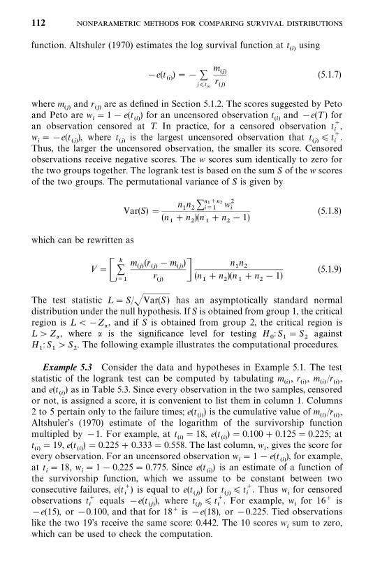
function. Altshuler (1970) estimates the log survival function at t��
using
�e(t��
) �� �j�t
��
m��
r��
(5.1.7)
where m��
and r��
are as defined in Section 5.1.2. The scores suggested by Petoand Peto are w
�� 1 � e(t
�� ) for an uncensored observation t
�� and �e(T ) for
an observation censored at T. In practice, for a censored observation t��
,w���e(t
�� ), where t
�� is the largest uncensored observation that t
�� � t�
�.
Thus, the larger the uncensored observation, the smaller its score. Censoredobservations receive negative scores. The w scores sum identically to zero forthe two groups together. The logrank test is based on the sum S of the w scoresof the two groups. The permutational variance of S is given by
Var(S) �n�n�������
���w��
(n�� n
�)(n
�� n
�� 1)
(5.1.8)
which can be rewritten as
V �������
m��
(r��
�m��
)
r��
�n�n�
(n�� n
�)(n
�� n
�� 1)
(5.1.9)
The test statistic L � S/�Var(S ) has an asymptotically standard normaldistribution under the null hypothesis. If S is obtained from group 1, the criticalregion is L ��Z� , and if S is obtained from group 2, the critical region isL �Z� , where � is the significance level for testing H
�: S
�� S
�against
H�
: S��S
�. The following example illustrates the computational procedures.
Example 5.3 Consider the data and hypotheses in Example 5.1. The teststatistic of the logrank test can be computed by tabulating m
�� , r
�� , m
�� /r
�� ,
and e(t��
) as in Table 5.3. Since every observation in the two samples, censoredor not, is assigned a score, it is convenient to list them in column 1. Columns2 to 5 pertain only to the failure times; e(t
�� ) is the cumulative value of m
�� /r
�� ,
Altshuler’s (1970) estimate of the logarithm of the survivorship functionmultipled by �1. For example, at t
�� � 18, e(t
�� ) � 0.100 � 0.125 � 0.225; at
t��
� 19, e(t��
) � 0.225 � 0.333 � 0.558. The last column, w�, gives the score for
every observation. For an uncensored observation w�� 1 � e(t
�� ), for example,
at t�� 18, w
�� 1 � 0.225 � 0.775. Since e(t
�� ) is an estimate of a function of
the survivorship function, which we assume to be constant between twoconsecutive failures, e(t�
�) is equal to e(t
�� ) for t
�� � t�
�. Thus w
�for censored
observations t��
equals �e(t��
), where t��
� t��
. For example, w�
for 16� is�e(15), or �0.100, and that for 18� is �e(18), or �0.225. Tied observationslike the two 19’s receive the same score: 0.442. The 10 scores w
�sum to zero,
which can be used to check the computation.
112
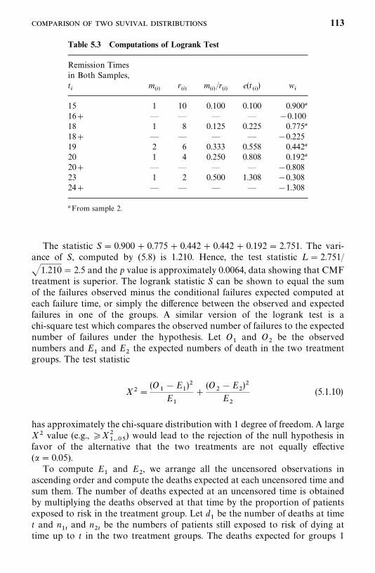
Table 5.3 Computations of Logrank Test
Remission Timesin Both Samples,t�
m��
r��
m�� /r
�� e(t
�� ) w
�
15 1 10 0.100 0.100 0.900�
16� — — — — �0.10018 1 8 0.125 0.225 0.775�
18� — — — — �0.22519 2 6 0.333 0.558 0.442�
20 1 4 0.250 0.808 0.192�
20� — — — — �0.80823 1 2 0.500 1.308 �0.30824� — — — — �1.308
� From sample 2.
The statistic S� 0.900 � 0.775 � 0.442 � 0.442 � 0.192 � 2.751. The vari-ance of S, computed by (5.8) is 1.210. Hence, the test statistic L � 2.751/
�1.210 � 2.5 and the p value is approximately 0.0064, data showing that CMFtreatment is superior. The logrank statistic S can be shown to equal the sumof the failures observed minus the conditional failures expected computed ateach failure time, or simply the difference between the observed and expectedfailures in one of the groups. A similar version of the logrank test is achi-square test which compares the observed number of failures to the expectednumber of failures under the hypothesis. Let O
�and O
�be the observed
numbers and E�
and E�
the expected numbers of death in the two treatmentgroups. The test statistic
X��(O
��E
�)�
E�
�(O
��E
�)�
E�
(5.1.10)
has approximately the chi-square distribution with 1 degree of freedom. A largeX� value (e.g., �X�
����) would lead to the rejection of the null hypothesis in
favor of the alternative that the two treatments are not equally effective(�� 0.05).
To compute E�
and E�
, we arrange all the uncensored observations inascending order and compute the deaths expected at each uncensored time andsum them. The number of deaths expected at an uncensored time is obtainedby multiplying the deaths observed at that time by the proportion of patientsexposed to risk in the treatment group. Let d
�be the number of deaths at time
t and n��
and n��
be the numbers of patients still exposed to risk of dying attime up to t in the two treatment groups. The deaths expected for groups 1
113
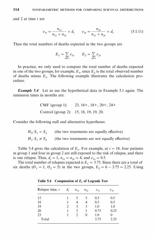
Table 5.4 Computation of E1 of Logrank Test
Relapse time, t d�
n��
n��
e��
e��
15 1 5 5 0.5 0.518 1 4 4 0.5 0.519 2 3 3 1.0 1.020 1 3 1 0.75 0.2523 1 2 0 1.0 0
Total 3.75 2.25
and 2 at time t are
e��
�n��
n��
� n��
� d�
e��
�n��
n��
� n��
� d�
(5.1.11)
Then the total numbers of deaths expected in the two groups are
E�� �
��� �
e��
E�� �
��� �
e��
In practice, we only need to compute the total number of deaths expectedin one of the two groups, for example, E
�, since E
�is the total observed number
of deaths minus E�
. The following example illustrates the calculation pro-cedure.
Example 5.4 Let us use the hypothetical data in Example 5.1 again. Theremission times in months are:
CMF (group 1): 23, 16�, 18�, 20�, 24�
Control (group 2): 15, 18, 19, 19, 20.
Consider the following null and alternative hypotheses:
H�
:S�� S
�(the two treatments are equally effective)
H�
:S�� S
�(the two treatments are not equally effective)
Table 5.4 gives the calculation of E�. For example, at t� 18, four patients
in group 1 and four in group 2 are still exposed to the risk of relapse, and thereis one relapse. Thus, d
�� 1, n
��� n
��� 4, and e
��� 0.5.
The total number of relapses expected is E�� 3.75. Since there are a total of
six deaths (O�� 1, O
�� 5) in the two groups, E
�� 6 � 3.75 � 2.25. Using
114
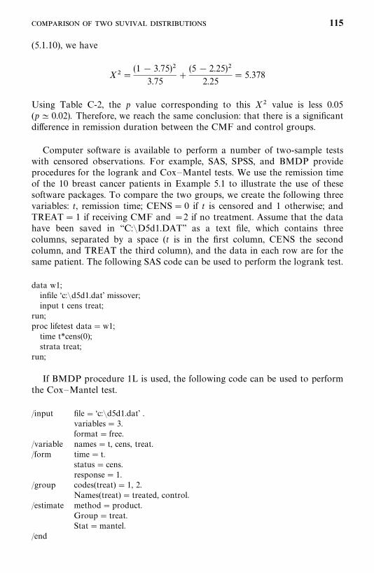
(5.1.10), we have
X��(1 � 3.75)�
3.75�
(5 � 2.25)�
2.25� 5.378
Using Table C-2, the p value corresponding to this X� value is less 0.05(p� 0.02). Therefore, we reach the same conclusion: that there is a significantdifference in remission duration between the CMF and control groups.
Computer software is available to perform a number of two-sample testswith censored observations. For example, SAS, SPSS, and BMDP provideprocedures for the logrank and Cox—Mantel tests. We use the remission timeof the 10 breast cancer patients in Example 5.1 to illustrate the use of thesesoftware packages. To compare the two groups, we create the following threevariables: t, remission time; CENS � 0 if t is censored and 1 otherwise; andTREAT � 1 if receiving CMF and �2 if no treatment. Assume that the datahave been saved in ‘‘C:�D5d1.DAT’’ as a text file, which contains threecolumns, separated by a space (t is in the first column, CENS the secondcolumn, and TREAT the third column), and the data in each row are for thesame patient. The following SAS code can be used to perform the logrank test.
data w1;infile ‘c:�d5d1.dat’ missover;input t cens treat;
run;proc lifetest data � w1;
time t*cens(0);strata treat;
run;
If BMDP procedure 1L is used, the following code can be used to performthe Cox—Mantel test.
/input file � ‘c:�d5d1.dat’ .variables � 3.format � free.
/variable names � t, cens, treat./form time � t.
status � cens.response � 1.
/group codes(treat) � 1, 2.Names(treat)� treated, control.
/estimate method � product.Group � treat.Stat � mantel.
/end
115
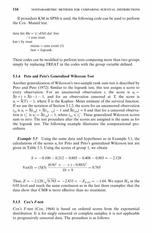
If procedure KM in SPSS is used, the following code can be used to performthe Cox—Mantel test.
data list file � ‘c:�d5d1.dat’ free/ t cens treat.
km t by treat/status � cens event (1)/test � logrank.
These codes can be modified to perform tests comparing more than two groupssimply by replacing TREAT in the codes with the group variable defined.
5.1.4 Peto and Peto’s Generalized Wilcoxon Test
Another generalization of Wilcoxon’s two-sample rank sum test is described byPeto and Peto (1972). Similar to the logrank test, this test assigns a score toevery observation. For an uncensored observation t, the score is u
��
S (t�) �S (t�) � 1, and for an observation censored at T, the score isu�� S (T ) � 1, where S is the Kaplan—Meier estimate of the survival function.
If we use the notation of Section 5.1.2, the score for an uncensored observationt��
is u��S (t
�� ) � S (t
���� ) � 1 and S (t
�� ) � 0 and that for a censored observa-
tion is t��
is u�� S (t
�� ) � 1, where t
�� � t�
�. These generalized Wilcoxon scores
sum to zero. The test procedure after the scores are assigned is the same as forthe logrank test. The following example illustrates the computational pro-cedures.
Example 5.5 Using the same data and hypotheses as in Example 5.1, thecalculations of the scores u
�for Peto and Peto’s generalized Wilcoxon test are
given in Table 5.5. Using the scores of group 1, we obtain
S� �0.100 � 0.212 � 0.605 � 0.408 � 0.803 ��2.128
Var(S) � (5)(5)(0.9)� � �� (�0.803)�
10 � 9� 0.765
Thus, Z��2.128/�0.765� �2.433 ��Z���
��1.64. We reject H�
at the0.05 level and reach the same conclusion as in the last three examples: that thedata show that CMB is more effective than no treatment.
5.1.5 Cox’s F-test
Cox’s F-test (Cox, 1964) is based on ordered scores from the exponentialdistribution. It is for singly censored or complete samples; it is not applicableto progressively censored data. The procedure is as follows:
116
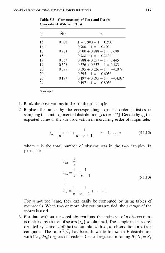
Table 5.5 Computations of Peto and Peto’sGeneralized Wilcoxon Test
t��
S (t) u�
15 0.900 1 � 0.900 � 1 � 0.90016� — 0.900 � 1 ��0.100�
18 0.788 0.900 � 0.788 � 1 � 0.68818� — 0.788 � 1 ��0.212�
19 0.657 0.788 � 0.657 � 1 � 0.44519 0.526 0.526 � 0.657 � 1 � 0.18320 0.395 0.395 � 0.526 � 1 ��0.07920� — 0.395 � 1 ��0.605�
23 0.197 0.197 � 0.395 � 1 ��04.08�
24� — 0.197 � 1 ��0.803�
� Group 1.
1. Rank the observations in the combined sample.
2. Replace the ranks by the corresponding expected order statistics insampling the unit exponential distribution [ f (t) � e��]. Denote by t
��the
expected value of the rth observation in increasing order of magnitude,
t��
�1
n���
1
n� r� 1r� 1, . . . , n (5.1.12)
where n is the total number of observations in the two samples. Inparticular,
t��
�1
n
t��
�1
n�
1
n� 1
t��
�1
n�
1
n� 1� �� 1
(5.1.13)
For n not too large, they can easily be computed by using tables ofreciprocals. When two or more observations are tied, the average of thescores is used.
3. For data without censored observations, the entire set of n observationsis replaced by the set of scores �t
��� so obtained. The sample mean scores
denoted by t �
and t �
of the two samples with n�, n
�observations are then
computed. The ratio t �/t �
has been shown to follow an F distributionwith (2n
�, 2n
�) degrees of freedom. Critical regions for testing H
�: S
��S
�
117
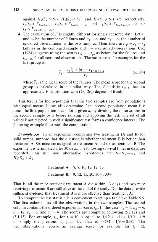
against H�
(S��S
�), H
�(S
�� S
�), and H
�(S
��S
�) are, respectively,
t �/ t
��F
���������, t
�/ t
��F
���������� , and t �/t ��F
����������or t
�/
t ��F
������������ .
4. The calculation of F is slightly different for singly censored data. Let r�
and r�
be the number of failures and n�� r
�and n
�� r
�the number of
censored observations in the two samples. Then there are p� r�� r
�failures in the combined sample and n� p censored observations. Cox(1964) suggests using the scores t
��, . . . , t
�as before for the failures and
t��� �
for all censored observations. The mean score, for example, for thefirst group is
t ��
r�t ��� (n
�� r
�)t��� �
r�
(5.1.14)
where t ��
is the mean score of the failures. The mean score for the secondgroup is calculated in a similar way. The F-statistic t
�/t
�, has an
approximate F-distribution with (2r�
, 2r�) degrees of freedom.
This test is for the hypothesis that the two samples are from populationswith equal means. It can also determine if the second population mean is ktimes the first population mean, for a given k, by dividing the observations inthe second sample by k before ranking and applying the test. The set of allvalues k not rejected in such a significance test forms a confidence interval. Thefollowing example illustrates the computation.
Example 5.6 In an experiment comparing two treatments (A and B) forsolid tumor, suppose that the question is whether treatment B is better thantreatment A. Six mice are assigned to treatment A and six to treatment B. Theexperiment is terminated after 30 days. The following survival times in days arerecorded. Our null and alternative hypotheses are H
�:S
�S
�and
H�
: S
�S�
.
Treatment A: 8, 8, 10, 12, 12, 13
Treatment B: 9, 12, 15, 20, 30�, 30�
That is, all the mice receiving treatment A die within 13 days and two micereceiving treatment B are still alive at the end of the study. Do the data providesufficient evidence that treatment B is more effective than treatment A?
To compute the test statistic, it is convenient to set up a table like Table 5.6.The first column lists all the observations in the two samples. The secondcolumn contains the ordered exponential scores t
��. In this case, n
�� 6, n
�� 6,
n� 12, r�� 6, and r
�� 4. The scores are computed following (5.1.12) and
(5.1.13). For example, t��
for t�� 10 is equal to 1/12 � 1/11 � 1/10 � 1/9
or simply the previous t��
plus 1/9, that is, 0.274 � 1/9 � 0.385. Thetied observations receive an average score: for example, for t
�� 12,
118
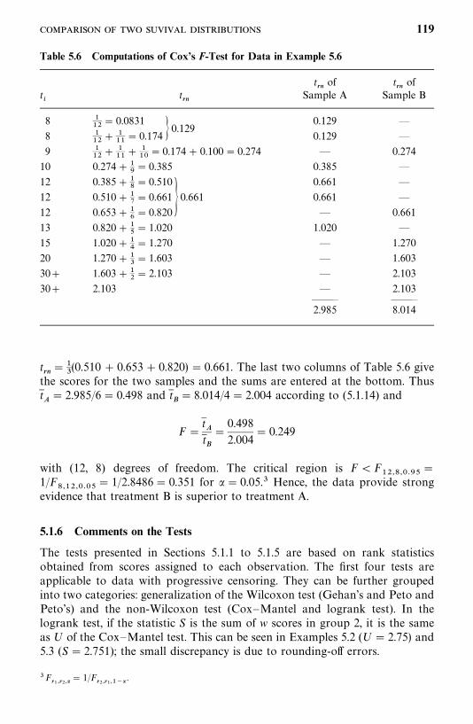
Table 5.6 Computations of Cox’s F-Test for Data in Example 5.6
t��
of t��
oft�
t��
Sample A Sample B
8 ���
� 0.0831 0.129 —
8 ���
� ���
� 0.174 � 0.1290.129 —
9 ���
� ���
� ���
� 0.174 � 0.100 � 0.274 — 0.274
10 0.274 ���� 0.385 0.385 —
12 0.385 ���� 0.510 0.661 —
12 0.510 ���� 0.661 � 0.661 0.661 —
12 0.653 ���� 0.820 — 0.661
13 0.820 ���� 1.020 1.020 —
15 1.020 ���� 1.270 — 1.270
20 1.270 ���� 1.603 — 1.603
30� 1.603 ���� 2.103 — 2.103
30� 2.103 — 2.103——— ———2.985 8.014
t��
���
(0.510 � 0.653 � 0.820) � 0.661. The last two columns of Table 5.6 givethe scores for the two samples and the sums are entered at the bottom. Thust
� 2.985/6 � 0.498 and t �� 8.014/4 � 2.004 according to (5.1.14) and
F�t t �
�0.498
2.004� 0.249
with (12, 8) degrees of freedom. The critical region is F�F��������
�
1/F��������
� 1/2.8486 � 0.351 for �� 0.05.� Hence, the data provide strongevidence that treatment B is superior to treatment A.
5.1.6 Comments on the Tests
The tests presented in Sections 5.1.1 to 5.1.5 are based on rank statisticsobtained from scores assigned to each observation. The first four tests areapplicable to data with progressive censoring. They can be further groupedinto two categories: generalization of the Wilcoxon test (Gehan’s and Peto andPeto’s) and the non-Wilcoxon test (Cox—Mantel and logrank test). In thelogrank test, if the statistic S is the sum of w scores in group 2, it is the sameas U of the Cox—Mantel test. This can be seen in Examples 5.2 (U� 2.75) and5.3 (S� 2.751); the small discrepancy is due to rounding-off errors.
�F�������
� 1/F��������� .
119
The only reason to choose one test over another in a given circumstance isif it will be more powerful, that is, more likely to reject a false hypothesis. Whensample sizes are small (n, n
�� 50), Gehan and Thomas (1969) show that Cox’s
F-test is more powerful than Gehan’s generalized Wilcoxon test if samples arefrom exponential or Weibull distributions and if there are no censoredobservations or the observations are singly censored. Comparisons of Gehan’sWilcoxon test to several other tests are reported by Lee et al. (1975). Theyshow that when samples are from exponential distributions, with or withoutcensoring, the Cox—Mantel and logrank tests are more powerful and moreefficient than the generalized Wilcoxon tests of Gehan and Peto and Peto.There is little difference between the Cox—Mantel and logrank tests andbetween the two generalized Wilcoxon tests. When the samples are taken fromWeibull distributions with a constant hazard ratio (i.e., the ratio of the twohazard functions does not vary with time), the results are essentially the sameas in the exponential case. However, when the hazard ratio is nonconstant,the two generalizations of the Wilcoxon test have more power than the othertests. Thus, the logrank test is more powerful than the Wilcoxon tests indetecting departures when the two hazard functions are parallel (proportionalhazards) or when there is random but equal censoring and when there is nocensoring in the samples (Crowley and Thomas, 1975). The generalizedWilcoxon tests appear to be more powerful than the logrank test for detectingmany other types of differences, for example, when the hazard functions are notparallel and when there is no censoring and the logarithm of the survival timesfollow the normal distribution with equal variance but possibly differentmeans.
The generalized Wilcoxon tests give more weight to early failures than laterfailures, whereas the logrank test gives equal weight to all failures. Therefore,the generalized Wilcoxon tests are more likely to detect early differences in thetwo survival distributions, whereas the logrank test is more sensitive todifferences in the right tails. Prentice and Marek (1979) show that Gehan’sWilcoxon statistic is subject to a serious criticism when censoring rates arehigh. If heavy censoring exists, the test statistic is dominated by a small numberof early failures and has very low power.
There are situations in which neither the logrank nor Wilcoxon test is veryeffective. When the two distributions differ but their hazard functions orsurvivorship functions cross, neither the Wilcoxon nor logrank test is verypowerful, and it will be sensible to consider other tests. For example, Taroneand Ware (1977) discuss general statistics of similar form (using scores) andFleming and Harrington (1979) and Fleming et al. (1980) present a two-sampletest based on the maximum of a Smirnov-type statistic designed to measure themaximum distance between estimates of two distributions. The latter approachis shown to be more effective than the logrank or Wilcoxon tests when twosurvival distributions differ substantially for some range of t values, but notnecessarily elsewhere. These statistics have not been widely applied. Interestedreaders are referred to the original papers.
120
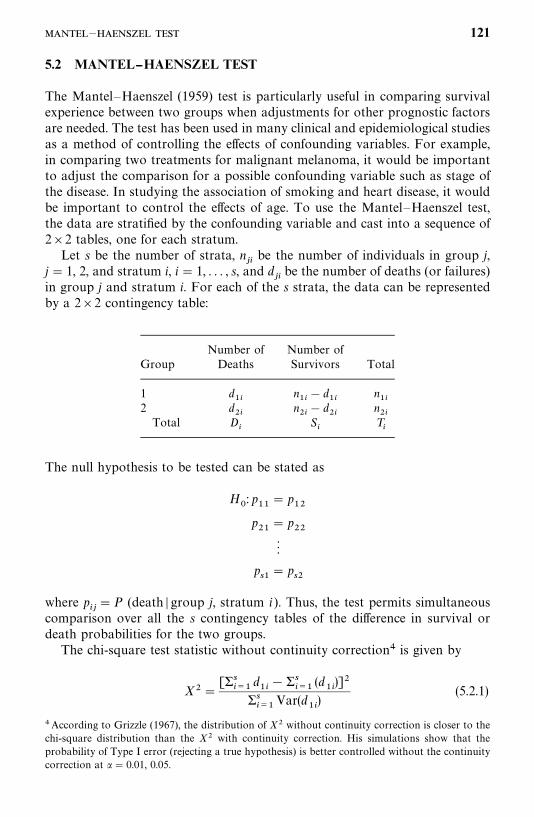
5.2 MANTEL--HAENSZEL TEST
The Mantel—Haenszel (1959) test is particularly useful in comparing survivalexperience between two groups when adjustments for other prognostic factorsare needed. The test has been used in many clinical and epidemiological studiesas a method of controlling the effects of confounding variables. For example,in comparing two treatments for malignant melanoma, it would be importantto adjust the comparison for a possible confounding variable such as stage ofthe disease. In studying the association of smoking and heart disease, it wouldbe important to control the effects of age. To use the Mantel—Haenszel test,the data are stratified by the confounding variable and cast into a sequence of2�2 tables, one for each stratum.
Let s be the number of strata, n��
be the number of individuals in group j,j� 1, 2, and stratum i, i� 1, . . . , s, and d
��be the number of deaths (or failures)
in group j and stratum i. For each of the s strata, the data can be representedby a 2�2 contingency table:
Number of Number ofGroup Deaths Survivors Total
1 d��
n��
� d��
n��
2 d��
n��
� d��
n��
Total D�
S�
T�
The null hypothesis to be tested can be stated as
H�
: p��
� p��
p��
� p��
p��
� p��
where p���P (death � group j, stratum i ). Thus, the test permits simultaneous
comparison over all the s contingency tables of the difference in survival ordeath probabilities for the two groups.
The chi-square test statistic without continuity correction� is given by
X��[��
���d��
������
(d��
)]�
�����
Var(d��
)(5.2.1)
� According to Grizzle (1967), the distribution of X� without continuity correction is closer to thechi-square distribution than the X� with continuity correction. His simulations show that theprobability of Type I error (rejecting a true hypothesis) is better controlled without the continuitycorrection at �� 0.01, 0.05.
— 121
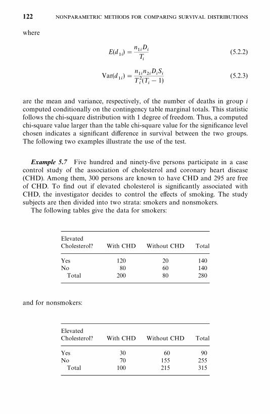
where
E(d��
) �n��D
�T�
(5.2.2)
Var(d��
) �n��n��D
�S�
T ��(T
�� 1)
(5.2.3)
are the mean and variance, respectively, of the number of deaths in group icomputed conditionally on the contingency table marginal totals. This statisticfollows the chi-square distribution with 1 degree of freedom. Thus, a computedchi-square value larger than the table chi-square value for the significance levelchosen indicates a significant difference in survival between the two groups.The following two examples illustrate the use of the test.
Example 5.7 Five hundred and ninety-five persons participate in a casecontrol study of the association of cholesterol and coronary heart disease(CHD). Among them, 300 persons are known to have CHD and 295 are freeof CHD. To find out if elevated cholesterol is significantly associated withCHD, the investigator decides to control the effects of smoking. The studysubjects are then divided into two strata: smokers and nonsmokers.
The following tables give the data for smokers:
ElevatedCholesterol? With CHD Without CHD Total
Yes 120 20 140No 80 60 140
Total 200 80 280
and for nonsmokers:
ElevatedCholesterol? With CHD Without CHD Total
Yes 30 60 90No 70 155 255
Total 100 215 315
122
Using (5.2.2) and (5.2.3), we obtain
E(d��
) �140 � 200
280� 100 E(d
��) �
90 � 100
315� 28.571
Var(d��
) �140 � 140 � 200 � 80
(280)�(280 � 1)� 14.337
Var(d��
) �90 � 225 � 100 � 215
(315)�(315 � 1)� 13.974
Using (5.2.1) and d��
� 120, d��
� 30, we have
X� �(150 � 128.571)�
14.337 � 13.974� 16.220
which is significant at the 0.001 level. Thus, elevated cholesterol is significantlyassociated with CHD after adjusting for the effects of smoking.
Example 5.8 Table 5.7 gives survival data in life-table format of male caseswith localized cancer of the rectum in Connecticut for 1935—1944 and1945—1954. We use Mantel and Haenszel’s chi-square test to see if the survivaldistribution of patients diagnosed in 1935—1944 is the same as for patientsdiagnosed in 1945—1954. The null hypothesis is that the two survival distribu-tions are the same. It is not necessary to set up 10 contingency tables for the10 intervals. The chi-square value is easily calculated by constructing columns7 to 12 directly from the life table. Using the sums in columns 1, 10, and 12,we obtain
X��(330.0 � 246.50)�
132.491� 52.624
which is significant at the 0.001 level. Thus, the data show a significantdifference between the survival distributions of patients diagnosed in 1935—1944 and 1945—1954.
It should be noted that this chi-square test statistic, when applied to lifetables, gives more weight to those deaths that occur in an early time intervalrather than later. That is, if the two groups are subject to the same probabilityof surviving through the entire study period, (5.2.1)—(5.2.3) will give highmortality for the group in which early deaths occur. Mantel (1966) gives thefollowing illustration.
Consider two groups of 100 persons each. Both have 50 deaths. In group 1all deaths occur in the first interval, and in group 2 all deaths occur in the
— 123
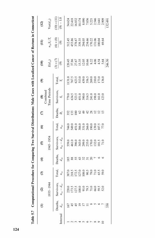
Tab
le5.
7C
ompu
tati
onal
Pro
cedu
refo
rC
ompa
ring
Tw
oSu
rviv
alD
istr
ibut
ions
:Mal
eC
ases
wit
hL
ocal
ized
Can
cer
ofR
ectu
min
Con
nect
icut
(1)
(2)
(3)
(4)
(5)
(6)
(7)
(8)
(9)
(10)
(11)
(12)
Com
bin
ed19
35—
1944
1945
—19
54T
ime
Per
iods
E(d
��)
n ��S�/T�
Var
(d��
)
Dea
ths,
Surv
ivor
s,T
otal
,D
eath
s,Su
rviv
ors,
Tot
al,
Dea
ths,
Surv
ivor
s,T
otal
,In
tern
ald ��
n ���
d ��n ��
d ��n ��
�d ��
n ��D
�S�
T�
(3)�
(7)
(9)
(6)�
(8)
(9)
(10)
�(1
1)
(9)�
1.0
116
722
0.0
387.
018
555
9.0
744.
035
277
9.0
1131.0
120.
4551
2.45
54.6
242
4517
3.5
218.
588
461.
054
9.0
133
634.
576
7.5
37.8
645
3.86
22.4
183
4512
7.5
172.
555
396.
045
1.0
100
523.
562
3.5
27.6
737
8.67
16.8
324
1910
8.0
127.
043
343.
038
6.0
6245
1.0
513.
015.3
533
9.35
10.1
745
1791.0
108.
032
299.
033
1.0
4939
0.0
439.
012.0
529
4.05
8.09
06
1179.5
90.5
3123
5.0
266.
042
314.
535
6.5
10.6
623
4.66
7.03
67
871.0
79.0
2017
0.0
190.
028
241.
026
9.0
8.22
170.
225.
221
85
66.0
71.0
713
2.0
139.
012
198.
021
0.0
4.06
131.
062.
546
96
59.5
65.5
610
1.5
107.
512
161.
017
3.0
4.54
100.
042.
641
107
52.0
59.0
671.0
77.0
1312
3.0
136.
05.
6469.6
42.
909
——
——
——
———
330
246.
5013
2.49
1
124
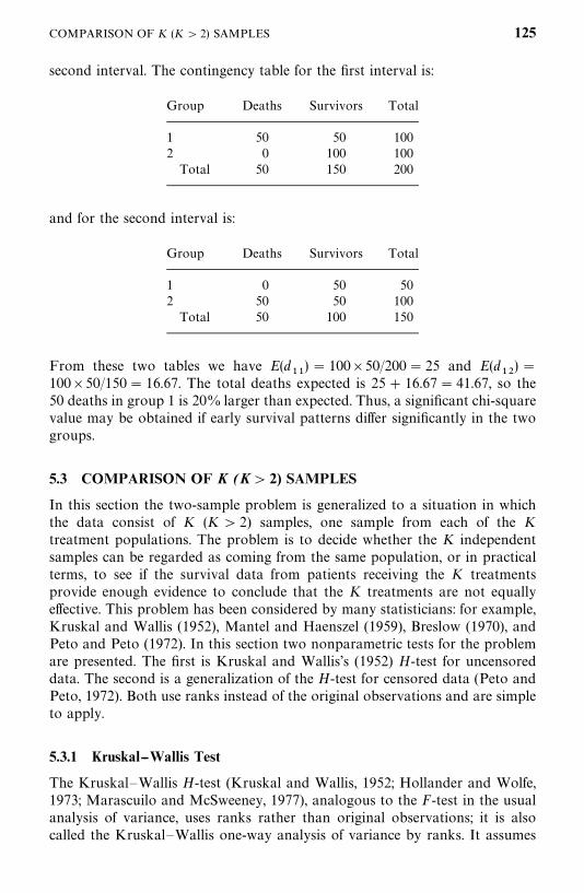
second interval. The contingency table for the first interval is:
Group Deaths Survivors Total
1 50 50 1002 0 100 100
Total 50 150 200
and for the second interval is:
Group Deaths Survivors Total
1 0 50 502 50 50 100
Total 50 100 150
From these two tables we have E(d��
) � 100�50/200 � 25 and E(d��
) �
100�50/150 � 16.67. The total deaths expected is 25 � 16.67 � 41.67, so the50 deaths in group 1 is 20% larger than expected. Thus, a significant chi-squarevalue may be obtained if early survival patterns differ significantly in the twogroups.
5.3 COMPARISON OF K (K � 2) SAMPLES
In this section the two-sample problem is generalized to a situation in whichthe data consist of K (K � 2) samples, one sample from each of the Ktreatment populations. The problem is to decide whether the K independentsamples can be regarded as coming from the same population, or in practicalterms, to see if the survival data from patients receiving the K treatmentsprovide enough evidence to conclude that the K treatments are not equallyeffective. This problem has been considered by many statisticians: for example,Kruskal and Wallis (1952), Mantel and Haenszel (1959), Breslow (1970), andPeto and Peto (1972). In this section two nonparametric tests for the problemare presented. The first is Kruskal and Wallis’s (1952) H-test for uncensoreddata. The second is a generalization of the H-test for censored data (Peto andPeto, 1972). Both use ranks instead of the original observations and are simpleto apply.
5.3.1 Kruskal--Wallis Test
The Kruskal—Wallis H-test (Kruskal and Wallis, 1952; Hollander and Wolfe,1973; Marascuilo and McSweeney, 1977), analogous to the F-test in the usualanalysis of variance, uses ranks rather than original observations; it is alsocalled the Kruskal—Wallis one-way analysis of variance by ranks. It assumes
COMPARISON OF K (K � 2) SAMPLES 125
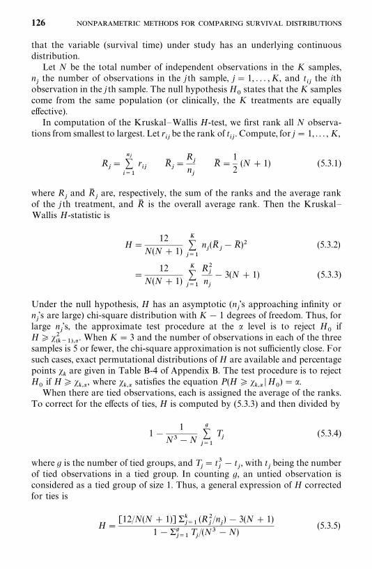
that the variable (survival time) under study has an underlying continuousdistribution.
Let N be the total number of independent observations in the K samples,n�
the number of observations in the jth sample, j� 1, . . . , K, and t��
the ithobservation in the j th sample. The null hypothesis H
�states that the K samples
come from the same population (or clinically, the K treatments are equallyeffective).
In computation of the Kruskal—Wallis H-test, we first rank all N observa-tions from smallest to largest. Let r
��be the rank of t
��. Compute, for j� 1, . . . , K,
R��
������
r��
R ��
R�
n�
R �1
2(N � 1) (5.3.1)
where R�
and R �
are, respectively, the sum of the ranks and the average rankof the j th treatment, and R is the overall average rank. Then the Kruskal—Wallis H-statistic is
H�12
N(N � 1)
����
n�(R
��R )� (5.3.2)
�12
N(N � 1)
����
R��
n�
� 3(N � 1) (5.3.3)
Under the null hypothesis, H has an asymptotic (n�’s approaching infinity or
n�’s are large) chi-square distribution with K� 1 degrees of freedom. Thus, for
large n�’s, the approximate test procedure at the � level is to reject H
�if
H������� �� . When K� 3 and the number of observations in each of the three
samples is 5 or fewer, the chi-square approximation is not sufficiently close. Forsuch cases, exact permutational distributions of H are available and percentagepoints �
�are given in Table B-4 of Appendix B. The test procedure is to reject
H�
if H� ���� , where �
��� satisfies the equation P(H ����� �H�
) � �.When there are tied observations, each is assigned the average of the ranks.
To correct for the effects of ties, H is computed by (5.3.3) and then divided by
1 �1
N��N
�����
T�
(5.3.4)
where g is the number of tied groups, and T�� t�
�� t
�, with t
�being the number
of tied observations in a tied group. In counting g, an untied observation isconsidered as a tied group of size 1. Thus, a general expression of H correctedfor ties is
H�[12/N(N� 1)] ��
���(R�
�/n
�) � 3(N � 1)
1 ������
T�/(N� �N)
(5.3.5)
126
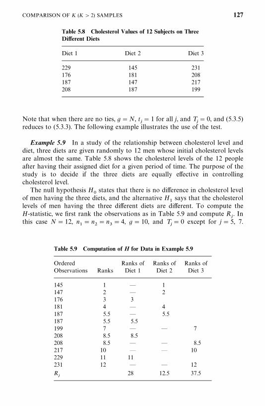
Table 5.8 Cholesterol Values of 12 Subjects on ThreeDifferent Diets
Diet 1 Diet 2 Diet 3
229 145 231176 181 208187 147 217208 187 199
Table 5.9 Computation of H for Data in Example 5.9
Ordered Ranks of Ranks of Ranks ofObservations Ranks Diet 1 Diet 2 Diet 3
145 1 — 1147 2 — 2176 3 3181 4 — 4187 5.5 — 5.5187 5.5 5.5199 7 — — 7208 8.5 8.5208 8.5 — — 8.5217 10 — — 10229 11 11231 12 — — 12
R�
28 12.5 37.5
Note that when there are no ties, g�N, t�� 1 for all j, and T
�� 0, and (5.3.5)
reduces to (5.3.3). The following example illustrates the use of the test.
Example 5.9 In a study of the relationship between cholesterol level anddiet, three diets are given randomly to 12 men whose initial cholesterol levelsare almost the same. Table 5.8 shows the cholesterol levels of the 12 peopleafter having their assigned diet for a given period of time. The purpose of thestudy is to decide if the three diets are equally effective in controllingcholesterol level.
The null hypothesis H�
states that there is no difference in cholesterol levelof men having the three diets, and the alternative H
�says that the cholesterol
levels of men having the three different diets are different. To compute theH-statistic, we first rank the observations as in Table 5.9 and compute R
�. In
this case N� 12, n�� n
�� n
�� 4, g� 10, and T
�� 0 except for j� 5, 7.
COMPARISON OF K (K � 2) SAMPLES 127
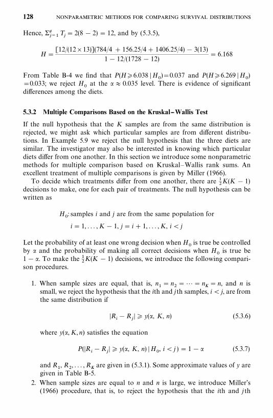
Hence, �����
T�� 2(8 � 2) � 12, and by (5.3.5),
H�[12/(12�13)](784/4 � 156.25/4 � 1406.25/4) � 3(13)
1 � 12/(1728 � 12)� 6.168
From Table B-4 we find that P(H�6.038 �H�
)�0.037 and P(H�6.269 �H�)
�0.033; we reject H�
at the �� 0.035 level. There is evidence of significantdifferences among the diets.
5.3.2 Multiple Comparisons Based on the Kruskal--Wallis Test
If the null hypothesis that the K samples are from the same distribution isrejected, we might ask which particular samples are from different distribu-tions. In Example 5.9 we reject the null hypothesis that the three diets aresimilar. The investigator may also be interested in knowing which particulardiets differ from one another. In this section we introduce some nonparametricmethods for multiple comparison based on Kruskal—Wallis rank sums. Anexcellent treatment of multiple comparisons is given by Miller (1966).
To decide which treatments differ from one another, there are ��K(K � 1)
decisions to make, one for each pair of treatments. The null hypothesis can bewritten as
H�: samples i and j are from the same population for
i� 1, . . . , K� 1, j� i� 1, . . . , K, i� j
Let the probability of at least one wrong decision when H�
is true be controlledby � and the probability of making all correct decisions when H
�is true be
1 � �. To make the ��K(K � 1) decisions, we introduce the following compari-
son procedures.
1. When sample sizes are equal, that is, n�� n
���� n
� n, and n is
small, we reject the hypothesis that the ith and jth samples, i� j, are fromthe same distribution if
�R��R
��� y(�, K, n) (5.3.6)
where y(�, K, n) satisfies the equation
P(�R��R
�� � y(�, K, n) �H
�, i� j ) � 1 � � (5.3.7)
and R�, R
�, . . . , R
are given in (5.3.1). Some approximate values of y are
given in Table B-5.
2. When sample sizes are equal to n and n is large, we introduce Miller’s(1966) procedure, that is, to reject the hypothesis that the ith and j th
128
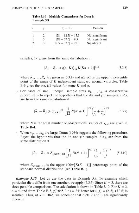
Table 5.10 Multiple Comparisons for Data inExample 5.9
i j �R��R
�� Decision
1 2 �28 � 12.5�� 15.5 Not significant1 3 �28 � 37.5�� 9.5 Not significant2 3 �12.5 � 37.5�� 25.0 Significant
samples, i� j, are from the same distribution if
�R ��R
�� � q(a, K)[ �
��K(Kn � 1)]�� (5.3.8)
where R �
, . . . , R
are given in (5.3.1) and q(�, K) is the upper � percentilepoint of the range of K independent standard normal variables. TableB-6 gives the q(�, K) values for some K and �.
3. For cases of small unequal sample sizes n�, . . . , n
, a conservative
procedure is to reject the hypothesis that the ith and jth samples, i� j,are from the same distribution if
�R ��R
�� � (x�� )�� �
1
12N(N � 1)�
��
�1
n�
�1
n����
(5.3.9)
where N is the total number of observations. Values of x��
are given inTable B-4.
4. When n�, . . . , n
are large, Dunn (1964) suggests the following procedure.
Reject the hypothesis that the ith and jth samples, i� j, are from thesame distribution if
�R ��R
���Z�� � �� � �
1
12N(N� 1)�
��
�1
n�
�1
n����
(5.3.10)
where Z�� � �� �is the upper 100�/[K(K � 1)] percentage point of the
standard normal distribution (see Table B-1).
Example 5.10 Let us use the data in Example 5.9. To examine whichparticular diets differ from one another, we apply (5.3.6). Since K� 3, there arethree possible comparisons. The calculation is shown in Table 5.10. For K� 3,n� 4, and from Table B-5, y(0.045, 3, 4) � 24; hence for (i, j ) � (2, 3), (5.3.6) issatisfied. Thus, at �� 0.045, we conclude that diets 2 and 3 are significantlydifferent.
COMPARISON OF K (K � 2) SAMPLES 129
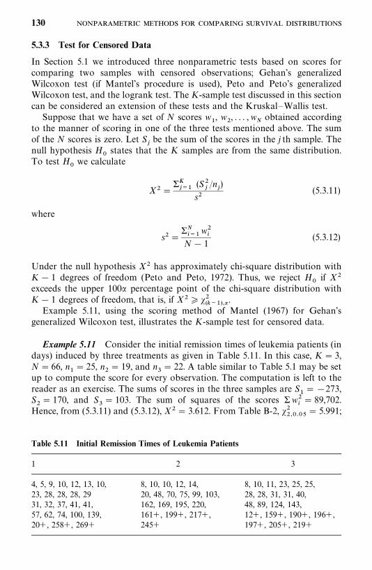
Table 5.11 Initial Remission Times of Leukemia Patients
1 2 3
4, 5, 9, 10, 12, 13, 10, 8, 10, 10, 12, 14, 8, 10, 11, 23, 25, 25,23, 28, 28, 28, 29 20, 48, 70, 75, 99, 103, 28, 28, 31, 31, 40,31, 32, 37, 41, 41, 162, 169, 195, 220, 48, 89, 124, 143,57, 62, 74, 100, 139, 161�, 199�, 217�, 12�, 159�, 190�, 196�,20�, 258�, 269� 245� 197�, 205�, 219�
5.3.3 Test for Censored Data
In Section 5.1 we introduced three nonparametric tests based on scores forcomparing two samples with censored observations; Gehan’s generalizedWilcoxon test (if Mantel’s procedure is used), Peto and Peto’s generalizedWilcoxon test, and the logrank test. The K-sample test discussed in this sectioncan be considered an extension of these tests and the Kruskal—Wallis test.
Suppose that we have a set of N scores w�, w
�, . . . , w
�obtained according
to the manner of scoring in one of the three tests mentioned above. The sumof the N scores is zero. Let S
�be the sum of the scores in the j th sample. The
null hypothesis H�
states that the K samples are from the same distribution.To test H
�we calculate
X��� ���
(S��/n
�)
s�(5.3.11)
where
s����
���w��
N� 1(5.3.12)
Under the null hypothesis X� has approximately chi-square distribution withK� 1 degrees of freedom (Peto and Peto, 1972). Thus, we reject H
�if X�
exceeds the upper 100� percentage point of the chi-square distribution withK� 1 degrees of freedom, that is, if X� ���
���� �� .Example 5.11, using the scoring method of Mantel (1967) for Gehan’s
generalized Wilcoxon test, illustrates the K-sample test for censored data.
Example 5.11 Consider the initial remission times of leukemia patients (indays) induced by three treatments as given in Table 5.11. In this case, K� 3,N� 66, n
�� 25, n
�� 19, and n
�� 22. A table similar to Table 5.1 may be set
up to compute the score for every observation. The computation is left to thereader as an exercise. The sums of scores in the three samples are S
���273,
S�� 170, and S
�� 103. The sum of squares of the scores �w�
�� 89,702.
Hence, from (5.3.11) and (5.3.12), X�� 3.612. From Table B-2, �������
� 5.991;
130
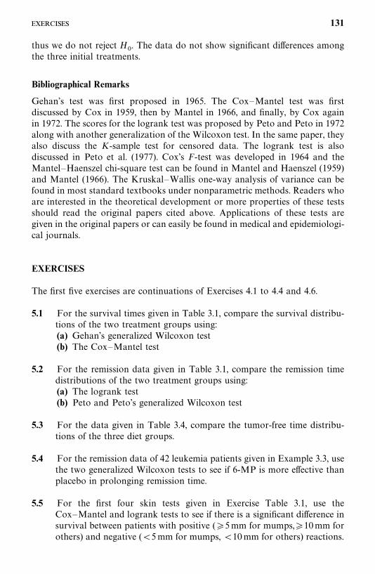
thus we do not reject H�. The data do not show significant differences among
the three initial treatments.
Bibliographical Remarks
Gehan’s test was first proposed in 1965. The Cox—Mantel test was firstdiscussed by Cox in 1959, then by Mantel in 1966, and finally, by Cox againin 1972. The scores for the logrank test was proposed by Peto and Peto in 1972along with another generalization of the Wilcoxon test. In the same paper, theyalso discuss the K-sample test for censored data. The logrank test is alsodiscussed in Peto et al. (1977). Cox’s F-test was developed in 1964 and theMantel—Haenszel chi-square test can be found in Mantel and Haenszel (1959)and Mantel (1966). The Kruskal—Wallis one-way analysis of variance can befound in most standard textbooks under nonparametric methods. Readers whoare interested in the theoretical development or more properties of these testsshould read the original papers cited above. Applications of these tests aregiven in the original papers or can easily be found in medical and epidemiologi-cal journals.
EXERCISES
The first five exercises are continuations of Exercises 4.1 to 4.4 and 4.6.
5.1 For the survival times given in Table 3.1, compare the survival distribu-tions of the two treatment groups using:(a) Gehan’s generalized Wilcoxon test(b) The Cox—Mantel test
5.2 For the remission data given in Table 3.1, compare the remission timedistributions of the two treatment groups using:(a) The logrank test(b) Peto and Peto’s generalized Wilcoxon test
5.3 For the data given in Table 3.4, compare the tumor-free time distribu-tions of the three diet groups.
5.4 For the remission data of 42 leukemia patients given in Example 3.3, usethe two generalized Wilcoxon tests to see if 6-MP is more effective thanplacebo in prolonging remission time.
5.5 For the first four skin tests given in Exercise Table 3.1, use theCox—Mantel and logrank tests to see if there is a significant difference insurvival between patients with positive (�5 mm for mumps,�10 mm forothers) and negative (�5 mm for mumps, �10 mm for others) reactions.
131
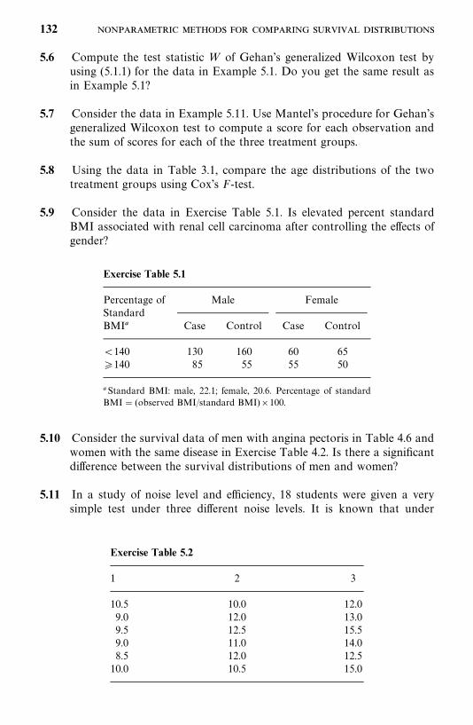
Exercise Table 5.1
Percentage of Male FemaleStandardBMI� Case Control Case Control
�140 130 160 60 65�140 85 55 55 50
� Standard BMI: male, 22.1; female, 20.6. Percentage of standardBMI � (observed BMI/standard BMI)�100.
Exercise Table 5.2
1 2 3
10.5 10.0 12.09.0 12.0 13.09.5 12.5 15.59.0 11.0 14.08.5 12.0 12.5
10.0 10.5 15.0
5.6 Compute the test statistic W of Gehan’s generalized Wilcoxon test byusing (5.1.1) for the data in Example 5.1. Do you get the same result asin Example 5.1?
5.7 Consider the data in Example 5.11. Use Mantel’s procedure for Gehan’sgeneralized Wilcoxon test to compute a score for each observation andthe sum of scores for each of the three treatment groups.
5.8 Using the data in Table 3.1, compare the age distributions of the twotreatment groups using Cox’s F-test.
5.9 Consider the data in Exercise Table 5.1. Is elevated percent standardBMI associated with renal cell carcinoma after controlling the effects ofgender?
5.10 Consider the survival data of men with angina pectoris in Table 4.6 andwomen with the same disease in Exercise Table 4.2. Is there a significantdifference between the survival distributions of men and women?
5.11 In a study of noise level and efficiency, 18 students were given a verysimple test under three different noise levels. It is known that under
132
Exercise Table 5.3
1 2 2 3
4 1 3 55 4 7 159 9 14 20
12 12 20 3120� 15 27 3925 23 30 4730� 30 32� 55�
50� 67�
normal conditions, they should be able to finish the test in 10 minutes.The students were randomly assigned to the three levels. Exercise Table5.2 gives the time required to finish the test. Are the three noise levelssignificantly different? If they are, determine which levels differ from oneanother.
5.12 Exercise Table 5.3 gives the survival time in weeks of 30 brain tumorpatients receiving four different treatments. Are the four treatmentsequally effective?
133
CHAPTER 6
Some Well-Known ParametricSurvival Distributionsand Their Applications
Usually, there are many physical causes that lead to the failure or death of aperson at a particular time. It is very difficult, if not impossible, to isolate thesephysical causes and account mathematically for all of them. Therefore, choos-ing a theoretical distribution to approximate survival data is as much an artas a scientific task. In this chapter, several theoretical distributions that havebeen used widely to describe survival time are discussed, their characteristicssummarized, and their applications illustrated.
6.1 EXPONENTIAL DISTRIBUTION
The simplest and most important distribution in survival studies is theexponential distribution. In the late 1940s, researchers began to choose theexponential distribution to describe the life pattern of electronic systems. Davis(1952) gives a number of examples, including bank statement and ledger error,payroll check errors, automatic calculating machine failure, and radar setcomponent failure, in which the failure data are well described by theexponential distribution. Epstein and Sobel (1953) report why they select theexponential distribution over the popular normal distribution and show howto estimate the parameter when data are singly censored. Epstein (1958) alsodiscusses in some detail the justification for the assumption of an exponentialdistribution. The exponential distribution has since continued to play a role inlifetime studies analogous to that of the normal distribution in other areas ofstatistics.The exponential distribution is often referred to as a purely random failure
pattern. It is famous for its unique ‘‘lack of memory,’’ which requires that theage of the animal or person does not affect future survival. Although many
134
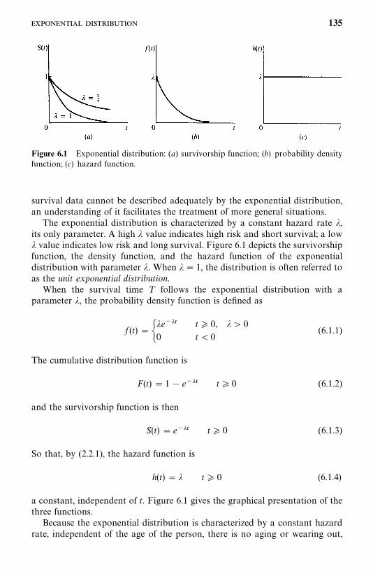
Figure 6.1 Exponential distribution: (a) survivorship function; (b) probability densityfunction; (c) hazard function.
survival data cannot be described adequately by the exponential distribution,an understanding of it facilitates the treatment of more general situations.The exponential distribution is characterized by a constant hazard rate �,
its only parameter. A high � value indicates high risk and short survival; a low� value indicates low risk and long survival. Figure 6.1 depicts the survivorshipfunction, the density function, and the hazard function of the exponentialdistribution with parameter �. When � � 1, the distribution is often referred toas the unit exponential distribution.When the survival time T follows the exponential distribution with a
parameter �, the probability density function is defined as
f (t)� ��e���0
t� 0, �� 0
t� 0(6.1.1)
The cumulative distribution function is
F(t)� 1� e��� t� 0 (6.1.2)
and the survivorship function is then
S(t) � e��� t� 0 (6.1.3)
So that, by (2.2.1), the hazard function is
h(t)� � t� 0 (6.1.4)
a constant, independent of t. Figure 6.1 gives the graphical presentation of thethree functions.Because the exponential distribution is characterized by a constant hazard
rate, independent of the age of the person, there is no aging or wearing out,
135
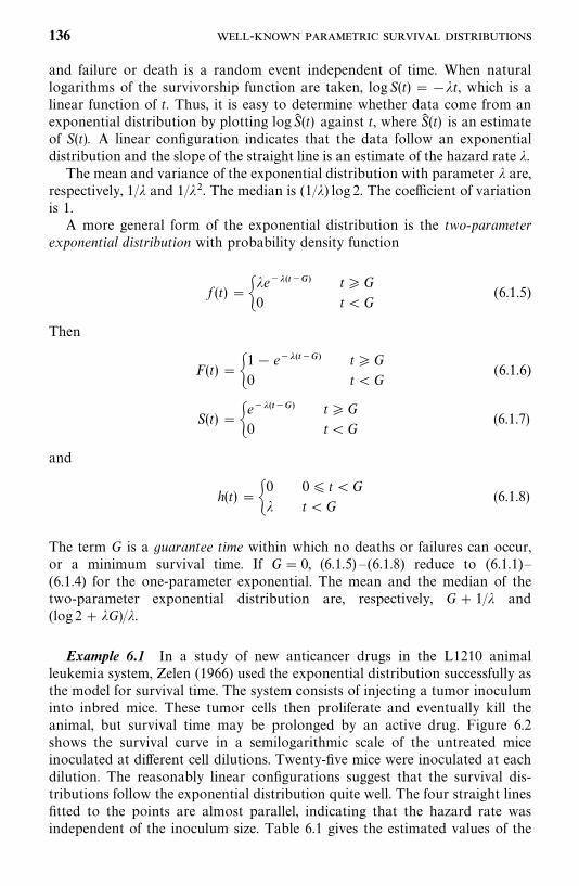
and failure or death is a random event independent of time. When naturallogarithms of the survivorship function are taken, log S(t)���t, which is alinear function of t. Thus, it is easy to determine whether data come from anexponential distribution by plotting log S� (t) against t, where S� (t) is an estimateof S(t). A linear configuration indicates that the data follow an exponentialdistribution and the slope of the straight line is an estimate of the hazard rate �.The mean and variance of the exponential distribution with parameter � are,
respectively, 1/� and 1/��. The median is (1/�) log 2. The coefficient of variationis 1.A more general form of the exponential distribution is the two-parameter
exponential distribution with probability density function
f (t)���e�������
0
t�G
t�G(6.1.5)
Then
F(t)� �1� e�������
0
t�G
t�G(6.1.6)
S(t)� �e�������
0
t�G
t�G(6.1.7)
and
h(t)��0
�0� t�G
t�G(6.1.8)
The term G is a guarantee time within which no deaths or failures can occur,or a minimum survival time. If G� 0, (6.1.5) —(6.1.8) reduce to (6.1.1)—(6.1.4) for the one-parameter exponential. The mean and the median of thetwo-parameter exponential distribution are, respectively, G� 1/� and(log 2� �G)/�.
Example 6.1 In a study of new anticancer drugs in the L1210 animalleukemia system, Zelen (1966) used the exponential distribution successfully asthe model for survival time. The system consists of injecting a tumor inoculuminto inbred mice. These tumor cells then proliferate and eventually kill theanimal, but survival time may be prolonged by an active drug. Figure 6.2shows the survival curve in a semilogarithmic scale of the untreated miceinoculated at different cell dilutions. Twenty-five mice were inoculated at eachdilution. The reasonably linear configurations suggest that the survival dis-tributions follow the exponential distribution quite well. The four straight linesfitted to the points are almost parallel, indicating that the hazard rate wasindependent of the inoculum size. Table 6.1 gives the estimated values of the
136 -
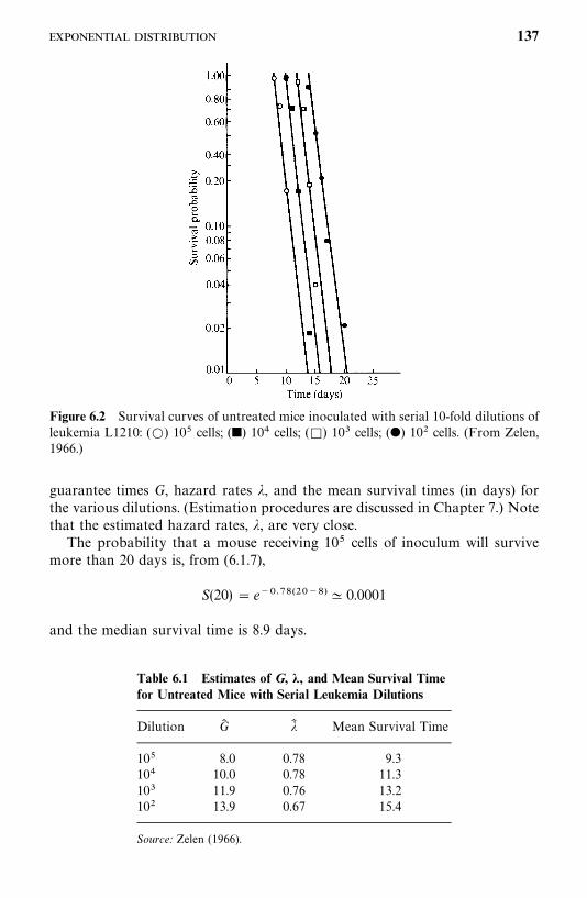
Figure 6.2 Survival curves of untreated mice inoculated with serial 10-fold dilutions ofleukemia L1210: (�) 10� cells; (�) 10 cells; (�) 10 cells; (�) 10� cells. (From Zelen,1966.)
Table 6.1 Estimates of G, �, and Mean Survival Timefor Untreated Mice with Serial Leukemia Dilutions
Dilution G� �� Mean Survival Time
10� 8.0 0.78 9.310 10.0 0.78 11.310 11.9 0.76 13.210� 13.9 0.67 15.4
Source: Zelen (1966).
guarantee times G, hazard rates �, and the mean survival times (in days) forthe various dilutions. (Estimation procedures are discussed in Chapter 7.) Notethat the estimated hazard rates, �, are very close.The probability that a mouse receiving 10� cells of inoculum will survive
more than 20 days is, from (6.1.7),
S(20) � e��� �������� 0.0001
and the median survival time is 8.9 days.
137
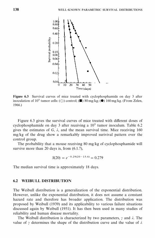
Figure 6.3 Survival curves of mice treated with cyclophosphamide on day 3 afterinoculation of 10� tumor cells: (�) control; (�) 80mg/kg; (�) 160mg/kg. (From Zelen,1966.)
Figure 6.3 gives the survival curves of mice treated with different doses ofcyclophosphamide on day 3 after receiving a 10� tumor inoculum. Table 6.2gives the estimates of G, �, and the mean survival time. Mice receiving 160mg/kg of the drug show a remarkably improved surivival pattern over thecontrol group.The probability that a mouse receiving 80 mg/kg of cyclophosphamide will
survive more than 20 days is, from (6.1.7),
S(20)� e��������������� 0.279
The median survival time is approximately 18 days.
6.2 WEIBULL DISTRIBUTION
The Weibull distribution is a generalization of the exponential distribution.However, unlike the exponential distribution, it does not assume a constanthazard rate and therefore has broader application. The distribution wasproposed by Weibull (1939) and its applicability to various failure situationsdiscussed again by Weibull (1951). It has then been used in many studies ofreliability and human disease mortality.The Weibull distribution is characterized by two parameters, � and �. The
value of � determines the shape of the distribution curve and the value of �
138 -
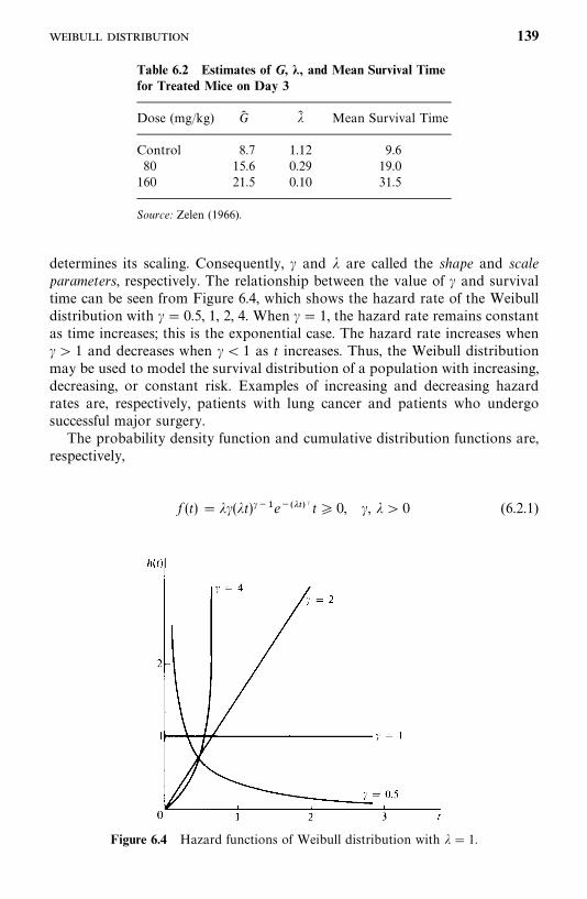
Table 6.2 Estimates of G, �, and Mean Survival Timefor Treated Mice on Day 3
Dose (mg/kg) G� �� Mean Survival Time
Control 8.7 1.12 9.680 15.6 0.29 19.0160 21.5 0.10 31.5
Source: Zelen (1966).
Figure 6.4 Hazard functions of Weibull distribution with �� 1.
determines its scaling. Consequently, � and � are called the shape and scaleparameters, respectively. The relationship between the value of � and survivaltime can be seen from Figure 6.4, which shows the hazard rate of the Weibulldistribution with �� 0.5, 1, 2, 4. When �� 1, the hazard rate remains constantas time increases; this is the exponential case. The hazard rate increases when�� 1 and decreases when �� 1 as t increases. Thus, the Weibull distributionmay be used to model the survival distribution of a population with increasing,decreasing, or constant risk. Examples of increasing and decreasing hazardrates are, respectively, patients with lung cancer and patients who undergosuccessful major surgery.The probability density function and cumulative distribution functions are,
respectively,
f (t) � ��(�t)���e����� � t� 0, �, �� 0 (6.2.1)
139
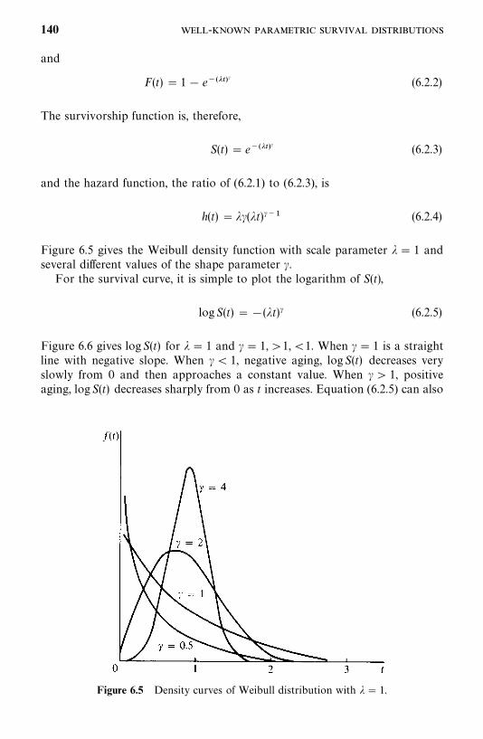
Figure 6.5 Density curves of Weibull distribution with �� 1.
and
F(t)� 1� e������ (6.2.2)
The survivorship function is, therefore,
S(t)� e������ (6.2.3)
and the hazard function, the ratio of (6.2.1) to (6.2.3), is
h(t) � ��(�t)��� (6.2.4)
Figure 6.5 gives the Weibull density function with scale parameter �� 1 andseveral different values of the shape parameter �.For the survival curve, it is simple to plot the logarithm of S(t),
logS(t) ��(�t)� (6.2.5)
Figure 6.6 gives log S(t) for �� 1 and �� 1,�1,�1. When �� 1 is a straightline with negative slope. When �� 1, negative aging, logS(t) decreases veryslowly from 0 and then approaches a constant value. When � � 1, positiveaging, logS(t) decreases sharply from 0 as t increases. Equation (6.2.5) can also
140 -
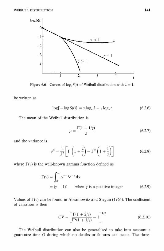
Figure 6.6 Curves of log�S(t) of Weibull distribution with �� 1.
be written as
log[�logS(t)]� � log��� � log
�t (6.2.6)
The mean of the Weibull distribution is
��(1� 1/�)
�(6.2.7)
and the variance is
��1
�� � �1�2
���� �1�1
��� (6.2.8)
where (�) is the well-known gamma function defined as
(�) ���
�
x���e��dx
� (� � 1)! when � is a positive integer (6.2.9)
Values of (�) can be found in Abramowitz and Stegun (1964). The coefficientof variation is then
CV� �(1� 2/�)�(1� 1/�)
� 1����
(6.2.10)
The Weibull distribution can also be generalized to take into account aguarantee time G during which no deaths or failures can occur. The three-
141
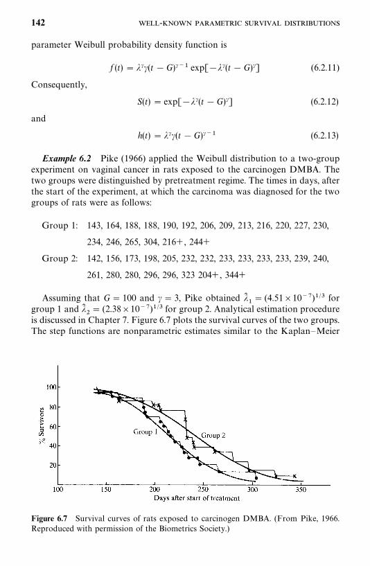
Figure 6.7 Survival curves of rats exposed to carcinogen DMBA. (From Pike, 1966.Reproduced with permission of the Biometrics Society.)
parameter Weibull probability density function is
f (t)� ���(t �G)��� exp[���(t �G)�] (6.2.11)
Consequently,
S(t)� exp[���(t �G)�] (6.2.12)
and
h(t)� ���(t �G)��� (6.2.13)
Example 6.2 Pike (1966) applied the Weibull distribution to a two-groupexperiment on vaginal cancer in rats exposed to the carcinogen DMBA. Thetwo groups were distinguished by pretreatment regime. The times in days, afterthe start of the experiment, at which the carcinoma was diagnosed for the twogroups of rats were as follows:
Group 1: 143, 164, 188, 188, 190, 192, 206, 209, 213, 216, 220, 227, 230,
234, 246, 265, 304, 216�, 244�
Group 2: 142, 156, 173, 198, 205, 232, 232, 233, 233, 233, 233, 239, 240,
261, 280, 280, 296, 296, 323 204�, 344�
Assuming that G� 100 and � � 3, Pike obtained ���� (4.51�10� )�� for
group 1 and ���� (2.38�10� )�� for group 2. Analytical estimation procedure
is discussed in Chapter 7. Figure 6.7 plots the survival curves of the two groups.The step functions are nonparametric estimates similar to the Kaplan—Meier
142 -
Table 6.3 Calculation of Survivorship Functions for Group 2 of Rats Exposed to DMBA
Kaplan— ModifiedMeier Kaplan—Meier S� (t) Obtained
Estimates, Estimates�, from WeibullTime r n� r� 1
n� r
n� r� 1 S� (t) S� (t) Plotted Fit
142 1 21 0.9524 0.9524 0.9546 0.9825156 2 20 0.9500 0.9048 0.9091 0.9590163 3 19 0.9474 0.8572 0.8637 0.9421198 4 18 0.9444 0.8095 0.8182 0.7990204� — 17 1.0000 0.8095 0.8182 0.7647205 6 16 0.9375 0.7589 0.7700 0.7588232 7 15 0.9333 0.7083 0.7218 0.5778232 8 14 0.9286 0.6577 0.6737 0.5778232 9 13 0.9231 0.6071 0.6255 0.5706233 10 12 0.9167 0.5565 0.5773 0.5706233 11 11 0.9091 0.5059 0.5292 0.5706233 12 10 0.9000 0.4553 0.4810 0.5706239 13 9 0.8888 0.4047 0.4320 0.5271240 14 8 0.8750 0.3541 0.3847 0.5198261 15 7 0.8571 0.3035 0.3365 0.3697280 16 6 0.8333 0.2529 0.2883 0.2489280 17 5 0.8000 0.2023 0.2402 0.2489296 18 4 0.7500 0.1517 0.1920 0.1660296 19 3 0.6667 0.1011 0.1439 0.1660323 20 2 0.5000 0.0506 0.0958 0.0710344� — 1 1.0000 0.0506 0.0958 0.0313
� Instead of (n � r)/(n � r� 1), Pike uses (n � r� 1)/(n � r� 2) in the Kaplan—Meier product-limit estimate to avoid (n � r)/(n � r� 1)� 0.
Source: Pike (1966). Reproduced with permission of the Biometric Society.
estimate. The smooth curves are obtained from the Weibull fits. Table 6.3shows the calculation of the plotting points for group 2.It is obvious that the Weibull distributions with G� 100, � � 3,
���� (4.51�10� )��, and ��
�� (2.38�10� )�� fit the carcinoma-free time of
the two groups of rats very well.
6.3 LOGNORMAL DISTRIBUTION
In its simplest form the lognormal distribution can be defined as the distribu-tion of a variable whose logarithm follows the normal distribution. Its originmay be traced as far back as 1879, when McAlister (1879) described explicitlya theory of the distribution. Most of its aspects have since been under study.Gaddum (1945a, b) gave a review of its application in biology, followed by
143
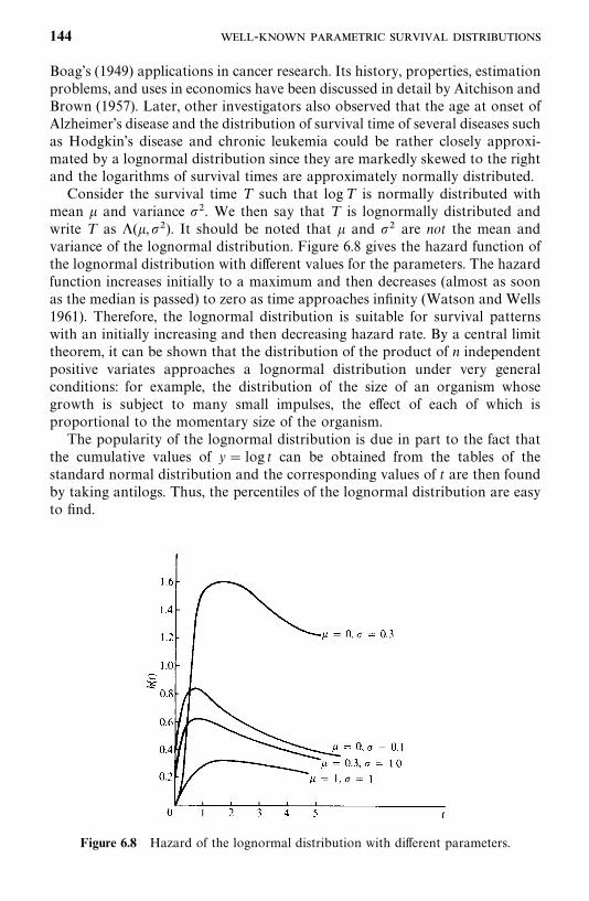
Figure 6.8 Hazard of the lognormal distribution with different parameters.
Boag’s (1949) applications in cancer research. Its history, properties, estimationproblems, and uses in economics have been discussed in detail by Aitchison andBrown (1957). Later, other investigators also observed that the age at onset ofAlzheimer’s disease and the distribution of survival time of several diseases suchas Hodgkin’s disease and chronic leukemia could be rather closely approxi-mated by a lognormal distribution since they are markedly skewed to the rightand the logarithms of survival times are approximately normally distributed.Consider the survival time T such that logT is normally distributed with
mean � and variance �. We then say that T is lognormally distributed andwrite T as �(�,�). It should be noted that � and � are not the mean andvariance of the lognormal distribution. Figure 6.8 gives the hazard function ofthe lognormal distribution with different values for the parameters. The hazardfunction increases initially to a maximum and then decreases (almost as soonas the median is passed) to zero as time approaches infinity (Watson and Wells1961). Therefore, the lognormal distribution is suitable for survival patternswith an initially increasing and then decreasing hazard rate. By a central limittheorem, it can be shown that the distribution of the product of n independentpositive variates approaches a lognormal distribution under very generalconditions: for example, the distribution of the size of an organism whosegrowth is subject to many small impulses, the effect of each of which isproportional to the momentary size of the organism.The popularity of the lognormal distribution is due in part to the fact that
the cumulative values of y� log t can be obtained from the tables of thestandard normal distribution and the corresponding values of t are then foundby taking antilogs. Thus, the percentiles of the lognormal distribution are easyto find.
144 -
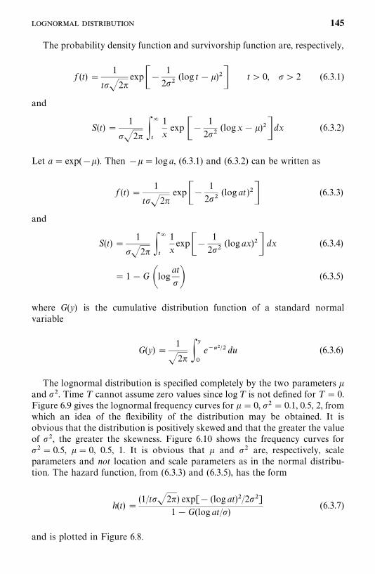
The probability density function and survivorship function are, respectively,
f (t)�1
t�2�exp��
1
2�(log t��)�� t� 0, � 2 (6.3.1)
and
S(t)�1
�2� ��
�
1
xexp ��
1
2�(log x��)�� dx (6.3.2)
Let a� exp(��). Then ��� log a, (6.3.1) and (6.3.2) can be written as
f (t)�1
t�2�exp��
1
2�(log at )�� (6.3.3)
and
S(t)�1
�2� ��
�
1
xexp��
1
2�(log ax)�� dx (6.3.4)
� 1�G �logat
� (6.3.5)
where G(y) is the cumulative distribution function of a standard normalvariable
G(y)�1
�2� ��
�
e����� du (6.3.6)
The lognormal distribution is specified completely by the two parameters �and �. Time T cannot assume zero values since log T is not defined for T � 0.Figure 6.9 gives the lognormal frequency curves for � � 0, �� 0.1, 0.5, 2, fromwhich an idea of the flexibility of the distribution may be obtained. It isobvious that the distribution is positively skewed and that the greater the valueof �, the greater the skewness. Figure 6.10 shows the frequency curves for�� 0.5, �� 0, 0.5, 1. It is obvious that � and � are, respectively, scaleparameters and not location and scale parameters as in the normal distribu-tion. The hazard function, from (6.3.3) and (6.3.5), has the form
h(t)�(1/t�2�) exp[� (log at)�/2�]
1�G(log at/)(6.3.7)
and is plotted in Figure 6.8.
145

Figure 6.9 Lognormal density curves with �� 0.
Figure 6.10 Lognormal density curves with �� 0.5.
The mean and variance of the two-parameter lognormal distribution are,respectively, exp(���
��) and [exp(�) � 1] exp(2���). The coefficient of
variation of the distribution is then [exp(�)� 1]���. The median is e� and themode is exp(���).The two-parameter lognormal distribution can also be generalized to a
three-parameter distribution by replacing t with t�G in (6.3.1). In otherwords, the survival time log(T �G) follows the normal distribution with mean� and variance �. In certain situations the value of G may be determined apriori and should not be regarded as an unknown parameter that requiresestimation. If this is so, the variable T �G may be considered in place of Tand the distribution of T �G has all the properties of the two-parameterlognormal distribution. However, the estimation procedures developed for thetwo-parameter case are not directly applicable to the distribution of T �G.
146 -
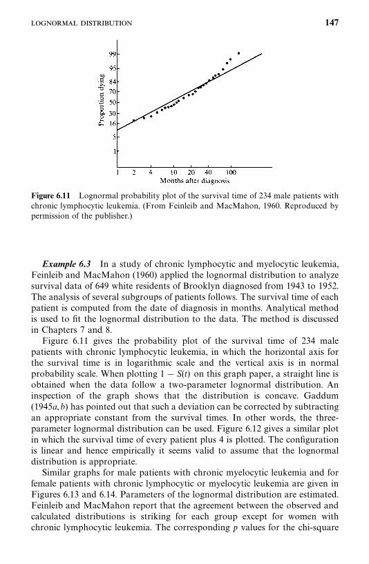
Figure 6.11 Lognormal probability plot of the survival time of 234 male patients withchronic lymphocytic leukemia. (From Feinleib and MacMahon, 1960. Reproduced bypermission of the publisher.)
Example 6.3 In a study of chronic lymphocytic and myelocytic leukemia,Feinleib and MacMahon (1960) applied the lognormal distribution to analyzesurvival data of 649 white residents of Brooklyn diagnosed from 1943 to 1952.The analysis of several subgroups of patients follows. The survival time of eachpatient is computed from the date of diagnosis in months. Analytical methodis used to fit the lognormal distribution to the data. The method is discussedin Chapters 7 and 8.Figure 6.11 gives the probability plot of the survival time of 234 male
patients with chronic lymphocytic leukemia, in which the horizontal axis forthe survival time is in logarithmic scale and the vertical axis is in normalprobability scale. When plotting 1� S(t) on this graph paper, a straight line isobtained when the data follow a two-parameter lognormal distribution. Aninspection of the graph shows that the distribution is concave. Gaddum(1945a,b) has pointed out that such a deviation can be corrected by subtractingan appropriate constant from the survival times. In other words, the three-parameter lognormal distribution can be used. Figure 6.12 gives a similar plotin which the survival time of every patient plus 4 is plotted. The configurationis linear and hence empirically it seems valid to assume that the lognormaldistribution is appropriate.Similar graphs for male patients with chronic myelocytic leukemia and for
female patients with chronic lymphocytic or myelocytic leukemia are given inFigures 6.13 and 6.14. Parameters of the lognormal distribution are estimated.Feinleib and MacMahon report that the agreement between the observed andcalculated distributions is striking for each group except for women withchronic lymphocytic leukemia. The corresponding p values for the chi-square
147
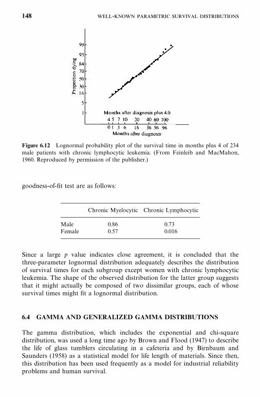
Figure 6.12 Lognormal probability plot of the survival time in months plus 4 of 234male patients with chronic lymphocytic leukemia. (From Feinleib and MacMahon,1960. Reproduced by permission of the publisher.)
goodness-of-fit test are as follows:
Chronic Myelocytic Chronic Lymphocytic
Male 0.86 0.73Female 0.57 0.016
Since a large p value indicates close agreement, it is concluded that thethree-parameter lognormal distribution adequately describes the distributionof survival times for each subgroup except women with chronic lymphocyticleukemia. The shape of the observed distribution for the latter group suggeststhat it might actually be composed of two dissimilar groups, each of whosesurvival times might fit a lognormal distribution.
6.4 GAMMA AND GENERALIZED GAMMA DISTRIBUTIONS
The gamma distribution, which includes the exponential and chi-squaredistribution, was used a long time ago by Brown and Flood (1947) to describethe life of glass tumblers circulating in a cafeteria and by Birnbaum andSaunders (1958) as a statistical model for life length of materials. Since then,this distribution has been used frequently as a model for industrial reliabilityproblems and human survival.
148 -
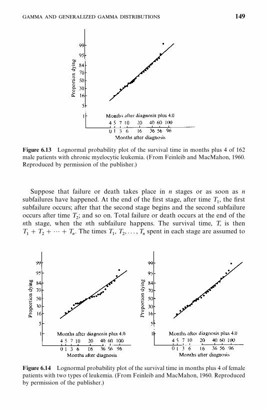
Figure 6.13 Lognormal probability plot of the survival time in months plus 4 of 162male patients with chronic myelocytic leukemia. (From Feinleib and MacMahon, 1960.Reproduced by permission of the publisher.)
Figure 6.14 Lognormal probability plot of the survival time in months plus 4 of femalepatients with two types of leukemia. (From Feinleib and MacMahon, 1960. Reproducedby permission of the publisher.)
Suppose that failure or death takes place in n stages or as soon as nsubfailures have happened. At the end of the first stage, after time T
�, the first
subfailure occurs; after that the second stage begins and the second subfailureoccurs after time T
�; and so on. Total failure or death occurs at the end of the
nth stage, when the nth subfailure happens. The survival time, T, is thenT��T
���T
�. The times T
�, T
�, . . . , T
�spent in each stage are assumed to
149
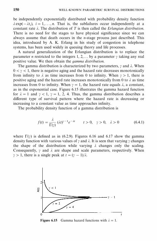
Figure 6.15 Gamma hazard functions with �� 1.
be independently exponentially distributed with probability density function� exp(��t
), i� 1, . . . , n. That is, the subfailures occur independently at a
constant rate �. The distribution of T is then called the Erlangian distribution.There is no need for the stages to have physical significance since we canalways assume that death occurs in the n-stage process just described. Thisidea, introduced by A. K. Erlang in his study of congestion in telephonesystems, has been used widely in queuing theory and life processes.A natural generalization of the Erlangian distribution is to replace the
parameter n restricted to the integers 1, 2, . . . by a parameter � taking any realpositive value. We then obtain the gamma distribution.The gamma distribution is characterized by two parameters, � and �. When
0�� � 1, there is negative aging and the hazard rate decreases monotonicallyfrom infinity to � as time increases from 0 to infinity. When � � 1, there ispositive aging and the hazard rate increases monotonically from 0 to � as timeincreases from 0 to infinity. When �� 1, the hazard rate equals �, a constant,as in the exponential case. Figure 6.15 illustrates the gamma hazard functionfor �� 1 and �� 1, �� 1, 2, 4. Thus, the gamma distribution describes adifferent type of survival pattern where the hazard rate is decreasing orincreasing to a constant value as time approaches infinity.The probability density function of a gamma distribution is
f (t)��
(�)(�t)���e��� t� 0, �� 0, �� 0 (6.4.1)
where (�) is defined as in (6.2.9). Figures 6.16 and 6.17 show the gammadensity function with various values of � and �. It is seen that varying � changesthe shape of the distribution while varying � changes only the scaling.Consequently, � and � are shape and scale parameters, respectively. When�� 1, there is a single peak at t� (� � 1)/�.
150 -
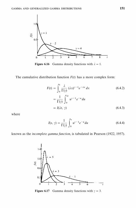
Figure 6.16 Gamma density functions with �� 1.
Figure 6.17 Gamma density functions with � � 3.
The cumulative distribution function F(t) has a more complex form:
F(t)� ��
�
�(�)
(�x)���e��� dx (6.4.2)
�1
(�) ���
�
u���e�� du
� I(�t, �) (6.4.3)
where
I(s, �)�1
(�) �
�
u���e��du (6.4.4)
known as the incomplete gamma function, is tabulated in Pearson (1922, 1957).
151
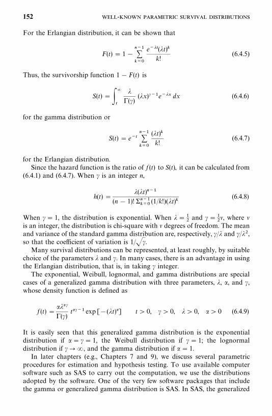
For the Erlangian distribution, it can be shown that
F(t)� 1���� ���
e���(�t)�k!
(6.4.5)
Thus, the survivorship function 1�F(t) is
S(t)���
�
�(�)
(�x)���e��� dx (6.4.6)
for the gamma distribution or
S(t)� e����� ���
(�t)�k!
(6.4.7)
for the Erlangian distribution.Since the hazard function is the ratio of f (t) to S(t), it can be calculated from
(6.4.1) and (6.4.7). When � is an integer n,
h(t)��(�t)���
(n � 1)! �������(1/k!)(�t)�
(6.4.8)
When �� 1, the distribution is exponential. When ����and ���
��, where �
is an integer, the distribution is chi-square with � degrees of freedom. The meanand variance of the standard gamma distribution are, respectively, �/� and �/��,so that the coefficient of variation is 1/��.Many survival distributions can be represented, at least roughly, by suitable
choice of the parameters � and �. In many cases, there is an advantage in usingthe Erlangian distribution, that is, in taking � integer.The exponential, Weibull, lognormal, and gamma distributions are special
cases of a generalized gamma distribution with three parameters, �, �, and �,whose density function is defined as
f (t)����(�)
t��� exp [�(�t)] t� 0, � � 0, �� 0, �� 0 (6.4.9)
It is easily seen that this generalized gamma distribution is the exponentialdistribution if �� � � 1, the Weibull distribution if � � 1; the lognormaldistribution if �� �, and the gamma distribution if � � 1.In later chapters (e.g., Chapters 7 and 9), we discuss several parametric
procedures for estimation and hypothesis testing. To use available computersoftware such as SAS to carry out the computation, we use the distributionsadopted by the software. One of the very few software packages that includethe gamma or generalized gamma distribution is SAS. In SAS, the generalized
152 -
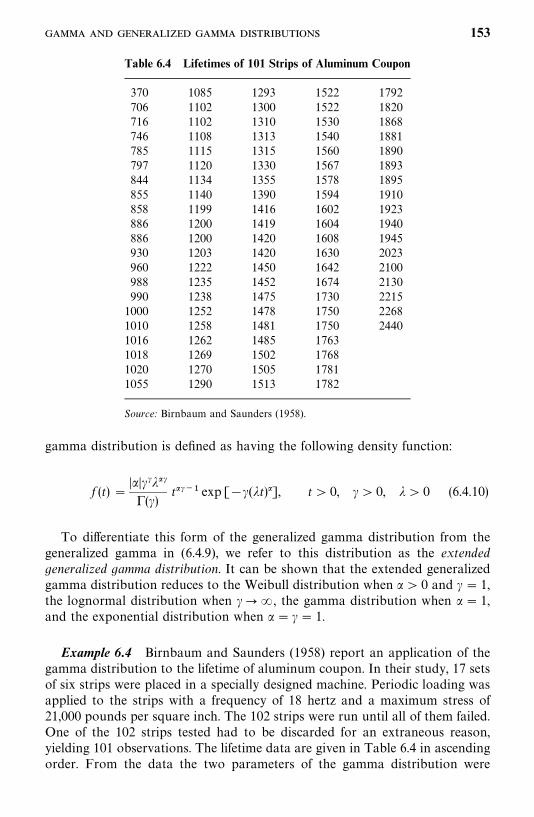
Table 6.4 Lifetimes of 101 Strips of Aluminum Coupon
370706716746785797844855858886886930960988990100010101016101810201055
108511021102110811151120113411401199120012001203122212351238125212581262126912701290
129313001310131313151330135513901416141914201420145014521475147814811485150215051513
152215221530154015601567157815941602160416081630164216741730175017501763176817811782
17921820186818811890189318951910192319401945202321002130221522682440
Source: Birnbaum and Saunders (1958).
gamma distribution is defined as having the following density function:
f (t)��������(�)
t��� exp [��(�t)], t� 0, �� 0, �� 0 (6.4.10)
To differentiate this form of the generalized gamma distribution from thegeneralized gamma in (6.4.9), we refer to this distribution as the extendedgeneralized gamma distribution. It can be shown that the extended generalizedgamma distribution reduces to the Weibull distribution when � � 0 and � � 1,the lognormal distribution when ���, the gamma distribution when � � 1,and the exponential distribution when � � �� 1.
Example 6.4 Birnbaum and Saunders (1958) report an application of thegamma distribution to the lifetime of aluminum coupon. In their study, 17 setsof six strips were placed in a specially designed machine. Periodic loading wasapplied to the strips with a frequency of 18 hertz and a maximum stress of21,000 pounds per square inch. The 102 strips were run until all of them failed.One of the 102 strips tested had to be discarded for an extraneous reason,yielding 101 observations. The lifetime data are given in Table 6.4 in ascendingorder. From the data the two parameters of the gamma distribution were
153
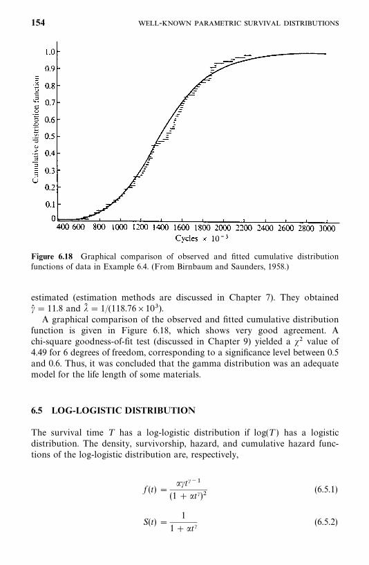
Figure 6.18 Graphical comparison of observed and fitted cumulative distributionfunctions of data in Example 6.4. (From Birnbaum and Saunders, 1958.)
estimated (estimation methods are discussed in Chapter 7). They obtained�� � 11.8 and �� � 1/(118.76�10).A graphical comparison of the observed and fitted cumulative distribution
function is given in Figure 6.18, which shows very good agreement. Achi-square goodness-of-fit test (discussed in Chapter 9) yielded a �� value of4.49 for 6 degrees of freedom, corresponding to a significance level between 0.5and 0.6. Thus, it was concluded that the gamma distribution was an adequatemodel for the life length of some materials.
6.5 LOG-LOGISTIC DISTRIBUTION
The survival time T has a log-logistic distribution if log(T ) has a logisticdistribution. The density, survivorship, hazard, and cumulative hazard func-tions of the log-logistic distribution are, respectively,
f (t) ���t���
(1� �t�)�(6.5.1)
S(t) �1
1� �t�(6.5.2)
154 -
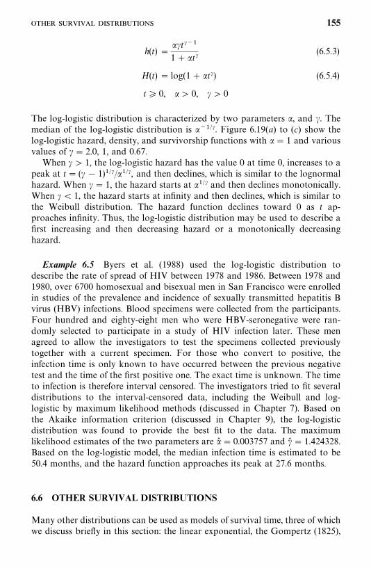
h(t) ���t���
1� �t�(6.5.3)
H(t)� log(1� �t�) (6.5.4)
t� 0, �� 0, � � 0
The log-logistic distribution is characterized by two parameters �, and �. Themedian of the log-logistic distribution is �����. Figure 6.19(a) to (c) show thelog-logistic hazard, density, and survivorship functions with �� 1 and variousvalues of � � 2.0, 1, and 0.67.When � � 1, the log-logistic hazard has the value 0 at time 0, increases to a
peak at t� (� � 1)���/����, and then declines, which is similar to the lognormalhazard. When �� 1, the hazard starts at ���� and then declines monotonically.When �� 1, the hazard starts at infinity and then declines, which is similar tothe Weibull distribution. The hazard function declines toward 0 as t ap-proaches infinity. Thus, the log-logistic distribution may be used to describe afirst increasing and then decreasing hazard or a monotonically decreasinghazard.
Example 6.5 Byers et al. (1988) used the log-logistic distribution todescribe the rate of spread of HIV between 1978 and 1986. Between 1978 and1980, over 6700 homosexual and bisexual men in San Francisco were enrolledin studies of the prevalence and incidence of sexually transmitted hepatitis Bvirus (HBV) infections. Blood specimens were collected from the participants.Four hundred and eighty-eight men who were HBV-seronegative were ran-domly selected to participate in a study of HIV infection later. These menagreed to allow the investigators to test the specimens collected previouslytogether with a current specimen. For those who convert to positive, theinfection time is only known to have occurred between the previous negativetest and the time of the first positive one. The exact time is unknown. The timeto infection is therefore interval censored. The investigators tried to fit severaldistributions to the interval-censored data, including the Weibull and log-logistic by maximum likelihood methods (discussed in Chapter 7). Based onthe Akaike information criterion (discussed in Chapter 9), the log-logisticdistribution was found to provide the best fit to the data. The maximumlikelihood estimates of the two parameters are �� � 0.003757 and �� � 1.424328.Based on the log-logistic model, the median infection time is estimated to be50.4 months, and the hazard function approaches its peak at 27.6 months.
6.6 OTHER SURVIVAL DISTRIBUTIONS
Many other distributions can be used as models of survival time, three of whichwe discuss briefly in this section: the linear exponential, the Gompertz (1825),
155
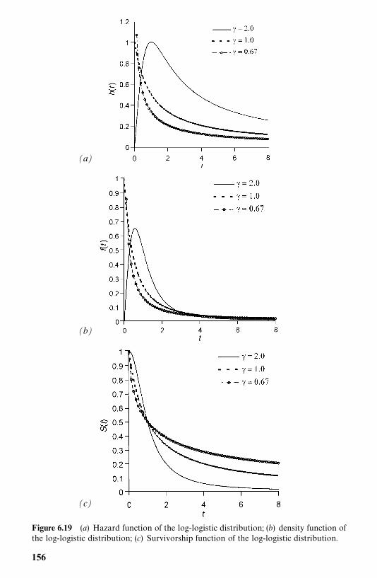
(a)
(b)
(c)
Figure 6.19 (a) Hazard function of the log-logistic distribution; (b) density function ofthe log-logistic distribution; (c) Survivorship function of the log-logistic distribution.
156
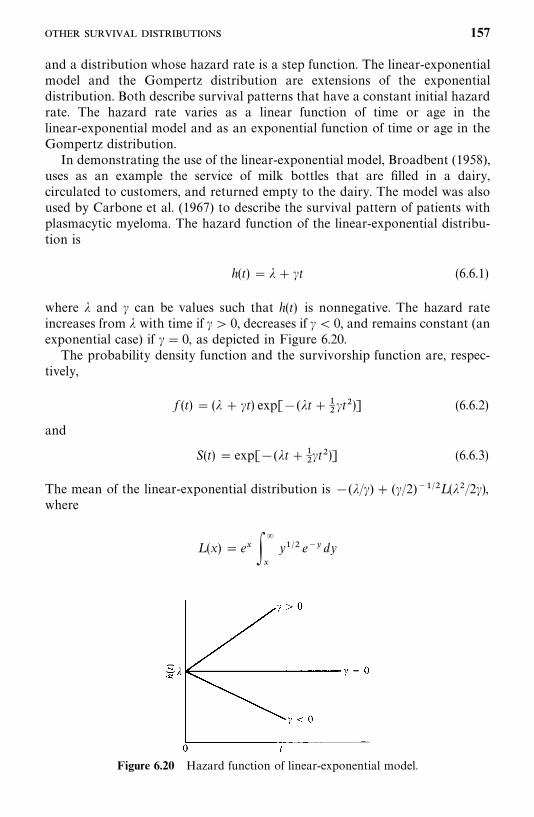
Figure 6.20 Hazard function of linear-exponential model.
and a distribution whose hazard rate is a step function. The linear-exponentialmodel and the Gompertz distribution are extensions of the exponentialdistribution. Both describe survival patterns that have a constant initial hazardrate. The hazard rate varies as a linear function of time or age in thelinear-exponential model and as an exponential function of time or age in theGompertz distribution.In demonstrating the use of the linear-exponential model, Broadbent (1958),
uses as an example the service of milk bottles that are filled in a dairy,circulated to customers, and returned empty to the dairy. The model was alsoused by Carbone et al. (1967) to describe the survival pattern of patients withplasmacytic myeloma. The hazard function of the linear-exponential distribu-tion is
h(t)� �� �t (6.6.1)
where � and � can be values such that h(t) is nonnegative. The hazard rateincreases from � with time if �� 0, decreases if � � 0, and remains constant (anexponential case) if �� 0, as depicted in Figure 6.20.The probability density function and the survivorship function are, respec-
tively,
f (t) � (� � �t) exp[�(�t����t�)] (6.6.2)
and
S(t) � exp[�(�t����t�)] (6.6.3)
The mean of the linear-exponential distribution is �(�/�) � (�/2)����L (��/2�),where
L (x)� e� ��
�
y��� e�� dy
157
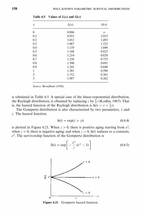
Table 6.5 Values of L(x) and G(x)
x L (x) G(x)
0 0.886 �0.1 0.951 2.0150.2 1.012 1.4930.3 1.067 1.2230.4 1.119 1.0480.5 1.168 0.9230.6 1.214 0.8280.7 1.258 0.7530.8 1.300 0.6910.9 1.341 0.6401 1.381 0.5962 1.712 0.3613 1.987 0.262
Source: Broadbent (1958).
Figure 6.21 Gompertz hazard function.
is tabulated in Table 6.5. A special case of the linear-exponential distribution,the Rayleigh distribution, is obtained by replacing � by �
�� (Kodlin, 1967). That
is, the hazard function of the Rayleigh distribution is h(t) � �����t.
The Gompertz distribution is also characterized by two parameters, � and�. The hazard function,
h(t)� exp(� � �t) (6.6.4)
is plotted in Figure 6.21. When �� 0, there is positive aging starting from e�;when �� 0, there is negative aging; and when �� 0, h(t) reduces to a constant,e�. The survivorship function of the Gompertz distribution is
S(t)� exp��e��(e�� � 1)� (6.6.5)
158 -
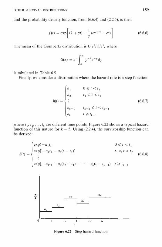
Figure 6.22 Step hazard function.
and the probability density function, from (6.6.4) and (2.2.5), is then
f (t)� exp�(� � �t)�1
�(e� �� � e�)� (6.6.6)
The mean of the Gompertz distribution is G(e�/�)/e�, where
G(x)� e� ��
�
y��e��dy
is tabulated in Table 6.5.Finally, we consider a distribution where the hazard rate is a step function:
h(t)��a�
a��
a���
a�
0� t� t�
t�� t� t
�
t���
� t� t���
t� t���
(6.6.7)
where t�, t
�, . . . , t
�are different time points. Figure 6.22 shows a typical hazard
function of this nature for k� 5. Using (2.2.4), the survivorship function canbe derived:
S(t)��exp(�a
�t) 0� t� t
�exp[�a
�t�� a
�(t � t
�)] t
�� t� t
��
exp[�a�t�� a
�(t�� t
�)� � a
�(t � t
���) t� t
���
(6.6.8)
159
The probability density function f (t) can then be obtained from (6.6.7) and(6.6.8) using (2.2.5):
f (t)��a�exp(�a
�t) 0� t� t
�a�exp[�a
�t�� a
�(t � t
�)] t
�� t� t
��
a�exp[�a
�t�� a
�(t�� t
�)�� a
�(t � t
���) t� t
���
(6.6.9)
One application of this distribution is the life-table analysis discussed inChapter 4. In a life-table analysis, time is divided into intervals and the hazardrate is assumed to be constant in each interval. However, the overall hazardrate is not necessarily constant.The nine distributions described above are, among others, reasonable
models for survival time distribution. All have been designed by considering abiological failure, a death process, or an aging property. They may or may notbe appropriate for many practical situations, but the objective here is toillustrate the various possible techniques, assumptions, and arguments that canbe used to choose the most appropriate model. If none of these distributionsfits the data, investigators might have to derive an original model to suit theparticular data, perhaps by using some of the ideas presented here.
Bibliographical Remarks
In addition to the papers on the distributions cited in this chapter, Mann et al.(1974), Hahn and Shapiro (1967), Johnson and Kotz (1970a, b), Elandt-Johnson and Johnson (1980), Lawless (1982), Nelson (1982), Cox and Oakes(1984), Gertsbakh (1989), and Klein and Moeschberger (1997) also discussstatistical failure models, including the exponential, Weibull, gamma, lognor-mal, generalized gamma, and log-logistic distributions. Applications of survivaldistributions can be found easily in medical and epidemiological journals. Thefollowing are a few examples: Dharmalingam et al. (2000), Riffenburgh andJohnstone (2001), and Mafart et al. (2002).
EXERCISES
6.1 Summarize the distributions discussed in this chapter, answering thefollowing questions.(a) What distributions describe constant hazard rates? Give the range of
parameter values.(b) What distributions describe increasing hazard rates? If there are more
than one, discuss the differences between them.(c) What distributions describe decreasing hazard rates? If there are more
than one, discuss the differences between them.
160 -
6.2 Suppose that the survival distribution of a group of patients follows theexponential distribution with G� 0 (year), �� 0.65. Plot the survivor-ship function and find:(a) The mean survival time(b) The median survival time(c) The probability of surviving 1.5 years or more
6.3 Suppose that the survival distribution of a group of patients follows theexponential distribution with G� 5 (years) and � � 0.25. Plot the surviv-orship function and find:(a) The mean survival time(b) The median survival time(c) The probability of surviving 6 years or more
6.4 Consider the following two Weibull distributions as survival models:(i) G� 0, � � 1, �� 0.5
(ii) G� 0, � � 0.5, �� 2For each distribution, plot the survivorship function and the hazardfunction and find:(a) The mean(b) The variance(c) The coefficient of variationWhich distribution gives the larger probability of surviving at least 3 unitsof time?
6.5 Suppose that the survival time follows the lognormal distribution with�� 1 and � 0.5. Find:(a) The mean survival time(b) The variance(c) The coefficient of variation(d) The median(e) The mode
6.6 Suppose that pain relief time follows the gamma distribution with � � 1,�� 0.5. Find:(a) The mean(b) The variance(c) The coefficient of variation
6.7 Suppose that the survival distribution is (1) Gompertz and (2) linear-exponential, and � � 1, � � 2.0. Plot the hazard function and find:(a) The mean(b) The probability of surviving longer than 1 unit of time
6.8 Consider the survival times of hypernephroma patients given in ExerciseTable 3.1. From the plot you obtained in Exercise 4.5, suggest adistribution that might fit the data.
161
CHAPTER 7
Estimation Procedures forParametric Survival Distributionswithout Covariates
In this chapter we discuss some analytical procedures for estimating the mostcommonly used survival distributions discussed in Chapter 6. We introduce themaximum likelihood estimates (MLEs) of the parameters of these distributions.The general asymptotic likelihood inference results that are most widely usedfor these distributions are given in Section 7.1. We begin to used the generalsymbol b� (b
�, b
�, . . . , b
�) to denote a set of parameters. For example, in
discussing the Weibull distribution, b�could be � and b
�could be �, and p� 2.
b is called a vector in linear algebra. Readers who are not familiar with linearalgebra or are not interested in the mathematical details may skip this sectionand proceed to Section 7.2 without loss of continuity. In Sections 7.2 to 7.7 weintroduce the MLEs for the parameters of the exponential, Weibull, lognormal,gamma, log-logistic, and Gompertz distributions for data with and withoutcensored observations. The related BMDP or SAS programming codes thatmay be used to obtain the MLE are given in the respective sections.
7.1 GENERAL MAXIMUM LIKELIHOOD ESTIMATIONPROCEDURE
7.1.1 Estimation Procedures for Data with Right-Censored Observations
Suppose that persons were followed to death or censored in a study. Let t�,
t�, . . . , t
�, t�
���, . . . , t�
�be the survival times observed from the n individuals,
with r exact times and (n� r) right-censored times. Assume that the survivaltimes follow a distribution with the density function f (t, b) and survivorshipfunction S(t, b), where b� (b
�, . . . , b
�) denotes unknown p parameters
b�, . . . , b
�in the distribution. As shown in Chapter 6, an exponential distribu-
tion has one (p� 1) parameter �, the Weibull distribution has two (p� 2)
162
parameters � and �, and so on. If the survival time is discrete (i.e., it is observedat discrete time only), f (t, b) represents the probability of observing t and S(t, b)represents the probability that the survival or event time is greater than t. Inother words, f (t, b) and S(t, b) represent the information that can be obtainedfrom an observed uncensored survival time and an observed right-censoredsurvival time, respectively. Therefore, the product ��
���f (t
�,b) represents
the joint probability of observing the uncensored survival times, and��
�����S(t�
�, b) represents the joint probability of those right-censored survival
times. The product of these two probabilities, denoted by L (b),
L (b) ��
����
f (t�, b)
��
�����
S(t��, b)
represents the joint probability of observing t�, t
�, . . . , t
�, t�
���, . . . , t�
�. A similar
interpretation applies to continuous survival. L (b) is called the likelihoodfunction of b, which can also be interpreted as a measure of the likelihood ofobserving a specific set of survival times t
�, t
�, . . . , t
�, t�
���, . . . , t�
�, given a
specific set of parameters b. The method of the MLE is to find an estimator ofb that maximizes L (b), or in other words, which is ‘‘most likely’’ to haveproduced the observed data t
�, t
�, . . . , t
�, t�
���, . . . , t�
�. Take the logarithm of
L (b) and denote it by l(b),
l(b) � log L (b) ��
����
log[ f (t�, b)] �
��
�����
log[S(t��, b)] (7.1.1)
Then the MLE b� of b is the set of b��, . . . , b�
�that maximizes l(b):
l(b� ) �max��� b
(l(b)).
It is clear that b� is a solution of the following simultaneous equations, whichare obtained by taking the derivative of l(b) with respect to each b
�:
�l(b)�b
�
� 0 j� 1, 2, . . . , p (7.1.2)
The exact forms of (7.1.2) for the parametric survival distributions discussed inChapter 6 are given in Sections 7.2 to 7.7. Often, there is no closed solution forthe MLE b� from (7.1.2). To obtain the MLE b� , one can use a numericalmethod. A commonly used numerical method is the Newton—Raphson iter-ative procedure, which can be summarized as follows.
1. Let the initial values of b�, . . . , b
�be zero; that is, let
b��� 0
163
2. The changes for b at each subsequent step, denoted by ���, is obtained bytaking the second derivative of the log-likelihood function:
��������l(b���)
�b �b �� �l(b���)
�b(7.1.3)
3. Using ���, the value of b�� at j th step is
b��� b���� ��� j� 1, 2, . . .
The iteration terminates at, say, the mth step if ��� � �, where � is a givenprecision, usually a very small value, 10� or 10�. Then the MLE b� is definedas
b� � b��� (7.1.4)
The estimated covariance matrix of the MLE b� is given by
V� (b� ) �Co� v(b� ) �����l(b� )�b �b�
�(7.1.5)
One of the good properties of a MLE is that if b� is the MLE of b, then g(b� ) isthe MLE of g(b) if g(b) is a finite function and need not be one-to-one. Theconcept of the Newton—Raphson method for p� 1 is illustrated in detail inAppendix A.
The estimated 100(1� )% confidence interval for any parameter b�is
(b���Z� ��v
��, b�
��Z� ��v
��) (7.1.6)
where v��is the ith diagonal element of V� (b� ) and Z� � is the 100(1� /2)
percentile point of the standard normal distribution [P(Z�Z� �) � /2]. Fora finite function g(b
�) of b
�, the estimated 100(1� )% confidence interval for
g(b�) is its respective range R on the confidence interval (7.1.6), that is,
R� �g(b�) : b
�� (b�
��Z� ��v
��, b�
��Z� ��v
��)� (7.1.7)
In case g(b�) is monotone in b
�, the estimated 100(1� )% confidence interval
for g(b�) is
[g(b���Z� ��v
��), g(b�
��Z� ��v
��)] (7.1.8)
164
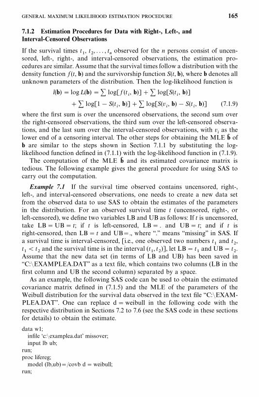
7.1.2 Estimation Procedures for Data with Right-, Left-, andInterval-Censored Observations
If the survival times t�, t
�, . . . , t
�observed for the n persons consist of uncen-
sored, left-, right-, and interval-censored observations, the estimation pro-cedures are similar. Assume that the survival times follow a distribution with thedensity function f (t, b) and the survivorship function S(t, b), where b denotes allunknown parameters of the distribution. Then the log-likelihood function is
l(b) � log L (b) � � log[ f (t�, b)]� � log[S(t
�, b)]
� � log[1� S(t�, b)]� � log[S(v
�, b) � S(t
�, b)] (7.1.9)
where the first sum is over the uncensored observations, the second sum overthe right-censored observations, the third sum over the left-censored observa-tions, and the last sum over the interval-censored observations, with v
�as the
lower end of a censoring interval. The other steps for obtaining the MLE b� ofb are similar to the steps shown in Section 7.1.1 by substituting the log-likelihood function defined in (7.1.1) with the log-likelihood function in (7.1.9).
The computation of the MLE b� and its estimated covariance matrix istedious. The following example gives the general procedure for using SAS tocarry out the computation.
Example 7.1 If the survival time observed contains uncensored, right-,left-, and interval-censored observations, one needs to create a new data setfrom the observed data to use SAS to obtain the estimates of the parametersin the distribution. For an observed survival time t (uncensored, right-, orleft-censored), we define two variables LB and UB as follows: If t is uncensored,take LB�UB� t; if t is left-censored, LB� . and UB� t; and if t isright-censored, then LB� t and UB�., where ‘‘.’’ means ‘‘missing’’ in SAS. Ifa survival time is interval-censored, [i.e., one observed two numbers t
�and t
�,
t�
� t�and the survival time is in the interval (t
�, t
�)], let LB� t
�and UB� t
�.
Assume that the new data set (in terms of LB and UB) has been saved in‘‘C:�EXAMPLEA.DAT’’ as a text file, which contains two columns (LB in thefirst column and UB the second column) separated by a space.
As an example, the following SAS code can be used to obtain the estimatedcovariance matrix defined in (7.1.5) and the MLE of the parameters of theWeibull distribution for the survival data observed in the text file ‘‘C:�EXAM-PLEA.DAT’’. One can replace d�weibull in the following code with therespective distribution in Sections 7.2 to 7.6 (see the SAS code in these sectionsfor details) to obtain the estimate.
data w1;infile ‘c:�examplea.dat’ missover;input lb ub;
run;proc lifereg;model (lb,ub)�/covb d�weibull;
run;
165
7.2 EXPONENTIAL DISTRIBUTION
7.2.1 One-Parameter Exponential Distribution
The one-parameter exponential distribution has the following density function;
f (t) � �e�� (7.2.1)
survivorship function;
S(t) � e�� (7.2.2)
and hazard function;
h(t) � � (7.2.3)
where t� 0, � � 0. Obviously, the exponential distribution is characterized byone parameter, �. The estimation of � by maximum likelihood methods fordata without censored observations will be given first followed by the case withcensored observations.
Estimation of � for Data without Censored ObservationsSuppose that there are n persons in the study and everyone is followed to deathor failure. Let t
�, t
�, . . . , t
�be the exact survival times of the n people. The
likelihood function, using (7.2.1) and (7.1.1), is
L ��
����
�e���
and the log-likelihood function is
l(�) � n log � � ��
����
t�
(7.2.4)
From (7.1.2), the MLE of � is
�� �n
�����
t�
(7.2.5)
Since the mean � of the exponential distribution is 1/� and a MLE is invariantunder an one-to-one transformation, the MLE of � is
�� �1
���
�����
t�
n� t� (7.2.6)
166
It can be shown 2n�� /� has an exact chi-square distribution with 2n degrees offreedom (Epstein and Sobel, 1953). Since � � 1/� and �� � 1/�� , an exact100(1� )% confidence interval for � is
�� ������� �2n
� � ��� ��
���� �2n
(7.2.7)
where ������ is the 100 percentage point of the chi-square distribution with 2n
degrees of freedom, that is, P(����
� ������) � (Table B-2). When n is large
(n� 25, say), �� is approximately normally distributed with mean � andvariance ��/n. Thus, an approximate 100(1� )% confidence interval for � is
�� ��� Z� ��n
� � � �� ��� Z� ��n
(7.2.8)
where Z� � is the 100 /2 percentage point, P(Z�Z� �) � /2, of the standardnormal distribution (Table B-1).
Since 2n�� /� has an exact chi-square distribution with 2n degrees of freedom,an exact 100(1� a)% confidence interval for the mean survival time is
2n�������� �
� � �2n��
������� �
(7.2.9)
The following example illustrates the procedures.
Example 7.2 Consider the following remission times in weeks for 21patients with acute leukemia: 1, 1, 2, 2, 3, 4, 4, 5, 5, 6, 8, 8, 9, 10, 10, 12, 14, 16,20, 24, and 34. Assume that remission duration follows the exponentialdistribution. Let us estimate the parameter � by using the formulas givenabove.
According to (7.2.5), the MLE of the relapse rate, �, is
�� �21
198� 0.106 per week
The mean remission time � is then 198/21� 9.429 weeks. Using the analyticalprocedures given above, confidence intervals for � and � can also be obtained.
A 95% confidence interval for the relapse rate �, following (7.2.7), isapproximately
(0.106)(24.433)42
� � �(0.106)(59.342)
42
or (0.062, 0.150). A 95% confidence interval for the mean remission time,
167
following (7.2.9), is
(42)(9.429)59.342
� � �(42)(9.429)24.433
or (6.673, 16.208).Once the parameter � is estimated, other estimates can be obtained. For
example, the probability of staying in remission for at least 20 weeks, estimatedfrom (7.2.2), is S� (20) � exp[�0.106(20)]� 0.120. Any percentile of survivaltime t
�may be estimated by equating S(t) to p and solving for t
�, that is,
t�� �log p/�� . For example, the median (50th percentile) survival time can be
estimated by t���
� �log 0.5/�� � 6.539 weeks.
Estimation of � for Data with Censored ObservationsWe first consider singly censored and then progressively censored data.Suppose that without loss of generality, the study or experiment begins at time0 with a total of n subjects. Survival times are recorded and the data becomeavailable when the subjects die one after the other in such a way that theshortest survival time comes first, the second shortest second, and so on.Suppose that the investigator has decided to terminate the study after r out ofthe n subjects have died and to sacrifice the remaining n� r subjects at thattime. Then the survival times for the n subjects are
t��
� t��
� � � t��
� t�����
��� t���
where a superscript plus indicates a sacrificed subject, and thus t���is a censored
observation. In this case, n and r are fixed values and all of the n� r censoredobservations are equal.
The likelihood function, using (7.1.1), (7.2.1), and (7.2.2), is
L �n!
(n� r)!
�����
�e����(e����)��
and from (7.1.2), the MLE of � is
�� �r
�����
t��
� �������
t���
(7.2.10)
The mean survival time � � 1/� can then be estimated by
�� �1
���
�����
t��
� �������
t���
r(7.2.11)
It is shown by Halperin (1952) that 2r�/�� has a chi-square distribution with 2r
168
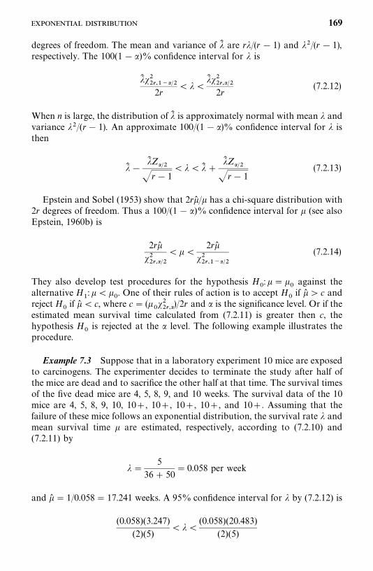
degrees of freedom. The mean and variance of �� are r�/(r� 1) and ��/(r� 1),respectively. The 100(1� )% confidence interval for � is
�� ������� �2r
� � ��� ��
���� �2r
(7.2.12)
When n is large, the distribution of �� is approximately normal with mean � andvariance ��/(r� 1). An approximate 100/(1� )% confidence interval for � isthen
�� ��� Z� �
�r� 1� � � �� �
�� Z� ��r� 1
(7.2.13)
Epstein and Sobel (1953) show that 2r�� /� has a chi-square distribution with2r degrees of freedom. Thus a 100/(1� )% confidence interval for � (see alsoEpstein, 1960b) is
2r�������� �
� � �2r��
������� �
(7.2.14)
They also develop test procedures for the hypothesis H�: � � �
�against the
alternative H�: � � �
�. One of their rules of action is to accept H
�if �� � c and
reject H�if �� � c, where c� (�
�������)/2r and is the significance level. Or if the
estimated mean survival time calculated from (7.2.11) is greater then c, thehypothesis H
�is rejected at the level. The following example illustrates the
procedure.
Example 7.3 Suppose that in a laboratory experiment 10 mice are exposedto carcinogens. The experimenter decides to terminate the study after half ofthe mice are dead and to sacrifice the other half at that time. The survival timesof the five dead mice are 4, 5, 8, 9, and 10 weeks. The survival data of the 10mice are 4, 5, 8, 9, 10, 10�, 10�, 10�, 10�, and 10�. Assuming that thefailure of these mice follows an exponential distribution, the survival rate � andmean survival time � are estimated, respectively, according to (7.2.10) and(7.2.11) by
� �5
36� 50� 0.058 per week
and �� � 1/0.058� 17.241 weeks. A 95% confidence interval for � by (7.2.12) is
(0.058)(3.247)(2)(5)
� � �(0.058)(20.483)
(2)(5)
169
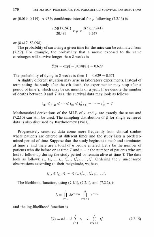
or (0.019, 0.119). A 95% confidence interval for � following (7.2.13) is
2(5)(17.241)20.483
� � �2(5)(17.241)
3.247
or (8.417, 53.098).The probability of surviving a given time for the mice can be estimated from
(7.2.2). For example, the probability that a mouse exposed to the samecarcinogen will survive longer than 8 weeks is
S� (8) � exp[�0.058(8)]� 0.629
The probability of dying in 8 weeks is then 1� 0.629� 0.371.A slightly different situation may arise in laboratory experiments. Instead of
terminating the study after the rth death, the experimenter may stop after aperiod of time T, which may be six months or a year. If we denote the numberof deaths between 0 and T as r, the survival data may look as follows:
t��
� t��
� � � t��
� t�����
�� � t���
�T
Mathematical derivations of the MLE of � and � are exactly the same and(7.2.10) can still be used. The sampling distribution of �� for singly censoreddata is also discussed by Bartholomew (1963).
Progressively censored data come more frequently from clinical studieswhere patients are entered at different times and the study lasts a predeter-mined period of time. Suppose that the study begins at time 0 and terminatesat time T and there are a total of n people entered. Let r be the number ofpatients who die before or at time T and n� r the number of patients who arelost to follow-up during the study period or remain alive at time T. The datalook as follows: t
�, t
�, . . . , t
�, t�
���, t�
���, . . . , t�
�. Ordering the r uncensored
observations according to their magnitude, we have
t��
� t��
� � � t�, t�
���, t�
���, . . . , t�
�
The likelihood function, using (7.1.1), (7.2.1), and (7.2.2), is
L ��
����
�e�����
������
e����
and the log-likelihood function is
l(�) � n� � ��
����
t�� �
��
�����
t��
(7.2.15)
170
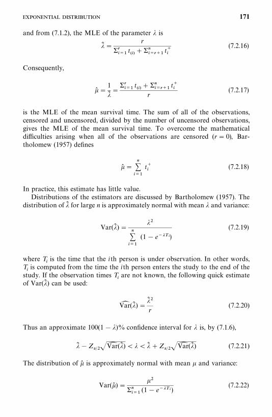
and from (7.1.2), the MLE of the parameter � is
�� �r
�����
t��
� �������
t��
(7.2.16)
Consequently,
�� �1
���
�����
t��
� �������
t��
r(7.2.17)
is the MLE of the mean survival time. The sum of all of the observations,censored and uncensored, divided by the number of uncensored observations,gives the MLE of the mean survival time. To overcome the mathematicaldifficulties arising when all of the observations are censored (r� 0), Bar-tholomew (1957) defines
�� ��
����
t��
(7.2.18)
In practice, this estimate has little value.Distributions of the estimators are discussed by Bartholomew (1957). The
distribution of �� for large n is approximately normal with mean � and variance:
Var(�� ) ���
�����
(1� e��)
(7.2.19)
where T�is the time that the ith person is under observation. In other words,
T�is computed from the time the ith person enters the study to the end of the
study. If the observation times T�are not known, the following quick estimate
of Var(�� ) can be used:
Var� (�� ) ��� �r
(7.2.20)
Thus an approximate 100(1� �)% confidence interval for � is, by (7.1.6),
�� �Z� ��Var� (�� ) � � � �� �Z� ��Var� (�� ) (7.2.21)
The distribution of �� is approximately normal with mean � and variance:
Var(�� ) ���
�����
(1� e��)(7.2.22)
171
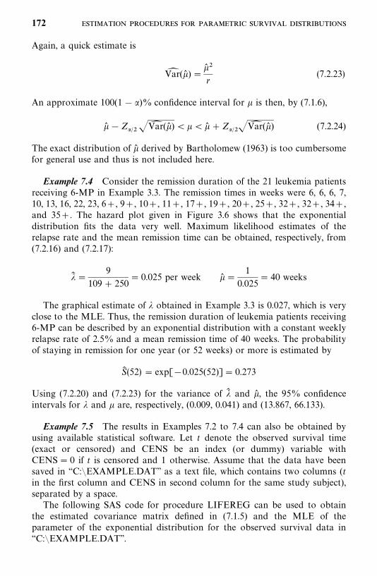
Again, a quick estimate is
Var� (�� ) ��� �r
(7.2.23)
An approximate 100(1� )% confidence interval for � is then, by (7.1.6),
�� �Z� � �Var� (�� ) � � � �� �Z� ��Var� (�� ) (7.2.24)
The exact distribution of �� derived by Bartholomew (1963) is too cumbersomefor general use and thus is not included here.
Example 7.4 Consider the remission duration of the 21 leukemia patientsreceiving 6-MP in Example 3.3. The remission times in weeks were 6, 6, 6, 7,10, 13, 16, 22, 23, 6�, 9�, 10�, 11�, 17�, 19�, 20�, 25�, 32�, 32�, 34�,and 35�. The hazard plot given in Figure 3.6 shows that the exponentialdistribution fits the data very well. Maximum likelihood estimates of therelapse rate and the mean remission time can be obtained, respectively, from(7.2.16) and (7.2.17):
�� �9
109� 250� 0.025 per week �� �
1
0.025� 40 weeks
The graphical estimate of � obtained in Example 3.3 is 0.027, which is veryclose to the MLE. Thus, the remission duration of leukemia patients receiving6-MP can be described by an exponential distribution with a constant weeklyrelapse rate of 2.5% and a mean remission time of 40 weeks. The probabilityof staying in remission for one year (or 52 weeks) or more is estimated by
S� (52) � exp[�0.025(52)]� 0.273
Using (7.2.20) and (7.2.23) for the variance of �� and �� , the 95% confidenceintervals for � and � are, respectively, (0.009, 0.041) and (13.867, 66.133).
Example 7.5 The results in Examples 7.2 to 7.4 can also be obtained byusing available statistical software. Let t denote the observed survival time(exact or censored) and CENS be an index (or dummy) variable withCENS� 0 if t is censored and 1 otherwise. Assume that the data have beensaved in ‘‘C:�EXAMPLE.DAT’’ as a text file, which contains two columns (tin the first column and CENS in second column for the same study subject),separated by a space.
The following SAS code for procedure LIFEREG can be used to obtainthe estimated covariance matrix defined in (7.1.5) and the MLE of theparameter of the exponential distribution for the observed survival data in‘‘C:�EXAMPLE.DAT’’.
172
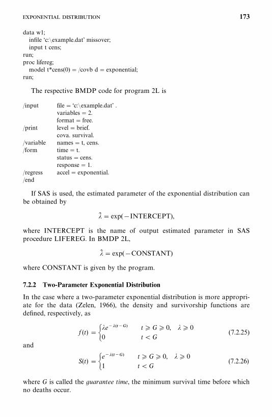
data w1;infile ‘c:�example.dat’ missover;input t cens;
run;proc lifereg;model t*cens(0) � /covb d� exponential;
run;
The respective BMDP code for program 2L is
/input file� ‘c:�example.dat’ .variables� 2.format� free.
/print level�brief.cova. survival.
/variable names� t, cens./form time� t.
status� cens.response� 1.
/regress accel� exponential./end
If SAS is used, the estimated parameter of the exponential distribution canbe obtained by
�� � exp(�INTERCEPT),
where INTERCEPT is the name of output estimated parameter in SASprocedure LIFEREG. In BMDP 2L,
�� � exp(�CONSTANT)
where CONSTANT is given by the program.
7.2.2 Two-Parameter Exponential Distribution
In the case where a two-parameter exponential distribution is more appropri-ate for the data (Zelen, 1966), the density and survivorship functions aredefined, respectively, as
f (t) ���e���
0
t�G� 0, � � 0
t�G(7.2.25)
and
S(t) ��e���
1
t�G� 0, � � 0
t�G(7.2.26)
where G is called the guarantee time, the minimum survival time before whichno deaths occur.
173
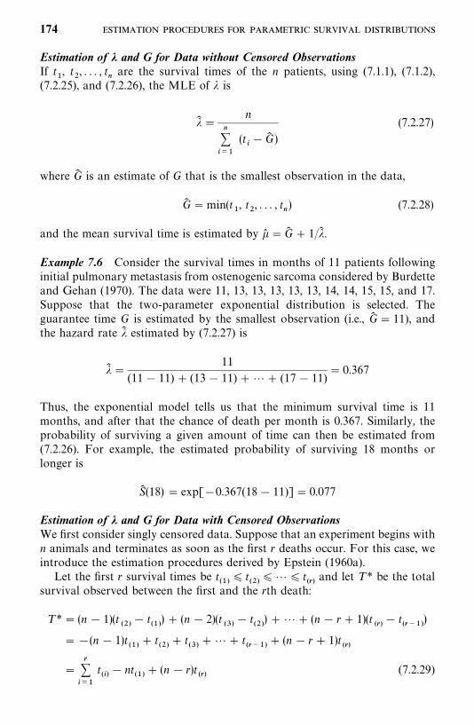
Estimation of � and G for Data without Censored ObservationsIf t
�, t
�, . . . , t
�are the survival times of the n patients, using (7.1.1), (7.1.2),
(7.2.25), and (7.2.26), the MLE of � is
�� �n
�����
(t��G� )
(7.2.27)
where G� is an estimate of G that is the smallest observation in the data,
G� �min(t�, t
�, . . . , t
�) (7.2.28)
and the mean survival time is estimated by �� �G� � 1/�� .
Example 7.6 Consider the survival times in months of 11 patients followinginitial pulmonary metastasis from ostenogenic sarcoma considered by Burdetteand Gehan (1970). The data were 11, 13, 13, 13, 13, 13, 14, 14, 15, 15, and 17.Suppose that the two-parameter exponential distribution is selected. Theguarantee time G is estimated by the smallest observation (i.e., G� � 11), andthe hazard rate �� estimated by (7.2.27) is
�� �11
(11� 11) � (13� 11) ��� (17� 11)� 0.367
Thus, the exponential model tells us that the minimum survival time is 11months, and after that the chance of death per month is 0.367. Similarly, theprobability of surviving a given amount of time can then be estimated from(7.2.26). For example, the estimated probability of surviving 18 months orlonger is
S� (18) � exp[�0.367(18� 11)]� 0.077
Estimation of � and G for Data with Censored ObservationsWe first consider singly censored data. Suppose that an experiment begins withn animals and terminates as soon as the first r deaths occur. For this case, weintroduce the estimation procedures derived by Epstein (1960a).
Let the first r survival times be t��
� t��
� � � t��
and let T * be the totalsurvival observed between the first and the rth death:
T *� (n� 1)(t��
� t��) � (n� 2)(t
��� t
��) � �� (n� r� 1)(t
��� t
���)
��(n� 1)t��
� t��
� t��
��� t���
� (n� r� 1)t��
��
����
t��
� nt��
� (n� r)t��
(7.2.29)
174
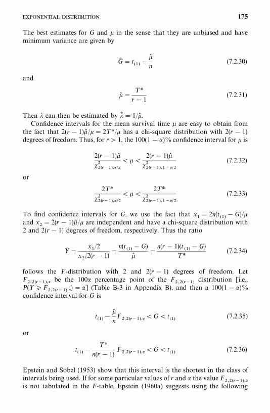
The best estimates for G and � in the sense that they are unbiased and haveminimum variance are given by
G� � t��
���n
(7.2.30)
and
�� �T *
r� 1(7.2.31)
Then � can then be estimated by �� � 1/�� .Confidence intervals for the mean survival time � are easy to obtain from
the fact that 2(r� 1)�� /� � 2T */� has a chi-square distribution with 2(r� 1)degrees of freedom. Thus, for r� 1, the 100(1� )%confidence interval for � is
2(r� 1)���������� �
� � �2(r� 1)��
��������� �
(7.2.32)
or
2T *
�������� �
� � �2T *
��������� �
(7.2.33)
To find confidence intervals for G, we use the fact that x�� 2n(t
���G)/�
and x�� 2(r� 1)�� /� are independent and have a chi-square distribution with
2 and 2(r� 1) degrees of freedom, respectively. Thus the ratio
Y �x�/2
x�/2(r� 1)
�n(t
���G)
���n(r� 1)(t
���G)
T *(7.2.34)
follows the F-distribution with 2 and 2(r� 1) degrees of freedom. LetF�������� be the 100 percentage point of the F
������distribution [i.e.,
P(Y �F��������) � ] (Table B-3 in Appendix B), and then a 100(1� )%
confidence interval for G is
t��
���nF
�������� �G� t��
(7.2.35)
or
t��
�T *
n(r� 1)F
�������� �G� t��
(7.2.36)
Epstein and Sobel (1953) show that this interval is the shortest in the class ofintervals being used. If for some particular values of r and the value F
��������is not tabulated in the F-table, Epstein (1960a) suggests using the following
175
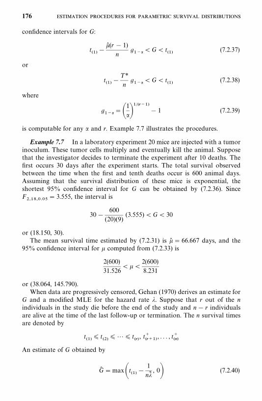
confidence intervals for G:
t��
��� (r� 1)
ng�� �G� t
��(7.2.37)
or
t��
�T *
ng�� �G� t
��(7.2.38)
where
g��� �
1
�� ���
� 1 (7.2.39)
is computable for any and r. Example 7.7 illustrates the procedures.
Example 7.7 In a laboratory experiment 20 mice are injected with a tumorinoculum. These tumor cells multiply and eventually kill the animal. Supposethat the investigator decides to terminate the experiment after 10 deaths. Thefirst occurs 30 days after the experiment starts. The total survival observedbetween the time when the first and tenth deaths occur is 600 animal days.Assuming that the survival distribution of these mice is exponential, theshortest 95% confidence interval for G can be obtained by (7.2.36). SinceF���������
� 3.555, the interval is
30�600
(20)(9)(3.555) �G� 30
or (18.150, 30).The mean survival time estimated by (7.2.31) is �� � 66.667 days, and the
95% confidence interval for � computed from (7.2.33) is
2(600)
31.526� � �
2(600)
8.231
or (38.064, 145.790).When data are progressively censored, Gehan (1970) derives an estimate for
G and a modified MLE for the hazard rate �. Suppose that r out of the nindividuals in the study die before the end of the study and n� r individualsare alive at the time of the last follow-up or termination. The n survival timesare denoted by
t��
� t��
� � � t��, t�
����, . . . , t�
��
An estimate of G obtained by
G� �max�t�� �1
n��, 0� (7.2.40)
176
and the variance of G� is
Var(G� ) �1
(n�� )� �1�1
r� 1� (7.2.41)
When n is large, G and Var(G� ) can be estimated by
G� � t��
(7.2.42)
and
Var� (G� ) �1
(n�� )�(7.2.43)
A modified MLE for � is
�� �r� 1
�����
t��
� �������
t���
� nt��
(7.2.44)
with variance
Var(�� ) ���
r� 1(7.2.45)
Any percentile of survival time t�may be estimated by equating S(t) to p and
solving for t��; that is, t�
���(log
�p)/�� �G� .
The following example illustrates the procedures.
Example 7.8 Suppose that 19 patients with brain tumor are followed in aclinical trial for a year. Their survival times in weeks are 3, 4, 6, 8, 8, 10, 12,16, 17, 30, 33, 3�, 8�, 13�, 21�, 26�, 35�, 44�, and 45�. In this case n� 19,r� 11, t
��� 3, ���
���t��
� 147, and �������
t���
� 195. The hazard rate � per weekand its variance may be estimated by (7.2.44) and (7.2.45) as
�� �10
147� 195� 19(3)� 0.035
and
Var� (�� ) �(0.035)�
10� 0.0001
The guarantee time G and its variance may then be estimated by (7.2.40) and(7.2.41):
177
G� �max �3�1
19�0.035, 0�� 1.496
and
Var� (G� ) �1
(19�0.035)� �1�1
10�� 2.487
Thus, after a guarantee time of approximately 1.5 weeks, the chance of deathper week is 0.035. The estimated median survival time is
t����
��log 0.5
0.035� 1.496� 21.3 weeks
The probability of surviving at least six months (or 26 weeks) is estimated by
S� (26) � exp[�0.35(26� 1.496)]� 0.424
7.3 WEIBULL DISTRIBUTION
The Weibull distribution has the density and survivorship functions
f (t) � ���t�� exp[�(�t)�]
S(t) � e���� t� 0, � � 0, � � 0 (7.3.1)
The MLE of the parameters � and � involves equations to be solved simulta-neously. Numerical methods such as the Newton—Raphson iterative procedure(7.1.13) can be applied. We begin with the case where no censored observationsare presented.
Let t�, t
�, . . . , t
�be the exact survival times of n individuals under investiga-
tion. If their survival times follow the Weibull distribution, the log-likelihoodfunction is
l(�, �) � n log � � n� log � ��
����
[(� � 1) log t�� ��t�
�] (7.3.2)
The MLE of � and � in (7.3.1) can be obtained by solving the following twoequations simultaneously:
n� �� �� �����
t��� � 0 (7.3.3)
n
��� n log �� �
�����
log t�� �� �� �
����
t��� (log�� � log t
�) � 0 (7.3.4)
178
Next, let us consider a typical laboratory experiment in which subjects areentered at the same time and the experiment is terminated after r of the nsubjects have failed (or after a fixed period of time T ). In both of these casesthe data collected are singly censored. The ordered survival data are
t��
� t��
� � � t��
� t�����
��� t���
If the time to failure follows the Weibull distribution with the density functiongiven in (7.3.1), the MLE of � and � may be obtained by solving the followingtwo equations simultaneously:
r� �� �� ��
����
t��� � (n� r)t��
���� 0 (7.3.5)
r
��� r log �� �
�����
log t�
� �� �� ��
����
t��� (log �� � log t
�) � (n� r)t��
��(log �� � log t
��)�� 0 (7.3.6)
When data are progressively censored, we have
t��
� t��
� � � t��, t�
����, . . . , t�
��
If the survival distribution is Weibull defined by (7.3.1), the log-likelihoodfunction is
l(�, �) � r log � � r� log � ��
����
[(� � 1)log t��
� ��t���]�
��
�����
��t����
(7.3.7)
The MLE of � and � may be obtained by solving the following two equationssimultaneously:
r� �� �� ��
����
t��� �
��
�����
t��
���� 0 (7.3.8)
r
��� r log �� �
�����
log t�� �� �� �
����
t��� (log �� � log t
�)
� �� �� ��
�����
t���� (log �� � log t�
�) � 0 (7.3.9)
The following example illustrates the use of available computer software toobtain the MLE of � and �.
179
Example 7.9 Referring to Example 7.5, for the observed survival data inthe file ‘‘EXAMPLE.DAT’’, we can use either SAS or BMDP to obtain theestimated parameters of the Weibull distribution. The codes given in Example7.5 can be used except that d� exponential in the SAS code must be changedto d�weibull and accel� exponential in BMDP code be changed to ac-cel�weibull. If SAS is used, the estimated parameters of the Weibull distribu-tion are
�� � exp(�INTERCEPT) and �� �1
SCALE
where INTERCEPT and SCALE are produced by SAS procedure LIFEREG.If BMDP is used,
�� � exp(�INTERCEPT) and �� �1
SCALE
where CONSTANT and SCALE are given by procedure 2L.
7.4 LOGNORMAL DISTRIBUTION
If the survival time T follows the lognormal distribution with density function
f (t) �1
t��2�exp��
1
2��(log t� �)�� (7.4.1)
the mean and the variance are exp(� �����) and [exp(��) � 1] exp(2� � ��),
respectively. Estimation of the two parameters � and �� has been investigatedeither by using (7.4.1) directly or by using the fact that Y � logT follows thenormal distribution with mean � and variance ��. In the following, we discussthe estimation of � and �� for samples with and without censored observations.
7.4.1 Estimation of � and �2 for Data without Censored Observations
Estimations of � and �� for complete samples by maximum likelihood methodshave been studied by many authors: for example, Cohen (1951) and Harter andMoore (1966). But the simplest way to obtain estimates of � and �� withoptimum properties is by considering the distribution of Y � logT. Let t
�,
t�, . . . , t
�be the survival times of n subjects. The MLE of � is the sample mean
of Y given by
�� �1
n
�����
log t�
(7.4.2)
The MLE of �� is
�� ��1
n ��
����
(log t�)� �
(�����
log t�)�
n � (7.4.3)
180
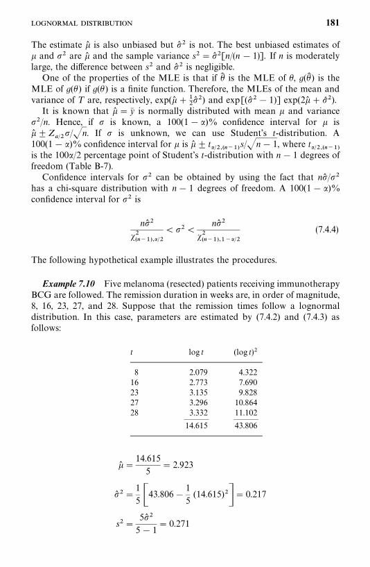
The estimate �� is also unbiased but �� � is not. The best unbiased estimates of� and �� are �� and the sample variance s�� �� �[n/(n� 1)]. If n is moderatelylarge, the difference between s� and �� � is negligible.
One of the properties of the MLE is that if ��� is the MLE of �� , g(��� ) is theMLE of g(�� ) if g(�� ) is a finite function. Therefore, the MLEs of the mean andvariance of T are, respectively, exp(�� ��
��� �) and exp[(�� �� 1)] exp(2�� � �� �).
It is known that �� � y� is normally distributed with mean � and variance��/n. Hence, if � is known, a 100(1� )% confidence interval for � is�� �Z
��/�n. If � is unknown, we can use Student’s t-distribution. A
100(1� )% confidence interval for � is �� � t� �����s/�n� 1, where t� �����
is the 100 /2 percentage point of Student’s t-distribution with n� 1 degrees offreedom (Table B-7).
Confidence intervals for �� can be obtained by using the fact that n�� /��
has a chi-square distribution with n� 1 degrees of freedom. A 100(1� )%confidence interval for �� is
n�� �������� �
� �� �n�� �
�������� �
(7.4.4)
The following hypothetical example illustrates the procedures.
Example 7.10 Five melanoma (resected) patients receiving immunotherapyBCG are followed. The remission duration in weeks are, in order of magnitude,8, 16, 23, 27, and 28. Suppose that the remission times follow a lognormaldistribution. In this case, parameters are estimated by (7.4.2) and (7.4.3) asfollows:
t log t (log t)�
8 2.079 4.32216 2.773 7.69023 3.135 9.82827 3.296 10.86428 3.332 11.102
——— ———14.615 43.806
�� �14.615
5� 2.923
�� ��1
5 �43.806�1
5(14.615)��� 0.217
s��5�� �5� 1
� 0.271
181
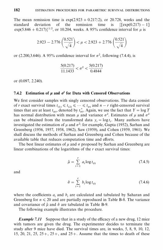
The mean remission time is exp(2.923� 0.217/2), or 20.728, weeks and thestandard deviation of the remission time is �[exp(0.217)� 1]exp(5.846� 0.217)�� �, or 10.204, weeks. A 95% confidence interval for � is
2.923� 2.776 �0.521
�4 �� � � 2.923� 2.776 �0.521
�4 �or (2.200,3.646). A 95% confidence interval for ��, following (7.4.4), is
5(0.217)11.1433
� �� �5(0.217)0.4844
or (0.097, 2.240).
7.4.2 Estimation of � and �2 for Data with Censored Observations
We first consider samples with singly censored observations. The data consistof r exact survival times t
��� t
��� � � t
��and n� r right-censored survival
times that are at least t��, denoted by t�
��. Again, we use the fact that Y � logT
has normal distribution with mean � and variance ��. Estimates of � and ��
can be obtained from the transformed data y�� log t
�. Many authors have
investigated the estimation of � and ��: for example, Gupta (1952), Sarhan andGreenberg (1956, 1957, 1958, 1962), Saw (1959), and Cohen (1959, 1961). Weshall discuss the methods of Sarhan and Greenberg and Cohen because of theavailable table that reduces computation time and efforts.
The best linear estimates of � and � proposed by Sarhan and Greenberg arelinear combinations of the logarithms of the r exact survival times:
�� ��
����
a�log t
��(7.4.5)
and
�� ��
����
b�log t
��(7.4.6)
where the coefficients a�and b
�are calculated and tabulated by Saharan and
Greenberg for n� 20 and are partially reproduced in Table B-8. The varianceand covariance of �� and �� are tabulated in Table B-9.
The following example illustrates the procedure.
Example 7.11 Suppose that in a study of the efficacy of a new drug, 12 micewith tumors are given the drug. The experimenter decides to terminate thestudy after 9 mice have died. The survival times are, in weeks, 5, 8, 9, 10, 12,15, 20, 21, 25, 25�, 25�, and 25�. Assume that the times to death of these
182
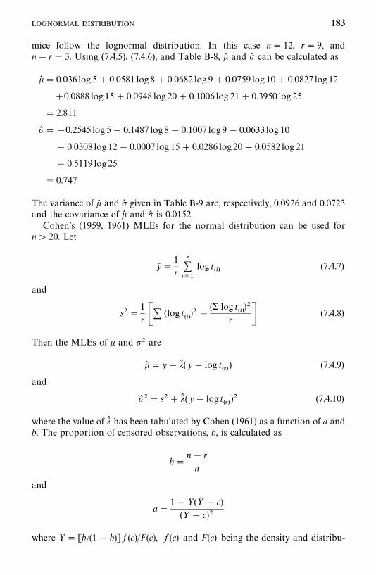
mice follow the lognormal distribution. In this case n� 12, r� 9, andn� r� 3. Using (7.4.5), (7.4.6), and Table B-8, �� and �� can be calculated as
�� � 0.036 log 5� 0.0581 log 8� 0.0682 log 9� 0.0759 log 10� 0.0827 log 12
�0.0888 log 15� 0.0948 log 20� 0.1006 log 21� 0.3950 log 25
� 2.811
�� � �0.2545 log 5� 0.1487 log 8� 0.1007 log 9� 0.0633 log 10
� 0.0308 log 12� 0.0007 log 15� 0.0286 log 20� 0.0582 log 21
� 0.5119 log 25
� 0.747
The variance of �� and �� given in Table B-9 are, respectively, 0.0926 and 0.0723and the covariance of �� and �� is 0.0152.
Cohen’s (1959, 1961) MLEs for the normal distribution can be used forn� 20. Let
y� �1
r
�����
log t��
(7.4.7)
and
s��1
r �� (log t��)� �
(� log t��)�
r � (7.4.8)
Then the MLEs of � and �� are
�� � y� � �� ( y� � log t��) (7.4.9)
and
�� � � s�� �� ( y� � log t��)� (7.4.10)
where the value of �� has been tabulated by Cohen (1961) as a function of a andb. The proportion of censored observations, b, is calculated as
b�n� r
n
and
a�1� Y (Y � c)
(Y � c)�
where Y � [b/(1 � b)] f (c)/F(c), f (c) and F(c) being the density and distribu-
183
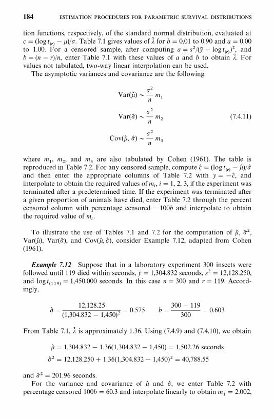
tion functions, respectively, of the standard normal distribution, evaluated atc� (log t
��� �)/�. Table 7.1 gives values of �� for b� 0.01 to 0.90 and a� 0.00
to 1.00. For a censored sample, after computing a� s�/(y� � log t��)�, and
b� (n� r)/n, enter Table 7.1 with these values of a and b to obtain �� . Forvalues not tabulated, two-way linear interpolation can be used.
The asymptotic variances and covariance are the following:
Var(�� ) ���
nm
�
Var(�� ) ���
nm
�(7.4.11)
Cov(�� , �� ) ���
nm
�
where m�, m
�, and m
�are also tabulated by Cohen (1961). The table is
reproduced in Table 7.2. For any censored sample, compute c� � (log t��
� �� )/��and then enter the appropriate columns of Table 7.2 with y� �c� , andinterpolate to obtain the required values of m
�, i� 1, 2, 3, if the experiment was
terminated after a predetermined time. If the experiment was terminated aftera given proportion of animals have died, enter Table 7.2 through the percentcensored column with percentage censored� 100b and interpolate to obtainthe required value of m
�.
To illustrate the use of Tables 7.1 and 7.2 for the computation of �� , �� �,Var(�� ), Var(�� ), and Cov(�� , �� ), consider Example 7.12, adapted from Cohen(1961).
Example 7.12 Suppose that in a laboratory experiment 300 insects werefollowed until 119 died within seconds, y� � 1,304.832 seconds, s�� 12,128.250,and log t
����� 1,450.000 seconds. In this case n� 300 and r� 119. Accord-
ingly,
a� �12,128.25
(1,304.832 � 1,450)�� 0.575 b�
300� 119
300� 0.603
From Table 7.1, �� is approximately 1.36. Using (7.4.9) and (7.4.10), we obtain
�� � 1,304.832� 1.36(1,304.832� 1,450) � 1,502.26 seconds
�� � � 12,128.250� 1.36(1,304.832� 1,450)�� 40,788.55
and �� �� 201.96 seconds.For the variance and covariance of �� and �� , we enter Table 7.2 with
percentage censored 100b� 60.3 and interpolate linearly to obtain m�� 2.002,
184
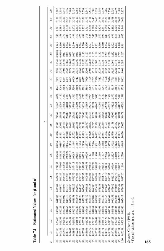
Tab
le7.1
Estim
ated
Value
sfor
��an
d�2
b
a.01
.02
.03
.04
.05
.06
.07
.08
.09
.10
.15
.20
.25
.30
.35
.40
.45
.50
.55
.60
.65
.70
.80
.90
.00
.010100
.020400
.030902
.041583
.052507
.063627
.074953
.086488
.09824
.11020
.17342
.24268
.31862
.4021
.4941
.5961
.7096
0.8368
0.9808
1.145
1.336
1.561
2.176
3.282
.05
.010551
.021294
.032225
.043350
.054670
.066189
.077909
.089834
.10197
.11431
.17935
.25033
.32793
.4130
.5066
.6101
.7252
0.8540
0.9994
1.166
1.358
1.585
2.203
3.314
.10
.010950
.022082
.033398
.044902
.056596
.068483
.080568
.092852
.10534
.11804
.18479
.25741
.33662
.4233
.5184
.6234
.7400
0.8703
1.017
1.185
1.379
1.608
2.229
3.345
.15
.011310
.022798
.034466
.046318
.058356
.070586
.038009
.095629
.10845
.12148
.18985
.26405
.34480
.4330
.5296
.6361
.7542
0.8860
1.035
1.204
1.400
1.630
2.255
3.376
.20
.011642
.023459
.035453
.047629
.059990
.072539
.085280
.098216
.11135
.12469
.19460
.27031
.35255
.4422
.5403
.6483
.7678
0.9012
1.051
1.222
1.419
1.651
2.280
3.405
.25
.011952
.024076
.036377
.048858
.061522
.074372
.087413
.10065
.11408
.12772
.19910
.27626
.35993
.4510
.5506
.6600
.7810
0.9158
1.067
1.240
1.439
1.672
2.305
3.435
.30
.012243
.024658
.037249
.050018
.062969
.076106
.089433
.10295
.11667
.13059
.20338
.28193
.36700
.4595
.5604
6.713
.7937
0.9300
1.083
1.257
1.457
1.693
2.329
3.464
.35
.012520
.025211
.038077
.051120
.064345
.077756
.091355
.10515
.11914
.13333
.20747
.28737
.37379
.4676
.5699
.6821
.8060
0.9437
1.098
1.274
1.476
1.713
2.353
3.492
.40
.012784
.025738
.038866
.052173
.065660
.079332
.093193
.10725
.12150
.13595
.21139
.29260
.38033
.4755
.5791
.6927
.8179
0.9570
1.113
1.290
1.494
1.732
2.376
3.520
.45
.013036
.026243
.039624
.053182
.066921
.080845
.094958
.10926
.12377
.13847
.21517
.29765
.38665
.4831
.5880
.7029
.8295
0.9700
1.127
1.306
1.511
1.751
2.399
3.547
.50
.013279
.026728
.040352
.054153
.068135
.082301
.096657
.11121
.12595
.14090
.21882
.30253
.39276
.4904
.5967
.7129
.8408
0.9826
1.141
1.321
1.528
1.770
2.421
3.575
.55
.013513
.027196
.041054
.055089
.069306
.083708
.098298
.11308
.12806
.14325
.22235
.30725
.39870
.4976
.6051
.7225
.8517
0.9950
1.155
1.337
1.545
1.788
2.443
3.601
.60
.013739
.027649
.041733
.055995
.070439
.085068
.099887
.11490
.13011
.14552
.22578
.31184
.40447
.5045
.6133
.7320
.8625
1.007
1.169
1.351
1.561
1.806
2.465
3.628
.65
.013958
.028087
.042391
.056874
.071538
.086388
.10143
.11666
.13209
.14773
.22910
.31630
.41008
.5114
.6213
.7412
.8729
1.019
1.182
1.366
1.577
1.824
2.486
3.654
.70
.014171
.028513
.043030
.057726
.072605
.087670
.10292
.11837
.13402
.14987
.23234
.32065
.41555
.5180
.6291
.7502
.8832
1.030
1.195
1.380
1.593
1.841
2.507
3.679
.75
.014378
.028927
.043652
.058556
.073643
.088917
.10438
.12004
.13590
.15196
.23550
.32489
.42090
.5245
.6367
.7590
.8932
1.042
1.207
1.394
1.608
1.858
2.528
3.705
.80
.014579
.029330
.044258
.059364
.074655
.090133
.10580
.12167
.13773
.15400
.23858
.32903
.42612
.5308
.6441
.7676
.9031
1.053
1.220
1.408
1.624
1.875
2.548
3.730
.85
.014755
.029723
.044848
.060153
.075642
.901319
.10719
.12325
.13952
.15599
.24158
.33307
.43122
.5370
.6515
.7761
.9127
1.064
1.232
1.422
1.639
1.892
2.568
3.754
.90
.014967
.030107
.045425
.060923
.076606
.092477
.10854
.12480
.14126
.15793
.24452
.33703
.43622
.5430
.6586
.7844
.9222
1.074
1.244
1.435
1.653
1.908
2.588
3.779
.95
.015154
.030483
.045989
.061676
.077549
.0093611
.10987
.12632
.14297
.15983
.24740
.34091
.44112
.5490
.6656
.7925
.9314
1.085
1.255
1.448
1.668
1.924
2.607
3.803
1.00
.015338
.030850
.046540
.062413
.078471
.094720
.11116
.12780
.14465
.16170
.25022
.34471
.44592
.5548
.6724
.8005
.9406
1.095
1.267
1.461
1.682
1.940
2.626
3.827
Source:Cohen
(1961).
Forallvalues
0�a
�1,
��
0.
185
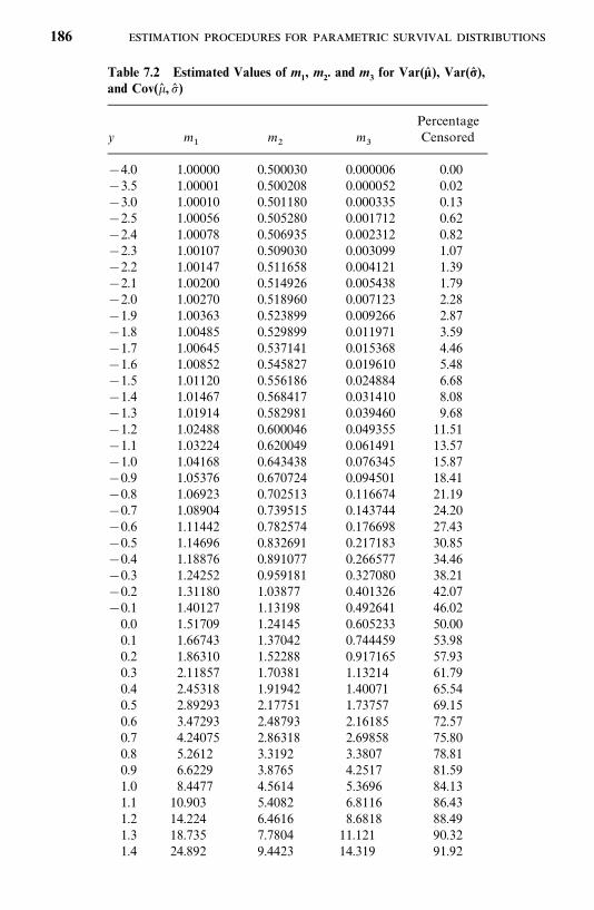
Table 7.2 Estimated Values of m1, m2. and m3 for Var(�� ), Var(�� ),and Cov(�� ,�� )
Percentagey m
�m
�m
�Censored
�4.0 1.00000 0.500030 0.000006 0.00�3.5 1.00001 0.500208 0.000052 0.02�3.0 1.00010 0.501180 0.000335 0.13�2.5 1.00056 0.505280 0.001712 0.62�2.4 1.00078 0.506935 0.002312 0.82�2.3 1.00107 0.509030 0.003099 1.07�2.2 1.00147 0.511658 0.004121 1.39�2.1 1.00200 0.514926 0.005438 1.79�2.0 1.00270 0.518960 0.007123 2.28�1.9 1.00363 0.523899 0.009266 2.87�1.8 1.00485 0.529899 0.011971 3.59�1.7 1.00645 0.537141 0.015368 4.46�1.6 1.00852 0.545827 0.019610 5.48�1.5 1.01120 0.556186 0.024884 6.68�1.4 1.01467 0.568417 0.031410 8.08�1.3 1.01914 0.582981 0.039460 9.68�1.2 1.02488 0.600046 0.049355 11.51�1.1 1.03224 0.620049 0.061491 13.57�1.0 1.04168 0.643438 0.076345 15.87�0.9 1.05376 0.670724 0.094501 18.41�0.8 1.06923 0.702513 0.116674 21.19�0.7 1.08904 0.739515 0.143744 24.20�0.6 1.11442 0.782574 0.176698 27.43�0.5 1.14696 0.832691 0.217183 30.85�0.4 1.18876 0.891077 0.266577 34.46�0.3 1.24252 0.959181 0.327080 38.21�0.2 1.31180 1.03877 0.401326 42.07�0.1 1.40127 1.13198 0.492641 46.020.0 1.51709 1.24145 0.605233 50.000.1 1.66743 1.37042 0.744459 53.980.2 1.86310 1.52288 0.917165 57.930.3 2.11857 1.70381 1.13214 61.790.4 2.45318 1.91942 1.40071 65.540.5 2.89293 2.17751 1.73757 69.150.6 3.47293 2.48793 2.16185 72.570.7 4.24075 2.86318 2.69858 75.800.8 5.2612 3.3192 3.3807 78.810.9 6.6229 3.8765 4.2517 81.591.0 8.4477 4.5614 5.3696 84.131.1 10.903 5.4082 6.8116 86.431.2 14.224 6.4616 8.6818 88.491.3 18.735 7.7804 11.121 90.321.4 24.892 9.4423 14.319 91.92
186
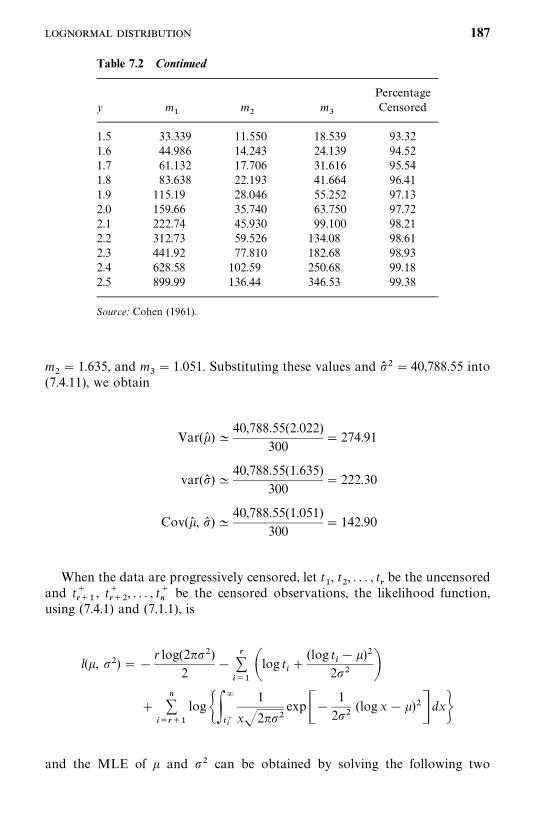
Table 7.2 Continued
Percentagey m
�m
�m
�Censored
1.5 33.339 11.550 18.539 93.321.6 44.986 14.243 24.139 94.521.7 61.132 17.706 31.616 95.541.8 83.638 22.193 41.664 96.411.9 115.19 28.046 55.252 97.132.0 159.66 35.740 63.750 97.722.1 222.74 45.930 99.100 98.212.2 312.73 59.526 134.08 98.612.3 441.92 77.810 182.68 98.932.4 628.58 102.59 250.68 99.182.5 899.99 136.44 346.53 99.38
Source: Cohen (1961).
m�� 1.635, and m
�� 1.051. Substituting these values and �� � � 40,788.55 into
(7.4.11), we obtain
Var(�� ) �40,788.55(2.022)
300� 274.91
var(�� ) �40,788.55(1.635)
300� 222.30
Cov(�� , �� ) �40,788.55(1.051)
300� 142.90
When the data are progressively censored, let t�, t
�, . . . , t
�be the uncensored
and t����
, t����
, . . . , t��
be the censored observations, the likelihood function,using (7.4.1) and (7.1.1), is
l(�, ��) ��r log(2���)
2�
������log t� �
(log t�� �)�
2�� ��
��
�����
log���
���
1
x�2���exp��
1
2��(logx� �)�� dx�
and the MLE of � and �� can be obtained by solving the following two
187
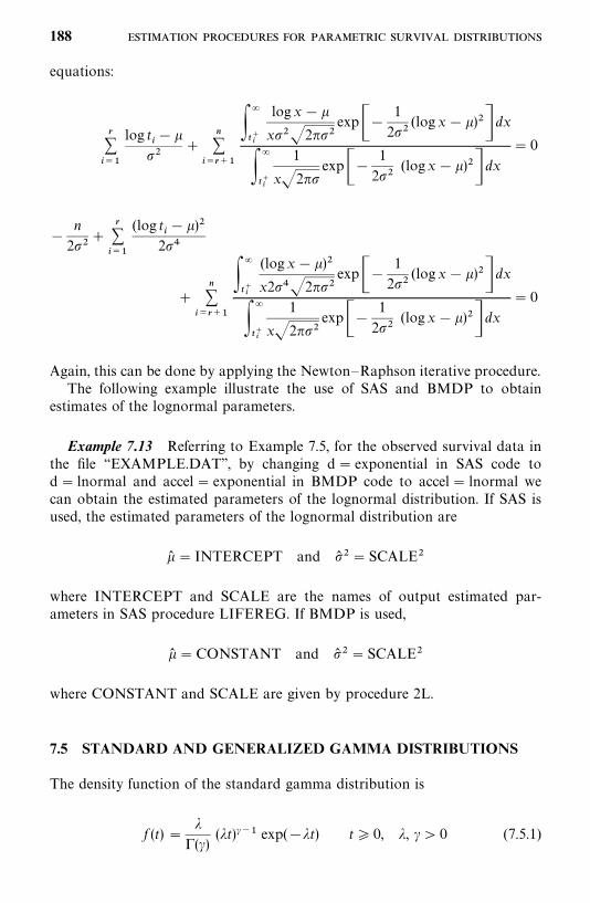
equations:
�����
log t�� �
���
��
�����
��
���
logx� �
x���2���exp��
1
2��(logx� �)�� dx
��
���
1
x�2��exp��
1
2��(logx� �)�� dx
� 0
�n
2���
�����
(log t�� �)�
2��
��
������
��
���
(logx� �)�
x2���2���exp��
1
2��(logx� �)�� dx
��
���
1
x�2���exp��
1
2��(logx� �)�� dx
� 0
Again, this can be done by applying the Newton—Raphson iterative procedure.The following example illustrate the use of SAS and BMDP to obtain
estimates of the lognormal parameters.
Example 7.13 Referring to Example 7.5, for the observed survival data inthe file ‘‘EXAMPLE.DAT’’, by changing d� exponential in SAS code tod� lnormal and accel� exponential in BMDP code to accel� lnormal wecan obtain the estimated parameters of the lognormal distribution. If SAS isused, the estimated parameters of the lognormal distribution are
�� � INTERCEPT and �� �� SCALE�
where INTERCEPT and SCALE are the names of output estimated par-ameters in SAS procedure LIFEREG. If BMDP is used,
�� �CONSTANT and �� ��SCALE�
where CONSTANT and SCALE are given by procedure 2L.
7.5 STANDARD AND GENERALIZED GAMMA DISTRIBUTIONS
The density function of the standard gamma distribution is
f (t) ��
�(�)(�t)�� exp(��t) t� 0, �, � � 0 (7.5.1)
188
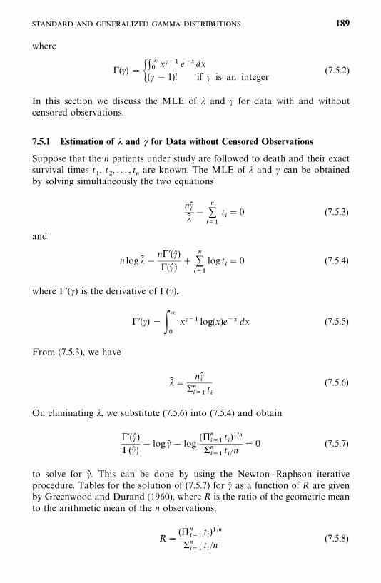
where
�(�) �����x�� e� dx
(� � 1)! if � is an integer(7.5.2)
In this section we discuss the MLE of � and � for data with and withoutcensored observations.
7.5.1 Estimation of � and � for Data without Censored Observations
Suppose that the n patients under study are followed to death and their exactsurvival times t
�, t
�, . . . , t
�are known. The MLE of � and � can be obtained
by solving simultaneously the two equations
n����
��
����
t�� 0 (7.5.3)
and
n log �� �n�(�� )�(�� )
��
����
log t�� 0 (7.5.4)
where �(�) is the derivative of �(�),
�(�) ���
�
x�� log(x)e� dx (7.5.5)
From (7.5.3), we have
�� �n��
�����
t�
(7.5.6)
On eliminating �, we substitute (7.5.6) into (7.5.4) and obtain
�(�� )�(�� )
� log �� � log(��
���t�)� �
�����
t�/n
� 0 (7.5.7)
to solve for �� . This can be done by using the Newton—Raphson iterativeprocedure. Tables for the solution of (7.5.7) for �� as a function of R are givenby Greenwood and Durand (1960), where R is the ratio of the geometric meanto the arithmetic mean of the n observations:
R�(��
���t�)� �
�����
t�/n
(7.5.8)
189

Wilk et al. (1962a) show that the relationship between �� and 1/(1�R) is linear.A table of �� values of as a function of 1/(1�R) given in their paper isreproduced in Table B-10. Thus if R and 1/(1�R) are computed from thesample, a MLE of � can be found from Table B-10. For values not tabulated,linear interpolation can be used. Having �� so determined, �� can be obtainedfrom (7.5.6).
In the method of moments (Fisher, 1922), the estimators are obtainedsimply by equating the population mean and variance to the sample mean andvariance. The moment estimators of � and � are
�*������
t�
�����
(t�� t� )�
(7.5.9)
and
�*�(��
���t�)�
n�����
(t�� t� )�
(7.5.10)
Both types of estimators give biased estimates. The moment estimators areeasy to calculate but are inefficient in the sense that their variances are largerthan the variance of the MLE. To reduce the bias, Lilliefors (1971) suggestscorrection factors for these two types of estimators. The corrected MLE of �and � are, respectively,
����
��1� 3/n
(7.5.11)
and
����
���t� �1�
1
n���� (7.5.12)
The corrected moments estimators of � and � are
�*��
�*1� 2/n
�3
n(7.5.13)
and
�*��
�*�t �1�
1
n�*�� (7.5.14)
Lilliefors shows by the Monte Carlo method that the corrected MLE andthe method-of-moment estimates are approximately unbiased. In addition, aslong as � � 2, the corrected moments estimators have no more bias than thecorrected MLE and for n� 10 have considerably less bias. For n� 10, 20 and� � 2, the variance is close to that of the MLE.
190
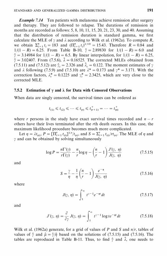
Example 7.14 Ten patients with melanoma achieve remission after surgeryand therapy. They are followed to relapse. The durations of remission inmonths are recorded as follows: 5, 8, 10, 11, 15, 20, 21, 23, 30, and 40. Assumingthat the distribution of remission duration is standard gamma, we firstcalculate the MLE of � and � according to Wilk et al. (1962a). To compute R,we obtain ��
���t�� 183 and (��
���t�)� �� � 15.43. Therefore R� 0.84 and
1/(1�R) � 6.25. From Table B-10, �� � 2.89830 for 1/(1�R) � 6.0 and�� � 3.14984 for 1/(1�R) � 6.5. By linear interpolation, for 1/(1�R) � 6.25,�� � 3.02407. From (7.5.6), �� � 0.16525. The corrected MLEs obtained from(7.5.11) and (7.5.12) are ��
�� 2.326 and ��
�� 0.122. The moment estimates of �
and � following (7.5.9) and (7.5.10) are �*� 0.173 and �*� 3.171. With thecorrection factors, �*
�� 0.1225 and �*
�� 2.3425, which are very close to the
corrected MLE.
7.5.2 Estimation of � and � for Data with Censored Observations
When data are singly censored, the survival times can be ordered as
t��
� t��
� � � t��
� t�����
��� t���
where r persons in the study have exact survival times recorded and n� rothers have their lives terminated after the rth death occurs. In this case, themaximum likelihood procedure becomes much more complicated.
Let � � �t��, P� [��
���t��]� �/t
��, and S� ��
���t��/rt
��. The MLE of � and
� and can be obtained by solving simultaneously
logP�n�(�)r�(�)
�n
rlog � ��
n
r� 1�
J(�, �)J(�, �)
(7.5.15)
and
S����
1
� �n
r� 1�
eJ(�, �)
(7.5.16)
where
J(�, �) � ��
�
t��e� dt (7.5.17)
and
J (�, �) ����J(�, �) � �
�
�
t�� log te�dt (7.5.18)
Wilk et al. (1962a) generate, for a grid of values of P and S and n/r, tables ofvalues of �� and �� � �� /�� based on the solutions of (7.5.15) and (7.5.16). Thetables are reproduced in Table B-11. Thus, to find �� and �� , one needs to
191
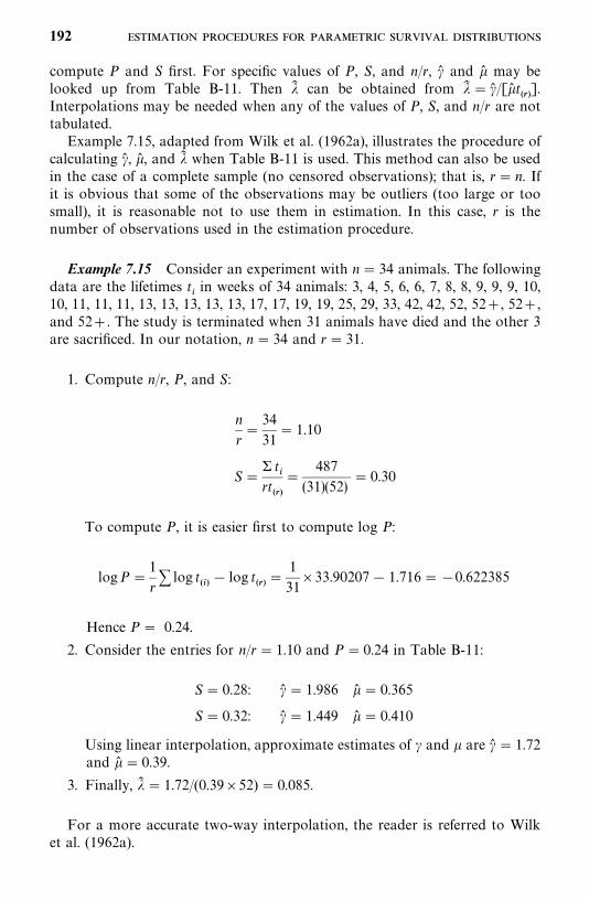
compute P and S first. For specific values of P, S, and n/r, �� and �� may belooked up from Table B-11. Then �� can be obtained from �� � �� /[�� t
��].
Interpolations may be needed when any of the values of P, S, and n/r are nottabulated.
Example 7.15, adapted from Wilk et al. (1962a), illustrates the procedure ofcalculating �� , �� , and �� when Table B-11 is used. This method can also be usedin the case of a complete sample (no censored observations); that is, r� n. Ifit is obvious that some of the observations may be outliers (too large or toosmall), it is reasonable not to use them in estimation. In this case, r is thenumber of observations used in the estimation procedure.
Example 7.15 Consider an experiment with n� 34 animals. The followingdata are the lifetimes t
�in weeks of 34 animals: 3, 4, 5, 6, 6, 7, 8, 8, 9, 9, 9, 10,
10, 11, 11, 11, 13, 13, 13, 13, 13, 17, 17, 19, 19, 25, 29, 33, 42, 42, 52, 52�, 52�,and 52�. The study is terminated when 31 animals have died and the other 3are sacrificed. In our notation, n� 34 and r� 31.
1. Compute n/r, P, and S:
n
r�
34
31� 1.10
S�� t
�rt
��
�487
(31)(52)� 0.30
To compute P, it is easier first to compute log P:
logP�1
r� log t
��� log t
���
1
31�33.90207� 1.716��0.622385
Hence P� 0.24.
2. Consider the entries for n/r� 1.10 and P� 0.24 in Table B-11:
S� 0.28: �� � 1.986 �� � 0.365
S� 0.32: �� � 1.449 �� � 0.410
Using linear interpolation, approximate estimates of � and � are �� � 1.72and �� � 0.39.
3. Finally, �� � 1.72/(0.39�52) � 0.085.
For a more accurate two-way interpolation, the reader is referred to Wilket al. (1962a).
192
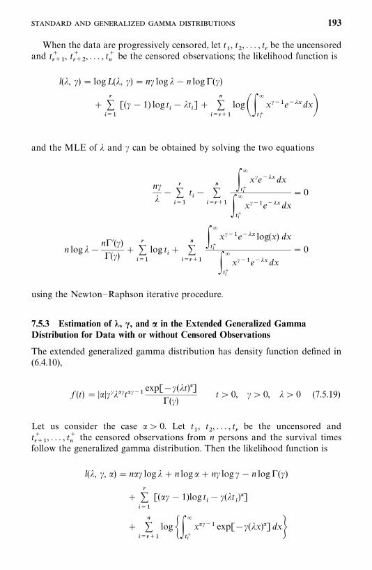
When the data are progressively censored, let t�, t
�, . . . , t
�be the uncensored
and t����
, t����
, . . . , t��be the censored observations; the likelihood function is
l(�, �) � log L (�, �) � n� log � � n log�(�)
��
����
[(� � 1) log t�� �t
�]�
��
�����
log���
���
x��e��dx�
and the MLE of � and � can be obtained by solving the two equations
n��
��
����
t��
��
�����
��
���x�e�� dx
��
���x��e�� dx
� 0
n log � �n�(�)�(�)
��
����
log t��
��
�����
��
���x��e�� log(x) dx
��
���x��e�� dx
� 0
using the Newton—Raphson iterative procedure.
7.5.3 Estimation of �, �, and � in the Extended Generalized GammaDistribution for Data with or without Censored Observations
The extended generalized gamma distribution has density function defined in(6.4.10),
f (t) � �����t���exp[��(�t)�]
�(�)t� 0, � � 0, � � 0 (7.5.19)
Let us consider the case � 0. Let t�, t
�, . . . , t
�be the uncensored and
t����
, . . . , t��
the censored observations from n persons and the survival timesfollow the generalized gamma distribution. Then the likelihood function is
l(�, �, ) � n � log � � n log � n� log � � n log�(�)
��
����
[( � � 1)log t�� �(�t
�)�]
��
������
log���
���x��� exp[��(�x)�] dx�
193
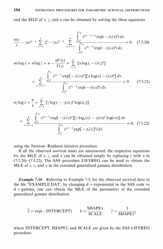
and the MLE of �, �, and can be obtained by solving the three equations
n ��
� � ����
����
t��� � ���
��
�����
��
���x����� exp(��(�x)�) dx
��
���x��� exp(��(�x)�) dx
� 0 (7.5.20)
n log � � n log � � n�n�(�)�(�)
��
����
[ log t�� (�t
�)�]
��
������
��
���x��� exp[��(�x)�][ log(x) � (�x)�] dx
��
���x��� exp(��(�x)�) dx
� 0 (7.5.21)
n� log � �n
�
�����
[� log t�� �(�t
�)� log(�t
�)]
��
������
��
���x��� exp[��(�x)�][� log
�(x) � �(�x)� log(�x)] dx
��
���x��� exp[��(�x]�) dx
� 0 (7.5.22)
using the Newton—Raphson iterative procedure.If all the observed survival times are uncensored, the respective equations
for the MLE of �, �, and can be obtained simply by replacing r with n in(7.5.20)—(7.5.22). The SAS procedure LIFEREG can be used to obtain theMLE of �, �, and in the extended generalized gamma distribution.
Example 7.16 Referring to Example 7.5, for the observed survival data inthe file ‘‘EXAMPLE.DAT‘, by changing d� exponential in the SAS code tod� gamma, one can obtain the MLE of the parameters of the extendedgeneralized gamma distribution:
�� � exp(�INTERCEPT) � �SHAPE1
SCALE�� �
1
SHAPE1�
where INTERCEPT, SHAPE1, and SCALE are given by the SAS LIFEREGprocedure.
194
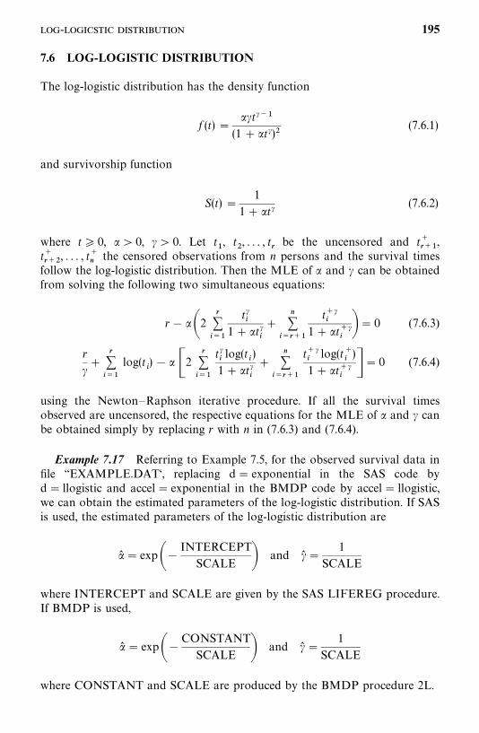
7.6 LOG-LOGISTIC DISTRIBUTION
The log-logistic distribution has the density function
f (t) � �t��
(1 � t�)�(7.6.1)
and survivorship function
S(t) �1
1� t�(7.6.2)
where t� 0, � 0, � � 0. Let t�, t
�, . . . , t
�be the uncensored and t�
���,
t����
, . . . , t��
the censored observations from n persons and the survival timesfollow the log-logistic distribution. Then the MLE of and � can be obtainedfrom solving the following two simultaneous equations:
r� �2�
����
t��
1� t��
��
������
t���
1� t����� 0 (7.6.3)
r
��
�����
log(t�) � �2
�����
t��log(t
�)
1� t��
��
������
t���
log(t��)
1� t����� 0 (7.6.4)
using the Newton—Raphson iterative procedure. If all the survival timesobserved are uncensored, the respective equations for the MLE of and � canbe obtained simply by replacing r with n in (7.6.3) and (7.6.4).
Example 7.17 Referring to Example 7.5, for the observed survival data infile ‘‘EXAMPLE.DAT‘, replacing d� exponential in the SAS code byd� llogistic and accel� exponential in the BMDP code by accel� llogistic,we can obtain the estimated parameters of the log-logistic distribution. If SASis used, the estimated parameters of the log-logistic distribution are
� � exp��INTERCEPT
SCALE � and �� �1
SCALE
where INTERCEPT and SCALE are given by the SAS LIFEREG procedure.If BMDP is used,
� � exp��CONSTANT
SCALE � and �� �1
SCALE
where CONSTANT and SCALE are produced by the BMDP procedure 2L.
- 195
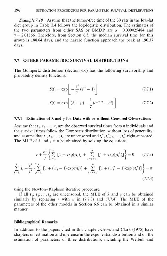
Example 7.18 Assume that the tumor-free time of the 30 rats in the low-fatdiet group in Table 3.4 follows the log-logistic distribution. The estimates ofthe two parameters from either SAS or BMDP are � � 0.000025484 and�� � 2.01866. Therefore, from Section 6.5, the median survival time for thisgroup is 188.64 days, and the hazard function approach the peak at 190.37days.
7.7 OTHER PARAMETRIC SURVIVAL DISTRIBUTIONS
The Gompertz distribution (Section 6.6) has the following survivorship andprobability density functions:
S(t) � exp��e��(e�� � 1)� (7.7.1)
f (t) � exp�(� � �t) �1
�(e���� � e�)� (7.7.2)
7.7.1 Estimation of � and � for Data with or without Censored Observations
Assume that t�, t
�, . . . , t
�are the observed survival times from n individuals and
the survival times follow the Gompertz distribution, without loss of generality,and assume that t
�, t
�, . . . , t
�are uncensored and t�
�, t�
���, . . . , t�
�right-censored.
The MLE of � and � can be obtained by solving the equations
r�e�� �
�����
[1� exp(�t�)] �
��
�����
[1� exp(�t��)]�� 0 (7.7.3)
�����
t��e��� �
�����
[1� (�t�� 1) exp(�t
�)] �
��
�����
[1� (�t��
� 1) exp(�t��)]�� 0
(7.7.4)
using the Newton—Raphson iterative procedure.If all t
�, t
�, . . . , t
�are uncensored, the MLE of � and � can be obtained
similarly by replacing r with n in (7.7.3) and (7.7.4). The MLE of theparameters of the other models in Section 6.6 can be obtained in a similarmanner.
Bibliographical Remarks
In addition to the papers cited in this chapter, Gross and Clark (1975) havechapters on estimation and inference in the exponential distribution and on theestimation of parameters of three distributions, including the Weibull and
196
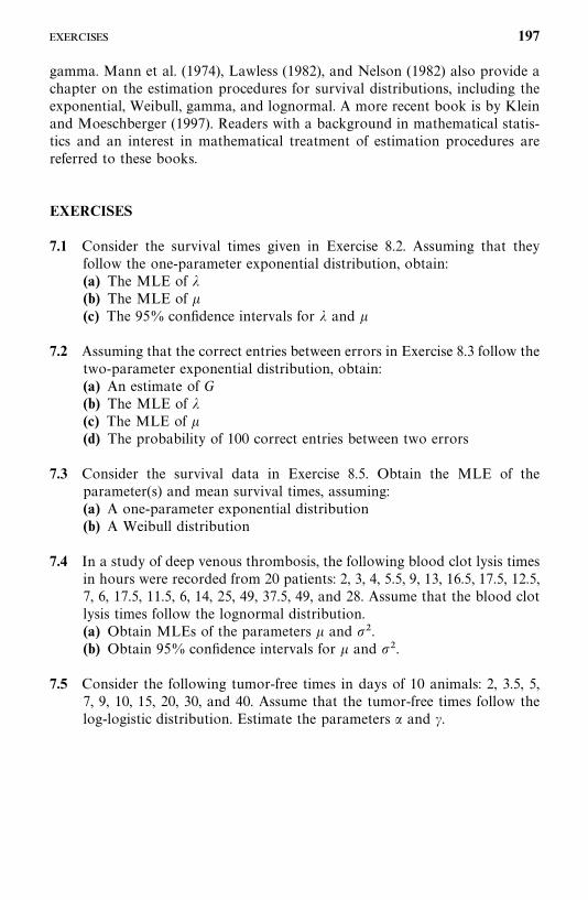
gamma. Mann et al. (1974), Lawless (1982), and Nelson (1982) also provide achapter on the estimation procedures for survival distributions, including theexponential, Weibull, gamma, and lognormal. A more recent book is by Kleinand Moeschberger (1997). Readers with a background in mathematical statis-tics and an interest in mathematical treatment of estimation procedures arereferred to these books.
EXERCISES
7.1 Consider the survival times given in Exercise 8.2. Assuming that theyfollow the one-parameter exponential distribution, obtain:(a) The MLE of �(b) The MLE of �(c) The 95% confidence intervals for � and �
7.2 Assuming that the correct entries between errors in Exercise 8.3 follow thetwo-parameter exponential distribution, obtain:(a) An estimate of G(b) The MLE of �(c) The MLE of �(d) The probability of 100 correct entries between two errors
7.3 Consider the survival data in Exercise 8.5. Obtain the MLE of theparameter(s) and mean survival times, assuming:(a) A one-parameter exponential distribution(b) A Weibull distribution
7.4 In a study of deep venous thrombosis, the following blood clot lysis timesin hours were recorded from 20 patients: 2, 3, 4, 5.5, 9, 13, 16.5, 17.5, 12.5,7, 6, 17.5, 11.5, 6, 14, 25, 49, 37.5, 49, and 28. Assume that the blood clotlysis times follow the lognormal distribution.(a) Obtain MLEs of the parameters � and ��.(b) Obtain 95% confidence intervals for � and ��.
7.5 Consider the following tumor-free times in days of 10 animals: 2, 3.5, 5,7, 9, 10, 15, 20, 30, and 40. Assume that the tumor-free times follow thelog-logistic distribution. Estimate the parameters and �.
197
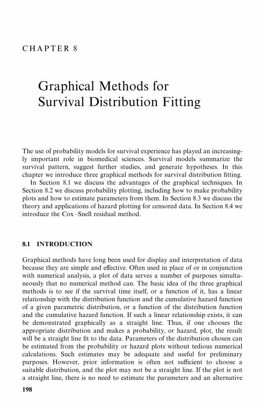
CHAPTER 8
Graphical Methods forSurvival Distribution Fitting
The use of probability models for survival experience has played an increasing-ly important role in biomedical sciences. Survival models summarize thesurvival pattern, suggest further studies, and generate hypotheses. In thischapter we introduce three graphical methods for survival distribution fitting.
In Section 8.1 we discuss the advantages of the graphical techniques. InSection 8.2 we discuss probability plotting, including how to make probabilityplots and how to estimate parameters from them. In Section 8.3 we discuss thetheory and applications of hazard plotting for censored data. In Section 8.4 weintroduce the Cox—Snell residual method.
8.1 INTRODUCTION
Graphical methods have long been used for display and interpretation of databecause they are simple and effective. Often used in place of or in conjunctionwith numerical analysis, a plot of data serves a number of purposes simulta-neously that no numerical method can. The basic idea of the three graphicalmethods is to see if the survival time itself, or a function of it, has a linearrelationship with the distribution function and the cumulative hazard functionof a given parametric distribution, or a function of the distribution functionand the cumulative hazard function. If such a linear relationship exists, it canbe demonstrated graphically as a straight line. Thus, if one chooses theappropriate distribution and makes a probability, or hazard, plot, the resultwill be a straight line fit to the data. Parameters of the distribution chosen canbe estimated from the probability or hazard plots without tedious numericalcalculations. Such estimates may be adequate and useful for preliminarypurposes. However, prior information is often not sufficient to choose asuitable distribution, and the plot may not be a straight line. If the plot is nota straight line, there is no need to estimate the parameters and an alternative
198
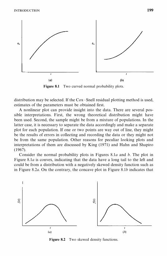
Figure 8.1 Two curved normal probability plots.
Figure 8.2 Two skewed density functions.
distribution may be selected. If the Cox—Snell residual plotting method is used,estimates of the parameters must be obtained first.
A nonlinear plot can provide insight into the data. There are several pos-sible interpretations. First, the wrong theoretical distribution might havebeen used. Second, the sample might be from a mixture of populations. In thelatter case, it is necessary to separate the data accordingly and make a separateplot for each population. If one or two points are way out of line, they mightbe the results of errors in collecting and recording the data or they might notbe from the same population. Other reasons for peculiar looking plots andinterpretations of them are discussed by King (1971) and Hahn and Shapiro(1967).
Consider the normal probability plots in Figures 8.1a and b. The plot inFigure 8.1a is convex, indicating that the data have a long tail to the left andcould be from a distribution with a negatively skewed density function such asin Figure 8.2a. On the contrary, the concave plot in Figure 8.1b indicates that
199
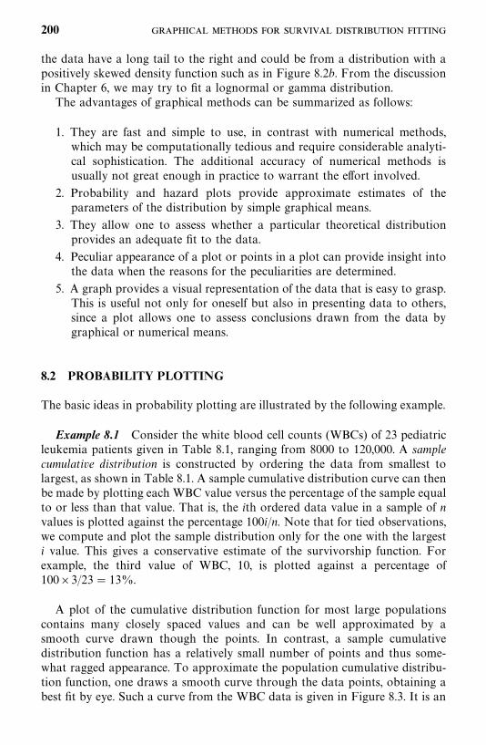
the data have a long tail to the right and could be from a distribution with apositively skewed density function such as in Figure 8.2b. From the discussionin Chapter 6, we may try to fit a lognormal or gamma distribution.
The advantages of graphical methods can be summarized as follows:
1. They are fast and simple to use, in contrast with numerical methods,which may be computationally tedious and require considerable analyti-cal sophistication. The additional accuracy of numerical methods isusually not great enough in practice to warrant the effort involved.
2. Probability and hazard plots provide approximate estimates of theparameters of the distribution by simple graphical means.
3. They allow one to assess whether a particular theoretical distributionprovides an adequate fit to the data.
4. Peculiar appearance of a plot or points in a plot can provide insight intothe data when the reasons for the peculiarities are determined.
5. A graph provides a visual representation of the data that is easy to grasp.This is useful not only for oneself but also in presenting data to others,since a plot allows one to assess conclusions drawn from the data bygraphical or numerical means.
8.2 PROBABILITY PLOTTING
The basic ideas in probability plotting are illustrated by the following example.
Example 8.1 Consider the white blood cell counts (WBCs) of 23 pediatricleukemia patients given in Table 8.1, ranging from 8000 to 120,000. A samplecumulative distribution is constructed by ordering the data from smallest tolargest, as shown in Table 8.1. A sample cumulative distribution curve can thenbe made by plotting each WBC value versus the percentage of the sample equalto or less than that value. That is, the ith ordered data value in a sample of nvalues is plotted against the percentage 100i/n. Note that for tied observations,we compute and plot the sample distribution only for the one with the largesti value. This gives a conservative estimate of the survivorship function. Forexample, the third value of WBC, 10, is plotted against a percentage of100�3/23� 13%.
A plot of the cumulative distribution function for most large populationscontains many closely spaced values and can be well approximated by asmooth curve drawn though the points. In contrast, a sample cumulativedistribution function has a relatively small number of points and thus some-what ragged appearance. To approximate the population cumulative distribu-tion function, one draws a smooth curve through the data points, obtaining abest fit by eye. Such a curve from the WBC data is given in Figure 8.3. It is an
200
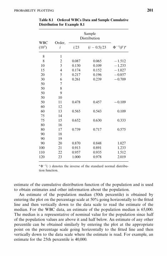
Table 8.1 Ordered WBCs Data and Sample CumulativeDistribution for Example 8.1
SampleDistribution
WBC Order,(10�) i i/23 (i � 0.5)/23 ���(F )�
8 18 2 0.087 0.065 �1.512
10 3 0.130 0.109 �1.23315 4 0.174 0.152 �1.02720 5 0.217 0.196 �0.85730 6 0.261 0.239 �0.70950 750 850 950 1050 11 0.478 0.457 �0.10960 1260 13 0.565 0.543 0.10975 1475 15 0.652 0.630 0.33380 1680 17 0.739 0.717 0.57590 1890 1990 20 0.870 0.848 1.027100 21 0.913 0.891 1.233110 22 0.957 0.935 1.512120 23 1.000 0.978 2.019
����( · ) denotes the inverse of the standard normal distribu-tion function.
estimate of the cumulative distribution function of the population and is usedto obtain estimates and other information about the population.
An estimate of the population median (50th percentile) is obtained byentering the plot on the percentage scale at 50%going horizontally to the fittedline and then vertically down to the data scale to read the estimate of themedian. For the WBC data, an estimate of the population median is 65,000.The median is a representative of nominal value for the population since halfof the population values are above it and half below. An estimate of any otherpercentile can be obtained similarly by entering the plot at the appropriatepoint on the percentage scale going horizontally to the fitted line and thenvertically down to the data scale where the estimate is read. For example, anestimate for the 25th percentile is 40,000.
201
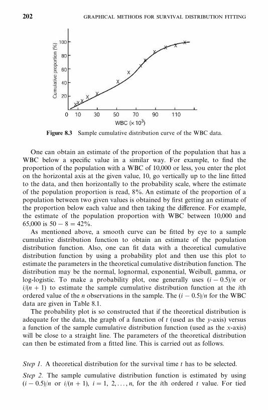
Figure 8.3 Sample cumulative distribution curve of the WBC data.
One can obtain an estimate of the proportion of the population that has aWBC below a specific value in a similar way. For example, to find theproportion of the population with a WBC of 10,000 or less, you enter the ploton the horizontal axis at the given value, 10, go vertically up to the line fittedto the data, and then horizontally to the probability scale, where the estimateof the population proportion is read, 8%. An estimate of the proportion of apopulation between two given values is obtained by first getting an estimate ofthe proportion below each value and then taking the difference. For example,the estimate of the population proportion with WBC between 10,000 and65,000 is 50� 8� 42%.
As mentioned above, a smooth curve can be fitted by eye to a samplecumulative distribution function to obtain an estimate of the populationdistribution function. Also, one can fit data with a theoretical cumulativedistribution function by using a probability plot and then use this plot toestimate the parameters in the theoretical cumulative distribution function. Thedistribution may be the normal, lognormal, exponential, Weibull, gamma, orlog-logistic. To make a probability plot, one generally uses (i� 0.5)/n ori/(n � 1) to estimate the sample cumulative distribution function at the ithordered value of the n observations in the sample. The (i� 0.5)/n for the WBCdata are given in Table 8.1.
The probability plot is so constructed that if the theoretical distribution isadequate for the data, the graph of a function of t (used as the y-axis) versusa function of the sample cumulative distribution function (used as the x-axis)will be close to a straight line. The parameters of the theoretical distributioncan then be estimated from a fitted line. This is carried out as follows.
Step 1. A theoretical distribution for the survival time t has to be selected.
Step 2. The sample cumulative distribution function is estimated by using(i� 0.5)/n or i/(n � 1), i� 1, 2, . . . , n, for the ith ordered t value. For tied
202
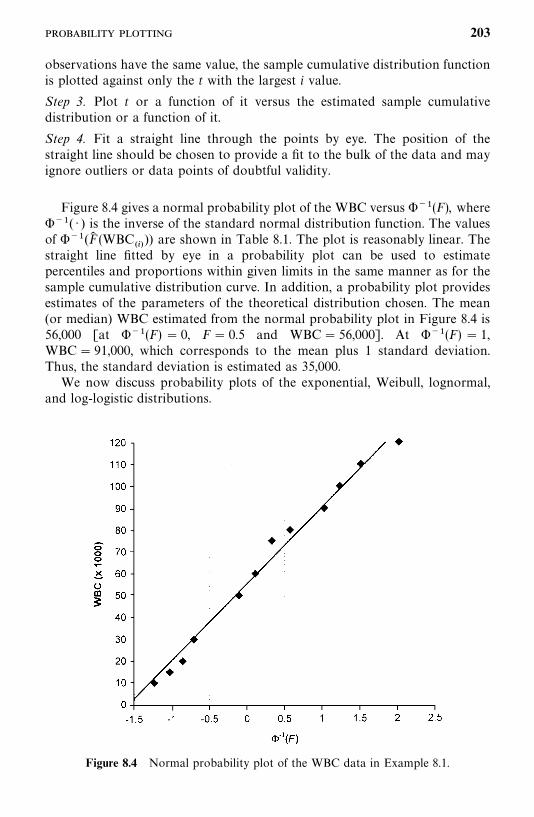
Figure 8.4 Normal probability plot of the WBC data in Example 8.1.
observations have the same value, the sample cumulative distribution functionis plotted against only the t with the largest i value.
Step 3. Plot t or a function of it versus the estimated sample cumulativedistribution or a function of it.
Step 4. Fit a straight line through the points by eye. The position of thestraight line should be chosen to provide a fit to the bulk of the data and mayignore outliers or data points of doubtful validity.
Figure 8.4 gives a normal probability plot of the WBC versus ���(F), where���( · ) is the inverse of the standard normal distribution function. The valuesof ���(F� (WBC
���)) are shown in Table 8.1. The plot is reasonably linear. The
straight line fitted by eye in a probability plot can be used to estimatepercentiles and proportions within given limits in the same manner as for thesample cumulative distribution curve. In addition, a probability plot providesestimates of the parameters of the theoretical distribution chosen. The mean(or median) WBC estimated from the normal probability plot in Figure 8.4 is56,000 [at ���(F) � 0, F� 0.5 and WBC� 56,000]. At ���(F) � 1,WBC� 91,000, which corresponds to the mean plus 1 standard deviation.Thus, the standard deviation is estimated as 35,000.
We now discuss probability plots of the exponential, Weibull, lognormal,and log-logistic distributions.
203
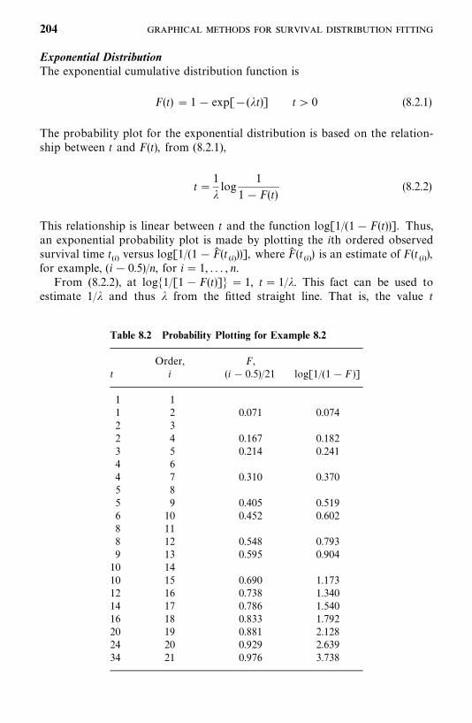
Table 8.2 Probability Plotting for Example 8.2
Order, F,t i (i � 0.5)/21 log[1/(1� F)]
1 11 2 0.071 0.0742 32 4 0.167 0.1823 5 0.214 0.2414 64 7 0.310 0.3705 85 9 0.405 0.5196 10 0.452 0.6028 118 12 0.548 0.7939 13 0.595 0.90410 1410 15 0.690 1.17312 16 0.738 1.34014 17 0.786 1.54016 18 0.833 1.79220 19 0.881 2.12824 20 0.929 2.63934 21 0.976 3.738
Exponential DistributionThe exponential cumulative distribution function is
F(t) � 1� exp[�(�t)] t� 0 (8.2.1)
The probability plot for the exponential distribution is based on the relation-ship between t and F(t), from (8.2.1),
t �1
�log
1
1�F(t)(8.2.2)
This relationship is linear between t and the function log[1/(1� F(t))]. Thus,an exponential probability plot is made by plotting the ith ordered observedsurvival time t
���versus log[1/(1�F� (t
���))], where F� (t
���) is an estimate of F(t
���),
for example, (i� 0.5)/n, for i � 1, . . . , n.From (8.2.2), at log�1/[1�F(t)]� � 1, t� 1/�. This fact can be used to
estimate 1/� and thus � from the fitted straight line. That is, the value t
204
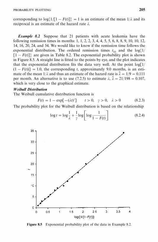
Figure 8.5 Exponential probability plot of the data in Example 8.2.
corresponding to log�1/[1�F(t)]� � 1 is an estimate of the mean 1/� and itsreciprocal is an estimate of the hazard rate �.
Example 8.2 Suppose that 21 patients with acute leukemia have thefollowing remission times in months: 1, 1, 2, 2, 3, 4, 4, 5, 5, 6, 8, 8, 9, 10, 10, 12,14, 16, 20, 24, and 34. We would like to know if the remission time follows theexponential distribution. The ordered remission times t
���and the log�1/
[1�F(t)]� are given in Table 8.2. The exponential probability plot is shownin Figure 8.5. A straight line is fitted to the points by eye, and the plot indicatesthat the exponential distribution fits the data very well. At the point log[1/(1�F(t))] � 1.0, the corresponding t, approximately 9.0 months, is an esti-mate of the mean 1/� and thus an estimate of the hazard rate is �� � 1/9� 0.111per month. An alternative is to use (7.2.5) to estimate �, �� � 21/198� 0.107,which is very close to the graphical estimate.
Weibull DistributionThe Weibull cumulative distribution function is
F(t) � 1� exp[�(�t)�] t� 0, � � 0, � � 0 (8.2.3)
The probability plot for the Weibull distribution is based on the relationship
log t� log1
��
1
�log�log
1
1�F(t)� (8.2.4)
205
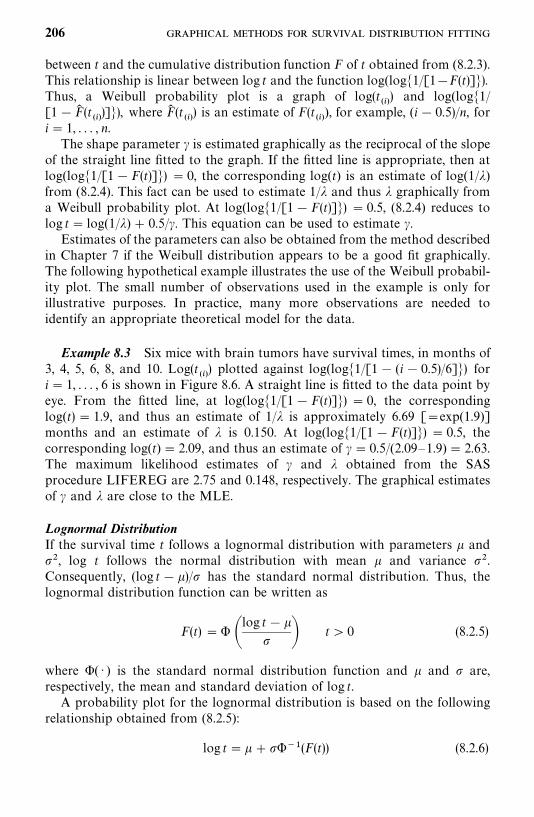
between t and the cumulative distribution function F of t obtained from (8.2.3).This relationship is linear between log t and the function log(log�1/[1�F(t)]�).Thus, a Weibull probability plot is a graph of log(t
���) and log(log�1/
[1�F� (t���)]�), where F� (t
���) is an estimate of F(t
���), for example, (i� 0.5)/n, for
i � 1, . . . , n.The shape parameter � is estimated graphically as the reciprocal of the slope
of the straight line fitted to the graph. If the fitted line is appropriate, then atlog(log�1/[1�F(t)]�) � 0, the corresponding log(t) is an estimate of log(1/�)from (8.2.4). This fact can be used to estimate 1/� and thus � graphically froma Weibull probability plot. At log(log�1/[1�F(t)]�) � 0.5, (8.2.4) reduces tolog t� log(1/�) � 0.5/�. This equation can be used to estimate �.
Estimates of the parameters can also be obtained from the method describedin Chapter 7 if the Weibull distribution appears to be a good fit graphically.The following hypothetical example illustrates the use of the Weibull probabil-ity plot. The small number of observations used in the example is only forillustrative purposes. In practice, many more observations are needed toidentify an appropriate theoretical model for the data.
Example 8.3 Six mice with brain tumors have survival times, in months of3, 4, 5, 6, 8, and 10. Log(t
���) plotted against log(log�1/[1� (i� 0.5)/6]�) for
i � 1, . . . , 6 is shown in Figure 8.6. A straight line is fitted to the data point byeye. From the fitted line, at log(log�1/[1� F(t)]�) � 0, the correspondinglog(t) � 1.9, and thus an estimate of 1/� is approximately 6.69 [�exp(1.9)]months and an estimate of � is 0.150. At log(log�1/[1�F(t)]�) � 0.5, thecorresponding log(t) � 2.09, and thus an estimate of � � 0.5/(2.09—1.9) � 2.63.The maximum likelihood estimates of � and � obtained from the SASprocedure LIFEREG are 2.75 and 0.148, respectively. The graphical estimatesof � and � are close to the MLE.
Lognormal DistributionIf the survival time t follows a lognormal distribution with parameters � and, log t follows the normal distribution with mean � and variance .Consequently, (log t��)/ has the standard normal distribution. Thus, thelognormal distribution function can be written as
F(t) �� �log t��
� t � 0 (8.2.5)
where �( · ) is the standard normal distribution function and � and are,respectively, the mean and standard deviation of log t.
A probability plot for the lognormal distribution is based on the followingrelationship obtained from (8.2.5):
log t �� ����(F(t)) (8.2.6)
206
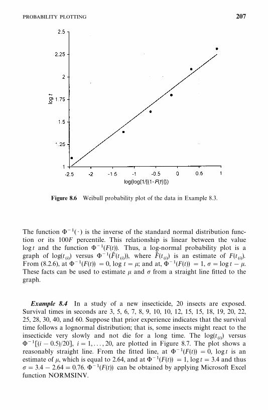
Figure 8.6 Weibull probability plot of the data in Example 8.3.
The function ���( · ) is the inverse of the standard normal distribution func-tion or its 100F percentile. This relationship is linear between the valuelog t and the function ���(F(t)). Thus, a log-normal probability plot is agraph of log(t
���) versus ���(F� (t
���)), where F� (t
���) is an estimate of F(t
���).
From (8.2.6), at ���(F(t)) � 0, log t� �; and at, ���(F(t)) � 1, � log t��.These facts can be used to estimate � and from a straight line fitted to thegraph.
Example 8.4 In a study of a new insecticide, 20 insects are exposed.Survival times in seconds are 3, 5, 6, 7, 8, 9, 10, 10, 12, 15, 15, 18, 19, 20, 22,25, 28, 30, 40, and 60. Suppose that prior experience indicates that the survivaltime follows a lognormal distribution; that is, some insects might react to theinsecticide very slowly and not die for a long time. The log(t
���) versus
���[(i � 0.5)/20], i� 1, . . . , 20, are plotted in Figure 8.7. The plot shows areasonably straight line. From the fitted line, at ���(F(t)) � 0, log t is anestimate of �, which is equal to 2.64, and at ���(F(t)) � 1, log t� 3.4 and thus� 3.4� 2.64� 0.76. ���(F(t)) can be obtained by applying Microsoft Excelfunction NORMSINV.
207
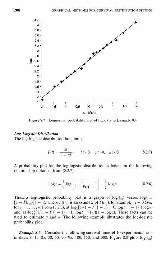
Figure 8.7 Lognormal probability plot of the data in Example 8.4.
Log-Logistic DistributionThe log-logistic distribution function is
F(t) �t�
1� t�t� 0, �� 0, � 0 (8.2.7)
A probability plot for the log-logistic distribution is based on the followingrelationship obtained from (8.2.7):
log t�1
�log �
1
1� F(t)� 1��
1
�log (8.2.8)
Thus, a log-logistic probability plot is a graph of log(t���) versus log(�1/
[1�F� (t���)]� � 1), where F� (t
���) is an estimate of F(t
���), for example, (i� 0.5)/n,
for i � 1, . . . , n. From (8.2.8), at log�[1/(1�F )] � 1� � 0, log t ��(1/�) log ;and at log�[1/(1�F )] � 1� � 1, log t� (1/�)(1 � log ). These facts can beused to estimate � and . The following example illustrates the log-logisticprobability plot.
Example 8.5 Consider the following survival times of 10 experimental ratsin days: 8, 15, 25, 30, 50, 90, 95, 100, 150, and 300. Figure 8.8 plots log(t
���)
208
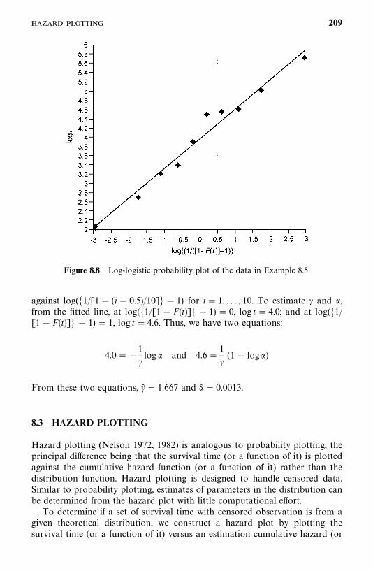
Figure 8.8 Log-logistic probability plot of the data in Example 8.5.
against log(�1/[1� (i� 0.5)/10]� � 1) for i � 1, . . . , 10. To estimate � and ,from the fitted line, at log(�1/[1�F(t)]� � 1) � 0, log t� 4.0; and at log(�1/[1�F(t)]� � 1) � 1, log t� 4.6. Thus, we have two equations:
4.0��1
�log and 4.6�
1
�(1� log )
From these two equations, �� � 1.667 and � � 0.0013.
8.3 HAZARD PLOTTING
Hazard plotting (Nelson 1972, 1982) is analogous to probability plotting, theprincipal difference being that the survival time (or a function of it) is plottedagainst the cumulative hazard function (or a function of it) rather than thedistribution function. Hazard plotting is designed to handle censored data.Similar to probability plotting, estimates of parameters in the distribution canbe determined from the hazard plot with little computational effort.
To determine if a set of survival time with censored observation is from agiven theoretical distribution, we construct a hazard plot by plotting thesurvival time (or a function of it) versus an estimation cumulative hazard (or
209
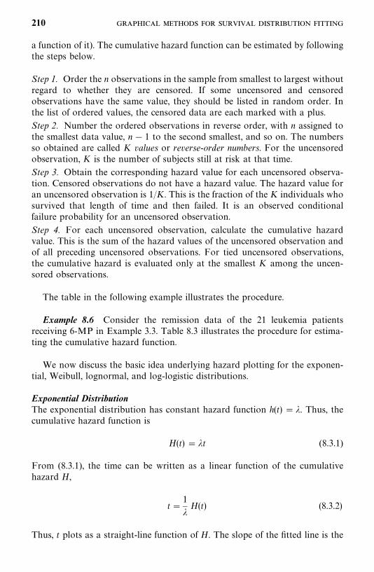
a function of it). The cumulative hazard function can be estimated by followingthe steps below.
Step 1. Order the n observations in the sample from smallest to largest withoutregard to whether they are censored. If some uncensored and censoredobservations have the same value, they should be listed in random order. Inthe list of ordered values, the censored data are each marked with a plus.
Step 2. Number the ordered observations in reverse order, with n assigned tothe smallest data value, n� 1 to the second smallest, and so on. The numbersso obtained are called K values or reverse-order numbers. For the uncensoredobservation, K is the number of subjects still at risk at that time.
Step 3. Obtain the corresponding hazard value for each uncensored observa-tion. Censored observations do not have a hazard value. The hazard value foran uncensored observation is 1/K. This is the fraction of the K individuals whosurvived that length of time and then failed. It is an observed conditionalfailure probability for an uncensored observation.
Step 4. For each uncensored observation, calculate the cumulative hazardvalue. This is the sum of the hazard values of the uncensored observation andof all preceding uncensored observations. For tied uncensored observations,the cumulative hazard is evaluated only at the smallest K among the uncen-sored observations.
The table in the following example illustrates the procedure.
Example 8.6 Consider the remission data of the 21 leukemia patientsreceiving 6-MP in Example 3.3. Table 8.3 illustrates the procedure for estima-ting the cumulative hazard function.
We now discuss the basic idea underlying hazard plotting for the exponen-tial, Weibull, lognormal, and log-logistic distributions.
Exponential DistributionThe exponential distribution has constant hazard function h(t) � �. Thus, thecumulative hazard function is
H(t) � �t (8.3.1)
From (8.3.1), the time can be written as a linear function of the cumulativehazard H,
t�1
�H(t) (8.3.2)
Thus, t plots as a straight-line function of H. The slope of the fitted line is the
210
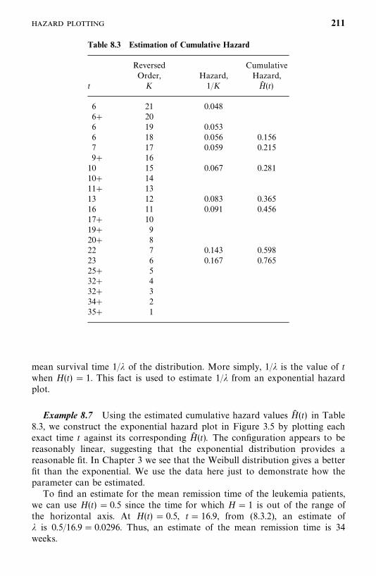
Table 8.3 Estimation of Cumulative Hazard
Reversed CumulativeOrder, Hazard, Hazard,
t K 1/K H� (t)
6 21 0.0486� 206 19 0.0536 18 0.056 0.1567 17 0.059 0.2159� 1610 15 0.067 0.28110� 1411� 1313 12 0.083 0.36516 11 0.091 0.45617� 1019� 920� 822 7 0.143 0.59823 6 0.167 0.76525� 532� 432� 334� 235� 1
mean survival time 1/� of the distribution. More simply, 1/� is the value of twhen H(t) � 1. This fact is used to estimate 1/� from an exponential hazardplot.
Example 8.7 Using the estimated cumulative hazard values H� (t) in Table8.3, we construct the exponential hazard plot in Figure 3.5 by plotting eachexact time t against its corresponding H� (t). The configuration appears to bereasonably linear, suggesting that the exponential distribution provides areasonable fit. In Chapter 3 we see that the Weibull distribution gives a betterfit than the exponential. We use the data here just to demonstrate how theparameter can be estimated.
To find an estimate for the mean remission time of the leukemia patients,we can use H(t) � 0.5 since the time for which H� 1 is out of the range ofthe horizontal axis. At H(t) � 0.5, t� 16.9, from (8.3.2), an estimate of� is 0.5/16.9� 0.0296. Thus, an estimate of the mean remission time is 34weeks.
211
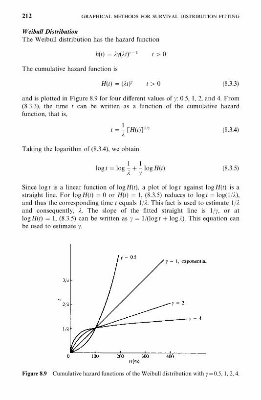
Figure 8.9 Cumulative hazard functions of the Weibull distribution with ��0.5, 1, 2, 4.
Weibull DistributionThe Weibull distribution has the hazard function
h(t) � ��(�t)��� t� 0
The cumulative hazard function is
H(t) � (�t)� t� 0 (8.3.3)
and is plotted in Figure 8.9 for four different values of �: 0.5, 1, 2, and 4. From(8.3.3), the time t can be written as a function of the cumulative hazardfunction, that is,
t�1
�[H(t)]�� (8.3.4)
Taking the logarithm of (8.3.4), we obtain
log t� log1
��
1
�logH(t) (8.3.5)
Since log t is a linear function of logH(t), a plot of log t against logH(t) is astraight line. For logH(t) � 0 or H(t) � 1, (8.3.5) reduces to log t� log(1/�),and thus the corresponding time t equals 1/�. This fact is used to estimate 1/�and consequently, �. The slope of the fitted straight line is 1/�, or atlogH(t) � 1, (8.3.5) can be written as �� 1/(log t� log �). This equation canbe used to estimate �.
212
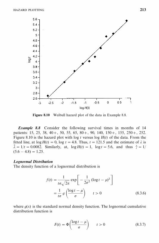
Figure 8.10 Weibull hazard plot of the data in Example 8.8.
Example 8.8 Consider the following survival times in months of 14patients: 15, 25, 38, 40�, 50, 55, 65, 80�, 90, 140, 150�, 155, 250�, 252.Figure 8.10 is the hazard plot with log t versus log H(t) of the data. From thefitted line, at logH(t) � 0, log t � 4.8. Thus, t� 121.5 and the estimate of � is�� � 1/t� 0.0082. Similarly, at, logH(t) � 1, log t � 5.6, and thus �� � 1/(5.6� 4.8) � 1.25.
Lognormal DistributionThe density function of a lognormal distribution is
f (t) �1
t�2�exp��
1
2(log t��)�
�1
tg �
log t� � � t� 0 (8.3.6)
where g(x) is the standard normal density function. The lognormal cumulativedistribution function is
F(t) � ��log t��
� t � 0 (8.3.7)
213
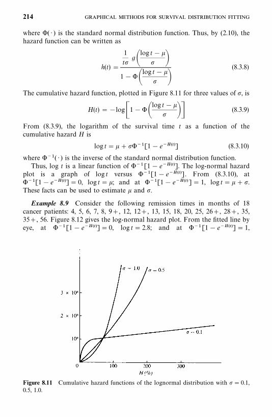
Figure 8.11 Cumulative hazard functions of the lognormal distribution with � 0.1,0.5, 1.0.
where �( · ) is the standard normal distribution function. Thus, by (2.10), thehazard function can be written as
h(t) �
1
tg�
log t�� �
1���log t� �
�(8.3.8)
The cumulative hazard function, plotted in Figure 8.11 for three values of , is
H(t) ��log�1���log t ��
�� (8.3.9)
From (8.3.9), the logarithm of the survival time t as a function of thecumulative hazard H is
log t� �����[1� e�����] (8.3.10)
where ���( · ) is the inverse of the standard normal distribution function.Thus, log t is a linear function of ���[1� e�����]. The log-normal hazard
plot is a graph of log t versus ���[1� e�����]. From (8.3.10), at���[1� e�����]� 0, log t��; and at ���[1� e�����]� 1, log t�� �.These facts can be used to estimate � and .
Example 8.9 Consider the following remission times in months of 18cancer patients: 4, 5, 6, 7, 8, 9�, 12, 12�, 13, 15, 18, 20, 25, 26�, 28�, 35,35�, 56. Figure 8.12 gives the log-normal hazard plot. From the fitted line byeye, at ���[1� e�����]� 0, log t� 2.8; and at ���[1� e�����]� 1,
214
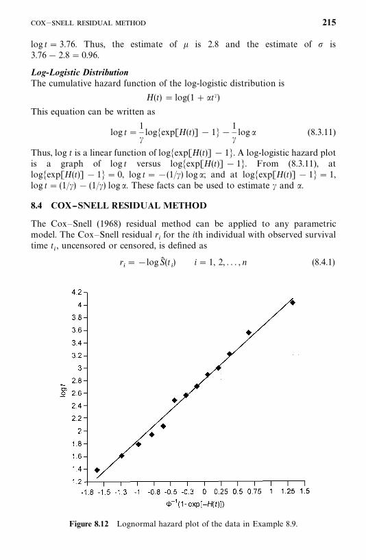
Figure 8.12 Lognormal hazard plot of the data in Example 8.9.
log t� 3.76. Thus, the estimate of � is 2.8 and the estimate of is3.76� 2.8� 0.96.
Log-Logistic DistributionThe cumulative hazard function of the log-logistic distribution is
H(t) � log(1� t�)This equation can be written as
log t�1
�log�exp[H(t)] � 1��
1
�log (8.3.11)
Thus, log t is a linear function of log�exp[H(t)] � 1�. A log-logistic hazard plotis a graph of log t versus log�exp[H(t)] � 1�. From (8.3.11), atlog�exp[H(t)] � 1�� 0, log t��(1/�) log ; and at log�exp[H(t)] � 1� � 1,log t� (1/�) � (1/�) log . These facts can be used to estimate � and .
8.4 COX--SNELL RESIDUAL METHOD
The Cox—Snell (1968) residual method can be applied to any parametricmodel. The Cox—Snell residual r
�for the ith individual with observed survival
time t�, uncensored or censored, is defined as
r���logS� (t
�) i � 1, 2, . . . , n (8.4.1)
— 215
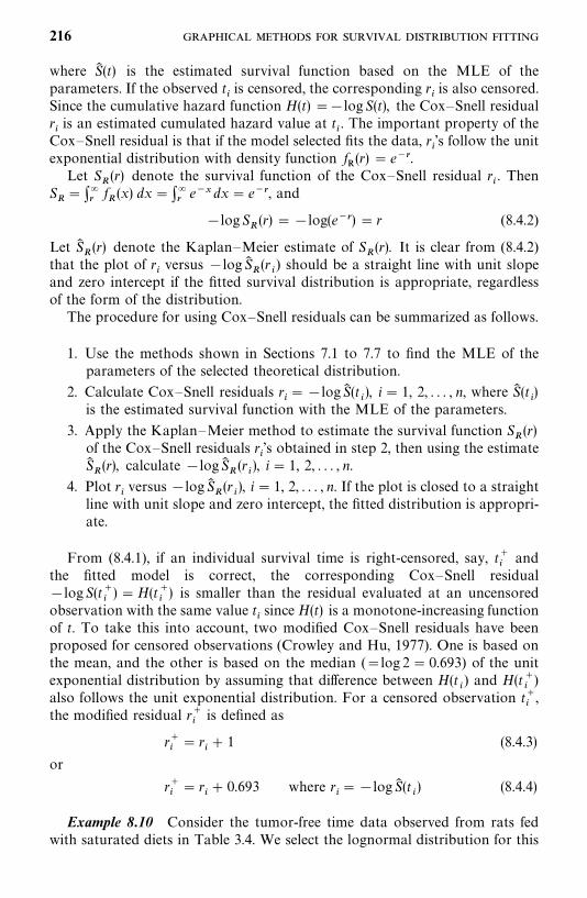
where S� (t) is the estimated survival function based on the MLE of theparameters. If the observed t
�is censored, the corresponding r
�is also censored.
Since the cumulative hazard function H(t) ��logS(t), the Cox—Snell residualr�is an estimated cumulated hazard value at t
�. The important property of the
Cox—Snell residual is that if the model selected fits the data, r�’s follow the unit
exponential distribution with density function f�(r) � e��.
Let S�(r) denote the survival function of the Cox—Snell residual r
�. Then
S�� �
�f�(x) dx� �
�e�� dx� e��, and
�logS�(r) � �log(e��) � r (8.4.2)
Let S��(r) denote the Kaplan—Meier estimate of S
�(r). It is clear from (8.4.2)
that the plot of r�versus �log S�
�(r
�) should be a straight line with unit slope
and zero intercept if the fitted survival distribution is appropriate, regardlessof the form of the distribution.
The procedure for using Cox—Snell residuals can be summarized as follows.
1. Use the methods shown in Sections 7.1 to 7.7 to find the MLE of theparameters of the selected theoretical distribution.
2. Calculate Cox—Snell residuals r���logS� (t
�), i� 1, 2, . . . , n, where S� (t
�)
is the estimated survival function with the MLE of the parameters.
3. Apply the Kaplan—Meier method to estimate the survival function S�(r)
of the Cox—Snell residuals r�’s obtained in step 2, then using the estimate
S��(r), calculate �logS�
�(r
�), i� 1, 2, . . . , n.
4. Plot r�versus �log S�
�(r
�), i � 1, 2, . . . , n. If the plot is closed to a straight
line with unit slope and zero intercept, the fitted distribution is appropri-ate.
From (8.4.1), if an individual survival time is right-censored, say, t��
andthe fitted model is correct, the corresponding Cox—Snell residual�logS(t�
�) �H(t�
�) is smaller than the residual evaluated at an uncensored
observation with the same value t�since H(t) is a monotone-increasing function
of t. To take this into account, two modified Cox—Snell residuals have beenproposed for censored observations (Crowley and Hu, 1977). One is based onthe mean, and the other is based on the median (�log 2� 0.693) of the unitexponential distribution by assuming that difference between H(t
�) and H(t�
�)
also follows the unit exponential distribution. For a censored observation t��,
the modified residual r��is defined as
r��
� r�� 1 (8.4.3)
or
r��
� r�� 0.693 where r
���logS� (t
�) (8.4.4)
Example 8.10 Consider the tumor-free time data observed from rats fedwith saturated diets in Table 3.4. We select the lognormal distribution for this
216
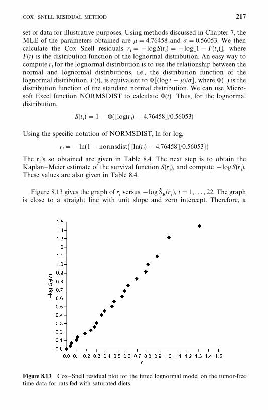
Figure 8.13 Cox—Snell residual plot for the fitted lognormal model on the tumor-freetime data for rats fed with saturated diets.
set of data for illustrative purposes. Using methods discussed in Chapter 7, theMLE of the parameters obtained are � � 4.76458 and � 0.56053. We thencalculate the Cox—Snell residuals r
���log S(t
�) ��log[1�F(t
�)], where
F(t) is the distribution function of the lognormal distribution. An easy way tocompute r
�for the lognormal distribution is to use the relationship between the
normal and lognormal distributions, i.e., the distribution function of thelognormal distribution, F(t), is equivalent to �[(log t� �)/], where �( ) is thedistribution function of the standard normal distribution. We can use Micro-soft Excel function NORMSDIST to calculate �(t). Thus, for the lognormaldistribution,
S(t�) � 1��([log(t
�) � 4.76458]/0.56053)
Using the specific notation of NORMSDIST, ln for log,
r�� �ln(1�normsdist�[ln(t
�) � 4.76458]/0.56053�)
The r�’s so obtained are given in Table 8.4. The next step is to obtain the
Kaplan—Meier estimate of the survival function S(r�), and compute �logS(r
�).
These values are also given in Table 8.4.
Figure 8.13 gives the graph of r�versus �logS�
�(r
�), i � 1, . . . , 22. The graph
is close to a straight line with unit slope and zero intercept. Therefore, a
— 217
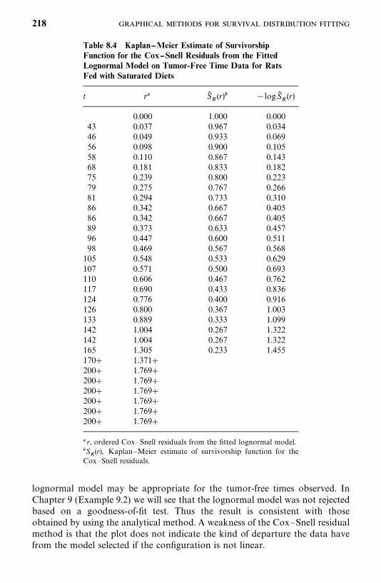
Table 8.4 Kaplan--Meier Estimate of SurvivorshipFunction for the Cox--Snell Residuals from the FittedLognormal Model on Tumor-Free Time Data for RatsFed with Saturated Diets
t r� S��(r) �logS�
�(r)
0.000 1.000 0.00043 0.037 0.967 0.03446 0.049 0.933 0.06956 0.098 0.900 0.10558 0.110 0.867 0.14368 0.181 0.833 0.18275 0.239 0.800 0.22379 0.275 0.767 0.26681 0.294 0.733 0.31086 0.342 0.667 0.40586 0.342 0.667 0.40589 0.373 0.633 0.45796 0.447 0.600 0.51198 0.469 0.567 0.568105 0.548 0.533 0.629107 0.571 0.500 0.693110 0.606 0.467 0.762117 0.690 0.433 0.836124 0.776 0.400 0.916126 0.800 0.367 1.003133 0.889 0.333 1.099142 1.004 0.267 1.322142 1.004 0.267 1.322165 1.305 0.233 1.455170� 1.371�200� 1.769�200� 1.769�200� 1.769�200� 1.769�200� 1.769�200� 1.769�
� r, ordered Cox—Snell residuals from the fitted lognormal model.S
�(r), Kaplan—Meier estimate of survivorship function for the
Cox—Snell residuals.
lognormal model may be appropriate for the tumor-free times observed. InChapter 9 (Example 9.2) we will see that the lognormal model was not rejectedbased on a goodness-of-fit test. Thus the result is consistent with thoseobtained by using the analytical method. A weakness of the Cox—Snell residualmethod is that the plot does not indicate the kind of departure the data havefrom the model selected if the configuration is not linear.
218
Bibliographical Remarks
Probability plotting has been widely used since Daniel’s (1959) classical workon the use of half-normal plot. A quite complete and excellent treatment ofprobability plotting is given by King (1971). Although examples given areapplications to industrial reliability, its interpretation of probability plots ofmany distributions, such as the uniform, lognormal, Weibull, and gamma, areapplicable to biomedical research. Recent applications of probability plottinginclude Leitner et al. (1986), Horner (1987), Waters et al. (1991), andTsumagari et al. (2000).
Hazard plotting was developed by Nelson (1972, 1982). Applications in-cluded Gore (1983) and Wurpel et al. (1986).
EXERCISES
8.1 Show that the Cox—Snell residuals defined in (8.4.1) follow the unitexponential distribution with density function f (r) � exp(�r).
8.2 Consider the following survival times of 16 patients in weeks: 4, 20, 22,25, 38, 38, 40, 44, 56, 83, 89, 98, 110, 138, 145, and 27.(a) Does the exponential distribution provide a reasonable fit to the
survival data? Use the probability plotting technique.(b) Estimate graphically the parameter � of the exponential distribution
and consequently, the mean survival time.
8.3 To computerize patients’ records, a data clerk is hired to transcribemedical data from the patients’ charts to computer coding forms. Thenumber of correct entries between errors is listed in chronological orderof occurrence over a period of five days as follows: 73, 12, 40, 65, 100,15, 70, 40, 110, 64, 200, 6, 90, 102, 20, 102, 90, 34. The assumption is thatthe data clerk, during the five days, would not change her error rateappreciably. Use the technique of probability plotting to evaluate theassumption above. What is your conclusion?
8.4 Twenty-five rats were injected with a give tumor inoculum. Their times,in days, to the development of a tumor of a certain size are given below.
30 53 77 91 11838 54 78 95 12045 58 81 101 12546 66 84 108 13450 69 85 115 135
Which of the distributions discussed in this chapter provide a reasonablefit to the data? Estimate graphically the parameters of the distributionchosen.
219
8.5 In a clinical study, 28 patients with cancer of the head and neck did notrespond to chemotherapy. Their survival times in weeks are given below.
1.7 8.3 14.0 22.7 6.0� 13.1�5.1 9.6 15.9 33.0 7.4� 13.4�5.3 11.3 16.7 3.7� 8.0� 16.1�6.0 12.1 17.0 5.0� 8.3�8.3 12.3 21.0 5.9� 9.1�
(a) Make a hazard plot for each of the following distributions: exponen-tial, Weibull, lognormal, and log-logistic.
(b) Which distribution provides a reasonable fit to the data? Estimategraphically the parameters of the distribution chosen.
8.6 Thirty-one patients with advanced melanoma treated with combinedchemotherapy, immunotherapy, and hormonal therapy have survivaltimes as given below.
26.3� 16.1 24.0 4.3 31.3�94.0 49.6 77.9 97.6� 17.6�9.1 27.3 16.6� 7.3 16.334.6� 61.9� 3.4 75.6�9.4 46.6� 10.9 14.325.7 22.4� 13.0 56.488.7 7.1 64.4� 9.1
(a) Make a hazard plot for each of the following distributions: exponen-tial, Weibull, lognormal, and log-logistic.
(b) Which distribution provides a reasonable fit to the data? Estimatethe parameters of the distribution chosen.
8.7 Consider the survival times of the hypernephroma patients in ExerciseTable 3.1 (see Exercise 4.5). Make a hazard plot for the distribution youchose in Exercise 6.8. Did you make a good selection? If not, try twoother distributions.
8.8 Consider the following survival times in weeks of 10 mice with injectionof tumor cells: 5, 16, 18�, 20, 22�, 24�, 25, 30�, 35, 40�. Make anexponential hazard plot. Does the exponential distribution provide areasonable fit? If not, is the lognormal distribution better?
8.9 Consider the following survival times in months of 25 patients withcancer of the prostate. Use a graphical method to see if the survival timeof prostate cancer patients follows the exponential distribution with�� 0.01: 2, 19, 19, 25, 30, 35, 40, 45, 45, 48, 60, 62, 69, 89, 90, 110, 145,160, 9�, 10�, 20�, 40�, 50�, 110�, 130�.
8.10 Make a log-logistic hazard plot of the following data and estimate thetwo parameters: 20, 30, 32�, 40, 60, 100, 150, 200�, 300.
220
CHAPTER 9
Tests of Goodness of Fitand Distribution Selection
In Chapter 8 we discuss three graphical methods for checking if a parametricdistribution fits the observed data. Parametric distributions can be groupedinto families. First, any given distribution with different parameter values formsa family. Second, if a distribution includes other distributions as its specialcases, this distribution is a nesting (larger) family of these distributions. Forexample, the distributions introduced in Chapter 6 belong to more than onenested family. First, the Weibull distribution reduces to the exponential when�� 1. Therefore, the exponential distribution is a special case of the Weibulland the two distributions are said to belong to one family, the Weibull family.Second, consider the standard gamma distribution; when �� 1, it reduces tothe exponential, and when ���
�and ���
��, it becomes the chi-square
distribution with � degrees of freedom. Thus, the gamma distribution includesthe exponential and chi-square as a family. Now let us consider the generalizedgamma distribution. It reduces to the exponential if � � �� 1, the Weibull if�� 1, the lognormal if � ��, and the gamma if �� 1. Thus, the generalizedgamma distribution includes these four distributions and represents a largefamily of distributions. The relationship of the generalized gamma distributionto the exponential, Weibull, lognormal, and gamma distributions allows us toevaluate the appropriateness of these distributions relative to each other andto a more general distribution. It is known that the generalized gammadistribution is a special case of the generalized F-distribution and thereforebelongs to the generalized F family (Kalbfleisch and Prentice, 1980) Becauseof its complexity, we do not cover the generalized F family.
In this chapter we discuss several analytical procedures for comparingparametric distributions and assessing goodness of fit. In Section 9.1 weintroduce several widely used statistics for testing the appropriateness of adistribution. Readers who are not familiar with linear algebra or are notinterested in the mathematical details may skip this section without loss ofcontinuity. In Section 9.2 we discuss statistics for testing whether a distribution
221
is appropriate by comparing it with other distributions in the same family ora more general family. Section 9.3 covers the selection of a distribution basedon Baysian information criteria. Section 9.4 covers the statistics for testingwhether a given distribution with known parameters is appropriate. All the teststatistics discussed in Sections 9.1 to 9.4 are based on asymptotic likelihoodinferences. In Section 9.5 we introduce the test statistic of Hollander andProschan (1979) for testing whether a distribution with given parameters isappropriate. Computer codes for BMDP or SAS that can be used to carry outthe test procedures are provided.
9.1 GOODNESS-OF-FIT TEST STATISTICS BASED ONASYMPTOTIC LIKELIHOOD INFERENCES
We take the exponential distribution as an example to see how to constructstatistics to test whether it is appropriate for the observed survival times. Asnoted in Chapter 6, the Weibull family with �� 1, the gamma family with�� 1, and the generalized gamma family with � � �� 1 reduce to theexponential distribution. Therefore, to test if the exponential distribution isappropriate for the observed survival time, we can first fit a Weibull distribu-tion and test if �� 1, or fit a gamma distribution, then test if � � 1, or fit ageneralized gamma distribution, then test if �� � � 1. Similarly, to testwhether the family of Weibull distributions, or the gamma distributions, or thelognormal distributions is appropriate for the survival data observed, we canfit a generalized gamma distribution (their nesting distribution) and then testif � � 1, or �� 1, or with � ��, respectively. Thus, testing the appropriatenessof a family of distributions is equivalent to testing whether a subset of theparameters in its nesting distribution equal to some specific values. If the datacan be assumed to follow a certain distribution but the values of its parametersare uncertain, we need to test only that the parameters are equal to certainvalues. In the following, we separately introduce test statistics for testingwhether some of the parameters in a distribution are equal to certain valuesand whether all parameters in a distribution are equal to certain values.Readers who are interested in a detailed discussion of these statistics arereferred to Kalbfleisch and Prentice (1980).
9.1.1 Testing a Subset of Parameters in a Distribution
Let b� (b�,b
�) denote all the parameters in a parametric distribution, where
b�and b
�are subsets of parameters, and let the hypothesis be
H�: b
�� b
�(9.1.1)
where b�is a vector of specific numbers. Let b� be the MLE of b, b�
�(b
�) the
MLE of b�given b
�� b
�, and V�
�(b� ) the submatrix of the covariance matrix in
222
(7.1.5), V� (b� ), corresponding to b�. Under H
�and some mild assumptions, both
of the following two statistics have an asymptotic chi-square distribution withdegrees of freedom equal to the dimension of (or the number of parameters in)b�.
Log-likelihood ratio statistic:
X�� 2[l(b� ) � l(b�
�(b
�), b
�)] (9.1.2)
Wald statistic:
X�
� (b��� b
�)�V� ��
�(b� )(b�
�� b
�) (9.1.3)
If the number of parameters in b�is equal to q, for a given significant level
�, H�is rejected if X
�� ��
���when the likelihood ratio statistic is used; or if
X�
�������� or X
���
�������, (two-sided test) or X�
������ (one-sided test)
when the Wald’s statistic is used, where ����� , ��
����� and ��������� are the
100(1� �), 100(1� �/2), and 100�/2 percentile points of the chi-square dis-tribution with q degrees of freedom; that is,
P(���� ��
���) � � and P(���� ��
�����) �P(�����
�������) ��2
Example 9.1 Suppose that we wish to test whether the observed data arefrom an exponential distribution. We can use a Weibull distribution and testwhether its shape parameter, �, is equal to 1. The Weibull distribution has twoparameters, � and �; thus b� (�, �) and the null and alternative hypotheses are:
H�: � � 1 (the underlying distribution is an exponential distribution)
(9.1.4)
H�: � � 1 (the underlying distribution is a Weibull distribution)
Let b� � (�� , �� ) be the MLE of b, l�(b� ) � l
�(�� , �� ) and l
�(�� ) be the log-likelihood
of the Weibull and exponential distributions, respectively, l�
(�� ) � l�(�� (1), 1),
where �� (1) is the MLE of � in the Weibull distribution given �� 1. Thelog-likelihood ratio and Wald statistics defined in (9.1.2) and (9.1.3) in this casebecome
X�� 2[l
�(�� , �� ) � l
�(�� (1), 1)] (9.1.5)
and
X�
� (� � 1)V� ���
(�� , � )(� � 1) (9.1.6)
-- 223
respectively, where V��(�� , � ) is the second diagonal element of the covariance
matrix
V� (�� , � ) �����l
�(�� , � )
���
��l�(�� , � )
�� ��
��l�(�� , � )
�� ����l
�(�� , � )
��� ���
(9.1.7)
and
V� ���
(�� , � ) ��[��l
�(�� , � )/���][��l
�(�� , � )/���] � (��l
�(�� , � )/�� ��)�
��l�(�� , � )/���
(9.1.8)
For a given significant-level �, H�is rejected if X
����
��� , when the likelihoodratio statistic is used; or if X
����
����� or X�
���������, when the Wald
statistic is used.It must be pointed out that failure to reject H
�in (9.1.4) does not imply that
an exponential distribution provides the best fit to the data. On the other hand,rejection of H
�does not indicate that a Weibull distribution is the choice
either. Further testing of other distributions is needed. The details andexamples are given in Section 9.2.
Since the gamma and generalized gamma distribution also include theexponential as a special case, similar test statistics can be constructed to testthe null hypothesis that the data are from the exponential distribution by usingthe gamma, the generalized gamma, or the extended generalized gammadistribution.
9.1.2 Testing All Parameters in a Distribution
To test whether all of the parameters in b equal a given set of known valuesb�, the null hypothesis is
H�: b� b
�(9.1.9)
and the following three test statistics can be used.
Log-likelihood ratio statistic:
X�� 2[l(b� ) � l(b
�)] (9.1.10)
Wald statistic:
X�
��(b� � b�)�
��l(b�)
�b �b�(b� � b
�) �or� �(b� � b
�)�
��l(b� )�b �b�
(b� � b�)�
(9.1.11)
224
Score statistic:
X���
�l(b�)
�b ����
��l(b�)
�b �b� ��� �l(b
�)
�b �or� ��l(b
�)
�b ��V� (b� )
�l(b�)
�b �(9.1.12)
where V� (b� ) is the estimated covariance matrix in (7.1.5). Under H�and the
assumption that b� has approximately multinormal distribution, each of thethree statistics has an asymptotic chi-square distribution with p (the dimensionof b or the number of parameters in b) degrees of freedom.
For a given significant-level �, H�
is rejected if X����
�� , when thelikelihood ratio statistic is used; or if X
�� ��
���� or X�
�������� , when the
Wald statistic is used; or if X�� ��
���� or X���
������, when the score statisticis used.
It must be pointed out that rejection of H�in (9.1.9) means only that the
given distribution with the known parameters b�, not the family of distribu-
tions to which the given distribution belongs, is not appropriate for theobserved data. It is possible that a distribution with different b
�in the family
may be appropriate.
9.2 TESTS FOR APPROPRIATENESS OF A FAMILY OFDISTRIBUTIONS
The usual method for testing whether a distribution is appropriate for theobserved data is to compare the distribution with a larger or more generalfamily that includes the distribution of interest as a special case (Hagar andBain, 1970).
Let l�(�), l
�(�, �), l
(�, �), l
��(�, �), and l
(�, �, �) denote, respectively,
the log-likelihood function defined in (7.1.1) based on the exponential, Weibull,gamma, lognormal, and extended generalized gamma distribution, and l
�(�� ),
l�
(�� , � ), l(�� , � ), l
��(� , �), and l
(� , �� , � ) denote the respective log-likelihood
values where �� , (�� , � ), (�� , � ), (� , �), and (� , �� , � ) are the MLE. For example, thelog-likelihood of the exponential distribution can be obtained from
l�
(�� ) ��� �
log(�� e��� t )
��
���
log(e��t� ) � r log �� � ��
�� �
t � ��
��
���
t�
for a set of observed survival times t�, . . . , t
�, t�
���, . . . , t�
�. The log-likelihood
value and the estimated covariance matrix in (7.1.5) and parameters for eachof the distributions discussed in Sections 7.2 to 7.6 can be obtained from SASor BMDP. The results can be used to construct the log-likelihood ratio statisticand the Wald statistic defined in (9.1.2) and (9.1.3). In the following, we
225
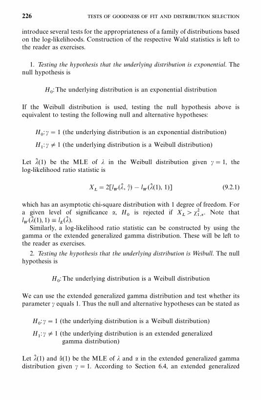
introduce several tests for the appropriateness of a family of distributions basedon the log-likelihoods. Construction of the respective Wald statistics is left tothe reader as exercises.
1. Testing the hypothesis that the underlying distribution is exponential. Thenull hypothesis is
H�: The underlying distribution is an exponential distribution
If the Weibull distribution is used, testing the null hypothesis above isequivalent to testing the following null and alternative hypotheses:
H�: � � 1 (the underlying distribution is an exponential distribution)
H�: � � 1 (the underlying distribution is a Weibull distribution)
Let �� (1) be the MLE of � in the Weibull distribution given �� 1, thelog-likelihood ratio statistic is
X�� 2[l
�(�� , � ) � l
�(�� (1), 1)] (9.2.1)
which has an asymptotic chi-square distribution with 1 degree of freedom. Fora given level of significance �, H
�is rejected if X
����
��� . Note thatl�
(�� (1), 1) � l�
(�� ).Similarly, a log-likelihood ratio statistic can be constructed by using the
gamma or the extended generalized gamma distribution. These will be left tothe reader as exercises.
2. Testing the hypothesis that the underlying distribution is Weibull. The nullhypothesis is
H�: The underlying distribution is a Weibull distribution
We can use the extended generalized gamma distribution and test whether itsparameter � equals 1. Thus the null and alternative hypotheses can be stated as
H�: � � 1 (the underlying distribution is a Weibull distribution)
H�: � � 1 (the underlying distribution is an extended generalized
gamma distribution)
Let �� (1) and � (1) be the MLE of � and � in the extended generalized gammadistribution given � � 1. According to Section 6.4, an extended generalized
226
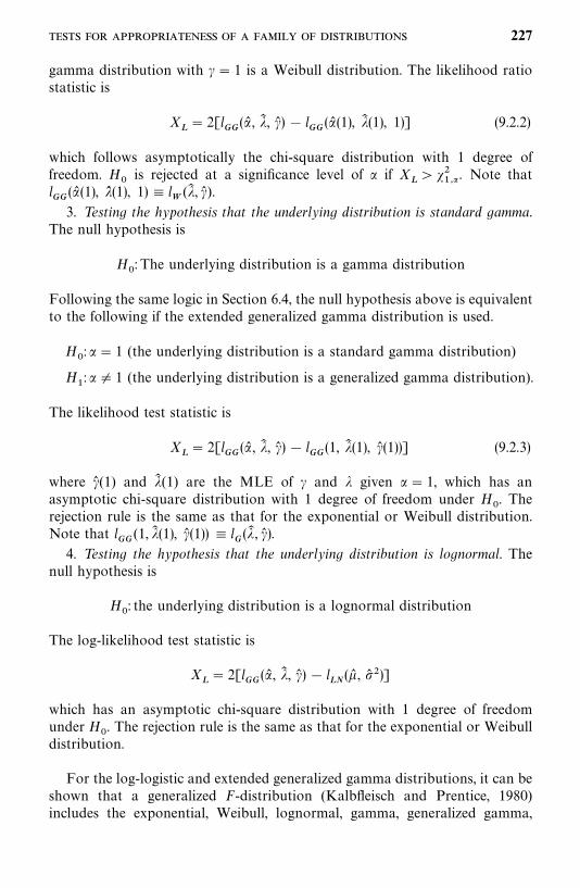
gamma distribution with �� 1 is a Weibull distribution. The likelihood ratiostatistic is
X�� 2[l
(� , �� , � ) � l
(� (1), �� (1), 1)] (9.2.2)
which follows asymptotically the chi-square distribution with 1 degree offreedom. H
�is rejected at a significance level of � if X
����
��� . Note thatl
(� (1), � (1), 1) � l�
(�� , � ).3. Testing the hypothesis that the underlying distribution is standard gamma.
The null hypothesis is
H�: The underlying distribution is a gamma distribution
Following the same logic in Section 6.4, the null hypothesis above is equivalentto the following if the extended generalized gamma distribution is used.
H�: �� 1 (the underlying distribution is a standard gamma distribution)
H�: �� 1 (the underlying distribution is a generalized gamma distribution).
The likelihood test statistic is
X�� 2[l
(� , �� , � ) � l
(1, �� (1), � (1))] (9.2.3)
where � (1) and �� (1) are the MLE of � and � given � � 1, which has anasymptotic chi-square distribution with 1 degree of freedom under H
�. The
rejection rule is the same as that for the exponential or Weibull distribution.Note that l
(1, �� (1), � (1)) � l
(�� , � ).
4. Testing the hypothesis that the underlying distribution is lognormal. Thenull hypothesis is
H�: the underlying distribution is a lognormal distribution
The log-likelihood test statistic is
X�� 2[l
(� , �� , � ) � l
��(� , �)]
which has an asymptotic chi-square distribution with 1 degree of freedomunder H
�. The rejection rule is the same as that for the exponential or Weibull
distribution.
For the log-logistic and extended generalized gamma distributions, it can beshown that a generalized F-distribution (Kalbfleisch and Prentice, 1980)includes the exponential, Weibull, lognormal, gamma, generalized gamma,
227
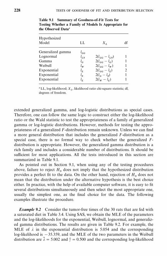
Table 9.1 Summary of Goodness-of-Fit Tests forTesting Whether a Family of Models Is Appropriate forthe Observed Data�
HypothesizedModel LL X
�df
Generalized gamma l
Lognormal l��
2(l
� l��) 1
Gamma l
2(l
� l) 1
Weibull l�
2(l
� l�) 1
Exponential l�
2(l
� l�) 2
Exponential l�
2(l� l
�) 1
Exponential l�
2(l�
� l�) 1
�LL, log-likelihood; X�, likelihood ratio chi-square statistic; df,
degrees of freedom.
extended generalized gamma, and log-logistic distributions as special cases.Therefore, one can follow the same logic to construct either the log-likelihoodratio or the Wald statistic to test the appropriateness of a family of generalizedgamma or log-logistic distributions. However, methods for testing the appro-priateness of a generalized F-distribution remain unknown. Unless we can finda more general distribution that includes the generalized F-distribution as aspecial case, there is no formal way to check whether the generalized F-distribution is appropriate. However, the generalized gamma distribution is arich family and includes a considerable number of distributions. It should besufficient for most applications. All the tests introduced in this section aresummarized in Table 9.1.
As pointed out in Section 9.1, when using any of the testing proceduresabove, failure to reject H
�does not imply that the hypothesized distribution
provides a perfect fit to the data. On the other hand, rejection of H�does not
mean that the distribution under the alternative hypothesis is the best choiceeither. In practice, with the help of available computer software, it is easy to fitseveral distributions simultaneously and then select the most appropriate one,usually the simplest one, as the final choice for the data. The followingexamples illustrate the procedure.
Example 9.2 Consider the tumor-free times of the 30 rats that are fed witha saturated diet in Table 3.4. Using SAS, we obtain the MLE of the parametersand the log-likelihoods for the exponential, Weibull, lognormal, and generaliz-ed gamma distributions. The results are given in Table 9.2. For example, theMLE of � in the exponential distribution is 5.054 and the correspondinglog-likelihood is �35.359, and the MLE of the two parameters in the Weibulldistribution are �� � 5.002 and � � 0.500 and the corresponding log-likelihood
228
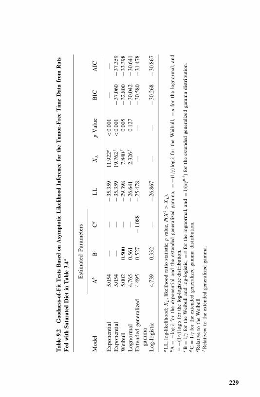
Table
9.2
Goodness-of-FitTests
Based
onAsymptotic
LikelihoodInferencefortheTum
or-FreeTim
eDatafrom
Rats
Fed
withSa
turatedDietin
Tab
le3.4�
Estim
ated
Param
eters
Mod
elA
�B�
C�
LL
X�
pValue
BIC
AIC
Exp
onential
5.054
——
�35.359
11.922
�0.001
——
Exp
onential
5.054
——
�35.359
19.762
�0.001
�37.060
�37.359
Weibu
ll5.00
20.50
0—
�29.398
7.840�
0.005
�32.800
�33.398
Log
norm
al4.76
50.561
—�26.641
2.326�
0.127
�30.042
�30.641
Extendedgeneralized
4.49
50.527
�1.088
�25.478
——
�30.580
�31.478
gamma
Log
-logistic
4.73
90.33
2—
�26.867
——
�30.268
�30.867
�LL,log
-likelihood
;X
�,likelihoo
dratiostatistic;
pvalue,
P(X
��
X�).
�A�
�log
�fortheexpo
nential
andtheextendedgeneralized
gamma,
��
(1/�
)log
�fortheWeibu
ll,�
�forthelogn
ormal,an
d�
�(1/�
)log
�forthelog-logistic
distribution.
�B�
1/�fortheWeibullan
dlog-logistic,�
forthelogn
ormal,a
nd
�1/
(���
��)fortheextendedgeneralized
gammadistribution.
�C
�1/
�fortheextend
edgeneralized
gammadistribu
tion
.�R
elativeto
theWeibu
ll.�Relativew
totheextend
edgeneralized
gamma.
229
is �29.398. To test the null hypothesis that the underlying distribution is anexponential distribution versus the alternative hypothesis that the underly-ing distribution is Weibull (or extended generalized gamma), the likelihoodratio test statistic X
�� 2(35.359�29.398)� 11.922 [or 2(35.359� 25.478) �
19.762]. The probability of observing such a chi-square value is 0.001;therefore, the exponential distribution is rejected and the Weibull or thegeneralized gamma is preferred.
However, the Weibull distribution is also rejected at the 0.001 level relativeto the extended generalized gamma distribution (X
�� 7.840, p 0.001). This
implies that the extended generalized gamma distribution may be better.However, the extended generalized gamma distribution is not significantlybetter than the lognormal distribution (X
�� 2.326, p� 0.127). Thus, among
these distributions, the lognormal and extended generalized gamma distribu-tions are our choices. Because of its simplicity, we may select the lognormaldistribution as the choice for this set of data.
Example 9.3 Table 9.3 contains a set of remission times from 137 cancerpatients. These remission times are a subset of the data from a bladder cancerstudy and are used here only for illustrative purposes. The results of goodnessof fit tests based on asymptotic likelihood inferences are shown in Table 9.4.From this table, we see that the exponential distribution is not rejected relativeto the Weibull distribution based on the statistic defined in (9.2.1) (X
�� 0.638,
p� 0.425). The hypothesis that the underlying distribution is exponentialversus the alternative hypothesis that the distribution is the extended general-ized gamma is rejected (X
�� 6.772, p� 0.034). Furthermore, the Weibull and
lognormal distributions are also rejected in favor of the extended generalizedgamma (X
�� 6.135, 8.120, p� 0.013 and 0.004, respectively). This implies that
the exponential distribution may not be an appropriate distribution since theWeibull distribution (its nesting distribution) is rejected. Therefore, we mayaccept the extended generalized gamma as our final choice of distribution forthe data.
9.3 SELECTION OF A DISTRIBUTION USING BIC OR AICPROCEDURES
The test procedures discussed in Section 9.2 require knowledge of the distribu-tion family to which the distribution of interest belongs. In this section weintroduce a simpler selection procedure called the Baysian information criterion(BIC; Schwarz, 1978). This criterion is based on the log-likelihood l(b� ), thenumber of parameters in the distribution (p), and the total number ofobservations (n). For each candidate distribution, compute
r� l(b� ) �p
2log n (9.3.1)
230
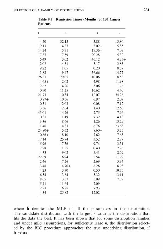
Table 9.3 Remission Times (Months) of 137 CancerPatients
t t t t
4.50 32.15 3.88 13.8019.13 4.87 3.02 5.8514.24 5.71 19.36 7.097.87 7.59 20.28 5.325.49 3.02 46.12 4.332.02 4.51 5.17 2.839.22 1.05 0.20 8.373.82 9.47 36.66 14.7726.31 79.05 10.06 8.534.65 2.02 4.98 11.982.62 4.26 5.06 1.760.90 11.25 16.62 4.4021.73 10.34 12.07 34.260.87 10.66 6.97 2.070.51 12.03 0.08 17.123.36 2.64 1.40 12.6343.01 14.76 2.75 7.660.81 1.19 7.32 4.183.36 8.66 1.26 13.291.46 14.83 6.76 23.6324.80 5.62 8.60 3.2510.86 18.10 7.62 7.6317.14 25.74 3.52 2.8715.96 17.36 9.74 3.317.28 1.35 0.40 2.264.33 9.02 5.41 2.6922.69 6.94 2.54 11.792.46 7.26 2.69 5.343.48 4.70 8.26 6.934.23 3.70 0.50 10.756.54 3.64 5.32 13.118.65 3.57 5.09 7.395.41 11.64 2.092.23 6.25 7.934.34 25.82 12.02
where b� denotes the MLE of all the parameters in the distribution.The candidate distribution with the largest r value is the distribution thatfits the data the best. It has been shown that for some distribution familiesand under mild assumptions, for sufficiently large n, the distribution select-ed by the BIC procedure approaches the true underlying distribution, ifit exists.
231
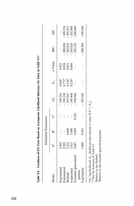
Table
9.4
Goodness-of-FitTests
Based
onAsymptotic
LikelihoodInferenceforDatain
Table
9.3�
Estim
ated
Param
eters
Mod
elA
�B�
C�
LL
X�
pValue
BIC
AIC
Exp
onential
2.303
——
�198.234
0.638�
0.425
——
Exp
onential
2.303
——
�198.234
6.772�
0.034
�200.694
�200.234
Weibu
ll2.32
20.94
9—
�197.915
6.134�
0.013
�202.835
�201.915
Log
norm
al1.82
11.090
—�198.908
8.120�
0.004
�203.828
�202.908
Extendedgeneralized
2.08
70.999
0.520
�194.848
——
�202.228
�200.848
gamma
Log
-logistic
1.86
60.59
1—
�195.344
——
�200.264
�199.344
�LL,log
-likelihood
;X
�,likelihoo
dratiostatistic;
pvalue,
P(X
��
X�).
�����See
thefootnotes
inTab
le9.2.
�Relativeto
theWeibull.
�Relativeto
theextend
edgeneralized
gamma.
232
In general, the larger the number of parameters p in a distribution, the largerthe log-likelihood l(b� ) in (9.3.1). Thus the first term represents the gain by usinga distribution with more parameters. But the larger the p, the larger the secondterm in (9.3.1) is, which represents a penalty by having more parameters in thedistribution. Therefore, the BIC provides a balance between the gain and thepenalty.
Another widely used criterion is called an information criterion (AIC;Akaike, 1969), in which r is defined as
r� l (b� ) � 2p (9.3.2)
Example 9.4 The values of the BIC and AIC for the various distributionsconsidered in Examples 9.2 and 9.3 are listed in the last two columns in Tables9.2 and 9.4. Based on Table 9.2, the lognormal distribution would be selectedby either the BIC or AIC procedure, which is consistent with the resultsobtained in Example 9.2. The results in Table 9.4 show that the log-logisticdistribution, rather than the extended generalized gamma distribution, shouldbe selected based on either the BIC or AIC procedure.
9.4 TESTS FOR A SPECIFIC DISTRIBUTION WITH KNOWNPARAMETERS
In this section we introduce the likelihood ratio statistic for testing if thesurvival data observed follow a given distribution with known parameters. Weuse the same notations as in Section 9.2. In addition to the exponential,Weibull, lognormal, gamma, generalized gamma distributions, we also considerthe log-logistic distribution. Let l
��(�, �) and l
��(� , � ) denote its log-likelihood
function and the log-likelihood with (� , � ), the MLE of (�, �).
1. Testing the hypothesis that the underlying distribution is exponential withknown parameter �
�. The null hypothesis is
H�: the underlying distribution is the exponential distribution with � � �
�
The likelihood ratio test statistic based on (9.1.10) is
X�� 2[l
�(�� ) � l
�(�
�)] (9.4.1)
X�has an asymptotic chi-square distribution with 1 degree of freedom under
H�. H
�is rejected if X
��X�
��� , where � is the significance level. Similarly, theWald test statistic and the score statistic can be derived by following (9.1.11)and (9.1.12). This is left to the reader as exercises.
Example 9.5 Consider the following survival times in weeks of 10 micewith a given tumor: 1, 3, 5, 8, 10, 15, 18, 19, 22, 25. We test the following
233
null hypothesis:
H�: the underlying distribution of the observed data isexponential with �� 0.06
In this case, n� 10, r� 8, �� �
t � 91, and ��
���t�
� 35. The MLE of �based on (7.2.16) is
�� �8
91 35� 0.0635
and l�(�� ) � 8(log 0.0635) � 0.0635(91) � 0.0635(35)� �30.055. Under H
�,
l�(�
�) � 8(log 0.06) � 0.06(91) � 0.06(35) ��30.067. Thus, following (9.4.1),
X�� 2[�30.055� (�30.067)] � 0.024. X�
������� 3.84; therefore, we cannot
reject the null hypothesis that the data are from the exponential distributionwith � � 0.06.
2. Testing the hypothesis that the underlying distribution is Weibull withknown parameters �
�and �
�. The null hypothesis is
H�: the underlying distribution is Weibull with known parameters � � �
�and � � �
�
Based on (9.1.10), the likelihood ratio test statistic is
X�� 2[l
�(�� , � ) � l
�(�
�, �
�)] (9.4.2)
Under H�, X
�has an asymptotic chi-square distribution with 2 degrees of
freedom. H�is rejected if X
��X�
��� where � is the significance level.
3. Testing the hypothesis that the underlying distribution is lognormal withknown parameters �
�and �
�. Similar to the procedures above, the likelihood
ratio test statistic is
X�� 2[l
��(� , �) � l
��(�
�, �
�)] (9.4.3)
Under H�, X
�has an asymptotic chi-square distribution with 2 degrees of
freedom.
4. Testing the hypothesis that the underlying distribution is standard gammawith known parameters �
�and �
�. The likelihood ratio test statistic is
X�� 2[l
(�� , � ) � l
(�
�, �
�)] (9.4.4)
Under H�, X
�is asymptotically chi-square distributed with 2 degrees of
freedom.
234
5. Testing the hypothesis that the underlying distribution is generalized gammawith known parameters �
�, �
�, and �
�. The likelihood ratio test statistic is
X�� 2[l
(� , �� , � ) � l
(�
�, �
�, �
�)] (9.4.5)
Under H�, X
�is asymptotically chi-square distributed with 3 degrees of
freedom.
6. Testing the hypothesis that the underlying distribution is log-logistic withknown parameters �
�and �
�. The likelihood ratio test statistic is
X�� 2[l
��(� , � ) � l
��(�
�, �
�)] (9.4.6)
Under H�, X
�has an asymptotic chi-square distribution with 2 degrees of
freedom.
Note that the respective Wald and score statistics can be constructed forthese tests by following (9.1.11) and (9.1.12). These are left to the reader asexercises. As noted in Section 9.3, the log-likelihood and estimated covariancematrix and parameters in (9.1.10)—(9.1.12) for each of the distributions dis-cussed in Sections 7.2 to 7.6 can be obtained from SAS or BMDP. The otherterms in these test statistics can also be obtained by using SAS or BMDP. Thefollowing example illustrates the use of SAS and BMDP.
Example 9.6 To use the likelihood ratio statistic (9.4.1) to test the nullhypothesis in Example 9.5, H
�: �� �
�� 0.06, we need to calculate the
log-likelihood l�(�� ) and l
�(�
�). l
�(�� ) can be obtained by applying either the
SAS or BMDP codes in Example 7.5. We now show how to use SAS or BMDPto calculate l
�(�
�). Suppose that the survival data of the 10 mice in Example
9.5 are saved in the file ‘‘C:�EXAMPLE.DAT’’. If SAS is used, we specify thatthe distribution is exponential by using D�EXPONENTIAL in the ‘‘model’’statement and letting INTERCEPT� 2.813 [� � log �
��
�log(0.06)]. If BMDP is used, we specify the distribution by letting AC-CEL�EXPONENTIAL and CONSTANT� 2.813. The following SAS orBMDP codes can be used to obtain the l
�(�
�) and the terms needed for the
Wald and score statistics in (9.1.11) and (9.1.12).
SAS code:
data w1;infile ‘c:�example.dat’ missover;input t cens;
run;proc lifereg;model t*cens(0)�/maxit�0 covb itprint d�exponential intercept�2.813;
run;
235
BMDP code:
/input file� ‘c:�example.dat’ .variables� 2.format� free.
/print level�brief.cova. iterations.
/variable names� t, cens./form time� t.
status� cens.response� 1.
/regress iteration� 0.accel� exponential.constant� 2.813.
/end
Similarly, to obtain the log-likelihood ratio statistic, the Wald and the scorestatistics in (9.1.10)—(9.1.12) for testing null hypotheses about the parametersof other distributions, we can follow the same procedure but change the D�
and ACCEL� statements to reflect the distribution under the null hypothesis.We also need to provide values for the input variables INTERCEPT andSCALE, for Weibull, lognormal, and log-logistic distributions, if SAS is used.For the extended generalized gamma distribution, we need to provide a valuefor SHAPE1. BMDP does not have a procedure for the gamma distribution.For the Weibull, lognormal, and log-logistic distributions, we need to providevalues for CONSTANT and SCALE. All of these input variables are based onthe distribution and their relationship to the parameters under the nullhypothesis (see notes at the end of each of the SAS or BMDP codes in Section7.2 to 7.6).
9.5 HOLLANDER AND PROSCHAN’S TEST FORAPPROPRIATENESS OF A GIVEN DISTRIBUTION WITH KNOWNPARAMETERS
Another test for the appropriateness of a parametric distribution with knownparameters was proposed by Hollander and Proschan (1979). Let0� t
�� t
�� t
��� t
��be a set of distinct ordered survival times and
some of the t �’s may be censored. If censored observations are tied with
uncensored observations, treat the censored observations of tie as being greaterthan the uncensored of the tie. Let S(t) be the underlying survivorship functionand S
�(t) the survivorship function of the specific distribution. The null
hypothesis is
H�:S(t) �S
�(t)
236
Using the Kaplan—Meier product-limit method, S(t) is estimated as
S� (t) ��������
�n� j
n� j 1�� ��
t ����
t� t ��, k� 1, . . . , n
0 t� t ��
(9.5.1)
where � ��
� 1 if t ��
is uncensored and � ��
� 0 if t ��
is censored. Hollander andProschan’s test statistic for the null hypothesis that the data are from adistribution with survivorship function S(t) is
C� ���� �������������� ����
S�(t
�) f� (t
�) (9.5.2)
where f � (t �) is the jump of the Kaplan—Meier estimates at consecutive
uncensored observation and at the largest observation, uncensored or not,
f� (t �) �
1
n
������n� j 1
n� j ���� ��
. (9.5.3)
Under the null hypothesis,
C*��n(C � 0.5)
(9.5.4)
follows approximately the standard normal distribution, where is an estimateof the standard deviation of C and
� �1
16
�� �
n
n� i 1[S�
�(t ���
) �S��(t �)] (9.5.5)
To test H�: S� S
�versus H
�:S�S
�, we reject H
�if C* �Z� ; to test H
�versus H
�:SS
�, we reject H
�if C*�Z� ; and to test H
�versus H
�:S�S
�,
we reject H�if C* �Z��� or C*�Z��� , where Z� is the upper � percentile
point of the standard normal distribution.The procedure for the calculation of C* can be summarized as follows.
1. Compute the Kaplan—Meier estimate S� (t) for each uncensored observa-tion.
2. Compute the jump of the Kaplan—Meier distribution at each t �uncen-
sored, that is, f� (t �), which is the difference of F� (t) � 1�S� (t) at two
consecutive uncensored observations.
3. Compute S�(t
�) for each observation.
’ 237
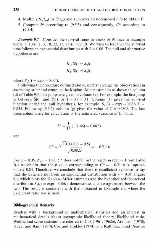
4. Multiply S�(t �) by f� (t
�) and sum over all uncensored t
�’s to obtain C.
5. Compute � according to (9.5.5) and consequently, C* according to(9.5.4).
Example 9.7 Consider the survival times in weeks of 10 mice in Example9.5: 8, 5, 10, 1, 3, 18, 22, 15, 25, and 19. We wish to test that the survivaltime follows an exponential distribution with �� 0.06. The null and alternativehypotheses are
H�:S(t) �S
�(t)
H�:S(t) �S
�(t)
where S�(t) � exp(�0.06t).
Following the procedure outlined above, we first arrange the observations inascending order and compute the Kaplan—Meier estimates as shown in column(d) of Table 9.5. The jumps are given in column (e). For example, the first jumpis between S� (0) and S� (1) or 1� 0.9� 0.1. Column (f) gives the survivalfunction under the null hypothesis, for example, S
�(3) � exp(�0.06�3) �
0.835. Following (9.5.2), column (g) gives the value of C� 0.4808. The lastthree columns are for calculation of the estimated variance of C. Thus,
��1
16(1.3166) � 0.0823
and
C*��10(0.4808 � 0.5)
�0.0823��0.2116
For � � 0.05, Z���� 1.96, C* does not fall in the rejection region. From TableB-1 we obtain that the p value corresponding to C*��0.2116 is approxi-mately 0.84. Therefore, we conclude that there is insufficient evidence to saythat the data are not from an exponential distribution with �� 0.06. Figure9.1, which plots the Kaplan—Meier estimates and the hypothesized theoreticaldistribution S
�(t) � exp(�0.06t), demonstrates a close agreement between the
two. The result is consistent with that obtained in Example 9.5, where thelikelihood ratio test is used.
Bibliographical Remarks
Readers with a background in mathematical statistics and an interest inmathematical details about asymptotic likelihood theory, likelihood ratio,Wald’s, and score statistics are referred to Cox (1961, 1962a), Atkinson (1970),Hagar and Bain (1970), Cox and Hinkley (1974), and Kalbfleisch and Prentice
238
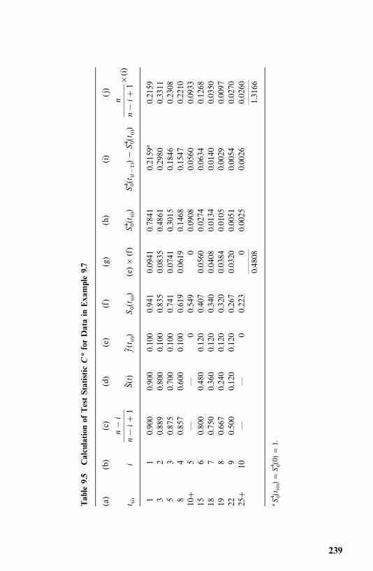
Table
9.5
Calculation
ofTestStatistic
C*forDatain
Exa
mple9.7
(a)
(b)
(c)
(d)
(e)
(f)
(g)
(h)
(i)
(j)
t �i
n�
i
n�
i1
S�(t)
f�(t �)
S�(t �)
(e)�
(f)
S� �(t �)
S� �(t �
��)�
S� �(t �)
n
n�
i1�
(i)
11
0.90
00.90
00.100
0.941
0.0941
0.7841
0.2159
�0.2159
32
0.88
90.80
00.100
0.835
0.0835
0.4861
0.2980
0.3311
53
0.87
50.70
00.100
0.741
0.0741
0.3015
0.1846
0.2308
84
0.85
70.60
00.100
0.619
0.0619
0.1468
0.1547
0.2210
10
5—
—0
0.549
00.0908
0.0560
0.0933
156
0.80
00.48
00.120
0.407
0.0560
0.0274
0.0634
0.1268
187
0.75
00.36
00.120
0.340
0.0408
0.0134
0.0140
0.0350
198
0.66
70.24
00.120
0.320
0.0384
0.0105
0.0029
0.0097
229
0.50
00.12
00.120
0.267
0.0320
0.0051
0.0054
0.0270
25
10—
—0
0.223
00.0025
0.0026
0.0260
———
———
0.4808
1.3166
�S� �(t �
�)�
S� �(0)
�1.
239
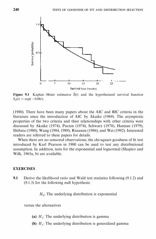
Figure 9.1 Kaplan—Meier estimator S� (t) and the hypothesized survival functionS�(t) � exp(�0.06t).
(1980). There have been many papers about the AIC and BIC criteria in theliterature since the introduction of AIC by Akaike (1969). The asymptoticproperties of the two criteria and their relationships with other criteria werediscussed by Akaike (1974), Parzen (1974), Schwarz (1978), Hannan (1979),Shibata (1980), Wang (1984, 1989), Rissanen (1986), and Wei (1992). Interestedreaders are referred to these papers for details.
When there are no censored observations, the chi-square goodness of fit testintroduced by Karl Pearson in 1900 can be used to test any distributionalassumption. In addition, tests for the exponential and lognormal (Shapiro andWilk, 1965a, b) are available.
EXERCISES
9.1 Derive the likelihood ratio and Wald test statistics following (9.1.2) and(9.1.3) for the following null hypothesis:
H�: The underlying distribution is exponential
versus the alternatives
(a) H�: The underlying distribution is gamma
(b) H�: The underlying distribution is generalized gamma
240
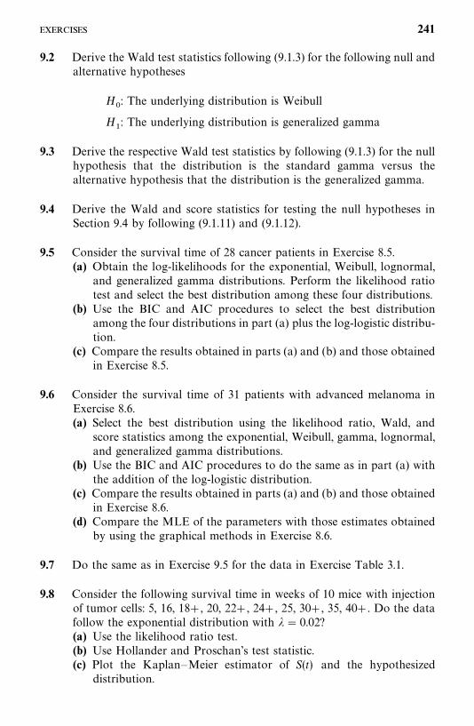
9.2 Derive the Wald test statistics following (9.1.3) for the following null andalternative hypotheses
H�: The underlying distribution is Weibull
H�: The underlying distribution is generalized gamma
9.3 Derive the respective Wald test statistics by following (9.1.3) for the nullhypothesis that the distribution is the standard gamma versus thealternative hypothesis that the distribution is the generalized gamma.
9.4 Derive the Wald and score statistics for testing the null hypotheses inSection 9.4 by following (9.1.11) and (9.1.12).
9.5 Consider the survival time of 28 cancer patients in Exercise 8.5.(a) Obtain the log-likelihoods for the exponential, Weibull, lognormal,
and generalized gamma distributions. Perform the likelihood ratiotest and select the best distribution among these four distributions.
(b) Use the BIC and AIC procedures to select the best distributionamong the four distributions in part (a) plus the log-logistic distribu-tion.
(c) Compare the results obtained in parts (a) and (b) and those obtainedin Exercise 8.5.
9.6 Consider the survival time of 31 patients with advanced melanoma inExercise 8.6.(a) Select the best distribution using the likelihood ratio, Wald, and
score statistics among the exponential, Weibull, gamma, lognormal,and generalized gamma distributions.
(b) Use the BIC and AIC procedures to do the same as in part (a) withthe addition of the log-logistic distribution.
(c) Compare the results obtained in parts (a) and (b) and those obtainedin Exercise 8.6.
(d) Compare the MLE of the parameters with those estimates obtainedby using the graphical methods in Exercise 8.6.
9.7 Do the same as in Exercise 9.5 for the data in Exercise Table 3.1.
9.8 Consider the following survival time in weeks of 10 mice with injectionof tumor cells: 5, 16, 18, 20, 22, 24, 25, 30, 35, 40. Do the datafollow the exponential distribution with �� 0.02?(a) Use the likelihood ratio test.(b) Use Hollander and Proschan’s test statistic.(c) Plot the Kaplan—Meier estimator of S(t) and the hypothesized
distribution.
241
9.9 Consider the following survival time in months of 25 patients withcancer of the prostate. Test the hypothesis that the survival time ofprostate cancer patients follows the exponential distribution with�� 0.01: 2, 19, 19, 25, 30, 35, 40, 45, 45, 48, 60, 62, 69, 89, 90, 110, 145,160, 9, 10, 20, 40, 50, 110, 130.
9.10 The Gompertz distribution belongs to the Gompertz—Makeham dis-tribution family and the Gompertz—Makeham distribution (Makeham,1860) has the following hazard function:
h(t) � � exp(� �t) � � 0
Construct a likelihood ratio statistic and Wald’s statistic to test the appro-priateness of a Gompertz distribution.
242
CHAPTER 10
Parametric Methods for ComparingTwo Survival Distributions
In Chapter 5 we discussed several nonparametric tests for comparing twosurvival distributions. If the distributions follow a known model, parametrictests are more powerful than nonparametric tests, but their computation ismore tedious. In this chapter we first discuss the likelihood ratio test in generalfor comparing two survival distributions in Section 10.1. Readers who are notfamiliar with linear algebra may skip this section without loss of continuity. InSections 10.2 to 10.4 we present either the likelihood ratio test or other testsfor the comparison of two survival patterns that follow the exponential,Weibull, and gamma distributions.
10.1 LIKELIHOOD RATIO TEST FOR COMPARING TWOSURVIVAL DISTRIBUTIONS
Let x�, . . . , x
��, and y
�, . . . , y
��be the observed exact or censored survival times
of n�and n
�subjects from two groups. Assume that the survival times from the
two groups follow the same distribution with different parameters. We use thegeneral notation b� (b
�, b
�, . . . , b
�) to denote the set of parameters of the
distribution, p� 1. Let l�(b
�), i� 1, 2, denote the log-likelihood function for the
observed survival times from each group, where b�� (b
��, . . . , b
��,
b����
, . . . , b��) � (b
��, b
��), and b
��� (b
��, . . . , b
��) and b
��� (b
����, . . . , b
��) are
two subsets of the p parameters, i� 1, 2. Then the joint log-likelihood functionfor the two groups is l(b
�, b
�) � l
�(b
�) � l
�(b
�). Let b�
�denote the MLE of b
�,
and b���
(b�) denote the MLE of b
��given b
��� b
�, where b
�is known.
For example, if the survival time of the two groups follows the Weibulldistribution with a scale parameter � and a shape parameter �. Then p � 2,b�� (�
�, �
�), and b
�� (�
�, �
�), where �
�, �
�and �
�, �
�are the respective
parameters in the two Weibull distributions. Let l�(�
�, �
�) and l
�(�
�, �
�) denote
the log-likelihood functions of the observed survival times from two groups;
243
then the joint log-likelihood function for the two groups is
l(��, �
�, �
�, �
�) � l
�(�
�, �
�) � l
�(�
�, �
�)
In this case, b��may be a singleton �
�, and similarly, b
��may be �
�.
The following tests are widely used in comparing two survival distributions.
Case 1. All parameters are unknown. When b�, i � 1, 2, are unknown, we
test the hypothesis
H�: b
�� b
�� b (10.1.1)
that is, that the two groups have the same survival distribution with equal butunknown parameters b. The log-likelihood ratio test statistic
X���2[l(b� , b� ) � l(b�
�, b�
�)]
� 2[l�(b�
�) � l
�(b�
�) � l(b� , b� )] (10.1.2)
has an asymptotic chi-square distribution with p degrees of freedom. For agiven significance level �, H
�is rejected if
X�� ��
��� (10.1.3)
or equivalently, if
P(����X
�) �� (10.1.4)
where ���denotes the chi-square random variable with p degrees of freedom,
and ����� is its 100(1� �) percentile points, P(��
����
���) � �.In the case of comparing two Weibull distributions, it reduces to
H�: �
�� �
�� � and �
�� �
�� �
where � and � are unknown,
X�� 2[l
�(��
�, �
�) � l
�(��
�, �
�) � l(�� , � , �� , � )]
and H�is rejected if X
����
��� , or equivalently, if P(����X
�) ��.
Case 2. A subset of the parameters of the two survival distributions areknown and equal, say, b
��� b
��� b
�, where the values of b
�are known. The
null hypothesis is the equality of the remaining parameters, or
H�: b
��� b
��� b
��(10.1.5)
244
where b��is unknown. The log-likelihood ratio statistic is
X�� 2[l
�(b
�, b�
��(b
�)) � l
�(b
�, b�
��(b
�)) � l((b
�, b�
��(b
�)), (b
�, b�
��(b
�))]
(10.1.6)
where b���
(b�) is the MLE of b
��given b
��� b
�, and so are the others. X
�has
an asymptotic chi-square distribution with degrees of freedom equal to thenumber of parameters in b
��(or b
��).
In the case of comparing two Weibull distributions, we may assume that��� �
�� �
�(or �
�� �
�� �
�), where the value of �
�(or �
�) is known, and test
the null hypothesis
H�: �
�� �
�� � (or �
�� �
�� �)
Then
X�� 2[l
�(�
�, �
�(�
�)) � l
�(�
�, �
�(�
�)) � l(�
�, � (�
�), �
�, � (�
�))]
(or X�� 2[l
�(��
�(�
�), �
�) � l
�(��
�(�
�), �
�) � l(�� (�
�), �
�, �� (�
�), �
�)]
and H�is rejected if X
����
��� , equivalently, if P(����X
�) ��.
Case 3. A subset of the parameters of the two survival distributions areequal but unknown, say, if b
��� b
��� b
��and the values of b
��are unknown.
The null hypothesis is the equality of the remaining parameters, or
H�: b
��� b
��� b
��(10.1.7)
where b��is unknown and needs to be estimated. In addition, b
��also needs to
be estimated. The log-likelihood ratio statistic,
X�� 2[l((b�
��, b�
��), (b�
��, b�
��)) � l (b� , b� )] (10.1.8)
has an asymptotic chi-square distribution with degrees of freedom equal to thenumber of parameters in b
��(or b
��).
For the case of comparing two Weibull distributions, the derivation of X�
in (10.1.8) is left to the reader as an exercise.
Case 4. A subset of the parameters of the two survival distributions areknown but not equal, say, if b
��� b
��, b
��� b
��, and b
��and b
��are known
245
but b��
� b��. The null hypothesis is the equality of the remaining parameters,
or
H�: b
��� b
��� b
��(10.1.9)
The log-likelihood ratio statistic
X�� 2[l
�(b
��, b�
��(b
��)) � l
�(b
��, b�
��(b
��))
� l((b��, b�
��(b
��, b
��)), (b
��, b�
��(b
��, b
��)))] (10.1.10)
has an asymptotic chi-square distribution with degrees of freedom equal to thenumber of parameters in b
��or b
��.
For the case of comparing two Weibull distributions, the derivation of X�
in (10.1.10) is left to the reader as an exercise.
10.2 COMPARISON OF TWO EXPONENTIAL DISTRIBUTIONS
Suppose that two survival distributions follow the exponential model withparameters �
�and �
�, respectively. Two tests can compare the distributions:
the likelihood ratio test and an F-test suggested by Cox (1953). These two testscan test the hypothesis that the two exponential distributions are equalwhether or not the samples include censored observations.
10.2.1 Likelihood Ratio Test
Suppose that there are n�and n
�individuals in groups 1 and 2, respectively,
x�, . . . , x
��uncensored and x�
����, . . . , x�
��censored in group 1, and y
�, . . . , y
��uncensored and y�����
, . . . , y���censored in group 2. Thus, in group 1, there are
r�uncensored and n
�� r
�censored observations. In group 2, there are r
�uncensored and n
�� r
�censored observations. If it is known that the survival
times of the two groups follow the exponential distribution with densityfunction f
�(t) � �
�e�� �, i � 1, 2, testing the equality of two exponential distribu-
tions is equivalent to testing the hypothesis H�: �
�� �
�. This is because the two
exponential distributions are characterized by the two parameters ��and �
�.
Thus, the null hypothesis is H�: �
�� �
�� � and the alternative hypothesis is
H�: �
�� �
�. According to (10.1.2), the test statistic for the likelihood ratio test
is
X���2 log
L (�� , �� )L (��
�, ��
�)
(10.2.1)
246
where the denominator is the likelihood function for the two groups combined,
L (���, ��
�) � �� ��
��� ���exp����
� �����
x��
��
�����
x�� �
� ��� �
����
y��
��
�����
y�� �� (10.2.2)
and ���and ��
�are the MLE of �
�and �
�, respectively, from groups 1 and 2.
From Section 7.2,
����
r�
����
x����
�����x��
����
r�
����
y����
�����y��
(10.2.3)
The numerator in (10.2.1) is the likelihood function for the combined sampleunder the null hypothesis, that is, �
�� �
�� �,
L (�� , �� ) � �� ����� exp���� �����
x��
��
�����
x��
�����
y��
��
�������(10.2.4)
where �� is the MLE of � obtained from the combined sample,
�� �r�� r
���
��x����
�����x��
�����
y����
�����y��
(10.2.5)
From Section 10.1, X�has an approximate chi-square distribution with 1
degree of freedom for samples of at least 25 (n�� n
�� 25) under the null
hypothesis. For a given significance level �, H�is rejected if X
����
��� , orequivalently, if P(��
��X
�) ��.
The test procedure can be summarized as follows:
1. Compute ���and ��
�following (10.2.3).
2. Compute L (���, ��
�) in (10.2.2) using the given data and ��
�and ��
�obtained
in step 1.
3. Compute �� following (10.2.5).4. Compute L (�� , �� ) in (10.2.4).5. Compute X
�in (10.2.1). If X
����
��� (Table B-2), reject H�and conclude
that the two exponential survival distributions are not equal. Otherwise,the data do not provide enough evidence to reject the null hypothesis.
If there are no censored observations in the data, (10.2.1)—(10.2.5) are alsoapplicable simply be letting n
�� r
�, n
�� r
�and omitting the terms involving
247
x��
and y��. The likelihood ratio test is primarily for two-sided tests and is
difficult to apply to a one-sided test. It is approximate and should be used withcaution when the sample size is small. The power of the test, similar to that ofother likelihood tests, is not high. That is, if the likelihood ratio test is usedregularly, one is more likely not to reject the null hypothesis when the twosurvival distributions are not equal.
Example 10.1 Consider the remission data of the two treatment groupsgiven in Example 5.1. The remission times in months are as follows:
CMF: 23, 16�, 18�, 20�, 24�
Control: 15, 18, 19, 19, 20
Assume that the two distributions are exponential with parameters ��and �
�,
respectively. Using the likelihood ratio test, we test the following null hypoth-esis
H�: �
�� �
�� � (the two treatments are equally effective)
against
H�: �
�� �
�(the two treatments are not equally effective)
Following the above, we proceed as follows:
1. Compute ���and ��
�in (10.2.3): In this case, n
�� n
�� 5, r
�� 1, r
�� 5,
����
x�� 23, ��
�����x��
� 78, ����
y�� 91, ��
�����y��
� 0,
����
1
23� 78�
1
101� 0.0099
����
5
91� 0.0549
2. Compute L (���, ��
�) in (10.2.2):
L (���, ��
�) � (0.0099)(0.0549)� exp[�0.0099(101)� 0.0549(91)]
� 1.2290(10)��
3. Compute �� in (10.2.5):
�� �1� 5
23� 78� 91�
6
192� 0.0313
248
4. Compute L (���, ��
�) in (10.2.4):
L (���, ��
�) � (0.0313)� exp[�0.0313(192)]� 2.3085(10)��
5. Compute X�in (10.2.1):
X���2 log
2.3085(10)��
1.2290(10)��� �2 log(0.1878)� 3.344
From Table B-2 we obtain ����� ��
� 3.84. Thus we cannot reject H�at the
0.05 level. Recall that in Chapter 5 the null hypothesis was rejected at the 0.05level by using the four nonparametric tests.
10.2.2 Cox’s F-Test for Exponential Distributions
If the times to failure can be assumed to follow the exponential distribution inboth treatment groups, an F-test suggested by Cox (1953) can be used to testfor treatment differences whether or not censored observations are present.Suppose that we wish to test the hypothesis H
�: �
�� �
�against either the
one-sided alternative H�: �
���
�(or H
�: �
���
�) or the two-sided alternative
H�: �
�� �
�. An efficient test is to take t�
�/t��as having an F-distribution with
(2r�, 2r
�) degrees of freedom, where
t���
����
x����
�����x��
r�
(10.2.6)
t���
����
y����
�����y��
r�
(10.2.7)
The test procedures are (1) for H�, reject H
�if t�
�/t���F
��������� ; (2) for H�,
reject H�if t�
�/t���F
���������� ; and (3) for H�, reject H
�if t�
�/t���F
����������� ort��/t�
��F
������������, where � is the significance level and F��������� is the upper
100� percentage point of the F-distribution with (2r�, 2r
�) degrees of freedom.
Similarly, the hypothesis that ��/�
�� k can be tested by referring kt�
�/t��to the
table of the F-distribution.When there are no censored observations, that is, n
�� r
�, n
�� r
�, the
second terms of the numerators in (10.2.6) and (10.2.7) are zero. Then the teststatistic t�
�/t��has an F-distribution with (2n
�, 2n
�) degrees of freedom.
Confidence intervals for the ratio ��/�
�can be obtained from the fact that
��t��/�
�t��has the F-distribution with (2n
�, 2n
�) degrees of freedom. It follows
that a 100(1� �)%confidence interval for the ratio of two hazard rates ��/�
�is
t��
t��
F�������������
��
��
�t��
t��
F����������� (10.2.8)
249
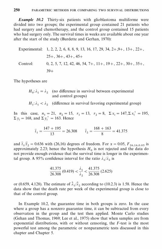
Example 10.2 Thirty-six patients with glioblastoma multiforme weredivided into two groups; the experimental group contained 21 patients whohad surgery and chemotherapy, and the control group contained 15 patientswho had surgery only. The survival times in weeks are available about one yearafter the start of the study (Burdette and Gerhan, 1970):
Experimental: 1, 2, 2, 2, 6, 8, 8, 9, 13, 16, 17, 29, 34, 2�,9�, 13�, 22�,
25�, 36�, 43�, 45�
Control: 0, 2, 5, 7, 12, 42, 46, 54, 7�, 11�, 19�, 22�, 30�, 35�,
39�
The hypotheses are
H�: �
�� �
�(no difference in survival between experimentaland control groups)
H�: �
���
�(difference in survival favoring experimental group)
In this case, n�� 21, n
�� 15, r
�� 13, r
�� 8, � x
�� 147,� x�
�� 195,
� y�� 168, and � y�
�� 163. Hence
t���
147� 195
13� 26.308 t�
��
168� 163
8� 41.375
and t��/t��� 0.636 with (26,16) degrees of freedom. For � � 0.05, F
������� ��is
approximately 2.23; hence the hypothesis H�is not rejected and the data do
not provide enough evidence that the survival time is longer in the experimen-tal group. A 95% confidence interval for the ratio �
�/�
�is
41.375
26.308(0.419) �
��
��
�41.375
26.308(2.625)
or (0.659, 4.128). The estimate of ���/��
�according to (10.2.3) is 1.58. Hence the
data show that the death rate per week of the experimental group is close tothat of the control group.
In Example 10.2, the guarantee time in both groups is zero. In the casewhere a group has a nonzero guarantee time, it can be subtracted from everyobservation in the group and the test then applied. Monte Carlo studies(Gehan and Thomas, 1969; Lee et al., 1975) show that when samples are fromexponential distributions, with or without censoring, the F-test is the mostpowerful test among the parametric or nonparametric tests discussed in thischapter and Chapter 5.
250
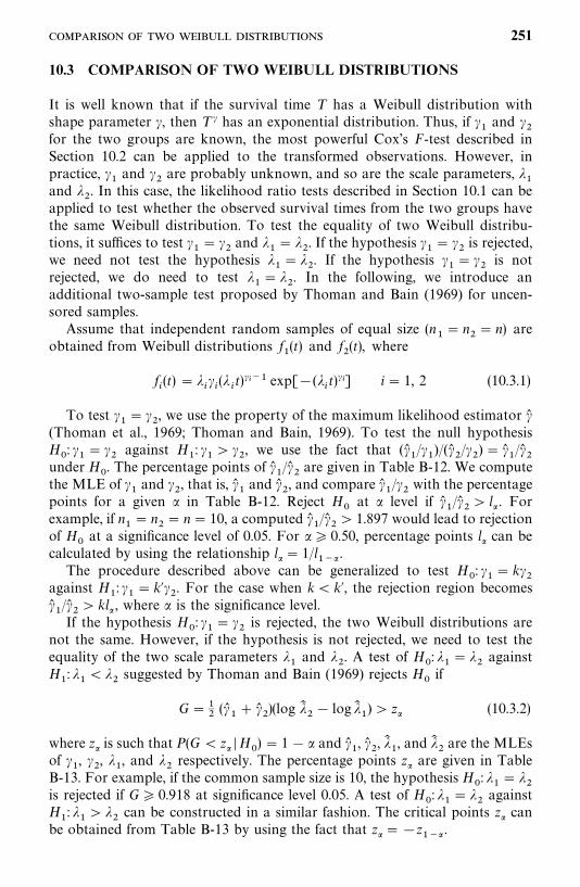
10.3 COMPARISON OF TWO WEIBULL DISTRIBUTIONS
It is well known that if the survival time T has a Weibull distribution withshape parameter �, then T � has an exponential distribution. Thus, if �
�and �
�for the two groups are known, the most powerful Cox’s F-test described inSection 10.2 can be applied to the transformed observations. However, inpractice, �
�and �
�are probably unknown, and so are the scale parameters, �
�and �
�. In this case, the likelihood ratio tests described in Section 10.1 can be
applied to test whether the observed survival times from the two groups havethe same Weibull distribution. To test the equality of two Weibull distribu-tions, it suffices to test �
�� �
�and �
�� �
�. If the hypothesis �
�� �
�is rejected,
we need not test the hypothesis ��� �
�. If the hypothesis �
�� �
�is not
rejected, we do need to test ��� �
�. In the following, we introduce an
additional two-sample test proposed by Thoman and Bain (1969) for uncen-sored samples.
Assume that independent random samples of equal size (n�� n
�� n) are
obtained from Weibull distributions f�(t) and f
�(t), where
f�(t) � �
���(�
�t)��� exp[�(�
�t)��] i � 1, 2 (10.3.1)
To test ��� �
�, we use the property of the maximum likelihood estimator �
(Thoman et al., 1969; Thoman and Bain, 1969). To test the null hypothesisH
�: �
�� �
�against H
�: �
���
�, we use the fact that (�
�/�
�)/(�
�/�
�) � �
�/�
�under H
�. The percentage points of �
�/�
�are given in Table B-12. We compute
the MLE of ��and �
�, that is, �
�and �
�, and compare �
�/�
�with the percentage
points for a given � in Table B-12. Reject H�at � level if �
�/�
�� l� . For
example, if n�� n
�� n� 10, a computed �
�/�
�� 1.897 would lead to rejection
of H�at a significance level of 0.05. For �� 0.50, percentage points l� can be
calculated by using the relationship l�� 1/l�� .
The procedure described above can be generalized to test H�: �
�� k�
�against H
�: �
�� k �
�. For the case when k� k , the rejection region becomes
��/�
�� kl� , where � is the significance level.
If the hypothesis H�: �
�� �
�is rejected, the two Weibull distributions are
not the same. However, if the hypothesis is not rejected, we need to test theequality of the two scale parameters �
�and �
�. A test of H
�: �
�� �
�against
H�: �
���
�suggested by Thoman and Bain (1969) rejects H
�if
G ���(�
�� �
�)(log ��
�� log ��
�) � z� (10.3.2)
where z� is such that P(G � z� �H�) � 1� � and �
�, �
�, ��
�, and ��
�are the MLEs
of ��, �
�, �
�, and �
�respectively. The percentage points z� are given in Table
B-13. For example, if the common sample size is 10, the hypothesis H�: �
�� �
�is rejected if G � 0.918 at significance level 0.05. A test of H
�: �
�� �
�against
H�: �
���
�can be constructed in a similar fashion. The critical points z� can
be obtained from Table B-13 by using the fact that z���z�� .
251
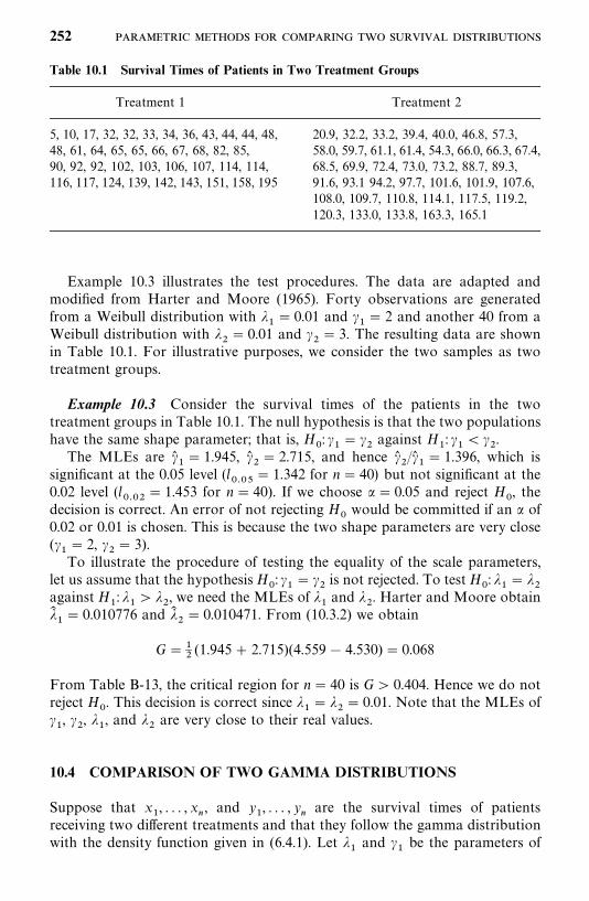
Table 10.1 Survival Times of Patients in Two Treatment Groups
Treatment 1 Treatment 2
5, 10, 17, 32, 32, 33, 34, 36, 43, 44, 44, 48,48, 61, 64, 65, 65, 66, 67, 68, 82, 85,90, 92, 92, 102, 103, 106, 107, 114, 114,116, 117, 124, 139, 142, 143, 151, 158, 195
20.9, 32.2, 33.2, 39.4, 40.0, 46.8, 57.3,58.0, 59.7, 61.1, 61.4, 54.3, 66.0, 66.3, 67.4,68.5, 69.9, 72.4, 73.0, 73.2, 88.7, 89.3,91.6, 93.1 94.2, 97.7, 101.6, 101.9, 107.6,108.0, 109.7, 110.8, 114.1, 117.5, 119.2,120.3, 133.0, 133.8, 163.3, 165.1
Example 10.3 illustrates the test procedures. The data are adapted andmodified from Harter and Moore (1965). Forty observations are generatedfrom a Weibull distribution with �
�� 0.01 and �
�� 2 and another 40 from a
Weibull distribution with ��� 0.01 and �
�� 3. The resulting data are shown
in Table 10.1. For illustrative purposes, we consider the two samples as twotreatment groups.
Example 10.3 Consider the survival times of the patients in the twotreatment groups in Table 10.1. The null hypothesis is that the two populationshave the same shape parameter; that is, H
�: �
�� �
�against H
�: �
���
�.
The MLEs are ��� 1.945, �
�� 2.715, and hence �
�/�
�� 1.396, which is
significant at the 0.05 level (l� ��
� 1.342 for n� 40) but not significant at the0.02 level (l
� ��� 1.453 for n � 40). If we choose �� 0.05 and reject H
�, the
decision is correct. An error of not rejecting H�would be committed if an � of
0.02 or 0.01 is chosen. This is because the two shape parameters are very close(�
�� 2, �
�� 3).
To illustrate the procedure of testing the equality of the scale parameters,let us assume that the hypothesis H
�: �
�� �
�is not rejected. To test H
�: �
�� �
�against H
�: �
���
�, we need the MLEs of �
�and �
�. Harter and Moore obtain
���� 0.010776 and ��
�� 0.010471. From (10.3.2) we obtain
G ���
(1.945� 2.715)(4.559� 4.530) � 0.068
From Table B-13, the critical region for n� 40 is G� 0.404. Hence we do notreject H
�. This decision is correct since �
�� �
�� 0.01. Note that the MLEs of
��, �
�, �
�, and �
�are very close to their real values.
10.4 COMPARISON OF TWO GAMMA DISTRIBUTIONS
Suppose that x�, . . . , x
�, and y
�, . . . , y
�are the survival times of patients
receiving two different treatments and that they follow the gamma distributionwith the density function given in (6.4.1). Let �
�and �
�be the parameters of
252
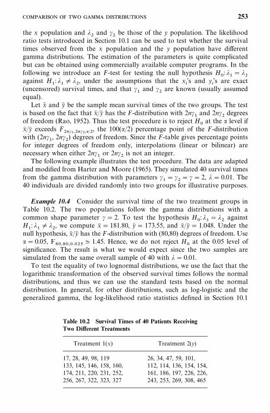
Table 10.2 Survival Times of 40 Patients ReceivingTwo Different Treatments
Treatment 1(x) Treatment 2(y)
17, 28, 49, 98, 119 26, 34, 47, 59, 101,133, 145, 146, 158, 160, 112, 114, 136, 154, 154,174, 211, 220, 231, 252, 161, 186, 197, 226, 226,256, 267, 322, 323, 327 243, 253, 269, 308, 465
the x population and ��and �
�be those of the y population. The likelihood
ratio tests introduced in Section 10.1 can be used to test whether the survivaltimes observed from the x population and the y population have differentgamma distributions. The estimation of the parameters is quite complicatedbut can be obtained using commercially available computer programs. In thefollowing we introduce an F-test for testing the null hypothesis H
�: �
�� �
�against H
�: �
�� �
�, under the assumptions that the x
�’s and y
�’s are exact
(uncensored) survival times, and that ��and �
�are known (usually assumed
equal).Let x� and y� be the sample mean survival times of the two groups. The test
is based on the fact that x� /y� has the F-distribution with 2n��and 2n�
�degrees
of freedom (Rao, 1952). Thus the test procedure is to reject H�at the � level if
x� /y� exceeds F�������������, the 100(�/2) percentage point of the F-distribution
with (2n��, 2n�
�) degrees of freedom. Since the F-table gives percentage points
for integer degrees of freedom only, interpolations (linear or bilinear) arenecessary when either 2n�
�or 2n�
�is not an integer.
The following example illustrates the test procedure. The data are adaptedand modified from Harter and Moore (1965). They simulated 40 survival timesfrom the gamma distribution with parameters �
�� �
�� � � 2, �� 0.01. The
40 individuals are divided randomly into two groups for illustrative purposes.
Example 10.4 Consider the survival time of the two treatment groups inTable 10.2. The two populations follow the gamma distributions with acommon shape parameter �� 2. To test the hypothesis H
�: �
�� �
�against
H�: �
�� �
�, we compute x� � 181.80, y� � 173.55, and x� /y� � 1.048. Under the
null hypothesis, x� /y� has the F-distribution with (80,80) degrees of freedom. Use�� 0.05, F
������� ���� 1.45. Hence, we do not reject H
�at the 0.05 level of
significance. The result is what we would expect since the two samples aresimulated from the same overall sample of 40 with � � 0.01.
To test the equality of two lognormal distributions, we use the fact that thelogarithmic transformation of the observed survival times follows the normaldistributions, and thus we can use the standard tests based on the normaldistribution. In general, for other distributions, such as log-logistic and thegeneralized gamma, the log-likelihood ratio statistics defined in Section 10.1
253
can be applied to test whether the survival times observed from two groupshave the same distribution. Readers can follow Example 10.2.1 in Section 10.2and use the respective likelihood functions derived in Chapter 7 to constructthe needed tests.
Bibliographical Remarks
In addition to the papers cited in this chapter, readers are referred to Mann etal. (1974), Gross and Clark (1975), Lawless (1982), and Nelson (1982).
EXERCISES
10.1 Derive the likelihood ratio tests in (10.1.8) and (10.1.10) for testing theequality of two Weibull distributions.
10.2 Derive the likelihood ratio test in (10.1.2) for testing the equality of twolog-logistic distributions with unknown parameters.
10.3 Consider the remission data of the leukemia patients in Example 3.3.Assume that the remission times of the two treatment groups follow theexponential distribution. Test the hypothesis that the two treatments areequally effective using:(a) The likelihood ratio test(b) Cox’s F-testObtain a 95% confidence interval for the ratio of the two hazard rates.
10.4 For the same data in Exercise 10.3, test the hypothesis that ��� 5�
�.
10.5 Suppose that the survival time of two groups of lung cancer patientsfollows the Weibull distribution. A sample of 30 patients (15 from eachgroup) was studied. Maximun likelihood estimates obtained from thetwo groups are, respectively, �
�� 3, ��
�� 1.2 and �
�� 2, ��
�� 0.5. Test
the hypothesis that the two groups are from the same Weibull distribu-tion.
10.6 Divide the lifetimes of 100 strips (delete the last one) of aluminumcoupon in Table 6.4 randomly into two equal groups. This can be doneby assigning the observations alternately to the two groups. Assume thatthe two groups follow a gamma distribution with shape parameter�� 12. Test the hypothesis that the two scale parameters are equal.
10.7 Twelve brain tumor patients are randomized to receive radiation ther-apy or radiation therapy plus chemotherapy (BCNU) in a one-yearclinical trial. The following survival times in weeks are recorded:
254
1. Radiation�BCNU: 24, 30, 42, 15�, 40�, 42�
2. Radiation: 10, 26, 28, 30, 41, 12�
Assuming that the survival time follows the exponential distribution, useCox’s F-test for exponential distributions to test the null hypothesisH
�: �
�� �
�versus the alternative H
�: �
���
�.
10.8 Use one of the nonparametric tests discussed in Chapter 5 to test theequality of survival distributions of the experimental and control groupsin Example 10.2. Compare your result with that obtained in Example10.2.
255
CHAPTER 11
Parametric Methods for RegressionModel Fitting and Identificationof Prognostic Factors
Prognosis, the prediction of the future of an individual patient with respect toduration, course, and outcome of a disease plays an important role in medicalpractice. Before a physician can make a prognosis and decide on the treatment,a medical history as well as pathologic, clinical, and laboratory data are oftenneeded. Therefore, many medical charts contain a large number of patient (orindividual) characteristics (also called concomitant variables, independent vari-ables, covariates, prognostic factors, or risk factors), and it is often difficult tosort out which ones are most closely related to prognosis. The physician canusually decide which characteristics are irrelevant, but a statistical analysis isusually needed to prepare a compact summary of the data that can reveal theirrelationship. One way to achieve this purpose is to search for a theoreticalmodel (or distribution), that fits the observed data and identify the mostimportant factors. These models, usually regression models, extend themethods discussed in previous chapters to include covariates. In this chapterwe focus on parametric regression models (i.e., we assume that the survivaltime follows a theoretical distribution). If an appropriate model can beassumed, the probability of surviving a given time when covariates areincorporated can be estimated.In Section 11.1 we discuss briefly possible types of response and prognostic
variables and things that can be done in a preliminary screening before aformal regression analysis. This section applies to methods discussed in thenext four chapters. In Section 11.2 we introduce the general structure of acommonly used parametric regression model, the accelerated failure time(AFT) model. Sections 11.3 to 11.7 cover several special cases of AFT models.Fitting these models often involves complicated and tedious computations andrequires computer software. Fortunately, most of the procedures are availablein software packages such as SAS and BMDP. The SAS and BMDP code that
256
can be used to fit the models are given at the end of the examples. Readers mayfind these codes helpful. Section 11.8 introduces two other models. In Section11.9 we discuss the model selection methods and goodness of fit tests.
11.1 PRELIMINARY EXAMINATION OF DATA
Information concerning possible prognostic factors can be obtained either fromclinical studies designed mainly to identify them, sometimes called prognosticstudies, or from ongoing clinical trials that compare treatments as a subsidiaryaspect. The dependent variable (also called the response variable), or theoutcome of prediction, may be dichotomous, polychotomous, or continuous.Examples of dichotomous dependent variables are response or nonresponse,life or death, and presence or absence of a given disease. Polychotomousdependent variables include different grades of symptoms (e.g., no evidence ofdisease, minor symptom, major symptom) and scores of psychiatric reactions(e.g., feeling well, tolerable, depressed, or very depressed). Continuous depend-ent variables may be length of survival from start of treatment or length ofremission, both measured on a numerical scale by a continuous range of values.Of these dependent variables, response to a given treatment (yes or no),development of a specific disease (yes or no), length of remission, and lengthof survival are particularly common in practice. In this chapter we focus ourattention on continuous dependent variables such as survival time and re-mission duration. Dichotomous and multiple-response dependent variables arediscussed in Chapter 14.A prognostic variable (or independent variable) or factor may be either
numerical or nonnumerical. Numerical prognostic variables may be discrete,such as the number of previous strokes or number of lymph node metastases,or continuous, such as age or blood pressure. Continuous variables can bemade discrete by grouping patients into subcategories (e.g., four age subgroups:�20, 20—39, 40—59, and �60). Nonnumerical prognostic variables may beunordered (e.g., race or diagnosis) or ordered (e.g., severity of disease may beprimary, local, or metastatic). They can also be dichotomous (e.g., a liver eitheris or is not enlarged). Usually, the collection of prognostic variables includessome of each type.Before a statistical calculation is done, the data have to be examined
carefully. If some of the variables are significantly correlated, one of thecorrelated variables is likely to be a predictor as good as all of them.Correlation coefficients between variables can be computed to detect signifi-cantly correlated variables. In deleting any highly correlated variables, infor-mation from other studies has to be incorporated. If other studies show that agiven variable has prognostic value, it should be retained.In the next eight sections we discuss multivariate or regression techniques,
which are useful in identifying prognostic factors. The regression techniquesinvolve a function of the independent variables or possible prognostic factors.
257
The variables must be quantitative, with particular numerical values for eachpatient. This raises no problem when the prognostic variables are naturallyquantitative (e.g., age) and can be used in the equation directly. However, if aparticular prognostic variable is qualitative (e.g., a histological classificationinto one of three cell types A, B, or C), something needs to be done. Thissituation can be covered by the use of two dummy variables, e.g., x
�, taking
the value 1 for cell type A and 0 otherwise, and x�, taking the value 1 for cell
type B and 0 otherwise. Clearly, if there are only two categories (e.g., sex), onlyone dummy variable is needed: x
�is 1 for a male, 0 for a female. Also, a better
description of the data might be obtained by using transformed values of theprognostic variables (e.g., squares or logarithms) or by including products suchas x
�x�
(representing an interaction between x�and x
�). Transforming the
dependent variable (e.g., taking the logarithm of a response time) can alsoimprove the fit.In practice, there are usually a larger number of possible prognostic factors
associated with the outcomes. One way to reduce the number of factors beforea multivariate analysis is attempted is to examine the relationship between eachindividual factor and the dependent variable (e.g., survival time). From theunivariate analysis, factors that have little or no effect on the dependentvariable can be excluded from the multivariate analysis. However, it would bedesirable to include factors that have been reported to have prognostic valuesby other investigators and factors that are considered important from biomedi-cal viewpoints. It is often useful to consider model selection methods to choosethose significant factors among all possible factors and determine an adequatemodel with as few variables as possible. Very often, a variable of significantprognostic value in one study is unimportant in another. Therefore, confirma-tion in a later study is very important in identifying prognostic factors.Another frequent problem in regression analysis is missing data. Three
distinctions about missing data can be made: (1) dependent versus independentvariables, (2) many versus few missing data, and (3) random versus nonrandomloss of data. If the value of the dependent variable (e.g., survival time) isunknown, there is little to do but drop that individual from analysis and reducethe sample size. The problem of missing data is of different magnitudedepending on how large a proportion of data, either for the dependent variableor for the independent variables, is missing. This problem is obviously lesscritical if 1% of data for one independent variable is missing than if 40% ofdata for several independent variables is missing. When a substantial propor-tion of subjects has missing data for a variable, we may simply opt to dropthem and perform the analysis on the remainder of the sample. It is difficult tospecify ‘‘how large’’ and ‘‘how small,’’ but dropping 10 or 15 cases out of severalhundred would raise no serious practical objection. However, if missing dataoccur in a large proportion of persons and the sample size is not comfortablylarge, a question of randomness may be raised. If people with missing data donot show significant differences in the dependent variable, the problem is notserious. If the data are not missing randomly, results obtained from dropping
258
subjects will be misleading. Thus, dropping cases is not always an adequatesolution to the missing data problem.If the independent variable is measured on a nominal or categorical scale,
an alternative method is to treat individuals in a group with missing informa-tion as another group. For quantitatively measured variables (e.g., age), themean of the values available can be used for a missing value. This principle canalso be applied to nominal data. It does not mean that the mean is a goodestimate for the missing value, but it does provide convenience for analysis.A more detailed discussion on missing data can be found in Cohen and
Cohen (1975, Chap. 7), Little and Rubin (1987), Efron (1994), Crawford et al.(1995), Heitjan (1997), and Schafer (1999).
11.2 GENERAL STRUCTURE OF PARAMETRIC REGRESSIONMODELS AND THEIR ASYMPTOTIC LIKELIHOOD INFERENCE
When covariates are considered, we assume that the survival time, or afunction of it, has an explicit relationship with the covariates. Furthermore,when a parametric model is considered, we assume that the survival time (ora function of it) follows a given theoretical distribution (or model) and has anexplicit relationship with the covariates. As an example, let us consider theWeibull distribution in Section 6.2. Let x � (x
�, . . . , x
�) denote the p covariates
considered. If the parameter � in the Weibull distribution is related to x asfollows:
�� e�(a����
���a�x�) � exp[�(a
�� a�x)]
where a� (a�, . . . , a
�) denote the coefficients for x, then the hazard function of
the Weibull distribution in (6.2.4) can be extended to include the covariates asfollows:
h(t,x) � ���t���� �t���e�(a����
���a�x�)� � �t��� exp[�(a
�� a�x)�] (11.2.1)
The survivorship function in (6.2.3) becomes
S(t, x)� (e���)exp(��(a��a�x)) (11.2.2)
or
log[�logS(t, x)]���(a�� a�x) � � log t (11.2.3)
which presents a linear relationship between log[�logS(t, x)] and log t and thecovariates. In Sections 11.2 to 11.7 we introduce a special model called theaccelerated failure time model.Analogous to conventional regression methods, survival time can also be
analyzed by using the accelerated failure time (AFT) model. The AFT model
259
for survival time assumes that the relationship of logarithm of survival time Tand the covariates is linear and can be written as
logT � a��
�����
a�x��� (11.2.4)
where x�, j� 1, . . . , p, are the covariates, a
�, j� 0, 1, . . . , p the coefficients, �
(� 0) is an unknown scale parameter, and , the error term, is a randomvariable with known forms of density function g(, d) and survivorship functionG(, d) but unknown parameters d. This means that the survival is dependenton both the covariate and an underlying distribution g.Consider a simple case where there is only one covariate x with values 0 and
1. Then (11.2.4) becomes
logT � a�� a
�x��
Let T�and T
�denote the survival times for two individuals with x� 0 and
x� 1, respectively. Then, T�� exp(a
�� �), and T
�� exp(a
�� a
�� �)�
T�exp(a
�). Thus, T
�T
�if a
� 0 and T
��T
�if a
�� 0. This means that the
covariate x either ‘‘accelerates’’ or ‘‘decelerates’’ the survival time or time tofailure— thus the name accelerated failure time models for this family of models.In the following we discuss the general form of the likelihood function of
AFT models, the estimation procedures of the regression parameters (a�, a, �,
and d) in (11.2.4) and tests of significance of the covariates on the survival time.The calculations of these procedures can be carried out using availablesoftware packages such as SAS and BMDP. Readers who are not interested inthe mathematical details may skip the remaining part of this section and moveon to Section 11.3 without loss of continuity.Let t
�, t
�, . . . , t
�be the observed survival times from n individuals, including
exact, left-, right-, and interval-censored observations. Assume that the logsurvival time can be modeled by (11.2.4) and let a�� (a
�, a
�, . . . , a
�), and
b�� (a�, d�, a�, �). Similar to (7.1.1), the log-likelihood function in terms of the
density function g() and survivorship function G() of is
l(b) � log L (b) � � log[g(�)]�� log[G(
�)]
� log[1�G(�)]�� log[G(�
�)�G(
�)] (11.2.5)
where
��log t
�� a
����
���a�x��
�(11.2.6)
���log �
�� a
�� ��
���a�x��
�(11.2.7)
260
The first term in the log-likelihood function sums over uncensored observa-tions, the second term over right-censored observations, and the third termover left-censored observations, and the last term over interval-censoredobservations with �
�as the lower end of a censoring interval. Note that the last
two summations in (11.2.5) do not exist if there are no left- and interval-censored data.Alternatively, let
�� a
��
�����
a�x��
i� 1, 2, . . . , n (11.2.8)
Then (11.2.4) becomes
logT � �� (11.2.9)
The respective alternative log-likelihood function in terms of the densityfunction f (t, b) and survivorship function S(t, b) of T is
l(b) � log L (b) �� log[ f (t�, b)]�� log[S(t
�, b)]
� � log[1� S(t�, b)]�� log[S(�
�, b)� S(t
�, b)] (11.2.10)
where f (t, b) can be derived from (11.2.4) through the density function g() byapplying the density transformation rule
f (t, b)�g((log t� )/�)
�t(11.2.11)
and S(t, b) is the corresponding survivorship function. The vector b in (11.2.10)and (11.2.11) includes the regression coefficients and other parameters of theunderlying distribution.Either (11.2.5) or (11.2.10) can be used to derive the maximum likelihood
estimates (MLEs) of parameters in the model. For a given log-likelihoodfunction l(b), the MLE b� is a solution of the following simultaneous equations:
�(l(b))�b
�
� 0 for all i (11.2.12)
Usually, there is no closed solution for the MLE b� from (11.2.12) and theNewton—Raphson iterative procedure in Section 7.1 must be applied to obtainb� . By replacing the parameters b with its MLE b� in S(t
�, b), we have an
estimated survivorship function S(t, b� ), which takes into consideration thecovariates.All of the hypothesis tests and the ways to construct confidence intervals
shown in Section 7.1 can be applied here. In addition, we can use the followingtests to test linear relationships among the regression coefficients a
�, a
�, . . . , a
�.
261
To test a linear relationship among x�, . . . , x
�is equivalent to testing the
null hypothesis that there is a linear relationship among a�, a
�, . . . , a
�. H
�can
be written in general as
H�:La� c (11.2.13)
where L is a matrix or vector of constants for the linear hypothesis and c is aknown column vector of constants. The following Wald’s statistics can be used:
X�
� (La� � c)�[LV��(a� )L�]��(La� � c) (11.2.14)
where V� �(a� ) is the submatrix of the covariance matrix V� (b� ) corresponding to a.Under the H
�and some mild assumptions, X
�has an asymptotic chi-square
distribution with � degrees of freedom, where � is the rank of L. For a givensignificance level �, H
�is rejected if X
� ����� or X�
����,1��/2.For example, if p� 3 and we wish to test if x
�and x
�have equal effects on
the survival time, the null hypothesis is H�: a
�� a
�(or a
�� a
�� 0). It is easy
to see that for this hypothesis, the corresponding L� (1,�1, 0) and c� 0 since
La� (1, �1, 0)(a�, a
�, a
�)� � a
�� a
�
Let the (i, j ) element of V��(a� ) be �
��; then the X
�defined in (11.2.14) becomes
X�
� (a��� a�
�) �(1, �1, 0) �
���
���
���
���
���
���
���
���
�����
1
�1
0����
(a��� a�
�)
�(a�
�� a�
�)�
���
� ���
� 2���
X�has an asymptotic chi-square distribution with 1 degree of freedom (the
rank of L is 1).In general, to test if any two covariates have the same effects on T , the null
hypothesis can be written as
H�: a
�� a
�(or a
�� a
�� 0) (11.2.15)
The corresponding L� (0, . . . , 0, 1, 0, . . . , 0, �1, 0, . . . , 0) and c� 0, and theX
�in (11.2.14) becomes
X�
�(a�
�� a�
�)�
���� �
��� 2�
��
(11.2.16)
262
which has an asymptotic chi-square distribution with 1 degree of freedom. H�
is rejected if X�
����� or X�
�������� .
To test that none of the covariates is related to the survival time, the nullhypothesis is
H�: a� 0 (11.2.17)
The respective test statistics for this overall null hypothesis are shown inSection 9.1. For example, the log-likelihood ratio statistics there becomes
X���2[l(0, d� (0), a�
�(0), �� (0)) � l(b� )] (11.2.18)
which has an asymptotic chi-square distribution with p degrees of freedomunder H
�, where p is the number of covariates; d� (0), a�
�(0), and �� (0) are the
MLE of d, a�, and � given a� 0.
11.3 EXPONENTIAL REGRESSION MODEL
To incorporate covariates into the exponential distribution, we use (11.2.4) forthe log survival time and let � � 1:
logT�� a
��
�����
a�x���
��
��
�, (11.3.1)
where �� a
����
���a�x��,
�’s are independently identically distributed (i.i.d.)
random variables with a double exponential or extreme value distributionwhich has the following density function g() and survivorship function G():
g() � exp[� exp()] (11.3.2)
G() � exp[�exp()] (11.3.3)
This model is the exponential regression model. T has the exponentialdistribution with the following hazard, density, and survivorship functions.
h(t, ��)� �
�� exp���a��
�����
a�x����� exp(�
�) (11.3.4)
f (t, ��)� �
�exp(��
�t) (11.3.5)
S(t, ��)� exp(��
�t) (11.3.6)
where ��is given in (11.3.4). Thus, the exponential regression model assumes a
linear relationship between the covariates and the logarithm of hazard. Let
263
h�(t, �
�) and h
�(t, �
�) be the hazards of individuals i and j ; the hazard ratio of
these two individuals is
h�(t, �
�)
h�(t, �
�)�
��
��
� exp[�( ��
�)]� exp��
����
a(x
��x
�)� (11.3.7)
This ratio is dependent only on the differences of the covariates of the twoindividuals and the coefficients. It does not depend on the time t. In Chapter12 we introduce a class of models called proportional hazard models in whichthe hazard ratio of any two individuals is assumed to be a time-independentconstant. The exponential regression model is therefore a special case of theproportional hazard models.The MLE of b� (a
�, a
�, . . . , a
�) is a solution of (11.2.12), using (11.2.10),
where f (t, �) and S(t, �) are given in (11.3.5) and (11.3.6). Computer programsin SAS or BMDP can be used to carry out the computation.In the following we introduce a practical exponential regression model.
Suppose that there are n� n�� n
��� � n
individuals in k treatment
groups. Let t��be the survival time and x
���, x
���, . . . , x
���the covariates of the
jth individual in the ith group, where p is the number of covariates considered,i� 1, . . . , k, and j� 1, . . . , n
�. Define the survivorship function for the jth
individual in the ith group as
S��(t) � exp(��
��t) (11.3.8)
where
���� exp(�
��) and
�����a���
����
ax��� (11.3.9)
This model was proposed by Glasser (1967) and was later investigated byPrentice (1973) and Breslow (1974). The term exp(�a
��) represents the
underlying hazard of the ith group when covariates are ignored. It is clear that ��defined in (11.3.9) is a special case of (11.3.4) by adding a new index for the
treatment groups. To construct the likelihood function, we use the followingindicator variables to distinguish censored observations from the uncensored:
�����
1 if t��uncensored
0 if t��censored
According to (11.2.10) and (11.3.8), the likelihood function for the data canthen be written as
L (���)�
����
������
(���)��� exp(��
��t��
)
264
Substituting (11.3.9) in the logarithm of the function above, we obtain thelog-likelihood function of a
�� (a
��, a
��, . . . , a
�) and a� (a
�, a
�, . . . , a
�):
l(a�, a) �
����
���������� �a���
����
ax���� t
��exp�a�� �
����
ax����
������a��r� �
����
as�� exp(a
��)
������
t��exp�
����
ax���� (11.3.10)
where
s��
������
���x��
is the sum of the lth covariate corresponding to the uncensored survival timesin the ith group and r
�is the number of uncensored times in that group.
Maximum likelihood estimates of a��’s and a
’s can be obtained by solving
the following k� p equations simultaneously. These equations are obtained bytaking the derivative of l(a
�, a) in (11.3.10) with respect to the k a
��’s and p a
’s:
r�� exp(a�
��)
������
t��exp�
����
a�x���� 0 i� 1, . . . , k (11.3.11)
�����s� � exp(a�
�)
������
t��x��exp�
����
a�x����� 0 l� 1, . . . , p (11.3.12)
This can be done by using the Newton—Raphson iterative procedure in Section7.1. The statistical inferences for the MLE and the model are the same as thosestated in Section 7.1. Let a�
�and a� be the MLE of a
�and a in (11.3.10), and
a��(0) be the MLE of a
�given a� 0. According to (11.2.18), the difference
between l(a��, a� ) and l(a�
�(0), 0) can be used to test the overall null hypothesis
(11.2.17) that none of the covariates is related to the survival time byconsidering
X���2(l(a�
�(0), 0) � l(a�
�, a� )) (11.3.13)
as chi-square distributed with p degrees of freedom. A X�greater than the 100�
percentage point of the chi-square distribution with p degrees of freedomindicates significant covariates. Thus, fitting the model with subsets of thecovariates x
�, x
�, . . . , x
�allows selection of significant covariates of prognostic
variables. For example, if p� 2, to test the significance of x�after adjusting for
x�, that is, H
�: a
�� 0, we compute
X���2[l(a�
�(0), a�
�(0), 0)� l(a�
�, a�
�, a�
�)]
265
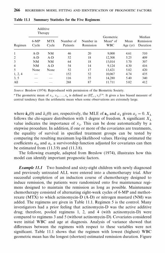
Table 11.1 Summary Statistics for the Five Regimens
AdditiveTherapy
Geometric Median6-MP MTX Number of Number in Mean� of Mean Remission
Regimen Cycle Cycle Patients Remission WBC Age (yr) Duration
1 A-D NM 46 20 9,000 4.61 5102 A-D A-D 52 18 12,308 5.25 4093 NM NM 64 18 15,014 5.70 3074 NM A-D 54 14 9,124 4.30 4165 None None 52 17 13,421 5.02 4201, 2, 4 — — 152 52 10,067 4.74 4353, 5 — — 116 35 14,280 5.40 340All — — 268 87 11.711 5.02 412
Source: Breslow (1974). Reproduced with permission of the Biometric Society.
�The geometric mean of x�, x
�, . . . , x
�is defined as (��
���x�)��. It gives a less biased measure of
central tendency than the arithmetic mean when some observations are extremely large.
where a��(0) and a�
�(0) are, respectively, the MLE of a
�and a
�given a
�� 0. X
�follows the chi-square distribution with 1 degree of freedom. A significant X
�value indicates the importance of x
�. This can be done automatically by a
stepwise procedure. In addition, if one or more of the covariates are treatments,the equality of survival in specified treatment groups can be tested bycomparing the resulting maximum log-likelihood values. Having estimated thecoefficients a
��and a
, a survivorship function adjusted for covariates can then
be estimated from (11.3.9) and (11.3.8).The following example, adapted from Breslow (1974), illustrates how this
model can identify important prognostic factors.
Example 11.1 Two hundred and sixty-eight children with newly diagnosedand previously untreated ALL were entered into a chemotherapy trial. Aftersuccessful completion of an induction course of chemotherapy designed toinduce remission, the patients were randomized onto five maintenance regi-mens designed to maintain the remission as long as possible. Maintenancechemotherapy consisted of alternating eight-week cycles of 6-MP and methot-rexate (MTX) to which actinomycin-D (A-D) or nitrogen mustard (NM) wasadded. The regimens are given in Table 11.1. Regimen 5 is the control. Manyinvestigators had a prior feeling that actinomycin-D was the active additivedrug; therefore, pooled regimens 1, 2, and 4 (with actinomycin-D) werecompared to regimens 3 and 5 (without actinomycin-D). Covariates consideredwere initial WBC and age at diagnosis. Analysis of variance showed thatdifferences between the regimens with respect to these variables were notsignificant. Table 11.1 shows that the regimen with lowest (highest) WBCgeometric mean has the longest (shortest) estimated remission duration. Figure
266
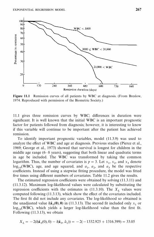
Figure 11.1 Remission curves of all patients by WBC at diagnosis. (From Breslow,1974. Reproduced with permission of the Biometric Society.)
11.1 gives three remission curves by WBC; differences in duration weresignificant. It is well known that the initial WBC is an important prognosticfactor for patients followed from diagnosis; however, it is interesting to knowif this variable will continue to be important after the patient has achievedremission.To identify important prognostic variables, model (11.3.9) was used to
analyze the effect of WBC and age at diagnosis. Previous studies (Pierce et al.,1969; George et al., 1973) showed that survival is longest for children in themiddle age range (6—8 years), suggesting that both linear and quadratic termsin age be included. The WBC was transformed by taking the commonlogarithm. Thus, the number of covariates is p� 3. Let x
�, x
�, and x
�denote
log��
(WBC), age, and age squared, and a�, a
�, and a
�be the respective
coefficients. Instead of using a stepwise fitting procedure, the model was fittedfive times using different numbers of covariates. Table 11.2 gives the results.The estimated regression coefficients were obtained by solving (11.3.11) and
(11.3.12). Maximum log-likelihood values were calculated by substituting theregression coefficients with the estimates in (11.3.10). The X
�values were
computed following (11.3.13), which show the effect of the covariates included.The first fit did not include any covariates. The log-likelihood so obtained isthe unadjusted value l(a�
�(0), 0) in (11.3.13). The second fit included only x
�or
log��
(WBC), which yields a larger log-likelihood value than the first fit.Following (11.3.13), we obtain
X���2(l(a�
�(0), 0) � l(a�
�, a�
�)) ��2(�1332.925� 1316.399)� 33.05
267
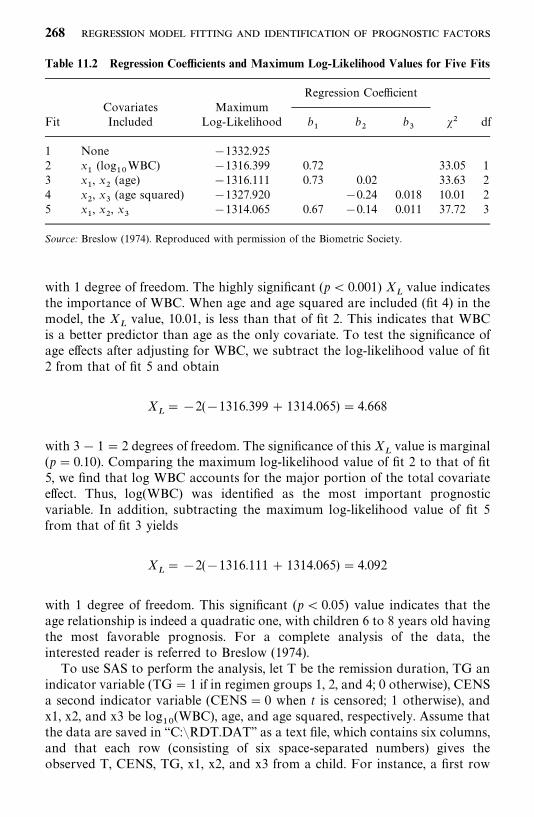
Table 11.2 Regression Coefficients and Maximum Log-Likelihood Values for Five Fits
Regression CoefficientCovariates Maximum
Fit Included Log-Likelihood b�
b�
b�
�� df
1 None �1332.9252 x
�(log
��WBC) �1316.399 0.72 33.05 1
3 x�, x
�(age) �1316.111 0.73 0.02 33.63 2
4 x�, x
�(age squared) �1327.920 �0.24 0.018 10.01 2
5 x�, x
�, x
��1314.065 0.67 �0.14 0.011 37.72 3
Source: Breslow (1974). Reproduced with permission of the Biometric Society.
with 1 degree of freedom. The highly significant (p� 0.001) X�value indicates
the importance of WBC. When age and age squared are included (fit 4) in themodel, the X
�value, 10.01, is less than that of fit 2. This indicates that WBC
is a better predictor than age as the only covariate. To test the significance ofage effects after adjusting for WBC, we subtract the log-likelihood value of fit2 from that of fit 5 and obtain
X�� �2(�1316.399� 1314.065)� 4.668
with 3� 1� 2 degrees of freedom. The significance of this X�value is marginal
(p� 0.10). Comparing the maximum log-likelihood value of fit 2 to that of fit5, we find that log WBC accounts for the major portion of the total covariateeffect. Thus, log(WBC) was identified as the most important prognosticvariable. In addition, subtracting the maximum log-likelihood value of fit 5from that of fit 3 yields
X�� �2(�1316.111� 1314.065)� 4.092
with 1 degree of freedom. This significant (p� 0.05) value indicates that theage relationship is indeed a quadratic one, with children 6 to 8 years old havingthe most favorable prognosis. For a complete analysis of the data, theinterested reader is referred to Breslow (1974).To use SAS to perform the analysis, let T be the remission duration, TG an
indicator variable (TG� 1 if in regimen groups 1, 2, and 4; 0 otherwise), CENSa second indicator variable (CENS� 0 when t is censored; 1 otherwise), andx1, x2, and x3 be log
��(WBC), age, and age squared, respectively. Assume that
the data are saved in ‘‘C:�RDT.DAT’’ as a text file, which contains six columns,and that each row (consisting of six space-separated numbers) gives theobserved T, CENS, TG, x1, x2, and x3 from a child. For instance, a first row
268
in RDT.DAT may be
500 1 0 4.079 5.2 27.04
which represents that a 5.2-year-old child with initial log��
(WBC)� 4.079 whoreceived regimen 3 or 5 relapsed after 500 days [i.e., t� 500, CENS� 1,TG� 0, x1� 4.079, x2� 5.2, and x3 (age squared) � 27.04].For this data set, the following SAS code can be used to perform fits 1 to 5
in Table 11.2 by using procedure LIFEREG.
data w1;infile ‘c:�rdt.dat’ missover;input t cens tg x1 x2 x3;
run;proc lifereg;model 1: model t*cens(0) � tg / d� exponential;model 2: model t*cens(0) � tg x1/ d� exponential;model 3: model t*cens(0) � tg x1 x2/ d� exponential;model 4: model t*cens(0) � tg x2 x3/ d� exponential;model 5: model t*cens(0) � tg x1 x2 x3/ d� exponential;
run;
For BMDP procedure 2L the following code can be used for fit 5.
/input file� ‘c:�rdt.dat’.variables� 6.format� free.
/print level�brief./variable names� t, cens, tg, x1, x2, x3./form time� t.
status� cens.response� 1.
/regress covariates� tg, x1, x2, x3.accel� exponential.
/end
11.4 WEIBULL REGRESSION MODEL
To consider the effects of covariates, we use the model (11.2.4); that is, thelog-survival-time of individual i is
logT�� a
��
����
ax�
����
�� �
�(11.4.1)
where �� a
����
��ax�and has the distribution defined in (11.3.2) and
269
(11.3.3). This model is the Weibull regression model. T has the Weibulldistribution with
��� exp��
�
�� and ��1
�(11.4.2)
and the following hazard, density, and survivorship functions that are relatedwith covariates via �
�in (11.4.2):
h(t, ��, �)� �
��t��� (11.4.3)
f (t, ��, �)� �
��t��� exp(��
�t�) (11.4.4)
S(t, ��, �)� exp(��
�t�) (11.4.5)
The hazard ratio of any two individuals i and j, based on (11.4.3) and (11.4.2),is
h�h�
� exp�� ��
�� �� exp��
1
�����
a(x
��x
�)�
which is not time-dependent. Therefore, similar to the exponential regressionmodel, the Weibull regression model is also a special case of the proportionalhazard models.The following example illustrates the use of the Weibull regression model
and of computer software packages.
Example 11.2 Consider the tumor-free time in Table 3.4. Suppose that wewish to know if three diets have the same effect on the tumor-free time. Let Tbe the tumor-free time; CENS be an index (or dummy) variable withCENS� 0 if T is censored and 1 otherwise; and LOW, SATU, and UNSA beindex variables indicating that a rat was fed a low-fat, saturated fat, orunsaturated fat diet, respectively (e.g., LOW� 1 if fed a low-fat diet; 0otherwise). The data from the 90 rats in Table 3.4 can be presented using thesefive variables. For example, the three observations in the first row of Table 3.4can be rearranged as
T CENS LOW SATU UNSA140 1 1 0 0124 1 0 1 0112 1 0 0 1
Assume that the rearranged data are saved in the text file ‘‘C:�RAT.DAT’’,which contains the data from the 90 rats in five columns as above and the fivenumbers in each row are space-separated. This data file is ready for almost all
270
of the statistical software packages for parametric survival analysis currentlyavailable, such as SAS and BMDP. Suppose that the tumor-free time followsthe Weibull distribution and the following Weibull regression model is used:
logT�� a
�� a
�SATU
�� a
�UNSA
���
��
���
�(11.4.6)
where �has a double exponential distribution as defined in (11.3.2) and
(11.3.3). Note that from (11.4.3) and (11.4.2),
log h(t, ��, �)� log �
�� log(�t���)
� � �
�� log(�t���)
��a
�� a
�SATU
�� a
�UNSA
��
� log(�t���) (11.4.7)
Denote the hazard function of a rat fed an unsaturated, saturated, and low-fatdiet as h
�, h
�, and h
, respectively. From (11.4.7), log h
�� (�a
�� a
�)/
�� log(�t���), log h�� (�a
�� a
�)/� � log(�t���), and log h
��a
�/
�� log(�t���). Thus, the logarithm of the hazard ratio of rats fed a low-fatdiet and those fed a saturated fat diet is log(h
/h
�)� a
�/�, and the similar ratios
of rats fed a low-fat diet and those an unsaturated fat diet, and of rats fed asaturated fat diet and those fed an unsaturated fat diet are, respectively,log(h
/h
�)� a
�/� and log(h
�/h
�)� (a
�� a
�)/�. These ratios are constants and
are independent of time. Therefore, to test the null hypothesis that the threediets have an equal effect on tumor-free time is equivalent to testing thefollowing three hypotheses: H
�: h
/h
�� 1 or a
�� 0, H
�: h
/h
�� 1, or a
�� 0,
and H�: h
�/h
�� 1 or a
�� a
�. The statistic defined in Section 9.1.1 can be used
to test the first two null hypotheses, and the statistic defined in (11.2.16) canbe used for the third one. Failure to reject a null hypothesis implies that thecorresponding log-hazard ratio is not statistically different from zero; that is,there are no statistically significant differences between the two correspondingdiets. For example, failure to reject H
�: a
�� 0 means that there are no
significant differences between the hazards for rats fed a low-fat diet and ratsfed a saturated fat diet. When all three hypotheses H
�: a
�� 0, H
�: a
�� 0, and
H�: a
�� a
�are rejected, we conclude that the three diets have significantly
different effects on tumor-free time. Furthermore, a positive (negative) es-timated implies that the hazard of a rat fed a low-fat diet is exp(a
�/�) times
higher (lower) than that of a rat fed a saturated fat diet. Similarly, a positive(negative) estimated a
�and (a
�� a
�) imply, respectively, the hazard of a rat
fed a low-fat diet is exp(a�/�) times higher (lower) than that of a rat fed an
unsaturated fat diet, and the hazard of a rat fed a saturated fat diet isexp[(a
�� a
�)/�] times higher (lower) than that of a rat fed an unsaturated fat
diet.
271
To estimate the unknown coefficients, a�, a
�, a
�, and �, we construct the
log-likelihood function by replacing in (11.4.2), (11.4.4), and (11.4.5) with(11.4.6). Next, place the resulting f (t
�, �
�, �) and S(t
�, �
�, �) in the log-likelihood
function (11.2.10). The log-likelihood function for the observed 90 exact orright-censored tumor-free times, t
�, t
�, . . . , t
��, in the three diet groups is
l(a�, a
�, a
�, �)� � log[ f (t
�, �
�, �)]� � log[S(t
�, �
�, �)]
� � [log � � (�� 1) log t�� �
�� t�
�exp(��
�)]
�� [�t��exp(��
�)]
� � �log � � (�� 1) log t�� �(a
�� a
�SATU
�� a
�UNSA
�)
�t��exp[��(a
�� a
�SATU
�� a
�UNSA
�)]�
����t��exp[��(a
�� a
�SATU
�� a
�UNSA
�)]�
The first term in the log-likelihood function sums over the uncensoredobservations, and the second term sums over the right-censored observations.The MLE (a�
�, a�
�, a�
�, �� ) of (a
�, a
�, a
�,�) where � � 1/� is a solution of (11.2.12)
with the above log-likelihood function by applying the Newton—Raphsoniterative procedure. The results from SAS are shown in Table 11.3, whereINTERCPT� a
�and SCALE� �. The MLE �� � 0.43, a�
���0.394,
a����0.739, and a�
�� a�
���0.345. H
�: a
�� 0 (or h
/h
�� 1), H
�: a
�� 0 (or
h/h
�� 1), and H
�: a
�� a
�� 0 (or h
�/h
�� 1) are rejected at significance level
p� 0.0065, p� 0.0001, and p� 0.0038, respectively. The conclusion that thedata indicate significant differences among the three diets is the same as thatobtained in Chapter 3 using the k-sample test. Furthermore, both a�
�and a�
�are negative and h�
/h�
�� exp(a�
�/�� )� exp(�0.916) � 0.40, h�
/h�
�� exp(a�
�/
�� )� exp(�1.719)� 0.18, and h��/h�
�� exp((a�
�� a�
�)/�� )� exp(�0.802)� 0.45.
Thus, based on the data observed, the hazard of rats fed a low-fat diet is 40%and 18% of the hazard of rats a saturated fat diet and an unsaturated fat diet,respectively, and the hazard of rats fed a saturated fat diet is 45% of that ofrats fed an unsaturated fat diet.The survivorship function in (11.4.5) can be estimated by using (11.4.2) and
the MLE of a�, a
�, a
�, and �:
S� (t, �, �)� exp(��� t�� )
� exp��exp��1
��(a�
�� a�
�SATU� a�
�UNSA)� t1/���
� exp[�exp(�12.56� 0.92�SATU� 1.72�UNSA)t� ��]
Based on S� (t, ��, �), we can estimate the probability of surviving a given time
for rats fed with any of the diets. For example, for rats fed a low-fat diet,
272
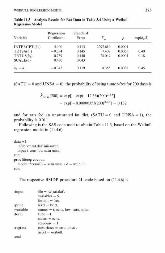
Table 11.3 Analysis Results for Rat Data in Table 3.4 Using a WeibullRegression Model
Regression StandardVariable Coefficient Error X
�p exp(a�
�/�� )
INTERCPT (a��) 5.400 0.113 2297.610 0.0001
TRTSA(a��) �0.394 0.145 7.407 0.0065 0.40
TRTUS(a��) �0.739 0.140 28.049 0.0001 0.18
SCALE(�� ) 0.430 0.043
a��� a�
��0.345 0.119 8.355 0.0038 0.45
(SATU� 0 and UNSA� 0), the probability of being tumor-free for 200 days is
S����
(200)� exp[�exp(�12.56)(200)� ��]
� exp[�0.00000353(200)� ��]� 0.132
and for rats fed an unsaturated fat diet, (SATU� 0 and UNSA� 1), theprobability is 0.011.Following is the SAS code used to obtain Table 11.3, based on the Weibull
regression model in (11.4.6).
data w1;infile ‘c:�rat.dat’ missover;input t cens low satu unsa;
run;proc lifereg covout;model t*cens(0) � satu unsa / d�weibull;
run;
The respective BMDP procedure 2L code based on (11.4.6) is
/input file� ‘c:�rat.dat’.variables� 5.format� free.
/print level�brief./variable names� t, cens, low, satu, unsa./form time� t.
status� cens.response� 1.
/regress covariates� satu, unsa .accel�weibull.
/end
273
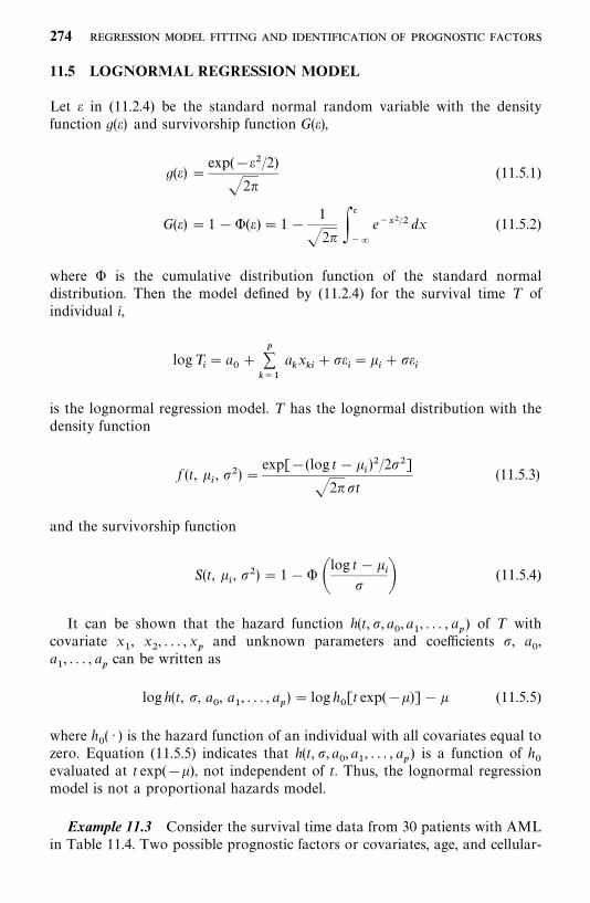
11.5 LOGNORMAL REGRESSION MODEL
Let in (11.2.4) be the standard normal random variable with the densityfunction g() and survivorship function G(),
g() �exp(��/2)
�2�(11.5.1)
G() � 1��() � 1�1
�2� ��
��
e� �� dx (11.5.2)
where � is the cumulative distribution function of the standard normaldistribution. Then the model defined by (11.2.4) for the survival time T ofindividual i,
logT�� a
��
����
ax�
����
�� �
�
is the lognormal regression model. T has the lognormal distribution with thedensity function
f (t, �, ��)�
exp[�(log t� �)�/2��]
�2��t(11.5.3)
and the survivorship function
S(t, �, ��)� 1�� �
log t� �
� � (11.5.4)
It can be shown that the hazard function h(t, �, a�, a
�, . . . , a
�) of T with
covariate x�, x
�, . . . , x
�and unknown parameters and coefficients �, a
�,
a�, . . . , a
�can be written as
log h(t, �, a�, a
�, . . . , a
�)� log h
�[t exp(� )]� (11.5.5)
where h�( · ) is the hazard function of an individual with all covariates equal to
zero. Equation (11.5.5) indicates that h(t, �, a�, a
�, . . . , a
�) is a function of h
�evaluated at t exp(� ), not independent of t. Thus, the lognormal regressionmodel is not a proportional hazards model.
Example 11.3 Consider the survival time data from 30 patients with AMLin Table 11.4. Two possible prognostic factors or covariates, age, and cellular-
274
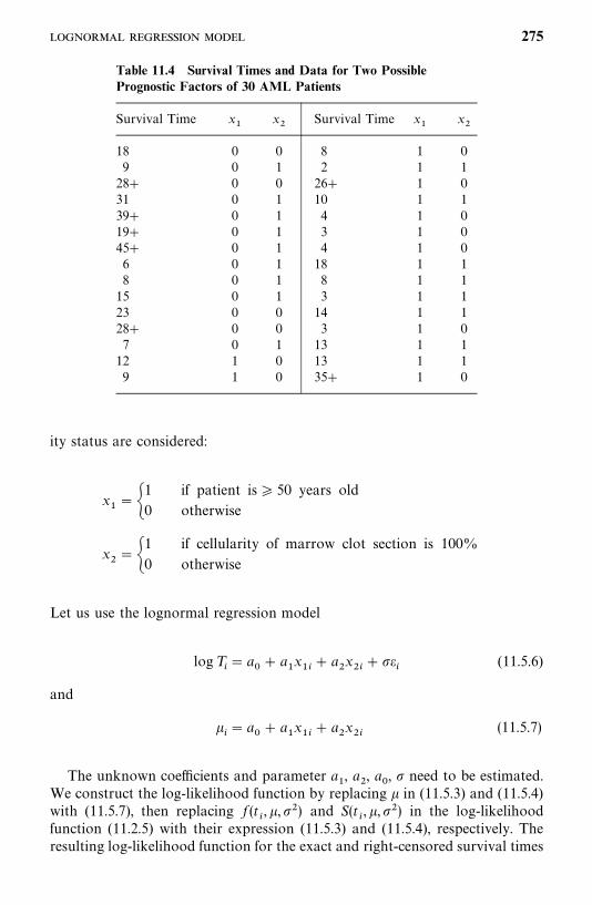
Table 11.4 Survival Times and Data for Two PossiblePrognostic Factors of 30 AML Patients
Survival Time x�
x�
Survival Time x�
x�
18 0 0 8 1 09 0 1 2 1 128� 0 0 26� 1 031 0 1 10 1 139� 0 1 4 1 019� 0 1 3 1 045� 0 1 4 1 06 0 1 18 1 18 0 1 8 1 115 0 1 3 1 123 0 0 14 1 128� 0 0 3 1 07 0 1 13 1 112 1 0 13 1 19 1 0 35� 1 0
ity status are considered:
x���
1 if patient is� 50 years old
0 otherwise
x���
1 if cellularity of marrow clot section is 100%
0 otherwise
Let us use the lognormal regression model
log T�� a
�� a
�x��
� a�x��
���
(11.5.6)
and
�� a
�� a
�x��
� a�x��
(11.5.7)
The unknown coefficients and parameter a�, a
�, a
�, � need to be estimated.
We construct the log-likelihood function by replacing in (11.5.3) and (11.5.4)with (11.5.7), then replacing f (t
�, ,��) and S(t
�, ,��) in the log-likelihood
function (11.2.5) with their expression (11.5.3) and (11.5.4), respectively. Theresulting log-likelihood function for the exact and right-censored survival times
275
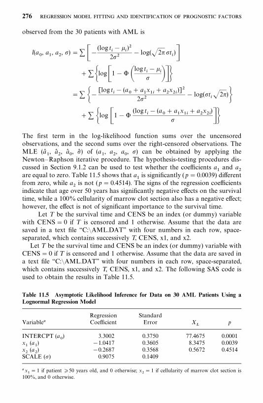
Table 11.5 Asymptotic Likelihood Inference for Data on 30 AML Patients Using aLognormal Regression Model
Regression StandardVariable� Coefficient Error X
�p
INTERCPT (a�) 3.3002 0.3750 77.4675 0.0001
x�(a
�) �1.0417 0.3605 8.3475 0.0039
x�(a
�) �0.2687 0.3568 0.5672 0.4514
SCALE (�) 0.9075 0.1409
�x�� 1 if patient �50 years old, and 0 otherwise; x
�� 1 if cellularity of marrow clot section is
100%, and 0 otherwise.
observed from the 30 patients with AML is
l(a�, a
�, a
�, �)�� ��
(log t��
�)�
2��� log(�2��t
�)�
� ��log�1� � �log t
��
�� ���
�� ��[log t
�� (a
�� a
�x��
� a�x��)]�
2��� log(�t
��2�)�
� � �log �1��(log t
�� (a
�� a
�x��
� a�x��)
� ��The first term in the log-likelihood function sums over the uncensoredobservations, and the second sums over the right-censored observations. TheMLE (a�
�, a�
�, a�
�, �� ) of (a
�, a
�, a
�, �) can be obtained by applying the
Newton—Raphson iterative procedure. The hypothesis-testing procedures dis-cussed in Section 9.1.2 can be used to test whether the coefficients a
�and a
�are equal to zero. Table 11.5 shows that a
�is significantly (p� 0.0039) different
from zero, while a�is not (p� 0.4514). The signs of the regression coefficients
indicate that age over 50 years has significantly negative effects on the survivaltime, while a 100% cellularity of marrow clot section also has a negative effect;however, the effect is not of significant importance to the survival time.
Let T be the survival time and CENS be an index (or dummy) variablewith CENS� 0 if T is censored and 1 otherwise. Assume that the data aresaved in a text file ‘‘C:�AML.DAT’’ with four numbers in each row, space-separated, which contains successively T, CENS, x1, and x2.Let T be the survival time and CENS be an index (or dummy) variable with
CENS� 0 if T is censored and 1 otherwise. Assume that the data are saved ina text file ‘‘C:�AML.DAT’’ with four numbers in each row, space-separated,which contains successively T, CENS, x1, and x2. The following SAS code isused to obtain the results in Table 11.5.
276

data w1;infile ‘c:�aml.dat’ missover;input t cens x1 x2;
run;proc lifereg;model 1: model t*cens(0) � x1 x2 / d� lnormal;
run;
If BMDP is used, the following 2L code is suggested.
/input file� ‘c:�aml.dat’.variables� 4.format� free.
/print level�brief./variable names� t, cens, x1, x2./form time� t.
status� cens.response� 1.
/regress covariates� x1, x2.accel� lnormal.
/end
11.6 EXTENDED GENERALIZED GAMMA REGRESSION MODEL
In this section we introduce a regression model that is based on an extendedform of the generalized gamma distribution defined in Section 6.4. Assume thatthe survival time T of individual i and covariates x
�, . . . , x
�have the relation-
ship given in (11.4.1), where has the log-gamma distribution with the densityfunction g() and survivorship function G():
g() ����[exp(�)/��]��� exp[�exp(�)/��]
�(1/��)(11.6.1)
G() ��I�exp(�)
��,1
��� if �� 0
1� I �exp(�)
��,1
��� if � 0 ��� �
(11.6.2)
(11.6.3)
This model is the extended generalized gamma regression model. It can beshown that T has the extended generalized gamma distribution with thedensity function
f (t, �, �, �)���������
�t���� exp[��(�
�t)�]
�(�)(11.6.4)
and survivorship function
S(t, �, �, �)��I(�(�
�t)�, �)
1� I(�(��t)�, �)
if � � 0
if � 0
(11.6.5)(11.6.6)
277
where
��� exp(�
�) � �
��
��1
��(11.6.7)
�(x) is the complete gamma function defined in (6.2.9), I(a, x) is the incompletegamma function defined in (6.4.4), and � is a shape parameter. We used theextended generalized gamma distribution in (11.6.4) here because it is thedistribution used in SAS. The derivation is left to the reader as an exercise(Exercise 11.12).The estimation procedures for the parameters, regression coefficients, and
the covariate adjusted survivorship function are similar to those discussed inSections 11.3 and 11.4.
Example 11.4 Consider the survival times (T ) in days and a set ofprognostic factors or covariates from 137 lung cancer patients, presented inAppendix I of Kalbfleisch and Prentice (1980). The covariates include theKarnofsky measure of the overall performance status (KPS) of the patient atentry into the trial, time in months from diagnosis to entry into the trial(DIAGTIME), age in years (AGE), prior therapy (INDPRI, yes or no),histological type of tumor, and type of therapy. There are four histologicaltypes of tumor: adeno, small, large, and squamous cell and two types oftherapies: standard and experimental. The values of KPS have the followingmeanings: 10—30 completely hospitalized, 40—60 partial confinement, 70—90able to care for self. Assume that the survival time follows the extendedgeneralized gamma regression model, we wish to identify the most significantprognostic variables.First we define several index (or dummy) variables for the categorical
variables and the censoring status. Let CENS� 0 when the survival time T iscensored and 1 otherwise; INDADE� 1, INDSMA� 1, and INDSQU� 1 ifthe type of cancer cell is adeno, small, and squamous, respectively, and 0otherwise; INDTHE� 1 if the standard therapy is received and 0 otherwise;and INDPRI� 1 if there is a prior therapy and 0 otherwise. The model is
logT�� a
�� a
�KPS
�� a
�AGE
�� a
�DIAGTIME
�� a
�INDPRI
�
� a�INDTHE
�� a
�INDADE
�� a
�INDSMA
�� a
�INDSQU
�� �
�
(11.6.8)
where the density function of �is defined in (11.6.1). Thus,
�� a
�� a
�KPS
�� a
�AGE
�� a
�DIAGTIME
�� a
�INDPRI
�� a
�INDTHE
�
� a�INDADE
�� a
�INDSMA
�� a
�INDSQU
�(11.6.9)
To estimate a�, . . . , a
�, �, a
�, and �, we construct the log-likelihood function by
replacing in (11.6.7) and (11.6.4)—(11.6.6) with (11.6.9), then replacing f (t�, b)
and S(t�,b) in the likelihood function (11.2.10) by those in (11.6.4) and (11.6.5)
or (11.6.6). The MLE (a��, . . . , a�
�, �� , a�
�, �� ) of (a
�, . . . , a
�, �, a
�, �) can be
278
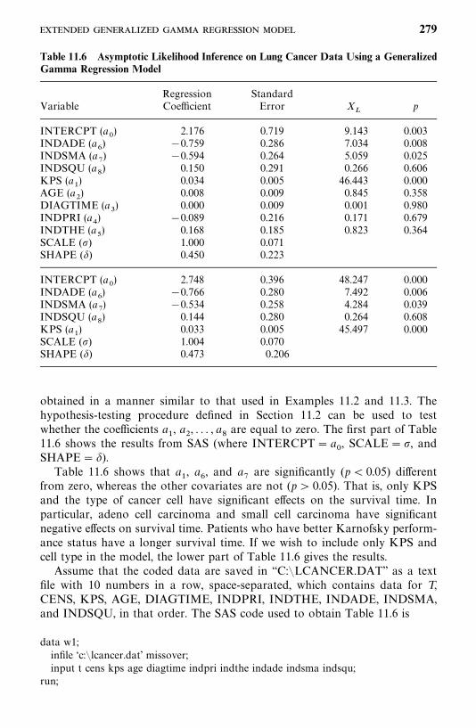
Table 11.6 Asymptotic Likelihood Inference on Lung Cancer Data Using a GeneralizedGamma Regression Model
Regression StandardVariable Coefficient Error X
�p
INTERCPT (a�) 2.176 0.719 9.143 0.003
INDADE (a�) �0.759 0.286 7.034 0.008
INDSMA (a�) �0.594 0.264 5.059 0.025
INDSQU (a�) 0.150 0.291 0.266 0.606
KPS (a�) 0.034 0.005 46.443 0.000
AGE (a�) 0.008 0.009 0.845 0.358
DIAGTIME (a�) 0.000 0.009 0.001 0.980
INDPRI (a�) �0.089 0.216 0.171 0.679
INDTHE (a�) 0.168 0.185 0.823 0.364
SCALE (�) 1.000 0.071SHAPE (�) 0.450 0.223
INTERCPT (a�) 2.748 0.396 48.247 0.000
INDADE (a�) �0.766 0.280 7.492 0.006
INDSMA (a�) �0.534 0.258 4.284 0.039
INDSQU (a�) 0.144 0.280 0.264 0.608
KPS (a�) 0.033 0.005 45.497 0.000
SCALE (�) 1.004 0.070SHAPE (�) 0.473 0.206
obtained in a manner similar to that used in Examples 11.2 and 11.3. Thehypothesis-testing procedure defined in Section 11.2 can be used to testwhether the coefficients a
�, a
�, . . . , a
�are equal to zero. The first part of Table
11.6 shows the results from SAS (where INTERCPT� a�, SCALE��, and
SHAPE� �).Table 11.6 shows that a
�, a
�, and a
�are significantly (p� 0.05) different
from zero, whereas the other covariates are not (p 0.05). That is, only KPSand the type of cancer cell have significant effects on the survival time. Inparticular, adeno cell carcinoma and small cell carcinoma have significantnegative effects on survival time. Patients who have better Karnofsky perform-ance status have a longer survival time. If we wish to include only KPS andcell type in the model, the lower part of Table 11.6 gives the results.Assume that the coded data are saved in ‘‘C:�LCANCER.DAT’’ as a text
file with 10 numbers in a row, space-separated, which contains data for T,CENS, KPS, AGE, DIAGTIME, INDPRI, INDTHE, INDADE, INDSMA,and INDSQU, in that order. The SAS code used to obtain Table 11.6 is
data w1;infile ‘c:�lcancer.dat’ missover;input t cens kps age diagtime indpri indthe indade indsma indsqu;
run;
279
proc lifereg;Model 1: model t*cens(0) �kps age diagtime indpri indthe indade indsma indsqu /
d� gamma;Model 2: model t*cens(0)� kps indade indsma indsqu / d� gamma;
run;
11.7 LOG-LOGISTIC REGRESSION MODEL
Assume that the relationship between the survival time T�for individual i and
a set of covariates, x�, . . . , x
�can be expressed by the AFT model in (11.4.1),
where �has a logistic distribution with the density function
g() �exp()
[1� exp()]�(11.7.1)
and survivorship function
G() �1
1� exp()(11.7.2)
This model is the log-logistic regression model. Then T has the log-logisticdistribution defined in Section 6.5. The parameter � in the distribution is afunction of the covariates:
��� exp��
�
�� ��1
�(11.7.3)
Substituting (11.7.3) in the survivorship function in (6.5.2), we obtain
logS(t, b)
1�S(t, b)��log(�t�)�
�
� � log t (11.7.4)
or
logS(t, b)
1� S(t, b)�a��
�1
�����
ax� � log t (11.7.5)
where b� (a�, a
�, . . . , a
�, �). Since S(t
�, b) is the probability of surviving longer
than t, S(t�, b)/[1�S(t
�, b)] is the odds of surviving longer than t. Let OR
�and
OR�denote the odds of surviving longer than t for individuals i and j,
respectively. The logarithm of the odds ratio is
logOR
�OR
�
�1
�����
a(x
��x
�) (11.7.6)
This ratio is independent of time. Therefore, the log-logistic regression modelis a proportional odds model, not a proportional hazards model.
280
Example 11.5 We fit the log-logistic regression model above to the data inExample 11.6.1 using only KPS and the three cancer cell type index variables.That is,
logT�� a
�� a
�KPS
�� a
�INDADE
�� a
�INDSMA
�� a
�INDSQU
�� �
�
(11.7.7)
where the density function of �is defined in (11.7.1). Thus,
�� a
�� a
�KPS
�� a
�INDADE
�� a
�INDSMA
�� a
�INDSQU
�(11.7.8)
To estimate b� (a�, a
�, . . . , a
�, �)�, we construct the log-likelihood function by
using the � and � in (11.7.3) as parameters in the density and survivorshipfunctions of the log-logistic distribution in Section 6.5. The resulting log-likelihood function for the 137 observed exact or right-censored survival times is
l(b) �� ��
��
� log��1��
�log t
�� 2 log�1� exp�
� �
� � t�� ��� � ��log �1� exp�
� �
� � t��� ��
�� ��1
�(a
�� a
�KPS
�� a
�INDADE
�� a
�INDSMA
�� a
�INDSQU
�)
� log��1��
�log t
�
� 2 log�1� exp��1
�(a
�� a
�KPS
�� a
�INDADE
�� a
�INDSMA
�
� a�INDSQU
�)� t�� ��
� � �log �1� exp��1
�(a
�� a
�KPS
�� a
�INDADE
�� a
�INDSMA
�
� a�INDSQU
�)� t�� ��
The first term in the log-likelihood function sums over the uncensoredobservations, and the second sums over the right-censored observations. TheMLE (a�
�, . . . , a�
�, a�
�, �� ) of (a
�, . . . , a
�, a
�, �) are given in Table 11.7, with their
- 281
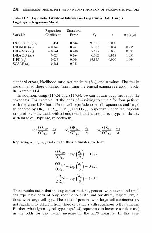
Table 11.7 Asymptotic Likelihood Inference on Lung Cancer Data Using aLog-Logistic Regression Model
Regression StandardVariable Coefficient Error X
�p exp(a
�/a)
INTERCPT (a�) 2.451 0.344 50.911 0.000 —
INDADE (a�) �0.749 0.261 8.217 0.004 0.275
INDSMA (a�) �0.661 0.240 7.565 0.006 0.321
INDSQU (a�) 0.029 0.264 0.012 0.913 1.051
KPS (a�) 0.036 0.004 66.885 0.000 1.064
SCALE (�) 0.581 0.043 — — —
standard errors, likelihood ratio test statistics (X�), and p values. The results
are similar to those obtained from fitting the general gamma regression modelin Example 11.4.In addition, using (11.7.5) and (11.7.6), we can obtain odds ratios for the
covariates. For example, let the odds of surviving to time t for four patientswith the same KPS but different cell type (adeno, small, squamous and large)be denoted by OR
��, OR
��, OR
��, and OR
��, respectively; then the log-odds
ratios of the individuals with adeno, small, and squamous cell types to the onewith large cell type are, respectively,
logOR
��OR
��
�a��
logOR
��OR
��
�a��
logOR
��OR
��
�a��
Replacing a�, a
�, a
�, and � with their estimates, we have
OR��
OR��
� exp�a���� �� 0.275
OR��
OR��
� exp�a���� �� 0.321
OR��
OR��
� exp�a���� �� 1.051
These results mean that in lung cancer patients, persons with adeno and smallcell type have odds of only about one-fourth and one-third, respectively, ofthose with large cell type. The odds of persons with large cell carcinoma arenot significantly different from those of patients with squamous cell carcinoma.Further, when ignoring cell type, exp(a�
�/�� ) represents an increase (or decrease)
in the odds for any 1-unit increase in the KPS measure. In this case,
282
exp(a��/�� )� 1.064; thus for a 1-unit increase in the KPS measure, the odds
increase by 6.4%. The results are, in general, consistent with those obtained inExample 11.4.The following SAS code can be used to obtain the results in Table 11.7.
data w1;infile ‘c:�lcancer.dat’ missover;input t cens kps age diagtime indpri indthe indade indsma indsqu;
run;proc lifereg;model t*cens(0) �kps indade indsma indsqu / d� llogistic;
run;
The following BMDP 2L code is also applicable.
/input file� ‘c:�lcancer.dat’.variables� 10.format� free.
/print level� brief./variable names� t, cens, kps, age, diagtime, indpri, indthe, indade, indsma, indsqu./form time� t.
status� cens.response� 1.
/regress covariates�kps, indade, indsma, indsqu.accel� llogistic.
/end
11.8 OTHER PARAMETRIC REGRESSION MODELS
In this section we discuss two models in which the survival time T is assumedto follow the exponential distribution with density and survivorship functionsas defined in (6.1.1) and (6.1.3), respectively, and the mean survival time 1/� orhazard rate � has the following linear relationship with the covariates:
Model 1:1
��
� a��
�����
a�x��
Model 2: ��� a
��
�����
a�x��
Model 1 is considered by Feigl and Zelen (1965) and extended to includecensored data by Zippin and Armitage (1966). Model 2 is used by Byar et al.(1974).
283
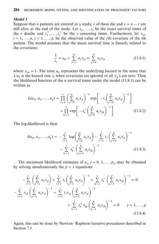
Model 1Suppose that n patients are entered in a study; r of these die and s� n� r arestill alive at the end of the study. Let t
�, . . . , t
�be the exact survival times of
the r deaths and t��, . . . , t�
�be the s censoring times. Furthermore, let x
��,
i� 1, . . . , n, j� 1, . . . , p, be the observed value of the j th covariate of the ithpatient. The model assumes that the mean survival time is linearly related tothe covariates:
1
��
� a��
�����
a�x���
�����
a�x��
(11.8.1)
where x��
� 1. The term a�represents the underlying hazard in the sense that
1/a�is the hazard rate �
�when covariates are ignored or all x
��’s are zero. Then
the likelihood function of the n survival times under the model (11.8.1) can bewritten as
L (a�, a
�, . . . , a
�)�
������
�����
a�x���
��exp��t��
�����
a�x���
��
��
����
exp��t� ������
a�x��
��
� (11.8.2)
The log-likelihood is then
l(a�, a
�, . . . , a
�)��
�����
log������
a�x����
�����
t� �
�����
a�x���
��
�����
t� �
�����
a�x��
��(11.8.3)
The maximum likelihood estimates of a�, j� 0, 1, . . . , p
�, may be obtained
by solving simultaneously the p� 1 equations:
�������
�����
a�x����
�����
t� �
�����
a�x���
���
����
t� �
�����
a�x��
��� 0
������
x�� �
�����
a�x���
���
�����
t�x�� �
�����
a�x���
��
�����
t�x� �
�����
a�x��
��� 0 j� 1, . . . , p
(11.8.4)
Again, this can be done by Newton—Raphson iterative procedures described inSection 7.1.
284
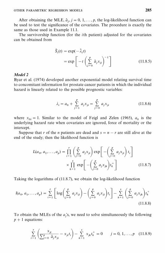
After obtaining the MLE, a��, j� 0, 1, . . . , p, the log-likelihood function can
be used to test the significance of the covariates. The procedure is exactly thesame as those used in Example 11.1.The survivorship function (for the ith patient) adjusted for the covariates
can be obtained from
S��(t) � exp(���
�t)
� exp ��t ������
a��x���
��
� (11.8.5)
Model 2Byar et al. (1974) developed another exponential model relating survival timeto concomitant information for prostate cancer patients in which the individualhazard is linearly related to the possible prognostic variables:
��� a
��
�����
a�x���
�����
a�x��
(11.8.6)
where x��
� 1. Similar to the model of Feigl and Zelen (1965), a�is the
underlying hazard rate when covariates are ignored, force of mortality or theintercept.Suppose that r of the n patients are dead and s� n� r are still alive at the
end of the study; then the likelihood function is
L (a�, a
�, . . . , a
�)�
������
�����
a�x��� exp���
�����
a�x��� t��
��
���
exp��������
a�x�� t� � (11.8.7)
Taking the logarithms of (11.8.7), we obtain the log-likelihood function
l(a�, a
�, . . . , a
�)�
������log�
�����
a�x�����
�����
a�x��� t���
����
������
a�x�� t�(11.8.8)
To obtain the MLEs of the a�’s, we need to solve simultaneously the following
p� 1 equations:
������
x��
�����
a��x��
�x��t���
����
x�t�
� 0 j� 0, 1, . . . , p (11.8.9)
285
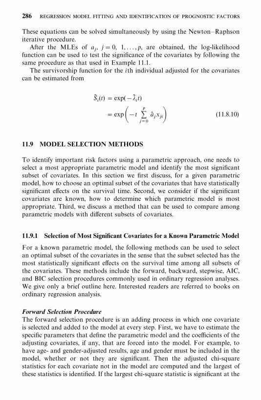
These equations can be solved simultaneously by using the Newton—Raphsoniterative procedure.After the MLEs of a
�, j� 0, 1, . . . , p, are obtained, the log-likelihood
function can be used to test the significance of the covariates by following thesame procedure as that used in Example 11.1.The survivorship function for the ith individual adjusted for the covariates
can be estimated from
S��(t) � exp(���
�t)
� exp��t�����
a��x��� (11.8.10)
11.9 MODEL SELECTION METHODS
To identify important risk factors using a parametric approach, one needs toselect a most appropriate parametric model and identify the most significantsubset of covariates. In this section we first discuss, for a given parametricmodel, how to choose an optimal subset of the covariates that have statisticallysignificant effects on the survival time. Second, we consider if the significantcovariates are known, how to determine which parametric model is mostappropriate. Third, we discuss a method that can be used to compare amongparametric models with different subsets of covariates.
11.9.1 Selection of Most Significant Covariates for a Known Parametric Model
For a known parametric model, the following methods can be used to selectan optimal subset of the covariates in the sense that the subset selected has themost statistically significant effects on the survival time among all subsets ofthe covariates. These methods include the forward, backward, stepwise, AIC,and BIC selection procedures commonly used in ordinary regression analyses.We give only a brief outline here. Interested readers are referred to books onordinary regression analysis.
Forward Selection ProcedureThe forward selection procedure is an adding process in which one covariateis selected and added to the model at every step. First, we have to estimate thespecific parameters that define the parametric model and the coefficients of theadjusting covariates, if any, that are forced into the model. For example, tohave age- and gender-adjusted results, age and gender must be included in themodel, whether or not they are significant. Then the adjusted chi-squarestatistics for each covariate not in the model are computed and the largest ofthese statistics is identified. If the largest chi-square statistic is significant at the
286
� level specified (usually, �� 0.15) for entry, the corresponding covariate isadded to the model.Let a
�be the vector of the parameters or coefficients of covariates already in
the model and l( · ) be the log-likelihood function. The forward selectionprocedure will select x
�, which is not yet in the model, to enter the model if the
difference between the log-likelihood values with x�and without x
�is largest
among all the x’s that are not in the model. That is, the coefficient a
�of x
�satisfies
X�� 2[(l(a�
�, a�
�) � l(a�
��(0))]
�max
�2[l(a�, a�
�) � l(a�
�(0))], for any x
that is not in the model�
(11.9.1)
and X���
�� where a is the coefficient of x not yet in the model, (a� , a� �), isthe MLE of (a
, a
�), a�
�(0) is the MLE of a
�given a
� 0, and ��
�� is the �-levelcritical point of the chi-square distribution with 1 degree of freedom. In theforward selection procedure, once a covariate is entered into the model, it willnever be removed. The process is repeated until none of the remainingcovariates meet the level � specified for entry or until a predetermined numberof covariates have been entered.
Backward Selection ProcedureThe backward selection procedure is an elimination process in which all thecovariates are included in the model at the beginning and are removed one byone according to a significance criterion. The specific parameters that definethe parametric model and the coefficients of all the covariates are estimatedfirst. Then the Wald test is used to examine each covariate. The least significantcovariate that does not meet the specified level � (usually, �� 0.15) forstaying in the model is removed. That is, covariate x
�will be removed from the
model if
X�
�a� ��v���
�min�a� �v�
for any xthat is in the model� (11.9.2)
and X�
����� where a� is the corresponding coefficient for x� and v
���is the
estimated variance of a��. In the backward selection procedure, once a covariate
is removed from the model, it remains excluded. The process is repeated untilall the covariates remained in the model meet the specified significance level �for staying or until a predetermined number of covariates remain in the model.The advantages of the backward procedure have been discussed by Mantel(1970).
287
Stepwise Selection ProcedureThe stepwise selection procedure is a combination of forward and backwardselection procedures. At first, it is similar to the forward selection procedure;however, covariates already in the model do not necessarily remain. Covariatesalready in the model may be removed later if they are no longer significant. Thestepwise selection process terminates if no significant covariate can be added tothe model or if the covariate just entered into the model is removed and nomore covariates can be added.
Information Criterion (AIC and BIC) ProceduresThe Baysian information criterion (BIC) selection procedure discussed inSection 9.3 can be used to select the best parametric model with covariates.This can be done easily by replacing the log-likelihood function l(b� ) in (9.3.1)with the log-likelihood function with subsets of covariates defined in previoussections of this chapter. The subset of covariates that produces the largest rvalue in (9.3.1) among all possible subsets is the choice. If the number ofcovariates is large, one may apply the forward, backward, and stepwiseselection method first to reduce the number of candidate covariates, then usethe BIC procedure. The AIC criterion can be applied in a similar manner.
11.9.2 Selection of a Parametric Model with a Fixed Subset of Covariates
If the most significant subset of covariates is known, selection of an appropriateparametric model can be carried out by using a procedure similar to those basedon the likelihood functions and discussed in Section 9.2. The procedures areexactly the same except that all the likelihood functions are replaced by thosewith covariates, for example, those given in (11.3.10) and Examples 11.2 and11.5. With computer software packages available commercially, the procedurecan easily be applied. The following example illustrates the application.
Example 11.6 Consider the lung cancer patients who did not receive anyprior therapy in Example 11.4. Assume that the three covariates KPS,INDADE, and INDSMA are most significant. For these three fixed covariates,the log-likelihood values based on the exponential, Weibull, lognormal, log-logistic, and generalized gamma models are given in Table 11.8. From thistable, the lognormal, Weibull and exponential models (relative to the general-ized gamma model), with the three covariates, are rejected at �� 0.0325, 0.016and 0.024, respectively. It appears that the exponential model, relative to theWeibull, is not rejected (p� 0.194). However, since the exponential modelbelongs to the Weibull distribution family and the Weibull model has beenrejected, the exponential model with the three covariates is not appropriate forthe data, as noted earlier in Chapter 9. Thus, we conclude that none of thethree models (exponential, Weibull, and lognormal), with covariates, providean appropriate fit to the data. In Example 11.7 we will see that the log-logisticmodel is the best fit among all these models.
288
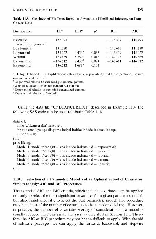
Table 11.8 Goodness-of-Fit Tests Based on Asymptotic Likelihood Inference on LungCancer Data
Distribution LL� LLR� p� BIC AIC
Extended �132.793 — — �146.517 �144.793generalized gamma
Log-logistic �131.230 — — �142.667 �141.230Lognormal �135.022 4.459� 0.035 �146.459 �145.022Weibull �135.669 5.752� 0.016 �147.106 �145.669Exponential �136.512 7.438� 0.024 �145.661 �144.512Exponential �136.512 1.686� 0.194 — —
�LL, log-likelihood; LLR, log-likelihood ratio statistic; p, probability that the respective chi-squarerandom variable LLR.�Lognormal relative to extended generalized gamma.�Weibull relative to extended generalized gamma.�Exponential relative to extended generalized gamma.�Exponential relative to Weibull.
Using the data file ‘‘C:�LCANCER.DAT’’ described in Example 11.4, thefollowing SAS code can be used to obtain Table 11.8.
data w1;infile ‘c:�lcancer.dat’ missover;input t cens kps age diagtime indpri indthe indade indsma indsqu;if indpri� 0;
run;proc lifereg;Model 1: model t*cens(0)� kps indade indsma / d� exponential;Model 2: model t*cens(0)� kps indade indsma / d�weibull;Model 3: model t*cens(0)� kps indade indsma / d� lnormal;Model 4: model t*cens(0)� kps indade indsma / d� gamma;Model 5: model t*cens(0)� kps indade indsma / d� llogistic;
run;
11.9.3 Selection of a Parametric Model and an Optimal Subset of CovariatesSimultaneously: AIC and BIC Procedures
The extended AIC and BIC criteria, which include covariates, can be appliednot only to select the most significant covariates for a given parametric model,but also, simultaneously, to select the best parametric model. The proceduremay be tedious if the number of covariates to be considered is large. However,in practice, the number of covariates worthy of consideration in a model isusually reduced after univariate analyses, as described in Section 11.1. There-fore, the AIC or BIC procedure may not be too difficult to apply. With the aidof software packages, we can apply the forward, backward, and stepwise
289
selection methods in Section 11.9.1 first to fit different parametric regressionmodels to the data and then include in the AIC or BIC procedure all or asubset of the significant covariates identified in each fit.
Example 11.7 Consider the lung cancer data of Example 11.6. We applythe methods of Section 11.9.1 to select the best subset of covariates separatelyfor the exponential, Weibull, lognormal, log-logistic, and generalized gammamodels. The same three covariates (KPS, INDADE, and INDSMA) areselected (at the 0.05 level) as the most significant covariates in every of theseparametric models. The last column of Table 11.8 gives the r values of the BICfor the different parametric models with the same three covariates. Based onthese values, the log-logistic model with the three covariates should be selectedas the final model for the data since its BIC or AIC value is the largest amongall the models. However, it is not known if the log-logistic model is significantlybetter than the other models.
11.9.4 Cox--Snell Residual Procedure with Covariates
The AFT models in Sections 11.2 to 11.7 assume the following linear relation-ship between log T and the p covariates:
logT�� a
��
����
ax�
����
�� �
�(11.9.3)
where �has survival function G(). Once a specified parametric model and a
subset of covariates are selected, to assess the goodness of fit of this model, oneapproach is to compute the regression residuals
���log t
�� �
���
i� 1, 2, . . . , n (11.9.4)
where
��� a�
��
����
a�x�
and a��, a�
�, a�
�, . . . , a�
�and �� are the MLE of a
�, a
�, a
�, . . . , a
�and �, respectively,
and t�’s are observed survival times. An �
�is taken as censored if the
corresponding t�is censored. If the model fitted is correct, the corresponding
survival function G() is the survival function of the fitted model. For example,if T indeed follows the log-logistic regression model with a selected subset ofcovariates, the corresponding �
�’s should follow the log-logistic distribution.
Moreover, if the fitted model is correct, the Cox—Snell residuals defined in(8.4.1) are
r���logG(�
�; d� ) ��logG �
log t�� �
���
; d� � i� 1, 2, . . . , n (11.9.5)
290
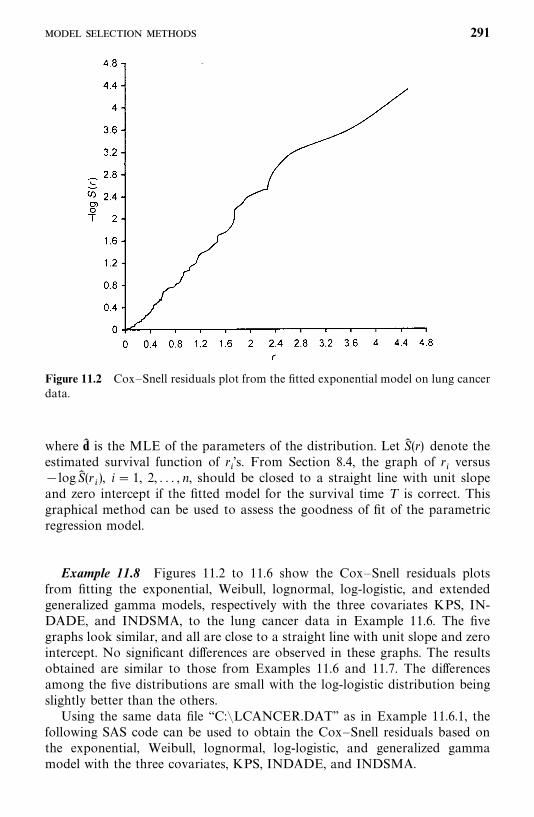
Figure 11.2 Cox—Snell residuals plot from the fitted exponential model on lung cancerdata.
where d� is the MLE of the parameters of the distribution. Let S� (r) denote theestimated survival function of r
�’s. From Section 8.4, the graph of r
�versus
�logS� (r�), i� 1, 2, . . . , n, should be closed to a straight line with unit slope
and zero intercept if the fitted model for the survival time T is correct. Thisgraphical method can be used to assess the goodness of fit of the parametricregression model.
Example 11.8 Figures 11.2 to 11.6 show the Cox—Snell residuals plotsfrom fitting the exponential, Weibull, lognormal, log-logistic, and extendedgeneralized gamma models, respectively with the three covariates KPS, IN-DADE, and INDSMA, to the lung cancer data in Example 11.6. The fivegraphs look similar, and all are close to a straight line with unit slope and zerointercept. No significant differences are observed in these graphs. The resultsobtained are similar to those from Examples 11.6 and 11.7. The differencesamong the five distributions are small with the log-logistic distribution beingslightly better than the others.Using the same data file ‘‘C:�LCANCER.DAT’’ as in Example 11.6.1, the
following SAS code can be used to obtain the Cox—Snell residuals based onthe exponential, Weibull, lognormal, log-logistic, and generalized gammamodel with the three covariates, KPS, INDADE, and INDSMA.
291
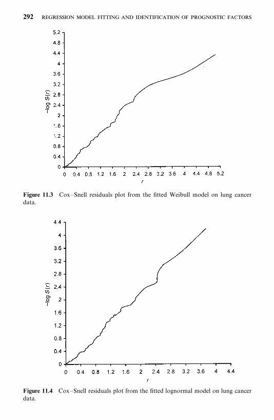
Figure 11.3 Cox—Snell residuals plot from the fitted Weibull model on lung cancerdata.
Figure 11.4 Cox—Snell residuals plot from the fitted lognormal model on lung cancerdata.
292
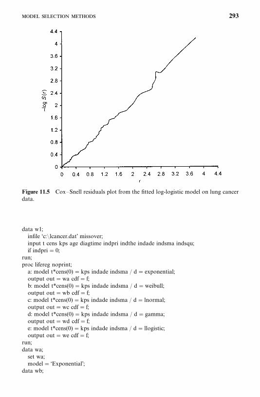
Figure 11.5 Cox—Snell residuals plot from the fitted log-logistic model on lung cancerdata.
data w1;infile ‘c:�lcancer.dat’ missover;input t cens kps age diagtime indpri indthe indade indsma indsqu;if indpri� 0;
run;proc lifereg noprint;a: model t*cens(0) �kps indade indsma / d� exponential;output out�wa cdf� f;b: model t*cens(0) �kps indade indsma / d�weibull;output out�wb cdf� f;c: model t*cens(0) �kps indade indsma / d� lnormal;output out�wc cdf� f;d: model t*cens(0) �kps indade indsma / d� gamma;output out�wd cdf� f;e: model t*cens(0) �kps indade indsma / d� llogistic;output out�we cdf� f;
run;data wa;set wa;model� ‘Exponential’;
data wb;
293
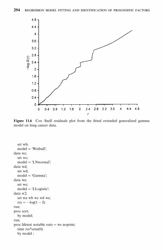
Figure 11.6 Cox—Snell residuals plot from the fitted extended generalized gammamodel on lung cancer data.
set wb;model� ‘Weibull’;
data wc;set wc;model� ‘LNnormal’;
data wd;set wd;model� ‘Gamma’;
data we;set we;model� ‘LLogistic’;
data w2;set wa wb wc wd we;rcs��log(1� f);
run;proc sort;by model;
run;proc lifetest notable outs�ws noprint;time rcs*cens(0);by model ;
294
run;data ws;set ws;mls��log(survival);
run;title ‘Cox-Snell Residuals (rcs) and -log(estimated survival function of rcs) (mls)’;proc print data�ws;var model rcs mls;
run;
Bibliographical Remarks
An excellent expository paper on statistical methods for the identification anduse of prognostic factors has been written by Armitage and Gehan (1974).Many studies of prognostic factors have been published, including Sirott et al.(1993), Brancato et al. (1997), Linka et al. (1998), and Lassarre (2001). Theaccelerated failure time (AFT) model was introduced by Cox (1972). Thedetailed statistical inference of the AFT models and the theoretical aspects ofmodel-selecting methods are included in the works cited in the bibliographicalremarks at the end of Chapter 9 and in the papers and books cited in thischapter.
EXERCISES
11.1 Consider the data given in Exercise Table 3.1. In addition to the fiveskin tests, age and gender may also have prognostic value. Examine therelationship between survival and each of the seven possible prognosticvariables as in Table 3.12. For each variable, group the patientsaccording to different cutoff points. Estimate and draw the survivalfunction for each subgroup by the product-limit method and then usethe methods discussed in Chapter 5 to compare survival distributionsof the subgroups. Prepare a table similar to Table 3.12. Interpret yourresults. Is there a subgroup of any variable that shows significantlylonger survival times? (For the skin test results, use the larger diameterof the two.)
11.2 Consider the seven variables in Exercise 11.1. Use the Weibull re-gression model to identify the most significant variables. Compare yourresults with that obtained in Exercise 11.1.
11.3 Consider the data given in Exercise Table 3.3. Examine the relationshipbetween remission duration and survival time and each of the ninepossible prognostic variables: age, gender, family history of melanoma,and the six skin tests. Group the patients according to different cutoff
295
points. Estimate and draw remission and survival curves for eachsubgroup. Compare the remission and survival distributions of sub-groups using the methods discussed in Chapter 5. Prepare tablessimilar to Table 3.8.
11.4 Perform the following analyses: (1) Use the exponential, Weibull,lognormal, generalized gamma, or log-logistic regression models sepa-rately to identify the significant variables in Exercise 11.3 for their relativeimportance to remission duration and survival time. (2) Select a modelamong these final models using the BIC or AIC method. (3) Calculateseparately the respective likelihood for the exponential, Weibull, lognor-mal, or generalized gamma regressionmodelwith the fixed variables in themodel selected in step (2), then use themethod in Section 11.9.2 to choosea model and see whether this model is the model selected in step (2).
11.5 Perform the same analyses as in Exercise 11.4 for survival time in the157 diabetic patients given in Exercise Table 3.4.
11.6 Using the notations in Example 11.2, show that if we use the follow-ing model to replace the model defined in (11.4.6), logT
�� a
�� a
�LOW
�� a
�UNSA
�� �
��
���
�, the hypothesis H
�: h
�� h
�is
equivalent to H�: a
�� 0.
11.7 Following Examples 11.2 and 11.3, obtain the log-likelihood functionbased on (11.6.8) for the 137 observed exact and right-censored survivaltimes from the lung cancer patients.
11.8 Using the same notation as in Example 11.5, show that if weuse the model logT
�� a
�� a
�KPS
�� a
�INDLAR
�� a
�INDSMA
��a
�INDSQU
���
�, where INDLAR� 1 if the type of cancer is large,
and 0 otherwise, to replace the model defined in (11.7.8), the hypothesesH
�: a
��0 and H
�: a
�� 0 are equivalent to H
�:OR
���OR
��and
H�:OR
���OR
��, respectively. Moreover, if we use the model
log T�� a
�� a
�KPS
�� a
�INDLAR
�� a
�INDADE
�� a
�INDSQU
���
�to replace the model defined in (11.7.8), the hypothesis H
�: a
�� 0
is equivalent to H�:OR
���OR
��.
11.9 Let be a survival time with the density function g()�exp[�exp()].Show that the survival time T defined by logT � �� has theWeibull distribution with �� exp(� /�) and � � 1/� by applying thedensity transformation rule in (11.2.11).
11.10 Let be a survival time with the standard normal distribution N(0, 1).Show that the survival time T defined by log T� �� has thelognormal distribution by applying the density transformation rule in(11.2.11).
296
11.11 Let u be a survival time with the density function f (u),
f (u) �exp[u/��� exp(u)]
�(1/��)
where �( · ) is the gamma function defined in (6.2.8).(a) Show that the survival time defined by � /�� (log ��)/� has
the following density function,
g() ����[exp(�)/��]��� exp[�exp(�)/��]
�(1/��)��� �
and survival function,
G() ��I �exp(�)
��,1
��� if � � 0
1� I �exp(�)
��,1
��� if � 0
where I( · , · ) is the incomplete gamma function defined as in (6.4.4).(b) Show that the survival time T defined by logT� � � has the
extended gamma density function defined in (11.6.4).
11.12 If has a logistic distribution with the density function
g() �exp()
[1� exp()]�
show that the survival time T defined by logT � �� has the log-logisticdistribution with �� exp(� /�) and �� 1/� by applying the densitytransformation rule in (11.2.11).
297
CHAPTER 12
Identification of Prognostic FactorsRelated to Survival Time:Cox Proportional Hazards Model
In Chapter 11 we discussed parametric survival methods for model fitting andfor identifying significant prognostic factors. These methods are powerful if theunderlying survival distribution is known. The estimation and hypothesistesting of parameters in the models can be conducted by applying standardasymptotic likelihood techniques. However, in practice, the exact form of theunderlying survival distribution is usually unknown and we may not be ableto find an appropriate model. Therefore, the use of parametric methods inidentifying significant prognostic factors is somewhat limited. In this chapterwe discuss a most commonly used model, the Cox (1972) proportional hazardsmodel, and its related statistical inference. This model does not requireknowledge of the underlying distribution. The hazard function in this modelcan take on any form, including that of a step function, but the hazardfunctions of different individuals are assumed to be proportional and indepen-dent of time. The usual likelihood function is replaced by the partial likelihoodfunction. The important fact is that the statistical inference based on the partiallikelihood function is similar to that based on the likelihood function.
12.1 PARTIAL LIKELIHOOD FUNCTION FOR SURVIVAL TIMES
The Cox proportional hazards model possesses the property that differentindividuals have hazard functions that are proportional, i.e., [h(t �x
�)/h(t � x
�)],
the ratio of the hazard functions for two individuals with prognostic factors orcovariates x
�� (x
��,x
��, . . . , x
��)�, and x
�� (x
��, x
��, . . . , x
��)� is a constant
(does not vary with time t). This means that the ratio of the risk of dying oftwo individuals is the same no matter how long they survive. In Sections 11.3
298
and 11.4, we showed that the exponential and Weibull regression modelspossess this property. This property implies that the hazard function given aset of covariates x� (x
�,x
�, . . . , x
�)� can be written as a function of an
underlying hazard function and a function, say g(x�, . . . , x
�), of only the
covariates, that is,
h(t � x�, . . . , x
�) � h
�(t)g(x
�, . . . , x
�) or h(t �x)� h
�(t)g(x) (12.1.1)
The underlying hazard function, h�(t), represents how the risk changes with
time, and g(x) represents the effect of covariates. h�(t) can be interpreted as the
hazard function when all covariates are ignored or when g(x) � 1, and is alsocalled the baseline hazard function. The hazard ratio of two individuals withdifferent covariates x
�and x
�is
h(t �x�)
h(t �x�)�h�(t)g(x
�)
h�(t)g(x
�)�g(x
�)
g(x�)
(12.1.2)
which is a constant, independent of time.The Cox (1972) proportional hazard model assumes that g(x) in (12.1.1) is
an exponential function of the covariates, that is,
g(x) � exp������
b�x��� exp(b�x)
and the hazard function is
h(t � x)� h�(t) exp�
�����
b�x��� h
�(t) exp(b�x) (12.1.3)
where b� (b�, . . . , b
�) denotes the coefficients of covariates. These coefficients
can be estimated from the data observed and indicate the magnitude of theeffects of their corresponding covariates. For example, if there is only onecovariate treatment, let x
�� 0 if a person receives placebo and x
�� 1 if a
person receives the experimental drug. The hazard ratio of the patient receivingthe experimental drug and the one receiving placebo based on (12.1.2) and(12.1.3) is
h(t � x�� 1)
h(t � x�� 0)
� exp(b�)
Thus, the two treatments are equally effective if b�� 0 and the experimental
drug introduces lower (higher) risk for survival than placebo if b�� 0 (b
�� 0).
It can be shown that (12.1.3) is equivalent to
S(t � x) � [S�(t)] exp(��
���b�x�) � [S
�(t)] exp(b�x) (12.1.4)
299
Thus the covariates can be incorporated into the survivorship function. Theuse of (12.1.3) can be exemplified as follows.
1. Two-sample problems. Suppose that p� 1; that is, there is only onecovariate, x
�, which is an indicator variable:
x��
��0 if the ith individual is from group 0
1 if the ith individual is from group 1
Then according to (12.1.3), the hazard functions of groups 0 and 1 are,respectively, h
�(t) and h
�(t) � h
�(t) exp(b
�). The hazard function of group
1 is equal to the hazard function of group 0 multiplied by a constantexp(b
�), or the two hazard functions are proportional. In terms of the
survivorship function,
S(t) � [S�(t)]�
where the constant c� exp(b�) (Nadas, 1970). The two-sample test develop-
ed from (12.1.3) is the Cox—Mantel test discussed in Chapter 5. It is nowapparent that the test is based on the assumption of a proportionalhazard between the two groups.
2. Two-sample problems with covariates. The covariates in (12.1.3) can eitherbe indicator variables such as x
�in the two-group problem above or
prognostic factors. Having one or more covariates representing prognos-tic factors in (12.1.1) enables us to examine the relation between twogroups, adjusting for the presence of prognostic factors.
3. Regression problems. Dividing both sides of (12.1.3) by h�(t) and taking
its logarithm, we obtain
logh�(t)
h�(t)
� b�x��
� b�x��
��� b�x��
������
b�x��� b�x
�(12.1.5)
where the x’s are covariates for the ith individual. The left side of (12.1.5) isa function of hazard ratio (or relative risk) and the right side is a linearfunction of the covariates and their respective coefficients.
As mentioned earlier, h�(t) is the hazard function when all covariates are
ignored. If the covariates are standardized about the mean and the model usedis
logh�(t)
h�(t)
� b�(x
���x�
�) � b
�(x
���x�
�) ��� b
�(x
���x�
�) � b�(x
��x� )
(12.1.6)
300
where x� � � (x��, x�
�, . . . , x�
�) and x�
�is the average of the jth covariate for all
patients, the left side of (12.1.6) is the logarithm of the ratio of risk of failurefor a patient with a given set of values x�
�� (x
��,x
��, . . . , x
��) to that for an
average patient who has an average value for every covariate.In this chapter we focus on the use of (12.1.5), and the main interest here is
to identify important prognostic factors. In other words, we wish to identifyfrom the p covariates a subset of variables that affect the hazard moresignificantly, and consequently, the length of survival of the patient. We areconcerned with the regression coefficients. If b
�is zero, the corresponding
covariate is not related to survival. If b�is not zero, it represents the magnitude
of the effect of x�on hazard when the other covariates are considered
simultaneously.To estimate the coefficients, b
�, . . . , b
�, Cox (1972) proposes a partial
likelihood function based on a conditional probability of failure, assuming thatthere are no tied values in the survival times. However, in practice, tied survivaltimes are commonly observed and Cox’s partial likelihood function wasmodified to handle ties (Kalbfleisch and Prentice, 1980; Breslow, 1974; Efron,1977). In the following we describe the estimation procedure without and withties.
12.1.1 Estimation Procedures without Tied Survival Times
Suppose that k of the survival times from n individuals are uncensored anddistinct, and n� k are right-censored. Let t
��� t
����� t
��be the ordered
k distinct failure times with corresponding covariates x��, x
��, . . . , x
��. Let
R(t��) be the risk set at time t
��. R(t
��) consists of all persons whose survival
times are at least t��. For the particular failure at time t
��, conditionally on the
risk set R(t��
), the probability that the failure is on the individual as observed is
exp������
b�x���
�l �R(t
��) exp���
���b�x��) ��
exp(b�x��
)�l �R(t
��) exp(b�x
�)�
Each failure contributes a factor and hence the partial likelihood function is
L (b) �����
exp������
b�x���
�l �R(t
��) exp���
���b�x��) ��
����
exp(b�x��
)�l�R(t
��) exp(b�x
�)� (12.1.7)
and the log-partial likelihood is
l(b) � log L (b) ������
�����
b�x���
�����
log� �l �R(t
��)
exp������
b�x����
�������b�x��� log� �
l �R(t��)
exp(b�x�)�� (12.1.8)
301
The maximum partial likelihood estimator (MPLE) b� of b can be obtained bythe steps shown in (7.1.2)—(7.1.4). That is, b�
�, . . . , b�
�are obtained by solving
the following simultaneous equations:
�(l(b))�b
� 0
or
�l(b)�b
�
������
[x���
�A��(b)] � 0 u� 1, 2, . . . , p (12.1.9)
where
A��
(b) ��l �R(t
��) x��
exp������
b�x��)
�l�R(t
��) exp���
���b�x��
��l�R(t
��) x��
exp(b�x�)
�l �R(t
��) exp(b�x
�)
(12.1.10)
by applying the Newton—Raphson iterated procedure. The second partialderivatives of l(b) with respective to b
�and b
�, u, v� 1, 2, . . . , p, in the
Newton—Raphson iterative procedure are
I��(b) �
��l(b)
�b��b
�
�������
C����
(b�, . . . , b
�) ��
�����
C����
(b) u, v� 1, 2, . . . , p
(12.1.11)
where
C����
(b) ��l �R(t
��) x��
x��exp���
���b�x��)
�l �R(t
��) exp���
���b�x��)
�A��(b)A
��(b) (12.1.12)
The covariance matrix of the MPLE b� , defined similarly as V� (b) defined in(7.1.5), is
V� (b� ) �Cov� (b� ) �����l(b� )�b�b��
�(12.1.13)
where ���l(b� )/�b�b� is called the observed information matrix with �I��
(b� ) asits (u, v) element and where I
��(b) is defined in (12.1.11). Let the (i, j ) element
of V� (b� ) in (12.1.13) be v��; then the 100(1� )% confidence interval for b
�is,
according to (7.1.6),
�b���Z����v
��, b�
��Z����v
�� (12.1.14)
12.1.2 Estimation Procedure with Tied Survival Times
Suppose that among the n observed survival times there are k distinctuncensored times t
��� t
���� � t
��. Let m
��denote the number of people
302
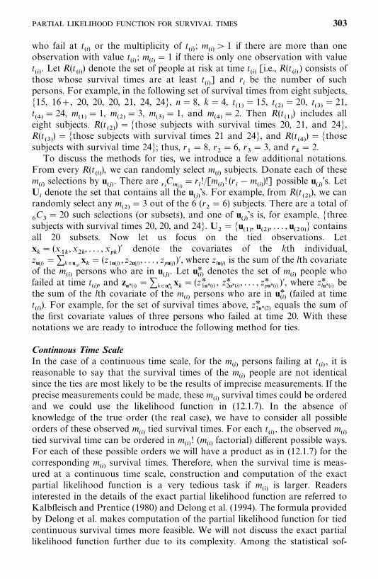
who fail at t��or the multiplicity of t
��; m
��� 1 if there are more than one
observation with value t��; m
��� 1 if there is only one observation with value
t��. Let R(t
��) denote the set of people at risk at time t
��[i.e., R(t
��) consists of
those whose survival times are at least t��] and r
�be the number of such
persons. For example, in the following set of survival times from eight subjects,�15, 16�, 20, 20, 20, 21, 24, 24�, n� 8, k� 4, t
��� 15, t
��� 20, t
��� 21,
t�
� 24, m��
� 1, m��
� 3, m��
� 1, and m�
� 2. Then R(t��) includes all
eight subjects. R(t��) � �those subjects with survival times 20, 21, and 24�,
R(t��) � �those subjects with survival times 21 and 24�, and R(t
� ) � �those
subjects with survival time 24�; thus, r�� 8, r
�� 6, r
�� 3, and r
� 2.
To discuss the methods for ties, we introduce a few additional notations.From every R(t
��), we can randomly select m
��subjects. Donate each of these
m��selections by u
��. There are
�
C��
� r�!/[m
��! (r
��m
��)!] possible u
��’s. Let
U�denote the set that contains all the u
��’s. For example, from R(t
��), we can
randomly select any m��
� 3 out of the 6 (r�� 6) subjects. There are a total of
�C
�� 20 such selections (or subsets), and one of u
��’s is, for example, �three
subjects with survival times 20, 20, and 24�. U�� �u
��, u
��, . . . , u
���� contains
all 20 subsets. Now let us focus on the tied observations. Letx�� (x
��, x
��, . . . , x
��)� denote the covariates of the kth individual,
zu(j) ��k � u��x�� (z1u(j) , z2u(j) , . . . , zpu(j))�, where zlu(j) is the sum of the lth covariate
of the m��persons who are in u
��. Let u*
��denotes the set of m
��people who
failed at time t��, and zu*(i) ��k � u*
��x�� (z*1u*(i) , z*2u*(i) , . . . , z*pu*(i) )�, where z*lu*(i) be
the sum of the lth covariate of the m��persons who are in u*
��(failed at time
t��
). For example, for the set of survival times above, z*1u*(2) equals the sum ofthe first covariate values of three persons who failed at time 20. With thesenotations we are ready to introduce the following method for ties.
Continuous Time ScaleIn the case of a continuous time scale, for the m
��persons failing at t
��, it is
reasonable to say that the survival times of the m��people are not identical
since the ties are most likely to be the results of imprecise measurements. If theprecise measurements could be made, these m
��survival times could be ordered
and we could use the likelihood function in (12.1.7). In the absence ofknowledge of the true order (the real case), we have to consider all possibleorders of these observed m
��tied survival times. For each t
��, the observed m
��tied survival time can be ordered in m
��! (m
��factorial) different possible ways.
For each of these possible orders we will have a product as in (12.1.7) for thecorresponding m
��survival times. Therefore, when the survival time is meas-
ured at a continuous time scale, construction and computation of the exactpartial likelihood function is a very tedious task if m
��is larger. Readers
interested in the details of the exact partial likelihood function are referred toKalbfleisch and Prentice (1980) and Delong et al. (1994). The formula providedby Delong et al. makes computation of the partial likelihood function for tiedcontinuous survival times more feasible. We will not discuss the exact partiallikelihood function further due to its complexity. Among the statistical sof-
303
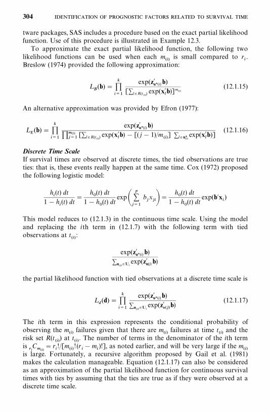
tware packages, SAS includes a procedure based on the exact partial likelihoodfunction. Use of this procedure is illustrated in Example 12.3.
To approximate the exact partial likelihood function, the following twolikelihood functions can be used when each m
��is small compared to r
�.
Breslow (1974) provided the following approximation:
L�
(b) ��
���
exp(z�u*(i)b)[�l �R(t
��) exp(x�
�b)]m��
(12.1.15)
An alternative approximation was provided by Efron (1977):
L�
(b) �����
exp(z�u*(i) b)��
���[�l �R(t
��) exp(x�
�b) � [( j� 1)/m
��] �l � u*
��exp(x�
�b)]
(12.1.16)
Discrete Time ScaleIf survival times are observed at discrete times, the tied observations are trueties: that is, these events really happen at the same time. Cox (1972) proposedthe following logistic model:
h�(t) dt
1� h�(t) dt
�h�(t) dt
1� h�(t) dt
exp������
b�x����
h�(t) dt
1� h�(t) dt
exp(b�x�)
This model reduces to (12.1.3) in the continuous time scale. Using the modeland replacing the ith term in (12.1.7) with the following term with tiedobservations at t
��:
exp(z�u*(i)b)�u
���U
�exp(z�u(j) b)
the partial likelihood function with tied observations at a discrete time scale is
L (d) �
����
exp(z�u*(i)b)�u
���U
�exp(z�
���b)
(12.1.17)
The ith term in this expression represents the conditional probability ofobserving the m
��failures given that there are m
��failures at time t
��and the
risk set R(t��
) at t��. The number of terms in the denominator of the ith term
is�C
��� r
�!/[m
��! (r
��m
�)!], as noted earlier, and will be very large if the m
��is large. Fortunately, a recursive algorithm proposed by Gail et al. (1981)makes the calculation manageable. Equation (12.1.17) can also be consideredas an approximation of the partial likelihood function for continuous survivaltimes with ties by assuming that the ties are true as if they were observed at adiscrete time scale.
304
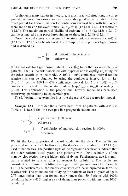
As shown in many papers in literature, in most practical situations, the threepartial likelihood functions above are reasonably good approximations of theexact partial likelihood function for continuous survival time with ties. Whenthere are no ties on the event times (i.e., m
��� 1), (12.1.15) —(12.1.17) reduce to
(12.1.7). The maximum partial likelihood estimate of b in (12.1.15)—(12.1.17)can be estimated using procedures similar to those in (12.1.8)—(12.1.14).
Once the coefficients are estimated, relative risk (or relative hazard) in(12.1.2) or (12.1.5) can be obtained. For example, if x
�represents hypertension
and is defined as
x���
1 if patient is hypertensive
0 otherwise
the hazard rate for hypertensive patients is exp(b��) times that for normotensive
patients. That is, the risk associated with hypertension is exp(b��) adjusting for
the other covariates in the model. A 100(1� )% confidence interval for therelative risk can be obtained by using the confidence interval for b
�. Let
(b��, b
��) be the 100(1� )% confidence interval for b
�; a 100(1� )%
confidence interval for the relative risk is (exp(b��), exp(b
��)) according to
(7.1.8). This application of the proportional hazards model has been usedextensively, particularly by epidemiologists.
The following three examples illustrate the use of Cox’s regression model.
Example 12.1 Consider the survival data from 30 patients with AML inTable 11.4. Recall that the two possible prognostic factors are
x���
1 if patient is �50 years
0 otherwise
x�� �
1 if cellularity of marrow clot section is 100%
0 otherwise
We fit the Cox proportional hazard model to the data. The results arepresented in Table 12.1 In this case, Breslow’s approximation in (12.1.15) isused to handle ties. The positive signs of the regression coefficients indicate thatthe older patients (�50 years) and patients with 100% cellularity of themarrow clot section have a higher risk of dying. Furthermore, age is signifi-cantly related to survival after adjustment for cellularity. The results areconsistent with those from fitting the lognormal regression model in Example11.3. The coefficients of the binary covariates can be interpreted in terms ofrelative risk. The estimated risk of dying for patients at least 50 years of age is2.75 times higher than that for patients younger than 50. Patients with 100%cellularity have a 42% higher risk of dying than patients with less than 100%cellularity.
305
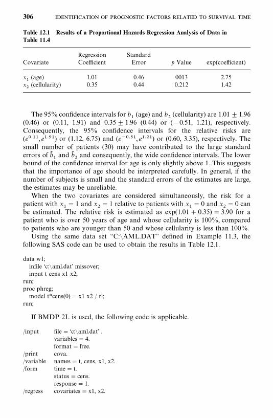
Table 12.1 Results of a Proportional Hazards Regression Analysis of Data inTable 11.4
Regression StandardCovariate Coefficient Error p Value exp(coefficient)
x�
(age) 1.01 0.46 0013 2.75x�
(cellularity) 0.35 0.44 0.212 1.42
The 95% confidence intervals for b�
(age) and b�
(cellularity) are 1.01� 1.96(0.46) or (0.11, 1.91) and 0.35� 1.96 (0.44) or (�0.51, 1.21), respectively.Consequently, the 95% confidence intervals for the relative risks are(e����, e����) or (1.12, 6.75) and (e����, e����) or (0.60, 3.35), respectively. Thesmall number of patients (30) may have contributed to the large standarderrors of b�
�and b�
�and consequently, the wide confidence intervals. The lower
bound of the confidence interval for age is only slightly above 1. This suggeststhat the importance of age should be interpreted carefully. In general, if thenumber of subjects is small and the standard errors of the estimates are large,the estimates may be unreliable.
When the two covariates are considered simultaneously, the risk for apatient with x
�� 1 and x
�� 1 relative to patients with x
�� 0 and x
�� 0 can
be estimated. The relative risk is estimated as exp(1.01� 0.35) � 3.90 for apatient who is over 50 years of age and whose cellularity is 100%, comparedto patients who are younger than 50 and whose cellularity is less than 100%.
Using the same data set ‘‘C:�AML.DAT’’ defined in Example 11.3, thefollowing SAS code can be used to obtain the results in Table 12.1.
data w1;infile ‘c:�aml.dat’ missover;input t cens x1 x2;
run;proc phreg;model t*cens(0) � x1 x2 / rl;
run;
If BMDP 2L is used, the following code is applicable.
/input file� ‘c:�aml.dat’ .variables� 4.format� free.
/print cova./variable names� t, cens, x1, x2./form time� t.
status� cens.response� 1.
/regress covariates� x1, x2.
306
If SPSS is used, the following code suffices.
data list file� ‘c:�aml.dat’ free/ t cens x1 x2.
coxreg t with x1 x2/status� cens event (1)/print� all.
Example 12.2 In a study (Buzdar et al., 1978) to evaluate a combinationof 5-flourouracil, adramycin, cyclophosphamide, and BCG (FAC-BCG) asadjuvant treatment in stage II and III breast cancer patients with positiveaxillary nodes, 131 patients receiving FAC-BCG after surgery and radiationtherapy were compared with 151 patients receiving surgery and radiationtherapy only (control group).
Cox’s regression model was used to identify prognostic factors and toevaluate the comparability of the two treatment groups. The model was fittedto the data from 151 patients to determine the variables related to length ofremission. The possible prognostic variables considered were age (years),menopausal status (1, premenopausal; 0, other), size of primary tumor (2, �3cm; 4, 3—5 cm; 7, �5 cm), state of disease (2, stage II; 3, stage III), location ofsurgery (1, M. D. Anderson Hospital; 0, other), number of nodes involved (2,�4; 7, 4—10; 12, �10), and race (1, Caucasian; 2, other). The covariates wereselected by the forward selection method outlined in Section 11.9. Threevariables—number of nodes involved, state of disease, and menopausalstatus—were selected for use in the model, all related significantly (p� 0.1) todisease-free time. The regression equation including these variables only is
logh�(t)
h�(t)
� 0.111(number of nodes� 6.16) � 0.8122(stage� 2.39)
� 0.872(menopausal� 0.26)
Table 12.2 gives the details of the fit. Relative risk was taken as h�(t)/h
�(t), the
ratio of the risk of death per unit of time for a patient with a given set ofprognostic variables to the risk for a patient whose prognostic variables wereaverage in value. The relative risk for each variable was calculated byconsidering favorable or unfavorable values of that variable, assuming thatother variables were at their average value. Note that the risk of relapse perunit time for a patient with 12 positive nodes is 3.04 (ratio or risk) times thatfor a patient with only two positive nodes. The risk of relapse per unit time fora stage III patient was 2.25 times that of a stage II patient.
The Cox’s regression model was also fitted to the combined group ofFAC-BCG and control patients, including type of treatment (0, control; 1,FAC-BCG), menopausal status, size of primary tumor, and number of involvednodes as potential prognostic variables. The regression equation with three
307
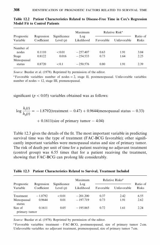
Table 12.2 Patient Characteristics Related to Disease-Free Time in Cox’s RegressionModel Fit to Control Patients
Maximum Relative Risk�Prognostic Regression Significance Log Ratio ofVariable Coefficient Level (p) Likelihood Favorable Unfavorable Risks
Number ofnodes 0.1110 �0.01 �257.407 0.63 1.91 3.04
Stage 0.8122 0.016 �254.533 0.73 1.64 2.25Menopausalstatus 0.8720 �0.1 �250.576 0.80 1.91 2.39
Source: Buzdar et al. (1978). Reprinted by permission of the editor.
�Favorable variables: number of nodes� 2, stage II, postmenopausal. Unfavorable variables:number of nodes� 12, stage III, premenopausal.
Table 12.3 Patient Characteristics Related to Survival, Treatment Included
Maximum Relative Risks�Prognostic Regression Significance Log Ratio ofVariable Coefficient Level (p) Likelihood Favorable Unfavorable Risks
Treatment �1.8792 �0.01 �201.200 0.37 2.42 6.55Menopausal 0.9644 0.01 �197.719 0.73 1.91 2.62status
Size of 0.1611 0.05 �195.865 0.72 1.61 2.24primary tumor
Source: Buzdar et al. (1978). Reprinted by permission of the editor.
�Favorable variables: treatment—FAC-BCG, postmenopausal, size of primary tumor 2 cm.Unfavorable variables: no adjuvant treatment, premenopausal, size of primary tumor 7 cm.
significant (p� 0.05) variables obtained was as follows:
logh�(t)
h�(t)
��1.8792(treatment� 0.47) � 0.9644(menopausal status� 0.33)
� 0.1611(size of primary tumor� 4.04)
Table 12.3 gives the details of the fit. The most important variable in predictingsurvival time was the type of treatment (FAC-BCG favorable); other signifi-cantly important variables were menopausal status and size of primary tumor.The risk of death per unit of time for a patient receiving no adjuvant treatment(control group) was 6.55 times that for a patient receiving the treatment,showing that FAC-BCG can prolong life considerably.
308
Example 12.3 Suppose that demographic, personal, clinical, and labora-tory data are collected from an interview and physical examination of 200participants in a study of cardiovascular disease (CVD). These participants,aged 50—79 years and free of CVD at the time of the baseline examination, arethen followed for 10 years. During the follow-up period, 96 of the 200participants develop or die of CVD. We use this set of simulated data toillustrate further the use of the proportional hazards model in identifyingimportant risk factors. Table 12.4 gives a subset of the simulated data of 68participants.
The event time T of interest is CVD-free time, which is defined as the timein years from baseline examination to the first time that a participant wasdiagnosed as having CVD or confirmed as a CVD death. CVD includescoronary heart disease (CHD) and stroke. The covariates of interest are age(AGE), gender (SEX� 1 if male and �0 if female); smoking status(SMOKE� 1 if current smoker, and 0 otherwise); body mass index(BMI�weight in kilograms divided by height in meter squared); systolicblood pressure (SBP); logarithm of ratio of urinary albumin and creatinine(LACR); logarithm of triglycerides (LTG); hypertension status (HTN� 1 ifSBP� 140 mmHg or DBP� 90 mmHg or under treatments of hypertension,and �0 otherwise); and diabetes status (DM� 1 if fasting glucose� 126mg/dL or under the treatments of diabetes, and �0 otherwise). For the CVDoutcome of interest, we let DG denote the type of CVD. DG� 0 if theparticipant is free of CVD at the end of the study or confirmed as a non-CVDdeath (thus the CVD-free time is censored), �1 if the participant had a stroke,�2 if the participant had a CHD, and �3 if the participant had other CVDs.It is of interest to compare the risk of CVD among the three age groups: 50—59,60—69, and 70—79. We create two dummy variables: AGEA� 1 if aged 50—69,�0 otherwise; and AGEB� 1 if aged 60—69, and �0 otherwise. Thus for a 70to 79-year-old, AGEA� 0 and AGEB� 0. We also create a variable to denotethe censoring status: CENS� 0 if t is censored, and� 1 if uncensored.
To illustrate the different methods to handle ties, we fit the Cox proportionalhazards model with the following six covariates: AGEA, AGEB, SEX,SMOKE, BMI, and LACR. The approximated partial likelihood functiondefined in (12.1.15)—(12.1.17) as well as the exact partial likelihood function(Delong et al., 1994) are applied. As noted in Sections 11.3 and 11.4, theexponential and Weibull regression models are also proportional hazardmodels. Therefore, for comparisons we also fit an exponential and a Weibullregression model with the same covariates to the data. The estimated re-gression coefficients obtained from the proportional hazards model withapproximated discrete, Breslow, Efron, and exact partial likelihood functionsas well as those from the exponential and Weibull regression models are givenin Table 12.5. All of the estimates based on the Cox model and an approxi-mated partial likelihood function are very closed to those based on the exactpartial likelihood. Those based on Efron’s approximation are almost identicalto those (different only at the fourth decimal place) based on the exact partial
309
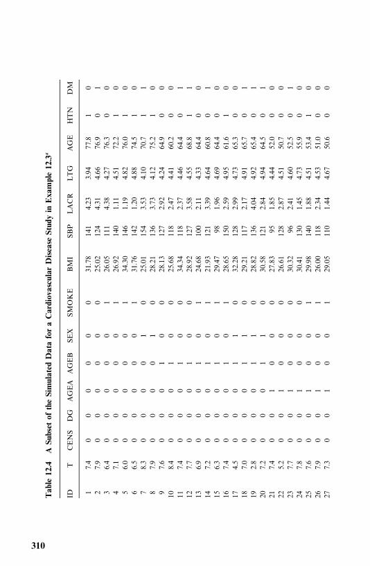
Table12.4
ASubsetoftheSimulatedDataforaCardiovascularDiseaseStudyinExample12.3
�
IDT
CENS
DG
AGEA
AGEB
SEX
SMOKE
BMI
SBP
LACR
LTG
AGE
HTN
DM
17.4
00
00
00
31.78
141
4.23
3.94
77.8
10
27.9
00
00
00
25.02
124
4.31
4.66
76.9
01
36.4
00
00
01
26.05
111
4.38
4.27
76.3
00
47.1
00
00
01
26.92
140
1.11
4.51
72.2
10
56.0
00
00
01
34.30
146
1.19
4.82
76.0
10
66.5
00
00
01
31.76
142
1.20
4.88
74.5
10
78.3
00
00
10
25.01
154
3.53
4.10
70.7
11
87.9
00
00
10
28.21
136
3.73
4.12
75.2
10
97.6
00
01
00
28.13
127
2.92
4.24
64.9
00
108.4
00
01
00
25.68
118
2.47
4.41
60.2
00
117.4
00
01
00
34.34
118
2.37
4.46
64.4
01
127.7
00
01
00
28.92
127
3.58
4.55
68.8
11
136.9
00
01
01
24.68
100
2.11
4.33
64.4
00
147.2
00
01
01
21.93
121
3.39
4.64
60.8
01
156.3
00
01
01
29.47
981.96
4.69
64.4
00
167.4
00
01
01
28.65
150
2.59
4.95
61.6
10
174.5
00
01
10
32.28
128
2.99
4.73
65.3
00
187.0
00
01
10
29.21
117
2.17
4.91
65.7
01
192.8
00
01
10
28.82
136
4.04
4.92
65.4
01
207.2
00
01
10
30.58
121
2.84
4.94
64.5
01
217.4
00
10
00
27.83
951.85
4.44
52.0
00
225.2
00
10
00
26.61
128
2.87
4.51
50.7
00
237.7
00
10
00
30.32
962.41
4.60
52.5
01
247.8
00
10
00
30.41
130
1.45
4.73
55.9
00
257.6
00
10
01
29.98
140
1.88
4.51
53.4
10
267.9
00
10
01
26.00
118
2.34
4.53
51.0
00
277.3
00
10
01
29.05
110
1.44
4.67
50.6
00
310
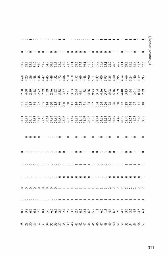
288.2
00
10
01
27.21
131
2.50
4.68
57.7
00
293.8
00
10
10
36.97
141
4.60
4.25
58.7
10
306.9
00
10
10
29.44
115
2.89
4.26
53.6
01
316.1
00
10
10
33.85
154
3.48
4.48
51.2
10
327.2
00
10
10
32.13
122
2.92
4.48
55.2
00
338.4
00
10
11
27.52
135
2.39
4.42
53.7
00
345.0
00
10
11
30.64
114
1.39
4.45
54.9
10
356.5
00
10
11
29.94
120
2.96
4.49
50.7
00
366.4
00
10
11
29.89
115
1.68
4.52
51.3
00
372.6
11
00
00
30.88
189
5.38
4.72
73.9
11
382.7
11
00
01
25.05
200
3.37
4.86
77.2
11
392.7
11
00
10
26.80
130
2.31
5.10
73.5
00
403.3
11
00
11
21.67
111
3.53
4.18
71.1
00
412.9
11
01
00
36.83
114
2.64
4.52
68.2
00
420.2
11
01
01
21.49
125
4.61
4.69
67.3
00
432.1
11
01
10
31.05
131
1.38
4.48
69.1
00
446.8
11
01
11
26.78
134
4.36
4.90
61.0
10
455.7
11
10
00
35.78
132
9.93
5.11
52.5
01
461.1
11
10
01
28.44
134
3.54
4.32
55.7
00
476.6
11
10
10
24.38
124
4.16
4.00
51.8
01
481.3
11
10
11
34.13
126
5.87
3.95
53.1
01
494.6
12
00
00
43.23
128
5.08
5.25
72.2
01
506.3
12
00
01
38.67
126
5.16
4.50
76.8
11
512.0
12
00
10
34.49
130
2.69
3.95
76.7
11
524.2
12
00
11
20.78
127
4.40
4.54
73.1
00
533.6
12
01
00
28.40
118
5.43
4.66
69.3
11
543.2
12
01
01
28.73
154
1.94
5.24
68.9
11
554.5
12
01
10
44.25
972.01
4.40
68.6
01
564.5
12
01
11
32.46
141
0.74
4.39
63.5
10
576.1
12
10
00
39.72
118
2.39
3.93
52.6
01
(Continuedoverleaf)
311
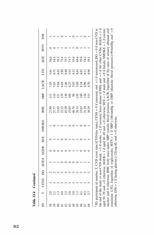
Table12.4
Con
tinu
ed
IDT
CENS
DG
AGEA
AGEB
SEX
SMOKE
BMI
SBP
LACR
LTG
AGE
HTN
DM
583.0
12
10
01
27.90
117
7.45
5.61
56.0
01
592.1
12
10
10
27.77
119
7.03
4.71
54.3
01
601.3
12
10
11
31.03
151
3.94
4.43
59.2
11
614.9
13
00
00
25.22
129
6.69
3.90
75.4
10
622.5
13
00
01
45.29
130
2.46
4.40
75.7
01
633.8
13
00
10
25.03
188
6.25
5.63
71.7
11
645.0
13
01
10
46.76
963.93
4.12
65.6
10
651.5
13
01
11
28.53
126
3.09
4.65
68.6
01
664.1
13
10
00
23.63
144
8.24
4.82
59.4
11
670.5
13
10
10
31.39
134
6.96
4.11
54.2
10
682.7
13
10
11
30.29
115
4.70
4.98
59.1
11
�ID
,participantid
num
ber;T,C
VD
eventtime
(CVD-freetime);CENS
�0ifcensored,and
�1ifuncensored;DG
�0ifnon-CVD
attheendof
thestudy
orno
n-CVD
death,�1ifstroke,�2ifcoronaryheartdisease
(CHD
),and
�3iftheother
CVDs;AGEA
�1if
aged
50—59
and
�0otherwise;AGEB
�1ifaged
60—69
and
�0otherwise;SEX
�1ifmaleand
�0iffemale;SMOKE
�1ifcurrent
smoker
and0otherwise;BMI,body
massindex;SBP,systolic
bloodpressure;LACR,logarithm
oftheratioofurinaryalbum
inand
creatinine;LTG,logarithm
oftriglycerides;HTN
�1ifSB
P�140mmHgor
DBP
(diastolic
bloodpressure
)�90
mmHgand
�0
otherwise;DM
�1iffastingglucose�
126mg/dL
and
�0otherwise.
312
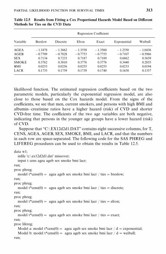
Table 12.5 Results from Fitting a Cox Proportional Hazards Model Based on DifferentMethods for Ties on the CVD Data
Regression Coefficient
Variable Breslow Discrete Efron Exact Exponential Weibull
AGEA �1.3478 �1.3662 �1.3558 �1.3560 �1.2550 �1.0436AGEB �0.7709 �0.7828 �0.7753 �0.7755 �0.7107 �0.5966SEX 0.7134 0.7233 0.7187 0.7189 0.6862 0.5659SMOKE 0.3762 0.3810 0.3776 0.3776 0.3440 0.2855BMI 0.0253 0.0256 0.0255 0.0255 0.0233 0.0194LACR 0.1735 0.1759 0.1739 0.1740 0.1658 0.1357
likelihood function. The estimated regression coefficients based on the twoparametric models, particularly the exponential regression model, are alsoclose to those based on the Cox hazards model. From the signs of thecoefficients, we see that men, current smokers, and persons with high BMI andalbumin—creatinine ratios have a higher hazard (risk) of CVD and shorterCVD-free time. The coefficients of the two age variables are both negative,indicating that persons in the younger age groups have a lower hazard (risk)of CVD.
Suppose that ‘‘C:�EX12d2d1.DAT’’ contains eight successive columns, for T,CENS, AGEA, AGEB, SEX, SMOKE, BMI, and LACR, and that the numbersin each row are space-separated. The following code for the SAS PHREG andLIFEREG procedures can be used to obtain the results in Table 12.5.
data w1;infile ‘c:�ex12d2d1.dat’ missover;input t cens agea ageb sex smoke bmi lacr;
run;proc phreg;model t*cens(0) � agea ageb sex smoke bmi lacr / ties�breslow;
run;proc phreg;model t*cens(0) � agea ageb sex smoke bmi lacr / ties�discrete;
run;proc phreg;model t*cens(0) � agea ageb sex smoke bmi lacr / ties� efron;
run;proc phreg;model t*cens(0) � agea ageb sex smoke bmi lacr / ties� exact;
run;proc lifereg;Model a: model t*cens(0)� agea ageb sex smoke bmi lacr / d� exponential;Model b: model t*cens(0) � agea ageb sex smoke bmi lacr / d�weibull;
run;
313
12.2 IDENTIFICATION OF SIGNIFICANT COVARIATES
As noted earlier, one principal interest is to identify significant prognosticfactors or covariates. This involves hypothesis testing and covariate selectionprocedures, similar to those discussed in Chapter 11 for parametric methods.The differences are that the Cox proportional hazard model has a partiallikelihood function in which the only parameters are the coefficientsassociated with the covariates. However, statistical inference based on thepartial likelihood function has asymptotic properties similar to those basedon the usual likelihood. Therefore, the estimation procedure (discussed inSection 12.1) is similar to those in Section 7.1, and the hypothesis-testingprocedures are similar to those in Sections 9.1 and 11.2. For example, theWald statistic in (9.1.4) can be used to test if any one of the covariates has noeffect on the hazard, that is, to test H
�: b
�� 0. By replacing the log-likelihood
function with the log partial likelihood function, the log-likelihood ratiostatistic, the Wald statistic, and the score statistic in (9.1.10), (9.1.11), and(9.1.12) can be used to test the null hypothesis that all the coefficients areequal to zero, that is, to test
H�: b
�� 0, b
�� 0, . . . , b
�� 0
or H�: b� 0 in (9.1.9). Similarly the forward, backward, and stepwise selection
procedures discussed in Section 11.9.1 are applicable to the Cox proportionalhazard model.
The following example, using the SAS PHREG procedure, illustrates theseprocedures.
Example 12.4 We use the entire CVD data set in Example 12.3 todemonstrate how to identify the most important risk factors among all thecovariates. Suppose that the effects of age, gender, and current smoking statuson CVD risk are of fundamental interest and we wish to include these variablesin the model. In epidemiology this is often referred to as adjusting for thesevariables. Thus, AGEA, AGEB, SEX, and SMOKE are forced into the modeland we are to select the most important variables from the remainingcovariates (BMI, SBP, LACR, LTG, HTN, and DM), adjusting for age, gender,and current smoking status.
The SAS procedure PHREG is used with Breslow’s approximation for ties(default procedure) and three variable selection methods (forward, backward,and stepwise). Two covariates, BMI and LACR, are selected at the 0.05significance level by all three selection methods. The final model, in the formof (12.1.5), including only the four covariates that we purposefully included andthe two most significant ones identified by the selection method, is
314
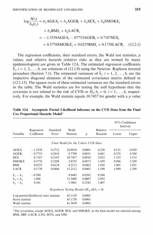
Table 12.6 Asymptotic Partial Likelihood Inference on the CVD Data from the FinalCox Proportional Hazards Model�
95% ConfidenceInterval
Regression Standard Wald RelativeVariable Coefficient Error Statistic p Hazards Lower Upper
Final Model for the Cohort CVD Data
AGEA �1.3558 0.2712 24.9910 0.0001 0.258 0.151 0.439AGEB �0.7753 0.2618 8.7709 0.0031 0.461 0.276 0.769SEX 0.7187 0.2193 10.7457 0.0010 2.052 1.335 3.153SMOKE 0.3776 0.2208 2.9235 0.0873 1.459 0.946 2.249BMI 0.0255 0.0124 4.2113 0.0402 1.026 1.001 1.051LACR 0.1739 0.0446 15.2112 0.0001 1.190 1.090 1.299
b�� b
��0.580 4.9443 0.0262 0.560
b�� b
1.096 11.5409 0.0007 2.993
b�� b
0.341 1.3001 0.2542 1.407
Hypothesis Testing Results (H�: all b
�� 0)
Log-partial-likelihood ratio statistic 42.1130 0.0001Score statistic 43.1750 0.0001Wald statistic 41.3830 0.0001
�The covariates, except AGEA, AGEB, SEX, and SMOKE, in the final model are selected amongBMI, SBP, LACR, LTG, HTN, and DM.
logh(t
�)
h�(t�)� b
�AGEA
�� b
�AGEB
�� b
�SEX
�� b
SMOKE
�
� b�BMI
�� b
�LACR
�
��1.3558AGEA�� 07753AGEB
�� 0.7187SEX
�
� 0.3776SMOKE�� 0.0255BMI
�� 0.1739LACR
�(12.2.1)
The regression coefficients, their standard errors, the Wald test statistics, pvalues, and relative hazards (relative risks as they are termed by manyepidemiologists) are given in Table 12.6. The estimated regression coefficientsb��, i� 1, 2, . . . , 6, are solutions of (12.1.9) using the Newton—Raphson iterated
procedure (Section 7.1). The estimated variances of b��, i� 1, 2, . . . , 6, are the
respective diagonal elements of the estimated covariance matrix defined in(12.1.13). The square roots of these estimated variances are the standard errorsin the table. The Wald statistics are for testing the null hypothesis that thecovariate is not related to the risk of CVD or H
�: b
�� 0, i� 1, . . . , 6, respect-
ively. For example, the Wald statistic equals 10.7457 for gender with a p value
315
of 0.0010 and b� 0.7187. It indicates that after adjusting for all the variablesin the model (12.2.1), gender is a significant predictor for the development ofCVD, with men having a higher risk than women. The relative hazard (or risk)is exp(b�
�), and for the covariate gender, it is exp(0.7187) � 2.052, which implies
that men aged 50—79 years have about twice the risk of developing CVD in 10years. The 95% confidence interval for the relative risk is (1.335, 3.153), whichis calculated according to (7.1.8). For a continuous variable, exp(b�
�) represents
the increase in risk corresponding to a 1-unit increase in the variable. Forexample, for BMI, exp (0.0255) � 1.026; that is, for every unit increase in BMI,the risk for CVD increases 2.6%.
To compare hazards among different age groups, between genders, orbetween smokers and nonsmokers, let h
����(t), h
����(t), h
����(t), h
���(t),
h���
(t), h��(t), and h
���(t) denote hazard functions for participants that are
50—59, 60—69, 70—79 years old, male, female, current smoker, and not currentsmoker, respectively. The log hazard ratio of a person in the 50 to 59-yearage group to a person in the 70 to 79-year group assuming the two people areof same gender and the same current smoking status, BMI and LACR, islog[h
����(t)/h
����(t)] � b
�; similarly, log[h
����(t)/h
����(t)] � b
�and
log[h����
(t)/h����
(t)] � b�� b
�. Assuming that the two people are in the
same age group and have the same BMI and LACR, the log hazard ratio ofmale to females is
logh���
(t)
h���
(t)� b
�
Similarly, assuming that the two people are in the same age group, of the samegender, and have the same BMI and LACR, the hazard ratio of a smoker to anonsmoker is
logh��(t)
h���
(t)� b
Thus, testing whether risk of CVD are the same among different age groups isequivalent to testing H
�: b
�� 0, H
�: b
�� 0, and H
�: b
�� b
�� 0. Similarly, to
test if the risk of CVD is the same between males and females or betweensmokers and nonsmokers is equivalent to tasting the null hypothesisH
�: b
�� 0
or H�: b
� 0, respectively.
To consider more than one covariate, we also can formulate the nullhypothesis by using (12.2.1). For example, if we wish to compare malenonsmokers to female smokers, from (12.2.1),
logh������h�����
� b�� b
316
assuming that they are in the same age group and have the same BMI andLACR. Thus to test if these two groups of people have the same risk of CVD,we test the null hypothesis H
�: b
�� b
� 0. Similarly, to compare male
smokers to female nonsmokers, we can test the null hypothesisH�: b
�� b
� 0.
These null hypotheses are in the form of linear combinations of the coefficients.Using the notations in Section 11.2, the hypotheses H
�: b
�� b
�� 0 and
H�: b
�� b
� 0 are the hypotheses in (11.2.13) with c� 0, L� (1�1 0 0 0 0),
and L� (0 0 1 1 0 0), respectively. The Wald statistics in Table 12.6 arecalculated according to (11.2.14). By assuming that the patients have the sameBMI and LACR, we can construct hypotheses to compare subgroups definedby age groups, gender, and current smoking status.
The last part of Table 12.6 shows the results of testing the null hypothesisthat none of these covariates have any effect on the development of CVD. Thelog partial likelihood ratio, Wald, and score statistics, X
�, X
�, and X
�are
calculated according to (9.1.10), (9.1.11), and (9.1.12), respectively. Table 12.6indicates that the hypotheses, H
�: b
�� 0, H
�: b
�� 0, H
�: b
�� b
�� 0,
H�: b
�� 0, H
�: b
�� 0, H
�: b
�� 0, and H
�: b
�� b
� 0 are rejected at a signifi-
cance level of p� 0.05. However, the hypotheses H�: b
� 0 and
H�: b
�� b
� 0 are not rejected at a 0.05 level. The null hypothesis
H�: all b
�� 0, i� 1, . . . , 6, is rejected with p� 0.0001 by using any of these
tests.Assuming that the other covariates are the same, based on the relative
hazards shown in the table, we conclude that (1) participants aged 50—59and 60—69 have, respectively, about 25% and 50% lower CVD risk thanthose aged 70—79 (H
�: b
�� 0 and H
�: b
�� 0 are rejected); (2) participants
aged 50—59 have 50% lower CVD risk than those aged 60—69 (H�: b
�� b
�� 0
is rejected); (3) men’s CVD risk is twice as high as that of women (H�: b
�� 0
is rejected); (4) BMI and LACR have a significant effect on CVD risk(H
�: b
�� 0 and H
�: b
�� 0 are rejected) and the risk increases about 3% and
19%, respectively, for every 1-unit increase in BMI and LACR, respectively; (5)male smokers have a CVD risk three times higher than that of femalenonsmokers (H
�: b
�� b
� 0 is rejected); (6) male nonsmokers have CVD risk
similar to that of female smokers (H�: b
�� b
� 0 is not rejected); (7) consider-
ing current smoking status alone, smokers had similar CVD risk as non-smokers (H
�: b
� 0 is not rejected). This example is solely for the purpose of
illustrating the use of the proportional hazards model and the interpretationof its results. Other hypotheses of interest can be constructed in a similarmanner. The construction of null hypotheses for comparisons among sub-groups defined by AGEGROUP*SEX*SMOKE are left to the reader asexercises.
Suppose that ‘‘C:�EX12d4d1.DAT’’ is a text data file that contains12 successive columns for T, CENS, AGEA, AGEB, SEX, SMOKE, BMI,LACR, SBP, LTG, HTN, and DM. The following SAS code is used to obtainedthe results in Table 12.6.
317
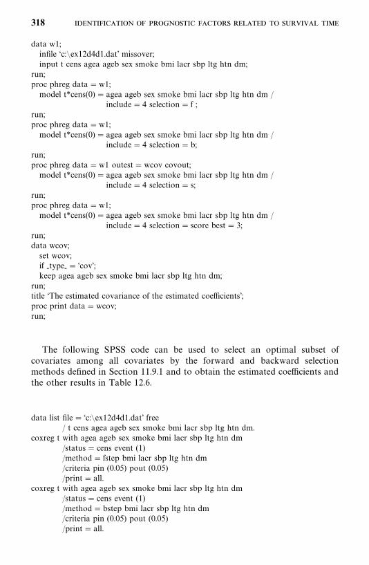
data w1;infile ‘c:�ex12d4d1.dat’ missover;input t cens agea ageb sex smoke bmi lacr sbp ltg htn dm;
run;proc phreg data�w1;model t*cens(0) � agea ageb sex smoke bmi lacr sbp ltg htn dm /
include� 4 selection� f ;run;proc phreg data�w1;model t*cens(0) � agea ageb sex smoke bmi lacr sbp ltg htn dm /
include� 4 selection�b;run;proc phreg data�w1 outest�wcov covout;model t*cens(0) � agea ageb sex smoke bmi lacr sbp ltg htn dm /
include� 4 selection� s;run;proc phreg data�w1;model t*cens(0) � agea ageb sex smoke bmi lacr sbp ltg htn dm /
include� 4 selection� score best� 3;run;data wcov;set wcov;if -type-� ‘cov’;keep agea ageb sex smoke bmi lacr sbp ltg htn dm;
run;title ‘The estimated covariance of the estimated coefficients’;proc print data�wcov;run;
The following SPSS code can be used to select an optimal subset ofcovariates among all covariates by the forward and backward selectionmethods defined in Section 11.9.1 and to obtain the estimated coefficients andthe other results in Table 12.6.
data list file� ‘c:�ex12d4d1.dat’ free/ t cens agea ageb sex smoke bmi lacr sbp ltg htn dm.
coxreg t with agea ageb sex smoke bmi lacr sbp ltg htn dm/status� cens event (1)/method� fstep bmi lacr sbp ltg htn dm/criteria pin (0.05) pout (0.05)/print� all.
coxreg t with agea ageb sex smoke bmi lacr sbp ltg htn dm/status� cens event (1)/method�bstep bmi lacr sbp ltg htn dm/criteria pin (0.05) pout (0.05)/print� all.
318
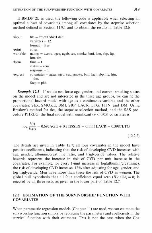
If BMDP 2L is used, the following code is applicable when selecting anoptimal subset of covariates among all covariates by the stepwise selectionmethod defined in Section 11.9.1 and to obtain the results in Table 12.6.
/input file� ‘c:�ex12d4d1.dat’ .variables� 12.format� free.
/print cova./variable names� t,cens, agea, ageb, sex, smoke, bmi, lacr, sbp, ltg,
htn, dm./form time� t.
status� cens.response� 1.
/regress covariates� agea, ageb, sex, smoke, bmi, lacr, sbp, ltg, htn,dm.
Step�phh.
Example 12.5 If we do not force age, gender, and current smoking statuson the model and are not interested in the three age groups, we can fit theproportional hazard model with age as a continuous variable and the othercovariates: SEX, SMOKE, BMI, SBP, LACR, LTG, HTN, and DM. UsingBreslow’s method for ties, the stepwise selection method, and the SAS pro-cedure PHREG, the final model with significant (p� 0.05) covariates is
logh(t)
h�(t)
� 0.697AGE� 0.7528SEX� 0.1111LACR� 0.3987LTG
(12.2.2)
The details are given in Table 12.7; all four covariates in the model havepositive coefficients, indicating that the risk of developing CVD increases withage, gender, albumin/creatinine ratio, and triglyceride values. The relativehazards represent the increase in risk of CVD per unit increase in thecovariates. For example, for every 1-unit increase in log(albumin/creatinine),the risk of developing CVD increases 12% after adjusting for age, gender, andlog triglyceride. Men have more than twice the risk of CVD as women. Theglobal null hypothesis that all four coefficients equal zero (H
�: all b
�� 0) is
rejected by all three tests, as given in the lower part of Table 12.7.
12.3 ESTIMATION OF THE SURVIVORSHIP FUNCTION WITHCOVARIATES
When parametric regression models (Chapter 11) are used, we can estimate thesurvivorship function simply by replacing the parameters and coefficients in thesurvival function with their estimates. This is not the case when the Cox
319
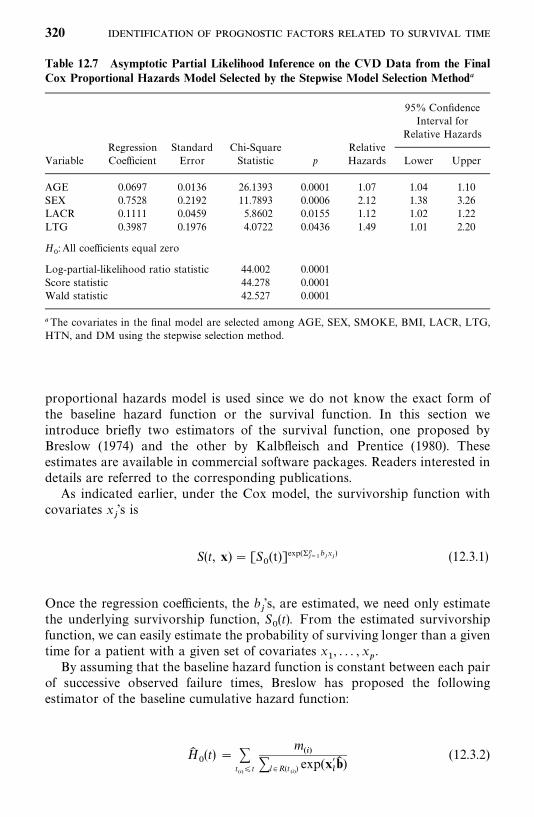
Table 12.7 Asymptotic Partial Likelihood Inference on the CVD Data from the FinalCox Proportional Hazards Model Selected by the Stepwise Model Selection Method�
95% ConfidenceInterval for
Relative HazardsRegression Standard Chi-Square Relative
Variable Coefficient Error Statistic p Hazards Lower Upper
AGE 0.0697 0.0136 26.1393 0.0001 1.07 1.04 1.10SEX 0.7528 0.2192 11.7893 0.0006 2.12 1.38 3.26LACR 0.1111 0.0459 5.8602 0.0155 1.12 1.02 1.22LTG 0.3987 0.1976 4.0722 0.0436 1.49 1.01 2.20
H�: All coefficients equal zero
Log-partial-likelihood ratio statistic 44.002 0.0001Score statistic 44.278 0.0001Wald statistic 42.527 0.0001
�The covariates in the final model are selected among AGE, SEX, SMOKE, BMI, LACR, LTG,HTN, and DM using the stepwise selection method.
proportional hazards model is used since we do not know the exact form ofthe baseline hazard function or the survival function. In this section weintroduce briefly two estimators of the survival function, one proposed byBreslow (1974) and the other by Kalbfleisch and Prentice (1980). Theseestimates are available in commercial software packages. Readers interested indetails are referred to the corresponding publications.
As indicated earlier, under the Cox model, the survivorship function withcovariates x
�’s is
S(t, x) � [S�(t)]exp(��
���b�x�) (12.3.1)
Once the regression coefficients, the b�’s, are estimated, we need only estimate
the underlying survivorship function, S�(t). From the estimated survivorship
function, we can easily estimate the probability of surviving longer than a giventime for a patient with a given set of covariates x
�, . . . , x
�.
By assuming that the baseline hazard function is constant between each pairof successive observed failure times, Breslow has proposed the followingestimator of the baseline cumulative hazard function:
H��(t) � �
t���t
m��
�l �R(t��) exp(x�
�b� )
(12.3.2)
320
Following (2.15), the baseline survival function can be estimated as
S��(t) � exp[�H�
�(t)] �
t���t �exp�
m��
�l �R(t��) exp(x�
�b� )�� (12.3.3)
and the survivorship function for a person with a set of covariatesx� (x
�, . . . , x
�) is
S� (t, x) � [S��(t)] exp(��
���b��x�) � [S�
�(t)] exp(b� �x) (12.3.4)
Under mild assumptions, S� (t, x) has an asymptotic normal distribution withmean S(t, x). Since S(t, x) � exp[�H(t, x)], the variance estimator Var� (S� (t, x))of S� (t, x) is
Var� (S� (t, x)) � [S� (t, x)]�Var� (H� (t, x))
We will not give H� (t, x) here because of its complexity. The asymptoticconfidence bands for the survivorship function is
�S� (t, x)�Z����Var� (S� (t, x)) , S� (t, x) �Z����Var� (S� (t, x)) (12.3.5)
where Z��� is the upper 100(1� /2) percentile point of the standard normaldistribution.
An alternative estimator has been suggested by Kalbfleisch and Prentice inwhich the baseline survivorship function S
�(t) is estimated to be a step function
and
S��(t) �
�����
��
t���
� t� t��, i� 1, . . . , k� 1 (12.3.6)
where ��� 1 and �
�, �
�, . . . , �
�are the solution of the following k simultaneous
equations:
�j� u*
��
exp(x��b� )
1� ��exp(x�
�b� ) � �
l �R(t��)
exp(x��b� ) i� 1, . . . , k (12.3.7)
When there are no ties,
��� �1�
exp(x���b� )
�l�R(t��) exp(x�
�b� )�
exp(�x���b� )
i� 1, . . . , k (12.3.8)
and
S��(t) �
������1�
exp(x�� �b� )
�l �R(t��) exp(x�
�b� )�
exp(�x���b� )
t���
� t� t��
i� 1, . . . , k� 1
321
Thus,
S� (t, x) � [S��(t)] exp(b� �x) (12.3.9)
Under mild assumptions, the Kalbfleisch and Prentice estimator in (12.3.9) alsofollows an asymptotic normal distribution with mean S(t, x) and a variancethat can be estimated. Thus confidence bands for the survivorship function canalso be constructed.
Using (12.3.4) with S�(t) in (12.3.3) or (12.3.6), the survivorship function can
be estimated with any given values of x�, . . . , x
�. If the observed average of
every covariate, x��, . . . , x�
�is used, the estimated survivorship function can be
interpreted as the survivorship function of an ‘‘average’’ person.Both the Breslow and Kalbfleisch—Prentice estimators are available in the
SAS procedure PHREG. The Breslow estimator is also available in BMDP(program 2L) and SPSS (program COXREG). The following example illus-trates the procedures.
Example 12.6 Again, we use the CVD data in the Example 12.3, the dataset ‘‘C:�EX12d2d1.DAT’’, and the SAS procedure PHREG. We use the averageof each of the covariates in (12.2.1), and therefore the estimated survivorshipfunction is for an average person. The Kalbfleisch—Prentice and Breslowestimates of the survival function, defined in (12.3.9) and (12.3.4) (Efronadjustment for ties is used), and the lower and upper 95% confidence bands,calculated based on (12.3.5), are shown in Figures 12.1 and 12.2. Theseestimated survival functions, using all the covariates in the model with averagevalues, are often referred to as the global covariate—adjusted survivorshipfunctions. The two figures are almost identical, which indicates that the twomethods produce very similar results for this set of data. From Figure 12.1 itappears that the global covariates—adjusted survivorship function decreasessomewhat more rapidly after 3.5 years. This means that the process to developCVD accelerates after 3.5 years.
Using the data set ‘‘C:�EX12d2d1.DAT’’ defined in Example 12.3, the SAScode used for this example is the following.
data w1;infile ‘c:�ex12d2d1.dat’ missover;input t cens agea ageb sex smoke bmi lacr;
run;proc phreg data�w1 noprint;model t*cens(0) � agea ageb sex smoke bmi lacr / ties� efron;baseline out�base1 survival� survival l� lowb u�uppb / method�p l;
run;title ’K-P estimate of the survival function and its lower and upper bands’;proc print data�base1;var t survival lowb uppb;
run;
322
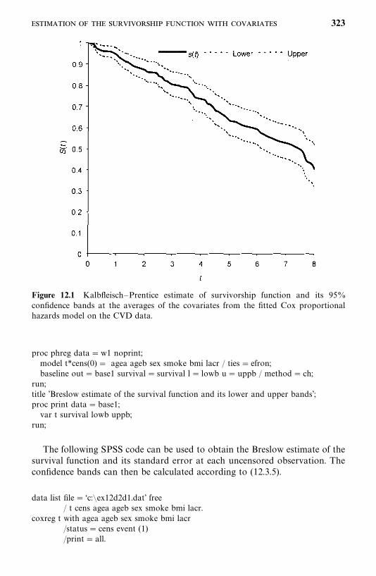
Figure 12.1 Kalbfleisch—Prentice estimate of survivorship function and its 95%confidence bands at the averages of the covariates from the fitted Cox proportionalhazards model on the CVD data.
proc phreg data�w1 noprint;model t*cens(0) � agea ageb sex smoke bmi lacr / ties� efron;baseline out�base1 survival� survival l� lowb u� uppb / method� ch;
run;title ’Breslow estimate of the survival function and its lower and upper bands’;proc print data�base1;var t survival lowb uppb;
run;
The following SPSS code can be used to obtain the Breslow estimate of thesurvival function and its standard error at each uncensored observation. Theconfidence bands can then be calculated according to (12.3.5).
data list file� ‘c:�ex12d2d1.dat’ free/ t cens agea ageb sex smoke bmi lacr.
coxreg t with agea ageb sex smoke bmi lacr/status� cens event (1)/print� all.
323
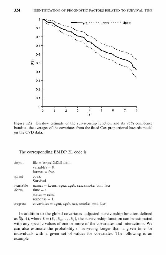
Figure 12.2 Breslow estimate of the survivorship function and its 95% confidencebands at the averages of the covariates from the fitted Cox proportional hazards modelon the CVD data.
The corresponding BMDP 2L code is
/input file� ‘c:�ex12d2d1.dat’ .variables� 8.format� free.
/print cova.Survival.
/variable names� t,cens, agea, ageb, sex, smoke, bmi, lacr./form time� t.
status� cens.response� 1.
/regress covariates� agea, ageb, sex, smoke, bmi, lacr.
In addition to the global covariates—adjusted survivorship function definedas S� (t, x� ), where x� � (x�
�, x�
�, . . . , x�
�), the survivorship function can be estimated
with any specific values of one or more of the covariates and interactions. Wecan also estimate the probability of surviving longer than a given time forindividuals with a given set of values for covariates. The following is anexample.
324
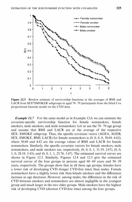
Figure 12.3 Breslow estimate of survivorship functions at the averages of BMI andLACR from SEX*SMOKER subgroups in aged 70—79 participants from the fitted Coxproportional hazards model on the CVD data.
Example 12.7 For the same model as in Example 12.6, we can estimate thecovariate-specific survivorship function for female nonsmokers, femalesmokers, male smokers, and male nonsmokers. Let us use the 70—79 age groupand assume that BMI and LACR are at the average of the respectiveSEX—SMOKE subgroup. Thus, the specific covariate vector (AGEA, AGEB,SEX, SMOKE, BMI, LACR) for female nonsmokers is (0, 0, 0, 0, 30.69, 4.62),where 30.69 and 4.62 are the average values of BMI and LACR for femalenonsmokers. Similarly, the specific covariate vectors for female smokers, malenonsmokers, and male smokers are, respectively, (0, 0, 0, 1, 31.19, 2.67), (0, 0,1, 0, 28.19, 3.43), and (0, 0, 1, 1, 25.76, 3.47). The estimated survival curves areshown in Figure 12.3. Similarly, Figures 12.4 and 12.5 give the estimatedsurvival curves of the four groups in persons aged 60—69 years and 50—59years, respectively. The groups show that in all these age groups, females havea lower risk of developing CVD (longer CVD-free time) than males. Femalenonsmokers have a slightly lower risk than female smokers and the differencesincrease as age decreases. However, among males, the differences in the risk ofCVD between smokers and nonsmokers are almost negligible in the youngestgroup and much larger in the two older groups. Male smokers have the highestrisk of developing CVD (shortest CVD-free time) among the four groups.
325
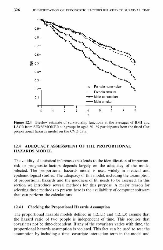
Figure 12.4 Breslow estimate of survivorship functions at the averages of BMI andLACR from SEX*SMOKER subgroups in aged 60—69 participants from the fitted Coxproportional hazards model on the CVD data.
12.4 ADEQUACY ASSESSMENT OF THE PROPORTIONALHAZARDS MODEL
The validity of statistical inferences that leads to the identification of importantrisk or prognostic factors depends largely on the adequacy of the modelselected. The proportional hazards model is used widely in medical andepidemiological studies. The adequacy of this model, including the assumptionof proportional hazards and the goodness of fit, needs to be assessed. In thissection we introduce several methods for this purpose. A major reason forselecting these methods to present here is the availability of computer softwarethat can perform the calculations.
12.4.1 Checking the Proportional Hazards Assumption
The proportional hazards models defined in (12.1.1) and (12.1.3) assume thatthe hazard ratio of two people is independent of time. This requires thatcovariates not be time-dependent. If any of the covariates varies with time, theproportional hazards assumption is violated. This fact can be used to test theassumption by including a time—covariate interaction term in the model and
326
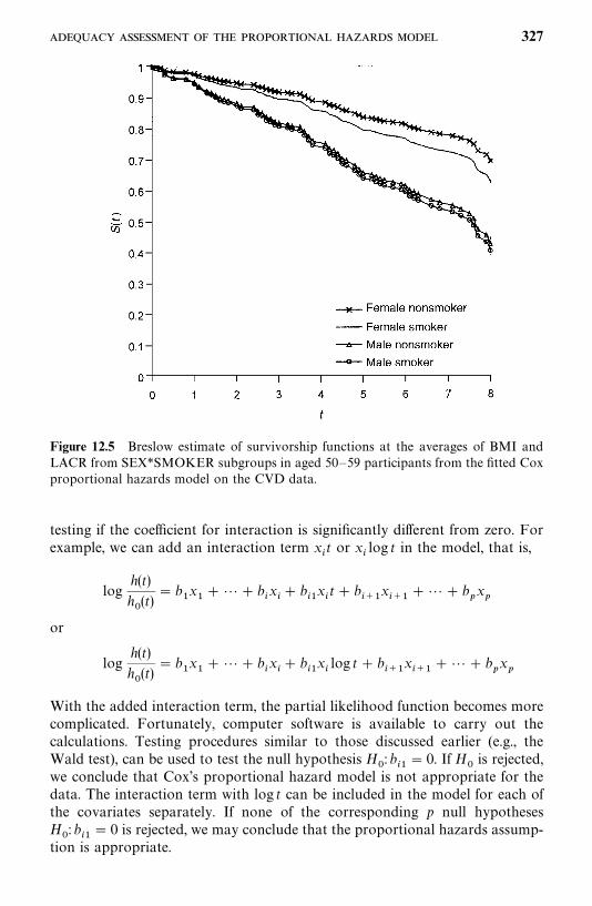
Figure 12.5 Breslow estimate of survivorship functions at the averages of BMI andLACR from SEX*SMOKER subgroups in aged 50—59 participants from the fitted Coxproportional hazards model on the CVD data.
testing if the coefficient for interaction is significantly different from zero. Forexample, we can add an interaction term x
�t or x
�log t in the model, that is,
logh(t)
h�(t)
� b�x���� b
�x�� b
��x�t� b
���x���
�� � b�x�
or
logh(t)
h�(t)
� b�x���� b
�x�� b
��x�log t� b
���x���
�� � b�x�
With the added interaction term, the partial likelihood function becomes morecomplicated. Fortunately, computer software is available to carry out thecalculations. Testing procedures similar to those discussed earlier (e.g., theWald test), can be used to test the null hypothesis H
�: b
��� 0. If H
�is rejected,
we conclude that Cox’s proportional hazard model is not appropriate for thedata. The interaction term with log t can be included in the model for each ofthe covariates separately. If none of the corresponding p null hypothesesH
�: b
��� 0 is rejected, we may conclude that the proportional hazards assump-
tion is appropriate.
327
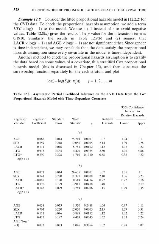
Table 12.8 Asymptotic Partial Likelihood Inference on the CVD Data from the CoxProportional Hazards Model with Time-Dependent Covariate
95% ConfidenceInterval for
Relative HazardsRegressor Regressor Standard Wald RelativeVariable Coefficient Error Statistic p Hazards Lower Upper
(a)
AGE 0.068 0.014 25.249 0.0001 1.07 1.04 1.1SEX 0.759 0.218 12.056 0.0005 2.14 1.39 3.28LACR 0.111 0.046 5.781 0.0162 1.12 1.02 1.22LTG 0.915 0.435 4.420 0.0355 2.50 1.06 5.86LTG* �0.390 0.298 1.710 0.1910 0.68 0.38 1.22log(t�1)
(b)
AGE 0.071 0.014 26.635 0.0001 1.07 1.05 1.1SEX 0.741 0.220 11.327 0.0008 2.10 1.36 3.23LACR �0.087 0.120 0.519 0.4714 0.92 0.72 1.16LTG 0.395 0.199 3.917 0.0478 1.48 1 2.19LACR* 0.143 0.079 3.269 0.0706 1.15 0.99 1.35log(t�1)
(c)
AGE 0.038 0.033 1.330 0.2488 1.04 0.97 1.11SEX 0.764 0.220 12.020 0.0005 2.15 1.39 3.31LACR 0.111 0.046 5.888 0.0152 1.12 1.02 1.22LTG 0.417 0.197 4.469 0.0345 1.52 1.03 2.24AGE*log(t�1) 0.023 0.023 1.046 0.3064 1.02 0.98 1.07
Example 12.8 Consider the fitted proportional hazards model in (12.2.2) forthe CVD data. To check the proportional hazards assumption, we add a termL TG�log(t� 1) to the model. We use t� 1 instead of t to avoid negativevalues. Table 12.8(a) gives the results. The p value for the interaction term is0.1910. Similarly, the results in Table 12.9(b) and (c) suggest thatLACR�log(t� 1) and AGE�log(t� 1) are not significant either. Since genderis time-independent, we may conclude that the data satisfy the proportionalhazards assumption since every covariate in the model is time-independent.
Another method to check the proportional hazards assumption is to stratifythe data based on some values of a covariate, fit a stratified Cox proportionalhazards model (this is discussed in Chapter 13), and then construct thesurvivorship function separately for the each stratum and plot
log(�log(S��(t; x�
�))) j� 1, 2, . . . ,m
328
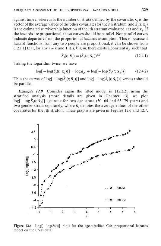
Figure 12.6 Log[�log(S(t))] plots for the age-stratified Cox proportional hazardsmodel on the CVD data.
against time t, where m is the number of strata defined by the covariate, x��is the
vector of the average values of the other covariates for the jth stratum, and S��(t;x�
�)
is the estimated survivorship function of the jth stratum evaluated at t and x��. If
the hazards are proportional, them curves should be parallel. Nonparallel curvesindicate departure from the proportional hazards assumption. This is because ifhazard functions from any two people are proportional, it can be shown from(12.1.1) that, for any j� k and 1� j, k�m, there exists a constant d
��such that
S��(t; x�
�) � (S�
�(t; x�
�)) �� (12.4.1)
Taking the logarithm twice, we have
log[�log(S��(t; x�
�))]� log d
��� log[�log(S�
�(t; x�
�))] (12.4.2)
Thus the curves of log[�log(S��(t; x�
�))] and log[�log(S�
�(t; x�
�))] versus t should
be parallel.
Example 12.9 Consider again the fitted model in (12.2.2); using thestratified analysis (more details are given in Chapter 13), we plotlog[�logS�
�(t; x�
�)] against t for two age strata (50—64 and 65—79 years) and
two gender strata separately, where x��denotes the average values of the other
covariates for the jth stratum. These graphs are given in Figures 12.6 and 12.7,
329
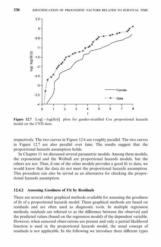
Figure 12.7 Log[�log(S(t))] plots for gender-stratified Cox proportional hazardsmodel on the CVD data.
respectively. The two curves in Figure 12.6 are roughly parallel. The two curvesin Figure 12.7 are also parallel over time. The results suggest that theproportional hazards assumption holds.
In Chapter 11 we discussed several parametric models. Among these models,the exponential and the Weibull are proportional hazards models, but theothers are not. Thus, if one of the other models provides a good fit to data, wewould know that the data do not meet the proportional hazards assumption.This procedure can also be served as an alternative for checking the propor-tional hazards assumption.
12.4.2 Assessing Goodness of Fit by Residuals
There are several other graphical methods available for assessing the goodnessof fit of a proportional hazards model. These graphical methods are based onresiduals and are often used as diagnostic tools. In multiple regressionmethods, residuals are referred to as the difference between the observed andthe predicted values (based on the regression model) of the dependent variable.However, when censored observations are present and only a partial likelihoodfunction is used in the proportional hazards model, the usual concept ofresiduals is not applicable. In the following we introduce three different types
330
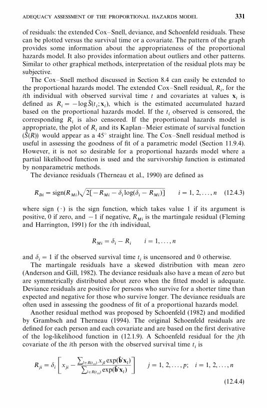
of residuals: the extended Cox—Snell, deviance, and Schoenfeld residuals. Thesecan be plotted versus the survival time or a covariate. The pattern of the graphprovides some information about the appropriateness of the proportionalhazards model. It also provides information about outliers and other patterns.Similar to other graphical methods, interpretation of the residual plots may besubjective.
The Cox—Snell method discussed in Section 8.4 can easily be extended tothe proportional hazards model. The extended Cox—Snell residual, R
�, for the
ith individual with observed survival time t and covariates at values x�is
defined as R�� �logS� (t
�;x
�), which is the estimated accumulated hazard
based on the proportional hazards model. If the t�observed is censored, the
corresponding R�is also censored. If the proportional hazards model is
appropriate, the plot of R�and its Kaplan—Meier estimate of survival function
(S� (R)) would appear as a 45° straight line. The Cox—Snell residual method isuseful in assessing the goodness of fit of a parametric model (Section 11.9.4).However, it is not so desirable for a proportional hazards model where apartial likelihood function is used and the survivorship function is estimatedby nonparametric methods.
The deviance residuals (Therneau et al., 1990) are defined as
R��
� sign(R��
)�2[�R��
� ��log(�
��R
��)] i� 1, 2, . . . , n (12.4.3)
where sign ( · ) is the sign function, which takes value 1 if its argument ispositive, 0 if zero, and �1 if negative, R
��is the martingale residual (Fleming
and Harrington, 1991) for the ith individual,
R��
� ���R
�i� 1, . . . , n
and ��� 1 if the observed survival time t
�is uncensored and 0 otherwise.
The martingale residuals have a skewed distribution with mean zero(Anderson and Gill, 1982). The deviance residuals also have a mean of zero butare symmetrically distributed about zero when the fitted model is adequate.Deviance residuals are positive for persons who survive for a shorter time thanexpected and negative for those who survive longer. The deviance residuals areoften used in assessing the goodness of fit of a proportional hazards model.
Another residual method was proposed by Schoenfeld (1982) and modifiedby Grambsch and Therneau (1994). The original Schoenfeld residuals aredefined for each person and each covariate and are based on the first derivativeof the log-likelihood function in (12.1.9). A Schoenfeld residual for the jthcovariate of the ith person with the observed survival time t
�is
R��� �
� �x����l�R(t
��) x��
exp(b� �x�)
�l �R(t��) exp(b� �x
�) � j� 1, 2, . . . , p ; i� 1, 2, . . . , n
(12.4.4)
331
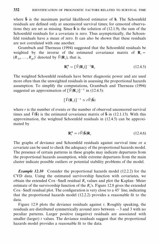
where b� is the maximum partial likelihood estimator of b. The Schoenfeldresiduals are defined only at uncensored survival times; for censored observa-tions they are set as missing. Since b� is the solution of (12.1.9), the sum of theSchoenfeld residuals for a covariate is zero. Thus asymptotically, the Schoen-feld residuals have a mean of zero. It can also be shown that these residualsare not correlated with one another.
Grambsch and Therneau (1994) suggested that the Schoenfeld residuals beweighted by the inverse of the estimated covariance matrix of R
��
(R��, . . . ,R
��)� denoted by V� (R
�), that is,
R*�� [V� (R
�)]�R
�(12.4.5)
The weighted Schoenfeld residuals have better diagnostic power and are usedmore often than the unweighted residuals in assessing the proportional hazardsassumption. To simplify the computations, Grambsch and Therneau (1994)suggested an approximation of [V� (R
�)]� in (12.4.5):
[V� (R�)]�� rV� (b� )
where r is the number of events or the number of observed uncensored survivaltimes and V� (b� ) is the estimated covariance matrix of b� in (12.1.13). With thisapproximation, the weighted Schoenfeld residuals in (12.4.5) can be approxi-mated by
R*�� rV� (b� )R
�(12.4.6)
The graphs of deviance and Schoenfeld residuals against survival time or acovariate can be used to check the adequacy of the proportional hazards model.The presence of certain patterns in these graphs may indicate departures fromthe proportional hazards assumption, while extreme departures from the maincluster indicate possible outliers or potential stability problems of the model.
Example 12.10 Consider the proportional hazards model (12.2.2) for theCVD data. Using the estimated survivorship function with covariates, weobtain the extended Cox—Snell residual R
�values and plot the Kaplan—Meier
estimate of the survivorship function of the R�’s. Figure 12.8 gives the extended
Cox—Snell residual plot. The configuration is very close to a 45° line, indicatingthat the proportional hazards model (12.2.2) provides a reasonable fit to thedata.
Figure 12.9 plots the deviance residuals against t. Roughly speaking, theresiduals are distributed symmetrically around zero between �3 and 3 with nopeculiar patterns. Larger positive (negative) residuals are associated withsmaller (larger) t values. The deviance residuals suggest that the proportionalhazards model provides a reasonable fit to the data.
332
Figure 12.8 Cox—Snell residuals plot from the fitted Cox proportional hazards modelon the CVD data.
The weighted Schoenfeld residuals versus AGE, LACR, and LTG are givenin Figures 12.10 to 12.12. In all these graphs, the residuals are distributedsymmetrically around zero except that in Figure 12.12, there are two outliersin the upper right corner. These extremely large residuals are from people withexceptionally high values of triglyceride. A large number of the residuals equalzero or are very close to zero, particularly those for AGE and LACR,suggesting that the model is accurate in predicting the risk of developing CVDfor these people.
We also fit several parametric models to the data. Table 12.9 gives thegoodness of fit assessments for five parametric models. The likelihood ratio testresults suggest that the Weilbull regression model provides an adequate fit(p� 0.2534). The Weilbull fit also gives the largest BIC and AIC values,suggesting that the Weilbull fit is best among these five models. As mentionedearlier, the Weilbull model is a proportional hazards model. Thus, theparametric model fitting provides additional evidence that the proportionalhazards model is adequate.
Using the data set ‘‘C:�EX12d4d1.DAT’’ in Example 12.4, the following SAScode is used to obtain the Cox—Snell, deviance, and weighted Schoenfeldresiduals for AGE, LTG, and LACR in Example 12.10.
333
Figure 12.9 Deviance residuals from the fitted Cox proportional hazards model on theCVD data.
data w1;infile ‘c:�ex12d4d1.dat’ missover;input t cens agea ageb sex smoke bmi lacr sbp ltg age htn dm;
run;proc phreg data�w1 noprint;model t*cens(0) � age sex lacr ltg / ties� efron;output out�out1 logsurv� ls resdev� rdev wtressch� rage r2 rlacr rltg;
run;data out1;set out1;rcs� -ls;
run;proc lifetest data�out1 notable outs�ws noprint;time rcs*cens(0);
run;data ws;set ws;mls� -log(survival);
run;title ‘Cox-Snell Residuals (rcs) and -log(estimated survival function of rcs) (mls)’;proc print data�ws;var rcs mls;
334
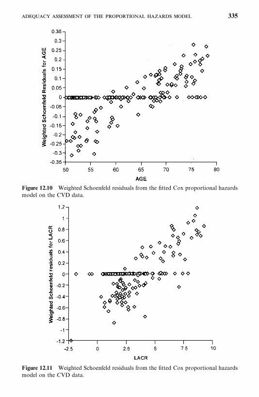
Figure 12.10 Weighted Schoenfeld residuals from the fitted Cox proportional hazardsmodel on the CVD data.
Figure 12.11 Weighted Schoenfeld residuals from the fitted Cox proportional hazardsmodel on the CVD data.
335
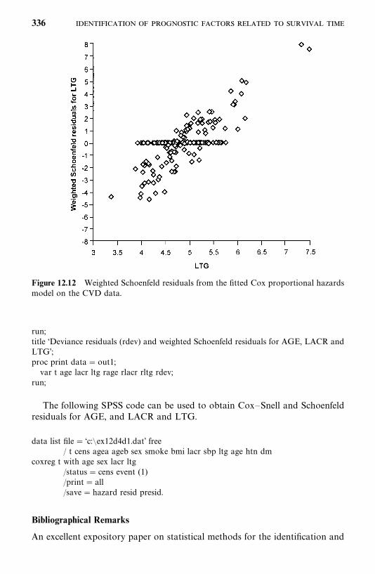
Figure 12.12 Weighted Schoenfeld residuals from the fitted Cox proportional hazardsmodel on the CVD data.
run;title ‘Deviance residuals (rdev) and weighted Schoenfeld residuals for AGE, LACR andLTG’;proc print data�out1;var t age lacr ltg rage rlacr rltg rdev;
run;
The following SPSS code can be used to obtain Cox—Snell and Schoenfeldresiduals for AGE, and LACR and LTG.
data list file� ‘c:�ex12d4d1.dat’ free/ t cens agea ageb sex smoke bmi lacr sbp ltg age htn dm
coxreg t with age sex lacr ltg/status� cens event (1)/print� all/save�hazard resid presid.
Bibliographical Remarks
An excellent expository paper on statistical methods for the identification and
336
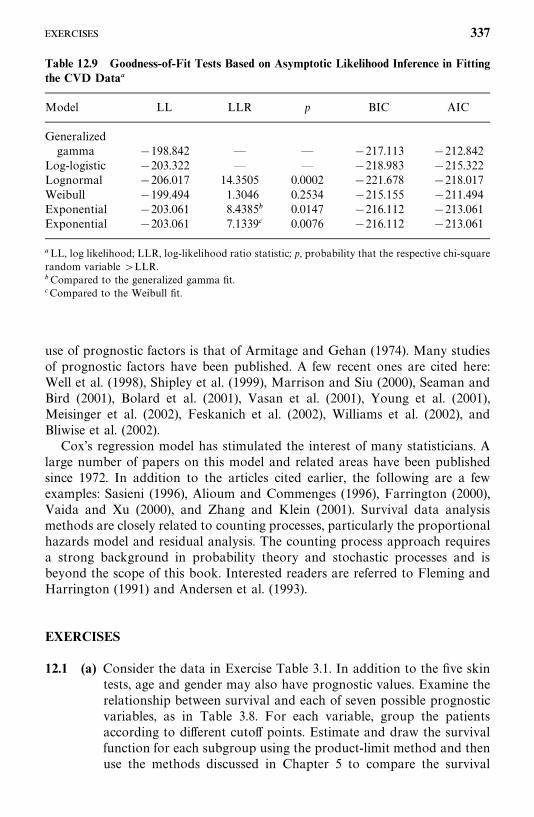
Table 12.9 Goodness-of-Fit Tests Based on Asymptotic Likelihood Inference in Fittingthe CVD Data�
Model LL LLR p BIC AIC
Generalizedgamma �198.842 — — �217.113 �212.842
Log-logistic �203.322 — — �218.983 �215.322Lognormal �206.017 14.3505 0.0002 �221.678 �218.017Weibull �199.494 1.3046 0.2534 �215.155 �211.494Exponential �203.061 8.4385� 0.0147 �216.112 �213.061Exponential �203.061 7.1339� 0.0076 �216.112 �213.061
�LL, log likelihood; LLR, log-likelihood ratio statistic; p, probability that the respective chi-squarerandom variable �LLR.�Compared to the generalized gamma fit.�Compared to the Weibull fit.
use of prognostic factors is that of Armitage and Gehan (1974). Many studiesof prognostic factors have been published. A few recent ones are cited here:Well et al. (1998), Shipley et al. (1999), Marrison and Siu (2000), Seaman andBird (2001), Bolard et al. (2001), Vasan et al. (2001), Young et al. (2001),Meisinger et al. (2002), Feskanich et al. (2002), Williams et al. (2002), andBliwise et al. (2002).
Cox’s regression model has stimulated the interest of many statisticians. Alarge number of papers on this model and related areas have been publishedsince 1972. In addition to the articles cited earlier, the following are a fewexamples: Sasieni (1996), Alioum and Commenges (1996), Farrington (2000),Vaida and Xu (2000), and Zhang and Klein (2001). Survival data analysismethods are closely related to counting processes, particularly the proportionalhazards model and residual analysis. The counting process approach requiresa strong background in probability theory and stochastic processes and isbeyond the scope of this book. Interested readers are referred to Fleming andHarrington (1991) and Andersen et al. (1993).
EXERCISES
12.1 (a) Consider the data in Exercise Table 3.1. In addition to the five skintests, age and gender may also have prognostic values. Examine therelationship between survival and each of seven possible prognosticvariables, as in Table 3.8. For each variable, group the patientsaccording to different cutoff points. Estimate and draw the survivalfunction for each subgroup using the product-limit method and thenuse the methods discussed in Chapter 5 to compare the survival
337
distribution of the subgroups. Prepare a table similar to Table 3.8.Interpret your results. Is there a subgroup of any variable that showssignificantly longer survival times? (For the skin test results, use thelarger diameter of the two.)
(b) Consider the seven variables in part (a). Use Cox’s model to identifythe most significant variables. Compare your results with thoseobtained in part (a).
12.2 (a) Consider the data given in Exercise Table 3.3. Examine the relation-ship between remission duration and survival time for each of thenine possible prognostic variables: age, gender, family history ofmelanoma, and the six skin tests. Group the patients according todifferent cutoff points. Estimate and draw remission and survivalcurves for each subgroup. Compare remission and survival distribu-tion of subgroups using the methods discussed in Chapter 5. Preparetables similar to Table 3.8.
(b) Use Cox’s regression model to identify the significant variables inpart (a) for their relative importance to remission duration andsurvival time. Check the appropriateness of the proportional hazardsmodel using the significant variables identified and the stratifiedanalysis and weighted Shoenfeld residuals. Interpret the results.
12.3 Use the proportional hazards model to identify the most importantfactors related to survival time in the 157 diabetic patients in ExerciseTable 3.4. Check the appropriateness of the model using all the methodsdiscussed in Section 12.4 and interpret the results.
12.4 (a) Construct a table similar to Table 3.8 using the data given in Table3.6.
(b) Use the proportional hazards model to identify the most importantfactors related to survival time.
(c) Is the proportional hazards model appropriate for this data set?
12.5 Using the data given in Table 12.4, perform similar analyses as inExamples 12.3 to 12.10 and discuss the results obtained.
338
CHAPTER 13
Identification of Prognostic FactorsRelated to Survival Time:Nonproportional Hazards Models
In Chapter 12 we discussed the proportional hazards model for the identifica-tion of important prognostic factors, in which the covariates are assumed tobe independent of time. We also assume that there is only one cause of failure;that is, the event or failure is allowed to occur only once for each person, andthere is no correlation among failure times of different persons. However, inpractice, the covariates may be observed more than once during the study, andtheir values change with time, failure may be due to more than one event orcause, the same event or failure may recur during a follow-up study, and theevent or failure time observed may be from related persons in a family or fromthe same person at different times. In this chapter we discuss several modelsfor these situations. The first two models are extensions of the proportionalhazards model to handle time-dependent covariates and to perform stratifiedanalysis. Other models introduced in this chapter are for multiple causes offailure, recurrent events, and related observations.
13.1 MODELS WITH TIME-DEPENDENT COVARIATES
In the Cox proportional hazards model, the ratio of hazard functions for anytwo persons is assumed to be independent of time t, or the covariates are nottime-dependent. However, it is common in practice that a study include bothtime-dependent and time-independent covariates. For example, in a longitudi-nal study of heart disease, certain demographic variables, such as gender andrace, do not change with time and are usually collected only once at thebaseline examination. Other variables, such as lipids, may vary with time andare often collected in subsequent examinations. The partial likelihood functionallowing time-dependent covariates has the same form as that in (12.1.7) except
339
that the covariates are now a function of time. That is, the partial likelihoodfunction with time-dependent covariates is
L (b) ������
exp[�����
b�x����(t���)]
� l�R(t���) exp[��
���b�x��(t���
)] �������
exp[b�x���(t
���)]
�l �R(t���) exp[b�x�
(t���
)]� (13.1.1)
where k is the number of distinct failure times, R(t���
) is the risk set that containsall persons at risk at time t
���, x
�(t���) � (x
��(t���), x
��(t���), . . . , x
��(t
���))� denotes
the covariates observed from person l at the ordered uncensored event time t���,
and b�� (b�, b
�, . . . , b
�)� denotes the unknown coefficients. For covariates that
are not time varying, their values are constant over time. For example, let x��
denote gender of person k, then x��(t) �x
��(0) �x
��for all t. Thus, in practice,
we usually have a mixture of non-time-dependent and time-dependent covari-ates in the likelihood function. The estimation procedure for the coefficients, b
�,
is similar to that discussed in Chapter 12. We can also apply the modelselection methods mentioned in Chapter 11 to select the optimal subset ofcovariates as the most important prognostic or risk factors.
There are two kinds of time-dependent covariates: (1) covariates that areobserved repeatedly at different follow-up time points prior to the occurrenceof the event or the end of a study or the censored time; and (2) covariates thatchange with time according to a known mathematical function and covariatesthat have different values due to therapy, age, or the changes in medicalconditions.
The following example illustrates how the Cox proportional hazards modelis extended to fit observed survival or event time data with the first kind oftime-dependent covariates, that is, covariates observed several times before theevent.
Example 13.1 A study was conducted to examine whether biomarkerprofiles could be used for risk assessment and bladder cancer detection in acohort of workers occupationally exposed to benzidine and at risk of bladdercancer (Hemstreet et al., 2001). These workers were free of bladder cancer atthe time of initial (or baseline) examination and were reexamined at least oncebased on their risk assessments in a seven-year period. The event timeconsidered in this study is the cancer-free time from baseline examination tolast follow-up. To simplify the analysis, we consider only four covariates: age,level of benzidine exposure, and two biomarkers, M1 and M2. The level ofbenzidine exposure (LEX) is scored based on the worker’s job position in thefactory and is considered fixed (time independent). In addition, age (AGEB)and the two biomarkers M1B (�0 is negative, �1 if positive) and M2B (�0if negative, �1 if positive) were measured at baseline examination (they are notchanged with time). At subsequent examinations, age (AGET) and the twobiomarkers, M1T and M2T, were measured again (they are changed with time)with the status of bladder cancer and the cancer-free time from baselineexamination to subsequent examination (TR). We selected a subset of 61
340
persons from this study for this example. The data reproduced in Table 13.1are solely for the purpose of illustrating the proportional hazards model withtime-dependent covariates. Thus, the results should not be interpreted as thetrue findings of this large study.
Table 13.1 gives the baseline and follow-up data from the 61 participantsselected from the study. We use ID numbers to distinguish the data observedfrom different participants. For example, the person in the table with ID� 4had LEX� 36, diagnosed as M1 positive and M2 negative (M1B� 1 andM2B� 0), and was 47.82 years old (AGEB� 47.82) at the baseline examin-ation (time 0). He was diagnosed with negative M1 and M2 (M1T� 0 andM2T� 0) and without cancer at 42.94 months (TR� 42.94) from the baselineexamination and at 51.39 years of age (AGET� 51.39) (thus 42.94 wasconsidered a censored event time, CS� 0). His third examination was conduc-ted at 67.06 months (TR� 67.06) and he was still cancer free with both M1and M2 negative (M1T� 0 and M2T� 0) at 53.40 years old (AGET� 53.40)(thus 67.06 was considered a censored event time, CS� 0). In other words, forthis person, AGET� 51.39, M1T� 0, and M2T� 0 during the time interval(0, 42.94] and AGET� 53.40, M1T� 0, and M2T� 0 during the time interval(42.94, 67.06]. The event time TR was censored at the end of the first timeinterval (TR� 42.94 months, CS� 0) and also at the end of the second timeinterval (TR� 67.06 months, CS� 0). The left endpoint of a time interval isdenoted as TL in the table. Thus, in this example, covariates LEX, AGEB,M1B, and M2B are fixed for all time intervals, but AGET, M1T, and M2T aretime-dependent covariates, which may change from one interval to another.
To facilitate better understanding of (13.1.1.), we use only the data from thefirst six people to illustrate how to construct the likelihood function (13.1.1.).If we have only the data from the first six people, there are two (k� 2) distinctuncensored cancer-free times, t
���� 14.65 (observed from the person with
ID� 2) and t���
� 24.61 (observed from the persons with ID� 1). At t���, all
six people are at risk and R(t���) contains all six. At time t
���, only four people
(ID� 1, 3, 4, and 6) are at risk and R(t���) contains these four. The person with
ID� 5 is censored at 14.78 months, prior to t���. Table 13.2 gives those in the
risk sets for t���
and t���
with values of the seven covariates.
Let
x�(t���) � (LEX
�, AGEB
�, M1B
�, M2B
�, AGET
�(t
���), M1T
�(t
���), M2T
�(t���))�
denote the covariates from person l (ID� l) evaluated at the ordered uncen-sored event time t
���, i� 1, 2; l� 1, 2, . . . , 6, and b� � (b
�, b
�, . . . , b
�)� denote the
unknown coefficients. Then the first term in (13.1.1) for t���
is
exp[b�x�(t
���)]
�����
exp[b�x�(t���)]
- 341
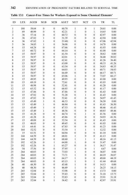
Table 13.1 Cancer-Free Times for Workers Exposed to Some Chemical Elements�
ID LEX AGEB M1B M2B AGET M1T M2T CS TR TL
1 180 58.64 0 0 60.70 1 0 1 24.61 0.002 69 40.99 0 0 42.21 1 0 1 14.65 0.003 36 57.14 0 0 60.72 0 0 0 42.97 0.004 36 47.82 1 0 51.39 0 0 0 42.94 0.004 36 47.82 1 0 53.40; 0 0 0 67.06 42.945 36 34.85 1 0 36.08 0 0 0 14.78 0.006 15 64.24 0 0 67.66 0 1 0 41.03 0.007 15 60.72 0 0 64.14 0 0 0 41.00 0.008 15 58.97 0 0 61.54 0 0 0 30.82 0.008 15 58.97 0 0 62.01 1 0 0 36.40 30.828 15 58.97 0 0 62.41 1 0 0 41.26 36.408 15 58.97 0 0 63.00 0 0 0 48.33 41.268 15 58.97 0 0 63.54 0 0 0 54.83 48.338 15 58.97 0 0 64.03 1 0 0 60.71 54.838 15 58.97 0 0 64.49 0 0 0 66.17 60.718 15 58.97 0 0 65.06 1 0 0 73.07 66.179 15 49.95 0 0 49.95 0 0 0 41.00 0.0010 15 69.19 0 0 72.61 0 0 0 41.03 0.0011 15 48.98 0 0 52.41 0 0 0 41.20 0.0012 15 65.52 0 0 68.95 0 0 0 41.17 0.0013 15 47.86 0 0 47.86 0 0 0 41.43 0.0014 15 47.82 0; 0 51.28 0 1 0 41.43 0.0014 15 47.82 0 0 52.41 0 0 0 54.97 41.4315 15 43.49 1 0 46.53 0 0 0 36.50 0.0015 15 43.49 1 0 46.94 0 0 0 41.43 36.5015 15 43.49 1 0 47.53 0 0 0 48.46 41.4315 15 43.49 1 0 48.56 0 0 0 60.85 48.4616 15 41.28 0 0 44.74 0 1 0 41.56 0.0016 15 41.28 0 0 45.86 0 0 0 54.93 41.5617 15 49.09 0 0 52.54 0 0 0 41.43 0.0018 15 46.03 0 0 49.45 0 0 0 41.03 0.0019 15 64.41 0 0 67.85 0 0 0 41.23 0.0020 164 52.52 0 0 53.54 1 1 1 12.32 0.0021 15 61.51 0 0 64.94 0 0 0 41.10 0.0022 144 64.59 0 0 68.01 1 0 0 41.13 0.0022 144 64.59 0 0 68.60 1 1 1 48.16 41.1323 192 62.26 0 1 64.88 1 0 0 31.47 0.0023 192 62.26 0 1 65.27 0 0 1 36.17 31.4724 54 57.56 0 0 57.95 1 0 1 4.67 0.0025 264 60.03 0 0 73.03 1 0 0 36.07 0.0025 264 60.03 0 0 73.71 1 0 0 44.19 36.0725 264 60.03 0 0 64.17 1 0 0 49.68 44.1925 264 60.03 0 0 65.15 1 0 1 61.44 49.6826 40 44.30 0 0 45.48 1 0 0 14.13 0.0026 40 44.30 0 0 46.49 1 0 1 26.25 14.1327 265 52.84 0 1 53.98 0 0 0 13.73 0.0027 265 52.84 0 1 55.43 0 0 0 31.18 13.7327 265 52.84 0 1 55.83 0 0 0 35.91 31.1827 265 52.84 0 1 56.42 0 0 1 42.97 35.91
342
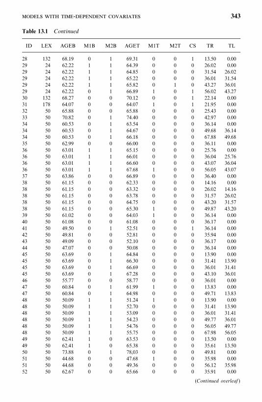
Table 13.1 Continued
ID LEX AGEB M1B M2B AGET M1T M2T CS TR TL
28 132 68.19 0 1 69.31 0 0 1 13.50 0.0029 24 62.22 1 1 64.39 0 0 0 26.02 0.0029 24 62.22 1 1 64.85 0 0 0 31.54 26.0229 24 62.22 1 1 65.22 0 0 0 36.01 31.5429 24 62.22 1 1 65.82 0 1 0 43.27 36.0129 24 62.22 0 1 66.89 1 0 1 56.02 43.2730 132 68.27 0 0 70.12 0 0 1 22.14 0.0031 178 64.07 0 0 64.07 1 0 1 21.95 0.0032 50 65.88 0 0 65.88 0 0 0 25.43 0.0033 50 70.82 0 1 74.40 0 0 0 42.97 0.0034 50 60.53 0 1 63.54 0 0 0 36.14 0.0034 50 60.53 0 1 64.67 0 0 0 49.68 36.1434 50 60.53 0 1 66.18 0 0 0 67.88 49.6835 50 62.99 0 0 66.00 0 0 0 36.11 0.0036 50 63.01 1 1 65.15 0 0 0 25.76 0.0036 50 63.01 1 1 66.01 0 0 0 36.04 25.7636 50 63.01 1 1 66.60 0 0 0 43.07 36.0436 50 63.01 1 1 67.68 1 0 0 56.05 43.0737 50 63.86 0 0 66.89 0 0 0 36.40 0.0038 50 61.15 0 0 62.33 0 0 0 14.16 0.0038 50 61.15 0 0 63.32 0 0 0 26.02 14.1638 50 61.15 0 0 63.78 0 0 0 31.57 26.0238 50 61.15 0 0 64.75 0 0 0 43.20 31.5738 50 61.15 0 0 65.30 1 0 0 49.87 43.2039 50 61.02 0 0 64.03 1 0 0 36.14 0.0040 50 61.08 0 0 61.08 0 0 0 36.17 0.0041 50 49.50 0 1 52.51 0 0 1 36.14 0.0042 50 49.81 0 0 52.81 0 0 0 35.94 0.0043 50 49.09 0 0 52.10 0 0 0 36.17 0.0044 50 47.07 0 0 50.08 0 0 0 36.14 0.0045 50 63.69 0 1 64.84 0 0 0 13.90 0.0045 50 63.69 0 1 66.30 0 0 0 31.41 13.9045 50 63.69 0 1 66.69 0 0 0 36.01 31.4145 50 63.69 0 1 67.28 0 0 0 43.10 36.0146 50 55.77 0 0 58.77 0 0 0 36.01 0.0047 50 60.84 0 1 61.99 1 0 0 13.83 0.0047 50 60.84 0 1 64.98 0 0 0 49.71 13.8348 50 50.09 1 1 51.24 1 0 0 13.90 0.0048 50 50.09 1 1 52.70 0 0 0 31.41 13.9048 50 50.09 1 1 53.09 0 0 0 36.01 31.4148 50 50.09 1 1 54.23 0 0 0 49.77 36.0148 50 50.09 1 1 54.76 0 0 0 56.05 49.7748 50 50.09 1 1 55.75 0 0 0 67.98 56.0549 50 62.41 1 0 63.53 0 0 0 13.50 0.0049 50 62.41 1 0 65.38 0 0 0 35.61 13.5050 50 73.88 0 1 78,03 0 0 0 49.81 0.0051 50 44.68 0 0 47.68 1 0 0 35.98 0.0051 50 44.68 0 0 49.36 0 0 0 56.12 35.9852 50 62.67 0 0 65.66 0 0 0 35.91 0.00
(Continued overleaf )
- 343
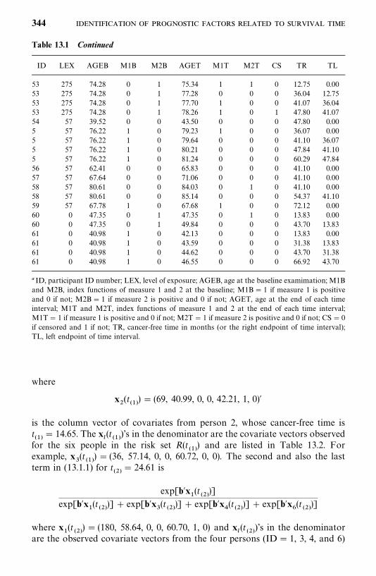
Table 13.1 Continued
ID LEX AGEB M1B M2B AGET M1T M2T CS TR TL
53 275 74.28 0 1 75.34 1 1 0 12.75 0.0053 275 74.28 0 1 77.28 0 0 0 36.04 12.7553 275 74.28 0 1 77.70 1 0 0 41.07 36.0453 275 74.28 0 1 78.26 1 0 1 47.80 41.0754 57 39.52 0 0 43.50 0 0 0 47.80 0.005 57 76.22 1 0 79.23 1 0 0 36.07 0.005 57 76.22 1 0 79.64 0 0 0 41.10 36.075 57 76.22 1 0 80.21 0 0 0 47.84 41.105 57 76.22 1 0 81.24 0 0 0 60.29 47.8456 57 62.41 0 0 65.83 0 0 0 41.10 0.0057 57 67.64 0 0 71.06 0 0 0 41.10 0.0058 57 80.61 0 0 84.03 0 1 0 41.10 0.0058 57 80.61 0 0 85.14 0 0 0 54.37 41.1059 57 67.78 1 0 67.68 1 0 0 72.12 0.0060 0 47.35 0 1 47.35 0 1 0 13.83 0.0060 0 47.35 0 1 49.84 0 0 0 43.70 13.8361 0 40.98 1 0 42.13 0 0 0 13.83 0.0061 0 40.98 1 0 43.59 0 0 0 31.38 13.8361 0 40.98 1 0 44.62 0 0 0 43.70 31.3861 0 40.98 1 0 46.55 0 0 0 66.92 43.70
� ID, participant ID number; LEX, level of exposure; AGEB, age at the baseline examimation; M1Band M2B, index functions of measure 1 and 2 at the baseline; M1B� 1 if measure 1 is positiveand 0 if not; M2B� 1 if measure 2 is positive and 0 if not; AGET, age at the end of each timeinterval; M1T and M2T, index functions of measure 1 and 2 at the end of each time interval;M1T� 1 if measure 1 is positive and 0 if not; M2T� 1 if measure 2 is positive and 0 if not; CS� 0if censored and 1 if not; TR, cancer-free time in months (or the right endpoint of time interval);TL, left endpoint of time interval.
where
x�(t
���) � (69, 40.99, 0, 0, 42.21, 1, 0)�
is the column vector of covariates from person 2, whose cancer-free time ist���
� 14.65. The x�(t���
)’s in the denominator are the covariate vectors observedfor the six people in the risk set R(t
���) and are listed in Table 13.2. For
example, x(t���) � (36, 57.14, 0, 0, 60.72, 0, 0). The second and also the last
term in (13.1.1) for t���
� 24.61 is
exp[b�x�(t
���)]
exp[b�x�(t���)] exp[b�x
(t
���)] exp[b�x
�(t���)] exp[b�x
�(t
���)]
where x�(t
���) � (180, 58.64, 0, 0, 60.70, 1, 0) and x
�(t���
)’s in the denominatorare the observed covariate vectors from the four persons (ID� 1, 3, 4, and 6)
344
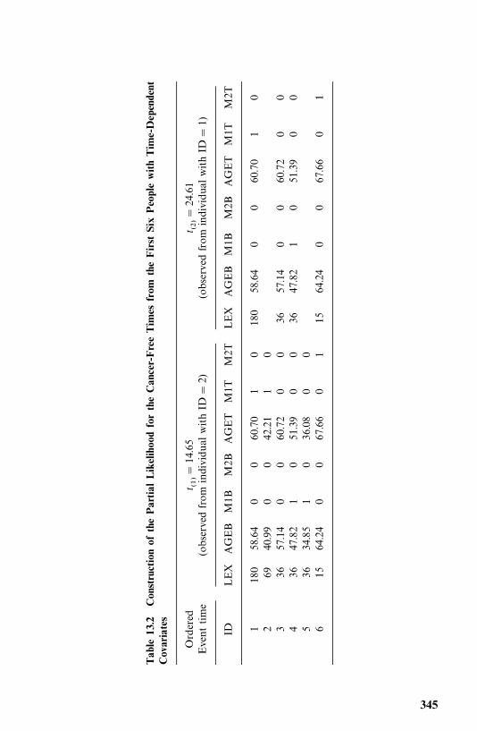
Table13.2
ConstructionofthePartialLikelihoodfortheCancer-FreeTimesfrom
theFirstSixPeoplewithTime-Dependent
Covariates
Ordered
t ����
14.65
t ����
24.61
Eventtime
(observed
from
individualwithID
�2)
(observedfrom
individualwithID
�1)
IDLEX
AGEB
M1B
M2B
AGET
M1T
M2T
LEX
AGEB
M1B
M2B
AGET
M1T
M2T
1180
58.64
00
60.70
10
180
58.64
00
60.70
10
269
40.99
00
42.21
10
336
57.14
00
60.72
00
3657.14
00
60.72
00
436
47.82
10
51.39
00
3647.82
10
51.39
00
536
34.85
10
36.08
00
615
64.24
00
67.66
01
1564.24
00
67.66
01
345
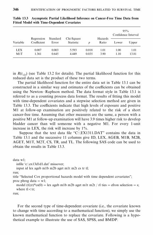
Table 13.3 Asymptotic Partial Likelihood Inference on Cancer-Free Time Data fromFitted Model with Time-Dependent Covariates
95%Confidence Interval
Regression Standard Chi-Square HazardsVariable Coefficient Error Statistic p Ratio Lower Upper
LEX 0.007 0.003 5.593 0.018 1.01 1.00 1.01M1T 1.361 0.645 4.449 0.035 3.90 1.10 13.81
in R(t���) (see Table 13.2 for details). The partial likelihood function for this
reduced data set is the product of these two terms.The partial likelihood function for the entire data set in Table 13.1 can be
constructed in a similar way and estimates of the coefficients can be obtainedusing the Newton—Raphson method. The data format style in Table 13.1 isreferred to as a counting process data format. The results of fitting this modelwith time-dependent covariates and a stepwise selection method are given inTable 13.3. The coefficients indicate that high levels of exposure and positiveM1 at follow-up examination are positively related to the risk of a shortcancer-free time. Assuming that other measures are the same, a person with apositive M1 at follow-up examination will have 3.9 times higher risk to developbladder cancer than will someone with a negative M1. For every 1-unitincrease in LEX, the risk will increase by 1%.
Suppose that the text data file ‘‘C:�EX1311.DAT’’ contains the data inTable 13.1 and the successive 11 columns give ID, LEX, AGEB, M1B, M2B,AGET, M1T, M2T, CS, TR, and TL. The following SAS code can be used toobtain the results in Table 13.3.
data w1;infile ‘c:�ex13d1d1.dat’ missover;input id lex ageb m1b m2b aget m1t m2t cs tr tl;
run;title ‘‘Selected Cox proportional hazards model with time dependent covariates’’;proc phreg data�w1;model (tl,tr)*cs(0) � lex ageb m1b m2b aget m1t m2t / rl ties� efron selection� s;where tl�tr;
run;
For the second type of time-dependent covariate (i.e., the covariate knownto change with time according to a mathematical function), we simply use theknown mathematical function to replace the covariate. Following is a hypo-thetical example to illustrate the use of SAS, SPSS, and BMDP.
346
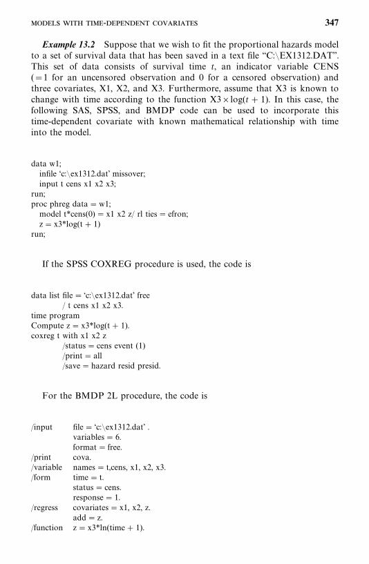
Example 13.2 Suppose that we wish to fit the proportional hazards modelto a set of survival data that has been saved in a text file ‘‘C:�EX1312.DAT’’.This set of data consists of survival time t, an indicator variable CENS(�1 for an uncensored observation and 0 for a censored observation) andthree covariates, X1, X2, and X3. Furthermore, assume that X3 is known tochange with time according to the function X3�log(t 1). In this case, thefollowing SAS, SPSS, and BMDP code can be used to incorporate thistime-dependent covariate with known mathematical relationship with timeinto the model.
data w1;infile ‘c:�ex1312.dat’ missover;input t cens x1 x2 x3;
run;proc phreg data�w1;model t*cens(0) � x1 x2 z/ rl ties� efron;z� x3*log(t 1)
run;
If the SPSS COXREG procedure is used, the code is
data list file� ‘c:�ex1312.dat’ free/ t cens x1 x2 x3.
time programCompute z� x3*log(t 1).coxreg t with x1 x2 z
/status� cens event (1)/print� all/save�hazard resid presid.
For the BMDP 2L procedure, the code is
/input file� ‘c:�ex1312.dat’ .variables� 6.format� free.
/print cova./variable names� t,cens, x1, x2, x3./form time� t.
status� cens.response� 1.
/regress covariates� x1, x2, z.add� z.
/function z� x3*ln(time 1).
- 347
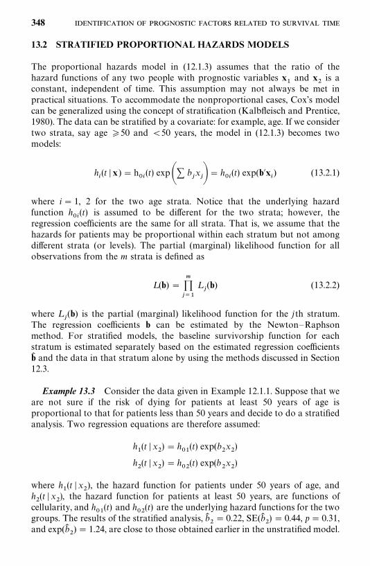
13.2 STRATIFIED PROPORTIONAL HAZARDS MODELS
The proportional hazards model in (12.1.3) assumes that the ratio of thehazard functions of any two people with prognostic variables x
�and x
�is a
constant, independent of time. This assumption may not always be met inpractical situations. To accommodate the nonproportional cases, Cox’s modelcan be generalized using the concept of stratification (Kalbfleisch and Prentice,1980). The data can be stratified by a covariate: for example, age. If we considertwo strata, say age �50 and �50 years, the model in (12.1.3) becomes twomodels:
h�(t � x) �h
��(t) exp�� b
�x��� h
��(t) exp(b�x
�) (13.2.1)
where i� 1, 2 for the two age strata. Notice that the underlying hazardfunction h
��(t) is assumed to be different for the two strata; however, the
regression coefficients are the same for all strata. That is, we assume that thehazards for patients may be proportional within each stratum but not amongdifferent strata (or levels). The partial (marginal) likelihood function for allobservations from the m strata is defined as
L (b) ������
L�(b) (13.2.2)
where L�(b) is the partial (marginal) likelihood function for the jth stratum.
The regression coefficients b can be estimated by the Newton—Raphsonmethod. For stratified models, the baseline survivorship function for eachstratum is estimated separately based on the estimated regression coefficientsb� and the data in that stratum alone by using the methods discussed in Section12.3.
Example 13.3 Consider the data given in Example 12.1.1. Suppose that weare not sure if the risk of dying for patients at least 50 years of age isproportional to that for patients less than 50 years and decide to do a stratifiedanalysis. Two regression equations are therefore assumed:
h�(t �x
�) � h
��(t) exp(b
�x�)
h�(t �x
�) � h
��(t) exp(b
�x�)
where h�(t � x
�), the hazard function for patients under 50 years of age, and
h�(t �x
�), the hazard function for patients at least 50 years, are functions of
cellularity, and h��(t) and h
��(t) are the underlying hazard functions for the two
groups. The results of the stratified analysis, b��� 0.22, SE(b�
�) � 0.44, p� 0.31,
and exp(b��) � 1.24, are close to those obtained earlier in the unstratified model.
348
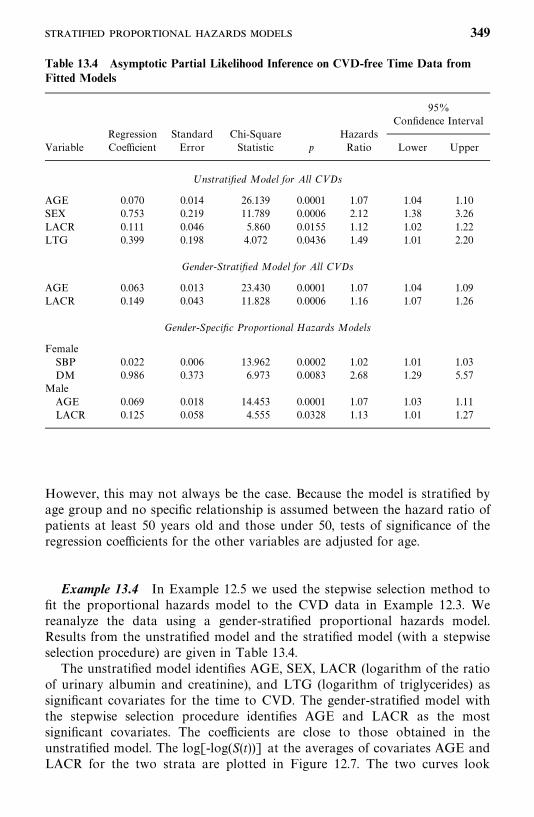
Table 13.4 Asymptotic Partial Likelihood Inference on CVD-free Time Data fromFitted Models
95%Confidence Interval
Regression Standard Chi-Square HazardsVariable Coefficient Error Statistic p Ratio Lower Upper
Unstratified Model for All CVDs
AGE 0.070 0.014 26.139 0.0001 1.07 1.04 1.10SEX 0.753 0.219 11.789 0.0006 2.12 1.38 3.26LACR 0.111 0.046 5.860 0.0155 1.12 1.02 1.22LTG 0.399 0.198 4.072 0.0436 1.49 1.01 2.20
Gender-Stratified Model for All CVDs
AGE 0.063 0.013 23.430 0.0001 1.07 1.04 1.09LACR 0.149 0.043 11.828 0.0006 1.16 1.07 1.26
Gender-Specific Proportional Hazards Models
FemaleSBP 0.022 0.006 13.962 0.0002 1.02 1.01 1.03DM 0.986 0.373 6.973 0.0083 2.68 1.29 5.57
MaleAGE 0.069 0.018 14.453 0.0001 1.07 1.03 1.11LACR 0.125 0.058 4.555 0.0328 1.13 1.01 1.27
However, this may not always be the case. Because the model is stratified byage group and no specific relationship is assumed between the hazard ratio ofpatients at least 50 years old and those under 50, tests of significance of theregression coefficients for the other variables are adjusted for age.
Example 13.4 In Example 12.5 we used the stepwise selection method tofit the proportional hazards model to the CVD data in Example 12.3. Wereanalyze the data using a gender-stratified proportional hazards model.Results from the unstratified model and the stratified model (with a stepwiseselection procedure) are given in Table 13.4.
The unstratified model identifies AGE, SEX, LACR (logarithm of the ratioof urinary albumin and creatinine), and LTG (logarithm of triglycerides) assignificant covariates for the time to CVD. The gender-stratified model withthe stepwise selection procedure identifies AGE and LACR as the mostsignificant covariates. The coefficients are close to those obtained in theunstratified model. The log[-log(S(t))] at the averages of covariates AGE andLACR for the two strata are plotted in Figure 12.7. The two curves look
349
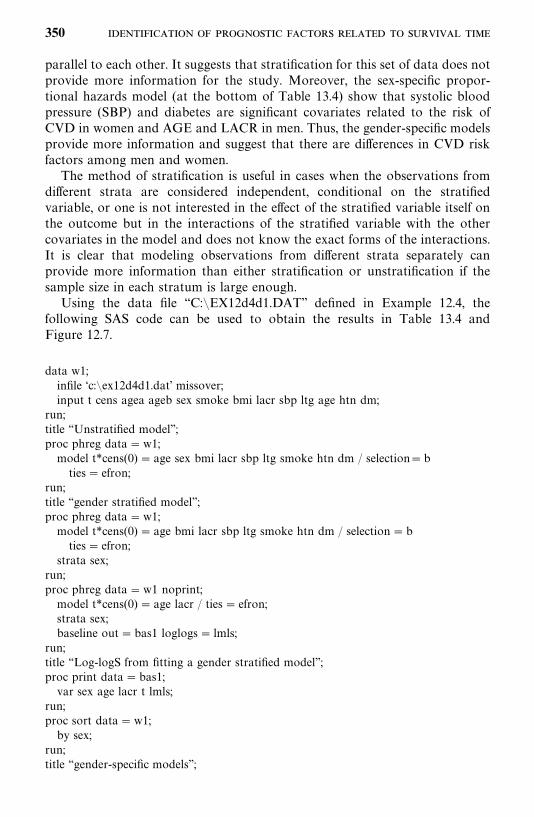
parallel to each other. It suggests that stratification for this set of data does notprovide more information for the study. Moreover, the sex-specific propor-tional hazards model (at the bottom of Table 13.4) show that systolic bloodpressure (SBP) and diabetes are significant covariates related to the risk ofCVD in women and AGE and LACR in men. Thus, the gender-specific modelsprovide more information and suggest that there are differences in CVD riskfactors among men and women.
The method of stratification is useful in cases when the observations fromdifferent strata are considered independent, conditional on the stratifiedvariable, or one is not interested in the effect of the stratified variable itself onthe outcome but in the interactions of the stratified variable with the othercovariates in the model and does not know the exact forms of the interactions.It is clear that modeling observations from different strata separately canprovide more information than either stratification or unstratification if thesample size in each stratum is large enough.
Using the data file ‘‘C:�EX12d4d1.DAT’’ defined in Example 12.4, thefollowing SAS code can be used to obtain the results in Table 13.4 andFigure 12.7.
data w1;infile ‘c:�ex12d4d1.dat’ missover;input t cens agea ageb sex smoke bmi lacr sbp ltg age htn dm;
run;title ‘‘Unstratified model’’;proc phreg data�w1;model t*cens(0) � age sex bmi lacr sbp ltg smoke htn dm / selection�bties� efron;
run;title ‘‘gender stratified model’’;proc phreg data�w1;model t*cens(0) � age bmi lacr sbp ltg smoke htn dm / selection�bties� efron;
strata sex;run;proc phreg data�w1 noprint;model t*cens(0) � age lacr / ties� efron;strata sex;baseline out�bas1 loglogs� lmls;
run;title ‘‘Log-logS from fitting a gender stratified model’’;proc print data�bas1;var sex age lacr t lmls;
run;proc sort data�w1;by sex;
run;title ‘‘gender-specific models’’;
350
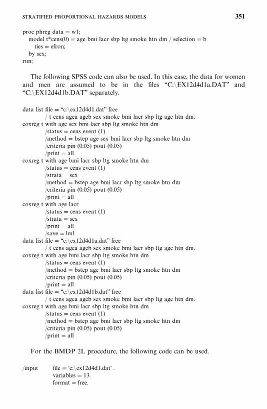
proc phreg data�w1;model t*cens(0) � age bmi lacr sbp ltg smoke htn dm / selection�bties� efron;
by sex;run;
The following SPSS code can also be used. In this case, the data for womenand men are assumed to be in the files ‘‘C:�EX12d4d1a.DAT’’ and‘‘C:�EX12d4d1b.DAT’’ separately.
data list file� ‘‘c:�ex12d4d1.dat’’ free/ t cens agea ageb sex smoke bmi lacr sbp ltg age htn dm.
coxreg t with age sex bmi lacr sbp ltg smoke htn dm/status� cens event (1)/method�bstep age sex bmi lacr sbp ltg smoke htn dm/criteria pin (0.05) pout (0.05)/print� all
coxreg t with age bmi lacr sbp ltg smoke htn dm/status� cens event (1)/strata� sex/method�bstep age bmi lacr sbp ltg smoke htn dm/criteria pin (0.05) pout (0.05)/print� all
coxreg t with age lacr/status� cens event (1)/strata� sex/print� all/save� lml.
data list file� ‘‘c:�ex12d4d1a.dat’’ free/ t cens agea ageb sex smoke bmi lacr sbp ltg age htn dm.
coxreg t with age bmi lacr sbp ltg smoke htn dm/status� cens event (1)/method�bstep age bmi lacr sbp ltg smoke htn dm/criteria pin (0.05) pout (0.05)/print� all
data list file� ‘‘c:�ex12d4d1b.dat’’ free/ t cens agea ageb sex smoke bmi lacr sbp ltg age htn dm.
coxreg t with age bmi lacr sbp ltg smoke htn dm/status� cens event (1)/method�bstep age bmi lacr sbp ltg smoke htn dm/criteria pin (0.05) pout (0.05)/print� all
For the BMDP 2L procedure, the following code can be used.
/input file� ‘c:�ex12d4d1.dat’ .variables� 13.format� free.
351
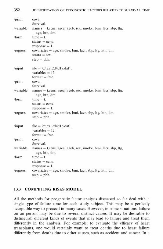
/print cova.Survival.
/variable names� t,cens, agea, ageb, sex, smoke, bmi, lacr, sbp, ltg,age, htn, dm.
/form time� t.status� cens.response� 1.
/regress covariates� age, smoke, bmi, lacr, sbp, ltg, htn, dm.strata� sex.step� phh.
/input file� ‘c:�ex12d4d1a.dat’ .variables� 13.format� free.
/print cova.Survival.
/variable names� t,cens, agea, ageb, sex, smoke, bmi, lacr, sbp, ltg,age, htn, dm.
/form time� t.status� cens.response� 1.
/regress covariates� age, smoke, bmi, lacr, sbp, ltg, htn, dm.step� phh.
/input file� ‘c:�ex12d4d1b.dat’ .variables� 13.format� free.
/print cova.Survival.
/variable names� t,cens, agea, ageb, sex, smoke, bmi, lacr, sbp, ltg,age, htn, dm.
/form time� t.status� cens.response� 1.
/regress covariates� age, smoke, bmi, lacr, sbp, ltg, htn, dm.step� phh.
13.3 COMPETING RISKS MODEL
All the methods for prognostic factor analysis discussed so far deal with asingle type of failure time for each study subject. This may be a perfectlyacceptable way to proceed in many cases. However, in some situations, failureon an person may be due to several distinct causes. It may be desirable todistinguish different kinds of events that may lead to failure and treat themdifferently in the analysis. For example, to evaluate the efficacy of hearttransplants, one would certainly want to treat deaths due to heart failuredifferently from deaths due to other causes, such as accident and cancer. In a
352
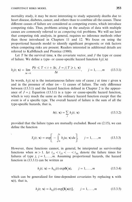
mortality study, it may be more interesting to study separately deaths due toheart disease, diabetes, cancer, and others than to combine all the causes. Thesedifferent causes of failure are considered as competing events, which introducecompeting risks. Thus, problems arising in the analysis of data with multiplecauses are commonly referred to as competing risk problems. We will see laterthat competing risk analysis, in general, requires no inference methods otherthan those introduced in Chapters 11 and 12. We focus on using theproportional hazards model to identify significant prognostic or risk factorswhen competing risks are present. Readers interested in additional details arereferred to Kalbfleisch and Prentice (1980).
Let T be the survival time, x the covariate vector, and J the type or causeof failure. We define a type- or cause-specific hazard function h
�(t; x)
h�(t; x) � lim
���
P(t T � tt, J� j �T � t, x)t
, j� 1, . . . ,m (13.3.1)
In words, h�(t; x) is the instantaneous failure rate of cause j at time t given x
and in the presence of other (m 1) causes of failure. The only differencebetween (13.3.1) and the hazard function defined in Chapter 2 is the appear-ance of J� j. Equation (13.3.1) is a type- or cause-specific hazard function,which is very much the same as the ordinary hazard function except that theevent is of a specific type. The overall hazard of failure is the sum of all thetype-specific hazards, that is,
h(t; x) ���
h�(t; x) (13.3.2)
provided that the failure types are mutually excluded. Based on (2.15), we candefine the function
.S�(t; x)� exp� �
�
�
h�(u; x) du�, j� 1, . . . , m (13.3.3)
However, these functions cannot, in general, be interpreted as survivorshipfunctions when m� 1. Let t
��� t
����� t
���denote the failure times for
failures of type j, j� 1, . . . , m. Assuming proportional hazards, the hazardfunction in (13.3.1) can be written as
h�(t; x)� h
��(t) exp(b�
�x), j� 1, . . . ,m (13.3.4)
which can be generalized for time-dependent covariates by replacing x withx(t), that is,
h�(t; x) � h
��(t) exp[b�
�x(t)], j� 1, . . . ,m (13.3.5)
353
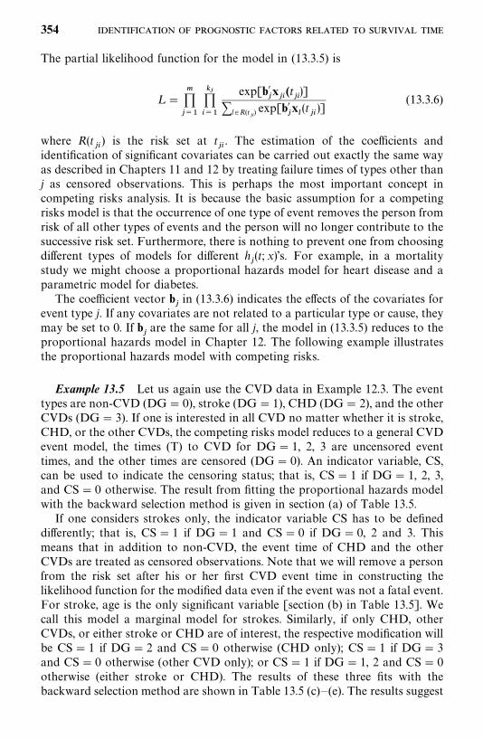
The partial likelihood function for the model in (13.3.5) is
L ������
���
���
exp[b��x��(t
��)]
�l �R(t��) exp[b��x�
(t��)]
(13.3.6)
where R(t��
) is the risk set at t��. The estimation of the coefficients and
identification of significant covariates can be carried out exactly the same wayas described in Chapters 11 and 12 by treating failure times of types other thanj as censored observations. This is perhaps the most important concept incompeting risks analysis. It is because the basic assumption for a competingrisks model is that the occurrence of one type of event removes the person fromrisk of all other types of events and the person will no longer contribute to thesuccessive risk set. Furthermore, there is nothing to prevent one from choosingdifferent types of models for different h
�(t; x)’s. For example, in a mortality
study we might choose a proportional hazards model for heart disease and aparametric model for diabetes.
The coefficient vector b�in (13.3.6) indicates the effects of the covariates for
event type j. If any covariates are not related to a particular type or cause, theymay be set to 0. If b
�are the same for all j, the model in (13.3.5) reduces to the
proportional hazards model in Chapter 12. The following example illustratesthe proportional hazards model with competing risks.
Example 13.5 Let us again use the CVD data in Example 12.3. The eventtypes are non-CVD (DG� 0), stroke (DG� 1), CHD (DG� 2), and the otherCVDs (DG� 3). If one is interested in all CVD no matter whether it is stroke,CHD, or the other CVDs, the competing risks model reduces to a general CVDevent model, the times (T) to CVD for DG� 1, 2, 3 are uncensored eventtimes, and the other times are censored (DG� 0). An indicator variable, CS,can be used to indicate the censoring status; that is, CS� 1 if DG� 1, 2, 3,and CS� 0 otherwise. The result from fitting the proportional hazards modelwith the backward selection method is given in section (a) of Table 13.5.
If one considers strokes only, the indicator variable CS has to be defineddifferently; that is, CS� 1 if DG� 1 and CS� 0 if DG� 0, 2 and 3. Thismeans that in addition to non-CVD, the event time of CHD and the otherCVDs are treated as censored observations. Note that we will remove a personfrom the risk set after his or her first CVD event time in constructing thelikelihood function for the modified data even if the event was not a fatal event.For stroke, age is the only significant variable [section (b) in Table 13.5]. Wecall this model a marginal model for strokes. Similarly, if only CHD, otherCVDs, or either stroke or CHD are of interest, the respective modification willbe CS� 1 if DG� 2 and CS� 0 otherwise (CHD only); CS� 1 if DG� 3and CS� 0 otherwise (other CVD only); or CS� 1 if DG� 1, 2 and CS� 0otherwise (either stroke or CHD). The results of these three fits with thebackward selection method are shown in Table 13.5 (c)—(e). The results suggest
354
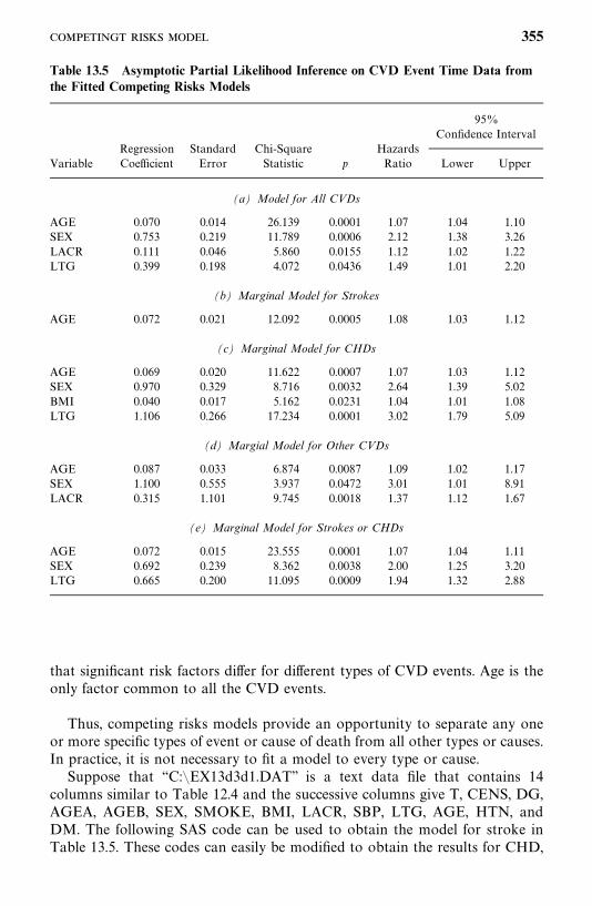
Table 13.5 Asymptotic Partial Likelihood Inference on CVD Event Time Data fromthe Fitted Competing Risks Models
95%Confidence Interval
Regression Standard Chi-Square HazardsVariable Coefficient Error Statistic p Ratio Lower Upper
(a) Model for All CVDs
AGE 0.070 0.014 26.139 0.0001 1.07 1.04 1.10SEX 0.753 0.219 11.789 0.0006 2.12 1.38 3.26LACR 0.111 0.046 5.860 0.0155 1.12 1.02 1.22LTG 0.399 0.198 4.072 0.0436 1.49 1.01 2.20
(b) Marginal Model for Strokes
AGE 0.072 0.021 12.092 0.0005 1.08 1.03 1.12
(c) Marginal Model for CHDs
AGE 0.069 0.020 11.622 0.0007 1.07 1.03 1.12SEX 0.970 0.329 8.716 0.0032 2.64 1.39 5.02BMI 0.040 0.017 5.162 0.0231 1.04 1.01 1.08LTG 1.106 0.266 17.234 0.0001 3.02 1.79 5.09
(d) Margial Model for Other CVDs
AGE 0.087 0.033 6.874 0.0087 1.09 1.02 1.17SEX 1.100 0.555 3.937 0.0472 3.01 1.01 8.91LACR 0.315 1.101 9.745 0.0018 1.37 1.12 1.67
(e) Marginal Model for Strokes or CHDs
AGE 0.072 0.015 23.555 0.0001 1.07 1.04 1.11SEX 0.692 0.239 8.362 0.0038 2.00 1.25 3.20LTG 0.665 0.200 11.095 0.0009 1.94 1.32 2.88
that significant risk factors differ for different types of CVD events. Age is theonly factor common to all the CVD events.
Thus, competing risks models provide an opportunity to separate any oneor more specific types of event or cause of death from all other types or causes.In practice, it is not necessary to fit a model to every type or cause.
Suppose that ‘‘C:�EX13d3d1.DAT’’ is a text data file that contains 14columns similar to Table 12.4 and the successive columns give T, CENS, DG,AGEA, AGEB, SEX, SMOKE, BMI, LACR, SBP, LTG, AGE, HTN, andDM. The following SAS code can be used to obtain the model for stroke inTable 13.5. These codes can easily be modified to obtain the results for CHD,
355
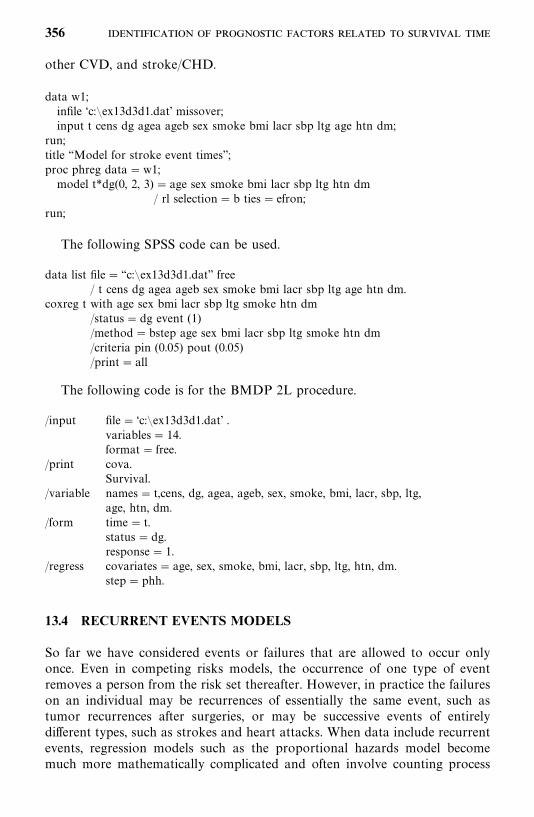
other CVD, and stroke/CHD.
data w1;infile ‘c:�ex13d3d1.dat’ missover;input t cens dg agea ageb sex smoke bmi lacr sbp ltg age htn dm;
run;title ‘‘Model for stroke event times’’;proc phreg data�w1;model t*dg(0, 2, 3) � age sex smoke bmi lacr sbp ltg htn dm
/ rl selection�b ties� efron;run;
The following SPSS code can be used.
data list file� ‘‘c:�ex13d3d1.dat’’ free/ t cens dg agea ageb sex smoke bmi lacr sbp ltg age htn dm.
coxreg t with age sex bmi lacr sbp ltg smoke htn dm/status�dg event (1)/method�bstep age sex bmi lacr sbp ltg smoke htn dm/criteria pin (0.05) pout (0.05)/print� all
The following code is for the BMDP 2L procedure.
/input file� ‘c:�ex13d3d1.dat’ .variables� 14.format� free.
/print cova.Survival.
/variable names� t,cens, dg, agea, ageb, sex, smoke, bmi, lacr, sbp, ltg,age, htn, dm.
/form time� t.status�dg.response� 1.
/regress covariates� age, sex, smoke, bmi, lacr, sbp, ltg, htn, dm.step� phh.
13.4 RECURRENT EVENTS MODELS
So far we have considered events or failures that are allowed to occur onlyonce. Even in competing risks models, the occurrence of one type of eventremoves a person from the risk set thereafter. However, in practice the failureson an individual may be recurrences of essentially the same event, such astumor recurrences after surgeries, or may be successive events of entirelydifferent types, such as strokes and heart attacks. When data include recurrentevents, regression models such as the proportional hazards model becomemuch more mathematically complicated and often involve counting process
356
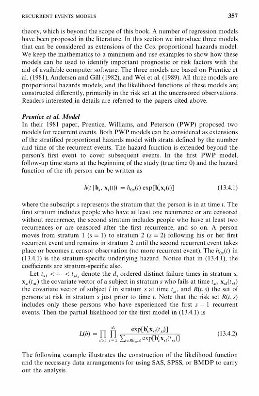
theory, which is beyond the scope of this book. A number of regression modelshave been proposed in the literature. In this section we introduce three modelsthat can be considered as extensions of the Cox proportional hazards model.We keep the mathematics to a minimum and use examples to show how thesemodels can be used to identify important prognostic or risk factors with theaid of available computer software. The three models are based on Prentice etal. (1981), Andersen and Gill (1982), and Wei et al. (1989). All three models areproportional hazards models, and the likelihood functions of these models areconstructed differently, primarily in the risk set at the uncensored observations.Readers interested in details are referred to the papers cited above.
Prentice et al. ModelIn their 1981 paper, Prentice, Williams, and Peterson (PWP) proposed twomodels for recurrent events. Both PWP models can be considered as extensionsof the stratified proportional hazards model with strata defined by the numberand time of the recurrent events. The hazard function is extended beyond theperson’s first event to cover subsequent events. In the first PWP model,follow-up time starts at the beginning of the study (true time 0) and the hazardfunction of the ith person can be written as
h(t � b, x
�(t)) � h
�(t) exp[b�
x�(t)] (13.4.1)
where the subscript s represents the stratum that the person is in at time t. Thefirst stratum includes people who have at least one recurrence or are censoredwithout recurrence, the second stratum includes people who have at least tworecurrences or are censored after the first recurrence, and so on. A personmoves from stratum 1 (s� 1) to stratum 2 (s� 2) following his or her firstrecurrent event and remains in stratum 2 until the second recurrent event takesplace or becomes a censor observation (no more recurrent event). The h
�(t) in
(13.4.1) is the stratum-specific underlying hazard. Notice that in (13.4.1), thecoefficients are stratum-specific also.
Let t�
��� t��
denote the dordered distinct failure times in stratum s,
x�(t�
) the covariate vector of a subject in stratum s who fails at time t�, x
�(t�
)the covariate vector of subject l in stratum s at time t
�, and R(t, s) the set of
persons at risk in stratum s just prior to time t. Note that the risk set R(t, s)includes only those persons who have experienced the first s 1 recurrentevents. Then the partial likelihood for the first model in (13.4.1) is
L (b) � �s�1
�����
exp[b�x�(t
�)]
�l �R(t�,s) exp[b�
x�(t�)]
(13.4.2)
The following example illustrates the construction of the likelihood functionand the necessary data arrangements for using SAS, SPSS, or BMDP to carryout the analysis.
357
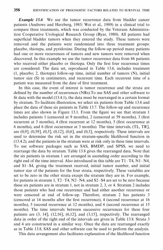
Example 13.6 We use the tumor recurrence data from bladder cancerpatients (Andrews and Herzberg, 1985; Wei et al., 1989) in a clinical trial tocompare three treatments, which was conducted by the Veterans Administra-tion Cooperative Urological Research Group (Byar, 1980). All patients hadsuperficial bladder tumors when they entered the study. These tumors wereremoved and the patients were randomized into three treatment groups:placebo, thiotepa, and pyridoxine. During the follow-up period many patientshad one or more recurrences of tumors and new tumors were removed whendiscovered. In this example we use the tumor recurrence data from 86 patientswho received either placebo or thiotepa. Only the first four recurrence timesare considered. The data set, reproduced in Table 13.6, includes treatment(1, placebo; 2, thiotepa) follow-up time, initial number of tumors (N), initialtumor size (S) in centimeters, and recurrent time. Each recurrent time of apatient was measured from the date of first treatment.
In this case, the event of interest is tumor recurrence and the strata aredefined by the number of recurrences (NRs).To use SAS and other software tofit data with the model (13.4.1), the data must be rearranged in a certain formatby stratum. To facilitate illustration, we select six patients from Table 13.6 andplace the data of these six patients in Table 13.7. The follow-up and recurrencetimes are also shown in Figure 13.1. From the figure we see that stratum 1includes patients 1 (censored at 9 months), 2 (censored at 59 months), 3 (firstrecurrent at 3 months), 4 (first recurrent at 12 months), 5 (first occurrence at6 months), and 6 (first occurrence at 3 months). The time intervals, (TL, TR],are (0,9], (0,59], (0,3], (0,12], (0,6], and (0,3], respectively. These intervals areused to determine the risk set in the stratum-specific likelihood function in(13.4.2), and the patients in the stratum were at risk only in these time intervals.To use software packages such as SAS, BMDP, and SPSS, we need torearrange the data by stratum. Table 13.8 gives the rearranged data. Note thatthe six patients in stratum 1 are arranged in ascending order according to theright end of the time interval. Also introduced in this table are T1—T4, N1—N4,and S1—S4, giving the treatment received, initial tumor number, and initialtumor size of the patients for the four strata, respectively. These variables areset to be zero in the other strata except the stratum they are in. For example,for patients in stratum 1, T2—T4, N2—N4, and S2—S4 are set to be zero becausethese six patients are in stratum 1, not in stratum 2, 3, or 4. Stratum 2 includesthose patients who had one recurrence and had either another recurrence orwere censored at end of follow-up. Therefore, stratum 2 has patients 3(censored at 14 months after the first recurrence), 4 (second recurrence at 16months), 5 (second recurrence at 12 months), and 6 (second recurrence at 15months). The time intervals between successive recurrences for these fourpatients are (3, 14], (12,16], (6,12], and (3,15], respectively. The rearrangeddata in order of the right end of the intervals are given in Table 13.8. Strata 3and 4 are constructed in a similar way. Once the data are rearranged exactlyas in Table 13.8, SAS and other software can be used to perform the analysis.
This data arrangement also facilitates explanation of the likelihood function
358
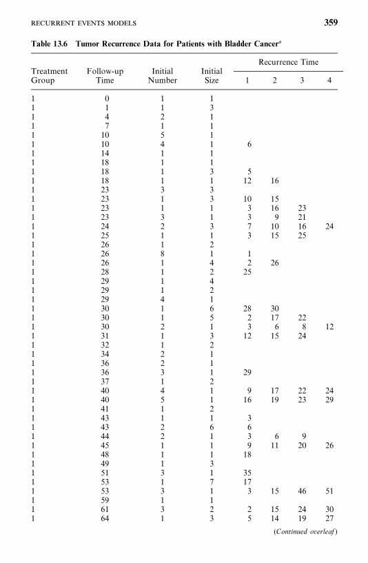
Table 13.6 Tumor Recurrence Data for Patients with Bladder Cancer�
Recurrence TimeTreatment Follow-up Initial InitialGroup Time Number Size 1 2 3 4
1 0 1 11 1 1 31 4 2 11 7 1 11 10 5 11 10 4 1 61 14 1 11 18 1 11 18 1 3 51 18 1 1 12 161 23 3 31 23 1 3 10 151 23 1 1 3 16 231 23 3 1 3 9 211 24 2 3 7 10 16 241 25 1 1 3 15 251 26 1 21 26 8 1 11 26 1 4 2 261 28 1 2 251 29 1 41 29 1 21 29 4 11 30 1 6 28 301 30 1 5 2 17 221 30 2 1 3 6 8 121 31 1 3 12 15 241 32 1 21 34 2 11 36 2 11 36 3 1 291 37 1 21 40 4 1 9 17 22 241 40 5 1 16 19 23 291 41 1 21 43 1 1 31 43 2 6 61 44 2 1 3 6 91 45 1 1 9 11 20 261 48 1 1 181 49 1 31 51 3 1 351 53 1 7 171 53 3 1 3 15 46 511 59 1 11 61 3 2 2 15 24 301 64 1 3 5 14 19 27
(Continued overleaf )
359
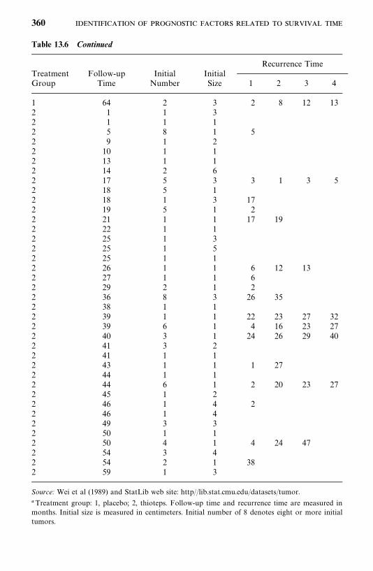
Table 13.6 Continued
Recurrence TimeTreatment Follow-up Initial InitialGroup Time Number Size 1 2 3 4
1 64 2 3 2 8 12 132 1 1 32 1 1 12 5 8 1 52 9 1 22 10 1 12 13 1 12 14 2 62 17 5 3 3 1 3 52 18 5 12 18 1 3 172 19 5 1 22 21 1 1 17 192 22 1 12 25 1 32 25 1 52 25 1 12 26 1 1 6 12 132 27 1 1 62 29 2 1 22 36 8 3 26 352 38 1 12 39 1 1 22 23 27 322 39 6 1 4 16 23 272 40 3 1 24 26 29 402 41 3 22 41 1 12 43 1 1 1 272 44 1 12 44 6 1 2 20 23 272 45 1 22 46 1 4 22 46 1 42 49 3 32 50 1 12 50 4 1 4 24 472 54 3 42 54 2 1 382 59 1 3
Source: Wei et al (1989) and StatLib web site: http//lib.stat.cmu.edu/datasets/tumor.
�Treatment group: 1, placebo; 2, thioteps. Follow-up time and recurrence time are measured inmonths. Initial size is measured in centimeters. Initial number of 8 denotes eight or more initialtumors.
360
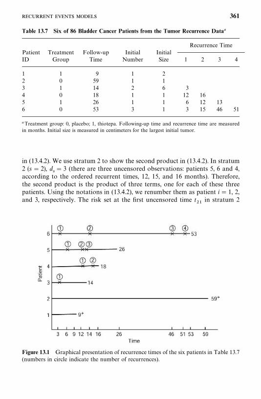
Figure 13.1 Graphical presentation of recurrence times of the six patients in Table 13.7(numbers in circle indicate the number of recurrences).
Table 13.7 Six of 86 Bladder Cancer Patients from the Tumor Recurrence Data�
Recurrence TimePatient Treatment Follow-up Initial InitialID Group Time Number Size 1 2 3 4
1 1 9 1 22 0 59 1 13 1 14 2 6 34 0 18 1 1 12 165 1 26 1 1 6 12 136 0 53 3 1 3 15 46 51
�Treatment group: 0, placebo; 1, thiotepa. Following-up time and recurrence time are measuredin months. Initial size is measured in centimeters for the largest initial tumor.
in (13.4.2). We use stratum 2 to show the second product in (13.4.2). In stratum2 (s� 2), d
� 3 (there are three uncensored observations: patients 5, 6 and 4,
according to the ordered recurrent times, 12, 15, and 16 months). Therefore,the second product is the product of three terms, one for each of these threepatients. Using the notations in (13.4.2), we renumber them as patient i� 1, 2,and 3, respectively. The risk set at the first uncensored time t
��in stratum 2
361
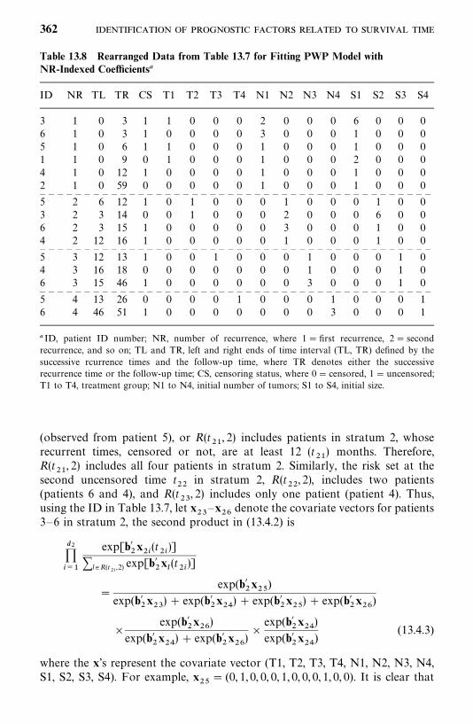
Table 13.8 Rearranged Data from Table 13.7 for Fitting PWP Model withNR-Indexed Coefficients�
ID NR TL TR CS T1 T2 T3 T4 N1 N2 N3 N4 S1 S2 S3 S4
3 1 0 3 1 1 0 0 0 2 0 0 0 6 0 0 06 1 0 3 1 0 0 0 0 3 0 0 0 1 0 0 05 1 0 6 1 1 0 0 0 1 0 0 0 1 0 0 01 1 0 9 0 1 0 0 0 1 0 0 0 2 0 0 04 1 0 12 1 0 0 0 0 1 0 0 0 1 0 0 02 1 0 59 0 0 0 0 0 1 0 0 0 1 0 0 0— — — — — — — — — — — — — — — — — — — — — — — — — — — — — — — — — — — — — — — — — — — —5 2 6 12 1 0 1 0 0 0 1 0 0 0 1 0 03 2 3 14 0 0 1 0 0 0 2 0 0 0 6 0 06 2 3 15 1 0 0 0 0 0 3 0 0 0 1 0 04 2 12 16 1 0 0 0 0 0 1 0 0 0 1 0 0— — — — — — — — — — — — — — — — — — — — — — — — — — — — — — — — — — — — — — — — — — — —5 3 12 13 1 0 0 1 0 0 0 1 0 0 0 1 04 3 16 18 0 0 0 0 0 0 0 1 0 0 0 1 06 3 15 46 1 0 0 0 0 0 0 3 0 0 0 1 0— — — — — — — — — — — — — — — — — — — — — — — — — — — — — — — — — — — — — — — — — — — —5 4 13 26 0 0 0 0 1 0 0 0 1 0 0 0 16 4 46 51 1 0 0 0 0 0 0 0 3 0 0 0 1
� ID, patient ID number; NR, number of recurrence, where 1� first recurrence, 2� secondrecurrence, and so on; TL and TR, left and right ends of time interval (TL, TR) defined by thesuccessive rcurrence times and the follow-up time, where TR denotes either the successiverecurrence time or the follow-up time; CS, censoring status, where 0� censored, 1� uncensored;T1 to T4, treatment group; N1 to N4, initial number of tumors; S1 to S4, initial size.
(observed from patient 5), or R(t��, 2) includes patients in stratum 2, whose
recurrent times, censored or not, are at least 12 (t��) months. Therefore,
R(t��, 2) includes all four patients in stratum 2. Similarly, the risk set at the
second uncensored time t��
in stratum 2, R(t��, 2), includes two patients
(patients 6 and 4), and R(t�, 2) includes only one patient (patient 4). Thus,
using the ID in Table 13.7, let x�—x
��denote the covariate vectors for patients
3—6 in stratum 2, the second product in (13.4.2) is
������
exp[b��x��(t
��)]
�l �R(t��,2) exp[b��x�
(t��)]
�exp(b�
�x��
)exp(b�
�x�) exp(b�
�x��) exp(b�
�x��) exp(b�
�x��
)
�exp(b�
�x��)
exp(b��x��) exp(b�
�x��)�
exp(b��x��)
exp(b��x��
)(13.4.3)
where the x’s represent the covariate vector (T1, T2, T3, T4, N1, N2, N3, N4,S1, S2, S3, S4). For example, x
��� (0, 1, 0, 0, 0, 1, 0, 0, 0, 1, 0, 0). It is clear that
362
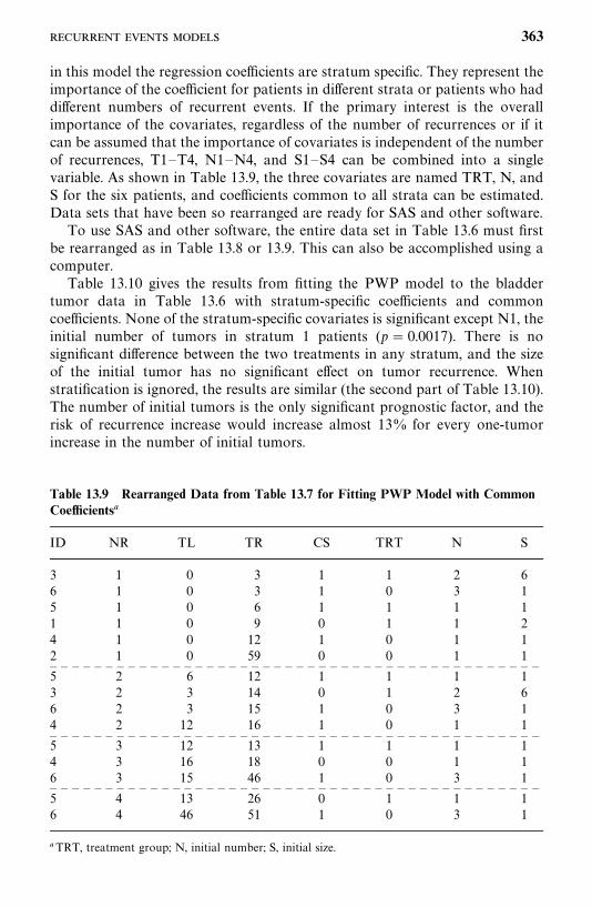
Table 13.9 Rearranged Data from Table 13.7 for Fitting PWP Model with CommonCoefficients�
ID NR TL TR CS TRT N S
3 1 0 3 1 1 2 66 1 0 3 1 0 3 15 1 0 6 1 1 1 11 1 0 9 0 1 1 24 1 0 12 1 0 1 12 1 0 59 0 0 1 1— — — — — — — — — — — — — — — — — — — — — — — — — — — — — — — — — — — — — — — — — — — —5 2 6 12 1 1 1 13 2 3 14 0 1 2 66 2 3 15 1 0 3 14 2 12 16 1 0 1 1— — — — — — — — — — — — — — — — — — — — — — — — — — — — — — — — — — — — — — — — — — — —5 3 12 13 1 1 1 14 3 16 18 0 0 1 16 3 15 46 1 0 3 1— — — — — — — — — — — — — — — — — — — — — — — — — — — — — — — — — — — — — — — — — — — —5 4 13 26 0 1 1 16 4 46 51 1 0 3 1
�TRT, treatment group; N, initial number; S, initial size.
in this model the regression coefficients are stratum specific. They represent theimportance of the coefficient for patients in different strata or patients who haddifferent numbers of recurrent events. If the primary interest is the overallimportance of the covariates, regardless of the number of recurrences or if itcan be assumed that the importance of covariates is independent of the numberof recurrences, T1—T4, N1—N4, and S1—S4 can be combined into a singlevariable. As shown in Table 13.9, the three covariates are named TRT, N, andS for the six patients, and coefficients common to all strata can be estimated.Data sets that have been so rearranged are ready for SAS and other software.
To use SAS and other software, the entire data set in Table 13.6 must firstbe rearranged as in Table 13.8 or 13.9. This can also be accomplished using acomputer.
Table 13.10 gives the results from fitting the PWP model to the bladdertumor data in Table 13.6 with stratum-specific coefficients and commoncoefficients. None of the stratum-specific covariates is significant except N1, theinitial number of tumors in stratum 1 patients (p� 0.0017). There is nosignificant difference between the two treatments in any stratum, and the sizeof the initial tumor has no significant effect on tumor recurrence. Whenstratification is ignored, the results are similar (the second part of Table 13.10).The number of initial tumors is the only significant prognostic factor, and therisk of recurrence increase would increase almost 13% for every one-tumorincrease in the number of initial tumors.
363
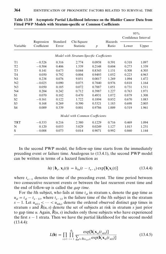
Table 13.10 Asymptotic Partial Likelihood Inference on the Bladder Cancer Data fromFitted PWP Models with Stratum-specific or Common Coefficients
95%Confidence Interval
Regression Standard Chi-Square HazardsVariable Coefficient Error Statistic p Ratio Lower Upper
Model with Stratum-Specific Coefficients
T1 0.526 0.316 2.774 0.0958 0.591 0.318 1.097T2 0.504 0.406 1.539 0.2148 0.604 0.273 1.339T3 0.141 0.673 0.044 0.8345 1.151 0.308 4.305T4 0.050 0.792 0.004 0.9493 1.052 0.223 4.963N1 0.238 0.076 9.851 0.0017 1.269 1.094 1.472N2 0.025 0.090 0.075 0.7840 0.976 0.818 1.164N3 0.050 0.185 0.072 0.7887 1.051 0.731 1.511N4 0.204 0.242 0.712 0.3987 1.227 0.763 1.971S1 0.070 0.102 0.470 0.4931 1.072 0.879 1.308S2 0.161 0.122 1.722 0.1894 0.852 0.670 1.083S3 0.168 0.269 0.390 0.5321 1.183 0.698 2.005S4 0.009 0.339 0.001 0.9786 1.009 0.519 1.961
Model with Common Coefficients
TRT 0.333 0.216 2.380 0.1229 0.716 0.469 1.094N 0.120 0.053 5.029 0.0249 1.127 1.015 1.251S 0.008 0.073 0.014 0.9071 0.992 0.860 1.144
In the second PWP model, the follow-up time starts from the immediatelypreceding event or failure time. Analogous to (13.4.1), the second PWP modelcan be written in terms of a hazard function as
h(t � b, x
�(t)) � h
�(t t
��) exp[b�
x�(t)] (13.4.4)
where t��
denotes the time of the preceding event. The time period betweentwo consecutive recurrent events or between the last recurrent event time andthe end of follow-up is called the gap time.
For the lth subject, who fails at time t�in stratum s, denote the gap time as
u�� t
� t
���, where t
���is the failure time of the lth subject in the stratum
s 1. Let u���
��� u��
��denote the ordered observed distinct gap times in
stratum s and R� (u, s) denote the set of subjects at risk in stratum s just priorto gap time u. Again, R� (u, s) includes only those subjects who have experiencedthe first s 1 strata. Then we have the partial likelihood for the second model(13.4.4):
L (b) � �s�1
��i� 1
exp[b�x�(t
���)]
�l �R� (u���,s) exp(b�
x�(t���)]
(13.4.5)
364
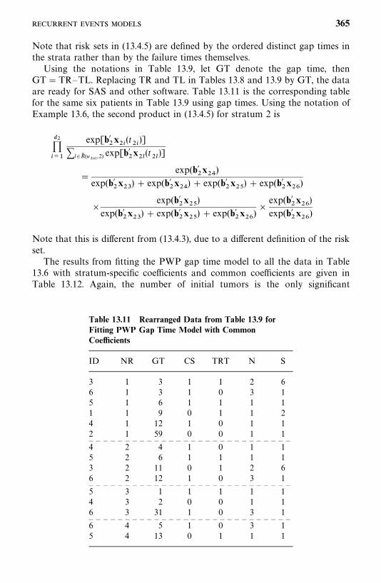
Table 13.11 Rearranged Data from Table 13.9 forFitting PWP Gap Time Model with CommonCoefficients
ID NR GT CS TRT N S
3 1 3 1 1 2 66 1 3 1 0 3 15 1 6 1 1 1 11 1 9 0 1 1 24 1 12 1 0 1 12 1 59 0 0 1 1— — — — — — — — — — — — — — — — — — — — — — — — — — — —4 2 4 1 0 1 15 2 6 1 1 1 13 2 11 0 1 2 66 2 12 1 0 3 1— — — — — — — — — — — — — — — — — — — — — — — — — — — —5 3 1 1 1 1 14 3 2 0 0 1 16 3 31 1 0 3 1— — — — — — — — — — — — — — — — — — — — — — — — — — — —6 4 5 1 0 3 15 4 13 0 1 1 1
Note that risk sets in (13.4.5) are defined by the ordered distinct gap times inthe strata rather than by the failure times themselves.
Using the notations in Table 13.9, let GT denote the gap time, thenGT�TR—TL. Replacing TR and TL in Tables 13.8 and 13.9 by GT, the dataare ready for SAS and other software. Table 13.11 is the corresponding tablefor the same six patients in Table 13.9 using gap times. Using the notation ofExample 13.6, the second product in (13.4.5) for stratum 2 is
������
exp[b��x��(t��)]
�l �R� (u����
,2) exp[b��x��(t��)]
�exp(b�
�x��
)exp(b�
�x�) exp(b�
�x��) exp(b�
�x��) exp(b�
�x��
)
�exp(b�
�x��)
exp(b��x�) exp(b�
�x��) exp(b�
�x��
)�
exp(b��x��)
exp(b��x��
)
Note that this is different from (13.4.3), due to a different definition of the riskset.
The results from fitting the PWP gap time model to all the data in Table13.6 with stratum-specific coefficients and common coefficients are given inTable 13.12. Again, the number of initial tumors is the only significant
365
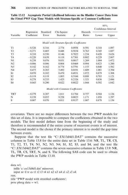
Table 13.12 Asymptotic Partial Likelihood Inference on the Bladder Cancer Data fromthe Fitted PWP Gap Time Models with Stratum-Specific or Common Coefficients
95%Confidence Interval
Regression Standard Chi-Square HazardsVariable Coefficient Error Statistic p Ratio Lower Upper
Model with Stratum-Specific Coefficients
T1 0.526 0.316 2.774 0.0958 0.591 0.318 1.097T2 0.271 0.405 0.448 0.5034 0.763 0.345 1.687T3 0.210 0.550 0.146 0.7022 1.234 0.420 3.626T4 0.220 0.639 0.119 0.7301 0.802 0.229 2.807N1 0.238 0.076 9.851 0.0017 1.269 1.094 1.472N2 0.006 0.096 0.004 0.9469 0.994 0.823 1.200N3 0.142 0.162 0.774 0.3791 1.153 0.840 1.582N4 0.475 0.203 5.492 0.0191 1.609 1.081 2.394S1 0.070 0.102 0.470 0.4931 1.072 0.879 1.308S2 0.119 0.119 1.003 0.3166 0.888 0.703 1.121S3 0.278 0.233 1.425 0.2326 1.321 0.836 2.086S4 0.043 0.290 0.022 0.8822 1.044 0.592 1.842
Model with Common Coefficients
TRT 0.279 0.207 1.811 0.1784 0.757 0.504 1.136N 0.158 0.052 9.258 0.0023 1.171 1.058 1.297S 0.007 0.070 0.011 0.9157 1.007 0.878 1.156
covariates. There are no major differences between the two PWP models forthis set of data. It is impossible to compare the coefficients obtained in the twomodels. The first model defines time from the beginning of the study andtherefore is recommended if the entire course of recurrent events is of interest.The second model is the choice if the primary interest is to model the gap timebetween events.
Suppose that the text file ‘‘C:�EX13d4d1.DAT’’ contains the successivecolumns in Table 13.8 for the entire data set in Table 13.6: NR, TL, TR, CS,T1, T2, T3, T4, N1, N2, N3, N4, S1, S2, S3, and S4, and the text file‘‘C:�EX13d4d2.DAT’’ contains the seven successive columns in Table 13.9: NR,TL, TR, CS, TRT, N, and S. The following SAS code can be used to obtainthe PWP models in Table 13.10.
data w1;infile ‘c:�ex13d4d1.dat’ missover;input nr tl tr cs t1 t2 t3 t4 n1 n2 n3 n4 s1 s2 s3 s4;
run;title ‘‘PWP model with stratified coefficients‘;proc phreg data�w1;
366
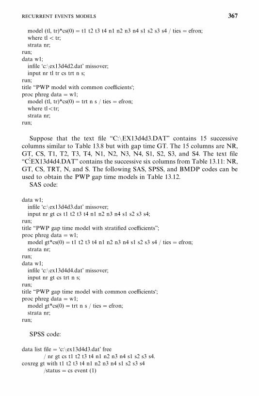
model (tl, tr)*cs(0) � t1 t2 t3 t4 n1 n2 n3 n4 s1 s2 s3 s4 / ties� efron;where tl� tr;strata nr;
run;data w1;infile ‘c:�ex13d4d2.dat’ missover;input nr tl tr cs trt n s;
run;title ‘‘PWP model with common coefficients‘;proc phreg data�w1;model (tl, tr)*cs(0) � trt n s / ties� efron;where tl�tr;strata nr;
run;
Suppose that the text file ‘‘C:�EX13d4d3.DAT’’ contains 15 successivecolumns similar to Table 13.8 but with gap time GT. The 15 columns are NR,GT, CS, T1, T2, T3, T4, N1, N2, N3, N4, S1, S2, S3, and S4. The text file‘‘C:KEX13d4d4.DAT’’ contains the successive six columns from Table 13.11: NR,GT, CS, TRT, N, and S. The following SAS, SPSS, and BMDP codes can beused to obtain the PWP gap time models in Table 13.12.
SAS code:
data w1;infile ‘c:�ex13d4d3.dat’ missover;input nr gt cs t1 t2 t3 t4 n1 n2 n3 n4 s1 s2 s3 s4;
run;title ‘‘PWP gap time model with stratified coefficients’’;proc phreg data�w1;model gt*cs(0) � t1 t2 t3 t4 n1 n2 n3 n4 s1 s2 s3 s4 / ties� efron;strata nr;
run;data w1;infile ‘c:�ex13d4d4.dat’ missover;input nr gt cs trt n s;
run;title ‘‘PWP gap time model with common coefficients‘;proc phreg data�w1;model gt*cs(0) � trt n s / ties� efron;strata nr;
run;
SPSS code:
data list file� ‘c:�ex13d4d3.dat’ free/ nr gt cs t1 t2 t3 t4 n1 n2 n3 n4 s1 s2 s3 s4.
coxreg gt with t1 t2 t3 t4 n1 n2 n3 n4 s1 s2 s3 s4/status� cs event (1)
367
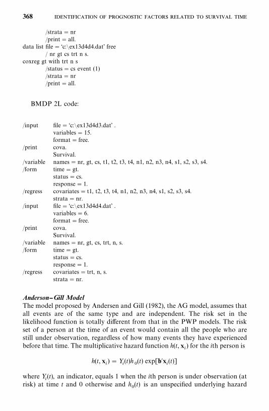
/strata� nr/print� all.
data list file� ‘c:�ex13d4d4.dat’ free/ nr gt cs trt n s.
coxreg gt with trt n s/status� cs event (1)/strata� nr/print� all.
BMDP 2L code:
/input file� ‘c:�ex13d4d3.dat’ .variables� 15.format� free.
/print cova.Survival.
/variable names�nr, gt, cs, t1, t2, t3, t4, n1, n2, n3, n4, s1, s2, s3, s4./form time� gt.
status� cs.response� 1.
/regress covariates� t1, t2, t3, t4, n1, n2, n3, n4, s1, s2, s3, s4.strata�nr.
/input file� ‘c:�ex13d4d4.dat’ .variables� 6.format� free.
/print cova.Survival.
/variable names�nr, gt, cs, trt, n, s./form time� gt.
status� cs.response� 1.
/regress covariates� trt, n, s.strata�nr.
Anderson--Gill ModelThe model proposed by Andersen and Gill (1982), the AG model, assumes thatall events are of the same type and are independent. The risk set in thelikelihood function is totally different from that in the PWP models. The riskset of a person at the time of an event would contain all the people who arestill under observation, regardless of how many events they have experiencedbefore that time. The multiplicative hazard function h(t, x
�) for the ith person is
h(t, x�) � Y
�(t)h
�(t) exp[b�x
�(t)]
where Y�(t), an indicator, equals 1 when the ith person is under observation (at
risk) at time t and 0 otherwise and h�(t) is an unspecified underlying hazard
368
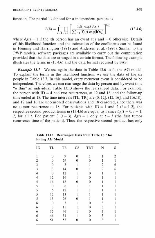
Table 13.13 Rearranged Data from Table 13.7 forFitting AG Model
ID TL TR CS TRT N S
1 0 9 0 1 1 22 0 59 0 0 1 13 0 3 1 1 2 63 3 14 0 1 2 64 0 12 1 0 1 14 12 16 1 0 1 14 16 18 0 0 1 15 0 6 1 1 1 15 6 12 1 1 1 15 12 13 1 1 1 15 13 26 0 1 1 16 0 3 1 0 3 16 3 15 1 0 3 16 15 46 1 0 3 16 46 51 1 0 3 16 51 53 0 0 3 1
function. The partial likelihood for n independent persons is
L (b) ������
�����
Y�(t) exp(b�x
�)
�����
Y�(t) exp(b�x
�)�
�����(13.4.6)
where �(t) � 1 if the ith person has an event at t and �0 otherwise. Details
of this likelihood function and the estimation of the coefficients can be foundin Fleming and Harrington (1991) and Andersen et al. (1993). Similar to thePWP models, software packages are available to carry out the computationprovided that the data are arranged in a certain format. The following exampleillustrates the terms in (13.4.6) and the data format required by SAS.
Example 13.7 We use again the data in Table 13.6 to fit the AG model.To explain the terms in the likelihood function, we use the data of the sixpeople in Table 13.7. In this model, every recurrent event is considered to beindependent. Therefore, we can rearrange the data by person and by event time‘‘within’’ an individual. Table 13.13 shows the rearranged data. For example,the person with ID� 4 had two recurrences, at 12 and 16, and the follow-uptime ended at 18. The time intervals (TL, TR] are (0, 12], (12, 16], and (16,18],and 12 and 16 are uncensored observations and 18 censored, since there wasno tumor recurrence at 18. For patients with ID� 1 and 2 (i� 1, 2), therespective second product terms in (13.4.6) are equal to 1 since
�(t) � 0, i� 1,
2, for all t. For patient 3 (i� 3), �(t) � 1 only at t� 3 (the first tumor
recurrence time of the patient). Thus, the respective second product has only
369
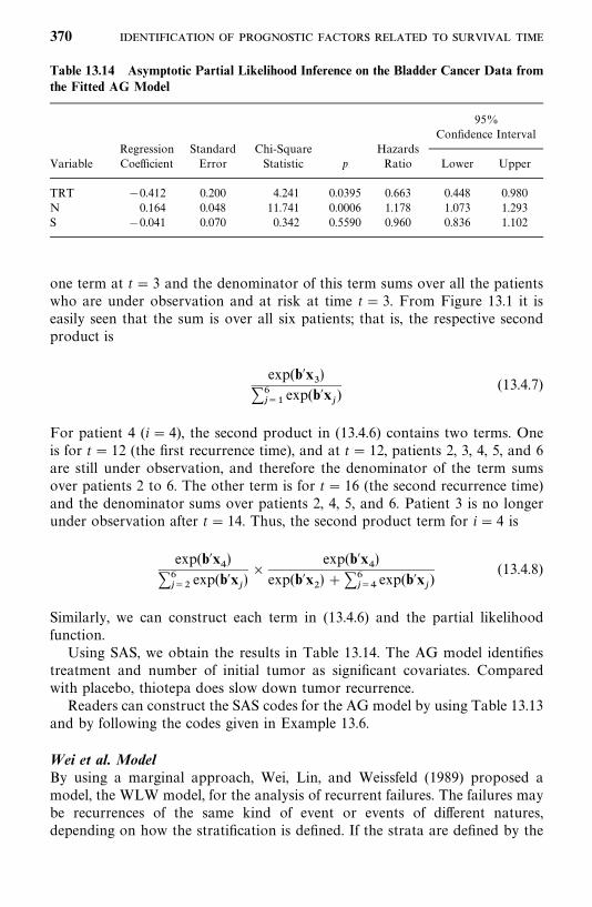
Table 13.14 Asymptotic Partial Likelihood Inference on the Bladder Cancer Data fromthe Fitted AG Model
95%Confidence Interval
Regression Standard Chi-Square HazardsVariable Coefficient Error Statistic p Ratio Lower Upper
TRT 0.412 0.200 4.241 0.0395 0.663 0.448 0.980N 0.164 0.048 11.741 0.0006 1.178 1.073 1.293S 0.041 0.070 0.342 0.5590 0.960 0.836 1.102
one term at t� 3 and the denominator of this term sums over all the patientswho are under observation and at risk at time t� 3. From Figure 13.1 it iseasily seen that the sum is over all six patients; that is, the respective secondproduct is
exp(b�x)
�����
exp(b�x�)
(13.4.7)
For patient 4 (i� 4), the second product in (13.4.6) contains two terms. Oneis for t� 12 (the first recurrence time), and at t� 12, patients 2, 3, 4, 5, and 6are still under observation, and therefore the denominator of the term sumsover patients 2 to 6. The other term is for t� 16 (the second recurrence time)and the denominator sums over patients 2, 4, 5, and 6. Patient 3 is no longerunder observation after t� 14. Thus, the second product term for i� 4 is
exp(b�x�)
�����
exp(b�x�)�
exp(b�x�)
exp(b�x�) ��
���exp(b�x
�)
(13.4.8)
Similarly, we can construct each term in (13.4.6) and the partial likelihoodfunction.
Using SAS, we obtain the results in Table 13.14. The AG model identifiestreatment and number of initial tumor as significant covariates. Comparedwith placebo, thiotepa does slow down tumor recurrence.
Readers can construct the SAS codes for the AG model by using Table 13.13and by following the codes given in Example 13.6.
Wei et al. ModelBy using a marginal approach, Wei, Lin, and Weissfeld (1989) proposed amodel, the WLW model, for the analysis of recurrent failures. The failures maybe recurrences of the same kind of event or events of different natures,depending on how the stratification is defined. If the strata are defined by the
370
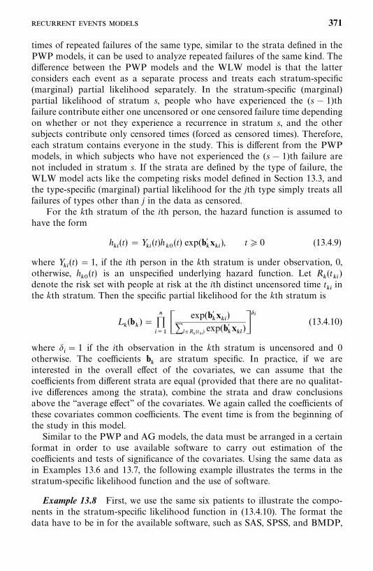
times of repeated failures of the same type, similar to the strata defined in thePWP models, it can be used to analyze repeated failures of the same kind. Thedifference between the PWP models and the WLW model is that the latterconsiders each event as a separate process and treats each stratum-specific(marginal) partial likelihood separately. In the stratum-specific (marginal)partial likelihood of stratum s, people who have experienced the (s 1)thfailure contribute either one uncensored or one censored failure time dependingon whether or not they experience a recurrence in stratum s, and the othersubjects contribute only censored times (forced as censored times). Therefore,each stratum contains everyone in the study. This is different from the PWPmodels, in which subjects who have not experienced the (s 1)th failure arenot included in stratum s. If the strata are defined by the type of failure, theWLW model acts like the competing risks model defined in Section 13.3, andthe type-specific (marginal) partial likelihood for the jth type simply treats allfailures of types other than j in the data as censored.
For the kth stratum of the ith person, the hazard function is assumed tohave the form
h��(t) �Y
��(t)h
��(t) exp(b�
�x��), t� 0 (13.4.9)
where Y��(t) � 1, if the ith person in the kth stratum is under observation, 0,
otherwise, h��(t) is an unspecified underlying hazard function. Let R
�(t��
)denote the risk set with people at risk at the ith distinct uncensored time t
��in
the kth stratum. Then the specific partial likelihood for the kth stratum is
L�(b
�) �
������
exp(b��x��)
�l �R�(t��) exp(b�
�x��
)���
(13.4.10)
where �� 1 if the ith observation in the kth stratum is uncensored and 0
otherwise. The coefficients b�are stratum specific. In practice, if we are
interested in the overall effect of the covariates, we can assume that thecoefficients from different strata are equal (provided that there are no qualitat-ive differences among the strata), combine the strata and draw conclusionsabove the ‘‘average effect’’ of the covariates. We again called the coefficients ofthese covariates common coefficients. The event time is from the beginning ofthe study in this model.
Similar to the PWP and AG models, the data must be arranged in a certainformat in order to use available software to carry out estimation of thecoefficients and tests of significance of the covariates. Using the same data asin Examples 13.6 and 13.7, the following example illustrates the terms in thestratum-specific likelihood function and the use of software.
Example 13.8 First, we use the same six patients to illustrate the compo-nents in the stratum-specific likelihood function in (13.4.10). The format thedata have to be in for the available software, such as SAS, SPSS, and BMDP,
371
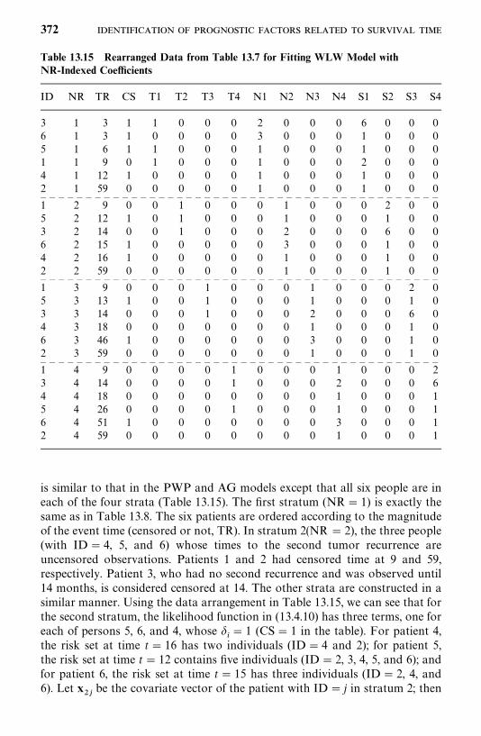
Table 13.15 Rearranged Data from Table 13.7 for Fitting WLW Model withNR-Indexed Coefficients
ID NR TR CS T1 T2 T3 T4 N1 N2 N3 N4 S1 S2 S3 S4
3 1 3 1 1 0 0 0 2 0 0 0 6 0 0 06 1 3 1 0 0 0 0 3 0 0 0 1 0 0 05 1 6 1 1 0 0 0 1 0 0 0 1 0 0 01 1 9 0 1 0 0 0 1 0 0 0 2 0 0 04 1 12 1 0 0 0 0 1 0 0 0 1 0 0 02 1 59 0 0 0 0 0 1 0 0 0 1 0 0 0— — — — — — — — — — — — — — — — — — — — — — — — — — — — — — — — — — — — — — — — — — — —1 2 9 0 0 1 0 0 0 1 0 0 0 2 0 05 2 12 1 0 1 0 0 0 1 0 0 0 1 0 03 2 14 0 0 1 0 0 0 2 0 0 0 6 0 06 2 15 1 0 0 0 0 0 3 0 0 0 1 0 04 2 16 1 0 0 0 0 0 1 0 0 0 1 0 02 2 59 0 0 0 0 0 0 1 0 0 0 1 0 0— — — — — — — — — — — — — — — — — — — — — — — — — — — — — — — — — — — — — — — — — — — —1 3 9 0 0 0 1 0 0 0 1 0 0 0 2 05 3 13 1 0 0 1 0 0 0 1 0 0 0 1 03 3 14 0 0 0 1 0 0 0 2 0 0 0 6 04 3 18 0 0 0 0 0 0 0 1 0 0 0 1 06 3 46 1 0 0 0 0 0 0 3 0 0 0 1 02 3 59 0 0 0 0 0 0 0 1 0 0 0 1 0— — — — — — — — — — — — — — — — — — — — — — — — — — — — — — — — — — — — — — — — — — — —1 4 9 0 0 0 0 1 0 0 0 1 0 0 0 23 4 14 0 0 0 0 1 0 0 0 2 0 0 0 64 4 18 0 0 0 0 0 0 0 0 1 0 0 0 15 4 26 0 0 0 0 1 0 0 0 1 0 0 0 16 4 51 1 0 0 0 0 0 0 0 3 0 0 0 12 4 59 0 0 0 0 0 0 0 0 1 0 0 0 1
is similar to that in the PWP and AG models except that all six people are ineach of the four strata (Table 13.15). The first stratum (NR� 1) is exactly thesame as in Table 13.8. The six patients are ordered according to the magnitudeof the event time (censored or not, TR). In stratum 2(NR � 2), the three people(with ID� 4, 5, and 6) whose times to the second tumor recurrence areuncensored observations. Patients 1 and 2 had censored time at 9 and 59,respectively. Patient 3, who had no second recurrence and was observed until14 months, is considered censored at 14. The other strata are constructed in asimilar manner. Using the data arrangement in Table 13.15, we can see that forthe second stratum, the likelihood function in (13.4.10) has three terms, one foreach of persons 5, 6, and 4, whose
�� 1 (CS� 1 in the table). For patient 4,
the risk set at time t� 16 has two individuals (ID� 4 and 2); for patient 5,the risk set at time t� 12 contains five individuals (ID� 2, 3, 4, 5, and 6); andfor patient 6, the risk set at time t� 15 has three individuals (ID� 2, 4, and6). Let x
��be the covariate vector of the patient with ID� j in stratum 2; then
372
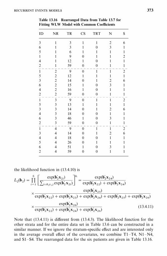
Table 13.16 Rearranged Data from Table 13.7 forFitting WLW Model with Common Coefficients
ID NR TR CS TRT N S
3 1 3 1 1 2 66 1 3 1 0 3 15 1 6 1 1 1 11 1 9 0 1 1 24 1 12 1 0 1 12 1 59 0 0 1 1— — — — — — — — — — — — — — — — — — — — — — — — — — — —1 2 9 0 1 1 25 2 12 1 1 1 13 2 14 0 1 2 66 2 15 1 0 3 14 2 16 1 0 1 12 2 59 0 0 1 1— — — — — — — — — — — — — — — — — — — — — — — — — — — —1 3 9 0 1 1 25 3 13 1 1 1 13 3 14 0 1 2 64 3 18 0 0 1 16 3 46 1 0 3 12 3 59 0 0 1 1— — — — — — — — — — — — — — — — — — — — — — — — — — — —1 4 9 0 1 1 23 4 14 0 1 2 64 4 18 0 0 1 15 4 26 0 1 1 16 4 51 1 0 3 12 4 59 0 0 1 1
the likelihood function in (13.4.10) is
L�(b
�) �
������
exp(b��x��)
�l �R�(t��) exp(b�
�x��
)���
�exp(b�
�x��
)exp(b�
�x��) exp(b�
�x��
)
�exp(b�
�x��
)exp(b�
�x��
) exp(b��x�
) exp(b��x��
) exp(b��x��) exp(b�
�x��
)
�exp(b�
�x��)
exp(b��x��
) exp(b��x��
) exp(b��x��
)(13.4.11)
Note that (13.4.11) is different from (13.4.3). The likelihood function for theother strata and for the entire data set in Table 13.6 can be constructed in asimilar manner. If we ignore the stratum-specific effect and are interested onlyin the average overall effect of the covariates, we combine T1—T4, N1—N4,and S1—S4. The rearranged data for the six patients are given in Table 13.16.
373
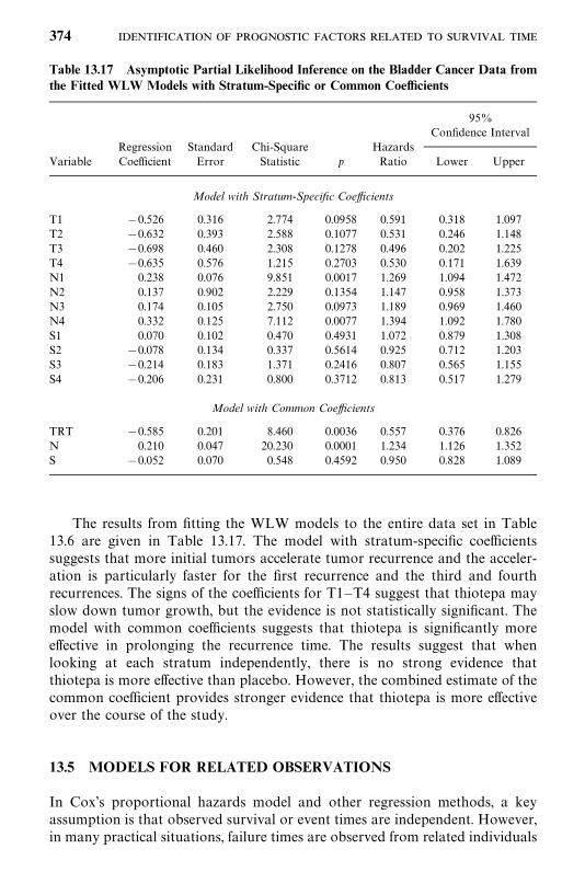
Table 13.17 Asymptotic Partial Likelihood Inference on the Bladder Cancer Data fromthe Fitted WLW Models with Stratum-Specific or Common Coefficients
95%Confidence Interval
Regression Standard Chi-Square HazardsVariable Coefficient Error Statistic p Ratio Lower Upper
Model with Stratum-Specific Coefficients
T1 0.526 0.316 2.774 0.0958 0.591 0.318 1.097T2 0.632 0.393 2.588 0.1077 0.531 0.246 1.148T3 0.698 0.460 2.308 0.1278 0.496 0.202 1.225T4 0.635 0.576 1.215 0.2703 0.530 0.171 1.639N1 0.238 0.076 9.851 0.0017 1.269 1.094 1.472N2 0.137 0.902 2.229 0.1354 1.147 0.958 1.373N3 0.174 0.105 2.750 0.0973 1.189 0.969 1.460N4 0.332 0.125 7.112 0.0077 1.394 1.092 1.780S1 0.070 0.102 0.470 0.4931 1.072 0.879 1.308S2 0.078 0.134 0.337 0.5614 0.925 0.712 1.203S3 0.214 0.183 1.371 0.2416 0.807 0.565 1.155S4 0.206 0.231 0.800 0.3712 0.813 0.517 1.279
Model with Common Coefficients
TRT 0.585 0.201 8.460 0.0036 0.557 0.376 0.826N 0.210 0.047 20.230 0.0001 1.234 1.126 1.352S 0.052 0.070 0.548 0.4592 0.950 0.828 1.089
The results from fitting the WLW models to the entire data set in Table13.6 are given in Table 13.17. The model with stratum-specific coefficientssuggests that more initial tumors accelerate tumor recurrence and the acceler-ation is particularly faster for the first recurrence and the third and fourthrecurrences. The signs of the coefficients for T1—T4 suggest that thiotepa mayslow down tumor growth, but the evidence is not statistically significant. Themodel with common coefficients suggests that thiotepa is significantly moreeffective in prolonging the recurrence time. The results suggest that whenlooking at each stratum independently, there is no strong evidence thatthiotepa is more effective than placebo. However, the combined estimate of thecommon coefficient provides stronger evidence that thiotepa is more effectiveover the course of the study.
13.5 MODELS FOR RELATED OBSERVATIONS
In Cox’s proportional hazards model and other regression methods, a keyassumption is that observed survival or event times are independent. However,in many practical situations, failure times are observed from related individuals
374
or from successive recurrent events or failures of the same person. For example,in an epidemiological study of heart disease, some of the participants may befrom the same family and therefore are not independent. These families withmultiple participants may be called clusters. In this case, the regressionmethods we introduced earlier may not be appropriate. Several types of modelsintroduced especially for related observations are discussed by Andersen et al.(1993), Liang et al. (1995), Klein and Moeschberger (1997), and Ibrahim et al.(2001). Details about these models are beyond the scope of this book. In thefollowing, we introduce briefly the frailty models.
The frailty models assume that there is an unmeasured random variable(frailty) in the hazard function. This random variable accounts for the variationor heterogeneity among individuals in a cluster. It is also assumed that thefrailty is independent of censoring. Let n be the total number of participants inthe study, some of them related and forming clusters. Let v
�be the unknown
random variable, frailty, associated with the ith cluster, 1 i� n. The frailtymodel associated with the proportional hazards model can be written in termsof the log hazard function as
log[h��(t; x
��� v
�)]� log[h
�(t)] v
� b�x
��(13.5.1)
for 1 jm�and 1 i� n, where b denotes the p�1 column vector of
unknown regression coefficients, x��is the covariate vector of the jth person in
the ith cluster, m�is the number of individuals in the ith cluster, and h
�(t) is an
unknown underlying hazard function. Compared with the Cox proportionalhazards model, the difference here is the random effect v
�. Because v
�remains
the same in the ith cluster, the association between failure and covariateswithin each cluster in this model is assumed to have a symmetric pattern. In afamily study, this model can be used, for example, to model failure timesobserved from siblings by treating each family as a cluster. This model wasproposed by Vaupel et al. (1979) and developed and discussed by manyresearchers, including Clayton and Cuzick (1985). The main approach to thismodel is to assume that v
�follows a parametric distribution.
The frailty model in (13.5.1) can be extended to handle more complicatedsituations. For example, the frailty can be a time-dependent variable [replacev�by v
�(t) in (13.5.1)]. The frailty model with v
�(t) can be used to model
successive or recurrent failure time as an alternative to the models in Section13.4. Another example is that there may be more than one type of frailty ineach cluster, and v
�in (13.5.1) can be replaced by v
� u
�or v
� u
�w
�, and
so on.Inferences of these frailty models are also based on either a likelihood
function or a partial likelihood function. Since the models involve a parametricdistribution, the likelihood or partial likelihood functions are complicated andare beyond the level of this book.
The frailty models have not been used widely primarily because of the lackof commercially available software. There are some computer programs
375
available; for example, a SAS macro is available for a gamma frailty model atthe Web site of Klein and Moeschberger (1997), and another program isdescribed by Jenkins (1997).
Bibliographical Remarks
Most of the major references for nonproportional hazards models have beencited in the text of this chapter. Applications of these models include: stratifiedmodels: Vasan et al. (1997), Aaronson et al. (1997), and Yakovlev et al. (1999);frailty models: Yashin and Iachine (1997), Kessing et al. (1999), Siegmund et al.(1999), Albert (2000), Lee and Yau (2001), Wienke el al. (2001), and Xue (2001);competing risks models: Mackenbach et al. (1995), Fish et al. (1998), Albertsenet al. (1998), Blackstone and Lytle (2000), Yan et al. (2000), and Tai et al.(2001).
EXERCISES
13.1 Consider the cancer-free times from the participants with IDs 15 to 23in Table 13.1. Follow Example 13.1 to construct the partial likelihoodfunction based on the observed cancer-free times from these nine partici-pants.
13.2 Consider the survival times from 30 resected melanoma patients in Table3.1. Let AGEG denote age group, AGEG� 1 if age �45 and AGEG� 2otherwise. Fit the survival times with an AGEG-stratified Cox propor-tional hazards model with the covariates age, gender, initial stage, andtreatment received. Discuss the association of the treatment received withthe survival time.
13.3 Using the data in Table 12.4, following Example 13.5 and the samplecodes for SAS, SPSS, or BMDP, fit the competing risk model for stroke,CHD, other CVD, or STROKE/CHD separately, and discuss the resultsobtained.
13.4 Using the rearranged data in Tables 13.7 to 13.13 and followingExamples 13.6 to 13.8, complete construction of the remaining terms inthe partial likelihood function based on the PWP model (13.4.2), PWPgap time model (13.4.3), and AG model (13.4.9), and the remaining threemarginal likelihood functions based on the WLW model (13.4.13).
376
CHAPTER 14
Identification of Risk FactorsRelated to Dichotomous andPolychotomous Outcomes
In biomedical research we are often interested in whether a certain survival-related event will occur and the important factors that influence its occurrence.Such events may involve two or more possible outcomes; examples are thedevelopment of a given condition and response to a given treatment. If thegiven condition is diabetes and we are only interested in whether someonedevelops the disease (yes or no), the outcome is binary or dichotomous. If weare interested in whether the person develops impaired glucose tolerance,diabetes, or remains having normal glucose tolerance, there are three possibleoutcomes, or we say the outcome is trichotomous. Similarly, response to a giventreatment can have dichotomous (response or no response) or polychotomousoutcomes (complete response, partial response, or no response).
To determine whether one is likely to develop a given disease, we need toknow the important characteristics (or factors) related to its development.High- and low-risk groups can then be defined accordingly. Factors closelyrelated to the development of a given disease are usually called risk factors orrisk variables by epidemiologists. We shall use these terms in a broader senseto mean factors closely related to the occurrence of any event of interest. Forexample, to find out whether a woman will develop breast cancer because oneof her relatives did, we need to know whether a family history of breast canceris an important risk factor. Therefore, we need to know the following:
1. Of age, race, family history of breast cancer, number of pregnancies,experience of breast-feeding, and use of oral contraceptives—which aremost important?
2. Can we predict, on the basis of the important risk factors, whether awoman will develop breast cancer or is more likely to develop breastcancer than another person?
377
In this chapter we introduce several methods for answering these ques-tions. The general approach is to relate various patient characteristics(or independent variables, or covariates) to the occurrence of an event(dependent or response variable) on the basis of data collected frompatients in each of the outcome groups. In the case of dichotomous out-comes, there are two outcome groups. For example, to relate variables suchas age, race, and number of pregnancies to the development of breast cancer,we need to collect information about these variables from a group of breastcancer patients as well as from a group of healthy normal women. For an eventwith polychotomous outcomes, we need to collect data from each outcomegroup.
Often, a large number of patient characteristics deserve consideration.These characteristics may be demographic variables such as age; geneticvariables such as gene variant or phenotype; behavioral variables such assmoking or drinking behavior and use of estrogen or progesterone medic-ation; environmental variables such as exposure to sun, air pollution, oroccupational dust; or clinical variables such as blood cell counts, weight, andblood pressure. The number of possible risk factors can be reduced throughmedical knowledge of the disease and careful examination of the possible riskfactors individually.
In Section 14.1 we present two methods for examination of individualvariables. One is to compare the distribution of each possible risk variableamong the outcome groups. The other method is the chi-square test for acontingency table. This test is particularly useful when the risk variables arecategorical: for example, dichotomous or trichotomous. In this case, a 2�c orr�c contingency table can be set up and a chi-square test performed. InSection 14.2 we discuss logistic, conditional logistic, and other regressionmodels for binary responses and for examining the possible risk variablessimultaneously. Models for multiple outcomes are discussed in Section 14.3.
14.1 UNIVARIATE ANALYSIS
14.1.1 Comparing the Distributions of Risk Variables Among Groups
When the outcome is binary, it is often convenient to call an observation asuccess or a failure. Success may mean that a survival-related event occurred,and failure that it failed to occur. Thus, a success may be a respondingpatient, a patient who survives more than five years after surgery, or aperson who develops a given disease. A failure may be a nonrespond-ing patient, a patient who dies within five years after surgery, or a personwho does not develop a given disease. A preliminary examination of thedata can compare the distribution of the risk variables in the success andfailure groups. This method is especially appropriate if the risk variable is
378
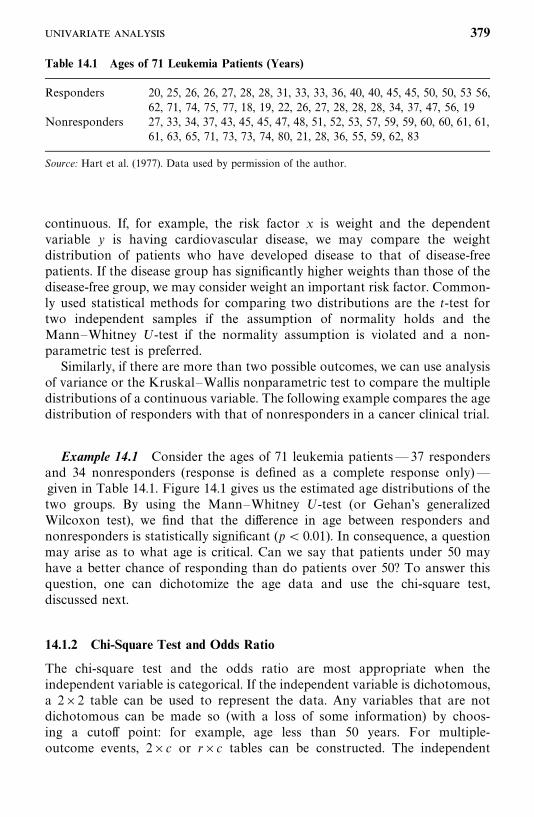
Table 14.1 Ages of 71 Leukemia Patients (Years)
Responders 20, 25, 26, 26, 27, 28, 28, 31, 33, 33, 36, 40, 40, 45, 45, 50, 50, 53 56,62, 71, 74, 75, 77, 18, 19, 22, 26, 27, 28, 28, 28, 34, 37, 47, 56, 19
Nonresponders 27, 33, 34, 37, 43, 45, 45, 47, 48, 51, 52, 53, 57, 59, 59, 60, 60, 61, 61,61, 63, 65, 71, 73, 73, 74, 80, 21, 28, 36, 55, 59, 62, 83
Source: Hart et al. (1977). Data used by permission of the author.
continuous. If, for example, the risk factor x is weight and the dependentvariable y is having cardiovascular disease, we may compare the weightdistribution of patients who have developed disease to that of disease-freepatients. If the disease group has significantly higher weights than those of thedisease-free group, we may consider weight an important risk factor. Common-ly used statistical methods for comparing two distributions are the t-test fortwo independent samples if the assumption of normality holds and theMann—Whitney U-test if the normality assumption is violated and a non-parametric test is preferred.
Similarly, if there are more than two possible outcomes, we can use analysisof variance or the Kruskal—Wallis nonparametric test to compare the multipledistributions of a continuous variable. The following example compares the agedistribution of responders with that of nonresponders in a cancer clinical trial.
Example 14.1 Consider the ages of 71 leukemia patients—37 respondersand 34 nonresponders (response is defined as a complete response only)—given in Table 14.1. Figure 14.1 gives us the estimated age distributions of thetwo groups. By using the Mann—Whitney U-test (or Gehan’s generalizedWilcoxon test), we find that the difference in age between responders andnonresponders is statistically significant (p � 0.01). In consequence, a questionmay arise as to what age is critical. Can we say that patients under 50 mayhave a better chance of responding than do patients over 50? To answer thisquestion, one can dichotomize the age data and use the chi-square test,discussed next.
14.1.2 Chi-Square Test and Odds Ratio
The chi-square test and the odds ratio are most appropriate when theindependent variable is categorical. If the independent variable is dichotomous,a 2�2 table can be used to represent the data. Any variables that are notdichotomous can be made so (with a loss of some information) by choos-ing a cutoff point: for example, age less than 50 years. For multiple-outcome events, 2�c or r�c tables can be constructed. The independent
379
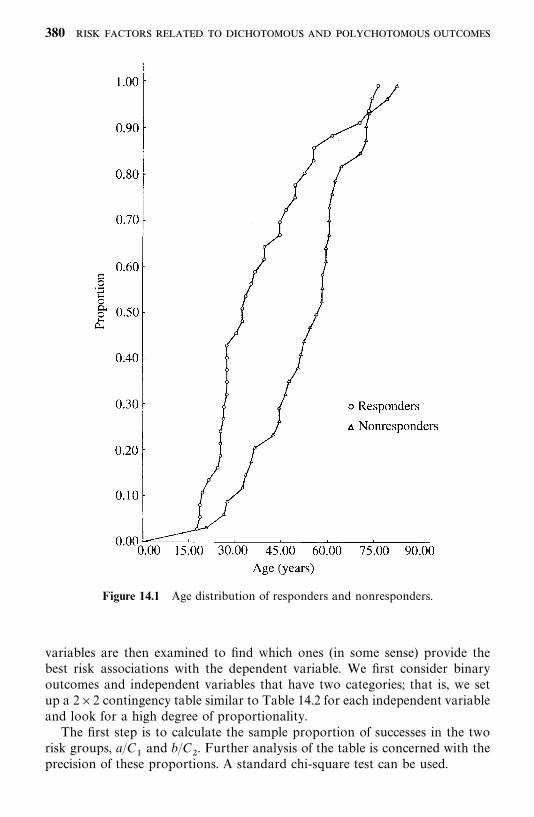
Figure 14.1 Age distribution of responders and nonresponders.
variables are then examined to find which ones (in some sense) provide thebest risk associations with the dependent variable. We first consider binaryoutcomes and independent variables that have two categories; that is, we setup a 2�2 contingency table similar to Table 14.2 for each independent variableand look for a high degree of proportionality.
The first step is to calculate the sample proportion of successes in the tworisk groups, a/C
�and b/C
�. Further analysis of the table is concerned with the
precision of these proportions. A standard chi-square test can be used.
380
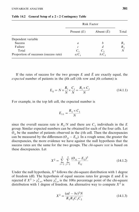
Table 14.2 General Setup of a 2�2 Contingency Table
Risk Factor
Present (E ) Absent (E� ) Total
Dependent variableSuccess a b R
�Failure c d R
�Total C
�C
�N
Proportion of successes (success rate) a/C�
b/C�
If the rates of success for the two groups E and E� are exactly equal, theexpected number of patients in the ijth cell (ith row and jth column) is
E��� N�
R�
N�
C�
N�
R��C
�N
(14.1.1)
For example, in the top left cell, the expected number is
E��
�R
��C
�N
since the overall success rate is R�/N and there are C
�individuals in the E
group. Similar expected numbers can be obtained for each of the four cells. LetO
��be the number of patients observed in the ijth cell. Then the discrepancies
can be measured by the differences (O���E
��). In a rough sense, the greater the
discrepancies, the more evidence we have against the null hypothesis that thesuccess rates are the same for the two groups. The chi-square test is based onthese discrepancies. Let
X�������
�����
(O���E
��)�
E��
(14.1.2)
Under the null hypothesis, X� follows the chi-square distribution with 1 degreeof freedom (df). The hypothesis of equal success rates for groups E and E� isrejected if X� ���
��� , where ����� is the 100� percentage point of the chi-square
distribution with 1 degree of freedom. An alternative way to compute X� is
X��(ad � bc)�N
R�R
�C
�C
�
(14.1.3)
381
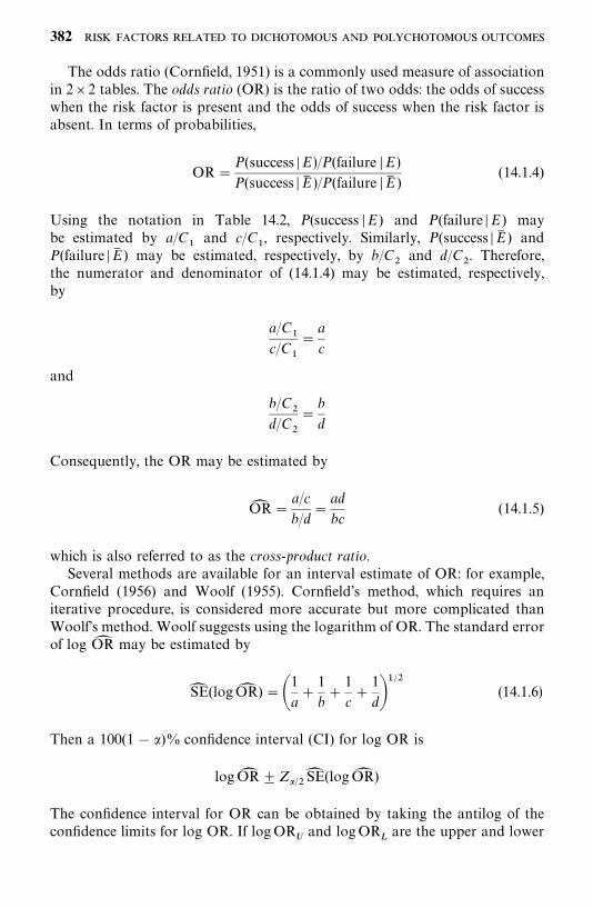
The odds ratio (Cornfield, 1951) is a commonly used measure of associationin 2�2 tables. The odds ratio (OR) is the ratio of two odds: the odds of successwhen the risk factor is present and the odds of success when the risk factor isabsent. In terms of probabilities,
OR�P(success � E)/P(failure � E )P(success � E� )/P(failure �E� )
(14.1.4)
Using the notation in Table 14.2, P(success �E) and P(failure � E) maybe estimated by a/C
�and c/C
�, respectively. Similarly, P(success � E� ) and
P(failure �E� ) may be estimated, respectively, by b/C�and d/C
�. Therefore,
the numerator and denominator of (14.1.4) may be estimated, respectively,by
a/C�
c/C�
�a
c
and
b/C�
d/C�
�b
d
Consequently, the OR may be estimated by
OR� �a/c
b/d�
ad
bc(14.1.5)
which is also referred to as the cross-product ratio.Several methods are available for an interval estimate of OR: for example,
Cornfield (1956) and Woolf (1955). Cornfield’s method, which requires aniterative procedure, is considered more accurate but more complicated thanWoolf’s method. Woolf suggests using the logarithm of OR. The standard errorof log OR� may be estimated by
SE� (logOR� ) ��1
a�
1
b�
1
c�
1
d����
(14.1.6)
Then a 100(1� �)% confidence interval (CI) for log OR is
logOR� Z���SE� (logOR� )
The confidence interval for OR can be obtained by taking the antilog of theconfidence limits for log OR. If logOR
�and logOR
�are the upper and lower
382
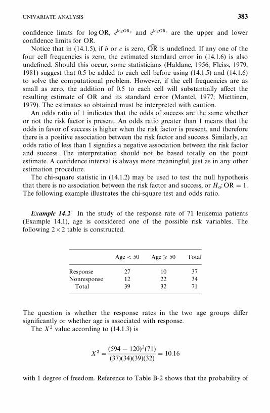
confidence limits for logOR, elogOR� and elogOR� are the upper and lowerconfidence limits for OR.
Notice that in (14.1.5), if b or c is zero, OR� is undefined. If any one of thefour cell frequencies is zero, the estimated standard error in (14.1.6) is alsoundefined. Should this occur, some statisticians (Haldane, 1956; Fleiss, 1979,1981) suggest that 0.5 be added to each cell before using (14.1.5) and (14.1.6)to solve the computational problem. However, if the cell frequencies are assmall as zero, the addition of 0.5 to each cell will substantially affect theresulting estimate of OR and its standard error (Mantel, 1977; Miettinen,1979). The estimates so obtained must be interpreted with caution.
An odds ratio of 1 indicates that the odds of success are the same whetheror not the risk factor is present. An odds ratio greater than 1 means that theodds in favor of success is higher when the risk factor is present, and thereforethere is a positive association between the risk factor and success. Similarly, anodds ratio of less than 1 signifies a negative association between the risk factorand success. The interpretation should not be based totally on the pointestimate. A confidence interval is always more meaningful, just as in any otherestimation procedure.
The chi-square statistic in (14.1.2) may be used to test the null hypothesisthat there is no association between the risk factor and success, or H
: OR� 1.
The following example illustrates the chi-square test and odds ratio.
Example 14.2 In the study of the response rate of 71 leukemia patients(Example 14.1), age is considered one of the possible risk variables. Thefollowing 2�2 table is constructed.
Age� 50 Age 50 Total
Response 27 10 37Nonresponse 12 22 34Total 39 32 71
The question is whether the response rates in the two age groups differsignificantly or whether age is associated with response.
The X� value according to (14.1.3) is
X��(594� 120)�(71)(37)(34)(39)(32)
� 10.16
with 1 degree of freedom. Reference to Table B-2 shows that the probability of
383
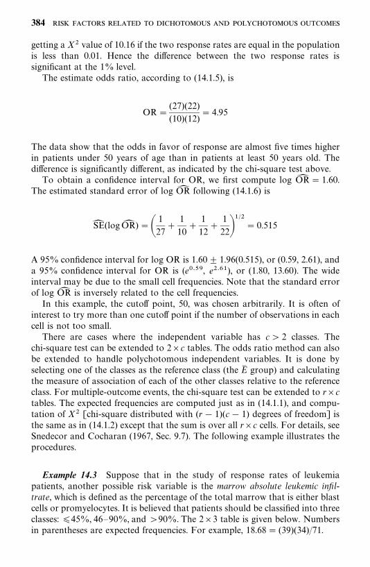
getting a X� value of 10.16 if the two response rates are equal in the populationis less than 0.01. Hence the difference between the two response rates issignificant at the 1% level.
The estimate odds ratio, according to (14.1.5), is
OR�(27)(22)(10)(12)
� 4.95
The data show that the odds in favor of response are almost five times higherin patients under 50 years of age than in patients at least 50 years old. Thedifference is significantly different, as indicated by the chi-square test above.
To obtain a confidence interval for OR, we first compute log OR� � 1.60.The estimated standard error of log OR� following (14.1.6) is
SE� (logOR� ) ��1
27�
1
10�
1
12�
1
22����
� 0.515
A 95% confidence interval for log OR is 1.60 1.96(0.515), or (0.59, 2.61), anda 95% confidence interval for OR is (e�� , e����), or (1.80, 13.60). The wideinterval may be due to the small cell frequencies. Note that the standard errorof log OR� is inversely related to the cell frequencies.
In this example, the cutoff point, 50, was chosen arbitrarily. It is often ofinterest to try more than one cutoff point if the number of observations in eachcell is not too small.
There are cases where the independent variable has c� 2 classes. Thechi-square test can be extended to 2�c tables. The odds ratio method can alsobe extended to handle polychotomous independent variables. It is done byselecting one of the classes as the reference class (the E� group) and calculatingthe measure of association of each of the other classes relative to the referenceclass. For multiple-outcome events, the chi-square test can be extended to r�ctables. The expected frequencies are computed just as in (14.1.1), and compu-tation of X� [chi-square distributed with (r � 1)(c� 1) degrees of freedom] isthe same as in (14.1.2) except that the sum is over all r�c cells. For details, seeSnedecor and Cocharan (1967, Sec. 9.7). The following example illustrates theprocedures.
Example 14.3 Suppose that in the study of response rates of leukemiapatients, another possible risk variable is the marrow absolute leukemic infil-trate, which is defined as the percentage of the total marrow that is either blastcells or promyelocytes. It is believed that patients should be classified into threeclasses: 45%, 46—90%, and �90%. The 2�3 table is given below. Numbersin parentheses are expected frequencies. For example, 18.68� (39)(34)/71.
384
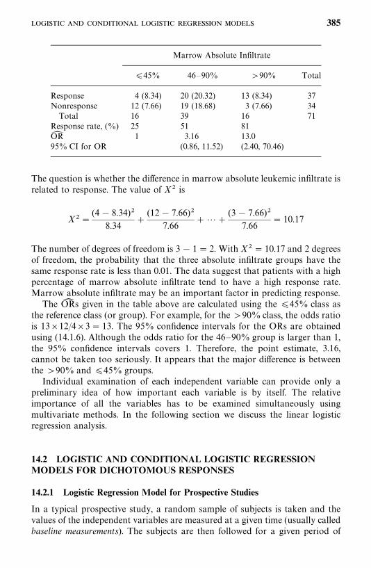
Marrow Absolute Infiltrate
45% 46—90% �90% Total
Response 4 (8.34) 20 (20.32) 13 (8.34) 37Nonresponse 12 (7.66) 19 (18.68) 3 (7.66) 34Total 16 39 16 71
Response rate, (%) 25 51 81OR� 1 3.16 13.095% CI for OR (0.86, 11.52) (2.40, 70.46)
The question is whether the difference in marrow absolute leukemic infiltrate isrelated to response. The value of X� is
X��(4� 8.34)�
8.34�
(12� 7.66)�7.66
� ��(3� 7.66)�
7.66� 10.17
The number of degrees of freedom is 3� 1� 2. With X� � 10.17 and 2 degreesof freedom, the probability that the three absolute infiltrate groups have thesame response rate is less than 0.01. The data suggest that patients with a highpercentage of marrow absolute infiltrate tend to have a high response rate.Marrow absolute infiltrate may be an important factor in predicting response.
The OR� s given in the table above are calculated using the 45% class asthe reference class (or group). For example, for the �90% class, the odds ratiois 13�12/4�3� 13. The 95% confidence intervals for the ORs are obtainedusing (14.1.6). Although the odds ratio for the 46—90% group is larger than 1,the 95% confidence intervals covers 1. Therefore, the point estimate, 3.16,cannot be taken too seriously. It appears that the major difference is betweenthe �90% and 45% groups.
Individual examination of each independent variable can provide only apreliminary idea of how important each variable is by itself. The relativeimportance of all the variables has to be examined simultaneously usingmultivariate methods. In the following section we discuss the linear logisticregression analysis.
14.2 LOGISTIC AND CONDITIONAL LOGISTIC REGRESSIONMODELS FOR DICHOTOMOUS RESPONSES
14.2.1 Logistic Regression Model for Prospective Studies
In a typical prospective study, a random sample of subjects is taken and thevalues of the independent variables are measured at a given time (usually calledbaseline measurements). The subjects are then followed for a given period of
385
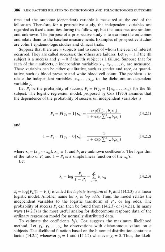
time and the outcome (dependent) variable is measured at the end of thefollow-up. Therefore, for a prospective study, the independent variables areregarded as fixed quantities during the follow-up, but the outcomes are randomand unknown. The purpose of a prospective study is to examine the outcomesand relate them to the baseline measurements. Examples of prospective studiesare cohort epidemiologic studies and clinical trials.
Suppose that there are n subjects and to some of whom the event of interestoccurred. They are called successes; the others are failures. Let y
�� 1 if the ith
subject is a success and y�� 0 if the ith subject is a failure. Suppose that for
each of the n subjects, p independent variables x��, x
��, . . . , x
��are measured.
These variables can be either qualitative, such as gender and race, or quanti-tative, such as blood pressure and white blood cell count. The problem is torelate the independent variables, x
��, . . . , x
��, to the dichotomous dependent
variable y�.
Let P�be the probability of success, P
��P(y
�� 1 � x
��, . . . , x
��), for the ith
subject. The logistic regression model, proposed by Cox (1970) assumes thatthe dependence of the probability of success on independent variables is
P�� P( y
�� 1 �x
�) �
exp(����
b�x��)
1� exp(����
b�x��)
(14.2.1)
and
1�P�� P( y
�� 0 �x
�) �
1
1� exp(����
b�x��)
(14.2.2)
where x�� (x
�� x
��), x
�� 1, and b
�are unknown coefficients. The logarithm
of the ratio of P�and 1�P
�is a simple linear function of the x
��’s.
Let
��� log
P�
1�P�
�����
b�x��
(14.2.3)
��� log[P
�/(1 �P
�)] is called the logistic transform of P
�and (14.2.3) is a linear
logistic model. Another name for ��is log odds. Thus, the model relates the
independent variables to the logistic transform of P�, or log odds. The
probability of success P�can then be found from (14.2.3) or (14.2.1). In many
ways (14.2.3) is the most useful analog for dichotomous response data of theordinary regression model for normally distributed data.
To estimate the coefficients b�’s, Cox suggests the maximum likelihood
method. Let y�, y
�, . . . , y
�be observations with dichotomous values on n
subjects. The likelihood function based on the binomial distribution contains afactor (14.2.1) whenever y
�� 1 and (14.2.2) whenever y
�� 0. Thus, the likeli-
386
hood function is
L (b, b
�, . . . , b
�) �
�����
P���(1 �P
�)����
���
���exp(y
���
��b�x��)
�����
[1� exp(����
b�x��)]
�exp(��
��b�t�)
�����
[1� exp(����
b�x��)]
(14.2.4)
where t�� ��
���x��y�. The log-likelihood function is
l(b, b
�, . . . , b
�) � log L �
����
b�t��
�����
log�1� exp�����
b�x���� (14.2.5)
The maximum likelihood estimates of b�’s that maximize the log-likelihood
function in (14.2.5) can be obtained by solving the following p equationssimultaneously:
t��
�����
x��exp(��
��b�x��)
1� exp(����
b�x��)� 0 j � 0, 1, . . . , p (14.2.6)
This can be done by an iterative procedure such as the Newton—Raphsonprocedure. The second derivative of l in (14.2.5) is
I*����
� �l
b��
b��
�������
x���
x���exp(��
��b�x��)
1� exp(����
b�x��)
j�� 0, . . . , p; j
�� 0, . . . , p (14.2.7)
Let I����
� (�1)I*����
. Then the estimated inverse of the I matrix, I� ��, is theasymptotic covariance matrix of the b
�’s. If we use the notation in Section 7.1
and let b� � (b�, b�
�, . . . , b�
�)� denote the MLE of b, the estimated covariance
matrix of the MLE b� is V� (b� ) � (v��) � (� �l (b� )/ b b�)�� � I� ��, where v
��denotes the ijth element of V� (b� ) or the ijth element of I� ��.
The coefficients so obtained indicate the relationships between the variablesand the log odds in favor of success. For a continuous variable, the correspond-ing coefficient gives the change in the log odds for an increase of 1 unit in thevariable. For a categorical variable, the coefficient is equal to the log odds ratio(see Section 14.1).
An approximate 100(1� �)% confidence interval for b�is
b�� Z����v
��(14.2.8)
where Z��� is the 100(1� �/2) percentile of the standard normal distribution.
387
To test the hypothesis that some of the b�’s are zero, a likelihood ratio test
can be used. For example, to test H: b
�� 0, the log-likelihood ratio test
statistic is
X���2[l(b�
, b�
�, . . . , b�
���, 0, b�
��, . . . , b�
�) � l (b�
, b�
�, b�
�, . . . , b�
�)]
(14.2.9)
where the first term is the maximized log-likelihood subject to the constraintb�� 0. If the hypothesis is true, X
�is distributed asymptotically as chi-square
with 1 degree of freedom.An alternative test for the significance of the coefficients is the Wald test,
which can be written as
X
�b� ��
v��
(14.2.10)
Under the null hypothesis that b�� 0, X
has an asymptotic chi-square
distribution with 1 degree of freedom. Although the Wald test is used by many,it is less powerful than the likelihood ratio test (Hauck and Donner, 1977;Jennings, 1986). In other words, the Wald test often leads the user to concludethat the coefficient (consequently, the respective risk factor) is not significantwhen, in fact, it is significant.
Similar to earlier discussion of model selection, forward, backward, andstepwise variable selection methods can be used to select the risk factors thatare significantly associated with a dichotomous response. The independentvariables x
��in this model do not have to be the original variables. They can
be any meaningful transforms of the original variables: for example, thelogarithm of the original variable, logx
��, and the deviation of the variable
from its mean, x��� x�
�.
From (14.2.1) and (14.2.2), the logarithm of the odds ratio for ith and kthsubjects is
logP�/(1 �P
�)
P�/(1 �P
�)�
�����
b�(x
���x
��) (14.2.11)
Thus, an estimate of the odds ratio can be obtained by replacing b�in (14.2.11)
with its MLE, b��.
From the estimated regression equation, a predicted probability of successcan be computed by substituting the values of the risk factors in the equation.Using these predicted probabilities, a goodness-of-fit test can be performed totest the hypothesis that the model fits the data adequately. Several such testsare available (Lemeshow and Hosmer, 2000): for example, the Pearson chi-square test, the Hosmer—Lemeshow (Hosmer and Lemeshow, 1980) test, a teststatistic suggested by Tsiatis (1980), and the score of Brown (1982). In thefollowing, we introduce the Hosmer—L emeshow test.
388
Let p�be the estimate of P
�obtained from the fitted logistic regression
equation for the ith subject, i � 1, . . . , n. The p�’s can be arranged in ascending
order from smallest to largest. Those probabilities and the correspondingsubjects are then divided into g groups according to some cutoff points of theprobability. For example, let g� 10 and the cutoff points of the probability beequal to k/10, k� 1, 2, . . . , 10. Thus, the first group contains all subjects whoseestimated probabilities are less than or equal to 0.1, the second group containsall subjects whose estimated probabilities are less than or equal to 0.2, and soon. Let n
�be the number of subjects in the kth group. The estimated expected
number of successes for the kth group is
E��
������
p�
k � 1, 2, . . . , g
The Hosmer—Lemeshow test statistic is defined as
C������
(O��E
�)�
n�p��(1 � p�
�)
(14.2.12)
where O�is the observed number of successes in the kth group and p�
�is the
average estimated probability of the kth group, that is,
p���
1
n�
������
p�
Under the null hypothesis that the model is adequate, the distribution of C in(14.2.12) is well approximated by the chi-square distribution with g� 2 degreesof freedom. The test is basically a chi-square test of the discrepancy betweenthe observed and predicted frequencies of success. Thus, a C value larger thanthe 100� percentage point of the chi-square distribution (or p value less than�) indicates that the model is inadequate.
Similar to other chi-square goodness-of-fit tests, the approximation dependson the estimated expected frequencies being reasonably large. If a large number(say, far more than 20%) of the expected frequencies are less than 5, theapproximation may not be appropriate and the p value must be interpretedcarefully. If this is the case, adjacent groups may be combined to increase theestimated expected frequencies. However, Hosmer and Lemeshow warn that iffewer than six groups are used to calculate C, the test would be insensitive andwould almost always indicate that the model is adequate.
Most statistical software packages provide programs for logistic regressionanalysis: for example, SAS (procedures LOGISTIC, PHREG, and CATMOD),BMDP (procedures LR and PR), and SPSS (procedures NOMREG, PROBIT,PLUM, and LOGISTIC). Most of them provide estimates of the coefficientsand test statistics, variable selection procedures, and tests of goodness of fit.
389
Example 14.4 In a study of 238 non-insulin-dependent diabetic patients,10 covariates are considered possible risk factors for proteinuria (the outcomevariable). The logistic regression method is used to identify the most importantrisk factors and to predict the probability of proteinuria on the basis of theserisk factors. The 10 potential risk factors are age, gender (1, male; 2, female),smoking status (0, no; 1, yes), percentage of ideal body mass index, hyperten-sion (0, no; 1, yes), use of insulin (0, no; 1, yes), glucose control (0, no; 1, yes),duration of diabetes mellitus (DM) in years, total cholesterol, and totaltriglyceride. Among the 238 patients, 69 have proteinuria (y
�� 1).
Using the stepwise procedure in BMDP, it is estimated that at step 1, themodel contains only b
and b�
� �0.896 and l(b�
) in (14.2.5) is �143.292. At
step 2, duration of diabetes is added to the model because its maximumlog-likelihood value is the largest among all the covariates. The MLEs of thetwo coefficients are b�
��1.467 and b�
���0.055, and l(b�
, b�
�) ��139.429.
Since
X���2[l(b�
) � l(b�
, b�
�)] � 7.726
which is significant (p� 0.005), the duration of DM is related significantly tothe chance of proteinuria. The Hosmer—Lemeshow test statistic for goodness offit with only duration of DM in the model, C� 9.814 with 8 degrees offreedom, gives a p value of 0.278.
At step 3, gender is added to the model because its addition yields the largestmaximum log-likelihood value among all the remaining covariates. The maxi-mum log-likelihood value, l(b�
, b�
�, b�
�) ��137.749, b�
��1.453, b�
���0.060,
and b����0.279. To test if gender is significantly related to proteinuria after
duration of DM, we perform the likelihood ratio test
X���2[l(b�
, b�
�) � l(b�
, b�
�, b�
�)] � 3.360
which is significant at p � 0.067. The stepwise procedure terminates after thethird step because no other covariates are significant enough to enter theregression model; that is, none of the other covariates have a p value less than0.15, which is set by the program (BMDP). If any covariate already in theregression becomes insignificant after some other variables are in, the insignifi-cant variable would be removed. The p values for entering and removing avariable can be determined by the user. The default values for entering andremoving a variable are, respectively, 0.10 and 0.15. Thus, the procedureidentifies duration of DM and gender as the two most important risk factorsbased on the data given. A question that may be raised at this point is whetherone should include gender in the equation since its significance level is largerthan the commonly used 0.05. The recommendation is to include it since it isclose to 0.05 and since the p value should not be the only basis for determiningwhether a covariate should be included in the model. In addition, theHosmer—Lemeshow goodness of fit test statistic C � 5.036, when gender is
390
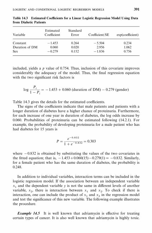
Table 14.3 Estimated Coefficients for a Linear Logistic Regression Model Using Datafrom Diabetic Patients
Estimated StandardVariable Coefficient Error Coefficient/SE exp(coefficient)
Constant �1.453 0.264 �5.504 0.234Duration of DM 0.060 0.020 2.956 1.062Sex �0.279 0.152 �1.836 0.756
included, yields a p value of 0.754. Thus, inclusion of this covariate improvesconsiderably the adequacy of the model. Thus, the final regression equationwith the two significant risk factors is
logP�
1�P�
��1.453� 0.060 (duration of DM) � 0.279 (gender)
Table 14.3 gives the details for the estimated coefficients.The signs of the coefficients indicate that male patients and patients with a
longer duration of diabetes have a higher chance of proteinuria. Furthermore,for each increase of one year in duration of diabetes, the log odds increase by0.060. Probabilities of proteinuria can be estimated following (14.2.1). Forexample, the probability of developing proteinuria for a male patient who hashad diabetes for 15 years is
P �e�����
1� e������ 0.303
where �0.832 is obtained by substituting the values of the two covariates inthe fitted equation; that is, �1.453�0.060(15)�0.279(1)��0.832. Similarly,for a female patient who has the same duration of diabetes, the probability is0.248.
In addition to individual variables, interaction terms can be included in thelogistic regression model. If the association between an independent variablex�and the dependent variable y is not the same in different levels of another
variable, x�, there is interaction between x
�and x
�. To check if there is
interaction, one can include the product of x�and x
�in the regression model
and test the significance of this new variable. The following example illustratesthe procedure.
Example 14.5 It is well known that adriamycin is effective for treatingcertain types of cancer. It is also well known that adriamycin is highly toxic.
391
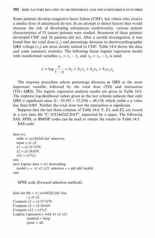
Some patients develop congestive heart failure (CHF), but others who receivea similar dose of adriamycin do not. In an attempt to detect factors that wouldincrease the risk of developing adriamycin cardotoxicity, various patientcharacteristics of 53 cancer patients were studied. Seventeen of these patientsdeveloped CHF and 36 patients did not. After a careful investigation, it wasfound that the total dose (z
�) and percentage decrease in electrocardiographic
QRS voltage (z�) are most closely related to CHF. Table 14.4 shows the data
and some summary statistics. The following linear logistic regression modelwith transformed variables z
�� z
�� z�
�and x
�� z
�� z�
�is used:
�� logp
1� p� b
� b
�x�� b
�x�� b
�x�x�
The stepwise procedure selects percentage decrease in QRS as the mostimportant variable, followed by the total dose (TD) and interaction(TD�QRS). The logistic regression analysis results are given in Table 14.5.The stepwise log-likelihood values given in the last column indicate that onlyQRS is significant since 2(�10.185� 33.254)� 46.138, which yields a p valueless than 0.001. Neither the total dose nor the interaction is significant.
Suppose that the last three columns of Table 14.4, Y, Z1, and Z2, are storedin a text data file ‘‘C:�EX14d2d2.DAT’’, separated by a space. The followingSAS, SPSS, or BMDP codes can be used to obtain the results in Table 14.5.
SAS code:
data w1;infile ‘c:�ex14d2d2.dat’ missover;input y z1 z2;x1� z1-517.679;x2� z2-26.019;x12� x1*x2;
run;proc logistic data�w1 descending;model y� x1 x2 x12/ selection� s plcl plrl lackfit;
run;
SPSS code (forward selection method):
data list file� ‘c:�ex14d2d2.dat’ free/ y z1 z2.
Compute x1� z1-517.679.Compute x2� z2-26.019.Compute x12� x1*x2.Logistic regression y with x1 x2 x12
/method� fstep/print� all.
392
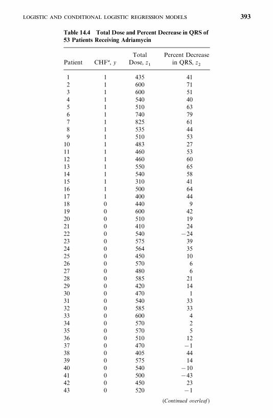
Table 14.4 Total Dose and Percent Decrease in QRS of53 Patients Receiving Adriamycin
Total Percent DecreasePatient CHF , y Dose, z
�in QRS, z
�
1 1 435 412 1 600 713 1 600 514 1 540 405 1 510 636 1 740 797 1 825 618 1 535 449 1 510 5310 1 483 2711 1 460 5312 1 460 6013 1 550 6514 1 540 5815 1 310 4116 1 500 6417 1 400 4418 0 440 919 0 600 4220 0 510 1921 0 410 2422 0 540 �2423 0 575 3924 0 564 3525 0 450 1026 0 570 627 0 480 628 0 585 2129 0 420 1430 0 470 131 0 540 3332 0 585 3333 0 600 434 0 570 235 0 570 536 0 510 1237 0 470 �138 0 405 4439 0 575 1440 0 540 �1041 0 500 �4342 0 450 2343 0 520 �1
(Continued overleaf )
393
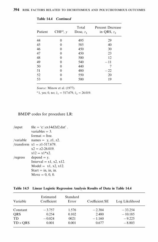
Table 14.4 Continued
Total Percent DecreasePatient CHF , y Dose, z
�in QRS, z
�
44 0 495 2945 0 585 4046 0 450 3047 0 450 2348 0 500 1249 0 540 �1150 0 440 751 0 480 �2252 0 550 2053 0 500 19
Source: Minow et al. (1977).
1, yes; 0, no; z��� 517.679, z�
�� 26.019.
Table 14.5 Linear Logistic Regression Analysis Results of Data in Table 14.4
Estimated StandardVariable Coefficient Error Coefficient/SE Log Likelihood
Constant �3.757 1.576 �2.384 �33.254QRS 0.254 0.102 2.480 �10.185TD �0.024 0021 �1.160 �9.225TD�QRS 0.001 0.001 0.677 �8.803
BMDP codes for procedure LR:
/input file� ‘c:�ex14d2d2.dat’ .variables� 3.format� free.
/variable names� y, z1, z2./transform x1� z1-517.679.
x2� z2-26.019.x12� x1*x2.
/regress depend� y.Interval� x1, x2, x12.Model� x1, x2, x12.Start� in, in, in.Move� 0, 0, 0.
394
Method�mlr./print cell�used./end
When the independent variables are dichotomous or polychotomous, thelogistic regression coefficients can be linked with odds ratios. Consider thesimplest case, where there is one independent variable, x
�, which is either 0 or
1. The linear regression model in (14.2.1) and (14.2.2) becomes
P(y� 1 � x�) �
eb�b
�x�
1� eb�b
�x�
P(y � 0 � x�) �
1
1� eb�b
�x�
Values of the model when x�� 0, 1 are
P(y� 1 �x�� 0) �
eb
1� eb
P(y � 1 � x�� 1) �
eb�b
�
1� eb�b
�
P(y � 0 � x�� 0) �
1
1� eb
P(y � 0 � x�� 1) �
1
1� eb�b
�
The odds ratio in (14.1.4) is
OR�P(y� 1 � x
�� 1)/P( y� 0 �x
�� 1)
P(y� 1 � x�� 0)/P( y� 0 �x
�� 0)
�eb
�b
�
eb
� eb�
and the log odds ratio is log(OR) � log(eb�) � b
�[this can also be derived
directly from (14.2.11)]. Thus, the estimated logistic regression coefficient alsoprovides an estimate of the odds ratio, that is, OR� � eb�
�. If (b��, b
��) is the
confidence interval for b�, the corresponding interval for OR is (eb
��, eb��).
Example 14.6 Consider the age (x) and response (y) data from the 71leukemia patients presented in Table 14.6 (Examples 14.1 and 14.2). Thelogistic regression analysis results are given in Table 14.7. Notice thatexp(b
�) � exp(1.5994)� 4.95, which is equal to the estimate of OR obtained in
Example 14.2 using (14.1.5), and the standard error of b��is the same as that
of logOR� except for a small rounding-off error. The confidence interval for ORcan also be obtained from the logistic regression analysis results.
395
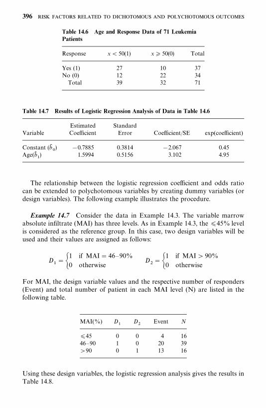
Table 14.6 Age and Response Data of 71 LeukemiaPatients
Response x� 50(1) x 50(0) Total
Yes (1) 27 10 37No (0) 12 22 34Total 39 32 71
Table 14.7 Results of Logistic Regression Analysis of Data in Table 14.6
Estimated StandardVariable Coefficient Error Coefficient/SE exp(coefficient)
Constant (b�) �0.7885 0.3814 �2.067 0.45
Age(b��) 1.5994 0.5156 3.102 4.95
The relationship between the logistic regression coefficient and odds ratiocan be extended to polychotomous variables by creating dummy variables (ordesign variables). The following example illustrates the procedure.
Example 14.7 Consider the data in Example 14.3. The variable marrowabsolute infiltrate (MAI) has three levels. As in Example 14.3, the 45% levelis considered as the reference group. In this case, two design variables will beused and their values are assigned as follows:
D���
1 if MAI� 46—90%
0 otherwiseD
���
1 if MAI� 90%
0 otherwise
For MAI, the design variable values and the respective number of responders(Event) and total number of patient in each MAI level (N) are listed in thefollowing table.
MAI(%) D�
D�
Event N
45 0 0 4 1646—90 1 0 20 39�90 0 1 13 16
Using these design variables, the logistic regression analysis gives the results inTable 14.8.
396
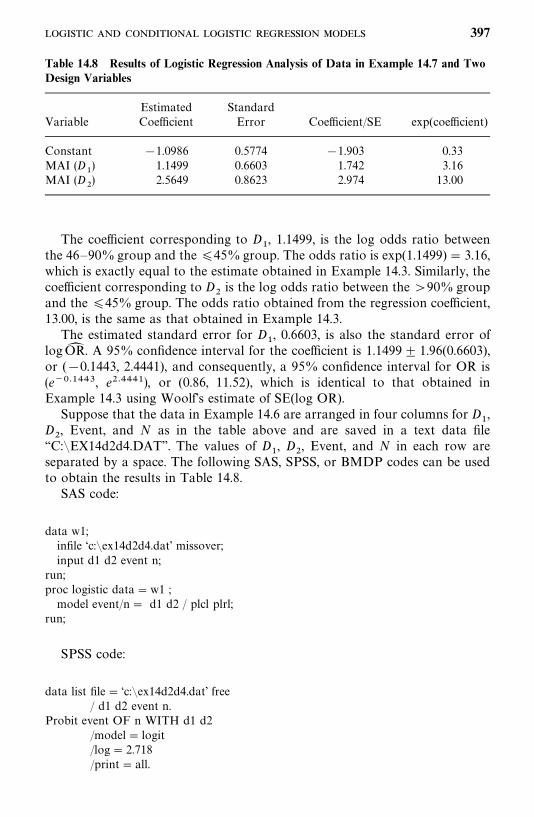
Table 14.8 Results of Logistic Regression Analysis of Data in Example 14.7 and TwoDesign Variables
Estimated StandardVariable Coefficient Error Coefficient/SE exp(coefficient)
Constant �1.0986 0.5774 �1.903 0.33MAI (D
�) 1.1499 0.6603 1.742 3.16
MAI (D�) 2.5649 0.8623 2.974 13.00
The coefficient corresponding to D�, 1.1499, is the log odds ratio between
the 46—90% group and the 45%group. The odds ratio is exp(1.1499)� 3.16,which is exactly equal to the estimate obtained in Example 14.3. Similarly, thecoefficient corresponding to D
�is the log odds ratio between the �90% group
and the 45% group. The odds ratio obtained from the regression coefficient,13.00, is the same as that obtained in Example 14.3.
The estimated standard error for D�, 0.6603, is also the standard error of
logOR� . A 95% confidence interval for the coefficient is 1.1499 1.96(0.6603),or (�0.1443, 2.4441), and consequently, a 95% confidence interval for OR is(e������, e������), or (0.86, 11.52), which is identical to that obtained inExample 14.3 using Woolf’s estimate of SE(log OR).
Suppose that the data in Example 14.6 are arranged in four columns for D�,
D�, Event, and N as in the table above and are saved in a text data file
‘‘C:�EX14d2d4.DAT’’. The values of D�, D
�, Event, and N in each row are
separated by a space. The following SAS, SPSS, or BMDP codes can be usedto obtain the results in Table 14.8.
SAS code:
data w1;infile ‘c:�ex14d2d4.dat’ missover;input d1 d2 event n;
run;proc logistic data�w1 ;model event/n� d1 d2 / plcl plrl;
run;
SPSS code:
data list file� ‘c:�ex14d2d4.dat’ free/ d1 d2 event n.
Probit event OF n WITH d1 d2/model� logit/log� 2.718/print� all.
397
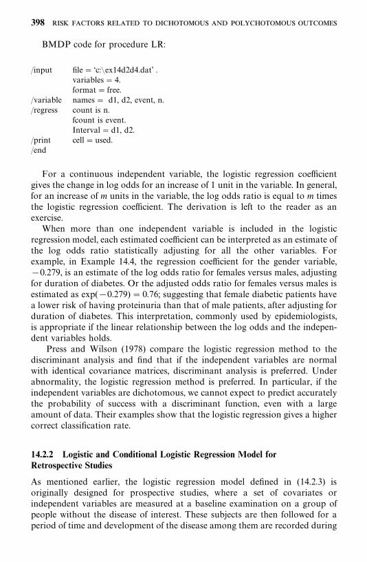
BMDP code for procedure LR:
/input file� ‘c:�ex14d2d4.dat’ .variables� 4.format� free.
/variable names� d1, d2, event, n./regress count is n.
fcount is event.Interval�d1, d2.
/print cell�used./end
For a continuous independent variable, the logistic regression coefficientgives the change in log odds for an increase of 1 unit in the variable. In general,for an increase of m units in the variable, the log odds ratio is equal to m timesthe logistic regression coefficient. The derivation is left to the reader as anexercise.
When more than one independent variable is included in the logisticregression model, each estimated coefficient can be interpreted as an estimate ofthe log odds ratio statistically adjusting for all the other variables. Forexample, in Example 14.4, the regression coefficient for the gender variable,�0.279, is an estimate of the log odds ratio for females versus males, adjustingfor duration of diabetes. Or the adjusted odds ratio for females versus males isestimated as exp(�0.279) � 0.76; suggesting that female diabetic patients havea lower risk of having proteinuria than that of male patients, after adjusting forduration of diabetes. This interpretation, commonly used by epidemiologists,is appropriate if the linear relationship between the log odds and the indepen-dent variables holds.
Press and Wilson (1978) compare the logistic regression method to thediscriminant analysis and find that if the independent variables are normalwith identical covariance matrices, discriminant analysis is preferred. Underabnormality, the logistic regression method is preferred. In particular, if theindependent variables are dichotomous, we cannot expect to predict accuratelythe probability of success with a discriminant function, even with a largeamount of data. Their examples show that the logistic regression gives a highercorrect classification rate.
14.2.2 Logistic and Conditional Logistic Regression Model forRetrospective Studies
As mentioned earlier, the logistic regression model defined in (14.2.3) isoriginally designed for prospective studies, where a set of covariates orindependent variables are measured at a baseline examination on a group ofpeople without the disease of interest. These subjects are then followed for aperiod of time and development of the disease among them are recorded during
398
follow-up. The model can be extended to analyze data from retrospectivestudies, such as a case—control study. In a case—control study, cases (subjectswith the disease of interest) and controls (subjects without the disease) are firstselected and risk factor data such as exposure variables and other covariatesare collected retrospectively. For example, in a case—control study of lungcancer and cigarette smoking, a group of lung cancer patients and a group ofpeople without lung cancer are selected. Their smoking histories are thencollected along with other risk factors. Therefore, in a case—control study,participants are selected first based on their disease status, and their history ofrisk factor exposures is collected later. The purpose of a case—control study isto estimate the association between the risk factors and the disease understudy. Using probability terms, we are dealing with the probability that the riskfactors take on certain values given that a person is a case or a control. Wedenote this conditional probability by P(x � y), where x denote the covariatesand y the outcome variable. Using the same notation, the probability ofinterest in a prospective study is P(y � x). Based on conditional probabilitytheory, P(x � y) can be written as
P(x � y) �P(y � x)P(x)
P(y)(14.2.13)
where y� 1 for cases and 0 for controls. Thus, P(x � y) is a function of P( y �x),P(x), and P(y).
The likelihood function of the logistic regression model for a retrospectivestudy, similar to (14.2.4), is the product of terms in the form of P(x � y) in(14.2.13) for the cases and controls selected [(P(x � y� 1) from a case andP(x � y� 0) from a control)]. We introduce here two most widely usedapproaches to this likelihood function. One approach considers the probabilityof case/control selection. Since in case—control studies, the cases and controlsare selected from the population and the likelihood function is based on subjectselection, we introduce an indicator variable to denote whether a person isselected (s � 1) or is not selected (s� 0). Let n
�and n
be, respectively, the
numbers of selected cases and controls in the study. The likelihood function is
L��
�������
P(x�� y
�� 1, s� 1)
�����
P(x�� y
�� 0, s � 1) (14.2.14)
Define
���P(s � 1 � y� 1)
to be the probability that a diseased person is selected for the study as a caseand
��P(s � 1 � y� 0)
399
to be the probability that a disease-free person is selected for the study as acontrol. Assume that the sampling probabilities depend only on disease statusand not on the covariates. Using Bayes’ theorem in probability theory and(14.2.1), it can be shown (the derivation is left to the reader as an exercise) thatthe probability that a person is diseased given that he or she has risk factorsx and was selected for the study can be written as
P(y�� 1 �x
�, s� 1) �
exp(b*� ��
���b�x��)
1� exp(b*
������
b�x��)
(14.2.15)
where
b*� b
� log
��
�
(14.2.16)
According to the conditional probability in (14.2.13), the first term in thelikelihood function in (14.2.14) is
P(x�� y
�� 1, s� 1) �
exp(b*� ��
���b�x��)
1� exp(b*
������
b�x��) �
P(x�� s� 1)
P(y� 1 � s� 1)� (14.2.17)
Similarly, the second term in (14.2.14) for y�� 0 can be obtained:
P(x�� y
�� 0, s� 1) �
1
1� exp(b*� ��
���b�x��) �
P(x�� s� 1)
P( y � 0 � s� 1)� (14.2.18)
Substituting (14.2.17) and (14.2.18) into (14.2.14), we obtain the likelihoodfunction for a case—control study:
L��
� L (b*, b
�, . . . , b
�)�
�����
P(x�� s� 1)
P(y � s � 1)(14.2.19)
where n � n� n
�, L (b*
, b
�, . . . , b
�) is the likelihood function for prospective
studies in (14.2.4) except that the intercept term bis replaced by b*
in
(14.2.16). If we assume that the probability distribution of the covariates, P(x),contains no information about the parameters of interest, or P(x) is indepen-dent of the coefficients b
�, and the selection is independent of x, then
maximizing L��to obtain estimates of b
�is equivalent to maximizing only L (b*
,
b�, . . . , b
�) since P(y� 1 � s � 1) � n
�/n and P(y� 0 � s� 1) � n
/n. This im-
plies that we can use the computer program for prospective studies to analyzecase—control study data except that the intercept term cannot be interpretedmeaningfully unless �
�and �
are known.
In most practical situations, the assumption made above about P(x) isreasonable. Historically, in early applications of the logistic regression method,the covariates were assumed to have multivariate normal distribution. Then
400
estimation of the coefficients, b�in (14.2.19), would involve the distribution P(x)
and thus became much more complicated. However, in practice, many of thecovariates are categorical or discrete and are therefore distinctly nonnormal.Thus, it is appropriate to allow P(x) to remain completely arbitrary and usesimply L (b*
, b
�, . . . , b
�) in (14.2.19) in case—control studies.
Another approach to the likelihood function based on (14.2.13) is toconsider a conditional probability instead. Suppose that n
�cases and n
controls were selected in a case—control study and n � n
�� n
; let x
�,
x�, . . . , x
�be the risk factor sets of the n subjects without specifying which of
them pertain to the cases and which to the controls. Then the conditionalprobability that the first n
�x’s are observed from the n
�cases and the
remainder are from the ncontrols may be written as
������
P(x�� y � 1) ��
�����P(x
�� y � 0)
��l�,...,l
���(���
���P(x
��� y� 1) ��
�����P(x
��
� y� 0))(14.2.20)
where the summation in the denominator is over the n!/(n�! n
!) possible ways
of selecting n�individuals as cases from the n subjects, with the remaining n
as controls. By using (14.2.13) and (14.2.1), (14.2.20) reduces to
������
exp(�����
b�x��)
��l�,...,l
��� ���
���exp(��
���b�x���)
(14.2.21)
Comparing with (12.1.17), (14.2.21) can be considered as a special case of(12.1.17) in which there is only one distinct uncensored failure time, say att� 1, and all of the n
�persons failed at t� 1. The remaining n
subjects
survive longer than 1 and are censored, say at t� 2, while all n subjects are atrisk at t� 1. This interpretation of (14.2.21) permits us to apply the methodand computer software for the Cox proportional hazards model with a discretetime scale and ties to obtain an estimate of b in the logistic regression modeland to perform the corresponding inferences. The procedure is illustrated inExample 14.8. When n
�and n
are large enough, it can be shown that an
analysis based on this conditional probability will produce results equivalent tothose based on the likelihood function defined in (14.2.19) (Efron, 1975;Farewell, 1979; Breslow and Day, 1980). When n
�and n
are large, one may
prefer using (14.2.19) to (14.2.21) since the former is easier. However, for acase—control study with a matched or stratified design, analysis based on theconditional probability defined in (14.2.21) is a better choice than (14.2.19)(Efron, 1975; Farewell, 1979; Breslow and Day, 1980). In the following sectionwe discuss the application of logistic regression analysis for two widelyaccepted matched designs in case—control studies.
1 : R Matched DesignA widely used case—control design is to have one or more controls matched
401
for each case based on matching variables such as age and gender. Supposethat for each case there are R(1) matched controls. Let x
���denote the
observed value of the jth covariate ( j� 1, . . . , p) from the kth subject (k� 1for the case and k � 2, . . . ,R � 1 for matched controls) in the ith matched set(i � 1, . . . , n). The n matched sets are considered as the samples from the ndifferent strata defined by the matching variables. Following (14.2.21) withn�� 1 and n
�R, the conditional probability for the matched set (1 case and
R controls) in the ith stratum is
exp(�����
b�x���)
exp(�����
b�x���) � ���
���exp(��
���b�x���)�
1
1�������
exp[�����
b�(x
����x
���)]
(14.2.22)
and thus the conditional likelihood function for all n strata is the product ofthe n terms in (14.2.22), that is,
�����
1
1� ������
exp[�����
b�(x
���� x
���)]
(14.2.23)
When R� 1, that is, a one-to-one pair matching, the conditional likelihoodfunction obtained from (14.2.23) reduces to
L (b�, . . . , b
�)�
�����
1
1�exp[�����
b�(x
����x
���)]
��
����
exp[�����
b�(x
����x
���)]
1�exp[�����
b�(x
����x
���)]
(14.2.24)
Compared with the likelihood function for the ordinary logistic regression in(14.2.4), the conditional likelihood function (14.2.24) can be treated as a specialcase of (14.2.4) with y
�� 1, b
� 0, and x
��can be replaced by the difference in
x��between the case and its matched control. This fact permits the use of
computer programs for ordinary logistic regression in one-to-one matchedcase—control studies. The procedure is as follows:
1. Let n be the number of case—control pairs.
2. Use x���
� x���, the difference between covariates for the case (x
���) and
its matched control (x���
), as the independent variable in the model.
3. Let y�� 1 for all pairs.
4. Delete the intercept term bfrom the model.
402
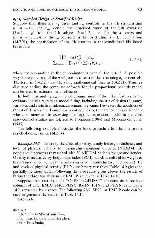
n1 : n0 Matched Design or Stratified DesignSuppose that there are n
�cases and n
controls in the ith stratum and
n� n�� n
. Let x
���denote the observed value of the jth covariate
( j� 1, . . . , p) from the kth subject (k� 1, 2, . . . , n�for the n
�cases and
k� n�� 1, . . . , n for the n
controls) in the ith stratum (i � 1, . . . ,m). From
(14.2.21), the contribution of the ith stratum to the conditional likelihoodfunction is
������
exp(�����
b�x���)
��k�,...,k
��� ���
���exp(��
���b�x���
�
)(14.2.25)
where the summation in the denominator is over all the n!/(n�! n
!) possible
ways to select n�out of the n subjects as cases and the remaining n
as controls.
The term in (14.2.25) has the same mathematical form as (14.2.21). Thus, asdiscussed earlier, the computer software for the proportional hazards modelcan be used to estimate the coefficients.
In both 1 :R and n�: n
matched designs, most of the other features in the
ordinary logistic regression model fitting, including the use of design (dummy)variables and statistical inferences, remain the same. However, the goodness offit test of Hosmer and Lemeshow is not applicable to matched designs. Readerswho are interested in assessing the logistic regression model in matchedcase—control studies are referred to Pregibon (1984) and Moolgavkar et al.(1985).
The following example illustrates the basic procedure for the one-to-onematched design using (14.2.24).
Example 14.8 To study the effect of obesity, family history of diabetes, andlevel of physical activity to non-insulin-dependent diabetes (NIDDM), 30nondiabetic persons are matched with 30 NIDDM patients by age and gender.Obesity is measured by body mass index (BMI), which is defined as weight inkilograms divided by height in meters squared. Family history of diabetes (FH)and levels of physical activity (PHY) are binary variables. Table 14.9 gives thepartially fictitious data. Following the procedure given above, the results offitting the three variables using BMDP are given in Table 14.10.
Suppose that text data file ‘‘C:�EX14d2d5.DAT’’ contains six successivecolumns of data: BMIC, FHC, PHYC, BMIN, FHN, and PHYN, as in Table14.9, separated by a space. The following SAS, SPSS, or BMDP code can beused to generate the results in Table 14.10.
SAS code:
data w1;infile ‘c:�ex14d2d5.dat’ missover;input bmic fhc phyc bmin fhn phyn;bmi� bmic-bmin;
403
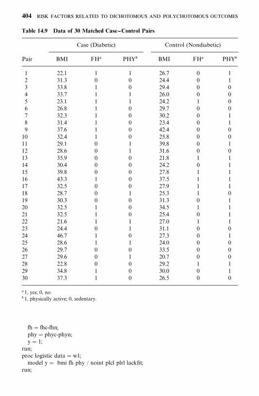
Table 14.9 Data of 30 Matched Case--Control Pairs
Case (Diabetic) Control (Nondiabetic)
Pair BMI FH PHY� BMI FH PHY�
1 22.1 1 1 26.7 0 12 31.3 0 0 24.4 0 13 33.8 1 0 29.4 0 04 33.7 1 1 26.0 0 05 23.1 1 1 24.2 1 06 26.8 1 0 29.7 0 07 32.3 1 0 30.2 0 18 31.4 1 0 23.4 0 19 37.6 1 0 42.4 0 010 32.4 1 0 25.8 0 011 29.1 0 1 39.8 0 112 28.6 0 1 31.6 0 013 35.9 0 0 21.8 1 114 30.4 0 0 24.2 0 115 39.8 0 0 27.8 1 116 43.3 1 0 37.5 1 117 32.5 0 0 27.9 1 118 28.7 0 1 25.3 1 019 30.3 0 0 31.3 0 120 32.5 1 0 34.5 1 121 32.5 1 0 25.4 0 122 21.6 1 1 27.0 1 123 24.4 0 1 31.1 0 024 46.7 1 0 27.3 0 125 28.6 1 1 24.0 0 026 29.7 0 0 33.5 0 027 29.6 0 1 20.7 0 028 22.8 0 0 29.2 1 129 34.8 1 0 30.0 0 130 37.3 1 0 26.5 0 0
1, yes; 0, no.� 1, physically active; 0, sedentary.
fh� fhc-fhn;phy�phyc-phyn;y� 1;
run;proc logistic data�w1;model y� bmi fh phy / noint plcl plrl lackfit;
run;
404
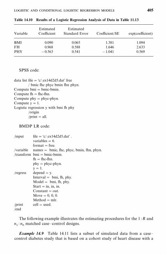
Table 14.10 Results of a Logistic Regression Analysis of Data in Table 11.13
Estimated EstimatedVariable Coefficient Standard Error Coefficient/SE exp(coefficient)
BMI 0.090 0.065 1.381 1.094FH 0.968 0.588 1.646 2.633PHY �0.563 0.541 �1.041 0.569
SPSS code:
data list file� ‘c:�ex14d2d5.dat’ free/ bmic fhc phyc bmin fhn phyn.
Compute bmi�bmic-bmin.Compute fh� fhc-fhn.Compute phy�phyc-phyn.Compute y� 1.Logistic regression y with bmi fh phy
/origin/print� all.
BMDP LR code:
/input file� ‘c:�ex14d2d5.dat’ .variables� 6.format� free.
/variable names� bmic, fhc, phyc, bmin, fhn, phyn./transform bmi� bmic-bmin.
fh� fhc-fhn.phy�phyc-phyn.y� 1.
/regress depend� y.Interval� bmi, fh, phy.Model� bmi, fh, phy.Start� in, in, in.Constant�out.Move� 0, 0, 0.Method�mlr.
/print cell�used./end
The following example illustrates the estimating procedures for the 1 :R andn�: n
matched case—control designs.
Example 14.9 Table 14.11 lists a subset of simulated data from a case—control diabetes study that is based on a cohort study of heart disease with a
405
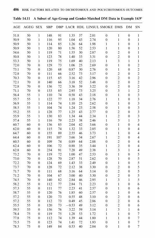
Table 14.11 A Subset of Age-Group and Gender-Matched DM Data in Example 14.9
AGE AGEG SEX SBP DBP LACR HDL LINSUL SMOKE DMS DM SN
51.8 50 1 148 91 1.35 37 2.81 0 1 0 150.9 50 1 116 95 1.04 43 2.74 0 1 0 150.9 50 1 114 85 1.26 64 1.98 1 1 0 150.9 50 1 120 80 1.56 52 2.53 1 1 0 154.6 50 1 119 71 1.55 30 2.87 0 2 0 150.8 50 1 123 78 1.40 33 3.31 0 2 0 153.3 50 1 119 75 1.69 40 2.13 1 3 1 172.0 70 0 129 73 1.06 25 2.69 0 1 0 273.1 70 0 120 68 0.87 30 2.76 0 1 0 272.8 70 0 111 66 2.52 73 3.17 0 2 0 270.3 70 0 115 65 3.16 42 2.96 0 2 0 272.1 70 0 140 66 3.18 52 3.48 0 2 0 272.8 70 0 136 72 3.36 59 3.22 0 2 0 271.1 70 0 133 85 2.95 73 3.25 0 3 1 256.4 55 1 110 74 0.58 43 2.18 0 1 0 355.7 55 1 122 77 1.18 34 2.76 1 1 0 356.9 55 1 114 74 1.10 25 2.62 0 1 0 358.5 55 1 104 74 1.24 23 2.58 0 1 0 355.2 55 1 128 77 1.25 43 2.77 0 2 0 355.9 55 1 130 83 1.34 44 2.34 1 2 0 357.4 55 1 116 79 2.23 38 2.46 1 3 1 360.7 60 0 136 85 2.04 42 3.66 0 1 0 462.0 60 0 115 74 1.32 33 2.85 0 1 0 464.7 60 0 155 89 2.55 46 3.73 1 1 0 464.4 60 0 191 107 3.66 34 2.67 1 2 0 460.5 60 0 109 74 0.89 64 2.88 0 2 0 462.4 60 0 106 72 0.88 35 3.44 1 2 0 462.8 60 0 234 91 7.28 49 2.38 1 3 1 473.2 70 0 119 72 1.00 47 2.53 0 1 0 573.0 70 0 128 70 2.87 51 2.62 0 1 0 572.2 70 0 124 69 1.43 33 2.49 0 1 0 573.7 70 0 128 72 2.12 38 3.30 0 2 0 571.7 70 0 111 68 3.16 64 3.14 0 2 0 571.2 70 0 104 67 3.00 40 3.30 0 2 0 574.5 70 0 140 82 2.84 46 2.95 1 3 1 558.2 55 0 112 77 2.84 71 2.23 0 1 0 657.3 55 0 111 77 2.23 41 2.57 0 1 0 658.7 55 0 120 76 1.85 60 2.57 0 1 0 657.2 55 0 120 73 0.55 48 3.10 0 2 0 657.2 55 0 112 73 0.49 45 2.86 0 2 0 655.5 55 0 120 73 �0.53 49 3.12 0 2 0 659.5 55 0 156 76 3.22 59 3.14 1 3 1 678.4 75 0 119 75 1.28 53 1.72 1 1 0 777.8 75 0 112 74 1.39 44 1.80 1 1 0 775.5 75 0 123 74 1.41 72 1.93 0 1 0 778.3 75 0 149 84 0.53 40 2.84 0 1 0 7
406
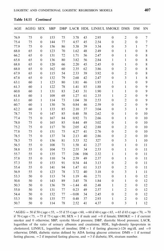
Table 14.11 Continued
AGE AGEG SEX SBP DBP LACR HDL LINSUL SMOKE DMS DM SN
76.9 75 0 153 75 3.78 43 2.95 0 2 0 775.4 75 0 144 77 4.57 45 2.54 0 2 0 777.9 75 0 156 86 5.38 39 3.34 0 3 1 768.0 65 0 123 70 1.62 48 2.49 0 1 0 866.2 65 0 131 72 1.71 56 2.47 0 1 0 865.8 65 0 136 80 3.82 56 2.84 1 1 0 868.8 65 0 120 66 2.20 45 2.45 0 1 0 868.0 65 0 162 60 2.35 62 3.86 0 2 0 867.9 65 0 115 54 2.33 39 3.92 0 2 0 867.8 65 0 132 79 2.68 42 2.47 0 3 1 863.1 60 1 123 80 1.81 46 1.93 1 1 0 961.3 60 1 122 78 1.41 85 1.88 0 1 0 960.8 60 1 131 83 2.43 31 1.90 1 1 0 961.8 60 1 109 69 1.27 61 2.35 1 2 0 963.1 60 1 114 73 1.04 38 2.53 0 2 0 960.7 60 1 130 76 0.84 46 2.59 0 2 0 962.2 60 1 133 85 2.10 37 3.04 0 3 1 978.7 75 0 147 85 0.48 58 2.62 0 1 0 1077.4 75 0 167 84 0.92 71 2.66 0 1 0 1078.0 75 0 165 85 0.44 49 3.02 0 1 0 1075.2 75 0 117 70 2.05 42 2.88 0 2 0 1077.8 75 0 151 75 4.27 41 2.76 0 2 0 1078.5 75 0 137 74 2.13 40 2.86 0 2 0 1078.5 75 0 156 81 5.33 52 327 0 3 1 1056.5 55 0 108 71 1.58 41 2.27 0 1 0 1158.8 55 0 104 73 2.55 34 2.53 0 1 0 1155.7 55 0 135 77 2.06 106 2.32 1 1 0 1157.8 55 0 110 74 2.59 49 2.37 0 1 0 1157.3 55 0 153 91 0.54 44 3.13 0 2 0 1155.4 55 0 141 94 1.47 61 3.15 0 2 0 1156.9 55 0 123 78 3.72 40 3.18 0 3 1 1153.3 50 0 113 74 1.19 46 2.71 0 1 0 1250.8 50 0 143 89 3.45 78 1.84 0 1 0 1250.3 50 0 136 79 �1.44 48 2.48 1 2 0 1255.0 50 0 131 77 0.23 49 2.57 1 2 0 1254.4 50 0 132 77 �0.08 34 2.45 0 2 0 1253.3 50 0 135 77 0.48 37 2.93 1 2 0 1250.7 50 0 114 78 2.52 41 4.37 0 3 1 12
AGEG� 50 if 50age�55, �55 if 55age�60, �60 if 60age�65, �65 if 65age�70, �70if 70age�75, �75 if 75age�80; SEX� 1 if male and �0 if female; SMOKE� 1 if currentsmoker and 0 otherwise; SBP, systolic blood pressure; DBP, diastolic blood pressure; LACR,logarithm of the ratio of urinary albumin and creatinine; HDL, high-density lipoprotein incholesterol; LINSUL, logarithm of insuline; DM� 1 if fasting glucose126 mg/dL and �0otherwise; DMS, diabetic status defined by ADA fasting glucose criterion: DMS� 1 if normalfasting glucose, �2 if impaired fasting glucose, and �3 if diabetic; SN, stratum number.
407
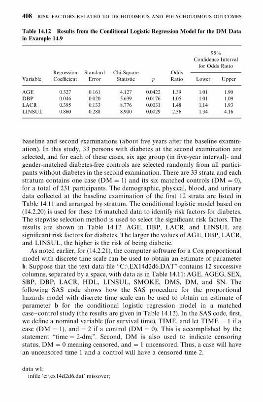
Table 14.12 Results from the Conditional Logistic Regression Model for the DM Datain Example 14.9
95%Confidence Intervalfor Odds Ratio
Regression Standard Chi-Square OddsVariable Coefficient Error Statistic p Ratio Lower Upper
AGE 0.327 0.161 4.127 0.0422 1.39 1.01 1.90DBP 0.046 0.020 5.639 0.0176 1.05 1.01 1.09LACR 0.395 0.133 8.776 0.0031 1.48 1.14 1.93LINSUL 0.860 0.288 8.900 0.0029 2.36 1.34 4.16
baseline and second examinations (about five years after the baseline examin-ation). In this study, 33 persons with diabetes at the second examination areselected, and for each of these cases, six age group (in five-year interval)- andgender-matched diabetes-free controls are selected randomly from all partici-pants without diabetes in the second examination. There are 33 strata and eachstratum contains one case (DM� 1) and its six matched controls (DM� 0),for a total of 231 participants. The demographic, physical, blood, and urinarydata collected at the baseline examination of the first 12 strata are listed inTable 14.11 and arranged by stratum. The conditional logistic model based on(14.2.20) is used for these 1:6 matched data to identify risk factors for diabetes.The stepwise selection method is used to select the significant risk factors. Theresults are shown in Table 14.12. AGE, DBP, LACR, and LINSUL aresignificant risk factors for diabetes. The larger the values of AGE, DBP, LACR,and LINSUL, the higher is the risk of being diabetic.
As noted earlier, for (14.2.21), the computer software for a Cox proportionalmodel with discrete time scale can be used to obtain an estimate of parameterb. Suppose that the text data file ‘‘C:�EX14d2d6.DAT’’ contains 12 successivecolumns, separated by a space, with data as in Table 14.11: AGE, AGEG, SEX,SBP, DBP, LACR, HDL, LINSUL, SMOKE, DMS, DM, and SN. Thefollowing SAS code shows how the SAS procedure for the proportionalhazards model with discrete time scale can be used to obtain an estimate ofparameter b for the conditional logistic regression model in a matchedcase—control study (the results are given in Table 14.12). In the SAS code, first,we define a nominal variable (for survival time), TIME, and let TIME� 1 if acase (DM� 1), and� 2 if a control (DM� 0). This is accomplished by thestatement ‘‘time� 2-dm;’’. Second, DM is also used to indicate censoringstatus, DM� 0 meaning censored, and� 1 uncensored. Thus, a case will havean uncensored time 1 and a control will have a censored time 2.
data w1;infile ‘c:�ex14d2d6.dat’ missover;
408
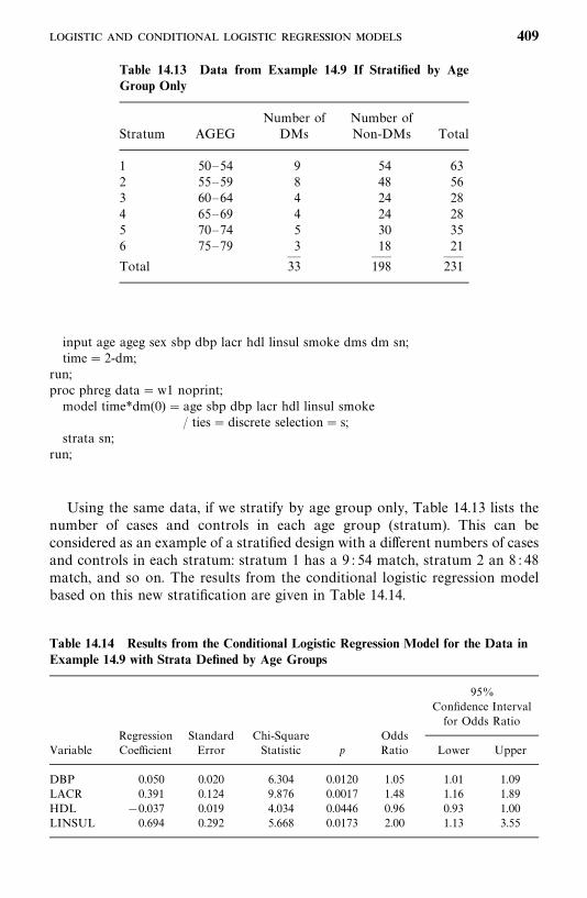
Table 14.13 Data from Example 14.9 If Stratified by AgeGroup Only
Number of Number ofStratum AGEG DMs Non-DMs Total
1 50—54 9 54 632 55—59 8 48 563 60—64 4 24 284 65—69 4 24 285 70—74 5 30 356 75—79 3 18 21
— —— ——Total 33 198 231
Table 14.14 Results from the Conditional Logistic Regression Model for the Data inExample 14.9 with Strata Defined by Age Groups
95%Confidence Intervalfor Odds Ratio
Regression Standard Chi-Square OddsVariable Coefficient Error Statistic p Ratio Lower Upper
DBP 0.050 0.020 6.304 0.0120 1.05 1.01 1.09LACR 0.391 0.124 9.876 0.0017 1.48 1.16 1.89HDL �0.037 0.019 4.034 0.0446 0.96 0.93 1.00LINSUL 0.694 0.292 5.668 0.0173 2.00 1.13 3.55
input age ageg sex sbp dbp lacr hdl linsul smoke dms dm sn;time� 2-dm;
run;proc phreg data�w1 noprint;model time*dm(0) � age sbp dbp lacr hdl linsul smoke
/ ties�discrete selection� s;strata sn;
run;
Using the same data, if we stratify by age group only, Table 14.13 lists thenumber of cases and controls in each age group (stratum). This can beconsidered as an example of a stratified design with a different numbers of casesand controls in each stratum: stratum 1 has a 9 : 54 match, stratum 2 an 8 : 48match, and so on. The results from the conditional logistic regression modelbased on this new stratification are given in Table 14.14.
409
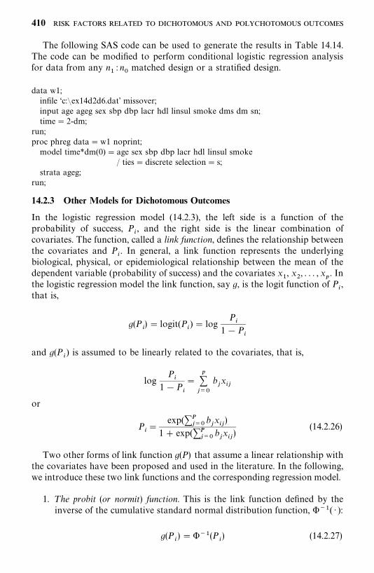
The following SAS code can be used to generate the results in Table 14.14.The code can be modified to perform conditional logistic regression analysisfor data from any n
�: n
matched design or a stratified design.
data w1;infile ‘c:�ex14d2d6.dat’ missover;input age ageg sex sbp dbp lacr hdl linsul smoke dms dm sn;time� 2-dm;
run;proc phreg data�w1 noprint;model time*dm(0) � age sex sbp dbp lacr hdl linsul smoke
/ ties�discrete selection� s;strata ageg;
run;
14.2.3 Other Models for Dichotomous Outcomes
In the logistic regression model (14.2.3), the left side is a function of theprobability of success, P
�, and the right side is the linear combination of
covariates. The function, called a link function, defines the relationship betweenthe covariates and P
�. In general, a link function represents the underlying
biological, physical, or epidemiological relationship between the mean of thedependent variable (probability of success) and the covariates x
�, x
�, . . . , x
�. In
the logistic regression model the link function, say g, is the logit function of P�,
that is,
g(P�) � logit(P
�) � log
P�
1�P�
and g(P�) is assumed to be linearly related to the covariates, that is,
logP�
1�P�
�����
b�x��
or
P��
exp(����
b�x��)
1� exp(����
b�x��)
(14.2.26)
Two other forms of link function g(P) that assume a linear relationship withthe covariates have been proposed and used in the literature. In the following,we introduce these two link functions and the corresponding regression model.
1. T he probit (or normit) function. This is the link function defined by theinverse of the cumulative standard normal distribution function, ���( · ):
g(P�) ����(P
�) (14.2.27)
410
The corresponding model is
���(P�) �
����
b�x��
or
P��� �
�����
b�x��� (14.2.28)
2. The complementary log-log link function. This function is defined by
g(P�) � log[�log(1�P
�)] (14.2.29)
The corresponding model is
log[�log(1�P�)]�
����
b�x��
or
P�� 1� exp ��exp�
����
b�x���� (14.2.30)
The logistic regression model in (14.2.26) is for binary outcomes such asdiseased versus nondiseased. The model (14.2.28) can be thought of as analternative model for binary outcome. In addition, it can be used to modelthose binary outcomes that are defined by a cutoff point on the basis of anormally distributed variable. For example, the cutoff point may be defined bythe last quintile or quartile of a continuous measurement in an epidemiologicalstudy. When the binary outcomes are defined by a cutoff point in anasymmetric distribution, the model in (14.2.30) may be appropriate. The model(14.2.30) can also be considered as a version of the Cox proportional hazardsmodel for grouped survival times (Kalbfleisch and Prentice, 1973).
Let y�, y
�, . . . , y
�be the observations with dichotomous values on the n
subjects: y�� 1 for success and y
�� 0 for failure. Similar to (14.2.4), the
likelihood functions for the models in (14.2.28) and (14.2.30) can be obtainedby replacing the corresponding P
�in the following formula:
L (b, b
�, . . . , b
�) �
�����
P���(1 �P
�)����
The MLEs of the coefficients and the asymptotic likelihood inferences aresimilar to those given in Section 14.2.1 for the ordinary logistic regressionmodel except that interpretation of the odds ratio is not possible for the lattertwo models. The procedure LOGISTIC in SAS provides options for all threemodels.
411
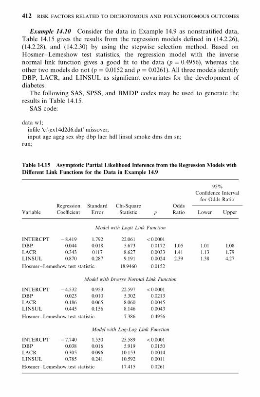
Table 14.15 Asymptotic Partial Likelihood Inference from the Regression Models withDifferent Link Functions for the Data in Example 14.9
95%Confidence Intervalfor Odds Ratio
Regression Standard Chi-Square OddsVariable Coefficient Error Statistic p Ratio Lower Upper
Model with L ogit L ink Function
INTERCPT �8.419 1.792 22.061 �0.0001DBP 0.044 0.018 5.673 0.0172 1.05 1.01 1.08LACR 0.343 0117 8.627 0.0033 1.41 1.13 1.79LINSUL 0.870 0.287 9.191 0.0024 2.39 1.38 4.27
Hosmer—Lemeshow test statistic 18.9460 0.0152
Model with Inverse Normal Link Function
INTERCPT �4.532 0.953 22.597 �0.0001DBP 0.023 0.010 5.302 0.0213LACR 0.186 0.065 8.060 0.0045LINSUL 0.445 0.156 8.146 0.0043
Hosmer—Lemeshow test statistic 7.386 0.4956
Model with Log-Log Link Function
INTERCPT �7.740 1.530 25.589 �0.0001DBP 0.038 0.016 5.919 0.0150LACR 0.305 0.096 10.153 0.0014LINSUL 0.785 0.241 10.592 0.0011
Hosmer—Lemeshow test statistic 17.415 0.0261
Example 14.10 Consider the data in Example 14.9 as nonstratified data,Table 14.15 gives the results from the regression models defined in (14.2.26),(14.2.28), and (14.2.30) by using the stepwise selection method. Based onHosmer—Lemeshow test statistics, the regression model with the inversenormal link function gives a good fit to the data (p � 0.4956), whereas theother two models do not (p� 0.0152 and p� 0.0261). All three models identifyDBP, LACR, and LINSUL as significant covariates for the development ofdiabetes.
The following SAS, SPSS, and BMDP codes may be used to generate theresults in Table 14.15.
SAS code:
data w1;infile ‘c:�ex14d2d6.dat’ missover;input age ageg sex sbp dbp lacr hdl linsul smoke dms dm sn;
run;
412
title ‘‘Regression model with the logit link function-generalized logistic regression’’;proc logistic data�w1 descending;model dm� age sex sbp dbp lacr hdl linsul smoke
/ selection� s lackfit link� logit;run;title ‘‘Regression model with the inverse normal link function‘;proc logistic data�w1 descending;model dm� age sex sbp dbp lacr hdl linsul smoke
/ selection� s lackfit link�probit;run;title ‘‘Regression model with the log-log link funtion‘;proc logistic data�w1 descending;model dm� age sex sbp dbp lacr hdl linsul smoke
/ selection� s lackfit link� cloglog;run;
SPSS code for the model in (14.2.28) with the forward selection method:
data list file� ‘c:�ex14d2d6.dat’ free/ age ageg sex sbp dbp lacr hdl linsul smoke dms dm sn.
Logistic regression dm with age sex sbp dbp lacr hdl linsul smoke htn/method� fstep/print� all.
BMDP code for procedure LR and the model in (14.2.28):
/input file� ‘c:�ex14d2d6.dat’ .variables� 12.format� free.
/variable names� age, ageg, sex, sbp, dbp, lacr, hdl, linsul, smoke,dms, dm, sn.
Use� age, sex to smoke./regress depend�dm.
Interval� age, sex to smoke.Method�mlr.
/print cell�used./end
14.3 MODELS FOR POLYCHOTOMOUS OUTCOMES
The regression models in Section 14.2 can be extended to handle outcomes thathave more than two categories. These categories may be nominal, for example,different types of heart disease or psychological conditions; or ordinal, forexample, different levels of glucose intolerance or different severity of communi-cation disorders. An outcome variable with more than two possibilities is calledpolychotomous or polytomous. In this section we discuss first the model for
413
nominal polychotomous outcomes (generalized logistic regression model), thenthe model for ordinal polychotomous outcomes (ordinal regression model).Details regarding these models can be found in Aitchison and Silvey (1957),McCullagh (1980), Green (1984), McCullagh and Nelder (1989), Hosmer andLemeshow (1989, 2000), Cox and Snell (1989), Afifi and Clark (1990), Agresti(1990), Collett (1991), and Ananth and Kleinbaum (1997).
14.3.1 Models for Nominal Polychotomous Outcomes:Generalized Logistic Regression Models
Let Y�denote the outcome for individual i. The outcome can be one of the m
nominal categories, such as different cell types of lung cancer. Let Y�� k denote
that Y�belongs to the kth category and k� 1, 2, . . . ,m. Suppose that for each
of n subjects, p independent variables x�� (x
��, x
��, . . . , x
��)� are measured.
These variables can be either qualitative or quantitative. Let P(Y�� k � x
�) be
the probability that Y�� k given the p measured covariates x
�; then
�����
P(Y�� k � x
�) � 1. Without loss of generality, using the last catalog as the
reference, the generalized logistic regression model
logP(Y
�� k �x
�)
P(Y�� m � x
�)� a
��
�����
b��
x��
k� 1, 2, . . . ,m � 1 (14.3.1)
can be used to study the association of the covariates x to the outcome. Tosimplify the notation, let u
��� a
����
���b��
x��. Similar to (14.2.1) and (14.2.2),
the model in (14.3.1) assumes that the dependence on the covariates of theprobability of being in the kth category is
P(Y�� k �x
�) ��
exp(u��
)1�����
���exp(u
��)
k� 1, 2, . . . ,m � 1
1
1��������
exp(u��)
k� m
(14.3.2)
This model reduces to the logistic regression model in (14.2.1) and (14.2.2)when m � 2.
Let k�, . . . , k
�be the outcomes observed for the n subjects. Then the
log-likelihood function based on the n outcomes observed is the logarithm ofthe product of all P(Y
�� k
��x
�)’s from the n subjects, that is,
l(a�, a
�, . . . , a
���, b
�, b
�, . . . , b
���) � log L � log �
�����
P(Y�� k
�� x
�)� (14.3.3)
where P(Y�� k
�� x
�) is given in (14.3.2) and b
�� (b
��, . . . , b
��)�, k � 1,
2, . . . ,m � 1. There are a total of (m� 1)(p� 1) unknown coefficients. Theestimation and hypothesis testing procedures for the coefficients are similar to
414
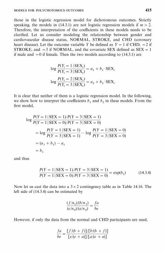
those in the logistic regression model for dichotomous outcomes. Strictlyspeaking, the models in (14.3.1) are not logistic regression models if m � 2.Therefore, the interpretation of the coefficients in these models needs to beclarified. Let us consider modeling the relationship between gender andcardiovascular disease status, NORMAL, STROKE, and CHD (coronaryheart disease). Let the outcome variable Y be defined as Y � 1 if CHD, �2 ifSTROKE, and �3 if NORMAL, and the covariate SEX defined as SEX� 1if male and �0 if female. Then the two models according to (14.3.1) are
logP(Y
�� 1 � SEX
�)
P(Y�� 3 � SEX
�)� a
�� b
�· SEX
�
logP(Y
�� 2 �SEX
�)
P(Y�� 3 �SEX
�)� a
�� b
�· SEX
�
It is clear that neither of them is a logistic regression model. In the following,we show how to interpret the coefficients b
�and b
�in these models. From the
first model,
logP(Y � 1 � SEX� 1)/P(Y � 3 �SEX� 1)P(Y � 1 � SEX� 0)/P(Y � 3 �SEX� 0)
� logP(Y � 1 �SEX� 1)P(Y � 3 �SEX� 1)
� logP(Y � 1 �SEX� 0)P(Y � 3 �SEX� 0)
� (a�� b
�) � a
�� b
�
and thus
P(Y � 1 � SEX� 1)/P(Y � 3 � SEX� 1)P(Y � 1 � SEX� 0)/P(Y � 3 � SEX� 0)
� exp(b�) (14.3.4)
Now let us cast the data into a 3�2 contingency table as in Table 14.16. Theleft side of (14.3.4) can be estimated by
( f /n�)/(b/n
�)
(e/n)/(a/n
)�
fa
be
However, if only the data from the normal and CHD participants are used,
fa
be�
[ f /(b � f )]/[b/(b � f )]
[e/(e � a)]/[a/(e � a)]
415
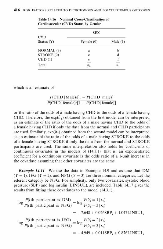
Table 14.16 Nominal Cross-Classification ofCardiovascular (CVD) Status by Gender
SEXCVDStatus (Y) Female (0) Male (1)
NORMAL (3) a bSTROKE (2) c dCHD (1) e f
— —Total n
n�
which is an estimate of
P(CHD �Male)/[1�P(CHD �male)]P(CHD � female)/[1�P(CHD � female)]
or the ratio of the odds of a male having CHD to the odds of a female havingCHD. Therefore, the exp(b�
�) obtained from the first model can be interpreted
as an estimate of the ratio of the odds of a male having CHD to the odds ofa female having CHD if only the data from the normal and CHD participantsare used. Similarly, exp(b�
�) obtained from the second model can be interpreted
as an estimate of the ratio of the odds of a male having STROKE to the oddsof a female having STROKE if only the data from the normal and STROKEparticipants are used. The same interpretation also holds for coefficients ofcontinuous covariates in the models of (14.3.1); that is, an exponentiatedcoefficient for a continuous covariate is the odds ratio of a 1-unit increase inthe covariate assuming that other covariates are the same.
Example 14.11 We use the data in Example 14.9 and assume that DM(Y � 1), IFG (Y � 2), and NFG (Y � 3) are three nominal categories. Let thereferent category be NFG. For simplicity, only two covariates, systolic bloodpressure (SBP) and log insulin (LINSUL), are included. Table 14.17 gives theresults from fitting these covariates to the model (14.3.1).
logP(i th participant is DM)P(i th participant is NFG)
� logP(Y
�� 1 � x
�)
P(Y�� 3 � x
�)
��7.648� 0.026SBP�� 1.047LINSUL
�
logP(i th participant is IFG)P(i th participant is NFG)
� logP(Y
�� 2 � x
�)
P(Y�� 3 � x
�)
��4.949� 0.011SBP�� 0.876LINSUL
�
416
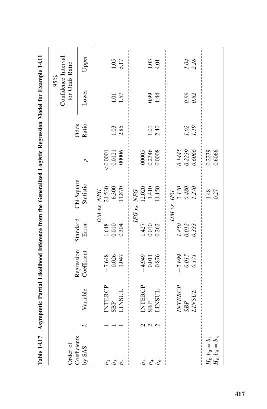
Tab
le14.17
Asymptotic
Partial
Likelihoo
dInferencefrom
theGeneralized
Log
isticRegressionMod
elforExa
mple14
.11
95%
Confidence
Interval
Order
offorOddsRatio
Coefficients
Regression
Standard
Chi-Square
Odds
bySAS
kVariable
Coefficient
Error
Statistic
pRatio
Lower
Upper
DM
vs.
NF
Gb �
1IN
TERCP
�7.648
1.648
21.530
�0.0001
b �1
SBP
0.026
0.010
6.300
0.0121
1.03
1.01
1.05
b �1
LIN
SUL
1.047
0.304
11.870
00006
2.85
1.57
5.17
----------------------------------------------------------------------------------------------------------
IFG
vs.
NF
Gb �
2IN
TERCP
�4.949
1.427
12.020
00005
b �2
SBP
0.011
0.010
1.410
0.2346
1.01
0.99
1.03
b �2
LIN
SUL
0.876
0.262
11.150
0.0008
2.40
1.44
4.01
----------------------------------------------------------------------------------------------------------
DM
vs.
IFG
INT
ER
CP
�2.
699
1.85
02.
130
0.14
45S
BP
0.01
50.
012
0.48
00.
2239
1.02
0.99
1.04
LIN
SU
L0.
171
0.33
31.
270
0.60
661.
190.
622.
28--
----
----
----
----
----
----
----
----
----
----
----
----
----
----
----
----
----
----
----
----
----
----
----
----
----
----
H:
b ��
b �1.48
0.2239
H:
b ��
b �0.27
0.6066
417
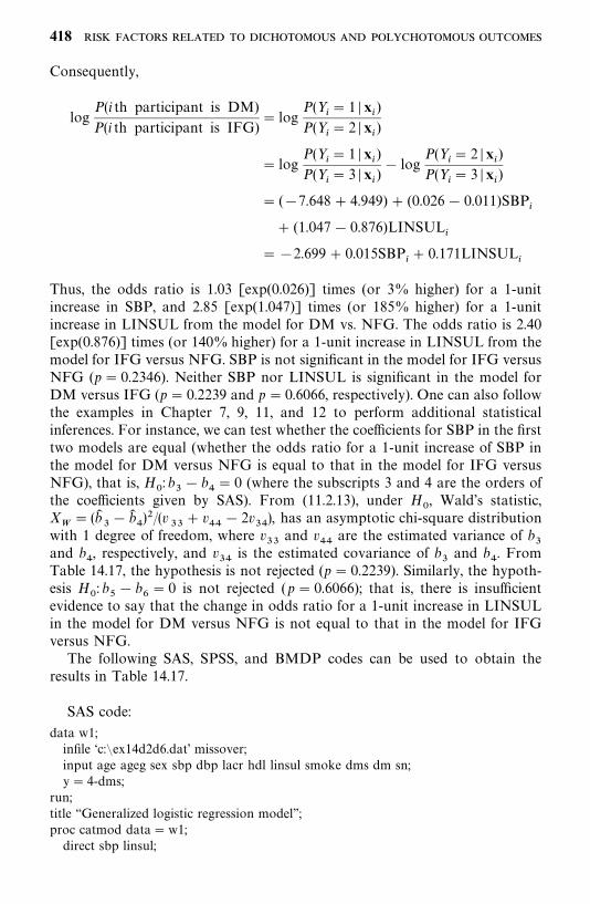
Consequently,
logP(i th participant is DM)P(i th participant is IFG)
� logP(Y
�� 1 � x
�)
P(Y�� 2 � x
�)
� logP(Y
�� 1 � x
�)
P(Y�� 3 � x
�)� log
P(Y�� 2 �x
�)
P(Y�� 3 �x
�)
� (�7.648� 4.949) � (0.026� 0.011)SBP�
� (1.047� 0.876)LINSUL�
��2.699� 0.015SBP�� 0.171LINSUL
�
Thus, the odds ratio is 1.03 [exp(0.026)] times (or 3% higher) for a 1-unitincrease in SBP, and 2.85 [exp(1.047)] times (or 185% higher) for a 1-unitincrease in LINSUL from the model for DM vs. NFG. The odds ratio is 2.40[exp(0.876)] times (or 140% higher) for a 1-unit increase in LINSUL from themodel for IFG versus NFG. SBP is not significant in the model for IFG versusNFG (p� 0.2346). Neither SBP nor LINSUL is significant in the model forDM versus IFG (p � 0.2239 and p � 0.6066, respectively). One can also followthe examples in Chapter 7, 9, 11, and 12 to perform additional statisticalinferences. For instance, we can test whether the coefficients for SBP in the firsttwo models are equal (whether the odds ratio for a 1-unit increase of SBP inthe model for DM versus NFG is equal to that in the model for IFG versusNFG), that is, H
: b
�� b
�� 0 (where the subscripts 3 and 4 are the orders of
the coefficients given by SAS). From (11.2.13), under H, Wald’s statistic,
X
� (b��� b�
�)�/(v
��� v
��� 2v
��), has an asymptotic chi-square distribution
with 1 degree of freedom, where v��
and v��
are the estimated variance of b�
and b�, respectively, and v
��is the estimated covariance of b
�and b
�. From
Table 14.17, the hypothesis is not rejected (p � 0.2239). Similarly, the hypoth-esis H
: b
�� b
�� 0 is not rejected (p� 0.6066); that is, there is insufficient
evidence to say that the change in odds ratio for a 1-unit increase in LINSULin the model for DM versus NFG is not equal to that in the model for IFGversus NFG.
The following SAS, SPSS, and BMDP codes can be used to obtain theresults in Table 14.17.
SAS code:
data w1;infile ‘c:�ex14d2d6.dat’ missover;input age ageg sex sbp dbp lacr hdl linsul smoke dms dm sn;y� 4-dms;
run;title ‘‘Generalized logistic regression model’’;proc catmod data�w1;direct sbp linsul;
418
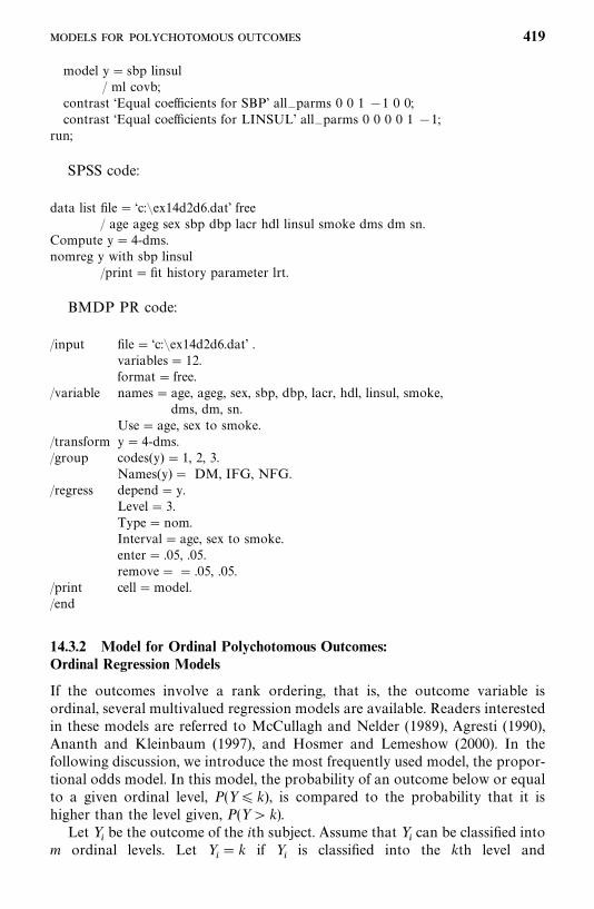
model y� sbp linsul/ ml covb;
contrast ‘Equal coefficients for SBP’ all—parms 0 0 1 �1 0 0;contrast ‘Equal coefficients for LINSUL’ all—parms 0 0 0 0 1 �1;
run;
SPSS code:
data list file� ‘c:�ex14d2d6.dat’ free/ age ageg sex sbp dbp lacr hdl linsul smoke dms dm sn.
Compute y� 4-dms.nomreg y with sbp linsul
/print�fit history parameter lrt.
BMDP PR code:
/input file� ‘c:�ex14d2d6.dat’ .variables� 12.format� free.
/variable names� age, ageg, sex, sbp, dbp, lacr, hdl, linsul, smoke,dms, dm, sn.
Use� age, sex to smoke./transform y� 4-dms./group codes(y) � 1, 2, 3.
Names(y) � DM, IFG, NFG./regress depend� y.
Level� 3.Type� nom.Interval� age, sex to smoke.enter� .05, .05.remove� � .05, .05.
/print cell�model./end
14.3.2 Model for Ordinal Polychotomous Outcomes:Ordinal Regression Models
If the outcomes involve a rank ordering, that is, the outcome variable isordinal, several multivalued regression models are available. Readers interestedin these models are referred to McCullagh and Nelder (1989), Agresti (1990),Ananth and Kleinbaum (1997), and Hosmer and Lemeshow (2000). In thefollowing discussion, we introduce the most frequently used model, the propor-tional odds model. In this model, the probability of an outcome below or equalto a given ordinal level, P(Y k), is compared to the probability that it ishigher than the level given, P(Y � k).
Let Y�be the outcome of the ith subject. Assume that Y
�can be classified into
m ordinal levels. Let Y�� k if Y
�is classified into the kth level and
419
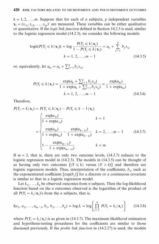
k� 1, 2, . . . ,m. Suppose that for each of n subjects, p independent variablesx�� (x
��, x
��, . . . , x
��)� are measured. These variables can be either qualitative
or quantitative. If the logit link function defined in Section 14.2.3 is used, similarto the logistic regression model (14.2.3), we consider the following models:
logit(P(Y� k � x
�)) � log
P(Y� k � x
�)
1�P(Y� k � x
�)� a
��
�����
b�x��
k� 1, 2, . . . ,m � 1 (14.3.5)
or, equivalently, let u��
� a����
���b�x��,
P(Y� k � x
�) �
exp(a����
���b�x��)
1� exp(a����
���b�x��)�
exp(u��)
1� exp(u��)
k� 1, 2, . . . ,m � 1 (14.3.6)
Therefore,
P(Y�� k � x
�) �P(Y
� k �x
�) �P(Y
� k � 1 � x
�)
��exp(u
��)
1� exp(u��)
k� 1
exp(u��)
1� exp(u��)�
exp(u����
)
1� exp(u����
)k� 2, . . . ,m� 1
1�exp(u
����)
1� exp(u����
)k�m
(14.3.7)
If m � 2, that is, there are only two outcome levels, (14.3.7) reduces to thelogistic regression model in (14.2.3). The models in (14.3.5) can be thought ofas having only two outcomes [(Y k ) versus (Y � k)] and therefore arelogistic regression models. Thus, interpretation of the coefficients, b
�, such as
the exponentiated coefficient [exp(b�)] for a discrete or a continuous covariate
is similar to that in a logistic regression model.Let k
�, . . . , k
�be observed outcomes from n subjects. Then the log-likelihood
function based on the n outcomes observed is the logarithm of the product ofall P(Y
�� k
��x
�)’s from the n subjects, that is,
l(a�, a
�, . . . , a
���, b
�, b
�, . . . , b
�) � log L � log�
�����
P(Y�� k
��x
�)� (14.3.8)
where P(Y�� k
��x
�) is as given in (14.3.7). The maximum likelihood estimation
and hypothesis-testing procedures for the coefficients are similar to thosediscussed previously. If the probit link function in (14.2.27) is used, the models
420
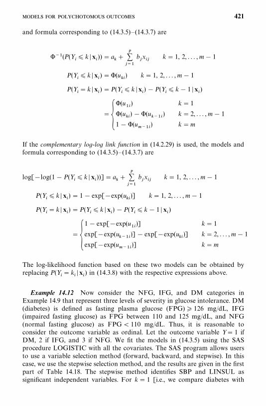
and formula corresponding to (14.3.5)—(14.3.7) are
���(P(Y� k �x
�)) � a
��
�����
b�x��
k � 1, 2, . . . ,m� 1
P(Y� k �x
�) ��(u
��) k� 1, 2, . . . ,m � 1
P(Y�� k �x
�) �P(Y
� k �x
�) �P(Y
� k� 1 �x
�)
���(u
��) k � 1
�(u��) ��(u
����) k � 2, . . . ,m � 1
1� �(u����
) k �m
If the complementary log-log link function in (14.2.29) is used, the models andformula corresponding to (14.3.5)—(14.3.7) are
log[�log(1� P(Y� k � x
�))]� a
��
�����
b�x��
k� 1, 2, . . . ,m � 1
P(Y� k � x
�) � 1� exp[�exp(u
��)] k� 1, 2, . . . ,m� 1
P(Y�� k � x
�) �P(Y
� k �x
�) �P(Y
� k � 1 � x
�)
��1� exp[�exp(u
��)] k� 1
exp[�exp(u����
)]� exp[�exp(u��)] k� 2, . . . ,m � 1
exp[�exp(u����
)] k�m
The log-likelihood function based on these two models can be obtained byreplacing P(Y
�� k
��x
�) in (14.3.8) with the respective expressions above.
Example 14.12 Now consider the NFG, IFG, and DM categories inExample 14.9 that represent three levels of severity in glucose intolerance. DM(diabetes) is defined as fasting plasma glucose (FPG) 126 mg/dL, IFG(impaired fasting glucose) as FPG between 110 and 125 mg/dL, and NFG(normal fasting glucose) as FPG� 110 mg/dL. Thus, it is reasonable toconsider the outcome variable as ordinal. Let the outcome variable Y� 1 ifDM, 2 if IFG, and 3 if NFG. We fit the models in (14.3.5) using the SASprocedure LOGISTIC with all the covariates. The SAS program allows usersto use a variable selection method (forward, backward, and stepwise). In thiscase, we use the stepwise selection method, and the results are given in the firstpart of Table 14.18. The stepwise method identifies SBP and LINSUL assignificant independent variables. For k� 1 [i.e., we compare diabetes with
421
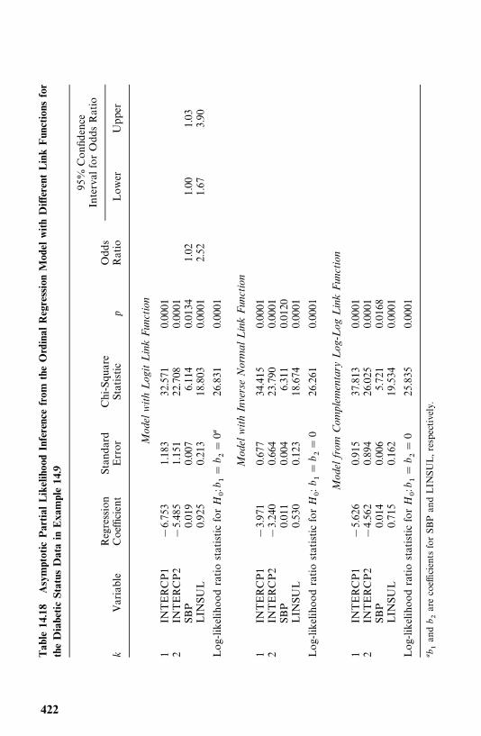
Tab
le14
.18
Asymptotic
Partial
LikelihoodInferencefrom
theOrdinal
RegressionModel
withDifferent
LinkFunctions
for
theDiabeticStatus
Datain
Exa
mple14.9
95%
Confidence
IntervalforOddsRatio
Regression
Standard
Chi-Square
Odds
kVariable
Coefficient
Error
Statistic
pRatio
Lower
Upper
Mod
elw
ith
Log
itL
ink
Fun
ctio
n
1IN
TERCP1
�6.753
1.183
32.571
0.0001
2IN
TERCP2
�5.485
1.151
22.708
0.0001
SBP
0.019
0.007
6.114
0.0134
1.02
1.00
1.03
LIN
SUL
0.925
0.213
18.803
0.0001
2.52
1.67
3.90
Log-likelihoodratiostatisticfor
H:
b ��
b ��
0 26
.831
0.0001
Mod
elw
ith
Inve
rse
Nor
mal
Lin
kF
unct
ion
1IN
TERCP1
�3.971
0.677
34.415
0.0001
2IN
TERCP2
�3.240
0.664
23.790
0.0001
SBP
0.011
0.004
6.311
0.0120
LIN
SUL
0.530
0.123
18.674
0.0001
Log-likelihoodratiostatisticfor
H:
b ��
b ��
026
.261
0.0001
Mod
elfr
omC
ompl
emen
tary
Log
-Log
Lin
kF
unct
ion
1IN
TERCP1
�5.626
0.915
37.813
0.0001
2IN
TERCP2
�4.562
0.894
26.025
0.0001
SBP
0.014
0.006
5.721
0.0168
LIN
SUL
0.715
0.162
19.534
0.0001
Log-likelihoodratiostatisticfor
H:
b ��
b ��
025
.835
0.0001
b�and
b �arecoefficientsforSBPandLIN
SUL,respectively.
422
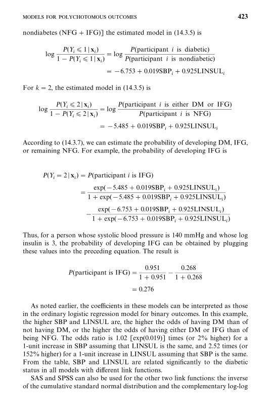
nondiabetes (NFG� IFG)] the estimated model in (14.3.5) is
logP(Y
� 1 �x
�)
1�P(Y� 1 � x
�)� log
P(participant i is diabetic)P(participant i is nondiabetic)
� �6.753� 0.019SBP�� 0.925LINSUL
�
For k� 2, the estimated model in (14.3.5) is
logP(Y
� 2 � x
�)
1� P(Y� 2 � x
�)� log
P(participant i is either DM or IFG)P(participant i is NFG)
��5.485� 0.019SBP�� 0.925LINSUL
�
According to (14.3.7), we can estimate the probability of developing DM, IFG,or remaining NFG. For example, the probability of developing IFG is
P(Y�� 2 � x
�) �P(participant i is IFG)
�exp(�5.485� 0.019SBP
�� 0.925LINSUL
�)
1� exp(�5.485� 0.019SBP�� 0.925LINSUL
�)
�exp(�6.753� 0.019SBP
�� 0.925LINSUL
�)
1� exp(�6.753� 0.019SBP�� 0.925LINSUL
�)
Thus, for a person whose systolic blood pressure is 140 mmHg and whose loginsulin is 3, the probability of developing IFG can be obtained by pluggingthese values into the preceding equation. The result is
P(participant is IFG) �0.951
1� 0.951�
0.268
1� 0.268
� 0.276
As noted earlier, the coefficients in these models can be interpreted as thosein the ordinary logistic regression model for binary outcomes. In this example,the higher SBP and LINSUL are, the higher the odds of having DM than ofnot having DM, or the higher the odds of having either DM or IFG than ofbeing NFG. The odds ratio is 1.02 [exp(0.019)] times (or 2% higher) for a1-unit increase in SBP assuming that LINSUL is the same, and 2.52 times (or152% higher) for a 1-unit increase in LINSUL assuming that SBP is the same.From the table, SBP and LINSUL are related significantly to the diabeticstatus in all models with different link functions.
SAS and SPSS can also be used for the other two link functions: the inverseof the cumulative standard normal distribution and the complementary log-log
423
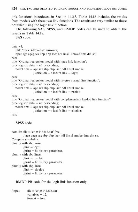
link functions introduced in Section 14.2.3. Table 14.18 includes the resultsfrom models with these two link functions. The results are very similar to thoseobtained using the logit link function.
The following SAS, SPSS, and BMDP codes can be used to obtain theresults in Table 14.18.
SAS code:
data w1;infile ‘c:�ex14d2d6.dat’ missover;input age ageg sex sbp dbp lacr hdl linsul smoke dms dm sn;
run;title ‘‘Ordinal regression model with logic link function’’;proc logistic data�w1 descending;model dms� age sex sbp dbp lacr hdl linsul smoke
/ selection� s lackfit link� logit;run;title ‘‘Ordinal regression model with inverse normal link function‘;proc logistic data�w1 descending;model dms� age sex sbp dbp lacr hdl linsul smoke
/ selection� s lackfit link�probit;run;title ‘‘Ordinal regression model with complementary log-log link function’’;proc logistic data�w1 descending;model dms� age sex sbp dbp lacr hdl linsul smoke
/ selection� s lackfit link� cloglog;run;
SPSS code:
data list file� ‘c:�ex14d2d6.dat’ free/ age ageg sex sbp dbp lacr hdl linsul smoke dms dm sn.
Compute y� 4-dms.plum y with sbp linsul
/link� logit/print�fit history parameter.
plum y with sbp linsul/link� probit/print�fit history parameter.
plum y with sbp linsul/link� cloglog/print�fit history parameter.
BMDP PR code for the logit link function only:
/input file� ‘c:�ex14d2d6.dat’ .variables� 12.format� free.
424
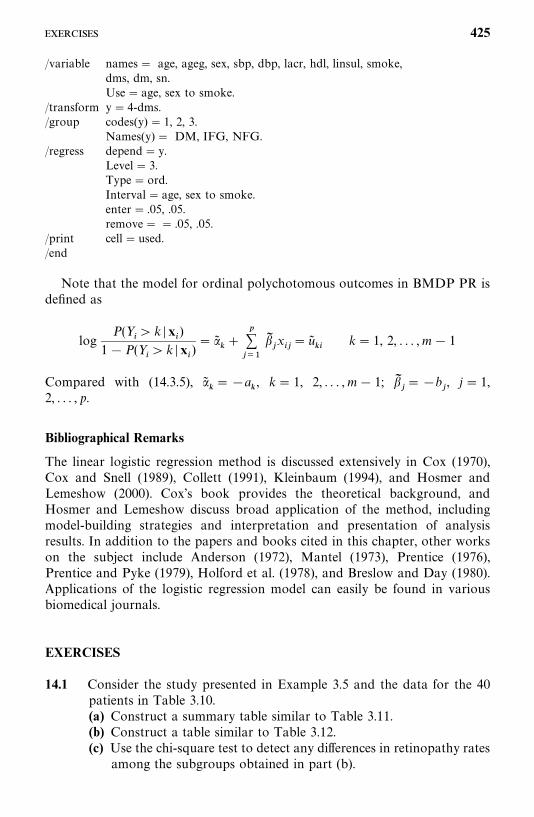
/variable names� age, ageg, sex, sbp, dbp, lacr, hdl, linsul, smoke,dms, dm, sn.Use� age, sex to smoke.
/transform y� 4-dms./group codes(y) � 1, 2, 3.
Names(y) � DM, IFG, NFG./regress depend� y.
Level� 3.Type� ord.Interval� age, sex to smoke.enter� .05, .05.remove� � .05, .05.
/print cell�used./end
Note that the model for ordinal polychotomous outcomes in BMDP PR isdefined as
logP(Y
�� k � x
�)
1� P(Y�� k � x
�)� ��
��
�����
���x��� u�
��k� 1, 2, . . . ,m � 1
Compared with (14.3.5), �����a
�, k� 1, 2, . . . ,m � 1; ��
���b
�, j � 1,
2, . . . , p.
Bibliographical Remarks
The linear logistic regression method is discussed extensively in Cox (1970),Cox and Snell (1989), Collett (1991), Kleinbaum (1994), and Hosmer andLemeshow (2000). Cox’s book provides the theoretical background, andHosmer and Lemeshow discuss broad application of the method, includingmodel-building strategies and interpretation and presentation of analysisresults. In addition to the papers and books cited in this chapter, other workson the subject include Anderson (1972), Mantel (1973), Prentice (1976),Prentice and Pyke (1979), Holford et al. (1978), and Breslow and Day (1980).Applications of the logistic regression model can easily be found in variousbiomedical journals.
EXERCISES
14.1 Consider the study presented in Example 3.5 and the data for the 40patients in Table 3.10.(a) Construct a summary table similar to Table 3.11.(b) Construct a table similar to Table 3.12.(c) Use the chi-square test to detect any differences in retinopathy rates
among the subgroups obtained in part (b).
425
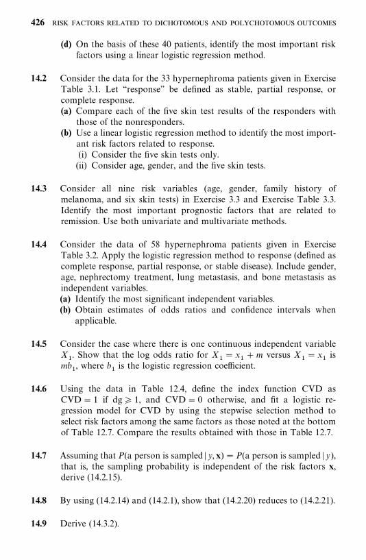
(d) On the basis of these 40 patients, identify the most important riskfactors using a linear logistic regression method.
14.2 Consider the data for the 33 hypernephroma patients given in ExerciseTable 3.1. Let ‘‘response’’ be defined as stable, partial response, orcomplete response.(a) Compare each of the five skin test results of the responders with
those of the nonresponders.(b) Use a linear logistic regression method to identify the most import-
ant risk factors related to response.(i) Consider the five skin tests only.
(ii) Consider age, gender, and the five skin tests.
14.3 Consider all nine risk variables (age, gender, family history ofmelanoma, and six skin tests) in Exercise 3.3 and Exercise Table 3.3.Identify the most important prognostic factors that are related toremission. Use both univariate and multivariate methods.
14.4 Consider the data of 58 hypernephroma patients given in ExerciseTable 3.2. Apply the logistic regression method to response (defined ascomplete response, partial response, or stable disease). Include gender,age, nephrectomy treatment, lung metastasis, and bone metastasis asindependent variables.(a) Identify the most significant independent variables.(b) Obtain estimates of odds ratios and confidence intervals when
applicable.
14.5 Consider the case where there is one continuous independent variableX
�. Show that the log odds ratio for X
��x
��m versus X
��x
�is
mb�, where b
�is the logistic regression coefficient.
14.6 Using the data in Table 12.4, define the index function CVD asCVD� 1 if dg 1, and CVD� 0 otherwise, and fit a logistic re-gression model for CVD by using the stepwise selection method toselect risk factors among the same factors as those noted at the bottomof Table 12.7. Compare the results obtained with those in Table 12.7.
14.7 Assuming that P(a person is sampled � y, x) �P(a person is sampled � y),that is, the sampling probability is independent of the risk factors x,derive (14.2.15).
14.8 By using (14.2.14) and (14.2.1), show that (14.2.20) reduces to (14.2.21).
14.9 Derive (14.3.2).
426
14.10 Consider the data in Table 12.4. Fit the generalized logistic regressionmodel in (14.3.1) for DG with covariates AGE, SEX, LACR, and LTGby using the SAS CATMOD, SPSS NOMREG, or BMDP PRprocedure. Select risk factors among those noted at the bottom ofTable 12.7 using the stepwise selection method in the BMDP PRprocedure. Compare the results with those given in Table 13.5.
14.11 Using the same notation and data as in Table 14.11, (1) fit the outcomevariable Y with the generalized logistic regression model in (14.3.1) withSEX as the covariate; (2) fit a logistic regression for the binary outcomeDM versus NFG, with SEX as the covariate, by using the data fromDM and NFG participants only; (3) fit a logistic regression for thebinary outcome IFG versus NFG, with SEX as the covariate, by usingthe data from IFG and NFG participants only; (4) compare thecoefficients obtained from (2) and (3) with the coefficients obtainedfrom (1), and (5) report what you have found.
14.12 Perform the same analyses as in Exercise 14.11 but use SBP as thecovariate, and discuss your findings.
427
A P P E N D I X A
Newton--Raphson Method
The Newton—Raphson method (Ralston and Wilf, 1967; Carnahan et al., 1969)is a numerical iterative procedure that can be used to solve nonlinearequations. An iterative procedure is a technique of successive approximations,and each approximation is called an iteration. If the successive approximationsapproach the solution very closely, we say that the iterations converge. Themaximum likelihood estimates of various parameters and coefficients discussedin Chapters 7, 9, and 11 to 14 can be obtained by using the Newton—Raphsonmethod. In this appendix we discuss and illustrate the use of this method, firstconsidering a single nonlinear equation and then a set of nonlinear equations.
Let f (x) � 0 be the equation to be solved for x. The Newton—Raphsonmethod requires an initial estimate of x, say x�
�, such that f (x�
�) is close to zero
preferably, and then the first approximate iteration is given by
x���x�
��
f (x��
)
f �(x��)
(A.1)
where f �(x��
) is the first derivative of f (x) evaluated at x �x��. In general, the
(k � 1)th iteration or approximation is given by
x����
�x���
f (x�)
f �(x�)
(A.2)
where f �(x��) is the first derivative of f (x) evaluated at x� x�
�. The iteration
terminates at the kth iteration if f (x��) is close enough to zero or the difference
between x��
and x����
is negligible. The stopping rule is rather subjective.Acceptable rules are that f (x�
�) or d�x�
��x�
���is in the neighborhood of
10�� or 10��.
Example A.1 Consider the function
f (x) � x� x� 2
428
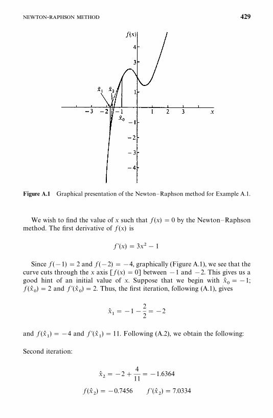
Figure A.1 Graphical presentation of the Newton—Raphson method for Example A.1.
We wish to find the value of x such that f (x) � 0 by the Newton—Raphsonmethod. The first derivative of f (x) is
f �(x) � 3x� 1
Since f (�1) � 2 and f (�2) ��4, graphically (Figure A.1), we see that thecurve cuts through the x axis [ f (x) � 0] between �1 and �2. This gives us agood hint of an initial value of x. Suppose that we begin with x�
���1;
f (x��
) � 2 and f �(x��) � 2. Thus, the first iteration, following (A.1), gives
x��� �1 �
2
2��2
and f (x��
) ��4 and f �(x��) � 11. Following (A.2), we obtain the following:
Second iteration:
x���2 �
4
11��1.6364
f (x�
) ��0.7456 f �(x�
) � 7.0334
- 429
Third iteration:
x�� �1.6364 �
0.7456
7.0334��1.5304
f (x�
) ��0.054 f �(x�) � 6.0264
Fourth iteration:
x����1.5304 �
0.054
6.0264��1.52144
f (x��) ��0.00036 f �(x�
�) � 5.9443
Fifth iteration:
x��� �1.52144�
0.00036
5.9443��1.52138
f (x��
) � 0.0000017
At the fifth iteration, for x� �1.52138, f (x) is very close to zero. If thestopping rule is that f (x) � 10��, the iterative procedure would terminate afterthe fifth iteration and x��1.52138 is the root of the equation x� x� 2 � 0.Figure A.1 gives the graphical presentation of f (x) and the iteration.
It should be noted that the Newton—Raphson method can only find the realroots of an equation. The equation x �x � 2 � 0 has only one real root, asshown in Figure A.1; the other two are complex roots.
The Newton—Raphson method can be extended to solve a system ofequations with more than one unknown. Suppose that we wish to find valuesof x
�, x
, . . . , x
�such that
f�(x
�, . . . , x
�) � 0
f(x
�, . . . , x
�) � 0
�
f�
(x�
, . . . , x�
) � 0
Let a��
be the partial derivative of f�
with respect to x�; that is, a
��� � f
�/�x
�.
430 -
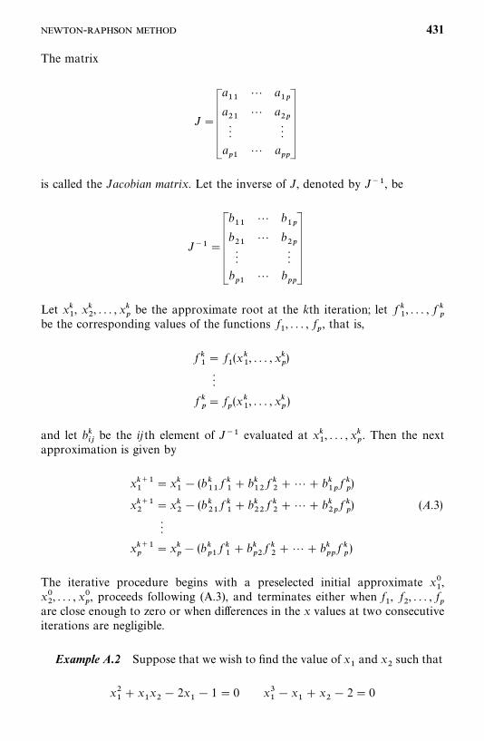
The matrix
J �
a��
� a��
a�
� a�
� �
a��
� a��
is called the Jacobian matrix. Let the inverse of J, denoted by J��, be
J���
b��
� b��
b�
� b�
� �
b��
� b��
Let x��, x�
, . . . , x�
�be the approximate root at the kth iteration; let f �
�, . . . , f �
�be the corresponding values of the functions f
�, . . . , f
�, that is,
f ��� f
�(x�
�, . . . , x�
�)
�
f ��� f
�(x�
�, . . . , x�
�)
and let b���
be the ijth element of J�� evaluated at x��
, . . . , x��
. Then the nextapproximation is given by
x����
�x��� (b�
��f ��� b�
�f ���� b�
��f ��)
x���
�x�� (b�
�f ��� b�
f ���� b�
�f ��) (A.3)
�
x����
�x��� (b�
��f ��� b�
�f ���� b�
��f ��
)
The iterative procedure begins with a preselected initial approximate x��
,x�
, . . . , x��
, proceeds following (A.3), and terminates either when f�
, f, . . . , f
�are close enough to zero or when differences in the x values at two consecutiveiterations are negligible.
Example A.2 Suppose that we wish to find the value of x�
and x
such that
x�� x
�x� 2x
�� 1 � 0 x
��x
�� x
� 2 � 0
- 431
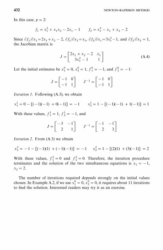
In this case, p � 2:
f�� x
�� x
�x� 2x
�� 1 f
�x
��x
�� x
� 2
Since � f�/�x
��2x
��x
� 2, � f
�/�x
�x
�, � f
/�x
��3x
��1, and � f
/�x
� 1,
the Jacobian matrix is
J ��2x
��x
� 2
3x�� 1
x�
1 � (A.4)
Let the initial estimates be x��� 0, x�
� 1, f �
���1, and f �
��1:
J���1 0
�1 1� J��� ��1 0
�1 1�Iteration 1. Following (A.3), we obtain
x��� 0 � [(�1)(�1) � 0(�1)] ��1 x�
� 1 � [(�1)(�1) � 1(�1)] � 1
With these values, f ��� 1, f �
��1, and
J���3 �1
2 1� J��� ��1 �1
2 3�Iteration 2. From (A.3) we obtain
x���1 � [(�1)(1) � (�1)(�1)] ��1 x
� 1 � [(2)(1) � (3)(�1)] � 2
With these values, f �� 0 and f
� 0. Therefore, the iteration procedure
terminates and the solution of the two simultaneous equations is x���1,
x� 2.
The number of iterations required depends strongly on the initial valueschosen. In Example A.2, if we use x�
�� 0, x�
� 0, it requires about 11 iterations
to find the solution. Interested readers may try it as an exercise.
432 -
APPENDIX B
Statistical Tables
433
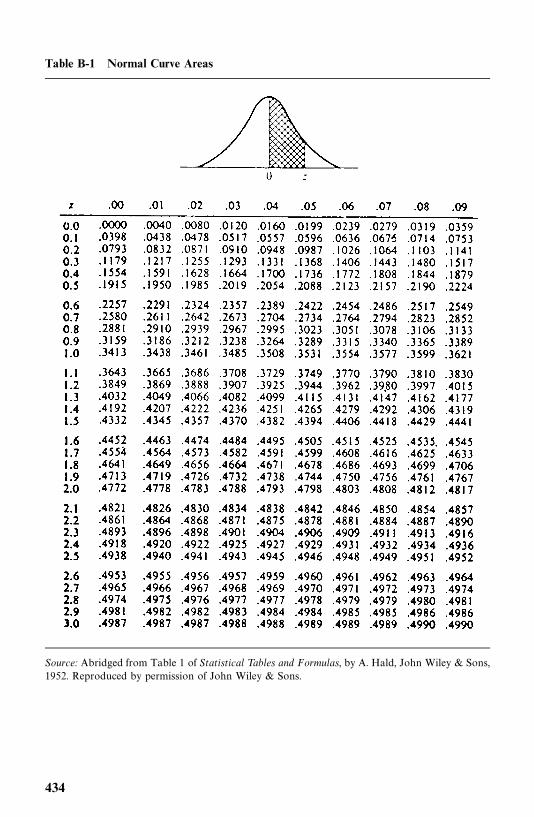
Table B-1 Normal Curve Areas
Source: Abridged from Table 1 of Statistical Tables and Formulas, by A. Hald, John Wiley & Sons,1952. Reproduced by permission of John Wiley & Sons.
434
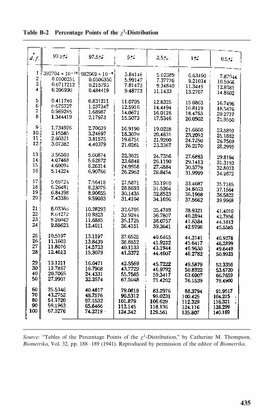
Table B-2 Percentage Points of the �2-Distribution
Source: ‘‘Tables of the Percentage Points of the ��-Distribution,’’ by Catherine M. Thompson,Biometrika, Vol. 32, pp. 188—189 (1941). Reproduced by permission of the editor of Biometrika.
435
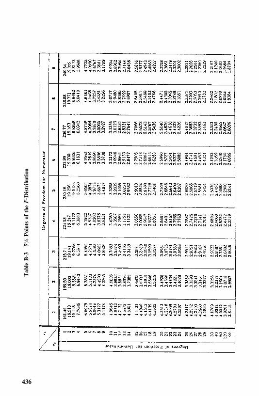
Table
B-3
5%Pointsof
the
F-D
istribution
436
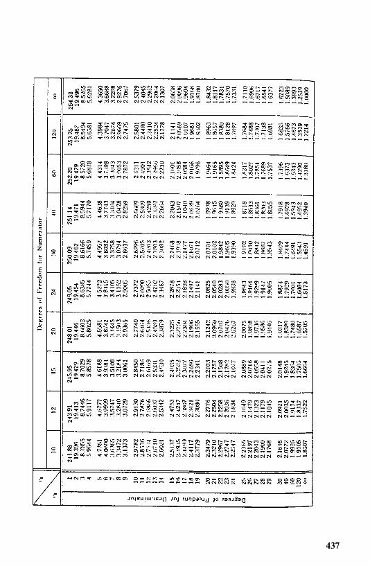
437
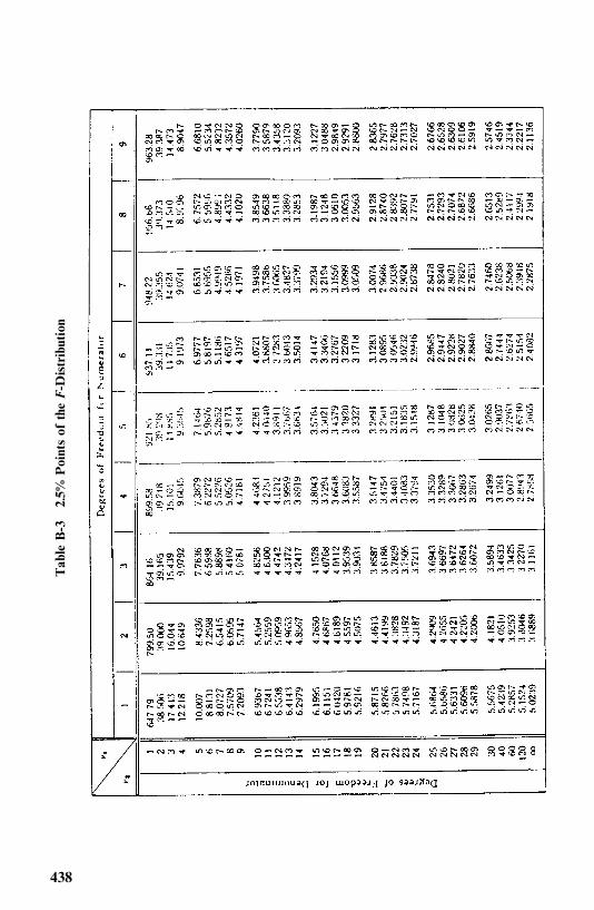
Table
B-3
2.5%
Pointsof
the
F-D
istribution
438
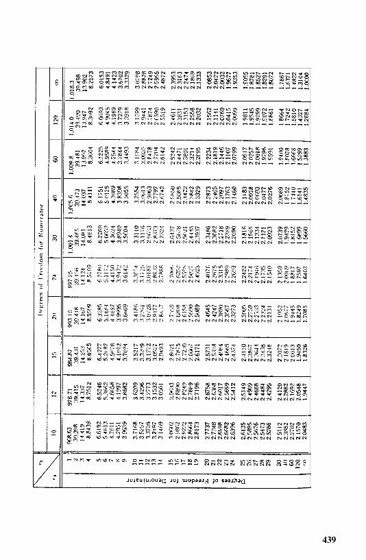
439
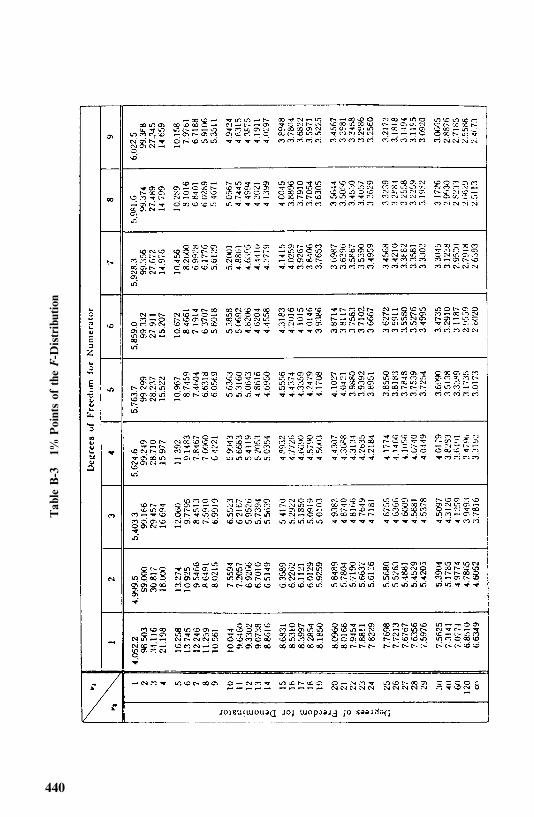
Table
B-3
1%Pointsof
the
F-D
istribution
440
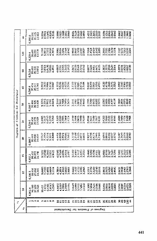
441
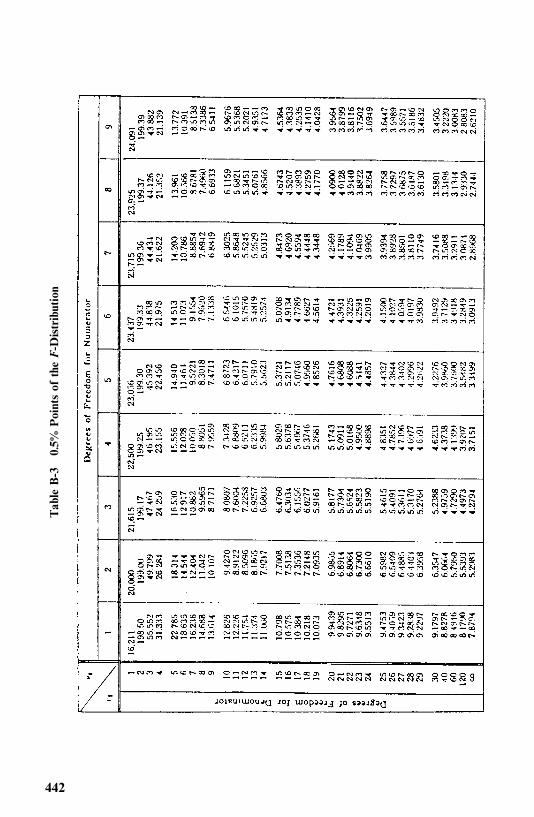
Table
B-3
0.5%
Pointsof
the
F-D
istribution
442
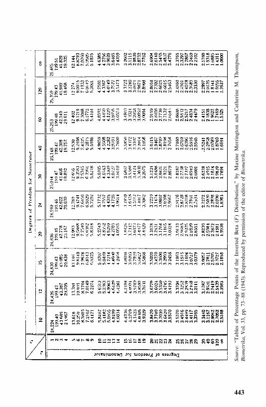
Sour
ce:‘‘TablesofPercentage
Points
oftheInverted
Beta
(F)Distribution,’’
byMaxineMerringtonandCatherineM.Thom
pson,
Bio
met
rika,Vol.3 3,p p.7 3
—88
(1943).Reprodu
cedbyperm
ission
oftheeditor
ofB
iom
etrika
.
443
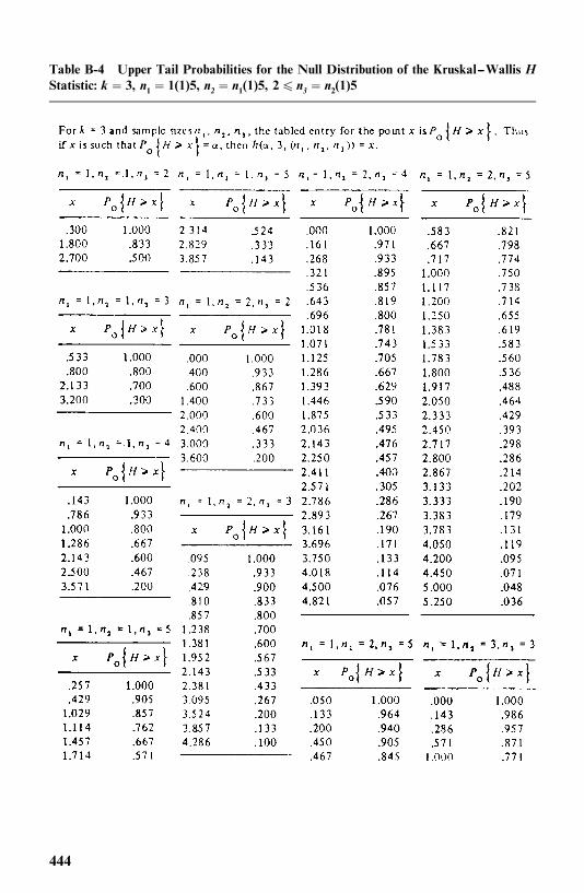
Table B-4 Upper Tail Probabilities for the Null Distribution of the Kruskal--Wallis HStatistic: k � 3, n1� 1(1)5, n2 � n1(1)5, 2� n3 � n2(1)5
444
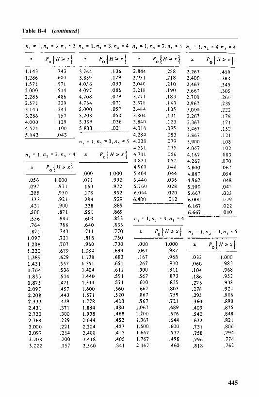
Table B-4 (continued)
445
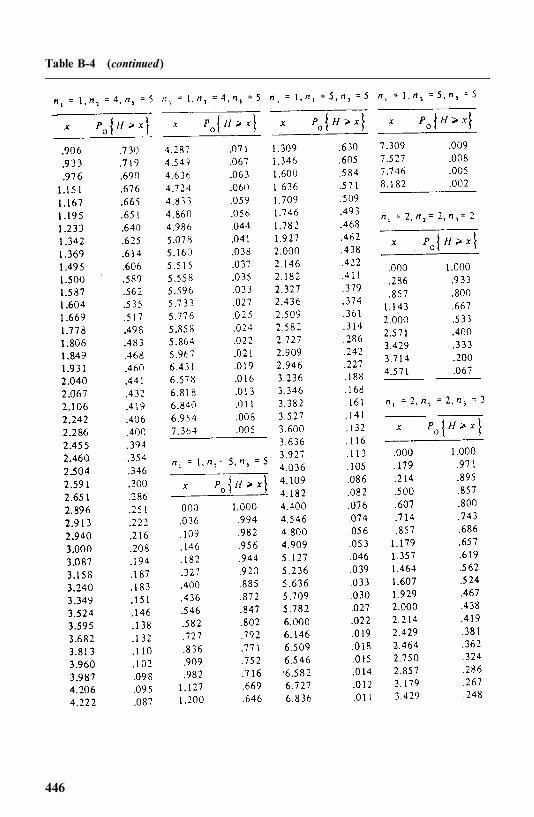
Table B-4 (continued)
446
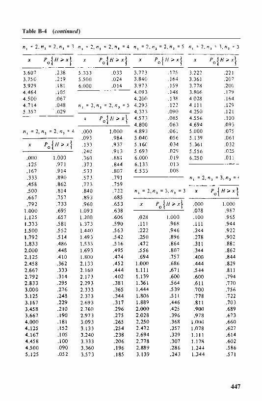
Table B-4 (continued)
447
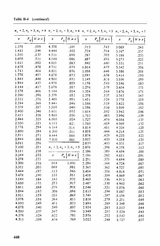
Table B-4 (continued)
448
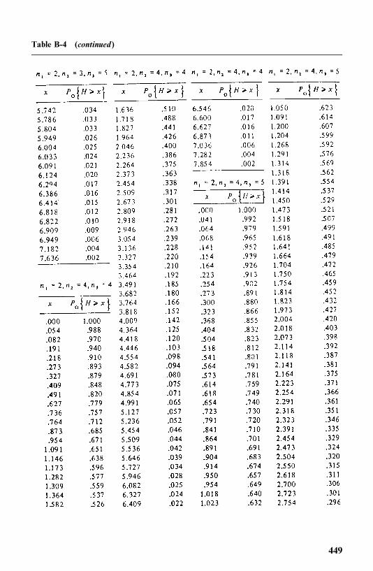
Table B-4 (continued)
449
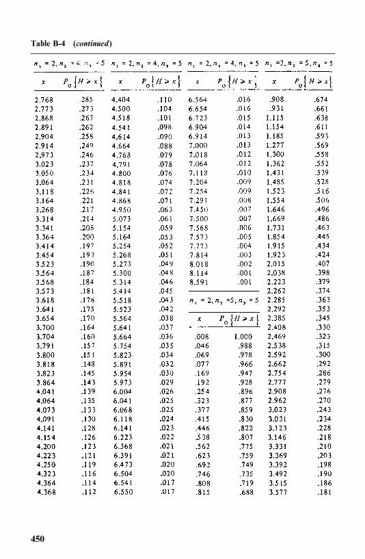
Table B-4 (continued)
450
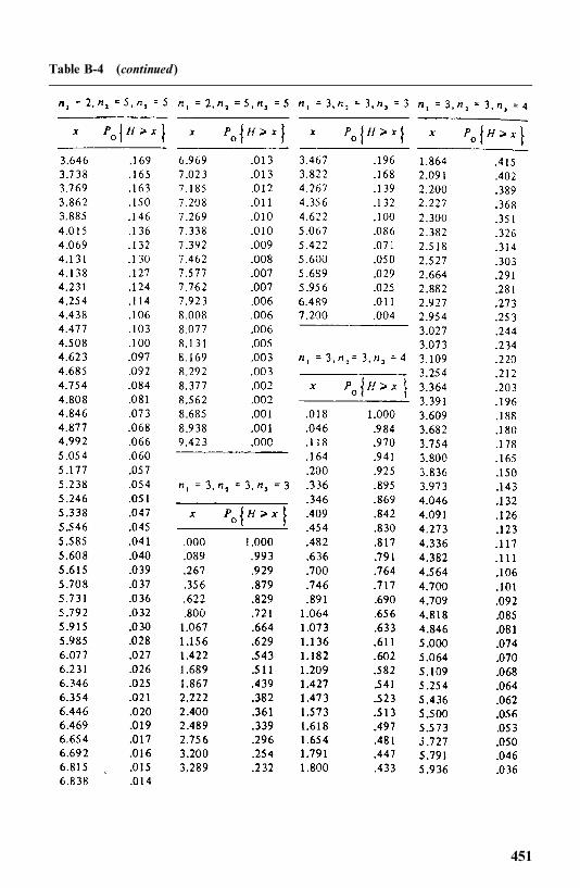
Table B-4 (continued)
451
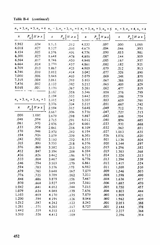
Table B-4 (continued)
452
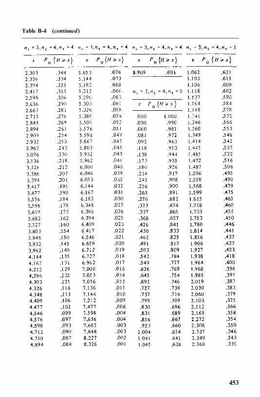
Table B-4 (continued)
453
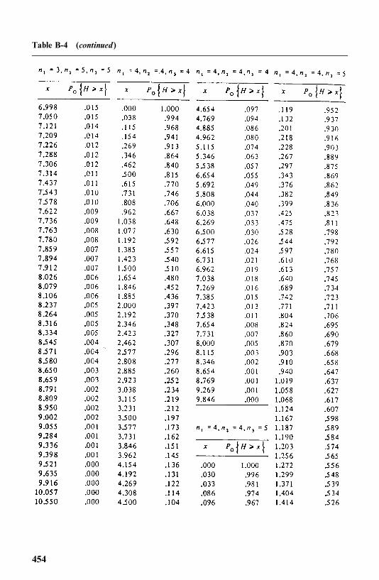
Table B-4 (continued)
454
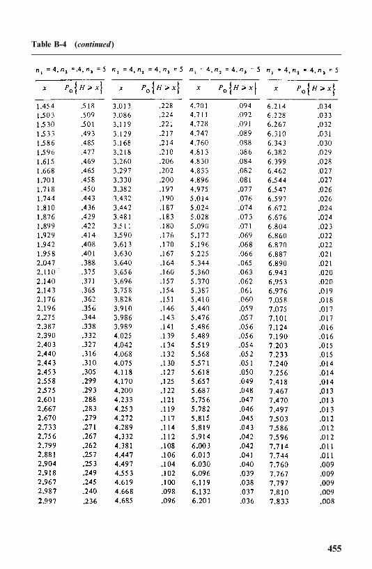
Table B-4 (continued)
455
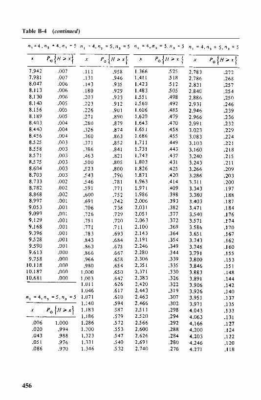
Table B-4 (continued)
456
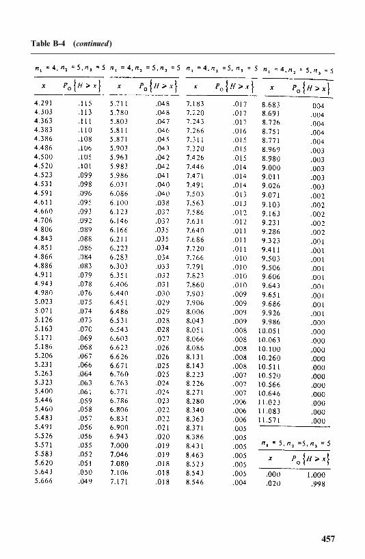
Table B-4 (continued)
457
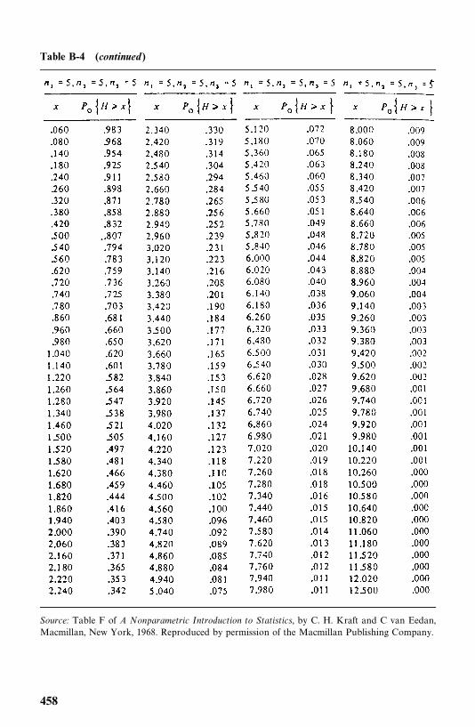
Table B-4 (continued)
Source: Table F of A Nonparametric Introduction to Statistics, by C. H. Kraft and C van Eedan,Macmillan, New York, 1968. Reproduced by permission of the Macmillan Publishing Company.
458
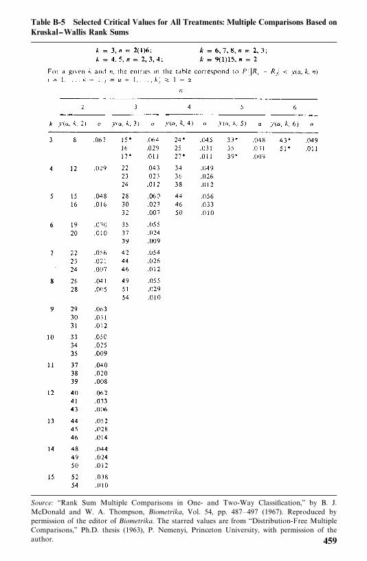
Table B-5 Selected Critical Values for All Treatments: Multiple Comparisons Based onKruskal--Wallis Rank Sums
Source: ‘‘Rank Sum Multiple Comparisons in One- and Two-Way Classification,’’ by B. J.McDonald and W. A. Thompson, Biometrika, Vol. 54, pp. 487—497 (1967). Reproduced bypermission of the editor of Biometrika. The starred values are from ‘‘Distribution-Free MultipleComparisons,’’ Ph.D. thesis (1963), P. Nemenyi, Princeton University, with permission of theauthor. 459
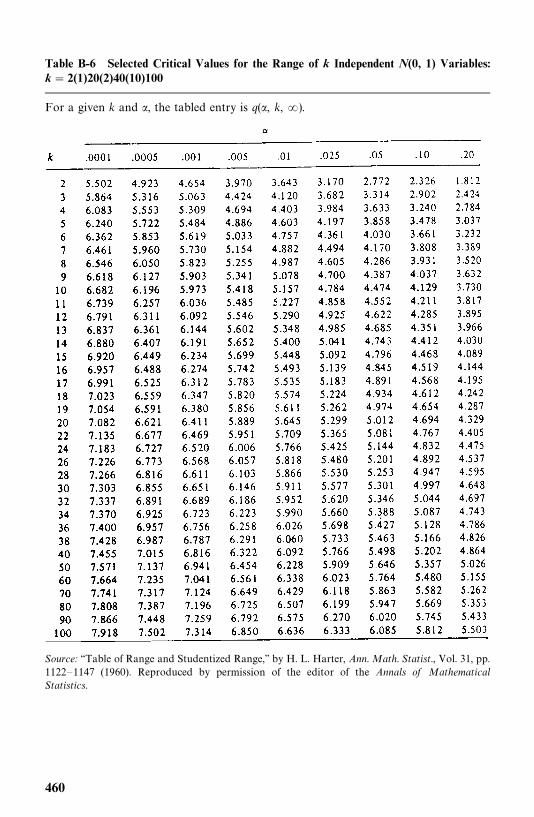
Table B-6 Selected Critical Values for the Range of k Independent N(0, 1) Variables:k � 2(1)20(2)40(10)100
For a given k and �, the tabled entry is q(�, k, �).
Source: ‘‘Table of Range and Studentized Range,’’ by H. L. Harter, Ann. Math. Statist., Vol. 31, pp.1122—1147 (1960). Reproduced by permission of the editor of the Annals of MathematicalStatistics.
460
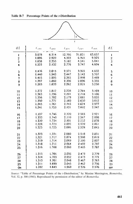
Table B-7 Percentage Points of the t-Distribution
Source: ‘‘Table of Percentage Points of the t-Distribution,’’ by Maxine Merrington, Biometrika,Vol. 32, p. 300 (1941). Reproduced by permission of the editor of Biometrika.
461
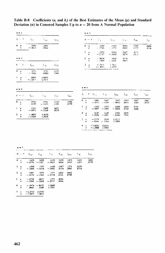
Table B-8 Coefficients (ai and bi) of the Best Estimates of the Mean (�) and StandardDeviation (�) in Censored Samples Up to n � 20 from A Normal Population
462
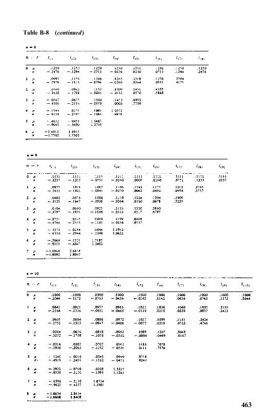
Table B-8 (continued)
463
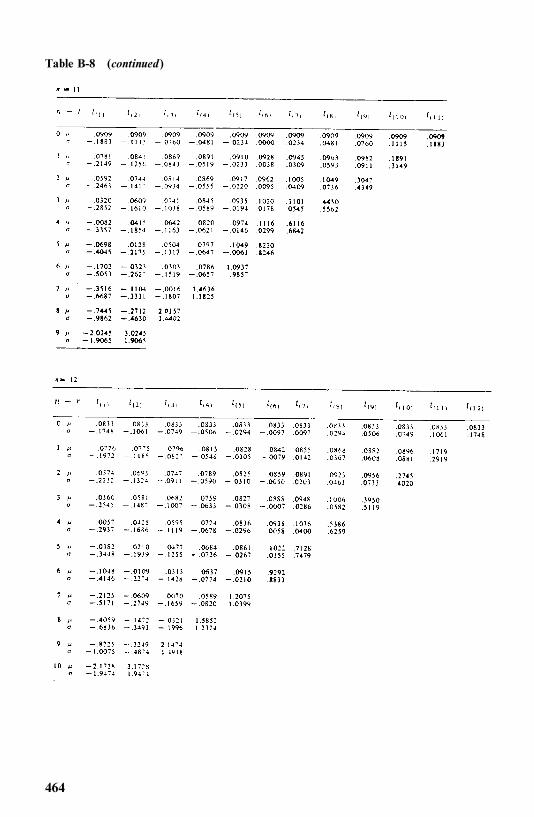
Table B-8 (continued)
464
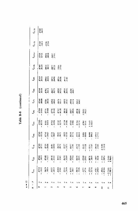
Tab
leB-8
(con
tinu
ed)
465
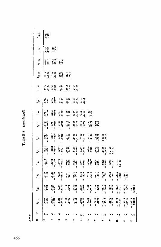
Tab
leB-8
(con
tinu
ed)
466
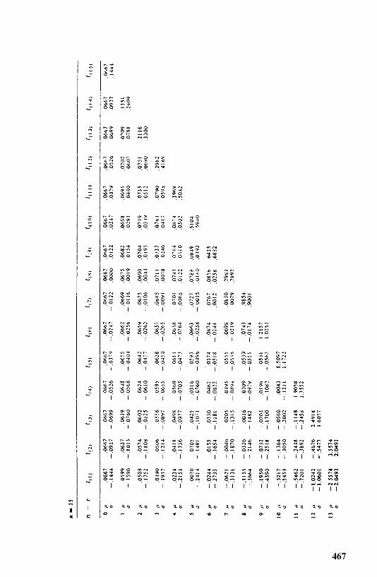
467
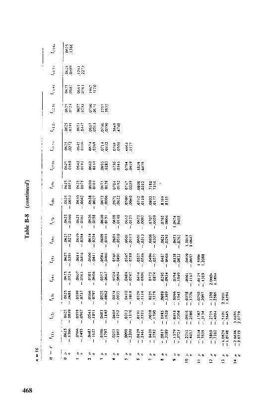
Tab
leB-8
(con
tinu
ed)
468
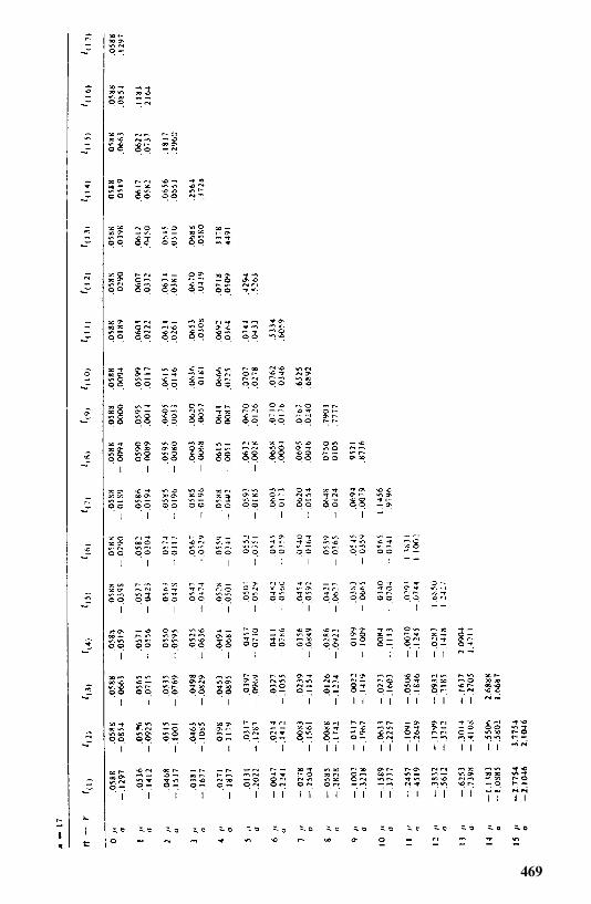
469
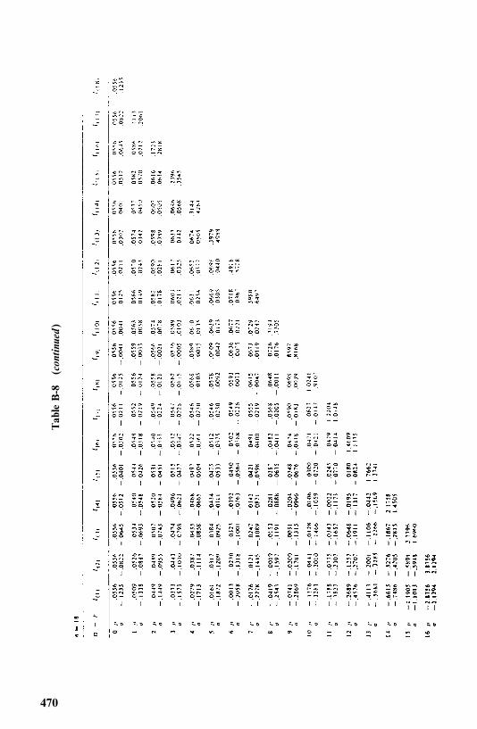
Tab
leB-8
(con
tinu
ed)
470
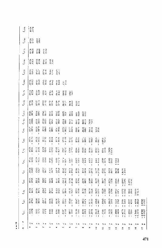
471
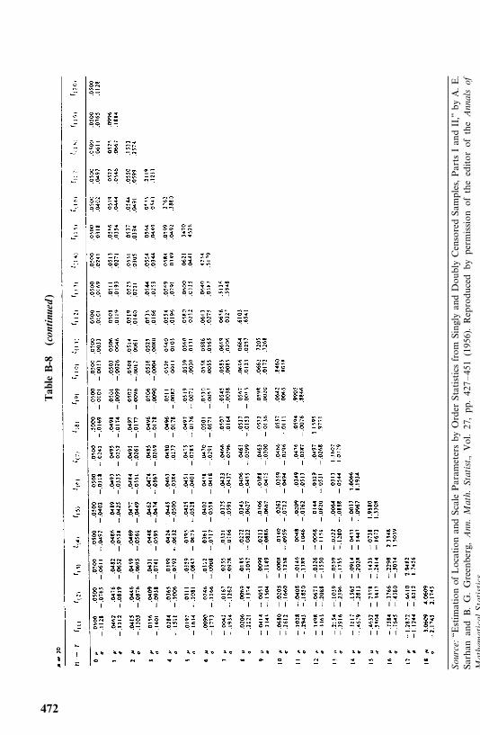
Table
B-8
(con
tinu
ed)
Sour
ce:‘‘E
stimationofLocationandScaleParam
etersby
Order
St atisticsfrom
SinglyandDoubly
CensoredSam
ples,PartsIa ndII,’’byA.E.
Sa rha n
a ndB.G.Gr ee nb er g,
Ann
.M
ath.
Stat
ist.,
Vol.27,pp.427—451
(1956 ).Reproducedby
permissionoftheeditorofthe
Ann
als
ofM
athe
mat
ical
Sta
tist
ics.
472
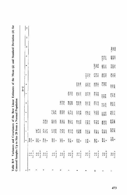
Table
B-9
Variances
andCovariances
oftheBestLinearEstim
ates
oftheMean(��)
andStanda
rdDeviation
(��)
for
CensoredSa
mples
Upto
Size
20from
aNormal
Population
473
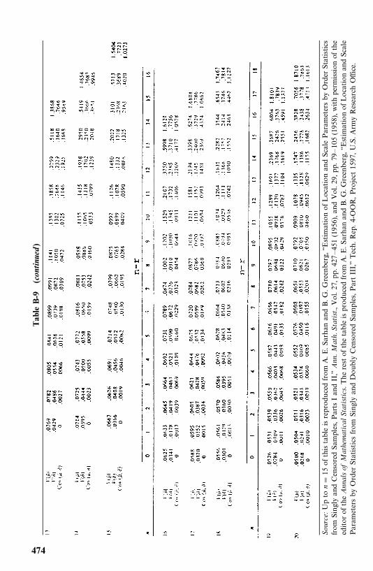
Table
B-9
(con
tinu
ed)
Sour
ce:Upto
n�
15ofthistableisreproducedfrom
A.E
.Sarhan
andB.G
.Greenberg,‘‘E
stimationofLocationandScaleParam
etersbyOrder
Statistics
from
SinglyandCensoredSam
ples,P
artsIandII,’’
Ann
.Mat
h.Sta
tist.,Vol.27,pp.427
—451
(1956),and
Vo l.29 ,pp .7 9
—105
(1958),w
ithperm
ission
ofthe
editorofthe
Ann
alsof
Mat
hem
atic
alSt
atistics.T
herestofthetableisproducedfrom
A.E
.Sarhan
andB.G
.Greenberg,‘‘E
stimationofLocationandScale
Param
etersby
Order
Statisticsfrom
SinglyandDoublyCensoredSamples,PartIII,’’Tech.Rep.4-OOR,Project1597,U.S.Arm
yResearchOffice.
474
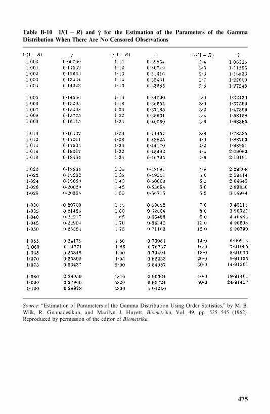
Table B-10 1/(1� R) and �� for the Estimation of the Parameters of the GammaDistribution When There Are No Censored Observations
Source: ‘‘Estimation of Parameters of the Gamma Distribution Using Order Statistics,’’ by M. B.Wilk, R. Gnanadesikan, and Marilyn J. Huyett, Biometrika, Vol. 49, pp. 525—545 (1962).Reproduced by permission of the editor of Biometrika.
475
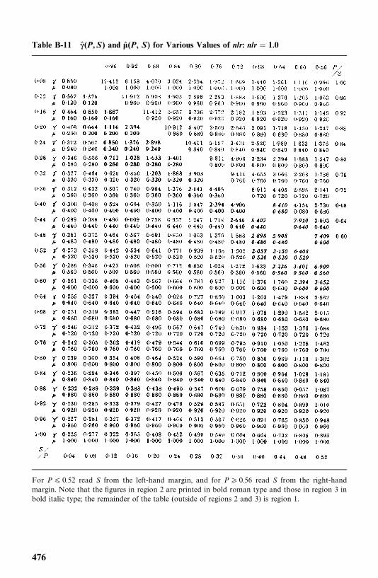
Table B-11 �� (P,S) and �� (P, S) for Various Values of n/r: n/r � 1.0
For P� 0.52 read S from the left-hand margin, and for P � 0.56 read S from the right-handmargin. Note that the figures in region 2 are printed in bold roman type and those in region 3 inbold italic type; the remainder of the table (outside of regions 2 and 3) is region 1.
476
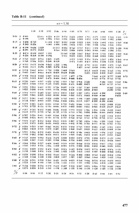
Table B-11 (continued)
477
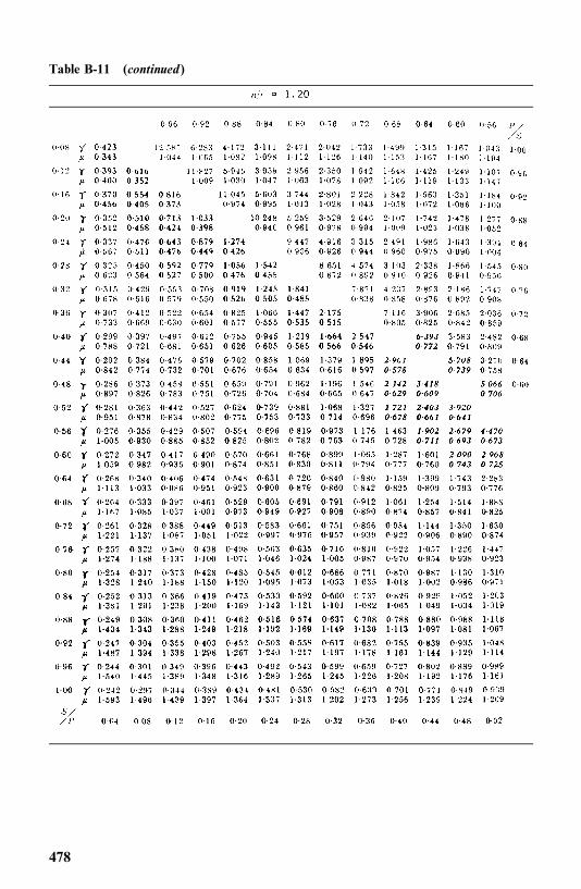
Table B-11 (continued)
478
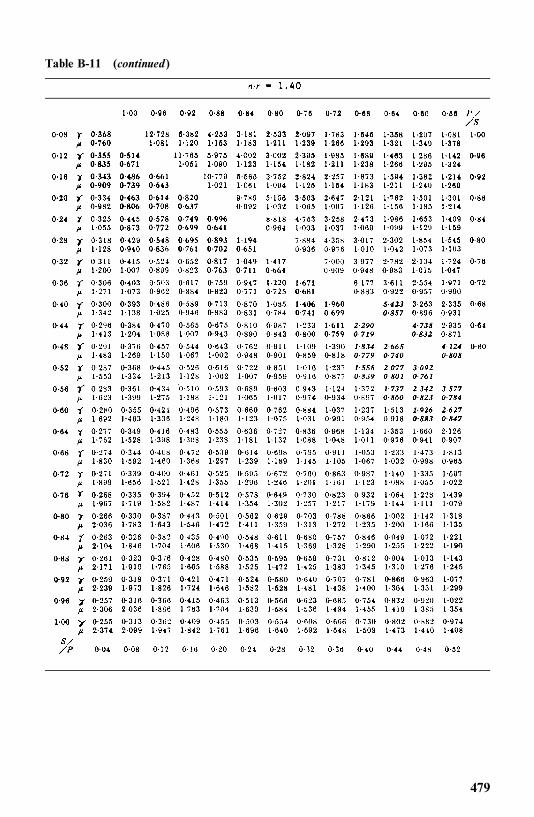
Table B-11 (continued)
479
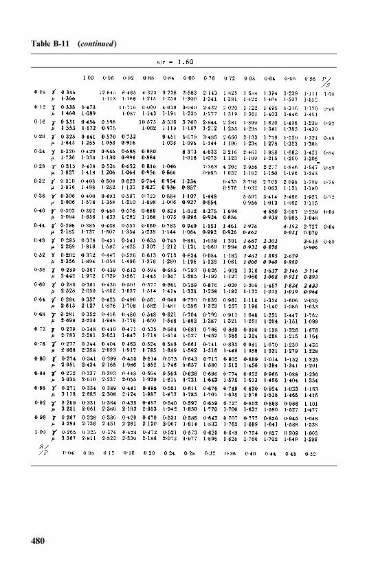
Table B-11 (continued)
480
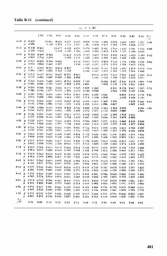
Table B-11 (continued)
481
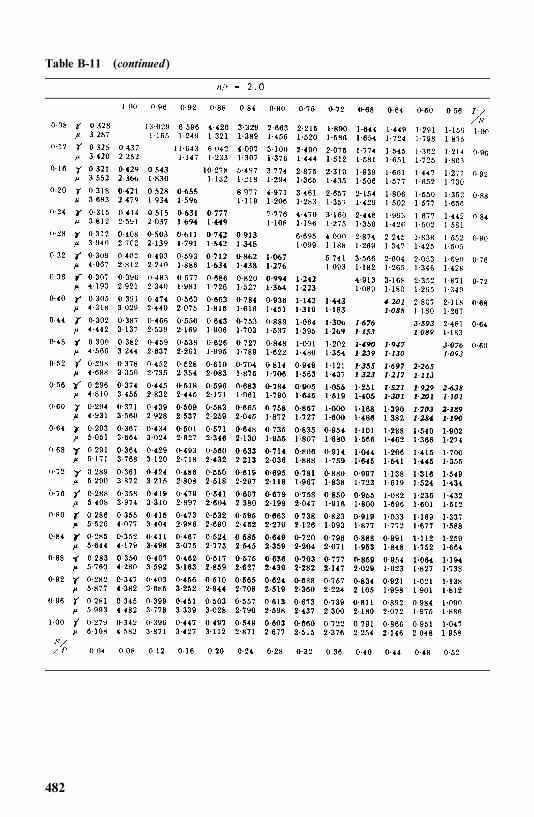
Table B-11 (continued)
482
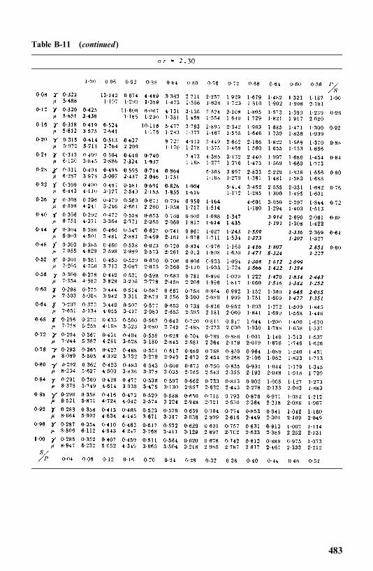
Table B-11 (continued)
483
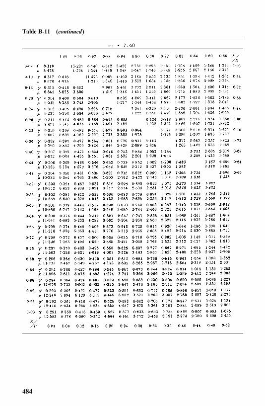
Table B-11 (continued)
484
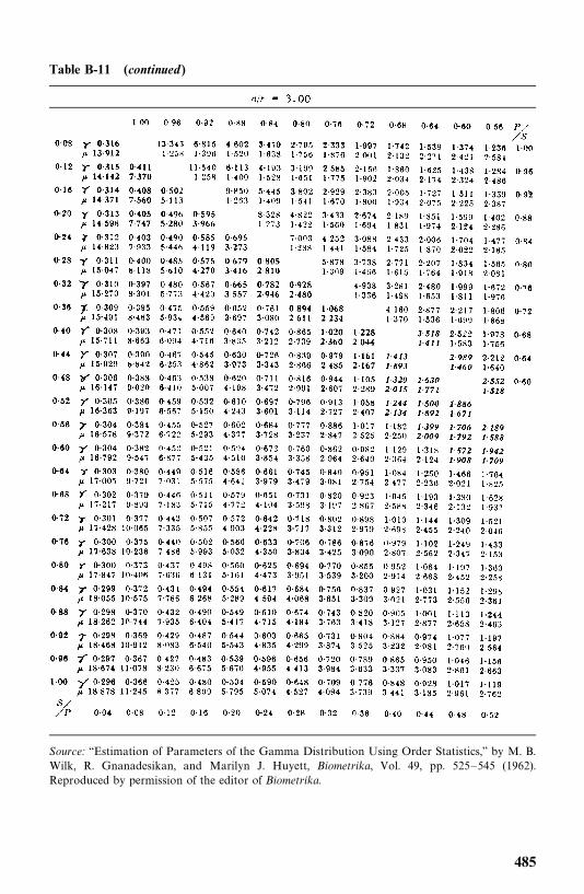
Table B-11 (continued)
Source: ‘‘Estimation of Parameters of the Gamma Distribution Using Order Statistics,’’ by M. B.Wilk, R. Gnanadesikan, and Marilyn J. Huyett, Biometrika, Vol. 49, pp. 525—545 (1962).Reproduced by permission of the editor of Biometrika.
485
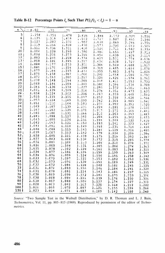
Table B-12 Percentage Points l� Such That P(�� 1/�� 2 � l�)� 1��
Source: ‘‘Two Sample Test in the Weibull Distribution,’’ by D. R. Thoman and L. J. Bain,Technometrics, Vol. 11, pp. 805—815 (1969). Reproduced by permission of the editor of Techno-metrics.
486
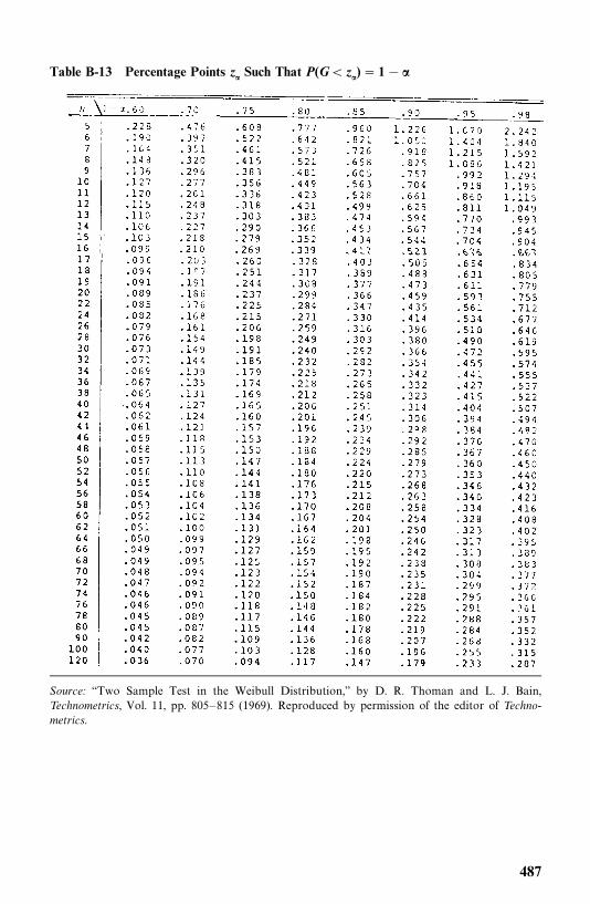
Table B-13 Percentage Points z� Such That P(G� z�)� 1��
Source: ‘‘Two Sample Test in the Weibull Distribution,’’ by D. R. Thoman and L. J. Bain,Technometrics, Vol. 11, pp. 805—815 (1969). Reproduced by permission of the editor of Techno-metrics.
487
References
Aaronson, K. D., Schwartz, J. S., Chen, T. M., Wong, K. L., Goin, J. E, and Mancini,D.M. (1997). Development and Prospective Validation of a Clinical Index to PredictSurvival in Ambulatory Patients Referred for Cardiac Transplant Evaluation.Circulation, 95, 2660—2667.
Abramowitz, M., and Stegun, I. A. (1964). Handbook of Mathematical Functions withFormulas, Graphs, and Mathematical Tables. Applied Mathematics Series 55.National Bureau of Standards, Washington, DC.
Afifi, A. A., and Clark, V. (1990). Computer-Aided Multivariate Analysis, 2nd ed.Lifetime Learning Publications, Belmont, CA.
Agresti, A. (1990). Categorical Data Analysis. Wiley, New York.
Aitchison, J. (1970). Statistical Problems of Treatment Allocation. Journal of the RoyalStatistical Society, Series A, 133, 206—238
Aitchison, J., and Brown, J. A. C. (1957). The Lognormal Distribution. CambridgeUniversity Press, Cambridge.
Aitchison, J., and Silvey, S. D. (1957). The Generalization of Probit Analysis to the Caseof Multiple Responses. Biometrika, 44, 131—140.
Aitkin, M., Laird, N., and Francis, B. (1983). A Reanalysis of the Stanford HeartTransplant Data (with discussion). Journal of the American Statistical Association,78, 264—292.
Akaike, H. (1969). Fitting Autoregressive Models for Prediction. Annals of the Instituteof Statistical Mathematics, 21, 243—247.
Akaike, H. (1974). A New Look at the Statistical Model Identification. IEEE Transac-tions on Automatic Control, AC-19, 716—723.
Albert, I. J. (2000). The Use of Frailty Models in Genetic Studies: Application to theRelationship between End-Stage Renal Failure and Mutation Type in AlportSyndrome. European Community Alport Syndrome Concerted Action Group(ECASCA). Journal of Epidemiology and Biostatistics, 5(3), 169—175.
Albertson, P. C., Hanley, J. A., Gleason, D. F., and Barry, M. J. (1998). Competing RiskAnalysis of Men Aged 55 to 74 Years at Diagnosis Managed Conservatively forClinically Localized Prostate Cancer. Journal of the American Medical Association,280(11), 975—980.
488
Alioum, A., and Commenges, D. (1996). A Proportional Hazards Model for ArbitrarilyCensored and Truncated Data. Biometrics, 52, 512—524.
Altshuler, B. (1970). Theory for Measurement of Competing Risks in Animal Experi-ments. Mathematical Biosciences, 6, 1—11.
Ananth, C. V., and Kleinbaum, D. G. (1977). Regression Models for Ordinal Data: AReview of Methods and Application. International Journal of Epidemiology, 26,1323—1333.
Andersen, P. K. (1982). Testing Goodness of Fit of Cox’s Regression Model. Biometrics,38, 67—77.
Andersen, P. K. (1992). Repeated Assessment of Risk Factors in Survival Analysis.Statistical Methods in Medical Research, 1, 297—315
Andersen, P. K., Borgan, O., Gill, R. D., and Keiding, N. (1993). Statistical ModelsBased on Counting Processes. Springer-Verlag, New York.
Andersen, P. K., and Gill, R. D. (1982). Cox’s Regression Model Counting Process: ALarge Sample Study. Annals of Statistics, 10, 1100—1120
Anderson, J. A. (1972). Separate Sample Logistic Discrimination, Biometrika, 59, 19—35.
Andrews, D. F., and Herzberg, A. M. (1985). Data: A Collection of Problems from ManyFields for the Student and Research Worker. Springer-Verlag, New York.
ARIC Investigators. (1989). The Atherosclerosis Risk in Communities (ARIC) Study:Design and Objectives. American Journal of Epidemiology, 129, 687—702.
Arjas, E. (1988). A Graphical Method for Assessing Goodness of Fit in Cox’sProportional Hazards Model. Journal of the American Statistical Association, 83,204—212.
Armitage, P. (1959). The Comparison of Survival Curves. Journal of the RoyalStatistical Society, Series A, 122, 279—300.
Armitage, P. (1971). Statistical Methods in Medical Research. Blackwell ScientificPublications, Oxford.
Armitage, P. (1981). Importance of Prognostic Factors in the Analysis of Data fromClinical Trials. Controlled Clinical Trials, 1, 347—353.
Armitage, P., and Gehan, E. A. (1974). Statistical Methods for the Identification andUse of Prognostic Factors. International Journal of Cancer, 13, 16—35.
Asal, N. R., Geyer, J. R., Risser, D. R., Lee, E. T., Kadamani, S., and Cherng, N. (1988a).Risk Factors in Renal Cell Carcinoma, Part I. Methodology, Demographics,Tobacco, Beverage and Obesity. Cancer Detection and Prevention, 11, 359—377.
Barnard, G. A. (1963). Some Aspects of the Fiducial Argument. Journal of the RoyalStatistical Society, Series B, 34, 216—217.
Bartholomew, D. J. (1957). A Problem in Life Testing. Journal of the AmericanStatistical Association, 52, 350—355.
Bartholomew, D. J. (1963). The Sampling Distribution of an Estimate Arising in LifeTesting. Technometrics, 5, 361—374.
Baumgartner, R. N., Roche, A. F., et al. (1987). Fatness and Fat Patterns: Associationswith Plasma Lipids and Blood Pressure in Adults, 18 to 57 Years of Age. AmericanJournal of Epidemiology, 126, 614—628.
489
Beale, E. M. L., Kendall, M. G., and Mann, D. W. (1976). The Discarding of Variablein Multivariate Analysis. Biometrika, 54, 357—366.
Berkson, J. (1942). The Calculation of Survival Rates, in Carcinoma and OtherMalignant Lesions of the Stomach, edited by W. Walters, H. K. Gray, and J. T.Priestley. W.B. Saunders, Philadelphia.
Berkson, J., and Gage, R. R. (1950). Calculation of Survival Rates for Cancer.Proceedings of Staff Meetings, Mayo Clinic, 25, 250.
Birnbaum, Z. W., and Saunders, S. C. (1958). A Statistical Model for Life-Length ofMaterials. Journal of the American Statistical Association, 53, 151—160.
Blackstone, E. H., and Lytle, B. W. (2000). Competing Risks after Coronary BypassSurgery: The Influence of Death on Reintervention. Journal of Thoracic andCardiovascular Surgery, 119(6), 1221—1230.
Bliwise, D. L., Kutner, N. G., Zhang, R., and Parker, K. P. (2002). Survival by Time ofDay of Hemodialysis in an Elderly Cohort. Journal of the American MedicalAssociation, 286(21), 2690—2694.
Boag, J. W. (1949). Maximum Likelihood Estimates of Proportion of Patients Curedby Cancer Therapy. Journal of the Royal Statistical Society, Series B, 11, 15.
Bolard, P., Quantin, C. P., Esteve, J., Faivre, J., and Abrahamowicz, M. (2001).Modeling Time-Dependent Hazard Ratios in Relative Survival: Application toColon Cancer. Journal of Clinical Epidemiology, 54 (10) 986—996.
Bonadonna, G., et al. (1976). Combination Chemotherapy as an Adjuvant Treatmentin Operable Breast Cancer. New England Journal of Medicine, 294, 405—410.
Brancato, G., Pezzotti, P., Rapiti, E., Perucci, C. A., Abeni, D., Babbalacchio, A., andRezza, G. (1997). Multiple Imputation Method for Estimating Incidence of HIVInfection: The Multicenter Prospective HIV Study. International Journal of Epi-demiology, 26(5), 1107—1114.
Breslow, N. (1970). A Generalized Kruskal—Wallis Test for Comparing K SamplesSubject to Unequal Pattern of Censorship. Biometrika, 57, 579—594.
Breslow, N. (1974). Covariance Analysis of Survival Data under the ProportionalHazards Model. International Statistical Review, 43, 43—54.
Breslow, N. E. (1975). Analysis of Survival Data under the Proportional HazardsModel. International Statistical Review, 43, 45—48.
Breslow, N. E., and Crowley, J. (1974). A Large Sample Study of the Life Table andProduct Limit Estimates under Random Censoring. Annals of Statistics, 2,437—453.
Breslow, N. E., and Day, N. E. (1980). Statistical Methods in Cancer Research,Vol. 1, The Analysis of Case-Control Studies. International Agency for Researchon Cancer, Lyon, France.
Breslow, N., and Powers, W. (1978). Are There Two Logistic Regressions for Retrospec-tive Studies? Biometrics, 34, 100—105.
Breslow, N. E., Day, N. E., Halvorsen, K. T., Prentice, R. L., and Sabai, C. (1978).Estimation of Multiple Relative Risk Functions in Matched Case-Control Studies.American Journal of Epidemiology, 108, 299—307.
Broadbent, S. (1958). Simple Mortality Rates. Journal of Applied Statistics, 7, 86.
490
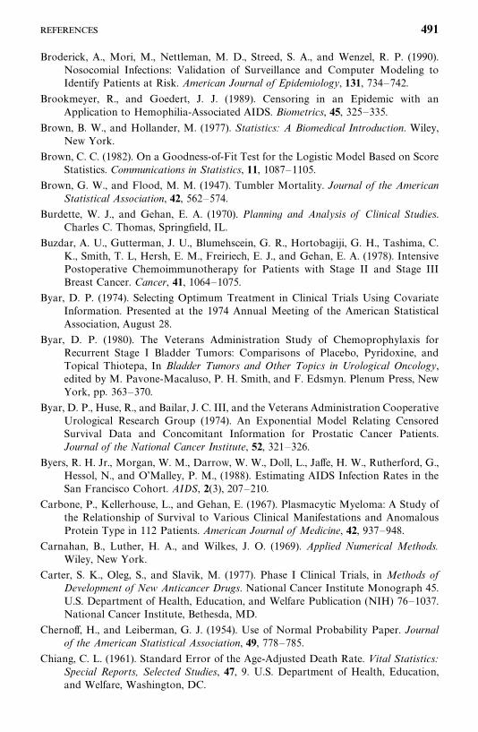
Broderick, A., Mori, M., Nettleman, M. D., Streed, S. A., and Wenzel, R. P. (1990).Nosocomial Infections: Validation of Surveillance and Computer Modeling toIdentify Patients at Risk. American Journal of Epidemiology, 131, 734—742.
Brookmeyer, R., and Goedert, J. J. (1989). Censoring in an Epidemic with anApplication to Hemophilia-Associated AIDS. Biometrics, 45, 325—335.
Brown, B. W., and Hollander, M. (1977). Statistics: A Biomedical Introduction. Wiley,New York.
Brown, C. C. (1982). On a Goodness-of-Fit Test for the Logistic Model Based on ScoreStatistics. Communications in Statistics, 11, 1087—1105.
Brown, G. W., and Flood, M. M. (1947). Tumbler Mortality. Journal of the AmericanStatistical Association, 42, 562—574.
Burdette, W. J., and Gehan, E. A. (1970). Planning and Analysis of Clinical Studies.Charles C. Thomas, Springfield, IL.
Buzdar, A. U., Gutterman, J. U., Blumehscein, G. R., Hortobagiji, G. H., Tashima, C.K., Smith, T. L, Hersh, E. M., Freiriech, E. J., and Gehan, E. A. (1978). IntensivePostoperative Chemoimmunotherapy for Patients with Stage II and Stage IIIBreast Cancer. Cancer, 41, 1064—1075.
Byar, D. P. (1974). Selecting Optimum Treatment in Clinical Trials Using CovariateInformation. Presented at the 1974 Annual Meeting of the American StatisticalAssociation, August 28.
Byar, D. P. (1980). The Veterans Administration Study of Chemoprophylaxis forRecurrent Stage I Bladder Tumors: Comparisons of Placebo, Pyridoxine, andTopical Thiotepa, In Bladder Tumors and Other Topics in Urological Oncology,edited by M. Pavone-Macaluso, P. H. Smith, and F. Edsmyn. Plenum Press, NewYork, pp. 363—370.
Byar, D. P., Huse, R., and Bailar, J. C. III, and the Veterans Administration CooperativeUrological Research Group (1974). An Exponential Model Relating CensoredSurvival Data and Concomitant Information for Prostatic Cancer Patients.Journal of the National Cancer Institute, 52, 321—326.
Byers, R. H. Jr., Morgan, W. M., Darrow, W. W., Doll, L., Jaffe, H. W., Rutherford, G.,Hessol, N., and O’Malley, P. M., (1988). Estimating AIDS Infection Rates in theSan Francisco Cohort. AIDS, 2(3), 207—210.
Carbone, P., Kellerhouse, L., and Gehan, E. (1967). Plasmacytic Myeloma: A Study ofthe Relationship of Survival to Various Clinical Manifestations and AnomalousProtein Type in 112 Patients. American Journal of Medicine, 42, 937—948.
Carnahan, B., Luther, H. A., and Wilkes, J. O. (1969). Applied Numerical Methods.Wiley, New York.
Carter, S. K., Oleg, S., and Slavik, M. (1977). Phase I Clinical Trials, in Methods ofDevelopment of New Anticancer Drugs. National Cancer Institute Monograph 45.U.S. Department of Health, Education, and Welfare Publication (NIH) 76—1037.National Cancer Institute, Bethesda, MD.
Chernoff, H., and Leiberman, G. J. (1954). Use of Normal Probability Paper. Journalof the American Statistical Association, 49, 778—785.
Chiang, C. L. (1961). Standard Error of the Age-Adjusted Death Rate. Vital Statistics:Special Reports, Selected Studies, 47, 9. U.S. Department of Health, Education,and Welfare, Washington, DC.
491
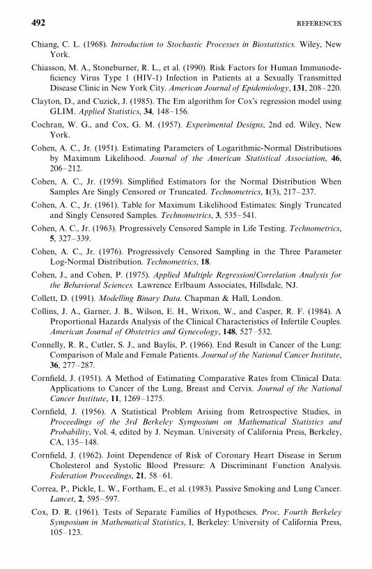
Chiang, C. L. (1968). Introduction to Stochastic Processes in Biostatistics. Wiley, NewYork.
Chiasson, M. A., Stoneburner, R. L., et al. (1990). Risk Factors for Human Immunode-ficiency Virus Type 1 (HIV-1) Infection in Patients at a Sexually TransmittedDisease Clinic in New York City. American Journal of Epidemiology, 131, 208—220.
Clayton, D., and Cuzick, J. (1985). The Em algorithm for Cox’s regression model usingGLIM. Applied Statistics, 34, 148—156.
Cochran, W. G., and Cox, G. M. (1957). Experimental Designs, 2nd ed. Wiley, NewYork.
Cohen, A. C., Jr. (1951). Estimating Parameters of Logarithmic-Normal Distributionsby Maximum Likelihood. Journal of the American Statistical Association, 46,206—212.
Cohen, A. C., Jr. (1959). Simplified Estimators for the Normal Distribution WhenSamples Are Singly Censored or Truncated. Technometrics, 1(3), 217—237.
Cohen, A. C., Jr. (1961). Table for Maximum Likelihood Estimates: Singly Truncatedand Singly Censored Samples. Technometrics, 3, 535—541.
Cohen, A. C., Jr. (1963). Progressively Censored Sample in Life Testing. Technometrics,5, 327—339.
Cohen, A. C., Jr. (1976). Progressively Censored Sampling in the Three ParameterLog-Normal Distribution. Technometrics, 18.
Cohen, J., and Cohen, P. (1975). Applied Multiple Regression/Correlation Analysis forthe Behavioral Sciences. Lawrence Erlbaum Associates, Hillsdale, NJ.
Collett, D. (1991). Modelling Binary Data. Chapman & Hall, London.
Collins, J. A., Garner, J. B., Wilson, E. H., Wrixon, W., and Casper, R. F. (1984). AProportional Hazards Analysis of the Clinical Characteristics of Infertile Couples.American Journal of Obstetrics and Gynecology, 148, 527—532.
Connelly, R. R., Cutler, S. J., and Baylis, P. (1966). End Result in Cancer of the Lung:Comparison of Male and Female Patients. Journal of the National Cancer Institute,36, 277—287.
Cornfield, J. (1951). A Method of Estimating Comparative Rates from Clinical Data:Applications to Cancer of the Lung, Breast and Cervix. Journal of the NationalCancer Institute, 11, 1269—1275.
Cornfield, J. (1956). A Statistical Problem Arising from Retrospective Studies, inProceedings of the 3rd Berkeley Symposium on Mathematical Statistics andProbability, Vol. 4, edited by J. Neyman. University of California Press, Berkeley,CA, 135—148.
Cornfield, J. (1962). Joint Dependence of Risk of Coronary Heart Disease in SerumCholesterol and Systolic Blood Pressure: A Discriminant Function Analysis.Federation Proceedings, 21, 58—61.
Correa, P., Pickle, L. W., Fortham, E., et al. (1983). Passive Smoking and Lung Cancer.Lancet, 2, 595—597.
Cox, D. R. (1961). Tests of Separate Families of Hypotheses. Proc. Fourth BerkeleySymposium in Mathematical Statistics, I, Berkeley: University of California Press,105—123.
492
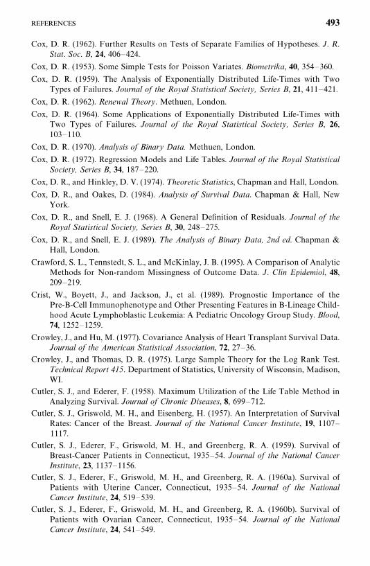
Cox, D. R. (1962). Further Results on Tests of Separate Families of Hypotheses. J. R.Stat. Soc. B, 24, 406—424.
Cox, D. R. (1953). Some Simple Tests for Poisson Variates. Biometrika, 40, 354—360.
Cox, D. R. (1959). The Analysis of Exponentially Distributed Life-Times with TwoTypes of Failures. Journal of the Royal Statistical Society, Series B, 21, 411—421.
Cox, D. R. (1962). Renewal Theory. Methuen, London.
Cox, D. R. (1964). Some Applications of Exponentially Distributed Life-Times withTwo Types of Failures. Journal of the Royal Statistical Society, Series B, 26,103—110.
Cox, D. R. (1970). Analysis of Binary Data. Methuen, London.
Cox, D. R. (1972). Regression Models and Life Tables. Journal of the Royal StatisticalSociety, Series B, 34, 187—220.
Cox, D. R., and Hinkley, D. V. (1974). T heoretic Statistics, Chapman and Hall, London.
Cox, D. R., and Oakes, D. (1984). Analysis of Survival Data. Chapman & Hall, NewYork.
Cox, D. R., and Snell, E. J. (1968). A General Definition of Residuals. Journal of theRoyal Statistical Society, Series B, 30, 248—275.
Cox, D. R., and Snell, E. J. (1989). The Analysis of Binary Data, 2nd ed. Chapman &Hall, London.
Crawford, S. L., Tennstedt, S. L., and McKinlay, J. B. (1995). A Comparison of AnalyticMethods for Non-random Missingness of Outcome Data. J. Clin Epidemiol, 48,209—219.
Crist, W., Boyett, J., and Jackson, J., et al. (1989). Prognostic Importance of thePre-B-Cell Immunophenotype and Other Presenting Features in B-Lineage Child-hood Acute Lymphoblastic Leukemia: A Pediatric Oncology Group Study. Blood,74, 1252—1259.
Crowley, J., and Hu, M. (1977). Covariance Analysis of Heart Transplant Survival Data.Journal of the American Statistical Association, 72, 27—36.
Crowley, J., and Thomas, D. R. (1975). Large Sample Theory for the Log Rank Test.Technical Report 415. Department of Statistics, University of Wisconsin, Madison,WI.
Cutler, S. J., and Ederer, F. (1958). Maximum Utilization of the Life Table Method inAnalyzing Survival. Journal of Chronic Diseases, 8, 699—712.
Cutler, S. J., Griswold, M. H., and Eisenberg, H. (1957). An Interpretation of SurvivalRates: Cancer of the Breast. Journal of the National Cancer Institute, 19, 1107—1117.
Cutler, S. J., Ederer, F., Griswold, M. H., and Greenberg, R. A. (1959). Survival ofBreast-Cancer Patients in Connecticut, 1935—54. Journal of the National CancerInstitute, 23, 1137—1156.
Cutler, S. J., Ederer, F., Griswold, M. H., and Greenberg, R. A. (1960a). Survival ofPatients with Uterine Cancer, Connecticut, 1935—54. Journal of the NationalCancer Institute, 24, 519—539.
Cutler, S. J., Ederer, F., Griswold, M. H., and Greenberg, R. A. (1960b). Survival ofPatients with Ovarian Cancer, Connecticut, 1935—54. Journal of the NationalCancer Institute, 24, 541—549.
493
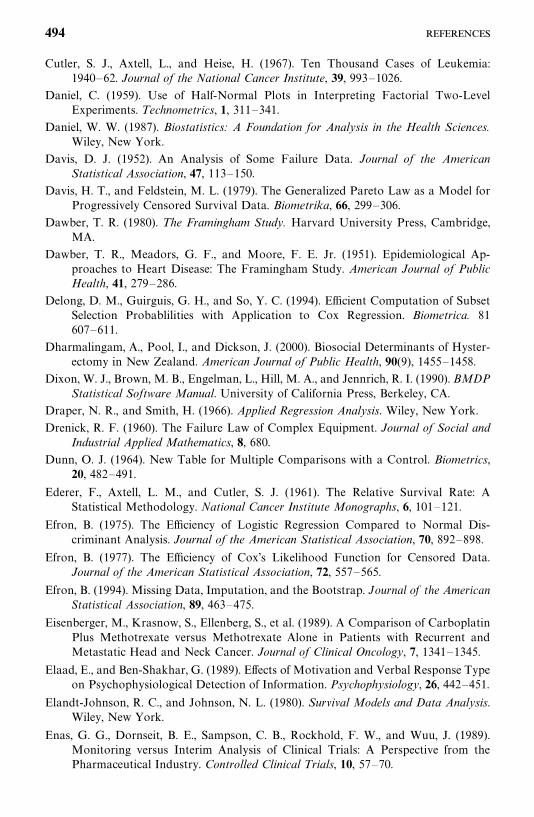
Cutler, S. J., Axtell, L., and Heise, H. (1967). Ten Thousand Cases of Leukemia:1940—62. Journal of the National Cancer Institute, 39, 993—1026.
Daniel, C. (1959). Use of Half-Normal Plots in Interpreting Factorial Two-LevelExperiments. Technometrics, 1, 311—341.
Daniel, W. W. (1987). Biostatistics: A Foundation for Analysis in the Health Sciences.Wiley, New York.
Davis, D. J. (1952). An Analysis of Some Failure Data. Journal of the AmericanStatistical Association, 47, 113—150.
Davis, H. T., and Feldstein, M. L. (1979). The Generalized Pareto Law as a Model forProgressively Censored Survival Data. Biometrika, 66, 299—306.
Dawber, T. R. (1980). The Framingham Study. Harvard University Press, Cambridge,MA.
Dawber, T. R., Meadors, G. F., and Moore, F. E. Jr. (1951). Epidemiological Ap-proaches to Heart Disease: The Framingham Study. American Journal of PublicHealth, 41, 279—286.
Delong, D. M., Guirguis, G. H., and So, Y. C. (1994). Efficient Computation of SubsetSelection Probablilities with Application to Cox Regression. Biometrica. 81607—611.
Dharmalingam, A., Pool, I., and Dickson, J. (2000). Biosocial Determinants of Hyster-ectomy in New Zealand. American Journal of Public Health, 90(9), 1455—1458.
Dixon, W. J., Brown, M. B., Engelman, L., Hill, M. A., and Jennrich, R. I. (1990). BMDPStatistical Software Manual. University of California Press, Berkeley, CA.
Draper, N. R., and Smith, H. (1966). Applied Regression Analysis. Wiley, New York.
Drenick, R. F. (1960). The Failure Law of Complex Equipment. Journal of Social andIndustrial Applied Mathematics, 8, 680.
Dunn, O. J. (1964). New Table for Multiple Comparisons with a Control. Biometrics,20, 482—491.
Ederer, F., Axtell, L. M., and Cutler, S. J. (1961). The Relative Survival Rate: AStatistical Methodology. National Cancer Institute Monographs, 6, 101—121.
Efron, B. (1975). The Efficiency of Logistic Regression Compared to Normal Dis-criminant Analysis. Journal of the American Statistical Association, 70, 892—898.
Efron, B. (1977). The Efficiency of Cox’s Likelihood Function for Censored Data.Journal of the American Statistical Association, 72, 557—565.
Efron, B. (1994). Missing Data, Imputation, and the Bootstrap. Journal of the AmericanStatistical Association, 89, 463—475.
Eisenberger, M., Krasnow, S., Ellenberg, S., et al. (1989). A Comparison of CarboplatinPlus Methotrexate versus Methotrexate Alone in Patients with Recurrent andMetastatic Head and Neck Cancer. Journal of Clinical Oncology, 7, 1341—1345.
Elaad, E., and Ben-Shakhar, G. (1989). Effects of Motivation and Verbal Response Typeon Psychophysiological Detection of Information. Psychophysiology, 26, 442—451.
Elandt-Johnson, R. C., and Johnson, N. L. (1980). Survival Models and Data Analysis.Wiley, New York.
Enas, G. G., Dornseit, B. E., Sampson, C. B., Rockhold, F. W., and Wuu, J. (1989).Monitoring versus Interim Analysis of Clinical Trials: A Perspective from thePharmaceutical Industry. Controlled Clinical Trials, 10, 57—70.
494
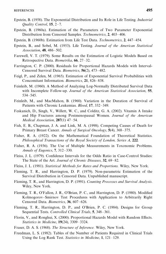
Epstein, B. (1958). The Exponential Distribution and Its Role in Life Testing. IndustrialQuality Control, 15, 2—7.
Epstein, B. (1960a). Estimation of the Parameters of Two Parameter ExponentialDistribution from Censored Samples. Technometrics, 2, 403—406.
Epstein, B. (1960b). Estimation from Life Test Data. Technometrics, 2, 447—454.
Epstein, B., and Sobel, M. (1953). Life Testing. Journal of the American StatisticalAssociation, 48, 486—502.
Farewell, V. T. (1979). Some Results on the Estimation of Logistic Models Based onRetrospective Data. Biometrika, 66, 27—32.
Farrington, C. P. (2000). Residuals for Proportional Hazards Models with Interval-Censored Survival Data. Biometrics, 56(2), 473—482.
Feigl, P., and Zelen, M. (1965). Estimation of Exponential Survival Probabilities withConcomitant Information. Biometrics, 21, 826—838.
Feinleib, M. (1960). A Method of Analyzing Log-Normally Distributed Survival Datawith Incomplete Follow-up. Journal of the American Statistical Association, 55,534—545.
Feinleib, M., and MacMahon, B. (1960). Variation in the Duration of Survival ofPatients with Chronic Leukemias. Blood, 17, 332—349.
Feskanich, D., Singh, V., Willett, W. C., and Colditz, G. A. (2002). Vitamin A Intakeand Hip Fractures among Postmenopausal Women. Journal of the AmericanMedical Association, 287(1) 47—54.
Fish, E. B., Chapman, J. A. and Link, M. A. (1998). Competing Causes of Death forPrimary Breast Cancer. Annals of Surgical Oncology, 5(4), 368—375.
Fisher, R. A. (1922). On the Mathematical Foundation of Theoretical Statistics.Philosophical Transactions of the Royal Society of London, Series A, 222.
Fisher, R. A. (1936). The Use of Multiple Measurements in Toxonomic Problems.Annals of Eugenics, 7, 312—330.
Fleiss, J. L. (1979). Confidence Intervals for the Odds Ratio in Case-Control Studies:The State of the Art. Journal of Chronic Diseases, 32, 69—82.
Fleiss, J. L. (1981). Statistical Methods for Rates and Proportions. Wiley, New York.
Fleming, T. R., and Harrington, D. P. (1979). Non-parametric Estimation of theSurvival Distribution in Censored Data. Unpublished manuscript.
Fleming, T. R., and Harrington, D. P. (1991). Counting Processes and Survival Analysis.Wiley, New York.
Fleming, T. R., O’Fallon, J. R., O’Brian, P. C., and Harrington, D. P. (1980). ModifiedKolmogorov—Smirnov Test Procedures with Application to Arbitrarily RightCensored Data. Biometrics, 36, 607—626.
Fleming, T. R., Harrington, D. P., and O’Brien, P. C. (1984). Designs for GroupSequential Tests. Controlled Clinical Trials, 5, 348—361.
Florin, V., and Ronghui, X. (2000). Proportional Hazards Model with Random Effects.Statistics in Medicine, 19(24), 3309—3324.
Fraser, D. A. S. (1968). The Structure of Inference. Wiley, New York.
Freedman, L. S. (1982). Tables of the Number of Patients Required in Clinical TrialsUsing the Log Rank Test. Statistics in Medicine, 1, 121—129.
495
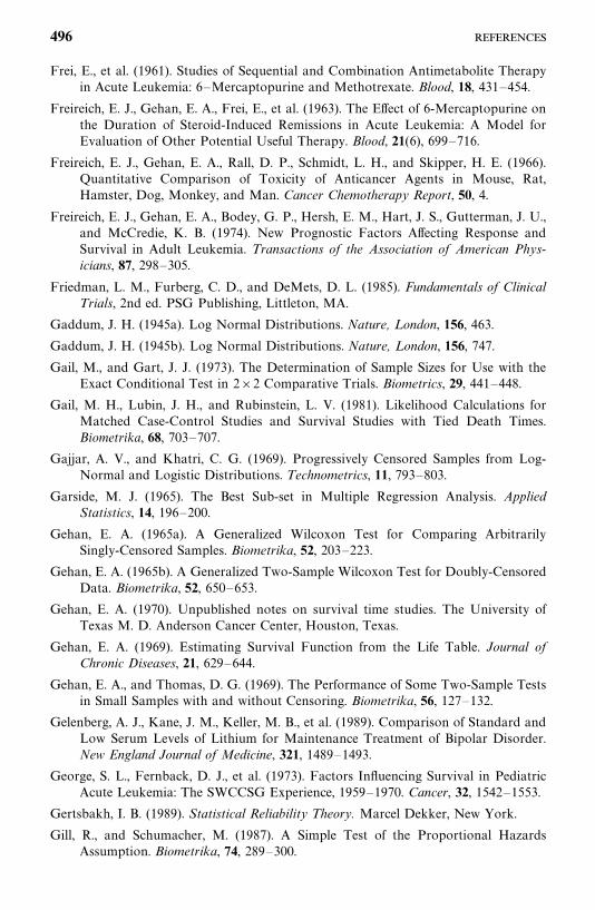
Frei, E., et al. (1961). Studies of Sequential and Combination Antimetabolite Therapyin Acute Leukemia: 6—Mercaptopurine and Methotrexate. Blood, 18, 431—454.
Freireich, E. J., Gehan, E. A., Frei, E., et al. (1963). The Effect of 6-Mercaptopurine onthe Duration of Steroid-Induced Remissions in Acute Leukemia: A Model forEvaluation of Other Potential Useful Therapy. Blood, 21(6), 699—716.
Freireich, E. J., Gehan, E. A., Rall, D. P., Schmidt, L. H., and Skipper, H. E. (1966).Quantitative Comparison of Toxicity of Anticancer Agents in Mouse, Rat,Hamster, Dog, Monkey, and Man. Cancer Chemotherapy Report, 50, 4.
Freireich, E. J., Gehan, E. A., Bodey, G. P., Hersh, E. M., Hart, J. S., Gutterman, J. U.,and McCredie, K. B. (1974). New Prognostic Factors Affecting Response andSurvival in Adult Leukemia. Transactions of the Association of American Phys-icians, 87, 298—305.
Friedman, L. M., Furberg, C. D., and DeMets, D. L. (1985). Fundamentals of ClinicalTrials, 2nd ed. PSG Publishing, Littleton, MA.
Gaddum, J. H. (1945a). Log Normal Distributions. Nature, London, 156, 463.
Gaddum, J. H. (1945b). Log Normal Distributions. Nature, London, 156, 747.
Gail, M., and Gart, J. J. (1973). The Determination of Sample Sizes for Use with theExact Conditional Test in 2�2 Comparative Trials. Biometrics, 29, 441—448.
Gail, M. H., Lubin, J. H., and Rubinstein, L. V. (1981). Likelihood Calculations forMatched Case-Control Studies and Survival Studies with Tied Death Times.Biometrika, 68, 703—707.
Gajjar, A. V., and Khatri, C. G. (1969). Progressively Censored Samples from Log-Normal and Logistic Distributions. Technometrics, 11, 793—803.
Garside, M. J. (1965). The Best Sub-set in Multiple Regression Analysis. AppliedStatistics, 14, 196—200.
Gehan, E. A. (1965a). A Generalized Wilcoxon Test for Comparing ArbitrarilySingly-Censored Samples. Biometrika, 52, 203—223.
Gehan, E. A. (1965b). A Generalized Two-Sample Wilcoxon Test for Doubly-CensoredData. Biometrika, 52, 650—653.
Gehan, E. A. (1970). Unpublished notes on survival time studies. The University ofTexas M. D. Anderson Cancer Center, Houston, Texas.
Gehan, E. A. (1969). Estimating Survival Function from the Life Table. Journal ofChronic Diseases, 21, 629—644.
Gehan, E. A., and Thomas, D. G. (1969). The Performance of Some Two-Sample Testsin Small Samples with and without Censoring. Biometrika, 56, 127—132.
Gelenberg, A. J., Kane, J. M., Keller, M. B., et al. (1989). Comparison of Standard andLow Serum Levels of Lithium for Maintenance Treatment of Bipolar Disorder.New England Journal of Medicine, 321, 1489—1493.
George, S. L., Fernback, D. J., et al. (1973). Factors Influencing Survival in PediatricAcute Leukemia: The SWCCSG Experience, 1959—1970. Cancer, 32, 1542—1553.
Gertsbakh, I. B. (1989). Statistical Reliability Theory. Marcel Dekker, New York.
Gill, R., and Schumacher, M. (1987). A Simple Test of the Proportional HazardsAssumption. Biometrika, 74, 289—300.
496
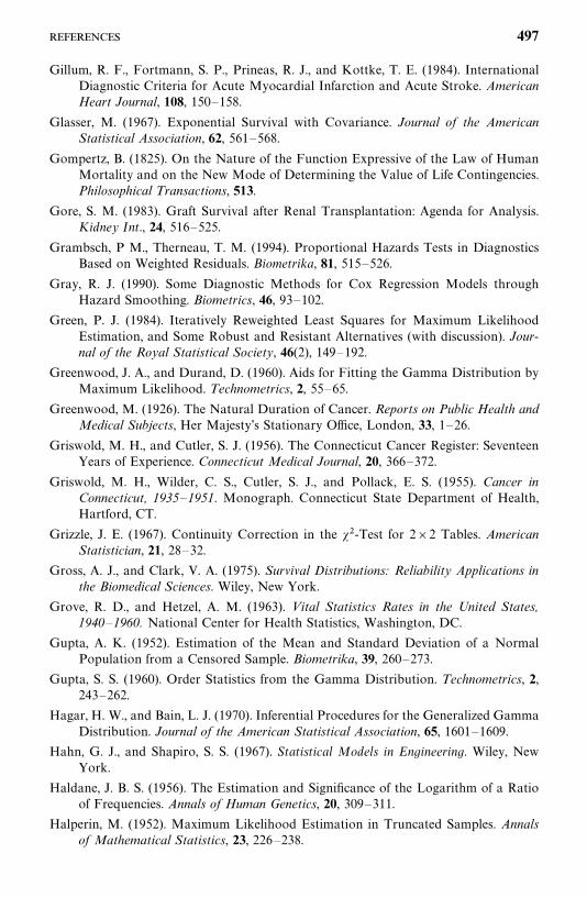
Gillum, R. F., Fortmann, S. P., Prineas, R. J., and Kottke, T. E. (1984). InternationalDiagnostic Criteria for Acute Myocardial Infarction and Acute Stroke. AmericanHeart Journal, 108, 150—158.
Glasser, M. (1967). Exponential Survival with Covariance. Journal of the AmericanStatistical Association, 62, 561—568.
Gompertz, B. (1825). On the Nature of the Function Expressive of the Law of HumanMortality and on the New Mode of Determining the Value of Life Contingencies.Philosophical Transactions, 513.
Gore, S. M. (1983). Graft Survival after Renal Transplantation: Agenda for Analysis.Kidney Int., 24, 516—525.
Grambsch, P M., Therneau, T. M. (1994). Proportional Hazards Tests in DiagnosticsBased on Weighted Residuals. Biometrika, 81, 515—526.
Gray, R. J. (1990). Some Diagnostic Methods for Cox Regression Models throughHazard Smoothing. Biometrics, 46, 93—102.
Green, P. J. (1984). Iteratively Reweighted Least Squares for Maximum LikelihoodEstimation, and Some Robust and Resistant Alternatives (with discussion). Jour-nal of the Royal Statistical Society, 46(2), 149—192.
Greenwood, J. A., and Durand, D. (1960). Aids for Fitting the Gamma Distribution byMaximum Likelihood. Technometrics, 2, 55—65.
Greenwood, M. (1926). The Natural Duration of Cancer. Reports on Public Health andMedical Subjects, Her Majesty’s Stationary Office, London, 33, 1—26.
Griswold, M. H., and Cutler, S. J. (1956). The Connecticut Cancer Register: SeventeenYears of Experience. Connecticut Medical Journal, 20, 366—372.
Griswold, M. H., Wilder, C. S., Cutler, S. J., and Pollack, E. S. (1955). Cancer inConnecticut, 1935—1951. Monograph. Connecticut State Department of Health,Hartford, CT.
Grizzle, J. E. (1967). Continuity Correction in the ��-Test for 2�2 Tables. AmericanStatistician, 21, 28—32.
Gross, A. J., and Clark, V. A. (1975). Survival Distributions: Reliability Applications inthe Biomedical Sciences. Wiley, New York.
Grove, R. D., and Hetzel, A. M. (1963). Vital Statistics Rates in the United States,1940—1960. National Center for Health Statistics, Washington, DC.
Gupta, A. K. (1952). Estimation of the Mean and Standard Deviation of a NormalPopulation from a Censored Sample. Biometrika, 39, 260—273.
Gupta, S. S. (1960). Order Statistics from the Gamma Distribution. Technometrics, 2,243—262.
Hagar, H. W., and Bain, L. J. (1970). Inferential Procedures for the Generalized GammaDistribution. Journal of the American Statistical Association, 65, 1601—1609.
Hahn, G. J., and Shapiro, S. S. (1967). Statistical Models in Engineering. Wiley, NewYork.
Haldane, J. B. S. (1956). The Estimation and Significance of the Logarithm of a Ratioof Frequencies. Annals of Human Genetics, 20, 309—311.
Halperin, M. (1952). Maximum Likelihood Estimation in Truncated Samples. Annalsof Mathematical Statistics, 23, 226—238.
497
Halperin, M., Blackwelder, W. C., and Verter, J. I. (1971). Estimation of the Multivari-ate Logistic Risk Function: A Comparison of the Discriminant Function andMaximum Likelihood Approaches. Journal of Chronic Diseases, 24, 125—158.
Hammond, I. W., Lee, E. T., Davis, A. W., and Booze, C. F. (1984). Prognostic FactorsRelated to Survival and Complication-Free Times in Airmen Medically Certifiedafter Coronary Bypass Surgery. Aviation, Space, and Environmental Medicine,April, pp. 321—331.
Hannan, E. J. (1979). The Determination of the Order of an Autoregression. Journal ofthe Royal Statistical Society, Series B, 41, 190—195.
Hanson, B. S., Isacsson, S-O., Janzon, L., and Lindell, S. E. (1989). Social Network andSocial Support Influence Mortality in Elderly Men. American Journal of Epi-demiology, 130, 100—111.
Harrison, J. D., Jones, J. A., and Morris, D. L. (1990). The Effect of the Gastrin ReceptorAntagonist Proglumide on Survival in Gastric Carcinoma. Cancer, 66, 1449—1452.
Hart, J. S., George, S. L., Frei, E., Bodey, G. P., Nickerson, R. C., and Freireich, E. J.(1977). Prognostic Significance of Pretreatment Proliferative Activity in AdultAcute Leukemia. Cancer, 39, 1603—1617.
Harter, H. L., and Moore, A. H. (1965). Maximum Likelihood Estimation of theParameters of Gamma and Weibull Populations from Complete and from Cen-sored Samples. Technometrics, 7, 639—643.
Harter, H. L., and Moore, A. H. (1966). Local Maximum Likelihood Estimation of theParameters of Three-Parameter Log-Normal Population from Complete andCensored Sample. Journal of the American Statistical Association, 61, 842—851.
Harter, H. L., and Moore, A. H. (1967). Asymptotic Variance and Covariances ofMaximum Likelihood Estimators, from Censored Samples, of the Parameters ofWeibull and Gamma Parameters. Annals of Mathematical Statistics, 38, 557—570.
Hastings, N. A. J., and Peacock, J. B. (1974). Statistical Distributions. Butterworth,London.
Hauck, W. W., Jr., and Donner, A. (1977). Wald’s Test as Applied to Hypotheses inLogit Analysis. Journal of the American Statistical Association, 72, 851—853.
Haughton, D. M. A. (1988). On the Choice of a Model to Fit Data from an ExponentialFamily. Annals of Statistics, 16, 342—355.
Heitjan, D. F. (1997). Annotation: What Can be Done About Missing Data? Ap-proaches to imputation, Am. J. Public Health, 87, 548—550.
Hemstreet, G. P., Yin, S., Ma, Z., Bonner, R. B., Bi, W., Rao, J. Y., Zang, M., Zheng,Q., Bane, B., Asal, N., Li, G., Feng, P., Hurst, R. E., and Wang, W. (2001).Biomarker Risk Assessment and Bladder Cancer Detection in a Cohort Exposedto Benzidine, Journal of the National Cancer Institute, 93, 427—436.
Hill, A. B. (1960a). Controlled Clinical Trials. Blackwell Scientific, Oxford
Hill, A. B. (1960b). Statistical Methods in Clinical and Preventive Medicine. OxfordUniversity Press, Oxford.
Hill, A. B. (1971). Principles of Medical Statistics. Oxford University Press, New York.
Hirayama, T. (1981). Non-smoking Wives of Heavy Smokers Have a Higher Risk ofLung Cancer: A Study from Japan. British Medical Journal, 282, 183—185.
498
Hoel, D. G., Sobel, M., and Weiss, G. H. (1975). A Survey of Adaptive Sampling forClinical Trials. Perspectives in Biometrics, 1, 29—61.
Holford, T. R., White, C., and Kelsey, J. L. (1978). Multivariate Analysis for MatchedCase-Control Studies. American Journal of Epidemiology, 107, 245—256.
Hollander, M., and Proschan, F. (1979). Testing to Determine the Underlying Distribu-tion Using Randomly Censored Data. Biometrics, 35, 393—401.
Hollander, M., and Wolfe, D. A. (1973). Nonparametric Statistical Methods. Wiley, NewYork.
Horner, R. D. (1987). Age at Onset of Alzheimer’s Disease: Clue to the RelativeImportance of Etiologic Factors? American Journal of Epidemiology, 126, 409—414.
Hosmer, D. W., and Lemeshow, S. (1980). A Goodness-of-Fit Test for the MultipleLogistic Regression Model. Communications in Statistics, A10, 1043—1069.
Hosmer, D. W., and Lemeshow, S. (1999). Applied Survival Analysis, 2nd ed. Wiley, NewYork.
Hosmer, D. W., and Lemeshow, S. (2000). Applied Logistic Regression. Wiley, NewYork.
Howell, D. W. (1987). Statistical Methods for Psychology. Duxbury Press, Boston.
Hung, C. T., Lim, J. K. C., and Zoest, A. R. (1988). Optimization of High-PerformanceLiquid Chromatographic Analysis for Isoxazolye Penicillins Using FactorialDesign. Journal of Chromatography, 425, 331—341.
Ibrahim, J. G., Chen, M. H., and Sinha, D. (2001). Bayesian Survival Analysis.Springer-Verlag, New York
Ingram, D. D., and Kleinman, J. C. (1989). Empirical Comparisons of ProportionalHazards and Logistic Regression Models. Statistics in Medicine, 8, 525—538.
Irwin, J. O. (1949). The Standard Error of an Estimate of Expectational Life. Journalof Hygiene, 47, 188—189.
Jenkins, S. P. (1997). Discrete Time Proportional Hazards Regression. Stata TechnicalBulletin, 39, 17—32.
Jennings, D. E. (1986). Judging Inference Adequacy in Logistic Regression. Journal ofthe American Statistical Association, 81, 471—476.
Johnson, N. L., and Kotz, S. (1970a). Distributions in Statistics: Continuous UnivariateDistributions (Vol. 1) Houghton Mifflin, Boston.
Johnson, N. L., and Kotz, S. (1970b). Distributions in Statistics: Continuous UnivariateDistributions. (Vol. 2) Houghton Mifflin, Boston
Johnson, P., and Pearce, J. M. (1990). Recurrent Spontaneous Abortion and PolycysticOvarian Disease: Comparison of Two Regimens to Induce Ovulation. BritishMedical Journal, 300, 154—156.
Kahn, H. A. (1983). An Introduction to Epidemiologic Methods. Oxford University Press,New York.
Kalbfleisch, J. D. (1974). Some Extensions and Applications of Cox’s Regression andLife Model. Presented at the joint meeting of the Biometric Society and theAmerican Statistical Association, Tallahassee, FL, March 20—22.
Kalbfleisch, J. D., and Prentice, R. L. (1973). Marginal Likelihoods Based on Cox’sRegression and Life Table Model. Biometrika, 60, 267—278.
499
Kalbfleisch, J. D., and Prentice, R. L. (1980). The Statistical Analysis of Failure TimeData. Wiley, New York.
Kao, J. H. K. (1958). Computer Methods for Estimating Weibull Parameters inReliability Studies. I.R.E. Transactions on Reliability and Quality Control, PGRQC13, 15—22.
Kaplan, E. L., and Meier, P. (1958). Nonparametric Estimation from IncompleteObservations. Journal of the American Statistical Association, 53, 457—481.
Kay, R. (1979). Proportional Hazard Regression Models and the Analysis of CensoredSurvival Data. Applied Statistics, 26, 227—237.
Kay, R. (1984). Goodness of Fit Methods for the Proportional Hazards Model: AReview. Revue Epidemiologie et de Santé Publique, 32, 185—198.
Kelsey, J. L., Thompson, W. D., and Evans, A. S. (1986). Methods in ObservationalEpidemiology. Oxford University Press, New York.
Kessing, L.V., Olsen, E. W., and Andersen, P. K. (1999). Recurrence in AffectiveDisorder: Analyses with Frailty Models. American Journal of Epidemiology, 149(5),404—411.
King, J. R. (1971). Probability Charts for Decision Making. Industrial Press, New York.
King, M., Bailey, D. M., Gibson, D. G., Pitha, J. V., and McCay, P. B. (1979). Incidenceand Growth of Mammary Tumors Induced by 7,12-Dimethylbenz(�)antheacene asRelated to the Dietary Content of Fat and Antioxidant. Journal of the NationalCancer Institute, 63, 656—664.
Kitagawa, E. M. (1964). Standardized Comparisons in Population Research. Demogra-phy, 1, 296—315.
Klein, J. P., and Moeschberger, M. L. (1997) Survival Analysis. Springer-Verlag, NewYork.
Kleinbaum, D. G. (1994). L ogistic Regression: A Self-L earning Text. Springer-Verlag,New York.
Kleinbaum, D. G., Kupper, L. L., and Muller, K. E. (1988). Applied Regression Analysisand Other Multivariate Methods, 2nd ed. PWS-Kent, Boston.
Kodlin, D. (1967). A New Response Time Distribution. Biometrics, 23, 227—239.
Krishna, I. P. V. (1951). A Non-parametric Method of Testing k Samples. Nature, 167,33.
Kruskal, W. H., and Wallis, W. A. (1952). Use of Ranks in One-Criterion VarianceAnalysis. Journal of the American Statistical Association, 47, 583—621.
Kuzma, J. W. (1967). A Comparison of Two Life Table Methods. Biometrics, 23, 51—64.
Lagakos, S. W. (1980). The Graphical Evaluation of Explanatory Variables in Propor-tional Hazard Regression Models. Biometrika, 68, 93—98.
Lan, K. K. G., and DeMets, D. L. (1983). Discrete Sequential Boundaries for ClinicalTrials. Biometrika, 70, 659—663.
Lan, K. K. G., and DeMets, D. L. (1989). Changing Frequency of Interim Analysis inSequential Monitoring. Biometrics, 45, 1017—1020.
Lassare, S. (2001). Analysis of Progress in Road Safety in Ten European Countries.Accident Analysis and Prevention, 33(6), 743—751.
Lawless, J. F. (1982). Statistical Methods and Model for Lifetime Data. Wiley, NewYork.
500
Lawless, J. F. (1983). Statistical Methods in Reliability. Technometrics, 25, 305—316.
Lee, A. H., and Yau, K. K. (2001) Determining the Effects of Patient Case Mix onLength of Hospital Stay: A Proportional Hazards Frailty Model Approach.Methods of Information in Medicine, 40(4), 288—292.
Lee, E. T. (1980). Statistical Methods for Survival Data Analysis. Lifetime LearningPublications, Belmont, CA.
Lee, E. T. (1992). Statistical Methods for Survival Data Analysis, second edition, Wiley,New York.
Lee, E. T., and Thomas, D. R. (1980). Confidence Interval for Comparing Two LifeDistributions. IEEE Transactions on Reliability, R-29, 51—56.
Lee, E. T., Desu, M. M., and Gehan, E. A. (1975). A Monte-Carlo Study of the Powerof Some Two-Sample Tests. Biometrika, 62, 425—432.
Lee, E. T., Ishmael, D. R., Bottomley, R. H., and Murray, J. L. (1982). An Analysis ofSkin Tests and Their Relationship to Recurrence and Survival in Stage III andStage IV Melanoma Patients. Cancer, 49, 2336—2341.
Lee, E. T., Yeh, J. L., Cleves, M. A., and Shafer, D. (1988). Vascular Complications inNoninsulin Dependent Diabetic Oklahoma Indians. Diabetes, 37(Suppl. 1).
Lee, E. T., Lee, V. S., Lu, M., et al. (1992). Incidence and Risk Factors of DiabeticRetinopathy in Oklahoma Indians with NIDDM. Diabetes Care, 15, 1620—1627.
Lee, E. T., Russell, D., Jorge, N., Kenny, S., and Yu, M. (1993). A Follow-up Study ofDiabetic Oklahoma Indians: Mortality and Causes of Death. Diabetes Care, 16,300—305.
Leenen, F. H. H., Balfe, J. A., Pelech, A. N., et al. (1987). Postoperative Hypertensionafter Repair of Coarctation of Aorta in Children: Protective Effect of Propranolol.American Heart Journal, 113, 1164—1173.
Lehmann, E. L. (1953). The Power of Rank Tests. Annals of Mathematical Statistics, 24,23—43.
Leitner, L. M., Roumy, M. Ruckebusch, M., Sutra, J. F. (1986). Monoamines and TheirCatabolites in the Rabbit Carotid Body. Effets of reserpine, sympathectomy andcarotid sinus nerve section, European Journal of Physiology, 406, 552—556.
Lemeshow, S., and Hosmer, D. W. (1982). A Review of Goodness-of-Fit Statistics forUse in the Development of Logistic Regression Models. American Journal ofEpidemiology, 115, 92—106.
Leyland-Jones, B., Donnelly, H., Groshen, S., Myskowski, P., Donner, A. L., Fanucchi,M., Fox, J., and the Memorial Sloan-Kettering Antiviral Working Group (1986).2�-Fluror-5-Iodoarabinosylcytosine, A New Potent Antiviral Agent: Efficacy inImmunosuppressed Individuals with Herpes Zoster. Journal of Infectious Diseases,154, 430—436.
Liang, K. Y., Self, S. G., and Liu, X. (1990). The Cox Proportional Hazards Model withChange Point: An Epidemiologic Application. Biometrics, 46, 783—793.
Liang, K. Y., Self, S. G., Bandeen-Roche, K. J., and Zeger, S. L. (1995). Some RecentDevelopments for Regression Analysis of Multivariate Failure Time Data. Life-time Data Analysis, 1, 403—415.
Lieblein, J., and Zelen, M. (1956). Statistical Investigation of the Fatigue Life ofDeep-Grove Ball Bearings. Journal of Research of the National Bureau of Stan-dards, 57, 273—316.
501
Lilliefors, H. W. (1971). Reducing the Bias of Estimators of Parameters for the Erlangand Gamma Distribution. Unpublished manuscript.
Lindley, D. V. (1968). The Choice of Variables in Multiple Regression. Journal of theRoyal Statistical Society, Series B, 30, 31—53.
Linka, A. Z., Sklenar, J., Wei, K. I., Jayaweera, A. R., Skyba, D. M., and Kaul, S. (1998).Assessment of Transmural Distribution of Myocardial Perfusion with ContrastEchocardiography. Circulation 3; 98(18); 1912—1920.
Little, R. J., and Rubin, D. B. (1987). Statistical Analysis with Missing Data, John Wiley& Sons, New York.
Liu, P. Y., and Crowley, J. (1978). Large Sample Theory of the MLE Based on Cox’sRegression Model for Survival Data. Technical Report 1. Wisconsin ClinicalCancer Center (Biostatistics), University of Wisconsin, Madison, WI.
Lubin, J. H. (1981). A Computer Program for the Analysis of Matched Case-ControlStudies. Computers and Biomedical Research, 14, 138—143.
McAlister, D. (1879). The Law of the Geometric Mean. Proceedings of the RoyalSociety, 29, 367.
McCracken, D. D., and Dorn, W. S. (1964). Numerical Methods and Fortran Pro-gramming. Wiley, New York.
McCullagh, P. (1980). Regression Model for Ordinal Data. Journal of the RoyalStatistical Society, 42(2), 109—142.
McCullagh, P., and Nelder, J. A. (1989). Generalized Linear Models. Chapman & Hall,London.
McFadden, D. (1976). A Comment on Discriminant Analysis ‘‘versus’’ Logit Analysis.Annals of Economic and Social Measurement, 5, 511—523.
Mackenbach, J. P., Kunst, A. E., Lautenbach, H., Bijlsma, F., and Oei, Y.B. (1995).Competing Causes of Death: An Analysis Using Multiple-Cause-of-Death Datafrom The Netherlands. 141(5), 466—475.
Mafart, P., Couvert, O., Gaillard, S., and Leguerinel, I. (2002). On Calculating Sterilityin Thermal Preservation Methods: Application of the Weibull Frequency Distribu-tion Model. International Journal of Food Microbiology, 72(12); 107—113.
Mann, H. B., and Whitney, D. R. (1947). On a Test of Whether One of Two RandomVariables Is Stochastically Larger Than the Other. Annals of MathematicalStatistics, 18, 50—60.
Mann, N. R. (1970). Estimators and Exact Confidence Bounds for Weibull ParametersBased on a Few Ordered Observations. Technometrics, 12, 345—361.
Mann, N. R., Schafer, R. E., and Singpurwalla, N. D. (1974). Methods for StatisticalAnalysis of Reliability and Life Data. Wiley, New York.
Manninen, O. (1988). Changes in Hearing, Cardiovascular Functions, Haemodynamics,Upright Body Sway, Urinary Catecholamines and Their Correlates after Pro-longed Successive Exposure to Complex Environmental Conditions. InternationalArchives of Occupational and Environmental Health, 60, 249—272.
Mantel, N. (1966). Evaluation of Survival Data and Two New Rank Order StatisticsArising in Its Consideration. Cancer Chemotherapy Reports, 50, 163—170.
Mantel, N. (1967). Ranking Procedures for Arbitrarily Restricted Observations. Biomet-rics, 23, 65—78.
502
Mantel, N. (1970). Why Stepdown Procedures in Variable Selection. Technometrics, 12,621—625.
Mantel, N. (1973). Synthetic Retrospective Studies and Related Topics. Biometrics, 29,479—486.
Mantel, N. (1977). Test and Limits for the Common Odds Ratio of Several 2�2Contingency Tables: Methods in Analogy with the Mantel—Haenszel Procedure.Journal of Statistical Planning Information, 1, 179—189.
Mantel, N., and Haenszel, W. (1959). Statistical Aspects of the Analysis of Data fromRetrospective Studies of Disease. Journal of the National Cancer Institute, 22,719—748.
Mantel, N., and Hankey, B. F. (1978). A Logistic Regression Analysis of Response-TimeData Where the Hazard Function Is Time Dependent. Communications in Statis-tics A: Theory and Methods, 7, 333—347.
Mantel, N., and Myers, M. (1971). Problems of Convergence of Maximum LikelihoodIterative Procedures in Multiparameter Situation. Journal of the American Statis-tical Association, 66, 484—491.
Mantel, N., and Stark, C. R. (1968). Computation of Indirect Adjusted Rates in thePresence of Confounding. Biometrics, 24, 997—1005.
Marascuilo, L. A., and McSweeney, M. (1977). Nonparametric and Distribution-FreeMethods for the Social Sciences. Brooks/Cole, Monterey, CA.
Marubini, E., and Valsecchi, M. G. (1995). Analyzing Survival Data from Clinical Trialsand Observational Studies. Wiley, New York.
Matthews, D. E., and Farewell, V. (1985). Using and Understanding Medical Statistics.S. Karger, New York.
Mausner, J. S., and Kramer, S. (1985). Epidemiology: An Introductory Text. W.B.Saunders, Philadelphia.
Meier, P. (1975a). Statistics and Medical Experimentation. Biometrics, 31, 511—529.
Meier, P. (1975b). Estimation of a Distribution Function from Incomplete Observa-tions, in Perspectives in Probability and Statistics, edited by J. Gaui. AppliedProbability Trust, Sheffield, England.
Meisinger, C., Thorand, B., Schneider, A., Stieber, J., Doring, A., and Lowel, H. (2002)Sex Differences in Risk Factors for Incident Type 2 Diabetes Mellitus: theMONICA Augsburg Cohort Study. Arch Intern Med, 162, 82—89.
Miettinen, O. S. (1979). Comments on ‘‘Confidence Intervals for the Odds Ratio inCase-Control Studies: The State of the Art,’’ by J. L. Fleiss. Journal of ChronicDiseases, 32, 80—82.
Miller, R. G., Jr. (1966). Simultaneous Statistical Inference. McGraw-Hill, New York.
Miller, R. G. (1981). Survival Analysis. Wiley, New York.
Minow, R. A., Benjamin, R. S., Lee, E. T., and Gottlieb, J. A. (1977). AdriamycinCardiomyopathy: Risk Factors. Cancer, 39, 1397—1402.
Molloy, D. W., Guyatt, G. H., Wilson, D. B., et al. (1991). Effect of Tetrahydroaminoac-ridine on Cognition, Function and Behaviour in Alzheimer’s Disease. CanadianMedical Association Journal, 144, 29—34.
Montaner, J. S. G., Lawson, L. M., Levitt, N., et al. (1990). Costicorsteroids PreventEarly Deterioration in Patients with Moderately Severe Pneumocystis Carinii
503
Pneumonia and the Acquired Immunodeficiency Syndrome (AIDS). Annals ofInternal Medicine, 113, 14—20.
Moolgavkar, S., Lustbader, E., and Venzon, D. J. (1985). Assessing the Adequacy of theLogistic Regression Model for Matched Case-Control Studies. Statistics in Medi-cine, 4, 425—435.
Moreau, T., O’Quigley, J., and Mesbah, M. (1985). A Global Goodness-of-Fit Statisticfor the Proportional Hazards Model. Applied Statistics, 34, 212—218.
Morrison, D. F. (1967). Multivariate Statistical Methods. McGraw-Hill, New York.
Morrison, R. S., and Siu, A. L. (2000). Survival in End-Stage Dementia Following AcuteIllness. Journal of the American Medical Association, 284(1), 47—52.
Myers, M., Hankey, B. F., and Mantel, N. (1973). A Logistic-Exponential Model forUse with the Response-Time Data Involving Regressor Variables. Biometrics, 29,257—269.
Myers, M. H. (1969). A Computing Procedure for a Significance Test of the Differencebetween Two Survival Curves. Methodological Note 18 in Methodological Notes.End Results Sections, National Cancer Institute, National Institutes of Health,Bethesda, MD.
Nadas, A. (1970). On Proportional Hazard Functions. Technometrics, 12, 413—416.
National Cancer Institute (1970). Proceedings of the Symposium on Statistical Aspectsof Protocol Design, San Juan, Puerto Rico, December 9—10.
Natrella, M. G. (1963). Experimental Statistics. National Bureau of Standards Hand-book 91. U.S. Government Printing Office, Washington, DC, Tables A-25, A-26.
Nelson, W. (1972). Theory and Applications of Hazard Plotting for Censored FailureData. Technometrics, 14, 945—966.
Nelson, W. (1982). Applied Life Data Analysis. Wiley, New York.
Nemenyi, P. (1963). Distribution-Free Multiple Comparisons. Ph.D. dissertation, Prin-ceton University.
Neter, J., and Wasserman, W. (1974). Applied Linear Statistical Models. Richard D.Irwin, Homewood, IL.
Nie, N. H., Hull, C. H., Jenkins, J. G., Steinbrenner, K., and Bent, D. H. (1975). SPSS:Statistical Package for the Social Sciences. McGraw-Hill, New York.
O’Brien, P. C., and Fleming, T. R. (1979). A Multiple Testing Procedure for ClinicalTrials. Biometrics, 35, 549—556.
Osgood, E. W. (1958). Methods for Analyzing Survival Data, Illustrated by Hodgkin’sDisease. American Journal of Medicine, 24, 40—47.
Parker, R. L., Dry, T. J., Willius, F. A., and Gage, R. P. (1946). Life Expectancy inAngina Pectoris. Journal of the American Medical Association, 131, 95—100.
Parzan, E. (1974). Some Recent Advances in Time Series Modeling. IEEE Transactionson Automatic Control. AC-19, 723—730.
Pearson, E. S., and Hartely, N. O. (1958). Biometrika Tables for Statisticians, Vol. 1.Cambridge University Press, Cambridge.
Pearson, K. (1922, 1957). Tables of the Incomplete �-Function. Cambridge UniversityPress, Cambridge.
Pershagen, G. (1986). Review of Epidemiology in Relation to Passive Smoking. Archivesof Toxicology, 9(Suppl.), 63—73.
504
Pershagen, G., Hrubec, Z., and Svensson, C. (1987). Passive Smoking and Lung Cancerin Swedish Women. American Journal of Epidemiology, 125, 17—24.
Peto, R., and Lee, P. N. (1973). Weibull Distributions for Continuous CarcinogenesisExperiments. Biometrics, 29, 457—470.
Peto, R., and Peto, J. (1972). Asymptotically Efficient Rank Invariant Procedures.Journal of the Royal Statistical Society, Series A, 135, 185—207.
Peto, R., Lee, P. N., and Paige, W. S. (1972). Statistical Analysis of the Bioassay ofContinuous Carcinogens. British Journal of Cancer, 26, 258—261.
Peto, R., Pike, M. C., Armitage, P., Breslow, N. E., Cox, D. R., Howard, S. V., Mantel,N., McPherson, K., Peto, J., and Smith, P. G. (1976, 1977). Design and Analysisof Randomized Clinical Trials Requiring Prolonged Observation of Each Patient.British Journal of Cancer, Part I, 34, 585—612, 1976; Part II, 35, 1—39, 1977.
Pierce, M., Borges, W. H., Heyn, R., Wolfe, J., and Gilbert, E. S. (1969). EpidemiologicalFactors and Survival Experience in 1770 Children with Acute Leukemia. Cancer,23, 1296—1304.
Pike, M. C. (1966). A Method of Analysis of a Certain Class of Experiments inCarcinogenesis. Biometrics, 22, 142—161.
Piper, J. M., Matanoski, G. M., and Tonascia, J. (1986). Bladder Cancer in YoungWomen. American Journal of Epidemiology, 123, 1033—1042.
Pregibon, D. (1984). Data Analytic Methods for Matched Case-Control Studies.Biometrics, 40, 639—651.
Prentice, R. L. (1973). Exponential Survivals with Censoring and Explanatory Vari-ables. Biometrika, 60, 279—288.
Prentice, R. L. (1974). A Log-Gamma Model and Its Maximum Likelihood Estimation.Biometrica. 61 539—544.
Prentice, R. L. (1976). Use of the Logistic Model in Retrospective Studies. Biometrics,32, 599—606.
Prentice, R. L., and Gloeckler, L. A. (1978). Regression Analysis of Grouped SurvivalData with Application to Breast Cancer Data. Biometrics, 34, 57—67.
Prentice, R. L., and Kalbfleisch, J. D. (1979). Hazard Rate Models with Covariates.Biometrics, 35, 25—39.
Prentice, R. L., and Marek, P. (1979). A Quantitative Discrepancy between CensoredData Rank Tests. Biometrics, 35, 861—867.
Prentice, R. L., and Pyke, R. (1979). Logistic Disease Incidence Models and Case-control Studies. Biometrica, 73, 403—411.
Prentice, R. L., Williams, B. J., and Peterson, A. V. (1981). On the Regression Analysisof Multivariate Failure Time Data. Biometrica, 68, 373—379.
Press, S. J. (1972). Applied Multivariate Analysis. Holt, Rinehart & Winston, New York.
Press, S. J., and Wilson, S. (1978). Choosing between Logistic Regression and Dis-criminant Analysis. Journal of the American Statistical Association, 73, 699—705.
Ralston, A., and Wilf, H. (1967). Mathematical Methods for Digital Computers. Wiley,New York.
Rao, C. R. (1952). Advanced Statistical Methods in Biometric Research. Wiley, NewYork.
505
Rao, C. R. (1973). Linear Statistical Inference and Its Application, 2nd ed. Wiley, NewYork.
Riffenburgh, R. H., and Johnstone, P. A. (2001). Survival Patterns of Cancer Patients.Cancer, 91(12), 2469—2475.
Rissanen, J. (1986). A Predictive Least-Squares Principle. IMA Journal of MathematicalControl of Information, 3, 211—222.
Rowe-Jones, D. C., Peel, A. L. G., Kingston, R. D., Shaw, J. F. L., Teasdale, C., andCole, D. S. (1990). Single Dose Cefotaxime Plus Metronidazole versus Three DoseCefuroxime Plus Metronidazole as Prophylaxis against Wound Infection inColorectal Surgery: Multicentre Prospective Randomised Study. British MedicalJournal, 300, 18—22.
Sacher, G. A. (1956). On the Statistical Nature of Mortality, with Special Reference toChronic Radiation Mortality. Radiology, 67, 250—257.
Sarhan, A. E., and Greenberg, B. G. (1956). Estimation of Location and ScaleParameters by Order Statistics from Singly and Doubly Censored Samples, PartI, The Normal Distribution up to Samples of Size 10. Annals of MathematicalStatistics, 27, 427—451.
Sarhan, A. E., and Greenberg, B. G. (1957). Estimation of Location and ScaleParameters by Order Statistics from Singly and Doubly Censored Samples, PartIII. Technical Report 4-OOR, Project 1597. U.S. Army Research Office.
Sarhan, A. E., and Greenberg, B. G. (1958). Estimation of Location and ScaleParameters by Order Statistics from Singly and Doubly Censored Samples, PartII. Annals of Mathematical Statistics, 29, 79—105.
Sarhan, A. E., and Greenberg, B. G. (1962). Contribution to Order Statistics. Wiley, NewYork.
Sacks, H., Chalmers, T. C., and Smith, H. (1982). Randomized versus Historical Controlfor Clinical Trials. American Journal of Medicine, 72, 233—240.
SAS Institute. (2000). SAS/STAT User’s Guide, Version 8.1. SAS Institute, Cary, NC.
Sasieni, P. D. (1996). Proportional Excess Hazards. Biometrika, 83(1), 127—141.Savage, I. R. (1956). Contributions to the Theory of Rank Order Statistics: The Two
Sample Case. Annals of Mathematical Statistics, 27, 590—615.Saw, J. G. (1959). Estimation of the Normal Population Parameters Given a Singly
Censored Sample. Biometrika, 46, 150—159.Schade, D. S., Mitchell, W. J., and Griego, G. (1987). Addition of Sulfonylurea to Insulin
Treatment in Poorly Controlled Type II Diabetes. Journal of the AmericanMedical Association, 257, 2441—2445.
Schafer, J. L. (1999). Multiple Imputation: a Primer. Stat Methods, 8, 3—15.Schlesselman, J. J. (1982). Case-Control Studies. Oxford University Press, New York.
Schoenfeld, D. (1982). Partial Residuals for Proportional Hazards Regression Model.Biometrica. 69, 239—241.
Schwarz, G. (1978). Estimating the Dimension of a Model. Annals of Statistics 6,461—222.
Seaman, S. R., and Bird, S. M. (2001). Proportional Hazards Model for Interval-Censored Failure Times and Time-Dependent Covariates: Application to Hazardof HIV Infection of Injecting Drug Users in Prison. Statistics in Medicine, 20(12),1855—1870.
506
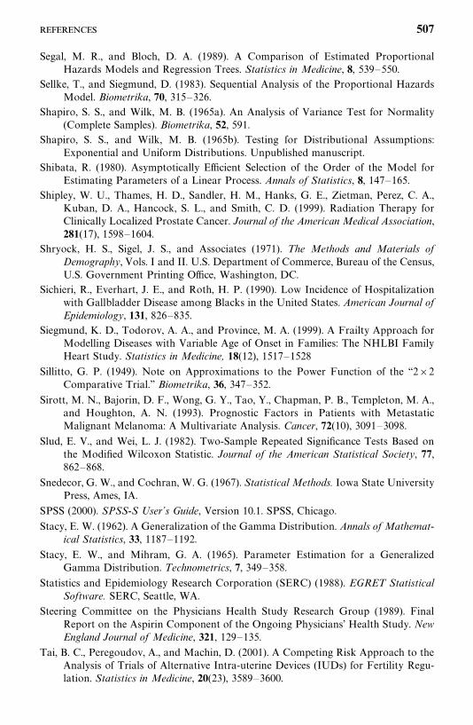
Segal, M. R., and Bloch, D. A. (1989). A Comparison of Estimated ProportionalHazards Models and Regression Trees. Statistics in Medicine, 8, 539—550.
Sellke, T., and Siegmund, D. (1983). Sequential Analysis of the Proportional HazardsModel. Biometrika, 70, 315—326.
Shapiro, S. S., and Wilk, M. B. (1965a). An Analysis of Variance Test for Normality(Complete Samples). Biometrika, 52, 591.
Shapiro, S. S., and Wilk, M. B. (1965b). Testing for Distributional Assumptions:Exponential and Uniform Distributions. Unpublished manuscript.
Shibata, R. (1980). Asymptotically Efficient Selection of the Order of the Model forEstimating Parameters of a Linear Process. Annals of Statistics, 8, 147—165.
Shipley, W. U., Thames, H. D., Sandler, H. M., Hanks, G. E., Zietman, Perez, C. A.,Kuban, D. A., Hancock, S. L., and Smith, C. D. (1999). Radiation Therapy forClinically Localized Prostate Cancer. Journal of the American Medical Association,281(17), 1598—1604.
Shryock, H. S., Sigel, J. S., and Associates (1971). The Methods and Materials ofDemography, Vols. I and II. U.S. Department of Commerce, Bureau of the Census,U.S. Government Printing Office, Washington, DC.
Sichieri, R., Everhart, J. E., and Roth, H. P. (1990). Low Incidence of Hospitalizationwith Gallbladder Disease among Blacks in the United States. American Journal ofEpidemiology, 131, 826—835.
Siegmund, K. D., Todorov, A. A., and Province, M. A. (1999). A Frailty Approach forModelling Diseases with Variable Age of Onset in Families: The NHLBI FamilyHeart Study. Statistics in Medicine, 18(12), 1517—1528
Sillitto, G. P. (1949). Note on Approximations to the Power Function of the ‘‘2�2Comparative Trial.’’ Biometrika, 36, 347—352.
Sirott, M. N., Bajorin, D. F., Wong, G. Y., Tao, Y., Chapman, P. B., Templeton, M. A.,and Houghton, A. N. (1993). Prognostic Factors in Patients with MetastaticMalignant Melanoma: A Multivariate Analysis. Cancer, 72(10), 3091—3098.
Slud, E. V., and Wei, L. J. (1982). Two-Sample Repeated Significance Tests Based onthe Modified Wilcoxon Statistic. Journal of the American Statistical Society, 77,862—868.
Snedecor, G. W., and Cochran, W. G. (1967). Statistical Methods. Iowa State UniversityPress, Ames, IA.
SPSS (2000). SPSS-S User’s Guide, Version 10.1. SPSS, Chicago.
Stacy, E. W. (1962). A Generalization of the Gamma Distribution. Annals of Mathemat-ical Statistics, 33, 1187—1192.
Stacy, E. W., and Mihram, G. A. (1965). Parameter Estimation for a GeneralizedGamma Distribution. Technometrics, 7, 349—358.
Statistics and Epidemiology Research Corporation (SERC) (1988). EGRET StatisticalSoftware. SERC, Seattle, WA.
Steering Committee on the Physicians Health Study Research Group (1989). FinalReport on the Aspirin Component of the Ongoing Physicians’ Health Study. NewEngland Journal of Medicine, 321, 129—135.
Tai, B. C., Peregoudov, A., and Machin, D. (2001). A Competing Risk Approach to theAnalysis of Trials of Alternative Intra-uterine Devices (IUDs) for Fertility Regu-lation. Statistics in Medicine, 20(23), 3589—3600.
507
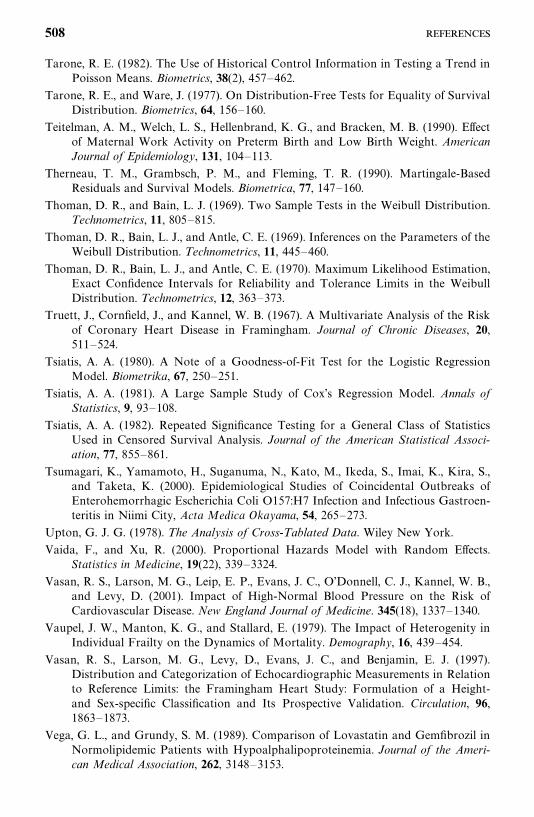
Tarone, R. E. (1982). The Use of Historical Control Information in Testing a Trend inPoisson Means. Biometrics, 38(2), 457—462.
Tarone, R. E., and Ware, J. (1977). On Distribution-Free Tests for Equality of SurvivalDistribution. Biometrics, 64, 156—160.
Teitelman, A. M., Welch, L. S., Hellenbrand, K. G., and Bracken, M. B. (1990). Effectof Maternal Work Activity on Preterm Birth and Low Birth Weight. AmericanJournal of Epidemiology, 131, 104—113.
Therneau, T. M., Grambsch, P. M., and Fleming, T. R. (1990). Martingale-BasedResiduals and Survival Models. Biometrica, 77, 147—160.
Thoman, D. R., and Bain, L. J. (1969). Two Sample Tests in the Weibull Distribution.Technometrics, 11, 805—815.
Thoman, D. R., Bain, L. J., and Antle, C. E. (1969). Inferences on the Parameters of theWeibull Distribution. Technometrics, 11, 445—460.
Thoman, D. R., Bain, L. J., and Antle, C. E. (1970). Maximum Likelihood Estimation,Exact Confidence Intervals for Reliability and Tolerance Limits in the WeibullDistribution. Technometrics, 12, 363—373.
Truett, J., Cornfield, J., and Kannel, W. B. (1967). A Multivariate Analysis of the Riskof Coronary Heart Disease in Framingham. Journal of Chronic Diseases, 20,511—524.
Tsiatis, A. A. (1980). A Note of a Goodness-of-Fit Test for the Logistic RegressionModel. Biometrika, 67, 250—251.
Tsiatis, A. A. (1981). A Large Sample Study of Cox’s Regression Model. Annals ofStatistics, 9, 93—108.
Tsiatis, A. A. (1982). Repeated Significance Testing for a General Class of StatisticsUsed in Censored Survival Analysis. Journal of the American Statistical Associ-ation, 77, 855—861.
Tsumagari, K., Yamamoto, H., Suganuma, N., Kato, M., Ikeda, S., Imai, K., Kira, S.,and Taketa, K. (2000). Epidemiological Studies of Coincidental Outbreaks ofEnterohemorrhagic Escherichia Coli O157:H7 Infection and Infectious Gastroen-teritis in Niimi City, Acta Medica Okayama, 54, 265—273.
Upton, G. J. G. (1978). The Analysis of Cross-Tablated Data. Wiley New York.
Vaida, F., and Xu, R. (2000). Proportional Hazards Model with Random Effects.Statistics in Medicine, 19(22), 339—3324.
Vasan, R. S., Larson, M. G., Leip, E. P., Evans, J. C., O’Donnell, C. J., Kannel, W. B.,and Levy, D. (2001). Impact of High-Normal Blood Pressure on the Risk ofCardiovascular Disease. New England Journal of Medicine. 345(18), 1337—1340.
Vaupel, J. W., Manton, K. G., and Stallard, E. (1979). The Impact of Heterogenity inIndividual Frailty on the Dynamics of Mortality. Demography, 16, 439—454.
Vasan, R. S., Larson, M. G., Levy, D., Evans, J. C., and Benjamin, E. J. (1997).Distribution and Categorization of Echocardiographic Measurements in Relationto Reference Limits: the Framingham Heart Study: Formulation of a Height-and Sex-specific Classification and Its Prospective Validation. Circulation, 96,1863—1873.
Vega, G. L., and Grundy, S. M. (1989). Comparison of Lovastatin and Gemfibrozil inNormolipidemic Patients with Hypoalphalipoproteinemia. Journal of the Ameri-can Medical Association, 262, 3148—3153.
508
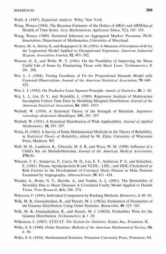
Wald, A. (1947). Sequential Analysis. Wiley, New York.
Wang, Wenyu (1984). The Bayesian Estimater of the Orders of AR(k) and ARMA(p,q)Models of Time Series. Acta Mathematicae Applicatae Sinica, 7(2), 185—195.
Wang, Wenyu (1989). Statistical Inference on Aggregated Markov Processes. Ph.D.dissertation. Department of Mathematics, University of Maryland.
Waters, M. A., Selvin, S., and Rappaport, S. M. (1991). A Measure of Goodness-of-fit forthe Lognormal Model Applied to Occupational Exposures, American IndustrialHygiene Association Journal, 52, 493—502.
Watson, G. S., and Wells, W. T. (1961). On the Possibility of Improving the MeanUseful Life of Items by Eliminating Those with Short Lives. Technometrics, 3,281—298.
Wei, L. J. (1984). Testing Goodness of Fit for Proportional Hazards Model withCensored Observations. Journal of the American Statistical Association, 79, 649—652.
Wei, L. J. (1992). On Predictive Least Squares Principle. Annals of Statistics, 20, 1—42.
Wei, L. J., Lin, D. Y., and Weissfeld, L. (1989). Regression Analysis of MultivariateIncomplete Failure Time Data by Modeling Marginal Distribution. Journal of theAmerican Statistical Association, 84, 1065—1073.
Weibull, W. (1939). A Statistical Theory of the Strength of Materials. Ingenioersvetenskaps akakemien Handlingar, 151, 293—297.
Weibull, W. (1951). A Statistical Distribution of Wide Applicability. Journal of AppliedMathematics, 18, 293—297.
Weiss, H. (1963). A Survey of Some Mathematical Methods in the Theory of Reliability,in Statistical Theory of Reliability, edited by M. Zelen. University of WisconsinPress, Madison, WI.
Well, M. D., Lamborn, K., Edwards, M. S. B., and Wara, W. M. (1998). Influence of aChild’s Sex on Medulloblastoma. Journal of the American Medical Association,279(18).
Whayne, T. F., Alaupovic, P., Curry, M. D., Lee, E. T., Anderson, P. S., and Schechter,E. (1981). Plasma Apolipoprotein B and VLDL-, LDL-, and HDL-Cholesterol asRisk Factors in the Development of Coronary Heart Disease in Male PatientsExamined by Angiography. Atherosclerosis, 39, 411—424.
Wienke, A., Holm, N. V., Skytthe, A., and Yashin, A. L. (2001). The Heritability ofMortality Due to Heart Diseases: A Correlated Frailty Model Applied to DanishTwins. Twin Research, 4(4), 266—274.
Wilcoxon, F. (1945). Individual Comparison by Ranking Methods. Biometrics, 1, 80—83.
Wilk, M. B., Gnanadesikan, R., and Huyett, M. J. (1962a). Estimation of Parameters ofthe Gamma Distribution Using Order Statistics. Biometrika, 49, 525—545.
Wilk, M. B., Gnanadesikan, R., and Huyett, M. J. (1962b). Probability Plots for theGamma Distribution. Technometrics, 4, 1—20.
Wilkinson, L. (1987). SYSTAT: The System for Statistics. Systat, Inc., Evanston, IL.
Wilks, S. S. (1948). Order Statistics. Bulletin of the American Mathematical Society, 54,6—50.
Wilks, S. S. (1950). Mathematical Statistics. Princeton University Press, Princeton, NJ.
509
Williams, C. A., Jr. (1950). On the Choice of the Number and Width of Classes for theChi-Square Test of Goodness of Fit. Journal of the American Statistical Associ-ation, 45, 77—86.
Williams, J. E., Nieto, F. J., Sanford, C. P., and Tyroler, H. A. (2002). The Associationbetween Trait Anger and Incident Stroke Risk: The Atherosclerosis Risk inCommunities (ARIC) Study. Stroke, 33(1), 13—20.
Winkleby, M. A., Ragland, D. R., and Syme, L. (1988). Self-Reported Stressors andHypertension: Evidence of an Inverse Association. American Journal of Epidemiol-ogy, 127, 124—134.
Winter, F. D., Snell, P. G., and Stray-Gundersen, J. (1989). Effects of 100% Oxygen onPerformance of Professional Soccer Players. Journal of the American MedicalAssociation, 262, 227—229.
Woolf, B. (1955). On Estimating the Relation between Blood Group and Disease.Annals of Human Genetics, 19, 251—253.
Wurpel, J. N., Dundore, R. L., Barbella, Y. R., Balaban, C. D., Keil, L. C., and Severs,W. B. (1986). Barrel Rotation Evoked by Intracerebroventricular VasopressinInjections in Conscious Rats. I. Description and General Pharmacology. BrainResearch, 365, 21—29.
Xue, X. (2001). Analysis of Childhood Brain Tumour Data in New York City UsingFrailty Models. Statistics in Medicine, 20(22), 3459—3473.
Yakovlev, A. Y., Tsodikov, A. D., Boucher, K., and Kerber, R. (1999). The Shape of theHazard Function in Breast Carcinoma: Curability of the Disease Revisited.Cancer, 85, 1789—1798.
Yan, Y., Moore, R. D., and Hoover, D. R. (2000). Competing Risk Adjustment ReducesOverestimation of Opportunistic Infection Rates in AIDS. Journal of ClinicalEpidemiology. 53(8), 817—822.
Yashin, A. I., and Iachine, I. A. (1997). How Frailty Models Can Be Used for EvaluatingLongevity Limits: Taking Advantage of an Interdisciplinary Approach. Demogra-phy, 34(1), 31—48.
Young, E. M., and Fors, S. W. (2001). Factors Related to the Eating Habits of Studentsin Grades 9—12. Journal of School Health, 71, 483—488.
Zelen, M. (1966). Applications of Exponential Models to Problems in Cancer Research.Journal of the Royal Statistical Society, Series A, 129, 368—398.
Zhang, M. J., and Klein, J. P. (2001). Confidence Bands for the Difference of TwoSurvival Curves under Proportional Hazards Model. L ifetime Data Analysis, 7,243—254.
Zippin, C., and Armitage, P. (1966). Use of Concomitant Variables and IncompleteSurvival Information in the Estimation of an Exponential Survival Parameter.Biometrics, 22, 665—672.
510
Index
Accelerated failure time (AFT) model, 259Age-specific failure rate, 11AIC, 230, 241, 288, 289Anderson—Gill model, 368Annual survival ratio, 94
BIC, 230, 241, 288, 289BMDP, 7, 94, 115, 173, 180, 188, 196, 235, 269,
273, 277, 283, 306, 319, 324, 347,351, 356, 367, 368, 389, 394, 398, 403,405, 413, 419, 424
Case-control study, 399Censored observations, 2progressively censored data, 4singly censored data, 4
Censoringinterval, 4, 260left, 4, 260random, 4right, 4, 260type I, 2type II, 2type III, 3
Chi-square test, 379, 381Competing risk, 352Conditional mortality rate, 11Conditional probability, 399, 401Corrected survival rate, 94Cox’s F-test, 116, 249Cox—Mantel test, 109Cox—Snell residual, 199, 215, 290, 331Cross-product ratio, 382Cumulative hazard function, 13Cumulative survival rate, 9
Density function:definition of, 10types of:exponential, 135extended generalized gamma, 153gamma, 150generalized gamma, 152log-logistic, 154lognormal, 145Weibull, 139
Deviance residual, 331Dichotomous outcomes, 377
Exponential distribution, 134, 263unit exponential distribution, 135two-parameter, 136goodness-of-fit test, 226, 233test for equality of two distributions, 246, 249
Five-year survival rate, 94Force of mortality, 11Frailty model, 375
Gamma and generalized gamma distribution,148, 277
goodness-of-fit test, 227, 234, 235test for equality of two distributions, 252
Gap time, 364Gehan’s generalized Wilcoxon test, 107Gompertz distribution, 157, 242Guarantee time, 136, 173, 175
Hazard function:definition of, 11exponential, 135
511
Hazard function (Continued)gamma, 152log-logistic, 155lognormal, 145Weibull, 140
Hazard plotting, 29, 209exponential, 210log-logistic, 215lognormal, 213Weibull, 212
Hollander—Proschan’s test, 236Hosmer—Lemeshow test of goodness-of-fit, 388
Incomplete gamma function, 151Instantaneous failure rate, 11
Kaplan—Meier method, 20, 68, 216, 237Kruskal—Wallis test, 125multiple comparison, 128
K-sample test for censored data, 130
Life tables:abridged, 86clinical, 87cohort, 77current, 77population, 77
Likelihood ratio test, 243, 246Link function, 410logit, 410probit, 410complementary log-log, 411
Linear exponential distribution, 155Log-logistic distribution, 154, 280goodness-of-fit test, 235
Log odds, 386Logistic regression, 45, 385conditional, 398dichotomous outcomes, 377polychotomous outcomes, 377, 413nominal, 414ordinal, 419
Logistic transform, 386Log-likelihood ratio statistic, 223, 224, 388Lognormal distribution, 143, 274three-parameter, 146goodness-of-fit test, 227, 234
Logrank test, 111
Mantel—Haenszel method, 28, 121Maximum likelihood estimate:exponential, 166Gompertz, 196
interval-censored data, 165, 260left-censored data, 165, 260log-logistic, 195lognormal, 180right-censored data, 162, 260standard and generalized gamma, 188two-parameter exponential, 174Weibull, 178
Martingale residual, 331Matched design, 4011 : R, 401n�: n
�, 403
Median remaining lifetime, 91Model selection method, 230, 233, 286, 288,
289, 310
Normit function, 410
Odds ratio, 379, 382
Partial likelihood function, 301, 304, 340, 348,354, 357, 364, 369, 371
Peto and Peto’s generalized Wilcoxon test, 116Polychotomous outcomes, 377, 413nominal, 414ordinal, 419
Printice, Williams, and Peterson (PWP) model,357, 363
Probability density function, 10Probability plotting, 29, 200exponential, 204log-logistic, 208lognormal, 206normal, 203Weibull, 205
Probit function, 410, 420Product-limit estimate, 65estimate of mean survival time, 74variance, 70variance of estimated mean survival time, 75
Prognostic factors, 32, 256, 339, 377Prognostic homogeneity, 21Proportional hazard model, 264, 270, 298assessment of, 326
Proportional odds, 280
Rayleigh distribution, 158Recurrent events, 356Related observations, 374Relative mortality, 32Relative survival rate, 94Retrospective study, 398
512
SAS, 7, 94, 115, 172, 173, 80, 188, 194, 196, 235,268, 273, 276, 279, 283, 289, 291,306, 310, 317, 322, 333, 346, 350, 355,366, 389, 392, 397, 403, 408, 410,412, 418, 424
Schoenfeld residual, 331weighted, 332
Score statistic, 225SPSS, 7, 94, 115, 318, 323, 336, 347, 351, 356,
367, 389, 392, 397, 405, 413, 419, 424Standardized rate and ratio, 97direct method, 98indirect method, 99SIR, 97SMR, 97
Standardized mortality ratio, 97Stritification, 328, 348Survival curve, 9Survivorship function:definition of, 8estimation of, 319
types:exponential, 135gamma, 152log-logistic, 154lognormal, 145two-parameter-exponential, 136Weibull, 140
Test of goodness of fit, 221, 222, 226, 227, 233,234, 235, 330
Tied survival times, 302Time-dependent covariates, 326, 339
Unconditional failure rate, 11
Wald statistic, 223, 224, 262, 388Wei, Lin, and Weissfeld (WLW) model, 370Weibull distribution, 138, 269three-parameter, 141goodness-of-fit test, 226, 234test for equality of two distributions, 251
513
WILEY SERIES IN PROBABILITY AND STATISTICS
Established by WALTER A. SHEWHART and SAMUEL S. WILKS
Editors: David J. Balding, Peter Bloomfield, Noel A. C. Cressie, Nicholas I. Fisher, Iain M. Johnstone, J. B. Kadane, Louise M. Ryan, David W. Scott, Adrian F. M. Smith, Jozef L. TeugelsEditors Emeriti: Vic Barnett, J. Stuart Hunter, David G. Kendall
A complete list of the titles in this series appears at the end of this volume.
p&s-cp.qxd 3/25/03 9:47 AM Page 1
WILEY SERIES IN PROBABILITY AND STATISTICSESTABLISHED BY WALTER A. SHEWHART AND SAMUEL S. WILKS
Editors: David J. Balding, Peter Bloomfield, Noel A. C. Cressie,Nicholas I. Fisher, Iain M. Johnstone, J. B. Kadane, Louise M. Ryan,David W. Scott, Adrian F. M. Smith, Jozef L. TeugelsEditors Emeriti: Vic Barnett, J. Stuart Hunter, David G. Kendall
The Wiley Series in Probability and Statistics is well established and authoritative. It coversmany topics of current research interest in both pure and applied statistics and probabilitytheory. Written by leading statisticians and institutions, the titles span both state-of-the-artdevelopments in the field and classical methods.
Reflecting the wide range of current research in statistics, the series encompasses applied,methodological and theoretical statistics, ranging from applications and new techniquesmade possible by advances in computerized practice to rigorous treatment of theoreticalapproaches.
This series provides essential and invaluable reading for all statisticians, whether in aca-demia, industry, government, or research.
ABRAHAM and LEDOLTER · Statistical Methods for ForecastingAGRESTI · Analysis of Ordinal Categorical DataAGRESTI · An Introduction to Categorical Data AnalysisAGRESTI · Categorical Data Analysis, Second EditionANDEL · Mathematics of ChanceANDERSON · An Introduction to Multivariate Statistical Analysis, Second Edition
*ANDERSON · The Statistical Analysis of Time SeriesANDERSON, AUQUIER, HAUCK, OAKES, VANDAELE, and WEISBERG ·
Statistical Methods for Comparative StudiesANDERSON and LOYNES · The Teaching of Practical StatisticsARMITAGE and DAVID (editors) · Advances in BiometryARNOLD, BALAKRISHNAN, and NAGARAJA · Records
*ARTHANARI and DODGE · Mathematical Programming in Statistics*BAILEY · The Elements of Stochastic Processes with Applications to the Natural
SciencesBALAKRISHNAN and KOUTRAS · Runs and Scans with ApplicationsBARNETT · Comparative Statistical Inference, Third EditionBARNETT and LEWIS · Outliers in Statistical Data, Third EditionBARTOSZYNSKI and NIEWIADOMSKA-BUGAJ · Probability and Statistical InferenceBASILEVSKY · Statistical Factor Analysis and Related Methods: Theory and
ApplicationsBASU and RIGDON · Statistical Methods for the Reliability of Repairable SystemsBATES and WATTS · Nonlinear Regression Analysis and Its ApplicationsBECHHOFER, SANTNER, and GOLDSMAN · Design and Analysis of Experiments for
Statistical Selection, Screening, and Multiple ComparisonsBELSLEY · Conditioning Diagnostics: Collinearity and Weak Data in RegressionBELSLEY, KUH, and WELSCH · Regression Diagnostics: Identifying Influential
Data and Sources of CollinearityBENDAT and PIERSOL · Random Data: Analysis and Measurement Procedures,
Third Edition
*Now available in a lower priced paperback edition in the Wiley Classics Library.
p&s-cp.qxd 3/25/03 9:47 AM Page 2

BERRY, CHALONER, and GEWEKE · Bayesian Analysis in Statistics andEconometrics: Essays in Honor of Arnold Zellner
BERNARDO and SMITH · Bayesian TheoryBHAT and MILLER · Elements of Applied Stochastic Processes, Third EditionBHATTACHARYA and JOHNSON · Statistical Concepts and MethodsBHATTACHARYA and WAYMIRE · Stochastic Processes with ApplicationsBILLINGSLEY · Convergence of Probability Measures, Second EditionBILLINGSLEY · Probability and Measure, Third EditionBIRKES and DODGE · Alternative Methods of RegressionBLISCHKE AND MURTHY (editors) · Case Studies in Reliability and MaintenanceBLISCHKE AND MURTHY · Reliability: Modeling, Prediction, and OptimizationBLOOMFIELD · Fourier Analysis of Time Series: An Introduction, Second EditionBOLLEN · Structural Equations with Latent VariablesBOROVKOV · Ergodicity and Stability of Stochastic ProcessesBOULEAU · Numerical Methods for Stochastic ProcessesBOX · Bayesian Inference in Statistical AnalysisBOX · R. A. Fisher, the Life of a ScientistBOX and DRAPER · Empirical Model-Building and Response Surfaces
*BOX and DRAPER · Evolutionary Operation: A Statistical Method for ProcessImprovement
BOX, HUNTER, and HUNTER · Statistics for Experimenters: An Introduction toDesign, Data Analysis, and Model Building
BOX and LUCEÑO · Statistical Control by Monitoring and Feedback AdjustmentBRANDIMARTE · Numerical Methods in Finance: A MATLAB-Based IntroductionBROWN and HOLLANDER · Statistics: A Biomedical IntroductionBRUNNER, DOMHOF, and LANGER · Nonparametric Analysis of Longitudinal Data in
Factorial ExperimentsBUCKLEW · Large Deviation Techniques in Decision, Simulation, and EstimationCAIROLI and DALANG · Sequential Stochastic OptimizationCHAN · Time Series: Applications to FinanceCHATTERJEE and HADI · Sensitivity Analysis in Linear RegressionCHATTERJEE and PRICE · Regression Analysis by Example, Third EditionCHERNICK · Bootstrap Methods: A Practitioner’s GuideCHERNICK and FRIIS · Introductory Biostatistics for the Health SciencesCHILÈS and DELFINER · Geostatistics: Modeling Spatial UncertaintyCHOW and LIU · Design and Analysis of Clinical Trials: Concepts and MethodologiesCLARKE and DISNEY · Probability and Random Processes: A First Course with
Applications, Second Edition*COCHRAN and COX · Experimental Designs, Second Edition
CONGDON · Bayesian Statistical ModellingCONOVER · Practical Nonparametric Statistics, Second EditionCOOK · Regression GraphicsCOOK and WEISBERG · Applied Regression Including Computing and GraphicsCOOK and WEISBERG · An Introduction to Regression GraphicsCORNELL · Experiments with Mixtures, Designs, Models, and the Analysis of Mixture
Data, Third EditionCOVER and THOMAS · Elements of Information TheoryCOX · A Handbook of Introductory Statistical Methods
*COX · Planning of ExperimentsCRESSIE · Statistics for Spatial Data, Revised EditionCSÖRGO and HORVÁTH · Limit Theorems in Change Point AnalysisDANIEL · Applications of Statistics to Industrial ExperimentationDANIEL · Biostatistics: A Foundation for Analysis in the Health Sciences, Sixth Edition
*Now available in a lower priced paperback edition in the Wiley Classics Library.
p&s-cp.qxd 3/25/03 9:47 AM Page 3
*DANIEL · Fitting Equations to Data: Computer Analysis of Multifactor Data, Second Edition
DASU and JOHNSON · Exploratory Data Mining and Data CleaningDAVID · Order Statistics, Second Edition
*DEGROOT, FIENBERG, and KADANE · Statistics and the LawDEL CASTILLO · Statistical Process Adjustment for Quality ControlDETTE and STUDDEN · The Theory of Canonical Moments with Applications in
Statistics, Probability, and AnalysisDEY and MUKERJEE · Fractional Factorial PlansDILLON and GOLDSTEIN · Multivariate Analysis: Methods and ApplicationsDODGE · Alternative Methods of Regression
*DODGE and ROMIG · Sampling Inspection Tables, Second Edition*DOOB · Stochastic ProcessesDOWDY and WEARDEN · Statistics for Research, Second EditionDRAPER and SMITH · Applied Regression Analysis, Third EditionDRYDEN and MARDIA · Statistical Shape AnalysisDUDEWICZ and MISHRA · Modern Mathematical StatisticsDUNN and CLARK · Applied Statistics: Analysis of Variance and Regression, Second
EditionDUNN and CLARK · Basic Statistics: A Primer for the Biomedical Sciences,
Third EditionDUPUIS and ELLIS · A Weak Convergence Approach to the Theory of Large Deviations
*ELANDT-JOHNSON and JOHNSON · Survival Models and Data AnalysisENDERS · Applied Econometric Time SeriesETHIER and KURTZ · Markov Processes: Characterization and ConvergenceEVANS, HASTINGS, and PEACOCK · Statistical Distributions, Third EditionFELLER · An Introduction to Probability Theory and Its Applications, Volume I,
Third Edition, Revised; Volume II, Second EditionFISHER and VAN BELLE · Biostatistics: A Methodology for the Health Sciences
*FLEISS · The Design and Analysis of Clinical ExperimentsFLEISS · Statistical Methods for Rates and Proportions, Second EditionFLEMING and HARRINGTON · Counting Processes and Survival AnalysisFULLER · Introduction to Statistical Time Series, Second EditionFULLER · Measurement Error ModelsGALLANT · Nonlinear Statistical ModelsGHOSH, MUKHOPADHYAY, and SEN · Sequential EstimationGIFI · Nonlinear Multivariate AnalysisGLASSERMAN and YAO · Monotone Structure in Discrete-Event SystemsGNANADESIKAN · Methods for Statistical Data Analysis of Multivariate Observations,
Second EditionGOLDSTEIN and LEWIS · Assessment: Problems, Development, and Statistical IssuesGREENWOOD and NIKULIN · A Guide to Chi-Squared TestingGROSS and HARRIS · Fundamentals of Queueing Theory, Third Edition
*HAHN and SHAPIRO · Statistical Models in EngineeringHAHN and MEEKER · Statistical Intervals: A Guide for PractitionersHALD · A History of Probability and Statistics and their Applications Before 1750HALD · A History of Mathematical Statistics from 1750 to 1930HAMPEL · Robust Statistics: The Approach Based on Influence FunctionsHANNAN and DEISTLER · The Statistical Theory of Linear SystemsHEIBERGER · Computation for the Analysis of Designed ExperimentsHEDAYAT and SINHA · Design and Inference in Finite Population SamplingHELLER · MACSYMA for StatisticiansHINKELMAN and KEMPTHORNE: · Design and Analysis of Experiments, Volume 1:
Introduction to Experimental Design
*Now available in a lower priced paperback edition in the Wiley Classics Library.
p&s-cp.qxd 3/25/03 9:47 AM Page 4
HOAGLIN, MOSTELLER, and TUKEY · Exploratory Approach to Analysisof Variance
HOAGLIN, MOSTELLER, and TUKEY · Exploring Data Tables, Trends and Shapes*HOAGLIN, MOSTELLER, and TUKEY · Understanding Robust and Exploratory
Data AnalysisHOCHBERG and TAMHANE · Multiple Comparison ProceduresHOCKING · Methods and Applications of Linear Models: Regression and the Analysis
of Variance, Second EditionHOEL · Introduction to Mathematical Statistics, Fifth EditionHOGG and KLUGMAN · Loss DistributionsHOLLANDER and WOLFE · Nonparametric Statistical Methods, Second EditionHOSMER and LEMESHOW · Applied Logistic Regression, Second EditionHOSMER and LEMESHOW · Applied Survival Analysis: Regression Modeling of
Time to Event DataHØYLAND and RAUSAND · System Reliability Theory: Models and Statistical MethodsHUBER · Robust StatisticsHUBERTY · Applied Discriminant AnalysisHUNT and KENNEDY · Financial Derivatives in Theory and PracticeHUSKOVA, BERAN, and DUPAC · Collected Works of Jaroslav Hajek—
with CommentaryIMAN and CONOVER · A Modern Approach to StatisticsJACKSON · A User’s Guide to Principle ComponentsJOHN · Statistical Methods in Engineering and Quality AssuranceJOHNSON · Multivariate Statistical SimulationJOHNSON and BALAKRISHNAN · Advances in the Theory and Practice of Statistics: A
Volume in Honor of Samuel KotzJUDGE, GRIFFITHS, HILL, LÜTKEPOHL, and LEE · The Theory and Practice of
Econometrics, Second EditionJOHNSON and KOTZ · Distributions in StatisticsJOHNSON and KOTZ (editors) · Leading Personalities in Statistical Sciences: From the
Seventeenth Century to the PresentJOHNSON, KOTZ, and BALAKRISHNAN · Continuous Univariate Distributions,
Volume 1, Second EditionJOHNSON, KOTZ, and BALAKRISHNAN · Continuous Univariate Distributions,
Volume 2, Second EditionJOHNSON, KOTZ, and BALAKRISHNAN · Discrete Multivariate DistributionsJOHNSON, KOTZ, and KEMP · Univariate Discrete Distributions, Second EditionJUREC KOVÁ and SEN · Robust Statistical Procedures: Aymptotics and InterrelationsJUREK and MASON · Operator-Limit Distributions in Probability TheoryKADANE · Bayesian Methods and Ethics in a Clinical Trial DesignKADANE AND SCHUM · A Probabilistic Analysis of the Sacco and Vanzetti EvidenceKALBFLEISCH and PRENTICE · The Statistical Analysis of Failure Time Data, Second
EditionKASS and VOS · Geometrical Foundations of Asymptotic InferenceKAUFMAN and ROUSSEEUW · Finding Groups in Data: An Introduction to Cluster
AnalysisKEDEM and FOKIANOS · Regression Models for Time Series AnalysisKENDALL, BARDEN, CARNE, and LE · Shape and Shape TheoryKHURI · Advanced Calculus with Applications in Statistics, Second EditionKHURI, MATHEW, and SINHA · Statistical Tests for Mixed Linear ModelsKLUGMAN, PANJER, and WILLMOT · Loss Models: From Data to DecisionsKLUGMAN, PANJER, and WILLMOT · Solutions Manual to Accompany Loss Models:
From Data to Decisions
*Now available in a lower priced paperback edition in the Wiley Classics Library.
p&s-cp.qxd 3/25/03 9:47 AM Page 5
KOTZ, BALAKRISHNAN, and JOHNSON · Continuous Multivariate Distributions,Volume 1, Second Edition
KOTZ and JOHNSON (editors) · Encyclopedia of Statistical Sciences: Volumes 1 to 9with Index
KOTZ and JOHNSON (editors) · Encyclopedia of Statistical Sciences: SupplementVolume
KOTZ, READ, and BANKS (editors) · Encyclopedia of Statistical Sciences: UpdateVolume 1
KOTZ, READ, and BANKS (editors) · Encyclopedia of Statistical Sciences: UpdateVolume 2
KOVALENKO, KUZNETZOV, and PEGG · Mathematical Theory of Reliability ofTime-Dependent Systems with Practical Applications
LACHIN · Biostatistical Methods: The Assessment of Relative RisksLAD · Operational Subjective Statistical Methods: A Mathematical, Philosophical, and
Historical IntroductionLAMPERTI · Probability: A Survey of the Mathematical Theory, Second EditionLANGE, RYAN, BILLARD, BRILLINGER, CONQUEST, and GREENHOUSE ·
Case Studies in BiometryLARSON · Introduction to Probability Theory and Statistical Inference, Third EditionLAWLESS · Statistical Models and Methods for Lifetime Data, Second EditionLAWSON · Statistical Methods in Spatial EpidemiologyLE · Applied Categorical Data AnalysisLE · Applied Survival AnalysisLEE and WANG · Statistical Methods for Survival Data Analysis, Third EditionLEPAGE and BILLARD · Exploring the Limits of BootstrapLEYLAND and GOLDSTEIN (editors) · Multilevel Modelling of Health StatisticsLIAO · Statistical Group ComparisonLINDVALL · Lectures on the Coupling MethodLINHART and ZUCCHINI · Model SelectionLITTLE and RUBIN · Statistical Analysis with Missing Data, Second EditionLLOYD · The Statistical Analysis of Categorical DataMAGNUS and NEUDECKER · Matrix Differential Calculus with Applications in
Statistics and Econometrics, Revised EditionMALLER and ZHOU · Survival Analysis with Long Term SurvivorsMALLOWS · Design, Data, and Analysis by Some Friends of Cuthbert DanielMANN, SCHAFER, and SINGPURWALLA · Methods for Statistical Analysis of
Reliability and Life DataMANTON, WOODBURY, and TOLLEY · Statistical Applications Using Fuzzy SetsMARDIA and JUPP · Directional StatisticsMASON, GUNST, and HESS · Statistical Design and Analysis of Experiments with
Applications to Engineering and Science, Second EditionMcCULLOCH and SEARLE · Generalized, Linear, and Mixed ModelsMcFADDEN · Management of Data in Clinical TrialsMcLACHLAN · Discriminant Analysis and Statistical Pattern RecognitionMcLACHLAN and KRISHNAN · The EM Algorithm and ExtensionsMcLACHLAN and PEEL · Finite Mixture ModelsMcNEIL · Epidemiological Research MethodsMEEKER and ESCOBAR · Statistical Methods for Reliability DataMEERSCHAERT and SCHEFFLER · Limit Distributions for Sums of Independent
Random Vectors: Heavy Tails in Theory and Practice*MILLER · Survival Analysis, Second Edition
MONTGOMERY, PECK, and VINING · Introduction to Linear Regression Analysis,Third Edition
MORGENTHALER and TUKEY · Configural Polysampling: A Route to PracticalRobustness
*Now available in a lower priced paperback edition in the Wiley Classics Library.
p&s-cp.qxd 3/25/03 9:47 AM Page 6
MUIRHEAD · Aspects of Multivariate Statistical TheoryMURRAY · X-STAT 2.0 Statistical Experimentation, Design Data Analysis, and
Nonlinear OptimizationMYERS and MONTGOMERY · Response Surface Methodology: Process and Product
Optimization Using Designed Experiments, Second EditionMYERS, MONTGOMERY, and VINING · Generalized Linear Models. With
Applications in Engineering and the SciencesNELSON · Accelerated Testing, Statistical Models, Test Plans, and Data AnalysesNELSON · Applied Life Data AnalysisNEWMAN · Biostatistical Methods in EpidemiologyOCHI · Applied Probability and Stochastic Processes in Engineering and Physical
SciencesOKABE, BOOTS, SUGIHARA, and CHIU · Spatial Tesselations: Concepts and
Applications of Voronoi Diagrams, Second EditionOLIVER and SMITH · Influence Diagrams, Belief Nets and Decision AnalysisPANKRATZ · Forecasting with Dynamic Regression ModelsPANKRATZ · Forecasting with Univariate Box-Jenkins Models: Concepts and Cases
*PARZEN · Modern Probability Theory and Its ApplicationsPEÑA, TIAO, and TSAY · A Course in Time Series AnalysisPIANTADOSI · Clinical Trials: A Methodologic PerspectivePORT · Theoretical Probability for ApplicationsPOURAHMADI · Foundations of Time Series Analysis and Prediction TheoryPRESS · Bayesian Statistics: Principles, Models, and ApplicationsPRESS · Subjective and Objective Bayesian Statistics, Second EditionPRESS and TANUR · The Subjectivity of Scientists and the Bayesian ApproachPUKELSHEIM · Optimal Experimental DesignPURI, VILAPLANA, and WERTZ · New Perspectives in Theoretical and Applied
StatisticsPUTERMAN · Markov Decision Processes: Discrete Stochastic Dynamic Programming
*RAO · Linear Statistical Inference and Its Applications, Second EditionRENCHER · Linear Models in StatisticsRENCHER · Methods of Multivariate Analysis, Second EditionRENCHER · Multivariate Statistical Inference with ApplicationsRIPLEY · Spatial StatisticsRIPLEY · Stochastic SimulationROBINSON · Practical Strategies for ExperimentingROHATGI and SALEH · An Introduction to Probability and Statistics, Second EditionROLSKI, SCHMIDLI, SCHMIDT, and TEUGELS · Stochastic Processes for Insurance
and FinanceROSENBERGER and LACHIN · Randomization in Clinical Trials: Theory and PracticeROSS · Introduction to Probability and Statistics for Engineers and ScientistsROUSSEEUW and LEROY · Robust Regression and Outlier DetectionRUBIN · Multiple Imputation for Nonresponse in SurveysRUBINSTEIN · Simulation and the Monte Carlo MethodRUBINSTEIN and MELAMED · Modern Simulation and ModelingRYAN · Modern Regression MethodsRYAN · Statistical Methods for Quality Improvement, Second EditionSALTELLI, CHAN, and SCOTT (editors) · Sensitivity Analysis
*SCHEFFE · The Analysis of VarianceSCHIMEK · Smoothing and Regression: Approaches, Computation, and ApplicationSCHOTT · Matrix Analysis for StatisticsSCHUSS · Theory and Applications of Stochastic Differential EquationsSCOTT · Multivariate Density Estimation: Theory, Practice, and Visualization
*SEARLE · Linear ModelsSEARLE · Linear Models for Unbalanced Data
*Now available in a lower priced paperback edition in the Wiley Classics Library.
p&s-cp.qxd 3/25/03 9:47 AM Page 7
SEARLE · Matrix Algebra Useful for StatisticsSEARLE, CASELLA, and McCULLOCH · Variance ComponentsSEARLE and WILLETT · Matrix Algebra for Applied EconomicsSEBER and LEE · Linear Regression Analysis, Second EditionSEBER · Multivariate ObservationsSEBER and WILD · Nonlinear RegressionSENNOTT · Stochastic Dynamic Programming and the Control of Queueing Systems
*SERFLING · Approximation Theorems of Mathematical StatisticsSHAFER and VOVK · Probability and Finance: It’s Only a Game!SMALL and MCLEISH · Hilbert Space Methods in Probability and Statistical InferenceSRIVASTAVA · Methods of Multivariate StatisticsSTAPLETON · Linear Statistical ModelsSTAUDTE and SHEATHER · Robust Estimation and TestingSTOYAN, KENDALL, and MECKE · Stochastic Geometry and Its Applications, Second
EditionSTOYAN and STOYAN · Fractals, Random Shapes and Point Fields: Methods of
Geometrical StatisticsSTYAN · The Collected Papers of T. W. Anderson: 1943–1985SUTTON, ABRAMS, JONES, SHELDON, and SONG · Methods for Meta-Analysis in
Medical ResearchTANAKA · Time Series Analysis: Nonstationary and Noninvertible Distribution TheoryTHOMPSON · Empirical Model BuildingTHOMPSON · Sampling, Second EditionTHOMPSON · Simulation: A Modeler’s ApproachTHOMPSON and SEBER · Adaptive SamplingTHOMPSON, WILLIAMS, and FINDLAY · Models for Investors in Real World MarketsTIAO, BISGAARD, HILL, PEÑA, and STIGLER (editors) · Box on Quality and
Discovery: with Design, Control, and RobustnessTIERNEY · LISP-STAT: An Object-Oriented Environment for Statistical Computing
and Dynamic GraphicsTSAY · Analysis of Financial Time SeriesUPTON and FINGLETON · Spatial Data Analysis by Example, Volume II:
Categorical and Directional DataVAN BELLE · Statistical Rules of ThumbVIDAKOVIC · Statistical Modeling by WaveletsWEISBERG · Applied Linear Regression, Second EditionWELSH · Aspects of Statistical InferenceWESTFALL and YOUNG · Resampling-Based Multiple Testing: Examples and
Methods for p-Value AdjustmentWHITTAKER · Graphical Models in Applied Multivariate StatisticsWINKER · Optimization Heuristics in Economics: Applications of Threshold AcceptingWONNACOTT and WONNACOTT · Econometrics, Second EditionWOODING · Planning Pharmaceutical Clinical Trials: Basic Statistical PrinciplesWOOLSON and CLARKE · Statistical Methods for the Analysis of Biomedical Data,
Second EditionWU and HAMADA · Experiments: Planning, Analysis, and Parameter Design
OptimizationYANG · The Construction Theory of Denumerable Markov Processes
*ZELLNER · An Introduction to Bayesian Inference in EconometricsZHOU, OBUCHOWSKI, and MCCLISH · Statistical Methods in Diagnostic Medicine
*Now available in a lower priced paperback edition in the Wiley Classics Library.
p&s-cp.qxd 3/25/03 9:47 AM Page 8