SISSA 37/2009/EP DFPD-09/TH/13

Lepton Flavour Violation in a Supersymmetric Model

with A4 Flavour Symmetry

Ferruccio Feruglio a)1, Claudia Hagedorn b)2,

Yin Lin a)3 and Luca Merlo a)4

a) Dipartimento di Fisica ‘G. Galilei’, Universita di Padova

INFN, Sezione di Padova, Via Marzolo 8, I-35131 Padua, Italyb) SISSA, Scuola Internazionale Superiore di Studi Avanzati

Via Beirut 2-4, I-34014 Trieste, Italy

and

INFN, Sezione di Trieste, Italy

Abstract

We compute the branching ratios for µ → eγ, τ → µγ and τ → eγ in a super-symmetric model invariant under the flavour symmetry group A4 ×Z3 ×U(1)FN , inwhich near tri-bimaximal lepton mixing is naturally predicted. At leading order inthe small symmetry breaking parameter u, which is of the same order as the reactormixing angle θ13, we find that the branching ratios generically scale as u2. Applyingthe current bound on the branching ratio of µ→ eγ shows that small values of u ortanβ are preferred in the model for mass parameters mSUSY and m1/2 smaller than1000 GeV. The bound expected from the on-going MEG experiment will provide asevere constraint on the parameter space of the model either enforcing u ≈ 0.01 andsmall tanβ or mSUSY and m1/2 above 1000 GeV. In the special case of universal softsupersymmetry breaking terms in the flavon sector a cancellation takes place in theamplitudes and the branching ratios scale as u4, allowing for smaller slepton masses.The branching ratios for τ → µγ and τ → eγ are predicted to be of the same orderas the one for µ→ eγ, which precludes the possibility of observing these τ decays inthe near future.

1e-mail address: feruglio@pd.infn.it2e-mail address: hagedorn@sissa.it3e-mail address: yin.lin@pd.infn.it4e-mail address: merlo@pd.infn.it

arX

iv:0

911.

3874

v1 [

hep-

ph]

19

Nov

200

9

1 Introduction

Flavour violation in the lepton sector (LFV) has been firmly established in neutrino oscil-

lations. A direct evidence of conversion of electron neutrinos into a combination of muon

and tau neutrinos is provided by solar neutrino oscillations. In a three neutrino framework

atmospheric neutrino data can only be explained by the dominant oscillation of muon neu-

trinos into tau neutrinos. It is natural to expect that LFV takes place, at least at some

level, in other processes such as those involving charged leptons. Flavour violating decays

of charged leptons, strictly forbidden in the Standard Model (SM), are indeed allowed as

soon as neutrino mass terms are considered. If neutrino masses are the only source of

LFV, the effects are too small to be detected, but in most extensions of the SM in which

new particles and new interactions with a characteristic scale M are included, the pres-

ence of new sources of flavour violation, in particular in the lepton sector, is a generic

feature. In a low-energy description, the corresponding effects can be parametrized by

higher-dimensional operators describing flavour-violating rare decays of the charged lep-

tons. The dominant terms are represented by dimension six operators, suppressed by two

powers of M . The present bounds on the branching ratios [1] of these decays set strin-

gent limits on combinations of the scale M and the coefficients of the involved operators.

Typically, for coefficients of order one, the existing bounds require a large scale M , several

orders of magnitude larger than the TeV scale. Conversely, to allow for new physics at

the TeV scale, coefficients much smaller than one are required, which might suggest the

presence of a flavour symmetry.

New physics at the TeV scale supplemented by a flavour symmetry provides an in-

teresting framework. Flavour symmetries have been invoked to describe the observed

pattern of lepton masses and mixing angles [2], but quite often this approach is limited

to a fit of the existing data, with very few new testable predictions [3]. Specific relations

among LFV processes are usually consequences of flavour symmetries and of their pat-

tern of symmetry breaking. This allows to get independent information on the flavour

symmetry in the charged lepton sector. Moreover, if M is sufficiently small, new parti-

cles might be produced and detected at the LHC, with features that could additionally

confirm or reject the assumed symmetry pattern. In [4] we have recently analyzed in an

effective Lagrangian approach LFV processes within a class of models possessing a flavour

symmetry Gf = A4 × Z3 × U(1)FN . Models of this class [5–8] automatically reproduce

nearly tri-bimaximal (TB) lepton mixing at the leading order (LO) via a vacuum alignment

mechanism. 1 In this type of models [5–8,10,11], corrections to TB mixing are generically

proportional to the symmetry breaking parameter u, especially the reactor mixing angle

θ13 is of the order of u.2 The parameter u is expected to vary between a few per mil and

a few percent. In particular we have evaluated the normalized branching ratios Rij for the

LFV transitions li → ljγ:

Rij =BR(li → ljγ)

BR(li → ljνiνj). (1)

1Due to the success of these models in the lepton sector several extensions to the quark sector can befound in the literature [9].

2For alternative scenarios see [12,13].

1

In [4] we found that the generic expectation for the ratios Rij is:

Rij =48π3α

G2FM

4|wij u|2 (2)

where α is the fine structure constant, GF is the Fermi constant and wij are dimensionless

parameters that cannot be predicted within the effective Lagrangian approach, but are

expected to be of order one. Given the range of u, it turns out that the present bound on

µ→ eγ requires the scale M to be larger than about 10 TeV. If the underlying fundamental

theory is weakly interacting, this translates into a lower bound of about gM/(4π) on the

typical mass of the new particles. At variance with this generic estimate, it was also

observed that, if the flavour symmetry is realized in a supersymmetric (SUSY) model, a

cancellation might take place in the amplitudes for LFV transitions. An argument was

given suggesting that in this case the ratios RSUSYij are of the form:

RSUSYij =

48π3α

G2FM

4

[|w(1)

ij u2|2 +

m2j

m2i

|w(2)ij u|2

](3)

where M now corresponds to the supersymmetry breaking scale, mi (i = e, µ, τ) are the

charged lepton masses and w(1,2)ij are unknown dimensionless quantities of order one. There-

fore in a supersymmetric context the predicted rates are more suppressed, allowing for new

physics close to the TeV scale, without conflicting with the present bounds. Since the can-

cellation expected in the supersymmetric case considerably changes the conclusion that can

be derived from the existing bound on µ→ eγ, it is important to perform a direct compu-

tation of the branching ratios within an explicit supersymmetric model incorporating the

flavour symmetry A4 × Z3 × U(1)FN .

In the present paper we consider the A4 realization proposed in [4] in which SUSY

breaking effects were ignored and we extend it to a more realistic model, by adding a full

set of SUSY breaking terms consistent with the flavour symmetry. We assume that the

breaking of supersymmetry occurs at a scale higher than or comparable to the flavour scale,

simulated in our effective Lagrangian by a cutoff, so that at energies close to the cutoff scale

we have non-universal boundary conditions for the soft SUSY breaking terms, dictated by

the flavour symmetry. Depending on the assumed mechanism of SUSY breaking we may

have boundary conditions different from these, possibly enforced at a smaller energy scale.

For this reason, our approach maximizes the possible effects on LFV processes.

Through a detailed calculation of the slepton mass matrices in the physical basis, in

which kinetic terms are canonical and leptons are in their mass eigenbasis, and evaluation

of Rij in the mass insertion (MI) approximation we find that the behaviour of Rij, expected

from the SUSY variant of the effective Lagrangian approach, given in eq. (3) is violated by

a single, flavour independent contribution. The correct scaling of Rij is the one of eq. (2),

with a universal constant wij. This implies Rµe = Rτµ = Rτe at the LO in u. We identify

the source of violation of the expected behaviour in a contribution to the right-left (RL)

block of the slepton mass matrix, associated to the sector necessary to maintain the correct

breaking of the flavour symmetry A4. We also enumerate the conditions under which such

a contribution is absent and the behavior in eq. (3) is recovered, though we could not find

a dynamical explanation to justify the realization of these conditions in our model.

2

As shown in the MI approximation the coefficient wij of the leading contribution in eq.

(2) is numerically small in a large region of the parameter space, where the sub-leading

contributions play an important role. We then provide a numerical study of Rij by using full

one-loop expressions and explore the parameter space of the model. Thereby, we assume

a supergravity (SUGRA) framework with a common mass scale mSUSY for soft sfermion

and Higgs masses and a common mass m1/2 for gauginos at high energies. Applying

the current MEGA bound on Rµe we find that small values of u or tan β are favoured

for mSUSY and m1/2 below 1000 GeV. Employing the foreseen bound coming from the

MEG experiment constrains the model severely allowing only for small u and tan β for

mSUSY ,m1/2 . 1000 GeV or requires larger mSUSY and m1/2 reducing the prospects for

detection of sparticles at LHC. Furthermore, it turns out to be rather unnatural to reconcile

the values of superparticle masses necessary to account for the measured deviation δaµ in

aµ, the muon anomalous magnetic moment, from the SM value with the present bound on

Rµe. In our model values of δaµ smaller than 100× 10−11 are favoured.

The paper is structured as follows: in section 2 we review the basic features of the

SUSY A4 model and calculate kinetic terms and mass matrices of leptons and sleptons in

an expansion in the symmetry breaking parameters. In section 3 we compute the slepton

mass matrices in the physical basis. Furthermore, we estimate the possible effects on the

slepton masses coming from renormalization group (RG) running. Section 4 is dedicated

to the study of the quantities Rij in the MI approximation, while in section 5 we discuss

Rµe in a more quantitative way in the SUGRA context and comment on the size of the

measured deviation in the muon anomalous magnetic moment aµ in our model. Finally,

we conclude in section 6. Appendix A contains details about the group theory of A4,

appendix B details of the calculation of the slepton mass matrices in the physical basis

and in appendix C conventions and formulae, used in the numerical study of section 5, are

given.

2 A SUSY model with A4 flavour symmetry

In this section, we first discuss the main features and predictions of the lepton mixing in

the class of A4 realizations to which the present SUSY model belongs. Then we will present

the Kahler and the superpotential of our model from which kinetic and mass terms are

derived for leptons and sleptons.

2.1 General features

The flavour symmetry A4 can give rise to TB mixing in the lepton sector, if it is broken in

a specific way, as discussed in [5–8, 10]. The group A4 is the group of even permutations

of four objects which is isomorphic to the tetrahedral group. It has 12 elements and four

irreducible representations: three inequivalent singlets, denoted by 1, 1′ and 1′′ and a triplet

3. A4 is generated by two generators S and T which fulfill the following relations [14]:

S2 = (ST )3 = T 3 = 1 . (4)

3

A set of generators S and T for all representations as well as Kronecker products and

Clebsch Gordan coefficients are given in appendix A. The specific breaking pattern of A4

which leads to TB mixing for leptons requires that a Z3 subgroup, called GT , is preserved

in the charged lepton sector, whereas a Z2 group, GS, remains unbroken in the neutrino

sector. The Z3 group is generated by the element T and is left intact, if a scalar triplet

ϕ = (ϕ1, ϕ2, ϕ3) acquires a vacuum expectation value (VEV) of the form:

〈ϕ〉 ∝ (1, 0, 0) . (5)

Breaking A4 down to GS is achieved by a triplet which gets a VEV:

〈ϕ〉 ∝ (1, 1, 1) . (6)

Apart from A4, being responsible for TB mixing, the theory is invariant under additional

flavour symmetries so that the full symmetry is:

Gf = A4 × Z3 × U(1)FN × U(1)R . (7)

The cyclic symmetry Z3 (not to be confused with the Z3 subgroup of A4 preserved at LO

in the charged lepton sector) is necessary in order to avoid large mixing effects between the

flavons that give masses to the charged leptons and those giving masses to neutrinos. The

mass hierarchy among the charged leptons is explained through the U(1)FN factor [15]. The

second U(1) factor, U(1)R, is a continuous R-symmetry containing R-parity as a subgroup.

The flavour symmetry Gf is broken by the chiral superfields ϕT , ϕS, ξ and θFN whose

transformation properties under Gf are shown in table 1 together with those of the lepton

supermultiplets l, ec, µc, τ c and of the electroweak doublets Hu,d. Introducing the driving

fields ϕT0 , ϕS0 and ξ0, see also table 1, we can write down the following superpotential: 3

wd = MT (ϕT0 ϕT ) + g(ϕT0 ϕTϕT )

+ g1(ϕS0ϕSϕS) + g2ξ(ϕ

S0ϕS) + g3ξ0(ϕSϕS) + g4ξ0ξ

2 + g5ξ0ξξ + g6ξ0ξ2 + .... (8)

where dots denote sub-leading non-renormalizable corrections. By (· · · ) we denote the

contraction to an A4 invariant. In the limit of unbroken supersymmetry all F terms

vanish. From these conditions we can derive the vacuum alignment of the flavons ϕT , ϕSand ξ:

〈ϕT 〉Λf

= (u, 0, 0) + (c′u2, cu2, cu2) +O(u3)

〈ϕS〉Λf

= cb(u, u, u) +O(u2) (9)

〈ξ〉Λf

= cau+O(u2)

where c, c′, ca,b are complex numbers with absolute value of order one and u is one of the

two small symmetry breaking parameters in the theory. The scale Λf is the cutoff scale

3The additional flavon field ξ transforms in the same way under the symmetries of the model as thefield ξ. However, it does not acquire a VEV at LO and thus is not relevant for our discussion here. Forfurther details see [6].

4

associated to the flavour symmetry. Its value is expected to be around the scale of grand

unification 1016 GeV. We display the sub-leading O(u2) corrections, which arise from non-

renormalizable terms in the superpotential wd and which have been studied in detail in [6],

only for the field ϕT , since only these are relevant in the following analysis, whereas those

of the fields ξ and ϕS are important in the computation of neutrino masses and lepton

mixings. We remark that in the SUSY limit the VEVs of the driving fields ϕT0 , ϕS0 and ξ0are zero. This is however in general no longer true, if we include soft SUSY breaking terms

into the flavon potential, as we shall see in the next section and as has been discussed

in [16].

For the Froggatt-Nielsen (FN) field θFN to acquire a VEV, we assume that the symmetry

U(1)FN is gauged such that θFN gets its VEV through a D term. The corresponding

potential is of the form:

VD,FN =1

2(M2

FI − gFN |θFN |2 + ...)2 (10)

where gFN is the gauge coupling constant of U(1)FN and M2FI denotes the contribution

of the Fayet-Iliopoulos (FI) term. Dots in eq.(10) represent e.g. terms involving the

right-handed charged leptons ec and µc which are charged under U(1)FN . These terms are

relevant in the calculation of the different contributions to the soft mass terms of right-right

(RR) type, as we shall see below. VD,FN leads in the SUSY limit to:

|〈θFN〉|2 =M2

FI

gFN(11)

which we parametrize as:〈θFN〉

Λf

= t (12)

with t being the second small symmetry breaking parameter in our model. Both u and t

can also be in general complex, but through field redefinitions of the supermultiplets ϕTand θFN , they can be made real and positive.

Field l ec µc τ c Hu,d ϕT ϕS ξ θFN ϕT0 ϕS0 ξ0

A4 3 1 1′′ 1′ 1 3 3 1 1 3 3 1

Z3 ω ω2 ω2 ω2 1 1 ω ω 1 1 ω ω

U(1)FN 0 2 1 0 0 0 0 0 −1 0 0 0

U(1)R 1 1 1 1 0 0 0 0 0 2 2 2

Table 1: Transformation properties of the fields under A4, Z3, U(1)FN and U(1)R.

At the LO, the mass matrices of charged leptons and light neutrinos have the following

form:

ml ∝

yet2 0 0

0 yµt 0

0 0 yτ

u , (13)

5

and

mν ∝

a+ 2b/3 −b/3 −b/3−b/3 2b/3 a− b/3−b/3 a− b/3 2b/3

u , (14)

with ye, yµ, yτ , a and b being complex numbers with absolute values of order one. As one

can see the relative hierarchy among the charged lepton masses is given by the parameter

t for which we take:

t ≈ 0.05 . (15)

The neutrino mass matrix is diagonalized by:

UTTBmνUTB ∝ diag(a+ b, a,−a+ b)u , (16)

where UTB, up to phases, is the TB mixing matrix [17]:

UTB =

√

2/3 1/√

3 0

−1/√

6 1/√

3 −1/√

2

−1/√

6 1/√

3 +1/√

2

. (17)

The allowed range of the parameter u is determined by the requirement that sub-leading

corrections which perturb the LO result are not too large and by the requirement that the

τ Yukawa coupling yτ does not become too large. The first requirement results in an upper

bound on u of about 0.05, which mainly comes from the fact that the solar mixing angle

should remain in its 1σ range [2]. The second one gives a lower bound which we estimate

as:

u =tan β

|yτ |

√2mτ

v≈ 0.01

tan β

|yτ |(18)

where v ≈ 246 GeV and tan β is the ratio between the VEVs of the neutral spin zero

components of Hu and Hd, the two doublets responsible for electroweak symmetry breaking.

For the τ lepton we use its pole mass mτ = (1776.84±0.17) MeV [18]. Requesting |yτ | < 3

we find a lower limit on u close to the upper bound 0.05 for tan β = 15, whereas tan β = 24 gives as lower limit u & 0.007. Obviously, these limits depend on the largest allowed

value of |yτ |, as well as on whether we identify mτ with the pole mass or with the τ mass

renormalized at some reference scale, such as the scale of grand unification. We choose as

maximal range:

0.007 . u . 0.05 , (19)

which shrinks when tan β is increased from 2 to 15. Concerning the relative size of the two

symmetry breaking parameters we note that u . t holds for all values of u.

4It is known that tanβ cannot be too small [19]. Here we take tanβ = 2 as the smallest allowed value.

6

2.2 The SUSY Lagrangian and the soft SUSY breaking terms

We analyse the Lagrangian of the model:

L =

∫d2θd2θK(z, e2V z) +

[∫d2θw(z) + h.c.

]+

1

4

[∫d2θf(z)WW + h.c.

], (20)

where K(z, z) is the Kahler potential, a real gauge-invariant function of the chiral super-

fields z and their conjugates, of dimensionality (mass)2; w(z) is the superpotential, an

analytic gauge-invariant function of the chiral superfields, of dimensionality (mass)3; f(z)

is the gauge kinetic function, a dimensionless analytic gauge-invariant function; V is the

Lie-algebra valued vector supermultiplet, describing the gauge fields and their superpart-

ners. Finally W is the chiral superfield describing, together with the function f(z), the

kinetic terms of gauge bosons and their superpartners. Each of the terms on the right-

hand side can be written in an expansion in powers of the flavon fields. Since we have

two independent symmetry breaking parameters, u and t, see eqs. (9) and eq. (12), we

consider a double expansion of L in powers of u and t. In this expansion we keep terms up

to the second order in u, i.e. terms quadratic in the fields ϕS,T and ξ. The expansion in

the parameter t, responsible for the breaking of the Froggatt-Nielsen U(1)FN symmetry, is

stopped at the first non-trivial order, that is by allowing as many powers of the field θFN as

necessary in order to obtain non-vanishing values for all entries of the matrices describing

lepton masses as well as for the entries of the matrices describing kinetic terms and slepton

masses. 5 Finally, second order corrections in u also arise from the sub-leading terms of

the VEV 〈ϕT 〉, eq. (9), and are included in our estimates.

The soft SUSY breaking terms are generated from the SUSY Lagrangian by promoting

all coupling constants, such as Yukawa couplings, couplings in the flavon superpotential and

couplings in the Kahler potential, to superfields with constant θ2 and θ2θ2

components [20].

Through this we derive subsequently the soft masses (m2(e,ν)LL)K and (m2

eRR)K from the

Kahler potential. One contribution to m2eRL, which we call (m2

eRL)1 in the following, arises

from the Yukawa couplings present in the superpotential w.

Important contributions to slepton masses originate from the modification of the VEVs

of flavons and driving fields due to SUSY breaking effects. A detailed study of the VEVs

of these fields and their dependence on the soft SUSY breaking parameters is presented

in [16] and we summarize the main results here. When soft SUSY breaking terms are

included into the flavon potential, the VEVs in eq. (9) receive additional contributions

of order mSUSY , completely negligible compared to Λf u. At the same time, the driving

fields ϕT0 , ϕS0 and ξ0 develop a VEV of the size of the soft SUSY breaking scale mSUSY .

An equivalent statement is that the auxiliary fields of the flavons acquire a VEV at the

5Concerning the Kahler potential we observe that we can additionally write down operators involvingthe total invariant θFNθFN = |θFN |2. These contribute to the diagonal elements of the kinetic terms andthe slepton masses. In the Kahler potential for the left-handed fields they can be safely neglected, sincethe LO correction is of O(u). In the right-handed sector, they contribute at the same order as the termsarising through a double flavon insertion.

7

LO of the size of mSUSY × uΛf . Especially, for the auxiliary fields contained in the flavon

supermultiplet ϕT we have [16]:

1

Λf

⟨∂w

∂ϕT

⟩= ζ mSUSY

{(u, 0, 0) + (c′Fu

2, cFu2, cFu

2)}

(21)

where ζ, c′F and cF are in general complex numbers with absolute value of order one.

The parameter ζ vanishes in the special case of universal soft mass terms in the flavon

potential. When different from zero, the VEVs of the auxiliary components of the flavon

supermultiplet ϕT generate another contribution to the soft masses of RL-type, which

we denote as (m2eRL)2. This contribution is analogous to the one which has been found

before in the supergravity context and which can have a considerable effect on the size of

the branching ratio of radiative leptonic decays, as shown in [21, 22]. Indeed, as we shall

see below, in the global SUSY model under consideration the leading dependence of the

normalized branching ratios Rij on u is dominated by (m2eRL)2. We remark that the VEVs

in eq. (21) and those of the corresponding flavon field ϕT in eq. (9) have a similar structure

but they are not proportional, in general. This is due to the different coefficients c, c′ and

cF , c′F , which can be qualitatively understood as follows: the coefficients c, c′ mainly

depend on a set of parameters that remain in the SUSY limit and receive completely

negligible corrections from the SUSY breaking terms. On the contrary 〈∂w/∂ϕT 〉 vanishes

in the SUSY limit, to all orders in u, and cF , c′F crucially depend on the set of parameters

describing the SUSY breaking. We will see that, if c and cF accidentally coincide (up to

complex conjugation), a cancellation in the leading behaviour of Rij takes place.

Similarly, the VEV of the FN field θFN becomes shifted, when soft SUSY breaking

terms are included into the potential, so that:

M2FI

gFN− |〈θFN〉|2 = cθm

2SUSY , (22)

with cθ being an order one number, holds. This will lead to a contribution (m2eRR)D,FN

to the soft masses of RR-type, since only the right-handed charged leptons ec and µc

are charged under U(1)FN . Apart from these there are supersymmetric contributions

to m2(e,ν)LL and m2

eRR from F and D terms, (m2(e,ν)LL)F (D) and (m2

eRR)F (D), as well as a

contribution to m2eRL coming from the F term of Hd, called (m2

eRL)3 in the following.

In our notation a chiral superfield and its R-parity even component are denoted by the

same letter. The R-parity odd component is indicated by a tilde in the following and the

conjugate (anti-chiral) superfield is denoted by a bar.

2.2.1 Kahler potential

The expansion of the Kahler potential can be written as:

K = K(0) +K(1) +K(2) + ... (23)

In our model the Kahler potential deviates from the canonical form, K(z, z) = zz, due

to the contributions of non-renormalizable terms, invariant under both the gauge and the

flavour symmetries. Such contributions are sub-leading in the (u, t) expansion, but in

8

principle they are non-negligible, since the redefinitions required to arrive at canonically

normalized fields can also affect lepton and slepton mass matrices. The LO term in u is

given by:

K(0) = k0

3∑i=1

lili+3∑i=1

[(kc0)i + (kc0)i

|θFN |2

Λ2f

]lcil

ci +ku|Hu|2 +kd|Hd|2 +kFN |θFN |2 + ... (24)

where lc = (ec, µc, τ c) and dots stand for additional contributions related to the flavon sec-

tor. The quantities k0, (kc0)i, (kc0)i, ku,d, kFN and the corresponding ones in the following

formulae, are treated as superfields with a constant θ2θ2

component, as is explained above.

Concerning the effect of the superfield θFN on the Kahler potential K(0) of the supermul-

tiplets li and lci note that for our purposes we can neglect such terms, with the exception

of the right-handed sector, where terms up to the second order in t have to be taken into

account.

At the first order in u we have:

K(1) =kSΛf

(ϕT (ll)S) +kAΛf

(ϕT (ll)A) +k′SΛf

(ϕT (ll)S) +k′AΛf

(ϕT (ll)A) + h.c. (25)

(· · ·) denotes an invariant under A4, while (· · ·)′ and (· · ·)′′ stand for the 1′ and 1′′ singlets.

Finally two A4 triplets, a and b, can be combined into the symmetric triplet (ab)S or the

anti-symmetric one (ab)A. The SU(2) singlet fields lc are not affected by the first-order

correction K(1).

At the second order in u we have a richer structure:

K(2) = K(2)L +K(2)

R , (26)

with the labels L and R referring to lepton doublets l and singlets lc, respectively. For

lepton doublets we find:

K(2)L =

7∑i=1

kiΛ2f

(Xill) (27)

where X is the list of Z3-invariant operators, bilinear in the flavon superfields ϕS,T and ξ

and their conjugates,

X ={ξξ, ϕ2

T , (ϕT )2, ϕTϕT , ϕSϕS, ξϕS, ϕSξ}

, (28)

and each quantity ki represents a list of parameters since there can be different non-

equivalent ways of combining Xi with ll to form an A4-invariant. There are also obvious

relations among the coefficients ki to guarantee that K(2)L is real. Note that the sum in eq.

(27) runs over all bilinears which can couple to form A4-invariants. Whether they lead to

a non-trivial contribution to the relevant terms depends on the VEVs of the flavons.

For lepton singlets, we can distinguish a diagonal contribution and a non-diagonal one:

K(2)R = [K(2)

R ]d + [K(2)R ]nd (29)

[K(2)R ]d =

1

Λ2f

5∑i=1

[(kce)i(Xi)ece

c + (kcµ)i(Xi)µcµc + (kcτ )i(Xi)τ cτ

c]

(30)

9

[K(2)R ]nd =

5∑i=2

[(kceµ)i

Λ3f

(Xi)′θFN ecµ

c + h.c.

]

+5∑i=2

[(kceτ )i

Λ4f

(Xi)′′(θFN)2ecτ c + h.c.

](31)

+5∑i=2

[(kcµτ )i

Λ3f

(Xi)′θFN µcτ

c + h.c.

].

Due to the structure of the flavon VEVs only the term with i = 5 gives a non-vanishing

contribution in the sum in eq. (31). In order to generate a set of supersymmetry breaking

soft mass terms, the quantities:

kI = {k0, (kc0)i, (k

c0)i, ku,d, kFN , kS, kA, k

′S, k

′A, kj, (k

ce)l, (k

cµ)l, (k

cτ )l, (k

ceµ)l, (k

ceτ )l, (k

cµτ )l}

(32)

are treated as superfields with a constant θ2θ2

component:

kI = pI + qIθ2θ

2m2SUSY (33)

where pI and qI do not depend on the Grassmann variables .6 The quantities pI and qI are

parameters with absolute values of order one. In particular, it is not restrictive to choose

(see eq. (24)):

k0 = 1 + q0 θ2θ

2m2SUSY , (kc0)i = 1 + (qc0)i θ

2θ2m2SUSY , (34)

ku,d = 1 + qu,d θ2θ

2m2SUSY , kFN = 1 + qFN θ2θ

2m2SUSY . (35)

When the flavon fields acquire a VEV according to the pattern shown in eqs. (9) and

eq. (12), the Kahler potential K gives rise to non-canonical kinetic terms for lepton and

slepton fields of the following form:7

Lkin = i Kij liσµDµlj + i Kc

ij lciσµDµl

cj

+ KijDµliDµlj +KcijD

µlciDµlcj (36)

The matrices K and Kc are given by:

K =

1 + 2t1 u t4 u2 t5 u

2

t4 u2 1− (t1 + t2) u t6 u

2

t5 u2 t6 u

2 1− (t1 − t2) u

, (37)

6In principle we could allow for a more general expansion in the Grassmann variables θ and/or θ,including also terms proportional to θ2 and to θ

2. These terms can be absorbed in our parametrization

after a suitable redefinition of the parameters.7We adopt two-component spinor notation, so for example e (ec) denotes the left-handed (right-handed)

component of the electron field. For instance, in terms of the four-component spinor ψTe = (e ec), thebilinears eσνe and ecσνec correspond to ψeγνPLψe and ψeγνPRψe [PL,R = 1

2 (1∓γ5)] respectively. We takeσµ ≡ (1, ~σ), σµ ≡ (1,−~σ), σµν ≡ 1

4 (σµσν−σν σµ), σµν ≡ 14 (σµσν−σνσµ) and gµν = diag(+1,−1,−1,−1),

where ~σ = (σ1, σ2, σ3) are the 2 × 2 Pauli matrices. Here the four-component matrix γµ is in the chiralbasis, where the 2×2 blocks along the diagonal vanish, the upper-right block is given by σµ and thelower-left block is equal to σµ.

10

Kc =

1 + tc1 u2 + t′c1 t

2 tc4 u2t tc5 u

2t2

tc4 u2t 1 + tc2 u

2 + t′c2 t2 tc6 u

2t

tc5 u2t2 tc6 u

2t 1 + tc3 u2 + t′c3 t

2

. (38)

The coefficients t1,2, tc1,2,3 and t′c1,2,3 are real, while the remaining coefficients are complex.

As one can see, the corrections to the kinetic terms which render these non-canonical

are small, at most at order O(u) and O(t2). They have to be taken into account when

calculating lepton and slepton masses. The coefficients ti and tci are linearly related to the

parameters pI introduced before, see eq. (33). Such a relation is not particularly significant

and in the rest of this paper we will treat ti and tci as input parameters, with absolute values

of order one.

Notice that we have neglected possible sub-leading contributions to the kinetic terms of

Hu,d, and to the flavons themselves and θFN , which have no impact on the present analysis.

Note further that through the expansion of ku,d as given in eq. (35) also the soft masses

m2Hu,d

for the Higgs doublets Hu and Hd are generated of size qu,dm2SUSY . Similarly, the

expansion of kFN gives rise to a soft mass term for θFN of size qFNm2SUSY .

2.2.2 Superpotential

We continue with the discussion of the superpotential:

w = wl + wν + wd + wh + ... (39)

There is a part responsible for the charged lepton masses:

wl = w(1)l + w

(2)l + ... (40)

The leading term in the u expansion is:

w(1)l =

xeΛ3f

θ2FNe

cHd (ϕT l) +xµΛ2f

θFNµcHd (ϕT l)

′ +xτΛf

τ cHd (ϕT l)′′ . (41)

At the next order in u we find:

w(2)l =

x′eΛ4f

θ2FNe

cHd

(ϕ2T l)

+x′µΛ3f

θFNµcHd

(ϕ2T l)′

+x′τΛ2f

τ cHd

(ϕ2T l)′′

. (42)

To generate both the Yukawa interactions and the soft mass contribution (m2eRL)1, we

regard the quantities xf and x′f as constant superfields, of the type:

xf = yf − zfθ2mSUSY , x′f = y′f − z′fθ2mSUSY (f = e, µ, τ) , (43)

where the coefficients yf , zf , y′f and z′f have absolute values of order one. From eqs. (41)

and (42), after the breaking of the flavour and the electroweak symmetries, we find the

following mass matrix for the charged leptons:

ml =

yet2u+ (y′e + c′ ye)t

2u2 c yet2u2 c yet

2u2

c yµtu2 yµtu+ (y′µ + c′ yµ)tu2 c yµtu

2

c yτu2 c yτu

2 yτu+ (y′τ + c′ yτ )u2

v cos β√2

(44)

11

Note that the matrix ml is shown in the basis in which the kinetic terms for the lepton

fields are given by eqs. (36,37,38). At the LO in the u expansion, ml matches the matrix

shown in eq. (13). The off-diagonal elements of ml, all proportional to c, originate from the

sub-leading contributions to the VEV of the ϕT multiplet. Similarly, the superpotential

giving rise to neutrino masses can be expanded as:

wν = w(1)ν + w(2)

ν + ... (45)

with the LO terms:

w(1)ν =

xaΛfΛL

ξ(HulHul) +xb

ΛfΛL

(ϕSHulHul) , (46)

where ΛL is the scale at which lepton number is violated. Also in this case xa,b are constant

superfields:

xa,b = ya,b + za,bθ2mSUSY . (47)

The terms in w(1)ν lead to the form of mν as in eq. (14) with a = yaca and b = ybcb. The

next term in the expansion w(2)ν is not relevant for our discussion here, however gives rise to

deviations of relative order u from TB mixing. The form of wd, responsible for the vacuum

alignment of the flavon fields, has already been displayed above in eq. (8). Finally, the

term wh is associated with the µ parameter:

wh = µHuHd . (48)

This term explicitly breaks the (continuous) U(1)R symmetry of the model, while preserving

R-parity. The µ term might originate from the Kahler potential of the theory [23], after

SUSY breaking:1

Λ

∫d2θd2θ(XHuHd + h.c.) (49)

where Λ is some large scale as, for instance, the Planck scale and X is a chiral superfield,

whose F component FX develops a VEV. This gives rise to µ = 〈FX〉/Λ. In our model

we simply assume the existence of the term in eq. (48) in the superpotential and allow

for an explicit breaking of the U(1)R symmetry controlled by the parameter µ. The soft

SUSY breaking term Bµ can then arise from the µ term by considering µ as superfield

µ + θ2Bµ. A source of the µ term within our model are terms which involve one driving

field, a certain number of flavons and the two Higgs doublets Hu and Hd. The lowest order

term in the superpotential w, allowed by all symmetries of the model, is:

(ϕT0 ϕT )HuHd/Λf . (50)

This term generates a contribution to the µ term of the order ofmSUSY×u, when the driving

fields acquire VEVs through the inclusion of soft SUSY breaking terms into the flavon

potential [16]. The size of such a term is expected to be . 50 GeV for mSUSY ∼ O(1TeV).

12

2.2.3 Slepton masses

From the Kahler potential and the superpotential we can read off the slepton masses; they

can be parametrized as follows:

−Lm ⊃3∑

i,j=1

[¯ei(m

2eLL)ij ej + ¯ei(m

2eLR)ij

¯ecj + eci(m

2eRL)ij ej + eci(m

2eRR)ij

¯ecj

]+

3∑i,j=1

¯νi(m2νLL)ij νj

(51)

where m2(e,ν)LL and m2

eRR are hermitian matrices and m2eLR = (m2

eRL)†. In the sneutrino

sector only the block m2νLL is present. We neglect contributions to the sneutrino masses

associated to wν . Each of these blocks receives several contributions:

m2(e,ν)LL = (m2

(e,ν)LL)K + (m2(e,ν)LL)F + (m2

(e,ν)LL)D ,

m2eRR = (m2

eRR)K + (m2eRR)F + (m2

eRR)D + (m2eRR)D,FN . (52)

The contribution to the slepton masses from the SUSY breaking terms in the Kahler

potential is given by:

(m2eLL)K = (m2

νLL)K =

n0 + 2n1 u n4 u2 n5 u

2

n4 u2 n0 − (n1 + n2) u n6 u

2

n5 u2 n6 u

2 n0 − (n1 − n2) u

m2SUSY ,

(53)

(m2eRR)K =

nc1 nc4 u2t nc5 u

2t2

nc4 u2t nc2 nc6 u

2t

nc5 u2t2 nc6 u

2t nc3

m2SUSY , (54)

where the coefficients are complex, except for n0,1,2 and nc1,2,3.8 The coefficients ni and nci

are linearly related to the parameters qI introduced in eq. (33). Again, such a relation is

not particularly significant and in the rest of this paper we will treat ni and nci as input

parameters, with absolute values of order one.

The SUSY contribution from the F terms is completely negligible for sneutrinos, i.e.

(m2νLL)F = 0. For charged sleptons (m2

eLL)F and (m2eRR)F read:

(m2eLL)F = m†l (Kc)−1 ml , (m2

eRR)F = ml (K−1)T m†l , (55)

where ml is the charged lepton mass matrix and K, Kc are the matrices specifying the

kinetic terms, eqs. (37) and (38).

The SUSY D term contribution is:

(m2eLL)D =

(−1

2+ sin2 θW

)cos 2β m2

ZK ,

(m2νLL)D =

(+

1

2

)cos 2β m2

ZK , (56)

(m2eRR)D = (−1) sin2 θW cos 2β m2

Z(Kc)T ,

8Additionally, we assume that n0 and nc1,2,3 are positive in order to have positive definite square-masses,to avoid electric-charge breaking minima and further sources of electroweak symmetry breaking.

13

where mZ is the Z mass and θW is the Weinberg angle. Notice again the presence of the

matrices K and Kc.

For the right-handed charged leptons we find an additional D term contribution stem-

ming from the fact that θFN , ec and µc are charged under the Froggatt-Nielsen symmetry

U(1)FN , which we assume to be gauged. The relevant contribution of the U(1)FN group

to the scalar potential (through a D term) is:

VD,FN =1

2

(M2

FI + gFN QiFN

∂K∂zi

zi

)2

+ qFNm2SUSY |θFN |2

= g2FN cθm

2SUSY

(2|ec|2 + |µc|2 + tc4 u

2t¯ecµc + tc4 u

2t¯µcec

)+ ... (57)

where QiFN stands for the FN charge of the scalar field zi, and in the second line we have

displayed only the leading contribution to the terms quadratic in the matter fields. One

can check that this contribution is of a similar form and size as the one originating from

the Kahler potential, (m2eRR)K . Thus, we can simply absorb it by redefining the -anyway-

unknown coefficients nci , i = 1, ..., 6 parametrizing (m2eRR)K in eq. (54).

Concerning the block m2eRL, this receives three contributions:

m2eRL = (m2

eRL)1 + (m2eRL)2 + (m2

eRL)3 . (58)

The first one originates from the superpotential, eqs. (41) and (42), and is proportional to

the parameters zf and z′f of the decomposition in eq. (43):

(m2eRL)1 = A1

v cos β√2

mSUSY (59)

with

A1 =

zet2u+ (z′e + c′ ze)t

2u2 c zet2u2 c zet

2u2

c zµtu2 zµtu+ (z′µ + c′ zµ)tu2 c zµtu

2

c zτu2 c zτu

2 zτu+ (z′τ + c′ zτ )u2

. (60)

The second one is related to the fact that the auxiliary fields of the flavon supermultiplet

ϕT acquire non-vanishing VEVs of the form as shown in eq. (21), when soft SUSY breaking

terms are included into the flavon potential. Formally the contribution can be written as:⟨∂w

∂ϕT

⟩⟨∂3w

∂ϕT∂eci∂lj

⟩eci ej + h.c. (61)

so that the soft mass matrix (m2eRL)2 reads:

(m2eRL)2 = A2

v cos β√2

mSUSY (62)

with

A2 = ζ

yet2u+ (2y′e + c′F ye)t

2u2 cF yet2u2 cF yet

2u2

cF yµtu2 yµtu+ (2y′µ + c′F yµ)tu2 cF yµtu

2

cF yτu2 cF yτu

2 yτu+ (2y′τ + c′F yτ )u2

.

(63)

14

The third contribution is proportional to the charged lepton mass matrix and is enhanced

in the large tan β regime:

(m2eRL)3 = −µ tan β ml . (64)

We remark that the origins of the second and the third contribution are quite similar, since

both arise from the auxiliary component of a superfield: the second one is attributed to

the auxiliary component of the flavon superfield ϕT , while the third one originates from

the auxiliary component associated to the Higgs doublet Hd.

3 The physical basis and its stability under renormal-

ization group running

In this section we first discuss the results for the slepton masses in the physical basis and

comment on results found in the literature. In the second part, we give an estimate of the

renormalization group effects on the slepton masses and show in the leading logarithmic

approximation that these effects can be neglected or absorbed into the parametrization of

the soft mass terms.

3.1 Slepton masses in the physical basis

All matrices above are given in the basis in which the kinetic terms of the slepton and lepton

fields are non-canonical. To derive the physical masses and the unitary transformations

that enter our computation, we have to go into a basis in which kinetic terms are canonical,

for both, slepton and lepton, fields. Subsequently, we diagonalize the mass matrix of the

charged leptons via a biunitary transformation. To avoid flavour-violating gaugino-lepton-

slepton vertices in this intermediate step, we perform the same transformation on both

fermion and scalar components of the involved chiral superfields. This procedure, described

in detail in appendix B, gives us the physical slepton mass matrices m2(e,ν)LL, m2

eRR and

m2eRL. The results shown here are obtained under the assumption that all parameters of

the model are real. The analytical expressions for the slepton mass matrices in the physical

basis contain the first non-vanishing order in each of the matrix elements. We start with the

left-left (LL) block. The contribution from the soft breaking terms is common to charged

sleptons and sneutrinos and reads:

(m2eLL)K = (m2

νLL)K

=

n0 + 2 n1 u (n4 + (3 n1 + n2) c)u2 (n5 + (3 n1 − n2) c)u

2

(n4 + (3 n1 + n2) c)u2 n0 − (n1 + n2)u (n6 − 2 n2 c)u

2

(n5 + (3 n1 − n2) c)u2 (n6 − 2 n2 c)u

2 n0 − (n1 − n2)u

m2SUSY

ni = ni − tin0 for i = 1, 2, 4, 5, 6 (65)

The supersymmetric F and D term contributions are given by:

(m2eLL)F = mT

l ml , (m2νLL)F = 0 (66)

15

and

(m2eLL)D =

(−1

2+ sin2 θW

)cos 2β m2

Z×1 , (m2νLL)D =

(+

1

2

)cos 2β m2

Z×1 , (67)

with ml being the mass matrix for the charged leptons in the same basis, i.e. diagonal

and with canonically normalized kinetic terms. The supersymmetric D term contributions

are proportional to the unit matrix. Notice that in the physical basis all SUSY contri-

butions are diagonal in flavour space. Both, the F and the D term, contributions are

small compared to that coming from the Kahler potential. The relative suppression is of

order mTl ml/m

2SUSY and m2

Z/m2SUSY , respectively, which do not exceed the per cent level

for typical values of mSUSY around 1 TeV. Note also that the SUSY part is the only one

that distinguishes between charged sleptons and sneutrinos. The dominant mass matrix,

(m2eLL)K = (m2

νLL)K , has a structure which is very similar to that of the corresponding

matrix in the original basis, i.e. all matrix elements in the two bases are of the same order

in the (u, t) expansion. They only differ for coefficients of order one.

For m2eRR we find that (m2

eRR)K is given by:

(m2eRR)K =

nc1 2 c (nc1 − nc2)

me

mµ

u 2 c (nc1 − nc3)me

mτ

u

2 c (nc1 − nc2)me

mµ

u nc2 2 c (nc2 − nc3)mµ

mτ

u

2 c (nc1 − nc3)me

mτ

u 2 c (nc2 − nc3)mµ

mτ

u nc3

m2SUSY .

(68)

The supersymmetric terms are:

(m2eRR)F = mlm

Tl and (m2

eRR)D = − sin2 θW cos 2β m2Z × 1 . (69)

Also in this case the SUSY contributions are diagonal and numerically negligible in most

of our parameter space. The dominant contribution is thus (m2eRR)K . We note that

(m2eRR)K at variance with (m2

(e,ν)LL)K does not depend on the parameters describing the

non-canonical kinetic terms. Comparing the size of the entries of (m2eRR)K with those of

(m2eRR)K we see that the diagonal elements are still of the same order in t and u, whereas all

off-diagonal elements are enhanced by a factor 1/u. This can be understood in terms of the

rotation done on the right-handed leptons to diagonalize the charged lepton mass matrix.

Such a rotation is characterized by small angles proportional to c ye/yµ tu, c ye/yτ t2u and

c yµ/yτ tu in the sectors 12, 13 and 23, respectively. By making the same rotation on the

corresponding right-handed sleptons, we obtain the off-diagonal terms of m2eRR.

Finally, coming to the RL block of the mass matrix for charged sleptons, we find:

(m2eRL)1 =

zeyeme 2c

(zeyµ − zµye)yeyµ

meu 2c(zeyτ − zτye)

yeyτmeu

c(zµy

′µ − z′µyµ)

y2µ

mµu2 zµ

yµmµ 2c

(zµyτ − zτyµ)

yµyτmµu

c(zτy

′τ − z′τyτ )y2τ

mτu2 c

(zτy′τ − z′τyτ )y2τ

mτu2 zτ

yτmτ

mSUSY ,

(70)

16

(m2eRL)2 = ζ

me (cF − c)meu (cF − c)meu

(cF − c)mµu mµ (cF − c)mµu

(cF − c)mτu (cF − c)mτu mτ

mSUSY , (71)

and

(m2eRL)3 = −µ tan β ml . (72)

The matrix m2eRL, which is the sum of these three contributions, does not depend on the

parameters describing the non-canonical kinetic terms through K and Kc. An important

feature of (m2eRL)1 is that the elements below the diagonal are suppressed by a factor

u compared to the corresponding elements of (m2eRL)1, i.e. before the transformations for

canonical normalization of the kinetic terms and diagonalization of the charged lepton mass

matrix are applied. However, this does not happen for the second contribution associated

to the non-vanishing VEVs of the auxiliary components of the supermultiplet ϕT so that

the elements of (m2eRL)2 are still of the same order in the expansion parameters t and u as

those of the matrix (m2eRL)2. Nevertheless there are cases in which this contribution can be

suppressed. In the first case the VEVs of the auxiliary fields contained in the supermultiplet

ϕT vanish, i.e. the parameter ζ is zero, due to the fact that the soft SUSY breaking terms

in the flavon potential are (assumed to be) universal, that is equal to the terms of the

superpotential wd up to an overall proportionality constant [16]. The second possibility

arises, if the VEVs of the auxiliary fields can be completely aligned with those of the flavon

ϕT at LO as well as NLO, such that cF becomes equal to c. In both cases the off-diagonal

elements of (m2eRL)2 are further suppressed than shown in eq. (71). We emphasize this fact

here, since it turns out that the suppression of the off-diagonal elements below the diagonal

as it occurs in the case of (m2eRL)1 is relevant for the actual size of the leading behaviour of

the normalized branching ratios Rij with respect to the expansion in u. As we shall see in

section 4, in a general case Rij ∝ u2 holds, whereas, if the contribution in eq. (71) vanishes

or is also suppressed, Rij is proportional to u4. The contribution (m2eRL)3 is diagonal in

flavour space. Concerning the possible size of this contribution, note that |µ| tan β/mSUSY

is the relative magnitude of the non-vanishing elements of (m2eRL)3 with respect to the

corresponding ones in (m2eRL)1,2. Notice finally that the (31) and (32) element of m2

eRL

coincide.

We can compare our results with those found in [24], where the slepton mass matrices for

a model possessing the same flavour symmetry were also estimated in a similar framework.

The main difference between the two setups is that in our model SUSY is a softly broken

global symmetry, whereas in [24] the model has been embedded into SUGRA. We agree on

the structure of the matrix (m2eLL)K (m2

L in the notation of [24]). Concerning the matrix

(m2eRR)K (m2

R in [24]), we see that the off-diagonal matrix elements of m2R are all of order

u2, whereas we find that those of (m2eRR)K are of order u. Such a discrepancy has a minor

impact on the estimate of the rates for the radiative transitions, since, as we shall see in

the next section, the RR block gives a subdominant contribution. It is interesting to note

that also in the SUGRA context analyzed in [24] the VEVs of the auxiliary components of

the flavon supermultiplets give rise to (m2LR)21 ≈ mµmSUSY u, which corresponds to our

(m2eRL)2,21 ≈ mµmSUSY u, with similar implication on the rate of µ→ eγ.

17

3.2 Estimate of renormalization group effects

Here we briefly comment on possible effects of the running from the scale Λf ≈ ΛL at which

the sfermion masses originate in our effective theory, down to the low energy scale, at which

the amplitudes of LFV transitions are evaluated. The renormalization group equations for

the soft mass terms (m2(e,ν)LL)K , (m2

eRR)K and Ae ≡√

2[(m2eRL)1 + (m2

eRL)2]/(v cos β),

denoting t′ ≡ log(ΛL/mSUSY ), are [25]:

16π2 d

dt′(m2eLL

)Kij

= −(

6

5g21 |M1|2 + 6g2

2 |M2|2)δij −

3

5g21 S δij

+(

(m2eLL)K Y

†e Ye + Y †e Ye(m

2eLL)K

)ij

+ 2(Y †e (m2

eRR)K Ye +m2HdY †e Ye + A†eAe

)ij

,

16π2 d

dt′(m2eRR

)Kij

= −24

5g21 |M1|2 δij +

6

5g21 S δij

+ 2(

(m2eRR)K YeY

†e + YeY

†e (m2

eRR)K

)ij

+ 4(Ye(m

2eLL)K Y

†e +m2

HdYeY

†e + AeA

†e

)ij

, (73)

16π2 d

dt′

(Ae

)ij

=

(−9

5g21 − 3g2

2 + 3Tr(Y †d Yd) + Tr(Y †e Ye)

)(Ae

)ij

+ 2

(9

5g21M1 + 3g2

2M2 + 3Tr(Y †d Ad) + Tr(Y †e Ae)

)Yeij

+ 4(YeY

†e Ae

)ij

+ 5(AeY

†e Ye

)ij

,

16π2 d

dt′Yeij

=

(−9

5g21 − 3g2

2 + 3 Tr(YdY†d ) + Tr(YeY

†e )

)Yeij

+ 3(YeY

†e Ye

)ij

,

where g1,2 are the gauge couplings 9 of SU(2)L×U(1)Y , M1,2 the corresponding gaugino

mass terms, Ye,d ≡√

2ml,d/(v cos β) are the Yukawa matrices for charged leptons and down

quarks, Ad =√

2[(m2dRL)1 + (m2

dRL)2]/(v cos β) and:

S = Tr(m2qLL + m2

dRR − 2m2uRR − (m2

eLL)K + (m2eRR)K)−m2

Hd+m2

Hu.

The matrix (m2νLL)K coincides with (m2

eLL)K and has the same evolution. For squarks we

have introduced soft mass terms analogous to those previously discussed for sleptons. To

estimate the corrections to the slepton masses induced by the renormalization group evo-

lution we adopt the leading logarithmic approximation and substitute each of the running

quantities with their initial conditions at the scale ΛL ≈ Λf in eqs. (73). In particular, for

the matrices (m2(e,ν)LL)K , (m2

eRR)K and Ae, these initial conditions are given in eqs. (65),

(68) and (70), (71), respectively. In this approximation one easily sees that the largest

corrections to the matrices (m2(e,ν)LL)K and (m2

eRR)K come from electroweak gauge inter-

actions and are proportional to the identity matrix in flavour space. Due to the negative

9In the GUT normalization, such that g2 = g and g1 =√

5/3g′.

18

sign of the dominant contribution these diagonal elements increase by evolving the mass

matrices from the cutoff scale down to the electroweak scale. This effect is taken into

account in our numerical study presented in section 5. 10 Each off-diagonal element of

(m2(e,ν)LL)K receives at most a relative correction of order:

1

16π2u log

(ΛL

mSUSY

), (74)

while those to (m2eRR)K are even more suppressed, i.e.

1

16π2u2 log

(ΛL

mSUSY

). (75)

All such contributions can be safely neglected.

The matrix Ae gets a first correction by an overall multiplicative factor that can be

absorbed, for instance, by a common rescaling of the parameters, and a second correction

of the type Ae → Ae +K Ye, which can be absorbed by the redefinition z(′)f → z

(′)f + k y

(′)f ,

where K and k are constants. In our numerical study these effects are treated in this way.

Finally, additional corrections to the off-diagonal elements of Ae are negligible. We can

conclude that the corrections induced by the RG running are either negligible or could be

absorbed in our parametrization. Thus, in our model the soft mass terms of sleptons are

completely controlled by the flavour symmetry and by its spontaneous breaking. We recall

that our model does not contain right-handed neutrinos and ignores the dynamics above

the scale ΛL ≈ Λf . Notice that the Yukawa couplings of the charged leptons, Ye, remain

diagonal during the evolution.

In a see-saw version, one should also include the effects of the running from the cutoff

scale down to the right-handed neutrino mass scale(s) and the corresponding threshold

effects. In this case the previous conclusions might change, since we expect for generic

order one contributions from RG running that they enter the amplitudes of the branching

ratios at the level of 1/(16π2), due to the loop suppression, which is (roughly) equal to a

contribution of order u2 in the amplitude in our context.

4 Results in the mass insertion approximation

We can now evaluate the normalized branching ratios Rij for the LFV transitions µ→ eγ,

τ → µγ and τ → eγ. In this section we establish the leading dependence of the quantities

Rij on the symmetry breaking parameter u. We recall that in the class of models based on

the flavour symmetry group A4×Z3×U(1)FN an estimate based on an effective Lagrangian

approach suggests that Rij generically scales as u2, which can be reconciled with the present

bound on Rµe only if the scale M of new physics is sufficiently large, above 10 TeV. The

effective Lagrangian approach also indicates that, under certain conditions, in the SUSY

case a cancellation might take place, and Rij might scale as a combination of two terms, one

proportional to u4 and one proportional to (m2j/m

2i )u

2, as shown in eq. (3), thus allowing

for a substantially smaller scale of new physics, in the range of (1÷ 10) TeV. When Rµe is

10This effect can also be viewed as a redefinition of the initial parameters n0 and nc1,2,3.

19

dominated by a one-loop amplitude with virtual particles of mass mSUSY , M and mSUSY

are roughly related by M = (4π/g)mSUSY and a given lower bound on M corresponds to

a lower bound on mSUSY one order of magnitude smaller. Here we determine the actual

leading order behaviour of Rij by expressing the result as a power series in the parameter

u.

4.1 Analytic results

In order to do so it is useful to first analyse the predictions in the so-called mass insertion

(MI) approximation, where we have a full control of the results in its analytic form. A

more complete discussion based on one-loop results can be found in section 5. For the

case at hand, the MI approximation consists in expanding the amplitudes in powers of the

off-diagonal elements of the slepton mass matrices, normalized to their average mass. From

the expression of the mass matrices of the previous section we see that in our case such

an expansion amounts to an expansion in the parameters u and t, which we can directly

compare with eq. (3). A common value in the diagonal entries of both LL and RR blocks

is assumed and we consequently set n0 = nc1 = nc2 = nc3 = 1 and also n1 = n2 = 0 in

this section, so that the average mass becomes mSUSY . On the contrary, no assumptions

have been made for the trilinear soft terms, which keep the expression as in eqs. (70-

72). Concerning chargino and neutralino mass matrices, they carry a dependence on the

vector boson masses mW,Z through off-diagonal matrix elements. Such a dependence is not

neglected in this approximation, but only the leading order term of an expansion in mW,Z

over the relevant SUSY mass combination is kept. At the same time, to be consistent, we

have to neglect the supersymmetric contributions of m2νLL and m2

eLL and therefore m2νLL

and m2eLL coincide. Using these simplifications, the ratios Rij can be expressed as:

Rij =48π3α

G2Fm

4SUSY

(|AijL |

2 + |AijR|2)

. (76)

At the LO, the amplitudes AijL and AijR are given by:

AijL = aLL(δij)LL + aRLmSUSY

mi

(δij)RL

AijR = aRR(δij)RR + aLRmSUSY

mi

(δij)LR (77)

where aCC′ (C,C ′ = L,R) are dimensionless functions of the ratios M1,2/mSUSY , µ/mSUSY

and of tan θW . Their typical size is one tenth of g2/(16π2), g being the SU(2)L gauge

20

coupling constant. In our conventions their explicit expression is given by:

aLL =g2

16π2

[f1n(a2) + f1c(a2) +

M2µ tan β

M22 − µ2

(f2n(a2, b) + f2c(a2, b)

)+ tan2 θW

(f1n(a1)−

M1µ tan β

M21 − µ2

f2n(a1, b)−M1

((ziyi

+ ζ

)mSUSY − µ tan β

)f3n(a1)

m2SUSY

)]aRL =

g2

16π2tan2 θW

M1

mSUSY

2f2n(a1) (78)

aRR =g2

16π2tan2 θW

[4f1n(a1) + 2

M1µ tan β

M21 − µ2

f2n(a1, b)−M1

((ziyi

+ ζ

)mSUSY − µ tan β

)f3n(a1)

m2SUSY

]aLR =

g2

16π2tan2 θW

M1

mSUSY

2f2n(a1)

where a1,2 = M21,2/m

2SUSY , b = µ2/m2

SUSY and fi(c,n)(x, y) = fi(c,n)(x) − fi(c,n)(y). The

functions fin(x) and fic(x), slightly different from those in [26], are given by:

f1n(x) = (−17x3 + 9x2 + 9x− 1 + 6x2(x+ 3) log x)/(24(1− x)5)

f2n(x) = (−5x2 + 4x+ 1 + 2x(x+ 2) log x)/(4(1− x)4)

f3n(x) = (1 + 9x− 9x2 − x3 + 6x(x+ 1) log x)/(2(1− x)5) (79)

f1c(x) = (−x3 − 9x2 + 9x+ 1 + 6x(x+ 1) log x)/(6(1− x)5)

f2c(x) = (−x2 − 4x+ 5 + 2(2x+ 1) log x)/(2(1− x)4) .

Notice that aCC′ do neither depend on u nor on the fermion masses mi,j. Finally, (δij)CC′

ij wLLij wRLij wRRij wLRij

µe n4 ζ(cF − c) 0 2(zeyµ − zµye)

yeyµc+ ζ(cF − c)

τe n5 ζ(cF − c) 0 2(zeyτ − zτye)

yeyτc+ ζ(cF − c)

τµ n6 ζ(cF − c) 0 2(zµyτ − zτyµ)

yµyτc+ ζ(cF − c)

Table 2: Coefficients wCC′

ij characterizing the transition amplitudes for µ → eγ, τ → eγ and τ → µγ, inthe MI approximation in which n0 and nci are set to one and n1,2 to zero so that wRRij vanish.

parametrize the MIs and are defined as:

(δij)CC′ =(m2

eCC′)ijm2SUSY

. (80)

From the mass matrices of the previous section, we find (j < i):

(δij)LL = wLLij u2 , (δij)RL =

mi

mSUSY

(wRLij u+ w

′RLij u2

)(δij)RR = wRRij

mj

mi

u , (δij)LR = wLRijmj

mSUSY

u .(81)

21

where for the mass insertion (δij)RL we have also displayed the NLO contributions, in order

to better compare our results with those of the effective Lagrangian approach. The explicit

expression for the LO coefficients wCC′

ij are listed in table 2. Also the NLO coefficients

w′RLij are dimensionless combinations of order one parameters. By substituting the mass

insertions of eq. (81) into the amplitudes AijL,R of eq. (77) and by using eq. (76), we get:

RSUSYij =

48π3α

G2FM

4

[|w(0)

ij u|2 + 2w(0)ij w

(1)ij u

3 + |w(1)ij u

2|2 +m2j

m2i

|w(2)ij u|2

](82)

with M = (4π/g)mSUSY and

w(0)ij =

16π2

g2aRLw

RLij ,

w(1)ij =

16π2

g2

(aLLw

LLij + aRLw

′RLij

),

w(2)ij =

16π2

g2

(aRRw

RRij + aLRw

LRij

). (83)

The behaviour displayed in eq. (82) differs from the one expected on the basis of the

effective Lagrangian approach in the SUSY case, eq. (3). This is due to the presence

of the term w(0)ij ∝ wRLij . Assuming wRLij = 0 we recover what is expected from the

effective Lagrangian approach in the SUSY case, whereas when wRLij does not vanish, the

LO behaviour matches the prediction of the effective Lagrangian approach in the generic,

non-supersymmetric case, eq. (2). As shown in table 2, the coefficient wRLij is universal,

namely it is independent from the flavour indices and it vanishes in two cases:

i) cF = c, which reflects the alignment of the VEVs of the scalar and auxiliary compo-

nents of the flavon supermultiplet ϕT , see eqs. (9) and (21).

ii) ζ = 0 which can be realized by special choices of the soft SUSY breaking terms in

the flavon sector, i.e. the assumption of universal soft SUSY breaking terms in the

flavon potential.

In our model none of these possibilities is natural, see [16], and both require a tuning of

the underlying parameters. If wRLij = 0, the result expected from the effective Lagrangian

approach in the SUSY case is obtained in a non-trivial way. Indeed, it is a consequence

of a cancellation taking place when going from the Lagrangian to the physical basis. In

particular, for wRLij = 0 the MI (δij)RL scales as miu2/mSUSY and not as miu/mSUSY as

we might naively guess by looking at eq. (60). As a consequence RSUSYij scales as u4 and

not as u2 for mj = 0.

In the general case when wRLij is non-vanishing, the dominant contribution to RSUSYij

regarding the expansion in u is flavour independent and, at the LO in the u expansion, we

predict Rµe = Rτµ = Rτe, at variance with the predictions of most of the other models,

where, for instance, Rµe/Rτµ can be much smaller than one [1, 27, 28]. If wRLij is non-

vanishing, it is interesting to analyze the relative weight of the leading and sub-leading

contributions to Rij. For this purpose we list in table 3 the expressions and the numerical

values of the functions aCC′ , in the limit µ = M1,2 = mSUSY . As one can see, in this limit

22

aLL1

240

g2

16π2

[1− 3

(1 + 4

(ziyi

+ ζ

))tan2 θW + 4

(4 + 5 tan2 θW

)tan β

]+(2.0÷ 16.3)

aRL = aLR1

12

g2

16π2tan2 θW 0.30

aRR1

60

g2

16π2tan2 θW

[−3− 3

(ziyi

+ ζ

)− tan β

]−(0.5÷ 1.3)

Table 3: Coefficients aCC′ characterizing the transition amplitudes for µ → eγ, τ → eγ and τ → µγ,in the MI approximation in which n0 and nci are set to one and n1,2 to zero and by taking the limitthe µ = M1,2 = mSUSY . Numerical values are given in units of g2/(192π2) and using sin2 θW = 0.23,(zi/yi + ζ) = 1, and tanβ = 2÷ 15.

the dominant coefficient is aLL, which is larger than aRL = aLR by a factor 7÷54, and larger

than aRR by a factor −(4÷ 13), depending on tan β = 2÷ 15. Assuming coefficients wCC′

ij

of order one in eqs. (83), we see that the most important contributions in the amplitudes

for the considered processes are aRLu and aLLu2. The ratio between the sub-leading and

the leading one is (aLL/aRL)u ≈ (7 ÷ 54)u. When u is close to its lower bound, which in

our model requires a small value of tan β, the leading contribution clearly dominates over

the sub-leading one. However, for u close to 0.05, which allows to consider larger values of

tan β ≈ 15, the non-leading contribution can be as large as the leading one and can even

dominate over it. The transition between the two regimes occurs towards larger values of

u.

The numerical dominance of the coefficient aLL has also another consequence: for

vanishing wRLij , Rij is dominated by the contributions of aLLwLLij , whose values are not

universal, but expected to be of the same order of magnitude for all channels. Thus even

when wRLij = 0, we predict Rµe ≈ Rτµ ≈ Rτe. Even if to illustrate our results explicitly

we have taken the special limit µ = M1,2 = mSUSY , a numerical study confirms that they

remain approximately correct when more generic regions of the parameter space of the

model are considered.

4.2 Failure of the effective Lagrangian approach

Why the results of the effective Lagrangian approach in the SUSY case do not apply in the

model under consideration? It is worth to summarize the main assumptions underlying

the effective Lagrangian approach in the SUSY case in [4]:

1. The only sources of chirality flip are either fermion masses or sfermion masses of

RL-type.

23

2. Both, fermion masses and sfermion masses of RL-type, up to the order u2, are dom-

inated by the insertions of ϕT or ϕ2T in the relevant operators.

As a consequence also the operators describing dipole transitions, which have the same

chiral structure as the charged lepton mass terms, are dominated by the insertions of ϕTor ϕ2

T , up to the order u2. For instance one such operator is:

e

m2SUSY

θ2FN

Λ2f

ecHdσµνFµν

(ϕTΛf

l

)+ ... (84)

and similarly for µc and τ c. Dots denote additional contributions such as those coming

from the insertion of ϕ2T . Here e is the electric charge.

Indeed, in our model condition 2 is violated. The explicit SUSY model considered here

contains another set of fields which was not present in the effective Lagrangian framework,

namely the driving fields ϕT0 . The driving fields represent an important ingredient of our

model, since they are directly responsible for the vacuum alignment of the flavon fields.

In the effective Lagrangian approach the alignment was postulated, without referring to a

specific dynamical mechanism to generate it, and the driving fields were not included among

the relevant degrees of freedom. In our model ϕT0 has no direct coupling to matter fields.

Such a coupling arises indirectly through the mediation of the flavon ϕT , which is coupled

to matter via interactions suppressed by 1/Λf and to ϕT0 via interactions proportional to

e.g. a large scale MT :

w = xeθ2FN

Λ2f

ecHd

(ϕTΛf

l

)+MT (ϕT0 ϕT ) + ... (85)

MT is a mass scale of the order of the VEV of ϕT , MT ≈ u Λf and dots denote further

contributions. It can be shown that the VEV of ϕT0 is proportional to mSUSY [16]. When

the auxiliary fields of ϕT are eliminated slepton masses of RL-type receive a contribution

from the insertion of ϕT0 :

yeθ2FN

Λ2f

ecHd

(MT

ϕT0Λf

l

)+ ... (86)

Similar terms for µc and τ c are also present. Therefore dipole operators with the same

type of insertions are expected in the low-energy limit. Up to loop factors:

e

m3SUSY

θ2FN

Λ2f

ecHdσµνFµν

(MT

ϕT0Λf

l

)+ ... (87)

Since ϕT0 has a dominant VEV of order mSUSY and MT/Λf ≈ u, this operator is similar in

size to the operator of eq. (84). A similar contribution arises, if the coupling of two flavons

ϕT to the driving field ϕT0 is taken into account instead of the term MT (ϕT0 ϕT ). Operators

of this type were not included in the effective Lagrangian approach, simply because the

driving field ϕT0 was absent. The set of operators of type as in eq. (87) and eq. (84)

are aligned in flavour space only to the LO. At the NLO such an alignment fails and this

produces a non-vanishing term wRLij . Notice that the insertion of ϕT0 both in the slepton

mass and in the dipole operators occurs through a combination of the type MTϕT0 /Λf . If

24

we did not account for the large coupling of order MT , the mere insertion of ϕT0 /Λf in

the mass and in the dipole operators would largely underestimate the effect. It would be

interesting to investigate the low-energy structure of dipole operators in a complete SUSY

model in which the driving fields are absent and the alignment of flavon vacua is realized

via some alternative mechanism. This would allow to verify whether the failure of the

effective Lagrangian approach is entirely due to the presence of the driving fields or other

subtleties occur when performing the low-energy limit.

5 Numerical analysis

In this section we perform a numerical study of the normalized branching ratios Rij and

of the deviation δaµ of the anomalous magnetic moment of the muon from the SM value.

We use the full one-loop results for the branching ratios of the radiative decays as well as

for δaµ. These can be found in [29–32] and are displayed in appendix C for convenience.

5.1 Framework

As discussed in the preceding sections, in our model the flavour symmetry A4 × Z3 ×U(1)FN × U(1)R constrains not only the mass matrices of leptons, but also those of

sfermions. These are given at the high energy scale Λf ≈ ΛL, which we assume to be

close to 1016 GeV, the SUSY grand unification scale. The flavour symmetry does not fix

the soft SUSY mass scale mSUSY . It also does not constrain the parameters involved in

the gaugino as well as the Higgs(ino) sector. These are fixed by our choice of a SUGRA

framework in which mSUSY is the common soft mass scale for all scalar particles (in the

literature usually denoted as m0) and m1/2 the common mass scale of the gauginos. Thus,

at the scale Λf ≈ ΛL we have 11

M1(ΛL) = M2(ΛL) = m1/2 . (88)

Effects of RG running lead at low energies (at the scale mW of the W mass) to the following

masses for gauginos

M1(mW ) ' α1(mW )

α1(ΛL)M1(ΛL) M2(mW ) ' α2(mW )

α2(ΛL)M2(ΛL) , (89)

where αi = g2i /4π (i = 1, 2) and according to gauge coupling unification at Λf ≈ ΛL,

α1(ΛL) = α2(ΛL) ' 1/25. Concerning the effects of the RG running on the soft mass terms,

as we have seen in section 3.2 these are small or can be absorbed into our parametrization

of the soft mass terms. Thus, in the contributions (m2eRL)1,2 to the RL block we take

mSUSY as input parameter. Nevertheless, we explicitly take into account the RG effect on

the average mass scale of the LL block, m2L, and in the RR block, m2

R,

m2L(mW ) ' m2

L(ΛL) + 0.5M22 (ΛL) + 0.04M2

1 (ΛL) ' m2SUSY + 0.54m2

1/2 ,

m2R(mW ) ' m2

R(ΛL) + 0.15M21 (ΛL) ' m2

SUSY + 0.15m21/2 .

(90)

11The gluino mass parameter M3 is not relevant in our analysis.

25

The parameter µ is fixed through the requirement of correct electroweak symmetry breaking

|µ|2 =m2Hd−m2

Hutan2 β

tan2 β − 1− 1

2m2Z . (91)

Since in the SUGRA framework the soft Higgs mass parameters are also given by mSUSY

at the high energy scale, m2Hu

(ΛL) = m2Hd

(ΛL) = m2SUSY , the relation in eq. (91) reads at

low energies

|µ|2 ' −m2Z

2+m2

SUSY

1 + 0.5 tan2 β

tan2 β − 1+m2

1/2

0.5 + 3.5 tan2 β

tan2 β − 1, (92)

so that µ is determined by mSUSY , m1/2 and tan β up to its sign. We recall that in our

model the low energy parameter tan β is related to the size of the expansion parameter u,

the mass of the τ lepton and the τ Yukawa coupling yτ , as shown in eq. (18). For this

reason, requiring 1/3 . |yτ | . 3 constrains tan β to lie in the range 2 . tan β . 15. As

already commented, the lower bound tan β = 2 is almost excluded experimentally, since

such low values of tan β usually lead to a mass for the lightest Higgs below the LEP2 bound

of 114.4 GeV [33]. 12

In our numerical analysis the parameters are the following: the two independent mass

scales mSUSY and m1/2, the sign of the parameter µ and the parameters of the slepton

mass matrices shown in section 3.1 in the physical basis. We recall that the results of

section 3.1 have been obtained under the assumption that the parameters are real and

we keep working under the same assumption here. We also assume that the parameters

on the diagonal of the slepton mass matrices (m2(e,ν)LL)K and (m2

eRR)K , n0 and nc1,2,3, are

positive in order to favour positive definite square-masses, to avoid electric-charge breaking

minima and further sources of electroweak symmetry breaking. The absolute value of the

O(1) parameters is varied between 1/2 and 2. We will chose some representative values for

u in the allowed range 0.007 . u . 0.05. The other expansion parameter t is fixed to be

0.05. In the analysis of the normalized branching ratios Rij we fix tan β and u and then

we derive the Yukawa couplings ye, yµ and yτ . When discussing the anomalous magnetic

moment of the muon instead we vary yτ between 1/3 and 3 and calculate tan β by using

eq. (18). Having determined tan β, the Yukawa couplings ye and yµ can be computed.

The allowed region of the parameter space is determined by performing several tests.

We check whether the mass of the lightest chargino is above 100 GeV [18], whether the

lightest neutralino is lighter than the lightest charged slepton, whether the lower bounds

for the charged slepton masses are obeyed [18] and whether the masses of all sleptons are

positive. The constraint on the mass of the lightest chargino implies a lower bound on m1/2

which slightly depends on the sign of µ. In our plots for Rij we also show the results for

points of the parameter space that do not respect the chargino mass bound. For low values

of mSUSY , e.g. mSUSY = 100 GeV, the requirement that the lightest neutralino is lighter

than the lightest charged slepton is equivalent to the requirement that the parameters in

the diagonal entries of the slepton mass matrices (m2(e,ν)LL)K and (m2

eRR)K are larger than

one. For larger values of mSUSY , e.g. mSUSY = 1000 GeV, this requirement does not affect

12This bound assumes that the Higgs is SM-like. For the case of generic MSSM Higgs the bound is muchlower, 91.0 GeV [34].

26

our analysis anymore. We note that masses of charginos and neutralinos are essentially

independent from the O(1) parameters of the slepton mass matrices and thus their masses

fulfill with very good accuracy (better for larger m1/2)

Meχ01≈ 0.4m1/2 ,Meχ0

2≈Meχ−1 ≈ 0.8m1/2 ,Meχ0

3≈Meχ0

4≈Meχ−2 ≈ |µ| . (93)

For the slepton masses we find certain ranges which depend on our choice of the O(1)

parameters.

5.2 Results for radiative leptonic decays

We first discuss the results for the branching ratio of the decay µ → eγ. This branching

ratio is severely constrained by the result of the MEGA experiment [35]

Rµe ≈ BR(µ→ eγ) < 1.2× 10−11 (94)

and will be even more constrained by the on-going MEG experiment [36] which will probe

the regime

Rµe ≈ BR(µ→ eγ) & 10−13 . (95)

We explore the parameter space of the model by considering two different values of the

expansion parameter u, u = 0.01 and u = 0.05, two different values of tan β, tan β = 2 and

tan β = 15, as well as two different values of the mass scale mSUSY , mSUSY = 100 GeV

and mSUSY = 1000 GeV. We show our results in scatter plots in Figure 1 choosing m1/2

to be m1/2 . 1000 GeV. All plots shown in Figure 1 are generated for µ > 0.

As one can see from Figure 1(a), for very low tan β = 2, small u = 0.01, small mSUSY =

100 GeV the experimental upper limit from the MEGA experiment on BR(µ→ eγ) can be

passed in almost all parameter space of our model for values of m1/2 as small as 450 GeV.

For mSUSY = 100 GeV and m1/2 = 450 GeV the sparticle masses are rather light: the

lightest neutralino has a mass of 175 GeV, the lightest chargino of 350 GeV, the masses of

the right-handed (charged) sleptons vary between 175 and 285 GeV and the masses of the

left-handed sleptons are in the range (250 ÷ 500) GeV. Thus, especially the right-handed

sleptons are expected to be detected at LHC. In a model also including quarks (and hence

squarks) we find for the squarks that they can have masses & 700 GeV and gluinos with

masses of about 1000 GeV, all accessible at LHC. To pass the prospective bound coming

from the MEG experiment in a sizable portion of parameter space of our model m1/2 has to

be chosen larger, m1/2 & 600 GeV. Then, however, the masses of the sleptons might only

be detected at LHC in case of right-handed sleptons. As one can see, values of m1/2 . 155

GeV are excluded due to the constraint on the lightest chargino mass. Studying the same

value of tan β and u, but taking mSUSY to be as large as 1000 GeV, we can see from Figure

1(b) that now the bound set by the MEGA experiment on BR(µ → eγ) is respected in

the whole parameter space of our model for all values of m1/2. Also the foreseen limit of

the MEG experiment can only exclude a smaller part of the parameter space of the model

for all values of m1/2. In this setup, the prospects for detecting SUSY particles at LHC

are the best for gauginos due to the possible low value of m1/2. The slepton masses are

expected to be roughly mSUSY and thus too large to allow for a detection at LHC.

27

Increasing the value of the expansion parameter u from u = 0.01 to u = 0.05, as

done in Figure 1(c) and 1(d), increases also the branching ratio of the decay µ → eγ by

approximately two orders of magnitude, since the different contributions to the branching

ratio scale at least with u2, as analyzed in section 4. For this reason for low values of

mSUSY = 100 GeV, m1/2 has to take values m1/2 & 600 GeV in order for the result of

BR(µ → eγ) to be compatible with the MEGA bound at least in some portion of the

parameter space of our model. For the point (mSUSY ,m1/2) = (100 GeV, 600 GeV) the

sparticle spectrum is characterized as follows: the lightest neutralino has a mass of 240

GeV, the lightest chargino of 470 GeV, right-handed sleptons between 250 and 350 GeV

and left-handed sleptons generally above 300 GeV. For this reason there still exists the

possibility to detect right-handed sleptons at LHC. Concerning gluinos and squarks these

are expected to have masses between 1000 and 1500 GeV so that they also can be detected

at LHC. As one can see from Figure 1(c) the on-going MEG experiment can probe nearly

the whole parameter space of the model for tan β = 2, u = 0.05 and mSUSY = 100 GeV

for values of m1/2 . 1000 GeV. Increasing the parameter mSUSY to 1000 GeV shows that

applying the existing bound on BR(µ→ eγ) of 1.2× 10−11 cannot exclude small values of

m1/2. The situation changes, if the expected bound from the MEG experiment is employed,

because then values of m1/2 smaller than 1000 GeV become disfavoured.

Finally, we show in Figure 1(e) and 1(f) the results obtained for tan β = 15. We

remind that this value is the largest possible one of tan β in our model. Requiring that the

τ Yukawa coupling does not become too large entails that tan β = 15 fixes the expansion

parameter u to take a value close to its upper limit, u = 0.05. The value of BR(µ → eγ)

is thus enhanced through tan β as well as u. This is clearly shown in Figure 1(e) and

1(f), because for a low value of mSUSY = 100 GeV already the MEGA bound practically

excludes almost the whole parameter space of our model for all values of m1/2 . 1000

GeV. Increasing the mass parameter mSUSY to 1000 GeV slightly improves the situation,

because now there exists a marginal probability to pass the MEGA bound. Again, however,

the MEG experiment can probe all parameter space of our model for m1/2 . 1000 GeV.

Thus, for mSUSY . 1000 GeV and m1/2 . 1000 GeV the parameter space of our model is

already severely constrained for moderate values of tan β which entail large u ≈ 0.05 by

the bound coming from the MEGA collaboration, but surely will be conclusively probed

by the MEG experiment. Choosing µ < 0 hardly affects the results presented here apart

from slightly decreasing the lower bound on m1/2 coming from the chargino mass bound.

Thus, all statements made also apply for µ < 0.

In summary, the current bound on BR(µ→ eγ) prefers regions in the parameter space

of our model with small u or small tan β, as long as the SUGRA mass parameters should

be chosen smaller than 1000 GeV. The foreseen MEG bound strongly favours regions in

which u is small for mSUSY and m1/2 being not too large. The fact that smaller values of u

are preferred has consequences also for the expectations of the detection prospects for the

reactor mixing angle θ13, because this angle scales with u: it might thus not be possible to

detect θ13 with the reactor and neutrino beam experiments under preparation [37,38].

Concerning the radiative τ decays, τ → µγ and τ → eγ, the result found in the

MI approximation that the branching ratios of these decays are of the same order of

28

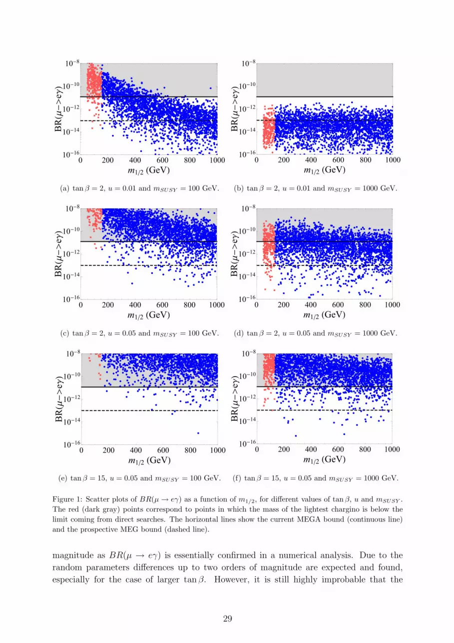
0 200 400 600 800 100010 16

10 14

10 12

10 10

10 8

m1 2 GeV

BR

e

(a) tanβ = 2, u = 0.01 and mSUSY = 100 GeV.

0 200 400 600 800 100010 16

10 14

10 12

10 10

10 8

m1 2 GeV

BR

e

(b) tanβ = 2, u = 0.01 and mSUSY = 1000 GeV.

0 200 400 600 800 100010 16

10 14

10 12

10 10

10 8

m1 2 GeV

BR

e

(c) tanβ = 2, u = 0.05 and mSUSY = 100 GeV.

0 200 400 600 800 100010 16

10 14

10 12

10 10

10 8

m1 2 GeV

BR

e

(d) tanβ = 2, u = 0.05 and mSUSY = 1000 GeV.

0 200 400 600 800 100010 16

10 14

10 12

10 10

10 8

m1 2 GeV

BR

e

(e) tanβ = 15, u = 0.05 and mSUSY = 100 GeV.

0 200 400 600 800 100010 16

10 14

10 12

10 10

10 8

m1 2 GeV

BR

e

(f) tanβ = 15, u = 0.05 and mSUSY = 1000 GeV.

Figure 1: Scatter plots of BR(µ→ eγ) as a function of m1/2, for different values of tanβ, u and mSUSY .The red (dark gray) points correspond to points in which the mass of the lightest chargino is below thelimit coming from direct searches. The horizontal lines show the current MEGA bound (continuous line)and the prospective MEG bound (dashed line).

magnitude as BR(µ → eγ) is essentially confirmed in a numerical analysis. Due to the

random parameters differences up to two orders of magnitude are expected and found,

especially for the case of larger tan β. However, it is still highly improbable that the

29

decays τ → µγ and τ → eγ could be detected at a SuperB factory, assuming a prospective

limit of BR(τ → µγ), BR(τ → eγ) & 10−9 [39].

5.3 Results for anomalous magnetic moment of the muon

As is well known, the value found for the anomalous magnetic moment of the muon [40]

aEXPµ = 116592080(63)× 10−11 (96)

shows a 3.4 σ deviation

δaµ = aEXPµ − aSMµ = +302(88)× 10−11 (97)

from the value expected in the SM [41]

aSMµ = 116591778(61)× 10−11 . (98)

Similar discrepancies have been reported in [42]. Thus, it might be interesting to consider

the case in which this deviation is attributed to the presence of SUSY particles with masses

of a few hundred GeV. The one-loop contribution to the anomalous magnetic moment of the

muon in supersymmetric extensions of the SM has been studied by several authors [29]. We

(a) u = 0.01. (b) u = 0.05.

Figure 2: Scatter plots in the plane BR(µ → eγ) − δaµ, for values of u = 0.01, 0.05. The value of tanβis fixed through the relation with the τ Yukawa coupling, which lies in the interval [1/3, 3]. The values ofmSUSY and of m1/2 are chosen between 10 and 300 GeV for the left panel and between 10 and 1000 GeVin the right one. The horizontal lines correspond to the MEGA (continuous line) and the MEG bounds(dashed line); the vertical lines correspond to the measurements on δaµ: the continuous one is the best fitvalue and the dashed ones correspond to the 3σ boundaries.

study the compatibility between the requirement that δaµ is explained by the exchange of

relatively light SUSY particles and the experimental upper limit on BR(µ → eγ) coming

from the MEGA experiment. We choose again two different values of u, u = 0.01 and

u = 0.05. To better explore the parameter space we vary the τ Yukawa coupling between

1/3 and 3 and fix the value of tan β through the relation given in eq. (18). As a consequence

in the plot for u = 0.01, see Figure 2(a), 2 . tan β . 3 holds and for u = 0.05 tan β

30

takes values 2 . tan β . 15. Similarly, mSUSY and m1/2 are chosen to lie in intervals

[10 GeV, 300 GeV] and [10 GeV, 1000 GeV] for u = 0.01 and u = 0.05, respectively. The

different choice of intervals is due to the fact that values of a few hundred GeV for mSUSY

and m1/2 are disfavoured by the existing limit on BR(µ → eγ) when u = 0.05. As one

can clearly see from Figure 2, in almost the whole parameter space of our model it is not

natural to reproduce the observed deviation of the muon anomalous magnetic moment and

at the same time to respect the existing bound on the branching ratio of µ→ eγ.

This kind of incompatibility is well known in supersymmetric theories, because the

explanation of the 3.4σ discrepancy necessitates small values of mSUSY and m1/2 and

larger values of tan β, which in turn enhance the branching ratio of the radiative LFV

decays. Thus, we have to conclude that either there exist further sources of contributions

to the anomalous magnetic moment of the muon beyond those present in our model, or -

as is also discussed in the literature - the theoretical value aSMµ found in the SM is closer

to aEXPµ so that the eventual discrepancy becomes less than 100 × 10−11, a value which

could well be explained in our model.

6 Conclusion

While awaiting the start of LHC and the first exploration of the TeV scale, the solution

to the hierarchy problem offered by SUSY still represents a very appealing option, with

several interesting consequences, such as a successful gauge coupling unification, a viable

particle candidate for dark matter and a possible explanation of the observed discrepancy

in the anomalous magnetic moment of the muon. Nevertheless the existence of new states

carrying flavour indices at the TeV scale is a serious problem in model building, given the

success of the SM in describing all known phenomena involving flavour transitions. The

lepton sector makes no exception. The flavour conversion observed in neutrino oscillations

might be related to potentially large effects in rare decays of the charged leptons. A naive

dimensional estimate of these effects, assuming new physics at the TeV scale, requires a

large suppression in the relevant amplitudes, to pass the existing bounds. A possible expla-

nation for such a suppression is the presence of a flavour symmetry, which is independently

motivated by the hierarchy in the charged lepton mass spectrum and by the nearly TB

mixing pattern of the lepton mixing matrix. Here we have considered a SUSY model in-

variant under the flavour symmetry group A4×Z3×U(1)FN , originally proposed in order

to describe lepton masses and mixing angles. We have extended the original model by in-

cluding SUSY breaking terms consistent with all symmetry requirements. Our model is an

effective theory, valid at energy scales below a cutoff Λf ≈ ΛL, where we have derived the

spectrum of SUSY particles, in the slepton sector, under the assumption that the SUSY

breaking scale is larger than Λf . It provides an example of a model in which the slepton

mass matrices at the scale Λf are not universal. Left-handed sleptons are approximately

universal, with a small departure from universality controlled by u, the flavour symmetry

breaking parameter. Right-handed sleptons have soft masses of the same order, but the

relative difference among them is expected to be of order one. Off-diagonal elements in

both sectors, as well as in the RL block, are small and have a characteristic pattern in

31

terms of powers of u. This structure is maintained by the effects coming from the RG

running from Λf ≈ ΛL down to the electroweak scale. The symmetry breaking parameter

u lies in a restricted range around few per cent and has a size similar to the reactor mixing

angle θ13. We have exploited the knowledge of the slepton mass matrices to compute the

normalized branching ratios Rij for the transitions µ→ eγ, τ → µγ and τ → eγ. At vari-

ance with other models based on flavour symmetries we found Rµe ≈ Rτµ ≈ Rτe and, given

the present limit on Rµe, these rare τ decays are practically unobservable in our model.

On a more theoretical side, the scaling Rij ∝ u2, found in the MI approximation, violates

an expectation based on an effective Lagrangian approach, which suggested Rij ∝ u4 in

the limit of massless final charged lepton. We have identified the source of such a violation

in a single, flavour independent, contribution of the RL block of the slepton mass matrix.

Such a contribution originates from the VEVs of the auxiliary components of the flavon

supermultiplets. We have classified the conditions under which this universal contribution

is absent.

In a numerical analysis of Rµe we found that already the current bound from the

MEGA experiment requires the parameter u to be small or tan β to be small for SUSY

mass parameters mSUSY and m1/2 below 1000 GeV, to guarantee detection of sparticles at

LHC. Applying the prospective MEG bound tightens the parameter space of our model

even more to small u and tan β or requires mass parameters mSUSY and m1/2 above 1000

GeV. Furthermore, we showed that the deviation of the experimentally observed value of

the magnetic moment of the muon from the SM one cannot be naturally explained in our

framework, for BR(µ → eγ) below the current bound. The maximal value of δaµ in our

model is around 100× 10−11 for BR(µ→ eγ) . 10−11.

Acknowledgments

We thank Lorenzo Calibbi, Stefano Rigolin and Fabio Zwirner for many useful discussions.

We recognize that this work has been partly supported by the European Commission under

contracts PITN-GA-2009-237920 (UNILHC) and MRTN-CT-2006-035505.

32

Appendix A The group A4

The group A4 is generated by two elements S and T obeying the relations [14]:

S2 = (ST )3 = T 3 = 1 . (99)

It has three independent one-dimensional representations, 1, 1′ and 1′′ and one three-

dimensional representation 3. The one-dimensional representations are given by:

1 S = 1 T = 1 ,

1′ S = 1 T = ei4π/3 ≡ ω2 ,

1′′ S = 1 T = ei2π/3 ≡ ω .(100)

The three-dimensional representation, in a basis where the generator T is diagonal, is given

by:

T =

1 0 0

0 ω2 0

0 0 ω

, S =1

3

−1 2 2

2 −1 2

2 2 −1

. (101)

The multiplication rule for triplet representations is the following:

3× 3 = 1 + 1′ + 1′′ + 3S + 3A (102)

If we denote by:

a = (a1, a2, a3) , b = (b1, b2, b3) (103)

two triplets, the singlets contained in their product are given by:

1 ≡ (ab) = (a1b1 + a2b3 + a3b2)

1′ ≡ (ab)′ = (a3b3 + a1b2 + a2b1)

1′′ ≡ (ab)′′ = (a2b2 + a1b3 + a3b1)

(104)

The two triplets can be separated into a symmetric and an antisymmetric part:

3S ≡ (ab)S =1

3(2a1b1 − a2b3 − a3b2, 2a3b3 − a1b2 − a2b1, 2a2b2 − a1b3 − a3b1)

3A ≡ (ab)A =1

2(a2b3 − a3b2, a1b2 − a2b1, a3b1 − a1b3) (105)

Moreover, if c, c′ and c′′ are singlets transforming as 1, 1′ and 1′′, and a = (a1, a2, a3) is

a triplet, then the products ac, ac′ and ac′′ are triplets explicitly given by (a1c, a2c, a3c),

(a3c′, a1c

′, a2c′) and (a2c

′′, a3c′′, a1c

′′), respectively. Note that due to the choice of complex

representation matrices for the real representation 3 the conjugate a of a ∼ 3 does not

transform as 3, but rather (a1, a3, a2) transforms as triplet under A4. The reason for this is

that T ? = UTTU and S? = UTSU = S where U is the matrix which exchanges the second

and third row and column.

33

Appendix B Canonical normalization of the kinetic

terms and diagonalization of the charged lepton mass

matrix ml

We perform the following transformations on the superfields: the kinetic terms are canon-

ically normalized, i.e. we find the basis in which the matrices K and Kc, shown in eqs.

(37,38), are unit matrices, and in a second step the charged lepton mass matrix ml, eq.

(44), is diagonalized. As explained in the main text, we perform these transformations

not only on the lepton fields, but also on the sleptons in order to ensure that the gaugino-

lepton-slepton vertices do not violate flavour at this stage.

To diagonalize the hermitian matrices K and Kc we apply the unitary transformations

W and W c:

W †KW = diag and (W c)†KcW c = diag . (106)

Normalizing K and Kc requires a rescaling of the fields via the real (diagonal) matrices R

and Rc:

RW †KWR = 1 and Rc(W c)†KcW cRc = 1 . (107)

The superfields l and lc (lc = (ec, µc, τ c) as above) are expressed as:

l = WR l′ and lc = W cRclc ′ (108)

so that the kinetic terms for leptons and sleptons are in their the canonical form, i.e. eq.

(36) becomes:

i l′iσµDµl

′i + i lc

′iσµDµl

c ′i + |Dµl

′i|2 + |Dµlc

′i|2 .

The mass matrices for leptons and sleptons in this basis read:

lcml l = lc ′Rc(W c)TmlWR l′ ≡ lc ′m′ll′, (109)

and 13

lcm2RL l = lc

′Rc(W c)Tm2

RLWR l′ ,¯l m2

LL l = ¯l′RW †m2LLWR l′ , (110)

lcm2RR

¯lc = lc ′Rc(W c)Tm2

RRWc ?Rc ¯

lc ′ .

We diagonalize the resulting mass matrix m′l of the charged leptons by the usual bi-unitary

transformation:

UTm′lV = diag(me,mµ,mτ ) (111)

and arrive at the mass eigenbasis l′′ and lc ′′:

lc ′ = Ulc ′′ and l′ = V l′′ . (112)

13Note that the matrix m2LL stands for both, the mass matrix of the left-handed charged sleptons and

the one of the sneutrinos.

34

Finally, the slepton mass matrices m2RL, m2

LL and m2RR are given as:

lcm2RL l = lc

′′[UTRc(W c)Tm2

RLWRV ] l′′ ≡ lc′′m2RL l

′′ ,¯l m2

LL l = ¯l′′[V †RW †m2LLWRV ] l′′ ≡ ¯l′′m2

LL l′′ , (113)

lcm2RR

¯lc = ˜lc ′′[UTRc(W c)Tm2

RRWc ?Rc U?]

¯lc ′′ ≡ ˜lc ′′m2

RR¯lc ′′ .

As we assume for the actual calculation of m2RL, m2

LL and m2RR that all couplings

involved are real, the matrices W , W c, U and V turn out to be orthogonal instead of

unitary. Furthermore, we express the small parameter u in terms of t as u = xt with x ≤ 1

according to eq. (15) and eq. (19). We then can do the calculation in just one expansion

parameter t. 14 In the course of the calculation we pose the following requirements: the

kinetic terms are canonically normalized up to and including O(t5), m′l is diagonal also up

to and including O(t5), and the matrices W , W c, U and V are orthogonal up to the same

order. These calculations have been checked by using two independent methods.

Appendix C Notations and one-loop formulae for Rij

and δaSUSYµ

In this part we fix the notations and we report the formulae for Rij and for δaSUSYµ which

we have used in section 5. The main references are [29–32] and we follow these.

The mass matrix of the charginos is given by:

− Lm ⊃(W−R H−2R

)Mc

(W−L

H−1L

)+ h.c. (114)

with

Mc =

(M2

√2mW cos β√

2mW sin β µ

). (115)

This matrix is diagonalized by 2× 2 rotation matrices OL and OR as:

ORMcOTL = diag

(Meχ−1 ,Meχ−2

), (116)

where the diagonalizing matrices connect mass and interaction eigenstates in the following

way: (χ−1Lχ−2L

)= OL

(W−L

H−1L

),

(χ−1Rχ−2R

)= OR

(W−R

H−2R

)(117)

and the mass eigenstates are written as χ−A = χ−AL + χ−AR (A = 1, 2) with masses Meχ−A .

The neutralino mass matrix is given by:

− Lm ⊃1

2

(BL W 0

L H01L H0

2L

)MN

BL

W 0L

H01L

H02L

+ h.c. (118)

14The different factors of t and u are recovered in the final result by replacing x with ut .

35

with

MN =

M1 0 −mZ sin θW cos β mZ sin θW sin β

0 M2 mZ cos θW cos β −mZ cos θW sin β

−mZ sin θW cos β mZ cos θW cos β 0 −µmZ sin θW sin β −mZ cos θW sin β −µ 0

(119)

We can diagonalize MN by a rotation matrix ON :

ONMNOTN = diag

(Meχ0

1,Meχ0

2,Meχ0

3,Meχ0

4

), (120)

where ON connects mass and interaction eigenstates in the following way:χ0

1L

χ02L

χ03L

χ04L

= ON

BL

W 0L

H01L

H02L

(121)

and the mass eigenstates are given by χ0A = χ0

AL + χ0AR (A = 1, 2, 3, 4) with masses Meχ0

A.

The mass matrices for the charged sleptons and for sneutrinos are given by:

− Lm ⊃(

¯l lc)M2

e

(l¯lc

)+ ¯νm2

νLLν (122)

with

M2e =

(m2eLL m2

eLR

m2eRL m2

eRR

)(123)

where m2(e,ν)LL and m2

eRR are in general hermitian matrices and m2eLR = (m2

RL)†. We

diagonalize the mass matrix M2e by a 6× 6 rotation matrix U l as:

U lM2eU

l T = m2l

(124)

where the mass eigenstates are:

lX = U lX,ili + U l

X,i+3¯lci (125)

with masses m2lX

(X = 1, . . . , 6).

Analogously, the sneutrino mass matrix is diagonalized by:

U νm2νLLU

νT = m2ν (126)

where the mass eigenstates are:

νX = U νX,iνi (127)

with masses m2νX

(X = 1, 2, 3).

The normalized branching ratios, Rij, for the LFV transitions li → ljγ are:

Rij =BR(li → ljγ)

BR(li → ljνiνj)=

48π3α

G2F

(|AL2 |2 + |AR2 |2

)(128)

36

and the decay rates are given by:

Γ(li → ljνiνj) =G2F

192π3m5i , Γ(li → ljγ) =

e2

16πm5i

(|AL2 |2 + |AR2 |2

). (129)

Each coefficient AL,R2 can be written as a sum of two terms:

AL,R2 = A(n)L,R2 + A

(c)L,R2 , (130)

where A(n)L,R2 and A

(c)L,R2 stand for the contributions from the neutralino and from the

chargino loops, respectively. These coefficients are explicitly given by:

A(n)L2 =

1

32π2

1

m2lX

[NLjAXN

LiAXg1n(xAX)+NR

jAXNRiAX

mj

mi

g1n(xAX)+NLjAXN

RiAX

Mχ0A

mi

g2n(xAX)

](131)

and A(n)R2 = A

(n)L2 |L↔R with xAX = M2

χ0A/m2

lX, and

A(c)L2 = − 1

32π2

1

m2νX

[CLjAXC

LiAXg1c(xAX)+CR

jAXCRiAX

mj

mi

g1c(xAX)+CLjAXC

RiAX

Mχ−A

mi

g2c(xAX)

](132)

and A(c)R2 = A

(c)L2 |L↔R with xAX = M2

χ−A/m2

νX.

The terms NiAX and CiAX and the loop functions gin and gic read as follows:

NLiAX = − g2√

2

{[−(ON)A,2 − (ON)A,1 tan θW ]U l

X,i +mi

mW cos β(ON)A,3U

lX,i+3

}(133)

NRiAX = − g2√

2

{mi

mW cos β(ON)A,3U

lX,i + 2(ON)A,1 tan θWU

lX,i+3

}(134)

CLiAX = −g2(OR)A,1U

νX,i (135)

CRiAX = g2

mi√2mW cos β

(OL)A,2UνX,i (136)

and

g1n(xAX) =1

6(1− xAX)4

(1− 6xAX + 3x2

AX + 2x3AX − 6x2

AX lnxAX)

(137)

g2n(xAX) =1

(1− xAX)3

(1− x2

AX + 2xAX lnxAX)

(138)

g1c(xAX) =1

6(1− xAX)4

(2 + 3xAX − 6x2

AX + x3AX + 6xAX lnxAX

)(139)

g2c(xAX) =1

(1− xAX)3

(−3 + 4xAX − x2

AX − 2 lnxAX). (140)

We note that the functions fin and fic , displayed in section 4, are related to the loop

functions gin and gic, mostly through taking the first derivative.

The deviation of the muon anomalous magnetic moment, δaSUSYµ , due to SUSY contri-

butions can be written as:

δaSUSY`i=g

(n)`i

+ g(c)`i

2(141)

37

with

g(n,c)`i

= g(n,c)L`i

+ g(n,c)R`i

. (142)

These terms are explicitly given by:

g(c)L`i

=1

16π2

m2i

m2νX

[CLiAXC

LiAXg1c(xAX) + CR

iAXCRiAXg1c(xAX) + CL

iAXCRiAX

Mχ−A

mi

g2c(xAX)

](143)

and g(c)R`i

= g(c)L`i|L↔R with xAX = M2

χ−A/m2

νX, and

g(n)L`i

= − 1

16π2

m2i

m2lX

[NLiAXN

LiAXg1n(xAX) +NR

iAXNRiAXg1n(xAX) +NL

iAXNRiAX

Mχ0A

mi

g2n(xAX)

](144)

and g(n)R`i

= g(n)L`i|L↔R with xAX = M2

χ0A/m2

lX. The terms NiAX and CiAX and the functions

gin and gic have been already introduced in eqs. (133-136) and in eqs. (137-140).

38

References

[1] For a review, see M. Raidal et al., Eur. Phys. J. C 57 (2008) 13 [arXiv:0801.1826

[hep-ph]].

[2] A. Strumia and F. Vissani, arXiv:hep-ph/0606054; M. C. Gonzalez-Garcia and

M. Maltoni, Phys. Rept. 460 (2008) 1 [arXiv:0704.1800 [hep-ph]]; Phys. Lett. B 663

(2008) 405 [arXiv:0802.3699 [hep-ph]]; G. L. Fogli et al., Nucl. Phys. Proc. Suppl. 168

(2007) 341; A. Bandyopadhyay, S. Choubey, S. Goswami, S. T. Petcov and D. P. Roy,

arXiv:0804.4857 [hep-ph]; G. L. Fogli, E. Lisi, A. Marrone, A. Palazzo and A. M. Ro-

tunno, Phys. Rev. Lett. 101 (2008) 141801 [arXiv:0806.2649 [hep-ph]]; G. L. Fogli,

E. Lisi, A. Marrone, A. Palazzo and A. M. Rotunno, arXiv:0809.2936 [hep-ph].

[3] For a review, see G. Altarelli, arXiv:0711.0161 [hep-ph], and references therein.

[4] F. Feruglio, C. Hagedorn, Y. Lin and L. Merlo, Nucl. Phys. B 809 (2009) 218

[arXiv:0807.3160 [hep-ph]]; F. Feruglio, C. Hagedorn, Y. Lin and L. Merlo, in the

Proceedings of NO-VE 2008, 4th International Workshop on Neutrino Oscillations

in Venice (Venice, Italy, 2008), University of Padua publication (Papergraf Edition,

Padua, 2008), 29-43 [arXiv:0808.0812 [hep-ph]].

[5] G. Altarelli and F. Feruglio, Nucl. Phys. B 720 (2005) 64 [arXiv:hep-ph/0504165].

[6] G. Altarelli and F. Feruglio, Nucl. Phys. B 741 (2006) 215 [arXiv:hep-ph/0512103].

[7] G. Altarelli, F. Feruglio and Y. Lin, Nucl. Phys. B 775 (2007) 31 [arXiv:hep-

ph/0610165].

[8] G. Altarelli, F. Feruglio and C. Hagedorn, JHEP 0803 (2008) 052 [arXiv:0802.0090

[hep-ph]].

[9] S. F. King and M. Malinsky, Phys. Lett. B 645 (2007) 351 [arXiv:hep-ph/0610250];

F. Feruglio, C. Hagedorn, Y. Lin and L. Merlo, Nucl. Phys. B 775 (2007) 120

[arXiv:hep-ph/0702194]; M. C. Chen and K. T. Mahanthappa, Phys. Lett. B 652

(2007) 34 [arXiv:0705.0714 [hep-ph]]; P. H. Frampton and T. W. Kephart, JHEP

0709 (2007) 110 [arXiv:0706.1186 [hep-ph]]; G. J. Ding, Phys. Rev. D 78 (2008)

036011 [arXiv:0803.2278 [hep-ph]]; P. H. Frampton and S. Matsuzaki, Phys. Lett. B

679 (2009) 347 [arXiv:0902.1140 [hep-ph]].

[10] E. Ma and G. Rajasekaran, Phys. Rev. D 64 (2001) 113012 [arXiv:hep-ph/0106291];

K. S. Babu, E. Ma and J. W. F. Valle, Phys. Lett. B 552 (2003) 207 [arXiv:hep-

ph/0206292]; M. Hirsch, J. C. Romao, S. Skadhauge, J. W. F. Valle and A. Vil-

lanova del Moral, arXiv:hep-ph/0312244; Phys. Rev. D 69 (2004) 093006 [arXiv:hep-

ph/0312265]; E. Ma, Mod. Phys. Lett. A 17 (2002) 627 [arXiv:hep-ph/0203238];

Phys. Rev. D 70 (2004) 031901 [arXiv:hep-ph/0404199]; New J. Phys. 6 (2004)

104 [arXiv:hep-ph/0405152]; arXiv:hep-ph/0409075; Phys. Rev. D 72 (2005) 037301

[arXiv:hep-ph/0505209]; Mod. Phys. Lett. A 20 (2005) 2601 [arXiv:hep-ph/0508099];

39

Phys. Rev. D 73 (2006) 057304 [arXiv:hep-ph/0511133]; Mod. Phys. Lett. A 21

(2006) 2931 [arXiv:hep-ph/0607190]; Mod. Phys. Lett. A 22 (2007) 101 [arXiv:hep-

ph/0610342]; S. L. Chen, M. Frigerio and E. Ma, Nucl. Phys. B 724 (2005) 423

[arXiv:hep-ph/0504181]; K. S. Babu and X. G. He, arXiv:hep-ph/0507217; A. Zee,

Phys. Lett. B 630 (2005) 58 [arXiv:hep-ph/0508278]; X. G. He, Y. Y. Keum and

R. R. Volkas, JHEP 0604 (2006) 039 [arXiv:hep-ph/0601001]; B. Adhikary, B. Brah-

machari, A. Ghosal, E. Ma and M. K. Parida, Phys. Lett. B 638 (2006) 345 [arXiv:hep-

ph/0603059]; L. Lavoura and H. Kuhbock, Mod. Phys. Lett. A 22 (2007) 181

[arXiv:hep-ph/0610050]; S. F. King and M. Malinsky, Phys. Lett. B 645 (2007) 351

[arXiv:hep-ph/0610250]; S. Morisi, M. Picariello and E. Torrente-Lujan, Phys. Rev.

D 75 (2007) 075015 [arXiv:hep-ph/0702034]; F. Yin, Phys. Rev. D 75 (2007) 073010

[arXiv:0704.3827 [hep-ph]]; F. Bazzocchi, S. Kaneko and S. Morisi, JHEP 0803 (2008)

063 [arXiv:0707.3032 [hep-ph]]; F. Bazzocchi, S. Morisi and M. Picariello, Phys. Lett.

B 659 (2008) 628 [arXiv:0710.2928 [hep-ph]]; M. Honda and M. Tanimoto, Prog.

Theor. Phys. 119 (2008) 583 [arXiv:0801.0181 [hep-ph]]; B. Brahmachari, S. Choubey

and M. Mitra, Phys. Rev. D 77 (2008) 073008 [Erratum-ibid. D 77 (2008) 119901]

[arXiv:0801.3554 [hep-ph]]; F. Bazzocchi, S. Morisi, M. Picariello and E. Torrente-

Lujan, J. Phys. G 36 (2009) 015002 [arXiv:0802.1693 [hep-ph]]; B. Adhikary and

A. Ghosal, Phys. Rev. D 78 (2008) 073007 [arXiv:0803.3582 [hep-ph]]; M. Hirsch,

S. Morisi and J. W. F. Valle, Phys. Rev. D 78 (2008) 093007 [arXiv:0804.1521 [hep-

ph]]; Y. Lin, Nucl. Phys. B 813 (2009) 91 [arXiv:0804.2867 [hep-ph]]; C. Csaki,

C. Delaunay, C. Grojean and Y. Grossman, JHEP 0810, 055 (2008) [arXiv:0806.0356

[hep-ph]]; P. H. Frampton and S. Matsuzaki, arXiv:0806.4592 [hep-ph]; W. Grimus

and L. Lavoura, JHEP 0904, 013 (2009) [arXiv:0811.4766 [hep-ph]]; F. Bazzocchi,

M. Frigerio and S. Morisi, Phys. Rev. D 78, 116018 (2008) [arXiv:0809.3573 [hep-

ph]]; F. Bazzocchi and S. Morisi, arXiv:0811.0345 [hep-ph]; S. Morisi, Phys. Rev. D

79 (2009) 033008 [arXiv:0901.1080 [hep-ph]]; P. Ciafaloni, M. Picariello, E. Torrente-

Lujan and A. Urbano, Phys. Rev. D 79, 116010 (2009) [arXiv:0901.2236 [hep-ph]];

F. Bazzocchi, L. Merlo and S. Morisi, Phys. Rev. D 80 (2009) 053003 [arXiv:0902.2849

[hep-ph]]; M. C. Chen and S. F. King, JHEP 0906, 072 (2009) [arXiv:0903.0125 [hep-

ph]]; Y. Lin, Phys. Rev. D 80 (2009) 076011 [arXiv:0903.0831 [hep-ph]]; G. Altarelli

and D. Meloni, J. Phys. G 36, 085005 (2009) [arXiv:0905.0620 [hep-ph]]; M. Hirsch,

S. Morisi and J. W. F. Valle, Phys. Lett. B 679 (2009) 454 [arXiv:0905.3056 [hep-ph]].

[11] C. I. Low and R. R. Volkas, Phys. Rev. D 68 (2003) 033007 [arXiv:hep-ph/0305243];

S. F. King, JHEP 0508 (2005) 105 [arXiv:hep-ph/0506297]; I. de Medeiros Varzielas

and G. G. Ross, Nucl. Phys. B 733 (2006) 31 [arXiv:hep-ph/0507176]; J. Ma-

tias and C. P. Burgess, JHEP 0509 (2005) 052 [arXiv:hep-ph/0508156]; E. Ma,

Phys. Lett. B 632 (2006) 352 [arXiv:hep-ph/0508231]; Europhys. Lett. 79 (2007)

61001 [arXiv:hep-ph/0701016]; Phys. Lett. B 660 (2008) 505 [arXiv:0709.0507 [hep-

ph]]; S. Luo and Z. z. Xing, Phys. Lett. B 632 (2006) 341 [arXiv:hep-ph/0509065];

I. de Medeiros Varzielas, S. F. King and G. G. Ross, Phys. Lett. B 644 (2007)

153 [arXiv:hep-ph/0512313]; Phys. Lett. B 648 (2007) 201 [arXiv:hep-ph/0607045];

N. Haba, A. Watanabe and K. Yoshioka, Phys. Rev. Lett. 97 (2006) 041601 [arXiv:hep-

40

ph/0603116]; P. Kovtun and A. Zee, Phys. Lett. B 640 (2006) 37 [arXiv:hep-

ph/0604169]; Z. z. Xing, H. Zhang and S. Zhou, Phys. Lett. B 641 (2006) 189

[arXiv:hep-ph/0607091]; S. F. King and M. Malinsky, JHEP 0611 (2006) 071

[arXiv:hep-ph/0608021]; C. S. Lam, Phys. Rev. D 74 (2006) 113004 [arXiv:hep-

ph/0611017]; Phys. Lett. B 656 (2007) 193 [arXiv:0708.3665 [hep-ph]]; Int. J.

Mod. Phys. A 23 (2008) 3371 [arXiv:0711.3795 [hep-ph]]; C. Luhn, S. Nasri and

P. Ramond, Phys. Lett. B 652 (2007) 27 [arXiv:0706.2341 [hep-ph]]; Y. Koide,

arXiv:0707.0899 [hep-ph]; S. Antusch, S. F. King and M. Malinsky, JHEP 0806

(2008) 068 [arXiv:0708.1282 [hep-ph]]; I. de Medeiros Varzielas, arXiv:0804.0015

[hep-ph]. N. Haba, R. Takahashi, M. Tanimoto and K. Yoshioka, Phys. Rev. D 78

(2008) 113002 [arXiv:0804.4055 [hep-ph]]; S. W. Li and B. Q. Ma, Phys. Rev. D 77

(2008) 093005 [arXiv:0806.0670 [hep-ph]]. H. Ishimori, Y. Shimizu and M. Tanimoto,

arXiv:0812.5031 [hep-ph]; F. Bazzocchi, L. Merlo and S. Morisi, Nucl. Phys. B 816

(2009) 204 [arXiv:0901.2086 [hep-ph]].

[12] G. Altarelli, F. Feruglio and L. Merlo, JHEP 0905 (2009) 020 [arXiv:0903.1940 [hep-

ph]].

[13] Y. Lin, Nucl. Phys. B 824 (2010) 95 [arXiv:0905.3534 [hep-ph]].

[14] M. Hamermesh, Group Theory and Its Application to Physical Problems, Reading,

Mass.:Addison-Wesley (1962) 509 p; J. F. Cornwell, Group Theory in Physics: An

Introduction, San Diego, USA: Academic (1997) 349 p; D. E. Littlewood, The Theory

of Group Characters (and Matrix Representations of Groups), Oxford University Press

(1958) 310 p; A. D. Thomas and G. V. Wood, Group Tables, Shiva Publishing

Limited.

[15] C. D. Froggatt and H. B. Nielsen, Nucl. Phys. B 147 (1979) 277.

[16] F. Feruglio, C. Hagedorn and L. Merlo, arXiv:0910.4058 [hep-ph].

[17] P. F. Harrison, D. H. Perkins and W. G. Scott, Phys. Lett. B 530 (2002) 167

[arXiv:hep-ph/0202074]; P. F. Harrison and W. G. Scott, Phys. Lett. B 535 (2002)

163 [arXiv:hep-ph/0203209]; Z. z. Xing, Phys. Lett. B 533 (2002) 85 [arXiv:hep-

ph/0204049]; P. F. Harrison and W. G. Scott, Phys. Lett. B 547 (2002) 219 [arXiv:hep-

ph/0210197]; Phys. Lett. B 557 (2003) 76 [arXiv:hep-ph/0302025]; arXiv:hep-

ph/0402006; Phys. Lett. B 594 (2004) 324 [arXiv:hep-ph/0403278].

[18] C. Amsler et al. [Particle Data Group], Phys. Lett. B 667 (2008) 1.

[19] S. Schael et al. [ALEPH collaboration and DELPHI collaboration and L3 collaboration

and OPAL collaborations and LEP Working Group for Higgs Boson Searches], Eur.

Phys. J. C 47 (2006) 547 [arXiv:hep-ex/0602042].

[20] M. A. Luty, arXiv:hep-th/0509029.

[21] G. G. Ross and O. Vives, Phys. Rev. D 67 (2003) 095013 [arXiv:hep-ph/0211279].

41

[22] G. G. Ross, L. Velasco-Sevilla and O. Vives, Nucl. Phys. B 692 (2004) 50 [arXiv:hep-

ph/0401064]; S. Antusch, S. F. King, M. Malinsky and G. G. Ross, Phys. Lett. B 670

(2009) 383 [arXiv:0807.5047 [hep-ph]].

[23] G. F. Giudice and A. Masiero, Phys. Lett. B 206 (1988) 480.

[24] H. Ishimori, T. Kobayashi, Y. Omura and M. Tanimoto, JHEP 0812 (2008) 082

[arXiv:0807.4625 [hep-ph]]; A. Hayakawa, H. Ishimori, Y. Shimizu and M. Tanimoto,

Phys. Lett. B 680 (2009) 334 [arXiv:0904.3820 [hep-ph]].

[25] S. P. Martin and M. T. Vaughn, Phys. Rev. D 50 (1994) 2282 [Erratum-ibid. D 78

(2008) 039903] [arXiv:hep-ph/9311340]; J. Hisano, T. Moroi, K. Tobe and M. Yam-

aguchi, Phys. Rev. D 53 (1996) 2442 [arXiv:hep-ph/9510309].

[26] P. Paradisi, JHEP 0510 (2005) 006 [arXiv:hep-ph/0505046]; M. Ciuchini, A. Masiero,

P. Paradisi, L. Silvestrini, S. K. Vempati and O. Vives, Nucl. Phys. B 783 (2007) 112

[arXiv:hep-ph/0702144].

[27] V. Cirigliano, B. Grinstein, G. Isidori and M. B. Wise, Nucl. Phys. B 728 (2005)

121 [arXiv:hep-ph/0507001]; Nucl. Phys. B 763 (2007) 35 [arXiv:hep-ph/0608123];

S. Davidson and F. Palorini, Phys. Lett. B 642 (2006) 72 [arXiv:hep-ph/0607329].

[28] K. Hamaguchi, M. Kakizaki and M. Yamaguchi, Phys. Rev. D 68 (2003) 056007

[arXiv:hep-ph/0212172]; W. F. Chang and J. N. Ng, Phys. Rev. D 71 (2005) 053003

[arXiv:hep-ph/0501161]; A. Mondragon, M. Mondragon and E. Peinado, Phys. Rev.

D 76 (2007) 076003 [arXiv:0706.0354 [hep-ph]]; S. Antusch, S. F. King and M. Ma-

linsky, JHEP 0806 (2008) 068 [arXiv:0708.1282 [hep-ph]]; S. Antusch and S. F. King,

Phys. Lett. B 659 (2008) 640 [arXiv:0709.0666 [hep-ph]]; L. Calibbi, J. Jones-Perez

and O. Vives, Phys. Rev. D 78 (2008) 075007 [arXiv:0804.4620 [hep-ph]]; L. Calibbi,

A. Faccia, A. Masiero and S. K. Vempati, Phys. Rev. D 74 (2006) 116002 [arXiv:hep-

ph/0605139]; R. Dermisek, M. Harada and S. Raby, Phys. Rev. D 74 (2006) 035011

[arXiv:hep-ph/0606055].

[29] T. Moroi, Phys. Rev. D 53 (1996) 6565 [Erratum-ibid. D 56 (1997) 4424] [arXiv:hep-

ph/9512396]; S. P. Martin and J. D. Wells, Phys. Rev. D 64 (2001) 035003 [arXiv:hep-

ph/0103067]; D. Stockinger, J. Phys. G 34 (2007) R45 [arXiv:hep-ph/0609168];

A. Czarnecki and W. J. Marciano, Phys. Rev. D 64 (2001) 013014 [arXiv:hep-

ph/0102122].

[30] J. Hisano, T. Moroi, K. Tobe and M. Yamaguchi, Phys. Rev. D 53 (1996) 2442

[arXiv:hep-ph/9510309]; T. Fukuyama, A. Ilakovac and T. Kikuchi, Eur. Phys. J. C

56 (2008) 125 [arXiv:hep-ph/0506295].

[31] E. Arganda and M. J. Herrero, Phys. Rev. D 73 (2006) 055003 [arXiv:hep-

ph/0510405].

[32] J. Hisano, T. Moroi, K. Tobe, M. Yamaguchi and T. Yanagida, Phys. Lett. B

357 (1995) 579 [arXiv:hep-ph/9501407]; J. Hisano and K. Tobe, Phys. Lett. B 510

42

(2001) 197 [arXiv:hep-ph/0102315]; G. Isidori, F. Mescia, P. Paradisi and D. Temes,

Phys. Rev. D 75 (2007) 115019 [arXiv:hep-ph/0703035]; M. Endo and T. Shindou,

arXiv:0805.0996 [hep-ph].

[33] R. Barate et al. [LEP Working Group for Higgs boson searches and ALEPH collab-

oration and DELPHI collaboration and L3 collaboration and OPAL collaboration],

Phys. Lett. B 565 (2003) 61 [arXiv:hep-ex/0306033].

[34] LEP Higgs Working Group and ALEPH collaboration and DELPHI collaboration and

L3 collaboration and OPAL collaboration, arXiv:hep-ex/0107030.

[35] M. L. Brooks et al. [MEGA Collaboration], Phys. Rev. Lett. 83 (1999) 1521

[arXiv:hep-ex/9905013].

[36] A. Maki, AIP Conf. Proc. 981 (2008) 363.

[37] T. Schwetz, AIP Conf. Proc. 981 (2008) 8 [arXiv:0710.5027 [hep-ph]].

[38] J. Burguet-Castell, D. Casper, E. Couce, J. J. Gomez-Cadenas and P. Hernandez,

Nucl. Phys. B 725 (2005) 306 [arXiv:hep-ph/0503021]; P. Huber, J. Kopp, M. Lind-

ner, M. Rolinec and W. Winter, JHEP 0605 (2006) 072 [arXiv:hep-ph/0601266];

J. E. Campagne, M. Maltoni, M. Mezzetto and T. Schwetz, JHEP 0704 (2007) 003

[arXiv:hep-ph/0603172]; P. Huber, M. Lindner, M. Rolinec and W. Winter, Phys.

Rev. D 74 (2006) 073003 [arXiv:hep-ph/0606119].

[39] M. Bona et al., arXiv:0709.0451 [hep-ex]; A. G. Akeroyd et al. [SuperKEKB Physics

Working Group], arXiv:hep-ex/0406071.

[40] G. W. Bennett et al. [Muon g-2 Collaboration], Phys. Rev. D 73 (2006) 072003

[arXiv:hep-ex/0602035].

[41] M. Passera, W. J. Marciano and A. Sirlin, Phys. Rev. D 78 (2008) 013009

[arXiv:0804.1142 [hep-ph]]; M. Passera, W. J. Marciano and A. Sirlin, AIP Conf.

Proc. 1078 (2009) 378 [arXiv:0809.4062 [hep-ph]].

[42] K. Hagiwara, A. D. Martin, D. Nomura and T. Teubner, Phys. Lett. B 649 (2007)

173 [arXiv:hep-ph/0611102].

43